AERONAUTICAL RESEARCH COUNCIL CURRENT PAPERS

C.P. No. 394 C.P. No. 394 (19.485)

A.R.C. Technical Report (19,485)

A.R.C. Technical Report

MINISTRY OF SUPPLY

AERONAUTICAL RESEARCH COUNCIL

CURRENT PAPERS

A Technique for Improving the Predictions of Linearised Theory on the Drag of Straight-Edged Wings

D.G.Randall, B.Sc.

LONDON: HER MAJESTY’S STATIONERY OFFICE

1958

SIX SHILLINGS NET

C.P. No. 394

U.D.C. No. 533.691.11:533.6.013.12:533.6.011.35/5

Technical Note No. Aero 2474

January, 1957

ROYAL AIRCRAFT ESTABLISHLENT -

A technxque for Improvmg the Prediotlons of Linearised Theory on the Drag of Straight-e&ed Vkngs

D. G. Randall, B.Sc.

EXRATA

The Mach number, M, in equatlon (28a) on pa e 11 * nunlber and not the local Mach number. Equation ~'28b)*o~sp~~ %e~s~t~~?k%~~,

unnecessary.

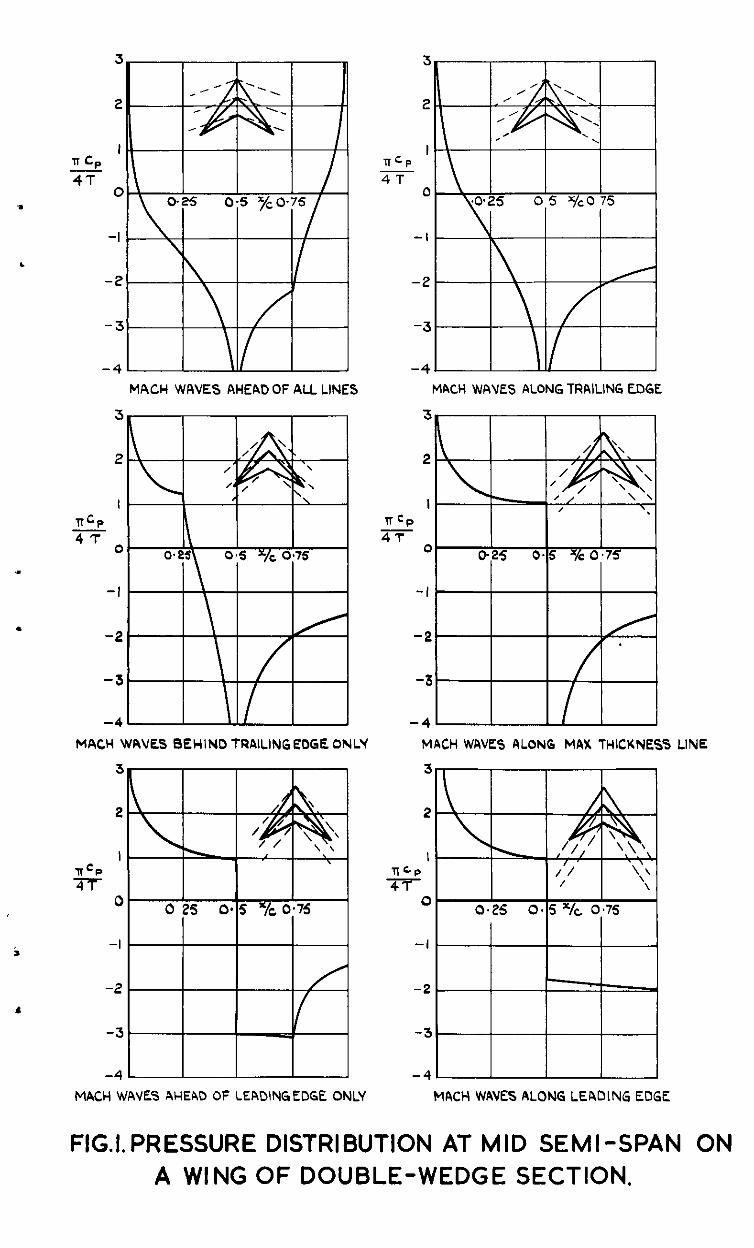
. As a result of this aberration, F~gwes 3,4,5,6 and 7 require correction. The curve labelled "Modified Theory" in Fig. 3 should be red.raw~ to pass through the points (0,0.638), (0.1, 0.371), (0.2, 0.303), (0.3, 0.272),

t 0.4, 0.255 ,

1 t 0.9, 0.229 ) 0.5, 0.W ,(o.6, o.237), (0.7, o.233), (0.8, o.231),

1 1.0, 0.229 . In Fig 4, the dashes at the left-hand sxde of the figure, vlhlch are labelled "Xodlfled Result", should be changed as follow: for B = 1, from 0.554 to 0.638; for B = 3, from 0.364 to 0.383. The points of tangency (the crosses) are now approxunotely given by c = 2.5 and not Z = 3.0, so that the factor 3/2 in equations (49) to(52) inclusive wuld be better replaced by 5/4. This ~11, however, have a negll&lble effect on the calculations.

Finally, the crosses In Flgnres 5,6 and 7 are moorrect. The following changes should be made, (readmg from left to right In each case). In Fig 5: 1.92 t0 2.15; q.75 t0 4.m. In Fig 6: 1.86 to 2.03; 1.70 to 1.72. In Fig 7. 0.98 to 1.06; 1.72 to 1.87; 1.68 to 1.76; 1.62 to 1.67; 1.47 to 1.9.

The cnncluslorsm section 6 remam unaltered, since the above errors are all snail in comparison with the deviations bctwen knearxed theory and experiment.

Addenda Although it.?@ be-n shown that (24) satisfies (22) together with (21),

the uniquen?+s<.~of.&s $olu@n~has not been proved in p~wel's

A "solution" of (22) the first substl- o'&=%k@~Qe odta~ned by~successlve substitution,

:- =53*. 1; tutlon belngz.fe=%%*Jt can'be to the expa&$?$&-(24)

shown that the series so obtained corresponils

solution of ($!)j:~~~~=, " It IS, therefore, probable that (24‘ 1s the uruque

s;: After equatlok(4@) the words "where terms of higher order than E have

been omitted' should be inserted.

C.P. No. 394

U.D.C. No. 533.6~1.11:~33.6.013.12:533.6.011.35/5

Tuohmcal Note NC. Awe 247$.

Janwry, 1957

ROYAL AIRCPAE'T iiSTiiBrXiBENT -----

A technque for Improving the Predxklcns of Linearised Theory on the Drag of Straight-edged Wings

D. G. Radal.1, B.S.

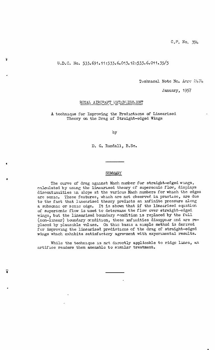
The curve cf drag aganst Mach number for straighkdgedwlngs, caloulated by using the linearised theory cf superscnic flav, displays discontmuities in slope at the varicus Mach numbers for whxh the edges are Sonlo. These features, whxh are not cbserve+. in practroe, are due to the fact that llnenrised theory predicts an infinite pressure nlcng a subscnx or scnx edge. It is shown that if the linearised equation of supersonic flow is used to deterrmne the flow over straight-edged wings, but the linearised boundary rendition 1s replaced by the f’ull

(non-lmear) bounkry ocnditlon, these xnfuiities disappear c.nd are re- placed by plausible values. On thx baas a simple method is derived far imprcvz.ng the linearised prediatxcns of the drag of straight-edged w-k~!s whxh exhibits satisfactory agreement with exper~mentd results.

While the technque 1s net dxectly applicable to ridge knes, an a.rtif'~ce renders them amenable to sxniiar treatment.

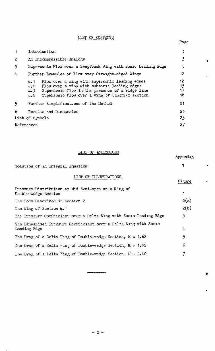
LIST OF cOP?lXNl'S w

3

3 3 5

12

1 Intrcduction

2 An Inccmpressible Analogy

3 Supsrscnic Plcw ever a Sweptback Wing wrth Sonic Leading Edge

4 Further Examples of 310~ over Straight-edged ?Jjngs

4.1 Flow wer a win& with superswic leadwg edges 4.2 Flow ever a wing with subsonlc leading edges 4.3 Supersonic flew in the presence of a rzAge line 4.4 Superscnlc flow over a wing of blconv-x scctlon

5 Further Slmpllflcatlcns of the Method

6 Results and D1scussicn List of Symbcls References

LIST OF APFENDICES

Solution of an Integral Equation

LISP OF ILLUSTRATIONS

Pressure Distributlcn at Mid Semi-span on awing of Double-wedge Section

The Body Described in Seotlcn 2

The Xing of Sectlcn 4.1

The Pressure Coefficient over a Delta Wmg vrlth Scnlc Leadzng Edge

Tke Linearised Presswe Ccef'flclent over a Delta Gng with Sonzc Leading Edge

The Drag of a Pelta Vmg of Double-wedge Section, M = 1.62

The Drag of a Delta idug of Double-wedge Sectlon, M = 1.92

Tne Drag of a Delta ?ing of Double-wedge Section. LI z 2.40

12 15 17 18

21

23 25 27

Apperfllx

I .

Fiqme .

1

2(a)

2(b)

3

Y

-2-

1 Intrcducticn

i

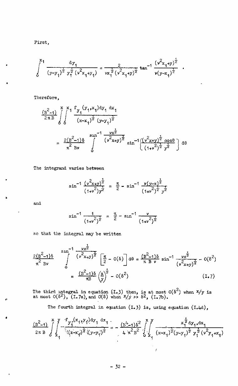
Linear theory has been used with success tc determine the flow over thin wings at moderate supersonic Mach numbers; a full description of the methods which have been used is given in Ref.1. In general, the results obtained for aerodynamic forces and mcments are physloally +.usilJle and agree wdh expervnent as well as can be expected, but there are cases where the linear theory produoes seemingly incorrect results. These ooou in the study of the flow over a wing the planform of which has straight edges* s&or ridge lines. When the free stream Mach number is such that the Mach lines are parsllel to one of the straight edges or ridge lines cf the wing a discontinuity in slope (Vulgarly, a "klnkl) appears in the graph of, for example, the wave drag of' the wing against Mach number. Further, the drag curve rises very steeply to the value at the discontinuity as the appropriate Mach number is approached frombelow. Neither the disoontinuities nor the steep rises are observed in praotlce.

The explanation of this phenomenon lies in the nature of the pressure distribution predicted by linear theory. The flow over a delta wing with wedge section placed in a supersonic free stream wfll serve for an examale. If the leading edge of the wing is superscollc, then over the region between the Msch line from the apex and the leading edge the pressure is ocnstant. This constant value becomes arbitrarily large as the hiach number deoreases untl1,i.n the limit, when the leading edge becomes sanlc, the oonstsnt beoomes infinite. At this stage the region of oonstsnt pressure has beacme vanistigly small and the pressure dose to the leading edge ten& to infinity as the square root of the red-al of the distance from the lesding edge. As the free stream Mach number drops further the pressure still tends to infinity at the leading edge but the infinity becomes less severe. This is the case of a subsonic leading edge and the pressure tends to infinity as the logarithm of the distanoefrcln the lea?&g edge. It is this failure of the linear theory to predict the pressures z.n the region of straight edges and ridge lines of a wlnp; correctly, (at any rate for s rsnge of Mach numbers), which leads to the spurges disocntinuities mentioned above. (Examples of pressure distributions on linear theory are drawn in Fig.1).

The reosonwhy linear theory gives such completely wrong answers for the pressures near straight edges is ususlly stated to be that the deviation cf flow qsntities (velooities etc.) from their free stream vehes js, in actual faot, large, and so the conditions for validity of the linear theory are not fulfilled. It will be suggested further on that the answer is nct,perhaps, qdte so simple as this; here, it is sufficient tc note that the pressures near the leading edge may in reality be much larger than those over the rest of the wing.

Any attempt to eliminate the disoontinuities fmmthe linear theory predictions, (and such an attempt is clearly desirable), must, almost certaidy involve a limiting of the vslues of the linear theory pressures near straight edged. This note presents a method for doing ths which invclves satisfying the full boundary condition on the surface of the wing as distinct from the linearised boundary condition; the governing differential equation is still the linear equation of supersonic flow.

2 An Incompressible Analofr~

The appsarsnoe of the infidties in the linearised pressure distribu- tion over awing with straight edges can be more easily understood by ocnsidering a problem in two-dimensional incompressible flow. This

* If the edges are cuspidal, no difficulties arise from the use of linearised theory. The teohnique described in this note is cmly necessary for wings with edges which are not cuspidsl.

-3-

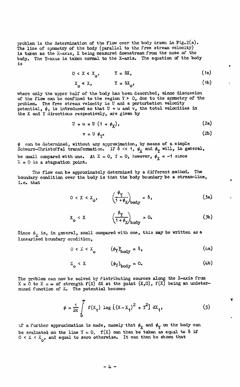
problem is the detennina tion of the flov; over the bcdy &raw-n in Fig.2(a). The line of symnetq' of the body (parallel to the free stream velocity) is taken as the X-axis, X being measured downstream from the nose of the body. The Y-axes is taken normal to the X-axis. The eqation of the body is

0 < x c x0, Y = 6X, (14

where only the upper half of the body hasbeen described, sinoe discussion of the flow can be confined to the region Y > 0, due to the syxnzetry of the problem. The free stream velocity is U and a perturbation velocity potential, qi, is introduced so that U + u snd v, the total velocities in the X and Y directions respeotively, sre given by

u +,u=u (I +#x,,, (24

v = u $y. (%I

$ can be determined, without any apixxdme.tion, by means of a simple Schwarz-Christoffel transformation. If 6 << I, $x an* $ wilJ., In general, be small ccmpared with one. X = 0 is a sta~ation point.

At X = 0, Y s 0, however, #X = -1 since

The flow osn be approximately determined by a different methcd. The boudary condition over the body is that the bcdy boundarybe a stream-line, i.e. that .

0 < x < x0, = 6,

= 0. Since $6, is, in general, small compared with one, this may be written asa linearised boundary ccndition,

(34 .

The problem can now be solved by distributing sources X = 0 to X = w of strength f(X) dX at the point (X,0), uoned function of 8. The potential beccsnes

the X-axis frcxn being an undeter-

co

i f(X,) log c(x-x,)2 + 31 a,, (5)

0

If a further appraximation is made, mmelythat $ and tiy onthebody can be evaluated on the line Y e 0. f(X) oanthenbetsken as equal t0 6 if O<X<X o, snd equal to zero otherwise. It oan then be shown that

-4-

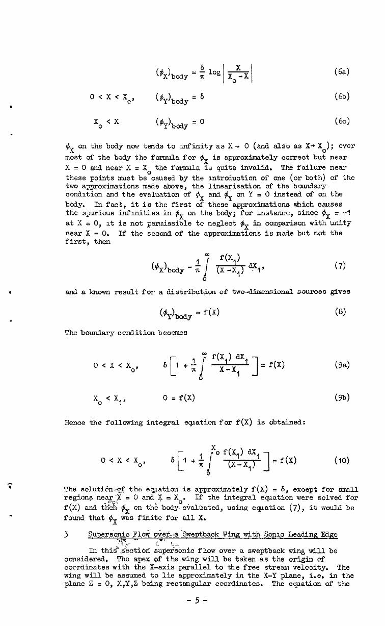
($xX)body = ; 1% * I I

(#,),, = 0 (60)

$X on the body now tends to mfinity as X+ 0 (snd slso as X+X,); over most of the bcdy the formula for $x is approximately correct but near X = 0 and near X = X0 the formula is quite invalid. The failure near these points must be caused by the mtrcduotion of one (or both) of ihe two a~roximations made above, the linearisation of the boundary condition and the evaluation cf $5X and $ on Y = 0 instead of on the bcdy. In fact, it is the first of these approximations &ich causes the spurious infmities in $x on the body; for mstsnce, since $x = -1 at X = 0, It is not permissible to neglect #X in co~psrison with unity near X = 0. If the seem-d of the approximations is made but not the first, then

and a known result for a distribution of twdimens ional sources gives

($lbody = f(X)

Theboundaryocnditicnbeocmes

0 < x < x0, 6 1,; c0 f-0 1 fi,

[ i x'-x 1 = f(X)

0 I

0 = f(X)

(94

(Yb)

Hence the following integral eqaticn for f(X) is obtained:

0 < x < x0, 6 1 xo fcq a, [ +‘6 .v]=f(x) (10)

The scluti&nn@ the eplation is approximately f(X) = 6, except for small region? near-.X = 0 and 2$ = X0. If the integral eqation were solved for f(X) and <2X $x on td body-ebaltiated, using eplation (7), it would be found that $x was finite for all X.

3 Super<onic Flow ove&ra:Sweptback Wing with Sonic Leading Ed& '%", -- .;T' in.

In thi.$&cti6fi supe&tinio flow over a sweptback wing will be considered. The apex of the wing will be taken as the origin cf cocrdinntes with the X-axis parallel to the free strem velocity. The wing will be assumed to lie apprcximately in the X-Y plane, i.e. in the plane Z = 0, X,Y,Z being rectsngular coordinates. The eqation of the

-5-

(scnic) leading edge 1s X = + BY, where 3 = (I&* - 1)s ani M is the free stream Mach number. The equzticn of the uppermsurface of t% wiug in the regicn tc be ccnsidered is taken as

* 2 = 6(X - BY), Y>O (lla)

2 = b(X + BY), Y < 0. (Ilb) .

where 6 is a constant small ccmpared wath unity. These eplaticns represent the up:?er surface of a delta wing with a wedge secticn. If? the magnitude cf the free stresm velocity is U, then a perturbaticn velocity potential can be intrcduaed so that U + u, v and w, the velccities an the X, Y and 2 directions re=peotrvely, are given by

lJ+u=v(1 +tixx,

v=u$b, Y

l-r = u @Z'

(W

(Ia)

(QC)

The governing partial differential eplaticn is ~~ICVKI to be

(13)

The bcundsry ccnditicn to be satisfied on that part of the wing, for whach Y > 0 1s that there shculd be no flew velocity normal tc the surface, i.e. that

z = 0, &(I + $x) - B6 $y - $z = 0, (14)

the bcwdary condition being ap$ied cn the plane Z = 0 rather than on the wulg Itself. eq=ticn (14).

A scluticn cf equatwn (13) 1s reqmred which satisfies

The lntegralswhxh arise m the scluticn ef ecplaticn (13) are hsndledxxe eastiy rf the fcllowng trsnsfcnnaticn cf ccsrdmates IY made.

X-BY x=z-'

X+BY y=5-'

z=Z (Isa), (I%), (15c)

The governing partial differential eqaticn becomes

and t!le su;face bcundary ccnditicn becomes

(16)

(17)

An ele;lentul source sclution of equaticn (13) is

-6-

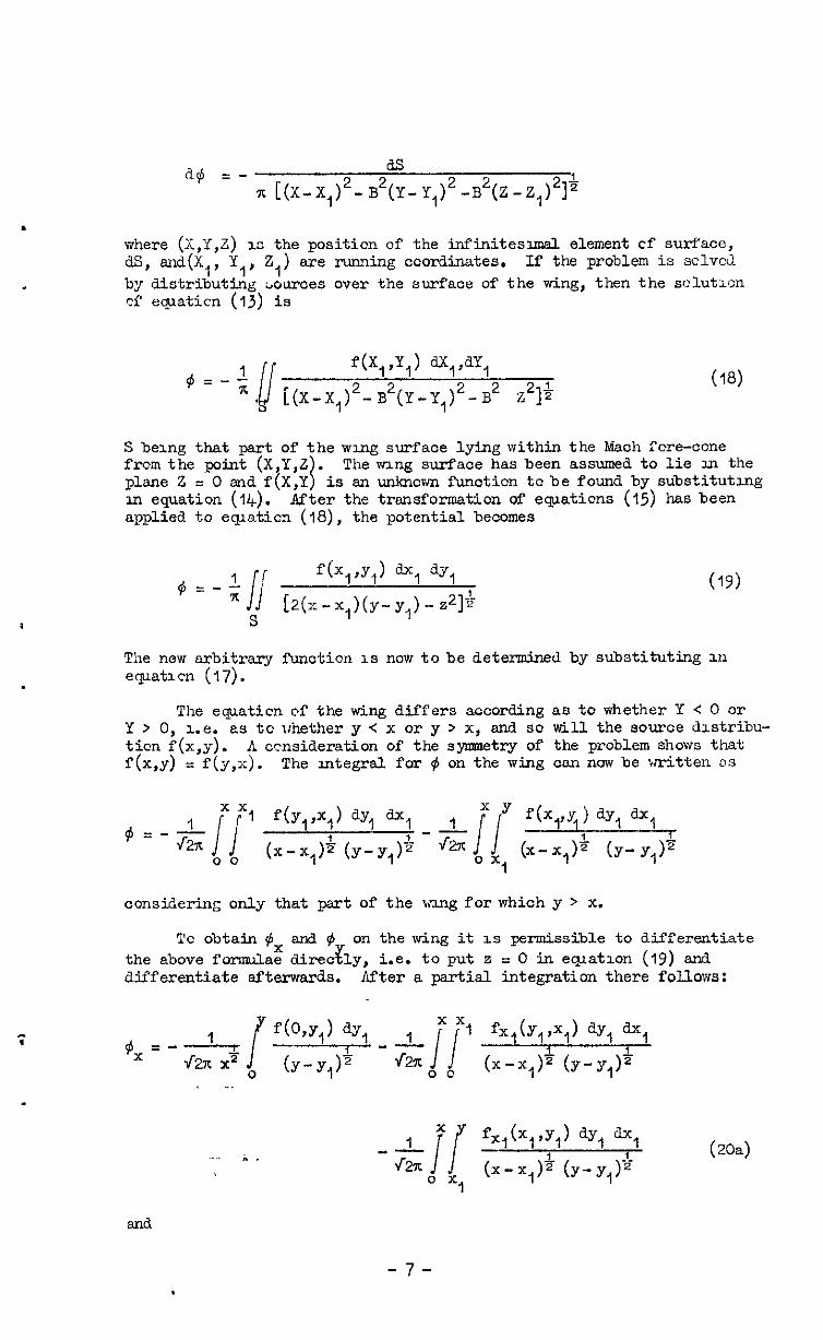
d$ =- as 7c [(x-x,)2- B2(Y- Y,12-B2(Z - zJ21&

where (X,Y,Z) 1s the position of the infinitesmsl element cf surface, a, aa+, Y,' 2,) are running coordinates. If the problem is sclvcil by distributing umrces over the surface of the wing, then the sclutlon cf equaticn (13) is

(18)

S bemg that part of the wmg surface lying within the Maoh fcre-cone frcm the point (X,Y,Z plsne Z = 0 and f(X,Y 1

. The vnng surface has been assumed to lie m the is an untcnovm function tc be found by substituting

111 equation (14). After the transformation of equations (15) has been applied to eqmticn (la), the potential becomes

+; r /I

fb,‘Y,) h, dY,

S [2(x-x,)(y-y,)- 43

(19)

The new arbitrary function 1s now to be determined by substituting 111 equat~cn (17).

The eqnticn cf the wing differs according as to whether Y -C 0 or Y>O,~e.astovhethery<xory>x, and so till the source dlstribu- ticn f(x,y). A ccnsideration of the symmetry of the problem shows that f(X,Y) = f(Y,4. The integral for # on the wing can now be written as

1 $=-z

x 7 f(Y, ,x,1 dY, k,

ii )3 (y-y,)$ - k

x y f(yg dY, h,

ii T

00 (x-x, ox I G-x,$ (Y- Y,F

constiering only that part of the mng for which y > X.

Tc obtain $5x and # on the wing it 1s permissible to differentiate the above formulae direc ly, f i.e. to put e = 0 in e*atlon (IV) and differentiate afterwards. After a partial integration there follows:

$x=-4 f(O,Y,) dY, , x xl fX,(Y,‘X,) dY, h,

(2% XT i --1--

o (Y-Y,P <2x JJ 7 1

00 b-x,)5 (Y’Y,F ” _.

x 1 f (x 1’1 Y 1 dY, b,

-z iJ 21 1

ox I

(x-x, 9 (Y- Y,)” ( 234

-7-

$yy=- ' $yy=- ' x f(O,x,) b, x f(O,x,) b,

i i , , x x1 fqY,JX,) dy, axl x x1 fqY,JX,) dy, axl

{2X y+, {2X y+, '-Ir- - z '-Ir- - z

(x-x,)2 (x-x,)2 ii ii cl 0 cl 0 (x- x1)$ (y- (x- x1)$ (y-

x y f x y f 1 1

ii ii

(x JY 1 dY, a, (x JY 1 dY, a, Y, 1 1 Y, 1 1

-zi -zi 4 4 1 1

o Xl o Xl (x-q2 (Y-Y,F (x-q2 (Y-Y,F

A kncrm result ~'cr a distribution of scurces gives, on the wing,

An integrd eqation for f(x,y) is obtained when tnesc values of $x, #y and $x are substltded in eplatlon (17).

Frnn the fomnila for $x it follows that $x (and hence t!le pressure) will tend to infinity as x tends to zero unless

y f(O,Y,) dY,

o (Y-Y,)* = 1 0 (21)

'The solution cf this Abel equation 1s simply f(O,y) = 0; therefore, the mfinity in the pressure distribution predicted by linear theory can only be rermved if f(x,y), the solution of the lntegrdl e+s.tlon derlved fmm ewaticn (17), is such that f(O,y) = 0. Asswing that this is so, the inte&rsl equaticn becomes

cc

B2-I XX

+2xB ii 0 c

f (Y,‘X,) dY, a, B2+1

x Y f xi

11

x, (x 1 JY 1 1 dY, dx,

(x-x,+ (Y-Y,)? 2xB 4

O 7 (x-x, 1" (Y-Y,)+

fy, (Y, ,x,1 dY, k, B2-1

x y f (x JY 1 dY, b, Y, 1 1 I +m (x-x,$ (y- yp i I, (X-jqJq- 3

=f(x,y) ox

(27-I

and a sclution cf this is required such that f(O,y) = 0.

f(x,y) ad the varies flow quantities will be ccnstsnt along straight liaes drawn through the apex cf the wing, i.e. they will be funotioqs of x/y cnly. If it 1s assumed that f(x,y) vanishes at x = 0 as k(x/y)T, with a ccnstent tc be dete-ed, then, near x = 0.

I

fx(Y,X) -- idi 26’

-a-

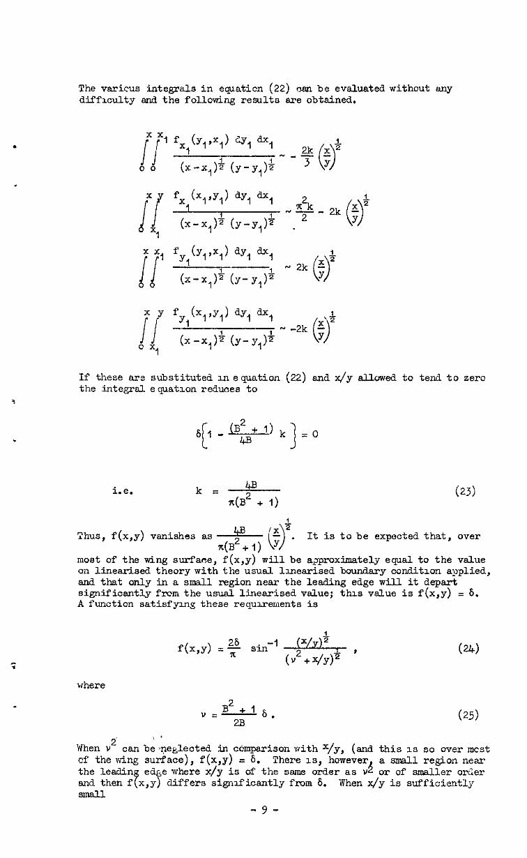
The varicus integrals in equation (22) osn be evaluated without any difficulty and the following results sre obtained.

f (Y 1 Y, 1 ,x 1 dY, dx,

- 2k ; 0 + 2

00

x Y f

ii

(x ,Y 1 dY, dx, Y, 1 1 \&

x

0 ox

1 (x -x1 )3 (y-y,)& - -2k y

If these are substituted m equation (22) and x/y sllowed to tend to zero the integral equation reduces to

i.e. k= 48 ?r(B2 + 1)

(23)

Thus, f(x,y) vanishes as 4B '5 ,(B2+l) iy?

It is to be expected that, over

most of the wing surface, f(x,y) will be approximately equal to the value on linearised theory with the usual llnesrised boundsry condition EGplied, and that only in a small region near the leading edge will it depart significantly frcm the usual linearised. value; this velue is f(x,y) = 6. A function satisfying these requlralents is

f(x,y) =$ sin-' +&- , (u +x/yF

where

B2 Y= +' 6. 2B

(24)

(25)

1 ‘

When y2 can bemeglected in cOmpsrison with x/y, (and this zs so over mcst cf the wing suksce), f(x,y) = 6. There 1s) however

edge where x/y is of the 8eme order as .3 a small region near

v or of smaller order Sffers significantly fmm 6. Xhen x/y is sufficiently

saall -v-

so that f(x,y) vanishes as & [G)' .

It is shcwn in Appendix I that the Punctlon defined in equation (24) satisfies the integral equation (22) tc an accuracy of order 6 everywhere on the wing incltiing the region close to the leading edge where ordinary linearised theory breaks down. In appendix I the following fodae fcr the partial derivatives of $ on the yang are derlved:

#x = g sin-’ ,*

(Y2y+x)5 r

Revert- to the original coordinates X,Y and 2 by usmg equations (15), it 1s found that

SC that the X-velccity is Liven by

u+u=u I- i

2 x(B2+1)

sin- g$-$ - & ($ ) . (264

The Y-velocity is given by

sin-’ As-s ($1 . (26b)

The Z-velocity is given by

(26~)

- 10 -

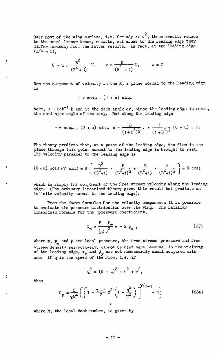
Over most of the wing surface, i.e. for x/y >> 6', these results reduce to the usual linear theory results, but close to the leading edge they differ markedlyfrcm the latter results. h fad, at the leading edge WY = 01,

u+u= B2 u B

(B2 + 'I) , V=

(B2 + 1) u, WC0

Now the component of velocity in the X, Y plane normalto the leading edge is

- v cosp + (u + u) sinp

here, p = cot-' B end is the Mach angle or, sinoe the leading edge is sonic, the semi-apex angle of the wng. But elong the leading edge

- v cosg + (u + u) sinp = - B 1

(l+B2)av + (I +B2$ (u + u) = 0.

The theory predicts that, at a pornt of the lending edge, the flow in the plane through this point normal. to the leading edge is br.xght to rest. The velocity parallel to the leading edge is

(u+u) cosp+v SW =u c

B2 B B 1

(B2+,) ' (B2+1)" + (B2+1) . (B2+1)H = u cosg

which is siqly the component of the free stream velocity along the lead5ng edge. (The or&nary linearised theory gwes this result but predicts an infinite velocity nomxal to the leading edge).

From the above formulae for the velocity components it 1s possible to evaluate the pressure distribution over the wing. The familiar linearised fornula for the pressure coefficient,

cp= P - P,

2-PU 2 =-2$x,

where p, p, end p are local pressure, the free stream pressure end free stream density res~otively, cannot be used here because, in the vicinity of the leadme; edge, #x and $y are not neoessanly small compardwlth one. If q is the speed of the flow, i.e. if

q2 = (u + u)2 + t2 + “2, then

(284

.

where M, the local Mach number, is given by

- 11 -

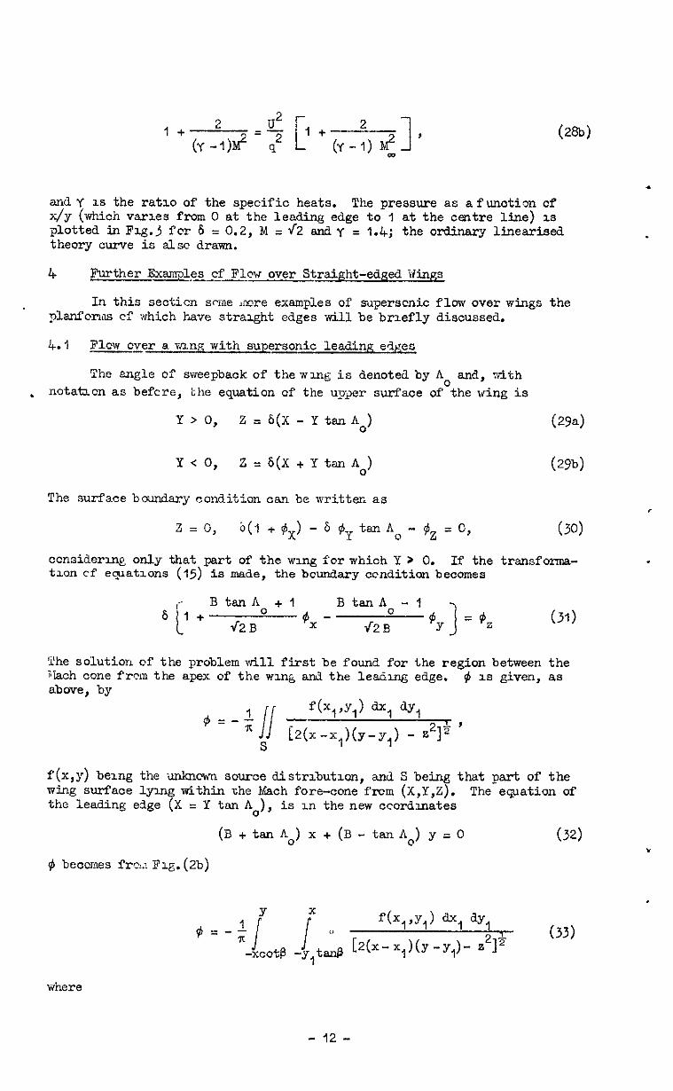
1-k 2 u2 (Y-1$ =7 [

-- ’ + (y-f) I( ’ 1 (2f3tJ)

and Y 1s the ratlo of the specific heats. The pressure as a function of x/y (which varies from 0 at the leading edge to 1 at the centre line) 1s plotted in Flg.5 fcr 6 = 0.2, M = f2 and y = 1.4; the ordineuy linearised theory curve is also drawn.

4 Further Examdes cf Flew over Straight-edged Wings ----

In this secticn spine acre examples of superscnic flow over wings the planfcn%m ci' which have straight edges will be brlefly discussed.

4.1 Flow over a gang with supersonic leading dges

The angle of sweepback of thewmg is denoted by ho and, :tith . notahcn as befcre, the equation of the uF$er surf'aoe of the wing is

Y > 0, 2 = 6(X - Y tan no) (29d

Y < 0, z = 6(X .I. Y tan no) (29b)

The surface boundary condition can be writtm as

z = 0, b(1 + &J - 6 $y ten ho - $bz = 0, (30) '

ccnsidermg only that part of the wing forwhich Y > 0. If the transfozma- tlon cf eyatzons (15) is made, the bcundary ocnditicm becomes

6 '-4 + BtanAo +I BtanA -1

1 <2B $x - $2," #y = B,

3 (31)

The solution of the problem will first be found for the region between the ;iaoh cone frcmthe apex of the wln~j and the leadug edge. $ 1s given, as above, by

s 12(x-XJY-Y,) - z21’ ’

f(x,y) being the unknown souroe distrlbutun, and S being that part of the wtig surface lying within the h&h fore-cone frcm (X,Y,Z). The eqation of the leading edge (X = Y tan ho), is In the new ccordlnates

(B + tan Ao) x + (B - tan Ao) y = 0 (32) I $ becoxes frc..: Flg.(2b)

Y x $=-;

1 1

f(X,'Y,) h, dY,

-xcotp WY,&@ Lax- x1 1 (Y -Y,) - z21+ (33)

- 12 -

.

Thus,

B- IanP =

tan ho

B+tanho (34)

Smce the flow is locally two-dimensional in the region under considera- tion flew quantities along lines parallel to the leading edge are constant. They are also constant along lines through the apex, and so are constant everywhere in the region. This suggests putting f(x,y) = K where K is a ccnstant to be determined fxm the surface boundary condition. wing surface, (taken to be z = O),is given by

$ on the

Y x $=-;

J i

Ic 5 WI 7-

.’ -xcotP -y,tme (2 b-x,+ b-q

Y K

i ayl

=-TG -xcotp (Y- [-2(x - x, ‘+Cy, t&y

=-@ ( x + Y, tad+ dy, ?r

(Y-Y,F

(y+x cctlq+ = _ 2\12K

7t (x+y tFd-II2 tanl3) au

Y2

= 2f2K - y-0 (y+x co@) (tad+ cos*e $3 c

=-&.(Y +x cot+) (tan&

(354

Substxtuting-<in the.bcdd.ary oondition,, equation (31),

K is given by

- 13 -

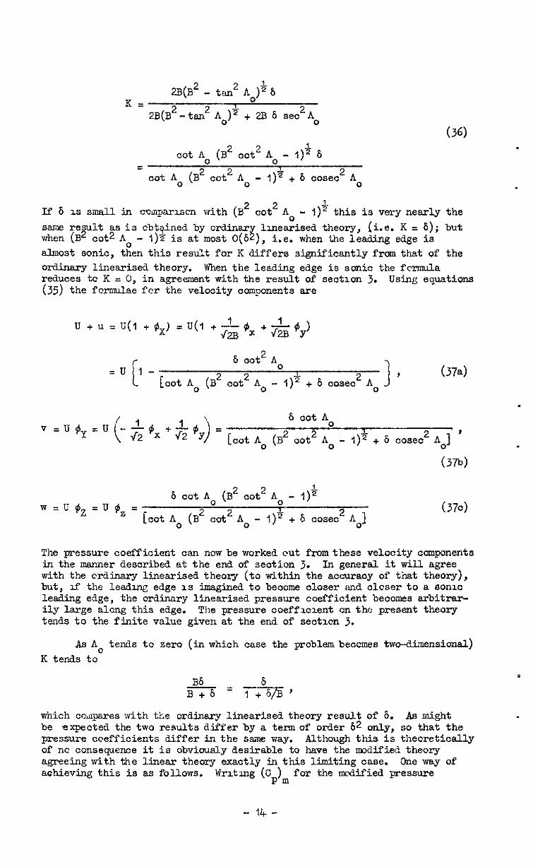
2B(B2 - K=

tan2 no): 6

2B(B2- 1

tan2 ho)2 + 2B 6 seo2Ao

cot Ao (B2 cot2 A, - ,+ 6 =

cot A0 (B2 cot2 A0 - I)~ + 6 cosec2 ii0

(36) .

If 6 1s small in cod+rlscn with (B2 cot2 A - 1)' this is very nearly the same result as is when (B2 cot2 A0 -

cbtqined by crdinsr I)1 is at most O(6 3

lmeaked theory, (i.e. K = 6); but ), i.e. when the leading edge is

almost sonic, then this result for K differs significantly from that of the ordinary linearised theory. When the leading edge is sonic the formula reiluces tc Ii = 0, in agreement with the result of sectlon 3. Using equations (35) the formulae for the velocity components are

lJ+u=U(l +q =u(i +Lmx+&6y) \rzB

6 cot2 A 0 I

iCOt A0 (B2 cot' A0 - 1)5 + 6 cosec* A0 ' (374

. 6 cot A

[cot ho (B2 oot2 A; - I)’ + 6 coseo' no] ' .

(3Tb)

w=u$Z=U$e= 6 cot A0 (B2 cot2 A - ,+

0

[cot A0 (B2 cot2 A0 - I)' + 6 cosec2 ho] (37c)

The pressure coefficient can now be worked cut from these velocity components in the msnner described at the end of section 3. In general it will. agree with the crdinary linearised theory (to within the aocuraoy of that theory), but, ti the lead- edge 1s imagined to become closer snnd closer to a sonx leading edge, the ordinary linearised. pressure coefficient becomes arbitrar- ily large alcng this edge. The pressure coefflclent on the present theory tends to the finite value given at the end of sectlcn 3.

As A0 tends tc zero (in which case the problembeccmes two-dimensional) K tends to

a6 6 B+6 = -bj/B

which coqares with ti.e ordinary linearised theory result of 6. As might be expected the two results differ by a term of order 62 only, so that the pressure ccefficients differ in the same way. Although this is theoretically of nc consequence it is obviously desirable to have the modified theory agreeing with the linear theory exactly in this Smiting case. One way of achieving this is as follows. Wrltmg (Gp)m for the modified pressure

- 14 -

coefficient and (C ) for the linearised pressure coefficient, the quantity Pd

(Cp)m + - (Cp)m 1 (B2 cot* A, - 1)

B* cot2 ho

has the foll If the leading ed sonic it is equal tc (Cp)mt as (B* cot* ho - I the leading edge is almcst sonic. other hand, when A = 0 snd the problem 1s twc- dimensional, the above qusntity reduces exagtlyto (Cp)4. In fact, this quantity never differs significantly from (C ) but it has the advantage that it is exactly equal to the linearised v&.te in the limiting case Of a twc-dimensicnel problem.

Over the re 'on cf the wing between the Mach ccne frcm the apex and the centre line f is no longer a constant everywhere, although it is still constant along lines through the apex. It will start with the vslue given by equation (36) on the trace of the Mach cone (X = BY) end, in a region close to this line, it will fall rapidly to approximately the vslue given by ordinary linearised theory, which is simply f(x,y) = 6. The exact variation of f(x,y) can be found only by sclving a rather complicated integral equation derived from the boundary condition of equation (31). For the moment it is suffiaient to remark that the pressure coefficient has a value on the line X=BY which osnbe obtained from equations (37) and then also falls rapidly, in a region close to this line, to apprcxi- mately the value of ordanary linearised theory.

4.2 Flow over a wing with subsonic leading edges

The equation cf the u surface of the wing end the notation used are the ssnm as m section the surface boundary condition is again

6 I+ c Btenho +I R tan A0 - 1

<2B @x - fl2B 'Y = $2 3

There is now cnly one region to consider since the Mach cone lies outside the leading edge. Ordinary linearised theory gives for the source diatribu- tion over the wing,

f-(&Y) = 6

This leads to logarithmic infinities in $x end $ at the leading edge; these arise because the linearised boundary has il een used instead of the fullbtiery condition snd these two ocnditicns differ considerably from one another in the vicinity of the leading edge. If $x is written out in terms of f(x,y), as in section 3, it can be shcpm that $x will be infinite at the leading edge unless f(x,y) = 0 there. Thus, the integral equation for f(x,y) obtained from equation (31) must possess a solution which vanishes elcng the leading edge if the pressure coefficient is to remain finite there. It will be assumed that such a solution exists.

At the leading edge, then,

f(X,Y) = #z = 0,

snd from equation (31)

- 15 -

I + Btanho+l Btsnho-1

J2B #x - J2B #y = 0

lkm the velocity ncrmal to the leading edge is

(u + Lz) co9 A0 - vsinho=Uoosho[l +$x-$pnho]

= u ccs no t

I Btsnho+l

+ v'2B #x -

= 0

Therefcre, as II-I the ease of a sonio leaking edge, the flew at a pomt of the leadinp edge m a plsne normsl ta the edge is brought to rest. The velocity slcng the edge 1s

(U + u) sin ho + v oos A0 = U sin A0 (I + #X + $Y cct a).

As in seotion 3 ordinary lmesr theory doss not break down 111 the deter- minatlon of the oomponent of vsloclty along the leading edge. In this case It gives

# 5-- (xcotA,+y) cash' @* B2Tc3tAo ) + (xcot AO-r) oosh-' (X-a2ycot " , n(~cotA~+~) B(XcotAo-Y) 1

(I+ B*Y cot A,, (A- B*Ycot A,, ) + cash-’

1

, B(X Cot fi.o + Y) B(X c,tAG - 1)

cash-, (x+ 8% cot A,, 1 - ah-’

(x- s2y cut ho)

B(X cot A0 + Y) B(X cot A,,- Y) 1 '

u s,n ho{?+ $x+ $y mt AJ = u s,n A0 L

2 bcot A, I (X+B2 YCD~ A ) I - Gosh

“I

. VT (l-B2 cot2 ho)* B(X cot A0 + Y)

Along the leading edge, then, the velocity is

.

2 b cot A0

x(1-B2 cot2 Ao)h

The pressure coefficient can now be obtained as at the end of section 3. To determine the pressure coefficient over the rest of the wing, f(x,y) would have to be found by satisfying the boundary condition, e

i" ation (31). This condition yields a complicated integral equation for

f x,y); if this were solved it would be found that, except for a small region olose to the leeding edge, f(x,y) would be almost equal to 6, its value on ordinary linearised theory. Close to the leading edge f(x,y) would rise rapidly from the value there of zero to approximately the value 6. The pressure coefficient has a value at the leading edge which can be obtained from the theory of this section end then falls rapidly from this velue to approximately the ordinary linearised value in a region close to the leading edge. Thereafter, up to the centre line, it remains approximately the same as the ordinary linearised value.

4.3 Supersonic flow in the presence of a ridge line

Further difficulties arise in the application of linear theory to the supersonio flow over thin wings when straight ridge lines are present, (as in the case of a delta vnng of double wedge section). If the ridge line is sonic or subsonic the pressure coefficient along the ridge line is infinite on linearised theory; if the ridge line is supersonic but nearly sonic the pressure coefficient can become arbitrarily large. The curve of the drag of the wing plotted against free stream Mach number displays a discontinuity in slope at the Mach number at which the ridge line beocunes sank; this discontcnuity is not obtained II~ practice. The presence of this discontinuity can be traced to the use of a linearised boundary condition which neglects a term not negligible near the ridge line.

It is not possible direotlyto improve the results of linearised theory by using the technique of this note. The reason for this can best be demonstrated by an example, that of the flcsv over the rear part of a delta wing of double wedge section with a supersonic ridge line. The trailing edge will be taken to be a line in the X, Y plane normal to the dire&ion of the free stream, The flow upstream of the ridge line will be ignored in this example; the results obtained are unaffected if its effeot is included. The equation of the rear part of the upper surface of the wing is

z = - 6X

The origin of ooordinates has been moved to the point where the ridge line meets the centre line, and a value of -6 has been taken for the slope of the rear part of the wing. The boundary conditionbecomes

6 (1 + #xx, + $Z = 0.

The transformation of equations (15) turns the above equation into

If the problem of the flow over the wing is solved by distributing sources over the wing, then the souroe distribution function in the region between the trace of the Mach cone from the origin and the ridge line is a constant, K say, as in section 4.1. Using equations (35), equation (40) becomes

- 17 -

- 2B (B2 - :. K, =

tan2 no)3 6

2B(B2 - tan2 no)4 - (B + tan Ao) 6 - (B - tan no)6

- (B2 - tan2 Ao)$ 6 =

(B2 - ta-I2 Ao)Z - 6 (41)

Thus, when (B2 - tan2 Ao) = h2, the source distribution over a finite region

of the wing becomes infinite, together with the velocity components and the theory breaks down ccmpletely. If the ridge line is subsonic or sonic the preceding theory gives sensible results for all csses. Nevertheless, it 1s olear that the theory cannot be applied direotly to flow over a wing with straight ridge lines.

The diffioulty aanbe overcome by the following subterfuge. When ordinary linearised theory is applied to determine the flow over a thin delta wing of double wedge section the wing is regarded as one delta pnng supers imposed on another, the first delta wing having a positive slope, and the second having a negative slope. The modified theory already developed in this note can be used to obtain the flow over the first wing since this has a positive slcpe. Again, oonsiderlng two delta vvlngs of the same plan- form and with equal and opposite slopes, it is evident that the distribu- tions of pressure coefficient on ordinary linearised theory will be identical except for sign. It will be assumed that this result holds true in practice, so that the pressure coefficient of a wing withnegative slope will be every- where taken as the negative of the pressure coefficient of the wing which is the xmage in the X, Y plane of the original wing.

The Justification for thus step is first that it is correct on ordinary linearised theory and it is therefore to be expected that in practice the pressure coefficients will have approximately the same absolute value. Seoondly, the method developed in this note is no more than an artifice to eliminate the spurious disccmtinuities present in the -e of drag against Mach number. All that is required of such a method is that it shall remove the discontinuities and shall replace them by a plausible Curve; the method of this note does fulfil both these rewirements sn.3 this is its ultimate Justification.

The technique of this note oan be used, then,to obtain the drag of a delta Hnng of double-wedge section. As in ordinary linearised theory the wzng is assumed to consist of two deltas superimposed and the technique is applied to each delta separately. This means that the surface boundary comidion IS not exactly satisfied since the interference of one delta on tine other is ignored. It can be shown, however, that this interference can be negleoted, without involving an error sny larger than that normally tolerated in linearlsed theory.

I+.,4 Supersonic flow over a wing of bxor.vex section

SO far all the wings considered have had regions of constant Slope; the example of this sect&x 1s a wing the slope of Vd7zh varies. The equation of the upper surface of this wing is

- 18 -

O<Y<s, Z = 2c (X - BY) [I - (X-BY)], e << 1 (424

-s<Y<O, Z=~E(X+BY)[I-(X+BY)] (42b)

which represents awing of constant chord, this aonstsnt being taken as the unit of length, span 29, and thickness-chod ratio E. The leading edge is sonic. The wing is symetrical about the line Y = 0 and only that part of the wing defined by Y * 0 will be ocnsidcred. The boundary ccnhticn becomes

28 [I - 2(X - BY)] [I + $x - B $,] - $, z~ 0

With the ssme transformation as before, i.e. that of eplations (15), this becomes

2s [I B2 + I # _ B2 - 1 ,+y A?.B x Aa3 1

-$*x0 (43)

# my be wt ewd. to #, + #,, where $5, and ti2 both satisfy the linearised equation of supersonic flowwhile $, satisfies the boundary oonditicn

2E 1 + B;; ' $b,* - B;; ' [

$,y 1 - #is q 0

and $2 satisfies the boundary condition

-4 J2ExB I + B2 + 1 ti2x _ B2 - 1

e?B ?2B ti2y 1 - $2s = 0 bb)

$, satisfies aboundary condition which is the ssme as equation (31)

except that 6 has been replaced by 2E and so $,x, $,y and $J,~ have

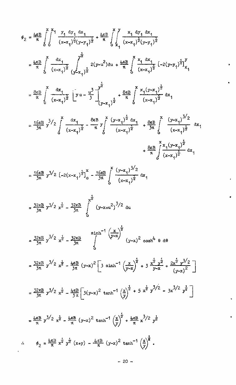
effectively been found slresdy. If $2 is determined by distributing s-es ever the wing surface, f(x,y) being the source distribution function, ordinary linearised theory gives

f(x,y) = - 442 BEX,

using equations (200) and (&b). Now, as in equation (IV),

x xl f(Y, ,x,1 dY, a, x

#2=--1- (2% l-1 (x-x$ (y - y,)& - kc x il

fb,‘Y,) dY, a,

- ’ c c 1

b-q (Y-Y,)T

and SC

- 19 -

.

.

BEE +-F &I

&kB +- x

'

,&

(y-x+u2)3/2 au

0

+ 1 3/i +5x2y - Jx3/2 # 1

= 4$2 y3/2 ,s _ LEE (yvx)2 tti-’ ‘Is h + ‘x 0 Y e x3/2 p

:. 6 4EB &

= y 4 x 8 y (x+y) - 2 -4g- (y-x)2 ta&l-’ 0 5 .

- 20 -

Hence,

2sB y3/2 h #2x = -;;-

2sB y (y-x) - -

6SB $ $ ,h A y&

+-yx Y

DEB $ 3 @ (y-x) td-~ /X =yx y + A (77

while

(b 2Y

_ DEB & 3 -yy x +y- + 2;B x3?

Y2

(45a)

(4%)

h& al-d + 2Y

are O(E) everywhere, even at the leading edge x = 0 where, in fact, they vanish; this means that ordinary linearised theory predicts a plausible value for the pressure coeffioient (or at least for that part of the pressure coefficient involving $,). The part of the pressure coeffloient involving #.,oan be dealt withby the technique already developed in this note and so the problem of flow over a wing of parabolic arc section requires nc extension of the theory.

The above discussion ignores tip effects. If the wzng is of large span It 1s probably sufficiently acrrtrate to work out the flow in the region influenced by the tip on ordinary linearised theory; if It 18 felt neoessary to improve the linearised results III this region also, this can be done by using the method of this note since the tip can be regarded as a subsonic edge.

5 Further Simplirications of the Method

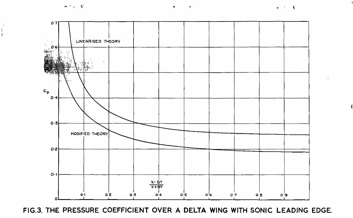
In Fig.& the pressure ooefficient dete?.mined fmm ordinary linearised theory, over the wing of section 3 is shown; this w5ng was a symnetrioal delta wing with sonic leading edge and a constant slope of 6. plotted against S where

BCp is

2 Z= x- ’ x

(3+,)2 g2 Y -77’

for two values -bf B (B = I and 3) and three values of 6 (6 = 0, 0.1 and 0.2). The pressure coefficient is given by

on ordinary linearised theory ad so 6 = 0 is a limiting oase in which

- 21 -

cP = 4

.(B* + I) f-4 (48)

On the axis Z = 0 two points are marked; the wdified pressure coefficient takes at the

these are the values which leading edge, using the .~ theory of section 3.

B and not on 6. This pressure coefficient at 5 = 0 depends only on

The pressure coefficient on modified theory beaanes approximately the same as the ordinary linearised coeffxient at a very smallvalue of%, this value being O(S2), so that G is O(1). A aonsiderable smount of work would be involved if the wessure coefficient derivedfromqations (26) was used to work out the drag of the wing. It is proposed instead to draw the tangent from the point on the axis C = 0 which represents the modified pressure coefficient at the lea&ng edge to the linearised curve and then continue with this curve until the centre line (Y = 0) is reached. negligible.

The error incurred in doing th1.s should be It 1s possible to simplify the oslculation still further.

Each of the linearised curves of Fig.4 (drawn for various values of B and 6) has one point marked on it with a cross; this 1s the point at which the tangent described above touches the curve, It will be seenthat to sufficient accuracy all these points are given by 6 = 3, i.e.

4.B* 5, 2 X - BY

(B* + l)*a2 y (B* + .1)*S2 ' + BY = 3,

j + 3(B2 + l)*S2 X y=B 4B

B* +*,,'6* - B

1 -3( c

r,&!t+i I

(49)

4B2

Thus, the pressure coefficient over the wing will be taken as falling X-BY linearly m- X+By from the modified value at the leading edge to the value

gwen by ordinary linear theory when X/Y becomes equal to the quantity 111 equation (49). From then until the centre line (Y = 0) the ordinary linearised curve will be used.

For the cases of subsonic and supersonic edges a similar prucedure 3.5 suggested.. Thus, for a supersonic edge the pressure coeffxient ~111 be

X-BY taken as fallmgl3nearly 3.n- X+BB from the modified value at the &is& line (determned in section 4.1) to the value given by or&nary linear theory when

1 and ordinary linesrlsed theory will be used from then on. The factor

1 B* cot2 AC

has been intrcduced sconce it is to be expected that, keeping

- 22 -

the free stream Mach number constant and varying the sweepback an&s, the region ul which ordinary linearised theory is invalid will become progressively smaller as the edge becomes more supersonic. For a sub- sonic edge the pressure coefficient will be taken as falling linearly in $$$ fran the nmdified vslue at the edge (determined in section 4.2) to the value given by ordinary linearised theory when

X -=tAIlh B2 + l)*S* Y 0 2

cot2 ho 3 "

The factor B2 cot* A0 has been introduaed slnoe it is to be expected that, keeping the free stresm b;ach number constant and varying the sweepbaok angle, the reglcn in which ordinary linearised theory is invalid will become progressively smaller as the edge becomes more subsonic. In some cases the behaviour of the pressure coefficient in the region lying mithin the Mich cone from the apex but outside the edge is rsqulred; in this region tsn Ao > X/Y > B. The pressure coefficient will be taken as

X-BY falling linearly i.nx+~y from the modified value at the edge (determined in section 4.2) to the vaiue given by ordinary linearised theory when

X - = tan ho - (tan A0 - B) 3( B2 Y

+ 112S2 cot2 A 2 0

The factor BC cotL A, has been introduced for the same reason as before. In both these cases ordinary llnear theory is to be used for values of X/Y respectively greater end less than those given by eqations (51) and (52).

The above formulae may seem arbitrary, and so they are, but they simply xnvolve replaoing the curve of the modified pressure by one which has the correct value at $I% = 0, is then incorre& (probably only

X-BY slightly so) for an interval of order 62, and then from X+BY = O(S2) to X-BY - = 1 has sn error negligible in a linearised theory. X+BY

The calaulation of the aerodynamic forces now involves integrating the pressure coefficient nmltiplied by the local slope over the wing. The integration over that part of the wing where the pressure coefficient is to be taken as havlxg the ordinary linearised value leads to a double integral which is not very diffioult to evaluate, but the integration over the rest of the wing does give a rather complicated result. Since this region is small it 1s possible to make a further simplification; the mean of the lntegrand at the two extremes of the region (the line given by the ap-ropriate formula of equations (49) to (52) inclusive, and the edge itself t; is multiplied by the area of the region. The validity of this approximation was checked for the examples of the following seotion, and was found to be satisfactory.

6 Results and Dlscusslon

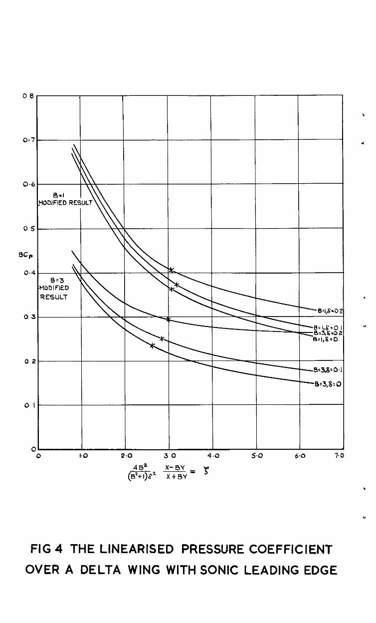
It is clearly desirable that the theory should be checked against experimental determinations of the drag of straight-edged wings; such determinations are unfortunately, very rare. Ref.2 gives the results of measurements of, among other things, the drags of certain delta wings. The wungs are of double wedge section, having thiotiess-chord ratio of

- 23 -

8% with the maximum thmlmess occurring at 18cjo of the root chord measured from the apex. The measurements were at Mach numbers of 1.62, 1.92 and 2.40, and were made for a range of sweepback angles.

Roth theoretical and experimental results are plotted in Figs.5 to 7 inclusive. The or3insrylinesrised curve is shown as a full lme snd the two sharp discontinuities in slope oanbe seen clearly. Experimental points are show-o by circles and a chasmdotted curve has been drawn through these points. Finally, sme points calculated using the modified theory of section 5 are shown by crosses snd a dashed line has been drawn through these points. Although there is still a sharp rise at the Maoh nuuher at which the ridge line becmes sonic, the modified curve lies much closer to the experimental results than does the 0-y linearised -e.

A few remarks about these figures mast be made here. The custcmsry form of plotting has ‘been employed, i.e. CD/AT~ against AD, where A is the aspect ratio of the wing T the thickness-chord ratio and CD, the drag coefficient, is given by

D CD = - &pU2S

S being the area of the wing and D the drag. The theoretical drag is the wave drag, of course, whereas the measurements of Ref.2 included skin friction drag. For each kiach number an estimated value of the skin friction drag coefficient has been subtracted from the experimental result; this value was 0.009 for M = 1.62, 0.0085 for M = 1.92 sd 0.008 for M = 2.40.

s The final

point to be mentioned concerning these figures is the construotion of the modified curve. Five points were calculated for Fig.7 (M = 2.40) snd this enabled the curve to be drawn fairly accurately, but for the remaining two . figures only the Roints corresponding to a sonic ridge line and a sonic leading edge mere oaloulated. These two points are obviously the two most important and, together with a knowledge of the ordinary linearised curve snd an example in Fig.7 of a complete ntodified curve, there should not be any difficulty in drawing a curve to pass through these two points and t0 fair into the ordinary linearised curve for vslues of AR both small and large aompared with unity.

Finally, a brief discussion of the theory of this note will be given. It is obvious that the theory can be immediately extended to a swept trail- ing edge; the wing (assuming it tobe a fully tapered sing) is regarded as being canposed of three superimposed deltas and the modified theory applied to each of the deltas. Separating the flow field into three distinct flow fields in this way means that the surface boundary condition is not exaotly satisfied but, as in seotion 4.3, this results in a negligible error. It might also be supposed that the extension to the incidenoe Case, a.e. to the removal of the discontinuity in slope in the Curve of lift coefficient against Xach nunioer, as very simple; this, however, is not the Case. Suppose that the incidence of the wing is a snd that the slope at a certain point is 6 while the pressure coefficient at this point is (Gp)u on the upper surface . and (Cp)4 on the lower surface; (this pressure coefficient is the coefficient on an exact theory). Now the required quantity is CIa the lift-curve Slope, and this requires the evaluation first of .

L- (cpL - (OpJ4 1 Gp (8 + a) - Cp (6 - a) a = a- 0 i a 1 U'O

In evaluating the drag of straight-edged wings the exact pressure coefficient was replaced by a modified coefficient which behaved everywhere in a manner which was at any rate plausible and the results of this section suggest that this was quite sufficient. The evaluation of the lift-curve slope, however, involves the derivative of the exact pressure coefficient and much more care must be exercised in replacing this coefficient by a "suitably chosen" function. It is very doubtful. whether any method of the ty-pe employed In this note (that 19, any method involving the limiting of Pressures near the leading edge) could justifiably be used to improve the values of lift-curve slope predicted by linearised theory when a straight e?lge is almost sonic. No attempt has been made to do so in this note.

The justification for the method as applied to the evaluation of the wave drag of wings lies almost entirely in the agreement of the results obtained by the theory with those obtained by experiment. The agreement has been shown to be satisfactory. It would have been interesting to have compared the pressures predicted at the leading edges of deltawlngs with those obtsined in praatioe but it is, of oourse,very diffiault to measure pressures at leading edges and so the comparison oannot be made. All that can be said is that the overall aerodynamic forces exhibit satisfaotory a&reement with experiment, while the method has the advantage that it is qulok and simple to apply in sny Particular case. It is, of course, no longer possible by judicious ohoice of parameters to reduoe the plotting of the drag of a large class of delta wings against Maah number to a single curve as oenbe done using ordinsrylineazisedtheory. Cn the other hand, it is diffioult to conceive of an improved theory d-&h WW.IJ~ retain this Property, and it is certainly more realistic to have VAT” for a fixed Mach number varying slightly with =.

A

B

cD

OLa c

Cple' (Cp)m

(cp).e' (cp)u

c

D

f

K

LIST CF SYMBOLS

Aspeot ratio

(h< - I)$

D/&U2S

Lift-curve slope

P-PJ&pv2

Linearised and modified Cp respeotively, (Section !+.I)

Cp on lower and upper surface respectively (Section 6)

Rcot chord.

Vave drag

Souroe distribution function

A constant source distribution in section 4.1

- 25 -

k

M

M m

P

Ta

4

s

E r;

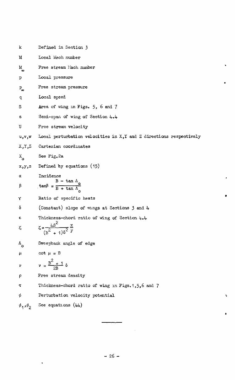
Defined in Section 3

Local Mach number

Free stream ?iach number

Local pressure

Free stream pressure

Local speed

Area of wmg m Figs. 5, 6 and 7

Semi-spa of wing of Se&ion 4.4

Free stream velocity

Local perturbation velocities in X,Y and. 2 directions respectively

Cartesian coordinates

See Pig.2a

Defined by epations (15)

Incidenae B-

.tanp = tan A0

B+tanho

Ratio of specific heats

(Constant) slope of mngs at Sections 3 and 4

Thickness-chord ratio of wing of Section 4.4

r;=@2 5 (B2 + l)b2

Sweepback angle of edge

cot p = B

Free stream density

Thickness-chord ratio of wtig m .E'igs.l,5,6 end 7

Perturbation velocity potential.

See equations (44)

- 26 -

NC. - Author Title, etc.

1 W. R. Seers

2 E. S. Love

REFEREXXS

General Theory of High Speed Aerodynamias Oxford, 1955, Section D, Chapter 3

Investigations at Supersonic Speeds of 22 Triangular Wings Representing Two Au-foil Sections for each of II Apex Angles NACA Report 1236, 1955.

- 27 -

.

.

. .

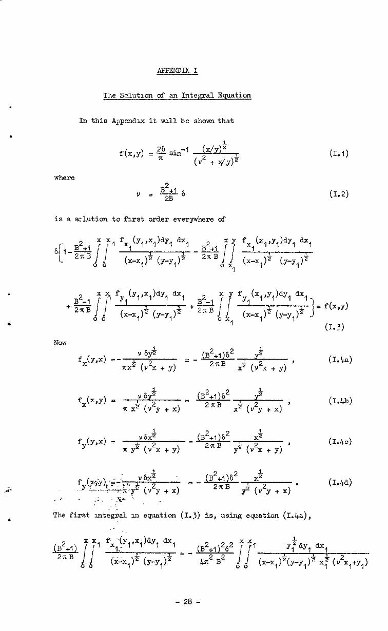
The Sclutlon of an&tegral Equation

In this A>pendx it Will be shown that

where B*+l Y =X6

is a solution to first order everywhere of

(1.1)

(I.21

f (x,,Y,)~Y, *, x1

7 (x-x, 1” (Y-Y, 1”

B2-1 f b, ,x,h, hi

+2xB Yl B2-1 'i

f

I = f(X,Y)

o o OX 1 (1.3)

Now

fx(YA =- !&-

L XX2 bJ*x + Y)

=d&.&q" , x;’ (Y2X + y)

i fy(Y,4 =

v 63 &g, ,4

?I yz (v2x + y) $ (“2, + y) 2

= (BkrjB2 x' , yF (v2y + x)

,J I .; _ . .p : / _ > .

The first mtegesl m equation (1.3) is, using ewation (1.4a),

(1.k.)

(I.4b)

(1.40)

(IA4

= Yl dyl 9 1 (X-X,)F(Y.-y,)z X:(Y2X,+y,)

- 28 -

None & the integrations in this Appendix offers any diffioulty and inter- mediate steps are outted. First, then,

x

1

: YY'dY, = 2 -1 "1- : sin

0

2YX,& I( v2x, + Y) & .

o (Y-Y,F b2x, + Y,) Y - l- (A+ + Y)" sin- (1

7 T + v2)F yF

. Next,

XX

11

1 Y$Y, dx,

o o (x-x,)" (Y-Y,F XT b2x, + Y,) = 4 p [ ($ sine] de

I& x x1

ii

fx (Y JX MY, hi 1 ' ' , = _ qp-I [ (+qae

7t2 B2 00 (x-x, 1” (Y-Y, 1"

i

2 .

s3n-’ (v;+y)6

-/‘I sin- , b2x+y&se ae

3

1

(I+"*)3 yz J

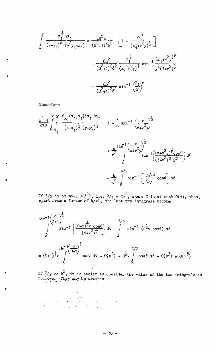
If "/y 1s at most O(a2) thus result is at most O(b3) (I.54

If “/y >> 62, this result is O(b2) 0.5b)

The second integral In equation (1.3) is, using (Id),

(x ,Y MY, ilx, x, 1 1

' (x-x,)~ (Y-Y,)'

Fl.rst,

.

- 29 -

8~' x 4

(*2+,)Z62 sin-' -+ i>

Therefore

If x/y is at most 0(6'), i.e. "/y = Cv2, where C is at most O(l), then, apart from a factor of 4/x2, the last two integrals become

r! Sk-1 - a ( i c +I

sin-l (G+& oose v2

i I 227 aa- :

0 (1+v )" 3 i

sin-' (G-v oos8) de 0

= (G+l)+v s~ptoso de + O(2) - ch pose de + O(J) = o(J)

0 - 0 . . *

If x/y >> 6 2 . , follows. .They

It IS easier to consider the value of the two integrals as iray be vrntten ** .:. ,- ._

. .

. I ,-

- 30 -

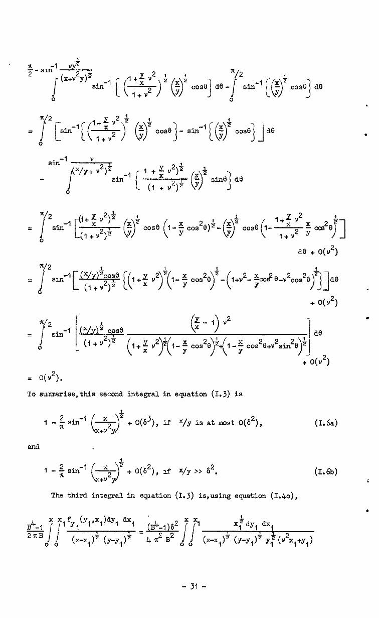
= o(v2). To smise,this second integral in ewation (1.3) is

2. , - : sin-1

G > x * + O(fj3), if "/y is at nest O(h2), +v2y

end

-1 x’- d; J

: 1 - $ sin

*v2y + O(S2), 3.f x/y >> 62.

(1.6a)

(1.6b) i

The third integral in eqgation (1.3) is,using equation (I.&c),

. x x f (Y, ‘X,)dY, h,

1

B4-1 2nBo i

I' Yl xf-dy, b,

,I (x-x,)+ (y-y,)* = 1 1 1

(x-q (Y-Y,F Y;(Y2x,+Y,)

- 31 -

First,

Xl 1

i

Q.1 2 (Y2X +y)Z

(Y-Y,P Y1” b2x,+Y,)

= , 1 tan-’ --L--a o xc,” ( v2x,+y)" dY-x, 1'

Therefore,

(B2-11 i' x x1

2nB j i

fy (Y 9 MY, a, I ' '

.I. 7 00 (x-x,)2 (Y-Y, 1"

= Z(B*-1)s sLn-' -&

x2 Bv i 0

The integrand varies between

sin-l (&& = $ _ sb-' AZ&

( 1+v2)yF ( 1+v2)” YF

i and

sin-’ (,+:*)g = $ - su-l-’ /*+

so that the integral may be written

(I-7)

P The thid integral in equation 61.3) tiyn, is at most O(h*) when x/Y is at most O(h2), (1.7&),and O(c) when "& >> b2, (I.7b).

The fotih integral in egution (1.3) is, using equation (I.@),

I

- 32 -

First,

Y f i Yl 1 2 tan-' (Y-X, 14 1 7-

x, -(y-y,F Y,~(Y*y,+x,) = x,E(x,+Y2y)T 2 -:* (x,+v Y)

Therefore, .$

ii

f b rY )dYp-y Y, ' ' (BQ x y (x J 2=B cx 1

(x-x, 1;: (Y-Y, 1'

= _ (pIti sin-' * i' 0

and is at most O(S2). (f.8)

Thus, in equation (1.3), if X/y is at most O(S2), the first, third and fourth integrsls are at most O(b2) while the seoond is i ++g’ x2 2 c, > + O(b2); +v Y the left hand side of (1.3) beccmes then

26 7 sin- i x4 G > + v'y

+ O(S2)

which is, to first order, f(%Y). If x/y >> ti2, the first and fourth integrals are O(b2), while the seuond snd third combine to give

\$ ,.+in” x G ) +v”y

+ o(a2) = 1 A[;- O(6)]= O(6).

The left hand side of (1.3) becomes then, 6 + O(s2); the right hand side is also 6 + O(62)) if x/y >> 62. Hence, the integral equation (1.3) is satisfied everywhere to first order by

f(X,Y) = $ sin" -&

From equation (20a)

(1.9)

- 33 -

mth an error O(S2); here, (1.5)and (1.6) have been used. From equation (2Ob)

= _ + ($, (1.10)

with an error 0(6*); here, (1.7) and(I.8) have been used. From lquhons (2oc) and(I.1)

2pations (I.V), (1.10) and (1.11) are valid cm the wing only.

(1.11)

- 34 -

H~.20?8.C.P.39Y.K3 - Prmted tn Gent Witam

r=, 4T

2

/

\ /

‘I\“$“i’

I

0

-I

-2

-3

-4

;I---

MACH WAVES AHEAD OF AU LINES MACH WAVES ALONG TRAILING EDGE

lT=, I L I I I

3, 3 I I I I

2

I TTCP

4r 0

-I -I I \ I I

-2 -2

-3 -3

-4 -4’ I III I I

MACH WRVES BEHIND TRAILINGEDGE ONLY MACH WAVES ALONG MAX THICKNESS LINE

-41

MACH WAVES AHEAD OF LEADINGEDGE ONLY MACH WAVES ALONG LEADING EDGE

3 3

2 2

I I TlCP TlCP 4T 4T

0 0

-I -I

-2 -2

-3 -3

-41 -41 I I I II I II I I I I

TCP 47

3

2

I TCP 47

0

-I

-2 -2

-3 -3

-4 -41 I I I I I

I I I I

FIGLPRESSURE DISTRIBUTION AT MID SEMI-SPAN ON A WING OF DOUBLE-WEDGE SECTION.

.

FIG.2 a THE BODY DESCRIBED IN SECTION 2

/

// \ ‘,/l / \ \ (XT z \ \

MACH LINES \ \

FIG. 2 b. THE WING OF SECTION 4.1

LINEARISED THEORY

0.1 02 0.5 0.4 0.5 O:b 0 ‘7 08 09 0 I I I 1 I I I I

FIG.3. THE PRESSURE COEFFICIENT OVER A DELTA WING WITH SONIC LEADING EDGE.

08

o-7

04

05

BCP

0.4

01

Oi

01

c 0 I.0 2.0 30 4.0 50 6.0 1

FIG 4 THE LINEARISED PRESSURE COEFFICIENT

OVER A DELTA WING WITH SONIC LEADING EDGE

I.0 -

5-

.0 -

.5 -

*O-

,.5 -

O- 0

Y

b c I

DELTA WING

DOUBLE WEDGE SECTlON

MAXIMUM THICKNESS AT 0 18C

Y--1.62. I

.’ _H. /IQ --__- ‘I’=

I I.0 2.0

( 1’1 I /

SC RI’ L

L VC

I

I \

‘\ 0‘..

0 “0- __

I )NlC SOr;lC DGE LEADING INE EDGE

I

\

\ .4

40 50

AS

I. .

I I

LINEARISED THEORV

x x POINTS CALCULRTED FROM MODIFIED THEORY

_----- MODIFIED CURVE (BY COMPARlSOl WITH FIG 7)

0 0 EXPERIMENTAL POINTS

-.-.-.- EXPERI

I

y-.

L.\ ‘. . .

‘.

-I-

:NTRL CURVE.

60 70 8.0 90

FIG.5 THE DRAG OF A DELTA WING OF DOUBLE-WEDGE SECTION M = I.62

26*1= W N01133S 3Sl3M-318flOCJ JO E)NIM Vll3Q V JO WtrCl 3H1’9’~ld SW

06 OS OL 0.9 OS 0.9 0.f 0. I 0

3 81.0 IV

- NOl133S 33am 31slloc!

SlNIOd lVLN3WlU3d%3 0 0

-----

htl03HL a3uioow wotlj a3hv-mv3 SlNlOd x x

- h~03l-u a3Sltlw3Nll

0.1

5.1

zl.w 03

0 07

0 a,

0 r-

0 9

0 w

C.P. No. 394 (19,485)

A.R.C. Technical Report

0 Crown copyrrght 1958

Pubbshed by HER MAJESTY’S STATIONERY OFFICE

To be purchased from York House, Kmgsway, London w c 2

423 Oxford Street, London w.1 13~ Castle Street, Edmburgh 2

109 St Mary Street, Cardiff 39 Kmg Street, Manchester 2

Tower Lane, Bristol 1 2 Edmund Street, Bmn&am 3

80 Chichester Street, Belfast or through any bookseller

5.0. Code No. 23-9010-94

C.P. No. 394