Aeroelasticity of Structurally Nonlinear Lifting Surfaces Using Linear Modally Reduced Aerodynamic Generalized Forces

Dynamic Aeroelasticity of Structurally Nonlinear

Configurations Using Linear Modally Reduced

Aerodynamic Generalized Forces

Luciano Demasi∗ and Eli Livne††

University of Washington, Seattle, Washington 98195-2400

Steady state and time domain methods for integrating commonly used frequency-domainunsteady aerodynamic modeling based on a modal approach with full order finite elementmodels for structures with geometric nonlinearities are introduced. The methods are aimedat airplane configurations where geometric stiffness effects are important but where de-formations are moderate, flow is attached, and linear unsteady aerodynamic modeling isadequate, such as joined-wing and strut-braced wings at small to moderate angles of attackor low aspect ratio wing. Results obtained using full order nonlinear structural modelingand full order aerodynamic modeling (including aerodynamic influence coefficients for allaerodynamic panels) are compared to results obtained using full order structural modelingwith generalized aerodynamic matrices obtained using a modal approach.

I. Introduction

WHILE addressed rigorously for years in helicopter rotor aeroelasticity, structural nonlinearity due tolarge deformation and geometric stiffness effects, was not considered a major factor in the aeroelasticity

of conventional fixed-wing configurations. Using nonlinear beam models the aeroelasticity of geometricallynonlinear high aspect-ratio configurations was studied in the 1970s and 1980s, focusing on gliders and human-powered vehicles.1−3

With the subsequent appearance of high-altitude long-endurance UAVs, renewed interest in the nonlinearaeroelastic effects of large deformation led to additional research based on the coupling of nonlinear beammodels with essentially 2D unsteady aerodynamics, suitable for the modeling of configurations of very highaspect ratios.4−9

Other configurations affected structurally by geometric nonlinear behavior also emerged: the strut-bracedwing more recently,10−12 and earlier the Joined-Wing (JW) configuration.13−19

Interest in aeroelastic limit cycle oscillation (LCO) behavior with initial focus on the contribution ofcontrol surface free-play and the behavior of thin fighter wings carrying external stores, led to a search forother possible structural nonlinearities that may cause LCO, such as the stiffening of plate structures subjectto large deformation. Theoretical and experimental studies of plate-like and beam-like wings with geomet-ric structural nonlinearity20−23 have indeed confirmed the importance of understanding where structuralgeometric nonlinear effects become aeroelastically important and of accounting for them.

Most of the nonlinear aeroelastic modeling work done to date was based, in the structural area, onnonlinear beam or Ritz plate models to account for large deformations. These models are very useful formodeling simple wind tunnel models or very high aspect ratio wings, but they cannot be used to modelgeneral configurations, and their major limitation is their inability to capture local effects. Such local effectsinclude the behavior at and around joints and the calculation of reliable stress information, especially in areasof high stress concentration. Nonlinear finite elements can allow capturing such local effects and modelingof general configurations at complexity levels that can represent real airplanes. But in the very few cases inwhich nonlinear finite elements were used to model a geometrically nonlinear structure they were coupled withcomputational fluid dynamics (CFD) models for the flow. This was done for static aeroelastic modeling using

∗Postdoctoral Research Associate, Department of Aeronautics and Astronautics, BOX 352400. Member AIAA.†Professor, Department of Aeronautics and Astronautics, BOX 352400. Associate Fellow AIAA.

1 of 42

American Institute of Aeronautics and Astronautics

48th AIAA/ASME/ASCE/AHS/ASC Structures, Structural Dynamics, and Materials Conference23 - 26 April 2007, Honolulu, Hawaii

AIAA 2007-2105

Copyright © 2007 by Luciano Demasi and Eli Livne . Published by the American Institute of Aeronautics and Astronautics, Inc., with permission.

sequential application of nonlinear structural and CFD models. Capabilities that in a integrated mannercouple nonlinear finite elements with steady and unsteady CFD aerodynamics already exist,24,25 but theyrequire a lengthy model set up and meshing process as well as considerable computational resources.

Since for capturing both stability and dynamic response behavior (especially gust response) of nonlinearaeroelastic systems time domain modeling is required, appropriate unsteady aerodynamic modeling alsobecomes a challenge. In the case of high aspect-ratio configurations and structural geometric nonlinearity,as stated before, 2D linear potential unsteady aerodynamic models in the time domain have been usedwith considerable success to capture aeroelastic behavior in subsonic flow.26 Such models can be used toalso model dynamic stall effects.27 For low aspect ratio wings, where deformation is small enough that theunsteady aerodynamic loads are linear but large enough to cause structural geometric nonlinearity, dedicatedtime marching vortex lattice models proved adequate.21−23 These dedicated time-marching vortex latticemodels are limited to planar configurations of simple planforms and to incompressible flow.

Linear compressible unsteady aerodynamic theory - the foundation of aeroelastic analysis and clearance ofall flight vehicles flying today - has been so far not used for the aeroelastic modeling of structurally nonlinearairplanes. Computer capabilities such as the Doublet Lattice Methods (DLM) codes,28−37 PANAIR,38 orZAERO39−41 and other linear unsteady potential aerodynamic codes have been used and are still being usedsuccessfully in aeroelastic analyses of flight vehicles over a wide range of flight conditions. These codes can beused to model general three-dimensional configurations made of lifting surfaces, control surfaces, fuselages,nacelles, external stores, etc. One problem is that they are based on a frequency domain formulation, whereunsteady aerodynamic force terms are calculated for simple harmonic motion at given reduced frequencies.These need to be transformed to the time domain for integration with time domain nonlinear structuralmodels. But the main problem with the utilization of linear unsteady aerodynamic codes for the aeroelasticmodeling of structures with geometric nonlinearities is that they are tailored for a modal approach. That is,these codes produce generalized unsteady aerodynamic force terms for a set of mode shapes of motion givenas input.

In a modern modal approach the detailed finite element model of a structural dynamic system is reduced inorder by describing the motion using a superposition of mode shape vectors. The problem with this approachin the case of geometrically nonlinear structures, or any structural system for that matter, is that when localeffects become important and unpredictably spread the modal approach usually fails. Successful modal orderreduction of structural models in the linear case can be achieved in the case of strong local effects when thelocation of these effects is known a-priori. The structural nonlinear case, however, is different. Because ofthe dependence of geometric stiffness matrices on stress distributions and because of the large changes suchstress distributions can portray as loading increases and the structure approaches instability, modal orderreduction tends to fail when used to reduce the order of general structures undergoing large deformation.The case of the joined wing configuration is even more severe. Concentrated loads transferred through thejoint connecting the main wing and the rear wing attached to it affect stress distributions around the jointarea. The structural dynamics of the configuration is extremely sensitive to the location and details of thejoint design. Studies of the nonlinear structural dynamics of this configuration using a number of modalorder reduction approaches showed failure of all those approaches to yield accurate reduced order structuraldynamic models capable of capturing both displacement and stress behavior.42

Now, both joined-wing and strut-braced wing configurations display strong geometrically nonlinear struc-tural dynamic behavior even without the large deformation typical in HALE vehicle wings. For attached flowconditions typical of high dynamic pressure straight and level or maneuvering flight, the unsteady aerody-namics of such configurations is expected to be properly modeled by potential linear unsteady aerodynamicmethods - the same methods used for the aeroelastic simulation of conventional configurations in compress-ible subsonic and supersonic flow. It is important, then, to develop the capability to simulate aeroelasticstructurally nonlinear configurations of flight vehicles using an integration of nonlinear structural finite el-ement models in full order (to avoid the difficulties with modal reduction in this case) with the standardlinear modally-based unsteady aerodynamic models, which can be used to model general configurations, andfor which significant experience exists.

The present paper will present such a modeling capability for investigating nonlinear aeroelastic problemsof planar and nonplanar wing systems in general and of joined wing configurations in particular. Integrationof the nonlinear structural FE capability with linear steady and linearized unsteady aerodynamic modelswill be discussed as well as static and dynamic aeroelastic solution techniques.

Studies in which coupling of full order nonlinear finite element models with generalized aerodynamic force

2 of 42


models was compared to coupling of full order nonlinear finite element models with full order aerodynamicpanel methods were presented43 before with focus on the steady case. That formulation has now beenrevised and modified. It is also extended here to the unsteady cases. In particular, generalized aerodynamicforce matrices produced by standard linear unsteady aerodynamic codes are transformed to the time domainand used with full order structurally nonlinear finite element models to simulate time dependent nonlinearaeroelastic behavior.

II. Terminology

The two quantities displacement vector and cumulative displacement vector will be used in both staticand dynamic cases. They are introduced here for the steady case first for the sake of simplicity. Thedisplacement vector ustepλ iter n is referred to the configuration at the beginning of the current iteration nof load step λ in the Newton Raphson procedure. The vector which contains the coordinates of all thestructural nodes of the wing system will be xstepλ iter n. The coordinates are relative to the configurationbefore the displacement vector is added. We will use an Updated Lagrangian Formulation44−46 and so thecoordinates of the nodes will be continuously updated during the iteration process.The quantity xα=0 represents the coordinate vector of all structural nodes at a reference aerodynamicconfiguration with no angle of attack. Aerodynamic panels are defined based on the geometry of thatreference configurations and structural motion away from the reference configuration is small.The concept of cumulative displacement vector is also introduced. This quantity (indicated in the steadycase with the symbol U stepλ iter n) is defined as the summation of all the displacements that have occurredduring the iteration process up to the current iteration. Basically, the coordinates at a particular loadlevel are obtained by adding the vector of the coordinates in the undeformed configuration (xα=0) to thetranslational part of all the displacements that the structure was subjected to all the previous load levels.

III. Present Doublet Lattice Method

The doublet lattice method is a very well established procedure for the calculation of linear unsteadyaerodynamic matrices in subsonic compressible flow.28−37 In the present paper a dedicated Doublet Latticecode has been developed. The approach is similar to the one introduced by Sulaeman.12,36 Basically, theunsteady aerodynamic kernel47−49 is integrated using a gaussian quadrature formula. To perform the cal-culation of the complicate kernels (expressed in Landhal’s form48), Ueda’s formulas50 has been adopted. Aspecial procedure, similar to the one introduced by Sulaeman12 is used to isolate the singular part, and theintegrals defined in the Hadamard finite-part sense51,52 are analytically calculated. The usage of gaussianquadrature formula allows the user to integrate the kernel with high accuracy. Therefore, the quality of theresult is good even for the steady case and the use of a Vortex Lattice approach (this is the typical approachused in the literature31 when the steady case is studied with DLM) is not necessary. Validation of the presentDoublet Lattice code has been done by comparing the results using different wing configurations reportedin the literature.12,36,35,53,54

IV. Nonlinear Structural Model

The geometrically nonlinear structural model for thin walled aerospace structures is created using flattriangular elements.44−46 The tangent stiffness matrix is built adding the linear elastic stiffness matrix andthe geometric stiffness matrix. The geometric stiffness matrix is derived by applying the load perturbationmethod: the gradient (with respect to the coordinates) of the nodal force vector (when the stresses areconsidered fixed) is calculated. The geometric stiffness matrix is calculated adding 4 matrices:44−46

[KeG]shell

TOTAL = [KeG]mem

IP + [KeG]plate

IP + [KeG]mem

OUT + [KeG]plate

OUT (1)

The matrix [KeG]mem

IP , representing the in-plane contribution of the plane stress constant strain triangularelement (CST), is obtained taking the gradient of the nodal forces. The matrix [Ke

G]plateIP , representing the in-

plane contribution of the flat triangular plate bending element, is calculated using a similar approach appliedto the triangular element based on the Discrete Kirchoff Theory (DKT). The matrix [Ke

G]memOUT representing

the out-of-plane contribution of the membrane, is calculated considering the change of a vector force which is

3 of 42


subjected to a small rigid rotation vector ω. A similar approach is adopted in order to calculate the matrix[Ke

G]plateOUT which represents the out-of-plane contribution of the plate.

A particular procedure44 is then used in order to remove the rigid body motion and calculate the unbalancedload as the analysis (Newton Raphson) progresses.

V. Mesh to Mesh Transformations - Deformation Splining

A. The steady case - Vortex Lattice and Doublet Lattice Methods

For linear potential steady and unsteady aerodynamics used in fixed-wing airplane aeroelasticity only thecomponent perpendicular to the surfaces is important. The aerodynamic modeling used here is based onreference surfaces with initial angles of attack that are zero but with possibly non-zero dihedral angles. Thisis consistent with unsteady aerodynamic kernel function definitions used in lifting surface theories.

The local x axis of an aerodynamic lifting surface is always the global x axis - direction of the flow. Eachaerodynamic reference surface is divided into strips of panels. Low order modeling, where each panel has aload point and a control point is used. The Doublet Lattice Method (DLM) and Vortex Lattice Method55−56

(VLM) use the same downwash and load points.Let the 4 nodes which define a generic aerodynamic reference surface (denoted as macro-panel or wing

Figure 1. Local coordinate system on a reference surface (which does not have angle of attack)

segment) be denoted 1S , 2S , 3S and 4S (see figure 1). These points are chosen using the following rules:

xS1 > xS

2 xS4 > xS

3 (2)

We start with the steady case in which the load is increased gradually and a Newton Raphson57 procedureis used.

A new incremental displacement vector ustep λ iter n is sought which is referred to the deformed configu-ration xstep λ iter n reached in the previous iteration.The wing system is divided into large trapezoidal reference wing surfaces. Each aerodynamic surface hasto be associated with nodes on the structural mesh that affect its motion. That is done by referring bothaerodynamic and structural nodes to the reference configuration and identifying the IDs of the structuralnodes associated with each wing surface.IS is the matrix that transforms the incremental displacements in global coordinates ustep λ iter n to thedisplacements of the only structural nodes on aerodynamic surface S. This matrix is not affected by theactual value of the displacements and depends on the identities of the nodes included in wing segment S.Thus, this matrix is constant. The matrix IS

d extracts the translational displacements on wing segment S.Again, it is constant.

Using these two matrices, it is possible to express the translational displacement vector uS step λ iter nd

4 of 42


(expressed in global coordinates) as follows:

uS step λ iter nd = IS

d · IS · ustep λ iter n (3)

The vector ustep λ iter n contains all incremental displacements and node rotations of all nodes on the structures(i.e., all wing segments are included) referred to the deformation configuration xstep λ iter n. ustep λ iter n has6Nn components, where Nn is the number of all structural nodes in the model. The vector uS step λ iter n

d

has a dimension of 3NSn × 1, where NS

n is the number of structural nodes on aerodynamic surface S that isbeing considered. The matrix IS , thus, has dimension 6NS

n × 6Nn, whereas the matrix ISd has dimension

3NSn × 6NS

n .At this point we introduce the augmented configuration nodal coordinate vector x step λ iter n. x step λ iter n

is obtained by adding zero rows in places corresponding to rotational structural Finite Element degrees offreedom to the vector xstep λ iter n which contains the nodes of all wing system. Thus, x step λ iter n can beformally treated as a finite element deformation vector, with 6 degrees of freedom associated with each node.The nodal coordinate location vector of structural nodes included in wing surface S is, then, given by arelation that is identical to equation 3:

xS step λ iter n = ISd · IS · x step λ iter n (4)

The matrices ISd and IS are constant for the whole process.

The coordinates of the final location of structural nodes included in wing segment S are denotedXS step λ iter n and they are obtained adding the coordinates of the nodes included in wing segment S withthe translational displacements of the same nodes. These two quantities are calculated using equations 3and 4. The explicit form of the vector of nodal coordinates after the current iteration of a generic load stepis completed is:

XS step λ iter n = ISd · IS · x step λ iter n + IS

d · IS · ustep λ iter n (5)

To carry out splining transformation of motions from the structural to the aerodynamic mesh structuraland aerodynamic nodes are referred to the reference configuration, and it is necessary to define a coordinatesystem on the reference wing surface S (see figure 1). The vectors iS , jS and kS are expressed in the globalcoordinate system as

iS = eS11i + eS

12j + eS13k

jS = eS21i + eS

22j + eS23k

kS = eS31i + eS

32j + eS33k

(6)

Therefore, it is possible to define a 3× 3 matrix eS which is a coordinate transformation matrix from globalto local coordinates. This matrix contains the direction cosines (see equation 6).The global coordinates of points 2S on the reference surface S are denoted x2S , y2S and z2S . The coordinatesof each of the points on the wing segment S expressed in the local coordinate system are determined bysubtracting the global coordinates of the point 2S and multiplying the result by the matrix eS . We introducethe vector x2S (which has dimension 3NS

n × 1):

x2S = [x2S y2S z2S ... x2S y2S z2S ]T (7)

and the matrix ES which is a block diagonal matrix, where the matrix eS is repeated for all the structuralnodes of each wing segment. The coordinates of the structural points on wing segment S can be expressedin the local coordinate system (notice that the dimension of ES is 3NS

n × 3NSn ) are:

XS step λ iter nloc = ES ·

[XS step λ iter n − x2S

]= ES ·

[IS

d · IS · x step λ iter n + ISd · IS · ustep λ iter n − x2S

](8)

At this point, the dihedral angle of the reference surface S is calculated. All panels of this surface will havethe same dihedral angle. The dihedral is important because it is used in the expressions of the unsteadykernel in the Doublet Lattice Method.48

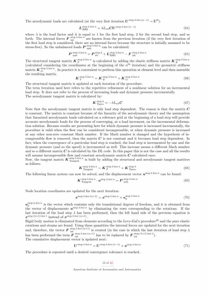
We need to calculate the corresponding final coordinates of the load points to know the coordinates ofpoints at which the aerodynamic forces are applied - perpendicular to the reference surface and so in thelocal z direction. Also local coordinates and slopes of the aerodynamic control points are needed. All

5 of 42


Figure 2. Wing surface S. Meaning ofdZS

k loc

dxS.

these interpolations are performed by using the Infinite Plate Spline Method.41,58 In order to calculate theaerodynamic incidence in each panel of the wing surface S, it is necessary to calculate the derivative of theconfiguration and deformation shapes with respect to the local x axis xS (see figure 1). To do that, thelocal coordinates ZS step λ iter n

loc in the zS direction is isolated. Calling ISz the constant matrix which allows

extraction of the zS component (the dimension of that matrix is NSn × 3NS

n ) it is possible to write (seeequation 8):

ZS step λ iter nloc = IS

z ·XS step λ iter nloc = IS

z ·ES ·[IS


](9)

Using the fitted surface spline shape it is possible to calculate the derivatives of such shape and the associatedlocal angle of attack. Suppose that the ith structural point on wing segment S is considered. The local zcoordinate of the point i will be ZS

i loc,where the superscript “step λ itern” has been dropped for simplicityof the equations (it will be reinstated later).

ZSi loc = ZS

i loc

(xS

i loc, ySi loc

)(10)

Again it has to be clear that xSi loc, yS

i loc are the local coordinates of the point i in which the local z coordinateZS

i loc is considered. We make the assumption that the displacements are not very large. So, the aerodynamiclinear theory holds. Also, under this assumption, it is reasonable to consider the local in-plane coordinates ofthe nodes, the load points and the control points of a generic wing segment constant. Only the out-of-planelocal displacement will change during the iteration process. With this hypothesis, all the splining matricesare constant and they can be calculated once.

6 of 42


For each structural point i of wing segment S the corresponding ZSi loc

(xS

i loc, ySi loc

)is written as

ZSi loc = aS

0 + aS1 xS

i loc + aS2 yS

i loc +NS

n∑

j=1

FSj (rS

ij loc)2 ln(rS

ij loc)2 (11)

where (rSij loc

)2=

(xS

i loc − xSj loc

)2+

(yS

i loc − ySj loc

)2(12)

Equation 11 can be rewritten introducing the matrix KS which is defined as

KSij = (rS

ij loc)2 ln(rS

ij loc)2 (13)

Thus,

ZSi loc

(xS

i loc, ySi loc

)= aS

0 + aS1 xS

i loc + aS2 yS

i loc +NS

n∑

j=1

FSj KS

ij (14)

Setting (notice that ZS?loc is coincident with ZS

loc except for the fact that three rows of zeros have been added)

ZS?loc =

[0 0 0 ZS

1 loc ZS2 loc ZS

3 loc ... ZSNS

n loc

]T

F S =[

aS0 aS

1 aS2 FS

1 FS2 FS

3 ... FSNS

n

]T(15)

and defining

GS =

0 RS

[RS

]T

KS

(16)

Based on the spline formulation (details are omitted here, but can be found in the literature41,58)

ZS?loc = GSF S (17)

Notice that RS has dimension 3×NSn , KS has dimension NS

n ×NSn , F S has dimension

(3 + NS

n

)× 1 andGS has dimension

(3 + NS

n

) × (3 + NS

n

). Inverting the relation expressed by equation 17, it is possible to

find the NSn + 3 unknowns represented by the components of the vector F S :

F S =[GS

]−1

ZS?m loc (18)

Now the coefficients that have to be used for the spline are known.The Wall Tangency Condition (WTC) is enforced at the aerodynamic control points. Let the local coor-dinates (in the reference plane) of the ith control point be indicated with XS

i loc and YSi loc. The coordinate

ZSi loc in the direction of zS of the ith control point will be calculated using the equation of the spline:

ZSi loc

(XSi loc,YS

i loc

)= aS

0 + aS1XS

i loc + aS2YS

i loc +NS

n∑

j=1

FSj KS

ij (19)

WhereKS

ij = (RSij loc)

2 ln(RSij loc)

2 (20)

and(RS

ij loc)2 =

(XSi loc − xS

j loc

)2+

(YSi loc − yS

j loc

)2(21)

The number of control points is the same as the number of aerodynamic panels (NS). To impose theboundary conditions the derivatives with respect to xS are required. In reality there is no difference betweenx and xS because the reference surfaces do not have angle of attack; however we keep here the notation xS

to designate that the local coordinate system of wing segment S is considered (see Figure 2). Therefore,it is necessary to differentiate the spline equation with respect to xS and calculate the result in the local

7 of 42


coordinates of the control points. dZS

locdxS is the vector which contains the slopes of the control points. DS is

a matrix which multiplied by the vector containing the coefficients of the spline gives the vector dZS

locdxS . The

explicit form of this matrix is not listed here and is straightforward to obtain. Using these definitions, theslopes can be written as functions of the coefficients of the spline fit:

dZSloc

dxS= DSF S (22)

Notice thatdZS

loc

dxShas dimension NS × 1, DS has dimension NS × (NS

n + 3). Using equation 18, equation22 can be written as

dZSloc

dxS= DSF S = DS

[GS

]−1

ZS?m loc (23)

Observing that the first three rows of ZS?loc are zeros, it is possible to eliminate the first three columns of the

matrix[GS

]−1

without changing the result. Defining SS , the matrix[GS

]−1

with the first three columns

eliminated, and defining ZSm loc, the vector ZS ?

loc without the first three rows, equation 23 can be rewrittenas

dZSloc

dxS= DSSSZS

loc (24)

Notice that SS has dimension (NSn + 3)×NS

n and ZSloc has dimension NS

n × 1. Using equation 9, equation24 can be written as (at this point we reinstate the superscript “stepλ iter n” earlier dropped)

dZS step λ iter nloc

dxS= DSSSIS

z ES[IS


](25)

We now observe that the the slope of a deformed configuration is not dependent on the actual position ofthe origin of local coordinate system. So the only possibility to have the independence is that

DSSSISz ESx2S = 0 (26)

Therefore, expression 25 is simplified as

dZS step λ iter nloc

dxS= DSSSIS

z ESISd IS

[x step λ iter n + ustep λ iter n

](27)

Introducing the definitionaS

3 = SSISz ESIS

d IS (28)

we getdZS step λ iter n

loc

dxS= DSaS

3


](29)

This formula relates the slope of all the control points of all panels of wing surface S to the augmentedcoordinate vector at the beginning of the current iteration in the Newton Raphson procedure. Also, theslopes are related to the unknown vector of displacements ustep λ iter n. This last term will be used to generatethe aerodynamic tangent matrix for the steady case. Equation 29 can be written for all wing segments andso an assembly procedure is required to have all the local slopes of all the panels of the entire wing system asa function of the augmented coordinate vector and displacement vector of the full structural finite elementmodel.

B. The Unsteady Case (Doublet Lattice Method)

When the unsteady case is considered, a known set of motion shapes is considered as generalized motions forunsteady aerodynamic generalized force generation. Let Φm be one generic shape of the set. The equivalentof equation 29 is:

dZSm loc

dxS= DSaS

3

[xα=0 + Φm

](30)

8 of 42


The generic shape Φm is referred to the reference configuration. When Φm = 0 the reference configurationis obtained. Considering the fact that in the reference configuration we do not have slopes in the localcoordinate system (there is no angle of attack) it can be deduced DSaS

3 xα=0 = 0. Equation 30 is then

dZSm loc

dxS= DSaS

3 Φm (31)

In the unsteady case we also need the vector ZSm loc and not only its derivative given in equation 31 to impose

the unsteady wall boundary conditions at the control points. Using again the splines we can demonstratethe following formula:

ZSm loc = DS ?SSIS

z ·ES ·[IS

d · IS · x α=0 + ISd · IS ·Φm − x2S

](32)

If the shape is exactly coincident with the reference configuration (i.e., Φm = 0), then the local z coordinatesare exactly zeros. Thus, it can be deduced (see equation 32)

DS ?SSISz ·ES ·

[IS

d · IS · x α=0 − x2S

]= 0 (33)

Using this finding, equation 32 is simplified as

ZSm loc = DS ?SSIS

z ·ES · ISd · IS ·Φm (34)

orZS

m loc = DS ?aS3 ·Φm (35)

In the calculation of the generalized aerodynamic matrices, it is required to also transform loads at aerody-namic load points to nodes on the structural grid. Using a procedure formally identical to the one used toobtain equation 35 it is possible to demonstrate that:

ZS

m loc = DS ?aS

3 ·Φm (36)

DS ?has a formal expression identical to DS ?. The only difference is that the local coordinates of the load

points are considered instead of the local coordinates of the control points.

C. Boundary Conditions Using Doublet Lattice Method

Under the assumption of simple harmonic motion, it is possible to demonstrate that the vector which containsthe normalized (using the velocity V∞) normalwash of all panels included in wing surface S has the followingexpression (the boundary condition is enforced on all control points of wing surface S)

wSm = i

ω

V∞ZS

m loc +∂ZS

m loc

∂xS= ikZS

m loc +∂ZS

m loc

∂xS(37)

In the previous equation all the vector quantities have to be understood as vectors of amplitudes of harmonicmotion. k is defined as the ratio ω/V∞ (it is the reduced frequency k? divided by the reference chord).

D. Assembling of the Matrices Used for Mesh to Mesh Transformations

The aerodynamic panels are numbered so as to have the first N1 panels of the surface 1 and then the secondN2 panels of the surface 2 and so forth. The assembly process is simple and all the prescribed values ofthe normalwash of all panels can be calculated and later equated to the values obtained by integrating theunsteady kernel. The assembly process is carried out by calculating all the products (for all wing segments)DSaS

3 , DS ?aS3 and DS ?

aS3 and observing that the trapezoidal wing segments do not have aerodynamic

panels in common. After the assembly, at wing system level, equations 29 (used in the steady case only),31, 35 and 36 are written as

dZstep λ iter nloc

dx= A3


]

dZm loc

dx= A3 ·Φm

Zm loc = A?3 ·Φm

Zm loc = A?

3 ·Φm

(38)

9 of 42


The vector which contains the normalized normalwash of all panels of all wing system is:

wm = ikZm loc +dZm loc

dx(39)

VI. Full Order Steady Aerodynamic Forces

When geometric nonlinearities are included computation of the steady state aeroelastic response has tobe done incrementally. If a single aerodynamic influence coefficients matrix for aerodynamics correspondingto a constant Mach number is to be used, then this can be done by starting a reference configuration atzero angle of attack and gradually increasing its angle of attack, or by starting at a low dynamic pressureat constant Mach number and gradually increasing the dynamic pressure. Gradual increase of dynamicpressure at constant altitude by using a sequence of aerodynamic influence coefficient matrices at differentMach numbers is also possible.Because of an initial focus on low-speed cases in this paper, it is assumed aerodynamics at Mach number ofzero for all the load steps. At each load step the pressure is incremented. At the final load step the dynamicpressure will have reached its final value.The formulation presented here covers both the Vortex Lattice and Doublet Lattice Methods. A note onthe DLM capability used here is in order. This capability integrates the unsteady kernel using Ueda’sformulas12,36,50 and a Gaussian quadrature formula. Because of this it is not necessary to subtract thesteady part of the kernel and use a Vortex Lattice formulation for the steady case, as was done with thecommonly used Doublet Lattice codes.31

The singularity of the kernel is handled by calculating the integrals analytically when the receiving panelis in the wake of the sending panel. The DLM capability used here predicts the steady case well with aformulation that is accurate for both zero and non-zero reduced frequencies. Comparison of results from theDLM capability used here and a conventional VLM capability will confirm this.In the steady case, considering that the structure changes configuration when it deforms, the boundarycondition used for the DL formulation is (see equations 39 and 38):

w step λ iter n =dZ step λ iter n

loc

dx= A3


](40)

where all the quantities are real numbers (steady case). The Doublet Lattice key equation is, for the steadycase:

w step λ iter n = AD ·∆p step λ iter n (41)

where AD is the aerodynamic influence coefficient matrix for the aerodynamic panels. This matrix iscalculated once using the geometry of the aerodynamic reference configuration. ∆p step λ iter n is a vectorwhich contains all the pressure loads on all aerodynamic panels. For a generic panel the aerodynamic force,applied at the load point of that panel is obtained by multiplying a fraction of the dynamic pressure (in thenonlinear steady analysis reported here the load is not applied at once and load steps correspond to a gradualincrease in dynamic pressure) by some geometrical quantities of the panel and by the pressure load. Sincethis applies to all the wing system segments, then the vector which contains the scalar components of theaerodynamic forces of all the panels is written as a product between the fraction of the dynamic pressure anda matrix ID which depends on the planform geometry. This matrix has to multiply the vector containingall the pressure loads. Thus

L step λ iter n = λLrefID ·∆p step λ iter n (42)

where Lref is the reference aerodynamic load. Its expression is

Lref =12ρ∞V 2

∞Nstep

(43)

Nstep is the number of load steps. From equations 40 and 41 it is possible to relate the vector containing thepressure differences to the augmented coordinate vector and displacement vector (this last is unknown):

∆p step λ iter n =[AD

]−1

w step λ iter n =[AD

]−1

A3


](44)

10 of 42


The pressure difference, also named here pressure loads, are the pressure differences between lower and uppersurfaces of individual aerodynamic boxes. The vector with the aerodynamic forces (equation 42) is then

L step λ iter n = λLrefID ·[AD

]−1

A3


](45)

With the help of the definition

c.= ID

[AD

]−1

A3 (46)

we obtainL step λ iter n = λLrefc


](47)

The aerodynamic loads (forces) of equation 47 are applied at the load points of the aerodynamic panels.They are transferred to the structural nodes using the following algorithm.For all aerodynamic load points, the aerodynamic forces are extracted from equation 47. Then the triangularstructural finite element that includes the load point of the generic aerodynamic panel is found. The equiva-lent loads applied at the nodes of the triangular FE element (which contains the load point) are obtained byusing the area coordinates.57 Finally, an assembly procedure is required (a node in general connects moreFE elements). Notice that some zero rows in correspondence of the rotational degrees of freedom have to beadded. The vector of the aerodynamic forces applied at the structural nodes is written as

L step λ iter nstr = λLrefC

(x step λ iter n + ustep λ iter n

)(48)

C is a constant matrix. Notice also that K step λTaero

.= −λLrefC is the aerodynamic tangent matrix.It is convenient to write equation 48 in the form

L step λ iter nstr = L step λ iter n

RHS + L step λ iter nLHS (49)

whereL step λ iter n

RHS = λLrefCx step λ iter n (50)

L step λ iter nLHS = λLrefCustep λ iter n = −K step λ

Taeroustep λ iter n (51)

The subscript LHS is used to point out that the term L step λ iter nLHS will go to the left hand side of the equation

iteratively solved in the Newton Raphson procedure. If the Vortex Lattice Method is used the final expression48 is formally identical. In both DLM and VLM cases the reference configuration is the one with no angleof attack. This in theory is not required by the VLM, but it is used to keep the same formalism valid forthe DLM.

VII. Full Order Steady Aerodynamic Forces Using the Concept of CumulativeDisplacement Vector

The aerodynamic forces can be written in a different form using the concept of cumulative displacementvector. This equivalent writing is used in the dynamic case and, therefore, is introduced here. The steadyaerodynamic loads can be written in a more elegant form by considering that when α = 0 for all aerodynamicboxes we do not have aerodynamic loads. So we can write:

L step λ iter nstr = λLref

Cx step λ iter n −

This term is zero︷︸︸︷Cxα=0 +Custep λ iter n

(52)

The coordinates at the beginning of the current iteration are the summation of all translational displacementsthat occurred in all the previous iterations and the coordinates of the nodes of the reference configuration.So, the product between the aerodynamic matrix C and the difference of the augmented coordinate vectorat the beginning of the current iteration and the augmented coordinate vector at the reference configurationis equal to the product between the matrix C and the cumulative displacement vector U step λ iter (n−1) atthe end of the previous iteration. This is because the local FE rotations at nodes do not influence theaerodynamic loads. It is of course

x step λ iter n − xα=0 6= U step λ iter (n−1) (53)

11 of 42


But since the FE rotations do not provide aerodynamic contribution it can be concluded that

C x step λ iter n −C xα=0 = C U step λ iter (n−1) (54)

The aerodynamic loads can then be written as

L step λ iter nstr = λLref

(CU step λ iter (n−1) + Custep λ iter n

)(55)

which is a convenient form for application for the Newton Raphson method. Note that at the end of aparticular iteration the cumulative displacement vector is defined as the summation of all the displacementsof the previous iterations and the displacement of the current iteration. So, the loads can be written in aneven more compact form. This, however, is not convenient in practice because we need to have a separatecontribution in which the vector of the current displacements appears to identify the aerodynamic tangentmatrix as the matrix which multiplies the unknown displacements.

L step λ iter nstr = λLrefCU step λ iter n (56)

where U step λ iter n is the cumulative displacement vector of the current iteration and it is obtained as

U step λ iter n = U step λ iter (n−1) + ustep λ iter n (57)

A similar formula will be obtained in the dynamic case.If the concept of cumulative displacement is used, then the RHS of the aerodynamic loads is written as

L step λ iter nRHS = λLrefCU step λ iter (n−1) (58)

VIII. Solution of the Nonlinear Steady State Equations

The wing is loaded by external aerodynamic loads, motion dependent aerodynamic loads, and other loads(indicated with P ext) such as the inertial loads. The Newton Raphson solution procedure used proceedsas follows: The reference aerodynamic pressure Lref is first calculated. This is the increment in dynamicpressure from one load step to another.

Lref =12ρ∞V 2

∞Nstep

(59)

An increment of external concentrated loads can similarly be defined. The reference magnitude Pref of thatloads will be

Pref =1

Nstep(60)

Note that because aerodynamic influence coefficients are calculated for a configuration with zero angles ofattack for all aerodynamic boxes and because this is the geometry from which motion starts, no motiondependent aerodynamic loads appear initially, and unless there is a non aerodynamic external load thestructure will not move. At the very first iteration of the Newton Raphson procedure an initial angle ofattack perturbation is imposed:

xstep 1 iter 1 = xpert 6= xα=0 (61)

Considering this perturbation of the system, the cumulative displacement vector is initialized. (see equation54):

x step 1 iter 1 − xα=0 = U0 (62)

Mathematically equation 62 is not correct (see equation 53) and the RHS and LHS of the equation are notequivalent. However, according to equation 54, when these quantities are multiplied by the aerodynamicmatrix then the equivalence is correct. So, the initialization 62 can be done without introducing errors andwith a great simplification of the theory.The applied non-aerodynamic loads (of the non-follower force type) are only step dependent and they arecalculated by using the following expression:

P step λstr = λ · Pref · P ext (63)

12 of 42


The aerodynamic loads are calculated (at the very first iteration U step λ iter (n−1) = U0):

L step λ iter nRHS = λLrefCU step λ iter (n−1) (64)

where λ is the load factor and it is equal to 1 for the first load step, 2 for the second load step, and soforth. The internal forces F step λ iter n

int are known from the previous iteration (if the very first iteration ofthe first load step is considered, there are no internal forces because the structure is initially assumed to bestress-free). So the unbalanced loads P step λ iter n

unb can be calculated:

P step λ iter nunb = P step λ

str + L step λ iter nRHS − F step λ iter n

int (65)

The structural tangent matrix K step λ iter nT is calculated by adding the elastic stiffness matrix K step λ iter n

E

(calculated considering the coordinates at the beginning of the nth iteration) and the geometric stiffnessmatrix K step λ iter n

G . In practice it is convenient to perform this operation at element level and then assemblethe resulting matrix.

K step λ iter nT = K step λ iter n

E + K step λ iter nG (66)

The structural tangent matrix is updated at each iteration of the procedure.The term iteration used here refers to the repetitive refinement of a nonlinear solution for an incrementalload step. It does not refer to the process of increasing loads and dynamic pressure incrementally.The aerodynamic tangent matrix is calculated by:

K step λTaero = −λLrefC (67)

Note that the aerodynamic tangent matrix is only load step dependent. The reason is that the matrix Cis constant. The matrix is constant because of the linearity of the aerodynamic theory and the assumptionthat linearized aerodynamic loads calculated on a reference grid at the beginning of a load step will provideaccurate aerodynamic loads for the process of converging, at a load increment, on the incremental deforma-tion solution. Because results are presenting here for which dynamic pressure is increased incrementally, theprocedure is valid when the flow can be considered incompressible, or when dynamic pressure is increasedat any other non-zero constant Mach number. If the Mach number is changed and the hypothesis of in-compressible flow is removed, then the matrix C is not constant and it becomes load step dependent. Infact, when the convergence of a particular load step is reached, the load step is incremented by one and thedynamic pressure (and so the speed) is incremented as well. This increase means a different Mach numberand so a different matrix C is calculated by the DL code. In this paper this is not the case and all the resultswill assume incompressible flow and constant aerodynamic matrix C calculated once.Now, the tangent matrix K step λ iter n

Tangent is built by adding the structural and aerodynamic tangent matricesas follows:

K step λ iter nTangent = K step λ iter n

T + K step λTaero (68)

The following linear system can now be solved, and the displacement vector ustep λ iter n can be found:

K step λ iter nTangent · ustep λ iter n = P step λ iter n

unb (69)

Node location coordinates are updated for the next iteration:

xstep λ iter (n+1) = xstep λ iter n + ustep λ iter nd (70)

ustep λ,iter nd is the vector which contains only the translational degrees of freedom, and it is obtained from

the vector of displacements ustep λ iter n by eliminating the rows corresponding to the rotations. If thelast iteration of the load step λ has been performed, then the left hand side of the previous equation isxstep (λ+1) iter 1 instead of xstep λ iter (n+1).Rigid body motion is eliminated from elements according to the Levy-Gal’s procedure46 and the pure elasticrotations and strains are found. Using these quantities the internal forces are updated for the next iterationand, therefore, the vector F

step λ iter (n+1)int is created (in the case in which the last iteration of load step λ

has been performed the term Fstep λ iter (n+1)int has to be replaced by F

step (λ+1) iter 1int ).

The cumulative displacement vector is updated next:

U step λ iter n = U step λ iter (n−1) + ustep λ iter n (71)

The procedure is repeated until a desired convergence tolerance is reached.

13 of 42


IX. Steady Aeroelastic Case: Full Order Structural Model and ModallyReduced Order Aerodynamic Model

A. Approximated Aerodynamic Tangent Matrix Obtained from the GeneralizedAerodynamic Tangent Matrix

Order reduction of the structural system by using a known set of deformation shape vectors (which can befor example the natural modes of the structure or other sets of assigned shapes) is a major challenge whengeometrical nonlinearities are considered. For example, in the Joined Wing configuration in-plane forcesin the rear wing and the inner section of the main wing are important in the calculation of the geometricstiffness matrix. A modal basis has to be able to capture stress distributions as well as deformation shapes.The fact that the nodes are moving and can move significantly also adds to difficulty. The conventionalmodal approach, so wide spread in linear aeroelasticity, does not work with joined-wings. As a matter offact, it has already been shown that a basis built by adopting this procedure leads to poor results unlessthe basis is continuously updated, leading to expensive computation.42 Advanced procedures, such as theuse of modes and modal derivatives, improve the approximation, but also tend to fail when joined-wings areconcerned.

The approach proposed in this paper is to use the full order structural matrices to capture the nonlinearstructural behavior and a modally reduced aerodynamic matrix calculated, for example, by adopting acommercial code such as ZAERO or other package. In this paper a dedicated DLM code is used.

When dynamic aeroelastic cases are considered the proposed approach is particularly attractive becauseit allows utilization of existing standard unsteady aerodynamic codes.

Consider a set Ψ of R known shape vectors:

Ψ =[

Φ1 Φ2 Φ3 ... ΦR

](72)

Let A0 be the generalized aerodynamic matrix calculated for the steady case, so k? = 0 where k? is thereduced frequency and obtained by using a commercial code using the basis Ψ. The matrix A0 has dimensionR ×R. The generalized aerodynamic tangent matrix AZ is defined by multiplying A0 by the fraction ofthe aerodynamic pressure related to the current load step λ. We use the negative sign to have an expressionon the left hand side (LHS) of the equilibrium equation without negative signs:

AZ.= −λ ·

12ρ∞V 2

∞Nstep

A0 = −λ · LrefA0 (73)

Suppose we approximate the displacements of iteration n of load step λ by using the basis Ψ and the vectorqstep λ iter n of generalized coordinates as follows:

ustep λ iter n ≈[

Φ1 Φ2 Φ3 ... ΦR

]

qstep λ iter n1

qstep λ iter n2

qstep λ iter n3

...

qstep λ iter nR

= Ψqstep λ iter n (74)

By applying the Least Square Method (LSM) it is possible to express the generalized displacements as afunctions of the full order displacements. But the finite element degrees of freedom include nodal rotationswhich are usually not used in the interpolation of displacement and angle of attack over lifting surfaces foraeroelastic applications. The least squares approximation should focus on matching the modal approximationto the full order displaced shape of lifting surface panels. The relation full order displacements to generalizeddisplacements is represented by equation 74. Notice that ustep λ iter n includes the rotations. By eliminatingthe rows which correspond to the rotations, the translational displacements ustep λ iter n

d are found as

ustep λ iter nd = Ψdq

step λ iter n (75)

where Ψd contains only translational components of the R shape vectors of the basis Ψ. The dimension ofΨd is then 3Nn ×R.

14 of 42


ustep λ iter nd = Ψdq

step λ iter n ⇒ ΨTd ustep λ iter n

d = ΨTd Ψdq

step λ iter n (76)

qstep λ iter n =[ΨT

d Ψd

]−1

ΨTd ustep λ iter n

d = T dustep λ iter nd (77)

whereT d =

[ΨT

d Ψd

]−1

ΨTd (78)

T d is a matrix with dimension R×3Nn. Another possibility is to perform the LSM fit only on the componentof the displacements perpendicular to the surfaces. Considering that the model analyzed in this paper (thedelta wing of Refs. 22 and 23) is contained in the x−y plane, the displacement perpendicular to the surfacesis the displacement uz. So the LSM fit can be performed only on the translational displacement uz of allnodes. If this approach is chosen, the matrix T d has dimension R×Nn (instead of R×3Nn), the matrix Ψd

has dimension Nn ×R (instead of 3Nn ×R) and the vector ustep λ iter nd contains just Nn elements (instead

of 3Nn).It is preferable to work with the vector ustep λ iter n instead of the vector ustep λ iter n

d . Therefore, columns ofzeros in correspondence to the finite element nodal rotations (and the displacements ux, uy in the case inwhich the LSM fit is performed on the component uz only) in matrix T d are added. T is defined as thematrix T d after the columns have been added. The dimension of this matrix is R × 6Nn. Considering thisnew matrix, an equivalent writing of equation 77 that uses all DOFs is the following:

qstep λ iter n = Tustep λ iter n (79)

Now, the generalized aerodynamic tangent matrix has to be converted to correspond to the full order struc-tural model. This is achieved by imposing work/energy conservation.The generalized forces are (the negative sign is a consequence of the negative sign used in equation 73):

Qstep λ iter n = −AZqstep λ iter n = +λ · LrefA0qstep λ iter n (80)

The work done by the generalized aerodynamic forces is:

δW = δ[qstep λ iter n

]T ·Qstep λ iter n (81)

The work done by the equivalent aerodynamic forces L step λ iter nLHS applied on the structural mesh is:

δW = δ[ustep λ iter n

]T ·L step λ iter nLHS (82)

Using equation 79 and equating equation 81 and equation 82 it is possible to write:

δ[ustep λ iter n

]T ·L step λ iter nLHS = δ

[qstep λ iter n

]T ·Qstep λ iter n (83)

From which it follows:L step λ iter n

LHS = T T ·Qstep λ iter n (84)

Using equation 80 and 79:

L step λ iter nLHS = +λLrefT

T A0qstep λ iter n = +λLrefT

T A0Tustep λ iter n (85)

To keep the formalism used when the aerodynamic tangent matrix was obtained using the doublet latticeformulation, we indicate the approximated aerodynamic tangent matrix with the symbol K step λ

TZaero. Thefollowing definition is also made:

K step λTZaero

.= −λ · LrefCZ (86)

CZ is the approximated counterpart of the matrix C earlier defined.Equation 85 is then rewritten as (see also the analog equation 67 for the full order “exact” case)

Lstep λ iter nLHS = −K step λ

TZaeroustep λ iter n = +λLrefCZustep λ iter n (87)

Using equation 85 it can be deduced that

CZ = +T T A0T (88)

K step λTZaero = −λLrefCZ is the approximated aerodynamic tangent matrix obtained by using the generalized

aerodynamic matrix A0 calculated with the aerodynamic commercial code.

15 of 42


X. Unsteady Case: Time Domain Simulations with Full Order StructuralModel and Reduced Order Aerodynamic Model

The Fourier Transform of the unsteady aerodynamic force corresponding to the full order structural finiteelement model is:

Lunsteady (jω) =12ρ∞V 2

∞Afull (jω) · [x− xα=0](jω) (89)

where x is the augmented coordinate vector (that is, the vector of nodal motions with rotational nodalmotions zeroed out) and xα=0 is the vector of initial nodal coordinates corresponding to the condition ofzero angle of attack on all aerodynamic boxes (rotational nodal motions removed as well). The differencex − xα=0 is a function of jω because of the time dependence of nodal positions. For the unsteady case weuse the same transformation from generalized coordinates to full order finite element coordinates as in thesteady case using the same transformation matrix T . We have:

Afull (jω) = T T A (jω) T (90)

The matrix A (jω) generated by an unsteady aerodynamic linear potential code is a non-rational function ofthe reduced frequency k? = ωb

V∞: A = A (jk?). In the present DL code the reduced frequency was calculated

based on a reference semi-chord of 1. That is, as k = ωV∞

. A Roger procedure59−60 is used to obtain arational function approximation of the generalized unsteady loads. In particular:

A (jk?) = A0 + (jk?) A1 + (jk?)2 A2 +Nlag∑

i=1

jk?

jk? + βiA2+i (91)

Recalling the definition of reduced frequency k? = ωbV∞

, defining βi = V∞b βi, simplifying and using analytical

continuation to expand from the imaginary axis to the Laplace domain adjacent to it jω → s, it is possibleto write the aerodynamic generalized matrix in the Laplace domain, where s is the Laplace variable:

A (s) = A0 + sb

V∞A1 + s2 b2

V 2∞A2 +

Nlag∑

i=1

s

s + βi

A2+i (92)

The aerodynamic force vector in the Laplace domain is:

Lunsteady (s) =12ρ∞V 2

∞T T

A0 + s

b

V∞A1 + s2 b2

V 2∞A2 +

Nlag∑

i=1

s

s + βi

A2+i

T

[x− xα=0

](s) (93)

The following definitions are now introduced:

A?0

.=12ρ∞V 2

∞T T A0T ; A?1

.=12ρ∞bV∞T T A1T

A?2

.=12ρ∞b2T T A2T ; A?

2+i.=

12ρ∞V 2

∞T T A2+iT i = 1, Nlag

(94)

The unsteady aerodynamic forces in the Laplace domain can now be expressed as:

Lunsteady (s) =

A?

0 + sA?1 + s2A?

2 +Nlag∑

i=1

s

s + βi

A?2+i

[

x− xα=0](s) (95)

Using the Inverse Laplace Transform (ILT)61 expressions in the time domain can be obtained. We can write:

L−1[A?

0 ·[x− xα=0

](s)

]= A?

0 ·[x− xα=0

](t)

L−1[sA?

1 ·[x− xα=0

](s)

]= A?

1 ·ddt

[x− xα=0

](t)

L−1[s2A?

2 ·[x− xα=0

](s)

]= A?

2 ·d2

dt2[x− xα=0

](t)

(96)

16 of 42


The previous equations are valid if at t = 0 displacements, speeds, and accelerations are all zero. Totransform the lag terms to the time domain convolution integrals are used.60 Using the Dirac delta functionδ (t), the ILT of the term s

s+βi

is:

L−1

[s

s + βi

]= δ (t)− βie

−βit (97)

Then, by applying the convolution theorem, we have:

L−1

[s

s + βi

A?2+i ·

[x− xα=0

](s)

]=

t∫

0

[δ (t− τ)− βie

−βi(t−τ)]A?

2+i ·[x− xα=0

](τ) dτ (98)

or

L−1

[s

s + βi

A?2+i ·

[x− xα=0

](s)

]= A?

2+i ·[x− xα=0

](t)− βiA?

2+i

t∫

0

[x− xα=0

](τ) e−βi(t−τ) dτ (99)

Using these inverse Laplace Transform equations (equations 96 and 99), the unsteady aerodynamic loads inthe time domain become:

Lunsteady (t) = A?[x− xα=0

](t) + A?

1 ·ddt

[x− xα=0

](t)

+ A?2 ·

d2

dt2[x− xα=0

](t)−

Nlag∑

i=1

βiA?2+i

t∫

0

[x− xα=0

](τ) e−βi(t−τ) dτ

(100)

where

A? .= A?0 +

Nlag∑

i=1

A?2+i (101)

As for the steady case, in general U 6= x − xα=0. But since structural rotational motions at nodes do notaffect the unsteady aerodynamic loads in our formulation (slopes obtained from interpolated deformationshapes do), it is possible to replace the quantity x−xα=0 with the cumulative displacement vector U . Thefollowing definitions are now introduced:

U (t) .=tU ; tU

.=d[U (t)]

dt; tU

.=d2[U (t)]

dt2; tLunsteady

.= Lunsteady (t) (102)

and the time domain aerodynamic forces will have the expression (see equation 100):

tLunsteady = A? · tU + A?1 · tU + A?

2 · tU −Nlag∑

i=1

βiA?2+i

t∫

0

τUe−βi(t−τ) dτ (103)

The expression of the aerodynamic loads (equation 103) covers also the steady case (equation 56). Todemonstrate that, consider equation 103. In the steady case there is no time dependency and no contributionsof aerodynamic lag terms. Aerodynamic pressure loads are applied gradually and load steps are required.The steady counterpart of equation 103 is therefore:

L step λ iter nstr = A? step λ

0 ·U step λ iter n (104)

The definition of the matrix A? step λ0 is (see equation 94):

A? step λ0 =

λ

Nstep

12ρ∞V 2

∞T T A0T = λLrefTT A0T (105)

Using equation 88:A? step λ

0 = λLrefCZ (106)

17 of 42


Substitution of this result into equation 104 leads to

L step λ iter nstr = λLrefCZ ·U step λ iter n (107)

which is the approximated counterpart of equation 56. The procedure used here to approximate the unsteadyaerodynamic loads thus leads to the procedure used to approximate the aerodynamic loads in the steadycase and is consistent with it.

XI. Newmark’s Method

Newmark’s method57 can be expressed using the following equations (∆t is the time step):

t+∆tU = tU +[(1− δ) tU + δ t+∆tU

]∆t (108)

t+∆tU = tU + tU∆t +[(

12− α

)tU + αt+∆tU

]∆t2 (109)

Thent+∆tU =

1α∆t2

(t+∆tU − tU

)− 1α∆t

tU −(

12α

− 1)

tU (110)

The values δ = 12 and α = 1

4 are used here. Define:

a0 =1

α (∆t)2; a1 =

δ

α∆t; a2 =

1α∆t

; a3 =12α

− 1;

a4 =δ

α− 1; a5 =

∆t

2

(δ

α− 2

); a6 = ∆t (1− δ) ; a7 = δ∆t.

(111)

Now acceleration and velocity vectors become:

t+∆tU = a0

(t+∆tU − tU

)− a2tU − a3

tU (112)

t+∆tU = tU + a6tU + a7

t+∆tU (113)

XII. Newmark Time IntegrationUnsteady Newton-Raphson Method for the Case of Mechanical Loads Only.

The Newton-Raphson method can be written as:

M · t+∆tUn

+ CD · t+∆tUn

+t+∆t KnT · t+∆tun = t+∆tP ext − t+∆tF

(n−1)int (114)

Un

and Un

are the realizations of the acceleration and speed vectors at time t + ∆t when iteration nis performed. t+∆tun is the displacement vector (not known yet) that is calculated at iteration n and itis referred to the previous iteration, i.e. it is referred to the coordinates at the beginning of iteration n.Considering the definition of cumulative displacement vector, it is clear that the cumulative displacementvector at time t+∆t, when iteration n is completed, is the summation of the cumulative displacement vectorat time t + ∆t at iteration (n− 1) and the displacement vector (not known yet) of iteration n:

t+∆tUn = t+∆tU (n−1) + t+∆tun (115)

Using 115, the acceleration and velocity vectors become:

t+∆tUn = t+∆tUnnd + t+∆tun

t+∆tUn

= t+∆tUn

nd + a7a0t+∆tun

t+∆tUn

= t+∆tUn

nd + a0t+∆tun

(116)

18 of 42


wheret+∆tUn

nd = t+∆tU (n−1)

t+∆tUn

nd = tU + a6tU + a7a0

t+∆tU (n−1) − a7a0tU − a7a2

tU − a7a3tU

t+∆tUn

nd = a0t+∆tU (n−1) − a0

tU − a2tU − a3

tU

(117)

This compact form has the advantage that the terms which multiply the displacements of the currentiterations are clearly separated. This is important in the definition of the tangent matrix of the entiresystem (the so called effective tangent matrix). Substituting equation 116 into 114:

M ·[

t+∆tUn

nd + a0t+∆tun

]+ CD ·

[t+∆tU

n

nd + a7a0t+∆tun

]+t+∆t Kn

T · t+∆tun = t+∆tP ext− t+∆tF(n−1)int

(118)leading to

[t+∆tKn

T + a0M + a7a0CD

] · t+∆tun = t+∆tP ext −M · t+∆tUn

nd −CD · t+∆tUn

nd − t+∆tF (n−1)

(119)or [

t+∆tKnT + KT

systemdyn

]· t+∆tun = t+∆tP ext + t+∆tP

ndyn − t+∆tF (n−1) (120)

ort+∆tKn

T eff · t+∆tun = t+∆tPn

eff − t+∆tF (n−1) (121)

t+∆tKnT eff is the effective tangent matrix, KT

systemdyn is the dynamic contribution (constant) to the effective

tangent matrix, t+∆tPneff are the effective loads, including the dynamic effects t+∆tP

ndyn. We have:

t+∆tKnT eff = t+∆tKn

T + KTsystemdyn

KTsystemdyn = a0M + a7a0CD

t+∆tPn

eff = t+∆tP ext + t+∆tPn

dyn

t+∆tPn

dyn = −M · t+∆tUn


nd

(122)

The iterative procedure of a more general case with motion dependent aerodynamic loads is explained next.

XIII. Newmark Time IntegrationUnsteady Newton-Raphson Method with Unsteady Aerodynamics.

Suppose to have both unsteady non-aerodynamic and aerodynamic loads. The Newton Raphson proce-dure for this case is (see also equation 114):

M · t+∆tUn

+ CD · t+∆tUn

+t+∆t KnT · t+∆tun = t+∆tP ext + t+∆tLn

unsteady − t+∆tF(n−1)int (123)

where t+∆tLnunsteady is the nth realization of the aerodynamic loads at time t + ∆t. The explicit form of the

loads is (see equation 103):

t+∆tLnunsteady = A? · t+∆tUn + A?

1 · t+∆tUn

+ A?2 · t+∆tU

n −Nlag∑

i=1

βiA?2+i

t+∆t∫

0

τUne−βi(t+∆t−τ) dτ

(124)A short discussion is in order regarding the time step. Considering that Newmark’s method for time inte-gration is implicit, the time step can be relatively large. However, the aerodynamic force models are basedon forces obtained in the frequency domain by using set of modes and tabulated reduced frequencies. Themaximum reduced frequency used for the aerodynamic simulation in the frequency domain and at which wecan expect the Roger approximation to still be accurate is:

k?max =

ωmaxb

V∞(125)

19 of 42


The maximum circular frequency, for which the this generalized aerodynamics model has meaning is then

ωmax =k?maxV∞

b(126)

The associated frequency is

fmax = ωmax/2π =k?maxV∞2πb

(127)

The associated period is therefore:

Tmin =1

fmax=

2πb

k?maxV∞

(128)

To have a meaningful representation of the unsteady aerodynamic forces, the time step size should be smallerthan Tmin so as to allow capturing in the time simulation the highest frequency for which the model is valid.For example, we could take

∆t =Tmin

Ntime step(129)

Where Ntime step ≥ 1 is chosen by the user. We focus now on the generic time step over the intervalt ≤ τ ≤ t + ∆t.To express the aerodynamic forces, we need to calculate the integrals on the RHS of equation 124. In theformulation so far the integrals already involve the equilibrium solution at time t + ∆t and this solution isnot known. Moreover, the change over time of the cumulative displacement vector is also not known. Toovercome these issues consider the generic integral t+∆tIi of the lag term i :

t+∆tIi.=

t+∆t∫

0

τUe−βi(t+∆t−τ) dτ (130)

Since the time step size is smaller than the minimum period of the the considered aerodynamic forces (seeequation 129), it is reasonable to assume that the cumulative displacement at time t + ∆t (actually itsapproximation given by the nth iteration) and the cumulative displacement at a time τ (with the obviouscondition t ≤ τ ≤ t + ∆t in the interval) are related by a linear relation. The following relation can now bewritten (τUn is the nth realization of the quantity τU):

t+∆tUn − tU

t + ∆t− t=

τUn − tU

τ − tt ≤ τ ≤ t + ∆t (131)

Using the definition t+∆tU? nnd

.= t+∆tUnnd − tU = t+∆tU (n−1) − tU we finally obtain

τUn =[

t+∆tun

∆t+

t+∆tU? nnd

∆t

]τ +

[−

t+∆tun

∆tt−

t+∆tU? nnd

∆tt + tU

](132)

Based on equation 130) the following identity holds:

t+∆tIi = e−βi∆t · tIi + e−βi(t+∆t)

t+∆t∫

t

τUeβiτ dτ (133)

The nth realization of the integral t+∆tIi of the generic lag term is (see equation 133):

t+∆tIni = e−βi∆t · tIi + e−βi(t+∆t)

t+∆t∫

t

τUneβiτ dτ (134)

This equation 134 can be further developed if the cumulative displacement vector is approximated usingequation 132 and leads to simple integrals which can be obtained analytically. To calculate the integral onthe RHS, we use for the function τU its approximation in the integration domain (see equation 132). Aftersome algebra the following formula is reached:

t+∆tIni = t+∆tI? n

i +t+∆tun

∆tΛi (135)

20 of 42


wheret+∆tI? n

i = e−βi∆t · tIi +t+∆tU? n

nd

∆tΛi + tUλi

Λi =e−βi∆t + βi∆t− 1

β2

i

λi =1− e−βi∆t

βi

(136)

All the terms needed to evaluate the unsteady aerodynamic force vector expressed in equation 124 are nowavailable. Using equation 116 the aerodynamic force vector is written as

t+∆tLnunsteady = A? · t+∆tUn

nd + A?1 · t+∆tU

n

nd + A?2 · t+∆tU

n

nd −Nlag∑

i=1

βiA?2+i

t+∆tI? ni

+

A? + a7a0A?

1 + a0A?2 −

Nlag∑

i=1

βiΛi

∆tA?

2+i

t+∆tun

(137)

The final system of equations that has to be solved is similar to the one obtained for the pure mechanicalcase with no aerodynamics. We have:

t+∆tKnT eff · t+∆tun = t+∆tP

n

eff − t+∆tF (n−1) (138)

wheret+∆tKn

T eff = t+∆tKnT + KT

systemdyn + KT

systemaero

KTsystemdyn = a0M + a7a0CD

KTsystemaero = −A? − a7a0A?

1 − a0A?2 +

Nlag∑

i=1

βiΛi

∆tA?

2+i

t+∆tPn


dyn + t+∆tPn

aero

t+∆tPn



nd

t+∆tPn

aero = A? · t+∆tUnnd + A?

1 · t+∆tUn

nd + A?2 · t+∆tU

n

nd −Nlag∑

i=1

βiA?2+i

t+∆tI? ni

(139)

Figures 3 and 4 show how the displacements are approximated in time in order to calculate the lag termintegrals. Note that the approximation is more accurate if the size of the step used in the time integration issmall. It may be argued that if the time step is too small, aerodynamics for reduced frequencies beyond themaximum reduced frequency used in the calculation of the aerodynamic generalized matrices are included.This is in theory true, but numerical experiments shown in this paper demonstrates the convergence whenthe time step is reduced. Filtering of any errors due to high frequency behavior is also due to the stabilityof the Newmark method.CD is the full order damping matrix. In this paper a viscous damping model is used as follows. The referencegeneralized damping matrix is built considering a set of modes that are in general not coincident with thebasis used to define the aerodynamic generalized matrices. Then, the reference generalized damping matrixis expanded to be of the same order of the generalized aerodynamic matrices. This operation is done byconsidering as a new set of modes the same modes used to define the generalized aerodynamic matrices andthe transformation matrix T and by applying the Least Squares Method to move from one set of modesto another. The generalized damping matrix is obtained in the same modal cordinates as the generalizedaerodynamic matrix. Finally, the full order damping matrix CD is obtained from the generalized dampingmatrix by using a transformation similar to equation 90.

XIV. Newmark’s Method and Unsteady Aerodynamics: Iterative Procedure

The procedures described above can now be summarized.

21 of 42


Figure 3. First iteration of the generic load step. Approximation used for the calculations of the integralscontaining the lag terms

1. Initial Calculations

First, the maximum size step is chosen by using

∆t =Tmin

Ntime step=

2πb

k?maxV∞Ntime step

(140)

k?max = ωmaxb

V∞is the maximum reduced frequency used for the Roger fit; Ntime step is a number chosen by

user. If this number is larger the lag terms are more accurately calculated. CPU time increases considerably,however, when Ntime step is large.Next the following quantities are calculated:

a0 =1

α (∆t)2; a1 =

δ

α∆t; a2 =

1α∆t

; a3 =12α

− 1;

a4 =δ

α− 1; a5 =

∆t

2

(δ

α− 2

); a6 = ∆t (1− δ) ; a7 = δ∆t.

(141)

In which δ = 12 and α = 1

4 .The parameters used in the derivation of the aerodynamic contribution are:

βi =V∞b

βi Λi =e−βi∆t + βi∆t− 1

β2

i

λi =1− e−βi∆t

βi

(142)

For calculation of the dynamic contribution KTsystemdyn to the effective tangent matrix (this contribution is

constant) we have:KT

systemdyn = +a0M + a7a0CD (143)

Contribution to the tangent matrix due to the aerodynamic part:

KTsystemaero = −A? − a7a0A?

1 − a0A?2 +

Nlag∑

i=1

βiΛi

∆tA?

2+i (144)

This contribution does not depend on the load step or iteration and it is calculated once.

22 of 42


Figure 4. Second iteration of the generic load step. Approximation used for the calculations of the integralscontaining the lag terms

2. Time Step Calculations

For calculation of the external loads t+∆tP ext using the assigned temporal law notice that each time stepdefines a variation of the parameters over the interval [t, t + ∆t].Some auxiliary quantities are calculated:

t+∆tUnnd = t+∆tU (n−1)

t+∆tUn

nd = tU + a6tU + a7a0

t+∆tU (n−1) − a7a0tU − a7a2

tU − a7a3tU

t+∆tUn

nd = a0t+∆tU (n−1) − a0

tU − a2tU − a3

tU

t+∆tU? nnd = t+∆tUn

nd − tU = t+∆tU (n−1) − tU

t+∆tI? ni = e−βi∆t · tIi +

t+∆tU? nnd

∆tΛi + tUλi

(145)

This operation is performed at each iteration. If the first iteration of the current load step is considered,then the previous realization of the cumulative displacement will be t+∆tU (n−1) = tU . In case the very firstiteration is considered, then all the quantities are coincident with the initial (if different than zero) values.For example, tU = 0U . In this particular case it is also tIi = 0Ii = 0. This is because the integrals areperformed over an interval which is zero.The loads are also calculated:

t+∆tPn



nd

t+∆tPn

aero = A? · t+∆tUnnd + A?

1 · t+∆tUn

nd + A?2 · t+∆tU

n

nd −Nlag∑

i=1

βiA?2+i

t+∆tI? ni

t+∆tPn


dyn + t+∆tPn

aero

(146)

23 of 42


The external loads t+∆tP ext change only when another load step is considered. Regarding the calculationof the effective tangent matrix:

t+∆tKnT eff = t+∆tKn

T + KTsystemdyn + KT

systemaero (147)

The linear system is solved:

t+∆tKTneff · t+∆tun = t+∆tP n

eff − t+∆tF(n−1)int (148)

The displacements t+∆tun are used to update the coordinates of the nodes.The cumulative displacement vector is updated for the next iteration:

t+∆tUn = t+∆tU (n−1) + t+∆tun (149)

The internal forces t+∆tF nint are calculated for the next iteration. Another iteration is performed unless the

convergence criteria is satisfied. If so, the iterative process in the time step is considered complete and thevectors are updated.

t+∆tU = t+∆tUn = t+∆tUnnd + t+∆tun

t+∆tU = t+∆tUn

= t+∆tUn

nd + a7a0t+∆tun

t+∆tU = t+∆tUn

= t+∆tUn

nd + a0t+∆tun

t+∆tIi =t+∆t Ini = e−βi∆t · tIi +

t+∆tU − tU

∆tΛi + tUλi

(150)

The process restarts with the updating of the time: t → t + ∆t.The updating of the integrals involving the lag terms in equation 150 has been derived as follows:

t+∆tIi =t+∆t Ini = t+∆tI? n

i +t+∆tun

∆tΛi = e−βi∆t · tIi +

t+∆tU? nnd

∆tΛi +

t+∆tun

∆tΛi + tUλi

= e−βi∆t · tIi +t+∆tU

n − tU

∆tΛi + tUλi = e−βi∆t · tIi +

t+∆tU − tU

∆tΛi + tUλi

(151)

A. Initial Conditions

The unsteady aerodynamic forces in the time domain are given in expression 103. If this formula is writtenfor the initial instant t = 0, the integral of the lag terms is zero because the limits of the integral arecoincident. So we have:

0Lunsteady = A? · 0U + A?1 · 0U + A?

2 · 0U (152)

It is reasonable to assume that the speed of nodal motion (not the aerodynamic speed V∞ which is differentthan zero) is zero:

0U = 0 (153)

The aerodynamic force vector is then:

0Lunsteady = A? · 0U + A?2 · 0U (154)

The lag terms are still present in the aerodynamic stiffness matrix A?. We next assume a perturbed initialconfiguration x pert, for example a configuration with a small angle of attack. So, it is important that

x pert 6= xα=0 (155)

Based on this assumption, we augment the vectors x pert and xα=0 by adding zeros in correspondence ofthe rotation degrees of freedom of the structural nodes, and we get the vectors x pert and xα=0 respectively.The cumulative displacement at the initial instant is according to the following formula:

0U = x pert − xα=0 (156)

24 of 42


Now the aerodynamic loads are then partially known, and to find the acceleration, we consider the equilibriumequation written at the initial instant t = 0 and we consider that the nodal speeds are zero. We then have(see equation 123):

M · 0U = 0P ext + 0Lunsteady − 0F int (157)

Suppose now that the initial condition is a stress free one. No internal forces are present therefore and wecan write with the help of equation 154:

M · 0U = 0P ext + A? · 0U + A?2 · 0U (158)

from which we can get the initial value for the acceleration:

0U = [M −A?2]−1 · [0P ext + A? · 0U

](159)

With this formulation, even in the case of absence of non-aerodynamic loads (0P ext = 0) we have nonzeroaccelerations. The time step procedure (Newmark + Newton-Raphson) can now be started with the initialconditions 153, 156 and 159 and with the initial coordinate vector x pert.

25 of 42


XV. Results

We consider steady and unsteady solution using the proposed procedure. It has to be pointed out thatthe steady part has been deeply revised and modified with respect to the one presented in an earlier workby the authors.43 Therefore, new steady numerical evaluations are reported here. As far as the steadysimulation is concerned, the main difference between the former and the new approach is that now onlya single aerodynamic matrix is used whereas in an early work43 three different matrices were used. Thetwo approaches are exactly equivalent in the full order case, where aerodynamic matrices of the order ofthe number of all aerodynamic boxes in the aerodynamic model are used. But the formulations are notequivalent when the aerodynamic matrix C earlier defined is approximated with the procedure describedin this paper. A delta wing model is selected as the first test case for validation and evaluation of the new

Figure 5. The delta wing.

approach. It is a well known model22−23 for which both numerical and experimental results are available.Data for the mathematical model (the delta wing) is as follows: 16 wing segments; 318 structural nodes, 552structural (triangular) elements, 252 aerodynamic panels, 17 terms for the Ueda’s formulas used to generatethe unsteady kernel function approximation for the Doublet Lattice method, and Mach = 0.

Reduced frequencies (defined as k? = ωbV∞

, where b is half root chord) used to generate a Roger modelare: 0, 0.02, 0.05, 0.1, 0.2, 0.3, 0.4, 0.5, 0.6, 0.7, 0.75, 0.8, 0.85, 0.9, 0.95, 1, 1.2, 1.4, 1.6, 1.8, 2. The selectedlag terms are: β1 = 0.25, β2 = 0.5, β3 = 0.9, β4 = 1.5,β5 = 1.7, β6 = 2.0.

A. Linear Flutter Results. Comparison Against MD NASTRAN

The comparison shows excellent correlation (see table 1). The P-K method was used in MD-NASTRAN,whereas in the present capability the flutter speed has been calculated by using the root locus procedurebased on a linear time invariant state space model. Twenty modes were used to calculate the generalizedmatrices. Viscous damping ratios are indicated with ζi and the number of modes used to define referencegeneralized damping matrix is 20 as well.

B. Nonlinear Static deflection With Full Order Aerodynamic Matrices

Both Doublet Lattice Method and Vortex Lattice Method have yielded the same numerical results, demon-strating the good steady performances of the present Doublet Lattice Formulation. This is accordance withthe literature,12,36 where with a similar approach the correlation between DLM and VLM is very good. Thecorrelation against nonlinear steady results by Attar et al. is reported in table 2.

26 of 42


Table 1. Linear flutter speed and frequency. Comparison against MD NASTRAN.

Flutter Speed [m/s] Flutter Frequency [Hz]

Present (ζi = 0) 21.77 15.21Present (ζi = 0.01) 22.70 14.67Present MD NASTRAN (ζi = 0) 21.76 15.32

Table 2. Nonlinear nondimensional tip displacement uz/h under aerodynamic static load (speed 21 [m/s]).Comparison with the reference numerical results [courtesy by Peter J. Attar].

α = π180

Reference Present8.80 8.07

C. Steady Case: Full Order Structure and Reduced Order Aerodynamics

Four different methods have been used:

• Method 1The basis Ψ (see equation 72) is built by using natural modes. However the lumped mass matrix usedto calculate the modes is modified by reducing the terms related to the ux and uy DOFs by 99%. Withthis reduction the modes have mainly the out-of-plane components and the basis is more tailored toapproximate the out-of-plane displacement uz. The Least Squares Method is performed only on thecomponent uz.

• Method 2The basis Ψ is built by using natural modes. The mass matrix is not modified. The LSM is performedonly on the component uz

• Method 3The basis Ψ is built by using natural modes and the mass matrix is modified as in the Method 1. TheLSM is performed on all the translational displacements ux, uy and uz.

• Method 4The basis Ψ is built by using natural modes and the mass matrix is not modified as in the Method 2.The LSM is performed on all the translational displacements ux, uy and uz

The effect of the different methods is reported in table 3. It is clear that no significant difference is foundwhen the different methods are used.In order to model cases where the wing is placed initially at a rigid angle of attack or with some initialshape the modal basis Ψ is modified by replacing the last mode (last column in the matrix) by the initialshape. That is, the last mode is replaced by the difference xpert − xα=0. The reference shape - the shapewith no angle of attack of aerodynamic boxes- has to be subtracted because the modal base has to representmotion that is a perturbation with respect to the reference shape. The cases presented here for the deltawing involve the condition of a rigid angle of attack equal to 1 deg. The VLM (modified to be consistent

27 of 42


Figure 6. Full order structure and reduced aerodynamic model. Effect of the number of modes (The deltawing). In this case the LSM is performed on the component uz and the terms on the mass matrix related tothe displacements ux and uy have been reduced by 99%. In all cases the DLM was used.

Table 3. Tip displacement uz [mm]. Full order and approximated case (10 modes). Comparison between thedifferent methods used in the construction of the approximated aerodynamic matrix. The DLM was used. Thelast mode has been replaced by the quantity xpert − x α=0. The excessive number of digits is used for clarity.

λ V [m/s] Full order Method 1 Method 2 Method 3 Method 4

5 8.57 2.7228 2.7218 2.7218 2.7218 2.722010 12.12 5.2197 5.2190 5.2190 5.2190 5.219515 14.85 7.4768 7.4770 7.4770 7.4770 7.477720 17.15 9.4994 9.5007 9.5007 9.5008 9.501525 19.17 11.3045 11.3071 11.3071 11.3071 11.307930 21.00 12.9147 12.9182 12.9182 12.9182 12.9190

with the DLM, so the reference configuration has no angle of attack on aerodynamic boxes) and DLM donot show numerical differences. In all cases, the results are practically coincident.

If the last mode of the basis used to build the transformation matrix (adopted to convert the reduced orderaero matrix to the full order one) is replaced by the quantity xpert − xα=0 the improvement is significant.With just three modes the displacements are very well captured. There is no practical numerical differencebetween the 4 methods used to build the transformation matrix. If the basis of modes is not modified (i.e.the last mode is not replaced with the quantity xpert − xα=0) then the convergence is very slow (resultsomitted for brevity). This is not surprising, since a set of cantilevered modes cannot capture a rigid bodypitch motion well. If the basis is modified then with just 5 modes the convergence is excellent (figures 6-7)

D. Nonlinear Transient Analysis of the Delta Wing - Pure Structural Case

The case presented here covers structural nonlinearity and concentrated applied loads applied at once andkept constant in time. The loads are applied at the tip of the wing. The correlation with NASTRAN isexcellent (see figure 8). The time integration has been carried out by using Newmark’s method.57

28 of 42


Figure 7. Full order structure and reduced aerodynamic model. Effect of the number of modes (The deltawing). In this case the LSM is performed on the component uz and the terms on the mass matrix related tothe displacements ux and uy have been reduced by 99%. In all cases the DLM was used.

Figure 8. In-plane tip displacement uz (transient analysis). Comparison with NASTRAN.

29 of 42


E. Nonlinear Transient Analysis of the Delta Wing - Aerodynamic Effects Included

In figure 9 results of simulations with three different values of Ntime step are presented. It is clear thatwith Ntime step > 8 convergence is reached and the aerodynamic forces are well calculated. Notice that thetransformation matrix used to calculate the full order aerodynamic matrices is calculated using method 1:the mass matrix is modified and the LSM is performed on the uz displacement (in the steady case we havedemonstrated that there is not much difference between the 4 methods, see table 3). For the cantilveredwing cases presented here it is crucial to replace the last modal shape of the modes used in the aerodynamicapproximation by using the perturbed shape (in this case the shape corresponding to a rigid pitching rotationof α = 1 deg). It also should be noticed that the flight speed is for the case of ζi = 0.01 V∞ = 21m/s. Thisspeed is smaller than the linear flutter speed corresponding to the same damping ratio. Therefore, it is notsurprising that in Figure 9 the oscillations are damped.Also the speed considered is applied all at once as a step input. The reference damping matrix is obtained byassigning viscous damping ratios to 20 natural modes (with no modified mass matrix). Then, using the LSM,a transformation is carried out between these modes and 50 modes for which the generalized aerodynamicmatrices are built. These 50 modes have been built by using a modified mass matrix (method 1). The lastmodal shape has been replaced with the quantity xpert − xα=0 as for the steady case. The same 50 shapesare also used to build the transformation matrix from reduced modal order to full order. Method 1 is usedand the LSM is performed on the component uz. The damping matrix will subsequently, then, be expandedto full order using the same transformation matrix used to expand the aerodynamic generalized matrices.In the formulation here the transformation matrix and the generalized matrices are calculated using thesame modes, which can be modified accordingly to the 4 methods explained in the steady case.In figure 10 the effect of the damping coefficient is shown. It can be seen that when ζi is increased the flutter

Figure 9. The delta wing. Transient response (V∞ = 21m/s); effect of the parameter Ntime step

speed is higher and so the oscillations are much more damped if the speed is not changed. The convergenceto the steady solution that was found using the steady approach (Newton-Raphson) is clearly evident. Thetime domain and steady state methods are consistent. The number of modes and the other parameters usedin the generation of figure 10 are the same as the ones used for the generations of the results reported infigure 9, unless otherwise shown in the figure.

A post-flutter case is analyzed in figure 11. The transformation matrices and other parameters are thesame as the ones used in the derivation of figure 9. Again, it is demonstrated that Ntime step = 8 or higheris sufficient to integrate the unsteady aerodynamic forces accurately. The wing respondes in a Limit CycleOscillation. Calculated LCO frequency is shown in figure 12 and is excellent agreement with figure 11 ofthe reference article.23 The experimental value23 of the LCO frequency is about 14.5 Hz. In figure 13 it ispossible to see the nodal velocity of the LCO at a point on the wing. The reference value23 is 1.36 m/s, whilehere, with damping coefficient ζi = 0.05, it is about 1 m/s. Since the damping coefficient has significantinfluence, and since it is not clear from the reference23 what damping coefficients were used, other tests tostudy the effect of changing the damping coefficient are needed. In Figures 14 and 15 the case with damping

30 of 42


Figure 10. The delta wing. Transient response (V∞ = 21m/s); effect of the damping coefficient

ζi = 0.03 is considered. It can be seen that the LCO frequency is not affected much, while the LCO speed iscloser to the experimental value. The modal convergence of the approximation (tip displacement) is demon-strated in figures 16 and 17: with 5 modes the convergence is practically achieved, as it was demonstratedfor the steady case (figures 6-7). The convergence of the tip speed is shown in figures 18 and 19. Again, theconvergence is achieved with just 5 modes.

It is important to consider other speeds and see the effect on the LCO amplitude and frequency. Infigures 20 and 21 the LCO is plotted for the speed V∞ = 28m/s. In Figures 22 and 23 the LCO is plottedfor the speed V∞ = 26m/s. The case with damping coefficient ζi = 0.03 showed good correlation withthe experimental data. It is then necessary to verify if the nonlinear flutter speed and frequency are wellcorrelated with the wind tunnel results. For this flutter calculation, the modes used were not the same onesused to build the transformation matrix. In fact, in the generation of the transformation matrix the modesare calculated using method 1 and the last shape is replaced by the quantity xpert−xα=0. The modes usedin the flutter analysis are just the natural modes obtained without modification of the mass matrix andwithout replacing the last modal shape. The linear flutter speed is V linear

F = 23.70[m/s]; the correspondingflutter frequency is f linear

F = 14.01[Hz].In figures 14-23 the “consistent” flutter speed is mentioned and comparison with the linear flutter speedand with the experimental value is made. We now clarify what this terminology means. The linear flutterspeed V linear

F is calculated considering a basis of shapes (the modes in this paper) referred to the referenceconfiguration. So, the modes are calculated by using the linear stiffness matrix of the unloaded structure atthe reference configuration with no angle of attack.The “consistent” flutter speed V consistent

F is not the linear flutter speed. It is calculated as follows. A flowspeed V ′

∞, which is a candidate flutter speed, is assumed. Then, the full order static aeroelastic analysis, asearlier introduced, is performed. A deformed configuration will be the one corresponding to the nonlinearstatic equilibrium at the assumed flow speed V ′

∞. At this point, the tangent matrix relative to this configu-ration is calculated and used to find the tangent modes. These tangent modes are now the shapes used for alinear flutter analysis, done as for the linear case. The used shapes in this case are relative to the deformedconfiguration. The flutter speed calculated with this method is called V ′

F in general smaller than V ′∞ if this

speed was assumed sufficiently small. At this point, the procedure is repeated62 by increasing the flutterspeed candidate. Let V ′′

∞ be the new flutter speed candidate. The new linearized flutter speed, determinedusing the modes of the static equilibrium configuration at V ′′

∞, is found. If this flutter speed V ′′F is not equal

to the flutter speed candidate V ′′∞, we repeat the procedure by increasing the candidate flutter speed. If,

instead, V ′′F = V ′′

∞, then the “consistent” flutter speed has been found: V consistentF = V ′′

F = V ′′∞. Therefore,

the “consistent” flutter speed we use is defined as the speed at which the linearized structure about a steadyequilibrium point loses stability at that point. That is, linearized generalized mass and stiffness matrices andmode shapes about this speed lead to the same speed as linear flutter speed predicted by linear flutter analysis

31 of 42


Figure 11. The delta wing. Post-flutter response (V∞ = 27m/s); effect of the parameter Ntime step

In the results presented here, with ζi = 0.03 and 20 modes used for both the damping (the dampingmatrix is updated at the equilibrium configuration by calculating the tangent modes and using LSM) andaerodynamic generalized matrices we have: V consistent

F = 24.5[m/s], f consistentF = 14.5[Hz] which are exactly

coincident with the reference23 experimental data.It can be concluded that the viscous damping ζi = 0.03 gives the best overall correlation with experimental

results from the literature (flutter speed and frequency, LCO amplitude and frequency).

32 of 42


Figure 12. The delta wing. Post-flutter LCO. V∞ = 27m/s.


33 of 42



Figure 15. The delta wing. Post-flutter LCO speed. V∞ = 27m/s.

34 of 42


Figure 16. Dowell’s delta wing. Post-flutter LCO (tip displacement). V∞ = 27m/s. Comparison of the resultsfor aerodynamics approximated with 2,3 and 5 modes respectively

Figure 17. Dowell’s delta wing. Post-flutter LCO (tip displacement). V∞ = 27m/s. Comparison of the resultsfor aerodynamics approximated with 5,10,20 and 50 modes respectively

35 of 42


Figure 18. Dowell’s delta wing. Post-flutter LCO (tip velocity). V∞ = 27m/s. Comparison of the results foraerodynamics approximated with 2,3 and 5 modes respectively

Figure 19. Dowell’s delta wing. Post-flutter LCO (tip velocity). V∞ = 27m/s. Comparison of the results foraerodynamics approximated with 5,10,20 and 50 modes respectively

36 of 42


Figure 20. The delta wing. Post-flutter LCO (tip displacement). V∞ = 28m/s.

37 of 42


Figure 21. Dowell’s delta wing. Post-flutter LCO (tip velocity). V∞ = 28m/s.

Figure 22. The delta wing. Post-flutter LCO (tip displacement). V∞ = 26m/s.

38 of 42


Figure 23. Dowell’s delta wing. Post-flutter LCO (tip velocity). V∞ = 26m/s.

39 of 42


XVI. Conclusions

A method for integrating generalized aerodynamic matrices, obtained by standard linear unsteady aero-dynamic codes for a modal base in the frequency domain, with full order nonlinear structural finite elementmodels has been presented. Consistency of formulation and results between the steady aeroelastic andunsteady aeroelastic cases has been demonstrated. The idea is to use least squares interpolation to createtransformation matrices that allow (based on equivalent work principles) expansion of modally reduced mod-els to full order finite element size. Full order finite element analysis for general nonlinear structures capturetheir behavior well without the accuracy difficulties encountered by nonlinear structural modal approaches.The combination of full order nonlinear finite element analysis with frequency domain linear unsteady aero-dynamics allows expansion into the nonlinear structural dynamic domain of methods that have been usedsuccessfully for years in the analysis, design, and clearance of practically all advanced aircraft flying today.Accuracy and consistency of the new formulation have been demonstrated using a delta wing for whichnonlinear numerical and experimental results are available. But the method presented here is general andcapable of analysis complex structurally nonlinear configurations such as the joined wing configuration.Nonlinear results for that configuration will be presented in subsequent papers.

40 of 42


References

1Boyd, W.N., “Effect of chordwise forces and deformations and deformations due to steady lift on wing flutter”, AIAAPaper 1979-794.

2Drela, M., “Method for simultaneous wing aerodynamic and structural load prediction”, Journal of Aircraft, vol. 27, no.8, 1990, pp. 692-699.

3Drela, M., “Integrated simulation model for preliminary aerodynamic, structural, and control-law design of aircraft”,AIAA-1999-1394, 40th AIAA/ASME/ASCE/AHS/ASC Structures, Structural Dynamics, and Materials Conference, St. Louis,MO, Apr. 12-15, 1999, Vol. 3 (A99-24601 05-39).

4Livne E., Weisshaar T.A., “Aeroelasticity of Nonconventional Airplane Configurations-Past and Future”, Journal ofAircraft, Vol. 40, No. 6, pages 1047-1065, 2003.

5Patil M. J., Hodges D.H. and Cesnik C.E.S., “Nonlinear Aeroelastic Analysis of Complete Aircraft in Subsonic Flow”,Journal of Aircraft, vol.37 no.5, pp.753-760, 2000.

6Patil M. J., Hodges D.H. and Cesnik C.E.S., “Nonlinear Aeroelasticity and Flight Dynamics of High-Altitude Long-Endurance Aircraft”, Journal of Aircraft, vol.38 no.1, pp. 88-94, 2001.

7Cesnik C. E. S., Su W., “Nonlinear Aeroelastic Modeling and Analysis of Fully Flexible Aircraft”, 46th

AIAA/ASME/ASCE/AHS/ASC Structures, Structural Dynamics & Materials Conference, Austin, Texas, 18-21 April 2005.8Snyder R. D., Hur J.Y., Strong D. S., Beran P. S., “Aeroelastic Analysis of High-Altitude Long-Endurance Joined-Wing

Aircraft”, 46th AIAA/ASME/ASCE/AHS/ASC Structures, Structural Dynamics & Materials Conference, Austin, Texas, 18-21April 2005.

9Patil M. J., Hodges D. H. “On the Importance of Aerodynamic and Structural Geometrical Nonlinearities in AeroelasticBehavior of High-Aspect-Ratio Wings”, 41th AIAA/ASME/ASCE/AHS/ASC Structures, Structural Dynamics & MaterialsConference, Atlanta, April 2000.

10Sulaeman E., Kapania R. and Haftka R.T., “Effect of Compressive Force on Flutter Speed of a Strut-Braced Wing”,AIAA-2003-1943 44th AIAA/ASME/ASCE/AHS/ASC Structures, Structural Dynamics, and Materials Conference, Norfolk,Virginia, Apr. 7-10, 2003.

11Sulaeman E., Kapania R. and Haftka R.T., “Parametric Studies of Flutter Speed in a Strut-Braced Wing”, AIAA-2002-1487 43rd AIAA/ASME/ASCE/AHS/ASC Structures, Structural Dynamics, and Materials Conference, Denver, Colorado, Apr.22-25, 2002.

12Sulaeman E., “Effect of Compressive Force on Aeroelastic Stability of a Strut-Braced Wing”, PhD dissertation, November26, 2001, Blacksburg, Virginia

13Livne, E., “Aeroelasticity of joined-wing airplane configurations - Past work and future challenges - a survey”, AIAAPaper 2001-1370, 42nd AIAA/ASME/ASCE/AHS/ASC Structures, Structural Dynamics, and Materials Conference, Seattle,WA, Apr. 16-19, 2001

14Wolkovitch J., “The joined wing aircraft: an overview”, Journal of Aircraft, n. 23, 1986.15Rasmussen C., Canfield R. and Blair M., “Joined-Wing Sensor-Craft Configuration Design”, AIAA-2004-1760, 45th

AIAA/ASME/ASCE/AHS/ASC Structures, Structural Dynamics and Materials Conference, Palm Springs, California, Apr.19-22, 2004.

16Schwartz J., Canfield R. and Blair M., “Aero-Structural Coupling and Sensitivity of a Joined-Wing SensorCraft”, AIAA-2003-1580 , 44th AIAA/ASME/ASCE/AHS/ASC Structures, Structural Dynamics, and Materials Conference, Norfolk, Virginia,Apr. 7-10, 2003.

17Patil M. J., “Nonlinear Aeroelastic Analysis of Joined-Wing Aircraft”, 44th AIAA/ASME/ASCE/AHS/ASC Structures,Structural Dynamics & Materials Conference, Norfolk, Virginia, Apr. 7-10, 2003.

18Lee D. and Chen P.C., “Nonlinear Aeroelastic Studies on a Joined-Wing with Wing Buckling Effects”, AIAA-2004-194445th AIAA/ASME/ASCE/AHS/ASC Structures, Structural Dynamics and Materials Conference, Palm Springs, California,Apr. 19-22, 2004.

19Rasmussen C., Canfield R. and Blair, M., “Optimization Process for Configuration of Flexible Joined-Wing”, AIAA-2004-4330, 10th AIAA/ISSMO Multidisciplinary Analysis and Optimization Conference, Albany, New York, Aug. 30-1, 2004.

20Tang D., Henry J.K. and Dowell E.H., “Limit Cycle Oscillations of Delta Wing Models in Low Subsonic Flow”, AIAAJournal, vol.37 no.11, pp.1355-1362, 1999.

21Tang D., Dowell E.H. and Hall K.C., “Limit Cycle Oscillations of a Cantilevered Wing in Low Subsonic Flow”, AIAAJournal, vol.37 no.3, pp. 364-371, 1999.

22Attar P.J., Dowell E.H., White J.R., “Modeling the LCO of a Delta Wing Using a High Fidelity Structural Model”,45th AIAA/ASME/ASCE/AHS/ASC Structures, Structural Dynamics & Materials Conference, Palm Springs, California, Apr.19-22, 2004.

23Attar P.J., Dowell E.H., White J.R., “Modeling Delta Wing Limit-Cycle Oscillations Using a High-Fidelity StructuralModel”, Journal of Aircraft Vol. 42, No. 5, September-October 2005

24Geuzaine, P, Brown, G., Harris, C., and Farhat, C., “ Aeroelastic Dynamic Analysis of a Full F-16 Configuration forVarious Flight Conditions”, AIAA Journal, vol.41 no.3, 2003, pp. 363-371.

25Maute, K., Nikbay, M., and Farhat, C., “Coupled Analytical Sensitivity Analysis and Optimization of Three-DimensionalNonlinear Aeroelastic Systems”, AIAA Journal, vol.39 no.11, 2001, pp. 2051-2061.

26Tang, D., Dowell, E., H., “Experimental and Theoretical Study on Aeroelastic Response of High-Aspect-Ratio Wings”,AIAA Journal Vol. 39, No. 8, August 2001.

27Peters, A.A., and Johnson, M.J., “Finite-State Airloads for Deformable Airfoils on Fixed and Rotating Wings”, inAeroelasticity and Fluid Structure Interaction Problems, ASME - American Society of Mechanical Engineers, AD-Vo. 44, 1994International Mechanical Engineering Congress and Exposition, Chicago, IL, November 6-11, 1994, edited by P.P. Friedmannand J.C.I Chang

41 of 42


https://www.researchgate.net/publication/245430105_Aeroelasticity_of_Nonconventional_Airplane_ConfigurationsPast_and_Future?el=1_x_8&enrichId=rgreq-1f2e9b8e-335a-46c5-824a-19378cd76434&enrichSource=Y292ZXJQYWdlOzI0NTQyNjI5OTtBUzoxMzkwNTcwMzYyNzE2MTZAMTQxMDE2NTE4OTI5NA==



https://www.researchgate.net/publication/245430351_Modeling_Delta_Wing_Limit-Cycle_Oscillations_Using_a_High-Fidelity_Structural_Model?el=1_x_8&enrichId=rgreq-1f2e9b8e-335a-46c5-824a-19378cd76434&enrichSource=Y292ZXJQYWdlOzI0NTQyNjI5OTtBUzoxMzkwNTcwMzYyNzE2MTZAMTQxMDE2NTE4OTI5NA==

https://www.researchgate.net/publication/245430351_Modeling_Delta_Wing_Limit-Cycle_Oscillations_Using_a_High-Fidelity_Structural_Model?el=1_x_8&enrichId=rgreq-1f2e9b8e-335a-46c5-824a-19378cd76434&enrichSource=Y292ZXJQYWdlOzI0NTQyNjI5OTtBUzoxMzkwNTcwMzYyNzE2MTZAMTQxMDE2NTE4OTI5NA==

https://www.researchgate.net/publication/245425518_Aeroelastic_Dynamic_Analysis_of_a_Full_F-16_Configuration_for_Various_Flight_Conditions?el=1_x_8&enrichId=rgreq-1f2e9b8e-335a-46c5-824a-19378cd76434&enrichSource=Y292ZXJQYWdlOzI0NTQyNjI5OTtBUzoxMzkwNTcwMzYyNzE2MTZAMTQxMDE2NTE4OTI5NA==

https://www.researchgate.net/publication/245425518_Aeroelastic_Dynamic_Analysis_of_a_Full_F-16_Configuration_for_Various_Flight_Conditions?el=1_x_8&enrichId=rgreq-1f2e9b8e-335a-46c5-824a-19378cd76434&enrichSource=Y292ZXJQYWdlOzI0NTQyNjI5OTtBUzoxMzkwNTcwMzYyNzE2MTZAMTQxMDE2NTE4OTI5NA==

https://www.researchgate.net/publication/264623222_Nonlinear_aeroelasticity_and_flight_dynamics_of_High-Altitude_Long-Endurance_aircraft?el=1_x_8&enrichId=rgreq-1f2e9b8e-335a-46c5-824a-19378cd76434&enrichSource=Y292ZXJQYWdlOzI0NTQyNjI5OTtBUzoxMzkwNTcwMzYyNzE2MTZAMTQxMDE2NTE4OTI5NA==



https://www.researchgate.net/publication/245429582_Nonlinear_Aeroelastic_Analysis_of_Complete_Aircraft_in_Subsonic_Flow?el=1_x_8&enrichId=rgreq-1f2e9b8e-335a-46c5-824a-19378cd76434&enrichSource=Y292ZXJQYWdlOzI0NTQyNjI5OTtBUzoxMzkwNTcwMzYyNzE2MTZAMTQxMDE2NTE4OTI5NA==



https://www.researchgate.net/publication/245428865_Method_for_simultaneous_wing_aerodynamic_and_structural_load_prediction?el=1_x_8&enrichId=rgreq-1f2e9b8e-335a-46c5-824a-19378cd76434&enrichSource=Y292ZXJQYWdlOzI0NTQyNjI5OTtBUzoxMzkwNTcwMzYyNzE2MTZAMTQxMDE2NTE4OTI5NA==

https://www.researchgate.net/publication/245428865_Method_for_simultaneous_wing_aerodynamic_and_structural_load_prediction?el=1_x_8&enrichId=rgreq-1f2e9b8e-335a-46c5-824a-19378cd76434&enrichSource=Y292ZXJQYWdlOzI0NTQyNjI5OTtBUzoxMzkwNTcwMzYyNzE2MTZAMTQxMDE2NTE4OTI5NA==

https://www.researchgate.net/publication/23894832_Effect_of_chordwise_forces_and_deformations_and_deformations_due_to_steady_lift_on_wing_flutter?el=1_x_8&enrichId=rgreq-1f2e9b8e-335a-46c5-824a-19378cd76434&enrichSource=Y292ZXJQYWdlOzI0NTQyNjI5OTtBUzoxMzkwNTcwMzYyNzE2MTZAMTQxMDE2NTE4OTI5NA==

https://www.researchgate.net/publication/23894832_Effect_of_chordwise_forces_and_deformations_and_deformations_due_to_steady_lift_on_wing_flutter?el=1_x_8&enrichId=rgreq-1f2e9b8e-335a-46c5-824a-19378cd76434&enrichSource=Y292ZXJQYWdlOzI0NTQyNjI5OTtBUzoxMzkwNTcwMzYyNzE2MTZAMTQxMDE2NTE4OTI5NA==

28Rodden W. P., Taylor P. F., McIntosh Jr S.C., “Further Refinement of the Subsonic Doublet-Lattice Method”, Journalof Aircraft Vol. 35, No. 5, September-October 1998

29Giesing J. P., Kalman T. P., Rodden W. P. “Subsonic Unsteady Aerodynamics for General Configurations, Part I, Vol IDirect Application of the Nonplanar Doublet Lattice Method”, Air force Flight Dynamics Laboratory Report No. AFFDL-TR-71-5, Part I, Vol I, 1971

30Rodden W. P., Giesing J. P., Kalman T. P., “New Developments and Applications pf the Subsonic Doublet Lattice Methodfor Nonplanar Configurations”, Symposium on Unsteady Aerodynamics for Aeroelastic Analyses of Interfering Surfaces, Paper4, AGARD-CP-80-71, 1970

31Albano E., Rodden W. P., “A Doublet Lattice Method for Calculating Lift Distributions on Oscillating Surfaces inSubsonic Flows”, AIAA Journal, Vol. 7, No. 2, 1970

32Kalman T. P., Rodden W. P., Giesing J. P., “Application of the Doublet Lattice Method to Nonplanar Configurations inSubsonic Flow”, Journal of Aircraft Vol. 8, No. 6, 1971

33Richard M., Harrison B. A., “A program to Compute Three-Dimensional Subsonic Unsteady Aerodynamic CharacteristicsUsing Doublet Lattice Method, L216 (DUBFLX)”, Contract NAS1-13918, October 1979

34Miller R. D., Kroll R. I., Clemmons R. E. “Dynamic Loads Analysis System (DYLOFLEX) Summary”, Contract NAS1-13918, September 1979

35Blair M., “A Compilation of the Mathematics Leading to the Doublet-Lattice Method”, WL-TR-95-3022, November 199436Sulaeman E., “Discrete Element Methods for Calculating Aerodynamic Loadings on Lifting Surfaces in Unsteady Subsonic

Flows”, Master thesis, August 1993, Dayton, Ohio37Arendsen P., “The B2000 Doublet Lattice Processor: B2DL”, NLR-TP-2002, based on a presentation held on 4th biannual

B2000 Workshop, at Ligerz Switzerland on 24/25 October 200238Magnus, A. E. and Epton, M. A., “PAN AIR-A Computer Program for Predicting Subsonic or Supersonic Linear

Potential Flows About Arbitrary Configurations Using A Higher Order Panel Method”, Vol. 1. Theory Document (Version1.0), NASA CR-3251, 1980.

39Chen, P.C., and Liu, D.D., “Unsteady Supersonic Computations of Arbitrary Wing-Body Configurations Including Ex-ternal Stores”, Journal of Aircraft, Vol. 27, No. 2, February 1990, pp. 108-116.

40Chen, P.C., Lee, H.W., and Liu, D.D.,“Unsteady Subsonic Aerodynamics for Bodies and Wings with External StoresIncluding Wake Effect”, Journal of Aircraft, Vol. 30, No.5, September-October 1993.

41ZONA Thechnology, Inc, “ZAERO”, Theoretical Manual, Version 7.1, 2004.42Demasi L., Livne E., “The Structural Order Reduction Challenge in the Case of Geometrically Nonlinear Joined-Wing

Configurations”, 48th AIAA/ASME/ASCE/AHS/ASC Structures, Structural Dynamics & Materials Conference, Honolulu,Hawaii, 23-26 April 2007.

43Demasi L., Livne E., “Aeroelasticity of Structurally Nonlinear Lifting Surfaces Using Linear Modally Reduced Aerody-namic Generalized Forces”, 47th AIAA/ASME/ASCE/AHS/ASC Structures, Structural Dynamics & Materials Conference,Newport, Rhode Island, 1-4 May 2006.

44Levy R., Gal E. “Triangular Shell Element for Large Rotations Analysis”, AIAA Journal 41, 2505-2508, 2003.45Levy R., Spillers W.R. “Analysis of Geometrically Nonlinear Structures”, Chapman & Hall, 1995.46Gal E., Levy R. “The geometric stiffness of triangular composite-materials shell elements”, Computers and Structures

83, 2318-2333, 200547Vivian H. T., Andrews L. V. “Unsteady Aerodynamics for Advanced Configurations. Part I - Application of the Subsonic

Kernel Function to Nonplanar Lifting Surfaces”, FDL-TDR-64-152, PART I, May 196548Landahl M. T. “Kernel Function for Nonplanar Oscillating Surfaces in a Subsonic flow”, AIAA Journal, Vol. 5, No. 5,

May 1967, pp. 1045-104649Carson Yates E. “A Kernel Function Formulation for Nonplanar Lifting Surfaces Oscillating in Subsonic Flow”, AIAA

Journal, Vol. 4, No. 8, pp. 1486-1488, 196650Ueda T. “Expansion Series of Integral Functions Occuring in Unsteady Aerodynamics”, Journal of Aircraft Vol. 19, No.

7, April 1982, pp. 345-34751Mangler, K. W.,“Improper integrals in theoretical aerodynamics”, Report no. 2424, Royal Aircraft Establishment, Farn-

borough, 195152Monegato, G., “Numerical evaluation of hypersingular integrals”, Journal of Computational and Applied Mathematics,

Vol. 50, Nos. 1-3, 1994, pp. 9-31.53Stark V. J. E. “Application of the Polar Coordinate Method to Oscillating Wing Configurations”, SAAB TN 69, 197354Lottati I., Nissim E., “Three-Dimensional Oscillatory Piecewise Continuous-Kernel Function Method-Part II: Geomet-

rically Continuos Wings”, Journal of Aircraft, vol. 18, No. 5, pp 352-355, 1981.55Hedman S.G., “Vortex Lattice Method for Calculation of Quasi Steady State Loadings on Thin Wings In Subsonic Flow”,

FFA Report 105, pp. 5-17.56Katz J., Plotkin A., “Low-Speed Aerodynamics”, McGrw-Hill, Inc, 1991.57Bathe, K.-J., “Finite Element Procedures”, Prentice Hall, Englewood Cliffs, NJ, USA, 1996.58Harder R.L., Desmarais R. N., “Interpolation Using Surface Splines”, Journal of Aircraft, vol. 9, No. 2, pp 189-192, 1972.59Roger K. L., “Airplane Math Modeling Methods for Active Control Design”, AGARD Rept. 228, 1977.60Brase L. O., Eversman W., “Application of transient aerodynamics to the structural nonlinear flutter problem”, Journal

of Aircraft, vol. 25 No. 11, pp 1060-1068, 1988.61Kreyszig E., 1999, “Advanced Engineering Mathematics” John Wiley & Sons, INC.62Demasi L., Livne E., “Exploratory Studies of Joined Wing Aeroelasticity”, 46th AIAA/ASME/ASCE/AHS/ASC Struc-

tures, Structural Dynamics & Materials Conference, Austin, Texas, 18-21 April 2005.

42 of 42


https://www.researchgate.net/publication/239413864_Application_of_the_Doublet-Lattice_Method_to_Nonplanar_Configurations_in_Subsonic_Flow?el=1_x_8&enrichId=rgreq-1f2e9b8e-335a-46c5-824a-19378cd76434&enrichSource=Y292ZXJQYWdlOzI0NTQyNjI5OTtBUzoxMzkwNTcwMzYyNzE2MTZAMTQxMDE2NTE4OTI5NA==

https://www.researchgate.net/publication/239413864_Application_of_the_Doublet-Lattice_Method_to_Nonplanar_Configurations_in_Subsonic_Flow?el=1_x_8&enrichId=rgreq-1f2e9b8e-335a-46c5-824a-19378cd76434&enrichSource=Y292ZXJQYWdlOzI0NTQyNjI5OTtBUzoxMzkwNTcwMzYyNzE2MTZAMTQxMDE2NTE4OTI5NA==

https://www.researchgate.net/publication/245428438_Three-Dimensional_Oscillatory_Piecewise_Continuous-Kernel_Function_Method-Part_II_Geometrically_Continuous_Wings?el=1_x_8&enrichId=rgreq-1f2e9b8e-335a-46c5-824a-19378cd76434&enrichSource=Y292ZXJQYWdlOzI0NTQyNjI5OTtBUzoxMzkwNTcwMzYyNzE2MTZAMTQxMDE2NTE4OTI5NA==





https://www.researchgate.net/publication/245419813_A_kernel-function_formulation_for_nonplanar_lifting_surfaces_oscillating_in_subsonic_flow?el=1_x_8&enrichId=rgreq-1f2e9b8e-335a-46c5-824a-19378cd76434&enrichSource=Y292ZXJQYWdlOzI0NTQyNjI5OTtBUzoxMzkwNTcwMzYyNzE2MTZAMTQxMDE2NTE4OTI5NA==

https://www.researchgate.net/publication/245419813_A_kernel-function_formulation_for_nonplanar_lifting_surfaces_oscillating_in_subsonic_flow?el=1_x_8&enrichId=rgreq-1f2e9b8e-335a-46c5-824a-19378cd76434&enrichSource=Y292ZXJQYWdlOzI0NTQyNjI5OTtBUzoxMzkwNTcwMzYyNzE2MTZAMTQxMDE2NTE4OTI5NA==

https://www.researchgate.net/publication/245428760_Application_of_transient_aerodynamics_to_the_structural_nonlinear_flutter_problem?el=1_x_8&enrichId=rgreq-1f2e9b8e-335a-46c5-824a-19378cd76434&enrichSource=Y292ZXJQYWdlOzI0NTQyNjI5OTtBUzoxMzkwNTcwMzYyNzE2MTZAMTQxMDE2NTE4OTI5NA==





https://www.researchgate.net/publication/252103319_Kernel_Function_for_Nonplanar_Oscillating_Surfaces_in_a_Subsonic_Flow?el=1_x_8&enrichId=rgreq-1f2e9b8e-335a-46c5-824a-19378cd76434&enrichSource=Y292ZXJQYWdlOzI0NTQyNjI5OTtBUzoxMzkwNTcwMzYyNzE2MTZAMTQxMDE2NTE4OTI5NA==

https://www.researchgate.net/publication/252103319_Kernel_Function_for_Nonplanar_Oscillating_Surfaces_in_a_Subsonic_Flow?el=1_x_8&enrichId=rgreq-1f2e9b8e-335a-46c5-824a-19378cd76434&enrichSource=Y292ZXJQYWdlOzI0NTQyNjI5OTtBUzoxMzkwNTcwMzYyNzE2MTZAMTQxMDE2NTE4OTI5NA==

https://www.researchgate.net/publication/23869689_Expansion_series_of_integral_functions_occurring_in_unsteady_aerodynamics?el=1_x_8&enrichId=rgreq-1f2e9b8e-335a-46c5-824a-19378cd76434&enrichSource=Y292ZXJQYWdlOzI0NTQyNjI5OTtBUzoxMzkwNTcwMzYyNzE2MTZAMTQxMDE2NTE4OTI5NA==

https://www.researchgate.net/publication/234198662_Errata_Doublet-Lattice_Method_for_Calculating_Lift_Distributions_on_Oscillating_Surfaces_in_Subsonic_Flows?el=1_x_8&enrichId=rgreq-1f2e9b8e-335a-46c5-824a-19378cd76434&enrichSource=Y292ZXJQYWdlOzI0NTQyNjI5OTtBUzoxMzkwNTcwMzYyNzE2MTZAMTQxMDE2NTE4OTI5NA==

https://www.researchgate.net/publication/234198662_Errata_Doublet-Lattice_Method_for_Calculating_Lift_Distributions_on_Oscillating_Surfaces_in_Subsonic_Flows?el=1_x_8&enrichId=rgreq-1f2e9b8e-335a-46c5-824a-19378cd76434&enrichSource=Y292ZXJQYWdlOzI0NTQyNjI5OTtBUzoxMzkwNTcwMzYyNzE2MTZAMTQxMDE2NTE4OTI5NA==

https://www.researchgate.net/publication/235143664_A_Compilation_of_the_Mathematics_Leading_to_the_Doublet_Lattice_Method?el=1_x_8&enrichId=rgreq-1f2e9b8e-335a-46c5-824a-19378cd76434&enrichSource=Y292ZXJQYWdlOzI0NTQyNjI5OTtBUzoxMzkwNTcwMzYyNzE2MTZAMTQxMDE2NTE4OTI5NA==

https://www.researchgate.net/publication/250696760_The_geometric_stiffness_of_triangular_composite-materials_shell_elements?el=1_x_8&enrichId=rgreq-1f2e9b8e-335a-46c5-824a-19378cd76434&enrichSource=Y292ZXJQYWdlOzI0NTQyNjI5OTtBUzoxMzkwNTcwMzYyNzE2MTZAMTQxMDE2NTE4OTI5NA==

https://www.researchgate.net/publication/250696760_The_geometric_stiffness_of_triangular_composite-materials_shell_elements?el=1_x_8&enrichId=rgreq-1f2e9b8e-335a-46c5-824a-19378cd76434&enrichSource=Y292ZXJQYWdlOzI0NTQyNjI5OTtBUzoxMzkwNTcwMzYyNzE2MTZAMTQxMDE2NTE4OTI5NA==

https://www.researchgate.net/publication/235185079_UNSTEADY_AERODYNAMICS_FOR_ADVANCED_CONFIGURATIONS_PART_I_APPLICATION_OF_THE_SUBSONIC_KERNEL_FUNCTION_TO_NONPLANAR_LIFTING_SURFACES?el=1_x_8&enrichId=rgreq-1f2e9b8e-335a-46c5-824a-19378cd76434&enrichSource=Y292ZXJQYWdlOzI0NTQyNjI5OTtBUzoxMzkwNTcwMzYyNzE2MTZAMTQxMDE2NTE4OTI5NA==

https://www.researchgate.net/publication/235185079_UNSTEADY_AERODYNAMICS_FOR_ADVANCED_CONFIGURATIONS_PART_I_APPLICATION_OF_THE_SUBSONIC_KERNEL_FUNCTION_TO_NONPLANAR_LIFTING_SURFACES?el=1_x_8&enrichId=rgreq-1f2e9b8e-335a-46c5-824a-19378cd76434&enrichSource=Y292ZXJQYWdlOzI0NTQyNjI5OTtBUzoxMzkwNTcwMzYyNzE2MTZAMTQxMDE2NTE4OTI5NA==

Aeroelasticity of Structurally Nonlinear Lifting Surfaces Using Linear Modally Reduced Aerodynamic Generalized Forces

Documents