AERO97028 Introductory Mathematics 2020/2021

Welcome message from author
This document is posted to help you gain knowledge. Please leave a comment to let me know what you think about it! Share it to your friends and learn new things together.
Transcript
AERO97028
Introductory Mathematics
2020/2021

2
Table of Contents:
Introductory Mathematics .........................................................................................................................................4
1 Function Expansion & Transforms ...........................................................................................................................7
1.1 Power Series .....................................................................................................................................................7
1.1.1 Taylor Series ..............................................................................................................................................7
1.1.2 Fourier Series .......................................................................................................................................... 12
1.1.3 Complex Fourier series ........................................................................................................................... 14
1.1.4 Termwise Integration and Differentiation.............................................................................................. 15
1.1.5 Fourier series of Odd and Even functions ....................................................................................... 17
1.2 Integral Transform ......................................................................................................................................... 19
1.2.1 Fourier Transform ................................................................................................................................... 20
1.2.2 Laplace Transform .................................................................................................................................. 21
2. Vector Spaces, vector Fields & Operators ........................................................................................................... 24
2.1 Scalar (inner) product of vector fields ........................................................................................................... 25
2.1.1 Lp norms .................................................................................................................................................. 26
2.2 Vector product of vector fields ...................................................................................................................... 28
2.3 Vector operators ........................................................................................................................................... 29
2.3.1 Gradient of a scalar field......................................................................................................................... 29
2.3.2 Divergence of a vector field .................................................................................................................... 32
2.3.3 Curl of a vector field ............................................................................................................................... 34
2.4 Repeated Vector Operations – The Laplacian ............................................................................................... 36
3. Linear Algebra, Matrices & Eigenvectors ............................................................................................................ 41
3.1 Basic definitions and notation ....................................................................................................................... 41
3.2 Multiplication of matrices and multiplication of vectors and matrices ........................................................ 43
3.2.1 Matrix multiplication .............................................................................................................................. 43
3.2.2 Traces and determinants of square Cayley products ............................................................................. 44
3.2.3 The Kronecker product ........................................................................................................................... 44
3.3 Matrix Rank and the Inverse of a full rank matrix ......................................................................................... 46
3.3.1 Full Rank matrices................................................................................................................................... 46
3.3.2 Solutions of linear equations .................................................................................................................. 47
3.3.3 Preservation of positive definiteness ..................................................................................................... 47

3
3.3.4 A lower bound on the rank of a matrix product ..................................................................................... 48
3.3.5 Inverse of products and sums of matrices ............................................................................................. 48
3.4 Eigensystems ................................................................................................................................................. 49
3.5 Diagonalisation of symmetric matrices ......................................................................................................... 52
4. Generalised Vector Calculus – Integral Theorems ............................................................................................. 55
4.1 The gradient theorem for line integral .......................................................................................................... 55
4.2 Green’s Theorem ........................................................................................................................................... 56
4.3 Stokes’ Theorem ............................................................................................................................................ 61
4.4 Divergent Theorem ........................................................................................................................................ 67
5. Ordinary Differential Equations ......................................................................................................................... 70
5.1 First-Order Linear Differential Equations ...................................................................................................... 70
5.2 Second-Order Linear Differential Equations ................................................................................................. 72
5.3 Initial-Value and Boundary-Value Problems ................................................................................................. 76
5.4 Non-homogeneous linear differential equation ........................................................................................... 79
6. Partial Differential Equations ............................................................................................................................. 82
6.1 Introduction to Differential Equations .......................................................................................................... 82
6.2 Initial Conditions and Boundary Conditions .................................................................................................. 82
6.3 Linear and Nonlinear Equations .................................................................................................................... 83
6.4 Examples of PDEs .......................................................................................................................................... 85
6.5 Three types of Second-Order PDEs ............................................................................................................... 85
6.6 Solving PDEs using Separation of Variables Method .................................................................................... 86
6.6.1 The Heat Equation .................................................................................................................................. 87
6.6.2 The Wave Equation ................................................................................................................................ 94

4
Introductory Mathematics
What is Mathematics?
Different schools of thought, particularly in philosophy, have put forth radically different definitions of
mathematics. All are controversial and there is no consensus.
Leading definitions
1. Aristotle defined mathematics as: The science of quantity. In Aristotle's classification of the
sciences, discrete quantities were studied by arithmetic, continuous quantities by geometry.
2. Auguste Comte's definition tried to explain the role of mathematics in coordinating phenomena in
all other fields: The science of indirect measurement, 1851. The ``indirectness'' in Comte's
definition refers to determining quantities that cannot be measured directly, such as the distance to
planets or the size of atoms, by means of their relations to quantities that can be measured directly.
3. Benjamin Peirce: Mathematics is the science that draws necessary conclusions, 1870.
4. Bertrand Russell: All Mathematics is Symbolic Logic, 1903.
5. Walter Warwick Sawyer: Mathematics is the classification and study of all possible patterns, 1955.
Most contemporary reference works define mathematics mainly by summarizing its main topics and
methods:
6. Oxford English Dictionary: The abstract science which investigates deductively the conclusions
implicit in the elementary conceptions of spatial and numerical relations, and which includes as
its main divisions geometry, arithmetic, and algebra, 1933.
7. American Heritage Dictionary: The study of the measurement, properties, and relationships of
quantities and sets, using numbers and symbols, 2000.
Other playful, metaphorical, and poetic definitions
8. Bertrand Russell: The subject in which we never know what we are talking about, nor whether
what we are saying is true, 1901.
9. Charles Darwin: A mathematician is a blind man in a dark room looking for a black cat which isn't
there.
10. G. H. Hardy: A mathematician, like a painter or poet, is a maker of patterns. If his patterns are
more permanent than theirs, it is because they are made with ideas, 1940.
5
Field of Mathematics
Mathematics can, broadly speaking, be subdivided into the study of quantity, structure, space, and change
(i.e. arithmetic, algebra, geometry, and analysis). In addition to these main concerns, there are also
subdivisions dedicated to exploring links from the heart of mathematics to other fields: to logic, to set
theory (foundations), to the empirical mathematics of the various sciences (applied mathematics), and
more recently to the rigorous study of uncertainty.
Mathematical awards
Arguably the most prestigious award in mathematics is the Fields Medal, established in 1936 and now
awarded every four years. The Fields Medal is often considered a mathematical equivalent to the Nobel
Prize.
The Wolf Prize in Mathematics, instituted in 1978, recognizes lifetime achievement, and another major
international award, the Abel Prize, was introduced in 2003. The Chern Medal was introduced in 2010 to
recognize lifetime achievement. These accolades are awarded in recognition of a particular body of work,
which may be innovational, or provide a solution to an outstanding problem in an established field.
A famous list of 23 open problems, called Hilbert's problem, was compiled in 1900 by German
mathematician David Hilbert. This list achieved great celebrity among mathematicians, and at least nine
of the problems have now been solved. A new list of seven important problems, titled the Millennium
Prize Problems, was published in 2000. A solution to each of these problems carries a $1 million reward,
and only one (the Riemann hypothesis) is duplicated in Hilbert's problems.
Mathematics in Aeronautics
Mathematics in aeronautics includes calculus, differential equations, and linear algebra, etc.
Calculus1
Calculus has been an integral part of man's intellectual training and heritage for the last twenty-five
hundred years. Calculus is the mathematical study of change, in the same way that geometry is the study
of shape and algebra is the study of operations and their application to solving equations. It has two major
branches, differential calculus (concerning rates of change and slopes of curves), and integral calculus
(concerning accumulation of quantities and the areas under and between curves); these two branches are
related to each other by the fundamental theorem of calculus. Both branches make use of the fundamental
notions of convergence of infinite sequences and infinite series to a well-defined limit. Generally, modern
calculus is considered to have been developed in the 17th century by Isaac Newton and Gottfried Leibniz,
1 Extracted from: Boyer, Carl Benjamin. The history of the calculus and its conceptual development. Courier Dover Publications, 1949.

6
today calculus has widespread uses in science, engineering and economics and can solve many problems
that algebra alone cannot.
Differential and integral calculus is one of the great achievements of the human mind. The fundamental
definitions of the calculus, those of the derivative and the integral, are now so clearly stated in textbooks
on the subject, and the operations involving them are so readily mastered, that it is easy to forget the
difficulty with which these basic concepts have been developed. Frequently a clear and adequate
understanding of the fundamental notions underlying a branch of knowledge has been achieved
comparatively late in its development. This has never been more aptly demonstrated than in the rise of the
calculus. The precision of statement and the facility of application which the rules of the calculus early
afforded were in a measure responsible for the fact that mathematicians were insensible to the delicate
subtleties required in the logical development of the discipline. They sought to establish the calculus in
terms of the conceptions found in the traditional geometry and algebra which had been developed from
spatial intuition. During the eighteenth century, however, the inherent difficulty of formulating the
underlying concepts became increasingly evident, and it then became customary to speak of the
“metaphysics of the calculus”, thus implying the inadequacy of mathematics to give a satisfactory
exposition of the bases. With the clarification of the basic notions --which, in the nineteenth century, was
given in terms of precise mathematical terminology-- a safe course was steered between the intuition of
the concrete in nature (which may lurk in geometry and algebra) and the mysticism of imaginative
speculation (which may thrive on transcendental metaphysics). The derivative has throughout its
development been thus precariously situated between the scientific phenomenon of velocity and the
philosophical noumenon of motion.
The history of integration is similar. On the one hand, it had offered ample opportunity for interpretations
by positivistic thought in terms either of approximations or of the compensation of errors, views based on
the admitted approximate nature of scientific measurements and on the accepted doctrine of superimposed
effects. On the other hand, it has at the same time been regarded by idealistic metaphysics as a
manifestation that beyond the finitism of sensory percipiency there is a transcendent infinite which can be
but asymptotically approached by human experience and reason. Only the precision of their mathematical
definition --the work of the nineteenth century-- enables the derivative and the integral to maintain their
autonomous position as abstract concepts, perhaps derived from, but nevertheless independent of, both
physical description and metaphysical explanation.
7
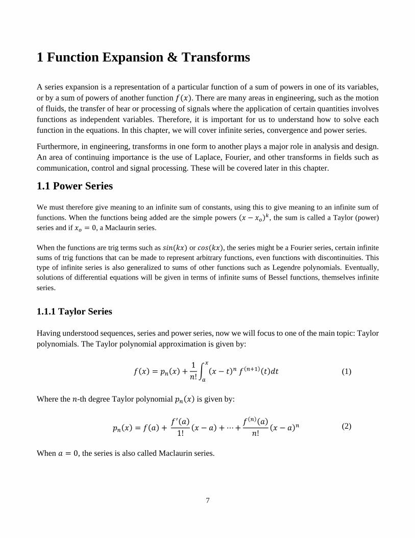
1 Function Expansion & Transforms
A series expansion is a representation of a particular function of a sum of powers in one of its variables,
or by a sum of powers of another function 𝑓(𝑥). There are many areas in engineering, such as the motion
of fluids, the transfer of hear or processing of signals where the application of certain quantities involves
functions as independent variables. Therefore, it is important for us to understand how to solve each
function in the equations. In this chapter, we will cover infinite series, convergence and power series.
Furthermore, in engineering, transforms in one form to another plays a major role in analysis and design.
An area of continuing importance is the use of Laplace, Fourier, and other transforms in fields such as
communication, control and signal processing. These will be covered later in this chapter.
1.1 Power Series
We must therefore give meaning to an infinite sum of constants, using this to give meaning to an infinite sum of
functions. When the functions being added are the simple powers (𝑥 − 𝑥𝑜)𝑘, the sum is called a Taylor (power)
series and if 𝑥𝑜 = 0, a Maclaurin series.
When the functions are trig terms such as 𝑠𝑖𝑛(𝑘𝑥) or 𝑐𝑜𝑠(𝑘𝑥), the series might be a Fourier series, certain infinite
sums of trig functions that can be made to represent arbitrary functions, even functions with discontinuities. This
type of infinite series is also generalized to sums of other functions such as Legendre polynomials. Eventually,
solutions of differential equations will be given in terms of infinite sums of Bessel functions, themselves infinite
series.
1.1.1 Taylor Series
Having understood sequences, series and power series, now we will focus to one of the main topic: Taylor
polynomials. The Taylor polynomial approximation is given by:
𝑓(𝑥) = 𝑝𝑛(𝑥) +1
𝑛!∫ (𝑥 − 𝑡)𝑛 𝑓(𝑛+1)(𝑡)𝑑𝑡
𝑥
𝑎
(1)
Where the 𝑛-th degree Taylor polynomial 𝑝𝑛(𝑥) is given by:
𝑝𝑛(𝑥) = 𝑓(𝑎) + 𝑓′(𝑎)
1!(𝑥 − 𝑎) + ⋯+
𝑓(𝑛)(𝑎)
𝑛!(𝑥 − 𝑎)𝑛 (2)
When 𝑎 = 0, the series is also called Maclaurin series.
8
There are 2 conditions apply:
1. 𝑓 (𝑥), 𝑓(1)(𝑥),⋯ , 𝑓(𝑛+1)(𝑥) are continuous in a closed interval containing 𝑥 = 𝑎.
2. 𝑥 is any point in the interval.
A Taylor series represents a function for a given value as an infinite sum of terms that are calculated from
the value of the function’s derivatives.
Therefore, the Taylor series of a function 𝑓 (𝑥) for a value 𝑎 is the power series, and can be written as:
𝑓(𝑥) = ∑𝑓𝑛(𝑎)
𝑛!
∞
𝑛=0
(𝑥 − 𝑎)𝑛 (3)
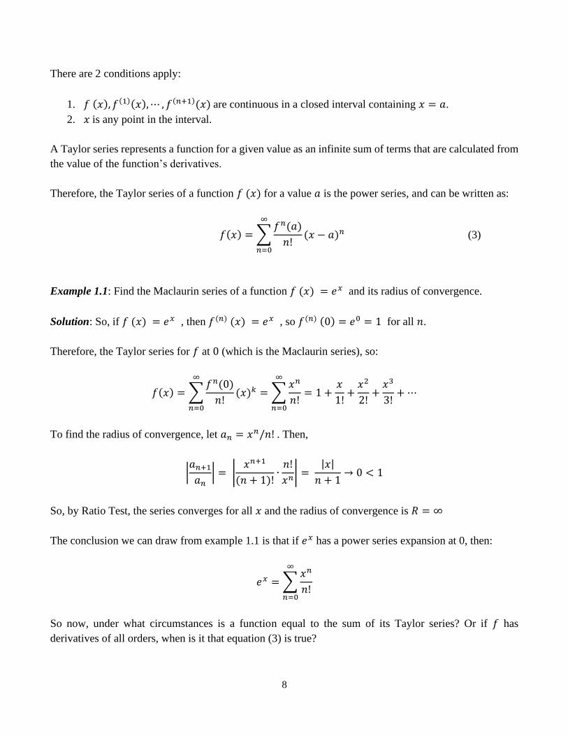
Example 1.1: Find the Maclaurin series of a function 𝑓 (𝑥) = 𝑒𝑥 and its radius of convergence.
Solution: So, if 𝑓 (𝑥) = 𝑒𝑥 , then 𝑓(𝑛) (𝑥) = 𝑒𝑥 , so 𝑓(𝑛) (0) = 𝑒0 = 1 for all 𝑛.
Therefore, the Taylor series for 𝑓 at 0 (which is the Maclaurin series), so:
𝑓(𝑥) = ∑𝑓𝑛(0)
𝑛!
∞
𝑛=0
(𝑥)𝑘 = ∑𝑥𝑛
𝑛!
∞
𝑛=0
= 1 +𝑥
1!+
𝑥2
2!+
𝑥3
3!+ ⋯
To find the radius of convergence, let 𝑎𝑛 = 𝑥𝑛/𝑛! . Then,
|𝑎𝑛+1
𝑎𝑛| = |
𝑥𝑛+1
(𝑛 + 1)!∙𝑛!
𝑥𝑛| =
|𝑥|
𝑛 + 1→ 0 < 1
So, by Ratio Test, the series converges for all 𝑥 and the radius of convergence is 𝑅 = ∞
The conclusion we can draw from example 1.1 is that if 𝑒𝑥 has a power series expansion at 0, then:
𝑒𝑥 = ∑𝑥𝑛
𝑛!
∞
𝑛=0
So now, under what circumstances is a function equal to the sum of its Taylor series? Or if 𝑓 has
derivatives of all orders, when is it that equation (3) is true?

9
With any convergent series, this means that 𝑓(𝑥) is the limit of the sequence of partial sums. In the case
of Taylor series, the partial sums can be written as in as equation (2), where:
𝑝𝑛(𝑥) = 𝑓(𝑎) + 𝑓′(𝑎)
1!(𝑥 − 𝑎) +
𝑓′′(𝑎)
2!(𝑥 − 𝑎)2 ⋯+
𝑓(𝑛)(𝑎)
𝑛!(𝑥 − 𝑎)𝑛
For the example of the exponential function 𝑓 (𝑥) = 𝑒𝑥, the results from example 1.1 shows that the
Taylor polynomials at 0 (or Maclaurin polynomials) with 𝑛 = 1, 2 and 3 are:
𝑝1(𝑥) = 1 + 𝑥
𝑝2(𝑥) = 1 + 𝑥 +𝑥2
2!
𝑝3(𝑥) = 1 + 𝑥 +𝑥2
2!+
𝑥3
3!
In general, 𝑓 (𝑥) is the sum of its Taylor series if
𝑓(𝑥) = lim𝑛→∞
𝑝𝑛(𝑥) (4)
If we let
𝑅𝑛(𝑥) = 𝑓(𝑥) − 𝑝𝑛(𝑥) so that 𝑓(𝑥) = 𝑝𝑛(𝑥) + 𝑅𝑛(𝑥) (5)
Then, 𝑅𝑛(𝑥) is called the remainder of the Taylor series.
If we show that lim𝑛→∞
𝑅𝑛(𝑥) = 0, then it follows that from equation (5):
lim𝑛→∞
𝑝𝑛(𝑥) = lim𝑛→∞
[𝑓(𝑥) − 𝑅𝑛(𝑥)] = 𝑓 (𝑥) − lim𝑛→∞
𝑅(𝑥) =𝑓(𝑥)
We have therefore proved the following:
If 𝑓(𝑥) = 𝑝𝑛(𝑥) + 𝑅𝑛(𝑥), where 𝑝𝑛 is the 𝑛th degree Taylor Polynomial of 𝑓 at 𝑎 and
lim𝑛→∞
𝑅𝑛(𝑥) = 0 (6)
for |𝑥 − 𝑎| < 𝑅, then 𝑓 is equals to the sum of its Taylor series on the interval |𝑥 − 𝑎| < 𝑅.
10
Therefore, if 𝑓 has 𝑛 + 1 derivatives in an interval 𝐼 that contains the number 𝑎, then for 𝑥 in 𝐼 there is a
number 𝑧 strictly between 𝑥 and 𝑎 such that the remainder term in the Taylor series can be expressed as
𝑅𝑛(𝑥) = 𝑓(𝑛+1)(𝑎)
(𝑛 + 1)!(𝑥 − 𝑎)𝑛+1 (7)
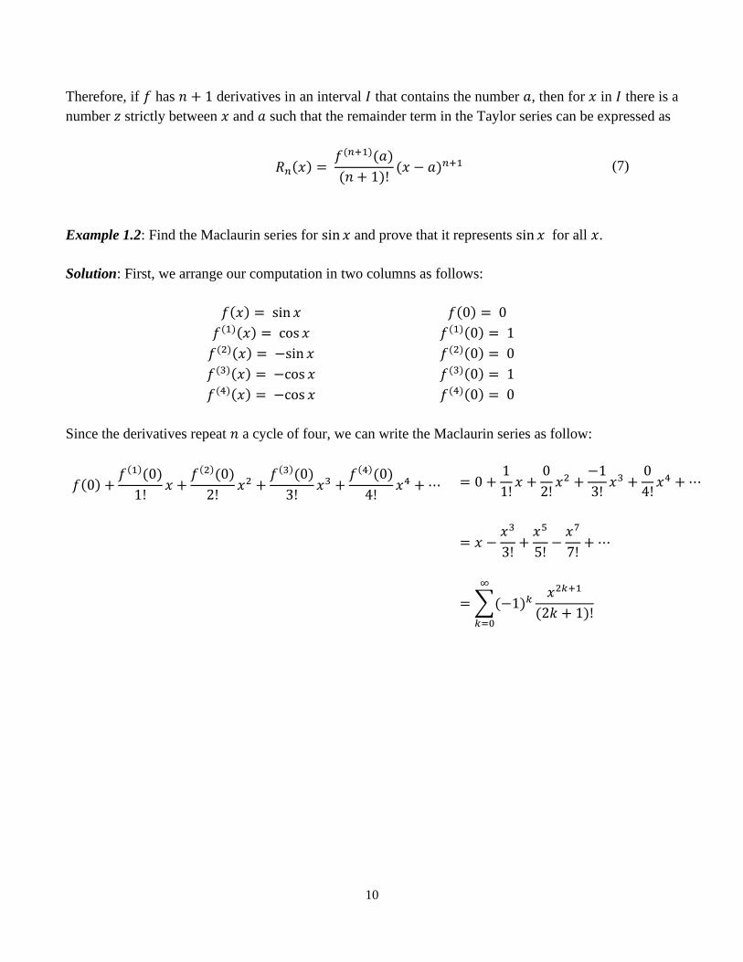
Example 1.2: Find the Maclaurin series for sin 𝑥 and prove that it represents sin 𝑥 for all 𝑥.
Solution: First, we arrange our computation in two columns as follows:
𝑓(𝑥) = sin 𝑥 𝑓(0) = 0
𝑓(1)(𝑥) = cos 𝑥 𝑓(1)(0) = 1
𝑓(2)(𝑥) = −sin 𝑥 𝑓(2)(0) = 0
𝑓(3)(𝑥) = −cos 𝑥 𝑓(3)(0) = 1
𝑓(4)(𝑥) = −cos 𝑥 𝑓(4)(0) = 0
Since the derivatives repeat 𝑛 a cycle of four, we can write the Maclaurin series as follow:
𝑓(0) +𝑓(1)(0)
1!𝑥 +
𝑓(2)(0)
2!𝑥2 +
𝑓(3)(0)
3!𝑥3 +
𝑓(4)(0)
4!𝑥4 + ⋯ = 0 +
1
1!𝑥 +
0
2!𝑥2 +
−1
3!𝑥3 +
0
4!𝑥4 + ⋯
= 𝑥 −
𝑥3
3!+
𝑥5
5!−
𝑥7
7!+ ⋯
= ∑(−1)𝑘
∞
𝑘=0
𝑥2𝑘+1
(2𝑘 + 1)!
11
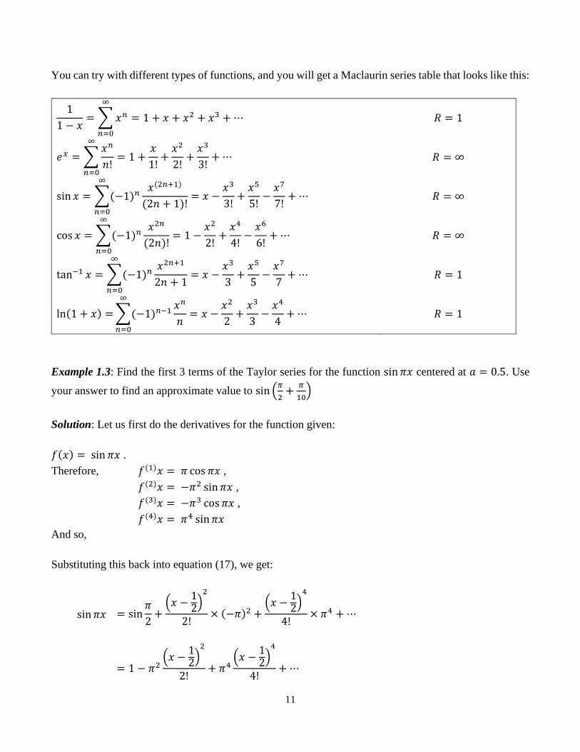
You can try with different types of functions, and you will get a Maclaurin series table that looks like this:
1
1 − 𝑥= ∑ 𝑥𝑛
∞
𝑛=0
= 1 + 𝑥 + 𝑥2 + 𝑥3 + ⋯ 𝑅 = 1
𝑒𝑥 = ∑𝑥𝑛
𝑛!
∞
𝑛=0
= 1 +𝑥
1!+
𝑥2
2!+
𝑥3
3!+ ⋯ 𝑅 = ∞
sin 𝑥 = ∑(−1)𝑛𝑥(2𝑛+1)
(2𝑛 + 1)!
∞
𝑛=0
= 𝑥 −𝑥3
3!+
𝑥5
5!−
𝑥7
7!+ ⋯ 𝑅 = ∞
cos 𝑥 = ∑(−1)𝑛𝑥2𝑛
(2𝑛)!
∞
𝑛=0
= 1 −𝑥2
2!+
𝑥4
4!−
𝑥6
6!+ ⋯ 𝑅 = ∞
tan−1 𝑥 = ∑(−1)𝑛𝑥2𝑛+1
2𝑛 + 1
∞
𝑛=0
= 𝑥 −𝑥3
3+
𝑥5
5−
𝑥7
7+ ⋯ 𝑅 = 1
ln(1 + 𝑥) = ∑(−1)𝑛−1𝑥𝑛
𝑛
∞
𝑛=0
= 𝑥 −𝑥2
2+
𝑥3
3−
𝑥4
4+ ⋯ 𝑅 = 1
Example 1.3: Find the first 3 terms of the Taylor series for the function sin 𝜋𝑥 centered at 𝑎 = 0.5. Use
your answer to find an approximate value to sin (𝜋
2+
𝜋
10)
Solution: Let us first do the derivatives for the function given:
𝑓(𝑥) = sin 𝜋𝑥 .
Therefore, 𝑓(1)𝑥 = 𝜋 cos 𝜋𝑥 ,
𝑓(2)𝑥 = −𝜋2 sin 𝜋𝑥 ,
𝑓(3)𝑥 = −𝜋3 cos 𝜋𝑥 ,
𝑓(4)𝑥 = 𝜋4 sin 𝜋𝑥
And so,
Substituting this back into equation (17), we get:
sin 𝜋𝑥 = sin𝜋
2+
(𝑥 −12)
2
2!× (−𝜋)2 +
(𝑥 −12)
4
4!× 𝜋4 + ⋯
= 1 − 𝜋2
(𝑥 −12)
2
2!+ 𝜋4
(𝑥 −12)
4
4!+ ⋯
12
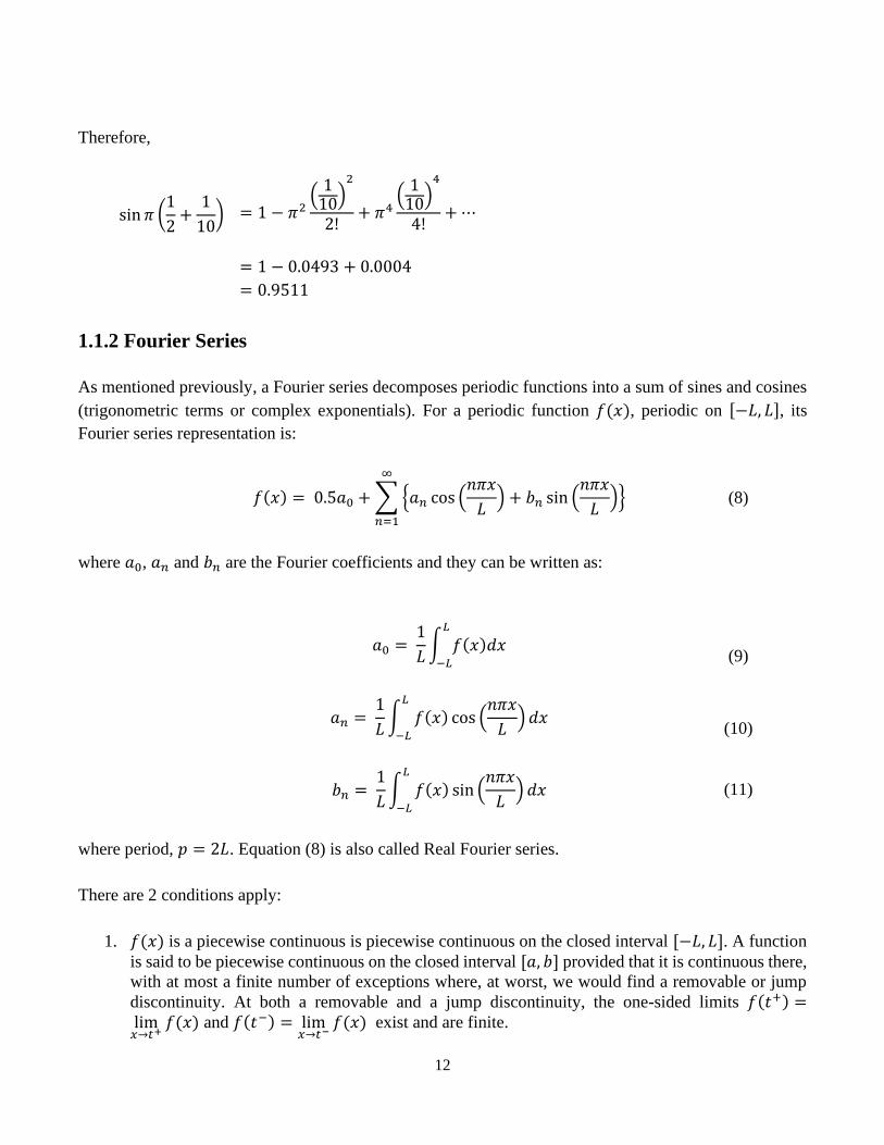
Therefore,
sin 𝜋 (1
2+
1
10) = 1 − 𝜋2
(110)
2
2!+ 𝜋4
(110)
4
4!+ ⋯
= 1 − 0.0493 + 0.0004
= 0.9511
1.1.2 Fourier Series
As mentioned previously, a Fourier series decomposes periodic functions into a sum of sines and cosines
(trigonometric terms or complex exponentials). For a periodic function 𝑓(𝑥), periodic on [−𝐿, 𝐿], its
Fourier series representation is:
𝑓(𝑥) = 0.5𝑎0 + ∑ {𝑎𝑛 cos (𝑛𝜋𝑥
𝐿) + 𝑏𝑛 sin (
𝑛𝜋𝑥
𝐿)}
∞
𝑛=1
(8)
where 𝑎0, 𝑎𝑛 and 𝑏𝑛 are the Fourier coefficients and they can be written as:
𝑎0 =
1
𝐿∫ 𝑓(𝑥)𝑑𝑥
𝐿
−𝐿
(9)
𝑎𝑛 =
1
𝐿∫ 𝑓(𝑥) cos (
𝑛𝜋𝑥
𝐿)𝑑𝑥
𝐿
−𝐿
(10)
𝑏𝑛 =
1
𝐿∫ 𝑓(𝑥) sin (
𝑛𝜋𝑥
𝐿) 𝑑𝑥
𝐿
−𝐿
(11)
where period, 𝑝 = 2𝐿. Equation (8) is also called Real Fourier series.
There are 2 conditions apply:
1. 𝑓(𝑥) is a piecewise continuous is piecewise continuous on the closed interval [−𝐿, 𝐿]. A function
is said to be piecewise continuous on the closed interval [𝑎, 𝑏] provided that it is continuous there,
with at most a finite number of exceptions where, at worst, we would find a removable or jump
discontinuity. At both a removable and a jump discontinuity, the one-sided limits 𝑓(𝑡+) =lim𝑥→𝑡+
𝑓(𝑥) and 𝑓(𝑡−) = lim𝑥→𝑡−
𝑓(𝑥) exist and are finite.
13
2. A sum of continuous and periodic functions converges pointwise to a possibly discontinuous and
non-periodic function. This was a startling realisation for mathematicians of the early nineteenth
century.
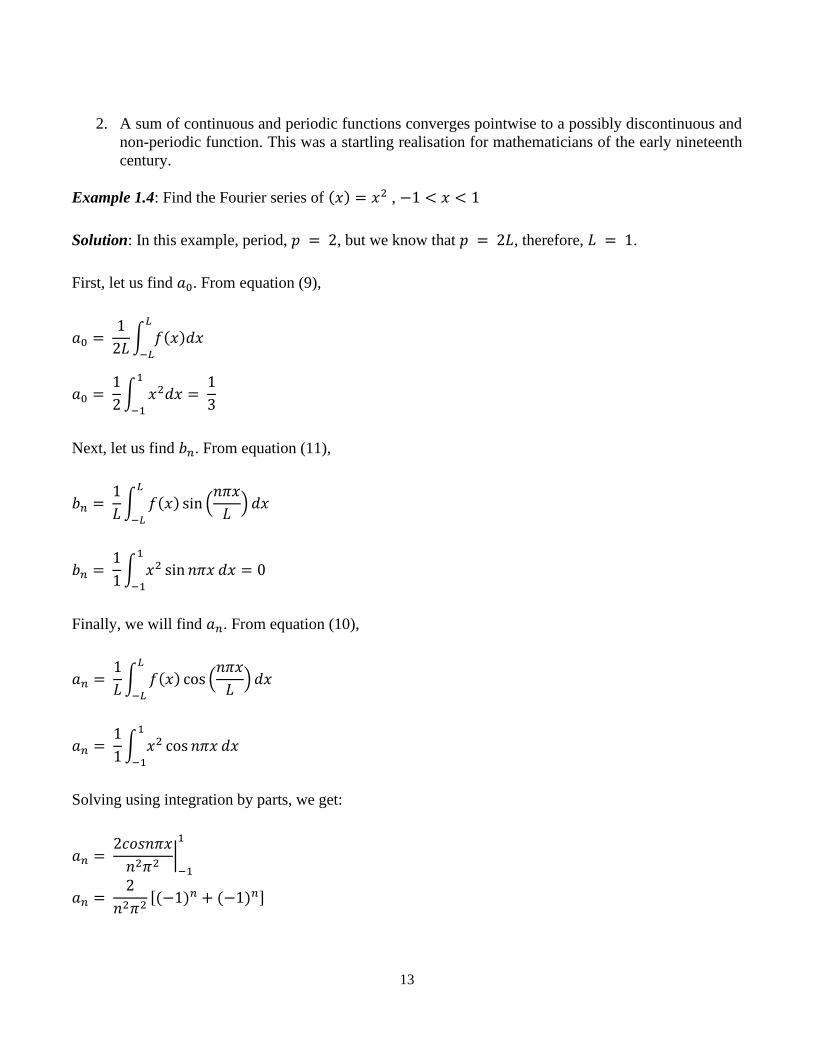
Example 1.4: Find the Fourier series of (𝑥) = 𝑥2 , −1 < 𝑥 < 1
Solution: In this example, period, 𝑝 = 2, but we know that 𝑝 = 2𝐿, therefore, 𝐿 = 1.
First, let us find 𝑎0. From equation (9),
𝑎0 = 1
2𝐿∫ 𝑓(𝑥)𝑑𝑥
𝐿
−𝐿
𝑎0 = 1
2∫ 𝑥2𝑑𝑥 =
1
3
1
−1
Next, let us find 𝑏𝑛. From equation (11),
𝑏𝑛 = 1
𝐿∫ 𝑓(𝑥) sin (
𝑛𝜋𝑥
𝐿) 𝑑𝑥
𝐿
−𝐿
𝑏𝑛 = 1
1∫ 𝑥2 sin 𝑛𝜋𝑥 𝑑𝑥
1
−1
= 0
Finally, we will find 𝑎𝑛. From equation (10),
𝑎𝑛 = 1
𝐿∫ 𝑓(𝑥) cos (
𝑛𝜋𝑥
𝐿)𝑑𝑥
𝐿
−𝐿
𝑎𝑛 = 1
1∫ 𝑥2 cos 𝑛𝜋𝑥 𝑑𝑥
1
−1
Solving using integration by parts, we get:
𝑎𝑛 = 2𝑐𝑜𝑠𝑛𝜋𝑥
𝑛2𝜋2|−1
1
𝑎𝑛 = 2
𝑛2𝜋2[(−1)𝑛 + (−1)𝑛]

14
𝑎𝑛 = 4(−1)𝑛
𝑛2𝜋2
Therefore, the Fourier series can be written as:
𝑓(𝑥2) = 1
3+ ∑
4(−1)𝑛
𝑛2𝜋2 cos(𝑛𝜋𝑥)
∞
𝑛=1
1.1.3 Complex Fourier series
A function 𝑓(𝑥) can also be expressed as a Complex Fourier series and can be defined to be:
𝑓(𝑥) = ∑𝑐𝑛𝑒𝑖𝑛𝜋𝑥/𝐿
+∞
−∞
(12)
where
𝑐𝑛 =1
2𝜋∫ 𝑓(𝑥)𝑒−𝑖𝑛𝑥
𝜋
−𝜋
(13)
We know that:
𝑒𝑖𝑥 = cos 𝑥 + 𝑖 sin 𝑥
𝑒−𝑖𝑥 = cos 𝑥 − 𝑖 sin 𝑥
𝑒𝑖𝑥 − 𝑒−𝑖𝑥 = 2𝑖 sin 𝑥
𝑒𝑖𝑥 + 𝑒−𝑖𝑥 = 2 cos 𝑥
(14)
Therefore, from equation (13),
𝑐𝑛 =1
2𝜋∫ 𝑓(𝑥)𝑒−𝑖𝑛𝑥
𝜋
−𝜋
𝑐𝑛 =1
2[1
𝜋∫ 𝑓(𝑥) cos 𝑛𝑥 𝑑𝑥 − 𝑖
𝜋
−𝜋
1
𝜋∫ 𝑓(𝑥) sin 𝑛𝑥 𝑑𝑥
𝜋
−𝜋
]
15
Hence, we can write:
⟹ 𝑐𝑛 =1
2(𝑎𝑛 − 𝑖𝑏𝑛) , 𝑛 > 0
⟹ 𝑐𝑛 =1
2(𝑎−𝑛 + 𝑖𝑏−𝑛) , 𝑛 < 0
⟹ 𝑐𝑛 = 𝑎0 , 𝑛 = 0
Example 1.5: Write the complex Fourier transform of 𝑓(𝑥) = 2 sin 𝑥 − cos 10𝑥
Solution: Here, we can expand the function by substituting the sin and cos functions from equation (14),
we get:
𝑓(𝑥) = 2𝑒𝑖𝑥 − 𝑒−𝑖𝑥
2𝑖−
𝑒10𝑖𝑥 + 𝑒−10𝑖𝑥
2
𝑓(𝑥) =1
𝑖𝑒𝑖𝑥 −
1
𝑖𝑒−𝑖𝑥 −
1
2𝑒10𝑖𝑥 −
1
2𝑒−10𝑖𝑥
Therefore:
𝑐1 =1
𝑖 , 𝑐10 = −
1
2 , 𝑐−1 = −
1
𝑖 , 𝑐−10 = −
1
2
1.1.4 Termwise Integration and Differentiation
Parseval’s Identity
Consider a Fourier series below and expand it
𝑓(𝑥) = 𝑎0 + ∑{𝑎𝑛 cos 𝑛𝑥 + 𝑏𝑛 sin 𝑛𝑥} = 𝑎0 + 𝑎1 cos 𝑥 + 𝑏1 sin 𝑥 + 𝑎2 cos 2𝑥 + 𝑏2 sin 2𝑥 + ⋯
∞
𝑛=1
Square it, we get:
16
𝑓2(𝑥) = 𝑎02 + ∑(𝑎𝑛
2 cos2 𝑛𝑥 + 𝑏𝑛2 sin2 𝑛𝑥) + 2𝑎0 ∑(
𝑁
𝑛=1
𝑎𝑛 cos 𝑛𝑥 + 𝑏𝑛 sin 𝑛𝑥)
𝑁
𝑛=1
+ 2𝑎1 cos 𝑥 𝑏1 sin 𝑥 + 2𝑎1 cos 𝑥 ∑(
𝑁
𝑛=1
𝑎𝑛 cos 𝑛𝑥 + 𝑏𝑛 sin 𝑛𝑥) + ⋯
+ 2𝑎𝑁 cos𝑁𝑥 𝑏𝑁 sin𝑁𝑥
Integrate both sides, we get:
∫ 𝑓2(𝑥) 𝑑𝑥𝜋
−𝜋
= ∫ {𝑎02 + ∑(𝑎𝑛
2 cos2 𝑛𝑥 + 𝑏𝑛2 sin2 𝑛𝑥) + ⋯
𝑁
𝑛=1
}𝜋
−𝜋
𝑑𝑥
⟹ ∫ 𝑓2(𝑥) 𝑑𝑥𝜋
−𝜋
= 2𝜋𝑎02 + ∑(𝜋𝑎𝑛
2 + 𝜋𝑏𝑛2) + 0
𝑁
𝑛=1
Parseval’s Identity can be written as:
1
𝐿∫ |𝑓(𝑥)|2 𝑑𝑥 = 2|𝑎0|
2𝐿
−𝐿
+ ∑(|𝑎𝑛|2 + |𝑏𝑛|2)
∞
𝑛=1
(15)
If:
a) 𝑓(𝑥) is continuous, and 𝑓′(𝑥) is a piecewise continuous on [−𝐿, 𝐿]
b) 𝑓(𝐿) = 𝑓(−𝐿)
c) 𝑓′′(𝑥) exist at 𝑥 in (−𝐿, 𝐿),
Therefore:
𝑓′(𝑥) =𝜋
𝐿∑ 𝑛
∞
𝑛=1
(−𝑎𝑛 sin𝑛𝜋𝑥
𝐿+ 𝑏𝑛 cos
𝑛𝜋𝑥
𝐿) (16)
Example 1.6: From Example 1.4, we found that the Fourier series is:
𝑓(𝑥2) = 1
3+ ∑
4(−1)𝑛
𝑛2𝜋2 cos(𝑛𝜋𝑥) , 𝑥2
∞
𝑛=1
17
Solution: Applying Parseval’s to the equation above, we get:
2 (1
3)2
+ ∑16
𝑛4𝜋4
∞
𝑛=1
= ∫ 𝑥41
−1
𝑑𝑥 = 2
5
⟹ ∑16
𝑛4𝜋4
∞
𝑛=1
= 2
5−
2
9=
8
45
⟹ ∑1
𝑛4
∞
𝑛=1
= 𝜋4
90
1.1.5 Fourier series of Odd and Even functions
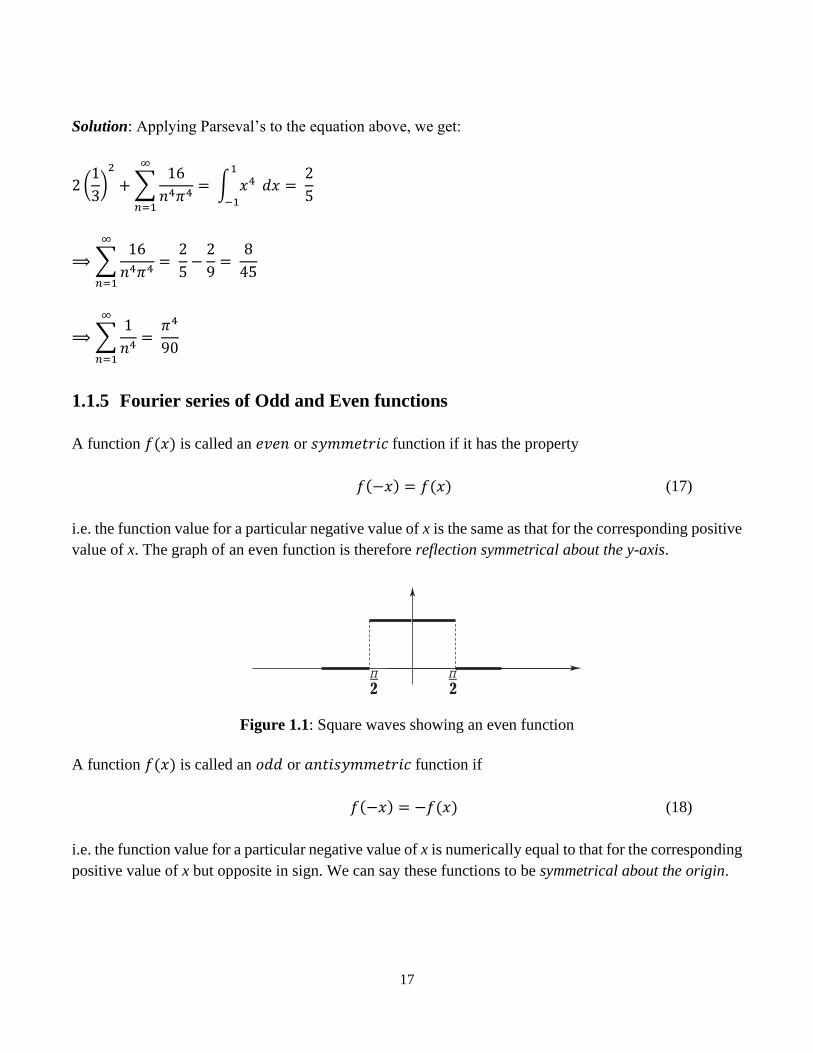
A function 𝑓(𝑥) is called an 𝑒𝑣𝑒𝑛 or 𝑠𝑦𝑚𝑚𝑒𝑡𝑟𝑖𝑐 function if it has the property
𝑓(−𝑥) = 𝑓(𝑥) (17)
i.e. the function value for a particular negative value of x is the same as that for the corresponding positive
value of x. The graph of an even function is therefore reflection symmetrical about the y-axis.
Figure 1.1: Square waves showing an even function
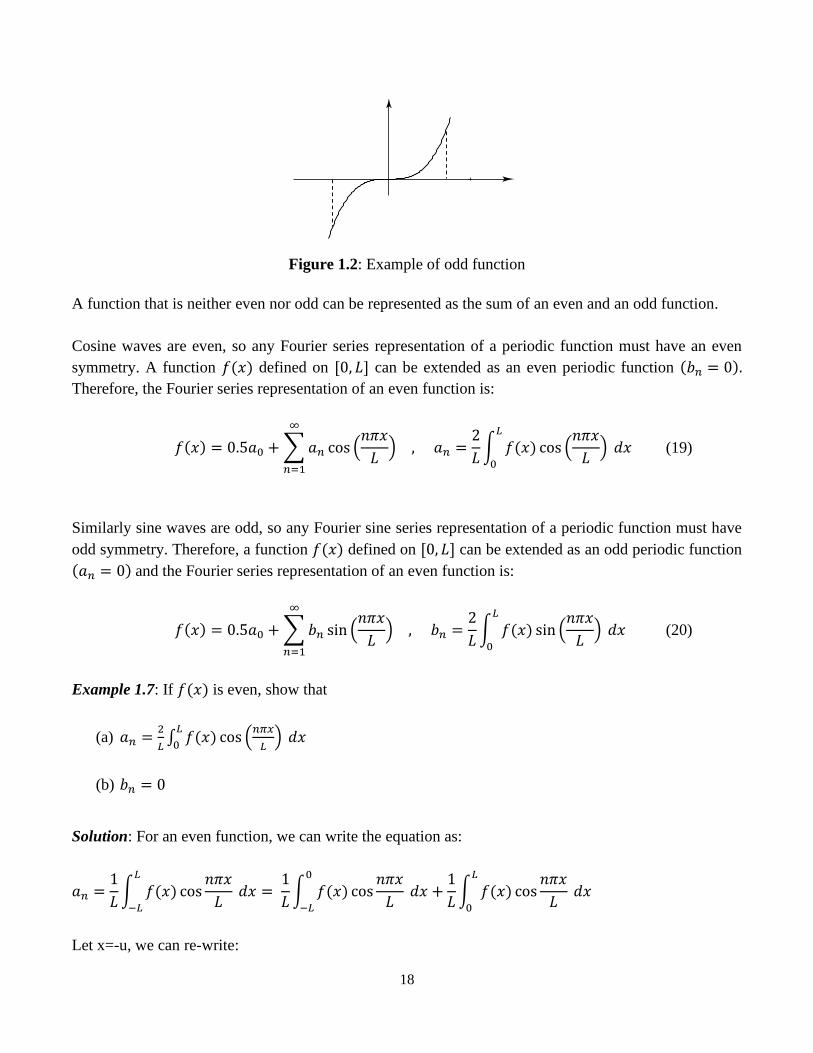
A function 𝑓(𝑥) is called an 𝑜𝑑𝑑 or 𝑎𝑛𝑡𝑖𝑠𝑦𝑚𝑚𝑒𝑡𝑟𝑖𝑐 function if
𝑓(−𝑥) = −𝑓(𝑥) (18)
i.e. the function value for a particular negative value of x is numerically equal to that for the corresponding
positive value of x but opposite in sign. We can say these functions to be symmetrical about the origin.
18
Figure 1.2: Example of odd function
A function that is neither even nor odd can be represented as the sum of an even and an odd function.
Cosine waves are even, so any Fourier series representation of a periodic function must have an even
symmetry. A function 𝑓(𝑥) defined on [0, 𝐿] can be extended as an even periodic function (𝑏𝑛 = 0).
Therefore, the Fourier series representation of an even function is:
𝑓(𝑥) = 0.5𝑎0 + ∑ 𝑎𝑛 cos (𝑛𝜋𝑥
𝐿)
∞
𝑛=1
, 𝑎𝑛 =2
𝐿∫ 𝑓(𝑥) cos (
𝑛𝜋𝑥
𝐿)
𝐿
0
𝑑𝑥 (19)
Similarly sine waves are odd, so any Fourier sine series representation of a periodic function must have
odd symmetry. Therefore, a function 𝑓(𝑥) defined on [0, 𝐿] can be extended as an odd periodic function
(𝑎𝑛 = 0) and the Fourier series representation of an even function is:
𝑓(𝑥) = 0.5𝑎0 + ∑ 𝑏𝑛 sin (𝑛𝜋𝑥
𝐿)
∞
𝑛=1
, 𝑏𝑛 =2
𝐿∫ 𝑓(𝑥) sin (
𝑛𝜋𝑥
𝐿)
𝐿
0
𝑑𝑥 (20)
Example 1.7: If 𝑓(𝑥) is even, show that
(a) 𝑎𝑛 =2
𝐿∫ 𝑓(𝑥) cos (
𝑛𝜋𝑥
𝐿)
𝐿
0 𝑑𝑥
(b) 𝑏𝑛 = 0
Solution: For an even function, we can write the equation as:
𝑎𝑛 =1
𝐿∫ 𝑓(𝑥) cos
𝑛𝜋𝑥
𝐿
𝐿
−𝐿
𝑑𝑥 = 1
𝐿∫ 𝑓(𝑥) cos
𝑛𝜋𝑥
𝐿
0
−𝐿
𝑑𝑥 +1
𝐿∫ 𝑓(𝑥) cos
𝑛𝜋𝑥
𝐿
𝐿
0
𝑑𝑥
Let x=-u, we can re-write:

19
1
𝐿∫ 𝑓(𝑥) cos
𝑛𝜋𝑥
𝐿
0
−𝐿
𝑑𝑥 =1
𝐿∫ 𝑓(−𝑢) cos (
−𝑛𝜋𝑢
𝐿)
𝐿
0
𝑑𝑢 =1
𝐿∫ 𝑓(𝑢) cos (
𝑛𝜋𝑢
𝐿)
𝐿
0
𝑑𝑢
Since by definition of an even function f(-u) = f(u). Then:
𝑎𝑛 =1
𝐿∫ 𝑓(𝑢) cos (
𝑛𝜋𝑢
𝐿)
𝐿
0
𝑑𝑢 +1
𝐿∫ 𝑓(𝑥) cos
𝑛𝜋𝑥
𝐿
𝐿
0
𝑑𝑥 =2
𝐿∫ 𝑓(𝑥) cos
𝑛𝜋𝑥
𝐿
𝐿
0
𝑑𝑥
To show that 𝑏𝑛 = 0, we can write the expression as
𝑏𝑛 =1
𝐿∫ 𝑓(𝑥) sin (
𝑛𝜋𝑥
𝐿)
𝐿
−𝐿
𝑑𝑥 = 1
𝐿∫ 𝑓(𝑥) sin (
𝑛𝜋𝑥
𝐿)
0
−𝐿
𝑑𝑥 +1
𝐿∫ 𝑓(𝑥) sin (
𝑛𝜋𝑥
𝐿)
𝐿
0
𝑑𝑥
If we make the transformation x=-u in the first integral on the right of the equation above, we obtain:
1
𝐿∫ 𝑓(𝑥) sin (
𝑛𝜋𝑥
𝐿)
0
−𝐿
𝑑𝑥 =1
𝐿∫ 𝑓(−𝑢) sin (−
𝑛𝜋𝑢
𝐿)
𝐿
0
𝑑𝑢 = −1
𝐿∫ 𝑓(𝑢) sin (
𝑛𝜋𝑢
𝐿)
𝐿
0
𝑑𝑢
= −
1
𝐿∫ 𝑓(𝑢) sin (
𝑛𝜋𝑢
𝐿)
𝐿
0
𝑑𝑢 = −1
𝐿∫ 𝑓(𝑥) sin (
𝑛𝜋𝑥
𝐿)
𝐿
0
𝑑𝑥
Therefore, substituting this into the equation for 𝑏𝑛, we get
𝑏𝑛 = −1
𝐿∫ 𝑓(𝑥) sin (
𝑛𝜋𝑥
𝐿)
𝐿
0
𝑑𝑥 +1
𝐿∫ 𝑓(𝑥) sin (
𝑛𝜋𝑥
𝐿)
𝐿
0
𝑑𝑥 = 0
1.2 Integral Transform
An integral transform is any transform of the following form
𝐹(𝑤) = ∫ 𝐾(𝑤, 𝑥)𝑓(𝑥)𝑥2
𝑥1
𝑑𝑥 (21)
With the following inverse transform

20
𝑓(𝑥) = ∫ 𝐾−1(𝑤, 𝑥)𝐹(𝑤)𝑤2
𝑤1
𝑑𝑤 (22)
1.2.1 Fourier Transform
A Fourier series expansion of a function 𝑓(𝑥) of a real variable 𝑥 with a period of 2𝐿 is defined over a
finite interval −𝐿 ≤ 𝑥 ≤ 𝐿 . If the interval becomes infinite and we sum over infinitesimals, we then obtain
the Fourier integral
𝑓(𝑥) =1
2𝜋∫ 𝐹(𝑤)𝑒𝑖𝑤𝑥
∞
−∞
𝑑𝑤 (23)
with the coefficients
𝐹(𝑤) = ∫ 𝑓(𝑥)𝑒−𝑖𝑤𝑥∞
−∞
𝑑𝑥 (24)
Equation (24) is the Fourier transform of 𝑓(𝑥). The Fourier integral is also known as the inverse Fourier
transform of 𝐹(𝑤). In this example, 𝑥1 = 𝑤1 = −∞, 𝑥2 = 𝑤2 = ∞ and 𝐾(𝑤, 𝑥) = 𝑒−𝑖𝑤𝑥. The Fourier
transform transforms a function of one variable (e.g. time in seconds) which lives in the time domain to a
second function which lives in the frequency domain and changes the basis of the function to cosines and
sines.
Example 1.8: Find the Fourier transform of
𝑓(𝑡) = {𝑡 ∶ −1 ≤ 𝑡 ≤ 10 ∶ 𝑒𝑙𝑠𝑒𝑤ℎ𝑒𝑟𝑒
Solution: Recalling the Fourier transform in equation (24), we can write
𝐹(𝑤) = ∫ 𝑓(𝑥)𝑒−𝑖𝑤𝑥∞
−∞
𝑑𝑥
= ∫ 𝑡 ∙ 𝑒−𝑖𝑤𝑡1
−1
𝑑𝑡
By applying integration by parts, we get:
= [𝑡
−𝑖𝑤𝑒𝑖𝑤𝑡]
−1
1
− ∫1
−𝑖𝑤𝑒−𝑖𝑤𝑡
1
−1
𝑑𝑡
21
We can also rewrite −1
𝑖= 𝑖, therefore:
= [𝑖𝑡
𝑤𝑒𝑖𝑤𝑡]
−1
1
+ [1
𝑖𝑤∙
1
−𝑖𝑤𝑒𝑖𝑤𝑡]
−1
1
= [𝑖𝑡
𝑤𝑒𝑖𝑤𝑡]
−1
1
+ [1
𝑤2𝑒𝑖𝑤𝑡]
−1
1
=𝑖
𝑤(𝑒−𝑖𝑤 + 𝑒𝑖𝑤) +
1
𝑤2(𝑒−𝑖𝑤 + 𝑒𝑖𝑤)
= 2𝑖
𝑤
1
2(𝑒−𝑖𝑤 + 𝑒𝑖𝑤) + (−
2𝑖
𝑤2∙1
2𝑖) (𝑒𝑖𝑤 − 𝑒−𝑖𝑤)
=2𝑖
𝑤cos𝑤 −
2𝑖
𝑤2sin𝑤
=2𝑖
𝑤(cos𝑤 −
1
𝑤sin𝑤)
1.2.2 Laplace Transform
The Laplace transform is an example of an integral transform that will convert a differential equation into
an algebraic equation. The Laplace transform of a function 𝑓(𝑥) of a variable 𝑥 is defined as the integral
𝐹(𝑠) = ℒ{𝑓(𝑡)} = ∫ 𝑓(𝑡)𝑒−𝑠𝑡∞
0
𝑑𝑡 (25)
where 𝑠 is a positive real parameter that serves as a supplementary variable. The conditions are: if 𝑓(𝑡) is
piecewise continuous on (0,∞), and of exponential order (|𝑓(𝑡)| ≤ 𝐾𝑒𝛼𝑡 for some 𝐾 and 𝛼 > 0), then
𝐹(𝑠) exists for 𝑠 > 𝛼. Several Laplace transforms are given in the table below, where 𝑎 is a constant and
𝑛 is an integer.
Example 1.9: Find the Laplace transforms of the following functions:
𝑓(𝑡) = {3 ∶ 0 < 𝑡 < 50 ∶ 𝑡 > 0

22
Solution:
ℒ{𝑓(𝑡)} = ∫ 𝑓(𝑡) 𝑒−𝑠𝑡∞
0
𝑑𝑡 = ∫ 3 ∙ 𝑒−𝑠𝑡 𝑑𝑡 + ∫ 0 ∙ 𝑒−𝑠𝑡 𝑑𝑡∞
5
5
0
= 3 |𝑒−𝑠𝑡
−𝑠|0
5
+ 0
= 3 |𝑒−5𝑠
−𝑠−
1
−𝑠|
=3
𝑠(1 − 𝑒−5𝑠)
Example 1.10: Find the Laplace transforms of the following functions:
𝑓(𝑡) = {𝑡 ∶ 0 < 𝑡 < 𝑎𝑏 ∶ 𝑡 > 𝑎
Solution:
ℒ{𝑓(𝑡)} = ∫ 𝑓(𝑡) 𝑒−𝑠𝑡∞
0
𝑑𝑡 = ∫ 𝑡 ∙ 𝑒−𝑠𝑡 𝑑𝑡 + ∫ 𝑏 ∙ 𝑒−𝑠𝑡 𝑑𝑡∞
𝑎
𝑎
0
= |𝑒−𝑠𝑡
−𝑠𝑡 −
𝑒−𝑠𝑡
𝑠2∙ 1|
0
𝑎
+ 𝑏 |𝑒−𝑠𝑡
−𝑠|𝑎
∞
= 𝑒−𝑎𝑠 (−𝑎
𝑠−
1
𝑠2) − 𝑒0 (0 −
1
𝑠2) −
𝑏
𝑠(0 − 𝑒−𝑎𝑠)
= 1
𝑠2+ [
𝑏 − 𝑎
𝑠−
1
𝑠2] 𝑒−𝑎𝑠
Example 1.11: Determine the Laplace transform of the function below:
𝑓(𝑡) = 5 − 3𝑡 + 4 sin 2𝑡 − 6𝑒4𝑡
Solution: First, let’s break the equation one by one, we get:
ℒ{5} =5
𝑠 , 𝑅𝑒 (𝑠) > 0

23
ℒ{𝑡} =1
𝑠2 , 𝑅𝑒 (𝑠) > 0
ℒ{sin 2𝑡} =2
𝑠2 + 4 , 𝑅𝑒 (𝑠) > 0
ℒ{𝑒4𝑡} =1
𝑠 − 4 , 𝑅𝑒 (𝑠) > 4
Therefore, by linearity property,
ℒ{𝑓(𝑡)} = ℒ{5 − 3𝑡 + 4 sin 2𝑡 − 6𝑒4𝑡}
= ℒ{5} − 3ℒ{𝑡} + 4ℒ{sin 2𝑡} − 6ℒ{𝑒4𝑡}
=5
𝑠−
3
𝑠2+
8
𝑠2 + 4−
6
𝑠 − 4
LAPLACE TRANSFORMS
𝒇(𝒙) = 𝓛−𝟏{𝑭(𝒔)} 𝑭(𝒔) = 𝓛{𝒇(𝒔)}
𝒂 𝑎
𝑠
𝒕 1
𝑠2
𝒙𝒏 (𝑛!)
𝑠𝑛+1
𝒆𝒂𝒙 1
(𝑠 − 𝑎)
𝐬𝐢𝐧 𝒂𝒙 𝑎
(𝑠2 + 𝑎2)
𝐜𝐨𝐬 𝒂𝒙 𝑠
(𝑠2 + 𝑎2)
𝐬𝐢𝐧𝐡𝒂𝒙 𝑎
(𝑠2 − 𝑎2)
𝐜𝐨𝐬𝐡 𝒂𝒙 𝑠
(𝑠2 − 𝑎2)
24
2. Vector Spaces, vector Fields & Operators
In the context of physics, we are often interested in a quantity or property which varies in a smooth and
continuous way over some one-, two-, or three-dimensional region of space. This constitutes either a scalar
field or a vector field, depending on the nature of property. In this chapter, we consider the relationship
between a scalar field involving a variable potential and a vector field involving ‘field’, where this means
force per unit mass or change. The properties of scalar and vector fields are described and how they lead
to important concepts, such as that of a conservative field, and the important and useful Gauss and Stokes
theorems. Finally, examples will be given to demonstrate the ideas of vector analysis.
There are basically four types of functions involving scalars and vectors:
• Scalar functions of a scalar, 𝑓(𝑥)
• Vector function of a scalar, 𝒓(𝑡)
• Scalar function of a vector, 𝜑(𝒓)
• Vector function of a vector, 𝑨(𝒓)
1. The vector x is normalised if xTx = 1
2. The vectors x and y are orthogonal if xTy = 0
3. The vectors x1, x2, …, x𝑛 are linearly independent if the only numbers which satisfy the equation
𝑎1x1 + 𝑎2x2 + … + 𝑎𝑛x𝑛 = 0 are 𝑎1 = 𝑎2 = . . . = 𝑎𝑛 = 0
4. The vectors x1, x2, …, x𝑛 form a basis for a 𝑛 −dimensional vector-space if any vector x in the vector-
space can be written as a linear combination of vectors in the basis thus x = 𝑎1x1 + 𝑎2x2 + ⋯+ 𝑎𝑛x𝑛
where 𝑎1, 𝑎2, ⋯ , 𝑎𝑛 are scalars.
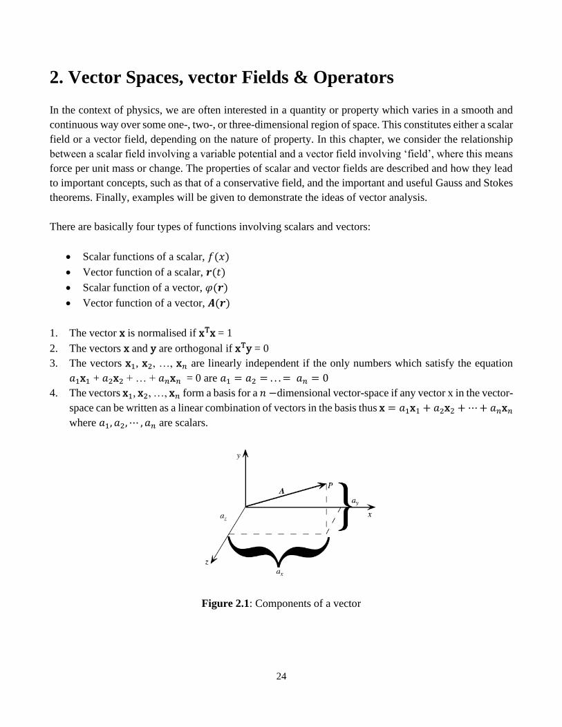
Figure 2.1: Components of a vector
25
For example, a vector A from the origin in the figure above to a point P in the 3-dimensions takes the
form
𝑨 = 𝑎𝑥𝒊 + 𝑎𝑦𝒋 + 𝑎𝑧𝒌 (26)
Where {𝒊, 𝒋, 𝒌}are unit vectors along the {𝑥, 𝑦, 𝑧} axes, respectively. The vector components {𝑎𝑥, 𝑎𝑦, 𝑎𝑧, }
are the corresponding distances along the axes. The length or magnitude of Vector 𝑨 is
|𝑨| = √𝑎𝑥2 + 𝑎𝑦
2 + 𝑎𝑧2 (27)
2.1 Scalar (inner) product of vector fields
The scalar product of vector fields is also called as the dot product. For example, if we have 2 vectors as
𝑨 = (𝐴1, 𝐴2, 𝐴3) and 𝑩 = (𝐵1, 𝐵2, 𝐵3), therefore,
⟨𝑨, 𝑩⟩ = 𝑨 ∙ 𝑩 = 𝑨𝑇𝑩 = 𝐴1𝐵1 + 𝐴2𝐵2 + 𝐴3𝐵3 (28)
We can also write
𝑨 ∙ 𝑩 = ‖𝑨‖‖𝑩‖ cos 𝜃 (29)
where 𝜃 is the angle between 𝑨 and 𝑩 satisfying 0 ≤ 𝜃 ≤ 𝜋. The inner product of vectors is a scalar.
The scalar product obeys the product laws which are listed below:
Product laws:
1. Commutative: 𝑨 ∙ 𝑩 = 𝑩 ∙ 𝑨
2. Associative: 𝑚𝑨 ∙ 𝑛𝑩 = 𝑚𝑛𝑨 ∙ 𝑩
3. Distributive: 𝑨 ∙ (𝑩 + 𝑪) = 𝑨 ∙ 𝑩 + 𝑨 ∙ 𝑪
4. Cauchy-Schwarz inequality: 𝑨 ∙ 𝑩 ≤ (𝑨 ∙ 𝑨)1
2(𝑩 ∙ 𝑩)1
2
Note that a relation such as 𝑨 ∙ 𝑩 = 𝑨 ∙ 𝑪 does not imply that 𝑩 = 𝑪, as
𝑨 ∙ 𝑩 − 𝑨 ∙ 𝑪 = 𝑨 ∙ (𝑩 − 𝑪) = 0 (30)
Therefore, the correct conclusion is that 𝑨 is perpendicular to the vector 𝑩 − 𝑪.
Example 2.1: Determine the angle between 𝑨 = ⟨1,3, −2⟩ and 𝑩 = ⟨−2, 4, −1⟩.
26
Solution: All we need to do here is to rewrite equation (29) as:
cos 𝜃 =𝑨 ∙ 𝑩
‖𝑨‖‖𝑩‖
Therefore, we know that:
cos 𝜃 =𝑨 ∙ 𝑩
‖𝑨‖‖𝑩‖
We will first have to compute the individual parameters
𝑨 ∙ 𝑩 = 12 ‖𝑨‖ = √14 ‖𝑩‖ = √21
Hence, the angle between the vectors is:
cos 𝜃 =12
√14√21= 0.69985 ⟹ 𝜃 = cos−1(0.69985) = 45.58°
2.1.1 Lp norms
There are many norms that could be defined for vectors. One type of norms is called the 𝐿𝑝 norm, often
denoted as ‖ ∙ ‖𝑝. For 𝑝 ≥ 1, it is defined as the 𝑝 − 𝑛𝑜𝑟𝑚 and can be written as:
‖𝑥‖𝑝 = (∑‖𝑥𝑖‖𝑝
𝑛
𝑖=1
)
1𝑝
, 𝑥 = [𝑥1, ⋯ 𝑥𝑛]𝑇 (31)
There are a few types of norms such as the following:
1. ‖𝑥‖1 = ∑ |𝑥𝑖|𝑖 , also called the Manhattan norm because it corresponds to sums of distances along
coordinate axes, as one would travel along the rectangular street plan of Manhattan.
2. ‖𝑥‖2 = √∑ |𝑥𝑖|2𝑖 , also called the Euclidean norm, the Euclidean length, or just the length of the
vector.
3. ‖𝑥‖∞ = 𝑚𝑎𝑥𝑖|𝑥𝑖|, also called the max norm or the Chebyshev norm.
27
Some relationships of norms are as below:
‖𝑥‖∞ ≤ ‖𝑥‖2 ≤ ‖𝑥‖1
‖𝑥‖∞ ≤ ‖𝑥‖2 ≤ √𝑛‖𝑥‖∞
‖𝑥‖2 ≤ ‖𝑥‖1 ≤ √𝑛‖𝑥‖2
(32)
If we define the inner product induced norm ‖𝑥‖ = √⟨𝑥, 𝑥⟩. Then,
(‖𝑥‖ + ‖𝑦‖)2 ≥ ‖𝑥 + 𝑦‖2 , ‖𝑥 + 𝑦‖2 = ‖𝑥‖2 + ‖𝑦‖2 + 2⟨𝑥, 𝑦⟩ (33)
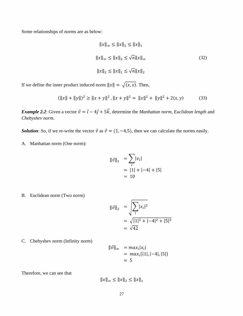
Example 2.2: Given a vector �⃗� = 𝑖 − 4𝑗 + 5�⃗⃗�, determine the Manhattan norm, Euclidean length and
Chebyshev norm.
Solution: So, if we re-write the vector �⃗� as �⃗� = (1,−4,5), then we can calculate the norms easily.
A. Manhattan norm (One norm):
‖�⃗�‖1 = ∑|𝑣𝑖|
𝑖
= |1| + |−4| + |5|
= 10
B. Euclidean norm (Two norm)
‖�⃗�‖2 = √∑|𝑥𝑖|2
𝑖
= √|1|2 + |−4|2 + |5|2
= √42
C. Chebyshev norm (Infinity norm)
‖�⃗�‖∞ = 𝑚𝑎𝑥𝑖|𝑥𝑖|
= 𝑚𝑎𝑥𝑖{|1|, |−4|, |5|}
= 5
Therefore, we can see that
‖𝑥‖∞ ≤ ‖𝑥‖2 ≤ ‖𝑥‖1
28
5 ≤ √42 ≤ 10
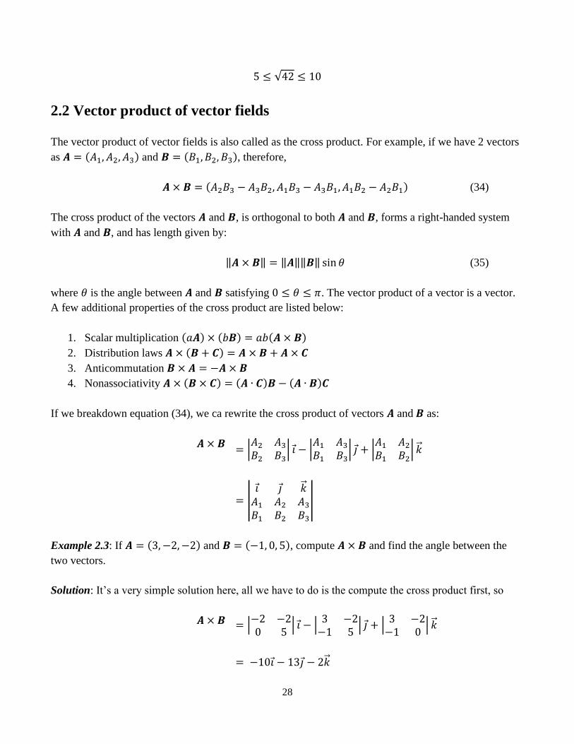
2.2 Vector product of vector fields
The vector product of vector fields is also called as the cross product. For example, if we have 2 vectors
as 𝑨 = (𝐴1, 𝐴2, 𝐴3) and 𝑩 = (𝐵1, 𝐵2, 𝐵3), therefore,
𝑨 × 𝑩 = (𝐴2𝐵3 − 𝐴3𝐵2, 𝐴1𝐵3 − 𝐴3𝐵1, 𝐴1𝐵2 − 𝐴2𝐵1) (34)
The cross product of the vectors 𝑨 and 𝑩, is orthogonal to both 𝑨 and 𝑩, forms a right-handed system
with 𝑨 and 𝑩, and has length given by:
‖𝑨 × 𝑩‖ = ‖𝑨‖‖𝑩‖ sin 𝜃 (35)
where 𝜃 is the angle between 𝑨 and 𝑩 satisfying 0 ≤ 𝜃 ≤ 𝜋. The vector product of a vector is a vector.
A few additional properties of the cross product are listed below:
1. Scalar multiplication (𝑎𝑨) × (𝑏𝑩) = 𝑎𝑏(𝑨 × 𝑩)
2. Distribution laws 𝑨 × (𝑩 + 𝑪) = 𝑨 × 𝑩 + 𝑨 × 𝑪
3. Anticommutation 𝑩 × 𝑨 = −𝑨 × 𝑩
4. Nonassociativity 𝑨 × (𝑩 × 𝑪) = (𝑨 ∙ 𝑪)𝑩 − (𝑨 ∙ 𝑩)𝑪
If we breakdown equation (34), we ca rewrite the cross product of vectors 𝑨 and 𝑩 as:
𝑨 × 𝑩 = |
𝐴2 𝐴3
𝐵2 𝐵3| 𝑖 − |
𝐴1 𝐴3
𝐵1 𝐵3| 𝑗 + |
𝐴1 𝐴2
𝐵1 𝐵2| �⃗⃗�
= |𝑖 𝑗 �⃗⃗�
𝐴1 𝐴2 𝐴3
𝐵1 𝐵2 𝐵3
|
Example 2.3: If 𝑨 = (3, −2,−2) and 𝑩 = (−1, 0, 5), compute 𝑨 × 𝑩 and find the angle between the
two vectors.
Solution: It’s a very simple solution here, all we have to do is the compute the cross product first, so
𝑨 × 𝑩 = |−2 −20 5
| 𝑖 − |3 −2
−1 5| 𝑗 + |
3 −2−1 0
| �⃗⃗�
= −10𝑖 − 13𝑗 − 2�⃗⃗�

29
Angle between the two vectors are given as: ‖𝑨 × 𝑩‖ = ‖𝑨‖‖𝑩‖ sin 𝜃. Rearranging equation (51), we
get:
sin 𝜃 =‖𝑨 × 𝑩‖
‖𝑨‖‖𝑩‖
=
√(−10)2 + (−13)2 + (−2)2
√(3)2 + (−2)2 + (−2)2√(−1)2 + (0)2 + (5)2
=
√273
√17√26
𝜃 = 51.80°
2.3 Vector operators
Certain differential operations may be done on a scalar and vector fields. This may have a wide range of
applications in physical sciences. The most important tasks are those of finding the gradient of a scalar
field and the divergence and curl of a vector field. In the following topics, we will discuss the mathematical
and geometrical definitions of these, which will rely on concepts of integrating vector quantities along
lines and over surfaces. In the midst of these differential operations is the vector operator ∇, which is
called as del (or nabla) and in Cartesian coordinates, ∇ is defined as:
𝛁 ≡ 𝜕
𝜕𝑥𝒊 +
𝜕
𝜕𝑦𝒋 +
𝜕
𝜕𝑧𝒌 (36)
2.3.1 Gradient of a scalar field
The gradient of a scalar field 𝜑(𝑥, 𝑦, 𝑧) is defined as
grad φ = 𝛁φ = 𝜕𝜑
𝜕𝑥𝒊 +
𝜕𝜑
𝜕𝑦𝒋 +
𝜕𝜑
𝜕𝑧𝒌
𝜕𝜑
𝜕𝑥 (37)
Clearly, ∇φ is a vector field whose 𝑥, 𝑦 and 𝑧 components are the first partial derivatives of 𝜑(𝑥, 𝑦, 𝑧) with
respect to 𝑥, 𝑦 and 𝑧.

30
Example 2.4: Find the gradient of the scalar field 𝜑 = 𝑥𝑦2𝑧3.
Solution: We can easily solve this problem by using equation (37), so the gradient of the scalar field 𝜑 =
𝑥𝑦2𝑧3 is
grad φ = 𝜕𝜑
𝜕𝑥𝒊 +
𝜕𝜑
𝜕𝑦𝒋 +
𝜕𝜑
𝜕𝑧𝒌
= 𝑦2𝑧3𝒊 + 2𝑥𝑦𝑧3𝒋 + 3𝑥𝑦2𝑧2𝒌
If we consider a surface in 3D space with 𝜑(𝒓) = 𝑐𝑜𝑛𝑠𝑡𝑎𝑛𝑡 then the direction normal (i.e. perpendicular)
to the surface at the point 𝒓 is the direction of grad 𝜑. The magnitude of the greater rate of change of 𝜑(𝒓)
is the magnitude of grad 𝜑.
Figure 2.2. Direction of gradient
In physical situations, we may have a potential, 𝜑, which varies over a particular region and this constitutes
a field 𝐸, satisfying:
𝐸 = −∇φ = −( 𝜕𝜑
𝜕𝑥𝒊 +
𝜕𝜑
𝜕𝑦𝒋 +
𝜕𝜑
𝜕𝑧𝒌)
Example 2.5: Calculate the electric field at point (𝑥, 𝑦, 𝑧) due to a charge 𝑞1 at (2, 0, 0) and a charge 𝑞2
at (-2, 0, 0) where charges are in coulombs and distances are in metres.
Solution: We need to understand the equation for Electric field which is given by:
𝐸 = 𝑘𝑐
𝑞
𝑟
∇φ
𝜑 = constant
31
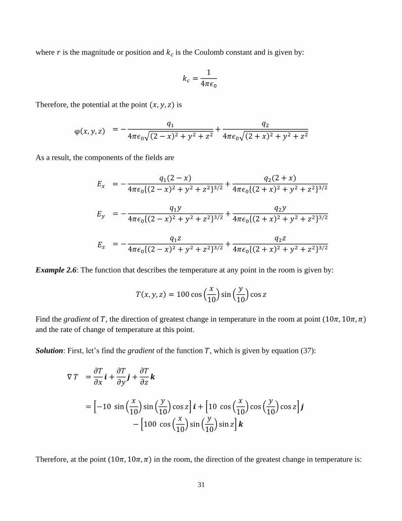
where 𝑟 is the magnitude or position and 𝑘𝑐 is the Coulomb constant and is given by:
𝑘𝑐 =1
4𝜋𝜖0
Therefore, the potential at the point (𝑥, 𝑦, 𝑧) is
φ(𝑥, 𝑦, 𝑧) = −𝑞1
4𝜋𝜖0√(2 − 𝑥)2 + 𝑦2 + 𝑧2+
𝑞2
4𝜋𝜖0√(2 + 𝑥)2 + 𝑦2 + 𝑧2
As a result, the components of the fields are
𝐸𝑥 = −𝑞1(2 − 𝑥)
4𝜋𝜖0{(2 − 𝑥)2 + 𝑦2 + 𝑧2}3/2+
𝑞2(2 + 𝑥)
4𝜋𝜖0{(2 + 𝑥)2 + 𝑦2 + 𝑧2}3/2
𝐸𝑦 = −𝑞1𝑦
4𝜋𝜖0{(2 − 𝑥)2 + 𝑦2 + 𝑧2}3/2+
𝑞2𝑦
4𝜋𝜖0{(2 + 𝑥)2 + 𝑦2 + 𝑧2}3/2
𝐸𝑧 = −𝑞1𝑧
4𝜋𝜖0{(2 − 𝑥)2 + 𝑦2 + 𝑧2}3/2+
𝑞2𝑧
4𝜋𝜖0{(2 + 𝑥)2 + 𝑦2 + 𝑧2}3/2
Example 2.6: The function that describes the temperature at any point in the room is given by:
𝑇(𝑥, 𝑦, 𝑧) = 100 cos (𝑥
10) sin (
𝑦
10) cos 𝑧
Find the gradient of 𝑇, the direction of greatest change in temperature in the room at point (10𝜋, 10𝜋, 𝜋)
and the rate of change of temperature at this point.
Solution: First, let’s find the gradient of the function 𝑇, which is given by equation (37):
∇ 𝑇 =𝜕𝑇
𝜕𝑥𝒊 +
𝜕𝑇
𝜕𝑦𝒋 +
𝜕𝑇
𝜕𝑧𝒌
= [−10 sin (𝑥
10) sin (
𝑦
10) cos 𝑧] 𝒊 + [10 cos (
𝑥
10) cos (
𝑦
10) cos 𝑧] 𝒋
− [100 cos (𝑥
10) sin (
𝑦
10) sin 𝑧] 𝒌
Therefore, at the point (10𝜋, 10𝜋, 𝜋) in the room, the direction of the greatest change in temperature is:

32
∇ 𝑇 = 0𝒊 − 10𝒋 + 0𝒌
And the rate of change of temperature at this point is the magnitude of the gradient, which is
|∇ 𝑇| = √(−10)2 = 10
2.3.2 Divergence of a vector field
The divergence of a vector field 𝑨(𝑥, 𝑦, 𝑧) is defined as the dot product of the operator ∇ and 𝑨:
div 𝑨 = ∇ ∙ 𝑨 = 𝜕𝐴1
𝜕𝑥+
𝜕𝐴2
𝜕𝑦+
𝜕𝐴3
𝜕𝑧 (38)
where 𝐴1, 𝐴2 and 𝐴3 are the 𝑥−, 𝑦 − and 𝑧 − components of 𝑨. Clearly, ∇ ∙ 𝑨 is a scalar field. Any vector
field 𝑨 for which ∇ ∙ 𝑨 = 0 is said to be solenoidal.
Example 2.7: Find the divergence of a vector field 𝑨 = 𝑥2𝑦2𝑖 + 𝑦2𝑧2𝑗 + 𝑥2𝑧2�⃗⃗�
Solution: This is a straightforward example, using equation (38) we can solve this easily:
∇ ∙ 𝑨 = 𝜕𝐴1
𝜕𝑥+
𝜕𝐴2
𝜕𝑦+
𝜕𝐴3
𝜕𝑧
= 2(𝑥𝑦2 + 𝑦𝑧2 + 𝑥2𝑧)
Example 2.8: Find the divergence of a vector field 𝑭 = (𝑦𝑧𝑒𝑥𝑦, 𝑥𝑧𝑒𝑥𝑦, 𝑒𝑥𝑦 + 3 cos 3𝑧)
Solution: Again, using equation (38) we can solve this easily:
∇ ∙ 𝑭 = 𝜕𝐹1
𝜕𝑥+
𝜕𝐹2
𝜕𝑦+
𝜕𝐹3
𝜕𝑧
= 𝑦2𝑧𝑒𝑥𝑦 + 𝑥2𝑧𝑒𝑥𝑦 − 9 sin 3𝑧
The value of the scalar div 𝑨 at point 𝑟 gives the rate at which the material is expanding or flowing away
from the point 𝑟 (outward flux per unit volume).

33
2.3.2.1 Theorem involving Divergence
Divergence theorem, also known as Gauss theorem, relates a volume integral and a surface integral within
a vector field. Let 𝑭 be a vector field, 𝑆 be a closed surface and ℛ be the region inside of 𝑆, then:
∬ 𝑭 ∙ 𝑑𝑨𝑆
= ∭ ∇ ∙ 𝑭𝑑𝑉ℛ
(39)
Example 2.9: Evaluate the following
∬ (3𝑥𝑖 + 2𝑦𝑗) ∙ 𝑑𝑨𝑆
where 𝑆 is the sphere 𝑥2 + 𝑦2 + 𝑧2 = 9.
Solution: We could parameterize the surface and evaluate the surface integral, but it is much faster to use
the divergence theorem. Since:
div (3𝑥𝒊 + 2𝑦𝒋) = 𝜕
𝜕𝑥(3𝑥) +
𝜕
𝜕𝑦(2𝑦) +
𝜕
𝜕𝑧(0) = 5
The divergence theorem gives:
∬ (3𝑥𝒊 + 2𝑦𝒋) ∙ 𝑑𝑨𝑆
= ∭ 5 𝑑𝑉ℛ
= 5 × (Volume of sphere)
= 180π
Example 2.10: Evaluate the following
∬ (𝑦2𝑧𝒊 + 𝑦3𝒋 + 𝑥𝑧𝒌) ∙ 𝑑𝑨𝑆
where 𝑆 is the boundary of the cube defined by −1 ≤ 𝑥 ≤ 1, −1 ≤ 𝑦 ≤ 1, 𝑎𝑛𝑑 0 ≤ 𝑧 ≤ 2.
34
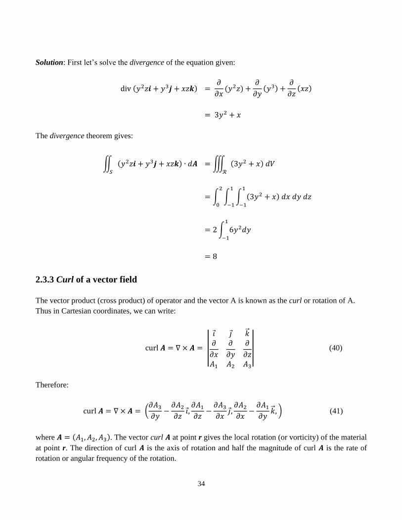
Solution: First let’s solve the divergence of the equation given:
div (𝑦2𝑧𝒊 + 𝑦3𝒋 + 𝑥𝑧𝒌) = 𝜕
𝜕𝑥(𝑦2𝑧) +
𝜕
𝜕𝑦(𝑦3) +
𝜕
𝜕𝑧(𝑥𝑧)
= 3𝑦2 + 𝑥
The divergence theorem gives:
∬ (𝑦2𝑧𝒊 + 𝑦3𝒋 + 𝑥𝑧𝒌) ∙ 𝑑𝑨𝑆
= ∭ (3𝑦2 + 𝑥) 𝑑𝑉ℛ
= ∫ ∫ ∫ (3𝑦2 + 𝑥) 𝑑𝑥 𝑑𝑦 𝑑𝑧1
−1
1
−1
2
0
= 2 ∫ 6𝑦2𝑑𝑦
1
−1
= 8
2.3.3 Curl of a vector field
The vector product (cross product) of operator and the vector A is known as the curl or rotation of A.
Thus in Cartesian coordinates, we can write:
curl 𝑨 = ∇ × 𝑨 = ||
𝑖 𝑗 �⃗⃗�𝜕
𝜕𝑥
𝜕
𝜕𝑦
𝜕
𝜕𝑧𝐴1 𝐴2 𝐴3
|| (40)
Therefore:
curl 𝑨 = ∇ × 𝑨 = (𝜕𝐴3
𝜕𝑦−
𝜕𝐴2
𝜕𝑧𝑖,𝜕𝐴1
𝜕𝑧−
𝜕𝐴3
𝜕𝑥𝑗,
𝜕𝐴2
𝜕𝑥−
𝜕𝐴1
𝜕𝑦�⃗⃗�, ) (41)
where 𝑨 = (𝐴1, 𝐴2, 𝐴3). The vector curl 𝑨 at point r gives the local rotation (or vorticity) of the material
at point r. The direction of curl 𝑨 is the axis of rotation and half the magnitude of curl 𝑨 is the rate of
rotation or angular frequency of the rotation.
35
Example 2.11: Find the curl of a vector field 𝒂 = 𝑥2𝑦2𝑧2𝑖 + 𝑦2𝑧2𝑗 + 𝑥2𝑧2�⃗⃗�
Solution: This is a straightforward question. All we have to do is to put the equation in the form of equation
(41), we get:
∇ × 𝒂 = ||
𝒊 𝒋 𝒌𝜕
𝜕𝑥
𝜕
𝜕𝑦
𝜕
𝜕𝑧
𝑥2𝑦2𝑧2 𝑦2𝑧2 𝑥2𝑧2
||
= [𝜕
𝜕𝑦(𝑥2𝑧2) −
𝜕
𝜕𝑧(𝑦2𝑧2)] 𝒊 − [
𝜕
𝜕𝑥(𝑥2𝑧2) −
𝜕
𝜕𝑧(𝑥2𝑦2𝑧2)] 𝒋 + [
𝜕
𝜕𝑥(𝑦2𝑧2) −
𝜕
𝜕𝑦(𝑥2𝑦2𝑧2)] 𝒌
= −2[𝑦2𝑧𝒊 + (𝑥𝑧2 − 𝑥2𝑦2𝑧)𝒋 + 𝑥2𝑦𝑧2𝒌]
2.3.3.1 Theorem involving Curl
The theorem involving curl of vectors is better known as Stoke’s theorem. If we consider a surface 𝑆 in
ℝ3 that has a closed non-intersecting boundary, 𝐶, the topology of, say, one half of a tennis ball. That is,
“if we move along C and fall to our left, we hit the side of the surface where the normal vectors are sticking
out”. Stoke’s theorem states that for a vector field 𝑭 within which the surface is situated is given by:
∮ 𝑭 ∙ 𝑑𝒓𝐶
= ∯ (∇ × 𝑭) ∙ 𝒏 𝑑𝑆𝑆
(42)
The theorem can be useful in either direction: sometimes the line integral is easier than the surface integral,
and sometimes vice-versa.
Example 2.12: Evaluate the line integral of the function 𝑭(𝑥, 𝑦, 𝑧) = ⟨𝑥2𝑦3, 𝑒𝑥𝑦+𝑧 , 𝑥 + 𝑧2⟩ around a
circle 𝑥2 + 𝑦2 = 1 in the plane 𝑦 = 0, oriented counterclock-wise as viewed from the positive
𝑦 −direction.
Solution: Whenever we want to integrate a vector field around a closed curve, and it looks like the
computation might be messy, think of applying Stoke’s Theorem. The circle 𝐶 in question is the positively-
oriented boundary of the disc 𝑆 given by 𝑥2 + 𝑦2 ≤ 1, 𝑦 = 0, with the unit normal vector �⃗⃗� pointing in
the positive 𝑦 −direction. That is 𝒏 = 𝒋 = ⟨0, 1, 0⟩.

36
Stoke’s Theorem tells us that:
∮ 𝑭 ∙ 𝑑𝒓𝐶
= ∯ (∇ × 𝑭) ∙ 𝒏 𝑑𝑆𝑆
Evaluating the curl of 𝑭, we get:
∇ × 𝑭 = ||
𝒊 𝒋 𝒌𝜕
𝜕𝑥
𝜕
𝜕𝑦
𝜕
𝜕𝑧
𝑥2𝑦3 𝑒𝑥𝑦+𝑧 𝑥 + 𝑧2
||
= (−𝑒𝑥𝑦+𝑧𝒊 − 𝒋 + (𝑦𝑒𝑥𝑦+𝑧 − 3𝑥2𝑦2)𝒌)
(∇ × 𝑭) ∙ 𝒏 = (−𝑒𝑥𝑦+𝑧𝒊 − 𝒋 + (𝑦𝑒𝑥𝑦+𝑧 − 3𝑥2𝑦2)𝒌) ∙ (0, 1, 0)
= −1
∮ 𝑭 ∙ 𝑑𝒓𝐶
= ∯ (∇ × 𝑭) ∙ 𝒏𝑑𝑆𝑆
= ∯ −1 𝑑𝑆𝑆
= −𝑎𝑟𝑒𝑎(𝑆)
= −𝜋
2.4 Repeated Vector Operations – The Laplacian
So far, note the following:
i. grad must operate on a scalar field and gives a vector field in return
ii. div operates on a vector field and gives a scalar field in return, and,
iii. curl operates on a vector field and gives a vector field in return
In addition to the vector relations involving del (∇) mentioned above, there are six other combinations in
which del appears twice. The most important one which involves a scalar is:
37
𝒅𝒊𝒗 𝒈𝒓𝒂𝒅 𝜑 = ∇ ∙ ∇φ = ∇2𝜑 (43)
where 𝜑(𝑥, 𝑦, 𝑧) that is a scalar point function. The operator ∇2= ∇ ∙ ∇, is also known as the Laplacian,
takes a particularly simple form in Cartesian coordinates, which are:
∇2= 𝜕2
𝜕𝑥2+
𝜕2
𝜕𝑦2+
𝜕2
𝜕𝑧2 (44)
When applied to a vector, it yields a vector, which is given in Cartesian coordinates:
∇2𝑨 = 𝜕2𝑨
𝜕𝑥2+
𝜕2𝑨
𝜕𝑦2+
𝜕2𝑨
𝜕𝑧2 (45)
The cross product of two dels operating on a scalar function yields
∇ × ∇φ = 𝒄𝒖𝒓𝒍 𝒈𝒓𝒂𝒅 φ =|
|
𝒊 𝒋 𝒌𝜕
𝜕𝑥
𝜕
𝜕𝑦
𝜕
𝜕𝑧𝜕𝜑
𝜕𝑥
𝜕𝜑
𝜕𝑦
𝜕𝜑
𝜕𝑧
|
|= 0 (46)
If ∇ × 𝑨 = 0 for any vector 𝑨, then 𝑨 = ∇𝜑. In this case, 𝑨 is irrotational.
Similarly,
∇ ∙ ∇ × 𝑨 = 𝒅𝒊𝒗 𝒄𝒖𝒓𝒍 𝑨 = 0 (47)
Finally, a useful expansion is given by:
∇ × (∇ × 𝑨) = 𝒄𝒖𝒓𝒍 𝒄𝒖𝒓𝒍 𝑨 = ∇(∇ ∙ 𝑨) − ∇2𝑨 (48)
Other forms for other coordinate systems for ∇2 are as follows:
1. Spherical polar coordinates:
∇2= 1
𝑟2
𝜕
𝜕𝑟𝑟2
𝜕
𝜕𝑟+
1
𝑟2 sin 𝜃
𝜕
𝜕𝜃(sin 𝜃
𝜕
𝜕𝜃) +
1
𝑟2 sin2 𝜃
𝜕2
𝜕𝜙2 (49)
38
2. Two-dimensional polar coordinates:
∇2= 𝜕2
𝜕𝑟2+
1
𝑟
𝜕
𝜕𝑟+
1
𝑟2
𝜕2
𝜕𝜃2 (50)
3. Cylindrical coordinates:
∇2= 𝜕2
𝜕𝑟2+
1
𝑟
𝜕
𝜕𝑟+
1
𝑟2
𝜕2
𝜕𝜃2+
𝜕2
𝜕𝑧2 (51)
Several other useful relations are summarised below:
DEL OPERATOR RELATIONS
Let 𝜑 and 𝜓 be scalar fields and 𝑨 and 𝑩 be vector fields
Sum of fields ∇(𝜑 + 𝜓) = ∇𝜑 + ∇𝜓
∇ ∙ (𝑨 + 𝑩) = ∇ ∙ 𝑨 + ∇ ∙ 𝑩
∇ × (𝑨 + 𝑩) = ∇ × 𝑨 + ∇ × 𝑩
Product of fields ∇(𝜑𝜓) = 𝜑(∇𝜓) + 𝜓(∇𝜑)
∇ ∙ (𝜑𝑨) = 𝜑(∇ ∙ 𝑨) + (∇𝜑) ∙ 𝑨
∇ × (𝜑𝑨) = 𝜑(∇ × 𝑨) + (∇𝜑) × 𝑨
∇ ∙ (𝑨 × 𝑩) = 𝑩 ∙ (∇ × 𝑨) − 𝑨 ∙ (∇ × 𝑩)
∇ × (𝑨 × 𝑩) = 𝑨 ∙ (∇ ∙ 𝑩) + (𝑩 ∙ ∇)𝑨 − 𝑩(∇ ∙ 𝑨) − (𝑨 ∙ ∇)𝑩
∇(𝑨 ∙ 𝑩) = 𝑨 × (∇ × 𝑩) − 𝑩(∇ ∙ 𝑨) + (𝑩 ∙ ∇)𝑨 − (𝑨 ∙ ∇)𝑩
Laplacian ∇ ∙ (∇𝜑) = ∇2𝜑
∇ × (∇ × 𝑨) = ∇(∇ ∙ 𝑨) − ∇2𝑨

39
Example 2.13: If 𝑨 = 2𝑦𝑧𝒊 − 𝑥2𝑦𝒋 + 𝑥𝑧2𝒌,𝑩 = 𝑥2𝒊 + 𝑦𝑧𝒋 − 𝑥𝑦𝒌 and 𝜙 = 2𝑥2𝑦𝑧3, find
(a) (𝑨 ∙ ∇)𝜙
(b) 𝑨 ∙ ∇𝜙
(c) 𝑩 × ∇𝜙
(d) ∇2𝜙
Solution:
(a)
(𝑨 ∙ ∇)𝜙 = [(2𝑦𝑧𝒊 − 𝑥2𝑦𝒋 + 𝑥𝑧2𝒌) ∙ (𝜕
𝜕𝑥𝒊 +
𝜕
𝜕𝑦𝒋 +
𝜕
𝜕𝑧𝒌)] 𝜙
= [2𝑦𝑧𝜕
𝜕𝑥− 𝑥2𝑦
𝜕
𝜕𝑦+ 𝑥𝑧2
𝜕
𝜕𝑧] 2𝑥2𝑦𝑧3
= 2𝑦𝑧𝜕
𝜕𝑥(2𝑥2𝑦𝑧3) − 𝑥2𝑦
𝜕
𝜕𝑦(2𝑥2𝑦𝑧3) + 𝑥𝑧2
𝜕
𝜕𝑧(2𝑥2𝑦𝑧3)
= 2𝑦𝑧(4𝑥𝑦𝑧3) − 𝑥2𝑦(2𝑥2𝑧3) + 𝑥𝑧2(6𝑥2𝑦𝑧2)
= 8𝑥𝑦2𝑧4 − 2𝑥4𝑦𝑧3 + 6𝑥3𝑦𝑧4
(b)
∇𝜙 =𝜕
𝜕𝑥(2𝑥2𝑦𝑧3)𝒊 +
𝜕
𝜕𝑦(2𝑥2𝑦𝑧3)𝒋 +
𝜕
𝜕𝑧(2𝑥2𝑦𝑧3)𝒌
= 4𝑥𝑦𝑧3𝒊 + 2𝑥2𝑧3𝒋 + 6𝑥2𝑦𝑧2𝒌
Therefore
𝑨 ∙ ∇𝜙 = (2𝑦𝑧𝒊 − 𝑥2𝑦𝒋 + 𝑥𝑧2𝒌) ∙ (4𝑥𝑦𝑧3𝒊 + 2𝑥2𝑧3𝒋 + 6𝑥2𝑦𝑧2𝒌)
= 8𝑥𝑦2𝑧4 − 2𝑥4𝑦𝑧3 + 6𝑥3𝑦𝑧4
(c)
∇𝜙 = 4𝑥𝑦𝑧3𝒊 + 2𝑥2𝑧3𝒋 + 6𝑥2𝑦𝑧2𝒌 , therefore:
𝑩 × ∇𝜙 = |
𝒊 𝒋 𝒌
𝑥2 𝑦𝑧 −𝑥𝑦
4𝑥𝑦𝑧3 2𝑥2𝑧3 6𝑥2𝑦𝑧2
|

40
= (6𝑥2𝑦2𝑧3 + 2𝑥3𝑦𝑧3)𝒊 + (−4𝑥2𝑦2𝑧3 − 6𝑥4𝑦𝑧2)𝒋 + (2𝑥4𝑧3 − 4𝑥𝑦2𝑧4)𝒌
(d)
∇2𝜙 =𝜕2
𝜕𝑥2(2𝑥2𝑦𝑧3) +
𝜕2
𝜕𝑦2(2𝑥2𝑦𝑧3) +
𝜕2
𝜕𝑧2(2𝑥2𝑦𝑧3)
= 4𝑦𝑧3 + 0 + 12𝑥2𝑦𝑧

41
3. Linear Algebra, Matrices & Eigenvectors
In many practical systems, there naturally arises a set of quantities that can conveniently be represented
as a certain dimensional array, referred to as matrix. If matrices were simply a way of representing array
of numbers, then they would have only a marginal utility as a means of visualising data. However, a whole
branch of mathematics has evolved, involving manipulation of matrices, which has become a powerful
tool for the solution f many problems.
For example, consider the set of 𝑛 linear equations with 𝑛 unknowns
𝑎11𝑌1 + 𝑎12𝑌2 + ⋯+ 𝑎1𝑛𝑌𝑛 = 0
(52) 𝑎21𝑌1 + 𝑎22𝑌2 + ⋯+ 𝑎2𝑛𝑌𝑛 = 0
∙∙∙∙∙∙∙∙∙∙∙∙∙∙∙∙∙∙∙∙∙∙∙∙∙∙∙∙∙∙∙∙
𝑎𝑛1𝑌1 + 𝑎𝑛2𝑌2 + ⋯+ 𝑎𝑛𝑛𝑌𝑛 = 0
The necessary and sufficient condition for the set to have a non-trivial solution (other than 𝑌1 = 𝑌2 = ⋯ =
𝑌𝑛 = 0) is that the determinant of the array of coefficients is zero: 𝑑𝑒𝑡(𝐴) = 0.
3.1 Basic definitions and notation
A matrix is an array of numbers with 𝑚 rows and 𝑛 columns. The (i, j)th element is the element found in
row 𝑖 and column 𝑗.
For example, have a look at the matrix below. Tis matrix has 𝑚 = 2 rows, 𝑛 = 3 column, and therefore
the matrix order is 2 × 3. The (i, j)th element is 𝑎𝑖𝑗
𝐴 = [𝑎11 𝑎12 𝑎13
𝑎21 𝑎22 𝑎23] (53)
Matrices may be categorized based on the properties of its elements. Some basic definitions include:
1. The transpose of matrix 𝐴 (or 𝐴𝑇) is formed by interchanging element 𝑎𝑖𝑗 with element 𝑎𝑗𝑖.
Therefore:
𝐴𝑇 = (𝑎𝑗𝑖) , (𝐴 + 𝐵)𝑇 = 𝐴𝑇 + 𝐵𝑇 , (𝐴𝐵)𝑇 = 𝐴𝑇𝐵𝑇 (54)
A symmetric matrix is equals to its transpose, 𝐴 = 𝐴𝑇.
42
2. Diagonal matrix is a square matrix (𝑚 = 𝑛) that has it’s only non-zero elements along the
leading diagonal. For example:
𝑑𝑖𝑎𝑔 𝐴 = [𝑎11 0 00 𝑎22 00 0 𝑎33
]
Diagonal can also be written for a list of matrices as:
𝑑𝑖𝑎𝑔 (𝑎11, 𝑎22, ⋯ 𝑎𝑛𝑛)
Which denotes the block diagonal matrix with elements 𝑎11, 𝑎22, ⋯ 𝑎𝑛𝑛 along te diagonal and
zeros elsewhere. A matrix is formed in this way is sometimes called a direct sum of
𝑎11, 𝑎22, ⋯ 𝑎𝑛𝑛 and the operation is denoted by ⨁:
𝑎11⨁⋯⨁ 𝑎𝑛𝑛 = 𝑑𝑖𝑎𝑔 (𝑎11, 𝑎22, ⋯ 𝑎𝑛𝑛)
3. In a square matrix of order n, the diagonal containing elements 𝑎11, 𝑎22, ⋯ 𝑎𝑛𝑛 is called the
principle or leading diagonal. The sum of elements in this diagonal is called the trace of 𝑛 × 𝑛
square matrix A, hence:
𝑇𝑟𝑎𝑐𝑒 (𝐴) = 𝑇𝑟 (𝐴) = ∑ 𝑎𝑖𝑖𝑖
(55)
We can also define a few more notations for Trace as:
𝑇𝑟(𝐴) = 𝑇𝑟(𝐴𝑇), 𝑇𝑟(𝑐𝐴) = 𝑐𝑇𝑟(𝐴), 𝑇𝑟(𝐴 + 𝐵) = 𝑇𝑟(𝐴) + 𝑇𝑟(𝐵) (56)
4. Determinant of a square 𝑛 × 𝑛 matrix 𝐴 is denoted as det(𝐴) or |𝐴|. It is determined by:
|𝐴| = ∑𝑎𝑖𝑗𝑎(𝑖𝑗)
𝑛
𝑗=1
(57)
where:
𝑎(𝑖𝑗) = (−1)𝑖+𝑗|𝐴(𝑖)(𝑗)| (58)
with |𝐴(𝑖)(𝑗)| denoting the submatrix that is formed from 𝐴 by removing the 𝑖th row and the 𝑗th
column.
Determinant of a matrix can also be defined as the following:

43
|𝐴𝐵| = |𝐴||𝐵|, |𝐴| = |𝐴𝑇|, |𝑐𝐴| = 𝑐𝑛|𝐴| (59)
5. Adjugate of a 𝑛 × 𝑛 matrix 𝐴 is defined as an 𝑛 × 𝑛 matrix of the cofactors of the elements of
the transposed matrix. Therefore, we can write Adjugate of 𝑛 × 𝑛 matrix 𝐴 as:
𝑎𝑑𝑗(𝐴) = (𝑎(𝑗𝑖)) = (𝑎(𝑖𝑗))𝑇 (60)
Adjugate has an interesting property:
𝐴 𝑎𝑑𝑗(𝐴) = 𝑎𝑑𝑗(𝐴)𝐴 = |𝐴|𝐼 (61)
3.2 Multiplication of matrices and multiplication of vectors and matrices
3.2.1 Matrix multiplication
If we let 𝐴 be order 𝑚 × 𝑛 and 𝐵 of order 𝑛 × 𝑝. Then the product of two matrices 𝐴 and 𝐵 is
𝐶 = 𝐴𝐵 (62)
or
𝑐𝑖𝑗 = ∑ 𝑎𝑖𝑘𝑏𝑘𝑗
𝑛
𝑘=1
(63)
where the resulting matrix 𝐶 is in the order of 𝑚 × 𝑝.
Square matrices obey the laws expressed as below:
Associative: 𝐴(𝐵𝐶) = (𝐴𝐵)𝐶 (64)
Distributive: (𝐴 + 𝐵)𝐶 = 𝐴𝐶 + 𝐵𝐶, (𝐵 + 𝐶)𝐴 = 𝐵𝐴 + 𝐶𝐴 (65)
Matrix Polynomials
Polynomials in square matrices are similar to the more familiar polynomials in scalars. Let us consider:
𝑝(𝐴) = 𝑏0𝐼 + 𝑏1𝐴 + ⋯𝑏𝑘𝐴𝑘 (66)
The value of this polynomial is a matrix. The theory of polynomials in general holds, we have the useful
factorizations of monomials:

44
For any positive integer k,
𝐼 − 𝐴𝑘 = ((𝐼 − 𝐴)(𝐼 + 𝐴 + ⋯𝐴𝑘−1) (67)
For an odd positive integer k,
𝐼 + 𝐴𝑘 = ((𝐼 + 𝐴)(𝐼 − 𝐴 + ⋯𝐴𝑘−1) (68)
3.2.2 Traces and determinants of square Cayley products
The useful property of the trace for the matrix 𝐴 and 𝐵 that are conformable for the multiplication 𝐴𝐵 and
𝐵𝐴 is
𝑇𝑟(𝐴𝐵) = 𝑇𝑟 (𝐵𝐴) (69)
This is obvious from the definitions of matrix multiplication and the trace. Due to associativity of matrix
multiplications, equation (18) can be further extended to:
𝑇𝑟(𝐴𝐵𝐶) = 𝑇𝑟 (𝐵𝐶𝐴) = 𝑇𝑟(𝐶𝐴𝐵) (70)
If 𝐴 and 𝐵 are square matrices conformable for multiplication, then an important property of the
determinant is
|𝐴𝐵| = |𝐴||𝐵| (71)
Or we can write the equation as:
|[𝐴 0−𝐼 𝐵
]| = |𝐴||𝐵| (72)
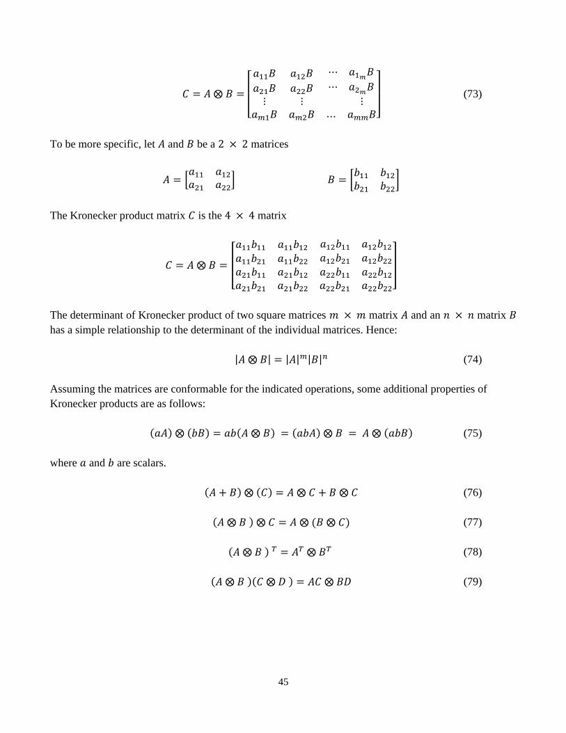
3.2.3 The Kronecker product
The Kronecker multiplication, denoted by ⨂, is not commutative, rather it is associative. Therefore,
𝐴 ⨂ 𝐵 may not equal to 𝐵 ⨂ 𝐴. Let us have a 𝑚 × 𝑚 matrix 𝐴 and an 𝑛 × 𝑛 matrix 𝐵. We can then
form an 𝑚𝑛 × 𝑚𝑛 matrix 𝐶 by defining the direct product as:
45
𝐶 = 𝐴 ⨂ 𝐵 =
[ 𝑎11𝐵 𝑎12𝐵 ⋯ 𝑎1𝑚
𝐵
𝑎21𝐵 𝑎22𝐵 ⋯ 𝑎2𝑚𝐵
⋮𝑎𝑚1𝐵
⋮𝑎𝑚2𝐵 ⋯
⋮𝑎𝑚𝑚𝐵]
(73)
To be more specific, let 𝐴 and 𝐵 be a 2 × 2 matrices
𝐴 = [𝑎11 𝑎12
𝑎21 𝑎22] 𝐵 = [
𝑏11 𝑏12
𝑏21 𝑏22]
The Kronecker product matrix 𝐶 is the 4 × 4 matrix
𝐶 = 𝐴 ⨂ 𝐵 = [
𝑎11𝑏11 𝑎11𝑏12 𝑎12𝑏11 𝑎12𝑏12
𝑎11𝑏21 𝑎11𝑏22 𝑎12𝑏21 𝑎12𝑏22
𝑎21𝑏11
𝑎21𝑏21
𝑎21𝑏12
𝑎21𝑏22
𝑎22𝑏11
𝑎22𝑏21
𝑎22𝑏12
𝑎22𝑏22
]
The determinant of Kronecker product of two square matrices 𝑚 × 𝑚 matrix 𝐴 and an 𝑛 × 𝑛 matrix 𝐵
has a simple relationship to the determinant of the individual matrices. Hence:
|𝐴 ⨂ 𝐵| = |𝐴|𝑚|𝐵|𝑛 (74)
Assuming the matrices are conformable for the indicated operations, some additional properties of
Kronecker products are as follows:
(𝑎𝐴) ⨂ (𝑏𝐵) = 𝑎𝑏(𝐴 ⨂ 𝐵) = (𝑎𝑏𝐴) ⨂ 𝐵 = 𝐴 ⨂ (𝑎𝑏𝐵) (75)
where 𝑎 and 𝑏 are scalars.
(𝐴 + 𝐵) ⨂ (𝐶) = 𝐴 ⨂ 𝐶 + 𝐵 ⨂ 𝐶 (76)
(𝐴 ⨂ 𝐵 ) ⨂ 𝐶 = 𝐴 ⨂ (𝐵 ⨂ 𝐶) (77)
(𝐴 ⨂ 𝐵 ) 𝑇 = 𝐴𝑇 ⨂ 𝐵𝑇 (78)
(𝐴 ⨂ 𝐵 )(𝐶 ⨂ 𝐷 ) = 𝐴𝐶 ⨂ 𝐵𝐷 (79)
46
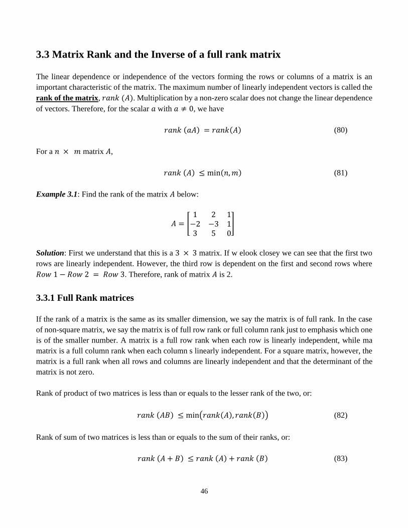
3.3 Matrix Rank and the Inverse of a full rank matrix
The linear dependence or independence of the vectors forming the rows or columns of a matrix is an
important characteristic of the matrix. The maximum number of linearly independent vectors is called the
rank of the matrix, 𝑟𝑎𝑛𝑘 (𝐴). Multiplication by a non-zero scalar does not change the linear dependence
of vectors. Therefore, for the scalar 𝑎 with 𝑎 ≠ 0, we have
𝑟𝑎𝑛𝑘 (𝑎𝐴) = 𝑟𝑎𝑛𝑘(𝐴) (80)
For a 𝑛 × 𝑚 matrix 𝐴,
𝑟𝑎𝑛𝑘 (𝐴) ≤ min(𝑛,𝑚) (81)
Example 3.1: Find the rank of the matrix 𝐴 below:
𝐴 = [1 2 1
−2 −3 13 5 0
]
Solution: First we understand that this is a 3 × 3 matrix. If w elook closey we can see that the first two
rows are linearly independent. However, the third row is dependent on the first and second rows where
𝑅𝑜𝑤 1 − 𝑅𝑜𝑤 2 = 𝑅𝑜𝑤 3. Therefore, rank of matrix 𝐴 is 2.
3.3.1 Full Rank matrices
If the rank of a matrix is the same as its smaller dimension, we say the matrix is of full rank. In the case
of non-square matrix, we say the matrix is of full row rank or full column rank just to emphasis which one
is of the smaller number. A matrix is a full row rank when each row is linearly independent, while ma
matrix is a full column rank when each column s linearly independent. For a square matrix, however, the
matrix is a full rank when all rows and columns are linearly independent and that the determinant of the
matrix is not zero.
Rank of product of two matrices is less than or equals to the lesser rank of the two, or:
𝑟𝑎𝑛𝑘 (𝐴𝐵) ≤ min(𝑟𝑎𝑛𝑘(𝐴), 𝑟𝑎𝑛𝑘(𝐵)) (82)
Rank of sum of two matrices is less than or equals to the sum of their ranks, or:
𝑟𝑎𝑛𝑘 (𝐴 + 𝐵) ≤ 𝑟𝑎𝑛𝑘 (𝐴) + 𝑟𝑎𝑛𝑘 (𝐵) (83)
47
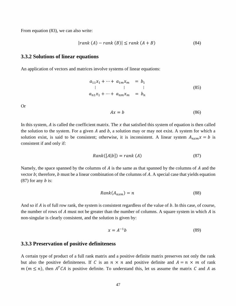
From equation (83), we can also write:
|𝑟𝑎𝑛𝑘 (𝐴) − 𝑟𝑎𝑛𝑘 (𝐵)| ≤ 𝑟𝑎𝑛𝑘 (𝐴 + 𝐵) (84)
3.3.2 Solutions of linear equations
An application of vectors and matrices involve systems of linear equations:
𝑎11𝑥1 + ⋯+ 𝑎1𝑚𝑥𝑚 = 𝑏1
⋮ ⋮ ⋮ (85)
𝑎𝑛1𝑥1 + ⋯+ 𝑎𝑛𝑚𝑥𝑚 = 𝑏𝑛
Or
𝐴𝑥 = 𝑏 (86)
In this system, 𝐴 is called the coefficient matrix. The 𝑥 that satisfied this system of equation is then called
the solution to the system. For a given 𝐴 and 𝑏, a solution may or may not exist. A system for which a
solution exist, is said to be consistent; otherwise, it is inconsistent. A linear system 𝐴𝑛𝑥𝑚𝑥 = 𝑏 is
consistent if and only if:
𝑅𝑎𝑛𝑘([𝐴|𝑏]) = 𝑟𝑎𝑛𝑘 (𝐴) (87)
Namely, the space spanned by the columns of 𝐴 is the same as that spanned by the columns of 𝐴 and the
vector 𝑏; therefore, 𝑏 must be a linear combination of the columns of 𝐴. A special case that yields equation
(87) for any 𝑏 is:
𝑅𝑎𝑛𝑘(𝐴𝑛𝑥𝑚) = 𝑛 (88)
And so if 𝐴 is of full row rank, the system is consistent regardless of the value of 𝑏. In this case, of course,
the number of rows of 𝐴 must not be greater than the number of columns. A square system in which 𝐴 is
non-singular is clearly consistent, and the solution is given by:
𝑥 = 𝐴−1𝑏 (89)
3.3.3 Preservation of positive definiteness
A certain type of product of a full rank matrix and a positive definite matrix preserves not only the rank
but also the positive definiteness. If 𝐶 is an 𝑛 × 𝑛 and positive definite and 𝐴 = 𝑛 × 𝑚 of rank
𝑚 (𝑚 ≤ 𝑛), then 𝐴𝑇𝐶𝐴 is positive definite. To understand this, let us assume the matrix 𝐶 and 𝐴 as

48
described. Let 𝑥 be any 𝑚-vector such that 𝑥 ≠ 0 and ley 𝑦 = 𝐴𝑥. Because 𝐴 is a full column rank,
therefore 𝑦 ≠ 0, we then have:
𝑥𝑇(𝐴𝑇𝐶𝐴)𝑥 = (𝑥𝐴)𝑇𝐶(𝐴𝑥) = 𝑦𝑇𝐶𝑦 > 0 (90)
Therefore, to summarise:
1. If 𝐶 is positive definite and 𝐴 is of full column rank, then 𝐴𝑇𝐶𝐴 is positive definite.
Furthermore, we then have the converse:
2. If 𝐴𝑇𝐶𝐴 is positive definite, then 𝐴 is of full column rank.
For otherwise there exists an 𝑥 ≠ 0 such that 𝐴𝑥 = 0, and so 𝑥𝑇(𝐴𝑇𝐶𝐴)𝑥 = 0.
3.3.4 A lower bound on the rank of a matrix product
Equation (82) gives an upper bound on the rank of the product of two matrices; where the rank cannot be
greater than the rank of either of the factors. Now, we will develop a lower bound of the rank of the product
of two matrices if one of them is square.
If 𝐴 is an 𝑛 × 𝑛 (square) and 𝐵 is a matrix with n rows, then:
𝑟𝑎𝑛𝑘 (𝐴𝐵) ≥ 𝑟𝑎𝑛𝑘 (𝐴) + 𝑟𝑎𝑛𝑘 (𝐵) − 𝑛 (91)
3.3.5 Inverse of products and sums of matrices
The inverse of the Cayley product of two nonsingular matrices of the same size is particularly easy to
form. If 𝐴 and 𝐵 are square full rank matrices of the same size, then:
(𝐴𝐵)−1 = 𝐵−1𝐴−1 (92)
𝐴(𝐼 + 𝐴)−1 = (𝐼 + 𝐴−1)−1 (93)
(𝐴 + 𝐵𝐵 )−1𝐵 = 𝐴−1𝐵(𝐼 + 𝐵𝑇𝐴−1𝐵)−1 (94)
(𝐴−1 + 𝐵−1 )−1 = 𝐴(𝐴 + 𝐵)−1𝐵 (95)

49
𝐴 − 𝐴(𝐴 + 𝐵 )−1𝐴 = 𝐵 − 𝐵(𝐴 + 𝐵 )−1𝐵 (96)
𝐴−1 + 𝐵−1 = 𝐴−1(𝐴 + 𝐵)𝐵−1 (97)
(𝐼 + 𝐴𝐵 )−1 = 𝐼 − 𝐴(𝐼 + 𝐵𝐴)−1𝐵 (98)
(𝐼 + 𝐴𝐵 )−1𝐴 = 𝐴(𝐼 + 𝐵𝐴)−1 (99)
(𝐴 ⨂ 𝐵 )−1 = 𝐴−1 ⨂ 𝐵−1 (100)
Note: When 𝐴 and/or 𝐵 are not full rank, the inverse may not exist.
3.4 Eigensystems
Suppose 𝐴 is an 𝑛 × 𝑛 matrix. The number 𝜆 is said to be an eigenvalue of 𝐴 if some non-zero vector 𝒙,
𝐴𝒙 = 𝜆𝒙. Any non-zero vector 𝒙 for which this equation holds is called an eigenvector for eigenvalue 𝜆
or an eigenvector of 𝐴 corresponding to eigenvalue 𝜆.
How to find eigenvalues and eigenvectors? To determine whether 𝜆 is an eigenvalue of 𝐴, we need to
determine whether there are any non-zero solutions to the matrix equation 𝐴𝒙 = 𝜆𝒙. To do this, we can
define the following:
(a) The eigenvalues of a symmetric matrix 𝐴 are the numbers 𝜆 that satisfy |𝐴 − 𝜆𝐼| = 0
(b) The eigenvectors of a symmetric matrix 𝐴 are the vectors 𝒙 that satisfy (𝐴 − 𝜆𝐼)𝒙 = 0
There are two theorems involved in the eigensystems and they are:
1. The eigenvalues of any real symmetric matrix are real.
2. The eigenvectors of any real symmetric matric corresponding to different eigenvalues are
orthogonal.
Example 3.2: Let 𝐴 be a square matrix as below. Find the eigenvalues and eigenvectors of matrix 𝐴
𝐴 = [1 12 2
]
Solution: To find the eigenvalues, we will need to find the determinant of |𝐴 − 𝜆𝐼| = 0, therefore:

50
|𝐴 − 𝜆𝐼| = |(1 12 2
) − 𝜆 (1 00 1
)|
= |1 − 𝜆 1
2 2 − 𝜆|
= (1 − 𝜆)(2 − 𝜆) − 2
= 𝜆2 − 3𝜆
So, the eigenvalues are the solutions of 𝜆2 − 3𝜆 = 0. We could simplify the equation is 𝜆(𝜆 − 3) = 0
with the solutions of 𝜆 = 0 and 𝜆 = 3. Hence the eigenvalues of 𝐴 are 0 and 3.
Now to find the eigenvectors for eigenvalue 0 we can solve the system (𝐴 − 0𝐼)𝒙 = 0, that is 𝐴𝒙 = 0, or
𝐴𝒙 = 0
[1 12 2
] [𝑥1
𝑥2] = [
00]
We then have to solve for
𝑥1 + 𝑥2 = 0 , 2𝑥1 + 2𝑥2 = 0
Which gives 𝑥1 = −𝑥2 = −1. Therefore, the eigenvectors for eigenvalue 0 is:
𝒙 = [−11
]
Similarly, to find the eigenvector for eigenvalue 3, we will solve (𝐴 − 3𝐼)𝒙 = 0 which is:
(𝐴 − 3𝐼)𝒙 = 0
[−2 12 −1
] [𝑥1
𝑥2] = [
00]
This is equivalent to the equations
−2𝑥1 + 𝑥2 = 0 , 2𝑥1 − 𝑥2 = 0
Which gives 𝑥2 = 2𝑥1. If we choose 𝑥1 = 1, we then obtain the eigenvectors

51
𝒙 = [12]
Example 3.3: Suppose that
𝐴 = [4 0 40 4 44 4 8
]
Find the eigenvalues of 𝐴 and obtain one eigenvector for each eigenvalues.
Solutions: To find the eigenvalues, we will solve |𝐴 − 𝜆𝐼| = 0, so we can write as:
|𝐴 − 𝜆𝐼| = |4 − 𝜆 0 4
0 4 − 𝜆 44 4 8 − 𝜆
|
= (4 − 𝜆) |4 − 𝜆 4
4 8 − 𝜆| + 4 |
0 4 − 𝜆4 4
|
= (4 − 𝜆) ((4 − 𝜆)(8 − 𝜆) − 16) + 4(−4(4 − 𝜆))
= (4 − 𝜆) ((4 − 𝜆)(8 − 𝜆) − 16) − 16(4 − 𝜆)
= (4 − 𝜆) ((4 − 𝜆)(8 − 𝜆) − 16 − 16)
= (4 − 𝜆) (32 − 12𝜆 + 𝜆2 − 32)
= (4 − 𝜆) (𝜆2 − 12𝜆)
= (4 − 𝜆) 𝜆 (𝜆 − 12)
Therefore, we can solve |𝐴 − 𝜆𝐼| = 0 and the eigenvalues are 4, 0, 12.
To find the eigenvectors for eigenvalue of 4, we solve the equation (𝐴 − 4𝐼)𝒙 = 0, that is,
(𝐴 − 4𝐼)𝒙 = 0
[0 0 40 0 44 4 4
] [
𝑥1
𝑥2
𝑥3
] = [000]
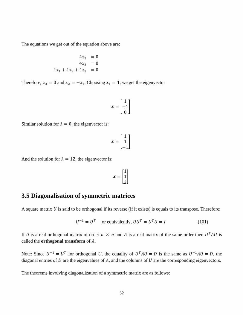
52
The equations we get out of the equation above are:
4𝑥3 = 0
4𝑥3 = 0
4𝑥1 + 4𝑥2 + 4𝑥3 = 0
Therefore, 𝑥3 = 0 and 𝑥2 = −𝑥1. Choosing 𝑥1 = 1, we get the eigenvector
𝒙 = [1
−10
]
Similar solution for 𝜆 = 0, the eigenvector is:
𝒙 = [11
−1]
And the solution for 𝜆 = 12, the eigenvector is:
𝒙 = [112]
3.5 Diagonalisation of symmetric matrices
A square matrix 𝑈 is said to be orthogonal if its reverse (if it exists) is equals to its transpose. Therefore:
𝑈−1 = 𝑈𝑇 or equivalently, 𝑈𝑈𝑇 = 𝑈𝑇𝑈 = 𝐼 (101)
If 𝑈 is a real orthogonal matrix of order 𝑛 × 𝑛 and 𝐴 is a real matrix of the same order then 𝑈𝑇𝐴𝑈 is
called the orthogonal transform of 𝐴.
Note: Since 𝑈−1 = 𝑈𝑇 for orthogonal U, the equality of 𝑈𝑇𝐴𝑈 = 𝐷 is the same as 𝑈−1𝐴𝑈 = 𝐷, the
diagonal entries of 𝐷 are the eigenvalues of 𝐴, and the columns of 𝑈 are the corresponding eigenvectors.
The theorems involving diagonalization of a symmetric matrix are as follows:

53
1. If 𝐴 is a symmetric matrix in the order of 𝑛 × 𝑛 then it is possible to find an orthogonal matrix
𝑈 of the same order such that the orthogonal transform of 𝐴 with respect to 𝑈 is diagonal and the
diagonal elements of the transform are the eigenvalues of 𝐴.
2. Cayley-Hamilton Theorem: A real square matrix satisfies its own characteristic equation (i.e. its
own eigenvalue equation).
𝐴𝑛 + 𝑎𝑛−1𝐴𝑛−1 + 𝑎𝑛−2𝐴
𝑛−2 + ⋯+ 𝑎1𝐴 + 𝑎0𝐼 = 0
Where
𝑎0 = (−1)𝑛|𝐴| , 𝑎𝑛−1 = (−1)𝑛−1𝑡𝑟(𝐴)
3. Trace Theorem: The sum of eigenvalues of matrix 𝐴 is equals to the sum of the diagonal elements
of 𝐴 and is defined as 𝑇𝑟(𝐴).
4. Determinant Theorem: The product of eigenvalues of 𝐴 is equals to the determinant of 𝐴.
Example 3.4: If we worked on the same matrix as in example 3 before, find the orthogonal matrix U, and
shows that 𝑈𝑇𝐴𝑈 = 𝐷:
𝐴 = [4 0 40 4 44 4 8
]
Solution: As we already observed, matrix A is symmetric, and we have calculated the three distinct
eigenvalues 4, 0, 12 (in that order) and the eigenvectors associated with them are:
[1
−10
] , [11
−1] , [
112]
Now these eigenvectors are not f length 1. For example, the first eigenvector has a length of
√12 + (−1)2 + 02 = √2. So, if we divide each row by √2., we will indeed obtain eigenvector of length
1.
[1/√2
−1/√20
]
We can similarly normalize the other two vectors and therefore we obtain:

54
[
1/√3
1/√3
−1/√3
] , [
1/√6
1/√6
2/√6
]
Now we can form the matrix 𝑈 whose columns are these normalized eigenvectors:
𝑈 = [
1/√2 1/√3 1/√6
−1/√2 1/√3 1/√6
0 −1/√3 2/√6
]
Therefore, U is orthogonal and 𝑈𝑇𝐴𝑈 = 𝐷 = diag(4, 0, 12).
55
4. Generalised Vector Calculus – Integral Theorems
The four fundamental theorems of vector calculus are generalisations of the fundamental theorem of
calculus, which equates the integral of the derivative G'(t) to the values of G(t) at the interval boundary
points:
∫ 𝐺′(𝑡) 𝑑𝑡𝑏
𝑎
= 𝐺(𝑏) − 𝐺(𝑎) (102)
Similarly, the fundamental theorems of vector calculus state that an integral of some type of derivative
over some object is equal to the values of function along the boundary of that object. The four fundamental
theorems are the gradient theorem for line integral, Green’s theorem, Stokes’ theorem and the divergence
theorem.
4.1 The gradient theorem for line integral
The Gradient Theorem is also referred to as the Fundamental Theorem of Calculus for Line Integrals. It
represents the generalisation of an integration along an axis, e.g. dx or dy, to the integration of vector fields
along arbitrary curves, C, in their base space. It is expressed by
∫ ∇𝑓 ∙ 𝑑𝒔𝐶
= 𝑓(𝐪) − 𝑓(𝐩) (103)
where p and q are the endpoints of C. This means the line integral of the gradient of some function is just
the difference of the function evaluated at the endpoints of the curve. In particular, this means that the
integral of f does not depend on the curve itself. A few notes to remember when using this theorem:
i. For closed curves, the line integral is zero
∫ ∇𝑓 ∙ 𝑑𝒔𝐶
= 0
ii. Gradient fields are path independent: if F = f, then the line integral between two points P
and Q does not depend on the path connecting the two points.
iii. The theorem holds in any dimensions. In one-dimension, it reduces to the fundamental theorem
of calculus as per equation (103) above.
iv. The theorem justifies the name conservative for gradient vector fields.
56
Example 4.1: Let f (x, y, z) = x2 + y4 + z. Find the line integral of the vector field F (x, y, z) = f (x, y, z)
along the path s(t) = cos(5t), sin(2t), t2 from t = 0 to t = 2.
Solution:
At t = 0, s(0) = 1, 0, 0, therefore, f (s (0)) = 1
At t = 2, s(2) = 1, 0, 42, therefore f (s (2)) = 1+42
Hence:
∫ ∇𝑓 ∙ 𝑑𝒔𝐶
= 𝑓(𝐬 (2)) − 𝑓(𝐬 (0))
∫ ∇𝑓 ∙ 𝑑𝒔𝐶
= 1 + 42 − 𝑓(𝐬 (0)) = 42
4.2 Green’s Theorem
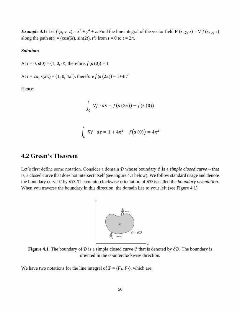
Let’s first define some notation. Consider a domain 𝒟 whose boundary 𝒞 is a simple closed curve – that
is, a closed curve that does not intersect itself (see Figure 4.1 below). We follow standard usage and denote
the boundary curve 𝒞 by 𝜕𝒟. The counterclockwise orientation of 𝜕𝒟 is called the boundary orientation.
When you traverse the boundary in this direction, the domain lies to your left (see Figure 4.1).
Figure 4.1. The boundary of 𝒟 is a simple closed curve 𝒞 that is denoted by 𝜕𝒟. The boundary is
oriented in the counterclockwise direction.
We have two notations for the line integral of F = F1, F2, which are:

57
∫ 𝐅 ∙ 𝑑𝒔𝐶
and ∫ 𝐹1 𝑑𝑥 + 𝐹2 𝑑𝑦𝐶
(104)
If 𝒞 is parametrized by c (t) = (x (t), y (t)) for a t b, then
𝑑𝑥 = 𝑥′(𝑡)𝑑𝑡, 𝑑𝑦 = 𝑦′(𝑡)𝑑𝑡
∫ 𝐹1 𝑑𝑥 + 𝐹2 𝑑𝑦 = ∫ [𝐹1 (𝑥(𝑡), 𝑦(𝑡))𝑥′(𝑡) + 𝐹2 (𝑥(𝑡), 𝑦(𝑡))𝑦′(𝑡)]𝑑𝑡𝑏
𝑎𝐶
(105)
In this section, we will assume that the components of all vector fields have continuous partial derivatives,
and also that 𝒞 is smooth (𝒞 has a parametrization with derivatives of all orders) or piecewise smooth (a
finite union of smooth curves joined together at corners).
Green’s Theorem: Let 𝒟 be a domain whose boundary 𝜕𝒟 is a simple closed curve, oriented
counterclockwise. Then:
∫ 𝐹1 𝑑𝑥 + 𝐹2 𝑑𝑦𝜕𝒟
= ∬ (𝜕𝐹2
𝜕𝑥−
𝜕𝐹1
𝜕𝑦) 𝑑𝐴
𝒟
(106)
Proof:
A complete proof is quite technical, so we shall make the simplifying assumption that the boundary of 𝒟
can be described as the union of two graphs y = g (x) and y = f (x), with g (x) f (x), as in figure 4.2 and
also as the union of two graphs x = g1 (y) and x = f1 (y), with g1 (y) f1 (y), as in Figure 4.3.
Green’s Theorem splits up into two equations, one for F1 and one for F2:
∫ 𝐹1 𝑑𝑥𝜕𝒟
= −∬𝜕𝐹1
𝜕𝑦 𝑑𝐴
𝒟
(107)
∫ 𝐹2 𝑑𝑦𝜕𝒟
= ∬𝜕𝐹2
𝜕𝑥 𝑑𝐴
𝒟
(108)
In other words, Green’s Theorem is obtained by adding equations (107) and (108). To prove equation
(107), we write:
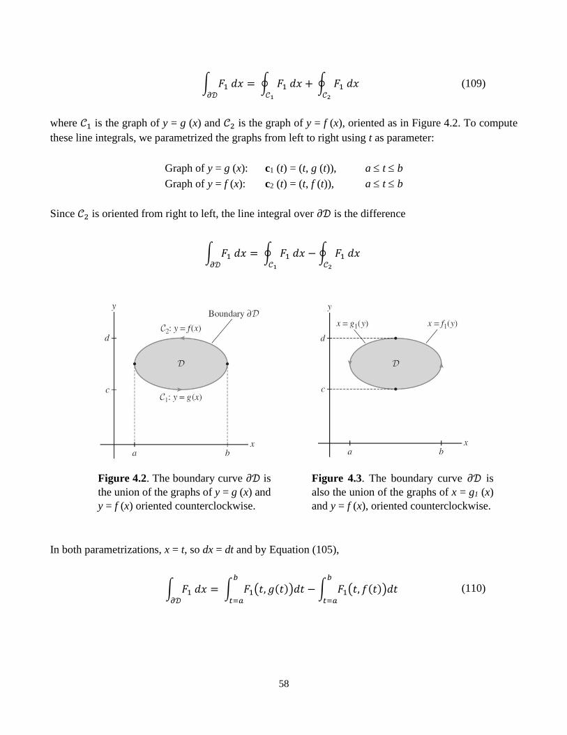
58
∫ 𝐹1 𝑑𝑥𝜕𝒟
= ∮ 𝐹1 𝑑𝑥 + 𝒞1
∮ 𝐹1 𝑑𝑥 𝒞2
(109)
where 𝒞1 is the graph of y = g (x) and 𝒞2 is the graph of y = f (x), oriented as in Figure 4.2. To compute
these line integrals, we parametrized the graphs from left to right using t as parameter:
Graph of y = g (x): c1 (t) = (t, g (t)), a t b
Graph of y = f (x): c2 (t) = (t, f (t)), a t b
Since 𝒞2 is oriented from right to left, the line integral over 𝜕𝒟 is the difference
∫ 𝐹1 𝑑𝑥𝜕𝒟
= ∮ 𝐹1 𝑑𝑥𝒞1
− ∮ 𝐹1 𝑑𝑥 𝒞2
In both parametrizations, x = t, so dx = dt and by Equation (105),
∫ 𝐹1 𝑑𝑥𝜕𝒟
= ∫ 𝐹1(𝑡, 𝑔(𝑡))𝑑𝑡𝑏
𝑡=𝑎
− ∫ 𝐹1(𝑡, 𝑓(𝑡))𝑑𝑡𝑏
𝑡=𝑎
(110)
Figure 4.2. The boundary curve 𝜕𝒟 is
the union of the graphs of y = g (x) and
y = f (x) oriented counterclockwise.
Figure 4.3. The boundary curve 𝜕𝒟 is
also the union of the graphs of x = g1 (x)
and y = f (x), oriented counterclockwise.
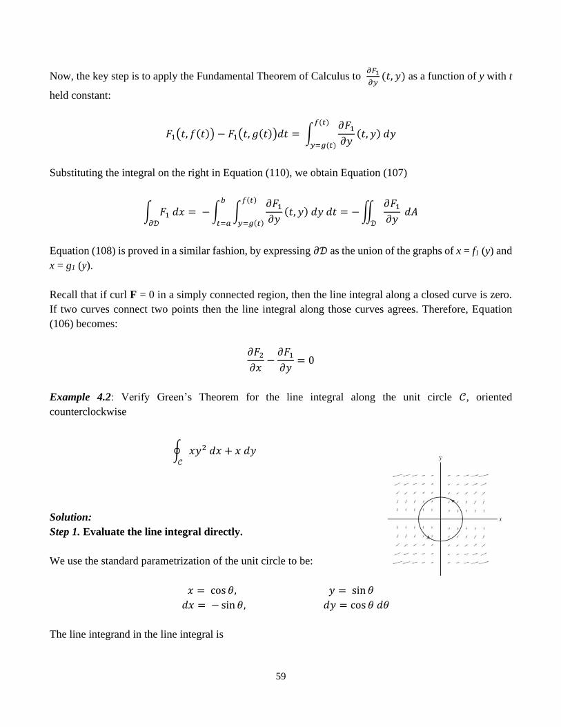
59
Now, the key step is to apply the Fundamental Theorem of Calculus to 𝜕𝐹1
𝜕𝑦(𝑡, 𝑦) as a function of y with t
held constant:
𝐹1(𝑡, 𝑓(𝑡)) − 𝐹1(𝑡, 𝑔(𝑡))𝑑𝑡 = ∫𝜕𝐹1
𝜕𝑦(𝑡, 𝑦) 𝑑𝑦
𝑓(𝑡)
𝑦=𝑔(𝑡)
Substituting the integral on the right in Equation (110), we obtain Equation (107)
∫ 𝐹1 𝑑𝑥𝜕𝒟
= −∫ ∫𝜕𝐹1
𝜕𝑦(𝑡, 𝑦) 𝑑𝑦 𝑑𝑡
𝑓(𝑡)
𝑦=𝑔(𝑡)
𝑏
𝑡=𝑎
= −∬𝜕𝐹1
𝜕𝑦 𝑑𝐴
𝒟
Equation (108) is proved in a similar fashion, by expressing 𝜕𝒟 as the union of the graphs of x = f1 (y) and
x = g1 (y).
Recall that if curl F = 0 in a simply connected region, then the line integral along a closed curve is zero.
If two curves connect two points then the line integral along those curves agrees. Therefore, Equation
(106) becomes:
𝜕𝐹2
𝜕𝑥−
𝜕𝐹1
𝜕𝑦= 0
Example 4.2: Verify Green’s Theorem for the line integral along the unit circle 𝒞, oriented
counterclockwise
∮ 𝑥𝑦2 𝑑𝑥 + 𝑥 𝑑𝑦𝒞
Solution:
Step 1. Evaluate the line integral directly.
We use the standard parametrization of the unit circle to be:
𝑥 = cos 𝜃, 𝑦 = sin 𝜃
𝑑𝑥 = − sin 𝜃, 𝑑𝑦 = cos 𝜃 𝑑𝜃
The line integrand in the line integral is
60
𝑥𝑦2 𝑑𝑥 + 𝑥 𝑑𝑦 = cos 𝜃 sin2 𝜃(− sin 𝜃 𝑑𝜃) + cos 𝜃 (cos 𝜃 𝑑𝜃)
= (−cos 𝜃 sin3 𝜃 + cos2 𝜃) 𝑑𝜃
And
∮ 𝑥𝑦2 𝑑𝑥 + 𝑥 𝑑𝑦𝒞
= ∫ (−cos 𝜃 sin3 𝜃 + cos2 𝜃) 𝑑𝜃2𝜋
0
= −sin4 𝜃
4|0
2𝜋
+1
2(𝜃 +
1
2sin 2𝜃)|
0
2𝜋
= 0 +1
2(2𝜋 + 0)
= 𝜋
Step 2: Evaluate the line integral using Green’s Theorem.
In this example, F1 = xy2 and F2 = x, so
𝜕𝐹2
𝜕𝑥−
𝜕𝐹1
𝜕𝑦=
𝜕
𝜕𝑥𝑥 −
𝜕
𝜕𝑦𝑥𝑦2 = 1 − 2𝑥𝑦
According to Green’s Theorem, from Equation (106):
∮ 𝑥𝑦2 𝑑𝑥 + 𝑥 𝑑𝑦𝒞
= ∬ (𝜕𝐹2
𝜕𝑥−
𝜕𝐹1
𝜕𝑦) 𝑑𝐴
𝒟
= ∬ 1 − 2𝑥𝑦 𝑑𝐴𝒟
Where 𝒟 is the disk x2 + y2 1 enclosed by 𝒞. The integral 2xy over 𝒟 is zero by symmetry – the
contributions for positive and negative x cancel. We can check this directly:
∬ 1 − 2𝑥𝑦 𝑑𝐴𝒟
= −2∫ ∫ 𝑥𝑦 𝑑𝑦 𝑑𝑥 = −√1−𝑥2
𝑦=−√1−𝑥2
1
𝑥=−1
∫ 𝑥𝑦2|𝑦=−√1−𝑥2√1−𝑥2
𝑑𝑥1
𝑥=−1
= 0
Therefore,
∬ (𝜕𝐹2
𝜕𝑥−
𝜕𝐹1
𝜕𝑦) 𝑑𝐴
𝒟
= ∬ 1 𝑑𝐴 = Area (𝒟) = 𝜋𝒟

61
4.3 Stokes’ Theorem
Stokes’ Theorem is an extension of Green’s Theorem to thre dimensions in which circulation is related to
a surface integral in ℝ3 (rather than to a double integral in the plane). In order to state it, let’s first introduce
some definitions and terminology.
Figure 4.4 shows three surfaces with different types of boundaries. The boundary of a surface is denoted
as 𝜕𝑆. Observe that the boundary in (A) is a single, simple closed curve and the boundary in (B) consists
of three closed curves. The surface in (C) is called a closed surface because its boundary is empty. In this
case, we write 𝜕𝑆 = 0.
Figure 4.4. Surfaces and their boundaries.
Recall that an orientation is a continuously varying choice of unit normal vector at each point of a surface
S. When S is oriented, we can specify an orientation of 𝜕𝑆, called the boundary orientation.
Imagine that you are a unit vector walking along the boundary curve. The boundary orientation is the
direction for which the surface is on your left as you walk. For example, the boundary of the surface in
Figure 4.5 consists of two curves, 𝒞1 and 𝒞2.
In Figure 4.5 (A), the normal vector points to the outside. The woman (representing the normal vector) is
walking along 𝒞1 and has the surface to her left, so she is walking in the positive direction. The curve 𝒞2
is oriented in the opposite direction because she would have to walk along 𝒞2 in that direction to keep the
surface to her left.
The boundary orientations in Figure 4.5 (B) are reversed because the opposite normal has been selected
to orient the surface.

62
Figure 4.5. The orientation of the boundary 𝜕𝑆 for each of the two possible orientations of the surface S.
Recall from Chapter 2: All that is left to do is to define curl. The curl of a vector field F = F1, F2, F3 is
a vector field defined by the symbolic determinant
curl (𝐅) = ||
𝒊 𝒋 𝒌𝜕
𝜕𝑥
𝜕
𝜕𝑦
𝜕
𝜕𝑧𝐹1 𝐹2 𝐹3
||
= (𝜕𝐹3
𝜕𝑦−
𝜕𝐹2
𝜕𝑧 ) 𝒊 − (
𝜕𝐹3
𝜕𝑥−
𝜕𝐹1
𝜕𝑧 ) 𝒋 + (
𝜕𝐹2
𝜕𝑥−
𝜕𝐹1
𝜕𝑦)𝒌
Recall from Chapter 2, the curl is the symbolic cross product
curl (𝐅) = ∇ × 𝐅
where is the del “operator” (also called “nabla”):
∇= ⟨𝜕
𝜕𝑥,𝜕
𝜕𝑦,𝜕
𝜕𝑧⟩
It is straightforward to check that curl obeys the linearity rules:
curl (F + G) = curl (F) + curl (G)
curl (c F) = c curl (F) (c being any constant)

63
Now, going back to Stokes’ Theorem, let’s assume that S is an oriented surface with parametrization G :
𝒟 → S, where 𝒟 is a domain in the plane bounded by smooth, simple closed curves, and G is one-to-one
and regular, except possibly on the boundary of 𝒟. More generally, S may be a finite union of surfaces of
this type. The surfaces in applications we consider, such as spheres, cubes and graphs of functions, satisfy
these conditions.
For surface S described above, Stokes’ Theorem gives:
∮ 𝐅. 𝑑𝐬𝜕𝑆
= ∫∫ curl (𝐅). 𝑑𝐬𝑆
(111)
The integral on the left is defined relative to the boundary orientation of 𝜕𝑆. If S is closed (that is, 𝜕𝑆 is
empty), then the surface integral on the right is zero.
Proof:
Each side of Equation (111) is equal to a sum over the components of F:
∮ 𝐅. 𝑑𝐬𝒞
= ∮ 𝐹1 𝑑𝑥 + 𝐹2 𝑑𝑦 + 𝐹3 𝑑𝑧𝒞
∫∫ curl (𝐅). 𝑑𝐬 = ∫∫ curl (𝐹1𝒊). 𝑑𝐬𝑆
+ ∫∫ curl (𝐹2𝒋). 𝑑𝐬𝑆
+ ∫∫ curl (𝐹3𝒌). 𝑑𝐬𝑆𝑆
The proof consists of showing that the F1-, F2-, and F3- terms are separately equal.
We will proof this under the simplifying assumption that S is the graph of a function z = f (x, y) lying over
a domain in the xy-plane. Furthermore, we will carry the details only for the F1- terms. The calculation for
F2- and F3- components are similar.
Thus we shall prove that
∮ 𝐹1 𝑑𝑥𝒞
= ∫∫ curl (𝐹1(𝑥, 𝑦, 𝑧)𝒊). 𝑑𝐬𝑆
(112)
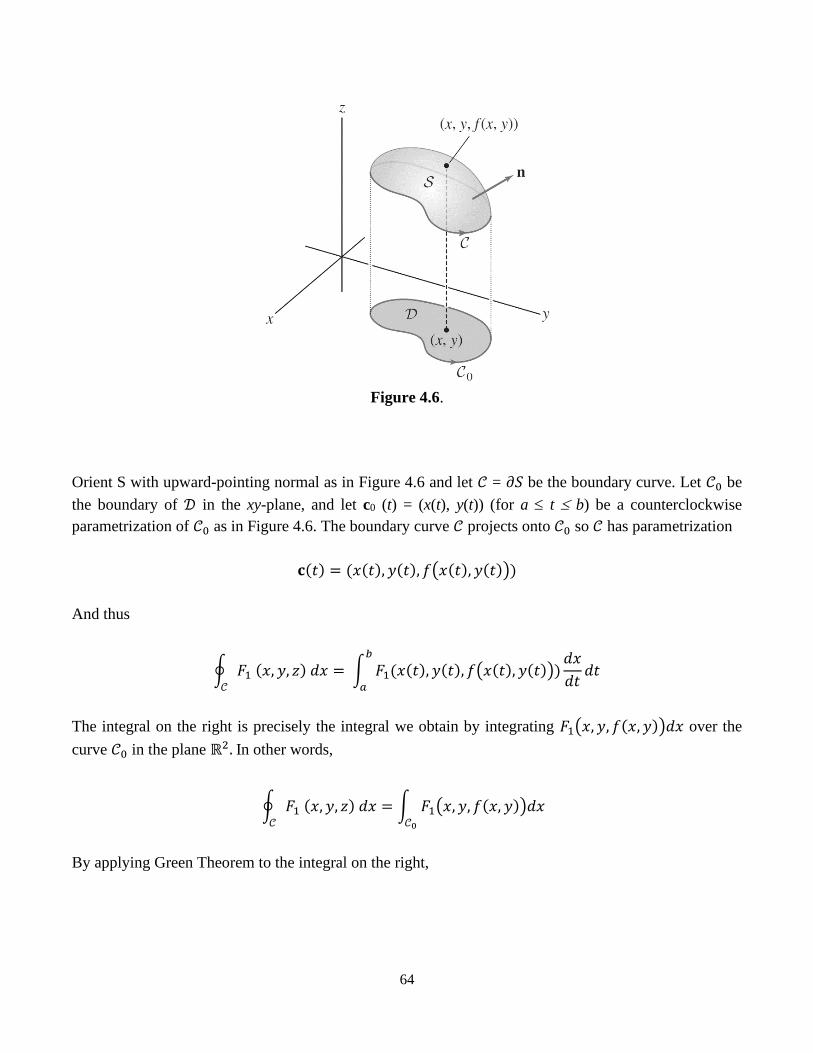
64
Figure 4.6.
Orient S with upward-pointing normal as in Figure 4.6 and let 𝒞 = 𝜕𝑆 be the boundary curve. Let 𝒞0 be
the boundary of 𝒟 in the xy-plane, and let c0 (t) = (x(t), y(t)) (for a t b) be a counterclockwise
parametrization of 𝒞0 as in Figure 4.6. The boundary curve 𝒞 projects onto 𝒞0 so 𝒞 has parametrization
𝐜(𝑡) = (𝑥(𝑡), 𝑦(𝑡), 𝑓(𝑥(𝑡), 𝑦(𝑡)))
And thus
∮ 𝐹1 (𝑥, 𝑦, 𝑧) 𝑑𝑥𝒞
= ∫ 𝐹1(𝑥(𝑡), 𝑦(𝑡), 𝑓(𝑥(𝑡), 𝑦(𝑡)))𝑑𝑥
𝑑𝑡𝑑𝑡
𝑏
𝑎
The integral on the right is precisely the integral we obtain by integrating 𝐹1(𝑥, 𝑦, 𝑓(𝑥, 𝑦))𝑑𝑥 over the
curve 𝒞0 in the plane ℝ2. In other words,
∮ 𝐹1 (𝑥, 𝑦, 𝑧) 𝑑𝑥𝒞
= ∫ 𝐹1(𝑥, 𝑦, 𝑓(𝑥, 𝑦))𝑑𝑥 𝒞0
By applying Green Theorem to the integral on the right,
65
∮ 𝐹1 (𝑥, 𝑦, 𝑧) 𝑑𝑥𝒞
= ∫∫𝜕
𝜕𝑦𝐹1(𝑥, 𝑦, 𝑓(𝑥, 𝑦)) 𝑑𝐴
𝒟
By the Chain Rule,
𝜕
𝜕𝑦𝐹1(𝑥, 𝑦, 𝑓(𝑥, 𝑦)) = 𝐹1𝑦(𝑥, 𝑦, 𝑓(𝑥, 𝑦)) + 𝐹1𝑧(𝑥, 𝑦, 𝑓(𝑥, 𝑦))𝑓𝑦(𝑥, 𝑦)
So, we finally obtain
∮ 𝐹1 𝑑𝑥𝒞
= ∫∫ (𝐹1𝑦(𝑥, 𝑦, 𝑓(𝑥, 𝑦)) + 𝐹1𝑧(𝑥, 𝑦, 𝑓(𝑥, 𝑦))𝑓𝑦(𝑥, 𝑦)) 𝑑𝐴𝒟
(113)
To finish the proof, we will compute the surface integral of curl (𝐹1𝑖) using the parametrization G (x, y) =
(x, y, f(x, y)) of S:
(Note that n is the upward-pointing normal)
𝐧 = ⟨−𝑓𝑥(𝑥, 𝑦), −𝑓𝑦(𝑥, 𝑦), 1⟩
curl (𝐹1𝑖) ∙ 𝐧 = ⟨0, 𝐹1𝑧 , −𝐹1𝑦⟩ ∙ ⟨−𝑓𝑥(𝑥, 𝑦),−𝑓𝑦(𝑥, 𝑦), 1⟩
= 𝐹1𝑧(𝑥, 𝑦, 𝑓(𝑥, 𝑦)𝑓𝑦(𝑥, 𝑦) − 𝐹1𝑦(𝑥, 𝑦, 𝑓(𝑥, 𝑦)
∫∫ curl (𝐹1𝑖) ∙ 𝑑𝐬𝑆
= −∫∫ (𝐹1𝑧(𝑥, 𝑦, 𝑓(𝑥, 𝑦)𝑓𝑦(𝑥, 𝑦) − 𝐹1𝑦(𝑥, 𝑦, 𝑓(𝑥, 𝑦) 𝑑𝐴𝒟
(114)
The right-hand sides of Equation (113) and Equation (114) are equal. This proves Equation (112)
Example 4.3: Let F(x, y, z) = −𝑦2𝑖 + 𝑥𝑗 + 𝑧2�⃗⃗� and 𝒞 is the curve of intersection of the plane y + z = 2
and the cylinder x2 + y2 = 1 (Orient 𝒞 to be counterclockwise when viewed from above). Evaluate
∫ 𝐅 ∙ 𝑑𝐫𝒞

66
Solution:
We first compute for F(x, y, z) = −𝑦2𝑖 + 𝑥𝑗 + 𝑧2�⃗⃗�;
𝑐𝑢𝑟𝑙 𝐹 = ||
𝑖 𝑗 �⃗⃗�𝜕
𝜕𝑥
𝜕
𝜕𝑦
𝜕
𝜕𝑧
−𝑦2 𝑥 𝑧2
|| = (1 + 2𝑦)�⃗⃗�
If we look at the figure above, there are many surfaces with boundary 𝒞. The most convenient choice,
though, is the elliptical region S in the plane y + z = 2 that is bounded by 𝒞. If we orient S upward, 𝒞 has
the induced positive orientation.
The projection 𝒟 of S on the xy-plane is the disk x2 + y2 1, so by using the equation z = 2 – y and applying
the Stokes’ Theorem, we obtain:
∫ 𝐅 ∙ 𝑑𝐫𝒞
= ∫∫ curl 𝐅 ∙ 𝑑𝐒𝑆
= ∫∫ (1 + 2𝑦) 𝑑𝐴𝒟
= ∫ ∫ (1 + 2𝑟 sin 𝜃) 𝑟 𝑑𝑟 𝑑𝜃1
0
2𝜋
0
= ∫ [𝑟2
2+ 2
𝑟3
3sin 𝜃]
0
`2𝜋
0
𝑑𝜃
= ∫ (1
2+
2
3sin 𝜃) 𝑑𝜃
2𝜋
0
67
=1
2(2𝜋) + 0 = 𝜋
4.4 Divergent Theorem
In section 4.2, Green Theorem was written in a vector version as:
∫ 𝐹1 𝑑𝑥 + 𝐹2 𝑑𝑦𝐶
= ∬ (𝜕𝐹2
𝜕𝑥−
𝜕𝐹1
𝜕𝑦) 𝑑𝐴
𝒟
= ∬ div 𝐅(𝑥, 𝑦) 𝑑𝐴𝒟
where 𝐶 is the positively oriented boundary curve of the plane region 𝒟. If we were seeking to extend this
theorem to vector fields on ℝ3, we might make the guess that
∬ 𝐅.𝐧 𝑑𝑆 = ∭ div 𝐅 (𝑥, 𝑦, 𝑧)𝑑𝑉
𝐸𝑆
(115)
where S is the boundary surface of the solid region E.
Let E be a simple solid region and let S be the boundary surface of E, given positive outward orientation
and F be a vector field whose component functions have continuous partial derivatives on an open region
that contains E. Therefore, Divergence Theorem can be written as:
∬ 𝐅 𝑑𝑆 = ∭ div 𝐅 𝑑𝑉
𝐸𝑆
(116)
Note that Divergent Theorem are also usually called Gauss Theorem.
Example 4.4: Evaluate
∬ 𝐅 𝑑𝑆𝑆
Where F(x, y, z) = 𝑥𝑦𝒊 + (𝑦2 + 𝑒𝑥𝑧2)𝒋 + sin(𝑥𝑦) 𝒌 and S is the surface of the region E bounded by the
parabolic cylinder 𝑧 = 1 − 𝑥2 and the planes 𝑧 = 0, 𝑦 = 0, 𝑦 + 𝑧 = 2
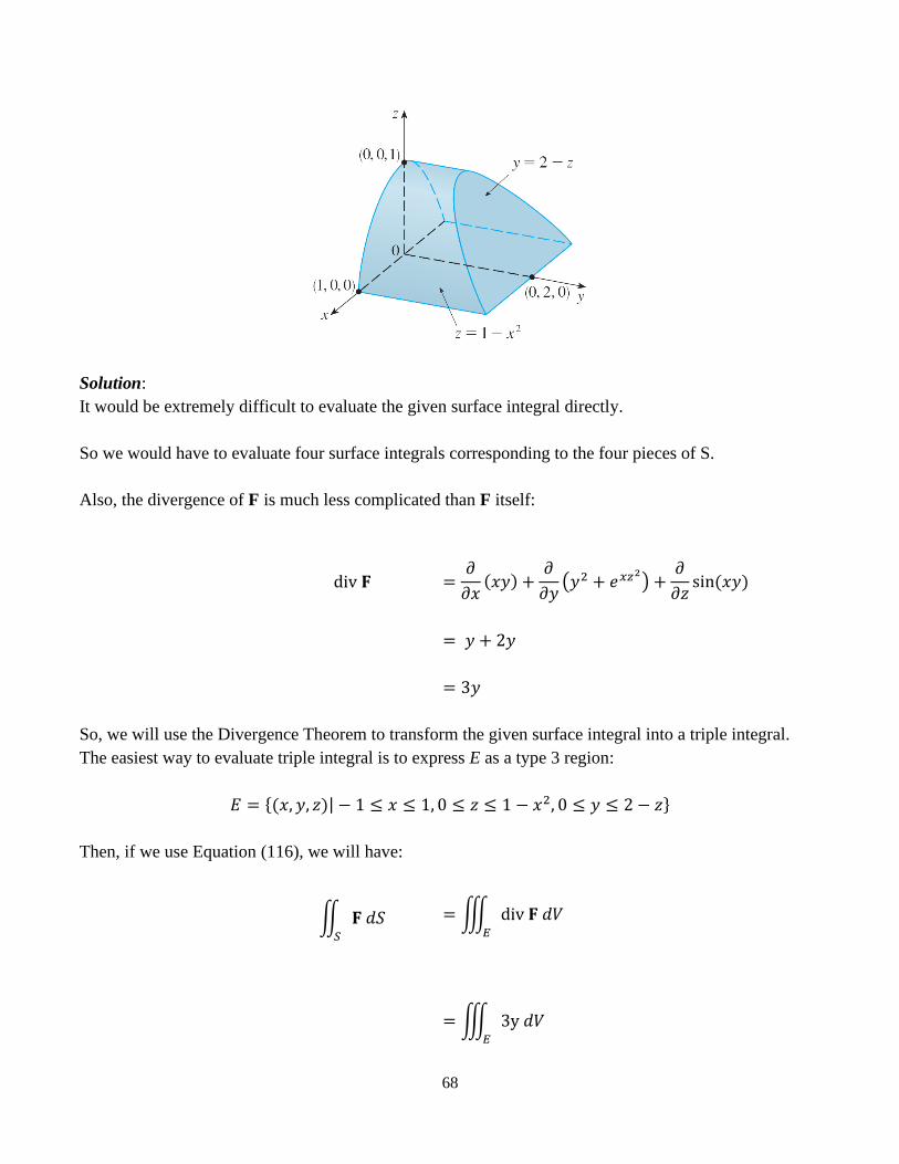
68
Solution:
It would be extremely difficult to evaluate the given surface integral directly.
So we would have to evaluate four surface integrals corresponding to the four pieces of S.
Also, the divergence of F is much less complicated than F itself:
div 𝐅 =𝜕
𝜕𝑥(𝑥𝑦) +
𝜕
𝜕𝑦(𝑦2 + 𝑒𝑥𝑧2
) +𝜕
𝜕𝑧sin(𝑥𝑦)
= 𝑦 + 2𝑦
= 3𝑦
So, we will use the Divergence Theorem to transform the given surface integral into a triple integral.
The easiest way to evaluate triple integral is to express E as a type 3 region:
𝐸 = {(𝑥, 𝑦, 𝑧)| − 1 ≤ 𝑥 ≤ 1, 0 ≤ 𝑧 ≤ 1 − 𝑥2, 0 ≤ 𝑦 ≤ 2 − 𝑧}
Then, if we use Equation (116), we will have:
∬ 𝐅 𝑑𝑆
𝑆
= ∭ div 𝐅 𝑑𝑉𝐸
= ∭ 3y 𝑑𝑉𝐸

69
= 3 ∫ ∫ ∫ 𝑦2−𝑧
0
1−𝑥2
0
1
−1
𝑑𝑦 𝑑𝑧 𝑑𝑥
= 3 ∫ ∫(2 − 𝑧)2
2
1−𝑥2
0
1
−1
𝑑𝑧 𝑑𝑥
=3
2∫ [
(2 − 𝑧)3
3]0
1−𝑥21
−1
𝑑𝑥
= −1
2∫ [(𝑥2 + 1)3 − 8]
1
−1
𝑑𝑥
= −∫ (𝑥6 + 3𝑥4 + 3𝑥2 − 7)1
0
𝑑𝑥
=184
35
70
5. Ordinary Differential Equations
5.1 First-Order Linear Differential Equations
The first order linear differential equation takes the form of
𝑑𝑦
𝑑𝑥+ 𝑃(𝑥)𝑦 = 𝑄(𝑥) (117)
where 𝑃 and 𝑄 are continuous functions on a given interval.
Let’s take an easy example of a linear equation 𝑥𝑦′ + 𝑦 = 2𝑥, for 𝑥 ≠ 0. We can rewrite this equation as:
𝑦′ +1
𝑥𝑦 = 2 (118)
Using the Product Rule, we can rewrite the original equation as
𝑥𝑦′ + 𝑦 = (𝑥𝑦)′
Now we can rewrite the above equation as
(𝑥𝑦)′ = 2𝑥
Now if we integrate both sides, we get
𝑥𝑦 = 𝑥2 + 𝐶 or 𝑦 = 𝑥 +𝐶
𝑥
We can solve every first-order differential equation in a similar fashion by multiplying both sides of
Equation (117) by a suitable function I(x) called an integrating factor. We try to find 𝐼 so that the left side
of Equation (117) when multiplied by 𝐼(𝑥), becomes the derivative of the product 𝐼(𝑥)𝑦:
𝐼(𝑥)(𝑦′ + 𝑃(𝑥)𝑦) = (𝐼(𝑥)𝑦)′ (119)
If we can find such a function I, then Equation (117) becomes
(𝐼(𝑥)𝑦)′ = 𝐼(𝑥)𝑄(𝑥)
Integrating both sides, we would have

71
𝐼(𝑥)𝑦 = ∫ 𝐼(𝑥)𝑄(𝑥) 𝑑𝑥 + 𝐶
So the solution would be
𝑦(𝑥) =1
𝐼(𝑥)[∫ 𝐼(𝑥)𝑄(𝑥) 𝑑𝑥 + 𝐶] (120)
To find such an 𝐼, we expand Equation (119) and cancel terms
𝐼(𝑥)𝑦′ + 𝐼(𝑥)𝑃(𝑥)𝑦 = (𝐼(𝑥)𝑦)′ = 𝐼′(𝑥)𝑦 + 𝐼(𝑥)𝑦′
𝐼(𝑥)𝑃(𝑥) = 𝐼′(𝑥)
This is a separable differential equation for 𝐼, which we solve as follows:
∫𝑑𝐼
𝐼 = ∫𝑃(𝑥)𝑑𝑥
ln|𝐼| = ∫𝑃(𝑥)𝑑𝑥
𝐼 = 𝐴𝑒∫𝑃(𝑥)𝑑𝑥
where 𝐴 = ±𝑒𝑐. Let’s take 𝐴 = 1, as we are looking for a particular integrating factor
𝐼(𝑥) = 𝑒∫𝑃(𝑥)𝑑𝑥 (121)
Therefore, to solve a linear differential equation 𝑦′ + 𝑃(𝑥)𝑦 = 𝑄(𝑥), multiply both sides with the
integrating factor 𝐼(𝑥) = 𝑒∫𝑃(𝑥)𝑑𝑥 and integrate both sides.
Example 5.1: Find the solution of the initial-value problem
𝑥2𝑦′ + 𝑥𝑦 = 1 𝑥 > 0 𝑦(1) = 2
Solution: We must first divide both sides by the coefficient of 𝑦’ to put the differential equation into
standard form
𝑦′ +1
𝑥𝑦 =
1
𝑥2 𝑥 > 0 (122)

72
The integrating factor is
𝐼(𝑥) = 𝑒∫(1𝑥)𝑑𝑥 = 𝑒ln 𝑥 = 𝑥
Multiplication of Equation (122) by 𝑥 gives
𝑥𝑦′ + 𝑦 =1
𝑥 or (𝑥𝑦)′ =
1
𝑥
Then:
𝑥𝑦 = ∫1
𝑥𝑑𝑥 = ln 𝑥 + 𝐶
𝑦 =ln 𝑥 + 𝐶
𝑥
Since 𝑦(1) = 2, we have
2 =ln 1 + 𝐶
1= 𝐶
Therefore, the solution to the initial-value problem is
𝑦 =ln 𝑥 + 2
𝑥
5.2 Second-Order Linear Differential Equations
A second-order linear differential equation has the form
𝑃(𝑥)𝑑2𝑦
𝑑𝑥2+ 𝑄(𝑥)
𝑑𝑦
𝑑𝑥+ 𝑅(𝑥)𝑦 = 𝐺(𝑥) (123)
where 𝑃, 𝑄, 𝑅 and 𝐺 are continuous functions. In this section, we will only cover the case where 𝐺(𝑥) = 0
for all 𝑥, in Equation (123). Such equations are called homogeneous linear differential equations. Hence,
the form of second order linear differential equation is

73
𝑃(𝑥)𝑑2𝑦
𝑑𝑥2+ 𝑄(𝑥)
𝑑𝑦
𝑑𝑥+ 𝑅(𝑥)𝑦 = 0 (124)
If 𝐺(𝑥) ≠ 0 for some 𝑥, Equation (123) is nonhomogeneous and will be dealt with in section 5.3.
Two basic facts enable us to solve homogeneous linear differential equations.
A. If we know two solutions 𝑦1 and 𝑦2 of such an equation, then the linear combination 𝑦 =
𝑐1𝑦1(𝑥) + 𝑐2𝑦2(𝑥) is also a solution. Therefore, if 𝑦1(𝑥) and 𝑦2(𝑥) are both solutions of the linear
homogeneous equation and 𝑐1 and 𝑐2 are any constants, then the function in Equation (125) below
is also a solution of Equation (124)
𝑦(𝑥) = 𝑐1𝑦1(𝑥) + 𝑐2𝑦2(𝑥) (125)
Let’s proof this: Since 𝑦1 and 𝑦2 are solutions of Equation (124), we then have
𝑃(𝑥)𝑦1′′ + 𝑄(𝑥)𝑦1
′ + 𝑅(𝑥)𝑦1 = 0
𝑃(𝑥)𝑦2′′ + 𝑄(𝑥)𝑦2
′ + 𝑅(𝑥)𝑦2 = 0
And therefore, suing the basic rule for differentiation, we have
𝑃(𝑥)𝑦′′ + 𝑄(𝑥)𝑦′ + 𝑅(𝑥)𝑦 = 𝑃(𝑥)( 𝑐1𝑦1 + 𝑐2𝑦2)′′ + 𝑄(𝑥)( 𝑐1𝑦1 + 𝑐2𝑦2)
′ + 𝑅(𝑥)( 𝑐1𝑦1 + 𝑐2𝑦2)
= 𝑃(𝑥)( 𝑐1𝑦1′′ + 𝑐2𝑦2
′′) + 𝑄(𝑥)(𝑐1𝑦1′ + 𝑐2𝑦2
′) + 𝑅(𝑥)( 𝑐1𝑦1 + 𝑐2𝑦2)
= 𝑐1[𝑃(𝑥)𝑦1′′ + 𝑄(𝑥)𝑦1
′ + 𝑅(𝑥)𝑦1] + 𝑐2[𝑃(𝑥)𝑦2′′ + 𝑄(𝑥)𝑦2
′ + 𝑅(𝑥)𝑦2]
= 𝑐1(0) + 𝑐2(0) = 0
Thus, 𝑦 = 𝑐1𝑦1 + 𝑐2𝑦2 is a solution of Equation (124).
B. The second means of solving the equation says that the general solution is a linear combination of
two linearly independent solutions 𝑦1 and 𝑦2. This means that neither 𝑦1 nor 𝑦2 is a constant
multiple of the other. For instance, the functions 𝑓(𝑥) = 𝑥2 and 𝑔(𝑥) = 5𝑥2 are linearly
dependent, but 𝑓(𝑥) = 𝑒2 and 𝑔(𝑥) = 𝑥𝑒𝑥 are linearly independent. Therefore, if 𝑦1 and 𝑦2 are
linearly independent solutions of Equation (124), and 𝑃(𝑥) is never 0, then the general solution is
given by:

74
𝑦(𝑥) = 𝑐1𝑦1(𝑥) + 𝑐2𝑦2(𝑥) (126)
where 𝑐1 and 𝑐2 are arbitrary constants.
In general, it is not easy to discover solutions to a second-order linear differential equation. But it is always
possible to do so if the coefficient 𝑃, 𝑄 and 𝑅 are constant functions, i.e., if the differential equation has
the form
𝑎𝑦′′ + b𝑦′ + cy = 0 (127)
where 𝑎, 𝑏 and 𝑐 are constants and 𝑎 ≠ 0.
We know that the exponential function 𝑦 = 𝑒𝑟𝑥 (where 𝑟 is a constant) has the property that its derivative
is a constant multiple of itself, i.e., 𝑦′ = 𝑟𝑒𝑟𝑥. Furthermore, 𝑦′′ = 𝑟2𝑒𝑟𝑥. If we substitute these
expressions into Equation (127), we get:
𝑎𝑟2𝑒𝑟𝑥 + b𝑟𝑒𝑟𝑥 + c𝑒𝑟𝑥 = 0
(𝑎𝑟2 + 𝑏𝑟 + 𝑐)𝑒𝑟𝑥 = 0
But 𝑒𝑟𝑥 is never 0. Therefore, 𝑦 = 𝑒𝑟𝑥 is a solution of Equation (127) is 𝑟 is a root of the equation
𝑎𝑟2 + 𝑏𝑟 + 𝑐 = 0 (128)
Equation (128) is called auxiliary equation (or characteristic equation) of the differential equation 𝑎𝑦′′ +
b𝑦′ + cy = 0. Realise that it is an algebraic equation that is obtained from the differential equation by
replacing 𝑦′′ by 𝑟2, 𝑦′ by 𝑟 and 𝑦 by 1.
Sometimes the roots 𝑟1 and 𝑟2 of the auxiliary equation can be found by factoring. Sometimes they are
found by using the quadratic formula:
𝑟1 =−𝑏 + √𝑏2 − 4𝑎𝑐
2𝑎 𝑟2 =
−𝑏 − √𝑏2 − 4𝑎𝑐
2𝑎 (129)
From Equation (129), let’s look at the expression of 𝑏2 − 4𝑎𝑐

75
Case A. If 𝒃𝟐 − 𝟒𝒂𝒄 > 𝟎
In this case, the roots 𝑟1 and 𝑟2 , of the auxiliary equation are real and distinct. If the roots 𝑟1 and 𝑟2 of the
auxiliary equation 𝑎𝑟2 + 𝑏𝑟 + 𝑐 = 0 are real and unequal, then the general solution of 𝑎𝑦′′ + b𝑦′ + cy =
0 is
𝑦 = 𝑐1𝑒𝑟1𝑥 + 𝑐2𝑒
𝑟2𝑥 (130)
Case B. If 𝒃𝟐 − 𝟒𝒂𝒄 = 𝟎
In this case, 𝑟1 = 𝑟2 , that is the roots of the auxiliary equation are real and equal. If the auxiliary equation
𝑎𝑟2 + 𝑏𝑟 + 𝑐 = 0 has only one real root 𝑟, then the general solution of 𝑎𝑦′′ + b𝑦′ + cy = 0 is
𝑦 = 𝑐1𝑒𝑟𝑥 + 𝑐2𝑥𝑒𝑟𝑥 (131)
Case C. If 𝒃𝟐 − 𝟒𝒂𝒄 < 𝟎
In this case, the roots 𝑟1 and 𝑟2 of the auxiliary equation are complex numbers, we can write
𝑟1 = 𝛼 + 𝑖𝛽 𝑟2 = 𝛼 − 𝑖𝛽
where 𝛼 and 𝛽 are real numbers. In fact, we can write:
𝛼 =−𝑏
2𝑎 𝛽 =
√4𝑎𝑐 − 𝑏2
2𝑎
Then, using Euler’s equation
𝑒𝑖𝜃 = cos 𝜃 + 𝑖 sin 𝜃
So, we can write the solution of the differential equation as
𝑦 = 𝐶1𝑒𝑟1𝑥 + 𝐶2𝑒
𝑟2𝑥
= 𝐶1𝑒(𝛼+𝑖𝛽)𝑥 + 𝐶2𝑒
(𝛼−𝑖𝛽)𝑥
= 𝐶1𝑒𝛼𝑥(cos 𝛽𝑥 + 𝑖 sin 𝛽𝑥) + 𝐶2𝑒
𝛼𝑥( cos 𝛽𝑥 − 𝑖 sin 𝛽𝑥)
= 𝑒𝛼𝑥[(𝐶1 + 𝐶2) cos 𝛽𝑥 + 𝑖(𝐶1 − 𝐶2) sin 𝛽𝑥]

76
= 𝑒𝛼𝑥[𝑐1 cos 𝛽𝑥 + 𝑐2 sin 𝛽𝑥]
where 𝑐1 = 𝐶1 + 𝐶2, 𝑐2 = 𝑖(𝐶1 − 𝐶2). This gives all solutions (real and complex) of differential equation.
The solution is real when constants 𝑐1 and 𝑐2 are real.
Therefore, if the roots of the auxiliary equation 𝑎𝑟2 + 𝑏𝑟 + 𝑐 = 0 are the complex numbers 𝑟1 = 𝛼 + 𝑖𝛽,
𝑟2 = 𝛼 − 𝑖𝛽, then the general solution of 𝑎𝑦′′ + b𝑦′ + cy = 0 is
𝑦 = 𝑒𝛼𝑥(𝑐1 cos 𝛽𝑥 + 𝑐2 sin 𝛽𝑥) (132)
5.3 Initial-Value and Boundary-Value Problems
An initial-value problem for the second order Equation (124) or Equation (125) consists of finding a
solution 𝑦 of the differential equation that also satisfies initial conditions of the form
𝑦(𝑥0) = 𝑦0 𝑦′(𝑥0) = 𝑦1
where 𝑦0 and 𝑦1 are given constants. If 𝑃, 𝑄, 𝑅 and 𝐺 are continuous on an interval and 𝑃(𝑥) ≠ 0, then
this guarantees the existence and uniqueness of a solution to this initial-value problem.
Example 5.2: Solve the initial-value problem
𝑦′′ + 𝑦′ − 6𝑦 = 0 𝑦(0) = 1 𝑦′(0) = 0
Solution: The auxiliary equation is then
𝑟2 + 𝑟 − 6 = (𝑟 − 2)(𝑟 + 3) = 0
Therefore, the roots are 𝑟 = 2 and −3. So, the general equation (given by Equation (131)) is
𝑦(𝑥) = 𝑐1𝑒2𝑥 + 𝑐2𝑒
−3𝑥
Differentiating this equation, we get:
𝑦′(𝑥) = 2𝑐1𝑒2𝑥 − 3𝑐2𝑒
−3𝑥
To satisfy the initial conditions, we require that
𝑦(0) = 𝑐1 + 𝑐2 = 1

77
𝑦′(0) = 2𝑐1 − 3𝑐2 = 0
Solving for 𝑐1 and 𝑐2, we get
𝑐1 =3
5 , 𝑐2 =
2
5
Substituting these values, the solution of the initial-value problem is
𝑦(𝑥) =3
5𝑒2𝑥 +
2
5𝑒−3𝑥
Example 5.3: Solve the initial-value problem
𝑦′′ + 𝑦 = 0 𝑦(0) = 2 𝑦′(0) = 3
Solution: The auxiliary equation here is 𝑟2 + 1 = 0 or 𝑟2 = −1, whose roots are ±𝑖. Thus, 𝛼 = 0, 𝛽 = 1,
and since 𝑒0𝑥 = 1, the general solution is
𝑦 (𝑥) = 𝑐1 cos 𝑥 + 𝑐2 sin 𝑥 (133)
Differentiating Equation (133), we get
𝑦′ (𝑥) = −𝑐1 sin 𝑥 + 𝑐2 cos 𝑥
The initial conditions become
𝑦(0) = 𝑐1 = 2 , 𝑦′(0) = 𝑐2 = 3
Therefore, the solution of the initial-value problem is
𝑦 (𝑥) = 2 cos 𝑥 + 3 sin 𝑥
A boundary-value problem however consists of finding a solution y of the differential equation that also
satisfies boundary conditions of the form
𝑦(𝑥0) = 𝑦0 𝑦(𝑥1) = 𝑦1
78
In contrast with the situation for initial-value problems, a boundary-value problem does not always have
a solution.
Example 5.4: Solve the boundary-value problem
𝑦′′ + 2𝑦′ + 𝑦 = 0 𝑦(0) = 1 𝑦(1) = 3
Solution: The auxiliary equation is
𝑟2 + 2𝑟 + 1 = 0 or (𝑟 + 1)2 = 0
whose only root is 𝑟 = −1. Therefore, the general solution is:
𝑦(𝑥) = 𝑐1𝑒−𝑥 + 𝑐2𝑥𝑒−𝑥
The boundary conditions are satisfied if
𝑦(0) = 𝑐1 = 1
𝑦(1) = 𝑐1𝑒−1 + 𝑐2𝑒
−1 = 3
The first condition gives 𝑐1 = 1, so the second condition becomes
𝑒−1 + 𝑐2𝑒−1 = 3
Solving this equation for 𝑐2 by first multiplying through by 𝑒, we get
1 + 𝑐2 = 3𝑒 so 𝑐2 = 3𝑒 − 1
Thus, the solution of the boundary-value problem is
𝑦(𝑥) = 𝑒−𝑥 + (3𝑒 − 1)𝑥𝑒−𝑥

79
Summary:
Solutions of 𝒂𝒚′′ + 𝒃𝒚′ + 𝒄 = 𝟎 are as follows:
Roots of 𝒂𝒓𝟐 + 𝒃𝒓 + 𝒄 = 𝟎 General solution
𝒓𝟏, 𝒓𝟐 real and distinct 𝑦 = 𝑐1𝑒𝑟1𝑥 + 𝑐2𝑒
𝑟2𝑥
𝒓𝟏 = 𝒓𝟐 = 𝒓 𝑦 = 𝑐1𝑒𝑟𝑥 + 𝑐2𝑥𝑒𝑟𝑥
𝒓𝟏, 𝒓𝟐 complex: 𝜶 ± 𝒊𝜷 𝑦 = 𝑒𝛼𝑥(𝑐1 cos 𝛽𝑥 + 𝑐2 sin 𝛽𝑥)
5.4 Non-homogeneous linear differential equation
Remember from section 5.3, the second-order nonhomogeneous linear differential equation with constant
coefficients has the form
𝑎𝑦′′ + 𝑏𝑦′ + 𝑐𝑦 = 𝐺(𝑥) (134)
where 𝑎, 𝑏 and 𝑐 are constants and 𝐺 is a continuous function. The related homogeneous equation
(Equation (127)) is also called the complementary equation and is important in solving the
nonhomogeneous equation.
The general solution of the nonhomogeneous differential equation (Equation (133)) can be written as
𝑦(𝑥) = 𝑦𝑝(𝑥) + 𝑦𝑐(𝑥) (135)
where 𝑦𝑝 is a particular solution of Equation (124) and 𝑦𝑐 is the general solution of the complementary
Equation (127).
Example 5.5: Solve the equation 𝑦′′ + 𝑦′ − 2𝑦 = 𝑥2
Solution: The auxiliary equation for 𝑦′′ + 𝑦′ − 2𝑦 = 0 is
𝑟2 + 𝑟 − 2 = (𝑟 − 1)(𝑟 + 2) = 0
With roots 𝑟 = 1 and −2. So the solution of the complementary equation is
80
𝑦𝑐 = 𝑐1𝑒𝑥 + 𝑐2𝑒
−2𝑥
Since 𝐺(𝑥) = 𝑥2 is a polynomial of degree 2, we seek a particular solution of the form
𝑦𝑝(𝑥) = 𝐴𝑥2 + 𝐵𝑥 + 𝐶
Then
𝑦𝑝′ = 2𝐴𝑥 + 𝐵
𝑦𝑝′′ = 2𝐴
Substituting these into the given differential equation, we get
(2𝐴) + (2𝐴𝑥 + 𝐵) − 2(𝐴𝑥2 + 𝐵𝑥 + 𝐶) = 𝑥2
−2𝐴𝑥2 + (2𝐴 − 2𝐵)𝑥 + (2𝐴 + 𝐵 − 2𝐶) = 𝑥2
Polynomials are equal when their coefficients are equal. Thus
−2𝐴 = 1 2𝐴 − 2𝐵 = 0 2𝐴 + 𝐵 − 2𝐶 = 0
The solution of this system of equation is
𝐴 = −1
2 𝐵 = −
1
2 𝐶 = −
3
4
A particular solution is therefore
𝑦𝑝(𝑥) = −1
2𝑥2 −
1
2𝑥 −
3
4
And the general solution according to Equation (129) is
𝑦 = 𝑦𝑝 + 𝑦𝑐 = 𝑐1𝑒𝑥 + 𝑐2𝑒
−2𝑥 −1
2𝑥2 −
1
2𝑥 −
3
4
81
Example 5.6: Solve 𝑦′′ + 4𝑦 = 𝑒3𝑥
Solution: The auxiliary equation is 𝑟2 + 4 = 0 with roots ±2𝑖, so the solution of the complementary
equation is
𝑦𝑐 = 𝑐1 cos 2𝑥 + 𝑐2 sin 2𝑥
For a particular solution, we try 𝑦𝑝(𝑥) = 𝐴𝑒3𝑥. Then 𝑦𝑝′(𝑥) = 3𝐴𝑒3𝑥 and 𝑦𝑝′′(𝑥) = 9𝐴𝑒3𝑥. Substituting
into the differential equation, we have
9𝐴𝑒3𝑥 + 4(𝐴𝑒3𝑥) = 𝑒3𝑥
So, 13𝐴𝑒3𝑥 = 𝑒3𝑥
𝐴 =1
13
Therefore,
𝑦𝑝(𝑥) =1
13𝑒3𝑥
And the general solution is
𝑦(𝑥) = 𝑐1 cos 2𝑥 + 𝑐2 sin 2𝑥 +1
13𝑒3𝑥

82
6. Partial Differential Equations
6.1 Introduction to Differential Equations
Although we have introduced the ordinary differential equation in Chapter 5, let’s just recap and get a bit
into the details of differential equations. A differential equation is an equation that relates the derivatives
of a (scalar) function depending on one or more variables. For example,
𝑑4𝑢
𝑑𝑥4+
𝑑2𝑢
𝑑𝑥2+ 𝑢3 = cos 𝑥 (136)
is a differential equation for the function u (x) depending on a single variable x while
𝜕𝑢
𝜕𝑡=
𝜕2𝑢
𝜕𝑥2+
𝜕2𝑢
𝜕𝑦2− 𝑢 (137)
is a differential equation involving a function u (t, x, y) of three variables.
A differential equation is called ordinary if the function u depends on only a single variable, and partial
if it depends on more than one variable. The order of a differential equation is that of the highest-order
derivatives that appears in the equation. Thus, Equation (136) is a fourth-order ordinary differential
equation (ODE) while Equation (137) is a second-order partial differential equation (PDE).
There are 2 common notations for partial derivatives, and we shall use them interchangeably. The first,
used in Equation (136) and Equation (137) is the familiar Leibniz notation that employs a d to denote
ordinary derivatives of a function of single variable and the 𝜕 symbol (usually pronounced “dee”) for
partial derivatives of functions of more than one variable. An alternative, more compact notation employs
subscripts to indicate partial derivatives. For example, ut represent 𝜕𝑢/𝜕𝑡, while uxx is used for 𝜕2𝑢/𝜕𝑥2
and 𝜕3𝑢/𝜕𝑥2𝜕𝑦 for uxxy. Thus, in subscript notation, the partial differential equation for Equation (137)
is written as:
𝑢𝑡 = 𝑢𝑥𝑥 + 𝑢𝑦𝑦 − 𝑢 (138)
6.2 Initial Conditions and Boundary Conditions
How many solutions does a partial differential equation have? In general, lots! The solutions to dynamical
ordinary differential equations are singled out by the imposition of initial conditions, resulting in an initial
83
value problem. On the other hand, equations modelling equilibrium phenomena require boundary
conditions to specify their solutions uniquely, resulting in a boundary-value problem.
For partial differential equations modeling dynamic process, the number of initial conditions required
depends on the highest-order time derivative that appears in the equation. On bounded domains, one must
also impose suitable boundary conditions in order to uniquely characterise the solution and hence the
subsequent dynamical behavior of the physical system. The combination of the partial differential
equation, the initial conditions, and the boundary conditions leads to an initial-boundary value problem.
We will encounter and solve many important examples of such problem throughout this section.
6.3 Linear and Nonlinear Equations
Linearity means that all instances of the unknown and its derivatives enter the equation linearly. We can
use the concept of a linear differential operator 𝓛. Such operator is assembled by summing the basic partial
derivative operators, with either constant coefficients or ore generally, coefficients depending on the
independent variables. A linear differential equation has the form:
𝓛[𝑢] = 0 (139)
For example, if 𝓛 =𝜕2
𝜕𝑥2 + 1, then 𝓛[𝑢] = 𝑢𝑥𝑥 + 𝑢
The operator 𝓛 is called linear if
𝓛(𝑢 + 𝑣) = 𝓛𝑢 + 𝓛𝑣 and 𝓛(𝑐𝑢) = 𝑐𝓛𝑢 (140)
for any functions u, v and a constant c.
Example 6.1: Is the heat equation 𝑢𝑡 − 𝑢𝑥𝑥 = 0 linear or non-linear?
Solution:
𝓛(𝑢 + 𝑣) = (𝑢 + 𝑣)𝑡 − (𝑢 + 𝑣)𝑥𝑥 = 𝑢𝑡 + 𝑣𝑡 − 𝑢𝑥𝑥 − 𝑣𝑥𝑥 = (𝑢𝑡 − 𝑢𝑥𝑥) + (𝑣𝑡 − 𝑣𝑥𝑥) = 𝓛𝑢 + 𝓛𝑣
And
𝓛(𝑐𝑢) = 𝑐𝓛𝑢 = (𝑐𝑢)𝑡 − (𝑐𝑢)𝑥𝑥 = 𝑐𝑢𝑡 − 𝑐𝑢𝑥𝑥 = 𝑐(𝑢𝑡 − 𝑢𝑥𝑥) = 𝑐𝓛𝑢.
Therefore, the heat equation is a linear equation, since it is given by a linear operator.

84
Example 6.2: Is the Burger’s equation 𝑢𝑡 + 𝑢𝑢𝑥 = 0 linear or non-linear?
Solution:
𝓛(𝑢 + 𝑣) = (𝑢 + 𝑣)𝑡 + (𝑢 + 𝑣)(𝑢 + 𝑣)𝑥 = 𝑢𝑡 + 𝑣𝑡 + (𝑢 + 𝑣)(𝑢𝑥 + 𝑣𝑥)
= (𝑢𝑡 + 𝑢𝑢𝑥) + (𝑣𝑡 + 𝑣𝑣𝑥) + 𝑢𝑣𝑥 + 𝑣𝑢𝑥 ≠ 𝓛𝑢 + 𝓛𝑣
Therefore, the Burger’s equation is a non-linear differential equation.
Equation (139) is also called homogeneous linear PDE, while the Equation (141) below:
𝓛[𝑢] = 𝑔(𝑥, 𝑦) (141)
is called inhomogeneous linear equation. If uh is a solution to the homogeneous Eq. (139), and up is a
particular solution to the inhomogeneous Equation (141), then uh + up is also a solution to the
inhomogeneous Equation (141). Indeed
𝓛(𝑢ℎ + 𝑢𝑝) = 𝓛𝑢ℎ + 𝓛𝑢𝑝 = 0 + 𝑔 = 𝑔
Therefore, in order to find the general solution to the inhomogeneous Eq. (6), it is enough to find the
general solution of the homogeneous Equation (139), and add to this particular solution of the
inhomogeneous equation (check that the difference of any two solutions of the inhomogeneous equation
is a solution of the homogeneous equation). In this sense, there is similarity between ODEs and PDEs,
since this principle relies only on the linearity of the operator 𝓛.
Notice that where the solution of an ODE contains arbitrary constants, the solution to a PDE contains
arbitrary functions.
The potential degree of non-linearity embedded in PDE of first order leads to the following
differentiations:
PDE Type Description
Linear Constant coefficient 𝑎, 𝑏, 𝑐 are constant functions
Linear 𝑎, 𝑏, 𝑐 are functions of x and y only
Semi-Linear 𝑎, 𝑏 functions of x and y, 𝑐 may depend on u
Quasi-Linear 𝑎, 𝑏, 𝑐 are functions of x, y and u
Non-Linear The derivatives carry exponents, e.g. (𝑢𝑥)
2, or
derivatives cross-terms exist, e.g. 𝑢𝑥 𝑢𝑦

85
Let’s assume a first-order PDE in the form:
𝑎(𝑥, 𝑦)𝜕𝑢(𝑥, 𝑦)
𝜕𝑥+ 𝑏(𝑥, 𝑦)
𝜕𝑢(𝑥, 𝑦)
𝜕𝑦= 𝑐(𝑥, 𝑦, 𝑢(𝑥, 𝑦)) (142)
Hence, Equation (142) represents a semi-linear PDE, because it permits for light non-linearities in the
source term, 𝑐(𝑥, 𝑦, 𝑢(𝑥, 𝑦)).
6.4 Examples of PDEs
Some examples of PDEs of physical significance are listed below:
𝑢𝑥 + 𝑢𝑦 = 0 Transport equation (143)
𝑢𝑡 + 𝑢𝑢𝑥 − 𝑣𝑢𝑥𝑥 = 0 Viscous Burger’s equation (144)
𝑢𝑡 + 𝑢𝑢𝑥 = 0 Inviscid Burger’s equation (145)
𝑢𝑥𝑥 + 𝑢𝑦𝑦 = 0 Laplace’s equation (146)
𝑢𝑡𝑡 − 𝑢𝑥𝑥 = 0 Wave equation (147)
𝑢𝑡 − 𝑢𝑥𝑥 = 0 Heat equation (148)
𝑢𝑡 + 𝑢𝑢𝑥 + 𝑢𝑥𝑥𝑥 = 0 Kortewedge Vries equation (149)
6.5 Three types of Second-Order PDEs
The classification theory of real linear second-order PDEs for scalar-valued function 𝑢(𝑡, 𝑥) depending
on two variables proceed as follows. The most general such equation has the form
𝓛 [𝑢] = 𝐴𝑢𝑡𝑡 + 𝐵𝑢𝑡𝑥 + 𝐶𝑢𝑥𝑥 + 𝐷𝑢𝑡 + 𝐸𝑢𝑥 + 𝐹𝑢 = 𝐺 (150)
Where the coefficients 𝐴, 𝐵, 𝐶, 𝐷, 𝐸, 𝐹 are all allowed to be functions of (𝑡, 𝑥), as is the inhomogeneity
or forcing function 𝐺(𝑡, 𝑥). The equation is homogenous if and only if 𝐺 ≡ 0. We assume that at least
one of the leading coefficients 𝐴, 𝐵, 𝐶 is not identically zero, since otherwise, the equation degenerates
to a first-order equation. The key quantity that determines the type of such a PDE is its discriminant:
86
∆ = 𝐵2 − 4𝐴𝐶 (151)
This should (and for good reason) remind you of the discriminant of the quadratic equation
𝑄(𝑥, 𝑦) = 𝐴𝑥2 + 𝐵𝑥𝑦 + 𝐶𝑦2 + 𝐷𝑥 + 𝐸𝑦 + 𝐹 = 0 (152)
Therefore, at a point (𝑡, 𝑥), the linear second-order PDE Equation (150) is called:
i. Hyperbolic, if ∆(𝑡, 𝑥) > 0
ii. Parabolic, if ∆(𝑡, 𝑥) = 0 but 𝐴2 + 𝐵2 + 𝐶2 ≠ 0
iii. Elliptic, if ∆(𝑡, 𝑥) < 0
In particular:
• The wave equation (Equation (147)) 𝑢𝑡𝑡 − 𝑢𝑥𝑥 = 0 has discriminant ∆ = 4, and is hyperbolic
• The heat equation (Equation (148)) 𝑢𝑥𝑥 − 𝑢𝑡 = 0 has discriminant ∆ = 0, and is parabolic
• The Laplace equation (Equation (146)) 𝑢𝑥𝑥 + 𝑢𝑦𝑦 = 0 has discriminant ∆ = −4, and is elliptic
Example 6.3: The Tricomi equation from the theory of supersonic aerodynamics is written as:
𝑥𝜕2𝑢
𝜕𝑡2−
𝜕2𝑢
𝜕𝑥2= 0
Comparing the equation above to Equation (150), we find that
𝐴 = 𝑥, 𝐵 = 0, 𝐶 = −1 while 𝐷 = 𝐸 = 𝐹 = 𝐺 = 0
The discriminant in this particular case is:
∆ = 𝐵2 − 4𝐴𝐶 = 4𝑥
Hence, the equation is hyperbolic when 𝑥 > 0, elliptic when 𝑥 < 0, and parabolic on the transition line
𝑥 = 0. In this physical model, the hyperbolic region corresponds to subsonic flow, while the supersonic
regions are of elliptic type. The transitional parabolic boundary represents the sock line between the sub-
and super-sonic regions – the familiar sonic boom as an airplane crosses the sound barrier.
6.6 Solving PDEs using Separation of Variables Method
The separation of variables method is used for solving key PDEs in their two-independent-variables
incarnations. For wave and heat equations (Equation (147) and (148), respectively), the variables are time,
87
t, and a single space coordinate, x, leading to initial boundary value problems modelling the dynamic
behavior of the one-dimensional medium. For the Laplace equation (Equation (146)), the variables
represent space coordinates, 𝑥 and 𝑦, and the associated boundary value problems model the equilibrium
configuration of a planar body, e.g., the deformation of a membrane.
In order to use the separation of variables method, we must be working with a linear homogeneous PDEs
with linear homogeneous boundary conditions. The separation of variables method relies upon the
assumption that a function of the form,
𝑢(𝑥, 𝑡) = 𝜑(𝑥)𝐺(𝑡) (153)
will be a solution to a linear homogeneous PDE in 𝑥 and 𝑡. This is called a product solution and provided
the boundary conditions are also linear and homogeneous, this will also satisfy the boundary conditions.
6.6.1 The Heat Equation
Let’s start with the one-dimensional heat equation:
𝜕𝑢
𝜕𝑡= 𝑘
𝜕2𝑢
𝜕𝑥2 (154)
Let the initial and boundary conditions be:
𝑢(𝑥, 0) = 𝑓(𝑥) 𝑢(0, 𝑡) = 0 𝑢(𝐿, 𝑡) = 0
So, we have the heat equation with fixed boundary conditions (that are also homogeneous) and an initial
condition. The separation of variables method tells us to assume that the solution will take the form of the
product (Equation (153)),
𝑢(𝑥, 𝑡) = 𝜑(𝑥)𝐺(𝑡)
So, all we have to do here is substituting Equation (153) into Equation (154), we obtain
𝜕
𝜕𝑡(𝜑(𝑥)𝐺(𝑡)) = 𝑘
𝜕2
𝜕𝑥2(𝜑(𝑥)𝐺(𝑡))
𝜑(𝑥)𝑑𝐺
𝑑𝑡= 𝑓𝐺(𝑡)
𝑑2𝜑
𝑑𝑥2
88
Therefore, we can factor the 𝜑(𝑥) out of the time derivative and similarly we can factor 𝐺(𝑡) out of the
spatial derivative. Also note that after we have factored these out, we no longer have partial derivatives
left in the problem. In the time derivative, we are only differentiating 𝐺(𝑡) with respect to 𝑡 and this is
now an ordinary derivative. Likewise, in the spatial derivative, we are now only differentiating 𝜑(𝑥) with
respect to 𝑥 so again we have ordinary derivative.
Now, to solve the equation, we want to get all the 𝑡’s on one side of the equation and all the 𝑥’s on the
other side. In other words, we want to “separate the variables”. In this case, we can just divide both sides
by 𝜑(𝑥)𝐺(𝑡) but this is not always the case. So, diving gives us:
1
𝐺
𝑑𝐺
𝑑𝑡= 𝑘
1
𝜑
𝑑2𝜑
𝑑𝑥2 ⟹
1
𝑘𝐺
𝑑𝐺
𝑑𝑡=
1
𝜑
𝑑2𝜑
𝑑𝑥2
Let’s pause here for a bit. How is it possible that a function of 𝑡’s only can be equal to a function of only
𝑥’s regardless of the choice of 𝑡 and/or 𝑥? This is impossible until there is one way it can be true. If both
functions (i.e. both sides of the equation) were in fact a constant and of the same constant, then they can
in fact be equal. So, we must have
1
𝑘𝐺
𝑑𝐺
𝑑𝑡=
1
𝜑
𝑑2𝜑
𝑑𝑥2= −𝜆 (155)
where −𝜆 is called the separation constant and is arbitrary.
The next step is to acknowledge that we can take Equation (155) and split it into the following two ordinary
differential equations.
𝑑𝐺
𝑑𝑡= −𝑘𝜆𝐺
𝑑2𝜑
𝑑𝑥2= −𝜆𝜑
Both of these are very simple differential equations. However, since we do not know what 𝜆 is, we can’t
solve them yet.
The last step in the process is to make sure our product solution (Equation (153)), satisfy the boundary
conditions so let’s substitute it into both of the boundary conditions.
𝑢(0, 𝑡) = 𝜑(0)𝐺(𝑡) = 0 𝑢(𝐿, 𝑡) = 𝜑(𝐿)𝐺(𝑡) = 0
Let’s consider the first one. We have two options. Either 𝜑(0) = 0 or 𝐺(𝑡) = 0 for every 𝑡. However, if
we have 𝐺(𝑡) = 0 for every 𝑡, then we will also have 𝑢(𝑥, 𝑡) = 0. Instead, let’s assume that we must have
89
𝜑(0) = 0. Likewise, from the second boundary condition, we will get 𝜑(𝐿) = 0 to avoid having a trivial
solution.
Now, let’s try and solve the problem. Note the general solution for differential equation cases for 𝜆
• Case (i): 𝜆 > 0: 𝑦(𝑥) = 𝑐1 cos(√𝜆𝑥) + 𝑐2 sin(√𝜆𝑥)
• Case (ii): 𝜆 = 0: 𝑦(𝑥) = 𝑎 + 𝑏𝑥, 𝐺(𝑡) = 𝑐
• Case (ii): 𝜆 < 0: Always ignore since this case only gives trivial solution satisfying the PDE and
boundary conditions.
Let’s look at case (i), 𝜆 > 0
We now know that the solution to the differential equation is
𝜑(𝑥) = 𝑐1 cos(√𝜆𝑥) + 𝑐2 sin(√𝜆𝑥)
Applying the first boundary condition gives:
0 = 𝜑(0) = 𝑐1
Now, applying the second boundary condition, and using the above result gives:
0 = 𝜑(𝐿) = 𝑐2 sin(𝐿√𝜆)
Now we are after non-trivial solutions and therefore we must have:
sin(𝐿√𝜆) = 0
𝐿√𝜆 = 𝑛𝜋 𝑛 = 1, 2, 3, ….
The positive eigenvalues and their corresponding eigenfunctions of this boundary problem are:
𝜆𝑛 = (𝑛𝜋
𝐿)2
𝜑𝑛(𝑥) = sin (𝑛𝜋𝑥
𝐿) 𝑛 = 1, 2, 3, … .
Let’s look at case (ii), 𝜆 = 0
The solution to differential equation is:
90
𝜑(𝑥) = 𝑐1 + 𝑐2𝑥
Applying the boundary conditions, we get
0 = 𝜑(0) = 𝑐1
0 = 𝜑(𝐿) = 𝑐2𝐿 ⟹ 𝑐2 = 0
So, in this case, the only solution is the trivial solution, so 𝜆 = 0 is not an eigenvalue for this boundary
value problem.
Let’s look at case (iii), 𝜆 < 0
Here, the solution to the differential equation is
𝜑(𝑥) = 𝑐1 cosh(√−𝜆𝑥) + 𝑐2 sinh(√−𝜆𝑥)
Applying the first boundary condition gives:
0 = 𝜑(0) = 𝑐1
Now, applying the second boundary condition gives:
0 = 𝜑(𝐿) = 𝑐2 sinh(𝐿√−𝜆)
So, we are assuming 𝜆 < 0 and so 𝐿√−𝜆 ≠ 0 and this means that sinh(𝐿√−𝜆) ≠ 0. Therefore, we must
have 𝑐2 = 0 and again, we can only get the trivial solution in this case.
Therefore, there will be no negative eigenvalues for this boundary value problem.
Hence, the complete list of eigenvalues and eigenfunctions for this problem are:
𝜆𝑛 = (𝑛𝜋
𝐿)2
𝜑𝑛(𝑥) = sin (𝑛𝜋𝑥
𝐿) 𝑛 = 1, 2, 3, … .
Now, let’s solve the time differential equation,
𝑑𝐺
𝑑𝑡= −𝑘𝜆𝑛𝐺

91
This is a simple linear first order differential equation and therefore the solution is:
𝐺(𝑡) = 𝑐𝑒−𝑘𝜆𝑛𝑡 = 𝑐𝑒−𝑘(𝑛𝜋𝐿
)2𝑡
Now, we have solved both ordinary differential equations, we can finally write down a solution. The
product solution is therefore
𝑢𝑛(𝑥, 𝑡) = 𝐵𝑛 sin (𝑛𝜋𝑥
𝐿) 𝑒−𝑘(
𝑛𝜋𝐿
)2𝑡 𝑛 = 1, 2, 3, ….
Please note that we have denoted the product solution to 𝑢𝑛 to acknowledge that each value of 𝑛 will
result in different solutions. Also note that we’ve changed 𝑐 to 𝐵𝑛 to denote that it might also be different
for any value of 𝑛 as well.
Example 6.4: Solve the initial-boundary value problem
𝑢𝑡 = 𝑢𝑥𝑥 0 < 𝑥 < 2, 𝑡 > 0
𝑢(𝑥, 0) = 𝑥2 − 𝑥 + 1 0 ≤ 𝑥 ≤ 2
𝑢(0, 𝑡) = 1, 𝑢(2, 𝑡) = 3 𝑡 > 0
Find lim𝑡→+∞𝑢(𝑥, 𝑡).
Solution:
First, we need to obtain a function 𝑣 that satisfies 𝑣𝑡 = 𝑣𝑥𝑥 and takes 0 boundary conditions. So, let
𝑣(𝑥, 𝑡) = 𝑢(𝑥, 𝑡) + (𝑎𝑥 + 𝑏) (156)
where 𝑎 and 𝑏 are constants to be determined. Then,
𝑣𝑡 = 𝑢𝑡
𝑣𝑡𝑡 = 𝑢𝑡𝑡
Thus,
𝑣𝑡 = 𝑣𝑡𝑡
92
We need Equation (156) to take 0 boundary conditions for 𝑣(0, 𝑡)and 𝑣(2, 𝑡):
𝑣(0, 𝑡) = 0 = 𝑢(0, 𝑡) + 𝑏 = 1 + 𝑏 ⟹ 𝑏 = −1
𝑣(2, 𝑡) = 0 = 𝑢(2, 𝑡) + 2𝑎 − 1 = 2𝑎 + 2 ⟹ 𝑎 = −1
Therefore, Equation (156) becomes
𝑣(𝑥, 𝑡) = 𝑢(𝑥, 𝑡) − 𝑥 − 1 (157)
The new problem now is
𝑣𝑡 = 𝑣𝑥𝑥
𝑣(𝑥, 0) = (𝑥2 − 𝑥 + 1) − 𝑥 − 1 = 𝑥2 − 2𝑥
𝑣(0, 𝑡) = 𝑣(2, 𝑡) = 0
Let’s solve the problem for 𝑣 using separation of variables method.
Let
𝑣(𝑥, 𝑡) = 𝜑(𝑥)𝐺(𝑡)
Which gives (Equation (155)):
1
𝐺
𝑑𝐺
𝑑𝑡=
1
𝜑
𝑑2𝜑
𝑑𝑥2= −𝜆
From
𝑑2𝜑
𝑑𝑥2+ 𝜆𝜑 = 0,
We get,
𝜑𝑛(𝑥) = 𝑎𝑛 cos(√𝜆𝑥) + 𝑏𝑛 sin(√𝜆𝑥)
Using boundary conditions, we have
𝑣(0, 𝑡) = 𝜑(0)𝐺(𝑡) = 0 𝑣(2, 𝑡) = 𝜑(2)𝐺(𝑡) = 0

93
Therefore, 𝜑(0) = 𝜑(2) = 0
Hence,
𝜑𝑛(0) = 𝑎𝑛 = 0
𝜑𝑛(𝑥) = 𝑏𝑛 sin(√𝜆𝑥)
𝜑𝑛(2) = 𝑏𝑛 sin(2√𝜆) ⟹ 2√𝜆 = 𝑛𝜋 ⟹ 𝜆𝑛 = (𝑛𝜋
2)2
Therefore,
𝜑𝑛(𝑥) = 𝑏𝑛 sin𝑛𝜋𝑥
2 , 𝜆𝑛 = (
𝑛𝜋
2)2
With these values of 𝜆𝑛, we solve
𝑑𝐺
𝑑𝑡+ 𝜆𝐺 = 0
Or can be written as
𝑑𝐺
𝑑𝑡+ (
𝑛𝜋
2)2
𝐺 = 0
And we get:
𝐺𝑛(𝑡) = 𝑐𝑛𝑒−(𝑛𝜋2
)2𝑡
Therefore,
𝑣(𝑥, 𝑡) = ∑ 𝜑𝑛(𝑥)𝐺𝑛(𝑡) =
∞
𝑛=1
∑ �̃�𝑛𝑒−(𝑛𝜋2
)2𝑡 sin
𝑛𝜋𝑥
2
∞
𝑛=1
Coefficients �̃�𝑛 are obtained using the initial condition:
𝑣(𝑥, 0) = ∑ �̃�𝑛 sin𝑛𝜋𝑥
2
∞
𝑛=1
= 𝑥2 − 2𝑥
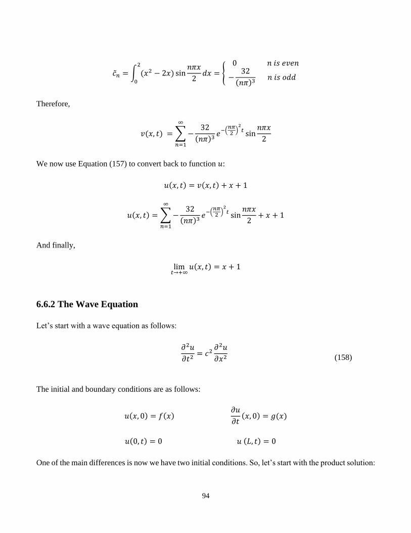
94
�̃�𝑛 = ∫ (𝑥2 − 2𝑥)2
0
sin𝑛𝜋𝑥
2𝑑𝑥 = {
0 𝑛 𝑖𝑠 𝑒𝑣𝑒𝑛
−32
(𝑛𝜋)3 𝑛 𝑖𝑠 𝑜𝑑𝑑
Therefore,
𝑣(𝑥, 𝑡) = ∑ −32
(𝑛𝜋)3𝑒−(
𝑛𝜋2
)2𝑡 sin
𝑛𝜋𝑥
2
∞
𝑛=1
We now use Equation (157) to convert back to function 𝑢:
𝑢(𝑥, 𝑡) = 𝑣(𝑥, 𝑡) + 𝑥 + 1
𝑢(𝑥, 𝑡) = ∑ −32
(𝑛𝜋)3𝑒−(
𝑛𝜋2
)2𝑡 sin
𝑛𝜋𝑥
2
∞
𝑛=1
+ 𝑥 + 1
And finally,
lim𝑡→+∞
𝑢(𝑥, 𝑡) = 𝑥 + 1
6.6.2 The Wave Equation
Let’s start with a wave equation as follows:
𝜕2𝑢
𝜕𝑡2= 𝑐2
𝜕2𝑢
𝜕𝑥2
(158)
The initial and boundary conditions are as follows:
𝑢(𝑥, 0) = 𝑓(𝑥) 𝜕𝑢
𝜕𝑡(𝑥, 0) = 𝑔(𝑥)
𝑢(0, 𝑡) = 0 𝑢 (𝐿, 𝑡) = 0
One of the main differences is now we have two initial conditions. So, let’s start with the product solution:

95
𝑢(𝑥, 𝑡) = 𝜑(𝑥)ℎ(𝑡)
Substituting the two boundary conditions gives:
𝜑(0) = 0 𝜑(𝐿) = 0
Substituting the product solution into the differential equation (Eq. 21), separating and introducing a
separation constant gives:
𝜕2
𝜕𝑡2 (𝜑(𝑥)ℎ(𝑡)) = 𝑐2
𝜕2
𝜕𝑥2(𝜑(𝑥)ℎ(𝑡))
𝜑(𝑥)𝑑2ℎ
𝑑𝑡2 = 𝑐2ℎ(𝑡)
𝑑2𝜑
𝑑𝑥2
1
𝑐2ℎ
𝑑2ℎ
𝑑𝑡2 =
1
𝜑
𝑑2𝜑
𝑑𝑥2= −𝜆
We moved the 𝑐2 to the left side for convenience and chose −𝜆 for the separation constant so the
differential equation for 𝜑 would match a known (and solved) case.
The two ordinary differential equations we get from separation of variables methods are:
𝑑2ℎ
𝑑𝑡2+ 𝑐2𝜆ℎ = 0
𝑑2𝜑
𝑑𝑥2+ 𝜆𝜑 = 0
𝜑(0) = 0 𝜑(𝐿) = 0
We have solved the boundary value problem above in the Example in solving the Heat Equation in section
6.6.1, so the eigenvalues and eigenfunctions for this problem are:
𝜆𝑛 = (𝑛𝜋
𝐿)2
𝜑𝑛(𝑥) = sin (𝑛𝜋𝑥
𝐿) 𝑛 = 1, 2, 3, … .
The first ordinary differential equation is now
𝑑2ℎ
𝑑𝑡2+ (
𝑛𝜋𝑐
𝐿)2
ℎ = 0
And because the coefficient of the ℎ is clearly positive the solution to this is
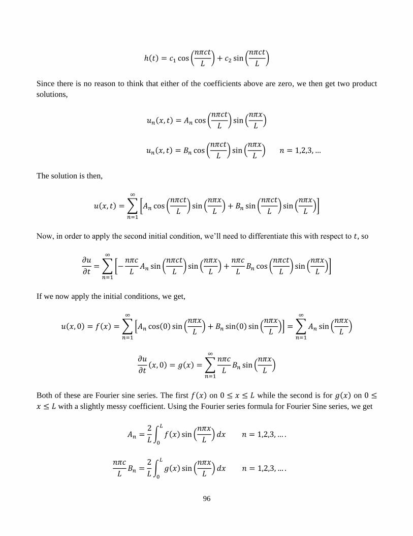
96
ℎ(𝑡) = 𝑐1 cos (𝑛𝜋𝑐𝑡
𝐿) + 𝑐2 sin (
𝑛𝜋𝑐𝑡
𝐿)
Since there is no reason to think that either of the coefficients above are zero, we then get two product
solutions,
𝑢𝑛(𝑥, 𝑡) = 𝐴𝑛 cos (𝑛𝜋𝑐𝑡
𝐿) sin (
𝑛𝜋𝑥
𝐿)
𝑢𝑛(𝑥, 𝑡) = 𝐵𝑛 cos (𝑛𝜋𝑐𝑡
𝐿) sin (
𝑛𝜋𝑥
𝐿) 𝑛 = 1,2,3, …
The solution is then,
𝑢(𝑥, 𝑡) = ∑ [𝐴𝑛 cos (𝑛𝜋𝑐𝑡
𝐿) sin (
𝑛𝜋𝑥
𝐿) + 𝐵𝑛 sin (
𝑛𝜋𝑐𝑡
𝐿) sin (
𝑛𝜋𝑥
𝐿)]
∞
𝑛=1
Now, in order to apply the second initial condition, we’ll need to differentiate this with respect to 𝑡, so
𝜕𝑢
𝜕𝑡= ∑ [−
𝑛𝜋𝑐
𝐿𝐴𝑛 sin (
𝑛𝜋𝑐𝑡
𝐿) sin (
𝑛𝜋𝑥
𝐿) +
𝑛𝜋𝑐
𝐿𝐵𝑛 cos (
𝑛𝜋𝑐𝑡
𝐿) sin (
𝑛𝜋𝑥
𝐿)]
∞
𝑛=1
If we now apply the initial conditions, we get,
𝑢(𝑥, 0) = 𝑓(𝑥) = ∑ [𝐴𝑛 cos(0) sin (𝑛𝜋𝑥
𝐿) + 𝐵𝑛 sin(0) sin (
𝑛𝜋𝑥
𝐿)]
∞
𝑛=1
= ∑ 𝐴𝑛
∞
𝑛=1
sin (𝑛𝜋𝑥
𝐿)
𝜕𝑢
𝜕𝑡(𝑥, 0) = 𝑔(𝑥) = ∑
𝑛𝜋𝑐
𝐿𝐵𝑛 sin (
𝑛𝜋𝑥
𝐿)
∞
𝑛=1
Both of these are Fourier sine series. The first 𝑓(𝑥) on 0 ≤ 𝑥 ≤ 𝐿 while the second is for 𝑔(𝑥) on 0 ≤
𝑥 ≤ 𝐿 with a slightly messy coefficient. Using the Fourier series formula for Fourier Sine series, we get
𝐴𝑛 =2
𝐿∫ 𝑓(𝑥) sin (
𝑛𝜋𝑥
𝐿) 𝑑𝑥 𝑛 = 1,2,3, … .
𝐿
0
𝑛𝜋𝑐
𝐿𝐵𝑛 =
2
𝐿∫ 𝑔(𝑥) sin (
𝑛𝜋𝑥
𝐿) 𝑑𝑥 𝑛 = 1,2,3, … .
𝐿
0
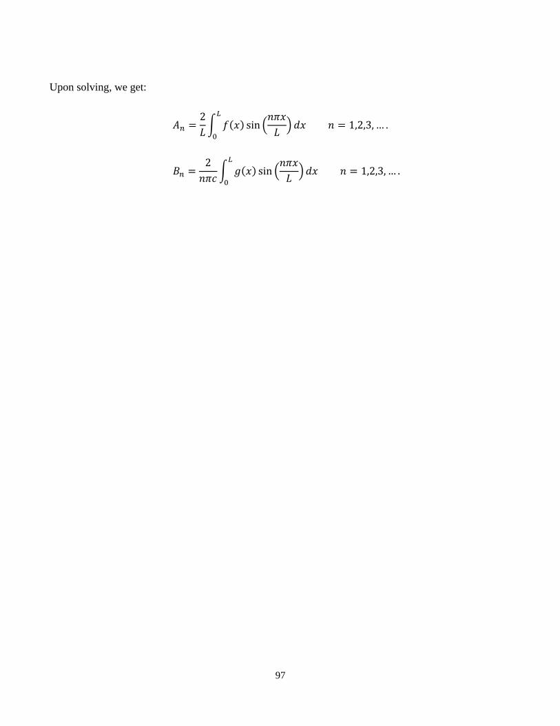
97
Upon solving, we get:
𝐴𝑛 =2
𝐿∫ 𝑓(𝑥) sin (
𝑛𝜋𝑥
𝐿) 𝑑𝑥 𝑛 = 1,2,3, … .
𝐿
0
𝐵𝑛 =2
𝑛𝜋𝑐∫ 𝑔(𝑥) sin (
𝑛𝜋𝑥
𝐿)𝑑𝑥 𝑛 = 1,2,3, … .
𝐿
0
Related Documents


![Applied Mathematics Introductory Module - PDST Maths Module [final].pdf · Applied Mathematics Introductory Module ... Science, Technology and ... ii. how to form mathematical models](https://static.cupdf.com/doc/110x72/5af58cc37f8b9a4d4d8f3bdb/applied-mathematics-introductory-module-maths-module-finalpdfapplied-mathematics.jpg)