Aero Model Implementation

1

SIMULATOR AERO MODEL IMPLEMENTATION

Thomas S. Alderete1

SUMMARY

A general discussion of the type of mathematical model used in a real-time, flightsimulation is presented. It is recommended that the approach to math model developmentinclude modularity and standardization as modification and maintenance of the modelwill be much more efficient with this approach. The general equations of motion for anaircraft are developed in a form best suited to real time simulation. Models for a fewhelicopter subsystems are discussed in terms of general approaches that are commonlytaken in today's simulations.

INTRODUCTION

This chapter is intended to provide the reader with a understanding of the type ofmathematical model used in a real-time flight simulation. A flight simulation system isstudied in order to gain a better understanding of the real (or planned) aircraft. Theunderstanding or knowledge to be gained can be in a wide variety of areas including,engineering studies, handling qualities, or pilot training. To properly perform simulation,we need a total system, including a mathematical model, simulator hardware, visualsystem, and motion system, whose behavior is sufficiently similar to the real aircraft inthe areas under investigation. The mathematical model is a key part of this totalsimulation system.

Before delving into some of the technical aspects, it is important to examine what ismeant by the phrase "mathematical model", or more simply, "math model". Is it theequations and data that describe the aircraft's behavior? Is it the computer program andall the associated data used to compute where the aircraft is and what it is doing? Does itinclude "fudge factors" used to "tune-up" the simulation's performance? What about allthe integration algorithms and numerical "tricks" to improve the solution; are they part ofthe math model? Naturally, there are different opinions as to what the math modelincludes; the following provides a definition useful to the present discussion.

The mathematical model is the description and specification of the aircraft's dynamicbehavior. This "behavior" comprises the various motions of the airframe and the statesand performance of the various subsystems, such as the engine, landing gear, andavionics. The math model considers all the external and internal influences on theaircraft and defines the resultant states of the aircraft and it's subsystems.

The model is best presented by mathematical equations, schematic diagrams, logicdiagrams, tables and graphs of data including geometry, aerodynamic coefficients, gainschedules, etc. These engineering equations, diagrams, and data comprise themathematical model.

The digital computer program and its associated data is an implementation of themathematical model. It is not the model itself, but rather a method (non-unique) ofcomputing the model. The answers obtained via these calculations are used to validatethe mathematical model. The basic idea of validation (covered elsewhere in this volume) 1 NASA Ames Research Center, Moffett Field, California.

2

is twofold. One issue is to verify whether or not the program accurately solves theequations of the model. The other issue is to validate that the model accurately describes(predicts) the behavior of the real aircraft.

SCOPE

This discussion of simulation mathematical modeling will describe the general elementsof a model. The complete model can be thought of in two parts, the general equations ofmotion and the specific aircraft subsystems. The general equations of motion for a rigidbody will be derived. Since these equations and their derivation are well known, not alldetails will be given here. Emphasis will be given to a particular form of the generalequations that is best suited to real time simulation. Modeling methods for varioussubsystems such as aerodynamics, engine, control systems, and so forth will be discussedin much less detail, without derivation or specific model examples. The subsystems are,of course, specific to a given aircraft design and configuration. Some general approachesused in today's simulations will be discussed.

THE SIMULATION MATHEMATICAL MODEL

Model Structure

The common and highly recommended approach to math model development is toemploy the principles of modularity and standardization. Later, when the computerprogram implementation of the math model is designed, these principles will provide asignificant pay-off in efficiency and maintainability. A modular approach requires thatthe model be broken down into smaller parts that share information and interact in clearand meaningful ways. The modules usually follow along lines that correspond to thephysical components of the aircraft (the program design may not). Standardization ofaxis systems, nomenclature, and various mathematical and engineering conventions alsohas significant benefits both in the programming implementation and in communicatingthe meaning of the model to others. These principles have great economic benefit if morethan one type or model of aircraft is to be simulated. Modules can be updated or replacedwithout a complete program rewrite. Also, standardization allows modules to be sharedbetween different simulations.

With a modular approach to math modeling, it becomes necessary to define informationinterfaces. What does each module need for input? What does it provide as output toother modules? In some cases, an output requirement is defined by some other module.For instance, the rotor module may not actually need to compute "horsepower required"to model all the rotor states, but a transmission module may require it. Some moduleswill require inputs and/or will provide outputs to the "outside world", that is, external toany modeling. Pilot controls are an example of an external input and pilot stationaccelerations might be an example of a output needed for a motion generation system, butnot by the model itself.

In Fig. 1 below, a typical model organization is depicted. The bubbles indicate aparticular module and the lines and arrows indicate information flow. Certainly there willbe numerous other modules and other information paths as dictated by the actual aircraft'ssubsystems. Also, it would be common for nearly all the modules to have access to theenvironmental parameters and the aircraft's state variables.

3

The modular breakdown of the math model shown in Fig. 1 suggests a major designapproach and some guidelines for standardization. The modules to the left of thesummation bubble all are specific to a particular aircraft. The summation, equations ofmotion, and environment are general to all aircraft and can form the standard or "core"modules for any simulation. The specific description of a particular aircraft shouldinclude the aerodynamic, propulsion, and landing gear forces and moments acting on theaircraft center of gravity. The standard modules sum the reactions and produce aircraftstate variables (as well as numerous ancillary computations).

Figure 1 Typical Model Organization

External Inputs

State VariablesAero

Engine

Controls

Gear

Rotor

Force & Moment Summation

Equations of Motion

Environment

The math model will be examined in two steps. First the general equations of motion thatform the core of the simulation will be developed. All the equations necessary to predictthe aircraft's state when the external forces and moments are known will be derived. Astandard text on dynamics should provide any details omitted in this treatment (Refs. 1,2). Next, some of the typical aircraft specific modules will be examined. The equationsfor these modules will not be derived or presented in any detail. Instead, a generaldiscussion will give the reader some idea of what might be included in an actual model.

General Equations of Motion

An aircraft in flight has six degrees of freedom, three translational and three rotational. Ifthe equations are written relative to the aircraft's center of mass, the translational androtational sets of equations are independent of each other and can be derived separately.For this derivation, a non-rotating earth will be assumed which simplifies theunderstanding of the equations. If required, the effects of the earth's rotation can beadded to the general equations at a later time without much difficulty. Also, wind andturbulence are not considered in the derivation that follows. Guidance on how airdisturbances may be added is given in a later section.

Axis Systems. Before beginning the derivation, the various axis systems that arecommonly used in flight simulation will be discussed. These axis systems are germane tothe equations of motion. Other axis systems will be mentioned when discussing some ofthe aircraft subsystems.

Body Axis. The equations of motion are written with respect to the body axis system.Referring to Fig. 2, the body axis has its origin at the aircraft center of gravity, CG. The

4

x-axis is pointed forward out the nose; the y-axis is pointed out the right side of theaircraft, and the z-axis is directed down through the underside of the aircraft. The bodyaxis is fixed to the aircraft and moves along with it. It forms a right-handed triad.

Y-axis

X-axis

Z-axis

Figure 2 Body Axis System

Local Axis System. The local axis system also has its origin at the aircraft's CG, but hasa fixed orientation. The XL-axis always points north, the YL-axis points east, and the ZL-axis points down. The local frame is depicted in Fig. 3.

Inertial Axis System. For purposes of this discussion, an inertial frame is taken as onethat has its origin fixed at some point on the earth's surface. (For a rotating earth, placingthe origin at the earth's center would be a better choice.) Its fixed orientation is the sameas the Local frame and is also depicted in Fig. 3.

Turning attention once again to the body axis system, some other definitions andrelationships can be developed. Whenever the x, y, or z axes are referred to without anysubscripts, the body axis is implied. The six body axis velocities are shown in Fig. 3.The terms u, v, and w are the body axis translational velocities in the x, y, and zdirections, respectively. The terms p, q, and r are the body axis rotational velocitiesabout the x, y, and z axes, respectively.

The aircraft orientation is described by an ordered set of three Euler angles, ψ , θ, and φ ,that relate the orientation of the body axis relative to the local axis system. In Fig. 4, theaxis system designated by X1, Y1, and Z1, is the initial reference orientation (in thiswork, it corresponds to the Local frame). First, the aircraft is given a rotation,ψ , aboutthe Z1 axis in the sense shown in the figure. This aligns the body axis with the systemlabeled X2, Y2, and Z2. Next, the aircraft is rotated by,θ, about the Y2 axis. The resultis now the X3, Y3, and Z3 frame. Finally, the aircraft is rotated by,φ , about the X3 axis,yielding the X, Y, Z frame, the final orientation of the body axis system.

5

Figure 3 Inertial (E), Local (L), And Body (B) Axes

XE

YE

ZE

XL

YL

ZL

XB

YB

ZB

Flight Path

North

North

u

v

w

p

q

r

X1

X2

X3, X

Y1

Y2, Y3

Y

Z1, Z2Z3Z

Figure 4 Aircraft Orientation Using Euler Angles

A pair of useful transformation matrices are those that rotate a vector from the Local toBody axis system and from the Body to Local axis system. Referring again to Fig. 4, thefollowing three equations can be written.

6

The first rotation, ψ , results in

X

Y

Z

X

Y

Z

2

2

2

1

1

1

0

0

0 0 1

= −

cos sin

sin cos

ψ ψψ ψ

Next, the rotation, θ, results in

X

Y

Z

X

Y

Z

3

3

3

2

2

2

0

0 1 0

0

=−

cos sin

sin cos

θ θ

θ θ

And, finally, the rotation φ, yields

X

Y

Z

X

Y

Z

=−

1 0 0

0

0

3

3

3

cos sin

sin cos

φ φφ φ

Combining the three matrix multiplications into one, results in

X

Y

Z

X

Y

Z

=−

− + ++ − +

cos cos sin cos sin

sin cos cos sin sin cos cos sin sin sin cos sin

sin sin cos sin cos cos sin sin sin cos cos cos

ψ θ ψ θ θψ φ ψ θ φ ψ φ ψ θ φ θ φ

ψ φ ψ θ φ ψ φ ψ θ φ θ φ

1

1

1

This transformation matrix will be referred to as LtoB[ ] (read "local to body"), and theabove equation can be written as

X

Y

Z

LtoB

X

Y

Z

B

B

B

L

L

L

= [ ]

Also, since the transformation matrix is orthogonal, the inverse matrix can be obtained bya simple transpose. Therefore,

BtoL LtoB LtoB T[ ] = [ ] = [ ]−1

and

X

Y

Z

BtoL

X

Y

Z

L

L

L

B

B

B

= [ ]

7

Translational Equations. The equations of motion are developed in the body axissystem since the external forces are most easily defined in a coordinate system fixed inthe aircraft. If

vF is the total external force acting on the aircraft,

vv is the absolute

velocity of the center of mass, and m is the aircraft mass, then the following can bewritten.

v vF mv= ˙

The vF and

vv vectors may be written in terms of their x, y, and z components.

v

v

F F i F j F k

v ui vj wk

x y z= + +

= + +

ˆ ˆ ˆ

ˆ ˆ ˆ

where ˆ, ˆ,i j and k are an orthogonal triad of unit vectors aligned with the x, y, and z bodyaxes, respectively. If the aircraft (and the body axis frame) is rotating with angularvelocity

vω , then the absolute acceleration can be found as follows.

v v v v˙ ( ˙)v v vr= + ×ω

Where (˙)vv r is the acceleration as viewed from the body axis system and the " × " symbol

signifies a vector cross product. This expression for the rate of change of a vector in arotating system will be used repeatedly in the following derivations. The relativeacceleration can be expanded as:

(˙) ˙ˆ ˙ˆ ˙ ˆvv ui vj wkr = + +

Also, the rotational velocity vector can be written as:

vω = + +pi qj rkˆ ˆ ˆ

Now the cross product can be evaluated and written as follows.

v vω × = − + − + −v wq vr i ur wp j vp uq k( )ˆ ( ) ˆ ( ) ˆ

Gathering terms and writing the vector equation in terms of three scalar relationships, wehave:

F m u wq vr

F m v ur wp

F m w vp uq

x

y

z

= + −= + −

= + −

( ˙ )

( ˙ )

( ˙ )

Note that in some formulations, the gravitational force terms are explicitly written at thisjuncture. They are not included here for reasons to be made clear later. However, forillustration, the three force components could be written as follows.

8

F F mg

F F mg

F F mg

x x Applied

y y Applied

z z Applied

= −

= +

= +

sin

cos sin

cos cos

θθ φθ φ

Rotational Equations. If v

M is the total external moment acting at the center of massand

vH is the angular momentum, then the following can be stated.

v v

M H= ˙

The applied moment, v

M , can be written as:

v

M Li Mj Nk= + +ˆ ˆ ˆ

The first task will be to write an expression for the angular momentum, then find its rateof change with respect to time. The angular momentum of a rigid body about it center ofmass is given by

v v vH R m Ri

ii i= ×∑ ˙

where vR is the position vector of a particle mi . Assuming the position of each particle is

fixed in the body, then the velocity of each particle is simply

v v vR Ri i= ×ω

where vω is the absolute angular velocity of the body. Further assuming that the body has

a continuous mass distribution, the particle mass can be represented by its density timesan elemental volume, ρ dV (mass density is ρ ). Substituting the expressions for velocityand elemental volume, the summation can be replaced by an integral as follows.

v v v vH R R dV

V= × ×∫ ρ ω( )

Let vR xi yj zk= + +ˆ ˆ ˆ for a given elemental volume and, as previously,

vω = + +pi qj rkˆ ˆ ˆ .The vector cross products can be written as follows.

v v vR R y z p xyq xzr i

yxp x z q yzr j

zxp zyq x y r k

× × = + − −[ ]+ − + + −[ ]+ − − + +[ ]

( ) ( ) ˆ

( ) ˆ

( ) ˆ

ω 2 2

2 2

2 2

Now, the moments and products of inertia can be defined as

9

I y z dV

I x z dV

I x y dV

I I xydV

I I xzdV

I I yzdV

xx V

yy V

zz V

xy yx V

xz zx V

yz zy V

= +

= +

= +

= =

= =

= =

∫∫∫

∫∫∫

ρ

ρ

ρ

ρ

ρ

ρ

( )

( )

( )

2 2

2 2

2 2

Substituting these definitions, plus the cross product terms, the angular momentumbecomes

vH I p I q I r i

I p I q I r j

I p I q I r k

xx xy xz

yx yy yz

zx zy zz

= − −

+ − + −

+ − − +

( )ˆ

( ) ˆ

( ) ˆ

For the typical aircraft case of symmetry with respect to the xz-plane

I I I Ixy yx yz zy= = = = 0

Simplifying the expression for angular momentum, we have

vH I p I r i I q j I p I r kxx xz yy xz zz= − + + − +( )ˆ ( ) ˆ ( ) ˆ

Now, turning attention back to the rotational equation of motion, the time rate of changeof angular momentum can be written as

v v

v v vM H

H Hr

=

= + ×

˙

( ˙ ) ωwhere (

˙ )vH r is the rate of change of angular momentum observed from the body axis

system (rotating system). Expanding terms

(˙ ) ( ˙ ˙)ˆ ˙ ˆ ( ˙ ˙) ˆv

H I p I r i I q j I p I r kr xx xz yy xz zz= − + + − +

and,

10

v vω × = − + − + −

= − + −[ ]+ − − − +[ ]+ − −[ ]

H H q H r i H r H p j H p H q k

I p I r q I q r i

I p I r r I p I r p j

I q p I p I r q k

z y x z y x

xz zz yy

xx xz xz zz

yy xx xz

( )ˆ ( ) ˆ ( ) ˆ

( ) ( ) ˆ

( ) ( ) ˆ

( ) ( ) ˆ

Collecting terms and writing in terms of three scalar equations.

L I p I r I pq I I qr

M I q I I pr I p r

N I r I p I I pq I rq

xx xz xz zz yy

yy xx zz xz

zz xz yy xx xz

= − − + −

= + − + −

= − + − +

˙ ˙ ( )

˙ ( ) ( )

˙ ˙ ( )

2 2

The above three equations, plus the three translational equations comprise the equationsof motion for the rigid body aircraft. However, a number of problems arise if theseequations are used to compute the aircraft's dynamic state for simulation purposes.

With the translational equations, one problem is that the body axis is moving along theflight path and so the position of the aircraft relative to some fixed point (like a runway)is not easily specified. Another problem or "undesirable" feature is the presence of thevarious products involving rotational velocity terms, such as (wq) and (vr). These termscould cause problems with numerical accuracy when rotational velocities have largemagnitude or frequency content. This situation is remedied by a transformation to aninertial frame, located on the earth's surface.

For the rotational equations, one problem is that the equations are coupled via ˙,p ˙,q and˙,r which can lead to complications during numerical integration. To resolve thatproblem, the three equations can easily be decoupled by algebraic manipulation. Anotherissue is that the aircraft orientation cannot be found by simply integrating the rotationalvelocities. A change of variables is required to some other set of parameters, such asEuler angles.

Transformation of Translational Equations to an Inertial Frame. For the flat, non-rotating earth considered here, any fixed frame of reference can be employed as aninertial frame. The three forces acting on the aircraft center of gravity in the body axissystem are rotated back through the Euler angles to the local frame and translated back tosome convenient origin.

Again, the rotation from body axes to the local frame is given by

F

F

F

BtoL

F

F

F

N

E

D

x

y

z

= [ ]

Where the subscripts, N, E, and D designate north, east, and down pointing directions.The accelerations are then

11

˙

˙

˙

/

/

/

V

V

V

F m

F m

F m

N

E

D

N

E

D

=

A note can be made here about computer program implementation. If the body axisforces are taken so as to not include the gravitational terms, then the aircraft's weight canbe added into the above equation as follows.

˙

˙

˙

/

/

( ) /

V

V

V

F m

F m

F weight m

N

E

D

N

E

D

=+

This implementation avoids having to rotate the gravitational terms twice. That is,instead of projecting the aircraft weight into the body axis and then rotating the summedforces into the inertial frame, the above suggestion allows the weight to be summeddirectly into the "down" force component in the inertial frame.

The accelerations can then be integrated to get velocities in the local frame and integratedagain for displacements. The displacements can be referenced to any convenient locationsuch as a runway threshold, navigation waypoint, or whatever is most useful to asimulation. The set of translational equations previously defined in the body axis systemwill prove useful for computing body axis accelerations at a later time.

Modifications to the Rotational Equations. The equations for L, M, and N aremanipulated to yield ˙,p ˙,q and r on the left-hand side. The results are the following.

˙( ) ( )

pI

DL

I

DN

I I I I

Dpq

I I I I

Drqzz xz xx yy zz xz yy zz zz xz= + +

− +

+− −

2

˙( )

( )qI

MI I

Ipr

I

Ir p

yy

zz xx

yy

xz

yy

= + − + −1 2 2

˙( ) ( )

rI

DL

I

DN

I I I I

Dpq

I I I I

Drqxz xx xx yy xx xz yy xx zz xz= + +

− +

+

− −

2

where D is defined as

D I I IXX ZZ XZ= − 2

These uncoupled equations can now be integrated with respect to time to obtain p, q, andr. The resultant rotational velocities cannot be integrated to get angular displacements.That is, one cannot find a set of three parameters which define the aircraft's orientationand have p, q, and r as their time derivatives. In some formulations, direction cosines areused to describe the angular orientation. This involves nine direction cosines and sixequations of constraint. One can also use various four parameter systems, so calledquaternions. Quaternions have the advantage of not having singularities (gimbal lock),

12

having one half the frequency content, and involve one equation of constraint. Aircraftorientation can also be specified by the use of Euler angles. Remember that Euler anglesare an ordered set of three parameters and that there will be a singularity when the aircraftis pointed straight up or down.

What is needed is a relationship between time rates of change of the Euler angles and the

body axis rotational rates. Assume that v,φ

v,θ and

vψ are the angular velocity vectors associated with rates of change in the corresponding Euler angles. Then the totalrotational rate vector can be written as

v v v v

ω ψ θ φ= + +˙ ˙ ˙

Note that v,φ

v,θ and

vψ are not a mutually orthogonal vector triad, but are non-orthogonalcomponents of

vω . Referring to Fig. 5,

Figure 5 Euler Angle Rates

relationships can be written between the body axis rotational rates and v,φ

v,θ and

vψ by

summing the orthogonal projections of v,φ

v,θ and

vψ onto the x, y, and z axes.

p

q

r

= −

= +

= −

˙ ˙ sin

˙ cos ˙ cos sin

˙ cos cos ˙sin

φ ψ θ

θ φ ψ θ φ

ψ θ φ θ φ

or conversely,

13

˙ ( sin cos )sec

˙ cos sin

˙ ( sin cos ) tan

ψ φ φ θ

θ φ φ

φ φ φ θ

= +

= −

= + +

q r

q r

p q r

Now with this last transformation we can change from the body axis rotational rates toEuler angle rates. The Euler angle rates can be integrated with respect to time to yield theEuler angles, thus specifying the aircraft's orientation. Keep in mind that the

relationships are undefined at θ π= ±2

. Though not presented here, there are methods of

treating this singularity if required.

Other Relationships. There are a number of other important relationships between thevarious state variables. Once the translational accelerations in the local frame areformed, they can be integrated to obtain velocities and again for displacements, thus

V

V

V

V

V

V

dtN

E

D

N

E

D

=

∫˙

˙

˙

and

D

D

D

V

V

V

dtN

E

D

N

E

D

=

∫

The velocities can be transformed to the body axis system to yield u, v, and w.

u

v

w

LtoB

V

V

V

N

E

D

= [ ]

Using the translational equations of motion that were written in the body axis system, thebody axis accelerations can be solved for as follows.

˙

˙

˙

/

/

/

˙

˙

˙

u

v

w

vr wq

wp ur

uq vp

F m

F m

F m

vr wq

wp ur

uq vp

LtoB

V

V

V

x

y

z

N

E

D

=−−−

+

=−−−

+ [ ]

The body axis velocities can be used to obtain the aircraft angle of attack and sideslip.

14

α

β

=

=+

−

−

tan ( )

tan (( )

)

1

1

2 2

w

uv

u w

Equation Summary. Given that the forces and moments acting on the aircraft's CGhave been summed, the translation dynamics are described by the following equations.

F

F

F

BtoL

F

F

F

N

E

D

x

y

z

= [ ]′′′

(where the primes indicates body axis forces without gravitational terms)

˙

˙

˙

/

/

( ) /

V

V

V

F m

F m

F weight m

N

E

D

N

E

D

=+

V

V

V

V

V

V

dtN

E

D

N

E

D

=

∫˙

˙

˙

D

D

D

V

V

V

dtN

E

D

N

E

D

=

∫

˙

˙

˙

˙

˙

˙

u

v

w

vr wq

wp ur

uq vp

LtoB

V

V

V

N

E

D

=−−−

+ [ ]

u

v

w

LtoB

V

V

V

N

E

D

= [ ]

The rotational dynamics are defined by the following equations.

˙( ) ( )

pI

DL

I

DN

I I I I

Dpq

I I I I

Drqzz xz xx yy zz xz yy zz zz xz= + +

− +

+− −

2

˙( )

( )qI

MI I

Ipr

I

Ir p

yy

zz xx

yy

xz

yy

= + − + −1 2 2

15

˙( ) ( )

rI

DL

I

DN

I I I I

Dpq

I I I I

Drqxz xx xx yy xx xz yy xx zz xz= + +

− +

+

− −

2

D I I IXX ZZ XZ= − 2

p

q

r

p

q

r

dt

=

∫˙

˙

˙

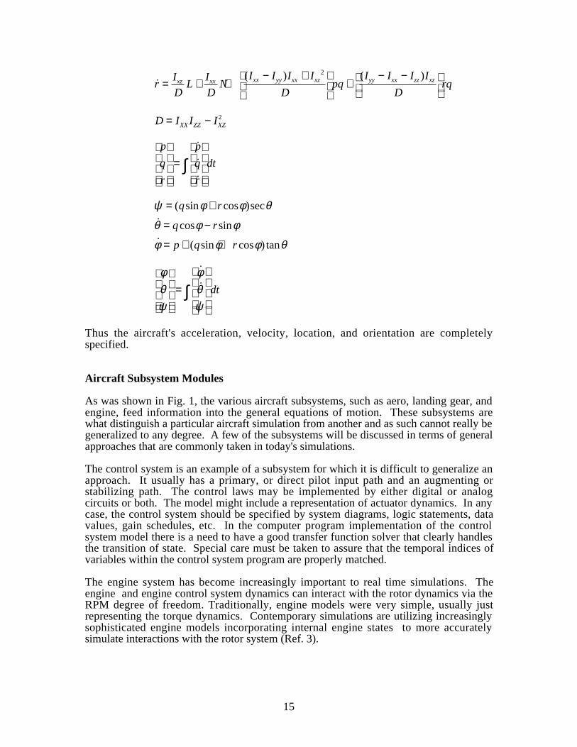
˙ ( sin cos )sec

˙ cos sin

˙ ( sin cos ) tan

ψ φ φ θ

θ φ φ

φ φ φ θ

= +

= −

= + +

q r

q r

p q r

φθψ

φθψ

=

∫˙

˙

˙

dt

Thus the aircraft's acceleration, velocity, location, and orientation are completelyspecified.

Aircraft Subsystem Modules

As was shown in Fig. 1, the various aircraft subsystems, such as aero, landing gear, andengine, feed information into the general equations of motion. These subsystems arewhat distinguish a particular aircraft simulation from another and as such cannot really begeneralized to any degree. A few of the subsystems will be discussed in terms of generalapproaches that are commonly taken in today's simulations.

The control system is an example of a subsystem for which it is difficult to generalize anapproach. It usually has a primary, or direct pilot input path and an augmenting orstabilizing path. The control laws may be implemented by either digital or analogcircuits or both. The model might include a representation of actuator dynamics. In anycase, the control system should be specified by system diagrams, logic statements, datavalues, gain schedules, etc. In the computer program implementation of the controlsystem model there is a need to have a good transfer function solver that clearly handlesthe transition of state. Special care must be taken to assure that the temporal indices ofvariables within the control system program are properly matched.

The engine system has become increasingly important to real time simulations. Theengine and engine control system dynamics can interact with the rotor dynamics via theRPM degree of freedom. Traditionally, engine models were very simple, usually justrepresenting the torque dynamics. Contemporary simulations are utilizing increasinglysophisticated engine models incorporating internal engine states to more accuratelysimulate interactions with the rotor system (Ref. 3).

16

Aerodynamic Model. To simulate the aircraft in all flight regimes, a fairlycomprehensive, total force aerodynamic model is usually required. The model shouldseparate the various airframe components, such as fuselage, wings, empennage, and anyother attachments. This separation allows the inclusion of local effects of the airstreamsuch as rotor wake, wing downwash, air turbulence, and other disturbances. The mostcommon approach to modeling the aerodynamic forces and moments is with the use oftables of aerodynamic coefficients.

The data is normally produced from wind tunnel tests where lift, drag, and pitch momentsare measured over a range of angles of attack, sideslip, and if appropriate, Mach number.This basic data, in a variety of combinations and for various airframe components makesup the "aero data" for the simulation model.

The aero data is usually in dimensionless coefficient form in the wind axis system. Thesecoefficients are computed by taking the force (lift or drag) and dividing by the term1

2

2ρv A , where ρ is the air density, v is the velocity relative to the air mass, and A is a

reference area (such as wing area). The moments are divided by ρv Al2 , where l is areference length (such as wing cord). The wind axis differs from the body axis byrotations through the angles of attack and sideslip. It must be noted that many variationsexist for the definitions of the coefficients and the of wind axis. A specific model mustdefine the conventions being used.

The typical scheme for modeling the "aero" is to define the local velocities, Machnumber, and angles of attack and sideslip. If the horizontal stabilizer is taken as anexample; the local velocity would be the velocity at the aircraft CG, modified by bodyrotational rates and wake effects from the wing, fuselage, and/or rotor system. The localangles of attack and sideslip are defined with respect to the local velocity components.Aerodynamic coefficients are found (interpolated) in the database using, for instance, theangle of attack and elevator deflection. The forces are found by multiplying thecoefficients by the non-dimensionalizing factors. The forces and moments aretransformed through the angles of attack and sideslip to the body axis. In some cases, theequations for wind axis forces and moments can become quite complicated as variousinfluences are modeled. Sideslip, rate of change of downwash, and airstream blockagesare examples. By modeling each airframe component separately, these specialconsiderations can easily be included. Once all the aerodynamic forces and moments foreach subsystem are modeled, they can be summed at the aircraft CG.

Helicopter Main Rotor Model. The rotor system model is usually the mostcomplicated module of the entire simulation mathematical model. Historically, the rotormodel was severely limited in complexity due to computational difficulties of running themodel in real time. With today's low cost, high speed computing systems, modelers arecontinually adding detail and new complexities to the model. The rotor modelingmethods are too vast to examine in any detail here, but general aspects will be discussed.

There are two modeling approaches used extensively by simulations; the blade elementmethod which is dominant in contemporary simulations, and the tip-path-plane methodwhich has a considerably reduced computational requirement (Refs. 4, 5, 6). For theblade element approach, the rotor blade dynamics are represented by degrees of freedomin a rotating coordinate system that spins with the rotor itself. The forces and momentsare defined in this rotating frame and summed at the hub. The tip-path-plane approachmakes use of a Fourier transformation to represent the rotor dynamics in a non-rotating

17

coordinate system. Essentially, the rotor is treated as a tilting disk and forces andmoment are described in this non-rotating frame. The discussion that follows willdescribe the general approach for the blade element modeling method.

The rotor model can be divided into several submodules; the rotor induced velocity orinflow, blade dynamics, rotor forces and moments, and various coordinatetransformations. The inflow model is the least exact submodule of the rotor model. Thesimple models in use today typically have a uniformly distributed component that comesfrom momentum theory plus harmonically distributed components based upon theperiodic moments acting on the rotor disk. It is also common to impose a "dynamic"behavior to the inflow by the use of empirically derived time lags.

The blade motions are represented by complex dynamic equations that are non-linear andhave periodic coefficients. The blades move as rigid bodies about a specific hinge orbearing arrangement. Various elastic modes of blade motion can also be represented.From these equations the blade velocities and displacements are known. Combining theblade state with the local velocities (airframe, rotor, and inflow), the blade loads can bedescribed. In the blade element model, the blade aerodynamic forces and moments aredefined in a manner similar to other areas of the helicopter aerodynamic model(described above). The blade is divided into a number of radially distributed segments(elements). For each segment, the local velocity and angle of attack are found.Tabulated values of section lift, drag, and pitch moment are interpolated to find the aeroforces and moments at each segment. The forces and moments are summed along eachblade and for all blades of the rotor.

There are a number of additional coordinate systems that can come into play with therotor model. The axis system conventions differ depending on the physical arrangementsof a particular rotor design. Typically there is an axis system that is a body axis alignedwith the rotor shaft. There are various rotating axis systems that progress from the hub,across the blade hinge points, and out to the blade segments. Finally, there is a wind axissystem at each blade segment where the aerodynamic forces and moments are defined.As one would imagine, it is absolutely necessary to carefully define each axis system andthe transformations from one to another in the model.

With the availability of high speed, parallel computer systems, new areas of rotor systemmodeling for simulation purposes have become possible. Modelers are adding elasticmodes to the blade dynamics and dynamic wake models to achieve a much higher fidelityrepresentation of rotor inflow (Refs. 7, 8). Combined, these advancements make possiblea real time, aeroelastic rotor model.

Tail Rotor Model. The mathematical model of the helicopter tail rotor is usually muchsimpler than that of the main rotor. Modern high speed computer systems allow tail rotormodels of greater complexity, but the benefits are not significant for most purposes. Formost cases it is sufficient to model the thrust and required torque of the tail rotor.

A common method for representing the tail rotor in a simple fashion is with the use of theBailey theory (Ref. 9). This is a closed form approach that uses parameters that onlydepend on blade pitch and the inflow ratio. A set of "t" coefficients are computed that arein turn used to calculate thrust and torque required. The thrust is resolved into body axisforces and moments. Torque can then be made available to a drive train model.

18

Environmental Model. The simulation requires certain characteristics about theairmass. The aero and engine models require air density, pressure, and temperature. Theaero model requires airmass velocities including steady or variable winds and gusts, windshears, and air turbulence. The first items are fairly standard and can be referred to as theatmospheric model. Simulations can use the standard atmospheric databases, "hot day"databases, or any collection of special ones (Ref. 10, 11). The databases are usuallyinterpolated with aircraft altitude to yield density, pressure, and temperature.

The velocity variations of the airmass are best modeled in two parts; the lower frequency,deterministic gusts, shears, and steady winds, and the higher frequency, randomturbulence. The deterministic velocities are defined in the fixed (inertial) frame ofreference and can be modeled as functions of time and spatial coordinates. A reasonablemethod of implementing these winds is to add them to the inertial velocities and thenrotate them to the body axis. These new definitions for the body axis translationalvelocities, u, v, and w, make them "relative velocities", i.e., relative to the wind. Theyare the velocities upon which aero forces and moments are based.

Air turbulence is usually represented by a statistical model (Ref. 2). These modelstypically assume the velocity variation to be random, isotropic, and with negligible cross-correlation between components. These models also assume Taylor's hypothesis, or thefrozen field concept, which states that a patch of turbulence is constant or "frozen intime". Grossly stated, each component of turbulence is modeled by running a normallydistributed noise signal through a shaping filter or correlation function. The Dryden andvon Karman models are examples. These models use a characteristic scale length whichcan be taken as a wing span or a rotor radius. The turbulence models have beencommonly used for fixed wing aircraft and have been "forced" into rotorcraft models.Because of the rotating blades, however, these models were not really appropriate torotorcraft. Recent work (Ref. 12) has attempted to improve the modeling for the case ofrotational sampling of the turbulent field.

SUMMARY REMARKS

In this chapter a general discussion of the type of mathematical model used in a real-time,flight simulation was presented. The mathematical model was defined as a descriptionand specification of the aircraft's dynamical behavior. This behavior comprises thevarious motions of the airframe and the states and performance of the varioussubsystems, such as the engine, landing gear, and avionics. The model is best presentedby mathematical equations, schematic diagrams, logic diagrams, tables and graphs of dataincluding geometry, aerodynamic coefficients, gain schedules, etc. These engineeringequations, diagrams, and data comprise the mathematical model.

It is recommended that the approach to math model development include modularity andstandardization. Standard conventions should be defined and adhered to by all modules.The information interfaces among modules must be defined as well as any interfaces tothe "outside world". Modification and maintenance of the model will be much moreefficient with this approach.

The discussion of simulation mathematical modeling included the general equations ofmotion and the specific aircraft subsystems. The general equations of motion that formthe core of the simulation were developed along with all the equations necessary topredict the aircraft's state when the external forces and moments are known. Finally,some of the typical aircraft specific modules were examined to give the reader some ideaof what might be included in contemporary flight simulation models.

19

SYMBOLS

DN, DE, DD aircraft position in the local axis system, ft

vF total external force acting on the aircraft, lb

Fx, Fy, Fz components of the total external force acting on the aircraft in the x, y,and z directions, respectively, lb

FN, FE, FD components of the total external force acting on the aircraft in the localaxis system , lb

g acceleration due to gravity, ft/sec/sec

vH the angular momentum, ft-lb-sec

Ixx, Iyy, Izz moments and products of inertia, lb-sec2-ftIxy, Ixz, Iyz

ˆ, ˆ,i j k orthogonal triad of unit vectors aligned with the x, y, and z body axes,respectively

L, M, N components of total moment about the x, y, z directions, ft-lb

m the aircraft mass, slugs (lb-sec2/ft)

v

M total external moment acting at the center of mass, ft-lbs

p, q, r the body axis rotational velocities about the x, y, and z axes,respectively, r/sec

u,v,w the body axis translational velocities in the x, y, and z directions,respectively, ft/sec

vv the absolute velocity of the center of mass, ft/sec

VN, VE, VD aircraft velocities in the local axis system, ft/sec

x, y, z the body axis; origin at the aircraft CG, the x-axis is pointed forwardout the nose; the y-axis is pointed out the right side of the aircraft, andthe z-axis is directed down through the underside of the aircraft

XL, YL, ZL the local axis; origin at the aircraft's CG with a fixed orientation, theXL-axis always points north, the YL-axis points east, and the ZL-axispoints down

XE, YE, ZE the inertial axis; origin fixed at some point on the earth's surface, XE-axis always points north, the YE-axis points east, and the ZE-axispoints down

20

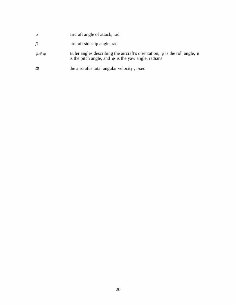
α aircraft angle of attack, rad

β aircraft sideslip angle, rad

φ ,θ , ψ Euler angles describing the aircraft's orientation; φ is the roll angle, θis the pitch angle, and ψ is the yaw angle, radians

vω the aircraft's total angular velocity , r/sec

21

REFERENCES

1. Greenwood, D.T. ; Principles Of Dynamics, Prentice-Hall, Inc. , Englewood Cliffs,New Jersey, 1965

2. Etkin, B. ; Dynamics Of Flight, John Wiley and Sons, Inc., New York, 1959

3. Ballin, M. G. ; A High Fidelity Real-Time Simulation Of A Small TurboshaftEngine, NASA TM 100991, July 1988

4. Howlett, J. J. ; UH-60A Black Hawk Engineering Simulation Program: Volume I -Mathematical Model, NASA CR 166309, December 1981

5. Johnson, W. ; Aeroelastic Analysis For Rotorcraft In Flight Or In A Wind Tunnel,NASA TN D-8515, July 1977

6. Chen, R. T. N. ; A Simplified Rotor System Mathematical Model For Piloted FlightDynamics Simulation, NASA TM 78575, May 1979

7. Du Val, R. W.; A Real-Time Blade Element Helicopter Simulation for HandlingQualities Analysis, Presented at the Fifteenth European Rotorcraft Forum,September, 1989

8. Lewis, W. D.; An Aeroelastic Model Structure Investigation for a Manned Real-Time Rotorcraft Simulation, American Helicopter Society, 49th Annual ForumProceedings, May 19-21, 1993

9. Bailey, F. J. Jr. ; A Simplified Theoretical Method Of Determining TheCharacteristics Of A Lifting Rotor In Forward Flight, NACA Report No. 716, 1941

10. United States Standard Atmosphere, 1962; ICAO, Washington, U.S. GPO, 1962

11. Charts: Standard Aircraft Characteristics and Performance, Piloted Aircraft (FixedWing),; Appendix 1C - Atmospheric Tables, USAF, MIL-C-5011B

12. Riaz, J., Prasad, J., Schrage, D., Gaonkar, G. ; Atmospheric Turbulence Simulationfor Rotorcraft Applications, Journal of the American Helicopter Society, January,1993