MLM.I463 AN EXPERIMENTAL VERIFICATION WITH KRYPTON OF THE THEORY OF THE THERMAL 0 ^ ^ ^ COLUMN FOR MULTICOMPONENT SYSTEMS W. J. Roos AEC Research and Development REPORT / u^^ ^tJ^ ^-iir-O^T ) L t. Ir . '*»• APS 1 G 'liSS STI MONSANTO RESEARCH CORPORATION * S U B K 1 D I A R V OF M O N S A N T O C O M P A N Y Monsanto This document is PUBLICLY RELEASABLE C>M ^cu>e^^$Jr/c5 re ^Authorizing Offioal W Date: fcA^/^f WOUND LABORATORY HIAMISBURG, OHIO OPERATED FOR UNITED STATES ATOMIC ENERGY COMMISSION US.GOVERNMENT CONTACT NO. AT-JM-OHM-SS

Welcome message from author
This document is posted to help you gain knowledge. Please leave a comment to let me know what you think about it! Share it to your friends and learn new things together.
Transcript

MLM.I463
AN EXPERIMENTAL VERIFICATION WITH KRYPTON OF THE THEORY OF THE THERMAL 0 ^ ^ ^
COLUMN FOR MULTICOMPONENT SYSTEMS
W. J. Roos
AEC Research and Development REPORT
/ u^^ ^tJ^ ^-iir-O^T )
L t. Ir . '*»•
APS 1 G 'liSS
STI
MONSANTO RESEARCH CORPORATION * S U B K 1 D I A R V O F
M O N S A N T O C O M P A N Y
Monsanto This document is
PUBLICLY RELEASABLE
C>M ^cu>e^^$Jr/c5 re ^Authorizing Offioal
W Date: fcA^/^f
W O U N D L A B O R A T O R Y HIAMISBURG, OHIO
OPERATED FOR
UNITED STATES ATOMIC ENERGY COMMISSION US.GOVERNMENT CONTACT NO. AT-JM-OHM-SS

MLM-1463 TID-4500 Category UC-22 Isotope Separation
AN EXPERIMENTAL VERIFICATION, WITH KRYPTON, OF THE THEORY OF THE THERMAL
DIFFUSION COLUMN FOR MULTICOMPONENT SYSTEMS
W. J. Roos Date: December, 1967
T h i s report of work performed at Mound Laboratory was submit ted as a thes is to the Un ive rs i t y of Dayton School of Eng ineer ing m part ia l f u l f i l lmen t of the requirements for the degree of Master of Science in Eng ineer ing .
M O N S A N T O R E S E A R C H C O R P O R A T I O N A Subsidiary of MonsantO Company
M O U N D LABORATORY Miamisburg. Ohio operated for
U N I T E D S T A T E S A T O M I C E N E R G Y C O M M I S S I O N U S GOVERNMENT CONTRACT NO AT 33 1 GEN S3
1

ii
TABLE OF CONTENTS
Page
TABLE OF NOMENCLATURE iii
ABSTRACT viii
INTRODUCTION 1
LITERATURE REVIEW 5
THEORY 26
EQUIPMENT 53
PROCEDURE 66
RESULTS 77
DISCUSSION OF RESULTS 93
CONCLUSIONS AND RECOMMENDATIONS 96
BIBLIOGRAPHY 97
ACKNOWLEDGEMENTS 102
APPENDICES 103

iii
TABLE OF NOMENCLATURE
Symbol
D Ordinary (self)diffusion coefficient, L' /t
dj Mass difference of component i with respect to the mass of the key component (defined by Equation 60), M
g (Vector) acceleration due to gravity, L/t^
G (r) A function related to the convection velocity (defined by Equation 66)
G(T) The function which results when G* is transformed from a function of r to a function of T.
H Transport equation coefficient, characteristic of the initial transport in a thermal diffusion column, for a binary system, M/t
Hj ij Transport equation coefficient, characteristic of the initial transport in a thermal diffusion column, for a multicomponent system, M/t
Hj\ Transport equation coefficient with pressure dependence removed, M/(t.atm^)
HQ Transport equation coefficient with isotope-pair-dependence removed, 1/t
HQJJ Transport equation coefficient, related to H^ by Equation 57, M/t
H' Transnort eaaation coefficient with pressure dependence and isotope-pair-dependence removed, l/(t.atm^)
h Shape factor, defined by Equation 100, dimension-less
ji (Vector) mass flux of component i relative to the •" mass average velocity (Bird (3)), M/L^t

iv
Symbol
K K„ + K^ , ML/t
Kg Transport equation coefficient, characteristic of the convective remixing in a thermal diffusion column, ML/t
Kj Transport equation coefficient with pressure dependence removed, ML/(t.atm^)
K^ Transport equation coefficient, characteristic of diffusive remixing, ML/t
K-l Transport equation coefficient, ML^/t
k. Thermal conductivity, ML/t^T
k Shape factor, defined by Equation 101, dimension-less
k Shape factor, defined by Equation 102, dimension-less
k Reduced thermal diffusion ratio (Hirschfelder (19)), dimensionless
L Length of the column, L
M Mean molecular weight, M/mol
mj Molecular weight of species i, M/mol
n.j (Vector) mass flux of component i relative to a fixed coordinate system (Bird (3)), M/L^t
p Pressure, M/Lt^
P Product mass flow rate, M/t
qjJ Separation factor for components i and j, defined by Equation 54b
q (Vector) heat flux, M/t^

2nQ is the radial heat flow per unit length of column, M/Lt^
Ideal gas law constant, 1.987 cal g-mol"^ "K"^
Radial coordinate in column; also, the inter-molecular distance in a molecular collision, L
Cold wall radius, L
Hot wall radius, L
Parameter for the Exponential-6 intermolecular potential model, L
Absolute temperature, "K
Cold wall absolute temperature, °K
Hot wall absolute temperature, "K
Reduced temperature, defined by T = J£T, dimension-less e
(Vector) mass average velocity, defined by
p^y^i
V
, L/t
(Vector) molar average velocity, units L/t, defined
by
T* =
c, v, ^ - i V
I ^ L 1
where Cj is the molar
density of component i and has units, mols/L^
(Vector) velocity of component i relative to fixed coordinates, L/t
Mole fraction of component i, dimensionless

vi
Symbol
z Longitudinal coordinate in column, L
a Parameter for the Exponential-6 intermolecular potential model, dimensionless
ttT Thermal diffusion factor for binary systems, dimensionless
a 1 i Thermal diffusion factor for components i and j of a multicomponent system, dimensionless
OQ Reduced thermal diffusion factor, dimensionless
e Parameter in Exponential-6 intermolecular potential model, ML^/t^
q Angular coordinate in column, radians
K Boltzmann's constant, ML^/t^T
^ Viscosity, M/Lt
Pj Mass density of component i, M/L^
p Mass density, M / L ^
Ti Mass flow rate of component i in product stream, M/t
rp Potential energy of interaction for a collision between two molecules, ML^/t^
uDj Mass fraction of component i, dimensionless
uup J Mass fraction of component i in the product stream, dimensionless
( i ) *
Q ' Reduced c o l l i s i o n in t eg ra l s (Hirschfelder (19)) , dimensionless

vii
Mathematical Symbols
V Divergence; in cylindrical coordinates it has the form
("3 dr
u, + \1 S I r d0_
He +
where u^, Ug and u are unit vectors in the various coordinate directions.
D_ Dt substantial derivative, defined by
D_ Dt
^- + V . V dt ~

viii
ABSTRACT
The extended form of the Jones and Furry theory, which
describes the behavior of a multicomponent heavy isotopic gas
in a Clusius-Dickel thermal diffusion column, is tested.
Experimental and theoretical values of the thermal diffusion
column transport equation coefficients Hj j , K^ and K , are
determined for krypton, a heavy isotopic gas with six iso
topes.
The experiments are carried out in a column of the hot
wire type, at three wire temperatures: T = 350''C, 500°C and
800 °C.
Good agreement is found between the theoretical and
experimental values of the coefficients. Seven of nine of the
experimentally determined values of the coefficients agree
within + 10% with the corresponding theoretical values. The
remaining two experimental values agree within + 20% with the
corresponding theoretical values.

1
INTRODUCTION
Thermal Diffusion
The thermal diffusion effect consists of the establish
ment of a concentration gradient in a liquid or gaseous
solution which initially has a uniform concentration, by means
of a temperature gradient across the container in which the
solution is enclosed. In gaseous solutions, the lighter mol
ecules usually tend to concentrate in the region of higher
temperature. The establishment of the concentration gradient,
by means of the thermal diffusion flux, is opposed by an
ordinary diffusion flux, and a state of dynamic equilibrium is
reached when the two opposing fluxes are equal in magnitude.
The thermal diffusion effect can be utilized to separate
partially the constituents of a binary or multicomponent
mixture of gases. Appendix A has descriptions of two devices
which utilize the thermal diffusion effect.
A greater degree of separation can be achieved if the
thermal diffusion effect is used in conjunction with a free
convection process. This combination of the thermal diffusion
effect and the free convection effect is the basis for the
operation of the Clusius-Dickel, or thermogravitational,
thermal diffusion column.
The theory of the operation of the Clusius-Dickel Column

2
may be separated into two parts: binary theory and multi-
component theory.
Binary Theory
A number of theories concerning the operation of the
thermal diffusion column have been advanced (1, 2, 16, 51).
This thesis is concerned specifically with that theory due to
Jones, Furry and Onsager (16), and with its extension to
multicomponent systems.
The exposition of Jones, Furry and Onsager (16) consists
of an analysis of the phenomenological behavior of the thermal
diffusion column, where the material contained in the column
is a heavy isotopic gas mixture. A heavy isotopic gas mixture
is one for which the percentage differences in the masses of
the various isotopes are small. The result of the afore
mentioned analysis is an equation, known as the transport
equation, which describes the rate at which one of the com
ponents is transported through the column in the longitudinal
direction. In addition to giving the form of the transport
equation, the theory also gives expressions for the coeffi
cients which appear in the transport equation.
A considerable amount of experimental work has been
carried out to test the validity of this theory (42). Until

3
quite recently, it appeared that the agreement between theo
retical predictions and experimental results, as determined by
a comparison between theoretical and experimental values of
the transport equation coefficients, would only be of a quali
tative nature. However, a recent series of experiments (30,
35, 37, 38, 39, 40), carried out with a relatively large
number of gases, has shown that reasonably good quantitative
agreement between theoretical predictions and experimental
results is possible.
Multicomponent Theory
Shortly after the publication of the Jones, Furry and
Onsager (16) binary theory, Jones (21) showed that it would be
possible to extend the theofy to the case of multicomponent
heavy isotopic gas mixtures. This extension is important,
because some gases have more than two isotopes. The extension
results in a system of simultaneous differential equations
describing the transport of the various components along the
column. As in the binary case, expressions are also given for
the coefficients which appear in these equations.
To date, relatively little work has been done in the area
of multicomponent systems.

4
General Objective of This Thesis
The reasonable amount of success achieved by the Jones,
Furry and Onsager theory in predicting the behavior of a
binary heavy isotopic gas mixture in the thermal diffusion
column leads one to surmise that the extended theory might
also be successful. It is the purpose of this thesis to
examine the theoretical predictions of the multicomponent
theory.
The multicomponent theory is tested by comparing the
experimentally determined values of the transport equation
coefficients with the theoretically predicted values. The
experimental determinations are carried out with krypton, a
heavy isotopic gas with six stable isotopes (mass numbers 78,
80, 82, 83, 84, 86).
It is necessary to employ numerical methods, both for the
calculation of the theoretical values of the transport equa
tion coefficients and also for the reduction of the experi
mental data.

5
LITERATURE REVIEW
Thermal Diffusion in Liquids
The thermal diffusion effect in liquids was first
observed in 1856 by Ludwig (26), when he noticed that a con
centration gradient was established in a sodium sulfate
solution which was in a non-uniformly heated vessel. Some
years later, Dufour (13, 14) reported the existence of a
reverse effect, the diffusion thermoeffect, whereby a temper
ature gradient resulted from an established concentration
gradient. This was the first evidence of a coupling effect
between energy and mass. Soret (44, 45, 46, 47) carried out
experiments based on Ludwig's work with liquid thermal dif
fusion. Since that time, much more experimental work has been
done. To date, however, attempts at a theoretical explanation
of the liquid thermal diffusion effect have met with little
success.
Thermal Diffusion in Gases
For the case of gases, the thermal diffusion effect was
predicted theoretically before it was observed experimentally.
The theoretical prediction of the gaseous thermal diffusion
effect came about through the rigorous kinetic theory devel
oped by Enskog (15) and independently by Chapman (6, 7).

6
Forms of kinetic theory introduced prior to the Chapman-Enskog
formulation were not sufficiently sophisticated to predict the
thermal diffusion effect. The existence of the effect was
actually observed for the first time in an experiment carried
out by Chapman and Dootson in 1917 (8).
In 1919, Chapman (9) suggested that the thermal diffusion
effect might be useful for separating isotopes. However, in
1922, Mulliken (31) concluded that separation methods based on
the thermal diffusion effect could not compete with other
separation methods, due to the smallness of the separation
brought about by this effect. This conclusion was correct
since the two-bulb apparatus (Appendix A) was the only device
known at the time to accomplish a separation by thermal
diffusion.
Separation of Binary Gas Mixtures by Thermal Diffusion
In 1938 Clusius and Dickel (11) described the thermo
gravitational thermal diffusion column. This device consists
essentially of two concentric vertical tubes, with the inner
tube maintained at a high temperature and the outer tube
maintained at a low temperature. The horizontal temperature
gradient leads to a horizontal concentration gradient, due to
the thermal diffusion effect. Simultaneously, natural

7
convection causes the gas in the cold region to move downward
and that in the hot region to move upward, establishing a con
centration difference between the top and bottom of the column.
This difference is much larger than that attainable by thermal
diffusion alone, which points out the importance of the free
convection process.
In addition to the mass diffusion flux set up by thermal
diffusion, there are two additional mass diffusion fluxes: a
horizontal ordinary diffusion flux in a direction opposite to
the thermal diffusion flux, and an ordinary diffusion flux in
the vertical direction. The various diffusion fluxes, as
well as the convection currents, are pictured in Figure 1.
The fluxes are depicted for the lighter component, for the
case where the lighter component diffuses toward the hot wall.
Within a short period after the publication of Clusius and
Dickel'si article, Jones, Furry and Onsager (16), as well as
Waldmann (51) and Bardeen (1, 2) presented theories to
describe the operation of the device.
The theory as developed by Jones, Furry and Onsager (16)
is for the separation, in a plane slit, of a binary heavy
isotopic gas mixture. While the plane slit model is suffi
ciently accurate for cylindrical columns in which the ratio of
the radius of the outer tube to that of the inner tube is

8
0
G>
<i)
0
0
Figure I Thermal d i f fus ion column convect ion currents and the d i f fus ion f luxes for the l ighter component, for the case where the l ighter component di f fuses toward the hot w a l l . ( I ) Thermal d i f fus ion f l ux . (2) Hor izontal ordinary d i f fus ion f lux . (3) Ver t ica l ordinary d i f fus ion f lux . (4) Convect ion currents.

9
nearly unity, it is a poor representation of those cylindrical
columns where the radius ratio is significantly larger than
unity. In a later paper (23), Jones and Furry carried out a
derivation for the cylindrical configuration. In a review
article which appeared in 1946, Jones and Furry (22) presented
a survey of the results which had been obtained for the binary
case.
The result of the derivation of Jones, Furry and Onsager
(16) is the binary transport equation.
T, - Hoj.d - ^,) - (K, +K,) ±^ (1)
dz
This equation describes the vertical transport of the lighter
isotope up the column. A similar equation describes the verti
cal transport of the heavier isotope down the column. Theo
retical expressions for the coefficients H, K and K are also
given by Jones and Furry (22). These expressions, which
involve the physical and transport properties of the gas in
the column, have the following physical significance. The
coefficient H is characteristic of the initial transport in
the column, i.e., the transport which occurs before a vertical
concentration gradient is present- The coefficient K^ is
characteristic of convective remixing, i.e., remixing which
takes place between the ascending and descending streams of

10
gas in the column. The coefficient K is characteristic of
remixing due to ordinary diffusion in the vertical direction.
Bardeen (1, 2), Saxena and Raman (42), and Reinhold (35)
carried out derivations similar to those of Jones and Furry,
Bardeen for the plane parallel case and the others for the
cylindrical case. Their derivations, which are more satis
fying than the derivations of Jones and furry, lead to a form
of the transport equation which differs from that obtained by
Jones and Furry. Specifically, the derivations of Saxena and
Raman, and Reinhold, lead to the equation
T, = Hoj.d - uji) - (K, + KJ ±£1. + K; dfj^ (2)
dz dz^
The expressions which they obtained for the coefficients H, K^
and Kj are identical to the expressions obtained by Jones and
Furry.
The status of experimental work up to about 1962 was
reviewed by Saxena and Raman (42). In general, they found that
the qualitative agreement between theory and experiment was
relatively good, whereas the quantitative agreement was rather
poor.
Recently, a series of papers by Rutherford et al. (37, 38,
39, 40) have reported rather good quantitative agreement
between theory and experiment. Reinhold (35) and Mueller (30)

11
have also reported cases in which good agreement was obtained.
These results would seem to indicate that the theory is appli
cable in many cases.
Separation of Multicomponent Gas Mixtures by Thermal Diffusion
Relatively little work has been done in the area of multi-
component systems. Casas et al. (5) have worked with krypton.
They have determined both experimental and theoretical values 1
for the quantities rh/(k^kj)^l and [k^/k^l , where h, k and
k are the shape factors« The shape factors, which are
functions of the column geometry, the ratio of hot and cold
wall temperatures and the intermolecular potential model,
arise because it is possible to separate the expressions for
each of the column transport equation coefficients H, K^ and K^
into two factors, one of which is known as the shape factor.
Theoretical values were calculated for the above quanti
ties for both the inverse power model and the Lennard-Jones
(12-6) model. Having plotted the theoretical and experimental
values, Casas et al, found relatively good qualitative agree
ment. The quantitative agreement was, however, rather bad. No
attempts were made by the authors to extract experimental
values of the individual shape factors,
Blumkin and Von Halle (4) have examined experimental data

12
for the separation of xenon isotopes. Using a method which
differs from that used in this thesis, they employed equilib
rium data in conjunction with unsteady state (transient) data
to determine experimental values for the individual transport
equation coefficients. The agreement was reasonably good in
a qualitative sense, but quantitative agreement was completely
lacking. It should be noted with regard to the work of Blumkin
and Von Halle, that the authors apparently were interested
mainly in determining an empirical basis from which design of
thermal diffusion columns for the separation of xenon isotopes
could be carried out. The work apparently was not carried out
for the express purpose of testing the quantitative validity
of the Jones and Furry theory.
A paper by Mueller (30) treated various methods for
determining the individual column transport equation coeffi
cients. He discussed the equations necessary for obtaining t he
coefficients from both steady state and unsteady state
(transient) experiments, and also some of the inherent diffi
culties, and advantages and disadvantages of the various
methods. He compared experimental values of H^^ and K for the
ternary system of argon isotopes with theoretical values calcu
lated from the shape factors of Reinhold (35). Excellent
quantitative agreement was found for H^^. A discrepancy was

13
found between the theoretical and experimental values of K.
No determination of the individual coefficients K^ and K^ was
made.
By way of summary, it appears that there are only two
places in the literature where more or less complete com
parisons between experimental and theoretical results have been
made: Von Halle and Blumkin (4) for xenon and Mueller (30) for
argon. In both of these cases, the equations used for determi
nation of the coefficient H^^ have involved approximations. It
does not appear that any comparisons have been made for the
case in which the coefficient H was determined from the exact o o
column transport equations.
Transport Properties
In order to carry out the calculation of the theoretical
values of the transport equation coefficients H, K^ and K^, it
is necessary to have values for the transport properties [i, k,
D and a^' It is best to base the calculation of the coeffi
cients on reliable experimental transport property data, when
ever it is available. If reliable data is available, it is
smoothed, and the smoothed values are used in calculating the
transport equation coefficients.
If reliable data is scarce or nonexistent, another

14
approach must be taken. This approach consists of calculating
the transport properties by means of expressions given by the
rigorous kinetic theory, which is not entirely desirable,
because an intermolecular potential model must be introduced.
Introduction of this model may lead to a certain amount of
ambiguity in interpreting the experimental results. Specifi
cally, if agreement is lacking between theoretical and experi
mental results, it may be impossible to determine whether the
lack of agreement is due to incorrect transport property
values or to some deficiency in the Jones and Furry theory.
For those temperature ranges where theoretical and experi
mental transport property values are in good agreement, it
makes no difference whether the calculations of the transport
equation coefficients are based on smoothed experimental
transport property values or values calculated from expressions
given by the kinetic theory.
Experimental transport property data
Viscosity Viscosity values have been determined for
krypton by a number of workers. The more recent determi
nations have been made by Clifton (10) and by Rigby and Smith
(36). Both of these papers also give experimental results
from earlier workers.

15
Rigby and Smith have plotted a large amount of experi
mental viscosity data for argon, xenon and krypton, employing
the principle of corresponding states. Their plot, which is
reproduced in Figure 2, shows that their values agree well
with those of other workers, whereas Clifton's values tend to
be low at the higher temperatures.
An additional source of data is (34). The recommended
values for the viscosity which are listed in this reference are
in good agreement with the data of Rigby and Smith.
Because of the good agreement between the results of
Rigby and Smith and the results of other workers, it is felt
that the results of Rigby and Smith are reliable.
Thermal conductivity Since there is a considerable
amount of disagreement among the various workers concerning
the values of the thermal conductivity, it is necessary to
determine which values are most reliable. In order to do this,
use is made of the expression (Bird (3))
. . i f i . (3)
which is given by the rigorous kinetic theory. When the avail
able experimental thermal conductivity values are converted to
corresponding viscosity values, by means of Equation 3, it is
found that the results of Kannuluik and Carman (24), the

16
20
16 —
13 —
I I —
10 —
O
8
."^
X tA
o o
/
0*00 • o
A Argon
O Krypton Cliflon (10)
• Krypton Rigby and Smith (16)
Q Xenon
T 'Tn
Figure 2. Exper imental v iscos i ty values for argon, krypton and xenon, plotted according to the pr in
c ip le of corresponding states.
T g Boyle temperature
T 0.7 T B
Bo - B
B second visual coe f f i c ien t
(Taken from Rigby and Smith (36).)

17
recommended values from (25, 34) and a number of results from
earlier workers, cited in Clifton (10), are consistent with
the viscosity values of Rigby and Smith (36) and of (34),
whereas the results of Schafer and Reiter (43), and the high
temperature value of von Ubisch (50) are not. For this reason,
the former sets of data (10, 24, 25, 34) are thought to be
more reliable than the latter sets (43, 50).
Thermal diffusion factor This transport property is
usually the most troublesome, from the standpoint of obtaining
reliable experimental values, because its measurement is
extremely difficult.
Three sets of determinations of the thermal diffusion
factor have been made for krypton, by Corbett and Watson (12),
by Moran and Watson (28) and by Paul and Watson (33). The
results of Paul and Watson are the most recent, and they show
the least amount of scatter. The results of Moran and Watson
show reasonable agreement with the results of Paul and Watson,
except at a few points, whereas the results of Corbett and
Watson deviate widely from both of the other sets of results.
Ordinary (self) diffusion coefficient The data for
this transport property is rather sparse. The values which are
reported (10, 18, 33, 52) exhibit a certain amount of scatter,

18
and, based solely on the experimental data, it is not clear
which values are the most reliable.
The Exponential-6 intermolecular potential model and the rigor
ous kinetic theory expressions for the transport properties
In certain instances, it is necessary or desirable to
calculate values for the transport properties from the expres
sions given by the rigorous kinetic theory. Calculation of
values for the transport properties by this method requires the
use of an intermolecular potential model, which represents the
potential energy of interaction of two colliding molecules.
Such a model is the Modified Buckingham, or Exponential-6, model,
which is given by Van Der Valk (48) as:
For r > r, m « X J
cp (r) [1 - (6/a) ]
a[l - (r/rjl (4a)
For r 5 r.
cp(r) = CO (4b)
This model has three adjustable parameters, e, a, io J V7hich
must be determined from experimental data and which are
generally different for different gases.
The expressions given by the rigorous kinetic theory for

19
the first approximations to the transport properties of a gas
composed of spherical monatomic molecules are (Hirschfelder
(19))
, = 2.6693 X 10- ^^V^^,,,^^ (5)
k = 1.9891 X 10- ^ V ^ 3 , 3 ) ^ (6)
D = 2.6280 X 10⁻² V T V M ^ (7)
= 105 k* = 15(2A*+5)(6C*-5) 118 ' 2A*(16A*-12B*4-55) (8)
Equation 8 is an approximate expression that holds for a
heavy isotopic gas mixture. The particular molecular model
for the collisions is incorporated in these expressions by
computing the collision integrals n^^'^' , using, in this case,
the Exponential-6 model.
In Equation 5 the viscosity is in poise, the temperature
in "K, r in A and M is the mean molecular weight. Use of the
mean molecular weight for the case of krypton should be
justified because the ratio of the masses of any two isotopes
is reasonably close to unity. The thermal conductivity in
Equation 6 is given in cal cm"^ sec"- °Yi.~^. In Equation 7 the
perfect gas law has been assumed to hold for krypton, and D is

20
given in cm^sec"^. The q u a n t i t i e s A*, B* and C* in Equation 8
a r e r a t i o s of va r ious n - i n t e g r a l s (19) .
The fo l lowing express ion ho lds ( 2 1 , 48) for ai j5
ai m - m, mj + mj
ttc (9)
where mj, m are the molecular weights of species i and j,
respectively.
At this point it is convenient to note that
D a F-i (10)
and p oc p (11)
whereas |j, k and a j are independent of pressure. These
results are used in a later section of this thesis.
Smoothing and extrapolation of the transport property data
Smoothing and extrapolation of the viscosity and thermal
conductivity data As stated previously, although
experimental data is used, whenever possible, for calculating
theoretical values of the transport equation coefficients, it
is not used directly. Rather, smoothed values are used. The
smoothing procedure for the viscosity and thermal conductivity
data consists of plotting the reliable thermal conductivity
data, in the form -A k , and the reliable viscosity data, 15 R
both on the same plot, and passing a smooth curve tnrough this

21
collection of points. It is not to be expected, and in fact
it does not happen, that the curve passes through all of the
points. The main requirements are that the curve be smooth
and that the experimental values be reasonably close to the
curve.
Because experimental data for these two transport prop
erties are not available in the higher temperature range, it
is necessary to extrapolate the data that is available. As
suggested by Equation 5, the experimental data is plotted
versus T on a log-log plot, and the line through this data,
which is very nearly straight, is extrapolated to obtain
values in the high temperature range.
Smoothing and extrapolation of the thermal diffusion
factor data Paul and Watson (33) have used their
thermal diffusion factor data, in conjunction with the vis
cosity data of Rigby and Smith (36), to determine a set of
values for the Exponential-6 parameters a, ^^ and e- The
values which they determined are tabulated in Table 1. The
quantity K is Boltzmann's constant.
Table 1. Paul and Watson values of the Exponential-6 parameters for krypton
a
16 .1 + 0 .6
r . (A)
3.88 + 0.02
e/K CK)
244 ± 13

22
As is shown in Figure 3, the theoretical curve calculated on
the basis of these parameters reproduces their data rather
well. Because of the good agreement between the theoretical
and experimental values of this property in the range where
experimental data is available, the theoretical curve, calcu
lated by use of the Paul and Watson parameters, is used to
smooth the experimental values and to extrapolate to the tem
peratures for which experimental data is not availalbe.
The ordinary (self) diffusion coefficient Because of
the uncertainty existing with regard to the experimental data
for the ordinary diffusion coefficient, use is made of the
expression (19, 52)
^ = | A * (12) ^ 5
which is given by the rigorous kinetic theory. The quantity
A* is a slowly varying function of T , where T* = KT/e, and,
for the range of temperatures considered in this thesis, is
very nearly equal to 1.10.
Thus, the values of D used in calculating the transport
equation coefficients are not smoothed experimental values, but
rather, are calculated from smoothed values of |a, by means of
Equation 12. Corresponding values of p are calculated from

23
0 40
0 30 —
0 20
0 10 —
0 0
Experimental
O Paul and Watson ( 3 3 )
9 Moran and Watson(26)
Theoretical
200 400 600 T ( K)
Figure 3. Temperature var ia t ion of the isotopic thermal d i f fus ion factor for krypton. Calcu la t ion of
the theoret ica l values is based on the Exponent ia l -6 model, us ing the parameters of Paul
and Watson.
(Taken from Paul and Watson (33).)

S 2 I
II-X
! -c
.c
^
x;
• -C
X
I J3
X
I
• O
CD
sO -^
.
O^
O
r^
T
1 l/l
-^ \D
sD
>
LP.
u-i
O
17
O
C
'
>S^
O
O
CO
O
f-i o
—
O
O
I
o o
—
- c
o
? S
S:
I O
t-N
O
m
r-.
—
o
__
.Z
)r
-0
U^
OC
CC
O'
9"
O'
^C
CQ
. 0
-.
-C
—
O-
rC
—
C
^ ss s

25
the idea l gas law. The values of D thus obtained are given in
Table 2, along with experimental, and smoothed and extrapolated
v i s cos i t y and thermal conduct ivi ty values.

26
THEORY
Preliminary Considerations
Assumptions
In deriving the thermal diffusion column multicomponent
transport equations, use is made of a number of simplifying
assumptions. They are listed in this section, for the sake
of clarity, and are referred to by number when used in the
derivation. It is pertinent to note at this point that the
derivation is carried out for a column consisting of two
vertical concentric tubes, the inner one of which is heated
and the outer one of which is cooled.
The assumptions are:
(1) The gas used is a heavy isotopic gas mixture.
From this it follows that
Xj = ^ ^ ^ = oj, (13)
r -" n-
where lou, = Zx, - 1, (14)
ilso that l^i-iLi ^ y.' Y.* = Ix^v, and also that L^iyii = :i = Z^ = x^v, (15) 1 1
because (D « Xj
(2) The intermolecular force fields for the various

27
isotopic pairs are identical.
(3) The transport and physical properties are independent
of isotopic composition.
(4) The system is at steady state and no chemical
reactions are occurring.
(5) The temperature is a function of r only, T = T(r).
(6) The only nonzero component of the convection
velocity is the z-component, which is a function of
r only, v = v, (r), v, = V0 = 0.
(7) In evaluating the properties p and D, which are
functions of pressure as well as temperature, the
pressure in the column is assumed to be constant.
(8) The gas properties are functions of T only, and
hence of r.
(9) The quantities
3uJi S^uu i- and U J i O ^ j
are independent of r.
(10) The mass fractions are functions of r and z, but not
of 9, uoj = uji (r,z).
(11) The perfect gas law holds.
(12) The temperature distribution in the column is
determined by conduction only.

28
(13) The flow in the column is laminar.
Saxena and Raman (42) and Reinhold (35) have stated that
assumption 12 holds well, except near the ends of the column.
They have also stated that assumption 13 is valid under
ordinary operating conditions.
The multicomponent molar and mass flux equations
For the case of a heavy isotopic gas mixture, Jones (21)
has obtained from the rigorous kinetic theory the multi-
component molar flux equation
(Vi - V*) = D(-Vlnxi + (^ai.xJvlnT) (16) k
where the q u a n t i t i e s ai j sa t i s fy the following re la t ionsh ips
a, , •= 0 (17a)
tti i = -aj i (17b)
tti J + ttjk = aiit (17c)
Mul t ip l i ca t ion of Equation 16 by x^ y ie lds
Xi(Vi - V*) = D(-vxi + X, (^ai .xJVlnT) (18)
This equation states that the diffusion flux of component i
is composed of an ordinary diffusion flux, described by the
?Xi term, and a thermal diffusion flux, described by the VlnT
term.

29
Using assumption 1 and the relation
UOi = p i / p
Equation 18 becomes, after some manipulation
ai pD VuUi - uOi ( ) a^ i^uaic)VlnT + uo pv
(19)
(20)
which is the multicomponent mass flux equation. This equation
can also be looked upon as a phenomenological relation, which
defines the quantities D and a^^-
It is easy to show that the quantities D and a are
measurable quantities. For measuring D, the temperature
gradient must be set equal to zero. Then, upon providing a
concentration gradient, Equation 20 becomes
n-i = - pDvuJi + puuiV (21)
and D can be determined therefrom.
In regard to the measurement of the quantities am, first
write Equation 16 for components i and j
(v, - V*) = -Dfvinxi - (2 ai,x,)VlnT
.V (v - V*) = -D Vlnxj - (^ajkXk)VlnT
(16)
(22)
Subtracting Equation 22 from Equation 16, Equation 23 results
(v, - Vj) = -D[vin(xi/xj) - ( (ai, - ajjxjvint] (23) k
At equilibrium v^ " ^Li "= OJ and making use of Equation 17c and
the fact that D ? 0, Equation 23 becomes

30
Vln(^) - a, , (XxJ^lnT = a, jVlnT (24) ^Xj
This equation can be used to determine values for the quan
tities ttj J •
Derivation of the Thermal Diffusion Column Transport Equations for Multicomponent Systems
In addition to the multicomponent mass flux equation.
Equation 20, the multicomponent equation of continuity is also
required for the derivation. Under assumption 4, the multi-
component equation of continuity for species i is
V.n, = 0 (25)
Equat ion 20 i s used for n^. Then, i n c y l i n d r i c a l c o o r d i
n a t e s and under assumptions 5 , 6 , 8 and 10, Equat ion 25 becomes
1 ^^ -aaJ^^ -d^uj^ 1 d r ^ ,7 .dlnTn V.n, = - 7 ^ ^ r p D ^^J - pD ^^a + " —[rpDoj^ (^a^ , U J J - 5 7 - J
+ pv, ii£L = 0 (26) Bz
Multiplication of Equation 26 by r, integration of the result
ing equation with respect to r between the limits r and r,
and application of assumption 9 yields
- rpDi^ - il^^^pDd? + rpDu.,(2;a,,a.J^ (27)
+ ^ 5pv,d5 - r , [-pDii£i.| + p D a . , ( X a , , u . . ) ^ | J = 0

can be
31
At this point the boundary condition \n^ I j- = 0
applied by noting that the term in brackets in Equation 27 is
equal to n I j- • Therefore, Equation 27 becomes, after
solving for ^J£L, dr
^ •' H k
(28) Sz
E q u a t i o n 28 i s needed l a t e r i n t h e d e r i v a t i o n .
C o n s i d e r now t h e z -componen t of t h e f l u x
n , - - pDiiiil. + pv,a)i (29)
^ dz
If it be supposed that a product is being removed from the
column at a rate of P gm/sec and that the concentration of
component i in the product stream is Wf , then
.2TT r^. ' i " \ \ " 1 r d r d e = 2Tr\ n^ r d r ^ H 0 ^ H
(30)
This equation holds at any level in the column, as is shown
by consideration of Equation 25.
Substitution of Equation 29 into Equation 30, and use of
assumption 9, yields
T « - 2TTii!iL\ °rpDdr + 2TT\ rp^J^^^dr /3X) dzJ rn •'rH

32
The second term on the right is integrated by parts to obtain
rr„^ ,r
{ 2nV rpv^uujdr = 2na)
Now, no te t h a t
i (ro ,2) f rpVjdr - 2 d ? Suui
^ Sr •H ' • H
•A •'r
P •= 2TT\ r p v . d r
(32)
(33)
T h e r e f o r e , us ing Equat ions 32 and 33 , Equation 31 can be
r e w r i t t e n as
Pujrj Ul) 1 ( r c , z ) ' &
- 2 3z Xc^
H ^ H
5 p v , d 5 j - ^ r
roDdr (34)
S u b s t i t u t i o n of the exp re s s ion for " i , Equation 28 , i n t o ar
Equat ion 34, use of assumption 9, and expansion of the r e s u l t
ing equa t ion y i e l d s , a f t e r some man ipu la t i on .
o \\ r f ° dlnTf f
I k "^H ^ H
?pv,d§ d r
- 2n L^[ §pv ,d§ d r dz
rpDdr Buu^
az
+ 2i fj^fspDa^IJ §pDd§j|_^ ?pv ,d§ d r B^ujt
-" dz'
+ Pa ; i ( r „ , z ) (35)
Tliis i s t h e thermal d i f f u s i o n column t r a n s p o r t equa t ion for

33
component i of a multicomponent heavy isotopic mixture. The
convection velocity v^, which is an unknown quantity at this
point in the derivation, is treated in a later portion of the
Theory section.
In order to describe the behavior of an n-component gas
in the column, n independent equations are needed. Equation 35
is one of a set of (n-1) independent simultaneous nonlinear
differential equations, all of which have the same form. The
n*** independent equation is Equation 14.
Two simplifications are now made in Equation 35. The
first simplification is to write total instead of partial
derivatives. This leads to
dz " ' dz^ (36) T. »?%, = [ZHika kJ - (K„ + K j ^ + Pu., + ^ ^ ^
k
where
H H
i
The quan t i t i e s defined by Equations 37-40 are known as the
Tiiulticomponent t ranspor t equation coefficients. ,
K4 = 2n\ rpDdr (39) V

34
This first simplification is equivalent to assuming that
cuj is independent of r. This is a modification of assumption
10 and it should be understood that this is nothing more than
a convenient assumption, one which simplifies the numerical
calculations. It is not mathematically exact, but it is
justifiable on physical grounds. To see that it is justifi
able, it is necessary only to note that the separation in the
radial direction at a given height z is due to thermal dif
fusion, and as such, is quite small. Thus,
uji(rH,z) = uui(r„,z) = lUi (z) (41)
This assumption could not have been made at the beginning of
the derivation because it would have led to incorrect results.
The second simplification is the deletion of the term
^' dz^
Very little work has been done with this term; there are only
two places in the literature where it has been considered
(2, 42). In both of these cases, which are by the way for
binary systems, calculations have indicated that neglect of
this term should lead to errors on the order of 1%.
It is conceivable that this term could be of significance
in precise work. Therefore it would be desirable to undertake
a more extensive investigation of it.

35
With the introduction of the second simplification,
Equation 36 reduces to
P(uor, ' ^,) ' a)i2Hik""k ' (o + K, ) ^ (42) 1 dz
k
At this point the theoretical treatment separates into
two branches. The first branch deals with putting Equation 42
into a form suitable for use in reducing the experimental data,
i.e., for determining the experimental values of the transport
equation coefficients. The second branch deals with putting
Equations 37-39 into forms suitable for making theoretical
calculations of the transport equation coefficients.
Transport Equation Coefficients: Experimental and Theoretical
Derivation of the equations necessary for experimental
determination of the transport equation coefficients
In order to experimentally determine the values of the
transport equation coefficients, it is necessary to carry out
two types of experiments. The first type is a static experi
ment and the second type may be either a transient (unsteady
state) experiment, or a flow experiment. In the work reported
in this thesis, flow experiments were performed.
Static experiments Consider first the case of a static
experiment (i.e., the case where the net flow P is zero). Then
Equation 42 reduces to

36
YH^.O), - K^lll^ = 0 (43) '-' dz
where K •• K^ + K^. Rewriting Equation 43 for component j
yields
IH^.O., - K ^ i ^ - 0 (44) k
S u b t r a c t i o n of Equation 44 from Equat ion 4 3 , and combination
of l i k e terms l eads to
Z(Hik - H,,)a., - K^2£i^iiJ^) = 0 (45) k
Using the definitions of Hj ^ and H^j^, and Equation 17c and
Equation 14, Equation 45 becomes
H, , - K ^ l ' ^ ( ^ i / ^ j ) r. 0 (46) ^ dz
o r
dln(uui /uuj ) _ H^ J dz K (47)
Integration of Equation 47 between the limits z = 0 and z = L
yields
ilLii = i»r(^i/'^^)|x , L1 (48) K [(^J^i)\^ - oj
Now, from Equat ions 10 and 11 i t i s known t h a t
D ex p - i ( 1 0 )
P <x p ( 1 1 )

37
'I J
0 '^
It can be shown from a consideration of the transport equation
coefficients that
H, , oc p3 (49)
(50)
-, - P- (51)
Therefore it is possible to introduce quantities H 'j and K^,
which are defined by the following expressions
Hi J = H,'jp= (52)
K„ = K^p* (53)
The quantities Hjj and K^ are thus seen to be independent of
pressure.
Using Equations 52 and 53, it is possible to rewrite
Equation 48 in the following form
Inq 1 i L2:
ap* + b (54a)
where
q u = (uUi/(JO, )
z = O
a =
(54b)
(54c)
(54d)
(ujj/ujj)|
K'/H^
K./H',
The experimentally determined compositions at the top
and bottom of the column are used to calculate values for Inq^ j
Then, using Equations 54a, b, c, d, a nonlinear least squares
fit is made of the experimental data (40). This fit yields

38
the experimental values of the ratios (Kj/Hij) and (K^/H'^).
Flow experiments Those experiments in which a non
zero net flow through the column exists, i.e., P j 0, are
known as flow experiments. The purpose of flow experiments is
to determine experimental values of the transport equation
coefficient H . The purpose of the present section is to
develop the procedure and equations needed to determine experi
mental values of H ^ from the experimental data.
The theoretical expression for a^ j is given by Equation 9,
Since, for a given gas, the quantity ao is a function of T
only, it follows that the dependence of a^ on any particular
isotope pair is due solely to the factor I Hii—l_£Ll|. Since Hj , [mi + m J
depends on a^^, this is also true for Hjj. A quantity HQO,
which is defined by Equation 55 may be introduced
H.. -r^i-^lH,, (55) [m^ + mJ
The quantity Hgo is the same for all pairs of isotopes of a
particular gas, for a given set of hot and cold wall tempera
tures and radii. Now, from assumption 1
m + mj - 2M (56)
Introducing a quantity H^, defined by
Ho = iki -fa _2oo— ^ _ 3 J — (57) 2M mj + mj m - m

39
it is possible to rewrite Equation 42 as
P(uufj - uoi) = («iHo2 (m, - m,)a), - K ^ (58) k dz
In order to further modify Equation 58, the concept of
a key component is introduced. The key component is some
component, arbitrarily chosen, with respect to which mass-
differences are to be calculated. Thus, for the case of
krypton, if the mass 86 isotope is chosen as the key component,
the mass differences for the isotopes with mass numbers 78, 80,
82, 83, 84 and 86 are -8, -6, -4, -3, -2 and 0, respectively.
Designating the mass of the key component by m^, it is possible
to write
(mj - m^) - (mj - m^) - (m - m J (59)
Introduction of a quantity d defined by
dj = (m - mJ (60)
enables Equation 58 to be rewritten, after some manipulation,
as
K d,ui Ho dz
Now define
and
11 r^i • Z^k^k " jf r i'i " ^1 J (^^^
y ^hl (62) K
„ = I- (63)

40
Then
^ - «3ik - Id,,,,] - a^^,^ - c.,] (64) k
Since there are n isotopes, there are n differential equations
of the form of Equation 64, of which (n - 1) are independent.
The nth independent equation is Equation 14.
The experimental data for a single flow run consists of
the measured isotopic compositions at the top and bottom of
the column, the net flow rate, and the column pressure, which
is essentially constant throughout any single run. Generally
speaking, a number of flow runs are made for a given hot wall
temperature. The column pressure may or may not be the same
for all of these runs. Now, it has been shown previously, in
Equations 49 and 55, that H ^ j is a function of both the
column pressure and the particular isotope pair being con
sidered. It has further been shown that the quantity HQ is
Independent of any particular isotope pair. It is now con
venient to remove the pressure dependence from H^ by intro
ducing a quantity H^, defined by
Ho = H^ p= (65)
The quantity H^ is independent of both the column pressure
and the choice of isotope pair. The procedure for determining
experimental values of Hj j is now discussed.

41
The first step in the process is to calculate Inqi^ for
each individual flow run. This is accomplished by use of the
measured top and bottom compositions, and Equation 54b. This
Inq, , L j ( p ' Next , a va lue i s i l J E X value of InqjJ is designated by
assumed for HQ. Then, beginning with the measured composition
at the bottom of the column, and using the flow rate, the
column pressure and the measured top concentration for that
particular run, the system of transport equations is integrated
numerically to yield a calculated value for the composition at
the top of the column. Using this calculated top composition
and the measured bottom composition, a value of Inq^j,
designated by Inqj JCALC is calculated for each individual
flow run. In general, Inqj^ ^ p and InqiJcAtc* ^°^ a given
flow run, are not equal. Therefore, a deviation between the
two values can be calculated for each flow run. Then, a root-
mean-square (RMS) deviation can be calculated for the series
of flow runs.
This procedure of choosing a value of HQ and determining
a corresponding RMS deviation, is then repeated for a series
of values of HQ• There results a series of values for the RMS
deviations, one value corresponding to each of the assumed
values of HQ• As is illustrated in Figure 4, these RMS
deviations are then plotted versus the corresponding values of

42
Minnnutii RMS Oeviat iun
* " o ' Experimental
Assumed H . Value
Figure A. I l lus t ra t ion of the method used for determining the experimental value of H^'. The exper i mental va lue IS that value which corresponds to the minimum point of the parabola, which has been passed through the three points that bracket th is minimum.

43
H Q , and a parabola is passed through the three points which
bracket the minimum RMS deviation. The value of H^ which
corresponds to the minimum point of this parabola is taken as
the experimental value of HQ. From this quantity, the values
of Hj J and Hj for any particular column pressure and any
particular isotope pair can be found.
Since the value of H/j is now known, the values of K^ and
K^ can be determined from the experimental values of the ratios
(Kp/H'j) and ( K J / H / J ) , which were determined in the static
experiments.
Theoretical values of the transport equation coefficients
Representation of the convection velocity in terms of the
function G* The starting point for this section is the
set of equations, Equations 37-39. Inspection of these equa
tions reveals that an expression for the convection velocity,
Vj, is needed in order to evaluate the expressions for Hu^
and KQ. It is possible to simplify the notation in the follow
ing treatment by introducing a function G*(r), defined by
r
G*(r) = ^ ) §pv,d? (66) pD-'r
H
The quantity Q is defined by
2nQ = - 2nkr^ (67) dr

44
Thus, 2TIQ is the radial heat flow per unit length of column.
Representation of the theoretical expressions for the
transport equation coefficients in terms of the function
G
yields
Introducing the G*-function into Equations 37-39
Hi
K,
2nf°a,,pDG*(r) dT^^ Q^ J kT dr
1 ) ^ 2 G*(r) =_jdr
K, - 2„f
k r
rpDdr
(68)
(69)
(70)
A change of variables from r to T in Equations 68-70 leads to
T.
>7 -L
i£pG(TK^
2n \ JJp
kT
G(T) dt
K. in L r^Dpk dt Q-'T
(71)
(72)
(73)
where G(T) is the function that results when the right hand
side of Equation 66 is expressed in terms of the variable T.
Derivation of a differential equation for the G-function
It is now necessary to find an expression from which values of

45
G(T) can be determined. To do this, consider (Bird (3)) the
general equation of motion for Newtonian fluids. Applying
assumption 6, the r-, 9- and z-components of this equation
reduce to
r-component: 2E. « 0
e-component: i. ^ «= 0 r 39
z-component: (" i ^^* r ar ar az
• pg*
(74)
(75)
(7 6)
Note that Equations 74-76 show that
P - P(z) (77)
Taking the partial derivative of both sides of Equation 76,
with respect to r, yields
dr [r ar Mr. av^ ar araz - IF[--] (78)
In view of the fact that p = p(z), it follows that
.tel LazJ
Lfel = 0 (79)
Thus Equation 78 reduces to
d 37 [Far^ar-]] ^M (80)
where g " -g^ and where total derivatives have been written
instead of partial derivatives because all of the quantities
involved are functions of r only.

46
At this point, refer back to Equation 66. Rearrangement
of and differentiation of this equation with respect to r
yields
V, = L. ^ ppG^col
rp drL kQ3 J
Substitution of Equation 81 into Equation 80 yields
(81)
dr Lr dr [_ dr [r p dr 'DpG*(r)"
L kQ= g' dr
(82)
Changing variables from r to T, Equation 82 becomes
d r 1 d_L d r 1 d dTLkr^ dTU k dT[
t)pG(T)' pkr^ dT ]]] - - '^ (83)
Since this differential equation is of fourth order, four
boundary conditions are needed in order to determine a solution.
Tlie boundary conditions can be determined in the following
manner. From the defining equation for the G*-function, the
two boundary conditions
(1) G*(rH) = 0, which implies that G (T J = 0 (84)
(2) G*(rc) = 0, which implies that G(T(.) = 0 (85)
are determined. Boundary condition 1 holds because at r = r^
(T = T^), the limits on the integral in the defining expression
for the G*-function are equal. Boundary condition 2 holds
because the integral in the defining expression for the
G*-function is proportional to the net flow through the column.
In practice, the net flow rates are either identically zero

47
( f o r t h e c a s e of a column o p e r a t i n g unde r s t a t i c c o n d i t i o n s )
o r , when n o n z e r o , a r e r e l a t i v e l y s m a l l .
I t s t i l l r e m a i n s t o f i n d two more boundary c o n d i t i o n s .
Note t h a t
d_ dT
bpG(T) d_ d r
•DpG*(r)' d r dT
(86)
Now,
DpG*(r) ^q^\ pv^rdr k - r .
(87)
and t h e r e f o r e
dr DpG*(r)
Q3pv r (88)
Equation 88 is equal to zero at r = r,; and r = r„ because
Vj,(rc) •= v^(r^) = 0. This shows that Equation 86 is equal to
zero at r = r and r •
Now, note that
H •
d rDpG(T)l „ Dp d . p p G ( T ) | = Dp d _ r g ( ^ ) - | ^ dTL k J k dTL J ' 'dT
G(T)1 M'° (89)
a t r = r^ and r = r „ . T h e r e f o r e , s i n c e G ( T H ) = 0 , i t f o l l o w s
t h a t
= 0 (90) d_ dT
G(T) •] T
This result is exact, whether a net flow exists or not. For
r - re (T = T(.), it is necessary to examine the term

48
dT[ kj G(T)
Since G (Tj.) = 0, the above term will be small, provided that
the quantity
d_ dT m
is not too large. Examination of Equations 6 and 7 shows that
the quantity 2£ is almost a constant for the temperature
L ^i range of i n t e r e s t . Therefore, the approximation
Dp = 0
T = Tc dTL HJ
is a good one, and, to a good approximation.
G(T)
(91)
d_ dx
= 0 T = T,
(92)
Equation 83 can be solved subject to the boundary con
ditions given in Equations 84, 85, 90, 92 by numerical methods.
With the values of G(T) thus calculated, it is possible to
evaluate the expressions for H i , K^ and K , provided that the
transport properties are known as functions of temperature and
also that the temperature distribution in the column is known.
(Note, that when the temperature distribution in the column is
known, the quantity Q can be evaluated from Equation 67.) The
method of determining the temperature distribution in the
column is discussed in the next section.

49
Calculation of the temperature profile in the column
It was stated previously that conduction is assumed to be
the only heat transfer mechanism of importance in establishing
the temperature profile. Thus, Fourier's Law is applicable:
q_ = - kVT (93)
By assumption ( 5 ) , F o u r i e r ' s Law reduces t o
q, = - kdT (94) dr
It is convenient at this point to let
Q = rq, (95)
Then, Fourier's Law may be written as
Q o - k r ^ (96) dr
It should be noted that the quantity Q defined by Equation 95
is identical to the quantity Q appearing in the immediately
preceding section.
Rearranging Equation 96 and integrating from the cold
wall to the hot wall leads to
- Qln 1 = C ": kdT (97)
Equation 96 may also be integrated from the cold wall to some
arbitrary point in the column. Thus
- Qln : ]-i ^ kdT (98)
Division of Equation 98 by Equation 97 leads to

50
In
In re
-1 f kdT (99)
i kdT From this expression, using numerical integration, it is
possible to determine T as a function of r.
The Shape Factors
Until relatively recently, the task of calculating the
thermal diffusion column transport equation coefficients was
extremely formidable. Because of this, it was desirable to
have a method which would reduce the number of calculations
necessary to cover the range of conditions met with in the
actual operation of thermal diffusion columns. A method which
met this requirement was the one which made use of shape
factors.
In general, it is possible to write the expressions for
the transport equation coefficients as products of two factors.
The first factor is a function of the gas properties at the
cold wall temperature and the prevailing column pressure, and
of the cold wall radius. This factor is independent of any
particular intermolecular potential model which may be used to
calculate the transport equation coefficients.
The second factor, which is known as the shape factor, is

51
dependent on the particular intermolecular potential model
which is being used to carry out the calculations. For the
case of the inverse power model, the shape factors are functions
of the ratios T /Tc and rc/r , (Jones (22)). For the Lennard-
Jones (12-6) model, the shape factors are functions of T /Tc ,
rc/r^ and also T* (Mclnteer (27)). For the Exponential-6
model, the shape factors are functions of T /T,-, x^/x^, T* and
also a (Saviron et al. (41)). a should not be confused with
the thermal diffusion factor aj.
By way of illustration, the expressions for H^^, K^ and K^,
for the case where the Exponential-6 model is used, are given
by
H,j « M ^ i o Z ^ j . h (a, Tf, TH/TC, r./rn) (100)
T = Tc
K. - 2 ?K^] • ° ^""^ *' ^ '=' ''• ^ ° ^ 9 T = T
K, = 2nrr3pDl . k, (a, T*, TJT,, XJX^) L J T = Tc
(102)
The quantities h, k and k are the shape factors. The defining
expressions for these quantities are given in Equations 20-22
of Mclnteer (27). It should be noted that the defining expres
sions have the same form for both the Lennard-Jones (12-6) model
and the Exponential-6 model. However, the quantities involved
in these expressions, such as the n-integrals, have different

52
values for different models.
At the present time, due mainly to the existence of high
speed digital computers, the task of calculating the shape
factors is not as formidable as it previously was. Since a
computer and program are available at Mound Laboratory for
calculating these quantities, the present practice is to
calculate the values of the shape factors as they are needed.
Strictly speaking, since this program is available, the shape
factor approach does not offer much of an advantage, i.e.,
the program could equally well have been written to calculate
the transport equation coefficients without separating the
expressions for these coefficients into two parts. However,
there is at least one advantage to using the shape factor
approach. Since the values of the shape factors depend on
the intermolecular potential model, the shape factors can be
used to compare the influence of the various models on the
values of the transport equation coefficients.

53
EQUIIMENT
This section is divided into two parts. The first deals
with the thermal diffusion column and the second deals with
accessory equipment.
Figure 5 is a schematic flow diagram of the system show
ing the relative location of the thermal diffusion column and
the accessory equipment. The names and addresses of the manu
facturers of the more specialized pieces of equipment are
given in the text. Pieces of equipment which were fabricated
at Mound Laboratory are denoted by the abbreviation ML.
Thermal Diffusion Column
The thermal diffusion column is built around a type 304L
stainless steel tube. The tube, which is approximately
24 feet in length has an inside diameter of 3/4" and an out
side diameter of 1-1/4". Manifolds (ML) shown in Figure 6,
permit access to the stainless steel gas tube and provide
support for the brass water jacket (ML). They are located at
4 feet intervals along the column. The machined manifolds are
slipped onto the stainless steel gas tube and then welded in
place. The holes depicted in the walls of the tube are drilled
after the manifolds have been welded in place.

54
Palladium Thimble
^ fc—'• —L
Product Line -CXI
-O
Calrod Heater
Electric Pump
Wallace Tiernan Gauge
_ 0 O < ' Sample Port I
Evacuated Tank
Surge Tank n Feed
Tank
Solenoid 44 Valve liJ
Wallace-Tiernan Gauge
Flowmeter
Frtgidaire Compressor
Figure 5. Schematic f low diagram of the system, showing the relat ive location of the thermal d i f fus ion column and accessory equipment.

55
Cover PUtcs
(Can be an/ o types (lepcndi tlic function oi tnanifoid ( t ) bl. (2) peephole sample port, or finger stay )
Brass Water Jacket
: :i ( b )
Figure 6. A f i gu re , showing a manifold mounted on the s ta in less steel tube, and also, the brass water jacket , (a) Top v iew of the mani fo ld , showing the holes through which cool ing water passes from one section of the water jacket to the rif-zt. (b) Side view.

56
The individual sections of the brass water jacket are
then slid into place. The ends of the sections overlap the
ends of the manifolds and are sealed by 0-rings located on the
outside ends of the manifolds, as depicted in Figure 6. The
water passes from one section of the water jacket to the next
through vertical holes drilled in the manifolds.
Cover plates (ML) with 0-ring seals, shown in Figure 7,
are used to close the openings to the gas tube in the manifold.
Removal of samples of gas from the coluimi is accomplished
through a sample port (ML), shown in Figure 7. The sample
port is connected to a valve located on a cover plate. All
valves, unless specifically stated to be otherwise, are Hoke
H4171M4B valves, manufactured by Hoke Incorporated, Cresskill,
New Jersey.
A drawing of the items located at the top of the column
is given in Figure 8. The nylon plug (ML) electrically insu
lates the wire support stud from the stainless steel tube.
Seals are maintained by 0-rings. The top of this steel stud
is connected by means of a brass connector to the power supply
and the bottom of the stud is fastened to the 1/16" electri
cally heated nichrome wire by means of the ferrule and wire nut.
This wire is 1/16" Nichrome V, obtainable from Driver-Harris Co.,

57
1 iiiiiiiQ
=gOi uniiiQ
10 ^0 Female Taper lODOOS"^ (a) Sample Bottle
(b)
IT SS Finger Pre«« Fitted Inlu A Nylon Holder
(d)
(c)
Figure 7. I l l us t ra t ion of var ious types of cover p lates and other related i tems, (a) Cover p late wi th
va lve and sample port, (b) Sample bot t le , (c) Finger stay cover plate, w i th a l ign ing f inger,
( c ' ) A drawing showing the end of an a l ign ing f inger, (d) Peephole wi th neoprene washer
and g lass window. The washer provides a cushion between the glass and the cover plate.
Not shown IS a blank cover plate, wh ich is ident ica l to the finger stay cover plate except
that I t has no recessed hole.

58
r~\
Brass Connector
Steol Wire Support Stud
0 Ring (lnl<!rnnl)
Nylon Plug
Nut
Ferrule
Wire Nut
0-Ring (ExtoriMl)
I 16" Nichronif V Vfir
Figure 8. Fxp loded v iew of the i tems located at the top of the column. These i tems, after being assembled, f i t into the top of the column, and are held down in place by a f lange (not shown) which IS then fastened w i th screws to the bracket (not shown) which supports the column.

59
Harrison, New Jersey. Aligning fingers, shown in Figure 7,
are used to keep the hot wire centered in the gas tube.
At the bottom of the column, as shown in Figure 9, the
end of the nichrome wire is connected to a steel rod by a
Swagelok fitting. Swagelok fittings are manufactured by
Crawford Fitting Co., Cleveland, Ohio. The steel rod extends
through an electrically insulating nylon plug (ML), which is
sealed in the same manner as the nylon plug at the top of the
column. The steel rod moves freely through the nylon plug
as the length of the nichrome wire changes, due to changes
in the temperature of the wire. At the bottom of the rod, a
brass weight is attached by means of a threaded stud. A flexi
ble braided copper wire connects the brass weight to electrical
ground.
Accessory Equipment
Three Wallace and Tiernan differential pressure gauges,
which are converted to absolute pressure gauges by evacuating
the static side of the gauge, are associated with the system.
These gauges are manufactured by Wallace and Tiernan Co.,
Belleville, New Jersey.
One gauge, a model number FA145 with a pressure range of
0 to 1500 torr is connected to the column. The other two

60
1/16" Nichrome V Wire
Standard 3/64" Swagelok Fitting
Steel Rod
0-Ring (External)
Nylon Plug
ORing (Internal)
Stud
Brass Weight
Figure 9. bxp loded v iew of the i tems located at the bottom of the column. They are held in place by
a f lange (not shown) wh ich is fastened wi th screws to a second f lange (not shown) located
at the bottom of the column.

61
gauges are connected to the tubing in such a way that one, a
model number FA145 with a pressure range of 0 to 5080 torr,
measures the pressure in the feed tank, while the other, a
model number FA160 with a pressure range of 0 to 50 torr,
measures the pressure on the downstream side of the variable
leak. The variable leak is an adjustable restriction, which
is used to vary flow rates through a line. The unit used is
a Model 5001-51 Adjustable Restriction, manufactured by
Andonian Associates Inc., Waltham, Massachusetts.
The compressors used for circulating the gas are
Frigidaire #5901285 Sealed Unit Compressors, manufactured by
Frigidaire Division CMC, Dayton, Ohio.
The flowmeter used is a Model 10A4137A, manufactured by
Fischer and Porter, Warminster, Pennsylvania.
The gauge used to measure wire elongation is a Model 25-
441 gauge, with graduations of 0.001", manufactured by the
Starrett Company, Athol, Massachusetts.
The pressure sensing device (ML), which is shown in
Figure 10, centers around a mercury manometer. One leg of the
manometer is open to the column and the other, which is evacu
ated, contains a glass tube in which two wires have been
sealed. The tube enters the leg through a fitting (ML) at the
top of the leg, and an 0-ring inside the fitting provides a

62
To Rcl.iy
To V.icuim
Mel.ll Fit l ing
: \^
Jk^
Glass Rod
0-Ring Colunin
Pressure
Sealed »ith
Epoxy
Manometer Tube
igiire 10. S impl i f ied drawing of the pressure sensing dev ice , showinjj, tlie features of the metal f i t
t ing at the top of the manometer leg .

63
seal between the fitting and the glass tube. The wires, which
have bare ends of different lengths, extend beyond the end of
the tube and into the mercury. At the other end of the tube,
the wires are connected to an Ultra-Sensitive Electronic Relay,
model number ST-511-2, manufactured by Servo-Tek Products Co.,
Hawthorne, New Jersey. When the bare ends of the wire are both
in contact with the mercury, the relay is closed which in turn
closes a solenoid valve. (Skinner Valve No. V52DB2100, manu
factured by Skinner Electric Valve Division, Skinner Precision
Industries, Inc., New Britain, Connecticut.) This shuts off
the gas to the column and surge tank. When the column pressure
drops to the point where the shorter bare wire is no longer in
contact with the mercury, the relay opens, and gas is admitted
into the surge tank and column. The desired operating pressure
is set by sliding the glass tube up and down in the manometer.
The tube is held in position by tightening a set screw in a
small metal collar which surrounds the tube and which rests on
top of the fitting at the top of the manometer leg.
An arrangement to permit purification of the gas in the
column is depicted at the top of the column in Figure 5. The
arrangement consists of a gas circulating loop, containing an
electric pump (ML), a hydrogen diffusion apparatus (ML) and a
large evacuated cylinder. The hydrogen diffusion apparatus

64
consists of a piece of large copper tubing, into which pro
trudes a palladium thimble. The large copper tubing is wound
in the vicinity of the palladium thimble with a small calrod
heating element, which permits the temperature of the palla
dium thimble to be raised. The hydrogen diffusion apparatus
is connected into the circulating loop in such a way that the
gas can be circulated past the heated palladium thimble. The
hydrogen diffuses through the thimble as the gas flows past it,
and from there the hydrogen passes into the evacuated tank.
The power supply to the column provides DC current and has
a maximum rating of 7.5 KW at 150 volts.
A Lab-Chron 1401 timer, manufactured by Lab-Line Instru
ments, Inc., Melrose Park, Illinois, is used for measuring
elapsed time when determining flow rates.
The sample bottle (ML), shown in Figure 7, consists of a
male standard (10/30) brass taper, a Poly-flo fitting, and two
Hoke H4171M4B valves, connected by fittings and a piece of
copper tubing. The Poly-flo tubing and fittings used in these
experiments are manufactured by Imperial-Eastman Corporation,
Chicago, Illinois. All of the copper tubing used is 1/4" out
side diameter.
The leak detector used for leak checking the system is a

65
Model 24-lOlA Leak Detector, manufactured by Consolidated
Electrodynamics Corporation, Pasadena, California.
The gas analyses are performed on a CEC Model 620 Mass
Spectrometer, manufactured by Consolidated Electrodynamics
Corporation, Pasadena, California.

66
PROCEDURE
This section is divided into three parts, general pro
cedures, static experiments and flow experiments.
General Procedures
This portion of the procedure section is devoted to con
sideration of a number of topics which are pertinent to both
static and flow experiments, or which must be carried out
prior to the initial startup of the column.
Leak checking
The initial step in the experimental procedure is checking
the system to make certain that it is either vacuum-or pressure-
tight, depending on whether the experiments are to be carried
out at pressures below or above atmospheric. The experiments
described in this thesis are all run at presures well below
atmospheric. Therefore, the system is checked for vacuum
tightness.
The checking procedure consists, first of all, of iso
lating a portion of the system and pumping on this section with
a vacuum pump for a period which is long enough to allow a
significant amount of out-gassing to occur. Out-gassing is a
term used to describe the evacuation of adsorbed materials.

67
such as grease or solvents, which are present in the system.
It generally takes considerably longer to remove such materials
than it does to remove air or other gases. If this material is
not removed, it will vaporize, causing a pressure rise that
will interfere with the leak-checking process. Also, a suffi
cient amount of this material can cause contamination of the
experimental gas. After evacuation, the section is isolated
and the rate of pressure rise in this section is measured. If
the section is vacuum-tight, the pressure will rise slightly
and then remain at a constant value. This is due to normal
outgassing by the small amount of residual adsorbed material.
A pressure rise due to a leak will continue until atmospheric
pressure is reached.
If a section is found to have a leak, the exact location
of the leak can ordinarily be found by a number of methods.
One method, which is usually quite effective, is to put helium,
under pressure, into the section under scrutiny and then to
"sniff" the outside of the section with a helium leak detector.
Wire oxidation
When the system is completely vacuum-tight, the next step
is to oxidize the surface of the wire which serves as the
column hot wall. It is desirable to do this, because it has

68
been found by experience that if this were not done, the sur
face of the wire would become oxidized in spots, due to the
presence of impurities in the gas. Because the wire temper
ature is lower at oxidized spots, due to higher radiation
losses, a nonuniformity of temperature along the length of the
wire would result. Oxidation of the surface of the wire
insures a more nearly uniform wire temperature.
The oxidation is accomplished by introducing high purity
oxygen into the evacuated column, and setting the wire temper
ature at about 800°C. The oxygen pressure is then adjusted to
about 500 torr absolute and the apparatus is allowed to remain
undisturbed for 16 hours. During this period, the column
pressure drops due to the reaction of the oxygen with the
metal of the wire.
Determination of wire temperature
The next topic to be discussed is methods for determining
the wire temperature.
At high temperatures (above 750°C) an optical pyrometer
can be used to determine the wire temperature. At lower tem
peratures, however, another method must be used. A rather con
venient method is measurement of the amount of elongation which
occurs in the wire as the temperature is increased. A

69
calibration chart is prepared (Figure 11), which gives the
elongation as a function of temperature. Since the calibration
chart is prepared for a 6 ft. (at room temperature) wire it is
necessary to determine the ratio of the elongation of the wire
in the experimental column to the elongation of the 6 ft. wire.
This is done by measuring the amount of elongation which occurs
when the temperature of the wire in the column is raised from
room temperature to 800"C. Since this temperature is in the
optical range, it is measured by an optical pyrometer. The
calibration chart is then consulted and the elongation for
the 6 ft. wire at the same temperature is ascertained. The
elongation for the wire in the experimental column is then
divided by the elongation for the 6 ft. wire. This ratio,
when multiplied by the elongation for the 6 ft. wire at any
other temperature, yields the elongation for the wire in the
experimental column at the same temperature.
Sampling procedure
Another topic of general interest is the procedure by
which a sample of gas is removed from the column. This is
accomplished through the sample ports which are located at
various places along the column. In the experiments described
in this thesis, the samples are taken at sample ports located.

70
TUU
800
700
600
500
TH. C
400
100
200
100
n
/
/
/
/ /
/
- /
/
1 1 1 1 1 1 02 0 4 06 0 1
Elongation (inches)
1 0 12
Figure I I. Ca l ib ra t ion chart g iv ing the elongat ion, as a funct ion of temperature, for a Nichrome V
wire which is 6 f t . long at room temperature.

71
respectively, 4 ft. from the top and 4 ft. from the bottom of
the column. This procedure is followed because it has been
found in previous experiments that end effects in the column
could lead to incorrect results if samples are taken too close
to the ends.
The procedure, which is quite simple, consists of insert
ing a sample bottle, into the sample port (see Figure 7). This
operation aligns three valves; one on the column and two on the
sample bottle. Opening both valves on the sample bottle allows
a vacuum to be drawn up to the valve on the column. The vacuum
is then shut off with the third valve. The column valve is
opened to allow the sample to enter the bottle and is then
closed. The second valve on the sample bottle is now closed,
isolating the sample in the sample bottle<- The samples are
then analyzed.
Static Experiments
For the static experiments, there is no net flow of
material through the column and the only gas withdrawn is that
used for samples.
A quantity of gas, sufficient to give a desired column
pressure, is introduced into the column, and the separation
process is allowed to proceed until concentration equilibrium

72
is established throughout the column. Samples are then taken
at the appropriate locations.
It is usually most convenient to begin at the highest
desired pressure and then, after the samples have been taken,
lower the pressure by removing some of the gas from the column.
By repeated application of this procedure a complete series of
values for Qij, the separation factor, as a function of pres
sure, can be obtained.
Flow Experiments
The experimental setup for the flow experiments, which are
more complex than the static experiments, is depicted in
Figure 12. The flow experiments are begun in the following
manner (see Figure 12). With the draw-off line closed, a flow
is started in the loop consisting of the feed tank, the solen
oid and throttle (A) valves, the surge tank, the bottom of the
column, throttle valve (B), the flow meter and the Frigidaire
compressor (F). The flow rate, as measured by the flow meter,
is controlled by means of throttle valves (A) and (B), and by
the solenoid valve, which is controlled by a pressure-sensing
device attached to the column. The pressure is kept very
nearly constant during each individual flow run.
The wire is then heated to the operating temperature.

73
Draw-Off Line
Column
Relay
Pressure Sensing Device
Throttle Valve (B) Flowmeter
— ® — D —
<8> \ ^ r
— C F Varinhlc
Leak
Wallacc-Ticrnan Gauge
Valve (C)
SurgG Tank
Feed Tank
T ^ ^ ; Solenoid
Valve
Frigidairc Compressor
(F)
Valve (E)
Frigidaire Compressor
(G)
Throttle Valve
(A)
Figure 12. S impl i f ied f low diagram of the system, showing the setup for the f low expenmen

74
This causes the convection currents to be established in the
column. When the operating temperature is attained, the draw-
off line is opened and a stream of gas exits at the top of the
column. The gas passes through valve (D), through the vari
able leak, through valve (C), through the compressor (G) and
back to the feed tank. The flow rate of this stream of gas is
regulated by means of the variable leak. It may be necessary,
after starting the draw-off, to readjust the throttle valves
in order to keep the column pressure and the two flow rates at
the desired values. When the flow rates and column pressure
are steady at the desired values, the system is allowed to
come to concentration equilibrium. After concentration equi
librium is established, samples are taken. The flow rate for
that particular experimental run is determined by closing
valve (C) and measuring the rate of pressure rise in the
volume included between the variable leak and valve (C). This
volume must be calibrated beforehand. While it is true that
the flow rate decreases as the pressure builds up on the down
stream side of the variable leak, this decrease can be shown
to be negligible, provided that the downstream pressure does
not become too large. In the experiments reported in this
thesis, care was taken not to allow the downstream pressure to
become too large.

75
The calibration of the above-mentioned volume can be
carried out in the following manner: close valves (C) and (D)
tightly. Through valve (E), evacuate the volume between valve
(C) and valve (D). This volume includes the volume of the
pressure side of the gauge. Now, close the variable leak as
tightly as possible and expand air at atmospheric pressure,
from a vessel whose volume is accurately known, into the
volume to be calibrated. The final pressure, after the expan
sion has taken place, is then determined from the gauge, and
this pressure, together with the known atmospheric pressure
and known volume of the vessel, can be used to determine the
desired volume.
When a given flow experiment is concluded, the draw-off
flow rate is readjusted to a new valve by changing the setting
of the variable leak. It may also be necessary to adjust
valves (A) and (B) slightly in order to maintain the column
pressure and the flow rate in the other loop at the desired
va lue s.
The occurence of hydrogen in the column caused a serious
problem with regard to the purity of the gas used in the experi
ments. Specifically, over an extended period of time, the
hydrogen concentration in the upper 4 feet of the column
became rather large, and hydrogen began to appear in the

76
product stream. The origin of this hydrogen could not be
ascertained and, therefore, in order to correct this situation,
use was made of the setup depicted at the top of the column in
Figure 5, and described in the Equipment Section. This pro
cedure proved to be quite successful in reducing the hydrogen
concentration.

77
RESULTS
The raw data, which consists of isotopic compositions for
each of the samples, as well as the other pertinent information,
such as the column pressures, hot wire temperatures and flow
rates, is given in Tables 13-21, which are located in Appendix
B. The flow rates are expressed in terms of "standard cc per
hour," that is, cc at standard conditions of temperature and
pressure (0°C, 760 torr). It should be noted that the volume
flow rate units are directly related to mass flow rate units,
because one mole of any gas occupies 22.4 liters at standard
conditions. Each sample is assigned a number, in order that
the raw data corresponding to any of the results reported in
this section may be easily located.,
In all cases, for both static and flow experiments, the
distance between sample ports (L) is 487.68 cm, the hot and
cold wall radii are 0.0794 cm and 0.9525 cm, respectively, and
the cold wall temperature is 288°K.
Static Data
In Figures 13-15, theoretical values of (HQ/K) are plotted
versus the column pressure, for T„ = 350°C, 500°C and 800°C,
respectively. On each of these figures, experimental values of
CHg/K), as determined for each of the three isotope pairs

78
4 00
1 50
3 00
2 SO
2 00 -
I 50 -
TH = 350 C
Theoretical
EKpennicntal
8°Kr- 86K , O
8"Kr « l K r A
J L _L I JL _L J L ±. 60 80 120 140 160 ISO 200 220 240 260 280
P torr
300 320 340
Figure 13. Plot of the quantity IH^ /K l as a function of pressure, for three isotope pairs, at T H 350 C.
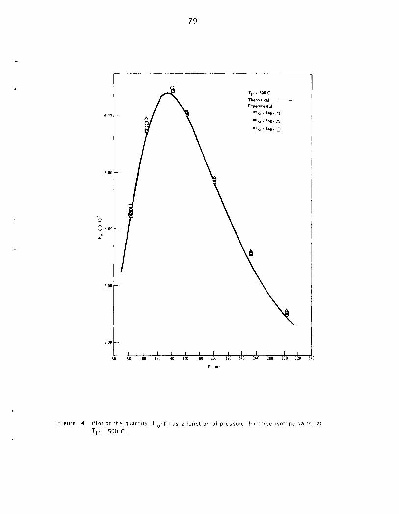
79
6 00
5 00
4 00
3 00
2 00
T H = 500 C
Theoretical
Experimental
'"Kr - S'Kr O
'°Kr - 14K, A
"Kr: 86K, a
I J L J L 80 120 140 160 180 200 220 240
P torr
260 280 300 320 340
Figure 14. Plot of the quantity iH^ 'K l as a function of pressure for three isotope pairs, at T H 5 0 0 ' C .

80
I I 00
10 00
9 00
8 00
^ ° 7 00
6 00
5 00
4 00
60 80 100 120 140 160 180 200 220 240 260 28u 300 320 340
P torr
Figure 15. Plot of the quantity IH^ 'K| as a function of pressure, for three isotope pairs, at T H 800 C.
J I \ I I 1 I I I I I L

81
^°Kr-^^Kr, s°Kr-^*Kr and ""^Kx-^^Kr, by use of Equations 48 and
57, are also plotted. The experimental and theoretical values
which are plotted in Figures 13-15, are tabulated in Tables 3-
5. Tables 3-5 also list the numbers of the samples used to
determine the experimental values, and the corresponding
column pressures«
Flow Data
In Tables 6-11, the values of In qij, calculated from the
experimentally determined top and bottom compositions, for the
above-mentioned isotope pairs are given, for two sets of flow
experiments, one set at relatively low pressures and the
other set at higher pressures, for each value of hot wall
temperature (T ). Also given are the corresponding calculated
values of In q^ ^. The calculated values of In q j are
determined from a numerical integration of Equation 14 and the
(n-1) equations of the form of Equation 64, using the value of
HQ which corresponds to the minimum RMS deviation. The flow
rates and column pressures, as well as the sample numbers cor
responding to each In q^ j value are also listed in the tables.
Theoretical and Experimental Values of the Coefficients Hg, K^ and K^
In Table 12 the theoretical and experimental values of HQ,

Table 3. Experimental and theoretical values of (Hg K), for the three isotope pairs ^°Kr- Kr, Kr-
and ^^Kr-^^Kr. The column length and hot and cold wall temperatures and radii are as folio
TH = 0.0794 cm T H = 350=C
^C = 0,9525 cm T c = I5=C L = 487,68 cm
Sample
Numbers
IT.B^)
2T,B
3T,B
4T.B
5T,B
.'-T.B
7T,B
Theoretical
(X 10^)
2.30
2.93
4.00
4.18
4.21
4.13
3.77
80Kr.86Kr
2.40
3.05
4.14
4.33
4.33
4.30
4.00
Experimental (X lO'')
80Kr-84Kr
2.38
3.06
4.08
4.26
4.34
4.26
3.99
82Kr-86Kr
2.40
3.1 1
4.33
4.54
4.44
4.38
4.09
Column
Pressure
(torr)
234.2
200.3
149.0
136.0 125.0
i 15.4
100.0
a) - T designates upper sample port, B designates lower sample port.

Table 4. Experimental and theoretical values of (Hg/K), for the three isotope pairs °'^Kr-''°Kr, and ^^Kr-^'Kr. The column length and hot and cold wall temperatures and radii are as fo
r^ = 0.0794 cm T^ = 500°C r^ = 0.9525 cm Tc = I5°C L = 487.68 cm
Colum Sample Theoretical Experimental (X 10^) Pressu umbers
8T,B 9T,B
I0T,B I IT .B I2T,B I3T,B 14T.B I5T,B I6T,B
(X 10'')
2.43 3.38 4.80 6.01 6.37 5.70 5.70 4.20 4.20
80Kr-86Kr
2.47 3.57 4.87 6.05 6.48 5.84 5.78 4.34 4.24
80Kr-84Kr
2.43 3.57 4.90 6.04 6.46 5.97 5.75 4.36 4.28
82Kr-86Kr
2.51 3.55 4.83 6.04 6.45 5.85 5.74 4.38 4.23
(torr)
304.2 252.4 201.1 162.4 142.2 105.6 105.6 82.6 82.6

Table 5. Experimental and theoretical values of (H^/K), for the three isotope pairs ^°Kr-^*Kr, ^"Kr and 8^Kr-8*Kr. The column length and hot and cold wall temperatures and radii are as folio
r^ = 0.0794 cm T^ = 800X re = 0.9525 cm T^ = I5°C L = 487.68 cm
Sample ''lumbers
I7T,B I8T,B I9T,B 20T,B 2IT,B 22T,B 23T,B 24T,B 25T,B 26T,B 27T,B 28T,B 29T,B 30T,B
Theoretical (X 104)
5.48 6.09 7.86 8.75 9.45
10.31 10.61 10.60 10.50 10.28 10.03 8.80 8.40 8.30
80Kr-86Kr
5.76 6.44 8.37 9.04 9.97
10.43 10.56 10.68 10.46 9.96 9.60 8.24 7.93 7.50
Experimental (X iO"*)
80Kr.84Kr
5.81 6.43 8.47 9.06
10.04 10.52 10.52 10.72 10.80 10.01 9.53 8.24 7.94 7.53
82Kr-86Kr
5.75 6.43 8.29 9.01 9.82
10.34 10.66 10.71 10.20 9.97 9.77 8.29 7.93 7.42
Pressur (torr)
304.5 286.4 241.2 221.5 206.2 182.2 162.7 161.5 148.0 141.0 136.2 1 17.2 112.5 110.5

Table 6. Experimental values of ' [ I n q j j ] , at low pressures, for the three isotope pairs ^OKr-^^Kr.
8°Kr-8 ' 'Kr and 82|^f.86|^f ^ ^ j corresponding values calculated by numerical integrat ion of
Equation 14 and the (n-1) equations of the form of Equat ion 64, using the experimental value
of Hj j ' . The column length and hot and cold wa l l temperatures and radi i are as fo l l ows :
r^ = 0.0794 cm r j . = 0.9525 cm L = 487.68 cm
350-C I5"C
( Sample
Numbers
31T,B
32T,B
33T,B
34T,B
35T,B
:8°Kr-86Kr)^ /SO
0.382
0.520
0.664
0.893
0.947
xp. (^°' Kr-S^Kr)^^
0.401
0.534
0.675
0.845
0.973
Lin qj
Kr-S^Kr)^ /GO
Ic . ^
0.243
0.334
0.423
0.561
0.600
j j
^p (S^Kr-S^Kr)^
Kr.8^Kr),^,^ (8^1
0.253
0.336
0.426
0.538
0.626
0.263
0.362
0.458
0.660
0.677
xp .
Kr-S^Kr)^^,
0.284
0.380
0.481
0.599
0.685
Column Pressure
ftorr'i Ic .
131.7
131.7
132.1
131.9
132.1
Flow Rate (Std cc/hr)
14.9
10.2
7.0
4.2
2.7

Table 7. Experimental values of [In q j j ] , at high pressures, for the three isotope pairs 80 Kr-8* Kr,
8°Kr-8' 'Kr and 82Kr-86Kr, and corresponding values calculated by numerical integrat ion of
Equation 14 and the (n-1) equations of the form of Equat ion 64, using the experimental value
of H '. The column length and hot and cold wa l l temperatures and radi i are as fo l l ows :
/80
Sample Numbers
36T,B
37T,B
38T,B
39T,B
40T,B
4IT,B
42T,B
43T,B
Kr-8*Kr)g (8C
0.385
0.384
0.482
0.455
0.574
0.545
0.609
0.72.5
r = 0,0794 cm r - = 0.9525 cm L = 487.68 cm
(^°K 'Kr-^^Kr),^,
0.379
0.395
0.458
0.483
0.530
0.568
0.650
0.704
[Inqj
: r -«^Kr) , ,
c. ('"X
0.237
0.259
0.312
0.291
0.358
0.366
0.419
0.463
T H =
Tc =
jl
p. (
:r-8^Kr)
0.246
0.255
0.298
0.313
0.346
0.369
0.424
0.465
350X I5^C
8^Kr-8*Kr)£ /82
Calc. ^
0.272
0.257
0.327
0.314
0.390
0.365
0.417
0.504
xp.
Kr-S^Kr)^^
0.257
0.268
0.313
0.330
0.364
0.390
0.447
0.488
Column Pressure
(torr) Ic.
227.0
210.8
225.8
210.8
226.5
210.8
210.5
210.6
Flow Rate (Std cc/hr)
41.1
35.8
27.7
24.6
18.4
16.3
10.0
6.1

Table 8. Experimental values of [In q j - ] , at lowpressures. for the three isotope pairs 8° Kr-8*Kr.
80Kr-8' 'Kr and 82Kr.86Kf jp^j corresponding values calculated by numerical integrat ion of
Equation 14 and the (n-1) equations of the form of Equation 64, using the experimental value
of HQ'. The column length and hot and cold wal l temperatures and radi i are as fo l lows :
( Sample
Numbers
44T,B
45T,B
46T,B
47T,B
48T,B
49T,B
50T,B
51T,B
5°Kr-8*Kr)^ (8C
0.587
0.667
0.801
0.903
1.066
1.088
1.246
1.345
fn = 0.0794 r - = 0.9525 L = 487.68
cm cm cm
[Inqj
T H =
Tc =
il
500 C 15 C
(80Kr-84Kr),^p (S^Kr-^^Kr),,
' K r - ^ ^ K r ) , , , . ( ^ V r . ^ ^ r ) ^ . , , . («^
0.541
0.660
0.785
0.939
1.098
1.102
1.263
1.361
0.365
0.402
0.500
0.563
0.669
0.676
0.812
0.855
0.339
0.41 1
0.488
0.585
0.689
0.691
0.800
0.868
0.419
0.499
0.577
0.640
0.757
0.769
0.880
0.940
<p.
Kr-8*Kr)c3
0.387
0.474
0.565
0.675
0.784
0.787
0.894
0.956
Column Pressure
(torr) Ic.
134.2
134.7
134.7
134.7
134.7
135.1
134.7
134.7
Flow Rate (Std cc hr)
15.0
11.8
9.3
7.0
5.2
5.2
3.7
3.0

Table 9. Experimental values of [ I n q j j l . at high pressures, for the three isotope pairs 80Kr-8*Kr.
80Kr.84|^^ and 8^Kr-®*Kr, and corresponding values ca lcu lated by numerical integration of
Equation 14 and the (n - l ) equations of the form of Equation 64, using the experimental value
of Hjj'. The column length and hot and cold wa l l temperatures and rad i i are as fo l l ows :
(8°Kr-86Kr)g
Sample ( ^ Numbers
52T,B
53T.B
54T,B
55T,B
56T,B
57T,B
0.332
0.388
0.524
0.697
0.849
0.927
r^ = 0.0794 r , = 0.9525 L = 487.68
xp. (^°K
'Kr-'*Kr)c^„
0.309
0.405
0.540
0.692
0.842
0.959
cm cm cm
[ Inqj
T H =
Tc =
i - ^ ^ K r ) , ^ ^ (
._ (3°Kr-S^Kr)
0.216
0.222
0.335
0.453
0.560
0.608
0.196
0.256
0.342
0.442
0.544
0.627
500 C 15 C
8^Kr-8*Kr)^, /8 2
C a l c . ^
0.231
0.304
0.366
0.477
0.560
0.626
xp.
Kr-86Kr)c3
0.219
0.287
0.381
0.482
0.578
0.649
Column
Pressure (torr)
I c .
238.4
238.7
238.4
237.7
238.2
238.2
Flow Rate (Std cc'hr)
86.5
62.1
40.4
24.8
13.9
7.2

Table 10. Experimental values of [ Inq; , ! , at lowpressures. for the three isotope pairs 8° Kr-8*Kr, 80 84 BO 86 'J '^
Kr- Kr and Kr- Kr, and corresponding values calculated by numerical integration of Equation 14 and the (n-l) equations of the form of Equation 64. using the experimental value of Hg. The column length and hot and cold wall temperatures and radii are as follows:
r^ = 0.0794 cm T^ = 800X rj- = 0 9525 cm T^- = IS'C L = 487 68 cm
/BO
Sample Numbers
58T,B
59T,B
60T,B
6IT,B
62T,B
63T,B
64T,B
65T,B
Kr-2*Kr)£.
r 0.501
0.736
0.753
1.132
1.112
1.476
1.922
2.290
/BO up ^
'Kr-86Kr)c3
0 473
0.692
0.712
1.075
1.069
1.520
2.027
2.365
l lnqj
K r - S ^ r ) ^
/BO Ic. ^
0.309
0.436
0.451
0.662
0.662
0.889
1.158
1.422
i ' (82
xp. *•
Kr.S^Kr)^^
0.291
0.413
a. 424
0.624
0.621
0.890
1.229
1.479
Kr-^ 'Kr)^
/82 ,lc. ^
0.352
0.543
0.560
0.827
0.814
1.074
1.415
1.635
xp.
Kr-S*Kr)c3|
0.335
0.502
0.517
0.796
0.792
1.130
1.480
1.688
Column Pressure
(torr)
Ic.
158.0
158.0
160.5
160.8
158.0
159.0
160.0
160.0
Flow Rate (Std cc hr)
31.6
21.0
21.0
12.8
12.4
7.4
4.0
2.4

Table I I. Experimental values of [In q j j ] , at high pressures, for the three isotope pairs 80Kr-8*Kr,
80Kr-8' 'Kr and 82|^r-86Kr and corresponding values ca lcu la ted by numerical integration of
Equation 14 and the (n-1) equations of the form of Equat ion 64, us ing the experimental value
of Hg'. The column length and hot and cold wal l temperatures and rad i i are as fo l l ows :
(
Sample Numbers
66T,B
67T,B
68T,B
69T,B
70T,B
8°Kr-86Kr)g (80
0.415
0.547
0.989
1.161
1.391
r^ = 0.0794 cm r . = 0.9525 cm L = 487.68 cm
/80| xp. "> Kr-86Kr)^^
0.432
0.542
1.010
1.191
1.330
[Inqj
Kr-S^Kr)^ /80
Ic. ^
0.250
0.341
0.608
0.717
0.823
OD
II II
X
(-
il
lOO C 15 C
xp. (^^Kr-B^Kr),,^
^'•^'^'^C.U. ( ' 'Xr-S^Kr)^^
0.260
0.323
0.607
0.729
0.824
0.304
0.338
0.716
0.812
0.975
0.305
0.385
0.723
0.844
0.937
Column Pressure
(torr) Ic.
278.0
279.0
278.0
282.0
279.0
Flow Rate (Std cc/hr)
1 16.4
90.7
37.7
27.3
20.6

91
Table 12. Theoretical and experimental values of the coefficients Hj,', K -'and Kj
Theoretical
Experimental
1. Low pressure flow runs
11. High pressure flow runs
Average
111. Low pressure flow runs
IV. High pressure flow runs
Average
V. Low pressure flow runs
VI. High pressure flow runs
T , ( C )
350 500 800
T „ ( " C )
350 350 350
350 350 350
500 500 500
500 500 500
800 800 800
800 800 800
Isotope Pair
80-86 80-84 82-86
80-86 80-84 82-86
80-86 80-84
82-86
80-86 80-84 82-86
80-86 80-84 82-86
80-86 80-84 82-86
H ; X 105
3.31 4.90 6.73
H x IQS O
3.81 3.81 3.83
4.10 4.15 3.92
3.94
4.98 5.10 4.99
5.06 5.04 5.17
5.06
6.36 6.40 6.29
6.95 6.72 6.91
K 1.37 1.19 0.70
Kc'
1.57 1.58 1.53
1.68 1.72 1.56
1.61
1.21 1.24 1.22
1.22 1.23 1.26
1.23
0.61 0.61 0.61
0.67 0.64 0.67
K , x 103
1.13 1.23 1.42
K j x 103
1.21 1.21 1.18
1.30 1.32 1.21
1.24
1.21 1.22 1.21
1.22 1.21 1.25
1.22
1.47 1.48 1.45
1.61 1.55 1.60
Calculated from data in Tables
13 & 13 & 13 &
13 & 13 & 13 &
14 & 14 & 14 &
14 & 14 & 14 &
16 16 16
17 17 17
18 18 18
19 19 19
15 & 20 15 & 20 15 & 20
15 & 21 15 & 21 15 & 2 I
Average 6.60 0.64 1.53

92
K^ and K^ are tabulated. Also given, for the experimental
values, are the numbers of the tables which contain the raw
data from which each set of experimental values of HQ, Kj and
Kj are calculated.

93
DISCUSSION OF RESULTS
As can be seen by an examination of Table 12, the agree
ment betv7een theory and experiment is rather good in all cases.
In order to illustrate this fact, and also to facilitate the
following discussion, the ratios of the theoretical values of
each of the coefficients to the average experimental values at
the corresponding temperatures are tabulated in Table 12a.
Table 12a. Ratios of theoretical to average experimental values of the transport equation coefficients
( H Q ) T H ( c ) T H (^d)? H
TH ( ^) ( H Q ) E X P . ^ ° ( K e ) E X P , A V a (K-^ ) E X P , f y S
350 0.84 0.85 0.91
500 0.97 0.97 1,01
800 1.02 1.09 0.93
The quantities tabulated in Table 12a show that in seven of
nine cases the experimental values of the coefficients are
within + 10% of the theoretical values. In the remaining two
cases, the experimental values are within + 20% of the theo
retical values. An attempt is now made to explain the dis
crepancies which exist between the theoretical and experimental
values of the coefficients.

94
First of all, the agreement is so good at T = 500°C that
it is reasonable to attribute the discrepancies to experimental
and analytical error. At T = 350"C and T^ = 800°C, however,
the agreement is not as good, and another possible source of
error must be considered. This is the set of values for the
ordinary diffusion coefficient which was used to calculate the
theoretical values of the column coefficients.
Consider first the results at T = 800°C. The agreement
is good for the coefficient H^. However, the theoretical value
of the coefficient K^ is high and the theoretical value of the
coefficient K^ is low. An examination of Equations 37, 38 and
39 shows that the coefficients K^ and K^ depend on the ordinary
diffusion coefficient, D, whereas the coefficient HQ does not.
Furthermore, the theoretical expression for the coefficient K^
contains D in the denominator of the integrand, whereas the
theoretical expression for K^ contains D in the numerator.
Thus, it can be seen that low values for the ordinary diffusion
coefficient, in the temperature range ~750''K~1100°K, would
lead to the observed situation. Because data for the ordinary
diffusion coefficient is non-existent in this temperature range,
it is not possible at present to determine whether or not this
is the cause of the observed discrepancies. However, there is
a very distinct possibility that it is.

95
For the results at T^ = 350''C, the discrepancies exhibit
a different type of behavior. For this case, all of the
theoretical values are lower than the corresponding average
experimental values. This behavior indicates that the average
experimental value for HQ is low. Also, the fact that the
ratio of the theoretical value of Kj to the average experi
mental value is lower than the corresponding ratio for K^ is
indicative of high values for D in the temperature range ~275''K
~650*'K. However, the major parts of the discrepancies are
undoubtedly due to the low average experimental value for HQ,
and hence, to experimental and analytical error. It is to be
expected that the analytical error will have its most serious
effect at low values of the hot wall temperature, because in
these cases the separations achieved are small and the values
of the separation factors are correspondingly more sensitive to
small errors in the values of the isotopic concentrations.

96
CONCLUSIONS AND RECOMMENDATIONS
From a study of the theoretical predictions and experi
mental results, it is concluded that the extended Jones and
Furry theory, which deals with multicomponent heavy isotopic
gases, gives a rather good quantitative description of the
behavior of such gases in a Clusius-Dickel thermal diffusion
column.
For future work, it is recommended that additional com
parisons between theory and experiment be made for hot wire
temperatures in the lower temperature range (~500°~650°K).
These comparisons should serve to pinpoint the cause or causes
of the discrepancies reported in this thesis, for T = 350°C.
It is also recommended that more work be done in the area
of the transport properties of krypton, with particular
attention to the ordinary diffusion coefficient and the thermal-
diffusion factor, with the aim of providing a reliable set of
values for these properties over a wide range of temperatures.

97
BIBLIOGRAPHY
Bardeen, J., Concentration of Isotopes by Thermal Diffusion: Rate of Approach to Equilibrium, Phys. Rev. 57: 35-41 (1940).
Concentration of Isotopes by Thermal Diffusion: Rate of Approach to Equilibrium, Phys. Rev. 58: 94-5 (1940).
Bird, R. B., Stewart, W. E. and Lightfoot, E. N., Transport Phenomena, New York, N. Y., John Wiley and Sons, Inc., 1960.
Blumkin, S. and Von Halle, E., Evaluation of the Performance of Thermal Diffusion Columns Separating Xenon Isotopes, A. I. Ch. E. Journal 9: 541-7 (1963).
Casas, J., Saviron, J. M., Gonzalez, D. and Quintanilla, M. , Difusion Termica en Kripton. Influencia de la Temperature en las Constantes de Separacion, Anales de la Real Sociedad Espanola de Fisica y Quimica 60: 153-8 (1964).
Chapman, S., Law of Distribution of Molecular Velocities, and Theory of Viscosity and Thermal Conductivity in a Non-Uniform Simple Monatomic Gas, Phil. Trans. Roy. Soc. London A216: 279-348 (1916) (Original not seen. Cited in Von Halle, A New Apparatus for Liquid Phase Thermal Diffusion.)
Kinetic Theory of Simple and Composite Monatomic Gases: Viscosity, Thermal Conductivity, and Diffusion, Proc. Roy. Soc. (London) A93: 1-20 (1916) (Original not seen. Cited in Von Halle, A New Apparatus for Liquid Phase Thermial Diffusion.)
and Dootson, F. W., Thermal Diffusion, Phil. Mag. 33: 248-53 (1917) (Original not seen. Cited in Von Halle, A New Apparatus for Liquid Phase Thermal Diffusion. )
The Possibility of Separating Isotopes, Phil. Mag. 38: 182-7 (1919) (Original not seen. Cited in Van Der Valk, Thermal Diffusion in Ternary Gas Mixtures.)

98
Clifton, D. G., Measurements of the Viscosity of Krypton, J. Chem. Phys. 38: 1123-31 (1963).
Clusius, K. and Dickel, G., New Process for Separation of Gas Mixtures and Isotopes, Naturwissenschaften 26: 546 (1938).
Corbett, J. W. and Watson, W. W. , Thermal Diffusion in Krypton and Argon, J. Chem. Phys. 25: 385-8 (1956).
Dufour, L., The Diffusion Thermoeffeet. Arch. Sci. (Geneva) 45: 9 (1872) (Original not seen. Cited in Von Halle, A New Apparatus for Liquid Phase Thermal Diffusion).
The Diffusion Thermoeffeet, Pogg. Ann. 148: 490 (1873) (Original not seen. Cited in Von Halle, A New Apparatus for Liquid Phase Thermal Diffusion).
Enskog, D., The Kinetic Theory of Phenomena in Rare Gases Upsala University Thesis (Ph.D,), Upsala, Sweden. 1917. (Original not seen. Cited in Von Halle, A New Apparatus for Liquid Phase Thermal Diffusion).
Furry, W. H., Jones, R. C. and Onsager, L., On the Theory of Isotope Separation by Thermal Diffusion, Phys. Rev. 55: 1083-95 (1939).
Grew, R. E. and Ibbs, T. L. , Thermal Diffusion in Gases, Cambridge, England, Cambridge University Press, 1952.
Groth, W. and Harteck, P., Die Selbstdiffusion des Xenons und des Kryptons, Z. Electrochem. 47: 167-72 (1941).
Hirschfelder, J. 0., Curtiss, C. F. and Bird, R. B., Molecular Theory of Gases and Liquids, New York, N. Y., John Wiley and Sons, Inc., 1954.
Jones, R. C , On the Theory of the Thermal Diffusion Coefficient for Isotopes, Phys. Rev. 58: 111-22 (1940).
On the Theory of the Tuermal Diffusion Coefficient for Isotopes. II., Phys. Rev. 59: 1019-33 (1941).

99
and Furry, W. H., The Separation of Isotopes by Thermal Diffusion, Rev. Mod. Phys. 18: 151-224 (1946).
_________________ and Isotope Separation by Thermal Diffusion: The Cylindrical Case, Phys. Rev. 69: 459-71 (1946).
Kannuluik, W. G. and Carman, Eo H., The Thermal Conductivity of Rare Gases, Proc» Phys.. Soc. (London) B65: 701-9 (1952).
Liley, P. Eo, Values for the Thermal Conductivity of 54 Gases at Atmospheric Pressure, Private Communication to W. M. Rutherford. 1967.
Ludwig, C , Diffusion Between Unequally Heated Regions of Initially Uniform Solutions, Sitzber, Akad. Wiss. Wien 20: 539 (1856) (Original not seen. Cited in Von Halle, A New Apparatus for Liquid Phase Thermal Diffusion.)
Mclnteer, B. B. and Reisfeld, M. J., Thermal-Diffusion Column Shape Factors for the Lennard-Jones (12-6) Potential, J. Chem. Phys. 33: 570-3 (1960).
Moran, T. I. and Watson, W. W. , Thermal Diffusion Factors for the Noble Gases, Phys. Rev. 109: 1184-90 (1958).
Mueller, G. , Zur kontinuierlichen Trennung polynarer Isotopengemische durch Thermodiffusion im Clusius-Dickel-Trennrohr, Zeitschrift fur Chemie 3: 478-9 (1963).
Methods for the Experimental Determination of the Constants of Clusius-Dickel Separation Columns for Binary and Multicomponent Isotope Mixtures, Kernenergie 8: 226-36 (1965).
Mulliken, R. S., The Separation of Isotopes by Thermal and Pressure Diffusion, J. Am. Chem, Soc. 44: 1033-51 (1922) (Original not seen. Cited in Furry et al. , On the Theory of Isotope Separation by Thermal Diffusion.)
Onsager, L. and Watson, W. W., Turbulence in Convection in Gases between Concentric Vertical Cylinders, Phys. Rev. 56: 474-7 (1939)

100
Paul, R. and Watson, W. W. , Isotopic Thermal-Diffusion Factors for Krypton, J, Chem, Phys, 45: 4132-4 (1966).
Purdue Research Foundation, Thermophysical Properties Research Center Data Book, Volume 2, Non-metallic Elements, Compounds and Mixtures [in Liquid and Gaseous States at Normal Temperature and Pressure]. (1966).
Reinhold, G. , Theorie und Berechnung der Formfaktoren von Thermodiffusions-Kolonnen, Z, Phys. Chem, 224: 384-418 (1963).
Rigby, M. and Smith, E. B., Viscosities of the Inert Gases, Trans. Far, Soc, 62: 54-8 (1966).
Rutherford, W. M., Thermal Diffusion Column Transport Coefficients for Mass 28 and Mass 29 Carbon Monoxide, J. Chem. Phys, 42: 869-72 (1965).
___________________ Thermal Diffusion Column Transport Coefficients for Isotopically Substituted Methane, J. Chem, Phys, 46: 900-5 (1967).
and Keller, J. M., Preparation of Highly Enriched Carbon 13 by Thermal Diffusion of Methane, J. Chem. Phys, 44: 723-736 (1966).
__ and Kaminski, K. J., Experimental Verification of Theory of the Thermal Diffusion Column, (In preparation).
Saviron, J. M., Gonzalez, D. and Madariaga, J, A,, Tabulated Values of Thermal Diffusion Column Shape Factors for the Buckingham (6-Exp) Potential, Lab.-Rep.-SIE-017, Zaragoza, 1965,
Saxena, S. C, and Raman, S., Theory and Performance of Thermal Diffusion Column, Rev. Mod, Phys. 34: 252-66 (1962).
Schafer, K. and Reiter, F. W., Eine Messmethode fur die Ermittlung des Warmeleitvermogens bis llOO^C, Z. Elektrochem. 61: 1230-5 (1957).

101
Soret, C , Equilibrium State of the Concentration of a Salt Solution of Which Two Regions Are Brought to Different Temperatures, Arch, Sci, (Geneva) 2: 48 (1879) (Original not seen. Cited in Von Halle, A New Apparatus for Liquid Phase Thermal Diffusion.)
Equilibrium State of the Concentration of a Salt Solution of Which Two Regions Are Brought to Different Temperatures, Arch. Sci. (Geneva) 4: 209 (1880) (Original not seen. Cited in Von Halle, A New Apparatus for Liquid Phase Thermal Diffusion.)
Influence of the Temperature on the Distribution of Salts in Their Solutions, Compt. rend, 91:289-91 (1880) (Original not seen. Cited in Von Halle, A New Apparatus for Liquid Phase Thermal Diffusion.)
On the Equilibrium State that Occurs, from the Point of View of Concentration, in an Originally Homogeneous Salt Solution When Two Portions of the Solution Are Brought to Different Temperatures, Ann. chim. Phys. 22: 293-7 (1881) (Original not seen. Cited in Von Halle, A New Apparatus for Liquid Phase Thermal Diffusion.)
Van Der Valk, F., Thermal Diffusion in Ternary Gas Mixtures, University of Amsterdam Thesis (Ph.D), Amsterdam, Netherlands. 1963.
Von Halle, E,, A New Apparatus for Liquid Phase Thermal Diffusion, University of Tennessee Thesis (Ph.D.) (AEC Research and Development Report K-1420, available from the Office of Technical Services, U. S. Department of Commerce, Washington 25, D, C), June 24, 1959.
von Ubisch, H., The Thermal Conductivities of Mixtures of Rare Gases at 29°C and 520°C, Arkiv. Fysik. 16: 93-100 (1959).
Waldmann, L,, Zur Theorie des Isotopentrennverfahrens von Clusius und Dickel, I,, Z, Physik. 114: 53-81 (1939).
Wendt, R. P., Mundy, J, N,, Weissman, S., and Mason, E. A. Gaseous Self-Diffusion in a Temperature Gradient, Phys. Fluids 6: 572-8 (1963).

102
ACKNOWLEDGEMENTS
The writer wishes to thank the Monsanto Research
Corporation and the United States Atomic Energy Commission
for supporting the work reported in this thesis. The work
was carried out at Mound Laboratory, which is operated by
the Monsanto Research Corporation for the United States
Atomic Energy Commission under Contract #AT-33-l-GEN-53.
The writer also wishes to thank Dr. Max Willis of the
University of Dayton, his thesis advisor; Dr. William
Rutherford, his supervisor and advisor at Mound Laboratory;
Larry Boehmer, Dr. John Eichelberger, Dr. Walter Haubach,
Ken Kaminski, Lane Myers, Mr. Frank Shearin, Dr. Stanley
Weissman and Barbara Whalen, all of Mound Laboratory,
without whose help this thesis could not have been under
taken or completed.
Thanks is also expressed to Dr. Michael Bobal and
Dr. C. Richard Horwedel, both of the University of Dayton,
for their interest in this work and their courteous treatment
of the writer.

I
103
APPENDIX A
DEVICES UTILIZED FOR EXPERIMENTAL
DETERMINATION OF THE THERMAL DIFFUSION FACTOR

104
DEVICES UTILIZED FOR EXPERIMENTAL DETERMINATION OF THE THERMAL DIFFUSION FACTOR
This section is devoted to a qualitative discussion of
the "two-bulb" apparatus and the "Trennschauckel," or, "Swing
Separator." These devices are utilized in making experimental
determinations of the thermal diffusion factor. They are not
used for separating large quantities of material. Separation
of large quantities of material is achieved by means of the
Clusius-Dickel column, which is described in the Literature
Review and Equipment sections.
Two-Bulb Apparatus
The first device to be discussed is the two-bulb appara
tus. The two-bulb apparatus, which is shown in Figure 16,
consists of two glass or metal bulbs joined by a connecting
tube. During operation, the two bulbs are held at different
temperatures. Then, because of the existence of the thermal
diffusion effect, a concentration difference is established,
which is usually such that the lighter constituent is enriched
in the high temperature bulb and the heavier constituent is
enriched in the low temperature bulb. When this behavior
holds, i.e., when the lighter constituent concentrates in the
hot bulb and the heavier constituent concentrates in the cold

105
Figure 16. S impl i f ied drawing of the two-bulb apparatus. Other valves located in the connect ing
tube, for removal of gas between expans ions, are not shown.

106
bulb, the thermal diffusion factor a is, by convention, taken
to be positive. When the opposite behavior holds, the thermal
diffusion factor is taken to be negative.
The establishment of the concentration difference by the
thermal diffusion flux is opposed by an ordinary diffusion
flux in the opposite direction. Since the thermal diffusion
flux and the ordinary diffusion flux are vectors which are
oppositely directed, a state of equilibrium is attained when
their magnitudes become equal.
It is possible to further increase the concentration of
one or the other of the constituents by closing the valve in
the middle of the connecting tube, removing the gas which is
enriched in the undesired component from the system (by means
of additional valves in the connecting tube, which are not
shown), and then allowing the gas which is enriched in the
desired constituent to fill both bulbs. This will result in
further separation. However, only one half of the original
amount of gas is now present. This procedure can be carried
out repeatedly. However, although this results in increased
separation, it also leads to a reduction in the amount of gas
in the system. Thus, although the final separation achieved
after a number of expansions is greater than after a single
expansion, the amount of gas remaining is likely to be quite

107
small. This is perhaps the chief drawback of the two-bulb
apparatus.
Trennschauckel
The other device to be discussed is the Trennschauckel,
or, "swing separator" (48). This device, a simplified
drawing of which appears in Figure 17, consists essentially of
a number of cells which are connected serially. The tops and
bottoms of these cells are maintained at, respectively, high
and low temperatures. The temperatures are the same for all
cells. The first and last cells are connected to two bellows,
which cause the gas to be "rocked" or "swung" back and forth.
When equilibrium has been established, the separation q which
has been effected between the top of the n ' cell, where n is
the number of cells, and the bottom of the first cell is very
nearly equal to (qj)", where q is the separation which would
be produced in a single two-bulb apparatus operating between
the same two temperatures. This device finds considerable
application in making experimental determinations of the
thermal diffusion factor cLy

-4
Figure 17 Simpl i f ied drawing of the Trennschauckel or 'Swing Separator' (Van Der Va lk (48)).

ON
o
1-4
X
M
W
PM
^ ^ ^

Table 13. Compositions of samples, expressed as mass fractions, for static experiments. The corresponding column pressures are also given. The column length and hot and cold wall tempera tures and radii are as follows:
Sample Numbers
I j a IB 2T 2B 3T 3B 4T 4B 5T 58 6T 6B 7T 7B
78
0.0046 0.0023 0.0038 0.0015 0.0046 0.0015 0.0051 0.0015 0.0056 0.0018 0.0057 0.0017 0.0061 0,0020
r = 0.0794 cm r . = 0.9525 cm L = 487.68 cm
80
0.0237 0.0174 0.0231 0.0128 0.0275 0.0126 0.0287 0.0128 0.0310 0.0137 0.0323 0.0145 0.0338 0.0161
T H
Tc
Mass 82
0.127 1 0.1022 0.1160 0.0855 0.1275 0.0843 0.1333 0.0870 0.1380 0.0910 0.1398 0.0939 0.1435 0.0992
= 350 C = 15 C
Fraction 83
0.1186 0.1067 0.1130 0.0965 0.1192 0.0965 0.1232 0.0994 0.1240 0.1014 0.1247 0.1033 0.1252 0.1055
84
0.5773 0,5848 0.5846 0.5882 0,5819 0.5909 0.5786 0.5920 0.5732 0.5909 0.5727 0.5897 0.5700 0.5908
86
0.1452 0.1865 0.1595 0.2155 0.1392 0.2143 0.1311 0.2073 0.1282 0.2012 0.1248 0.1969 0.1214 0.1863
Column Pressure
(torr)
234.2 234.2 200.3 200.3 149.0 149.0 136.0 136.0 125.0 125.0 115.4 115.4 100.0 100.0
a - T designates upper sample port, B designates lower sample port.

Table 14. Compositions of samples, expressed as mass fractions, for static experiments. The corresponding column pressures are also given. The column length and hot and cold wall temperatures and radii are as follows;
r^ = 0,0794 cm T„ = SOO C r = 0.9525 cm T^ = IS'C
Sample Numbers
8T 88 9T 9B
lOT 108 1 IT 118 12T 128 I3T I3B I4T 148 15T 158 16T 168
L
78
0.0052 0.0028 0.0061 0,0024 0,0078 0,0022 0.0096 0.0022 0.01 12 0.0020 0.0106 0,0024 0.0108 0.0042 0.0069 0,0024 0,0069 0.0023
= 487.68 cm
80
0.0218 0.0177 0.0327 0.0167 0.0392 0.0158 0.0468 0.0155 0.0523 0.0162 0.0512 0.0177 0.0505 0.0179 0.0384 0.0173 0.0381 0,0174
Mass 82
0,1296 0,1030 0,1391 0,1010 0,1531 0,1000 0,1684 0.1009 0.1785 0.1047 0.1782 0.1088 0.1749 0.1096 0.1570 0.1072 0.1561 0.1081
Fraction 83
0,1191 0,1086 0.1233 0,1073 0.1302 0.1083 0.1349 0.1094 0.1337 O.l l 13 0.1383 0.1131 0.1377 0.1152 0.1324 0.1129 0.1312 0.1132
84
0.5716 0.5780 0.5679 0.5825 0.5552 0.5818 0.5448 0.5862 0.5378 0,5872 0.5348 0.5920 0.5395 0.5868 0.5592 0.5901 0.5608 0.5902
86
0.1464 0.1899 0.1309 0.1901 0.1 145 0.1919 0.0955 0.1858 0.0865 0.1786 0.0869 0.1660 0.0866 0.1663 0.1061 0.1701 0.1069 0.1688
Column Pressure
(torr)
304.2 304,2 252,4 252.4 201.1 201.1 162.4 162.4 142.2 142.2 105.6 105.6 105.6 105.6 82.6 82,6 82,6 82,6

112
Table 15. Compositions of samples, expressed as mass fractions, for static experiments. The corresponding column pressures are also given. The column length and hot and cold wall temperatures and radii are as follows:
r^ = 0.0794 cm T ^ = 800'C r , = 0,9525 cm T^- = I5"C L = 487.68 cm
Sample Numbers
I7T I7B I8T I8B I9T 198 20T 208 2IT 2IB 22T 228 23T 238 24T 248 25T 25B 26T 268 27 T 27 B 28T 288 29T 298 30 T 308
78
0.0057 0.001 1 0.0059 0.0009 0.0077 0.0007 0.0090 0.0007 0.01 1 1 0.0007 0.0050 0.0002 0.0092 0.0005 0.0138 0.0007 0.0086 0.0002 0.0157 0.0010 0.0073 0.0004 0.0032 0.0002 0.0085 0.0008 0.0169 0.0023
80
0.0337 0.01 12 0.0350 0.0103 0.0436 0.0090 0.0486 0.0091 0.0568 0.0091 0.0368 0.0050 0.0486 0.0068 0.0683 0.0103 0.0491 0.0066 0.0739 0.0131 0.0414 0.0068 0.0260 0.0052 0.0469 0.0109 0.0775 0.0219
Mass 82
0.1442 0.0843 0.1485 0.0820 0.1695 0.0803 0.1779 0.0809 0.1934 0.0843 0.1674 0.0641 0.1813 0.0697 0.2151 0.0913 0.1801 0.0706 0.2240 0.1045 0.1673 0.0677 0.1378 0.0609 0.1759 0.0886 0.2250 0.1343
Fraction 83
0.1261 0.0980 0.1282 0.0981 0.1377 0.0981 0.1389 0.0987 0.1432 0.1022 0.1407 0.0898 0.1399 0.0922 0.1486 0.1084 0.1423 0.0922 0.1494 0.1163 0.1372 0.0904 0.1287 0.0858 0.1382 0.1026 0.1497 0.1298
84
0.5692 0.5882 0.5668 0.5852 0.5496 0.5925 0.5445 0.5965 0.5257 0.5967 0.5658 0.5980 0,5434 0,5919 0,503 1 0,6139 0,5373 0,5937 0,4905 0,6130 0.5553 0.5854 0.5865 0.5852 0.5457 0.5965 0.4857 0.5969
86
0.121 1 0.2173 0.1155 0.2235 0.0919 0.2194 0.0812 0.2141 0.0699 0.207 1 0.0844 0.2429 0.0776 0.2389 0.051 1 0.1754 0.0825 0.2367 0.0466 0.1521 0.0915 0.2493 0.1179 0.2627 0.0847 0.2005 0.0452 0.1148
Column Pressure
(torr)
304.5 304.5 286.4 286.4 241.2 241.2 221.5 221.5 206.2 206.2 182.2 182.2 162.7 162.7 161.5 161.5 148.0 148.0 141.0 141.0 136.2 136.2 117.2 117.2 112.5 112.5 110.5 1 10.5

Table 16, Compositions of samples, expressed as mass fractions, for flow experiments at low pressures. The corresponding column pressures and net flow rates are also given. The column length and hot and cold wall temperatures and radii are as follows;
r = 0.0794 cm T^ = 350-C r , = 0.9525 cm T^. = ISC L = 487,68 cm
Sample Numbers
3IT 3IB 32T 328 33T 338 34T 348 35T 35B
78
0,0045 0.0032 0.0052 0,0033 0,0058 0.0032 0,0070 0.0033 0.0074 0.0033
80
0.0271 0.0214 0.0295 0.0214 0,0321 0,0214 0,0363 0,0215 0.0381 0,0217
Mass 82
0.1264 0,1 124 0.1315 0.11 17 0.1373 0.1 125 0.1503 0.1124 0.1524 0.1137
Fraction 83
0,1182 0.1 1 13 0.1205 0,1 1 14 0,1231 0,1 1 19 0,1283 O.l l 14 0.1272 0,1 1 19
84
0.5757 0.5801 0.5725 0.5803 0,5695 0.5798 0.5622 0.5837 0.5612 0.5824
86
0.1482 0.1715 0,1408 0,1719 0.1321 0.1712 0,1159 0,1678 0,1137 0.1670
Column Pressure
(torr)
131.7 131.7 131.7 131,7 132.1 132,1 131.9 131.9 132.1 132.1
Flow Rate (Std cc'hr)
14.9 14.9 10.2 10.2 7.0 7.0 4.2 4.2 2.7 2.7

Table 17. Composit ions of samples, expressed as mass f ract ions, for f low experiments at high pres
sures. The corresponding column pressures and net f low rates are also g iven. The column
length and hot and cold wal l temperatures and rad i i are as f o l l ows ;
0.0794 cm T ^ = 350'C
T j . = I5=C
L = 487.68 cm
r j . = 0.9525 cm
Sample Numbers
36T 36B 37T 37B 38T 388 39T 398 40T 408 41T 418 42T 428 43T 438
78
0.0039 0.0029 0.0042 0.0032 0.0045 0.0029 0.0048 0.0032 0.0050 0.003 1 0.0052 0.0032 0.0058 0.0031 0.0064 0.0033
80
0.0248 0.0196 0.0267 0.0208 0.0267 0.0197 0.0277 0.0209 0.0290 0.0204 0.0298 0.0210 0.0319 0.0215 0.0339 0.0218
Mass 1 82
0.1208 0.1069 0.1245 0,1 101 0.1258 0.1084 0.1276 0.1 108 0.1301 0.1100 0.1318 0.1112 0.1378 0.1126 0.1417 0.1 136
Fraction 83
0.1154 0.1088 0.1173 0.1108 0.1177 0.1100 0.1188 0.1107 0,1196 0,1 1 1 1 0.1198 0,1110 0.1209 0.1117 0.1225 0.1117
84
0.5800 0.5814 0.5749 0.5808 0.5761 0.5807 0.5745 0.5799 0.5752 0.5790 0.5722 0.5819 0.5662 0.5807 0.5686 0.5811
86
0.1552 0.1804 0.1524 0.1743 0.1492 0.1783 0.1467 0.1745 0.1412 0.1764 0.141 1 0.1716 0.1374 0.1704 0.1269 0.1685
Column Pressure
(torr)
227.0 227.0 210.8 210.8 225.8 225.8 210.8 210.8 226.5 226.5 210.8 210.8 210.5 210.5 210.6 210.6
Flow Rate (Std cc'hr)
41.1 41.1 35.8 35.8 27,7 27,7 24,6 24,6 18,4 18,4 16,3 16,3 10,0 10,0 6,1 6,1

Table 19. Compositions of samples, expressed as mass fractions, for flow experiments at high pressures. The corresponding column pressures and net flow rates are also given. The column length and hot and cold wall temperatures and radii are as follows:
r ^ = 0.0794 cm T^ = 500-C r^ = 0.9525 cm T^. = I5°C L = 487.68 cm
Sample Numbers
52T 528 53T 538 54T 548 55T 558 56T 568 57T 57 B
78
0.0039 0.0028 0.0040 0.0029 0.0044 0.0029 0.0055 0.0023 0.0068 0.0028 0.0078 0.0031
80
0.0248 0.0201 0.0254 0.0204 0.0282 0.0204 0.0313 0.0203 0.0364 0.0214 0.0393 0.0222
Mass 82
0.1217 0.1092 0.1269 0.1108 0.1303 0.1104 0.1379 0.1 115 0.1459 0.1 145 0.1522 0.1162
Fraction 83
0.1 171 0.1113 0.1202 0.1130 0.1209 0.1 1 18 0.1237 0.1125 0.1262 0.1143 0.1277 0.1148
84
0.5754 0.5789 0.5723 0.5740 0.5733 0.5799 0.5696 0.5814 0.5623 0.5788 0.5561 0.5770
86
0.1571 0.1776 0.1512 0.1790 0.1429 0.1746 0.1319 0.1719 0.1224 0.1682 0.1 168 0.1668
Column Pressure
(torr)
238.4 238,4 238.7 238.7 238.4 238.4 237.7 237.7 238.2 238.2 238.2 238.2
Flow Rate (Std cc/hr)
86.5 86,5 62,1 62,1 40,4 40.4 24.8 24.8 13.9 13.9 7.2 7.2

Table 20. Compositions of samples, expressed as mass fractions, for flow experiments at low pres
sures. The corresponding column pressures and net flow rates are also given. The column
length and hot and cold wall temperatures and radii are as follows:
Sample Numbers
58T 588 59T 598 60T 608 61T 6IB 62T 628 63T 638 64T 648 65T 658
78
0.0041 0.0026 0.0049 0.0027 0.0051 0.0028 0.0064 0.0027 0,0063 0,0027 0,0086 0,0027 0,0122 0,0030 0.0176 0.0029
r^ = 0.0794 cm r . = 0.9525 cm L = 487.68 cm
80
0.0264 0.0195 0,0295 0,0193 0,0300 0,0194 0.0366 0.0194 0.0365 0.0194 0,0450 0,0197 0.0598 0.0212 0.0766 0.0222
Mass 82
0.1266 0.1085 0. 1366 0.1084 0.1370 0.1074 0.1533 0.1103 0.1529 0.1095 0. 1716 0.1122 0.1982 0.1 166 0.2188 0.1220
T H = 8
Tc =
Fraction 83
0.1189 0,1097 0,1242 0,1106 0,1246 0,1097 0,1314 0.1 1 15 0.1306 0,1112 0,1382 0,1134 0,1447 0,1166 0.1468 0.1190
00 c I 5 X
84
0.5781 0.5818 0.5749 0.5817 0.5748 0.5840 0.5675 0.5837 0.5665 0.5839 0.5500 0.5862 0.5216 0.5887 0.4892 0.5879
86
0.1459 0.1779 0.1298 0,1773 0.1286 0.1766 0.1048 0.1724 0.1072 0,1733 0.0865 0.1657 0.0635 0.1539 0.0510 0.1460
Column Pressure
(torr)
I58..0 158.0 158.0 158.0 160.5 160.5 160.8 160.8 158.0 158.0 159.0 159.0 160.0 160.0 160.0 160.0
Flow Rate (Std cc/hr)
31.6 31.6 21.0 21.0 21.0 21.0 12.8 12.8 12.4 12.4 7.4 7.4 4.0 4.0 2.4 2.4

Table 21. Compositions of samples, expressed as mass fractions, for flow experiments at high pressures. The corresponding column pressures and net flow rates are also given. The column length and hot and cold wall temperatures and radii are as follows:
r = 0.0794 cm T^ = 800-C rj. = 0.9525 cm T^, = I5'C L = 487.68 cm
Sample Numbers
66T 668 67T 678 68 T 688 69T 69 B 70T 70B
78
0.0040 0.0028 0.0045 0.0028 0.0062 0.0025 0.0075 0.0028 0.0083 0.0028
80
0.0251 0.0196 0.0269 0.0193 0.0348 0.0195 0.0400 0.0203 0.0440 0.0201
Mass 82
0.1244 0.1086 0.1279 0.1076 0.1480 0.1089 0..I584 0.1140 0.1613 0.1 1 17
Fraction 83
0.1 171 0.1105 0.1200 0.1095 0.1285 0.1 1 16 0.1313 0 . I I4 I 0.1314 0.1125
84
0.5790 0.5806 0.5772 0.5827 0.5680 0.5847 0.5599 0.5822 0.5651 0.5879
86
0.1503 0.1779 0.1436 0.1782 0.1146 0.1727 0.1028 0.1667 0.0898 0.1650
Column Pressure
(torr)
278.0 278.0 279.0 279.0 278.0 278.0 282.0 282.0 279.0 279.0
Flow Rate (Std cc/hr)
1 16.4 116.4 90.7 90.7 37.7 37.7 27.3 27.3 20.6 20.6
Related Documents