Advertising Effectiveness The Moderating Effect of Firm Strategy.pdf Can Sales Uncertainty Increase Firm Profits.pdf Community Participation and Consumer-to-Consumer Helping Does Participation in Third Party– Hosted Communities Reduce One’s Likelihood of Helping.pdf Consumer Preferences for Annuity Attributes Beyond Net Present Value.pdf Halo (Spillover) Effects in Social Media Do Product Recalls of One Brand Hurt or Help Rival Brands.pdf Homogeneous Contracts for Heterogeneous Agents Aligning Sales Force Composition and Compensation.pdf Investigating How Word-of-Mouth Conversations About Brands Influence Purchase and Retransmission Intentions.pdf Lower Connectivity Is Better The Effects of Network Structure on Redundancy of Ideas and Customer Innovativeness in Interdependent Ideation Tasks.pdf The Influence of Serotonin Deficiency on Choice Deferral and the Compromise Effect.pdf

Welcome message from author
This document is posted to help you gain knowledge. Please leave a comment to let me know what you think about it! Share it to your friends and learn new things together.
Transcript

Advertising Effectiveness The Moderating Effect of Firm Strategy.pdf
Can Sales Uncertainty Increase Firm Profits.pdf
Community Participation and Consumer-to-Consumer Helping Does Participation in Third Party–Hosted Communities Reduce One’s Likelihood of Helping.pdf
Consumer Preferences for Annuity Attributes Beyond Net Present Value.pdf
Halo (Spillover) Effects in Social Media Do Product Recalls of One Brand Hurt or Help Rival Brands.pdf
Homogeneous Contracts for Heterogeneous Agents Aligning Sales Force Composition and Compensation.pdf
Investigating How Word-of-Mouth Conversations About Brands Influence Purchase and Retransmission Intentions.pdf
Lower Connectivity Is Better The Effects of Network Structure on Redundancy of Ideas and Customer Innovativeness in Interdependent Ideation Tasks.pdf
The Influence of Serotonin Deficiency on Choice Deferral and the Compromise Effect.pdf
1
ADVERTISING EFFECTIVENESS: THE MODERATING EFFECT OF FIRM STRATEGY
Leigh McAlister Raji Srinivasan
Niket Jindal Albert A. Cannella*
July 2015
* The first two authors are Professors and the third a Doctoral Student in Marketing at University of Texas, Austin. The fourth is Professor of Management, Arizona State University. Correspond with Professor Leigh McAlister, Marketing Department, CBA 7.228, McCombs School of Business, University of Texas, Austin, TX 78712; [email protected]; 512-471-5458. The authors thank Professors Susan Broniarczyk, Craig Crossland, Jim Frederickson, Robert Freeman, Andrew Gershoff, Ty Henderson, Szu-Chi Huang, Amit Joshi, Praveen Kopalle, Steve Kachelmeier, MinChung Kim, Bill Kinney, Mark Lang, Brent Lao, Natalie Mizik, Chris Moorman, Neil Morgan, Thomas Reutterer, Martin Schreier, Manohar Singh, Garrett Sonnier, Shuba Srinivasan, Doug Vorhies; and the participants of the University of North Carolina Branding Conference, Marketing Meets Wall Street-Frankfurt, the Theory and Practice in Marketing Conference at Northwestern University, Marketing Research Seminars at University of South Carolina, Case Western Reserve University, University of Washington, Boston College and The University of Texas at Austin and Accounting Research Seminar at The University of Texas at Austin. The authors thank the McCombs School of Business for research support.
2
ADVERTISING EFFECTIVENESS: THE MODERATING EFFECT OF FIRM STRATEGY
Advertising’s influence on firm sales and firm value drew early attention from economists and accountants and more recent attention from marketers. Most studies investigating the link between advertising and sales find that link. However, studies investigating the link between advertising and firm value only sometimes find that link. Meta-analysis has failed to determine moderators that govern that link. We hypothesize that advertising should influence firm value for a differentiator because advertising can elaborate the firm’s point of difference into brand equity, thereby building firm value. Advertising cannot build brand equity for a cost leader because such a firm has no point of difference on which to build. Identifying differentiators and cost leaders by firms’ reactions to a change in accounting regulations, we confirm hypotheses: Advertising is related to sales for all firms but it is more strongly related to firm value for differentiators than for cost leaders. Beyond explaining differences in advertising effectiveness, our indicator of differentiation vs. cost leadership should enhance future analyses of marketing’s effect on firm level outcomes using archival financial data.
Key Words: Advertising, Differentiation, Cost Leadership, Sales, Firm Value
3
“…CEOs and CFOs, spurred by global competition, recession and stock market pressure
to deliver “the numbers,” have shown an increasing tendency to question—and cut—marketing
budgets…[T]hese reductions in marketing budgets have caught marketers’ attention and
strengthened the imperative to connect marketing spending to [its] financial impact on the firm”
Lehmann and Reibstein (2006, p. 3). Because of this industry imperative, the Marketing Science
Institute has long made the determination of return on marketing spending a top research priority.
In this paper we focus on the link between financial outcomes and a key element of
marketing spending, advertising expenditure. We note that there are at least two broad
approaches for measuring advertising effectiveness (Lehmann and Reibstein 2006). One focuses
on diagnostic marketing metrics (e.g., awareness, preference, customer satisfaction, and loyalty)
to fine-tune individual advertisements and the other focuses on evaluative marketing metrics
(e.g., sales, market share, profits, return on investment, cash flow, and firm value). In this paper,
we focus on evaluative marketing metrics, in particular sales and firm value, and consider the
ways in which advertising might influence those metrics.
The link between advertising expenditure and sales has been consistently supported (e.g.,
Bagwell 2007, Leone 1995, Lodish et al. 1995, Hanssens 2009). However there has been mixed
evidence in support of a link between advertising expenditure and firm value. Conchar, Crask,
and Zinkhan (2005) meta-analyze 88 estimated models linking advertising and firm value in
fifteen studies across the marketing, economics, and accounting literatures. They found that,
overall, the studies support a link between advertising and firm value. However, in 24 percent of
the models, there was no evidence of a link. Hirschey’s (1982) review of the economics
literature and Shah and Akbar’s (2008) review of the accounting literature arrive at a similar
conclusion: Sometimes advertising is related to firm value and sometimes it is not.
4
In their meta-analysis, Conchar, Crask and Zinkhan (2005) do not identify managerially
significant factors that govern the ability of advertising to influence firm value. They attribute
their inability to identify such factors to the fact that, for some of the studies in their meta-
analysis, advertising expenditure was a control variable rather than the variable of theoretical
interest. They therefore issued a call for research that identifies a richer set of factors that
determine whether advertising will or will not influence firm value.
Responding to that call, in this paper, we develop hypotheses relating a firm’s source of
competitive advantage (differentiation vs. cost leadership) to the effectiveness of its advertising.
We hypothesize that advertising should be linked to sales for all firms. However, advertising
should be more strongly linked to firm value for a differentiator than for a cost leader because
that differentiator has a point of difference that advertising can elaborate into brand equity. To
test the hypotheses, we develop an indicator of a firm’s source of competitive advantage that can
be inferred from the firm’s advertising expenditure disclosure behavior.
The paper’s insights have implications for accounting regulators, managers, marketing
researchers, marketing graduates and writers of marketing textbooks. For accounting regulators
who struggle with the question of whether advertising builds an asset (indicating that advertising
expenditure should be capitalized) or merely increases sales (indicating that advertising
expenditure should be expensed in the period it is incurred), this paper suggests that
differentiators should capitalize advertising expenditure while cost leaders should expense it.
The findings further suggest that managers in a cost leader firm should realize that no matter how
capable their marketing team, the firm’s advertising cannot build firm value in the way a
differentiating firm’s advertising builds firm value because a cost leader has no point of
difference that can be elaborated into brand equity. For marketing scholars, this paper points out
that the majority of publicly traded firms are excluded from published studies of marketing’s
5
value relevance because those firms do not disclose their advertising expenditure. If a firm’s
marketing emphasis were represented by the paper’s indicator of differentiation vs. cost
leadership rather than by advertising expenditure, analyses could be broadened to include a more
representative sample of publicly traded firms. Finally, because marketing’s role is likely to be
greater in firms that differentiate than in firms that are cost leaders, business school graduates
seeking insight into the likely scope of the marketing career path in a particular firm should
consider whether the firm is a differentiator or a cost leader, and the writers of marketing
textbooks should more clearly discuss the implications of a firm’s source of competitive
advantage for marketing challenges and opportunities in that firm.
In what follows, we develop hypotheses relating the effectiveness of a firm’s advertising
to that firm’s source of competitive advantage (differentiation vs. cost leadership). We then
present our proposed indicator of a firm’s source of competitive advantage and give evidence
consistent with that indicator being reliable and valid. We next test the hypotheses using our
indicator, check the robustness of our findings, discuss the implications of this work and lay out
future research questions to be explored.
THEORY AND HYPOTHESES
The management literature tells us that, at inception, a firm selects its strategy and that
strategy shapes the firm’s organizational structure. The resulting structure prioritizes business
functions that are central to the firm’s selected strategy and assigns secondary roles to business
functions that are less central (Hambrick and Mason 1984). Organizational structure is self-
perpetuating so a firm resists shifting its fundamental strategy partly because such a shift would
imply a significant organizational realignment (Boeker 1989). Given the stability of a firm’s
6
strategy and the implications of strategy for the firm’s pattern of resource allocation, it is not
unreasonable to imagine that advertising done by a firm with one strategy might be more
effective than advertising done by a firm with a different strategy.
To address the contention that a firm’s strategy moderates the effectiveness of its
advertising, we clarify the terms “firm strategy” and “advertising effectiveness.” Regarding firm
strategy, we note that management theorists summarize firms’ strategies as belonging to a few
categories. Miles and Snow (1978) developed those categories by crossing a firm’s “source of
competitive advantage” with its “aggressiveness”. Porter (1980) developed his categories of
firm strategy by crossing a firm’s “source of competitive advantage” with its “degree of focus”.
In the marketing literature, Walker and Ruekert (1987) synthesized the two previous typologies
by crossing a firm’s “source of competitive advantage” with its “intensity of product/market
development”. In this paper, we focus on the strategic dimension common to these typologies: a
firm’s source of competitive advantage.
The differentiator-cost leadership dichotomy is a widely accepted descriptor of strategic
difference. This dichotomy is prominent in strategy research in managementi and in marketingii.
The differentiation vs. cost leadership dichotomy is presented in most contemporary textbooks
(Campbell-Hunt, 2000) and, as mentioned above, is fundamental to the three primary strategic
typologies proposed in the management and marketing literatures (Miles and Snow 1978, Porter
1980, Walker and Ruekert 1987). Adding face validity, managers think about competitive
advantage in terms of differentiation vs. cost leadership (Day and Nedungadi 1994; Homburg,
Workman and Krohmer 1999). Consequently, in this paper, we will contrast the effectiveness of
advertising done by firms that draw competitive advantage from differentiation vs. firms that
draw competitive advantage from cost leadership.
7
Regarding “advertising effectiveness”, our review of the marketing literature suggests
that two important “evaluative” measures of advertising effectiveness are: (1) advertising’s
ability to increase current sales (e.g., Lodish et al. 1995) and (2) advertising’s ability to increase
both current and expected future sales (e.g., Joshi and Hanssens 2010). As the discounted sum of
expected future cash flows is closely related to the discounted sum of expected future sales, the
second meaning of advertising effectiveness could be restated as advertising’s ability to increase
firm value.
We note that economists are divided on the question of whether advertising merely
influences current sales (advertising as information view) or whether advertising influences
current and expected future sales (advertising as persuasion view). The first view, which holds
that advertising informs (e.g., Ozga 1960, Stigler 1961, Telser 1964), suggests that advertising
increases current sales because advertising increases awareness. (Consumers cannot buy a
product if they don’t know that it exists). The second view holds that it is advertising’s job to
persuade consumers. Proponents of this view (e.g., Robinson 1933, Bain 1956, Comanor and
Wilson 1967) suggest that advertising can create brand loyalty, an intangible asset that influences
sales in current and future periods, i.e., advertising influences firm value as well as sales.
Economists’ empirical studies produced conflicting findings across products and industries
(Bagwell 2007)iii. Sometimes advertising is found to be associated with firm value; other times,
it is not. Accountants, building from economists’ two views of advertising to determine the
appropriate accounting treatment for advertising expenditureiv, have also produced empirical
studies with conflicting findings. (See Shah and Akbar 2008, for a review of these studies.)
The marketing literature implicitly takes the position that advertising “persuades”. Since
the early 1970’s (e.g., Bass and Clarke 1972; Hanssens, Parsons, and Schultz 1990; Leone 1995),
marketing scholars have focused on the ability of advertising to increase not only current sales,
8
but also future sales. More recently, advertising’s ability to increase firm value is offered as
further evidence that advertising influences the firm’s current and expected future sales (see
Srinivasan and Hanssens 2009, for a summary of the findings). Joshi and Hanssens (2010)
support that contention by showing that (1) advertising increases sales in the current period and
those incremental sales increase firm value and (2) after controlling for advertising’s current-
sales-effect on firm value, advertising has an additional impact on firm value that can be
attributed to investors’ expectations that future sales will also increase. Most published
marketing studies provide evidence consistent with this “advertising persuades” position.
However, we note that there are exceptions. Erickson and Jacobson (1992), Aaker and Jacobson
(1994), and Tuli, Mukherjee, and DeKimpe (2012) fail to find an effect for advertising on firm
value.
In summary, across the economics, accounting and marketing literatures, we see evidence
that sometimes advertising merely informs consumers about product availability, thereby
increasing current sales. Other times advertising goes on to persuade consumers that the product
is superior, thereby increasing both current sales and firm value. In this paper we examine when
one should expect advertising to merely inform and when one can expect advertising to go
further and also persuade. We are interested in the role that firm strategy, in particular, the
firm’s source of competitive advantage (differentiation vs. cost leadership), plays in determining
whether advertising merely increases current sales or whether it also increases firm value.
To explore the impact that strategy might have on firm value, we begin with what is
known about differentiators and cost leaders. To produce products that uniquely meet a specific
customer need, differentiators emphasize the exploration of customer needs, development of
products/services that fit those needs and communication of products’ benefits to target
customers (Hambrick 1983a; McDaniel and Kolari 1987; McKee, Varadarajan, and Pride 1989).
9
The communication of those benefits, often through advertising, supports differentiators’
development of intangible assets (brands, customer relationships, channel relationships) which
enhance the firm’s sales and stock returns (Srivastava, Shervani and Fahey 1998). For cost
leaders producing acceptable, standard products, cost reduction is paramount. Such a firm
requires aggressive construction of scale-efficient facilities, vigorous pursuit of cost reductions
from experience, tight cost and overhead control, avoidance of marginal customer accounts, and
cost minimization in areas like research and development, customer service, sales force, and
advertising. With no point of difference other than price to communicate, a cost leader may see
advertising as a cost that can be cut with little long-term performance penalty.
Building from the notion that advertising informs for all firms, we propose that
advertising’s impact on current sales is not moderated by firm strategy. A firm’s advertising
should increase current sales whether the firm derives competitive advantage from differentiation
or cost leadership. In either case, advertising makes consumers aware that the advertised product
is available and, through enhanced awareness, increases current sales (e.g., Srinivasan et al.
2009).
H1: Advertising will be positively related to current sales for both firms that draw competitive advantage from differentiation and firms that draw competitive advantage from cost leadership.
To see why advertising’s ability to increase firm value might be moderated by firm
strategy we build from economists’ contention that persuasive advertising can develop brand
loyalty. Both Aaker (1991) and Keller (2002) tell us that brand loyalty is built by
communicating a brand’s point of difference. Further, Keller and Lehmann (2003) explain that
such communication builds links between the brand and its point of difference in consumers’
memories. This network of strong, positive and unique associations causes a consumer to be less
price sensitive, more responsive to the brand’s marketing efforts and more receptive to the

10
brand’s extensions, thus increasing the brand’s current sales and investors’ expectations of the
brand’s future sales, thereby increasing firm value. Consequently, we expect that, for a firm that
draws competitive advantage from differentiation, advertising can increase firm value. For a
firm that draws competitive advantage from cost leadership, however, there is no point of
difference that advertising can elaborate into a network of strong, positive and unique
associations in consumers’ memories and hence there little brand equity. Thus, for such firms,
advertising should have little influence on firm value.
H2: Advertising’s relationship with firm value will be stronger for firms drawing competitive advantage from differentiation than for firms drawing competitive advantage from cost leadership. In summary, advertising is “effective” for all firms. For those firms that derive
competitive advantage from cost leadership, advertising increases current sales by creating
awareness. For those firms that derive competitive advantage from differentiation, advertising
increases current sales by creating awareness and increases firm value by developing a network
of strong, positive and unique associations linking the brand and its point of difference in
consumers’ memories.
PROPOSED INDICATOR OF A FIRM’S SOURCE OF COMPETITIVE ADVANTAGE
Though prior marketing studies used survey-based indicators of a firm’s source of
competitive advantage (e.g., Homburg, Workman and Krohmer 1999; Verhoef and Leeflang
2009), we seek a secondary-data-based indicator to study advertising effectiveness across a large
number of publicly listed firms for several years. To infer that a particular firm is a differentiator
or a cost leader, we combine the insight that advertising is central to firm strategy for
differentiators but not for cost leaders with information about advertising’s strategic centrality

11
for a specific firm. If advertising is central to strategy for the firm, we infer that the firm is a
differentiator. If advertising is not central to strategy for the firm, we infer that the firm is a cost
leader.
We assert that advertising’s strategic centrality for a firm (i.e., the “importance” of
advertising for a firm) was revealed by the 1994 implementation of accounting regulation FRR44
(SEC Financial Reporting Release Number 44 detailed in the Appendix). That regulation was
primarily designed to simplify financial filings for US companies that had acquired a foreign
business. However, as a tangentially related add-on, FRR44 also changed the conditions under
which any publicly traded US firm (not just a US firm that had acquired a foreign business) is
required to disclose the level of its advertising expenditure. Before FRR44, advertising
expenditure disclosure was required for any firm that advertised. Since FRR44, only those firms
for which advertising is “material” are required to disclose advertising expenditure.
The concept of materiality comes to accounting from business law. Supreme Court case
TSC Industries vs. Northway, Inc. (1976) established the existing judicial standard of materiality
in securities litigation when it held that an item is material if there is “substantial likelihood that
the disclosure of the omitted fact would have been viewed by the reasonable investor as having
significantly altered the ‘total mix’ of information made available.”
SEC Staff Accounting Bulletin Number 99 on Materiality elaborates further (pages 2-4):
“Materiality concerns the significance of an item to users of a registrant’s financial statements.
A matter is ‘material’ if there is a substantial likelihood that a reasonable person would consider
it important…The FASB has long emphasized that materiality cannot be reduced to a numerical
formula…[M]agnitude by itself, without regard to the nature of the item and the circumstances in
which the judgment has to be made, will not generally be a sufficient basis for a materiality
judgment.”

12
Given this, a firm which discloses advertising expenditure after FRR44 is one for which
advertising is “material”, implying that advertising is important for that firm. Similarly, a firm
which ceases to disclose advertising expenditure after FRR44 is one for which that expenditure is
“not material”, implying that advertising is not important for that firm. Because we argued that
advertising is important for differentiators, but not for cost leaders, we propose that a firm’s post-
FRR44 advertising disclosure behavior is an indicator of that firm’s source of competitive
advantage. Firms that continue to disclose advertising after FRR44 are likely to be
differentiators. Firms that cease to disclose advertising after FRR44 are likely to be cost
leadersv.
In sum, we suggest that, for those firms that advertise, post-FRR44 advertising disclosure
behavior serves as an indicator of the firm’s source of competitive advantage. In the remainder
of this section, we provide evidence of the reliability and validity of this proposed indicator.
Reliability
We mentioned earlier that a firm sets its strategy—including the selection of its source of
competitive advantage—at its inception. Organizational structure then develops to support that
strategy. Because organizational structure is notoriously difficult to change, firm strategy is also
difficult to change (Boeker 1989; Eisenhardt and Schoonhoven 1990). Given this, one should
expect a firm’s source of competitive advantage to be relatively stable through time.
A reliable indicator of this stable firm characteristic (source of competitive advantage)
should produce consistent results from one measurement occasion to the next. In our context,
this suggests that a firm’s post FRR44 advertising disclosure behavior should be stable from year
to year. Consistent with this logic, considering 14,571 firms and 100,070 firm-year observations
between 1996 and 2009, we note that 96% of the firm-year observations showed no change in

13
advertising disclosure behavior in this 14 year period. The year-to-year correlation of the
indicator’s value, across all firms, is very high at .91 (p < .001). For 80% of the firms, the
proposed indicator is unchanged over the period 1996-2009. 16% of the firms make a single
change in advertising disclosure behavior; 4% make more than one changevi. We take the above
as evidence of the proposed indicator’s reliability.
Convergent Validity
We consider two kinds of evidence for convergent validity: (a) “Realized strategy
indicators” which have been used in the management literature to account for a firm’s tendency
toward differentiation vs. cost leadership and (b) the composition of a firm’s top management
team (TMT).
Management researchers have proposed “realized strategy indicators” (based on archival
financial data) in order to include firm strategy in predictive models, (Berman et al. 1999;
Hambrick 1983b; Kotha and Nair 1995). Some of these indicators are expected to be high if the
firm draws competitive advantage from differentiation (i.e., marketing intensity, selling
intensity). Others are expected to be low if the firm draws competitive advantage from cost
leadership (i.e., cost, capital expenditure and capital intensity).
As shown in Table 1 our proposed indicator of a firm’s source of competitive advantage
is consistent with these alternative indicators of a firm’s source of competitive advantage. In
particular, those firms that our indicator classifies as differentiators have higher marketing
intensity (i.e., scaled advertising expenditure) and higher selling intensity (i.e., scaled selling,
general and administrative expenditure) than firms the indicator classifies as cost leaders.
Similarly, those firms our indicator classifies as cost leaders have lower costs (i.e., scaled cost of
goods sold), lower capital expenditure (i.e., scaled capital expenditure) and lower asset intensity
(i.e., scaled plant, property and equipment) than firms the indicator classifies as differentiators.
14
The consistency of our proposed indicator with these alternative strategy indicators provides
evidence of convergent validity for our proposed indicator.
Insert Table 1 about here
For further evidence of convergent validity, we consider the makeup of a firm’s top
management team (TMT) and expect to find that marketing is more likely to be a part of the
TMT if the firm draws competitive advantage from differentiation (Hambrick and Mason 1984;
Nath and Mahajan 2008, 2011). Marketing is, almost by definition, critical for a firm that
differentiates (Day and Nedungadi 1994; Homburg, Workman and Krohmer 1999; Nath and
Mahajan 2008, 2011; Verhoef and Leeflang 2009). Marketing scans markets and customers in
search of differentiation opportunities. Marketing brings the voice of the customer to product
development, ensuring that the evolving product concept meets the unique need identified in the
market. Marketing manages pre-test and test market research and ensures a match between
unmet need and the product’s point of difference. Marketing manages the new product roll out
and then manages the resulting brand, built on the product’s point of difference, through the
brand’s life cycle.
Thus, in a firm that differentiates, it is marketers who plan and measure customer mindset
to track brand progress, draft positioning statements to guide advertising agencies, and
coordinate go-to-market plans with the sales function. In a firm that draws competitive
advantage from cost leadership, on the other hand, marketing’s role is more limited. Because a
cost leader has standard products with little differentiation, there is much less need for market
vigilance and little need for deep consumer insights. There is little, if any, need for bringing the
voice of the customer into product deliberations, for market testing or for mapping consumers’
mindsets. Marketers in a cost leader help with tactical execution, monitor compliance with
corporate trademark guidelines, coordinate the sharing of best practices across business units,
15
etc. (Hyde, Landry and Tipping 2004; Landry, Tipping and Dixon 2006). In sum: Marketing is
more likely to be a part of the top management team in a firm that differentiates than in a firm
that is a cost leader.
We explore this contention using ExecuComp data for S&P 500 companies from 1996-
2009 to identify the functional affiliation of each TMT member based on job title (e.g., titles
including the terms marketing, brand, customer, or advertising were classified as “Marketing”).
We draw control variables (firm profit, leverage and size; industry turbulence, growth,
concentration and percentage differentiators) from Compustat.
We model the dichotomous variable “Marketing on TMT” (1 = Marketing on TMT; 0 =
Marketing not on TMT) as a function of the proposed indicator, “Differentiatej” (1 = proposed
indicator classifies firm j as a differentiator; 0 = proposed indicator classified firm j as a cost
leader), conventional control variables mentioned above and industry- and year-specific
dummies. Consistent with recent longitudinal analysis of firms in marketing literature (Chiou
and Tucker 2012, DeKinder and Kohli 2008, Lee 2011, Nath and Mahajan 2011), we use a GEE
(Generalized Estimating Equation) to estimate the parameters of the model (Liang and Zeger
1986, Zeger and Liang 1986, Zeger et al. 1988). We specify a binomial distribution with a probit
link and assume a first-order autoregressive correlation structure. We estimate the model using
Liang and Zeger’s (1986) approach for estimating GEEs, which is an iteratively reweighted least
squares procedure closely related to quasi-likelihood estimation. Though GEE estimates are
robust to misspecifications of the correlation structure (Liang and Zeger 1986), we compute
robust standard errors in order to appropriately evaluate the statistical significance of the
coefficient estimates.
We report the estimated coefficients in Column 1 of Table 2. The results show, indeed,
that the coefficient of the proposed indicator is positive and significant (coefficient of
16
Differentiatej = .61, p < .05): Firms classified as differentiators by the proposed indicator are
more likely to have Marketing on the TMT than are firms classified as cost leaders, providing
evidence of the convergent validity of the proposed indicator of a firm’s source of competitive
advantage.
Insert Table 2 about here
Discriminant Validity
While we expect marketing’s probability of TMT membership to be influenced by the
firm’s source of competitive advantage, we do not expect the probability of other functions’
TMT membership to be so influenced. For example, engineering’s membership on the TMT is
more likely in a technical industry, whether the firm is a cost leader or a differentiator. Legal’s
membership on the TMT is more likely in a highly regulated industry, whether the firm is a cost
leader or a differentiator. Operations controls costs for cost leaders but it also delivers the point
of difference in many differentiated service firms (e.g., Starbucks, Nordstrom, Ritz-Carlton).
Finally, the risk associated with inaccurate public filings makes the inclusion of finance on the
TMT virtually universal. In summary, we do not expect a firm’s source of competitive
advantage to govern TMT membership for any function other than marketing, providing an
opportunity to consider the proposed indicator’s discriminant validity.
The last four columns of Table 2 address the question of the proposed indicator’s
discriminant validity. Each of these four columns represents a model estimated as was the model
in Column 1. The columns are distinguished by the dependent variable being modeled. In
Column 2 the dependent variable reports whether the Finance function is represented on the
firm’s TMT. In a similar way, Columns 3-5 represent models of TMT inclusion for the
Operations, Engineering and Legal functions, respectively. In none of the last four columns is
17
the coefficient of the proposed indicator (Differentiatej) statistically significant. That is, the
proposed indicator discriminates across business functions. It is a significant predictor of
Marketing’s presence on the TMT, but not a significant predictor of Finance’s, Operations’,
Engineering’s or Legal’s presence on the TMT.
Summary
In sum, we propose that a firm’s pre- and post-FRR44 advertising disclosure behavior is
an indicator of the firm’s source of competitive advantage. A firm that discloses advertising pre-
FRR44, but not post-FRR44, is classified as a cost leader. A firm that discloses advertising both
pre- and post-FRR44 is classified as a differentiator. As evidence of reliability, firms’ post-
FRR44 advertising disclosure behaviors were shown to be stable. As evidence of convergent
validity, we showed that our proposed indicator is consistent with indicators of differentiation
and cost leadership from the management literature (i.e., “realized strategy measures”), and we
also showed that firms classified as differentiators are more likely than firms classified as cost
leaders to have Marketing on the TMT. Finally, because we do not expect other functions’
probability of TMT membership to depend on a firm’s source of competitive advantage, we take
our demonstration that the proposed indicator is not a good predictor of TMT membership for
any other business function as evidence of discriminant validity.
Given this indicator of a firm’s source of competitive advantage, in the next sections, we
present the data and models we will use along with the indicator to test the hypotheses developed
earlier in this paper.
DATA, MEASURES, MODELS AND TESTS OF HYPOTHESES
18
We estimate models using data on publicly traded U.S. firms from Standard & Poor’s
CapitalIQ Compustat and the University of Chicago’s Booth School of Business’s Center for
Research in Stock Prices (CRSP). As noted earlier, we restrict analysis to those firms that spend
on advertising (i.e., firms that disclose advertising pre-FRR44) and use post-FRR44 advertising
disclosure behavior to infer a firm’s source of competitive advantage.
We use data from 1990-1993 to estimate models of advertising’s effectiveness because it
is only for the pre-FRR44 period that the level of advertising expenditure is disclosed by both
differentiators and cost leaders. Following the precedent in this literature, we exclude firms from
the financial industryvii and firm-year observations with missing data or negative revenues. We
Winsorize all continuous variables at the 1% and 99% level to reduce the impact of outliers.
Indicator of Differentiation vs Cost Leadership
Because some firms implemented the FRR44 requirements in 1994 and others in 1995,
we know that no firm had implemented the FRR44 requirements during the window 1990-1993
and that all firms had implemented the FRR44 requirements during the window 1996-2009. We
classify as “Differentiator” (Differentiatej = 1 for firm j) a firm that is in Compustat at least one
year between 1990 and 1993, at least one year between 1996 and 2009 and discloses its
advertising expenditure every year it is in Compustat between 1990 and 1993 and between 1996
and 2009. We classify as “Cost Leader” (Differentiatej = 0 for firm j) a firm that is in Compustat
at least one year between 1990 and 1993, at least one year between 1996 and 2009, discloses its
advertising expenditure between 1990 and 1993 and does not disclose advertising in any year
between 1996 and 2009.
Operationalization of Advertising
Guided by recent research (Reibstein and Wittink 2005, Steenkamp and Fang 2011), we
represent a firm’s advertising by that firm’s “share of voice” (i.e., the firm’s advertising
19
expenditure divided by the sum of all advertising expenditure in the firm’s industry). As
Steenkamp and Fang (2011) argue, advertising expenditures differ dramatically across industries,
consequently, relative measures for advertising are more comparable across industries than
absolute measures. Further, Reibstein and Wittink (2005, p.8) note that the use of advertising
share of voice allows for insights that are more managerially relevant
Finally, we note that representing advertising as share of voice is consistent with the way
that consumers process advertisements (Sternthal and Lee 2005). An advertising message is first
encoded in capacity-constrained, short-term memory. Factors governing the likelihood that the
content will move to more permanent, long-term memory (where it can influence future purchase
behavior) include message frequency, recency and elaboration. That is, ad content that is viewed
more frequently or more recently is more likely to influence future behavior. Similarly, ad
content that is linked to other accessible and related bits of information about the brand in long-
term memory is more likely to influence future behavior. A brand with higher advertising share
of voice projects messages more frequently, thus creating more associations in long-term
memory. Because of the brand’s high message frequency, it is also likely that its messages will
have been received more recently than the message of a competitor, further increasing the
probability that the brand’s message will be encoded in long-term memory. Finally, the
accumulated brand associations in long-term memory, built by prior ads, increase the likelihood
of elaboration for any new advertising message from the brand. Through this virtuous circle, the
brand whose ads are viewed more frequently builds a stronger network of brand associations in
long-term memory. The richer network of brand associations built by more frequent
advertisements should make consumers less price sensitive and more responsive to the brand’s
marketing programs and brand extensions.

20
Models
To test the hypotheses, we consider two models of advertising effectiveness:
Advertising’s ability to influence current period sales and advertising’s ability to influence firm
value. For both current period sales and firm value, we ask whether advertising’s relationship
with that variable is moderated by the firm’s source of competitive advantage. In particular,
Models 1 and 2 are:
(1) ln(Salesjt) = a0 + a1 Advjt + a2 (Advjt × Differentiatej) + a3 Differentiatej + a5 Levjt + a6 Sizejt + a7 IndTurbjt + a8 IndGrowjt + a9 IndConcjt + a10 IndDifferentiate%jt+ fi + bt + cj + ujt
(2) FirmValuejt = b0 + b1 Advjt + b2 (Advjt × Differentiatej) + b3 Differentiatej + b4 Profitjt +
b5 Levjt+ b6 Sizejt + b7 IndTurbjt + b8 IndGrowjt + b9 IndConcjt + b10 IndDifferentiate%jt
+ + + +
where j indexes firm, i indexes 4-digit SIC industry, t indexes year. Note that we propose the
same set of control variables for the model of ln(Salesjt) and for the model of FirmValuejt, with
the exception of Profitjt, because Profitjt can sensibly be thought of as a predictor of FirmValuejt,
but makes little sense as a predictor of ln(Salesjt). Let:
Salesjt = Total sales (in billions of 1980 dollars) for firm j in year t
FirmValuejt = Tobin’s Qjt =
for firm j in year t. Following Chung and Pruitt (1994), a firm’s market value of equity = share price × number of common shares outstanding, preferred stock = liquidating value of firm’s preferred stock, and debt = (short-term liabilities – short-term assets) + long-term debt; where all quantities are measured at the end of year t.
Differentiatej = 1, if firm j draws competitive advantage from differentiation (indicated if the
firm views advertising as “material”) = 0, if firm j draws competitive advantage from cost leadership (indicated if the firm does not view advertising as “material”)
AEjt = Firm j’s advertising expenditure in year tviii

21
Advjt = Firm j’s advertising share of voice in its 4-digit SIC code industry in year t
= ∑ ∈
EBITDAjt =Firm j’s Earnings before Interest, Taxes, Depreciation and Amortization in year t Profitjt = EBITDAjt / (Firm j’s sales in year t) Levjt = Total long-term debt/total assets for firm j in year t Sizejt = Natural logarithm of total assets (in 1980 ten billion dollars) for firm j in year t IndTurbjt = In a regression covering years t-τ (with τ = 1,2,…,5), which has year t- τ sales
for firm j’s 4-digit SIC code industry as the dependent variable and τ as a predictor variable, IndTurbjt = the standard error of τ’s estimated regression coefficient divided by industry sales average for years t-5 to t-1, following Cannella, Park and Lee (2008).
IndGrowthjt = In a regression covering years t- τ (with τ = 1,2,…,5), which has year t- τ sales
for firm j’s 4-digit SIC code industry as the dependent variable and τ as a predictor variable, IndGrowthjt = τ’s estimated regression coefficient divided by industry sales average for years t-5 to t-1, following Cannella, Park and Lee (2008).
IndConcjt = Herfindahl-Hirschman Index for firm j’s 4-digit SIC code industry in year t.
IndDifferentiate%jt = In firm j’s 4-digit SIC code industry, percentage of firms that draw competitive advantage from differentiation in year t
fi and = Unobserved effect of 4-digit SICE code industry i in the models of Salesjt and
FirmValuejt, respectively. bt and = Unobserved effect of year t in the models of Salesjt and FirmValuejt,
respectively cj and = Unobserved effect of firm j in the models of Salesjt and FirmValuejt,
respectively ujt and = Idiosyncratic error for firm j in year t in the models of Salesjt and FirmValuejt,
respectively
To control for firm effects, we consider 1) firm size to control for economies of scope
and scale in models of sales and firm value (Panzer and Willig 1977), 2) profits, in the firm
value model, as they affect cash flows, which are a key input to shareholder value (Connollly

22
and Hirschey 2005), and 3) leverage, which should provide capital needed to grow sales and
should, through signaling (Myers and Majluf 1984) and cost of capital (Harris and Raviv 1991),
affect shareholder value.
To control for industry effects in models of sales and firm value, we include as predictors
4-digit SIC code industry turbulence (Haleblian and Finkelstein 1993) and industry growth rate
(McDougall et al. 1994) which we expect to be positively related to firm value because the firm
is likely to grow rapidly if the industry is growing rapidly. We include industry concentration
(Hirschey and Weygandt 1985), which we expect will be positively related firm value because
firms in concentrated industries have greater market power. Further, as the central focus of our
investigation is differentiation, we also control for the percentage of firms in the industry that
draw competitive advantage from differentiation. We also include 4-digit SIC code industry-
and year-fixed effects and control for unobserved firm-specific effects.
Prior research has argued that some firms set their advertising budgets as a percentage of
their sales (e.g., Bass 1969), which suggests that those firms’ advertising expenditures are
endogenous to their sales. A benefit of using the firm’s advertising share of voice is that this
measure is not endogenous to the firm’s sales. Rather than being set a priori by a firm as a
function of its sales, the firm’s advertising share of voice is determined post hoc by the amount
of advertising spent by other firms in the same industry. Since a firm’s advertising share of voice
is exogenous to its sales, we follow Rossi’s (2014) guidance and do not use instrumental
variables. (As a robustness check, we use an instrumental variable approach to assess the
sensitivity of our results to this decision.)
We estimate Models 1 and 2 using GEEs specified with a normal distribution, identity
link, and first-order autoregressive correlation structure. We compute robust standard errors to
assess the significance of the estimated coefficients.
23
Tests of Hypotheses
H1 suggests that, in Model 1 (which takes as its baseline those firms that derive
competitive advantage from cost leadership) there should be a significant positive coefficient
for Advjt. (H1 includes no expectation about the sign or significance of the coefficient of the
interaction Advjt×Differentiatej.) Advertising share of voice should be associated with current
period sales for firms drawing competitive advantage from differentiation and for firms drawing
competitive advantage from cost leadership.
H2 suggests that, in Model 2 (which also takes as its baseline those firms that derive
competitive advantage from cost leadership) there should be a significant positive coefficient
for the interaction Advjt×Differentiatej. Advertising share of voice should have a stronger
relationship with firm value for firms drawing competitive advantage from differentiation than
for firms drawing competitive advantage from cost leadership.
RESULTS
Table 3 profiles differentiators and cost leaders by reporting, for each group, the average
value for each variable involved in model estimation. Table 4 provides descriptive statistics
(medians and correlations) for all variables involved in the estimation of models.
Insert Tables 3 and 4 about here
Investigating current period sales (ln(Salesjt)), Model 1 estimates are reported in Column
1 of Table 5. We see that, consistent with H1, the coefficient of Advjt is positive and significant
(coefficient = .47, p < .001). In addition, we note that the interaction Advjt×Differentiatej (where
Differentiatej is represented by our advertising materiality indicator) is not significant
(coefficient = -.08, p > .10). There is a significant relationship between advertising share of
24
voice and the level of current sales for both firms drawing competitive advantage from
differentiation and for firms drawing competitive advantage from cost leadership.
Insert Table 5 about here
Investigating firm value (FirmValuejt), Model 2 estimates are reported in Column 2 of
Table 5. We see that, consistent with H2, the interaction, Advjt x Differentiatej, (where
Differentiatej is represented by our advertising materiality indicator) is significant and positive
(coefficient = .53, p < .05). Thus, the relationship between advertising share of voice and firm
value is stronger for firms drawing competitive advantage from differentiation (i.e., firms for
which advertising is “material”) than for firms drawing competitive advantage from cost
leadership (i.e., firms for which advertising is not “material”).
Beyond the hypotheses, we note that the results of Main Effects models (Table 5:
Columns 3 and 4) are consistent with differentiators being able to convert advertising share of
voice into brand equity, resulting in differentiators having higher firm value than cost leaders
(Table 5, Column 4: Coefficient of Differentiatej = .23, p < .01). Further, these results are
consistent with brand equity enhancing differentiators’ sales (Table 5, Column 3: Coefficient of
Differentiatej = .10, p < .001).
Control Variables
To see that control variables operate as one would expect based on prior literature, we
first discuss the effects of control variables in the model of ln(Salesjt) (Table 5, Column 1) and
then discuss effects of control variables in the model of FirmValuejt (Table 5, Column 2).
Control variables in sales model. With respect to firm characteristics, consistent with the
concept of economies of scope and scale (Panzar and Willig 1977), Sizejt (coefficient = .87, p <
.001) is positively related to sales. With respect to industry characteristics, IndDifferentiate%jt

25
also has a positive association with sales (coefficient = .66, p < .001) suggesting higher sales for
industries with more differentiators.
Control variables in firm value model. With respect to firm characteristics, consistent
with Connolly and Hirschey (2005), Profitjt is (marginally significantly) positively associated
with intangible value (coefficient = .64, p =.06) and leverage is negatively associated with it
(coefficient = -.76, p < .001). Consistent with the well-documented “size effect” in the finance
literature (Schwert 1983), Sizejt (coefficient = -.14, p < .001) is negatively associated with firm
value. With respect to industry characteristics, consistent with the intuition that more buoyant
industries offer superior opportunities for firms to build firm value (McDougall et al. 1994),
IndGrowjt (coefficient = .41, p < .01) is positively associated with firm value. Finally,
inconsistent with expectations, IndConcjt is negatively associated with firm value (coefficient =
-1.21, p < .01). (We note that others—e.g., Montgomery and Wernerfelt, 1988—have also found
that industry concentration is negatively related to Tobin’s Q, suggesting that the relationship
between industry concentration and Tobin’s Q might be fruitfully explored in future research.)
Robustness Checks
While the above analyses provide evidence that is consistent with advertising
effectiveness depending on the firm’s source of competitive advantage (differentiation vs. cost
leadership), that evidence is necessarily restricted to data from the early 1990’s. It is only for the
years before FRR44 (i.e., before 1994) that cost leaders disclosed the level of their advertising
expenditure in public filings. To provide more current evidence related to our hypotheses, we
perform robustness checks using data from 1996-2009.
Given that more recent public filing data contains advertising expenditure for
differentiators but not for cost leaders, we approach our first set of robustness checks in two
ways. First, we ask whether it continues to be the case that advertising share of voice is

26
associated with both current sales and firm value for differentiators—those firms that disclose
advertising expenditure for 1996-2009. Second, given that strategy guides a firm’s advertising
expenditure and that strategy is reasonably stable through time, we estimate a cost leader’s 1996-
2009 advertising expenditures based on that cost leader’s average level of advertising/sales for
1990-1993 and, with the 1996-2009 data so augmented, ask whether it continues to be the case
that advertising share of voice is more strongly related to firm value for differentiators than for
cost leaders.
For the first analysis described above, we restrict consideration to firms that differentiate,
adapt Models 1 and 2 by dropping Differentiatej and Advjt* Differentiatej, and estimate adapted
Models 1 and 2 with data from 1996-2009. Consistent with our hypotheses, Columns 1 and 2 of
Table 6 indicate that for firms that differentiate, for the period 1996-2009, advertising share of
voice continues to be related to sales (Column 1, coefficient of Advjt = .21, p < .001) and firm
value (Column 2, coefficient of Advjt = .43, p < .05).
Insert Table 6 about here
As the second component of this robustness check, we approximate cost leaders’ 1996-
2009 advertising expenditure based on those firms’ 1990-1993 advertising expenditures and
estimate Models 1 and 2 using those expenditure approximations and data from 1996-2009.
Consistent with our hypotheses, Columns 3 and 4 of Table 6 indicate that, 1996-2009,
advertising share of voice continues to be related to sales for both differentiators and cost leaders
(Column 3: Coefficient of Advjt = .26, p < .001) and advertising share of voice continues to be
more strongly related to firm value for differentiators than for cost leaders (Column 4:
Coefficient of Advjt * Differentiatej = .41, p < .05).
In addition to showing that our hypotheses hold in more recent data, we consider two
additional sets of robustness checks. Reverting back to the complete 1990-1993 data (i.e., the
27
data which contains reported advertising expenditure for cost leaders), we check to see whether
the relationship between advertising share of voice and sales depends on the exclusion of profit
as a predictor. Next we check to see whether the relationship between advertising share of voice
and market share (a dependent variable which is structurally more consistent with advertising
share of voice) differs in nature from the relationship between advertising share of voice and
sales.
We first adapt models used to test Hypothesis 1 (Table 5, Column 1) and the Main Effect
Analysis of ln(Sales) (Table 5, Column 3) by including Profitjt as a predictor. Consistent with
our hypotheses, Columns 5 and 6 of Table 6 indicate that, even when profit is included as a
predictor, advertising share of voice continues to be related to sales for differentiators and cost
leaders in the full model (Column 5: Coefficient of Advjt = .49, p < .001) and in the main effects
model (Column 6: Coefficient of Advjt = .45, p < .001). When we replace dependent variable
ln(Salesjt) by MarketSharejt we find a significant relationship between advertising share of voice
and market share in the full model (Column 7: Coefficient of Advjt = .06, p < .01) and in the
main effects model (Column 8: Coefficient of Advjt = .07, p < .01).
As a final robustness check, we consider the possibility that advertising share of voice
might be endogenous with sales. We did not implement an instrumental variables approach for
our primary analysis because Rossi (2014) cautions that “a convincing argument must be made
that there is a first order endogoneity problem” before implementing an instrumental variables
approach and we are not aware of any convincing arguments for why a firm’s advertising share
of voice is endogenous to its sales. Further, prior research has shown that a firm’s advertising
share of voice is exogenous to its performance (Steenkamp and Fang 2011). However, given the
prevalence of instrumental variables approaches to address endogeneity, we first “test for”
28
potential endogeneity using the Hausman-Wu test and then “correct for” potential endogeneity
using the system GMM method.
We use the Hausman-Wu test to test whether Advjt and Advjt×Differentiatej are
endogenous in the sales model (Equation 1). We follow recent studies and use the industry
average advertising intensity lagged by one year (as well as its interaction with Differentiatej) as
instruments (Jindal and McAlister 2015, Tuli et al. 2012). We find that the Hausman-Wu test
statistic is not significant (X2 = 1.85, p > .10), indicating that advertising share of voice is not
endogenous in the sales model.
While the Hausman-Wu test indicates that endogeneity should not be a concern, we
nonetheless check the sensitivity our results to using instrumental variables. We use Arellano and
Bover’s (1995) system GMM approach, which has been adopted in recent marketing literature to
address endogeneity concerns (e.g., Rego, Morgan and Fornell 2013; Xiong and Bharadwaj
2014). The system GMM approach requires specifying the lagged dependent variable as a
predictor and, therefore, we modify the specification for the sales model (Equation 1) to include
ln(Salesj,t-1) as a predictor. Since the system GMM approach uses the lagged values of the
predictors in both levels and differences as instruments, we lose the first year of data. We find
that the estimated coefficients for variables involved in hypotheses are consistent, in terms of
both sign and significance, with our original findings (Table 5, Column 1). We note, however,
that the system GMM approach makes the strong assumption that the first-differenced
instruments are not correlated with the unobserved firm effects, which seems highly unlikely in
our model (e.g. a firm with superior management ability will likely have greater increases to
profitability).ix Hence our analyses do not provide evidence that there is an endogeneity

29
problem. To summarize, the Hausman-Wu test identifies no endogeneity in the sales model and
an instrumental variable re-estimation of the sales model does not alter the original findings.
In sum, this battery of tests establishes the robustness of our findings. Results hold when
models are estimated with more current data, when Profitjt is added to the ln(Salesjt) model and
when the sales model is adapted to include MarketSharejt as the dependent variable. Finally, our
assumption that advertising share of voice is not endogenous with sales is supported by a
Hausman-Wu test rejecting endogeneity and by the fact that the inclusion of instrumental
variables does not compromise findings.
GENERAL DISCUSSION
By 2017, total advertising spending is expected to be near $136 billion
(www.eMarketer.com, March 2013). With so much money spent on advertising every year,
managers place an understandable priority on determining the return for their advertising dollars.
This paper addressed that important problem by showing that a firm’s fundamental business
strategy moderates the effectiveness of its advertising. In particular, we hypothesized that
advertising is related to sales for all firms, but is more strongly related to firm value for
differentiators than for cost leaders (because it is differentiation that allows advertising to create
brand equity and intangible firm value).
To test these hypotheses, we first classified firms as drawing competitive advantage from
either differentiation or cost leadership based on their advertising expenditure disclosure
behavior following accounting regulation FRR44 in 1994. Firms that continued disclosing
advertising expenditure after FRR44 (indicating that their advertising is important) are classified

30
as differentiators. Firms that ceased disclosing advertising expenditure after FRR44 (indicating
that their advertising is not important) are classified as cost leaders.
Using advertising materiality as an indicator of a firm’s source of competitive advantage
(differentiation vs. cost leadership), we modeled the relationship between advertising share of
voice and sales and the relationship between advertising share of voice and firm value. We
found, as hypothesized, that advertising share of voice is related to sales for both those firms that
our indicator classifies as differentiators and those firms that our indicator classifies as cost
leaders. However, advertising share of voice is more strongly related to firm value for those
firms that our indicator classifies as differentiators than for those firms that our indicator
classifies as cost leaders. Robustness checks provide evidence that these effects, estimated with
1990-1993 data, continue to hold in 1996-2009 data.
In addition to providing results consistent with advertising effectiveness being moderated
by firm strategy, this paper provides evidence that the proposed indicator of firm strategy is
reliable and valid using evidence about indicator stability, “realized strategy indicators” from
firms’ financial statements and top management team composition.
Further, by developing a secondary-data based indicator of a firm’s source of competitive
advantage, we extend the marketing literature which has hitherto relied on primary, survey-based
measures of differentiation (Homburg, Workman and Krohmer 1999). We anticipate that this
measure of a firm’s source of competitive advantage will be useful to marketing scholars in
examining research questions pertaining to publicly listed firms.
We also note that our indicator gives no information about the source of competitive
advantage for that 63% of firms that did not disclose advertising pre-FRR44. While it is likely
that many such firms are cost leaders, it is also likely that some of those firms differentiate but
build their intangible, market-based assets through mechanisms other than advertisingx.
31
(Business-to-business firms, like Boeing, may develop intangible, market-based assets through
their selling organizations, rather than through advertising. Similarly, technology firms, like
Cisco, might develop intangible, market-based assets based on R&D, rather than advertising.)
We conclude that researchers analyzing data from public financial reports need to be
mindful of the change in firms’ advertising disclosure behavior resulting from FRR44. Studies
restricted to firms that report advertising expenditure should account for sample differences pre-
and post-1994. Studies analyzing advertising expenditure with post-1994 data (less than 40% of
publicly traded firms) should acknowledge and account for the fact that their analysis includes
only firms that draw competitive advantage from differentiation. Researchers who wish to study
the impact of marketing with a more representative, post-1994 set of firms might drop
advertising expenditure as a predictor and, instead, use the indicator developed in this paper as a
proxy for the marketing focus of differentiators.
Managerial Implications
The paper’s findings have implications for financial regulators who, in AICPA SOP 93-7,
1993, mandated that all advertising expenditure be expensed when incurred. Implicit in that
mandate was the assumption that advertising’s impact is limited to the period in which the
advertising is done, i.e., that advertising does not build intangible assets whose influence will be
felt for many periods to come. Regulators were probably influenced in their choice of this rather
conservative accounting treatment by the conflicting results in the accounting literature. Since
FRR44, firms only report advertising if that advertising is important, which we have argued in
the paper implies that the firm differentiates, which implies that advertising builds firm value. It
is exactly those firms that are currently obliged to disclose advertising expenditure that should be
capitalizing that expenditure and adding the resulting asset to the firm’s balance sheet. We
contend that, for firms that draw competitive advantage from differentiation, moving advertising
32
from an income statement expense to a balance sheet asset would better represent the firms’ asset
base. Such a move would reinforce C-suite executives’ view of advertising as the creator of
intangible value which can only be cut back if the firm is willing to accept negative effects on
their shareholder value.
The paper’s findings also generate implications for marketing practice. First, the findings
suggest that managers should realize that drawing competitive advantage from cost leadership
vs. differentiation has important implications for the effectiveness of their advertising. A
differentiator’s accumulated brand equity will cause that firm to expect higher sales and higher
firm value than an otherwise equivalent cost leader.
Second, the differentiator vs. cost leader dichotomy may correspond to the dichotomous
roles for the marketing function documented by Booz Allen Hamilton and the Association of
National Advertisers. Based on a series of studies (Hyde, Landry, and Tipping 2004; Landry,
Tipping, and Dixon 2005; and Landry, Tipping and Kumar 2006), they characterize marketing’s
role as either “growth driver” or “advisor/service provider.” When the marketing function is the
growth driver in the firm (which probably implies that the firm differentiates), these studies tell
us that the marketing function is the typical career path to general management, marketing
executives control budgets for brands, media and innovation, and senior marketing executives
partner with the Chief Executive Officer to propel the firm’s growth agenda. When the
marketing function is an advisor or service provider in the firm (which probably implies that the
firm is a cost leader), marketing rarely has budget authority or oversight of strategy or product
management and is more likely to be tasked with ensuring corporate trademark and brand
guideline compliance or coordinating the sharing of best practices across business units.
Understanding these differences in the role of marketing in firms that differentiate vs. in firms
that are cost leaders, and being able to make inferences about that role based on the firm’s
33
advertising disclosure behavior could be useful to candidates evaluating marketing job offers at
different firms and to consultants wishing to target firms with a strong marketing emphasis.
Finally, we note that most marketing textbooks, when introducing the marketing career
path, overlook the implications of a firm’s business strategy for that career path. The marketing
function is frequently presented as the growth driver, with budgetary authority and a clear path to
general management that one might expect in a firm that differentiates. If, in fact, marketing is
only cast in the role of growth driver in that 40% of publicly traded firms that differentiate, some
students may find themselves in firms that are cost leaders where marketing responsibilities and
career opportunities of the marketing job that they accept differ significantly from the
responsibilities and career opportunities that their marketing text books lead them to expect.
In the analysis of firms’ TMT makeup, we showed that marketing’s influence is higher in
differentiators than in cost leaders. This might explain why examples in marketing text books
almost exclusively feature differentiating firms. While financial reporting requirements cause
the finance function to be present on virtually all TMTs, the finance function plays a more robust
managerial role in a cost leader (where finance’s controls are key) than in a differentiator (where
finance supports brand managers).
Limitations and Opportunities for Further Research
In this paper, we build on prior literature when we asset that firms that differentiate are
likely to have greater marketing emphasis than firms that are cost leaders. We added further
evidence consistent with that assertion by showing that, in firms identified as differentiators, the
marketing function is more likely to be represented on the TMT. It would be useful to
complement this financial archive evidence with in-depth interviews and surveys that could more
directly link marketing emphasis to a firm’s source of competitive advantage.
34
Related, we suggested that there may be firms that draw competitive advantage from
differentiation but which build intangible assets through mechanisms other than advertising. If
one could identify firms that do not disclose advertising expenditure but which are likely to have
created substantial intangible, market-based assets through other means of differentiation,
incorporation of that information, along with the proposed indicator of firm strategy, could
broaden samples and enhance insights.
We note that most studies relating advertising to sales have not been done with financial
archive data. Further, research into the short-term and long-term effects of advertising has
almost universally considered advertising done by brands that differentiate. For example, Lodish
et al. (1995) works with data from the files of a marketing research firm that serves differentiated
firms that are actively managing differentiated brands; Joshi and Hanssens (2010) restrict
analysis to highly differentiated firms (Apple, Compaq, Dell, HP, IBM, Nike, Reebok, K-Swiss,
Sketchers). Future research should explore the contention underlying our research that
advertising does not influence long-term sales for cost leaders.
In addition, research is needed to determine the appropriate operationalization of
“advertising” in studies relating advertising to firm value. Some studies operationalize
advertising as “intensity”, scaling a firm’s advertising expenditure by sales (Hirschey and
Weygandt 1985, Bharadwaj et al. 1999, Morgan and Rego 2009), by assets (Hirschey 1982,
Sougiannis 1994), by capital expenditure (Lustgarten and Thomadakis 1987) or by stockholder
equity (Core et al. 2003). Other studies measure a firm’s advertising by its unscaled level (Tsai
2001), the log of its unscaled level (Joshi and Hanssens 2010, Frieder and Subrahmanyan 2005,
Mather and Mathur 2000), accumulated advertising stock (Graham and Frankenberger 2000,
Osinga et al. 2011, Jindal and McAlister 2015), unanticipated advertising (Aaker and Jacobson
35
1994, Erickson and Jacobson 1992, Osinga et al. 2011) or unanticipated advertising minus
unanticipated sales (Kim and McAlister 2011). Steenkamp and Fang (2011) measure advertising
with share of voice and Joshi and Hanssens (2010) Fosfuri and Giarratana (2009) and Simpson
(2008) include the firm’s own advertising expense and competitors’ advertising expense as
predictors, accomplishing something very similar to using advertising share of voice as a
predictor.
Finally, we note that our findings are limited by the nature of marketing expenditure data
included in public financial statements. If one could acquire more detailed marketing
expenditure data for a broad sample of firms, one could perform more nuanced analysis,
including consideration of synergies across communication vehicles and/or across elements of
the marketing mix.
In conclusion, we proposed and validated an indicator of a firm’s source of competitive
advantage and then used that indicator to show that advertising share of voice is related to sales
for both differentiators and cost leaders but advertising share of voice is more strongly related to
firm value for differentiators than for cost leaders. We hope this paper stimulates further work
relating marketing’s role in the organization, a firm’s source of competitive advantage and
moderators of advertising’s ability to influence firm value.

36
REFERENCES
Aaker, David A. (1991), Managing Brand Equity: Capitalizing on the Value of a Brand Name. New York: The Free Press.
__________ and Robert Jacobson (1994), “The Financial Information Content of Perceived Quality,” Journal of Marketing Research, 31 (2), 191–201.
Abdel-Khalik, A. Rashad (1975), “Advertising Effectiveness and Accounting Policy,” Accounting Review, 50 (October), 657-70.
Arellano, Manuel and Stephen Bond (1991) “Some Tests of Specification for Panel Data: Monte Carlo Evidence and an Application to Employment Equations,” The Review of Economic Studies, 58 (2), 277-97.
Arellano, Manuel and Olympia Bover (1995), “Another Look At the Instrumental Variable Estimation of Error-Components Models,” Journal of Econometrics, 68 (1), 29-51.
Bagwell, Kyle (2007), “The Economic Analysis of Advertising,” in Handbook of Industrial Organization, Vol. 3, Mark Armstrong and Rob Porter (eds.). Amsterdam: North-Holland, 1701-1844.
Bain, Joe S. (1956), Barriers to New Competition: Their Character and Consequences in Manufacturing Industries. Cambridge, MA: Harvard University Press.
Bass, Frank M (1969), “A New Product Growth for Model Consumer Durables,” Management Science 15 (5), 215–27.
__________ and Darral G. Clark (1972), “Testing Distributed Lag Models of Advertising Effects,” Journal of Marketing Research, 9 (August), 298-308.
Berman, Shawn L., Andrew C. Wicks, Suresh Kotha and Thomas M. Jones (1999), “Does Stakeholder Orientation Matter? The Relationship Between Stakeholder Management Models and Firm Financial Performance,” Academy of Management Journal, 42 (5), 488-506.
Blattberg, Robert C. and Abel P Jeuland (1981), "A Micromodeling Approach to Investigate the Advertising-Sales Relationship," Management Science, 27 (September), 988-1005.
Bharadwaj, Anandhi S., Sundar G. Bharadwaj and Benn R. Konsynski (1999), “Information Technology Effects on Firm Performance as Measured By Tobin's Q,” Management Science, 45 (7), 1008-24.
Boeker, Warren (1989), “Strategic Change: The Effects of Founding and History,” The Academy of Management Journal, 32 (3), 489-515.

37
Campbell-Hunt, Colin (2000), “What Have We Learned About Generic Competitive Strategy? A Meta-Analysis,” Strategic Management Journal, 21 (2), 127-54.
Cannella Jr., Albert A., Jong-Hun Park, and Ho-Uk Lee (2008), “Top Management Team Functional Background Diversity and Firm Performance: Examining the Roles of Team Members Colocation and Environmental Uncertainty,” Academy of Management Journal, 51 (4), 768-84.
Chiou, Lesley, and Catherine Tucker (2012), “How Does the Use of Trademarks by Third-Party Sellers Affect Online Search?” Marketing Science, 31 (5), 819-37.
Chung, Kee H. and Stephen W. Pruitt (1994), “A Simple Approximation of Tobin’s q,” Financial Management, 23 (Autumn), 70-4.
Comanor, William S. and Thomas A. Wilson (1967), “Advertising, Market Structure and Performance,” The Review of Economics and Statistics, 49 (4), 423-40.
Conchar, Margy P., Melvin R. Crask and George M. Zinkhan (2005), “Market Valuation Models of the Effect of Advertising and Promotional Spending: A Review and Meta-Analysis,” Journal of the Academy of Marketing Science, 33 (4), 445-60.
Connolly, Robert A. and Mark Hirschey (2005), “Firm Size and the Effect of R&D on Tobin’s q,” R&D Management, 35 (2/March), 217 – 23.
Core, John E., Wayne R. Guay and Andrew Van Buskirk (2003), “Market Valuations in the New economy: An Investigation of What Has Changed,” Journal of Accounting and Economics, 34 (January), 43-67.
Day, George S. and Prakash Nedungadi (1994), “Managerial Representations of Competitive Advantage,” Journal of Marketing, 58 (April), 31-44.
DeKinder, Jade S. and Ajay K. Kohli (2008), “Flow Signals: How Patterns Over Time Affect the Acceptance of Start-Up Firms,” Journal of Marketing, 72 (5), 84-97.
Desai, Hemang, Shivaram Rajgopal and Mohan Venkatachalam (2004), “Value-Glamour and Accruals Mispricing: One Anomaly or Two?” The Accounting Review, 79 (2), 355-385.
Eisenhardt, Kathleen M. and Claudia Bird Schoonhoven (1990), “Organizational Growth: Linking Founding Team, Strategy, Environment, and Growth Among U.S. Semiconductor Ventures, 1978-1988,” Administrative Science Quarterly, 35 (3), 504-29.
Erickson, Gary and Robert Jacobson (1992), “Gaining Comparative Advantage through Discretionary Expenditures: The Returns to R&D and Advertising,” Management Science, 38 (9), 1264–79.
Fosfuri, Andrea and Marco S. Giarratana (2009), “Masters of War: Rivals’ Product Innovation and New Advertising in Mature Product Markets,” Management Science, 55 (2), 181-91.

38
Frieder, Laura and Avanidhar Subrahmanyam (2005), “Brand Perceptions and the Market for Common Stock,” Journal of Financial and Quantitative Analysis, 40 (1), 57-85.
Graham, Roger C. Jr. and Kristina D. Frankenberger (2000), “The Contribution of Changes in Advertising Expenditures to Earnings and Market Values,” Journal of Business Research, 50 (2), 149-55.
Haleblian, Jerayr and Sydney Finkelstein (1993), “Top Management Team Size, CEO Dominance, and Firm Performance: The Moderating Roles of Environmental Turbulence and Discretion,” Academy of Management Journal, 36 (4), 844-63.
Hambrick, Donald C. (1983a), “Some Tests of the Effectiveness and Functional Attributes of Miles and Snow’s Strategic Types,” Academy of Management Journal, 26 (1), 5-26.
__________ (1983b), “High Profit Strategies in Mature Capital Goods Industries: A Contingency Approach,” Academy of Management Journal, 26 (4), 687-707.
__________ and Phyllis A. Mason (1984), “Upper Echelons: The Organization as a Reflection of Its Top Managers,” Academy of Management Review, 9 (2), 193-206.
Hanssens, Dominique M. (2009), Empirical Generalizations about Marketing Impact,. Cambridge, MA: Marketing Science Institute.
___________, Leonard J. Parsons, and Randal L. Schultz (1990), Market Response Models: Econometric and Time Series Analysis. Boston: Kluwer Academic Publishers.
Harris Milton and Artur Raviv (1991), “The Theory of Capital Structure,” The Journal of Finance, 46 (1), 321-49.
Hirschey, Mark (1982), “Intangible Capital Aspects of Advertising and R&D Expenditures,” The Journal of Industrial Economics, 30 (4), 375-90.
__________ and Jerry J. Weygandt (1985), “Amortization Policy for Advertising and Research and Development Expenditures,” Journal of Accounting Research, 23 (1), 326-35.
Homburg, Christian, John P. Workman, Jr., and Harley Krohmer (1999), “Marketing’s Influence within the Firm,” Journal of Marketing, 63 (April), 1-17.
Hyde, Paul, Edward Landry, and Andrew Tipping (2004), “Making the Perfect Marketer,” (accessed June 26, 2015), [available at http://www.strategy-business.com/article/04405?gko=4cadc],
Jindal, Niket and Leigh McAlister (2015), “The Impacts of Advertising Assets and R&D Assets on Reducing Bankruptcy Risk,” Marketing Science, forthcoming,
Joshi, Amit, and Dominique M. Hanssens (2010), “The Direct and Indirect Effects of Advertising Spending on Firm Value,” Journal of Marketing, 74 (1), 20–33.

39
Kayhan, Ayla and Titman, Sheridan (2007), “Firms’ Histories and their Capital Structures,” Journal of Financial Economics, 83 (1), 1-32.
Keller, Kevin Lane (2002), Strategic Brand Management: Building, Measuring, and Managing Brand Equity. Englewood Cliffs, NJ: Prentice Hall.
__________ and Donald R. Lehmann (2003), “How Do Brands Create Value?” Marketing Management 12 (3, May-June), 26-31.
Kim, MinChung and Leigh McAlister (2011), “Stock Market Reaction to Unexpected Growth in Marketing Expenditure: Negative for Salesforce, Contingent on Spending Level for Advertising,” Journal of Marketing, 75 (4, July), 68-85.
Kotha, Suresh and Anil Nair (1995), “Strategy and Environment as Determinants of Performance: Evidence from the Japanese Machine Tool Industry,” Strategic Management Journal, 16 (7), 497-518.
Kumar, V., Nita Umashankar, Kihyun Hannah Kim and Yashoda Bhagwat (2014), “Assessing the Influence of Economic and Customer Experience Factors on Service Purchase Behaviors,” Marketing Science, 33 (5), 673-92.
Landry, Edward, Andrew Tipping, and Brodie Dixon (2005), “Six Types of Marketing Organizations: Where Do You Fit In?” (accessed June 26, 2015), [available at http://www.strategy-business.com/article/rr00025?gko=489ba].
Landry, Edward, Andrew Tipping, and Jay Kumar (2006), “Growth Champions,” (accessed June 26, 2015), [available at http://www.strategy-business.com/article/06206 ].
Lee, Jongkuk (2011), “The Alignment of Contract Terms for Knowledge-Creating and Knowledge-Appropriating Relationship Portfolios,” Journal of Marketing, 75 (4), 110-27.
Lehmann, Donald R. and David J. Reibstein (2006), Marketing Metrics and Financial Performance. Cambridge, MA.: Marketing Science Institute.
Leone, Robert (1995), “Generalizing what is Known of Temporal Aggregation and Advertising Carryover,” Marketing Science, 14 (3), G141–50.
Liang, Kung-Yee, and Scott L. Zeger (1986), “Longitudinal Data Analysis Using Generalized Linear Models,” Biometrika, 73 (1), 13–22.
Lindenberg, Eric B. and Stephen A. Ross (1981), “Tobin’s Q Ratio and Industrial Organization,” Journal of Business, 54 (1), 1-32.
Lodish, Leonard M. Magid Abraham, Stuart Kalmenson, Jeanne Livelsberger, BethLubetkin, Bruce Richardson and Mary Ellen Stevens (1995), “How T.V. Advertising Works: A
40
Meta-Analysis of 389 Real World Split Cable T.V. Advertising Experiment,” Journal of Marketing Research, 32 (2, May), 125-39.
Lustgarten, S. and S. Thomadakis (1987), “Mobility Barriers and Tobin’s q,” Journal of Business, 60, 519-537.
Mathur, Lynette Knowles and Ike Mathur (2000), “An Analysis of the Wealth Effects of Green Marketing Strategies,” Journal of Business Research, 50 (2), 193-200.
McConnell, Dennis, John Hasten and Virginia Gibson (1986), “President’s Letter to Stockholders: A New Look,” Financial Analysts Journal, 42 (5, Sept/Oct), 66-70.
McDaniel, Stephen W. and James Kolari (1987), “Marketing Strategy Implications of the Miles and Snow Strategic Typology,” Journal of Marketing, 51 (4), 19-30.
McDougall, Patricia P., Jeffrey G. Covin, Richard B Robinson., and Lanny Herron (1994), “The Effects of Industry Growth and Strategic Breadth on New Venture Performance and Strategy Content,” Strategic Management Journal, 15 (7), 537-54.
McKee, Daryl, P. Rajan Varadarajan, and William M. Pride (1989), “Strategic Adaptability and Firm Performance: A Market-Contingent Perspective,” Journal of Marketing, 53 (July), 21-35.
Miles, Raymond E., and Charles C. Snow (1978), Organizational Strategy, Structure, and Process. New York: McGraw-Hill.
Montgomery, Cynthia, and Birger Wernerfelt (1988), “Diversification, Ricardian Rents, and Tobin’s q,” Rand Journal of Economics, 19 (Winter), 623–32.
Morgan, Neil A. and Lopo Rego (2009), “Brand Portfolio Strategy and Firm Performance,”
Journal of Marketing, 73 (January), 59-74. Myers, S. C., & Majluf, N. S. (1984), “Corporate Financing and Investment Decisions When
Firms Have Information That Investors Do Not Have,” Journal of Financial Economics, 13 (2), 187-221.
Nath, Pravin and Vijay Mahajan (2008), “Chief Marketing Officers: A Study of Their Presence in Firms’ Top Management Teams,” Journal of Marketing, 72 (January), 65-81.
________ and ________ (2011), “Marketing in the C-Suite: A Study of Chief Marketing Officer Power in Firms’ Top Management Teams,” Journal of Marketing, 75 (January), 60-77.
Osinga, Ernst C., Peter S.H. Leeflang, Shuba Srinivasan and Jaap E. Wieringa (2011), “Why Do Firms Invest in Consumer Advertising With Limited Sales Response? A Shareholder Perspective,” Journal of Marketing, 75 (1), 109-24.
Ozga, S. A. (1960), “Imperfect Markets Through Lack of Knowledge,” Quarterly Journal of Economics, 74 (1), 29-52.

41
Panzar, John C. and Robert D. Willig (1977), “Economies of Scale in Multi-Output Production,” Quarterly Journal of Economics, 91 (3), 481-93.
Peles, Yoram (1971), “Rates of Amortization of Advertising Expenditures,” Journal of Political Economy, 79 (September/October), 1032-58.
Porter, Michael E. (1980), Competitive Strategy. New York: Free Press.
______ (1985) Competitive Advantage. New York: Free Press.
Price Waterhouse Coopers (2010), “Practical Guide to IFRS: Retail and Consumer Industry Supplement—July 2010,” (accessed June 26, 2015), [available at http://www.pwc.dk/da/ifrs/assets/retail-consumer.pdf].
Rego, Lopo, Neil A. Morgan and Claes Forell (2013),"Reexamining the Market Share–Customer Satisfaction Relationship," Journal of Marketing, September, 77 (5), 1-20.
Reibstein, David J. and Dick R. Wittink, (2005), “Competitive Responsiveness,” Marketing Science, 24 (1), 8-11.
Robinson, Joan (1933), Economics of Imperfect Competition. London: MacMillan and Co.
Rossi, Peter (2014), “Even the Rich Can Make Themselves Poor: A Critical Examination of the Use of IV Methods in Marketing,” Marketing Science, 33 (5), 655-72.
SEC Staff Accounting Bulletin: No. 99—Materiality (1999), (accessed June 26, 2015) [available at https://www.sec.gov/interps/account/sab99.htm].
Schmalensee, Richard (1972), The Economics of Advertising. Amsterdam: North-Holland.
Schwert, G.William (1983), “Size and Stock Returns, and Other Empirical Regularities,” Journal of Financial Economics, 12 (1), 3−12.
Shah, Dinesh, V. Kumar and Kihyun Hannah Kim (2014), “Managing Customer Profits: The Power of Habits,” Journal of Marketing Research,” 51 (6), 726-41.
Shah, Syed Zulfiqar Ali and Saeed Akbar (2008), “Value Relevance of Advertising Expenditure: A Review of the Literature,” International Journal of Management Reviews, 10 (4) 301-25.
Simpson, Ana (2008), “Voluntary Disclosure of Advertising Expenditures,” Journal of Accounting, Auditing and Finance, 23 (3), 403-36.
Slater Stanley F. and Eric M. Olson (2001), “Marketing’s Contribution to the Implementation of Business Strategy: An Empirical Analysis,” Strategic Management Journal, 22 (11), 1055-67.

42
Sougiannis, Theodore (1994), “The Accounting Based Valuation of Corporate R&D,” Accounting Review, 69 (1), 44-68.
Srinivasan, Shuba and Dominique M. Hanssens (2009), “Marketing and Firm Value: Metrics, Methods, Findings and Future Directions,” Journal of Marketing Research, 46 (3), 293–312.
Srivastava, Rajendra K., Tassadduq A. Shervani, and Liam Fahey (1998), “Market-Based Assets and Shareholder Value: A Framework for Analysis,” Journal of Marketing, 62 (2, January), 2-18.
Steenkamp, Jan-Benedict E.M. and Eric Fang (2011), “The Impact of Economic Contractions on the Effectiveness of R&D and Advertising: Evidence from U.S. Companies Spanning Three Decades,” Marketing Science, 30 (July-August), 628-45.
Sternthal, Brian and Angela Lee (2005), “Building Brands Through Effective Advertising,” in Kellogg on Branding, Alice Tybout and Tim Calkins eds. Hoboken, New Jersey: John Wiley & Sons, Inc, 129-49.
Stigler, Geroge J. (1961), “The Economics of Information,” The Journal of Political Economy, 69 (3, June), 213-25.
Swales, George S. Jr. (1988), “Another Look at the President's Letter to Stockholders,” Financial Analysts Journal, 44 (2, Mar-Apr), 71-3.
TSC Industries, Inc. v. Northway, Inc. Supreme Court Case 426 U.S. 438 (1976), (accessed June 26, 2015), [available at https://en.wikipedia.org/wiki/TSC_Industries,_Inc._v._Northway,_Inc.].
Telser, Lester G. (1964), “Advertising and Competition,” The Journal of Political Economy, 72 (6, December), 537-62.
Tuli, Kapil R., Anirban Mukherjee, and Marnik G. Dekimpe (2012), “On the Value Relevance of Retailer Advertising Spending and Same-store Sales Growth,” Journal of Retailing, 88 (4) 447–61.
Verhoef, Peter C. and Peter S. H. Leeflang (2009), “Understanding the Marketing Department’s Influence within the Firm,” Journal of Marketing, 73 (March), 14-37.
Vorhies, Douglas W., Robert E. Morgan and Chad W. Autrey (2009), “Product-Market Strategy and the Marketing Capabilities of the Firm: Impact on Market Effectiveness and Cash Flow Performance,” Strategic Management Journal, 30 (12), 1300-34.
Walker, Orville C., Jr., and Robert W. Ruekert (1987), “Marketing’s Role in the Implementation of Business Strategies: A Critical Review and Conceptual Framework,” Journal of Marketing, 51 (July), 15-33.

43
Woodside, Arch G., Daniel P. Sullivan, and Randolph J. Trappey III (1999), “Assessing Relationships among Strategic Types, Distinctive Marketing Competencies and Organizational Performance,” Journal of Business Research, 45 (2), 135-46.
Xiong, Guiyang and Sundar Bharadwaj (2014), “Pre-Release Buzz Evolution Patterns and New Product Performance”, Marketing Science, 33 (3), 401-21.
Zeger, Scott L, Kung-Yee Liang (1986), “Longitudinal Data Analysis for Discrete and Continuous Outcomes,” Biometrics, 42 (1), 121–30.
______, ______, Paul S Albert (1988), “Models for Longitudinal Data: A Generalized Estimating Equation Approach,” Biometrics, 44 (4), 1049-60.

44
Table 1: Average Values of “Realized Strategy Indicators” are Consistent with Advertising-Disclosure-Based Indicator of Differentiation and Cost Leadership
Source: B=Berman et al (1999), H=Hambrick (1983b), K=Kotha and Nair (1995)
Alternative Indicators: “Realized Strategy Indicators”
A Average Value of Alternative Indicator for Firms Classified as Differen-tiator
B Average Value of Alternative Indicator for Firms Classified as Cost Leaer
A – B Average for Firms Classified as Differentiator Minus Average for Firms Classified as Cost Leader
Expected Sign of A-B
p-level for sig. of A-B
Differentiation H, K Marketing Intensity
AE/Assets .07 .03 .04 + <.001
B Selling Intensity SG&A/Assets
.48 .41 .06 + <.001
Cost Effectiveness K, B Cost
COGS/Assets .94 .76 .17 + <.001
Asset Parsimony H,K,B Capital Expenditure
CAPX/Assets
.07 .06 .01 + <.001
H Capital Intensity PPE(net)/Assets
.31 .27 .03 + <.001
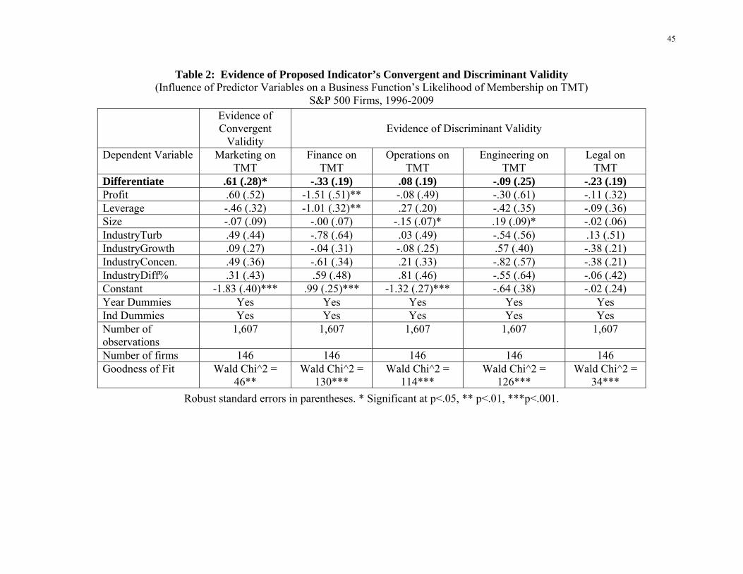
45
Table 2: Evidence of Proposed Indicator’s Convergent and Discriminant Validity (Influence of Predictor Variables on a Business Function’s Likelihood of Membership on TMT)
S&P 500 Firms, 1996-2009
Robust standard errors in parentheses. * Significant at p<.05, ** p<.01, ***p<.001.
Evidence of Convergent
Validity
Evidence of Discriminant Validity
Dependent Variable Marketing on TMT
Finance on TMT
Operations on TMT
Engineering on TMT
Legal on TMT
Differentiate .61 (.28)* -.33 (.19) .08 (.19) -.09 (.25) -.23 (.19) Profit .60 (.52) -1.51 (.51)** -.08 (.49) -.30 (.61) -.11 (.32) Leverage -.46 (.32) -1.01 (.32)** .27 (.20) -.42 (.35) -.09 (.36) Size -.07 (.09) -.00 (.07) -.15 (.07)* .19 (.09)* -.02 (.06) IndustryTurb .49 (.44) -.78 (.64) .03 (.49) -.54 (.56) .13 (.51) IndustryGrowth .09 (.27) -.04 (.31) -.08 (.25) .57 (.40) -.38 (.21) IndustryConcen. .49 (.36) -.61 (.34) .21 (.33) -.82 (.57) -.38 (.21) IndustryDiff% .31 (.43) .59 (.48) .81 (.46) -.55 (.64) -.06 (.42) Constant -1.83 (.40)*** .99 (.25)*** -1.32 (.27)*** -.64 (.38) -.02 (.24) Year Dummies Yes Yes Yes Yes Yes Ind Dummies Yes Yes Yes Yes Yes Number of observations
1,607 1,607 1,607 1,607 1,607
Number of firms 146 146 146 146 146 Goodness of Fit Wald Chi^2 =
46** Wald Chi^2 =
130*** Wald Chi^2 =
114*** Wald Chi^2 =
126*** Wald Chi^2 =
34***

46
Table 3: Cost Leaders and Differentiator Profiles: Average Variable Values (1990-1993)
Quantity in Model
Definition of Quantity
Differentiators (Disclose
Advertising both Before and After
FRR44)
Cost Leaders (Disclose
Advertising Before but not After
FRR44) Sales
In Models: ln(Salesjt ) Underlying Measure: Salesjt (1980 $)
-2.03
$1.28 B
-3.11
$.43 B
Firm Value FirmValuejt = Tobin’s Qjt 1.42 1.30
Differentiation Indicator
= 1 if firm discloses advert.
= 0 if firm does not disclose
1 0
Advertising
Firm’s share of voice in industry advertising
.16 .12
Profit EBITDA / Revenue .10 .07
Leverage Long term debt / Total assets .20 .19
Firm Size
In Model: ln(Assets) Underlying Measure: Assets
-4.61
$1.43 B
-5.45
$.53 B Industry Turbulence
Extent to which industry growth is unpredictable
.04 .05
Industry Growth Industry Revenue Growth Rate
.08 .10
Industry Concentration
Herfindal-Hirschman Index .24 .23
Industry Differentiation %
Within an industry, percent of firms that disclose advertising
.22 .08
Number of Firms 547 883 Number of Observations 1,907 2,564

47
Table 4: Descriptive Statistics: Means and Correlations (1990 – 1993)
(4,471 firm-year observationsa; 1,430 firms)
Mean 1 2 3 4 5 6 7 8 9 10 11
1. ln(Sales) -2.65 1
2. FirmValue 1.35 -.05 1
3. Differentiate .43 .24 .04 1
4. Adv .14 .41 -.07 .10 1
5. Profit .09 .37 .01b .07 .12 1
6. Lev .20 .17 -.13 .04 .05 .07 1
7. Size -5.09 .96 -.10 .18 .40 .37 .20 1
8. IndTurb .04 -.10 -.04 -.06 .11 -.02 b .00 b -.10 1
9. IndGrow .09 -.03 .08 -.06 -.07 .00 b -.07 -.03 b .14 1
10. IndCon .24 -.01 b -.10 .01 b .28 -.04 -.04 -.02 b .26 .00 b 1
11. IndDiff% .14 .26 -.04 .51 -.01 b .03 b .06 .19 -.07 -.08 .07 1
a: Note that correlations with FirmValue are built with only 3,670 observations because some firms are missing values for components of Tobin’s Q. b: (Un-marked correlations are significant at p < .05 or better. Correlations marked with b are not significant at p < .05)
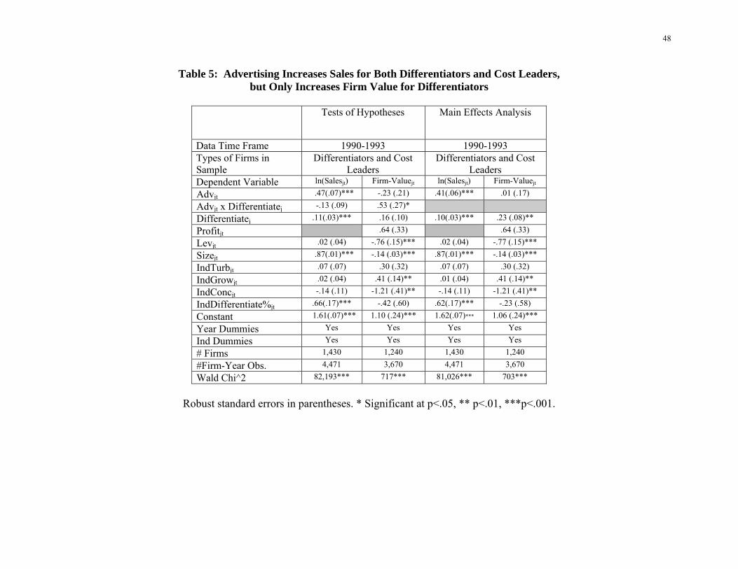
48
Table 5: Advertising Increases Sales for Both Differentiators and Cost Leaders, but Only Increases Firm Value for Differentiators
Tests of Hypotheses Main Effects Analysis
Data Time Frame 1990-1993 1990-1993 Types of Firms in Sample
Differentiators and Cost Leaders
Differentiators and Cost Leaders
Dependent Variable ln(Salesjt) Firm-Valuejt ln(Salesjt) Firm-Valuejt
Advjt .47(.07)*** -.23 (.21) .41(.06)*** .01 (.17)
Advjt x Differentiatej -.13 (.09) .53 (.27)*
Differentiatej .11(.03)*** .16 (.10) .10(.03)*** .23 (.08)**
Profitjt .64 (.33) .64 (.33)
Levjt .02 (.04) -.76 (.15)*** .02 (.04) -.77 (.15)***
Sizejt .87(.01)*** -.14 (.03)*** .87(.01)*** -.14 (.03)***
IndTurbjt .07 (.07) .30 (.32) .07 (.07) .30 (.32)
IndGrowjt .02 (.04) .41 (.14)** .01 (.04) .41 (.14)**
IndConcjt -.14 (.11) -1.21 (.41)** -.14 (.11) -1.21 (.41)**
IndDifferentiate%jt .66(.17)*** -.42 (.60) .62(.17)*** -.23 (.58)
Constant 1.61(.07)*** 1.10 (.24)*** 1.62(.07)*** 1.06 (.24)***
Year Dummies Yes Yes Yes Yes
Ind Dummies Yes Yes Yes Yes
# Firms 1,430 1,240 1,430 1,240
#Firm-Year Obs. 4,471 3,670 4,471 3,670
Wald Chi^2 82,193*** 717*** 81,026*** 703***
Robust standard errors in parentheses. * Significant at p<.05, ** p<.01, ***p<.001.
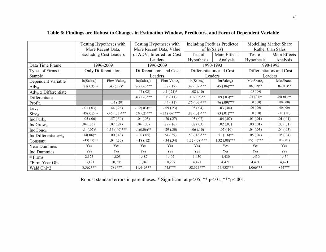
49
Table 6: Findings are Robust to Changes in Estimation Window, Predictors, and Form of Dependent Variable
Testing Hypotheses with More Recent Data,
Excluding Cost Leaders
Testing Hypotheses with More Recent Data, Value of ADVjt Inferred for Cost
Leaders
Including Profit as Predictor of ln(Sales)
Modelling Market Share Rather than Sales
Test of Hypothesis
Main Effects Analysis
Test of Hypothesis
Main Effects Analysis
Data Time Frame 1996-2009 1996-2009 1990-1993 1990-1993 Types of Firms in Sample
Only Differentiators Differentiators and Cost Leaders
Differentiators and Cost Leaders
Differentiators and Cost Leaders
Dependent Variable ln(Salesjt) Firm-Valuejt ln(Salesjt) Firm-Valuejt ln(Salesjt) ln(Salesjt) MktSharejt MktSharejt
Advjt .21(.03)*** .43 (.17)* .26(.06)*** .32 (.17) .49 (.07)*** .45 (.06)*** .06(.02)** .07(.03)**
Advjt x Differentiatej -.07 (.08) .41 (.21)* -.08 (.10) .05 (.06)
Differentiatej .40(.06)*** .03 (.11) .10 (.03)** .09 (.03)** .03 (.01)* .04(.01)***
Profitjt -.04 (.29) .44 (.31) .76 (.09)*** .76 (.09)*** .00 (.00) .00 (.00)
Levjt -.01 (.03) .44 (.26) -.12(.03)*** -.09 (.23) .03 (.04) .03 (.04) .00 (.00) .00 (.00)
Sizejt .49(.01)*** -.46 (.05)*** .53(.02)*** -.33 (.06)*** .83 (.01)*** .83 (.01)*** .00 (.00) -.00 (.00)
IndTurbjt -.05 (.06) .57 (.50) .04 (.05) -.20 (.27) .05 (.07) .04 (.07) .01 (.01) .01 (.01)
IndGrowjt .04 (.03)^ .07 (.24) .04 (.03) .27 (.16) .02 (.03) .02 (.03) .00 (.01) .00 (.01)
IndConcjt -.14(.07)* -1.36 (.40)*** -.16(.06)** -.29 (.30) -.06 (.10) -.07 (.10) .04 (.03) .04 (.03)
IndDifferentiate%jt .14(.06)* .00 (.43) -.00 (.05) .64 (.39) .53 (.16)*** .51 (.16)** .05 (.04) .05 (.04)
Constant -.43(.08)*** .04 (.30) -.18 (.12) -.34 (.34) 1.32 (.08)*** 1.32 (.08)*** .05(.01)*** .03 (.01)
Year Dummies Yes Yes Yes Yes Yes Yes Yes Yes
Ind Dummies Yes Yes Yes Yes Yes Yes Yes Yes
# Firms 2,123 1,805 1,487 1,402 1,430 1,430 1,430 1,430
#Firm-Year Obs. 13,191 10,706 11,040 10,297 4,471 4,471 4,471 4,471
Wald Chi^2 8,562*** 789*** 11,446*** 645*** 58,675*** 57,938*** 1,066*** 844***
Robust standard errors in parentheses. * Significant at p<.05, ** p<.01, ***p<.001.

50
APPENDIX: FRR44 Sections Relevant to Advertising Disclosure Reported in Detail—Key Passages in Bold. For Other Sections, We Delete Explanatory Text and Report Section Headings Only.
Full version: https://www.sec.gov/rules/final/dissuer.txt SECURITIES AND EXCHANGE COMMISSION 17 CFR PARTS 210, 229 and 249 RELEASE NOS. 33-7118; 34-35094; IC-20766; FRR44 INTERNATIONAL SERIES NO. 758 FILE NO. S7-12-94 RIN 3235-AG17 FINANCIAL STATEMENTS OF SIGNIFICANT FOREIGN EQUITY INVESTEES AND ACQUIRED FOREIGN BUSINESSES OF DOMESTIC ISSUERS AND FINANCIAL SCHEDULES AGENCY: Securities and Exchange Commission. ACTION: Final rules. SUMMARY: The Commission is announcing the adoption of amendments to Regulation S-X, which governs the form and content of financial statements and schedules furnished by public companies in filings with the Commission, and Form 20-F, which is applicable to foreign private issuers. The amendments extend accommodations adopted recently with respect to financial statements of foreign issuers to filings by domestic issuers that are required to include financial statements of foreign equity investees or acquired foreign businesses. The accommodations relate to the age of financial statements and the reconciliation of financial statements to U.S. generally accepted accounting principles. In addition, the amendments revise the tests for determining whether financial statements of an equity investee must be provided, and they eliminate the requirement to furnish certain supplemental financial schedules. I. INTRODUCTION The Commission today is adopting several amendments that will extend financial statement accommodations available to foreign issuers to filings by domestic issuers that are required to include financial statements of foreign equity investees or acquired foreign businesses. The accommodations relate to the age of financial statements and the reconciliation of financial statements to U.S. generally accepted accounting principles ("GAAP") for those foreign entities. In addition, the adopted amendments revise the tests of significance for determining whether financial statements of an equity investee must be provided. The amendments also eliminate certain supplemental financial schedules that were eliminated recently for foreign issuers, as well as eliminate two additional schedules that foreign and domestic issuers have been required to include in annual reports and registration statements filed with the Commission. The amendments adopted today were proposed by the Commission on April 19, 1994. Comment letters received from registrants, accounting firms, and related professional membership associations generally supported the proposals and frequently commented that the schedules were generally redundant to information already required in the financial statements and that the costs of preparing the schedules therefore outweighed the benefit. Comments by financial analysts were critical of the proposed amendments, expressing a general concern about a perceived relaxation of disclosure requirements. The Commission believes concerns regarding the revised requirements do not consider fully the offsetting effects of other disclosure requirements that must be met by reporting companies. The amendments are being adopted substantially as proposed because the Commission believes they will result in reduced costs of registration and reporting by public companies without loss of material basic disclosure for the protection of investors. II. FINANCIAL STATEMENTS OF SIGNIFICANT BUSINESS ACQUISITIONS AND EQUITY INVESTEES A. Tests of Significance of Equity Investees B. Reconciliation of Financial Statements of Significant Foreign Equity Investees and Foreign Acquirees C. Age of Financial Statements of Significant Foreign Equity Investees or Foreign Acquirees III. STREAMLINING OF REQUIRED FINANCIAL STATEMENT SCHEDULES The amendments adopted today eliminate the following six schedules that had previously been

51
eliminated for foreign private issuers: (1) Rule 12-02 - Marketable Securities – Other Investments including Schedule XIII (2) Rule 12-03 - Amounts Receivable from Related Parties and Underwriters, Promoters and Employees Other Than Related Parties (3) Rule 12-05 - Indebtedness of and to Related Parties - Not Current. (4) Rule 12-06 - Property, Plant and Equipment (5) Rule 12-07 - Accumulated Depreciation, Depletion (6) Rule 12-08 - Guarantees of Securities of Other Issuers Two additional schedules previously required for both foreign and domestic issuers also will be eliminated: (1) Rule 12-10 - Short-term Borrowings (2) Rule 12-11 - Supplementary Income Statement Information A. Schedules Previously Eliminated from Foreign Issuer Filings 1. Marketable securities - other investments 2. Amounts receivable from related parties and underwriters, promoters and employees other than related parties and indebtedness of and to related parties 3. Property, plant, and equipment, and accumulated depreciation, depletion, and amortization 4. Guarantees of securities of other issuers B. Additional Schedules Eliminated for both Foreign and Domestic Issuers 1. Short term borrowings 2. Supplementary income statement information The Commission has eliminated this schedule by today's amendments. While the amounts of the items formerly referenced by this schedule (maintenance and repairs; depreciation and amortization of the cost of intangible assets, preoperating costs and similar deferred costs; taxes other than payroll; royalties; and advertising costs) need not be disclosed on an ongoing basis by registrants, discussion of discretionary expenses and other items in the schedule, quantified to the extent practicable, will be required in the company's Management's Discussion and Analysis where necessary to explain material trends and uncertainties that affected operating results, liquidity or financial condition of the registrant, or that may be reasonably likely to affect future results, liquidity or financial condition. IV. COST-BENEFIT ANALYSIS Several registrants provided quantified estimates of the cost reductions which would vary from registrant to registrant. All of the registrants and accounting firms that addressed the cost-benefit of the amendments indicated that the cost of preparation and audit of the schedules and other information that have been eliminated today exceeded their benefit. Several financial analysts indicated that they thought that the actual costs of providing this information is small, and that the benefits exceeded such costs. They suggested that the reduced disclosures could lead to an increase in the costs of capital due to an increase in investor uncertainty. For reasons discussed above, the Commission believes that the adoption of these rules will reduce the regulatory burden and costs of the vast majority of the registrants without a loss of information that is necessary for investor protection. V. AVAILABILITY OF FINAL REGULATORY FLEXIBILITY ANALYSIS VI. STATUTORY BASIS FOR RULES VII. EFFECTIVE DATE TEXT OF AMENDMENTS

52
i The differentiator-cost leader dichotomy has been applied in shipping, banking, hospital services; Ireland, Portugal, Korea, China; human resource strategy, information technology, industrial engineering, manufacturing strategy environmental scanning, planning processes, management selection and managerial biases (Campbell-Hunt 2000, p. 128). ii Verhoef , Leeflang (2009), Vorhies, Morgan, Autry (2009), Slater, Olson (2001), Homburg, Workman, Krohmer (1999), Woodside, Sullivan, Trappey (1999): Marketing is more important in differentiators. Day, Nedungadi (1994): Differentiation vs cost leadership shapes managers’ mental representations of competition. iii Advertising influences firm value for beer and cigarettes, not automobiles (Peles 1972); for food, drugs and cosmetics, not tobacco, soap and cleanser (Abdel-Khalik 1975); for the cigarette industry and some cigarette firms, but not other cigarette firms (Schmalensee 1972). iv The information view suggests that advertising impacts only current period sales and should thus be expensed. The persuasion view suggests that advertising builds an asset and should therefore be capitalized, creating a brand asset on the balance sheet. v A firm that is not a differentiator or cost leader is “stuck in the middle” and doomed to fail (Porter 1985, p. 16-17). Such firms will be mis-classified in our data, adding noise and biasing against hypotheses. vi Both the 16% of firms that changed advertising disclosure behavior once and the 4% that changed multiple times did so because of acquisitions, divestitures, bankruptcies, etc. vii Consistent with empirical precedent in research in finance (e.g., Kayhan and Titman, 2007) and accounting (e.g., Desai, Rajgopal, and Venkatachalam, 2004), financial services firms’ federal regulation regimes make it inappropriate to include them in analysis of unregulated firms. . viii Compustat’s “advertising and promotion” does not include price promotions because those discounts must be recorded as a reduction of revenue. Only payment-for-a-distinct-good promotion, like retailer-run co-op advertising, can be included in “advertising and promotion” (Price Waterhouse Coopers 2010). ix While researchers often use Arellano and Bond’s (1991) “difference GMM” approach to relax this assumption (e.g., Kumar et al. 2014; Shah, Kumar, and Kim 2014), that approach is not an option for models such as ours that have time-constant predictors. x If a firm differentiated in one industry while cost-leading in another it would incur policy and cultural spillovers which would cause the firm to be ineffective in both industries (Porter 1985, p. 17-18).

Can Sales Uncertainty Increase Firm Profits?
Niladri Syam*
Department of Marketing Trulaske College of Business
University of Missouri Columbia, MO 65211
Email: [email protected] Phone: 573-882-9727
James D. HessDepartment of Marketing and Entrepreneurship
C. T. Bauer College of Business University of Houston Houston, TX 77204
Email: [email protected] Phone: 713-743-4175
Ying Yang Department of Marketing
Tippie College of Business, University of Iowa
Iowa City, IA 52242 Email: [email protected]
Forthcoming: Journal of Marketing Research
June 22, 2015
*Corresponding Author
Do not cite without permission

1
Can Sales Uncertainty Increase Firm Profits?
Abstract: We add to the sales management literature in three ways. First we demonstrate that a firm can benefit from higher sales uncertainty. This is contrary to the finding in the standard principal-agent models that more sales uncertainty hurts the firm when agents are risk-averse. Second, we also find that the risk-averse agent’s total pay can increase in uncertainty, and this too is contrary to the standard principal-agent model. Third, we provide intuition for our surprising result by showing that it holds when the slope of the sales response function is random but not when the intercept is random. When the responsiveness (slope) of sales to a decision variable (of the firm or the agent) is random then information about randomness becomes decision-relevant and the firm can exploit learnt information. In our model, the agent and firm can receive noisy signals of random demand. When the customers’ response to effort (or price) is random the decision about effort (price) responds optimally to information in a way that benefits the firm. When uncertainty is high there is more information potential for the firm to exploit profitably owing to the convexity of the sales with respect to the uncertainty parameter. This is enough to dominate the negative impact that uncertainty has owing to agents’ risk-aversion. When randomness only affects baseline sales (intercept), received signals are not decision-relevant. In this case, higher uncertainty only has a negative impact just as in standard principal-agent models.
Keywords: adaptive selling, sales uncertainty, principal-agent, information, signals, sales force
2
1. Introduction
The role of uncertainty has received much attention in the sales force management
literature which has studied it both from theoretical and empirical perspectives. In the sales force
management context, the risk-averse salespeoples’ incentives are crucial since risk-aversion
creates costs for the firm that employs them. In other contexts, such as in finance, it has been
suggested that uncertainty could be beneficial, implying that firms may voluntarily want to
expose themselves to risk (Buehler and Pritsch, 2003; Hartford, 2011). Importantly, studies in
these other contexts set aside employee attitudes toward risk. Thus, two questions for sales force
management are: Can the firm benefit from uncertainty when it must incentivize a risk-averse
salesperson? How does the risk-averse salesperson’s total compensation respond to larger
uncertainty?
The theoretical sales management literature, which uses the principal-agent model as the
workhorse, unambiguously predicts that higher sales uncertainty should reduce firm profits
(Bolton and Dewatripont, 2005, p. 139; Salanie, 1997, p. 133; Lal and Srinivasan 1993). We
have two main results. First, contrary to the standard principal-agent model, information about
sales randomness can be extracted and used in a way that the firm can actually benefit from
higher uncertainty even though it needs to incentivize a risk-averse agent. Second, we show that,
also contrary to the standard principal-agent model, the agent’s total pay can increase with higher
uncertainty. The standard principal-agent model predicts that sales uncertainty decreases total
pay (Bolton and Dewatripont, 2005, p. 139; Coughlan and Narasimhan, 1992, p. 96; Basu, Lal,
Srinivasan, Staelin, 1985, p. 282, etc.) Related to our first result, in the finance literature
Alexandrov (2011) theoretically shows that firms could benefit from cost uncertainty, but this
work is not in the principal-agent framework and ignores the added complexity of motivating a

3
risk-averse agent. Related to our second result, Misra, Coughlan and Narasimhan (2005)
theoretically show that the agent’s total pay can increase in uncertainty, but only when the
principal is sufficiently risk-averse. Consistent with the standard, and the most commonly used,
principal-agent models we have assumed a risk-neutral principal.
Interestingly, empirical tests of the principal-agent model regarding the effect of
uncertainty on agent’s total pay seem to support our theoretical prediction. The standard PA
model predicts that agent’s total pay should decrease in uncertainty, but consistent with our
prediction, Coughlan and Narasimhan (1992) empirically find that higher uncertainty increases
agent’s total pay (although not statistically significant). Similarly, Joseph and Kalwani (1995)
investigate the effect of uncertainty on total pay and proportion of incentive pay and note that
“for both of these comparisons, the observed effects are in a direction opposite to that
hypothesized” (pp. 194). Misra, Coughlan and Narasimhan (2005) analyze two data sets and find
no effect of uncertainty on salesperson’s total pay in one data set and a statistically significant
positive effect in the other data set. Interestingly, unlike the field evidence provided by these
above mentioned papers, Umanath, Ray and Campbell (1993) test the principal-agent model’s
predictions in an experimental setup. Thus, these authors are able to ensure that they remain true
to the theoretical model’s assumptions of a risk-neutral principal and a risk-averse agent. They
find that, contrary to the model’s prediction, there is a positive and significant effect of
uncertainty on agent’s total pay. Lal, Outland and Staelin (1994) offers significant supporting
evidence for the theoretically predicted effects of uncertainty on salary and on the ratio of salary
to total pay, but they do not study the effect on total pay alone. In sum, the bulk of empirical
evidence runs counter to the theoretical prediction that total pay should decrease in uncertainty.

4
As will be clear below, our results hold where the slope of the sales response function is
random. Whereas most theoretical principal-agent models assume a random intercept (Basu, Lal,
Srinivasan, Staelin; Lal and Srinivasan 1993, etc.), Godes (2003) is one of the few models where
the effectiveness of effort (that is, the slope of the response function) is random.
The sales management literature recommends that salespeople should avoid uncertainty,
perhaps driven by a mistaken belief about the impact of uncertainty as mentioned above. Among
other things, this is especially harmful for a critical success factor for firms, which is new
product success, since uncertainty avoidance induces salespeople to shy away from selling new
products in favor of serving established products and customers. Hultink and Atuahene-Gima
(2000) state that, “With increasing market uncertainties [our italics] and the rapid pace of
technological change, new product marketing poses unique challenges to market participants.” In
a similar vein, Ahearne, Rapp, Hughes and Jindal (2010) mention that, “They [salespeople] may
even be unwilling to expend the energy necessary to sell a new product… preferring instead to
focus on selling established products because this requires less effort and engenders greater
certainty [our italics] than attempting to generate interest in a new product.”
The key managerial message of our paper is that both sales managers and salespeople can
benefit from greater uncertainty if the following conditions hold: (a) managers/salespeople
possess or can install information systems designed to generate accurate, decision-relevant
information about the sales environment and (b) sales processes are flexible and adaptive, so that
agents can nimbly adjust their selling efforts and/or managers can adjust the marketing mix
(prices, advertising, etc.) to reflect the acquired information.
Why are sales higher with greater uncertainty? The critical driver is the salesperson’s
ability to adapt her efforts, or other decisions, to the acquired information. For example, the

5
salesperson may discuss the customer’s needs and concerns and then adjust the frequency of
sales calls or price discounts to reflect these assessments. Consider uncertainty regarding
consumers’ preference for a product. A higher uncertainty implies a higher variance around
typical consumer preferences: more consumers love the product and more hate the product. In
such cases there is more of a potential upside, and the acquired information allows the
salesperson to benefit from it by increasing her effort. Of course, there is also more of a
potential downside, but now acquired information allows the salesperson to decrease her effort
and thereby reduce costs without substantially effecting sales. This minimizes the negative effect
of the potential downside. Thus, this type of ‘adaptive selling’, where effort adapts to
information, ensures that the salesperson and firm benefit more from the upside of uncertainty
while not suffering as much from the downside.
We demonstrate our findings with two important selling decisions, the salesperson’s
effort (as in the principal-agent model) and product’s price (as a representative of a variety of
other marketing mix variables). First, when demand responds only to salesperson’s effort, we
show that the expected profit can increase in uncertainty when the effectiveness of effort is
random (slope), but not when baseline demand (intercept) is random. Second, when the sales
response function also includes price, profit can increase in uncertainty even when randomness
enters additively (see also, Weinberg 1975; Bhardwaj 2001; Joseph 2001; Kalra, Shi and
Srinivasan 2003). The critical driver of our result is that the sensitivity of the firm’s profit to a
choice variable of the firm and/or the agent is the source of uncertainty. In both cases, adaptive
selling convexifies the sales with respect to uncertainty, and therefore, higher uncertainty implies
more information potential in the system for the firm to benefit from.

6
Our model resembles Godes (2003) where sales randomness pertains to the effectiveness
of effort and noisy signals of effort effectiveness are received by the agent. However, unlike his
model, we assume the firm and the agents have the same information and thus signaling by the
agents to the firm is moot. Our research connects to the rich literature in marketing that
investigates the role of sales uncertainty in various aspects of interest to a selling organization
(Godes 2004). Other researchers (Lal et al. 1994; Joseph and Kalwani 1995; Krafft et al. 2004)
have studied how sales uncertainty affects the firm’s compensation decision. We also connect to
the literature on informational aspects of principal-agent models (Nalebuff and Stiglitz 1983;
Singh 1985; Sobel 1993).
As already mentioned, in this paper we distinguish between uncertainty that affects the
intercept of the sales response function and uncertainty that affects the slope. The former is more
commonly used in the principal-agent literature and can be thought of as uncertainty about
baseline demand (market size). That is, there is randomness about how many customers the
salesperson will be able to sell to but the response of any given customer to salesperson’s effort
is known. The counter-intuitive result that we present in this paper occurs when there is
uncertainty about the slope, and this can be thought of as uncertainty about customers’ response
to salesperson’s effort. This could be related to the customer’s unknown preference for the
product. Clearly, if the customer likes the firm’s product more, the agent’s effort will lead more
easily to sales. Therefore, in practical terms, the uncertainty can be thought of as the firm’s and
agent’s uncertainty about how much the customer likes the product.
Our theory is relevant to situations where a product is being sold to new customers and
there is heterogeneity in these customers’ liking of the product: some may respond to sales calls
and some may not. If the compensation plan period is shorter than the sales cycle, then the
7
agent’s compensation can be changed in the next plan period to reflect newly acquired
information. For instance, in complex sales (e.g., in ‘solution’ selling) the product-and-service
combination is novel and therefore the customer’s preference is unknown. Moreover, the longer
sales cycles of these complex sales implies that the firm has ample opportunities to customize the
marketing mix (e.g. the price) and/or the agent’s compensation depending on what is learnt about
the customer’s preference for the product. As is quite common, the firm does ride-alongs with
the agent, especially at the beginning when the company is establishing rapport with the
customer. Through these joint visits both the manager and agent receive signals about the
customer’s preference. The firm’s compensation in the next plan period, the agent’s efforts and
the firm’s marketing mix (or a subset of these) can be conditioned on information received.
Usually there is no ‘list-price’ for such complex offerings; prices are negotiated with buyers and
can be conditioned on new information. Our theory also holds when marketing mix elements can
be adapted in light of new information.
2. Profit Can Increase in Sales Uncertainty in a Principal-Agent Model
2.1 Random slope
Consider a firm (firm plays the role of the principal in the principal-agent model) that
sells its product through a sales agent. Let the sales response function be
.e1s θ+= (1) As is common in principal-agent models, the sales s are random and here randomness is given by
the coefficient θ, whose mean is 1 and variance is V. We could interpret θ as the effectiveness,
or productivity, of sales effort. The sales response function in (1) captures a situation where the
uncertainty is about the customers’ response to the sales agent’s effort. On average the sales will
increase 1 unit for every extra unit of effort, but the customers’ response to effort may exceed or

8
fall short of this at random (see Godes 2003 for a different approach to this). We take the
variance of θ as the measure of sales uncertainty (Lal and Srinivasan 1993). In subsection 2.2,
we analyze the more common sales response function where uncertainty concerns the demand
intercept rather than slope. The contrasting effects of sales uncertainty on expected profit when
the slope versus the intercept is random is the major insight of this paper.
Prior to the agent choosing effort and the principal choosing its compensation, suppose
both principal and agent receive a signal η about θ. Others scholars have used this idea of
imperfect signals about consumers being available in the system. Like Godes (2003), we model a
situation where the effectiveness/productivity of effort is random (the randomness could be
interpreted as the customer’s response to effort for example). He models the randomness as
discrete where effort is either “effective” or “ineffective.” Similar to our setup, the agent in
Godes’ analysis chooses action after receiving a noisy signal about the effectiveness of her effort
and Joseph (2001) analyzes a situation where salespeople gather customer information through
prospecting.
Specifically, suppose the joint distribution of productivity and signal is Normal:
.
VVV,
01
N~
ΣΣρΣρ
ηθ
(2)
Obviously the covariance matrix can be parameterized in different, equivalent ways, but we have
expressed the covariance matrix in terms of correlation ρ for a very specific purpose: as we
change the uncertainty V we would like to keep the accuracy of the signal constant. We use the
squared correlation ρ2 as a measure of the accuracy, or information quality, of the signal (like the
coefficient of determination in regression analysis). The conditional distribution of customers’
response given the signal is

9
( ))-V(1,/V1N~ 2ρηΣρ+ηθ . (3)
The signal allows the agency to reduce the prior variance of θ, which is V, to the posterior
variance V(1- ρ2). The absolute reduction in the variance Vρ2 depends upon the initial
uncertainty V, but the proportional reduction in variance Vρ2 /V=ρ2 is constant across initial
uncertainty. Thus, ρ2, which is the squared correlation of θ and η, is a measure of the accuracy of
the signal η, with ρ2 =1 implying that the signal is completely accurate and ρ2 =0 implying that
the signal is completely inaccurate; we assume that ρ2<1 because the basic issue of agency
theory is uncertainty. We explore the effect of higher uncertainty V on firm profits and agent’s
total pay keeping the signal accuracy, i.e., the proportional reduction in uncertainty, constant.
How can uncertainty about selling effectiveness increase in such a way that the agent gets
signals of effectiveness that proportionately reduce uncertainty? The initial uncertainty about the
two customers A and B could be based on a history of calls. Suppose the agent has M and 2M
historical observations of sales calls and resulting purchases, respectively, so there is greater
initial uncertainty about customer A, who has a shorter history compared to customer B.
Subsequently, assume the salesperson asks questions and records the customers’ reactions in a
pattern that mirrors previous sales calls. Let the number of question-and-answer interactions
with A and B be N and 2N times. This difference could be because the salesperson feels
comfortable asking more questions of a customer with whom he has had more previous
interactions. These Q&A interactions could generate signals that reduce the uncertainty by the
same proportion for customers A and B.1 In sum, even though the a priori uncertainty is greater
for customer A, the signals are equally accurate.
1 The prior uncertainty for A is proportional to 1/M and, after N question and answer sessions, the posterior uncertainty is proportional to 1/(M+N). The proportional reduction in uncertainty for A is [M-1- (M+N)-1]/M-1. Similarly, the proportional reduction in uncertainty for B is [(2M)-1- (2M+2N)-1]/(2M)-1, but the 2s cancel.

10
Suppose the agent is paid a salary and commission on sales, Pay=S+Cs, a common
system both in practice and in analytical models of sales force compensation (Joseph and
Thevarajan 1998; Kalra, Shi and Srinivasan 2003). Further, let the agent’s cost of effort be 2e21 .
A constant risk-averse salesperson’s utility is
−θ++−
−=2e
21e] C[1Sr
ebaU , where a and b are
arbitrary positive constants, so expected utility equals
−= −θ++−
ηθηθ)ee] C[1r(S
||2
21
eEba[U]E ,
where the subscript θη makes it clear that the expectation is taken with respect to the
conditional distribution.
The certainty equivalent (CE) of the job is the certain payment that gives identical
expected utility:2
)1(VerCe)e/Ve1(CS)(CE 222212
21 ρ−−−ηΣρ+++=η . (4)
Conditional upon the signal, the effort that maximizes the agent’s certainty equivalent is
)1(VrC1/V1C)(e 22
*
ρ−+
ηΣρ+=η . (5)
It is important to note that in this case where the uncertainty is about the customers’ response to
effort, the optimal effort adjusts to the productivity signal, η. Information is decision-relevant.3
The principal chooses the salary and commission rate so that the agent’s certainty
equivalent equals that of the second best possible alternative employment U . Conditional upon
2 This uses the fact that if X~N(µ,σ2) the moment generating function is E[exp(tX)]=exp(tµ+ ½ t2σ2). 3 In contrast, when uncertainty is about the baseline level of sales, effort is independent of the signal which is decision-irrelevant; see equation (14) in Appendix.

11
the signal, the expected profit of the principal is the expected sales (normalized price is 1) minus
salary and commission,
( ) U)1(VrC1
CC2/V11)]([E 22
2221
| −ρ−+
−ηΣρ++=ηπηθ . (6)
The optimal commission rate C* is the solution of the first order condition
0)1(1 2*2* =−−− CrVC ρ . (7)
Clearly C* does not depend upon the value of the signal, η. One can easily see that the
commission rate increases if the information system is more accurate (ρ2 increases), because
information reduces the perceived risk that the risk-averse agent must bear.
The principal must calculate the unconditional expected profit as anticipated prior to
observing the signal. Since C* is independent of η and η~N(0, Σ), this calculation leads to
[ ] ( ) U)V1(*C1UV1
)1(VrC1
CC21)]([EE*E 2212
22*
2**
21 −ρ++=−ρ+
ρ−+
−+=ηπ=π ηθη . (8)
How does this ex-ante expected profit respond to an increase in the uncertainty about the
agent’s effort effectiveness?
Theorem 1: If the sales response function is such that the customers’ response to effort is random, s=1+θe, then as sales uncertainty V increases, the expected profits of the firm increases if signals are sufficiently accurate (ρ2 large enough).
(All proofs are found in the Appendix.) Theorem 1 offers the main theoretical insight of this
paper. Contrary to the finding in the standard principal-agent models (Bolton and Dewatripont,
2005, p. 139; Salanie, 1997, p. 133; Lal and Srinivasan 1993), information extraction can imply
that the firm’s profits increases with higher sales uncertainty. Why does this happen?
12
Risk aversion corresponds to a utility function that bends concavely downward as
realized pay increases, such that expected utility is below the utility function. This disutility
implies that when the environment is more uncertain, it imposes a larger cost on the firm and this
has the effect of reducing sales and profits.
However, if the effectiveness of effort is random and if signals of this effectiveness are
available, there is a counter-balancing effect. When signals of effectiveness are available, the
agent increases effort if the observed signal η is better (see (5)), and this dependence is stronger
if the uncertainty is larger (for sufficiently accurate signals). The expected value of the
effectiveness of effort θ also increases with the signal η (see (3)), and this dependence too is
stronger if uncertainty is larger. Thus, the expected sales becomes convex in the signal (see (1)),
and is more convexly curved for higher uncertainty. Higher uncertainty might increase both
effort and expected effectiveness by 10% for a given signal but this would increase expected
sales by 1.10×1.10, or 21%. So, averaging across all possible signals can increase the expected
sales as uncertainty increases. Crucially, and pertinent to the sales force management context,
this convexifying force is enough to counteract the negative effect of risk aversion of the
employees. Of course, uncertainty is beneficial only when information is accurate.4
It is important to note two aspects of Theorem 1. First, our result is not merely a
statement about the value-of-information: that additional information is valuable to the principal.
Value-of-information refers to the levels of profits when more accurate information is available
(ρ2 is larger). This obviously holds in our model. From the profit expression in (8), and because
4 The simple form of the sales response function in equation (1) could be easily generalized, so long as there is an interaction of effort and uncertainty, and Theorem 1 will be applicable. For example, one could show that it is also true for a sales response function ε++= e1s , which has the property that the marginal productivity of effort is influenced by the magnitude of the random term. We thank an anonymous reviewer for this suggestion.

13
(7) implies that 2
*
ρ∂∂C >0, the profit clearly increases with information quality ρ2. Instead,
Theorem 1 demonstrates how the firm can exploit greater sales uncertainty, so our result is about
the marginals of profit with respect to uncertainty when the firm can and cannot exploit
information about randomness – the marginal is positive in the former case and negative in the
latter. Second, our result is independent of the level of risk-aversion. Because r enters the optimal
profit only indirectly through C* and (7) implies thatr
C*
∂∂ <0, the profit decreases with risk-
aversion, consistent with expectation. Instead, Theorem 1 shows that the benefit of reflecting
learnt information in optimal decisions is large enough to overcome the drag due to risk-aversion
for all levels of risk-aversion r.
What about the agent’s total pay? One can show that total pay of the agent is expected to
equal )V1(*C2
*CU 22
21 ρ+
−+ . Differentiating this with respect to variance V and evaluating it
when ρ2 approaches 1, one can see that the total pay increases as uncertainty rises.
Theorem 2: If the sales response function is such that the customers’ response to effort is random, s=1+θe, then as sales uncertainty V increases, the total pay of the agent increases if signals are sufficiently accurate (ρ2 large enough).
Interestingly, Theorem 2 also is the opposite of that in the standard principal-agent model where
the agent’s total pay decreases in uncertainty (Bolton and Dewatripont, 2005, p. 139; Coughlan
and Narasimhan, 1992, p. 96; Basu, Lal, Srinivasan, Staelin, 1985, p. 282 etc.). In Table 1,
inaccurate information, the lower row, corresponds to the standard finding: as variance increases,
reliance on commissions to motivate effort is diminished and total pay is expected to fall.
However, with accurate decision-relevant information, top row of Table 1, expected sales
increase with variance and this leads to an increase of total pay for the agent.
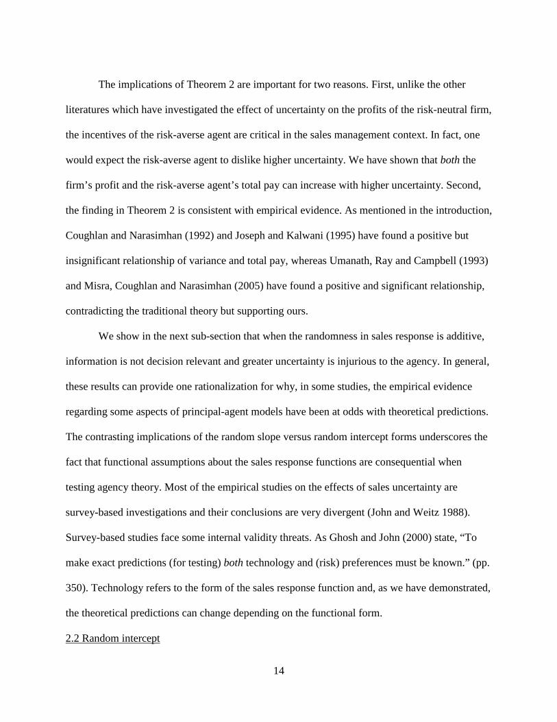
14
The implications of Theorem 2 are important for two reasons. First, unlike the other
literatures which have investigated the effect of uncertainty on the profits of the risk-neutral firm,
the incentives of the risk-averse agent are critical in the sales management context. In fact, one
would expect the risk-averse agent to dislike higher uncertainty. We have shown that both the
firm’s profit and the risk-averse agent’s total pay can increase with higher uncertainty. Second,
the finding in Theorem 2 is consistent with empirical evidence. As mentioned in the introduction,
Coughlan and Narasimhan (1992) and Joseph and Kalwani (1995) have found a positive but
insignificant relationship of variance and total pay, whereas Umanath, Ray and Campbell (1993)
and Misra, Coughlan and Narasimhan (2005) have found a positive and significant relationship,
contradicting the traditional theory but supporting ours.
We show in the next sub-section that when the randomness in sales response is additive,
information is not decision relevant and greater uncertainty is injurious to the agency. In general,
these results can provide one rationalization for why, in some studies, the empirical evidence
regarding some aspects of principal-agent models have been at odds with theoretical predictions.
The contrasting implications of the random slope versus random intercept forms underscores the
fact that functional assumptions about the sales response functions are consequential when
testing agency theory. Most of the empirical studies on the effects of sales uncertainty are
survey-based investigations and their conclusions are very divergent (John and Weitz 1988).
Survey-based studies face some internal validity threats. As Ghosh and John (2000) state, “To
make exact predictions (for testing) both technology and (risk) preferences must be known.” (pp.
350). Technology refers to the form of the sales response function and, as we have demonstrated,
the theoretical predictions can change depending on the functional form.
2.2 Random intercept

15
In a contrast to randomness of slope in (1), consider the more traditional case of the
additive random term in the sales response function:
.e1s +ε+= (9) Here, the intercept of demand, 1+ε, is random but the customers’ response to effort is fixed (Lal
and Staelin 1986; Joseph and Thevarajan 1998; Kalra and Shi 2001).
As in sub-section 2.1, prior to the agent choosing effort and the firm choosing its
compensation both firm and agent receive a signal η about demand fluctuations, ε. Suppose the
joint distribution of level of demand and signal is Normal, similar to distribution (2). The
expected sales are 1+e, the same as with the response function in (1). The analysis of this case is
similar to that in sub-section 2.1 and is relegated to the Appendix.
Theorem 3: If the sales response function has a random intercept, s=1+ε+e, then as sales uncertainty V increases, the expected profits of the firm decreases regardless of the accuracy of signals about the uncertainty.
Of course, in standard principal-agent models where there are no opportunities to gather
demand signals, increased sales uncertainty always decreases expected profits because of the
agent’s risk-aversion (see Bolton and Dewatripont, 2005, p.139; Salanie, p.133; Lal and
Srinivasan 1993). The analysis in sub-section 2.1 establishes that decision-relevant information
can reverse this conclusion. To be decision-relevant, the randomness needs to be about the
customers’ response to agent effort, rather than baseline level of sales.5
We have focused on the simplest model of an agency, where the only choice that
influences demand is the agent’s sales effort. Our result is more general, however. So long as the
5 A reviewer of this paper pointed out that it is possible for an increase in the variance of a random variable to automatically increase its mean, making expected sales increase with variance. For example, if ε was distributed χ2 with k degrees of freedom, its mean is k and its variance is 2k. Theorem 3 applies when random sales has a mean that is independent of its variance as is assumed in the standard PA model.
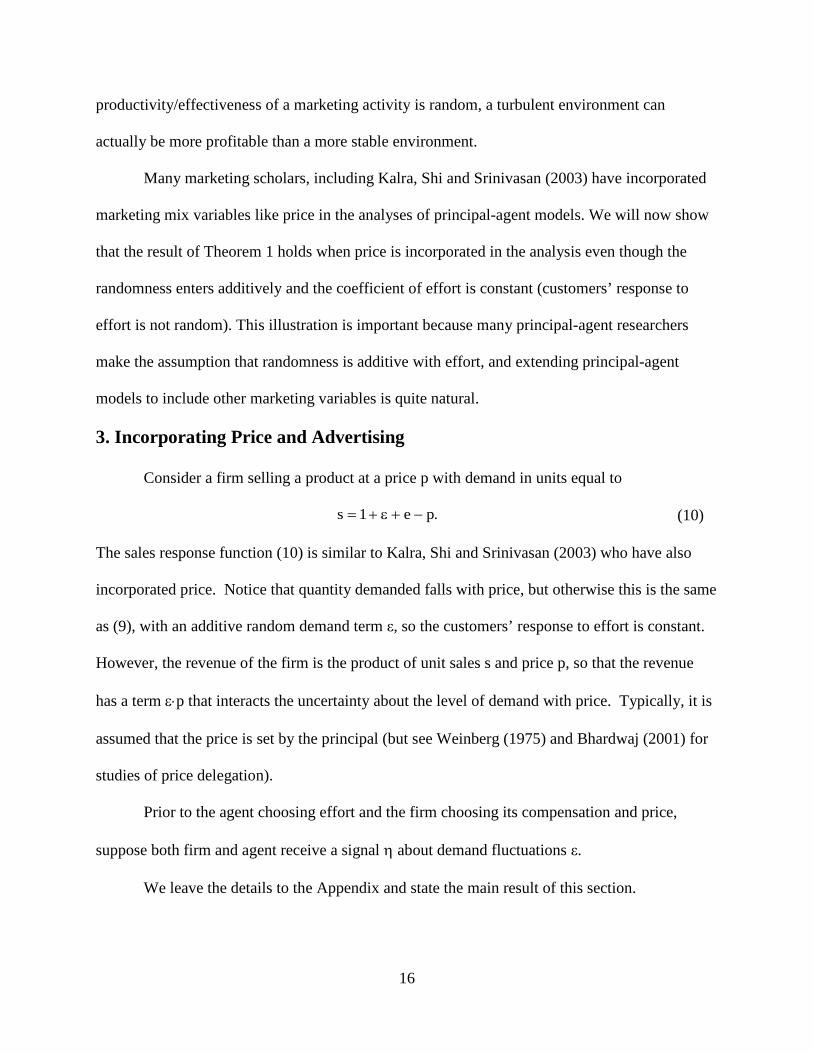
16
productivity/effectiveness of a marketing activity is random, a turbulent environment can
actually be more profitable than a more stable environment.
Many marketing scholars, including Kalra, Shi and Srinivasan (2003) have incorporated
marketing mix variables like price in the analyses of principal-agent models. We will now show
that the result of Theorem 1 holds when price is incorporated in the analysis even though the
randomness enters additively and the coefficient of effort is constant (customers’ response to
effort is not random). This illustration is important because many principal-agent researchers
make the assumption that randomness is additive with effort, and extending principal-agent
models to include other marketing variables is quite natural.
3. Incorporating Price and Advertising
Consider a firm selling a product at a price p with demand in units equal to
.pe1s −+ε+= (10) The sales response function (10) is similar to Kalra, Shi and Srinivasan (2003) who have also
incorporated price. Notice that quantity demanded falls with price, but otherwise this is the same
as (9), with an additive random demand term ε, so the customers’ response to effort is constant.
However, the revenue of the firm is the product of unit sales s and price p, so that the revenue
has a term ε⋅p that interacts the uncertainty about the level of demand with price. Typically, it is
assumed that the price is set by the principal (but see Weinberg (1975) and Bhardwaj (2001) for
studies of price delegation).
Prior to the agent choosing effort and the firm choosing its compensation and price,
suppose both firm and agent receive a signal η about demand fluctuations ε.
We leave the details to the Appendix and state the main result of this section.

17
Theorem 4: If the unit sales response function has a random intercept, s=1+ε+e-p, but the firm can adjust price based upon a sufficiently accurate signal of demand intercept, then as sales uncertainty increases, the expected profits of the firm increases.
The result in Theorem 4 is qualitatively the same as Theorem 1 even though the uncertainty
pertains to the level of demand, not the customers’ response to effort.
How does the finding of the traditional principal-agent model flip in this case? Here the
signal η is decision relevant for the firm’s price, rather than agent effort. Observe that the profit
is sales × price which has the effect of making the randomness multiplicative with price. Thus,
the responsiveness of the firm’s profit to a decision variable, price in this case, is random just as
we had the responsiveness of profit to effort being random in sub section 2.1.
There are two differences between the extension presented in the current section and the
standard principal-agent model: (1) the firm can obtain signals about the random term, and (2)
this information is used to change some element of the marketing mix. Both of these are critical.
First, if there is no signal, then in terms of our model it would imply that ρ2=0. As shown in the
proof of Theorem 4, a signal with ρ2=0 implies that V
*
∂π∂ <0. In others words, the firm’s profit
would decrease in sales uncertainty consistent with the standard principal-agent model. Second,
if price is not endogenized then we can show that the firm’s profit decreases in sales uncertainty,
again consistent with the standard principal-agent model. Then the optimal profit of the firm is
U)]-rV(122[1
)]-rV(1[1*E 2
2−
ρ+
ρ+=π , which always decreases in sales uncertainty:
dV*dEπ <0.
We can extend our analysis to incorporate advertising. Suppose the demand is a function
of awareness advertising A, Aes )1( ε++= (see Hauser and Shugan 1983). The random variable
ε multiplies the marketing decision variable A, much like it did price above. This means that

18
signals about demand are decision-relevant for advertising and one could show that the resulting
expected profit increases with uncertainty if the information is accurate enough.
4. Conclusion
We show that the selling firm’s profit and the risk-averse sales agent’s total pay can
increase with greater uncertainty, both of which are contrary to the results in the standard
principal-agent model. If the uncertainty is potentially discoverable prior to decisions (even
when signals of uncertainty are imperfect), then the firm/salesperson can exploit such
information. The core issue is whether the information could change the agent’s efforts or the
firm’s price (or other marketing mix variables). The managerial implication is that marketing
research should focus on learning about customer’s response to effort rather than about baseline
sales. When uncertainty is high there could be both higher upside and higher downside of
uncertainty. Adaptive selling ensures that the salesperson and firm benefit more from the upside
of uncertainty while not suffering as much from the downside. In this paper we assumed a salary
plus commission type of compensation contract, but we have also explored non-linear contract
forms, like the bonus-quota contract, and find that the main result of Theorem 1 continues to
hold. We have assumed a very standard utility function used in principal-agent models, but
future research could do explorations with different utility functions.
References
Ahearne, Michael, Adam Rapp, Douglas Hughes and Rupinder Jindal (2010), “Managing Sales
Force Product Perceptions and Control Systems in the Success of New Product Introductions,” Journal of Marketing Research, Vol. XLVII, 764-776.
Alexandrov, Alexei (2011), “Firms Should be Risky at the Margin,” Working Paper, University
of Rochester. Anderson, Erin and Richard Oliver (1987), “Perspectives on Behavior-Based Versus Outcome-
Based Salesforce Control Systems,” Journal of Marketing, 51 (Oct), 76-88.

19
Basu, Amiya, Rajiv Lal, V. Srinivasan and Richard Staelin (1985), “Salesforce Compensation
Plans: An Agency Theoretic Perspective,” Marketing Science, 4 (4), 267-291. Bhardwaj, Pradeep. (2001), “Delegating Pricing Decisions,” Marketing Science, 20(2), 143-169. Bolton, Patrick and Mathias Dewatripont (2005), Contract Theory, MIT Press, Cambridge, MA. Buehler, Kevin S. and Gunnar Pritsch (2003), “Running with risk,” McKinsey Quarterly, 4,
40–49. Coughlan, Anne and Charravarthi Narasimhan (1992), “An Empirical Analysis of Salesforce
Compensation Plans,” Journal of Business, 65(1), 93-121. Ghosh, Mrinal and George John (2000), “Experimental Evidence for Agency Models of
Salesforce Compensation,” Marketing Science, 19(4), 348-365. Godes, David (2003), “In the Eye of the Beholder: An Analysis of the Relative Value of a Top
Sales Rep Across Firms and Products,” Marketing Science, 22(2), 161-187. Godes, David (2004), “Contracting under Endogenous Risk,” Quantitative Marketing and
Economics, 2, 321-345. Hartford, Tim, (2011), “Adapt: Why Success Always Starts with Failure,” Farrar, Straus and
Giroux. Hauser, John R. and Steven M. Shugan (1983), “Defensive Marketing Strategies,” Marketing
Science, 2(4), 319-360. Hultink, Eric Jan and Kwaku Atuahene-Gima (2000), “The Effect of Sales Force Adoption on
New Product Selling Performance,” Journal of Product Innovation Management, 17, 435-450.
John, George and Barton Weitz (1988), “Explaining Variation in Sales Compensation Plans:
Empirical Evidence for the Basu et al Model,” Working Paper, Department of Marketing, University of Minnesota.
Joseph, Kissan (2001), “On the Optimality of Delegating Pricing Authority to the Sales Force,”
Journal of Marketing, 65(1), 62-70. Joseph, Kissan and Alex Thevarajan (1998), “Monitoring and Incentives in Sales Organizations:
An Agency Theoretic Perspective,” Marketing Science, 17(2), 107-123. Joseph, Kissan, and Manohar Kalwani (1995), “The Impact of Environmental Uncertainty on the
Design of Salesforce Compensation Plans,” Marketing Letters, 6, 183–197.

20
Kalra, Ajay, and Mengze Shi (2001), “Designing optimal sales contests: A theoretical Perspective,” Marketing Science 20(2), 170-193.
Kalra, Ajay, Mengze Shi and Kanan Srinivasan (2003) “Salesforce Compensation Schemes and
Consumer Inferences,” Management Science, 49(5), 655-672. Lal Rajiv, Donald Outland and Richard Staelin (1994), “Salesforce Compensation Plans: An
Individual Level Analysis,” Marketing Letters, 5(2), 117-130. Lal, Rajiv, and V. Srinivasan (1993), “Compensation Plans for Single- and Multi-Product
Salesforces: An Application of the Holmstrom-Milgrom Model,” Management Science, 39(7), 777-793.
Misra, Sanjog, Anne Coughlan and Chakravarthi Narasimhan (2005), “Salesforce Compensation:
An Analytical and Empirical Examination of the Agency Theoretic Approach,” Quantitative Marketing and Economics, 3, 5-39.
Salanie, Bernard (1997), The Economics of Contracts, MIT Press, Cambridge, MA. Sobel, Joel (1993), “Information Control in the Principal-Agent Problem,” International
Economic Review, 34(2), 259-269. Umanath, Narayan, Manash Ray and Terry Campbell (1993), “The Impact of Perceived
Environmental Uncertainty and Perceived Agent Effectiveness on the Composition of Compensation Contracts,” Management Science, 39 (1), 32-45.
Ustuner, Tuba and David Godes (2006), “Better Sales Networks,” Harvard Business Review,
July-August, 84(7/8), 102-112. Weinberg, Charles. B. (1975), “An Optimal Commission Plan for Salesmen’s Control Over
Price,” Management Science, 21(8), 937-943.
Appendix Proof of Theorem 1:
Differentiating (7) with respect to V gives ).1(r*C2
*CdV
*dC 23
ρ−−
−= Differentiating (8) with
respect to V and substituting the above gives )1()V1(rC2
CCdV
*dE 22*
3*2 ρ−
ρ+
−−+ρ=
π * .
The marginal expected profit is a weighted average of a positive term and a negative term, with
weights ρ2 and 1-ρ2. If signal accuracy ρ2 is near 1, the weighted average is positive.

21
Proof of Theorem 2: Differentiate )V1(*C2
*CU]Pay[E 22
21 ρ+
−+= with respect to V to get
ρ
−+ρ+
−
−= 2
22
*
2*
**
21
*C2*C)V1(
dVdC
)C2()C4(C
dV]Pay[dE . The derivative of C* is found in the proof
of Theorem 1, so after substitution, ( )
)1()V1(C2
)C4(CrC2
CdV
]Pay[dE 222
2
212
2
21 ρ−
ρ+
−
−−+ρ
−= .
The marginal expected pay is a weighted average of a positive term and a negative term, with
weights ρ2 and 1-ρ2. If signal accuracy ρ2 is near 1, the weighted average is positive.
Proof of Theorem 3: The distribution of intercept and signal is
.
VVV,
00
N~
ΣΣρΣρ
ηε
(11)
As before, the squared correlation of ε and η, ρ2, is a measure of the accuracy of the signal η.
The conditional distribution of ε given η is
( ))-V(1,/VN~ 2ρηΣρηε . (12)
The risk-averse agent has a certainty equivalent
.)V(1rCee]V/[1 CS)CE( 22212
21 ρ−−−+ηΣρ++=η (13)
The effort that maximizes this certainty equivalent is
e*=C. (14)
Unlike the optimal effort when slope is random, here the effort is independent of the signal. This
decision-irrelevance is a crucial difference from the random slope model; contrast (14) and (5).
The principal will choose compensation to hold the agent’s certainty equivalent constant:
).)V(1r1(CU CommissionSalary 2221 ρ−++=+ (15)

22
Notice that compensation is independent of the signal about demand level, contrary to the
finding for random slope. The expected profit conditional on the observed signal η is
))rV(11(C
21U /VC1)]([E 22
| ρ−+−−ηΣρ++=ηπηε . (16)
The profit maximizing commission rate is
)rV(111C 2
*
ρ−+= , (17)
independent of the signal about demand level, η. The optimized profit conditional on η is
U
)rV(111
21/V1)]([E 2 −
ρ−++ηΣρ+=ηπηε . (18)
The principal must calculate the unconditional expected profit anticipated prior to observing η.
U
)rV(111
211)]]([E[E*E 2 −
ρ−++=ηπ=π ηεη . (19)
The signal is not “decision relevant” and greater uncertainty reduces expected profit.
Proof of Theorem 4: Suppose the random demand and signal are distributed as in (11). The
agent’s certainty equivalent is
)V(1rCe]V/p-e[1 CS)CE( 22212
21 ρ−−−ηΣρ+++=η , (20)
and the effort that maximizes it is the same as (14) , independent of the signal η.
To hold the agent’s certainty equivalent to zero, the salary of the agent is set equal to
.)V(1rCV/CCCpCUS 22212
21 ρ−+ηΣρ−−+−= (21)
The firm’s expected profit conditional on the observed signal is
.U-)V(1rCCp]V/pC1[][E 22212
21
| ρ−−−ηΣρ+−+=πηε (22)
The profit maximizing price and commission rate are

23
( )
−ρ−+
ρ−+ηΣρ+=
1)]rV(12[1)]rV(1[1/V1p 2
2* and (23)
1)]rV(12[1/V1C 2
*
−ρ−+
ηΣρ+= . (24)
Notice that both price and commission rate depend on the value of the signal, η. In other words,
the signal η is decision-relevant for the firm. With the appropriate substitutions the optimal
expected profit in terms of η is
( ) U)]-2rV(12[1
)]-rV(1[1/V1)]([E 2
22−
ρ+
ρ+ηΣρ+=ηπηε . (25)
The firm’s unconditional expected profit anticipated prior to observing signal η is
U
)]ρ2rV(12[1)]ρrV(1V)[1ρ(1])]([E[E*E 2
22−
−+
−++=ηπ=π ηεη . (26)
The response of the expected profit (26) to increasing sales uncertainty V is clearly a function of
the accuracy of the information, ρ2. The derivative dV
*dEπ is the same as the sign of
)ρr(1])V)ρ2r(1(1[1ρ 222221 −−−++ , which is negative if ρ2=0 and positive if ρ2=1.
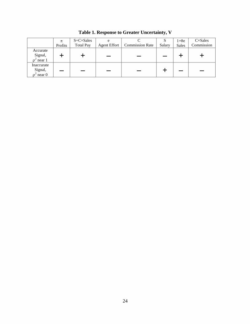
24
Table 1. Response to Greater Uncertainty, V π
Profits S+C×Sales Total Pay
e Agent Effort
C Commission Rate
S Salary
1+θe Sales
C×Sales Commission
Accurate Signal,
ρ2 near 1 + + – – – + +
Inaccurate Signal,
ρ2 near 0 – – – – + – –
1
Community Participation and Consumer to Consumer Helping: Does Participation in Third‐Party
Hosted Communities Reduce the Likelihood to Help?
Scott A. Thompson*, Molan Kim, and Keith Marion Smith
Scott A. Thompson*, Assistant Professor of Marketing
Terry College of Business, University of Georgia
116 Brooks Hall, Athens, GA 30602
(706) 542–3540
Email: [email protected]
Molan Kim, Assistant Professor of Marketing
School of Business, SUNY New Paltz
1 Hawk Drive, New Paltz, NY 12561
(845) 257–2957
Email: [email protected]
Keith Marion Smith, Doctoral Student
Terry College of Business, University of Georgia
148 Brooks Hall, Athens, GA 30602
(706) 542–2123
Email: [email protected]
2
Community Participation and Consumer to Consumer Helping: Does Participation in
Third-Party Hosted Communities Reduce the Likelihood to Help?
Abstract
Third-party hosted consumer communities in general, and brand communities in
particular, have been touted for their ability to generate value for firms by promoting consumer
to consumer (C2C) helping. However, little research has examined whether consumer
communities actually foster C2C helping, and who is helped. In contrast, the brand community
literature suggests community strategies may reduce the likelihood to help non-members. If so,
strategies that promote third-party hosted brand or product category communities may be
counterproductive in fostering C2C helping. Should firms focus on promoting brand
communities, promoting product category communities, or both? Based on a hazard model
analysis of 9,192 actual C2C helping events over a 25-month period, and supported by a second
cross-sectional study, this paper examines how participation in brand and product category
communities influences the likelihood to help others. We find that brand community
participation increases the likelihood to help fellow members while reducing the likelihood to
help members of rival brand communities. Surprisingly, product category community
participation reduces the likelihood to help members of brand communities. Managerial
recommendations are discussed.
Keywords: Consumer to consumer helping; consumer communities; brand communities;
oppositional loyalty
3
Consumer to consumer (C2C) helping behavior—defined as “behavior that enhances the
welfare of a needy other, by providing aid or benefit, usually with little or no commensurate
reward in return” (Bendapudi, Singh, and Bendapudi 1996, p. 34)—generates value for both the
consumer and the firm (Berry, Seiders, and Grewal 2002; Gruen, Osmonbekov, and Czaplewski
2007, 2006). Research on technology products finds that over 40% of consumers turn to online
consumer communities for help with products, resulting in more than a 15% reduction in service
cases for the firms (Maoz 2012). Furthermore, Gartner estimates that, by 2014, firms that
integrate online consumer communities into their customer support will realize a 10–50%
reduction in support costs (CFO Innovation Asia Staff 2012; Sussin 2012). Notably, research by
ComBlu (2010) has found that the operation of these communities is dominated by third-party
websites. By promoting third-party hosted websites that provide access to the greater brand
community, firms can encourage and capture value from C2C helping.
While prior research has shown that C2C helping behavior is one of the defining
characteristics of consumer communities (e.g., Muñiz and O’Guinn 2001), marketers lack
research on the relative merits of third-party hosted brand communities versus product category
communities in promoting C2C helping behavior. While firms rarely host online sites for
competitors’ products, these competitor consumer community members still participate in third-
party hosted sites, representing untapped potential for firms. No research has examined the role
that general product category communities may have in leveraging competitor community
members by facilitating product category C2C helping behavior.
In addition, while the existing literature has focused primarily on the benefits of brand
communities, recent research is finding that communities may have unintended, and detrimental,
consequences (e.g., Zhu et al. 2012) that may reduce C2C helping from competitors’ community

4
members. The brand community literature suggests that participation in brand communities
increases helping behavior within that specific community (Schau, Muñiz, and Arnould 2009;
Muñiz and O’Guinn 2001), but also increases hostility toward rival community members in the
form of “oppositional loyalty” (Muñiz and O’Guinn 2001; Thompson and Sinha 2008).
If oppositional loyalty extends to the willingness to help owners of other brands,
increased brand community participation could potentially destroy value for competitors by
reducing the willingness of a firm’s consumers to help rival brand owners. Furthermore, the
proliferation and growth of multiple brand communities in a product category could lead to an
environment of hostile rival factions between different brands. The result would be a product
category in which consumers primarily help fellow brand community members, undermining the
total amount of C2C helping and therefore reducing the value generated for all firms. However,
this behavior is not readily apparent on firm-hosted websites because of the typical absence of
rival brand forums. The inability to observe the response of rival brand community members on
single brand firm-hosted websites may therefore mask the loss of value from the independent
patchwork of third-party hosted sites.
Finally, the degree to which brand community participation influences the willingness to
help consumers within the associated product category community is unclear. Recent research
has found that open community strategies are associated with higher levels of product success
(Gruner, Homburg, and Lukas 2014). If brand communities and product category communities
also show bias against one another, community management strategies may be problematic or
even counterproductive in fostering C2C helping. If oppositional loyalty is only directed at rival
brand communities, the impact on the overall level of help available to consumers at the product
category level may be limited. However, the larger impact that participation may have on helping

5
behavior between brand and product category communities remains largely unexplored. As a
result, firms have little guidance on which third-party hosted communities to support in order to
promote C2C helping behavior. Specifically, should firms focus on promoting brand
communities, promoting product category communities, or both?
To address these questions, we collect actual C2C helping behavior and participation
behavior data from two third-party hosted brand communities and the associated product
category community. This paper contributes to the consumer to consumer helping literature, the
brand community literatures, and the broader consumption community literature in the following
ways. First, we contribute to the brand community and C2C helping literature by examining
when and the degree to which participation in brand communities actually promotes C2C helping
behavior between individual members. Furthermore, we contribute to the literature by examining
the impact that participation in product category communities may have on the likelihood to help
both within the product category community and in related brand communities. Second, we
contribute to the extant literature by exploring whether brand community participation may also
reduce C2C helping behavior towards members of rival brand communities. Third, we determine
the extent to which, and the conditions under which, community strategies may backfire,
reducing access to help for the firm’s own customers. In doing so, we reveal that the impact of
participation on the likelihood to help members of other communities is not limited to brand
community members, but extends to product community members who demonstrate a reduced
likelihood to help brand community members.
COMMUNITY PARTICIPATION AND HELPING BEHAVIOR
Studies have shown that beyond providing unpaid technical support, C2C information
exchange increases the value of the firm’s offerings and increases repurchase intentions (Gruen,

6
Osmonbekov, and Czaplewski 2007, 2006). At the same time, help provided by fellow
consumers reduces the time and effort consumers must expend as well as increases the value
consumers realize from a product or service (Berry, Seiders, and Grewal 2002; Feick and Price
1987). Furthermore, helping behavior is common in the computer-mediated forums where brand
community members frequently interact (Muñiz and Schau 2005). Indeed, a sense of moral
responsibility and the willingness to help fellow members in the use of products is one of the
defining characteristics of communities, including non-brand specific “consumption
communities” (Muñiz and O’Guinn 2001). However, prior research has tended to focus more on
the impact that community participation has on purchase behavior and word of mouth
(Thompson and Sinha 2008; Algesheimer, Dholakia, and Herrmann 2005). In comparison, little
research has been conducted on C2C helping behavior in these communities. As a result, our
understanding of when and how community participation promotes, or inhibits, C2C helping
behavior is limited.
Prior research on helping behavior defines helping from the perspective of the recipient
(e.g., Bendapudi, Singh, and Bendapudi 1996; Gruen, Osmonbekov, and Czaplewski 2006).
From this perspective, an action constitutes helping only if the recipient acknowledges it as such.
This approach avoids potential deceptive or self-serving declarations by individuals claiming to
provide help. However, it represents a conservative approach in that a potentially helpful action
may be overlooked and thus not receive the acknowledgement of the recipient. To build on the
extant literature, we adopt this view while acknowledging its limitations.
Research has also shown that people help others when they have both the ability to help
and are motivated to do so (Guy and Patton 1988; Berry, Seiders, and Grewal 2002). Ability to
help reflects the degree to which a consumer possesses the necessary knowledge, expertise, and

7
resources to provide assistance. This may take the form of knowledge about the relative merits of
different brands, expertise in installing or configuring a product, knowledge of how to
troubleshoot a problem with a product, and so on. Motivation reflects the willingness and desire
of a consumer to provide assistance (Bendapudi, Singh, and Bendapudi 1996), especially to
consumers whom they view as similar to them (ibid; Levine et al. 2005). In consumer
communities, individuals may provide assistance to fellow group members to conform to
community norms or to build legitimacy (Muñiz and O’Guinn 2001). Individuals may help out
of an intrinsic motive such as feelings of guilt or because they derive joy from helping (Hoffman
1981; Arnett, German, and Hunt 2003), which leads some individuals to be more likely to help in
general (Piliavin and Callero 1990; Danko and Stanley 1986; Guy and Patton 1988).
Participation and Helping within Brand Communities
Prior research suggests that participation in a brand community has the potential to
influence both the ability and motivation to help fellow brand community members in a number
of ways. First, the more members participate in a brand community, the more knowledge and
expertise they develop about the brand and its products leading to an enhanced ability to help
(Muñiz and O’Guinn 2001). In addition, higher participation strengthens members’ social
identification with the community (ibid; Algesheimer, Dholakia, and Herrmann 2005;
McAlexander, Schouten, and Koenig 2002), increasing their willingness to help fellow members
whom they perceive as similar to themselves (Bendapudi, Singh, and Bendapudi 1996; Piliavin
et al. 1981; Margolis 1982).
However, many product categories contain multiple rival brand communities, each
dedicated to a brand competing in the product category. Interactions between different rival
brand communities occur as consumers interact across the different third-party websites

8
associated with a product category. While participation in a brand community leads to enhanced
knowledge and expertise about the product category as a whole (Muñiz and O’Guinn 2001), the
brand community literature has found clear evidence of oppositional loyalty directed at
competing brands and their supporters (e.g., Thompson and Sinha 2008), with higher levels of
participation increasing this out-group bias against rivals (Brauer and Judd 1996; Hogg and
Abrams 2003). This suggests that while higher participation in a brand community will increase
willingness to help fellow members, it will reduce the likelihood to help members in a rival
brand community.
Participation and Helping in a Product Category Community
The brand community literature has primarily focused on how members treat fellow in-
group members and, to a lesser extent, the out-group members in rival brand communities. As a
result, it provides guidance on how participation may influence helping within and between rival
brand communities. Yet, in many product categories, communities dedicated to the general
product category, rather than to a specific brand, have at least as many members as brand
specific communities. While brand community members may also be members of the broader
product category, the literature provides mixed guidance on how participation in a brand
community influences behavior toward others in the product category.
On the one hand, participation in a brand community may reduce the motivation to help
members of the product category. Muñiz and O’Guinn (2001) warned of the possibility that
highly involved members of brand communities may show hostility toward other consumers. If
the oppositional loyalty and out-group bias fostered by brand community participation is also
directed at members in general product category communities, the prognosis is straightforward,
but grim. Participants in product category communities would be viewed as out-group members
9
along with participants in rival brand communities, resulting in a decrease in the willingness to
help members of the product category communities.
On the other hand, the brand community literature provides evidence that while
community members demonstrate out-group bias, they also seek to draw in and retain new
members (Schau, Muñiz, and Arnould 2009; McAlexander, Schouten, and Koenig 2002). This
desire to build the brand community may motivate members to assist members of the product
category community in hope of attracting new members. Furthermore, while participation in a
brand community generates out-group bias toward rival brand community members, this may not
be the case for the more general product category members. Specifically, if members of two
groups possess a common superordinate identity (e.g., consumers of the product category), out-
group bias may be diminished or even eliminated (Gaertner et al. 1993; Gaertner et al. 1989;
Crisp, Stone, and Hall 2006; Hewstone, Rubin, and Willis 2002). Therefore, we offer:
H1: Higher participation in a brand community increases the likelihood of individuals helping
members within the product category community
Product Category Participation and Helping
In many product categories, the majority of consumers are not members of a brand
community. Instead, they interact with fellow consumers in forums and communities that focus
on the product category as a whole. Despite this, prior research has tended to focus on how brand
community participation influences behavior—overlooking the impact of product category
participation. As a result, there is relatively little research on how participation in a product
category community may influence helping behavior. However, social identity research suggests
that participation in a product category community should give rise to a shared social
identification (Hogg and Abrams 2003; Diehl 1990). Since shared social identifications enhance

10
helping behavior between fellow brand community members, we predict that participation in a
product category community will similarly increase the likelihood of helping fellow members
within the product category community.
H2: Higher participation in a product category community increases the likelihood of
individuals helping members within the product category community
However, how product category members will react to brand community members is
ambiguous. If product category members view brand communities as out-groups, greater
participation in the product category community will lead to oppositional behavior and reduced
helping behavior in brand communities. On the other hand, if product community members share
a superordinate identity with brand community members as discussed above, out-group bias will
be mitigated. Also, greater participation within a product category community should lead to
greater knowledge and expertise relevant to products from the various brands within the
category—enhancing the ability to assist members of the various brand communities within the
product category. As a result, higher levels of participation in the product category community
should lead to a greater likelihood of helping members of brand communities as well as members
of the product category community.
H3: Higher participation in a product category community increases the likelihood of
individuals helping members within brand communities
Membership Duration and Helping
To this point, we have considered the impact that the level of participation may have on
C2C helping behavior. Prior research has found that membership duration, or the length of time a
member has participated, also influences behavior (Schoberth, Armin, and Preece 2006; Preece
and Shneiderman 2009). Newer members in brand communities often find their legitimacy as

11
members of the community challenged and thus are faced with a need to establish their
legitimacy (Muñiz and O’Guinn 2001). Research on group socialization has found that recent
members (with shorter term membership) are more prone to engage in prototypical group
behavior in order to establish legitimacy (Ellemers, Spears, and Doosje 2002; Levine and
Moreland 1994). In particular, helping in-group members is a common strategy used by newer
members (Ellemers, Spears, and Doosje 2002). This suggests that shorter term members will be
more likely to help fellow in-group members.
H4: Shorter membership duration in a brand community increases the likelihood of
individuals helping members within the brand community
H5: Shorter membership duration in a product category community increases the likelihood
of individuals helping members within the product category community
The need for legitimacy should influence newer members’ behaviors toward rival groups
as well. Since oppositional loyalty is a prototypical behavior in brand communities, shorter term
brand community members should show more oppositional loyalty in the form of a reduced
likelihood of helping members of rival brand communities, relative to longer duration members.
Additionally, the need of newer brand community members to establish their legitimacy as
adherents to one particular brand should encourage them to shun the product category
community, which does not espouse a loyalty to any one brand.
H6: Shorter membership duration in a brand community decreases the likelihood of
individuals helping members in a rival brand community
H7: Shorter membership duration in a brand community decreases the likelihood of
individuals helping members in the product category community
In summary these hypotheses are complementary, predicting that membership duration
12
affects helping in rival communities. However, the lack of a brand loyalty requirement among
product category members suggests that the legitimacy of product category members would not
be questioned for helping individuals who do favor a brand. Therefore, there is no basis for
predicting that product category membership duration will influence the likelihood of helping
members within a brand community, above and beyond the impact of the level of participation.
STUDY CONTEXT
Consistent with prior research on brand communities, we collect data from online forums
dedicated to the communities (Muñiz and O’Guinn 2001; Thompson and Sinha 2008). While
interactions between different rival brand communities occur as consumers interact across firm-
hosted and third-party websites on the Internet, rival brand behavior is impossible to observe on
firm-hosted sites because of the lack of competitor brand forums on firm-hosted websites.
Therefore, data was collected from a third-party hosted site in order to examine interactions
between rival brand and product category communities. Third-party sites allow for observation
of both intra- and inter-brand community interactions that are obscured on firm-hosted forums.
The product category from which the communities were selected was discrete 3D computer
graphics cards (also called, generically, video cards). This product category provides a rich
context in which to examine C2C helping behavior within and between communities. Since the
category is effectively a duopoly dominated by two brands that account for over 98% of sales—
ATI and NVIDIA (Shilov 2006) —the two rival brand communities within the category are
readily identifiable.
Prior research has demonstrated that brand communities exist around both of these brands
(Thompson and Sinha 2008). Prior to data collection, each forum was examined for markers
associated with community (Muñiz and O’Guinn 2001). In addition to a sense of moral

13
obligation expressed by providing technical support, consciousness of kind is evident in member
interaction and community language. One example is the use of the term “fanboy” to refer to
someone dedicated to one of the two brands, regardless of the merits of any particular product. A
set of practices have developed around the use of this term, resulting in an asymmetry in its use.
To be called a “fanboy” of the rival brand is an insult, often meant to discredit a particular
person. However, members regard being a “fanboy” of the group’s preferred brand to be a badge
of honor, even voluntarily labeling themselves “fanboys” of their preferred brand.
Within the product category community, consciousness of kind takes a different form and
leads to different practices. Members identify themselves based on explicitly disavowing loyalty
to any one brand; any indication of loyalty to either ATI or NVIDIA is grounds for suspicion. As
a result, the term “fanboy” is universally derogatory, regardless of brand. This has led to
practices designed to identify and control “fanboys” in the midst. For instance, excessive
enthusiasm for one brand’s product risks inquisition. When participants attempt to defend
branded products in the product category community, dedicated product category members
respond with posts such as, “If you weren’t an [ATI] fanboy, this wouldn’t burn your bottom so
much as to post this drivel.”
While enthusiasts of each video card brand share similar problems, they possess
competing brand loyalties—the strength of which often surprises those not familiar with the
product category. Brand choice has important social implications for buyers since 3D video cards
are used heavily to play online multiplayer computer games. Having a faster card not only
provides the individual with an advantage, but also contributes to the success of fellow
teammates in online multiplayer environments. Thus, owning a brand judged inferior by one’s
friends not only jeopardizes success in games, but undermines one’s social status and

14
relationships. By the same token, helping friends and acquaintances to properly install,
configure, and optimize their video cards reinforces these social relationships and contributes to
the team’s success. The technical nature of the product category makes C2C helping important to
the firms involved. It also leads to heterogeneity in both the ability to help and the need for
assistance. Specifically, this context includes consumers with high levels of technical knowledge
as well as large numbers of consumers who need help in order to purchase and use these
products. Furthermore, many of the issues that spawn helping behavior are common across
brands such as installation procedures in Windows, hardware installation questions, and video
driver installation and configuration. Consequently, C2C helping plays an important role in this
product category, both within and across brands.
To measure helping behavior and participation in the rival brand communities, we
collected data from brand forums hosted on one of the largest computer related sites on the
Internet. This environment presented numerous advantages. First, participants are required to use
a common account across the various forums. This made it possible to track behavior by unique
user IDs between the rival brand communities. Second, the site hosts a general Graphics Card
forum and two rival brand forums—giving members the opportunity to participate in the ATI
brand community, NVIDIA brand community, and/or the product category community with
equal ease. Furthermore, the site allows users to give a “Thank You” to any post whenever
someone helps them. Members can mark any single post as helpful, and a single helping event
can receive Thank You’s from multiple members. These Thank You’s are publicly visible and
can be tracked within as well as across each forum. Thus, they provide a measure of helping
behavior that is measured from the perspective of the person receiving help, as stipulated by the
extant literature on helping behavior. See Appendix A for an example of a “Thank You”

15
acknowledgement.
DATA
The primary data collection phase involved the collection of all messages posted in a
forum as well as the Thank You’s each post received, across all three forums. In addition,
general account information for each unique user ID was collected which provided information
about each member for the full history of the account. The participation data (how many
messages were posted), helping data (how many Thank You’s were given), and account data
files (member names, duration, and other factors) for each forum were merged to create a dataset
that tracked every member’s helping behavior both within and across the three forums under
study. To avoid bias due to members exiting the study but still being included in the analysis, the
last month on which each member participated in any of the three forums was determined. This
reflects the time at which a member has left the study.
The web site contained another 31 forums dedicated to areas such as “Programming,”
“Storage,” and “Hot Deals.” A secondary data collection phase was conducted to gather data on
behavior across these forums for each unique user ID that could serve as control variables and
allow us to address alternative explanations. To capture the overall level of helping behavior
each member received, the total number of times an individual thanked another for helping them
in any of the 34 forums was collected. Thus, each member’s tendency to participate and help in
online forums, outside of the product category under study, was additionally collected.
Across the two data collection phases, a total of 1,069,066 messages were collected from
17,026 unique users spanning a 69-month period from August 2004 to April 2010. To avoid bias
due to the presence of individuals who had never participated in one of three forums under study
(ATI, NVIDIA, Graphics Card), members were selected who had participated in at least one of

16
the three forums in the period under study. Thus, the analysis focuses on 4,501 unique users who
participated in at least one of the three forums over a 25-month period from April 2008 to April
2010 during which all three forums were available—constituting the full population of users
available to engage in helping behavior.
Measuring Helping Behavior
While the Thank You’s reported in the forums provide a theoretically valid measure of
helping behavior, operationalizing the form of the dependent variable presented challenges.
Since a single act of helping can receive multiple Thank You’s, the base count of Thank You’s
provides a general measure of helpfulness. However, this count comprises two phenomena: (1)
the likelihood to help and (2) how helpful a particular act of helping is. For example, an
individual may post a message seeking to provide help by answering a question. This represents
a single helping instance by the individual. However, 20 people may find this one act helpful,
resulting in 20 Thank You’s. On the other hand, an individual may engage in the helping
behavior three times, and receive only one Thank You in each instance, leading to a count of
three Thank You’s. Since the purpose of the study is to examine the impact of community
membership on the likelihood to help, the focal event of interest is whether an individual
received one or more Thank You’s, rather than the count of Thank You’s received. Doing so
ensures that the measure reflects the willingness to help, rather than the number of people that
benefited from a single helping event.
To address this issue, the data was aggregated by the user posting the messages on a
monthly basis to provide a record of whether each member provided any help to other members
in a given month for each of the three forums in the study (ATI, NVIDIA, Graphics Card). Thus,
the dependent variable reflects whether an individual helped in a given month, independent of

17
how helpful a particular act was. Additionally, the data contains repeated events since an
individual may help in more than one month. The results, in turn, represent the impact that each
independent variable (IV) has on the likelihood to help in a given month.
The decision to aggregate at the monthly versus weekly or daily (or minute) level was
driven by the fact that there is a delay between when a helping act is committed and when it is
acknowledged with a Thank You. With a weekly or daily aggregation, there is a significant risk
that the dependent variable will not accurately reflect the week or day in which the helping
occurred. This lag, in turn, would potentially bias the estimates of the relationship between
participation and helping behavior. A monthly aggregation, by comparison, minimizes these
issues since delays shorter than one month would not influence the results. Nonetheless, the use
of a monthly aggregation must be kept in mind when interpreting the results.
Measures
The following section describes each of the measures in the dataset in detail. Descriptive
statistics for the measures appear in Appendix B.
Help month. For each of the 25 months, each member was observed in each forum (ATI,
NVIDIA, Graphics Cards) to determine whether they provided help. For each forum, help month
is the observed dependent variable and indicates the month in which help was provided,
measured from the time that each member first began participating in the forum. Thus, a value of
five indicates that the member provided help in the fifth month since joining the forum.
Measuring whether an individual helped in a given month allows for the estimation of the
likelihood to help for each individual, providing a test of the hypotheses. Note that each post
receiving a “Thank You” is only counted as a helping event in the month in which it was posted
to avoid double counting helping events that received Thank You’s spanning months.

18
Forum participation variables. Participation is based on number of posts made,
consistent with prior research (Thompson and Sinha 2008). Forum participation variables
indicate the number of posts each user made in each of the three forums in the prior three months
in units of 100. Using measures of participation prior to the month in which help occurs ensures
that the measures are independent. A three month period was chosen based on prior literature
(ibid); a six month period showed similar results. Since some members may participate in more
than one forum, participation variables are included for all three forums.
Membership duration variables. Membership duration variables reflect the number of
months that have elapsed since a member first posted in each forum. A value of zero indicates
that a member has never posted in the forum and thus has a membership duration of zero months.
Thanks in ATI, NVIDIA, and Graphics. These variables indicate the number of Thank
You’s a member has received in the brand and product category forums. They provide measures
of the amount of help given in these forums and are included to test the degree to which helping
behavior in other forums influences the likelihood to help in a given forum.
Thanked in other forums. This variable indicates the number of Thank You’s received in
the other 31 forums not related to this product category. It provides a measure of the general
helpfulness of the member outside of this specific product context.
Thanks given to others. This variable reflects the number of Thank You’s given to others,
across all 34 forums. It provides a general measure of the amount of help each member has
received in the online forums.
Posts per day. This variable is based on the participation of each member across all 34
forums. It indicates the average number of posts made by each member per day, from the time
they first participated in any of the 34 forums on the site. Thus, it provides a control variable that
19
reflects the general intensity with which each user participates in online forums.
MODEL AND ESTIMATION
Hazard models are the preferred approach when analyzing event data. Hazard models are
able to accommodate time varying covariates, such as the participation variables in this study, as
well as repeated failure events, as is the case with the dependent measure in this study (Cleves,
Gould, and Gutierrez 2004). Therefore, we employ a repeated failure hazard modeling approach,
with each member’s forum unique user ID number denoting events associated with a single
subject. Users who did not participate in any of the three forums during the observed period were
excluded to avoid bias resulting from the inclusion of individuals who are not at risk of engaging
in helping behavior (Cleves, Gould, and Gutierrez 2004). To evaluate the robustness of the
results to distributional assumptions and the impact of unobserved sources of heterogeneity such
as omitted variables, we first estimate a Proportional Hazard model followed by a parametric
hazard model.
We fit the Proportional Hazard model first proposed by Cox (1975). This model does not
rely on parametric assumptions for the underlying hazard distribution and is often taken as a
reference for assessing the results for sensitivity to distributional assumptions (Cleves, Gould,
and Gutierrez 2004). The Cox PH model provides hazard ratios that are easily interpreted since
the model is estimated based on a reduced set of assumptions including parametric assumptions
for the underlying distribution (Hosmer, Lemeshow, and May 2008).
Since the Cox PH model assumes only one baseline hazard model between individuals
over time, it is unable to account for possible unobserved heterogeneous individual
characteristics. Therefore, we also fit a parametric hazard model which includes a frailty term to
account for the presence of unobserved heterogeneity (ibid; Gutierrez 2002). As recommended

20
by Cleves, Gould, and Gutierrez (2004), a range of distributions for the baseline hazard were
evaluated including Weibull, Gamma, Gompertz, exponential, lognormal, and loglogistic, as well
as alternative specifications for the frailty term. Comparing the Akaike information criterion
(AIC) for various distributions, we found the Gompertz distribution combined with an inverse
Gaussian distribution for the unobserved effect provided the best empirical fit for the data. The
likelihood ratio test for the presence of heterogeneity was significant for all three forums (p
< .01). Therefore, we report the results of the nonparametric Cox PH model and the parametric
Gompertz frailty model. However, since the likelihood test for the presence of heterogeneity was
significant, we focus our discussion on the results from the Gompertz frailty model.
RESULTS
Since the brand community analyses include data on product category community
participation and vice versa, we organize our discussion of the related hypotheses around each of
the analyses. We evaluate these hypotheses based on the Gompertz parametric model, which
includes a frailty term for the presence of unobserved heterogeneity. Note that hazard ratios
range from 0 to positive infinity, with a value less than 1 indicating that an increase in the IV has
a negative impact (reduced likelihood) on the likelihood of an event. Conversely, a value greater
than 1 indicates than an increase in the IV has a positive impact (increased likelihood) on the
likelihood of an event. Afterwards, we consider a range of alternative explanations for the
results. Model results appear in Table 1.
Brand Community Helping Behavior
ATI helping. Examining the results of the Gompertz model, we find that 100 posts in the
ATI forum in the prior three months increases the likelihood that an individual will provide help
in the ATI forum in a subsequent month by 230.4% (1 – 3.304) (HR:Hazard Ratio = 3.304, p <

21
.01). Furthermore, the Gompertz parametric model indicates that 100 posts in the rival NVIDIA
forum reduces the likelihood of helping in the ATI forum in a subsequent month by 58.1% (1 –
.419) (HR = .419, p < .01), approximately cutting it in half. These results provide evidence of
both in-group bias and oppositional loyalty between brand communities as predicted by the
brand community literature. However, 100 posts in the Graphics Card product category forum
decreases the likelihood of helping in the ATI forum in a subsequent month by 27.6% (1 – .724)
(HR = 1.372, p < .05). This result fails to support H3, indicating instead that higher participation
in a product category community will decrease the likelihood of helping members of brand
communities. Participation in the product category community has a similar impact on the
likelihood to help as participation in a rival brand community, reducing the likelihood to help.
Insert Table 1 about here
An examination of membership duration on the likelihood to help in the ATI forum,
controlling for the impact of participation, reveals that newer members in the ATI forum are
more likely to help in the ATI forum, in support of H4. Each month of membership in the ATI
forum decreases the likelihood to help by 7.8% (HR = .922, p < .01). On the other hand, newer
members of the rival NVIDIA forum are less likely to help in the ATI forum, with each month of
membership increasing the likelihood to help by 4.1% (HR = 1.041, p < .01). This supports H6,
which stated that shorter-term membership duration in a brand community will decrease the
likelihood of helping members in a rival brand community. Finally, while not hypothesized,
membership duration in the product category forum does not impact the likelihood of helping in
the ATI forum (p > .10).
NVIDIA helping. Shifting to results for the competing brand’s forum, NVIDIA, there is
again evidence of the in-group bias and oppositional loyalty in helping behavior between the

22
brand communities. 100 posts in the NVIDIA forum increases the likelihood of providing help in
a subsequent month in the NVIDIA forum by 1576.8% (1 – 16.768) (HR = 16.768, p < .01),
while 100 posts in the ATI forum decreases the likelihood of providing help in a subsequent
month in the rival NVIDIA forum by 27.9% (1 – .721) (HR = .721, p < .05). However,
participation in the product category forum again reduces the likelihood of helping in the
NVIDIA forum by 39.5% (1 – .605) (HR = .605, p < .05), failing to support H3. Rather than
increasing the likelihood of helping, participation in the product category forum instead has a
similar impact on helping as participation in the opposing brand forum.
The impact of membership duration on the likelihood to help in the NVIDIA forum
mirrors the impact seen in the ATI forum. Specifically, newer members of the NVIDIA forum
are more likely to help in the NVIDIA forum, with each month of membership decreasing the
likelihood to help by 5.9% (HR = .941, p < .01). On the other hand, newer members of the ATI
forum are less likely to help in the NVIDIA forum, with each month of membership increasing
the likelihood to help by 1.1% (HR = 1.011, p < .10). As a result, H4 and H6 are again supported.
As we saw with the rival ATI forum, membership duration in the product category forum does
not impact the likelihood of helping in the NVIDIA forum (p > .10).
Product Category Helping
Examining the model results for the product category forum, 100 posts in the Graphics
Card forum increases the likelihood that an individual will provide help in the Graphics Card
forum in a subsequent month by 29.5% (1 –1.295) (HR = 1.295, p < .05). Thus, H2, which stated
that higher levels of participation in a product category community will increase the likelihood of
helping members within that community, is supported. An examination of the impact of brand
forum participation on product category helping revealed hazard ratios for both forums greater

23
than 1. However, only the impact of participation in the ATI forum is statistically significant,
with 100 posts in the ATI forum increasing the likelihood of helping in the product category
forum by 75.9% (HR = 1.759, p < .01). As a result, H1, that higher levels of participation in the
ATI and NVIDIA brand forums will lead to a greater likelihood of providing help in the product
category forum, is partially supported.
Examining the membership duration variables indicates that newer members of the
product category forum are more likely to help in the product category forum. Specifically, each
month of membership in the product category forum reduces the likelihood of helping by 11.1%
(HR = .889, p < .01). This supports H5 which stated that shorter-term membership duration in a
product category community increases the likelihood of helping members within the product
category community. Furthermore, ATI and NVIDIA membership duration impacts the
likelihood to help in the product category community. In support of H7, longer duration brand
membership in ATI (HR = 1.034, p < .01) and NVIDIA (HR =1.079, p < .01) communities is
associated with a greater likelihood to help in the product category.
Evidence of the Ability to Help
The C2C literature argues that helping behavior requires both the ability and the
motivation to help. The results show that participation in a brand forum increased the likelihood
of helping fellow members of that forum, but reduced the likelihood of helping in the rival brand
forum. However, one could argue that the negative relationships seen in the results may simply
mean that the ability to help in one brand forum does not translate to an ability to help with the
rival brand. In other words, the lack of C2C helping may be due to a lack of ability or knowledge
regarding the rival product rather than oppositional loyalty.
To account for this, the number of Thank You’s received in the rival brand forum and the
24
product category forum were included in the models in Table 1. The results for the ATI forum
reveal that helping in the NVIDIA forum is associated with a greater likelihood to help in the
ATI forums (HR = 1.101, p < .01). Similarly, the results for the NVIDIA forum show the same
pattern, helping in the ATI forum is associated with a greater likelihood to help in the NVIDIA
forums (HR = 1.061, p < .01). This suggests that, after controlling for the impact of participation,
helping in the brand forum increased the ability to help in the rival brand forum. Yet, higher
levels of activity in a brand forum led members to withhold this help from rival forums.
An examination of the impact of helping in the product category forum on the likelihood
to help in the two brand forums suggests a similar conclusion. Table 1 shows that helping in the
product category community is associated with a greater likelihood to help in the ATI forum (HR
= 1.047, p < .01). Similarly, helping in the product category community is associated with a
greater likelihood to help in the NVIDIA forum (HR = 1.047, p < .01). This provides evidence
that members of the product category community forum are able to help in the brand forums, but
that higher levels of participation in the product category community reduce their likelihood of
providing that help.
Finally, brand forum members possess the ability to help in the product category forum.
Helping in the ATI forum increased the likelihood of helping in the product category forum (HR
= 1.051, p < .01), as did helping in the NVIDIA forum (HR = 1.055, p < .05). However, rather
than encouraging members to withhold this help, participation in the brand forums made
members more likely to provide help in the product category forum.
Interestingly, the relationship between helping in these forums does not extend beyond
these products. As shown in Table 1, helping in the other 31 forums does not increase the
likelihood of helping in the ATI, NVIDIA, or product category forum. In fact, helping in the

25
other 31 forums does not have a statistically significant impact on the likelihood to help in the
NVIDIA forums (p > .10). And, in the ATI and product category forums, helping in the other 31
forums is associated with a small but statistically significant reduction in the likelihood to help
(HR = .999, p < .01 in ATI and HR = .999, p < .01 in Graphics).
Overall, the results suggest that members of the brand and product category forums
possess the ability to help one another. However, the level of participation in the different forums
alters their willingness to do so. But the impact is not purely reciprocal. The brand forums show
evidence of out-group bias in their helping behavior towards one another. More importantly, the
product category community shows out-group bias against both brand forums. However, the
brand forums do not show out-group bias against the product category forum.
Opportunity Cost and Helping between Forums
Another alternative explanation is that the negative relationship between participation in
one forum and the likelihood to help in another could be due to opportunity costs. In other
words, members have a finite amount of time which they can dedicate to helping others. Thus,
the more time a member spends participating in one forum, the less time they have to help in
other forums. If the results are being driving by such tradeoffs, there should be a negative
relationship between participation and the likelihood to help in another forum for all forums.
If we only focus on the results for ATI and NVIDIA in Table 1, this explanation is
plausible. In the brand forums, participation in the two other forums is associated with a
reduction in the likelihood to help. However, the results for the product category forum cast
doubt on this explanation. We find that participation in the other two brand forums does not
reduce the likelihood to help in the product category forum, even though it represents a greater
time commitment. In fact, participation in the ATI forum has the exact opposite impact than this

26
explanation predicts: more time spent participating in the ATI forum actually increases the
likelihood to help in the product category community. Finally, a correlation was performed
between the three month average participation in the ATI and NVIDIA forum. If opportunity
costs were driving the results, this correlation should be negative. Instead, the correlation was
positive and significant (corrATI NVIDIA = .636, p < .01). Thus, the opportunity cost explanation for
the negative relationships fails to match the overall pattern of results.
Propensity to Participate in Online Forums and Reciprocity
Individuals differ in the degree to which they participate in online forums. It is possible
that this general tendency to participate could also account for helping behavior. Therefore, a
“posts per day” variable was included to account for differences in the intensity with which
individuals generally participate in online forums. This measure reflects the intensity of
participation across all 34 forums. Not surprisingly, Table 1 shows that individuals who
participate more in online forums are more likely to help in each of the three forums, with the
posts per day variable being significant at the p < .01 level. However, even with this propensity
accounted for in the model, participation in the product category and brand forums has a
statistically significant impact on the likelihood to help.
It is also possible that helping behavior may be influenced by reciprocity. In this case,
individuals may differ in their general tendency to seek and receive help online. If the members
of one forum are more prone to seek and receive help, reciprocity may also lead them to be more
likely to render it. To account for this, a control variable, “thanks given,” was included in the
analysis. This variable reflects the number of Thank You’s each member has given to others
across the forums for help received. Examining the results, we find that the amount of help
received is not statistically significant at the p < .10 level in any of the forums. Thus, the results
27
are robust, even when differences in the tendency to seek and receive help are accounted for.
Additional Robustness Checks
An additional series of analyses were conducted to assess the robustness of the results.
First, an alternative measure of the participation variables was computed based on the number of
threads each member participated in rather than the number of posts made. The results are
presented in Appendix C. The resulting thread based participation measures were highly
correlated with the post based measures (ATICorr = .877, p < .01, NVCorr = .861, p < .01,
GraphCorr = .575, p < .01) and produced results that closely matched those reported in Table 1.
This suggests that the results are robust to alternative specifications of the participation variables.
Next, to assess the influence of the most frequent participants on the results, the top 5% most
frequent participants were dropped and the Gompertz models for each forum were re-run. Again,
the results closely matched those in Table 1, with evidence of intergroup bias in C2C helping
behavior clearly evident among the remaining members in the ATI and product category forums.
The primary difference was a loss of significance for the rival forum participation measures in
the NVIDIA forum. This is likely due to the smaller sample size for the NVIDIA forum.
However, it also suggests that top participants play a role in generating out-group bias between
the communities. Finally, to assess the possible impact of cultural differences on helping
behavior, member provided information on their location was gathered, and each member was
coded based on whether they indicated they were located inside or outside of the U.S. A total of
1,464 of the members provided valid location information, with 42.3% indicating they resided in
the U.S. Gompertz models were then re-run with the location dummy variable. The pattern of
results for the subset of people who reported location closely matches that for the full sample,
despite the loss of power and the self-selected nature of those who reported location.
28
STUDY 2
The main study accounted for a range of alternative explanations including differences in
the ability to help, opportunity costs, and reciprocity effects. However, since the study was
conducted in a single context, questions remain regarding the generalizability of the results. It is
possible that unidentified characteristics of the context may have influenced the results. In
particular, the results could be influenced by the “Thank You” system specific to the website.
Many online environments lack such systems, requiring members to acknowledge help by
posting a reply message explicitly thanking others for their help. This raises the possibility that
the results would be different in environments lacking such a system.
Furthermore, the product in question (3D video cards) is optional in the sense that
computer owners can rely on the integrated video standard in systems without the need to install
a higher performance discrete 3D video card. Prior research has suggested that the desire to
recruit new members plays a significant role in how brand community members treat non-
members (Muñiz and O’Guinn 2001). In a product category where the product is optional, brand
community members should therefore be more motivated to help others in order to promote the
use of the products in general. On the other hand, in a category where a product is not optional,
brand community members should be less motivated to do so. As a result, it is unclear whether
members of the brand communities would feel compelled to help product category members in a
context where the product is required.
Therefore, a second study was conducted in a separate category, desktop computer
processors. This context was chosen since it contains two dominant competitors, Intel and AMD,
which allows a direct comparison between easily identified competitors. Second, unlike the prior
context, the product is required rather than optional. Finally, prior research has documented

29
existing brand communities around both brands (Thompson and Sinha 2008).
Data and Measures
Since one of the goals of Study 2 was to determine whether the results of the original
study were influenced by the presence of a system to acknowledge helping, Study 2 was
conducted in a context that lacked such a system. In the absence of such a system, members must
post a separate message in order to explicitly thank others for the help they provided. Therefore,
measures of helping were constructed by examining individual messages. This approach has the
advantage of being generalizable to contexts that do not contain systems for awarding “Thank
You’s.” However, it is necessarily extremely labor intensive and thus limits the length of time
that can be practically examined. Accordingly, message data was collected from two brand
forums (Intel and AMD) and the associated product category forum (General Hardware)
covering a four month period from June to September 2007. This period was selected since it
matches the time period during which prior research documented brand communities in these
specific forums (Thompson and Sinha 2008). Furthermore, this period lacked major holidays or
product releases that may have influenced the results. Participation and membership duration
variables were constructed consistent with the main study. Specifically, the first three months
were used to compute a three month participation variable for each member in each forum, and
membership duration was measured in months based on when each member first posted in each
forum, in the same manner as the main study.
Helping behavior was identified in each forum for the fourth month, with members being
coded 0 or 1 based on whether they engaged in helping behavior in each forum, as in the main
study. As a result, likelihood to help is based on a full month measure as in the main study.
Consistent with prior research, helping behavior was defined based on whether an individual

30
acknowledged a message post helpful (e.g., Bendapudi, Singh, and Bendapudi 1996). Since the
forums lacked the “Thank You” system in the main study, content analysis was used to identify
messages in which a member used the word “thank” in any form or tense to express thanks. This
required the examination of 1,022 message threads containing 7,147 messages. Each of the
messages containing any form of “thanks” was then coded based on the member or members the
subject was thanking. Across the three forums, 210 unique members engaged in helping behavior
within the month.
Analysis and Results
To assess the impact of participation and membership duration on the willingness to help,
a logistic regression was conducted for each forum, with the individual member as the unit of
analysis, the participation and membership duration variables for each forum as IVs, the number
of thanks given as a control variable, and whether the member engaged in helping behavior as
the dependent variable. Full results of all three models appear in Table 21, and descriptive
statistics appear in Web Appendix A. Models for both brand forums were significant
(Nagelkerke R2Intel = .396, p < .01, Nagelkerke R2
AMD = .390, p < .01) as was the model for the
product category forum (Nagelkerke R2Genera l= .450, p < .01). However, the thanks given control
variable was not significant in any of the three models at the α = .10 level.
Insert Table 2 about here
Higher participation in the Intel forum increased likelihood to help in the Intel forum (B
= 13.23, p < .01) while reducing the likelihood to help in the AMD forum (B = –7.38, p < .01).
Similarly, higher participation in the AMD forum increased the likelihood to help in the AMD
forum (B = 13.23, p < .01) while reducing the likelihood to help in the Intel forum (B = –6.68, p
1 The models were also run with log transformed participation variables to address possible bias due to skewed levels of participation. The results matched those reported in Table 2 and appear in Web Appendix B.
31
= .01). This provides evidence of the in-group bias and oppositional loyalty between rival brand
communities predicted by the brand community literature.
In the product category forum, higher participation led to a greater likelihood to help in
the product category forum (B = 21.18, p < .01), supporting H2. Furthermore, evidence of out-
group bias directed at brand forum members by product category members was again present,
with higher participation in the product category forum leading to a reduced likelihood to help in
both the Intel (B = –4.51, p < .05) and the AMD (B = –5.44, p < .05) forums. Thus, the
relationship is again the opposite of that predicted by H3. Interestingly, there is also evidence of
out-group bias from the brand forums directed at the general product category. Specifically,
higher participation in the Intel forum reduced the likelihood of helping in the product category
forum (B = –6.54, p < .01) as did higher participation in the AMD forum (B = –4.21, p < .05).
This fails to provide support for H1.
Finally, membership duration variables failed to achieve significant at the α = .10 level in
any of the three forums. This suggests that membership duration failed to account for sufficient
variance beyond that attributed to participation to achieve significance with the smaller sample
size in Study 2. As a result, the hypotheses for membership duration are not supported.
Discussion
By employing a different a modeling approach, study context, and measure of helping
behavior, Study 2 contributes additional insights into the relationships between community
participation and C2C helping while reproducing key findings from the main study. As in the
first study, intergroup bias in helping behavior is not limited to rival brand communities, but also
extends to product category communities. This suggests that the surprising out-group bias
evidenced by the product category community in the main study is not merely an artifact of one
32
product category, but instead is a characteristic of product category communities more generally.
Study 2 also supports the main study findings by providing evidence that this intergroup bias is
primarily driven by participation.
In addition, Study 2 contributes important new insights into how product characteristics
may influence C2C helping behavior within and between communities. A primary motivation in
the selection of the Study 2 context was to compare the results between a product category in
which the product was optional (3D video cards) to one in which it was not (processors). In the
case of an optional product, prior work suggests that brand community members are motivated to
help others as a means to recruit potential new members (Muñiz and O’Guinn 2001).
Accordingly, the main study found that increased participation in the ATI forum led to a greater
willingness to help in the product category forum. However, in Study 2 the product was not
optional. Consumers need the product to perform any computing tasks. This alleviates the need
for brand community members to recruit consumers into the product category as a whole.
Consistent with the work of Muñiz and O’Guinn (2001), Study 2 found that when alleviated of
this need to recruit into the product category, brand community members do not show the same
propensity to help product category members. In particular, increased participation in both the
AMD and Intel forums leads to a reduced likelihood to help in the product category forum.
These results indicate that intergroup bias in helping behavior between brand and product
communities may actually be greater in product categories where brand community members
have less of an incentive to recruit other consumers as in the case of non-optional products.
The failure of the membership duration variables to achieve significance while the
participation variables did is consistent with original findings. In the main study, participation
consistently showed greater main effects than membership duration. The reduced sample size

33
necessitated by manually measuring helping in Study 2 made significance more difficult to
achieve. More importantly, the extremely large sample in the original study allowed for a time
series modeling approach capable of detecting the effects of changes in membership duration
within subjects as well as between subjects. The lack of significance in the cross-sectional
second study indicates that duration effects in the original study may have been driven, at least in
part, by changes within members over time.
GENERAL DISCUSSION
This study examined the effects of community participation on consumer to consumer
helping behavior. Prior research has focused on helping behavior within brand communities. We
extend this literature by considering the role played by product category as well as brand
communities. Furthermore, we contribute to the consumer helping literature by investigating the
impact that participation has across brand and product category communities, not just within
them. To our knowledge, this is the first study to examine actual helping behavior between, as
well as within, these communities. Also, we examine the role that the level of participation has
versus the duration of participation. In doing so, we contribute to the consumer to consumer
helping literature by revealing the impact that both participation and membership duration in
different types of consumer communities has on the likelihood of consumers to help fellow
consumers. Finally, while it may seem intuitive that higher participation should lead to a greater
likelihood to help, we reveal conditions under which the opposite occurs, with participation
actually reducing consumer to consumer helping behavior.
The brand community literature suggests that participation in a brand community should
increase the likelihood of helping fellow brand community members. Using longitudinal data on
actual helping behavior in two brand communities, we find that participation increases the
34
likelihood to help fellow members, as predicted by the extant literature. Our results extend the
literature by revealing that participation in product category communities has a similar effect.
Specifically, higher levels of participation in a product category community increase the
likelihood that an individual will help fellow product category members. Thus, product category
communities offer an alternative means of promoting consumer to consumer helping.
Prior research on brand communities has focused on the role that participation plays in
fostering helping within the community. In comparison, little work has been done on the impact
it may have on helping others outside the brand community. We find that while higher levels of
participation increase the likelihood to help within the brand community, it reduces the
likelihood to help in rival brand communities. This provides evidence that the oppositional
loyalty documented in the purchase behavior of rival brand communities (Thompson and Sinha
2008) also extends to helping behavior. Furthermore, this reduction in the likelihood to help
comes despite clear evidence that these consumers possess the ability to do so, suggesting that
the proliferation of brand communities within a product market could have a balkanizing effect
on consumer helping behavior, with rival brand community members withholding assistance
from one another. However, this oppositional loyalty in helping behavior may be limited in
product categories where brand community members must recruit others into the product
category. In these markets, higher levels of participation in a brand community may not reduce
the likelihood of helping in the product category community, and may even increase it. On the
other hand, in product categories where a product is a necessity, brand communities can show
the same out-group bias in helping behavior toward product category members that they show
against one another, furthering the fragmentation in C2C helping.
While brand community members may refrain from oppositional loyalty toward the

35
product category community in some markets, product category members are not as generous.
We contribute to the consumption community and helping literatures by showing that
participation in a product category community gives rise to the kind of out-group bias associated
with rival brand communities. Thus, while brand communities promote helping behavior among
members, this increase in helping behavior is partially offset by a reduced likelihood to help on
the part of not just rival brand communities, but members of the product category community.
Finally, we contribute to the consumer to consumer helping literature by considering how
the level of participation versus the duration of participation influences the likelihood to help.
The results of the two studies suggest that membership duration has less of an effect on helping
behavior than participation. Furthermore, the impact of membership duration may be due to
changes over time within members. Over a two year period, the main study found that within a
brand community, new members show a greater likelihood to help fellow members once the
level of participation is taken into account. C2C helping behavior may provide new members
with an easy way to establish legitimacy. However, newer brand community members exhibited
a reduced likelihood to help in a rival brand community. Moreover, newer members of brand
communities also show a reduced likelihood to help in the product category community. Thus,
newer members can show such bias, suggesting that the proliferation of new brand communities
within a market can contribute to a reduction in helping behavior within the product category
community. However, Study 2 suggests that the negative impact may fade with time as
membership duration increases and the need to establish legitimacy diminishes.
Similarly, newer members of a product category community are more likely to help
fellow members. While higher levels of participation in a product category community reduce
the likelihood to help in brand communities, membership duration in the product category

36
community does not have any additional impact above and beyond participation in either the
main study or Study 2. As a result, the age of a product category does not create barriers to
helping brand community members.
It could be argued that membership duration may function as a proxy for member
diagnosticity or for participation efficiency. As members develop an understanding of
community behavior, they may be capable of providing help only where it is needed and where
their contribution is unique. Were this the case, the effect would be present in both brand and
product category communities. However, this effect does not appear in either study. Further, the
process of developing an understanding of community practices is a key component of the
legitimacy process of brand community membership, suggesting that increased efficiency is a
move towards prototypical community behavior.
Managerial Implications
For managers, the results provide new insights into the effects, both intended and
unintended, different community configurations have on promoting and inhibiting C2C helping
behavior. Specifically, we show that brand communities are a two-edged sword with regards to
C2C helping behavior. Brand community strategies not only promote helping among the firm’s
customers, but they also reduce helping in rival firms’ brand communities. Thus, building and
growing a brand community is a means to not only benefit your customers, but also to blunt the
advantage of a rival’s brand community.
However, pursuing a brand community strategy also carries risks. While they increase the
likelihood to help within the group, brand community strategies also reduce access to help from
product category members, who show a reduced willingness to help in the brand community. In
a market with a large existing product category community, firms may benefit more from

37
directing their customers to the product category community rather than trying to promote a
brand community to promote C2C helping. Doing so would ensure access to helping from the
large established base of product category members. In contrast, promoting a new brand
community reduces access to help from not only rival brand community members, but also the
large product category community. On the other hand, in a truly new market where a product
category community has not developed, supporting or encouraging a brand community in order
to promote helping behavior is preferable. In this case, there is no opportunity cost associated
with forgoing help from the product category community since it does not exist. At the same
time, the brand community may serve as a barrier to later entrants who will need to either foster
a product category community or attempt to build a rival brand community of their own.
Regardless, firms should be wary of “all of the above” strategies that simultaneously
promote both brand and product category communities. When there are no strong existing
product category communities, a product category community strategy will subsidize support for
rivals. However, if there is a strong extant product category community, simultaneously
promoting a brand community while supporting the product category community is likely to
generate little additional value for the firm. Instead, firms should pursue either a brand
community strategy or a product category community strategy to promote C2C helping,
depending on the state of their product market.
Limitations and Future Research
This research has a number of limitations which, in turn, point to opportunities for future
research. This paper focused on the likelihood to help, not on the value of the help. Future
research could examine the degree to which participation enhances, or reduces, how helpful a
particular helping act is. For example, a message post containing a solution to a problem that
38
represents a single act of helping may receive one “Thank You” or dozens, depending on how
many people benefitted. This raises the question of whether the help provided by brand
community participants is more helpful than that provided by product category participants.
The studies examined two product categories that were both technological in nature.
Because of the complex technical nature of the products, C2C helping plays an important role in
both product categories. However, C2C helping can also occur with less technical products such
as cellphones and appliances, as well as non-technological products such as cleaning products.
Future research should examine the degree to which communities influence helping behavior
associated with a wider range of product categories, including those which are not technological
in nature. In particular, future research should consider whether less complex products are more
dependent on product category communities for C2C helping. If so, the focus on technological
products in the existing studies may understate the potential for backfire effects associated with
brand community strategies.
Market structure may play an important role in helping behavior and brand community
interactions. The ratio of brand market share to its product category and the competition between
different brand shares may influence oppositional behavior between brand communities and
product category. Brands under greater perceived threat may exhibit higher levels of oppositional
loyalty that may extend to the product category when the general product category is perceived
as an out-group. Future research should consider more disproportionate markets to understand
the impact of market threat on helping behavior. Also, characteristics of the product category,
such as whether the product is necessary or optional for consumers, may influence the degree to
which brand and product category community members help one another. To date, the impact of
product characteristics has gone largely unexamined within the brand community literature.

39
Future studies should explore how such characteristics may moderate relationships between
brand community involvement and key outcomes such as C2C helping and product adoption.
The finding that product category members show out-group bias towards brand
community members also raises a number of interesting questions. First, does this bias extend
beyond just helping behavior? For example, do product category members become averse to
adopting products championed by large, vocal brand communities? Muñiz and O’Guinn (2001)
speculated that brand communities may indeed drive off customers if they become too strident. If
so, it would mean that the value and impact of brand community strategies may be moderated by
the size and strength of the product category community. Furthermore, the results suggest that
important cultural differences may exist between brand and product category communities. For
example, brand communities may have a more competitive culture by their very nature. Such
culture differences, in turn, may be driving the out-group bias shown by product category
members against brand community members. Future research should explore the role cultural
differences play in driving intergroup bias between members of different communities.
Finally, research should further explore the mechanisms and processes that mediate the
relationships between community participation and C2C helping. Prior research on brand
communities suggests that participation contributes to expertise. In addition, brand community
members gain credibility by being non-objective advocates for the brand. Future research should
explore the mediating roles that expertise and credibility play in shaping C2C helping behavior
within brand communities, as well as in product category communities.
40
References
Algesheimer, René, Utpal M. Dholakia, and Andreas Herrmann (2005), “The Social Influence of
Brand Community: Evidence from European Car Clubs,” Journal of Marketing, 69
(July), 19–34.
Arnett, Dennis B., Steve D. German, and Shelby D. Hunt (2003), “The Identity Salience Model
of Relationship Marketing Success: The Case of Nonprofit Marketing,” Journal of
Marketing, 67 (April), 89–105.
Bendapudi, Neeli, Surendra N. Singh, and Venkat Bendapudi (1996), “Enhancing Helping
Behavior: An Integrative Framework for Promotion Planning,” Journal of Marketing, 60
(July), 33–49.
Berry, Leonard L., Kathleen Seiders, and Dhruv Grewal (2002), “Understanding Service
Convenience,” Journal of Marketing, 66 (July), 1–17.
Brauer, Markus and Charles M. Judd (1996), “Group Polarization and Repeated Attitude
Expressions: A New Take on an Old Topic,” in European Review of Social Psychology,
Wolfgang Stroebe and Miles Hewstone, eds. Chichester, England: John Wiley, 173–207.
CFO Innovation Asia Staff (2012), “Peer-to-Peer Customer Support Can Reduce Costs by 50
Percent,” (accessed April 1, 2012), [available at
http://www.cfoinnovation.com/content/peer-peer-customer-support-can-reduce-costs-50-
percent].
Cleves, Mario A., William W. Gould, and Roberto G. Gutierrez (2004), An Introduction to
Survival Analysis using Stata®. College Station, TX: Stata Press.
ComBlu (2010), “State of Online Communities,” (accessed Sept. 30, 2014), [available at
http://www.slideshare.net/comblu/com-blu-stateofonlinecommunities2010].

41
Cox, DR (1975), “Partial Likelihood,” Biometrika, 62 (2), 269–76.
Crisp, Richard J., Catriona H. Stone, Natalie R. Hall (2006), “Recategorization and Subgroup
Identification: Predicting and Preventing Threats from Common Ingroups,” Personality
and Social Psychology Bulletin, 32 (2), 230–43.
Danko, William D. and Thomas J. Stanley (1986), “Identifying and Reaching the Donation-
Prone Individual: A Nationwide Assessment,” Journal of Professional Services
Marketing, 2 (Fall/Winter), 117–22.
Diehl, Michael (1990), “The Minimal Group Paradigm: Theoretical Explanations and Empirical
Findings,” European Review of Social Psychology, 1, 263–92.
Ellemers, Naomi, Russell Spears, and Bertjan Doosje (2002), “Self and Social Identity,” Annual
Review of Psychology, 53, 161–86.
Feick, Lawrence and Linda L. Price (1987), “The Market Maven: A Diffuser of Marketplace
Information,” Journal of Marketing, 51 (January), 83–97.
Gaertner, Samuel L., John F. Dovidio, Phyllis A. Anastasio, Betty A. Bachman, and Mary C.
Rust (1993), “The Common Ingroup Identity Model: Recategorization and the Reduction
of Intergroup Bias,” European Review of Social Psychology, 4, 1–26.
———, Jeffrey Mann, Audrey Murrell, and John F. Dovidio (1989), “Reducing Intergroup Bias:
The Benefits of Recategorization,” Journal of Personality and Social Psychology, 57 (2),
239–49.
Gruen, Thomas W., Talai Osmonbekov, and Andrew J. Czaplewski (2007), “Customer-to-
Customer Exchange: Its MOA Antecedents and Its Impact on Value Creation and
Loyalty,” Journal of the Academy of Marketing Science, 35, 537–49.
———, ———, and ——— (2006), “eWOM: The Impact of Customer-to-Customer Online

42
Know-How Exchange on Customer Value and Loyalty,” Journal of Business Research,
59, 449–456.
Gruner, Richard L., Christian Homburg, and Bryan A. Lukas (2014), “Firm-hosted online brand
communities and new product success,” Journal of the Academy of Marketing Science, 42
(1), 29–48.
Gutierrez, Roberto G. (2002), “Parametric Frailty and Shared Frailty Survival Models,” The
Stata Journal, 2 (1), 22–44.
Guy, Bonnie S. and Wesley E. Patton (1988), “The Marketing of Altruistic Causes:
Understanding Why People Help,” The Journal of Services Marketing, 2 (1), 5–16.
Hewstone, Miles, Mark Rubin, and Hazel Willis (2002), “Intergroup Bias,” Annual Review of
Psychology, 53, 575–604.
Hoffman, Martin L. (1981), “The Development of Empathy,” in Altruism and Helping Behavior:
Social, Personality, and Developmental Perspectives, J. Philippe Rushton and Richard
M. Sorrentino, eds. Hillsdale, NJ: Erlbaum, 41–63.
Hogg, Michael A. and Dominic Abrams (2003), “Intergroup Behavior and Social Identity,” in
The Sage Handbook of Social Psychology, Michael A. Hogg and Joel Cooper, eds.
London: SAGE, 407–22.
Hosmer, David W., Stanley Lemeshow, and Susanne May (2008), Applied Survival Analysis:
Regression Modeling of Time To Event Data. New York: Wiley-Interscience.
Levine, John M. and Richard L. Moreland (1994), “Group Socialization: Theory and Research,”
in European Review of Social Psychology, Wolfgang Stroebe and Miles Hewstone, eds.
Chichester, England: John Wiley, 305–36.
Levine, Mark, Amy Prosser, David Evans, and Stephen Reicher (2005), “Identity and
43
Emergency Intervention: How Social Group Membership and Inclusiveness of Group
Boundaries Shape Helping Behavior,” Personality and Social Psychology Bulletin, 31,
443–53.
Maoz, Michael (2012), “Social CRM for Customer Support – Peer Power,” (accessed April 1,
2012), [available at http://blogs.gartner.com/michael_maoz/2012/01/31/social-crm-for-
customer-support-peer-power/].
Margolis, Howard (1982), Selfishness, Altruism and Rationality. Cambridge: Cambridge
University Press.
McAlexander, James H., John W. Schouten, and Harold F. Koenig (2002), “Building Brand
Community,” Journal of Marketing, 66 (January), 38–54.
Muñiz, Albert M. Jr. and Thomas C. O’Guinn (2001), “Brand Community,” Journal of
Consumer Research, 27 (4), 412–32.
——— and Hope Jensen Schau (2005), “Religiosity in the Abandoned Apple Newton Brand
Community,” Journal of Consumer Research, 31 (4), 737–47.
Piliavin, Jane Allyn and Peter L. Callero (1990), Giving the Gift of Life to Unnamed Strangers.
Baltimore: Johns Hopkins University Press.
———, Jack F. Dovidio, Samuel Gaertner, and Russell D. Clark, III (1981), Emergency
Intervention. New York: Academic Press.
Preece, Jennifer and Ben Shneiderman (2009). The Reader-to-Leader Framework: Motivating
Technology-Mediated Social Participation. Transactions on Human-Computer Interaction,
1 (1), 13–32.
Schau, Hope Jensen, Albert M. Muñiz Jr., and Eric J. Arnould (2009), “How Brand Community
Practices Create Value,” Journal of Marketing, 73 (September), 30–51

44
Schoberth, Thomas, Armin Heinzl, and Jenny Preece (2006). Exploring Communication
Activities in Online Communities: A longitudinal analysis in the financial services industry.
Journal of Organizational Computing and Electronic Commerce, 16 (3–4), 247–65.
Shilov, Anton (2006), “Nvidia Expands Desktop Market Share, ATI Sustains Growth,” (accessed
May 11, 2007), [available at
http://www.xbitlabs.com/news/video/display/20060522074653.html].
Sussin, Jenny (2012), “How to Decrease Support Costs with Peer-to-Peer Customer
Communities,” (accessed April 1, 2012), [available at
http://www.gartner.com/id=1950115].
Thompson, Scott A. and Rajiv K. Sinha (2008), “Brand Communities and New Product
Adoption: The Influence and Limits of Oppositional Loyalty,” Journal of Marketing, 72
(November), 65–80.
Zhu, Rui, Utpal M. Dholakia, Xinlei Chen, and René Algesheimer (2012), “Does Online
Community Participation Foster Risk Financial Behavior?,” Journal of Marketing
Research, 49 (June), 394–407.
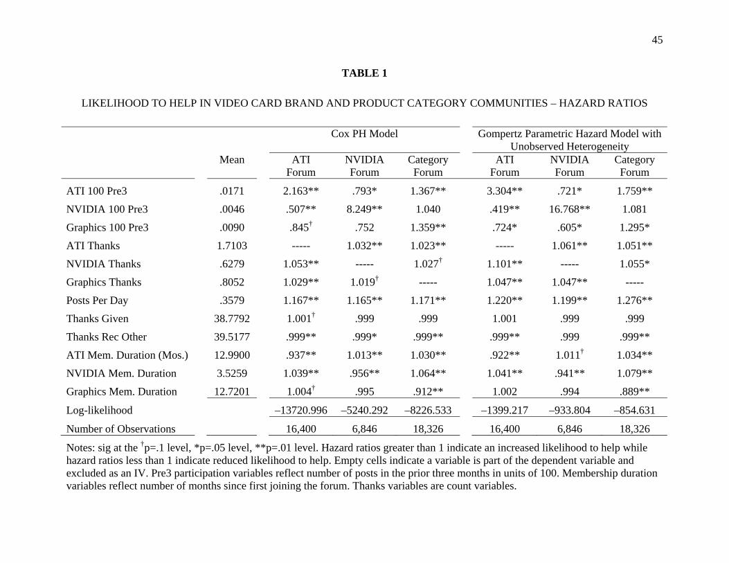
45
TABLE 1
LIKELIHOOD TO HELP IN VIDEO CARD BRAND AND PRODUCT CATEGORY COMMUNITIES – HAZARD RATIOS
Cox PH Model Gompertz Parametric Hazard Model with Unobserved Heterogeneity
Mean ATI Forum
NVIDIA Forum
Category Forum
ATI Forum
NVIDIA Forum
Category Forum
ATI 100 Pre3 .0171 2.163** .793* 1.367** 3.304** .721* 1.759**
NVIDIA 100 Pre3 .0046 .507** 8.249** 1.040 .419** 16.768** 1.081
Graphics 100 Pre3 .0090 .845† .752 1.359** .724* .605* 1.295*
ATI Thanks 1.7103 ----- 1.032** 1.023** ----- 1.061** 1.051**
NVIDIA Thanks .6279 1.053** ----- 1.027† 1.101** ----- 1.055*
Graphics Thanks .8052 1.029** 1.019† ----- 1.047** 1.047** -----
Posts Per Day .3579 1.167** 1.165** 1.171** 1.220** 1.199** 1.276**
Thanks Given 38.7792 1.001† .999 .999 1.001 .999 .999
Thanks Rec Other 39.5177 .999** .999* .999** .999** .999 .999**
ATI Mem. Duration (Mos.) 12.9900 .937** 1.013** 1.030** .922** 1.011† 1.034**
NVIDIA Mem. Duration 3.5259 1.039** .956** 1.064** 1.041** .941** 1.079**
Graphics Mem. Duration 12.7201 1.004† .995 .912** 1.002 .994 .889**
Log-likelihood –13720.996 –5240.292 –8226.533 –1399.217 –933.804 –854.631
Number of Observations 16,400 6,846 18,326 16,400 6,846 18,326
Notes: sig at the †p=.1 level, *p=.05 level, **p=.01 level. Hazard ratios greater than 1 indicate an increased likelihood to help while hazard ratios less than 1 indicate reduced likelihood to help. Empty cells indicate a variable is part of the dependent variable and excluded as an IV. Pre3 participation variables reflect number of posts in the prior three months in units of 100. Membership duration variables reflect number of months since first joining the forum. Thanks variables are count variables.
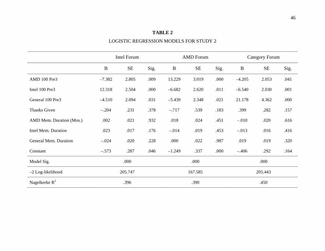
46
TABLE 2
LOGISTIC REGRESSION MODELS FOR STUDY 2
Intel Forum AMD Forum Category Forum
B SE Sig. B SE Sig. B SE Sig.
AMD 100 Pre3 –7.382 2.805 .009 13.229 3.019 .000 –4.205 2.053 .041
Intel 100 Pre3 12.318 2.504 .000 –6.682 2.620 .011 –6.540 2.030 .001
General 100 Pre3 –4.510 2.094 .031 –5.439 2.348 .021 21.178 4.362 .000
Thanks Given –.204 .231 .378 –.717 .539 .183 .399 .282 .157
AMD Mem. Duration (Mos.) .002 .021 .932 .018 .024 .451 –.010 .020 .616
Intel Mem. Duration .023 .017 .176 –.014 .019 .453 –.013 .016 .416
General Mem. Duration –.024 .020 .228 .000 .022 .987 .019 .019 .320
Constant –.573 .287 .046 –1.249 .337 .000 –.406 .292 .164
Model Sig. .000 .000 .000
–2 Log-likelihood 205.747 167.585 205.443
Nagelkerke R2 .396 .390 .450

47
Appendix A
The figure below shows an example of two posts (a request and response for help) and a “Thank
You” acknowledgement from the ATI forum. A member named “trickson” posted a problem s/he
was having with the software for an ATI based video card in the ATI forum. Another ATI
member posted a reply message with a solution. An acknowledgement of the help was provided
by “trickson” by clicking the “Thank You” button, generating the “Thank You” section below
the helpful post.
Example of Post, Reply, and Thank You
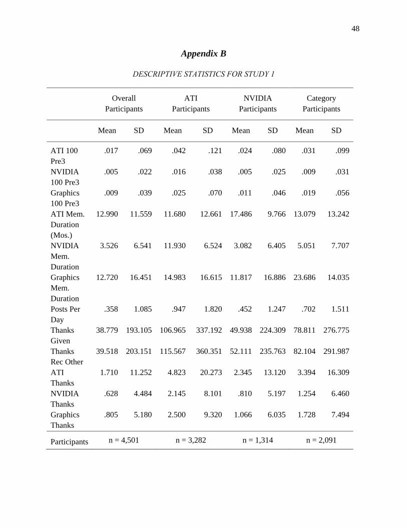
48
Appendix B
DESCRIPTIVE STATISTICS FOR STUDY 1
Overall Participants
ATI Participants
NVIDIA Participants
Category Participants
Mean SD Mean SD Mean SD Mean SD
ATI 100 Pre3
.017 .069 .042 .121 .024 .080 .031 .099
NVIDIA 100 Pre3
.005 .022 .016 .038 .005 .025 .009 .031
Graphics 100 Pre3
.009 .039 .025 .070 .011 .046 .019 .056
ATI Mem. Duration (Mos.)
12.990 11.559 11.680 12.661 17.486 9.766 13.079 13.242
NVIDIA Mem. Duration
3.526 6.541 11.930 6.524 3.082 6.405 5.051 7.707
Graphics Mem. Duration
12.720 16.451 14.983 16.615 11.817 16.886 23.686 14.035
Posts Per Day
.358 1.085 .947 1.820 .452 1.247 .702 1.511
Thanks Given
38.779 193.105 106.965 337.192 49.938 224.309 78.811 276.775
Thanks Rec Other
39.518 203.151 115.567 360.351 52.111 235.763 82.104 291.987
ATI Thanks
1.710 11.252 4.823 20.273 2.345 13.120 3.394 16.309
NVIDIA Thanks
.628 4.484 2.145 8.101 .810 5.197 1.254 6.460
Graphics Thanks
.805 5.180 2.500 9.320 1.066 6.035 1.728 7.494
Participants n = 4,501 n = 3,282 n = 1,314 n = 2,091
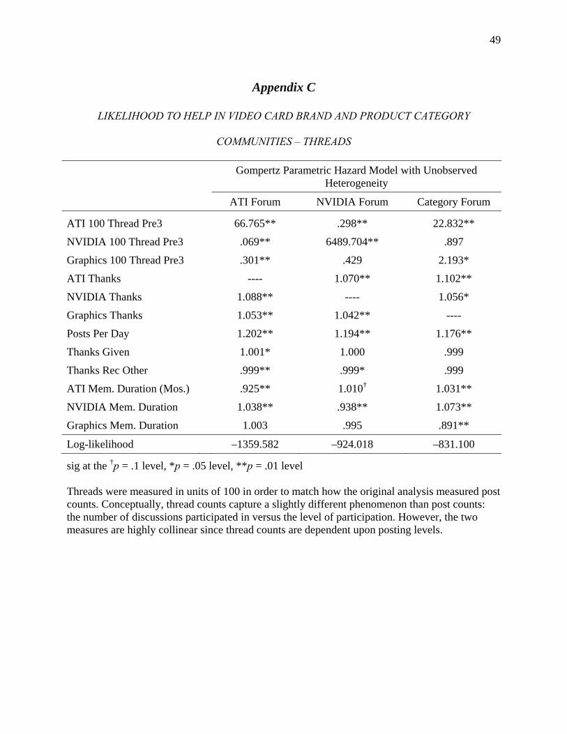
49
Appendix C
LIKELIHOOD TO HELP IN VIDEO CARD BRAND AND PRODUCT CATEGORY
COMMUNITIES – THREADS
Gompertz Parametric Hazard Model with Unobserved Heterogeneity
ATI Forum NVIDIA Forum Category Forum
ATI 100 Thread Pre3 66.765** .298** 22.832**
NVIDIA 100 Thread Pre3 .069** 6489.704** .897
Graphics 100 Thread Pre3 .301** .429 2.193*
ATI Thanks ---- 1.070** 1.102**
NVIDIA Thanks 1.088** ---- 1.056*
Graphics Thanks 1.053** 1.042** ----
Posts Per Day 1.202** 1.194** 1.176**
Thanks Given 1.001* 1.000 .999
Thanks Rec Other .999** .999* .999
ATI Mem. Duration (Mos.) .925** 1.010† 1.031**
NVIDIA Mem. Duration 1.038** .938** 1.073**
Graphics Mem. Duration 1.003 .995 .891**
Log-likelihood –1359.582 –924.018 –831.100
sig at the †p = .1 level, *p = .05 level, **p = .01 level Threads were measured in units of 100 in order to match how the original analysis measured post counts. Conceptually, thread counts capture a slightly different phenomenon than post counts: the number of discussions participated in versus the level of participation. However, the two measures are highly collinear since thread counts are dependent upon posting levels.
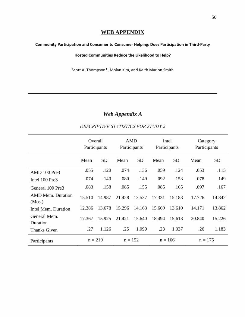
50
WEB APPENDIX
Community Participation and Consumer to Consumer Helping: Does Participation in Third‐Party
Hosted Communities Reduce the Likelihood to Help?
Scott A. Thompson*, Molan Kim, and Keith Marion Smith
Web Appendix A
DESCRIPTIVE STATISTICS FOR STUDY 2
Overall Participants
AMD Participants
Intel Participants
Category Participants
Mean SD Mean SD Mean SD Mean SD
AMD 100 Pre3 .055 .120 .074 .136 .059 .124 .053 .115
Intel 100 Pre3 .074 .140 .080 .149 .092 .153 .078 .149
General 100 Pre3 .083 .158 .085 .155 .085 .165 .097 .167
AMD Mem. Duration (Mos.)
15.510 14.987 21.428 13.537 17.331 15.183 17.726 14.842
Intel Mem. Duration 12.386 13.678 15.296 14.163 15.669 13.610 14.171 13.862
General Mem. Duration
17.367 15.925 21.421 15.640 18.494 15.613 20.840 15.226
Thanks Given .27 1.126 .25 1.099 .23 1.037 .26 1.183
Participants n = 210 n = 152 n = 166 n = 175
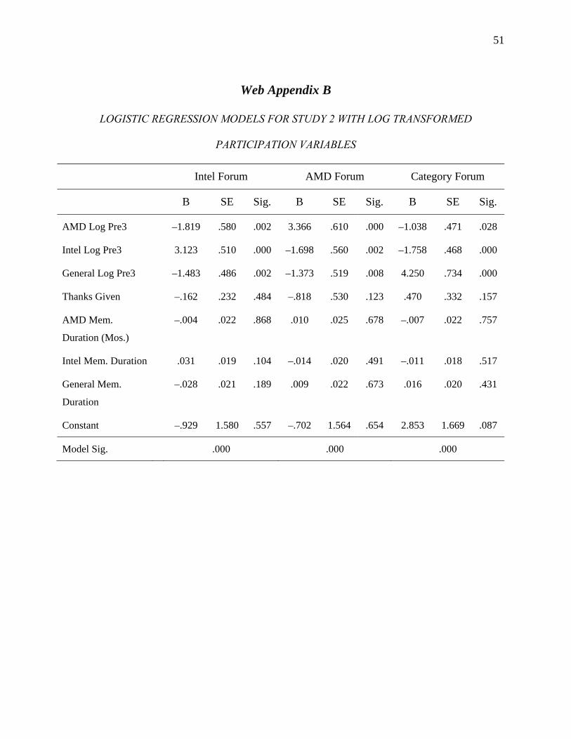
51
Web Appendix B
LOGISTIC REGRESSION MODELS FOR STUDY 2 WITH LOG TRANSFORMED
PARTICIPATION VARIABLES
Intel Forum AMD Forum Category Forum
B SE Sig. B SE Sig. B SE Sig.
AMD Log Pre3 –1.819 .580 .002 3.366 .610 .000 –1.038 .471 .028
Intel Log Pre3 3.123 .510 .000 –1.698 .560 .002 –1.758 .468 .000
General Log Pre3 –1.483 .486 .002 –1.373 .519 .008 4.250 .734 .000
Thanks Given –.162 .232 .484 –.818 .530 .123 .470 .332 .157
AMD Mem.
Duration (Mos.)
–.004 .022 .868 .010 .025 .678 –.007 .022 .757
Intel Mem. Duration .031 .019 .104 –.014 .020 .491 –.011 .018 .517
General Mem.
Duration
–.028 .021 .189 .009 .022 .673 .016 .020 .431
Constant –.929 1.580 .557 –.702 1.564 .654 2.853 1.669 .087
Model Sig. .000 .000 .000
SUZANNE B. SHU, ROBERT ZEITHAMMER, and JOHN W. PAYNE*
Decisions about life annuities are an important part of consumerdecumulation of retirement assets, yet they are relatively underexploredby marketing researchers studying consumer financial decision making.In this article, the authors propose and estimate a model of individualpreferences for life annuity attributes using a choice-based stated-preference survey. Annuities are presented in terms of consumer-relevantattributes such as monthly income, yearly adjustments, period certainguarantees, and company financial strength. The authors find that theseattributes directly influence consumer preferences beyond their impacton the annuity’s expected present value. The strength of the directinfluence depends on how annuities are described: when annuities arerepresented only through basic attributes, consumers undervalueinflation protection, and preferences are not monotonically increasingin duration of period certain guarantees. When descriptions of annuitiesare enriched with cumulative payment information, consumers no longerundervalue inflation protection, but nonlinear preferences for periodcertain options remain. The authors find that among annuities with thesame expected payout but different annual increases and period certainguarantees, the proportion of consumers who choose the annuity overself-management can vary by more than a factor of 2.
Keywords: financial decision making, annuities, conjoint analysis
Online Supplement: http://dx.doi.org/10.1509/jmr.13.0004
Consumer Preferences for Annuity Attributes:Beyond Net Present Value
With baby boomers now retiring at the rate of almost10,000 per day, the issue of decumulation of retirementassets is increasingly important to economists, publicpolicy experts, and the financial services industry. It shouldalso be of interest to researchers in marketing becauseconsumers in the market for decumulation products, such asannuities, face a choice problem with large financial stakes,limited learning opportunities, difficult consumption trade-offs, multiple sources of uncertainty, issues of trust and
branding, and long time periods. All of these aspects of thedecumulation problem are topics on which marketing re-search can offer important insights.
This article examines the structure of consumer prefer-ences for life annuities, an important class of decumulationproducts. We employ a choice-based conjoint analysis tomeasure consumer preferences and relate them to the un-derlying financial value of the products. Annuities, as wellas many other financial products, provide a unique settingfor choice modeling because most annuity attributes havecalculable expected present value that can be directlycompared with consumers’ revealed utilities. Conse-quently, we are able to see whether an attribute influencesdemand only through its contribution to the normative netpresent value (NPV) of the annuity product or whetherattribute values have psychological worth beyond NPV.We find that a typical consumer choosing from a set ofannuities does not merely maximize the expected financial
*Suzanne B. Shu is Associate Professor, Anderson School ofManagement,University of California, Los Angeles (e-mail: [email protected]). Robert Zeithammer is Associate Professor, Anderson School of Man-agement, University of California, Los Angeles (e-mail: [email protected]).John W. Payne is Joseph R. Ruvane Jr. Professor, Fuqua School of Business,Duke University (e-mail: [email protected]). This research was supported bygrants to the first and third authors from the Russell Sage and Alfred P. SloanFoundations. John Lynch served as associate editor for this article.
© 2016, American Marketing Association Journal of Marketing ResearchISSN: 0022-2437 (print) Ahead of Print
1547-7193 (electronic) DOI: 10.1509/jmr.13.00041
value but also reacts to several product attributes directly—expressing preferences beyond the effect of attributes onthe financial value. For example, most consumers over-value medium (10–20 years) levels of period certainguarantee relative to their financial impact, but they gen-erally undervalue inflation protection with respect to annualincreases in payments.
Our second goal is to understand how annuity attributevaluations are affected by changes in information pre-sentation. Varying information presentation has long beenpart of the tool kit available to marketers and is increasinglyseen as a tool available to policy makers in their efforts to“nudge” consumers toward purchases that can increaseconsumer welfare (Thaler and Sunstein 2008). We predictthat the strength of the influence of attributes on consumerpreferences beyond their impact on NPV will depend onhow the annuity products are described. In one of thepresentation conditions of our study, we describe eachannuity product in terms of its basic attributes as per currentindustry norms. In another presentation condition, weenrich the product description with nondiscounted cumu-lative payment information for a few representative “live-to” ages. Note that this “enriched information” conditiondoes not provide consumers with additional information—itmerely helps them get a sense of possible payouts givenexactly the same underlying attributes. Not surprisingly, wefind that consumers in the enriched information conditionundervalue inflation protection attributes less than con-sumers in the basic information condition. In contrast to thispartial de-biasing effect of the enriched information, withrespect to period certain guarantees, consumers in theenriched information condition continue to exhibit under-and overvaluation very similar to that seen in the basicinformation condition. We also find that enrichment ofinformation increases the baseline preference for annuiti-zation over self-management.
In each information condition, we also find significantindividual differences in preferences for annuity attributescorrelated with consumer characteristics such as amountsaved for retirement, subjective life expectancy, numeracy,and perceived annuity fairness. Most of these character-istics are correlated with preferences in a qualitativelysimilar manner regardless of the product description con-dition, with the exception of subjective life expectancy,which is positively correlated with a preference for annualincreases only in the enriched information condition.
Our findings provide several insights regarding con-sumer annuity choice and ways that marketers can improveconsumers’ acceptance of annuitization without paying outmore money in expectation. For example, a marketer canincrease demand for an annuity of a fixed expected presentvalue by reducing the amount of an annual increase andusing the resulting savings to fund an increase in the du-ration of the period certain guarantee up to 20 years. Whichproducts the issuer should offer depends on the way theywill be described (e.g., shorter period certain guarantees aremore optimal under enriched information than under basicinformation). Regardless of the information presentation,we find that such “repackaging” of the payout stream canhave a large effect on demand, sometimes even doublingthe take-up rate of annuities in the population we study.Before presenting the detailed methods and results of the
conjoint analysis of annuity product features, we next turnto a brief review of the role of annuities in the retirementjourney.
THE ROLE OF ANNUITIES IN CONSUMERDECUMULATION
As one approaches retirement, there are a number ofdifficult decisions, including questions of when to retirefrom work and when to begin claiming Social Securitybenefits (Coile et al. 2002; Knoll 2011). The most complexdecision of all, however, is how to optimally spend downsaved assets. In the growing body of research on consumerfinancial decision making (Lynch 2011), the emphasis hasoften been on the accumulation stage of wealth manage-ment, addressing issues such as retirement savings de-cisions (Hershfield et al. 2011; Soman and Cheema 2011)and investment choice (Morrin et al. 2012; Strahilevitz,Odean, and Barber 2011). Although these issues of how toaccumulate wealth during the 30 years prior to retirementare crucially important for workers, the decumulation ofwealth in the 30 years after retirement is also an importantproblem and thus far has been relatively unaddressed inmarketing research.
The size of the decumulation problem is substantial, withapproximately $9.2 trillion in retirement assets held ineither defined contribution plans (e.g., a 401k) or IRAs(Benartzi, Previtero, and Thaler 2011). The consumer’srisks in consuming saved assets include either spendingtoo quickly, which might lead to running out of money, orspending too slowly, which severely constrains con-sumption and might lead to the consumer dying with un-used funds. Also complicating this decision is the largeuncertainty about life expectancy, a crucial piece ofknowledge for determining the optimal intertemporalconsumption path (Payne et al. 2013).
The economics literature has long recognized that lifeannuities are a compelling marketplace solution to thedecumulation problem (for reviews, see Benartzi, Previtero,and Thaler 2011; Brown 2007; and Davidoff, Brown, andDiamond 2005). The simplest form of a life annuity is theimmediate single-payer life annuity, in which a consumerexchanges a lump sum for a guaranteed stream of paymentsfor as long as he or she lives. In a sense, life annuities offerthe opportunity for the retiree to convert retirement assetssaved through a defined contribution plan into an incomestream more similar to a defined benefit (pension) plan. Theimplied insurance against outliving one’s assets is thebiggest advantage of life annuities. Another advantage isthat life annuities often pay out higher percentage returnsthan is normally feasible with self-managed accounts. Forexample, a life annuity might pay a 6.8% annual rate ofreturn rather than the 4%–5% one would collect from aself-managed account. This higher return is a result ofbenefits to survivorship, because accounts of those whodie early are used, in part, to pay income to annuity holderswho continue to live. However, a consumer’s purchase of alife annuity carries some disadvantages. First, one’s estate(i.e., heirs) receives no payment when one dies with atraditional type of life annuity; the money remains with thecompany that issued the annuity, implying a possible lossor negative return on the original purchase. Another dis-advantage is a loss of control over the assets because the
2 JOURNAL OF MARKETING RESEARCH, Ahead of Print
investment funds are given to the annuity company tomanage, which may result in not benefiting from potentialreturns from stocks and other risky financial products(Milevsky and Young 2007). Issuing companies vary infinancial strength ratings, which is clearly important giventhe fact that the choice to purchase an annuity has impli-cations for many years and because government backingfor such products is dependent on state-level regulations.Finally, life annuities typically provide relatively poorliquidity (i.e., cash availability) in case of emergencies.Nonetheless, most economic analyses have concluded thatpurchasing a life annuity should be part of the decumulationstrategies of most consumers. It has therefore been a puzzlethat life annuities have not been more popular: research onchoices among pre-retirees who are able to choose betweenannuities and lump-sum payouts for their retirement sav-ings has found that, often, less than 10% choose the annuity(Johnson, Burman, and Kobes 2004; Poterba, Venti, andWise 2011).
As a result, companies that offer life annuities haveintroduced a variety of product features in an effort to makeannuities more attractive. These options include attributessuch as period certain guarantees, deferred start dates,annual income increases to compensate for inflation, andjoint annuities (e.g., for married couples). Period certainoptions guarantee payments for a specified number ofyears, even if the annuitant passes away, with remainingpayments going to designated heirs; after the specifiednumber of years, a period certain annuity becomes like astandard annuity, with payments that continue until theindividual dies. These annuities thus protect against totalloss of the principal investment due to early death while stillbeing able to offer income for life. Annuities with deferredstart dates, also called longevity annuities, require a lowerup-front payment, in exchange for delayed payouts that willnot begin until a certain time in the future, assuming thepurchaser is still alive then. Offering annuities with consumer-oriented options, such as period certain guarantees, carriesfinancial trade-offs; the issue for the offering company iswhether consumers are willing to accept higher prices in ex-change for these benefits.
Our focus is on understanding how the product featuresdiscussed in the previous paragraph are valued by con-sumers. The features are presumably offered in response toconsumers’ needs. These needs consist of both economicconcerns (e.g., risks of inflation, probability of receivingpayouts) and psychological concerns (e.g., desire to pro-vide for family, issues of fairness). Research on annuitieshas tried to assess the strength of these different needs,particularly to explain differences in overall consumerdemand for annuity products. Although rational economicarguments can explain demand for some annuity features,several researchers have suggested that psychological fac-tors also need to be considered (Brown 2007; Goldstein,Hershfield, and Benartzi 2015). Whether the demand is basedon purely economic concerns or driven by psychological needscan significantly influence a consumer’s willingness to payfor a given feature. A feature that addresses strong psycho-logical concerns might be worth more to the consumer than itcosts the company to offer; conversely, a feature that does notmeet a psychological need may be undervalued by the con-sumer relative to its full financial impact.
Consider first one of the most popular annuity options:a period certain guarantee, which ensures payouts for a setnumber of years even in the case of the annuitant’s death. Aconsumer’s concerns about leaving a bequest in case of anearly death might account for less than full annuitizationduring retirement (Brown 2007; Davidoff, Brown, andDiamond 2005; Yaari 1965). Such bequest concerns couldexplain preference for period certain guarantees as a way toensure that money is provided for heirs in the case of earlydeath. However, bequest motives cannot explain patterns inwhich people without heirs choose period certain guar-antees and/or almost no annuitization. A different expla-nation for the popularity of period certain options can befound by considering the decision using concepts fromcumulative prospect theory (Tversky and Kahneman 1992).For example, loss aversion might make annuities un-attractive when consumers perceive the forfeiture of theannuity purchase price due to early death as a loss either tothemselves or to their family and heirs (Hu and Scott 2007).Furthermore, prospect theory suggests that the risk oflosing the full value of the annuity can be further high-lighted by consumers’ tendency to overweight smallprobabilities. Finding that period certain guarantees areovervalued by consumers relative to their expected fi-nancial value could indicate that these psychological con-cerns play a role in consumer demand for this feature.
Risks of inflation might also be expected to worryconsumers, and annuity providers sometimes offer annualincreases as a feature to address this financial concern.Although having inflation protection makes rational sense,consumers might think of an annuity purchase more as agamble or an investment than as a source of consumptionincome, which could weaken the perceived benefit of in-flation protection (Agnew et al. 2008; Brown et al. 2008;Hu and Scott 2007). Further complicating valuation ofannual increases are psychological biases in judgingintertemporal payouts, especially those described inpercentage terms rather than fixed terms (McKenzieand Liersch 2011). Studies on intertemporal choice thatdocument differential discounting of gains and losses,predictions of resource slack, myopia and hyperopia,construal, procrastination, and/or intertemporal consump-tion have all offered evidence that consumers are likely toundervalue long-term annual increases (e.g., Shu 2008;Soman 1998; Zauberman and Lynch 2005). Furthermore,consumer uncertainty surrounding judgments of futurehealth, economic outcomes (e.g., inflation), and life ex-pectancy can lead to biased evaluations of the future utilityof those payouts. Considering these facts together, we ex-pect that consumers will undervalue the financial benefits ofannual increases when selecting annuities.
Finally, rational consumers might worry about risk ofdefault by the annuity issuer. In the annuity marketplace,default risk is captured through financial strength ratings(e.g., AA, AAA) of the issuing company. Actual risk ofdefault for companies with high ratings is quite low,1 butoverweighting of small probabilities may cause consumersto perceive the risk as much higher. Babbel and Merrill
1For example, from 1981 to 2008, no companies rated AAAby Standard&Poor’s ever defaulted, and mean annual default rate for companies rated AAwas .02%.
Consumer Preferences for Annuity Attributes 3
(2006) show that even a small objective default risk canhave a large economic impact on annuity purchasing.
Given the complexity of annuity products and the psy-chological processes that affect how these attributes areevaluated, consumers’ preferences might be significantlyinfluenced by the way information about the annuities ispresented during the choice process. As noted earlier, re-search on the impacts of different ways to present the sameinformation has a long history in the field of consumerbehavior (e.g., Bettman and Kakkar 1977; Russo 1977),and it is increasingly seen as a way to influence consumerwelfare through variations in information architectures. Arecent example of such changes in information architec-ture is the new credit card statements that provide cal-culations on how long it will take a consumer to pay off hisor her credit card balance with just the minimum requiredpayment or a slightly increased monthly payment (Soll,Keeney, and Larrick 2013). Specific to annuities, Kunreuther,Pauly, and McMorrow (2013, p. 142) suggest providing“better and more convincing information on the attractiveproperties of annuities” and their potential long-term payoutas a solution to the annuity puzzle; our enriched presentationformat offers an initial test of such a solution.
Beyond general population judgmental biases, individ-ual differences in how consumers handle financial purchasedecisions are important to consider. For example, recentfindings regarding consumers’ financial knowledge (bothobjective and subjective knowledge), financial literacy,numeracy, and overall cognitive ability offer importantpredictions of how consumers who differ in individualabilities may react to annuity offerings (Fernandes, Lynch,and Netemeyer 2014; Frederick 2005; Peters et al. 2006). Acomprehensive survey of all individual factors that caninfluence annuity choice is outside the feasibility of arelatively short consumer study, so we focus on individualmeasures that closely relate to the trade-offs inherent in ourchosen attribute set. In particular, we measure age, gender,retirement savings, numeracy, loss aversion, perceivedfairness of annuity products, and subjective life expecta-tions. We now turn to an experimental study designed toinvestigate how consumers value annuity attributes beyondtheir impact on NPV.
A STUDY OF CONSUMER PREFERENCES FORANNUITY ATTRIBUTES
To carefully measure how consumers value and maketrade-offs between annuity attributes, the remainder ofthis article proposes and estimates a model of individualpreferences for annuities using a discrete-choice experi-ment (DCE). Our model is distinct from other applicationsof DCE in the sense that the product attributes jointlyimply an expected present financial value of the product.Knowing the financial value of each product in our DCEallows us to see whether an attribute influences demandonly through its contribution to the financial value orwhether it also has psychological worth beyond NPV. Wealso apply our estimated model to the product-designproblem and characterize how marketers and policy makerscan increase consumer acceptance of annuities without nec-essarily increasing the expected payout.
The remaining sections proceed in four stages, as fol-lows. First, we lay out our model, including how we chose
attributes and how those attributes can be converted to anexpected present value that is central to our model specifica-tion. Second, we describe our subject population and ourmethods, including an enriched information presentationtreatment hypothesized to affect participants’ valuation ofparticular attributes. Third, we describe our results, pre-senting both model-free evidence and choice-model esti-mates. Finally, we suggest implications for the marketing ofannuities and suggest how specific attributes make annuitiesmore appealing to particular demographic groups.
Study Design: Attribute Selection, Model Specification, andStatistical Optimization
Our DCE consists of 20 choice tasks. In every choicetask, we asked participants, “If you were 65 and consideringputting $100,000 of your retirement savings into an an-nuity, which of the following would you choose?” Theythen saw three annuity options and a fourth no-choiceoption that read, “None: If these were my only options, Iwould defer my choice and continue to self-manage myretirement assets.”
Attribute selection. The attributes we use include start-ing income, insurance company financial strength ratings,amount and type of annual income increases, and periodcertain guarantees. Each attribute can take on several levelsselected to span the range of levels commonly observed inthe market today (see Table 1).
We now briefly explain our motives in selecting theseattributes and their levels for our study. Beyond startingincome, which is clearly one of the most important financialattributes for an annuity, we include insurance companyfinancial strength ratings to test the theory by Babbel andMerrill (2006) that even a small default risk can have a largeeconomic impact on annuity purchasing. We included onlyAA and AAA rating levels to focus on small differences indefault risk near the top of the financial strength range,where many real-world annuity providers operate.
Including annual increases as one of our primary attri-butes allows us to test the importance of inflation protectionin annuity purchases. The seven levels of annual incomeincrease we use in this study include three increasesexpressed additively (e.g., “every year, payments increaseby an amount $X”), three increases expressed multiplica-tively (e.g., “every year, payments increase by Y%”), andone level for no increase. We chose levels of additive in-crease and multiplicative increase that roughly match eachother in the initial years of the annuity in terms of theexpected payout; for example, a 7% annual increase isroughly equal to a $500 annual increase for an annuity withstarting monthly payments of $600. Inclusion of bothpercentage and fixed increases of similar amounts tests thepossibility that individuals underestimate income growthfor rates expressed in percentages (McKenzie and Liersch2011; Wagenaar and Sagaria 1975). This misunderstandingof exponential growth may be especially important forindividuals who have low skills in financial literacy andnumeracy (Lusardi and Mitchell 2007).
The third attribute we focus on is the period certainguarantee. Period certain guarantees include periods of0 years (no period certain), 5 years, 10 years, 20 years, andan extreme option of 30 years. As documented by Scott,Watson, and Hu (2011) and Benartzi et al. (2011), the
4 JOURNAL OF MARKETING RESEARCH, Ahead of Print
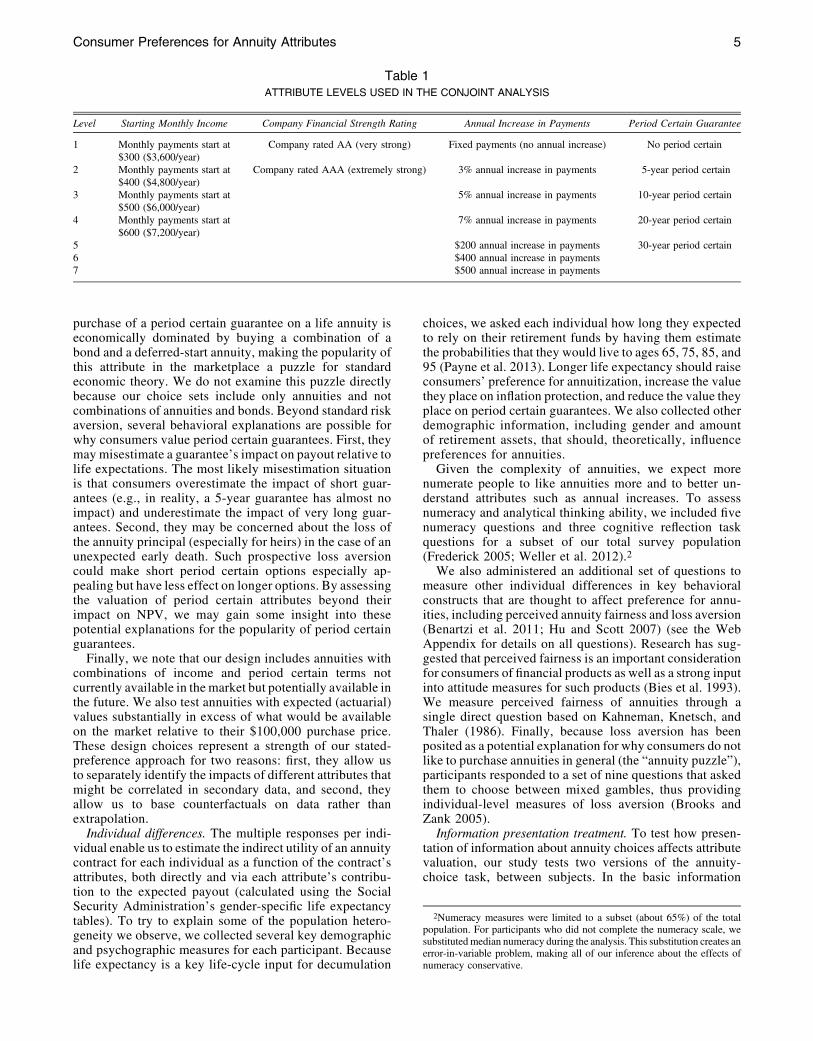
purchase of a period certain guarantee on a life annuity iseconomically dominated by buying a combination of abond and a deferred-start annuity, making the popularity ofthis attribute in the marketplace a puzzle for standardeconomic theory. We do not examine this puzzle directlybecause our choice sets include only annuities and notcombinations of annuities and bonds. Beyond standard riskaversion, several behavioral explanations are possible forwhy consumers value period certain guarantees. First, theymay misestimate a guarantee’s impact on payout relative tolife expectations. The most likely misestimation situationis that consumers overestimate the impact of short guar-antees (e.g., in reality, a 5-year guarantee has almost noimpact) and underestimate the impact of very long guar-antees. Second, they may be concerned about the loss ofthe annuity principal (especially for heirs) in the case of anunexpected early death. Such prospective loss aversioncould make short period certain options especially ap-pealing but have less effect on longer options. By assessingthe valuation of period certain attributes beyond theirimpact on NPV, we may gain some insight into thesepotential explanations for the popularity of period certainguarantees.
Finally, we note that our design includes annuities withcombinations of income and period certain terms notcurrently available in the market but potentially available inthe future. We also test annuities with expected (actuarial)values substantially in excess of what would be availableon the market relative to their $100,000 purchase price.These design choices represent a strength of our stated-preference approach for two reasons: first, they allow usto separately identify the impacts of different attributes thatmight be correlated in secondary data, and second, theyallow us to base counterfactuals on data rather thanextrapolation.
Individual differences. The multiple responses per indi-vidual enable us to estimate the indirect utility of an annuitycontract for each individual as a function of the contract’sattributes, both directly and via each attribute’s contribu-tion to the expected payout (calculated using the SocialSecurity Administration’s gender-specific life expectancytables). To try to explain some of the population hetero-geneity we observe, we collected several key demographicand psychographic measures for each participant. Becauselife expectancy is a key life-cycle input for decumulation
choices, we asked each individual how long they expectedto rely on their retirement funds by having them estimatethe probabilities that they would live to ages 65, 75, 85, and95 (Payne et al. 2013). Longer life expectancy should raiseconsumers’ preference for annuitization, increase the valuethey place on inflation protection, and reduce the value theyplace on period certain guarantees. We also collected otherdemographic information, including gender and amountof retirement assets, that should, theoretically, influencepreferences for annuities.
Given the complexity of annuities, we expect morenumerate people to like annuities more and to better un-derstand attributes such as annual increases. To assessnumeracy and analytical thinking ability, we included fivenumeracy questions and three cognitive reflection taskquestions for a subset of our total survey population(Frederick 2005; Weller et al. 2012).2
We also administered an additional set of questions tomeasure other individual differences in key behavioralconstructs that are thought to affect preference for annu-ities, including perceived annuity fairness and loss aversion(Benartzi et al. 2011; Hu and Scott 2007) (see the WebAppendix for details on all questions). Research has sug-gested that perceived fairness is an important considerationfor consumers of financial products as well as a strong inputinto attitude measures for such products (Bies et al. 1993).We measure perceived fairness of annuities through asingle direct question based on Kahneman, Knetsch, andThaler (1986). Finally, because loss aversion has beenposited as a potential explanation for why consumers do notlike to purchase annuities in general (the “annuity puzzle”),participants responded to a set of nine questions that askedthem to choose between mixed gambles, thus providingindividual-level measures of loss aversion (Brooks andZank 2005).
Information presentation treatment. To test how presen-tation of information about annuity choices affects attributevaluation, our study tests two versions of the annuity-choice task, between subjects. In the basic information
Table 1ATTRIBUTE LEVELS USED IN THE CONJOINT ANALYSIS
Level Starting Monthly Income Company Financial Strength Rating Annual Increase in Payments Period Certain Guarantee
1 Monthly payments start at$300 ($3,600/year)
Company rated AA (very strong) Fixed payments (no annual increase) No period certain
2 Monthly payments start at$400 ($4,800/year)
Company rated AAA (extremely strong) 3% annual increase in payments 5-year period certain
3 Monthly payments start at$500 ($6,000/year)
5% annual increase in payments 10-year period certain
4 Monthly payments start at$600 ($7,200/year)
7% annual increase in payments 20-year period certain
5 $200 annual increase in payments 30-year period certain6 $400 annual increase in payments7 $500 annual increase in payments
2Numeracy measures were limited to a subset (about 65%) of the totalpopulation. For participants who did not complete the numeracy scale, wesubstitutedmedian numeracy during the analysis. This substitution creates anerror-in-variable problem, making all of our inference about the effects ofnumeracy conservative.
Consumer Preferences for Annuity Attributes 5
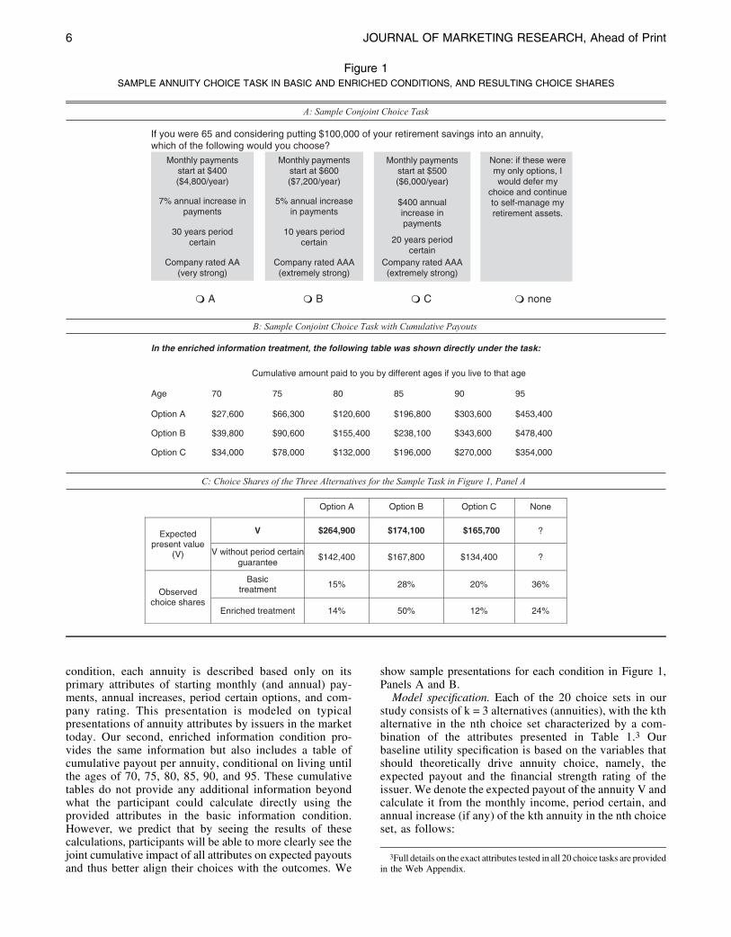
condition, each annuity is described based only on itsprimary attributes of starting monthly (and annual) pay-ments, annual increases, period certain options, and com-pany rating. This presentation is modeled on typicalpresentations of annuity attributes by issuers in the markettoday. Our second, enriched information condition pro-vides the same information but also includes a table ofcumulative payout per annuity, conditional on living untilthe ages of 70, 75, 80, 85, 90, and 95. These cumulativetables do not provide any additional information beyondwhat the participant could calculate directly using theprovided attributes in the basic information condition.However, we predict that by seeing the results of thesecalculations, participants will be able to more clearly see thejoint cumulative impact of all attributes on expected payoutsand thus better align their choices with the outcomes. We
show sample presentations for each condition in Figure 1,Panels A and B.
Model specification. Each of the 20 choice sets in ourstudy consists of k = 3 alternatives (annuities), with the kthalternative in the nth choice set characterized by a com-bination of the attributes presented in Table 1.3 Ourbaseline utility specification is based on the variables thatshould theoretically drive annuity choice, namely, theexpected payout and the financial strength rating of theissuer. We denote the expected payout of the annuity V andcalculate it from the monthly income, period certain, andannual increase (if any) of the kth annuity in the nth choiceset, as follows:
Figure 1SAMPLE ANNUITY CHOICE TASK IN BASIC AND ENRICHED CONDITIONS, AND RESULTING CHOICE SHARES
A: Sample Conjoint Choice Task
If you were 65 and considering putting $100,000 of your retirement savings into an annuity,which of the following would you choose?
A B C none
B: Sample Conjoint Choice Task with Cumulative Payouts
In the enriched information treatment, the following table was shown directly under the task:
Cumulative amount paid to you by different ages if you live to that age
Age 70 75 80 85 90 95
Option A $27,600 $66,300 $120,600 $196,800 $303,600 $453,400
Option B $39,800 $90,600 $155,400 $238,100 $343,600 $478,400
Option C $34,000 $78,000 $132,000 $196,000 $270,000 $354,000
C: Choice Shares of the Three Alternatives for the Sample Task in Figure 1, Panel A
Option A Option B Option C None
Expected present value
(V)
V $264,900 $174,100 $165,700 ?
V without period certainguarantee
$142,400 $167,800 $134,400 ?
Observed choice shares
Basic treatment
15% 28% 20% 36%
Enriched treatment 14% 50% 12% 24%
Monthly paymentsstart at $600($7,200/year)
5% annual increasein payments
10 years periodcertain
Company rated AAA(extremely strong)
Monthly paymentsstart at $400($4,800/year)
7% annual increase inpayments
30 years periodcertain
Company rated AA(very strong)
Monthly paymentsstart at $500($6,000/year)
$400 annualincrease inpayments
20 years periodcertain
None: if these weremy only options, Iwould defer my
choice and continueto self-manage myretirement assets.
Company rated AAA(extremely strong)
3Full details on the exact attributes tested in all 20 choice tasks are providedin the Web Appendix.
6 JOURNAL OF MARKETING RESEARCH, Ahead of Print
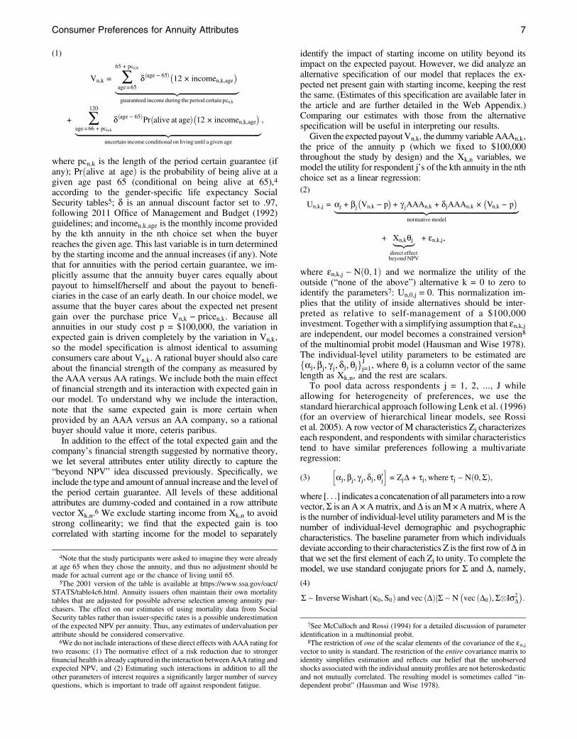
(1)
Vn,k = 65 + pcn,k
age=65dðage − 65Þ12 × incomen,k,age
|fflfflfflfflfflfflfflfflfflfflfflfflfflfflfflfflfflfflfflfflfflfflfflfflfflfflfflfflfflfflfflzfflfflfflfflfflfflfflfflfflfflfflfflfflfflfflfflfflfflfflfflfflfflfflfflfflfflfflfflfflfflfflguaranteed income during the period certain pcn,k
+ 120
age=66 + pcn,k
dðage − 65ÞPrðalive at ageÞ12 × incomen,k,age
|fflfflfflfflfflfflfflfflfflfflfflfflfflfflfflfflfflfflfflfflfflfflfflfflfflfflfflfflfflfflfflfflfflfflfflfflfflfflfflfflfflfflfflfflfflfflfflfflfflzfflfflfflfflfflfflfflfflfflfflfflfflfflfflfflfflfflfflfflfflfflfflfflfflfflfflfflfflfflfflfflfflfflfflfflfflfflfflfflfflfflfflfflfflfflfflfflfflffluncertain income conditional on living until a given age
,
where pcn,k is the length of the period certain guarantee (ifany); Prðalive at ageÞ is the probability of being alive at agiven age past 65 (conditional on being alive at 65),4according to the gender-specific life expectancy SocialSecurity tables5; d is an annual discount factor set to .97,following 2011 Office of Management and Budget (1992)guidelines; and incomen;k;age is the monthly income providedby the kth annuity in the nth choice set when the buyerreaches the given age. This last variable is in turn determinedby the starting income and the annual increases (if any). Notethat for annuities with the period certain guarantee, we im-plicitly assume that the annuity buyer cares equally aboutpayout to himself/herself and about the payout to benefi-ciaries in the case of an early death. In our choice model, weassume that the buyer cares about the expected net presentgain over the purchase price Vn,k − pricen,k. Because allannuities in our study cost p = $100,000, the variation inexpected gain is driven completely by the variation in Vn,k,so the model specification is almost identical to assumingconsumers care about Vn,k. A rational buyer should also careabout the financial strength of the company as measured bythe AAA versus AA ratings. We include both the main effectof financial strength and its interaction with expected gain inour model. To understand why we include the interaction,note that the same expected gain is more certain whenprovided by an AAA versus an AA company, so a rationalbuyer should value it more, ceteris paribus.
In addition to the effect of the total expected gain and thecompany’s financial strength suggested by normative theory,we let several attributes enter utility directly to capture the“beyond NPV” idea discussed previously. Specifically, weinclude the type and amount of annual increase and the level ofthe period certain guarantee. All levels of these additionalattributes are dummy-coded and contained in a row attributevector Xk,n.6 We exclude starting income from Xk,n to avoidstrong collinearity; we find that the expected gain is toocorrelated with starting income for the model to separately
identify the impact of starting income on utility beyond itsimpact on the expected payout. However, we did analyze analternative specification of our model that replaces the ex-pected net present gain with starting income, keeping the restthe same. (Estimates of this specification are available later inthe article and are further detailed in the Web Appendix.)Comparing our estimates with those from the alternativespecification will be useful in interpreting our results.
Given the expected payoutVn,k, the dummyvariableAAAn,k,the price of the annuity p (which we fixed to $100,000throughout the study by design) and the Xk,n variables, wemodel the utility for respondent j’s of the kth annuity in the nthchoice set as a linear regression:(2)
Un,k,j = aj + bjVn,k − p
+ g jAAAn,k + djAAAn,k ×
Vn,k − p
|fflfflfflfflfflfflfflfflfflfflfflfflfflfflfflfflfflfflfflfflfflfflfflfflfflfflfflfflfflfflfflfflfflfflfflfflfflfflfflfflfflfflfflfflfflfflfflfflfflzfflfflfflfflfflfflfflfflfflfflfflfflfflfflfflfflfflfflfflfflfflfflfflfflfflfflfflfflfflfflfflfflfflfflfflfflfflfflfflfflfflfflfflfflfflfflfflfflffl
normativemodel
+ Xn,kqj|fflfflzfflffldirect effectbeyondNPV
+ en,k,j,
where en,k,j ~ Nð0; 1Þ and we normalize the utility of theoutside (“none of the above”) alternative k = 0 to zero toidentify the parameters7: Un,0,j = 0. This normalization im-plies that the utility of inside alternatives should be inter-preted as relative to self-management of a $100,000investment. Together with a simplifying assumption that en,k,jare independent, our model becomes a constrained version8of the multinomial probit model (Hausman and Wise 1978).The individual-level utility parameters to be estimated arefaj, bj, g j, dj, qjgJj=1, where qj is a column vector of the samelength as Xk,n, and the rest are scalars.
To pool data across respondents j = 1, 2, ..., J whileallowing for heterogeneity of preferences, we use thestandard hierarchical approach following Lenk et al. (1996)(for an overview of hierarchical linear models, see Rossiet al. 2005). A row vector of M characteristics Zj characterizeseach respondent, and respondents with similar characteristicstend to have similar preferences following a multivariateregression:
haj,bj, g j, dj, q
0j
i= ZjD + tj, where tj ~ Nð0,SÞ,(3)
where [. . .] indicates a concatenation of all parameters into a rowvector,S is anA × Amatrix, andD is anM×Amatrix, where Ais the number of individual-level utility parameters andM is thenumber of individual-level demographic and psychographiccharacteristics. The baseline parameter from which individualsdeviate according to their characteristics Z is the first row ofD inthat we set the first element of each Zj to unity. To complete themodel, we use standard conjugate priors for S and D, namely,
(4)
S ~ InverseWishart ðk0, S0Þ and vec ðDÞjS ~ Nvec ðD0Þ,SÄIs2
D:
4Note that the study participants were asked to imagine they were alreadyat age 65 when they chose the annuity, and thus no adjustment should bemade for actual current age or the chance of living until 65.
5The 2001 version of the table is available at https://www.ssa.gov/oact/STATS/table4c6.html. Annuity issuers often maintain their own mortalitytables that are adjusted for possible adverse selection among annuity pur-chasers. The effect on our estimates of using mortality data from SocialSecurity tables rather than issuer-specific rates is a possible underestimationof the expected NPV per annuity. Thus, any estimates of undervaluation perattribute should be considered conservative.
6We do not include interactions of these direct effects with AAA rating fortwo reasons: (1) The normative effect of a risk reduction due to strongerfinancial health is already captured in the interaction betweenAAA rating andexpected NPV, and (2) Estimating such interactions in addition to all theother parameters of interest requires a significantly larger number of surveyquestions, which is important to trade off against respondent fatigue.
7See McCulloch and Rossi (1994) for a detailed discussion of parameteridentification in a multinomial probit.
8The restriction of one of the scalar elements of the covariance of the en,jvector to unity is standard. The restriction of the entire covariance matrix toidentity simplifies estimation and reflects our belief that the unobservedshocks associated with the individual annuity profiles are not heteroskedasticand not mutually correlated. The resulting model is sometimes called “in-dependent probit” (Hausman and Wise 1978).
Consumer Preferences for Annuity Attributes 7
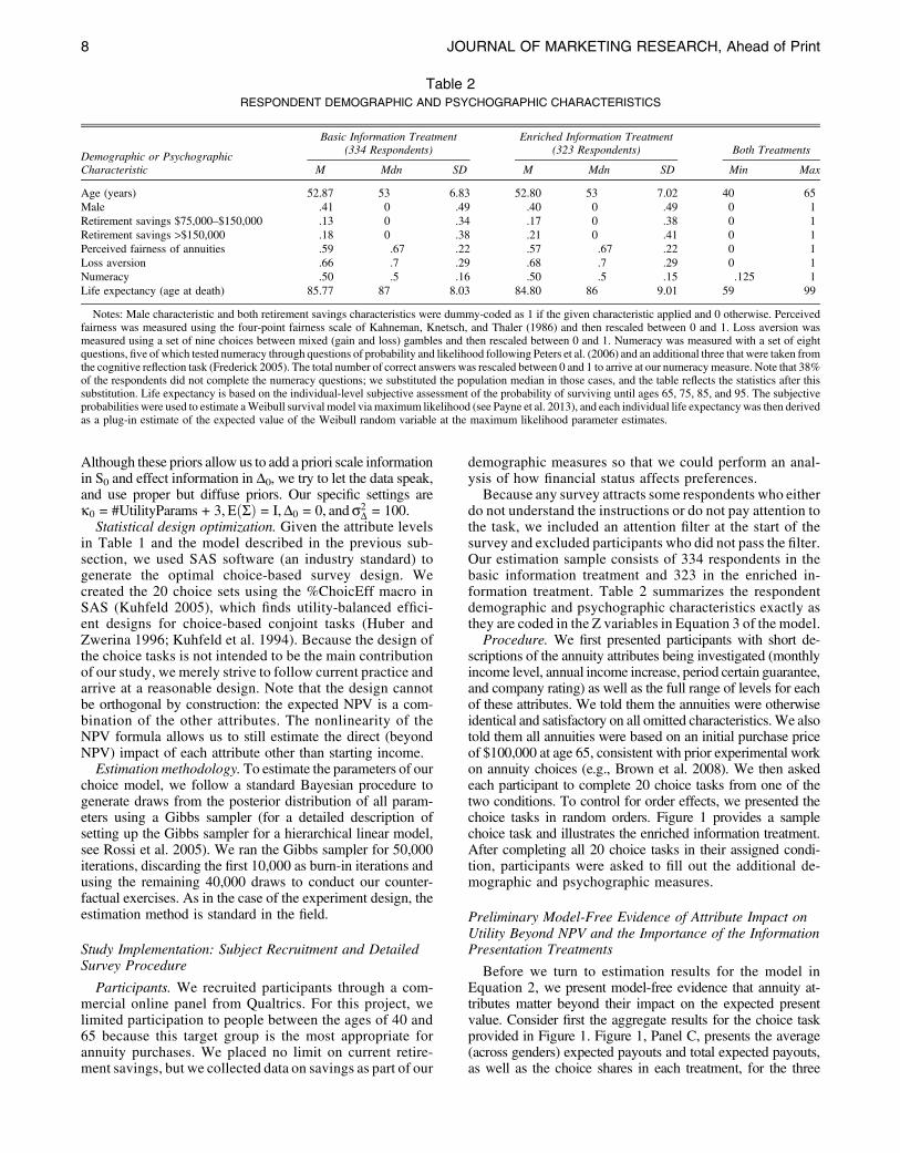
Although these priors allow us to add a priori scale informationin S0 and effect information in D0, we try to let the data speak,and use proper but diffuse priors. Our specific settings arek0 = #UtilityParams + 3, EðSÞ = I,D0 = 0, ands2
D = 100.Statistical design optimization. Given the attribute levels
in Table 1 and the model described in the previous sub-section, we used SAS software (an industry standard) togenerate the optimal choice-based survey design. Wecreated the 20 choice sets using the %ChoicEff macro inSAS (Kuhfeld 2005), which finds utility-balanced effici-ent designs for choice-based conjoint tasks (Huber andZwerina 1996; Kuhfeld et al. 1994). Because the design ofthe choice tasks is not intended to be the main contributionof our study, we merely strive to follow current practice andarrive at a reasonable design. Note that the design cannotbe orthogonal by construction: the expected NPV is a com-bination of the other attributes. The nonlinearity of theNPV formula allows us to still estimate the direct (beyondNPV) impact of each attribute other than starting income.
Estimation methodology. To estimate the parameters of ourchoice model, we follow a standard Bayesian procedure togenerate draws from the posterior distribution of all param-eters using a Gibbs sampler (for a detailed description ofsetting up the Gibbs sampler for a hierarchical linear model,see Rossi et al. 2005). We ran the Gibbs sampler for 50,000iterations, discarding the first 10,000 as burn-in iterations andusing the remaining 40,000 draws to conduct our counter-factual exercises. As in the case of the experiment design, theestimation method is standard in the field.
Study Implementation: Subject Recruitment and DetailedSurvey Procedure
Participants. We recruited participants through a com-mercial online panel from Qualtrics. For this project, welimited participation to people between the ages of 40 and65 because this target group is the most appropriate forannuity purchases. We placed no limit on current retire-ment savings, but we collected data on savings as part of our
demographic measures so that we could perform an anal-ysis of how financial status affects preferences.
Because any survey attracts some respondents who eitherdo not understand the instructions or do not pay attention tothe task, we included an attention filter at the start of thesurvey and excluded participants who did not pass the filter.Our estimation sample consists of 334 respondents in thebasic information treatment and 323 in the enriched in-formation treatment. Table 2 summarizes the respondentdemographic and psychographic characteristics exactly asthey are coded in the Z variables in Equation 3 of the model.
Procedure. We first presented participants with short de-scriptions of the annuity attributes being investigated (monthlyincome level, annual income increase, period certain guarantee,and company rating) as well as the full range of levels for eachof these attributes. We told them the annuities were otherwiseidentical and satisfactory on all omitted characteristics.We alsotold them all annuities were based on an initial purchase priceof $100,000 at age 65, consistent with prior experimental workon annuity choices (e.g., Brown et al. 2008). We then askedeach participant to complete 20 choice tasks from one of thetwo conditions. To control for order effects, we presented thechoice tasks in random orders. Figure 1 provides a samplechoice task and illustrates the enriched information treatment.After completing all 20 choice tasks in their assigned condi-tion, participants were asked to fill out the additional de-mographic and psychographic measures.
Preliminary Model-Free Evidence of Attribute Impact onUtility Beyond NPV and the Importance of the InformationPresentation Treatments
Before we turn to estimation results for the model inEquation 2, we present model-free evidence that annuity at-tributes matter beyond their impact on the expected presentvalue. Consider first the aggregate results for the choice taskprovided in Figure 1. Figure 1, Panel C, presents the average(across genders) expected payouts and total expected payouts,as well as the choice shares in each treatment, for the three
Table 2RESPONDENT DEMOGRAPHIC AND PSYCHOGRAPHIC CHARACTERISTICS
Demographic or PsychographicCharacteristic
Basic Information Treatment(334 Respondents)
Enriched Information Treatment(323 Respondents) Both Treatments
M Mdn SD M Mdn SD Min Max
Age (years) 52.87 53 6.83 52.80 53 7.02 40 65Male .41 0 .49 .40 0 .49 0 1Retirement savings $75,000–$150,000 .13 0 .34 .17 0 .38 0 1Retirement savings >$150,000 .18 0 .38 .21 0 .41 0 1Perceived fairness of annuities .59 .67 .22 .57 .67 .22 0 1Loss aversion .66 .7 .29 .68 .7 .29 0 1Numeracy .50 .5 .16 .50 .5 .15 .125 1Life expectancy (age at death) 85.77 87 8.03 84.80 86 9.01 59 99
Notes: Male characteristic and both retirement savings characteristics were dummy-coded as 1 if the given characteristic applied and 0 otherwise. Perceivedfairness was measured using the four-point fairness scale of Kahneman, Knetsch, and Thaler (1986) and then rescaled between 0 and 1. Loss aversion wasmeasured using a set of nine choices between mixed (gain and loss) gambles and then rescaled between 0 and 1. Numeracy was measured with a set of eightquestions, five of which tested numeracy through questions of probability and likelihood following Peters et al. (2006) and an additional three that were taken fromthe cognitive reflection task (Frederick 2005). The total number of correct answers was rescaled between 0 and 1 to arrive at our numeracy measure. Note that 38%of the respondents did not complete the numeracy questions; we substituted the population median in those cases, and the table reflects the statistics after thissubstitution. Life expectancy is based on the individual-level subjective assessment of the probability of surviving until ages 65, 75, 85, and 95. The subjectiveprobabilities were used to estimate aWeibull survival model via maximum likelihood (see Payne et al. 2013), and each individual life expectancywas then derivedas a plug-in estimate of the expected value of the Weibull random variable at the maximum likelihood parameter estimates.
8 JOURNAL OF MARKETING RESEARCH, Ahead of Print
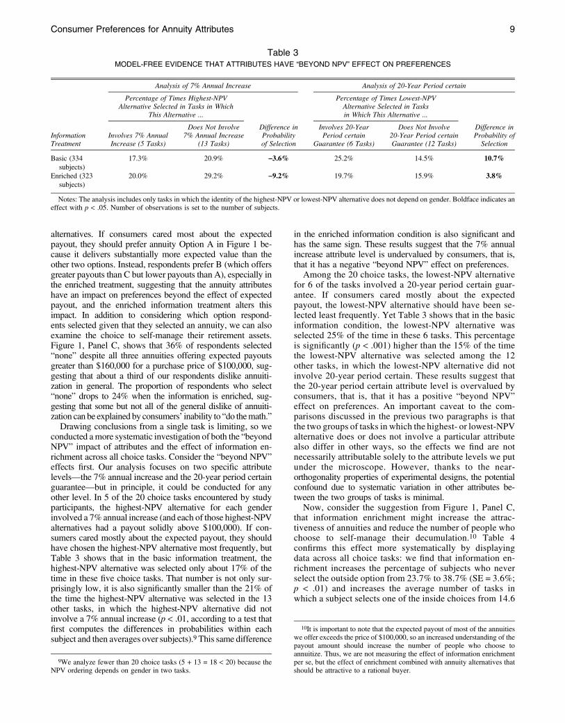
alternatives. If consumers cared most about the expectedpayout, they should prefer annuity Option A in Figure 1 be-cause it delivers substantially more expected value than theother two options. Instead, respondents prefer B (which offersgreater payouts than C but lower payouts than A), especially inthe enriched treatment, suggesting that the annuity attributeshave an impact on preferences beyond the effect of expectedpayout, and the enriched information treatment alters thisimpact. In addition to considering which option respond-ents selected given that they selected an annuity, we can alsoexamine the choice to self-manage their retirement assets.Figure 1, Panel C, shows that 36% of respondents selected“none” despite all three annuities offering expected payoutsgreater than $160,000 for a purchase price of $100,000, sug-gesting that about a third of our respondents dislike annuiti-zation in general. The proportion of respondents who select“none” drops to 24% when the information is enriched, sug-gesting that some but not all of the general dislike of annuiti-zation can be explained by consumers’ inability to “do themath.”
Drawing conclusions from a single task is limiting, so weconducted amore systematic investigation of both the “beyondNPV” impact of attributes and the effect of information en-richment across all choice tasks. Consider the “beyond NPV”effects first. Our analysis focuses on two specific attributelevels—the 7% annual increase and the 20-year period certainguarantee—but in principle, it could be conducted for anyother level. In 5 of the 20 choice tasks encountered by studyparticipants, the highest-NPV alternative for each genderinvolved a 7% annual increase (and each of those highest-NPValternatives had a payout solidly above $100,000). If con-sumers cared mostly about the expected payout, they shouldhave chosen the highest-NPV alternative most frequently, butTable 3 shows that in the basic information treatment, thehighest-NPV alternative was selected only about 17% of thetime in these five choice tasks. That number is not only sur-prisingly low, it is also significantly smaller than the 21% ofthe time the highest-NPV alternative was selected in the 13other tasks, in which the highest-NPV alternative did notinvolve a 7% annual increase (p < .01, according to a test thatfirst computes the differences in probabilities within eachsubject and then averages over subjects).9 This same difference
in the enriched information condition is also significant andhas the same sign. These results suggest that the 7% annualincrease attribute level is undervalued by consumers, that is,that it has a negative “beyond NPV” effect on preferences.
Among the 20 choice tasks, the lowest-NPV alternativefor 6 of the tasks involved a 20-year period certain guar-antee. If consumers cared mostly about the expectedpayout, the lowest-NPV alternative should have been se-lected least frequently. Yet Table 3 shows that in the basicinformation condition, the lowest-NPV alternative wasselected 25% of the time in these 6 tasks. This percentageis significantly (p < .001) higher than the 15% of the timethe lowest-NPV alternative was selected among the 12other tasks, in which the lowest-NPV alternative did notinvolve 20-year period certain. These results suggest thatthe 20-year period certain attribute level is overvalued byconsumers, that is, that it has a positive “beyond NPV”effect on preferences. An important caveat to the com-parisons discussed in the previous two paragraphs is thatthe two groups of tasks in which the highest- or lowest-NPValternative does or does not involve a particular attributealso differ in other ways, so the effects we find are notnecessarily attributable solely to the attribute levels we putunder the microscope. However, thanks to the near-orthogonality properties of experimental designs, the potentialconfound due to systematic variation in other attributes be-tween the two groups of tasks is minimal.
Now, consider the suggestion from Figure 1, Panel C,that information enrichment might increase the attrac-tiveness of annuities and reduce the number of people whochoose to self-manage their decumulation.10 Table 4confirms this effect more systematically by displayingdata across all choice tasks: we find that information en-richment increases the percentage of subjects who neverselect the outside option from 23.7% to 38.7% (SE = 3.6%;p < .01) and increases the average number of tasks inwhich a subject selects one of the inside choices from 14.6
Table 3MODEL-FREE EVIDENCE THAT ATTRIBUTES HAVE “BEYOND NPV” EFFECT ON PREFERENCES
InformationTreatment
Analysis of 7% Annual Increase Analysis of 20-Year Period certain
Percentage of Times Highest-NPVAlternative Selected in Tasks in Which
This Alternative ...
Difference inProbabilityof Selection
Percentage of Times Lowest-NPVAlternative Selected in Tasksin Which This Alternative ...
Difference inProbability ofSelection
Involves 7% AnnualIncrease (5 Tasks)
Does Not Involve7% Annual Increase
(13 Tasks)
Involves 20-YearPeriod certain
Guarantee (6 Tasks)
Does Not Involve20-Year Period certainGuarantee (12 Tasks)
Basic (334subjects)
17.3% 20.9% −3.6% 25.2% 14.5% 10.7%
Enriched (323subjects)
20.0% 29.2% −9.2% 19.7% 15.9% 3.8%
Notes: The analysis includes only tasks in which the identity of the highest-NPV or lowest-NPV alternative does not depend on gender. Boldface indicates aneffect with p < .05. Number of observations is set to the number of subjects.
9We analyze fewer than 20 choice tasks (5 + 13 = 18 < 20) because theNPV ordering depends on gender in two tasks.
10It is important to note that the expected payout of most of the annuitieswe offer exceeds the price of $100,000, so an increased understanding of thepayout amount should increase the number of people who choose toannuitize. Thus, we are not measuring the effect of information enrichmentper se, but the effect of enrichment combined with annuity alternatives thatshould be attractive to a rational buyer.
Consumer Preferences for Annuity Attributes 9
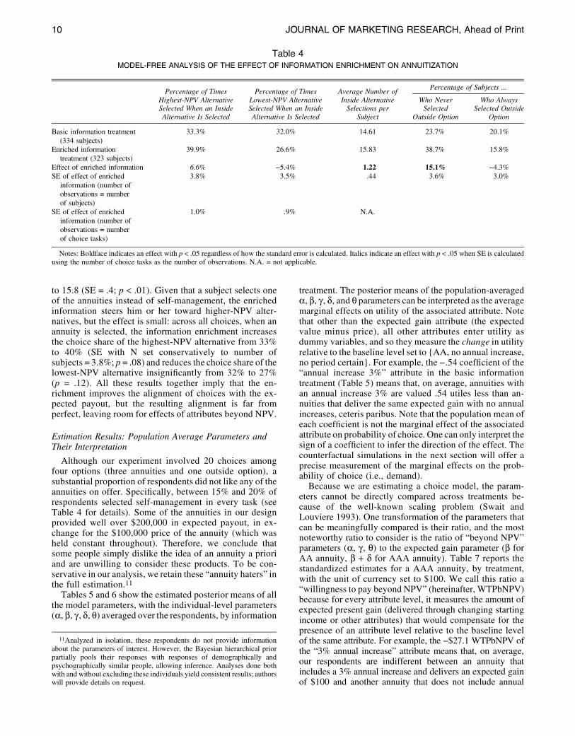
to 15.8 (SE = .4; p < .01). Given that a subject selects oneof the annuities instead of self-management, the enrichedinformation steers him or her toward higher-NPV alter-natives, but the effect is small: across all choices, when anannuity is selected, the information enrichment increasesthe choice share of the highest-NPV alternative from 33%to 40% (SE with N set conservatively to number ofsubjects = 3.8%; p = .08) and reduces the choice share of thelowest-NPV alternative insignificantly from 32% to 27%(p = .12). All these results together imply that the en-richment improves the alignment of choices with the ex-pected payout, but the resulting alignment is far fromperfect, leaving room for effects of attributes beyond NPV.
Estimation Results: Population Average Parameters andTheir Interpretation
Although our experiment involved 20 choices amongfour options (three annuities and one outside option), asubstantial proportion of respondents did not like any of theannuities on offer. Specifically, between 15% and 20% ofrespondents selected self-management in every task (seeTable 4 for details). Some of the annuities in our designprovided well over $200,000 in expected payout, in ex-change for the $100,000 price of the annuity (which washeld constant throughout). Therefore, we conclude thatsome people simply dislike the idea of an annuity a prioriand are unwilling to consider these products. To be con-servative in our analysis, we retain these “annuity haters” inthe full estimation.11
Tables 5 and 6 show the estimated posterior means of allthe model parameters, with the individual-level parameters(a, b, g , d, q) averaged over the respondents, by information
treatment. The posterior means of the population-averageda, b, g , d, and q parameters can be interpreted as the averagemarginal effects on utility of the associated attribute. Notethat other than the expected gain attribute (the expectedvalue minus price), all other attributes enter utility asdummy variables, and so they measure the change in utilityrelative to the baseline level set to AA, no annual increase,no period certain. For example, the −.54 coefficient of the“annual increase 3%” attribute in the basic informationtreatment (Table 5) means that, on average, annuities withan annual increase 3% are valued .54 utiles less than an-nuities that deliver the same expected gain with no annualincreases, ceteris paribus. Note that the population mean ofeach coefficient is not the marginal effect of the associatedattribute on probability of choice. One can only interpret thesign of a coefficient to infer the direction of the effect. Thecounterfactual simulations in the next section will offer aprecise measurement of the marginal effects on the prob-ability of choice (i.e., demand).
Because we are estimating a choice model, the param-eters cannot be directly compared across treatments be-cause of the well-known scaling problem (Swait andLouviere 1993). One transformation of the parameters thatcan be meaningfully compared is their ratio, and the mostnoteworthy ratio to consider is the ratio of “beyond NPV”parameters (a, g , q) to the expected gain parameter (b forAA annuity, b + d for AAA annuity). Table 7 reports thestandardized estimates for a AAA annuity, by treatment,with the unit of currency set to $100. We call this ratio a“willingness to pay beyond NPV” (hereinafter, WTPbNPV)because for every attribute level, it measures the amount ofexpected present gain (delivered through changing startingincome or other attributes) that would compensate for thepresence of an attribute level relative to the baseline levelof the same attribute. For example, the −$27.1 WTPbNPV ofthe “3% annual increase” attribute means that, on average,our respondents are indifferent between an annuity thatincludes a 3% annual increase and delivers an expected gainof $100 and another annuity that does not include annual
Table 4MODEL-FREE ANALYSIS OF THE EFFECT OF INFORMATION ENRICHMENT ON ANNUITIZATION
Percentage of TimesHighest-NPV AlternativeSelected When an InsideAlternative Is Selected
Percentage of TimesLowest-NPV AlternativeSelected When an InsideAlternative Is Selected
Average Number ofInside AlternativeSelections per
Subject
Percentage of Subjects ...
Who NeverSelected
Outside Option
Who AlwaysSelected Outside
Option
Basic information treatment(334 subjects)
33.3% 32.0% 14.61 23.7% 20.1%
Enriched informationtreatment (323 subjects)
39.9% 26.6% 15.83 38.7% 15.8%
Effect of enriched information 6.6% −5.4% 1.22 15.1% −4.3%SE of effect of enriched
information (number ofobservations = numberof subjects)
3.8% 3.5% .44 3.6% 3.0%
SE of effect of enrichedinformation (number ofobservations = numberof choice tasks)
1.0% .9% N.A.
Notes: Boldface indicates an effect with p < .05 regardless of how the standard error is calculated. Italics indicate an effect with p < .05 when SE is calculatedusing the number of choice tasks as the number of observations. N.A. = not applicable.
11Analyzed in isolation, these respondents do not provide informationabout the parameters of interest. However, the Bayesian hierarchical priorpartially pools their responses with responses of demographically andpsychographically similar people, allowing inference. Analyses done bothwith and without excluding these individuals yield consistent results; authorswill provide details on request.
10 JOURNAL OF MARKETING RESEARCH, Ahead of Print
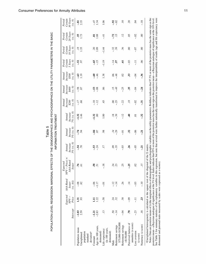
Tab
le5
POPULA
TIO
N-LEVELREGRESSIO
N:MARGINALEFFECTSOFTHEDEMOGRAPHICSAND
PSYCHOGRAPHICSON
THEUTILITYPARAMETERSIN
THEBASIC
INFORMATIO
NTREATMENT
Intercept
Expected
NPV−
Price
AAA-Rated
Issuer
(vs.AA)
Expected
NPV−Price)×
AAA-Rated
Issuer
Ann
ual
Increase
3%(vs.0)
Annua
lIncrease
5%(vs.0)
Ann
ual
Increase
7%(vs.0)
Ann
ual
Increase
$200
(vs.0)
Annua
lIncrease
$400
(vs.0)
Ann
ual
Increase
$500
(vs.0)
Period
Certain
5Years
(vs.0)
Period
Certain
10Years
(vs.0)
Period
Certain
20Years
(vs.0)
Period
Certain
30Years
(vs.0)
Populationmean
−1.03
1.31
−.08
.76
−.54
−.74
−1.32
−.17
−.58
−.63
−.52
.18
.55
−.81
Unexplained
populatio
nstandard
deviationa
2.59
.93
.82
.61
.70
.94
1.46
.68
.87
1.19
.97
1.35
1.73
2.35
Constant
−1.21
1.11
−.06
.58
−.53
−.84
−1.32
−.10
−.53
−.60
−.65
.20
.81
−.45
Age
(in10
0years,
demeaned)
−2.83
1.22
−1.17
.51
−.24
.07
.00
−.12
−.08
−.46
−.15
1.09
1.88
1.34
Lifeexpectancy
(in10
0years,
demeaned)
.13
−.58
−.01
−.18
.17
.98
1.00
.45
.86
1.38
−1.19
−1.44
−.41
1.06
Male
.50
.24
−.12
.24
.09
.34
.18
.00
.15
.06
−.14
−.32
−.72
−.92
Retirem
entsavings
$75,00
0–$1
50,000
−.14
.32
−.14
.23
−.35
−.29
−.39
−.25
−.48
−.48
.57
.39
.15
−.02
Retirem
entsavings
>$15
0,00
0−.04
.30
.26
.25
−.03
−.01
−.12
−.22
−.25
.02
.61
.36
.12
.10
Perceived
fairness
ofannuities
(z-score)
.78
−.09
.14
−.25
.26
.32
.40
.18
.35
.33
−.03
.00
.05
.20
Lossaversion
(z-score)
−.23
−.11
−.03
.02
−.05
−.06
.01
−.02
−.04
−.04
−.11
−.07
−.02
.04
Num
eracy(z-score)
.18
.23
−.10
.15
−.21
−.21
−.32
−.31
−.24
−.36
.06
.00
.00
−.18
a Unexplained
heterogeneity
iscalculated
asthesquare
root
ofthediagonal
oftheSmatrix.
Notes:D
ataareposteriorm
eans
ofD(the
marginaleffectsof
demographicandpsychographicvariableson
theutilityparameters).B
oldfaceindicatesthat97.5%
ormoreof
theposteriorm
asshasthesamesign
asthe
posteriorm
ean—
aBayesiananalog
ueof
sign
ificanceatthe5%
level.Italicsindicatethat95%or
moreof
theposteriorm
asshasthesamesign
astheposteriorm
ean—
aBayesiananalog
ueof
sign
ificanceatthe10
%level.
See
Table3forsummarystatisticsof
theexplanatoryvariablesin
thisregression,butnote
that
severalwerefurtherstatistically
transformed
toim
provetheinterpretabilityof
results
(age
andlifeexpectancy
were
demeanedandpersonal
traitsmeasuredby
scales
wereexpressedas
z-scores).
Consumer Preferences for Annuity Attributes 11
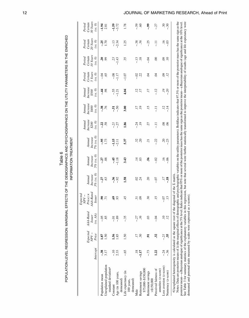
Tab
le6
POPULA
TIO
N-LEVELREGRESSIO
N:MARGINALEFFECTSOFTHEDEMOGRAPHICSAND
PSYCHOGRAPHICSON
THEUTILITYPARAMETERSIN
THEENRICHED
INFORMATIO
NTREATMENT
Intercept
Expected
NPV−
Price
AAA-Rated
Issuer
(vs.AA)
Expected
NPV−
Price)×
AAA-Rated
Issuer
Ann
ual
Increase
3%(vs.0)
Ann
ual
Increase
5%(vs.0)
Ann
ual
Increase
7%(vs.0)
Annua
lIncrease
$200
(vs.0)
Ann
ual
Increase
$400
(vs.0)
Ann
ual
Increase
$500
(vs.0)
Period
Certain
5Years
(vs.0)
Period
Certain
10Years
(vs.0)
Period
Certain
20Years
(vs.0)
Period
Certain
30Years
(vs.0)
Populationmean
−.38
1.87
−.05
.90
−.27
−.27
−.95
−.22
−.38
−.44
−.04
.20
−.25
−1.94
Unexplained
populatio
nstandard
deviationa
3.17
1.50
.85
.71
.63
.88
1.73
.58
.76
.98
.65
.99
1.70
2.81
Constant
−.10
1.56
−.01
.69
−.36
−.45
−1.15
−.21
−.51
−.55
−.08
.23
−.13
−1.59
Age
(in10
0years,
demeaned)
2.33
1.85
−.89
.93
−.92
−1.18
−2.11
−.27
−.50
−1.21
−1.17
−1.43
−2.34
−3.72
Lifeexpectancy
(in
100years,
demeaned)
−.65
1.50
−.35
.45
1.58
3.43
5.37
1.86
3.00
4.04
−1.07
.35
1.25
1.78
Male
.18
.17
−.27
.31
.02
.14
.32
−.24
.17
.12
−.02
−.13
−.38
−.59
Retirem
entsavings
$75,00
0–$1
50,000
−1.17
.30
.36
.09
.24
.03
.20
.19
.19
.17
.22
.18
.56
.60
Retirem
entsavings
>$15
0,00
0−.73
.91
.03
.30
.20
.56
.21
.27
.15
.17
.04
−.04
−.25
−.99
Perceived
fairness
ofannuities
(z-score)
1.22
.32
−.04
.15
−.07
−.02
−.22
−.11
−.11
−.12
.04
.00
−.11
−.27
Lossaversion
(z-score)
−.24
−.21
.10
−.07
.17
.16
.20
.08
.12
.19
.09
.09
.16
.30
Num
eracy(z-score)
−.36
.35
.12
.13
−.18
−.06
−.23
.06
−.14
−.20
.12
.10
−.03
−.30
a Unexplained
heterogeneity
iscalculated
asthesquare
root
ofthediagonal
oftheSmatrix.
Notes:D
ataareposteriorm
eans
ofD(the
marginaleffectsof
demographicandpsychographicvariableson
theutilityparameters).B
oldfaceindicatesthat97.5%
ormoreof
theposteriorm
asshasthesamesign
asthe
posteriorm
ean—
aBayesiananalog
ueof
sign
ificanceatthe5%
level.Italicsindicatethat95%or
moreof
theposteriorm
asshasthesamesign
astheposteriorm
ean—
aBayesiananalog
ueof
sign
ificanceatthe10
%level.
See
Table3forsummarystatisticsof
theexplanatoryvariablesin
thisregression,butnote
that
severalwerefurtherstatistically
transformed
toim
provetheinterpretabilityof
results
(age
andlifeexpectancy
were
demeanedandpersonal
traitsmeasuredby
scales
wereexpressedas
z-scores).
12 JOURNAL OF MARKETING RESEARCH, Ahead of Print
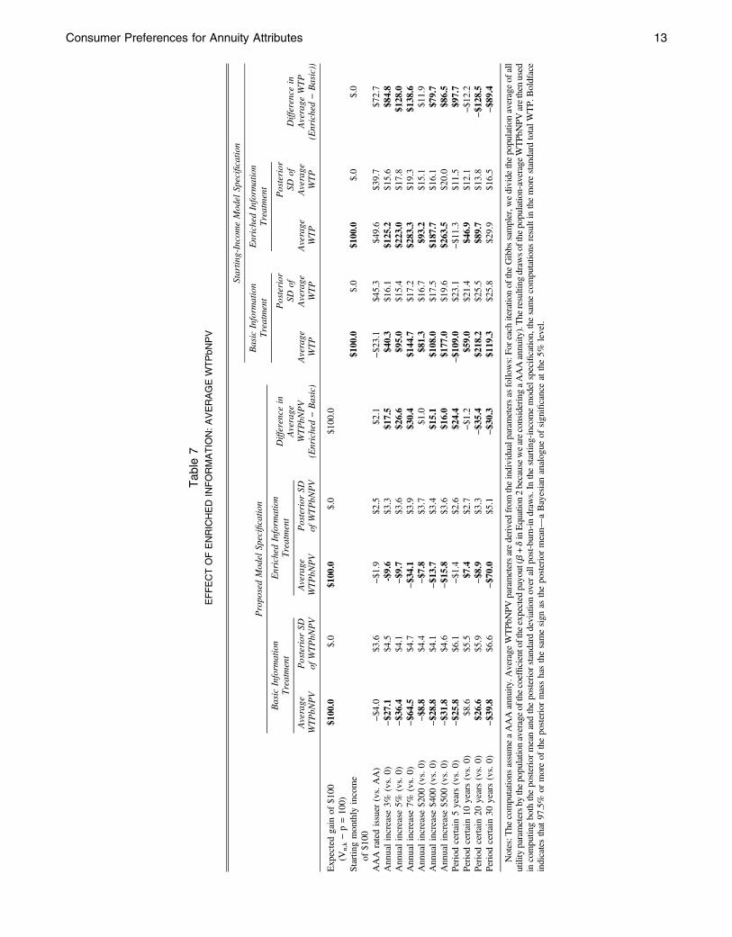
Tab
le7
EFFECTOFENRICHED
INFORMATIO
N:AVERAGEWTPbN
PV
Propo
sedMod
elSp
ecificatio
n
Startin
g-IncomeModel
Specificatio
n
Basic
Inform
ation
Treatment
EnrichedInform
ation
Treatment
Difference
inAverage
WTPbN
PV
(Enriched−Basic)
Basic
Inform
ation
Treatment
EnrichedInform
ation
Treatment
Difference
inAverage
WTP
(Enriched−Basic))
Average
WTPbN
PV
Posterior
SDof
WTPbN
PV
Average
WTPbN
PV
Posterior
SDof
WTPbN
PV
Average
WTP
Posterior
SDof
Average
WTP
Average
WTP
Posterior
SDof
Average
WTP
Expectedgain
of$1
00(V
n,k−p=10
0)$1
00.0
$.0
$100.0
$.0
$100.0
Startingmon
thly
income
of$1
00$1
00.0
$.0
$100.0
$.0
$.0
AAA
ratedissuer
(vs.AA)
−$4
.0$3
.6−$1
.9$2
.5$2
.1−$2
3.1
$45.3
$49.6
$39.7
$72.7
Ann
ualincrease
3%(vs.0)
−$2
7.1
$4.5
-$9.6
$3.3
$17.5
$40.3
$16.1
$125.2
$15.6
$84.8
Ann
ualincrease
5%(vs.0)
−$3
6.4
$4.1
−$9
.7$3
.6$2
6.6
$95.0
$15.4
$223.0
$17.8
$128
.0Ann
ualincrease
7%(vs.0)
−$6
4.5
$4.7
−$3
4.1
$3.9
$30.4
$144.7
$17.2
$283.3
$19.3
$138
.6Ann
ualincrease
$200
(vs.0)
−$8
.8$4
.4−$7
.8$3
.7$1
.0$8
1.3
$16.7
$93.2
$15.1
$11.9
Ann
ualincrease
$400
(vs.0)
−$2
8.8
$4.1
−$1
3.7
$3.4
$15.1
$108.0
$17.5
$187.7
$16.1
$79.7
Ann
ualincrease
$500
(vs.0)
−$3
1.8
$4.6
−$1
5.8
$3.6
$16.0
$177.0
$19.6
$263.5
$20.0
$86.5
Periodcertain5years(vs.0)
−$2
5.8
$6.1
−$1
.4$2
.6$2
4.4
−$1
09.0
$23.1
−$1
1.3
$11.5
$97.7
Periodcertain10
years(vs.0)
$8.6
$5.5
$7.4
$2.7
−$1
.2$5
9.0
$21.4
$46.9
$12.1
−$1
2.2
Periodcertain20
years(vs.0)
$26.6
$5.9
−$8
.9$3
.3−$3
5.4
$218.2
$25.5
$89.7
$13.8
−$1
28.5
Periodcertain30
years(vs.0)
−$3
9.8
$6.6
−$7
0.0
$5.1
−$3
0.3
$119.3
$25.8
$29.9
$16.5
−$8
9.4
Notes:T
hecomputatio
nsassumeaAAAannuity
.Average
WTPb
NPV
parametersarederivedfrom
theindividualparametersas
follo
ws:Fo
reach
iteratio
nof
theGibbs
sampler,w
edivide
thepopulatio
naverageof
all
utilityparametersby
thepopulatio
naverageofthecoefficientofthe
expected
payout(b
+dinEquation2becauseweareconsideringaAAAannuity
).The
resulting
draw
softhepopulatio
n-averageWTPb
NPV
arethen
used
incomputin
gboth
theposteriormeanandtheposteriorstandard
deviationover
allp
ost-burn-indraw
s.In
thestartin
g-incomemodelspecificatio
n,thesamecomputatio
nsresultin
themorestandard
totalW
TP.
Boldface
indicatesthat
97.5%
ormoreof
theposteriormasshasthesamesign
astheposteriormean—
aBayesiananalogue
ofsignificanceat
the5%
level.
Consumer Preferences for Annuity Attributes 13
increases and somehow (presumably through other at-tributes) delivers the same expected gain plus −$27.1,namely, an expected gain of $72.9. Thus, WTPbNPV iswillingness to pay while the expected payout is keptconstant.
The WTPbNPV concept arising naturally from ourproposed model specification can be contrasted with a morestandard marginal willingness to pay (hereafter, WTP) thatresults when the same ratio is calculated under the starting-income model specification, in which the expected gain isreplaced with starting income. Table 7 also contains all such“standard” WTP estimates; the raw parameter estimatesof that specification (analogues of Tables 5 and 6) areavailable in Table 8 and Table A4 in the Web Appendix.For example, theWTP of $40.3 for the 3% annual increasemeans that, on average, our respondents are indifferentbetween an annuity that includes a 3% annual increaseand $100 of additional starting income and an otherwiseidentical annuity that does not include annual increasesbut involves $140.3 ($100 + $40.3) of starting income.
Comparing WTPbNPV with WTP highlights the noveltyof our model. Note that because WTPbNPV is measured interms of expected gain and WTP is measured in terms ofstarting monthly income, the dollar quantities are notcomparable between the two model specifications. How-ever, one can safely compare their signs. In the case of 3%increase, the WTP is positive, meaning that 3% increase ismore valuable than no increase while initial monthly in-come and all other attributes are kept the same. On the otherhand, the WTPbNPV is negative, meaning that 3% is lessvaluable than no increase while the expected payout is keptthe same.
Estimation Results: Average Preferences in the BasicInformation Treatment
We first consider the results for the basic informationtreatment. Several conclusions can be drawn from theparameters (in Table 5) and their associated WTPbNPVvalues (in Table 7). As expected, the average coefficients ofboth the expected gain and its interaction with the AAArating are positive. The insignificant coefficient of the AAAdummy shows that consumer preference for financially safeissuers manifests itself solely through an increased weighton expected gain, not as a shift in the intercept of the utilityfunction. A qualitative comparison with the starting-income model specification rules out a simplistic theoryabout the antecedents of the significant interaction betweenAAA and expected gain: Under the starting-income modelspecification (Table 8), neither the AAA dummy nor itsinteraction with starting income is significant at the pop-ulation level, suggesting that the significant coefficient forExpected_gain × AAA is not merely capturing the respon-dents’ higher valuation of starting income when the annuityis provided by a AAA issuer. Instead, the respondents seemto value some NPV-like combination of the starting in-come with other attributes (annual increases and/or cer-tainty guarantees) more when the annuity is provided by anAAA issuer.
The coefficients of the annual-increase and period cer-tain dummies are mostly significant and often large, indi-cating that consumer behavior is not well captured byonly the expected-payout and financial-strength variables.We
discuss each of the “beyond NPV” influences from thesedifferent attributes in turn.
Annual increases. The negative signs on all of the per-centage increase coefficients suggest that consumers sys-tematically undervalue the benefits of annual paymentincreases. From the WTPbNPV estimates, we can see thatthe magnitude of the undervaluation can be large, espe-cially for the percentage increases. For example, theWTPbNPV of −$64.5 on the 7% annual increase means ourrespondents are indifferent between an annuity that gen-erates an expected gain of $100 with a constant monthlyincome and another annuity that generates an expected gainof $164.50 by starting at a lower monthly income level andadding 7% per year. In contrast, the WTP values under thestarting-income model specification are all positive. To-gether, these results indicate that consumers pay attentionto increases and value them positively, but they system-atically undervalue them relative to their true expectedvalues.
The additive increases exhibit a similar pattern, but theyare generally undervalued less, which echoes the results ofMcKenzie and Liersch (2011). To see the difference inTable 7, recall that we selected the levels of annual increaseas pairs matched across the type of increase (additive vs.percentage). Specifically, the $500/year increase results inapproximately12 the same expected payout as the 7%/yearincrease, and the $300/5% increase and $200/3% increasepairs are matched analogously. Therefore, we can comparethe WTPbNPV values within these matched pairs andconclude that the average consumer prefers additive in-creases to percentage increases, ceteris paribus. In the latersection “Counterfactual Simulations of Market Demand,”we quantify the difference in terms of demand by simu-lating the magnitude of the effect of various increases ontotal market demand using counterfactual experiments.
Period certain guarantees. The positive average co-efficient of the 20-year period certain guarantee suggeststhat consumers like this option beyond its impact on theexpected payout. Conversely, the short (5-year) and verylong (30-year) period certain guarantees are undervalued.The WTP values under the starting-income model speci-fication reveal that not only do consumers undervalue the 5-year period certain when expected payout is the same, theyalso undervalue it relative to no period certain when otherattributes are the same. Moreover, the WTP for a 30-yearperiod certain is about half the WTP for a 20-year periodcertain despite the much higher expected payout from theformer. Therefore, the inverse-U pattern we find is not anartifact of our specification or our particular calculation ofthe expected gain.
Note that this inverse-U pattern does not fit well witheither of the theories proposed in the literature as expla-nations for consumers’ overall preference for period certainoptions: both underestimation of life expectancies andprospective loss aversion should lead to overvaluation ofshort (5-year) options. Our empirical results suggest con-sumers do not simply prefer any period certain guarantee tono guarantee. Instead, they have a strong preference formedium-length periods but generally dislike long and short
12The magnitude of the difference in expected payout depends on gender,starting income, and other attributes.
14 JOURNAL OF MARKETING RESEARCH, Ahead of Print
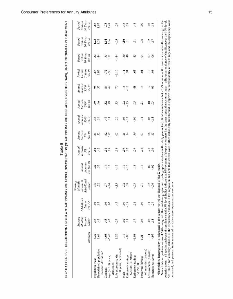
Tab
le8
POPULA
TIO
N-LEVELREGRESSIO
NUNDER
ASTARTING-INCOMEMODELSPECIFICATIO
N(STARTING
INCOMEREPLA
CESEXPECTED
GAIN),BASIC
INFORMATIO
NTREATMENT
Intercept
Startin
gMon
thly
Income
($10
0)
AAA-Rated
Issuer
(vs.AA)
Startin
gMonthly
Income×
AAA-Rated
Issuer
Ann
ual
Increase
3%(vs.0)
Ann
ual
Increase
5%(vs.0)
Ann
ual
Increase
7%(vs.0)
Ann
ual
Increase
$200
(vs.0)
Ann
ual
Increase
$400
(vs.0)
Ann
ual
Increase
$500
(vs.0)
Period
Certain
5Years
(vs.0)
Period
Certain
10Years
(vs.0)
Period
Certain
20Years
(vs.0)
Period
Certain
30Years
(vs.0)
Populationmean
−4.32
.48
−.04
.06
.22
.52
.81
.45
.59
.98
−.58
.33
1.23
.67
Unexplained
populatio
nstandard
deviationa
3.64
.45
.85
.22
.35
.42
.52
.39
.46
.55
1.05
1.44
1.68
1.97
Constant
−4.08
.43
−.05
.07
.14
.31
.62
.47
.52
.84
−.72
.33
1.34
.73
Age
(in10
0years,
demeaned)
−5.43
.42
.02
−.24
.12
.68
1.32
.11
.49
.48
−.30
1.11
2.36
2.49
Lifeexpectancy
(in
100years,demeaned)
1.85
−.27
.45
−.15
−.17
.38
.05
.20
.33
.70
−1.16
−1.44
−.65
.29
Male
.17
.02
−.07
−.02
.17
.39
.25
.03
.22
.15
−.11
−.30
−.50
−.45
Retirem
entsavings
$75,00
0–$1
50,000
−.90
.11
−.38
.08
−.16
.02
.14
−.13
−.25
−.12
.57
.40
.31
.28
Retirem
entsavings
>$15
0,00
0−1.08
.17
.51
−.03
.18
.29
.36
−.06
.05
.48
.63
.43
.31
.48
Perceived
fairness
ofannuities
(z-score)
1.31
−.06
.07
−.01
.14
.16
.07
.11
.21
.14
−.01
−.04
−.08
.00
Lossaversion
(z-score)
−.11
−.03
−.11
.02
−.09
−.13
−.08
−.05
−.10
−.12
−.12
−.07
−.02
−.03
Num
eracy(z-score)
−.97
.18
.29
−.06
−.02
.06
.13
−.15
.03
.05
.08
.06
.17
.18
a Unexplained
heterogeneity
iscalculated
asthesquare
root
ofthediagonal
oftheSmatrix.
Notes:D
ataareposteriorm
eans
ofD(the
marginaleffectsof
demographicandpsychographicvariableson
theutilityparameters).B
oldfaceindicatesthat97.5%
ormoreof
theposteriorm
asshasthesamesign
asthe
posteriorm
ean—
aBayesiananalog
ueof
sign
ificanceatthe5%
level.Italicsindicatethat95%or
moreof
theposteriorm
asshasthesamesign
astheposteriorm
ean—
aBayesiananalog
ueof
sign
ificanceatthe10
%level.
See
Table3forsummarystatisticsof
theexplanatoryvariablesin
thisregression,butnote
that
severalwerefurtherstatistically
transformed
toim
provetheinterpretabilityof
results
(age
andlifeexpectancy
were
demeaned,
andpersonal
traitsmeasuredby
scales
wereexpressedas
z-scores).
Consumer Preferences for Annuity Attributes 15
options. In the section “Counterfactual Simulations ofMarket Demand,” we measure the magnitude of the effectof the period certain guarantee on total market demand,using counter-factual experiments. We now consider howthe average preferences shift due to the enriched infor-mation treatment.
Effect of the Enriched Information Treatment on AveragePreferences
Recall that only the standardized coefficients (WTPbNPV inTable 7) can be meaningfully compared across treatments.Table 7 provides both the WTPbNPV for the enriched in-formation treatment and the difference in WTPbNPV betweentreatments.
We offer three observations: First, the magnitudes of thevalues of WTPbNPV for annual increases are much smallerin the enriched condition, which indicates that the apparentdislike of the increases observed in the basic treatmentcould be due to the subjects’ inability to “do the math” oncompounding, rather than to a more fundamental aversionto annual increases. The WTP values under the starting-income model specification all increase, in support of theinterpretation that respondents value increases more in theenriched information condition. At the same time, however,the WTPbNPV values are still negative, indicating that therespondents undervalue annual increases even in the en-riched information condition.
Second, the difference between additive and percentageincreases mostly vanishes in the enriched treatment, withthe exception of the $500/7% annual increase pair, forwhich a larger undervaluation of the percentage increase isobserved. But even for that extreme pair, the differencebetween the values of WTPbNPV is reduced from about$33 to about $18. This finding agrees with prior work onindividuals’ difficulty with compounding in financial de-cisions (e.g., McKenzie and Liersch 2011; Wagenaar andSagaria 1975). By seeing a table of cumulative payouts,individuals can better appreciate the impact of the per-centage increases over time.
Finally, respondents in the enriched treatment continueto exhibit the inverse-U relationship pattern betweenpreferences and the duration of period certain guarantees(even under the starting-income model specification), butthe peak of the preference shifts toward shorter periodcertain durations (10-year period certain becomes the mostovervalued). The persistence of the inverse-U patternacross the two information treatments suggests the re-lationship is not fundamentally driven by consumers’ mis-calculation or inability to “do the math”when estimating theimpact of a guarantee on payout.
Estimation Results: Population Heterogeneity of Preferences
We find a lot of heterogeneity in preferences, some ofwhich can be explained by variance in demographics andpsychographics and some of which remains unexplained.We show the unexplained part (the square root of theposterior mean of Ʃ) in Tables 5 and 6 to give a sense of itsmagnitude. The average of the D parameter (also in Tables 5and 6) captures the part of the heterogeneity of preferencesthat is explained by demographics and psychographics (seeEquation 3).
The most easily interpreted effects are those of de-mographics and psychographics (Z) on the intercept ofutility (a), that is, on the individual’s baseline liking ofannuities. One effect stands out as large: regardless of theinformation treatment,13 we find that an individual’s per-ceived fairness of annuities is strongly correlated with thatperson’s baseline liking of annuities. In the enriched in-formation treatment, individuals with higher perceivedfairness value expected gain more. In the basic informationtreatment, individuals with higher perceived fairness showincreased liking of annual increases beyond NPV, but notincreased enough to reverse their undervaluation of annualincreases.
Several other effects of demographics and psycho-graphics also deserve a mention. As one would expect,more numerate individuals care more about the expectedpayout regardless of treatment. More surprisingly, theyundervalue annual increases even more than less numeratepeople, especially in the basic information treatment. Fi-nally, as a rational model would predict, higher life ex-pectancy increases the liking of annual increases, but thiseffect exists only in the enriched information treatment. Tosee how much longer than average a respondent needs toexpect to live to eliminate the undervaluation of annualincreases, one can calculate the ratios of the population-average beyond-NPV coefficients and the D coefficient ofdemeaned life expectancy. The result is between 8 and 17years, that is, between one and two standard deviations oflife expectancy (see Table 8). Thus, we find that theenriched treatment leads to more accurate valuation ofannual increases for people who expect to live more thanone standard deviation longer than the average lifeexpectancy—an important finding for annuity sellers whoare concerned about both consumer targeting and adverseselection.
The population-level parameters (D) also shed light onwhich consumers are most sensitive to period certainguarantees. The undervaluation of 5-year period certainguarantees is present only in the basic information treat-ment, and it is almost completely driven by people with lessthan $75,000 of savings; the D coefficients of retirementsavings of more than $75,000 on the beyond-NPV valua-tion of 5-year period certain (.57 and .61) compensate forthe −.65 constant in the same regression. Surprisingly,neither lower life expectancy nor greater loss aversionsignificantly increases the preference for a longer periodcertain guarantee in either information condition. Instead,we find that the undervaluation of 30-year period certainis correlated with being male, especially in the basic in-formation condition. In the enriched information condition,the same undervaluation is also correlated with havingretirement savings of more than $150,000. Why individualswith low savings undervalue short guarantees in the basictreatment and individuals with high savings undervaluelong guarantees in the enriched treatment is unexplored inany current theories of annuity choice; further research onhow individuals interpret such options is needed.
13Recall that we cannot compare the coefficients between Tables 6 and 7directly (Swait and Louviere 1993). We thus confine ourselves to broadqualitative observations of the effect of the enriched information on ourestimates.
16 JOURNAL OF MARKETING RESEARCH, Ahead of Print
Retirement savings also play another role: people with ahigh level of retirement savings (>$75,000) show strongeroverall dislike for annuities when they see the contingentcumulative payout tables. Whether these individuals areconfident that they can self-manage their assets betterwithout annuities or they are evaluating the payback on anannuity in an investment frame (Brown et al. 2008), pro-viding them with cumulative payout information does notseem to increase their overall liking for annuities as much asit does for other respondents. Since we did not collectinformation about Social Security eligibility from our re-spondents, it is possible that this retirement-savings mea-sure is correlated with expected Social Security benefits,and the D parameter for retirement savings may simply becapturing the unmeasured effect of Social Security eligi-bility as a substitute for annuitization.
Counterfactual Simulations of Market Demand
Population averages of the utility coefficients provideonly limited insight into the marginal effects of annuityattributes on demand. In this section, we conduct a series ofcounterfactual simulations to assess the magnitude of theseeffects. In all our simulations, we consider a specific focalannuity offering along with a no-choice option (i.e., theoutside option) as the set of alternatives available to thecustomer. We then separately estimate the probability ofbuying the focal annuity for every individual in our sample,using the estimated posterior distributions of individual-level utility parameters. Adding the probabilities togetheryields an estimate of total demand within our subjectsample. To account for estimation error, we compute theprobability separately for each of the 40,000 post-burn-inposterior draws of ½aj,bj, g j, dj, q
0j and then average the
probabilities over the draws. To account for the randomcomponent of utility given a particular draw, we averageeach probability over 100 draws of the random utility edrawn independently and identically distributed fromnormal (0,1). One way to think about our simulationstrategy is to imagine each respondent generating fourmillion pseudopeople, each with his or her own½aj,bj, g j, dj, q
0j, ej vector. Assume each of the four million
pseudopeople picks his or her utility-maximizing alter-native, and the original respondent’s choice probability isthe percentage of the respondent’s alter egos (i.e., thepseudopeople who have the same vectors as the respondent)who select the given choice. In the statistical literature, thiskind of posterior predictive simulation is the standard ap-proach (Rossi et al. 2005). We now turn to the specificsimulations and the results.
Result 1: Fixed annual increases boost demand more thanequal-payout percentage increases in the basic, but not theenriched, treatment condition. The left side of Figure 2displays the estimated demand from women (results formen are available from the authors) for an annuity from aAAA-rated company with $400 starting monthly income,no period certain guarantee, and different types and mag-nitudes of annual increase. The top left plot shows the de-mand for the basic information treatment, and the bottomleft plot shows it for the enriched information treatment.The dashed “control” lines in each plot indicate predicteddemand for annuities that do not include annual increases
but deliver higher expected present value through higherstarting incomes. Thus, we interpret demand above thecontrol line as an overvaluation of the particular level ofannual increase relative to payout-equivalent increases inthe starting income, and demand below the control line as anundervaluation.
Looking first at the basic-treatment data in the top leftplot of Figure 2, we see that additive increases generateconsistently higher demand relative to payout-equivalentpercentage increases. Whereas the $200 increase is valuedabout as much as the payout-equivalent increases in thestarting income, the 3% increase is clearly undervalued.Interestingly, raising either the additive yearly increaseabove $200 or the percentage increase above 0 does notraise demand very much at all. For example, the impliedelasticity of demand due to raising the yearly additiveincrease from $200 to $500 is only about .04. In otherwords, even if expected payout can be increased for free,the only large boost to demand available in the basic in-formation treatment is the boost from no increase to $200annual increase.
The demand curves look completely different in the en-riched information treatment: undervaluation is no longerpresent, and a relative preference for additive increasesover percentage increases no longer exists. In other words,annual increases are valued at almost exactly their financialvalue in the enriched information condition, because linesfor both types of increases match the control line. Thus,as suggested by the estimation results described previously,providing consumers with a table of cumulative payoutsappears to bring their attribute valuations for annual in-creases more in line with expected present value.
Result 2: Medium-length period certain guarantees boostdemand, whereas short ones decrease it. The right side ofFigure 2 displays the estimated demand from women for anannuity from a AAA-rated company with a $500 startingmonthly income, no annual increases, and different lengthsof period certain guarantees. The top right plot shows thedemand for the basic information treatment, and the bottomright plot shows it for the enriched information treatment.Consider the basic treatment (top right plot) first. As in thecase of annual increases, overall market demand is con-sistent with the average consumer’s preferences: the 20-year period certain guarantee yields the highest demand andis dramatically overvalued relative to control (increasingdemand by about a third compared to the payout-equivalentincrease in starting income). By contrast, the no-guaranteeoption is preferred to a 5-year period certain guarantee. Thisfinding is surprising in the sense that even a 5-year periodcertain guarantee provides some protection from full lossin case the buyer unexpectedly dies soon after purchasingthe annuity, perhaps after being hit by the proverbial bus.Finally, the demand for 30-year period certain guarantees isslightly below that for 10-year guarantees, despite the muchlarger expected payout of the 30-year guarantee. Theseresults suggest consumers will not respond positively toissuers’ offers of very short or very long period certainguarantees.
The inverse-U shape of demand for period certainguarantees is also visible for annuities presented in theenriched information treatment. The persistence of theinverse-U shape across both treatments, as well as its
Consumer Preferences for Annuity Attributes 17
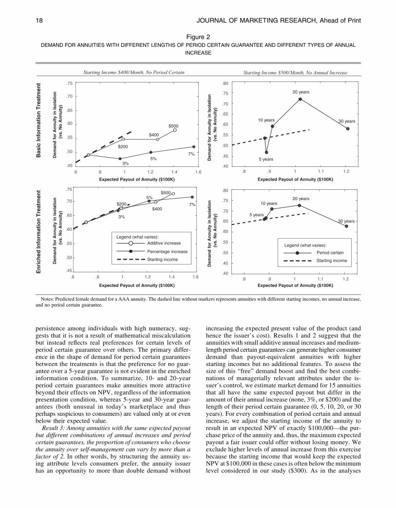
persistence among individuals with high numeracy, sug-gests that it is not a result of mathematical miscalculationbut instead reflects real preferences for certain levels ofperiod certain guarantee over others. The primary differ-ence in the shape of demand for period certain guaranteesbetween the treatments is that the preference for no guar-antee over a 5-year guarantee is not evident in the enrichedinformation condition. To summarize, 10- and 20-yearperiod certain guarantees make annuities more attractivebeyond their effects on NPV, regardless of the informationpresentation condition, whereas 5-year and 30-year guar-antees (both unusual in today’s marketplace and thusperhaps suspicious to consumers) are valued only at or evenbelow their expected value.
Result 3: Among annuities with the same expected payoutbut different combinations of annual increases and periodcertain guarantees, the proportion of consumers who choosethe annuity over self-management can vary by more than afactor of 2. In other words, by structuring the annuity us-ing attribute levels consumers prefer, the annuity issuerhas an opportunity to more than double demand without
increasing the expected present value of the product (andhence the issuer’s cost). Results 1 and 2 suggest that theannuities with small additive annual increases and medium-length period certain guarantees can generate higher consumerdemand than payout-equivalent annuities with higherstarting incomes but no additional features. To assess thesize of this “free” demand boost and find the best combi-nations of managerially relevant attributes under the is-suer’s control, we estimate market demand for 15 annuitiesthat all have the same expected payout but differ in theamount of their annual increase (none, 3%, or $200) and thelength of their period certain guarantee (0, 5, 10, 20, or 30years). For every combination of period certain and annualincrease, we adjust the starting income of the annuity toresult in an expected NPV of exactly $100,000—the pur-chase price of the annuity and, thus, the maximum expectedpayout a fair issuer could offer without losing money. Weexclude higher levels of annual increase from this exercisebecause the starting income that would keep the expectedNPV at $100,000 in these cases is often below the minimumlevel considered in our study ($300). As in the analyses
Figure 2DEMAND FOR ANNUITIES WITH DIFFERENT LENGTHS OF PERIOD CERTAIN GUARANTEE AND DIFFERENT TYPES OF ANNUAL
INCREASE
Bas
ic In
form
atio
n T
reat
men
tE
nri
ched
Info
rmat
ion
Tre
atm
ent
.6 .8 1 1.2 1.4 1.6
.45
.50
.55
.60
.65
.70
.75
Dem
and
fo
r A
nn
uit
y in
Iso
lati
on
(v
s. N
o A
nn
uit
y)
$400
$200
$500
3%5%
7%
$400$200
$500
3%
5%
7%
.8 .9 1 1.1 1.2.40
.45
.50
.55
.60
.65
.70
.75
.80
5 years
10 years
20 years
30 years
20 years10 years
5 years
30 years
Starting Income $400/Month, No Period Certain Starting Income $500/Month, No Annual Increase
Legend (what varies):
Period certain
Starting income
Legend (what varies):Additive increase
Percentage increase
Starting income
Expected Payout of Annuity ($100K) Expected Payout of Annuity ($100K)
Expected Payout of Annuity ($100K)Expected Payout of Annuity ($100K)
Dem
and
fo
r A
nn
uit
y in
Iso
lati
on
(v
s. N
o A
nn
uit
y)
.45
.50
.55
.60
.65
.70
.75
.6 .8 1 1.2 1.4 1.6
Dem
and
fo
r A
nn
uit
y in
Iso
lati
on
(v
s. N
o A
nn
uit
y)D
eman
d f
or
An
nu
ity
in Is
ola
tio
n
(vs.
No
An
nu
ity)
.40
.45
.50
.55
.60
.65
.70
.75
.80
.8 .9 1 1.1 1.2
Notes: Predicted female demand for a AAA annuity. The dashed line without markers represents annuities with different starting incomes, no annual increase,and no period certain guarantee.
18 JOURNAL OF MARKETING RESEARCH, Ahead of Print
underlying results 1 and 2, we then compute the marketdemand each of the 15 possible annuities would receive if itwere the only offering in the market other than self-management.
Figure 3 plots the estimated demand as a function ofperiod certain, by gender and information treatment.14Under both information treatments and for both genders,the demand-maximizing (hereinafter called “optimal”)annuities do not involve any annual increases, consistentwith the average preferences in Tables 5 and 6. Gender doesnot affect the optimal annuity beyond starting income, andproviding enriched information lowers the optimal periodcertain length from 20 years to 10 years. Specifically, theoptimal annuity under the basic information conditionincludes a 20-year period certain guarantee and a startingincome of $491 for females and $510 for males (see TableA3 in the Web Appendix for the starting incomes). Theoptimal annuity under the enriched information treatmentincludes a 10-year period certain guarantee for both gendersand a starting income of $550 for females and $601 formales. Enriching the information thus reduces but does noteliminate the disadvantage of annual increases in the eyesof consumers.
The most striking aspect of Figure 3 is the large dif-ference between the demand for the optimal annuitiesdiscussed previously and the lowest-demand annuities.Even when we ignore the unpopular 30-year period certainguarantee as unrealistic, the difference can be large: underthe basic information condition, the female demand for anexpected-payout-equivalent annuity with a starting incomeof $329, 5-year period certain, and 3% annual increase isabout half of the demand for the optimal annuity. Enrichingthe information reduces but does not eliminate this gap: theworst-performing annuity in the male market ($377 startingincome, 3% annual increase, and 20-year period certain)generates only 73% of the demand for the optimal annuity.
DISCUSSION
This study presents a case for marketing research aboutdecumulation products, proposes a model of consumerpreferences for attributes of immediate life annuities, andestimates the model using stated preferences in a DCEwith a national panel of people aged 40–65 years. Our mainmethodological contribution is a model specification thatallows direct measurement of the direct influence of at-tributes on preferences beyond their impact through theexpected NPV of the annuity, or what we call “beyondNPV.” We find that consumers’ valuation increases withthe expected NPV of the payout, but some annuity attri-butes also influence consumer preferences directly, beyondtheir impact on financial value.
One attribute that influences preferences beyond NPV isinflation protection through annual payment increases, andits influence depends on the way product information ispresented. We find that consumers who see only basicattribute information undervalue annual increases and show
stronger preference for fixed nominal annual increasesrelative to percentage increases, when the expected payoutis held constant. However, consumers who also see a tableof the annuities’ contingent cumulative payouts undervalueannual increases much less and do not care whether theincreases are expressed in the form of percentages or fixeddollar amounts. These findings are consistent with priorbehavioral research on consumers’ biases in understand-ing compounding interest (McKenzie and Liersch 2011;Wagenaar and Sagaria 1975). Consistent with the recom-mendations of Kunreuther et al (2013), our findings suggestthat policy makers trying to align consumer annuity choiceswith expected payout should encourage annuity issuers toinclude cumulative payout information in their marketingmaterials, rather than simply listing attributes, as seems tobe current industry practice.
Another attribute with a strong influence beyond NPV isthe period certain guarantee. We find that regardless of theinformation presentation, consumers (especially women)overvalue medium-length (10-year and 20-year) periodcertain guarantees, and they (especially men) undervaluevery long (30-year) guarantees. In the basic informationcondition, consumers also undervalue very short (5-year)guarantees, an effect mostly driven by people with lowretirement savings. The demographics one would expect todrive preferences for period certain guarantees, such as lossaversion and life expectancy (Brown et al. 2008), do notcorrelate strongly with the pattern of over- and undervaluationwe find, and additional research is clearly needed.
Finally, company financial strength rating is also im-portant to consumers, with AAA-rated companies preferredto those with an AA rating. Interestingly, preference forfinancially safe issuers manifests solely through an in-creased weight on expected financial gain, and not as anupward shift in the utility function intercept. This resultadds to prior evidence that consumers consider insurancecompany financial strength during annuity purchase(Babbel and Merrill 2006).
Demand for annuities is correlated with demographicsand psychographics. Three correlations are consistentacross both information treatments. First, respondents whohave more money saved for retirement (>$75,000) likeannuities less. This finding is a bit of a paradox, wherebythe people who can afford annuitization are the same peoplewho are not interested in it. Second, more numerate con-sumers exhibit a higher preference for maximizing ex-pected financial gain (the slope of their utility in expectedgain is about 18% steeper than that of less numerateconsumers), consistent with the idea that annuities arecomplex financial products that require the ability to “dothe math” to understand. Surprisingly, more numerate in-dividuals also undervalue annual increases more (espe-cially in the basic information treatment), which suggeststhat their choices might not necessarily be better alignedwith higher expected payout. Finally, respondents whoconsider annuities to be fair (measured by the scale ofKahneman, Knetsch, and Thaler [1986]) like annuitiesmore, consistent with behavioral explanations for the an-nuity puzzle (Benartzi, Previtero, and Thaler 2011; Hu andScott 2007). Perceived fairness plays other roles in ourmodel, depending on the information treatment: in theenriched information treatment, individuals with higher
14Table A3 in the Web Appendix contains the data behind this figure,including the starting incomes needed for each combination of annual in-crease and period certain guarantee to achieve the same expected payout of$100,000. Note that holding expected payout constant leads to a direct trade-off between higher starting incomes and annual increases.
Consumer Preferences for Annuity Attributes 19
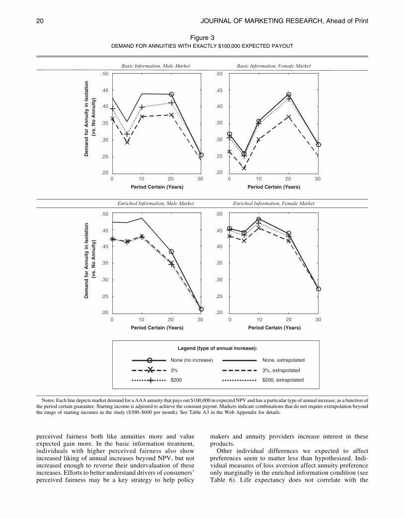
perceived fairness both like annuities more and valueexpected gain more. In the basic information treatment,individuals with higher perceived fairness also showincreased liking of annual increases beyond NPV, but notincreased enough to reverse their undervaluation of theseincreases. Efforts to better understand drivers of consumers’perceived fairness may be a key strategy to help policy
makers and annuity providers increase interest in theseproducts.
Other individual differences we expected to affectpreferences seem to matter less than hypothesized. Indi-vidual measures of loss aversion affect annuity preferenceonly marginally in the enriched information condition (seeTable 6). Life expectancy does not correlate with the
Figure 3DEMAND FOR ANNUITIES WITH EXACTLY $100,000 EXPECTED PAYOUT
0 10 20 30.20
.25
.30
.35
.40
.45
.50
Dem
and
fo
r A
nn
uit
y in
Iso
lati
on
(v
s. N
o A
nn
uit
y)
Basic Information, Male Market
Enriched Information, Male Market
Basic Information, Female Market
None (no increase) None, extrapolated
3% 3%, extrapolated
$200 $200, extrapolated+x
Enriched Information, Female Market
Period Certain (Years)
Legend (type of annual increase):
Dem
and
fo
r A
nn
uit
y in
Iso
lati
on
(v
s. N
o A
nn
uit
y)
.20
.25
.30
.35
.40
.45
.50
.20
.25
.30
.35
.40
.45
.50
.20
.25
.30
.35
.40
.45
.50
0 10 20 30
0 10 20 30 0 10 20 30
Period Certain (Years)
Period Certain (Years)Period Certain (Years)
Notes: Each line depicts market demand for a AAA annuity that pays out $100,000 in expectedNPV and has a particular type of annual increase, as a function ofthe period certain guarantee. Starting income is adjusted to achieve the constant payout. Markers indicate combinations that do not require extrapolation beyondthe range of starting incomes in the study ($300–$600 per month). See Table A3 in the Web Appendix for details.
20 JOURNAL OF MARKETING RESEARCH, Ahead of Print
baseline liking of annuities, but it does affect preference forannual increases in the enriched information treatment,with those expecting to live longer valuing such increasesmore highly.
One of the major limitations of our study is the inherentincompleteness of its individual difference measures. Wemade the strategic choice to focus on a limited number ofmeasures that have been mostly unexplored in annuityresearch but have also been suggested as theoreticallyimportant, such as perceived annuity fairness and lossaversion. Future studies should continue testing both de-mographics and psychographics that may correlate withannuity preferences, such as Social Security eligibility,the existence of beneficiaries, wealth illusion, and inter-temporal patience.
One of the main managerial contributions of our model isthe design of products that maximize demand without in-creasing the expected payout. The highest-demand prod-ucts are good “smart defaults” (Smith, Goldstein, andJohnson 2013), candidates for policy makers interested inincreasing annuitization. We find that when we consider aset of annuity products with equivalent NPVs, carefulselection of an optimal mix of attributes can more thandouble demand for annuity products relative to the poorest-performing attribute mixes. Regardless of the informationtreatment, the demand-maximizing annuities involvemedium-length period certain guarantees and no annualincreases. The optimal length of the period certain guar-antee depends on the information treatment: it is shorterwhen information is enriched. This dependence makesTables 3 and 4 an incomplete measure of the informationenrichment’s potential to increase the frequency of pur-chase of annuities in the market. Whereas Tables 3 and 4show that enriching the product information increasesdemand averaged over a fixed set of annuities (the set usedin our experimental design), we need to compare the de-mand between the annuities that managers would selectunder each treatment (20-year period certain under basicand 10-year period certain under enriched). For eachgender, this comparison reveals that enriching informationincreases achievable demand by about 10%. Further in-vestigation of such information presentation options mayoffer a deeper understanding of how choice architecture canhelp address the annuity puzzle.
Although our study provides several insights about howconsumers respond to different annuity attributes, bothindividually and in aggregate, several open questions re-main. The first major open question concerns what else wecan understand about the decision process, and especiallyhow consumers actively make trade-offs between annuityattributes. The current study provides a step forward bymeasuring individual-level preferences for annuity attri-butes through their effects on both expected payout andvalue beyond financial measures and then seeing howindividual-level characteristics interact with those attributepreferences. To get an even better understanding of theactual decision process, researchers can turn to methodssuch as eye tracking to directly observe which attributesrespondents attend to.
A second open question is how individuals value otherannuity attributes that exist in the marketplace but areunaddressed in this particular study. One attribute of
importance is the start date of the annuity. All of the choicetasks presented in this study involve immediate life an-nuities that begin payment at age 65. However, the mar-ketplace also offers annuities with delayed start dates(known as deferred annuities, advanced life deferred an-nuities, or longevity insurance), and recent governmentreports encourage greater use of such annuities. Ourmethodology could be used to assess the value of thisrecommendation by including a deferred start date as anattribute.
A final question regards the options available to mar-keters and public-policy experts for increasing consumers’preference for annuities. Our findings provide some insightinto this question through our testing of a cumulativepayout information display. However, our results from bothtreatment conditions assume particular presentations of theannuity attributes; given the extensive findings in the be-havioral literature on how information presentation affectspreferences, we expect that different ways of presenting theinformation will result in further differences in preferences.For example, our participants’ responses to percentageversus fixed annual increases were significantly affectedwhen payments were shown in cumulative rather than per-period formats, but the pattern of sensitivity to periodcertain guarantees was generally unchanged. Other in-formation presentation formats that might highlight theprobability of death and/or certainty of payouts at certainages could potentially reverse this finding. Testing of thesetypes of presentational styles for annuity attributes couldprovide additional useful insights for interventions thatwould address the annuity puzzle.
REFERENCES
Agnew, Julie R., Lisa R. Anderson, Jeffrey R. Gerlach, and Lisa R.Szykman (2008), “Who Chooses Annuities? An ExperimentalInvestigation of the Role of Gender, Framing, and Defaults,”American Economic Review, 98 (2), 418–22.
Babbel, David F. and Craig B. Merrill (2006), “Rational Decu-mulation.” Wharton Financial Institutions Paper No. 06-14.Philadelphia: Wharton Financial Institutions Center.
Benartzi, Shlomo, Alessandro Previtero, and Richard Thaler (2011),“Annuitization Puzzles,” Journal of Economic Perspectives,25 (4), 143–64.
Bettman, James R., and Pradeep Kakkar (1977). “Effects of In-formation Presentation Format on Consumer Information Ac-quisition Strategies,”. Journal of Consumer Research 3.4,233–40.
Bies, Robert J., Thomas M. Tripp, and Margaret A. Neale (1993),“Procedural Fairness and Profit Seeking: The Perceived Legiti-macy of Market Exploitation,” Journal of Behavioral DecisionMaking, 6 (4), 243–56.
Brooks, Peter and Horst Zank (2005), “Loss Averse Behavior,”Journal of Risk and Uncertainty, 31 (3), 301–25.
Brown, Jeffrey R. (2007), “Rational and Behavioral Perspectives onthe Role of Annuities in Retirement Planning,” NBER WorkingPaper No. 13537. Cambridge, MA: National Bureau of EconomicResearch.
———, Jeffrey R. Kling, Sendhil Mullainathan, and Marian V.Wrobel (2008), “Why Don’t People Insure Late-Life–Consumption? A Framing Explanation of the Under-Annuitization Puzzle,” American Economic Review, 98 (2),304–09.
Consumer Preferences for Annuity Attributes 21

Coile, Courtney, Peter Diamond, Jonathan Gruber, and AlainJousten (2002), “Delays in Claiming Social Security Benefits,”NBER Working Paper No. 7318. Cambridge, MA: NationalBureau of Economic Research.
Davidoff, Thomas, Jeffrey R. Brown, and Peter A. Diamond (2005),“Annuities and IndividualWelfare,”American Economic Review,95 (5), 1573–90.
Fernandes, Daniel, John G. Lynch Jr., and Richard G. Nete-meyer (2014), “Financial Literacy, Financial Education, andDownstream Financial Behaviors,” Management Science 60 (8),1861–83.
Frederick, Shane (2005), “Cognitive Reflection and DecisionMaking,” Journal of Economic Perspectives, 19 (4), 25–42.
Goldstein, Daniel G., Hal E. Hershfield, and Shlomo Benartzi(2015), “The Illusion of Wealth and Its Reversal,” Journal ofMarketing Research, forthcoming (published electronicallyDecember 11), [DOI: 19.1509/jmr.14.0652].
Hausman, Jerry A. andDavidA.Wise (1978), “AConditional ProbitModel for Qualitative Choice: Discrete Decisions RecognizingInterdependence and Heterogeneous Preferences,” Econo-metrica, 46 (2), 403–26.
Hershfield, Hal E., Daniel G. Goldstein, William F. Sharpe, JesseFox, Leo Yeykelis, Laura L. Carstensen, et al. (2011), “IncreasingSaving Behavior Through Age-Progressed Renderings of theFuture Self,” Journal of Marketing Research, 48 (Special Issue),S23–37.
Hu, Wei-Yin and Jason Scott (2007), “Behavioral Obstacles tothe Annuity Market,” Financial Analysts Journal, 63 (6),71–82.
Huber, Joel and Klaus Zwerina (1996), “The Importance of UtilityBalance in Efficient Choice Designs,” Journal of MarketingResearch, 33 (August), 307–17.
Johnson, Richard W., Leonard E. Burman, and Deborah I. Kobes(2004), “Annuitized Wealth at Older Ages: Evidence from theHealth and Retirement Study,” Final Report to the EmployeeBenefits Security Administration. Washington: The UrbanInstitute [available at http://www.urban.org/sites/default/files/alfresco/publication-pdfs/411000-Annuitized-Wealth-at-Older-Ages.PDF].
Kahneman, Daniel, Jack L. Knetsch, and Richard H. Thaler(1986), “Fairness as a Constraint on Profit-Seeking: Entitle-ments in the Market,” American Economic Review, 76 (4),728–41.
Knoll, Melissa A.Z. (2011), “Behavioral and Psychological Aspectsof the Retirement Decision,” Social Security Bulletin, 71 (4),15–32.
Kuhfeld, Warren F. (2005), “Marketing Research Methods in SAS:Experimental Design, Choice, Conjoint, and Graphical Tech-niques.” Cary, NC: SAS Institute [available at https://support.sas.com/techsup/technote/mr2010.pdf].
———, Randall D. Tobias, and Mark Garratt (1994), “EfficientExperimental Design with Marketing Research Applica-tions,” Journal of Marketing Research, 31 (November),545–57.
Kunreuther, Howard C., Mark V. Pauly, and Stacey McMorrow(2013), Insurance and Behavioral Economics. New York:Cambridge University Press.
Lenk, Peter J., Wayne S. DeSarbo, Paul E. Green, and Martin R.Young (1996), “Hierarchical Bayes Conjoint Analysis: Recoveryof Partworth Heterogeneity from Reduced Experimental De-signs,” Marketing Science, 15 (2), 173–91.
Lusardi, Annamaria, and Olivia S. Mitchell (2007), “FinancialLiteracy and Retirement Preparedness: Evidence and Implica-tions for Financial Education Programs,” Business Economics,42 (1), 35–44.
Lynch, John G., Jr. (2011), “Introduction to the Journal of Mar-keting Research Special Interdisciplinary Issue on ConsumerFinancial Decision Making,” Journal of Marketing Research,48 (Special Issue), Siv–Sviii.
McCulloch, Robert and Peter E. Rossi (1994), “AnExact LikelihoodAnalysis of the Multinomial Probit Model,” Journal of Econo-metrics, 64 (1), 207–40.
McKenzie, Craig andMichael J. Liersch (2011), “MisunderstandingSavings Growth: Implications for Retirement Savings Behavior,”Journal of Marketing Research, 48 (Special Issue), S1–S13.
Milevsky, Moshe A. and Virginia R. Young (2007), “Annuitizationand Asset Allocation,” Journal of Economic Dynamics & Con-trol, 31 (9), 3138–77.
Morrin, Maureen, J. Jeffrey Inman, Susan M. Broniarczyk, GerganaY. Nenkov, and Jonathan Reuter (2012), “Investing for Re-tirement: The Moderating Effect of Fund Assortment Size on the1/N Heuristic,” Journal of Marketing Research, 49 (August),537–50.
Office of Management and Budget (1992), “Guidelines and Dis-count Rates for Benefit-Cost Analysis of Federal Programs,”Circular No. A-94, [available at https://www.whitehouse.gov/omb/circulars_a094/].
Payne, John, Namika Sagara, Suzanne B. Shu, Kirsten Appelt, andEric Johnson (2013), “Life Expectancy as a Constructed Belief:Evidence of a Live-To or Die-By Framing Effect,” Journal of Riskand Uncertainty, 46 (1), 27–50.
Peters, Ellen, Daniel Vastfjall, Paul Slovic, C.K. Mertz, KettiMazzocco, and Stephan Dickert (2006), “Numeracy and DecisionMaking,” Psychological Science, 17 (5), 407–13.
Poterba, JamesM., Steven F. Venti, andDavidA.Wise (2011), “TheComposition and Draw-Down of Wealth in Retirement,” NBERWorking Paper No. 17536. Cambridge, MA: National Bureau ofEconomic Research.
Rossi, Peter, Greg Allenby, and Robert McCulloch (2005),Bayesian Statistics and Marketing. Hoboken, NJ: JohnWiley & Sons.
Russo, J. Edward (1977), “The Value of Unit Price Information,”Journal of Marketing Research, May, 193–201.
Scott, Jason S., Watson, John G. and Hu, Wei-Yin (2011), “WhatMakes a Better Annuity?” Journal of Risk and Insurance, 78:213–44.
Shu, Suzanne B. (2008), “Future-Biased Search: The Quest forthe Ideal,” Journal of Behavioral Decision Making, 21 (4),352–77.
Smith, Craig, Daniel G. Goldstein, and Eric J. Johnson (2013),“Choice Without Awareness: Ethical and Policy Implications ofDefaults,” Journal of Public Policy & Marketing, 32 (Fall),159–72.
Soll, Jack B., Ralph L. Keeney, and Richard P. Larrick (2013),“Consumer Misunderstanding of Credit Card Use, Payments, andDebt: Causes and Solutions,” Journal of Public Policy & Mar-keting, 32 (Spring), 66–81.
Soman, Dilip (1998), “The Illusion of Delayed Incentives: Evalu-ating Future Effort-Monetary Transactions,” Journal of Mar-keting Research, 35 (November), 427–37.
——— and Amar Cheema (2011), “Earmarking and Partitioning:Increasing Saving by Low-Income Households,” Journal ofMarketing Research, 48 (Special Issue), S14–22.
Strahilevitz, Michal Ann, Terrance Odean, and Brad M. Barber(2011), “Once Burned, Twice Shy: How Naive Learning,Counterfactuals, and Regret Affect the Repurchase of StocksPreviously Sold,” Journal of Marketing Research, 48 (SpecialIssue), S102–20.
Swait, Joffre and Jordan Louviere (1993), “The Role of the ScaleParameter in the Estimation and Comparison of Multinomial
22 JOURNAL OF MARKETING RESEARCH, Ahead of Print

Logit Models,” Journal of Marketing Research, 30 (August),305–14.
Thaler, Richard H., and Cass R. Sunstein (2008), Nudge: ImprovingDecisions About Health, Wealth, and Happiness. New Haven,CT: Yale University Press.
Tversky, Amos and Daniel Kahneman (1992), “Advances inProspect Theory: Cumulative Representation of Uncertainty,”Journal of Risk and Uncertainty, 5 (4), 297–323.
Wagenaar,WillemA. and Sabato D. Sagaria (1975), “Misperceptionof Exponential Growth,” Attention, Perception & Psychophysics,18 (6), 416–22.
Weller, Joshua A., Nathan F. Dieckmann, Martin Tusler, C.K. Mertz,William J.Burns, andEllen Peters (2012), “Development andTestingof an Abbreviated Numeracy Scale: A Rasch Analysis Approach,”Journal of Behavioral Decision Making, 26 (2), 198–212.
Yaari, MenahemE. (1965), “Uncertain Lifetime, Life Insurance, andthe Theory of the Consumer,” Review of Economic Studies,32 (2), 137–50.
Zauberman, Gal and John G. Lynch Jr. (2005), “Resource Slackand Propensity to Discount Delayed Investments of TimeVersus Money,” Journal of Experimental Psychology, 134 (1),23–37.
Consumer Preferences for Annuity Attributes 23
1
Halo (Spillover) Effects in Social Media: Do Product Recalls of One Brand Hurt or Help Rival Brands?
Abhishek Borah and Gerard J. Tellis Abhishek Borah is Assistant Professor of Marketing at the Foster School of Business, University of Washington. Address: 485 Paccar Hall, Box 353226, Seattle, WA 98195-3200, USA. Tel: +1. 206.543.4569, fax: +1. 206.543.7472, E-mail: [email protected]. This article is based on the first author's dissertation. Gerard J. Tellis is Professor of Marketing and Management & Organization, Director of the Center for Global Innovation and Neely Chair of American Enterprise at the Marshall School of Business, University of Southern California. Address: P.O. Box 90089-1421, Los Angeles, California, USA. Tel: +1.213.740.5031, fax: +1.213.740.7828, E-mail: [email protected].
2
Halo (Spillover) Effects in Social Media:
Do Product Recalls of One Brand Hurt or Help Rival Brands?
Abstract
Online chatter is important because it is spontaneous, passionate, information rich,
granular, and live. Thus, it can forewarn and be diagnostic about potential problems with
automobile models, known as nameplates. The authors define perverse halo (or negative
spillover) as the phenomenon whereby negative chatter about one nameplate increases negative
chatter for another nameplate. The authors test the existence of such perverse halo for 48
nameplates from 4 different brands during a series of automobile recalls. The analysis is by
individual and panel Vector AutoRegressive models.
Perverse halo is extensive. It occurs for nameplates within the same brand across
segments and across brands within segments. It is strongest between brands of the same country.
Perverse halo is asymmetric, being stronger from a dominant brand to a less dominant brand than
vice versa. Apology advertising about recalls has harmful effects on both the recalled brand and
its rivals. Further, these halo effects impact downstream performance metrics such as sales and
stock market performance. Online chatter amplifies the negative effect of recalls on downstream
sales by about 4.5 times.
KEYWORDS: Brand; Online Chatter; Product Recall; Halo; Perverse Halo; Spillover; Vector
Autoregressive Models; Panel Vector Autoregressive Models; Dynamic Response
3
Online chatter is spontaneous, passionate, widely available, low cost, granular, and live
(Tirunillai & Tellis 2014). Further, it affects consumer behavior because consumers have high
trust in chatter from other consumers (Blackshaw & Nazarro 2006). For example, 92% of
consumers trust recommendations from friends and family more than any other form of
advertising (Lithium 2014). Prior research has shown that online chatter is a leading indicator of
sales (Liu 2006; Dellarocas, Zhang & Awad. 2007; Asur & Huberman 2010; Stephen & Galak
2012) and stock market performance (Lou 2009; Tirunillai & Tellis 2012). Moreover, online
chatter is easier for firms to measure and monitor than traditional word-of-mouth (Tirunillai &
Tellis 2012). The high visibility and impact of online chatter can be catastrophic for negative
events. Classic examples include iPhone antenna fiasco, “Dell hell” (Businessweek 2005), and
United breaks guitars (Deighton & Kornfeld 2010). Indeed, researchers find that bad news
travels fast in social media and negative chatter is more informative of firm performance than
positive chatter (Chevalier & Mayzlin 2006; Kwak et al. 2010; Tirunillai & Tellis 2012).
Product recalls are one of the most frequent negative events that firms face in the current
marketplace. Firms from various industries such as food, toy, automobile, and drugs encounter
product recalls. The number of product recalls has increased substantially over the last two
decades and is likely to rise in the future (Dawar & Pillutla 2000). In 2010 alone, National
Highway Traffic Safety Administration (NHTSA) reports that more than 20 million vehicles
were recalled. Recently, automobile recalls in 2014 reached a record of 63.5 million vehicles in
800 separate recall campaigns (Detroit News 2015). Such recalls may damage a firm’s
reputation, trust, and brand equity with consumers (Dawar & Pillutla 2000; Rhee & Haunschild
2006) and lead to losses in sales and market value (Chu, Lin & Prather. 2005; Rhee &
4
Haunschild 2006; Van Heerde, Helsen & Dekimpe 2007; Cleeren, Dekimpe & Helsen 2008;
Chen, Ganesan & Liu 2009).
However, prior research on the effect of recalls on rival brands is very scarce (see Table
A1 in Online Appendix A). Prior research on product recalls mostly focuses on the recalled firm.
Anecdotal evidence suggests that rival firms may get affected too. For example, after regional
supermarkets in California voluntarily recalled specific lots of peaches, chatter in social network
sites like Facebook alleged that food retail giants like Wal-Mart, Costco and Trader Joe’s had
similar issues1. Another recent study found that after Shuanghui Group recalled its meat
products, consumers in online forums discussed about a rival brand having similar issues (Yang
& Yu 2013).
This study is different from prior studies in analyzing the effects of recalls in 3 ways.
First, it focuses on the effect of recalls on online chatter besides that on stock market returns and
sales. Online chatter in social media sites is now an important piece of the product recall process.
The Consumer Product Safety Commission (CPSC) has set up a social media guide for firms
issuing recalls2. For example, firms should post the recall information (press release) on all social
media outlets such as Facebook, Pinterest, Google+, Instagram, Twitter, etc. Second, it analyses
the effects of a recall at the daily level. Daily dynamics are critical as crises evolve from day to
day, especially in the current age of digital diffusion of information. Daily analyses can provide
managers with an early warning of harm and an early prescription for a remedy. Third, it
examines halo (or spillover) effects at the nameplate level across 48 nameplates. Analyses at the
nameplate level provide more depth, less bias, and more insight than aggregate analyses.
1 http://evolve24.com/food-recalls-year-ever-4-key-learnings-recalls/; https://www.facebook.com/frisco.moms/posts/787703921251086 2 http://www.cpsc.gov/en/Business--Manufacturing/Recall-Guidance/Social-Media-Guide-for-Recalling-Companies/

5
In particular, the current study seeks to answer the following questions:
Does perverse halo exist in online chatter? That is, does negative online chatter of one nameplate spill over into negative online chatter of another nameplate?
What are the patterns of perverse halo across nameplates within and between brands?
Is perverse halo affected by a brands’ market share and country of origin? How quickly do these effects take to wearin and wearout? That is, what are the
dynamics of the effect? What is the effect of apology advertising about recalls on the online chatter of the
recalled nameplate and its rivals? What are the effects of perverse halo on downstream sales and stock market
performance?
In order to answer the queries above, we assemble a dataset of online chatter for 48
nameplates across 3 Japanese and 1 American car brands during a series of product recalls.
Automobiles are a relevant category in which to test the phenomenon because they have recently
witnessed approximately 157 million recalls in the last 6 years representing a 61% increase over
the recalls in the prior 6 years (The New York Times 2014). We use a range of metrics and
econometric models to ensure that the results are robust. In our disaggregate analysis, we
assemble data at a daily level for a period of 470 days. We evaluate whether negative chatter of
one nameplate increases the negative online chatter of another nameplate. Next, we run two
types of aggregate analysis. We analyze the effect of negative chatter on stock market
performance (daily) at the brand level and sales (monthly) at the nameplate level. We aggregate
the chatter of the nameplates to the brand level for analyzing the effect of negative chatter of the
recalled brand on a rival brand’s abnormal stock returns. We aggregate the negative chatter to the
monthly level for analyzing the effect of the chatter of the recalled nameplate on another
nameplate’s sales. Moreover, we also evaluate the role of apology advertising about product
recalls in influencing the negative online chatter of the recalled nameplate and its rivals.
Relative to the literature, we find that negative chatter about product recalls of a focal
brand can increase negative chatter of rival brands. We call this phenomenon perverse halo.

6
Perverse halo depends on the similarity between the focal and rival brand’s market share and
country of origin. It is stronger for brands that are from the same country and have similar
market share. Moreover, we find that the negative chatter of a focal brand can have damaging
effects on the sales and stock market performance of rivals.
The rest of the paper is organized as follows. The second section presents the theory, the
third section explains the method, the fourth section describes the model, and the last two
sections present the results and discussion.
Theory
Definitions
We define the key terms relevant to the study: brand, sub-brand, nameplate, and
perverse halo. There are three levels of branding in the automobile industry. The term brand
refers to the manufacturer that makes the automobiles (e.g., Toyota Motor Corporation). Sub-
brand refers to automobiles with their own name and visual identity, which are under the
manufacturer brand (e.g. Toyota or Lexus), and nameplate is the name of the automobile model
under the sub-brand (e.g., Corolla or Camry for certain Toyota nameplates). We define
perverse halo as the phenomenon whereby negative chatter about one nameplate spills over into
negative chatter for another nameplate.
Why Does Perverse Halo Occur?
The accessibility-diagnosticity theory proposed by Feldman and Lynch (1988) suggests
that if a consumer thinks nameplate A is diagnostic i.e., informative of nameplate B, the
consumer will use perceptions of nameplate A’s quality to infer quality of nameplate B.
However, this inference occurs only when both nameplates and their quality perceptions are
accessible, i.e., retrievable from memory, at the same time. Thus, the possibility of perverse halo

7
depends on the existence and strength of association between nameplates in a consumer’s
memory.
Associative Network theory posits that consumers have networks where information
about products and their attributes reside in the consumer’s knowledge network as
interconnected nodes (Collins and Loftus 1975; Janakiraman, Sismeiro & Dutta 2009).
Nameplates are interconnected in the consumer’s mind through linkages between such nodes.
The strength of the linkage between nodes of two nameplates A and B increases the accessibility
of nameplate A, if nameplate B is mentioned.
We posit that perverse halo occurs when two nameplates are similar. High similarity
leads to an increase in both accessibility and diagnosticity (Janakiraman, Sismeiro & Dutta
2009). Some factors that can increase the perception of similarity between nameplates are
common ownership, similar attributes such as size, country of origin, and production processes.
Perverse halo is initiated by the announcement of the recall. The announcement of the
recall can be voluntary where the firm recalls without any external persuasion. Or it can be
involuntary where the firm is pressured by the National Highway Transport Safety
administration (NHTSA) to recall. Consumers learn about the recall directly from sources such
as the firm, NHTSA, and news media if they miss the firm or NHTSA announcement. Prior
research finds that recalls damage the firm’s reputation in the consumer’s minds (Dawar 1998;
Dawar & Pillutla 2000). Such damage leads consumers to post negative chatter about the
recalled nameplate in message boards, forums, blogs, and review sites. Indeed, consumer use of
social media is pervasive and mobile. Nowadays, nearly four in five active Internet users engage
in social media (Nielsen Q3 2011). Negative chatter about the recalled nameplate then affects
negative chatter of other nameplates of the same brand and of different brands.
8
Here, online chatter about the recalled nameplate appears to the consumers as “negative
news” spread over days. Indeed, consumers educate themselves about nameplates, brands,
products, and services through online chatter that inform their purchase and loyalty behavior
(Blackshaw & Nazzaro 2006).
We posit that after the recall announcement, consumers react by posting negative chatter
about the recalled nameplate. Such negative chatter could range from the faulty attribute
(“safety”) to the overall quality of the nameplate. In fact, such chatter may provide scoops and
insights, which the recall announcement missed. For example, an affected consumer might
indicate a reason for the faulty vehicle. Subsequently, unaware consumers, who miss the
announcement of the recall read the negative chatter and infer that another nameplate of the same
brand or of a different brand can have similar problems. Or unaffected consumers, who at first
don’t infer a similar nameplate’s quality negatively, over time, change their minds. The above
reasoning suggests that,
H1: Perverse halo exists in online chatter
Does Perverse Halo Depend on the Country of Origin?
Several factors can increase perceptions of similarity between nameplates leading to
perverse halo. One factor is the “country of origin” of the nameplates. Research on “country of
origin” effects suggests that country perceptions can moderate perverse halo (Maheshwaran and
Chen 2006). Prior research suggests that consumers might use “country” as an attribute and
make similar inferences for nameplates, which belong to the same country as the recalled
nameplate and opposing inferences for nameplates, which belong to a different country (Hong
and Wyer 1989, 1990). For example, consumers might think that nameplates of the same
country have similar processes to develop a product. Indeed, in many cases, nameplates of
9
different brands use the same source and production processes to develop products (Kraljic 1983;
Hora, Bapuji & Roth 2011).
Maheshwaran 1994 finds that both experts and novices use “country of origin” in product
evaluations when there is ambiguity in attribute information. Indeed, high ambiguity exists in
determining the root cause of automobile recalls. For example, the Toyota acceleration crises
exemplified this ambiguity as there was lingering doubt on the cause of the sudden
accelerations3. Moreover, Maheshwaran and Chen 2006 find that “country of origin” effects
occur more when consumers are angry. Anger among consumers tends to be common in
automobile recalls (Choi and Lin 2009)4. The above reasoning suggests that,
H2: Perverse halo affects are stronger for brands from the same country
Does Perverse Halo Depend upon a Brand’s Dominance?
We define brand dominance by the brand’s market share: a higher share would mean
greater dominance. Perceptions of similarity between a nameplate and its rival nameplate can be
asymmetric, which leads to asymmetric perverse halo effects. For example, a product recall at
nameplate A may not influence evaluations of nameplate B to the same extent as the same crisis
at nameplate B influences evaluations of nameplate A. Indeed, Associative Network theory
posits that linkages between two nameplates can point in both directions and that there can be
asymmetry in the strength of brand associations from one direction to the other (e.g., Collins and
Loftus 1975). Thus, this asymmetric strength of association suggests asymmetric vulnerability of
nameplates.
3http://www.safetyresearch.net/Library/ToyotaSUA020510FINAL.pdf 4 http://www.cbsnews.com/2100-18563_162-6152162.html
10
We posit that perverse halo will be stronger from a dominant brand to a less dominant
brand than vice versa. That is, downward perverse halo is stronger than upward perverse halo.
We suggest the following reasons for this asymmetry. Categorization theory suggests one factor:
typicality of the brand in a product category (Smith and Medin 1981; Barselou 1992). Typicality
is the “brand-to-category associative strength”, where a brand name activates various features
that categorize the focal category (Farquhar, Herr & Fazio 1990). Prior research suggests that a
brand scandal is more likely to spillover to other brands in the same category if the focal brand is
typical rather an atypical member of the category (Roehm and Tybout 2006). Dominant brands
are perceived by consumers to be more typical of a category (Loken and Ward 1990, p. 112).
Thus, perverse halo is more likely to occur from nameplates of more dominant brands to
nameplates from less dominant brands.
The above line of reasoning suggests:
H3: Perverse halo affects are stronger from a dominant brand to a less dominant brand
(downward) than vice versa (upward)
Method
This section describes the research design, data collection, and measures.
Research Design
The next subsections explain the industry context, sampling of nameplates, timeframe,
and design of the study.
Industry Context
We select the U.S. automobile industry to analyze the effect of recalls for several reasons.
11
First, this industry has a high frequency of recalls. This high rate provides an ample
number of recall events for our analysis. Between 19665 and 2014, firms and the National
Highway Transport Safety Administration (NHTSA) recalled approximately more than 588
million vehicles (New York Times 2014). Recalls have increased since 1990 peaking in 2014 (63
million vehicles). Reasons for this increase, among others, include complexity of cars, changes
in the regulatory environment, and common sourcing (Peters 2005; Bae & Benítez-Silva 2012).
Second, the automobile industry provides considerable amount of daily online chatter as
consumers actively and frequently participate in numerous social media sites dedicated to the
auto industry. The high involvement nature of the automobile category leads consumers to
discuss and gather information related to nameplates. Other industries with frequent recalls may
not have as rich a data source at the daily level with which to work. Such disaggregate temporal
analysis is essential to get deep insights into dynamics and avoid biased estimates (Tellis &
Franses 2006). Third, offline advertising such as TV advertising and media citations for
nameplates are available and vary at the daily level. Variation in advertising expenditure and
media citations at the daily level is necessary to synchronize with online chatter at the daily
level. Fourth, the automobile industry is of considerable economic significance. It represents 3%
of US’s GDP and accounts for 1 in 7 jobs in the US economy (Pauwels & Srinivasan 2004;
Kalaignanam etl.al 2013). As automobile recalls can be voluntary or involuntary, we select both
voluntary and involuntary recalls in our empirical analysis.
Sampling of Brands and Nameplates
We select 48 nameplates from 4 brands for our empirical analysis. Table B1 in Online
Appendix B lists the nameplates used in our empirical analysis.
5 The recall system was introduced in the USA in 1966 through the National Traffic and Motor Vehicle Safety Act. This was done to remove potentially dangerous vehicles from the road and solve safety issues.

12
We use the following brands in our sample: Toyota, Honda, Nissan, and Chrysler. We
select these brands as they constitute four out of the top five brands with the most recalls in
2010. Toyota led the number of recalled units followed by General Motors, Honda, Nissan, and
Chrysler (Jensen 2011). We were unable to get chatter data about General Motor’s brands or
nameplates. These remaining four brands provide ample number of recalls to test perverse halo
in online chatter. In general, the market share rank has been fairly stable in the order of Toyota,
Honda, Nissan, and Chrysler for many years. Even though Toyota, Honda, and Nissan have been
moving manufacturing to the US, consumers still view these brands as Japanese, because of their
origin and ownership. Thus, this sampling strategy allows us to evaluate to some extent if
perverse halo is moderated by market share and country.
In our disaggregate analysis, we analyze halo at the nameplate level for several reasons.
First, distinct branding takes place at the nameplate level (e.g., Camry versus Accord). Second, it
is more granular, permitting for halo across 48 nameplates instead of only 4 brands. Third, it
allows us to analyze perverse halo by segment (e.g., large pickup, small van). This allows us to
tease out idiosyncratic segment effects and selection bias due to brand participation. Fourth, it
allows us to test against no recalls because some nameplates did not have any product recalls.
Timeframe
We focus on the period from Jan 1st 2009 to April 15th 2010 as this period witnessed a
high number of recalls and because we could obtain online chatter data only till April 15th 2010.
In 2010 alone, more than 20 million vehicles were recalled.
Design
We exploit the large number, high variability, and seemingly randomness of the recalls. .
We acknowledge that recalls could be endogenously determined by consumer reaction as
mentioned in online chatter and thus our design is not a rigorous experiment. However, we test

13
the assumption of “recalls as a random shock” in our empirical tests. We run the typical Time
Series checks such as testing for serial correlation, trends, seasonality, and stationarity. We find
no evidence of temporal causality from negative online chatter to recalls, i.e., negative online
chatter does not “Granger cause” recalls (Granger 1969).
We assume that a recall shock leads to a big increase in negative online chatter for the
recalled nameplate. But in the absence of perverse halo (the null hypothesis), recalls should not
affect negative online chatter of other nameplates. We track chatter before, during, and after the
recall as well as against any other nameplates that had no recalls. Thus, the effect of “recalls” on
chatter allows for a quasi-experimental manipulation and our design constitutes a repeated
natural event or quasi-experiment.
Data Collection of Online Chatter
We obtain the online chatter from a third party data provider. The firm uses its
proprietary software to mine and content code the chatter using techniques such as Natural
Language Processing (NLP), machine learning, text mining, and statistical analysis. The online
chatter span postings about the 4 brands and 48 nameplates on different platforms of social
media. The online chatter is sourced from forums such as www.automotiveforums.com, blogs
such as www.thetruthaboutcars.com, and review sites such as www.edmunds.com. Overall,
approximately 1000 sites were sourced to obtain the data. In the original data provided to us, the
nameplate was not mentioned. Thus, we went to the specific blog, review, or forum and picked
up the nameplate discussed in order to link the chatter to the nameplate level. This effort took
about 250 man hours.
The third party data provider scraped these sites to obtain any chatter across these social
media platforms that mentioned the nameplate across the timeframe of our study. The firm then

14
used its proprietary algorithm that quantifies the content of the chatter by generating tag data
(similar to “coding”) on three dimensions at the sentence level: subject, attribute, and valence.
For example, for online chatter with a sentence such as: “one cannot be safe in a Corolla”, the
subject is Corolla, the attribute is safety, and the valence is negative. The algorithm also
considers other inherent attributes of online chatter in its classification such as the URL, author
information, post time, etc. Moreover, to get accuracy, the algorithm goes beyond keyword-
based technology. In keyword-based technology, any chatter is decomposed into a list of words
without any stemming (e.g., love, loved, loving, etc. stemmed to “love”) and any consideration
of their meaning (e.g., “stock” can mean “company share”, “stored goods”, “broth”). This
implies that in classifications, the algorithm returns only the chatter with words written exactly
as the user writes them. The details of the 3rd party’s classification algorithm are in Online
Appendix C.
We independently check the accuracy of the algorithm’s classification with the help of
two research assistants. For this purpose, we randomly select 500 samples of online chatter from
the total corpus of negative online chatter. Two research assistants independently read each post
in the chatter and classify the chatter as positive, negative, and neutral. The inter-rater agreement
is 86%. We find a classification accuracy of 80%, i.e., 80% of the chatter classified as negative
by the algorithm are also negative as per both Research Assistants.
Measures of Endogenous Variables
This section explains the measures of the endogenous variables in the VARX equations:
online chatter, media citations about recalls, ABC news coverage, negative events in Toyota’s
acceleration crisis, advertising, and key developments.
15
Measures of Online Chatter
We use negative online chatter about the nameplate’s recall attribute as the measure of
online chatter for all nameplates belonging to the three Japanese brands. By recall attribute, we
mean chatter that mentions product recall. We use negative online chatter about the nameplate’s
acceleration attribute as the online chatter metric for the 6 nameplates belonging to the American
brand (Chrysler). We use negative chatter about the acceleration attribute and not the recall
attribute for Chrysler’s nameplates because negative chatter about recall was not collected by the
3rd party data provider and hence is not available for Chrysler’s nameplates. We use the term
concerns to mean negative chatter about either the recall or the acceleration attribute.
Measure of Media Citations
We measure media citations about recalls or acceleration as the number of articles in
print media in each day, which cover the nameplate’s recall or acceleration. We use media
citations about recalls for the VARX models between the Japanese brands and media citations
about acceleration for the VARX models between Toyota and Chrysler. We carry out a search
for any article that mentions the nameplate name and its recall or acceleration using Lexis-Nexis.
We search all newspapers or newswires except non-US newspapers that mention the nameplate
name and its recall or acceleration on any given day. We use Lexis-Nexis’ relevancy score
feature to ensure that we only select articles that are relevant and not chance mentions. We
identify an article as relevant if Lexis-Nexis gives a relevancy score of 60%. We use 60% as the
threshold because prior research uses it (Tirunillai and Tellis 2012) and because a higher score
(e.g., 70%) may miss out articles that are related to the product recall or acceleration.
We use media citations as an endogenous variable in our model as the agenda setting
theory argues that consumers regard an issue as important due to the saliency (as per the rate and
prominence of coverage) of the issue in the media (McCombs & Shaw 1972). Moreover, it is

16
possible that journalists read about the nameplate’s recall in blogs, forums, and review sites,
which in turn inform their journalistic pieces. Thus, online chatter of a nameplate can trigger
media citations about the recalled nameplate and other nameplates.
ABC News Coverage
Our sample period covers the crisis about Toyota cars’ spontaneous acceleration, which
was first broken by ABC news and heavily covered by that network. So, we control for this
coverage and measure ABC News coverage of the acceleration crisis by counting the number of
times Toyota’s recall was mentioned in ABC news programs. We use the Lexis-Nexis database
to obtain the ABC transcripts and text-mine the transcripts to find keywords related to Toyota’s
acceleration. We include ABC news as an endogenous variable because the explosion of the
crisis among consumers in social media may have spurred further news coverage by ABC.
Negative Events in Toyota’s Acceleration Crisis
We measure negative events related to Toyota’s acceleration crisis by an indicator
variable (1: Negative event; 0: No negative event) on the day the event occurred. We examine
content related to the crisis in the Lexis-Nexis and Factiva databases and use the Toyota: The
Accelerator Crisis case (Greto, Schotter & Teagarden 2010) to identify the dates. Online
Appendix D lists the negative events. We use these events as an endogenous variable because
they could stimulate concerns for both Toyota’s nameplates and nameplates from other brands.
Reversely, negative events could be spurred by the online chatter of Toyota.
Advertising
We measure a nameplate’s advertising by the daily dollar spend for the nameplate in
television stations in the United States of America. We obtain the advertising data from the
Kantar Stradegy database. We deflate the advertising spend by the monthly consumer price
index. Further, we classify advertising by the content of the creative. We classify advertisements

17
into 4 types: general, promotional, leasing, and Toyota’s apology advertisements about product
recall. Note that Toyota’s apology advertisement is not for a specific nameplate. Toyota ran a TV
advertisement campaign where the firm apologized about its acceleration crisis. We use Kantar
Stradegy database’s categorization scheme to ascertain the type of advertising content.
We use advertising as an endogenous variable because nameplates may advertise in
response to an increase in concerns. However, prior research finds a decrease in the recalled
brand’s own advertising elasticities (Van Heerde, Helsen & Dekimpe 2007). Indeed, competing
brands often increase their advertising in the wake of a brand’s misfortune (Cleeren, Dekimpe &
Helsen 2008). Rivals see recalls as an opportunity to win over consumers from the recalled
brand.
Key Developments
We measure key developments, which include the brand’s press releases, by counting the
number of times a brand underwent a key development such as earnings announcements,
acquisitions, strategic alliances, awards, etc. We use key developments as an endogenous
variable because these developments may affect online chatter and in turn online chatter could
lead brands to engage in a key development. We obtain the key developments data from the
brand’s website and the Capital IQ database.
Measures of Exogenous Variables
We describe the measures of the exogenous variables and why they could possibly
influence the results: Recalls and new product introductions.
Recalls
We use the total number of recalled units in each recall as the measure for recalls. We use
the Office of Defects Investigation’s (ODI) database of recalls to identify the dates, nameplates,
brands, and units involved in each recall. This database captures all recalls, voluntary or

18
involuntary. The database covers all vehicle and equipment recalls for which the brand has
official responsibility6. We do not have data on the severity of the recall as it is no longer
provided by the NHTSA7. We match the recalled nameplates with each of the four brands (e.g.,
Toyota Corolla Sedan matched with Toyota Motor Corporation). To confirm the details and date
of the recall, we consult automobile sites (such as www.cars.com, www.autoblog.com) and
teaching cases (such as Greto, Schotter & Teagarden 2010 and Quelch, Knoop & Johnson 2010).
Online Appendix E lists the recalls. We use recalls as an exogenous variable because the recall
event for any one of the nameplates of the brand leads to an increase in negative chatter for the
recalled nameplate/s and other nameplate/s. We run Granger Causality tests to check if recalls is
endogenous. We run Granger Causality tests till 20 lags and don’t find substantial evidence that
concerns significantly “Granger Cause” recalls (Granger 1969).
New Product Introductions
We measure new product introductions by counting the number of times a brand
introduced a new product. We used the brand’s website and the Capital IQ database to collect the
data. We use new product announcements as an exogenous variable because it may increase
overall chatter or reduce concerns due to consumers’ enthusiasm about new cars. We don’t find
evidence that concerns significantly “Granger Cause” New Product Introductions (Granger
1969).
6 We also estimate VARX equations where an outside manufacturer claims responsibility for faulty equipment used in any one of the 48 car nameplates in our sample, and find similar results. For example, Sabersport recalling 16,270 lamp assemblies used in some Toyota car nameplates. 7 The severity or hazard level of the recall included four levels. This score was provided by NHTSA until it stopped in 2001.

19
Statistical Modeling
This section first explains why we use the Vector Auto-Regressive (VARX) approach to
estimate the relationship among concerns of the various nameplates and then explains the VARX
equation (Dekimpe & Hanssens 1995). Because the VARX framework has been used in prior
research, we explain the steps in Online Appendix F.
Why Vector Auto-Regressive Framework?
We use the Vector Auto-Regressive (VARX) framework for three reasons. First, it allows
estimation of “Granger Causality” among a set of variables (endogenous variables) via use of
their lagged values. Second, it ensures robustness of the model to issues of non-stationarity,
spurious causality, endogeneity, serial correlation, and reverse causality (Granger & Newbold
1986). Third, it enables estimation of the long term or cumulative effects of causal variables
using the impulse response functions (Tirunillai & Tellis 2012; Nijs, Srinivasan & Pauwels
2007).
Vector Auto-Regressive Framework with Exogenous Variables (VARX)
We estimate the relationships between concerns and other endogenous variables of the
various nameplates using the Vector Auto-Regressive framework with exogenous variables
(VARX). For ease of exposition, below is the specification using levels of the variables for the
Japanese nameplates belonging to the Small Pickup segment (see Table A1 in Online Appendix
A).
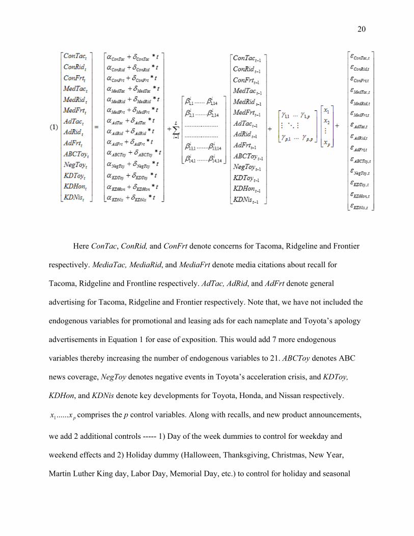
20
Here ConTac, ConRid, and ConFrt denote concerns for Tacoma, Ridgeline and Frontier
respectively. MediaTac, MediaRid, and MediaFrt denote media citations about recall for
Tacoma, Ridgeline and Frontline respectively. AdTac, AdRid, and AdFrt denote general
advertising for Tacoma, Ridgeline and Frontier respectively. Note that, we have not included the
endogenous variables for promotional and leasing ads for each nameplate and Toyota’s apology
advertisements in Equation 1 for ease of exposition. This would add 7 more endogenous
variables thereby increasing the number of endogenous variables to 21. ABCToy denotes ABC
news coverage, NegToy denotes negative events in Toyota’s acceleration crisis, and KDToy,
KDHon, and KDNis denote key developments for Toyota, Honda, and Nissan respectively.
pxx ......1 comprises the p control variables. Along with recalls, and new product announcements,
we add 2 additional controls ----- 1) Day of the week dummies to control for weekday and
weekend effects and 2) Holiday dummy (Halloween, Thanksgiving, Christmas, New Year,
Martin Luther King day, Labor Day, Memorial Day, etc.) to control for holiday and seasonal

21
effects. Consumers may be less receptive to news about recall events during holidays. t is the
deterministic-trend variable, which captures the effect of omitted, gradually changing variables.
γand,β,δ,α are the parameters to be estimated and tε are white noise residuals which are
distributed as N (0, Σ ).
The coefficients 3,12,1 βandβ estimate the effect of perverse halo of online chatter from
Ridgeline and Frontline on Tacoma respectively. The coefficients 3,21,2 βandβ estimate the
effect of perverse effect of online chatter from Tacoma and Frontline on Ridgeline respectively.
The coefficients 2,31,3 βandβ estimate the effect of perverse halo of online chatter from Tacoma
and Ridgeline on Frontline respectively. Based on the ADF, Phillips-Perron, and cointegration
test, we choose the proper appropriate specification for the endogenous variables that enter the
VARX equation.
Results
This section presents the descriptive results, the results of the disaggregate analysis,
which include the tests and estimates of VARX framework, and Estimates of Halo. Note that all
analysis here is at the nameplate level. However, for purposes of summarization and ease of
presentation, we then aggregate these estimates to the brand level. Next, we present the results of
the aggregate analysis, which include the effects on sales and stock market performance.
Descriptive Results
Figure 1 shows the pattern of recalls and concerns during the timeframe of the study for
all nameplates of the Japanese automobile brands. The solid arrows below the horizontal axis
show recalls and other events related to Toyota’s recall (e.g., ABC news investigation report on
Nov 3rd). The arrow sizes suggest the size of the recall in terms of number of units recalled. Not

22
all recalls are shown due to space limits. Concerns seem to correlate with recalls. There are
spikes in Toyota’s concerns for its large recalls. Similarly, there are spikes in Honda’s concerns
for its large recalls. Note the steep rise in the number of concerns for Toyota from Jan 21st 2010.
It takes about two months for the concerns to die down and return to their previous level. There
are minor spikes in the number of concerns for Honda during that week. Other recall events in
the graph increase not only the recalled brand’s concerns, but also a rival’s concerns. For
example, Honda’s recall on March 16th increases concerns for both Honda and Toyota.
Note that there is considerable variation in the timing and size of recalls, which enables a
rich analysis of variance. Due to concomitant other effects (e.g., media citations, advertising), it
is difficult to determine statistical effects or temporal causality merely from these graphical
associations. The VARX framework will enable us to rigorously test if such associations are
causal in the sense of Granger causality. We identify the effects of one nameplate’s recall on
another by 1) exploiting the separation of the recall dates across nameplates, 2) using the
variation in the number of units recalled for each nameplate, 3) including a number of
nameplates from the 4 brands (Toyota, Honda, Nissan, and Chrysler) that have no product recalls
in the sample timeframe. In case of an overlap of recall dates, the variation in recalled units
between the two nameplates enables us to estimate the effects. Online Appendix G contains the
descriptive results (means and standard deviations) of the endogenous variables across the
VARX equations.
Estimates of VARX Framework
The results for test for stationarity, cointegration, and structural break are in the Online
Appendix H. The optimal lag length is 1 for most of the 17 VARX equations except in a few
cases when it is 2 as per the (Schwartz’s) Bayesian Information Criteria. Our results are not
23
affected by the presence of any residual correlation, non-normality of residuals, and
heteroskedasticity. We estimate the VARX models using an Ordinary Least Square (OLS)
regression accounting for Heteroskedasticity and potential serial correlation with the Newey-
West Estimator (Newey & West 1987). The average parameter to observation ratio for each
equation across the 17 VARX models is 1: 16.6. We report the number of parameters and
degrees of freedom in Online Appendix I. Note that because each equation contains exactly the
same set of regressors, the OLS estimates are numerically identical to seemingly unrelated
regression estimates (Zellner 1962). Using these estimates, we then compute the effect of one
variable on another over time, taking current and carryover effects, using the generalized impulse
response function (GIRF), explained in the Online Appendix F. In our robustness tests, in the
interests of parsimony in specification and efficiency in estimation, we drop variables from the
VARX model that don’t significantly affect the dependent variables (across each equation) at
least 25% of the time. The VARX model is then then re-estimated using only the “important”
variables. The results of this procedure are available in Online Appendix J. Our findings remain
the same using this method.
Estimation of Halo
We use the estimates of the GIRF from the VARX equations to calculate the amount of
overlap of perverse halo among the 3 Japanese brands and between Toyota and Chrysler. To
explain the meaning of these estimates, Table 1 provides a simple case of two nameplates (A, B)
and two endogenous variables (concerns and media citations about recall). In this example, the
key off diagonal elements (cross nameplate effects shaded in red) in the first two columns
provide estimates of perverse halo, because they capture the effect of concerns (an independent

24
or causal variable) of one nameplate on concerns (dependent or effect variable) of the other
nameplate8.
Estimates of Halo among Brands by Segments
We first examine perverse halo between nameplates of different brands.
Recall that the generalized impulse response function (GIRF) tracks the impact over-time
of a unit shock (one standard deviation) to one independent variable on a dependent variable.
Because the number of nameplates is large (48 nameplates), a single VARX equation to estimate
all cross nameplate effects would result in 2256 GIRF estimates (nP2 = 48* 47 = 2256). It would
be extremely complex to keep track of and interpret all these cross-nameplate effects. In the
interests of parsimony and ease of presentation, we first estimate GIRF cross nameplate effects
by segments of nameplates. In addition, estimating the GIRF effects by segments allows us to
tease out idiosyncratic segment effects and selection bias due to brand participation.
For the 3 Japanese brands, we use 12 segments based on the definition of nameplate
segmentation of Ward’s Auto (See Table A2 in Online Appendix A). Ward’s Automotive
Yearbook divides cars into different segments based on length of the vehicle and price range.
Prior research has used Ward’s classification scheme by segments (Olivares and Cachon 2009).
Note that we analyze the data separately for the 3 Japanese brands and Toyota-Chrysler
separately because there is a discrepancy in the attributes of online chatter between these two
groups of brands.9 Thus, we estimate 12 VARX equations, one for each segment of nameplates
8 The VARX equation also provides estimate of carryover (past values of a variable on its current value of the same car nameplate), direct effects (past effects of media citations on concerns for the same car nameplate), feedback (past effects of concerns to media citations of the same car nameplate) and reaction (past effects of media citations from one car nameplate to media citations of another car nameplate). In the interest of parsimony, we will not discuss these types of estimates, i.e., our focus is on perverse halo estimated by coefficients when concerns are both the cause and effect variable.
9 We have online chatter about the recall attribute for the 3 Japanese manufacturers and online chatter about the acceleration attribute for Toyota and Chrysler.
25
belonging to the Japanese brands. Similarly, Table A3 in Online Appendix A shows the 5
segments that Ward’s classifies for the Toyota and Chrysler nameplates. Here, we estimate 5
VARX equations, one for each segment of nameplates belonging to the Toyota and Chrysler.
Online Appendix I reports the cumulative GIRF for these 17 VARX equations.
Computation of Halo among Brands by Segments
The computation of halo is based only on the sign and significance of cross nameplate
GIRF estimates, between any two nameplates. Consistent with the VAR literature (Sims & Zha
1999; Pauwels, Hanssens, & Siddarth 2002; Pauwels & Srinivasan 2004; Trusov, Bucklin &
Pauwels 2009), we follow established practice in marketing research and assess the statistical
significance of each impulse response value by applying a one-standard-error band to evaluate
whether each generalized impulse response value is significantly different from zero. We also
use different significance levels10 and our substantial results remain the same. To provide a
measure of perverse halo, we compute the extent of perverse halo between brands within a
segment, as the percentage of times that concerns of any nameplate of one brand has a significant
and positive effect on concerns of any nameplate of another brand. A value of 0% would imply
no perverse halo suggesting that the two brands were completely distinct in consumers’
perceptions. A value of 100% would imply perfect perverse halo suggesting the two brands are
indistinguishable in consumers’ perceptions. Any value between these two would signify the
extent to which negative concerns about one brand perversely affect the other brand. Note that all
this is based on the cross nameplate GIRF estimates within segments.
We define the extent of one-way perverse halo from brand A to brand B, based on the
nameplates of these brands as follows:
10 *p < .10 (one-tailed test); **p < .05 (one-tailed test); ***p < .01 (one-tailed test);

26
(3)
)()1( )1( )(
PxQ
EH Qtoq Ptop BqAp
BA
where )( BqApE takes on the value 1 if the GIRF estimate in the VARX equation running from the
pth model of Brand A to qth model of Brand B is significantly positive and 0 otherwise. The
symmetric 2-way perverse halo between Brand A and Brand B is the simple average of one- way
perverse halos from A to B and B to A.
We define the extent of one-way perverse halo from Brand A to both Brand B and Brand
C, based on the nameplates of these brands as follows:
(4)
)()()1( )1( )()1( )1( )(
PxR
EX
PxQ
EH Rtor Ptop CrApQtoq Ptop BqAp
CBA
The total symmetric 3-way perverse halo between Brand A, Brand B, and Brand C is the simple
average of CBAH , ACBH , and BACH .
Thus, the formula for the total symmetric 2-way perverse halo excluding the total
symmetric 3-way perverse halo (using Toyota as the case) is:
(5) Total symmetric 2-way perverse halo for Toyota = Symmetric 2-way perverse halo
between Toyota and Honda + Symmetric 2-way perverse halo between Toyota and Nissan -
2*Total symmetric 3-way perverse halo
The exclusivity for a brand (using Toyota as the case) is given by the formula:
(6) TOYOTAyExclusivit = 100% - (Total symmetric 3-way perverse halo) – (Total
symmetric 2-way perverse halo for Toyota)
Presentation of Perverse Halo among Brands by Segments
Figure 2a shows the estimated perverse halo among Toyota, Honda, and Nissan based on
the above formulas. We find a considerable total symmetric 3-way perverse halo (26%) among

27
the 3 Japanese car brands. We find the highest symmetric 2-way perverse halo between Toyota
and Honda (50%) and Honda and Nissan (50%) followed by Toyota and Nissan (43%). Most
importantly, we find that for each brand, exclusivity (i.e., isolation from all perverse halo) is
rather low at only 26% for Honda and 33% for both Toyota and Nissan. Thus, perverse halo
seems to be quite extensive among the three Japanese brands. Thus, we find support for
Hypothesis H1 i.e., perverse halo exists in online chatter. Honda appears to be the least exclusive
of the three brands.
There is a 36% symmetric 2-way perverse halo between nameplates of Toyota and
Chrysler. This value is lower than the 2-way overlap between the 3 Japanese brands. The average
symmetric 2-way perverse halo between the Japanese car brands is 48%. This result suggests that
perverse halo could be affected by “country of origin” perceptions of consumers. Thus, we find
moderate support for Hypothesis H2, that perverse halo is stronger for brands from the same
country. In contrast, we find that negative chatter about a nameplate decreases negative chatter
for another nameplate 17% of the time between Toyota and Chrysler. On average, negative
chatter about one nameplate of a Japanese brand decreases negative chatter about a nameplate of
another Japanese brand 12% of the time. This result again supports Hypothesis H2 that perverse
halo could be moderated by country of origin.
Next, we test if perverse halo depends upon a brand’s dominance. Based on the market
shares of the brands, Toyota is the most dominant followed by Honda and Nissan (Ward’s
Yearbook 2010). Prior research shows that dominance and market shares are highly correlated
(Fazio 1987). Figure 2b shows the percentage of one-way downward perverse halo, 3-way
downward perverse halo, and exclusivity among car nameplates of Toyota, Honda, and Nissan.
The downward 3-way perverse halo is the extent of one-way perverse halo from a dominant

28
brand A to two less dominant brands B and C. A downward perverse halo occurs only when
there is perverse halo from Toyota to Honda, Toyota to Nissan, and Honda to Nissan. We find a
considerable 3-way downward perverse halo (35%) between nameplates of the 3 Japanese
brands. We find the highest one-way downward perverse halo between Toyota and Honda
(56%), followed by Toyota and Nissan (52%), and Honda and Nissan (45%).
Figure 2c shows the percentage of one-way upward perverse halo, 3-way upward
perverse halo, and exclusivity between car nameplates of Toyota, Honda, and Nissan. The
upward 3-way perverse halo is the extent of one-way perverse halo from a less dominant brand A
to two dominant brands B and C. Thus, an upward perverse halo occurs only when there is
perverse halo from Honda to Toyota, Nissan to Toyota, and Nissan to Honda. We find a 3-way
upward perverse halo of 26% among nameplates of the 3 Japanese brands. Thus, the 3-way
overlap is higher in downward perverse halo than upward perverse halo. We find the highest
one-way upward perverse halo between Nissan and Honda (55%), followed by Toyota and
Honda (44%), and Toyota and Nissan (35%). The one-way perverse halo effect is stronger from
Toyota to Honda than vice versa (56% vs. 44%), from Toyota to Nissan than vice versa (52% vs.
35%), and from Nissan to Honda than vice versa (55% vs. 45%). Except the last finding of the
effect from Nissan to Honda being stronger than Honda to Nissan, the results support the premise
that perverse halo is stronger from dominant brands to less dominant brands. Thus, we find
considerable support for Hypothesis H3.
We next report the average elasticity of the effects. Table 2 reports the results. We find
that the symmetric 2-way perverse halo between Toyota and Nissan is 7.3, between Honda and
Nissan is 7.0, and between Toyota and Honda is 12.1. This number means 1% increase in
negative chatter about one nameplate increases negative chatter for another nameplate of the
29
same country by around 8.8% (averaging the symmetric 2-way perverse halo). We find that the
symmetric 2-way perverse halo between Toyota and Chrysler is 5.9.
As for the dynamics, we find that perverse halo has a short wear-in of 1 day and most of
the accumulated effect of concerns of one nameplate on concerns of another nameplate reaches
the asymptote within 6 days. As positive chatter can be diagnostic of firm performance too, in
the robustness tests, we control for positive chatter at the brand level and include it as another
endogenous variable in the VARX models. The detailed results are available in Online Appendix
K. The results are similar to the main results.
Estimates of Halo across Nameplates within Brand
We also examine perverse halo among nameplates of the same brand and find substantial
within-brand perverse halo. Toyota (91%) nameplates suffer the highest perverse halo followed
by Honda (75%), Chrysler (73%), and Nissan (56%). We find that the larger the brand, the
greater the overlap in perverse halo among nameplates that belong to that brand. These results
suggest that perverse halo is a result of consumer awareness of the family brand (e.g., Toyota)
associated with the nameplate (e.g. Camry). The details of the results are in Online Appendix L.
Effects of Apology Advertising about Recalls
We find that on average, Toyota’s apology advertisements about product recall
significantly increase concerns for the two other Japanese brands 62% of the time, while these
advertisements significantly increase concerns for Chrysler 40% of the time. These results
suggest that consumers get primed about recalls due to such advertisements. This priming leads
consumers to raise concerns more so for rival brands from the same country than for rival brands
from different countries. We find that Toyota’s apology advertisements about product recall
significantly increase its own concerns 71% of the time. This result suggests that brands with
product recalls should decrease spending on apology advertisements during product recalls.

30
Aggregate Analysis
Next we present the analysis and results of the effect of online chatter on sales and stock
market performance.
Effect on Rival’s Sales
We test if halo effects can affect sales of a rival’s nameplates. Because, it is difficult if
not impossible to obtain sales of nameplates at the daily or the even the weekly level, we
ascertain the relationship between concerns and sales using monthly data. Thus, we aggregate the
concerns and relevant endogenous variables to the monthly level. We obtain the monthly sales of
the nameplates from the Ward’s Automotive Yearbook (Ward’s 2010; 2011).
We have 15 months of complete data for concerns and sales for 48 nameplates. Because
of the very short time series for each nameplate, we cannot estimate a simple Vector
Autoregressive Model as before. Instead, we pool the nameplates and estimate a Panel Vector
Autoregressive (PVAR) Model. Similar to our prior design we estimate one PVAR for the 3
Japanese brands and another PVAR for Toyota and Chrysler brands.
We proceed as follows: For each nameplate of one brand, we find the nearest rival from a
different brand. We consult various automobile sources such as the Ward’s Yearbook,
automobile sites such as Edmunds.com, and online reports to ascertain the pairs. The list of pairs
is in Online Appendix M. We then include the nearest rival nameplate’s concerns as another
endogenous variable in the PVAR to test the association between a rival nameplate’s concerns on
the sales of a focal nameplate.
We now explain the Panel Vector Auto-Regressive model (PVAR), which we use to
estimate the relationship between concerns and sales (Holtz-Eakin 1988). The PVAR technique
combines the traditional VAR approach that treats all the variables in the system as endogenous,

31
with the panel data approach that pools across nameplates but allows for unobserved nameplate-
level heterogeneity. We specify a panel VAR with l lags as:
(7) TtNieyyyy ittilitlititit ,..,1;,.....,3,2,1,..........22110
where ity =(KDFjt, MEDFit, GENADSFit, SALESADSFit, CHATFit, CHATRrt, SALESFit,)
is a 7-variable vector. KDFjt denotes key developments by the brand j that owns focal nameplate
i, MEDFit denotes media citations about recalls or acceleration for the focal nameplate i,
GENADSFit denotes general ads by the focal nameplate i, SALESADSFit denotes sales ads by the
focal nameplate i, CHATFit denotes concerns of the focal nameplate i, CHATRrt denotes
concerns of the nearest rival r of the focal nameplate i, and SALESFit denotes sales of the focal
nameplate i.
l are 7 X 7 coefficient matrices; i denote unobserved nameplate-specific effects; t
denotes time-effects; and ite is a 7 X 1 vector of white-noise residuals. We model the
contemporaneous effects in the variance-covariance matrix of the white-noise residuals (Luo
2009). We can impose a restriction that the underlying structure is the same for each cross-
sectional unit (nameplate), i.e., the coefficients in the matrices l is the same for all the
nameplates in our sample. However, as this assumption is most likely to be violated, we allow
for “individual heterogeneity” in levels of the variables by introducing fixed effects, which is
denoted by i in the model.
Thus, our model (7) is a system of dynamic panel data equations. Prior research has
demonstrated that the fixed effects i are correlated with the regressors because of the lags of
the dependent variables (Arellano and Bond 1991; Arelanno and Bover 1995; Blundell and Bond
1998). The usual “within” transformation to eliminate the fixed effects would create biased

32
coefficients in this dynamic panel setting. Thus, we use the forward orthogonal deviations
suggested by Arellano and Bover 1995 to eliminate the fixed effects. Also known as the Helmert
transformation, this procedure removes only the forward mean, i.e., the mean of all the future
observations for each nameplate-month in our dataset. This data transformation preserves the
orthogonality between the transformed variables and the lagged regressor. Hence, we can use the
lagged regressors as instruments and estimate the coefficients by system Generalized Method of
Moments (Arellano and Bover 1995). Also, the use of forward orthogonal deviations does not
induce autocorrelation in the error terms and frees us from serial correlation (Drakos &
Konstantinou 2014).
In the PVAR for the Japanese brands, we use 39 nameplates because we have no rival
nameplates for 350Z and 370Z of Nissan and because Ward’s does not report sales for Matrix of
Toyota. We use a lag of 3 based on the (Schwartz’s) Bayesian Information Criteria and the
ability of the model to converge. Our results remain the same if we use 1 or 2 lags. The
parameter estimates of the PVAR are in Online Appendix M3.
We find that concerns of the focal nameplate significantly decrease the focal nameplate’s
sales with an elasticity of -4.3 (See Table 3, Panel A). This number means a 1% increase in
concerns of a nameplate decreases its sales by 4.3%. Assuming monthly sales of 7,236 units for a
nameplate (average sales across the 39 nameplates for the 15 months in our timeframe) we find
that a 1% increase in concerns of a nameplate in a month reduces its monthly sales by 311 units.
This translates into a loss of 8.6 million USD11 for a nameplate in 1 month. More importantly,
we find that concerns of the nearest rival significantly decrease the focal nameplate’s sales
consistent with Hypothesis H1. A 1% increase in the concerns of a nameplate’s nearest rival
11 We use an average new car price of 27,500 based on new car prices in 2009 and 2010: http://www.usatoday.com/story/money/cars/2013/09/04/record-price-new-car-august/2761341/
33
decreases the focal nameplate’s sales by 1.9%. Using the same assumptions as above, we find
that a 1% increase in concerns of a rival nameplate in a month decreases the focal nameplate’s
monthly sales by 137 units. This translates into a loss of 3.8 million USD for a nameplate in 1
month. The parameter estimates of the PVAR are in Online Appendix M4.
Next, we report the results of the Forecast Error Variance Decomposition (FEVD). This
analysis determines to what extent the endogenous variables contribute to the deviation in the
focal nameplate’s sales from its baseline expectations. The relative importance of the
endogenous variables in the PVAR is established based on FEVD values at 10 days, which
reduces sensitivity to short-term fluctuations. Concerns of the focal nameplate explain relatively
more of the variance of the focal nameplate’s sales than concerns of the nearest rival (6.6% vs.
2.1%).
In the PVAR for Chrysler and Toyota, we use 5 nameplates out of the 6 for Chrysler
because we could not identify a clear rival for Dodge from Toyota’s list of nameplates. We use a
lag of 3 based on the (Schwartz’s) Bayesian Information Criteria and the ability of the model to
converge. We find that concerns of the focal nameplate significantly decrease the focal
nameplate’s sales (See Table 3, Panel B). A 1% increase in concerns of a nameplate decreases its
sales by 0.11. Assuming monthly sales of 9,659 units for a nameplate (average sales across the
10 nameplates for the 15 months in our timeframe) we find that a 1% increase in concerns of a
nameplate in a month reduces its monthly sales by 1062 units. This translates into a loss of 29
million USD for a nameplate in 1 month due to concerns. Note that we use the negative online
chatter of the acceleration attribute here and because of Toyota’s acceleration issues during the
study timeframe; the effect of concerns is much more potent in affecting sales in this PVAR
model than the prior one. More importantly, we find that concerns of the nearest foreign rival
34
significantly increases the focal nameplate’s sales consistent with Hypothesis H2. A 1% increase
in concerns of a nameplate’s nearest rival from a different country brand increases the focal
nameplate’s sales by 0.022. Using the same assumptions as above, a 1% increase in concerns of
a nameplate’s nearest rival from a different country brand increases the focal nameplate’s
monthly sales by 212 units. This translates into a gain of 5.8 million USD for a focal nameplate
in 1 month due to concerns about a rival’s acceleration. As for the FEVD result, concerns of the
focal nameplate explain much more of the variance of the focal nameplate’s sales than concerns
of the nearest rival brand from a different country (46% vs.6%).
Effect on Rival’s Stock Market Performance
We next test if perverse halo affects a rival brand’s stock market performance. An
analysis at the nameplate level may be too noisy to find a pattern on stock market metrics (e.g., effect
of Honda Ridgeline’s concerns on Honda’s abnormal returns), we aggregate the concerns of the
nameplates to the brand level for analyzing the effect of concerns of the recalled brand on a rival
brand’s abnormal stock returns. We use the VARX model to ascertain the relationship between
concerns and stock returns. Similar to our prior design, we estimate one VARX for the 3 Japanese
brands and another VARX for Toyota and Chrysler. We include the same endogenous and
exogenous variables similar to the VARX models in the disaggregate analysis, but aggregate the
data to the brand level. However, we exclude the ads for sales and leasing for model parsimony.
We include Toyota and Honda’s abnormal returns in the VARX model for the Japanese brands
and only Toyota’s abnormal returns in the VARX model for Toyota and Chrysler, because only
Toyota and Honda are traded in the American Stock Exchanges (NASDAQ, NYSE, and
AMEX). The VARX model includes both own-brand and across-brand effects of concerns on
the abnormal stock returns. Therefore, the VARX model for the 3 Japanese brands includes the
abnormal returns of Toyota and Honda and concerns of Toyota, Honda, and Nissan. While, the
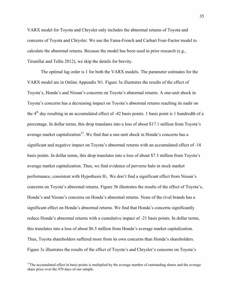
35
VARX model for Toyota and Chrysler only includes the abnormal returns of Toyota and
concerns of Toyota and Chrysler. We use the Fama-French and Carhart Four-Factor model to
calculate the abnormal returns. Because the model has been used in prior research (e.g.,
Tirunillai and Tellis 2012), we skip the details for brevity.
The optimal lag order is 1 for both the VARX models. The parameter estimates for the
VARX model are in Online Appendix N1. Figure 3a illustrates the results of the effect of
Toyota’s, Honda’s and Nissan’s concerns on Toyota’s abnormal returns. A one-unit shock in
Toyota’s concerns has a decreasing impact on Toyota’s abnormal returns reaching its nadir on
the 4th day resulting in an accumulated effect of -42 basis points. 1 basis point is 1 hundredth of a
percentage. In dollar terms, this drop translates into a loss of about $17.1 million from Toyota’s
average market capitalization12. We find that a one-unit shock in Honda’s concerns has a
significant and negative impact on Toyota’s abnormal returns with an accumulated effect of -18
basis points. In dollar terms, this drop translates into a loss of about $7.3 million from Toyota’s
average market capitalization. Thus, we find evidence of perverse halo in stock market
performance, consistent with Hypothesis H1. We don’t find a significant effect from Nissan’s
concerns on Toyota’s abnormal returns. Figure 3b illustrates the results of the effect of Toyota’s,
Honda’s and Nissan’s concerns on Honda’s abnormal returns. None of the rival brands has a
significant effect on Honda’s abnormal returns. We find that Honda’s concerns significantly
reduce Honda’s abnormal returns with a cumulative impact of -21 basis points. In dollar terms,
this translates into a loss of about $6.5 million from Honda’s average market capitalization.
Thus, Toyota shareholders suffered more from its own concerns than Honda’s shareholders.
Figure 3c illustrates the results of the effect of Toyota’s and Chrysler’s concerns on Toyota’s
12The accumulated effect in basis points is multiplied by the average number of outstanding shares and the average share price over the 470 days of our sample.
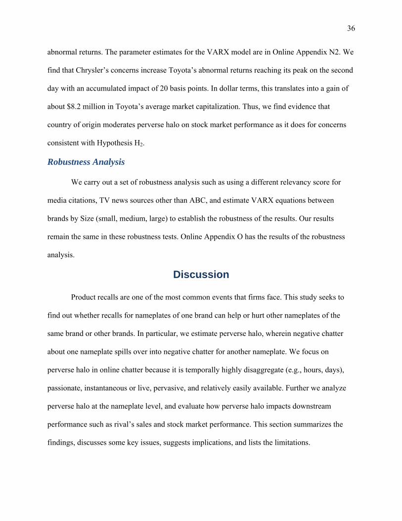
36
abnormal returns. The parameter estimates for the VARX model are in Online Appendix N2. We
find that Chrysler’s concerns increase Toyota’s abnormal returns reaching its peak on the second
day with an accumulated impact of 20 basis points. In dollar terms, this translates into a gain of
about $8.2 million in Toyota’s average market capitalization. Thus, we find evidence that
country of origin moderates perverse halo on stock market performance as it does for concerns
consistent with Hypothesis H2.
Robustness Analysis
We carry out a set of robustness analysis such as using a different relevancy score for
media citations, TV news sources other than ABC, and estimate VARX equations between
brands by Size (small, medium, large) to establish the robustness of the results. Our results
remain the same in these robustness tests. Online Appendix O has the results of the robustness
analysis.
Discussion
Product recalls are one of the most common events that firms face. This study seeks to
find out whether recalls for nameplates of one brand can help or hurt other nameplates of the
same brand or other brands. In particular, we estimate perverse halo, wherein negative chatter
about one nameplate spills over into negative chatter for another nameplate. We focus on
perverse halo in online chatter because it is temporally highly disaggregate (e.g., hours, days),
passionate, instantaneous or live, pervasive, and relatively easily available. Further we analyze
perverse halo at the nameplate level, and evaluate how perverse halo impacts downstream
performance such as rival’s sales and stock market performance. This section summarizes the
findings, discusses some key issues, suggests implications, and lists the limitations.

37
Summary of Findings
The key findings of the study are the following:
Perverse halo is extensive. Between 67% to 74% of the effect of negative chatter is shared
with one or more brands. That is, only 26 to 33% of the effect of negative chatter is truly
brand-specific. And within a brand, between 56% to 91% of the effect of negative chatter is
shared among its nameplates. That is, perverse halo exists for both nameplates within the
same brand and for nameplates across brands.
The direction of perverse halo is asymmetric with perverse halo being stronger from a
dominant brand to a less dominant brand than vice versa.
Perverse halo is strongest between brands that are of the same country.
Perverse halo has a short wear-in of 1 day and a modest wear-out of about 6 days. However,
even though these time lags seem short, concerns arise daily and if unaddressed can lead to
persistent effects.
Perverse halo impacts performance metrics such as sales and stock market performance. A
1% increase in concerns of a rival nameplate leads to a monthly loss in sales revenue of 3.8
million USD (elasticity of -1.9%) for a focal nameplate while a one-unit shock in rival
brand’s concerns erodes about $7.3 million (-18 basis points) from the focal brand’s average
market capitalization over 6 days.
Online chatter amplifies the negative effect of recalls on downstream sales by about 4.5
times.
Apology advertising about recalls increases concerns for both the recalled brand and its
rivals.

38
Implications
This study has the following implications.
First, firms undergoing a crisis need to consider apology ads very carefully. In general,
such ads may backfire because they increase attention to, evoking of, and elaboration about the
crisis (Siomkos & Shrivastava 1993; Heerde, Helsen & Dekimpe 2007). Indeed, we find that such
ads increase concerns not only for the recalled brand but also its rivals.
Second, firms from the same country and same size should keep an eye on rival’s recall
events. We find that negative chatter about one nameplate of one brand spills over into negative
chatter for a nameplate for another brand and this effect gets aggravated for brands from the
same country and size as the recalled brand. So, we speculate that as soon as a rival has a recall,
firms should lie low and avoid comparisons with firms undergoing a recall crisis thereby
minimizing perverse halo or negative spillover (Snyder, Higgins & Stucky 1983). Social
comparison theory suggests that firms can protect their image or status by avoiding comparisons
with less reputable others (Snyder, Lassegard & Ford 1986) or those undergoing a crisis. A
denial strategy of stating how their sourcing, manufacturing, designs, and scientific procedures
have no link with the focal recall could backfire for the rival (Siomkos & Shrivastava 1993).
Third, we speculate that firms from a different country and size to the recalled firms
could emphasize their strengths and uniqueness when the recalled firm is under crisis (Hauser &
Shugan 1983).
Fourth, we speculate that firms need to give more thought to the role of consumer
opinions in determining their rivals. This knowledge of consumer thinking will allow the firms to
strategically deviate from consumer perspectives (Kim & Tsai 2012). If consumers think two
firms are similar and comparable, the innocent rival faces the danger of receiving negative
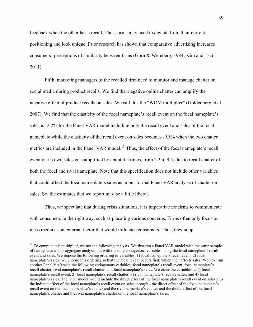
39
feedback when the other has a recall. Thus, firms may need to deviate from their current
positioning and look unique. Prior research has shown that comparative advertising increases
consumers’ perceptions of similarity between firms (Gorn & Weinberg, 1984; Kim and Tsai
2011).
Fifth, marketing managers of the recalled firm need to monitor and manage chatter on
social media during product recalls. We find that negative online chatter can amplify the
negative effect of product recalls on sales. We call this the “WOM multiplier” (Goldenberg et al.
2007). We find that the elasticity of the focal nameplate’s recall event on the focal nameplate’s
sales is -2.2% for the Panel VAR model including only the recall event and sales of the focal
nameplate while the elasticity of the recall event on sales becomes -9.5% when the two chatter
metrics are included in the Panel VAR model.13 Thus, the effect of the focal nameplate’s recall
event on its own sales gets amplified by about 4.5 times, from 2.2 to 9.5, due to recall chatter of
both the focal and rival nameplate. Note that this specification does not include other variables
that could affect the focal nameplate’s sales as in our formal Panel VAR analysis of chatter on
sales. So, the estimates that we report may be a little liberal.
Thus, we speculate that during crisis situations, it is imperative for firms to communicate
with consumers in the right way, such as placating various concerns. Firms often only focus on
mass media as an external factor that would influence consumers. Thus, they adopt
13 To compute this multiplier, we run the following analysis. We first run a Panel VAR model with the same sample of nameplates as our aggregate analysis but with the only endogenous variables being the focal nameplate’s recall event and sales. We impose the following ordering of variables: 1) focal nameplate’s recall event, 2) focal nameplate’s sales. We choose this ordering so that the recall event occurs first, which then affects sales. We next run another Panel VAR with the following endogenous variables: focal nameplate’s recall event, focal nameplate’s recall chatter, rival nameplate’s recall chatter, and focal nameplate’s sales. We order the variables as 1) focal nameplate’s recall event, 2) focal nameplate’s recall chatter, 3) rival nameplate’s recall chatter, and 4) focal nameplate’s sales. The latter model would include the direct effect of the focal nameplate’s recall event on sales plus the indirect effect of the focal nameplate’s recall event on sales through - the direct effect of the focal nameplate’s recall event on the focal nameplate’s chatter and the rival nameplate’s chatter and the direct effect of the focal nameplate’s chatter and the rival nameplate’s chatter on the focal nameplate’s sales.
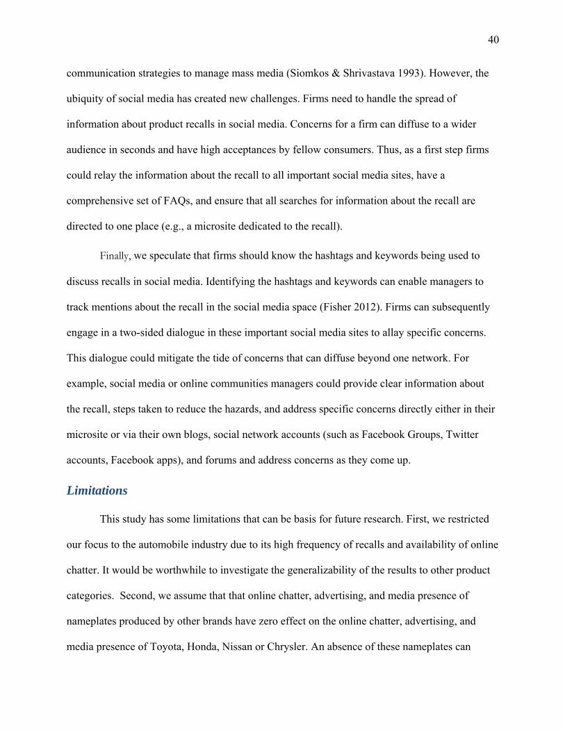
40
communication strategies to manage mass media (Siomkos & Shrivastava 1993). However, the
ubiquity of social media has created new challenges. Firms need to handle the spread of
information about product recalls in social media. Concerns for a firm can diffuse to a wider
audience in seconds and have high acceptances by fellow consumers. Thus, as a first step firms
could relay the information about the recall to all important social media sites, have a
comprehensive set of FAQs, and ensure that all searches for information about the recall are
directed to one place (e.g., a microsite dedicated to the recall).
Finally, we speculate that firms should know the hashtags and keywords being used to
discuss recalls in social media. Identifying the hashtags and keywords can enable managers to
track mentions about the recall in the social media space (Fisher 2012). Firms can subsequently
engage in a two-sided dialogue in these important social media sites to allay specific concerns.
This dialogue could mitigate the tide of concerns that can diffuse beyond one network. For
example, social media or online communities managers could provide clear information about
the recall, steps taken to reduce the hazards, and address specific concerns directly either in their
microsite or via their own blogs, social network accounts (such as Facebook Groups, Twitter
accounts, Facebook apps), and forums and address concerns as they come up.
Limitations
This study has some limitations that can be basis for future research. First, we restricted
our focus to the automobile industry due to its high frequency of recalls and availability of online
chatter. It would be worthwhile to investigate the generalizability of the results to other product
categories. Second, we assume that that online chatter, advertising, and media presence of
nameplates produced by other brands have zero effect on the online chatter, advertising, and
media presence of Toyota, Honda, Nissan or Chrysler. An absence of these nameplates can

41
produce omitted variable bias in the estimates. Nevertheless, what we have are still important
and well-known brands and provide many insights. Likewise, a number of papers in marketing
use only one/two firm’s rivals rather than include every possible rival (e.g., Tirunillai and Tellis
2012; Joshi and Hanssens 2009).
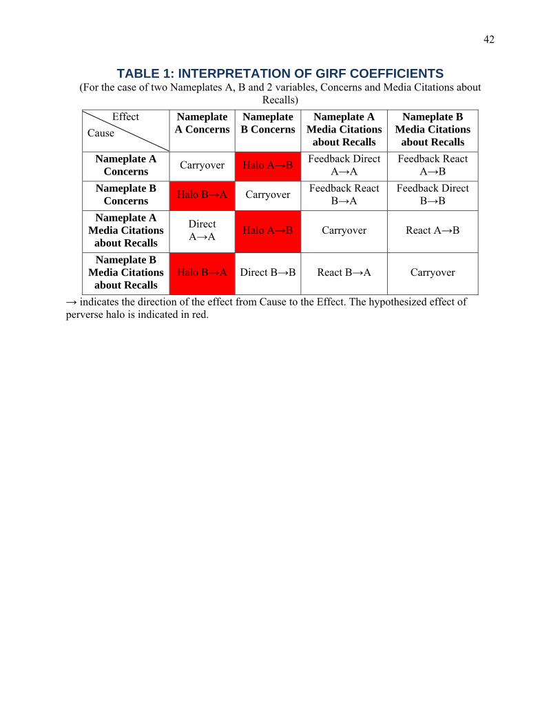
42
TABLE 1: INTERPRETATION OF GIRF COEFFICIENTS (For the case of two Nameplates A, B and 2 variables, Concerns and Media Citations about
Recalls)
Effect
Cause
Nameplate A Concerns
Nameplate B Concerns
Nameplate A Media Citations
about Recalls
Nameplate B Media Citations
about Recalls
Nameplate A Concerns
Carryover Halo A→B Feedback Direct
A→A Feedback React
A→B
Nameplate B Concerns
Halo B→A Carryover Feedback React
B→A Feedback Direct
B→B
Nameplate A Media Citations
about Recalls
Direct A→A
Halo A→B Carryover React A→B
Nameplate B Media Citations
about Recalls Halo B→A Direct B→B React B→A Carryover
→ indicates the direction of the effect from Cause to the Effect. The hypothesized effect of perverse halo is indicated in red.

43
TABLE 2: ELASTICITIES OF ONLINE CHATTER Perverse Halo Mean Elasticities of Chatter
One‐way Perverse Halo from Toyota to Nissan 13.7 %**
One‐way Perverse Halo from Nissan to Toyota .5 %
Symmetric 2‐way Perverse Halo between Toyota and Nissan 7.1 %*
One‐way Perverse Halo from Honda to Nissan 6.5 %
One‐way Perverse Halo from Nissan to Honda 7.4 %*
Symmetric 2‐way Perverse Halo between Honda and Nissan 7.0 %*
One‐way Perverse Halo from Toyota to Honda 17.0 %*
One‐way Perverse Halo from Honda to Toyota 7.1 %
Symmetric 2‐way Perverse Halo between Toyota and Honda 12.1 %*
One‐way Perverse Halo from Toyota to Chrysler 6.4%
One‐way Perverse Halo from Chrysler to Toyota 5.5%
Symmetric 2‐way Perverse Halo between Toyota and Chrysler 5.9%
*p < 0.05 (two-tailed test); **p < 0.01 (two-tailed test); ***p < 0.001 (two-tailed test);
TABLE 3: AGGREGATE ANALYSIS OF SALES Panel A
Japanese Brands
Panel B
Toyota and Chrysler Elasticity+
Relative Importance++
Elasticity+
Relative Importance++
Focal Nameplate Chatter
-4.3% *** 6.6%*** -11.37%*** 45.9%***
Nearest Nameplate Chatter
-1.9% *** 2.1%*** 2.16%* 6.4%*
*p < 0.05 (two-tailed test); **p < 0.01 (two-tailed test); ***p < 0.001 (two-tailed test); +Arc elasticity formula used to calculate elasticity (e.g., Trusov, Bucklin & Pauwels. 2009); ++ We measure the Relative Importance using the Forecast Error Variance Decomposition technique (see Hanssens 1998 for a Marketing application). The Forecast Error Variance Decomposition is like a partial R2 (Stock and Watson 2001). Thus, Relative importance is the improvement in R-square in a PVAR model with vs. without the focal independent variable. The table above denotes the marginal contribution of variables in the row in explaining the variance of sales of the focal nameplate when the other endogenous variables are included in the model. That is, how much of the lift or decrease in sales of the focal nameplate is due to the row variables.
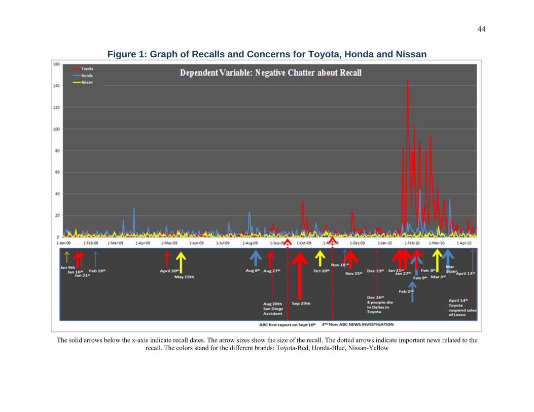
44
Figure 1: Graph of Recalls and Concerns for Toyota, Honda and Nissan
The solid arrows below the x-axis indicate recall dates. The arrow sizes show the size of the recall. The dotted arrows indicate important news related to the
recall. The colors stand for the different brands: Toyota-Red, Honda-Blue, Nissan-Yellow
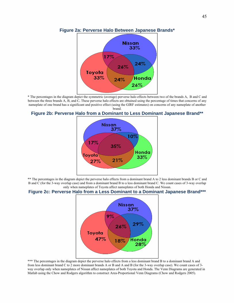
45
Figure 2a: Perverse Halo Between Japanese Brands*
* The percentages in the diagram depict the symmetric (average) perverse halo effects between two of the brands A, B and C and between the three brands A, B, and C. These perverse halo effects are obtained using the percentage of times that concerns of any nameplate of one brand has a significant and positive effect (using the GIRF estimates) on concerns of any nameplate of another
brand. Figure 2b: Perverse Halo from a Dominant to Less Dominant Japanese Brand**
** The percentages in the diagram depict the perverse halo effects from a dominant brand A to 2 less dominant brands B or C and B and C (for the 3-way overlap case) and from a dominant brand B to a less dominant brand C. We count cases of 3-way overlap
only when nameplates of Toyota affect nameplates of both Honda and Nissan.
Figure 2c: Perverse Halo from a Less Dominant to a Dominant Japanese Brand***
*** The percentages in the diagram depict the perverse halo effects from a less dominant brand B to a dominant brand A and from less dominant brand C to 2 more dominant brands A or B and A and B (for the 3-way overlap case). We count cases of 3-way overlap only when nameplates of Nissan affect nameplates of both Toyota and Honda. The Venn Diagrams are generated in Matlab using the Chow and Rodgers algorithm to construct Area-Proportional Venn Diagrams (Chow and Rodgers 2005).
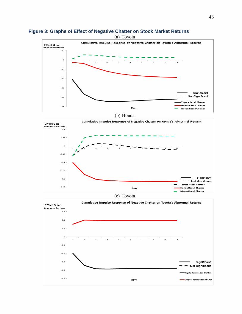
46
Figure 3: Graphs of Effect of Negative Chatter on Stock Market Returns (a) Toyota
(b) Honda
(c) Toyota

47
References
Ahluwalia, Rohini (2002). How Prevalent Is the Negativity Effect in Consumer Environments? Journal of Consumer Research, 292, 270-279
Allsop, Dee T., Bryce R. Bassett, and James A. Hoskins (2007). Word-of-Mouth Research: Principles and Applications. Journal of Advertising Research, 474, 398-411
Arellano, Manuel, and Stephen Bond (1991). Some tests of specification for panel data: Monte Carlo evidence and an application to employment equations. Review of Economic Studies, 58(2), p277
---- & Olympia Bover (1995). Another look at the instrumental variable estimation of error-components models. Journal of Econometrics, 68(1), 29-51.
Arndt, Johan (1967). Role of Product-Related Conversations in the Diffusion of a New Product. Journal of Marketing Research, 43, 291-295
Asur, Sitaram, and Bernardo Huberman (2010). Predicting the future with social media. HP Labs. Bae, Y-K, Benítez-Silva, H. 2013. The Effects of Automobile Recalls on the Severity of Accidents.
Economic Inquiry, 51(2), 1232-1250. Babic Ana., Sotgiu, Francesca., Valck Kristine de, Bijmolt T.H.A. (2014). Factors Influencing the
Effect of Electronic Word of Mouth on Sales: A Meta-Analytic Review. Working Paper. Barsalou, Lawrence W (1992). Cognitive Psychology: An Overview for Cognitive Psychologists.
Hillsdale, NJ: Erlbaum and Associates. --- and Daniel Sewell (1985). Contrasting the Representation of Scripts and Categories, Journal of
Memory and Language, 24, 646-665. Birnbaum, Michael (1972). Morality judgments: Tests of an averaging model. Jrnl of Exp. Psy., 93,
35 Blackshaw, Pete, and Mike Nazzaro (2006). Consumer-Generated Media (CGM) 101. Word-of-
Mouth in the Age of the Web-Fortified Consumer. (2nd ed.) New York: BuzzMetrics Blundell, Richard, and Stephen Bond (1998). Initial conditions and moment restrictions in dynamic
panel data models. Journal of Econometrics, 87(1), 115-143. Businessweek (2005). Inside "Dell Hell", Accessed Nov 25 2014,
http://www.businessweek.com/the_thread/techbeat/archives/2005/09/inside_dell_hel.html. Olivares, Marcelo, and Gérard P. Cachon (2009). Competing retailers and inventory: An empirical
investigation of General Motors' dealerships in isolated US markets. Mgmt. Science, 55(9),1586 Chen, Yubo, Shankar Ganesan, and Yong Liu (2009). Does a Firm's Product Recall Strategy Affect
its Financial Value? An Examination of Strategic Alternatives during Product-harm Crises. Journal of Marketing, 73 (6), 214-226.
Chevalier, Judith A., and Dina Mayzlin (2006). The Effect of Word of Mouth on Sales: Online Book Reviews. Journal of Marketing Research, 43(3), 345-354
Choi, Yoonhyeung, and Ying-Hsuan Lin (2009). Consumer responses to Mattel product recalls posted on online bulletin boards: Exploring two types of emotion. Journal of Public Relations Research, 21(2), 198-207.
Chow, Stirling, and Peter Rodgers (2005). Constructing area-proportional Venn and Euler diagrams with three circles. Euler Diagrams Workshop, Paris.

48
Chu, Ting-Heng, Che-Chun Lin, and Larry J. Prather (2005). An Extension of Security Price Reactions Around Product Recall Announcements. Quarterly Journal of Business & Economics, 44 , 33-47
Cleeren, Kathleen, Marnik G. Dekimpe, and Kristiaan Helsen (2008). Weathering product-harm crises. Journal of the Academy of Marketing Science, 362, 262-270
---- , Harald J. Van Heerde, and Marnik G. Dekimpe. 2013. Rising from the Ashes: How Brands and Categories Can Overcome Product-Harm Crises. Journal of Marketing, 77(2), 58-77.
Collins, Allan M., and Elizabeth F. Loftus (1975). A spreading-activation theory of semantic processing. Psychological review, 82(6), 407.
Dawar, Niraj (1998). Product-Harm Crises and the Signaling Ability of Brands. International Studies of Management & Organization, 283, 109
---- and Madan M. Pillutla (2000). Impact of Product-Harm Crises on Brand Equity: The Moderating Role of Consumer Expectations. Journal of Marketing Research, 37(2), 215-226
Deighton, John A., and Leora Kornfeld (2008). Obama versus Clinton: the YouTube primary. HBS Dekimpe, Marnik G., and Dominique M. Hanssens (1995). The Persistence of Marketing Effects on
Sales. Marketing Science 14(1), 1-21. Dellarocas, Chrysanthos, Xiaoquan Michael Zhang, and Neveen F. Awad (2007). Exploring the
Value of Online Product Reviews in Forecasting Sales: The Case of Motion Pictures. Journal of Interactive Marketing 21 (4), 23
Detroit News (2015). Recall woes follow GM into new year. http://www.detroitnews.com/story/business/autos/general-motors/2015/01/01/gm-recalls-suvs-trucks-ignition-issue/21149405/. Accessed Jan 7th 2015.
Drakos, Konstantinos, and Panagiotis Th Konstantinou (2014). Terrorism, crime and public spending: Panel VAR evidence from Europe. Defence and Peace Economics, 25(4), 349-361.
Enders, Walter (2014). Applied econometric time series. Wiley, New York. 4th edition Farquhar, Peter H., Paul M. Herr, and Russell H. Fazio (1990). A Relational Model for Category
Extensions of Brands. Advances in consumer research, 17(1), Pages 856-860 Fazio, Russell H. 1987 Category-Brand Associations and their Activation from Memory, Ogilvy
Center for Research and Development. Feldman, Jack M., and John G. Lynch (1988). Self-generated validity and other effects of
measurement on belief, attitude, intention, and behavior. Journal of Applied Psychology, 73, 421. Fisher, T (2012). Tips for Using Social Media in Product Recall. Accessed June 24th 2012.
http://socialmediatoday.com/emoderation/492735/tips-using-social-media-product-recall Giles, David (2011). http://davegiles.blogspot.com/2011/04/testing-for-granger-causality.html Godes, David, and Dina Mayzlin (2004). Using online conversations to study word-of-mouth
communication. Marketing Science, 23(4), 545-560. Goldenberg, Jacob., Libai, Barak, Moldovan, Sarit, and Muller, Eitan (2007). The NPV of bad
news. International Journal of Research in Marketing, 24(3), 186-200. Gorn, Gerald J., and Charles B. Weinberg (1984). The impact of comparative advertising on
perception and attitude: some positive findings. Journal of Consumer Research 11: 719–727 Greto, Michael, Andreas Schotter, and Mary B. Teagarden (2010). Toyota: The Accelerator Crisis.
Source: Thunderbird School of Global Management 24 pages. Publication date: Dec 15, 2010. Granger, Clive WJ (1969). Investigating causal relations by econometric models and cross-spectral
methods. Econometrica, 37 (3), 424-438. Granger, Clive WJ, and Paul Newbold (1974). Spurious regressions in econometrics. Journal of
Econometrics 2 (2): 111–120

49
Hanssens, Dominique M (1998). Order forecasts, retail sales, and the marketing mix for consumer durables. Journal of Forecasting, 17(34), 327-346.
Hauser, John R., and Steven M. Shugan (1983). Defensive Marketing Strategy. Mktg. Sci., 2, 4, 319. Herr, Paul M., Frank R. Kardes, and John Kim (1991). Effects of Word-of-Mouth and Product-
Attribute Information of Persuasion: An Accessibility-Diagnosticity Perspective. Journal of Consumer Research, 174, 454-462
Holtz-Eakin, Douglas, Whitney Newey, and Harvey S. Rosen (1988). Estimating vector autoregressions with panel data. Econometrica, 1371-1395.
Hong, Sung-Tai, and Robert S. Wyer Jr (1989). Effects of country-of-origin and product-attribute information on product evaluation: An information processing perspective. Jrnl. of Consumer Research, 175.
…. 1990. Determinants of product evaluation: Effects of the time interval between knowledge of a product's country of origin and information about its specific attributes. Journal of Consumer Research, 277-288.
Hora, Manpreet, Hari Bapuji, and Aleda V. Roth (2011). Safety hazard and time to recall: The role of recall strategy, product defect type, and supply chain player in the US toy industry. Journal of Operations Management, 29(7), 766-777.
Hu, Minqing, and Bing Liu (2004). Mining and summarizing customer reviews. Proceedings of the ACM SIGKDD International Conference on Knowledge Discovery & Data Mining (KDD-2004, full paper), Seattle, Washington, USA, Aug 22-25, 2004.
Janakiraman, Ramkumar, Catarina Sismeiro, and Shantanu Dutta (2009). Perception spillovers across competing brands: a disaggregate model of how and when. Journal of Marketing Research, 46(4), 467-481.
Jensen, C. 2011. 2010 a Record Year for ‘Voluntary’ Recalls. Accessed March 2nd 2012. http://wheels.blogs.nytimes.com/2011/01/20/2010-a-record-year-for-voluntary-recalls/
Joshi, Amit, and Dominique M. Hanssens (2010). The direct and indirect effects of advertising spending on firm value. Journal of Marketing, 74(1), 20-33.
Kalaignanam, Kartik, Tarun Kushwaha, and Meike Eilert (2013). The Impact of Product Recalls on Future Product Reliability and Future Accidents: Evidence from Automobile Industry. Journal
of Marketing, 77(2), 41-57. Kim, Kwang Ho, and Wenpin Tsai (2012). Social comparison among competing firms. Strategic
Management Journal, 33, 2, 115–136 Kraljic, Peter (1983). Purchasing must become supply management, HBR, Vol 61, pp. 109-117 Kwak, Haewoon, Lee, Changhyun, Park, Hosung, Moon, Sue (2010). What is Twitter, a social
network or a news media? Proceedings of the 19th international conference on World wide web, April 26-30, 2010, Raleigh, North Carolina, USA
Lei, Jing, Niraj Dawar, and Jos Lemmink (2008). Negative spillover in brand portfolios: exploring the antecedents of asymmetric effects. Journal of Marketing, 72(3), 111-123.
Lithium 2014. 9 Big Reasons for Serious WOMM. http://aci.info/wp-content/uploads/2014/02/lithium-wom-marketing-infographic.png. Accessed Dec 10th, 2014
Liu, Yong 2006. Word-of-Mouth for Movies: Its Dynamics and Impact on Box Office Revenue. Journal of Marketing, 70 (3): 74-89.
Loken, Barbara, and James Ward (1990). Alternative approaches to understanding the determinants of typicality. Journal of Consumer Research, 111-126.
Luo, Xueming 2009. Quantifying the Long-Term Impact of Negative Word of Mouth on Cash Flow and Stock Price Volatility. Marketing Science, 28(1), 148-65
50
Maheswaran, Durairaj (1994). Country of Origin as Stereotypes: The Effects of Consumer Expertise and Attribute Information on Product Evaluations. Journal of Consumer Research, 21, 354-365
-- and Cathy Yi Chen (2006). Nation Equity: Incidental Emotions in Country-of-Origin Effects. Journal of Consumer Research, 33(December), 370-376
McCombs, Maxwell E., and Donald L. Shaw (1972). The Agenda-Setting Function of Mass Media. Public Opinion Quarterly 36 (2): 176
Mizerski, Richard W (1982). An Attribution Explanation of the Disproportionate Influence of Unfavorable Information, Journal of Consumer Research Vol. 9, pp. 301-310
Newey, Whitney K., and Kenneth D. West (1987). A simple, positive semi-definite, heteroskedasticity and autocorrelation consistent covariance matrix. Econometrica, 703
Nielsen 2011. State of the Media: The Social Media Report – Q3 2011 Nijs, Vincent R., Shuba Srinivasan, and Koen Pauwels (2007). Retail-Price Drivers and Retailer
Profits. Marketing Science, 26 (4), 473-487 Olson, James M., and Mark P. Zanna (1993). Attitudes and attitude change. Annual Review of
Psychology, 44(1), 117-154. Pauwels, Koen, and Shuba Srinivasan (2004). Who Benefits from Store Brand Entry? Marketing
Science, 23, 3 364-390 Peters, J. 2005. More complex cars and stricter rules lead to more recalls. Accessed May 30, ‘12
http://www.nytimes.com/2005/10/26/automobiles/autospecial/26peters.html?pagewanted=all. Rhee, Mooweon, and Pamela R. Haunschild (2006). The Liability of Good Reputation: A Study of
Product Recalls in the U.S. Automobile Industry. Organization Science, 17(1), 101-117 Quelch, J., C. I. Knoop, and R. Johnson (2011). Toyota Recalls (A): Hitting the Skids. HBS Case 9-
511-016. Boston: Harvard Business School Publishing. Roehm, Michelle L., and Alice M. Tybout (2006). When Will a Brand Scandal Spill Over, and How
Should Competitors Respond? Journal of Marketing Research, 43 (August), 366–73. Rubel, Olivier, Prasad A. Naik, and Shuba Srinivasan (2011). Optimal Advertising When
Envisioning a Product-Harm Crisis. Marketing Science November/December 2011 vol. 30 no. 6 1048-1065
Shazam 2013. http://shazam.econ.ubc.ca/intro/dummy.htm Sims, Christopher A., and Tao Zha (2003). Error Bands for Impulse Responses. Econometrica. 67,
5, p1113 MLA Siomkos, George, and Paul Shrivastava (1993). Responding to Product Liability Crises. Long
Range Planning, 265, 72-79 Smith, Edward E., and Douglas L. Medin (1981). Categories and concepts. Cambridge: Harvard
University Press. Snyder, Charles Richard, Raymond L. Higgins, and Rita J. Stucky (1983). Excuses: Masquerades in
Search of Grace. Wiley --- MaryAnne Lassegard, and Carol E. Ford (1986). Distancing after group success and failure:
basking in reflected glory and cutting off reflected failure. JPSS, 51(2): 382–388 Stephen, Andrew T., and Jeff Galak (2012). The Effects of Traditional and Social Earned Media on
Sales: A Study of a Microlending Marketplace. Journal of Marketing Research, 49 (5), 624-639. Stock, James H., and Mark W. Watson (2001). Vector autoregressions. Journal of Economic
perspectives, 101-115.

51
Strapparava, Carlo, and Alessandro Valitutti (2004). Wordnet-affect: an affective extension of wordnet. Proceedings of the 4th International Conference on Language Resources and Evaluation, Lisbon.
--- and Rada Mihalcea (2007). Task 14: Affective Text. SemEval 2007: Proceedings of the 4th International Workshop on Semantic Evaluations, Prague, Czech Rep.
Tellis, Gerard J., and Philip Hans Franses (2006). Optimal data interval for estimating advertising response. Marketing Science, 25(3), 217
The New York Times 2014. http://www.nytimes.com/interactive/2014/12/30/business/a-record-year-for-auto-recalls.html?_r=0 Accessed Dec 16th, 2014
Tirunillai, Seshadri, and Gerard J. Tellis (2012). Does Chatter Really Matter? Impact of User Generated Content on Stock Market Performance. Marketing Science,31(2), 198-215
---- (2014) Mining Marketing Meaning from Online Chatter: Strategic Brand Analysis of Big Data Using Latent Dirichlet Allocation. Journal of Marketing Research, 51(4), 463-479.
Trusov, Michael, Randolph E. Bucklin, and Koen Pauwels (2009). Effects of Word-of-Mouth Versus Traditional Marketing: Findings from an Internet Social Networking Site. Jrnl of Mktg, 73, p90
Van Heerde, Harald, Kristiaan Helsen, and Marnik G. Dekimpe (2007). The Impact of a Product-Harm Crisis on Marketing Effectiveness. Marketing Science, 262, 230-245
Ward’s 2010. Ward’s Automotive Yearbook. Wards Communications. Wyer, Robert S (1973). Category ratings as "subjective expected values": Implications for attitude
formation and change. Psychological Review, Volume: 80, Issue: 6, Pages: 446-467 Yang, Yufeng, and Weiping Yu (2014), January. Brand Scandals Spillover Model Based on the
GMDH. In Proceedings of the 7th International Conference on Management Science and Engineering Management (pp. 591-601). Springer Berlin Heidelberg.
Zellner, Arnold (1962). An efficient method of estimating seemingly unrelated regressions and tests for aggregation bias. Journal of the American Statistical Association, 57(298), 348-368.

52
WEB APPENDIX
Halo (Spillover) Effects in Social Media: Do Product Recalls of One Brand Hurt or Help Rival Brands?
Abhishek Borah and Gerard J. Tellis

53
Web Appendix A
Table A1: Prior Literature on Product Recalls Papers Focus
on Rivals
Consumer Sentiment Metric: Online Chatter
Firm Performance Metric
Dynamics Highly Disaggregate Data
Nameplate Level Analysis
Industry
Dawar & Pillutla 2000
X X Likelihood of Purchase
X X X Instant Coffee, Soft Drink
Chu et al. 2005
X X Yes, Stock Market Returns
X X X Non‐Automotive (Drugs, Cosmetic, etc.)
Rhee & Haunschild 2006
X X Yes, Market Share
X X X Automotive
Van Heerde et al. 2007
Yes, only 1 rival
X Yes, Sales Yes X, Only Weekly
X Peanut Butter
Cleeren et al. 2008
X X Yes, Sales X X X Peanut Butter
Chen et al. 2009
X X Yes, Stock Market Returns
X X X Non‐Automotive (Drugs, toys, etc.)
Rubel et al. 2011
X X Yes, Sales Yes X, Only Weekly
Yes, only 3 nameplates
Automotive
Cleeren et al. 2013
X, on category & not on specific non‐affected rivals
X Yes, Brand Share; Category Sales
X X X FMCGs
Kalaignanam et al. 2013
X X X X X X Automotive
This Paper Yes Yes Yes, Sales & Stock Market Returns
Yes Yes, Daily Yes, 48 nameplates
Automotive

54
Web Appendix B Table B1: List of Nameplates
Serial No. Brand Nameplate 1 Toyota 4Runner 2 Toyota Avalon 3 Toyota Camry 4 Toyota Corolla 5 Toyota FJ Cruiser 6 Toyota Highlander 7 Toyota Land Cruiser 8 Toyota Lexus 9 Toyota Matrix 10 Toyota Prius 11 Toyota RAV4 12 Toyota Sequoia 13 Toyota Sienna 14 Toyota Tacoma 15 Toyota Tundra 16 Toyota Venza 17 Toyota Yaris 18 Honda Accord 19 Honda Acura 20 Honda Civic 21 Honda CRV 22 Honda Fit 23 Honda Insight 24 Honda Odyssey 25 Honda Pilot 26 Honda Ridgeline 27 Nissan 350Z 28 Nissan 370Z 29 Nissan Altima 30 Nissan Armada 31 Nissan Cube 32 Nissan Frontier 33 Nissan GT-R 34 Nissan Infiniti 35 Nissan Maxima 36 Nissan Murano 37 Nissan Pathfinder 38 Nissan Quest 39 Nissan Rouge 40 Nissan Sentra 41 Nissan Titan 42 Nissan Xterra 43 Chrysler 300 44 Chrysler Dodge 45 Chrysler Jeep 46 Chrysler Ram 47 Chrysler Sebring 48 Chrysler Town & Country

55
Table B2: Car Segments with Nameplates for Japanese Brands
* Combine luxury large sport/utility & luxury specialty; ** Author defined segment.
No nameplates from Toyota and Honda for the Middle Specialty segment. Nissan has 350Z, 370Z in this segment.
No nameplates from Toyota and Nissan for the Small Cross/Utility segment. Honda has Element in this segment.
Table B3: Car Segments with Nameplates for Toyota and Chrysler
*Author defined segments for Chrysler nameplates
Serial No. Segment Toyota Nameplates
Honda Nameplates
Nissan Nameplates
1 Large Car Avalon Maxima
2 Large Pickup Tundra Titan
3 Large Sport/Utility Sequoia Armada
4 Lower Small Yaris Fit
5 Small Pickup Tacoma Ridgeline Frontier
6 Luxury Specialty/Large sport/utility*
Land Cruiser GTR
7 Small Van Sienna Odyssey Quest
8 Middle Sport/Utility 4Runner, FJ Cruiser Pathfinder, Xterra
9 Middle Cross/Utility Highlander, RAV4, Venza
Pilot, CR‐V Murano, Rogue
10 Upper Middle Camry, Prius Accord, Insight Altima
11 Upper Small Corolla, Matrix Civic Sentra, Cube
12 Luxury** Lexus Acura Infiniti
Serial No. Segment ToyotaNameplates
Chrysler Nameplates
1 Large Car Avalon 300
2 Upper Middle Camry, Prius Sebring
3 Small Van Sienna Town & Country
4 Pickups* Tundra, Tacoma Ram
5 Middle Cross/Sport Utility*
Highlander, RAV4, Venza,
4Runner, FJ Cruiser
Jeep

56
Web Appendix C ‐ Details of Classification Algorithm
The third party’s classification algorithm determines the valence of an online
conversation by focusing on the situation where an attribute is used. For example, the word
“long” can indicate positive or negative valence on a product attribute depending on the attribute.
An online conversation (e.g., review, blog post, etc.) sentence may contain many product
attributes ( )m1 a,....a and many valence words nww ,.....1 . An example of an attribute is “safety”
and examples of valence words are “good”, “bad”, etc.
The objective is to determine the overall valence expressed on each attribute ia in an
online conversation. Below are the steps involved in the algorithm:
1. Use a list of around 7000 positive, negative, and situation dependent valence words,
including phrases and idioms.
2. Partition each online conversation (e.g., review) into sentences (e.g., sentence s ) that
form the online conversation.
3. Partition each sentence susing words such as “but” and phrases such as “except that”.
If attribute ia is in sentence part ks , the valence score of ia in sentence part ks is
determined by the valence value of the word jw divided by the distance between the
word jw and the attribute ia . Thus, words far away from the attribute are given low
weights while words close to the attribute are given high weights. The valence value
of a word is +1 for positive word and -1 for negative word.
4. All valence scores for each sentence segment ks that contain the attribute are summed
to arrive at an overall valence score for sentence s . All valence scores for each
sentence s in a review or blog or forum post are summed to arrive at an overall
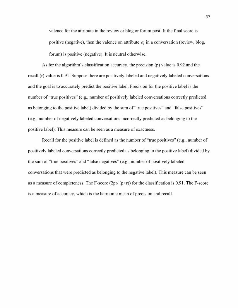
57
valence for the attribute in the review or blog or forum post. If the final score is
positive (negative), then the valence on attribute ia in a conversation (review, blog,
forum) is positive (negative). It is neutral otherwise.
As for the algorithm’s classification accuracy, the precision (p) value is 0.92 and the
recall (r) value is 0.91. Suppose there are positively labeled and negatively labeled conversations
and the goal is to accurately predict the positive label. Precision for the positive label is the
number of “true positives” (e.g., number of positively labeled conversations correctly predicted
as belonging to the positive label) divided by the sum of “true positives” and “false positives”
(e.g., number of negatively labeled conversations incorrectly predicted as belonging to the
positive label). This measure can be seen as a measure of exactness.
Recall for the positive label is defined as the number of “true positives” (e.g., number of
positively labeled conversations correctly predicted as belonging to the positive label) divided by
the sum of “true positives” and “false negatives” (e.g., number of positively labeled
conversations that were predicted as belonging to the negative label). This measure can be seen
as a measure of completeness. The F-score (2pr/ (p+r)) for the classification is 0.91. The F-score
is a measure of accuracy, which is the harmonic mean of precision and recall.

58
Web Appendix D – List of Toyota’s Negative Events
Serial No. Date Negative Event
1 28‐Aug‐09 A family of four driving a Lexus ES 350 is killed. Moments before the crash, the driver calls 911 to report that his accelerator was stuck
2 29‐Sep‐09
Toyota issues a safety notice for 3.8 million vehicles due to the crash risk posed by the gas pedal becoming caught under the floor mat. NHTSA calls for the recall of the 3.8 million vehicles
3 4‐Nov‐09 NHTSA accuses Toyota of providing owners with “inaccurate and misleading information” about its floor mat recall
4 26‐Dec‐09 Four people die near Dallas when their Toyota Avalon accelerates off of the road
5 26‐Jan‐10 Toyota suspends sales and halts production of 8 nameplates due to accelerator pedal problems
6 29‐Jan‐10 Toyota expands its recall to models sold in Europe.
7 2‐Feb‐10 U.S. Transportation Secretary LaHood criticizes Toyota's response to the problems with the gas pedals.
8 3‐Feb‐10
Transportation Secretary LaHood warns consumers not to drive recalled cars, then claims this was a misstatement and consumers should contact their dealers. NHTSA claims to have received more than 100 complaints about braking system problems in the Prius.
9 4‐Feb‐10
Toyota says the recalls for gas pedal-related issues could end up costing the company US$2 billion. Toyota also confirms on this date that the recalls total 8.1 million vehicles. The automaker blames a software glitch for braking problems in its 2010 Prius. The NHTSA opens a formal investigation into the braking system of the Prius hybrid model.
10 13‐Feb‐10 Toyota announces the recall of 8000 Tacoma trucks in North America for potential defects in the front drive shaft of certain 2010 models.
11 16‐Feb‐10
Toyota announces plans to suspend production at two US plants as sales slow following the recalls. NHTSA orders Toyota to provide documents showing when and how it learned of the defects affecting about 6 million US vehicles
12 17‐Feb‐10
Toyota president Akio Toyoda says he will not appear before US lawmakers, and the company will take steps to fix problems with its cars. The US government plans to open an investigation to probe possible steering issues on about 500,000 Toyota Corollas.
13 21‐Feb‐10
In an internal presentation, Toyota staffers say the company saved US$100 million by negotiating an "equipment" recall rather than a “vehicle” recall
14 22‐Feb‐10 Toyota says it has received a federal grand jury subpoena for documents relating to Prius braking problems.
15 23‐Feb‐10 Consumer Reports drops two of the four Toyotas that would have made its annual list of Top Pick cars because of a "stop sale" order.
16 5‐Apr‐10
The NHTSA sent a letter to Toyota demanding that the company pay a US$16.4 million civil penalty-the maximum under the law-for its slow response to the sticking accelerator pedal.
17 14‐Apr‐10
Toyota asked dealers to temporarily suspend sales of the new 2010 Lexus GX 460 after Consumer Reports issued a "Don't Buy" safety warning on the SUV.

59
Web Appendix E
Table E.1: Toyota Recalls Serial
No. Date Recalled
Units Recalled
Nameplate Trims/Years
Problem Part
1 16-Jan-09 214570 Lexus IS, LS, GS 2006-2008
Engine and Engine Cooling
2 21-Jan-09 26501 Sienna 2004 Vehicle Speed Control:
Accelerator Pedal
3 29-Jan-09 134895 Yaris 2006-2007 Seat Belts:Front:Retractor
4 30-Apr-09 39100 Highlander Regular, Hybrid
2008 Equipment
5 15-Jun-09 27080
Yaris, Tundra, Highlander, Scion,
Sienna, Yaris, Tacoma, RAV4, FJ Cruiser, Land
Cruiser
Yaris Hybrid, Yaris Regular,
Highlander Hybrid,
Highlander Regular, Scion XA, Scion XB,
Scion TC
Equipment:Other:Labels
6 25-Jun-09 2204 Sienna, Lexus Lexus GX, 2005-2009
Equipment:Other:Labels
7 19-Aug-09 1309 Corolla 2009 Equipment:Other:Labels
8 27-Aug-09 95705 Scion, Corolla, Matrix Scion XD, 2008-2010
Service Brakes, Hydraulic:Power Assist:Vacuum
9 29-Sep-09 3800000 Avalon, Camry, Prius,
Tacoma, Tundra 2004-2010
Vehicle Speed Control:Accelerator Pedal
10 18-Nov-09 110000 Tundra 2000-2003 Structure: Frame And
Members:Underbody Shields
11 25-Nov-09 4260000 Avalon, Camry, Prius,
Tacoma, Tundra, Lexus
Lexus ES 350, IS, 2004-2010
Vehicle Speed Control:Accelerator Pedal
12 21-Jan-10 2230661
Sequoia, Matrix, Corolla, Camry, RAV4,
Avalon, Tundra, Highlander
2005-2010 Vehicle Speed
Control:Accelerator Pedal
13 27-Jan-10 1126915 Matrix, Venza,
Highlander, Corolla 2008-2010
Vehicle Speed Control:Accelerator Pedal
14 9-Feb-10 155863 Prius, Camry, Lexus Lexus HS 250
H 2010 Service Brakes,
Air:Antilock:Control Unit/Module 15 18-Feb-10 8000 Tacoma 2010 Power Train:Driveline:Driveshaft
16 10-Mar-10 2 Tundra 2010 Power Train:Axle Assembly:Axle
Shaft

60
Table E.2: Honda Recalls Serial
No. Date Recalled
Units Recalled
Nameplate Trims/Years
Problem Part
1 18‐Feb‐09 421
Odyssey 2009 Parking
Brake:Driveline:Hydraulic:Hoses, Lines/Piping, And Fittings
2
8‐Jul‐09 440000
Acura, Civic, Accord
Acura TL, ZDX 2002-2003;
Civic, Accord 2001-2002
Air Bags:Frontal:Driver Side Inflator Module
3 18‐Nov‐09 3700 Accord 2008-2010 Equipment
4 4‐Jan‐10 76644
Ridgeline, Acura Ridgeline 2006-
2007; Acura MDX
Electrical System: Instrument Panel
5 2‐Feb‐10 141000 Fit 2007-2008 Visibility:Power Window Devices
And Controls
6 9‐Feb‐10 379000
Odyssey, Pilot, CR-V, Civic, Accord, Acura
2001-2003; Acura TL, CL
2002-2003 Air Bags
7 23‐Feb‐10 21776 Odyssey 2005 Structure:Body:Hatchback/Liftgate
8 16‐Mar‐10 412000 Odyssey, Element 2007-2008 Service Brakes, Air
9 13‐Apr‐10 1854 Acura Acura ZDX
2010 Airbags
Table E.3: Nissan Recalls
Serial No.
Date Recalled Units
Recalled Nameplate
Trims/Years
Problem Part
1 9‐Jan‐09 225 Altima 2009 Structure:Body:Door
2 19‐May‐09 362891 Murano 2003-2007 Engine And Engine Cooling
3 16‐Sep‐09 26398 Maxima, Altima 2009-2010 Suspension
4 7‐Oct‐09 143223 Cube, Murano, Rogue,
Infiniti 2008-2009,
Infiniti 35,45 Tires:Pressure Monitoring And
Regulating Systems 5 20‐Oct‐09 163659 Rogue 2008-2009 Steering:Gear Box:Shaft Pitman
6 3‐Nov‐09 10586
Sentra 2008 Service Brakes,
Hydraulic:Foundation Components:Master Cylinder
7 2‐Mar‐10 179383 Titan, Armada, Quest,
Infiniti 2008-2010;
Infiniti QX56 Service Brakes, Hydraulic:Pedals
And Linkages
8 3‐Mar‐10 420689
Titan, Armada, Infiniti, Frontier, Xterra,
Pathfinder
2005-2009; Infiniti QX56
Fuel System, Other:Storage:Fuel Gauge System
9 24‐Mar‐10 4038 Xterra, Pathfinder 2010 Steering:Gear Box:Shaft Sector

61
Web Appendix F: Steps of Vector Autoregressive Framework
TESTFORUNITROOT
The Unit Root test examines if the endogenous variables in our dataset are evolving or are
stationary. We use the Augmented Dickey‐Fuller (ADF) test recommended by Enders (1995). This test is
carried out under the null hypothesis that there exists a unit root. Though, the ADF test is the most
widely used unit root test in marketing, the results of the test may be biased if there is
heteroscedasticity in the error term (Maddala & Kim 1998). If there is heteroscedasticity in the error
term, the Phillips‐Perron (PP) test is the appropriate unit root test (Phillip & Perron 1988).
TESTFORCOINTEGRATION
If the variables contain a unit root, (Johansen 1995), we test for the possible presence of
cointegration (Granger & Newbold 1974). That is, we test whether, if variables evolve, they evolve
together. For this purpose, we run the Johansen’s test for cointegration. If we find evidence that the
variables evolve together, we use the error correction model.
GENERALIZEDIMPULSERESPONSEFUNCTION(GIRF)
The parameters of the VARX framework provide the effects of one variable on another, at each
point in time. These estimates include contemporaneous effects and lagged or carryover effects. There
is no closed‐form solution to obtain the total or cumulative effects of one variable on another. So, we
compute the total effects using the Generalized Impulse Response Function (Pesaran & Shin 1998;
Dekimpe & Hanssens 1999). We use the simulations of the Generalized Impulse Response Function to
obtain the significance, sign, and cumulative effects of the independent variables. Using the estimated
VARX parameters, the generalized impulse response function tracks the over‐time impact of a unit shock
(one standard deviation) to one independent variable on a dependent variable. We define the wear‐in
time as the time‐to‐peak effect of an independent variable on a dependent variable. We define the total

62
impact as the accumulated impact of the impulse response function (e.g., of the effect of concerns of
nameplate A on concerns of nameplate B) to reach its asymptote.
The impulse response functions serve two purposes for our analysis. First, they allow us to
quantify the total effect of a “shock” to one independent variable on the future values of a dependent
variable incorporating the direct and indirect effects. Impulse response functions provide the difference
between two forecasts: one based on an information set, which does not take the “shock” into account,
and another which takes the “shock” into account (Dekimpe & Hanssens 2004). Second, they allow us to
measure the dynamics (wearin and wearout) of the effect of one variable on another. We use the
Generalized Impulse Response Function (Pesaran & Shin 1998) to identify the effects. The Generalized
Impulse Response function is invariant to the temporal ordering of the variables in the VARX system.
This method uses information in the residual variance‐covariance matrix of equation (1) to capture the
contemporaneous effects. The Generalized Impulse Response Function estimates of a unit shock in
independent variable i on value of dependent variable j at time t is:
(F.1) ..21 ...,,i,j=σ
ΣeΠe=GIRF
ii
iT'j
ij,t
Here, is the covariance matrix of residuals, ji ee , are column vectors, t is the coefficient
matrix of the residuals at time t of the infinite moving average representation of equation 1, iii
is the unit shock to independent variable i. To evaluate the accuracy of our GIRF estimates, we compute
the confidence intervals using the bootstrapping approach with 1000 runs (Benkwitz et al. 2001).

63
TESTFORSTRUCTURALBREAK
We test if the data generating process remains the same before and after major recalls using the
Chow Test for Structural Break. It is possible that a major recall creates a “regime shift”, which leads to a
structural change in some or all of the parameters of the VARX equation. We use the following formula
to determine the presence of a structural break:
(F.2) knnkFknnRSSRSS
kRSSRSSRSSChow 2,
2121
2121
~)2/()(
/)(
RSS is the sum of squared errors for pooled data that contains the whole timeframe of our
sample. RSS1 and RSS2 are the sum of squared errors for the two sample periods that are divided by the
structural break point. We use dates of all product recalls across all the 4 brands and the General
Motors bankruptcy date to test for the presence of Structural Breaks.

64
Web Appendix G – Means and Std. Deviation of Endogenous Variables
Nameplate Chatter (Recall)
Chatter (Acc)
Media Cites
(Recall)
Media Cites (Acc)
General Ads
Prom. Ads
Leasing Ads
Toy Apology Ads
Key Dev
Neg. Evts.
ABCNews
4Runner 0.09 (05) 0.05 (0.4) 0.14 (0.9) 0.07
(0.53)
Avalon 2.06 (7.05) 1.93 (6.91) 0.92
(3.53) 0.51 (2.2)
Camry 3.68 (9.94) 3.17 (9.53) 2.18(6.88) 1.28
(4.16) $42, 572
($155,977) $7,139
($37,002) $4 ($28)
Corolla 2.30 (8.88) 1.94 (8.46) 1.76 (6.42) 0.83
(3.31) $1507
($5304) $1 ($14)
FJ Cruiser 0.03 (0.21) 0.02 (0.17) 0.10 (0.67) 0.06
(0.49)
Highlander 1.17 (6.63)
1.07 (6.53) 0.68 (3.62) 0.36
(2.21)
Land Cruiser 0.05 (0.34) 0.03
(0.28) 0.12 (0.84)
0.08 (0.63)
Lexus 2.04 (5.14)
1.79 (4.96) 2.41 (7.12) 1.47
(3.87) $322619
($565932) $60383
($194440) $2560
($15179)
Matrix 1.3 (6.5) 1.22 (6.42) 1.36 (4.86) 0.77
(3.17)
Prius 1.69 (4.4) 1.43 (4.16) 2.64
(10.02) 1.55
(4.45) $313 mil
($659 mil)
RAV4 1.1 (6.05) 1.0 (5.95) 0.95 (4.35) 0.46
(2.44) $68 ($437)
Sequoia 0.88 (5.54) 0.84 (5.46) 0.59 (2.92) 0.3
(1.69)
Sienna 0.14 (0.65) 0.09 (0.53) 0.23 (1.53) 0.14
(1.21) $72791
($269043)
Tacoma 1.03 (2.76) 0.93 (2.63) 0.55 (1.89) 0.36
(1.52)
Tundra 1.99 (6.95) 1.83 (6.84) 0.88 (3.8) 0.5
(2.62) $37121
($260200) $21 ($419) $5 ($35)
Venza 0.15 (1.27) 0.14 (1.26) 0.33 (1.88) 0.2 (1.3) $201228
($537318)
Yaris 0.13 (0.7) 0.08 (0.58) 0.34 (1.42) 0.11 (0.6)
$3013 ($7889)
Accord 1.24 (2.72) 0.26 (1.82) $124954
($373075) $20695
($81289) $17461
($74719)
Acura 0.77 (2.15) 0.22 (1.36) $53,569
($182,756) $25250
($137517) $56794
($154940)
Civic 1.46 (2.75) 0.26 (1.72) $11964
($65670) $33311
($112753) $15718
($70912)
CR-V 0.2 (1.77) 0.13 (1.37) $8175
($23518) $5331
($42935) $205
($2062)
Fit 0.18 (1.0) 0.17 (0.98) $20693
($90820)
Insight 0.04 (0.22) 0.08 (0.34) $103007
($318914)
Odyssey 0.3 (2.45) 0.27 (2.6) $7315
($20954) $70 ($803) $8 ($85)
Pilot 0.17 (1.51) 0.05 (0.4) $5451
($33016) $2067
($23207) $221
($4669)
Ridgeline 0.03 (0.21) 0.04 (0.48) $5110
(20972)
350Z 0.03 (0.18) 0.01 (0.1)

65
Note: The figure in the parenthesis is the standard deviation.
370Z 0.19 (0.53) 0.01 (0.13)
Altima 0.17 (0.57) 0.02 (0.15) $120659
($291095) $73327
($468854) $49057
($176828)
Armada 0.03 (0.22) 0.05 (0.5)
Cube 0.01 (0.09) 0.01 (0.1) $5747
($27243)
Frontier 0.08 (0.3) 0.04 (0.4)
GTR 0.12 (0.38)
Infiniti 0.1 (0.38) 0.05 (0.44) $107971
($256832) $5988
($26687) $5012
($18424)
Maxima 0.17 (0.52) 0.02 (0.17) $57913
($266335) $44730
($458160) $11743
($62377)
Murano 0.04 (0.2) 0.01 (0.13) $1922
($8828) $7945
($50278)
Pathfinder 0.1 (0.36) 0.04 (0.4)
Quest 0.02 (0.13) 0.04 (0.41)
Rouge 0.02 (0.15) $3189
($15761) $1852
($14086)
Sentra 0.11 (0.38) 0.02(0.17) $6524
($37025) $7234
($41564)
Titan 0.21 (0.61) 0.05 (0.51) $6749
($72318)
Xterra 0.11 (0.37) 0.04 (0.4)
300 0.04 (0.21) 0.06
(0.25) $13131
($58811)
Dodge 0.64 (0.91) 0.15
(0.44) $40878
($192241)
Jeep 0.3 (0.68) 0.1
(0.32) $66363
($222305) $28208
($228843)
Ram 0.21 (0.48) 0.04
(0.24) $158541
($743382) $63 ($754)
Sebring 0.01 (0.12) 0.03
(0.18)
Town & Country
0.01 (0.1) 0.04
(0.22)
Toyota $58107
($259200) 0.94 (1.4)
0.04 (0.19)
2.51 (9.99)
Honda 0.44
(0.91)
Nissan 0.66
(1.03)
Chrysler 0.66
(1.09)

66
Web Appendix H
RESULTSFORUNITROOTFORCOINTEGRATION
We test stationarity for the all the endogenous variables in our empirical analyses using the
Augmented Dickey Fuller (ADF) test. We use the iterative procedure recommended by Enders (2004,
page 213‐214) to determine if a time trend or intercept should be included in this test. Accord’s,
Infiniti’s and 300’s general advertisements and Tundra’s leasing advertisements have a unit root (See
Table H1 below). Besides these 4 variables, none of the variables has a unit root as per the ADF test. The
Phillips‐Perron test reveals that none of the variables evolve (See Table H2 below). Because none of the
4 variables with a unit root are estimated together in one VARX equation, we don’t test for cointegration
and thus only use the difference of these variables. In all the other VARX equations, we use levels of the
variables. This is the specification in Equation 1 in the main text.
RESULTSFORSTRUCTURALBREAK
We test for structural breaks at the brand level. Thus, we include all the endogenous and
exogenous variables for one VARX equation using only the 3 Japanese brands and one VARX equation
using Toyota and Chrysler. Because the break date could be unknown, we tested for a Structural Break
across all the 470 days of the timeframe (Andrews 1993; Perron and Vogelsang 1992). We don’t find
evidence of a structural break for both the VARX equations. We do not resort to testing for structural
break at the nameplate level because inclusion of the Recalls variable serves as a control for the
structural break (Giles 2013; Shazam 2013). Indeed, when we test for Structural breaks excluding the
Recalls variable, we find evidence of one structural break.
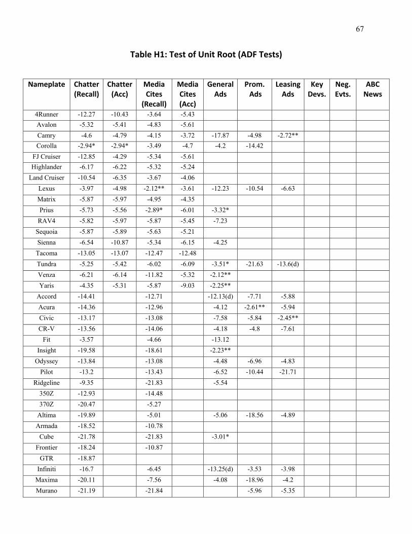
67
Table H1: Test of Unit Root (ADF Tests)
Nameplate Chatter (Recall)
Chatter (Acc)
Media Cites
(Recall)
Media Cites (Acc)
General Ads
Prom. Ads
Leasing Ads
Key Devs.
Neg. Evts.
ABC News
4Runner -12.27 -10.43 -3.64 -5.43
Avalon -5.32 -5.41 -4.83 -5.61
Camry -4.6 -4.79 -4.15 -3.72 -17.87 -4.98 -2.72**
Corolla -2.94* -2.94* -3.49 -4.7 -4.2 -14.42
FJ Cruiser -12.85 -4.29 -5.34 -5.61
Highlander -6.17 -6.22 -5.32 -5.24
Land Cruiser -10.54 -6.35 -3.67 -4.06
Lexus -3.97 -4.98 -2.12** -3.61 -12.23 -10.54 -6.63
Matrix -5.87 -5.97 -4.95 -4.35
Prius -5.73 -5.56 -2.89* -6.01 -3.32*
RAV4 -5.82 -5.97 -5.87 -5.45 -7.23
Sequoia -5.87 -5.89 -5.63 -5.21
Sienna -6.54 -10.87 -5.34 -6.15 -4.25
Tacoma -13.05 -13.07 -12.47 -12.48
Tundra -5.25 -5.42 -6.02 -6.09 -3.51* -21.63 -13.6(d)
Venza -6.21 -6.14 -11.82 -5.32 -2.12**
Yaris -4.35 -5.31 -5.87 -9.03 -2.25**
Accord -14.41 -12.71 -12.13(d) -7.71 -5.88
Acura -14.36 -12.96 -4.12 -2.61** -5.94
Civic -13.17 -13.08 -7.58 -5.84 -2.45**
CR-V -13.56 -14.06 -4.18 -4.8 -7.61
Fit -3.57 -4.66 -13.12
Insight -19.58 -18.61 -2.23**
Odyssey -13.84 -13.08 -4.48 -6.96 -4.83
Pilot -13.2 -13.43 -6.52 -10.44 -21.71
Ridgeline -9.35 -21.83 -5.54
350Z -12.93 -14.48
370Z -20.47 -5.27
Altima -19.89 -5.01 -5.06 -18.56 -4.89
Armada -18.52 -10.78
Cube -21.78 -21.83 -3.01*
Frontier -18.24 -10.87
GTR -18.87
Infiniti -16.7 -6.45 -13.25(d) -3.53 -3.98
Maxima -20.11 -7.56 -4.08 -18.96 -4.2
Murano -21.19 -21.84 -5.96 -5.35
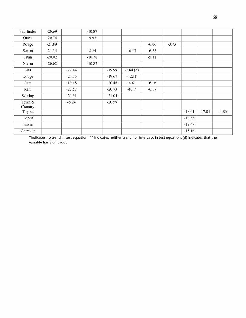
68
*indicates no trend in test equation; ** indicates neither trend nor intercept in test equation; (d) indicates that the variable has a unit root
Pathfinder -20.69 -10.87
Quest -20.74 -9.93
Rouge -21.89 -6.06 -3.73
Sentra -21.34 -8.24 -6.55 -6.75
Titan -20.02 -10.78 -5.81
Xterra -20.02 -10.87
300 -22.44 -19.99 -7.64 (d)
Dodge -21.35 -19.67 -12.18
Jeep -19.48 -20.46 -4.61 -6.16
Ram -23.57 -20.73 -8.77 -6.17
Sebring -21.91 -21.04
Town & Country
-8.24 -20.59
Toyota -18.01 -17.04 -4.86
Honda -19.83
Nissan -19.48
Chrysler -18.16
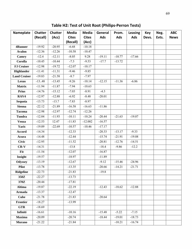
69
Table H2: Test of Unit Root (Philips‐Perron Tests)
Nameplate Chatter (Recall)
Chatter (Acc)
Media Cites
(Recall)
Media Cites (Acc)
General Ads
Prom. Ads
Leasing Ads
Key Devs.
Neg. Evts.
ABC News
4Runner -19.92 -20.95 -6.68 -10.18
Avalon -12.36 -12.26 -10.58 -10.47
Camry -12.4 -12.11 -8.05 9.28 -19.11 -10.77 -17.66
Corolla -10.45 -10.44 -7.3 -9.53 -17.7 -13.72
FJ Cruiser -12.98 -19.72 -12.07 -10.17
Highlander -11.41 -11.31 -9.46 -9.85
Land Cruiser -19.83 -21.58 -8.7 -7.97
Lexus -13..48 -13.45 -9.26 -10.14 -12.15 -11.36 -6.86
Matrix -11.94 -11.87 -7.94 -10.63
Prius -14.76 -15.12 -7.03 -8.91 -4.3
RAV4 -12.97 -12.88 -6.92 -8.48 -20.01
Sequoia -13.73 -13.7 -7.83 -8.97
Sienna -22.12 -21.89 -16.58 -16.63 -11.86
Tacoma -12.98 -12.97 -12.74 -12.26
Tundra -12.04 -11.93 -10.11 -10.24 -20.44 -21.63 -19.07
Venza -12.53 12.47 -11.83 -12.002 -16.57
Yaris -19.09 -22.69 -10.57 -10.46 -17.17
Accord -14.34 -12.33 -20.33 -13.17 -9.33
Acura -14.48 -12.44 -15.74 -21.91 -19.08
Civic -12.95 -11.52 -20.81 -12.76 -14.51
CR-V -14.31 -13.8 -18.4 -9.86 -12.2
Fit -11.54 -12.07 -16.87
Insight -19.57 -18.97 -11.89
Odyssey -13.19 -12.67 -9.12 -15.46 -24.96
Pilot -13.78 -13.35 -20.66 -14.21 -21.71
Ridgeline -22.73 -21.83 -19.8
350Z -22.27 -13.73
370Z -20.44 -17.81
Altima -19.87 -22.19 -12.43 -18.62 -12.88
Armada -13.37 -12.47
Cube -21.78 -21.83 -20.64
Frontier -18.27 -13.99
GTR -18.69
Infiniti -16.61 -10.16 -15.48 -5.22 -7.15
Maxima -20.09 -20.74 -18.44 -19.01 -18.73
Murano -21.22 -21.84 -10.21 -16.74

70
Pathfinder -20.69 -13.99
Quest -20.75 -15.31
Rogue -21.91 -11.96 -18.46
Sentra -21.37 -22.13 -16.04 -13.58
Titan -20.1 -12.77 -7.03
Xterra -20.01 -13.99
300 -22.51 -20.00 -17.1
Dodge -21.35 -19.68 -19.6
Jeep -19.79 -20.41 -14.61 -19.78
Ram -23.47 -20.74 -20.16 -13.98
Sebring -21.95 -20.97
Town & Country
-23.96 -20.45
Toyota -17.63 -17.56 -15.13
Honda -19.89
Nissan -19.39
Chrsysler -17.95
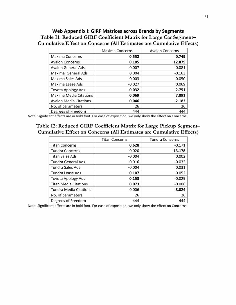
71
Web Appendix I: GIRF Matrices across Brands by Segments Table I1: Reduced GIRF Coefficient Matrix for Large Car Segment–
Cumulative Effect on Concerns (All Estimates are Cumulative Effects) Maxima Concerns Avalon Concerns Maxima Concerns 0.552 0.749
Avalon Concerns 0.105 12.879
Avalon General Ads ‐0.007 ‐0.081
Maxima General Ads 0.004 ‐0.163
Maxima Sales Ads 0.003 0.050
Maxima Lease Ads ‐0.027 0.069
Toyota Apology Ads ‐0.032 2.751
Maxima Media Citations 0.069 7.891
Avalon Media Citations 0.046 2.183
No. of parameters 26 26 Degrees of Freedom 444 444
Note: Significant effects are in bold font. For ease of exposition, we only show the effect on Concerns.
Table I2: Reduced GIRF Coefficient Matrix for Large Pickup Segment– Cumulative Effect on Concerns (All Estimates are Cumulative Effects)
Titan Concerns Tundra Concerns Titan Concerns 0.628 ‐0.171
Tundra Concerns ‐0.020 13.178
Titan Sales Ads ‐0.004 0.002
Tundra General Ads 0.016 ‐0.032
Tundra Sales Ads ‐0.004 0.031
Tundra Lease Ads 0.107 0.052
Toyota Apology Ads 0.153 ‐0.029
Titan Media Citations 0.073 ‐0.006
Tundra Media Citations ‐0.006 8.024
No. of parameters 26 26
Degrees of Freedom 444 444 Note: Significant effects are in bold font. For ease of exposition, we only show the effect on Concerns.
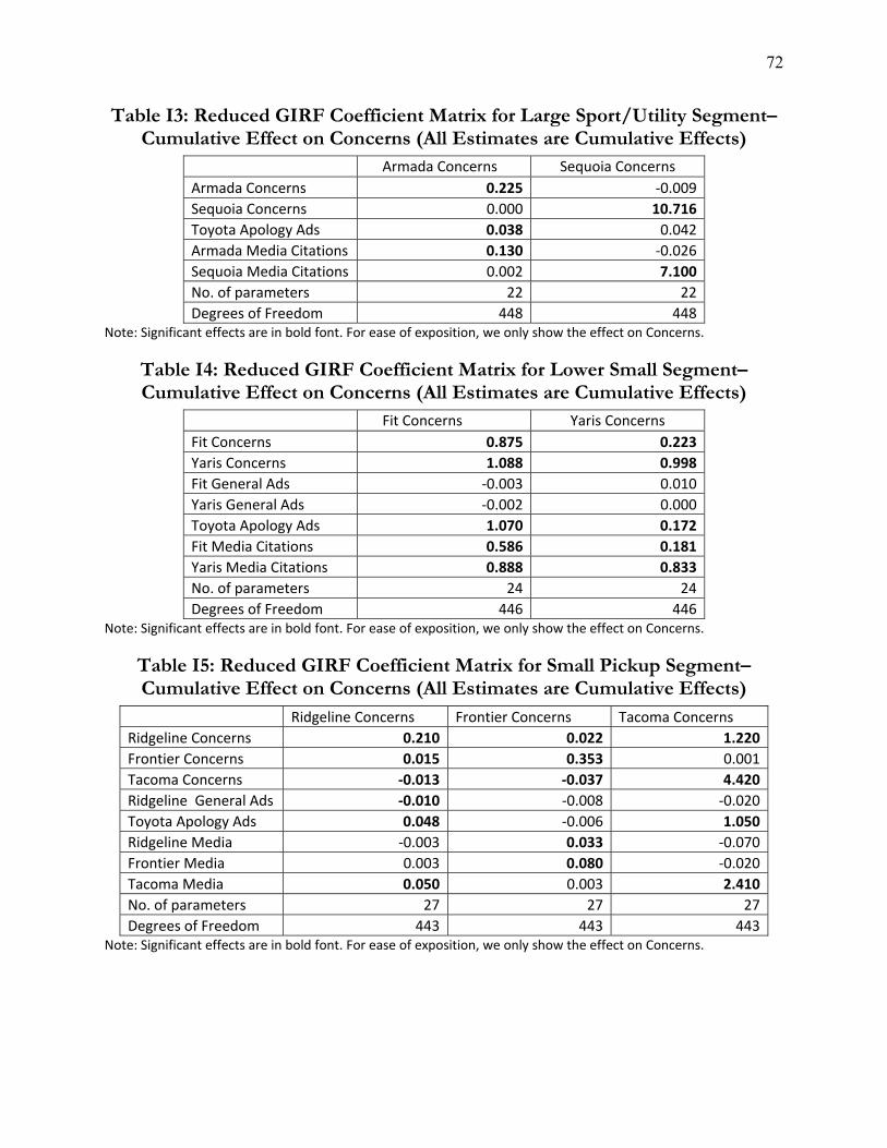
72
Table I3: Reduced GIRF Coefficient Matrix for Large Sport/Utility Segment– Cumulative Effect on Concerns (All Estimates are Cumulative Effects)
Armada Concerns Sequoia Concerns Armada Concerns 0.225 ‐0.009
Sequoia Concerns 0.000 10.716
Toyota Apology Ads 0.038 0.042
Armada Media Citations 0.130 ‐0.026
Sequoia Media Citations 0.002 7.100
No. of parameters 22 22
Degrees of Freedom 448 448 Note: Significant effects are in bold font. For ease of exposition, we only show the effect on Concerns.
Table I4: Reduced GIRF Coefficient Matrix for Lower Small Segment– Cumulative Effect on Concerns (All Estimates are Cumulative Effects)
Fit Concerns Yaris Concerns Fit Concerns 0.875 0.223
Yaris Concerns 1.088 0.998
Fit General Ads ‐0.003 0.010
Yaris General Ads ‐0.002 0.000
Toyota Apology Ads 1.070 0.172
Fit Media Citations 0.586 0.181
Yaris Media Citations 0.888 0.833
No. of parameters 24 24
Degrees of Freedom 446 446 Note: Significant effects are in bold font. For ease of exposition, we only show the effect on Concerns.
Table I5: Reduced GIRF Coefficient Matrix for Small Pickup Segment– Cumulative Effect on Concerns (All Estimates are Cumulative Effects)
Ridgeline Concerns Frontier Concerns Tacoma Concerns
Ridgeline Concerns 0.210 0.022 1.220
Frontier Concerns 0.015 0.353 0.001
Tacoma Concerns ‐0.013 ‐0.037 4.420
Ridgeline General Ads ‐0.010 ‐0.008 ‐0.020
Toyota Apology Ads 0.048 ‐0.006 1.050
Ridgeline Media ‐0.003 0.033 ‐0.070
Frontier Media 0.003 0.080 ‐0.020
Tacoma Media 0.050 0.003 2.410
No. of parameters 27 27 27
Degrees of Freedom 443 443 443Note: Significant effects are in bold font. For ease of exposition, we only show the effect on Concerns.
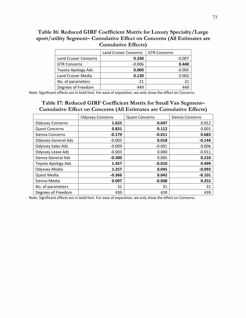
73
Table I6: Reduced GIRF Coefficient Matrix for Luxury Specialty/Large sport/utility Segment– Cumulative Effect on Concerns (All Estimates are
Cumulative Effects) Land Cruiser Concerns GTR Concerns
Land Cruiser Concerns 0.330 ‐0.007
GTR Concerns ‐0.006 0.440
Toyota Apology Ads 0.060 ‐0.005
Land Cruiser Media 0.130 0.002
No. of parameters 21 21
Degrees of Freedom 449 449 Note: Significant effects are in bold font. For ease of exposition, we only show the effect on Concerns.
Table I7: Reduced GIRF Coefficient Matrix for Small Van Segment– Cumulative Effect on Concerns (All Estimates are Cumulative Effects)
Odyssey Concerns Quest Concerns Sienna Concerns
Odyssey Concerns 1.625 0.047 0.012
Quest Concerns 0.831 0.112 0.001
Sienna Concerns ‐0.179 ‐0.011 0.683
Odyssey General Ads ‐0.005 0.018 ‐0.144
Odyssey Sales Ads ‐0.009 ‐0.001 ‐0.006
Odyssey Lease Ads ‐0.003 0.000 ‐0.011
Sienna General Ads ‐0.300 0.005 0.210
Toyota Apology Ads 1.457 ‐0.010 0.499
Odyssey Media 1.257 0.045 ‐0.093
Quest Media ‐0.366 0.042 ‐0.101
Sienna Media 0.097 ‐0.008 0.252
No. of parameters 31 31 31
Degrees of Freedom 439 439 439Note: Significant effects are in bold font. For ease of exposition, we only show the effect on Concerns.
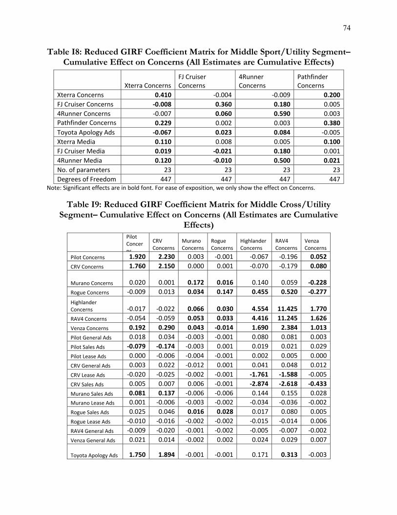
74
Table I8: Reduced GIRF Coefficient Matrix for Middle Sport/Utility Segment– Cumulative Effect on Concerns (All Estimates are Cumulative Effects)
Xterra Concerns FJ Cruiser Concerns
4Runner Concerns
Pathfinder Concerns
Xterra Concerns 0.410 ‐0.004 ‐0.009 0.200
FJ Cruiser Concerns ‐0.008 0.360 0.180 0.005
4Runner Concerns ‐0.007 0.060 0.590 0.003
Pathfinder Concerns 0.229 0.002 0.003 0.380
Toyota Apology Ads ‐0.067 0.023 0.084 ‐0.005
Xterra Media 0.110 0.008 0.005 0.100
FJ Cruiser Media 0.019 ‐0.021 0.180 0.001
4Runner Media 0.120 ‐0.010 0.500 0.021
No. of parameters 23 23 23 23
Degrees of Freedom 447 447 447 447Note: Significant effects are in bold font. For ease of exposition, we only show the effect on Concerns.
Table I9: Reduced GIRF Coefficient Matrix for Middle Cross/Utility Segment– Cumulative Effect on Concerns (All Estimates are Cumulative
Effects) Pilot
Concerns
CRV Concerns
Murano Concerns
Rogue Concerns
Highlander Concerns
RAV4 Concerns
Venza Concerns
Pilot Concerns 1.920 2.230 0.003 ‐0.001 ‐0.067 ‐0.196 0.052
CRV Concerns 1.760 2.150 0.000 0.001 ‐0.070 ‐0.179 0.080
Murano Concerns 0.020 0.001 0.172 0.016 0.140 0.059 ‐0.228
Rogue Concerns ‐0.009 0.013 0.034 0.147 0.455 0.520 ‐0.277
Highlander Concerns ‐0.017 ‐0.022 0.066 0.030 4.554 11.425 1.770
RAV4 Concerns ‐0.054 ‐0.059 0.053 0.033 4.416 11.245 1.626
Venza Concerns 0.192 0.290 0.043 ‐0.014 1.690 2.384 1.013
Pilot General Ads 0.018 0.034 ‐0.003 ‐0.001 0.080 0.081 0.003
Pilot Sales Ads ‐0.079 ‐0.174 ‐0.003 0.001 0.019 0.021 0.029
Pilot Lease Ads 0.000 ‐0.006 ‐0.004 ‐0.001 0.002 0.005 0.000
CRV General Ads 0.003 0.022 ‐0.012 0.001 0.041 0.048 0.012
CRV Lease Ads ‐0.020 ‐0.025 ‐0.002 ‐0.001 ‐1.761 ‐1.588 ‐0.005
CRV Sales Ads 0.005 0.007 0.006 ‐0.001 ‐2.874 ‐2.618 ‐0.433
Murano Sales Ads 0.081 0.137 ‐0.006 ‐0.006 0.144 0.155 0.028
Murano Lease Ads 0.001 ‐0.006 ‐0.003 ‐0.002 ‐0.034 ‐0.036 ‐0.002
Rogue Sales Ads 0.025 0.046 0.016 0.028 0.017 0.080 0.005
Rogue Lease Ads ‐0.010 ‐0.016 ‐0.002 ‐0.002 ‐0.015 ‐0.014 0.006
RAV4 General Ads ‐0.009 ‐0.020 ‐0.001 ‐0.002 ‐0.005 ‐0.007 ‐0.002
Venza General Ads 0.021 0.014 ‐0.002 0.002 0.024 0.029 0.007
Toyota Apology Ads 1.750 1.894 ‐0.001 ‐0.001 0.171 0.313 ‐0.003
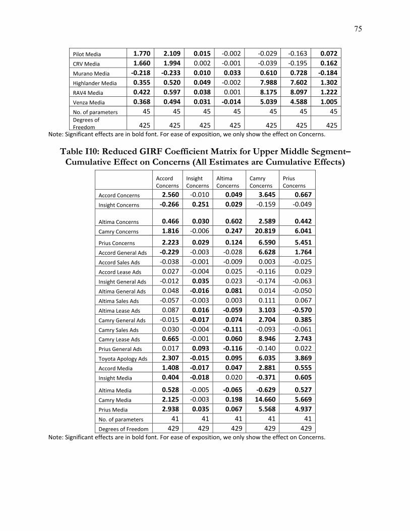
75
Pilot Media 1.770 2.109 0.015 ‐0.002 ‐0.029 ‐0.163 0.072
CRV Media 1.660 1.994 0.002 ‐0.001 ‐0.039 ‐0.195 0.162
Murano Media ‐0.218 ‐0.233 0.010 0.033 0.610 0.728 ‐0.184
Highlander Media 0.355 0.520 0.049 ‐0.002 7.988 7.602 1.302
RAV4 Media 0.422 0.597 0.038 0.001 8.175 8.097 1.222
Venza Media 0.368 0.494 0.031 ‐0.014 5.039 4.588 1.005
No. of parameters 45 45 45 45 45 45 45Degrees of Freedom 425 425 425 425 425 425 425
Note: Significant effects are in bold font. For ease of exposition, we only show the effect on Concerns.
Table I10: Reduced GIRF Coefficient Matrix for Upper Middle Segment– Cumulative Effect on Concerns (All Estimates are Cumulative Effects)
Accord Concerns
Insight Concerns
Altima Concerns
Camry Concerns
Prius Concerns
Accord Concerns 2.560 ‐0.010 0.049 3.645 0.667
Insight Concerns ‐0.266 0.251 0.029 ‐0.159 ‐0.049
Altima Concerns 0.466 0.030 0.602 2.589 0.442
Camry Concerns 1.816 ‐0.006 0.247 20.819 6.041
Prius Concerns 2.223 0.029 0.124 6.590 5.451
Accord General Ads ‐0.229 ‐0.003 ‐0.028 6.628 1.764
Accord Sales Ads ‐0.038 ‐0.001 ‐0.009 0.003 ‐0.025
Accord Lease Ads 0.027 ‐0.004 0.025 ‐0.116 0.029
Insight General Ads ‐0.012 0.035 0.023 ‐0.174 ‐0.063
Altima General Ads 0.048 ‐0.016 0.081 0.014 ‐0.050
Altima Sales Ads ‐0.057 ‐0.003 0.003 0.111 0.067
Altima Lease Ads 0.087 0.016 ‐0.059 3.103 ‐0.570
Camry General Ads ‐0.015 ‐0.017 0.074 2.704 0.385
Camry Sales Ads 0.030 ‐0.004 ‐0.111 ‐0.093 ‐0.061
Camry Lease Ads 0.665 ‐0.001 0.060 8.946 2.743
Prius General Ads 0.017 0.093 ‐0.116 ‐0.140 0.022
Toyota Apology Ads 2.307 ‐0.015 0.095 6.035 3.869
Accord Media 1.408 ‐0.017 0.047 2.881 0.555
Insight Media 0.404 ‐0.018 0.020 ‐0.371 0.605
Altima Media 0.528 ‐0.005 ‐0.065 ‐0.629 0.527
Camry Media 2.125 ‐0.003 0.198 14.660 5.669
Prius Media 2.938 0.035 0.067 5.568 4.937
No. of parameters 41 41 41 41 41
Degrees of Freedom 429 429 429 429 429 Note: Significant effects are in bold font. For ease of exposition, we only show the effect on Concerns.
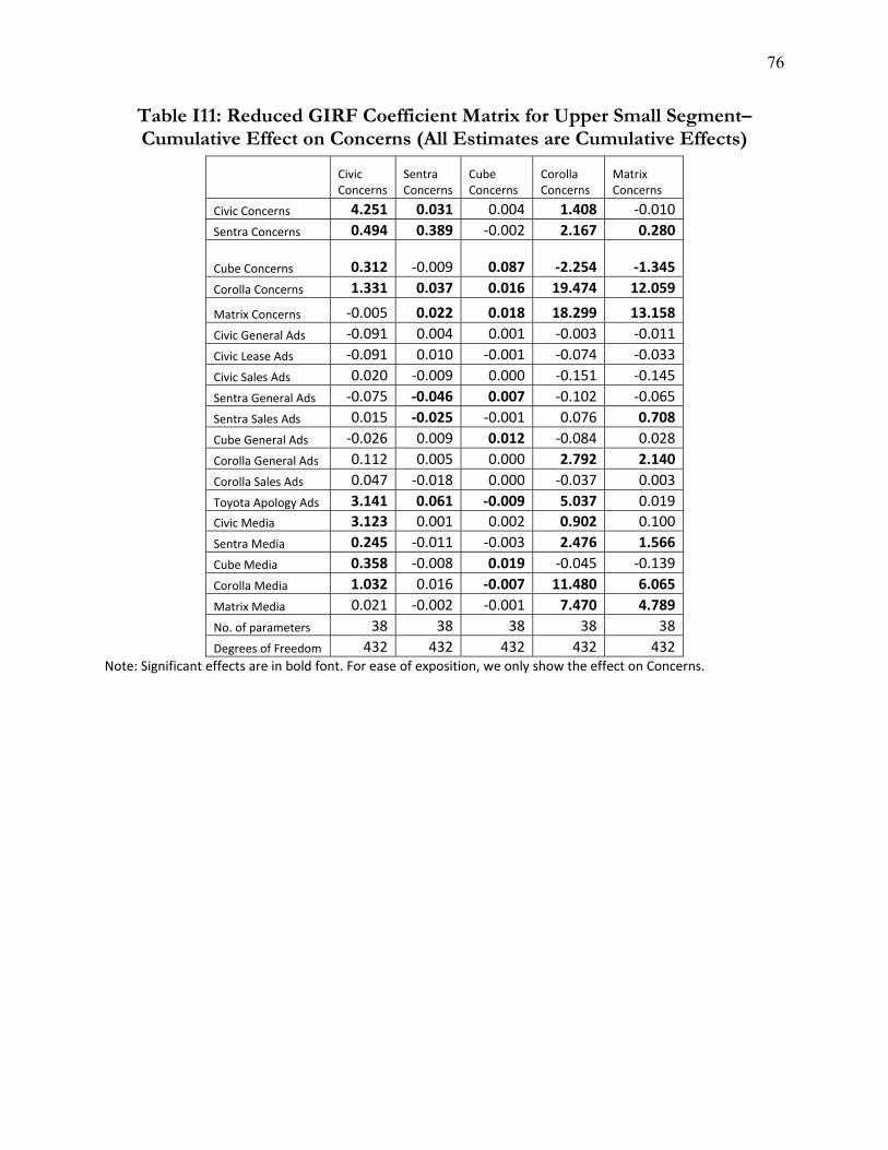
76
Table I11: Reduced GIRF Coefficient Matrix for Upper Small Segment– Cumulative Effect on Concerns (All Estimates are Cumulative Effects)
Civic Concerns
Sentra Concerns
Cube Concerns
Corolla Concerns
Matrix Concerns
Civic Concerns 4.251 0.031 0.004 1.408 ‐0.010
Sentra Concerns 0.494 0.389 ‐0.002 2.167 0.280
Cube Concerns 0.312 ‐0.009 0.087 ‐2.254 ‐1.345
Corolla Concerns 1.331 0.037 0.016 19.474 12.059
Matrix Concerns ‐0.005 0.022 0.018 18.299 13.158
Civic General Ads ‐0.091 0.004 0.001 ‐0.003 ‐0.011
Civic Lease Ads ‐0.091 0.010 ‐0.001 ‐0.074 ‐0.033
Civic Sales Ads 0.020 ‐0.009 0.000 ‐0.151 ‐0.145
Sentra General Ads ‐0.075 ‐0.046 0.007 ‐0.102 ‐0.065
Sentra Sales Ads 0.015 ‐0.025 ‐0.001 0.076 0.708
Cube General Ads ‐0.026 0.009 0.012 ‐0.084 0.028
Corolla General Ads 0.112 0.005 0.000 2.792 2.140
Corolla Sales Ads 0.047 ‐0.018 0.000 ‐0.037 0.003
Toyota Apology Ads 3.141 0.061 ‐0.009 5.037 0.019
Civic Media 3.123 0.001 0.002 0.902 0.100
Sentra Media 0.245 ‐0.011 ‐0.003 2.476 1.566
Cube Media 0.358 ‐0.008 0.019 ‐0.045 ‐0.139
Corolla Media 1.032 0.016 ‐0.007 11.480 6.065
Matrix Media 0.021 ‐0.002 ‐0.001 7.470 4.789
No. of parameters 38 38 38 38 38
Degrees of Freedom 432 432 432 432 432 Note: Significant effects are in bold font. For ease of exposition, we only show the effect on Concerns.
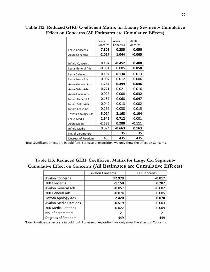
77
Table I12: Reduced GIRF Coefficient Matrix for Luxury Segment– Cumulative Effect on Concerns (All Estimates are Cumulative Effects)
Lexus Concerns
Acura Concerns
Infiniti Concerns
Lexus Concerns 7.801 0.235 0.050
Acura Concerns ‐2.027 1.044 ‐0.065
Infiniti Concerns 0.187 ‐0.452 0.400
Lexus General Ads ‐0.061 0.005 0.050
Lexus Sales Ads 0.192 0.134 ‐0.013
Lexus Lease Ads 0.007 0.012 ‐0.006
Acura General Ads 1.264 0.499 0.046
Acura Sales Ads 0.221 0.021 ‐0.016
Acura Lease Ads ‐0.026 ‐0.008 0.032
Infiniti General Ads 0.157 ‐0.068 0.047
Infiniti Sales Ads ‐0.049 ‐0.013 0.002
Infiniti Lease Ads ‐0.167 ‐0.038 0.015
Toyota Apology Ads 5.024 2.168 0.104
Lexus Media 2.646 0.712 ‐0.001
Acura Media ‐2.583 0.288 ‐0.111
Infiniti Media 0.024 ‐0.663 0.163
No. of parameters 35 35 35
Degrees of Freedom 435 435 435Note: Significant effects are in bold font. For ease of exposition, we only show the effect on Concerns.
Table I13: Reduced GIRF Coefficient Matrix for Large Car Segment– Cumulative Effect on Concerns (All Estimates are Cumulative Effects)
Avalon Concerns 300 Concerns Avalon Concerns 12.979 ‐0.017
300 Concerns ‐1.150 0.207
Avalon General Ads ‐0.057 ‐0.002
300 General Ads ‐0.074 0.005
Toyota Apology Ads 2.420 0.070
Avalon Media Citations 6.519 0.003
300 Media Citations ‐0.022 0.009
No. of parameters 21 21
Degrees of Freedom 449 449 Note: Significant effects are in bold font. For ease of exposition, we only show the effect on Concerns.
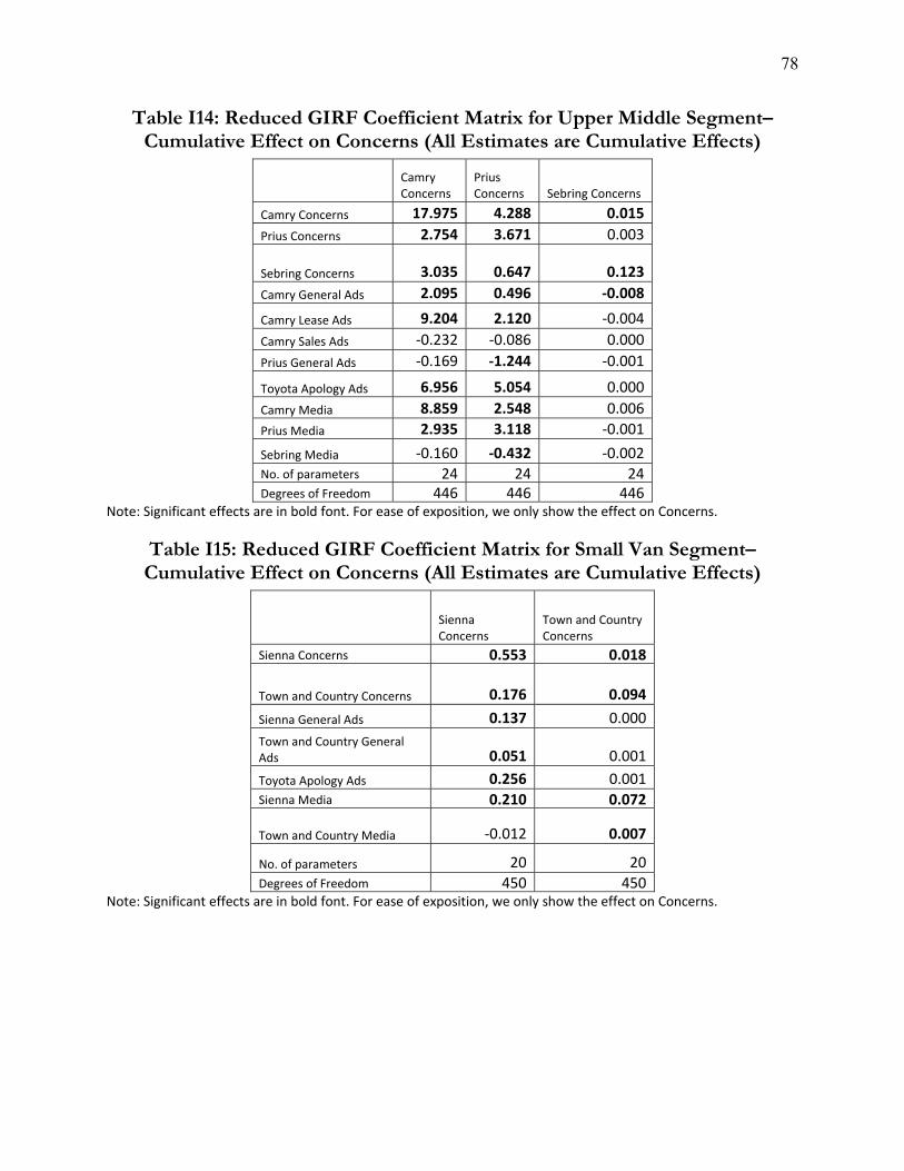
78
Table I14: Reduced GIRF Coefficient Matrix for Upper Middle Segment– Cumulative Effect on Concerns (All Estimates are Cumulative Effects)
Camry Concerns
Prius Concerns Sebring Concerns
Camry Concerns 17.975 4.288 0.015
Prius Concerns 2.754 3.671 0.003
Sebring Concerns 3.035 0.647 0.123
Camry General Ads 2.095 0.496 ‐0.008
Camry Lease Ads 9.204 2.120 ‐0.004
Camry Sales Ads ‐0.232 ‐0.086 0.000
Prius General Ads ‐0.169 ‐1.244 ‐0.001
Toyota Apology Ads 6.956 5.054 0.000
Camry Media 8.859 2.548 0.006
Prius Media 2.935 3.118 ‐0.001
Sebring Media ‐0.160 ‐0.432 ‐0.002 No. of parameters 24 24 24 Degrees of Freedom 446 446 446
Note: Significant effects are in bold font. For ease of exposition, we only show the effect on Concerns.
Table I15: Reduced GIRF Coefficient Matrix for Small Van Segment– Cumulative Effect on Concerns (All Estimates are Cumulative Effects)
Sienna Concerns
Town and Country Concerns
Sienna Concerns 0.553 0.018
Town and Country Concerns 0.176 0.094
Sienna General Ads 0.137 0.000
Town and Country General Ads 0.051 0.001
Toyota Apology Ads 0.256 0.001 Sienna Media 0.210 0.072
Town and Country Media ‐0.012 0.007
No. of parameters 20 20 Degrees of Freedom 450 450
Note: Significant effects are in bold font. For ease of exposition, we only show the effect on Concerns.
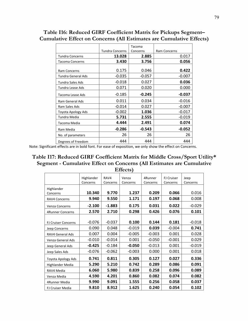
79
Table I16: Reduced GIRF Coefficient Matrix for Pickups Segment– Cumulative Effect on Concerns (All Estimates are Cumulative Effects)
Tundra Concerns
Tacoma Concerns Ram Concerns
Tundra Concerns 13.028 2.885 0.017 Tacoma Concerns 3.430 3.756 0.056
Ram Concerns 0.175 0.046 0.422 Tundra General Ads ‐0.035 ‐0.057 ‐0.007
Tundra Sales Ads ‐0.018 0.027 0.036 Tundra Lease Ads 0.071 0.020 0.000
Tacoma Lease Ads ‐0.185 ‐0.245 ‐0.037
Ram General Ads 0.011 0.034 ‐0.016 Ram Sales Ads ‐0.014 0.027 ‐0.007 Toyota Apology Ads ‐0.002 1.036 ‐0.017 Tundra Media 5.731 2.555 ‐0.019
Tacoma Media 4.444 2.491 0.074
Ram Media ‐0.286 ‐0.543 ‐0.052
No. of parameters 26 26 26
Degrees of Freedom 444 444 444 Note: Significant effects are in bold font. For ease of exposition, we only show the effect on Concerns.
Table I17: Reduced GIRF Coefficient Matrix for Middle Cross/Sport Utility* Segment - Cumulative Effect on Concerns (All Estimates are Cumulative
Effects)
Highlander Concerns
RAV4 Concerns
Venza Concerns
4Runner Concerns
FJ Cruiser Concerns
Jeep Concerns
Highlander Concerns 10.340 9.770 1.237 0.209 0.066 0.016
RAV4 Concerns 9.940 9.550 1.171 0.197 0.068 0.008
Venza Concerns ‐2.100 ‐1.883 0.175 0.031 0.022 ‐0.029
4Runner Concerns 2.570 2.710 0.298 0.426 0.076 0.101
FJ Cruiser Concerns ‐0.076 ‐0.037 0.100 0.144 0.181 ‐0.018
Jeep Concerns 0.090 0.048 ‐0.019 0.039 ‐0.004 0.741
RAV4 General Ads 0.007 0.004 ‐0.005 ‐0.003 0.001 0.028
Venza General Ads ‐0.010 ‐0.014 0.001 ‐0.050 ‐0.001 0.029
Jeep General Ads ‐0.425 ‐0.184 ‐0.050 ‐0.013 0.001 ‐0.019
Jeep Sales Ads ‐0.076 ‐0.062 ‐0.003 0.000 0.001 0.018
Toyota Apology Ads 0.741 0.811 0.305 0.127 0.027 0.336
Highlander Media 5.290 5.210 0.742 0.289 0.086 0.091
RAV4 Media 6.060 5.980 0.839 0.258 0.096 0.089
Venza Media 4.590 4.201 0.860 0.082 0.074 0.082
4Runner Media 9.990 9.091 1.555 0.256 0.058 0.037
FJ Cruiser Media 9.810 8.912 1.625 0.240 0.054 0.102

80
Jeep Media ‐0.810 ‐0.561 ‐0.118 ‐0.006 ‐0.021 0.059
No. of parameters 30 30 30 30 30 30
Degree of Freedom 440 440 440 440 440 440Note: Significant effects are in bold font. For ease of exposition, we only show the effect on Concerns.
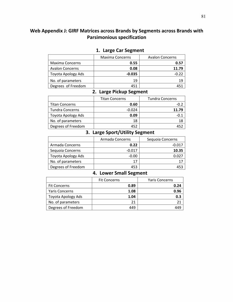
81
Web Appendix J: GIRF Matrices across Brands by Segments across Brands with Parsimonious specification
1. Large Car Segment
Maxima Concerns Avalon Concerns Maxima Concerns 0.55 0.57
Avalon Concerns 0.08 11.79
Toyota Apology Ads ‐0.035 ‐0.22
No. of parameters 19 19
Degrees of Freedom 451 451
2. Large Pickup Segment Titan Concerns Tundra Concerns Titan Concerns 0.60 ‐0.2
Tundra Concerns ‐0.024 11.79
Toyota Apology Ads 0.09 ‐0.1
No. of parameters 18 18
Degrees of Freedom 452 452
3. Large Sport/Utility Segment Armada Concerns Sequoia Concerns Armada Concerns 0.22 ‐0.017
Sequoia Concerns ‐0.017 10.35
Toyota Apology Ads ‐0.00 0.027
No. of parameters 17 17
Degrees of Freedom 453 453
4. Lower Small Segment Fit Concerns Yaris Concerns Fit Concerns 0.89 0.24
Yaris Concerns 1.08 0.96
Toyota Apology Ads 1.04 0.3
No. of parameters 21 21
Degrees of Freedom 449 449
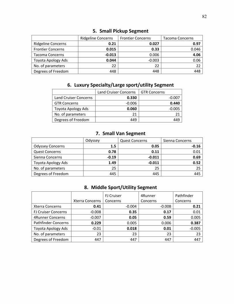
82
5. Small Pickup Segment Ridgeline Concerns Frontier Concerns Tacoma Concerns
Ridgeline Concerns 0.21 0.027 0.97
Frontier Concerns 0.015 0.33 0.046
Tacoma Concerns ‐0.013 0.006 4.06
Toyota Apology Ads 0.044 ‐0.003 0.06
No. of parameters 22 22 22
Degrees of Freedom 448 448 448
6. Luxury Specialty/Large sport/utility Segment Land Cruiser Concerns GTR Concerns
Land Cruiser Concerns 0.330 ‐0.007
GTR Concerns ‐0.006 0.440
Toyota Apology Ads 0.060 ‐0.005
No. of parameters 21 21
Degrees of Freedom 449 449
7. Small Van Segment Odyssey Quest Concerns Sienna Concerns
Odyssey Concerns 1.5 0.05 ‐0.16
Quest Concerns 0.78 0.11 0.01
Sienna Concerns ‐0.19 ‐0.011 0.69
Toyota Apology Ads 1.49 ‐0.011 0.52
No. of parameters 25 25 25
Degrees of Freedom 445 445 445
8. Middle Sport/Utility Segment
Xterra Concerns FJ Cruiser Concerns
4Runner Concerns
Pathfinder Concerns
Xterra Concerns 0.41 ‐0.004 ‐0.008 0.21
FJ Cruiser Concerns ‐0.008 0.35 0.17 0.01
4Runner Concerns ‐0.007 0.05 0.59 0.005
Pathfinder Concerns 0.229 0.005 0.006 0.387
Toyota Apology Ads ‐0.01 0.018 0.01 ‐0.005
No. of parameters 23 23 23 23
Degrees of Freedom 447 447 447 447
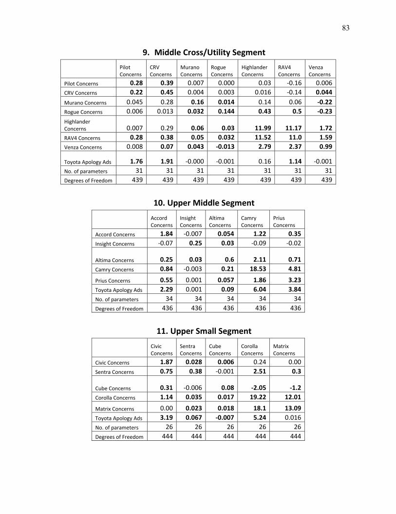
83
9. Middle Cross/Utility Segment Pilot
Concerns CRV Concerns
Murano Concerns
Rogue Concerns
Highlander Concerns
RAV4 Concerns
Venza Concerns
Pilot Concerns 0.28 0.39 0.007 0.000 0.03 ‐0.16 0.006
CRV Concerns 0.22 0.45 0.004 0.003 0.016 ‐0.14 0.044
Murano Concerns 0.045 0.28 0.16 0.014 0.14 0.06 ‐0.22
Rogue Concerns 0.006 0.013 0.032 0.144 0.43 0.5 ‐0.23
Highlander Concerns 0.007 0.29 0.06 0.03 11.99 11.17 1.72
RAV4 Concerns 0.28 0.38 0.05 0.032 11.52 11.0 1.59
Venza Concerns 0.008 0.07 0.043 ‐0.013 2.79 2.37 0.99
Toyota Apology Ads 1.76 1.91 ‐0.000 ‐0.001 0.16 1.14 ‐0.001
No. of parameters 31 31 31 31 31 31 31
Degrees of Freedom 439 439 439 439 439 439 439
10. Upper Middle Segment
Accord Concerns
Insight Concerns
Altima Concerns
Camry Concerns
Prius Concerns
Accord Concerns 1.84 ‐0.007 0.054 1.22 0.35
Insight Concerns ‐0.07 0.25 0.03 ‐0.09 ‐0.02
Altima Concerns 0.25 0.03 0.6 2.11 0.71
Camry Concerns 0.84 ‐0.003 0.21 18.53 4.81
Prius Concerns 0.55 0.001 0.057 1.86 3.23
Toyota Apology Ads 2.29 0.001 0.09 6.04 3.84
No. of parameters 34 34 34 34 34
Degrees of Freedom 436 436 436 436 436
11. Upper Small Segment
Civic Concerns
Sentra Concerns
Cube Concerns
Corolla Concerns
Matrix Concerns
Civic Concerns 1.87 0.028 0.006 0.24 0.00
Sentra Concerns 0.75 0.38 ‐0.001 2.51 0.3
Cube Concerns 0.31 ‐0.006 0.08 ‐2.05 ‐1.2
Corolla Concerns 1.14 0.035 0.017 19.22 12.01
Matrix Concerns 0.00 0.023 0.018 18.1 13.09
Toyota Apology Ads 3.19 0.067 ‐0.007 5.24 0.016
No. of parameters 26 26 26 26 26
Degrees of Freedom 444 444 444 444 444
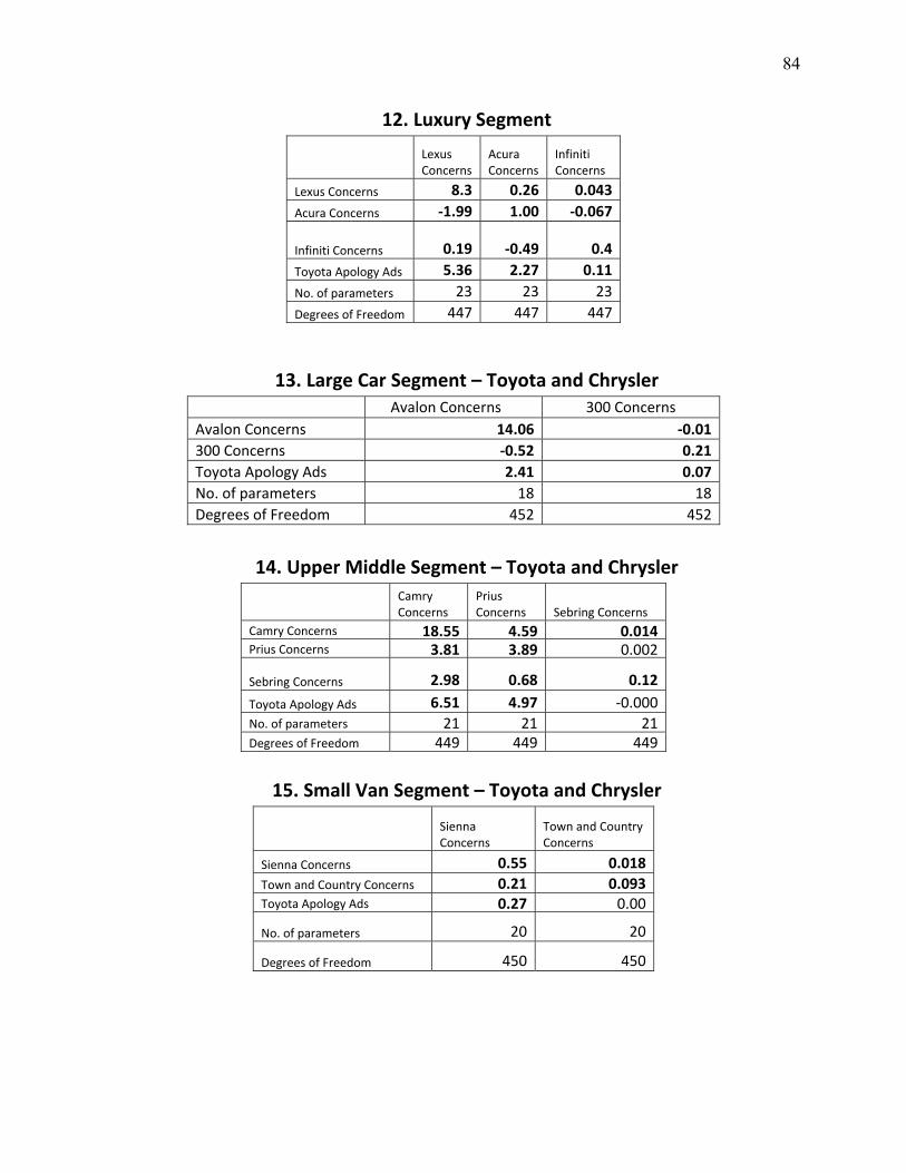
84
12. Luxury Segment
Lexus Concerns
Acura Concerns
Infiniti Concerns
Lexus Concerns 8.3 0.26 0.043
Acura Concerns ‐1.99 1.00 ‐0.067
Infiniti Concerns 0.19 ‐0.49 0.4
Toyota Apology Ads 5.36 2.27 0.11
No. of parameters 23 23 23
Degrees of Freedom 447 447 447
13. Large Car Segment – Toyota and Chrysler Avalon Concerns 300 Concerns Avalon Concerns 14.06 ‐0.01
300 Concerns ‐0.52 0.21
Toyota Apology Ads 2.41 0.07
No. of parameters 18 18
Degrees of Freedom 452 452
14. Upper Middle Segment – Toyota and Chrysler Camry
Concerns Prius Concerns Sebring Concerns
Camry Concerns 18.55 4.59 0.014 Prius Concerns 3.81 3.89 0.002
Sebring Concerns 2.98 0.68 0.12
Toyota Apology Ads 6.51 4.97 ‐0.000 No. of parameters 21 21 21 Degrees of Freedom 449 449 449
15. Small Van Segment – Toyota and Chrysler
Sienna Concerns
Town and Country Concerns
Sienna Concerns 0.55 0.018
Town and Country Concerns 0.21 0.093 Toyota Apology Ads 0.27 0.00
No. of parameters 20 20
Degrees of Freedom 450 450
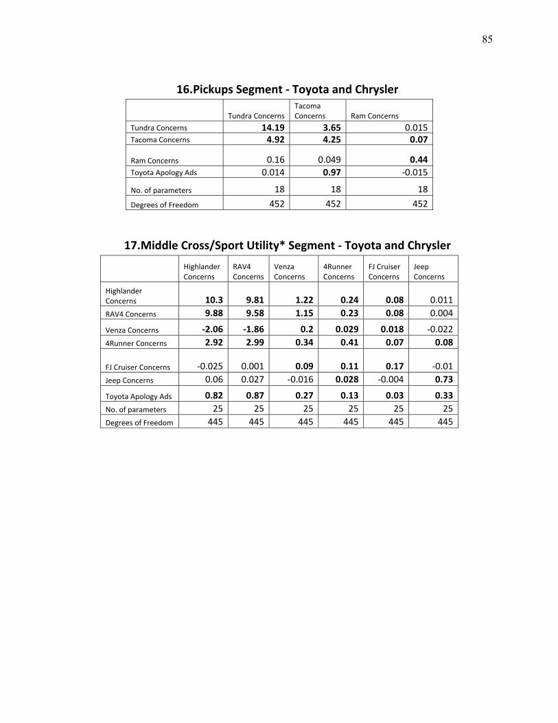
85
16. Pickups Segment ‐ Toyota and Chrysler
Tundra Concerns
Tacoma Concerns Ram Concerns
Tundra Concerns 14.19 3.65 0.015 Tacoma Concerns 4.92 4.25 0.07
Ram Concerns 0.16 0.049 0.44 Toyota Apology Ads 0.014 0.97 ‐0.015
No. of parameters 18 18 18
Degrees of Freedom 452 452 452
17. Middle Cross/Sport Utility* Segment ‐ Toyota and Chrysler
Highlander Concerns
RAV4 Concerns
Venza Concerns
4Runner Concerns
FJ Cruiser Concerns
Jeep Concerns
Highlander Concerns 10.3 9.81 1.22 0.24 0.08 0.011
RAV4 Concerns 9.88 9.58 1.15 0.23 0.08 0.004
Venza Concerns ‐2.06 ‐1.86 0.2 0.029 0.018 ‐0.022
4Runner Concerns 2.92 2.99 0.34 0.41 0.07 0.08
FJ Cruiser Concerns ‐0.025 0.001 0.09 0.11 0.17 ‐0.01
Jeep Concerns 0.06 0.027 ‐0.016 0.028 ‐0.004 0.73
Toyota Apology Ads 0.82 0.87 0.27 0.13 0.03 0.33
No. of parameters 25 25 25 25 25 25
Degrees of Freedom 445 445 445 445 445 445

86
Web Appendix K: GIRF Matrices across Brands by Segments with Brand Positive Chatter as another Endogenous Variable
We do not include positive chatter at the nameplate level because 1) it took numerous man‐
hours to collect just the negative chatter data for each nameplate. In the original data provided to us,
the nameplate was not mentioned. We went to the specific blog, review, or forum and picked up the
nameplate discussed in order to link each negative conversation to the nameplate level, 2) their
inclusion would drastically increase the numbers of parameters estimated, and 3) there is much sparser
data on positive and neutral chatter compared to negative chatter.
1. Large Car Segment Maxima Concerns Avalon Concerns Maxima Concerns 0.549 0.539Avalon Concerns 0.088 11.93Toyota Apology Ads ‐0.036 ‐0.21
Toyota Positive Chatter 0.142 7.42
Nissan Positive Chatter 0.095 0.21
No. of parameters 28 28
Degrees of Freedom 442 442
2. Large Pickup Segment
Titan Concerns Tundra Concerns Titan Concerns 0.618 ‐0.19
Tundra Concerns ‐0.022 12.39
Toyota Apology Ads 0.087 ‐0.11
Toyota Positive Chatter ‐0.00 7.56
Nissan Positive Chatter 0.026 0.18
No. of parameters 28 28
Degrees of Freedom 442 442
3. Large Sport/Utility Segment Armada Concerns Sequoia Concerns Armada Concerns 0.22 0.1
Sequoia Concerns 0.004 10.15
Toyota Apology Ads 0.04 0.009
Toyota Positive Chatter 0.03 4.54
Nissan Positive Chatter 0.03 0.023
No. of parameters 24 24
Degrees of Freedom 446 446
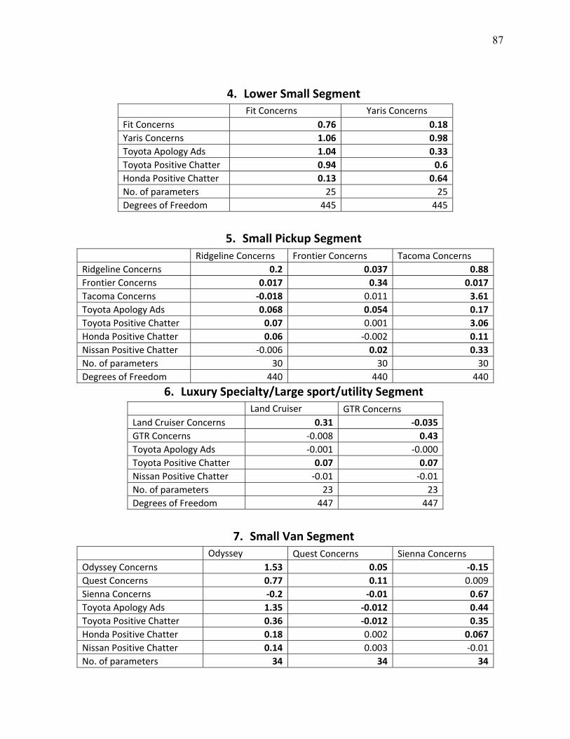
87
4. Lower Small Segment Fit Concerns Yaris Concerns Fit Concerns 0.76 0.18
Yaris Concerns 1.06 0.98
Toyota Apology Ads 1.04 0.33
Toyota Positive Chatter 0.94 0.6
Honda Positive Chatter 0.13 0.64
No. of parameters 25 25
Degrees of Freedom 445 445
5. Small Pickup Segment Ridgeline Concerns Frontier Concerns Tacoma Concerns
Ridgeline Concerns 0.2 0.037 0.88
Frontier Concerns 0.017 0.34 0.017
Tacoma Concerns ‐0.018 0.011 3.61
Toyota Apology Ads 0.068 0.054 0.17
Toyota Positive Chatter 0.07 0.001 3.06
Honda Positive Chatter 0.06 ‐0.002 0.11
Nissan Positive Chatter ‐0.006 0.02 0.33
No. of parameters 30 30 30
Degrees of Freedom 440 440 440
6. Luxury Specialty/Large sport/utility Segment Land Cruiser GTR Concerns
Land Cruiser Concerns 0.31 ‐0.035
GTR Concerns ‐0.008 0.43
Toyota Apology Ads ‐0.001 ‐0.000
Toyota Positive Chatter 0.07 0.07
Nissan Positive Chatter ‐0.01 ‐0.01
No. of parameters 23 23
Degrees of Freedom 447 447
7. Small Van Segment Odyssey Quest Concerns Sienna Concerns
Odyssey Concerns 1.53 0.05 ‐0.15
Quest Concerns 0.77 0.11 0.009
Sienna Concerns ‐0.2 ‐0.01 0.67
Toyota Apology Ads 1.35 ‐0.012 0.44
Toyota Positive Chatter 0.36 ‐0.012 0.35
Honda Positive Chatter 0.18 0.002 0.067
Nissan Positive Chatter 0.14 0.003 ‐0.01
No. of parameters 34 34 34
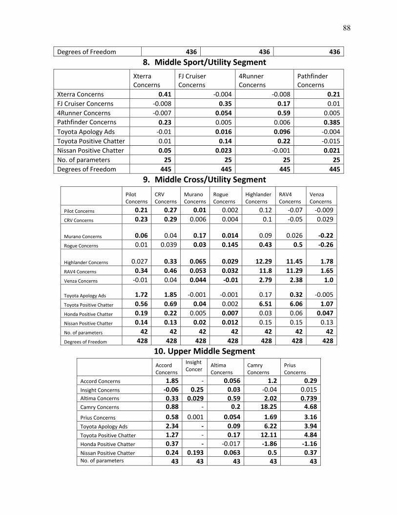
88
Degrees of Freedom 436 436 436
8. Middle Sport/Utility Segment Xterra
Concerns FJ Cruiser Concerns
4Runner Concerns
Pathfinder Concerns
Xterra Concerns 0.41 ‐0.004 ‐0.008 0.21
FJ Cruiser Concerns ‐0.008 0.35 0.17 0.01
4Runner Concerns ‐0.007 0.054 0.59 0.005
Pathfinder Concerns 0.23 0.005 0.006 0.385
Toyota Apology Ads ‐0.01 0.016 0.096 ‐0.004
Toyota Positive Chatter 0.01 0.14 0.22 ‐0.015
Nissan Positive Chatter 0.05 0.023 ‐0.001 0.021
No. of parameters 25 25 25 25
Degrees of Freedom 445 445 445 445
9. Middle Cross/Utility Segment
Pilot Concerns
CRV Concerns
Murano Concerns
Rogue Concerns
Highlander Concerns
RAV4 Concerns
Venza Concerns
Pilot Concerns 0.21 0.27 0.01 0.002 0.12 ‐0.07 ‐0.009
CRV Concerns 0.23 0.29 0.006 0.004 0.1 ‐0.05 0.029
Murano Concerns 0.06 0.04 0.17 0.014 0.09 0.026 ‐0.22
Rogue Concerns 0.01 0.039 0.03 0.145 0.43 0.5 ‐0.26
Highlander Concerns 0.027 0.33 0.065 0.029 12.29 11.45 1.78
RAV4 Concerns 0.34 0.46 0.053 0.032 11.8 11.29 1.65
Venza Concerns ‐0.01 0.04 0.044 ‐0.01 2.79 2.38 1.0
Toyota Apology Ads 1.72 1.85 ‐0.001 ‐0.001 0.17 0.32 ‐0.005
Toyota Positive Chatter 0.56 0.69 0.04 0.002 6.51 6.06 1.07
Honda Positive Chatter 0.19 0.22 0.005 0.007 0.03 0.06 0.047
Nissan Positive Chatter 0.14 0.13 0.02 0.012 0.15 0.15 0.13
No. of parameters 42 42 42 42 42 42 42
Degrees of Freedom 428 428 428 428 428 428 428
10. Upper Middle Segment Accord
Concerns
Insight Concerns
Altima Concerns
Camry Concerns
Prius Concerns
Accord Concerns 1.85 ‐ 0.056 1.2 0.29
Insight Concerns ‐0.06 0.25 0.03 ‐0.04 0.015 Altima Concerns 0.33 0.029 0.59 2.02 0.739 Camry Concerns 0.88 ‐ 0.2 18.25 4.68
Prius Concerns 0.58 0.001 0.054 1.69 3.16
Toyota Apology Ads 2.34 ‐ 0.09 6.22 3.94
Toyota Positive Chatter 1.27 ‐ 0.17 12.11 4.84
Honda Positive Chatter 0.37 ‐ ‐0.017 ‐1.86 ‐1.16
Nissan Positive Chatter 0.24 0.193 0.063 0.5 0.37 No. of parameters 43 43 43 43 43
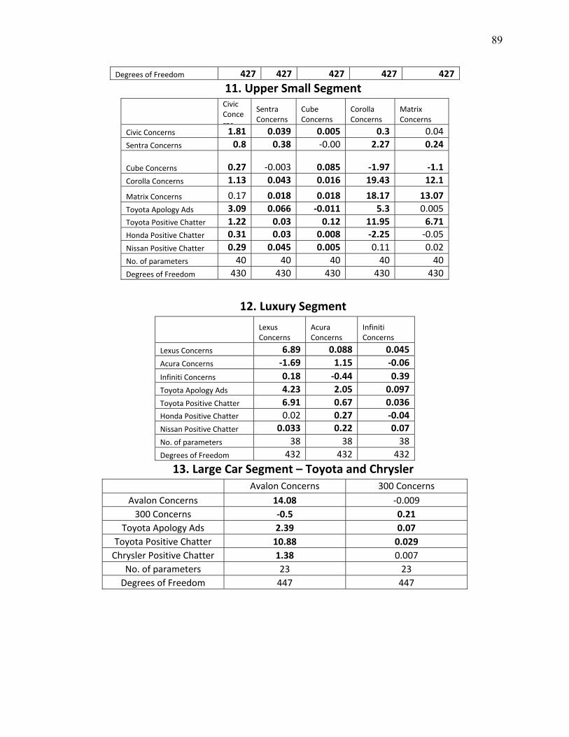
89
Degrees of Freedom 427 427 427 427 427
11. Upper Small Segment Civic
Concerns
Sentra Concerns
Cube Concerns
Corolla Concerns
Matrix Concerns
Civic Concerns 1.81 0.039 0.005 0.3 0.04
Sentra Concerns 0.8 0.38 ‐0.00 2.27 0.24
Cube Concerns 0.27 ‐0.003 0.085 ‐1.97 ‐1.1
Corolla Concerns 1.13 0.043 0.016 19.43 12.1
Matrix Concerns 0.17 0.018 0.018 18.17 13.07
Toyota Apology Ads 3.09 0.066 ‐0.011 5.3 0.005
Toyota Positive Chatter 1.22 0.03 0.12 11.95 6.71
Honda Positive Chatter 0.31 0.03 0.008 ‐2.25 ‐0.05
Nissan Positive Chatter 0.29 0.045 0.005 0.11 0.02
No. of parameters 40 40 40 40 40
Degrees of Freedom 430 430 430 430 430
12. Luxury Segment Lexus
Concerns Acura Concerns
Infiniti Concerns
Lexus Concerns 6.89 0.088 0.045
Acura Concerns ‐1.69 1.15 ‐0.06
Infiniti Concerns 0.18 ‐0.44 0.39
Toyota Apology Ads 4.23 2.05 0.097
Toyota Positive Chatter 6.91 0.67 0.036
Honda Positive Chatter 0.02 0.27 ‐0.04
Nissan Positive Chatter 0.033 0.22 0.07
No. of parameters 38 38 38
Degrees of Freedom 432 432 432
13. Large Car Segment – Toyota and Chrysler Avalon Concerns 300 Concerns
Avalon Concerns 14.08 ‐0.009
300 Concerns ‐0.5 0.21
Toyota Apology Ads 2.39 0.07
Toyota Positive Chatter 10.88 0.029
Chrysler Positive Chatter 1.38 0.007
No. of parameters 23 23
Degrees of Freedom 447 447
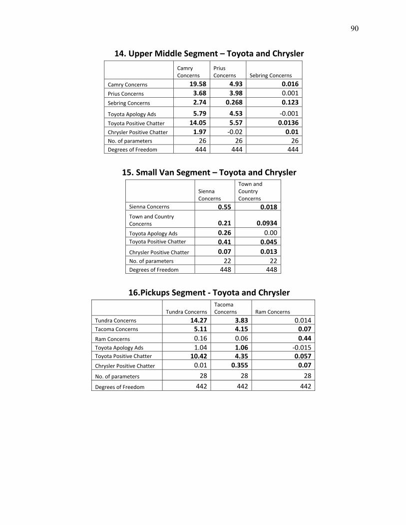
90
14. Upper Middle Segment – Toyota and Chrysler Camry
Concerns Prius Concerns Sebring Concerns
Camry Concerns 19.58 4.93 0.016
Prius Concerns 3.68 3.98 0.001
Sebring Concerns 2.74 0.268 0.123
Toyota Apology Ads 5.79 4.53 ‐0.001
Toyota Positive Chatter 14.05 5.57 0.0136
Chrysler Positive Chatter 1.97 ‐0.02 0.01 No. of parameters 26 26 26 Degrees of Freedom 444 444 444
15. Small Van Segment – Toyota and Chrysler
Sienna Concerns
Town and Country Concerns
Sienna Concerns 0.55 0.018
Town and Country Concerns 0.21 0.0934
Toyota Apology Ads 0.26 0.00Toyota Positive Chatter 0.41 0.045
Chrysler Positive Chatter 0.07 0.013No. of parameters 22 22Degrees of Freedom 448 448
16. Pickups Segment ‐ Toyota and Chrysler
Tundra Concerns Tacoma Concerns Ram Concerns
Tundra Concerns 14.27 3.83 0.014 Tacoma Concerns 5.11 4.15 0.07
Ram Concerns 0.16 0.06 0.44 Toyota Apology Ads 1.04 1.06 ‐0.015 Toyota Positive Chatter 10.42 4.35 0.057
Chrysler Positive Chatter 0.01 0.355 0.07
No. of parameters 28 28 28
Degrees of Freedom 442 442 442
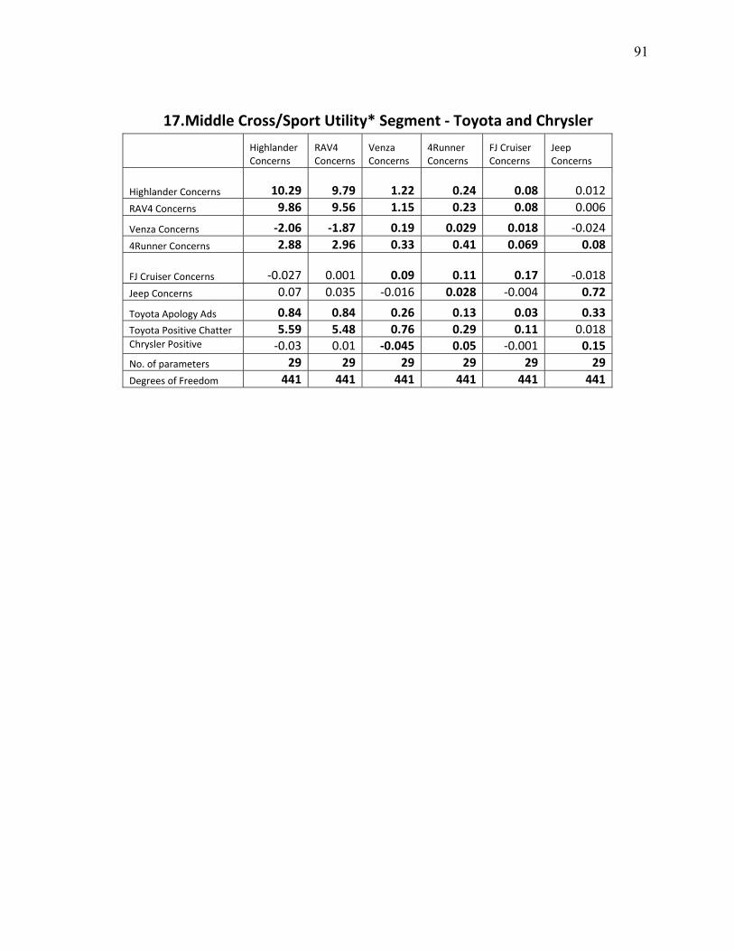
91
17. Middle Cross/Sport Utility* Segment ‐ Toyota and Chrysler Highlander
Concerns RAV4 Concerns
Venza Concerns
4Runner Concerns
FJ Cruiser Concerns
Jeep Concerns
Highlander Concerns 10.29 9.79 1.22 0.24 0.08 0.012
RAV4 Concerns 9.86 9.56 1.15 0.23 0.08 0.006
Venza Concerns ‐2.06 ‐1.87 0.19 0.029 0.018 ‐0.024
4Runner Concerns 2.88 2.96 0.33 0.41 0.069 0.08
FJ Cruiser Concerns ‐0.027 0.001 0.09 0.11 0.17 ‐0.018
Jeep Concerns 0.07 0.035 ‐0.016 0.028 ‐0.004 0.72
Toyota Apology Ads 0.84 0.84 0.26 0.13 0.03 0.33
Toyota Positive Chatter 5.59 5.48 0.76 0.29 0.11 0.018Chrysler Positive h
‐0.03 0.01 ‐0.045 0.05 ‐0.001 0.15
No. of parameters 29 29 29 29 29 29
Degrees of Freedom 441 441 441 441 441 441
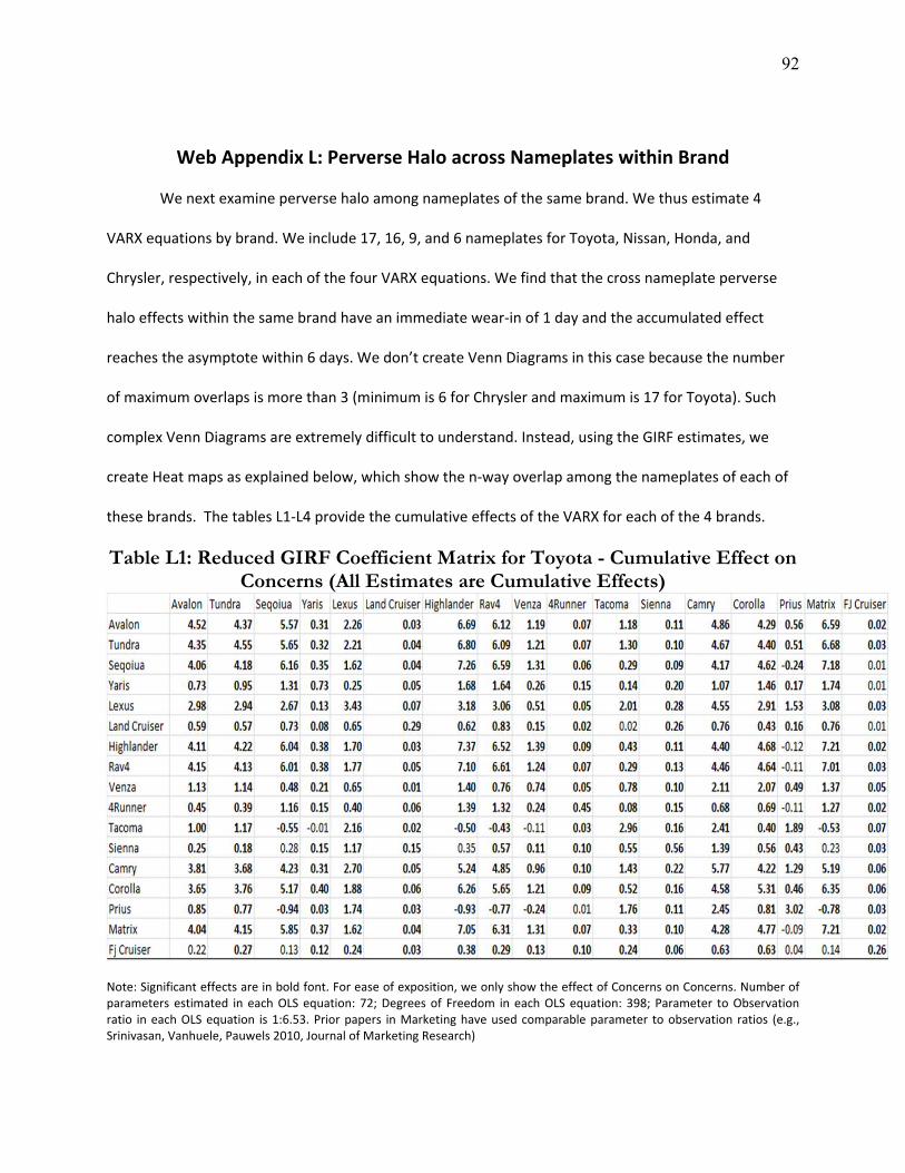
92
Web Appendix L: Perverse Halo across Nameplates within Brand
We next examine perverse halo among nameplates of the same brand. We thus estimate 4
VARX equations by brand. We include 17, 16, 9, and 6 nameplates for Toyota, Nissan, Honda, and
Chrysler, respectively, in each of the four VARX equations. We find that the cross nameplate perverse
halo effects within the same brand have an immediate wear‐in of 1 day and the accumulated effect
reaches the asymptote within 6 days. We don’t create Venn Diagrams in this case because the number
of maximum overlaps is more than 3 (minimum is 6 for Chrysler and maximum is 17 for Toyota). Such
complex Venn Diagrams are extremely difficult to understand. Instead, using the GIRF estimates, we
create Heat maps as explained below, which show the n‐way overlap among the nameplates of each of
these brands. The tables L1‐L4 provide the cumulative effects of the VARX for each of the 4 brands.
Table L1: Reduced GIRF Coefficient Matrix for Toyota - Cumulative Effect on Concerns (All Estimates are Cumulative Effects)
Note: Significant effects are in bold font. For ease of exposition, we only show the effect of Concerns on Concerns. Number of parameters estimated in each OLS equation: 72; Degrees of Freedom in each OLS equation: 398; Parameter to Observation ratio in each OLS equation is 1:6.53. Prior papers in Marketing have used comparable parameter to observation ratios (e.g., Srinivasan, Vanhuele, Pauwels 2010, Journal of Marketing Research)
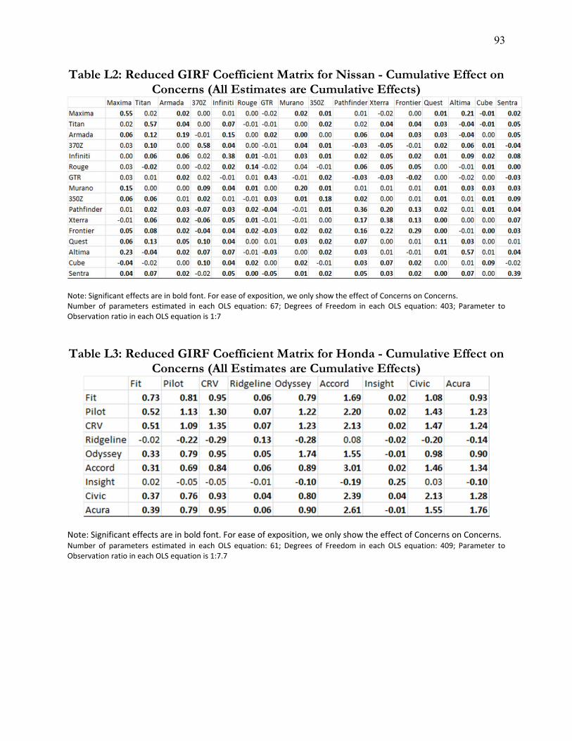
93
Table L2: Reduced GIRF Coefficient Matrix for Nissan - Cumulative Effect on Concerns (All Estimates are Cumulative Effects)
Note: Significant effects are in bold font. For ease of exposition, we only show the effect of Concerns on Concerns. Number of parameters estimated in each OLS equation: 67; Degrees of Freedom in each OLS equation: 403; Parameter to Observation ratio in each OLS equation is 1:7
Table L3: Reduced GIRF Coefficient Matrix for Honda - Cumulative Effect on
Concerns (All Estimates are Cumulative Effects)
Note: Significant effects are in bold font. For ease of exposition, we only show the effect of Concerns on Concerns. Number of parameters estimated in each OLS equation: 61; Degrees of Freedom in each OLS equation: 409; Parameter to Observation ratio in each OLS equation is 1:7.7

94
Table L4: Reduced GIRF Coefficient Matrix for Chrysler - Cumulative Effect on Concerns (All Estimates are Cumulative Effects)
Note: Significant effects are in bold font. For ease of exposition, we only show the effect of Concerns on Concerns.
Number of parameters estimated in each OLS equation: 40; Degrees of Freedom in each OLS equation: 430; Parameter to Observation ratio in each OLS equation is 1:11.75
COMPUTATIONANDPRESENTATIONOFHALOWITHINBRANDBYHEATMAPS
Tables L1‐L4 in Web Appendix L report the GIRF cross nameplate effects across the nameplates
of the same brand. Using the sign and significance of these effects, we create Heat Maps that indicate
the amount of perverse halo among these nameplates. We first explain the procedure to obtain the n‐
way overlaps provided in the Heat Maps. Analogous to the between brand case, the symmetric 2‐way
perverse halo between Nameplate 1 and Nameplate 2 is
(L.1) 2
1221
21
--),(
MMMMMMsym
EEH
where 21 MME takes on the value 1 if the GIRF estimate in the VARX equation running from nameplate
1 to nameplate 2 is significantly positive and 0 otherwise. Thus, the 2‐way overlap of a nameplate
(using Nameplate 1 as the case) is
(L.2) 1)1(
2 221
1
),(
CN
Hwayoverlap
NM
MMMsym
M
,
where N is the number of nameplates of a brand.
The exclusivity for a nameplate (using Nameplate 1 as the case) is 1‐ (1
2 Mwayoverlap ).

95
Analogous to the between brand case, we define the extent of one‐way perverse halo from
Nameplate 1 to both Nameplate 2 and Nameplate 3 as follows:
(L.3) 3221321
* MMMMMMM EEE .
Generalizing the above equation, we define the extent of one way perverse halo from
Nameplate 1 to each of the N nameplates of a brand as follows:
(L.4) NNN MMMMMMMMMM EEEE
13221321
.......**........
The symmetric 3‐way perverse halo between Nameplate 1, Nameplate 2, and Nameplate 3 is
(L.5) 3
213132321
321
------),,(
MMMMMMMMMMMMsym
EEEH
Generalizing the above equation, the symmetric n‐way perverse halo between Nameplate 1,
Nameplate 2 till Nameplate N is
(L.6)N
EEEH NNNN
N
MMMMMMMMMMMMMMMMsym
121132321
321
......---......--....--),......,,,(
......
The 3‐way overlap of a nameplate (using Nameplate 1 as the case) is
(L.7) 2)1(
-3
∑32
321
1
),,(
CN
H
wayoverlap
NM
MMMMMsym
M
Generalizing the above equation, the n‐way overlap of a nameplate (using Nameplate 1 as the
case) is
(L.8) )1()1(
∑.......≠
).........,,,(
32
321
1
nCN
H
wayoverlapn
N
N
N
M
MMMMMMMsym
M
PRESENTATIONOFHALOWITHINBRANDBYHEATMAPS
Figures La‐Ld are Heat Maps that show the within‐brand perverse halo for Toyota, Honda,
Nissan, and Chrysler respectively. We find an average exclusive value of 9% (average 2‐way overlap is
96
91%) for the 17 nameplates of Toyota. This indicates that Toyota nameplates as a group suffer very high
perverse halo, probably because the brand name of the nameplate (e.g., Corolla) always appears with
the family brand name, Toyota. This result indicates that on average, 91% of the times, at least one
other Toyota nameplate gets affected when anyone of their nameplates have a recall. The 17‐way
overlap for Toyota is 35%. This result indicates that on average, over a third of the time, all Toyota
nameplates suffer from perverse halo if any one Toyota nameplate has a recall.
We find an average exclusive value of 25% (average 2‐way overlap is 75%) for the 9 nameplates
of Honda. This result indicates that on average, 75% of the times, at least one other Honda nameplate
gets affected when anyone of their nameplates have a recall. This result indicates that Honda
nameplates as a group suffer high perverse halo, but not as high as Toyota. The 9‐way overlap for Honda
is 56%. Thus, on average, over half of the time, all Honda nameplates suffer from perverse halo if any
one Honda nameplate has a recall.
We find an average exclusive value of 44% (average 2‐way overlap is 56%) for the 16
nameplates of Nissan. This result indicates that on average, 56% of the times, at least one other Nissan
nameplate gets affected when anyone of their nameplates have a recall. This indicates that Nissan
nameplates as a group suffer less perverse halo than Toyota and Honda, suggesting that consumers
consider nameplates under the Nissan family brand as more distinct than those under the Toyota or
Honda brand names.
We find an average exclusive value of 27% (average 2‐way overlap is 73%) for the 6 nameplates
of Chrysler. This result indicates that on average, 73% of the times, at least one other Chrysler
nameplate gets affected when anyone of their nameplates has negative chatter about its acceleration.
Thus, within brand perverse halo is high for both Japanese and American brands.

97
We next correlate the exclusivity of each nameplate with its market share14. We find a
correlation of ‐0.4, which is significant at 1%. This result indicates the larger the brand, the greater the
overlap in perverse halo among nameplates that belong to that brand. These results suggest that
perverse halo is a result of consumer awareness of the family brand (e.g., Toyota) associated with the
nameplate (e.g. Camry).
14 These shares are segment specific market shares. Thus, Corolla’s market share is its share in the Upper Small segment. The shares are obtained from Ward’s Automotive yearbook.
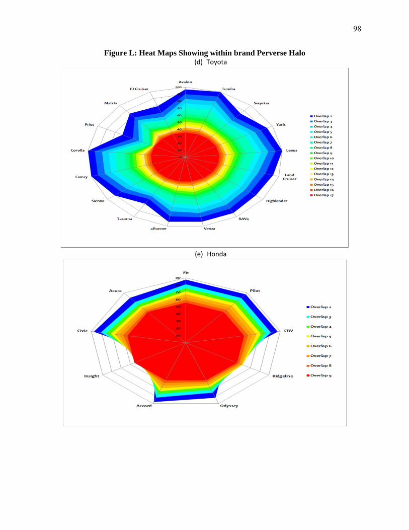
98
Figure L: Heat Maps Showing within brand Perverse Halo (d) Toyota
(e) Honda
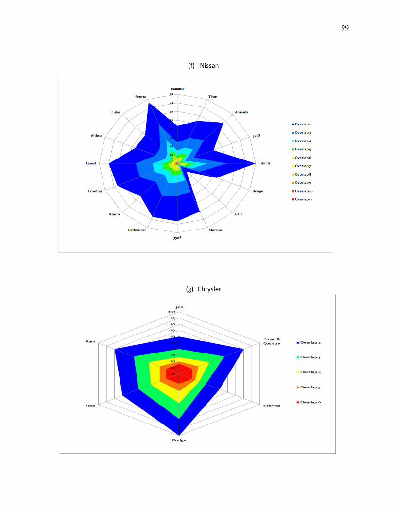
99
(f) Nissan
(g) Chrysler
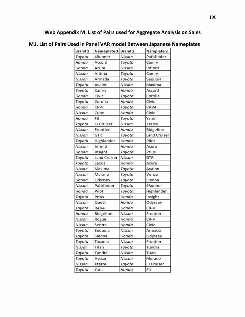
100
Web Appendix M: List of Pairs used for Aggregate Analysis on Sales
M1. List of Pairs Used in Panel VAR model Between Japanese Nameplates
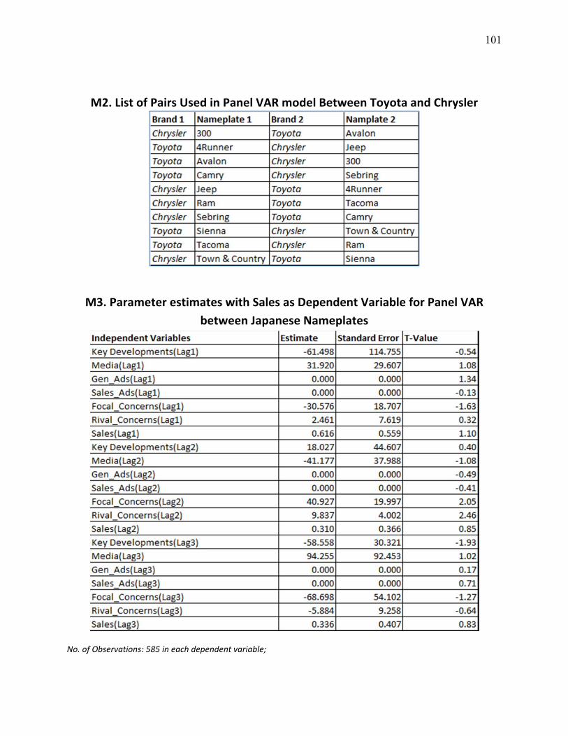
101
M2. List of Pairs Used in Panel VAR model Between Toyota and Chrysler
M3. Parameter estimates with Sales as Dependent Variable for Panel VAR
between Japanese Nameplates
No. of Observations: 585 in each dependent variable;
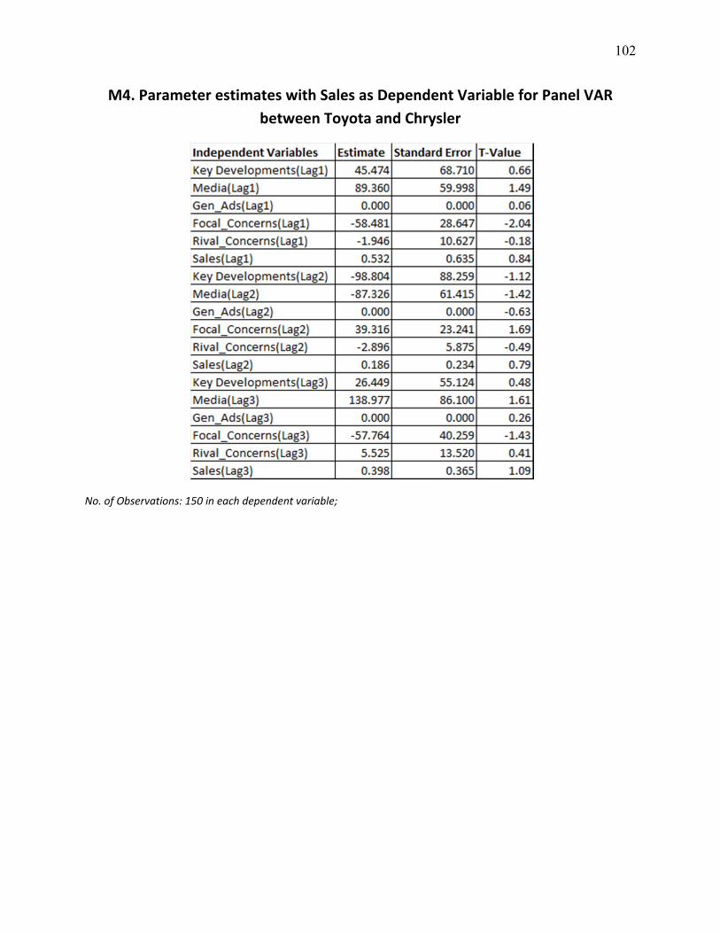
102
M4. Parameter estimates with Sales as Dependent Variable for Panel VAR
between Toyota and Chrysler
No. of Observations: 150 in each dependent variable;
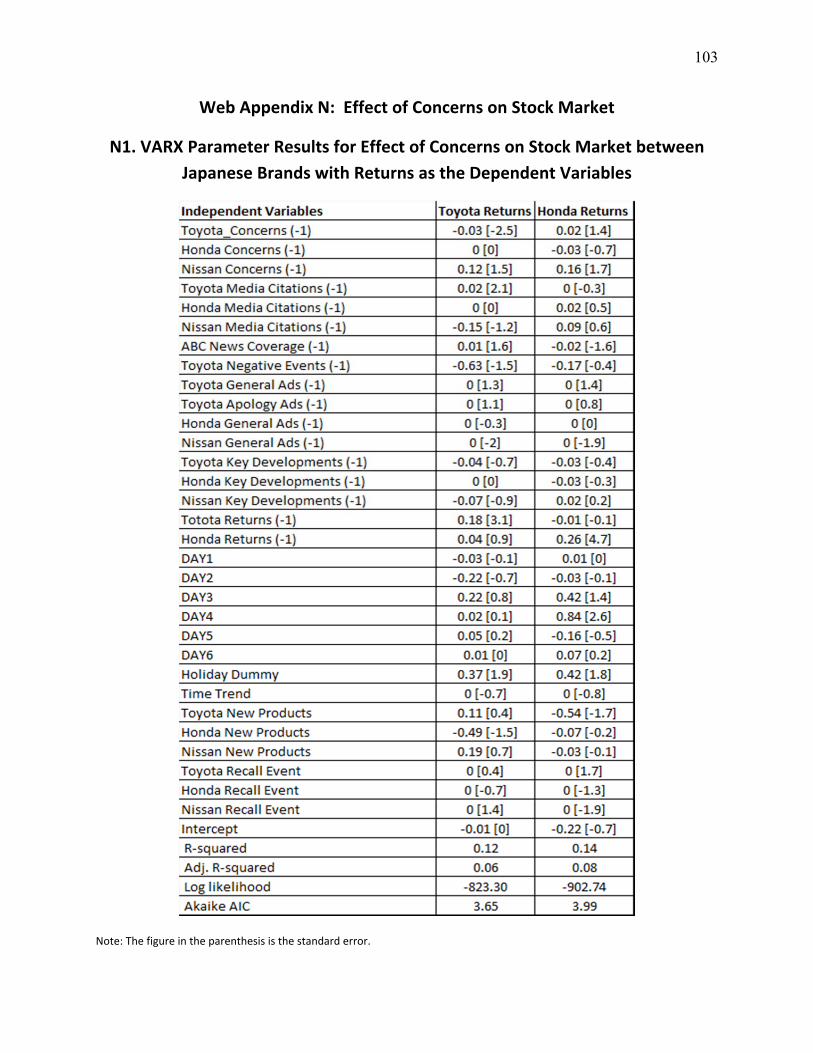
103
Web Appendix N: Effect of Concerns on Stock Market
N1. VARX Parameter Results for Effect of Concerns on Stock Market between
Japanese Brands with Returns as the Dependent Variables
Note: The figure in the parenthesis is the standard error.
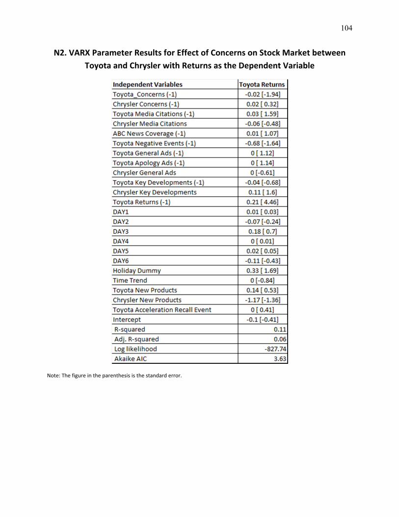
104
N2. VARX Parameter Results for Effect of Concerns on Stock Market between
Toyota and Chrysler with Returns as the Dependent Variable
Note: The figure in the parenthesis is the standard error.

105
Web Appendix O: Robustness Results
RELEVANCYSCOREFORMEDIACITATIONS
Instead of a relevancy score of 60% for obtaining media citations from Lexis‐Nexis, we use a
more conservative threshold as a robustness check. Thus, we collect all media citations about each
model using a relevancy score of 80% and re‐estimate each of the VARX equations. Our results remain
robust using a relevancy score of 80%.
TVNEWSCOVERAGE
We re‐estimate each of the VARX equations using not only ABC news as the TV channel covering
the Toyota acceleration recalls but also other TV channels. For example, MSNBC’s Dateline provided
investigative coverage of the product recalls. Thus, we collect mentions of Toyota’s recall across the
following TV channels: American Public Media, CBS News, CNBC News, CNN, CTV Television, Fox News
Network, MSNBC, National Public Radio (NPR), and NBC News. We use Lexis‐Nexis’ Broadcast
Transcripts database to collect TV coverage about the recall using the keywords “Toyota” and “Recall”.
Our results remain robust using more than 1 TV network.
ESTIMATESOFHALOBETWEENBRANDSBYSIZE
The amount of perverse halo between brands may be much higher if we estimated the full VAR
equation involving 2256 cross nameplate effects. Thus, our estimates of perverse halo are conservative.
Indeed, there is a possibility of perverse halo from an Upper Small nameplate of Toyota (e.g., Corolla) to
Lower Small nameplate of Honda (e.g., Fit). As it is extremely complex to estimate, keep track of and
interpret all these cross nameplate effects, we estimate the VARX equations by segment. However, to
ensure that our results are robust, we find a middle ground between intractability and accuracy and
estimate the cross nameplate effects between nameplates of different brands by their sizes. Thus, we
further categorize the segments by size: small, medium, and big. We estimate 3 VARX equations for
106
these 3 size categories. Table O.1 lists the nameplates by size and brand. We estimate the VARX
equations by size only for the Japanese brands as there are few Chrysler nameplates to categorize.
Similar to the segment level VARX equations, we create Venn Diagrams to indicate the amount
of perverse halo using the sign and significance of these effects.
Figures O.1a‐O.1c show the perverse halo effects by size. Medium sized nameplates such as
Camry, Accord, and Altima have the highest total symmetric 3‐way perverse halo. We find the highest
total symmetric 2‐way perverse halo between Honda and Nissan for big nameplates, between Toyota
and Honda for medium nameplates, and between Honda and Nissan for small nameplates. Honda has
the lowest exclusivity for its big nameplates (20%), Toyota for its medium nameplates, and Nissan for its
small nameplates (22%). Thus, these results suggest that (using Toyota as the case) many of Toyota’s
medium sized nameplates are affected by online chatter of medium sized nameplates of other brands.
Overall, similar to segment level results, we find that for each brand, exclusivity (i.e., isolation from
perverse halo) is low.
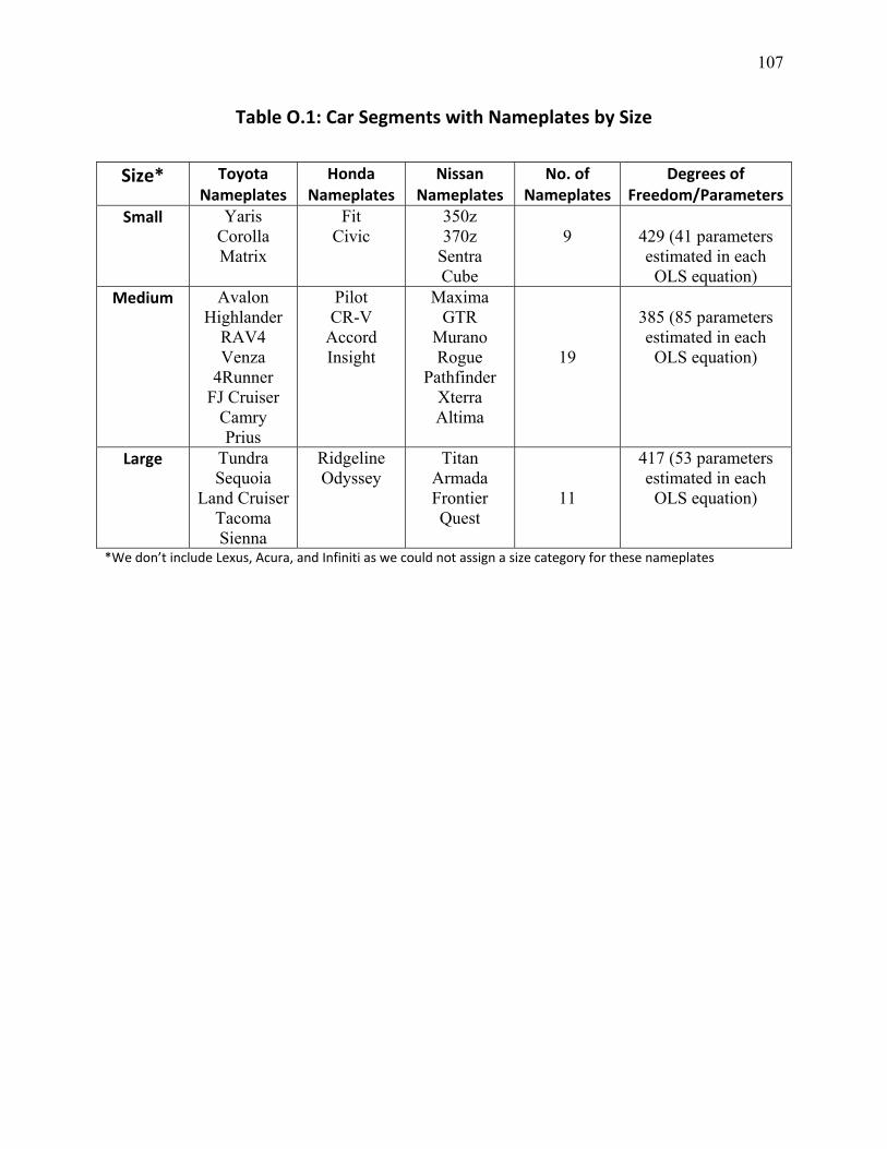
107
Table O.1: Car Segments with Nameplates by Size
*We don’t include Lexus, Acura, and Infiniti as we could not assign a size category for these nameplates
Size* Toyota Nameplates
Honda Nameplates
Nissan Nameplates
No. of Nameplates
Degrees of Freedom/Parameters
Small Yaris Corolla Matrix
Fit Civic
350z 370z
Sentra Cube
9
429 (41 parameters estimated in each
OLS equation) Medium Avalon
Highlander RAV4 Venza
4Runner FJ Cruiser
Camry Prius
Pilot CR-V
Accord Insight
Maxima GTR
Murano Rogue
Pathfinder Xterra Altima
19
385 (85 parameters estimated in each
OLS equation)
Large Tundra Sequoia
Land Cruiser Tacoma Sienna
Ridgeline Odyssey
Titan Armada Frontier Quest
11
417 (53 parameters estimated in each
OLS equation)
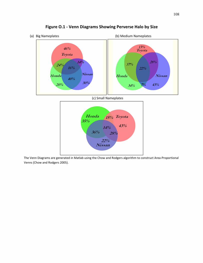
108
Figure O.1 ‐ Venn Diagrams Showing Perverse Halo by Size
(a) Big Nameplates (b) Medium Nameplates
(c) Small Nameplates
The Venn Diagrams are generated in Matlab using the Chow and Rodgers algorithm to construct Area‐Proportional
Venns (Chow and Rodgers 2005).
Homogenous Contracts for Heterogeneous Agents: AligningSalesforce Composition and Compensation∗
Øystein Daljord Sanjog Misra Harikesh S. Nair
Past versions: June 2012; Feb 2013, May 2015. This version: Sept 6, 2015
Abstract
Observed contracts in the real-world are often very simple, partly reflecting the constraints faced bycontracting firms in making the contracts more complex. We focus on one such rigidity, the constraintsfaced by firms in fine-tuning contracts to the full distribution of heterogeneity of its employees. We ex-plore the implication of these restrictions for the provision of incentives within the firm. Our applicationis to salesforce compensation, in which a firm maintains a salesforce to market its products. Consistentwith ubiquitous real-world business practice, we assume the firm is restricted to fully or partially setuniform commissions across its agent pool. We show this implies an interaction between the compositionof agent types in the contract and the compensation policy used to motivate them, leading to a “contrac-tual externality” in the firm and generating gains to sorting. This paper explains how this contractualexternality arises, discusses a practical approach to endogenize agents and incentives at a firm in itspresence, and presents an empirical application to salesforce compensation contracts at a US Fortune500 company that explores these considerations and assesses the gains from a salesforce architecturethat sorts agents into divisions to balance firm-wide incentives. Empirically, we find the restriction tohomogenous plans significantly reduces the payoffs of the firm relative to a fully heterogeneous planwhen it is unable to optimize the composition of its agents. However, the firm’s payoffs come very closeto that of the fully heterogeneous plan when it can optimize both composition and compensation. Thus,in our empirical setting, the ability to choose agents mitigates the loss in incentives from the restrictionto uniform contracts. We conjecture this may hold more broadly.
∗Daljord : Booth School of Business, University of Chicago, [email protected]; Misra: Booth Schoolof Business, University of Chicago, [email protected]; Nair : Graduate School of Business, StanfordUniversity, [email protected]. We thank Guy Arie, Nick Bloom, Francine Lafontaine, Ed Lazear, SridharMoorthy, Paul Oyer, Michael Raith, Kathryn Shaw, Chuck Weinberg, Jeff Zwiebel; our discussant at the QMEconference, Curtis Taylor; and Lanier Benkard and Ed Lazear in particular for their useful comments and suggestions.We also thank seminar participants at Arizona-Economics, Harvard-Economics, Michigan-Economics, MIT-Sloan,Stanford-GSB, UBC-Saunder, UC-Davis-GSM, UT-Austin-McCoombs, UToronto-Rotman, and at the 2012 IOFest,Marketing Dynamics, World Congress of Econometrics and QME conferences for useful feedback. The usual disclaimerapplies.
1
1 Introduction
In many interesting market contexts, firms face rigidities or constraints in fine-tuning their contracts
to reflect the full distribution of heterogeneity of the agents they are contracting with. For example,
auto-insurance companies are often prevented by regulation from conditioning their premiums on
consumer characteristics like race and credit scores. Royalty rates in business-format franchising in
the US are typically constrained by norm to be the same across all franchisees in a given chain.1
Wholesales contracts between manufacturers and downstream retailers in the US typically involve
similar wholesales prices to all downstream retailers within a given geographic area due to Robinson-
Patman considerations. In salesforces, the context of the empirical example in this paper, incentive
or commission rates on output are invariably set the same across all sales-agents within a firm. For
instance, a firm choosing a salary + commission salesforce compensation scheme typically sets the
same commission rate for every sales-agent on its payroll, in spite of the fact that exploring the
heterogeneity and setting an agent-specific commission may create theoretically better incentives
at the individual level. While reasons are varied, full or partial uniformity of this sort is well
documented to be an ubiquitous feature of real-world salesforce compensation (Rao 1990; Mantrala
et al. 1994; Raju and Srinivasan 1996; Zoltners et al. 2001; Lo et al. 2011).
The focus of this paper is on the implications to the principal of this restriction to similar
contract terms across agents. We do not take a strong stance on the source of the uniformity, but
focus on the fact that any such uniformity in the contract implies that agents and contract terms
have to be chosen jointly. In the salesforce context, for example, this creates an interaction between
the composition of agent types in the contract and the compensation policy used to motivate them,
leading to a “contractual externality” in the firm and generating gains to sorting. This paper explains
how this contractual externality arises, discusses a practical approach to endogenize agents and
incentives at a firm in its presence, and presents an empirical application to salesforce compensation1Quoting Lafontaine and Blair (2009, pp. 395-396), “Economic theory suggests that franchisors should tailor
their franchise contract terms for each unit and franchisee in a chain. In practice, however, contracts are remarkablyuniform across franchisees at a point in time within chains [emphasis ours]..[]..a business-format franchisor most oftenuses a single business-format franchising contract—a single royalty rate and franchise fee combination— for all of itsfranchised operations that join the chain at a given point..[]..Thus, uniformity, especially for monetary terms, is thenorm.”
2

contracts at a US Fortune 500 company that explores these considerations and assesses the gains
from a salesforce architecture that sorts agents into divisions to balance firm-wide incentives.
As a motivating example, consider a firm that has chosen a salary + commission scheme. Suppose
all agents have the same productivity, but there is heterogeneity in risk aversion amongst the agents.
The risk averse agents prefer that more of their pay arises from fixed salary, but the less risk averse
prefer more commissions. When commissions are restricted to be uniform across agents, including
the more risk averse types in the firm implies the firm cannot offer high commissions. Dropping
the bottom tail of agents from the firm may then enable the firm to profitably raise commissions
for the rest of agents. Knowing that, the firm should choose agents and commissions jointly. This
is our first point: the restriction to uniformity implies the composition and compensation are co-
dependent. To address this, the contracting problem has to be enlarged to allow the principal to
choose the distribution of types in his firm along with the optimal contract form given that type
distribution.
Our second point is that uniformity implies the presence of a sales-agent in the firm imposes an
externality on the other agents in the pool through its effect on the shape of the common element of
the incentive contract. For instance, suppose agents are homogenous in all respects except their risk
aversion, and there are three agents, A, B and C who could be employed, with C the most risk averse.
C needs more insurance than A and B and retaining him requires a lower common commission rate.
It could then be that A and B are worse off with C in the firm (lower commissions). Thus, the
presence of the low-type agent imposes an externality on the other sales-agent in the firm through
the endogeneity of contract choice.
This externality can be substantial when agent types are multidimensional (for example, when
agents are heterogeneous in risk aversion, productivity and costs of expending sales effort). Consider
the above example. It may be optimal for the principal to rank the three agents on the basis of their
risk aversion and to drop the “low-type” C from the agent pool. Hence, if risk aversion were the only
source of heterogeneity, and we enlarge the contracting problem to allow the principal to choose
both the optimal composition and compensation, it may be that “low-types” like C impose little
3

externalities because they are endogenously dropped from the firm. Now, consider what happens
when types are multidimensional. Suppose in addition to risk aversion, agents are heterogeneous in
their productivity (in the sense of converting effort into output), and C, the most risk averse is the
most productive. Then, the principal faces a tradeoff: dropping C from the pool enables him to set
more high powered incentives to A and B, but also entails a large loss in output because C is the
most productive. In this tradeoff, it may well be that the optimal strategy for the principal is to
retain C in the agent-pool and to offer all the lower common commission induced by his presence.
Thus multidimensional types increase the chance that the externalities we discussed above persist
in the optimally chosen contract. More generally, multidimensionality of the type space also points
to the need for a theory to describe who should be retained and who should be let go from the
salesforce, because agents cannot be ranked as desirable or undesirable on the basis of any one
single variable.
Our main question explores the co-dependence between composition and compensation. We ask
to what extent composition and compensation complement each other in realistic salesforce settings.
We use an agency theoretic set-up in which the principal chooses both the set of agents to retain in
the firm and the optimal contract to incentivize the retained agents. We use our model to simulate
how the contract form changes when the distribution of ability changes, which helps measure the
size of externalities and assess the value of policies to mitigate it. A realistic assessment of these
issues is dependent on the distribution of heterogeneity in the agent pool, and hence is inherently
an empirical question.
We leverage access to a rich dataset containing the joint distribution of output and contracts
for all sales-agents at a Fortune 500 contact lens company in the US. We build on our analysis in
Misra and Nair (2011), which used these data to identify primitive agent parameters (cost of effort,
risk aversion, productivity), and to estimate the multidimensional distribution of heterogeneity in
these parameters across agents at the firm. In the data, agents are paid according to a nonlinear,
quarterly incentive plan consisting of a salary and a linear commission which is earned if realized
sales are above a contracted quota and below a pre-specified ceiling. The nonlinearity of the incentive
4

contract creates dynamics in the agent’s actions, causing the agent to optimally vary his effort profile
as he moves closer to or above his quota. The joint distribution of output and the distance to the
quota thus identify “hidden” effort in this moral hazard setting. In Misra and Nair (2011), this
identification strategy is incorporated into a structural model of agent’s optimization behavior to
recover the primitives underpinning agent types. Here, we use these estimates as an input into a
model of simultaneous contact form and agent composition choice for the principal.
Solving this model involves computing a large-scale combinatorial optimization problem in which
the firm chooses one of 2N possible salesforce configurations from amongst a pool of N potential
agents, and solving for the optimal common incentive contract for the chosen pool. To find the
optimal composition of agents, we can always enumerate the profits for all 2N combinations when
N is small. If N is large, simple enumeration algorithm is practically infeasible (N is around 60
in our focal firm, and could number in the hundreds or thousands in other applications). Since
agents are allowed a multidimensional type space, it is generally not possible to find a simple cut-
off rule where agents above some parameter threshold are retained. Exploiting a characterization
of the optimal solution for a class of composition-compensation problems, we derive an algorithm
that allows us to search the exploding composition-compensation space by reducing it to a standard
optimization program for continuous functions on compact sets. The reduction makes the execution
time of the algorithm independent of the composition space itself. In examples we compute, we can
search a space of 25000 composition-compensations in fractions of a second. A power-set search of a
space of that size is otherwise prohibitive.
We use the algorithm to simulate counterfactual contracts and agent pools at the estimated
parameters. We explore to what extent a change in composition of the agents affects the nature
of optimal compensation for those agents, and quantify the profit impact of jointly optimizing over
composition and compensation. We find that allowing the firm to optimize the composition of its
types has bite in our empirical setting. When the firm is restricted to homogenous contracts and
no optimization over types, we estimate its payoffs are significantly lower than that under fully
heterogeneous contracts. However, the payoffs under homogeneous contracts when the firm can
5

optimize both composition and compensation come very close to that under fully heterogeneous
contracts. We demonstrate these results are robust to parameter uncertainty the principal may
have about its estimates of the agent’s types. Overall, we find the ability to choose agents helps
balance significantly the loss in incentives from the restriction to homogeneity. We conjecture this
may be broadly relevant in other settings and may help rationalize the prevalence of homogenous
contracts in many salesforce settings in spite of the profit consequences of reduced incentives.
We then simulate a variety of salesforce architectures in which the firm sorts its salesagents into
divisions. We restrict each division to offer a uniform commission to all within its purview, but allow
commissions to vary across divisions. We then simultaneously solve for the optimal commissions
and the optimal allocation of agents to divisions. In the context of our empirical example, we find
that a small number of divisions generates profits to the principal that come very close to that under
fully heterogeneous contracts. If the firm is allowed to choose its composition as well, this profit
gain is achieved with even fewer divisions. The main take-away is that simple contracts combined
with the ability to choose agents seem to do remarkably well compared to more complex contracts,
at least in the context of our empirical example.
Our analysis is related to a literature that emphasizes the “selection” effect of incentives, for
example, Lazear (2000a)’s famous analysis of Safelite Glass Corporation’s incentive plan for wind-
shield installers, in which he demonstrates that higher-ability agents remain with the company after
it switched from a straight salary to a piece-rate; or Bandiera et al. (2007)’s analysis of managers
at a fruit-picking company, who started hiring more high ability workers after they were switched
to a contract in which pay depends on the performance of those workers. Lazear and Bandiera et
al. present models of how the types of agents that sort into or are retained at the firm changes in
response to an exogenously specified piece-rate. In our set-up, the piece-rate itself changes as the
set of agents at the firm changes, because the firm jointly chooses the contract and the agents. The
endogenous adjustment of the contract as the types change is key to our story. The closest we know
to our point in the literature is Lazear (2000b), who shows that firms may choose incentives to
attract agents of high ability. Unlike our set-up though, Lazear considers unidimensional agents in
6

an environment with no asymmetric information or uncertainty, so many of the contractual forces
identified here are not a feature of his analysis. Lazear also makes a broader point that piece-rates
have an advantage of helping manage heterogeneity within the firm. Our analysis here has parallels
to this insight.
The literature on relative performance schemes and on teams (Holmstrom 1982; Kandel and
Lazear 1992; Hamilton et al. 2003; Misra, Pinker and Shumsky 2004) has identified other contexts
wherein one agent’s characteristics or actions substantively affects another’s welfare via an interac-
tion with incentives. The contractual externality we identify persists when agents have exclusive
territories and there are no across-agent complementarity or substitution effects in output, and is
relevant even when contracts are absolute and not relative. It is thus distinct from the mechanisms
identified in this literature. A related literature on contract design in which one principal contracts
with many agents focuses on the conditions where relative incentive schemes arise endogenously as
optimal, and not on the question of the joint choice of agents and incentives, which is our focus here.
Broadly speaking, the relative incentive scheme literature focuses on the value of contracts in filter-
ing out common shocks to demand and output, and on the advantages of contracting on the ordinal
aspect of outputs when output is hard to measure (e.g, Lazear and Rosen 1981; Green and Stokey
1983; Mookerjee 1984; Kalra and Shi 2001; Lim et al. 2009; Ridlon and Shin 2010). Common shocks
and noise in the output measure are not compelling features of our empirical setting which involves
selling of contact-lenses to optometricians, for which seasonality and co-movement in demand is
limited, and sales (output) are precisely tracked. A small theoretical literature also emphasizes why
a principal may choose a particular type of agent in order to signal commitment to a given policy
(e.g., shareholders may choose a “visionary” CEO with a reputation for change-management so as
to commit to implementing change within the firm: e.g., Rotemberg and Saloner, 2000). Our point,
that the principal may choose agents for incentive reasons, is distinct from that in this literature
which focuses on commitment as the rationale of the principal for its choice of agents. A related
theoretical literature has also noted that contracts may signal information that affects the set of
potential employees or franchisees a principal may contract with (Desai and Srinivasan 1995; Godes
7

and Mayzlin 2012), without focusing on the principal’s choice of agents explicitly.
Findings related to our results here − that it may be optimal for the principal to drop some
agents and to group together agents of differing types into divisions in order to achieve appropri-
ate separation − are also reflected in a small theoretical literature on multidimensional screening,
canonical examples of which are discussed in the context of nonlinear pricing in Armstrong (1996)
and Rochet and Chone (1998). For instance, Armstrong (1996) shows that the optimal price sched-
ule for a multiproduct firm facing consumers with (unknown) multidimensional types may involve
excluding some consumers from its products in order to extract more revenue from the high value
consumers. Rochet and Chone (1998) show such optimal contracts may typically involve some de-
gree of “bunching”, so that consumers of different types choose the same bundle of products. While
there are these parallels, note this literature focuses on adverse selection as the manifestation of
asymmetric information. In contrast, ours is a problem with moral hazard, which has a more com-
plicated structure because the unobservable “type” of the agent (i.e., hidden effort) changes with
the contract.
Our model predicts that agents and incentives across firms are simultaneously determined and
has implications for two related streams of empirical work. One stream measures the effect of in-
centives on workers, and tests implications of contract theory using data on observed contracts and
agent characteristics across firms (see Pendergast 1999 for a review). In an important contribution
to the econometrics in this area, Ackerberg and Botticini (2002) note that when agents are en-
dogenously matched to contracts, the correlation observed in data between outcomes and contract
characteristics should be interpreted with caution. A potential for confounds arises from unobserved
agent characteristics that may potentially be correlated with both outcomes and contract forms.
The resulting omitted variables problem may result in endogeneity biases when trying to measure
the causal effect of contracts on outcomes. Our model, which provides a rationale for why agent
and contracts characteristics are co-determined across firms, has similar implications for empirical
work using across-agent data. The model implies that the variation in contract terms across firms
is endogenous to worker characteristics at those firms. While Ackerberg and Botticini (2002) stress
8

the omitted variables problem, the endogeneity implied by our model derives from the simultaneity
of contracts and agents.
A second stream pertains to work that has measured complementarities in human resource
practices within firms, testing the theory developed in Milgrom and Roberts (1990) and Holmstrom
and Milgrom (1994), amongst others. This theory postulates that human resource activities like
worker training and incentive provision are complementary activities. A large body of empirical
work has measured the extent of these complementarities using across-firm data correlating worker
productivity with the incidence of these activities (e.g., Ichniowski, Shaw and Prennushi 1997 and
others). Our model predicts that workers and incentives (or HR practices, more generally) are
optimally jointly chosen. When better workers also have corresponding better productivity, the
simultaneity of worker choice and HR practices implies the incidence of HR practices are endoge-
nous in productivity regressions, which confounds the measurement of such complementaries using
across-firm data. A related implication of our model is that endogenously adjusting common clauses
of firm-wide contracts can generate across-agent dependencies in output that generate indirect com-
plementarities. If these are not accounted for, it may confound measurement of other sources of
direct complementarities like peer effects that researchers are interested in measuring using within-
firm personnel data. More research and better data are required to address these kinds of difficult
econometric concerns in empirical work. We now discuss our model set-up and present the rest of
the analysis.
2 Model
A firm wishes to optimize the composition and compensation of its salesforce. The firm is assumed
to know all the agent’s relevant characteristics with certainty, but is not able to observe their effort
with certainty. Conditional on the group of agents, the problem is similar to the classic hidden action
problem of Holmstrom (1979). Principal certainty of the agents characteristics may be a reasonable
assumption for the retention problem where the firm has known the agents for a long time (like
in our application), but is far more questionable as a point of departure for hiring. Attention is
9

therefore here restricted to the retention problem, on who the firm should retain when there are
contractual externalities that depend on the composition. To simplify the application, we abstract
away from uncertainty about the agents types to avoid issues of learning and adverse selection.
Learning about agent type is not of first-order importance in our application because most agents
have been with the firm for a long time (mean tenure 9 years). However, this may be an important
dynamic for new workers. We discuss these issues in more detail later in the paper.
Reflecting the empirical application, the firm has divided its potential market into N geographic
territories, and the maximum demand at the firm is for N sales-agents.2 There are N heterogeneous
sales-agents indexed by i = 1...N currently employed or employable. Let MN denote the power-set
spanned by N (that is, all possible sub-salesforces that could be generated by N), and WM the set
of compensation contracts possible for a specific sub-salesforceM. Let Si denote agent i’s output,
W (Si) his wages conditional on output, and F (Si|ei) denote the CDF of output conditional on
effort choice, ei. Effort ei is privately observed by the agent and not by the principal, while output
Si is observed by both the agent and the principal, and hence is contractible. As is common in
the agency literature, we assume that the agent chooses effort before sales are realized, that both
he and the principal share the same beliefs about the conditional distribution of output (F (Si|ei))
(common knowledge about outcomes). Since sales are stochastic, the principal cannot back out the
hidden effort from realized output, which generates the standard moral hazard problem.
The principal maximizes,
maxM∈MN ,W∈WM
Π =
ˆ ∑i∈M
[Si −W (Si)] dF (Si|ei) (1)
where the control, (M,W), is the set of active agents and their compensation. The maximization
is subject to the Incentive Compatibility (IC) constraints, that the effort chosen by each agent i is
optimal,
ei = arg maxe
ˆU (W (Si) , C (e;µi)) dF (Si|e) ∀i ∈M (2)
2More generally, the need for a maximum of N agents can be thought of as implying that total profit for the firmis concave in N .
10

and the Individual Rationality (IR) constraints that each active agent i receives at least expected
reservation utility U0i from staying with the firm and working under the suggested contract,
ˆU (W (Si) , C (e;µi)) dF (Si|ei) ≥ U0
i ∀i ∈M (3)
The above set-up endogenizes the principal’s choice of the agent pool in the following way. The
principal knows each agent’s type (including reservation utility). He designs a contract such that the
IR constraints in equation (3) are satisfied only for the set of agents inM and violated for all others.
This contract provides the chosen set of agents inM enough utility to stay; the rest are better off
pursuing their outside option. Thus the contract endogenously induces the preferred agents to stay
and the others to quit.3 To complete the model, we also need to specify what happens to demand
from a territory managed by an agent if that agent leaves. We assume that sales equivalent to the
intercept in the output function (discussed below) continue to accrue to the firm even if no agent
operates in that territory. This encapsulates the notion that a base level of sales will be generated
to the firm even in the absence of any marketing or salesforce effort. Given this, an equivalent
interpretation of the principal’s decision to offer a contract that induces an agent to quit is that he
has decided to vacate the territory managed by the agent. Obtaining only the base level of sales
from the territory but offering an improved contract to the others, is more beneficial than retaining
the agent and incurring the added pay and contractual externalities induced by his presence.
Equivalent Bi-level Setup We can reformulate the problem by allowing the principal to choose
the optimal contract in a first step, and then solving point wise for the optimal configuration for
the chosen contract. The program described above is equivalent to the case where the principal
maximizes,
Π = maxW∈WM
ˆ ∑i∈MW
[Si −W (Si)] dF (Si|ei)
3This need not be implemented by explicitly “firing” an agent. Not offering raises as part of a restructuringexercise, or providing only reduced pay could induce the outcome.
11

with,
MW = argmaxM∈MN
ˆ ∑i∈M
[Si −W (Si)] dF (Si|ei)
subject to the IC and IR constraints as before. Contractual externalities arise because some elements
of the contract W (Si) are common across agents, which makes the problem non-separable across
agents. SinceMW ∈MN is point-wise the optimal sub-salesforce plan for each considered contract
W, the solution to this revised problem returns the solution to the original program. Representing
the program this way helps understand our numerical algorithm for solution more clearly.
3 Application Setting
To illustrate the main forces at work clearly and to operationalize the setup above for our empirical
setting, we now discuss the parametric assumptions we impose. We employ a version of the well-
known Holmstrom and Milgrom (1987) model for two reasons:
1. The model has a closed-form solution that is useful from both an illustrational and a compu-tational point of view.
2. The optimal contracts are linear (salary plus commission) which is empirically relevant.
Though linear contracts are used as the illustrational vehicle, the qualitative aspects of the setup
holds more generally for any multilateral contracting problem with inter-agent externalities in-
duced by common contractual components. Each agent i is described completely by a tuple
hi, ki, di, ri, σi, Uoi . The elements of the tuple will become clear in what follows. Sales are as-
sumed to be generated by the following functional,
Si = hi + kiei + σiεi (4)
This functional has been used in the literature (see e.g. Lal and Srinivasan 1992) and interprets
h as the expected sales in the absence of selling effort (i.e. E [Si|ei = 0] = hi) , ki as the marginal
productivity of effort and σ2i as the uncertainty in the sales production process. As is usual, we
assume that the firm only observes Si and knows hi, ki, σi for all agents. The density F (Si|ei)
is induced by the density of εi. Under linear contracts, compensation is W (Si) = αi + βSi, where
12

αi is the salary, which can be agent-specific, and β is the commission rate which is common across
agents. The agent is assumed to have a CARA utility function Ui (Wi) = − exp −riWi, defined
over wealth Wi, which in turn is linear in output and quadratic (convex) in the cost of effort, i.e.
Wi = αi+βSi− di2 e
2i . The agent chooses effort to maximize expected utility, where the expectation is
taken over the shocks to sales: Eε [Ui (Wi)] = −´
exp[−ri
(αi + βSi − di
2 e2i
)]dF (εi) . The implied
Certainty Equivalent for the agent is,
CEi = αi + β (hi + kiei)−di2e2i −
ri2β2σ2i (5)
maximizing which implies the optimal effort choice for the agent is, ei (β) = β kidi .
3.1 The Principal’s Problem
The principal treats agents as exchangeable and cares only about expected profits, which he maxi-
mizes subject to the (IC, IR) constraints to find the agent-specific salaries and common commission
rate (αi, β) ,
max(αi,β)
E [Π] = EN∑i=1
(Si − βSi − αi) s.t.
IC : ei (β) = βkidi
∀i = 1., , .N
IR : CEi ≥ Uoi ∀i = 1., , .N
In the above, U0i is the certainty equivalent of the agent’s outside option utility. The principal’s
problem can be simplified by incorporating the IC constraint,
E [Π] =N∑i=1
(E (Si)− βE (Si)− αi) =N∑i=1
(1− β) (hi + kiei (β))− αi (6)
Further if the IR constraint is binding we can write,
αi (β) = Uoi − [β (hi + kiei)−di2e2i −
ri2β2σ2i ] (7)
13

and substituting in we have,
E [Π] =
N∑i=1
[ (1− β) (hi + kiei (β))− Uoi +β (hi + kiei (β))− di
2 ei (β)2 − ri2 β
2σ2i
]
=
N∑i=1
[hi + kiei (β)− Uoi −di2ei (β)2 − ri
2β2σ2i ] (8)
Differentiating with respect to β we get,
∂E [Π]
∂β=
N∑i=1
[kie′i (β)− die′i (β)− riβσ2i ] (9)
where, e′i (β) = ∂ei(β)∂β = ki
di. Solving (9) gives the optimal common commission,
β =1
1 + γ(10)
where, γ =∑Ni=1 riσ
2i∑N
i=1
k2idi
, is an aggregate measure of the distribution of types within the firm. The
salary, αi can be obtained by substitution.
Equation (10) encapsulates the effect of each agent type on the contract: the optimal αi, β
depends on the distribution of characteristics of the entire agent pool. Equation (10) demonstrates
the contractual externality implied by homogeneity restrictions: when an agent joins or leaves the
salesforce, he affects everyone else by changing the optimal β. Equation (10) also helps us build
intuition about how the distribution of types in the firms shifts the common commission rate.
Holding everything else fixed, an increase in the level of risk aversion in the salesforce increases γ,
which reduces the commission rate as expected. As normalized productivity, k2idi, increases in the
salesforce, γ falls, and optimal commissions increase as expected. Both are intuitive. An assessment
of the net effect on commissions as both risk aversion and normalized productivities change is more
difficult, as it depends on the extent of affiliation between these parameters in the salesforce (e.g.,
whether more risk-averse agents are more productive or less).
To see how the profit function depends overall on agent’s types, we can write equation (8)
14

evaluated at the optimal commission β as,
E [Π (β)] =
N∑i=1
(hi − Uoi ) +β
2
(N∑i=1
k2idi
)(11)
Noting that di is the agent’s cost of effort, we can think of 1/di as a measure of the agent’s
efficiency − those with higher 1/di expend the same effort at lesser cost. Equation (11) can be
interpreted as decomposing the firm’s total profits at the optimally chosen incentive level into two
components. The first comprises the total baseline revenue from each agent when each is employed,
but expending zero effort, (hi − U0i ). The second is the optimal commission rate times a weighted
average of each agent’s efficiency (1/di), where the weights correspond to each agent’s productivity
(k2i ). The first part is the insurance component of the incentive scheme, while the second part
reflects incentives. Equation (11) also shows that profits are separable across agents except for the
choice of β. In the absence of endogenizing β, the decision to retain an agent i in the pool has no
bearing on the decision to retain another.
Substituting for the optimal β from equation (10), we can write the total payoff to the principal
with optimally chosen incentives as,
E [Π] =N∑i=1
(hi − Uoi ) +1
2
(∑Ni=1
k2idi
)2(∑Ni=1
k2idi
+∑N
i=1 riσ2i
) (12)
Equation (12) shows that at the optimal β∗, the payoff across agents is no longer separable across
types. Equation (12) defines the firm’s optimization problem over the N agent types given optimal
choice of incentives for each sub-configuration.
To build intuition, suppose the firm has the option of retaining three agents with low, medium
and high risk aversion. If forced to retain all three on the payroll on a salary + commission scheme,
the firm is not able to have a very high-powered incentive scheme with a high commission rate
because the high risk-averse agent has to be provided significant insurance. Firing the high risk
averse agent will allow the firm to optimally charge a higher commission rate to the remaining two
agents. Depending on the productivity and cost parameters of the three agents, we can construct
examples where the payoffs to the firm with two agents and the high commission are higher than
15

with three agents and the lower commission.
A Simple 3-Agent Example
In the three agent example below, it is shown that the principal may not find the most prolific sales
agent attractive if that agent sufficiently skews the incentives of the other agents. The parameters
are set to (h, k, σ) = 1 for all agents. The remaining parameters are given by:
Parameter Agent 1 Agent 2 Agent 3
d 15
32
12
r 4 3 5
U0 94
1 0
Agent 1 has the lowest cost of effort d, agent 2 has the lowest risk aversion and agent 3 has the
lowest outside utility U0. Because of the multidimensional type space, it is not immediately clear
which agents are the most profitable.
The first three rows in the Table below gives the individually optimal contracts for all three
agents. With no contractual externalities, the firm would retain all agents and provide each agent
a commission tailored to his type and set a salary that just leaves each his reservation utility.
Composition Profits Commission Rate Sales Compensation
Uniform commissions M E [Π (β)] β E [∑Si] E [WM]
1 agent
(1, 0, 0) 0.14 0.56 3.78 3.64
(0, 1, 0) 0.06 0.18 1.12 1.06
(0, 0, 1) 1.29 0.29 1.57 0.29
2 agents
(1, 1, 0) 0.02 0.45 4.54 4.52
(1, 0, 1) 1.28 0.44 5.06 3.78
(0,1,1) 1.33 0.25 2.67 1.33
3 agents (1, 1, 1) 1.24 0.39 5.99 4.74
Individually optimal contracts (1, 1, 1) 1.49 (0.56,0.18,0.29) 6.47 4.99
In the fully heterogenous plan summarized in the last row, there are no externalities. Agent 1
gets the largest commission (56%), agent 2 the smallest (18%), and the firm makes a profit of 1.49.
Now consider what happens when the firm is restricted to a common commission, but individual
salaries for each agent. The results are given in the upper rows. Solving for each configuration,
we find that the firm would optimally drop agent 1 from the pool (expected payoff of 1.33 with an
optimal common commission rate to agents 2 and 3 of 25%). Including agent 1 in the composition
16

requires the firm to set a higher commission rate (39%), which is too high for the other agents,
reducing the firm’s payoffs to 1.24.
Looking at the first two rows of the two agent compositions, agent 1’s presence in the pool is
seen to exert skew the incentives of agent 2 and 3 away from their individually optimal commissions.
If only agent 1 is retained, he would be paid a high-powered commission rate of 56%, while agents
2 and 3 prefer commissions of only 18% and 29% respectively. In this example, the firm is better
off dropping the high-powered sales-agent from the pool. Without agent 1, the firm can set an
intermediate level of commissions (25%) that provides 2 and 3 better incentives. For a more dramatic
effect, consider agent 1 and 2 individually. At the heterogenous contracts at individual commissions
56% and 18%, they bring in profits of 0.20. Under a uniform commission of 45%, the profit is
reduced to 0.02, as agent 1 gets underpowered incentives and agent 2 gets overpowered incentives.
The firm makes lower sales with only agents 2 and 3 than with 3 agents (2.67 versus 5.99), but
compensation payout is also lower, and the net effect is a higher profit. By changing parameters, we
can generate other examples where the low-commission agent is dropped from the pool in order to
set high-powered incentives for the remaining agents, which is the mirror-image to this setting. The
example below also illustrates the complication induced by multidimensional types: the desirability
of an agent cannot be ordered on any one dimension by a simple cut-off rule.
Note that the profits under the optimal uniform commission plan (1.33) come close to that of the
individual optimal plan (1.49), despite the restriction to common commissions and the heterogeneity
in individually optimal commissions. The example illustrates how careful choice of composition can
compensate for the reduced incentives implied by the common contract terms, a point that also
shows up in our empirical application below.
The simple example shows how composition and compensation interact in influencing firm prof-
its. While the example has only three agents, it provides a glimpse into the workings of this
interaction, and in particular shows that commonly used performance measures such as sales (or
even profit contribution) may not be useful in determining which agents should stay. Indeed, in
the above example, agent 1 had the highest productivity in terms of sales (3.78 vs. 1.12 and 1.57
17

for agents 2 and 3) and the second highest profit contribution (.14 vs .06 and 1.29 for agents 2 and
3). However, keeping the agent in the pool distorted the incentives to the others. We conjecture
that similar patterns apply more generally in real world sales-forces. To examine this conjecture we
use data from a real salesforce below. Before doing so, we introduce our algorithm to compute the
optimal salesforce composition.
4 The Solution Algorithm
The composition-compensation problem above is a mixed integer program: the commission is a
continuous variable, and the composition choice is a binary integer program. The combinatorial
nature of integer programs generally requires computationally demanding algorithms. The example
above used a complete enumeration of possible salesforce compositions to examine the profitability
of the possible compositions. Since the space of possible compositions grows exponentially in the
number of agents, complete enumeration is not feasible for applications to real-world sales forces
where there may be hundreds or thousands agents. We provide an algorithm that collapses the
mixed integer program to a standard optimization problem of searching a continuous function on a
compact set. The complexity of the resulting optimization program is linear in N . It therefore scales
and leads to substantial improvements in computational time over alternative generic algorithms
for mixed integer programs, even for relatively small N .
The key idea is that holding the commission fixed, the individual profitability of any agent is
independent of the composition. The principal’s problem of whether to keep an agent or not at a
given commission therefore depends only on whether the agent is profitable at that commission, and
not on the composition itself. We can then solve the problem with an inner-outer loop procedure.
In the inner loop, we find the optimal composition for any commission by retaining only agents that
are profitable at that commission. In the outer loop, we search for the optimal commission over the
unit interval. We now formalize the idea.
Equation (10) gives the optimal common commission β for any considered composition profile.
18
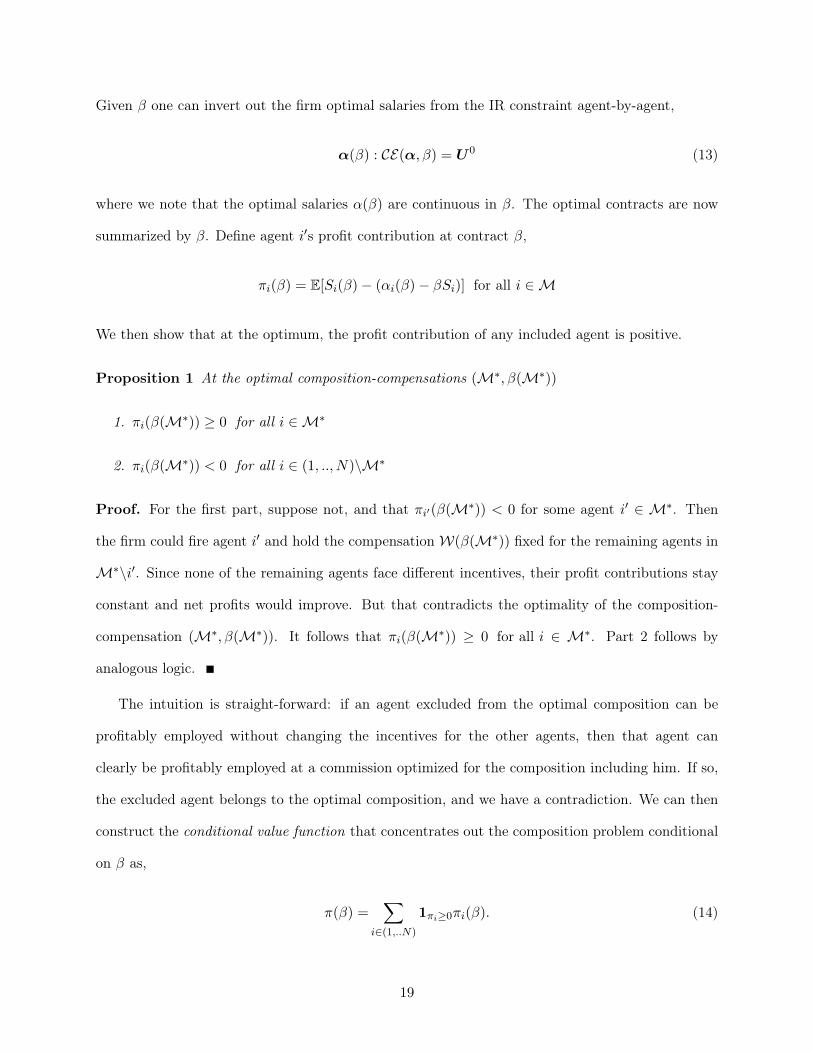
Given β one can invert out the firm optimal salaries from the IR constraint agent-by-agent,
α(β) : CE(α, β) = U0 (13)
where we note that the optimal salaries α(β) are continuous in β. The optimal contracts are now
summarized by β. Define agent i′s profit contribution at contract β,
πi(β) = E[Si(β)− (αi(β)− βSi)] for all i ∈M
We then show that at the optimum, the profit contribution of any included agent is positive.
Proposition 1 At the optimal composition-compensations (M∗, β(M∗))
1. πi(β(M∗)) ≥ 0 for all i ∈M∗
2. πi(β(M∗)) < 0 for all i ∈ (1, .., N)\M∗
Proof. For the first part, suppose not, and that πi′(β(M∗)) < 0 for some agent i′ ∈ M∗. Then
the firm could fire agent i′ and hold the compensation W(β(M∗)) fixed for the remaining agents in
M∗\i′. Since none of the remaining agents face different incentives, their profit contributions stay
constant and net profits would improve. But that contradicts the optimality of the composition-
compensation (M∗, β(M∗)). It follows that πi(β(M∗)) ≥ 0 for all i ∈ M∗. Part 2 follows by
analogous logic.
The intuition is straight-forward: if an agent excluded from the optimal composition can be
profitably employed without changing the incentives for the other agents, then that agent can
clearly be profitably employed at a commission optimized for the composition including him. If so,
the excluded agent belongs to the optimal composition, and we have a contradiction. We can then
construct the conditional value function that concentrates out the composition problem conditional
on β as,
π(β) =∑
i∈(1,..N)
1πi≥0πi(β). (14)
19

The concentrated value function sums the profit contributions of the agents that are retained in
the optimal composition conditional on β. Since the composition problem conditional on β involves
integer optimization, one may suspect the conditional value function is discontinuous, precluding a
smooth search over β. We now prove the following useful property of the conditional value function:
Proposition 2 The conditional value function π(β) is continuous in β.
Proof. Both the expectation of the sales process in Equation (4) and the concentrated salaries in
Equation (13) are continuous functions of β, so it follows that the πi(β) is continuous in β for all
i ∈ (1, .., N). The profit contribution of any agent i to π(β) is the upper envelope of two continuous
functions of β, that is max0, πi(β)], which is itself continuous. Finally, for any β, π(β) is the sum
of continuous functions, and is therefore itself also continuous.
4.1 Algorithm
The results above give us the solution algorithm:
1. For a given β, calculate πi(β) for all i ∈ (1, .., N).
2. Search the conditional value function (14) over [0, 1] for the optimal β∗.
At β∗, the optimal composition is i : πi(β∗) ≥ 0, i ∈ (1, .., N). The algorithm reduces the joint
problem to a search of a continuous function over a compact set, which is a standard optimization
problem. Utilizing this characterization enables us to reduce the problem to a unidimensional search
over β ∈ [0, 1], rather than a combinatorial search over the the space of 2N compositions. For N
moderately large, this approach can yield a significant improvement in terms of computational
time. Note that π(β) is continuous, piecewise differentiable, and not generally globally concave. We
provide some illustrations of its properties for various sizes of N in the appendix.
5 Empirical Application
Our data come from the direct selling arm of the sales-force division of a large contact lens manu-
facturer in the US (we cannot reveal the name of the manufacturer due to confidentiality reasons).
20
These data were used in Misra and Nair (2001), and some of the description in this section partially
borrows from that paper. Contact lenses are primarily sold via prescriptions to consumers from cer-
tified physicians. Importantly, industry observers and casual empiricism suggests that there is little
or no seasonality in the underlying demand for the product. The manufacturer employs a direct
salesforce in the U.S. to advertise and sell its product to physicians (also referred to as “clients”),
who are the source of demand origination. The data consist of records of direct orders made from
each doctor’s office via a online ordering system, and have the advantage of tracking the timing and
origin of sales precisely. Agents are assigned their own, non-overlapping, geographic territories, and
are paid according to a nonlinear period-dependent compensation schedule. Pricing issues play an
insignificant role for output since the salesperson has no control over the pricing decision and price
levels remained fairly stable during the period for which we have data. The compensation schedule
for the agents involves salaries, quotas and ceilings. Commissions are earned on any sales exceeding
quota and below the ceiling. The salary is paid monthly, and the commission, if any, is paid out at
the end of the quarter. The sales on which the output-based compensation is earned are reset every
quarter. Additionally, the quota may be updated at end of every quarter depending on the agent’s
performance (“ratcheting”). Our data includes the history of compensation profiles and payments
for every sales-agent, and monthly sales at the client-level for each of these sales-agents for a period
of about 3 years (38 months).
The firm in question has over 15,000 SKU-s (Stock Keeping Units) of the product. The prod-
uct portfolio reflects the large diversity in patient profiles (e.g. age, incidence of astigmatism,
nearsightedness, farsightedness etc.), patient needs (e.g. daily, disposable etc.) and contact lens
characteristics (e.g. hydrogel, silicone-hydrogel etc.). The product portfolio of the firm features new
product introductions and line extensions reflecting the large investments in R&D and testing in the
industry. The role of the sales-agent is partly informative, by providing the doctor with updated
information about new products available in the product-line, and by suggesting SKU-s that would
best match the needs of the patient profiles currently faced by the doctor. The sales-agent also
plays a persuasive role by showcasing the quality of the firm’s SKU-s relative to that of competi-
21

tors. While agent’s frequency of visiting doctors is monitored by the firm, the extent to which he
“promotes” the product once inside the doctor’s office cannot be monitored or contracted upon. In
addition, while visits can be tracked, whether a face-to-face interaction with a doctor occurs during
a visit in within the agent’s control (e.g., an unmotivated agent may simply “punch in” with the
receptionist, which counts as a visit, but is low on effort).4
Misra and Nair (2011) used these data to estimate the underlying parameters of the agent’s
preferences and environments using a structural dynamic model of forward-looking agents. For our
simulations, we use some parameters from that paper, while some are calibrated. We provide a
short overview of the model and estimation below, noting differences from their analysis in passing.
5.1 The Model for Sales-Agents
The compensation scheme involves a salary, αt, paid in month t, as well as a commission on sales,
βt. The sales on which the commission is accrued is reset every R months. The commission βt is
earned when total sales over the sales-cycle, Qt, exceeds a quota, at, and falls below a ceiling bt. No
commissions are earned beyond bt. Let It denote the months since the beginning of the sales-cycle,
and let qt denote the agent’s sales in month t. Further, let χt be an indicator for whether the agent
stays with the firm. χt = 0 indicates the agent has left the focal company and is pursuing his
outside option. Assume that once the agent leaves the firm, he cannot be hired back (i.e. χt = 0
is an absorbing state). The total sales, Qt, the current quota, at, the months since the beginning
of the cycle It, and his employment status χt are the state variables for the agent’s problem. We
collect these in a vector st = Qt, at, It, χt, and collect the observed parameters of his compensation
scheme in a vector Ψ = α, β .We will use the data in combination with a model of agent behavior
to back out the parameters indexing agent’s types. The results in this paper are obtained taking
these parameters as given.
The index i for agent is suppressed in what follows below. At the beginning of each period,
we assume the agent observes his state, and chooses to exert effort et. Based on his effort, sales qt4The firm does not believe that sales-visits are the right measure of effort. Even though sales-calls are observed,
the firm specifies compensation based on sales, not calls.
22

are realized at the end of the period. Sales qt is assumed to be a stochastic, increasing function of
effort, e and a demand shock, εt, qt = q (εt, e) . The agent’s utility is derived from his compensation,
which is determined by the incentive scheme. We write the agent’s monthly wealth from the firm
as, Wt = W (st, et, εt;µ,Ψ) and the cost function as de2t2 , where d is to be estimated. We assume
that agents are risk-averse, and that conditional on χt = 1, their per-period utility function is,
ut = u (Qt, at, It, χt = 1) = E [Wt]− r × var [Wt]−de2t2
(15)
Here, r is a parameter indexing the agent’s risk aversion, and the expectation and variance of
wealth is taken with respect to the demand shocks, εt. In the case of a salary + piece-rate of the
type considered before, equation (15) collapses to exactly the form denoted in equation (5) for the
certainty equivalent. We can thus interpret equation (15) as the nonlinear-contract analogue to the
certainty equivalent of the agent under a linear commission. The payoff from leaving the focal firm
and pursuing the outside option is normalized to U0, i.e., ut = u (Qt, at, It, χt = 0) = U0.
In this model, sales are assumed to be generated as a function of the agent’s effort, which is
chosen by the agent maximizing his present discounted payoffs subject to the transition of the state
variables. The first state variable, total sales, is augmented by the realized sales each month, except
at the end of the quarter, when the agent begins with a fresh sales schedule, i.e.,
Qt+1 =
Qt + qt if It < R
0 if It = R(16)
For the second state variable, quota, we estimate a semi-parametric transition function that relates
the updated quota to the current quota and the performance of the agent relative to that quota in
the current quarter,
at+1 =
at if It < R∑K
k=1 θkΓ (at, Qt + qt) + vt+1 if It = R(17)
In above, the new quota is allowed to depend flexibly on at and Qt + qt, via a Korder polynomial
basis indexed by parameters, θk to capture in a reduced-form way, the manager’s policy for updating
agent’s quotas. The term vt+1 is an i.i.d. random variate which is unobserved by the agent in
23

month t. The distribution of vt+1 is denoted Gv (.) , and will be estimated from the data. The
transition of the third state variable, months since the beginning of the quarter, is deterministic,
augmented by one with the passage of calendar time within the quarter. Finally, the agent’s
employment status in (t+ 1), depends on whether he decides to leave the firm in period t. Given
the above state-transitions, we can write the agent’s problem as choosing effort to maximize the
present-discounted value of utility each period, where future utilities are discounted by the factor,
ρ. We collect all the parameters describing the agent’s preferences and transitions in a vector Ω =
µ, d, r,Gε (.) ,Gv (.) , θk,k=1,..,K. In month It < R, the agent’s present-discounted utility under the
optimal effort policy can be represented by a value function that satisfies the following Bellman
equation,
V (Qt, at, It, χt; Ω,Ψ) =
maxχt+1∈(0,1),e>0
u (Qt, at, It, χt, e; Ω,Ψ)
+ρ´ε V (Qt+1 = Q (Qt, q (εt, e)) , at+1 = at, It + 1, χt+1; Ω,Ψ) f (εt) dεt
(18)
Similarly, in month It = R, the Bellman equation determining effort is,
V (Qt, at, R, χt; Ω,Ψ) =
maxχt+1∈(0,1),e>0
u (Qt, at, R, χt, e; Ω,Ψ)
+ρ´v
´ε V (Qt+1 = 0, at+1 = a (Qt, q (εt, e) , at, vt+1) , 1, χt+1; Ω,Ψ)
× f (εt)φ (vt+1) dεtdvt+1
(19)
Conditional on staying with the firm, the optimal effort in period t, et = e (st; Ω,Ψ) maximizes the
value function,
e (st; Ω,Ψ) = arg maxe>0
V (st; Ω,Ψ) (20)
The agent stays with the firm if the value from employment is positive, i.e.,
χt+1 = 1 if maxe>0V (st; Ω,Ψ) > 0
24
This completes the specification of the model specifying the agent’s behavior under the plan that
generated the data. Given this set-up, the structural parameters describing an agent Ω, are esti-
mated in two steps.
Estimation
First, we recognize that once effort, et is estimated, we can treat hidden actions as known. The
theory implies st is the state vector for the agent’s optimal dynamic effort choice. We can use the
theory, combined with dynamic programming to solve for the optimal policy function e∗ (st; Ω), given
a guess of the parameters Ω. Because et is known, we can then use et = e∗ (st; Ω) as a second-stage
estimating equation to recover Ω. Misra and Nair (2011) implement this approach agent-by-agent
to recover Ω for each agent separately. They exploit panel-data available at the client-level for each
agent to avoid imposing cross-agent restrictions, thereby obtaining a semi-parametric distribution
of the types in the firm.
The question remains how the effort policy, et = e (st) can be obtained? The intuition used
in Misra and Nair is to exploit the nonlinearity of the contract combined with panel data for
identification. The nonlinearity implies the history of output within a compensation horizon is
relevant for the current effort decision, because it affects the shadow cost of working today. Thus,
effort is time varying, and dynamically adjusted. The relationship between current output and
history is observed in the data. This relationship will pin down hidden effort. Intuitively, the
path of output within the compensation cycle is informative of effort. We refer the reader to that
paper for further details of estimation and identification.5 For the counterfactuals in this paper,
we need estimates ofh, k, d, r, U0,Gε (.)
. Here, we assume that Gε (.) ∼ N
(0, σ2
). So, we need
θ ≡h, k, d, r, U0, σ
. We use the same parameters from Misra and Nair for these, estimating σ
from imposing the normality assumption of the recovered demand-side errors from the model. The
parameter, k, is not estimated in Misra-Nair. Here, we exploit additional data not used in that
paper on the number of calls made by each agent i to a client j in month t, which we denote as, kijt.5See also, Steenburgh (2008) and Larkin (2010) who note that effort is affected by how far away the agent is from
his quota.
25
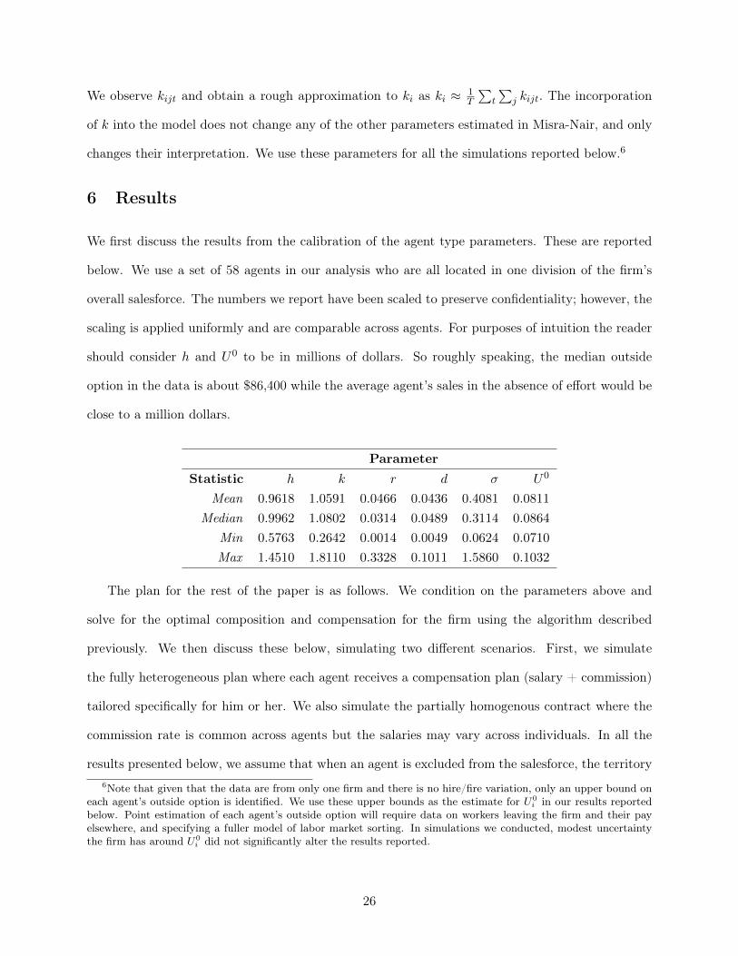
We observe kijt and obtain a rough approximation to ki as ki ≈ 1T
∑t
∑j kijt. The incorporation
of k into the model does not change any of the other parameters estimated in Misra-Nair, and only
changes their interpretation. We use these parameters for all the simulations reported below.6
6 Results
We first discuss the results from the calibration of the agent type parameters. These are reported
below. We use a set of 58 agents in our analysis who are all located in one division of the firm’s
overall salesforce. The numbers we report have been scaled to preserve confidentiality; however, the
scaling is applied uniformly and are comparable across agents. For purposes of intuition the reader
should consider h and U0 to be in millions of dollars. So roughly speaking, the median outside
option in the data is about $86,400 while the average agent’s sales in the absence of effort would be
close to a million dollars.
ParameterStatistic h k r d σ U0
Mean 0.9618 1.0591 0.0466 0.0436 0.4081 0.0811
Median 0.9962 1.0802 0.0314 0.0489 0.3114 0.0864
Min 0.5763 0.2642 0.0014 0.0049 0.0624 0.0710
Max 1.4510 1.8110 0.3328 0.1011 1.5860 0.1032
The plan for the rest of the paper is as follows. We condition on the parameters above and
solve for the optimal composition and compensation for the firm using the algorithm described
previously. We then discuss these below, simulating two different scenarios. First, we simulate
the fully heterogeneous plan where each agent receives a compensation plan (salary + commission)
tailored specifically for him or her. We also simulate the partially homogenous contract where the
commission rate is common across agents but the salaries may vary across individuals. In all the
results presented below, we assume that when an agent is excluded from the salesforce, the territory6Note that given that the data are from only one firm and there is no hire/fire variation, only an upper bound on
each agent’s outside option is identified. We use these upper bounds as the estimate for U0i in our results reported
below. Point estimation of each agent’s outside option will require data on workers leaving the firm and their payelsewhere, and specifying a fuller model of labor market sorting. In simulations we conducted, modest uncertaintythe firm has around U0
i did not significantly alter the results reported.
26

provides revenues equal to τh with τ = 0.95, and h is the intercept in the output equation. This
assumption reflects the fact that even if a territory is vacated, sales would still accrue on account of
the brand or because the firm might use some other (less efficient) selling approach like advertising.
We also explored alternative assumptions (e.g. τ = 0 and τ = 1); these results are available from
the authors upon request. Qualitatively, the results obtained were similar to those presented below.
Below we organize our discussion by presenting details of the optimal composition chosen by the
firm under these plans, and then present details of effort, sales and profits.
6.1 Composition
We start with the fully heterogeneous plan as a benchmark. We find all agents have positive
profit contributions when plans can be fully tailored to their types. Consequently, the optimal
configuration under the fully heterogeneous plan is to retain all agents (the “status quo”). This is
not surprising as noted in our 3-agent simulation previously.
Simulating the partially heterogeneous compensation plans, we find the optimal composition
in this salesforce would involve letting go of seven salespeople. It is interesting to investigate the
characteristics of the agents who are dropped and to relate it to that of the agent pool as a whole.
In Figure (1) we plot the joint distribution of the primitive agent typesh, k, d, r, U0, σ
for all
agents at the firm. The marginal densities of each parameter across agents is presented across
the diagonal. Each point in the various two-way plots along the off-diagonals is an agent, and
each two-way shows a scatter-plot of a particular pair of agents types, across the agent pool. For
instance, plot [4,1] in Figure (1) shows a scatter-plot of risk aversion (r) versus the cost of effort
(d) across all agents in the pool. Plot [1,4] is symmetric and shows a scatter-plot of cost of effort
(d) versus risk aversion (r). The seven agents who are not included in the optimal composition are
represented by non-solid symbols, highlighted in red. For instance, we see that one of the dropped
agents, represented as an “o”, has a high risk aversion (1st row), an average level of sales-territory
variance (2nd row), an average level of productivity (3rd row), a low cost of effort (4th row), a low
outside option (5th row), and a lower than average base level of sales (last row). This agent has a
low cost of effort. However, his high risk aversion, his lower outside option, as well as his fit relative
27

to the distribution of these characteristics across the rest of the agents, implies he is not included in
the preferred composition. Figure (1) illustrates the importance of multidimensional heterogeneity
in the composition-compensation tradeoff facing the principal, and emphasizes the importance of
allowing for rich heterogeneity in empirical incentive settings.
In Figure 2, we plot the location of these salespeople on the empirical marginal densities of the
profitability and sales across sales-agents. What is clear from Figure 2 is that there is no a priori
predictable pattern in the location of these agents. In some cases, the agents lie at the tail end of the
densities, though this does not hold generally. Further, the dropped agents are not uniformly at the
bottom of the heap in terms of expected sales or profit contribution under the fully heterogeneous
plan. For example, #33, one of the dropped agents, has expected sales of $1.70MM under the fully
heterogeneous plan which would place him/her in the top decile of agents in terms of sales. In
addition, he/she is also in the top decile across agents in terms of profitability. However, in his/her
case the variance of sales is the highest in the firm, and this creates a large distortion in the contract
via the effect it induced on the optimal commission rate (β). Not including this agent allows the firm
to improve the contract terms of other agents thereby increasing profits. Other agents are similarly
not included on account of some other externality that impacted the compensation contract.
Figure 1 and 2 accentuates the difficulties of ranking agents as desirable or not on the basis of
a single type-based metric and the need for a theory of value to assess sales-agents.
6.2 Compensation
We now discuss the optimal compensation implied for the firm under the optimal composition. We
compare the fully heterogeneous plan to the partially homogenous plans with and without optimizing
composition. Figure (3) plots the density of optimal commission rates under the fully heterogeneous
plan along with those for the partially homogenous plans. The solid vertical lines are drawn at
the common commission rate for the homogenous plans, with the blue vertical line corresponding
to optimizing composition and the black corresponding to not optimizing composition. Looking at
Figure (3), we see that the commission rates vary significantly across the sales-agents under the fully
heterogeneous plans, going as high as 2.5% for some agents (median commission of about 1.2%).
28

Figure 1: Joint Distribution of Characteristics of Agents who are Retained and Dropped from Firmunder Partially Homogenous Plans
r
500 1500 0.02 0.06 0.10 0.6 1.0 1.4
0.00
0.10
0.20
0.30
500
1000
s
k
0.5
1.0
1.5
0.02
0.06
0.10
d
u0
0.07
00.
085
0.10
0
0.00 0.15 0.30
0.6
1.0
1.4
0.5 1.5 0.070 0.090
h
29
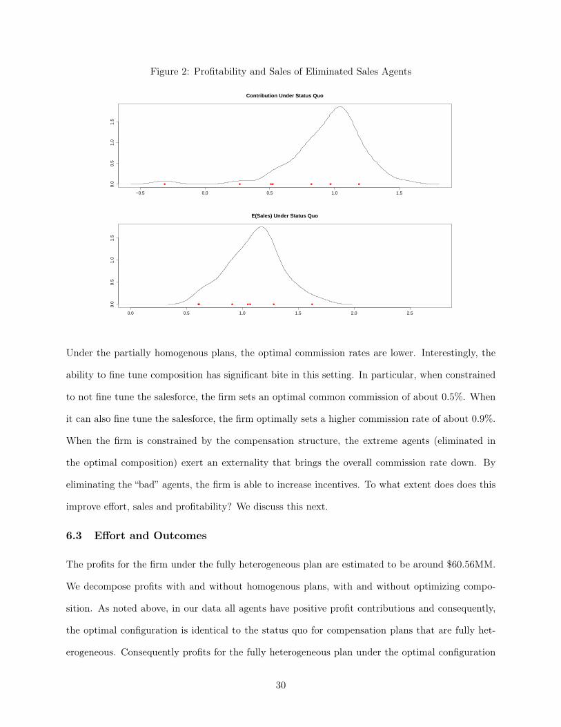
Figure 2: Profitability and Sales of Eliminated Sales Agents
−0.5 0.0 0.5 1.0 1.5
0.0
0.5
1.0
1.5
Contribution Under Status Quo
0.0 0.5 1.0 1.5 2.0 2.5
0.0
0.5
1.0
1.5
E(Sales) Under Status Quo
Under the partially homogenous plans, the optimal commission rates are lower. Interestingly, the
ability to fine tune composition has significant bite in this setting. In particular, when constrained
to not fine tune the salesforce, the firm sets an optimal common commission of about 0.5%. When
it can also fine tune the salesforce, the firm optimally sets a higher commission rate of about 0.9%.
When the firm is constrained by the compensation structure, the extreme agents (eliminated in
the optimal composition) exert an externality that brings the overall commission rate down. By
eliminating the “bad” agents, the firm is able to increase incentives. To what extent does does this
improve effort, sales and profitability? We discuss this next.
6.3 Effort and Outcomes
The profits for the firm under the fully heterogeneous plan are estimated to be around $60.56MM.
We decompose profits with and without homogenous plans, with and without optimizing compo-
sition. As noted above, in our data all agents have positive profit contributions and consequently,
the optimal configuration is identical to the status quo for compensation plans that are fully het-
erogeneous. Consequently profits for the fully heterogeneous plan under the optimal configuration
30
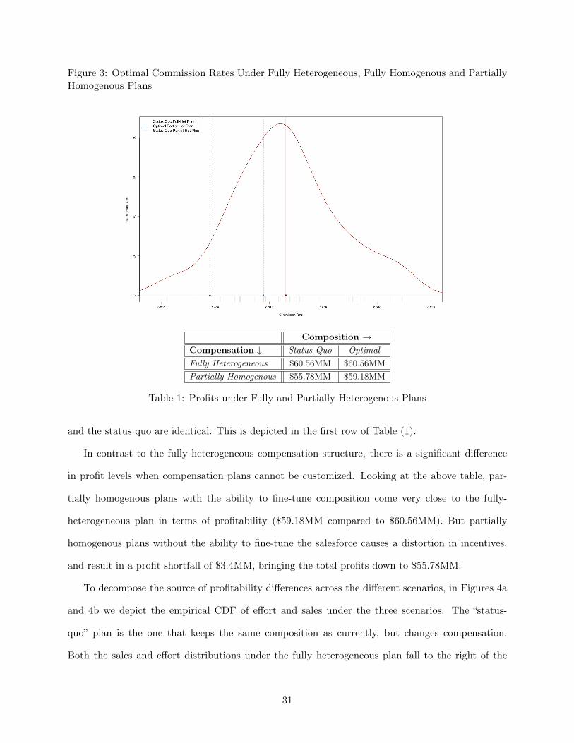
Figure 3: Optimal Commission Rates Under Fully Heterogeneous, Fully Homogenous and PartiallyHomogenous Plans
Composition →Compensation ↓ Status Quo OptimalFully Heterogeneous $60.56MM $60.56MMPartially Homogenous $55.78MM $59.18MM
Table 1: Profits under Fully and Partially Heterogenous Plans
and the status quo are identical. This is depicted in the first row of Table (1).
In contrast to the fully heterogeneous compensation structure, there is a significant difference
in profit levels when compensation plans cannot be customized. Looking at the above table, par-
tially homogenous plans with the ability to fine-tune composition come very close to the fully-
heterogeneous plan in terms of profitability ($59.18MM compared to $60.56MM). But partially
homogenous plans without the ability to fine-tune the salesforce causes a distortion in incentives,
and result in a profit shortfall of $3.4MM, bringing the total profits down to $55.78MM.
To decompose the source of profitability differences across the different scenarios, in Figures 4a
and 4b we depict the empirical CDF of effort and sales under the three scenarios. The “status-
quo” plan is the one that keeps the same composition as currently, but changes compensation.
Both the sales and effort distributions under the fully heterogeneous plan fall to the right of the
31
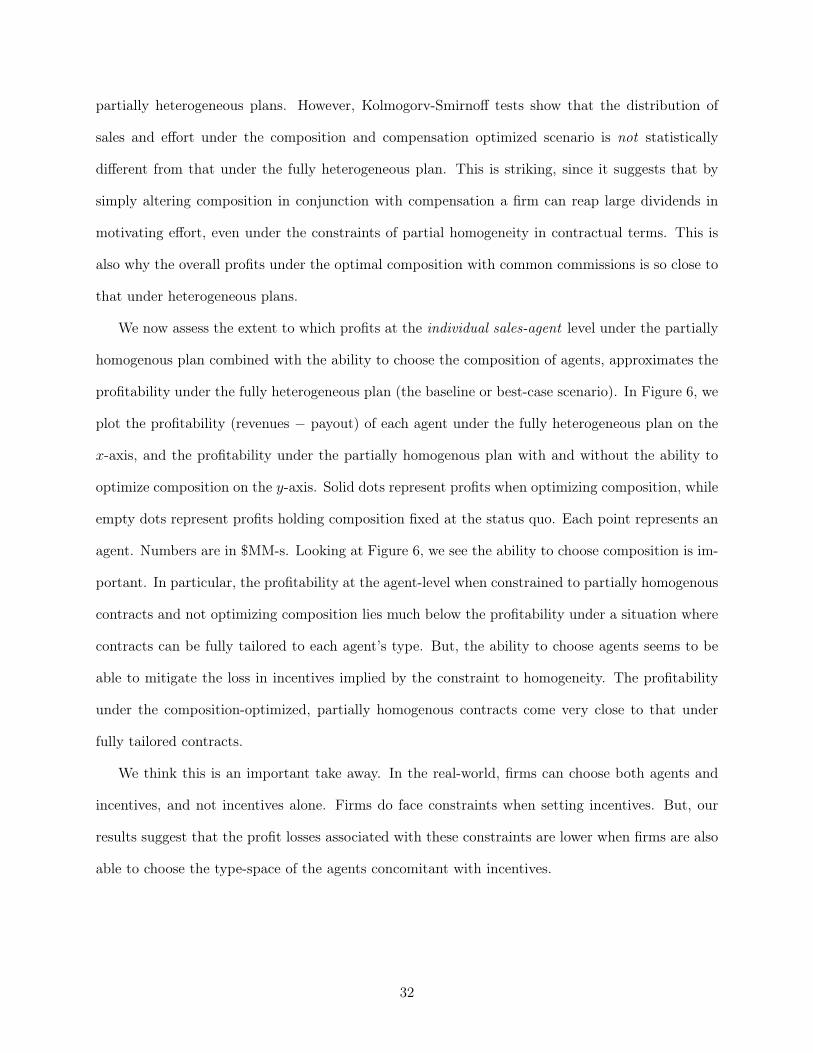
partially heterogeneous plans. However, Kolmogorv-Smirnoff tests show that the distribution of
sales and effort under the composition and compensation optimized scenario is not statistically
different from that under the fully heterogeneous plan. This is striking, since it suggests that by
simply altering composition in conjunction with compensation a firm can reap large dividends in
motivating effort, even under the constraints of partial homogeneity in contractual terms. This is
also why the overall profits under the optimal composition with common commissions is so close to
that under heterogeneous plans.
We now assess the extent to which profits at the individual sales-agent level under the partially
homogenous plan combined with the ability to choose the composition of agents, approximates the
profitability under the fully heterogeneous plan (the baseline or best-case scenario). In Figure 6, we
plot the profitability (revenues − payout) of each agent under the fully heterogeneous plan on the
x-axis, and the profitability under the partially homogenous plan with and without the ability to
optimize composition on the y-axis. Solid dots represent profits when optimizing composition, while
empty dots represent profits holding composition fixed at the status quo. Each point represents an
agent. Numbers are in $MM-s. Looking at Figure 6, we see the ability to choose composition is im-
portant. In particular, the profitability at the agent-level when constrained to partially homogenous
contracts and not optimizing composition lies much below the profitability under a situation where
contracts can be fully tailored to each agent’s type. But, the ability to choose agents seems to be
able to mitigate the loss in incentives implied by the constraint to homogeneity. The profitability
under the composition-optimized, partially homogenous contracts come very close to that under
fully tailored contracts.
We think this is an important take away. In the real-world, firms can choose both agents and
incentives, and not incentives alone. Firms do face constraints when setting incentives. But, our
results suggest that the profit losses associated with these constraints are lower when firms are also
able to choose the type-space of the agents concomitant with incentives.
32
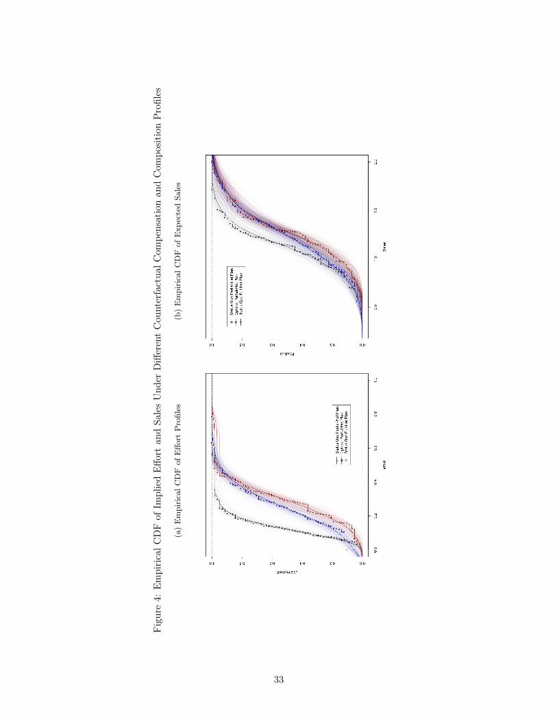
Figure4:
EmpiricalC
DFof
ImpliedEffo
rtan
dSa
lesUnd
erDifferentCou
nterfactua
lCom
pensationan
dCom
position
Profiles
(a)EmpiricalC
DFof
Effo
rtProfiles
(b)EmpiricalC
DFof
Exp
ectedSa
les
33

Mechanism
The question remains what is the mechanism that enables the firm to come close to the fully
heterogeneous plan when it optimizes the composition of its agents? The intuition is straightforward.
When constrained to set a homogenous plan, a firm can do much better if the agents it has to
incentivize are more homogenous. Consider an extreme case where the firm could find as many
agents of any type for filling its positions (no search costs for labor). Then, the firm would first pick
the agent from who it could obtain the highest profit (output − payout) under the fully tailored
heterogenous contract. It would then fill the N available positions with N replications of that agent.
Then, the uniform commission it charges for the salesforce as a whole will be optimal for every agent
in the firm. Thus, heterogeneity involves costs. In this sense, an increase in heterogeneity has two
roles for a firm constrained to uniform contracts. On the one hand, it increases the chance that
high quality agents are in the firm (a positive). But on the other hand, it also increases the level
of contractual externalities (a negative). The optimal composition has to balance these competing
forces.
To see this more formally, consider a firm that has demand for two agents, which it can fill with
A or B type agents. Let Θ index type and suppose typeA-s generate more profit than B-s when
employed at their individually optimal contracts:
ΘA 6= ΘB and E [π (A)] > E [π (B)]
Then, all things held equal, the firm would prefer composition A,A over B,B,
E [π (A,A)] > E [π (B,B)]
Now suppose that types are such that though ΘA 6= ΘB, A-s and B-s generate the same expected
profit when employed at their individually optimal contracts,
ΘA 6= ΘB but E [π (A)] = E [π (B)]
34

Then, even though individual profits are the same, the firm would prefer to have the composition
A,A or B,B over A,B, because composition A,B generates contractual externalities,
E [π (A,A)] = E [π (B,B)] > E [π (A,B)]
It is in this sense that the firm has a preference for heterogeneity reduction. Optimal contracting
requires the principal to satisfy both incentive rationality and incentive compatibility constraints for
its chosen agents. Allowing for agent-specific salaries allows the firm to satisfy incentive rationality
for the agents it wants to retain. But the constraint to a common commission implies that incentive
compatibility becomes harder to satisfy when the agent pool becomes more heterogeneous. Hence,
a firm that can also choose the pool prefers one that is relatively more homogenous, ceteris paribus.
To empirically assess this intuition, we compute two measures of the spread in the type distribu-
tion of the salesforce under the optimal partially homogenous contacts with and without the ability
to choose agents. Assessing the dispersion in types is complicated by the fact that the type-space
is multidimensional. We can separately compute the variance-covariance matrix of types in the
salesforce under the two scenarios. To compute a single metric that summarizes the distribution of
types, we define a measure of spread, dM, as the trace of the variance covariance matrix of agent
characteristics,7
dM = tr (ΣM) (21)
We find that dMStatusQuo = 78, 891.6, and dMOptimal = 51, 921.8, where dMStatusQuo is the trace
under the optimally chosen partially homogenous plan while retaining all agents in the firm, and
dMOptimal is the trace under an optimally chosen partially homogenous plan while jointly optimizing
the set of agents retained in the firm. We see that the optimal configuration involves about 34.2%
reduction in heterogeneity. As another metric, we use dM = det (ΣM). The determinant can be
interpreted as measuring the volume of the parallelepiped spanned by the vectors of agent types.
To the extent the volume is lower, the spread in types may roughly be interpreted as lesser. We
find that the determinant based measure of spread shows a 80.8% decline when the firm can pick7The trace of a matrix is the sum of its diagonals.
35
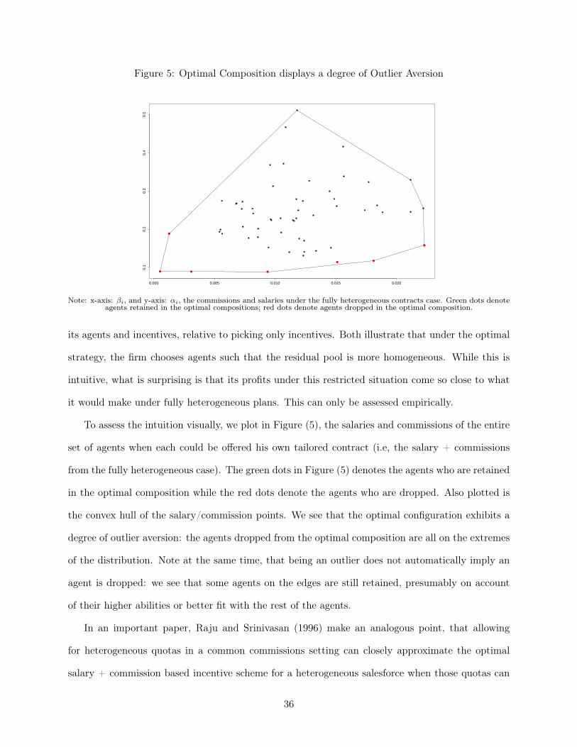
Figure 5: Optimal Composition displays a degree of Outlier Aversion
0.000 0.005 0.010 0.015 0.020
0.1
0.2
0.3
0.4
0.5
Note: x-axis: βi, and y-axis: αi, the commissions and salaries under the fully heterogeneous contracts case. Green dots denoteagents retained in the optimal compositions; red dots denote agents dropped in the optimal composition.
its agents and incentives, relative to picking only incentives. Both illustrate that under the optimal
strategy, the firm chooses agents such that the residual pool is more homogeneous. While this is
intuitive, what is surprising is that its profits under this restricted situation come so close to what
it would make under fully heterogeneous plans. This can only be assessed empirically.
To assess the intuition visually, we plot in Figure (5), the salaries and commissions of the entire
set of agents when each could be offered his own tailored contract (i.e, the salary + commissions
from the fully heterogeneous case). The green dots in Figure (5) denotes the agents who are retained
in the optimal composition while the red dots denote the agents who are dropped. Also plotted is
the convex hull of the salary/commission points. We see that the optimal configuration exhibits a
degree of outlier aversion: the agents dropped from the optimal composition are all on the extremes
of the distribution. Note at the same time, that being an outlier does not automatically imply an
agent is dropped: we see that some agents on the edges are still retained, presumably on account
of their higher abilities or better fit with the rest of the agents.
In an important paper, Raju and Srinivasan (1996) make an analogous point, that allowing
for heterogeneous quotas in a common commissions setting can closely approximate the optimal
salary + commission based incentive scheme for a heterogeneous salesforce when those quotas can
36

themselves reflect agent specific differences. Our point is analogous, that a firm constrained to a
homogenous slope on its incentive contract can come very close to the optimum by picking the
region of agent-types that it wants to retain. However, the mechanism we suggest is different. Raju
and Srinivasan (1996) suggest addressing the problem of providing incentives to a heterogeneous
salesforce by allowing for additional heterogeneity in contract terms. We suggest addressing the
problem of setting incentives to a heterogeneous pool of agents by making the salesforce more
homogenous. In another contribution, Lal and Staelin (1986) and Rao (1990) show that a firm
facing a heterogeneous salesforce can tailor incentives to the distribution of types it faces by offering
a menu of salesforce plans. Their approach uses agents’ self-selection into plans as the mechanism
for managing heterogeneity, and requires the firm to offer a menu of contracts taking the salesforce
composition as given. In our model, the firm offers only one contract to an agent, but chooses which
agent to make attractive contracts to (thus, the margin of choice for agents in our model is not over
contracts but over whether to stay in the firm or leave). Our model endogenizes the salesforce’s
composition and may be seen as applying to contexts where offering a menu of plans to employees
to choose from is not feasible, or desired. We think the three perspectives outlined above for the
practical management of heterogeneity in real-world settings are complementary to each other. In
the section below, we discuss the latter mechanism further.
6.4 Sorting Agents into Divisions
We now discuss whether we can further improve the management of heterogeneity in the firm by
sorting agents into divisions. We consider a salesforce architecture in which the firm creates |J |
divisions, and assigns each agent it retains to one of the |J | divisions. The divisions correspond to
different compensation profiles. We allow each division to have its own commission, but require that
all agents within a division are given the same commission. Salaries are allowed to be heterogeneous
as before. Such architectures are commonly observed in the real-world. For instance, salesagents
targeting large “key accounts” may be assigned into a division which offers more incentive pay, while
those targeting smaller clients may be in a division that offers more salary than commission. Or
alternatively, salesagents targeting urban versus rural clients may be in two different divisions each
37
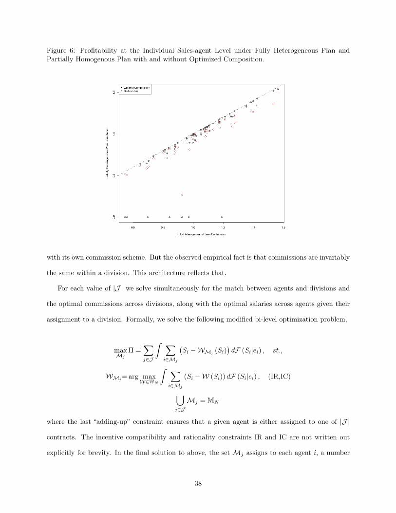
Figure 6: Profitability at the Individual Sales-agent Level under Fully Heterogeneous Plan andPartially Homogenous Plan with and without Optimized Composition.
with its own commission scheme. But the observed empirical fact is that commissions are invariably
the same within a division. This architecture reflects that.
For each value of |J | we solve simultaneously for the match between agents and divisions and
the optimal commissions across divisions, along with the optimal salaries across agents given their
assignment to a division. Formally, we solve the following modified bi-level optimization problem,
maxMj
Π =∑j∈J
ˆ ∑i∈Mj
(Si −WMj (Si)
)dF (Si|ei) , st.,
WMj = arg maxW∈WN
ˆ ∑i∈Mj
(Si −W (Si)) dF (Si|ei) , (IR,IC)
⋃j∈JMj = MN
where the last “adding-up” constraint ensures that a given agent is either assigned to one of |J |
contracts. The incentive compatibility and rationality constraints IR and IC are not written out
explicitly for brevity. In the final solution to above, the setMj assigns to each agent i, a number
38

0, 1, .., j, .., |J |, where 0 implies the agent is dropped from the firm, and j > 0 implies the agent
is assigned to division j with wage contract WMj . Our goal is to assess empirically how many
divisions (|J |) are required to fully span the heterogeneity and to come close to the profits under
the fully heterogeneous case. Additionally, we want to assess the extent to which the ability to
choose agents interacts with this mechanism for managing heterogeneity.
In Figure (7) we report on the results in which we simulated the profits to the firm from creating
upto |J | = 6 divisions. The x-axis of Figure (7) plots the number of divisions considered (|J |). The
y-axis of Figure (7) plots the total profits to the firm for each |J |. Each point corresponds to solving
the modified bi-level problem above for the corresponding value of |J |. The green-line shows the
profit profile in which we allow the firm to sort agents into divisions, but do not allow the firm to
optimize the composition (i.e., in the bi-level program above, we do not allow j = 0 as an option).
The blue-line in the figure shows the profit profile in which the allow the firm to sort agents into
divisions and allow the firm to optimize the composition as described above. The difference in the
profits under the blue versus the green lines indicates the extent to which composition choice adds
to profitability over and above the ability to sort agents into divisions.
We first discuss the situation where we allow the firm to sort agents into divisions but do not
allow the firm to choose composition. The top horizontal line in Figure (7) represents a profit
of $60.56M, the maximum profit possible under the fully heterogeneous contract (see Table (1)).
Looking at the green-line in Figure (7), we see that even without the ability to choose composition,
the firm is able to come very close to this value with as less as 6 divisions. Even two divisions
do a remarkably good job of managing heterogeneous incentives − profits under the green-line for
the 2-division case are more than $59M. Thus, one empirical take-away is that a small amount of
variation in contract terms seems to be sufficient to manage a large amount of heterogeneity in the
firm, at least in the context of these estimates.
We now discuss the situation where we allow the firm to sort agents into divisions and to optimize
its composition. We see the results are similar to the previous case, but the firm is able to achieve
a higher level of profit gains with fewer divisions (the blue-line is always above the green-line).
39

Thus, the ability to choose composition has bite even when one allows for sorting into divisions.
With |J | = 6 divisions, we find the firm ends up dropping 5 agents from the optimal composition
(compared to 6 agents with only one division). Thus, allowing for sorting does not automatically
imply that composition choice is not needed − the right perspective is that sorting and composition-
choice are two strategies to manage heterogeneity, and when used in combination, unlock powerful
complementaries in the provision of firm-wide incentives.
Finally, we show that heterogeneity reduction plays a role in improving profitability with sorting.
In Figure (8) we plot the log-distortion implied by the divisions against the number of contracts
offered. The distortion metric is simply a way to summarize the average heterogeneity within a
division. It captures the mean squared deviation from the average salesperson across divisions.
Formally, let θij denote the 6×1 vector of characteristics for agent i allocated to division j > 0 and
let θ(r)ij , r = 1, .., 6, denote the rth element of θij . Denoting Nj as the number of agents allocated to
division j, let θ(r)j =∑Nji=1 θ
(r)ij /Nj be the average value of characteristic r inside division j. We define
the distortion as,
dM = minr
1
|J |
|J |∑j=1
(θ(r)ij − θ
(r)j
)2(22)
In Figure (8), the lower line (red) corresponds to the model which allows for composition to be
optimized jointly with division-specific commissions, while the top line (blue) ignores the composi-
tion aspect. As one would expect, as more contracts are added to the compensation structure, the
distortion falls but allowing the firm to manage composition results in a more significant reduction.
In essence, with a small number of contracts, the firm finds it optimal to eliminate the outlying
agents and use the increased flexibility to better compensate those that are retained. As a result
the heterogeneity in the retained agent pool is managed much better. Ultimately, as the number
of contracts increase to match the total number of agents, the two curves would coincide. That
is, if every agent got a customized contract there would be no distortion. The broad point is that
sorting and composition choice together enable very effective management of heterogeneity even
with restricted contracts.
40
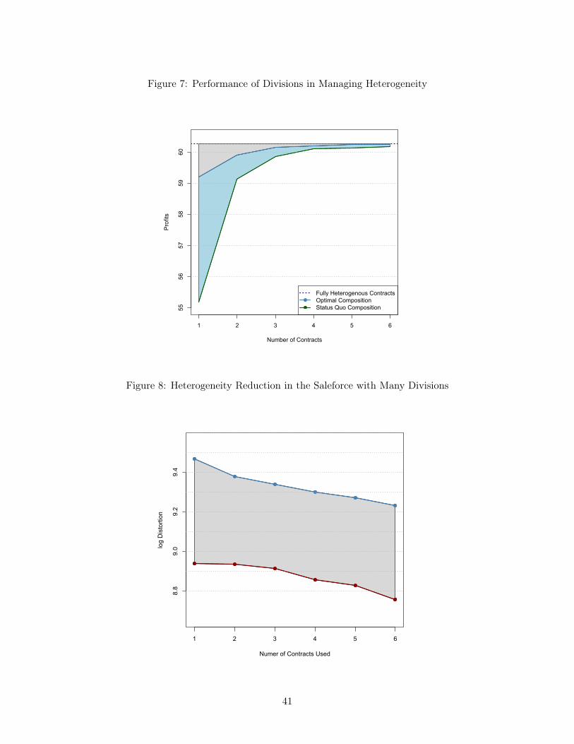
Figure 7: Performance of Divisions in Managing Heterogeneity
1 2 3 4 5 6
5556
5758
5960
Number of Contracts
Profits
Fully Heterogenous ContractsOptimal CompositionStatus Quo Composition
Figure 8: Heterogeneity Reduction in the Saleforce with Many Divisions
1 2 3 4 5 6
8.8
9.0
9.2
9.4
Numer of Contracts Used
log
Dis
torti
on
41
Discussion
We developed the above exercise under the assumption that the firm knows each agent’s type
perfectly and can sort agents into divisions based on that knowledge. As mentioned above, the
theory has emphasized an alternative mechanism in which the firm offers a menu of contracts to
all and the agent self-selects into one of the offered contracts based on his unknown type (this is
analogous to nonlinear pricing). This strategy helps manage heterogeneity when the firm does not
know types perfectly and emphasizes adverse-selection as the main difficulty in contract design,
as opposed to the moral hazard we emphasize. In practice, it is likely that both are at play in
many real-world contexts. Optimal contract design with both adverse-selection and moral hazard
is beyond the scope of this paper. In salesforce contexts, we believe the approach we have outlined
above is more realistic than self-selection contracts. First, unlike nonlinear pricing, self-selection
contracts are rarely observed in salesforce compensation (perhaps due to concerns with dynamic
signaling − if an agent chooses a contract with low commissions, he signals his type to the principal
which can be used to update his contracts in subsequent periods). The more common observation
is of salesforce divisions and of assignment of agents into divisions. Second, adverse-selection in
salesforce settings is usually addressed by monitoring, probation and training. New hires are often
placed on a salary-only probation period in which their performance is observed. The employment
offer is made full-time conditional on satisfactory performance in the probation period. New hires
are also provided significant sales training during the probation period and asked to “shadow” an
established sales-rep where real-time training is imparted and performance on the field is observed.
This monitoring helps the firm assess agent types before full-time offers are made. Thus, in our view,
for long-run salesforce composition and compensation with full-time salesagents, adverse selection
may be a second-order consideration. A limitation of our model is that it does not apply to the
interesting dynamics outlined above associated with new employee hiring and learning.
Finally, if the firm does not know types perfectly, the profits it can make when offering a menu
of divisions is strictly lower than the profits it can make when it knows types perfectly and can
assign each type to its preferred division (as in the simulations above). We reported above that
42

when types are known perfectly, firms still gain from the ability to choose composition. We interpret
this as implying that even if a menu of contracts are offered, the ability to choose agents that we
emphasize, will still have bite in terms of profits in the context of our empirical example.
6.5 Parameter Uncertainty and Robustness
A primitive assumption in our analysis is that the firm knows the agents’ types with complete
certainty. While this is a standard assumption in principal-agent models with pure moral hazard,
it poses some relevant questions for our analysis: Do the results continue to hold if the firm only
has access to “estimates” of the agents’ types? If the results are different, what are the nature and
magnitude of the differences? To answer these, we implemented extensive Monte Carlo simulations
in which the firm recognizes it has access to parameters of agent types that are estimated with error,
and maximizes an expected profit function that integrates out this estimation error.8
Under the assumption that firms acknowledge the presence of estimation error, we need a way
of incorporating the parameter uncertainty into the firm’s decision making process. We assume the
firm has access to the sampling distribution of the estimates. The firm then uses this information
to integrate out the uncertainty and maximizes expected profits. We simulate various levels of
uncertainty by perturbing the parameters we estimated. We add to each point estimate a noise
term that is normally distributed with mean zero and with standard deviations that vary so that
the effective range the firm believes each parameter can lie in goes from ±1% to as much as ±100%
of the point estimate. This corresponds to situations where is firm is able to estimate the parameter
with a high level of precision, to situations where the parameter estimates are no longer significant
at the α = 0.05 level (i.e., range contains zero). We used these perturbed parameters to compute the
expected profits faced by the firm. We then use the same optimization technology described in the
paper to compute the optimal compensation and composition under these simulated scenarios. All
comparisons to the status quo and heterogeneous plan outcomes are also based on the appropriate
expected profit functions.8For the sake of brevity, we do not include complete details of our simulations here. They are available from the
authors upon request.
43
Our simulations show the inclusion of parameter uncertainty does not alter our results quali-
tatively. We find the composition results are robust across simulations, in that, the same agents
are eliminated from the analysis as before in most. To see this, Figure (9) plots the retention or
exclusion of each agent in the optimal composition as a function of the degree of perturbation to
the parameter estimate. The agents’ ID-s are on the y-axis and the degree of perturbation is on
the x-axis (range ±1% to ±100%). Each column represents a perturbation level, and each square
in a vertical column represents an agent in the configuration. Agents dropped in the optimal con-
figuration are represented in red. The first column plots the original results with no perturbation
to the parameters. Each column thereafter plots the optimal composition found by maximizing ex-
pected profits (subject to appropriate IR and IC constraints) given a certain level of perturbation.
Expected profits are found by Monte Carlo simulation with R = 1, 000 draws over the parameter
range. Looking at Figure (9), we see the number of retained agents is fairly stable (usually around
the same level as the original result of 7 eliminations) and the identity of those dropped from the
pool is roughly preserved. When the perturbation error is substantial (> ±80%) there appear to
be frays in the optimal composition. Even so, some agents continue to be (optimally) excluded
in the solution set, suggesting that the broader point that composition choice can help mitigate
externalities under rigid contracts continues to hold even under extreme parameter uncertainty. In
another set of Monte-Carlo simulations (not reported here) when we resample the set of agents with
replacement, the results vary more significantly, suggesting that varying the heterogeneity in the
composition is more relevant to the profitability of the firm, than is the estimation error. Overall,
these simulations show our findings above are driven by meaningful differences in agent types (i.e.
by heterogeneity) not by parameter uncertainty per se. Looking at profits, we find the level of profits
between across the sets of results are not very different − even when the parameters are perturbed
by upto ±100%, the profit difference between those presented in the paper and the counterfactual
differ by only around 7%. Finally, the relative profits show the same patterns as before, with the
homogeneous plan faring the worst and the optimal composition-based plan coming fairly close to
the fully heterogeneous plan.
44
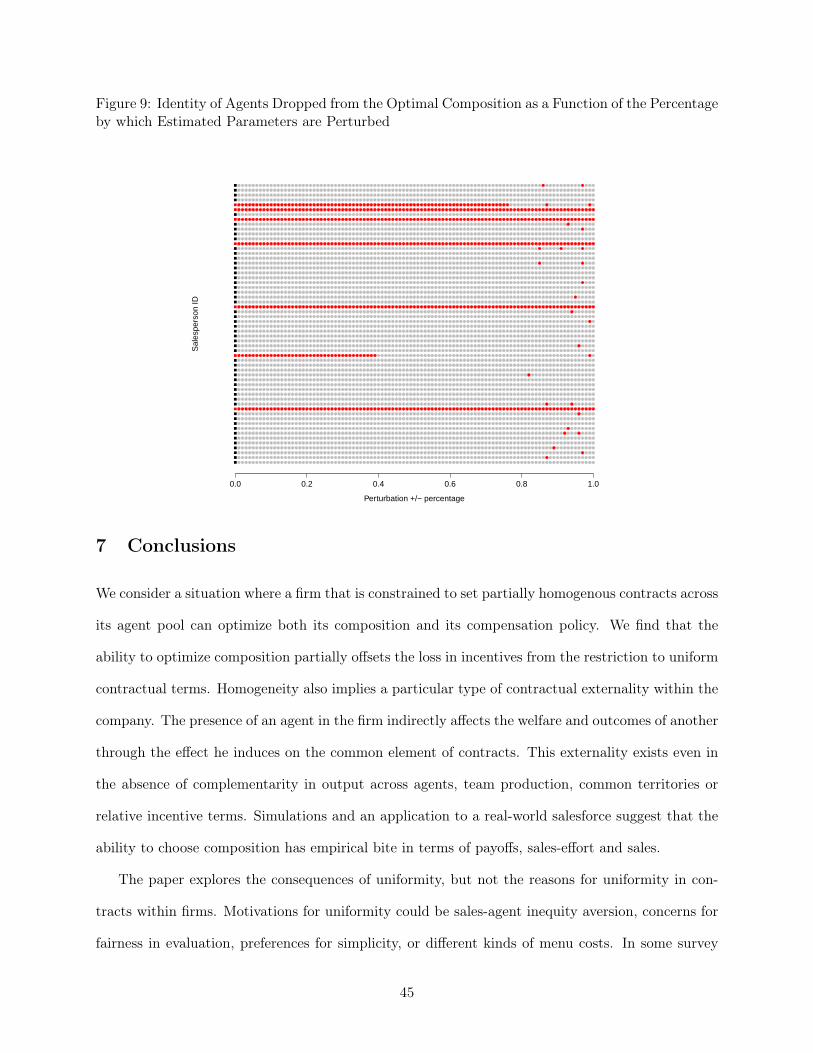
Figure 9: Identity of Agents Dropped from the Optimal Composition as a Function of the Percentageby which Estimated Parameters are Perturbed
Perturbation +/− percentage
Sal
espe
rson
ID
0.0 0.2 0.4 0.6 0.8 1.0
7 Conclusions
We consider a situation where a firm that is constrained to set partially homogenous contracts across
its agent pool can optimize both its composition and its compensation policy. We find that the
ability to optimize composition partially offsets the loss in incentives from the restriction to uniform
contractual terms. Homogeneity also implies a particular type of contractual externality within the
company. The presence of an agent in the firm indirectly affects the welfare and outcomes of another
through the effect he induces on the common element of contracts. This externality exists even in
the absence of complementarity in output across agents, team production, common territories or
relative incentive terms. Simulations and an application to a real-world salesforce suggest that the
ability to choose composition has empirical bite in terms of payoffs, sales-effort and sales.
The paper explores the consequences of uniformity, but not the reasons for uniformity in con-
tracts within firms. Motivations for uniformity could be sales-agent inequity aversion, concerns for
fairness in evaluation, preferences for simplicity, or different kinds of menu costs. In some survey
45
evidence, Lo et al. (2011) conduct field-interviews with managers at industrial firms in four sectors
(namely, electrical and non-electrical machinery, transportation equipment and instruments), and
report the two main reasons managers cite for not using agent-specific salesforce compensation plans
are (a) computational costs of developing complex plans, and, (b) costs associated with managing
ex post conflict amongst salesagents induced by differential evaluation. Relatedly, in a survey of
130 business-format franchisors, Lafontaine (1992) reports that 73% of surveyed franchisors choose
uniform royalty rates due to reasons of consistency and fairness towards franchisees, and 27% re-
ported choosing uniformity because it reduces the transaction costs of administering and enforcing
contracts. It seems therefore that fairness and menu costs play a large role in driving such contract
forms.9 Notwithstanding the reasons, the fact remains that the ability to choose agents and the
restriction to partially homogenous contracts is pervasive in real-world business settings. However,
principal-agent theory is surprisingly silent on both endogenizing the composition of agents, and
exploring the consequences of uniformity. We hope our first-cut on the topic will inspire richer the-
ory and empirical work on the mechanisms causing firms to choose similar contracts across agents,
and on the consequences of these choices.
We abstracted away from hiring and from the principal’s policies for learning new hires’ types.
Accommodating these complicates the model by introducing dynamics, but does not change our
main point about contractual externalities and the codependence of compensation and composition
when contracts cannot be tailored. In our data, we do not have a way of estimating the distribution
of worker types in the population or the distribution of search costs for labor amongst firms in this
market, both of which are critical inputs to a credible empirical model of labor market sorting.9We conducted interviews with salespeople and sales managers to understand why salaries are typically heteroge-
neous, while commissions are invariably homogenous in sales organizations. The common story we have heard is asfollows. Salaries are typically indexed against those at a hired employee’s previous job (typically set as a percentageraise). Thus, they reflect agents’ outside options. Agents perceive the differences as fair because the variation isjustified by managers as the costs to “beat” competitive salaries to hire their colleagues. There is some evidence inthe psychology literature that agents’s perceive variation as fair when it is linked to “justifiable” costs. For example,Kahneman et al. (1986) document that agents do not perceive price discrimination across consumers as unfair if theythink it derives from differences in costs as opposed to the desire to extract more surplus from those with highervaluations. On the other hand, commissions (and other incentive based pay) reflect a percentage payout to an agentof revenues brought into the firm. A dollar in revenue brought in by an agent A is equally valuable to the principalas a dollar brought in by another agent B; because of this, it becomes difficult for the principal to justify why A andB are rewarded different proportions of the dollar as commissions. Such a policy is typically seen as “unfair”. Clearly,the perception of fairness is linked to the deeper psychology of how human beings evaluate these kinds of tradeoffs.
46

With access to better data, an extension of this sort could be pursued. The reader should note
that such competition in contracts across firms have relatively been understudied in empirical work.
Finally, another margin along which the principle may manage heterogeneity is to optimize the
match between agents and territories (e.g., Skiera and Albers 1998). Analyzing this matching
problem while endogenizing the compensation contract is outside the scope of this paper, but is the
subject of our ongoing work.
While our context is salesforce compensation, similar ideas to the one explored here arise in
other contexts of interest to Marketing. One area is joint choice of consumers and promotions. For
instance, Belloni et al. (2012) discuss an algorithm that enables a University to jointly choose a
desirable mix of students and the level of scholarships required to attract them. The complication
associated with salesforce compensation relative to these situations is the presence of moral hazard.
To the extent that we discuss the implications of endogenizing the mix of agents at a firm, we believe
our analysis motivates development of richer empirical models of the joint choice of who and how
to offer product options to consumers in Marketing and Economics.
47

8 References1. Albers, S. and M. Mantrala. (2008). “Models for Sales Management Decisions,” Handbook of
Marketing Decision Models.
2. Ackerberg, D. and Botticini, M. (2002). “Endogenous Matching and the Empirical Determi-nants of Contract Form,” Journal of Political Economy, 110(3), 564-591.
3. Armstrong, M. (1996). “Multiproduct Nonlinear Pricing,” Econometrica, 64, pg. 51-75.
4. Bandiera, O., Barankay, I., and Rasul, I. (2007). “Incentives for Managers and InequalityAmong Workers: Evidence from a Firm-level Experiment,” Quarterly Journal of Economics,(May), 729-73.
5. Basu, A., R. Lal, V. Srinivasan and R. Staelin (1985). “Sales-force Compensation Plans: AnAgency Theoretic Perspective,” Marketing Science, 8 (3): 324-342.
6. Belloni, A., Lovett, M., Boulding, W. and Staelin. (2012). “Optimal Admission and Schol-arship Decisions: Choosing Customized Marketing Offers to Attract a Desirable Mix of Cus-tomers,” Marketing Science, 31 (4), 621-636.
7. Ichniowski, C., Shaw, K. and Prennushi, G. (1997). “The Effects of Human Resource Man-agement Practices on Productivity,”American Economic Review, 86,291-313.
8. Desai, P. S. and Srinivasan, K. (1995). “Demand Signaling under Unobservable Effort inFranchising: Linear and Non-linear Price Contracts,” Management Science 41(10), 1608-23.
9. Godes, D. and Mayzlin, D. (2012). “Using the Compensation Scheme to Signal the Ease of aTask,” working paper, University of Maryland.
10. Green, J. R., and Stokey, N. L. (1983). “A Comparison of Tournaments and Contracts,”Journal of Political Economy 91(3), 349-64.
11. Hamilton, B, J. Nickerson, and H. Owan. (2003). “Team Incentives and Worker Heterogeneity:An Empirical Analysis of the Impact of Teams on Productivity and Participation,” Journalof Political Economy 111, no. 3:465–97.
12. Holmstrom, B. (1979). “Moral Hazard and Observability”, Bell Journal of Economics, Vol.10.
13. Holmstrom, B. (1982). “Moral Hazard in Teams,” Bell Journal of Economics 13, no. 2:324–40.
14. Holmstrom, B. and P. Milgrom. (1987). “Aggregation and Linearity in the Provision ofIntertemporal Incentives,” Econometrica, 55, 303-328.
15. Joseph, K. and Kalwani, M. (1992). “Do Bonus Payments Help Enhance Sales-force Reten-tion?” Marketing Letters, 3 (4): 331-341.
16. John, G. and Weitz, B. (1989). “Salesforce Compensation: An Empirical Investigation of Fac-tors Related to Use of Salary Versus Incentive Compensation,” Journal of Marketing Research,26, 1-14.
17. Kalra, A. and Shi, M. (2001). “Designing Optimal Sales Contests: A Theoretical Perspective.”Marketing Science, 20(2), 170-193.
18. Kahneman, K., Knetsch, J.L, Thaler, R. (1986). “Fairness as a Constraint on Profit Seeking:Entitlements in the Market,” American Economic Review, 76(4), pp. 728-741, September.
19. Kandel, E., and E. Lazear. (1992). “Peer Pressure and Partnerships,” Journal of PoliticalEconomy, 100, no. 4:801–17.
48
20. Lafontaine, F. (1992). “How and Why Do Franchisors Do What They Do: A Survey Report,”in Franchising: Passport for Growth and World of Opportunity (Patrick J. Kaufmann ed.),Sixth Annual Proceedings of the Society of Franchising.
21. Lafontaine, F. and Blair, R. (2009). “The Evolution of Franchising and Franchising Contracts:Evidence from the United States,” Entrepreneurial Business Law Journal, Vol. 3.2, pp. 381-434.
22. Lal, R. and R. Staelin. (1986). “Salesforce Compensation Plans in Environments with Asym-metric Information,” Marketing Science 5(3), pg. 179-198.
23. Lal, R. and V. Srinivasan. (1993). “Compensation Plans for Single- and Multi-Product Sales-forces: An Application of the Holmstrom-Milgrom Model,” Management Science, 39 (7), 777-793.
24. Lazear, E. and Rosen, S. (1981). “Rank-Order Tournaments as Optimum Labor Contracts,”Journal of Political Economy 89, 841-864.
25. Lazear, E. (2000a). “Performance Pay and Productivity,” American Economic Review 90,5:1346–61.
26. Lazear, E. (2000b). “The Power of Incentives,” American Economic Review, P&P 90:2: 410-414.
27. Larkin, I. (2010). “The Cost of High-Powered Incentive Systems: Gaming Behavior in Enter-prise Software Sales,” working paper, Harvard Business School.
28. Lim, N., Ahearne, M. J. and Ham, S. H. (2009). “Designing Sales Contests: Does the PrizeStructure Matter?” Journal of Marketing Research, 46, 356-371.
29. Lo, D., Ghosh, M. and Lafontaine, F. (2011). “The Incentive and Selection Roles of SalesForce Compensation Contracts,” Journal of Marketing Research, 48(4), pp. 781-798.
30. Mantrala, M., P. Sinha and A. Zoltners. (1994). “Structuring a Multiproduct Sales Quota-Bonus Plan for a Heterogeneous sales-force: A Practical Model-Based Approach” MarketingScience, 13(2), 121-144.
31. Milgrom, P. and Roberts, J. (1990). “The Economics of Modern Manufacturing: Technology,Strategy, and Organization,” American Economic Review, 80, 511-528.
32. Misra S., A. Coughlan and C. Narasimhan (2005). “Sales-force Compensation: An Analyticaland Empirical Examination of the Agency Theoretic Approach,” Quantitative Marketing andEconomics, 3(1), 5-39.
33. Misra S., E. Pinker and R. Shumsky (2004). “Salesforce design with experience-based learn-ing,” IIE Transactions, 36(10), pp. 941-952
34. Misra S. and H. Nair. (2011) “A Structural Model of Sales-Force Compensation Dynamics:Estimation and Field Implementation,” Quantitative Marketing and Economics, 9(3), pp.211-257
35. Mookherjee, D. (1984). “Optimal Incentive Schemes with Many Agents,” Review of EconomicStudies 51, 433-446.
36. Pendergast, C. (1999). “The Provision of Incentives within Firms,” Journal of EconomicLiterature, 37(1), 7-63.
37. Raju, J. S., and V. Srinivasan. (1996). “Quota-based Compensation Plans for Multi-territoryHeterogeneous Sales-forces,” Management Science 42, 1454-1462.
38. Rao, R. (1990). “Compensating Heterogeneous Sales-forces: Some Explicit Solutions,” Mar-keting Science, 9(4), 319-342 41.
49
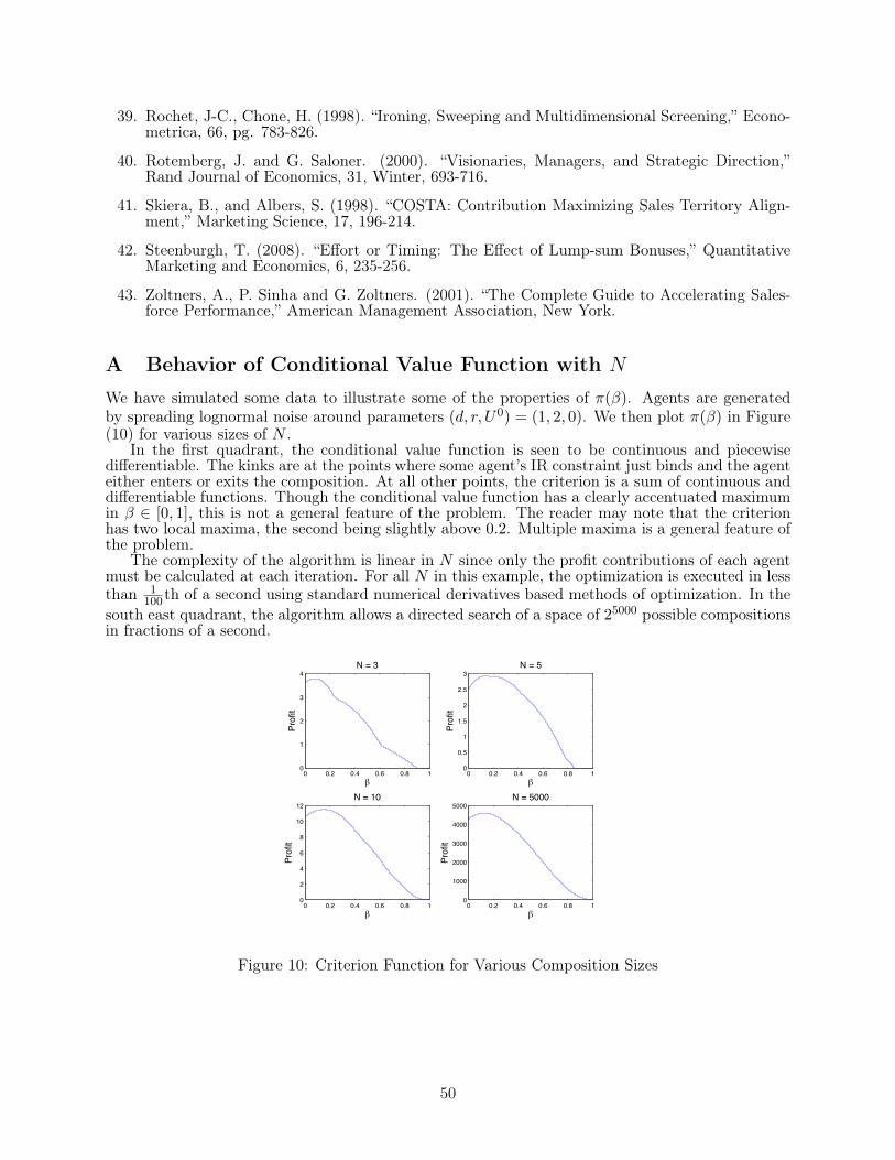
39. Rochet, J-C., Chone, H. (1998). “Ironing, Sweeping and Multidimensional Screening,” Econo-metrica, 66, pg. 783-826.
40. Rotemberg, J. and G. Saloner. (2000). “Visionaries, Managers, and Strategic Direction,”Rand Journal of Economics, 31, Winter, 693-716.
41. Skiera, B., and Albers, S. (1998). “COSTA: Contribution Maximizing Sales Territory Align-ment,” Marketing Science, 17, 196-214.
42. Steenburgh, T. (2008). “Effort or Timing: The Effect of Lump-sum Bonuses,” QuantitativeMarketing and Economics, 6, 235-256.
43. Zoltners, A., P. Sinha and G. Zoltners. (2001). “The Complete Guide to Accelerating Sales-force Performance,” American Management Association, New York.
A Behavior of Conditional Value Function with N
We have simulated some data to illustrate some of the properties of π(β). Agents are generatedby spreading lognormal noise around parameters (d, r, U0) = (1, 2, 0). We then plot π(β) in Figure(10) for various sizes of N .
In the first quadrant, the conditional value function is seen to be continuous and piecewisedifferentiable. The kinks are at the points where some agent’s IR constraint just binds and the agenteither enters or exits the composition. At all other points, the criterion is a sum of continuous anddifferentiable functions. Though the conditional value function has a clearly accentuated maximumin β ∈ [0, 1], this is not a general feature of the problem. The reader may note that the criterionhas two local maxima, the second being slightly above 0.2. Multiple maxima is a general feature ofthe problem.
The complexity of the algorithm is linear in N since only the profit contributions of each agentmust be calculated at each iteration. For all N in this example, the optimization is executed in lessthan 1
100th of a second using standard numerical derivatives based methods of optimization. In thesouth east quadrant, the algorithm allows a directed search of a space of 25000 possible compositionsin fractions of a second.
0 0.2 0.4 0.6 0.8 10
1
2
3
4N = 3
Prof
it
β0 0.2 0.4 0.6 0.8 1
0
0.5
1
1.5
2
2.5
3N = 5
Prof
it
β
0 0.2 0.4 0.6 0.8 10
2
4
6
8
10
12N = 10
Prof
it
β0 0.2 0.4 0.6 0.8 1
0
1000
2000
3000
4000
5000N = 5000
Prof
it
β
Figure 10: Criterion Function for Various Composition Sizes
50
Investigating How Word of Mouth Conversations About Brands Influence Purchase and Retransmission Intentions
Andrew M. Baker Naveen Donthu
V. Kumar*
Revised: June 15, 2015
Andrew M. Baker is an Assistant Professor at the College of Business Administration, San Diego State University, 5500 Campanile Drive, San Diego, CA 92182-8230, 619-594-4306, [email protected] Naveen Donthu is Distinguished University Professor, Katherine S. Bernhardt Research Professor and Chair of the Marketing Department at J. Mack Robinson College of Business, Georgia State University, 35 Broad Street NW, Atlanta, GA 30303, 404-413-7662, [email protected]. * Corresponding Author V. Kumar (VK) is a Regents Professor, the Richard and Susan Lenny Distinguished Chair Professor in Marketing, and the Executive Director, Center for Excellence in Brand & Customer Management at J. Mack Robinson College of Business, Georgia State University, Atlanta, GA; Chang Jiang Scholar, HUST, China; and Lee Kong Chian Fellow, Singapore Management University, Singapore. Phone: 404-413-7590; Email: [email protected] We thank the editor-in-chief, the AE and the reviewers for providing valuable guidance in the revision process. We also thank the faculty at our respective universities, and the audience at the 2012 Marketing Science Conference, 2014 Marketing Science ISMS Doctoral Consortium, Gregory S. Cohen, Gayatri Shukla and Amber McCain for their comments on an earlier version of the manuscript. We thank the Keller Fay Group for the data used for this study. Also, we thank Renu for copyediting this manuscript.

Investigating How Word of Mouth Conversations About Brands Influence Purchase and Retransmission Intentions
ABSTRACT
This study investigates how valence, channel, and strength of the social tie of a word-of-mouth
(WOM) conversation about a brand impact the purchase intentions and WOM retransmission
intentions of WOM recipients. The analysis uses a nationally-representative sample of 186,775
individual conversations on 804 different brands. The authors found insights linking WOM
valence, WOM channel and social tie strength that could not be revealed had the WOM
conversations been analyzed in an aggregated form. The findings contribute to research
investigating differences between offline WOM and online WOM. The authors find that the
relationship of WOM valence with purchase intentions is exacerbated when the conversation
occurs offline, while offline conversations tended to be more strongly associated with WOM
retransmission intentions regardless of the conversation’s valence. The results also provide
insights into how interpersonal characteristics influence WOM outcomes. Specifically, the authors
find that the strength of the social tie relationship does tend to influence a WOM receiver’s
intentions to purchase a brand; however, social tie strength had a much less significant impact on a
consumer’s WOM retransmission intentions.
Keywords: word of mouth valence, offline word of mouth, social ties, branding, word-of-mouth
retransmission, purchase intention

1
Industry studies report that, on average, 2.4 billion daily conversations involve a brand
(Keller and Fay 2012), and marketing managers continue to invest heavily in ways to directly
influence and understand consumer word-of-mouth (WOM) patterns (Berger and Schwartz 2011;
Libai, Muller, and Peres 2013). This investigation endeavors to shed some light on the
consequences these brand conversations have on consumers. Specifically, we investigate what
types of word-of-mouth (WOM) conversations are more or less likely to stimulate consumers’
intention to buy the brand or retransmit the received WOM conversation to others. Our
investigation is at the individual WOM conversation level; within each WOM conversation we
capture the valence of the brand sentiment, the channel of the conversation’s occurrence, and the
strength of the social relationship between those in the conversation. As such, our study is in line
with the recent call to investigate WOM impact in this ‘disaggregated’ form (King, Racherla, and
Bush (2014, p. 176)) to better understand how WOM receivers are influenced by WOM. It has
been noted that aggregate-level WOM analysis tends to assume that consumer impact of WOM is
equal across WOM (King, Racherla, and Bush 2014). Therefore, researchers have called for
‘disaggregated’ WOM analysis in order to test for differences in impact across different types of
WOM. Analyzing WOM at the conversation level is also important to brand managers because it
provides more precise insights into which forms of WOM conversations are most strongly
associated with managerially-desired consumer intention outcomes. Given that brand managers
are often concerned with monitoring and managing desirable forms of consumer WOM, the results
of this study allows managers to sharpen the focus of their efforts.
Two important outcomes of consumer WOM are stimulating consumer purchase and
motivating the retransmission of WOM. Although both outcomes have received extensive attention
in marketing investigations independently, simultaneous investigation of how WOM and brand
drivers relate to each outcome is scarce. The current study complements and extends extant
research by empirically evaluating how pertinent marketing WOM variables differently relate to
both purchase and WOM retransmission intention. By assessing both purchase and WOM

2
retransmission intentions, our findings allow managers to understand which type of WOM
conversations are most relevant depending on the manager’s immediate marketing objective.
This study analyzes nearly four years of organic offline and online WOM data for 804
brands. The data comes from Talk Track, a longitudinal database that tracks WOM from a
nationally representative panel of U.S. consumers. By analyzing WOM impact at the level of
individual conversations, we are able to properly investigate both the main and the interaction
effects among conversation-level WOM characteristics. The consequence of this is that we
identify several unique empirical insights that could not have been investigated if we had only
aggregated WOM about brands. Further, our study focuses on the impact of WOM conversations,
whereas recent studies have focused on the volume of WOM conversations. For example, the
research of Lovett, Peres, and Shachar (2013), Berger and Iyengar (2013), and Berger and
Milkman (2012) use different methodologies and contexts but aim to answer the question, What
generates more WOM? Our study is distinct by providing insights into the question, What type of
WOM matters the most? Indeed, the aforementioned articles do not distinguish between the
generation of PWOM or NWOM, nor do they assess how different types of WOM may differently
affect the behavioral intentions of WOM recipients.
As previously mentioned, this study investigates WOM at the conversation level (e.g.,
immediate consumer response to characteristics specific to the conversations). The selection of
WOM variables for this study was motivated by two considerations. First, we selected the
variables that would encompass all foundational elements of transactional interpersonal
communication frameworks (Barnlund 1970; Shannon 1948). As the second criteria, we identified
the communication framework variables that research has previously identified as having a
substantial impact on consumer outcomes. Regarding the message of WOM conversation, research
has established the valence of received consumer content as a driver of consumer response (Berger,
Sorensen, and Rasmussen 2010; Singh 1990). Further, the communication medium, in particular
the difference between offline and online WOM, can alter what consumers talk about with others

3
(Berger and Iyengar 2013; Lovett, Peres, and Shachar 2013). Finally, the strength of the social
relationship can affect how a message recipient responds to WOM (Brown and Reingen 1987;
Trusov, Bodapati, and Bucklin 2010). For each of these three WOM conversation characteristics,
there are different theoretical accounts for how they should relate to a WOM recipient’s behavioral
intentions. In the following section, we define the outcome variables in our study and then
summarize the differing perspectives about how WOM characteristics should empirically relate to
behavioral intention outcomes.
DEFINITIONS AND RESEARCH EXPECTATIONS This study defines a WOM conversation about a brand as an interactive exchange of
information between two or more consumers that is not commercially motivated. This definition is
consistent with historical marketing literature on WOM (Arndt 1967), but some clarification is
necessary to define the boundaries imposed by the definition we use herein. First, this definition
can include online dialogue between consumers so long as there is some interactive component
between the consumers. For example, a conversation about Ivory soap on Twitter with a complete
stranger would qualify as a WOM conversation; however, reading a product review on
Amazon.com would not (not interactive). Because of our focus on WOM conversations, our study
is not meant to include in its scope any “eWOM” that is not explicitly a conversation; Berger and
Rasmussen (2010) and Chevalier and Mayzlin (2006) are examples of research that has studied
such eWOM. Any comparisons of such studies to our present investigation should be done with
great caution.
In this study, we define “purchase intentions” as the WOM recipient’s degree of motivation
and willingness to eventually purchase the brand discussed in the WOM episode. Similarly, we
define “retransmission intentions” as the WOM recipient’s degree of motivation and willingness to
eventually pass along the content of the WOM communication about the brand to another person.
This is similar to the concept Berger and Milkman (2012) call “message transmission.” De Angelis
et al. (2012) use the term “WOM transmission” to describe when “consumers pass on information
4
about experiences with products and services they have heard occurred to someone else.”
While both purchase and WOM retransmission intentions deal with consumers’ calculation
of future behavioral action toward a brand, they have several important differences. First, purchase
and WOM retransmission intentions have different costs and risks that consumers are likely to
incorporate into their intention estimation. Typically, consumer purchase intentions are influenced
by calculations that include practical cost considerations (e.g., price) and other physical resources
necessary to make a purchase. Conversely, spreading WOM is relatively cheap in terms of physical
costs; yet what consumers choose to talk about with others is partly informed by the social risks
and benefits estimated to derive from talking with others (De Angelis et al. 2012). Second,
purchase intentions are informed by both the practical benefits estimated to come from a brand and
considerations about how the purchase may help achieve social goals, such as self-presentation and
conformance to social norms (Ajzen 1991). Conversely, WOM retransmission intentions are
usually based solely on how WOM can serve social goals, such as self-enhancement (Berger and
Iyengar 2013). Given these differences between purchase and retransmission intentions, we
proceed by considering how a WOM conversation’s valence, channel, and participants (social tie
strength) are expected to similarly and differently relate to purchase and retransmission intentions.
How WOM Characteristics Shape Purchase and WOM Retransmission Intentions
The Role of WOM Valence. The valence of WOM is the conversation’s attractiveness
(positivity) and averseness (negativity) of the information about a particular brand. Content with
strong valence typically stimulates more consumer arousal and interest than neutral content (Berger
and Milkman 2012). Consumer purchase behaviors as a result of valenced information tend to
include approach/avoidance responses that align with the directional valence of the information,
though research has identified factors that moderate this response (e.g., Berger, Sorensen, and
Rasmussen 2010; Dempsey and Mitchell 2010).
5
Research has established that positive word-of-mouth (PWOM) typically motivates brand
purchase or other positive brand outcomes (e.g., referrals) while negative word-of-mouth
(NWOM) generally reduces purchase intentions and inhibits other brand behaviors (Bansal and
Voyer 2000; Ryu and Feick 2007). Furthermore, previous research suggests that the relative effects
of PWOM and NWOM on purchase are asymmetric. That is, compared with neutral WOM,
NWOM will typically have a larger effect than PWOM because the NWOM content about the
brand is framed as a loss (Tversky and Kahneman 1991). East, Hammond, and Lomax (2008) find
that NWOM has a larger effect than PWOM on a consumer’s purchase probability when the pre-
WOM purchase probability was greater than 50%. WOM research provides a less clear picture
about how mixed (ambivalent) WOM conversations about a brand will tend to relate to purchase
intentions when compared to neutral WOM. On one hand, two-sided messages are often
considered by consumers to be more credible; this perspective implies mixed WOM could boost
the effect of the positive sentiment component of mixed WOM on purchase intentions. From
another perspective, mixed WOM sentiment may result in lower purchase intentions than neutral
WOM because the typically dominating asymmetrical effect of the negative sentiment component
of the mixed WOM message (Cheung and Thadani 2012).
How the valence of a WOM message influences intentions to retransmit a conversation
about a brand should differ from how valence affects purchase intentions. A great deal of research
has examined the drivers of initial PWOM and NWOM transmission (Alexandrov, Lilly, and
Babakus 2013; De Matos and Rossi 2008; Higie, Feick, and Price 1987). However, relatively less
research has directly explored how message valence shapes retransmission, despite evidence
indicating that the causal mechanisms for WOM transmission and retransmission are different (De
Angelis et al. 2012; Stephen and Lehmann 2009).
For WOM retransmission (secondhand accounts), research has shown that self-
enhancement theories, particularly the need to positively present and self-enhance, help explain
WOM retransmission. Alexandrov, Lilly, and Babakus (2013, p. 532) found that self-enhancement
6
motives had the strongest total effect on sharing PWOM. De Angelis et al. (2012) find that when
the need to self-enhance was high, people tended to discuss negative experiences when the brand
was experienced secondhand. Berger and Milkman (2012) studied the emotional content of media
and found affect-laden content, regardless of positive or negative emotions, is also likely to be
shared. We propose that message valence will relate to WOM retransmission intentions in a similar
manner. Specifically, PWOM should be the most likely form of WOM to be retransmitted because
it most closely aligns with common self-enhancement goals, such as being interesting and
presenting oneself as positive (Berger and Milkman 2012). However, NWOM and mixed WOM
about a brand should also be more commonly retransmitted than neutral WOM because such
content is still more interesting and, thus, more congruent with achieving self-enhancement goals.
Thus, NWOM, when compared to neutral WOM, should tend to be associated with higher WOM
retransmission intentions but lower purchase intentions.
How Channel Shapes the Impact of WOM. Online WOM differs from offline WOM in that
it is not face to face, is often presented in a highly structured format, tends to be asynchronous
(Berger and Iyengar 2013), is usually incapable of carrying nonverbal forms of communication
(Dennis and Kinney 1999), and can include commercially motivated “artificial” WOM that is more
ambiguously identifiable (Cho et al. 2011).
Media richness theory posits that offline communication will typically be more impactful
on behavioral responses than online WOM because offline WOM delivers more accurate and
detailed information to act upon due to rapid communicator adaptability (communicator can ensure
accurate transmission of the intended message) and more rich and complete communication of
nonverbal cues (Burgoon and Nimmo 1980, Daft and Lengel 1986). Offline PWOM about a brand
should result in greater purchase intentions than otherwise equivalent online PWOM, while
NWOM or mixed WOM offline should have a more substantial negative effect on purchase
intentions than otherwise equivalent online WOM.
For WOM retransmission, a self-enhancement account suggests that the additional richness

7
of the nonverbal communications in offline WOM makes PWOM, NWOM, and mixed WOM
seem even more interesting and worth sharing than their equivalent online WOM counterparts.
Interestingly, this rationale for offline WOM resulting in greater retransmission intentions than
online WOM is consistent with recent research that interesting brands are talked about in online
more often than in offline (Berger and Iyengar 2013; Lovett, Peres, and Shachar 2013). These
studies identify how online channels afford people more time to think of interesting brands to talk
about (a what kinds of brands will be talked about explanation), while the present perspective is
that, holding brand constant, offline conversations should provide more interesting content to share
with others in the future (an impact of a WOM conversation explanation).
On the other hand, online WOM could have higher retransmission intentions than
otherwise equivalent offline WOM conversations because WOM that initially occurs in an online
communication channel gives consumers an instantaneous means to find new people to engage
with in another online conversation. While this perspective may hold when it comes to sharing or
re-posting online content (e.g., clicking the “retweet” button on Twitter), we argue that this
viewpoint is less tenable in terms of retransmission intentions of an actual WOM conversation.
This is because maintaining enduring intentions to spread a WOM conversation means the ease of
retransmitting an online WOM conversation should be relatively unimportant to retransmitting the
content of the WOM conversation.
How Social Ties Shape the Impact of WOM Research indicates that the degree of social distance between consumers affects exchange
(Granovetter 1983) and information transmission (Frenzen and Nakamoto 1993). Research has
typically classified social tie strength into two discrete social tie categories: strong ties and weak
ties. With strong ties, members recognize the relationship’s overall importance, engage in frequent
relationship interaction, and usually define specific social relationships as close friends or
immediate family members. Weak ties lack valuations of enduring importance, tend to have less
frequent interactions, and typically have social designators such as acquaintance or stranger

8
(Weimann 1983). However, the dissimilarity and scarce interaction between weak social ties is
argued to have one upside with regard to information dissemination in social networks – in the
relatively rare instances where weak ties do engage in information exchange, it is much more likely
that the information will be novel to recipients. In other words, weak ties interact infrequently and
tend to be untrusted but are essential to spreading new information across a social network. This is
the so-called “strength of weak ties” (Granovetter1983).
As social tie strength increases, so does the likelihood of tailored, relevant, persuasive, and
personalized WOM communications. This is known as the “strength of strong ties” (Brown and
Reingen 1987). The strength-of-strong-ties effect should apply in the case of purchase intentions;
that is, a WOM recipient is more likely to take action on a WOM message received from his/her
strong ties because of a generally higher level of trust in the sender and higher level of homophily
between strong ties (McPherson, Smith-Lovin, and Cook 2001). Thus, PWOM about a brand from
a strong tie should be particularly salient in motivating purchase, while NWOM about a brand
should result in a strong unwillingness to purchase the brand. However, NWOM from strong ties
may not have as deleterious effects on purchase intentions as might be expected. This is because
the effect of increased trust on the negative sentiment from strong ties will be tempered by the
tendency of strong ties to talk about more personally relevant brands (Berger, Sorensen, and
Rasmussen 2010).
Regarding WOM retransmission intentions, the self-enhancement perspective and “strength
of strong ties” perspective both suggest that WOM from strong ties will be more frequently
retransmitted. Because strong social ties are viewed as more relevant, reliable, trustworthy, and
credible, relatively less risk is associated with retransmitting the informational content received
from a well-known source. Thus, self-enhancement goals can be pursued through WOM
retransmission with less risk. While the “strength of weak ties” perspective does suggest that weak
tie information will tend to be more novel, and thus perceived to be more valuable for WOM
retransmission, the “strength of weak ties” perspective also notes that the relative distrust and
9
skepticism toward weak ties means that even truly novel information received during a WOM
conversation will be, on average, heavily devalued as a candidate for WOM retransmission.
DATA
Database The database of WOM conversations come from the Talk Track proprietary database. Talk
Track is developed and maintained by the Keller Fay Group, a marketing consulting firm
specializing in providing clients with longitudinal information about U.S. consumers’ WOM
activity, both offline and online. On average, 700 respondents are recruited each week to
participate in the U.S. panel. The respondents are selected to be demographically representative of
consumers in the United States and are between the ages of 13 and 69 years.
Talk Track respondents are asked to recall the brand and product-related WOM
conversations they had in the previous 24 hours. Initially, the Talk Track survey instrument asks
the respondent to simply quantify the number of WOM conversations they had across a variety of
15 product categories (e.g. beverages). The Talk Track survey prompts the respondent to name
any specific brands, if any, mentioned in each conversation. Then, from a random list of no more
than 10 of those conversations, the respondent identifies where each conversation occurred. This is
the first Talk Track WOM conversation measure relevant to our study. Next, Talk Track randomly
selects from 10 brands mentioned in the WOM conversations (the brands are limited to ten to
minimize respondent fatigue). The respondent is prompted to recollect more detailed information
about what was said about each of the randomly selected brands. This recalled information
provides the key measures we use in our analysis. At this point, the valence of the WOM about the
brand is measured (the second key WOM conversation measure for our study). The Talk Track
system then asks the respondent to identify if any of these conversations included the Talk Track
respondent receiving specific advice or recommendations regarding a specific brand. If they did
receive advice, Talk Track captures the social relationship between the WOM sender and receiver
(our third and final WOM conversation variable), and the WOM recipient’s intentions to purchase

10
the brand or retransmit the WOM about the brand as a result of the conversation (our two
dependent variables). Thus, our study analyzes Talk Track WOM conversations in which the
WOM receiver received some advice from a WOM sender related to a specific brand. The specific
wording used for the Talk Track survey questions germane to our study are reported in the
Appendix (Table A-1).
The Talk Track system also captures other WOM conversation information as well as
information about the respondent. For example, it measures respondents’ demographic
information. Unfortunately, a limitation of our study is that we did not have all of the variables in
the Talk Track database. The Talk Track database is extensive; other WOM dimensions from Talk
Track have been used in recent marketing research (Berger and Iyengar 2013).
From this database, we included in the analysis 186,775 conversations between July 2006
and March 2010 from 804 brands. In our analyzed sample, the Talk Track respondents we
analyzed provided on average detailed evaluations of 1.37 brands. We excluded Talk Track
“brands” that were actually people (e.g., political figures, celebrities) or media properties (e.g.,
television shows, movies, video games). The brands in our sample had 232.30 detailed WOM
conversations on average (median = 81, σ = 545.40). As explained in detail when we present the
analysis, the fundamental unit of analysis for our investigation is each WOM brand conversation
and the resulting behavioral intentions from that conversation.
Talk Track Measures
Intentions to purchase and retransmit. We operationalized purchase and retransmission
intentions using respondents’ answers to two Talk Track survey questions that (1) asked how likely
the respondent was to buy the brand and (2) retransmit the WOM about the brand as a result of the
WOM conversation. Each question was on a ten-point scale (0 = “not at all likely,” 10 =
“extremely likely”). Purchase intention had a mean of 7.43 (σ = 2.17), and retransmission
intentions had a mean of 7.47 (σ = 1.66). The relatively high means for the intention measures are

11
partly due to the large percentage of PWOM (61.58%) about brands in the sample. The relatively
high intention scores should not be interpreted as directly indicative of WOM’s influence on actual
behavior. Previous research on the intention–behavior relationship has demonstrated that measured
intentions are imperfect predictors of actual purchase behavior, and the empirical relationship
between measured intentions and actual behavior tends to be positive but nonlinear and stated
intentions tend to overestimate actual purchases (Bemmaor 1995; Manski 1990).
Purchase and retransmission intentions are different – in their definition, their antecedents,
and factors that constrain a consumer’s ability to manifest their intention into behavior. At the
same time, the two constructs are also expected to positively correlate. We expect people to be
inclined to talk about brands they are also willing to purchase. Indeed, the bivariate correlation
between average purchase intention and retransmission scores among PWOM demonstrated
positive correlation (r=.45, p<.001). However, there was more discrepancy between purchase and
retransmission intentions with respect to NWOM (r=.12, p<.001), neutral WOM (r=.39, p<.001),
and mixed WOM (r=.37, p<.001).
WOM valence. Talk Track panel members report the valence of the information about the
brand in the WOM conversations as being either generally positive, negative, neutral, or mixed.
Neutral WOM conversations typically contain strictly informational content about a brand;
conversely, mixed WOM includes brand sentiment with both positive and negative elements. We
used dummy codes to operationalize WOM valence. Most conversations about brands were
positive (61.58%) or mixed (17.34%). A smaller proportion of WOM conversations were negative
(8.57%) and neutral (12.51%); thus, the ratio of PWOM to NWOM was 7.16-to-1. This proportion
is consistent with reports in other studies; Carl (2006) reports WOM activity as 71.1% positive,
20.6% neutral, and 7.7% negative (9.23-to-1 PWOM to NWOM). Like the Talk Track database we
used, the aforementioned study also collected WOM using survey instruments that aided
respondents as they recalled recent WOM activity. Table 1 reports the percentages of different
WOM types in our sample.

12
[Table 1 Here]
WOM channel. We dummy-coded the channel of the WOM episode as either offline or
online according to the respondent’s recall of the conversation channel (offline = face to face or
telephone; online = e-mail, text message, blog, online chatroom, Twitter, or social networking
site). We classified telephone conversations as offline because, though they do not enable
respondents to see nonverbal communications, they carry all the other signals linked with rich
channels of communication (e.g., synchronicity, transmission of subtle tonal inflections,
interactivity with immediate feedback) (Daft and Lengel 1986; Dennis and Kinney 1999; Rogers
1986). Berger and Iyengar (2013) also use this categorization scheme.
Most conversations occurred offline (94.84%). Our sample is more extreme than that in
other studies (Fay and Thomson 2012), in which approximately 90% offline WOM is typically
reported. This discrepancy is mostly due to our sample selection of brands; our exclusion of media
properties (e.g., television shows) favors a relatively higher rate of offline WOM because such
properties have particularly voluminous online WOM (Lovett, Peres, and Shachar 2013). This
atypical ratio of offline to online WOM is not a significant concern, however, because our research
objective is to assess the impact, not the volume, of the WOM channel.
Social tie strength. We coded tie strength in the WOM dyad as weak or strong.
Respondents identified their relationship with the person in the WOM episode either as
spouse/partner, family member, best friend, and personal friend (coded as strong tie) or as
coworker, other acquaintance, and stranger (coded as weak tie). Categorization of social
relationship designators into strong and weak ties was informed by De Bruyn and Lilien (2008),
who use Frenzen and Davis’s (1990) social strength scale to identify the mean social tie strength of
the same social relationship designators as in this study. Most conversations occurred between
strong social ties (80.99%); 19.01% of WOM was between weak ties.
WOM Volume. We included overall WOM volume of a brand as a proxy to control for
potential WOM repetition effects because the Talk Track data do not identify the total number of
13
same brand WOM a respondent has recently received. This measure was a simple count of all
WOM conversations in the Talk Track database for a given brand, divided by 1000 and mean-
centered (Mean = .000, SD = 1.83, Min = -1.52, Max = 5.092).
Product categories. We organized brands from the database into 14 categories: automotive,
beauty/personal care, beverages, children’s products, financial, food/dining (the reference
category), health care, household products, media/entertainment, retail/apparel, technology,
telecom, home, and travel. The three most populated categories were food/dining (21.02% of
brands), retail/apparel (12.19%), and beverages (11.19%). A complete description of the amount
of WOM across categories appears in the Appendix (Table A-2).
ANALYSES
To evaluate our research expectations for how WOM conversation valence, channel, and
social tie relate to purchase and retransmission intentions, we use the following linear mixed
models for purchase intentions (BUYi,j,k) and retransmission intentions (TRANSMITi,j,k). We
depict them using standard notation as follows:
1. BUY , , , , ∑ , , ∗ , , ∑ , , ∗ , , , , , ,
2. TRANSMIT , , , , ∑ , , ∗ , , ∑ , , ∗ , , , , , ,
The subscript i denotes WOM conversation, which is the first-level portion of model, and
subscript j denotes brand (second level), and k denotes the product category of the brand (third
level). The fixed portion of the model is captured by the fixed regression intercept, ξ 0,0,0 , the
coefficients , , to , , (indexed by a), and , , and , , (indexed by b). , , to , ,
represent the fifteen fixed regression parameters necessary to capture the full factorial of the WOM
conversation variables (valence [4] × channel [2] × social tie [2]). The , , predictors are all
dummy codes which represent different valence, channel, and social tie properties of a particular
WOM conversation. Using neutral, online WOM conversations between weak social ties acts as
the reference group, , , to , , represent the main effects of valence (PWOM, NWOM, and
14
mixed WOM, respectively), , , represents offline WOM (online WOM is the reference group),
and , , represents strong social tie (weak tie is the reference). The two-way interactions are
captured with , , to , , (WOM valence and channel), , , to , , (WOM valence and
social tie), and , , (channel and social tie). , , to , , represent the three-way interactions
between valence, channel, and social tie. The fixed coefficients , , and , , capture the brand-
level WOM volume control variable (main effect and quadratic effect). The parameter estimates
are also labeled for easy reference in Table 2.
The residual components of the model are the random part of the mixed model and are
captured by ri,j,k , u0,j,k , and w0,k . The random deviation of the intercept for product category k
from the overall regression model is represented by w0,k . The random deviation of the intercept for
brand j from the intercept of product category k from the overall regression model is represented by
u0,j,k , and the error in the WOM receiver’s predicted PURCHASE or TRANSMIT score from
conversation i about brand j in product category k is represented by ri,j,k. Given our objective is to
focus on the relationship between WOM conversation characteristics and purchase and
retransmission intentions, this multilevel modelling approach is appropriate as it allows us to also
account for both brand-level and product category-level clustering on the dependent variable. The
models were fitted using maximum likelihood estimation. The parameter estimates are reported in
Table 2.
[Table 2 Here]
RESULTS
Tables 3 and 4 report the predicted means and standard errors for purchase intentions and
WOM retransmission intentions across valence, channel of communication, and social tie strength.
We first proceed by discussing the results in terms of the individual role valence, channel, and
social tie play on purchase intentions and WOM retransmission intentions. We then investigate and
discuss the more nuanced interactions between the three WOM conversation properties, focusing
15
on how differences in WOM channel and social tie influence the relationship between WOM
valance and the dependent variables.
[Table 3 and Table 4 Here]
As expected, the valence of a WOM conversation plays a pivotal role in both the purchase
and WOM retransmission intentions. For both dependent variables, PWOM results in the highest
predicted means along with the standard error in parenthesis (8.37 (.136) purchase intentions and
8.05 (.062) retransmission intentions). However, the association of negative WOM sentiment on
the dependent variables differs between purchase and retransmission intentions. The predicted
mean for purchase intentions from NWOM (4.03 (.137)) is 40.4% lower than that of neutral WOM
(6.77 (.137)) (χ2 (1) = 31,692.19, p < .001) and mixed WOM is 4.7% lower (6.45 (.137)) than
neutral WOM (χ2 (1) = 637.40, p < .001).
In addition, with respect to purchase intentions, NWOM had a relatively larger absolute
difference from neutral WOM when compared to the difference PWOM had from neutral WOM.
The absolute difference of NWOM to neutral WOM (2.75) was significantly larger than the
PWOM to neutral WOM difference (1.6) (χ2 (1) = 2,431.86, p < .001). On the other hand, for
retransmission intentions the difference between PWOM and neutral WOM was the largest
absolute difference from the neutral WOM reference (1.8, p < .001), not NWOM as was the case
for purchase intentions.
When solely considering the channel of the WOM communication, there were much
smaller differences between offline WOM and online WOM communications on the predicted
means of purchase intentions and retransmission intentions. The predicted mean of purchase
intentions for offline WOM (7.47 (.136)) was only 0.1% higher than for online WOM (7.41 (.137))
(χ2 (1) = 5.87 p < .05). Likewise, retransmission intentions were predicted to be only 0.1% higher
among offline WOM (7.56 (.062)) than online WOM (7.49 (.064)) (χ2 (1) = 6.34, p < .01).
The overall predicted mean differences between strong tie and weak tie WOM on purchase
and retransmission intentions were more pronounced than was observed between offline and online

16
channels. When solely considering the social ties involved in the WOM conversation, the
predicted mean purchase intentions for strong tie WOM was 7.57% larger (7.57 (.136)) than weak
tie WOM (7.04 (.136)) (χ2 (1) = 3,622.06, p < .001). Strong tie WOM had predicted mean
retransmission intentions that were 2.6% greater than the predicted mean for weak tie WOM (7.59
(.062) and 7.40 (.062), respectively; χ2 (1) = 488.57, p < .001).
Summary. This previous analyses focused on the relationship each of the three WOM
conversation variables individually had with purchase and retransmission intentions. From this
investigation, it is clear that the valence of the WOM conversation had the most substantial
individual relationship with either purchase or retransmission intentions. The roles of PWOM and
NWOM fell mostly in line with expectations; that is, PWOM is positively associated with both
purchase and WOM retransmission and the effect of NWOM is relatively larger than PWOM on
purchase intentions. However, it also became clear that distinguishing between neutral and mixed
valence WOM about a brand was informative for both purchase and retransmission intentions;
mixed WOM purchase intentions were 4.7% lower than neutral WOM and mixed WOM
retransmission intentions were 12.5% higher than for neutral WOM. In addition, these results
suggest that the channel of the WOM conversation had little substantive direct influence on
purchase or retransmission intentions. On the other hand, social tie strength had a slightly more
substantive direct impact, with strong ties tending to positively relate to both purchase and
retransmission intentions.
Although informative, this previous analysis ignored the potential interaction between
valence, channel, and social tie. Considering their interactions are important; conceptually the
valence of the WOM conversation should act as a core driver of resulting consumer intentions,
while the surrounding context (the channel and the people talking) of the conversation should
shape the how someone reacts to the sentiment in the conversation. In the following analyses, we
proceed to investigate how the channel and the strength of the social tie in the WOM conversation
interact with the relationship of WOM valence and dependent variables.

17
Investigating the interaction of WOM valence, channel, and social tie. Figures 1 and 2
depict the predicted means for purchase intention and WOM retransmission intention while
allowing for interactions between WOM valence, channel, and social tie. The figures present the
16 possible combinations of valence, channel, and social tie by the rank order of their predicted
means on purchase intentions (Figure 1) and retransmission intentions (Figure 2). PWOM is
presented as white colored bars, NWOM as black colored bars, neutral as grey colored bars, and
the mixed WOM bars are colored as black and white alternating colored lines. Before proceeding
with formal statistical tests, these visualizations make it descriptively easier to approximate and
intuit the relative impact of each WOM conversation characteristic on purchase or retransmission
intentions. The tendency for the rank order of predicted means to be relatively grouped by WOM
valence (neutral and mixed WOM on purchase intentions being a notable exception) clearly shows
how WOM valence is the primary influence on purchase and retransmission intentions, while the
variation in rank order positions by social tie and channel within the WOM valence groups
illustrate the interactions these WOM conversation properties have with WOM valence. For
instance, PWOM among strong social ties (whether offline or online) have the highest predicted
means for both intention outcomes, followed in rank by PWOM among weak social ties. For
mixed and neutral WOM, the predicted mean purchase intentions tend to alternate in rank
importance; it is the presence of strong tie instead of weak tie that determines the relative
importance rank for neutral and mixed WOM (e.g., strong tie conversations of neutral or mixed
sentiment hold the 4th through 7th positions while neutral and mixed sentiment weak tie
conversations hold the 8th through 11th positions). NWOM takes the four lowest-ranked positions
for purchase intentions, and NWOM that occurs offline holds both of the lowest positions for
purchase intention predicted means. For retransmission intentions, neutral WOM comprises four
of the five lowest predicted means, and neutral WOM between weak social ties has the lowest
overall predicted mean. Mixed WOM tends to have higher predicted retransmission intentions
18
than NWOM, and the lowest retransmission intentions for NWOM and mixed WOM are both for
conversations between weak ties.
[Figure 1 and Figure 2 Here]
The Moderating Role of WOM Channel. We investigated if the channel of the WOM
conversation moderates the relationship of valence on purchase intentions and retransmission
intentions. We did this by using neutral WOM as a relative reference point and then comparing
how the size of the difference in the predicted means for either PWOM, NWOM, or mixed WOM
and the neutral WOM reference varied between offline and online WOM. The difference between
NWOM and neutral WOM on purchase intentions was strongly moderated by WOM channel (χ2
(2) = 123.85, p < .001). Specifically, the size of the NWOM and neutral WOM difference is
expected to be 36.9% more pronounced for offline conversations than online conversations among
strong ties and 30.3% larger when the conversation is among weak ties. On the other hand, the
channel of WOM conversation did not significantly moderate the size of the difference between
PWOM and neutral WOM on purchase intentions (χ2 (2) = 0.01, p > .90). The relative difference
between mixed WOM and neutral WOM for purchase intentions was also significantly greater in
offline channels than online channels. WOM channel also significantly moderated the difference
in purchase intentions between neutral WOM and mixed WOM (χ2 (2) = 19.92, p < .001). Upon
closer inspection, the difference in purchase intentions between mixed valence and neutral WOM
conversations in offline channels was statistically significantly lower (-5.6% for strong tie WOM, -
2.2% for weak tie WOM, p< .001), and while there was no significant difference between mixed
WOM and neutral WOM on purchase intentions in the case of online WOM conversations (p >
.50). Together, these results suggest that offline channels accentuate the negative impact of
negative brand sentiment in WOM conversations (NWOM and the partial negative sentiment in
mixed WOM) on purchase intentions.
The channel of the WOM conversation also positively moderated the size of the difference
between neutral WOM and PWOM and NWOM on retransmission intentions. The size of the

19
difference between PWOM and neutral WOM on retransmission intentions was significantly larger
when the conversation occurred offline rather than online (χ2 (2) = 44.86, p < .001); the expected
difference is 32.7% larger when the PWOM conversation occurs offline among strong ties and
58.1% larger when is occurs between weak ties. The difference between NWOM and neutral
WOM was also significantly larger when the conversation occurred offline instead of online (χ2
(2) = 36.77, p < .001). The size of the NWOM offline vs. online retransmission intention
difference is expected to be 79.6% larger when it occurs among strong ties and 290.1% larger
when it occurs between weak social ties. However, the difference in retransmission intentions
between mixed WOM and neutral WOM was not accentuated for offline WOM; the difference was
positively accentuated in the case of strong tie WOM (χ2 (1) = 8.87, p < .01) but there was no
significant difference in the case of weak tie WOM (χ2 (1) = 0.57, p > .40).
The results related to the interaction between WOM valence and channel support the idea
that offline WOM communications are more saliently linked with behavioral intentions than online
WOM. That is, offline WOM conversations appear to exacerbate WOM recipient response to the
valence of WOM content. This interpretation had support in the case of WOM with negative
sentiment for purchase intentions and for PWOM and NWOM in the case of retransmission
intentions. The propensity for a consumer to retransmit NWOM is particularly accentuated when it
occurs offline.
The Moderating Role of Social Tie. Again, we used neutral WOM as a relative reference
point and then compared how the size of the difference in purchase and retransmission intentions
between PWOM, NWOM, and mixed WOM differences and neutral WOM varied between strong
and weak social ties. With respect to the difference in purchase intentions between PWOM and
neutral WOM, the size of the difference among weak ties was unexpectedly greater than that of
WOM between strong ties (19.5% greater for offline, 20.1% greater for online; χ2 (2) = 127.73, p
< .001). However, the unexpected direction of the moderating effect of social tie strength did not
overtake the significant positive main effect strong social ties has on purchase intentions (as we
20
reported in the initial analyses). This is why strong tie PWOM still has the absolute largest
predicted mean for purchase intentions. The moderating effect suggests that the expected
difference between PWOM and neutral WOM purchase intentions is not as large as would be
expected solely by the main effect of strong tie WOM, though.
In terms of the difference in the size of the NWOM to neutral WOM effect on purchase
intentions, NWOM among strong social ties even further exacerbated the difference when
compared to weak tie WOM conversations (15.8% greater for offline WOM, 10.5% greater for
online WOM; χ2 (2) = 103.07, p < .001). As reported previously, the difference between mixed
WOM and neutral WOM on purchase intentions was only significantly different in the case of
offline WOM. The size of this negative difference between mixed WOM and neutral WOM was
188.1% larger for strong tie WOM conversations compared to weak tie WOM conversations (χ2
(1) = 60.84, p < .001).
With respect to WOM retransmission intentions, there was only limited evidence for social
tie strength moderating the size of the effects between PWOM, NWOM, mixed WOM and the
neutral WOM reference. Social tie strength did not moderate the size of the PWOM vs. neutral
WOM difference for retransmission intentions (χ2 (2) = 2.61, p > .2); the same was true for the
NWOM vs. neutral WOM difference (χ2 (2) = 3.14, p > .2). The difference in the predicted mean
for retransmission intention between mixed WOM and neutral WOM was not significant in the
case of online conversations (χ2 (1) = 2.70, p > .1) but was significant in the case of offline
conversations (χ2 (1) = 4.78, p < .05); WOM between strong ties further accentuated the tendency
for mixed WOM to have higher retransmission intentions than neutral WOM.
These results suggest that the strength of the social tie moderated the relationship between
WOM valence and behavioral intentions primarily in the case of purchase intentions, not
retransmission intentions. WOM from strong social ties tended to exacerbate the negative
influence of NWOM and mixed WOM on purchase intentions while weak tie WOM had a more
accentuated influence on the difference in purchase intentions between PWOM and neutral WOM.
21
However, given the strong main effect strong ties have on purchase intentions, strong tie PWOM
still reigns as having the highest overall purchase intentions.
Channel and Social Tie Influencing the Strength of NWOM Effect. The initial analysis
identified that, with respect to purchase intentions, NWOM had a relatively larger absolute
difference from neutral WOM when compared to the difference PWOM had from neutral WOM.
The degree of this absolute difference was most pronounced for WOM occurring between strong
ties in offline channels; there was a significantly larger relative size difference between NWOM
and neutral WOM than that of PWOM to neutral WOM between strong ties in offline channels (|Δ|
for PWOM – neutral WOM= 1.54, |Δ| for NWOM – neutral WOM = |-2.85|, significantly larger
and different from all other social tie and channel combinations, p < .001).
Preliminary Analysis: The Interplay between WOM Characteristics and Brand Properties.
Recent studies have investigated the relationship between brands and WOM creation and have
called for more work in the area of brand and WOM relationships (Lovett, Peres, and Shachar
2013). The characteristics of the brand in a WOM conversation act as an important piece of
content that can influence behavioral intentions to WOM, much like WOM valence did in our
present study. Indeed, the statistically significant (p < .001) brand-level (Level 2) variation we
observed in our mixed linear model (σ = 0.577 for purchase intentions, σ = 0.172 for
retransmission intentions) suggests that there may be theoretically-relevant brand-level
heterogeneity that could be accounted for with brand-level predictors. We extend our study by
incorporating into our model 19 brand-level predictors from multiple academic and professional
sources (Lovett, Peres, and Shachar 2014). This additional investigation included 504 brands
(retaining 62.6% of the original brands studied in the main analysis and 90.2% of the WOM
conversations) and revealed several interesting insights. The appendix provides a table with
illustrative brand names (Table A-3) for the continuous variable brand traits used in this
preliminary analysis.

22
Our results suggest that brand characteristics primarily moderated consumers’ purchase
intentions to received NWOM, while brand characteristics more heavily moderated retransmission
intentions to PWOM. We found that brands with strong social elements (e.g., highly differentiated
or visible in the environment) and those that stimulate emotional arousal (e.g., exciting or high
satisfaction) tend to be shielded somewhat from the adverse impact of NWOM on purchase
intentions. This brand-level analysis shows potential for a more rigorous evaluation via future
research.
DISCUSSION Our results provide insights into the behavioral intentions of people receiving WOM about
a brand. Compared with neutral brand sentiment, positive, mixed, and negative sentiment actually
increased intentions to retransmit the WOM message about a brand. PWOM had the greatest
absolute effect for retransmission intentions, while NWOM had the largest absolute relationship
with purchase intentions. We also found that distinguishing mixed-sentiment WOM from neutral
WOM is important to understand WOM recipient behavioral intentions: mixed WOM is associated
with lower purchase intentions while mixed WOM was associated with greater intentions to
retransmit the WOM conversations.
We also show that the valence of WOM has a greater effect on purchase intentions when it
occurs offline, in particular by making NWOM and mixed WOM even more damaging to
consumers’ intentions to buy or try a brand. Even more surprising, the results also demonstrate
that offline WOM conversations actually have higher retransmission intentions than online WOM.
The interaction between offline WOM and WOM valence is noteworthy and seems to contradict
traditional thinking about online WOM; the typical presumption is that the relative ease of online
WOM results in more frequently retransmission. While the ease of sharing online may indeed
drive eWOM (such as by simply retweeting a Twitter post), our study of actual WOM
conversations suggests that offline channels may be somewhat more influential at stimulating the
later sharing of actual conversations.

23
Another interesting finding was that the strength of the social tie in the WOM conversation
appears to play a larger role in purchase intentions than it does with retransmission intentions.
Strong tie WOM had a positive main effect with purchase intentions and social tie strength also
moderated the relative impact of PWOM, NWOM, and mixed WOM on purchase intentions. On
the other hand, WOM retransmission intentions only had a modest positive main effect from strong
ties, and there was little evidence of social tie strength moderating the influence of WOM valence.
Considered together, these results suggest that the source of WOM plays a more substantial role in
impacting purchase decisions than whether or not someone is willing to pass along a WOM
conversation to others.
Research Implications
Our findings complement other recent research with respect to WOM channel effects.
Specifically, Berger and Iyengar (2013) demonstrate the asynchronicity of offline communication
channels to explain why people are more likely to talk about interesting brands online. In contrast,
we show that the additional richness of the offline channel may explain why people are more
willing to retransmit interesting conversations (PWOM, NWOM, and mixed WOM about a brand)
when receiving secondhand information from others—that is, because of the increased clarity and
richness of the received WOM message in offline channels.
This study also contributes to the dialogue on the asymmetric effects of positive and
negative information on consumer response. While the results are consistent with other studies
demonstrating a general tendency for negative sentiment to have an asymmetrically greater effect
on consumer purchase behavior, this study also suggests that investigating asymmetric purchase
response to WOM does not fully explain consumer response to WOM activity. When considering
how a WOM episode from one consumer can subsequently influence other consumers’ behavior
through retransmission activities, it becomes even less clear whether NWOM or PWOM truly has
a net asymmetric influence. The results of this study suggest that PWOM has a much stronger
positive association on retransmission than NWOM; this notion receives further support from

24
evidence showing that mixed WOM sentiment is more positively related to WOM retransmission
than NWOM. This finding is consistent with Berger and Milkman (2012); they identify which
online news article content drove consumers to share (e.g., retransmit) the article with others. As in
our study, Berger and Milkman (2012) find that the positive valence of content is associated with
retransmission and that the overall emotionality of a message (which includes negative and
ambivalent content) is related to retransmission. They also show that psychologically arousing
emotions drive retransmission.
Finally, these provide implications for marketing studies that investigate how aggregated
quantities of WOM are linked to marketing outcomes, like sales or market share. Future
researchers working in this area would likely derive superior predictive models if they, at the least,
distinguish aggregated WOM by valence (including separating mixed and neutral WOM), channel
or conversation, and the participants in the conversation. It is known that brands vary in their
relative quantities of WOM valence, channel, and WOM participants; it thus follows to reason that
the conversation-level differences identified in our study can ultimately impact aggregate-level
brand outcomes.
Managerial Implications
Because WOM conversation properties tend to have different relationships with purchase
and retransmission intentions, it would be wise for brand managers to carefully consider which
types of WOM are most relevant depending on the immediate WOM objectives (driving more
immediate purchase or influencing the spread of additional WOM conversations). While it is clear
that PWOM is always most desirable, our results suggest that marketers may want to find ways to
mitigate the occurrence of mixed WOM conversations if the goal is immediately influencing
purchase. However, marketers may be willing to encourage mixed WOM if the primarily goal is
to stimulate more WOM conversation retransmissions.
We suggest that our findings may also be useful to marketing managers concerned with

25
designing WOM marketing campaigns. WOM marketing is commonly discussed and frequently
practiced in the context of eWOM (sharing social media content, posting consumer-generated
media content, etc.), and stimulating consumer engagement is recognized as an important metric of
such campaigns. For example one of the annual Word of Mouth Marketing Association’s awards
is the “Engagement Award.” Under the reasonable assumption that a WOM conversation will
generally be a more engaging experience than passive consumption of eWOM, our results suggest
it could be beneficial for marketers to carefully consider how to implement WOM marketing that is
designed to translate online sharing into engaging offline conversations, as our findings suggest
this is the platform where the impact on intentions to purchase and retransmit are most pronounced.
Limitations and Future Research Directions
The database provides a rich, extensive sample of WOM conversations. However, the
WOM measures have limitations. First, measures of WOM activity are not a perfect representation
of all WOM activity about brands. Because the database relies on respondent recollection, WOM
conversations occurring when the respondent had low motivation, ability, or opportunity to encode
the message are likely underrepresented. Another concern is that Talk Track respondents may have
simply disproportionately recalled favorable conversations about brands for which they already
had a preference. If the goal of our study was to quantify the volume of WOM about a brand, there
could be a risk of reverse causation. However, the goal of our study was to assess the purchase and
retransmission intentions from a WOM conversation; thus, so long as the recalled WOM
conversations are reported accurately, our findings should be accurate even if the reported
proportion of WOM types are suspect. However, there would be a simultaneity risk here if
respondents first recollected their intentions of how to react to a WOM conversation and then they
inaccurately recollected the properties of the WOM conversation to better conform to their naïve

26
theory of what type of conversation would give rise to their purchase or retransmission intentions.
Another limitation of our study is that our database did not have potentially informative variables
about our WOM recipients. It could be informative to know if WOM recipients were actively
seeking out advice, their level of involvement in a brand’s product category, and their personal pre-
conversation evaluations of the brand. This unobserved heterogeneity is a limitation of our study
and future research investigating WOM conversation properties should account for additional
person-specific variables.
We also stress that the scope of our investigation was limited to WOM conversations and
thus did not include “eWOM” like structured online product reviews or consumer’s reactions to
reading consumer posts on message boards. An interesting future direction would be to investigate
consumer differences in “eWOM” vs. “eWOM conversations;” that is, how do consumers behave
differently as a result of online WOM when the WOM does or does not include an interactive
discourse component? In a review of 47 eWOM research articles, Cheung and Thadani (2012)
observed that eWOM research is almost exclusively focused on studying online consumer reviews;
future work is needed to connect and differentiate what we know about eWOM and online WOM
conversations.
Another future avenue for research would be to establish the empirical link between WOM
retransmission intentions and actual WOM retransmission behaviors (Manski 1990; Morrison
1979; Morwitz, Steckel, and Gupta 2007). The empirical link between purchase intentions and
actual purchase behaviors has been examined rather extensively (Armstrong, Morwitz, and Kumar
2000; Morrison 1979; Morwitz, Steckel, and Gupta 2007), but we are not aware of research that
has assessed the empirical relationship between retransmission intentions and actual retransmission
behavior.

27
This investigation links a single WOM episode to consumer intentions; as such, this study
also does not investigate the effects of WOM “build-up.” A limitation of this approach is that it
does not directly account for whether a consumer may be motivated to act from a progressive
buildup of a variety of WOM episodes over time. Consider WOM in the automotive category.
Unsurprisingly, any single WOM might be ineffective at motivating purchase. A study that
explicitly incorporates measures of an individual consumer’s existing brand knowledge structures
(e.g., mind-set variables) would help address this limitation.
Finally, we see a need for additional research investigating how the characteristics of
brands shape how consumers react to WOM conversations. Previous work has linked aggregate
brand properties to offline and online WOM quantities for brands (Lovett, Peres, and Shachar
2013) and our preliminary investigation reported in this study linked aggregate brand properties to
differences in consumer purchase and retransmission intentions. For brand managers, it would be
valuable if research could provide as much instructive guidance as possible about which types of
brands and advantaged or disadvantaged in exploiting different quadrants of the “WOM
marketplace.” Aggregate brand measures are likely appropriate for this managerially-oriented
research since brand managers will generally be unable to know each consumer’s individualized
brand beliefs. However, from the perspective of building upon marketing theory, consumer-level
measures of brand perception are more appropriate as the goal will be to ascertain the causal role
of brands on WOM recipient behavior.

28
APPENDIX
Table A-1: OPERATIONALIZATION OF STUDY VARIABLES FROM THE TALK TRACK DATA BASE
Variable Name Conceptualization
OperationalizationDependent Variables
PURCHASEi,j,k The WOM recipient’s intention to purchase the brand as a consequence of the information received during the WOM conversation.
Respondent’s answer to the question “On a scale of 0 to 10 where 0 is not at all likely and 10 is extremely likely, how likely is it that you will purchase the brand or buy something from that company, based on what you heard from other people in that conversation?” (0 = “not at all likely”; 10 = “extremely likely”)
RETRANSMITi,j,k The WOM recipient’s degree of intention to pass along brand information that was previously received by the WOM recipient during a WOM conversation.
Respondent’s answer to the question “On a scale of 0 to 10 where 0 is not at all likely and 10 is extremely likely, how likely is it that you will pass along to others what you have learned from other people in the conversation, about that brand or company?” (0 = “not at all likely”; 10 = “extremely likely”)
Independent Variables: WOM level
VALENCE The conversations’ overall
attractiveness or averseness of the information about a particular brand during a WOM conversation. Ambivalent valence is the presence of a mixture of both positive and negative brand information.
While the Talk Track respondent was answering questions about the specific brand in the conversation, the following question was asked: “Overall did people have mostly good things to say about it, mostly bad things to say, or were the comments mixed or just neutral (neither positive nor negative)?” We created dummy codes for WOM that was mostly positive, negative, or mixed about the brand (neutral WOM is the reference).
CHANNEL
The medium through which the WOM conversation took place.
While the Talk Track respondent was answering questions regarding details about a specific WOM conversation, the following question was asked: “Was the conversation… (options: Face-to-face; on the phone; by email; instant/text message; through an online chatroom, blog, Twitter, or social networking site)” We created a dummy variable indicating if the respondent said the conversation occurred offline if it was “face to face” or “on the phone.” Other answers were considered online answers.
SOCIAL TIE
The overall importance of the relationship as identified by the social actors, the frequency of social interactions between the pair, and the social relationship designator assigned by the actors to the nature of the social relationship.
While the Talk Track respondent is answering questions about a specific WOM conversation where they received some advice about the specific brand, the following question was asked: “Now thinking about the conversations you discussed with somebody else, please answer the following questions about them. Relationship… (options: spouse/partner, family member, best friend, personal friend, co-worker, other acquaintance, stranger).” We created a dummy code indicating if the respondent said the conversation was either with a strong social tie, identified in the system as (1) “spouse/partner,” (2) “family member,” (3) “best friend,” or (4) “personal friend,” Thus, weak social ties is the reference value, identified in the Talk Track system as being a conversation was with a (1) “co-worker,” (2) “other acquaintance,” or (3) “stranger.”
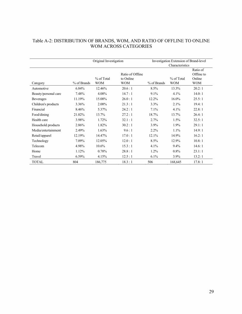
29
Table A-2: DISTRIBUTION OF BRANDS, WOM, AND RATIO OF OFFLINE TO ONLINE WOM ACROSS CATEGORIES
Original Investigation Investigation Extension of Brand-level
Characteristics
Category % of Brands % of Total WOM
Ratio of Offline to Online WOM % of Brands
% of Total WOM
Ratio of Offline to Online WOM
Automotive 6.84% 12.46% 20.6 : 1 8.5% 13.3% 20.2: 1
Beauty/personal care 7.48% 4.08% 14.7 : 1 9.1% 4.1% 14.0: 1
Beverages 11.19% 15.08% 26.0 : 1 12.2% 16.0% 25.5: 1
Children's products 3.36% 2.08% 21.3 : 1 3.3% 2.1% 19.4: 1
Financial 8.46% 5.37% 24.2 : 1 7.1% 4.1% 22.8: 1
Food/dining 21.02% 13.7% 27.2 : 1 18.7% 13.7% 26.4: 1
Health care 3.98% 1.72% 32.1 : 1 2.7% 1.5% 32.5: 1
Household products 2.86% 1.82% 30.2 : 1 3.9% 1.9% 29.1: 1
Media/entertainment 2.49% 1.63% 9.6 : 1 2.2% 1.1% 14.9: 1
Retail/apparel 12.19% 14.47% 17.0 : 1 12.1% 14.9% 16.2: 1
Technology 7.09% 12.05% 12.0 : 1 8.5% 12.9% 10.8: 1
Telecom 4.98% 10.6% 15.3 : 1 4.1% 9.4% 14.6: 1
Home 1.12% 0.78% 28.8 : 1 1.2% 0.8% 23.1: 1
Travel 6.59% 4.15% 12.5 : 1 6.1% 3.9% 13.2: 1
TOTAL 804 186,775 18.3 : 1 506 168,645 17.8: 1

30
Table A-3: REPRESENTATIVE BRANDS ACROSS DIFFERENT LEVELS OF BRAND TRAITS
Brand Characteristic Low Scores (≤20 percentile) Central Scores (40th to 60th percentile)
High Scores (≥80th percentile)
Interestingness Pine Sol, Alamo Jet Blue, Saab Mazda, Wendys Brand Differentiation Days Inn, Motrin Powerade, Nissan Bose, NetFlix Esteem Virgin Mobile, Kia Ragu, Dannon Home Depot, Windex Premium IHop, Suave Kraft, Heinz Jaguar, JCrew Relevance Saab, Sam Adams Zest, Starbucks Kleenex, Target Visibility Prada, Ivory Enterprise, Nestea Pepsi, Levis Excitement Tylenol, Wachovia Dr. Pepper, Subway Nikon, Ikea Satisfaction Delta, Alamo Whirlpool, Panera Chanel, Hoover Brand Age YouTube, Red Bull Brother, Dunkin Donuts Levis, Coors Complexity Pledge, Hostess Bose, Publix AIG, Ferrari Knowledge Meijer, Guiness HR Block, Reebok Lysol, Lego Perceived Risk Kleenex, Snickers Hyatt, Garmin Prilosec, Hollister Involvement Coca-Cola, Febreeze Luvs, Verizon Allstate, Nissan Advertising Ajax, Hollister Dennys, Corona Sears, Tampax Brand Equity Suzuki, AIG Ross, Poland Spring Whole Foods, Doritos Brand Usage Porsche, Etrade Costco, Bacardi Heinz, Subway WOM Volume Purex, Geico Sierra Mist, Nordstrom Apple, Nike
31
REFERENCES
Ajzen, Icek (1991), "The theory of planned behavior," Organizational behavior and human decision
processes, 50 (2), 179-211.
Alexandrov, Aliosha, Bryan Lilly, and Emin Babakus (2013), "The effects of social-and self-motives
on the intentions to share positive and negative word of mouth," Journal of the Academy of Marketing
Science, 41 (5), 531-46.
Armstrong, J. Scott, Vicki G. Morwitz, and V. Kumar (2000), "Sales forecasts for existing consumer
products and services: Do purchase intentions contribute to accuracy?," International Journal of
Forecasting, 16 (3), 383-97.
Arndt, Johan (1967), "Word of Mouth Advertising and Informal Communication," in Risk Taking and
Information Handling in Consumer Behavior, Donald F. Cox, ed. Boston: Harvard Business School.
Bansal, Harvir S. and Peter A. Voyer (2000), "Word-of-mouth processes within a services purchase
decision context," Journal of Service Research, 3 (2), 166-77.
Barnlund, Dean C. (1970), "A transactional model of communication," in Foundations of
Communication Theory, Kenneth K. Sereno and C. David Mortensen, eds. New York: Harper and
Row.
Bemmaor, Albert C (1995), "Predicting behavior from intention-to-buy measures: The parametric
case," Journal of Marketing Research, 176-91.

32
Berger, Jonah and Raghuram Iyengar (2013), "Communication Channels and Word of Mouth: How the
Medium Shapes the Message," Journal of Consumer Research, 40 (10), 567 - 79
Berger, Jonah and Katherine L. Milkman (2012), "What makes online content viral?," Journal of
Marketing Research, 49 (2), 192-205.
Berger, Jonah and Eric Schwartz (2011), "What Drives Immediate and Ongoing Word of Mouth?,"
Journal of Marketing Research, 48 (5), 869-80.
Berger, Jonah, Alan T. Sorensen, and Scott J. Rasmussen (2010), "Positive Effects of Negative
Publicity: When Negative Reviews Increase Sales," Marketing Science, 29 (5), 815-27.
Brown, Jacqueline Johnson and Peter H. Reingen (1987), "Social Ties and Word-of-Mouth Referral
Behavior," Journal of Consumer Research, 14 (3), 350-62.
Burgoon, Judee K. and D. Nimmo (1980), "Nonverbal communication research in the 1970s: An
overview," Communication Yearbook, 4, 179-97.
Carl, Walter J. (2006), "What's All the Buzz About?: Everyday Communication and the Relational
Basis of Word-of-Mouth and Buzz Marketing Practices," Management Communication Quarterly, 19
(4), 601-34.
Chevalier, Judith A. and Dina Mayzlin (2006), "The Effect of Word of Mouth on Sales: Online Book
Reviews," Journal of Marketing Research, 43 (3), 345-54.
33
Cho, Charles H, Martin L Martens, Hakkyun Kim, and Michelle Rodrigue (2011), "Astroturfing global
warming: It isn’t always greener on the other side of the fence," Journal of business ethics, 104 (4),
571-87.
Cheung, Christy M.K. and Dimple R. Thadani (2012), “The impact of electronic word-of-mouth
communication: A literature analysis and integrative model,” Decision Support Systems, 54 (1), 461-
470.
Daft, Richard L. and Robert H. Lengel (1986), "Organizational Information Requirements, Media
Richness and Structural Design," Management Science, 32 (5), 554-71.
De Angelis, Matteo , Andrea Bonezzi, Alessandro M. Peluso, Derek D. Rucker, and Michele Costabile
(2012), "On Braggarts and Gossips: A Self-Enhancement Account of Word-of-Mouth Generation and
Transmission," Journal of Marketing Research, 49 (4), 551-63.
De Bruyn, Arnaud and Gary L. Lilien (2008), "A Multi-Stage Model of Word-of-Mouth Influence
Through Viral Marketing," International Journal of Research in Marketing, 25 (3), 151-63.
De Matos, Celso Augusto and Carlos Alberto Vargas Rossi (2008), "Word-of-Mouth Communications
in Marketing: A Meta-Analytic Review of the Antecedents and Moderators," Journal of the Academy
of Marketing Science, 36 (4), 578-96.

34
Dempsey, Melanie A. and Andrew A. Mitchell (2010), "The Influence of Implicit Attitudes on Choice
When Consumers Are Confronted with Conflicting Attribute Information," Journal of Consumer
Research, 37 (4), 614-25.
Dennis, Alan R. and Susan T. Kinney (1999), "Testing Media Richness Theory in the New Media: The
Effects of Cues, Feedback, and Task Equivocality," Information Systems Research, 9 (3), 256-74.
East, Robert, Kathy Hammond, Wendy Lomax (2008), “Measuring the impact of positive and negative
word of mouth on brand purchase probability,” International Journal of Research in Marketing, 25 (3),
215-224.
Fay, Brad and Steve Thomson (2012), "WOM is More Offline than Online," AdMap (October), 24-26.
Frenzen, Jonathan K. and Harry L. Davis (1990), "Purchasing Behavior in Embedded Markets,"
Journal of Consumer Research, 17 (1), 1-12.
Frenzen, Jonathan and Kent Nakamoto (1993), "Structure, Cooperation, and the Flow of Market
Information," Journal of Consumer Research, 20 (3), 360-75.
Granovetter, Mark S. (1983), "The strength of weak ties: A network theory revisited," Sociological
Theory, 1 (1), 201-33.
Higie, Robin A., Lawrence F. Feick, and Linda L. Price (1987), "Types and Amount of Word-of-
Mouth Communications About Retailers," Journal of Retailing, 63 (3), 260-78.

35
King Robert Allen, Racherla Pradeep, Bush Victoria D. (2014),”What We Know and Don't Know
About Online Word-of-Mouth: A Review and Synthesis of the Literature,” Journal Of Interactive
Marketing;28(3):167-183.
Libai, Barak, Eitan Muller, and Renana Peres (2013), "Decomposing the Value of Word-of-Mouth
Seeding Programs: Acceleration Versus Expansion," Journal of Marketing Research, 50 (2), 161- 76.
Lovett, Mitchell J., Renana Peres, and Ron Shachar (2013), "On Brands and Word of Mouth," Journal
of Marketing Research, 50 (4), 427-44.
Lovett, Mitchell, Renana Peres, and Ron Shachar (2014), “A Data Set of Brands and Their
Characteristics,” Marketing Science, 33 (4), 609-617.
Manski, Charles F. (1990), "The use of intentions data to predict behavior: A best-case analysis,"
Journal of the American Statistical Association, 85 (412), 934-40.
McPherson, Miller, Lynn Smith-Lovin, and James M. Cook (2001), "Birds of a feather: Homophily in
social networks," Annual Review of Sociology, 27, 415-44.
Morrison, Donald G. (1979), "Purchase intentions and purchase behavior," Journal of Marketing, 43
(2), 65-74.
Morwitz, Vicki G., Joel H. Steckel, and Alok Gupta (2007), "When do purchase intentions predict
sales?," International Journal of Forecasting, 23 (3), 347-64.

36
Ryu, Gangseog and Lawrence Feick (2007), "A Penny for Your Thoughts: Referral Reward Programs
and Referral Likelihood," Journal of Marketing, 71 (1), 84-94.
Shannon, Claude Elwood (1948), "A mathematical theory of communication," Bell System Technical
Journal, 27 (1), 379-423 and 623-25.
Singh, Jagdip (1990), "Voice, Exit, and Negative Word-of-Mouth Behaviors: An Investigation Across
Three Service Categories," Journal of the Academy of Marketing Science, 18 (1), 1.
Stephen, Andrew T. and Donald R. Lehmann (2009), "Why Do People Transmit Word-of-Mouth? The
Effects of Recipient and Relationship Characteristics on Transmission Behaviors," in SSRN #1150996.
Sundaram, D.S., Kaushik Mitra, and Cynthia Webster (1998), "Word-of-Mouth Communications: A
Motivational Analysis," in Advances in Consumer Research, Joseph W. Alba and J. Wesley
Hutchinson (Eds.) Vol. 25. Provo, UT: Association for Consumer Research.
Trusov, Michael, Anand V. Bodapati, and Randolph E. Bucklin (2010), "Determining Influential Users
in Internet Social Networks," Journal of Marketing Research, 47 (4), 643-58.
Tversky, Amos and Daniel Kahneman (1991), "Loss aversion in riskless choice: A reference-dependent
model," The Quarterly Journal of Economics, 106 (4), 1039-61.
Weimann, Gabriel (1983), "The Strength of Weak Conversational Ties in the Flow of Information and
Influence," Social Networks, 5 (September), 245 - 67.
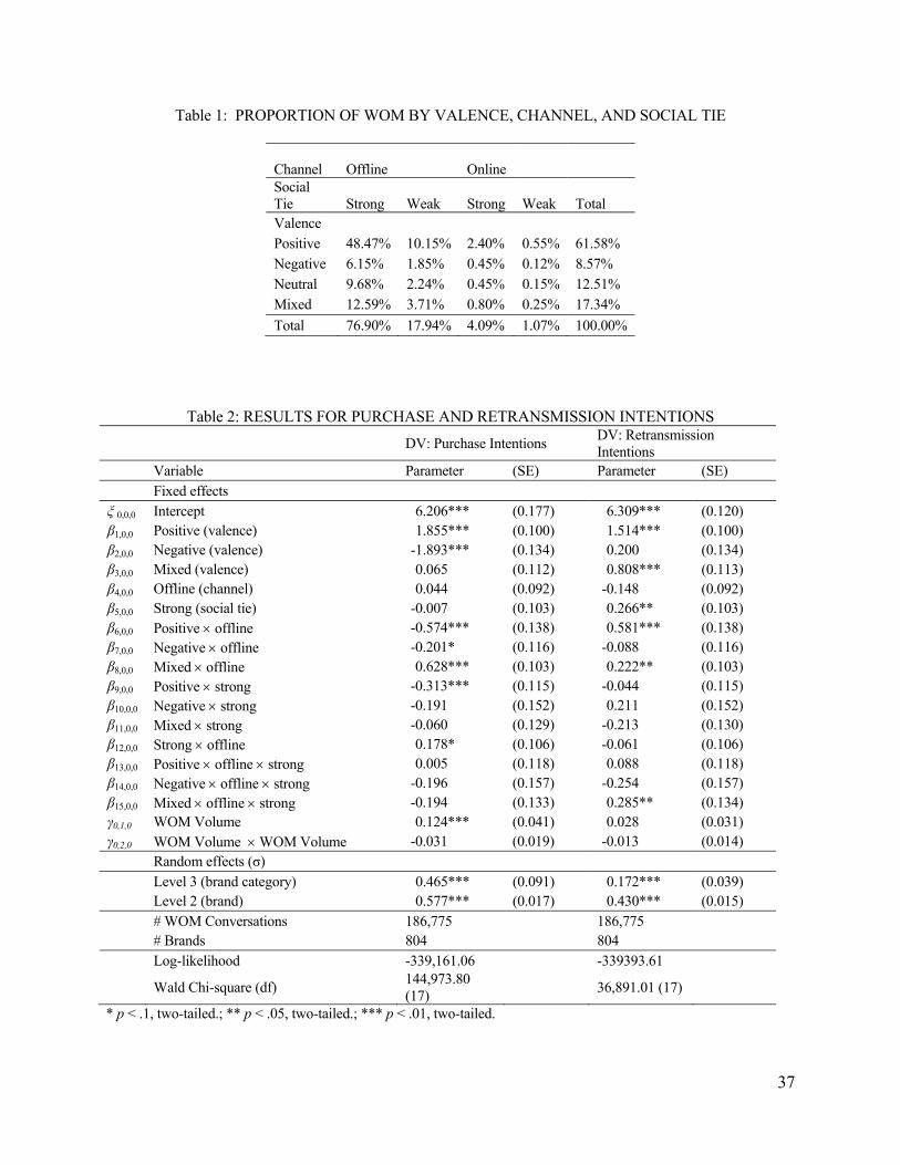
37
Table 1: PROPORTION OF WOM BY VALENCE, CHANNEL, AND SOCIAL TIE
Channel Offline Online
Social Tie Strong Weak Strong Weak Total Valence Positive 48.47% 10.15% 2.40% 0.55% 61.58% Negative 6.15% 1.85% 0.45% 0.12% 8.57% Neutral 9.68% 2.24% 0.45% 0.15% 12.51% Mixed 12.59% 3.71% 0.80% 0.25% 17.34%
Total 76.90% 17.94% 4.09% 1.07% 100.00%
Table 2: RESULTS FOR PURCHASE AND RETRANSMISSION INTENTIONS
DV: Purchase Intentions DV: Retransmission Intentions
Variable Parameter (SE) Parameter (SE) Fixed effects ξ 0,0,0 Intercept 6.206*** (0.177) 6.309*** (0.120) β1,0,0 Positive (valence) 1.855*** (0.100) 1.514*** (0.100) β2,0,0 Negative (valence) -1.893*** (0.134) 0.200 (0.134) β3,0,0 Mixed (valence) 0.065 (0.112) 0.808*** (0.113) β4,0,0 Offline (channel) 0.044 (0.092) -0.148 (0.092) β5,0,0 Strong (social tie) -0.007 (0.103) 0.266** (0.103) β6,0,0 Positive offline -0.574*** (0.138) 0.581*** (0.138) β7,0,0 Negative offline -0.201* (0.116) -0.088 (0.116) β8,0,0 Mixed offline 0.628*** (0.103) 0.222** (0.103) β9,0,0 Positive strong -0.313*** (0.115) -0.044 (0.115) β10,0,0 Negative strong -0.191 (0.152) 0.211 (0.152) β11,0,0 Mixed strong -0.060 (0.129) -0.213 (0.130) β12,0,0 Strong offline 0.178* (0.106) -0.061 (0.106) β13,0,0 Positive offline strong 0.005 (0.118) 0.088 (0.118) β14,0,0 Negative offline strong -0.196 (0.157) -0.254 (0.157) β15,0,0 Mixed offline strong -0.194 (0.133) 0.285** (0.134) γ0,1,0 WOM Volume 0.124*** (0.041) 0.028 (0.031) γ0,2,0 WOM Volume WOM Volume -0.031 (0.019) -0.013 (0.014) Random effects (σ) Level 3 (brand category) 0.465*** (0.091) 0.172*** (0.039) Level 2 (brand) 0.577*** (0.017) 0.430*** (0.015) # WOM Conversations 186,775 186,775 # Brands 804 804 Log-likelihood -339,161.06 -339393.61
Wald Chi-square (df) 144,973.80 (17)
36,891.01 (17)
* p < .1, two-tailed.; ** p < .05, two-tailed.; *** p < .01, two-tailed.
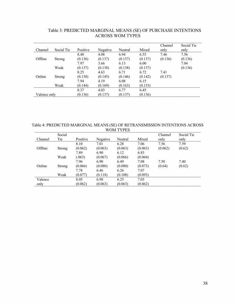
38
Table 3: PREDICTED MARGINAL MEANS (SE) OF PURCHASE INTENTIONS ACROSS WOM TYPES
Channel Social Tie Positive Negative Neutral Mixed Channel only
Social Tie only
Offline Strong 8.48 (0.136)
4.08 (0.137)
6.94 (0.137)
6.55 (0.137)
7.46 (0.136)
7.56 (0.136)
Weak 7.97 (0.137)
3.66 (0.138)
6.13 (0.138)
6.00 (0.137)
7.04 (0.136)
Online Strong 8.25 (0.138)
4.63 (0.145)
6.71 (0.146)
6.72 (0.142)
7.41 (0.137)
Weak 7.94 (0.144)
4.19 (0.169)
6.08 (0.163)
6.15 (0.153)
Valence only 8.37 (0.136)
4.03 (0.137)
6.77 (0.137)
6.45 (0.136)
Table 4: PREDICTED MARGINAL MEANS (SE) OF RETRANSMISSION INTENTIONS ACROSS WOM TYPES
Channel Social Tie Positive Negative Neutral Mixed
Channel only
Social Tie only
Offline Strong 8.10 (0.062)
7.01 (0.063)
6.28 (0.063)
7.06 (0.063)
7.56 (0.062)
7.59 (0.62)
Weak 7.89 (.063)
6.90 (0.067)
6.12 (0.066)
6.83 (0.064)
Online Strong 7.96 (0.066)
6.90 (0.080)
6.49 (0.080)
7.08 (0.073)
7.50 (0.64)
7.40 (0.62)
Weak 7.78 (0.077)
6.46 (0.118)
6.26 (0.108)
7.07 (0.093)
Valence only
8.05 (0.062)
6.98 (0.063)
6.25 (0.063)
7.03 (0.062)
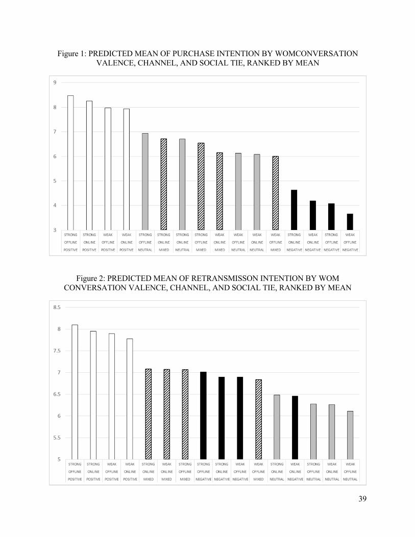
39
Figure 1: PREDICTED MEAN OF PURCHASE INTENTION BY WOMCONVERSATION VALENCE, CHANNEL, AND SOCIAL TIE, RANKED BY MEAN
Figure 2: PREDICTED MEAN OF RETRANSMISSON INTENTION BY WOM CONVERSATION VALENCE, CHANNEL, AND SOCIAL TIE, RANKED BY MEAN
1
LOWER CONNECTIVITY IS BETTER: THE EFFECTS OF NETWORK STRUCTURE
ON REDUNDANCY OF IDEAS AND CUSTOMER INNOVATIVENESS IN
INTERDEPENDENT IDEATION TASKS
Andrew T. Stephen L’Oréal Professor of Marketing
University of Oxford, Saïd Business School Park End Street, Oxford OX1 1HP, United Kingdom
Email [email protected]
Peter Pal Zubcsek Assistant Professor of Marketing
University of Florida, Warrington College of Business 212 Bryan Hall, Gainesville FL 32611
Email [email protected]
Jacob Goldenberg Professor of Marketing
Interdisciplinary Center, Herzliya, Israel Visiting Professor of Marketing, Columbia Business School
Email [email protected]
* Andrew T. Stephen is the L’Oréal Professor of Marketing at the Saïd Business School, University of Oxford. Peter Pal Zubcsek is Assistant Professor of Marketing at the Warrington College of Business, University of Florida. Jacob Goldenberg is Professor of Marketing at the School of Business Administration, IDC Herzliya, Israel and Visiting Professor of Marketing at Columbia Business School. The authors thank Joe Alba, Yakov Bart, Eyal Biyalogorsky, Nicole Coleman, Raghu Iyengar, Chris Janiszewski, Rajiv Jayaraman, Don Lehmann, Page Moreau, Prashant Sasatte, Cammy Crolic, Felipe Thomaz, Olivier Toubia, Christophe Van den Bulte, and seminar participants at Carnegie Mellon University, Dartmouth College, Harvard Business School, the Hebrew University of Jerusalem, IDC Herzliya, IE Business School, National University of Singapore, Tulane University, University of Georgia, University of Houston, University of Maryland, University of Miami, University of New South Wales, University of Oxford, University of Pennsylvania, University of Queensland, and University of Washington. This research was generously supported by the Marketing Science Institute (4-1683), with
2
additional financial support from the University of Pittsburgh Katz Faculty Fellowship and the INSEAD Alumni Fund. LOWER CONNECTIVITY IS BETTER: THE EFFECTS OF NETWORK STRUCTURE
ON REDUNDANCY OF IDEAS AND CUSTOMER INNOVATIVENESS IN
INTERDEPENDENT IDEATION TASKS
ABSTRACT
This paper examines the popular marketing practice of interdependent ideation where
firms solicit ideas from customers through online platforms that allow for customers to be
exposed to or “inspired” by other customers’ ideas when generating their own. Although being
exposed to others’ ideas means that customers are “connected” (at least implicitly) in a
communication network that facilities flows of ideas, the effect of network structure or
interconnectivity on individual innovativeness has not been considered in this context. The
authors examine how, when, and why network structure, specifically the clustering or
interconnectivity of one’s “inspirations” (other customers), affects the innovativeness of
individual customers’ product/service ideas in ideation tasks. Across five experiments it is shown
that (i) higher clustering/interconnectivity negatively affects the innovativeness of an
individual’s ideas, (ii) this occurs because idea inspirations are more likely to be similar or
redundant when the sources of those inspirations (i.e., other customers to which one is
connected) are clustered, (iii) higher redundancy among idea used as inspirations is what causes
lower innovativeness, and (iv) this effect is attenuated when customers do not rely on other
customers’ ideas for inspiration.
3
One of the most important marketing activities in which a firm engages is product and
service innovation. A critical initial stage in any innovation process is ideation, which
encompasses the generation of product or service ideas, either for general concepts or for
specific features or improvements (Cooper 1990; Urban and Hauser 1993). Ideation is
particularly important, since identifying potentially viable market opportunities as early as
possible in the innovation process can lead to greater efficiency at subsequent stages (Dahan and
Hauser 2002; Smith and Reinertsen 1992). A currently popular and fast-growing trend in
marketing ideation is for customers to be invited to contribute product or service ideas through
interactive online platforms (e.g., on social media sites or online discussion forums). This
approach is sometimes referred to as the “crowdsourcing” of product ideas (Bayus 2013;
Freedman 2012; Winsor 2009), and has been used by companies such as Dell, Delta Air Lines,
Google, Lego, McDonalds, PepsiCo, and Starbucks. This fast-growing approach to ideation is a
continuation of the longer-term trend of firms seeking customer input in product development
(e.g., focus groups, market research). This newer approach, however, is distinct because it uses
online platforms where customers not only suggest ideas to firms but also have the ability to see
other customers’ ideas when generating their own.
Firms typically use these types of customer-based ideation for soliciting ideas that can
then be fed into more conventional new product development processes. In the customer-based
ideation stage, the typical goal is to get as many highly innovative ideas as possible because it
expands the set of potentially viable alternatives that can be subsequently considered internally.
Thus, individual innovativeness, or a customer’s ability to generate innovative ideas, is critical in
this setting.1 Although individual innovativeness is affected by many factors, an important one in
1 This is consistent with online crowdsourcing research (e.g., Bayus 2013; Huang, Singh, and Srinivasan 2014).
4
this context could be the influence of other customers’ ideas on an individual’s ideas. Indeed,
prior literature on creativity and innovativeness in different contexts to the one we consider in
general suggests that individuals’ ideas can be influenced positively or negatively by others
around them who are working on the same or similar tasks (e.g., Lamm and Trommsdorff 2006;
Mason and Watts 2012; Pan, Alsthuler, and Pentland 2012).
A fundamental aspect of the online product ideation setting considered in this research is
that customers express ideas in front of others, meaning that an ideating customer can access,
and thus be exposed to and potentially influenced by, ideas previously contributed by other
customers on the platform. This access to other customers’ prior ideas means that ideating
customers are “connected” to each another in a network where ideas flow over network ties
between customers.2 In this research we posit that the networked, interconnected nature of the
online product ideation context plays a critical role in affecting individual customers’ abilities to
generate innovative ideas.
Specifically, we examine how, when, and why the connectivity structure—or network—
among ideating customers affects their innovativeness. We build on prior literature in different
contexts suggesting that individual creativity is reduced when ideation inputs (e.g., in our
context, other customer’s previous ideas) are similar, overlapping, or redundant (Lamm and
Trommsdorff 2006; Pan, Alsthuler, and Pentland 2012; Paulus et al. 2002; Pentland 2013), and
consider how network structure might affect the tendency for customers’ ideas to become more
or less redundant. We focus on the role of network clustering, or the extent to which a
2 Following common practice and convention we represent this network as a temporal “social” network. This does not imply, however, that customers who are connected to one another must know each other or be friends. Simply, the ties in this type of network at a minimum allow for ideas to be communicated between customers (i.e., a communication network).
5
customer’s “sources of inspiration” or network “neighbors” are connected to each other,3 and
show that neighbors’ ideas are more likely to form a redundant set of inspirations for an ideating
customer when the neighbors are more clustered. We also show that a customer’s ability to
generate innovative ideas is stifled by this clustering-driven greater redundancy among network
neighbors’ (or “social” sources of inspiration) ideas. Importantly, the negative effect of idea
redundancy with respect to neighbors’ ideas is found to only occur when customers rely on
others’ ideas as inputs into their own ideation processes. In sum, we demonstrate that the
innovativeness of customers’ product ideas suffers when they ideate by using others’ ideas as
input or for inspiration when the online network in which customers are situated is relatively
highly clustered. In practice, such networks tend to have higher (as opposed to lower) levels of
clustering on average. Thus, a major implication of our findings is that the typical structure used
for online interdependent product ideation tasks run by major companies such as Dell and
Starbucks is suboptimal in the sense that, when using others’ ideas for inspiration, customers’
abilities to formulate highly innovative ideas are stifled due to the underlying network structure.
Thus, according to our findings, firms can significantly improve the effectiveness of their
ideation platforms if they control or limit the clustering of the underlying networks.
We empirically test how clustering affects idea redundancy and innovativeness across
five experiments. A key distinction between this research and prior studies from outside
marketing is that we use controlled experiments whereby participants (who are anonymous to
each other) are randomly assigned to positions in exogenously determined network structures that
govern whose ideas they can see as they complete an ideation task in real time. This enables us
3 Clustering, or neighbor interconnectivity, is defined as the density of connections between the direct neighbors of a person, i.e. the proportion (between 0 and 1) of pairs among the person’s neighbors that are directly connected to each other. Higher clustering indicates greater interconnectivity among neighbors.
6
to identify how clustering affects ideation without concerns related to homophily and network
endogeneity that exist in related research on networks and creativity (e.g., Burt 2004, 2005;
Levine and Prietula 2013; Perry-Smith and Shalley 2003).
To preview our results, we find that (i) higher clustering among the other customers
whose ideas one is exposed to negatively affects the innovativeness of an individual’s ideas, (ii)
this occurs because idea inspirations are more likely to be similar or redundant when the sources
of those inspirations are highly interconnected or clustered, (iii) higher redundancy in one’s set
of inspirations causes lower innovativeness, and (iv) this effect is attenuated when customers do
not rely on others’ ideas. This research contributes to the literature on interdependent or network-
based ideation in a variety of fields by showing how, when, and why network clustering affects
individual innovativeness using a controlled experimental approach that is not subject to
endogeneity-, simultaneity-, or homophily-related concerns associated with related research in
other fields that use non-experimental (field) network data. We also build on non-marketing
research on topics such as brainstorming where redundancy has been linked to performance on
innovation and problem-solving tasks, but where networks are not examined or manipulated.
Finally, and most importantly, we contribute to the marketing ideation literature by showing how
network structure affects innovativeness and that current approaches are suboptimal. If correct,
our findings suggest that online interdependent product ideation platforms used by firms should
be reengineered so that the underlying networks linking ideating customers are less clustered.
BACKGROUND
Connections to other customers in communication networks allow for information flows
that can render individual behavior more interdependent than in situations where people ideate
7
without exposure to others’ ideas. Thus, we generally refer to our context as interdependent
ideation and consider it to be distinct from settings in which individuals generate ideas or
creatively solve problems on their own. Interdependent ideation simply means that individuals
are situated in communication networks and their ideas can potentially be influenced by the ideas
of others around them. Importantly, interdependent ideation does not entail individuals working
together in groups to generate ideas or solve problems collaboratively. The goal of the current
research is to better understand interdependent ideation for products or services by identifying
conditions under which it either enhances or diminishes the innovativeness of an individual
customer’s ideas for products or services.4 Unfortunately, while many firms have
“crowdsourced” product ideas by involving customers in various forms of interdependent
ideation tasks, results have been mixed. For example, firms typically implement very few of the
ideas submitted by customers in online interdependent ideation platforms (e.g., the success rates
for ideas from Dell’s IdeaStorm.com and Starbucks’ MyStarbucksIdea.com are less than 3% and
less than 1%, respectively). A problem faced by firms is that simply not enough of customers’
ideas are sufficiently innovative to warrant serious further consideration by internal teams.
Although this underperformance could occur for a variety of reasons (e.g., customers
having low task motivation and involvement, not taking the task seriously, not possessing
sufficient knowledge or expertise), one possibility is that ideating interdependently could
negatively affect individual innovativeness because having access to other customers’ ideas
could negatively affect or contaminate one’s ideation processes. As we mentioned earlier, access
to other customers’ ideas in this setting means that ideating customers are situated in a
communication network where information in the form of ideas (or underlying concepts and
4 Consistent with extant literature related to marketing outcomes, we consider innovative ideas to be creative/novel and to have the potential to be useful (Bayus 2013; Burroughs, Moreau, and Mick 2008).
8
themes) flows over network ties between customers who are exposed to each other’s ideas. The
structure of this type of network arguably determines the extent to which customers may ideate
interdependently, and we are interested in how, when, and why the structure of this type of
network affects individual innovativeness with respect to the product/service ideas they generate.
Theoretical Context
Three non-marketing literature streams offer a perspective on these questions, and
suggest that connections or networks can affect individual performance in complex problem-
solving tasks, including tasks involving creativity. We use these literatures as general
foundations for the conceptual framework we subsequently propose.
First, the wisdom of crowds literature (e.g., Pan, Alsthuler, and Pentland 2012; Pentland
2013) documents that “crowds” can be “less wise” as they become more interdependent. In other
words, connections to others could affect individual performance. However, this literature
(including experimental studies, e.g., Mason, Jones, and Goldstone 2008, Mason and Watts
2012) has limited applicability in the context of creative and innovative thinking because it
typically considers well defined “closed-ended” problems (i.e., problems with usually not more
than one or two objectively “correct” solutions). Conversely, in our context the “problem” is
usually ill defined and “open-ended” (i.e., with multiple solutions, none of which are necessarily
“correct,” but where some are subjectively better than others). Also, a typical wisdom of crowds
setting considers individual, seemingly independent contributions that are aggregated to find
solutions (e.g., the most-common or most-popular ideas). The interdependence referred to in this
literature is based on the notion that each person’s contribution may not be a truly independent
draw from a distribution, and thus the distribution of idea popularity used to identify an
aggregate solution is biased. Notwithstanding these key differences between the wisdom of
9
crowds literature and the current research, the notion that being exposed to others can affect
one’s ideas (albeit on very different tasks to the type we consider) is conceptually relevant here.
Second, the organizational sociology and networks literature suggests that the formal and
informal social networks connecting managers or employees in organizations can affect both
individual and workgroup performance on problem-solving tasks involving creative and
innovative thinking (e.g., Bavelas 1950; Burt 2004, 2005; Levine and Prietula 2013; Perry-Smith
and Shalley 2003). This literature shows that a person’s position in a network structure can be
important because their connections moderate access to resources. However, as Kleinbaum
(2012) points out, this literature generally suffers from serious endogeneity concerns that make it
difficult to generalize these results to other contexts (such as product ideation involving
customers) and to infer a causal effect of interdependent versus independent ideation on
individual innovative performance. This is because the organizational networks studied in this
literature develop endogenously over time and it is possible that, for instance, a manager who is
more creative is in a certain network position because of their performance, and not that their
creativity is a consequence of their network position.5 Another concern related to this problem is
that these networks have connections that carry multiple meanings, which also makes it hard to
identify specific effects of network position on innovation or creativity performance. For
instance, a connection between two people indicates the ability to communicate (i.e., exchange
information) as well as social (e.g., friendship) and/or professional relations (e.g.,
superior/subordinate). Thus, the networks in this literature are naturally confounded because
5 E.g., organizational sociology research using field (but endogenous) organization network data suggests that less-dense networks of workers are more innovative. This could be because lower density results in higher creativity, but it could also be that more creative workers form broader sets of ties spanning across an organization that result in lower density. I.e., it is unclear in which direction the effect goes.

10
connections can carry meaning beyond being merely communicative.6 We avoid this in our
experiments by connecting anonymous people in networks that are purely communicative and
thus the network ties in our experiments carry no social or relational connotations.
The organizational sociology literature also often focuses on how networks affect group
(not individual) performance or, if an individual unit of analysis is used, it is often with respect
to how individuals contribute to their work groups or teams. Our context differs from this
because we are interested solely in individual innovativeness in a completely non-collaborative
setting (i.e., individuals can be influenced by others but they do not work or collaborate with
others). Further, this literature considers very different tasks to those studied here, typically
focusing on longer-term innovation and problem solving processes in offline, intra-
organizational settings involving managers or employees. We instead consider short-term (close
to real-time) ideation in an online, non-organizational setting involving customers, and where
networks are temporary in that they are built for and last only for the duration of the ideation
task. Thus, while the organizational sociology literature that examines phenomena related to ours
does show that networks can matter (and indicates some specific ways in which they matter),
there are many points of distinction between that literature and the current research.
Third, the brainstorming literature, which is mostly in the organizational behavior and
psychology literatures, also provides a basic foundation for the current research. Brainstorming
studies show that allowing people to generate solutions or ideas in groups versus by themselves
can sometimes lead to better outcomes, but not always (e.g., Clemen and Winkler 1985; Gallupe
et al. 1992; Lamm and Trommsdorff 2006; Mullen et al. 1991; Pinsonneault et al. 1999). Further,
6 E.g., in actual social networks the ties between pairs of people allow for information to flow (i.e., communication ties) and have some degree of relationship strength (e.g., strangers, acquaintances, friends). How network structure/position characteristics influence individual outcomes in such networks can be interpreted in terms of communication flows, relational characteristics, or both. This makes it generally impossible to interpret observed effects of network position on individual outcomes because of the multiplicity of meanings associated with ties.

11
since much of the brainstorming research is within the social psychology paradigm, this literature
also provides some potential mechanisms for how ideating within groups can influence
individual and group outcomes (e.g., the literature on production blocking, which helps explain
why brainstorming groups sometimes underperform; Lamm and Trommsdorff 2006). However,
brainstorming findings have only limited applicability to the current research. This is because
communication network structure is not considered in brainstorming and therefore has never
been tested. In a brainstorming setting, people are in groups of a certain sizes. From a
communication network perspective, everyone is “connected” to everyone else in such groups,
and thus there is zero variation in how people are interconnected (i.e., a brainstorming group, if
represented as a network, will be always be fully connected). Another point of difference
between brainstorming and the current research is that often the outcome in brainstorming is at
the group level because brainstorming is largely a collaborative activity. Our context is different
to this because it involves individuals ideating in a non-collaborative manner.
In sum, although the current research is related to and draws from these research streams,
the phenomenon we study is distinct and our approach is novel. In Web Appendix A we compare
and contrast these three streams with the current research. How (or whether) network structure
affects individual innovativeness in an interdependent online product ideation setting is indeed
hinted at in prior work but it is neither well examined nor clearly understood. The research
mentioned in Web Appendix A indicates that network structure can be important, but considers
very different settings (i.e., not marketing-related) and types of ideators (i.e., not customers or
consumers). Also, findings from organizational sociology studies of creativity in networks are
subject to endogeneity concerns that make it impossible to identify causal effects of network
structure on creativity or innovativeness. Effects of network structure on innovativeness also
12
cannot be inferred from the brainstorming literature because in that literature people are
organized into groups where everyone is “connected” to everyone else, and thus there is no
variation in structure that allows for structure-related effects (e.g., clustering) to be identified.
Finally, when and why network structure, particularly clustering, affects innovativeness has been
largely ignored in these research streams.7 The current research, however, addresses this gap that
lies at the intersection of these three research streams by explaining how network clustering
negatively influences innovativeness when people use neighbors’ ideas as inputs or inspirations
because clustering makes neighbors’ ideas more likely to be redundant.
Practical Context
The current research is motivated by the growing popularity of various forms of
interdependent online product ideation used by companies in the earlier stages of their new
product development (or improvement) processes. Although this can take on many forms when
implemented by marketers, the setting we consider (and base our experimental paradigm on) is
intended to capture essential aspects common to many variants of interdependent online product
ideation seen in practice. Specifically, we consider on a customer-based product ideation setting
that has the following realistic characteristics: (i) customers generate ideas for products or
services, (ii) this occurs in an online setting where individuals can see other customers’ previous
ideas, (iii) participation is non-collaborative in that individuals do not work together to generate
ideas, (iv) connections between customers allow for information (ideas, concepts) to be
exchanged, and (v) these connections allow for possible interdependence.
A key difference, however, between what is commonly done in practice and what we do
here is that we explicitly manipulate network structure in a manner that allows us to assess the
7 We acknowledge that the organizational sociology literature conjectures a number of mechanisms, though many are not applicable to marketing or, if they are, they reflect ideation processes that unfold over months or even years.

13
full range of clustering. Our theory is, essentially, that innovative performance suffers at the
individual level when clustering is too high. Unfortunately, in practice clustering tends to be
quite high. For example, in settings that mimic electronic brainstorming groups, everyone is
“connected” to (or can see) everyone else, which means that clustering is very high. In settings
that allow for people who are connected to each other in existing online social networks (e.g.,
Facebook) to “share ideas” the average clustering also tends to not be small (e.g., Ugander et al.
2011). And in settings such as those used by Dell (IdeaStorm.com) and Starbucks
(MyStarbucksIdea.com) that take the form of “discussion boards” where network connections
are implicit based on who sees (or votes/comments on) whose ideas, the underlying networks can
also be relatively highly interconnected (e.g., a mapping of the network underlying Dell’s
IdeaStorm.com found an average clustering of .33 [SD = .20, median = .31, min. = 0, max. = 1];
see Web Appendix B). Thus, from a practical standpoint this research can help firms introduce a
new feature of controlling interconnectivity between ideating customers and optimizing it.
CONCEPTUAL FRAMEWORK
In this section we formalize the arguments made earlier about how, when, and why
network clustering affects the innovative performance of individual customers in interdependent
online product ideation tasks. Figure 1 summarizes our conceptual framework.
[INSERT FIGURE 1 ABOUT HERE]
We begin by considering how being connected to other ideating customers in a network
setting might impact an individual’s ideas. Others’ ideas could be helpful inputs to one’s own
idea-generating processes. Seeing what other customers have suggested, for instance, could be
useful inspirations for one’s own ideas, particularly given that using concepts from existing
14
knowledge—or from others—and arranging or combining them in new ways is a common
process through which innovative ideas are formed (Amabile 1988, 1996; Dahl and Moreau
2002; Fleming and Szigety 2006; Goldenberg et al. 1999a, b; Hargadon and Sutton 1997; Kohn
et al. 2011; Simonton 2003; Ward 1994). Thus, if a person is exposed to others’ previous ideas in
an online product ideation task, these ideas may be inputs or inspirations that are built upon or
combined in order to develop new innovative ideas. Situating customers in networks that
facilitate the flows of ideas between ideators could therefore be beneficial. This has been shown
for collaborative problem solving tasks (e.g., Mason and Watts 2012). Exposure to others’ ideas
could also be helpful because it makes an ideation task more stimulating, which is often a reason
for using brainstorming groups in various contexts (e.g., Dennis and Valacich 1993; Dugosh et
al. 2000; Nijstad et al. 2002; Nijstad and Stroebe 2006; Paulus et al. 2013; Valacich et al. 1994).8
Whether exposure to multiple sources of inspiration will enhance or diminish one’s
innovative performance depends on the nature of the set of ideas to which one is exposed. If
people are more creative when they arrange or combine concepts from existing knowledge or
other people in new ways, for multiple sources of inspiration to be maximally beneficial each
input/inspiration ideally should be distinct from the others in the set. In our context, we expect
that ideators will benefit most from other customers’ ideas when those ideas are distinct and
unique relative to each other. This means that idea redundancy, which we define as the extent to
which neighbors’ ideas are similar and not distinct, should not be high. Additionally, we expect
that network structure, specifically clustering (i.e., the extent to which one’s neighbors are
interconnected), plays a critical role in affecting how much neighbors’ ideas are likely to exhibit
8 More generally, the brainstorming and electronic brainstorming literature documents various situations in which individuals are better off ideating in groups as opposed to independently (e.g., Clemen and Winkler 1985; Gallupe et al. 1992; Lamm and Trommsdorff 2006; Mullen et al. 1991; Pinsonneault et al. 1999).

15
redundancy. Next we explain why and when idea redundancy is hypothesized to diminish
innovativeness, and following that we explain the impact of clustering on idea redundancy.
There are three reasons for why higher idea redundancy will lead to lower individual
innovativeness. First, the set of neighbors’ ideas that one can draw upon when ideating reduces
as idea redundancy increases. For example, at the top of Figure 1 we show networks in which the
focal customer (dark circle) has four neighbors. If the four ideas put forward by these others are
all very different (low idea redundancy) then the focal customer has four unique inspirations that
they can use. If the four ideas are very similar (high idea redundancy), however, they have less
than four unique inspirations to use (perhaps only one). We argue that the latter situation
provides the focal customer with an inferior set of inputs from an innovativeness perspective.9
Second, idea redundancy, even at moderate levels, could stifle individual innovativeness because
it interferes with the psychological mechanisms involved in processing others’ ideas. Even a
small amount of similarity among neighbors’ ideas could make it more likely for an ideating
customer to fixates on the more prevalent idea, theme, or concept at the expense of others.
Fixation has been associated with reduced creativity in group creativity and brainstorming tasks
(Kohn and Smith 2011; Marsh and Landau 1995; Smith, Ward, and Schumacher 1993).10
Fixation can be problematic even if the fixated-on concept is fairly innovative (Goldenberg,
Lehmann, and Mazursky 2001). Third, the recurrence of an idea, concept, or theme among a set
of neighbors’ ideas could also operate as a social proof signal, which would also result in
reduced innovativeness due to the production of ideas that are more consistent with or conform
9 An analogy is “production blocking” in brainstorming, in which a group’s performance suffers because a minority dominates, resulting in fewer unique perspectives being considered. See Lamm and Trommsdorff (2006). 10 In the related brainstorming literature this mechanism is referred to as social convergence, and is a major reason for the underperformance of brainstorming groups (Lamm and Trommsdorff 2006; Paulus et al. 2002).

16
to existing ideas. For these reasons we hypothesize that idea redundancy among one’s neighbors’
ideas will negatively impact the innovativeness of one’s product ideas.
However, we only expect this hypothesized negative effect to occur when customers
ideate in an interdependent manner, meaning that they pay attention to and make some use of
neighbors’ ideas when formulating their own. Being in an interdependent setting (i.e., an online
network) is insufficient because people can ignore others’ ideas or not use them. Ideating in an
interdependent manner in an interdependent setting is required for idea redundancy to have an
effect. The extent to which an ideating customer will do this is posited to depend on structural
(network), individual, or task characteristics. With respect to structural characteristics, having a
larger (smaller) set of neighbors11 can make ideating in an interdependent manner more likely.
The number of neighbors one has is a network-structure-based constraint on how interdependent
one can be. A customer with few neighbors (lower degree) will have to ideate more
independently and rely nearly exclusively on their own thoughts because they do not have many
sources of inspiration available to use, whereas a customer with many neighbors (higher degree)
does not face this constraint. With respect to individual characteristics, some people might be
more inclined to pay attention to and use their neighbors’ ideas than others. Customers who
inherently have a more interdependent ideation “style” will thus be more likely to be affected by
redundancy among their neighbors’ ideas. Finally, with respect to task characteristics,
redundancy among neighbors’ ideas should not impact individual innovativeness if the task is
designed such that ideators are encouraged to rely predominantly (or entirely) on their own
thoughts or, similarly, if they are discouraged from or not allowed to use other customers’ ideas
11 The number of neighbors a person has is called their degree centrality (or just degree) in network terms.

17
as inputs into their own ideas (e.g., based on stated rules or policies).12 Thus, in sum, we
hypothesize that the negative effect of idea redundancy on idea innovativeness occurs only when
customers ideate in an interdependent manner.
Finally, we consider the critical role of network structure, specifically clustering. We
posit that idea redundancy in a set of neighbors’ ideas is a consequence of a social learning
process related to (but not necessarily the same as) social contagion or informational cascades.
When people are more interconnected, it becomes more likely that idea redundancy arises
because more interconnectivity makes it easier for ideas (and underlying concepts or themes) to
diffuse more rapidly among people connected in a network. From a network structure
perspective, idea spreading will be easier and/or faster—and hence more likely to happen when
time is short or limited, such as in a real-time product ideation task—in denser networks or in
ego-networks with higher interconnectivity among neighbors, which means higher clustering.
For example, in the two ego-networks in Figure 1, customer 1’s neighbors are very
interconnected and thus highly clustered (clustering = .67 because four out of six possible ties
exist), whereas customer 2’s neighbors are not (clustering = .17 because only one of six possible
ties exists). Because the local network structure in customer 1’s ego network has higher
clustering it should be easier for ideas to spread or catch on among customer 1’s neighbors than
it would be among customer 2’s neighbors since customer 2’s ego network has lower clustering.
This is supported by research showing that information flows over networks are faster in more
interconnected/clustered parts of networks (Goldenberg et al. 2009; Watts 2002), and more
interconnected networks make information flows more efficient (Mason and Watts 2012).
12 In this situation it might still be better to be exposed to others in an interdependent setting because it makes the task more interesting or stimulating.
18
At the individual level, this suggests that the extent to which one’s neighbors are
clustered affects the redundancy of their ideas such that a set of neighbors that has higher
clustering (e.g., customer 1’s neighbors in Figure 1) will be more likely to have higher idea
redundancy than a set of neighbors that has lower clustering (e.g., customer 2’s neighbors in
Figure 1). Thus, we hypothesize that clustering increases idea redundancy. And because of this,
clustering will therefore have a negative effect on an individual customer’s innovativeness but,
as discussed earlier, only when customers ideate in at least a somewhat interdependent manner.
We acknowledge that these arguments are somewhat related to organizational sociology
research into how the density of intra-firm networks affects creativity (e.g., Burt 2004; Fleming
et al. 2007; Perry-Smith 2006; Tortoriello and Krackhardt 2010). Those studies suggest that
greater employee creativity is correlated with lower density and weaker social ties. However,
field data with endogenous networks in those studies make it impossible to infer whether lower
network density causes higher creativity. It could instead be that more (less) creative people tend
to be in less-dense (more-dense) regions of the organizational networks that were studied.
Further, the networks in those studies are social in the sense that connections indicate social
(and/or professional) long-term relations (at least months) in addition to being conduits for short-
term information flows. Thus, network effects on creativity might not be due to communication
(as we argue) but for social reasons. Hence, it is difficult to directly apply findings from the
organizational sociology literature to the current research (see Web Appendix C for details).
OVERVIEW OF STUDIES AND METHODOLOGY
In this section we provide a general overview of the studies used to test our conceptual
framework, and then describe key methodological aspects that they have in common. Using a
19
novel methodological approach, including network-controlling software that was developed
specifically for this research, we tested our hypotheses with five experimental studies. Taken
together, these experiments shed light on how, when, and why ideating customers are affected by
the interconnectivity of their neighbors in online product ideation tasks. An overview is
presented in Table 1. Study 1 shows the negative effect of clustering on idea innovativeness,
moderated by likelihood of ideating interdependently based on the structural characteristic of
degree. Study 2 replicates this using a different product, and also shows that ideas spread over
network connections over time. Study 3 shows idea redundancy mediates the effect of clustering
on innovativeness, and only a small amount of clustering is required for this to occur. Study 4
shows that idea redundancy lowers innovativeness provided that people ideate at least somewhat
interdependently based on the individual characteristic of ideation style. Finally, Study 5 shows
how marketers can make the negative effect of clustering on innovativeness go away by not
allowing customers to ideate in an interdependent manner (i.e., task characteristic moderator).
[INSERT TABLE 1 ABOUT HERE]
General Methodology and Procedure
Many methodological and procedural aspects are common across these experiments, so
we begin by describing the paradigm used in all experiments except for Study 4. Data were
collected using a custom-built, web-browser-based software application that allowed us to have
people participate in real-time interdependent online product ideation tasks in a controlled online
platform. We exogenously manipulated the structures of the communication networks that
connected participants, and randomly assigned anonymous participants to positions in these
communication networks. Participants who were connected could see each other’s ideas but
knew nothing else about their neighbors. This has two benefits. First, we could exogenously vary

20
clustering, thus allowing us to identify a causal effect of clustering (which is impossible in
natural, endogenous networks because clustering could be correlated with many other
properties). Second, exogenously determining network structures and randomly assigning
anonymous participants to positions allowed us to avoid both endogeneity and homophily
concerns, which arise when using data from naturally occurring networks (Manski 1993).
The following procedure was used in all studies in which participants interdependently
ideated with others (i.e., except Study 4). First, participants were invited to complete a task in
which they would develop ideas for new features for a product or service that would be both
innovative and make the product or service more useful. They were told this would be done
anonymously with others in real time in an online network. Participants received an incentive
that did not depend on performance ($5 for non-students and course credit for students).
Second, in each experimental run, participants were randomly assigned to a between-
subjects condition (depending on the study) and, within condition, were randomly assigned to a
position in an exogenously determined undirected communication network. Each participant had
specific clustering (extent of interconnectivity among neighbors) and degree (number of
neighbors). Across studies we varied network size (total number of participants per network) and
other network-level properties for robustness. During each experiment the network was fixed
(connections could not be added or removed by participants or experimenters). The networks we
used were designed to maximize variation in clustering and to have near-zero correlation
between clustering and degree (see Web Appendix D for details). Our objective was to use a
variety of networks to ensure that results were not peculiar to a specific network type. Further, to
boost external validity, we used networks with features found in real communication networks.

21
Third, participants completed an ideation task over multiple discrete rounds. Each round
had two parts. The first part required participants to type an idea into a box with a time limit. The
second part showed participants their neighbors’ ideas from that round, also with a time
limit. The time limits were usually two minutes for each part, although in one study we used
three minutes (as a robustness check). These limits are similar to idea-generation times reported
in brainstorming experiments (e.g., Diehl and Stroebe 1987; Gallupe et al. 1992). Participants
were told that they were free to use neighbors’ ideas when generating their own ideas in
subsequent rounds (except in one condition in Study 5 where this was explicitly forbidden).
Discrete rounds were used to mimic the “back and forth” nature of interdependent online product
ideation tasks in practice (e.g., in threaded discussion forums or real-time chat sessions). Also,
using multiple discrete rounds was needed for testing our theory because we had to assess
participants’ ideas after they had been exposed to other participants’ ideas. Using a finite number
of rounds and insisting that an idea be contributed by each participant in each round meant that
we could focus on idea innovativeness per participant, per round while holding constant the
number of ideas contributed by each participant (e.g., unlike in an unstructured brainstorming
task). Thus, we could focus on idea innovativeness without having to account for variation in
numbers of ideas.
Finally, after the final round, we measured some participant-level variables that we used
to control for participant-level heterogeneity in innovative ability, which was important because
we wanted to estimate effects of interest after controlling for participant-level factors that could
be correlated with latent ability and other factors that could have been related to task

22
involvement (which could also explain variance in innovativeness). In other words, we used a
carefully considered set of controls to mitigate potential omitted variables bias.13
Dependent Variable: Idea Innovativeness
Measurement. To capture the innovativeness of individuals’ ideas we developed a
procedure for measuring idea innovativeness, the dependent variable in all studies. The
procedure involved submitting each idea to multiple independent judges who were blind to the
details of the study (two or three judges per idea), had no information about the participants, and
were only shown the same general description of the ideation task that participants saw. We first
asked each judge to screen an idea for its validity (i.e., to confirm that it was an idea for the
specified product or service and that the writing could be understood). Ideas marked as invalid
were excluded, and invalidity rates in each study were low. If an idea was deemed valid, its
innovativeness was assessed using a seven-item scale with five-point Likert-scaled items (1 =
strongly disagree, 5 = strongly agree). Items are listed in Web Appendix E (e.g., “this idea is
original” and “this idea is innovative”) and are based on existing scales for idea novelty and
creativity (Goldenberg et al. 1999b; Moreau and Dahl 2005; Yang et al. 2012). Items were
averaged to form single judge-level measures of idea innovativeness for each idea, which were
then averaged over judges to arrive at a single measure of each idea’s innovativeness. Since this
judge-based measurement procedure was designed to capture average perceptions of idea
innovativeness, we were not primarily concerned with the extent to which judges’ ratings were
consistent (although, in general, they were; see below).
Note that this judging procedure is distinct from other creativity-judging approaches such
as Amabile’s (1983) “Consensual Assessment Technique” where expert judges are asked to
13 However, excluding control variables from our statistical models did not substantially alter any of our results.

23
“objectively” determine creativity. Our procedure was designed to measure the average intuitive,
external consumer-derived assessment of an idea’s level of innovativeness from the same (or
similar) population of people who contributed ideas (i.e., not experts). This is closer to what
happens in practice when customers post ideas online and other customers judge those ideas by
rating or voting. Further, our approach is consistent with research finding that consumers are
better than expert judges for finding “good” product ideas (Kornish and Ulrich 2014). Thus, our
procedure for assessing idea innovativeness is appropriate given the practical context of this
research. Nevertheless, not using expert judges may be a limitation of this research.
To validate our approach we tested the representativeness and reliability of judges’
ratings (see Web Appendix F for details). For representativeness, since each idea was assessed
by a small number of judges, our concern was that a few judges’ ratings would not be
representative of a larger set of judges’ ratings. Although using a small number of judges to rate
ideas on novelty, creativity, originality, or innovativeness is very common in extant literature
(e.g., Goldenberg et al. 1999b, Moreau and Dahl 2005) and small numbers of consumer judges
can make reliable predictions of idea quality (Kornish and Ulrich 2014), we validated the
representativeness of judges’ ratings have having a larger set of judges evaluate a random sample
of ideas from Study 1. The smaller set of original judges’ ratings were found to be consistent
with, and therefore sufficiently representative of, the larger set of validation judges’ ratings. For
reliability, we checked that our procedure produced reasonable inter-judge reliability. Standard
inter-judge reliability measures cannot be used because we did not have a fixed cohort of judges
who all assessed the same ideas. We did, however, do this for another randomly selected set of
ideas from Study 1 and found reasonable inter-judge reliability and good inter-judge agreement.
24
STUDY 1: CLUSTERING DIMINISHES INNOVATIVENESS
The goal of Study 1 is to test the hypothesis that clustering negatively affects idea
innovativeness when customers ideate in an interdependent manner, in this instance because they
have more neighbors (i.e., a structural characteristic—degree—making them more likely to use
others’ ideas as inputs). Sixty-four students at a southeastern-U.S. university participated over
four separate runs/sessions for course credit. In each run, participants were randomly assigned to
a position in a 16-node network that had sufficient variation in clustering and degree between
nodes (clustering: M = .36, SD = .27, min. = 0, max = .80; degree: M = 5.13, SD = 1.41, min. =
3, max. = 8) and a near-zero degree-by-clustering correlation (r = .02). The ideation task was for
features of a mobile banking smartphone application that would be innovative and useful to bank
customers (see Web Appendix G). Participants completed three, two-part rounds with each part
taking two minutes (i.e., two minutes to submit an idea, two minutes to look at neighbors’ ideas).
Of the 192 collected ideas, 177 (92.19%) were valid and thus useable in our analysis. Two or
three independent judges (M = 2.72) rated each idea on the innovativeness scale (α = .98).
Results
Since the ideas submitted in the first round are independent, we use the ideas submitted in
the second and third rounds for analysis, and control for the innovativeness of each participant’s
previous-round idea (i.e., state dependence). This resulted in a panel dataset of 119 valid ideas
from 61 participants (49% female) across four experimental runs.14 The average idea length was
207.10 characters (SD = 94.14, min. = 57, max. = 473). Also, since participants were
independent in the first round, the network variables should not have affected first-round idea
14 Three participants were dropped because they did not produce ideas in rounds 2 or 3 due to a software error.

25
innovativeness, which was the case. Examples of ideas are listed in Web Appendix G. Mean
(SD) innovativeness in rounds 1 to 3, respectively were 2.79 (.81), 3.08 (.72), and 3.33 (.65).
Our prediction is that the effect of clustering on idea innovativeness will be negative at
higher levels of degree (i.e., where using neighbors’ ideas is more likely). We first conducted a
model-free analysis by estimating the correlation between clustering and innovativeness at lower
(below mean) and higher (above mean) degree. Consistent with our hypothesis, when degree was
lower and thus there was a structural constraint on sources of inspiration such that ideating in an
interdependent manner was less possible, there was no correlation between clustering and
innovativeness (r = .006, p = .96). When degree was higher and this structural constraint was
relaxed, the correlation was, as expected, negative (r = -.388, p < .01).
Next we estimated a random effects model in which we regressed idea innovativeness on
(standardized) clustering, degree, the clustering × degree interaction, and a set of variables to
control for observed participant-level heterogeneity. The variables were (i) previous-round idea
innovativeness, (ii) dummy variables for year in college (as a proxy for age, which was not asked
in this study but was in other studies), (iii) a dummy variable for sex, (iv) dummy variables for
the experimental run, (v) a dummy variable for round, and (vi) the amount of time (seconds) it
took to write the idea. A participant random effect captured unobserved heterogeneity.
[INSERT TABLE 2 ABOUT HERE]
Regression results are reported in Table 2. There was a significant negative interaction
between clustering and degree (b = -.16, t = -2.04, p = .046), and the nature of this interaction is
consistent with our prediction: clustering negatively affects idea innovativeness as degree
increases.15 To illustrate, based on estimated means from the model, when degree is higher (1 SD
15 With covariates removed this interaction effect is the same: b = -.17, t = -2.02, p = .048.

26
above its mean), mean idea innovativeness is higher when clustering is lower (1 SD below its
mean; est-M = 4.40) and lower when clustering is higher (1 SD above its mean; est-M = 3.94). In
a spotlight analysis, the simple effect of clustering at higher degree is negative (p = .037). On the
other hand, the simple effect of clustering at lower degree is not significant (p = .36). Also, the
simple effects of degree at higher and lower levels of clustering were, respectively, marginally
negative (p = .08) and non-significant (p = .22). As a robustness check, we re-ran the analysis
excluding participants with the lowest degree (3) or the two lowest degrees (3 and 4) to rule out
the possibility that the clustering × degree interaction was driven by low degree and reduced
possibilities for variation in clustering when degree is low. The interaction was negative when
participants with degree = 3 were excluded (p = .024) and when participants with degree = 3 or 4
were excluded (p = .037). Finally, we centered clustering at its maximum (.80) and minimum
levels (0) and estimated degree simple effects. At maximum clustering, degree has a negative
effect on innovativeness (b = -.31, t = -1.93, p = .059), but not at minimum clustering (b = .15, t
= 1.51, p = .14). Thus, having higher degree does not hurt one’s innovativeness if one has low
clustering, and indicates that being connected to others is not necessarily always problematic.
Finally, we replicated this study and its results using the same task but with two different
types of networks to rule out the possibility that these results are artifacts of the specific network
structure used. Results are reported in Table 2 and full details are provided in Web Appendix H.
STUDY 2: IDEA CONCEPTS SPREAD OVER NETWORK CONNECTIONS
The goal of Study 2 is twofold: replicate Study 1’s findings in a different category and
empirical show that concepts upon which ideas are based spread between connected participants
over network connections between successive rounds. Showing that ideas spread over network
27
connections over time is critical for our theory because, as discussed earlier, our explanation for
how clustering increases redundancy among neighbors’ ideas is based on the assumption that
ideas spread over network connections in a social contagion-like manner. Thirty-six students at a
northeastern-U.S. university participated in this study over three separate runs for course credit.
The task involved generating ideas for new features of Facebook that were innovative and would
make the popular online social network more useful to people. All participants were active
Facebook users. In each run participants were randomly assigned to a position in a 12-node
network with properties similar to the first network in Study 1 (clustering: M = .53, SD = .27,
min. = 0, max. = 1; degree: M = 4.17, SD = 1.40, min. = 2, max. = 7; clustering-by-degree
correlation: r = -.06, p = .84). Except for the use of Facebook instead of mobile banking, the
procedure was identical to the previous study. Of the 108 collected ideas, 100 (92.59%) were
valid and rated by two or three independent judges (M = 2.84) for innovativeness (α = .92).
Results
Replication of the effect of clustering on innovativeness. The dataset contained 66 valid
second- and third-round ideas from 34 participants (36% female) across three runs,16 the average
idea length was 164.82 characters (SD = 103.96, min. = 31, max. = 462), and no network
position effects were found when the first-round ideas were analyzed separately. Examples of
submitted ideas are listed in Web Appendix G. Mean (SD) innovativeness in rounds 1 to 3,
respectively were 2.65 (.65), 2.80 (.62), and 2.70 (.56). Our prediction was the same as in Study
1: a negative effect of clustering on innovativeness when degree is higher. We again first
conducted a model-free analysis by estimating the correlation between clustering and
innovativeness at lower (below mean) and higher (above mean) degree and found a significant
16 Two participants were dropped because they did not produce ideas in rounds 2 or 3 due to a software error.

28
negative correlation at higher degree (r = -.41, p = .05) but not at lower degree (r = -.10, p = .50).
Next, we ran the same regression analysis as in Study 1 (see Table 3), and, as expected, the
clustering × degree interaction was negative (b = -.40, t = -3.19, p < .01).17 In a spotlight
analysis, the simple effect of clustering at higher degree was negative (p < .01), but the simple
effect of clustering at lower degree was not significant (p = .59). The simple effects of degree at
higher and lower levels of clustering were, respectively, negative (p < .01) and non-significant (p
= .88). Finally, when clustering was centered at its maximum (1) and minimum levels (0), degree
had a negative effect at clustering = 1 (p < .01), and a positive effect at clustering = 0 (p = .02).
[INSERT TABLE 3 ABOUT HERE]
Idea spreading analysis. To demonstrate that idea concepts spread over network
connections developed a method for assessing how similar participants’ ideas were across
successive rounds (but not the same round), and compared these similarity assessments for
connected versus random participant pairs. The logic is that if ideas spread over connections over
time, we should find greater similarity among connected pairs’ ideas than among random pairs’
ideas, and this can only happen between rounds because of the way our task was designed.
Quantifying the similarity of two ideas, however, is challenging because two ideas can be
conceptually or thematically very similar without being identical. Thus, we developed a natural
language processing procedure to quantify the similarity of pairs of ideas at the concept level.
The text of all valid ideas from all three rounds was subjected to the following procedure
(see Web Appendix I for full details). First, “noun chunks” (the concepts in contributed ideas) in
each entry were identified using the Natural Language Toolkit software (Bird et al. 2012). This
extracted noun chunks from each idea by identifying non-overlapping linguistic groups (noun
17 With covariates removed this interaction effect is the same: b = -.35, t = -2.67, p = .012.
29
phrases), which resulted in a set of concepts present in each idea. Second, the sets of concepts
were manually cleaned to remove duplicates, fix typographical errors, convert plurals to
singulars, convert abbreviations (e.g., “app”) to long forms (e.g., “application”), delete
nonsensical terms, and check that each original idea matched its concept set. We also removed
concepts that were part of the task description (e.g., “Facebook”). This resulted in a set of unique
concepts that were mapped to participants in each network in each round.
For each concept, we then looked at all pairs of participants in the same network for
whom the same concept occurred in different rounds.18 This allowed us to compute the empirical
probability that a pair of participants who had one or more common concepts in different rounds
were in fact directly connected to each other, which we defined as P(connected | common) = q.
The higher q, the more likely that participants ideated interdependently and ideas spread. We
compared this to the probability of two randomly selected nodes being connected, equal to the
density of the network (d = .38). If ideation was independent and ideas spread, pairs with
common concepts would occur only by chance, and q = d. Accordingly, q > d is evidence of
concepts spreading over connections (see Web Appendix J for a proof). Across runs and
concepts, q = .53, which is significantly greater than d = .38 (χ2(1) = 15.11, p < .001). Thus,
concepts likely spread over connections between rounds in a manner akin to social contagion.
Since our networks are exogenous and participants anonymous, this was not due to homophily.
STUDY 3: REDUNDANCY MEDIATES THE CLUSTERING EFFECT ON INNOVATIVENESS
The goal of Study 3 is to test the hypothesis that the negative effect of clustering on idea
innovativeness is mediated by idea redundancy. Sixty students at a northeastern-U.S. university
18 The nature of our sequential ideation procedure means that interdependence should be observed across rounds (e.g., for connected nodes A and B, node A’s concept in round 1 appears at node B in round 2 or round 3).
30
(62% female, mean age = 20 years) participated in this study over five runs for course credit.
Participants in each run were randomly assigned to one of two between-subjects conditions: no
clustering versus clustering. Within each condition, participants were then randomly assigned to
a position in a 6-node network. In both conditions each participant had three neighbors (i.e.,
degree = 3).19 In the no-clustering condition the network was structured so that each participants’
neighbors were not interconnected (clustering = 0). In the clustering condition the network was
structured so that each participant had the minimum level of nonzero clustering possible (.33;
one of the three pairs of their neighbors was connected).
The remainder of the procedure was similar to the previous studies, and the Facebook
ideation task from Study 2 was used. The main differences were for the sake of robustness: here
participants went through five two-part ideation rounds instead of three and each part lasted three
minutes instead of two. The same idea-judging procedure used in Studies 1 and 2 was used. Of
the 300 collected ideas, 285 (95%) were valid and rated by an average of 2.67 independent
judges on the innovativeness scale (α = .94). Mean (SD) innovativeness in rounds 1 to 5,
respectively were 2.68 (.81), 2.64 (.84), 2.71 (.65), 2.93 (.73), and 2.86 (.90). Note that we
designed this study to provide a conservative test of our predictions by holding degree constant
at three (which is low and where we would not expect a particularly strong clustering effect), and
by having only a minimal amount of clustering in the clustering condition.
To measure idea redundancy, in the post-task survey participants indicated agreement or
disagreement with two five-point Likert-scaled items (1 = strongly disagree, 5 = strongly agree):
“There was a lot of redundancy among my group members’ ideas” and “There was a lot of
overlap in the ideas submitted in my group.” These items were positively correlated (r = .58, p <
19 We expected that three neighbors would be large enough to make it likely that participants ideated in at least a somewhat interdependent manner (per Studies 1 and 2), but small enough to make this a conservative test.

31
.001) and were averaged to form a measure of neighbor-related perceived idea redundancy.
Additionally, participants responded to two five-point Likert-scaled items that measured their
attention to their neighbors’ ideas (r = .72, p < .001; “I paid close attention to my group
members’ ideas” and “I carefully read my group members’ ideas”). We measured attention to
allow for ruling out the possibility that clustering also affects attention paid to neighbors’ ideas
in general (as an indicator of involvement in the interdependent ideation task), which might
suggest a potential alternative process for the effect of clustering on idea innovativeness.20
Results
As in the previous studies, we first looked for model-free evidence in support of our
hypotheses. First, the mean for idea redundancy in the clustering condition was higher than in the
no-clustering condition (Mclustering = 3.32, SD = .76 vs. Mno-clustering = 3.03, SD = .96; p = .01), as
suggested by our theory. Second, idea innovativeness was lower in the clustering condition (M =
2.68, SD = .85) than in the no-clustering condition (M = 2.82, SD = .69), also consistent with our
hypothesis (although a comparison of means test was not significant, p = .16). Third, as
expected, there was a negative correlation between idea redundancy and idea innovativeness (r =
-.16, p = .015). Next, we formally tested our mediation hypothesis using a conditional indirect
effects analysis (Hayes 2013). As in the previous studies, we controlled for age, sex,
experimental run, round, and ideation time as potential sources of heterogeneity. Clustering had a
significant negative indirect effect on innovativeness mediated by idea redundancy (indirect
effect = -.04, SE = .025, 95% C.I. = [-.11, -.01]).21 There was no direct effect of clustering on
innovativeness controlling for redundancy (p = .95), clustering had a positive effect on idea
redundancy (b = .30, t = 2.55, p = .01), and idea redundancy had a negative effect on
20 In a regression, we found no effect of clustering on attention (p = .29). 21 With covariates removed this indirect effect is the same: effect = -.04, 95% C.I. = (-.10, -.01).

32
innovativeness (b = -.13, t = -2.05, p = .04). These results are consistent with our
conceptualization; specifically, they support the hypothesis that neighbor interconnectivity
reduces individual innovative performance because clustering increases the likelihood of
neighbors’ ideas being more redundant. Importantly, we found this using a weak clustering
manipulation (i.e., the minimum amount of nonzero clustering for degree = 3), and with a few
neighbors. This is a conservative test and we would expect that with higher clustering and degree
the effect of clustering through redundancy would be more negative.
STUDY 4: REDUNDANCY LOWERS INNOVATIVENESS
Overview and Procedure
The previous study showed a negative effect of measured, participant-perceived
redundancy on idea innovativeness, consistent with our conceptualization. The goal of Study 4 is
to examine the negative effect of idea redundancy on innovativeness in greater detail by
manipulating redundancy and by showing that the effect is stronger when customers ideate in a
more interdependent manner. Instead of using the structural characteristic moderator (degree)
from earlier studies, here we use a measured individual characteristic (interdependent ideation
“style”, IIS). Seventy members of a large U.S. online panel (46% female, mean age = 30 years)
participated in this study in exchange for a small payment.22 The Facebook task was used and all
participants reported being active Facebook users. Participants did not ideate in real-time with
other people (but instructions led them to believe they were). They did, however, complete a task
similar to Study 3, although with only two rounds that each had two, two-minute parts.
22 An additional 17 participants were excluded for failing a comprehension check (incorrectly recalled degree).
33
Participants were led to believe that they were in a network with four other people (i.e.,
degree = 4), and were randomly assigned to one of two between-subjects conditions: no
redundancy versus redundancy. Idea redundancy was manipulated using the purported
neighbors’ first-round ideas that participants were shown (ideas were presented in randomized
order within condition). In the no-redundancy condition, the first-round ideas that participants
saw from their apparent neighbors were distinct (i.e., four different ideas). In the redundancy
condition, two of the four neighbors’ ideas were similar (i.e., they really saw only three different
ideas). Both conditions had the same three ideas for improving Facebook, based on real ideas
collected in Study 2: (i) add a dislike button, (ii) allow users to see who “unfriends” them, and
(iii) make Facebook more like Pinterest. The fourth idea in the no-redundancy condition was
different to the other three (allow users to follow sports teams and get score updates), and in the
redundancy condition was the same as the first idea (add a dislike button) with slightly different
wording. Thus, the redundancy condition had the minimal amount of idea similarity possible for
degree = 4. After viewing neighbors’ first-round ideas, participants wrote their second-round
idea, which we expected would be less innovative for participants in the redundancy condition.
Finally, after the ideation task we measured items for checking the idea redundancy
manipulation (the same two items used to measure idea redundancy in Study 3; r = .46, p < .001)
and to measure the extent to which participants believed that they used an interdependent
ideation style (IIS). This was measured with seven five-point Likert-scaled items (1 = strongly
disagree, 5 = strongly agree; α = .95; e.g., “My ideas came from combining concepts that came
up in others’ ideas,” “I built my ideas by combining some aspects of group members’ ideas with
my previous ideas,” and “I linked concepts that came up in others’ ideas to form new ideas;” see
Web Appendix K). We expected that the negative effect of idea redundancy on idea

34
innovativeness would be stronger for higher-IIS participants, because idea redundancy should
only hurt one’s innovativeness if they actually ideate in a more interdependent manner.
Results
Manipulation check. We tested whether redundancy participants perceived greater idea
redundancy than no-redundancy participants. We regressed perceived idea redundancy on a
dummy variable for condition (0 = no-redundancy, 1 = redundancy) and found a positive effect
(b = .93, t = 5.02, p < .001). Thus, the manipulation operated as intended.
Effect of idea redundancy on innovativeness. Idea innovativeness was measured as it
was in previous studies; i.e., on the innovativeness scale (α = .94) using two or three independent
judges (M = 2.98). Of the 140 collected ideas, 137 (97.86%) were valid. The average idea length
was 145.41 characters (SD = 102.58, min. = 8, max. = 465) and no redundancy effect was found
when the first-round ideas were analyzed separately. Mean (SD) innovativeness in rounds 1 and
2 respectively were 2.88 (.72) and 2.89 (.68). As an initial test, a model-free analysis comparing
mean innovativeness between the conditions found lower innovativeness when there was
redundancy (M = 2.66, SD = .69) versus when there was no redundancy (M = 3.09, SD = .61; p
< .01). Also, the difference was larger when IIS above the scale midpoint (2.47 vs. 3.23, p =
.001) but not significant when IIS was below the midpoint (2.92 vs. 3.07, p = .55).
Next, we formally tested our hypothesis that idea redundancy negatively affects idea
innovativeness in the second round after having been exposed to some (albeit minimal)
redundancy in neighbors’ first-round ideas. We regressed second-round idea innovativeness on
the redundancy dummy variable and control variables to account for observed participant-level
heterogeneity (first-round idea innovativeness, age, sex, and ideation time in seconds).
Regression results are reported in Table 4. Redundancy negatively affected idea innovativeness
35
(b = -.46, t = -2.83, p = .006; est-Mno-redundancy = 3.09, est-Mredundancy = 2.63).23 We then ran a
spotlight analysis to estimate the simple effect of idea redundancy on innovativeness at three
levels of IIS. At lower IIS (1 SD below the mean), the effect of redundancy on innovativeness
was not significant (p = .44). However, at moderate (mean) and higher IIS (1 SD above the
mean), the simple effects were both negative (moderate: b = -.45, t = -2.66, p = .01; higher: b = -
.71, t = -3.00, p = .004). A floodlight analysis found that the negative effect of idea redundancy
is significant (at p = .05) when IIS ≥ 2.60 (on a 1-5 scale); i.e., at moderate IIS and higher.
[INSERT TABLE 4 ABOUT HERE]
STUDY 5: MODERATING THE CLUSTERING EFFECT USING TASK RULES
The previous four studies provide robust and comprehensive support for the hypothesized
relationships in our conceptual framework. The goal of this final study is to test another factor
that might affect the extent to which customers ideate in an interdependent manner as a
moderator of the negative effect of clustering on idea innovativeness shown previously. In
previous studies we considered structural and individual characteristics as factors that made
interdependent ideation more or less likely. Here we consider how the ideation task’s rules can
be altered to make ideating interdependently less likely, which should mitigate the negative
effect of clustering on innovativeness. The purpose of this is to show that it is possible to prevent
high levels of clustering from stifling creativity through a simple adjustment of task rules, which
has practical value in settings that have high clustering and where structure cannot be changed.
Theoretically, when ideating customers are less likely to fixate on neighbors’ ideas they may be
less susceptible to the effects of redundancy in higher-clustering settings. Thus, establishing a
23 With covariates removed this effect is the same: b = -.46, t = -2.92, p = .005.

36
task rule that discourages fixation should be effective. Here we use a simple rule: telling
participants that they are not allowed to use neighbors’ ideas when formulating their own.
Ninety-six students at a northeastern-U.S. university participated in this study over four
separate runs for course credit. The procedure was very similar to Study 2 and involved
generating ideas for improving Facebook. All participants reported being active Facebook users.
In each run, participants were randomly assigned to one of two between-subjects conditions, and
then, within condition, were randomly assigned to a position in a 12-node network (the same
network used in Study 2). The between-subjects factor manipulated the ideation style
participants were allowed to use: interdependent (“allowed to use neighbors’ ideas”) or
independent (“not allowed to use neighbors’ ideas”). In the interdependent condition,
participants were told that they could take neighbors’ ideas and use them as part of their own (as
was the case in the previous studies). In the independent or “not allowed” condition, participants
were explicitly told that they could not use neighbors’ ideas as inputs into their own and that they
should contribute only their own ideas. Participants completed three two-part ideation rounds in
this study. Of the 288 collected ideas 283 (98.27%) were valid and were rated by two or three
judges (M = 2.91) for innovativeness (α = .93).
Results
The dataset contained 189 valid second- and third-round ideas from 96 participants (47%
female, mean age = 20 years) across four experimental runs. The average idea length was 206.84
characters (SD = 110.41, min. = 10, max. = 554). No network position effects were found when
the first-round ideas were analyzed separately. Mean (SD) innovativeness in rounds 1 to 3,
respectively were 2.83 (.67), 2.92 (.60), and 2.95 (.69).

37
Manipulation check. At the end of the ideation task, participants completed a survey
where we measured three items used to indicate the extent to which participants felt they used (or
did not use) their neighbors’ ideas in generating their own ideas during the task. The first item
was “For each idea from round 2 onwards I tried to build on previous idea(s) that other people
had suggested” (1 = strongly disagree, 5 = strongly agree). The second and third items asked
participants to indicate the extent to which their ideas were completely their own versus inspired
by their neighbors’ ideas separately for the second and third rounds of the task (1 = 100% my
own idea and not inspired by neighbors, 5 = 100% inspired by neighbors and not at all my own
idea). As expected, participants in the allowed condition reported higher values on each of these
items (M1 = 3.42, M2 = 2.12, M3 = 2.16) than participants in the not-allowed condition (M1 =
2.48, M2 = 1.30, M3 = 1.53); all differences were significant (ps < .001).24
[INSERT TABLE 5 ABOUT HERE]
Effect of clustering on innovativeness. We first ran a model-free analysis, and found that
in the not-allowed condition there was no correlation between clustering and innovativeness
either at higher degree (r = -.17, p = .35) or lower degree (r = .01, p = .96). Next, we estimated a
regression model (see Table 5). There was a significant three-way condition × clustering ×
degree interaction (b = -.31, t = -1.72, p < .09).25 When the by-condition effects were estimated,
the clustering × degree interaction in the allowed condition was negative (b = -.25, t = -2.08, p =
.044), consistent with the previous studies.26 This was not the case, however, for the clustering ×
degree interaction in the not-allowed condition (p = .68). In a spotlight analysis, in the allowed
24 It is unlikely that participants in the not allowed condition completely ignored neighbors’ ideas. However, they appeared to make less use of neighbors’ ideas than participants in the allowed condition did. 25 Since our predicted effect is directional—the clustering × degree interaction only occurs in the allowed condition—a one-tailed test is acceptable (one-tailed p < .05). 26 With covariates removed this interaction effect is the same, although only marginally significant: b = -.23, t = -1.86, p = .067.

38
condition the simple effect of clustering at higher degree was negative (p = .06), but not
significant at lower degree (p = .31). Also, in the allowed condition the simple effects of degree
at higher and lower levels of clustering were, respectively, negative (p = .05) and non-significant
(p = .44). Also, in the allowed condition the simple effects of degree at maximum (1) and
minimum (0) levels of clustering showed that degree had a negative effect on innovativeness at
maximum clustering (p = .05), and a positive effect at minimum clustering (p = .06).
DISCUSSION
We present a summary of the findings from each of our studies in Table 6. Despite
different networks, task designs, products/services, participant populations, and ways of
operationalizing ideating in an interdependent manner (i.e., driven by structural, individual, or
task characteristics), our main finding of a negative effect of clustering on idea innovativeness
when customers ideate interdependently was consistent across all studies in which this effect was
tested. To demonstrate the robustness of the negative clustering × degree interaction specifically,
we pooled data from Studies 1 (including the replication), 2, and 5 and performed a meta-
analysis.27 These studies have 786 valid ideas from 263 participants. We estimated a similar
regression model to those reported in these studies, with study fixed effects to control for study
(we also converted the college year control variable in Study 1 to age to be consistent with the
other studies using typical ages corresponding to each college year). Results are reported in Web
Appendix L, and the clustering × degree interaction was negative (b = -.16, t = -3.67, p < .001).28
We also replaced the study fixed effect with other relevant controls using either product (mobile
banking or Facebook) or network size, and achieved consistent results.
[INSERT TABLE 6 ABOUT HERE]
27 For Study 5 we included only the “allowed” condition where the degree × clustering effect was significant. 28 With covariates removed this interaction effect is qualitatively the same: b = -.10, t = -2.29, p = .02.
39
A final general point worth noting is that all of our analyses considered how the mean
levels of idea innovativeness were affected by clustering. This is appropriate given that when
firms involve customers in their interdependent online ideation processes, managers primarily
want to maximize the innovativeness of each idea (i.e., maximizing individual innovative
performance). In practice, managers hope that this leads to more ideas falling above a certain
threshold, which implies that they want to increase the probability of an idea having an
innovativeness score that is better than a minimum acceptable level. For example, on our 1-5
innovativeness scale, a manager might want more ideas that score above the midpoint (3), since
this threshold delineates between “good” (> 3) and “bad” (≤ 3) ideas. We tested this alternative
“above threshold” outcome with a logistic regression using the same set of covariates used in the
linear regression meta-analysis model and a dependent variable equal to 1 if idea innovativeness
> 3 and 0 otherwise (see Web Appendix L for results). We found that the clustering × degree
interaction was again negative and significant (b = -.47, t = -3.08, p = .002).29
Given marketing practitioners’ growing interest in involving customers in interdependent
ideation processes in online “social” platforms, and the fact that customers in this setting are
connected to, and therefore potentially influenced by, each other, understanding how and why
communication network structure affects individual innovative performance is important.
Research on related but different contexts such as wisdom of crowds, organizational sociology,
and brainstorming offers some guidance, but those literatures consider situations that are distinct
to the marketing ideation setting considered here, do not always consider either network structure
effects on performance or individual-level behavioral outcomes, and generally do not offer much
in terms of explaining why network structure affects a person’s innovative performance. Thus,
29 We did this analysis separately for each study and found the clustering × degree interaction to be significantly negative in Studies 1 and 5 (all p < .05), and not significant but still negative in Study 2 (p = .26).
40
despite extant literature outside of marketing touching on this phenomenon, the effect of network
structure, particularly clustering, on real-time interdependent product ideation has not been
previously studied. Across our five experiments we found that clustering plays a key role in
affecting individual innovativeness, and explained that this occurs because highly clustered
neighbors are more likely to have higher idea redundancy.
Interestingly, we found that idea redundancy does not need to be very high for it to drive
the negative effect of clustering on innovativeness when customers ideate in an interdependent
manner, and clustering itself does not have to be very high for idea redundancy to be affected.
For instance, even a minimal amount of clustering triggered increased idea redundancy among
neighbors’ ideas in Study 3. Further, a minimal amount of redundancy negatively impacted
innovativeness in Study 4. As we discussed earlier, it is likely that idea redundancy is
problematic, even at small levels, because it leads people to fixate on redundant themes or
concepts and thus spend more time considering those versus considering the broader set of
inspirations from neighbors. This seems to be the case, because when people were less likely to
fixate on neighbors’ ideas because they were not allowed to use them in Study 5, clustering did
not stifle innovativeness. Fixation is problematic for two reasons. First, less time is spent
considering other inspirations, which makes it harder (in a fixed amount of time) to be creative
by combining and building on others’ inspirations. Second, participants might devote more
cognitive resources to trying to identify some distinctions between two otherwise redundant
concepts, which reduces the resources available for generating new innovative ideas. Simply put,
idea redundancy hurts innovativeness because it is cognitively burdensome and interferes with
the psychological mechanisms involved in how people process information when ideating.
41
It is important to note that the negative consequences of networks found here are due to
the interconnectivity of the network and not simply because of exposure to others’ ideas. Hence,
we do not suggest that isolating people is a viable approach for remedying these effects. In fact,
allowing people to ideate interdependently could be beneficial because it makes the task more
stimulating and, if this is the case, under the right conditions it might be good to have more
connections (higher degree). This is suggested by our data. For instance, in the meta-analysis, the
simple effect of degree when clustering is centered zero is positive (b = .28, t = 3.62, p < .001).
Conversely, the simple effect of degree when clustering is centered at one is negative (b = -.35, t
= -3.24, p = .001).
Practically, that clustering can negatively affect innovativeness is important because the
status quo in online ideation platforms is high clustering, as discussed earlier. A likely reason
why firms do not get more highly innovative ideas through these platforms is that ideating
customers are suboptimally interconnected. Instead of allowing everyone to see everyone else’s
ideas, firms should reduce interconnectivity among ideating customers by not allowing highly
clustered cliques to form. This could be achieved through “engineering” networks such that
clustering is on average low (to reduce idea redundancy), but with degree moderate or high (to
encourage ideating in an interdependent manner and to make the task more stimulating).
Controlling interconnectivity in online networks is possible by limiting to whom one is
exposed.30 In sum, our findings suggest that the current practice used by firms is suboptimal, and
reducing clustering by engineering networks will help firms increase the average level of idea
innovativeness in their online ideation platforms.
30 This is what Facebook’s “EdgeRank” algorithm does when deciding which friends’ posts one sees.
42
We conclude by acknowledging some limitations. First, while the networks used were
realistic, they were smaller than many found in practice. Network sizes were limited for
pragmatic reasons associated with experiment logistics. However, future research may attempt to
study larger networks in field settings. We note, however, that most large real-world social
networks can be (and perhaps should be) decomposed into small sub-networks (such as the
networks we used). Second, our studies were not incentive compatible in that participants were
not paid based on performance. Incentive mechanisms for ideation have been studied previously
(e.g., Burroughs et al. 2011; Toubia 2006). However, since many commercial marketing
applications of interdependent online ideation do not offer economic incentives to participating
customers, we avoided adding this extra layer of complexity. Third, our dependent variable was
consumer-judged innovativeness, which may not always be a good indicator of an idea’s market
success potential. Future research can consider alternative dependent variables. We do note,
however, that in the replication of Study 1 (see Web Appendix H) we measured the perceived
market potential of each idea and found this to be significantly positively correlated with idea
innovativeness. Finally, customer expertise was not considered in our theory or empirical
applications, beyond attempting to control for it as a source of heterogeneity. It is an open
question whether these tasks are better suited to more or less experienced customers, and future
research could consider this as well as related aspects such as training ideation participants or
giving them frameworks or templates to make the task easier. In conclusion, the current research
provides a new perspective on how network structure affects customer innovativeness in
interdependent online ideation. We hope this research spurs more work on this complex topic.

43
REFERENCES
Amabile, T. (1983), “The Social Psychology of Creativity: A Componential Conceptualization,”
Journal of Personality and Social Psychology, 45 (2), 357-376.
––– (1988), “A Model of Creativity and Innovation in Organizations,” in Research in Organizational
Behavior, Vol. 10, B. Staw and L. Cummings, eds. Greenwich, CT: JAI Press, 123-167.
––– (1996), Creativity in Context. Boulder, CO: Westview Press.
Bavelas, A. (1950), “Communication Patterns in Task-Oriented Groups,” Journal of the Acoustical
Society of America, 22 (6), 725–730.
Bayus, B. L. (2013), “Crowdsourcing New Product Ideas Over Time: An Analysis of the Dell
Ideastorm Community,” Management Science, 59 (1), 226-244.
Bird, S., D. Garrette, M. Korobov, P. Ljunglöf, M. M. Neergaard, and J. Nothman (2012), Natural
Language Toolkit: NLTK, version 2, [available at http://www.nltk.org].
Burroughs, J., C. P. Moreau, and D. Mick (2008), “Toward a Psychology of Consumer Creativity,”
in Handbook of Consumer Psychology, C. Haugtvedt, P. Herr, and F. Kardes, eds. New York:
Erlbaum.
–––, D. Dahl, C. P. Moreau, A. Chattopadhyay, and G. Gorn (2011), “Facilitating and Rewarding
Creativity during New Product Development,” Journal of Marketing, 75 (4), 53–67.
Burt, R. S. (2004), “Structural Holes and Good Ideas,” American Journal of Sociology, 110 (2), 349-
399.
––– (2005). Brokerage and Closure: An Introduction to Social Capital. Oxford University Press.
Clemen, R. T. and R. L. Winkler (1985), “Limits for the Precision and Value of Information from
Dependent Sources,” Operations Research, 33 (2), 427-442.
Cooper, R. (1990), “Stage-Gate Systems: A New Tool for Managing New Products,” Business
Horizons, 33 (3), 44-54.
Dahan, E. and J. Hauser (2002), “Product Development: Managing a Dispersed Process,” in
Handbook of Marketing, B. Weitz and R. Wensley, eds. London: Sage, 179-222.
Dahl, D. and C. P. Moreau (2002), “The Influence and Value of Analogical Thinking During New
Product Ideation,” Journal of Marketing Research, 39 (1), 47–60.
Dennis, A. and J. Valacich (1993), “Computer Brainstorms: More Heads Are Better than One,”
Journal of Applied Psychology, 78 (4), 531.
Diehl, M. and W. Stroebe (1987), “Productivity Loss in Brainstorming Groups: Toward the Solution
of a Riddle,” Journal of Personality and Social Psychology, 53 (3), 497.

44
Dugosh, K., P. Paulus, E. Roland, and H. Yang (2000), “Cognitive Stimulation in Brainstorming,”
Journal of Personality and Social Psychology, 79 (5), 722.
Fleming, L., S. Mingo, and D. Chen (2007). “Collaborative Brokerage, Generative Creativity, and
Creative Success.” Administrative Science Quarterly, 52 (3), 443-475.
––– and M. Szigety (2006), “Exploring the Tail of Creativity: An Evolutionary Model of
Breakthrough Invention,” Advances in Strategic Management, 23, 335-359.
Freedman, D. H. (2012), “Turning Facebook Followers into Online Focus Groups,” New York Times,
January 5.
Gallupe, R. B., A. R. Dennis, W. H. Cooper, J. S. Valacich, L. M. Bastianutti, and J. F. Nunamaker
Jr. (1992), “Electronic Brainstorming and Group Size,” Academy of Management Journal, 35
(2), 350-369.
Goldenberg, J., S. Han, D. R. Lehmann, and J. W. Hong (2009), “The Role of Hubs in the Adoption
Process,” Journal of Marketing, 73 (2), 1-13.
–––, D. R. Lehmann, and D. Mazursky (2001), “The Idea itself and the Circumstances of its
Emergence as Predictors of New Product Success,” Management Science, 47 (1), 69–84.
–––, D. Mazursky, and S. Solomon (1999a), “Creative Sparks,” Science, 285 (5433), 1495-1496.
–––, –––, and ––– (1999b), “Toward Identifying the Inventive Templates of New Products: A
Channeled Ideation Approach,” Journal of Marketing Research, 36 (2), 200-210.
Hargadon, A. and R. Sutton (1997), “Technology Brokering and Innovation in a Product Design
Firm,” Administrative Science Quarterly, 42(4), 716-749.
Hayes, A. F. (2013), Introduction to Mediation, Moderation, and Conditional Process Analysis:
A Regression-based Approach. Guilford Press.
Huang, Y., P. V. Singh, and K. Srinivasan (2014), “Crowdsourcing New Product Ideas under
Consumer Learning,” Management Science, 60 (9), 2138–2159.
Kleinbaum, A. M. (2012), “Organizational Misfits and the Origins of Brokerage in Intrafirm
Networks,” Administrative Science Quarterly, 57 (3), 407-452.
Kohn, N. W., P. B. Paulus, and Y. Choi (2011). Building on the Ideas of Others: An Examination of
the Idea Combination Process. Journal of Experimental Social Psychology, 47 (3), 554-561.
–––, and Smith, S. M. (2011). Collaborative Fixation: Effects of Others' Ideas on Brainstorming.
Applied Cognitive Psychology, 25 (3), 359-371.
Kornish, L. J. and K. T. Ulrich (2014), “The Importance of the Raw Idea in Innovation: Testing the
Sow’s Ear Hypothesis,” Journal of Marketing Research, 51 (1), 14-26.

45
Lamm, H. and G. Trommsdorff (2006), “Group versus Individual Performance on Tasks Requiring
Ideational Proficiency (Brainstorming): A Review,” European Journal of Social Psychology, 3
(4), 361-388.
Levine, S. S. and M. J. Prietula (2013), “The Hazards of Interaction: Why Isolation Can Benefit
Performance,” in Academy of Management Proceedings 2013 (1), 10736.
Manski, C. F. (1993), “Identification of Endogenous Social Effects: The Reflection Problem,”
Review of Economic Studies, 60, 531-542.
Marsh, R. and J. Landau (1995), “Item Availability in Cryptomnesia: Assessing Its Role in Two
Paradigms of Unconscious Plagiarism,” Journal of Experimental Psychology, 21 (6), 1568-
1582.
Mason, W. A., A. Jones, and R. L. Goldstone (2008). “Propagation of Innovations in Networked
Groups,” Journal of Experimental Psychology: General, 137 (3), 422.
––– and D. J. Watts (2012), “Collaborative Learning in Networks,” Proceedings of the National
Academy of Sciences, 109 (3), 764-769.
Moreau, C. P. and D. Dahl (2005), “Designing the Solution: The Impact of Constraints on
Consumers’ Creativity,” Journal of Consumer Research, 32 (1), 13–22.
Mullen, B., C. Johnson, and E. Salas (1991) “Productivity Loss in Brainstorming Groups: A Meta-
Analytic Integration,” Basic and Applied Social Psychology, 12 (1), 3-23.
Nijstad, B. A. and W. Stroebe (2006). How the Group Affects the Mind: A Cognitive Model of Idea
Generation in Groups. Personality and Social Psychology Review, 10 (3), 186-213.
–––, –––, and H. Lodewijkx (2002), “Cognitive Stimulation and Interference in Groups: Exposure
Effects in an Idea Generation Task,”" Journal of Experimental Social Psychology, 38 (6), 535-
544.
Pan, W., Y. Altshuler, and A. Pentland (2012). “Decoding Social Influence and the Wisdom of the
Crowd in Financial Trading Network,” in Privacy, Security, Risk and Trust (PASSAT), 2012
International Conference on and 2012 International Conference on Social Computing
(SocialCom), IEEE, 203-209.
Paulus, P. B., N. W. Kohn, L. E. Arditti, and R. M. Korde (2013). “Understanding the Group Size
Effect in Electronic Brainstorming,” Small Group Research, 44, 332-352.
–––, V. Putman, K. Dugosh, M. Dzindolet, and H. Coskun (2002), “Social and Cognitive Influences
in Group Brainstorming: Predicting Production Gains and Losses,” European Review of Social
Psychology, 12 (1), 299–325.
Pentland, A. S. (2013). “Beyond the Echo Chamber,” Harvard Business Review, 91(11), 80-86.

46
Perry-Smith, J. E., and C. E. Shalley (2003). “The Social Side of Creativity: A Static and Dynamic
Social Network Perspective,” Academy of Management Review, 28 (1), 89-106.
––– (2006), “Social Yet Creative: The Role of Social Relationships in Facilitating Individual
Creativity,” Academy of Management Journal, 49 (1), 85-101.
Pinsonneault, A., H. Barki, R. Gallupe, and N. Hoppen (1999), “Electronic Brainstorming: The
Illusion of Productivity,” Information Systems Research, 10 (2), 110-133.
Simonton, D. (2003), “Scientific Creativity as Constrained Stochastic Behavior: The Integration of
Product, Person and Process Perspectives,” Psychological Bulletin, 129 (4), 475-494.
Smith, P. and D. Reinertsen (1992), “Shortening the Product Development Cycle,” Research
Technology Management, 35 (3), 44-49.
Smith, S., T. Ward, and J. Schumacher (1993), “Constraining Effects of Examples in a Creative
Generation Task,” Memory and Cognition, 21 (6), 837-845.
Tortoriello, M., and Krackhardt, D. (2010). “Activating Cross-Boundary Knowledge: The Role of
Simmelian Ties in the Generation of Innovations,” Academy of Management Journal, 53 (1),
167-181.
Toubia, O. (2006), “Idea Generation, Creativity, and Incentives,” Marketing Science, 25 (5), 411-
425.
Ugander, J., B. Karrer, L. Backstrom, and C. Marlow (2011), “The Anatomy of the Facebook Social
Graph,” arXiv:1111.4503v1, November 18.
Urban, G. L. and J. R. Hauser (1993), Design and Marketing of New Products, Englewood Cliffs,
NJ: Prentice Hall.
Valacich, J., A. Dennis, and T. Connolly (1994), “Idea Generation in Computer-based Groups: A
New Ending to an Old Story,” Organizational Behavior and Human Decision Processes, 57 (3),
448-467.
Ward, T. (1994), “Structured Imagination: The Role of Conceptual Structure in Exemplar
Generation,” Cognitive Psychology, 27 (1), 1-40.
Watts, D. J. (2002), “A Simple Model of Global Cascades on Random Networks,” Proceedings of
the National Academy of Sciences, 99 (9), 5766-5771.
Winsor, J. (2009), “Crowdsourcing: What It Means for Innovation,” Businessweek, June 15.
Yang, H., A. Chattopadhyay, K. Zhang, and D. Dahl (2012), “Unconscious Creativity: When can
Unconscious Thought Outperform Conscious Thought?” Journal of Consumer Psychology, 22
(4), 573.
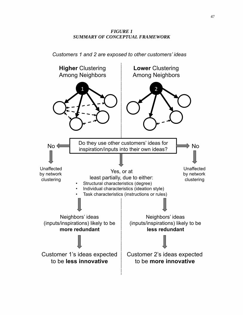
47
FIGURE 1 SUMMARY OF CONCEPTUAL FRAMEWORK

48
TABLE 1 OVERVIEW OF STUDIES
Study Part(s) of Conceptualization Primarily Tested
Interdep. Ideation
Moderator
Other Aspects
1 Clustering Innovativeness, when ideate interdependently
Structural (degree)
Replication with different networks (in web appendix)
2 Clustering Innovativeness, when ideate interdependently
Structural (degree)
Show ideas spread over time over network ties
3 Clustering Idea redundancy Innovativeness - Conservative/weak
manipulation of clustering
4 Idea redundancy
Innovativeness, when ideate interdependently
Individual (interdep.
style)
Conservative/weak manipulation of redundancy
5 Clustering Innovativeness, when ideate interdependently
Task (rules) -
TABLE 2 EFFECTS OF CLUSTERING AND DEGREE ON INNOVATIVENESS (STUDY 1)
Effect
Estimate (std. error)
Main Replication (see Web Appendix H) Including Nodes With Degree = 1
Excluding Nodes With Degree = 1
Intercept 4.11 (.57)*** 4.60 (.38)*** 4.50 (.39)*** Clustering -.08 (.06) -.20 (.09)** -.23 (.09)** Degree -.06 (.07) .09 (.08) .07 (.07) Clustering × Degree -.16 (.07)** -.21 (.09)** -.24 (.10)** Lagged Idea Innovativeness .08 (.07) -.15 (.07)** -.11 (.07) Age --- -.02 (.01)** -.02 (.01)** College Year (baseline = post-senior)
1 -.66 (.59) --- --- 2 -1.01 (.48)** --- --- 3 -.79 (.47)* --- --- 4 -.69 (.47) --- ---
Sex = female (baseline = male) -.11 (.12) -.01 (.07) .003 (.07) Run/session (baseline = 4)
1 .12 (.18) -.19 (.17) -.21 (.17) 2 .08 (.16) -.52 (.17)*** -.48 (.17)*** 3 -.15 (.16) -.62 (.18)*** -.57 (.18)***
Round = 2 (baseline = 3/final) -.28 (.12)** -.19 (.08)** -.19 (.08)** Ideation time -.001 (.002) .002 (.002) .002 (.002) Network type = ER (baseline = SW) --- -.03 (.14) -.06 (.14) Participant random effect .37 (.15)** .15 (.06)** .14 (.06)**
* p < .10, ** p < .05, *** p < .01. Model fits (McFadden’s Pseudo-R2): .09, .13, .12. Main: 177 valid first-, second-, and third-round ideas from 61 participants. Rep.: 226 valid first-, second-, and third-round ideas from 72 participants

49
TABLE 3 EFFECTS OF CLUSTERING AND DEGREE ON INNOVATIVENESS (STUDY 2)
Effect Estimate (std. error) Intercept 1.64 (.67)**
Clustering -.37 (.13)***
Degree -.40 (.12)***
Clustering × Degree -.40 (.13)***
Lagged Idea Innovativeness -.18 (.11) Age .09 (.04)**
Sex = female (baseline = male) .09 (.07) Run/session (baseline = 3)
1 -.09 (.17) 2 -.24 (.17)
Round = 2 (baseline = 3/final) .06 (.13)
Ideation time -.002 (.002) Participant random effect .26 (.05)***
* p < .10, ** p < .05, *** p < .01. Model fit (McFadden’s Pseudo-R2): .15. 100 valid first-, second-, and third-round ideas from 34 participants
TABLE 4
EFFECT OF IDEA REDUNDANCY ON INNOVATIVENESS (STUDY 4)
Effect Estimate (std. error) Intercept 2.97 (.85)***
Redundancy (1) vs. No-redundancy (0) -.46 (.16)***
Lagged Idea Innovativeness .18 (.11) Age -.01 (.01) Sex = female (baseline = male) -.04 (.17) Ideation time -.000 (.007)
* p < .10, ** p < .05, *** p < .01. Model fit (R2): .17. 137 valid first- and second-round ideas from 70 participants
TABLE 5
EFFECTS OF CLUSTERING AND DEGREE ON INNOVATIVENESS WHEN USING NEIGHBORS’ IDEAS IS OR IS NOT ALLOWED (STUDY 5)
Effect
Estimate (std. error) Using
Others’ Ideas Allowed
Using Others’ Ideas Not Allowed
Intercept 4.44 (1.87)** 4.50 (1.38)***
Clustering -.19 (.12) .10 (.12) Degree -.21 (.12)* .14 (.12) Clustering × Degree -.26 (.13)** .07 (.12)
Lagged Idea Innovativeness -.08 (.12) .09 (.09)

50
Age -.05 (.09) -.11 (.06)*
Sex = female (baseline = male) -.10 (.07) .08 (.07) Run/session (baseline = 4)
1 -.15 (.18) .03 (.19) 2 -.45 (.19)** .09 (.18) 3 -.28 (.18) .27 (.18)
Round = 2 (baseline = 3/final) -.11 (.13) .06 (.12) Ideation time -.001 (.003) .003 (.002) Participant random effect .38 (.06)*** .34 (.05)***
p < .10, ** p < .05, *** p < .01. Model fits (McFadden’s Pseudo-R2): .07, .08. Combined: Degree × clustering × Condition b = -.31, t = 1.72, p < .09, p < .05 (one-tailed); pseudo-R2 = .04. 283 valid first-, second-, and third-round from 96 participants.
TABLE 6 SUMMARY OF FINDINGS
Study Product Context
Network Size Per
Run Manipulation Main Findings 1 Smartphone
banking app 16 n/a • At higher levels of degree
(interdependent ideation more likely), idea innovativeness is higher when clustering is lower
1 rep.
Smartphone banking app
10 n/a • Replicated S1 with different network types (ER, SW)
• Positive correlation between idea innovativeness and market potential
2 Facebook 12 n/a • Replicated S1 • Evidence that ideas spread over
network connections 3 Facebook 6 Clustering vs.
No Clustering • Clustering leads to higher idea
redundancy among neighbors, which in turn lowers idea innovativeness
4 Facebook n/a Redundant vs. Not redundant
• Lower idea innovativeness when some idea redundancy among neighbors
• Stronger effect if use an interdependent ideation style
5 Facebook 12 Using others’ ideas allowed:
yes vs. no
• Replicated S1, S2, moderation in S4 • Effect only when interdependent
ideation is allowed
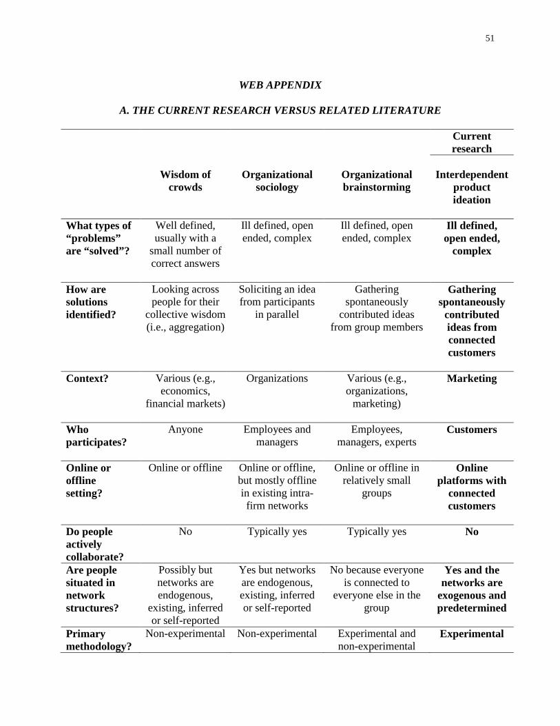
51
WEB APPENDIX
A. THE CURRENT RESEARCH VERSUS RELATED LITERATURE
Current
research
Wisdom of crowds
Organizational
sociology
Organizational brainstorming
Interdependent
product ideation
What types of “problems” are “solved”?
Well defined, usually with a
small number of correct answers
Ill defined, open ended, complex
Ill defined, open ended, complex
Ill defined, open ended,
complex
How are solutions identified?
Looking across people for their
collective wisdom (i.e., aggregation)
Soliciting an idea from participants
in parallel
Gathering spontaneously
contributed ideas from group members
Gathering spontaneously
contributed ideas from connected customers
Context? Various (e.g.,
economics, financial markets)
Organizations Various (e.g., organizations,
marketing)
Marketing
Who participates?
Anyone Employees and managers
Employees, managers, experts
Customers
Online or offline setting?
Online or offline Online or offline, but mostly offline in existing intra-firm networks
Online or offline in relatively small
groups
Online platforms with
connected customers
Do people actively collaborate?
No Typically yes Typically yes No
Are people situated in network structures?
Possibly but networks are endogenous,
existing, inferred or self-reported
Yes but networks are endogenous, existing, inferred or self-reported
No because everyone is connected to
everyone else in the group
Yes and the networks are
exogenous and predetermined
Primary methodology?
Non-experimental Non-experimental Experimental and non-experimental
Experimental
52
B. NETWORK ANALYSIS OF CONSUMER INTERACTIONS ON IDEASTORM.COM
As a demonstration of the importance of taking a network perspective in studying
interdependent ideation for products in online settings (such as discussion forums), we collected
data from Dell’s ideation platform, IdeaStorm.com, and used this to map the underlying network
of interactions between ideating consumers on this platform. The IdeaStorm.com platform is
similar to other mainstream interdependent online product ideation platforms (e.g.,
MyStarbucksIdea.com), and the experimental paradigm used in most of our studies was modeled
on these platforms in the sense that, over time, participants are exposed to other participants’
previous ideas. We do not provide a detailed description of IdeaStorm.com here; see Bayus
(2012) and Huang et al. (2014).
For the purposes of the following analysis, the process for contributing ideas on
IdeaStorm.com is as follows. Any user registered to the platform is allowed to post an idea at any
point in time. These ideas can be about almost anything related to Dell’s products and services,
but often ideas are solicited on particular topics. For example, in Figure B1 we show a screenshot
for a product ideation task in which consumers were invited to submit ideas for designing and
marketing a laptop for children. Each submitted idea is displayed on IdeaStorm.com, and other
users can view these ideas (they can also add comments below each idea, and vote “up” or
“down” each idea).
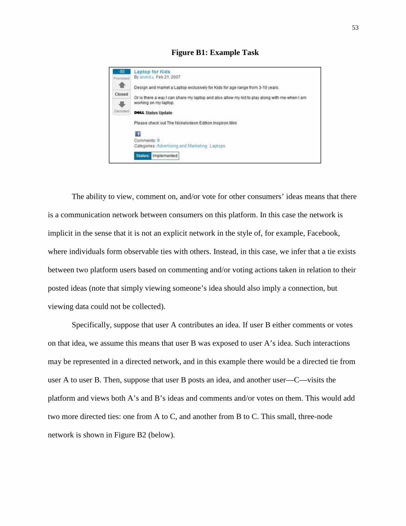
53
Figure B1: Example Task
The ability to view, comment on, and/or vote for other consumers’ ideas means that there
is a communication network between consumers on this platform. In this case the network is
implicit in the sense that it is not an explicit network in the style of, for example, Facebook,
where individuals form observable ties with others. Instead, in this case, we infer that a tie exists
between two platform users based on commenting and/or voting actions taken in relation to their
posted ideas (note that simply viewing someone’s idea should also imply a connection, but
viewing data could not be collected).
Specifically, suppose that user A contributes an idea. If user B either comments or votes
on that idea, we assume this means that user B was exposed to user A’s idea. Such interactions
may be represented in a directed network, and in this example there would be a directed tie from
user A to user B. Then, suppose that user B posts an idea, and another user—C—visits the
platform and views both A’s and B’s ideas and comments and/or votes on them. This would add
two more directed ties: one from A to C, and another from B to C. This small, three-node
network is shown in Figure B2 (below).

54
Figure B2: Network Construction
To summarize, in Figure B2, user B was exposed to user A’s idea, and user C was
exposed to user A’s idea and user B’s idea. In other words, user C saw ideas contributed by both
A and B, B saw an idea contributed by A, and A saw no one else’s ideas. Note that the three-
node network in Figure B2 is a directed graph, meaning that information (ideas) can flow in one
direction but not necessarily the other between pairs of people. This is different to the networks
used in our studies, where the graphs were undirected, thus meaning that for a connected pair of
participants, they could see each other’s ideas (this was done for simplification reasons).
Using the data collected from IdeaStorm.com and this approach to mapping implicit
network ties, we first created a node for each registered IdeaStorm.com user who had contributed
at least one idea between January 1, 2008 and October 26, 2011.31 Next, we collected all the
comments and votes for all 9,424 unique ideas available on IdeaStorm.com at the time of data
collection. We knew, for each idea’s comments and votes, who made the comment or vote.
Using this we created directed links from the idea contributors to everyone who commented or
voted on their ideas per the above illustration of network tie formation. This procedure resulted
in a network with 5,749 nodes (individual consumers) and 44,269 directed communication
31 The latter date corresponds to the time of collecting the data. In line with the findings of Huang et al. (2014), we ignored all idea contributors who abandoned the website before 2008. IdeaStorm launched on February 16, 2007.
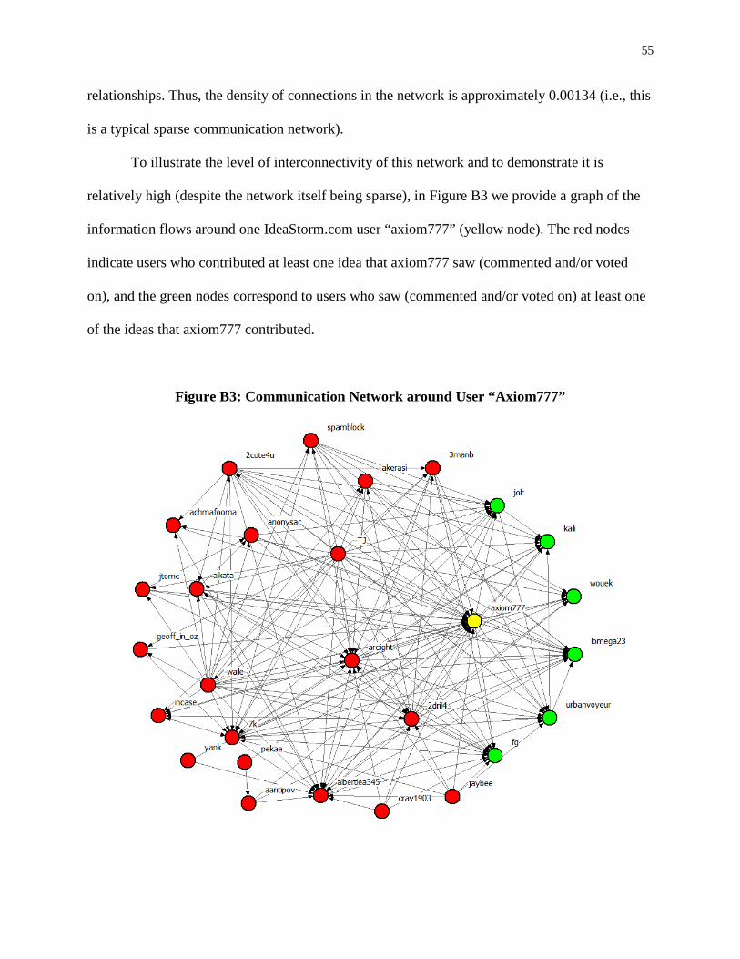
55
relationships. Thus, the density of connections in the network is approximately 0.00134 (i.e., this
is a typical sparse communication network).
To illustrate the level of interconnectivity of this network and to demonstrate it is
relatively high (despite the network itself being sparse), in Figure B3 we provide a graph of the
information flows around one IdeaStorm.com user “axiom777” (yellow node). The red nodes
indicate users who contributed at least one idea that axiom777 saw (commented and/or voted
on), and the green nodes correspond to users who saw (commented and/or voted on) at least one
of the ideas that axiom777 contributed.
Figure B3: Communication Network around User “Axiom777”

56
From Figure B3 it is easy to see that the relationships around axiom777 form a non-trivial
network. In particular, if we focus on the red nodes, which are axiom777’s “sources of
inspiration” in this particular ideation task, we can see high levels of interconnectivity—
clustering—among them. In other words, a high proportion of axiom777’s sources of inspiration
(red nodes) were each other’s sources of inspiration in the sense that they saw each other’s ideas.
This is consistent with our arguments that the networks (explicit or implicit) in online ideation
platforms such as IdeaStorm.com tend to be dense and highly clustered.
We next quantified the level of clustering, averaged over all nodes, in this network.
Because this is a directed graph (i.e., information flows do not have to go in both directions in
dyads), some care was required in defining clustering (as well as degree). Since we are interested
in how the ideas from others seen by individuals may affect subsequent ideation, for each node
in the network we calculated the number of incoming links, which is the number of other users’
whose ideas the user on that node saw (commented and/or voted on). For each node, this is the
size of that user’s set of neighbors who served as potential sources of inspiration. This measures
degree (or, more precisely, in-degree). For clustering, for each node, we calculated the
interconnectivity among the nodes that formed the set of neighbors who served as potential
sources of inspiration. Consistent with our studies, this was the proportion of connected pairs out
of all possible pairs of nodes. Based on these definitions of degree and clustering, in the three-
node network in Figure B2 above, the degree values for nodes A, B, and C are 0, 1, and 2. And
the clustering values for nodes A, B, and C are 0, 0, and 0.5 (note that ignoring the directed links
would mean that clustering coefficients for A, B, and C in Figure B2 would instead be 1, 1, and
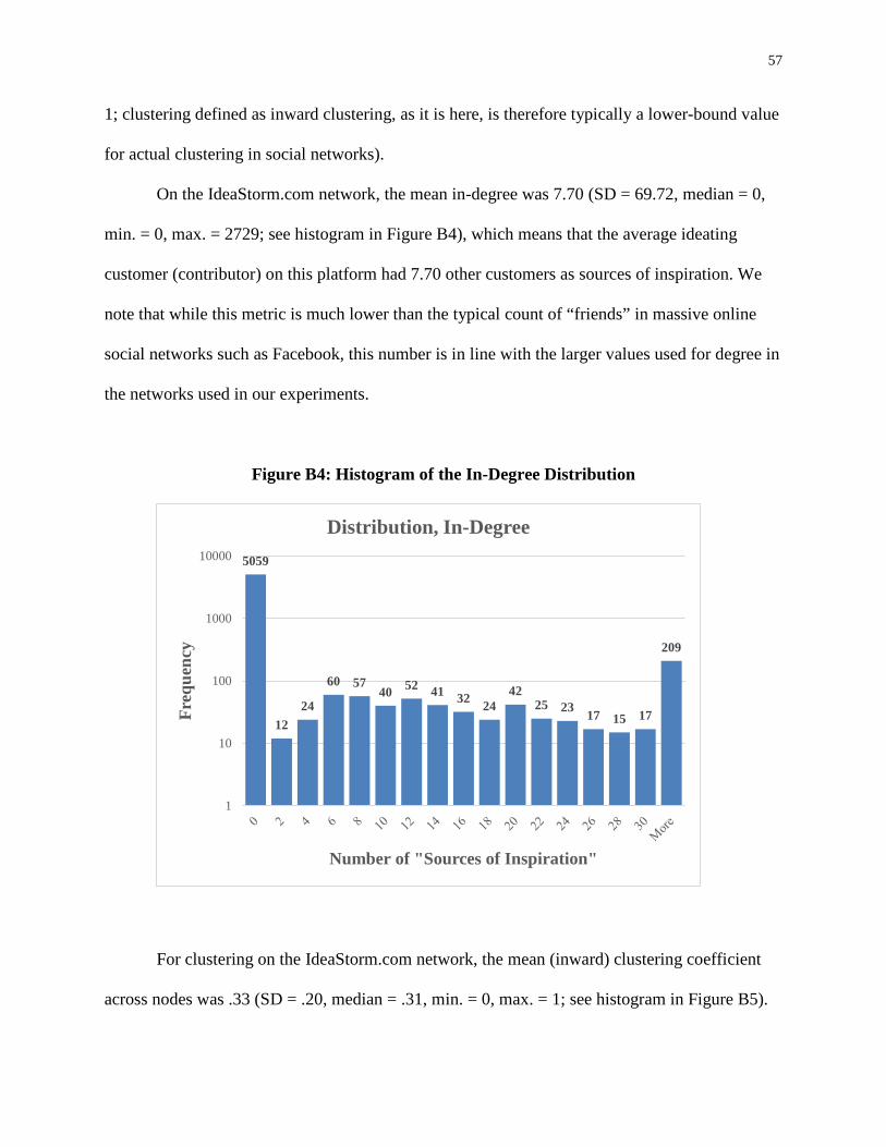
57
1; clustering defined as inward clustering, as it is here, is therefore typically a lower-bound value
for actual clustering in social networks).
On the IdeaStorm.com network, the mean in-degree was 7.70 (SD = 69.72, median = 0,
min. = 0, max. = 2729; see histogram in Figure B4), which means that the average ideating
customer (contributor) on this platform had 7.70 other customers as sources of inspiration. We
note that while this metric is much lower than the typical count of “friends” in massive online
social networks such as Facebook, this number is in line with the larger values used for degree in
the networks used in our experiments.
Figure B4: Histogram of the In-Degree Distribution
For clustering on the IdeaStorm.com network, the mean (inward) clustering coefficient
across nodes was .33 (SD = .20, median = .31, min. = 0, max. = 1; see histogram in Figure B5).
5059
12 24
60 57 40 52 41 32 24
42 25 23 17 15 17
209
1
10
100
1000
10000
Freq
uenc
y
Number of "Sources of Inspiration"
Distribution, In-Degree
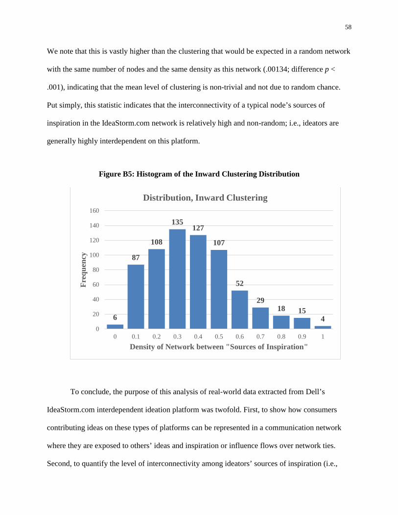
58
We note that this is vastly higher than the clustering that would be expected in a random network
with the same number of nodes and the same density as this network (.00134; difference p <
.001), indicating that the mean level of clustering is non-trivial and not due to random chance.
Put simply, this statistic indicates that the interconnectivity of a typical node’s sources of
inspiration in the IdeaStorm.com network is relatively high and non-random; i.e., ideators are
generally highly interdependent on this platform.
Figure B5: Histogram of the Inward Clustering Distribution
To conclude, the purpose of this analysis of real-world data extracted from Dell’s
IdeaStorm.com interdependent ideation platform was twofold. First, to show how consumers
contributing ideas on these types of platforms can be represented in a communication network
where they are exposed to others’ ideas and inspiration or influence flows over network ties.
Second, to quantify the level of interconnectivity among ideators’ sources of inspiration (i.e.,
6
87
108
135 127
107
52
29 18 15
4 0
20
40
60
80
100
120
140
160
0 0.1 0.2 0.3 0.4 0.5 0.6 0.7 0.8 0.9 1
Freq
uenc
y
Density of Network between "Sources of Inspiration"
Distribution, Inward Clustering

59
clustering) and show that it is non-trivial, relatively high, and indicative of interdependence
among ideating consumers. Our empirical analysis showed both of these key points, and supports
our claims of the ecological validity of the central phenomena in the current research and the
approach taken across our experimental studies.

C. ORGANIZATIONAL SOCIOLOGY LITERATURE VERSUS CURRENT RESEARCH
Paper Data DV (creativity /
innovativeness)
Network Source
Redundancy Metric
All selection issues
resolved?
Endogeneity issues resolved? Ideas Network Network
formation (nodes do
NOT choose ties)?
No common unobserved
shock?
Position cannot
appreciably improve
skills over time?
Tie strength NOT
correlated with
redundancy metric?
Our work Primary (experiments)
Perfectly observed
(experiments)
Innovativeness scale (2-3 raters
per idea)
Exogenous (6 different networks
tested)
Clustering coefficient
(triadic closure)
Yes Yes (exogenous networks)
Yes (random assignment to nodes +
econometric control)
Yes (3-5 rounds,
10-15 minutes)
Yes (random
assignment to nodes;
anonymous participation)
Burt (2004) Primary (surveys)
Inferred (surveys)
Two senior managers evaluate
potential of idea
Self-reported Local constraint
(triadic closure and hierarchical C4 closure)
No (self-
reporting)
No No No No
Fleming et al. (2007)
Secondary (patent
collaboration)
Inferred (patent
collaboration)
Number of (patent)
subcategory combinations
Inferred from joint
successes (9 networks
pooled)
Clustering coefficient32
No (successes
only / failures
unobserved)
No Yes (econometric
control)
Yes (econometric
control)
No
Perry-Smith (2006)
N/A Inferred (surveys)
Expert ratings of people, not ideas
Self-reported (2 networks)
Local constraint and betweenness
centrality
No (self-
reporting)
No No No No
Tortoriello and Krackhardt (2010)
Secondary (patent data)
Inferred (surveys)
Number of patent
applications
Self-reported Simmelian ties (yes/no
triadic closure)
No (self-
reporting)
No No No No
32 The term used in the paper is “cohesion”.
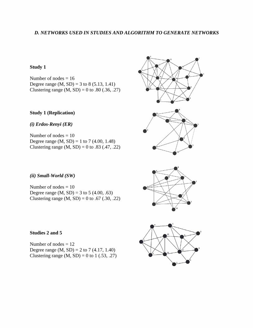
D. NETWORKS USED IN STUDIES AND ALGORITHM TO GENERATE NETWORKS
Study 1 Number of nodes = 16 Degree range (M, SD) = 3 to 8 (5.13, 1.41) Clustering range (M, SD) = 0 to .80 (.36, .27) Study 1 (Replication) (i) Erdos-Renyi (ER) Number of nodes = 10 Degree range (M, SD) = 1 to 7 (4.00, 1.48) Clustering range (M, SD) = 0 to .83 (.47, .22)
(ii) Small-World (SW) Number of nodes = 10 Degree range (M, SD) = 3 to 5 (4.00, .63) Clustering range (M, SD) = 0 to .67 (.30, .22) Studies 2 and 5 Number of nodes = 12 Degree range (M, SD) = 2 to 7 (4.17, 1.40) Clustering range (M, SD) = 0 to 1 (.53, .27)

3
Study 3 (i) Clustering Number of nodes = 6 Degree (M, SD) = (3.00, .00) Clustering (M, SD) = (.33, .00) (ii) No clustering Number of nodes = 6 Degree (M, SD) = (3.00, .00) Clustering (M, SD) = (.00, .00) Algorithm Used to Generate Networks in Studies 1, 2, and 5 Computer code used is available upon request from the authors. Below we list the steps in the algorithm (“pseudo-code”). Input: Size of network N, Desired degrees 𝐷𝐷1 ≥ 𝐷𝐷2 ≥ … ≥ 𝐷𝐷𝑁𝑁, with 1 < 𝐷𝐷𝑖𝑖 < 𝑁𝑁,
Degree-clustering correlation threshold t Output: A, an N×N matrix that describes the adjacency relationships in the output network. Procedure:
1. Reset matrix A to all zeroes. 2. Draw (𝐷𝐷1 + 𝐷𝐷2 + ⋯+ 𝐷𝐷𝑁𝑁)/2 edges randomly to the network, updating entries of A. 3. Calculate the degrees of the random network by totaling the values in each row of A. 4. Verify if the (sorted) degree distribution is the same as the input degrees. If not, start over
from Step 1. 5. Calculate the clustering coefficients in the network. (Since 𝐷𝐷𝑖𝑖 > 2, it is always defined.) 6. Verify that the maximum clustering is sufficiently large and the minimum clustering is 0.
If it isn’t, start over from Step 1. 7. Calculate the degree-clustering correlation. If it isn’t smaller than t, start from Step 1. 8. Output A as the random network instance meets all our requirements.
On average, the code based on this algorithm outputs a viable network in about 100,000 cycles, which takes less than 1 second on a typical machine.

4
E. ITEMS USED TO MEASURE IDEA INNOVATIVENESS
The following scale items were used to measure idea innovativeness on five-point Likert scales (1 = strongly disagree, 5 = strongly agree):
• This idea is original • This idea is novel • This idea is unconventional • This idea is out of the box • This idea is creative • A [product name] with this feature will be innovative • A [product name] with this feature will be original
F. RESULTS FROM IDEA-JUDGING VALIDATION STUDY
Representativeness The validation procedure for representativeness was as follows. First, we randomly
sampled 16 ideas (out of 177 valid ideas) from Study 1A and used a different set of 50 judges from the same population as the original judges. These judges completed the same idea-judging task that original judges had completed for judging idea innovativeness. Second, after completing this task, we told the 50 validation judges the mean innovativeness score from the original judges for the idea they had just rated and asked if they thought the score was “in the right direction and in the ballpark” (0 = no, 1 = yes) as a general measure of their agreement.
We tested for evidence of the original judges’ ratings being representative and consistent with the larger number of validation judges’ ratings in a number of ways. First, across ideas, the mean percentage of validation judges who were in general agreement with the original judges’ idea innovative score was 83.92% (SD = 8.36%, min. = 68.00%, max. = 97.96%, median = 83.33%). This is an indication that the validation judges concurred with the original judges.
Second, the correlation between the average ratings from the original and validation judges was positive (r = .79, p < .001), which is another indication of consistency between the original and validation judges’ ratings.
Third, we used a bootstrapping procedure to test whether sampling three judges from a larger set of judges was appropriate in terms of representativeness. For each idea, we randomly sampled three validation judges (out of the 50 judges) and computed the mean idea innovativeness for their ratings. This was done 50,000 times per idea, which produced a distribution of mean innovativeness ratings for each idea based on only three randomly sampled validation judges. We then checked if the 95% credible interval for each idea’s rating distribution included the mean innovativeness rating from the original judges. Results are summarized in the table below, and show that the original judges’ rating was always inside the 95% credible interval generated by the bootstrapping procedure on validation judges’ ratings.
Thus, we are confident in the validity of the judging procedure used in our studies with respect to the representativeness of a few judges’ idea ratings.
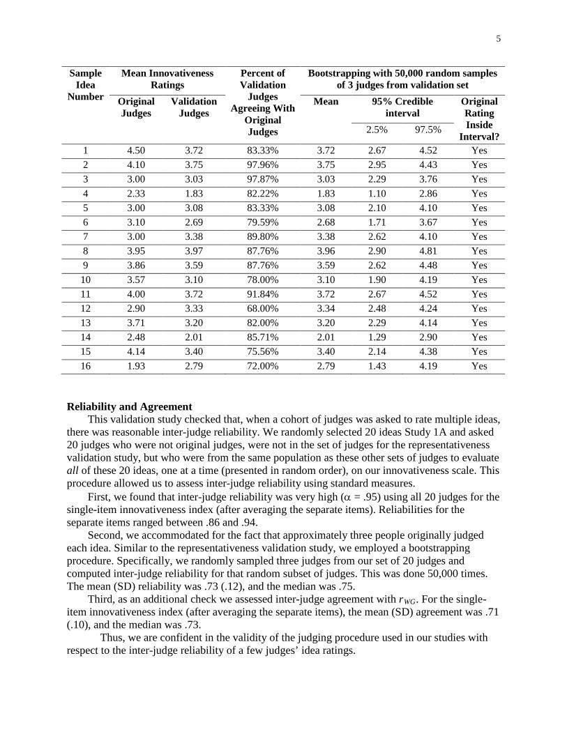
5
Sample Idea
Number
Mean Innovativeness Ratings
Percent of Validation
Judges Agreeing With
Original Judges
Bootstrapping with 50,000 random samples of 3 judges from validation set
Original Judges
Validation Judges
Mean 95% Credible interval
Original Rating Inside
Interval? 2.5% 97.5%
1 4.50 3.72 83.33% 3.72 2.67 4.52 Yes 2 4.10 3.75 97.96% 3.75 2.95 4.43 Yes 3 3.00 3.03 97.87% 3.03 2.29 3.76 Yes 4 2.33 1.83 82.22% 1.83 1.10 2.86 Yes 5 3.00 3.08 83.33% 3.08 2.10 4.10 Yes 6 3.10 2.69 79.59% 2.68 1.71 3.67 Yes 7 3.00 3.38 89.80% 3.38 2.62 4.10 Yes 8 3.95 3.97 87.76% 3.96 2.90 4.81 Yes 9 3.86 3.59 87.76% 3.59 2.62 4.48 Yes 10 3.57 3.10 78.00% 3.10 1.90 4.19 Yes 11 4.00 3.72 91.84% 3.72 2.67 4.52 Yes 12 2.90 3.33 68.00% 3.34 2.48 4.24 Yes 13 3.71 3.20 82.00% 3.20 2.29 4.14 Yes 14 2.48 2.01 85.71% 2.01 1.29 2.90 Yes 15 4.14 3.40 75.56% 3.40 2.14 4.38 Yes 16 1.93 2.79 72.00% 2.79 1.43 4.19 Yes
Reliability and Agreement This validation study checked that, when a cohort of judges was asked to rate multiple ideas,
there was reasonable inter-judge reliability. We randomly selected 20 ideas Study 1A and asked 20 judges who were not original judges, were not in the set of judges for the representativeness validation study, but who were from the same population as these other sets of judges to evaluate all of these 20 ideas, one at a time (presented in random order), on our innovativeness scale. This procedure allowed us to assess inter-judge reliability using standard measures.
First, we found that inter-judge reliability was very high (α = .95) using all 20 judges for the single-item innovativeness index (after averaging the separate items). Reliabilities for the separate items ranged between .86 and .94.
Second, we accommodated for the fact that approximately three people originally judged each idea. Similar to the representativeness validation study, we employed a bootstrapping procedure. Specifically, we randomly sampled three judges from our set of 20 judges and computed inter-judge reliability for that random subset of judges. This was done 50,000 times. The mean (SD) reliability was .73 (.12), and the median was .75.
Third, as an additional check we assessed inter-judge agreement with rWG. For the single-item innovativeness index (after averaging the separate items), the mean (SD) agreement was .71 (.10), and the median was .73.
Thus, we are confident in the validity of the judging procedure used in our studies with respect to the inter-judge reliability of a few judges’ idea ratings.

6
G. TASK DESCRIPTIONS AND EXAMPLES OF SUBMITTED IDEAS
Mobile banking smartphone application features (Study 1) A large retail/commercial bank is developing a new mobile banking application for smartphones. They want help thinking of features that this app should have. You will be asked to give your idea for an app feature. Try to be creative and original. Your goal is to think of features this app should have that the eventual users of the app would find useful and would like. Example ideas: Innovativeness Range Idea (score) > 1 and ≤ 2 • View bank balance (1.33)
• Red letters/numbers for the withdrawal of money (1.86). • Send an email to your phone every time you deposit or
withdrawal to keep up with your balance (1.95)
> 2 and ≤ 3 • Report transactions that weren't made by the customer...identity theft protection (2.19)
• The app should have the function of allowing someone to transfer funds to other individuals from either the same bank or other banks (2.38)
• Let people see pictures of checks that have been deposited either from the user or from people the user has written checks to (2.90)
> 3 and ≤ 4 • The app can have a visual representation of what you spend your money on (3.10)
• An app that let's you use your phone to pay without having to pull a credit or debit card out of your pocket would be really neat (3.71)
• The app should include live chat section where users can chat with a representative from the particular bank in texting format to ask any questions they have if they don't have the time to sit through a phone call and wait for a representative to become available (4.00)
> 4 and ≤ 5 • Finger print password (4.05) • An app that gives you one financial advice tip per day based on
your age and current saving/spending habits. you could rate it as "helpful" or "not helpful" and over time it would adapt to give you more and more relevant advice (4.11)
• Bill pay feature with the ability to use the phone itself as your banking card (5.00)

7
Facebook Features (Studies 2, 3, 4, 5) Facebook is seeking input from users like yourself to help them develop new features for their popular social networking platform. In this task you will develop ideas for Facebook. Specifically, your task is to develop ideas for making the Facebook user experience better and more useful for users like yourself. What real-world improvements do you think would make the Facebook user experience better? To make this task more specific we want to you focus on coming up with ideas for specific features/functions that Facebook could introduce. What are some useful features that Facebook does not have right now that you think it should have because it would improve the user experience and functionality? You should try to be as creative and original as possible. Example ideas: Innovativeness Range Idea (score) > 1 and ≤ 2 • Add email (1.64)
• Stop changing the format of Facebook every six months or so (1.62)
• Link to twitter, because Facebook is terrible (2.00) > 2 and ≤ 3 • Create a Facebook planner or calendar (2.03)
• A way to see a list of comments you’ve posted on other people’s walls (2.19)
• Add a dislike button (2.81) > 3 and ≤ 4 • Group video chatting for up to 30 people (3.10)
• Facebook can act like a dating website, it can match up single females and males based on their hobbies, favorite books/movies, and about me sections. This can either be part of the homepage or a separate application (3.57)
• Have some sort of translation device built into Facebook (3.86) > 4 and ≤ 5 • Divide Facebook into two segments where one is social and the
other is business. That way you can still integrate all your friends and coworkers into your profile (4.24)
• A feature is needed to hide a continuously embarrassing friend/relative who posts nonsense, rants, or offensive comments on your posts or wall all the time, however to make them think they are actually posting. This is good for a drunken relative whose feelings you don’t want to hurt by outright blocking or unfriending them (4.33)
• Personalize Facebook to make it more of a unique experience. When click on or mouse goes over about info (musicians, artists, likes), have the ability to listen or view their work (4.86)
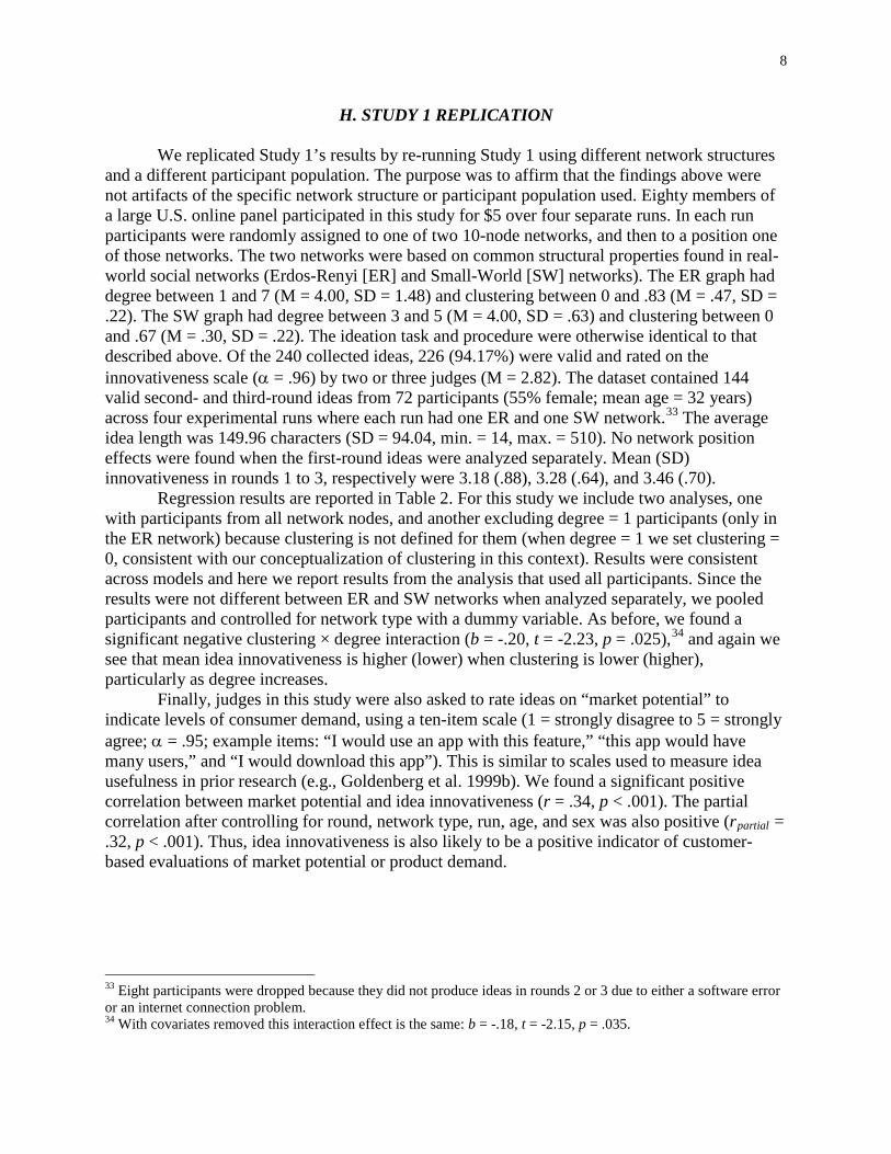
8
H. STUDY 1 REPLICATION We replicated Study 1’s results by re-running Study 1 using different network structures
and a different participant population. The purpose was to affirm that the findings above were not artifacts of the specific network structure or participant population used. Eighty members of a large U.S. online panel participated in this study for $5 over four separate runs. In each run participants were randomly assigned to one of two 10-node networks, and then to a position one of those networks. The two networks were based on common structural properties found in real-world social networks (Erdos-Renyi [ER] and Small-World [SW] networks). The ER graph had degree between 1 and 7 (M = 4.00, SD = 1.48) and clustering between 0 and .83 (M = .47, SD = .22). The SW graph had degree between 3 and 5 (M = 4.00, SD = .63) and clustering between 0 and .67 (M = .30, SD = .22). The ideation task and procedure were otherwise identical to that described above. Of the 240 collected ideas, 226 (94.17%) were valid and rated on the innovativeness scale (α = .96) by two or three judges (M = 2.82). The dataset contained 144 valid second- and third-round ideas from 72 participants (55% female; mean age = 32 years) across four experimental runs where each run had one ER and one SW network.33 The average idea length was 149.96 characters (SD = 94.04, min. = 14, max. = 510). No network position effects were found when the first-round ideas were analyzed separately. Mean (SD) innovativeness in rounds 1 to 3, respectively were 3.18 (.88), 3.28 (.64), and 3.46 (.70).
Regression results are reported in Table 2. For this study we include two analyses, one with participants from all network nodes, and another excluding degree = 1 participants (only in the ER network) because clustering is not defined for them (when degree = 1 we set clustering = 0, consistent with our conceptualization of clustering in this context). Results were consistent across models and here we report results from the analysis that used all participants. Since the results were not different between ER and SW networks when analyzed separately, we pooled participants and controlled for network type with a dummy variable. As before, we found a significant negative clustering × degree interaction (b = -.20, t = -2.23, p = .025),34 and again we see that mean idea innovativeness is higher (lower) when clustering is lower (higher), particularly as degree increases.
Finally, judges in this study were also asked to rate ideas on “market potential” to indicate levels of consumer demand, using a ten-item scale (1 = strongly disagree to 5 = strongly agree; α = .95; example items: “I would use an app with this feature,” “this app would have many users,” and “I would download this app”). This is similar to scales used to measure idea usefulness in prior research (e.g., Goldenberg et al. 1999b). We found a significant positive correlation between market potential and idea innovativeness (r = .34, p < .001). The partial correlation after controlling for round, network type, run, age, and sex was also positive (rpartial = .32, p < .001). Thus, idea innovativeness is also likely to be a positive indicator of customer-based evaluations of market potential or product demand.
33 Eight participants were dropped because they did not produce ideas in rounds 2 or 3 due to either a software error or an internet connection problem. 34 With covariates removed this interaction effect is the same: b = -.18, t = -2.15, p = .035.
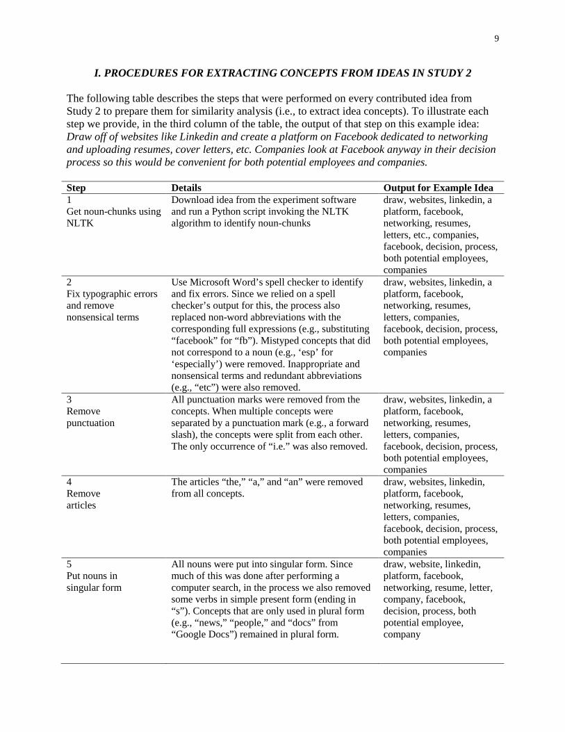
9
I. PROCEDURES FOR EXTRACTING CONCEPTS FROM IDEAS IN STUDY 2 The following table describes the steps that were performed on every contributed idea from Study 2 to prepare them for similarity analysis (i.e., to extract idea concepts). To illustrate each step we provide, in the third column of the table, the output of that step on this example idea: Draw off of websites like Linkedin and create a platform on Facebook dedicated to networking and uploading resumes, cover letters, etc. Companies look at Facebook anyway in their decision process so this would be convenient for both potential employees and companies.
Step Details Output for Example Idea 1 Get noun-chunks using NLTK
Download idea from the experiment software and run a Python script invoking the NLTK algorithm to identify noun-chunks
draw, websites, linkedin, a platform, facebook, networking, resumes, letters, etc., companies, facebook, decision, process, both potential employees, companies
2 Fix typographic errors and remove nonsensical terms
Use Microsoft Word’s spell checker to identify and fix errors. Since we relied on a spell checker’s output for this, the process also replaced non-word abbreviations with the corresponding full expressions (e.g., substituting “facebook” for “fb”). Mistyped concepts that did not correspond to a noun (e.g., ‘esp’ for ‘especially’) were removed. Inappropriate and nonsensical terms and redundant abbreviations (e.g., “etc”) were also removed.
draw, websites, linkedin, a platform, facebook, networking, resumes, letters, companies, facebook, decision, process, both potential employees, companies
3 Remove punctuation
All punctuation marks were removed from the concepts. When multiple concepts were separated by a punctuation mark (e.g., a forward slash), the concepts were split from each other. The only occurrence of “i.e.” was also removed.
draw, websites, linkedin, a platform, facebook, networking, resumes, letters, companies, facebook, decision, process, both potential employees, companies
4 Remove articles
The articles “the,” “a,” and “an” were removed from all concepts.
draw, websites, linkedin, platform, facebook, networking, resumes, letters, companies, facebook, decision, process, both potential employees, companies
5 Put nouns in singular form
All nouns were put into singular form. Since much of this was done after performing a computer search, in the process we also removed some verbs in simple present form (ending in “s”). Concepts that are only used in plural form (e.g., “news,” “people,” and “docs” from “Google Docs”) remained in plural form.
draw, website, linkedin, platform, facebook, networking, resume, letter, company, facebook, decision, process, both potential employee, company
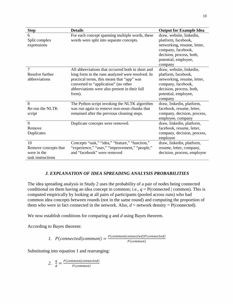
10
Step Details Output for Example Idea 6 Split complex expressions
For each concept spanning multiple words, these words were split into separate concepts.
draw, website, linkedin, platform, facebook, networking, resume, letter, company, facebook, decision, process, both, potential, employee, company
7 Resolve further abbreviations
All abbreviations that occurred both in short and long form in the runs analyzed were resolved. In practical terms, this meant that “app” was converted to “application” (no other abbreviations were also present in their full form).
draw, website, linkedin, platform, facebook, networking, resume, letter, company, facebook, decision, process, both, potential, employee, company
8 Re-run the NLTK script
The Python script invoking the NLTK algorithm was run again to remove non-noun chunks that remained after the previous cleaning steps.
draw, linkedin, platform, facebook, resume, letter, company, decision, process, employee, company
9 Remove Duplicates
Duplicate concepts were removed. draw, linkedin, platform, facebook, resume, letter, company, decision, process, employee
10 Remove concepts that were in the task instructions
Concepts “task,” “idea,” “feature,” “function,” “experience,” “user,” “improvement,” “people,” and “facebook” were removed
draw, linkedin, platform, resume, letter, company, decision, process, employee
J. EXPLANATION OF IDEA SPREADING ANALYSIS PROBABILITIES The idea spreading analysis in Study 2 uses the probability of a pair of nodes being connected conditional on them having an idea concept in common; i.e., q = P(connected | common). This is computed empirically by looking at all pairs of participants (pooled across runs) who had common idea concepts between rounds (not in the same round) and computing the proportion of them who were in fact connected in the network. Also, d = network density = P(connected). We now establish conditions for comparing q and d using Bayes theorem.
According to Bayes theorem:
1. 𝑃𝑃(𝑐𝑐𝑐𝑐𝑐𝑐𝑐𝑐𝑐𝑐𝑐𝑐𝑐𝑐𝑐𝑐𝑐𝑐|𝑐𝑐𝑐𝑐𝑐𝑐𝑐𝑐𝑐𝑐𝑐𝑐) = 𝑃𝑃(𝑐𝑐𝑐𝑐𝑐𝑐𝑐𝑐𝑐𝑐𝑐𝑐|𝑐𝑐𝑐𝑐𝑐𝑐𝑐𝑐𝑐𝑐𝑐𝑐𝑐𝑐𝑐𝑐𝑐𝑐)𝑃𝑃(𝑐𝑐𝑐𝑐𝑐𝑐𝑐𝑐𝑐𝑐𝑐𝑐𝑐𝑐𝑐𝑐𝑐𝑐)𝑃𝑃(𝑐𝑐𝑐𝑐𝑐𝑐𝑐𝑐𝑐𝑐𝑐𝑐)
Substituting into equation 1 and rearranging:
2. 𝑞𝑞𝑐𝑐
= 𝑃𝑃(𝑐𝑐𝑐𝑐𝑐𝑐𝑐𝑐𝑐𝑐𝑐𝑐|𝑐𝑐𝑐𝑐𝑐𝑐𝑐𝑐𝑐𝑐𝑐𝑐𝑐𝑐𝑐𝑐𝑐𝑐)𝑃𝑃(𝑐𝑐𝑐𝑐𝑐𝑐𝑐𝑐𝑐𝑐𝑐𝑐)

11
If ideation is independent then any pair of participants having common ideas between rounds and being connected are independent events; i.e., P(common | connected) = P(common), which results in equation 2 reducing to q/d = 1. If ideation is interdependent then it must be that P(common | connected) > P(common | not connected); i.e., the probability of having common idea concepts is higher among connected participants than not-connected participants. It must also be the case that having common ideas and not being connected are independent events; i.e., P(common | not connected) = P(common). Thus, P(common | connected) > P(common). This results in q/d > 1 under interdependent ideation where idea concepts spread between connected participants.
K. ITEMS USED TO MEASURE INTERDEPENDENT IDEATION STYLE (IIS)
The following scale items were used in Study 4 to measure IIS on five-point Likert scales (1 = strongly disagree, 5 = strongly agree):
• I tried to see connections between group members’ and my ideas. • I looked for “common ground” between group members’ and my ideas. • My ideas came from combining concepts that came up in others’ ideas. • I linked concepts that came up in others’ ideas to form new ideas. • I integrated or combined concepts and ideas from previous rounds (mine and others’). • I built my ideas by combining some aspects of group members’ ideas with my previous
ideas. • Creating my ideas involved blending parts of group members’ previous ideas and my
previous ideas.

12
L. META ANALYSIS OF RESULTS ACROSS STUDIES 1, 2, AND 5
Effect
Estimate (std. error) Linear
Regression Logistic
Regression (Innov. > 3)
Intercept 3.32 (.23)*** .36 (.67) Clustering -.11 (.04)** -.37 (.14)***
Degree -.06 (.04) -.24 (.14)*
Clustering × Degree -.16 (.05)*** -.47 (.15)***
Lagged Idea Innovativeness -.004 (.04) .24 (.23)
Age -.009 (.006) -.01 (.02) Sex = female (baseline = male) -.03 (.05) -.05 (.17) Run/session (baseline = 4)
1 -.18 (.09)* -.55 (.35)
2 -.29 (.10)*** -.90 (.35)**
3 -.25 (.10)** -.75 (.35)**
Round (baseline = 3) 2 -.15 (.06)*** -.54 (.21)**
Ideation time .001 (.001) .003 (.004) Study (baseline = 5)
1 .30 (.10)*** .74 (.34)*
1 replication .61 (.12)*** 1.47 (.43)***
2 -.14 (.11) -.46 (.39) Participant random effect .08 (.04)*** .41 (.29)
p < .10, ** p < .05, *** p < .01. Model fits (McFadden’s Pseudo-R2): .10, .12.

1
THE INFLUENCE OF SEROTONIN DEFICIENCY ON CHOICE DEFERRAL AND THE
COMPROMISE EFFECT
Marcel Lichters, Claudia Brunnlieb, Gideon Nave, Marko Sarstedt, Bodo Vogt
Marcel Lichters, Dr., Otto-von-Guericke-University Magdeburg, Department of Empirical
Economics, Faculty of Economics and Management, Universitätsplatz 2, 39106 Magdeburg,
Germany and Harz University of Applied Sciences, Department Business Studies,
Friedrichstrasse 57-59, 38855 Wernigerode, Germany, +49(0)3916718176,
Claudia Brunnlieb, Dr., Otto-von-Guericke-University Magdeburg, Institute for Social
Medicine, Epidemiology and Health Economics, Faculty of Medicine, Universitätsplatz 2,
39106 Magdeburg, Germany, +49(0)3916711636, [email protected]
Gideon Nave (), corresponding author, Department of Computation & Neural Systems,
California Institute of Technology, MC 228-77, Pasadena, California 91125, USA, +1(626)
395 4083 , [email protected]
Marko Sarstedt, Prof. Dr., Otto-von-Guericke-University Magdeburg, Institute for Marketing,
Faculty of Economics and Management, Universitätsplatz 2, 39106 Magdeburg, Germany and
University of Newcastle, Faculty of Business and Law, University Drive Callaghan NSW
2308, Australia, +49(0)3916718625, [email protected]
Bodo Vogt, Prof. Dr. Dr., Otto-von-Guericke-University Magdeburg, Department of
Empirical Economics, Faculty of Economics and Management and Institute for Social
Medicine, Epidemiology and Health Economics, Faculty of Medicine, Universitätsplatz 2,
39106 Magdeburg, Germany, -49(0)3916718426, [email protected]
Acknowledgment: The authors would like to thank Paul Bengart, Liri von Petersdorff and Dr.
Stephan Schosser for their valuable support during data collection.
2 © 2015, American Marketing Association
Journal of Marketing Research
PrePrint, Unedited
All rights reserved. Cannot be reprinted without the express
permission of the American Marketing Association.
THE INFLUENCE OF SEROTONIN DEFICIENCY ON CHOICE DEFERRAL AND THE
COMPROMISE EFFECT.
Psychological and physiological states such as mood, hunger, stress and sleep deprivation are
known to affect decision-making processes and therefore crucially impact consumer behavior.
A possible biological mechanism underlying the observed variability of consumer behavior is
the context-sensitive variation in the levels of neuromodulators in the brain. In a series of four
experimental studies, we pharmaceutically reduce the levels of the neurotransmitter serotonin
in the brain to diminish the availability of subjects’ cognitive resources. In doing so, we study
how serotonin brain levels influence (1) subjects’ tendency to avoid buying, and (2) their
preference for product options that are positioned as a compromise in a given choice set rather
than for more extreme alternatives (i.e., the compromise effect). Using realistic product
choice scenarios in a binding decision framework, we find that a reduction of serotonin brain
levels leads to choice deferral and eliminates the compromise effect, both as a within-subjects
and as a between-subjects choice phenomenon. As such, this study provides neurobiological
evidence for the assumption that the compromise effect is the result of deliberate and
demanding thought processes rather than intuitive decision-making.
Keywords: choice deferral, compromise effect, consumer behavior, real payments,
serotonin, tryptophan depletion

3
INTRODUCTION
Psychological and physiological states such as hunger, stress and sleep deprivation affect
decision-making processes and therefore crucially impact consumers’ buying behavior (e.g.,
Dai and Hsee 2013; Kamstra, Kramer, and Levi 2000, 2003; Mishra and Mishra 2010).
Individuals in positive mood states, for example, tend to evaluate advertisements (Srull 1983),
brands (Bagozzi, Gopinath, and Nyer 1999), and consumer goods (Gorn, Goldberg and Basu
1993; Isen et al. 1978) more positively. Candidate biological mechanisms that might underlie
the context and state dependency of consumer behavior are distinct neuromodulator systems
in the brain (Crockett and Fehr 2013). In particular, the neurotransmitters serotonin and
dopamine that act as neuromodulators affect neural activity in cerebral structures context
sensitively and have long been associated with adaptive behaviors involving decision-making
and reinforcement learning (Cools, Nakamura, and Daw 2010; Crockett and Fehr 2013; Daw,
Kakade, and Dayan 2002; Huys and Dayan 2009). In contrast to dopamine’s functional
framework that has been established extensively, the specific mechanisms by which the
serotonergic system modulates human decision-making are less understood (e.g., Cools,
Nakamura and Daw 2010). Prior research has shown that a reduction of serotonin levels
causes cognitive impairments in humans (e.g., Hayward et al. 2005; Riedel 2004), slows
down responses in discrimination and reversal learning tasks (Murphy et al., 2002), decreases
cognitive performance in learning, memory and executive function tests (Park et al. 1994;
Evers et al. 2004) and increases present-bias in intertemporal choice tasks (Cardinal 2006;
Denk et al. 2005; Schweighofer et al. 2008). Despite the multitude of studies demonstrating
serotonin’s critical role in modulating cognitive processing capabilities, research has not yet
broached the issue of whether serotonin levels also affect cognitive processes related to
consumer behavior. Such understanding may, however, be crucial for shedding further light
on the observed diversity of consumers’ buying behavior (Koc and Boz 2014; Mishra and

4
Mishra 2010) and its neurobiological origins. Moreover, studying the role of serotonin in
decision-making offers insights into the mechanisms through which contextual factors such as
weather changes (Lam et al. 1996; Lambert et al. 2002), social stressors (Shively et al. 2003),
drug consumption (antidepressants are the most frequently used drug by Americans aged 18–
44, Pratt, Brody, and Gu 2011) and physical exercise (Chaouloff, Laude, and Elghozi 1989;
Koc and Boz 2014)—that are known to influence serotonin levels—might influence consumer
behavior (Camerer 2008; Kamstra, Kramer, and Levi 2003; Lambert et al. 2002).
In a series of four studies, we manipulate serotonin brain levels using a placebo-
controlled double-blind protocol and acute tryptophan depletion (ATD) to examine how
serotonin influences consumers’ buying behavior.1 ATD is induced by oral administration of
an amino acid mixture that lacks tryptophan, the precursor of serotonin. This procedure
induces a marked reduction in blood plasma tryptophan that leads to lowered levels of
serotonin in the human brain (e.g., Carpenter et al. 1998; Crockett et al. 2010; Crockett and
Fehr 2013). ATD reduces neural activity throughout the entire serotonergic system, which
spreads from the raphe nuclei of the brainstem, comprising projections to the medial
prefrontal cortex, the amygdala, the hippocampus, the nucleus accumbens and to dopamine
neurons in the substantia nigra and ventral tegmental area (Berger, Gray, and Roth 2009;
Cools, Nakamura, and Daw, 2010). We examine how lowered serotonin levels affect
decision-making in terms of consumers’ tendency to defer buying (e.g., Dhar 1997; Dhar and
Simonson 2003) and in the context of the compromise effect (e.g., Simonson 1989; Simonson
and Tversky 1992; Tversky and Simonson 1993).
Consumers in the real world generally have the option to defer buying. Understanding
the circumstances that influence “choosing not to choose” is therefore of critical importance
for marketing practice aiming to increase sales (Dhar and Nowlis 2004). Choice deferral rates
were shown to be affected by the choice set composition and the state of the decision maker
5
(Chernev, Böckenholt, and Goodman 2015, Dhar, 1996). The current study is the first to
causally investigate the role of the decision maker’s serotonin levels on buying rates.
The compromise effect, according to which consumers tend to prefer options
positioned as a compromise in a given set of extreme options, ranks among the most
prominent context effects in the literature and has been replicated numerous times in different
settings (e.g., Chernev 2005; Hutchinson et al. 2000; Khan, Zhu, and Kalra 2011; Novemsky
et al. 2007). Sinn et al. (2007, p. 224) point out that context effects, such as the compromise
effect, “have provocative implications for choice research, as they often violate several
established choice axioms. Moreover, these effects have numerous strategic implications on
marketers’ decisions about positioning, line extensions, and assessments of a brand’s
vulnerability to the entry or repositioning of competitors.” At the core of the compromise
effect lies the assumption that consumers can recognize the inherent trade-offs between
product options and can deliberately make cognitively demanding comparisons between them
(Khan, Zhu, and Kalra 2011). Therefore, the compromise effect is assumed to be the result of
deliberate and demanding thought processes rather than intuitive decision-making (Dhar and
Gorlin 2013; Khan, Zhu, and Kalra 2011; Pocheptsova et al. 2009).
By impairing cognition using ATD, our research sets out to provide neurobiological
evidence for the assumption that the compromise effect is the result of deliberate and
demanding thought processes. Specifically, we show that serotonin deficiency eliminates the
compromise effect both as a within-subject and as a between-subjects choice phenomenon
and also fosters choice deferral. Our results suggest that marketing strategies that
systematically incorporate the compromise effect with the intent to promote a preference for
an intermediate compromise option, might not be as robust as one might hope under certain
conditions (e.g., in older consumers, Rehman and Masson 2001). Against this background,
marketing researchers and practitioners should more strongly consider the role of contextual
and demographic factors that are known to impact serotonin levels.
6
BACKGROUND AND HYPOTHESES
Serotonin and its Influence on Decision-Making
Serotonin is a neurotransmitter facilitating chemical information transmission between
neurons in the brain. Serotonin acts as a neuromodulator, such that its tonic brain level affects
information processing in various cerebral regions context sensitively (Cools, Nakamura, and
Daw 2010). Mental disorders like depression, anxiety, and antisocial behavior are associated
with decreased serotonin levels, making it a main target for therapeutic drug development,
including the most common antidepressants family of selective serotonin re-uptake inhibitors
(i.e., Fluoxetine and Sertraline; brand names: Prozac and Zoloft). Recent computational
theories, such as Dayan and Huys’ (2008) behavioral inhibition theory, suggest that serotonin
acts as inhibitor of negative chains of thoughts, such that low serotonin levels reduce such
inhibition, impairing valuations associated with actions of potentially negative consequences
and increasing action avoidance (see also Anderson, Richell, and Bradshaw 2003; Hayward et
al. 2005; LeMarquand et al. 1999).
Consistent with its role in cognition, serotonin was shown to be involved in decision-
making processes that require cognitive effort and self-control, such as choosing a large
delayed reward over an immediate small reward (Cardinal, 2006; Denk et al. 2005;
Schweighofer et al. 2008). A recent theory, the value appraisal hypothesis (Crockett and Fehr
2013), postulates that serotonin affects complex cognitive processes that generate value
appraisal and framing effects. Accordingly, ATD-induced serotonin reduction was shown to
reduce loss chasing (Campbell-Meiklejohn et al. 2010) and loss aversion (Crockett et al.
2012; Murphy et al. 2009), behavioral phenomena associated with mental accounting and
increased attention (Barberis and Huang 2001; Yechiam and Hochman, 2013) that persist
even with high incentives and deliberation (e.g., Fryer et al. 2012; Pope and Schweitzer
2011).
7
Serotonin Deficiency and Choice Deferral
Prior research has shown that consumers typically try to avoid complex and difficult decisions
to minimize cognitive effort (Dhar 1997; Meyer 1997; Tversky and Shafir 1992). Consumers
that face difficult decisions are generally less satisfied and confident with the chosen options
(Botti and Iyengar 2004; Diehl and Poynor 2010), show more post-decision regret (Inbar,
Botti and Hanko 2011), or simply defer to choose (Dhar 1997). In a recent meta-analysis,
Chernev, Böckenholt and Goodman (2015) find that higher levels of decision task difficulty,
choice set complexity and preference uncertainty facilitate choice deferral. Relatedly, choice
deferral increases under time pressure (Dhar and Nowlis 1999) and in cognitively demanding
decision tasks where no alternative in the choice set dominates the others (Dhar 1996).
Moreover, consumers’ tendency to forego difficult choice situations by opting for a
compromise option as an easy to justify strategy (i.e., the compromise effect) disappears when
a no-buy option is introduced, as deferral is less cognitively effortful than encoding the choice
set configuration to resolve difficult decisions (Dhar and Simonson, 2003). Taken together,
these findings provide converging evidence that choice deferral increases when the
availability cognitive resources is limited.
Serotonin deficiency impairs subjects’ cognition and reduces their capacities to cope
with complex decisions (Hayward et al. 2005; Park et al. 1994; Riedel 2004; Crockett et al.
2008); merging the findings from the fields of neuroscience and consumer behavior implies
that ATD-induced serotonin deficiency increases choice deferral. Accordingly, we expect
that:
H1: Consumers with an ATD-induced serotonin deficiency will buy less compared to those in
the placebo group. In other words, the rate of no-buy decisions will be higher in the treatment
group compared to the placebo group.
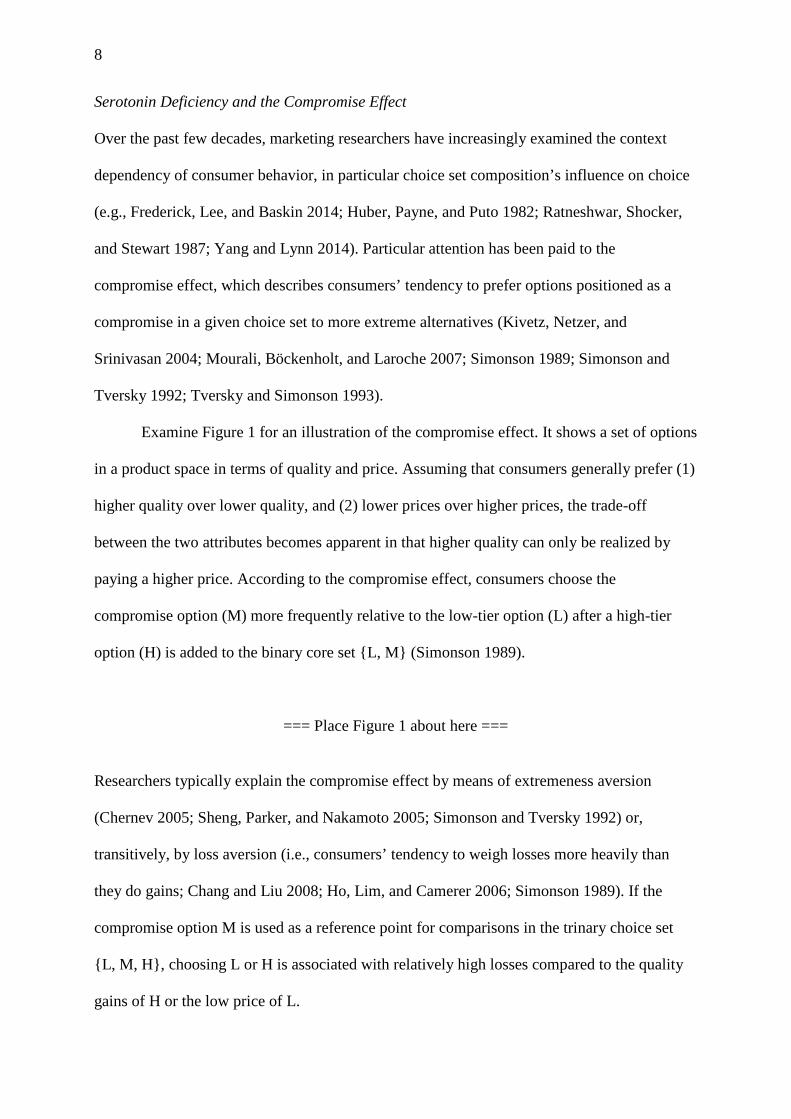
8
Serotonin Deficiency and the Compromise Effect
Over the past few decades, marketing researchers have increasingly examined the context
dependency of consumer behavior, in particular choice set composition’s influence on choice
(e.g., Frederick, Lee, and Baskin 2014; Huber, Payne, and Puto 1982; Ratneshwar, Shocker,
and Stewart 1987; Yang and Lynn 2014). Particular attention has been paid to the
compromise effect, which describes consumers’ tendency to prefer options positioned as a
compromise in a given choice set to more extreme alternatives (Kivetz, Netzer, and
Srinivasan 2004; Mourali, Böckenholt, and Laroche 2007; Simonson 1989; Simonson and
Tversky 1992; Tversky and Simonson 1993).
Examine Figure 1 for an illustration of the compromise effect. It shows a set of options
in a product space in terms of quality and price. Assuming that consumers generally prefer (1)
higher quality over lower quality, and (2) lower prices over higher prices, the trade-off
between the two attributes becomes apparent in that higher quality can only be realized by
paying a higher price. According to the compromise effect, consumers choose the
compromise option (M) more frequently relative to the low-tier option (L) after a high-tier
option (H) is added to the binary core set L, M (Simonson 1989).
=== Place Figure 1 about here ===
Researchers typically explain the compromise effect by means of extremeness aversion
(Chernev 2005; Sheng, Parker, and Nakamoto 2005; Simonson and Tversky 1992) or,
transitively, by loss aversion (i.e., consumers’ tendency to weigh losses more heavily than
they do gains; Chang and Liu 2008; Ho, Lim, and Camerer 2006; Simonson 1989). If the
compromise option M is used as a reference point for comparisons in the trinary choice set
L, M, H, choosing L or H is associated with relatively high losses compared to the quality
gains of H or the low price of L.
9
Theoretical accounts of the compromise effect see it as resulting from deliberate,
complex, cognitively demanding decision processes (“System 2”), rather than fast, intuitive
decision-making (“System 1”, Dhar and Gorlin 2013; Pocheptsova et al. 2009).2 That is,
consumers recognize the inherent trade-offs between product attributes, make cognitively
demanding comparisons between the options (Jang and Yoon 2015; Khan, Zhu, and Kalra
2011), but ultimately tend to choose the compromise option to reduce decision conflict (i.e.,
anticipated post-decision dissonances caused by counterfactual reasoning) by generating an
easy to justify solution to the decision problem.3 Accordingly, the compromise effect has been
found to be less pronounced when cognitive load was induced by experimental manipulations
such as introducing time pressure (Dhar, Nowlis, and Sherman 2000; Pettibone 2012), or
when decision makers were distracted by unrelated cognitive demanding tasks (Pocheptsova
et al. 2009). As Pocheptsova et al. (2009, p. 345) point out, “when resources for executive
control are depleted, consumers are less likely to engage in effortful trade-off comparisons,”
ATD-induced serotonin deficiency depletes subjects’ cognitive resources; hence, we
hypothesize that:4
H2a: The compromise effect will hold in the placebo group; thus, consumers will tend to
switch from a ‘low quality / low price’ option L in binary choice sets (comprising ‘low quality
/ price’ and ‘medium quality / price’) to a ‘medium quality / medium price’ option M in
trinary choice sets (comprising ‘low’, ‘medium’ and ‘high quality / price’).
H2b: The compromise effect will decrease for consumers under ATD-induced serotonin
deficiency. Hence, consumers will show less tendency to switch from a ‘low quality / price’
option L in binary choice sets to a ‘medium quality / price’ option M in trinary choice sets.
10
STUDY 1: THE EFFECTS OF ATD ON PURCHASE RATES AND THE COMPROMISE
EFFECT (WITHIN-SUBJECTS)
Experimental Design, Stimuli, Treatment, and Procedures
Experimental design: We used a 4x2x2 mixed factorial design with four product categories as
well as the number of products per choice (first two and then three) as within-subjects factors
and the experimental condition (treatment vs. placebo) as a between-subjects factor. Through
extensive pre-testing (focus groups with a total of nine participants and twelve face-to-face
interviews with members of the target audience), we identified four product categories that
were relevant to the experiment’s target audience and that have been used in context effect
studies and related research (e.g., Müller, Kroll, and Vogt 2012; Nowlis and Simonson 2000;
Simonson 1989; Voelckner 2006): hazelnut spread, headphones, ketchup, and mulled wine.
We deliberately decided to include relatively inexpensive fast-moving-consumer-goods
(FMCG) with short purchase intervals (e.g., hazelnut spread) along with more expensive
durables with longer purchase intervals (e.g., headphones) to span a wide product space for an
evaluation of the research questions. All products were described by a range of realistic
attributes; for example, headphones were described according to their technical attributes
(e.g., frequency response in Hz, sensitivity in dB) along with their product names and pictures
from Amazon.com and their respective product ratings (see the Appendix for an illustration).5
As such, our choice task was similar to real purchase situations. In order to stimulate
purchases, the product prices were about 10 percent lower than the cheapest actual market
prices (Web Appendix I shows the price scenarios for all four studies and the underlying
design principles).
Prior research has shown that forced choice situations may increase the compromise
effect because choosing the compromise option allows finding an easy to justify solution if
one is forced to make a choice (Dhar and Simonson, 2003). In the same vein, prior research
has shown that hypothetical decision settings may artificially increase the compromise effect
11
(Müller, Kroll, and Vogt 2012). To overcome these possible confounds and to reflect a more
realistic purchase scenario, we operated with binding decisions and included a no-buy option
that allowed consumers not to purchase a product (Lichters, Sarstedt, and Vogt 2015).
Specifically, we applied a random payoff mechanism (RPM) with one randomly selected
decision as the realized payoff, in order to elucidate the relevance of the no-buy decision.
Thus, if a subject accepted an offer to purchase a product and the RPM rendered this decision
relevant, he would pay the selling price and receive the product in exchange. In contrast,
subjects left the laboratory without the product if they chose the no-buy option in that RPM
decision. RPMs are commonly used in the field of experimental economics as they reveal
realistic demand properties in sequential multistage decisions that a single respondent makes,
since each choice might become payoff relevant (e.g., Cubitt, Starmer and Sugden 1998;
Grether and Plott 1979; Starmer and Sugden 1991; Wilcox 1993). Furthermore, RPMs ensure
that multiple observations per respondent can be interpreted to be mutually independent (e.g.,
Cubitt, Starmer and Sugden 1998) in that they suppress income or portfolio effects (Braga,
Humphrey and Starmer 2009).
Treatment administration: We induced a central serotonin reduction using ATD, a
standardized method commonly used to manipulate serotonin levels in humans (e.g.,
Carpenter et al. 1998; Crockett et al. 2013; Crockett, Clark and Robbins 2009; Crockett and
Fehr 2013). Subjects were randomly assigned to the treatment (i.e., ATD) and placebo groups
and consumed amino-acid drinks. The treatment group’s drink was identical to the placebo
group, except that it did not contain tryptophan, the neurobiological predecessor of serotonin.6
That is, the treatment group’s amino-acid drink temporarily lowered the brain serotonin levels
by limiting the availability of tryptophan (Carpenter et al. 1998; Cooper, Bloom, and Roth
2003), whereas the placebo group’s drink did not. Both drinks tasted equally. After
consuming their drinks, the participants had a resting period of five hours.
12
Mood questionnaire: To test for the treatment’s effect on the participants’ mood, they filled
out the 24-item multidimensional mood state questionnaire (MDMQ) before they ingested the
amino-acid mixture, and again five hours after consuming the drink. The MDMQ comprises
three mental state dimensions (pleasantness, wakefulness, and calmness) measured by eight
five-point items each (Steyer et al. 1994).
Risk attitude: To test for the treatment’s effect on risk-seeking, we incorporated two different
measures: the 11-point risk attitude measure used in the German Socio-Economic Panel
(SOEP) (Dohmen et al. 2010; Jaeger et al. 2010; Van Winden, Krawczyk, and Hopfensitz
2011) and the lottery procedure by Holt and Laury (2002) to measure financial risk (e.g., Faff,
Mulino, and Chai 2008; Harrison et al. 2005). Web Appendix II provides further details on
the procedure.
Research Procedure
Forty-seven students (nTreatment=23, nPlacebo=24) of a major German university participated in
study 1. To rule out any interactions of serotonin and estrogen during the menstrual cycle, we
invited only male students to participate (Rubinow, Schmidt, and Roca 1998). All subjects
were screened for psychiatric and neurological disorders and were asked to give written
informed consents. Exclusion criteria were cardiac, renal, pulmonary, neurological,
psychiatric or gastrointestinal disorders, medication / drug use, and a personal or family
history of a depressive disorder. All subjects received a show-up-fee of 8 EUR one week
before the experimental sessions; we deliberately paid the subjects in advance to avoid a
house money effect bias (Rosenboim and Shavit 2012; Thaler and Johnson 1990). The test
day began at 10 am with administration of either the ATD or placebo drink in a randomized
double-blind procedure. The main experiment sessions started at 3 pm.
As recommended by Lehmann and Pan (1994) and Lichters, Sarstedt, and Vogt
(2015), participants were given the opportunity to evaluate the products physically from a
prepared product shelf prior to the experiment. At this stage, all products were shown without
13
prices, to avoid the introduction of a price anchor in subsequent choice situations (Ariely,
Loewenstein, and Prelec 2006).
At the beginning of each session, the participants were randomly allocated to isolated
semi-cubicles in the lab, where they could not see or interact with each other. Next, the
experimenter delivered standardized oral instructions and the subjects had the opportunity to
ask questions. Subsequently, they filled out the questionnaires (MDMQ, followed by the
binary choice tasks, an unrelated distractor task, and the trinary choice tasks). Subjects made
their decisions at their own pace.
Product choices were first made in binary sets comprising L and M (CSbinary; Figure 1),
followed by trinary sets comprising L, M, and H such that M was positioned as a compromise
option (CStrinary; Figure 1). In both the binary and trinary choice sets in each of the four
categories, subjects made six choices from sets comprising the same two or three products but
with different prices. The participants had to indicate which product (if any) in each set they
would buy given the products’ prices. The price scenarios in CSbinary (first stage) contained a
systematic trade-off, realized by modifying the prices of options L and M. In CStrinary (second
stage), we used the same prices for L and M from the binary sets to allow direct comparisons
between the two stages. In each set, we ensured that the price of L was lower than the price of
M, whose price was always lower than the price of H in case of the trinary sets. Thus, no
option was a priori dominated by one of the other options in the choice set. In the trinary sets,
M was always a compromise between the extreme options L and H in terms of quality and
price.
In total, we collected 48 decisions per subject (five decisions for each of the four
product categories plus one validation decision per category in each of the two stages).
Following Müller, Vogt, and Kroll (2012), we deliberately duplicated one choice task in each
of the product categories, both in the binary and trinary choice stages, to assess the stability of

14
the subjects’ preferences and their attention. The corresponding decisions were excluded from
main analyses, resulting in 40 net decisions per subject.
After the respondents had completed the questionnaire, we ran the RPM by drawing a
number out of an urn to decide which of their decisions would be implemented. The
participants then fulfilled their buying obligations by paying (if they indicated that they
wanted to buy the specific product in the selected choice instance) and received their
purchases. The overall procedure lasted 90 minutes on average.
Results
Preliminary Analyses: First, we tested if respondents in the treatment group are comparable to
those of the placebo group (Hutchinson, Kamakura, and Lynch 2000). We found no
significant differences between the treatment and placebo groups in terms of age, height,
weight, monthly net income and subjects’ quality (versus price) orientation across all product
categories.7 Similarly, we found no significant differences in subjects’ aided brand awareness
of all products.
Next, we compared the scores of the three facets of the MDMQ (pleasantness,
wakefulness, and calmness) within the subjects (pre- versus post-treatment exposure) and
between the two groups to evaluate if ATD exerted an influence on mood. To test for
differences, we established mixed-effect general linear models. We defined the MDMQ
scores of the pre- and post-exposure as a within-subjects factor and the experimental
condition (treatment vs. placebo) as a between-subjects factor. We found no significant
differences between the treatment and placebo groups. Similarly, there were no significant
deviations between pre- and post-exposure (within) stage and no significant differences in the
change of mood dimensions between the treatment and the placebo groups as measured by the
treatment x (pre- vs. post) MDMQ dimensions. These results are in line with previous studies
that found no significant changes in mood induced by ATD (e.g., Campbell-Meiklejohn et al.
15
2010; Crockett et al. 2012; Murphy et al. 2009). Additionally, we found no significant
differences in the general risk attitudes or the financial risk taking behavior between the
treatment and placebo groups. Web Appendix III provides a detailed description of the
preliminary analyses results.
Analysis Of Purchase Decisions: Table 1 shows the aggregated purchase frequencies across
the four product categories. Table A3 in Web Appendix IV presents a detailed breakdown of
all observed choices. To test hypothesis H1, we compared the treatment and the placebo
groups’ buying rates by applying Fisher’s exact test. Across all of the decision situations, the
share of no-buy options was significantly (p≤0.001) lower in the placebo group (65.31%) than
in the treatment group (79.57%). In line with H1, ATD significantly lowers purchase rates
compared to the placebo group. To account for the multiple observations per respondent, we
also estimated a mixed-effect logit model that accounts for the data’s nested structure by
including a respondent-specific random intercept together with a nested product group-
specific random effect intercept. The results of this analysis provide further support for H1
(see Web Appendix V for a more detailed description and additional analyses).
=== Place Table 1 about here ===
To test H2a and H2b, we contrasted the subjects’ switching behavior regarding purchases
across the experimental conditions. Our statistical analysis only focused on switches between
the options L and M (see Huber, Payne, and Puto 1982) to evaluate if switching occurred
asymmetrically. Table 2 shows the corresponding results.
=== Place Table 2 about here ===

16
As shown in the upper part of Table 2, 14.81% of the placebo group’s decisions for the low
quality / price option L in the binary choice set (CSbinary), switched to the medium quality /
price option M in the trinary choice set (CStrinary). At the same time, no (reversed) switching
from M to L occurred. An exact McNemar test (e.g., Agresti 1992) demonstrates that the
number of switches from L to M is significantly greater than can be expected by chance
(p=0.008), providing support for H2a that the compromise effect holds as a within-subjects
choice anomaly in the placebo group. In contrast, no switches from L to M occurred in the
treatment group when the decision framework changed from binary to trinary (Table 2 lower
part). Thus, in line with H2b, we did not observe the compromise effect for subjects under
ATD-induced serotonin deficiency. In fact, 4.26% decision switches occurred in the opposite
direction from the compromise effect (i.e., from M to L), but this pattern was not statistically
significant (p=0.500).
To assess the stability of the subjects’ preferences, each subject made eight additional
decisions, two for every product category that were duplicates of previous choice tasks in the
experiment (see research procedure section). 97% of the 376 duplicated choices were
replicated, confirming a high degree of consistency even at the individual level and negligible
choice error rates. Finally, none of the participants tried to re-negotiate the terms of the
experiment and all of them fulfilled their buying obligations; hence, the participants were
fully aware of the economic consequences when solving the choice problems.
STUDY 2: THE EFFECTS OF ATD ON PURCHASE RATES AND THE COMPROMISE
EFFECT (BETWEEN-SUBJECTS)
Study 1 drew on a within-subjects design to explore preference reversals (changes from
option L to option M) at the individual level (Ratneshwar, Shocker and Stewart 1987). To
account for potential confounding influences in within-subjects designs resulting from
17
learning effects among participants in repeated choices (e.g., Ahn, Kim, and Ha 2015), motif
biases (e.g., McAlister and Pessemier 1982), or history effects (e.g., Campbell and Stanley
1963; Shadish, Cook, and Campbell 2002), study 2 replicates and extends the first study by
using (1) a between-subjects design setting, and (2) new product categories to broaden the
product range.
Experimental Design, Stimuli, Treatment, and Procedures
Study 2 draws on a 2x2x2 mixed factorial design with the experimental condition (treatment
vs. placebo) and the choice set composition (binary vs. trinary) as between-subjects factors
and the two product categories as a within-subjects factor. To ensure that the new product
categories were relevant to the target audience, we conducted additional focus group
discussions with twelve students and identified potato chips and toothpaste as particularly
suitable. All other elements of the experimental design and treatment administration in study
2 were analogous to study 1, for example, in terms of product descriptions (see Appendix),
choice set compositions, inclusion of a no-buy option, and the RPM implementation.8
Research Procedure
A total of 98 male students (nTreatment=49, nPlacebo=49) participated in study 2. We relied on the
same screening / exclusion criteria, test timings, and procedures as in study 1. Subjects in the
CSbinary and CStrinary conditions completed a series of binary and trinary choice tasks
respectively, using a paper-pen-questionnaire, at their own pace. In total, we collected twelve
decisions per subject (five choices and a validation decision for each of the two product
categories). Web Appendix I lists the used price scenarios. After all the decisions had been
made, the RPM determined which of them became payoff relevant and subjects fulfilled their
purchase transactions, if required. The overall procedure lasted about 20 minutes on average.
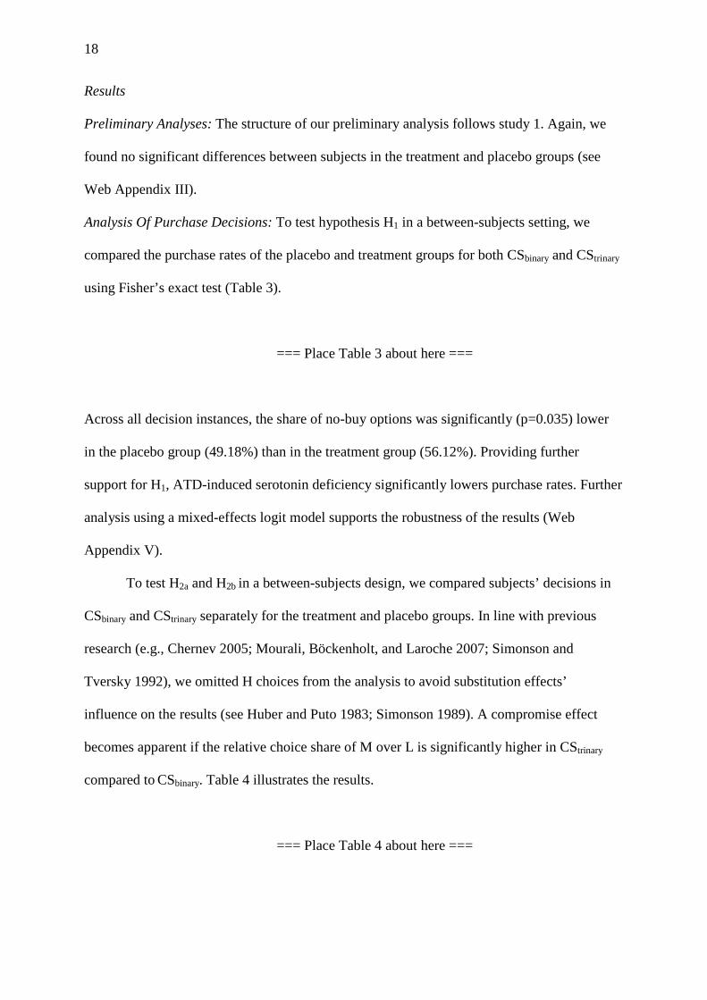
18
Results
Preliminary Analyses: The structure of our preliminary analysis follows study 1. Again, we
found no significant differences between subjects in the treatment and placebo groups (see
Web Appendix III).
Analysis Of Purchase Decisions: To test hypothesis H1 in a between-subjects setting, we
compared the purchase rates of the placebo and treatment groups for both CSbinary and CStrinary
using Fisher’s exact test (Table 3).
=== Place Table 3 about here ===
Across all decision instances, the share of no-buy options was significantly (p=0.035) lower
in the placebo group (49.18%) than in the treatment group (56.12%). Providing further
support for H1, ATD-induced serotonin deficiency significantly lowers purchase rates. Further
analysis using a mixed-effects logit model supports the robustness of the results (Web
Appendix V).
To test H2a and H2b in a between-subjects design, we compared subjects’ decisions in
CSbinary and CStrinary separately for the treatment and placebo groups. In line with previous
research (e.g., Chernev 2005; Mourali, Böckenholt, and Laroche 2007; Simonson and
Tversky 1992), we omitted H choices from the analysis to avoid substitution effects’
influence on the results (see Huber and Puto 1983; Simonson 1989). A compromise effect
becomes apparent if the relative choice share of M over L is significantly higher in CStrinary
compared to CSbinary. Table 4 illustrates the results.
=== Place Table 4 about here ===
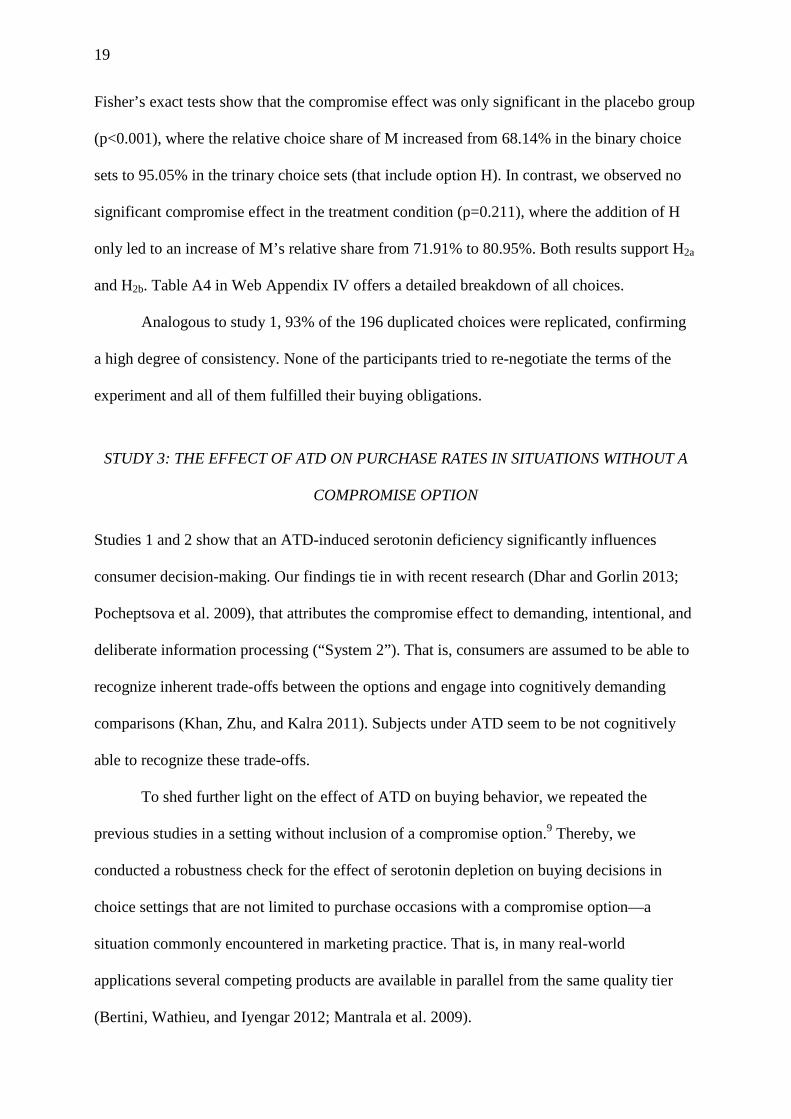
19
Fisher’s exact tests show that the compromise effect was only significant in the placebo group
(p<0.001), where the relative choice share of M increased from 68.14% in the binary choice
sets to 95.05% in the trinary choice sets (that include option H). In contrast, we observed no
significant compromise effect in the treatment condition (p=0.211), where the addition of H
only led to an increase of M’s relative share from 71.91% to 80.95%. Both results support H2a
and H2b. Table A4 in Web Appendix IV offers a detailed breakdown of all choices.
Analogous to study 1, 93% of the 196 duplicated choices were replicated, confirming
a high degree of consistency. None of the participants tried to re-negotiate the terms of the
experiment and all of them fulfilled their buying obligations.
STUDY 3: THE EFFECT OF ATD ON PURCHASE RATES IN SITUATIONS WITHOUT A
COMPROMISE OPTION
Studies 1 and 2 show that an ATD-induced serotonin deficiency significantly influences
consumer decision-making. Our findings tie in with recent research (Dhar and Gorlin 2013;
Pocheptsova et al. 2009), that attributes the compromise effect to demanding, intentional, and
deliberate information processing (“System 2”). That is, consumers are assumed to be able to
recognize inherent trade-offs between the options and engage into cognitively demanding
comparisons (Khan, Zhu, and Kalra 2011). Subjects under ATD seem to be not cognitively
able to recognize these trade-offs.
To shed further light on the effect of ATD on buying behavior, we repeated the
previous studies in a setting without inclusion of a compromise option.9 Thereby, we
conducted a robustness check for the effect of serotonin depletion on buying decisions in
choice settings that are not limited to purchase occasions with a compromise option—a
situation commonly encountered in marketing practice. That is, in many real-world
applications several competing products are available in parallel from the same quality tier
(Bertini, Wathieu, and Iyengar 2012; Mantrala et al. 2009).

20
Experimental Design, Stimuli, and Treatment
We used a 2x2 mixed factorial design with two product categories as within-subjects factors
and the experimental condition (treatment vs. placebo) as a between-subjects factor. In the
third study we used two product categories (headphones and hazelnut spread) to span the
continuum between cheap FMCG and relative expensive consumer durables. The research
design of study 3 was identical to study 1 except that product choices were only made in one
trinary setting comprising L, M, and a third option L2, which included a product of
comparable quality to L at a very similar price. Thus, the trinary sets had no compromise
option. All other aspects of the research design as well as the treatment administration
followed the same principles as in the previous studies.
Research Procedure
51 male students (nTreatment=26, nPlacebo=25) participated in study 3. We applied the same
screening criteria and test timings like in the two previous studies, following the same
research procedures.
Participants made five choices and an additional duplicated choice for validating
choice consistency for each category. In total, we collected twelve decisions per subject, ten
of which were used for the main analysis. After all choices were made, we ran the RPM. The
overall procedure lasted about 25 minutes on average.
Results
Preliminary Analyses: All preliminary analyses were analogous to studies 1 and 2 (see Web
Appendix III). Again, we did not find any significant differences between the groups that
would possibly exert confounding influences on our results.
Analysis Of Purchase Decisions: Table 5 summarizes purchase frequencies across the product
categories (see Web Appendix IV for further details).

21
=== Place Table 5 about here ===
The share of the no-buy decisions was significantly lower (p=0.004) in the placebo group
(60.80%) than in the treatment group (73.08%), replicating the results of study 1. Thus, in line
with H1, ATD significantly lowered purchase rates compared to the placebo group. Further
analysis using a mixed-effects logit model supports the robustness of the results (Web
Appendix V). Similarly to the first two studies, the consensus of the duplicated choices with
their counterparts—93% of the 204 decisions were replicated—indicates a high degree of
decision consistency and only limited choice error.
STUDY 4: THE EFFECT OF ATD ON THE COMPROMISE EFFECT IN
FORCED CHOICE SITUATIONS
The previous three studies relied on free choice settings (i.e., subjects had a no-buy option)
for two main reasons. First, in real-world settings, consumers typically have the option not to
purchase a product (Dhar and Nowlis 2004). Therefore, including a no-buy option ensures
correspondence between the experimental setup and the real-world setting to which an effect
is assumed to apply. Second, the availability of a no-buy option offers a more conservative
assessment of the compromise effect’s magnitude (Dhar and Simonson, 2003). Yet, the
majority of context effect studies conducted to this date did not include a no-buy option
(Lichters, Sarstedt, and Vogt 2015). To align our experimental design with previous research
and to generalize our findings to situations where consumers are practically forced to buy
(e.g., immediate demand without the option of postponing the purchase, such as having
forgotten to buy a present at the evening of Mother’s Day), we conducted an additional

22
robustness check of our results by replicating studies 1 and 2 in a forced choice framework
(studies 4a and 4b).9
Experimental Design, Stimuli, and Treatment
Analogous to study 1, study 4a used a 3x2x2 mixed factorial design with three product
categories (chips, ketchup, and toothpaste) as well as the number of products per choice (first
two and then three) as within-subjects factors and the experimental condition (treatment vs.
placebo) as between-subjects factor. For chips and ketchup we used the same stimuli as in the
previous studies but made some minor price adjustments due to changing market conditions.10
Study 4b followed study 2 by implementing a 2x2x2 mixed factorial design with the
experimental condition (treatment vs. placebo) and the choice set composition (binary vs.
trinary) as between-subjects factors and two product categories (hazelnut spread and
mouthwashes) as within-subjects factor.11 All other aspects of the design and treatment
administration followed the same principles as in the previous studies.
Research Procedure
In total, 49 male students (nTreatment=25, nPlacebo=24) participated in studies 4a and 4b. We used
the identical screening criteria and test timings as before, following the same research
procedures as in studies 1 and 2 with one exception. Since subjects were forced to buy one
item, we raised the participation fee to 15 EUR, which was handed over two weeks in
advance.
In study 4a, subjects made 18 decisions from binary sets comprising L and M in three
product categories and another 18 decisions from corresponding trinary sets. This approach
yields a total of 36 decisions per respondent, 30 of which were used for the main analysis (six
decisions were duplicated scenarios). The same sample of subjects also participated in study
4b that took place between the binary and the trinary choice stages of study 4a, and was
separated from each of these stages by unrelated distractor tasks. This procedure ensured that
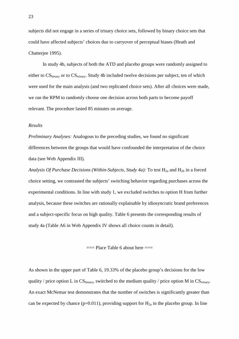
23
subjects did not engage in a series of trinary choice sets, followed by binary choice sets that
could have affected subjects’ choices due to carryover of perceptual biases (Heath and
Chatterjee 1995).
In study 4b, subjects of both the ATD and placebo groups were randomly assigned to
either to CSbinary or to CStrinary. Study 4b included twelve decisions per subject, ten of which
were used for the main analysis (and two replicated choice sets). After all choices were made,
we ran the RPM to randomly choose one decision across both parts to become payoff
relevant. The procedure lasted 85 minutes on average.
Results
Preliminary Analyses: Analogous to the preceding studies, we found no significant
differences between the groups that would have confounded the interpretation of the choice
data (see Web Appendix III).
Analysis Of Purchase Decisions (Within-Subjects, Study 4a): To test H2a and H2b in a forced
choice setting, we contrasted the subjects’ switching behavior regarding purchases across the
experimental conditions. In line with study 1, we excluded switches to option H from further
analysis, because these switches are rationally explainable by idiosyncratic brand preferences
and a subject-specific focus on high quality. Table 6 presents the corresponding results of
study 4a (Table A6 in Web Appendix IV shows all choice counts in detail).
=== Place Table 6 about here ===
As shown in the upper part of Table 6, 19.33% of the placebo group’s decisions for the low
quality / price option L in CSbinary, switched to the medium quality / price option M in CStrinary.
An exact McNemar test demonstrates that the number of switches is significantly greater than
can be expected by chance (p=0.011), providing support for H2a in the placebo group. In line

24
with H2b, only nine (7.89%) switches from L to M occurred in the treatment group when the
decision framework changed from binary to trinary (Table 6 lower part). Thus, we did not
observe a significant compromise effect for subjects under ATD-induced serotonin deficiency
(p=0.122).
Analysis Of Purchase Decisions (Between-Subjects): Table 7 summarizes the purchase counts
and frequencies across the two product categories of study 4b.
=== Place Table 7 about here ===
To test H2a and H2b in a between-subjects design, we compared subjects’ decisions in
the binary and trinary sets separately for the treatment and placebo groups. In line with H2a,
Fisher’s exact tests show that the compromise effect is only significant in the placebo group
(p<0.001), where the relative choice share of M increased from 44.17% in the binary choice
sets to 83.04% in the trinary choice sets. In support of H2b, we observed no significant
compromise effect in the treatment condition (p=0.301), where the addition of H only led to
an increase of M’s relative share from 51.67% to 63.39%.
In summary, studies 4a and 4b support our notion that ATD decreases the compromise
effect also in a forced choice scenario. In accordance with the preceding studies, the
consensus of the duplicated choices were identical to their counterparts—93% of the
decisions were replicated across studies 4a and 4b, indicating a high consistency levels.
GENERAL DISCUSSION AND IMPLICATIONS
Research in the field of neuroscience has underlined the influence of serotonergic modulation
on local information processing in various brain regions, suggesting that it regulates the state
and context-dependent aspects of human decision-making (Crockett and Fehr 2013). Tying in

25
with this stream of research, we systematically depleted subjects’ serotonin levels and were
able to demonstrate that this fosters choice deferral and eliminates the compromise effect,
both as a within-subject and as a between-subjects choice phenomenon, in free choice as well
as forced choice settings. Therefore, our study makes several contributions to marketing
research and practice.
First, our results demonstrate the moderating role of serotonin on consumers’ buying
behavior. Low levels of serotonin promote choice deferral, a mechanism that potentially
underlies a previous finding that older individuals defer more often than younger adults
(Chen, Ma, and Pethtel 2011). Against this background, marketing practitioners should
consider adopting strategies that are known to enhance serotonin levels (e.g., increasing
daylight exposure in retail space; Koc and Boz 2014) for increasing sales.
Second, we provide causal neurobiological evidence that the compromise effect is the
result of deliberate and demanding thought processes (Dhar and Gorlin 2013; Pocheptsova et
al. 2009). Reduced serotonin levels were shown to impair cognition (Evers et al 2004;
Hayward et al. 2005; Murphy et al. 2002; Park et al. 1994; Riedel 2004) and reduce framing
effects that are associated with increased attention and deliberation (Campbell-Meiklejohn et
al. 2010; Crockett et al. 2010; Murphy et al. 2009). Incorporating our findings corroborates
the notion that the compromise effect results from deliberate, complex, and cognitively
demanding decision processes (“System 2”), rather than fast, intuitive decision-making
("System 1”, Dhar and Gorlin 2013; Pocheptsova et al. 2009). These results suggest that
marketing strategies that systematically incorporate the compromise effect with the intent to
promote the choice of an intermediate compromise option might be less effective when the
target population’s serotonin levels are lowered (e.g., at old age or during winter; Taylor et al.
1984). While our results do not question the usefulness of context effects per se, they suggest
that marketing researchers and practitioners should more strongly consider their boundaries
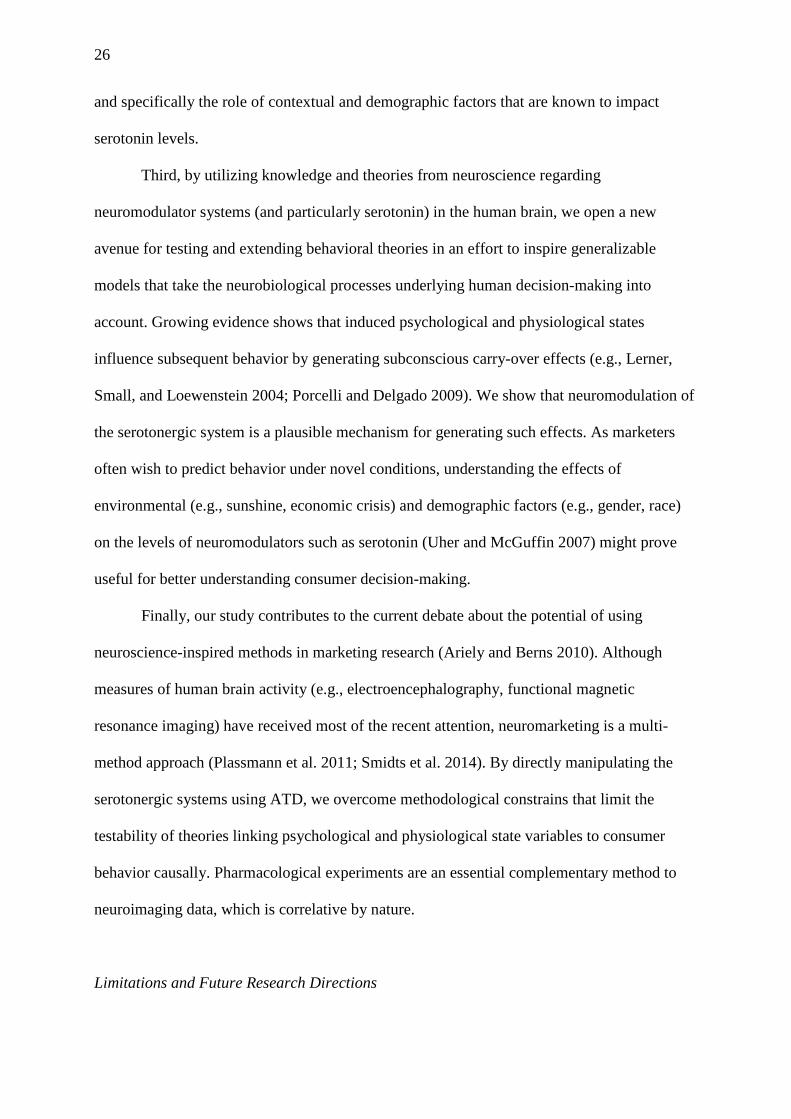
26
and specifically the role of contextual and demographic factors that are known to impact
serotonin levels.
Third, by utilizing knowledge and theories from neuroscience regarding
neuromodulator systems (and particularly serotonin) in the human brain, we open a new
avenue for testing and extending behavioral theories in an effort to inspire generalizable
models that take the neurobiological processes underlying human decision-making into
account. Growing evidence shows that induced psychological and physiological states
influence subsequent behavior by generating subconscious carry-over effects (e.g., Lerner,
Small, and Loewenstein 2004; Porcelli and Delgado 2009). We show that neuromodulation of
the serotonergic system is a plausible mechanism for generating such effects. As marketers
often wish to predict behavior under novel conditions, understanding the effects of
environmental (e.g., sunshine, economic crisis) and demographic factors (e.g., gender, race)
on the levels of neuromodulators such as serotonin (Uher and McGuffin 2007) might prove
useful for better understanding consumer decision-making.
Finally, our study contributes to the current debate about the potential of using
neuroscience-inspired methods in marketing research (Ariely and Berns 2010). Although
measures of human brain activity (e.g., electroencephalography, functional magnetic
resonance imaging) have received most of the recent attention, neuromarketing is a multi-
method approach (Plassmann et al. 2011; Smidts et al. 2014). By directly manipulating the
serotonergic systems using ATD, we overcome methodological constrains that limit the
testability of theories linking psychological and physiological state variables to consumer
behavior causally. Pharmacological experiments are an essential complementary method to
neuroimaging data, which is correlative by nature.
Limitations and Future Research Directions
27
Our study is subject to limitations, which offer several avenues for further research. First, as
the present study focused on male subjects due to the known changes in serotonin levels
during the menstrual cycle (Rubinow, Schmidt, and Roca 1998), future research should also
investigate the relation between the serotonergic system and female consumer behavior in
order to delineate whether the current findings can be generalized to women. Furthermore, we
did not include measurements of participants’ blood tryptophan level as a manipulation check,
as blood drawing could potentially induce stress that interferes with participants’ decision-
making processes (e.g., Porcelli and Delgado, 2009, Moschis, 2007). However, as we
conducted the ATD manipulations strictly according to the protocol of previous studies that
univocally proved a marked blood tryptophan reduction (e.g., Carpenter et al. 1998; Crockett
et al. 2013; Crockett, Clark, and Robbins 2009), it is reasonable to assume that the ATD
manipulations worked in our studies’ settings.
Prior research has shown that the perception of preference fluency (i.e., the meta-
cognition that forming a preference for a specific option is rather easy or not) is negatively
related to choice deferral (Novemsky et al. 2007). It is intriguing whether serotonin deficiency
has an influence on preference fluency and if this construct thus mediates the effect of
serotonin deficiency on purchase deferral. As the number of possible comparisons between
options increases exponentially with the number of available options, we expect the number
of choice deferrals to be even more pronounced under serotonin deficiency when choosing
from broader choice sets than in the present study. This is particularly intriguing, as real-
world buying decisions are typically characterized by many options (Kivetz, Netzer, and
Srinivasan 2004).
Similarly, future research should evaluate the moderating role that decision
complexity—operationalized by the number of options per choice set—plays in the link
between serotonin deficiency and purchase behavior. Prior research has shown that consumers
facing larger assortments are often prone to choice overload (Chernev, Böckenholt, and

28
Goodman 2015). Choice deferral—as researched in our study—is only one consequence of
choice overload. Future research should evaluate whether other antecedents, such as
satisfaction, confidence, and post-decision regret are also influenced by varying serotonin
levels. For example, if anticipated post-decision dissonances are higher for consumers with
low serotonin levels, marketers may desire to spend more effort in attempts to reduce such
dissonances (e.g., by offering money back guarantee for goods that are predominately sold in
the winter period). Relatedly, in light of the decreased purchase rates under ATD, follow-up
studies should also investigate whether serotonin deficiency increases subjects’ price
sensitivity and, therefore, the price elasticity of demand (Tellis 1988).
Future research should also examine serotonin’s role in the context of the attraction
effect as a prominent choice anomaly in consumer behavior (e.g., Heath and Chatterjee 1995;
Huber, Payne, and Puto 1982; Simonson and Tversky 1992). Prior research has shown that the
attraction effect increases in magnitude when (1) subjects’ cognitive resources are depleted
(Pocheptsova et al. 2009), or (2) subjects naturally rely heavily on intuitive reasoning in their
judgment and decision-making rather than on rational thinking (Mao and Oppewal 2012).
Based on the notion that cognitive load impairs deliberation and amplifies reliance on
intuitive information processing (Masicampo and Baumeister 2008), we expect that the
attraction effect will increase in magnitude with lower levels of serotonin induced by ATD.
Relatedly, only recently researchers have questioned the robustness and thereby the
usefulness of the attraction effect in real-world applications (e.g., Frederick, Lee, and Baskin
2014; Huber, Payne, and Puto 2014; Simonson 2014; Yang and Lynn 2014). Research on the
robustness of attraction effect and context effects in general would greatly benefit from
controlling for variations of serotonin levels as a possible moderator for the occurrence of
these effects.
Future studies may also investigate whether the serotonergic system plays a role in
possible age-related differences in consumer behavior (e.g., Cole et al. 2008; Phillips and
29
Sternthal 1977; Yoon and Cole 2008) as serotonin levels decrease with chronological age
(e.g., Rehman and Masson 2001). Studying serotonin’s effect on age-related phenomena, such
as subjects’ future time perspectives (Carstensen 2006), that recent marketing research has
investigated (Kuppelwieser and Sarstedt 2014a, 2014b), would be particularly promising in
this context.
Finally, the current work focused on a single neurotransmitter, serotonin, due to
methodological constraints. However, neurotransmitter systems never act in isolation, but
rather in concert with each other. In particular, the serotonergic system is known to interact
with the dopaminergic system (Daw, Kakade, and Dayan 2002), the oxytocinergic and
vasopressinergic systems (Ferris et al., 1997; Jørgensen et al. 2003; Mottolese et al. 2014).
Therefore, future research should also consider the interaction of the distinct neurotransmitter
systems during consumer decision-making.
REFERENCES
Agresti, Alan (1992), “A Survey of Exact Inference for Contingency Tables,” Statistical
Science, 7(1), 131–153.
Ahn, Sowon, Juyoung Kim and Young-Won Ha (2015), “Feedback Weakens the Attraction
Effect in Repeated Choices,” Marketing Letters, (in press).
Anderson, Ian M., Rebecca A. Richell, and Chris M. Bradshaw (2003), “The Effect of Acute
Tryptophan Depletion on Probabilistic Choice,” Journal of Psychopharmacology, 17(1), 3–
7.
Ariely, Dan, George Loewenstein, and Drazen Prelec (2006), “Tom Sawyer and The
Vonstruction of Value,” Journal of Economic Behavior & Organization, 60(1), 1–10.
——— and Gregory S. Berns (2010), “Neuromarketing: The Hope and Hype of
Neuroimaging in Business,” Nature Reviews Neuroscience, 11(4), 284–292.

30
Bagozzi, Richard P., Mahesh Gopinath, and Prashanth U. Nyer (1999), “The Role of
Emotions in Marketing,” Journal of the Academy of Marketing Science, 27(2), 184–206.
Barberis, Nicholas and Ming Huang (2001), “Mental Accounting, Loss Aversion, and
Individual Stock Returns,” The Journal of Finance, 56(4), 1247–1292.
Berger, Miles, John A. Gray, and Bryan L. Roth (2009), “The Expanded Biology of
Serotonin,” Annual Review of Medicine, 60, 355–366.
Bertini, Marco, Luc Wathieu and Sheena S. Iyengar (2012), “The Discriminating Consumer:
Product Proliferation and Willingness to Pay for Quality,” Journal of Marketing Research,
49(1), 39–49.
Botti, Simona and Iyengar, Sheena S. (2004), “The Psychological Pleasure and Pain of
Choosing: When People Prefer Choosing at the Cost of Subsequent Outcome Satisfaction,”
Journal of Personality and Social Psychology, 87(3), 312–326.
Braga, Jacinto, Steven J. Humphrey, and Chris Starmer (2009), “Market Experience
Eliminates some Anomalies—and Creates new Ones,” European Economic Review, 53(4),
401–416.
Camerer, Colin (2008), “The Case for Mindful Economics,” in Foundations of Positive and
Normative Economics, Andrew Caplin and Andrew Schotter, eds. Oxford: Oxford
University Press, 43–69.
Campbell-Meiklejohn, Daniel, Judi Wakeley, Vanessa Herbert, Jennifer Cook, Paolo Scollo,
Manaan K. Ray, Sudhakar Selvaraj, Richard E. Passingham, Phillip Cowen, and Robert D.
Rogers (2010), “Serotonin and Dopamine Play Complementary Roles in Gambling to
Recover Losses,” Neuropsychopharmacology, 36(2), 402–410.
Carpenter, Linda L., George M. Anderson, Gregory H. Pelton, Jeffrey A. Gudin, Paul D. S.
Kirwin, Lawrence H. Price, George R. Heninger, and Christopher J. McDougle (1998),
“Tryptophan Depletion During Continuous CSF Sampling in Healthy Human Subjects,”
Neuropsychopharmacology, 19(1), 26–35.
31
Cardinal, Rudolf N. (2006), “Neural Systems Implicated in Delayed and Probabilistic
Reinforcement,” Neural Networks, 19(8), 1277–1301.
Carstensen, Laura L. (2006), “The Influence of a Sense of Time on Human Development,”
Science, 312(5782), 1913–1915.
Celedon, Paulina, Sandra Milberg, and Francisca Sinn (2013), “Attraction and Superiority
Effects in the Chilean Marketplace: Do They Exist with Real Brands?,” Journal of Business
Research, 66(10), 1780–1786.
Chaouloff, F, D. Laude, and J. L. Elghozi (1989), “Physical Exercise: Evidence for
Differential Consequences of Tryptophan on 5-HT Synthesis and Metabolism in Central
Serotonergic Cell Bodies and Terminals,” Journal of Neural Transmission/General Section
JNT, 78(2), 121–130.
Chen, Yiwei, Ma, Xiaodong, and Pethtel, Olivia (2011), “Age Differences in Trade-off
Decisions: Older Adults Prefer Choice Deferral.” Psychology and Aging, 26(2), 269 –273.
Chernev, Alexander (2005), “Context Effects without a Context: Attribute Balance as a
Reason for Choice,” Journal of Consumer Research, 32(2), 213–223.
———, Ulf Böckenholt, and Joseph Goodman (2015), “Choice Overload: A Conceptual
Review and Meta-Analysis,” Journal of Consumer Psychology, (in press).
Cole, Catherine, Gilles Laurent, Aimee Drolet, Jane Ebert, Angela Gutchess, Raphaëlle
Lambert-Pandraud, Etienne Mullet, Michael I. Norton and Ellen Peters (2008), “Decision
Making and Brand Choice by Older Consumers,” Marketing Letters, 19(3-4), 355–365.
Cools, Roshan, Kae Nakamura and Nathaniel D. Daw (2010), “Serotonin and Dopamine:
Unifying Affective, Activational, and Decision Functions,” Neuropsychopharmacology,
36(1), 98–113.
Cooper, Jack R., Floyd E. Bloom, and Robert H. Roth (2003), The Biochemical Basis of
Neuropharmacology. Oxford: Oxford University Press.

32
Crockett, Molly J., Luke Clark, Golnaz Tabibnia, Matthew D. Lieberman, and Trevor W.
Robbins (2008), “Serotonin Modulates Behavioral Reactions to Unfairness,” Science,
320(5884), 1739–1739.
———, ———, and Trevor W. Robbins (2009), “Reconciling the Role of Serotonin in
Behavioral Inhibition and Aversion: Acute Tryptophan Depletion Abolishes Punishment-
induced Inhibition in Humans,” The Journal of Neuroscience, 29(38), 11993–11999.
———, ———, Matthew D. Lieberman, Golnaz Tabibnia, and Trevor W. Robbins (2010),
“Impulsive Choice and Altruistic Punishment Are Correlated and Increase in Tandem with
Serotonin Depletion,” Emotion, 10(6), 855–862.
———, ———, L. D. Smillie, and T. W. Robbins (2012), “The Effects of Acute Tryptophan
Depletion on Costly Information Sampling: Impulsivity or Aversive Processing?,”
Psychopharmacology, 219(2), 587–597.
——— and Ernst Fehr (2013), “Pharmacology of Economic and Social Decision Making,” in
Neuroeconomics: Decision Making and the Brain, (pp. 259–282), Paul W. Glimcher, and
Ernst Fehr, eds.: Academic Press Inc.
———, Annemieke Apergis-Schoute, Benedikt Herrmann, Matthew D. Lieberman, Ulrich
Müller, Trevor W. Robbins and Luke Clark (2013), “Serotonin Modulates Striatal
Responses to Fairness and Retaliation in Humans,” The Journal of Neuroscience, 33(8),
3505–3513.
Cubitt, Robin, Chris Starmer, and Robert Sugden (1998), “On the Validity of the Random
Lottery Incentive System,” Experimental Economics, 1(2), 115–131.
Dai, Xianchi and Christopher K. Hsee (2013), “Wish versus Worry: Ownership Effects on
Motivated Judgment,” Journal of Marketing Research, 50(2), 207–215.
Daw, Nathaniel D, Sham Kakade, and Peter Dayan (2002), “Opponent Interactions between
Serotonin and Dopamine,” Neural Networks, 15(4), 603–616.

33
Dayan, Peter and Quentin J. M. Huys (2008), “Serotonin, Inhibition, and Negative Mood,”
PLoS Computational Biology, 4(2), e4.
Denk, F, M. E. Walton, K. A. Jennings, T. Sharp, M. F. Rushworth, and D. M. Bannerman
(2005), “Differential Involvement of Serotonin and Dopamine Systems in Cost-benefit
Decisions About Delay or Effort,” Psychopharmacology, 179(3), 587–596.
Dhar, R. (1996), “The Effect of Decision Strategy on Deciding to Defer Choice,” Journal of
Behavioral Decision Making, 9(4), 265–281.
———, (1997), “Consumer Preference for a No-choice Option,” Journal of Consumer
Research, 24(2), 215–231.
——— and Margarita Gorlin (2013), “A Dual-system Framework to Understand Preference
Construction Processes in Choice,” Journal of Consumer Psychology, 23(4), 528–542.
——— and Stephen M. Nowlis (1999), “The Effect of Time Pressure on Consumer Choice
Deferral,” Journal of Consumer Research, 25(4), 369–384.
——— and ——— (2004), “To Buy or not to Buy: Response Mode Effects on Consumer
Choice,” Journal of Marketing Research, 41(4), 423–432.
———, ———, and Steven J. Sherman (2000), “Trying Hard or Hardly Trying: An Analysis
of Context Effects in Choice. Journal of Consumer Psychology, 9(4), 189–200.
——— and Itamar Simonson (2003), “The Effect of Forced Choice on Choice,” Journal of
Marketing Research, 40(2), 146–160.
Diehl, Kristin and Poynor, Cait. (2010), “Great Expectations?! Assortment Size, Expectations,
and Satisfaction,” Journal of Marketing Research, 47(2), 312–322.
Dohmen, Thomas, Armin Falk, David Huffman, and Uwe Sunde (2010), “Are Risk Aversion
and Impatience Related to Cognitive Ability?,” The American Economic Review, 100(3),
1238–1260.
Evans, Jonathan. S. B. (2008), “Dual-processing Accounts of Reasoning, Judgment, and
Social Cognition.” Annual Review of Psychology, 59, 255–278.

34
Evers, E. A, D. E. Tillie, Van Der Veen, FM, C. K. Lieben, J. Jolles, N. E. Deutz and J. A.
Schmitt (2004), “Effects of a Novel Method of Acute Tryptophan Depletion on Plasma
Tryptophan and Cognitive Performance in Healthy Volunteers,” Psychopharmacology,
177(1-2), 217–223.
Faff, Robert, Daniel Mulino, and Daniel Chai (2008), “On the Linkage Between Financial
Risk Tolerance and Risk Aversion,” Journal of Financial Research, 31(1), 1–23.
Fern, Edward F. and Kent B. Monroe (1996), “Effect-Size Estimates: Issues and Problems in
Interpretation,” Journal of Consumer Research, 23(2), 89–105.
Ferris, Craig F, Melloni Jr, Richard H, Gary Koppel, Kenneth W. Perry, Ray W. Fuller, and
Yvon Delville (1997), “Vasopressin/Serotonin Interactions in the Anterior Hypothalamus
Control Aggressive Behavior in Golden Hamsters,” The Journal of Neuroscience, 17(11),
4331–4340.
Fornell, Claes and David F. Larcker (1981), “Evaluating Structural Equation Models with
Unobservable Variables and Measurement Error,” Journal of Marketing Research, 18(1),
39–50.
Frederick, Shane, Leonard Lee, and Ernest Baskin (2014), “The Limits of Attraction,”
Journal of Marketing Research, 51(4), 487–507.
Fryer Jr, Roland G, Steven D. Levitt, John List and Sally Sadoff (2012), “Enhancing the
Efficacy of Teacher Incentives Through Loss Aversion: A Field Experiment,” National
Bureau of Economic Research Working Paper 18237.
Gardner, Meryl P. (1985), “Mood States and Consumer Behavior: A Critical Review,”
Journal of Consumer Research, 12(3), 281–300.
Gorn, Gerald J., Marvin E. Goldberg, and Kunal Basu (1993), “Mood Awareness and Product
Evaluation,” Journal of Consumer Psychology, 2(3), 237–256.
Grether, David M. and Charles R. Plott (1979), “Economic Theory of Choice and the
Preference Reversal Phenomenon,” The American Economic Review, 69(4), 623–638.
35
Harrison, Glenn W., Eric Johnson, Melayne M. McInnes, and Elisabet E. Rutström (2005),
“Risk Aversion and Incentive Effects: Comment,” American Economic Review, 95(3), 897–
901.
Hayward, Gail, Guy M. Goodwin, Phil J. Cowen, and Catherine J. Harmer (2005), “Low-dose
Tryptophan Depletion in Recovered Depressed Patients Induces Changes in Cognitive
Processing without Depressive Symptoms,” Biological Psychiatry, 57(5), 517–524.
Heath, Timothy B. and Subimal Chatterjee (1995), “Asymmetric Decoy Effects on Lower-
Quality Versus Higher-Quality Brands: Meta-Analytic and Experimental Evidence,”
Journal of Consumer Research, 22(3), 268–284.
Ho, Teck H., Noah Lim, and Colin F. Camerer (2006), “Modeling the Psychology of
Consumer and Firm Behavior with Behavioral Economics,” Journal of Marketing
Research, 43(3), 307–331.
Holt, Charles A. and Susan K. Laury (2002), “Risk Aversion and Incentive Effects,”
American Economic Review, 92(5), 1644–1655.
Huber, Joel, John W. Payne, and Christopher Puto (1982), “Adding Asymmetrically
Dominated Alternatives: Violations of Regularity and the Similarity Hypothesis,” Journal
of Consumer Research, 9(1), 90–98.
———, ———, and ——— (2014), “Let’s Be Honest About the Attraction Effect,” Journal
of Marketing Research, 51(4), 520–525.
——— and Christopher Puto (1983), “Market Boundaries and Product Choice: Illustrating
Attraction and Substitution Effects,” Journal of Consumer Research, 10(1), 31–44.
Hutchinson, J. Wesley, Wagner A. Kamakura, and John G. Lynch, Jr. (2000), “Unobserved
Heterogeneity as an Alternative Explanation for “Reversal” Effects in Behavioral
Research,” Journal of Consumer Research, 27(3), 324–344.
Huys, Quentin J. M. and Peter Dayan (2009), “A Bayesian Formulation of Behavioral
Control,” Cognition, 113(3), 314–328.
36
Inbar, Yoel, Botti, Simona, and Hanko, Karlene. (2011), “Decision Speed and Choice Regret.
When Haste Feels Like Waste,” Journal of Experimental Social Psychology, 47(3), 533–
540.
Isen, Alice M., Thomas E. Shalker, Margaret Clark, and Lynn Karp (1978), “Affect
Accessibility of Material in Memory and Behavior: A Cognitive Loop?,” Journal of
Personality and Social Psychology, 36(1), 1–12.
Jaeger, David A., Thomas Dohmen, Armin Falk, David Huffman, Uwe Sunde, and Holger
Bonin (2010), “Direct Evidence on Risk Attitudes and Migration,” The Review of
Economics and Statistics, 92(3), 684–689.
Jang, Jung M. and Song O. Yoon (2015), “The Effect of Attribute-based and Alternative-
based Processing on Consumer Choice in Context,” Marketing Letters, (in press).
Jørgensen, H, M. Riis, U. Knigge, A. Kjaer and J. Warberg (2003), “Serotonin Receptors
Involved in Vasopressin and Oxytocin Secretion,” Journal of Neuroendocrinology, 15(3),
242–249.
Kamstra, Mark J., Lisa A. Kramer, and Maurice D. Levi (2000), “Losing Sleep at the Market:
The Daylight Saving Anomaly,” The American Economic Review, 90(4), 1005–1011.
———, ———, and ——— (2003), “Winter Blues: A SAD Stock Market Cycle,” The
American Economic Review, 93(1), 324–343.
Khan, Uzma, Meng Zhu, and Ajay Kalra (2011), “When Trade-Offs Matter: The Effect of
Choice Construal on Context Effects,” Journal of Marketing Research, 48(1), 62–71.
Kivetz, Ran, Oded Netzer, and V. Srinivasan (2004), “Alternative Models for Capturing the
Compromise Effect,” Journal of Marketing Research, 41(3), 237–257.
Koc, Erdogan and Hakan Boz (2014), “Psychoneurobiochemistry of Tourism Marketing,”
Tourism Management, 44, 140–148.
Kuppelwieser, Volker G. and Marko Sarstedt (2014a), “Applying the Future Time Perspective
Scale to Advertising Research,” International Journal of Advertising, 33(1), 113–136.

37
——— and ——— (2014b), “Exploring the Influence of Customers’ Time Horizon
Perspectives on the Satisfaction‐loyalty Link,” Journal of Business Research, 67(12),
2620–2627.
Lam, Raymond W., Athanasios P. Zis, Arvinder Grewal, Pedro L. Delgado, Dennis S.
Charney, and John H. Krystal (1996), “Effects of Rapid Tryptophan Depletion in Patients
with Seasonal Affective Disorder in Remission After Light Therapy,” Archives of General
Psychiatry, 53(1), 41.
Lambert, G. W., Christopher Reid, D. M. Kaye, G. L. Jennings, and M. D. Esler (2002),
“Effect of Sunlight and Season on Serotonin Turnover in the Brain,” The Lancet,
360(9348), 1840–1842.
Lehmann, Donald R. and Yigang Pan (1994), “Context Effects, New Brand Entry, and
Consideration Sets,” Journal of Marketing Research, 31(3), 364–374.
LeMarquand, David G, Chawki Benkelfat, Robert O. Pihl, Roberta M. Palmour, and Simon
N. Young (1999), “Behavioral Disinhibition Induced by Tryptophan Depletion in
Nonalcoholic Young Men with Multigenerational Family Histories of Paternal
Alcoholism,” American Journal of Psychiatry, 156(11), 1771–1779.
Lichters, Marcel, Marko Sarstedt, and Bodo Vogt (2015), “On the Practical Relevance of the
Attraction Effect: A Cautionary Note and Guidelines for Context Effect Experiments,”
AMS Review, 5(1-2), 1–19.
Lerner, Jennifer S., Deborah A. Small, and George Loewenstein (2004), “Heart Strings and
Purse Strings Carryover Effects of Emotions on Economic Decisions,” Psychological
Science, 15(5), 337–341.
Mantrala, Murali K, Michael Levy, Barbara E. Kahn, Edward J. Fox, Peter Gaidarev, Bill
Dankworth, and Denish Shah (2009), “Why is Assortment Planning so Difficult for
Retailers? A framework and Research Agenda,” Journal of Retailing, 85(1), 71–83.

38
Mao, Wen and Harmen Oppewal (2012), “The Attraction Effect is More Pronounced for
Consumers who Rely on Intuitive Reasoning,” Marketing Letters, 23(1), 339–351.
Masicampo, Emer J. and Roy F. Baumeister (2008), “Toward a Physiology of Dual-process
Reasoning and Judgment: Lemonade, Willpower, and Expensive Rule-based Analysis,”
Psychological Science, 19(3), 255–260.
McAlister, Leigh and Edgar Pessemier (1982), “Variety Seeking Behavior: An
Interdisciplinary Review,” Journal of Consumer Research, 9(3), 311–322.
Meyer, Robert J. (1997), “The Effect of Set Composition on Stopping Behavior in a Finite
Search Among Assortments,” Marketing Letters, 8(1), 131–143.
Mishra, Arul and Himanshu Mishra (2010), “We Are What We Consume: The Influence of
Food Consumption on Impulsive Choice,” Journal of Marketing Research, 47(6), 1129–
1137.
Moschis, George P. (2007), “Stress and Consumer Behavior,” Journal of the Academy of
Marketing Science, 35(3), 430–444.
Mottolese, Raphaelle, Jérôme Redouté, Nicolas Costes, Didier Le Bars, and Angela Sirigu
(2014), “Switching Brain Serotonin with Oxytocin,” Proceedings of the National Academy
of Sciences, 111(23), 8637–8642.
Mourali, Mehdi, Ulf Böckenholt, and Michel Laroche (2007), “Compromise and Attraction
Effects under Prevention and Promotion Motivations,” Journal of Consumer Research,
34(2), 234–247.
Müller, Holger, Eike B. Kroll, and Bodo Vogt (2012) “Do Real Payments Really Matter? A
Re-examination of the Compromise Effect in Hypothetical and Binding Choice Settings,”
Marketing Letters, 23(1), 73–92.
———, Bodo Vogt, and Eike B. Kroll (2012), “To Be or Not to Be Price Conscious—a
Segment-Based Analysis of Compromise Effects in Market-like Framings,” Psychology
and Marketing, 29(2), 107–116.

39
Murphy, F., K. Smith, P. Cowen, T. Robbins, and B. Sahakian (2002), “The Effects of
Tryptophan Depletion on Cognitive and Affective Processing in Healthy Volunteers,”
Psychopharmacology, 163(1), 42–53.
Murphy, Susannah E., Carlo Longhitano, Rachael E. Ayres, Philip J. Cowen, Catherine J.
Harmer, and Robert D. Rogers (2009), “The Role of Serotonin in Nonnormative Risky
Choice: The Effects of Tryptophan Supplements on the ‘Reflection Effect’ in Healthy
Adult Volunteers,” Journal of Cognitive Neuroscience, 21(9), 1709–1719.
Nowlis, Stephen M. and Itamar Simonson (2000), “Sales Promotions and the Choice Context
as Competing Influences on Consumer Decision Making,” Journal of Consumer
Psychology, 9(1), 1–16.
Novemsky, Nathan, Ravi Dhar, Norbert Schwarz, and Itamar Simonson (2007), “Preference
Fluency in Choice,” Journal of Marketing Research, 44(3), 347–356.
Park, S. B., J. T. Coull, R. H. McShane, A. H. Young, B. J. Sahakian, T. W. Robbins, and P.
J. Cowen (1994), “Tryptophan Depletion in Normal Volunteers Produces Selective
Impairments in Learning and Memory,” Neuropharmacology, 33(3), 575–588.
Pettibone, Jonathan C. (2012), “Testing the Effect of Time Pressure on Asymmetric
Dominance and Compromise Decoys in Choice,” Judgment and Decision Making, 7(4),
513–523.
Phillips, Lynn W. and Brian Sternthal (1977), “Age Differences in Information Processing: A
Perspective on the Aged Consumer,” Journal of Marketing Research, 14(4), 444–457.
Plassmann, Hilke, Carolyn Yoon, Fred M. Feinberg, and Baba Shiv (2011), “Consumer
Neuroscience,” Wiley International Encyclopedia of Marketing.
Pocheptsova, Anastasiya, On Amir, Ravi Dhar, and Roy F. Baumeister (2009), “Deciding
Without Resources: Resource Depletion and Choice in Context,” Journal of Marketing
Research, 46(3), 344–355.

40
Pope, Devin G. and Maurice E. Schweitzer (2011), “Is Tiger Woods Loss Averse? Persistent
Bias in the Face of Experience, Competition, and High Stakes,” The American Economic
Review, 101(1), 129–157.
Porcelli, Anthony J. and Mauricio R. Delgado (2009), “Acute Stress Modulates Risk Taking
in Financial Decision Making,” Psychological Science, 20(3), 278–283.
Pratt, Laura A., Debra J. Brody, and Qiuping Gu (2011), “Antidepressant Use in Persons
Aged 12 and over: United States, 2005-2008.” NCHS Data Brief, 76(October), 1–8.
Ratneshwar, Srinivasan, Allan D. Shocker, and David W. Stewart (1987), “Toward
Understanding the Attraction Effect: The Implications of Product Stimulus Meaningfulness
and Familiarity,” Journal of Consumer Research, 13(4), 520–533.
Rehman, Habib U. and Ewan A. Masson (2001), “Neuroendocrinology of Ageing,” Age and
Ageing, 30(4), 279–287.
Riedel, Wim J. (2004), “Cognitive Changes After Acute Tryptophan Depletion: What Can
They Tell Us?,” Psychological Medicine, 34(1), 3–8.
Rosenboim, Mosi and Tal Shavit (2012), “Whose Money Is it Anyway? Using Prepaid
Incentives in Experimental Economics to Create a Natural Environment,” Experimental
Economics, 15(1), 145–157.
Rubinow, David R., Peter J. Schmidt, and Catherine A. Roca (1998), “Estrogen‐serotonin
Interactions: Implications for Affective Regulation,” Biological Psychiatry, 44(9), 839–
850.
Russo, J. E, Richard Staelin, Catherine A. Nolan, Gary J. Russell and Barbara L. Metcalf
(1986), “Nutrition Information in the Supermarket,” Journal of Consumer Research, 13(1),
48–70.
Schweighofer, Nicolas, Mathieu Bertin, Kazuhiro Shishida, Yasumasa Okamoto, Saori C.
Tanaka, Shigeto Yamawaki, and Kenji Doya (2008), “Low-serotonin Levels Increase

41
Delayed Reward Discounting in Humans,” The Journal of Neuroscience, 28(17), 4528–
4532.
Shadish, William R, Thomas D. Cook, and Donald T. Campbell (2002), Experimental and
Quasi-experimental Designs for Generalized Causal Inference. Boston, Mass: Houghton
Mifflin.
Sheng, Shibin, Andrew M. Parker, and Kent Nakamoto (2005), “Understanding the
Mechanism and Determinants of Compromise Effects,” Psychology and Marketing, 22(7),
591–609.
Shively, C. A., S. J. Mirkes, N. Z. Lu, J. A. Henderson, and C. L. Bethea (2003), “Soy and
Social Stress Affect Serotonin Neurotransmission in Primates,” The Pharmacogenomics
Journal, 3(2), 114–121.
Silberer, Günter (1985), “The Impact of Comparative Product Testing Upon Consumers.
Selected Findings of a Research Project,” Journal of Consumer Policy, 8(1), 1–27.
Simonson, Itamar (1989), “Choice Based on Reasons: The Case of Attraction and
Compromise Effects,” Journal of Consumer Research, 16(2), 158–174.
——— (2014), “Vices and Virtues of Misguided Replications: The Case of Asymmetric
Dominance,” Journal of Marketing Research, 51(4), 514–519.
——— and Amos Tversky (1992), “Choice in Context: Tradeoff Contrast and Extremeness
Aversion,” Journal of Marketing Research, 29(3), 281–295.
Sinn, Francisca, Sandra J. Milberg, Leonardo D. Epstein, and Ronald C. Goodstein (2007),
“Compromising the Compromise Effect: Brands Matter”, Marketing Letters, 18(4), 223–
236.
Smidts, Ale, Ming Hsu, Alan G. Sanfey, Maarten A. S. Boksem, Richard B. Ebstein, Scott A.
Huettel, Joe W. Kable, Uma R. Karmarkar, Shinobu Kitayama, Brian Knutson, and others
(2014), “Advancing Consumer Neuroscience,” Marketing Letters, 25(3), 257–267.

42
Srull, Thomas K. (1983), “Affect and Memory: The Impact of Affective Reactions in
Advertising on the Representation of Product Information in Memory,” Advances in
Consumer Research, 10(1), 520–525.
Starmer, Chris and Robert Sugden (1991), “Does the Random-lottery Incentive System Elicit
True Preferences? An Experimental Investigation,” The American Economic Review, 81(4),
971–978.
Steyer, Rolf, Peter Schwenkmezger, Peter Notz, and Michael Eid (1994), “Testtheoretische
Analysen des Mehrdimensionalen Befindlichkeitsfragebogen (MDBF),“ Diagnostica,
40(4), 320–328.
Strack, Fritz, Lioba Werth, and Roland Deutsch (2006), “Reflective and Impulsive
Determinants of Consumer Behavior,” Journal of Consumer Psychology, 16(3), 205–216.
Taylor, D. L., R. J. Mathew, B. T. Ho, M. L. and Weinman (1984), “Serotonin Levels and
Platelet Uptake During Premenstrual Tension,” Neuropsychobiology,12(1), 16–18.
Tellis, Gerard J. (1988), “The Price Elasticity of Selective Demand: A Meta-Analysis of
Econometric Models of Sales,” Journal of Marketing Research, 25(4), 331–341.
Thaler, Richard H. and Eric J. Johnson (1990), “Gambling with the House Money and Trying
to Break Even: The Effects of Prior Outcomes on Risky Choice,” Management Science,
36(6), 643–660.
Tversky, Amos and Eldar Shafir (1992), “Choice under Conflict: The Dynamics of Deferred
Decision,” Psychological Science, 3(6), 358–361.
——— and Itamar Simonson (1993), “Context-dependent Preferences,” Management
Science, 39(10), 1179–1189.
Uher, R. and P. McGuffin (2007), “The Moderation by the Serotonin Transporter Gene of
Environmental Adversity in the Aetiology of Mental Illness: Review and Methodological
Analysis,” Molecular Psychiatry, 13(2), 131–146.

43
Van Winden, Frans, Michal Krawczyk, and Astrid Hopfensitz (2011), “Investment,
Resolution of Risk, and the Role of Affect,” Journal of Economic Psychology, 32(6), 918–
939.
Voelckner, Franziska (2006), “An Empirical Comparison of Methods for Measuring
Consumers’ Willingness to Pay,” Marketing Letters, 17(2), 137–149.
Wason, P. C. and Jonathan S. B. T. Evans, (1975). “Dual Processes in Reasoning?”
Cognition, 3(2), 141–154.
Wilcox, Nathaniel T (1993), “Lottery Choice: Incentives, Complexity and Decision Time,”
The Economic Journal, 103(421), 1397–1417.
Yang, Sybil and Michael Lynn (2014), “More Evidence Challenging the Robustness and
Usefulness of the Attraction Effect,” Journal of Marketing Research, 51(4), 508–513.
Yechiam, Eldad and Guy Hochman (2013), “Losses as Modulators of Attention: Review and
Analysis of the Unique Effects of Losses Over Gains,” Psychological Bulletin, 139(2),
497–518.
Yoon, Carolyn and Catherine A. Cole (2008), “Aging and Consumer Behavior,” in Handbook
of Consumer Psychology, Curtis P. Haugtvedt, Paul Herr and Frank Kardes, eds. New
York: Lawrence Erlbaum Associates, 247–272.
44
FOOTNOTES
1 All data sets and syntax scripts are available for download at: [url blinded for review
purposes]
2 According to dual process theories of cognition (Evans, 2008; Wason and Evans, 1975),
there are two distinct information processing modes at work when humans make decisions.
“System 1,” the intuitive system, operates automatically, unconsciously and effortlessly,
processing information fast. “System 2,” the analytic or reflective system, is controlled,
deliberate and conscious, processing information slowly and in a serial manner.
3 On the contrary choice deferral is indeed an effort minimizing decision output, as subjects
avoid having to encode the choice set composition in the first place (e.g., Chernev,
Böckenholt and Goodman 2015; Dhar 1997).
4 Note that while hypotheses H2a and H2b are framed in a within-subjects design context, the
line of argumentation analogously holds for between-subjects designs. Testing corresponding
effects in a between-subjects design requires analyzing the relative choice shares between L
and M across CSbinary and CStrinary (e.g., Chernev 2005; Mourali, Böckenholt, and Laroche
2007; Müller, Kroll, and Vogt 2012).
5 We described hazelnut spread, ketchup, and mulled wine according to the following
attributes: (1) original product names, (2) product pictures, (3) item prices, and (4) Stiftung
Warentest product ratings. Stiftung Warentest is a well-established German institution for
product tests (the German equivalent of Consumer Reports; see Russo et al.1986). Past
research has shown that the institution’s product ratings are of instrumental value to
prospective buyers in product choice situations and are well known among German
consumers (Silberer 1985). Similar ratings have frequently been used to discriminate between
choice alternatives in the context effect literature (e.g., Lehmann and Pan 1994; Simonson and
Tversky 1992; Celedon, Milberg, and Sinn 2013).
45
6 The treatment group’s drink consisted of the following amino acids mixed with 200 ml of
cold water: L-Alanin (5.5 g), L-Arginin (4.9 g), L-Cystein (2.7 g), Glycin (3.2 g), L-Histidin
(3.2 g), L-Isoleucin (8.0 g), L-Leucin (13.5 g), L-Lysin Monohydrochlorid (8.9 g), L-
Methionin (3.0 g), L-Phenylalanin (5.7 g), L-Prolin (12.2 g), L-Serin (6.9 g), L-Threonin (6.5
g), L-Tyrosin (6.9 g), and L-Valin (8.9 g). The placebo group’s drink contained all of these
amino acids plus 2.3 g tryptophan mixed with 200 ml of cold water.
7 Quality vs. price orientation was measured by using a four-point bipolar scale ranging from
“I only pay attention to the price” to “I only pay attention to the quality” in respect of all the
individual product categories (e.g., Müller, Vogt, and Kroll 2012).
8 We used the following attributes for the description of the products: (1) Original product
names, (2) product pictures, (3) item prices, and (4) Stiftung Warentest product ratings.
9 We would like to thank an anonymous reviewer for this suggestion.
10 In the toothpaste category, we substituted option M (“Odol Med3 Original”) with a new
product (“blend-a-med complete plus”) because Odol’s product was no longer available in a
75ml variant.
11 For the new category mouthwashes we used the branded products “K classic,” “Odol
Med3,” and “Listerine Total Care” to represent the options L, M and H.

46
TABLES
Table 1 STUDY 1: PURCHASE DECISIONS
Purchase countsa (%)
Buy No-buy
Placebo (n=24)
333 (34.69%)
627 (65.31%)
Treatment (ATD) (n=23)
188 (20.43%)
732 (79.57%)
Fisher’s exact testb p<0.001 a Each respondent contributed 40 decisions to the analysis of this table; ten in every product category (five in the binary stage and five in the trinary stage). Therefore, the overall number of decisions is 960 in the placebo group and 920 in the treatment group. b Alternative analysis based on Yates’ Chi² yields identical findings (Chi²(1)=46.93, p<0.001).
Table 2 STUDY 1: WITHIN-SUBJECTS SWITCHING BY EXPERIMENTAL GROUP
CStrinary
a L M H No-Buy
Placebo (n=24)b C
S bin
ary
L 46 (85.19%)
8 (14.81%) 0 4
M 0 (0.00%)
68 (100%) 18 8
No-Buy 10 19 12 287
Treatment (ATD) (n=23)b C
S bin
ary
L 27 (100%)
0 (0.00%) 0 6
M 2 (4.26%)
45 (95.74%) 0 15
No-Buy 10 8 1 346 a This table presents switches. Multiplying each cell by a factor two yields the number of choices across both decision stages. b Placebo group’s switches from L to M: p=0.008; treatment groups’ switches from L to M: p=0.500 (both based on an exact version of the McNemar test). Alternative analysis based on asymptotic McNemar test yields identical findings (placebo: Chi²(1)=6.13, p=0.013; treatment: Chi²(1)=0.50, p=0.478).
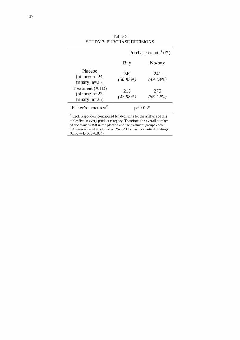
47
Table 3
STUDY 2: PURCHASE DECISIONS
Purchase countsa (%)
Buy No-buy
Placebo (binary: n=24, trinary: n=25)
249 (50.82%)
241 (49.18%)
Treatment (ATD) (binary: n=23, trinary: n=26)
215 (42.88%)
275 (56.12%)
Fisher’s exact testb p=0.035 a Each respondent contributed ten decisions for the analysis of this table; five in every product category. Therefore, the overall number of decisions is 490 in the placebo and the treatment groups each. b Alternative analysis based on Yates’ Chi² yields identical findings (Chi²(1)=4.46, p=0.034).
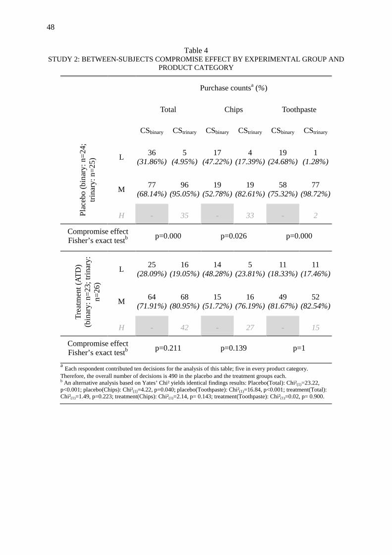
48
Table 4 STUDY 2: BETWEEN-SUBJECTS COMPROMISE EFFECT BY EXPERIMENTAL GROUP AND
PRODUCT CATEGORY
Purchase countsa (%)
Total Chips Toothpaste
CSbinary CStrinary CSbinary CStrinary CSbinary CStrinary
Plac
ebo
(bin
ary:
n=2
4;
trina
ry: n
=25)
L 36 (31.86%)
5 (4.95%)
17 (47.22%)
4 (17.39%)
19 (24.68%)
1 (1.28%)
M 77 (68.14%)
96 (95.05%)
19 (52.78%)
19 (82.61%)
58 (75.32%)
77 (98.72%)
H - 35 - 33 - 2
Compromise effect Fisher’s exact testb p=0.000 p=0.026 p=0.000
Trea
tmen
t (AT
D)
(bin
ary:
n=2
3; tr
inar
y:
n=26
)
L 25 (28.09%)
16 (19.05%)
14 (48.28%)
5 (23.81%)
11 (18.33%)
11 (17.46%)
M 64 (71.91%)
68 (80.95%)
15 (51.72%)
16 (76.19%)
49 (81.67%)
52 (82.54%)
H - 42 - 27 - 15
Compromise effect Fisher’s exact testb p=0.211 p=0.139 p=1
a Each respondent contributed ten decisions for the analysis of this table; five in every product category. Therefore, the overall number of decisions is 490 in the placebo and the treatment groups each. b An alternative analysis based on Yates’ Chi² yields identical findings results: Placebo(Total): Chi²(1)=23.22, p<0.001; placebo(Chips): Chi²(1)=4.22, p=0.040; placebo(Toothpaste): Chi²(1)=16.84, p<0.001; treatment(Total): Chi²(1)=1.49, p=0.223; treatment(Chips): Chi²(1)=2.14, p= 0.143; treatment(Toothpaste): Chi²(1)=0.02, p= 0.900.
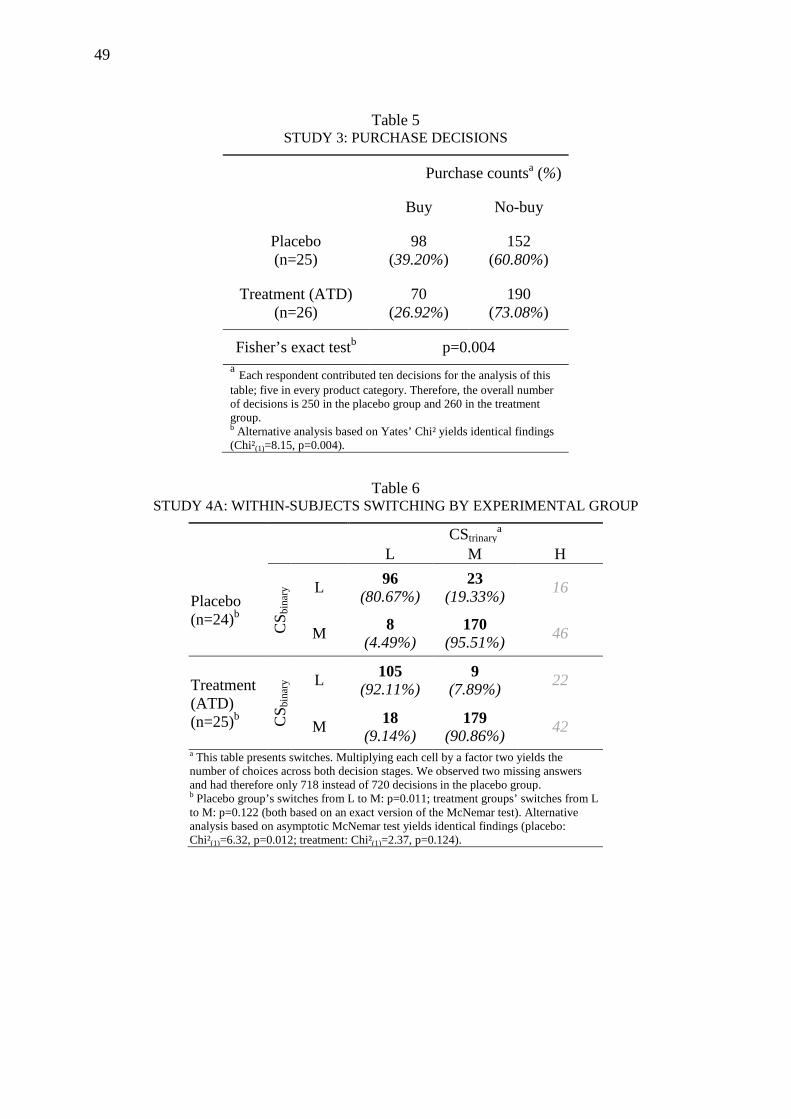
49
Table 5
STUDY 3: PURCHASE DECISIONS
Purchase countsa (%)
Buy No-buy
Placebo (n=25)
98 (39.20%)
152 (60.80%)
Treatment (ATD) (n=26)
70 (26.92%)
190 (73.08%)
Fisher’s exact testb p=0.004 a Each respondent contributed ten decisions for the analysis of this table; five in every product category. Therefore, the overall number of decisions is 250 in the placebo group and 260 in the treatment group. b Alternative analysis based on Yates’ Chi² yields identical findings (Chi²(1)=8.15, p=0.004).
Table 6 STUDY 4A: WITHIN-SUBJECTS SWITCHING BY EXPERIMENTAL GROUP
CStrinary
a L M H
Placebo (n=24)b C
S bin
ary L 96
(80.67%) 23
(19.33%) 16
M 8 (4.49%)
170 (95.51%) 46
Treatment (ATD) (n=25)b C
S bin
ary L 105
(92.11%) 9
(7.89%) 22
M 18 (9.14%)
179 (90.86%) 42
a This table presents switches. Multiplying each cell by a factor two yields the number of choices across both decision stages. We observed two missing answers and had therefore only 718 instead of 720 decisions in the placebo group. b Placebo group’s switches from L to M: p=0.011; treatment groups’ switches from L to M: p=0.122 (both based on an exact version of the McNemar test). Alternative analysis based on asymptotic McNemar test yields identical findings (placebo: Chi²(1)=6.32, p=0.012; treatment: Chi²(1)=2.37, p=0.124).
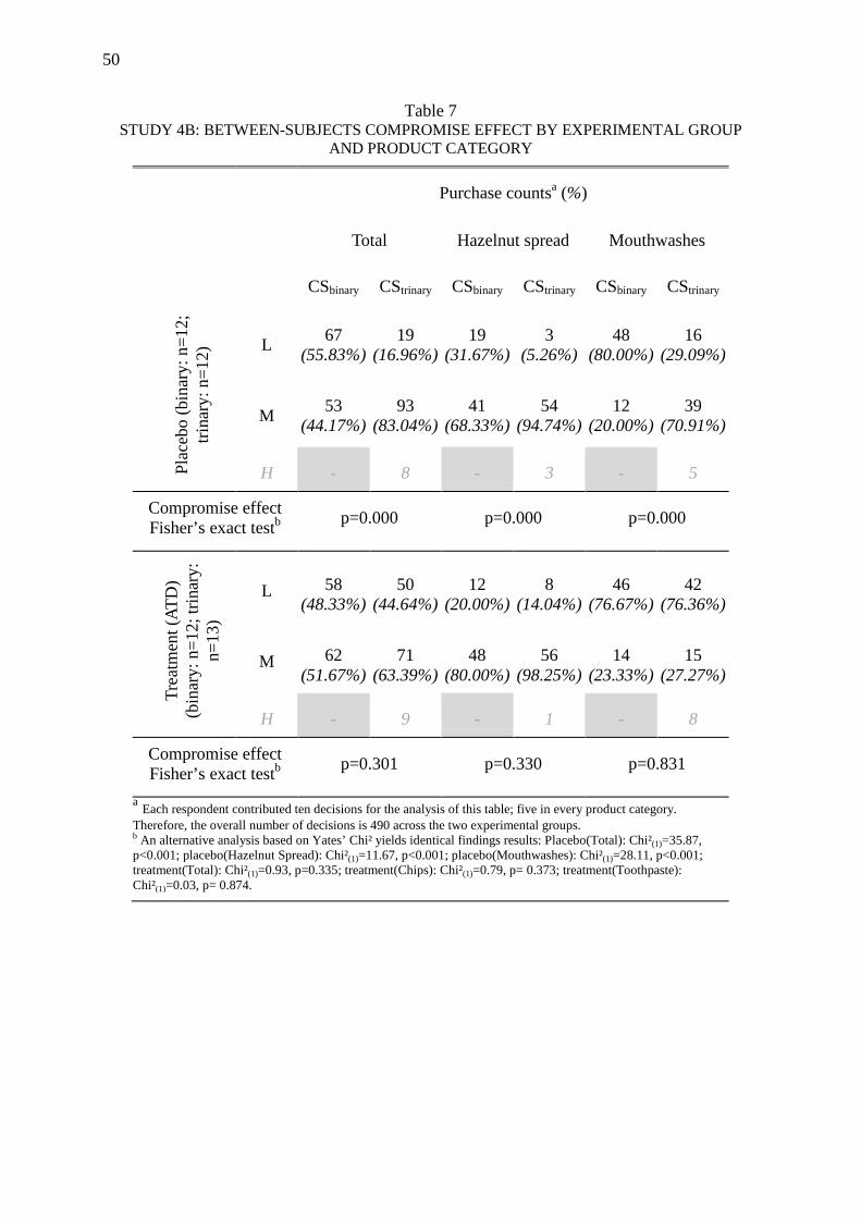
50
Table 7 STUDY 4B: BETWEEN-SUBJECTS COMPROMISE EFFECT BY EXPERIMENTAL GROUP
AND PRODUCT CATEGORY
Purchase countsa (%)
Total Hazelnut spread Mouthwashes
CSbinary CStrinary CSbinary CStrinary CSbinary CStrinary
Plac
ebo
(bin
ary:
n=1
2;
trina
ry: n
=12)
L 67 (55.83%)
19 (16.96%)
19 (31.67%)
3 (5.26%)
48 (80.00%)
16 (29.09%)
M 53 (44.17%)
93 (83.04%)
41 (68.33%)
54 (94.74%)
12 (20.00%)
39 (70.91%)
H - 8 - 3 - 5
Compromise effect Fisher’s exact testb p=0.000 p=0.000 p=0.000
Trea
tmen
t (AT
D)
(bin
ary:
n=1
2; tr
inar
y:
n=13
)
L 58 (48.33%)
50 (44.64%)
12 (20.00%)
8 (14.04%)
46 (76.67%)
42 (76.36%)
M 62 (51.67%)
71 (63.39%)
48 (80.00%)
56 (98.25%)
14 (23.33%)
15 (27.27%)
H - 9 - 1 - 8
Compromise effect Fisher’s exact testb p=0.301 p=0.330 p=0.831
a Each respondent contributed ten decisions for the analysis of this table; five in every product category. Therefore, the overall number of decisions is 490 across the two experimental groups. b An alternative analysis based on Yates’ Chi² yields identical findings results: Placebo(Total): Chi²(1)=35.87, p<0.001; placebo(Hazelnut Spread): Chi²(1)=11.67, p<0.001; placebo(Mouthwashes): Chi²(1)=28.11, p<0.001; treatment(Total): Chi²(1)=0.93, p=0.335; treatment(Chips): Chi²(1)=0.79, p= 0.373; treatment(Toothpaste): Chi²(1)=0.03, p= 0.874.
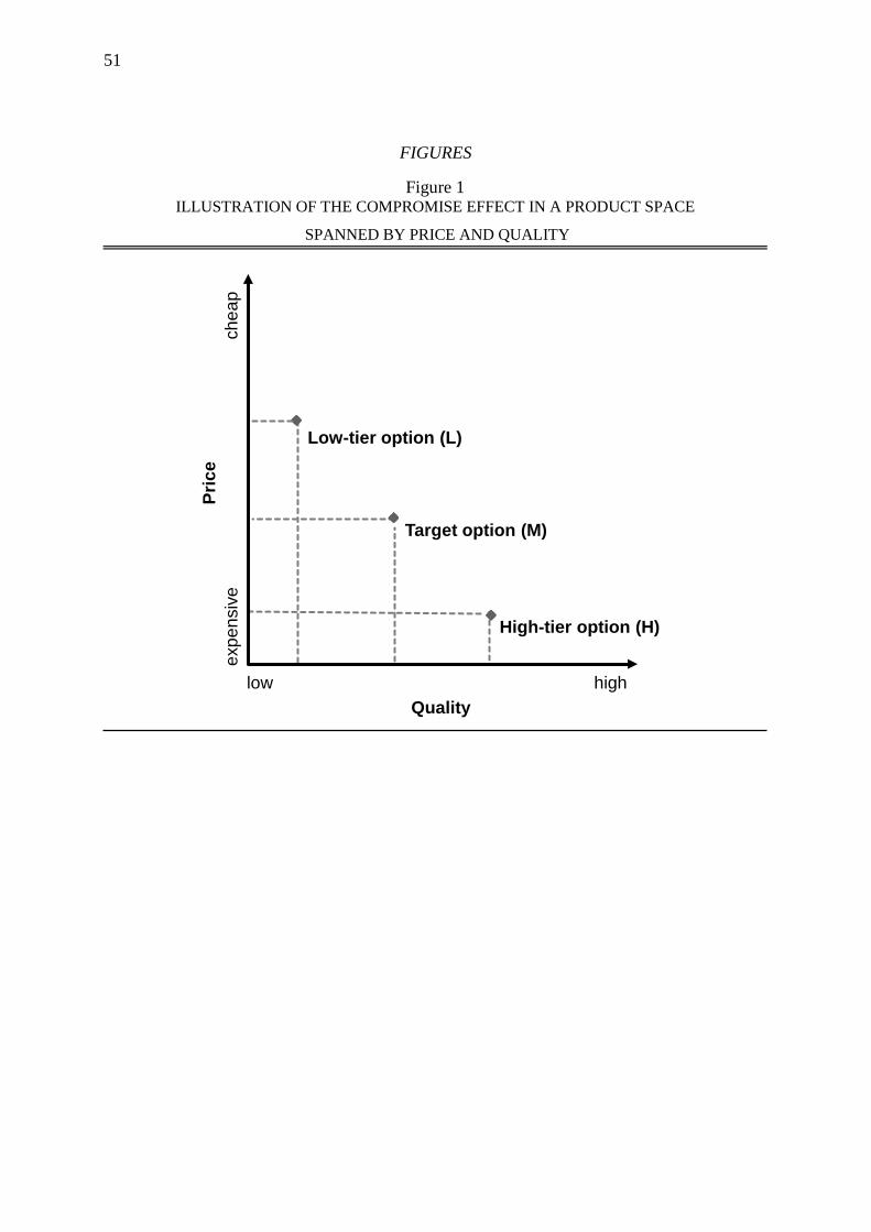
51
FIGURES
High-tier option (H)
Low-tier option (L)
Target option (M)
Quality
Pric
e
highlow
expe
nsiv
ech
eap
Figure 1 ILLUSTRATION OF THE COMPROMISE EFFECT IN A PRODUCT SPACE
SPANNED BY PRICE AND QUALITY
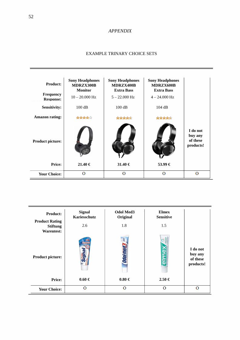
52
I do not buy any of these
products!
Product:
Product RatingStiftung
Warentest:
0.60 € 0.80 € 2.50 €
Product picture:
Price:
Your Choice:
SignalKariesschutz
Odol Med3Original
Elmex Sensitive
2.6 1.8 1.5
APPENDIX
Frequency Response:
Sensitivity:
Amazon rating:
Product picture:
21.40 €Price: 31.40 € 53.99 €
I do not buy any of these
products!
Your Choice:
Sony HeadphonesMDRZX300B
Monitor
10 – 20.000 Hz
100 dB
Product:Sony Headphones
MDRZX400B Extra Bass
5 – 22.000 Hz
100 dB 104 dB
4 – 24.000 Hz
Sony HeadphonesMDRZX600B
Extra Bass
EXAMPLE TRINARY CHOICE SETS
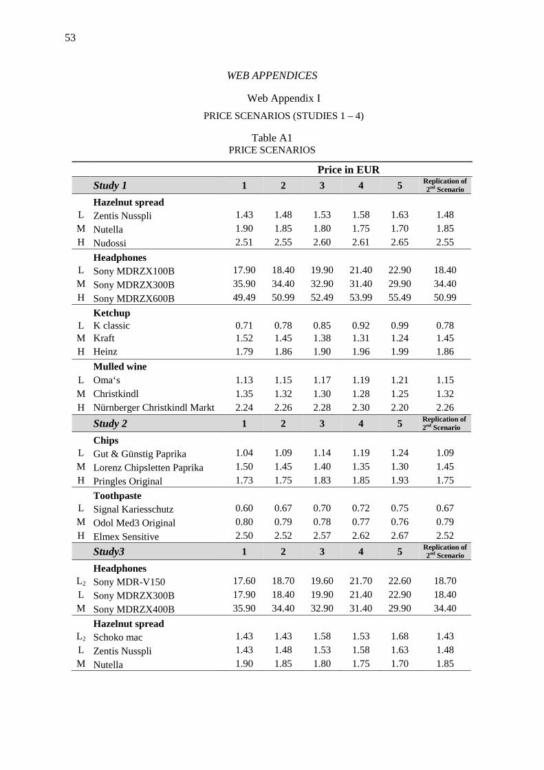
53
WEB APPENDICES
Table A1 PRICE SCENARIOS
Price in EUR Study 1 1 2 3 4 5 Replication of
2nd Scenario Hazelnut spread
L Zentis Nusspli 1.43 1.48 1.53 1.58 1.63 1.48 M Nutella 1.90 1.85 1.80 1.75 1.70 1.85 H Nudossi 2.51 2.55 2.60 2.61 2.65 2.55 Headphones
L Sony MDRZX100B 17.90 18.40 19.90 21.40 22.90 18.40 M Sony MDRZX300B 35.90 34.40 32.90 31.40 29.90 34.40 H Sony MDRZX600B 49.49 50.99 52.49 53.99 55.49 50.99 Ketchup
L K classic 0.71 0.78 0.85 0.92 0.99 0.78 M Kraft 1.52 1.45 1.38 1.31 1.24 1.45 H Heinz 1.79 1.86 1.90 1.96 1.99 1.86 Mulled wine
L Oma‘s 1.13 1.15 1.17 1.19 1.21 1.15 M Christkindl 1.35 1.32 1.30 1.28 1.25 1.32 H Nürnberger Christkindl Markt 2.24 2.26 2.28 2.30 2.20 2.26 Study 2 1 2 3 4 5 Replication of
2nd Scenario Chips
L Gut & Günstig Paprika 1.04 1.09 1.14 1.19 1.24 1.09 M Lorenz Chipsletten Paprika 1.50 1.45 1.40 1.35 1.30 1.45 H Pringles Original 1.73 1.75 1.83 1.85 1.93 1.75 Toothpaste
L Signal Kariesschutz 0.60 0.67 0.70 0.72 0.75 0.67 M Odol Med3 Original 0.80 0.79 0.78 0.77 0.76 0.79 H Elmex Sensitive 2.50 2.52 2.57 2.62 2.67 2.52 Study3 1 2 3 4 5 Replication of
2nd Scenario Headphones
L2 Sony MDR-V150 17.60 18.70 19.60 21.70 22.60 18.70 L Sony MDRZX300B 17.90 18.40 19.90 21.40 22.90 18.40 M Sony MDRZX400B 35.90 34.40 32.90 31.40 29.90 34.40 Hazelnut spread
L2 Schoko mac 1.43 1.43 1.58 1.53 1.68 1.43 L Zentis Nusspli 1.43 1.48 1.53 1.58 1.63 1.48 M Nutella 1.90 1.85 1.80 1.75 1.70 1.85
Web Appendix I PRICE SCENARIOS (STUDIES 1 – 4)
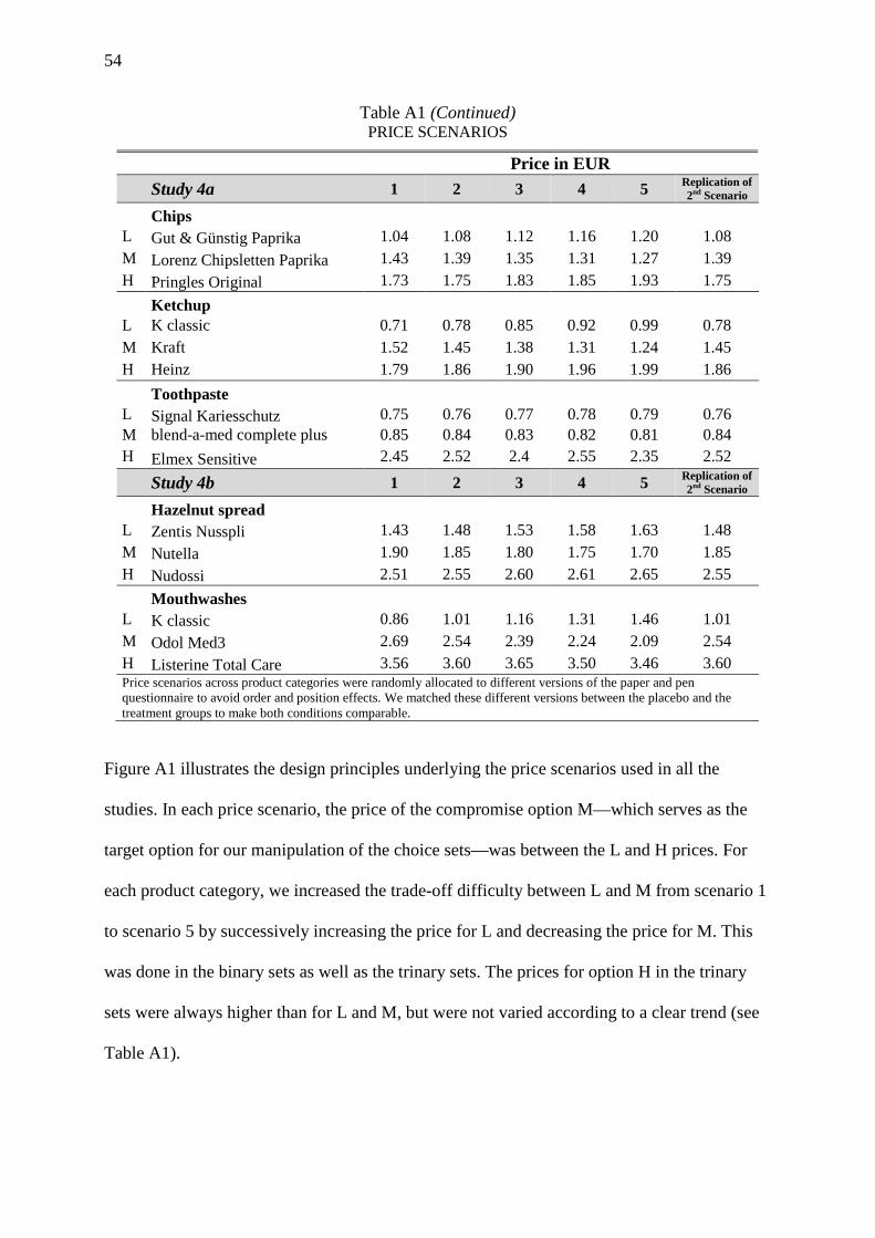
54
Table A1 (Continued) PRICE SCENARIOS
Price in EUR Study 4a 1 2 3 4 5 Replication of
2nd Scenario Chips
L Gut & Günstig Paprika 1.04 1.08 1.12 1.16 1.20 1.08 M Lorenz Chipsletten Paprika 1.43 1.39 1.35 1.31 1.27 1.39 H Pringles Original 1.73 1.75 1.83 1.85 1.93 1.75 Ketchup
L K classic 0.71 0.78 0.85 0.92 0.99 0.78 M Kraft 1.52 1.45 1.38 1.31 1.24 1.45 H Heinz 1.79 1.86 1.90 1.96 1.99 1.86 Toothpaste
L Signal Kariesschutz 0.75 0.76 0.77 0.78 0.79 0.76 M blend-a-med complete plus 0.85 0.84 0.83 0.82 0.81 0.84 H Elmex Sensitive 2.45 2.52 2.4 2.55 2.35 2.52 Study 4b 1 2 3 4 5 Replication of
2nd Scenario Hazelnut spread
L Zentis Nusspli 1.43 1.48 1.53 1.58 1.63 1.48 M Nutella 1.90 1.85 1.80 1.75 1.70 1.85 H Nudossi 2.51 2.55 2.60 2.61 2.65 2.55 Mouthwashes
L K classic 0.86 1.01 1.16 1.31 1.46 1.01 M Odol Med3 2.69 2.54 2.39 2.24 2.09 2.54 H Listerine Total Care 3.56 3.60 3.65 3.50 3.46 3.60 Price scenarios across product categories were randomly allocated to different versions of the paper and pen questionnaire to avoid order and position effects. We matched these different versions between the placebo and the treatment groups to make both conditions comparable.
Figure A1 illustrates the design principles underlying the price scenarios used in all the
studies. In each price scenario, the price of the compromise option M—which serves as the
target option for our manipulation of the choice sets—was between the L and H prices. For
each product category, we increased the trade-off difficulty between L and M from scenario 1
to scenario 5 by successively increasing the price for L and decreasing the price for M. This
was done in the binary sets as well as the trinary sets. The prices for option H in the trinary
sets were always higher than for L and M, but were not varied according to a clear trend (see
Table A1).
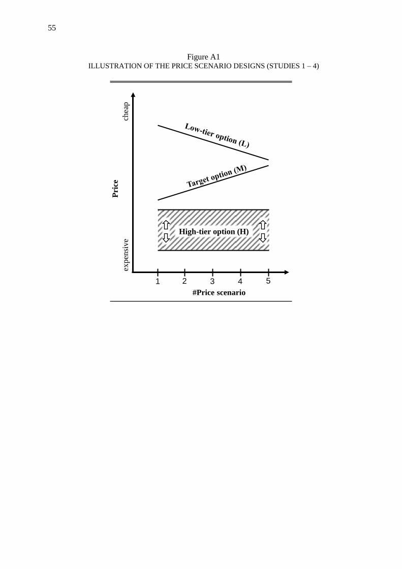
55
#Price scenario
Pric
e
High-tier option (H)
expe
nsiv
ech
eap
1 2 3 4 5
Figure A1 ILLUSTRATION OF THE PRICE SCENARIO DESIGNS (STUDIES 1 – 4)

56
To measure their risk attitude in the financial domain, subjects participated in a lottery choice
task where they were shown a series of lottery pairs (Holt and Laury 2002). Subjects had to
choose between a less risky lottery A (with a small payoff variance but a low initial expected
value) and a risky lottery B (with a greater payoff variance but a high initial expected value).
The lottery pairs included a systematic trade-off between the two lottery types, as the
expected payoff of the less risky lottery A increased, whereas the expected payoff of the risky
lottery B decreased from early to later decisions (Table A2). Accordingly, the subjects started
by choosing lottery B (risky) based on the much higher initial expected value (189 points
compared to 49 points for lottery A) in their first decisions and switched to the (less risky) A
lottery in the later decisions when the expected value of lottery A approached that of lottery B
(Holt and Laury 2002). The point where a subject switched from the risky lottery B to the less
risky lottery A is a measure of his risk attitude: a risk-neutral individual is expected to solely
base his decision on the expected payoffs of the two lotteries and is therefore assumed to
switch from B to A exactly when the expected value of lottery A exceeds the expected value
of lottery B. In contrast, a risk-averse decision maker is expected to switch earlier due to the
smaller variance in the decision outcomes inherent in the A lotteries. The later a participant
switches from the risky lottery B to the less risky lottery A, the less risk-averse this participant
is. Incentive compatibility of the procedure was ensured by randomly drawing one of the
participant’s lottery decisions to become payoff relevant.
Web Appendix II LOTTERY PROCEDURE – RISK ASSESSMENT IN THE FINANCIAL DOMAIN
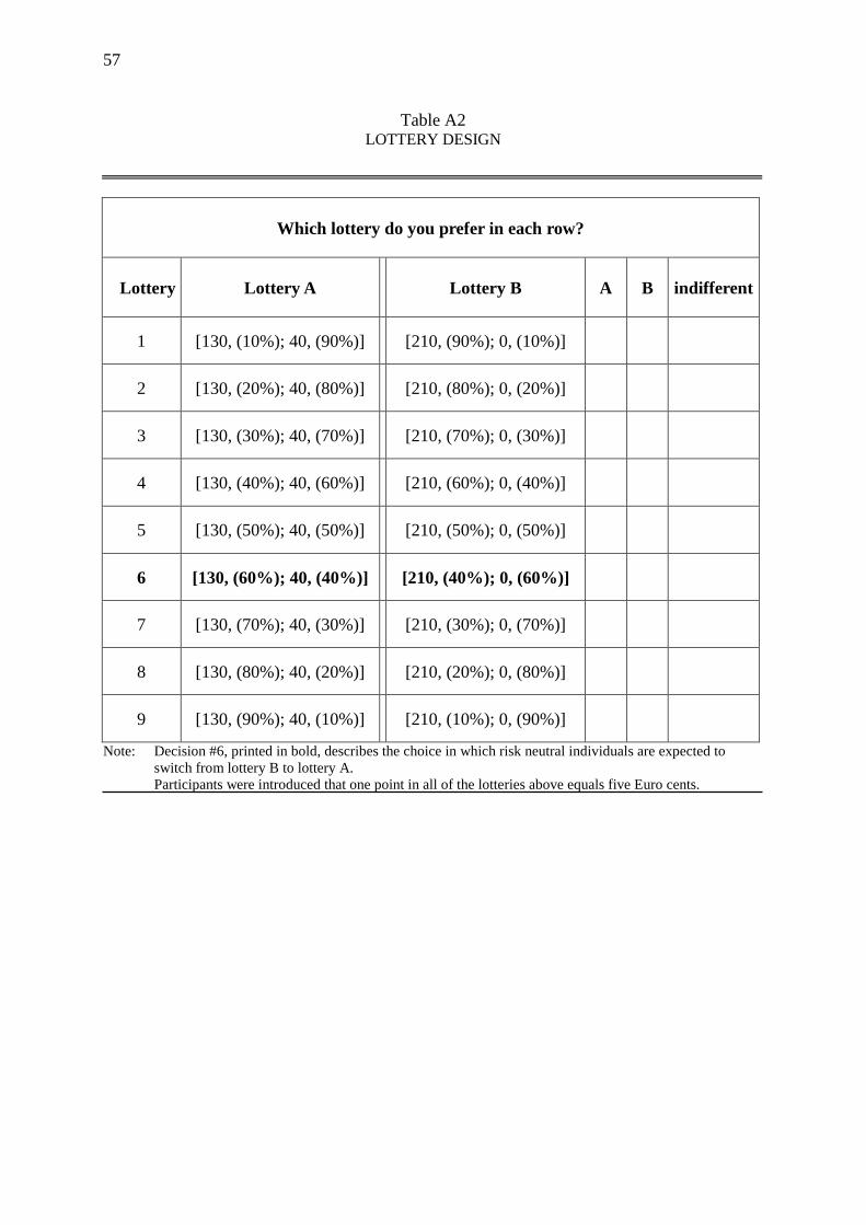
57
Table A2 LOTTERY DESIGN
Which lottery do you prefer in each row?
Lottery Lottery A Lottery B A B indifferent
1 [130, (10%); 40, (90%)] [210, (90%); 0, (10%)]
2 [130, (20%); 40, (80%)] [210, (80%); 0, (20%)]
3 [130, (30%); 40, (70%)] [210, (70%); 0, (30%)]
4 [130, (40%); 40, (60%)] [210, (60%); 0, (40%)]
5 [130, (50%); 40, (50%)] [210, (50%); 0, (50%)]
6 [130, (60%); 40, (40%)] [210, (40%); 0, (60%)]
7 [130, (70%); 40, (30%)] [210, (30%); 0, (70%)]
8 [130, (80%); 40, (20%)] [210, (20%); 0, (80%)]
9 [130, (90%); 40, (10%)] [210, (10%); 0, (90%)]
Note: Decision #6, printed in bold, describes the choice in which risk neutral individuals are expected to switch from lottery B to lottery A. Participants were introduced that one point in all of the lotteries above equals five Euro cents.

58
In study 1, we found no significant differences between subjects in the treatment and the
placebo group in terms of age in years (MTreatment=19.91, SDTreatment=2.19 vs. MPlacebo=19.88,
SDPlacebo=1.26; t(45)=0.07, p=0.942), height in cm (MTreatment=182.30, SDTreatment=7.13 vs.
MPlacebo=181.00, SDPlacebo=7.18; t(45)=0.63, p=0.535), weight in kg (MTreatment=77.70,
SDTreatment=9.77 vs. MPlacebo=73.58, SDPlacebo=8.89; t(45)=1.51, p=0.138), and monthly net
income in EUR (MTreatment=433.18, SDTreatment=288.48 vs. MPlacebo=486.43, SDPlacebo=259.95;
t(43)=-0.65, p=0.518). Following Fern and Monroe (1996), we also compared subjects’ quality
(versus price) orientation across all product categories, and subjects’ aided brand awareness of
all products, but found no significant differences. Subjects do not differ in terms of quality
(versus price) orientation for hazelnut spread (MTreatment=3.05, SDTreatment=0.59 vs.
MPlacebo=3.05, SDPlacebo=0.90; t(Welch, 36.43)=0.09, p=0.993), headphones (MTreatment=3.00,
SDTreatment=0.54 vs. MPlacebo=3.10, SDPlacebo=0.79; t(Welch, 32.74)=-0.45, p=0.658), ketchup
(MTreatment=2.50, SDTreatment=0.80 vs. MPlacebo=2.67, SDPlacebo=1.01;
t(44)=-0.62, p=0.540), and mulled wine (MTreatment=2.75, SDTreatment=0.86 vs. MPlacebo=2.44,
SDPlacebo=0.86; t(32)=1.04, p=0.307). Likewise, subjects do not differ in aided brand awareness
as indicated by a series of Fisher’s exact tests for hazelnut spread (p=1), headphones
(p=0.609), ketchup (p=1.000), and mulled wine (p=0.898).
We tested whether ATD affected subjects’ mood, which, in turn, could have an effect
on their buying behavior (Gardner 1985; Strack, Werth’, and Deutsch 2006). We first
analyzed the MDMQ dimensions’ internal consistency reliabilities, which yielded satisfactory
values between 0.78 (calmness) and 0.94 (wakefulness). Evaluation of the construct
measures’ convergent validity yielded average variance extracted values of between 0.47
(wakefulness) and 0.71 (calmness). Furthermore, discriminant validity was established as all
three dimensions shared more variance with their associated items than with the other two
Web Appendix III PRE-ANALYSIS OF STUDIES 1 – 4

59
constructs (Fornell and Larcker 1981). Next, we compared the MDMQ scores within the
subjects (pre- versus post-treatment exposure) and between the two groups. To test for
differences, we established mixed-effect general linear models, using a separate model for
each of the three MDMQ dimensions.
We defined the pleasantness scores of the pre- and post-exposure as a within-subjects
factor and the experimental condition (treatment vs. placebo) as a between-subjects factor.
We built analogous models for the wakefulness and calmness dimensions. The results
revealed no significant differences between the treatment and placebo groups (pleasantness:
F(1;44)≈0.12, p=0.735; wakefulness: F(1;44)≈1.05, p=0.312; calmness: F(1;42)≈0.29, p=0.595).
Similarly, there were no significant differences between pre- and post-exposure (within) in the
pleasantness (F(1;44)≈0.17, p=0.682) and wakefulness (F(1;44)≈2.08, p=0.156) dimensions, and
only a slight significance at the 10 percent level in the calmness (F(1;42)≈3.48, p=0.069)
dimension. Finally, we found no significant differences in the change of mood dimensions
between the treatment and the placebo groups as measured by the treatment x (pre- vs. post)
MDMQ dimensions (pleasantness: F(1;44)≈0.52, p=0.475; wakefulness: F(1;44)≈1.61, p=0.211;
calmness: F(1;42)≈1.15, p=0.290). Additionally, the results did not reveal any significant
differences in the general risk attitudes between the treatment and placebo groups as measured by
the risk-attitude scale (MTreatment = 6.04, SDTreatment = 1.87 vs. MPlacebo = 6.25, SDPlacebo = 1.45; t(45)
= -0.42; p = 0.674). Congruently, we found no significant differences in financial risk taking
(Mann-Whitney-U = 247.5; p = 0.539). The median switching point from the more risky lottery B
to the less risky lottery A was earlier than expected for risk-neutral individuals in both groups,
indicating risk-averse subjects (Web Appendix II). In sum, ATD did not have an influence on
subjects’ mood or risk attitude / risk taking behavior.
The pre-analysis in study 2 was analogous to that in study 1. In terms of age in years
(MTreatment=21.51, SDTreatment=2.37 vs. MPlacebo=20.94, SDPlacebo=1.63; t(84.92-Welch)=-1.391
p=0.168), height in cm (MTreatment=182.18, SDTreatment=7.09 vs. MPlacebo=181.94,

60
SDPlacebo=6.86; t(96)=-0.174, p=0.862), weight in kg (MTreatment=80.88, SDTreatment=12.11 vs.
MPlacebo=79.29, SDPlacebo=13.46; t(96)=-0.615, p=0.540), monthly net income in EUR
(MTreatment=446.15, SDTreatment=251.11 vs. MPlacebo=506.31, SDPlacebo=244.94; t(94)=1.19,
p=0.238) or general risk attitude (MTreatment=5.80, SDTreatment=2,02 vs. MPlacebo=5.80,
SDPlacebo=1.72; t(96)=0.00, p=1), we again did not find any significant differences between the
treatment and placebo groups. Furthermore, we found no significant differences in quality vs.
price orientation for chips (MTreatment=2.55, SDTreatment=0.79 vs. MPlacebo=2.52, SDPlacebo=0.90;
t(95)=-0.18, p=0.861) and toothpaste (MTreatment=2.71, SDTreatment=0.58 vs. MPlacebo=2.73,
SDPlacebo=0.64; t(95)=0.12, p=0.905) as well as aided brand awareness (chips p=0.987;
toothpaste p=0.963).
In study 3, we again found no significant differences between the subjects in the
treatment and placebo groups in terms of height in cm (MTreatment=182.08, SDTreatment=7.19 vs.
MPlacebo=182.84, SDPlacebo=6.57;t(49)=0.40, p=0.694), weight in kg (MTreatment=83.85,
SDTreatment=13.33 vs. MPlacebo=84.84, SDPlacebo=14.79; t(49)=0.25, p=0.802), or monthly net
income in EUR (MTreatment=457.69, SDTreatment=221.64 vs. MPlacebo=524.20, SDPlacebo=234.70;
t(49)=-0.65, p=0.518). Participants in the treatment group were slightly older (MTreatment=22.54,
SDTreatment=1.88 vs. MPlacebo=21.60, SDPlacebo=1.68; t(49)=-1.88, p=0.067) but we judge this
small difference (less than one year) as negligible. We found no significant differences with
respect to the consumer-related variables quality orientation versus price orientation for
hazelnut spread (MTreatment=3.00, SDTreatment=0.93 vs. MPlacebo=3.00, SDPlacebo=0.75; t(48)=0,
p=1), and for headphones (MTreatment=2.83, SDTreatment=1.01 vs. MPlacebo=3.18, SDPlacebo=0.73;
t(44)=1.331, p=0.190) as well as aided brand awareness for all the products (hazelnut spread
p=0.982; headphones p=0.490). Finally, we found no differences in the general risk attitudes
scale (MTreatment=5.58, SDTreatment=2.16 vs. MPlacebo=5.36, SDPlacebo=1.87; t(49)=-0.38, p=0.703).
Also in study 4, we did not detect any significant differences between the subjects in
the treatment and placebo groups in terms of height in cm (MTreatment=181.08, SDTreatment=6.40
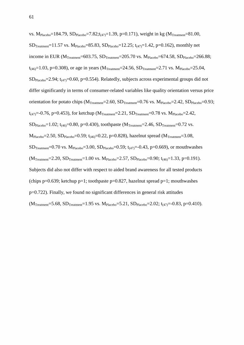
61
vs. MPlacebo=184.79, SDPlacebo=7.82;t(47)=1.39, p=0.171), weight in kg (MTreatment=81.00,
SDTreatment=11.57 vs. MPlacebo=85.83, SDPlacebo=12.25; t(47)=1.42, p=0.162), monthly net
income in EUR (MTreatment=603.75, SDTreatment=205.70 vs. MPlacebo=674.58, SDPlacebo=266.88;
t(46)=1.03, p=0.308), or age in years (MTreatment=24.56, SDTreatment=2.71 vs. MPlacebo=25.04,
SDPlacebo=2.94; t(47)=0.60, p=0.554). Relatedly, subjects across experimental groups did not
differ significantly in terms of consumer-related variables like quality orientation versus price
orientation for potato chips (MTreatment=2.60, SDTreatment=0.76 vs. MPlacebo=2.42, SDPlacebo=0.93;
t(47)=-0.76, p=0.453), for ketchup (MTreatment=2.21, SDTreatment=0.78 vs. MPlacebo=2.42,
SDPlacebo=1.02; t(46)=0.80, p=0.430), toothpaste (MTreatment=2.46, SDTreatment=0.72 vs.
MPlacebo=2.50, SDPlacebo=0.59; t(46)=0.22, p=0.828), hazelnut spread (MTreatment=3.08,
SDTreatment=0.70 vs. MPlacebo=3.00, SDPlacebo=0.59; t(47)=-0.43, p=0.669), or mouthwashes
(MTreatment=2.20, SDTreatment=1.00 vs. MPlacebo=2.57, SDPlacebo=0.90; t(46)=1.33, p=0.191).
Subjects did also not differ with respect to aided brand awareness for all tested products
(chips p=0.639; ketchup p=1; toothpaste p=0.827, hazelnut spread p=1; mouthwashes
p=0.722). Finally, we found no significant differences in general risk attitudes
(MTreatment=5.68, SDTreatment=1.95 vs. MPlacebo=5.21, SDPlacebo=2.02; t(47)=-0.83, p=0.410).

62
Table A3 STUDY 1: OBSERVED CHOICES (WITHIN-SUBJECTS DESIGN)
Purchase countsa (%)
Total Hazelnut spread Headphones Ketchup Mulled Wine
CSbinary CStrinary CSbinary CStrinary CSbinary CStrinary CSbinary CStrinary CSbinary CStrinary
Plac
ebo
(n=2
4)
L 58 (38.16)
56 (30.94)
12 (24.49)
10 (18.87)
15 (42.86)
12 (36.36)
27 (69.23)
32 (55.17)
4 (13.79)
2 (5.41)
M 94 (61.84)
95 (52.49)
37 (75.51)
39 (73.58)
20 (57.14)
16 (48.48)
12 (30.77)
14 (24.14)
25 (86.21)
26 (70.27)
H - 30 (16.57) - 4
(7.55) - 5 (15.15) - 12
(20.69) - 9 (24.32)
Buy 152 (31.67)
181 (37.71)
49 (40.83)
53 (44.17)
35 (29.17)
33 (27.50)
39 (32.50)
58 (48.33)
29 (24.17)
37 (30.83)
No-Buy
328 (68.33)
299 (62.29)
71 (59.17)
67 (55.83)
85 (70.83)
87 (72.50)
81 (67.50)
62 (51.67)
91 (75.83)
83 (69.17)
Trea
tmen
t (A
TD) (
n=23
)
L 33 (34.74)
39 (41.94)
3 (14.29)
6 (27.27)
12 (40.00)
13 (54.17)
18 (90.00)
19 (90.48)
0 (0)
1 (3.85)
M 62 (65.26)
53 (56.99)
18 (85.71)
16 (72.73)
18 (60.00)
11 (45.83)
2 (10.00)
1 (4.76)
24 (100)
25 (96.15)
H - 1 (1.08) - 0
(0) - 0 (0) - 1
(4.76) - 0 (0)
Buy 95 (20.65)
93 (20.22)
21 (18.26)
22 (19.13)
30 (26.09)
24 (20.87)
20 (17.39)
21 (18.26)
24 (20.87)
26 (22.61)
No-Buy
365 (79.35)
367 (79.78)
94 (81.74)
93 (80.87)
85 (73.91)
91 (79.13)
95 (82.61)
94 (81.74)
91 (79.13)
89 (77.39)
a Each respondent contributed 40 decisions for the analysis of this table, ten in every product category (five in the binary stage and five in the trinary stage).
Web Appendix IV
COMPLETE CHOICE DATA (STUDIES 1 – 4)
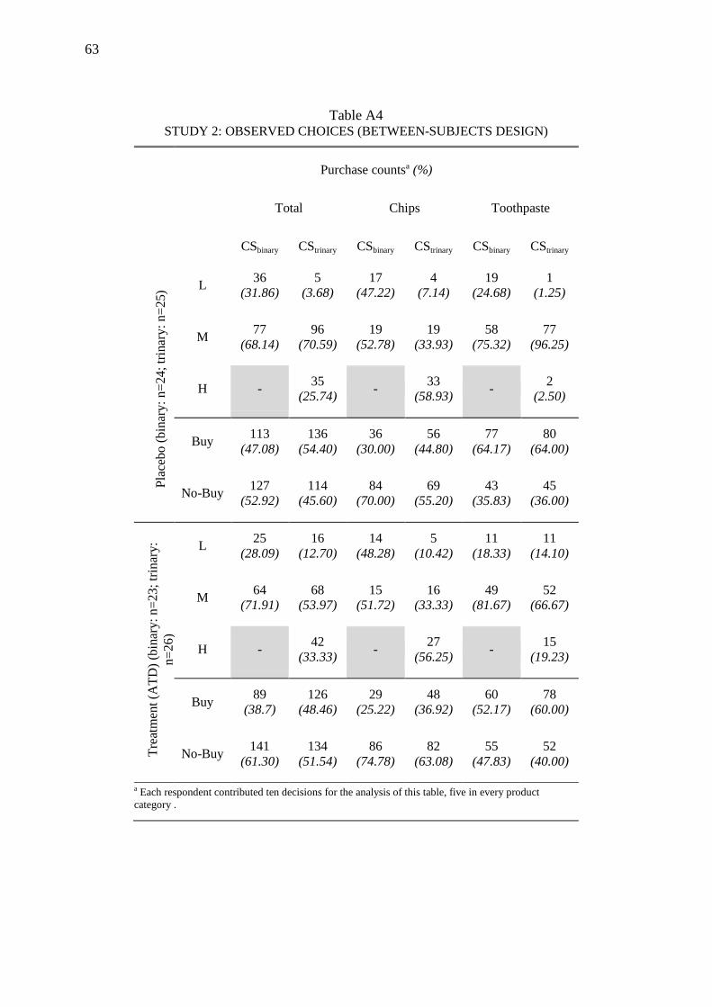
63
Table A4
STUDY 2: OBSERVED CHOICES (BETWEEN-SUBJECTS DESIGN)
Purchase countsa (%)
Total Chips Toothpaste
CSbinary CStrinary CSbinary CStrinary CSbinary CStrinary
Plac
ebo
(bin
ary:
n=2
4; tr
inar
y: n
=25)
L 36 (31.86)
5 (3.68)
17 (47.22)
4 (7.14)
19 (24.68)
1 (1.25)
M 77 (68.14)
96 (70.59)
19 (52.78)
19 (33.93)
58 (75.32)
77 (96.25)
H - 35 (25.74) - 33
(58.93) - 2 (2.50)
Buy 113 (47.08)
136 (54.40)
36 (30.00)
56 (44.80)
77 (64.17)
80 (64.00)
No-Buy 127 (52.92)
114 (45.60)
84 (70.00)
69 (55.20)
43 (35.83)
45 (36.00)
Trea
tmen
t (A
TD) (
bina
ry: n
=23;
trin
ary:
n=
26)
L 25 (28.09)
16 (12.70)
14 (48.28)
5 (10.42)
11 (18.33)
11 (14.10)
M 64 (71.91)
68 (53.97)
15 (51.72)
16 (33.33)
49 (81.67)
52 (66.67)
H - 42 (33.33) - 27
(56.25) - 15 (19.23)
Buy 89 (38.7)
126 (48.46)
29 (25.22)
48 (36.92)
60 (52.17)
78 (60.00)
No-Buy 141 (61.30)
134 (51.54)
86 (74.78)
82 (63.08)
55 (47.83)
52 (40.00)
a Each respondent contributed ten decisions for the analysis of this table, five in every product category .

64
Table A5
STUDY 3: OBSERVED CHOICES (BETWEEN-SUBJECTS DESIGN)
Purchase counts (%)
Total Hazelnut spread Headphones
Placebo (n=25)
Treatment (ATD) (n=26)
Placebo (n=25)
Treatment (ATD) (n=26)
Placebo (n=25)
Treatment (ATD) (n=26)
L2 14
(14.29) 21
(30.00) 7
(10.77) 20
(40.00) 7
(21.21) 1
(5.00)
L 36 (36.73)
6 (8.57)
20 (30.77)
3 (6.00)
16 (48.48)
3 (15.00)
M 48 (48.98)
43 (61.43)
38 (58.46)
27 (54.00)
10 (30.30)
16 (80.00)
Buy 98 (39.20)
70 (26.92)
65 (52.00)
50 (38.46)
33 (26.40)
20 (15.38)
No-Buy
152 (60.80)
190 (73.08)
60 (48.00)
80 (61.54)
92 (73.60)
110 (84.62)
a Each respondent contributed ten decisions for the analysis of this table, five in every product category.
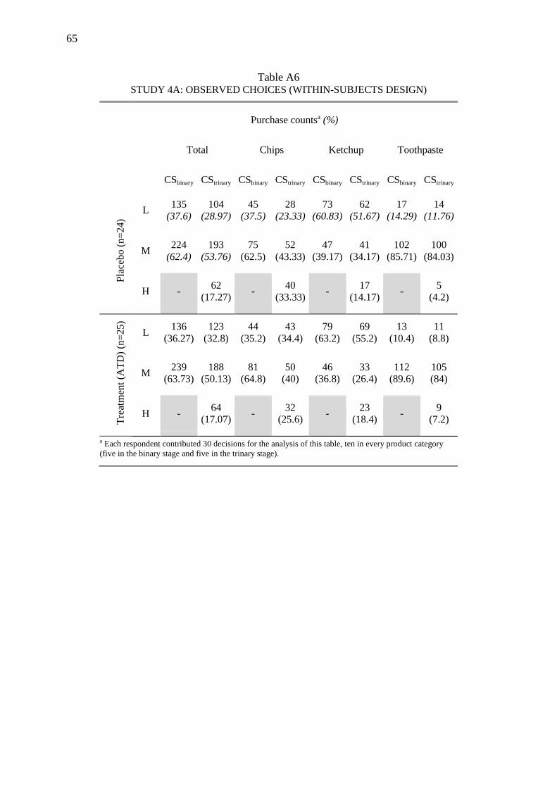
65
Table A6 STUDY 4A: OBSERVED CHOICES (WITHIN-SUBJECTS DESIGN)
Purchase countsa (%)
Total Chips Ketchup Toothpaste
CSbinary CStrinary CSbinary CStrinary CSbinary CStrinary CSbinary CStrinary
Plac
ebo
(n=2
4) L 135
(37.6) 104
(28.97) 45
(37.5) 28
(23.33) 73
(60.83) 62
(51.67) 17
(14.29) 14
(11.76)
M 224 (62.4)
193 (53.76)
75 (62.5)
52 (43.33)
47 (39.17)
41 (34.17)
102 (85.71)
100 (84.03)
H - 62 (17.27) - 40
(33.33) - 17 (14.17) - 5
(4.2)
Trea
tmen
t (A
TD) (
n=25
)
L 136 (36.27)
123 (32.8)
44 (35.2)
43 (34.4)
79 (63.2)
69 (55.2)
13 (10.4)
11 (8.8)
M 239 (63.73)
188 (50.13)
81 (64.8)
50 (40)
46 (36.8)
33 (26.4)
112 (89.6)
105 (84)
H - 64 (17.07) - 32
(25.6) - 23 (18.4) - 9
(7.2)
a Each respondent contributed 30 decisions for the analysis of this table, ten in every product category (five in the binary stage and five in the trinary stage).
66
Web Appendix V
ADDITIONAL ANALYSES (STUDIES 1 – 4) Analysis of Choice Deferral
To account for the multiple observations per respondent with regard to our hypothesis about
choice deferral in studies 1–3, we estimated mixed-effect logit models using a dependent
binary decision variable (1=buy, 0=no buy). The models accounted for the data’s nested
multilevel structure by including a respondent-specific random intercept together with a
nested product group-specific random effect intercept. The independent fixed effect predictor
was coded 1 if a subject belongs to the placebo group and 0 if belonging to the treatment
group. In accordance with our directional hypothesis, we expected the treatment’s coefficient
to be positive and significant, indicating that the subjects in the placebo group are less likely
to defer product decisions. Our analyses show that this holds for study 1 results (ß = 2.57,
one-sided p = 0.040), for study 2 results (ß=1.12, one-sided p<0.001), as well as study 3
results (ß=2.15, one-sided p=0.044).
Analysis of the Compromise Effect
For the within-subjects designs (studies 1 and 4a) we conducted a further robustness check to
account for multiple decisions per respondent. We averaged all the switching patterns of each
respondent, giving us the relative frequencies of a participant’s switches from L to M after
adding H. This measure of the within-subjects compromise effect ranges from 0 (if a
participant did not switch at all) to 1 (if switching was observed in all decision instances).
Next, we evaluated if the mean tendency to switch from L to M is significantly different from
zero. Our analysis of study 1 data reveals that this is the case for the placebo group (mean
difference = 0.017 (SD = 0.043), t(23) = 1.881; p = 0.037), but not for the treatment group
(mean difference = 0.000, (SD = 0.000) t(22) = 0; p = 1.000). The difference between both

67
experimental groups is also significant (t(23-Welch) = -1.881; p = 0.037). Our analogous, analysis
of study 4a reveals that the mean tendency to switch from L to M is significantly different
from zero for the placebo group (mean difference = 0.064 (SD = 0.080), t(23) = 3.922; p =
0.001) and also for the treatment group (mean difference = 0.024, (SD = 0.047) t(24) = 2.571; p
= 0.017). Consistent with our hypotheses, the within-subjects compromise effect is
significantly more pronounced in the placebo group compared to the treatment group (t(47) =
2.146; p = 0.037).
As a further robustness check of studies 2 and 4b results, we used a similar approach
as for studies 1 and 4a, but accounted for the fact that it was not possible to aggregate
switches in a between-subjects design setting. Therefore, we averaged the M and L decisions
of every respondent, which yielded the respondent-specific rates for choosing L and M. Next,
we computed a respondent-specific index for the attractiveness of M over L by subtracting the
L options’ rate from the M options’ rate. This measure is negative if a respondent—on
average—prefers L to M, and positive if M is more often preferred to L. In accordance with
our hypotheses, we found that option M was significantly more attractive in the trinary sets
than in the binary sets in the placebo group in study 2 (MeanTrinary = 0.36 (0.31) vs. MeanBinary
= 0.17 (0.44), t(47) = -1.76, p = 0.042), whereas this is not the case in the treatment group
(MeanTrinary = 0.20 (0.28) vs. MeanBinary = 0.17 (0.37), t(47) = -0.32, p = 0.374). The same result
holds for an equivalent analysis of the data of study 4b (placebo group: MeanTrinary = 0.62
(0.42) vs. MeanBinary = -0.12 (0.56), t(22) = -3.64, p = 0.001; treatment group: MeanTrinary =
0.16 (0.45) vs. MeanBinary = 0.03 (0.14), t(14.60) = -0.98, p = 0.346).
Analysis of Order Effects.
We also tested for order effects in subjects’ decisions from the earlier to the later price
scenarios as described in Web Appendix I. For this purpose, we analyzed the development of
the choice shares of the compromise option M as well as the no-buy option. As expected, we

68
observe higher choice shares for the target option M in later scenarios as M becomes cheaper
over time. This trend applies to both, binary and trinary sets and, therefore, does not cofound
the results interpretation. Beyond this trend, our analyses did not indicate any systematic
effects across the different price scenarios and studies regarding subjects’ choices of the
compromise option or the no-buy option. Likewise, we found no interaction of potential order
effects with the ATD treatment.
Related Documents