Adverse Selection as a Policy Instrument: Unraveling ...

Adverse Selection as a Policy Instrument:

Unraveling Climate Change∗

Steve Cicala

Tufts University

David Hemous

University of Zurich

Morten Olsen

University of Copenhagen

Click here for the latest version.

December 3, 2021

Abstract

This paper applies principles of adverse selection to overcome obstacles that prevent theimplementation of Pigouvian policies to internalize externalities. Focusing on negative exter-nalities from production (such as pollution), we evaluate settings in which aggregate emissionsare known, but individual contributions are unobserved by the government. We propose givingfirms the option to pay a tax on their voluntarily and verifiably disclosed emissions, or pay anoutput tax based on the average rate of emissions among the undisclosed firms. The certifica-tion of relatively clean firms raises the output-based tax, setting off a process of unraveling infavor of disclosure. We derive sufficient statistics formulas to calculate the welfare of such aprogram relative to mandatory output or emissions taxes. We find that our mechanism woulddeliver significant gains over output-based taxation in two empirical applications: methaneemissions from oil and gas fields, and carbon emissions from imported steel.

∗We are grateful to Thom Covert, Meredith Fowlie, Michael Greenstone, Suzi Kerr, Gib Metcalf, Mark Omara,Mar Reguant, James Sallee, Joseph Shapiro, Andrei Shleifer, Allison Stashko, Bob Topel and seminar participants atTufts, Universitat Bern, the Environmental Defense Fund, UC San Diego, the Midwest EnergyFest, Yale, Harvard,the Utah Winter Business Economics Conference, UC Santa Barbara, UC Berkeley, and the University of Chicagofor helpful comments. Ivan Higuera-Mendieta provided excellent research assistance. Cicala gratefully acknowledgesfunding from the 1896 Energy and Climate Fund at the University of Chicago, and along with Olsen thanks theUniversity of Zurich for hospitality. All errors remain our own. e-mail: [email protected], [email protected],[email protected]

1 Introduction

Uninternalized externalities abound. In spite of the simplicity of economists’ advice when

the magnitude of the harm is known, the obstacles to correcting such market failures are

myriad: political opposition, excessive implementation costs, the presence of havens induced

by competing jurisdictions, among others. In this paper we show the extent to which such

obstacles may be overcome in situations in which damage is caused by heterogenous agents.

We apply results from the literature on mechanism design under asymmetric information as

a policy lever to encourage program participation and voluntary revelation of harm.

We consider situations in which the aggregate level of harm (such as pollution or traffic

congestion) is known by the government, but the exact contributions of specific agents is not.

In such settings it is impossible to levy Pigouvian taxes due to the unobserved sources of

harm. The optimal uniform fee (such as an output tax on producers rather than an emissions

tax) falls short of the first best since the fee does not depend on one’s contribution to the

problem. It also fails to incentivize abatement to reduce damage (Cropper and Oates (1992);

Schmutzler and Goulder (1997); Fullerton et al. (2000); Farrokhi and Lashkaripour (2021)).

We propose creating the option to certify one’s damage, upon which a Pigouvian tax

will be levied, combined with an output-based fee that tracks the average rate of damage

among those choosing not to participate in the certification program.1 This encourages those

who inflict relatively little damage to certify, thus raising the output-based fee paid by non-

participants. This sets off an unraveling in favor of program participation as increasingly

damage-intensive agents seek to separate themselves from the tail of the distribution that

becomes concentrated by adverse selection.

We first develop a closed-economy model in which production is heterogenously associated

with an externality and derive the distance of an optimally-set output tax from the first-best

Pigouvian policy. We approximate with this distance with a sufficient statistics formula that

depends on marginal damages, the slope of the supply curve, variance of emissions, and

monitoring costs. We show how the option to reveal one’s emissions yields welfare objects

that are a linear combination of the outcomes under output and emissions taxes, with weights

equal to the relative variance of emissions under each policy. We also show that, under certain

conditions, the policy maker can achieve the same outcome by only knowing the mean of the

emissions distribution. This is achieved through an algorithm that encourages the gradual

unravelling of the emissions distribution, converging to an equilibrium in which the policy

1This can be calculated because the overall level of harm is observed, and subtracting the contribution ofcertified agents reveals the average contribution among those who remain uncertified.

1

maker has full information on the emissions distribution. We extend the analysis to allow

firms to abate and show that there is a natural complementarity between the two; only

through certification is it worthwhile for firms to abate.

As an empirical application of the closed-economy model, we use our mechanism to

internalize the cost of methane emissions from oil and gas production in the Permian basin

in Texas and New Mexico. The Permian is the source of 30% of U.S. oil production and

10% of natural gas (Administration (2019)). While royalty adders have been proposed to

address the climate externality of embodied carbon in these fuels on federal land (Prest and

Stock (2021)), methane emissions are a thornier problem. Methane is a potent greenhouse

gas that either leaks from the supply chain or is intentionally vented into the atmosphere

in an unmonitored fashion. Alvarez et al. (2018) estimate about 13 million tons of methane

leak from the oil and gas sector annually, for a social cost of about $20B. Nearly 60% of those

emissions occur during production, and in 2018 about 2.7 million metric tons were released

from the Permian basin, for a social cost of $4B (Zhang et al. (2020)). However, emissions

rates across wells are highly heterogeneous (Robertson et al. (2020)). We find that while

a royalty adder levied on production would reduces emissions by about 4%, a tax levied

directly on pollution would reduce emissions by 80%, before abatement. We find that our

sufficient statistics approximations deliver answers that closely follow more data-intensive,

bottom-up calculations. A voluntary emissions tax paired with a rolling output tax would

deliver identical outcomes as a emissions mandatory tax, with about $3B/year in benefits,

even with significant costs of emissions certification. The opt-in policy actually exceeds the

welfare of mandatory taxation as certification costs grow by allowing firms to economize on

the regulatory burden.

We then extend our model to an international setting, focusing on the constraints of

unilateral climate policy. Because greenhouse gases are global pollutants, it is natural that

research on climate policy has focused on international environmental agreements between

sovereign nations who regulate their respective producers.2 Such agreements must overcome

the unilateral incentive to shirk (Barrett (1994)), possibly by punishing countries outside

of the agreement (Nordhaus (2015)). Dynamic considerations also come into play as costly

investments in clean technology create hold-up problems in future negotiations due to their

complementarity with abatement (Beccherle and Tirole (2011); Harstad (2012); Battaglini

and Harstad (2016)). Governments are the key decisionmakers in this paradigm, and only

policies that are individually rational from each country’s perspective are feasible.

2See Chan et al. (2018) for a review.

2

The absence of strong, binding international agreements raises the question of how emis-

sions might be reduced through unilateral policy. The ability of unilateral carbon taxation to

reduce emissions is reduced (and possibly reversed) when production can profitably move to

unregulated jurisdictions, a problem known as ‘leakage’ (Bohm (1993); Copeland and Taylor

(1995); Aldy and Stavins (2012); HA c©mous (2016); Fowlie (2009); Fowlie et al. (2016)).

This prospect strengthens the incentive to shirk on international commitments by simulta-

neously reducing the effectiveness of the tax and increasing the benefits of becoming a haven.

Trade policy in the form of a “Border Carbon Adjustment” (BCA) has been considered the

primary instrument to mitigate the competitive disadvantage caused by taxing one’s own

emissions (Copeland (1996); Metcalf and Weisbach (2009); Elliott et al. (2010, 2013); Larch

and Wanner (2017), see Condon and Ignaciuk (2013) for a literature review). BCAs levy

tariffs based on the average carbon content of production in the country of origin so that

foreign producers (on average) cannot undercut domestic firms. Under such a policy foreign

producers remain effectively outside the reach of the government, as their tax burden is unre-

lated to firm-specific emissions. They face no individual incentives to abate their emissions,

and any pollution reductions depend on price elasticities of demand and supply.3

The goal of our approach in the international setting is to approximate the emissions

reductions that might be achieved with a widely-adopted price on carbon, but without re-

quiring the legally-binding international agreements that have proven elusive to date. To do

so, we focus on the direct interactions between a government and firms whose disclosures of

emissions are voluntary. International sovereignty may restrict what governments can man-

date of foreign firms, but does not foreclose the possibility of creating incentives to shape

their behavior. We do this by providing firms with the option to certify their emissions, and

basing the default rate on the average emissions of uncertified firms. This recasts the problem

of jurisdiction into one of screening, in which clean firms wish to separate themselves from

more intensive polluters (Spence (1973); Stiglitz (1975)). This separation causes the uncer-

tified mean to rise, setting off a process of unraveling that encourages further certification

(Akerlof (1970)).

We show the conditions under which the unraveling mechanism is preferable to a unilat-

eral domestic carbon tax, or a tax combined with a BCA. As an empirical application, we

consider the case of international trade in steel, an energy-intensive, trade-exposed sector

3Markusen (1975) and Hoel (1996) derive the optimal tariff in the presence of transboundary pollution.As highlighted by Keen and Kotsogiannis (2014) and Balistreri, Kaffine and Yonezawa (2019), an optimalenvironmental tariff generally differs from the BCA formula (even if a BCA were able to distinguish betweenthe carbon contents of different imports and even in the absence of terms of trade effects).

3

that is central to environmental trade policy (Miller and Boak (2021)). We consider trade

policy between the OECD and Brazil, a major steel exporter. Using the sufficient statis-

tics formulas we develop, we estimate that an optimally-implemented certification program

would achieve nearly 75% of the welfare gains of a universal carbon tax. However, we also

find that unrestricted access to such a program would create significant ‘backfilling’ wherein

the the dirtiest firms would expand their output to serve the untaxed foreign market. This

reduces the welfare benefits of certification, making the unrestricted program slightly inferior

to a standard border carbon adjustment. This example highlights the countervailing forces

that limit a government’s ability to reduce externalities outside of its jurisdiction, while also

presenting a mechanism to productively expand its reach.

The combination of optional disclosure and a rolling default creates a policy that mimics

the strategy that has been applied in private markets to ensure quality (Jovanovic (1982);

Grossman (1981); Milgrom and Roberts (1986); Milgrom (2008). See Dranove and Jin (2010)

for a review). In these settings firms voluntarily provide warranties or submit to audits in

order to separate themselves from low-quality producers. Even relatively lower-quality firms

become willing to make such disclosures to separate themselves from the absolute worst

offenders when consumers update their beliefs regarding those who decline to disclose (Jin

and Leslie (2003); Jin (2005); Lewis (2011)). It has also been used by firms to improve risk

selection for credit (Einav et al. (2012)), improve safety (Viscusi (1978); Hubbard (2000);

Jin and Vasserman (2019)), and has been suggested to encourage more efficient electricity

consumption (Borenstein (2005, 2013)) and fisheries management (Holzer (2015)). To our

knowledge this is the first paper to apply these principles to overcome obstacles to the

implementation of Pigouvian policies.

The use of screening mechanisms in public policy has been successfully applied to im-

prove the targeting of recipients of public benefits (Alatas et al. (2016); Finkelstein and

Notowidigdo (2019); Deshpande and Li (2019)). In such settings the government creates

hurdles so uptake is limited to those who value benefits more than the ordeal of enrollment.

These policies typically do not entail unraveling as the government is is free to choose the

magnitude of the enrollment ordeal so that the optimal point of separation is achieved im-

mediately (Kleven and Kopczuk (2011); Besley and Coate (1992); Nichols and Zeckhauser

(1982); Nichols et al. (1971)): The costs or benefits of non-participation are not program-

matically adjusted with the extent of participation. In our setting this would be analogous to

the government choosing its preferred carbon content of uncertified imports, which is likely

4

to run afoul of strategic trade considerations.4

There is a long tradition of regulation under asymmetric information in the mechanism

design literature (Baron and Myerson (1982); Laffont and Tirole (1993)). In the pollution

context, the regulator seeks to elicit information on abatement costs (Kwerel (1977); Roberts

and Spence (1976); Dasgupta et al. (1980); Baron (1985); Laffont (1994)) and must design

a policy schedule that elicits truthful revelation. In these settings, as in the context of

non-point source pollution, the lack of verifiability is the key constraint on the regulator

(Segerson (1988); Xepapadeas (1991); Laffont (1994); Xepapadeas (1995), among others.

For a review see Xepapadeas (2011)). While emissions remain unobserved at uncertified

firms, our focus on an optional, verifiable revelation of emissions converts the problem into

a traditional point-source setting in which firms face incentives to abate. Recent work on

voluntary environmental regulation notes the improved enforcement targeting for uncertified

firms, but does not unravel non-participation with changing in audit probabilities (Foster

and Gutierrez (2013, 2016)).

Organizationally, the paper separates the analysis between domestic and international

settings. In each setting we develop a theoretical model, and then apply the results from the

model to an empirical setting. The final section concludes.

2 Unraveling in the Domestic Case

To focus on the central issue of disclosure, we first consider a simplified setting of a closed

economy in which firms differ only in their emission rates. Throughout this section we focus

on a simple partial equilibrium model with an externality, though our approach would also

apply to a broader class of models. The government knows the full distribution of emis-

sions, but not those of individual firms unless they choose to certify. We take as given that

mandatory certification is not possible and characterize the welfare benefits of an optional

certification program.

First, we derive “sufficient statistics” in the sense of approximations to changes in wel-

fare that can be expressed through simple objects such as emissions variances and supply

elasticities. We begin by solving a benchmark model for any level of certification, and then

derive the optimal level of certification. We then weaken the information available to the

regulator and show the program may be implemented knowing only the first moment of the

4At the extreme, the government could simply prohibit imports from firms whose emissions are uncertified.This is not without precedent—the U.S. Food and Drug Administration mandates access for inspectors atfacilities abroad for any firm wishing to sell food or pharmaceuticals in the US (Federal Food, Drug andCosmetic Act, Section 807 (b) as amended by Section 306 of the FDA Food Safety Modernization Act). Thebasis of the jurisdiction problem we address is that such mandates are infeasible with respect to emissions.

5

emissions distribution. We conclude the section with a series of extensions to the benchmark

model: allowing for abatement, heterogeneous productivity, and adjustments that only occur

through entry and exit. These extensions yield minor adjustments to the exact expressions

of the benchmark model, but share a common fundamental structure.

2.1 Baseline model

We consider a closed economy and focus on a specific industry that produces a homogeneous

polluting good under perfect competition. A representative agent has preferences over this

good, represented by the following quasi-linear utility function:

U = C0 + u(C)− vG,

where C is total consumption of the polluting good and C0 is the consumption of an outside

good. The price of the outside good is normalized to 1. G denotes emissions from the

production of good C. The marginal social cost of emissions is v. The outside good does not

pollute.

The polluting good is produced by an (exogenous) mass 1 of firms who operate under

perfect competition. Firms have the same strictly convex cost function c(q) but vary in the

extent to which they pollute. The emissions rate per unit produced is denoted by e and

follows the cdf Ψ(e), with full support and corresponding pdf of ψ(e) > 0, on the domain

[e, e] where e ≥ 0 and e may be infinite. Though the overall distribution of emissions, Ψ,

and the production of each firm is observable, the emissions of an individual firm are private

information (unless the firm is certified as described below).

2.2 Equilibrium with an output tax or emission tax

In the following, we distinguish between a tax on emissions and one on output. First, consider

an output tax, t, which can be implemented even when individual emissions are not observed.

Let the market price be p and solve the firm’s problem in a decentralized equilibrium to get:

p = c′(q) + t. (1)

This defines a supply function q = s(p − t). With a mass 1 of firms this is also total

production, Q. The resulting profit function follows as π(p− t) = (p− t)s(p− t)−c(s(p− t)).The supply curve is upward-sloping by the convexity of the cost function and the profit

function is increasing in p − t. Utility maximization gives: u′(C) = p which together with

Q(p− t) = s(p− t) and C = Q defines an equilibrium price, p, and quantity, Q. Emissions

6

are given by:

G =

∫ e

e

s(p− t)eψ(e)de = s(p− t)E(e) (2)

Next, and in anticipation of the discussion of certification below, we solve for a setup in

which emissions are observable and taxed at τ . This gives an individual supply function of

s(p− τe) and aggregate supply and emissions of:

Q =

∫ e

e

s(p− τe)ψ(e)de = E [s(p− τe)] and G = E [es(p− τe)] (3)

The social planner would set t = vE(e) when emissions are not observed and τ = v when

emissions are observable. In the following, we solve for an equilibrium in which firms can

certify and be taxed based on their individual emissions.

2.3 Equilibrium with certification

We now introduce voluntary certification of emissions, in which a firm can choose between

two tax settings. If the firm chooses to (verifiably) reveal its level of emissions, e, it is

taxed at τe (where we do not necessarily impose that τ equals the social cost of carbon,

v). If the firm chooses not to reveal its level of emissions, it is taxed at the mean level of

emissions of the firms who do not certify t = τE(e|R), where R denotes the set of firms

who have not certified. We will keep this relationship between τ and t as an assumption

throughout most of the paper. We consider it a natural starting point since our interest lies

with the reallocation of taxes based on better information of underlying emissions and not

with changing the overall tax rates. Second, when the price of certification is set optimally

as in Section 2.4, t = τE(e|R) is in fact optimal.

When presenting this choice to firms, the policy maker must calculate R ex ante based on

knowledge of the distribution of emissions, Ψ(e). Here we assume that the policy maker can

do that. The total cost to a firm of certification equals the technical cost of certification, in

the form of a third-party expert, an objective monitoring system etc., F > 0 and a potential

additional tax/subsidy that the government might impose, f ≶ 0. In an equilibrium in which

some firms certify, and others do not, an indifferent firm with emissions level e is defined by:

π(p− τ e)− (F + f) = π(p− t). (4)

Since the left-hand side is decreasing in e, all firms with e < e certify and firms with e > e

do not. Consequently f is a tool to determine e. The resulting tax rate on output for firms

7

who do not certify is:

t = τE[e|e > e],

and where importantly, ∂t/∂e > 0, that is the rate at which uncertified firms are taxed is

increasing in the number of certified firms.

To facilitate the discussion below, we introduce ε, which is equal to the emissions rate at

which a firm is effectively taxed:

ε =

e

E(e|e > e)

if e ≤ e

if e > e,(5)

where E(ε) = E(e). Production by firms who do not certify is s(p − τE(e|e > e)) and for

those who do certify it is s(p− τe) such that total production i

Q =

∫ e

e

s(p− τe)ψ(e)de+ (1−Ψ(e))s(p− τE(e|e > e)) = E(s(p− τε)),

with corresponding emissions of:

G = E [εs(p− τε)] . (6)

The equilibrium price follows from market clearing, C = Q, and utility maximization,

u′(C) = p. We consider sufficient conditions for this equilibrium to be unique in Appendix

A. These include i) E[e|e > e] − e is decreasing in e and ii) s(· ) is weakly convex or τ is

small. The condition on E[e|e > e] is satisfied for most frequently used distributions and

below we will rely on first order approximations in which case ii) is satisfied.

For any variable x we let xV denote its value with certification and xU its value under

the output tax without certification. Comparing equations (6) and (2) gives the difference

in emissions between the two tax systems:

Lemma 1. The difference between emissions under voluntary certification, GV , and the

output tax, GU , is given by:

GV −GU = Cov[ε, s(pV − τε

)]+ E (e)

{E[s(pV − τε

)]− s

(pU − τE (e)

)}, (7)

where pV and pU are the equilibrium prices under certification and the output tax, respectively.

The effect of certification on emissions is generally ambiguous. However, emissions decline

8

when s is weakly convex and es(pV − τe) is concave in e. This is satisfied for linear supply

or small τ .

The equation in Lemma 1 consists of two terms. First, a reduction in emissions from a

reallocation effect: certification allows the reallocation of production from firms with high

emissions to those with low emissions. This is captured by the negative covariance term. The

second term combines two effects: i) a classical rebound effect as certified firms are taxed at a

lower rate and increase production and with it emissions and ii) a price effect in that possible

increases in the equilibrium price could further increase production. The condititions in the

lemma rule out these severe cases of rebound. They are automatically satisfied for linear

supply or small τ , in which case certification lowers total emissions: certification lowers the

tax rate for some firms and raises it for others, keeping the average tax rate constant at

τE(ε) = τE(e). With linear supply curves, total production and hence the market-clearing

price is unaffected by certification (when all firms remain in operation). With a reallocation

towards less polluting firms, but no change in aggregate production, total emissions must

decline.5

The following proposition gives the difference in welfare between the two settings for a

given tax rate, τ :

Proposition 1. The difference between social welfare with certification and the output tax

is given by:

W V −WU = E(π(pV − τε

))− π

(pV − τE (e)

)︸ ︷︷ ︸reallocation effect

+

∫ pV

pU(s (p− τE (e))−D (p)) dp︸ ︷︷ ︸

price effect

− (v − τ)(GV −GU

)︸ ︷︷ ︸untaxed emissions effect

− FΨ (e) . (8)

Where

a) The “reallocation effect” and the “price effect” are always weakly positive.

b) The “untaxed emissions effect” is zero for v = τ , and otherwise depends on whether

rising (falling) emissions are over (under) taxed relative to Pigouvian levels.

5Alternatively, consider a convex supply function, which implies that for a given price, total supply mustincrease with certification, so that the equilibrium price declines (pV < pU ). As a result, es(pV − τe) <es(pU − τe). In addition, when es(pV − τe) is concave in e an application of Jensen’s inequality ensures thatoverall emissions decline.

9

c) W V −WU + FΨ(e) is of ambiguous sign but when v ≥ τ it is positive when supply

curves are linear or for small τ .

Proof. Proof in Appendix 1.

The first term in equation (8) is a reallocation effect and captures the increase in profits

from a reallocation of production from firms with higher taxes to those with lower. ε is the

effective level of emission taxation under certification such that E[π(pV −τε)]−π(pV −τE(e))

is the average gain for firms. This effect is always positive.

Next, consider the untaxed emissions effect which captures the welfare effects of changing

emissions. These are zero when emissions are taxed at the Pigovian level, τ = v, whereas if

taxes are lower than this, there are net welfare gains from emissions reductions, which will

occur depending on the conditions of Lemma 1. That is, if τ < v, and the rebound effect

is not too strong, the untaxed emissions effect will be positive. FΨ(e) captures the fraction

Ψ(e) of firms and the F resources required to certify them.

Figure 1 illustrates how reallocation and price effects depend on the concavity of the

supply function. SV (p) always intersects the y-axis lower than the SU(p) curve because

firms with low emissions face lower taxes. For sufficiently low prices, the number of firms

producing is increasing along SV (p). When the price is high enough for all firms to produce,

the two curves overlap when supply curves are linear, as in Panel (a). In this region, the

positive supply effect for firms with lower taxes is exactly matched by the negative effect for

firms facing a higher tax. Total quantities are unchanged and there is no price effect. The

reallocation effect is measured by the increase in producer surplus, represented by the area

between SV (p) and SU(p).

When supply curves are not linear, the price need not remain constant. Panel b considers

the case of convex supply curves.6 Convexity implies that the firms that face lower taxes

will increase their production by more than the firms who face higher taxes will reduce their

production. Consequently, the supply curve will be to the right. Again, the reallocation

effect is captured by the area between the curves (C), whereas the price effect is captured

by B. The area A is just a reallocation from producers to consumers and does not feature

in aggregate welfare changes.

6Section A.1.5 in the Appendix considers the opposite case in which supply is concave and the priceincreases. Proposition 1 still holds, but the allocation of welfare between producers and consumers is different.

10

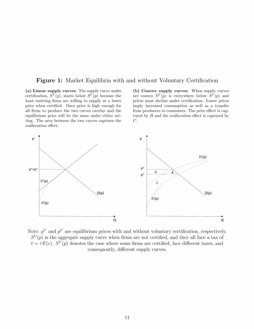
Figure 1: Market Equilibria with and without Voluntary Certification

(a) Linear supply curves: The supply curve undercertification, SV (p), starts below SU (p) because theleast emitting firms are willing to supply at a lowerprice when certified. Once price is high enough forall firms to produce the two curves overlay and theequilibrium price will be the same under either set-ting. The area between the two curves captures thereallocation effect.

D(p)

SU(p)

SV(p)

p

Q

pV=pU

(b) Convex supply curves: When supply curvesare convex SV (p) is everywhere below SU (p) andprices must decline under certification. Lower pricesimply increased consumption as well as a transferfrom producers to consumers. The price effect is cap-tured by B and the reallocation effect is captured byC.

SU(p)

SV(p)

pU

pVA B

C

D(p)

Q

p

Note: pV and pU are equilibrium prices with and without voluntary certification, respectively.SU(p) is the aggregate supply curve when firms are not certified, and they all face a tax oft = τE(e). SV (p) denotes the case where some firms are certified, face different taxes, and

consequently, different supply curves.

11

As can be intuited from Panel b, the price effect is of a higher order than the other terms.

Our goal is to establish “sufficient statistics” for changes in emissions and welfare that can be

easily evaluated using readily available data. In this pursuit, and with little loss of generality,

we will consider first-order approximations in τ in much of the analysis to come. This implies

that the price effect is zero and the reallocation effects and untaxed emission effects are both

positive (for τ ≤ v).

Corollary 1 considers such approximations. We assume that taxes, τ , and the social costs

of emissions, v, are small relative to prices. We then conduct Taylor expansions around τ = 0

(where v is of the same order).

Corollary 1. The expression W V −WU in Proposition 1 can be written as:

W V −WU =(v − τ

2

)s′ (p0)V ar (ε) τ − FΨ (e) + o

(τ 2), (9)

with a difference in emissions of:

GV −GU = −s′ (p0) τV ar (ε) + o(τ),

where p0 is the price when τ = 0. It holds that:

a) V ar(ε) = 0 if e = e and ∂V ar(ε)/∂e > 0.

b) W V −WU + FΨ(e) is positive if τ < 2v (to a second order).

c) GV −GU is negative (to a first order).7

d) These expressions hold exactly when supply curves are linear.

Proof. Appendix A.1.2.

Corollary 1 demonstrates that there is no price effect at first order and the primary

driver of the welfare consequences of certification come from the shift in production from

more to less polluting firms. With a constant production but a shift towards firms with

fewer emissions, total emissions are sure to decline. Even if average emissions were already

taxed efficiently, τ = v, total welfare increases because production is reallocated towards less

polluting firms. The size of this reallocation depends on the supply response, s′(p0), and the

variance of the taxed emissions rate, V ar(ε). When τ = v the entire welfare benefit from the

certification program accrues to firms (at first order). This result, however, depends on the

7When τ > v emissions are taxed excessively. The costs of doing so are quadratic in the deviations fromthe optimal tax, implying a quadratic distortion of increasingly high taxes on the dirtier firms. When τ > 2vthis effect dominates and causes negative welfare effects.

12

assumption of an exogenous unit mass of firms. Appendix A.1.6 demonstrates that if we allow

for endogenous entry of firms, all additional effects are of higher order and the expressions

of Corollary 1 remain unchanged, but the entire welfare benefit accrues to consumers.8

A natural question to ask is how far welfare of the voluntary certification in Proposition

1 is from the welfare that would be obtained if firm emission rates were known and taxable

(without necessarily imposing τ = v) (Jacobsen et al., 2020). Labeling such an equilibrium

with W FI for “full information” we find (at second order)

W V =V ar (ε)

V ar (e)W FI +WU

(1− V ar (ε)

V ar (e)

)− FΨ (e) + o(τ 2). (10)

By construction V ar(ε) ≤ V ar(e) so welfare under voluntary certification (gross of cer-

tification costs) is a weighted average of welfare with no certification, WU , and with full

information, W FI . The weight reflects the relative variance of the effectively-taxed emission

rate, ε, and the actual emission rates, e. This means that greater benefits of voluntary certi-

fication accrue as a larger share of the variance of emissions certify. Having additional firms

certify is only beneficial insofar as they represent a higher share of the emissions variance.

2.4 Optimal policy

In the following, we solve for the optimal combination of the three available policy tools: the

emissions tax on certified firms, τ , the output tax on uncertified firms, t, and the subsidy/tax

on certification, f . Appendix A.1.3 shows that these are

τ = v,

t = vE(e|e > e),

f = vE (e− e|e > e) s (p− vE (e|e > e)) > 0. (11)

The condition τ = v and t = vE(e|e > e) recover the standard Pigovian result that

emissions ought to be taxed at their (expected) social cost. Equation (11) shows that cer-

tification is excessive when τ and t are set optimally, and should be taxed. To see why, we

employ the first order condition with respect to f . This can equivalently be written wrt. to

8Specifically, we specify a free entry condition that E(π(ε)) = FE , where a slight abuse of notationpermits us to let π(ε) denote the profits of a firm with emissions rate ε. In this case, the mass of firms N isendogenous. The expressions in Corollary 1 take this into account by replacing s′(p0) with N0s

′(p0) whereN0 is the mass of firms under p0.

13

e as:

π (p− ve)− π (p− vE (e|e > e))− vE (e− e|e > e) s (p− vE (e|e > e))− F = 0. (12)

Increased certification implies higher profits for the marginal firm, e, captured by the first

two terms in the expression. In addition, the quantity tax on uncertified firms goes up, which

has a negative effect on profits for the uncertified firms. The third captures this whereas

the fourth term captures the social cost of certification, F. As τ = v emissions are taxed

correctly, and there is no marginal gain from changes to emissions. Comparing equation

(12) with the indifference condition of when firms certify (equation 4) we get Equation (11).

Since the certifying firms do not internalize the costs they impose on still non-certified firms,

the optimal policy requires a tax.

These considerations relate to the size of F and f . Corollary 1 does not specify the order

of F and f . Consider f = 0 (no tax or subsidy on certification). The gains from certification

are first order, so if F is first order, some firms will certify. Since welfare gains are second

order, equation (9) then delivers negative welfare benefits. If F is second order, almost all

firms certify. Neither of these is efficient, as just discussed. An f > 0 of first order according

to equation (11) ensures the optimal certification.

2.5 An “Unraveling” Algorithm

Having solved for the decentralized equilibrium and the social planner’s allocation, we take

a step back and assess the informational requirements needed to implement such a policy.

Whereas equation (9) gives an intuitive result of the welfare gains based on statistics that

are relatively easily obtained — such as the variance of emission rates and supply elasticities

— the implementation requires complete information on the distribution of e, which is rarely

available. We show the conditions under which a given “algorithm” can achieve a comparable

outcome without complete information on the distribution of e.

We assume that neither firms nor the government knows the distribution of emissions

rates, but they do observe the average emissions rate (through aggregated accounts or changes

in ambient pollution, for example). We further assume for this section that e <∞. Initially,

certification is not available and the government imposes an output tax t0 = τE(e). We

assume that the government introduces certification which allows firms to pay the emission

tax τ at some certification cost F . Since the government does not know the distribution Ψ(e),

it cannot predict the eventual threshold e and therefore cannot implement the equilibrium

described above by immediately announcing a new output tax τE (e|e > e).

14

Consider instead an iterative process where the government allows firms to certify at

increasing levels of emissions rates. That is, the government asks if firms with emissions

rate e want to certify and only those firms are allowed to do so. If they do, the level of

certification increases and the procedure starts again. The government continuously adjusts

the output tax as the emissions distribution is revealed. We show that we obtain a Nash

equilibrium when firms decide on certification as if they were the last ones to certify with

the information available at that point in time.

Assume that all firms with an emissions rate below e have certified and consider the

decision facing a firm with emissions rate e. The firm will certify if:

g (e) ≡ π (p (e)− τ e)− π (p (e)− τE (e|e > e))− F ≥ 0,

where p (e) is the price that would prevail on markets should the certification stop here and

the threshold be e = e. Since the distribution up to e has been revealed publicly and since

E (e) is known, both the government and the firm can compute E (e|e > e). Assuming that

g (e) > 0, then at least some firms will certify. Furthermore, with a bounded distribution,

g (e) = −F so not all firms will certify as long as F > 0. As firms decide sequentially to

certify, the process will continue up to the smallest emissions rate for which g switches sign,

which we denote e (which also corresponds to a laissez-faire equilibrium when the government

knows the full distribution ψ).

This leads to a Nash equilibrium because for firms with a lower emissions rate, e < e,

π (p (e)− τ e)− π (p (e)− τE (e|e > e))− F > g (e) = 0,

so that none of these firms would benefit from deviating from certification at the equilibrium.

Since g becomes negative just after e, firms with emission rate e + de, decide not to certify

and would indeed be worse off otherwise. Firms with a higher emission rate e > e, will not

certify either. Hence, even if the government does not know the distribution of Ψ(e) it can

implement an algorithm where the optimal certification decisions of firms gradually reveal

the shape of the distribution up until e.

The analysis can be straightforwardly extended to the social optimum if the government

continuously adjusts the certification tax f = τ (E (e|e > e)− e) s (p(e)− τE (e|e > e)) with

the information available.

15

2.6 Extensions

The following sections add two dimensions of flexibility to the baseline model: abatement

and heterogeneous productivity (Appendix A.1.6 allows for free entry). The extensions fit

easily in the framework presented so far, and we present them with a focus on the added

terms to emissions and welfare. The full explicit expressions are given in Appendix A.1.6.

Abatement

We keep the same structure as above but allow firms to spend b(a) per unit produced to

reduce their per-unit emissions by a. We require: b′(a) > 0 and b′′(a) > 0 for a > 0. For

simplicity, we further add b′(0) = b(0) = 0. Pre-abatement emissions are still distributed

according to Ψ(e), and a certified firm i pays an emission tax on e(i)− a(i) instead of e(i).

We continue to define ε in equation (5) as the pre-abatement emissions rate for certified

firms and the conditional mean of emissions for uncertified firms. Abatement investments

are not observable and non-certified firms consequently have no economic incentive to abate.

Hence, in an equilibrium without certification, no abatement takes place. Certified firms, in

contrast, do abate a strictly positive amount. They solve the problem:

maxq,apq − c(q)− τ(e− a)q − b(a)q

which leads to a common abatement level, a∗, among all firms that certify of a∗ = b′−1(τ).

We let A(τ) ≡ τa∗(τ) − b(a∗(τ)) > 0 denote the savings per unit of production due to

abatement. If e < a some firms sequester emissions. Individual supply functions of certified

firms with emissions rate e takes the form:

q = s (p− τe+ A(τ)) ,

such that supply is higher under abatement. The expression for changes in total emissions

with abatement takes the structure of Lemma 1 but adds two additional terms:

−a∗Ψ(e)E[s(pV − τe+ A(τ)

)|e < e

]+Ψ(e)E

{e[s(pV − τe+ A(τ)

)− s

(pV − τe

)]|e ≤ e

},

(13)

where (with slight misuse of notation) pV now represents the equilibrium price under cer-

tification with abatement. The first term in expression (13) is the direct impact of a mass

of Ψ(e) certifying and thereby abating their emissions by a∗. At the same time certification

lowers their tax burden, which yields a supply response analogous to a rebound effect on the

16

quantity produced. This additional effect pulls in the direction of higher emissions. If s is

convex and es(pV − τe) is increasing and weakly concave in e, then emissions must decline.

If τ is small emissions must decline as well.

Similarly, we can establish a result on welfare analogous to that of Proposition 1. Em-

bedded in equation (13) are the additional negative effects on emissions which increases the

positive untaxed emissions effect when v > τ . In addition, we get:

Ψ (e)(E(π(pV − τe+ A(τ)

)− π

(pV − τe

)|e ≤ e

)).

This captures the increase in profits to firms that receive a higher net price after abatement.

This benefit accrues only to the share of firms Ψ(e) that certify. For given price pV , profit

maximization ensures that this term is positive.

Finally, we continue our analysis using Taylor expansions and derive the following corol-

lary to Proposition 1:

Corollary 2. To a second-order approximation, the difference in social welfare when moving

to voluntary certification from an output tax in the presence of abatement is

W V −WU = τ(v − τ

2

)(s′(p0)V ar(ε) +

s(p0)Ψ (e)

b′′(0)

)− FΨ (e) + o

(τ 2),

where W V −WU+FΨ(e) is positive.

Corollary 2 takes advantage of the fact that to a first order e remains unchanged with

abatement and consequently we can add a single term to equation (9) from Corollary 1. b′′(0)

captures the curvature in the abatement costs. By assumption, it is always profitable to do

some abatement and a low curvature of the abatement function (b′′(0)), implies that, to a

first order, the optimal abatement level will be higher. Abatement benefits are proportional

to total production by the firms that abate: s (p0) Ψ(e). For this effect to be positive requires

τ < 2v (the reasoning is analogous to that of footnote 7).9

9Analogously to equation (10), to a first order, we can write welfare under certification with abatement asa weighted average of welfare without certification, WU , and welfare with full information under abatement,WFIA as:

WV = WFIAω + (1− ω)WU − FΨ(e) + o(τ2),

where ω =(V ar (ε) + s(p0)

s′(p0)b′′(0)Ψ (e)

)/(V ar (e) + s(p0)

s′(p0)b′′(0)

). Welfare under certification (gross of certi-

fication costs) continues to be a weighted average of the welfare with complete information and with no

information, but with the added term, s(p0)s′(p0)b′′(0)

Ψ(e) which captures (to a first order) the amount of abate-

ment done with certification.

17

Heterogeneous Productivity

In the following we again preclude abatement, but we allow firms to differ in their level of

productivity. In particular, firm i has costs of production of c(q)/ϕi, where c(q) has the

same properties as the cost function in Section 2 but ϕi > 0 differs across firms. We let

Ψ(e, ϕ) denote the joint distribution and allow unrestricted covariance between e and ϕ. We

consider supply functions with constant elasticity such that a firm i that certifies produces

qi = s0 [ϕi(p− τei)]α and the uncertified firms produce qu = s0 [ϕi(p− t)]α, where t is τ

times total emissions of uncertified firms divided by total production by uncertified firms.

This is also the optimal quantity tax rate under no certification.10

In this setup, firms differ both in their productivity and their emissions. Therefore, the

cut-off e of Section 2 is replaced by a cut-off function e(ϕ) which depends positively on

productivity.11 To a first order, the expressions for the change in emissions and welfare of

Corollary 2 take the same form, except V ar(ε) is replaced by the output-weighted variance

of emissions:˜V ar(ε) =

∫ϕ

∫ε

(ε− E(ε))2ψ(ϕ, ε)dεdϕ,

where ψ(ϕ, ε) = ϕαψ(ϕ, ε)/(∫

ϕ

∫εϕαψ(ϕ, ε)dεdϕ

)is a density distribution rescaled by out-

put (proportional to ϕα at price p0) such that E(ε) equals the average emissions per unit

without certification:

E(ε) =

∫ϕ

∫ε

εψ(ϕ, ε)dεdϕ = GU/SU

Intuitively, the reallocation effect is still the driving force behind our results, though firms’

emissions are now weighted by their size.

2.7 Adjustments along the extensive margin

The model presented above considered reallocation on the intensive margin. For complete-

ness, we consider situations in which the only margin of adjustment is whether to produce

or not. To focus on the supply side we consider an exogenous price p such that consumer

welfare (excluding emissions) is constant.12

10Although our approach could also be used with other supply functions, the analysis becomes morecomplicated, in particular because t is no longer the optimal quantity tax.

11Specifically, equation 4 is replaced by: 1ϕπ(ϕ(p − τ e(ϕ))) − (F + f) = 1

ϕπ(ϕ(p − t)) where π() is as

previously defined. This defines e(ϕ) where the cut-off emission rate depends positively on productivitybecause production increases with productivity whereas the certification cost, F + f , does not.

12This implies that we deviate from our assumption of a closed economy. Section 3 focuses explicitly on aninternational case, and here we do not explicitly model alternative consumers or suppliers. This approach is

18

Consider a mass 1 of potential firms each characterized by potential production q, entry

costs c and emissions, e. These are distributed according to Ψ(c, q, e) with a corresponding

pdf of ψ. The domain is [c, c] × [q, q] × [e, e] with weakly positive lower bounds and finite

upper bounds and Ψ has support everywhere. It will further be convenient to define the

unconditional distribution of e, ψe(e), and the two conditional distributions ψc(c|e, q) and

ψq(q|e). In the following we present only results and keep derivations in Appendix A.2.

Firms face a uniform price of p. In laissez-faire, a firm i produces if its individual draw

satisfies pqi ≥ ci. When a uniform quantity tax is imposed, this condition becomes (p−t)qi ≥ci.

Total production and emissions are then given by:

S(p− t) =

∫q1(p−t)q≥cdΨ(c, q, e), (14)

G(p− t) =

∫eq1(p−t)q≥cdΨ(c, q, e),

where 1(p−t)q≥c is the indicator function and it is understood that when not otherwise specified

integrals are over the full support of (c, q, e).

The slope of the aggregate supply curve is:

S ′(p− t) =

∫e

ψe(e)

∫q

q2ψc((p− t)q|e, q)ψq(q|e)dqde. (15)

The slope of the aggregate emission curve, G′(p − t), follows the same formula with eq2

instead of q2. Price or tax changes only affect production by firms on the margin of entry so

that ψc is only evaluated where c = (p − t)q. The “q2” reflects the fact that potential firms

with greater output are also more sensitive to per-unit price or tax changes. It will prove

useful to define

ψe(e) ≡(ψe(e)

∫q

q2ψc(pq|e, q)ψq(q|e)dq)/ (S ′(p)) ,

as the “sensitivity and size”-corrected distribution on e. ψe is the distribution of e scaling by

the size of firms (one q), their sensitivity to tax or price changes (the other q), evaluated at

t = 0 for the marginal firms (c = pq). Using this, the change in emissions (at t = 0) from

exact if i) demand is perfectly elastic at p, ii) there are no externalities associated with production elsewhereor iii) the externalities elsewhere are corrected by a Pigovian tax.

19

price changes is:

G′(p) = Eψe(e)× S′(p),

where Eψe simply denotes the expectation with respect to ψe. One can demonstrate that

(to a first order) the optimal uniform quantity tax is t∗ = vG′(p)/S ′(p) = vEψe(e), average

emissions weighted by q2 along the relevant margin of adjustment (where pq = c) and not

total emissions divided by total supply as was the case for the model on the intensive margin.

The difference arises because i) only firms on the margin of pq = c adjust to marginal price

changes and ii) larger firms are more important for changes to emissions and also more

sensitive to tax changes.

2.7.1 Equilibrium with certification

We set up a certification system along the same lines as for the intensive-margin case. We

assume that the certification cost F is second-order in τ . Firms with e ≤ e certify whereas

those with e > e do not.13 A firm that certifies will pay τe in emission tax and those that

do not will pay according to the average emissions of active non-certified firms:

t = τE (eq|e ≥ e, (p− t)q ≥ c)

E (q|e ≥ e, (p− t)q ≥ c)= τ

∫eq1e>e1(p−t)q≥cdΨ(c, q, e)∫q1e>e1(p−t)q≥cdΨ(c, q, e)

. (16)

This implies that total supply is given by:

S(p, τ, t) =

∫q(1e≤e1(p−τe)q≥c+F + 1e>e1(p−t)q≥c

)dΨ(c, q, e),

where corresponding expressions for total costs C(p, τ, t) and emissions G(p, τ, t) follow the

structure of S(p, τ, t) but replace q with c and eq, respectively. The total mass of firms who

certify is given by M =∫

1e≤e1(p−τe)q≥c+FdΨ(c, q, e). We proceed along the same lines as for

Corrollary 1 to arrive at the following result:

Proposition 2. Consider τ = v. The difference in welfare and emissions between certifica-

tion and no certification is given by:

W V −WU =v2

2S ′(p)×

13In the intensive margin case, it was immaterial whether we chose an exogenous e or a tax f to incentivizethe same level of certification. Here a tax, f , however, will affect both the margins of certification and ofentry and these two setups will not be equivalent. Therefore, we define e as the maximum emission rate thatthe government permits to certify. With F being second order in τ , the constraint binds and e = e.

20

[V arψe(ε) +

(G′(p)

S ′(p)− G(p)

S(p)

)2

−(

1− Ψe(e))(

Eψe(e|e > e)− E (eq|e ≥ e, pq ≥ c)

E (q|e ≥ e, pq ≥ c)

)2]−FM+o

(τ 2),

(17)

where G(p) and S(p) are evaluated at t = τ = 0 and Ψe(e) =∫ eeψe(e)de is the (sensitivity and

size-)corrected mass of firms with e ≤ e. ε is given by ε = e if e ≤ e and ε = Eψe(e|e > e)

otherwise.

Change in emissions is given by:

GV −GU = −τS ′(p)×[V arψe(ε) +

(G′(p)

S ′(p)− G(p)

S(p)

)Eψe(e) + (1− Ψe(e))

(G(p)

S(p)Eψe(e|e > e)− G′(p)

S ′(p)Eψe(e)

)]+o(τ).

(18)

Proof. See Appendix A.2.

Consider first the change in welfare which replicates the structure of welfare gains under

the intensive margin. As in the model with an intensive margin, the first term captures the

reallocation effect of moving from an optimally set uniform tax to an individual tax. However,

as discussed above, t = G(p)/S(p) in equation (16) is not set optimally. The change in welfare

is therefore best thought of as a two-step change: First moving to an optimal uniform tax

of G′(p)/S ′(p) (captured by the second term) and thereafter to the certification program

(captured by the first). The last term captures the fact that the uncertified firms do not pay

the optimal output tax. Naturally, if the uniform tax were already set to G′(p)/S ′(p) only

the reallocation (the first) term would appear.

The change in emissions share similar intuitions. The second term captures the change in

taxation rate for certified firms when moving from a uniform tax of G(p)/S(p) to G′(p)/S ′(p)

and the third term is a “correction”-term for the fact that uncertified firms are not taxed

according to individual emissions.

2.8 Domestic Empirical Application: Methane Emissions in the Permian Basin

A carbon-based economy has dizzying array of emissions sources for potential regulation.

One way to economize on enforcement costs while maximizing coverage is to focus attention

on fuel extraction rather than points of emission (Metcalf and Weisbach (2009)). The close

measurement of fuel production for royalties charges creates a point of taxation with minimal

21

additional regulatory cost. Taxation at the point of extraction also ensures the price of carbon

is reflected throughout the supply chain. Recent studies have evaluated the effects of pricing

coal as a ‘royalty adder’ above existing royalty rates in the Federal Coal Program (Gillingham

et al. (2016); Gerarden et al. (2020)) and oil and gas leasing more broadly (Prest and Stock

(2021)).

In this section we build on these royalty adder proposals to account for unmonitored

methane emissions from oil and gas fields. Methane (CH4) is a powerful greenhouse gas,

with an estimated social cost of $1500/metric ton (on Social Cost of Greenhouse Gases

(2021)), compared to $51/metric ton for carbon dioxide. It is the primary compound in

natural gas, and is released into the atmosphere during production from natural gas wells

due to faulty equipment, or from safety valves to relieve pressure. Methane is created when

longer hydrocarbon chains break down under heat and pressure underground. As a result,

wells drilled to recover oil also co-produce methane to varying degrees. In places without

sufficient infrastructure to deliver methane from oil wells to market, it is a waste product.

Best practices in such settings entail flaring the methane in situ, which converts the gas into

less-harmful carbon dioxide.14

We focus our analysis on the Permian Basin of west Texas and southeast New Mexico,

whose oil-rich shales yield nearly one-third of U.S. oil and 10% of natural gas production

(Administration (2019)). Poorly operated or malfunctioning flares, direct venting, and leaks

from these oil and gas fields are responsible for significant methane emissions. These are

recently estimated to be 2.7 million metric tons (Tg) per year based on the analysis of

satellite data (Zhang et al. (2020)), for a social cost of about $4B/year. Zhang et al. (2020)

calculate these emissions to have roughly similar global warming potential as CO2 emissions

from the entire U.S. residential sector.

The main regulatory challenge for internalizing methane emissions is that exact sources

are currently unobserved and enormously heterogeneous across leases. A random ground-

based sample of oil and gas wells in the Permian found that 70% of emissions came from

15% of the measured sites, while nearly one third of measurements were below detectible

levels (Robertson et al. (2020)). An output-based royalty adder that accounts for average

methane emissions falls short of an actual emissions tax according to the results of Section

2: there is too little output from clean leases and too much from polluting sources due to

14In North Dakota’s oil-rich Bakken Shale, for example, approximately one third of natural gas was flaredin the mid 2010’s, making the sparsely-populated oil fields prominently visible at night from space (Cicala(2015)). The state adopted regulations to reduce flaring, and recent work has found a drop of about 20%through 2016 (Lade and Rudik (2020)).

22

the lack of emissions-targeting.

We seek to answer the following questions: What are the differences in emissions and

welfare between an output-based tax and an emissions tax? How might adverse selection push

outcomes under an output-based tax with voluntary emissions taxation closer to those of a

fully mandatory emissions tax? To answer these questions we combine the complete annual

production data from New Mexico and Texas with emissions estimates from a stratified

random sample of wells (Robertson et al. (2020)). We use this sample to simulate the

distribution of lease-level emissions per barrel of oil equivalent (BOE) for 2019 in the Permian

Basin.

With the variance of emissions in hand, we require only the social cost of pollution

($1500/t) and the slope of the supply curve to approximate the emissions and welfare changes

due to voluntary certification according to Corollary 1. For this last number we use an

elasticity of supply of 0.89 from Newell et al. (2019),15 while limiting production to zero

for the share of leases whose emissions fees would exceed revenue.16 Output prices per

BOE are constructed by weighing spot market prices for fuels from the Energy Information

Administration by the site-level share of production from oil, gas, or natural gas liquids,

respectively. Further details on data construction and summary statistics are provided in

the Data Appendix.

The first column of Table 1 presents quantity and welfare calculations based on observed

outcomes in 2019. We calculate standard errors for objects involving emissions by bootstrap-

ping from the estimates of Zhang et al. (2020) and Robertson et al. (2020). Details of the

procedure are provided in Appendix B. For each bootstrap sample’s estimates of emissions,

we calculate the corresponding quantities and welfare measures. The table reports the means

and standard deviations across 1,000 iterations. When calculating welfare, we assume that

world prices are unchanged, and therefore do not calculate consumer surplus.

To test our approximations, we calculate quantity and welfare changes two different

ways—using aggregate statistics and micro data. The second column applies a uniform tax

per barrel to the aggregate supply function to calculate outcomes. Section 2.1 derives the

difference between output and emissions taxes as a function of market aggregates, allowing

15This is the drilling elasticity based on Anderson et al. (2018), not the short-term change in productionfrom existing wells, whose marginal costs are essentially ignorable. We are interested in the long-term supplyresponse to our program. In steady state, the production elasticity is equal to the drilling elasticity (Hausmanand Kellogg (2015)). Anderson et al. (2018); Newell and Prest (2019) find similar elasticity estimates.

16Corollary 1 assumes that all agents remain active. In Appendix A we derive the corresponding expressionswhen firms have the option to shut down. We assume that leases whose tax bill exceeds revenue will shut in(i.e. pause production), and apply the expressions that account for shutting in.

23

heterogeneity only with respect to emissions rates. We use the empirical analogs of equation

(9) with an adjustment for shut-ins (i.e. zero output), plus the second column to arrive

at the third column, which estimates how outcomes are affected by a mandatory methane

tax. With a mandatory methane tax, we assume certification is costless and compliance is

complete.

Applying aggregate statistics to Corollary (1) is sufficient to approximate the effects of

policy. In the fourth column we show how these approximations compare to a bottom-up

calculation from lease-level data.17 For each bootstrap sample we use linear supply curves,

and each lease’s emissions intensity to calculate production decisions, emissions, producer

surplus, and tax revenues.

We estimate that methane leaks from the Permian basin in 2019 had a social cost of

about $4B, which is about 7% of producer surplus. An optimal output tax based on average

emissions per barrel would be about $1.60, or a 3% tax on oil and an 11% tax on natural gas.

An output tax of this magnitude reduces output by a relatively small amount, and its poor

targeting of the externality means that it is not particularly effective at reducing emissions.

The tax revenue and reduced externality costs exceed the lost producer surplus by about

$80M.

Even without allowing firms to abate their emissions, taxing the externality directly yields

significant welfare improvements. Rather than scaling back output with a uniformly-applied

tax, targeting those with relatively higher emissions causes about 1% of output to shut-in.

This zero bound means that the reduction in output is less under an emissions tax than an

output tax—even though we are using linear supply curves. Emissions fall by nearly 80%,

producer surplus losses are about one quarter of those under an output tax, and net welfare

is about $3B higher per year. These results are essentially unchanged in the fourth column.

Estimates based on calculations using market aggregates and applying Corollary (1) closely

track those from bottom-up lease-level calculations of the effects of an emissions tax.

Figure 2 plots net welfare of three prospective policies as a function of the cost per well

of monitoring methane emissions, or “certification costs.” First, an output tax piggy-backs

on the royalty model of metering output, so no additional regulatory costs are involved. The

net welfare of an output tax is therefore flat with respect to certification costs. The second

prospective policy is a mandatory emissions fee with costly certification. This is depicted as

a dashed blue line in Figure 2. Such a policy loses ground relative to an output tax as the

17Emissions may come from an individual well or equipment at a ‘site’ shared across multiple wells. Sinceproduction and emissions are measured at the lease level, we refer to our unit of measurement as a lease.

24

social cost of enforcement rises. Ultimately there is a point at which the cost of monitoring

emissions is greater than the benefits of reduced pollution, and the output tax becomes

superior. In Figure 2, this occurs around $75,000 per well-year. When certification costs are

zero, the difference between output taxes and emissions fees are the values in Table 1.

Finally, the solid green line plots the net welfare associated with a voluntary emissions

tax combined with an output tax that reflects the average emissions of uncertified firms.

We continue to assume that output prices are unaffected by the policy. We implement the

discretized version of the algorithm in Section 2.5 to numerically solve for the equilibrium. For

certification costs less than $25,000 we find that all producers would be either participating in

the emissions program or shut-in, delivering an identical outcome to a mandatory emissions

tax.

Above $25,000 in certification costs per lease-year, the opt-in emissions tax becomes supe-

rior to both output and mandatory emissions taxes. The voluntary program delivers greater

social value than a mandatory tax by economizing on certification costs. Uncertified firms

are charged based on the conditional mean of emissions, which is closer to actual emissions

than the unconditional mean. Society therefore receives the benefit of fewer emissions (due

to reduced output) from high-emissions firms, while not having to bear significant certifica-

tion costs. We estimate that above $110,000 per lease-year, the voluntary program becomes

inferior to an output tax. At this high certification cost, business stealing largely dominates

the welfare calculation: expanded producer surplus and emissions at certified firms does not

exceed the value of reduced emissions and producer surplus at uncertified firms (facing a

higher output tax) by more than the cost of certification. Alternatively, a policy that in-

cludes an optimally-set certification tax will deliver outcomes that are weakly above both

the emissions and output taxes for all social costs of certification (see subsection 2.4).

Analysis from recently promulgated rules on the oil and gas sector suggests that the

per-site cost of well emissions certification is less than $600 (Agency (2020b)). Though

these calculations appear to focus on inspections rather than equipment costs, there are a

range of existing monitoring technologies that could economically be brought to bear on the

problem. Tamper-proof meters are already widely used to levy royalties, and similar devices

could prospectively used to record flaring and safety valve releases. Internet-ready methane

imaging cameras are widely available for less than $1000 to monitor malfunctioning flares.

It is therefore unlikely that the annual per-site monitoring cost would approach those that

begin to yield a meaningful difference between the voluntary and mandatory emissions taxes.

The upshot is that in the absence of a mandate to tax methane emissions directly, a

25

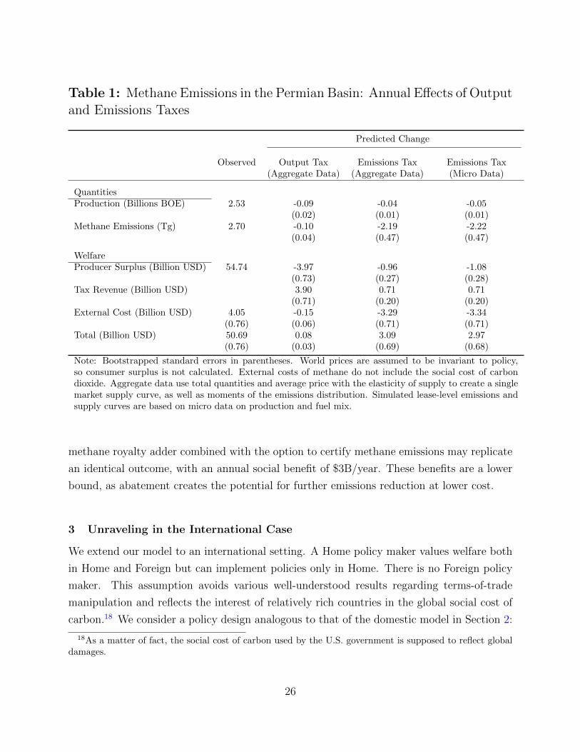
Table 1: Methane Emissions in the Permian Basin: Annual Effects of Outputand Emissions Taxes

Predicted Change

Observed Output Tax Emissions Tax Emissions Tax(Aggregate Data) (Aggregate Data) (Micro Data)

QuantitiesProduction (Billions BOE) 2.53 -0.09 -0.04 -0.05

(0.02) (0.01) (0.01)Methane Emissions (Tg) 2.70 -0.10 -2.19 -2.22

(0.04) (0.47) (0.47)

WelfareProducer Surplus (Billion USD) 54.74 -3.97 -0.96 -1.08

(0.73) (0.27) (0.28)Tax Revenue (Billion USD) 3.90 0.71 0.71

(0.71) (0.20) (0.20)External Cost (Billion USD) 4.05 -0.15 -3.29 -3.34

(0.76) (0.06) (0.71) (0.71)Total (Billion USD) 50.69 0.08 3.09 2.97

(0.76) (0.03) (0.69) (0.68)

Note: Bootstrapped standard errors in parentheses. World prices are assumed to be invariant to policy,so consumer surplus is not calculated. External costs of methane do not include the social cost of carbondioxide. Aggregate data use total quantities and average price with the elasticity of supply to create a singlemarket supply curve, as well as moments of the emissions distribution. Simulated lease-level emissions andsupply curves are based on micro data on production and fuel mix.

methane royalty adder combined with the option to certify methane emissions may replicate

an identical outcome, with an annual social benefit of $3B/year. These benefits are a lower

bound, as abatement creates the potential for further emissions reduction at lower cost.

3 Unraveling in the International Case

We extend our model to an international setting. A Home policy maker values welfare both

in Home and Foreign but can implement policies only in Home. There is no Foreign policy

maker. This assumption avoids various well-understood results regarding terms-of-trade

manipulation and reflects the interest of relatively rich countries in the global social cost of

carbon.18 We consider a policy design analogous to that of the domestic model in Section 2:

18As a matter of fact, the social cost of carbon used by the U.S. government is supposed to reflect globaldamages.

26

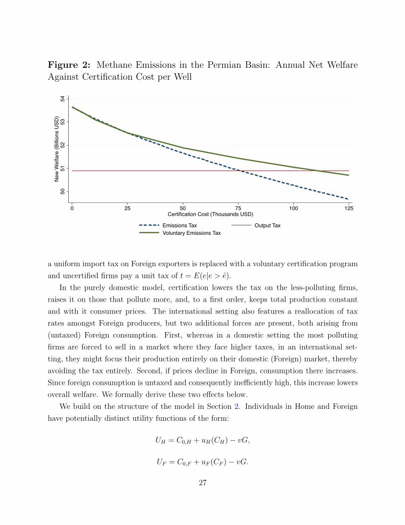
Figure 2: Methane Emissions in the Permian Basin: Annual Net WelfareAgainst Certification Cost per Well

5051

5253

54Ne

w W

elfa

re (B

illion

s US

D)

0 25 50 75 100 125Certification Cost (Thousands USD)

Emissions Tax Output TaxVoluntary Emissions Tax

a uniform import tax on Foreign exporters is replaced with a voluntary certification program

and uncertified firms pay a unit tax of t = E(e|e > e).

In the purely domestic model, certification lowers the tax on the less-polluting firms,

raises it on those that pollute more, and, to a first order, keeps total production constant

and with it consumer prices. The international setting also features a reallocation of tax

rates amongst Foreign producers, but two additional forces are present, both arising from

(untaxed) Foreign consumption. First, whereas in a domestic setting the most polluting

firms are forced to sell in a market where they face higher taxes, in an international set-

ting, they might focus their production entirely on their domestic (Foreign) market, thereby

avoiding the tax entirely. Second, if prices decline in Foreign, consumption there increases.

Since foreign consumption is untaxed and consequently inefficiently high, this increase lowers

overall welfare. We formally derive these two effects below.

We build on the structure of the model in Section 2. Individuals in Home and Foreign

have potentially distinct utility functions of the form:

UH = C0,H + uH(CH)− vG,

UF = C0,F + uF (CF )− vG.

27

These result in demand functions for Home, DH(p), and foreign, DF (p). Consumers in

both countries experience the same negative disutility, v, from global emissions, G. It costs

κ units of the outside good to transport the polluting good between Home and Foreign. It is

free to ship the outside good. The outside good, C0, is produced emissions-free, competitively

and one-for-one with labor. Labor is the only factor of production, and we choose the stock

in both Home and Foreign such that the outside sector is active in both countries. We

normalize the price to 1 in the outside good sector such that wages in both countries equal

1. The identical wages play no role in what follows.

The polluting good is produced competitively by a continuum of mass 1 of firms in Home

and a mass of 1 in Foreign. The emissions per unit produced in Home are distributed

according to ΨH(e) with ΨF (e) describing the Foreign distribution. Within each country,

firms differ only in their emissions and share a common cost function. To focus on the

international aspect and with little impact on the analysis to follow, we assume that all

emissions in Home are observable and emissions are taxed at τH . Firms can abate as described

in Section 2.6, and a Home firm will have a supply curve of sH(p − τHe + AH(τH)), where

AH(τH) ≡ τHaH(τH) − b(aH(τH)) is the net gain in price from abatement and aH(τH) =

b′−1(τH) is the level of abatement (and AF (τF ), analogously for Foreign). To streamline the

presentation, the main text will be devoted to comparing a tax policy analogous to that of

the domestic setting: Firms can choose to certify and be taxed according to emissions and

non-certified firms pay an output tax according to average emissions of uncertified firms.

Other comparisons exist, in particular allowing the output tax t to be set optimally. We will

discuss alternatives towards the end of this section and explore the optimal output tax in

Appendix A.3.3.

3.1 Equilibrium

Since the setting with no certification is a special case of the equilibrium with certification

(where no firm chooses to certify) we will solve for the general case. Consider an equilibrium

in which Home firms are all taxed at the emission rate of τH and certified Foreign firms pay an

emission tax of τF . There exists a cutoff e such that all Foreign firms with e ≤ e are certified

and all other Foreign firms pay a common output tariff on exports of τFEF (e|e > e) where

EF is the expectation operator over ΨF . In what follows, we take e as a policy parameter

determined either by an indifference condition such as equation (4) or by only permitting

firms below some predetermined level e to certify.

There are two subclasses of equilibria. In a pooled equilibrium, uncertified firms are

28

indifferent between selling domestically and exporting and continue to export to Home. In a

separating equilibrium uncertified firms only sell in the Foreign market. In either case, their

production can be evaluated at the foreign price denoted pF . If we define ρ as the difference

in net price between selling in Foreign and Home for an uncertified firm we have:

ρ ≡ pF − (pH − τFEF (e|e > e)− κ), (19)

where ρ = 0 in the pooled equilibrium and ρ ≥ 0 in the separating equilibrium.

The world market clearing condition for the polluting good is:

DH(pH) +DF (pF ) = (20)

EH [sH(pH − τHe+ AH)] + ΨF (e)EF [sF (pH − τF e− κ+ AF )|e < e] + (1−ΨF (e))sF (pF ).

The first line constitutes world demand as a function of the two consumer prices pH and

pF . The first term on the second line is Home production where emissions are always taxed

at τH and all firms abate. Hence, the second term of the second line is the production by

certified Foreign firms who face an emission tax of τF , transportation costs κ, abate at level

aF , and sell in the Home market at price pH . The equilibrium is characterized by the two

endogenous variables (pH , pF ). Equation (20) contributes one equilibrium equation. In the

pooled equilibrium equation (19) binds which adds the second equation of the equilibrium.

In such an equilibrium, equation (19) directly gives that the difference in consumer prices,

pH − pF , is increasing in e: the marginal exporter is more polluting and consequently faces

a higher import tariff which creates a higher price gap. Foreign prices must decline, but if

abatement is strong enough it is possible for prices in Home to decline as well (see details in

Appendix A.3).

The separating equilibrium features ρ ≥ 0 and the second identifying equation is instead

provided by market clearing in the Foreign market:

DF (pF ) = sF (pF )(1−ΨF (e)). (21)

This equation alone pins down pF as a function of the certification cutoff e. The function

is monotone positive: Higher certification implies fewer firms producing for the domestic

market and consequently a higher Foreign price. Conditional on this pF , the Home price pH

is then given by equation (20) and depends negatively on e.19 In the separating equilibrium,

19Specifically, the indifferent Foreign firm is defined as in equation (4), where F are the actual costs of

29

an increase in certification lowers prices in Home and raises them in Foreign.

The equilibrium conditions in the Home market are illustrated in Figure 3 which takes

as its starting point Figure 1 for the domestic case. For clarity and with little loss of

intuition, the figure is drawn for linear supply curves, without abatement, and no production

in Home. Instead of the market supply curve of Figure 3, we use two supply curves: one

representing each type of equilibrium. Consider first the pooling equilibrium (panel a).

Exports from Foreign to Home are given by total production less Foreign demand: SP (pH) =

sF × [pH − τEF (e)− κ] − DF (pH − τE(e|e > e)− κ) , where sF ≥ 0. For given pH total

production is independent of certification for reasons analogous to the domestic setting:

The expansion in output from certified firms exactly offsets the reduction from uncertified

firms. The second term of SP (pH) is consumption in Foreign. For a given pH , an increase in

certification will increase the spread in taxation between Home and Foreign for the marginal

firm (equation 21). This lowers the price in Foreign, increases consumption, and lowers

exports. Consequently, SVP (pH) must be to the left of SUP (pH) and a higher e moves the curve

leftward. This increases the Home price.20

The separating equilbrium is reached when all uncertified production is required to meetForeign demand, DF (pF ) = (1−Ψ(e))sF (pF ). In this case, the supply curve for Home marketis instead given only by certified Foreign firms, SS(pH) = ΨF (e)sF × [pH − τE(e|e < e)− κ].This is illustrated by the red lines in Figure 3(b). In this case a higher e, which increasesthe number of certified firms, will pivot the supply curve clockwise: each additional certifiedfirm sells only in the Home market at the expense of Foreign, reducing pH and raising pF .

Which equilibrium is active depends on the relative sizes of SS(pH) and SP (pH). If

SS(pH) < SP (pH) for a given price pH , certified firms cannot meet Home demand by them-

selves and the economy is in the pooled equilibrium. If the inequality is flipped, the economy

is in the separating equilibrium.

3.2 Welfare

We slightly abuse notation and let W denote world welfare. Under certification it obeys:

W = CSH+CSF+PSH+PSF−[(v − τH)GH + (v − τF )(GF −GF,dom) + vGF,dom]−FΨF (e),

certification and f is a tax or subsidy. Any desired e can be achieved with an appropriate f . In what follows,we will suppose that e is determined in this manner, though nothing would be lost by instead assuming thate is exogenously set.

πF (pH − τF e+AH − κ)− (F + f) = πF (pF ) (22)

20This positive effect of e on pH depends on the absence of abatement. With abatement increased certifi-cation may lead to an overall positive supply effect which could lower Home prices.

30

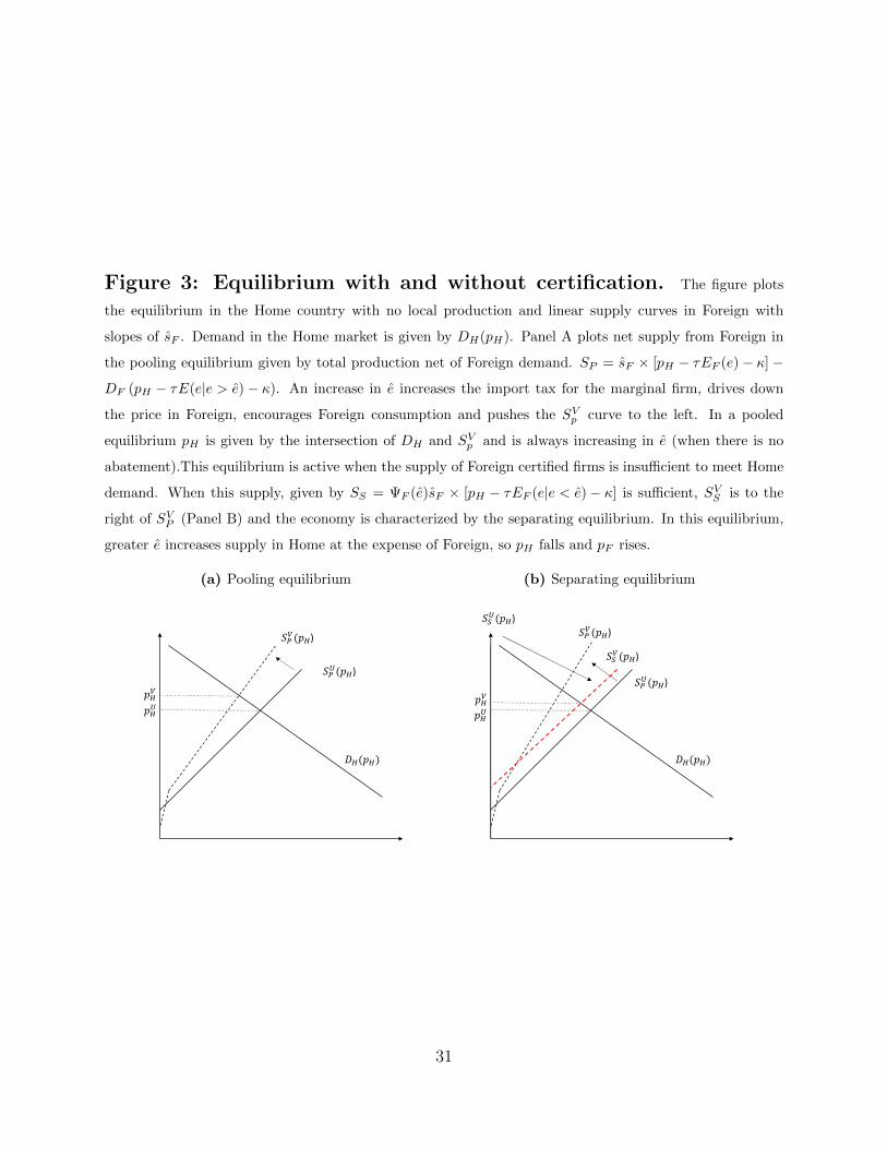
Figure 3: Equilibrium with and without certification. The figure plots

the equilibrium in the Home country with no local production and linear supply curves in Foreign with

slopes of sF . Demand in the Home market is given by DH(pH). Panel A plots net supply from Foreign in

the pooling equilibrium given by total production net of Foreign demand. SP = sF × [pH − τEF (e)− κ] −

DF (pH − τE(e|e > e)− κ). An increase in e increases the import tax for the marginal firm, drives down

the price in Foreign, encourages Foreign consumption and pushes the SVp curve to the left. In a pooled

equilibrium pH is given by the intersection of DH and SVp and is always increasing in e (when there is no

abatement).This equilibrium is active when the supply of Foreign certified firms is insufficient to meet Home

demand. When this supply, given by SS = ΨF (e)sF × [pH − τEF (e|e < e)− κ] is sufficient, SVS is to the

right of SVP (Panel B) and the economy is characterized by the separating equilibrium. In this equilibrium,

greater e increases supply in Home at the expense of Foreign, so pH falls and pF rises.

(a) Pooling equilibrium

𝐷 (𝑝 )

𝑆 (𝑝 )

𝑆 (𝑝 )

𝑝

𝑝

(b) Separating equilibrium

𝐷 (𝑝 )

𝑆 (𝑝 )

𝑆 (𝑝 )𝑆 (𝑝 )

𝑆 (𝑝 )

𝑝

𝑝

31

where CSH and PSH refer to consumer surplus and producer surplus in Home with corre-

sponding expressions for Foreign. These expressions are standard and the details are dele-

gated to Section A.3 in the appendix. The novel term is GF,dom = EF (e|e > e)DF (pF ). Only

uncertified firms supply the Foreign domestic market and consequently they have an average

emission rate of E(e|e > e) implying that emissions associated with Foreign consumption is

given by GF,dom. Both Home production, GH , and emissions from Foreign production but

exported to Home, (GF −GF,dom) are taxed under Home jurisdiction and can be taxed so as

to eliminate the externality (τH = τF = v). GF,dom is not taxed by the Home policy maker

but is still a function of e and prices.

The following Proposition, analogous to Corollary 1, gives the difference in welfare and

emissions between an equilibrium with voluntary certification and one without. Here we take

approximations in τ and take v and κ to be of the same order:

Proposition 3. To a second-order approximation in (τF , τH , v), the difference between global

welfare under certification for Foreign firms and with a uniform output-based tariff of τFEF (e)

is given by:

W V −WU = s′F τF

(v − 1

2τ

)V arF (ε)︸ ︷︷ ︸

Reallocation Effect

+ τF

(v − 1

2τF

)sFΨF (e)

b′′(0)︸ ︷︷ ︸Abatement Effect

(23)

−[(v − τH)EH(e)s′H + (v − τF )EF (e)s

′

F

]∆pH︸ ︷︷ ︸

Untaxed Average Emissions Effect

−D′F τF(τF (EF (e) + EF (e|e > e))− ρ

2

)∆pF︸ ︷︷ ︸

Consumption Leakage Effect

−s′F(1−ΨF (e)

)(∆pH + ρ

2+ (v − τF )E(e|e > e)

)ρ︸ ︷︷ ︸− FΨF (e)︸ ︷︷ ︸

Cost of Certification

Backfilling Effect

+ o(τ 2),

where ρ ≥ 0 — defined by equation (19) — is the (net of taxes) price premium for uncertified

Foreign firms of selling in Foreign compared with Home. We let ∆pH ≡ pVH − pUH and

∆pF ≡ pVF − pUF denote the changes in prices due to certification in each country. It holds

that

- The Reallocation and Abatement effects are always positive

- The Consumption Leakage effect has the same sign as ∆pF

- The Backfilling Effect is 0 in the pooling equilibrium.

- The total effect is ambiguous.

The corresponding changes in emissions are given by:

32

Corollary 3. To a first-order approximation change in emissions from moving to certifica-

tion is given by:

GVH −GU

H = EH (e) s′

H∆pH + o (τ) ,

GVF −GU

F

=s′F

(EF (e) ∆pH − τFV arF (ε) + ρEF (e|e > e) (1−ΨF (e))

)−ΨF (e) aF sF + o(τ)

.

The Proposition mirrors and extends the analysis in the domestic case.21 The Realloca-

tion and Abatement effects are as described in Section 2, and FΨF (e) continues to be the

cost of certification. We add the Untaxed Average Emissions Effect, which arises since prices

are no longer constant and an increase in home prices pH might encourage global production.

This is harmful to welfare if taxes are lower than v. In addition, we have the two terms with

which we opened this section:

The Consumption Leakage Effect — is new from the domestic case and builds on the

intuition of Figure 1. This is a leakage effect because when Home imposes an output-based

tariff (equal to τFEF (e)) the Foreign price goes down which encourages Foreign consumption

which is not taxed. With voluntary certification, this distortion increases further if the

Foreign price decreases, which always occurs in the pooling equilibrium. In contrast, in the

21Formally, we can use first and second order approximations to get expressions for the price changes. Weuse εD and εS to denote world demand and supply elasticities, which are the sum of share-weighted localelasticities, so εD = εDF θ

DF + εDHθ

DH , and similarly for supply (with θDH = DH/(DF + DH) and analogously

for other θ expressions). In Appendix A.3 we show that such a voluntary certification program will have thefollowing effect on the price at Home and in Foreign:

∆pH =−εDF θDFεS − εD

τF (EF (e|e > e)− EF (e))− (1−ΨF (e)) εSF θSF − εDF θDF

εS − εDρ+ o (τ) , (24)

∆pF =εDHθ

DH − εS

εS − εDτF (EF (e|e > e)− EF (e)) +

εS − εSF θSF (1−ΨF )− εDHθHDεS − εD

ρ+ o(τ), (25)

where elasticites are evaluated at p0 for Home and p0 − κ for Foreign. Further:

∆pH −∆pF = τF [EF (e|e > e)− EF (e)]− ρ. (26)

In the pooling equilibrium ρ = 0 and in the separating equilibrium it is ρ ≥ 0. In this latter case, ρ is givenby combining equations (19) and (22)

ρ = τF [EF (e|e > e)− e]− F + f

sF (p0 − κ)+ o(τ),

33

separating equilibrium, increased certification might reduce the pool of Foreign producers

servicing their own market so much that the Foreign price increases, in which case the

distortion is mitigated. The welfare cost is proportional to the underpricing which (to a first

approximation) equals (τF (EF (e) + EF (e|e > e))− ρ/2), the average of the price gap under

no certification and certification, respectively. This effect is only present when D′F < 0.22

The Backfilling Effect is also new. Whereas Consumption Leakage captures that Foreign

consumption faces a price that is too low, this term captures that the most polluting produc-

ers might receive a price that is “too” high. Recall that the reallocation effect captures that

uncertified firms receive a lower price and correspondingly reduce their production. This

is true in both the Domestic case and in the pooling equilibrium. However, in the sepa-

rating equilibrium where ρ > 0, Foreign firms can divert their sales entirely to the Foreign

market, which is untaxed. Because the relatively clean firms are exporters, those left to

serve demand in Foreign are relatively pollution-intensive. Uncertified Foreign firms conse-

quently receive a price that is too high by ρ. Their price changes by ∆pF and the size of

the distortion depends on the gap between ∆pF and what the price change would have been

had these Foreign firms been forced to export namely τF (EF (e) − EF (e|e > e)). Note that

∆pF − τF (EF (e)− EF (e|e > e)) = ∆pH + ρ. The welfare changes of the backfilling effect is

then given by ρ(∆pH +ρ)/2, where the division by 2 occurs for standard “Harberger” triangle

reasons (for ν = τF ). This effect is amplified when there Foreign emissions are under-taxed.

It is only active in the separating equilibrium. Unlike the Consumption Leakage Effect, it

does not require that D′F < 0 but only DF > 0.

The overall welfare effect is the sum of several terms and is in general ambigious. However,

if we consider a pooling equilbirium (ρ = 0), where taxes are Pigovian (τF = τH = ν),

abatement effects are large compared to fixed costs of certification (ν2

2sFb′′(0)

> F ), then s′Flarge enough relative to D′F is a sufficient condition. The relative size of s

′F and D

′F will play

some role in the empirical application below.

Changes in emissions in Corrolary 3 can be interpreted along similar lines. The Home

price change ∆pH increases emissions for all firms. Emissions in Foreign are reduced through

a reallocation effect and abatement, but increase because of a backfilling effect if ρ > 0.

Consequently, Proposition 3 shows how Foreign demand alters the conclusion from the

domestic model of Section 2. Though this policy continues to reallocate production from the

22An alternative intuition is to think of Foreign consumption as a zero-emission way of increasing inter-national supply. As such this “supply” should be given no tax and consequently be facing a price pH − κ.However, the actual price of Foreign consumption is pF (less than pH − κ) and consumption is consequentlytoo high. This problem grows when the Foreign price declines.

34

more polluting to the less polluting firms, the presence of Foreign consumption poses limits

to the taxing ability of the Home policy maker.

3.3 Alternative policy environments

This naturally raises the question of what the second-best policy is, that is the optimal

program where Home cannot treat Foreign producers differently unless they certify and where

Foreign does not impose any tax. We discuss this formally in Appendix A.3.3. We find that

in an attempt to reduce the Consumption Leakage Effect described above, the social planner

sets the output tax on uncertified firms, t∗, lower than τFE(e|e > e). A similar intuition

explains why in general, a border tariff adjustment (even tailored to the exact emission

rate of the exporter) is not the optimal environmental tariff (Balistreri et al., 2019; Keen

and Kotsogiannis, 2014; Markusen, 1975; Hoel, 1996). The optimal level of certification is

set through a positive tax f . Additional certification in the separating equilibrium creates

convergence in Home and Foreign prices, and divergence in the pooling equilibrium. A

tax on certification allows the government to control this process. Certification allows for

the separation of some Foreign exporters from their domestic market such that they are

essentially under the jurisdiction of the Home country. The emission tax is then set at their

Pigovian level: τF = τH = v.23

More broadly, the optimal policy also permits the policy maker to set taxes such that

Home exports to Foreign, thereby creating bilateral trade in a homogenous product. This

is not optimal when κ is first order but becomes more valuable as transportation costs fall.

In effect, the Home policy maker broadens its scope of taxation since it can tax production

23We compare the welfare under optimal policy W ∗ to that with a Laissez-faire setting, WLF , of no taxeson Foreign (τF = t = 0) and Pigouvian taxes on Home production (τH = v). We find:

W ∗ −WLF = s′

F (p0 − κ)v2

2V ar(ε) + ΨF (e)AF sF (p0 − κ)− FΨF (e)

+D′

F (p0 − κ)t∗

2EF (e|e > e)− s

′

F (p0 − κ)v

2EF (e)

(p∗H − vEF (e)− pLFH

).

t∗ is the optimally set output tax on imports, lower than its Pigovian value, and given by:

t∗ =s′

F (p0 − κ)(1−ΨF (e))

s′F (p0 − κ)(1−ΨF (e))−D′

F (p0 − κ)vE(e|e > e) < vE(e|e > e).

The first three terms on the RHS replicate the reallocation effect, gains from Abatement and the fixed costof certification. The Consumption Leakage effect is rederived as the subsequent element, though contrary toProposition 3 it is always negative because the spread between Home and Foreign consumer prices alwaysincreases in the optimum. The last term is novel to this setting: Since the comparison takes as a startingpoint no output tax, the “first step” is to introduce a uniform output tax at vEF (e). Adding in the associatedchange to prices p∗H − pLFH one gets the welfare change of the last term.

35

if it is either consumed or produced at Home. The result is Home exporting its production

to Foreign (covered under a domestic carbon tax), and importing certified production from

Foreign to Home (covered under the voluntary program). This reduces the Backfilling effect.

Though this is unlikely to be the optimal policy for international trade of steel, which is

relatively costly to transport, it might be relevant in other contexts such as electricity sold

on a grid that spans jurisdictional borders.

In the following section, we conduct a quantitative exercise where we calculate such

welfare gains explicitly for the steel trade.

3.4 International Empirical Application: Brazilian Steel Trade

To illustrate the implications of our program in the international setting, we conduct an

analysis based on our approximation formulas for trade in steel between Brazil and the

OECD. The iron and steel sector is one of the most energy and carbon-intensive sectors

responsible for 10.5% of total CO2 emissions (including indirect emissions from electricity

use, see IEA, 2020). Iron and steel are internationally traded, and it is therefore considered a

key sector for carbon leakage—for instance, the EU puts it on a list of highly exposed sectors

which get a disproportionately large share of free CO2 allowances in the EU cap-and-trade

system. Steel is mostly produced through two different processes. In the blast furnace-basic

oxygen furnace (BF-BOF) process, coke and iron ore are combined at high temperature to

produce liquid steel. This process emits CO2 emissions through the combustion of coke.

Alternatively, steel can be produced with scrap steel and electricity using an electric arc

furnace (EAF), a process which leads to fewer emissions. Within each process, there is still

a high level of heterogeneity in emissions depending on plant’s energy efficiency or on the

fuel used to produce electricity. This makes steel an interesting sector to explore the costs

and benefits of voluntary certification.

We calibrate our model to the Brazilian steel sector in 2019 and consider a two-country

world where OECD countries alone decide to implement carbon tariffs (either output-based

or with voluntary certification) on Brazilian steel. We will use the welfare formula given in

Proposition 3. This exercise requires a handful of key statistics and economic parameters

of supply and demand. We provide a brief overview here, and describe the sources and

calibration strategy in detail in Appendix B.2.

Production, trade and transport costs. Brazil produced 32.6 Mt of steel in 2019, exporting

8.5 Mt (on net) to OECD countries (including 6.1 Mt to the US, the largest net export market

for Brazilian steel) at an average price of $489/t, which we take as the laissez-faire price of

36

steel in Foreign in our calibration (Instituto Aco Brasil, 2021).24 We use data from World

Steel (2020) to determine production of steel in the OECD. We set the transport cost κ at

$50/t (Eckett (2021)).

Emissions rates. World Steel (2020) also reports the share of steel production with the

BF-BOF and EAF processes across countries in 2019. Hasanbeigi and Springer (2019) report

the emission rates per process in 2016 for the countries which produce the most steel, which

includes Brazil and the US. To give some context, the emission rate using BF-BOF is 2.07

tCO2/t steel in Brazil and 1.82 tCO2/t steel in the US, while the corresponding emission rates

using EAF are 0.46 and 0.62 tCO2/t steel. The EAF shares are 22.2 in Brazil and 69.7 in the

US. These numbers highlight that Brazilian steel is on average significantly dirtier than from

the US (or the average OECD country) even though its EAF producers are relatively clean.

We use the same data sources to estimate mean emission rates in the OECD. Of course,

there is still substantial variation in emission rates within each process. To account for this,

we assume that for each process, the emission rate distribution is a (both-sides) bounded

log-normal distribution. We then assume that the standard deviation of log emission rates

within each technology is the same as the standard deviation of log productivity in the basic

metal products sector in Brazil according to Schor (2004).25 See Appendix B.2 for details.

Social cost of carbon, abatement cost and certification cost. We set the social cost of

carbon at $51 (on Social Cost of Greenhouse Gases (2021)). We get an estimate for the

slope of the marginal abatement function b′′(0) using a marginal abatement cost curve for

the iron and steel sector in Brazil from Pinto et al. (2018). To estimate the certification

cost F , we rely on a study of the iron and steel sector in the US by the EPA which aimed

at evaluating the cost of reducing hazardous air pollutants (manganese, lead, benzene, etc.

but not CO2) in that industry Gallaher and Depro (2002). They found that the annualized

cost of monitoring pollutants for one plant was $1.04M in 2001. Assuming a constant fixed

cost to total output ratio, we find that this corresponds to $23M to certify all production in

Brazil (that is a cost of around $0.7 per ton).

24We keep constant net exports of Brazil to other countries. Therefore, in the OECD case, we removethe 2Mt of net exports to other countries. Net exports to the OECD therefore represent 27.7% of Brazilianproduction (excluding net exports to non-OECD countries).

25That is, once we control for the technology type, we consider that emission heterogeneity reflects theaverage productivity heterogeneity in the sector. This assumes implicitly that i) Once one controls forthe process-type, most heterogeneity reflects differences in energy intensity and that those move with TFPdifferences; ii) In the basic metal sector, within subsector heterogeneity dominates heterogeneity across sub-sectors. We adjust the total standard deviation of log productivity for the small productivity premiumenjoyed by the EAF process on average, using estimates for the US from Collard-Wexler and Loecker (2015).

37

Table 2: Emission and Welfare Effects from Environmental Trade Policies

Voluntary Voluntarycertification certification

First Best BCA f = 0 f = f ∗

Welfare

Gains in M USD 1161 714 692 850

% of First Best Gains 100 61.5 59.6 73.2

Emissions

Reduction in Mt 22.5 5.6 5.8 10.5

Note: All gains are calculated relative to a unilateral domestic carbon tax in the OECDwithout border adjustments. f is a tax on certification, with f ∗ denoting the optimum

certification tax.

Elasticities. Finally, we use Fernandez (2018) who derives demand elasticities for steel

in the US (−0.306) and in Brazil (−0.414). For the supply elasticity, we use a single value

of 3.5, which is the supply elasticity used by EPA (2002). Therefore the supply elasticity

is larger in magnitude than the demand elasticity. Data Appendix Table B.1 gives all

parameters and their sources.

Table 2 reports the effects on global welfare and emissions of introducing various taxation

programs. Each of the calculations report the gains relative to a Pigovian emission tax in the

OECD with no border adjustment. As a benchmark for comparison we calculate the welfare

gains that would result from a universal carbon tax covering production in both the OECD

and Brazil. To give some context to these numbers, note that the net export value of steel

from Brazil to the OECD is 4.1B USD. Adding an output-based carbon border adjustment

(i.e. a tariff on Brazilian exports of νEF (e)) increases welfare by 714M USD which is already

61% of the gains that could be achieved by implementing the universal carbon tax.

Without any certification tax, our voluntary certification program leads to a high level of

certification. The economy ends up in the separating equilibrium with a price gap between

Home and Foreign which is lower than in the output-based tariff case (105 USD versus 137

USD). As a result, voluntary certification reduces welfare relative to an output-based tariff.

This comes from a large negative “backfilling effect” of −228M USD, while the “reallocation

effect” leads to 150M USD. A tax or other program to limit certification to the optimal

38

level, however, brings 136M USD of additional welfare gains relative to the output-based

tariff. This corresponds to closing close to a third of the gap between the output-based tariff

and the first best policy. With the optimal certification tax, the equilibrium is still in the

separating case but the price gap slightly increases relative to the output-based tariff at 148

USD. This leads to a “backfilling effect” of a much smaller magnitude at −10M USD, while

the reallocation effect remains similar at 150M USD since the certification threshold is close

in both cases.26 The second best policy described in section 3.3 also leads to a separating

equilibrium. In that case, the tariff t∗ on uncertified exporters is irrelevant, so that the

second best policy coincides with the optimal certification tax case reported here.

Finally, note that while the output-based tariff reduces emissions by 5.6Mt of CO2,

the optimal certification program reduces emissions by 10.5Mt of CO2, nearly half of the

reductions of a first best policy which also taxes emissions in Brazil. To give an idea of the

magnitude involved, embodied carbon in the net exports of steel in laissez-faire represents

14.5Mt of CO2.

To illustrate how the benefits of an opt-in emissions taxation program change with the

extent of certification, Figure 4 displays the welfare gains of the certification program for

different values of the certification tax relative to a Pigovian tax in the OECD only. The

certification tax is expressed as a share of revenues in laissez-faire. For comparison, we also

plot the gains of a standard border carbon adjustment. For a sufficiently high certification

tax (corresponding to 15.6% of laissez-faire revenues), no firm certifies and the welfare gains

are the same as with the output based-tariff. As the certification tax decreases, the share

of firms certifying grows quickly, bringing most of the welfare gains from the certification

program. With a certification tax as high as 15% of laissez-faire revenues, 16.3% of firms

certify, close to 3/4 of EAF producers in Brazil. This reflects the presence of a sizable mass

of relatively clean producers in Brazil. The welfare gains remain high (above 100M USD) as

long as the certification tax remains above 5% of revenues, and they only disappear for very

small certification taxes.27

We stress that this exercise is a simple proof-of-concept and that our numbers are indica-

tive of orders of magnitude but not exact values. It shows that there are potentially large

26In the separating equilibrium the mass of certifying firms Ψ(e) is close to the export share in laissez-faire,i.e. Ψ(e) = 1−DF (p0 − κ)/SF (p0 − κ) + o(1). This is the reason why we show welfare gains as a functionof the certification tax instead of e in Figure 4 below.

27The small jump in Figure 4 marks the point where we switch from the separating to the pooling equilib-rium. This jump only occurs because we compute the welfare gains using Taylor approximations and woulddisappear if we were to compute welfare gains at higher orders.

39

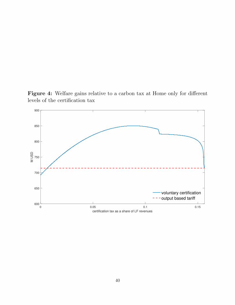
Figure 4: Welfare gains relative to a carbon tax at Home only for differentlevels of the certification tax

0 0.05 0.1 0.15

certification tax as a share of LF revenues

600

650

700

750

800

850

900

M U

SD

voluntary certification

output based tariff

40

emission reductions and significant welfare gains from our certification program, though it

may not be desirable to let certification occurs unabated if it leads to a large reduction in the

price gap between the two countries. Fortunately, prevailing price gaps relative to border ad-

justment fees are observable. This makes it possible for policymakers to adjust certification

criteria in order to avoid significant backfilling losses.

4 Conclusion

Settings in which a relatively small set of agents disproportionately contribute to a global

externality perfectly encapsulates the problem of concentrated benefits and diffuse costs

as described by Olson (1965). It should be unsurprising that there is limited appetite for

Pigouvian taxes to internalize such externalities. In this paper we study a mechanism that

counterbalances and ultimately unravels this dynamic.

The counterbalance comes from offering a substantial reduction in the tax burden to those

who contribute little to the externality. Low-emissions agents receive concentrated benefits

when they voluntarily certify their emissions for direct taxation. Increased certification raises

the output tax on uncertified firms, but this marginal increase is dispersed widely. Unraveling

occurs when the default output tax for uncertified firms is updated to reflect the higher mean

emissions of the uncertified group and the cost of certification is not too large. If unraveling

is complete, such a voluntary program achieves the same outcome as the otherwise-infeasible

mandate to tax emissions directly (minus certification costs). We show that the welfare gains

of such a policy scale with the variance of emissions and the slope of supply. The welfare

achieved by a voluntary program is a weighted average of the Pigouvian first-best and the

output-based tax, with the weights reflecting the relative variance of effective emissions

subject to taxation to the variance of emissions in the population.

We apply these results to oil and gas production in the Permian basin of New Mexico and

Texas, where methane emissions are a significant, largely unregulated problem. Coupling a

royalty adder based on the average of uncertified emissions per barrel of oil equivalent with

the option to certify emissions sets off an unraveling that converges on universal taxation,

even with significant implementation costs. This would have an annual social benefit of

about $3B.

In the international setting, our mechanism extends the incentive to abate emissions

beyond the borders of the country adopting a carbon tax. Such a policy is therefore most

attractive for countries whose carbon footprint is most heavily embodied in imports. We

show in addition to the variance of emissions, the elasticity of demand for carbon-intensive

41

goods in non-adopting countries plays a key role in prospective emissions reductions, as

demand responses to lower prices abroad offset reductions from certified firms’ abatement

efforts (consumption leakage). In addition, with too much certification there is a risk that

the most pollution-intensive foreign producers will expand operations to serve the foreign

market (backfilling). We derive the condition that determines whether such a program

would further reduce emissions beyond those achievable with border carbon adjustments.

Applying our sufficient statistics formulas to the Brazilian-OECD steel trade, we find that a

managed certification program could deliver nearly 75% of the welfare gains of a universal

carbon tax.

42

References

Administration, Energy Information, “Drilling Productivity Report,” 2019.

, “Spot Prices for Petroleum and Other Liquids,” 2021.

Agency, International Energy, “Iron and Steel Technology Roadmap Towards more sus-

tainable steelmaking,” 2020.

Agency, U.S. Environmental Protection, “Oil and Natural Gas Sector: Emission Stan-

dards for New, Reconstructed, and Modified Sources Reconsideration,” 2020.

Akerlof, George A., “The Market for “Lemons”: Quality Uncertainty and the Market

Mechanism,” The Quarterly Journal of Economics, 1970, 84, 488–500.

Alatas, Vivi, Abhijit Banerjee, Rema Hanna, Benjamin A. Olken, Ririn Purna-

masari, and Matthew Wai-Poi, “Self-Targeting: Evidence from a Field Experiment in

Indonesia,” The Journal of Political Economy, 2016, 124, 371–427.

Aldy, Joseph E. and Robert N. Stavins, “The Promise and Problems of Pricing Carbon

: Theory and Experience,” Journal of Environment and Development, 2012, 21, 152–180.

Alvarez, Ramon A, Daniel Zavala-Araiza, David R Lyon, David T Allen,

Zachary R Barkley, Adam R Brandt, Kenneth J Davis, Scott C Herndon,

Daniel J Jacob, Anna Karion, Eric A Kort, Brian K Lamb, Thomas Lau-

vaux, Joannes D Maasakkers, Anthony J Marchese, Mark Omara, Stephen W

Pacala, Jeff Peischl, Allen L. Robinson, Paul B. Shepson, Colm Sweeney,

Amy Townsend-Small, Steven C. Wofsy, and Steven P. Hamburg, “Assessment

of methane emissions from the U.S. oil and gas supply chain,” Science, 2018, 361, 186–188.

Anderson, Soren T., Ryan Kellogg, and Stephen W. Salant, “Hotelling Under Pres-

sure,” Journal of Political Economy, 2018, 126, 984–1026.

Association, World Steel, “Steel Statistical Yearbook 2020 Extended Version,” 2020.

Balistreri, Edward J, Daniel T Kaffine, and Hidemichi Yonezawa, Optimal Environ-

mental Border Adjustments Under the General Agreement on Tariffs and Trade, Vol. 74,

Springer Netherlands, 2019.

43

Baron, David P., “Regulation of Prices and Pollution Under Incomplete Information,”

Journal of Public Economics, 1985, 28, 211–231.

and Roger B. Myerson, “Regulating a monopolist with unknown costs,” Econometrica,

1982, 50, 911–930.

Barrett, Scott, “Self-enforcing environmental international agreements,” Oxford Economic

Papers, 1994, 46, 878–894.

Battaglini, Marco and B. Harstad, “Participation and Duration of Environmental Agree-

ments,” Journal of Political Economy, 2016, 124, 160–204.

Beccherle, Julien and Jean Tirole, “Regional initiatives and the cost of delaying binding

climate change agreements,” Journal of Public Economics, 2011, 95, 1339–1348.

Besley, Timothy and Stephen Coate, “Workfare versus Welfare: Incentive Arguments for

Work Requirements in Poverty-Alleviation Programs,” The American Economic Review,

1992, 82, 249–261.

Bohm, Peter, “Incomplete International Cooperation to Reduce CO2 Emissions: Alterna-

tive Policies,” Journal of Environmental Economics and Management, 1993, 24, 258–271.

Borenstein, Severin, “Time-Varying Retail Electricity Prices: Theory and Practice,” Elec-

tricity deregulation: choices and challenges, 2005.

, “Effective and Equitable Adoption of Opt-In Residential Dynamic Electricity Pricing,”

Review of Industrial Organization, 2013, 42, 127–160.

Center, Petroleum Recovery Research, “GO-TECH: ONGARD Data by County,” 2021.

Chan, Gabriel, Robert Stavins, and Zou Ji, “International Climate Change Policy,”

Annual Review of Resource Economics, 2018, 10, 335–60.

Cicala, Steve, “Comments and discussion: Welfare and distributional implications of shale

gas,” Brookings Papers on Economic Activity, 2015, Spring, 126–139.

Collard-Wexler, Allan and Jan De Loecker, “Reallocation and technology: Evidence

from the US steel industry,” American Economic Review, 2015, 105, 131–171.

Commission, Texas Railroad, “Production Data Query Dump,” 2021.

44

Condon, Madison and Ada Ignaciuk, “Border Carbon Adjustment and International

Trade: A Literature Review,” 2013.

Copeland, Brian R,“Pollution content tariffs , environmental rent shifting , and the control

of cross-border pollution,” 1996, 40, 459–476.

Copeland, Brian R. and M. Scott Taylor, “Trade and transboundary pollution,” Amer-

ican Economic Review, 1995, 85, 716–737.

Covert, Thomas R., “Experiential and Social Learning in Firms: The Case of Hydraulic

Fracturing in the Bakken Shale,” SSRN Electronic Journal, 2018.

Cropper, Maureen L. and Wallace E. Oates, “Environmental Economics : A Survey,”

Journal of Economic Literature, 1992, 30, 675–740.

Dasgupta, Partha, Peter Hammond, and Eric Maskin, “On Imperfect Information

and Optimal Pollution Control,” The Review of Economic Studies, 1980, 47, 857–860.

Deshpande, Manasi and Yue Li, “Who Is Screened Out? Application Costs and the

Targeting of Disability Programs,” American Economic Journal: Economic Policy, 2019,

11, 213–48.

Dranove, David and Ginger Zhe Jin, “Quality disclosure and certification: Theory and

practice,” 2010.

Eckett, Sam, “EMEA Freight Markets,” 2021.

Einav, Liran, Mark Jenkins, and Jonathan Levin, “Contract Pricing in Consumer

Credit Markets,” Econometrica, 2012, 80, 1387–1432.

Elliott, Joshua, Ian Foster, Samuel Kortum, G K Jush, Todd Munson, and David

Weisbach, “Unilateral carbon taxes, border adjustments, and carbon leakage,”Theoretical

Inquiries in Law, 2013, 14, 207–244.

, , , Todd Munson, Fernando PA c©rez Cervantes, and David Weisbach,

“Trade and carbon taxes,” American Economic Review, 2010, 100, 465–469.

Farrokhi, Farid and Ahmad Lashkaripour, “Can Trade Policy Mitigate Climate

Change?,” 2021.

45

Fernandez, Viviana, “Price and income elasticity of demand for mineral commodities,”

Resources Policy, 2018, 59, 160–183.

Finkelstein, Amy and Matthew J. Notowidigdo, “Take-up and targeting: experimental

evidence from SNAP,” The Quarterly Journal of Economics, 2019, pp. 1505–1556.

Foster, Andrew and Emilio Gutierrez, “The Informational Role of Voluntary Certifi-

cation: Evidence from the Mexican Clean Industry Program,” The American Economic

Review, 2013, 103, 303–308.

and , “Direct and Indirect Effects of Voluntary Certification: Evidence from the Mex-

ican Clean Industry Program,” 2016.

Fowlie, Meredith L., “Incomplete Environmental Regulation, Imperfect Competition, and

Emissions Leakage,” American Economic Journal: Economic Policy, 2009, 1, 72–112.

, Mar Reguant, and Stephen P Ryan, “Market-Based Emissions Regulation and

Industry Dynamics,” Journal of Political Economy, 2016, 124, 249–302.

Fullerton, Don, Inkee Hong, and Gilbert E. Metcalf, “A Tax on Output of the

Polluting Industry Is Not a Tax on Pollution: The Importance of Hitting the Target,”

2000.

Gallaher, Michael P. and Brooks M. Depro, “Economic Impact Analysis of Final

Integrated Iron and Steel NESHAP,” 9 2002.

Gerarden, Todd D., W Spencer Reeder, and James H Stock, “Federal Coal Program

Reform, the Clean Power Plan, and the Interaction of Upstream and Downstream Climate

Policies,” American Economic Journal: Economic Policy, 2020, 12, 167–199.

Gillingham, Kenneth, James B. Bushnell, Meredith L. Fowlie, Michael Green-

stone, Charles Kolstad, Alan Krupnick, Adele Morris, Richard Schmalensee,

and James Stock, “Reforming the U.S. coal leasing program,” Science, 2016, 354, 1096–

1098.

Grossman, Sanford J., “The Informational Role of Warranties and Private Disclosure

about Product Quality,” Journal of Law and Economics, 1981, 24, 461–483.

Harstad, B., “Climate Contracts: A Game of Emissions, Investments, Negotiations, and

Renegotiations,” Review of Economic Studies, 2012, 79, 1527–1557.

46

Hasanbeigi, Ali and Cecilia Springer, “How Clean Is the U.S. Steel Industry? An

International Benchmarking of Energy and CO2 Intensities,” 11 2019.

Hausman, Catherine H. and Ryan Kellogg, “Welfare and Distributional Implications

of Shale Gas,” Brookings Papers on Economic Activity, 2015.

Hoel, Michael, “Should a carbon tax be differentiated across sectors?,” Journal of Public

Economics, 1996, 59, 17–32.

Holzer, Jorge, “Property Rights and Choice: The Case of the Fishery,” American Journal

of Agricultural Economics, 2015, 97, 1175–1191.

Hubbard, Thomas N., “The Demand for Monitoring Technologies: The Case of Trucking,”

The Quarterly Journal of Economics, 2000, 115, 533–560.

HA c©mous, David, “The dynamic impact of unilateral environmental policies,” Journal of

International Economics, 2016, 103, 80–95.

Institute, Brazil Steel, “Brazilian Steel Industry Yearbook,” 2021.

Jacobsen, Mark R., Christopher R. Knittel, James M. Sallee, and Arthur A. Van

Benthem, “The use of regression statistics to analyze imperfect pricing policies,” Journal

of Political Economy, 2020, 128, 1826–1876.

Jin, Ginger Zhe, “Competition and disclosure incentives: an empirical study of HMOs.,”

The RAND Journal of Economics, 2005, 36, 93–112.

and Phillip Leslie, “The Effect Of Information On Product Quality: Evidence From

Restaurant Hygiene Grade Cards,” The Quarterly Journal of Economics, 2003, 118, 409–

451.

Jin, Yizhou and Shoshana Vasserman, “Buying Data from Consumers,” 2019.

Jovanovic, Boyan, “Truthful Disclosure of Information,” The Bell Journal of Economics,

1982, 13, 36–44.

Keen, Michael and Christos Kotsogiannis, “Coordinating climate and trade policies:

Pareto efficiency and the role of border tax adjustments,” Journal of International Eco-

nomics, 9 2014, 94, 119–128.

47

Kleven, Henrik Jacobsen and Wojciech Kopczuk, “Transfer Program Complexity and

the Take-Up of Social Benefits,” American Economic Journal: Applied Economics, 2011,

3, 54–90.

Kwerel, Evan, “To Tell the Truth: Imperfect Information and Optimal Pollution Control,”

The Review of Economic Studies, 1977, 44, 595–601.

Lade, Gabriel E and Ivan Rudik, “Costs of inefficient regulation: Evidence from the

Bakken,” Journal of Environmental Economics and Management, 2020, 102, 102336.

Laffont, Jean-Jacques, “Regulation of Pollution with Asymmetric Information,” 1994.

and Jean Tirole, A Theory of Incentives in Procurement and Regulation, MIT Press,

1993.

Larch, Mario and Joschka Wanner, “Carbon tariffs : An analysis of the trade, welfare,

and emission effects,” Journal of International Economics, 2017, 109, 195–213.

Lewis, Gregory, “Asymmetric information, adverse selection and online disclosure: The

case of ebay motors,” American Economic Review, 2011, 101, 1535–1546.

Markusen, James R, “International Externalities and Optimal Tax Structures,” Journal

of International Economics, 1975, 5, 15–29.

Metcalf, Gilbert E. and David Weisbach, “The Design of a Carbon Tax,” Harvard

Environmental Law Review, 2009, 33, 499–556.

Milgrom, Paul R,“What the Seller Won’t Tell You: Persuasion and Disclosure in Markets,”

The Journal of Economic Perspectives, 2008, 22, 115–131.

and John Roberts, “Relying on the Information of Interested Parties,” The RAND

Journal of Economics, 1986, 17, 18.

Miller, Zeke and Josh Boak, “US, EU say deal on steel tariffs will help on climate change,”

10 2021.

Newell, Richard G and Brian C Prest, “The unconventional oil supply boom: Aggregate

price response from microdata,” Energy Journal, 2019, 40, 1–30.

48

, , and Ashley B Vissing, “Trophy hunting versus manufacturing energy: The price

responsiveness of shale gas,” Journal of the Association of Environmental and Resource

Economists, 2019, 6, 391–431.

Nichols, Albert L and Richard J Zeckhauser, “Targeting Transfers through Restrictions

on Recipients,” The American Economic Review Papers and Proceedings, 1982, 72, 372–

377.

Nichols, D, E Smolensky, and T N Tideman, “Discrimination by Waiting Time in

Merit Goods,” The American Economic Review, 1971, 61, 312–323.

Nordhaus, William D., “Climate Clubs: Overcoming Free-riding in International Climate

Policy,” American Economic Review, 2015, 105, 1339–1370.

Olson, Mancur, The Logic of Collective Action: Public Goods and the Theory of Groups,

Harvard University Press, 1965.

on Social Cost of Greenhouse Gases, Interagency Working Group, “Technical Sup-

port Document: Social Cost of Carbon, Methane, and Nitrous Oxide Interim Estimates

under Executive Order 13990,” 2021.

Pinto, Raphael Guimaraes D., Alexandre S. Szklo, and Regis Rathmann, “CO2

emissions mitigation strategy in the Brazilian iron and steel sector—From structural to

intensity effects,” Energy Policy, 2018, 114, 380–393.

Prest, Brian C and James H Stock, “Climate Royalty Surcharges,” 2021.

Roberts, Marc J. and Michael Spence, “Effluent Charges and Licenses Under Uncer-

tainty,” Journal of Public Economics, 1976, 5, 193–208.

Robertson, Anna M, Rachel Edie, Robert A Field, David Lyon, Renee McVay,

Mark Omara, Daniel Zavala-Araiza, and Shane M Murphy, “New Mexico Permian

basin measured well pad methane emissions are a factor of 5–9 times higher than U.S. EPA

estimates,” Environmental Science and Technology, 2020, 54, 13926–13934.

Schmutzler, Armin and Lawrence H. Goulder, “The Choice between Emission Taxes

and Output Taxes under Imperfect Monitoring,” Journal of Environmental Economics and

Management, 1997, 32, 51–64.

49

Schor, Adriana, “Heterogeneous productivity response to tariff reduction. Evidence from

Brazilian manufacturing firms,” Journal of Development Economics, 2004, 75, 373–396.

Segerson, Kathleen, “Uncertainty and Incentives for Nonpoint Pollution Control,” Journal

of Environmental Economics and Management, 1988, 15, 87–98.

Spence, A. Michael, “Job Market Signaling,” The Quarterly Journal of Economics, 8 1973,

87, 355.

Stiglitz, Joseph E., “The Theory of ”Screening,” Education, and the Distribution of In-

come,” The American Economic Review, 1975, 65, 283–300.

Viscusi, W. Kip, “A note on “lemons” markets with quality certification,” The Bell Journal

of Economics, 1978, 9, 277–279.

Xepapadeas, Anastasios, “Environmental policy under imperfect information: Incentives

and moral hazard,” Journal of Environmental Economics and Management, 1991, 20, 113–

126.

, “Observability and choice of instrument mix in the control of externalities,” Journal of

Public Economics, 1995, 56, 485–498.

, “The Economics of Non-Point-Source Pollution,” Annual Review of Resource Economics,

2011, 3, 355–373.

Zhang, Yuzhong, Ritesh Gautam, Sudhanshu Pandey, Mark Omara, Joannes D.

Maasakkers, Pankaj Sadavarte, David Lyon, Hannah Nesser, Melissa P. Sul-

prizio, Daniel J. Varon, Ruixiong Zhang, Sander Houweling, Daniel Zavala-

Araiza, Ramon A. Alvarez, Alba Lorente, Steven P. Hamburg, Ilse Aben, and

Daniel J. Jacob, “Quantifying methane emissions from the largest oil-producing basin

in the United States from space,” Science Advances, 2020, 6, 1–10.

50

A Theory Appendix

In the following we first present the model of the domestic setting with an adjustment on

the intensive margin. We then proceed to the setting with an extensive margin and finally

consider the international model

A.1 The Domestic model

A.1.1 Setup and proof of uniqueness, Lemma 1 and Proposition 1.

We solve the model for the general case of certification at level e with the understanding that

the case of no certification can be found at e = e. The supply of uncertified and certified

firms are given by, respectively:

s(p− τE(e|e > e)),

s(p− τe).

An indifference condition determines which firms choose to certify:

π(p− τ e)− F − f = π(p− t),

where firms with e ≥ e certify. Consequently, for any given (t, τ, F ) there is a monotonic

relationship between e and f . We solve the model for given e.

Welfare derived from the operation of this market is the sum of consumer utility, net of

welfare costs from emissions, profits of firms, government revenue, and certification cost:

W = I − pC + u(C)− vG+ Eπ(p− τε) + τG− FΨ(e),

where the representative agent has exogenous income I and D(p) is demand function defined

by u′(D(p)) = p. We continue to employ the definition of ε of:

ε =

e

E(e|e > e)

if e ≤ e

if e > e.

and emissions are given by:

G = E[εs(p− τε)],

where p is determined by:

D(p) = E(s(p− τε)) (27)

51

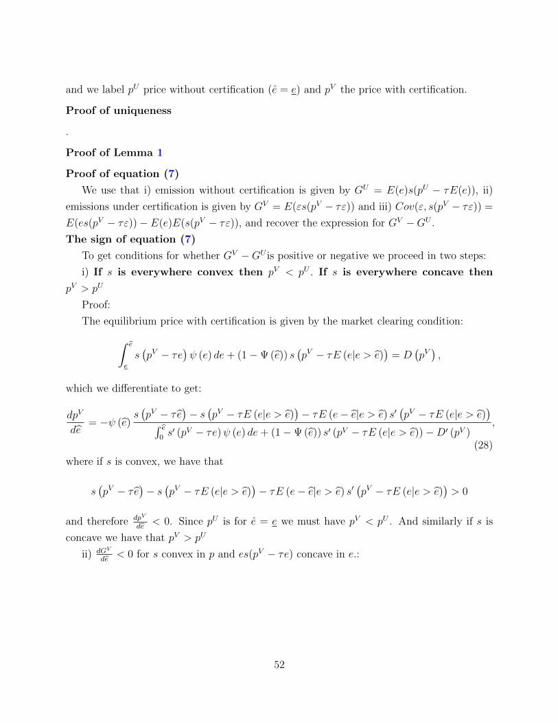
and we label pU price without certification (e = e) and pV the price with certification.

Proof of uniqueness

.

Proof of Lemma 1

Proof of equation (7)

We use that i) emission without certification is given by GU = E(e)s(pU − τE(e)), ii)

emissions under certification is given by GV = E(εs(pV − τε)) and iii) Cov(ε, s(pV − τε)) =

E(es(pV − τε))− E(e)E(s(pV − τε)), and recover the expression for GV −GU .

The sign of equation (7)

To get conditions for whether GV −GU is positive or negative we proceed in two steps:

i) If s is everywhere convex then pV < pU . If s is everywhere concave then

pV > pU

Proof:

The equilibrium price with certification is given by the market clearing condition:∫ e

e

s(pV − τe

)ψ (e) de+ (1−Ψ (e)) s

(pV − τE (e|e > e)

)= D

(pV),

which we differentiate to get:

dpV

de= −ψ (e)

s(pV − τ e

)− s

(pV − τE (e|e > e)

)− τE (e− e|e > e) s′

(pV − τE (e|e > e)

)∫ e0s′ (pV − τe)ψ (e) de+ (1−Ψ (e)) s′ (pV − τE (e|e > e))−D′ (pV )

,

(28)

where if s is convex, we have that

s(pV − τ e

)− s

(pV − τE (e|e > e)

)− τE (e− e|e > e) s′

(pV − τE (e|e > e)

)> 0

and therefore dpV

de< 0. Since pU is for e = e we must have pV < pU . And similarly if s is

concave we have that pV > pU

ii) dGV

de< 0 for s convex in p and es(pV − τe) concave in e.:

52

dGV

de=

d

deE(εs(pV − τε

))= ψ (e)

[es(pV − τ e

)− E (e|e > e) s

(pV − τE (e|e > e)

)+

(E (e|e > e)− e)(s(pV − τE (e|e > e)

)− τE (e|e > e) s′

(pV − τE (e|e > e)

)) ]

+E(εs′(pV − τε

)) dpVde

= ψ (e)[e(s(pV − τ e

)− s

(pV − τE (e|e > e)

))− (E (e|e > e)− e) τE (e|e > e) s′

(pV − τE (e|e > e)

)]︸ ︷︷ ︸A

+E(εs′(pV − τε

)) dpVde︸ ︷︷ ︸

B

If s is weakly convex we know that dpV

de≤ 0 and term B is negative.

We define h(e) = es(pV − τe) and write:

e(s(pV − τ e

)− s

(pV − τE (e|e > e)

))− (E (e|e > e)− e) τE (e|e > e) s′

(pV − τE (e|e > e)

)= h (e)− h (E (e|e > e))− (e− E (e|e > e))h′ (E (e|e > e)) .

If h is weakly concave in e then we must have

h (E (e|e > e))− h (e) ≥ (E (e|e > e)− e)h′ (E (e|e > e)) ,

such that term A is negative as well. Consequently:

dGV

de< 0 for s convex in p and h concave in e.

iii). Consider linear supply which implies from equation (28) that pV = pU . Second, we

write h(e) = e× s(pV −τe) where s and pV are constants. The second derivative is −2sτ < 0

and consequently part ii is met as well.

Emissions decline for small τ

For general h the second derivative is:

−2τs′(pV − τe) + τ 2es′′(pV − τe)

which is negative for τ → 0. Consequently, for 1small τ emissions decline with certification.

53

Proof of Proposition 1

We use superscript ”V ” for all variables associated with the equilibrium with certification

and ”U” for all variables when not certified. We write:

W V −WU (29)

= u(D(pV ))− u(D(pU)) +[π(pV − τE(e))− π(pU − τE(e))

]− [pVCV − pUCU ]

−(v − τ)[GV −GU

]+ Eπ(pV − τε)− π

(pV − τE(e)

)− FΨ(e)

=

∫ pV

pU[s(p− τE(e))−D(p)] dp−(v−τ)(GV −GU)+Eπ(pV −τε)−π

(pV − τE(e)

)−FΨ(e)

where we use ∂π/∂p = s and the first order condition of consumers: u′ = p.

To establish a) of the proposition, we first note that the price effect is trivially zero if

pV = pU . Assume that pU < pV . Note that s(p−τE(e))−D(p) is increasing in p and takes the

value zero at p = pU by definition of the equilibrium in the uncertified case. Consequently,

the integral must be positive. Conversely, if pU > pV then s(pU − τE(e))−D(pU) < 0 for all

p ∈ [pV , pU). It therefore follows that∫ pVpU

[s(p− τE(e))−D(p)] dp = −∫ pUpV

[s(p− τE(e))−D(p)]dp > 0. The price effect is therefore positive.

The weakly positive sign of the reallocation effect follows from the convexity of the profit

function in ε and Jensen’s inequality.

To establish c) note that for linear supply curves GV − GU < 0 and the price effect is

zero. The reallocation effect is positive and the untaxed emissions effect is weakly positive

such that W V −WU + FΨ(e) > 0. The result for small τ follows from Proof of Corollary 1

below.

A.1.2 Proof of Corollary 1

We establish the proof of the corrollary using first order approximations. Throughout we

take approximations in τ around τ = 0 and consider v to be of the same order. We label p0

the equlibrium price when τ = 0 (identical for both certified and uncertified equilibrium).

Taylor expansions of equilibrium prices

We take a first order expansion of pU using s(pU − τE (e)

)= D

(pU)

to get:

pU − p0 =E (e) s′ (p0)

s′ (p0)−D′ (p0)τ + o (τ) . (30)

54

We take a similar approach with pV using equation (27) which we write explicitly as:∫ e

e

s(pV − τe

)ψ (e) de+ (1−Ψ (e)) s

(pV − τE (e|e > e)

)= D

(pV),

such that:∫ e

e

(s (p0) + s′ (p0)

(pV − τe− p0

))ψ (e) de+(1−Ψ (e))

(s (p0) + s′ (p0)

(pV − τE (e|e > e)− p0

))= D (p0) +D′ (p0)

(pV − p0

)+ o (τ)⇔

s′ (p0)(pV − τE (e)− p0

)= D′ (p0)

(pV − p0

)+ o (τ) ,

which, when reordered returns equation (30) such that we establish that, to a first order,

prices are the same under certification and no certification:

pV = pU + o(τ)

Taylor expansion of welfare change W V −WU

We proceed under the assumption that W V −WU + FΨ(e) is second order in τ and will

demonstrate that this is so.

We take taylor expansions of each element of equation (29). We start with the price effect

and recall that pV − pU = o(τ)

∫ pV

pU[s(p− τE(e))−D(p)] dp

=

∫ pV

pU((s′ (p0) (p− τE (e)− p0)−D′ (p0) (p− p0)) + o (τ)) dp+ o(τ 2)

= (s′ (p0)−D′ (p0))

(pV − p0

)2 −(pU − p0

)2

2− τE (e) s′ (p0) o (τ) + o

(τ 2)

= o(τ 2),

such that the price effect is zero at second order.We proceed with the reallocation effect and note that the integral here is zeroth order

55

and develop profits correspondingly (at second order).

E(π(pV − τε

))− π

(pV − τE (e)

)=

∫ e

e

(π (p0) + s (p0)

(pV − τe− p0

)+s′ (p0)

(pV −τe−p0)2

2

)ψ (e) de

+ (1−Ψ (e))

(π (p0) + s (p0)

(pV − τE (e|e > e)− p0

)+s′ (p0)

(pV −τE(e|e>e)−p0)2

2

)−

(π (p0) + s (p0)

(pV − τE (e)− p0

)+s′ (p0)

(pV −τE(e)−p0)2

2

)+ o (τ)

2

=

(∫ e

e

(pV − τe− p0

)2ψ (e) de+ (1−Ψ (e))

(pV − τE (e|e > e)− p0

)2 − (pV − τE (e)− p0)2) s′ (p0)

2+ o (τ)

2

=

(∫ e

e

τ2e2ψ (e) de+ (1−Ψ (e)) τ2E (e|e > e)2 − τ2E (e)

2

)s′ (p0)

2+ o (τ)

2

=s′ (p0)

2τ2V ar (ε) + o

(τ2)> 0.

We proceed with the untaxed emission term. We take the approximation in τ but note that

our approach supposes that v is of the same order of τ such that we retain the term (v− τ):

(v − τ)E (e) s(pV − τE (e)

)− E

(εs(pV − τε

))= s′ (p0) τ (v − τ)

(∫ e

e

e2ψ (e) de+ (1−Ψ (e))E (e|e > e)2 − E (e)2

)+ o

(τ 2)

= (v − τ) s′ (p0) τV ar (ε) + o(τ 2),

which also delivers GV −GU = −s′ (p0) τV ar (ε) + o(τ). We combine these three terms (and

add the certification costs) to get equation 9:

W V −WU =(v − τ

2

)s′ (p0)V ar (ε) τ − FΨ (e) + o

(τ 2),

which established that the expression W V −WU + FΨ(e) is indeed second order.

Part a) follows directly from the definition of ε (equation 5)

Parts b+c) follow from 2v > τ whenever the distribution of ε is not degenerative.

For part d, we perform analogous operations as above and note that the expressions

become exact.

A.1.3 Optimal policy

We solve for the optimal allocation keeping the constraint that output cannot differ between

firms that are not certified. Consequently, we choose emissions of certified firms qV (e), those

56

that are not certified, qU as well as the level of certification to maximize welfare:

W = maxqV (e),qU ,e

I + u (C)−(∫ e

e

c(qV (e)

)ψ (e) de+ (1−Ψ (e)) c

(qU))− vG− FΨ (e) ,

where consumption and emissions are given by:

C =

∫ e

e

qV (e)ψ (e) de+ qU (1−Ψ (e)) ,

G =

∫ e

e

(e− a) qV (e)ψ (e) de+ qU∫ e

e

eψ (e) de.

We differentiate wrt qV (e) to get:

u′(C)− c′(qV (e))− ev = 0,

wrt qU to get:

u′(C)− c′(qU)− vE(e|e > e) = 0.

By denoting the marginal utility p = u′(C) and the emissions cost τ = v we recover:

qV (e) = s(p− τe) and qU = s(p− τE(e|e > e)),

which delivers that the social planner would want to set τ = v and t = vE(e|e > e). We

solve for the optimal threshold by taking first order conditions:

p(qV (e)− qU

)−(c(qV (e)

)− c

(qU))− τ e

(qV (e)− qU

)− F = 0,

Hence

π (p− τ e)− π (p− τE (e|e > e)) = F + τ (E (e− e|e > e)) s (p− τE(e|e > e)

such that, as stated in equation (12), the tax on certification has to equal:

f = v (E (e− e|e > e)) s (p− vE(e|e > e) > 0

57

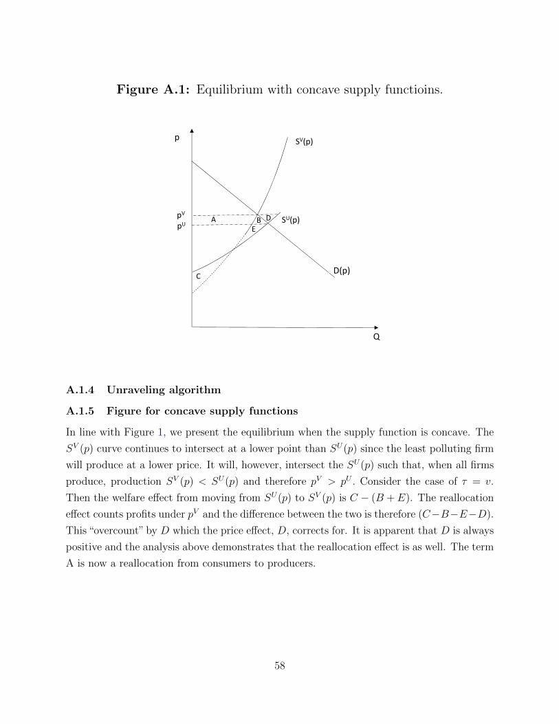
Figure A.1: Equilibrium with concave supply functioins.

SU(p)

SV(p)

pVpU

A B

CD(p)

Q

p

DE

A.1.4 Unraveling algorithm

A.1.5 Figure for concave supply functions

In line with Figure 1, we present the equilibrium when the supply function is concave. The

SV (p) curve continues to intersect at a lower point than SU(p) since the least polluting firm

will produce at a lower price. It will, however, intersect the SU(p) such that, when all firms

produce, production SV (p) < SU(p) and therefore pV > pU . Consider the case of τ = v.

Then the welfare effect from moving from SU(p) to SV (p) is C − (B +E). The reallocation

effect counts profits under pV and the difference between the two is therefore (C−B−E−D).

This “overcount” by D which the price effect, D, corrects for. It is apparent that D is always

positive and the analysis above demonstrates that the reallocation effect is as well. The term

A is now a reallocation from consumers to producers.

58

A.1.6 Extensions

Abatement

We add abatement by allowing all firms to reduce their emissions per unit from e to e−a by

spending b(a) of the outside good per unit, q, of production. We add that b(a) = 0 if a ≤ 0,

b′(0) = 0 as well as b′′(a) > 0 if a ≥ 0.

An uncertified firm cannot verify that it has abated and will consequently choose a = 0.

A certified ei chooses:

maxq,apq − c(q)− τ(ei − a)q − b(a)q,

which defines optimal abatement as τ = b′(a∗) which we write as a∗(τ). We define A(τ) =

τa∗(τ)− b(a∗(τ)). This leads to an optimal supply of:

qi = s(p− τei + A(τ)) = c′−1(p− τei − A(τ)).

For some tax on certification of f the equilibrium indifferent firm is then defined as:

π(p− τ e+ A(τ))− π(p− τE(e|e > e)) + F + f,

since uncertified firms are taxed on quantity at t = τE(e|e > e). With abatement it is

perfectly possible that all firms wish to certify even for F + f > 0.

Differences in emissions The difference in emissions between no certification and cer-

tification is given by:

GV −GU

= E (e) s(pU − τE (e)

)−(∫ e

e

(e− a∗) s(pV − τe+ A

)ψ (e) de+ s

(pV − τE (e|e > e)

)E (e|e > e) (1−Ψ (e))

)= E (e) s

(pU − τE (e)

)− E (e) s

(pV − τE (e)

)︸ ︷︷ ︸price effect

+ E (e) s(pV − τE (e)

)− E

(εs(pV − τε

))︸ ︷︷ ︸reallocation effect

+

∫ e

e

[es(pV − τe

)ψ (e)− (e− a∗) s

(pV − τe+ A(τ)

)ψ (e)

]de︸ ︷︷ ︸ .

abatement effect

The sum of the price effect and the reallocation effect replicate Lemma 1. The abatement

effect can be written to give equation (13). Note, that we have slightly misused notation: pV

59

and pU here refer to prices with abatement whereas in Lemma 1 they refer to those without

abatement.

Differences in welfare Writing the difference in welfare between certification and no

certification we get:

W V −WU =

∫ pV

pU(s (p− τE (e))−D (p)) dp︸ ︷︷ ︸

price effects

+ E(π(pV − τε

))− π

(pV − τE (e)

)︸ ︷︷ ︸reallocation gains

−(v − τ)(GV −GU

)︸ ︷︷ ︸untaxed emissions

+ Ψ (e)(E(π(pV − τe+ A(τ)

)− π

(pV − τe

)|e < e

))︸ ︷︷ ︸abatement gains

− FΨ (e) + o(τ 2),

where the abatement gains are what we add to the expression in the main text.

Taylor expansion. We follow an approach analogous to Section A.1.2 and let p0 be the

price at τ = 0. We start out by taking a Taylor expansion of the optimal level of abatement

b′(a) = τ to get:

b′(0) + ab′′(a) = τ + o(τ).

We exploit that b′(0) = 0 to write:

a =τ

b′′(0)+ o(τ),

which implies that:

A(τ) = τa− b(a) =τ 2

b′′(0)−(b′(0)a+

1

2b′′(0)a2

)+ o(τ 2) =

1

2

1

b′′(0)τ 2 + o(τ 2).

Since A(τ) is second order we recover the result that:

pV = pU + o(τ) = p0 + τE(e)s′(p0)

s′(p0)−D′(p0)+ o(τ).

We therefore recover the results of the price effect and the reallocation effect as:∫ pV

pU(s (p− τE (e))−D (p)) dp = o

(τ 2)

E(π(pV − τε

))− π

(pV − τE (e)

)=s′ (p0)

2τ 2V ar (ε) + o

(τ 2).

60

The abatement effect becomes:

Ψ (e)(E(π(pV − τe+ A(τ)

)− π

(pV − τe

)|e < e

))=

∫ e

e

(s (p0)

((pV − τe+ A(τ)− p0

)−(pV − τe− p0

))+ s′(p0)

2

((pV − τe+ A(τ)− p0

)2 −(pV − τe− p0

)2)

+ o (τ 2)

)de

= s (p0)τ 2

2b′′ (0)Ψ (e) + o

(τ 2).

Finally, the change in pollution is given by

GU −GV

= E (e) s(pU − τE (e)

)− E (e) s

(pV − τE (e)

)+ E (e) s

(pV − τE (e)

)− E

(εs(pV − τε

))+∫ e

e

[es(pV − τe

)ψ (e)− (e− a∗) s

(pV − τ (e− a∗)− b (a∗)

)]ψ (e) de+ o(τ)

= s′ (p0) τV ar (ε)

+

∫ e

e

e(s (p0) + s′ (p0)

(pV − τe− p0

))−e(s (p0) + s′ (p0)

(pV − τ (e− a∗)− b (a∗)− p0

))+a∗s (p0) + o (τ)

ψ (e) de+ o (τ)

= s′ (p0) τV ar (ε) +

∫ e

e

(−es′ (p0)

(τ 2

2b′′ (0)

)+

τ

b′′ (0)s (p0) + o (τ)

)ψ (e) de+ o (τ)

= s′ (p0) τV ar (ε) + Ψ (e)τ

b′′ (0)s (p0) + o (τ) .

We add these terms up (and multiply (GU −GV ) with (v − τ)) as well as FΨ(e) :

W V −WU = (v − τ

2)τ

[s′ (p0)V ar (ε) +

Ψ (e) s (p0)

b′′(0)

]− FΨ(e) + o(τ 2).

Heterogenous Productivity

We revert to a setting without abatement, but firms have heterogenous productivity ϕ > 0

such that costs of firm i is c(q)/ϕi. The resulting supply function of an (untaxed) firm is

s(ϕip). In the following, we will consider the special case of iso-elastic supply curve such that

supply of certified and uncertified firms, respectively, are:

qi = s0 [ϕi(p− τe)]α ,

61

qi = s0 [ϕi(p− t)]α ,

where α > 0. We let the (unconditional) distribution of productivity be given by ψϕ(ϕ) and

the conditional distribution of emissions on productivity be given by ψe(e|ϕ).

The indifferent firm e(ϕ) must be conditioned on productivity through:

1

ϕπ (ϕ (p− τ e(ϕ)))− 1

ϕπ (ϕ (p− t)) = F + f,

where e(ϕ) is monotonically increasing in ϕ.

The output tax is given by total emissions of uncertified firms divided by total output of

uncertified firms:

t = τ

∫ϕψϕ (ϕ)

∫∞eϕes (ϕ (p− t))ψe (e|ϕ) dedϕ∫

ϕψϕ (ϕ) s (ϕ (p− t)) (1−Ψe (e(ϕ)|ϕ)) dϕ

= τ

∫ϕψϕ (ϕ)

∫∞eϕeϕαψe (e|ϕ) dedϕ∫

ϕψϕ (ϕ)ϕα (1−Ψe (eϕ|ϕ)) dϕ

= τ

∫ϕE(eϕα|ϕ, e > e(ϕ))ψϕ(ϕ)dϕ∫

ϕϕαE(e|ϕ, e > e(ϕ))ψϕ(ϕ)dϕ

,

where we let tU denote the tax when no certification is in place (e(ϕ) = e for all ϕ) and tV

the tax on uncertified firm when certification is in place.

The market clearing condition is given by:

D (p) =

∫ϕ

(∫ e(ϕ)

e

s0 [ϕ (p− τe)]α ψ (e|ϕ) de+ s0 [ϕ (p− t)]α (1−Ψ (e(ϕ)))

)ψϕ(ϕ)dϕ.

(31)

We can collect welfare and emissions effects and write:

W V −WU (32)

=

∫ pV

pU

[(∫ϕ

s(ϕ(p− tU

))ψϕ (ϕ)

)dϕ−D (p)

]dp︸ ︷︷ ︸

price effects

+

∫ϕ

1

ϕ

( ∫ e(ϕ)

eπ(ϕ(pV − τe

))ψe (e|ϕ) de

+ (1−Ψe (e(ϕ)|ϕ))π(ϕ(pV − t

))− π

(ϕ(pV − tU

)) )ψϕ (ϕ) dϕ︸ ︷︷ ︸reallocation gains

−(v − τ)(GV −GU

)︸ ︷︷ ︸untaxed emissions

− F∫ϕ

ψϕ (ϕ) Ψϕ (eϕ|ϕ) dϕ,

62

where:

GV −GU

=

∫ϕ

ψϕ (ϕ)(s0

(ϕ(pU − tU

))α − s0

(ϕ(pV − tU

))α)E (e|ϕ) dϕ︸ ︷︷ ︸

price effect

+

∫ϕ

ψϕ (ϕ) dϕ

E (e|ϕ) s

(ϕ(pV − tV

))−[∫ e(ϕ)

es(ϕ(pV − τe

))eψe (e|ϕ) de

+ (1−Ψe (e(ϕ)|ϕ)) s0

(ϕ(pV − tV

))αE (e|e > e(ϕ), ϕ)

]

︸ ︷︷ ︸reallocation

.

Differentiating equation (31) returns:

pV = pU + o(τ)

and the elements of equation (32) are given by

Price Effects = o(τ 2),

Reallocation gains = τ 2S(p0) 12αp0V ar (ε) + o(τ 2),

where S(p0) is total production under p0:

S (p0) = D (p0) =

∫ϕ

s (ϕp0)ψϕ (ϕ) dϕ = s0pα0

∫ϕ

ϕαi ψϕ(ϕ)dϕ.

and S ′(p0) = αS(p0)/p0, such that we replicate the slope of aggregate supply from Corollary

1.

Furthermore:

V ar(ε) =

∫ϕ

∫ε

(ε− E(ε)

)2

ψ(ϕ, ε)dεdϕ,

where:

ψ(ϕ, ε) =ϕαψe(e|ϕ)ψϕ(ϕ)∫ϕ

∫εϕαψ(ϕ, ε)dεdϕ

is the output-scaled joint distribution of ϕ and ε. The expectation is defined analogously:

63

E(ε) =∫ϕ

∫εεψ(ϕ, ε)dεdϕ, such that:

E(ε) =

∫ϕ

∫εεϕαψe(e|ϕ)ψϕ(ϕ)∫

ϕ

∫εϕαψ(ϕ, ε)dεdϕ

dεdϕ =

∫ϕ

∫εε [ϕp0]α ψe(e|ϕ)ψϕ(ϕ)∫

ϕ

∫ε[ϕp0]α ψ(ϕ, ε)dεdϕ

dεdϕ

=

∫ϕ

[∫e>e(ϕ)

eψe(e|ϕ) +∫e<e(ϕ)

E(e|e > e(ϕ), ϕ)]pα0ϕ

αψϕ(ϕ)∫ϕ

∫ε[ϕp0]α ψ(ϕ, ε)dεdϕ

dεdϕ =GU

SU,

where GU and SU are emissions and total supply without certification.

Change in emissions are given by:

GV −GU = −τS (p0) αp0V ar (ε) ,

which then delivers:

W V −WU = τ(ν − τ

2

) αS (p0)

p0

V ar (ε)− FEϕΨϕ(e(ϕ)) + o(τ 2).

Free Entry

In the following we allow for free entry. In particular, firms pay an entry cost FE before

drawing an emission rate. This implies an endogenous mass of firms N . Consequently,

market clearing is given by:

D(p) = N

(∫ e

e

s(p− τe)ψ(e)de+ (1−Ψ(e))s(p− t)), (33)

where N is endogenously given by requiring entry costs to equal expected profits prior to

drawing the emission rate.∫ e

e

π(p− τe)ψ(e)de+ π(p− t)(1−Ψ(e)) = FE. (34)

We note that free entry implies that total profits equal 0. Consequently, we can take an

approach analogous to Section A.1.2 and find the change in welfare as

W V −WU = −∫ pV

pUD(p)dp− (v − τ)

(GV −GU

)−NV FΨ(e), (35)

64

where we note that profits equal zero due to free entry.

Emissions are given by:

GU −GV

= NV[E (e) s

(pU − τE (e)

)− E (e) s

(pV − τE (e)

)]︸ ︷︷ ︸price effect

+(NU −NV

)E (e) s

(pU − τE (e)

)︸ ︷︷ ︸entry effect

+NV

[E (e) s

(pV − τE (e)

)−[∫ e

e

es (p− τe)ψ (e) de+ s (p− t)E (e|e > e) (1−Ψ (e))

]]︸ ︷︷ ︸

reallocation effect

+ o(τ).

Taylor expansion

We take a Taylor expansion in equations (33) and (34) to find:

pV = pU + o (τ) = p0 + τE (e) + o (τ) ,

NV = NU + o (τ) = N0 + τD′ (p0)E (e)

s (p0)+ o(τ 2),

that is, at first order, the number of firms and the prices are the same in either equilibrium.

Consequently, at first order the welfare changes given by equation (35) excluding the certifi-

cation costs are zero. Since −∫ pVpU

D(p)dp is of the same order as (pV −pU) we therefore need

to develop pV − pU further. Analogous reasoning but taking a second order approximation

implies:

pV − pU = −τ2

2

s′ (p0)

s (p0)V ar (ε) + o

(τ 2),

which shows that the price will be lower with certification. The change in the number of

firms is given by:

NV −NU =τ 2

2

(−D′ (p0)

s′ (p0)

s (p0)+N0

((s′ (p0))2

s (p0)− s′′ (p0)

))V ar (ε) + o

(τ 2).

We then expand the first term of the welfare change to get:∫ pV

pU(−D (p)) dp = D (p0)

τ 2

2

s′ (p0)

s (p0)V ar (ε) + o

(τ 2)

=τ 2

2N0s

′ (p0)V ar (ε) ,

65

where we use that D(p0) = N0s(p0) at τ = 0.

And we proceed with the untaxed emissions term to get:

GV −GU = N0s′ (p0) τV ar (ε) + o (τ) ,

such that when τ is small:

W V −WU =(v − τ

2

)N0s

′ (p0) τV ar (ε)−NV FΨ (e) + o(τ 2).

The welfare expression is the same as in Corollary1 (regardless of whether τ = v or not).

Since profits are zero for producers the whole welfare effect (besides changes in emissions)

must accrue to consumers.

A.2 Adjustment on the extensive margin

A.2.1 Equilibrium without taxes

We consider a mass 1 of potential firms heterogenous in quantity they can produce, q, cost

of entry, c, and emissions per unit produced, e. All firms face the same price p which is

exogenous. The cost c has to be paid upfront and the firm faces to intensive margin of

construction. Consequently, without taxes, if pq ≥ c, the firm produces q and emits eq. The

joint distribution of (c, q, e) is Ψ(c, q, e). c has domain [c, c] and analogouosly for q and e.

The lower bound is positive for all. Ψ has full support. The aggregate supply function is

given by:

S =

∫ c

c

∫ q

q

∫ e

e

q1pq≥cdΨ(c, q, e). (36)

with corresponding emissions of:

G =

∫ c

c

∫ q

q

∫ e

e

eq1pq≥cdΨ(c, q, e). (37)

1pq≥c is an indicator function as is not differentiable at pq = c. Consequently, we employ

the Direct Delta Function and briefly remind the reader how this function operates. Strictly

speaking it is a functional with the properties that

δt−a = 0, for t 6= a,∫ a+ε

a−εf(t)δt−adt = f(a), for ε > 0,

66

that is a function that “picks out” the point t = a such that the integral around still sums

to 1.

For some vector (x, y) distributed according to Ψ(x, y) with pdf of ψ(x, y) and ψx(x) and

ψy(y|x). We consider the function:

F (a) =

∫x

∫y

1ax≥yf(y, x, a)dΨ(x, y),

for some constant a. We can differentiate wrt a to get:

F ′(a) =

∫x

∫y

∂g

∂a(x, y, a)δax=yf(y, x, a)dΨ(x, y) +

∫x

∫b

1ax≥y∂f

∂a(y, x, a)dΨ(x, y).

The second term is standard. The first term can be written as:∫x

∫y

xδax=yf(y, x, a)dΨ(x, y) =

∫x

x

∫y

δax=yf(y, x, a)ψy(y|x)ψx(x)dydx

=

∫x

xf(ax, x, a)ψy(ax|x)ψx(x)dydx.

We will be repeatedly exploiting this property in what follows.

In particular we differentiate equations (36) and (37) delivers:

S ′(p) =

∫c,q,e

q2δpq=cψc(c|e, q)ψq(q|e)ψe(e)dcdqde (38)

=

∫e

ψe(e)

∫q

q2ψc(pq|e, q)ψq(q|e)dqde,

G′(p) =

∫e

ψe(e)

∫q

eq2ψc(pq|e, q)ψq(q|e)dqde,

which gives equation (15) in the main text.

A.2.2 Equilibrium under certification

We consider a tax system in which, when certified a firm pays τ per unit emission for a total

tax of τeq. Instead of imposing a tax of f , we permit firms to certify to the point of e. Firms

still pay F . Consequently a firm with e > e will produce if:

(p− t)q ≥ 0,

67

and a firm with e ≤ e will produce if:

max{(p− τe)q − c− F, (p− t)q − c} ≥ 0.

Below we will use approximations. For reasons analoguous to the model on the intensive

margin welfare effects these welfare effects will only be positive if F is second order. Conse-

quently, any firm with e ≤ e with certify such that e = e and we can take e as an exogenous

variable.

t is defined (implicitly) as using the average emissions for uncertified firms:

t = τ

∫eq1e>e1(p−t)q≥cdΨ(c, q, e)∫q1e>e1(p−t)q≥cdΨ(c, q, e)

,

We write (where the integral is over (c, q, e) when not otherwise specified):

S(p, τ, t) =

∫q(1e≤e1(p−τe)q≥c+F + 1e>e1(p−t)q≥c

)dΨ(c, q, e),

G(p, τ, t) =

∫eq(1e≤e1(p−τe)q≥c+F + 1e>e1(p−t)q≥c

)dΨ(c, q, e),

where the mass of firms that certify is given by:

M =

∫1e≤e1(p−τe)q≥c+FdΨ(c, q, e).

We write welfare as:

W = pS − C − vG− FM

=

∫ [(pq − c− veq − F ) 1e≤e1(p−τe)q≥c+F + (pq − c− veq) 1e>e1(p−t)q≥c

]dΨ(c, q, e)

We seek Taylor approximations to W in τ but scale F and t accordingly. That is we define

F (τ) and t(τ) and differentiate wrt τ :

dW

dτ=

∫ [− (pq − c− veq − F ) (eq + F ′(τ)) 1e≤eδ(p−τe)q=c+F − (pq − c− veq) t′(τ)q1e>eδ(p−t)q=c

]dΨ(c, q, e)

(39)

−∫F ′(τ)1e≤e1(p−τe)q≥c+FdΨ(c, q, e).

Which, evaluated at τ = 0 and using that F is second order in τ and consequently F ′(0) = 0

68

as well as t(τ) = 0:

dW

dτ|τ=0 = −

∫[q (pq − c− veq) e1e≤eδpq=c + (pq − c− veq) 1e>et

′(0)δpq=c] dΨ(c, q, e). (40)

We define ψq(q) as the unconditional, ψe(e|q), and ψc(c|e, q) as the pdfs of Ψ. We use this

and substitute for c to get:

dW

dτ|τ=0 =

∫veq2 [e1e≤e + 1e>et

′(0)1e>e] δpq=cdΨ(c, q, e)

= v

∫q

q2ψq(q)

[∫e≤e

e2ψc(pq|e, q)ψe(e|q)de+

∫e>e

et′(0)ψc(pq|e, q)ψe(e|q)de]dq.

To get the second order derivative we rewrite equation (39) as:

dW

dτ=

∫q

ψq(q)q

[∫e≤e

(v − τ) eq (eq + F ′(τ))ψe(e|q)ψc((p− τe)q − F |e, q)de+

∫e>e

(ve− t(τ)) t′(τ)q2ψe(e|q)ψc((p− t)q|e, q)]dq

−∫q

ψq(q)F′(τ)

∫e≤e

ψe(e|q)Ψc((p− τe)q − F |e, q)dedq,

where Ψc(c|e, q) is the cdf of c conditional on e and q.

We differentiate again:

dW 2

dτ 2=

∫q

ψq(q)

[∫e≤e

ψe(e|q) (v − τ) eq (eq + F ′(τ)) (−eq − F ′(τ))ψ′c((p− τe)q − F |e, q) +

∫e>e

ψe(e|q) (ve− t) q2t′(τ) (−t′(τ)q)ψ′c((p− t)q|e, q)de]dq

+

∫q

ψq(q)

[∫e≤e

ψe(e|q) (v − τ) eqF ′′(τ)ψc ((p− τe)q − F |e, q) de+

∫e>e

ψe(e|q) (ve− t) q2t′′(τ)ψc ((p− t)q|e, q) de]dq

+

∫q

ψq(q)

[∫e≤e−ψe(e|q)eq (eq + F ′(τ))ψc ((p− τe)q − F |e, q) de+

∫e>e

−ψe(e|q)q2 (t′(τ))2ψc ((p− t)q|e, q) de

]dq

−∫ψq(q)F

′(τ)

∫e≤e

ψe(e|q) (−eq − F ′(τ))ψc ((p− τe)q − F |e, q) dedq

−∫q

ψq(q)F′′(τ)

∫e≤e

ψe(e|q)Ψc ((p− τe)q − F |e, q) dedq.

69

We evaluate this expression at τ = 0:

dW 2

dτ 2|τ=0 =

∫q

ψq(q)

(−∫e≤e

ψe(e|q)v (eq)3 ψ′c(pq|e, q)de−∫e>e

ψe(e|q)veq3 (t′(0))2ψ′c(pq|e, q)de

)dq

(41)

+

∫q

ψq(q)

(∫e≤e

ψe(e|q)veqF ′′(0)ψ′c(pq|e, q)de+

∫e>e

ψe(e|q)veq2t′′(0)ψc(pq|e, q)de)dq

+

∫q

ψq(q)

(∫e≤e−ψe(e|q) (eq)2 ψc(pq|e, q)de+

∫e>e

−ψe(e|q)q2 (t′(0))2ψc(pq|e, q)de

)dq

−∫q

ψq(q)F′′(0)

∫e≤e

ψe(e|q)Ψc(pq|e, q)dedq.

We will use this to perform a Taylor expansion of the welfare:

W (τ, v) = W (0, v) +dW

dτ|τ=0τ +

d2W

dτ 2|τ=0

τ 2

2+ o(τ 2),

and use equations (40) and (41) while noting that many terms are of higher than second

order. We further misuse notation and let ψe(e) be the unconditional distribution of e with

ψq(q|e) and ψc(c|e, q) denoting corresponding conditional distributions.

W (τ, v) = W (0, v) + τ

[ ∫e≤e

(v − τ

2

)ψe(e)e

2∫qψq(q|e)ψc(pq|e, q)dqde

+∫e>e

(ve− τ

2t′(0)

)t′(0)ψe(e)

∫qq2ψq(q|e)ψc(pq|e, q)dqde

]

+F

∫e≤e

ψe(e)

∫q

ψq(q|e)Ψc(pq|e, q)dedq + o(τ 2)

We use the definition of t(τ) to get:

t = τ

∫eq1e>e1(p−t)q≥cdΨ(c, q, e)∫q1e>e1(p−t)q≥cdΨ(c, q, e)

t′(τ) =

∫eq1e>e1(p−t)q≥cdΨ(c, q, e)∫q1e>e1(p−t)q≥cdΨ(c, q, e)

+ τ∂

∂τ

∫eq1e>e1(p−t)q≥cdΨ(c, q, e)∫q1e>e1(p−t)q≥cdΨ(c, q, e)

such that:

t = t(0) + t′(0)τ + o(τ 2) =

∫eq1e>e1pq≥cdΨ(c, q, e)∫q1e>e1pq≥cdΨ(c, q, e)

τ + o(τ 2).

70

We further define:

ψe (e) =ψe (e)

∫qψq (q|e) q2ψc (pq|e, q) dq∫

e′ψe (e′)

∫qψq (q|e′) q2ψc (pq|e′, q) dqde′

=ψe (e)

∫qψq (q|e) q2ψc (pq|e, q) dq

dSdp|τ=0

,

where dS/dp|τ=0 is given by equation 38. We then write:

W (τ, v) = W (0, v) +dS

dp|τ=0

[∫ e

0

τ(v − τ

2

)ψ(e)e2de+

∫e>e

(ve− t

2

)tψ(e)de

]

−F∫e≤e

ψe(e)

∫q

ψq(q|e)Ψc(pq|e, q)dedq + o(τ 2).

We introduce ε defined as:

ε =

e

E|ψe(e|e > e)

if e ≤ e

if e > e,

where E|ψe is the expection operator over ψe: E|ψe(e|e > e) =∫e>e eγe(e)de∫e>e γe(e)de

. Note this is

not the average emission rate above e > e since it is weighted by q2. We can also define

V ar|ψe(ε) = E|ψee2 − (E|ψee)

2. This gives:

W (τ, v)

= W (0, v) +dS

dp|τ=0

[τ(v − τ

2

)V ar|ψe (ε) + τ

(v − τ

2

) (E|ψe (e)

)2

+(

1− Ψe (e)) (t− τE|ψe (e|e > e)

) ((v − τ

2

)E|ψe (e|e > e)− t

2

) ]

−F∫e≤e

ψe(e)

∫q

ψq(q|e)Ψc(pq|e, q)dedq + o(τ 2),

where 1− Ψ(e) =∫e>e

ψ(e)de is the “share” of firms that don’t certify but weighted by q2.

We consider the welfare expression for τ = v to get:

W V (ν, ν)

= W (0, ν) +v2

2S ′(p)|τ=0

[V ar|ψe (ε) +

(E|ψe (e)

)2

−(

1− Ψe (e))(E|ψ (eq|e > e, pq > c)

E|ψ (q|e > e, pq > c)− E|ψe (e|e > e)

)2]

−F∫e<e

ψe (e)

∫q

ψq (q|e) Ψc (pq|e, q) dedq + o(τ 2),

71

where we make explicit that this is welfare for certification, W V , in anticipation for

welfare under no certification. We can make analoguous calculations as above to find that a

Taylor expansion of welfare under no certification is:

WU(t, v) = W (0, v) + t

∫q2δpq=c

[ve− 1

2t

]dΨ(q, c, e) + o(t2)

= W (0, v) + S ′(p)|τ=0E|ψe

(ve− 1

2τG (0)

S (0)

)τG (0)

S (0)+ o

(t2),

where G(0) and S(0) are emissions and supply under τ = 0. Then we can write:

W V−WU = S ′(p)|τ=0

v2

2V ar|ψe(ε) +

v2

2

(dGdp

dSdp

− G(0)

S(0)

)2

−(

1− Ψe(e)) v2

2

(E|ψe(e|e > e)− E|ψ(eq|e > e, pq > c)

E|ψ(q|e > e, pq > c)

)2

−F∫e≤e

ψe(e)

∫q

ψq(q|e)Ψc(pq|e, q)dedq + o(τ 2).

Change in emissions. Emissions are given by:

GV =

∫eq(1e≤e1(p−τe)q≥c+F + 1e>e1(p−tS)q≥c

)dΨ(c, q, e),

and

GU =

∫eq1(p−tU )q≥cdΨ(c, q, e),

where these refer taxes under Steve and uncertified.

We differentiate:

∂GV

∂τ= −

∫eq (eq + F ′(τ))

(1e≤eδ(p−τe)q=c+F

)dΨ(c, q, e)

−∫eq(tS ′q

) (1e>eδ(p−tS)q=c

)dΨ(c, q, e)

Evaluated at zero:

∂GV

∂τ|τ=0 = −

∫e2q2 (1e≤eδpq=c+F ) dΨ(c, q, e)−

∫eq2(tS ′(0)

)(1e>eδpq=c) dΨ(c, q, e)

= −∫e≤e

e2

∫q

q2ψc(pq|q, e)ψq(q|e)ψe(e)dqde− tS ′(0)

∫e>e

e

∫q

q2ψc(pq|q, e)ψq(q|e)ψe(e)dqde

72

= −S ′(p)∫e≤e

e2ψe(e)de− tV ′(0)S ′(p)

∫e>e

eψe(e)de

Further:∂GU

∂τ= −

∫eq2tU ′δ(p−tU )q=cdΨ(c, q, e)

such that:∂GU

∂τ|τ=0 = −S ′(p)tU ′(0)

∫eψe(e)de,

Let’s just look at

tU = τ

∫eq1(p−t)q≥cdΨ(c, q, e)∫q1(p−t)q≥cdΨ(c, q, e)

,

and we will get:tU

t=

∫eq1pq≥cdΨ(c, q, e)∫q1pq≥cdΨ(c, q, e)

+ o(τ)

tV

τ=

∫eq1e>e1pq≥cdΨ(c, q, e)∫q1e>e1pq≥cdΨ(c, q, e)

+ o(τ)

We use this for a first order taylor expansion in each and subtract the two:

GV−GU = −τS ′(p)[∫

e≤ee2ψe(e)de+

∫e>e

(E|ψe

)2

ψe(e)de−∫e>e

(E|ψe

)2

ψe(e)de+ tS ′(0)

∫e>e

eψe(e)de− tU ′(0)

∫eq2ψe(e)de

]

= −τS ′(p)[∫

e

ε2ψe(e)de−∫e>e

(E|ψe

)2

ψe(e)de+

∫eq1e>e1pq≥cdΨ(c, q, e)∫q1e>e1pq≥cdΨ(c, q, e)

∫e>e

eψe(e)de− tU ′(0)

∫eψe(e)de

]Change in emissions

We seek to establish what the change in emissions in given by:

GV =

∫eq(1e≤e1(p−τe)q≥c+F + 1e>e1(p−tV )q≥c

)dΨ(c, q, e),

and

GU =

∫eq1(p−tU )q≥cdΨ(c, q, e),

where these refer to t under certification and without. We wish to perform first-order Taylor-

expansions so we first find:

∂GV

∂τ|τ=0 = −S ′(p)

[V arψeε+

(E|ψee

)2Ψ(e) +

∫eq1e>e1pq≥cdΨ(c, q, e)∫q1e>e1pq≥cdΨ(c, q, e)

(1− Ψ(e))E|ψ(e)

],

73

∂GU

∂τ|τ=0 = −S ′(p)

∫eq1pq≥cdΨ(c, q, e)∫q1pq≥cdΨ(c, q, e)

E|ψ(e),

where we have used that

tV ′(0) =tV (0)

τ=

∫eq1e>e1pq≥cdΨ(c, q, e)∫q1e>e1pq≥cdΨ(c, q, e)

+ o(τ),

and likewise for tU .We write G(τ) = G(0) + ∂G/∂τ |τ=0 + o(τ) for both GV and GU and subtract to find:

GV−GU = −S′(p)τ[V arψe

(ε) +

(G′(p)

S′(p)− G(p)

S(p)

)Eψe

(e) + (1− Ψe(e))

(G(p)

S(p)Eψe

(e|e > e)− G′(p)

S′(p)Eψe

(e)

)]+o(τ),

which is equation (18) in the main text.

A.2.3 Special case for application to the Permian Basin

In the following we make two alterations to the expressions above. First, we let prices vary

across firms such that each firm is de+scribed by a vector (c, q, e, p) with an associated Ψ.

A firm receives a price per unit of p+ ρ, where ρ is a common element of prices.

Supply is given by:

S =

∫q(1e≤e1(p+ρ−τe)q>c+F + 1e>e1(p+ρ−t)q>c

)dΨ (c, q, e, p) .

and consequently:∂S

∂ρ|ρ=0,τ=0 =

∫c,q,e,p

q21pq>cdΨ(c, q, e, p).

We perform calculations in line with the section above to find:

W V (v, v)−WU (t (v) , v)

=dS

dρ|ρ=0,τ=0

v2

2V ar|ψe (ε) +

v2

2

(dGdρ

dSdρ

− G (0)

S (0)

)2

−(

1− Ψ (e)) v2

2

(E|ψe (e|e > e)− E|ψ (eq|e > e, pq > c)

E|ψ (q|e > e, pq > c)

)2

−FM + o(τ 2),

where:

ψe(e) =ψe (e)

∫pψp (p|e)

∫qψq (q|e, p) q2ψc (pq|e, q, p) dqdp

dSdρ|τ=0

,

and other expressions are done analoguously.

74

For our empirical investigation we impose:

c = upq,

where u is independent of (p, q, e). We use the distribution Γ(u, q, e, p) as the full distribu-

tion and defining the marginal distribution of u as Γu(u|q, e, p) = Γu(u). Further, we let

Γq,e,p(q, e, p) denote the distribution of (q, e, p). That is: Γ(u, q, e, p) = Γu(u)× Γq,e,p(q, e, p)

S =

∫u,q,e,p

q (1e≤e11≥u + 1e>e11≥u) dΓ (u, q, e, p) =

∫u

ψu(u)

∫q,e,p

qdΓq,e,p (q, e, p)

= Γu(1)

∫q,e,p

qdΓq,e,p (q, e, p) .

There is a mass 1 of potential firm so S denotes total production as well as average

production of potential firms.

Consequently:

E(q) =S

Γu(1)=

∫q,e,p

qdΓq,e,p (q, e, p)

is observable in the data where E(q) =∑

i qi/N is just the observed average in the pre-tax

equilibrium with N existing firms. Analogous calculations deliver:

E(q2) =

∫q,e,p

q2dΓq,e,p (q, e, p) ,

where E(q2) =∑

i q2i /N is the sample average of q2.

The expression for V arψe(ε) is:

V arψe (ε) = E

(ε2 q2

E (q2)

)−

(E

(eq2

E (q2)

))2

,

which naturally depends on the choice of e.

The remaining expressions are:

G (0)

S (0)=Edata (eq)

Edata (q).

Ψ (e) =Σ (q2|e > e)

Σ (q2),

75

E|ψ (eq|e > e, pq > c)

E|ψ (q|e > e, pq > c)=E (eq|e > e)

E (q|e > e),

M = Ndata (e ≤ e)

where∑

is just the sum in the data and |e > e only counts wells with e above the cutoff

e. Finally, M counts the number of firms with e ≤ e. Combining these terms gives equation

(??) in the main text.

A.3 The International Model

A.3.1 Baseline setting

We reproduce equations (20) and (19) in the pooling quilibrium (ρ = 0)

DH(pH) +DF (pF ) = (42)

EH [sH(pH − τHε+ AH)] +

∫ e

e

[sF (pH − τF e− κ+ AF )ψF (e)de] + (1−ΨF (e))sF (pF ).

pF = (pH − τFEF (e|e > e)− κ). (43)

And note that differentiating pH wrt. e gives:

dpH

de=

(D′F − (1−ΨF (e))s′F (pF )

)τF

∂EF (e|e>e)∂e

+ [sF (pF +AF )− sF (pF )]ψF (e){D′H(pH) +D′F (pF )−

∫ ee

[s′F (pH − τF e− κ+AF )ψF (e)de

]− (1−ΨF (e))s′F (pF )

} ,

dpF

de=−D′H(pH) +

∫ ee

[s′F (pH − τF e− κ+AF )ψF (e)de

]τF

∂EF (e|e>e)∂e

+ [sF (pF +AF )− sF (pF )]ψF (e){D′H(pH) +D′F (pF )−

∫ ee

[s′F (pH − τF e− κ+AF )ψF (e)de

]− (1−ΨF (e))s′F (pF )

} < 0,

where ∂E(e|e > e)/∂e > 0. Without abatement (AF = 0), pH must increase following an

increase in certification.

Proof of Proposition 3

The Welfare Expressions

We proceed under the assumption that W V −WU + FΨ(e) is second order in τ and will

demonstrate that this is so. W V is welfare under certification and WU is without certification.

W V is given by:

W V = CSH + CSF︸ ︷︷ ︸consumer surpluses

+ PSH + PSF︸ ︷︷ ︸producer surpluses

− [(v − τH)GH + (v − τF )GF + τFGF,dom]︸ ︷︷ ︸non-internalized emissions

− FΨF (e) ,

76

with

CSH = uH (CH)− pHCH and CSF = uF (CF )− pFCF .

PSH =

∫ ∞e

(pH − τHe+ AH) sH (pH − τHe+ AH)ψH (e) de−∫ ∞e

cH (sH (pH − τHe+ AH))ψH (e) de,

PSF =

∫ e

e

(pH − τF e+ AF − κ) sF (pH − τF e+ AF − κ)ψF (e) de

−∫ e

0

cF (sF (pH − τF e+ AF ))ψF (e) de+ (pF sF (pF )− cF (sF (pF ))) (1−ΨF (e)) ,

where cF and cH are the cost functions associated with Foreign and Home supply functions.

Further:

GH =

∫ e

e

(e− aH) sH (pH − τHe+ AH)ψH (e) de,

GF =

∫ e

e

(e− aF ) sF (pH − τF e+ AF − κ)ψF (e) de+ sF (pF )E (e|e > e) (1−ΨF (e)) ,

GF,dom = τFEF (e|e > e)DF (pF ) .

Taylor Approxiomations of price changes

We start out by taking a Taylor-approximation of the equilibrium without certification

(“U”) (equation (45 with e = e). Let p0 denote the prie in an equilibrium without taxes and

Foreign exports to Home. In such a setting p0 − κ is the price in Foreign. Letting the price

in the uncertified equilibrium be pUH this delivers:

pUH − p0 =s′H (p0) τHEH (e) + s

′F (p0 − κ) τFEF (e)−D′F (p0 − κ) τFEF (e)

s′H (p0) + s

′F (p0 − κ)−D′H (p0)−D′F (p0 − κ)

+ o (τ) . (44)

We derive approximations for the separating equilibrium with the understanding that

analogous derivations will deliver the expression for the pooling equilibrium.

It must always hold that:

DH(pH) +DF (pF )

=

∫ e

e

sH(pH − τHe+AH)ψH(e) +

∫ e

e

sF (pH − τF e+AF − κ)ψF (e)de+ sF (pF ) (1−ΨF (e))) ,

To a first order the expression above delivers:

D′H(p0)(pH − p0) +D′

F (p0 − κ)(pF − p0 + κ) (45)

77

= s′

H(p0)(pH−τHEH(e)−p0)+s′

F (p0−κ) (ΨF (e)(pH − τFEF (e|e < e) + (1−ΨF (e))(pF + κ)− p0)+o(τ),

where we use that:

AF = o(τ), AH = o(τ).

Further, for a separating equilibrium it must hold that at zeroth order:

sF (p0 − κ)(1−ΨF (e)) = DF (p0 − κ), (46)

which pins down e at zeroth order:

e = e0 + e+ o(τ), where e0 = Ψ−1F (1−DF (p0 − κ)/sF (p0 − κ)) ,

and e is the “first order” term of e. If e is such that equation (46) holds with “>” we are in

the pooling equilibrium, if it holds with “<” certified firms will not want to export. Note, e

and e0 differ only to a first order and consequently whether we evaluate functions at e or e0

will be equivalent in our Taylor expansions. For ease of exposition we will use e both here

and in equation (23) in the main text. This is correct, though a more stringent adherence

to convention would have us evaluate at e0 for the separating equilibrium.

Alternatively, Home firms export to Foreign. We preclude this here, but briefly discuss

the implications below. In effect this pins down e (at zeroth order).

From the certification condition, one gets (to a second order):

(pH − τF e−κ−pF )

(sF (p0 − κ) + s

′

F (p0 − κ)

(pH − τF e+ κ+ pF

2− p0

))= F + f + o(τ 2),

where again we use that AF = o(τ).(pH−τF e+κ+pF

2− p0

)is first order such that when (F+f)

is first order we get:

pH − τF e− pF = κ+

(F + f

sF (p0 − κ)

)+ o (τ) (47)

Note that this requires:

0 < τF (EF (e|e > e)− e)− F + f

sF (p0 − κ)< 2κ,

where both inequality use equation (47) and the first one ensures that profits from selling do-

78

mestically are strictly higher for uncertified Foreign firms and the right hand side guarantees

that Home firms would not want to export toWe use equation (47) along with equation (45) to get:

pVH − p0 =

s′H(p0)τHEH(e) + s

′F (p0 − κ)

(ΨF (e0)τFEF (e|e < e0) + (1−ΨF (e0))

(τF e0 + F+f

sF (p0−κ)

))−D′

F (p0 − κ)(τF e0 + F+f

sF (p0−κ)

) s′H(p0) + s

′F (p0 − κ)−D′

H(p0)−D′F (p0 − κ)

+ o(τ),

and combine this with equation (44) to get

pVH − pUH =

=

(1−ΨF (e0)) s′F (p0 − κ)

((τF e0 + F+f

sF (p0−κ)

)− τFEF (e|e > e0)

)−D′F (p0 − κ)

(τF e0 + F+f

s(p0−κ)− τFEF (e)

) s′H (p0) + s′H (p0 − κ)−D′H (p0)−D′F (p0 − κ)

+ o (τ) , (48)

and

pVF − pUF =

s′H (p0)

(τFEF (e)−

(τF e0 + f

sF (p0)

))+s

′F (p0 − κ)

(τFEF (e)− (1−ΨF (e)) τFEF (e|e > e0)−ΨF (e)

(τF e+ f

sF (p0−κ)

))−(τFEF (e)−

(τF e0 + f

sF (p0−κ)

))D

′H (p0)

s′H (p0) + s

′F (p0 − κ)−D′

H (p0)−D′F (p0 − κ)

+ o(τ) (49)

We define εDF = D′F (p0 − κ)(p0 − κ)/DF (p0 − κ) = D′F (p0 − κ)p0/DF (p − κ) + o(τ)

since κ is of the same order as τ . We further define Home share in demand θDF = DF (p0 −κ)/ (DF (p0 − κ) +DH(p0)). Analogous versions of ε and θ exist for Home and supply and

we let εD = θDF εDF + θDHε

DH . We then write:

pVH − pUH =

=

(1−ΨF (e0)) θSF εSF

((τF e0 + F+f

sF (p0−κ)

)− τFEF (e|e > e0)

)−εDF θDF

(τF e0 + F+f

s(p0−κ)− τFEF (e)

) εS − εD

+ o (τ) .

We then use the definition of ρ = pF−(pH−τFEF (e|e > e)−κ) = −(τF (e0 − EF (e|e > e0))+

79

(F+f

sF (p0−κ)

)) to write:

pVH − pUH =−εDF θDFεS − εD

τF (EF (e|e > e0)− EF (e))− (1−ΨF (e0)) εSF θSF − εDF θDF

εS − εDρ+ o (τ) .

Analgous derivations for pVF−pUF as well as the expressions for the pooling equilibrium delivers

the expressions in footnote 21.

Taylor approximations for welfare changes

We separate expressions from the welfare change. First, we write consumer and producer

surplus terms as:

CSVH + CSVF + PSVH + PSVF −(CSUH + CSUF + PSUH + PSUF

)=

EH

(∫ pVHpUH

sH (p− τHe+ AH) dp)

+ EF

(∫ pVHpUH

sF (p− τFEF (e)− κ) dp)

−(∫ pVF

pUFDH (p) dp+

∫ pVFpUF

DF (p) dp)

︸ ︷︷ ︸price effect

+(1−ΨF (e)) [πF (pF )− πF (pH − τFEF (e|e > e)− κ)]︸ ︷︷ ︸adjustment term

+ΨF (e)EF ((πF (pH − τF e+ AF − κ)− πF (pH − τF e− κ)) |e < e)︸ ︷︷ ︸abatement gains

+E (πF (pH − τF ε− κ))− πF (pH − τFEF (e)− κ)︸ ︷︷ ︸reallocation term

.

and handle the terms in order:

price effects

= EH

(∫ pVH

pUH

sH (p− τHe+ AH) dp

)+ EF

(∫ pVH

pUH

sF (p− τFEF (e)− κ) dp

)

−

(∫ pVF

pUF

DH (p) dp+

∫ pVF

pUF

DF (p) dp

)= −DF (p0 − κ)

(pVF − pVH + τFEF (e) + κ

)+(pVH − pUH

) s′H (p0)

(pVH+pUH

2− τHEH (e)− p0

)+sF ′ (p0 − κ)

(pVH+pUH

2− τFEF (e)− p0

)−D′H (p0)

(pVH+pUH

2− p0

) −D′F (p0 − κ)

(pVF − pUF

)(pVF + pUF2

− p0 + κ

).

80

Taylor approximations of the market clearing under certification and no certification, respec-

tively gives:

D′

H (p0)(pVH − p0

)+D

′

F (p0 − κ)(pVF − p0 + κ

)+ o (τ)

= s′

H (p0)(pVH − τHEH (e)− p0

)+s

′

F (p0 − κ)(ΨF (e)

(pVH − τFEF (e|e < e)

)+ (1−ΨF (e))

(pVF + κ

)− p0

)and

D′

H (p0)(pUH − p0

)+D

′

F (p0 − κ)(pUF − p0 + κ

)+ o (τ)

= s′

H (p0)(pUH − τHEH (e)− p0

)+ s

′

F (p0 − κ)(pUF + κ− p0

)summing up the two we have

s′

H (p0)

(pVH + pUH

2− τHEH (e)− p0

)+s

′

F (p0 − κ)

(ΨF (e)

(pVH − τFEF (e|e < e)

)+ (1−ΨF (e))

(pVF + κ

)+ pUH − τFEF (e)

2− p0

)

−D′H (p0)

(pVH + pUH

2− p0

)−D′F (p0 − κ)

(pVF + pUF

2− p0 + κ

)= 0,

which we use to get:

price effects

= −DF (p0 − κ) (pF − pH + τFEF (e) + κ)

+(pVH − pUH

)s′

F (p0 − κ)(1−ΨF (e))

(pVH − pVF − κ− τFEF

(e|e > eF

))2

+D′

F (p0 − κ)(pVH − pVF − τFEF (e)− κ

)(pVF + pUF2

− p0 + κ

)We continue with the reallocation term:

81

reallocation term

= E(πF(pVH − τF ε− κ

))− πF (pH − τFEF (e)− κ)

=s′F (p0 − κ)

2(τF )2 V arF (ε) + o

(τ 2)

and the abatement term:

abatement term = ΨF (e) sF (p0 − κ)AF + o(τ 2),

and

adjustment term

= (1−ΨF (e))(pVF + κ− pVH + τFE (e|e > e)

) [ sF (p0 − κ)

+s′F (p0 − κ)

[pVF+κ+pVH−τFE(e|e>e)

2− p0

] ]+ o(τ 2).

We add the terms with emissions:

(v − τH)(GVH −GU

H

)+ (v − τF )

(GVF −GU

F

)+ τF

(Gdom,VF −Gdom,U

F

)which we take in turn:

(v − τH)(GVH −GU

H

)= −

(ν − τH

)EH (e) sH′ (p0)

(pH,LB − pH

)+ o (τ)

(ν − τF )(GVF −GU

F

)= − (ν − τF )

s′F (p0 − κ)

( (pUH − pVH

)EF (e) + τFV arF (ε)

+(pVH − τFEF (e|e > e)− pVF − κ

)EF (e|e > e) (1−ΨF (e))

)+ΨF (e) aF sF (p0 − κ)

82

and further:

τF

(Gdom,VF −Gdom,U

F

)= −τF (EF (e)− EF (e|e > e))DF (p0 − κ)

−D′F (p0 − κ)[τFEF (e)

(pUF − p0 + κ

)− τFEF (e|e > e)

(pVF − p0 + κ

)]+ o

(τ 2)

We combine these terms with equations (48) and the corresponding expression for pF to get

(using that F is second order whereas f is (potentially) first order).

W V −WU (50)

= −s′F (p0 − κ)

2(1−ΨF (e))

(τEF (e|e > e)−

(τF e+

f

sF (p0 − κ)

))(pVF − pUF + τF (EF (e|e > e)− EF (e))

)−D

F ′ (p0 − κ)

2

(pVF − pUF

)(τFEF (e) + τF e+

f

sF (p0 − κ)

)+s′F (p0 − κ)

2(τF )2 V arF (ε) + ΨF (e) sF (p0 − κ)AF

+ (v − τH)(GUH −GV

H

)+ (v − τF )

(GUF −GV

F

)− FΨF (e) ,

and changes in emissions are given by:

GVH −GU

H = EH (e) s′

H (p0)(pVH − pUH

)+ o (τ) ,

GVF −GU

F

= −

s′F (p0 − κ)

( (pVH − pUH

)EF (e) + τFV arF (ε)

+(τF e+ f

sF (p0−κ)− τFE (e|e > e)

)EF (e|e > e) (1−ΨF (e))

)+ΨF (e) aF sF (p0 − κ)

+o(τ).

Combine the definition of the indifferent firms:

pVH − pVF = τF e+ κ+f

sF (p0 − κ)+ o (τ) , (51)

with the definition of ρ to get:

ρ = −(τF e+

(f

sF (p0 − κ)

)− τFE(e|e > e)

).

83

Further note that :

∆pH + ρ = ∆pF + τF [EF (e|e > e)− EF (e)] . (52)

Use these expressions as well as GVH − GU

H and GVF − GU

F in equation (50) to get equation

(23) in the main text.

∆pH + ρ > 0 and the Encouraged Foreign Production Effect is always (weakly)

positive

Note, that ∆pH + ρ = ∆pF + τF [EF (e|e > e)− EF (e)] such that:

∆pF + τF [EF (e|e > e)− EF (e)]

=

[sH′ (p0) + s

′FΨF −D

′H

]sH′ (p0) + sF ′ (p0 − κ)−DH′ (p0)−DF ′ (p0 − κ)

ρ

− τFD′ [EF (e|e > e0)− EF (e)]

sH′ (p0) + sF ′ (p0 − κ)−DH′ (p0)−DF ′ (p0 − κ),

where both ρ and [EF (e|e > e0)− EF (e)] are positive. Consequently ∆pH + ρ > 0 and the

Encouraged Foreign Production Effect is always positive in the separating equilibrium. In

the pooled equilibrium it is zero (since ρ = 0).

The sign of the Untaxed Foreign Consumption Effect is ambigious

First, we prove that τF [EF (e) + EF (e|e > e)]− ρ > 0

Recall that:

ρ = pF − (pH − τFEF (e|e > e)− κ),

and

pH − τF e− pF = κ+

(F + f

sF (p0 − κ)

)+ o (τ) .

such that:

τF (EF (e) + EF (e|e > e0))− ρ = τEF (e) +

(F + f

sF (p0 − κ)

)+ τF e > 0

Second, we prove that the sign ∆pF is ambigious. From footnote 21 we recall that:

∆pF =εDHθ

DH − εS

εS − εDτF (EF (e|e > e)− EF (e)) +

εS − εSF θSF (1−ΨF )− εDHθHDεS − εD

ρ,

84

where the first term is negative and the second term is positive. Clearly ∆pF ≤ 0 in the

pooling equilibrium (when ρ = 0) and by continuity for some parameters in the separating

equilibrium as well. e0 is defined by:

sF (p0 − κ)(1−ΨF (e0)) = DF (p0 − κ)

such that if DF (p0 − κ)/sF (p0 − κ) is less than but close to 1 we will have e0 ≈ e. Consider

a case where e = 0 and F + f ≈ 0. Then EF (e|e > e)− EF (e) ≈ 0 and:

pH − pF ≈ κ+ o (τ) .

and consequently:

ρ ≈ pF − (pH − τFEF (e|e > e)− κ) = τFEF (e|e > e) + o(τ) > 0,

and consequently ∆pF < 0.

A.3.2 The change in emissions

Calculations as above can be written as:

GH,LB −GH =(ν − τH

)EH (e) sH′ (p0)

(pH,LB − pH

)+ o (τ)

GF,LB −GF

=

sF ′ (p0 − κ)

( (pH,LB − pH

)EF (e) + τFV ar (ε)

+(τF eF + F+f

sF (p0−κ)− τFE

(e|e > eF

))E(e|e > eF

) (1−ΨF

(eF)) )

+ΨF(eF)aF sF (p0 − κ)

GH,LB −GH = EH (e) sH′ (p0)DF ′ (p0 − κ)

(τFE

(e|e > eF

)− τFEF (e)

)sH′ (p0) + sF ′ (p0 − κ)−DH′ (p0)−DF ′ (p0 − κ)

GF,LB −GH =

sF ′ (p0 − κ)

(DF ′(p0−κ)(τFE(e|e>eF )−τFEF (e))EF (e)

sH′(p0)+sF ′(p0−κ)−DH′(p0)−DF ′(p0−κ)+ τFV ar (ε)

)+ΨF

(eF)aF sF (p0 − κ)

we have

pVH − pUH =

85

=

(1−ΨF (e0)) s′F (p0 − κ)

((τF e0 + F+f

sF (p0−κ)

)− τFEF (e|e > e0)

)−D′F (p0 − κ)

(τF e0 + F+f

s(p0−κ)− τFEF (e)

) s′H (p0) + s′H (p0 − κ)−D′H (p0)−D′F (p0 − κ)

+ o (τ) , (53)

A.3.3 Optimal policy

In the following, we look at the optimal policy. A social planner offers a price pRE−τF (e−a) to

(Foreign) firms who reveal their e and undertake abatement a. It offers pUE to exporters who

do not reveal. The social planner can also pick a certification tax. Further, we potentially

allow for the social planner to choose exports from Home to Foreign (bilateral trade). The

social planner is constrained by market forces in Foreign and must take the behaviors of

foreign firms, inluding whether they choose to certify, and the resulting Foreign prices pF as

a given. Uncertified Foreign firms will export if:

pUE − κ = pF ,

and not if pUE − κ < pF . We preclude pUE − κ > pF by assuming that there is always some

Foreign demand. Uncertified exporting foreign firms, if they exist, must then make the

same profits as foreign firms selling for the domestic market. An indifferent firm exists with

πF(pRE − τF (e− a)− b (a)− κ

)− F − f = πF (pF ) , which must hold whether there are

uncertified exporters or not. f plays no other role than here and the social planner can

equivalently choose e.

The Foreign domestic market clears with:

u′F (CF ) = pF ∧ CF = DF (pF ) ,

qU = sF (pF ) ,

CF = sF (pF ) (1−ΨF (e))−M,

where qU is production by uncertified Foreign firms. M is the import from Home of uncertified

exports (from Foreign). M = 0 in the separating equilibrium and M > 0 in the pooling.

86

We write the objective function (world welfare) as:

W (54)

= uH

(∫ ∞0

qH (e)ψH (e) de+

∫ e

0

sF(pRE − τF (e− aF )− bF (aF )− κ

)ψF (e) de+MU

)−∫ ∞

0

(cH (qH (e)) + bH (aH (e)) qH (e))ψH (e) de

+uF (DF (pF ))−∫ e

0

(cF(sF(pRE − τF e+ AF − κ

))+ (bF (aF ) + κ) sF

(pRE − τF e+ AF − κ

))ψF (e) de− cF (sF (pF )) (1−ΨF (e))

−κ |M | − v(∫ ∞

0

(e− aH (e)) qH (e)ψH (e) de+

∫ e

0

(e− aF ) sF(pRE − τF (e− aF )− bF (aF )− κ

)ψF (e) de+ EF (e|e > e) sF (pF ) (1−ΨF (e))

)−FΨF (e) ,

with the constraint that Foreign markets clear: D(pF)

= sF(pF) (

1−ΨF(eF))−M . We

solve the corresponding Lagrange problem and let λ be the lagrange multiplier. The social

planner can choose [qH (e)]e≤e, [aH (e)]e≤e, pRE, τF , M and pF . We note that pUE is irrelevant

here: either M > 0 and it is equal to pF + κ or M ≤ 0 and the exact value does not matter

(because their are no uncertified exporting firms). We then derive first order conditions and

subsequently check the three cases of M (< 0, = 0 and > 0).

The first order conditions of this problem are:

wrt. qH(e): u′H (CH)− c′H (qH (e))− bH (aH (e))− v (e− aH (e)) = 0

wrt. aH(e) : b′H (aH (e)) = ν

so this is consistent with firms paying a tax τH = ν at home, undertaking optimal abatement

and facing a price pH = u′H (CH).

wrt. pRE :

∫ e

0

(pH − pRE + (τF − v) (e− aF )

)s′F(pRE − τF (e− aF )− bF (aF )− κ

)ψF (e) de = 0,

(55)

wrt. pF :D′F (pF ) pF−s′F (pF ) (pF + vEF (e|e > e)) (1−ΨF (e))+λ (s′F (pF ) (1−ΨF (e))−D′F (pF )) = 0,

87

FOC wrt to M :

λ = pH − κ if M > 0,

λ = pH + κ if M < 0,

or we have DF (pF ) = sF (pF ) (1−ΨF (e)) if M = 0.

FOC wrt τF leads to:∫ e

0

[ (pRE − pH + (ν − τF ) (e− aF )

)s′F(pRE − τF (e− aF )− bF (aF )− κ

)(− (e− aF ))

+daFdτF

(b′F (aF )− ν)(sF(pRE − τF (e− aF )− bF (aF )− κ

)) ]ψF (e) de(56)

= 0

FOC wrt eF

pHsF(pRE − τF

(eF − aF

)− bF (aF )− κ

)− cF

(sF(pRE − τF e+ AF − κ

))− (bF (aF ) + κ) aF

(pRE − τF e+ AF − κ

)+cF (sF (pF ))− v

((e− aF ) sF

(pRE − τF (e− aF )− bF (aF )− κ

)− esF (pF )

)− F − λaF (pF )

= 0.

Equations (55) and (56), give us that

pH = pRE and τF = τH = ν.

This leaves

pFD′F (pF )−s′F (pF ) (pF + vEF (e|e > e)) (1−ΨF (e))+λ (s′F (pF ) (1−ΨF (e))−D′F (pF )) = 0

λ = pH − κ if M > 0

λ = pH + κ if M < 0

πF (pH − τF (e− aF )− bF (aF )− κ)− F = (λ− ve) sF (pF )− cF (sF (pF )) .

88

Solving for these equations return:

t = vs′F (pF )EF (e|e > e) (1−ΨF (e))

s′F (pF ) (1−ΨF (e))−D′F (pF ),

and

πF (pH − τF (e− aF )− bF (aF )− κ)− F − f = πF (pF ) ,

with a certification tax

f = (t− ve) sF (pF ) .

Where if M > 0 (pooling equilibrium) we have λ = pH − κ and:

pF = pH − t− κ,

and if M < 0 (Home exports) we have λ = pH + κ and

pF = pH − t+ κ,

and if M = 0 (separating equilibrium) pF is defined by:

sF (pF ) (1−ΨF (e)) = DF (pF ) .

Which one of these equilibria is optimal depends on prices and transportation costs. This

requires:

pH − pF − κ < t < pH − pF + κ.

We compare welfare in equation (54) to that of a setting with no Home taxes on Foreign

exports, τF = t = 0, to find. We label this WLF (for laissaz-faire). We perform calculations

of a Taylor expansion along the lines of those in previous sections (details omitted) to find:

W ∗ −WLF = s′

F (p0 − κ)v2

2V ar(ε) + ΨF (e)AF sF (p0 − κ)− FΨF (e)

+D′

F (p0 − κ)t∗

2EF (e|e > e)− s′F (p0 − κ)

v

2EF (e)

(p∗H − vEF (e)− pLFH

),

where:

t∗ = vs′F (pF )EF (e|e > e) (1−ΨF (e))

s′F (pF ) (1−ΨF (e))−D′F (pF ),

is the optimal tax on uncertified exports. The welfare expression holds in all three cases,

89

though strictly speaking t∗ only applies as a tax in the pooling equilibrium.

B Data Appendix

B.1 Domestic Application

Lease-level annual production in the Permian basin is pulled from the online portals of the

states of Texas and New Mexico. In 2019, daily production was about 4.9 million barrels per

day of oil and 18 million barrels of oil-equivalent of natural gas. There were approximately

75,000 leases actively producing, two thirds of which were in Texas. Texas wells were more

productive on average, yielding 75-80% of the basin’s oil and gas.

The combination of a steep decline in production over the life of the well, and heteroge-

neous skill and deposit resource (Covert (2018)) means that there is enormous heterogeneity

in productivity across wells. This is plotted as a kernel density on a natural log scale in

Figure B.1a.

While 20% of wells produce only gas, and 13% only oil, the overwhemling majority of

output comes from wells that produce a mix of the two. In Figure B.1b this is presented as a

kernel density, in which the oil share is weighted by well production. Most output comes from

wells producing about 80% oil, which in the absence of sufficient collection infrastructure,

may make flaring an attractive option for economically disposing of methane.

To estimate emissions rates, we use the joined emissions-production data from the Sup-

plementary Information to Robertson et al. (2020). The oil share and whether the site was

‘simple’ or ‘complex’ is also reported. Complex sites have some combination of storage tanks

and compressors, disproportionate sources of emissions, and was the basis of stratification

in the study: nearly 90% of simple sites had emissions below detectible limits (BDL), which

was 0.036 kg/hr, while 27% of complex sites were BDL. Among those sites with detectible

emissions, the mean [sd] at simple sites was 1.35 [0.99] while at complex sites it was 6.78

[8.23].

In line with the prior literature on methane leaks from the oil and gas sector, Robertson

et al. (2020) finds emissions follow a log-normal distribution within site type. When draw-

ing bootstrap samples from the original emissions data to reflect the wider composition of

strata,28 we regress log emissions on log daily production separately by simple versus complex

site type. For each site type we draw annual emissions values for each site in the production

data using the regression coefficients and estimated standard deviations as log-normal dis-

28Robertson et al. (2020) use satellite images of sites in New Mexico to determine that approximately onethird are complex.

90

tribution parameters. We then classify whether a site is simple or complex by drawing from

a linear probability model in which site type is the dependent variable, and the share oil

is the independent variable in the bootstrap sample. Applying the predicted site type and

the corresponding draw from the emissions distribution yields a site-level value of annual

methane emissions. We scale emissions by the ratio of 2.7 (0.5) million BOE to the sum

of emissions in the bootstrap sample, so that aggregate emissions match the estimates from

satellite data in Zhang et al. (2020). In this way we are using Robertson et al. (2020) to

simulate the across-site heterogeneity in emissions that add up to the basin-level estimates

of Zhang et al. (2020).

91

Figure B.1: Permian Basin Lease Production and Oil Share

(a) Log(BOE per day)

0.0

5.1

.15

.2De

nsity

-5 0 5 10Log(BOE per day)

(b) Oil Share

01

23

4De

nsity

0 .2 .4 .6 .8 1Share of BOE

92

B.2 International Application: Steel

93

Table B.1: Parameters and Sources for the Steel Numerical Example

Parameter Value Source

OECD production 480.5 Mt World Steel (2020)Brazil consumption 22.1 Mt Instituo Aco Brazil (2021)Brazil net exports to OECD 8.5 Mt Instituo Aco Brazil (2021)Price for Brazil exports to OECD 489 USD USGSShare of EAF in Brazil 0.222 World Steel (2020)Share of EAF in OECD 0.454 World Steel (2020)EAF av. emission rate (Brazil) 0.46 t CO2 / t Hasanbeigi and Springer (2019)BOF av. emission rate (Brazil) 2.07 t CO2 / t HS 2019EAF av. emission rate (OECD) 0.66 t CO2 / t HS 2019BOF av. emission rate (OECD) 2.02 t CO2 / t HS 2019Minimal EAF rate 2/3*0.32 t CO2 / t 2/3 of France’s rate (HS 2019)Minimal BOF rate 2/3*1.46 t CO2 / t 2/3 of Canada’s rate (HS 2019)Maximal EAF rate 3/2*1.62 t CO2 / t 3/2 of India’s rate (HS 2019)Maximal EAF rate 3/2*2.80 t CO2 / t 3/2 of India’s rate (HS 2019)St. dev. of ln(prod.)in metal sector in Brazil 0.409 Schor (2004)Log prod. premium of EAF 0.074 Collard-Wexler and de Loecker (2015)Social cost of carbon 51 USD per ton US administrationTransport cost of carbon 50 USD per tonSlope of M.A.C curve, b′′(0) 490 USD per t CO2

2 Pinto et al.(2018) + own computationcertification cost (all economy) 23 M USD EPA (2002) + own computationOECD (US) demand elasticity -0.306 Fernandez (2018)Brazil demand elasticity -0.414 Fernandez (2018)Supply elasticity 3.5 EPA (2002)

94