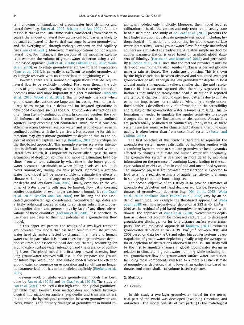
Advances in Water Resources 102 (2017) 53–67 Contents lists available at ScienceDirect Advances in Water Resources journal homepage: www.elsevier.com/locate/advwatres A global-scale two-layer transient groundwater model: Development and application to groundwater depletion Inge E.M. de Graaf a,b,∗ , Rens L.P.H. van Beek a , Tom Gleeson c , Nils Moosdorf d , Oliver Schmitz a , Edwin H. Sutanudjaja a , Marc F.P. Bierkens a,e a Department of Physical Geography, Faculty of Geosciences, Utrecht University, Netherlands b Department Geology and Geological Engineering, Colorado School of Mines, USA c Civil Engineering, University of Victoria, Canada d Leibniz-Center for Tropical Marine Research (ZMT), Bremen, Germany e Unit Soil and Groundwater Systems, Deltares, Utrecht, Netherlands a r t i c l e i n f o Article history: Received 14 November 2016 Revised 27 January 2017 Accepted 27 January 2017 Available online 4 February 2017 a b s t r a c t Groundwater is the world’s largest accessible source of freshwater to satisfy human water needs. More- over, groundwater buffers variable precipitation rates over time, thereby effectively sustaining river flows in times of droughts and evaporation in areas with shallow water tables. In this study, building on previ- ous work, we simulate groundwater head fluctuations and groundwater storage changes in both confined and unconfined aquifer systems using a global-scale high-resolution (5 ) groundwater model by deriving new estimates of the distribution and thickness of confining layers. Inclusion of confined aquifer systems (estimated 6–20% of the total aquifer area) improves estimates of timing and amplitude of groundwa- ter head fluctuations and changes groundwater flow paths and groundwater-surface water interaction rates. Groundwater flow paths within confining layers are shorter than paths in the underlying aquifer, while flows within the confined aquifer can get disconnected from the local drainage system due to the low conductivity of the confining layer. Lateral groundwater flows between basins are significant in the model, especially for areas with (partially) confined aquifers were long flow paths crossing catchment boundaries are simulated, thereby supporting water budgets of neighboring catchments or aquifer sys- tems. The developed two-layer transient groundwater model is used to identify hot-spots of groundwater depletion. Global groundwater depletion is estimated as 7013 km 3 (137 km 3 y −1 ) over 1960–2010, which is consistent with estimates of previous studies. © 2017 The Authors. Published by Elsevier Ltd. This is an open access article under the CC BY license. (http://creativecommons.org/licenses/by/4.0/) 1. Introduction As the world’s largest accessible source of freshwater, ground- water plays a vital role in satisfying the basic needs of human so- ciety (Gleeson et al., 2016; UNESCO, 2009). It serves as a primary source of drinking water and supplies water for agricultural and industrial activities. During periods of low or no rainfall, ground- water storage provides a natural buffer against water shortage, pre- serves evaporation in areas with shallow water tables, and sustains baseflows to rivers and wetlands, thereby supporting ecosystem habitats and biodiversity (e.g. Bierkens and van den Hurk, 2007; de Graaf et al., 2013; Wada et al., 2014). Moreover, groundwater often flows across topographical and administrative boundaries at ∗ Corresponding author. E-mail address: [email protected] (I.E.M. de Graaf). considerable rates, supporting water budgets of receiving catch- ments or aquifers (Schaller and Fan, 2009). However, groundwa- ter resources are increasingly threatened by excessive abstractions, particularly in irrigated areas where abstraction rates are high and groundwater is only slowly renewed (Gleeson et al., 2011). The most direct effects of groundwater depletion are falling water ta- bles and the irreversible loss of groundwater storage. As a conse- quence, pumping costs increase, and baseflow to rivers and wet- lands is reduced, negatively affecting ecosystems, and compaction of the emptied pore space may lead to land subsidence. Despite the importance of groundwater and the explicit treat- ment of groundwater recharge and pumping in global studies (Döll et al., 2014a; Wada et al., 2010), most global-scale hydrological models do not include a groundwater flow component. The obvi- ous reason for this missing component is the lack of consistent global-scale hydrogeological information. Such data is needed to obtain a realistic physical representation of the groundwater sys- http://dx.doi.org/10.1016/j.advwatres.2017.01.011 0309-1708/© 2017 The Authors. Published by Elsevier Ltd. This is an open access article under the CC BY license. (http://creativecommons.org/licenses/by/4.0/)

Welcome message from author
This document is posted to help you gain knowledge. Please leave a comment to let me know what you think about it! Share it to your friends and learn new things together.
Transcript

Advances in Water Resources 102 (2017) 53–67
Contents lists available at ScienceDirect
Advances in Water Resources
journal homepage: www.elsevier.com/locate/advwatres
A global-scale two-layer transient groundwater model: Development
and application to groundwater depletion
Inge E.M. de Graaf a , b , ∗, Rens L.P.H. van Beek
a , Tom Gleeson
c , Nils Moosdorf d , Oliver Schmitz
a , Edwin H. Sutanudjaja
a , Marc F.P. Bierkens a , e
a Department of Physical Geography, Faculty of Geosciences, Utrecht University, Netherlands b Department Geology and Geological Engineering, Colorado School of Mines, USA c Civil Engineering, University of Victoria, Canada d Leibniz-Center for Tropical Marine Research (ZMT), Bremen, Germany e Unit Soil and Groundwater Systems, Deltares, Utrecht, Netherlands
a r t i c l e i n f o
Article history:
Received 14 November 2016
Revised 27 January 2017
Accepted 27 January 2017
Available online 4 February 2017
a b s t r a c t
Groundwater is the world’s largest accessible source of freshwater to satisfy human water needs. More-
over, groundwater buffers variable precipitation rates over time, thereby effectively sustaining river flows
in times of droughts and evaporation in areas with shallow water tables. In this study, building on previ-
ous work, we simulate groundwater head fluctuations and groundwater storage changes in both confined
and unconfined aquifer systems using a global-scale high-resolution (5 ′ ) groundwater model by deriving
new estimates of the distribution and thickness of confining layers. Inclusion of confined aquifer systems
(estimated 6–20% of the total aquifer area) improves estimates of timing and amplitude of groundwa-
ter head fluctuations and changes groundwater flow paths and groundwater-surface water interaction
rates. Groundwater flow paths within confining layers are shorter than paths in the underlying aquifer,
while flows within the confined aquifer can get disconnected from the local drainage system due to the
low conductivity of the confining layer. Lateral groundwater flows between basins are significant in the
model, especially for areas with (partially) confined aquifers were long flow paths crossing catchment
boundaries are simulated, thereby supporting water budgets of neighboring catchments or aquifer sys-
tems. The developed two-layer transient groundwater model is used to identify hot-spots of groundwater
depletion. Global groundwater depletion is estimated as 7013 km
3 (137 km
3 y −1 ) over 1960–2010, which
is consistent with estimates of previous studies.
© 2017 The Authors. Published by Elsevier Ltd.
This is an open access article under the CC BY license. ( http://creativecommons.org/licenses/by/4.0/ )
1
w
c
s
i
w
s
b
h
d
o
c
m
t
p
g
m
b
q
l
o
m
e
h
0
. Introduction
As the world’s largest accessible source of freshwater, ground-
ater plays a vital role in satisfying the basic needs of human so-
iety ( Gleeson et al., 2016; UNESCO, 2009 ). It serves as a primary
ource of drinking water and supplies water for agricultural and
ndustrial activities. During periods of low or no rainfall, ground-
ater storage provides a natural buffer against water shortage, pre-
erves evaporation in areas with shallow water tables, and sustains
aseflows to rivers and wetlands, thereby supporting ecosystem
abitats and biodiversity (e.g. Bierkens and van den Hurk, 2007;
e Graaf et al., 2013; Wada et al., 2014 ). Moreover, groundwater
ften flows across topographical and administrative boundaries at
∗ Corresponding author.
E-mail address: [email protected] (I.E.M. de Graaf).
m
o
g
o
ttp://dx.doi.org/10.1016/j.advwatres.2017.01.011
309-1708/© 2017 The Authors. Published by Elsevier Ltd. This is an open access article u
onsiderable rates, supporting water budgets of receiving catch-
ents or aquifers ( Schaller and Fan, 2009 ). However, groundwa-
er resources are increasingly threatened by excessive abstractions,
articularly in irrigated areas where abstraction rates are high and
roundwater is only slowly renewed ( Gleeson et al., 2011 ). The
ost direct effects of groundwater depletion are falling water ta-
les and the irreversible loss of groundwater storage. As a conse-
uence, pumping costs increase, and baseflow to rivers and wet-
ands is reduced, negatively affecting ecosystems, and compaction
f the emptied pore space may lead to land subsidence.
Despite the importance of groundwater and the explicit treat-
ent of groundwater recharge and pumping in global studies ( Döll
t al., 2014a; Wada et al., 2010 ), most global-scale hydrological
odels do not include a groundwater flow component. The obvi-
us reason for this missing component is the lack of consistent
lobal-scale hydrogeological information. Such data is needed to
btain a realistic physical representation of the groundwater sys-
nder the CC BY license. ( http://creativecommons.org/licenses/by/4.0/ )
54 I.E.M. de Graaf et al. / Advances in Water Resources 102 (2017) 53–67
g
c
h
fi
d
w
a
a
s
i
d
u
b
g
a
t
i
a
o
fi
a
f
c
a
s
q
C
g
a
a
T
i
e
T
l
i
g
t
e
d
e
2
d
t
g
p
g
2
t
t
b
r
e
I
o
t
2
2
t
A
tem, allowing for simulation of groundwater head dynamics and
lateral flows (e.g. Fan et al., 2007; Schaller and Fan, 2009 ). Another
reason is that at the usual time scales considered (from season to
years), the amount of lateral flow across cell boundaries is likely to
be small compared to the vertical exchange between groundwater
and the overlying soil through recharge, evaporation and capillary
rise ( Lam et al., 2011 ). Moreover, many applications do not require
lateral flow. For instance, if the purpose of the modeling exercise
is to estimate the volume of groundwater depletion using a vol-
ume based approach ( Döll et al., 2014b; Pokhrel et al., 2012; Wada
et al., 2010 ), or to relate groundwater storage to land evaporation
( Lam et al., 2011 ), it generally is sufficient to model groundwater
as a single reservoir with no connections to neighboring cells.
However, there are a number of applications that do require
lateral flow to be explicitly modeled. First, even though the vol-
umes of groundwater traveling across cells is currently limited, it
becomes more and more important at higher resolutions ( Bierkens
et al., 2015; Wood et al., 2012 ). This is certainly the case when
groundwater abstractions are large and increasing. Second, partic-
ularly below megacities in deltas and for irrigated agriculture in
developed countries such as the U.S., groundwater abstractions are
often from (semi-) confined aquifers. In confined aquifers the spa-
tial influence of abstractions is much larger than in unconfined
aquifers, likely exceeding cell boundaries. Third, there is consider-
able interaction between surface water and groundwater, even in
confined aquifers, with the larger rivers. Not accounting for this in-
teraction may overestimate groundwater depletion due to the ne-
glect of increased capture (see e.g. Konikow, 2011 for a critique on
the flux-based approach). This groundwater-surface water interac-
tion is difficult to parameterize in a land-surface model without
lateral flow. Fourth, it is important to eventually surpass the mere
estimation of depletion volumes and move to estimating head de-
clines if one aims to estimate by what time in the future ground-
water becomes unattainable or when falling heads will results in
rivers running dry during low flow periods. Moreover, a ground-
water flow model will be more suitable to estimate the effects of
climate variability and change on ecologically relevant groundwa-
ter depths and low flows ( Fan, 2015 ). Finally, even though the vol-
umes of water crossing cells may be limited, flow paths crossing
aquifer boundaries or even larger catchment boundaries ( de Graaf
et al., 2015; Schaller and Fan, 2009 ) can be long and the asso-
ciated groundwater age considerable. Groundwater age dates are
a likely additional source of data to constrain subsurface proper-
ties (aquifer depth and permeability) by lack of any direct obser-
vations of these quantities ( Gleeson et al., 2016 ). It is beneficial to
use these age dates to their full potential in a groundwater flow
model.
In this paper we present the results of a two-layer transient
groundwater flow model that has been built to simulate ground-
water head dynamics affected by changes in climate and human
water use. In particular, it is meant to estimate groundwater deple-
tion volumes and associated head declines, thereby accounting for
groundwater- surface water interaction and the presence of confin-
ing layers. The global model is a first step toward assessing how
long groundwater reserves will last. It also prepares the ground
for future hyper-resolution land surface models where the effect of
groundwater convergence on evaporation and runoff can no longer
be parameterized but has to be modeled explicitly ( Bierkens et al.,
2015 ).
Previous work on global-scale groundwater models has been
done by Fan et al. (2013) and de Graaf et al. (2015) . The study of
Fan et al. (2013) produced a first high-resolution global groundwa-
ter table map. However, their method does not include hydroge-
ological information on aquifers (e.g. depths and transmissivities).
In addition the hydrological connection between groundwater and
rivers, which is the primary drainage of groundwater in humid re-
ions, is modeled only implicitly. Moreover, their model requires
alibration to head observations and only returns the steady state
ead distribution. The study of de Graaf et al. (2015) presents the
rst high-resolution global-scale groundwater model including hy-
rogeological information and accounting for groundwater-surface
ater interactions. Lateral groundwater flows for single unconfined
quifers are simulated at steady-state. A relative simple method for
quifer parameterization is used based on available global data-
ets of lithology ( Hartmann and Moosdorf, 2012 ) and permeabil-
ty ( Gleeson et al., 2011 ) such that the method provides results for
ata-poor environments. Also, aquifer thickness is derived globally
sing terrain attributes. The results are promising. This is shown
y the high correlation between observed and simulated averaged
roundwater heads, although shallow groundwater depths in local
lluvial aquifers in mountain valleys, smaller than the grid resolu-
ion ( < 10 km), are not captured. Also, the study ’s greatest lim-
tation is that only the steady-state head distribution is reported
nd temporal changes in groundwater head patterns due to climate
r human impacts are not considered. Also, only a single uncon-
ned aquifer is described and vital information on the accessibility
nd quality of the groundwater water resource is missing. This in-
ormation is needed to simulate the aquifer sensitivity to storage
hanges due to climate fluctuations or abstractions. Abstractions
re preferentially positioned in confined aquifer systems, as these
ystems are less sensitive for climate fluctuations and groundwater
uality is often better than from unconfined systems ( Foster and
hilton, 2003 ).
The first objective of this study is therefore to represent the
roundwater system more realistically, by including aquifers with
confining layer, in order to simulate groundwater head dynamics
ffected by changes in climate and human water use adequately.
he groundwater system is described in more detail by including
nformation on the presence of confining layers, leading to the cat-
gorization of world’s aquifers in confined and unconfined systems.
he improved physical groundwater representation is expected to
ead to a more realistic estimate of aquifer sensitivity to changes
n storage by climate or human impacts.
The second objective of this study is to provide estimates of
roundwater depletion and head declines worldwide. Previous es-
imates of groundwater depletion (e.g. Döll et al., 2012; Wada
t al., 2010; Konikow, 2011; Pokhrel et al., 2012 ) vary by an or-
er of magnitude. For example the flux-based approach of Wada
t al. (2010) estimate groundwater depletion at 283 ± 40 km
3 yr −1
010 as the residual of grid-based groundwater recharge and with-
rawal. The approach of Wada et al. (2010) overestimates deple-
ion as it does not account for increased capture due to decreased
roundwater discharge, nor for long-distance surface water trans-
orts. The volume-based approach of Konikow (2011) estimates
roundwater depletion at 145 ± 39 km
3 yr −1 between 2001 and
008 based on data for the US and other big aquifer systems by ex-
rapolation of groundwater depletion globally using the average ra-
io of depletion to abstractions observed in the US. Our study will
e the first to simulate changes in global groundwater storage in
elation to climate and groundwater pumping while including lat-
ral groundwater flow and groundwater-surface water interaction.
ncluding these components will lead to a more realistic estimate
f groundwater depletion, that is lower than earlier flux-based es-
imates and more similar to volume-based estimates.
. Methods
.1. General
In this study a two-layer groundwater model for the terres-
rial part of the world was developed (excluding Greenland and
ntarctica). The model consists of two parts: (1) the hydrological

I.E.M. de Graaf et al. / Advances in Water Resources 102 (2017) 53–67 55
Fig. 1. A) Original model structure of the hydrological model PCR-GLOBWB. B) The groundwater store (store 3 in PCR-GLOBWB) is replaced by a groundwater model. The
groundwater model is forced with net groundwater recharge minus capillary rise, and surface water levels calculated with PCR-GLOBWB. C) A cross-section illustrating the
difference between simulated regional-scale groundwater levels and perched water levels. The latter are simulated as interflow in PCR-GLOBWB.
m
w
B
k
m
g
t
s
2
a
n
s
t
J
a
m
t
t
m
o
p
c
o
l
l
r
t
w
k
r
a
t
i
t
b
u
w
p
i
r
p
c
s
r
d
l
v
c
f
a
i
g
A
p
l
d
b
g
2
2
S
G
a
T
s
r
r
w
u
f
(
c
T
t
v
2
w
m
(
s
t
f
t
w
h
odel PCR-GLOBWB ( van Beek et al., 2011 ) and (2) the ground-
ater model using MODFLOW ( McDonald and Harbaugh, 20 0 0 ).
oth models were run at 5 arc-minute resolution (approx. 10x10
m at the equator) over the period 1960–2010. The groundwater
odel was forced with outputs from PCR-GLOBWB, specifically via
roundwater recharge and river discharges ( Fig. 1 ). A brief descrip-
ion of the models and coupling is given here, a more detailed de-
cription is given in de Graaf et al. (2015) .
.1.1. Global hydrological model
The model PCR-GLOBWB simulates hydrological processes in
nd between two vertically stacked soil stores (maximum thick-
ess 0.3 and 1.2 m respectively) and one underlying groundwater
tore. The model was run at 5 ′ resolution at a daily time step. For
he climate forcing, monthly data from CRU TS 2.1 ( Mitchell and
ones, 2005 ) was downscaled using ERA-40 ( Uppala et al., 2005 )
nd ERA-interim ( Dee et al., 2011 ) reanalysis to obtain a daily cli-
ate forcing (see de Graaf et al., 2013 for a more detailed descrip-
ion of this forcing data-set). For each time step and every grid cell
he water balance of the soil column is calculated based on the cli-
atic forcing that imposes precipitation (rain or snow depending
n temperature), reference potential evapotranspiration, and tem-
erature. Vertical exchange between the soil and groundwater oc-
urs through percolation and capillary rise. In the original version
f the PCR- GLOBWB model no lateral groundwater flow is simu-
ated. Instead, groundwater dynamics are described by means of a
inear storage-outflow relation (Store 3 in Fig. 1 A) . Specific surface
unoff snow-melt, interflow, and baseflow are accumulated along
he drainage network that consists of laterally connected surface
ater elements representing river channels, lakes, or reservoirs. A
inematic wave approximation at a sub-daily time step is used to
oute surface water to the basin outlet.
PCR-GLOBWB also simulates human water use by calculating
t each time step sectoral water demand (i.e. the amount of wa-
er that would be abstracted if sufficient water were available) for
rrigation, industrial, domestic, and livestock), the associated wa-
er withdrawals (partitioned into groundwater and surface water
ased on availability and pumping capacity), consumptive water
se, and return flows. Irrigation is simulated by adding additional
ater to soils as a function of soil water deficit needed to achieve
otential evaporation. Sectorial water demands were estimated us-
ng country statistics and population numbers downscaled to 5 ′ esolution. To approximate economic development over the model
eriod, data of Gross Domestic Product, electricity, and household
onsumption were used. Industrial water demands were kept con-
tant over the year, while domestic demand reflect seasonality in
elation to air temperature. Water recycling ratios for industry and
omestic use are adopted from Wada et al. (2014) and were calcu-
ated per country on the basis of GDP and level of economic de-
elopment. Irrigation demands were calculated assuming optimal
rop growth, using maximum crop transpiration, and accounting
or bare soil evaporation and soil water availability. Losses during
bstraction and transport are calculated using a country specific
rrigation efficiency factor (used from Siebert and Döll, 2010 ). Irri-
ation evaporation losses during application are not accounted for.
lso, domestic irrigation is not included as it is very small com-
ared to crop irrigation. Total water demand was dynamically al-
ocated to surface water (rivers, lakes, and reservoirs) and depen-
ent on actual availability in the resource and accounting for feed-
acks such as return flows of unconsumed abstracted water and
roundwater-surface water interactions (following de Graaf et al.,
013 ).
.1.2. Global groundwater model
A two-layer MODFLOW model ( McDonald and Harbaugh, 20 0 0;
chmitz et al., 2009 ) replaces the linear groundwater store of PCR-
LOBWB. Aquifer properties were prescribed and include confined
nd unconfined aquifer systems (discussed in the next paragraph).
he MODFLOW model was forced with outputs from PCR-GLOBWB,
pecifically the flow between layer 2 and 3 ( Fig. 1 ) consisting of net
echarge (recharge minus capillary rise) and river levels. The net
echarge is the input for the MODFLOW’s recharge (RCH) package,
hile the MODFLOW’s river (RIV) and drain (DRN) packages are
sed to incorporate interactions between the groundwater and sur-
ace water. As PCR-GLOBWB runs on a Cartesian (or regular) grid
geographic projection) we have to take account of the fact that
ell areas and volumes of the MODFLOW grid do not vary in space.
his is done by adjusting recharge and the storage coefficient in
he RCH and BCF packages to account for varying cell areas and
olumes associated on a geographic grid (see Sutanudjaja et al.,
011 and de Graaf et al., 2015 for details). Apart from the river
ater levels, the boundary conditions of the global groundwater
odel were obtained as fixed heads set equal to global sea-level
reference level 0). Initial conditions were obtained by a steady
tate-state simulation of hydraulic head with average recharge and
hen warming up the model by running the year 1960 back-to-back
or 20 years to reach dynamic equilibrium.
Three levels of groundwater-surface water interactions are dis-
inguished: (1) large rivers, wider than 25 m, (2) smaller rivers
ith a width smaller than 25 m, and (3) springs and streams
igher up in the valley.
56 I.E.M. de Graaf et al. / Advances in Water Resources 102 (2017) 53–67
f
a
p
p
t
i
c
t
a
m
p
p
t
g
c
i
B
i
p
i
f
2
s
M
c
2
g
t
c
2
c
b
s
c
o
(
p
h
1
a
t
t
a
t
l
r
q
t
w
s
p
T
t
c
2
a
c
c
1. For large rivers, interactions are governed by actual ground-
water heads and river levels ( HRIV [m]). The latter was cal-
culated from river discharges ( Qchn [m
3 s −1 ]) simulated by
PCR-GLOBWB and using channel properties based (channel
width and depth) based on geomorphological relations to bank-
full discharge ( Qbkfl [m
3 s −1 ]) ( Lacey, 1930; Manning, 1891;
Savenije, 2003 ). The RIV-package calculates the water flux be-
tween the river and groundwater Qriv [m
3 d
−1 ]. Water infil-
trates the aquifer if the groundwater head lies below the river
head: Qriv is then positive. Water is drained from the aquifer if
groundwater head lies above the river head: Qriv is then nega-
tive. Qriv for the larger rivers ( Qriv.Big [m
3 d
−1 ]) was calculated
as:
Q riv.Big =
{c × ( HRIV − h ) if h > RBOT
c × ( HRIV − RBOT ) if h ≤ RBOT
(1)
where c [m
2 d
−1 ] is the river bed conductance calculated from
river length (approximated as the diagonal cell length), river
bed width and depth and river bed resistance (assumed 1 day),
h [m] is groundwater head, and RBOT [m] is the river bottom
calculated for bankfull conditions (taken as a rule of thumb
happening every 1.5 year). Surface elevation ( DEM [m]) is taken
as the reference level here.
2. Smaller rivers are defined as drains; water can only leave
the groundwater system through the drain when heads get
above the drainage level. In this case, the drainage levels were
taken equal to the DEM . The drainage was then calculated as
Qriv.Small [m
3 d
−1 ]:
Q riv.Small =
{c × ( DEM − h ) if h > DEM
0 if h ≤ DEM
(2)
3. Qriv.Big and Qriv.Small quantify flow between streams and
aquifers and are the main components of the baseflow, Qbf ,
which is negative when water is drained from the aquifer. At
the 5 ′ resolution however, the main stream is insufficient to
represent local sags, springs, and streams higher up in the
mountainous area. We assume that groundwater above the
floodplain level can be tapped by local springs that are repre-
sented by means of a linear storage-outflow relationship. From
the DEM and the storage estimated in S3 (in the PCR-GLOBWB
run) we calculate the amount of storage ([L], aquifer depth
times porosity). From this follows the local drainage flux. To be
consistent with the RIV and DRN packages, this linear storage
term is also negative when water is drained. Total drainage Qbf
[m
3 d
−1 ] is thus calculated as:
Q b f = (Q ri v .Big + Q ri v .Small ) − (J · S 3 , f lp ) (3)
where S 3, flp [m
3 ] is the groundwater storage above the flood-
plain (obtained from PCR-GLOBWB) and J [d
−1 ] is the recession
coefficient parameterized based on Kraaijenhof van der Leur
(1958) :
J =
πT
4 S y L 2 (4)
where T [m
2 d −1 ] is transmissivity, Sy [-] is the specific yield
(for each hydrolithological unit; Table 1 and L [m] is the av-
erage distance between streams and rivers as obtained from
the drainage density ( van Beek et al., 2011 ). Globally the local
drainage flux sums up to 50% of the total baseflow.
2.2. Model runs
PCR-GLOBWB and MODFLOW were only coupled one-way. This
means we first run PCR-GLOBWB at a daily timestep for 1960–
2010, and force MODFLOW with monthly averaged values of the
ollowing outputs: surface water levels are passed to the RIV pack-
ge, net recharge (groundwater recharge minus capillary rise) is
assed to the RCH package, and groundwater abstractions are
assed to the WELL package. As we do not know the actual loca-
ions of the pumping wells, we simulate abstractions with a pump-
ng well positioned in the middle of a MODFLOW cell (that coin-
ides with a PCR-GLOBWB cell with groundwater abstraction). Also
he linear storage term (i.e. J · S 3, flp ) is passed to the WELL pack-
ge. After that, MODFLOW was run over the period 1960–2010 at
onthly time steps with these fluxes and boundary conditions im-
osed.
This type of coupling ensures that the same amount of water
asses through the groundwater model as through the groundwa-
er zone ( Fig. 1 A store 3) of PCR-GLOBWB and also yields the same
lobal average flux between surface and groundwater. Thus, the
oupling ensures full terrestrial balance closure. Also, it implicitly
ncludes capillary rise, which is calculated in PCR-GLOBWB ( van
eek et al., 2011 ) and is included in the net recharge. However,
t does not include feedback effects of groundwater levels on the
ortioning of surface fluxes as a full coupling would do, nor does
t explicitly portray the effects of groundwater abstractions on sur-
ace water levels.
.3. Aquifer parameterization
The aquifer parameterization is based on available global data-
ets on lithology (Global Lithology Map (GLiM), ( Hartmann and
oosdorf, 2012 ) and permeability ( Gleeson et al., 2014; 2011 ),
ombined with an estimate of aquifer thicknesses ( de Graaf et al.,
015 ). A detailed description of the aquifer parameterization is
iven in ( de Graaf et al., 2015 ), a summary is given below since
he focus of this study is to extend the aquifer parameterization by
ategorizing world’s aquifers in confined and unconfined systems.
.3.1. General: aquifer permeability and transmissivity
Aquifer permeabilities were defined by lumping the lithology
lasses defined by Hartmann and Moosdorf (2012) to 7 com-
ined hydrolithologies (adopted from Gleeson et al., 2011 ), repre-
enting broad lithological categories with similar hydrogeological
haracteristics. These units were subdivided further on the basis
f texture for unconsolidated and consolidated sedimentary rocks
Table 1 ), resulting in a global map representing regional scale
ermeability. The polygons of the lithological map, delineating a
ydrogeological unit, were subsequently gridded to 30 ′ ′ (approx.
x1 km at the equator) and aggregated as the geometric mean
t 5 ′ resolution (approx. 10x10 km at the equator). To calculate
ransmissivities ( T [m
2 d
−1 ]) aquifer thicknesses are needed. These
hicknesses were estimated since no global data-set of observed
quifer thickness is available. Using the assumption that produc-
ive aquifers coincide with sedimentary basins and sediments be-
ow river valleys, the distinction is made between (1) mountain
anges, and (2) sediment basins representing the aquifers. Subse-
uently, aquifer thicknesses were estimated by relating these to
errain attributes (e.g. curvature) after calibration of these relations
ith reported aquifer thicknesses from U.S. groundwater modeling
tudies (see de Graaf et al., 2015 for an extensive description of this
rocedure to delineate aquifer systems and estimate thicknesses).
hese estimated thicknesses represent the productive aquifers until
he first impermeable basis, meaning that permeable and (thinner)
onfining units are lumped together into one big aquifer system.
.3.2. Delineation of confining layers
In this study we delineate confining layers and categorize the
quifers of the world in confined and unconfined aquifers. The
ategorization is done using information on grain sizes of un-
onsolidated sediments in the lithological map (GLiM) and addi-
I.E.M. de Graaf et al. / Advances in Water Resources 102 (2017) 53–67 57
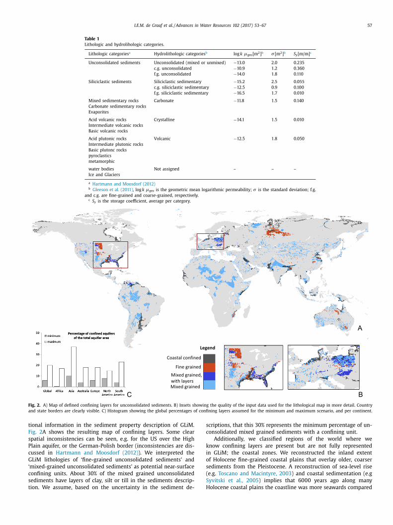
Table 1
Lithologic and hydrolihologic categories.
Lithologic categories a Hydrolithologic categories b log k μgeo [m
2 ] b σ [m
2 ] b S y [m/m] c
Unconsolidated sediments Unconsolidated (mixed or unmixed) −13.0 2 .0 0 .235
c.g. unconsolidated −10.9 1 .2 0 .360
f.g. unconsolidated −14.0 1 .8 0 .110
Siliciclastic sediments Siliciclastic sedimentary −15.2 2 .5 0 .055
c.g. siliciclastic sedimentary −12.5 0 .9 0 .100
f.g. siliciclastic sedimentary −16.5 1 .7 0 .010
Mixed sedimentary rocks Carbonate −11.8 1 .5 0 .140
Carbonate sedimentary rocks
Evaporites
Acid volcanic rocks Crystalline −14.1 1 .5 0 .010
Intermediate volcanic rocks
Basic volcanic rocks
Acid plutonic rocks Volcanic −12.5 1 .8 0 .050
Intermediate plutonic rocks
Basic plutonc rocks
pyroclastics
metamorphic
water bodies Not assigned – – –
Ice and Glaciers
a Hartmann and Moosdorf (2012) b Gleeson et al. (2011) , log k μgeo is the geometric mean logarithmic permeability; σ is the standard deviation; f.g.
and c.g. are fine-grained and coarse-grained, respectively. c S y is the storage coefficient, average per category.
Fig. 2. A) Map of defined confining layers for unconsolidated sediments. B) Insets showing the quality of the input data used for the lithological map in more detail. Country
and state borders are clearly visible. C) Histogram showing the global percentages of confining layers assumed for the minimum and maximum scenario, and per continent.
t
F
s
P
c
G
‘
c
s
t
s
c
k
i
o
s
(
S
H
ional information in the sediment property description of GLiM.
ig. 2 A shows the resulting map of confining layers. Some clear
patial inconsistencies can be seen, e.g. for the US over the High
lain aquifer, or the German-Polish border (inconsistencies are dis-
ussed in Hartmann and Moosdorf (2012) ). We interpreted the
LiM lithologies of ‘fine-grained unconsolidated sediments’ and
mixed-grained unconsolidated sediments’ as potential near-surface
onfining units. About 30% of the mixed grained unconsolidated
ediments have layers of clay, silt or till in the sediments descrip-
ion. We assume, based on the uncertainty in the sediment de-
criptions, that this 30% represents the minimum percentage of un-
onsolidated mixed grained sediments with a confining unit.
Additionally, we classified regions of the world where we
now confining layers are present but are not fully represented
n GLiM; the coastal zones. We reconstructed the inland extent
f Holocene fine-grained coastal plains that overlay older, coarser
ediments from the Pleistocene. A reconstruction of sea-level rise
e.g. Toscano and Macintyre, 2003 ) and coastal sedimentation (e.g
yvitski et al., 2005 ) implies that 60 0 0 years ago along many
olocene coastal plains the coastline was more seawards compared

58 I.E.M. de Graaf et al. / Advances in Water Resources 102 (2017) 53–67
Fig. 3. A) 2-dimensional schematization of coastal confined aquifer classification.
The star indicates the apex. B) Spatial extent of a coastal confined aquifer.
Fig. 4. Aquifer parameter settings used for unconsolidated sediments for confined
aquifer systems. D is thickness [m], D T is the total estimated aquifer thickness, D c is estimated thickness of the confining layer. For the confining layer horizontal and
vertical conductivities ( kh and kv [md −1 ]) were taken similar to fine grained un-
consolidated sediments (see Table 1 ), for the confined aquifer kh and kv were taken
similar to coarse grained unconsolidated sediments. S is the storage coefficient, de-
fined as specific yield (confining layer, values Table 1 ) or storage coefficient (con-
fined aquifer).
m
i
o
e
s
F
u
e
a
r
s
a
a
c
k
w
(
(
a
i
p
s
l
i
p
m
b
t
n
B
c
t
2
t
fl
a
s
(
c
m
to the modern situation. Coastlines have receded tens of kilome-
ters since in many deltas (e.g. Stanley and Warne, 1994 ). With
sea-level rising over the Holocene, the downstream gradient along
the river flattened, and sediments accumulated in the downstream
part. The apex of the delta and deposition areas indicate the point
where accumulation originated. This accumulation point is recon-
structed using the profile curvature along the river, with its occur-
rence where the curvature changes from convex to concave start-
ing from the coast. The accumulation points were identified glob-
ally for larger rivers ( > 25 m wide) with their outlet on, or near
the coast (i.e. within 50 km). Points at high elevations, clearly not
related to sedimentation in the coastal zone, were excluded.
Fig. 3 A shows a schematic cross-section of a coastal aquifer
with a confining layer on top. Thickness of the confining layer at
the coast is estimated using ocean bathymetry (elevation taken one
5 ′ grid-cell out of the coast). The thickness at the coastline is in-
terpolated along the river using the river gradient until the apex,
where thickness is minimal. The interpolation is done for all iden-
tified large rivers and thickness of the coastal plains is derived by
interpolation between the rivers, bounded by the elevation con-
tours on which the apex are situated ( Fig. 3 B. Following this ap-
proach, approximately 11% of the global coastline is classified as
confined after interpolation.
2.3.3. Confined aquifers: aquifer transmissivity and storativity
Confined aquifers are defined here as those aquifers overlain by
fine grained confining layers. We realize that the term ‘confined’
aquifers may not entirely cover the different hydrogeological set-
tings that are found in reality. First, aquifers covered with fine-
grained sediments may still allow vertical flow through the con-
fining layers and are thus in fact leaky or semi-confined aquifers.
Second, due to the varying thickness and permeability of the con-
fining layers certain areas may be in fact unconfined, depending
on the spatial scale under consideration. Third, in areas with ex-
cessive groundwater pumping the drawdown close to wells may
cause part of the originally (pressurized) groundwater head to fall
below the top of the aquifer, causing it to be partially unconfined.
All these cases mean that what we define here as confined aquifers
ay be better termed as partially and semi-confined aquifers. Hav-
ng noted this limitation, for the sake of briefness of terminol-
gy, we call all aquifers covered with fine grained confining lay-
rs ‘confined aquifers’, including the hydrogeological settings de-
cribed above. Finally, we note that in the implementation in MOD-
LOW we use a global two-layer model where for the areas with
nconfined aquifers the top layer is given the same hydraulic prop-
rties as the underlying aquifer.
The parameter settings used for the unconsolidated confined
quifers and the confining layers are shown in Fig. 4 . For all other
ocks and sediments the values from Table 1 are used. In ab-
ence of any other information, vertical conductivity was initially
ssumed to be the same as the horizontal conductivity and next,
calibration procedure was used to calibrate the storage coeffi-
ient, the horizontal conductivity as well as the anisotropy ratio
h/kv assuming kh ≥ kv (see Table 1 ). Aquifer storage capacities
ere parameterized using specific yields for unconfined aquifers
Table 1 ) and for confined aquifers a storage coefficient of 0.001
Heath, 1983 ) was assumed. As mentioned before, the estimated
quifer thicknesses represent productive aquifers until the first
mpermeable basis. This means that aquifers separated by semi-
ermeable layers are lumped into one big aquifer system. As a re-
ult, head declines may be underestimated. By including confining
ayers where fine-grained sediment properties are present and us-
ng an anisotropy ratio kh/kv (with kh ≥ kv), we expect to im-
licitly correct for neglecting semi-permeable layers and lumping
ulti- aquifers into one system.
Thickness of coastal confining layers is estimated using ocean
athymetry and interpolation (as described in 2.3.2). For 80% of
he coastal confined grid-cells the estimated confining layer thick-
ess is approximately 10% of the total estimated aquifer thickness.
ased on this finding and by lack of any other information, we de-
ided to apply a thickness of 10% of the total estimated thickness
o all confining layers not located near the coast.
.4. Analyzing the effect of schematization
We analyzed the effects of incorporating confined aquifer sys-
ems on simulated groundwater head fluctuations, groundwater
ow patterns, groundwater-surface water interactions and stor-
ge changes. Three scenarios were formulated describing different
patial distributions of confined and unconfined aquifer systems:
1) unconfined systems only (following de Graaf et al., 2015 ), (2)
onfined systems for fine grained unconsolidated sediments and
ixed grained unconsolidated sediments with fine grained layers

I.E.M. de Graaf et al. / Advances in Water Resources 102 (2017) 53–67 59
(
s
g
(
a
T
2
s
u
2
y
f
v
o
6
f
v
t
e
c
n
e
o
i
h
s
m
i
f
a
i
c
h
t
9
(
R
s
5
a
p
a
(
c
t
h
r
m
d
o
a
r
Q
w
e
R
w
e
v
f
n
a
t
o
(
t
d
2
C
a
t
2
fl
G
a
t
a
w
c
p
o
t
s
l
t
s
s
a
t
i
o
a
p
d
T
I
m
1
p
t
i
fi
2
a
w
2
s
t
c
t
d
m
n
t
30%) (in GLiM) and coastal confined regions (minimum confining
cenario), and (3) confined systems for fine grained and all mixed
rained unconsolidated sediments and coastal confined regions
maximum confining scenario). The parameter settings of confined
nd unconfined systems are used as described above ( Fig. 4 and
able 1 ).
.5. Calibration and validation of simulated groundwater heads
In order to calibrate and validate the groundwater model, time-
eries were selected from the US (available from the USGS: www.
sgs.gov/water ) and Europe (Rhine–Meuse basin: Sutanudjaja et al.,
011 ). The used time-series have a record covering at least five
ears and include seasonal variation; for the US ∼280 0 0 stations,
or Europe ∼60 0 0 stations were available. An earlier steady-state
ersion of the model ( de Graaf et al., 2015 ) was already validated
n all observations provided by Fan et al. (2013) (giving a total of
5 303 cells with observations), which also consist of observations
rom Spain, Brazil and Australia. However, many of these obser-
ations are not time series but single or time-average values. We
herefore used these in our previous steady-state version ( de Graaf
t al., 2015 ) but not to validate the present transient simulation. In
ase multiple stations were positioned in one grid cell, we chose
ot to average these but use them as they are, because the differ-
nt stations generally have observations over different time peri-
ds. Also, stations have different surface elevations or are placed
n different aquif ers (i.e. deep or shallow). We randomly selected
alf of the observations for calibration and half for validation (split
ample approach).
Limited calibration was used to better fit the groundwater
odel to the head observations. The calculation times (approx-
mately 2 weeks for a 1960–2010 run) were too long to allow
or an full-fledged automated calibration (e.g. Doherty, 2015 ). As
first step, we ran the groundwater model in steady state to cal-
brate the horizontal conductivity and the anisotropy ratio of the
onfining layers. A single global pre-factor was used varying the
orizontal and vertical conductivities between 0.01 and 100 times
he initial value, changing the anisotropy ratio kh / kv (a total of
x9 = 81 runs). Using the parameters of the best performing run
the parameter setting with the minimum root mean square error
MSE) we then further calibrated the model performing six tran-
ient runs while changing the storage coefficient between 0.1 and
times the initial value and allowing the horizontal conductivity
nd anisotropy ratio to be changed +/ −10%. This calibration was
erformed using the maximum confining conditions, as we see this
s the most realistic scenario. The best performing parameter set
with minimum RMSE) found was also used using the minimum
onfining conditions, and the results of both runs were compared.
The model performance was validated by evaluating simulated-
o observed water table head time-series (the other half of the
ead observation locations not used for calibration). Heads (with
eference to ocean level) instead of depths were used as heads
easure potential energy and are therefore more meaningful than
epths. The evaluation focused on mean monthly values, timing
f fluctuations (given by the cross-correlation coefficient R ), and
mplitudes. The latter is compared by the (relative) inter-quantile
ange error, QRE , calculated as:
RE =
I Q
m
7525 − I Q
o 7525
IQ
o 7525
(5)
here, IQ
m
7525 and IQ
o 7525
are the inter-quantile ranges of the mod-
led and observed data time series.
The cross-correlation is calculated as:
=
s mo
s m
s o (6)
here s m
and s o are the sample standard deviations of the mod-
led (m) and observed (o) samples, and s mo is the sample co-
ariance between the two. It was evaluated which stations per-
ormed good agreement in timing ( R > 0.5) and fluctuation mag-
itude ( Q RE < 50%). Results are shown in scatter plots. Addition-
lly, we compared averaged simulated heads to averaged heads of
he observed time series and a wider set of observations including
bservations of Spain, Brazil, and Australia provided by Fan et al.
2013) .
Apart from these global validation measures we also evaluated
he performance of the model in three areas where groundwater
epletion is severe (as follows from the global analysis, sections
.7 and 3.5): The High Plains aquifer (USA), The Central Valley of
alifornia (USA) and India. For these areas, we compared on an
quifer-by-aquifer basis the average head decline rates (shown in
he supplementary online information).
.6. Groundwater flow patterns
The effect of considering confined aquifers on groundwater
ow patterns is analyzed by simulating groundwater flow paths.
roundwater flow paths and travel times were simulated for heads
veraged over the simulation period, comparing two model se-
ups: unconfined and confined aquifer systems (the unconfined
nd maximum confining scenarios). Flow paths were calculated
ith particle tracking in MODPATH ( Pollock, 1994 ), using cell- to-
ell flux densities [volume/time/area] as input. In MODPATH a flow
ath is computed by tracking the particle through the subsoil from
ne cell to the next, from the location of recharge (at the water
able) toward the point of extraction or drainage (strong and weak
inks).
Following Schaller and Fan (2009) the spatial redistribution of
ocal recharge was evaluated using the ratio between groundwa-
er drainage and recharge: Qgw / Rgw . The ratio was estimated for
ub-basins that we defined using stream-orders, starting from the
econd stream-order at 5 ′ . The local drainage network was defined
t the 5 ′ grid-cell, and for every cell a stream is present. It follows
hat, for a ratio of 1, all water recharged in the basin is also drained
n the basin, or cross basin- boundary groundwater inflows and
utflows are approximately equal. If part of the water recharged in
catchment flows to a neighboring catchment and it is not com-
ensated by cross-boundary inflow, the catchment’s groundwater
rainage is less than groundwater recharge, thus Qgw / Rgw < 1.
he catchment is then classified as a ‘net groundwater exporter’.
f more water is drained than recharged in a catchment, the catch-
ent is classified as a ‘net groundwater importer’ and Qgw / Rgw >
. Deviations from 1 are primarily a function of geology and to-
ography, while climate and basin size influence the magnitude of
hese deviations ( Schaller and Fan, 2009 ). The spatial pattern of net
mporters and exporters is expected to change by including con-
ned aquifer systems.
.7. Analyzing the global effects of human groundwater use
We used the two-layer transient global groundwater model to
nalyze the effects of human groundwater withdrawals on ground-
ater heads. The groundwater abstractions taken from the 1960–
010 run with PCR-GLOBWB (including human water use) were
ubsequently used as input for the MODFLOW model through
he WELL-package. For confined systems all abstractions were lo-
ated in the confined aquifer, for unconfined systems abstrac-
ions were located in the lower layer, which has the same con-
uctivity and storage coefficient as the top layer. The MODFLOW
odel was additionally forced with PCR-GLOBWB river levels and
et recharge outputs (recharge minus capillary rise) that include
he effects of abstractions and corresponding return flows over

60 I.E.M. de Graaf et al. / Advances in Water Resources 102 (2017) 53–67
Table 2
Parameter values used in the calibration process.
Prefactors Parameter values Number of discrete values ‘best’ value
f kh ∈ { 10 −2 , . . . , 10 2 } kh = kh ori · f kh 9 kh ori · 1
f k v ∈ { 10 −2 , . . . , 10 2 } k v = k v ori · f k v 9 kv ori · 0.1
f Sc ∈ { 0 . 1 , 1 , . . . , 4 , 5 } Sc = Sc ori · f Sc 6 Sc ori · 3
The subscript ‘ori’ refers to the original values used in the model, as presented in Table 1
d
w
N
o
t
o
t
R
n
c
t
a
t
m
b
a
p
p
v
s
R
t
e
i
s
t
o
w
n
o
a
i
3
s
n
i
t
e
o
s
w
d
S
t
t
S
a
w
w
s
t
t
p
the model period 1960–2010. We subsequently analyzed the head
change over the period 1960–2010 from the simulations with the
global groundwater model. The PCR-GLOBWB runs show that over
the past decades, total water demand increased globally from ap-
proximately 900 km
3 y −1 for 1960 to 20 0 0 km
3 y −1 for 2010
( Wada et al., 2010 ). Total groundwater abstractions increased glob-
ally from approximately 460 km
3 y −1 for 1960 to 980 km
3 y −1 for
20 0 0 ( de Graaf et al., 2013 ). These values are in the same range
as previously reported rates by the International Groundwater As-
sessment Centre: 321 km
3 y −1 for 1960 to 734 km
3 y −1 for 20 0 0
( www.un-igrac.org ).
3. Results
3.1. Delineation of confining layers
Fig. 2 A shows the spatial distribution of the confining layers.
For the minimum confining scenario about 6% of the total aquifer
area is classified as confined, i.e. belonging to either coastal con-
fined, or fine grained and layered mixed grained unconsolidated
sediments (in GLiM, Hartmann and Moosdorf, 2012 ). This 6% is
assumed to be the minimum extent of confined aquifers systems
worldwide. For the maximum confining scenario about 20% of
the total aquifer area is classified as confined, belonging to either
coastal confined or fine grained and mixed grained unconsolidated
sediments. This scenario is assumed to represent the maximum ex-
tent of confined aquifer systems. The relative distribution per con-
tinent does not differ much between the two scenarios ( Fig. 2 C).
Combining coastal and non-coastal confined aquifers, respectively
5.39 x 10 6 km
2 to 17.34 x 10 6 km
2 of the world’s aquifers are clas-
sified as confined.
3.2. Calibration and validation
Table 2 shows the parameter ranges of horizontal ( k h ) and ver-
tical hydraulic conductivities ( k v ) and storage coefficients ( Sy ) used
in the calibration and the resulting ‘best’ parameter set (with min-
imum RMSE). It was found that the model performance is best
when the ratio between k h and k v is 1:0.1 and when Sy was mul-
tiplied by 3. With these parameters the model performance was
evaluated for the three scenarios (unconfined, minimum, or maxi-
mum confining) focusing on mean monthly values, timing of fluc-
tuations and amplitudes of groundwater heads. Simulated head
fluctuations were compared to the observed head time series (for
Europe and US) that are not used in the calibration. Note that the
locations of these head time series are often biased towards river
valleys, coastal ribbons, and productive aquifers.
Scatter plots, plotting the grid-cell minimum | Qre | ( Eq. (5) ) and
maximum R ( Eq. (6) ), for the three scenarios are given in Fig. 5 .
Overall these scatters show good agreement in timing ( R > 0.5),
which (slightly) improves when confined aquifer systems are in-
cluded, seen as more points above the 0.5-line. Also, overall ampli-
tude errors are small (| Qre | < 50%). When including confining lay-
ers the amplitude errors increase slightly, seen as more scatter to
the 50%-line and above this line. This slight increase in amplitude
errors is particularly found in areas with considerable recharge un-
der unconfined conditions and/or where groundwater levels are
isconnected from the local drainage in the confined scenario and
here the model most likely underestimates groundwater heads.
ext, we evaluated for how many head observations (averaged
ver the grid cell) our simulated heads show good agreement on
he two criteria (cluster I in Fig. 5 ), how many perform good on
ne criteria (good on amplitude: cluster II, good on timing: clus-
er III), and how many perform bad on both criteria (cluster IV).
esults are given in the table of Fig. 5 . For the unconfined sce-
ario 26% of the simulated head time-series show good agreement,
ompared to 29% for the maximum confined scenario. Examples of
ime-series of the observed and simulated heads for which timing
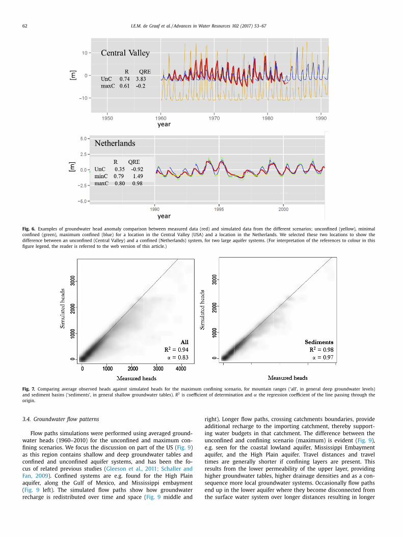
nd amplitude are well captured are given in Fig. 6 . Instead of plot-
ing actual head values, we plotted the anomalies related to their
ean values. The examples show that the model is able to capture
oth timing and amplitude of the observed heads reasonable well,
nd that including confining layers improves the estimates, seen in
articular for the amplitude estimate in the Central Valley exam-
le.
The scatter and statistics ( Fig. 7 ) of temporal mean simulated
alues against mean observed values for the maximum confining
cenario show that averaged values are reproduced well (very high
2 and α close to 1) and are slightly better when only head loca-
ions in areas with sediments and sedimentary basins are consid-
red in the comparison. Model performance of the other scenarios
s comparable (see the table of Fig. 5 . However, seen from both
catters the trend is for a general underestimation of groundwa-
er heads (meaning simulated groundwater levels are deeper than
bserved). This appears especially for the higher elevated areas,
here shallow water tables are most likely to be sampled but are
ot captured by our model as a result of the grid resolution. The R 2
f sediment basins is therefore slightly better than when mountain
reas are included in the evaluation, however groundwater heads
n sediment basins are underestimated.
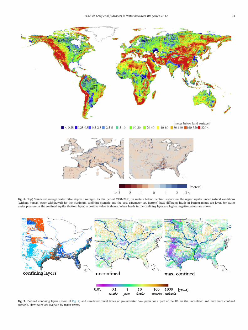
.3. Global map of groundwater depth
Fig. 8 (top) shows the long-term average groundwater depth
imulated for the maximum confining scenario simulated under
atural conditions (no groundwater pumping). General patterns
n groundwater depths can be identified, and are similar for the
hree scenarios and comparable to previous results by de Graaf
t al. (2015) . At the global-scale, sea level is the main control
f groundwater depth and throughout the entire coastal ribbon
hallow groundwater tables are found. These areas expand inland
here the coastal ribbon or coastal plains meets the major river
eltas, like the Mississippi, Indus, and large wetland areas of e.g.
outh America. At the regional scale, recharge is the main con-
rol together with topography. Topography influences for example
he heads in the flat areas of central Amazon and the lowlands of
outh America that receive groundwater from the higher elevated
reas. High, flat recharge regions also result in shallow ground-
ater tables, e.g. the tropical swamps of the Amazon. Regions
ith low recharge rates show deep groundwater tables; the deserts
tand out where groundwater, if present, is now disconnected from
he local topography. Also, for mountain regions deep groundwater
ables are simulated. In these areas local aquifers in sedimentary
ockets in mountain valleys are smaller than the grid resolution

I.E.M. de Graaf et al. / Advances in Water Resources 102 (2017) 53–67 61
Fig. 5. Scatter plots plotting amplitude error (| QRE |) against correlation ( R ) for the three scenarios, the maximum confined scenario shows the best agreement to the observed
head time series. When more than one observed time-series was available in a grid-cell, the result of the highest performance value is plotted in the scatter. In the top
figure cluster areas are indicated where simulated heads show good performance both on timing and amplitude error (I), good performance of timing (II), good performance
on amplitude error (III), and bad performance on both (IV). Percentage of simulated head time-series per cluster for the three scenarios are given in the table, as well as
model performance on average groundwater heads.
(
h
2
l
s
F
c
b
e
g
t
D
i
s
t
p
< 10 km) and are therefore not captured. As a result, groundwater
eads in these regions are likely underestimated ( de Graaf et al.,
015 ).
The differences in groundwater depth between the two model
ayers (top: confining layer, bottom: confined aquifer) are small. In-
ets of parts of the US and Europe illustrate this ( Fig. 8 bottom).
or unconfined systems, where top and bottom layers have equal
onductivities, any groundwater depth differences are expected to
e small. For confined systems, where conductivities are differ-
nt for the top confining layer and bottom confined aquifer, the
roundwater heads in the confined aquifers are often higher than
hose in the overlying layers. This is for example seen along the
utch coast, Po river, Rhone, and along the Gulf of Mexico, includ-
ng the Mississippi. However, when groundwater recharge does not
eep through the confining layer groundwater tables can exceed
he hydraulic heads of the confined aquifer. This is seen for exam-
le in the Mississippi embayment and the Garonne region (France).
62 I.E.M. de Graaf et al. / Advances in Water Resources 102 (2017) 53–67
Fig. 6. Examples of groundwater head anomaly comparison between measured data (red) and simulated data from the different scenarios; unconfined (yellow), minimal
confined (green), maximum confined (blue) for a location in the Central Valley (USA) and a location in the Netherlands. We selected these two locations to show the
difference between an unconfined (Central Valley) and a confined (Netherlands) system, for two large aquifer systems. (For interpretation of the references to colour in this
figure legend, the reader is referred to the web version of this article.)
Fig. 7. Comparing average observed heads against simulated heads for the maximum confining scenario, for mountain ranges (‘all’, in general deep groundwater levels)
and sediment basins (‘sediments’, in general shallow groundwater tables). R 2 is coefficient of determination and α the regression coefficient of the line passing through the
origin.
r
a
i
u
e
a
t
r
h
s
e
t
3.4. Groundwater flow patterns
Flow paths simulations were performed using averaged ground-
water heads (1960–2010) for the unconfined and maximum con-
fining scenarios. We focus the discussion on part of the US ( Fig. 9 )
as this region contains shallow and deep groundwater tables and
confined and unconfined aquifer systems, and has been the fo-
cus of related previous studies ( Gleeson et al., 2011; Schaller and
Fan, 2009 ). Confined systems are e.g. found for the High Plain
aquifer, along the Gulf of Mexico, and Mississippi embayment
( Fig. 9 left). The simulated flow paths show how groundwater
recharge is redistributed over time and space ( Fig. 9 middle and
ight). Longer flow paths, crossing catchments boundaries, provide
dditional recharge to the importing catchment, thereby support-
ng water budgets in that catchment. The difference between the
nconfined and confining scenario (maximum) is evident ( Fig. 9 ),
.g. seen for the coastal lowland aquifer, Mississippi Embayment
quifer, and the High Plain aquifer. Travel distances and travel
imes are generally shorter if confining layers are present. This
esults from the lower permeability of the upper layer, providing
igher groundwater tables, higher drainage densities and as a con-
equence more local groundwater systems. Occasionally flow paths
nd up in the lower aquifer where they become disconnected from
he surface water system over longer distances resulting in longer
I.E.M. de Graaf et al. / Advances in Water Resources 102 (2017) 53–67 63
Fig. 8. Top) Simulated average water table depths (averaged for the period 1960–2010) in meters below the land surface on the upper aquifer under natural conditions
(without human water withdrawal) for the maximum confining scenario and the best parameter set. Bottom) head different; heads in bottom minus top layer. For water
under pressure in the confined aquifer (bottom layer) a positive value is shown. When heads in the confining layer are higher, negative values are shown.
Fig. 9. Defined confining layers (zoom of Fig. 2 ) and simulated travel times of groundwater flow paths for a part of the US for the unconfined and maximum confined
scenario. Flow paths are overlain by major rivers.
64 I.E.M. de Graaf et al. / Advances in Water Resources 102 (2017) 53–67
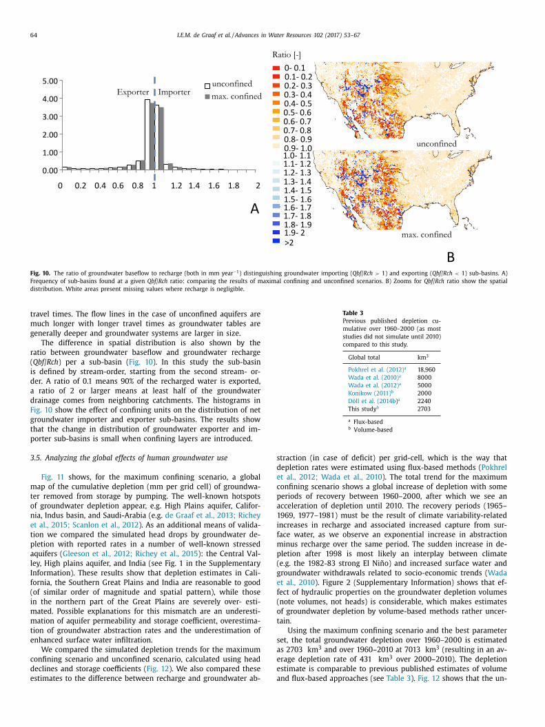
Fig. 10. The ratio of groundwater baseflow to recharge (both in mm year −1 ) distinguishing groundwater importing ( Qbf / Rch > 1) and exporting ( Qbf / Rch < 1) sub-basins. A)
Frequency of sub-basins found at a given Qbf / Rch ratio: comparing the results of maximal confining and unconfined scenarios. B) Zooms for Qbf / Rch ratio show the spatial
distribution. White areas present missing values where recharge is negligible.
Table 3
Previous published depletion cu-
mulative over 1960–20 0 0 (as most
studies did not simulate until 2010)
compared to this study.
Global total km
3
Pokhrel et al. (2012) a 18 ,960
Wada et al. (2010) a 80 0 0
Wada et al. (2012) a 50 0 0
Konikow (2011) b 20 0 0
Döll et al. (2014b ) a 2240
This study b 2703
a Flux-based b Volume-based
s
d
e
c
p
a
1
i
f
m
p
(
g
e
f
(
o
t
s
a
e
e
a
travel times. The flow lines in the case of unconfined aquifers are
much longer with longer travel times as groundwater tables are
generally deeper and groundwater systems are larger in size.
The difference in spatial distribution is also shown by the
ratio between groundwater baseflow and groundwater recharge
( Qbf / Rch ) per a sub-basin ( Fig. 10 ). In this study the sub-basin
is defined by stream-order, starting from the second stream- or-
der. A ratio of 0.1 means 90% of the recharged water is exported,
a ratio of 2 or larger means at least half of the groundwater
drainage comes from neighboring catchments. The histograms in
Fig. 10 show the effect of confining units on the distribution of net
groundwater importer and exporter sub-basins. The results show
that the change in distribution of groundwater exporter and im-
porter sub-basins is small when confining layers are introduced.
3.5. Analyzing the global effects of human groundwater use
Fig. 11 shows, for the maximum confining scenario, a global
map of the cumulative depletion (mm per grid cell) of groundwa-
ter removed from storage by pumping. The well-known hotspots
of groundwater depletion appear, e.g. High Plains aquifer, Califor-
nia, Indus basin, and Saudi-Arabia (e.g. de Graaf et al., 2013; Richey
et al., 2015; Scanlon et al., 2012 ). As an additional means of valida-
tion we compared the simulated head drops by groundwater de-
pletion with reported rates in a number of well-known stressed
aquifers ( Gleeson et al., 2012; Richey et al., 2015 ): the Central Val-
ley, High plains aquifer, and India (see Fig. 1 in the Supplementary
Information). These results show that depletion estimates in Cali-
fornia, the Southern Great Plains and India are reasonable to good
(of similar order of magnitude and spatial pattern), while those
in the northern part of the Great Plains are severely over- esti-
mated. Possible explanations for this mismatch are an underesti-
mation of aquifer permeability and storage coefficient, overestima-
tion of groundwater abstraction rates and the underestimation of
enhanced surface water infiltration.
We compared the simulated depletion trends for the maximum
confining scenario and unconfined scenario, calculated using head
declines and storage coefficients ( Fig. 12 ). We also compared these
estimates to the difference between recharge and groundwater ab-
traction (in case of deficit) per grid-cell, which is the way that
epletion rates were estimated using flux-based methods ( Pokhrel
t al., 2012; Wada et al., 2010 ). The total trend for the maximum
onfining scenario shows a global increase of depletion with some
eriods of recovery between 1960–20 0 0, after which we see an
cceleration of depletion until 2010. The recovery periods (1965–
969, 1977–1981) must be the result of climate variability-related
ncreases in recharge and associated increased capture from sur-
ace water, as we observe an exponential increase in abstraction
inus recharge over the same period. The sudden increase in de-
letion after 1998 is most likely an interplay between climate
e.g. the 1982-83 strong El Niño) and increased surface water and
roundwater withdrawals related to socio-economic trends ( Wada
t al., 2010 ). Figure 2 (Supplementary Information) shows that ef-
ect of hydraulic properties on the groundwater depletion volumes
note volumes, not heads) is considerable, which makes estimates
f groundwater depletion by volume-based methods rather uncer-
ain.
Using the maximum confining scenario and the best parameter
et, the total groundwater depletion over 1960–20 0 0 is estimated
s 2703 km
3 and over 1960–2010 at 7013 km
3 (resulting in an av-
rage depletion rate of 431 km
3 over 20 0 0–2010). The depletion
stimate is comparable to previous published estimates of volume
nd flux-based approaches (see Table 3 ). Fig. 12 shows that the un-

I.E.M. de Graaf et al. / Advances in Water Resources 102 (2017) 53–67 65
Fig. 11. Cumulative groundwater depletion (in mm over 1960–2010) resulting from human water use for the maximum confining scenario and the best parameter set. For
zoons of head declines see Fig. 1 .
Fig. 12. Trend of depletion globally, estimated for the maximum confining and unconfined scenario, and calculated as the cumulative deficit between recharge and abstrac-
tion for grid-cells where abstraction is larger than recharge.
c
e
d
c
o
d
a
i
r
o
1
g
t
P
t
p
i
f
onfined scenario shows in general the same trend. However, the
stimated groundwater depletion is larger. The estimated depletion
ifference is 4803 km
3 . This difference can be explained by the in-
rease in river capture under the confined scenario. The presence
f a confining layer results in a larger area of influence of head
ecline.
Despite the lower permeability of the confining layer, this larger
rea of influence causes a larger decrease in baseflow or a larger
ncrease in riverbed infiltration. Indeed, the groundwater drainage
ate of the confined aquifer model is ∼50 km
3 y −1 lower than that
r
f the unconfined aquifer model, which adds to 30 0 0 km
3 over
960–2010.
The estimated depletion calculated as the deficit between
roundwater recharge and abstraction for cells where more wa-
er is abstracted than recharged (flux-based method as used in e.g.
okhrel et al., 2012; Wada et al., 2010 ) shows much bigger deple-
ion volumes of 26,700 km
3 over 1960–2010 (with an average de-
letion rate of 323 km
3 over 20 0 0–2010). Again, the difference
n estimated depletion can be explained by the increase in sur-
ace water capture, which is not accounted for by calculating the
echarge-abstraction difference but is included in the groundwa-
66 I.E.M. de Graaf et al. / Advances in Water Resources 102 (2017) 53–67
t
t
G
e
t
h
a
c
i
c
t
s
t
a
T
g
m
d
t
t
m
o
a
d
c
a
g
c
t
i
o
t
g
d
t
c
t
i
s
w
c
l
l
r
o
e
A
S
a
D
s
d
v
m
S
f
ter model. The large difference confirms the need to use a lateral
groundwater model, accounting for groundwater- surface water in-
teractions, when sensitivity of aquifers to storage changes is stud-
ied.
4. Conclusions
This paper presents a global-scale groundwater model simulat-
ing lateral flows and head fluctuations caused by changes in cli-
mate or human water use over the period 1960–2010. It is the first
global-scale transient groundwater model that includes a param-
eterization of unconfined and confined systems (presented in two
model layers), and simulates lateral-flows and groundwater-surface
water interactions in these systems. This results in more realistic
estimates of groundwater head fluctuations and storage changes
than before.
One of the main contributions of this study is the parameter-
ization of the world‘s aquifer systems, including information on
their vertical structure. The model’s aquifer parameterization is
based on global data-sets of surface geology and hydraulic prop-
erties and topography-based estimates of the vertical structure of
the aquifer systems. Only globally available data sets are used in
order to keep the methods readily applicable to data-poor envi-
ronments. The world’s aquifers are classified into confined and un-
confined systems to understand aquifer sensitivity to groundwater
abstractions and to properly project future groundwater level de-
clines.
Results show that including confining layers (estimated 6–
20% of the total aquifer area) improve estimates of groundwater
head fluctuations and timing and change flow path patters and
groundwater-surface water interaction rates. Model performance
on average heads and timing of fluctuations is slightly better when
confined systems are considered, and best for the maximum sce-
nario (20% of the total aquifer area is confined). Groundwater flow
paths within confining layers are shorter compared to paths in the
aquifer, while flows within the confined aquifer can get discon-
nected from the local drainage system due to the low conductiv-
ity of the confining layer. This change in groundwater hydrology
is reflected in head fluctuations and flow magnitudes. Although
model performance in terms of heads is only slightly better when
confined aquifers are considered, the estimated depletion rates are
closer to previous volume-based estimates (e.g. Konikow, 2011 ) and
show that capture of surface-groundwater interaction are simu-
lated more realistically than before.
Lateral groundwater flows between basins are significant in the
model, especially for confined aquifer areas where long paths are
simulated crossing catchment boundaries, thereby supporting wa-
ter budgets of neighboring catchments or aquifer systems.
The estimated global depletion over the period 1960–2010 is
7013 km
3 . This value is in the range of earlier published val-
ues (e.g. 80 0 0 km
3 ( Wada et al., 2010 ), 50 0 0 km
3 ( Wada et al.,
2012 )). Hotspot regions of depletion are found for intensively irri-
gated areas, like the High Plains aquifer (simulated at 1390 km
3
for 20 0 0) or Central Valley (simulated at 48 km
3 for 20 0 0). Al-
though depletion is strongly overestimated for the Northern High
Plains compared to reported data ( ∼240 km
3 reported for 20 0 0
by USGS ( Scanlon et al., 2012 )), simulated temporal fluctuations
mimic measured data well. The same holds for Central Valley,
where we slightly underestimate total depletion (which is reported
at ∼53 km
3 for 20 0 0). The comparison of depletion volumes
for confined, unconfined, and estimated as the deficit between
recharge and abstraction, shows increased river capture lowers the
estimated depletion volume. This confirms that a lateral ground-
water model, with realistic parameter settings for its aquifers, is
preferred when sensitivity of aquifers to groundwater abstractions
is studied.
Of course there are several limitations to our approach. Firstly,
he grid-resolution (5 ′ , approx. 10x10 km at the equator) is still
oo coarse to capture local aquifers in higher and steeper terrain.
roundwater heads are underestimated for these areas. Note how-
ver, that perched water tables within the soil are accounted for in
he PCR-GLOBWB.
Secondly, our groundwater model is not fully coupled to our
ydrological model, meaning the groundwater-surface water inter-
ction is still simplified: two-way groundwater-surface water ex-
hange and the resulting groundwater recharge is first simulated
n PCR-GLOBWB. The simulated groundwater recharge, and the cal-
ulated river levels are imposed on the MODFLOW RIV package af-
erwards. Although this approach can be expected to preserve the
ame groundwater-surface water fluxes in the groundwater model,
he effects of groundwater pumping on the surface water system
re more intricate and would preferably require a tighter coupling.
hus, this modeling study is the next step towards a fully coupled
lobal surface water- groundwater model. In future work the two
odels will be fully coupled to incorporate feedback effects on a
aily time step basis.
Thirdly, the most obvious limitation is that the aquifer parame-
erization used in this study is a relative simple approximation of
he true 3D-hydrogeological setup of aquifer systems that contain
ultiple stacked aquifers and aquitards. Our model thus produces
nly a first-order estimate of head fluctuations, storage loss and
verage head decline over the entire aquifer set, most likely un-
erestimating depletion rates when abstraction comes from deeper
onfined aquifer systems. Hence, the global hydrogeological model,
lthough at the edge of what can be expected when using only
lobal information, leaves much room for improvement. A con-
erted effort of the hydrogeological community to use informa-
ion from regional on hydrological-and groundwater models hold-
ng more detailed information of e.g. presence of confining layers
r conductivity values, as well as observations to update the global
wo-layer model would likely lead to the largest improvement in
lobal groundwater assessments ( Bierkens et al., 2015 ). Also, more
etailed information on the precise vertical hydrogeological struc-
ure of the aquifers around the observation well screens, used for
alibration and validation of the model, would improve the calibra-
ion results. Knowledge on the sensitivity of aquifers to changes
n climate and human water use is vital and needed to ensure
ustainable water use particularly for the semi-arid regions of the
orld, where groundwater abstractions will intensify due to an in-
rease in drought frequency and duration combined with popu-
ation growth, expanding irrigation areas, and rising standards of
iving. Therefore it is important not only to focus only on areas al-
eady experiencing groundwater depletion, but to provide a global
verview revealing where and when in future new areas experi-
ncing water scarcity will develop in the near future.
cknowledgments
This research was funded by the Netherlands Organization for
cientific Research (NWO) under the program ‘Planetary bound-
ries of the global fresh water cycle’. This work was done on the
utch national supercomputer Cartesius with the support of SURF-
ara. We would like to thank several colleagues, among others prof.
r. Petra Döll (Goethe University) and prof. Ying Fan (Rutgers Uni-
ersity) and two anonymous reviewers, for their constructive com-
ents on an earlier version of this paper.
upplementary material
Supplementary material associated with this article can be
ound, in the online version, at 10.1016/j.advwatres.2017.01.011
I.E.M. de Graaf et al. / Advances in Water Resources 102 (2017) 53–67 67
R
v
B
B
D
D
D
D
D
F
F
F
F
G
G
G
G
d
d
H
H
K
L
L
K
M
M
M
P
P
R
S
S
S
S
S
S
S
S
T
U
U
W
W
W
W
eferences
an Beek, L. , Wada, Y. , Bierkens, M. , 2011. Global monthly water stress: 1. water
balance and water availability. Water Resour. Res. 47 (7) .
ierkens, M.F.P., Bell, V.A., Burek, P., Chaney, N., Condon, L.E., David, C.H., de Roo, A.,Döll, P., Drost, N., Famiglietti, J.S., Flörke, M., Gochis, D.J., Houser, P., Hut, R.,
Keune, J., Kollet, S., Maxwell, R.M., Reager, J.T., Samaniego, L., Sudicky, E., Su-tanudjaja, E.H., van de Giesen, N., Winsemius, H., Wood, E.F., 2015. Hyper-
resolution global hydrological modelling: what is next?: everywhere and locallyrelevant. Invited Commentary Hydrol. Processes 29 (2), 310–320. http://dx.doi.
org/10.1002/hyp.10391 .
ierkens, M.F.P., van den Hurk, B.J.J.M., 2007. Groundwater convergence as a pos-sible mechanism for multi-year persistence in rainfall. Geophys. Res. Lett. 34
(L02402). http://dx.doi.org/10.1029/2006GL028396 . ee, D., Uppala, S., Simmons, A., Berrisford, P., Poli, P., S., K., 2011. The era-interim
reanalysis: configuration and performance of the data assimilation system. Q. J.R. Meteorolog. Soc. 137 (656), 553–597. http://dx.doi.org/10.1002/qj.828 .
oherty, J. , 2015. Calibration and uncertainty analysis for complex environmentalmodels. Watermark Numerical Computing,Brisbane, Australia. .
öll, P. , Fritsche, M. , Eicker, H. , Schmied, M. , 2014. Seasonal water storage variations
as impacted by water abstractions: comparing the output of a global hydrolog-ical model with grace and gps observations. Surv. Geophys. 35, 1311–1331 .
öll, P. , Hoffmann-Dobrev, H. , Portmann, F. , Siebert, S. , Eicker, A. , Rodell, M. , 2012.Impact of water withdrawals from groundwater and surface water on continen-
tal water storage variations. J. Geodyn. 59–60, 143–156 . öll, P., Müller Schmied, H., Schuh, C., Portmann, F.T., Eicker, A., 2014. Global-scale
assessment of groundwater depletion and related groundwater abstractions:
combining hydrological modeling with information from well observations andgrace satellites. Water Resour. Res. 50 (7), 5698–5720. http://dx.doi.org/10.1002/
2014WR015595 . an, Y., 2015. Groundwater in the earth’s critical zone: relevance to large-scale pat-
terns and processes. Water Resour. Res. 51 (5), 3052–3069. http://dx.doi.org/10.1002/2015WR017037 .
an, Y., Li, H., Miguez-Macho, G., 2013. Global patterns of groundwater table depth.
Science 339, 940–943. http://dx.doi.org/10.1126/science.1229881 . an, Y., Miguez-Macho, G., Weaver, C.P., Walko, R., Robock, A., 2007. Incorporating
water table dynamics in climate modeling: 1. water table observations and equi-librium water table simulations. J. Geophys. Res.-Atmos. 112. http://dx.doi.org/
10.1029/20 06JD0 08111 . oster, S.S.D., Chilton, P.J., 2003. Groundwater: the processes and global significance
of aquifer degradation. Phil. Trans. R. Soc. Lond. B 358, 1957–1972. http://dx.doi.
org/10.1098/rstb.2003.1380 . leeson, T. , Jasechko, S. , Luijendijk, E. , Cardenas, M. , 2016. The global volume and
distribution of modern groundwater. Nat. Geosci. 9 (2), 161–167 . leeson, T., Moosdorf, N., Hartmann, J., van Beek, L.P.H., 2014. A glimpse beneath
earth’s surface: global hydrogeological maps (glhymps) of permeability andporosity. Geophys. Res. Lett. 41. http://dx.doi.org/10.1002/2014GL059856 .
leeson, T., Smith, L., Moosdorf, N., Hartmann, J., Dürr, H.H., Manning, A.H., van
Beek, L.P.H., Jellinek, A.M., 2011. Mapping permeability over the surface of theearth. Geophys. Res. Lett. 38. http://dx.doi.org/10.1029/2010GL045565 .
leeson, T., Wada, Y., Bierkens, M.F.P., Van Beek, L.P.H., 2012. Water balance of globalaquifers revealed by groundwater footprint. Nature 488 (7410), 197–200. http://
dx.doi.org/10.1038/nature11295 . e Graaf, I.E.M. , van Beek, L.P.H. , Sutanudjaja, S.H. , Bierkens, M.F.P. , 2015. A high-res-
olution global- scale groundwater model. HESS 2 (19), 823–837 .
e Graaf, I.E.M., van Beek, L.P.H., Wada, Y., Bierkens, M.F.P., 2013. Dynamic attribu-tion of global water demand to surface water and groundwater resources: ef-
fects of abstractions and return flows on river discharges. Adv. Water Resour.64, 21–33. http://dx.doi.org/10.1016/j.advwatres.2013.12.002 .
artmann, J., Moosdorf, N., 2012. The new global lithological map database glim: arepresentation of rock properties at the earth surface. Geochem. Geophy. Geosy.
13. http://dx.doi.org/10.1029/2012GC004370 . eath, R.C. , 1983. Basic groundwater hydrology. USGS, Wat. Sup. Pap. 2220 .
onikow, L.F., 2011. Contribution of global groundwater depletion since 1900 to sea-
level rise. Geophys. Res. Lett. 38. http://dx.doi.org/10.1029/2011GL048604 . acey, G. , 1930. Stable cchannel in alluvium. P. I. Civ. Eng. 229, 259–292 .
am, A., Karssenberg, D., van den Hurk, B.J.J.M., Bierkens, M.F.P., 2011. Spatial andtemporal connections in groundwater contribution to evaporation. Hydrol. Earth
Syst. Sci. 15, 2621–2630. http://dx.doi.org/10.5194/ hess- 15- 2621- 2011 . raaijenhof van der Leur, D. , 1958. A study of non-steady groundwater flow with
special reference to a reservoir coefficient. de ingenieur 70, 87–94 .
anning, R. , 1891. On the flow of water in open cchannel and pipes. Trans. Inst.Civil Eng. Irel., Dublin, 161–207 .
cDonald, M.G. , Harbaugh, A.W. , 20 0 0. Modflow-20 0 0, the us geological surveymodular ground-water model – user guide to modularmodular concepts and
the ground-water flow process. Tech. rep., US Geological Survey, Reston, Vir-ginia .
itchell, T.D. , Jones, P.D. , 2005. An improved method of constructing a database ofmonthly climate observations and associated high-resolution grids. Int. J. Clima-
tol. 25 (6), 693–712 . okhrel, Y. , Hanasaki, N. , Koirala, S. , Cho, J. , Yeh, P.J.F. , Kim, H. , 2012. Incorporating
anthropogenic water regulation modules into a land surface model. J. Hydrom-
eteorol. 13 (1), 255–269 . ollock, D. , 1994. User’s Guide for Modpath/Modpath-Plot, Version 3: A Parti-
cle Tracking Post-Processing Package for Modflow, the US Geological SurveyFinite-Difference Groundwater Flow Model. Technical report . US Geological Sur-
vey Open-File Report 94-464, US Geological Survey, Reston, Virginia ichey, A.S., Thomas, B.F., Lo, M.-H., Famiglietti, J.S., Swenson, S., Rodell, M., 2015.
Uncertainty in global groundwaer storage estimates in a total groundwater
stress framework. Water Resour. Res. http://dx.doi.org/10.1002/2015WR017351 . avenije, H.H., 2003. The width of a bankfull channel; lacey’s formula explained. J.
Hydrol. 276, 176–183. http://dx.doi.org/10.1016/S0022-1694(03)00069-6 . canlon, B.R., Faunt, C.C., Longuevergne, L., Reedy, R.C., Allley, W.M., McGuire, V.L.,
McMahon, B., 2012. Groundwaer depletion and sustainability of irrigation in theus high plains and central valley. PNAS 109 (24). http://dx.doi.org/10.1073/pnas.
1200311109 .
challer, M.F., Fan, Y., 2009. River basins as groundwater exporters and importers:implications for water cycle and climate modeling. J. Geophys. Res.-Atmos. 114.
http://dx.doi.org/10.1029/2008JD010636 . chmitz, O. , Karssenberg, D. , van Deursen, W. , Wesseling, C. , 2009. Linking external
components to spatio-temporal modeling framework: coupling modflow andpcraster. Environ. Modell. Softw. 24, 1088–1099 . 0.1016/j.envsoft.2009.02.018
iebert, S., Döll, P., 2010. Quantifying blue and green virtual water contents in global
crop production as well as potential production losses without irrigation. J. Hy-drol. 384(3-4), 198–217. http://dx.doi.org/10.1016/j.hydrol.2009.07.031 .
tanley, D.J. , Warne, A.G. , 1994. Worldwide initiation of holocene marine deltas bydeceleration of sea-level rise. Science 265, 228–231 .
utanudjaja, E.H., van Beek, L.P.H., de Jong, S.M., van Geer, F.C., Bierkens, M.F.P.,2011. Large-scale groundwater modeling using global datasets: a test case for
the rhine-meuse basin. Hydrol. Earth Syst. Sci. 15 (2913–2935). http://dx.doi.
org/10.5194/hess-15-2913-2011 . yvitski, J.P.M., Vörösmarty, C.J., Kettner, A.J., Green, P., 2005. Impact of humans on
flux of terrestrial sediment to the global coastal ocean. Science 308, 376–380.http://dx.doi.org/10.1126/science.1109454 .
oscano, M.A. , Macintyre, I.G. , 2003. Corrected western atlantic sea-level curve forthe last 11,0 0 0 years based on calibrated 14c dates from acropora palmata
framework and intertidal mangrove peat 22 (3), 257–270 .
NESCO , 2009. The United Nations World Water Development Report. Technical Re-port .
ppala, S.M. , Kållberg, P.W. , Simmons, A.J. , Andrae, U. , Bechtold, V.D.C. , Fiorino, M. ,Gibson, J.K. , Haseler, J. , Hernandez, A. , Kelly, G.A. , X., L. , Onogi, K. , Saari-
nen, S. , Sokka, N. , Allan, R.P. , Andersson, K. , Arpe, E. , Balmaseda, M.A. , Bel-jaars, A.C.M. , Berg, L.V.D. , Bidlot, J. , Bormann, N. , Caires, S. , Chevallier, F. ,
Dethof, A. , Dragosavac, M. , Fisher, M. , Fuentes, M. , Hagemann, S. , Hólm, E. ,Hoskins, B.J. , Isaksen, L. , Janssen, P.A.E.M. , Jenne, R. , Mcnally, A.P. , Mahfouf, J.-F. ,
Morcrette, J.-J. , Rayner, N.A. , Saunders, R.W. , Simon, P. , Sterl, A. , Trenberth, K.E. ,
Untch, A. , Vasiljevic, D. , Viterbo, P. , Woollen, J. , 2005. The era-40 re-analysis. Q.J. R. Meteorolog. Soc. 131 (612), 2961–3012 .
ada, Y. , van Beek, L.P.H. , Bierkens, M.F.P. , 2012. Nonsustainable groundwater sus-taining irrigation: a global assessment. Water Resour. Res. 48 (1) .
ada, Y. , Van Beek, L. , Van Kempen, C. , Reckman, J. , Vasak, S. , Bierkens, M. , 2010.Global depletion of groundwater resources. Geophys. Res. Lett. 37 (20) .
ada, Y., Wisser, D., Bierkens, M.F.P., 2014. Global modeling of withdrawal, alloca-
tion and consumptive use of surface water and groundwater resources. EarthSyst. Dynam. 5, 15–40. http://dx.doi.org/10.5194/esd- 5- 15- 2014 .
ood, E.F., Roundy, J.K., Troy, T.J., van Beek, R., Bierkens, M., Blyth, E., de Roo, A.,Döll, P., Ek, M., Famiglietti, J., Gochis, D., van de Giesen, N., Houser, P.,
Jaffe, P., Kollet, S., Lehner, B., Lettenmaier, D.P., Peters-Lidard, C.D., Sivapalan, M.,Sheffield, J., Wade, A.J., Whitehead, P., 2012. Reply to comment by keith, j. beven
and hannah, l. cloke on “hyperresolution global land surface modeling: meeting
a grand challenge for monitoring earth’s terrestrial water”. Water Resour. Res.48. http://dx.doi.org/10.1029/2011WR011202 .
Related Documents