Advances in Electron Microscopy with Deep Learning by Jeffrey Mark Ede Thesis To be submitted to the University of Warwick for the degree of Doctor of Philosophy in Physics Department of Physics January 2021

Welcome message from author
This document is posted to help you gain knowledge. Please leave a comment to let me know what you think about it! Share it to your friends and learn new things together.
Transcript
Advances in Electron Microscopy with Deep Learning
by
Jeffrey Mark Ede
Thesis
To be submitted to the University of Warwick
for the degree of
Doctor of Philosophy in Physics
Department of Physics
January 2021
Contents
Contents i
List of Abbreviations iii
List of Figures viii
List of Tables xvii
Acknowledgments xix
Declarations xx
Research Training xxv
Abstract xxvi
Preface xxviiI Initial Motivation . . . . . . . . . . . . . . . . . . . . . . . . . . . . . . . . . . . . . . . . . xxvii
II Thesis Structure . . . . . . . . . . . . . . . . . . . . . . . . . . . . . . . . . . . . . . . . . . xxvii
III Connections . . . . . . . . . . . . . . . . . . . . . . . . . . . . . . . . . . . . . . . . . . . . xxix
Chapter 1 Review: Deep Learning in Electron Microscopy 11.1 Scientific Paper . . . . . . . . . . . . . . . . . . . . . . . . . . . . . . . . . . . . . . . . . . 1
1.2 Reflection . . . . . . . . . . . . . . . . . . . . . . . . . . . . . . . . . . . . . . . . . . . . . 100
Chapter 2 Warwick Electron Microscopy Datasets 1012.1 Scientific Paper . . . . . . . . . . . . . . . . . . . . . . . . . . . . . . . . . . . . . . . . . . 101
2.2 Amendments and Corrections . . . . . . . . . . . . . . . . . . . . . . . . . . . . . . . . . . . 133
2.3 Reflection . . . . . . . . . . . . . . . . . . . . . . . . . . . . . . . . . . . . . . . . . . . . . 133
Chapter 3 Adaptive Learning Rate Clipping Stabilizes Learning 1363.1 Scientific Paper . . . . . . . . . . . . . . . . . . . . . . . . . . . . . . . . . . . . . . . . . . 136
3.2 Amendments and Corrections . . . . . . . . . . . . . . . . . . . . . . . . . . . . . . . . . . . 147
3.3 Reflection . . . . . . . . . . . . . . . . . . . . . . . . . . . . . . . . . . . . . . . . . . . . . 147
Chapter 4 Partial Scanning Transmission Electron Microscopy with Deep Learning 1494.1 Scientific Paper . . . . . . . . . . . . . . . . . . . . . . . . . . . . . . . . . . . . . . . . . . 149
4.2 Amendments and Corrections . . . . . . . . . . . . . . . . . . . . . . . . . . . . . . . . . . . 176
4.3 Reflection . . . . . . . . . . . . . . . . . . . . . . . . . . . . . . . . . . . . . . . . . . . . . 176
i
Chapter 5 Adaptive Partial Scanning Transmission Electron Microscopy with Reinforcement Learn-ing 1785.1 Scientific Paper . . . . . . . . . . . . . . . . . . . . . . . . . . . . . . . . . . . . . . . . . . 178
5.2 Reflection . . . . . . . . . . . . . . . . . . . . . . . . . . . . . . . . . . . . . . . . . . . . . 202
Chapter 6 Improving Electron Micrograph Signal-to-Noise with an Atrous Convolutional Encoder-Decoder 2036.1 Scientific Paper . . . . . . . . . . . . . . . . . . . . . . . . . . . . . . . . . . . . . . . . . . 203
6.2 Amendments and Corrections . . . . . . . . . . . . . . . . . . . . . . . . . . . . . . . . . . . 212
6.3 Reflection . . . . . . . . . . . . . . . . . . . . . . . . . . . . . . . . . . . . . . . . . . . . . 212
Chapter 7 Exit Wavefunction Reconstruction from Single Transmission Electron Micrographs withDeep Learning 2147.1 Scientific Paper . . . . . . . . . . . . . . . . . . . . . . . . . . . . . . . . . . . . . . . . . . 214
7.2 Reflection . . . . . . . . . . . . . . . . . . . . . . . . . . . . . . . . . . . . . . . . . . . . . 239
Chapter 8 Conclusions 240
References 243
Vita 263
ii
List of Abbreviations
AE Autoencoder
AFM Atomic Force Microscopy
ALRC Adaptive Learning Rate Clipping
ANN Artificial Neural Network
ASPP Atrous Spatial Pyramid Pooling
A-tSNE Approximate t-Distributed Stochastic Neighbour Embedding
AutoML Automatic Machine Learning
Bagged Bootstrap Aggregated
bfloat16 16 Bit Brain Floating Point
BM3D Block-Matching and 3D Filtering
BPTT Backpropagation Through Time
CAE Contractive Autoencoder
CBED Convergent Beam Electron Diffraction
CBOW Continuous Bag-of-Words
CCD Charge-Coupled Device
cf. Confer
Ch. Chapter
CIF Crystallography Information File
CLRC Constant Learning Rate Clipping
CNN Convolutional Neural Network
COD Crystallography Open Database
COVID-19 Coronavirus Disease 2019
CPU Central Processing Unit
CReLU Concatenated Rectified Linear Unit
CTEM Conventional Transmission Electron Microscopy
CTF Contrast Transfer Function
CTRNN Continuous Time Recurrent Neural Network
CUDA Compute Unified Device Architecture
cuDNN Compute Unified Device Architecture Deep Neural Network
DAE Denoising Autoencoder
DALRC Doubly Adaptive Learning Rate Clipping
DDPG Deep Deterministic Policy Gradients
iii
D-LACBED Digital Large Angle Convergent Beam Electron Diffraction
DLF Deep Learning Framework
DLSS Deep Learning Supersampling
DNN Deep Neural Network
DQE Detective Quantum Efficiency
DSM Doctoral Skills Module
EBSD Electron Backscatter Diffraction
EDX Energy Dispersive X-Ray
EE Early Exaggeration
EELS Electron Energy Loss Spectroscopy
e.g. Exempli Gratia
ELM Extreme Learning Machine
ELU Exponential Linear Unit
EM Electron Microscopy
EMDataBank Electron Microscopy Data Bank
EMPIAR Electron Microscopy Public Image Archive
EPSRC Engineering and Physical Sciences Research Council
Eqn. Equation
ESN Echo-State Network
ETDB-Caltech Caltech Electron Tomography Database
EWR Exit Wavefunction Reconstruction
FIB-SEM Focused Ion Beam Scanning Electron Microscopy
Fig. Figure
FFT Fast Fourier Transform
FNN Feedforward Neural Network
FPGA Field Programmable Gate Array
FT Fourier Transform
FT−1 Inverse Fourier Transform
FTIR Fourier Transformed Infrared
FTSR Focal and Tilt Series Reconstruction
GAN Generative Adversarial Network
GMS Gatan Microscopy Suite
GPU Graphical Processing Unit
GRU Gated Recurrent Unit
GUI Graphical User Interface
iv

HPC High Performance Computing
ICSD Inorganic Crystal Structure Database
i.e. Id Est
i.i.d. Independent and Identically Distributed
IndRNN Independently Recurrent Neural Network
JSON Javascript Object Notation
KDE Kernel Density Estimated
KL Kullback-Leibler
LR Learning Rate
LSTM Long Short-Term Memory
LSUV Layer-Sequential Unit-Variance
MAE Mean Absolute Error
MDP Markov Decision Process
MGU Minimal Gated Unit
MLP Multilayer Perceptron
MPAGS Midlands Physics Alliance Graduate School
MTRNN Multiple Timescale Recurrent Neural Network
MSE Mean Squared Error
N.B. Nota Bene
NiN Network-in-Network
NIST National Institute of Standards and Technology
NMR Nuclear Magnetic Resonance
MSE Neural Network Exchange Format
NTM Neural Turing Machine
ONNX Open Neural Network Exchange
OpenCL Open Computing Language
OU Ornstein-Uhlenbeck
PCA Principal Component Analysis
PDF Probability Density Function or Portable Document Format
v

PhD Doctor of Philosophy
POMDP Partially Observed Markov Decision Process
PReLU Parametric Rectified Linear Unit
PSO Particle Swarm Optimization
RADAM Rectified ADAM
RAM Random Access Memory
RBF Radial Basis Function
RDPG Recurrent Deterministic Policy Gradients
ReLU Rectified Linear Unit
REM Reflection Electron Microscopy
RHEED Reflection high-energy electron diffraction
RHEELS Reflection High Electron Energy Loss Spectroscopy
RL Reinforcement Learning
RMLP Recurrent Multilayer Perceptron
RMS Root Mean Squared
RNN Recurrent Neural Network
RReLU Randomized Leaky Rectified Linear Unit
RTP Research Technology Platform
RWI Random Walk Initialization
SAE Sparse Autoencoder
SELU Scaled Exponential Linear Unit
SEM Scanning Electron Microscopy
SGD Stochastic Gradient Descent
SNE Stochastic Neighbour Embedding
SNN Self-Normalizing Neural Network
SPLEEM Spin-Polarized Low-Energy Electron Microscopy
SSIM Structural Similarity Index Measure
STM Scanning Tunnelling Microscopy
SVD Singular Value Decomposition
SVM Support Vector Machine
TEM Transmission Electron Microscopy
TIFF Tag Image File Format
TPU Tensor Processing Unit
tSNE t-Distributed Stochastic Neighbour Embedding
TV Total Variation
vi
URL Uniform Resource Locator
US-tSNE Uniformly Separated t-Distributed Stochastic Neighbour Embedding
VAE Variational Autoencoder
VAE-GAN Variational Autoencoder Generative Adversarial Network
VBN Virtual Batch Normalization
VGG Visual Geometry Group
WDS Wavelength Dispersive Spectroscopy
WEKA Waikato Environment for Knowledge Analysis
WEMD Warwick Electron Microscopy Datasets
WLEMD Warwick Large Electron Microscopy Datasets
w.r.t. With Respect To
XAI Explainable Artificial Intelligence
XPS X-Ray Photoelectron Spectroscopy
XRD X-Ray Diffraction
XRF X-Ray Fluorescence
vii
List of Figures
Preface
1. Connections between publications covered by chapters of this thesis. An arrow from chapter x to chapter yindicates that results covered by chapter y depend on results covered by chapter x. Labels indicate types ofresearch outputs associated with each chapter, and total connections to and from chapters.
Chapter 1 Review: Deep Learning in Electron Microscopy
1. Example applications of a noise-removal DNN to instances of Poisson noise applied to 512×512 crops fromTEM images. Enlarged 64×64 regions from the top left of each crop are shown to ease comparison. Thisfigure is adapted from our earlier work under a Creative Commons Attribution 4.0 license.
2. Example applications of DNNs to restore 512×512 STEM images from sparse signals. Training as part of agenerative adversarial network yields more realistic outputs than training a single DNN with mean squarederrors. Enlarged 64×64 regions from the top left of each crop are shown to ease comparison. a) Input is aGaussian blurred 1/20 coverage spiral. b) Input is a 1/25 coverage grid. This figure is adapted from our earlierworks under Creative Commons Attribution 4.0 licenses.
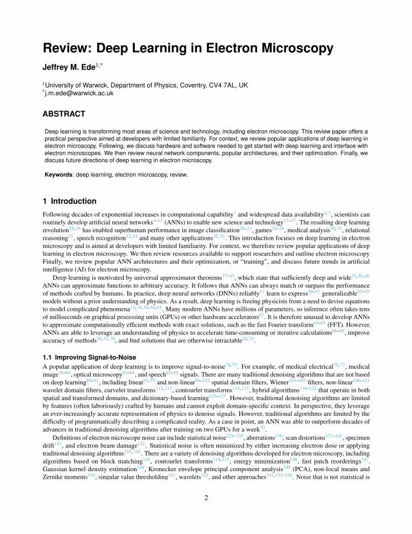
3. Example applications of a semantic segmentation DNN to STEM images of steel to classify dislocationlocations. Yellow arrows mark uncommon dislocation lines with weak contrast, and red arrows indicate thatfixed widths used for dislocation lines are sometimes too narrow to cover defects. This figure is adapted withpermission under a Creative Commons Attribution 4.0 license.
4. Example applications of a DNN to reconstruct phases of exit wavefunction from intensities of single TEMimages. Phases in [−π, π) rad are depicted on a linear greyscale from black to white, and Miller indices labelprojection directions. This figure is adapted from our earlier work under a Creative Commons Attribution 4.0license.
5. Reciprocity of TEM and STEM electron optics.
6. Numbers of results per year returned by Dimensions.ai abstract searches for SEM, TEM, STEM, STM andREM qualitate their popularities. The number of results for 2020 is extrapolated using the mean rate before14th July 2020.
7. Visual comparison of various normalization methods highlighting regions that they normalize. Regions can benormalized across batch, feature and other dimensions, such as height and width.
8. Visualization of convolutional layers. a) Traditional convolutional layer where output channels are sums ofbiases and convolutions of weights with input channels. b) Depthwise separable convolutional layer wheredepthwise convolutions compute one convolution with weights for each input channel. Output channels aresums of biases and pointwise convolutions weights with depthwise channels.
9. Two 96×96 electron micrographs a) unchanged, and filtered by b) a 5×5 symmetric Gaussian kernel with a2.5 px standard deviation, c) a 3×3 horizontal Sobel kernel, and d) a 3×3 vertical Sobel kernel. Intensities ina) and b) are in [0, 1], whereas intensities in c) and d) are in [-1, 1].
10. Residual blocks where a) one, b) two, and c) three convolutional layers are skipped. Typically, convolutionallayers are followed by batch normalization then activation.
viii

11. Actor-critic architecture. An actor outputs actions based on input states. A critic then evaluates action-statepairs to predict losses.
12. Generative adversarial network architecture. A generator learns to produce outputs that look realistic to adiscriminator, which learns to predict whether examples are real or generated.
13. Architectures of recurrent neural networks with a) long short-term memory (LSTM) cells, and b) gatedrecurrent units (GRUs).
14. Architectures of autoencoders where an encoder maps an input to a latent space and a decoder learns toreconstruct the input from the latent space. a) An autoencoder encodes an input in a deterministic latent space,whereas a b) traditional variational autoencoder encodes an input as means, µ, and standard deviations, σ, ofGaussian multivariates, µ+ σ · ε, where ε is a standard normal multivariate.
15. Gradient descent. a) Arrows depict steps across one dimension of a loss landscape as a model is optimizedby gradient descent. In this example, the optimizer traverses a small local minimum; however, it then getstrapped in a larger sub-optimal local minimum, rather than reaching the global minimum. b) ExperimentalDNN loss surface for two random directions in parameter space showing many local minima. The image inpart b) is reproduced with permission under an MIT license.
16. Inputs that maximally activate channels in GoogLeNet after training on ImageNet. Neurons in layers near thestart have small receptive fields and discern local features. Middle layers discern semantics recognisable byhumans, such as dogs and wheels. Finally, layers at the end of the DNN, near its logits, discern combinationsof semantics that are useful for labelling. This figure is adapted with permission under a Creative CommonsAttribution 4.0 license.
Chapter 2 Warwick Electron Microscopy Datasets
1. Simplified VAE architecture. a) An encoder outputs means, µ, and standard deviations, σ, to parameterizemultivariate normal distributions, z ∼ N(µ,σ). b) A generator predicts input images from z.
2. Images at 500 randomly selected points in two-dimensional tSNE visualizations of 19769 96×96 crops fromSTEM images for various embedding methods. Clustering is best in a) and gets worse in order a)→b)→c)→d).
3. Two-dimensional tSNE visualization of 64-dimensional VAE latent spaces for 19769 STEM images that havebeen downsampled to 96×96. The same grid is used to show a) map points and b) images at 500 randomlyselected points.
4. Two-dimensional tSNE visualization of 64-dimensional VAE latent spaces for 17266 TEM images that havebeen downsampled to 96×96. The same grid is used to show a) map points and b) images at 500 randomlyselected points.
Chapter 2 Supplementary Information: Warwick Electron Microscopy Datasets
S1. Two-dimensional tSNE visualization of the first 50 principal components of 19769 STEM images that havebeen downsampled to 96×96. The same grid is used to show a) map points and b) images at 500 randomlyselected points.
S2. Two-dimensional tSNE visualization of the first 50 principal components of 19769 96×96 crops from STEMimages. The same grid is used to show a) map points and b) images at 500 randomly selected points.
ix
S3. Two-dimensional tSNE visualization of the first 50 principal components of 17266 TEM images that havebeen downsampled to 96×96. The same grid is used to show a) map points and b) images at 500 randomlyselected points.
S4. Two-dimensional tSNE visualization of the first 50 principal components of 36324 exit wavefunctions thathave been downsampled to 96×96. Wavefunctions were simulated for thousands of materials and a largerange of physical hyperparameters. The same grid is used to show a) map points and b) wavefunctions at 500randomly selected points. Red and blue colour channels show real and imaginary components, respectively.
S5. Two-dimensional tSNE visualization of the first 50 principal components of 11870 exit wavefunctions thathave been downsampled to 96×96. Wavefunctions were simulated for thousands of materials and a smallrange of physical hyperparameters. The same grid is used to show a) map points and b) wavefunctions at 500randomly selected points. Red and blue colour channels show real and imaginary components, respectively.
S6. Two-dimensional tSNE visualization of the first 50 principal components of 4825 exit wavefunctions thathave been downsampled to 96×96. Wavefunctions were simulated for thousands of materials and a smallrange of physical hyperparameters. The same grid is used to show a) map points and b) wavefunctions at 500randomly selected points. Red and blue colour channels show real and imaginary components, respectively.
S7. Two-dimensional tSNE visualization of means parameterized by 64-dimensional VAE latent spaces for 19769STEM images that have been downsampled to 96×96. The same grid is used to show a) map points and b)images at 500 randomly selected points.
S8. Two-dimensional tSNE visualization of means parameterized by 64-dimensional VAE latent spaces for 1976996×96 crops from STEM images. The same grid is used to show a) map points and b) images at 500 randomlyselected points.
S9. Two-dimensional tSNE visualization of means parameterized by 64-dimensional VAE latent spaces for 19769TEM images that have been downsampled to 96×96. The same grid is used to show a) map points and b)images at 500 randomly selected points.
S10. Two-dimensional tSNE visualization of means and standard deviations parameterized by 64-dimensional VAElatent spaces for 19769 96×96 crops from STEM images. The same grid is used to show a) map points and b)images at 500 randomly selected points.
S11. Two-dimensional uniformly separated tSNE visualization of 64-dimensional VAE latent spaces for 1976996×96 crops from STEM images.
S12. Two-dimensional uniformly separated tSNE visualization of 64-dimensional VAE latent spaces for 19769STEM images that have been downsampled to 96×96.
S13. Two-dimensional uniformly separated tSNE visualization of 64-dimensional VAE latent spaces for 17266TEM images that have been downsampled to 96×96.
S14. Examples of top-5 search results for 96×96 TEM images. Euclidean distances between µ encoded for searchinputs and results are smaller for more similar images.
S15. Examples of top-5 search results for 96×96 STEM images. Euclidean distances between µ encoded for searchinputs and results are smaller for more similar images.
Chapter 3 Adaptive Learning Rate Clipping Stabilizes Learning
x

1. Unclipped learning curves for 2× CIFAR-10 supersampling with batch sizes 1, 4, 16 and 64 with and withoutadaptive learning rate clipping of losses to 3 standard deviations above their running means. Training is morestable for squared errors than quartic errors. Learning curves are 500 iteration boxcar averaged.
2. Unclipped learning curves for 2× CIFAR-10 supersampling with ADAM and SGD optimizers at stable andunstably high learning rates, η. Adaptive learning rate clipping prevents loss spikes and decreases errors atunstably high learning rates. Learning curves are 500 iteration boxcar averaged.
3. Neural network completions of 512×512 scanning transmission electron microscopy images from 1/20coverage blurred spiral scans.
4. Outer generator losses show that ALRC and Huberization stabilize learning. ALRC lowers final mean squarederror (MSE) and Huberized MSE losses and accelerates convergence. Learning curves are 2500 iterationboxcar averaged.
5. Convolutional image 2× supersampling network with three skip-2 residual blocks.
6. Two-stage generator that completes 512×512 micrographs from partial scans. A dashed line indicates that thesame image is input to the inner and outer generator. Large scale features developed by the inner generator arelocally enhanced by the outer generator and turned into images. An auxiliary inner generator trainer restoresimages from inner generator features to provide direct feedback.
Chapter 4 Partial Scanning Transmission Electron Microscopy with Deep Learning
1. Examples of Archimedes spiral (top) and jittered gridlike (bottom) 512×512 partial scan paths for 1/10, 1/20,1/40, and 1/100 px coverage.
2. Simplified multiscale generative adversarial network. An inner generator produces large-scale features frominputs. These are mapped to half-size completions by a trainer network and recombined with the input togenerate full-size completions by an outer generator. Multiple discriminators assess multiscale crops frominput images and full-size completions. This figure was created with Inkscape.
3. Adversarial and non-adversarial completions for 512×512 test set 1/20 px coverage blurred spiral scan inputs.Adversarial completions have realistic noise characteristics and structure whereas non-adversarial completionsare blurry. The bottom row shows a failure case where detail is too fine for the generator to resolve. Enlarged64×64 regions from the top left of each image are inset to ease comparison, and the bottom two rows shownon-adversarial generators outputting more detailed features nearer scan paths.
4. Non-adversarial generator outputs for 512×512 1/20 px coverage blurred spiral and gridlike scan inputs.Images with predictable patterns or structure are accurately completed. Circles accentuate that generatorscannot reliably complete unpredictable images where there is no information. This figure was created withInkscape.
5. Generator mean squared errors (MSEs) at each output pixel for 20000 512×512 1/20 px coverage test setimages. Systematic errors are lower near spiral paths for variants of MSE training, and are less structured foradversarial training. Means, µ, and standard deviations, σ, of all pixels in each image are much higher foradversarial outputs. Enlarged 64×64 regions from the top left of each image are inset to ease comparison, andto show that systematic errors for MSE training are higher near output edges.
6. Test set root mean squared (RMS) intensity errors for spiral scans in [0, 1] selected with binary masks. a) RMSerrors decrease with increasing electron probe coverage, and are higher than deep learning supersampling(DLSS) errors. b) Frequency distributions of 20000 test set RMS errors for 100 bins in [0, 0.224] and scancoverages in the legend.
xi
Chapter 4 Supplementary Information: Partial Scanning Transmission Electron Microscopy with Deep Learning
S1. Discriminators examine random w×w crops to predict whether complete scans are real or generated. Genera-tors are trained by multiple discriminators with different w. This figure was created with Inkscape.
S2. Two-stage generator that completes 512×512 micrographs from partial scans. A dashed line indicates that thesame image is input to the inner and outer generator. Large scale features developed by the inner generator arelocally enhanced by the outer generator and turned into images. An auxiliary trainer network restores imagesfrom inner generator features to provide direct feedback. This figure was created with Inkscape.
S3. Learning curves. a) Training with an auxiliary inner generator trainer stabilizes training, and converges to lowerthan two-stage training with fine tuning. b) Concatenating beam path information to inputs decreases losses.Adding symmetric residual connections between strided inner generator convolutions and transpositionalconvolutions increases losses. c) Increasing sizes of the first inner and outer generator convolutional kernelsdoes not decrease losses. d) Losses are lower after more interations, and a learning rate (LR) of 0.0004; ratherthan 0.0002. Labels indicate inner generator iterations - outer generator iterations - fine tuning iterations, andk denotes multiplication by 1000 e) Adaptive learning rate clipped quartic validation losses have not divergedfrom training losses after 106 iterations. f) Losses are lower for outputs in [0, 1] than for outputs in [-1, 1] ifleaky ReLU activation is applied to generator outputs.
S4. Learning curves. a) Making all convolutional kernels 3×3, and not applying leaky ReLU activation to generatoroutputs does not increase losses. b) Nearest neighbour infilling decreases losses. Noise was not added tolow duration path segments for this experiment. c) Losses are similar whether or not extra noise is added tolow-duration path segments. d) Learning is more stable and converges to lower errors at lower learning rates(LRs). Losses are lower for spirals than grid-like paths, and lowest when no noise is added to low-intensitypath segments. e) Adaptive momentum-based optimizers, ADAM and RMSProp, outperform non-adaptivemomentum optimizers, including Nesterov-accelerated momentum. ADAM outperforms RMSProp; however,training hyperparameters and learning protocols were tuned for ADAM. Momentum values were 0.9. f)Increasing partial scan pixel coverages listed in the legend decreases losses.
S5. Adaptive learning rate clipping stabilizes learning, accelerates convergence and results in lower errors thanHuberisation. Weighting pixel errors with their running or final mean errors is ineffective.
S6. Non-adversarial 512×512 outputs and blurred true images for 1/17.9 px coverage spiral scans selected withbinary masks.
S7. Non-adversarial 512×512 outputs and blurred true images for 1/27.3 px coverage spiral scans selected withbinary masks.
S8. Non-adversarial 512×512 outputs and blurred true images for 1/38.2 px coverage spiral scans selected withbinary masks.
S9. Non-adversarial 512×512 outputs and blurred true images for 1/50.0 px coverage spiral scans selected withbinary masks.
S10. Non-adversarial 512×512 outputs and blurred true images for 1/60.5 px coverage spiral scans selected withbinary masks.
S11. Non-adversarial 512×512 outputs and blurred true images for 1/73.7 px coverage spiral scans selected withbinary masks.
xii
S12. Non-adversarial 512×512 outputs and blurred true images for 1/87.0 px coverage spiral scans selected withbinary masks.
Chapter 5 Adaptive Partial Scanning Transmission Electron Microscopy with Reinforcement Learning
1. Example 8×8 partial scan with T = 5 straight path segments. Each segment in this example has 3 probingpositions separated by d = 21/2 px and their starts are labelled by step numbers, t. Partial scans are selectedfrom STEM images by sampling pixels nearest probing positions, even if the probing position is nominallyoutside an imaging region.
2. Test set 1/23.04 px coverage partial scans, target outputs and generated partial scan completions for 96×96crops from STEM images. The top four rows show adaptive scans, and the bottom row shows spiral scans.Input partial scans are noisy, whereas target outputs are blurred.
3. Learning curves for a-b) adaptive scan paths chosen by an LSTM or GRU, and fixed spiral and other fixedpaths, c) adaptive paths chosen by an LSTM or DNC, d) a range of replay buffer sizes, e) a range of penaltiesfor trying to sample at probing positions over image edges, and f) with and without normalizing or clippinggenerator losses used for critic training. All learning curves are 2500 iteration boxcar averaged and results indifferent plots are not directly comparable due to varying experiment settings. Means and standard deviationsof test set errors, “Test: Mean, Std Dev”, are at the ends of labels in graph legends.
Chapter 5 Supplementary Information: Adaptive Partial Scanning Transmission Electron Microscopy withReinforcement Learning
S1. Actor, critic and generator architecture. a) An actor outputs action vectors whereas a critic predicts losses.Dashed lines are for extra components in a DNC. b) A convolutional generator completes partial scans.
S2. Learning curves for a) exponentially decayed and exponentially decayed cyclic learning rate schedules, b)actor training with differentiation w.r.t. live or replayed actions, c) images downsampled or cropped from fullimages to 96×96 with and without additional Sobel losses, d) mean squared error and maximum regionalmean squared error loss functions, e) supervision throughout training, supervision only at the start, and nosupervision, and f) projection from 128 to 64 hidden units or no projection. All learning curves are 2500iteration boxcar averaged, and results in different plots are not directly comparable due to varying experimentsettings. Means and standard deviations of test set errors, “Test: Mean, Std Dev”, are at the ends of graphlabels.
S3. Learning rate optimization. a) Learning rates are increased from 10−6.5 to 100.5 for ADAM and SGDoptimization. At the start, convergence is fast for both optimizers. Learning with SGD becomes unstable atlearning rates around 2.2×10⁻⁵, and numerically unstable near 5.8×10⁻⁴, whereas ADAM becomes unstablearound 2.5×10⁻². b) Training with ADAM optimization for learning rates listed in the legend. Learning isvisibly unstable at learning rates of 2.5×10−2.5 and 2.5×10⁻², and the lowest inset validation loss is for alearning rate of 2.5×10−3.5. Learning curves in (b) are 1000 iteration boxcar averaged. Means and standarddeviations of test set errors, “Test: Mean, Std Dev”, are at the ends of graph labels.
S4. Test set 1/23.04 px coverage adaptive partial scans, target outputs, and generated partial scan completions for96×96 crops from STEM images.
S5. Test set 1/23.04 px coverage adaptive partial scans, target outputs, and generated partial scan completions for96×96 crops from STEM images.
S6. Test set 1/23.04 px coverage spiral partial scans, target outputs, and generated partial scan completions for96×96 crops from STEM images.
xiii
Chapter 6 Improving Electron Micrograph Signal-to-Noise with an Atrous Convolutional Encoder-Decoder
1. Simplified network showing how features produced by an Xception backbone are processed. Complexhigh-level features flow into an atrous spatial pyramid pooling module that produces rich semantic information.This is combined with simple low-level features in a multi-stage decoder to resolve denoised micrographs.
2. Mean squared error (MSE) losses of our neural network during training on low dose ( 300 counts ppx) andfine-tuning for high doses (200-2500 counts ppx). Learning rates (LRs) and the freezing of batch normalizationare annotated. Validation losses were calculated using one validation example after every five training batches.
3. Gaussian kernel density estimated (KDE) MSE and SSIM probability density functions (PDFs) for thedenoising methods in table 1. Only the starts of MSE PDFs are shown. MSE and SSIM performances weredivided into 200 equispaced bins in [0.0, 1.2] × 10−3 and [0.0, 1.0], respectively, for both low and high doses.KDE bandwidths were found using Scott’s Rule.
4. Mean absolute errors of our low and high dose networks’ 512×512 outputs for 20000 instances of Poissonnoise. Contrast limited adaptive histogram equalization has been used to massively increase contrast, revealinggrid-like error variation. Subplots show the top-left 16×16 pixels’ mean absolute errors unadjusted. Variationsare small and errors are close to the minimum everywhere, except at the edges where they are higher. Lowdose errors are in [0.0169, 0.0320]; high dose errors are in [0.0098, 0.0272].
5. Example applications of the noise-removal network to instances of Poisson noise applied to 512×512 cropsfrom high-quality micrographs. Enlarged 64×64 regions from the top left of each crop are shown to easecomparison.
6. Architecture of our deep convolutional encoder-decoder for electron micrograph denoising. The entry andmiddle flows develop high-level features that are sampled at multiple scales by the atrous spatial pyramidpooling module. This produces rich semantic information that is concatenated with low-level entry flowfeatures and resolved into denoised micrographs by the decoder.
Chapter 7 Exit Wavefunction Reconstruction from Single Transmission Electron Micrographs with Deep Learning
1. Wavefunction propagation. a) An incident wavefunction is perturbed by a projected potential of a material. b)Fourier transforms (FTs) can describe a wavefunction being focused by an objective lens through an objectiveaperture to a focal plane.
2. Crystal structure of In1.7K2Se8Sn2.28 projected along Miller zone axis [001]. A square outlines a unit cell.
3. A convolutional neural network generates w×w×2 channelwise concatenations of wavefunction componentsfrom their amplitudes. Training MSEs are calculated for phase components, before multiplication by inputamplitudes.
4. A discriminator predicts whether wavefunction components were generated by a neural network.
5. Frequency distributions show 19992 validation set mean absolute errors for neural networks trained toreconstruct wavefunctions simulated for multiple materials, multiple materials with restricted simulationhyperparameters, and In1.7K2Se8Sn2.28. Networks for In1.7K2Se8Sn2.28 were trained to predict phase com-ponents directly; minimising squared errors, and as part of generative adversarial networks. To demonstraterobustness to simulation physics, some validation set errors are shown for n = 1 and n = 3 simulation physics.We used up to three validation sets, which cumulatively quantify the ability of a network to generalize tounseen transforms consisting of flips, rotations and translations; simulation hyperparameters, such as thicknessand voltage; and materials. A vertical dashed line indicates an expected error of 0.75 for random phases, andfrequencies are distributed across 100 bins.
xiv
6. Training mean absolute errors are similar with and without adaptive learning rate clipping (ALRC). Learningcurves are 2500 iteration boxcar averaged.
7. Exit wavefunction reconstruction for unseen NaCl, B3BeLaO7, PbZr0.45Ti0.5503, CdTe, and Si input ampli-tudes, and corresponding crystal structures. Phases in [−π, π) rad are depicted on a linear greyscale fromblack to white, and show that output phases are close to true phases. Wavefunctions are cyclically periodicfunctions of phase so distances between black and white pixels are small. Si is a failure case where phaseinformation is not accurately recovered. Miller indices label projection directions.
Chapter 7 Supplementary Information: Exit Wavefunction Reconstruction from Single Transmission ElectronMicrographs with Deep Learning
S1. Input amplitudes, target phases and output phases of 224×224 multiple material training set wavefunctionsfor unseen flips, rotations and translations, and n = 1 simulation physics.
S2. Input amplitudes, target phases and output phases of 224×224 multiple material validation set wavefunctionsfor seen materials, unseen simulation hyperparameters, and n = 1 simulation physics.
S3. Input amplitudes, target phases and output phases of 224×224 multiple material validation set wavefunctionsfor unseen materials, unseen simulation hyperparameters, and n = 1 simulation physics.
S4. Input amplitudes, target phases and output phases of 224×224 multiple material training set wavefunctionsfor unseen flips, rotations and translations, and n = 3 simulation physics.
S5. Input amplitudes, target phases and output phases of 224×224 multiple material validation set wavefunctionsfor seen materials, unseen simulation hyperparameters, and n = 3 simulation physics.
S6. Input amplitudes, target phases and output phases of 224×224 multiple material validation set wavefunctionsfor unseen materials, unseen simulation hyperparameters are unseen, and n = 3 simulation physics.
S7. Input amplitudes, target phases and output phases of 224×224 validation set wavefunctions for restrictedsimulation hyperparameters, and n = 3 simulation physics.
S8. Input amplitudes, target phases and output phases of 224×224 validation set wavefunctions for restrictedsimulation hyperparameters, and n = 3 simulation physics.
S9. Input amplitudes, target phases and output phases of 224×224 In1.7K2Se8Sn2.28 training set wavefunctionsfor unseen flips, rotations and translations, and n = 1 simulation physics.
S10. Input amplitudes, target phases and output phases of 224×224 In1.7K2Se8Sn2.28 validation set wavefunctionsfor unseen simulation hyperparameters, and n = 1 simulation physics.
S11. Input amplitudes, target phases and output phases of 224×224 validation set wavefunctions for unseensimulation hyperparameters and materials, and n = 1 simulation physics. The generator was trained withIn1.7K2Se8Sn2.28 wavefunctions.
S12. Input amplitudes, target phases and output phases of 224×224 In1.7K2Se8Sn2.28 training set wavefunctionsfor unseen flips, rotations and translations, and n = 1 simulation physics.
S13. Input amplitudes, target phases and output phases of 224×224 In1.7K2Se8Sn2.28 validation set wavefunctionsfor unseen simulation hyperparameters, and n = 3 simulation physics.
xv
S14. Input amplitudes, target phases and output phases of 224×224 validation set wavefunctions for unseensimulation hyperparameters and materials, and n = 3 simulation physics. The generator was trained withIn1.7K2Se8Sn2.28 wavefunctions.
S15. GAN input amplitudes, target phases and output phases of 144×144 In1.7K2Se8Sn2.28 validation set wave-functions for unseen flips, rotations and translations, and n = 1 simulation physics.
S16. GAN input amplitudes, target phases and output phases of 144×144 In1.7K2Se8Sn2.28 validation set wave-functions for unseen simulation hyperparameters, and n = 1 simulation physics.
S17. GAN input amplitudes, target phases and output phases of 144×144 In1.7K2Se8Sn2.28 validation set wave-functions for unseen flips, rotations and translations, and n = 3 simulation physics.
S18. GAN input amplitudes, target phases and output phases of 144×144 In1.7K2Se8Sn2.28 validation set wave-functions for unseen simulation hyperparameters, and n = 3 simulation physics.
xvi
List of Tables
Preface
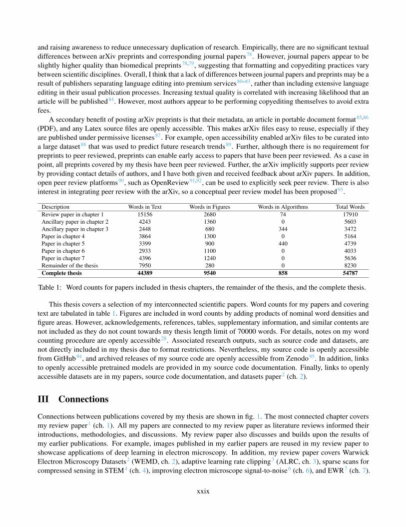
1. Word counts for papers included in thesis chapters, the remainder of the thesis, and the complete thesis.
Chapter 1 Review: Deep Learning in Electron Microscopy
1. Deep learning frameworks with programming interfaces. Most frameworks have open source code and manysupport multiple programming languages.
2. Microjob service platforms. The size of typical tasks varies for different platforms and some platformsspecialize in preparing machine learning datasets.
Chapter 2 Warwick Electron Microscopy Datasets
1. Examples and descriptions of STEM images in our datasets. References put some images into context to makethem more tangible to unfamiliar readers.
2. Examples and descriptions of TEM images in our datasets. References put some images into context to makethem more tangible to unfamiliar readers.
Chapter 2 Supplementary Information: Warwick Electron Microscopy Datasets
S1. To ease comparison, we have tabulated figure numbers for tSNE visualizations. Visualizations are for principalcomponents, VAE latent space means, and VAE latent space means weighted by standard deviations.
Chapter 3 Adaptive Learning Rate Clipping Stabilizes Learning
1. Adaptive learning rate clipping (ALRC) for losses 2, 3, 4 and∞ running standard deviations above theirrunning means for batch sizes 1, 4, 16 and 64. ARLC was not applied for clipping at∞. Each squared andquartic error mean and standard deviation is for the means of the final 5000 training errors of 10 experiments.ALRC lowers errors for unstable quartic error training at low batch sizes and otherwise has little effect. Meansand standard deviations are multiplied by 100.
2. Means and standard deviations of 20000 unclipped test set MSEs for STEM supersampling networks trainedwith various learning rate clipping algorithms and clipping hyperparameters, n↑ and n↓, above and below,respectively.
Chapter 4 Partial Scanning Transmission Electron Microscopy with Deep Learning
1. Means and standard deviations of pixels in images created by takings means of 20000 512×512 test setsquared difference images with intensities in [-1, 1] for methods to decrease systematic spatial error variation.Variances of Laplacians were calculated after linearly transforming mean images to unit variance.
Chapter 6 Improving Electron Micrograph Signal-to-Noise with an Atrous Convolutional Encoder-Decoder
xvii
1. Mean MSE and SSIM for several denoising methods applied to 20000 instances of Poisson noise and theirstandard errors. All methods were implemented with default parameters. Gaussian: 3×3 kernel with a 0.8px standard deviation. Bilateral: 9×9 kernel with radiometric and spatial scales of 75 (scales below 10 havelittle effect while scales above 150 cartoonize images). Median: 3×3 kernel. Wiener: no parameters. Wavelet:BayesShrink adaptive wavelet soft-thresholding with wavelet detail coefficient thresholds estimated using .Chambolle and Bregman TV: iterative total-variation (TV) based denoising, both with denoising weights of0.1 and applied until the fractional change in their cost function fell below 2.0× 10⁻⁴ or they reached 200iterations. Times are for 1000 examples on a 3.4 GHz i7-6700 processor and 1 GTX 1080 Ti GPU, except forour neural network time, which is for 20000 examples.
Chapter 7 Exit Wavefunction Reconstruction from Single Transmission Electron Micrographs with Deep Learning
1. New datasets containing 98340 wavefunctions simulated with clTEM are split into training, unseen, validation,and test sets. Unseen wavefunctions are simulated for training set materials with different simulationhyperparameters. Kirkland potential summations were calculated with n = 3 or truncated to n = 1 terms, anddashes (-) indicate subsets that have not been simulated. Datasets have been made publicly available at .
2. Means and standard deviations of 19992 validation set errors for unseen transforms (trans.), simulationshyperparameters (param.) and materials (mater.). All networks outperform a baseline uniform random phasegenerator for both n = 1 and n = 3 simulation physics. Dashes (-) indicate that validation set wavefunctionshave not been simulated.
xviii
Acknowledgments
Most modern research builds on a high variety of intellectual contributions, many of which are often overlooked asthere are too many to list. Examples include search engines, programming languages, machine learning frameworks,programming libraries, software development tools, computational hardware, operating systems, computing forums,research archives, and scholarly papers. To help developers with limited familiarity, useful resources for deeplearning in electron microscopy are discussed in a review paper covered by ch. 1 of my thesis. For brevity, theseacknowledgments will focus on personal contributions to my development as a researcher.
• Thanks go to Jeremy Sloan and Richard Beanland for supervision, internal peer review, and co-authorship.
• Thanks go to my Feedback Supervisors, Emma MacPherson and Jon Duffy, for comments needed to partiallyfulfil requirements of Doctoral Skills Modules (DSMs).
• I am grateful to Marin Alexe and Dong Jik Kim for supervising me during a summer project where Iprogrammed various components of atomic force microscopes. It was when I first realized that I want to be aprogrammer. Before then, I only thought of programming as something that I did in my spare time.
• I am grateful to James Lloyd-Hughes for supervising me during a summer project where I automated Fourieranalysis of ultrafast optical spectroscopy signals.
• I am grateful to my family for their love and support.
As a special note, I first taught myself machine learning by working through Mathematica documentation, imple-menting every machine learning example that I could find. The practice made use of spare time during a two-weekcourse at the start of my Doctor of Philosophy (PhD) studentship, which was needed to partially fulfil requirementsof the Midlands Physics Alliance Graduate School (MPAGS).
My Head of Department is David Leadley. My Director of Graduate Studies was Matthew Turner, then JamesLloyd-Hughes after Matthew Turner retired.
I acknowledge funding from Engineering and Physical Sciences Research Council (EPSRC) grant EP/N035437/1and EPSRC Studentship 1917382.
xix

Declarations
This thesis is submitted to the University of Warwick in support of my application for the degree of Doctorof Philosophy. It has been composed by myself and has not been submitted in any previous application forany degree.Parts of this thesis have been published by the author:The following publications1–8 are part of my thesis.
J. M. Ede. Review: Deep Learning in Electron Microscopy. arXiv preprint arXiv:2009.08328 (acceptedby Machine Learning: Science and Technology – https://doi.org/10.1088/2632-2153/abd614), 2020
J. M. Ede. Warwick Electron Microscopy Datasets. Machine Learning: Science and Technology, 1(4):045003, 2020
J. M. Ede and R. Beanland. Adaptive Learning Rate Clipping Stabilizes Learning. Machine Learning:Science and Technology, 1:015011, 2020
J. M. Ede and R. Beanland. Partial Scanning transmission Electron Microscopy with Deep Learning.Scientific Reports, 10(1):1–10, 2020
J. M. Ede. Adaptive Partial Scanning Transmission Electron Microscopy with Reinforcement Learning.arXiv preprint arXiv:2004.02786 (under review by Machine Learning: Science and Technology), 2020
J. M. Ede and R. Beanland. Improving Electron Micrograph Signal-to-Noise with an Atrous Convolu-tional Encoder-Decoder. Ultramicroscopy, 202:18–25, 2019
J. M. Ede, J. J. P. Peters, J. Sloan, and R. Beanland. Exit Wavefunction Reconstruction from SingleTransmission Electron Micrographs with Deep Learning. arXiv preprint arXiv:2001.10938 (underreview by Ultramicroscopy), 2020
J. M. Ede. Resume of Jeffrey Mark Ede. Zenodo, Online: https://doi.org/10.5281/zenodo.4429077, 2021
The following publications9–12 are part of my thesis. However, they are appendices.
J. M. Ede. Supplementary Information: Warwick Electron Microscopy Datasets. Zenodo, Online:https://doi.org/10.5281/zenodo.3899740, 2020
J. M. Ede. Supplementary Information: Partial Scanning Transmission Electron Microscopy with DeepLearning. Online: https://static-content.springer.com/esm/art%3A10.1038%2Fs41598-020-65261-0/MediaObjects/41598 2020 65261 MOESM1 ESM.pdf, 2020
J. M. Ede. Supplementary Information: Adaptive Partial Scanning Transmission Electron Microscopywith Reinforcement Learning. Zenodo, Online: https://doi.org/10.5281/zenodo.4384708, 2020
J. M. Ede, J. J. P. Peters, J. Sloan, and R. Beanland. Supplementary Information: Exit WavefunctionReconstruction from Single Transmission Electron Micrographs with Deep Learning. Zenodo, Online:https://doi.org/10.5281/zenodo.4277357, 2020
The following publications13–25 are not part of my thesis. However, they are auxiliary to publications that are part ofmy thesis.
xx
J. M. Ede. Warwick Electron Microscopy Datasets. arXiv preprint arXiv:2003.01113, 2020
J. M. Ede. Source Code for Warwick Electron Microscopy Datasets. Online: https://github.com/Jeffrey-Ede/datasets, 2020
J. M. Ede. Warwick Electron Microscopy Datasets Archive. Online: https://github.com/Jeffrey-Ede/datasets/wiki, 2020
J. M. Ede and R. Beanland. Adaptive Learning Rate Clipping Stabilizes Learning. arXiv preprintarXiv:1906.09060, 2019
J. M. Ede. Source Code for Adaptive Learning Rate Clipping Stabilizes Learning. Online: https://github.com/Jeffrey-Ede/ALRC, 2020
J. M. Ede and R. Beanland. Partial Scanning Transmission Electron Microscopy with Deep Learning.arXiv preprint arXiv:1910.10467, 2020
J. M. Ede. Deep Learning Supersampled Scanning Transmission Electron Microscopy. arXiv preprintarXiv:1910.10467, 2019
J. M. Ede. Source Code for Partial Scanning Transmission Electron Microscopy. Online: https://github.com/Jeffrey-Ede/partial-STEM, 2019
J. M. Ede. Source Code for Deep Learning Supersampled Scanning Transmission Electron Microscopy.Online: https://github.com/Jeffrey-Ede/DLSS-STEM, 2019
J. M. Ede. Source Code for Adaptive Partial Scanning Transmission Electron Microscopy withReinforcement Learning. Online: https://github.com/Jeffrey-Ede/adaptive-scans,2020
J. M. Ede. Improving Electron Micrograph Signal-to-Noise with an Atrous Convolutional Encoder-Decoder. arXiv preprint arXiv:1807.11234, 2018
J. M. Ede. Source Code for Improving Electron Micrograph Signal-to-Noise with an Atrous Convo-lutional Encoder-Decoder. Online: https://github.com/Jeffrey-Ede/Electron-Micrograph-Denoiser, 2019
J. M. Ede. Source Code for Exit Wavefunction Reconstruction from Single Transmission ElectronMicrographs with Deep Learning. Online: https://github.com/Jeffrey-Ede/one-shot,2019
The following publications26–32 are not part of my thesis. However, they are referenced by my thesis, or arereferenced by or associated with publications that are part of my thesis.
J. M. Ede. Progress Reports of Jeffrey Mark Ede: 0.5 Year Progress Report. Zenodo, Online: https://doi.org/10.5281/zenodo.4094750, 2020
J. M. Ede. Source Code for Beanland Atlas. Online: https://github.com/Jeffrey-Ede/Beanland-Atlas, 2018
J. M. Ede. Thesis Word Counting. Zenodo, Online: https://doi.org/10.5281/zenodo.4321429, 2020
J. M. Ede. Posters and Presentations. Zenodo, Online: https://doi.org/10.5281/zenodo.4041574, 2020
J. M. Ede. Autoencoders, Kernels, and Multilayer Perceptrons for Electron Micrograph Restoration andCompression. arXiv preprint arXiv:1808.09916, 2018
xxi
J. M. Ede. Source Code for Autoencoders, Kernels, and Multilayer Perceptrons for Electron MicrographRestoration and Compression. Online: https://github.com/Jeffrey-Ede/Denoising-Kernels-MLPs-Autoencoders, 2018
J. M. Ede. Source Code for Simple Webserver. Online: https://github.com/Jeffrey-Ede/simple-webserver, 2019
All publications were produced during my period of study for the degree of Doctor of Philosophy in Physics at theUniversity of Warwick.The work presented (including data generated and data analysis) was carried out by the author except in thecases outlined below:Chapter 1 Review: Deep Learning in Electron Microscopy
Jeremy Sloan and Martin Lotz internally reviewed my paper after I published it in the arXiv.
Chapter 2 Warwick Electron Microscopy Datasets
Richard Beanland internally reviewed my paper before it was published in the arXiv. Further, JonathanPeters discussed categories used to showcase typical electron micrographs for readers with limitedfamiliarity. At first, our datasets were openly accessible from my Google Cloud Storage. However,Richard Beanland contacted University of Warwick Information Technology Services to arrange for ourdatasets to also be openly accessible from University of Warwick data servers. Chris Parkin allocatedserver resources, advised me on data transfer, and handled administrative issues. In addition, datasetsare openly accessible from Zenodo and my Google Drive.
Simulated datasets were created with clTEM multislice simulation software developed by a previousEM group PhD student, Mark Dyson, and maintained by a previous EM group postdoctoral researcher,Jonathan Peters. Jonathan Peters advised me on processing data that I had curated from the Crystallog-raphy Open Database (COD) so that it could be input into clTEM simulations. Further, Jonathan Petersand I jointly prepared a script to automate multislice simulations. Finally, Jonathan Peters computed athird of our simulations on his graphical processing units (GPUs).
Experimental datasets were curated from University of Warwick Electron Microscopy (EM) ResearchTechnology Platform (RTP) dataservers, and contain images collected by dozens of scientists workingon hundreds of projects. Data was curated and published with permission of the Director of the EMRTP, Richard Beanland. In addition, data curation and publication were reviewed and approved byResearch Data Officers, Yvonne Budden and Heather Lawler. I was introduced to the EM dataserversby Richard Beanland and Jonathan Peters, and my read and write access to the EM dataservers was setup by an EM RTP technician, Steve York.
Chapter 3 Adaptive Learning Rate Clipping Stabilizes Learning
Richard Beanland internally reviewed my paper after it was published in the arXiv. Martin Lotz laterrecommend the journal that I published it in. In addition, a Scholarly Communications Manager,Julie Robinson, advised me on finding publication venues and open access funding. I also discussedpublication venues with editors of Machine Learning, Melissa Fearon and Peter Flach, and my Centrefor Scientific Computing Director, David Quigley.
Chapter 4 Partial Scanning Transmission Electron Microscopy with Deep Learning
xxii
Richard Beanland internally reviewed an initial draft of my paper on partial scanning transmissionelectron microscopy (STEM). After I published our paper in the arXiv, Richard Beanland contributedmost of the content in the first two paragraphs in the introduction of the journal paper. In addition,Richard Beanland and I both copyedited our paper.
Richard Beanland internally reviewed a paper on uniformly spaced scans after I published it in thearXiv. The uniformly spaced scans paper includes some experiments that we later combined into ourpartial STEM paper. Further, my experiments followed a preliminary investigation into compressedsensing with fixed randomly spaced masks, which Richard Beanland internally reviewed.
Chapter 5 Adaptive Partial Scanning Transmission Electron Microscopy with Reinforcement Learning
Jasmine Clayton, Abdul Mohammed, and Jeremy Sloan internally reviewed my paper after I publishedit in the arXiv.
Chapter 6 Improving Electron Micrograph Signal-to-Noise with an Atrous Convolutional Encoder-Decoder
After I published my paper in the arXiv, Richard Beanland internally reviewed it and advised that wepublish it in a journal. In addition, Richard Beanland and I both copyedited our paper.
Chapter 7 Exit Wavefunction Reconstruction from Single Transmission Electron Micrographs with Deep Learning
Jeremy Sloan internally reviewed an initial draft of our paper. Afterwards, Jeremy Sloan contributedall crystal structure diagrams in our paper. The University of Warwick X-Ray Facility Manager,David Walker, suggested materials to showcase with their crystal structures, and a University ofWarwick Research Fellow, Jessica Marshall, internally reviewed a figure showing exit wavefunctionreconstructions (EWRs) with the crystal structures.
Richard Beanland contacted a professor at Humboldt University of Berlin, Christoph Koch, to ask for aDigitalMicrograph plugin, which I used to collect experimental focal series. Further, Richard Beanlandhelped me get started with focal series measurements, and internally reviewed some of my first focalseries. In addition, Richard Beanland internally reviewed our paper.
Jonathan Peters drafted initial text about clTEM multislice simulations for a section of our paper on“Exit Wavefunction Datasets”. In addition, Jonathan Peters internally reviewed our paper.
This thesis conforms to regulations governing the examination of higher degrees by research:The following regulations33,34 were used during preparation of this thesis.
Guide to Examinations for Higher Degrees by Research. University of Warwick Doctoral College,Online: https://warwick.ac.uk/services/dc/pgrassessments/gtehdr, 2020
Regulation 38: Research Degrees. University of Warwick Calendar, Online: https://warwick.ac.uk/services/gov/calendar/section2/regulations/reg38pgr, 2020
The following guidance35 was helpful during preparation of this thesis.
Thesis Writing and Submission. University of Warwick Department of Physics, Online: https://warwick.ac.uk/fac/sci/physics/current/postgraduate/regs/thesis,2020
The following thesis template36 was helpful during preparation of this thesis.
xxiii
A Warwick Thesis Template. University of Warwick Department of Physics, Online: https://warwick.ac.uk/fac/sci/physics/staff/academic/mhadley/wthesis, 2020
Thesis structure and content was discussed with my previous Director of Graduate Studies, Matthew Turner, andmy current Director of Graduate Studies, James Lloyd-Hughes, after Matthew Turner retired. My thesis was alsodiscussed with my both my previous PhD supervisor, Richard Beanland, and my current PhD supervisor, JeremySloan. My formal thesis plan was then reviewed and approved by both Jeremy Sloan and my feedback supervisor,Emma MacPherson. Finally, my complete thesis was internally reviewed by both Jeremy Sloan and Jasmine Clayton.
Permission is granted by the Chair of the Board of Graduate Studies, Colin Sparrow, for my thesis appendices toexceed length requirements usually set by the University of Warwick. This is in the understanding that my thesisappendices are not usually crucial to the understanding or examination of my thesis.
xxiv

Research Training
This thesis presents a substantial original investigation of deep learning in electron microscopy. The only researcherin my research group or building with machine learning expertise was myself. This meant that I led the design,implementation, evaluation, and publication of experiments covered by my thesis. Where experiments werecollaborative, I both proposed and led the collaboration.
xxv
Abstract
Following decades of exponential increases in computational capability and widespread data availability, deeplearning is readily enabling new science and technology. This thesis starts with a review of deep learning in electronmicroscopy, which offers a practical perspective aimed at developers with limited familiarity. To help electronmicroscopists get started with started with deep learning, large new electron microscopy datasets are introducedfor machine learning. Further, new approaches to variational autoencoding are introduced to embed datasets inlow-dimensional latent spaces, which are used as the basis of electron microscopy search engines. Encodings arealso used to investigate electron microscopy data visualization by t-distributed stochastic neighbour embedding.Neural networks that process large electron microscopy images may need to be trained with small batch sizes to fitthem into computer memory. Consequently, adaptive learning rate clipping is introduced to prevent learning beingdestabilized by loss spikes associated with small batch sizes.
This thesis presents three applications of deep learning to electron microscopy. Firstly, electron beam exposurecan damage some specimens, so generative adversarial networks were developed to complete realistic images fromsparse spiral, gridlike, and uniformly spaced scans. Further, recurrent neural networks were trained by reinforcementlearning to dynamically adapt sparse scans to specimens. Sparse scans can decrease electron beam exposureand scan time by 10-100× with minimal information loss. Secondly, a large encoder-decoder was developed toimprove transmission electron micrograph signal-to-noise. Thirdly, conditional generative adversarial networks weredeveloped to recover exit wavefunction phases from single images. Phase recovery with deep learning overcomesexisting limitations as it is suitable for live applications and does not require microscope modification. To encouragefurther investigation, scientific publications and their source files, source code, pretrained models, datasets, and otherresearch outputs covered by this thesis are openly accessible.
xxvi
Preface
This thesis covers a subset of my scientific papers on advances in electron microscopy with deep learning. The paperswere prepared while I was a PhD student at the University of Warwick in support of my application for the degreeof PhD in Physics. This thesis reflects on my research, unifies covered publications, and discusses future researchdirections. My papers are available as part of chapters of this thesis, or from their original publication venues withhypertext and other enhancements. This preface covers my initial motivation to investigate deep learning in electronmicroscopy, structure and content of my thesis, and relationships between included publications. Traditionally,physics PhD theses submitted to the University of Warwick are formatted for physical printing and binding. However,I have also formatted a copy of my thesis for online dissemination to improve readability37.
I Initial Motivation
When I started my PhD in October 2017, we were unsure if or how machine learning could be applied to electronmicroscopy. My PhD was funded by EPSRC Studentship 191738238 titled “Application of Novel Computing andData Analysis Methods in Electron Microscopy”, which is associated with EPSRC grant EP/N035437/139 titled“ADEPT – Advanced Devices by ElectroPlaTing”. As part of the grant, our initial plan was for me to spend a coupleof days per week using electron microscopes to analyse specimens sent to the University of Warwick from theUniversity of Southampton, and to invest remaining time developing new computational techniques to help withanalysis. However, an additional scientist was not needed to analyse specimens, so it was difficult for me to getelectron microscopy training. While waiting for training, I was tasked with automating analysis of digital large angleconvergent beam electron diffraction40 (D-LACBED) patterns. However, we did not have a compelling use case formy D-LACBED software26,41. Further, a more senior PhD student at the University of Warwick, Alexander Hubert,was already investigating convergent beam electron diffraction40,42 (CBED).
My first machine learning research began five months after I started my PhD. Without a clear research directionor specimens to study, I decided to develop artificial neural networks (ANNs) to generate artwork. My dubiousplan was to create image processing pipelines for the artwork, which I would replace with electron micrographswhen I got specimens to study. However, after investigating artwork generation with randomly initialized multilayerperceptrons43,44, then by style transfer45,46, and then by fast style transfer47, there were still no specimens for meto study. Subsequently, I was inspired by NVIDIA’s research on semantic segmentation48 to investigate semanticsegmentation with DeepLabv3+49. However, I decided that it was unrealistic for me to label a large new electronmicroscopy dataset for semantic segmentation by myself. Fortunately, I had read about using deep neural networks(DNNs) to reduce image compression artefacts50, so I wondered if a similar approach based on DeepLabv3+ couldimprove electron micrograph signal-to-noise. Encouragingly, it would not require time-consuming image labelling.Following a successful investigation into improving signal-to-noise, my first scientific paper6 (ch. 6) was submitteda few months later, and my experience with deep learning enabled subsequent investigations.
II Thesis Structure
An overview of the first seven chapters in this thesis is presented in fig. 1. The first chapter is introductory andcovers a review of deep learning in electron microscopy, which offers a practical perspective aimed at developerswith limited familiarity. The next two chapters are ancillary and cover new datasets and an optimization algorithmused in later chapters. The final four chapters before conclusions cover investigations of deep learning in electronmicroscopy. Each of the first seven chapter covers a combination of journal papers, preprints, and ancillary outputs
xxvii
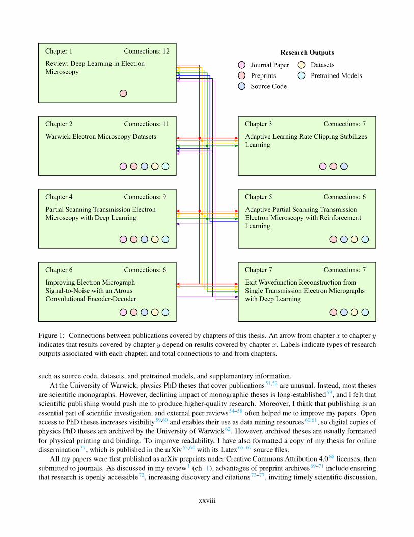
Figure 1: Connections between publications covered by chapters of this thesis. An arrow from chapter x to chapter yindicates that results covered by chapter y depend on results covered by chapter x. Labels indicate types of researchoutputs associated with each chapter, and total connections to and from chapters.
such as source code, datasets, and pretrained models, and supplementary information.At the University of Warwick, physics PhD theses that cover publications51,52 are unusual. Instead, most theses
are scientific monographs. However, declining impact of monographic theses is long-established53, and I felt thatscientific publishing would push me to produce higher-quality research. Moreover, I think that publishing is anessential part of scientific investigation, and external peer reviews54–58 often helped me to improve my papers. Openaccess to PhD theses increases visibility59,60 and enables their use as data mining resources60,61, so digital copies ofphysics PhD theses are archived by the University of Warwick62. However, archived theses are usually formattedfor physical printing and binding. To improve readability, I have also formatted a copy of my thesis for onlinedissemination37, which is published in the arXiv63,64 with its Latex65–67 source files.
All my papers were first published as arXiv preprints under Creative Commons Attribution 4.068 licenses, thensubmitted to journals. As discussed in my review1 (ch. 1), advantages of preprint archives69–71 include ensuringthat research is openly accessible72, increasing discovery and citations73–77, inviting timely scientific discussion,
xxviii
and raising awareness to reduce unnecessary duplication of research. Empirically, there are no significant textualdifferences between arXiv preprints and corresponding journal papers78. However, journal papers appear to beslightly higher quality than biomedical preprints78,79, suggesting that formatting and copyediting practices varybetween scientific disciplines. Overall, I think that a lack of differences between journal papers and preprints may be aresult of publishers separating language editing into premium services80–83, rather than including extensive languageediting in their usual publication processes. Increasing textual quality is correlated with increasing likelihood that anarticle will be published84. However, most authors appear to be performing copyediting themselves to avoid extrafees.
A secondary benefit of posting arXiv preprints is that their metadata, an article in portable document format85,86
(PDF), and any Latex source files are openly accessible. This makes arXiv files easy to reuse, especially if theyare published under permissive licenses87. For example, open accessibility enabled arXiv files to be curated intoa large dataset88 that was used to predict future research trends89. Further, although there is no requirement forpreprints to peer reviewed, preprints can enable early access to papers that have been peer reviewed. As a case inpoint, all preprints covered by my thesis have been peer reviewed. Further, the arXiv implicitly supports peer reviewby providing contact details of authors, and I have both given and received feedback about arXiv papers. In addition,open peer review platforms90, such as OpenReview91,92, can be used to explicitly seek peer review. There is alsointerest in integrating peer review with the arXiv, so a conceptual peer review model has been proposed93.
Description Words in Text Words in Figures Words in Algorithms Total WordsReview paper in chapter 1 15156 2680 74 17910Ancillary paper in chapter 2 4243 1360 0 5603Ancillary paper in chapter 3 2448 680 344 3472Paper in chapter 4 3864 1300 0 5164Paper in chapter 5 3399 900 440 4739Paper in chapter 6 2933 1100 0 4033Paper in chapter 7 4396 1240 0 5636Remainder of the thesis 7950 280 0 8230Complete thesis 44389 9540 858 54787
Table 1: Word counts for papers included in thesis chapters, the remainder of the thesis, and the complete thesis.
This thesis covers a selection of my interconnected scientific papers. Word counts for my papers and coveringtext are tabulated in table 1. Figures are included in word counts by adding products of nominal word densities andfigure areas. However, acknowledgements, references, tables, supplementary information, and similar contents arenot included as they do not count towards my thesis length limit of 70000 words. For details, notes on my wordcounting procedure are openly accessible28. Associated research outputs, such as source code and datasets, arenot directly included in my thesis due to format restrictions. Nevertheless, my source code is openly accessiblefrom GitHub94, and archived releases of my source code are openly accessible from Zenodo95. In addition, linksto openly accessible pretrained models are provided in my source code documentation. Finally, links to openlyaccessible datasets are in my papers, source code documentation, and datasets paper2 (ch. 2).
III Connections
Connections between publications covered by my thesis are shown in fig. 1. The most connected chapter coversmy review paper1 (ch. 1). All my papers are connected to my review paper as literature reviews informed theirintroductions, methodologies, and discussions. My review paper also discusses and builds upon the results ofmy earlier publications. For example, images published in my earlier papers are reused in my review paper toshowcase applications of deep learning in electron microscopy. In addition, my review paper covers WarwickElectron Microscopy Datasets2 (WEMD, ch. 2), adaptive learning rate clipping3 (ALRC, ch. 3), sparse scans forcompressed sensing in STEM4 (ch. 4), improving electron microscope signal-to-noise6 (ch. 6), and EWR7 (ch. 7).
xxix
Finally, compressed sensing with dynamic scan paths that adapt to specimens5 (ch. 5) motivated my review papersections on recurrent neural networks (RNNs) and reinforcement learning (RL).
The second most connected chapter, ch. 2, is ancillary and covers WEMD2, which include large new datasetsof experimental transmission electron microscopy (TEM) images, experimental STEM images, and simulated exitwavefunctions. The TEM images were curated to train an ANN to improve signal-to-noise6 (ch. 6) and motivatedthe proposition of a new approach to EWR7 (ch. 7). The STEM images were curated to train ANNs for compressedsensing4 (ch. 4). Training our ANNs with full-size images was impractical with our limited computational resources,so I created dataset variants containing 512×512 crops from full-size images for both the TEM and STEM datasets.However, 512×512 STEM crops were too large to efficiently train RNNs to adapt scan paths5 (ch. 5), so I alsocreated 96×96 variants of datasets for rapid initial development. Finally, datasets of exit wavefunctions weresimulated as part of our initial investigation into EWR from single TEM images with deep learning7 (ch. 7).
The other ancillary chapter, ch. 3, covers ALRC3, which was originally published as an appendix in the firstversion of our partial STEM preprint18 (ch. 4). The algorithm was developed to stabilize learning of ANNs beingdeveloped for partial STEM, which were destabilized by loss spikes when training with a batch size of 1. Myaim was to make experiments10 easier to compare by preventing learning destabilized by large loss spikes fromcomplicating comparisons. However, ALRC was so effective that I continued to investigate it, increasing the size ofthe partial STEM appendix. Eventually, the appendix became so large that I decided to turn it into a short paper. Tostabilize training with small batch sizes, ALRC was also applied to ANN training for uniformly spaced scans4,19
(ch. 4). In addition, ALRC inspired adaptive loss clipping to stabilize RNN training for adaptive scans5 (ch. 5).Finally, I investigated applying ALRC to ANN training for EWR7 (ch. 7). However, ALRC did not improve EWRas training with a batch size of 32 was not destabilized by loss spikes.
My experiments with compressed sensing showed that ANN performance varies for different scan paths4 (ch. 4).This motivated the investigation of scan shapes that adapt to specimens as they are scanned5 (ch. 5). I had found thatANNs for TEM denoising6 (ch. 6) and uniformly spaced sparse scan completion19 exhibit significant structuredsystematic error variation, where errors are higher near output edges. Subsequently, I investigated average partialSTEM output errors and found that errors increase with increasing distance from scan paths4 (ch. 4). In part,structured systematic error variation in partial STEM4 (ch. 4) motivated my investigation of adaptive scans5 (ch. 5)as I reasoned that being able to more closely scan regions where errors would otherwise be highest could decreasemean errors.
Most of my publications are connected by their source code as it was partially reused in successive experiments.Source code includes scripts to develop ANNs, plot graphs, create images for papers, and typeset with Latex.Following my publication chronology, I partially reused source code created to improve signal-to-noise6 (ch. 6) forpartial STEM4 (ch. 4). My partial STEM source code was then partially reused for my other investigations. Manyof my publications are also connected because datasets curated for my first investigations were reused in my laterinvestigations. For example, improving signal-to-noise6 (ch. 6) is connected to EWR7 (ch. 7) as the availability ofmy large dataset of TEM images prompted the proposition of, and may enable, a new approach to EWR. Similarly,partial STEM4 (ch. 4) is connected to adaptive scans5 (ch. 5) as my large dataset of STEM images was used toderive smaller datasets used to rapidly develop adaptive scan systems.
xxx
Chapter 1
Review: Deep Learning in ElectronMicroscopy
1.1 Scientific Paper
This chapter covers the following paper1.
J. M. Ede. Review: Deep Learning in Electron Microscopy. arXiv preprint arXiv:2009.08328 (accepted
by Machine Learning: Science and Technology – https://doi.org/10.1088/2632-2153/
abd614), 2020
1
Review: Deep Learning in Electron MicroscopyJeffrey M. Ede1,*
1University of Warwick, Department of Physics, Coventry, CV4 7AL, UK*[email protected]
ABSTRACT
Deep learning is transforming most areas of science and technology, including electron microscopy. This review paper offers apractical perspective aimed at developers with limited familiarity. For context, we review popular applications of deep learning inelectron microscopy. Following, we discuss hardware and software needed to get started with deep learning and interface withelectron microscopes. We then review neural network components, popular architectures, and their optimization. Finally, wediscuss future directions of deep learning in electron microscopy.
Keywords: deep learning, electron microscopy, review.
1 Introduction
Following decades of exponential increases in computational capability1 and widespread data availability2, 3, scientists canroutinely develop artificial neural networks4–11 (ANNs) to enable new science and technology12–17. The resulting deep learningrevolution18, 19 has enabled superhuman performance in image classification20–23, games24–29, medical analysis30, 31, relationalreasoning32, speech recognition33, 34 and many other applications35, 36. This introduction focuses on deep learning in electronmicroscopy and is aimed at developers with limited familiarity. For context, we therefore review popular applications of deeplearning in electron microscopy. We then review resources available to support researchers and outline electron microscopy.Finally, we review popular ANN architectures and their optimization, or “training”, and discuss future trends in artificialintelligence (AI) for electron microscopy.
Deep learning is motivated by universal approximator theorems37–45, which state that sufficiently deep and wide37, 40, 46
ANNs can approximate functions to arbitrary accuracy. It follows that ANNs can always match or surpass the performanceof methods crafted by humans. In practice, deep neural networks (DNNs) reliably47 learn to express48–51 generalizable52–59
models without a prior understanding of physics. As a result, deep learning is freeing physicists from a need to devise equationsto model complicated phenomena13, 14, 16, 60, 61. Many modern ANNs have millions of parameters, so inference often takes tensof milliseconds on graphical processing units (GPUs) or other hardware accelerators62. It is therefore unusual to develop ANNsto approximate computationally efficient methods with exact solutions, such as the fast Fourier transform63–65 (FFT). However,ANNs are able to leverage an understanding of physics to accelerate time-consuming or iterative calculations66–69, improveaccuracy of methods30, 31, 70, and find solutions that are otherwise intractable24, 71.
1.1 Improving Signal-to-NoiseA popular application of deep learning is to improve signal-to-noise74, 75. For example, of medical electrical76, 77, medicalimage78–80, optical microscopy81–84, and speech85–88 signals. There are many traditional denoising algorithms that are not basedon deep learning89–91, including linear92, 93 and non-linear94–102 spatial domain filters, Wiener103–105 filters, non-linear106–111
wavelet domain filters, curvelet transforms112, 113, contourlet transforms114, 115, hybrid algorithms116–122 that operate in bothspatial and transformed domains, and dictionary-based learning123–127. However, traditional denoising algorithms are limitedby features (often laboriously) crafted by humans and cannot exploit domain-specific context. In perspective, they leveragean ever-increasingly accurate representation of physics to denoise signals. However, traditional algorithms are limited by thedifficulty of programmatically describing a complicated reality. As a case in point, an ANN was able to outperform decades ofadvances in traditional denoising algorithms after training on two GPUs for a week70.
Definitions of electron microscope noise can include statistical noise128–135, aberrations136, scan distortions137–140, specimendrift141, and electron beam damage142. Statistical noise is often minimized by either increasing electron dose or applyingtraditional denoising algorithms143, 144. There are a variety of denoising algorithms developed for electron microscopy, includingalgorithms based on block matching145, contourlet transforms114, 115, energy minimization146, fast patch reorderings147,Gaussian kernel density estimation148, Kronecker envelope principal component analysis149 (PCA), non-local means andZernike moments150, singular value thresholding151, wavelets152, and other approaches141, 153–156. Noise that is not statistical is
arX
iv:2
009.
0832
8v6
[ee
ss.I
V]
31
Dec
202
0
2

Figure 1. Example applications of a noise-removal DNN to instances of Poisson noise applied to 512×512 crops from TEMimages. Enlarged 64×64 regions from the top left of each crop are shown to ease comparison. This figure is adapted from ourearlier work72 under a Creative Commons Attribution 4.073 license.
often minimized by hardware. For example, by using aberration correctors136, 157–159, choosing scanning transmission electronmicroscopy (STEM) scan shapes and speeds that minimize distortions138, and using stable sample holders to reduce drift160.Beam damage can also be reduced by using minimal electron voltage and electron dose161–163, or dose-fractionation acrossmultiple frames in multi-pass transmission electron microscopy164–166 (TEM) or STEM167.
Deep learning is being applied to improve signal-to-noise for a variety of applications168–176. Most approaches in electronmicroscopy involve training ANNs to either map low-quality experimental177, artificially deteriorated70, 178 or synthetic179–182
inputs to paired high-quality experimental measurements. For example, applications of a DNN trained with artificiallydeteriorated TEM images are shown in figure 1. However, ANNs have also been trained with unpaired datasets of low-quality and high-quality electron micrographs183, or pairs of low-quality electron micrographs184, 185. Another approach isNoise2Void168, ANNs are trained from single noisy images. However, Noise2Void removes information by masking noisyinput pixels corresponding to target output pixels. So far, most ANNs that improve electron microscope signal-to-noise havebeen trained to decrease statistical noise70, 177, 179–181, 181–184, 186 as other approaches have been developed to correct electronmicroscope scan distortions187, 188 and specimen drift141, 188, 189. However, we anticipate that ANNs will be developed to correcta variety of electron microscopy noise as ANNs have been developed for aberration correction of optical microscopy190–195 andphotoacoustic196 signals.
1.2 Compressed SensingCompressed sensing203–207 is the efficient reconstruction of a signal from a subset of measurements. Applications include fastermedical imaging208–210, image compression211, 212, increasing image resolution213, 214, lower medical radiation exposure215–217,and low-light vision218, 219. In STEM, compressed sensing has enabled electron beam exposure and scan time to be decreasedby 10-100× with minimal information loss201, 202. Thus, compressed sensing can be essential to investigations where the highcurrent density of electron probes damages specimens161, 220–226. Even if the effects of beam damage can be corrected bypostprocessing, the damage to specimens is often permanent. Examples of beam-sensitive materials include organic crystals227,metal-organic frameworks228, nanotubes229, and nanoparticle dispersions230. In electron microscopy, compressed sensing is
2/983

Figure 2. Example applications of DNNs to restore 512×512 STEM images from sparse signals. Training as part of agenerative adversarial network197–200 yields more realistic outputs than training a single DNN with mean squared errors.Enlarged 64×64 regions from the top left of each crop are shown to ease comparison. a) Input is a Gaussian blurred 1/20coverage spiral201. b) Input is a 1/25 coverage grid202. This figure is adapted from our earlier works under Creative CommonsAttribution 4.073 licenses.
especially effective due to high signal redundancy231. For example, most electron microscopy images are sampled at 5-10×their Nyquist rates232 to ease visual inspection, decrease sub-Nyquist aliasing233, and avoid undersampling.
Perhaps the most popular approach to compressed sensing is upsampling or infilling a uniformly spaced grid of signals234–236.Interpolation methods include Lancsoz234, nearest neighbour237, polynomial interpolation238, Wiener239 and other resamplingmethods240–242. However, a variety of other strategies to minimize STEM beam damage have also been proposed, includingdose fractionation243 and a variety of sparse data collection methods244. Perhaps the most intensively investigated approachto the latter is sampling a random subset of pixels, followed by reconstruction using an inpainting algorithm244–249. Randomsampling of pixels is nearly optimal for reconstruction by compressed sensing algorithms250. However, random samplingexceeds the design parameters of standard electron beam deflection systems, and can only be performed by collecting dataslowly138, 251, or with the addition of a fast deflection or blanking system247, 252.
Sparse data collection methods that are more compatible with conventional STEM electron beam deflection systemshave also been investigated. For example, maintaining a linear fast scan deflection whilst using a widely-spaced slow scanaxis with some small random ‘jitter’245, 251. However, even small jumps in electron beam position can lead to a significantdifference between nominal and actual beam positions in a fast scan. Such jumps can be avoided by driving functions withcontinuous derivatives, such as those for spiral and Lissajous scan paths138, 201, 247, 253, 254. Sang138, 254 considered a variety ofscans including Archimedes and Fermat spirals, and scans with constant angular or linear displacements, by driving electronbeam deflectors with a field-programmable gate array255 (FPGA) based system138. Spirals with constant angular velocityplace the least demand on electron beam deflectors. However, dwell times, and therefore electron dose, decreases with radius.Conversely, spirals created with constant spatial speeds are prone to systematic image distortions due to lags in deflectorresponses. In practice, fixed doses are preferable as they simplify visual inspection and limit the dose dependence of STEMnoise129.
Deep learning can leverage an understanding of physics to infill images256–258. Example applications include increasingscanning electron microscopy178, 259, 260 (SEM), STEM202, 261 and TEM262 resolution, and infilling continuous sparse scans201.Example applications of DNNs to complete sparse spiral and grid scans are shown in figure 2. However, caution should beused when infilling large regions as ANNs may generate artefacts if a signal is unpredictable201. A popular alternative to deeplearning for infilling large regions is exemplar-based infilling263–266. However, exemplar-based infilling often leaves artefacts267
3/984
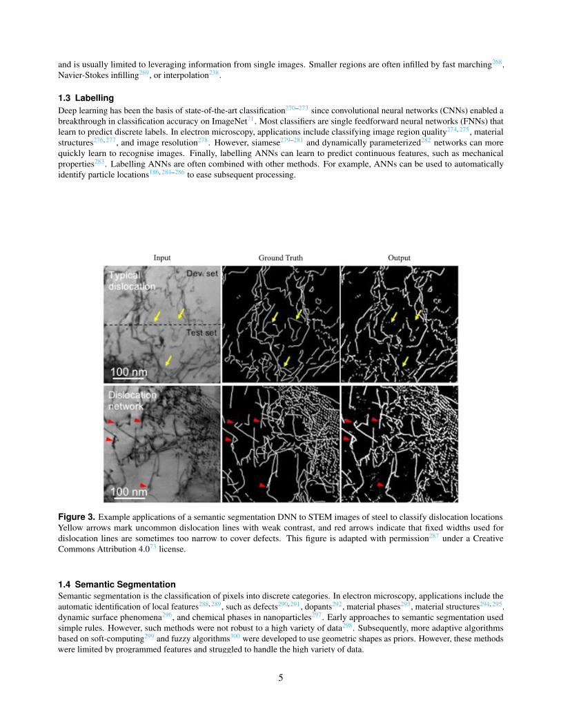
and is usually limited to leveraging information from single images. Smaller regions are often infilled by fast marching268,Navier-Stokes infilling269, or interpolation238.
1.3 LabellingDeep learning has been the basis of state-of-the-art classification270–273 since convolutional neural networks (CNNs) enabled abreakthrough in classification accuracy on ImageNet71. Most classifiers are single feedforward neural networks (FNNs) thatlearn to predict discrete labels. In electron microscopy, applications include classifying image region quality274, 275, materialstructures276, 277, and image resolution278. However, siamese279–281 and dynamically parameterized282 networks can morequickly learn to recognise images. Finally, labelling ANNs can learn to predict continuous features, such as mechanicalproperties283. Labelling ANNs are often combined with other methods. For example, ANNs can be used to automaticallyidentify particle locations186, 284–286 to ease subsequent processing.
Figure 3. Example applications of a semantic segmentation DNN to STEM images of steel to classify dislocation locations.Yellow arrows mark uncommon dislocation lines with weak contrast, and red arrows indicate that fixed widths used fordislocation lines are sometimes too narrow to cover defects. This figure is adapted with permission287 under a CreativeCommons Attribution 4.073 license.
1.4 Semantic SegmentationSemantic segmentation is the classification of pixels into discrete categories. In electron microscopy, applications include theautomatic identification of local features288, 289, such as defects290, 291, dopants292, material phases293, material structures294, 295,dynamic surface phenomena296, and chemical phases in nanoparticles297. Early approaches to semantic segmentation usedsimple rules. However, such methods were not robust to a high variety of data298. Subsequently, more adaptive algorithmsbased on soft-computing299 and fuzzy algorithms300 were developed to use geometric shapes as priors. However, these methodswere limited by programmed features and struggled to handle the high variety of data.
4/985
To improve performance, DNNs have been trained to semantically segment images301–308. Semantic segmentation DNNshave been developed for focused ion beam scanning electron microscopy309–311 (FIB-SEM), SEM311–314, STEM287, 315, andTEM286, 310, 311, 316–319. For example, applications of a DNN to semantic segmentation of STEM images of steel are shown infigure 3. Deep learning based semantic segmentation also has a high variety of applications outside of electron microscopy,including autonomous driving320–324, dietary monitoring325, 326, magnetic resonance images327–331, medical images332–334 suchas prenatal ultrasound335–338, and satellite image translation339–343. Most DNNs for semantic segmentation are trained withimages segmented by humans. However, human labelling may be too expensive, time-consuming, or inappropriate for sensitivedata. Unsupervised semantic segmentation can avoid these difficulties by learning to segment images from an additional datasetof segmented images344 or image-level labels345–348. However, unsupervised semantic segmentation networks are often lessaccurate than supervised networks.
Figure 4. Example applications of a DNN to reconstruct phases of exit wavefunction from intensities of single TEM images.Phases in [−π,π) rad are depicted on a linear greyscale from black to white, and Miller indices label projection directions.This figure is adapted from our earlier work349 under a Creative Commons Attribution 4.073 license.
1.5 Exit Wavefunction ReconstructionElectrons exhibit wave-particle duality350, 351, so electron propagation is often described by wave optics352. Applicationsof electron wavefunctions exiting materials353 include determining projected potentials and corresponding crystal structureinformation354, 355, information storage, point spread function deconvolution, improving contrast, aberration correction356,thickness measurement357, and electric and magnetic structure determination358, 359. Usually, exit wavefunctions are eitheriteratively reconstructed from focal series360–364 or recorded by electron holography352, 363, 365. However, iterative reconstructionis often too slow for live applications, and holography is sensitive to distortions and may require expensive microscopemodification.
Non-iterative methods based on DNNs have been developed to reconstruct optical exit wavefunctions from focal series69 orsingle images366–368. Subsequently, DNNs have been developed to reconstruct exit wavefunctions from single TEM images349,as shown in figure 4. Indeed, deep learning is increasingly being applied to accelerated quantum mechanics369–374. Otherexamples of DNNs adding new dimensions to data include semantic segmentation described in section 1.4, and reconstructing3D atomic distortions from 2D images375. Non-iterative methods that do not use ANNs to recover phase information fromsingle images have also been developed376, 377. However, they are limited to defocused images in the Fresnel regime376, or tonon-planar incident wavefunctions in the Fraunhofer regime377.
5/986
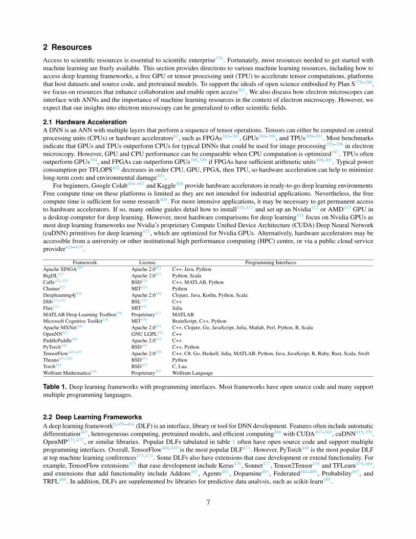
2 Resources
Access to scientific resources is essential to scientific enterprise378. Fortunately, most resources needed to get started withmachine learning are freely available. This section provides directions to various machine learning resources, including how toaccess deep learning frameworks, a free GPU or tensor processing unit (TPU) to accelerate tensor computations, platformsthat host datasets and source code, and pretrained models. To support the ideals of open science embodied by Plan S378–380,we focus on resources that enhance collaboration and enable open access381. We also discuss how electron microscopes caninterface with ANNs and the importance of machine learning resources in the context of electron microscopy. However, weexpect that our insights into electron microscopy can be generalized to other scientific fields.
2.1 Hardware AccelerationA DNN is an ANN with multiple layers that perform a sequence of tensor operations. Tensors can either be computed on centralprocessing units (CPUs) or hardware accelerators62, such as FPGAs382–385, GPUs386–388, and TPUs389–391. Most benchmarksindicate that GPUs and TPUs outperform CPUs for typical DNNs that could be used for image processing392–396 in electronmicroscopy. However, GPU and CPU performance can be comparable when CPU computation is optimized397. TPUs oftenoutperform GPUs394, and FPGAs can outperform GPUs398, 399 if FPGAs have sufficient arithmetic units400, 401. Typical powerconsumption per TFLOPS402 decreases in order CPU, GPU, FPGA, then TPU, so hardware acceleration can help to minimizelong-term costs and environmental damage403.
For beginners, Google Colab404–407 and Kaggle408 provide hardware accelerators in ready-to-go deep learning environments.Free compute time on these platforms is limited as they are not intended for industrial applications. Nevertheless, the freecompute time is sufficient for some research409. For more intensive applications, it may be necessary to get permanent accessto hardware accelerators. If so, many online guides detail how to install410, 411 and set up an Nvidia412 or AMD413 GPU ina desktop computer for deep learning. However, most hardware comparisons for deep learning414 focus on Nvidia GPUs asmost deep learning frameworks use Nvidia’s proprietary Compute Unified Device Architecture (CUDA) Deep Neural Network(cuDNN) primitives for deep learning415, which are optimized for Nvidia GPUs. Alternatively, hardware accelerators may beaccessible from a university or other institutional high performance computing (HPC) centre, or via a public cloud serviceprovider416–419.
Framework License Programming InterfacesApache SINGA420 Apache 2.0421 C++, Java, PythonBigDL422 Apache 2.0423 Python, ScalaCaffe424, 425 BSD426 C++, MATLAB, PythonChainer427 MIT428 PythonDeeplearning4j429 Apache 2.0430 Clojure, Java, Kotlin, Python, ScalaDlib431, 432 BSL433 C++Flux434 MIT435 JuliaMATLAB Deep Learning Toolbox436 Proprietary437 MATLABMicrosoft Cognitive Toolkit438 MIT439 BrainScript, C++, PythonApache MXNet440 Apache 2.0441 C++, Clojure, Go, JavaScript, Julia, Matlab, Perl, Python, R, ScalaOpenNN442 GNU LGPL443 C++PaddlePaddle444 Apache 2.0445 C++PyTorch446 BSD447 C++, PythonTensorFlow448, 449 Apache 2.0450 C++, C#, Go, Haskell, Julia, MATLAB, Python, Java, JavaScript, R, Ruby, Rust, Scala, SwiftTheano451, 452 BSD453 PythonTorch454 BSD455 C, LuaWolfram Mathematica456 Proprietary457 Wolfram Language
Table 1. Deep learning frameworks with programming interfaces. Most frameworks have open source code and many supportmultiple programming languages.
2.2 Deep Learning FrameworksA deep learning framework9, 458–464 (DLF) is an interface, library or tool for DNN development. Features often include automaticdifferentiation465, heterogeneous computing, pretrained models, and efficient computing466 with CUDA467–469, cuDNN415, 470,OpenMP471, 472, or similar libraries. Popular DLFs tabulated in table 1 often have open source code and support multipleprogramming interfaces. Overall, TensorFlow448, 449 is the most popular DLF473. However, PyTorch446 is the most popular DLFat top machine learning conferences473, 474. Some DLFs also have extensions that ease development or extend functionality. Forexample, TensorFlow extensions475 that ease development include Keras476, Sonnet477, Tensor2Tensor478 and TFLearn479, 480,and extensions that add functionality include Addons481, Agents482, Dopamine483, Federated484–486, Probability487, andTRFL488. In addition, DLFs are supplemented by libraries for predictive data analysis, such as scikit-learn489.
6/987
A limitation of the DLFs in table 1 is that users must use programming interfaces. This is problematic as many electronmicroscopists have limited, if any, programming experience. To increase accessibility, a range of graphical user interfaces (GUIs)have been created for ANN development. For example, ANNdotNET490, Create ML491, Deep Cognition492, Deep NetworkDesigner493, DIGITS494, ENNUI495, Expresso496, Neural Designer497, Waikato Environment for Knowledge Analysis498–500
(WEKA) and ZeroCostDL4Mic501. The GUIs offer less functionality and scope for customization than programming interfaces.However, GUI-based DLFs are rapidly improving. Moreover, existing GUI functionality is more than sufficient to implementpopular FNNs, such as image classifiers272 and encoder-decoders305–308, 502–504.
2.3 Pretrained ModelsTraining ANNs is often time-consuming and computationally expensive403. Fortunately, pretrained models are available from arange of open access collections505, such as Model Zoo506, Open Neural Network Exchange507–510 (ONNX) Model Zoo511,TensorFlow Hub512, 513, and TensorFlow Model Garden514. Some researchers also provide pretrained models via projectrepositories70, 201, 202, 231, 349. Pretrained models can be used immediately or to transfer learning515–521 to new applications. Forexample, by fine-tuning and augmenting the final layer of a pretrained model522. Benefits of transfer learning can includedecreasing training time by orders of magnitude, reducing training data requirements, and improving generalization520, 523.
Using pretrained models is complicated by ANNs being developed with a variety of DLFs in a range of programminglanguages. However, most DLFs support interoperability. For example, by supporting the saving of models to a common formator to formats that are interoperable with the Neural Network Exchange Format524 (NNEF) or ONNX formats. Many DLFsalso support saving models to HDF5525, 526, which is popular in the pycroscopy527, 528 and HyperSpy529, 530 libraries used byelectron microscopists. The main limitation of interoperability is that different DLFs may not support the same functionality.For example, Dlib431, 432 does not support recurrent neural networks531–536 (RNNs).
2.4 DatasetsRandomly initialized ANNs537 must be trained, validated, and tested with large, carefully partitioned datasets to ensure thatthey are robust to general use538. Most ANN training starts from random initialization, rather than transfer learning515–521, as:
1. Researchers may be investigating modifications to ANN architecture or ability to learn.
2. Pretrained models may be unavailable or too difficult to find.
3. Models may quickly achieve sufficient performance from random initialization. For example, training an encoder-decoderbased on Xception539 to improve electron micrograph signal-to-noise70 can require less training than for PASCAL VOC2012540 semantic segmentation305.
4. There may be a high computing budget, so transfer learning is unnecessary541, 542.
There are millions of open access datasets543, 544 and a range of platforms that host545–549 or aggregate550–553 machine learningdatasets. Openly archiving datasets drives scientific enterprise by reducing need to repeat experiments554–558, enabling newapplications through data mining559, 560, and standardizing performance benchmarks561. For example, popular datasets used tostandardize image classification performance benchmarks include CIFAR-10562, 563, MNIST564 and ImageNet565. A high rangeof both domain-specific and general platforms that host scientific data for free are listed by the Open Access Directory566 andNature Scientific Data567. For beginners, we recommend Zenodo568 as it is free, open access, has an easy-to-use interface, andwill host an unlimited number of datasets smaller than 50 GB for at least 20 years569.
There are a range of platforms dedicated to hosting electron microscopy datasets, including the Caltech Electron TomographyDatabase570 (ETDB-Caltech), Electron Microscopy Data Bank571–576 (EMDataBank), and the Electron Microscopy PublicImage Archive577 (EMPIAR). However, most electron microscopy datasets are small, esoteric or are not partitioned formachine learning231. Nevertheless, a variety of large machine learning datasets for electron microscopy are being published inindependent repositories231, 578, 579, including Warwick Electron Microscopy Datasets231 (WEMD) that we curated. In addition,a variety of databases host information that supports electron microscopy. For example, crystal structure databases provide datain standard formats580, 581, such as Crystallography Information Files582–585 (CIFs). Large crystal structure databases586–588
containing over 105 crystal structures include the Crystallography Open Database589–594 (COD), Inorganic Crystal StructureDatabase595–599 (ICSD), and National Institute of Standards and Technology (NIST) Crystal Data600, 601.
To achieve high performance, it may be necessary to curate a large dataset for ANN training2. However, large datasetslike DeepMind Kinetics602, ImageNet565, and YouTube 8M603 may take a team months to prepare. As a result, it may not bepractical to divert sufficient staff and resources to curate a high-quality dataset, even if curation is partially automated603–610.To curate data, human capital can be temporarily and cheaply increased by using microjob services611. For example, throughmicrojob platforms tabulated in table 2. Increasingly, platforms are emerging that specialize in data preparation for machine
7/988
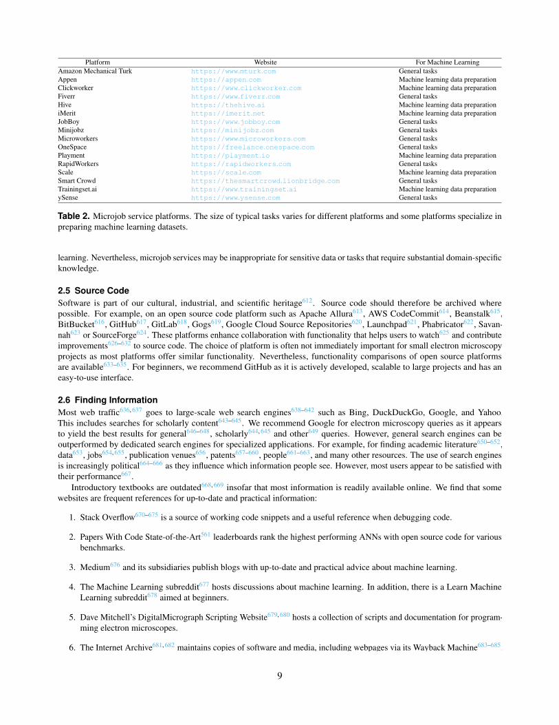
Platform Website For Machine LearningAmazon Mechanical Turk https://www.mturk.com General tasksAppen https://appen.com Machine learning data preparationClickworker https://www.clickworker.com Machine learning data preparationFiverr https://www.fiverr.com General tasksHive https://thehive.ai Machine learning data preparationiMerit https://imerit.net Machine learning data preparationJobBoy https://www.jobboy.com General tasksMinijobz https://minijobz.com General tasksMicroworkers https://www.microworkers.com General tasksOneSpace https://freelance.onespace.com General tasksPlayment https://playment.io Machine learning data preparationRapidWorkers https://rapidworkers.com General tasksScale https://scale.com Machine learning data preparationSmart Crowd https://thesmartcrowd.lionbridge.com General tasksTrainingset.ai https://www.trainingset.ai Machine learning data preparationySense https://www.ysense.com General tasks
Table 2. Microjob service platforms. The size of typical tasks varies for different platforms and some platforms specialize inpreparing machine learning datasets.
learning. Nevertheless, microjob services may be inappropriate for sensitive data or tasks that require substantial domain-specificknowledge.
2.5 Source CodeSoftware is part of our cultural, industrial, and scientific heritage612. Source code should therefore be archived wherepossible. For example, on an open source code platform such as Apache Allura613, AWS CodeCommit614, Beanstalk615,BitBucket616, GitHub617, GitLab618, Gogs619, Google Cloud Source Repositories620, Launchpad621, Phabricator622, Savan-nah623 or SourceForge624. These platforms enhance collaboration with functionality that helps users to watch625 and contributeimprovements626–632 to source code. The choice of platform is often not immediately important for small electron microscopyprojects as most platforms offer similar functionality. Nevertheless, functionality comparisons of open source platformsare available633–635. For beginners, we recommend GitHub as it is actively developed, scalable to large projects and has aneasy-to-use interface.
2.6 Finding InformationMost web traffic636, 637 goes to large-scale web search engines638–642 such as Bing, DuckDuckGo, Google, and Yahoo.This includes searches for scholarly content643–645. We recommend Google for electron microscopy queries as it appearsto yield the best results for general646–648, scholarly644, 645 and other649 queries. However, general search engines can beoutperformed by dedicated search engines for specialized applications. For example, for finding academic literature650–652,data653, jobs654, 655, publication venues656, patents657–660, people661–663, and many other resources. The use of search enginesis increasingly political664–666 as they influence which information people see. However, most users appear to be satisfied withtheir performance667.
Introductory textbooks are outdated668, 669 insofar that most information is readily available online. We find that somewebsites are frequent references for up-to-date and practical information:
1. Stack Overflow670–675 is a source of working code snippets and a useful reference when debugging code.
2. Papers With Code State-of-the-Art561 leaderboards rank the highest performing ANNs with open source code for variousbenchmarks.
3. Medium676 and its subsidiaries publish blogs with up-to-date and practical advice about machine learning.
4. The Machine Learning subreddit677 hosts discussions about machine learning. In addition, there is a Learn MachineLearning subreddit678 aimed at beginners.
5. Dave Mitchell’s DigitalMicrograph Scripting Website679, 680 hosts a collection of scripts and documentation for program-ming electron microscopes.
6. The Internet Archive681, 682 maintains copies of software and media, including webpages via its Wayback Machine683–685.
8/989
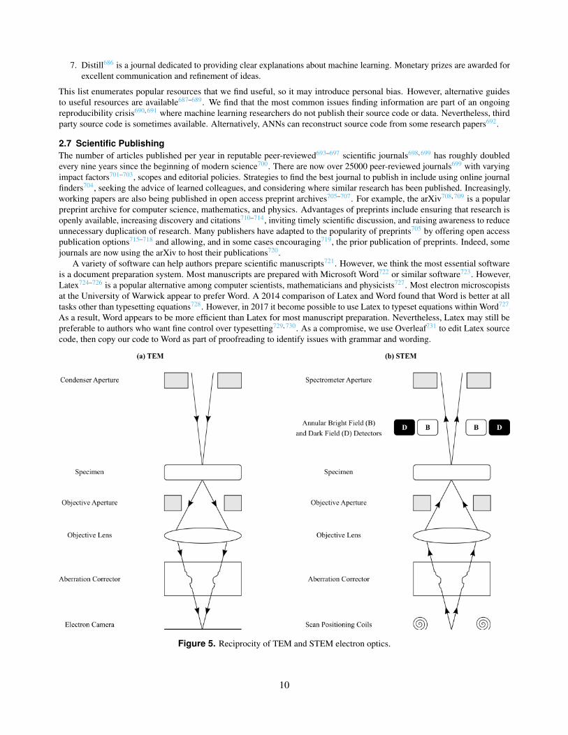
7. Distill686 is a journal dedicated to providing clear explanations about machine learning. Monetary prizes are awarded forexcellent communication and refinement of ideas.
This list enumerates popular resources that we find useful, so it may introduce personal bias. However, alternative guidesto useful resources are available687–689. We find that the most common issues finding information are part of an ongoingreproducibility crisis690, 691 where machine learning researchers do not publish their source code or data. Nevertheless, thirdparty source code is sometimes available. Alternatively, ANNs can reconstruct source code from some research papers692.
2.7 Scientific PublishingThe number of articles published per year in reputable peer-reviewed693–697 scientific journals698, 699 has roughly doubledevery nine years since the beginning of modern science700. There are now over 25000 peer-reviewed journals699 with varyingimpact factors701–703, scopes and editorial policies. Strategies to find the best journal to publish in include using online journalfinders704, seeking the advice of learned colleagues, and considering where similar research has been published. Increasingly,working papers are also being published in open access preprint archives705–707. For example, the arXiv708, 709 is a popularpreprint archive for computer science, mathematics, and physics. Advantages of preprints include ensuring that research isopenly available, increasing discovery and citations710–714, inviting timely scientific discussion, and raising awareness to reduceunnecessary duplication of research. Many publishers have adapted to the popularity of preprints705 by offering open accesspublication options715–718 and allowing, and in some cases encouraging719, the prior publication of preprints. Indeed, somejournals are now using the arXiv to host their publications720.
A variety of software can help authors prepare scientific manuscripts721. However, we think the most essential softwareis a document preparation system. Most manuscripts are prepared with Microsoft Word722 or similar software723. However,Latex724–726 is a popular alternative among computer scientists, mathematicians and physicists727. Most electron microscopistsat the University of Warwick appear to prefer Word. A 2014 comparison of Latex and Word found that Word is better at alltasks other than typesetting equations728. However, in 2017 it become possible to use Latex to typeset equations within Word727.As a result, Word appears to be more efficient than Latex for most manuscript preparation. Nevertheless, Latex may still bepreferable to authors who want fine control over typesetting729, 730. As a compromise, we use Overleaf731 to edit Latex sourcecode, then copy our code to Word as part of proofreading to identify issues with grammar and wording.
Figure 5. Reciprocity of TEM and STEM electron optics.
9/9810
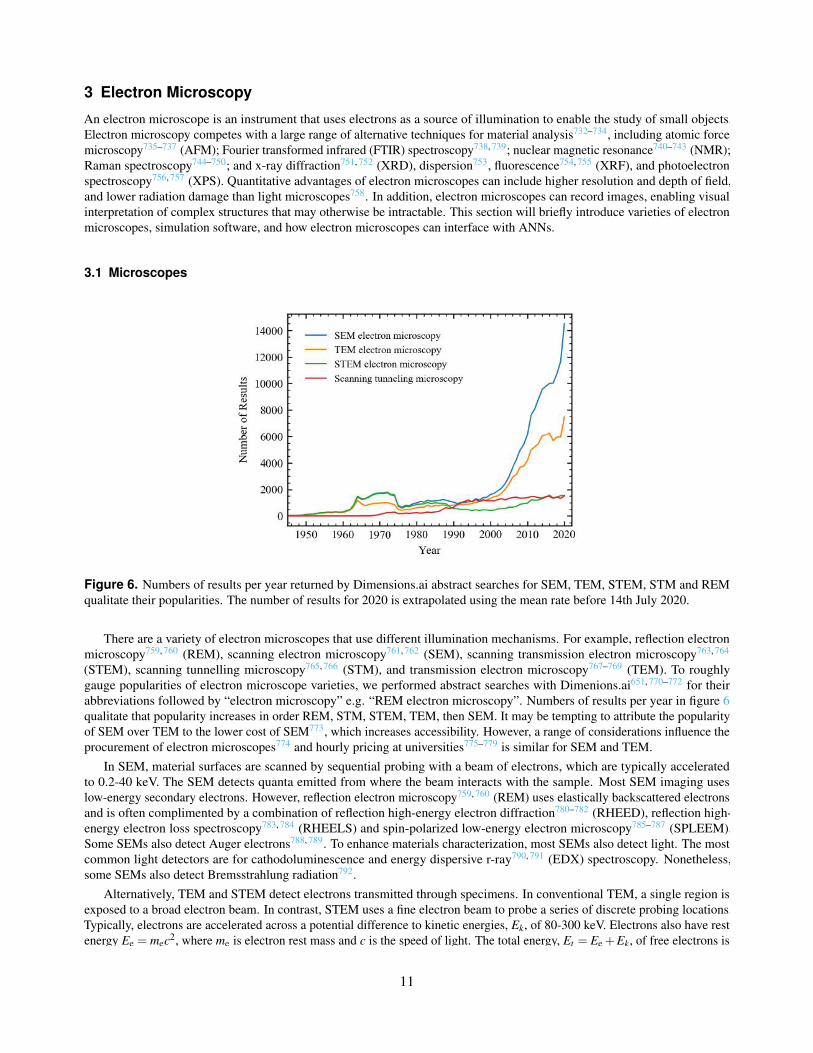
3 Electron Microscopy
An electron microscope is an instrument that uses electrons as a source of illumination to enable the study of small objects.Electron microscopy competes with a large range of alternative techniques for material analysis732–734, including atomic forcemicroscopy735–737 (AFM); Fourier transformed infrared (FTIR) spectroscopy738, 739; nuclear magnetic resonance740–743 (NMR);Raman spectroscopy744–750; and x-ray diffraction751, 752 (XRD), dispersion753, fluorescence754, 755 (XRF), and photoelectronspectroscopy756, 757 (XPS). Quantitative advantages of electron microscopes can include higher resolution and depth of field,and lower radiation damage than light microscopes758. In addition, electron microscopes can record images, enabling visualinterpretation of complex structures that may otherwise be intractable. This section will briefly introduce varieties of electronmicroscopes, simulation software, and how electron microscopes can interface with ANNs.
3.1 Microscopes
Figure 6. Numbers of results per year returned by Dimensions.ai abstract searches for SEM, TEM, STEM, STM and REMqualitate their popularities. The number of results for 2020 is extrapolated using the mean rate before 14th July 2020.
There are a variety of electron microscopes that use different illumination mechanisms. For example, reflection electronmicroscopy759, 760 (REM), scanning electron microscopy761, 762 (SEM), scanning transmission electron microscopy763, 764
(STEM), scanning tunnelling microscopy765, 766 (STM), and transmission electron microscopy767–769 (TEM). To roughlygauge popularities of electron microscope varieties, we performed abstract searches with Dimenions.ai651, 770–772 for theirabbreviations followed by “electron microscopy” e.g. “REM electron microscopy”. Numbers of results per year in figure 6qualitate that popularity increases in order REM, STM, STEM, TEM, then SEM. It may be tempting to attribute the popularityof SEM over TEM to the lower cost of SEM773, which increases accessibility. However, a range of considerations influence theprocurement of electron microscopes774 and hourly pricing at universities775–779 is similar for SEM and TEM.
In SEM, material surfaces are scanned by sequential probing with a beam of electrons, which are typically acceleratedto 0.2-40 keV. The SEM detects quanta emitted from where the beam interacts with the sample. Most SEM imaging useslow-energy secondary electrons. However, reflection electron microscopy759, 760 (REM) uses elastically backscattered electronsand is often complimented by a combination of reflection high-energy electron diffraction780–782 (RHEED), reflection high-energy electron loss spectroscopy783, 784 (RHEELS) and spin-polarized low-energy electron microscopy785–787 (SPLEEM).Some SEMs also detect Auger electrons788, 789. To enhance materials characterization, most SEMs also detect light. The mostcommon light detectors are for cathodoluminescence and energy dispersive r-ray790, 791 (EDX) spectroscopy. Nonetheless,some SEMs also detect Bremsstrahlung radiation792.
Alternatively, TEM and STEM detect electrons transmitted through specimens. In conventional TEM, a single region isexposed to a broad electron beam. In contrast, STEM uses a fine electron beam to probe a series of discrete probing locations.Typically, electrons are accelerated across a potential difference to kinetic energies, Ek, of 80-300 keV. Electrons also have restenergy Ee = mec2, where me is electron rest mass and c is the speed of light. The total energy, Et = Ee +Ek, of free electrons is
10/9811
related to their rest mass energy by a Lorentz factor, γ ,
Et = γmec2 , (1)
γ = (1− v2/c2)1/2 , (2)
where v is the speed of electron propagation in the rest frame of an electron microscope. Electron kinetic energies in TEM andSTEM are comparable to their rest energy, Ee = 511 keV793, so relativistic phenomena794, 795 must be considered to accuratelydescribe their dynamics.
Electrons exhibit wave-particle duality350, 351. Thus, in an ideal electron microscope, the maximum possible detection angle,θ , between two point sources separated by a distance, d, perpendicular to the electron propagation direction is diffraction-limited.The resolution limit for imaging can be quantified by Rayleigh’s criterion796–798
θ ' 1.22λd, (3)
where resolution increases with decreasing wavelength, λ . Electron wavelength increases with increasing accelerating voltage,as described by the relativistic de Broglie relation799–801,
λ = hc(E2
k +2EeEk)−1/2
, (4)
where h is Planck’s constant793. Electron wavelengths for typical acceleration voltages tabulated by JEOL are in picometres802.In comparison, Cu K-α x-rays, which are often used for XRD, have wavelengths near 0.15 nm803. In theory, electrons cantherefore achieve over 100× higher resolution than x-rays. Electrons and x-rays are both ionizing; however, electrons oftendo less radiation damage to thin specimens than x-rays758. Tangentially, TEM and STEM often achieve over 10 times higherresolution than SEM804 as transmitted electrons in TEM and STEM are easier to resolve than electrons returned from materialsurfaces in SEM.
In practice, TEM and STEM are also limited by incoherence805–807 introduced by inelastic scattering, electron energyspread, and other mechanisms. TEM and STEM are related by an extension of Helmholtz reciprocity808, 809 where the sourceplane in a TEM corresponds to the detector plane in a STEM810, as shown in figure 5. Consequently, TEM coherence is limitedby electron optics between the specimen and image, whereas STEM coherence is limited by the illumination system. Forconventional TEM and STEM imaging, electrons are normally incident on a specimen811. Advantages of STEM imaging caninclude higher contrast and resolution than TEM imaging, and lower radiation damage812. As a result, STEM is increasingbeing favoured over TEM for high-resolution studies. However, we caution that definitions of TEM and STEM resolution canbe disparate813.
In addition to conventional imaging, TEM and STEM include a variety of operating modes for different applications.For example, TEM operating configurations include electron diffraction814; convergent beam electron diffraction815–817
(CBED); tomography818–826; and bright field768, 827–829, dark field768, 829 and annular dark field830 imaging. Similarly, STEMoperating configurations include differential phase contrast831–834; tomography818, 820, 822, 823; and bright field835, 836 or darkfield837 imaging. Further, electron cameras838, 839 are often supplemented by secondary signal detectors. For example,elemental composition is often mapped by EDX spectroscopy, electron energy loss spectroscopy840, 841 (EELS) or wavelengthdispersive spectroscopy842, 843 (WDS). Similarly, electron backscatter diffraction844–846 (EBSD) can detect strain847–849 andcrystallization850–852.
3.2 Contrast SimulationThe propagation of electron wavefunctions though electron microscopes can be described by wave optics136. Following, the mostpopular approach to modelling measurement contrast is multislice simulation853, 854, where an electron wavefunction is itera-tively perturbed as it travels through a model of a specimen. Multislice software for electron microscopy includes ACEM854–856,clTEM857, 858, cudaEM859, Dr. Probe860, 861, EMSoft862, 863, JEMS864, JMULTIS865, MULTEM866–868, NCEMSS869, 870, NU-MIS871, Prismatic872–874, QSTEM875, SimulaTEM876, STEM-CELL877, Tempas878, and xHREM879–884. We find that mostmultislice software is a recreation and slight modification of common functionality, possibly due to a publish-or-perish culturein academia885–887. Bloch-wave simulation854, 888–892 is an alternative to multislice simulation that can reduce computationtime and memory requirements for crystalline materials893.
3.3 AutomationMost modern electron microscopes support Gatan Microscopy Suite (GMS) Software894. GMS enables electron microscopes tobe programmed by DigitalMicrograph Scripting, a propriety Gatan programming language akin to a simplified version of C++.
11/9812
A variety of DigitalMicrograph scripts, tutorials and related resources are available from Dave Mitchell’s DigitalMicrographScripting Website679, 680, FELMI/ZFE’s Script Database895 and Gatan’s Script library896. Some electron microscopists alsoprovide DigitalMicrograph scripting resources on their webpages897–899. However, DigitalMicrograph scripts are slow insofarthat they are interpreted at runtime, and there is limited native functionality for parallel and distributed computing. As a result,extensions to DigitalMicrograph scripting are often developed in other programming languages that offer more functionality.
Historically, most extensions were developed in C++900. This was problematic as there is limited documentation, thestandard approach used outdated C++ software development kits such as Visual Studio 2008, and programming expertiserequired to create functions that interface with DigitalMicrograph scripts limited accessibility. To increase accessibility, recentversions of GMS now support python901. This is convenient as it enables ANNs developed with python to readily interface withelectron microscopes. For ANNs developed with C++, users have the option to either create C++ bindings for DigitalMicrographscript or for python. Integrating ANNs developed in other programming languages is more complicated as DigitalMicrographprovides almost no support. However, that complexity can be avoided by exchanging files from DigitalMicrograph script toexternal libraries via a random access memory (RAM) disk902 or secondary storage903.
Increasing accessibility, there are collections of GMS plugins with GUIs for automation and analysis897–899, 904. In addition,various individual plugins are available905–909. Some plugins are open source, so they can be adapted to interface with ANNs.However, many high-quality plugins are proprietary and closed source, limiting their use to automation of data collection andprocessing. Plugins can also be supplemented by a variety of libraries and interfaces for electron microscopy signal processing.For example, popular general-purpose software includes ImageJ910, pycroscopy527, 528 and HyperSpy529, 530. In addition, thereare directories for tens of general-purpose and specific electron microscopy programs911–913.
4 Components
Most modern ANNs are configured from a variety of DLF components. To take advantage of hardware accelerators62, mostANNs are implemented as sequences of parallelizable layers of tensor operations914. Layers are often parallelized acrossdata and may be parallelized across other dimensions915. This section introduces popular nonlinear activation functions,normalization layers, convolutional layers, and skip connections. To add insight, we provide comparative discussion andaddress some common causes of confusion.
4.1 Nonlinear ActivationIn general, DNNs need multiple layers to be universal approximators37–45. Nonlinear activation functions916, 917 are thereforeessential to DNNs as successive linear layers can be contracted to a single layer. Activation functions separate artificial neurons,similar to biological neurons918. To learn efficiently, most DNNs are tens or hundreds of layers deep47, 919–921. High depthincreases representational capacity47, which can help training by gradient descent as DNNs evolve as linear models922 andnonlinearities can create suboptimal local minima where data cannot be fit by linear models923. There are infinitely manypossible activation functions. However, most activation functions have low polynomial order, similar to physical Hamiltonians47.
Most ANNs developed for electron microscopy are for image processing, where the most popular nonlinearities are rectifierlinear units924, 925 (ReLUs). The ReLU activation, f (x), of an input, x, and its gradient, ∂x f (x), are
f (x) = max(0,x) (5a) ∂ f (x)∂x
=
0, if x≤ 01, if x > 0
(5b)
Popular variants of ReLUs include Leaky ReLU926,
f (x) = max(αx,x) (6a) ∂ f (x)∂x
=
α, if x≤ 01, if x > 0
(6b)
where α is a hyperparameter, parametric ReLU22 (PreLU) where α is a learned parameter, dynamic ReLU where α is a learnedfunction of inputs927, and randomized leaky ReLU928 (RReLU) where α is chosen randomly. Typically, learned PreLU α arehigher the nearer a layer is to ANN inputs22. Motivated by limited comparisons that do not show a clear performance differencebetween ReLU and leaky ReLU929, some blogs930 argue against using leaky ReLU due to its higher computational requirementsand complexity. However, an in-depth comparison found that leaky ReLU variants consistently slightly outperform ReLU928. Inaddition, the non-zero gradient of leaky ReLU for x≤ 0 prevents saturating, or “dying”, ReLU931–933, where the zero gradientof ReLUs stops learning.
12/9813
There are a variety of other piecewise linear ReLU variants that can improve performance. For example, ReLUh activationsare limited to a threshold934, h, so that
f (x) = min(max(0,x),h) (7a) ∂ f (x)∂x
=
0, if x≤ 01, if 0 < x≤ h0, if x > h
(7b)
Thresholds near h = 6 are often effective, so popular choice is ReLU6. Another popular activation is concatenated ReLU935
(CReLU), which is the concatenation of ReLU(x) and ReLU(−x). Other ReLU variants include adaptive convolutional936,bipolar937, elastic938, and Lipschitz939 ReLUs. However, most ReLU variants are uncommon as they are more complicatedthan ReLU and offer small, inconsistent, or unclear performance gains. Moreover, it follows from the universal approximatortheorems37–45 that disparity between ReLU and its variants approaches zero as network depth increases.
In shallow networks, curved activation functions with non-zero Hessians often accelerate convergence and improveperformance. A popular activation is the exponential linear unit940 (ELU),
f (x) =
α(exp(x)−1), if x≤ 0x, if x≥ 0
(8a)∂ f (x)
∂x=
α exp(x), if x≤ 01, if x≥ 0
(8b)
where α is a learned parameter. Further, a scaled ELU941 (SELU),
f (x) =
λα(exp(x)−1), if x≤ 0λx, if x≥ 0
(9a)∂ f (x)
∂x=
λα exp(x), if x≤ 0λ , if x≥ 0
(9b)
with fixed α = 1.67326 and scale factor λ = 1.0507 can be used to create self-normalizing neural networks (SNNs). A SNNcannot be derived from ReLUs or most other activation functions. Activation functions with curvature are especially commonin ANNs with only a couple of layers. For example, activation functions in radial basis function (RBF) networks942–945, whichare efficient universal approximators, are often Gaussians, multiquadratics, inverse multiquadratics, or square-based RBFs946.Similarly, support vector machines947–949 (SVMs) often use RBFs, or sigmoids,
f (x) =1
1+ exp(−x)(10a)
∂ f (x)∂x
= f (x)(1− f (x)) (10b)
Sigmoids can also be applied to limit the support of outputs. Unscaled, or “logistic”, sigmoids are often denoted σ(x) and arerelated to tanh by tanh(x) = 2σ(2x)−1. To avoid expensive exp(−x) in the computation of tanh, we recommend K-tanH950,LeCun tanh951, or piecewise linear approximation952, 953.
The activation functions introduced so far are scalar functions than can be efficiently computed in parallel for each inputelement. However, functions of vectors, x = x1,x2, ..., are also popular. For example, softmax activation954,
f (x) =exp(x)
sum(exp(x))(11a)
f (x)∂x j
= ∑i
f (x)i(δi j− f (x) j) (11b)
is often applied before computing cross-entropy losses for classification networks. Similarly, Ln vector normalization,
f (x) =x||x||n
(12a) f (x)∂x j
=1||x||n
(1−
xnj
||x||nn
)(12b)
is often applied to n-dimensional vectors to ensure that they lie on a unit n-sphere349. Finally, max pooling955, 956,
13/9814
f (x) = max(x) (13a) f (x)∂x j
=
1, if j = argmax(x)0, if j 6= argmax(x)
(13b)
is another popular multivariate activation function that is often used for downsampling. However, max pooling has fallen outof favour as it is often outperformed by strided convolutional layers957. Other vector activation functions include squashingnonlinearities for dynamic routing by agreement in capsule networks958 and cosine similarity959.
There is a range of other activation functions that are not detailed here for brevity. Further, finding new activation functionsis an active area of research960, 961. Notable variants include choosing activation functions from a set before training962, 963
and learning activation functions962, 964–967. Activation functions can also encode probability distributions968–970 or includenoise953. Finally, there are a variety of other deterministic activation functions961, 971. In electron microscopy, most ANNsenable new or enhance existing applications. Subsequently, we recommend using computationally efficient and establishedactivation functions unless there is a compelling reason to use a specialized activation function.
4.2 NormalizationNormalization972–974 standardizes signals, which can accelerate convergence by gradient descent and improve performance.Batch normalization975–980 is the most popular normalization layer in image processing DNNs trained with minibatches of Nexamples. Technically, a “batch” is an entire training dataset and a “minibatch” is a subset; however, the “mini” is often omittedwhere meaning is clear from context. During training, batch normalization applies a transform,
µB =1N
N
∑i=1
xi , (14)
σ2B =
1N
N
∑i=1
(xi−µB)2 , (15)
x =x−µB
(σ2B + ε)1/2 , (16)
BatchNorm(x) = γ x+β , (17)
where x = x1, ...,xN is a batch of layer inputs, γ and β are a learnable scale and shift, and ε is a small constant added fornumerical stability. During inference, batch normalization applies a transform,
BatchNorm(x) =γ
(Var[x]+ ε)1/2 x+(
β − γE[x](Var[x]+ ε)1/2
), (18)
where E[x] and Var[x] are expected batch means and variances. For convenience, E[x] and Var[x] are often estimated withexponential moving averages that are tracked during training. However, E[x] and Var[x] can also be estimated by propagatingexamples through an ANN after training.
Increasing batch size stabilizes learning by averaging destabilizing loss spikes over batches261. Batched learning alsoenables more efficient utilization of modern hardware accelerators. For example, larger batch sizes improve utilization ofGPU memory bandwidth and throughput391, 981, 982. Using large batches can also be more efficient than many small batcheswhen distributing training across multiple CPU clusters or GPUs due to communication overheads. However, the performancebenefits of large batch sizes can come at the cost of lower test accuracy as training with large batches tends to converge tosharper minima983, 984. As a result, it often best not to use batch sizes higher than N ≈ 32 for image classification985. However,learning rate scaling541 and layer-wise adaptive learning rates986 can increase accuracy of training with fixed larger batch sizes.Batch size can also be increased throughout training without compromising accuracy987 to exploit effective learning rates beinginversely proportional to batch size541, 987. Alternatively, accuracy can be improved by creating larger batches from replicatedinstances of training inputs with different data augmentations988.
There are a few caveats to batch normalization. Originally, batch normalization was applied before activation976. However,applying batch normalization after activation often slightly improves performance989, 990. In addition, training can be sensitiveto the often-forgotten ε hyperparameter991 in equation 16. Typically, performance decreases as ε is increased above ε ≈ 0.001;however, there is a sharp increase in performance around ε = 0.01 on ImageNet. Finally, it is often assumed that batchesare representative of the training dataset. This is often approximated by shuffling training data to sample independent andidentically distributed (i.i.d.) samples. However, performance can often be improved by prioritizing sampling992, 993. Weobserve that batch normalization is usually effective if batch moments, µB and σB, have similar values for every batch.
14/9815
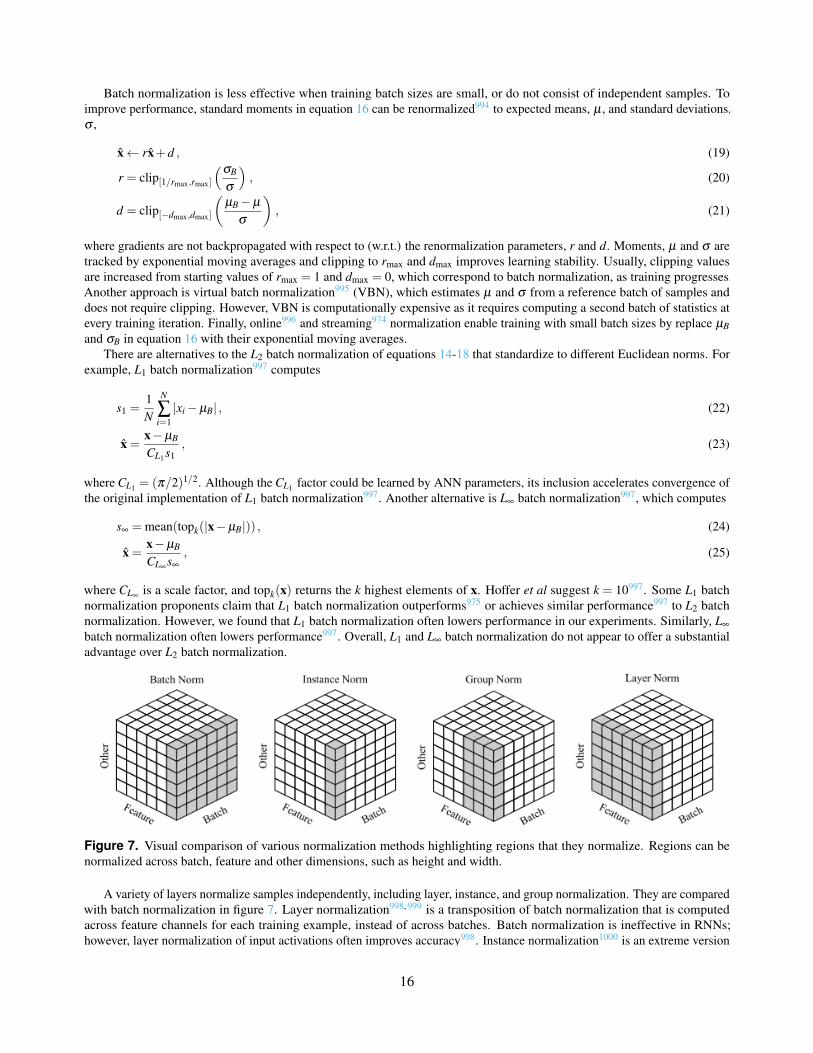
Batch normalization is less effective when training batch sizes are small, or do not consist of independent samples. Toimprove performance, standard moments in equation 16 can be renormalized994 to expected means, µ , and standard deviations,σ ,
x← rx+d , (19)
r = clip[1/rmax,rmax]
(σB
σ
), (20)
d = clip[−dmax,dmax]
(µB−µ
σ
), (21)
where gradients are not backpropagated with respect to (w.r.t.) the renormalization parameters, r and d. Moments, µ and σ aretracked by exponential moving averages and clipping to rmax and dmax improves learning stability. Usually, clipping valuesare increased from starting values of rmax = 1 and dmax = 0, which correspond to batch normalization, as training progresses.Another approach is virtual batch normalization995 (VBN), which estimates µ and σ from a reference batch of samples anddoes not require clipping. However, VBN is computationally expensive as it requires computing a second batch of statistics atevery training iteration. Finally, online996 and streaming974 normalization enable training with small batch sizes by replace µBand σB in equation 16 with their exponential moving averages.
There are alternatives to the L2 batch normalization of equations 14-18 that standardize to different Euclidean norms. Forexample, L1 batch normalization997 computes
s1 =1N
N
∑i=1|xi−µB| , (22)
x =x−µB
CL1s1, (23)
where CL1 = (π/2)1/2. Although the CL1 factor could be learned by ANN parameters, its inclusion accelerates convergence ofthe original implementation of L1 batch normalization997. Another alternative is L∞ batch normalization997, which computes
s∞ = mean(topk(|x−µB|)) , (24)
x =x−µB
CL∞s∞, (25)
where CL∞ is a scale factor, and topk(x) returns the k highest elements of x. Hoffer et al suggest k = 10997. Some L1 batchnormalization proponents claim that L1 batch normalization outperforms975 or achieves similar performance997 to L2 batchnormalization. However, we found that L1 batch normalization often lowers performance in our experiments. Similarly, L∞batch normalization often lowers performance997. Overall, L1 and L∞ batch normalization do not appear to offer a substantialadvantage over L2 batch normalization.
Figure 7. Visual comparison of various normalization methods highlighting regions that they normalize. Regions can benormalized across batch, feature and other dimensions, such as height and width.
A variety of layers normalize samples independently, including layer, instance, and group normalization. They are comparedwith batch normalization in figure 7. Layer normalization998, 999 is a transposition of batch normalization that is computedacross feature channels for each training example, instead of across batches. Batch normalization is ineffective in RNNs;however, layer normalization of input activations often improves accuracy998. Instance normalization1000 is an extreme version
15/9816
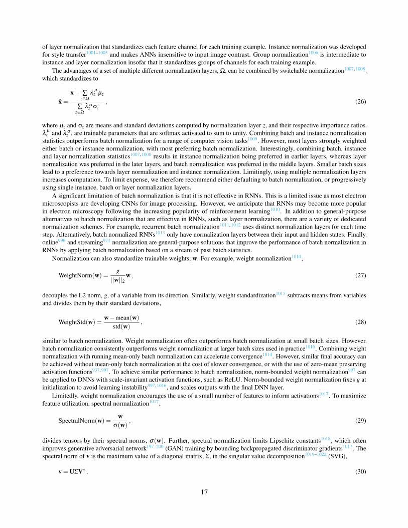
of layer normalization that standardizes each feature channel for each training example. Instance normalization was developedfor style transfer1001–1005 and makes ANNs insensitive to input image contrast. Group normalization1006 is intermediate toinstance and layer normalization insofar that it standardizes groups of channels for each training example.
The advantages of a set of multiple different normalization layers, Ω, can be combined by switchable normalization1007, 1008,which standardizes to
x =
x− ∑z∈Ω
λ µz µz
∑z∈Ω
λ σz σz
, (26)
where µz and σz are means and standard deviations computed by normalization layer z, and their respective importance ratios,λ µ
z and λ σz , are trainable parameters that are softmax activated to sum to unity. Combining batch and instance normalization
statistics outperforms batch normalization for a range of computer vision tasks1009. However, most layers strongly weightedeither batch or instance normalization, with most preferring batch normalization. Interestingly, combining batch, instanceand layer normalization statistics1007, 1008 results in instance normalization being preferred in earlier layers, whereas layernormalization was preferred in the later layers, and batch normalization was preferred in the middle layers. Smaller batch sizeslead to a preference towards layer normalization and instance normalization. Limitingly, using multiple normalization layersincreases computation. To limit expense, we therefore recommend either defaulting to batch normalization, or progressivelyusing single instance, batch or layer normalization layers.
A significant limitation of batch normalization is that it is not effective in RNNs. This is a limited issue as most electronmicroscopists are developing CNNs for image processing. However, we anticipate that RNNs may become more popularin electron microscopy following the increasing popularity of reinforcement learning1010. In addition to general-purposealternatives to batch normalization that are effective in RNNs, such as layer normalization, there are a variety of dedicatednormalization schemes. For example, recurrent batch normalization1011, 1012 uses distinct normalization layers for each timestep. Alternatively, batch normalized RNNs1013 only have normalization layers between their input and hidden states. Finally,online996 and streaming974 normalization are general-purpose solutions that improve the performance of batch normalization inRNNs by applying batch normalization based on a stream of past batch statistics.
Normalization can also standardize trainable weights, w. For example, weight normalization1014,
WeightNorm(w) =g||w||2
w , (27)
decouples the L2 norm, g, of a variable from its direction. Similarly, weight standardization1015 subtracts means from variablesand divides them by their standard deviations,
WeightStd(w) =w−mean(w)
std(w), (28)
similar to batch normalization. Weight normalization often outperforms batch normalization at small batch sizes. However,batch normalization consistently outperforms weight normalization at larger batch sizes used in practice1016. Combining weightnormalization with running mean-only batch normalization can accelerate convergence1014. However, similar final accuracy canbe achieved without mean-only batch normalization at the cost of slower convergence, or with the use of zero-mean preservingactivation functions937, 997. To achieve similar performance to batch normalization, norm-bounded weight normalization997 canbe applied to DNNs with scale-invariant activation functions, such as ReLU. Norm-bounded weight normalization fixes g atinitialization to avoid learning instability997, 1016, and scales outputs with the final DNN layer.
Limitedly, weight normalization encourages the use of a small number of features to inform activations1017. To maximizefeature utilization, spectral normalization1017,
SpectralNorm(w) =w
σ(w), (29)
divides tensors by their spectral norms, σ(w). Further, spectral normalization limits Lipschitz constants1018, which oftenimproves generative adversarial network197–200 (GAN) training by bounding backpropagated discriminator gradients1017. Thespectral norm of v is the maximum value of a diagonal matrix, Σ, in the singular value decomposition1019–1022 (SVG),
v = UΣV∗ , (30)
16/9817
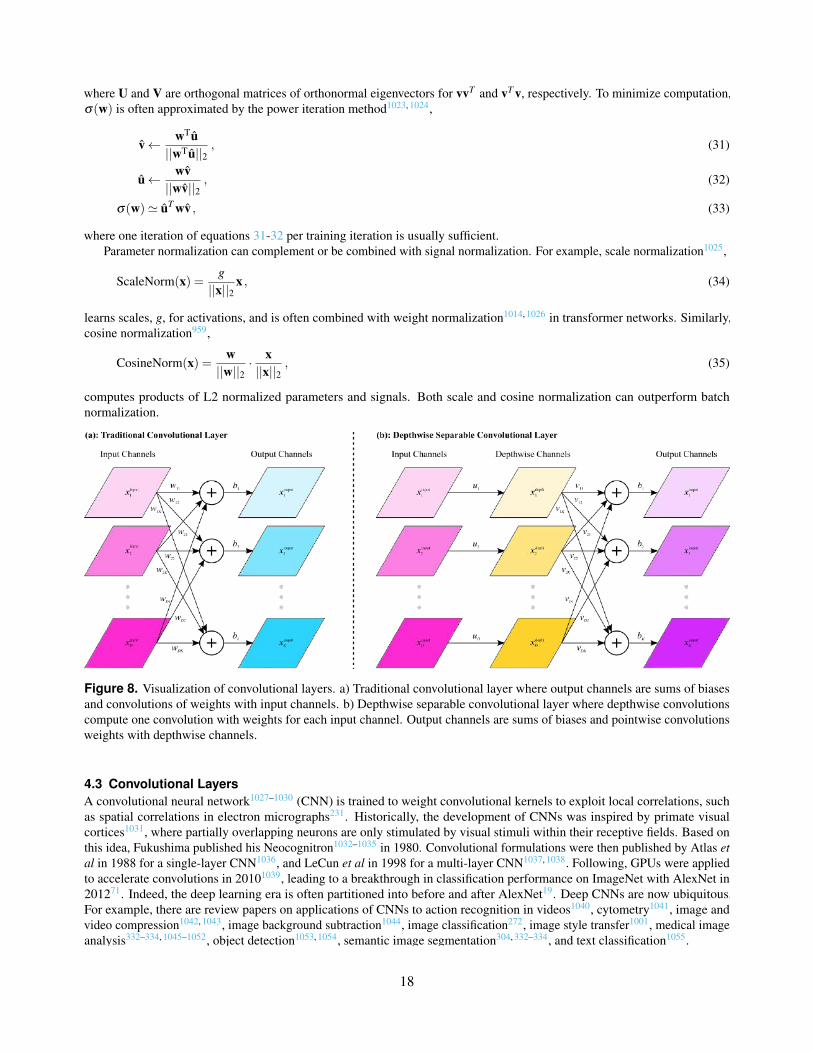
where U and V are orthogonal matrices of orthonormal eigenvectors for vvT and vT v, respectively. To minimize computation,σ(w) is often approximated by the power iteration method1023, 1024,
v← wTu||wTu||2
, (31)
u← wv||wv||2
, (32)
σ(w)' uT wv , (33)
where one iteration of equations 31-32 per training iteration is usually sufficient.Parameter normalization can complement or be combined with signal normalization. For example, scale normalization1025,
ScaleNorm(x) =g||x||2
x , (34)
learns scales, g, for activations, and is often combined with weight normalization1014, 1026 in transformer networks. Similarly,cosine normalization959,
CosineNorm(x) =w||w||2
· x||x||2
, (35)
computes products of L2 normalized parameters and signals. Both scale and cosine normalization can outperform batchnormalization.
Figure 8. Visualization of convolutional layers. a) Traditional convolutional layer where output channels are sums of biasesand convolutions of weights with input channels. b) Depthwise separable convolutional layer where depthwise convolutionscompute one convolution with weights for each input channel. Output channels are sums of biases and pointwise convolutionsweights with depthwise channels.
4.3 Convolutional LayersA convolutional neural network1027–1030 (CNN) is trained to weight convolutional kernels to exploit local correlations, suchas spatial correlations in electron micrographs231. Historically, the development of CNNs was inspired by primate visualcortices1031, where partially overlapping neurons are only stimulated by visual stimuli within their receptive fields. Based onthis idea, Fukushima published his Neocognitron1032–1035 in 1980. Convolutional formulations were then published by Atlas etal in 1988 for a single-layer CNN1036, and LeCun et al in 1998 for a multi-layer CNN1037, 1038. Following, GPUs were appliedto accelerate convolutions in 20101039, leading to a breakthrough in classification performance on ImageNet with AlexNet in201271. Indeed, the deep learning era is often partitioned into before and after AlexNet19. Deep CNNs are now ubiquitous.For example, there are review papers on applications of CNNs to action recognition in videos1040, cytometry1041, image andvideo compression1042, 1043, image background subtraction1044, image classification272, image style transfer1001, medical imageanalysis332–334, 1045–1052, object detection1053, 1054, semantic image segmentation304, 332–334, and text classification1055.
17/9818
In general, the convolution of two functions, f and g, is
( f ∗g)(x) :=∫
s∈Ω
f (s)g(x− s)ds , (36)
and their cross-correlation is
( f g)(x) :=∫
s∈Ω
f (s)g(x+ s)ds , (37)
where integrals have unlimited support, Ω. In a CNN, convolutional layers sum convolutions of feature channels with trainablekernels, as shown in figure 8. Thus, f and g are discrete functions and the integrals in equations 36-37 can be replaced withlimited summations. Since cross-correlation is equivalent to convolution if the kernel is flipped in every dimension, andCNN kernels are usually trainable, convolution and cross-correlation is often interchangeable in deep learning. For example,a TensorFlow function named “tf.nn.convolution” computes cross-correlations1056. Nevertheless, the difference betweenconvolution and cross-correlation can be source of subtle errors if convolutional layers from a DLF are used in an imageprocessing pipeline with static asymmetric kernels.
Figure 9. Two 96×96 electron micrographs a) unchanged, and filtered by b) a 5×5 symmetric Gaussian kernel with a 2.5 pxstandard deviation, c) a 3×3 horizontal Sobel kernel, and d) a 3×3 vertical Sobel kernel. Intensities in a) and b) are in [0, 1],whereas intensities in c) and d) are in [-1, 1].
Kernels designed by humans1057 are often convolved in image processing pipelines. For example, convolutions of electronmicrographs with Gaussian and Sobel kernels are shown in figure 9. Gaussian kernels compute local averages, blurring imagesand suppressing high-frequency noise. For example, a 5×5 symmetric Gaussian kernel with a 2.5 px standard deviation is
0.16890.21480.23260.21480.1689
[0.1689 0.2148 0.2326 0.2148 0.1689
]=
0.0285 0.0363 0.0393 0.0363 0.02850.0363 0.0461 0.0500 0.0461 0.03630.0393 0.0500 0.0541 0.0500 0.03930.0363 0.0461 0.0500 0.0461 0.03630.0285 0.0363 0.0393 0.0363 0.0285
. (38)
Alternatives to Gaussian kernels for image smoothing1058 include mean, median and bilateral filters. Sobel kernels computehorizontal and vertical spatial gradients that can be used for edge detection1059. For example, 3×3 Sobel kernels are
18/9819

121
[1 0 −1
]=
1 0 −12 0 −21 0 −1
(39a)
10−1
[1 2 1
]=
1 2 10 0 0−1 −2 −1
(39b)
Alternatives to Sobel kernels offer similar utility, and include extended Sobel1060, Scharr1061, 1062, Kayyali1063, Roberts cross1064
and Prewitt1065 kernels. Two-dimensional Gaussian and Sobel kernels are examples of linearly separable, or “flattenable”,kernels, which can be split into two one-dimensional kernels, as shown in equations 38-39b. Kernel separation can decreasecomputation in convolutional layers by convolving separated kernels in series, and CNNs that only use separable convolutionsare effective1066–1068. However, serial convolutions decrease parallelization and separable kernels have fewer degrees offreedom, decreasing representational capacity. Following, separated kernels are usually at least 5×5, and separated 3×3 kernelsare unusual. Even-sized kernels, such as 2×2 and 4×4, are rare as symmetric padding is needed to avoid information erosioncaused by spatial shifts of feature maps1069.
A traditional 2D convolutional layer maps inputs, xinput, with height H, width, W , and depth, D, to
xoutputki j = bk +
D
∑d=1
M
∑m=1
N
∑n=1
wdkmnxinputd(i+m−1)( j+n−1) , i ∈ [1,H−M+1] , j ∈ [1,W −N +1] , (40)
where K output channels are indexed by k ∈ [1,K], is the sum of a bias, b, and convolutions of each input channel with M×Nkernels with weights, w. For clarity, a traditional convolutional layer is visualized in figure 8a. Convolutional layers for 1D, 3Dand higher-dimensional kernels1070 have a similar form to 2D kernels, where kernels are convolved across each dimension.Most inputs to convolutional layers are padded1071, 1072 to avoid reducing spatial resolutions by kernel sizes, which couldremove all resolution in deep networks. Padding is computationally inexpensive and eases implementations of ANNs that wouldotherwise combine layers with different sizes, such as FractalNet1073, Inception1074–1076, NASNet1077, recursive CNNs1078, 1079,and ResNet1080. Pre-padding inputs results in higher performance than post-padding outputs1081. Following AlexNet71, mostconvolutional layers are padded with zeros for simplicity. Reflection and replication padding achieve similar results to zeropadding1072. However, padding based on partial convolutions1082 consistently outperforms other methods1072.
Convolutional layers are similar to fully connected layers used in multilayer perceptrons1083, 1084 (MLPs). For comparisonwith equation 40, a fully connected, or “dense”, layer in a MLP computes
xoutputk = bk +
D
∑d=1
wdkxinputd , (41)
where every input element is connected to every output element. Convolutional layers reduce computation by making localconnections within receptive fields of convolutional kernels, and by convolving kernels rather than using different weights ateach input position. Intermediately, fully connected layers can be regularized to learn local connections1085. Fully connectedlayers are sometimes used at the middle of encoder-decoders1086. However, such fully connected layers can often be replacedby multiscale atrous, or “holey”, convolutions955 in an atrous spatial pyramid pooling305, 306 (ASPP) module to decreasecomputation without a significant decrease in performance. Alternatively, weights in fully connected layers can be decomposedinto multiple smaller tensors to decrease computation without significantly decreasing performance1087, 1088.
Convolutional layers can perform a variety of convolutional arithmetic955. For example, strided convolutions1089 usuallyskip computation of outputs that are not at multiples of an integer spatial stride. Most strided convolutional layers are appliedthroughout CNNs to sequentially decrease spatial extent, and thereby decrease computational requirements. In addition, stridedconvolutions are often applied at the start of CNNs539, 1074–1076 where most input features can be resolved at a lower resolutionthan the input. For simplicity and computational efficiency, stride is typically constant within a convolutional layer; however,increasing stride away from the centre of layers can improve performance1090. To increase spatial resolution, convolutionallayers often use reciprocals of integer strides1091. Alternatively, spatial resolution can be increased by combining interpolativeupsampling with an unstrided convolutional layer1092, 1093, which can help to minimize output artefacts.
Convolutional layers couple the computation of spatial and cross-channel convolutions. However, partial decoupling ofspatial and cross-channel convolutions by distributing inputs across multiple convolutional layers and combining outputscan improve performance. Partial decoupling of convolutions is prevalent in many seminal DNN architectures, includingFractalNet1073, Inception1074–1076, NASNet1077. Taking decoupling to an extreme, depthwise separable convolutions539, 1094, 1095
shown in figure 8 compute depthwise convolutions,
xdepthdi j =
M
∑m=1
N
∑n=1
udmnxinputd(i+m−1)( j+n−1) , i ∈ [1,H−M+1] , j ∈ [1,W −N +1] , (42)
19/9820
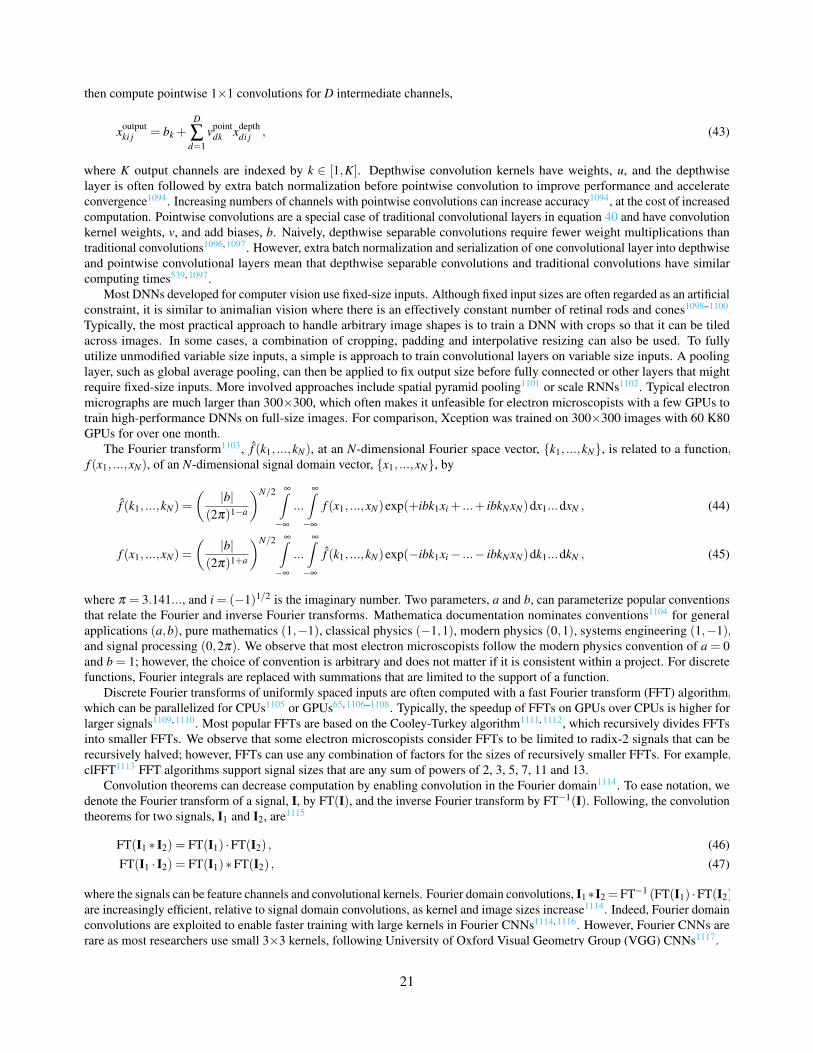
then compute pointwise 1×1 convolutions for D intermediate channels,
xoutputki j = bk +
D
∑d=1
vpointdk xdepth
di j , (43)
where K output channels are indexed by k ∈ [1,K]. Depthwise convolution kernels have weights, u, and the depthwiselayer is often followed by extra batch normalization before pointwise convolution to improve performance and accelerateconvergence1094. Increasing numbers of channels with pointwise convolutions can increase accuracy1094, at the cost of increasedcomputation. Pointwise convolutions are a special case of traditional convolutional layers in equation 40 and have convolutionkernel weights, v, and add biases, b. Naively, depthwise separable convolutions require fewer weight multiplications thantraditional convolutions1096, 1097. However, extra batch normalization and serialization of one convolutional layer into depthwiseand pointwise convolutional layers mean that depthwise separable convolutions and traditional convolutions have similarcomputing times539, 1097.
Most DNNs developed for computer vision use fixed-size inputs. Although fixed input sizes are often regarded as an artificialconstraint, it is similar to animalian vision where there is an effectively constant number of retinal rods and cones1098–1100.Typically, the most practical approach to handle arbitrary image shapes is to train a DNN with crops so that it can be tiledacross images. In some cases, a combination of cropping, padding and interpolative resizing can also be used. To fullyutilize unmodified variable size inputs, a simple is approach to train convolutional layers on variable size inputs. A poolinglayer, such as global average pooling, can then be applied to fix output size before fully connected or other layers that mightrequire fixed-size inputs. More involved approaches include spatial pyramid pooling1101 or scale RNNs1102. Typical electronmicrographs are much larger than 300×300, which often makes it unfeasible for electron microscopists with a few GPUs totrain high-performance DNNs on full-size images. For comparison, Xception was trained on 300×300 images with 60 K80GPUs for over one month.
The Fourier transform1103, f (k1, ...,kN), at an N-dimensional Fourier space vector, k1, ...,kN, is related to a function,f (x1, ...,xN), of an N-dimensional signal domain vector, x1, ...,xN, by
f (k1, ...,kN) =
( |b|(2π)1−a
)N/2 ∞∫
−∞
...
∞∫
−∞
f (x1, ...,xN)exp(+ibk1xi + ...+ ibkNxN)dx1...dxN , (44)
f (x1, ...,xN) =
( |b|(2π)1+a
)N/2 ∞∫
−∞
...
∞∫
−∞
f (k1, ...,kN)exp(−ibk1xi− ...− ibkNxN)dk1...dkN , (45)
where π = 3.141..., and i = (−1)1/2 is the imaginary number. Two parameters, a and b, can parameterize popular conventionsthat relate the Fourier and inverse Fourier transforms. Mathematica documentation nominates conventions1104 for generalapplications (a,b), pure mathematics (1,−1), classical physics (−1,1), modern physics (0,1), systems engineering (1,−1),and signal processing (0,2π). We observe that most electron microscopists follow the modern physics convention of a = 0and b = 1; however, the choice of convention is arbitrary and does not matter if it is consistent within a project. For discretefunctions, Fourier integrals are replaced with summations that are limited to the support of a function.
Discrete Fourier transforms of uniformly spaced inputs are often computed with a fast Fourier transform (FFT) algorithm,which can be parallelized for CPUs1105 or GPUs65, 1106–1108. Typically, the speedup of FFTs on GPUs over CPUs is higher forlarger signals1109, 1110. Most popular FFTs are based on the Cooley-Turkey algorithm1111, 1112, which recursively divides FFTsinto smaller FFTs. We observe that some electron microscopists consider FFTs to be limited to radix-2 signals that can berecursively halved; however, FFTs can use any combination of factors for the sizes of recursively smaller FFTs. For example,clFFT1113 FFT algorithms support signal sizes that are any sum of powers of 2, 3, 5, 7, 11 and 13.
Convolution theorems can decrease computation by enabling convolution in the Fourier domain1114. To ease notation, wedenote the Fourier transform of a signal, I, by FT(I), and the inverse Fourier transform by FT−1(I). Following, the convolutiontheorems for two signals, I1 and I2, are1115
FT(I1 ∗ I2) = FT(I1) ·FT(I2) , (46)FT(I1 · I2) = FT(I1)∗FT(I2) , (47)
where the signals can be feature channels and convolutional kernels. Fourier domain convolutions, I1∗I2 =FT−1 (FT(I1) ·FT(I2)),are increasingly efficient, relative to signal domain convolutions, as kernel and image sizes increase1114. Indeed, Fourier domainconvolutions are exploited to enable faster training with large kernels in Fourier CNNs1114, 1116. However, Fourier CNNs arerare as most researchers use small 3×3 kernels, following University of Oxford Visual Geometry Group (VGG) CNNs1117.
20/9821
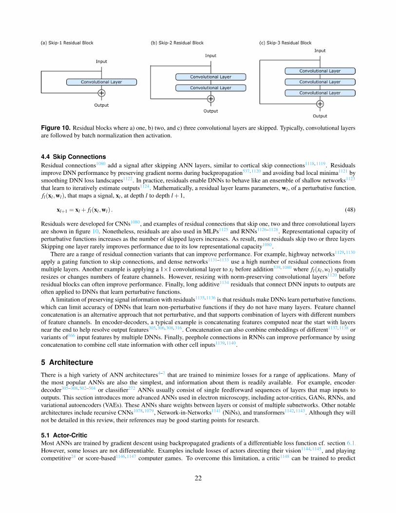
Figure 10. Residual blocks where a) one, b) two, and c) three convolutional layers are skipped. Typically, convolutional layersare followed by batch normalization then activation.
4.4 Skip ConnectionsResidual connections1080 add a signal after skipping ANN layers, similar to cortical skip connections1118, 1119. Residualsimprove DNN performance by preserving gradient norms during backpropagation537, 1120 and avoiding bad local minima1121 bysmoothing DNN loss landscapes1122. In practice, residuals enable DNNs to behave like an ensemble of shallow networks1123
that learn to iteratively estimate outputs1124. Mathematically, a residual layer learns parameters, wl , of a perturbative function,fl(xl ,wl), that maps a signal, xl , at depth l to depth l +1,
xl+1 = xl + fl(xl ,wl) . (48)
Residuals were developed for CNNs1080, and examples of residual connections that skip one, two and three convolutional layersare shown in figure 10. Nonetheless, residuals are also used in MLPs1125 and RNNs1126–1128. Representational capacity ofperturbative functions increases as the number of skipped layers increases. As result, most residuals skip two or three layers.Skipping one layer rarely improves performance due to its low representational capacity1080.
There are a range of residual connection variants that can improve performance. For example, highway networks1129, 1130
apply a gating function to skip connections, and dense networks1131–1133 use a high number of residual connections frommultiple layers. Another example is applying a 1×1 convolutional layer to xl before addition539, 1080 where fl(xl ,wl) spatiallyresizes or changes numbers of feature channels. However, resizing with norm-preserving convolutional layers1120 beforeresidual blocks can often improve performance. Finally, long additive1134 residuals that connect DNN inputs to outputs areoften applied to DNNs that learn perturbative functions.
A limitation of preserving signal information with residuals1135, 1136 is that residuals make DNNs learn perturbative functions,which can limit accuracy of DNNs that learn non-perturbative functions if they do not have many layers. Feature channelconcatenation is an alternative approach that not perturbative, and that supports combination of layers with different numbersof feature channels. In encoder-decoders, a typical example is concatenating features computed near the start with layersnear the end to help resolve output features305, 306, 308, 316. Concatenation can also combine embeddings of different1137, 1138 orvariants of366 input features by multiple DNNs. Finally, peephole connections in RNNs can improve performance by usingconcatenation to combine cell state information with other cell inputs1139, 1140.
5 Architecture
There is a high variety of ANN architectures4–7 that are trained to minimize losses for a range of applications. Many ofthe most popular ANNs are also the simplest, and information about them is readily available. For example, encoder-decoder305–308, 502–504 or classifier272 ANNs usually consist of single feedforward sequences of layers that map inputs tooutputs. This section introduces more advanced ANNs used in electron microscopy, including actor-critics, GANs, RNNs, andvariational autoencoders (VAEs). These ANNs share weights between layers or consist of multiple subnetworks. Other notablearchitectures include recursive CNNs1078, 1079, Network-in-Networks1141 (NiNs), and transformers1142, 1143. Although they willnot be detailed in this review, their references may be good starting points for research.
5.1 Actor-CriticMost ANNs are trained by gradient descent using backpropagated gradients of a differentiable loss function cf. section 6.1.However, some losses are not differentiable. Examples include losses of actors directing their vision1144, 1145, and playingcompetitive24 or score-based1146, 1147 computer games. To overcome this limitation, a critic1148 can be trained to predict
21/9822
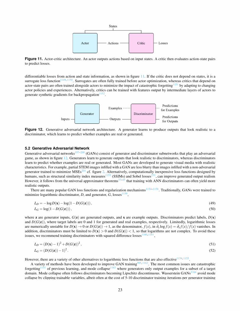
Figure 11. Actor-critic architecture. An actor outputs actions based on input states. A critic then evaluates action-state pairsto predict losses.
differentiable losses from action and state information, as shown in figure 11. If the critic does not depend on states, it is asurrogate loss function1149, 1150. Surrogates are often fully trained before actor optimization, whereas critics that depend onactor-state pairs are often trained alongside actors to minimize the impact of catastrophic forgetting1151 by adapting to changingactor policies and experiences. Alternatively, critics can be trained with features output by intermediate layers of actors togenerate synthetic gradients for backpropagation1152.
Figure 12. Generative adversarial network architecture. A generator learns to produce outputs that look realistic to adiscriminator, which learns to predict whether examples are real or generated.
5.2 Generative Adversarial NetworkGenerative adversarial networks197–200 (GANs) consist of generator and discriminator subnetworks that play an adversarialgame, as shown in figure 12. Generators learn to generate outputs that look realistic to discriminators, whereas discriminatorslearn to predict whether examples are real or generated. Most GANs are developed to generate visual media with realisticcharacteristics. For example, partial STEM images infilled with a GAN are less blurry than images infilled with a non-adversarialgenerator trained to minimize MSEs201 cf. figure 2. Alternatively, computationally inexpensive loss functions designed byhumans, such as structural similarity index measures1153 (SSIMs) and Sobel losses231, can improve generated output realism.However, it follows from the universal approximator theorems37–45 that training with ANN discriminators can often yield morerealistic outputs.
There are many popular GAN loss functions and regularization mechanisms1154–1158. Traditionally, GANs were trained tominimize logarithmic discriminator, D, and generator, G, losses1159,
LD =− logD(x)− log(1−D(G(z))) , (49)LG = log(1−D(G(z))) , (50)
where z are generator inputs, G(z) are generated outputs, and x are example outputs. Discriminators predict labels, D(x)and D(G(z)), where target labels are 0 and 1 for generated and real examples, respectively. Limitedly, logarithmic lossesare numerically unstable for D(x)→ 0 or D(G(z))→ 1, as the denominator, f (x), in ∂x log f (x) = ∂x f (x)/ f (x) vanishes. Inaddition, discriminators must be limited to D(x) > 0 and D(G(z)) < 1, so that logarithms are not complex. To avoid theseissues, we recommend training discriminators with squared difference losses1160, 1161,
LD = (D(x)−1)2 +D(G(z))2 , (51)
LG = (D(G(z))−1)2 . (52)
However, there are a variety of other alternatives to logarithmic loss functions that are also effective1154, 1155.A variety of methods have been developed to improve GAN training995, 1162. The most common issues are catastrophic
forgetting1151 of previous learning, and mode collapse1163 where generators only output examples for a subset of a targetdomain. Mode collapse often follows discriminators becoming Lipschitz discontinuous. Wasserstein GANs1164 avoid modecollapse by clipping trainable variables, albeit often at the cost of 5-10 discriminator training iterations per generator training
22/9823
iteration. Alternatively, Lipschitz continuity can be imposed by adding a gradient penalty1165 to GAN losses, such as differencesof L2 norms of discriminator gradients from unity,
x = G(z) , (53)x = εx+(1− ε)x , (54)
LD = D(x)−D(x)+λ (||∂xD(x)||2−1)2 , (55)LG =−D(G(z)) , (56)
where ε ∈ [0,1] is a uniform random variate, λ weights the gradient penalty, and x is an attempt to generate x. However, usinga gradient penalty introduces additional gradient backpropagation that increases discriminator training time. There are also avariety of computationally inexpensive tricks that can improve training, such as adding noise to labels995, 1075, 1166 or balancingdiscriminator and generator learning rates349. These tricks can help to avoid discontinuities in discriminator output distributionsthat can lead to mode collapse; however, we observe that these tricks do not reliably stabilize GAN training.
Instead, we observe that spectral normalization1017 reliably stabilizes GAN discriminator training in our electron microscopyresearch201, 202, 349. Spectral normalization controls Lipschitz constants of discriminators by fixing the spectral norms of theirweights, as introduced in section 4.2. Advantages of spectral normalization include implementations based on the poweriteration method1023, 1024 being computationally inexpensive, not adding a regularizing loss function that could detrimentallycompete1167, 1168 with discrimination losses, and being effective with one discriminator training iterations per generator trainingiteration1017, 1169. Spectral normalization is popular in GANs for high-resolution image synthesis, where it is also applied ingenerators to stabilize training1170.
There are a variety of GAN architectures1171. For high-resolution image synthesis, computation can be decreased bytraining multiple discriminators to examine image patches at different scales201, 1172. For domain translation characterizedby textural differences, a cyclic GAN1004, 1173 consisting of two GANs can map from one domain to the other and vice versa.Alternatively, two GANs can share intermediate layers to translate inputs via a shared embedding domain1174. Cyclic GANs canalso be combined with a siamese network279–281 for domain translation beyond textural differences1175. Finally, discriminatorscan introduce auxiliary losses to train DNNs to generalize to examples from unseen domains1176–1178.
5.3 Recurrent Neural Network
Recurrent neural networks531–536 reuse an ANN cell to process each step of a sequence. Most RNNs learn to model long-term dependencies by gradient backpropagation through time1179 (BPTT). The ability of RNNs to utilize past experiencesenables them to model partially observed and variable length Markov decision processes1180, 1181 (MDPs). Applications ofRNNs include directing vision1144, 1145, image captioning1182, 1183, language translation1184, medicine77, natural languageprocessing1185, 1186, playing computer games24, text classification1055, and traffic forecasting1187. Many RNNs are combinedwith CNNs to embed visual media1145 or words1188, 1189, or to process RNN outputs1190, 1191. RNNs can also be combinedwith MLPs1144, or text embeddings1192 such as BERT1192, 1193, continuous bag-of-words1194–1196 (CBOW), doc2vec1197, 1198,GloVe1199, and word2vec1194, 1200.
The most popular RNNs consist of long short-term memory1201–1204 (LSTM) cells or gated recurrent units1202, 1205–1207
(GRUs). LSTMs and GRUs are popular as they solve the vanishing gradient problem537, 1208, 1209 and have consistently highperformance1210–1215. Their architectures are shown in figure 13. At step t, an LSTM outputs a hidden state, ht , and cell state,Ct , given by
ft = σ(w f · [ht−1,xt ]+b f ) , (57)it = σ(wi · [ht−1,xt ]+bi) , (58)ct = tanh(wC · [ht−1,xt ]+bC) , (59)
Ct = ftCt−1 + itCt , (60)ot = σ(wo · [ht−1,xt ]+bo) , (61)ht = ot tanh(Ct) , (62)
where Ct−1 is the previous cell state, ht−1 is the previous hidden state, xt is the step input, and σ is a logistic sigmoid function ofequation 10a, [x,y] is the concatenation of x and y channels, and (w f ,b f ), (wi,bi), (wC,bC) and (wo,bo) are pairs of weights
23/9824

Figure 13. Architectures of recurrent neural networks with a) long short-term memory (LSTM) cells, and b) gated recurrentunits (GRUs).
and biases. A GRU performs fewer computations than an LSTM and does not have separate cell and hidden states,
zt = σ(wz · [ht−1,xt ]+bz) , (63)rt = σ(wr · [ht−1,xt ]+br) , (64)
ht = tanh(wh · [rtht−1,xt ]+bh) , (65)
ht = (1− zt)ht−1 + zt ht , (66)
where (wz,bz), (wr,br), and (wh,bh) are pairs of weights and biases. Minimal gated units (MGUs) can further reducecomputation1216. A large-scale analysis of RNN architectures for language translation found that LSTMs consistentlyoutperform GRUs1210. GRUs struggle with simple languages that are learnable by LSTMs as the combined hidden and cellstates of GRUs make it more difficult for GRUs to perform unbounded counting1214. However, further investigations found thatGRUs can outperform LSTMs on tasks other than language translation1211, and that GRUs can outperform LSTMs on somedatasets1212, 1213, 1217. Overall, LSTM performance is usually comparable to that of GRUs.
There are a variety of alternatives to LSTM and GRUs. Examples include continuous time RNNs1218–1222 (CTRNNs),Elman1223 and Jordan1224 networks, independently RNNs1225 (IndRNNs), Hopfield networks1226, recurrent MLPs1227 (RMLPs).However, none of the variants offer consistent performance benefits over LSTMs for general sequence modelling. Similarly,augmenting LSTMs with additional connections, such as peepholes1139, 1140 and projection layers1228, does not consistentlyimprove performance. For electron microscopy, we recommend defaulting to LSTMs as we observe that their performanceis more consistently high than performance of other RNNs. However, LSTM and GRU performance is often comparable, soGRUs are also a good choice to reduce computation.
There are a variety of architectures based on RNNs. Popular examples include deep RNNs1229 that stack RNN cellsto increase representational ability, bidirectional RNNs1230–1233 that process sequences both forwards and in reverse toimprove input utilization, and using separate encoder and decoder subnetworks1205, 1234 to embed inputs and generate outputs.Hierarchical RNNs1235–1239 are more complex models that stack RNNs to efficiently exploit hierarchical sequence information,
24/9825
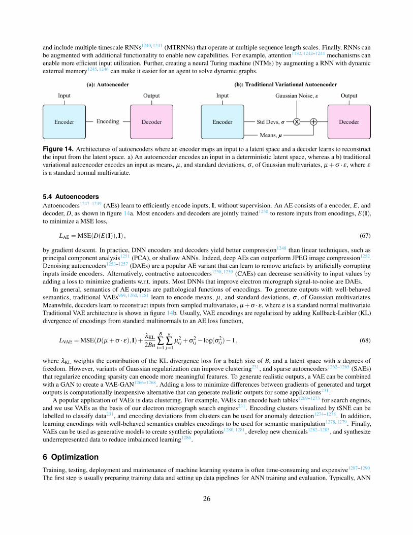
and include multiple timescale RNNs1240, 1241 (MTRNNs) that operate at multiple sequence length scales. Finally, RNNs canbe augmented with additional functionality to enable new capabilities. For example, attention1182, 1242–1244 mechanisms canenable more efficient input utilization. Further, creating a neural Turing machine (NTMs) by augmenting a RNN with dynamicexternal memory1245, 1246 can make it easier for an agent to solve dynamic graphs.
Figure 14. Architectures of autoencoders where an encoder maps an input to a latent space and a decoder learns to reconstructthe input from the latent space. a) An autoencoder encodes an input in a deterministic latent space, whereas a b) traditionalvariational autoencoder encodes an input as means, µ , and standard deviations, σ , of Gaussian multivariates, µ +σ · ε , where εis a standard normal multivariate.
5.4 AutoencodersAutoencoders1247–1249 (AEs) learn to efficiently encode inputs, I, without supervision. An AE consists of a encoder, E, anddecoder, D, as shown in figure 14a. Most encoders and decoders are jointly trained1250 to restore inputs from encodings, E(I),to minimize a MSE loss,
LAE = MSE(D(E(I)),I) , (67)
by gradient descent. In practice, DNN encoders and decoders yield better compression1248 than linear techniques, such asprincipal component analysis1251 (PCA), or shallow ANNs. Indeed, deep AEs can outperform JPEG image compression1252.Denoising autoencoders1253–1257 (DAEs) are a popular AE variant that can learn to remove artefacts by artificially corruptinginputs inside encoders. Alternatively, contractive autoencoders1258, 1259 (CAEs) can decrease sensitivity to input values byadding a loss to minimize gradients w.r.t. inputs. Most DNNs that improve electron micrograph signal-to-noise are DAEs.
In general, semantics of AE outputs are pathological functions of encodings. To generate outputs with well-behavedsemantics, traditional VAEs969, 1260, 1261 learn to encode means, µ , and standard deviations, σ , of Gaussian multivariates.Meanwhile, decoders learn to reconstruct inputs from sampled multivariates, µ +σ ·ε , where ε is a standard normal multivariate.Traditional VAE architecture is shown in figure 14b. Usually, VAE encodings are regularized by adding Kullback-Leibler (KL)divergence of encodings from standard multinormals to an AE loss function,
LVAE = MSE(D(µ +σ · ε),I)+ λKL
2Bu
B
∑i=1
u
∑j=1
µ2i j +σ2
i j− log(σ2i j)−1 , (68)
where λKL weights the contribution of the KL divergence loss for a batch size of B, and a latent space with u degrees offreedom. However, variants of Gaussian regularization can improve clustering231, and sparse autoencoders1262–1265 (SAEs)that regularize encoding sparsity can encode more meaningful features. To generate realistic outputs, a VAE can be combinedwith a GAN to create a VAE-GAN1266–1268. Adding a loss to minimize differences between gradients of generated and targetoutputs is computationally inexpensive alternative that can generate realistic outputs for some applications231.
A popular application of VAEs is data clustering. For example, VAEs can encode hash tables1269–1273 for search engines,and we use VAEs as the basis of our electron micrograph search engines231. Encoding clusters visualized by tSNE can belabelled to classify data231, and encoding deviations from clusters can be used for anomaly detection1274–1278. In addition,learning encodings with well-behaved semantics enables encodings to be used for semantic manipulation1278, 1279. Finally,VAEs can be used as generative models to create synthetic populations1280, 1281, develop new chemicals1282–1285, and synthesizeunderrepresented data to reduce imbalanced learning1286.
6 Optimization
Training, testing, deployment and maintenance of machine learning systems is often time-consuming and expensive1287–1290.The first step is usually preparing training data and setting up data pipelines for ANN training and evaluation. Typically, ANN
25/9826
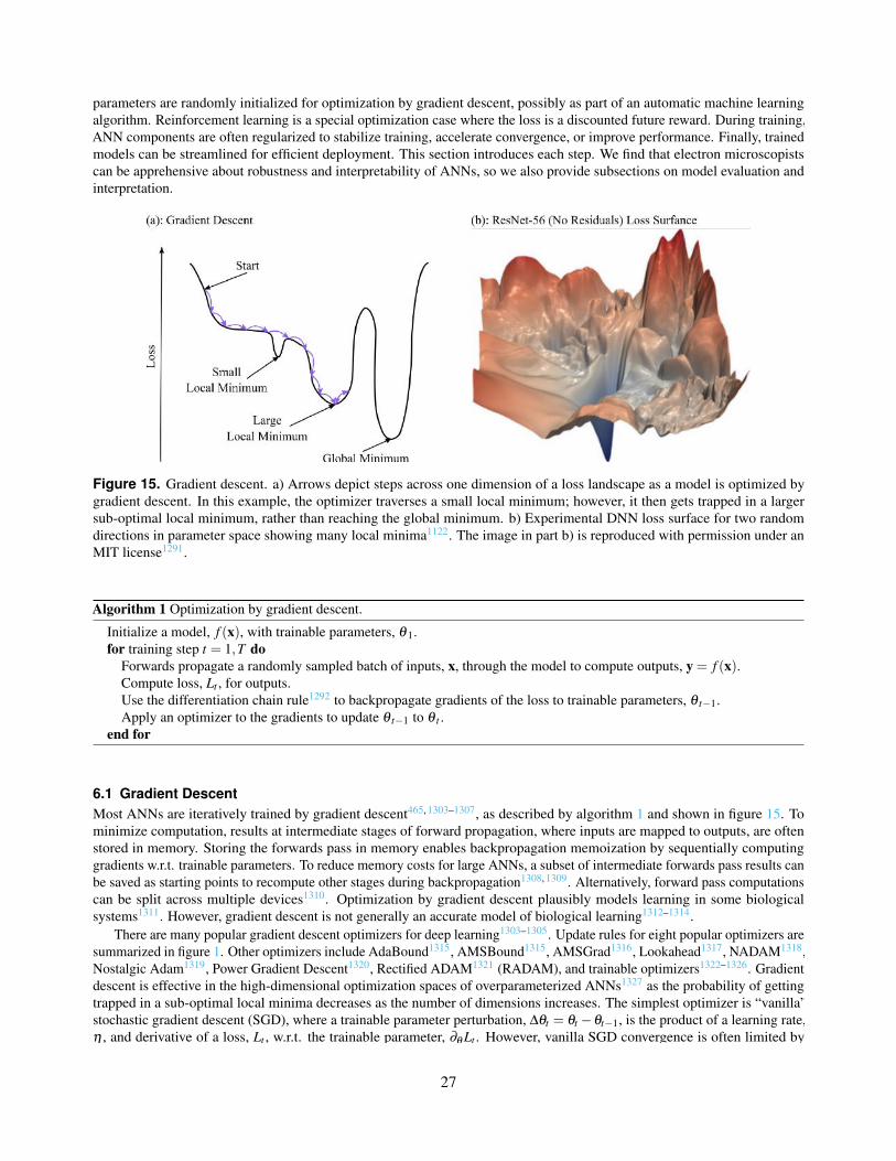
parameters are randomly initialized for optimization by gradient descent, possibly as part of an automatic machine learningalgorithm. Reinforcement learning is a special optimization case where the loss is a discounted future reward. During training,ANN components are often regularized to stabilize training, accelerate convergence, or improve performance. Finally, trainedmodels can be streamlined for efficient deployment. This section introduces each step. We find that electron microscopistscan be apprehensive about robustness and interpretability of ANNs, so we also provide subsections on model evaluation andinterpretation.
Figure 15. Gradient descent. a) Arrows depict steps across one dimension of a loss landscape as a model is optimized bygradient descent. In this example, the optimizer traverses a small local minimum; however, it then gets trapped in a largersub-optimal local minimum, rather than reaching the global minimum. b) Experimental DNN loss surface for two randomdirections in parameter space showing many local minima1122. The image in part b) is reproduced with permission under anMIT license1291.
Algorithm 1 Optimization by gradient descent.
Initialize a model, f (x), with trainable parameters, θ 1.for training step t = 1,T do
Forwards propagate a randomly sampled batch of inputs, x, through the model to compute outputs, y = f (x).Compute loss, Lt , for outputs.Use the differentiation chain rule1292 to backpropagate gradients of the loss to trainable parameters, θ t−1.Apply an optimizer to the gradients to update θ t−1 to θ t .
end for
6.1 Gradient DescentMost ANNs are iteratively trained by gradient descent465, 1303–1307, as described by algorithm 1 and shown in figure 15. Tominimize computation, results at intermediate stages of forward propagation, where inputs are mapped to outputs, are oftenstored in memory. Storing the forwards pass in memory enables backpropagation memoization by sequentially computinggradients w.r.t. trainable parameters. To reduce memory costs for large ANNs, a subset of intermediate forwards pass results canbe saved as starting points to recompute other stages during backpropagation1308, 1309. Alternatively, forward pass computationscan be split across multiple devices1310. Optimization by gradient descent plausibly models learning in some biologicalsystems1311. However, gradient descent is not generally an accurate model of biological learning1312–1314.
There are many popular gradient descent optimizers for deep learning1303–1305. Update rules for eight popular optimizers aresummarized in figure 1. Other optimizers include AdaBound1315, AMSBound1315, AMSGrad1316, Lookahead1317, NADAM1318,Nostalgic Adam1319, Power Gradient Descent1320, Rectified ADAM1321 (RADAM), and trainable optimizers1322–1326. Gradientdescent is effective in the high-dimensional optimization spaces of overparameterized ANNs1327 as the probability of gettingtrapped in a sub-optimal local minima decreases as the number of dimensions increases. The simplest optimizer is “vanilla”stochastic gradient descent (SGD), where a trainable parameter perturbation, ∆θt = θt −θt−1, is the product of a learning rate,η , and derivative of a loss, Lt , w.r.t. the trainable parameter, ∂θ Lt . However, vanilla SGD convergence is often limited by
26/9827
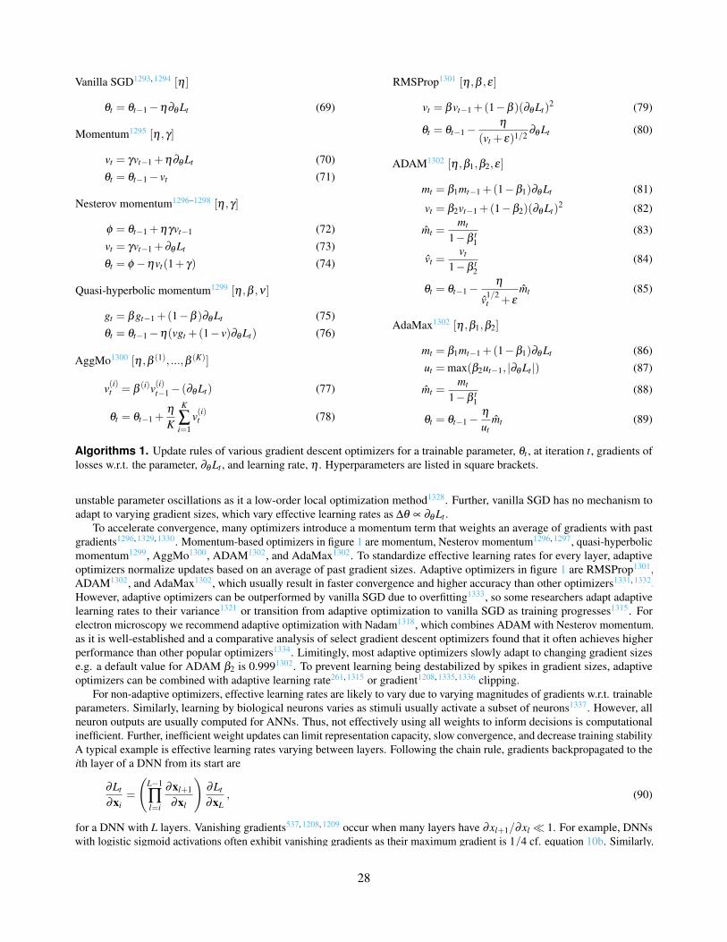
Vanilla SGD1293, 1294 [η ]
θt = θt−1−η∂θ Lt (69)
Momentum1295 [η ,γ]
vt = γvt−1 +η∂θ Lt (70)θt = θt−1− vt (71)
Nesterov momentum1296–1298 [η ,γ]
φ = θt−1 +ηγvt−1 (72)vt = γvt−1 +∂θ Lt (73)θt = φ −ηvt(1+ γ) (74)
Quasi-hyperbolic momentum1299 [η ,β ,ν ]
gt = βgt−1 +(1−β )∂θ Lt (75)θt = θt−1−η(vgt +(1− v)∂θ Lt) (76)
AggMo1300 [η ,β (1), ...,β (K)]
v(i)t = β (i)v(i)t−1− (∂θ Lt) (77)
θt = θt−1 +ηK
K
∑i=1
v(i)t (78)
RMSProp1301 [η ,β ,ε]
vt = βvt−1 +(1−β )(∂θ Lt)2 (79)
θt = θt−1−η
(vt + ε)1/2 ∂θ Lt (80)
ADAM1302 [η ,β1,β2,ε]
mt = β1mt−1 +(1−β1)∂θ Lt (81)
vt = β2vt−1 +(1−β2)(∂θ Lt)2 (82)
mt =mt
1−β t1
(83)
vt =vt
1−β t2
(84)
θt = θt−1−η
v1/2t + ε
mt (85)
AdaMax1302 [η ,β1,β2]
mt = β1mt−1 +(1−β1)∂θ Lt (86)ut = max(β2ut−1, |∂θ Lt |) (87)
mt =mt
1−β t1
(88)
θt = θt−1−ηut
mt (89)
Algorithms 1. Update rules of various gradient descent optimizers for a trainable parameter, θt , at iteration t, gradients oflosses w.r.t. the parameter, ∂θ Lt , and learning rate, η . Hyperparameters are listed in square brackets.
unstable parameter oscillations as it a low-order local optimization method1328. Further, vanilla SGD has no mechanism toadapt to varying gradient sizes, which vary effective learning rates as ∆θ ∝ ∂θ Lt .
To accelerate convergence, many optimizers introduce a momentum term that weights an average of gradients with pastgradients1296, 1329, 1330. Momentum-based optimizers in figure 1 are momentum, Nesterov momentum1296, 1297, quasi-hyperbolicmomentum1299, AggMo1300, ADAM1302, and AdaMax1302. To standardize effective learning rates for every layer, adaptiveoptimizers normalize updates based on an average of past gradient sizes. Adaptive optimizers in figure 1 are RMSProp1301,ADAM1302, and AdaMax1302, which usually result in faster convergence and higher accuracy than other optimizers1331, 1332.However, adaptive optimizers can be outperformed by vanilla SGD due to overfitting1333, so some researchers adapt adaptivelearning rates to their variance1321 or transition from adaptive optimization to vanilla SGD as training progresses1315. Forelectron microscopy we recommend adaptive optimization with Nadam1318, which combines ADAM with Nesterov momentum,as it is well-established and a comparative analysis of select gradient descent optimizers found that it often achieves higherperformance than other popular optimizers1334. Limitingly, most adaptive optimizers slowly adapt to changing gradient sizese.g. a default value for ADAM β2 is 0.9991302. To prevent learning being destabilized by spikes in gradient sizes, adaptiveoptimizers can be combined with adaptive learning rate261, 1315 or gradient1208, 1335, 1336 clipping.
For non-adaptive optimizers, effective learning rates are likely to vary due to varying magnitudes of gradients w.r.t. trainableparameters. Similarly, learning by biological neurons varies as stimuli usually activate a subset of neurons1337. However, allneuron outputs are usually computed for ANNs. Thus, not effectively using all weights to inform decisions is computationalinefficient. Further, inefficient weight updates can limit representation capacity, slow convergence, and decrease training stability.A typical example is effective learning rates varying between layers. Following the chain rule, gradients backpropagated to theith layer of a DNN from its start are
∂Lt
∂xi=
(L−1
∏l=i
∂xl+1
∂xl
)∂Lt
∂xL, (90)
for a DNN with L layers. Vanishing gradients537, 1208, 1209 occur when many layers have ∂xl+1/∂xl 1. For example, DNNswith logistic sigmoid activations often exhibit vanishing gradients as their maximum gradient is 1/4 cf. equation 10b. Similarly,
27/9828
exploding gradients537, 1208, 1209 occur when many layers have ∂xl+1/∂xl 1. Adaptive optimizers alleviate vanishing andexploding gradients by dividing gradients by their expected sizes. Nevertheless, it is essential to combine adaptive optimizerswith appropriate initialization and architecture to avoid numerical instability.
Optimizers have a myriad of hyperparameters to be initialized and varied throughout training to optimize performance1338
cf. figure 1. For example, stepwise exponentially decayed learning rates are often theoretically optimal1339. There are alsovarious heuristics that are often effective, such as using a DEMON decay schedule for an ADAM first moment of the momentumdecay rate1340,
β1 =1− t/T
(1−βinit)+βinit(1− t/T )βinit , (91)
where βinit is the initial value of β1, t is the iteration number, and T is the final iteration number. Developers often optimizeANN hyperparameters by experimenting with a range of heuristic values. Hyperparameter optimization algorithms1341–1346
can automate optimizer hyperparameter selection. However, automatic hyperparameter optimizers may not yield sufficientperformance improvements relative to well-established heuristics to justify their use, especially in initial stages of development.
Alternatives to gradient descent1347 are rarely used for parameter optimization as they are not known to consistentlyimprove upon gradient descent. For example, simulated annealing1348, 1349 has been applied to CNN training1350, 1351, andcan be augmented with momentum to accelerate convergence in deep learning1352. Simulated annealing can also augmentgradient descent to improve performance1353. Other approaches include evolutionary1354, 1355 and genetic1356, 1357 algorithms,which can be a competitive alternative to deep reinforcement learning where convergence is slow1358. Indeed, recent geneticalgorithms have outperformed a popular deep reinforcement learning algorithm1359. Another direction is to augment geneticalgorithms with ANNs to accelerate convergence1360–1363. Other alternatives to backpropagation include direct search1364, theMoore-Penrose Pseudo Inverse1365; particle swarm optimization1366–1369 (PSO); and echo-state networks1370–1372 (ESNs) andextreme learning machines1373–1379 (ELMs), where some randomly initialized weights are never updated.
6.2 Reinforcement LearningReinforcement learning1380–1386 (RL) is where a machine learning system, or “actor”, is trained to perform a sequence ofactions. Applications include autonomous driving1387–1389, communications network control1390, 1391, energy and environmentalmanagement1392, 1393, playing games24–29, 1146, 1394, and robotic manipulation1395, 1396. To optimize a MDP1180, 1181, a discountedfuture reward, Qt , at step t in a MDP with T steps is usually calculated from step rewards, rt , with Bellman’s equation,
Qt =T
∑t ′=t
γ t ′−trt ′ , (92)
where γ ∈ [0,1) discounts future step rewards. To be clear, multiplying Qt by −1 yields a loss that can be minimized using themethods in section 6.1.
In practice, many MDPs are partially observed or have non-differentiable losses that may make it difficult to learn agood policy from individual observations. However, RNNs can often learn a model of their environments from sequences ofobservations1147. Alternatively, FNNs can be trained with groups of observations that contain more information than individualobservations1146, 1394. If losses are not differentiable, a critic can learn to predict differentiable losses for actor training cf.section 5.1. Alternatively, actions can be sampled from a differentiable probability distribution1144, 1397 as training losses givenby products of losses and sampling probabilities are differentiable. There are also a variety of alternatives to gradient descentintroduced at the end of section 6.1 that do not require differentiable loss functions.
There are a variety of exploration strategies for RL1398, 1399. Adding Ornstein-Uhlenbeck1400 (OU) noise to actions iseffective for continuous control tasks optimized by deep deterministic policy gradients1146 (DDPG) or recurrent deterministicpolicy gradients1147 (RDPG) RL algorithms. Adding Gaussian noise achieves similar performance for optimization by TD31401
or D4PG1402 RL algorithms. However, a comparison of OU and Gaussian noise across a variety of tasks1403 found thatOU noise usually achieves similar performance to or outperforms Gaussian noise. Similarly, exploration can be induced byadding noise to ANN parameters1404, 1405. Other approaches to exploration include rewarding actors for increasing actionentropy1405–1407 and intrinsic motivation1408–1410, where ANNs are incentified to explore actions that they are unsure about.
RL algorithms are often partitioned into online learning1411, 1412, where training data is used as it is acquired; and offlinelearning1413, 1414, where a static training dataset has already been acquired. However, many algorithms operate in an intermediateregime, where data collected with an online policy is stored in an experience replay1415–1417 buffer for offline learning. Trainingdata is often sampled at random from a replay. However, prioritizing the replay of data with high losses993 or data that results inhigh policy improvements992 often improves actor performance. A default replay buffer size of around 106 examples is oftenused; however, training is sensitive to replay buffer size1418. If the replay is too small, changes in actor policy may destabilizetraining; whereas if the replay is too large, convergence may be slowed by delays before the actor learns from policy changes.
28/9829
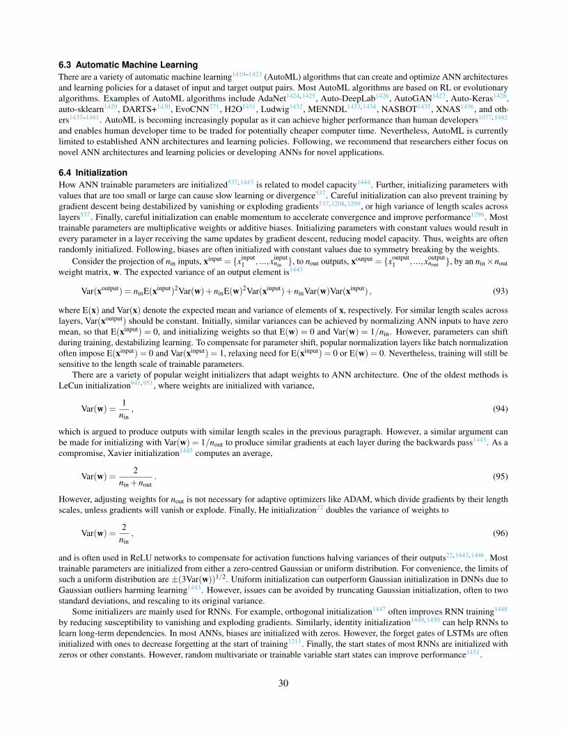
6.3 Automatic Machine LearningThere are a variety of automatic machine learning1419–1423 (AutoML) algorithms that can create and optimize ANN architecturesand learning policies for a dataset of input and target output pairs. Most AutoML algorithms are based on RL or evolutionaryalgorithms. Examples of AutoML algorithms include AdaNet1424, 1425, Auto-DeepLab1426, AutoGAN1427, Auto-Keras1428,auto-sklearn1429, DARTS+1430, EvoCNN271, H2O1431, Ludwig1432, MENNDL1433, 1434, NASBOT1435, XNAS1436, and oth-ers1437–1441. AutoML is becoming increasingly popular as it can achieve higher performance than human developers1077, 1442
and enables human developer time to be traded for potentially cheaper computer time. Nevertheless, AutoML is currentlylimited to established ANN architectures and learning policies. Following, we recommend that researchers either focus onnovel ANN architectures and learning policies or developing ANNs for novel applications.
6.4 InitializationHow ANN trainable parameters are initialized537, 1443 is related to model capacity1444. Further, initializing parameters withvalues that are too small or large can cause slow learning or divergence537. Careful initialization can also prevent training bygradient descent being destabilized by vanishing or exploding gradients537, 1208, 1209, or high variance of length scales acrosslayers537. Finally, careful initialization can enable momentum to accelerate convergence and improve performance1296. Mosttrainable parameters are multiplicative weights or additive biases. Initializing parameters with constant values would result inevery parameter in a layer receiving the same updates by gradient descent, reducing model capacity. Thus, weights are oftenrandomly initialized. Following, biases are often initialized with constant values due to symmetry breaking by the weights.
Consider the projection of nin inputs, xinput = xinput1 , ...,xinput
nin , to nout outputs, xoutput = xoutput1 , ...,xoutput
nout , by an nin×noutweight matrix, w. The expected variance of an output element is1443
Var(xoutput) = ninE(xinput)2Var(w)+ninE(w)2Var(xinput)+ninVar(w)Var(xinput) , (93)
where E(x) and Var(x) denote the expected mean and variance of elements of x, respectively. For similar length scales acrosslayers, Var(xoutput) should be constant. Initially, similar variances can be achieved by normalizing ANN inputs to have zeromean, so that E(xinput) = 0, and initializing weights so that E(w) = 0 and Var(w) = 1/nin. However, parameters can shiftduring training, destabilizing learning. To compensate for parameter shift, popular normalization layers like batch normalizationoften impose E(xinput) = 0 and Var(xinput) = 1, relaxing need for E(xinput) = 0 or E(w) = 0. Nevertheless, training will still besensitive to the length scale of trainable parameters.
There are a variety of popular weight initializers that adapt weights to ANN architecture. One of the oldest methods isLeCun initialization941, 951, where weights are initialized with variance,
Var(w) =1
nin, (94)
which is argued to produce outputs with similar length scales in the previous paragraph. However, a similar argument canbe made for initializing with Var(w) = 1/nout to produce similar gradients at each layer during the backwards pass1443. As acompromise, Xavier initialization1445 computes an average,
Var(w) =2
nin +nout. (95)
However, adjusting weights for nout is not necessary for adaptive optimizers like ADAM, which divide gradients by their lengthscales, unless gradients will vanish or explode. Finally, He initialization22 doubles the variance of weights to
Var(w) =2
nin, (96)
and is often used in ReLU networks to compensate for activation functions halving variances of their outputs22, 1443, 1446. Mosttrainable parameters are initialized from either a zero-centred Gaussian or uniform distribution. For convenience, the limits ofsuch a uniform distribution are ±(3Var(w))1/2. Uniform initialization can outperform Gaussian initialization in DNNs due toGaussian outliers harming learning1443. However, issues can be avoided by truncating Gaussian initialization, often to twostandard deviations, and rescaling to its original variance.
Some initializers are mainly used for RNNs. For example, orthogonal initialization1447 often improves RNN training1448
by reducing susceptibility to vanishing and exploding gradients. Similarly, identity initialization1449, 1450 can help RNNs tolearn long-term dependencies. In most ANNs, biases are initialized with zeros. However, the forget gates of LSTMs are ofteninitialized with ones to decrease forgetting at the start of training1211. Finally, the start states of most RNNs are initialized withzeros or other constants. However, random multivariate or trainable variable start states can improve performance1451.
29/9830
There are a variety of alternatives to initialization from random multivariates. Weight normalized1014 ANNs are a popularexample of data-dependent initialization, where randomly initialized weight magnitudes and biases are chosen to counteractvariances and means of an initial batch of data. Similarly, layer-sequential unit-variance (LSUV) initialization1452 consists oforthogonal initialization followed by adjusting the magnitudes of weights to counteract variances of an initial batch of data.Other approaches standardize the norms of backpropagated gradients. For example, random walk initialization1453 (RWI) findsscales for weights to prevent vanishing or exploding gradients in deep FNNs, albeit with varied success1452. Alternatively,MetaInit1454 scales the magnitudes of randomly initialized weights to minimize changes in backpropagated gradients periteration of gradient descent.
6.5 RegularizationThere are a variety of regularization mechanisms1455–1458 that modify learning algorithms to improve ANN performance. Oneof the most popular is LX regularization, which decays weights by adding a loss,
LX = λX ∑i
|θi|XX
, (97)
weighted by λX to each trainable variable, θi. L2 regularization1459–1461 is preferred1462 for most DNN optimization assubtraction of its gradient, ∂θiL2 = λ2θi, is equivalent to computationally-efficient multiplicative weight decay. Nevertheless, L1regularization is better at inducing model sparsity1463 than L2 regularization, and L1 regularization achieves higher performancein some applications1464. Higher performance can also be achieved by adding both L1 and L2 regularization in elastic nets1465.LX regularization is most effective at the start of training and becomes less important near convergence1459. Finally, L1 andL2 regularization are closely related to lasso1466 and ridge1467 regularization, respectively, whereby trainable parameters areadjusted to limit L1 and L2 losses.
Gradient clipping1336, 1468–1470 accelerates learning by limiting large gradients, and is most commonly applied to RNNs. Asimple approach is to clip gradient magnitudes to a threshold hyperparameter. However, it is more common to scale gradients,gi, at layer i if their norm is above a threshold, u, so that1208, 1469
gi←
gi, if ||gi||n ≤ uu||gi||n gi, if ||gi||n > u
(98)
where n = 2 is often chosen to minimize computation. Similarly, gradients can be clipped if they are above a global norm,
gnorm =
(L
∑i=1||gi||nn ,
)1/n
(99)
computed with gradients at L layers. Scaling gradient norms is often preferable to clipping to a threshold as scaling is akinto adapting layer learning rates and does not affect the directions of gradients. Thresholds for gradient clipping are often setbased on average norms of backpropagated gradients during preliminary training1471. However, thresholds can also be setautomatically and adaptively1335, 1336. In addition, adaptive gradient clipping algorithms can skip training iterations if gradientnorms are anomalously high1472, which often indicates an imminent gradient explosion.
Dropout1473–1477 often reduces overfitting by only using a fraction, pi, of layer i outputs during training, and multiplyingall outputs by pi for inference. However, dropout often increases training time, can be sensitive to pi, and sometimes lowersperformance1478. Improvements to dropout at the structural level, such as applying it to convolutional channels, paths, andlayers, rather than random output elements, can improve performance1479. For example, DropBlock1480 improves performanceby dropping contiguous regions of feature maps to prevent dropout being trivially circumvented by using spatially correlatedneighbouring outputs. Similarly, PatchUp1481 swaps or mixes contiguous regions with regions for another sample. Dropout isoften outperformed by Shakeout1482, 1483, a modification of dropout that randomly enhances or reverses contributions of outputsto the next layer.
Noise often enhances ANN training by decreasing susceptibility to spurious local minima1484. Adding noise to trainableparameters can improve generalization1485, 1486, or exploration for RL1404. Parameter noise is usually additive as it does notchange an objective function being learned, whereas multiplicative noise can change the objective1487. In addition, noise canbe added to inputs1253, 1488, hidden layers1158, 1489, generated outputs1490 or target outputs995, 1491. However, adding noise tosignals does not always improve performance1217. Finally, modifying usual gradient noise1492 by adding noise to gradients canimprove performance1493. Typically, additive noise is annealed throughout training, so that that final training is with a noiselessmodel that will be used for inference.
30/9831
There are a variety of regularization mechanisms that exploit extra training data. A simple approach is to create extratraining examples by data augmentation1494–1496. Extra training data can also be curated, or simulated for training by domainadaption1176–1178. Alternatively, semi-supervised learning1497–1502 can generate target outputs for a dataset of unpaired inputs toaugment training with a dataset of paired inputs and target outputs. Finally, multitask learning1503–1507 can improve performanceby introducing additional loss functions. For instance, by adding an auxiliary classifier to predict image labels from featuresgenerated by intermediate DNN layers1508–1511. Losses are often manually balanced; however, their gradients can also bebalanced automatically and adaptively1167, 1168.
6.6 Data PipelineA data pipeline prepares data to be input to an ANN. Efficient pipelines often parallelize data preparation across multipleCPU cores1512. Small datasets can be stored in RAM to decrease data access times, whereas large dataset elements areoften loaded from files. Loaded data can then be preprocessed and augmented1494, 1495, 1513–1515. For electron micrographs,preprocessing often includes replacing non-finite elements, such as NaN and inf, with finite values; linearly transformingintensities to a common range, such as [−1,1] or zero mean and unit variance; and performing a random combination offlips and 90 to augment data by a factor of eight70, 201, 202, 231, 349. Preprocessed examples can then be combined into batches.Typically, multiple batches that are ready to be input are prefetched and stored in RAM to avoid delays due to fluctuating CPUperformance.
To efficiently utilize data, training datasets are often reiterated over for multiple training epochs. Usually, training datasetsare reiterated over about 102 times. Increasing epochs can maximize utilization of potentially expensive training data; however,increasing epochs can lower performance due to overfitting1516, 1517 or be too computationally expensive539. Naively, batches ofdata can be randomly sampled with replacement during training by gradient descent. However, convergence can be acceleratedby reinitializing a training dataset at the start of each training epoch and randomly sampling data without replacement1518–1522.Most modern DLFs, such as TensorFlow, provide efficient and easy-to-use functions to control data sampling1523.
6.7 Model EvaluationThere are a variety of methods for ANN performance evaluation538. However, most ANNs are evaluated by 1-fold validation,where a dataset is partitioned into training, validation, and test sets. After ANN optimization with a training set, ability togeneralize is measured with a validation set. Multiple validations may be performed for training with early stopping1516, 1517 orANN learning policy and architecture selection, so final performance is often measured with a test set to avoid overfitting to thevalidation set. Most researchers favour using single training, validation, and test sets to simplify standardization of performancebenchmarks231. However, multiple-fold validation538 or multiple validation sets1524 can improve performance characterization.Alternatively, models can be bootstrap aggregated1525 (bagged) from multiple models trained on different subsets of trainingdata. Bagging is usually applied to random forests1526–1528 or other lightweight models, and enables model uncertainly to begauged from the variance of model outputs.
For small datasets, model performance is often sensitive to split of data between training and validation sets1529. Increasingtraining set size usually increases model accuracy, whereas increasing validation set size decreases performance uncertainty.Indeed, a scaling law can be used to estimate an optimal tradeoff1530 between training and validation set sizes. However, mostexperimenters follow a Pareto1531 splitting heuristic. For example, we often use a 75:15:10 training-validation-test split231.Heuristic splitting is justified for ANN training with large datasets insofar that sensitivity to splitting ratios decreases withincreasing dataset size2.
6.8 DeploymentIf an ANN is deployed1532–1534 on multiple different devices, such as various electron microscopes, a separate model can betrained for each device403, Alternatively, a single model can be trained and specialized for different devices to decrease trainingrequirements1535. In addition, ANNs can remotely service requests from cloud containers1536–1538. Integration of multipleANNs can be complicated by different servers for different DLFs supporting different backends; however, unified interfaces areavailable. For example, GraphPipe1539 provides simple, efficient reference model servers for Tensorflow, Caffe2, and ONNX;a minimalist machine learning transport specification based on FlatBuffers1540; and efficient client implementations in Go,Python, and Java. In 2020, most ANNs developed researchers were not deployed. However, we anticipate that deployment willbecome a more prominent consideration as the role of deep learning in electron microscopy matures.
Most ANNs are optimized for inference by minimizing parameters and operations from training time, like MobileNets1094.However, less essential operations can also be pruned after training1541, 1542. Another approach is quantization, where ANNbit depths are decreased, often to efficient integer instructions, to increase inference throughput1543, 1544. Quantization oftendecreases performance; however, the amount of quantization can be adapted to ANN components to optimize performance-throughput tradeoffs1545. Alternatively, training can be modified to minimize the impact of quantization on performance1546–1548.
31/9832
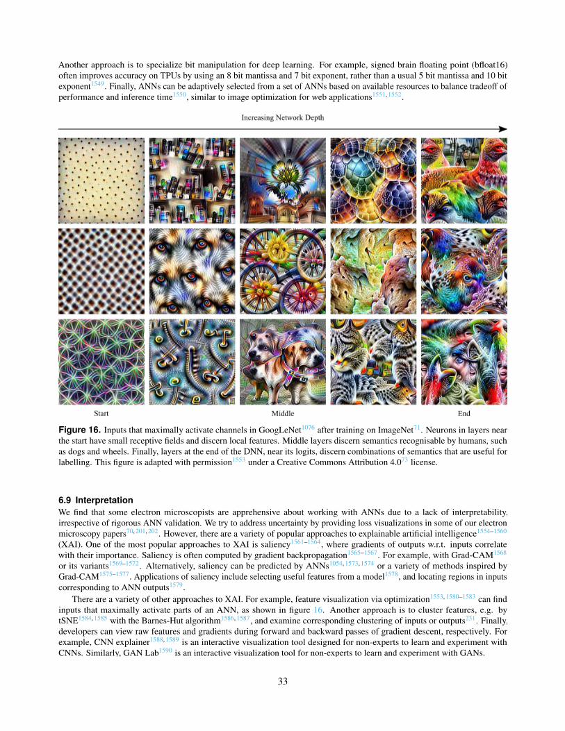
Another approach is to specialize bit manipulation for deep learning. For example, signed brain floating point (bfloat16)often improves accuracy on TPUs by using an 8 bit mantissa and 7 bit exponent, rather than a usual 5 bit mantissa and 10 bitexponent1549. Finally, ANNs can be adaptively selected from a set of ANNs based on available resources to balance tradeoff ofperformance and inference time1550, similar to image optimization for web applications1551, 1552.
Figure 16. Inputs that maximally activate channels in GoogLeNet1076 after training on ImageNet71. Neurons in layers nearthe start have small receptive fields and discern local features. Middle layers discern semantics recognisable by humans, suchas dogs and wheels. Finally, layers at the end of the DNN, near its logits, discern combinations of semantics that are useful forlabelling. This figure is adapted with permission1553 under a Creative Commons Attribution 4.073 license.
6.9 InterpretationWe find that some electron microscopists are apprehensive about working with ANNs due to a lack of interpretability,irrespective of rigorous ANN validation. We try to address uncertainty by providing loss visualizations in some of our electronmicroscopy papers70, 201, 202. However, there are a variety of popular approaches to explainable artificial intelligence1554–1560
(XAI). One of the most popular approaches to XAI is saliency1561–1564, where gradients of outputs w.r.t. inputs correlatewith their importance. Saliency is often computed by gradient backpropagation1565–1567. For example, with Grad-CAM1568
or its variants1569–1572. Alternatively, saliency can be predicted by ANNs1054, 1573, 1574 or a variety of methods inspired byGrad-CAM1575–1577. Applications of saliency include selecting useful features from a model1578, and locating regions in inputscorresponding to ANN outputs1579.
There are a variety of other approaches to XAI. For example, feature visualization via optimization1553, 1580–1583 can findinputs that maximally activate parts of an ANN, as shown in figure 16. Another approach is to cluster features, e.g. bytSNE1584, 1585 with the Barnes-Hut algorithm1586, 1587, and examine corresponding clustering of inputs or outputs231. Finally,developers can view raw features and gradients during forward and backward passes of gradient descent, respectively. Forexample, CNN explainer1588, 1589 is an interactive visualization tool designed for non-experts to learn and experiment withCNNs. Similarly, GAN Lab1590 is an interactive visualization tool for non-experts to learn and experiment with GANs.
32/9833
7 DiscussionWe introduced a variety of electron microscopy applications in section 1 that have been enabled or enhanced by deep learning.Nevertheless, the greatest benefit of deep learning in electron microscopy may be general-purpose tools that enable researchersto be more effective. Search engines based on deep learning are almost essential to navigate an ever-increasing number ofscientific publications700. Further, machine learning can enhance communication by filtering spam and phishing attacks1591–1593,and by summarizing1594–1596 and classifying1055, 1597–1599 scientific documents. In addition, machine learning can be applied toeducation to automate and standardize scoring1600–1603, detect plagiarism1604–1606, and identify at-risk students1607.
Creative applications of deep learning1608, 1609 include making new art by style transfer1001–1005, composing music1610–1612,and storytelling1613, 1614. Similar DNNs can assist programmers1615, 1616. For example, by predictive source code comple-tion1617–1622, and by generating source code to map inputs to target outputs1623 or from labels describing desired sourcecode1624. Text generating DNNs can also help write scientific papers. For example, by drafting scientific passages1625 ordrafting part of a paper from a list of references1626. Papers generated by early prototypes for automatic scientific papergenerators, such as SciGen1627, are realistic insofar that they have been accepted by scientific venues.
An emerging application of deep learning is mining scientific resources to make new scientific discoveries1628. Artificialagents are able to effectively distil latent scientific knowledge as they can parallelize examination of huge amounts of data,whereas information access by humans1629–1631 is limited by human cognition1632. High bandwidth bi-directional brain-machine interfaces are being developed to overcome limitations of human cognition1633; however, they are in the early stages ofdevelopment and we expect that they will depend on substantial advances in machine learning to enhance control of cognition.Eventually, we expect that ANNs will be used as scientific oracles, where researchers who do not rely on their services willno longer be able to compete. For example, an ANN trained on a large corpus of scientific literature predicted multipleadvances in materials science before they were reported1634. ANNs are already used for financial asset management1635, 1636
and recruiting1637–1640, so we anticipate that artificial scientific oracle consultation will become an important part of scientificgrant1641, 1642 reviews.
A limitation of deep learning is that it can introduce new issues. For example, DNNs are often susceptible to adversarialattacks1643–1647, where small perturbations to inputs cause large errors. Nevertheless, training can be modified to improverobustness to adversarial attacks1648–1652. Another potential issue is architecture-specific systematic errors. For example, CNNsoften exhibit structured systematic error variation70, 201, 202, 1092, 1093, 1653, including higher errors nearer output edges70, 201, 202.However, structured systematic error variation can be minimized by GANs incentifying the generation of realistic outputs201.Finally, ANNs can be difficult to use as they often require downloading code with undocumented dependencies, downloading apretrained model, and may require hardware accelerators. These issues can be avoided by serving ANNs from cloud containers.However, it may not be practical for academics to acquire funding to cover cloud service costs.
Perhaps the most important aspect of deep learning in electron microscopy is that it presents new challenges that can lead toadvances in machine learning. Simple benchmarks like CIFAR-10562, 563 and MNIST564 have been solved. Following, moredifficult benchmarks like Fashion-MNIST1654 have been introduced. However, they only partially address issues with solveddatasets as they do not present fundamentally new challenges. In contrast, we believe that new problems often invite newsolutions. For example, we developed adaptive learning rate clipping261 (ALRC) to stabilize training of DNNs for partialscanning transmission electron microscopy201. The challenge was that we wanted to train a large model for high-resolutionimages; however, training was unstable if we used small batches needed to fit it in GPU memory. Similar challenges aboundand can lead to advances in both machine learning and electron microscopy.
Data AvailabilityNo new data were created or analysed in this study.
AcknowledgementsThanks go to Jeremy Sloan and Martin Lotz for internally reviewing this article. In addition, part of the text in section 1.2 isadapted from our earlier work with permission201 under a Creative Commons Attribution 4.073 license. Finally, the authoracknowledges funding from EPSRC grant EP/N035437/1 and EPSRC Studentship 1917382.
Competing InterestsThe author declares no competing interests.
33/9834
References1. Leiserson, C. E. et al. There’s Plenty of Room at the Top: What Will Drive Computer Performance After Moore’s Law?
Science 368 (2020).
2. Sun, C., Shrivastava, A., Singh, S. & Gupta, A. Revisiting Unreasonable Effectiveness of Data in Deep Learning Era. InProceedings of the IEEE International Conference on Computer Vision, 843–852 (2017).
3. Hey, T., Butler, K., Jackson, S. & Thiyagalingam, J. Machine Learning and Big Scientific Data. Philos. TransactionsRoyal Soc. A 378, 20190054 (2020).
4. Sengupta, S. et al. A Review of Deep Learning with Special Emphasis on Architectures, Applications and Recent Trends.Knowledge-Based Syst. 4, 105596 (2020).
5. Shrestha, A. & Mahmood, A. Review of Deep Learning Algorithms and Architectures. IEEE Access 7, 53040–53065(2019).
6. Dargan, S., Kumar, M., Ayyagari, M. R. & Kumar, G. A Survey of Deep Learning and Its Applications: A New Paradigmto Machine Learning. Arch. Comput. Methods Eng. 27, 1071–1092 (2019).
7. Alom, M. Z. et al. A State-of-the-Art Survey on Deep Learning Theory and Architectures. Electronics 8, 292 (2019).
8. Zhang, Q., Yang, L. T., Chen, Z. & Li, P. A Survey on Deep Learning for Big Data. Inf. Fusion 42, 146–157 (2018).
9. Hatcher, W. G. & Yu, W. A Survey of Deep Learning: Platforms, Applications and Emerging Research Trends. IEEEAccess 6, 24411–24432 (2018).
10. LeCun, Y., Bengio, Y. & Hinton, G. Deep Learning. Nature 521, 436–444 (2015).
11. Schmidhuber, J. Deep Learning in Neural Networks: An Overview. Neural Networks 61, 85–117 (2015).
12. Ge, M., Su, F., Zhao, Z. & Su, D. Deep Learning Analysis on Microscopic Imaging in Materials Science. Mater. TodayNano 11, 100087 (2020).
13. Carleo, G. et al. Machine Learning and the Physical Sciences. Rev. Mod. Phys. 91, 045002 (2019).
14. Wei, J. et al. Machine Learning in Materials Science. InfoMat 1, 338–358 (2019).
15. Barbastathis, G., Ozcan, A. & Situ, G. On the Use of Deep Learning for Computational Imaging. Optica 6, 921–943(2019).
16. Schleder, G. R., Padilha, A. C., Acosta, C. M., Costa, M. & Fazzio, A. From DFT to Machine Learning: RecentApproaches to Materials Science – A Review. J. Physics: Mater. 2, 032001 (2019).
17. von Lilienfeld, O. A. Introducing Machine Learning: Science and Technology. Mach. Learn. Sci. Technol. 1, 010201(2020).
18. Sejnowski, T. J. The Deep Learning Revolution (MIT Press, 2018).
19. Alom, M. Z. et al. The History Began from AlexNet: A Comprehensive Survey on Deep Learning Approaches. arXivpreprint arXiv:1803.01164 (2018).
20. Wang, Y. & Kosinski, M. Deep Neural Networks are More Accurate than Humans at Detecting Sexual Orientation fromFacial Images. J. Pers. Soc. Psychol. 114, 246 (2018).
21. Kheradpisheh, S. R., Ghodrati, M., Ganjtabesh, M. & Masquelier, T. Deep Networks can Resemble Human Feed-ForwardVision in Invariant Object Recognition. Sci. Reports 6, 32672 (2016).
22. He, K., Zhang, X., Ren, S. & Sun, J. Delving Deep into Rectifiers: Surpassing Human-Level Performance on ImageNetClassification. In Proceedings of the IEEE International Conference on Computer Vision, 1026–1034 (2015).
23. Lu, C. & Tang, X. Surpassing Human-Level Face Verification Performance on LFW with GaussianFace. In Twenty-NinthAAAI Conference on Artificial Intelligence (2015).
24. Vinyals, O. et al. AlphaStar: Mastering the Real-Time Strategy Game StarCraft II. Online: https://deepmind.com/blog/alphastar-mastering-real-time-strategy-game-starcraft-ii/ (2019).
25. Firoiu, V., Whitney, W. F. & Tenenbaum, J. B. Beating the World’s Best at Super Smash Bros. with Deep ReinforcementLearning. arXiv preprint arXiv:1702.06230 (2017).
26. Lample, G. & Chaplot, D. S. Playing FPS Games with Deep Reinforcement Learning. In Thirty-First AAAI Conferenceon Artificial Intelligence (2017).
27. Silver, D. et al. Mastering the Game of Go with Deep Neural Networks and Tree Search. Nature 529, 484–489 (2016).
34/9835
28. Mnih, V. et al. Playing Atari with Deep Reinforcement Learning. arXiv preprint arXiv:1312.5602 (2013).
29. Tesauro, G. Programming Backgammon Using Self-Teaching Neural Nets. Artif. Intell. 134, 181–199 (2002).
30. Han, S. S. et al. Deep Neural Networks Show an Equivalent and Often Superior Performance to Dermatologists inOnychomycosis Diagnosis: Automatic Construction of Onychomycosis Datasets by Region-Based Convolutional DeepNeural Network. PLOS ONE 13, e0191493 (2018).
31. Wang, D., Khosla, A., Gargeya, R., Irshad, H. & Beck, A. H. Deep Learning for Identifying Metastatic Breast Cancer.arXiv preprint arXiv:1606.05718 (2016).
32. Santoro, A. et al. A Simple Neural Network Module for Relational Reasoning. In Advances in Neural InformationProcessing Systems, 4967–4976 (2017).
33. Xiong, W. et al. Achieving Human Parity in Conversational Speech Recognition. arXiv preprint arXiv:1610.05256(2016).
34. Weng, C., Yu, D., Seltzer, M. L. & Droppo, J. Single-Channel Mixed Speech Recognition Using Deep Neural Networks.In 2014 IEEE International Conference on Acoustics, Speech and Signal Processing (ICASSP), 5632–5636 (IEEE,2014).
35. Lee, K., Zung, J., Li, P., Jain, V. & Seung, H. S. Superhuman Accuracy on the SNEMI3D Connectomics Challenge.arXiv preprint arXiv:1706.00120 (2017).
36. Weyand, T., Kostrikov, I. & Philbin, J. Planet-Photo Geolocation with Convolutional Neural Networks. In EuropeanConference on Computer Vision, 37–55 (Springer, 2016).
37. Kidger, P. & Lyons, T. Universal Approximation with Deep Narrow Networks. arXiv preprint arXiv:1905.08539 (2019).
38. Lin, H. & Jegelka, S. ResNet with One-Neuron Hidden Layers is a Universal Approximator. In Advances in NeuralInformation Processing Systems, 6169–6178 (2018).
39. Hanin, B. & Sellke, M. Approximating Continuous Functions by ReLU Nets of Minimal Width. arXiv preprintarXiv:1710.11278 (2017).
40. Lu, Z., Pu, H., Wang, F., Hu, Z. & Wang, L. The Expressive Power of Neural Networks: A View from the Width. InAdvances in Neural Information Processing Systems, 6231–6239 (2017).
41. Pinkus, A. Approximation Theory of the MLP Model in Neural Networks. Acta Numer. 8, 143–195 (1999).
42. Leshno, M., Lin, V. Y., Pinkus, A. & Schocken, S. Multilayer Feedforward Networks with a Nonpolynomial ActivationFunction can Approximate any Function. Neural Networks 6, 861–867 (1993).
43. Hornik, K. Approximation Capabilities of Multilayer Feedforward Networks. Neural Networks 4, 251–257 (1991).
44. Hornik, K., Stinchcombe, M. & White, H. Multilayer Feedforward Networks are Universal Approximators. NeuralNetworks 2, 359–366 (1989).
45. Cybenko, G. Approximation by Superpositions of a Sigmoidal Function. Math. Control. Signals Syst. 2, 303–314(1989).
46. Johnson, J. Deep, Skinny Neural Networks are not Universal Approximators. arXiv preprint arXiv:1810.00393 (2018).
47. Lin, H. W., Tegmark, M. & Rolnick, D. Why Does Deep and Cheap Learning Work so Well? J. Stat. Phys. 168,1223–1247 (2017).
48. Gühring, I., Raslan, M. & Kutyniok, G. Expressivity of Deep Neural Networks. arXiv preprint arXiv:2007.04759(2020).
49. Raghu, M., Poole, B., Kleinberg, J., Ganguli, S. & Sohl-Dickstein, J. On the Expressive Power of Deep Neural Networks.In International Conference on Machine Learning, 2847–2854 (2017).
50. Poole, B., Lahiri, S., Raghu, M., Sohl-Dickstein, J. & Ganguli, S. Exponential Expressivity in Deep Neural NetworksThrough Transient Chaos. In Advances in Neural Information Processing Systems, 3360–3368 (2016).
51. Hanin, B. & Rolnick, D. Deep ReLU Networks Have Surprisingly Few Activation Patterns. In Advances in NeuralInformation Processing Systems, 361–370 (2019).
52. Cao, Y. & Gu, Q. Generalization Error Bounds of Gradient Descent for Learning Over-Parameterized Deep ReLUNetworks. In Thirty-Fourth AAAI Conference on Artificial Intelligence, 3349–3356 (2020).
53. Geiger, M. et al. Scaling Description of Generalization with Number of Parameters in Deep Learning. J. Stat. Mech.Theory Exp. 2020, 023401 (2020).
35/9836
54. Dziugaite, G. K. Revisiting Generalization for Deep Learning: PAC-Bayes, Flat Minima, and Generative Models. Ph.D.thesis, University of Cambridge (2020).
55. Cao, Y. & Gu, Q. Generalization Bounds of Stochastic Gradient Descent for Wide and Deep Neural Networks. InAdvances in Neural Information Processing Systems, 10836–10846 (2019).
56. Xu, Z. J. Understanding Training and Generalization in Deep Learning by Fourier Analysis. arXiv preprintarXiv:1808.04295 (2018).
57. Neyshabur, B., Bhojanapalli, S., McAllester, D. & Srebro, N. Exploring Generalization in Deep Learning. In Advancesin Neural Information Processing systems, 5947–5956 (2017).
58. Wu, L., Zhu, Z. et al. Towards Understanding Generalization of Deep Learning: Perspective of Loss Landscapes. arXivpreprint arXiv:1706.10239 (2017).
59. Kawaguchi, K., Kaelbling, L. P. & Bengio, Y. Generalization in Deep Learning. arXiv preprint arXiv:1710.05468(2017).
60. Iten, R., Metger, T., Wilming, H., Del Rio, L. & Renner, R. Discovering Physical Concepts with Neural Networks. Phys.Rev. Lett. 124, 010508 (2020).
61. Wu, T. & Tegmark, M. Toward an Artificial Intelligence Physicist for Unsupervised Learning. Phys. Rev. E 100, 033311(2019).
62. Chen, Y., Xie, Y., Song, L., Chen, F. & Tang, T. A Survey of Accelerator Architectures for Deep Neural Networks.Engineering 6, 264–274 (2020).
63. Garrido, M., Qureshi, F., Takala, J. & Gustafsson, O. Hardware Architectures for the Fast Fourier Transform. InHandbook of Signal Processing Systems, 613–647 (Springer, 2019).
64. Velik, R. Discrete Fourier Transform Computation Using Neural Networks. In 2008 International Conference onComputational Intelligence and Security, 120–123 (IEEE, 2008).
65. Moreland, K. & Angel, E. The FFT on a GPU. In Proceedings of the ACM SIGGRAPH/EUROGRAPHICS Conferenceon Graphics Hardware, 112–119 (Eurographics Association, 2003).
66. Breen, P. G., Foley, C. N., Boekholt, T. & Zwart, S. P. Newton Versus the Machine: Solving the Chaotic Three-BodyProblem Using Deep Neural Networks. Mon. Notices Royal Astron. Soc. 494, 2465–2470 (2020).
67. Ryczko, K., Strubbe, D. A. & Tamblyn, I. Deep Learning and Density-Functional Theory. Phys. Rev. A 100, 022512(2019).
68. Sinitskiy, A. V. & Pande, V. S. Deep Neural Network Computes Electron Densities and Energies of a Large Set ofOrganic Molecules Faster than Density Functional Theory (DFT). arXiv preprint arXiv:1809.02723 (2018).
69. Zhang, G. et al. Fast Phase Retrieval in Off-Axis Digital Holographic Microscopy Through Deep Learning. Opt. Express26, 19388–19405 (2018).
70. Ede, J. M. & Beanland, R. Improving Electron Micrograph Signal-to-Noise with an Atrous Convolutional Encoder-Decoder. Ultramicroscopy 202, 18–25 (2019).
71. Krizhevsky, A., Sutskever, I. & Hinton, G. E. ImageNet Classification with Deep Convolutional Neural Networks. InAdvances in Neural Information Processing Systems, 1097–1105 (2012).
72. Ede, J. M. Improving Electron Micrograph Signal-to-Noise with an Atrous Convolutional Encoder-Decoder. arXivpreprint arXiv:1807.11234 (2018).
73. Creative Commons Attribution 4.0 International (CC BY 4.0). Online: https://creativecommons.org/licenses/by/4.0(2020).
74. Liu, B. & Liu, J. Overview of Image Denoising Based on Deep Learning. In Journal of Physics: Conference Series, vol.1176, 022010 (IOP Publishing, 2019).
75. Tian, C. et al. Deep Learning on Image Denoising: An Overview. arXiv preprint arXiv:1912.13171 (2019).
76. Yoon, D., Lim, H. S., Jung, K., Kim, T. Y. & Lee, S. Deep Learning-Based Electrocardiogram Signal Noise Detectionand Screening Model. Healthc. Informatics Res. 25, 201–211 (2019).
77. Antczak, K. Deep Recurrent Neural Networks for ECG Signal Denoising. arXiv preprint arXiv:1807.11551 (2018).
78. Bai, T., Nguyen, D., Wang, B. & Jiang, S. Probabilistic Self-Learning Framework for Low-Dose CT Denoising. arXivpreprint arXiv:2006.00327 (2020).
36/9837
79. Jifara, W., Jiang, F., Rho, S., Cheng, M. & Liu, S. Medical Image Denoising Using Convolutional Neural Network: AResidual Learning Approach. The J. Supercomput. 75, 704–718 (2019).
80. Feng, D., Wu, W., Li, H. & Li, Q. Speckle Noise Removal in Ultrasound Images Using a Deep Convolutional NeuralNetwork and a Specially Designed Loss Function. In International Workshop on Multiscale Multimodal MedicalImaging, 85–92 (Springer, 2019).
81. de Haan, K., Rivenson, Y., Wu, Y. & Ozcan, A. Deep-Learning-Based Image Reconstruction and Enhancement inOptical Microscopy. Proc. IEEE 108, 30–50 (2019).
82. Manifold, B., Thomas, E., Francis, A. T., Hill, A. H. & Fu, D. Denoising of Stimulated Raman Scattering MicroscopyImages via Deep Learning. Biomed. Opt. Express 10, 3860–3874 (2019).
83. Devalla, S. K. et al. A Deep Learning Approach to Denoise Optical Coherence Tomography Images of the Optic NerveHead. Sci. Reports 9, 1–13 (2019).
84. Choi, G. et al. Cycle-Consistent Deep Learning Approach to Coherent Noise Reduction in Optical Diffractiontomography. Opt. Express 27, 4927–4943 (2019).
85. Azarang, A. & Kehtarnavaz, N. A Review of Multi-Objective Deep Learning Speech Denoising Methods. SpeechCommun. (2020).
86. Choi, H.-S., Heo, H., Lee, J. H. & Lee, K. Phase-Aware Single-Stage Speech Denoising and Dereverberation withU-Net. arXiv preprint arXiv:2006.00687 (2020).
87. Alamdari, N., Azarang, A. & Kehtarnavaz, N. Self-Supervised Deep Learning-Based Speech Denoising. arXivarXiv–1904 (2019).
88. Han, K. et al. Learning Spectral Mapping for Speech Dereverberation and Denoising. IEEE/ACM Transactions onAudio, Speech, Lang. Process. 23, 982–992 (2015).
89. Goyal, B., Dogra, A., Agrawal, S., Sohi, B. & Sharma, A. Image Denoising Review: From Classical to State-of-the-ArtApproaches. Inf. Fusion 55, 220–244 (2020).
90. Girdher, A., Goyal, B., Dogra, A., Dhindsa, A. & Agrawal, S. Image Denoising: Issues and Challenges. Available atSSRN 3446627 (2019).
91. Fan, L., Zhang, F., Fan, H. & Zhang, C. Brief Review of Image Denoising Techniques. Vis. Comput. for Ind. Biomed.Art 2, 7 (2019).
92. Gedraite, E. S. & Hadad, M. Investigation on the Effect of a Gaussian Blur in Image Filtering and Segmentation. InProceedings ELMAR, 393–396 (IEEE, 2011).
93. Deng, G. & Cahill, L. An Adaptive Gaussian Filter for Noise Reduction and Edge Detection. In 1993 IEEE ConferenceRecord Nuclear Science Symposium and Medical Imaging Conference, 1615–1619 (IEEE, 1993).
94. Chang, H.-H., Lin, Y.-J. & Zhuang, A. H. An Automatic Parameter Decision System of Bilateral Filtering withGPU-Based Acceleration for Brain MR Images. J. Digit. Imaging 32, 148–161 (2019).
95. Chaudhury, K. N. & Rithwik, K. Image Denoising Using Optimally Weighted Bilateral Filters: A Sure and FastApproach. In IEEE International Conference on Image Processing, 108–112 (IEEE, 2015).
96. Anantrasirichai, N. et al. Adaptive-Weighted Bilateral Filtering and Other Pre-Processing Techniques for OpticalCoherence Tomography. Comput. Med. Imaging Graph. 38, 526–539 (2014).
97. Tomasi, C. & Manduchi, R. Bilateral Filtering for Gray and Color Images. In Sixth International Conference onComputer Vision (IEEE Cat. No. 98CH36271), 839–846 (IEEE, 1998).
98. Budhiraja, S., Goyal, B., Dogra, A., Agrawal, S. et al. An Efficient Image Denoising Scheme for Higher Noise LevelsUsing Spatial Domain Filters. Biomed. Pharmacol. J. 11, 625–634 (2018).
99. Nair, R. R., David, E. & Rajagopal, S. A Robust Anisotropic Diffusion Filter with Low Arithmetic Complexity forImages. EURASIP J. on Image Video Process. 2019, 48 (2019).
100. Perona, P. & Malik, J. Scale-Space and Edge Detection Using Anisotropic Diffusion. IEEE Transactions on PatternAnalysis Mach. Intell. 12, 629–639 (1990).
101. Wang, Z. & Zhang, D. Progressive Switching Median Filter for the Removal of Impulse Noise from Highly CorruptedImages. IEEE Transactions on Circuits Syst. II: Analog. Digit. Signal Process. 46, 78–80 (1999).
37/9838
102. Yang, R., Yin, L., Gabbouj, M., Astola, J. & Neuvo, Y. Optimal Weighted Median Filtering Under Structural Constraints.IEEE Transactions on Signal Process. 43, 591–604 (1995).
103. Kodi Ramanah, D., Lavaux, G. & Wandelt, B. D. Wiener Filter Reloaded: Fast Signal Reconstruction WithoutPreconditioning. Mon. Notices Royal Astron. Soc. 468, 1782–1793 (2017).
104. Elsner, F. & Wandelt, B. D. Efficient Wiener Filtering Without Preconditioning. Astron. & Astrophys. 549, A111 (2013).
105. Robinson, E. A. & Treitel, S. Principles of Digital Wiener Filtering. Geophys. Prospect. 15, 311–332 (1967).
106. Bayer, F. M., Kozakevicius, A. J. & Cintra, R. J. An Iterative Wavelet Threshold for Signal Denoising. Signal Process.162, 10–20 (2019).
107. Mohideen, S. K., Perumal, S. A. & Sathik, M. M. Image De-Noising Using Discrete Wavelet Transform. Int. J. Comput.Sci. Netw. Secur. 8, 213–216 (2008).
108. Luisier, F., Blu, T. & Unser, M. A New SURE Approach to Image Denoising: Interscale Orthonormal WaveletThresholding. IEEE Transactions on Image Process. 16, 593–606 (2007).
109. Jansen, M. & Bultheel, A. Empirical Bayes Approach to Improve Wavelet Thresholding for Image Noise Reduction. J.Am. Stat. Assoc. 96, 629–639 (2001).
110. Chang, S. G., Yu, B. & Vetterli, M. Adaptive Wavelet Thresholding for Image Denoising and Compression. IEEETransactions on Image Process. 9, 1532–1546 (2000).
111. Donoho, D. L. & Johnstone, J. M. Ideal Spatial Adaptation by Wavelet Shrinkage. Biometrika 81, 425–455 (1994).
112. Ma, J. & Plonka, G. The Curvelet Transform. IEEE Signal Process. Mag. 27, 118–133 (2010).
113. Starck, J.-L., Candès, E. J. & Donoho, D. L. The Curvelet Transform for Image Denoising. IEEE Transactions on ImageProcess. 11, 670–684 (2002).
114. Ahmed, S. S. et al. Nonparametric Denoising Methods Based on Contourlet Transform with Sharp Frequency Localiza-tion: Application to Low Exposure Time Electron Microscopy Images. Entropy 17, 3461–3478 (2015).
115. Do, M. N. & Vetterli, M. The Contourlet Transform: An Efficient Directional Multiresolution Image Representation.IEEE Transactions on Image Process. 14, 2091–2106 (2005).
116. Diwakar, M. & Kumar, P. Wavelet Packet Based CT Image Denoising Using Bilateral Method and Bayes ShrinkageRule. In Handbook of Multimedia Information Security: Techniques and Applications, 501–511 (Springer, 2019).
117. Thakur, K., Damodare, O. & Sapkal, A. Hybrid Method for Medical Image Denoising Using Shearlet Transform andBilateral Filter. In 2015 International Conference on Information Processing (ICIP), 220–224 (IEEE, 2015).
118. Nagu, M. & Shanker, N. V. Image De-Noising by Using Median Filter and Weiner Filter. Image 2, 5641–5649 (2014).
119. Bae, T.-W. Spatial and Temporal Bilateral Filter for Infrared Small Target Enhancement. Infrared Phys. & Technol. 63,42–53 (2014).
120. Knaus, C. & Zwicker, M. Dual-Domain Image Denoising. In 2013 IEEE International Conference on Image Processing,440–444 (IEEE, 2013).
121. Danielyan, A., Katkovnik, V. & Egiazarian, K. BM3D Frames and Variational Image Deblurring. IEEE Transactions onImage Process. 21, 1715–1728 (2011).
122. Dabov, K., Foi, A., Katkovnik, V. & Egiazarian, K. Image Denoising by Sparse 3-D Transform-Domain CollaborativeFiltering. IEEE Transactions on Image Process. 16, 2080–2095 (2007).
123. Jia, L. et al. Image Denoising via Sparse Representation Over Grouped Dictionaries with Adaptive Atom Size. IEEEAccess 5, 22514–22529 (2017).
124. Shao, L., Yan, R., Li, X. & Liu, Y. From Heuristic Optimization to Dictionary Learning: A Review and ComprehensiveComparison of Image Denoising Algorithms. IEEE Transactions on Cybern. 44, 1001–1013 (2013).
125. Chatterjee, P. & Milanfar, P. Clustering-Based Denoising with Locally Learned Dictionaries. IEEE Transactions onImage Process. 18, 1438–1451 (2009).
126. Aharon, M., Elad, M. & Bruckstein, A. K-SVD: An Algorithm for Designing Overcomplete Dictionaries for SparseRepresentation. IEEE Transactions on Signal Process. 54, 4311–4322 (2006).
127. Elad, M. & Aharon, M. Image Denoising via Sparse and Redundant Representations Over Learned Dictionaries. IEEETransactions on Image processing 15, 3736–3745 (2006).
38/9839
128. Pairis, S. et al. Shot-Noise-Limited Nanomechanical Detection and Radiation Pressure Backaction from an ElectronBeam. Phys. Rev. Lett. 122, 083603 (2019).
129. Seki, T., Ikuhara, Y. & Shibata, N. Theoretical Framework of Statistical Noise in Scanning Transmission ElectronMicroscopy. Ultramicroscopy 193, 118–125 (2018).
130. Lee, Z., Rose, H., Lehtinen, O., Biskupek, J. & Kaiser, U. Electron Dose Dependence of Signal-to-Noise Ratio, AtomContrast and Resolution in Transmission Electron Microscope Images. Ultramicroscopy 145, 3–12 (2014).
131. Timischl, F., Date, M. & Nemoto, S. A Statistical Model of Signal–Noise in Scanning Electron Microscopy. Scanning34, 137–144 (2012).
132. Sim, K., Thong, J. & Phang, J. Effect of Shot Noise and Secondary Emission Noise in Scanning Electron MicroscopeImages. Scanning: The J. Scanning Microsc. 26, 36–40 (2004).
133. Boyat, A. K. & Joshi, B. K. A Review Paper: Noise Models in Digital Image Processing. arXiv preprint arXiv:1505.03489(2015).
134. Meyer, R. R. & Kirkland, A. I. Characterisation of the Signal and Noise Transfer of CCD Cameras for Electron Detection.Microsc. Res. Tech. 49, 269–280 (2000).
135. Kujawa, S. & Krahl, D. Performance of a Low-Noise CCD Camera Adapted to a Transmission Electron Microscope.Ultramicroscopy 46, 395–403 (1992).
136. Rose, H. H. Optics of High-Performance Electron Microscopes. Sci. Technol. Adv. Mater. 9, 014107 (2008).
137. Fujinaka, S., Sato, Y., Teranishi, R. & Kaneko, K. Understanding of Scanning-System Distortions of Atomic-ScaleScanning Transmission Electron Microscopy Images for Accurate Lattice Parameter Measurements. J. Mater. Sci. 55,8123–8133 (2020).
138. Sang, X. et al. Dynamic Scan Control in STEM: Spiral Scans. Adv. Struct. Chem. Imaging 2, 1–8 (2016).
139. Ning, S. et al. Scanning Distortion Correction in STEM Images. Ultramicroscopy 184, 274–283 (2018).
140. Ophus, C., Ciston, J. & Nelson, C. T. Correcting Nonlinear Drift Distortion of Scanning Probe and Scanning TransmissionElectron Microscopies from Image Pairs with Orthogonal Scan Directions. Ultramicroscopy 162, 1–9 (2016).
141. Jones, L. & Nellist, P. D. Identifying and Correcting Scan Noise and Drift in the Scanning Transmission ElectronMicroscope. Microsc. Microanal. 19, 1050–1060 (2013).
142. Karthik, C., Kane, J., Butt, D. P., Windes, W. & Ubic, R. In Situ Transmission Electron Microscopy of Electron-BeamInduced Damage Process in Nuclear Grade Graphite. J. nuclear materials 412, 321–326 (2011).
143. Roels, J. et al. An Interactive ImageJ Plugin for Semi-Automated Image Denoising in Electron Microscopy. Nat.Commun. 11, 1–13 (2020).
144. Narasimha, R. et al. Evaluation of Denoising Algorithms for Biological Electron Tomography. J. Struct. Biol. 164, 7–17(2008).
145. Mevenkamp, N. et al. Poisson Noise Removal from High-Resolution STEM Images based on Periodic Block Matching.Adv. Struct. Chem. Imaging 1, 3 (2015).
146. Bajic, B., Lindblad, J. & Sladoje, N. Blind Restoration of Images Degraded with Mixed Poisson-Gaussian Noise withApplication in Transmission Electron Microscopy. In 2016 IEEE 13th International Symposium on Biomedical Imaging(ISBI), 123–127 (IEEE, 2016).
147. Bodduna, K. & Weickert, J. Image Denoising with Less Artefacts: Novel Non-Linear Filtering on Fast Patch Reorderings.arXiv preprint arXiv:2002.00638 (2020).
148. Jonic, S. et al. Denoising of High-Resolution Single-Particle Electron-Microscopy Density Maps by Their ApproximationUsing Three-Dimensional Gaussian Functions. J. Struct. Biol. 194, 423–433 (2016).
149. Chung, S.-C. et al. Two-Stage Dimension Reduction for Noisy High-Dimensional Images and Application to CryogenicElectron Microscopy. arXiv arXiv–1911 (2020).
150. Wang, J. & Yin, C. A Zernike-Moment-Based Non-Local Denoising Filter for Cryo-EM Images. Sci. China Life Sci. 56,384–390 (2013).
151. Furnival, T., Leary, R. K. & Midgley, P. A. Denoising Time-Resolved Microscopy Image Sequences with Singular ValueThresholding. Ultramicroscopy 178, 112–124 (2017).
39/9840
152. Sorzano, C. O. S., Ortiz, E., López, M. & Rodrigo, J. Improved Bayesian Image Denoising Based on Wavelets withApplications to Electron Microscopy. Pattern Recognit. 39, 1205–1213 (2006).
153. Ouyang, J. et al. Cryo-Electron Microscope Image Denoising Based on the Geodesic Distance. BMC Struct. Biol. 18,18 (2018).
154. Du, H. A Nonlinear Filtering Algorithm for Denoising HR (S)TEM Micrographs. Ultramicroscopy 151, 62–67 (2015).
155. Kushwaha, H. S., Tanwar, S., Rathore, K. & Srivastava, S. De-noising Filters for TEM (Transmission Electron Mi-croscopy) Image of Nanomaterials. In 2012 Second International Conference on Advanced Computing & CommunicationTechnologies, 276–281 (IEEE, 2012).
156. Hanai, T., Morinaga, T., Suzuki, H. & Hibino, M. Maximum Entropy Restoration of Electron Microscope Images with aRandom-Spatial-Distribution Constraint. Scanning Microsc. 11, 379–390 (1997).
157. Pennycook, S. J. The Impact of STEM Aberration Correction on Materials Science. Ultramicroscopy 180, 22–33 (2017).
158. Ramasse, Q. M. Twenty Years After: How “Aberration Correction in the STEM” Truly Placed a “A Synchrotron in aMicroscope”. Ultramicroscopy 180, 41–51 (2017).
159. Hawkes, P. Aberration Correction Past and Present. Philos. Transactions Royal Soc. A: Math. Phys. Eng. Sci. 367,3637–3664 (2009).
160. Goodge, B. H., Bianco, E. & Kourkoutis, H. W. Atomic-Resolution Cryo-STEM Across Continuously VariableTemperature. arXiv preprint arXiv:2001.11581 (2020).
161. Egerton, R. F. Radiation Damage to Organic and Inorganic Specimens in the TEM. Micron 119, 72–87 (2019).
162. Egerton, R. F. Control of Radiation Damage in the TEM. Ultramicroscopy 127, 100–108 (2013).
163. Egerton, R. Mechanisms of Radiation Damage in Beam-Sensitive Specimens, for TEM Accelerating Voltages Between10 and 300 kV. Microsc. Res. Tech. 75, 1550–1556 (2012).
164. Mankos, M. et al. Electron Optics for a Multi-Pass Transmission Electron Microscope. Adv. Imaging Electron Phys.212, 71–86 (2019).
165. Koppell, S. A. et al. Design for a 10 keV Multi-Pass Transmission Electron Microscope. Ultramicroscopy 207, 112834(2019).
166. Juffmann, T. et al. Multi-Pass Transmission Electron Microscopy. Sci. Reports 7, 1–7 (2017).
167. Jones, L. et al. Managing Dose-, Damage- and Data-Rates in Multi-Frame Spectrum-Imaging. Microscopy 67, i98–i113(2018).
168. Krull, A., Buchholz, T.-O. & Jug, F. Noise2Void - Learning Denoising from Single Noisy Images. In Proceedings of theIEEE Conference on Computer Vision and Pattern Recognition, 2129–2137 (2019).
169. Guo, S., Yan, Z., Zhang, K., Zuo, W. & Zhang, L. Toward Convolutional Blind Denoising of Real Photographs. InProceedings of the IEEE Conference on Computer Vision and Pattern Recognition, 1712–1722 (2019).
170. Lefkimmiatis, S. Universal Denoising Networks: A Novel CNN Architecture for Image Denoising. In Proceedings ofthe IEEE Conference on Computer Vision and Pattern Recognition, 3204–3213 (2018).
171. Weigert, M. et al. Content-Aware Image Restoration: Pushing the Limits of Fluorescence Microscopy. Nat. Methods 15,1090–1097 (2018).
172. Zhang, K., Zuo, W. & Zhang, L. FFDNet: Toward a Fast and Flexible Solution for CNN-Based Image Denoising. IEEETransactions on Image Process. 27, 4608–4622 (2018).
173. Weigert, M., Royer, L., Jug, F. & Myers, G. Isotropic Reconstruction of 3D Fluorescence Microscopy Images UsingConvolutional Neural Networks. In International Conference on Medical Image Computing and Computer-AssistedIntervention, 126–134 (Springer, 2017).
174. Zhang, K., Zuo, W., Chen, Y., Meng, D. & Zhang, L. Beyond a Gaussian Denoiser: Residual Learning of Deep CNN forImage Denoising. IEEE Transactions on Image Process. 26, 3142–3155 (2017).
175. Tai, Y., Yang, J., Liu, X. & Xu, C. MemNet: A Persistent Memory Network for Image Restoration. In Proceedings ofthe IEEE International Conference on Computer Vision, 4539–4547 (2017).
176. Mao, X., Shen, C. & Yang, Y.-B. Image Restoration Using Very Deep Convolutional Encoder-Decoder Networks withSymmetric Skip Connections. In Advances in Neural Information Processing Systems, 2802–2810 (2016).
40/9841
177. Buchholz, T.-O., Jordan, M., Pigino, G. & Jug, F. Cryo-CARE: Content-Aware Image Restoration for Cryo-TransmissionElectron Microscopy Data. In 2019 IEEE 16th International Symposium on Biomedical Imaging (ISBI 2019), 502–506(IEEE, 2019).
178. Fang, L. et al. Deep Learning-Based Point-Scanning Super-Resolution Imaging. bioRxiv 740548 (2019).
179. Mohan, S. et al. Deep Denoising For Scientific Discovery: A Case Study In Electron Microscopy. arXiv preprintarXiv:2010.12970 (2020).
180. Giannatou, E., Papavieros, G., Constantoudis, V., Papageorgiou, H. & Gogolides, E. Deep Learning Denoising of SEMImages Towards Noise-Reduced LER Measurements. Microelectron. Eng. 216, 111051 (2019).
181. Chaudhary, N., Savari, S. A. & Yeddulapalli, S. S. Line Roughness Estimation and Poisson Denoising in ScanningElectron Microscope Images Using Deep Learning. J. Micro/Nanolithography, MEMS, MOEMS 18, 024001 (2019).
182. Vasudevan, R. K. & Jesse, S. Deep Learning as a Tool for Image Denoising and Drift Correction. Microsc. Microanal.25, 190–191 (2019).
183. Wang, F., Henninen, T. R., Keller, D. & Erni, R. Noise2Atom: Unsupervised Denoising for Scanning TransmissionElectron Microscopy Images. Res. Sq. DOI: 10.21203/rs.3.rs-54657/v1 (2020).
184. Bepler, T., Noble, A. J. & Berger, B. Topaz-Denoise: General Deep Denoising Models for CryoEM. bioRxiv 838920(2019).
185. Lehtinen, J. et al. Noise2Noise: Learning Image Restoration without Clean Data. In International Conference onMachine Learning, 2965–2974 (2018).
186. Tegunov, D. & Cramer, P. Real-Time Cryo-Electron Microscopy Data Preprocessing with Warp. Nat. Methods 16,1146–1152 (2019).
187. Zhang, C., Berkels, B., Wirth, B. & Voyles, P. M. Joint Denoising and Distortion Correction for Atomic ColumnDetection in Scanning Transmission Electron Microscopy Images. Microsc. Microanal. 23, 164–165 (2017).
188. Jin, P. & Li, X. Correction of Image Drift and Distortion in a Scanning Electron Microscopy. J. Microsc. 260, 268–280(2015).
189. Tong, X. et al. Image Registration with Fourier-Based Image Correlation: A Comprehensive Review of Developmentsand Applications. IEEE J. Sel. Top. Appl. Earth Obs. Remote. Sens. 12, 4062–4081 (2019).
190. Krishnan, A. P. et al. Optical aberration correction via phase diversity and deep learning. bioRxiv (2020).
191. Cumming, B. P. & Gu, M. Direct Determination of Aberration Functions in Microscopy by an Artificial Neural Network.Opt. Express 28, 14511–14521 (2020).
192. Wang, W., Wu, B., Zhang, B., Li, X. & Tan, J. Correction of Refractive Index Mismatch-Induced Aberrations UnderRadially Polarized Illumination by Deep Learning. Opt. Express 28, 26028–26040 (2020).
193. Tian, Q. et al. DNN-Based Aberration Correction in a Wavefront Sensorless Adaptive Optics System. Opt. Express 27,10765–10776 (2019).
194. Rivenson, Y. et al. Deep Learning Enhanced Mobile-Phone Microscopy. Acs Photonics 5, 2354–2364 (2018).
195. Nguyen, T. et al. Automatic Phase Aberration Compensation for Digital Holographic Microscopy Based on DeepLearning Background Detection. Opt. Express 25, 15043–15057 (2017).
196. Jeon, S. & Kim, C. Deep Learning-Based Speed of Sound Aberration Correction in Photoacoustic Images. In PhotonsPlus Ultrasound: Imaging and Sensing 2020, vol. 11240, 112400J (International Society for Optics and Photonics,2020).
197. Gui, J., Sun, Z., Wen, Y., Tao, D. & Ye, J. A Review on Generative Adversarial Networks: Algorithms, Theory, andApplications. arXiv preprint arXiv:2001.06937 (2020).
198. Saxena, D. & Cao, J. Generative Adversarial Networks (GANs): Challenges, Solutions, and Future Directions. arXivpreprint arXiv:2005.00065 (2020).
199. Pan, Z. et al. Recent Progress on Generative Adversarial Networks (GANs): A Survey. IEEE Access 7, 36322–36333(2019).
200. Wang, Z., She, Q. & Ward, T. E. Generative Adversarial Networks: A Survey and Taxonomy. arXiv preprintarXiv:1906.01529 (2019).
41/9842
201. Ede, J. M. & Beanland, R. Partial Scanning Transmission Electron Microscopy with Deep Learning. Sci. Reports 10,1–10 (2020).
202. Ede, J. M. Deep Learning Supersampled Scanning Transmission Electron Microscopy. arXiv preprint arXiv:1910.10467(2019).
203. Atta, R. E., Kasem, H. M. & Attia, M. A Comparison Study for Image Compression Based on Compressive Sensing. InEleventh International Conference on Graphics and Image Processing (ICGIP 2019), vol. 11373, 1137315 (InternationalSociety for Optics and Photonics, 2020).
204. Vidyasagar, M. An Introduction to Compressed Sensing (SIAM, 2019).
205. Rani, M., Dhok, S. B. & Deshmukh, R. A Systematic Review of Compressive Sensing: Concepts, Implementations andApplications. IEEE Access 6, 4875–4894 (2018).
206. Eldar, Y. C. & Kutyniok, G. Compressed Sensing: Theory and Applications (Cambridge University Press, 2012).
207. Donoho, D. L. Compressed Sensing. IEEE Transactions on Information Theory 52, 1289–1306 (2006).
208. Johnson, P. M., Recht, M. P. & Knoll, F. Improving the Speed of MRI with Artificial Intelligence. In Seminars inMusculoskeletal Radiology, vol. 24, 12 (NIH Public Access, 2020).
209. Ye, J. C. Compressed Sensing MRI: A Review from Signal Processing Perspective. BMC Biomed. Eng. 1, 1–17 (2019).
210. Lustig, M., Donoho, D. & Pauly, J. M. Sparse MRI: The Application of Compressed Sensing for Rapid MR Imaging.Magn. Reson. Medicine: An Off. J. Int. Soc. for Magn. Reson. Medicine 58, 1182–1195 (2007).
211. Yuan, X. & Haimi-Cohen, R. Image Compression Based on Compressive Sensing: End-to-end Comparison with JPEG.IEEE Transactions on Multimed. 22, 2889–2904 (2020).
212. Gunasheela, S. & Prasantha, H. Compressed Sensing for Image Compression: Survey of Algorithms. In EmergingResearch in Computing, Information, Communication and Applications, 507–517 (Springer, 2019).
213. Wang, Z., Chen, J. & Hoi, S. C. H. Deep Learning for Image Super-Resolution: A Survey. IEEE Transactions onPattern Analysis Mach. Intell. (2020).
214. Yang, W. et al. Deep Learning for Single Image Super-Resolution: A Brief Review. IEEE Transactions on Multimed.21, 3106–3121 (2019).
215. Shin, Y. J. et al. Low-Dose Abdominal CT Using a Deep Learning-Based Denoising Algorithm: A Comparison withCT Reconstructed with Filtered Back Projection or Iterative Reconstruction Algorithm. Korean J. Radiol. 21, 356–364(2020).
216. Cong, W. et al. Deep-Learning-Based Breast CT for Radiation Dose Reduction. In Developments in X-Ray TomographyXII, vol. 11113, 111131L (International Society for Optics and Photonics, 2019).
217. Barkan, O., Weill, J., Averbuch, A. & Dekel, S. Adaptive Compressed Tomography Sensing. In Proceedings of theIEEE Conference on Computer Vision and Pattern Recognition, 2195–2202 (2013).
218. Almasri, F. & Debeir, O. Robust Perceptual Night Vision in Thermal Colorization. arXiv preprint arXiv:2003.02204(2020).
219. Chen, C., Chen, Q., Xu, J. & Koltun, V. Learning to See in the Dark. In Proceedings of the IEEE Conference onComputer Vision and Pattern Recognition, 3291–3300 (2018).
220. Peet, M. J., Henderson, R. & Russo, C. J. The Energy Dependence of Contrast and Damage in Electron Cryomicroscopyof Biological Molecules. Ultramicroscopy 203, 125–131 (2019).
221. Zhang, X. et al. Radiation Damage in Nanostructured Materials. Prog. Mater. Sci. 96, 217–321 (2018).
222. Lehnert, T., Lehtinen, O., Algara-Siller, G. & Kaiser, U. Electron Radiation Damage Mechanisms in 2D MoSe2. Appl.Phys. Lett. 110, 033106 (2017).
223. Hermannsdörfer, J., Tinnemann, V., Peckys, D. B. & de Jonge, N. The Effect of Electron Beam Irradiation inEnvironmental Scanning Transmission Electron Microscopy of Whole Cells in Liquid. Microsc. Microanal. 22, 656–665(2016).
224. Johnston-Peck, A. C., DuChene, J. S., Roberts, A. D., Wei, W. D. & Herzing, A. A. Dose-Rate-Dependent Damage ofCerium Dioxide in the Scanning Transmission Electron Microscope. Ultramicroscopy 170, 1–9 (2016).
225. Jenkins, M. L. & Kirk, M. A. Characterisation of Radiation Damage by Transmission Electron Microscopy (CRC Press,2000).
42/9843
226. Egerton, R. F., Li, P. & Malac, M. Radiation Damage in the TEM and SEM. Micron 35, 399–409 (2004).
227. S’ari, M., Cattle, J., Hondow, N., Brydson, R. & Brown, A. Low Dose Scanning Transmission Electron Microscopy ofOrganic Crystals by Scanning Moiré Fringes. Micron 120, 1–9 (2019).
228. Mayoral, A., Mahugo, R., Sánchez-Sánchez, M. & Díaz, I. Cs-Corrected STEM Imaging of Both Pure and Silver-Supported Metal-Organic Framework MIL-100 (Fe). ChemCatChem 9, 3497–3502 (2017).
229. Gnanasekaran, K., de With, G. & Friedrich, H. Quantification and Optimization of ADF-STEM Image Contrast forBeam-Sensitive Materials. Royal Soc. Open Sci. 5, 171838 (2018).
230. Ilett, M., Brydson, R., Brown, A. & Hondow, N. Cryo-Analytical STEM of Frozen, Aqueous Dispersions of Nanoparti-cles. Micron 120, 35–42 (2019).
231. Ede, J. M. Warwick Electron Microscopy Datasets. Mach. Learn. Sci. Technol. 1, 045003 (2020).
232. Landau, H. J. Sampling, Data Transmission, and the Nyquist Rate. Proc. IEEE 55, 1701–1706 (1967).
233. Amidror, I. Sub-Nyquist Artefacts and Sampling Moiré effects. Royal Soc. Open Sci. 2, 140550 (2015).
234. Fadnavis, S. Image Interpolation Techniques in Digital Image Processing: An Overview. Int. J. Eng. Res. Appl. 4, 70–73(2014).
235. Getreuer, P. Linear Methods for Image Interpolation. Image Process. On Line 1, 238–259 (2011).
236. Turkowski, K. Filters for Common Resampling Tasks. In Graphics Gems, 147–165 (Morgan Kaufmann, 1990).
237. Beretta, L. & Santaniello, A. Nearest Neighbor Imputation Algorithms: A Critical Evaluation. BMC Med. InformaticsDecis. Mak. 16, 74 (2016).
238. Alfeld, P. A Trivariate Clough—Tocher Scheme for Tetrahedral Data. Comput. Aided Geom. Des. 1, 169–181 (1984).
239. Cruz, C., Mehta, R., Katkovnik, V. & Egiazarian, K. O. Single Image Super-Resolution Based on Wiener Filter inSimilarity Domain. IEEE Transactions on Image Process. 27, 1376–1389 (2017).
240. Zulkifli, N., Karim, S., Shafie, A. & Sarfraz, M. Rational Bicubic Ball for Image Interpolation. In Journal of Physics:Conference Series, vol. 1366, 012097 (IOP Publishing, 2019).
241. Costella, J. The Magic Kernel. Towards Data Science, Online: https://web.archive.org/web/20170707165835/http://johncostella.webs.com/magic (2017).
242. Olivier, R. & Hanqiang, C. Nearest Neighbor Value Interpolation. Int. J. Adv. Comput. Sci. Appl. 3, 25–30 (2012).
243. Jones, L. et al. Managing Dose-, Damage- and Data-Rates in Multi-Frame Spectrum-Imaging. Microscopy 67, i98–i113(2018).
244. Trampert, P. et al. How Should a Fixed Budget of Dwell Time be Spent in Scanning Electron Microscopy to OptimizeImage Quality? Ultramicroscopy 191, 11–17 (2018).
245. Stevens, A. et al. A Sub-Sampled Approach to Extremely Low-Dose STEM. Appl. Phys. Lett. 112, 043104 (2018).
246. Hwang, S., Han, C. W., Venkatakrishnan, S. V., Bouman, C. A. & Ortalan, V. Towards the Low-Dose Characterizationof Beam Sensitive Nanostructures via Implementation of Sparse Image Acquisition in Scanning Transmission ElectronMicroscopy. Meas. Sci. Technol. 28, 045402 (2017).
247. Hujsak, K., Myers, B. D., Roth, E., Li, Y. & Dravid, V. P. Suppressing Electron Exposure Artifacts: An ElectronScanning Paradigm with Bayesian Machine Learning. Microsc. Microanal. 22, 778–788 (2016).
248. Anderson, H. S., Ilic-Helms, J., Rohrer, B., Wheeler, J. & Larson, K. Sparse Imaging for Fast Electron Microscopy. InComputational Imaging XI, vol. 8657, 86570C (International Society for Optics and Photonics, 2013).
249. Stevens, A., Yang, H., Carin, L., Arslan, I. & Browning, N. D. The Potential for Bayesian Compressive Sensing toSignificantly Reduce Electron Dose in High-Resolution STEM Images. Microscopy 63, 41–51 (2013).
250. Candes, E. & Romberg, J. Sparsity and Incoherence in Compressive Sampling. Inverse Probl. 23, 969 (2007).
251. Kovarik, L., Stevens, A., Liyu, A. & Browning, N. D. Implementing an Accurate and Rapid Sparse Sampling Approachfor Low-Dose Atomic Resolution STEM Imaging. Appl. Phys. Lett. 109, 164102 (2016).
252. Béché, A., Goris, B., Freitag, B. & Verbeeck, J. Development of a Fast Electromagnetic Beam Blanker for CompressedSensing in Scanning Transmission Electron Microscopy. Appl. Phys. Lett. 108, 093103 (2016).
253. Li, X., Dyck, O., Kalinin, S. V. & Jesse, S. Compressed Sensing of Scanning Transmission Electron Microscopy (STEM)with Nonrectangular Scans. Microsc. Microanal. 24, 623–633 (2018).
43/9844
254. Sang, X. et al. Precision Controlled Atomic Resolution Scanning Transmission Electron Microscopy Using Spiral ScanPathways. Sci. Reports 7, 43585 (2017).
255. Gandhare, S. & Karthikeyan, B. Survey on FPGA Architecture and Recent Applications. In 2019 InternationalConference on Vision Towards Emerging Trends in Communication and Networking (ViTECoN), 1–4 (IEEE, 2019).
256. Qiao, M., Meng, Z., Ma, J. & Yuan, X. Deep Learning for Video Compressive Sensing. APL Photonics 5, 030801(2020).
257. Wu, Y., Rosca, M. & Lillicrap, T. Deep Compressed Sensing. arXiv preprint arXiv:1905.06723 (2019).
258. Adler, A., Boublil, D. & Zibulevsky, M. Block-Based Compressed Sensing of Images via Deep Learning. In 2017 IEEE19th International Workshop on Multimedia Signal Processing (MMSP), 1–6 (IEEE, 2017).
259. de Haan, K., Ballard, Z. S., Rivenson, Y., Wu, Y. & Ozcan, A. Resolution Enhancement in Scanning Electron MicroscopyUsing Deep Learning. Sci. Reports 9, 1–7 (2019).
260. Gao, Z., Ma, W., Huang, S., Hua, P. & Lan, C. Deep Learning for Super-Resolution in a Field Emission ScanningElectron Microscope. AI 1, 1–10 (2020).
261. Ede, J. M. & Beanland, R. Adaptive Learning Rate Clipping Stabilizes Learning. Mach. Learn. Sci. Technol. 1, 015011(2020).
262. Suveer, A., Gupta, A., Kylberg, G. & Sintorn, I.-M. Super-Resolution Reconstruction of Transmission ElectronMicroscopy Images Using Deep Learning. In 2019 IEEE 16th International Symposium on Biomedical Imaging,548–551 (IEEE, 2019).
263. Ahmed, M. W. & Abdulla, A. A. Quality Improvement for Exemplar-based Image Inpainting Using a Modified SearchingMechanism. UHD J. Sci. Technol. 4, 1–8 (2020).
264. Pinjarkar, A. V. & Tuptewar, D. Robust Exemplar-Based Image and Video Inpainting for Object Removal and RegionFilling. In Computing, Communication and Signal Processing, 817–825 (Springer, 2019).
265. Zhang, N., Ji, H., Liu, L. & Wang, G. Exemplar-Based Image Inpainting Using Angle-Aware Patch Matching. EURASIPJ. on Image Video Process. 2019, 70 (2019).
266. Criminisi, A., Pérez, P. & Toyama, K. Region Filling and Object Removal by Exemplar-Based Image Inpainting. IEEETransactions on Image Process. 13, 1200–1212 (2004).
267. Lu, M. & Niu, S. A Detection Approach Using LSTM-CNN for Object Removal Caused by Exemplar-Based ImageInpainting. Electronics 9, 858 (2020).
268. Telea, A. An Image Inpainting Technique Based on the Fast Marching Method. J. Graph. Tools 9, 23–34 (2004).
269. Bertalmio, M., Bertozzi, A. L. & Sapiro, G. Navier-Stokes, Fluid Dynamics, and Image and Video Inpainting. InProceedings of the 2001 IEEE Computer Society Conference on Computer Vision and Pattern Recognition, vol. 1, I–I(IEEE, 2001).
270. He, T. et al. Bag of Tricks for Image Classification with Convolutional Neural Networks. In Proceedings of the IEEEConference on Computer Vision and Pattern Recognition, 558–567 (2019).
271. Sun, Y., Xue, B., Zhang, M. & Yen, G. G. Evolving Deep Convolutional Neural Networks for Image Classification.IEEE Transactions on Evol. Comput. 24, 394–407 (2019).
272. Rawat, W. & Wang, Z. Deep Convolutional Neural Networks for Image Classification: A Comprehensive Review.Neural Comput. 29, 2352–2449 (2017).
273. Druzhkov, P. N. & Kustikova, V. D. A Survey of Deep Learning Methods and Software Tools for Image Classificationand Object Detection. Pattern Recognit. Image Analysis 26, 9–15 (2016).
274. Yokoyama, Y. et al. Development of a Deep Learning-Based Method to Identify “Good” Regions of a Cryo-ElectronMicroscopy Grid. Biophys. Rev. 12, 349–354 (2020).
275. Sanchez-Garcia, R., Segura, J., Maluenda, D., Sorzano, C. & Carazo, J. MicrographCleaner: A Python Package forCryo-EM Micrograph Cleaning Using Deep Learning. J. Struct. Biol. 107498 (2020).
276. Aguiar, J., Gong, M., Unocic, R., Tasdizen, T. & Miller, B. Decoding Crystallography from High-Resolution ElectronImaging and Diffraction Datasets with Deep Learning. Sci. Adv. 5, eaaw1949 (2019).
277. Vasudevan, R. K. et al. Mapping Mesoscopic Phase Evolution During E-Beam Induced Transformations via DeepLearning of Atomically Resolved Images. npj Comput. Mater. 4 (2018).
44/9845
278. Avramov, T. K. et al. Deep Learning for Validating and Estimating Resolution of Cryo-Electron Microscopy DensityMaps. Molecules 24, 1181 (2019).
279. Koch, G., Zemel, R. & Salakhutdinov, R. Siamese Neural Networks for One-Shot Image Recognition. In ICML DeepLearning Workshop, vol. 2 (Lille, 2015).
280. Chopra, S., Hadsell, R. & LeCun, Y. Learning a Similarity Metric Discriminatively, with Application to Face Verification.In 2005 IEEE Computer Society Conference on Computer Vision and Pattern Recognition (CVPR’05), vol. 1, 539–546(IEEE, 2005).
281. Bromley, J., Guyon, I., LeCun, Y., Säckinger, E. & Shah, R. Signature Verification Using a "Siamese" Time DelayNeural Network. In Advances in Neural Information Processing Systems, 737–744 (1994).
282. Cai, Q., Pan, Y., Yao, T., Yan, C. & Mei, T. Memory Matching Networks for One-Shot Image Recognition. InProceedings of the IEEE Conference on Computer Vision and Pattern Recognition, 4080–4088 (2018).
283. Li, X. et al. Predicting the Effective Mechanical Property of Heterogeneous Materials by Image Based Modeling andDeep Learning. Comput. Methods Appl. Mech. Eng. 347, 735–753 (2019).
284. Sanchez-Garcia, R., Segura, J., Maluenda, D., Carazo, J. M. & Sorzano, C. O. S. Deep Consensus, A Deep Learning-Based Approach for Particle Pruning in Cryo-Electron Microscopy. IUCrJ 5, 854–865 (2018).
285. Wang, F. et al. DeepPicker: A Deep Learning Approach for Fully Automated Particle Picking in Cryo-EM. J. Struct.Biol. 195, 325–336 (2016).
286. George, B. et al. CASSPER: A Semantic Segmentation Based Particle Picking Algorithm for Single Particle Cryo-Electron Microscopy. bioRxiv (2020).
287. Roberts, G. et al. Deep Learning for Semantic Segmentation of Defects in Advanced STEM Images of Steels. Sci.Reports 9, 1–12 (2019).
288. Madsen, J. et al. A Deep Learning Approach to Identify Local Structures in Atomic-Resolution Transmission ElectronMicroscopy Images. Adv. Theory Simulations 1, 1800037 (2018).
289. Ziatdinov, M. et al. Deep Learning of Atomically Resolved Scanning Transmission Electron Microscopy Images:Chemical Identification and Tracking Local Transformations. ACS Nano 11, 12742–12752 (2017).
290. Ziatdinov, M. et al. Building and Exploring Libraries of Atomic Defects in Graphene: Scanning Transmission Electronand Scanning Tunneling Microscopy Study. Sci. Adv. 5, eaaw8989 (2019).
291. Meyer, J. C. et al. Direct Imaging of Lattice Atoms and Topological Defects in Graphene Membranes. Nano Lett. 8,3582–3586 (2008).
292. Meyer, J. C. et al. Experimental Analysis of Charge Redistribution Due to Chemical Bonding by High-ResolutionTransmission Electron Microscopy. Nat. Mater. 10, 209–215 (2011).
293. He, X. et al. In Situ Atom Scale Visualization of Domain Wall Dynamics in VO2 Insulator-Metal Phase Transition. Sci.Reports 4, 6544 (2014).
294. Nagao, K., Inuzuka, T., Nishimoto, K. & Edagawa, K. Experimental Observation of Quasicrystal Growth. Phys. Rev.Lett. 115, 075501 (2015).
295. Li, X. et al. Direct Observation of the Layer-by-Layer Growth of ZnO Nanopillar by In Situ High ResolutionTransmission Electron Microscopy. Sci. Reports 7, 40911 (2017).
296. Schneider, S., Surrey, A., Pohl, D., Schultz, L. & Rellinghaus, B. Atomic Surface Diffusion on Pt NanoparticlesQuantified by High-Resolution Transmission Electron Microscopy. Micron 63, 52–56 (2014).
297. Hussaini, Z., Lin, P. A., Natarajan, B., Zhu, W. & Sharma, R. Determination of Atomic Positions from Time ResolvedHigh Resolution Transmission Electron Microscopy Images. Ultramicroscopy 186, 139–145 (2018).
298. Pham, D. L., Xu, C. & Prince, J. L. Current Methods in Medical Image Segmentation. Annu. Rev. Biomed. Eng. 2,315–337 (2000).
299. Mesejo, P., Valsecchi, A., Marrakchi-Kacem, L., Cagnoni, S. & Damas, S. Biomedical Image Segmentation UsingGeometric Deformable Models and Metaheuristics. Comput. Med. Imaging Graph. 43, 167–178 (2015).
300. Zheng, Y., Jeon, B., Xu, D., Wu, Q. M. & Zhang, H. Image Segmentation by Generalized Hierarchical Fuzzy C-MeansAlgorithm. J. Intell. & Fuzzy Syst. 28, 961–973 (2015).
45/9846
301. Hao, S., Zhou, Y. & Guo, Y. A Brief Survey on Semantic Segmentation with Deep Learning. Neurocomputing 406,302–321 (2020).
302. Sultana, F., Sufian, A. & Dutta, P. Evolution of Image Segmentation Using Deep Convolutional Neural Network: ASurvey. Knowledge-Based Syst. 201–202, 106062 (2020).
303. Minaee, S. et al. Image segmentation Using deep learning: A survey. arXiv preprint arXiv:2001.05566 (2020).
304. Guo, Y., Liu, Y., Georgiou, T. & Lew, M. S. A Review of Semantic Segmentation using Deep Neural Networks. Int. J.Multimed. Inf. Retr. 7, 87–93 (2018).
305. Chen, L.-C., Zhu, Y., Papandreou, G., Schroff, F. & Adam, H. Encoder-Decoder with Atrous Separable Convolutionfor Semantic Image Segmentation. In Proceedings of the European Conference on Computer Vision (ECCV), 801–818(2018).
306. Chen, L.-C., Papandreou, G., Schroff, F. & Adam, H. Rethinking Atrous Convolution for Semantic Image Segmentation.arXiv preprint arXiv:1706.05587 (2017).
307. Badrinarayanan, V., Kendall, A. & Cipolla, R. SegNet: A Deep Convolutional Encoder-Decoder Architecture for ImageSegmentation. IEEE Transactions on Pattern Analysis Mach. Intell. 39, 2481–2495 (2017).
308. Ronneberger, O., Fischer, P. & Brox, T. U-Net: Convolutional Networks for Biomedical Image Segmentation. InInternational Conference on Medical Image Computing and Computer-Assisted Intervention, 234–241 (Springer, 2015).
309. Yi, J., Yuan, Z. & Peng, J. Adversarial-Prediction Guided Multi-Task Adaptation for Semantic Segmentation of ElectronMicroscopy Images. In 2020 IEEE 17th International Symposium on Biomedical Imaging (ISBI), 1205–1208 (IEEE,2020).
310. Khadangi, A., Boudier, T. & Rajagopal, V. EM-net: Deep Learning for Electron Microscopy Image Segmentation.bioRxiv (2020).
311. Roels, J. & Saeys, Y. Cost-Efficient Segmentation of Electron Microscopy Images Using Active Learning. arXiv preprintarXiv:1911.05548 (2019).
312. Yu, Z. X. et al. High-Throughput, Algorithmic Determination of Pore Parameters from Electron Microscopy. Comput.Mater. Sci. 171, 109216 (2020).
313. Fakhry, A., Zeng, T. & Ji, S. Residual Deconvolutional Networks for Brain Electron Microscopy Image Segmentation.IEEE Transactions on Med. Imaging 36, 447–456 (2016).
314. Urakubo, H., Bullmann, T., Kubota, Y., Oba, S. & Ishii, S. UNI-EM: An Environment for Deep Neural Network-BasedAutomated Segmentation of Neuronal Electron Microscopic Images. Sci. Reports 9, 1–9 (2019).
315. Roberts, G. et al. DefectNet – A Deep Convolutional Neural Network for Semantic Segmentation of CrystallographicDefects in Advanced Microscopy Images. Microsc. Microanal. 25, 164–165 (2019).
316. Ibtehaz, N. & Rahman, M. S. MultiResUNet: Rethinking the U-Net Architecture for Multimodal Biomedical ImageSegmentation. Neural Networks 121, 74–87 (2020).
317. Groschner, C. K., Choi, C. & Scott, M. Methodologies for Successful Segmentation of HRTEM Images via NeuralNetwork. arXiv preprint arXiv:2001.05022 (2020).
318. Horwath, J. P., Zakharov, D. N., Megret, R. & Stach, E. A. Understanding Important Features of Deep Learning Modelsfor Transmission Electron Microscopy Image Segmentation. arXiv preprint arXiv:1912.06077 (2019).
319. Chen, M. et al. Convolutional Neural Networks for Automated Annotation of Cellular Cryo-Electron Tomograms. Nat.Methods 14, 983 (2017).
320. Feng, D. et al. Deep Multi-Modal Object Detection and Semantic Segmentation for Autonomous Driving: Datasets,Methods, and Challenges. IEEE Transactions on Intell. Transp. Syst. (2020).
321. Yang, K., Bi, S. & Dong, M. Lightningnet: Fast and Accurate Semantic Segmentation for Autonomous Driving Basedon 3D LIDAR Point Cloud. In 2020 IEEE International Conference on Multimedia and Expo, 1–6 (IEEE, 2020).
322. Hofmarcher, M. et al. Visual Scene Understanding for Autonomous Driving Using Semantic Segmentation. InExplainable AI: Interpreting, Explaining and Visualizing Deep Learning, 285–296 (Springer, 2019).
323. Blum, H., Sarlin, P.-E., Nieto, J., Siegwart, R. & Cadena, C. Fishyscapes: A Benchmark for Safe Semantic Segmentationin Autonomous Driving. In Proceedings of the IEEE International Conference on Computer Vision Workshops (2019).
46/9847
324. Zhou, W., Berrio, J. S., Worrall, S. & Nebot, E. Automated Evaluation of Semantic Segmentation Robustness forAutonomous Driving. IEEE Transactions on Intell. Transp. Syst. 21, 1951–1963 (2019).
325. Pfisterer, K. J. et al. Fully-Automatic Semantic Segmentation for Food Intake Tracking in Long-Term Care Homes.arXiv preprint arXiv:1910.11250 (2019).
326. Aslan, S., Ciocca, G. & Schettini, R. Semantic Food Segmentation for Automatic Dietary Monitoring. In 2018 IEEE 8thInternational Conference on Consumer Electronics-Berlin, 1–6 (IEEE, 2018).
327. Ghosh, S., Ray, N., Boulanger, P., Punithakumar, K. & Noga, M. Automated Left Atrial Segmentation from MagneticResonance Image Sequences Using Deep Convolutional Neural Network with Autoencoder. In 2020 IEEE 17thInternational Symposium on Biomedical Imaging, 1756–1760 (IEEE, 2020).
328. Memis, A., Varli, S. & Bilgili, F. Semantic Segmentation of the Multiform Proximal Femur and Femoral Head Boneswith the Deep Convolutional Neural Networks in Low Quality MRI Sections Acquired in Different MRI Protocols.Comput. Med. Imaging Graph. 81, 101715 (2020).
329. Duran, A., Jodoin, P.-M. & Lartizien, C. Prostate Cancer Semantic Segmentation by Gleason Score Group in mp-MRIwith Self Attention Model on the Peripheral Zone. In Medical Imaging with Deep Learning (2020).
330. Bevilacqua, V. et al. A Comparison Between Two Semantic Deep Learning Frameworks for the Autosomal DominantPolycystic Kidney Disease Segmentation Based on Magnetic Resonance Images. BMC Med. Informatics Decis. Mak.19, 1–12 (2019).
331. Liu, F. et al. Deep Convolutional Neural Network and 3D Deformable Approach for Tissue Segmentation in Muscu-loskeletal Magnetic Resonance Imaging. Magn. Reson. Medicine 79, 2379–2391 (2018).
332. Taghanaki, S. A., Abhishek, K., Cohen, J. P., Cohen-Adad, J. & Hamarneh, G. Deep Semantic Segmentation of Naturaland Medical Images: A Review. Artif. Intell. Rev. (2020).
333. Tajbakhsh, N. et al. Embracing Imperfect Datasets: A Review of Deep Learning Solutions for Medical ImageSegmentation. Med. Image Analysis 63, 101693 (2020).
334. Du, G., Cao, X., Liang, J., Chen, X. & Zhan, Y. Medical Image Segmentation Based on U-Net: A Review. J. ImagingSci. Technol. 64, 20508–1 (2020).
335. Yang, X. et al. Hybrid Attention for Automatic Segmentation of Whole Fetal Head in Prenatal Ultrasound Volumes.Comput. Methods Programs Biomed. 194, 105519 (2020).
336. Wang, X. et al. Joint Segmentation and Landmark Localization of Fetal Femur in Ultrasound Volumes. In 2019 IEEEEMBS International Conference on Biomedical & Health Informatics (BHI), 1–5 (IEEE, 2019).
337. Venturini, L., Papageorghiou, A. T., Noble, J. A. & Namburete, A. I. Multi-task CNN for Structural SemanticSegmentation in 3D Fetal Brain Ultrasound. In Annual Conference on Medical Image Understanding and Analysis,164–173 (Springer, 2019).
338. Yang, X. et al. Towards Automated Semantic Segmentation in Prenatal Volumetric Ultrasound. IEEE Transactions onMed. Imaging 38, 180–193 (2018).
339. Tasar, O., Tarabalka, Y., Giros, A., Alliez, P. & Clerc, S. StandardGAN: Multi-source Domain Adaptation for SemanticSegmentation of Very High Resolution Satellite Images by Data Standardization. In Proceedings of the IEEE/CVFConference on Computer Vision and Pattern Recognition Workshops, 192–193 (2020).
340. Barthakur, M. & Sarma, K. K. Deep Learning Based Semantic Segmentation Applied to Satellite Image. In DataVisualization and Knowledge Engineering, 79–107 (Springer, 2020).
341. Wu, M., Zhang, C., Liu, J., Zhou, L. & Li, X. Towards Accurate High Resolution Satellite Image Semantic Segmentation.IEEE Access 7, 55609–55619 (2019).
342. Wurm, M., Stark, T., Zhu, X. X., Weigand, M. & Taubenböck, H. Semantic Segmentation of Slums in Satellite ImagesUsing Transfer Learning on Fully Convolutional Neural Networks. ISPRS J. Photogramm. Remote. Sens. 150, 59–69(2019).
343. Zhou, L., Zhang, C. & Wu, M. D-LinkNet: LinkNet With Pretrained Encoder and Dilated Convolution for HighResolution Satellite Imagery Road Extraction. In CVPR Workshops, 182–186 (2018).
344. Joyce, T., Chartsias, A. & Tsaftaris, S. A. Deep Multi-Class Segmentation Without Ground-Truth Labels. In 1stConference on Medical Imaging with Deep Learning (2018).
47/9848
345. Araslanov, N. & Roth, S. Single-Stage Semantic Segmentation from Image Labels. In Proceedings of the IEEE/CVFConference on Computer Vision and Pattern Recognition, 4253–4262 (2020).
346. Chen, Z., Tian, Z., Li, X., Zhang, Y. & Dormer, J. D. Exploiting Confident Information for Weakly SupervisedProstate Segmentation Based on Image-Level Labels. In Medical Imaging 2020: Image-Guided Procedures, RoboticInterventions, and Modeling, vol. 11315, 1131523 (International Society for Optics and Photonics, 2020).
347. Jing, L., Chen, Y. & Tian, Y. Coarse-to-Fine Semantic Segmentation from Image-Level Labels. IEEE Transactions onImage Process. 29, 225–236 (2019).
348. Oh, S. J. et al. Exploiting Saliency for Object Segmentation from Image Level Labels. In IEEE Conference on ComputerVision and Pattern Recognition, 5038–5047 (IEEE, 2017).
349. Ede, J. M., Peters, J. J. P., Sloan, J. & Beanland, R. Exit Wavefunction Reconstruction from Single TransmissionElectron Micrographs with Deep Learning. arXiv preprint arXiv:2001.10938 (2020).
350. Frabboni, S., Gazzadi, G. C. & Pozzi, G. Young’s Double-Slit Interference Experiment with Electrons. Am. J. Phys. 75,1053–1055 (2007).
351. Matteucci, G. & Beeli, C. An Experiment on Electron Wave-Particle Duality Including a Planck Constant Measurement.Am. J. Phys. 66, 1055–1059 (1998).
352. Lehmann, M. & Lichte, H. Tutorial on Off-Axis Electron Holography. Microsc. Microanal. 8, 447–466 (2002).
353. Tonomura, A. Applications of Electron Holography. Rev. Mod. Phys. 59, 639 (1987).
354. Lentzen, M. & Urban, K. Reconstruction of the Projected Crystal Potential in Transmission Electron Microscopyby Means of a Maximum-Likelihood Refinement Algorithm. Acta Crystallogr. Sect. A: Foundations Crystallogr. 56,235–247 (2000).
355. Auslender, A., Halabi, M., Levi, G., Diéguez, O. & Kohn, A. Measuring the Mean Inner Potential of Al2O3 SapphireUsing Off-Axis Electron Holography. Ultramicroscopy 198, 18–25 (2019).
356. Fu, Q., Lichte, H. & Völkl, E. Correction of Aberrations of an Electron Microscope by Means of Electron Holography.Phys. Rev. Lett. 67, 2319 (1991).
357. McCartney, M. R. & Gajdardziska-Josifovska, M. Absolute Measurement of Normalized Thickness, t/λi, from Off-AxisElectron Holography. Ultramicroscopy 53, 283–289 (1994).
358. Park, H. S. et al. Observation of the Magnetic Flux and Three-Dimensional Structure of Skyrmion Lattices by ElectronHolography. Nat. Nanotechnol. 9, 337–342 (2014).
359. Dunin-Borkowski, R. E. et al. Off-Axis Electron Holography of Magnetic Nanowires and Chains, Rings, and PlanarArrays of Magnetic Nanoparticles. Microsc. Res. Tech. 64, 390–402 (2004).
360. Lubk, A. et al. Fundamentals of Focal Series Inline Electron Holography. In Advances in Imaging and Electron Physics,vol. 197, 105–147 (Elsevier, 2016).
361. Koch, C. T. Towards Full-Resolution Inline Electron Holography. Micron 63, 69–75 (2014).
362. Haigh, S. J., Jiang, B., Alloyeau, D., Kisielowski, C. & Kirkland, A. I. Recording Low and High Spatial Frequencies inExit Wave Reconstructions. Ultramicroscopy 133, 26–34 (2013).
363. Koch, C. T. & Lubk, A. Off-Axis and Inline Electron Holography: A Quantitative Comparison. Ultramicroscopy 110,460–471 (2010).
364. Van Dyck, D., de Beeck, M. O. & Coene, W. Object Wavefunction Reconstruction in High Resolution ElectronMicroscopy. In Proceedings of 1st International Conference on Image Processing, vol. 3, 295–298 (IEEE, 1994).
365. Ozsoy-Keskinbora, C., Boothroyd, C., Dunin-Borkowski, R., Van Aken, P. & Koch, C. Hybridization Approach toIn-Line and Off-Axis (Electron) Holography for Superior Resolution and Phase Sensitivity. Sci. Reports 4, 1–10 (2014).
366. Rivenson, Y., Zhang, Y., Günaydın, H., Teng, D. & Ozcan, A. Phase Recovery and Holographic Image ReconstructionUsing Deep Learning in Neural Networks. Light. Sci. & Appl. 7, 17141–17141 (2018).
367. Wu, Y. et al. Extended Depth-of-Field in Holographic Imaging Using Deep-Learning-Based AutofocUsing and PhaseRecovery. Optica 5, 704–710 (2018).
368. Sinha, A., Lee, J., Li, S. & Barbastathis, G. Lensless Computational Imaging Through Deep Learning. Optica 4,1117–1125 (2017).
48/9849
369. Beach, M. J. et al. QuCumber: Wavefunction Reconstruction with Neural Networks. arXiv preprint arXiv:1812.09329(2018).
370. Dral, P. O. Quantum Chemistry in the Age of Machine Learning. The J. Phys. Chem. Lett. 11, 2336–2347 (2020).
371. Liu, X. et al. Deep Learning for Feynman’s Path Integral in Strong-Field Time-Dependent Dynamics. Phys. Rev. Lett.124, 113202 (2020).
372. Bharti, K., Haug, T., Vedral, V. & Kwek, L.-C. Machine Learning Meets Quantum Foundations: A Brief Survey. arXivpreprint arXiv:2003.11224 (2020).
373. Carleo, G. et al. NetKet: A Machine Learning Toolkit for Many-Body Quantum Systems. arXiv preprintarXiv:1904.00031 (2019).
374. Schütt, K., Gastegger, M., Tkatchenko, A., Müller, K.-R. & Maurer, R. J. Unifying Machine Learning and QuantumChemistry with a Deep Neural Network for Molecular Wavefunctions. Nat. Commun. 10, 1–10 (2019).
375. Laanait, N., He, Q. & Borisevich, A. Y. Reconstruction of 3-D Atomic Distortions from Electron Microscopy with DeepLearning. arXiv preprint arXiv:1902.06876 (2019).
376. Morgan, A. J., Martin, A. V., D’Alfonso, A. J., Putkunz, C. T. & Allen, L. J. Direct Exit-Wave Reconstruction From aSingle Defocused Image. Ultramicroscopy 111, 1455–1460 (2011).
377. Martin, A. & Allen, L. Direct Retrieval of a Complex Wave From its Diffraction Pattern. Opt. communications 281,5114–5121 (2008).
378. Schlitz, M. Science Without Publication Paywalls a Preamble to: cOAlition S for the Realisation of Full and ImmediateOpen Access. Sci. Eur. (2018).
379. Coalition of European Funders Announces “Plan S” to Require Full OA, Cap APCs, & Disallow Publication in HybridJournals. SPARC, Online: https://sparcopen.org/news/2018/coalition-european-funders-announces-plan-s (2018).
380. cOAlition S. Plan S: Making Full and Immediate Open Access a Reality. Online: https://www.coalition-s.org (2020).
381. Banks, G. C. et al. Answers to 18 Questions About Open Science Practices. J. Bus. Psychol. 34, 257–270 (2019).
382. Shi, R. et al. FTDL: An FPGA-Tailored Architecture for Deep Learning Systems. In FPGA, 320 (2020).
383. Kaarmukilan, S., Poddar, S. et al. FPGA Based Deep Learning Models for Object Detection and Recognition Comparisonof Object Detection Comparison of Object Detection Models Using FPGA. In 2020 Fourth International Conference onComputing Methodologies and Communication (ICCMC), 471–474 (IEEE, 2020).
384. Wang, T., Wang, C., Zhou, X. & Chen, H. An Overview of FPGA Based Deep Learning Accelerators: Challenges andOpportunities. In 2019 IEEE 21st International Conference on High Performance Computing and Communications;IEEE 17th International Conference on Smart City; IEEE 5th International Conference on Data Science and Systems(HPCC/SmartCity/DSS), 1674–1681 (IEEE, 2019).
385. Guo, K., Zeng, S., Yu, J., Wang, Y. & Yang, H. [DL] A Survey of FPGA-Based Neural Network Inference Accelerators.ACM Transactions on Reconfigurable Technol. Syst. (TRETS) 12, 1–26 (2019).
386. Cano, A. A Survey on Graphic Processing Unit Computing for Large-Scale Data Mining. Wiley Interdiscip. Rev. DataMin. Knowl. Discov. 8, e1232 (2018).
387. Nvidia. Tesla V100 GPU Architecture Whitepaper. Online: https://images.nvidia.com/content/volta-architecture/pdf/volta-architecture-whitepaper.pdf (2017).
388. Gaster, B. R. Heterogeneous Computing with OpenCL, 2nd Edition (Elsevier/Morgan Kaufmann, 2013).
389. Gordienko, Y. et al. Scaling Analysis of Specialized Tensor Processing Architectures for Deep Learning Models. InDeep Learning: Concepts and Architectures, 65–99 (Springer, 2020).
390. Jouppi, N., Young, C., Patil, N. & Patterson, D. Motivation for and Evaluation of the First Tensor Processing Unit. IEEEMicro 38, 10–19 (2018).
391. Jouppi, N. P. et al. In-Datacenter Performance Analysis of a Tensor Processing Unit. In Proceedings of the 44th AnnualInternational Symposium on Computer Architecture, 1–12 (2017).
392. Mattson, P. et al. MLPerf Training Benchmark. arXiv preprint arXiv:1910.01500 (2020).
393. MLPerf: Fair and Useful Benchmarks for Measuring Training and Inference Performance of ML Hardware, Software,and Services. Online: https://mlperf.org (2020).
49/9850
394. Wang, Y. E., Wei, G.-Y. & Brooks, D. Benchmarking TPU, GPU, and CPU Platforms for Deep Learning. arXiv preprintarXiv:1907.10701 (2019).
395. Wang, Y. et al. Performance and Power Evaluation of AI Accelerators for Training Deep Learning Models. arXivpreprint arXiv:1909.06842 (2019).
396. Li, F., Ye, Y., Tian, Z. & Zhang, X. Cpu versus gpu: Which can perform matrix computation faster – performancecomparison for basic linear algebra subprograms. Neural Comput. Appl. 31, 4353–4365 (2019).
397. Awan, A. A., Subramoni, H. & Panda, D. K. An In-Depth Performance Characterization of CPU-and GPU-Based DNNTraining on Modern Architectures. In Proceedings of the Machine Learning on HPC Environments, 1–8 (2017).
398. Nurvitadhi, E. et al. Can FPGAs Beat GPUs in Accelerating Next-Generation Deep Neural Networks? In Proceedingsof the 2017 ACM/SIGDA International Symposium on Field-Programmable Gate Arrays, 5–14 (2017).
399. GPU vs FPGA Performance Comparison. Berten Digital Signal Processing, Online: http://www.bertendsp.com/pdf/whitepaper/BWP001_GPU_vs_FPGA_Performance_Comparison_v1.0.pdf (2016).
400. Nangia, R. & Shukla, N. K. Resource Utilization Optimization with Design Alternatives in FPGA Based ArithmeticLogic Unit Architectures. Procedia Comput. Sci. 132, 843–848 (2018).
401. Grover, N. & Soni, M. Design of fpga based 32-bit floating point arithmetic unit and verification of its vhdl code usingmatlab. Int. J. Inf. Eng. Electron. Bus. 6, 1 (2014).
402. Dolbeau, R. Theoretical Peak FLOPS Per Instruction Set: A Tutorial. The J. Supercomput. 74, 1341–1377 (2018).
403. Strubell, E., Ganesh, A. & McCallum, A. Energy and Policy Considerations for Deep Learning in NLP. arXiv preprintarXiv:1906.02243 (2019).
404. Nelson, M. J. & Hoover, A. K. Notes on Using Google Colaboratory in AI Education. In Proceedings of the 2020 ACMConference on Innovation and Technology in Computer Science Education, 533–534 (2020).
405. Bisong, E. Google Colaboratory. In Building Machine Learning and Deep Learning Models on Google Cloud Platform,59–64 (Springer, 2019).
406. Tutorialspoint. Colab Tutorial. Online: https://www.tutorialspoint.com/google_colab/google_colab_tutorial.pdf (2019).
407. Carneiro, T. et al. Performance Analysis of Google Colaboratory as a Tool for Accelerating Deep Learning Applications.IEEE Access 6, 61677–61685 (2018).
408. Kaggle Documentation. Online: https://www.kaggle.com/docs (2020).
409. Kalinin, S. V., Vasudevan, R. K. & Ziatdinov, M. Decoding the Relationship Between Domain Structure and Functionalityin Ferroelectrics via Hidden Latent Variables. arXiv preprint arXiv:2006.01374 (2020).
410. Green, O. How to Install a New Graphics Card – From Hardware to Drivers. Help Desk Geek, Online: https://helpdeskgeek.com/how-to/how-to-install-a-new-graphics-card-from-hardware-to-drivers (2019).
411. Ryan, T. How to Install a Graphics Card. PC World, Online: https://www.pcworld.com/article/2913370/how-to-install-a-graphics-card.html (2017).
412. Radecic, D. An Utterly Simple Guide on Installing Tensorflow-GPU 2.0 on Windows 10. Towards Data Science,Online: https://towardsdatascience.com/an-utterly-simple-guide-on-installing-tensorflow-gpu-2-0-on-windows-10-198368dc07a1 (2020).
413. Varile, M. Train Neural Networks Using AMD GPU and Keras. Towards Data Science, Online: https://towardsdatascience.com/train-neural-networks-Using-amd-gpus-and-keras-37189c453878 (2019).
414. Tim Dettmers. A Full Hardware Guide to Deep Learning. Online: https://timdettmers.com/2018/12/16/deep-learning-hardware-guide (2018).
415. Chetlur, S. et al. cuDNN: Efficient Primitives for Deep Learning. arXiv preprint arXiv:1410.0759 (2014).
416. List of Cloud Services for Deep Learning. Online: https://github.com/zszazi/Deep-learning-in-cloud (2020).
417. Marozzo, F. Infrastructures for High-Performance Computing: Cloud Infrastructures. Encycl. Bioinforma. Comput. Biol.240–246 (2019).
418. Joshi, N. & Shah, S. A Comprehensive Survey of Services Provided by Prevalent Cloud Computing Environments. InSmart Intelligent Computing and Applications, 413–424 (Springer, 2019).
419. Gupta, A., Goswami, P., Chaudhary, N. & Bansal, R. Deploying an Application Using Google Cloud Platform. In 20202nd International Conference on Innovative Mechanisms for Industry Applications (ICIMIA), 236–239 (IEEE, 2020).
50/9851
420. Ooi, B. C. et al. SINGA: A Distributed Deep Learning Platform. In Proceedings of the 23rd ACM internationalConference on Multimedia, 685–688 (2015).
421. Apache SINGA License. Online: https://github.com/apache/singa/blob/master/LICENSE (2020).
422. Dai, J. J. et al. BigDL: A Distributed Deep Learning Framework for Big Data. In Proceedings of the ACM Symposiumon Cloud Computing, 50–60 (2019).
423. BigDL License. Online: https://github.com/intel-analytics/BigDL/blob/master/LICENSE (2020).
424. Jia, Y. et al. Caffe: Convolutional Architecture for Fast Feature Embedding. In Proceedings of the 22nd ACMInternational Conference on Multimedia, 675–678 (2014).
425. Synced. Caffe2 Merges with PyTorch. Medium, Online: https://medium.com/@Synced/caffe2-merges-with-pytorch-a89c70ad9eb7 (2004).
426. Caffe License. Online: https://github.com/BVLC/caffe/blob/master/LICENSE (2017).
427. Tokui, S., Oono, K., Hido, S. & Clayton, J. Chainer: A Next-Generation Open Source Framework for Deep Learning.In Proceedings of Workshop on Machine Learning Systems (LearningSys) in the Twenty-Ninth Annual Conference onNeural Information Processing Systems (NIPS), vol. 5, 1–6 (2015).
428. Chainer License. Online: https://docs.chainer.org/en/stable/license.html (2020).
429. Gibson, A. et al. Deeplearning4j: Distributed, Open-Source Deep Learning for Java and Scala on Hadoop and Spark.Towards Data Science, Online: https://deeplearning4j.org (2016).
430. Deeplearning4j License. Online: https://github.com/eclipse/deeplearning4j/blob/master/LICENSE (2020).
431. King, D. E. Dlib-ml: A Machine Learning Toolkit. The J. Mach. Learn. Res. 10, 1755–1758 (2009).
432. Dlib C++ Library. Online: http://dlib.net (2020).
433. Dlib License. Online: https://github.com/davisking/dlib/blob/master/dlib/LICENSE.txt (2020).
434. Innes, M. Flux: Elegant Machine Learning with Julia. J. Open Source Softw. 3, 602 (2018).
435. Flux License. Online: https://github.com/FluxML/Flux.jl/blob/master/LICENSE.md (2020).
436. Beale, M., Hagan, M. & Demuth, H. PDF Documentation: MATLAB Deep Learning Toolbox User’s Guide. Online:https://uk.mathworks.com/help/deeplearning (2020).
437. MATLAB License. Online: https://mathworks.com/pricing-licensing.html (2020).
438. Seide, F. Keynote: The Computer Science Behind the Microsoft Cognitive Toolkit: An Open Source Large-Scale DeepLearning Toolkit for Windows and Linux. In 2017 IEEE/ACM International Symposium on Code Generation andOptimization (CGO), xi–xi (IEEE, 2017).
439. CNTK License. Online: https://github.com/microsoft/CNTK/blob/master/LICENSE.md (2020).
440. Chen, T. et al. MXNet: A Flexible and Efficient Machine Learning Library for Heterogeneous Distributed Systems.arXiv preprint arXiv:1512.01274 (2015).
441. MXNet License. Online: https://github.com/apache/incubator-mxnet/blob/master/LICENSE (2020).
442. OpenNN. Online: https://www.opennn.net (2020).
443. OpenNN License. Online: https://github.com/Artelnics/OpenNN/blob/master/LICENSE.txt (2020).
444. Ma, Y., Yu, D., Wu, T. & Wang, H. PaddlePaddle: An Open-Source Deep Learning Platform from Industrial Practice.Front. Data Comput. 1, 105–115 (2019).
445. PaddlePaddle License. Online: https://github.com/PaddlePaddle/Paddle/blob/develop/LICENSE (2020).
446. Paszke, A. et al. PyTorch: An Imperative Style, High-Performance Deep Learning Library. In Advances in NeuralInformation Processing Systems, 8024–8035 (2019).
447. PyTorch License. Online: https://github.com/pytorch/pytorch/blob/master/LICENSE (2020).
448. Abadi, M. et al. TensorFlow: A System for Large-Scale Machine Learning. In 12th USENIX Symposium on OperatingSystems Design and Implementation (OSDI 16), 265–283 (2016).
449. Abadi, M. et al. TensorFlow: Large-Scale Machine Learning on Heterogeneous Distributed Systems. arXiv preprintarXiv:1603.04467 (2016).
450. TensorFlow License. Online: https://github.com/tensorflow/tensorflow/blob/master/LICENSE (2020).
51/9852
451. Team, T. T. D. et al. Theano: A Python Framework for Fast Computation of Mathematical Expressions. arXiv preprintarXiv:1605.02688 (2016).
452. Ketkar, N. Introduction to Theano. In Deep Learning with Python, 35–61 (Springer, 2017).
453. Theano License. Online: https://github.com/Theano/Theano/blob/master/doc/LICENSE.txt (2020).
454. Collobert, R., Bengio, S. & Mariéthoz, J. Torch: A Modular Machine Learning Software Library. Tech. Rep., Idiap(2002).
455. Torch License. Online: https://github.com/torch/torch7/blob/master/COPYRIGHT.txt (2020).
456. Mathematica Neural Networks Documentation. Online: https://reference.wolfram.com/language/guide/NeuralNetworks.html (2020).
457. Mathematica Licenses. Online: https://www.wolfram.com/legal (2020).
458. Li, M. et al. The Deep Learning Compiler: A Comprehensive Survey. arXiv preprint arXiv:2002.03794 (2020).
459. Nguyen, G. et al. Machine Learning and Deep Learning Frameworks and Libraries for Large-Scale Data Mining: ASurvey. Artif. Intell. Rev. 52, 77–124 (2019).
460. Dai, W. & Berleant, D. Benchmarking Contemporary Deep Learning Hardware and Frameworks: A Survey of QualitativeMetrics. In 2019 IEEE First International Conference on Cognitive Machine Intelligence (CogMI), 148–155, DOI:10.1109/CogMI48466.2019.00029 (IEEE, 2019).
461. Kharkovyna, O. Top 10 Best Deep Learning Frameworks in 2019. Towards Data Science, Online: https://towardsdatascience.com/top-10-best-deep-learning-frameworks-in-2019-5ccb90ea6de (2019).
462. Zacharias, J., Barz, M. & Sonntag, D. A Survey on Deep Learning Toolkits and Libraries for Intelligent User Interfaces.arXiv preprint arXiv:1803.04818 (2018).
463. Parvat, A., Chavan, J., Kadam, S., Dev, S. & Pathak, V. A Survey of Deep-Learning Frameworks. In 2017 InternationalConference on Inventive Systems and Control (ICISC), 1–7 (IEEE, 2017).
464. Erickson, B. J., Korfiatis, P., Akkus, Z., Kline, T. & Philbrick, K. Toolkits and Libraries for Deep Learning. J. Digit.Imaging 30, 400–405 (2017).
465. Baydin, A. G., Pearlmutter, B. A., Radul, A. A. & Siskind, J. M. Automatic Differentiation in Machine Learning: ASurvey. The J. Mach. Learn. Res. 18, 5595–5637 (2017).
466. Barham, P. & Isard, M. Machine Learning Systems are Stuck in a Rut. In Proceedings of the Workshop on Hot Topics inOperating Systems, 177–183 (2019).
467. Afif, M., Said, Y. & Atri, M. Computer Vision Algorithms Acceleration Using Graphic Processors NVIDIA CUDA.Clust. Comput. 1–13 (2020).
468. Cook, S. CUDA Programming: A Developer’s Guide to Parallel Computing with GPUs (Morgan Kaufmann PublishersInc., San Francisco, CA, USA, 2012), 1st edn.
469. Nickolls, J., Buck, I., Garland, M. & Skadron, K. Scalable Parallel Programming with CUDA. Queue 6, 40–53 (2008).
470. Jordà, M., Valero-Lara, P. & Peña, A. J. Performance Evaluation of cuDNN Convolution Algorithms on NVIDIA VoltaGPUs. IEEE Access 7, 70461–70473 (2019).
471. de Supinski, B. R. et al. The Ongoing Evolution of OpenMP. Proc. IEEE 106, 2004–2019 (2018).
472. Dagum, L. & Menon, R. OpenMP: An Industry Standard API for Shared-Memory Programming. IEEE Comput. Sci.Eng. 5, 46–55 (1998).
473. He, H. The State of Machine Learning Frameworks in 2019. The Gradient, Online: https://thegradient.pub/state-of-ml-frameworks-2019-pytorch-dominates-research-tensorflow-dominates-industry (2019).
474. Papers With Code: Trends. https://paperswithcode.com/trends (2020).
475. TensorFlow Libraries and Extensions. Online: https://www.tensorflow.org/resources/libraries-extensions (2020).
476. Chollet, F. et al. Keras. Online: https://keras.io (2020).
477. Sonnet repository. Online: https://github.com/deepmind/sonnet (2020).
478. Vaswani, A. et al. Tensor2tensor for Neural Machine Translation. arXiv preprint arXiv:1803.07416 (2018).
479. Tang, Y. TF.Learn: TensorFlow’s High-Level Module for Distributed Machine Learning. arXiv preprintarXiv:1612.04251 (2016).
52/9853
480. Damien, A. et al. TFLearn Repository. Online: https://github.com/tflearn/tflearn (2019).
481. TensorFlow Addons. Online: https://github.com/tensorflow/addons (2020).
482. Sergio Guadarrama, Anoop Korattikara, Oscar Ramirez, Pablo Castro, Ethan Holly, Sam Fishman, Ke Wang, EkaterinaGonina, Neal Wu, Efi Kokiopoulou, Luciano Sbaiz, Jamie Smith, Gábor Bartók, Jesse Berent, Chris Harris, VincentVanhoucke, Eugene Brevdo. TF-Agents: A Library for Reinforcement Learning in TensorFlow. Online: https://github.com/tensorflow/agents (2018).
483. Castro, P. S., Moitra, S., Gelada, C., Kumar, S. & Bellemare, M. G. Dopamine: A Research Framework for DeepReinforcement Learning. arXiv preprint arXiv:1812.06110 (2018).
484. McMahan, B. & Ramage, D. Federated Learning: Collaborative Machine Learning Without Centralized Training Data.Google Res. Blog 4 (2017).
485. TensorFlow Federated. Online: https://github.com/tensorflow/federated (2018).
486. Caldas, S. et al. LEAF: A Benchmark for Federated Settings. arXiv preprint arXiv:1812.01097 (2018).
487. Dillon, J. V. et al. TensorFlow Distributions. arXiv preprint arXiv:1711.10604 (2017).
488. Hessel, M., Martic, M., de Las Casas, D. & Barth-Maron, G. Open Sourcing TRFL: A Library of ReinforcementLearning Building Blocks. DeepMind Blog, Online: https://blog.paperspace.com/geometric-deep-learning-framework-comparison (2018).
489. Pedregosa, F. et al. Scikit-learn: Machine Learning in Python. J. Mach. Learn. Res. 12, 2825–2830 (2011).
490. ANNdotNET. Online: https://github.com/bhrnjica/anndotnet (2020).
491. Create ML Documentation. Online: https://developer.apple.com/documentation/createml (2020).
492. Deep Cognition. Online: https://deepcognition.ai (2020).
493. MathWorks Deep Network Designer. Online: https://uk.mathworks.com/help/deeplearning/ref/deepnetworkdesigner-app.html (2020).
494. DIGITS. Online: https://developer.nvidia.com/digits (2020).
495. ENNUI. Online: https://math.mit.edu/ennui (2020).
496. Expresso. Online: http://val.serc.iisc.ernet.in/expresso (2020).
497. Neural Designer: Data Science and Machine Learning Platform. Online: https://www.neuraldesigner.com (2020).
498. Witten, I. H., Frank, E., Hall, M. A. & Pal, C. J. Data Mining: Practical Machine Learning Tools and Techniques(Morgan Kaufmann, 2016).
499. Hall, M. et al. The WEKA Data Mining Software: An Update. ACM SIGKDD Explor. Newsl. 11, 10–18 (2009).
500. Holmes, G., Donkin, A. & Witten, I. H. WEKA: A Machine Learning Workbench. In Proceedings of ANZIIS’94-Australian New Zealnd Intelligent Information Systems Conference, 357–361 (IEEE, 1994).
501. Von Chamier, L. et al. ZeroCostDL4Mic: An Open Platform to Simplify Access and Use of Deep-Learning inMicroscopy. BioRxiv (2020).
502. Ye, J. C. & Sung, W. K. Understanding Geometry of Encoder-Decoder CNNs. arXiv preprint arXiv:1901.07647 (2019).
503. Ye, J. C., Han, Y. & Cha, E. Deep Convolutional Framelets: A General Deep Learning Framework for Inverse Problems.SIAM J. on Imaging Sci. 11, 991–1048 (2018).
504. Sutskever, I., Vinyals, O. & Le, Q. V. Sequence to Sequence Learning with Neural Networks. In Advances in NeuralInformation Processing Systems, 3104–3112 (2014).
505. List of Collections of Pretrained Models. Online: https://awesomeopensource.com/projects/pretrained-models (2020).
506. Model Zoo. Online: https://modelzoo.co (2020).
507. Open Neural Network Exchange. Online: https://onnx.ai (2020).
508. Bai, J., Lu, F., Zhang, K. et al. ONNX: Open Neural Network Exchange. Online: https://github.com/onnx/onnx (2020).
509. Shah, S. Microsoft and Facebook’s Open AI Ecosystem Gains More Support. Engadget, Online: https://www.engadget.com/2017/10/11/microsoft-facebooks-ai-onxx-partners (2017).
53/9854
510. Boyd, E. Microsoft and Facebook Create Open Ecosystem for AI Model Interoperability. Microsoft Azure Blog,Online: https://azure.microsoft.com/en-us/blog/microsoft-and-facebook-create-open-ecosystem-for-ai-model-interoperability (2017).
511. ONNX Model Zoo. Online: https://github.com/onnx/models (2020).
512. Gordon, J. Introducing TensorFlow Hub: A Library for Reusable Machine Learning Modules in TensorFlow. Medium,Online: https://tfhub.dev (2018).
513. TensorFlow Hub. Online: https://tfhub.dev (2020).
514. TensorFlow Model Garden. Online: https://github.com/tensorflow/models (2020).
515. Liang, H., Fu, W. & Yi, F. A Survey of Recent Advances in Transfer Learning. In 2019 IEEE 19th InternationalConference on Communication Technology (ICCT), 1516–1523 (IEEE, 2019).
516. Zhuang, F. et al. A Comprehensive Survey on Transfer Learning. arXiv preprint arXiv:1911.02685 (2019).
517. Tan, C. et al. A Survey on Deep Transfer Learning. In International Conference on Artificial Neural Networks, 270–279(Springer, 2018).
518. Marcelino, P. Transfer Learning From Pre-Trained Models. Towards Data Science, Online: https://towardsdatascience.com/transfer-learning-from-pre-trained-models-f2393f124751 (2018).
519. Weiss, K., Khoshgoftaar, T. M. & Wang, D. A Survey of Transfer Learning. J. Big data 3, 9 (2016).
520. Yosinski, J., Clune, J., Bengio, Y. & Lipson, H. How Transferable are Features in Deep Neural Networks? In Advancesin Neural Information Processing Systems, 3320–3328 (2014).
521. Da Silva, F. L., Warnell, G., Costa, A. H. R. & Stone, P. Agents Teaching Agents: A Survey on Inter-Agent TransferLearning. Auton. Agents Multi-Agent Syst. 34, 9 (2020).
522. Shermin, T. et al. Enhanced Transfer Learning with ImageNet Trained Classification Layer. In Pacific-Rim Symposiumon Image and Video Technology, 142–155 (Springer, 2019).
523. Ada, S. E., Ugur, E. & Akin, H. L. Generalization in Transfer Learning. arXiv preprint arXiv:1909.01331 (2019).
524. The Khronos NNEF Working Group. Neural Network Exchange Format. Online: https://www.khronos.org/registry/NNEF (2020).
525. The HDF Group. Hierarchical Data Format, Version 5. Online: http://www.hdfgroup.org/HDF5 (2020).
526. HDF5 for Python. Online: http://www.h5py.org (2020).
527. Somnath, S., Smith, C. R., Laanait, N., Vasudevan, R. K. & Jesse, S. USID and Pycroscopy – Open Source Frameworksfor Storing and Analyzing Imaging and Spectroscopy Data. Microsc. Microanal. 25, 220–221 (2019).
528. Pycroscopy Repository. Online: https://github.com/pycroscopy/pycroscopy (2020).
529. HyperSpy. Online: https://hyperspy.org (2020).
530. de la Peña, F. et al. Electron Microscopy (Big and Small) Data Analysis with the Open Source Software PackageHyperSpy. Microsc. Microanal. 23, 214–215 (2017).
531. Rezk, N. M., Purnaprajna, M., Nordström, T. & Ul-Abdin, Z. Recurrent Neural Networks: An Embedded ComputingPerspective. IEEE Access 8, 57967–57996 (2020).
532. Du, K.-L. & Swamy, M. Recurrent Neural Networks. In Neural Networks and Statistical Learning, 351–371 (Springer,2019).
533. Yu, Y., Si, X., Hu, C. & Zhang, J. A Review of Recurrent Neural Networks: LSTM Cells and Network Architectures.Neural Comput. 31, 1235–1270 (2019).
534. Choe, Y. J., Shin, J. & Spencer, N. Probabilistic Interpretations of Recurrent Neural Networks. Probabilistic Graph.Model. (2017).
535. Choi, M., Kim, T. & Kim, J. Awesome Recurrent Neural Networks. Online: https://github.com/kjw0612/awesome-rnn(2017).
536. Lipton, Z. C., Berkowitz, J. & Elkan, C. A Critical Review of Recurrent Neural Networks for Sequence Learning. arXivpreprint arXiv:1506.00019 (2015).
537. Hanin, B. & Rolnick, D. How to Start Training: The Effect of Initialization and Architecture. In Advances in NeuralInformation Processing Systems, 571–581 (2018).
54/9855
538. Raschka, S. Model Evaluation, Model Selection, and Algorithm Selection in Machine Learning. arXiv preprintarXiv:1811.12808 (2018).
539. Chollet, F. Xception: Deep Learning with Depthwise Separable Convolutions. In Proceedings of the IEEE Conferenceon Computer Vision and Pattern Recognition, 1251–1258 (2017).
540. Everingham, M. et al. The PASCAL Visual Object Classes Challenge: A Retrospective. Int. J. Comput. Vis. 111, 98–136(2015).
541. Goyal, P. et al. Accurate, Large Minibatch SGD: Training ImageNet in 1 Hour. arXiv preprint arXiv:1706.02677 (2017).
542. Laanait, N. et al. Exascale Deep Learning for Scientific Inverse Problems. arXiv preprint arXiv:1909.11150 (2019).
543. Castelvecchi, D. Google Unveils Search Engine for Open Data. Nature 561, 161–163 (2018).
544. Noy, N. Discovering Millions of Datasets on the Web. The Keyword, Online: https://blog.google/products/search/discovering-millions-datasets-web (2020).
545. Plesa, N. Machine Learning Datasets: A List of the Biggest Machine Learning Datasets From Across the Web. Online:https://www.datasetlist.com (2020).
546. Dua, D. & Graff, C. UCI Machine Learning Repository. Online: http://archive.ics.uci.edu/ml (2020).
547. Kaggle Datasets. Online: https://www.kaggle.com/datasets (2020).
548. VisualData. Online: https://www.visualdata.io/discovery (2020).
549. Vanschoren, J., Van Rijn, J. N., Bischl, B. & Torgo, L. OpenML: Networked Science in Machine Learning. ACMSIGKDD Explor. Newsl. 15, 49–60 (2014).
550. Stanford, S. The Best Public Datasets for Machine Learning and Data Science. Towards AI, Online: https://towardsai.net/datasets (2020).
551. Datasets for Data Science and Machine Learning. Elite Data Science, Online: https://elitedatascience.com/datasets(2020).
552. Iderhoff, N. Natural Language Processing Datasets. Online: https://github.com/niderhoff/nlp-datasets (2020).
553. Deep Learning Datasets. Online: http://deeplearning.net/datasets (2017).
554. Hughes, I. & Hase, T. Measurements and Their Uncertainties: A Practical Guide to Modern Error Analysis (OxfordUniversity Press, 2010).
555. Working Group 1 of the Joint Committee for Guides in Metrology. JCGM 100: 2008 Evaluation of MeasurementData – Guide to the Expression of Uncertainty in Measurement. International Bureau of Weights and Measures, Online:https://www.bipm.org/utils/common/documents/jcgm/JCGM_100_2008_E.pdf (2008).
556. Vaux, D. L., Fidler, F. & Cumming, G. Replicates and Repeats - What is the Difference and is it Significant? A BriefDiscussion of Statistics and Experimental Design. EMBO Reports 13, 291–296 (2012).
557. Urbach, P. On the Utility of Repeating the ‘Same’ Experiment. Australas. J. Philos. 59, 151–162 (1981).
558. Musgrave, A. Popper and ‘Diminishing Returns From Repeated Tests’. Australas. J. Philos. 53, 248–253 (1975).
559. Senior, A. W. et al. Improved Protein Structure Prediction Using Potentials From Deep Learning. Nature 577, 706–710(2020).
560. Voß, H., Heck, C. A., Schallmey, M. & Schallmey, A. Database Mining for Novel Bacterial β -Etherases, Glutathione-Dependent Lignin-Degrading Enzymes. Appl. Environ. Microbiol. 86 (2020).
561. Papers With Code State-of-the-Art Leaderboards. Online: https://paperswithcode.com/sota (2020).
562. Krizhevsky, A., Nair, V. & Hinton, G. The CIFAR-10 Dataset. Online: http://www.cs.toronto.edu/~kriz/cifar.html(2014).
563. Krizhevsky, A. & Hinton, G. Learning Multiple Layers of Features from Tiny Images. Tech. Rep., Citeseer (2009).
564. LeCun, Y., Cortes, C. & Burges, C. MNIST Handwritten Digit Database. AT&T Labs, Online: http://yann.lecun.com/exdb/mnist (2010).
565. Russakovsky, O. et al. ImageNet Large Scale Visual Recognition Challenge. Int. J. Comput. Vis. 115, 211–252 (2015).
566. Open Access Directory Data Repositories. Online: http://oad.simmons.edu/oadwiki/Data_repositories (2020).
55/9856
567. Nature Scientific Data Rrecommended Data Repositories. Online: https://www.nature.com/sdata/policies/repositories(2020).
568. Zenodo. Online: https://about.zenodo.org (2020).
569. Zenodo Frequently Asked Questions. Online: https://help.zenodo.org (2020).
570. Ortega, D. R. et al. ETDB-Caltech: A Blockchain-Based Distributed Public Database for Electron Tomography. PLOSONE 14, e0215531 (2019).
571. EMDataResource: Unified Data Resource for 3DEM. Online: https://www.emdataresource.org/index.html (2020).
572. Lawson, C. L. et al. EMDataBank Unified Data Resource for 3DEM. Nucleic Acids Res. 44, D396–D403 (2016).
573. Esquivel-Rodríguez, J. et al. Navigating 3D Electron microscopy Maps with EM-SURFER. BMC Bioinforma. 16, 181(2015).
574. Lawson, C. L. et al. EMDataBank.org: Unified Data Resource for CryoEM. Nucleic Acids Res. 39, D456–D464 (2010).
575. Henrick, K., Newman, R., Tagari, M. & Chagoyen, M. EMDep: A Web-Based System for the Deposition and Validationof High-Resolution Electron Microscopy Macromolecular Structural Information. J. Struct. Biol. 144, 228–237 (2003).
576. Tagari, M., Newman, R., Chagoyen, M., Carazo, J.-M. & Henrick, K. New Electron Microscopy Database and DepositionSystem. Trends Biochem. Sci. 27, 589 (2002).
577. Iudin, A., Korir, P. K., Salavert-Torres, J., Kleywegt, G. J. & Patwardhan, A. EMPIAR: A Public Archive for RawElectron Microscopy Image Data. Nat. Methods 13, 387 (2016).
578. Aversa, R., Modarres, M. H., Cozzini, S., Ciancio, R. & Chiusole, A. The First Annotated Set of Scanning ElectronMicroscopy Images for Nanoscience. Sci. Data 5, 180172 (2018).
579. Levin, B. D. et al. Nanomaterial Datasets to Advance Tomography in Scanning Transmission Electron Microscopy. Sci.Data 3, 1–11 (2016).
580. Cerius2 Modeling Environment: File Formats. Online: http://www.chem.cmu.edu/courses/09-560/docs/msi/modenv/D_Files.html (2020).
581. CrystalMaker: File Formats Supported. Online: http://www.crystalmaker.com/support/advice/index.html?topic=cm-file-formats (2020).
582. Bernstein, H. J. et al. Specification of the Crystallographic Information File format, Version 2.0. J. Appl. Crystallogr.49, 277–284 (2016).
583. Hall, S. R. & McMahon, B. The Implementation and Evolution of STAR/CIF Ontologies: Interoperability andPreservation of Structured Data. Data Sci. J. 15, 3 (2016).
584. Brown, I. D. & McMahon, B. CIF: The Computer Language of Crystallography. Acta Crystallogr. Sect. B: Struct. Sci.58, 317–324 (2002).
585. Hall, S. R., Allen, F. H. & Brown, I. D. The Crystallographic Information File (CIF): A New Standard Archive File forCrystallography. Acta Crystallogr. Sect. A: Foundations Crystallogr. 47, 655–685 (1991).
586. Bruno, I. et al. Crystallography and Databases. Data Sci. J. 16 (2017).
587. Crystallographic Databases and Related Resources. Online: https://www.iucr.org/resources/data/databases (2020).
588. Crystal Structure Databases. Online: https://serc.carleton.edu/research_education/crystallography/xldatabases.html(2020).
589. Quirós, M., Gražulis, S., Girdzijauskaite, S., Merkys, A. & Vaitkus, A. Using SMILES Strings for the Description ofChemical Connectivity in the Crystallography Open Database. J. Cheminformatics 10, DOI: 10.1186/s13321-018-0279-6(2018).
590. Merkys, A. et al. COD::CIF::Parser: An Error-Correcting CIF Parser for the Perl Language. J. Appl. Crystallogr. 49,292–301, DOI: 10.1107/S1600576715022396 (2016).
591. Gražulis, S., Merkys, A., Vaitkus, A. & Okulic-Kazarinas, M. Computing Stoichiometric Molecular Composition FromCrystal Structures. J. Appl. Crystallogr. 48, 85–91, DOI: 10.1107/S1600576714025904 (2015).
592. Gražulis, S. et al. Crystallography Open Database (COD): An Open-Access Collection of Crystal Structures andPlatform for World-Wide Collaboration. Nucleic Acids Res. 40, D420–D427, DOI: 10.1093/nar/gkr900 (2012). http://nar.oxfordjournals.org/content/40/D1/D420.full.pdf+html.
56/9857
593. Gražulis, S. et al. Crystallography Open Database – An Open-Access Collection of Crystal Structures. J. Appl.Crystallogr. 42, 726–729, DOI: 10.1107/S0021889809016690 (2009).
594. Downs, R. T. & Hall-Wallace, M. The American Mineralogist Crystal Structure Database. Am. Mineral. 88, 247–250(2003).
595. Zagorac, D., Müller, H., Ruehl, S., Zagorac, J. & Rehme, S. Recent Developments in the Inorganic Crystal StructureDatabase: Theoretical Crystal Structure Data and Related Features. J. Appl. Crystallogr. 52, 918–925 (2019).
596. Allmann, R. & Hinek, R. The Introduction of Structure Types into the Inorganic Crystal Structure Database ICSD. ActaCrystallogr. Sect. A: Foundations Crystallogr. 63, 412–417 (2007).
597. Hellenbrandt, M. The Inorganic Crystal Structure Database (ICSD) - Present and Future. Crystallogr. Rev. 10, 17–22(2004).
598. Belsky, A., Hellenbrandt, M., Karen, V. L. & Luksch, P. New Developments in the Inorganic Crystal Structure Database(ICSD): Accessibility in Support of Materials Research and Design. Acta Crystallogr. Sect. B: Struct. Sci. 58, 364–369(2002).
599. Bergerhoff, G., Brown, I., Allen, F. et al. Crystallographic Databases. Int. Union Crystallogr. Chester 360, 77–95(1987).
600. Mighell, A. D. & Karen, V. L. NIST Crystallographic Databases for Research and Analysis. J. Res. Natl. Inst. StandardsTechnol. 101, 273 (1996).
601. NIST Standard Reference Database 3. Online: https://www.nist.gov/srd/nist-standard-reference-database-3 (2020).
602. Kay, W. et al. The Kinetics Human Action Video Dataset. arXiv preprint arXiv:1705.06950 (2017).
603. Abu-El-Haija, S. et al. YouTube-8M: A Large-Scale Video Classification Benchmark. arXiv preprint arXiv:1609.08675(2016).
604. Rehm, G. et al. QURATOR: Innovative Technologies for Content and Data Curation. arXiv preprint arXiv:2004.12195(2020).
605. van der Voort, S. R., Smits, M. & Klein, S. DeepDicomSort: An Automatic Sorting Algorithm for Brain MagneticResonance Imaging Data. Neuroinformatics (2020).
606. Pezoulas, V. C. et al. Medical Data Quality Assessment: On the Development of an Automated Framework for MedicalData Curation. Comput. Biol. Medicine 107, 270–283 (2019).
607. Bhat, M. et al. ADeX: A Tool for Automatic Curation of Design Decision Knowledge for Architectural Decisionrecommendations. In 2019 IEEE International Conference on Software Architecture Companion (ICSA-C), 158–161(IEEE, 2019).
608. Thirumuruganathan, S., Tang, N., Ouzzani, M. & Doan, A. Data curation with deep learning [vision]. arXiv preprintarXiv:1803.01384 (2018).
609. Lee, K. et al. Scaling up Data Curation Using Deep Learning: An application to Literature Triage in Genomic VariationResources. PLoS Comput. Biol. 14, e1006390 (2018).
610. Freitas, A. & Curry, E. Big Data Curation. In New Horizons for a Data-Driven Economy, 87–118 (Springer, 2016).
611. European Microcredit Whitepaper. Online: https://www.european-microfinance.org/sites/default/files/document/file/paris_europlace_whitepaper_on_microfinance_july_2019.pdf (2019).
612. Di Cosmo, R. & Zacchiroli, S. Software Heritage: Why and How to Preserve Software Source Code. In Proceedings of14th International Conference on Digital Preservation (iPRES2017) (2017).
613. Apache Allura. Online: https://allura.apache.org (2020).
614. AWS CodeCommit. Online: https://aws.amazon.com/codecommit (2020).
615. Beanstalk. Online: https://beanstalkapp.com (2020).
616. BitBucket. Online: https://bitbucket.org/product (2020).
617. GitHub. Online: https://github.com (2020).
618. GitLab. Online: https://about.gitlab.com (2020).
619. Gogs. Online: https://gogs.io (2020).
620. Google Cloud Source Repositories. Online: https://cloud.google.com/source-repositories (2020).
57/9858
621. Launchpad. Online: https://launchpad.net (2020).
622. Phabricator. Online: https://www.phacility.com/phabricator (2020).
623. Savannah. Online: https://savannah.gnu.org (2020).
624. SourceForge. Online: https://sourceforge.net (2020).
625. Sheoran, J., Blincoe, K., Kalliamvakou, E., Damian, D. & Ell, J. Understanding Watchers on GitHub. In Proceedings ofthe 11th Working Conference on Mining Software Repositories, 336–339 (2014).
626. Vale, G., Schmid, A., Santos, A. R., De Almeida, E. S. & Apel, S. On the Relation Between GitHub CommunicationActivity and Merge Conflicts. Empir. Softw. Eng. 25, 402–433 (2020).
627. Bao, L., Xia, X., Lo, D. & Murphy, G. C. A Large Scale Study of Long-Time Contributor Prediction for GitHub Projects.IEEE Transactions on Softw. Eng. (2019).
628. Elazhary, O., Storey, M.-A., Ernst, N. & Zaidman, A. Do as I Do, Not as I Say: Do Contribution Guidelines Matchthe GitHub Contribution Process? In 2019 IEEE International Conference on Software Maintenance and Evolution(ICSME), 286–290 (IEEE, 2019).
629. Pinto, G., Steinmacher, I. & Gerosa, M. A. More Common than Tou Think: An In-Depth Study of Casual Contributors.In 2016 IEEE 23rd International Conference on Software Analysis, Evolution, and Reengineering (SANER), vol. 1,112–123 (IEEE, 2016).
630. Kobayakawa, N. & Yoshida, K. How GitHub Contributing.md Contributes to Contributors. In 2017 IEEE 41st AnnualComputer Software and Applications Conference (COMPSAC), vol. 1, 694–696 (IEEE, 2017).
631. Lu, Y. et al. Studying in the ‘Bazaar’: An Exploratory Study of Crowdsourced Learning in GitHub. IEEE Access 7,58930–58944 (2019).
632. Qiu, H. S., Li, Y. L., Padala, S., Sarma, A. & Vasilescu, B. The Signals that Potential Contributors Look for WhenChoosing Open-source Projects. Proc. ACM on Human-Computer Interact. 3, 1–29 (2019).
633. Alamer, G. & Alyahya, S. Open Source Software Hosting Platforms: A Collaborative Perspective’s Review. J. Softw.12, 274–291 (2017).
634. Wikipedia Contributors. Comparison of source-code-hosting facilities — Wikipedia, the free encyclopedia. Online:https://en.wikipedia.org/w/index.php?title=Comparison_of_source-code-hosting_facilities&oldid=964020832 (2020).[Accessed 25-June-2020].
635. Apache Allura Feature Comparison. Online: https://forge-allura.apache.org/p/allura/wiki/Feature%20Comparison(2020).
636. Alexa Top Sites. Online: https://www.alexa.com/topsites (2020).
637. How are Alexa’s Traffic Rankings Determined. Online: https://support.alexa.com/hc/en-us/articles/200449744-How-are-Alexa-s-traffic-rankings-determined- (2020).
638. Haider, J. & Sundin, O. Invisible Search and Online Search Engines: The Ubiquity of Search in Everyday Life (Routledge,2019).
639. Vincent, N., Johnson, I., Sheehan, P. & Hecht, B. Measuring the Importance of User-Generated Content to SearchEngines. In Proceedings of the International AAAI Conference on Web and Social Media, vol. 13, 505–516 (2019).
640. Jain, A. The Role and Importance of Search Engine and Search Engine Optimization. Int. J. Emerg. Trends & technologyComput. Sci. 2, 99–102 (2013).
641. Brin, S. & Page, L. The Anatomy of a Large-Scale Hypertextual Web Search Engine. Comput. Networks 30, 107–117(1998).
642. Fröbe, M., Bittner, J. P., Potthast, M. & Hagen, M. The effect of content-equivalent near-duplicates on the evaluation ofsearch engines. In European Conference on Information Retrieval, 12–19 (Springer, 2020).
643. Kostagiolas, P., Strzelecki, A., Banou, C. & Lavranos, C. The Impact of Google on Discovering Scholarly Information:Managing STM publishers’ Visibility in Google. Collect. Curation (2020).
644. Gul, S., Ali, S. & Hussain, A. Retrieval Performance of Google, Yahoo and Bing for Navigational Queries in the Fieldof "Life Science and Biomedicine". Data Technol. Appl. 54, 133–150 (2020).
645. Shafi, S. & Ali, S. Retrieval Performance of Select Search Engines in the Field of Physical Sciences. NISCAIR-CSIR117–122 (2019).
58/9859
646. Steiner, M., Magin, M., Stark, B. & Geiß, S. Seek and You Shall Find? A Content Analysis on the Diversity of FiveSearch Engines’ Results on Political Queries. Information, Commun. & Soc. 1–25 (2020).
647. Wu, S., Zhang, Z. & Xu, C. Evaluating the Effectiveness of Web Search Engines on Results Diversification. Inf. Res. AnInt. Electron. J. 24, n1 (2019).
648. Rahim, I., Mushtaq, H., Ahmad, S. et al. Evaluation of Search Engines Using Advanced Search: Comparative Analysisof Yahoo and Bing. Libr. Philos. Pract. (2019).
649. Tazehkandi, M. Z. & Nowkarizi, M. Evaluating the Effectiveness of Google, Parsijoo, Rismoon, and Yooz to RetrievePersian Documents. Libr. Hi Tech (2020).
650. Gusenbauer, M. Google Scholar to Overshadow Them All? Comparing the Sizes of 12 Academic Search Engines andBibliographic Databases. Scientometrics 118, 177–214 (2019).
651. Hook, D. W., Porter, S. J. & Herzog, C. Dimensions: Building Context for Search and Evaluation. Front. Res. MetricsAnal. 3, 23 (2018).
652. Bates, J., Best, P., McQuilkin, J. & Taylor, B. Will Web Search Engines Replace Bibliographic Databases in theSystematic Identification of Research? The J. Acad. Librariansh. 43, 8–17 (2017).
653. Verheggen, K. et al. Anatomy and Evolution of Database Search Engines – A Central Component of Mass SpectrometryBased Proteomic Workflows. Mass Spectrom. Rev. 39, 292–306 (2020).
654. Li, S. et al. Deep Job Understanding at LinkedIn. In Proceedings of the 43rd International ACM SIGIR Conference onResearch and Development in Information Retrieval, 2145–2148 (2020).
655. Agazzi, A. E. Study of the Usability of LinkedIn: A Social Media Platform Meant to Connect Employers and Employees.arXiv preprint arXiv:2006.03931 (2020).
656. Forrester, A., Björk, B.-C. & Tenopir, C. New Web Services that Help Authors Choose Journals. Learn. Publ. 30,281–287 (2017).
657. Kang, D. M., Lee, C. C., Lee, S. & Lee, W. Patent Prior Art Search Using Deep Learning Language Model. InProceedings of the 24th Symposium on International Database Engineering & Applications, 1–5 (2020).
658. Kang, M., Lee, S. & Lee, W. Prior Art Search Using Multi-modal Embedding of Patent Documents. In 2020 IEEEInternational Conference on Big Data and Smart Computing (BigComp), 548–550 (IEEE, 2020).
659. Shalaby, W. & Zadrozny, W. Patent Retrieval: A Literature Review. Knowl. Inf. Syst. 61, 631–660 (2019).
660. Khode, A. & Jambhorkar, S. A Literature Review on Patent Information Retrieval Techniques. Indian J. Sci. Technol.10, 1–13 (2017).
661. Kong, X., Shi, Y., Yu, S., Liu, J. & Xia, F. Academic Social Networks: Modeling, Analysis, Mining and Applications. J.Netw. Comput. Appl. 132, 86–103 (2019).
662. Makri, K., Papadas, K. & Schlegelmilch, B. B. Global Social Networking Sites and Global Identity: A Three-CountryStudy. J. Bus. Res. (2019).
663. Acquisti, A. & Fong, C. An Experiment in Hiring Discrimination via Online Social Networks. Manag. Sci. 66,1005–1024 (2020).
664. Mustafaraj, E., Lurie, E. & Devine, C. The Case for Voter-Centered Audits of Search Engines During Political Elections.In Proceedings of the 2020 Conference on Fairness, Accountability, and Transparency, 559–569 (2020).
665. Kulshrestha, J. et al. Search Bias Quantification: Investigating Political Bias in Social Media and Web Search. Inf. Retr.J. 22, 188–227 (2019).
666. Puschmann, C. Beyond the Bubble: Assessing the Diversity of Political Search Results. Digit. Journalism 7, 824–843(2019).
667. Ray, L. 2020 Google Search Survey: How Much Do Users Trust Their Search Results? MOZ, Online: https://moz.com/blog/2020-google-search-survey (2020).
668. Johnson, D. M. Lectures, Textbooks, Academic Calendar, and Administration: An Agenda for Change. In The UncertainFuture of American Public Higher Education, 75–89 (Springer, 2019).
669. Lin, H. Teaching and Learning Without a Textbook: Undergraduate Student Perceptions of Open Educational Resources.Int. Rev. Res. Open Distributed Learn. 20, 1–18 (2019).
670. Stack Overflow. Online: https://stackoverflow.com/tour (2020).
59/9860
671. Wu, Y., Wang, S., Bezemer, C.-P. & Inoue, K. How do Developers Utilize Source Code from Stack Overflow? Empir.Softw. Eng. 24, 637–673 (2019).
672. Zhang, H., Wang, S., Chen, T.-H. & Hassan, A. E. Reading Answers on Stack Overflow: Not Enough! IEEETransactions on Softw. Eng. (2019).
673. Zhang, T., Gao, C., Ma, L., Lyu, M. & Kim, M. An Empirical Study of Common Challenges in Developing DeepLearning Applications. In 2019 IEEE 30th International Symposium on Software Reliability Engineering (ISSRE),104–115 (IEEE, 2019).
674. Ragkhitwetsagul, C., Krinke, J., Paixao, M., Bianco, G. & Oliveto, R. Toxic Code Snippets on Stack Overflow. IEEETransactions on Softw. Eng. (2019).
675. Zhang, T., Upadhyaya, G., Reinhardt, A., Rajan, H. & Kim, M. Are Code Examples on an Online Q&A Forum Reliable?:A Study of API Misuse on Stack Overflow. In 2018 IEEE/ACM 40th International Conference on Software Engineering(ICSE), 886–896 (IEEE, 2018).
676. Medium. Online: https://medium.com (2020).
677. Machine Learning Subreddit. Reddit, Online: https://www.reddit.com/r/MachineLearning (2020).
678. Learn Machine Learning Subreddit. Reddit, Online: https://www.reddit.com/r/learnmachinelearning (2020).
679. Mitchell, D. R. G. & Schaffer, B. Scripting-Customised Microscopy Tools for Digital Micrograph. Ultramicroscopy103, 319–332 (2005).
680. DigitalMicrograph Scripts. Online: http://www.dmscripting.com/scripts.html (2020).
681. Internet Archive. Online: ttps://archive.org (2020).
682. Kanhabua, N. et al. How to Search the Internet Archive Without Indexing It. In International Conference on Theory andPractice of Digital Libraries, 147–160 (Springer, 2016).
683. Internet Archive Wayback Machine. Online: https://archive.org/web (2020).
684. Bowyer, S. The Wayback Machine: Notes on a Re-Enchantment. Arch. Sci. (2020).
685. Grotke, A. Web Archiving at the Library of Congress. Comput. Libr. 31, 15–19 (2011).
686. About Distill. Online: https://distill.pub/about (2020).
687. Lewinson, E. My 10 Favorite Resources for Learning Data Science Online. Towards Data Science, Online: https://towardsdatascience.com/my-10-favorite-resources-for-learning-data-science-online-c645aa3d0afb (2020).
688. Chadha, H. S. Handpicked Resources for Learning Deep Learning in 2020. Towards Data Science, Online: https://towardsdatascience.com/handpicked-resources-for-learning-deep-learning-in-2020-e50c6768ab6e (2020).
689. Besbes, A. Here Are My Top Resources to Learn Deep Learning. Towards Data Science, Online: https://medium.com/datadriveninvestor/my-top-resources-to-learn-deep-learning-a14d1fc8e95a (2020).
690. Hutson, M. Artificial Intelligence Faces Reproducibility Crisis (2018).
691. Baker, M. Reproducibility Crisis? Nature 533, 353–66 (2016).
692. Sethi, A., Sankaran, A., Panwar, N., Khare, S. & Mani, S. DLPaper2Code: Auto-Generation of Code from DeepLearning Research Papers. arXiv preprint arXiv:1711.03543 (2017).
693. 2018 Global State of Peer Review. Publons, Online: https://publons.com/static/Publons-Global-State-Of-Peer-Review-2018.pdf (2018).
694. Tennant, J. P. The State of the Art in Peer Review. FEMS Microbiol. Lett. 365 (2018).
695. Walker, R. & Rocha da Silva, P. Emerging Trends in Peer Review – A Survey. Front. Neurosci. 9, 169 (2015).
696. Vesper, I. Peer Reviewers Unmasked: Largest Global Survey Reveals Trends. Nature (2018).
697. Tan, Z.-Y., Cai, N., Zhou, J. & Zhang, S.-G. On Performance of Peer Review for Academic Journals: Analysis Based onDistributed Parallel System. IEEE Access 7, 19024–19032 (2019).
698. Kim, L., Portenoy, J. H., West, J. D. & Stovel, K. W. Scientific Journals Still Matter in the Era of Academic SearchEngines and Preprint Archives. J. Assoc. for Inf. Sci. Technol. 71 (2019).
699. Rallison, S. What are Journals For? The Annals The Royal Coll. Surg. Engl. 97, 89–91 (2015).
60/9861
700. Bornmann, L. & Mutz, R. Growth Rates of Modern Science: A Bibliometric Analysis Based on the Number ofPublications and Cited References. J. Assoc. for Inf. Sci. Technol. 66, 2215–2222 (2015).
701. Kaldas, M., Michael, S., Hanna, J. & Yousef, G. M. Journal Impact Factor: A Bumpy Ride in an Open Space. J. Investig.Medicine 68, 83–87 (2020).
702. Orbay, K., Miranda, R. & Orbay, M. Building Journal Impact Factor Quartile into the Assessment of AcademicPerformance: A Case Study. Particip. Educ. Res. 7, 1–13, DOI: https://doi.org/10.17275/per.20.26.7.2 (2020).
703. Lei, L. & Sun, Y. Should Highly Cited Items be Excluded in Impact Factor Calculation? The Effect of Review Articleson Journal Impact Factor. Scientometrics 122, 1697–1706 (2020).
704. Top Most Research Tools For Selecting The Best Journal For Your Research Article. Pubrica, https://pubrica.com/academy/2019/11/14/topmost-research-tools-for-selecting-the-best-journal-for-your-research-article (2019).
705. Hoy, M. B. Rise of the Rxivs: How Preprint Servers are Changing the Publishing Process. Med. Ref. Serv. Q. 39, 84–89(2020).
706. Fry, N. K., Marshall, H. & Mellins-Cohen, T. In Praise of Preprints. Microb. Genomics 5 (2019).
707. Rodríguez, E. G. Preprints and Preprint Servers as Academic Communication Tools. Revista Cuba. de Información enCiencias de la Salud 30, 7 (2019).
708. About arXiv. Online: https://arxiv.org/about (2020).
709. Ginsparg, P. ArXiv at 20. Nature 476, 145–147 (2011).
710. Fraser, N., Momeni, F., Mayr, P. & Peters, I. The Relationship Between bioRxiv Preprints, Citations and Altmetrics.Quant. Sci. Stud. 1, 618–638 (2020).
711. Wang, Z., Glänzel, W. & Chen, Y. The Impact of Preprints in Library and Information Science: An Analysis of Citations,Usage and Social Attention Indicators. Scientometrics 125, 1403–1423 (2020).
712. Furnival, A. C. & Hubbard, B. Open Access to Scholarly Communications: Advantages, Policy and Advocacy. AccesoAbierto a la información en las Bibliotecas Académicas de América Latina y el Caribe 101–120 (2020).
713. Fu, D. Y. & Hughey, J. J. Meta-Research: Releasing a Preprint is Associated with More Attention and Citations for thePeer-Reviewed Article. eLife 8, e52646 (2019).
714. Niyazov, Y. et al. Open Access Meets Discoverability: Citations to Articles Posted to Academia.edu. PLOS ONE 11,e0148257 (2016).
715. Robinson-Garcia, N., Costas, R. & van Leeuwen, T. N. State of Open Access Penetration in Universities Worldwide.arXiv preprint arXiv:2003.12273 (2020).
716. Siler, K. & Frenken, K. The Pricing of Open Access Journals: Diverse Niches and Sources of Value in AcademicPublishing. Quant. Sci. Stud. 1, 28–59 (2020).
717. Green, T. Is Open Access Affordable? Why Current Models Do Not Work and Why We Need Internet-Era Transformationof Scholarly Communications. Learn. Publ. 32, 13–25 (2019).
718. Gadd, E., Fry, J. & Creaser, C. The Influence of Journal Publisher Characteristics on Open Access Policy Trends.Scientometrics 115, 1371–1393 (2018).
719. Why Should You Publish in Machine Learning: Science and Technology? IOP Science, Online: https://iopscience.iop.org/journal/2632-2153/page/about-the-journal (2020).
720. Gibney, E. Open Journals that Piggyback on arXiv Gather Momentum. Nat. News 530, 117 (2016).
721. Martínez-López, J. I., Barrón-González, S. & Martínez López, A. Which Are the Tools Available for Scholars? AReview of Assisting Software for Authors During Peer Reviewing Process. Publications 7, 59 (2019).
722. Microsoft Word. Online: https://www.microsoft.com/en-gb/microsoft-365/word (2020).
723. 10 Free MS Word Alternatives You Can Use Today. Investintech, https://www.investintech.com/resources/articles/tenwordalternatives (2020).
724. Pignalberi, G. & Dominici, M. Introduction to LATEX and to Some of its Tools. ArsTEXnica 28, 8–46 (2019).
725. Bransen, M. & Schulpen, G. Pimp Your Thesis: A Minimal Introduction to LATEX. IC/TC, U.S.S. Proton, Online:https://ussproton.nl/files/careerweeks/20180320-pimpyourthesis.pdf (2018).
726. Lamport, L. LATEX: A document Preparation System: User’s Guide and Reference Manual (Addison-Wesley, 1994).
61/9862

727. Matthews, D. Craft Beautiful Equations in Word with LaTeX (2019).
728. Knauff, M. & Nejasmic, J. An Efficiency Comparison of Document Preparation Systems Used in Academic Researchand Development. PloS one 9, e115069 (2014).
729. Why I Write with LaTeX (and Why You Should Too). Medium, Online: https://medium.com/@marko_kovic/why-i-write-with-latex-and-why-you-should-too-ba6a764fadf9 (2017).
730. Allington, D. The LaTeX Fetish (Or: Don’t Write in LaTeX! It’s Just for Typesetting). Online: http://www.danielallington.net/2016/09/the-latex-fetish (2016).
731. Overleaf Documentation. Online: https://www.overleaf.com/learn (2020).
732. Venkateshaiah, A. et al. Microscopic Techniques for the Analysis of Micro and Nanostructures of Biopolymers andTheir Derivatives. Polymers 12, 512 (2020).
733. Alqaheem, Y. & Alomair, A. A. Microscopy and Spectroscopy Techniques for Characterization of Polymeric Membranes.Membranes 10, 33 (2020).
734. Morrison, K. Characterisation Methods in Solid State and Materials Science (IOP Publishing, 2019).
735. Maghsoudy-Louyeh, S., Kropf, M. & Tittmann, B. Review of Progress in Atomic Force Microscopy. The OpenNeuroimaging J. 12, 86–104 (2018).
736. Rugar, D. & Hansma, P. Atomic Force Microscopy. Phys. Today 43, 23–30 (1990).
737. Krull, A., Hirsch, P., Rother, C., Schiffrin, A. & Krull, C. Artificial-Intelligence-Driven Scanning Probe Microscopy.Commun. Phys. 3, 1–8 (2020).
738. Dutta, A. Fourier Transform Infrared Spectroscopy. In Spectroscopic Methods for Nanomaterials Characterization,73–93 (Elsevier, 2017).
739. Griffiths, P. R. & De Haseth, J. A. Fourier Transform Infrared Spectrometry, vol. 171 (John Wiley & Sons, 2007).
740. Chien, P.-H., Griffith, K. J., Liu, H., Gan, Z. & Hu, Y.-Y. Recent Advances in Solid-State Nuclear Magnetic ResonanceTechniques for Materials Research. Annu. Rev. Mater. Res. 50, 493–520 (2020).
741. Lambert, J. B., Mazzola, E. P. & Ridge, C. D. Nuclear Magnetic Resonance Spectroscopy: An Introduction to Principles,Applications, and Experimental Methods (John Wiley & Sons, 2019).
742. Mlynárik, V. Introduction to Nuclear Magnetic Resonance. Anal. Biochem. 529, 4–9 (2017).
743. Rabi, I. I., Zacharias, J. R., Millman, S. & Kusch, P. A New Method of Measuring Nuclear Magnetic Moment. Phys.Rev. 53, 318 (1938).
744. Smith, E. & Dent, G. Modern Raman Spectroscopy: A Practical Approach (John Wiley & Sons, 2019).
745. Jones, R. R., Hooper, D. C., Zhang, L., Wolverson, D. & Valev, V. K. Raman techniques: Fundamentals and frontiers.Nanoscale Res. Lett. 14, 1–34 (2019).
746. Ameh, E. A Review of Basic Crystallography and X-Ray Diffraction Applications. The Int. J. Adv. Manuf. Technol.105, 3289–3302 (2019).
747. Rostron, P., Gaber, S. & Gaber, D. Raman Spectroscopy, Review. Int. J. Eng. Tech. Res. 6, 2454–4698 (2016).
748. Zhang, X., Tan, Q.-H., Wu, J.-B., Shi, W. & Tan, P.-H. Review on the Raman Spectroscopy of Different Types ofLayered Materials. Nanoscale 8, 6435–6450 (2016).
749. Epp, J. X-Ray Diffraction (XRD) Techniques for Materials Characterization. In Materials Characterization UsingNondestructive Evaluation (NDE) Methods, 81–124 (Elsevier, 2016).
750. Keren, S. et al. Noninvasive Molecular Imaging of Small Living Subjects using Raman Spectroscopy. Proc. Natl. Acad.Sci. 105, 5844–5849 (2008).
751. Khan, H. et al. Experimental Methods in Chemical Engineering: X-Ray Diffraction Spectroscopy – XRD. The Can. J.Chem. Eng. 98, 1255–1266 (2020).
752. Scarborough, N. M. et al. Dynamic X-Ray Diffraction Sampling for Protein Crystal Positioning. J. Synchrotron Radiat.24, 188–195 (2017).
753. Leani, J. J., Robledo, J. I. & Sánchez, H. J. Energy Dispersive Inelastic X-Ray Scattering Spectroscopy – A Review.Spectrochimica Acta Part B: At. Spectrosc. 154, 10–24 (2019).
62/9863
754. Vanhoof, C., Bacon, J. R., Fittschen, U. E. & Vincze, L. 2020 Atomic Spectrometry Update – A Review of Advances inX-Ray Fluorescence Spectrometry and its Special Applications. J. Anal. At. Spectrom. 35, 1704–1719 (2020).
755. Shackley, M. S. X-Ray Fluorescence Spectrometry (XRF). The Encycl. Archaeol. Sci. 1–5 (2018).
756. Greczynski, G. & Hultman, L. X-Ray Photoelectron Spectroscopy: Towards Reliable Binding Energy Referencing.Prog. Mater. Sci. 107, 100591 (2020).
757. Baer, D. R. et al. Practical Guides for X-Ray Photoelectron Spectroscopy: First Steps in Planning, Conducting, andReporting XPS Measurements. J. Vac. Sci. & Technol. A: Vacuum, Surfaces, Films 37, 031401 (2019).
758. Du, M. & Jacobsen, C. Relative Merits and Limiting Factors for X-Ray and Electron Microscopy of Thick, HydratedOrganic Materials (Revised) (2020).
759. Hsu, T. Technique of Reflection Electron Microscopy. Microsc. Res. Tech. 20, 318–332 (1992).
760. Yagi, K. Reflection Electron Microscopy. J. Appl. Crystallogr. 20, 147–160 (1987).
761. Mohammed, A. & Abdullah, A. Scanning Electron Microscopy (SEM): A Review. In Proceedings of the 2018International Conference on Hydraulics and Pneumatics, Baile Govora, Romania, 7–9 (2018).
762. Goldstein, J. I. et al. Scanning Electron Microscopy and X-Ray Microanalysis (Springer, 2017).
763. Keyse, R. Introduction to Scanning Transmission Electron Microscopy (Routledge, 2018).
764. Pennycook, S. J. & Nellist, P. D. Scanning Transmission Electron Microscopy: Imaging and Analysis (Springer Science& Business Media, 2011).
765. Sutter, P. Scanning Tunneling Microscopy in Surface Science. In Springer Handbook of Microscopy, 2–2 (Springer,2019).
766. Voigtländer, B. et al. Invited Review Article: Multi-Tip Scanning Tunneling Microscopy: Experimental Techniques andData Analysis. Rev. Sci. Instruments 89, 101101 (2018).
767. Carter, C. B. & Williams, D. B. Transmission Electron Microscopy: Diffraction, Imaging, and Spectrometry (Springer,2016).
768. Tang, C. & Yang, Z. Transmission Electron Microscopy (TEM). In Membrane Characterization, 145–159 (Elsevier,2017).
769. Harris, J. R. Transmission Electron Microscopy in Molecular Structural Biology: A Historical Survey. Arch. Biochem.Biophys. 581, 3–18 (2015).
770. Herzog, C., Hook, D. & Konkiel, S. Dimensions: Bringing Down Barriers Between Scientometricians and Data. Quant.Sci. Stud. 1, 387–395 (2020).
771. Bode, C., Herzog, C., Hook, D. & McGrath, R. A Guide to the Dimensions Data Approach. Digit. Sci. (2018).
772. Adams, J. et al. Dimensions-A Collaborative Approach to Enhancing Research Discovery. Digit. Sci. (2018).
773. Gleichmann, N. SEM vs TEM. Technology Networks: Analysis & Separations, Online: https://www.technologynetworks.com/analysis/articles/sem-vs-tem-331262 (2020).
774. Owen, G. Purchasing an Electron Microscope? – Considerations and Scientific Strategies to Help in the DecisionMaking Process. Microscopy (2018).
775. Electron Microscopy Suite: Price List. The Open University, Online: http://www9.open.ac.uk/emsuite/services/price-list(2020).
776. Electron Microscopy Research Services: Prices. Newcastle University, Online: https://www.ncl.ac.uk/emrs/prices(2020).
777. Sahlgrenska Academy: Prices for Electron Microscopy. University of Gothenburg, Online: https://cf.gu.se/english/centre_for_cellular_imaging/User_Information/Prices/electron-microscopy (2020).
778. Electron Microscopy: Pricelist. Harvard Medical School, Online: https://electron-microscopy.hms.harvard.edu/pricelist(2020).
779. Cambridge Advanced Imaging Centre: Services and Charges. University of Cambridge, Online: https://caic.bio.cam.ac.uk/booking/services (2020).
780. Ichimiya, A., Cohen, P. I. & Cohen, P. I. Reflection High-Energy Electron Diffraction (Cambridge University Press,2004).
63/9864
781. Braun, W. Applied RHEED: Reflection High-Energy Electron Diffraction During Crystal Growth, vol. 154 (SpringerScience & Business Media, 1999).
782. Xiang, Y., Guo, F., Lu, T. & Wang, G. Reflection High-Energy Electron Diffraction Measurements of Reciprocal SpaceStructure of 2D Materials. Nanotechnology 27, 485703 (2016).
783. Mašek, K., Moroz, V. & Matolín, V. Reflection High-Energy Electron Loss Spectroscopy (RHEELS): A New Approachin the Investigation of Epitaxial Thin Film Growth by Reflection High-Energy Electron Diffraction (RHEED). Vacuum71, 59–64 (2003).
784. Atwater, H. A. & Ahn, C. C. Reflection Electron Energy Loss Spectroscopy During Initial Stages of Ge Growth on Si byMolecular Beam Epitaxy. Appl. Phys. Lett. 58, 269–271 (1991).
785. Yu, L. et al. Aberration Corrected Spin Polarized Low Energy Electron Microscope. Ultramicroscopy 216, 113017(2020).
786. Bauer, E. LEEM, SPLEEM and SPELEEM. In Springer Handbook of Microscopy, 2–2 (Springer, 2019).
787. Li, Q. et al. A Study of Chiral Magnetic Stripe Domains Within an In-Plane Virtual Magnetic Field Using SPLEEM.APS 2017, L50–006 (2017).
788. Matsui, F. Auger Electron Spectroscopy. In Compendium of Surface and Interface Analysis, 39–44 (Springer, 2018).
789. MacDonald, N. & Waldrop, J. Auger Electron Spectroscopy in the Scanning Electron Microscope: Auger ElectronImages. Appl. Phys. Lett. 19, 315–318 (1971).
790. Scimeca, M., Bischetti, S., Lamsira, H. K., Bonfiglio, R. & Bonanno, E. Energy Dispersive X-Ray (EDX) Microanalysis:A Powerful Tool in Biomedical Research and Diagnosis. Eur. J. Histochem. 62 (2018).
791. Chen, Z. et al. Quantitative Atomic Resolution Elemental Mapping via Absolute-Scale Energy Dispersive X-RaySpectroscopy. Ultramicroscopy 168, 7–16 (2016).
792. Eggert, F., Camus, P., Schleifer, M. & Reinauer, F. Benefits from Bremsstrahlung Distribution Evaluation to getUnknown Information from Specimen in SEM and TEM. IOP Conf. Series: Mater. Sci. Eng. 304, 012005 (2018).
793. Mohr, P. J., Newell, D. B. & Taylor, B. N. CODATA Recommended Values of the Fundamental Physical Constants:2014. J. Phys. Chem. Ref. Data 45, 043102 (2016).
794. Romano, A. & Marasco, A. An Introduction to Special Relativity. In Classical Mechanics with Mathematica®, 569–597(Springer, 2018).
795. French, A. P. Special Relativity (CRC Press, 2017).
796. Rayleigh, L. XXXI. Investigations in Optics, with Special Reference to the Spectroscope. The London, Edinburgh,Dublin Philos. Mag. J. Sci. 8, 261–274 (1879).
797. Ram, S., Ward, E. S. & Ober, R. J. Beyond Rayleigh’s Criterion: A Resolution Measure with Application to Single-Molecule Microscopy. Proc. Natl. Acad. Sci. 103, 4457–4462 (2006).
798. The Rayleigh Criterion. HyperPhysics, Online: http://hyperphysics.phy-astr.gsu.edu/hbase/phyopt/Raylei.html (2020).
799. Güémez, J., Fiolhais, M. & Fernández, L. A. The Principle of Relativity and the de Broglie Relation. Am. J. Phys. 84,443–447 (2016).
800. MacKinnon, E. De Broglie’s Thesis: A Critical Retrospective. Am. J. Phys. 44, 1047–1055 (1976).
801. DeBroglie Wavelength. HyperPhysics, Online: http://hyperphysics.phy-astr.gsu.edu/hbase/quantum/debrog2.html#c5(2020).
802. Glossary of TEM Terms: Wavelength of Electron. JEOL, Online: https://www.jeol.co.jp/en/words/emterms/search_result.html?keyword=wavelength%20of%20electron (2020).
803. Mendenhall, M. H. et al. High-Precision Measurement of the X-Ray Cu Kα Spectrum. J. Phys. B: At. Mol. Opt. Phys.50, 115004 (2017).
804. Transmission Electron Microscopy vs Scanning Electron Microscopy. ThermoFisher Scientific, Online: https://www.thermofisher.com/uk/en/home/materials-science/learning-center/applications/sem-tem-difference.html (2020).
805. Latychevskaia, T. Spatial Coherence of Electron Beams from Field Emitters and its Effect on the Resolution of ImagedObjects. Ultramicroscopy 175, 121–129 (2017).
806. Van Dyck, D. Persistent Misconceptions about Incoherence in Electron Microscopy. Ultramicroscopy 111, 894–900(2011).
64/9865
807. Krumeich, F. Properties of Electrons, their Interactions with Matter and Applications in Electron Microscopy. Lab.Inorg. Chem. (2011).
808. Greffet, J.-J. & Nieto-Vesperinas, M. Field Theory for Generalized Bidirectional Reflectivity: Derivation of Helmholtz’sReciprocity Principle and Kirchhoff’s Law. JOSA A 15, 2735–2744 (1998).
809. Clarke, F. & Parry, D. Helmholtz Reciprocity: Its Validity and Application to Reflectometry. Light. Res. & Technol. 17,1–11 (1985).
810. Rose, H. & Kisielowski, C. F. On the Reciprocity of TEM and STEM. Microsc. Microanal. 11, 2114 (2005).
811. Peters, J. J. P. Structure and Ferroelectricity at the Atomic Level in Perovskite Oxides. Ph.D. thesis, University ofWarwick (2017).
812. Yakovlev, S., Downing, K., Wang, X. & Balsara, N. Advantages of HAADF vs. Conventional TEM Imaging for Studyof PSS-PMB Diblock Copolymer Systems. Microsc. Microanal. 16, 1698–1699 (2010).
813. Voelkl, E., Hoyle, D., Howe, J., Inada, H. & Yotsuji, T. STEM and TEM: Disparate Magnification Definitions and aWay Out. Microsc. Microanal. 23, 56–57 (2017).
814. Bendersky, L. A. & Gayle, F. W. Electron Diffraction Using Transmission Electron Microscopy. J. Res. Natl. Inst.Standards Technol. 106, 997 (2001).
815. Hubert, A., Römer, R. & Beanland, R. Structure Refinement from ‘Digital’ Large Angle Convergent Beam ElectronDiffraction Patterns. Ultramicroscopy 198, 1–9 (2019).
816. Beanland, R., Thomas, P. J., Woodward, D. I., Thomas, P. A. & Roemer, R. A. Digital Electron Diffraction – Seeing theWhole Picture. Acta Crystallogr. Sect. A: Foundations Crystallogr. 69, 427–434 (2013).
817. Tanaka, M. Convergent-Beam Electron Diffraction. Acta Crystallogr. Sect. A: Foundations Crystallogr. 50, 261–286(1994).
818. Hovden, R. & Muller, D. A. Electron Tomography for Functional Nanomaterials. arXiv preprint arXiv:2006.01652(2020).
819. Koneti, S. et al. Fast Electron Tomography: Applications to Beam Sensitive Samples and in situ TEM or OperandoEnvironmental TEM Studies. Mater. Charact. 151, 480–495 (2019).
820. Song, H. et al. Electron Tomography: A Unique Tool Solving Intricate Hollow Nanostructures. Adv. Mater. 31, 1801564(2019).
821. Chen, M. et al. A Complete Data Processing Workflow for Cryo-ET and Subtomogram Averaging. Nat. Methods 16,1161–1168 (2019).
822. Ercius, P., Alaidi, O., Rames, M. J. & Ren, G. Electron Tomography: A Three-Dimensional Analytic Tool for Hard andSoft Materials Research. Adv. Mater. 27, 5638–5663 (2015).
823. Weyland, M. & Midgley, P. A. Electron Tomography. Mater. Today 7, 32–40 (2004).
824. Wang, Z. et al. A Consensus Framework of Distributed Multiple-Tilt Reconstruction in Electron Tomography. J. Comput.Biol. 27, 212–222 (2020).
825. Doerr, A. Cryo-Electron Tomography. Nat. Methods 14, 34–34 (2017).
826. Öktem, O. Mathematics of Electron Tomography. Handb. Math. Methods Imaging 1 (2015).
827. Tichelaar, W., Hagen, W. J., Gorelik, T. E., Xue, L. & Mahamid, J. TEM Bright Field Imaging of Thick Specimens:Nodes in Thon Ring Patterns. Ultramicroscopy 216, 113023 (2020).
828. Fujii, T. et al. Toward Quantitative Bright Field TEM Imaging of Ultra Thin Samples. Microsc. Microanal. 24,1612–1613 (2018).
829. Vander Wal, R. L. Soot Precursor Carbonization: Visualization Using LIF and LII and Comparison Using Bright andDark Field TEM. Combust. Flame 112, 607–616 (1998).
830. Bals, S., Kabius, B., Haider, M., Radmilovic, V. & Kisielowski, C. Annular Dark Field Imaging in a TEM. Solid StateCommun. 130, 675–680 (2004).
831. Yücelen, E., Lazic, I. & Bosch, E. G. Phase Contrast Scanning Transmission Electron Microscopy Imaging of Light andHeavy Atoms at the Limit of Contrast and Resolution. Sci. Reports 8, 1–10 (2018).
832. Krajnak, M., McGrouther, D., Maneuski, D., O’Shea, V. & McVitie, S. Pixelated Detectors and Improved Efficiency forMagnetic Imaging in STEM Differential Phase Contrast. Ultramicroscopy 165, 42–50 (2016).
65/9866
833. Lazic, I., Bosch, E. G. & Lazar, S. Phase Contrast STEM for Thin Samples: Integrated Differential Phase Contrast.Ultramicroscopy 160, 265–280 (2016).
834. Müller-Caspary, K. et al. Comparison of First Moment STEM with Conventional Differential Phase contrast and theDependence on Electron Dose. Ultramicroscopy 203, 95–104 (2019).
835. Zhou, D. et al. Sample Tilt Effects on Atom Column Position Determination in ABF-STEM Imaging. Ultramicroscopy160, 110–117 (2016).
836. Okunishi, E. et al. Visualization of Light Elements at Ultrahigh Resolution by STEM Annular Bright Field Microscopy.Microsc. Microanal. 15, 164–165 (2009).
837. Van den Bos, K. H. et al. Unscrambling Mixed Elements Using High Angle Annular Dark Field Scanning TransmissionElectron Microscopy. Phys. Rev. Lett. 116, 246101 (2016).
838. McMullan, G., Faruqi, A. R. & Henderson, R. Direct Electron Detectors. In Methods in Enzymology, vol. 579, 1–17(Elsevier, 2016).
839. McMullan, G., Chen, S., Henderson, R. & Faruqi, A. Detective Quantum Efficiency of Electron Area Detectors inElectron Microscopy. Ultramicroscopy 109, 1126–1143 (2009).
840. Torruella, P. et al. Clustering Analysis Strategies for Electron Energy Loss Spectroscopy (EELS). Ultramicroscopy 185,42–48 (2018).
841. Pomarico, E. et al. Ultrafast Electron Energy-Loss Spectroscopy in Transmission Electron Microscopy. Mrs Bull. 43,497–503 (2018).
842. Koguchi, M., Tsuneta, R., Anan, Y. & Nakamae, K. Analytical Electron Microscope Based on Scanning TransmissionElectron Microscope with Wavelength Dispersive X-Ray Spectroscopy to Realize Highly Sensitive Elemental ImagingEspecially for Light Elements. Meas. Sci. Technol. 28, 015904 (2016).
843. Tanaka, M., Takeguchi, M. & Furuya, K. X-Ray Analysis and Mapping by Wavelength Dispersive X-Ray Spectroscopyin an Electron Microscope. Ultramicroscopy 108, 1427–1431 (2008).
844. Schwartz, A. J., Kumar, M., Adams, B. L. & Field, D. P. Electron Backscatter Diffraction in Materials Science, vol. 2(Springer, 2009).
845. Humphreys, F. Review Grain and Subgrain Characterisation by Electron Backscatter Diffraction. J. Mater. Sci. 36,3833–3854 (2001).
846. Winkelmann, A., Nolze, G., Vos, M., Salvat-Pujol, F. & Werner, W. Physics-Based Simulation Models for EBSD:Advances and Challenges. Nanoscale 12, 15 (2016).
847. Wright, S. I., Nowell, M. M. & Field, D. P. A Review of Strain Analysis Using Electron Backscatter Diffraction. Microsc.Microanal. 17, 316 (2011).
848. Wilkinson, A. J., Meaden, G. & Dingley, D. J. Mapping Strains at the Nanoscale Using Electron Back Scatter Diffraction.Superlattices Microstruct. 45, 285–294 (2009).
849. Wilkinson, A. J., Meaden, G. & Dingley, D. J. High-Resolution Elastic Strain Measurement from Electron BackscatterDiffraction Patterns: New Levels of Sensitivity. Ultramicroscopy 106, 307–313 (2006).
850. Wisniewski, W., Švancárek, P., Prnová, A., Parchoviansky, M. & Galusek, D. Y2O3–Al2O3 Microsphere CrystallizationAnalyzed by Electron Backscatter Diffraction (EBSD). Sci. Reports 10, 1–21 (2020).
851. Basu, I., Chen, M., Loeck, M., Al-Samman, T. & Molodov, D. Determination of Grain Boundary Mobility DuringRecrystallization by Statistical Evaluation of Electron Backscatter Diffraction Measurements. Mater. Charact. 117,99–112 (2016).
852. Zou, Y. et al. Dynamic Recrystallization in the Particle/Particle Interfacial Region of Cold-Sprayed Nickel Coating:Electron Backscatter Diffraction Characterization. Scripta Materialia 61, 899–902 (2009).
853. Kirkland, E. J. Image Simulation in Transmission Electron Microscopy. Cornell University, Online: http://muller.research.engineering.cornell.edu/sites/WEELS/summer06/mtutor.pdf (2006).
854. Kirkland, E. J. Computation in Electron Microscopy. Acta Crystallogr. Sect. A: Foundations Adv. 72, 1–27 (2016).
855. Kirkland, E. J. Advanced Computing in Electron Microscopy (Springer Science & Business Media, 2010).
856. computem Repository. Online: https://sourceforge.net/projects/computem (2017).
66/9867
857. Dyson, M. A. Advances in Computational Methods for Transmission Electron Microscopy Simulation and ImageProcessing. Ph.D. thesis, University of Warwick (2014).
858. Peters, J. J. P. & Dyson, M. A. clTEM. Online: https://github.com/JJPPeters/clTEM (2019).
859. cudaEM Repository. Online: https://github.com/ningustc/cudaEM (2018).
860. Barthel, J. Dr. Probe: A Software for High-Resolution STEM Image Simulation. Ultramicroscopy 193, 1–11 (2018).
861. Barthel, J. Dr. Probe - STEM Image Simulation Software. Online: https://er-c.org/barthel/drprobe (2020).
862. Singh, S., Ram, F. & De Graef, M. EMsoft: Open Source Software for Electron Diffraction/Image Simulations. Microsc.Microanal. 23, 212–213 (2017).
863. EMsoft Github Repository. Online: https://github.com/EMsoft-org/EMsoft (2020).
864. Stadelmann, P. JEMS. Online: https://web.archive.org/web/20151201081003/http://cimewww.epfl.ch/people/stadelmann/jemsWebSite/jems.html (2015).
865. Zuo, J. & Spence, J. Electron Microdiffraction (Springer Science & Business Media, 2013).
866. Lobato, I., Van Aert, S. & Verbeeck, J. Accurate and Fast Electron Microscopy Simulations Using the Open SourceMULTEM Program. In European Microscopy Congress 2016: Proceedings, 531–532 (Wiley Online Library, 2016).
867. Lobato, I., Van Aert, S. & Verbeeck, J. Progress and New Advances in Simulating Electron Microscopy Datasets UsingMULTEM. Ultramicroscopy 168, 17–27 (2016).
868. Lobato, I. & Van Dyck, D. MULTEM: A New Multislice Program to Perform Accurate and Fast Electron Diffractionand Imaging Simulations Using Graphics Processing Units with CUDA. Ultramicroscopy 156, 9–17 (2015).
869. O’Keefe, M. A. & Kilaas, R. Advances in High-Resolution Image Simulation. Pfefferkorn Conf. Proceeding (1988).
870. Electron Direct Methods. Online: http://www.numis.northwestern.edu/edm (2020).
871. Northwestern University Multislice and Imaging System. Online: http://www.numis.northwestern.edu/Software (2020).
872. Pryor, A., Ophus, C. & Miao, J. A Streaming Multi-GPU Implementation of Image Simulation Algorithms for ScanningTransmission Electron Eicroscopy. Adv. Struct. Chem. Imaging 3, 15 (2017).
873. Ophus, C. A Fast Image Simulation Algorithm for Scanning Transmission Electron Microscopy. Adv. Struct. Chem.Imaging 3, 13 (2017).
874. Prismatic Repository. Online: https://github.com/prism-em/prismatic (2020).
875. QSTEM. Online: https://www.physics.hu-berlin.de/en/sem/software/software_qstem (2020).
876. Gómez-Rodríguez, A., Beltrán-del Río, L. & Herrera-Becerra, R. SimulaTEM: Multislice Simulations for GeneralObjects. Ultramicroscopy 110, 95–104 (2010).
877. STEM-CELL. Online: http://tem-s3.nano.cnr.it/?page_id=2 (2020).
878. Tempas. Online: https://www.totalresolution.com/ (2020).
879. Ishizuka, K. A Practical Approach for STEM Image Simulation Based on the FFT Multislice Method. Ultramicroscopy90, 71–83 (2002).
880. Ishizuka, K. Prospects of Atomic Resolution Imaging with an Aberration-Corrected STEM. Microscopy 50, 291–305(2001).
881. Ishizuka, K. Multislice Formula for Inclined Illumination. Acta Crystallogr. Sect. A: Cryst. Physics, Diffraction, Theor.Gen. Crystallogr. 38, 773–779 (1982).
882. Ishizuka, K. Contrast Transfer of Crystal Images in TEM. Ultramicroscopy 5, 55–65 (1980).
883. Ishizuka, K. & Uyeda, N. A new theoretical and practical approach to the multislice method. Acta Crystallogr. Sect. A:Cryst. Physics, Diffraction, Theor. Gen. Crystallogr. 33, 740–749 (1977).
884. HREM Simulation Suite. HREM Research, Online: https://www.hremresearch.com/Eng/simulation.html (2020).
885. Gianola, S., Jesus, T. S., Bargeri, S. & Castellini, G. Publish or Perish: Reporting Characteristics of Peer-ReviewedPublications, Pre-Prints and Registered Studies on the COVID-19 Pandemic. medRxiv (2020).
886. Nielsen, P. & Davison, R. M. Predatory Journals: A Sign of an Unhealthy Publish or Perish Game? Inf. Syst. J. 30,635–638 (2020).
67/9868

887. Génova, G. & de la Vara, J. L. The Problem is not Professional Publishing, but the Publish-or-Perish Culture. Sci. Eng.Ethics 25, 617–619 (2019).
888. Zuo, J.-M. & Weickenmeier, A. On the Beam Selection and Convergence in the Bloch-Wave Method. Ultramicroscopy57, 375–383 (1995).
889. Yang, Y., Yang, Q., Huang, J., Cai, C. & Lin, J. Quantitative Comparison Between Real Space and Bloch Wave Methodsin Image Simulation. Micron 100, 73–78 (2017).
890. Peng, Y., Nellist, P. D. & Pennycook, S. J. HAADF-STEM Imaging with Sub-Angstrom Probes: A Full Bloch WaveAnalysis. J. Electron Microsc. 53, 257–266 (2004).
891. Cheng, L., Ming, Y. & Ding, Z. Bohmian Trajectory-Bloch Wave Approach to Dynamical Simulation of ElectronDiffraction in Crystal. New J. Phys. 20, 113004 (2018).
892. Beanland, R., Evans, K., Roemer, R. A. et al. Felix. Online: https://github.com/RudoRoemer/Felix (2020).
893. Morimura, T. & Hasaka, M. Bloch-Wave-Based STEM Image Simulation With Layer-by-Layer Representation.Ultramicroscopy 109, 1203–1209 (2009).
894. Gatan Microscopy Suite Software. Online: www.gatan.com/products/tem-analysis/gatan-microscopy-suite-software(2020).
895. FELMI/ZFE Script Database. Online: https://www.felmi-zfe.at/dm-script (2020).
896. Gatan Scripts Library. Online: https://www.gatan.com/resources/scripts-library (2020).
897. Potapov, P. temDM: Software for TEM in DigitalMicrograph. Online: http://temdm.com/web (2020).
898. Koch, C. Electron Microscopy Software. Online: https://www.physics.hu-berlin.de/en/sem/software (2016).
899. Schaffer, B. "How to script..." - Digital Micrograph Scripting Handbook. Online: http://digitalmicrograph-scripting.tavernmaker.de/HowToScript_index.htm (2015).
900. Mitchell, D. A Guide to Compiling C++ Code to Create Plugins for DigitalMicrograph (GMS 2.x). Dave Mitchell’sDigitalMicrograph Scripting Website, Online: http://www.dmscripting.com/tutorial_compiling_plugins_for_GMS2.pdf(2014).
901. Miller, B. & Mick, S. Real-Time Data Processing Using Python in DigitalMicrograph. Microsc. Microanal. 25, 234–235(2019).
902. Hoffman, C. RAM Disks Explained: What They Are and Why You Probably Shouldn’t Use One. How-To Geek,Online: https://www.howtogeek.com/171432/ram-disks-explained-what-they-are-and-why-you-probably-shouldnt-use-one (2019).
903. Coughlin, T., Hoyt, R. & Handy, J. Digital Storage and Memory Technology (Part 1). IEEE Technology TrendPaper, https://www.ieee.org/content/dam/ieee-org/ieee/web/org/about/corporate/ieee-industry-advisory-board/digital-storage-memory-technology.pdf (2017).
904. A dedicated Site for Quantitative Electron Microscopy. HREM Research, Online: https://www.hremresearch.com/index.html (2020).
905. Rene de Cotret, L. P. TCP Socket Plug-In for Gatan Microscopy Suite 3.x. Online: https://github.com/LaurentRDC/gms-socket-plugin (2019).
906. Schorb, M., Haberbosch, I., Hagen, W. J., Schwab, Y. & Mastronarde, D. N. Software Tools for Automated TransmissionElectron Microscopy. Nat. Methods 16, 471–477 (2019).
907. Peters, J. J. P. DM Stack Builder. Online: https://github.com/JJPPeters/DM-Stack-Builder (2018).
908. Wolf, D., Lubk, A. & Lichte, H. Weighted Simultaneous Iterative Reconstruction Technique for Single-Axis Tomography.Ultramicroscopy 136, 15–25 (2014).
909. Wolf, D. Tomography Menu. Online: http://wwwpub.zih.tu-dresden.de/~dwolf/ (2013).
910. Schindelin, J., Rueden, C. T., Hiner, M. C. & Eliceiri, K. W. The ImageJ Ecosystem: An Open Platform for BiomedicalImage Analysis. Mol. reproduction development 82, 518–529 (2015).
911. EM Software. EMDataResource, Online: https://www.emdataresource.org/emsoftware.html (2020).
912. Software Tools For Molecular Microscopy. WikiBooks, Online: https://en.wikibooks.org/wiki/Software_Tools_For_Molecular_Microscopy (2020).
68/9869
913. Centre for Microscopy and Microanalysis: Online Tools: Scientific Freeware. University of Queensland, Online:https://cmm.centre.uq.edu.au/online-tools (2020).
914. Ben-Nun, T. & Hoefler, T. Demystifying Parallel and Distributed Deep Learning: An In-Depth Concurrency Analysis.ACM Comput. Surv. (CSUR) 52, 1–43 (2019).
915. Dryden, N. et al. Channel and Filter Parallelism for Large-Scale CNN Training. In Proceedings of the InternationalConference for High Performance Computing, Networking, Storage and Analysis, 1–20 (2019).
916. Nwankpa, C., Ijomah, W., Gachagan, A. & Marshall, S. Activation Functions: Comparison of Trends in Practice andResearch for Deep Learning. arXiv preprint arXiv:1811.03378 (2018).
917. Hayou, S., Doucet, A. & Rousseau, J. On the Impact of the Activation Function on Deep Neural Networks Training.arXiv preprint arXiv:1902.06853 (2019).
918. Roos, M. Deep Learning Neurons versus Biological Neurons. Towards Data Science, Online: https://towardsdatascience.com/deep-learning-versus-biological-neurons-floating-point-numbers-spikes-and-neurotransmitters-6eebfa3390e9(2019).
919. Eldan, R. & Shamir, O. The Power of Depth for Feedforward Neural Networks. In Conference on learning theory,907–940 (2016).
920. Telgarsky, M. Benefits of Depth in Neural Networks. arXiv preprint arXiv:1602.04485 (2016).
921. Ba, J. & Caruana, R. Do Deep Nets Really Need to be Deep? In Advances in neural information processing systems,2654–2662 (2014).
922. Lee, J. et al. Wide Neural Networks of Any Depth Evolve as Linear Models Under Gradient Descent. In Advances inNeural Information Processing Systems, 8572–8583 (2019).
923. Yun, C., Sra, S. & Jadbabaie, A. Small Nonlinearities in Activation Functions Create Bad Local Minima in NeuralNetworks. arXiv preprint arXiv:1802.03487 (2018).
924. Nair, V. & Hinton, G. E. Rectified Linear Units Improve Restricted Boltzmann Machines. In Proceedings of the 27thInternational Conference on Machine Learning (ICML-10), 807–814 (2010).
925. Glorot, X., Bordes, A. & Bengio, Y. Deep Sparse Rectifier Neural Networks. In Proceedings of the FourteenthInternational Conference on Artificial Intelligence and Statistics, 315–323 (2011).
926. Maas, A. L., Hannun, A. Y. & Ng, A. Y. Rectifier Nonlinearities Improve Neural Network Acoustic Models. InProceedings of the International Conference on Machine Learning, vol. 30, 3 (2013).
927. Chen, Y. et al. Dynamic ReLU. arXiv preprint arXiv:2003.10027 (2020).
928. Xu, B., Wang, N., Chen, T. & Li, M. Empirical Evaluation of Rectified Activations in Convolutional Network. arXivpreprint arXiv:1505.00853 (2015).
929. Pedamonti, D. Comparison of Non-Linear Activation Functions for Deep Neural Networks on MNIST ClassificationTask. arXiv preprint arXiv:1804.02763 (2018).
930. Chris. Leaky ReLU: Improving Traditional ReLU. MachineCurve, Online: https://www.machinecurve.com/index.php/2019/10/15/leaky-relu-improving-traditional-relu (2019).
931. Arnekvist, I., Carvalho, J. F., Kragic, D. & Stork, J. A. The Effect of Target Normalization and Momentum on DyingReLU. arXiv preprint arXiv:2005.06195 (2020).
932. Lu, L., Shin, Y., Su, Y. & Karniadakis, G. E. Dying ReLU and Initialization: Theory and Numerical Examples. arXivpreprint arXiv:1903.06733 (2019).
933. Douglas, S. C. & Yu, J. Why RELU Units Sometimes Die: Analysis of Single-Unit Error Backpropagation in NeuralNetworks. In 2018 52nd Asilomar Conference on Signals, Systems, and Computers, 864–868 (IEEE, 2018).
934. Krizhevsky, A. & Hinton, G. Convolutional Deep Belief Networks on CIFAR-10. Tech. Rep. 40, 1–9 (2010).
935. Shang, W., Sohn, K., Almeida, D. & Lee, H. Understanding and Improving Convolutional Neural Networks viaConcatenated Rectified Linear Units. In International Conference on Machine Learning, 2217–2225 (2016).
936. Gao, H., Cai, L. & Ji, S. Adaptive Convolutional ReLUs. In AAAI, 3914–3921 (2020).
937. Eidnes, L. & Nøkland, A. Shifting Mean Activation Towards Zero with Bipolar Activation Functions. arXiv preprintarXiv:1709.04054 (2017).
69/9870
938. Jiang, X., Pang, Y., Li, X., Pan, J. & Xie, Y. Deep Neural Networks with Elastic Rectified Linear Units for ObjectRecognition. Neurocomputing 275, 1132–1139 (2018).
939. Basirat, M. & ROTH, P. L* ReLU: Piece-wise Linear Activation Functions for Deep Fine-grained Visual Categorization.In The IEEE Winter Conference on Applications of Computer Vision, 1218–1227 (2020).
940. Clevert, D.-A., Unterthiner, T. & Hochreiter, S. Fast and Accurate Deep Network Learning by Exponential Linear Units(ELUs). arXiv preprint arXiv:1511.07289 (2015).
941. Klambauer, G., Unterthiner, T., Mayr, A. & Hochreiter, S. Self-Normalizing Neural Networks. In Advances in NeuralInformation Processing Systems, 971–980 (2017).
942. Hryniowski, A. & Wong, A. DeepLABNet: End-to-end Learning of Deep Radial Basis Networks with Fully LearnableBasis Functions. arXiv preprint arXiv:1911.09257 (2019).
943. Dash, C. S. K., Behera, A. K., Dehuri, S. & Cho, S.-B. Radial Basis Function Neural Networks: A Topical State-of-the-Art Survey. Open Comput. Sci. 1, 33–63 (2016).
944. Orr, M. J. L. Introduction to radial basis function networks. Online: https://www.cc.gatech.edu/~isbell/tutorials/rbf-intro.pdf (1996).
945. Jang, J.-S. & Sun, C.-T. Functional Equivalence Between Radial Basis Function Networks and Fuzzy Inference Systems.IEEE Transactions on Neural Networks 4, 156–159 (1993).
946. Wuraola, A. & Patel, N. Computationally Efficient Radial Basis Function. In International Conference on NeuralInformation Processing, 103–112 (Springer, 2018).
947. Cervantes, J., Garcia-Lamont, F., Rodríguez-Mazahua, L. & Lopez, A. A Comprehensive Survey on Support VectorMachine Classification: Applications, Challenges and Trends. Neurocomputing 408, 189–215 (2020).
948. Scholkopf, B. & Smola, A. J. Learning with Kernels: Support Vector Machines, Regularization, Optimization, andBeyond (Adaptive Computation and Machine Learning Series, 2018).
949. Tavara, S. Parallel Computing of Support Vector Machines: A Survey. ACM Comput. Surv. (CSUR) 51, 1–38 (2019).
950. Kundu, A. et al. K-TanH: Hardware Efficient Activations For Deep Learning. arXiv preprint arXiv:1909.07729 (2019).
951. LeCun, Y. A., Bottou, L., Orr, G. B. & Müller, K.-R. Efficient Backprop. In Neural Networks: Tricks of the Trade, 9–48(Springer, 2012).
952. Abdelouahab, K., Pelcat, M. & Berry, F. Why TanH is a Hardware Friendly Activation Function for CNNs. InProceedings of the 11th International Conference on Distributed Smart Cameras, 199–201 (2017).
953. Gulcehre, C., Moczulski, M., Denil, M. & Bengio, Y. Noisy Activation Functions. In International Conference onMachine Learning, 3059–3068 (2016).
954. Dunne, R. A. & Campbell, N. A. On the Pairing of the Softmax Activation and Cross-Entropy Penalty Functions and theDerivation of the Softmax Activation Function. In Proceedings of the 8th Australian Conference on Neural Networks,Melbourne, vol. 181, 185 (Citeseer, 1997).
955. Dumoulin, V. & Visin, F. A Guide to Convolution Arithmetic for Deep Learning. arXiv preprint arXiv:1603.07285(2018).
956. Graham, B. Fractional Max-Pooling. arXiv preprint arXiv:1412.6071 (2014).
957. Springenberg, J. T., Dosovitskiy, A., Brox, T. & Riedmiller, M. Striving for Simplicity: The All Convolutional Net.arXiv preprint arXiv:1412.6806 (2014).
958. Sabour, S., Frosst, N. & Hinton, G. E. Dynamic Routing Between Capsules. In Advances in Neural InformationProcessing Systems, 3856–3866 (2017).
959. Luo, C. et al. Cosine Normalization: Using Cosine Similarity Instead of Dot Product in Neural Networks. In InternationalConference on Artificial Neural Networks, 382–391 (Springer, 2018).
960. Nader, A. & Azar, D. Searching for Activation Functions Using a Self-Adaptive Evolutionary Algorithm. In Proceedingsof the 2020 Genetic and Evolutionary Computation Conference Companion, 145–146 (2020).
961. Ramachandran, P., Zoph, B. & Le, Q. Searching for Activation Functions. Google Research, Online: https://research.google/pubs/pub46503 (2018).
962. Bingham, G. & Miikkulainen, R. Discovering Parametric Activation Functions. arXiv preprint arXiv:2006.03179(2020).
70/9871
963. Ertugrul, Ö. F. A Novel Type of Activation Function in Artificial Neural Networks: Trained Activation Function. NeuralNetworks 99, 148–157 (2018).
964. Lau, M. M. & Lim, K. H. Review of Adaptive Activation Function in Deep Neural Network. In 2018 IEEE-EMBSConference on Biomedical Engineering and Sciences (IECBES), 686–690 (IEEE, 2018).
965. Chung, H., Lee, S. J. & Park, J. G. Deep Neural Network Using Trainable Activation Functions. In 2016 InternationalJoint Conference on Neural Networks (IJCNN), 348–352 (IEEE, 2016).
966. Agostinelli, F., Hoffman, M., Sadowski, P. & Baldi, P. Learning Activation Functions to Improve Deep Neural Networks.arXiv preprint arXiv:1412.6830 (2014).
967. Wu, Y., Zhao, M. & Ding, X. Beyond Weights Adaptation: A New Neuron Model with Trainable Activation Functionand its Supervised Learning. In Proceedings of International Conference on Neural Networks (ICNN’97), vol. 2,1152–1157 (IEEE, 1997).
968. Lee, J. et al. ProbAct: A Probabilistic Activation Function for Deep Neural Networks. arXiv preprint arXiv:1905.10761(2019).
969. Kingma, D. P. & Welling, M. Auto-Encoding Variational Bayes. arXiv preprint arXiv:1312.6114 (2014).
970. Springenberg, J. T. & Riedmiller, M. Improving Deep Neural Networks with Probabilistic Maxout Units. arXiv preprintarXiv:1312.6116 (2013).
971. Bawa, V. S. & Kumar, V. Linearized Sigmoidal Activation: A Novel Activation Function with Tractable Non-LinearCharacteristics to Boost Representation Capability. Expert. Syst. with Appl. 120, 346–356 (2019).
972. Kurita, K. An Overview of Normalization Methods in Deep Learning. Machine Learning Explained, Online: https://mlexplained.com/2018/11/30/an-overview-of-normalization-methods-in-deep-learning (2018).
973. Ren, M., Liao, R., Urtasun, R., Sinz, F. H. & Zemel, R. S. Normalizing the Normalizers: Comparing and ExtendingNetwork Normalization Schemes. arXiv preprint arXiv:1611.04520 (2016).
974. Liao, Q., Kawaguchi, K. & Poggio, T. Streaming Normalization: Towards Simpler and More Biologically-PlausibleNormalizations for Online and Recurrent Learning. arXiv preprint arXiv:1610.06160 (2016).
975. Santurkar, S., Tsipras, D., Ilyas, A. & Madry, A. How Does Batch Normalization Help Optimization? In Advances inNeural Information Processing Systems, 2483–2493 (2018).
976. Ioffe, S. & Szegedy, C. Batch Normalization: Accelerating Deep Network Training by Reducing Internal CovariateShift. arXiv preprint arXiv:1502.03167 (2015).
977. Bjorck, N., Gomes, C. P., Selman, B. & Weinberger, K. Q. Understanding Batch Normalization. In Advances in NeuralInformation Processing Systems, 7694–7705 (2018).
978. Yang, G., Pennington, J., Rao, V., Sohl-Dickstein, J. & Schoenholz, S. S. A Mean Field Theory of Batch Normalization.arXiv preprint arXiv:1902.08129 (2019).
979. Ioffe, S. & Cortes, C. Batch Normalization Layers (2019). US Patent 10,417,562.
980. Lian, X. & Liu, J. Revisit Batch Normalization: New Understanding and Refinement via Composition Optimization. InThe 22nd International Conference on Artificial Intelligence and Statistics, 3254–3263 (2019).
981. Gao, P., Yu, L., Wu, Y. & Li, J. Low latency RNN Inference with Cellular Batching. In Proceedings of the ThirteenthEuroSys Conference, 1–15 (2018).
982. Fang, Z., Hong, D. & Gupta, R. K. Serving Deep Neural Networks at the Cloud Edge for Vision Applications on MobilePlatforms. In Proceedings of the 10th ACM Multimedia Systems Conference, 36–47 (2019).
983. Das, D. et al. Distributed Deep Learning Using Synchronous Stochastic Gradient Descent. arXiv preprintarXiv:1602.06709 (2016).
984. Keskar, N. S., Mudigere, D., Nocedal, J., Smelyanskiy, M. & Tang, P. T. P. On Large-Batch Training for Deep Learning:Generalization Gap and Sharp Minima. arXiv preprint arXiv:1609.04836 (2016).
985. Masters, D. & Luschi, C. Revisiting Small Batch Training for Deep Neural Networks. arXiv preprint arXiv:1804.07612(2018).
986. You, Y., Gitman, I. & Ginsburg, B. Scaling SGD Batch Size to 32k for ImageNet Training. Tech. Rep. UCB/EECS-2017-156, EECS Department, University of California, Berkeley (2017).
71/9872

987. Devarakonda, A., Naumov, M. & Garland, M. AdaBatch: Adaptive Batch Sizes for Training Deep Neural Networks.arXiv preprint arXiv:1712.02029 (2017).
988. Hoffer, E. et al. Augment Your Batch: Better Training With Larger Batches. arXiv preprint arXiv:1901.09335 (2019).
989. Hasani, M. & Khotanlou, H. An Empirical Study on Position of the Batch Normalization Layer in Convolutional NeuralNetworks. In 2019 5th Iranian Conference on Signal Processing and Intelligent Systems (ICSPIS), 1–4 (IEEE, 2019).
990. Mishkin, D., Sergievskiy, N. & Matas, J. Systematic Evaluation of Convolution Neural Network Advances on theImageNet. Comput. Vis. Image Underst. 161, 11–19 (2017).
991. Nado, Z. et al. Evaluating Prediction-Time Batch Normalization for Robustness Under Covariate Shift. arXiv preprintarXiv:2006.10963 (2020).
992. Zha, D., Lai, K.-H., Zhou, K. & Hu, X. Experience Replay Optimization. arXiv preprint arXiv:1906.08387 (2019).
993. Schaul, T., Quan, J., Antonoglou, I. & Silver, D. Prioritized Experience Replay. arXiv preprint arXiv:1511.05952(2015).
994. Ioffe, S. Batch Renormalization: Towards Reducing Minibatch Dependence in Batch-Normalized Models. In Advancesin Neural Information Processing Systems, 1945–1953 (2017).
995. Salimans, T. et al. Improved Techniques for Training GANs. In Advances in Neural Information Processing Systems,2234–2242 (2016).
996. Chiley, V. et al. Online Normalization for Training Neural Networks. In Advances in Neural Information ProcessingSystems, 8433–8443 (2019).
997. Hoffer, E., Banner, R., Golan, I. & Soudry, D. Norm Matters: Efficient and Accurate Normalization Schemes in DeepNetworks. In Advances in Neural Information Processing Systems, 2160–2170 (2018).
998. Ba, J. L., Kiros, J. R. & Hinton, G. E. Layer Normalization. arXiv preprint arXiv:1607.06450 (2016).
999. Xu, J., Sun, X., Zhang, Z., Zhao, G. & Lin, J. Understanding and Improving Layer Normalization. In Advances inNeural Information Processing Systems, 4381–4391 (2019).
1000. Ulyanov, D., Vedaldi, A. & Lempitsky, V. Instance Normalization: The Missing Ingredient for Fast Stylization. arXivpreprint arXiv:1607.08022 (2017).
1001. Jing, Y. et al. Neural Style Transfer: A Review. IEEE Transactions on Vis. Comput. Graph. 26, 3365–3385 (2019).
1002. Gatys, L. A., Ecker, A. S. & Bethge, M. Image Style Transfer Using Convolutional Neural Networks. In Proceedings ofthe IEEE Conference on Computer Vision and Pattern Recognition, 2414–2423 (2016).
1003. Gatys, L. A., Ecker, A. S. & Bethge, M. A neural algorithm of artistic style. arXiv preprint arXiv:1508.06576 (2015).
1004. Zhu, J.-Y., Park, T., Isola, P. & Efros, A. A. Unpaired Image-to-Image Translation Using Cycle-Consistent AdversarialNetworks. In Proceedings of the IEEE International Conference on Computer Vision, 2223–2232 (2017).
1005. Li, Y., Wang, N., Liu, J. & Hou, X. Demystifying Neural Style Transfer. arXiv preprint arXiv:1701.01036 (2017).
1006. Wu, Y. & He, K. Group Normalization. In Proceedings of the European Conference on Computer Vision (ECCV), 3–19(2018).
1007. Luo, P., Peng, Z., Ren, J. & Zhang, R. Do Normalization Layers in a Deep ConvNet Really Need to be Distinct? arXivpreprint arXiv:1811.07727 (2018).
1008. Luo, P., Ren, J., Peng, Z., Zhang, R. & Li, J. Differentiable Learning-to-Normalize Via Switchable Normalization. arXivpreprint arXiv:1806.10779 (2018).
1009. Nam, H. & Kim, H.-E. Batch-Instance Normalization for Adaptively Style-Invariant Neural Networks. In Advances inNeural Information Processing Systems, 2558–2567 (2018).
1010. Hao, K. We Analyzed 16,625 Papers to Figure Out Where AI is Headed Next. MIT Technol. Rev. (2019).
1011. Cooijmans, T., Ballas, N., Laurent, C., Gülçehre, Ç. & Courville, A. Recurrent Batch Normalization. arXiv preprintarXiv:1603.09025 (2016).
1012. Liao, Q. & Poggio, T. Bridging the Gaps Between Residual Learning, Recurrent Neural Networks and Visual Cortex.arXiv preprint arXiv:1604.03640 (2016).
1013. Laurent, C., Pereyra, G., Brakel, P., Zhang, Y. & Bengio, Y. Batch Normalized Recurrent Neural Networks. In 2016IEEE International Conference on Acoustics, Speech and Signal Processing (ICASSP), 2657–2661 (IEEE, 2016).
72/9873
1014. Salimans, T. & Kingma, D. P. Weight Normalization: A Simple Reparameterization to Accelerate Training of DeepNeural Networks. In Advances in Neural Information Processing Systems, 901–909 (2016).
1015. Qiao, S., Wang, H., Liu, C., Shen, W. & Yuille, A. Weight Standardization. arXiv preprint arXiv:1903.10520 (2019).
1016. Gitman, I. & Ginsburg, B. Comparison of Batch Normalization and Weight Normalization Algorithms for the Large-ScaleImage Classification. arXiv preprint arXiv:1709.08145 (2017).
1017. Miyato, T., Kataoka, T., Koyama, M. & Yoshida, Y. Spectral Normalization for Generative Adversarial Networks. arXivpreprint arXiv:1802.05957 (2018).
1018. Wood, G. R. & Zhang, B. P. Estimation of the Lipschitz Constant of a Function. J. Glob. Optim. 8, 91–103 (1996).
1019. Hui, J. Machine Learning — Singular Value Decomposition (SVD) & Principal Component Analysis (PCA). Medium,Online: https://medium.com/@jonathan_hui/machine-learning-singular-value-decomposition-svd-principal-component-analysis-pca-1d45e885e491 (2019).
1020. Afham, M. Singular Value Decomposition and its Applications in Principal Component Analysis. Towards Data Science,Online: https://towardsdatascience.com/singular-value-decomposition-and-its-applications-in-principal-component-analysis-5b7a5f08d0bd (2020).
1021. Wall, M. E., Rechtsteiner, A. & Rocha, L. M. Singular Value Decomposition and Principal Component Analysis. In APractical Approach to Microarray Data Analysis, 91–109 (Springer, 2003).
1022. Klema, V. & Laub, A. The Singular Value Decomposition: Its Computation and Some Applications. IEEE Transactionson Autom. Control. 25, 164–176 (1980).
1023. Yoshida, Y. & Miyato, T. Spectral Norm Regularization for Improving the Generalizability of Deep Learning. arXivpreprint arXiv:1705.10941 (2017).
1024. Golub, G. H. & Van der Vorst, H. A. Eigenvalue Computation in the 20th Century. J. Comput. Appl. Math. 123, 35–65(2000).
1025. Nguyen, T. Q. & Salazar, J. Transformers Without Tears: Improving the Normalization of Self-Attention. arXiv preprintarXiv:1910.05895 (2019).
1026. Nguyen, T. Q. & Chiang, D. Improving Lexical Choice in Neural Machine Translation. arXiv preprint arXiv:1710.01329(2017).
1027. Stewart, M. Simple Introduction to Convolutional Neural Networks. Towards Data Science, Online: https://towardsdatascience.com/simple-introduction-to-convolutional-neural-networks-cdf8d3077bac (2019).
1028. Wu, J. Introduction to Convolutional Neural Networks. Natl. Key Lab for Nov. Softw. Technol. 5, 23 (2017).
1029. McCann, M. T., Jin, K. H. & Unser, M. Convolutional Neural Networks for Inverse Problems in Imaging: A Review.IEEE Signal Process. Mag. 34, 85–95 (2017).
1030. O’Shea, K. & Nash, R. An Introduction to Convolutional Neural Networks. arXiv preprint arXiv:1511.08458 (2015).
1031. Hubel, D. H. & Wiesel, T. N. Receptive Fields and Functional Architecture of Monkey Striate Cortex. The J. Physiol.195, 215–243 (1968).
1032. Fukushima, K. A Self-Organizing Neural Network Model for a Mechanism of Pattern Recognition Unaffected by Shiftin Position. Biol. Cybern. 36, 193–202 (1980).
1033. Fukushima, K. & Miyake, S. Neocognitron: A Self-Organizing Neural Network Nodel for a Mechanism of VisualPattern Recognition. In Competition and Cooperation in Neural Nets, 267–285 (Springer, 1982).
1034. Fukushima, K. Neocognitron: A Hierarchical Neural Network Capable of Visual Pattern Recognition. Neural Networks1, 119–130 (1988).
1035. Fukushima, K. Neocognitron for Handwritten Digit Recognition. Neurocomputing 51, 161–180 (2003).
1036. Atlas, L. E., Homma, T. & Marks II, R. J. An Artificial Neural Network for Spatio-Temporal Bipolar Patterns:Application to Phoneme Classification. In Neural Information Processing Systems, 31–40 (1988).
1037. LeCun, Y., Bottou, L., Bengio, Y. & Haffner, P. Gradient-Based Learning Applied to Document Recognition. Proc.IEEE 86, 2278–2324 (1998).
1038. LeCun, Y., Haffner, P., Bottou, L. & Bengio, Y. Object Recognition with Gradient-Based Learning. In Shape, Contourand Grouping in Computer Vision, 319–345 (Springer, 1999).
73/9874

1039. Ciresan, D. C., Meier, U., Gambardella, L. M. & Schmidhuber, J. Deep, Big, Simple Neural Nets for Handwritten DigitRecognition. Neural Comput. 22, 3207–3220 (2010).
1040. Yao, G., Lei, T. & Zhong, J. A Review of Convolutional-Neural-Network-Based Action Recognition. Pattern Recognit.Lett. 118, 14–22 (2019).
1041. Gupta, A. et al. Deep Learning in Image Cytometry: A Review. Cytom. Part A 95, 366–380 (2019).
1042. Ma, S. et al. Image and Video Compression with Neural Networks: A Review. IEEE Transactions on Circuits Syst. forVideo Technol. 30, 1683–1698 (2019).
1043. Liu, D., Li, Y., Lin, J., Li, H. & Wu, F. Deep Learning-Based Video Coding: A Review and a Case Study. ACM Comput.Surv. (CSUR) 53, 1–35 (2020).
1044. Bouwmans, T., Javed, S., Sultana, M. & Jung, S. K. Deep Neural Network Concepts for Background Subtraction: ASystematic Review and Comparative Evaluation. Neural Networks 117, 8–66 (2019).
1045. Anwar, S. M. et al. Medical Image Analysis using Convolutional Neural Networks: A Review. J. Med. Syst. 42, 226(2018).
1046. Soffer, S. et al. Convolutional Neural Networks for Radiologic Images: A Radiologist’s Guide. Radiology 290, 590–606(2019).
1047. Yamashita, R., Nishio, M., Do, R. K. G. & Togashi, K. Convolutional Neural Networks: An Overview and Applicationin Radiology. Insights into Imaging 9, 611–629 (2018).
1048. Bernal, J. et al. Deep Convolutional Neural Networks for Brain Image Analysis on Magnetic Resonance Imaging: AReview. Artif. Intell. Medicine 95, 64–81 (2019).
1049. Fu, Y. et al. Deep Learning in Medical Image Registration: A Review. Phys. Medicine & Biol. 65 (2020).
1050. Badar, M., Haris, M. & Fatima, A. Application of Deep Learning for Retinal Image Analysis: A review. Comput. Sci.Rev. 35, 100203 (2020).
1051. Litjens, G. et al. A Survey on Deep Learning in Medical Image Analysis. Med. Image Analysis 42, 60–88 (2017).
1052. Liu, J. et al. Applications of Deep Learning to MRI Images: A Survey. Big Data Min. Anal. 1, 1–18 (2018).
1053. Zhao, Z.-Q., Zheng, P., Xu, S.-t. & Wu, X. Object Detection with Deep Learning: A Review. IEEE Transactions onNeural Networks Learn. Syst. 30, 3212–3232 (2019).
1054. Wang, W. et al. Salient Object Detection in the Deep Learning Era: An In-Depth Survey. arXiv preprint arXiv:1904.09146(2019).
1055. Minaee, S. et al. Deep Learning Based Text Classification: A Comprehensive Review. arXiv preprint arXiv:2004.03705(2020).
1056. TensorFlow Core v2.2.0 Python Documentation for Convolutional Layer. Online: https://web.archive.org/web/20200520184050/https://www.tensorflow.org/api_docs/python/tf/nn/convolution (2020).
1057. McAndrew, A. A Computational Introduction to Digital Image Processing (CRC Press, 2015).
1058. Smoothing Images. OpenCV Documentation, Online: https://opencv-python-tutroals.readthedocs.io/en/latest/py_tutorials/py_imgproc/py_filtering/py_filtering.html (2019).
1059. Vairalkar, M. K. & Nimbhorkar, S. Edge Detection of Images Using Sobel Operator. Int. J. Emerg. Technol. Adv. Eng. 2,291–293 (2012).
1060. Bogdan, V., Bonchis, C. & Orhei, C. Custom Extended Sobel Filters. arXiv preprint arXiv:1910.00138 (2019).
1061. Jähne, B., Scharr, H., Körkel, S. et al. Principles of filter design. Handb. Comput. Vis. Appl. 2, 125–151 (1999).
1062. Scharr, H. Optimal Operators in Digital Image Processing (in German). Ph.D. thesis, University of Heidelberg (2000).
1063. Kawalec-Latała, E. Edge Detection on Images of Pseudoimpedance Section Supported by Context and AdaptiveTransformation Model Images. Studia Geotech. et Mech. 36, 29–36 (2014).
1064. Roberts, L. G. Machine Perception of Three-Dimensional Solids. Ph.D. thesis, Massachusetts Institute of Technology(1963).
1065. Prewitt, J. M. Object Enhancement and Extraction. Pict. Process. Psychopictorics 10, 15–19 (1970).
1066. Jin, J., Dundar, A. & Culurciello, E. Flattened Convolutional Neural Networks for Feedforward Acceleration. arXivpreprint arXiv:1412.5474 (2014).
74/9875
1067. Chen, J., Lu, Z., Xue, J.-H. & Liao, Q. XSepConv: Extremely Separated Convolution. arXiv preprint arXiv:2002.12046(2020).
1068. Jaderberg, M., Vedaldi, A. & Zisserman, A. Speeding up Convolutional Neural Networks with Low Rank Expansions.arXiv preprint arXiv:1405.3866 (2014).
1069. Wu, S., Wang, G., Tang, P., Chen, F. & Shi, L. Convolution With Even-Sized Kernels and Symmetric Padding. InAdvances in Neural Information Processing Systems, 1194–1205 (2019).
1070. Kossaifi, J., Bulat, A., Panagakis, Y., Pantic, M. & Cambridge, S. A. Efficient N-Dimensional Convolutions viaHigher-Order Factorization. arXiv preprint arXiv:1906.06196 (2019).
1071. Chris. Using Constant Padding, Reflection Padding and Replication Padding with Keras. MachineCurve, On-line: https://www.machinecurve.com/index.php/2020/02/10/Using-constant-padding-reflection-padding-and-replication-padding-with-keras (2020).
1072. Liu, G. et al. Partial Convolution Based Padding. arXiv preprint arXiv:1811.11718 (2018).
1073. Larsson, G., Maire, M. & Shakhnarovich, G. FractalNet: Ultra-Deep Neural Networks Without Residuals. arXiv preprintarXiv:1605.07648 (2016).
1074. Szegedy, C., Ioffe, S., Vanhoucke, V. & Alemi, A. A. Inception-v4, Inception-ResNet and the Impact of ResidualConnections on Learning. In Thirty-First AAAI Conference on Artificial Intelligence (2017).
1075. Szegedy, C., Vanhoucke, V., Ioffe, S., Shlens, J. & Wojna, Z. Rethinking the Inception Architecture for Computer Vision.In Proceedings of the IEEE Conference on Computer Vision and Pattern Recognition, 2818–2826 (2016).
1076. Szegedy, C. et al. Going Deeper with Convolutions. In Proceedings of the IEEE Conference on Computer Vision andPattern Recognition, 1–9 (2015).
1077. Zoph, B., Vasudevan, V., Shlens, J. & Le, Q. V. Learning Transferable Architectures for Scalable Image Recognition. InProceedings of the IEEE Conference on Computer Vision and Pattern Recognition, 8697–8710 (2018).
1078. Kim, J., Kwon Lee, J. & Mu Lee, K. Deeply-Recursive Convolutional Network for Image Super-Resolution. InProceedings of the IEEE Conference on Computer Vision and Pattern Recognition, 1637–1645 (2016).
1079. Tai, Y., Yang, J. & Liu, X. Image Super-Resolution via Deep Recursive Residual Network. In Proceedings of the IEEEConference on Computer Vision and Pattern Recognition, 3147–3155 (2017).
1080. He, K., Zhang, X., Ren, S. & Sun, J. Deep Residual Learning for Image Recognition. In Proceedings of the IEEEConference on Computer Vision and Pattern Recognition, 770–778 (2016).
1081. Dwarampudi, M. & Reddy, N. Effects of Padding on LSTMs and CNNs. arXiv preprint arXiv:1903.07288 (2019).
1082. Liu, G. et al. Image Inpainting for Irregular Holes Using Partial Convolutions. In Proceedings of the EuropeanConference on Computer Vision (ECCV), 85–100 (2018).
1083. Peng, Z. Multilayer Perceptron Algebra. arXiv preprint arXiv:1701.04968 (2017).
1084. Pratama, M., Za’in, C., Ashfahani, A., Ong, Y. S. & Ding, W. Automatic Construction of Multi-Layer PerceptronNetwork from Streaming Examples. In Proceedings of the 28th ACM International Conference on Information andKnowledge Management, 1171–1180 (2019).
1085. Neyshabur, B. Towards Learning Convolutions from Scratch. arXiv preprint arXiv:2007.13657 (2020).
1086. Guo, L., Liu, F., Cai, C., Liu, J. & Zhang, G. 3D Deep Encoder-Decoder Network for Fluorescence MolecularTomography. Opt. Lett. 44, 1892–1895 (2019).
1087. Oseledets, I. V. Tensor-Train Decomposition. SIAM J. on Sci. Comput. 33, 2295–2317 (2011).
1088. Novikov, A., Podoprikhin, D., Osokin, A. & Vetrov, D. P. Tensorizing Neural Networks. In Advances in NeuralInformation Processing Systems, 442–450 (2015).
1089. Kong, C. & Lucey, S. Take it in Your Stride: Do We Need Striding in CNNs? arXiv preprint arXiv:1712.02502 (2017).
1090. Zaniolo, L. & Marques, O. On The Use of Variable Stride in Convolutional Neural Networks. Multimed. Tools Appl. 79,13581–13598 (2020).
1091. Shi, W. et al. Is the Deconvolution Layer the Same as a Convolutional Layer? arXiv preprint arXiv:1609.07009 (2016).
1092. Aitken, A. et al. Checkerboard Artifact Free Sub-Pixel Convolution: A Note on Sub-Pixel Convolution, ResizeConvolution and Convolution Resize. arXiv preprint arXiv:1707.02937 (2017).
75/9876
1093. Odena, A., Dumoulin, V. & Olah, C. Deconvolution and Checkerboard Artifacts. Distill 1 (2016).
1094. Howard, A. G. et al. MobileNets: Efficient Convolutional Neural Networks for Mobile Vision Applications. arXivpreprint arXiv:1704.04861 (2017).
1095. Guo, J., Li, Y., Lin, W., Chen, Y. & Li, J. Network Decoupling: From Regular to Depthwise Separable Convolutions.arXiv preprint arXiv:1808.05517 (2018).
1096. Depthwise Separable Convolutional Neural Networks. GeeksforGeeks, Online: https://www.geeksforgeeks.org/depth-wise-separable-convolutional-neural-networks (2020).
1097. Liu, T. Depth-wise Separable Convolutions: Performance Investigations. Online: https://tlkh.dev/depsep-convs-perf-investigations (2020).
1098. Gunther, L. The Eye. In The Physics of Music and Color, 325–335 (Springer, 2019).
1099. Lamb, T. D. Why Rods and Cones? Eye 30, 179–185 (2016).
1100. Cohen, A. I. Rods and Cones. In Physiology of Photoreceptor Organs, 63–110 (Springer, 1972).
1101. He, K., Zhang, X., Ren, S. & Sun, J. Spatial Pyramid Pooling in Deep Convolutional Networks for Visual Recognition.IEEE Transactions on Pattern Analysis Mach. Intell. 37, 1904–1916 (2015).
1102. Zhang, D.-Q. Image Recognition Using Scale Recurrent Neural Networks. arXiv preprint arXiv:1803.09218 (2018).
1103. Tanaka, N. Introduction to Fourier Transforms for TEM and STEM. In Electron Nano-Imaging, 219–226 (Springer,2017).
1104. Fourier Transform Conventions. Mathematica Documentation, Online: https://reference.wolfram.com/language/tutorial/Calculus.html#26017 (2020).
1105. Frigo, M. & Johnson, S. G. The Design and Implementation of FFTW3. Proc. IEEE 93, 216–231 (2005).
1106. Stokfiszewski, K., Wieloch, K. & Yatsymirskyy, M. The Fast Fourier Transform Partitioning Scheme for GPU’sComputation Effectiveness Improvement. In Conference on Computer Science and Information Technologies, 511–522(Springer, 2017).
1107. Chen, Y., Cui, X. & Mei, H. Large-Scale FFT on GPU Clusters. In Proceedings of the 24th ACM InternationalConference on Supercomputing, 315–324 (2010).
1108. Gu, L., Li, X. & Siegel, J. An Empirically Tuned 2D and 3D FFT Library on CUDA GPU. In Proceedings of the 24thACM International Conference on Supercomputing, 305–314 (2010).
1109. Puchała, D., Stokfiszewski, K., Yatsymirskyy, M. & Szczepaniak, B. Effectiveness of Fast Fourier Transform Implemen-tations on GPU and CPU. In 2015 16th International Conference on Computational Problems of Electrical Engineering(CPEE), 162–164 (IEEE, 2015).
1110. Ogata, Y., Endo, T., Maruyama, N. & Matsuoka, S. An Efficient, Model-Based CPU-GPU Heterogeneous FFT Library.In 2008 IEEE International Symposium on Parallel and Distributed Processing, 1–10 (IEEE, 2008).
1111. Cooley, J. W. & Tukey, J. W. An Algorithm for the Machine Calculation of Complex Fourier Series. Math. computation19, 297–301 (1965).
1112. Duhamel, P. & Vetterli, M. Fast Fourier Transforms: A Tutorial Review and A State of the Art. Signal Process. (Elsevier)19, 259–299 (1990).
1113. clFFT Repository. Online: https://github.com/clMathLibraries/clFFT (2017).
1114. Highlander, T. & Rodriguez, A. Very Efficient Training of Convolutional Neural Networks Using Fast Fourier Transformand Overlap-and-Add. arXiv preprint arXiv:1601.06815 (2016).
1115. Weisstein, E. W. Convolution Theorem. Wolfram Mathworld – A Wolfram Web Resource, Online: https://mathworld.wolfram.com/ConvolutionTheorem.html (2020).
1116. Pratt, H., Williams, B., Coenen, F. & Zheng, Y. FCNN: Fourier Convolutional Neural Networks. In Joint EuropeanConference on Machine Learning and Knowledge Discovery in Databases, 786–798 (Springer, 2017).
1117. Simonyan, K. & Zisserman, A. Very Deep Convolutional Networks for Large-Scale Image Recognition. arXiv preprintarXiv:1409.1556 (2014).
1118. Thomson, A. M. Neocortical Layer 6, A Review. Front. Neuroanat. 4, 13 (2010).
76/9877
1119. Fitzpatrick, D. The Functional Organization of Local Circuits in Visual Cortex: Insights From the Study of Tree ShrewStriate Cortex. Cereb. Cortex 6, 329–341 (1996).
1120. Zaeemzadeh, A., Rahnavard, N. & Shah, M. Norm-Preservation: Why Residual Networks can Become Extremely Deep?IEEE Transactions on Pattern Analysis Mach. Intell. (2020).
1121. Kawaguchi, K. & Bengio, Y. Depth with Nonlinearity Creates No Bad Local Minima in ResNets. Neural Networks 118,167–174 (2019).
1122. Li, H., Xu, Z., Taylor, G., Studer, C. & Goldstein, T. Visualizing the Loss Landscape of Neural Nets. In Advances inNeural Information Processing Systems, 6389–6399 (2018).
1123. Veit, A., Wilber, M. J. & Belongie, S. Residual Networks Behave Like Ensembles of Relatively Shallow Networks. InAdvances in Neural Information Processing Systems, 550–558 (2016).
1124. Greff, K., Srivastava, R. K. & Schmidhuber, J. Highway and Residual Networks Learn Unrolled Iterative Estimation.arXiv preprint arXiv:1612.07771 (2016).
1125. Martinez, J., Hossain, R., Romero, J. & Little, J. J. A Simple Yet Effective Baseline for 3D Human Pose Estimation. InProceedings of the IEEE International Conference on Computer Vision, 2640–2649 (2017).
1126. Yue, B., Fu, J. & Liang, J. Residual Recurrent Neural Networks for Learning Sequential Representations. Information 9,56 (2018).
1127. Kim, J., El-Khamy, M. & Lee, J. Residual LSTM: Design of a Deep Recurrent Architecture for Distant SpeechRecognition. In Proceedings of Interspeech 2017, 1591–1595 (2017).
1128. Wu, Y. et al. Google’s Neural Machine Translation System: Bridging the Gap Between Human and Machine Translation.arXiv preprint arXiv:1609.08144 (2016).
1129. Srivastava, R. K., Greff, K. & Schmidhuber, J. Training Very Deep Networks. In Advances in Neural InformationProcessing Systems, 2377–2385 (2015).
1130. Srivastava, R. K., Greff, K. & Schmidhuber, J. Highway Networks. arXiv preprint arXiv:1505.00387 (2015).
1131. Huang, G., Liu, Z., Pleiss, G., Van Der Maaten, L. & Weinberger, K. Convolutional Networks with Dense Connectivity.IEEE Transactions on Pattern Analysis Mach. Intell. (2019).
1132. Huang, G., Liu, Z., Van Der Maaten, L. & Weinberger, K. Q. Densely Connected Convolutional Networks. InProceedings of the IEEE Conference on Computer Vision and Pattern Recognition, 4700–4708 (2017).
1133. Tong, T., Li, G., Liu, X. & Gao, Q. Image Super-Resolution Using Dense Skip Connections. In Proceedings of the IEEEInternational Conference on Computer Vision, 4799–4807 (2017).
1134. Jiang, F. et al. An End-to-End Compression Framework Based on Convolutional Neural Networks. IEEE Transactionson Circuits Syst. for Video Technol. 28, 3007–3018 (2017).
1135. Yang, G. & Schoenholz, S. Mean Field Residual Networks: On the Edge of Chaos. In Advances in Neural InformationProcessing Systems, 7103–7114 (2017).
1136. Xiao, L., Bahri, Y., Sohl-Dickstein, J., Schoenholz, S. & Pennington, J. Dynamical Isometry and a Mean Field Theoryof CNNs: How to Train 10,000-Layer Vanilla Convolutional Neural Networks. In International Conference on MachineLearning, 5393–5402 (2018).
1137. Wu, Q. & Wang, F. Concatenate Convolutional Neural Networks for Non-Intrusive Load Monitoring Across ComplexBackground. Energies 12, 1572 (2019).
1138. Terwilliger, A. M., Perdue, G. N., Isele, D., Patton, R. M. & Young, S. R. Vertex Reconstruction of Neutrino InteractionsUsing Deep Learning. In 2017 International Joint Conference on Neural Networks (IJCNN), 2275–2281 (IEEE, 2017).
1139. Gers, F. A., Schraudolph, N. N. & Schmidhuber, J. Learning Precise Timing with LSTM Recurrent Networks. J. Mach.Learn. Res. 3, 115–143 (2002).
1140. Gers, F. A. & Schmidhuber, E. LSTM Recurrent Networks Learn Simple Context-Free and Context-Sensitive Languages.IEEE Transactions on Neural Networks 12, 1333–1340 (2001).
1141. Lin, M., Chen, Q. & Yan, S. Network-in-Network. arXiv preprint arXiv:1312.4400 (2013).
1142. Vaswani, A. et al. Attention is All You Need. In Advances in Neural Information Processing Systems, 5998–6008(2017).
1143. Alammar, J. The Illustrated Transformer. GitHub Blog, Online: http://jalammar.github.io/illustrated-transformer (2018).
77/9878
1144. Mnih, V., Heess, N., Graves, A. & Kavukcuoglu, K. Recurrent Models of Visual Attention. In Advances in NeuralInformation Processing Systems, 2204–2212 (2014).
1145. Ba, J., Mnih, V. & Kavukcuoglu, K. Multiple Object Recognition with Visual Attention. arXiv preprint arXiv:1412.7755(2014).
1146. Lillicrap, T. P. et al. Continuous Control with Deep Reinforcement Learning. arXiv preprint arXiv:1509.02971 (2015).
1147. Heess, N., Hunt, J. J., Lillicrap, T. P. & Silver, D. Memory-Based Control with Recurrent Neural Networks. arXivpreprint arXiv:1512.04455 (2015).
1148. Konda, V. R. & Tsitsiklis, J. N. Actor-Critic Algorithms. In Advances in Neural Information Processing Systems,1008–1014 (2000).
1149. Grabocka, J., Scholz, R. & Schmidt-Thieme, L. Learning Surrogate Losses. arXiv preprint arXiv:1905.10108 (2019).
1150. Neftci, E. O., Mostafa, H. & Zenke, F. Surrogate Gradient Learning in Spiking Neural Networks. IEEE Signal Process.Mag. 36, 61–63 (2019).
1151. Liang, K. J., Li, C., Wang, G. & Carin, L. Generative Adversarial Network Training is a Continual Learning Problem.arXiv preprint arXiv:1811.11083 (2018).
1152. Jaderberg, M. et al. Decoupled Neural Interfaces Using Synthetic Gradients. In International Conference on MachineLearning, 1627–1635 (2017).
1153. Wang, Z., Bovik, A. C., Sheikh, H. R. & Simoncelli, E. P. Image Quality Assessment: From Error Visibility to StructuralSimilarity. IEEE transactions on image processing 13, 600–612 (2004).
1154. Pan, Z. et al. Loss Functions of Generative Adversarial Networks (GANs): Opportunities and Challenges. IEEETransactions on Emerg. Top. Comput. Intell. 4, 500–522 (2020).
1155. Dong, H.-W. & Yang, Y.-H. Towards a Deeper Understanding of Adversarial Losses. arXiv preprint arXiv:1901.08753(2019).
1156. Mescheder, L., Geiger, A. & Nowozin, S. Which Training Methods for GANs do Actually Converge? arXiv preprintarXiv:1801.04406 (2018).
1157. Kurach, K., Lucic, M., Zhai, X., Michalski, M. & Gelly, S. A Large-Scale Study on Regularization and Normalization inGANs. In International Conference on Machine Learning, 3581–3590 (2019).
1158. Roth, K., Lucchi, A., Nowozin, S. & Hofmann, T. Stabilizing Training of Generative Adversarial Networks ThroughRegularization. In Advances in Neural Information Processing Systems, 2018–2028 (2017).
1159. Goodfellow, I. et al. Generative Adversarial Nets. In Advances in Neural Information Processing Systems, 2672–2680(2014).
1160. Mao, X. et al. On the Effectiveness of Least Squares Generative Adversarial Networks. IEEE Transactions on PatternAnalysis Mach. Intell. 41, 2947–2960 (2018).
1161. Mao, X. et al. Least Squares Generative Adversarial Networks. In Proceedings of the IEEE International Conference onComputer Vision, 2794–2802 (2017).
1162. Wiatrak, M. & Albrecht, S. V. Stabilizing Generative Adversarial Network Training: A Survey. arXiv preprintarXiv:1910.00927 (2019).
1163. Bang, D. & Shim, H. MGGAN: Solving Mode Collapse Using Manifold Guided Training. arXiv preprintarXiv:1804.04391 (2018).
1164. Arjovsky, M., Chintala, S. & Bottou, L. Wasserstein Generative Adversarial Networks. In International Conference onMachine Learning, 214–223 (2017).
1165. Gulrajani, I., Ahmed, F., Arjovsky, M., Dumoulin, V. & Courville, A. C. Improved Training of Wasserstein GANs. InAdvances in Neural Information Processing Systems, 5767–5777 (2017).
1166. Hazan, T., Papandreou, G. & Tarlow, D. Adversarial Perturbations of Deep Neural Networks, 311–342 (MIT Press,2017).
1167. Chen, Z., Badrinarayanan, V., Lee, C.-Y. & Rabinovich, A. GradNorm: Gradient Normalization for Adaptive LossBalancing in Deep Multitask Networks. arXiv preprint arXiv:1711.02257 (2017).
1168. Lee, S. & Son, Y. Multitask Learning with Single Gradient Step Update for Task Balancing. arXiv preprintarXiv:2005.09910 (2020).
78/9879
1169. Zhang, H., Goodfellow, I., Metaxas, D. & Odena, A. Self-Attention Generative Adversarial Networks. In InternationalConference on Machine Learning, 7354–7363 (2019).
1170. Brock, A., Donahue, J. & Simonyan, K. Large Scale GAN Training for High Fidelity Natural Image Synthesis. arXivpreprint arXiv:1809.11096 (2018).
1171. Hindupur, A. The GAN Zoo. Online: https://github.com/hindupuravinash/the-gan-zoo (2018).
1172. Wang, T.-C. et al. High-Resolution Image Synthesis and Semantic Manipulation with Conditional GANs. In Proceedingsof the IEEE Conference on Computer Vision and Pattern Recognition, 8798–8807 (2018).
1173. Bashkirova, D., Usman, B. & Saenko, K. Unsupervised Video-to-Video Translation. arXiv preprint arXiv:1806.03698(2018).
1174. Liu, M.-Y., Breuel, T. & Kautz, J. Unsupervised Image-to-Image Translation Networks. In Advances in NeuralInformation Processing Systems, 700–708 (2017).
1175. Amodio, M. & Krishnaswamy, S. TraVeLGAN: Image-to-Image Translation by Transformation Vector Learning. InProceedings of the IEEE Conference on Computer Vision and Pattern Recognition, 8983–8992 (2019).
1176. Tzeng, E., Hoffman, J., Saenko, K. & Darrell, T. Adversarial Discriminative Domain Adaptation. In Proceedings of theIEEE Conference on Computer Vision and Pattern Recognition, 7167–7176 (2017).
1177. Ganin, Y. & Lempitsky, V. Unsupervised Domain Adaptation by Backpropagation. In International Conference onMachine Learning, 1180–1189 (2015).
1178. Tzeng, E., Hoffman, J., Darrell, T. & Saenko, K. Simultaneous Deep Transfer Across Domains and Tasks. In Proceedingsof the IEEE International Conference on Computer Vision, 4068–4076 (2015).
1179. Werbos, P. J. Backpropagation Through Time: What It Does and How To Do It. Proc. IEEE 78, 1550–1560 (1990).
1180. Saldi, N., Yüksel, S. & Linder, T. Asymptotic Optimality of Finite Model Approximations for Partially ObservedMarkov Decision Processes With Discounted Cost. IEEE Transactions on Autom. Control. 65, 130–142 (2019).
1181. Jaakkola, T., Singh, S. P. & Jordan, M. I. Reinforcement Learning Algorithm for Partially Observable Markov DecisionProblems. In Advances in Neural Information Processing Systems, 345–352 (1995).
1182. Xu, K. et al. Show, Attend and Tell: Neural Image Caption Generation with Visual Attention. In InternationalConference on Machine Learning, 2048–2057 (2015).
1183. Vinyals, O., Toshev, A., Bengio, S. & Erhan, D. Show and Tell: A Neural Image Caption Generator. In Proceedings ofthe IEEE Conference on Computer Vision and Pattern Recognition, 3156–3164 (2015).
1184. Basmatkar, P., Holani, H. & Kaushal, S. Survey on Neural Machine Translation for Multilingual Translation System. In2019 3rd International Conference on Computing Methodologies and Communication (ICCMC), 443–448 (IEEE, 2019).
1185. Wu, S. et al. Deep Learning in Clinical Natural Language Processing: A Methodical Review. J. Am. Med. InformaticsAssoc. 27, 457–470 (2020).
1186. Otter, D. W., Medina, J. R. & Kalita, J. K. A Survey of the Usages of Deep Learning for Natural Language Processing.IEEE Transactions on Neural Networks Learn. Syst. (2020).
1187. Iyer, S. R., An, U. & Subramanian, L. Forecasting Sparse Traffic Congestion Patterns Using Message-Passing RNNs. InICASSP 2020-2020 IEEE International Conference on Acoustics, Speech and Signal Processing (ICASSP), 3772–3776(IEEE, 2020).
1188. Mandal, P. K. & Mahto, R. Deep CNN-LSTM with Word Embeddings for News Headline Sarcasm Detection. In 16thInternational Conference on Information Technology-New Generations (ITNG 2019), 495–498 (Springer, 2019).
1189. Rhanoui, M., Mikram, M., Yousfi, S. & Barzali, S. A CNN-BiLSTM Model for Document-Level Sentiment Analysis.Mach. Learn. Knowl. Extr. 1, 832–847 (2019).
1190. Zhang, X., Chen, F. & Huang, R. A Combination of RNN and CNN for Attention-Based Relation Classification.Procedia Comput. Sci. 131, 911–917 (2018).
1191. Qu, Y., Liu, J., Kang, L., Shi, Q. & Ye, D. Question Answering Over Freebase via Attentive RNN with Similarity MatrixBased CNN. arXiv preprint arXiv:1804.03317 38 (2018).
1192. Sieg, A. From Pre-trained Word Embeddings To Pre-trained Language Models – Focus on BERT. Towards Data Science,Online: https://towardsdatascience.com/from-pre-trained-word-embeddings-to-pre-trained-language-models-focus-on-bert-343815627598 (2019).
79/9880
1193. Devlin, J., Chang, M.-W., Lee, K. & Toutanova, K. BERT: Pre-Training of Deep Bidirectional Transformers forLanguage Understanding. arXiv preprint arXiv:1810.04805 (2018).
1194. Mikolov, T., Sutskever, I., Chen, K., Corrado, G. S. & Dean, J. Distributed Representations of Words and Phrases andTheir Compositionality. In Advances in Neural Information Processing Systems, 3111–3119 (2013).
1195. Mnih, A. & Kavukcuoglu, K. Learning Word Embeddings Efficiently with Noise-Contrastive Estimation. In Advancesin Neural Information Processing Systems, 2265–2273 (2013).
1196. Grave, É., Bojanowski, P., Gupta, P., Joulin, A. & Mikolov, T. Learning Word Vectors for 157 Languages. In Proceedingsof the Eleventh International Conference on Language Resources and Evaluation (LREC 2018) (2018).
1197. Le, Q. & Mikolov, T. Distributed Representations of Sentences and Documents. In International Conference on MachineLearning, 1188–1196 (2014).
1198. Lau, J. H. & Baldwin, T. An Empirical Evaluation of doc2vec with Practical Insights into Document EmbeddingGeneration. arXiv preprint arXiv:1607.05368 (2016).
1199. Pennington, J., Socher, R. & Manning, C. D. GloVe: Global Vectors for Word Representation. In Proceedings of the2014 Conference on Empirical Methods in Natural Language Processing (EMNLP), 1532–1543 (2014).
1200. Mikolov, T., Chen, K., Corrado, G. & Dean, J. Efficient Estimation of Word Representations in Vector Space. arXivpreprint arXiv:1301.3781 (2013).
1201. Sherstinsky, A. Fundamentals of Recurrent Neural Network (RNN) and Long Short-Term Memory (LSTM) Network.Phys. D: Nonlinear Phenom. 404, 132306 (2020).
1202. Olah, C. Understanding LSTM Networks. Online: https://colah.github.io/posts/2015-08-Understanding-LSTMs (2015).
1203. Gers, F. A., Schmidhuber, J. & Cummins, F. Learning to Forget: Continual Prediction with LSTM. Neural Comput. 12,2451–2471 (2000).
1204. Hochreiter, S. & Schmidhuber, J. Long Short-Term Memory. Neural Comput. 9, 1735–1780 (1997).
1205. Cho, K. et al. Learning Phrase Representations Using RNN Encoder-Decoder for Statistical Machine Translation. arXivpreprint arXiv:1406.1078 (2014).
1206. Dey, R. & Salemt, F. M. Gate-Variants of Gated Recurrent Unit (GRU) Neural Networks. In 2017 IEEE 60thInternational Midwest Symposium on Circuits and Systems (MWSCAS), 1597–1600 (IEEE, 2017).
1207. Heck, J. C. & Salem, F. M. Simplified Minimal Gated Unit Variations for Recurrent Neural Networks. In 2017 IEEE60th International Midwest Symposium on Circuits and Systems (MWSCAS), 1593–1596 (IEEE, 2017).
1208. Pascanu, R., Mikolov, T. & Bengio, Y. On the Difficulty of Training Recurrent Neural Networks. In InternationalConference on Machine Learning, 1310–1318 (2013).
1209. Hanin, B. Which Neural Net Architectures Give Rise to Exploding and Vanishing Gradients? In Advances in NeuralInformation Processing Systems, 582–591 (2018).
1210. Britz, D., Goldie, A., Luong, M.-T. & Le, Q. Massive Exploration of Neural Machine Translation Architectures. arXivpreprint arXiv:1703.03906 (2017).
1211. Jozefowicz, R., Zaremba, W. & Sutskever, I. An Empirical Exploration of Recurrent Network Architectures. InInternational Conference on Machine Learning, 2342–2350 (2015).
1212. Chung, J., Gulcehre, C., Cho, K. & Bengio, Y. Empirical Evaluation of Gated Recurrent Neural Networks on SequenceModeling. In NIPS 2014 Workshop on Deep Learning (2014).
1213. Gruber, N. & Jockisch, A. Are GRU Cells More Specific and LSTM Cells More Sensitive in Motive Classification ofText? Front. Artif. Intell. 3, 40 (2020).
1214. Weiss, G., Goldberg, Y. & Yahav, E. On the Practical Computational Power of Finite Precision RNNs for LanguageRecognition. arXiv preprint arXiv:1805.04908 (2018).
1215. Bayer, J., Wierstra, D., Togelius, J. & Schmidhuber, J. Evolving Memory Cell Structures for Sequence Learning. InInternational Conference on Artificial Neural Networks, 755–764 (Springer, 2009).
1216. Zhou, G.-B., Wu, J., Zhang, C.-L. & Zhou, Z.-H. Minimal Gated Unit for Recurrent Neural Networks. Int. J. Autom.Comput. 13, 226–234 (2016).
1217. Greff, K., Srivastava, R. K., Koutník, J., Steunebrink, B. R. & Schmidhuber, J. LSTM: A Search Space Odyssey. IEEETransactions on Neural Networks Learn. Syst. 28, 2222–2232 (2016).
80/9881
1218. Mozer, M. C., Kazakov, D. & Lindsey, R. V. Discrete Event, Continuous Time RNNs. arXiv preprint arXiv:1710.04110(2017).
1219. Funahashi, K.-i. & Nakamura, Y. Approximation of Dynamical Systems by Continuous Time Recurrent Neural Networks.Neural Networks 6, 801–806 (1993).
1220. Quinn, M. Evolving Communication Without Dedicated Communication Channels. In European Conference onArtificial Life, 357–366 (Springer, 2001).
1221. Beer, R. D. The Dynamics of Adaptive Behavior: A Research Program. Robotics Auton. Syst. 20, 257–289 (1997).
1222. Harvey, I., Husbands, P. & Cliff, D. Seeing the Light: Artificial Evolution, Real Vision. From Animals to Animat. 3,392–401 (1994).
1223. Elman, J. L. Finding Structure in Time. Cogn. Sci. 14, 179–211 (1990).
1224. Jordan, M. I. Serial Order: A Parallel Distributed Processing Approach. In Advances in Psychology, vol. 121, 471–495(Elsevier, 1997).
1225. Li, S., Li, W., Cook, C., Zhu, C. & Gao, Y. Independently Recurrent Neural Network (IndRNN): Building a Longer andDeeper RNN. In Proceedings of the IEEE Conference on Computer Vision and Pattern Recognition, 5457–5466 (2018).
1226. Sathasivam, S. & Abdullah, W. A. T. W. Logic Learning in Hopfield Networks. arXiv preprint arXiv:0804.4075 (2008).
1227. Tutschku, K. Recurrent Multilayer Perceptrons for Identification and Control: The Road to Applications. Inst. Comput.Sci. Res. Report, Univ. Würzburg Am Hubland (1995).
1228. Jia, Y., Wu, Z., Xu, Y., Ke, D. & Su, K. Long Short-Term Memory Projection Recurrent Neural Network Architecturesfor Piano’s Continuous Note Recognition. J. Robotics 2017 (2017).
1229. Pascanu, R., Gulcehre, C., Cho, K. & Bengio, Y. How to Construct Deep Recurrent Neural Networks. In Proceedings ofthe Second International Conference on Learning Representations (ICLR 2014) (2014).
1230. Schuster, M. & Paliwal, K. K. Bidirectional Recurrent Neural Networks. IEEE transactions on Signal Process. 45,2673–2681 (1997).
1231. Bahdanau, D., Cho, K. & Bengio, Y. Neural Machine Translation by Jointly Learning to Align and Translate. In 3rdInternational Conference on Learning Representations, ICLR 2015 (2015).
1232. Graves, A. & Schmidhuber, J. Framewise Phoneme Classification with Bidirectional LSTM and Other Neural NetworkArchitectures. Neural Networks 18, 602–610 (2005).
1233. Thireou, T. & Reczko, M. Bidirectional Long Short-Term Memory Networks for Predicting the Subcellular Localizationof Eukaryotic Proteins. IEEE/ACM Transactions on Comput. Biol. Bioinforma. 4, 441–446 (2007).
1234. Cho, K., Van Merriënboer, B., Bahdanau, D. & Bengio, Y. On the Properties of Neural Machine Translation: Encoder-Decoder Approaches. arXiv preprint arXiv:1409.1259 (2014).
1235. Zhang, T., Huang, M. & Zhao, L. Learning Structured Representation for Text Classification via Reinforcement Learning.In Thirty-Second AAAI Conference on Artificial Intelligence (2018).
1236. Chung, J., Ahn, S. & Bengio, Y. Hierarchical Multiscale Recurrent Neural Networks. arXiv preprint arXiv:1609.01704(2016).
1237. Sordoni, A. et al. A Hierarchical Recurrent Encoder-Decoder for Generative Context-Aware Query Suggestion. InProceedings of the 24th ACM International on Conference on Information and Knowledge Management, 553–562(2015).
1238. Paine, R. W. & Tani, J. How Hierarchical Control Self-Organizes in Artificial Adaptive Systems. Adapt. Behav. 13,211–225 (2005).
1239. Schmidhuber, J. Learning Complex, Extended Sequences Using the Principle of History Compression. Neural Comput.4, 234–242 (1992).
1240. Yamashita, Y. & Tani, J. Emergence of Functional Hierarchy in a Multiple Timescale Neural Network Model: AHumanoid Robot Experiment. PLoS Comput. Biol. 4, e1000220 (2008).
1241. Shibata Alnajjar, F., Yamashita, Y. & Tani, J. The Hierarchical and Functional Connectivity of Higher-Order CognitiveMechanisms: Neurorobotic Model to Investigate the Stability and Flexibility of Working Memory. Front. Neurorobotics7, 2 (2013).
81/9882
1242. Chaudhari, S., Polatkan, G., Ramanath, R. & Mithal, V. An Attentive Survey of Attention Models. arXiv preprintarXiv:1904.02874 (2019).
1243. Luong, M.-T., Pham, H. & Manning, C. D. Effective Approaches to Attention-Based Neural Machine Translation. arXivpreprint arXiv:1508.04025 (2015).
1244. Bahdanau, D., Cho, K. & Bengio, Y. Neural Machine Translation by Jointly Learning to Align and Translate. arXivpreprint arXiv:1409.0473 (2014).
1245. Graves, A. et al. Hybrid Computing Using a Neural Network with Dynamic External Memory. Nature 538, 471–476(2016).
1246. Graves, A., Wayne, G. & Danihelka, I. Neural Turing Machines. arXiv preprint arXiv:1410.5401 (2014).
1247. Tschannen, M., Bachem, O. & Lucic, M. Recent Advances in Autoencoder-Based Representation Learning. arXivpreprint arXiv:1812.05069 (2018).
1248. Hinton, G. E. & Salakhutdinov, R. R. Reducing the Dimensionality of Data with Neural Networks. science 313, 504–507(2006).
1249. Kramer, M. A. Nonlinear Principal Component Analysis Using Autoassociative Neural Networks. AIChE J. 37, 233–243(1991).
1250. Zhou, Y., Arpit, D., Nwogu, I. & Govindaraju, V. Is Joint Training Better for Deep Auto-Encoders? arXiv preprintarXiv:1405.1380 (2014).
1251. Jolliffe, I. T. & Cadima, J. Principal Component Analysis: A Review and Recent Developments. Philos. TransactionsRoyal Soc. A: Math. Phys. Eng. Sci. 374, 20150202 (2016).
1252. Theis, L., Shi, W., Cunningham, A. & Huszár, F. Lossy Image Compression with Compressive Autoencoders. arXivpreprint arXiv:1703.00395 (2017).
1253. Vincent, P. et al. Stacked Denoising Autoencoders: Learning Useful Representations in a Deep Network with a LocalDenoising Criterion. J. Mach. Learn. Res. 11, 3371–3408 (2010).
1254. Vincent, P., Larochelle, H., Bengio, Y. & Manzagol, P.-A. Extracting and Composing Robust Features with DenoisingAutoencoders. In Proceedings of the 25th International Conference on Machine Learning, 1096–1103 (2008).
1255. Gondara, L. Medical Image Denoising Using Convolutional Denoising Autoencoders. In 2016 IEEE 16th InternationalConference on Data Mining Workshops (ICDMW), 241–246 (IEEE, 2016).
1256. Cho, K. Simple Sparsification Improves Sparse Denoising Autoencoders in Denoising Highly Corrupted Images. InInternational Conference on Machine Learning, 432–440 (2013).
1257. Cho, K. Boltzmann Machines and Denoising Autoencoders for Image Denoising. arXiv preprint arXiv:1301.3468(2013).
1258. Rifai, S., Vincent, P., Muller, X., Glorot, X. & Bengio, Y. Contractive Auto-Encoders: Explicit Invariance DuringFeature Extraction. In International Conference on Machine Learning (2011).
1259. Rifai, S. et al. Higher Order Contractive Auto-Encoder. In Joint European conference on Machine Learning andKnowledge Discovery in Databases, 645–660 (Springer, 2011).
1260. Kingma, D. P. & Welling, M. An Introduction to Variational Autoencoders. arXiv preprint arXiv:1906.02691 (2019).
1261. Doersch, C. Tutorial on Variational Autoencoders. arXiv preprint arXiv:1606.05908 (2016).
1262. Makhzani, A. & Frey, B. k-Sparse Autoencoders. arXiv preprint arXiv:1312.5663 (2013).
1263. Nair, V. & Hinton, G. E. 3D Object Recognition with Deep Belief Nets. In Advances in Neural Information ProcessingSystems, 1339–1347 (2009).
1264. Arpit, D., Zhou, Y., Ngo, H. & Govindaraju, V. Why Regularized Auto-Encoders Learn Sparse Representation? InInternational Conference on Machine Learning, 136–144 (2016).
1265. Zeng, N. et al. Facial Expression Recognition via Learning Deep Sparse Autoencoders. Neurocomputing 273, 643–649(2018).
1266. Yin, Y., Ouyang, L., Wu, Z. & Yin, S. A Survey of Generative Adversarial Networks Based on Encoder-Decoder Model.Math. Comput. Sci. 5, 31 (2020).
82/9883
1267. Yu, X., Zhang, X., Cao, Y. & Xia, M. VAEGAN: A Collaborative Filtering Framework Based on Adversarial VariationalAutoencoders. In Proceedings of the 28th International Joint Conference on Artificial Intelligence, 4206–4212 (AAAIPress, 2019).
1268. Larsen, A. B. L., Sønderby, S. K., Larochelle, H. & Winther, O. Autoencoding Beyond Pixels Using a Learned SimilarityMetric. In International Conference on Machine Learning, 1558–1566 (2016).
1269. Zhuang, F. & Moulin, P. A New Variational Method for Deep Supervised Semantic Image Hashing. In ICASSP2020-2020 IEEE International Conference on Acoustics, Speech and Signal Processing (ICASSP), 4532–4536 (IEEE,2020).
1270. Jin, G., Zhang, Y. & Lu, K. Deep Hashing Based on VAE-GAN for Efficient Similarity Retrieval. Chin. J. Electron. 28,1191–1197 (2019).
1271. Khobahi, S. & Soltanalian, M. Model-Aware Deep Architectures for One-Bit Compressive Variational Autoencoding.arXiv preprint arXiv:1911.12410 (2019).
1272. Wang, B., Liu, K. & Zhao, J. Deep Semantic Hashing with Multi-Adversarial Training. In Proceedings of the 27th ACMInternational Conference on Information and Knowledge Management, 1453–1462 (2018).
1273. Patterson, N. & Wang, Y. Semantic Hashing with Variational Autoencoders (2016).
1274. Fan, Y. et al. Video Anomaly Detection and Localization via Gaussian Mixture Fully Convolutional VariationalAutoencoder. Comput. Vis. Image Underst. 195, 102920 (2020).
1275. Yao, R., Liu, C., Zhang, L. & Peng, P. Unsupervised Anomaly Detection Using Variational Auto-Encoder Based FeatureExtraction. In 2019 IEEE International Conference on Prognostics and Health Management (ICPHM), 1–7 (IEEE,2019).
1276. Xu, H. et al. Unsupervised Anomaly Detection via Variational Auto-Encoder for Seasonal KPIs in Web Applications. InProceedings of the 2018 World Wide Web Conference, 187–196 (2018).
1277. An, J. & Cho, S. Variational Autoencoder Based Anomaly Detection Using Reconstruction Probability. Special Lect. onIE 2, 1–18 (2015).
1278. Gauerhof, L. & Gu, N. Reverse Variational Autoencoder for Visual Attribute Manipulation and Anomaly Detection. In2020 IEEE Winter Conference on Applications of Computer Vision (WACV), 2103–2112 (IEEE, 2020).
1279. Klys, J., Snell, J. & Zemel, R. Learning Latent Subspaces in Variational Autoencoders. In Advances in NeuralInformation Processing Systems, 6444–6454 (2018).
1280. Borysov, S. S., Rich, J. & Pereira, F. C. How to Generate Micro-Agents? A Deep Generative Modeling Approach toPopulation Synthesis. Transp. Res. Part C: Emerg. Technol. 106, 73–97 (2019).
1281. Salim Jr, A. Synthetic Patient Generation: A Deep Learning Approach Using Variational Autoencoders. arXiv preprintarXiv:1808.06444 (2018).
1282. Gómez-Bombarelli, R. et al. Automatic Chemical Design Using a Data-Driven Continuous Representation of Molecules.ACS Cent. Sci. 4, 268–276 (2018).
1283. Zhavoronkov, A. et al. Deep Learning Enables Rapid Identification of Potent DDR1 Kinase Inhibitors. Nat. Biotechnol.37, 1038–1040 (2019).
1284. Griffiths, R.-R. & Hernández-Lobato, J. M. Constrained Bayesian Optimization for Automatic Chemical Design UsingVariational Autoencoders. Chem. Sci. 11, 577–586 (2020).
1285. Lim, J., Ryu, S., Kim, J. W. & Kim, W. Y. Molecular Generative Model Based on Conditional Variational Autoencoderfor de novo Molecular Design. J. Cheminformatics 10, 1–9 (2018).
1286. Wan, Z., Zhang, Y. & He, H. Variational Autoencoder Based Synthetic Data Generation for Imbalanced Learning. In2017 IEEE Symposium Series on Computational Intelligence (SSCI), 1–7 (IEEE, 2017).
1287. Zhang, J. M., Harman, M., Ma, L. & Liu, Y. Machine Learning Testing: Survey, Landscapes and Horizons. IEEETransactions on Softw. Eng. (2020).
1288. Amershi, S. et al. Software Engineering for Machine Learning: A Case Study. In 2019 IEEE/ACM 41st InternationalConference on Software Engineering: Software Engineering in Practice (ICSE-SEIP), 291–300 (IEEE, 2019).
1289. Breck, E., Cai, S., Nielsen, E., Salib, M. & Sculley, D. The ML Test Score: A Rubric for ML Production Readiness andTechnical Debt Reduction. In 2017 IEEE International Conference on Big Data (Big Data), 1123–1132 (IEEE, 2017).
83/9884
1290. Sculley, D. et al. Hidden Technical Debt in Machine Learning Systems. In Advances in Neural Information ProcessingSystems, 2503–2511 (2015).
1291. Li, H., Xu, Z., Taylor, G., Studer, C. & Goldstein, T. Loss landscape mit license. Online: https://github.com/tomgoldstein/loss-landscape/blob/master/LICENSE (2017).
1292. Rodríguez, O. H. & Lopez Fernandez, J. M. A Semiotic Reflection on the Didactics of the Chain Rule. The Math.Enthus. 7, 321–332 (2010).
1293. Kiefer, J. & Wolfowitz, J. Stochastic Estimation of the Maximum of a Regression Function. The Annals Math. Stat. 23,462–466 (1952).
1294. Robbins, H. & Monro, S. A Stochastic Approximation Method. The Annals Math. Stat. 22, 400–407 (1951).
1295. Polyak, B. T. Some Methods of Speeding up the Convergence of Iteration Methods. USSR Comput. Math. Math. Phys.4, 1–17 (1964).
1296. Sutskever, I., Martens, J., Dahl, G. & Hinton, G. On the Importance of Initialization and Momentum in Deep Learning.In International Conference on Machine Learning, 1139–1147 (2013).
1297. Su, W., Boyd, S. & Candes, E. A Differential Equation for Modeling Nesterov’s Accelerated Gradient Method: Theoryand Insights. In Advances in Neural Information Processing Systems, 2510–2518 (2014).
1298. TensorFlow Source Code for Nesterov Momentum. Online: https://github.com/tensorflow/tensorflow/blob/23c218785eac5bfe737eec4f8081fd0ef8e0684d/tensorflow/python/training/momentum_test.py#L40 (2018).
1299. Ma, J. & Yarats, D. Quasi-Qyperbolic Momentum and ADAM for Deep Learning. arXiv preprint arXiv:1810.06801(2018).
1300. Lucas, J., Sun, S., Zemel, R. & Grosse, R. Aggregated Momentum: Stability Through Passive Damping. arXiv preprintarXiv:1804.00325 (2018).
1301. Hinton, G., Srivastava, N. & Swersky, K. Neural Networks for Machine Learning Lecture 6a Overview of Mini-BatchGradient Descent. Online: https://www.cs.toronto.edu/~tijmen/csc321/slides/lecture_slides_lec6.pdf (2012).
1302. Kingma, D. P. & Ba, J. ADAM: A Method for Stochastic Optimization. arXiv preprint arXiv:1412.6980 (2014).
1303. Sun, S., Cao, Z., Zhu, H. & Zhao, J. A Survey of Optimization Methods from a Machine Learning Perspective. IEEETransactions on Cybern. 50, 3668–3681 (2019).
1304. Bottou, L., Curtis, F. E. & Nocedal, J. Optimization Methods for Large-Scale Machine Learning. Siam Rev. 60, 223–311(2018).
1305. Ruder, S. An Overview of Gradient Descent Optimization Algorithms. arXiv preprint arXiv:1609.04747 (2016).
1306. Curry, H. B. The Method of Steepest Descent for Non-Linear Minimization Problems. Q. Appl. Math. 2, 258–261(1944).
1307. Lemaréchal, C. Cauchy and the Gradient Method. Documenta Math. Extra 251, 254 (2012).
1308. Chen, T., Xu, B., Zhang, C. & Guestrin, C. Training Deep Nets with Sublinear Memory Cost. arXiv preprintarXiv:1604.06174 (2016).
1309. Cybertron AI. Saving Memory Using Gradient-Checkpointing. Online: https://github.com/cybertronai/gradient-checkpointing (2019).
1310. Jin, P., Ginsburg, B. & Keutzer, K. Spatially Parallel Convolutions. OpenReview.net (2018).
1311. Whittington, J. C. R. & Bogacz, R. Theories of Error Back-Propagation in the Brain. Trends Cogn. Sci. 23, 235–250(2019).
1312. Green, C. S. & Bavelier, D. Exercising Your Brain: A Review of Human Brain Plasticity and Training-Induced Learning.Psychol. Aging 23, 692 (2008).
1313. Bassett, D. S. et al. Dynamic Reconfiguration of Human Brain Networks During Learning. Proc. Natl. Acad. Sci. 108,7641–7646 (2011).
1314. O’Doherty, J. P. Reward Representations and Reward-Related Learning in the Human Brain: Insights from Neuroimaging.Curr. Opin. Neurobiol. 14, 769–776 (2004).
1315. Luo, L., Xiong, Y., Liu, Y. & Sun, X. Adaptive Gradient Methods with Dynamic Bound of Learning Rate. arXiv preprintarXiv:1902.09843 (2019).
84/9885
1316. Reddi, S. J., Kale, S. & Kumar, S. On the Convergence of ADAM and Beyond. arXiv preprint arXiv:1904.09237 (2019).
1317. Zhang, M., Lucas, J., Ba, J. & Hinton, G. E. Lookahead Optimizer: k Steps Forward, 1 Step Back. In Advances inNeural Information Processing Systems, 9597–9608 (2019).
1318. Dozat, T. Incorporating Nesterov Momentum into ADAM. OpenReview, Online: https://openreview.net/forum?id=OM0jvwB8jIp57ZJjtNEZ (2016).
1319. Huang, H., Wang, C. & Dong, B. Nostalgic Adam: Weighting More of the Past Gradients When Designing the AdaptiveLearning Rate. arXiv preprint arXiv:1805.07557 (2018).
1320. Baiesi, M. Power Gradient Descent. arXiv preprint arXiv:1906.04787 (2019).
1321. Liu, L. et al. On the Variance of the Adaptive Learning Rate and Beyond. arXiv preprint arXiv:1908.03265 (2019).
1322. Bello, I., Zoph, B., Vasudevan, V. & Le, Q. V. Neural Optimizer Search with Reinforcement Learning. arXiv preprintarXiv:1709.07417 (2017).
1323. Andrychowicz, M. et al. Learning to Learn by Gradient Descent by Gradient Descent. In Advances in Neural InformationProcessing Systems, 3981–3989 (2016).
1324. Li, K. & Malik, J. Learning to Optimize. arXiv preprint arXiv:1606.01885 (2016).
1325. Hochreiter, S., Younger, A. S. & Conwell, P. R. Learning to Learn Using Gradient Descent. In International Conferenceon Artificial Neural Networks, 87–94 (Springer, 2001).
1326. Duan, Y. et al. RL2: Fast Reinforcement Learning via Slow Reinforcement Learning. arXiv preprint arXiv:1611.02779(2016).
1327. Zou, D., Cao, Y., Zhou, D. & Gu, Q. Stochastic Gradient Descent Optimizes Over-Parameterized Deep ReLU Networks.arXiv preprint arXiv:1811.08888 (2018).
1328. Watt, J. Two Natural Weaknesses of Gradient Descent. Online: https://jermwatt.github.io/machine_learning_refined/notes/3_First_order_methods/3_7_Problems.html (2020).
1329. Goh, G. Why Momentum Really Works. Distill (2017).
1330. Qian, N. On the Momentum Term in Gradient Descent Learning Algorithms. Neural Networks 12, 145–151 (1999).
1331. Schmidt, R. M., Schneider, F. & Hennig, P. Descending Through a Crowded Valley – Benchmarking Deep LearningOptimizers. arXiv preprint arXiv:2007.01547 (2020).
1332. Choi, D. et al. On Empirical Comparisons of Optimizers for Deep Learning. arXiv preprint arXiv:1910.05446 (2019).
1333. Wilson, A. C., Roelofs, R., Stern, M., Srebro, N. & Recht, B. The Marginal Value of Adaptive Gradient Methods inMachine Learning. In Advances in Neural Information Processing Systems, 4148–4158 (2017).
1334. Dogo, E., Afolabi, O., Nwulu, N., Twala, B. & Aigbavboa, C. A Comparative Analysis of Gradient Descent-BasedOptimization Algorithms on Convolutional Neural Networks. In 2018 International Conference on ComputationalTechniques, Electronics and Mechanical Systems (CTEMS), 92–99 (IEEE, 2018).
1335. Seetharaman, P., Wichern, G., Pardo, B. & Roux, J. L. AutoClip: Adaptive Gradient Clipping for Source SeparationNetworks. arXiv preprint arXiv:2007.14469 (2020).
1336. Gorbunov, E., Danilova, M. & Gasnikov, A. Stochastic Optimization with Heavy-Tailed Noise via Accelerated GradientClipping. arXiv preprint arXiv:2005.10785 (2020).
1337. Yoshida, T. & Ohki, K. Natural Images are Reliably Represented by Sparse and Variable Populations of Neurons inVisual Cortex. Nat. Commun. 11, 1–19 (2020).
1338. Probst, P., Bischl, B. & Boulesteix, A.-L. Tunability: Importance of Hyperparameters of Machine Learning Algorithms.arXiv preprint arXiv:1802.09596 (2018).
1339. Ge, R., Kakade, S. M., Kidambi, R. & Netrapalli, P. The Step Decay Schedule: A Near Optimal, Geometrically DecayingLearning Rate Procedure. arXiv preprint arXiv:1904.12838 (2019).
1340. Chen, J. & Kyrillidis, A. Decaying Momentum Helps Neural Network Training. arXiv preprint arXiv:1910.04952(2019).
1341. Yang, L. & Shami, A. On Hyperparameter Optimization of Machine Learning Algorithms: Theory and Practice. arXivpreprint arXiv:2007.15745 (2020).
1342. Chandra, K. et al. Gradient Descent: The Ultimate Optimizer. arXiv preprint arXiv:1909.13371 (2019).
85/9886
1343. Akiba, T., Sano, S., Yanase, T., Ohta, T. & Koyama, M. Optuna: A Next-Generation Hyperparameter OptimizationFramework. In Proceedings of the 25th ACM SIGKDD International Conference on Knowledge Discovery & DataMining, 2623–2631 (2019).
1344. Lakhmiri, D., Digabel, S. L. & Tribes, C. HyperNOMAD: Hyperparameter Optimization of Deep Neural NetworksUsing Mesh Adaptive Direct Search. arXiv preprint arXiv:1907.01698 (2019).
1345. Ilievski, I., Akhtar, T., Feng, J. & Shoemaker, C. A. Efficient Hyperparameter Optimization of Deep Learning AlgorithmsUsing Deterministic RBF Surrogates. In Proceedings of the Thirty-First AAAI Conference on Artificial Intelligence,822–829 (AAAI Press, 2017).
1346. Lorenzo, P. R., Nalepa, J., Kawulok, M., Ramos, L. S. & Pastor, J. R. Particle Swarm Optimization for Hyper-ParameterSelection in Deep Neural Networks. In Proceedings of the Genetic and Evolutionary Computation Conference, 481–488(2017).
1347. Wilamowski, B. M. & Yu, H. Neural Network Learning Without Backpropagation. IEEE Transactions on NeuralNetworks 21, 1793–1803 (2010).
1348. Blum, A., Dan, C. & Seddighin, S. Learning Complexity of Simulated Annealing. arXiv preprint arXiv:2003.02981(2020).
1349. Ingber, L. Simulated Annealing: Practice versus Theory. Math. Comput. Model. 18, 29–57 (1993).
1350. Ayumi, V., Rere, L. R., Fanany, M. I. & Arymurthy, A. M. Optimization of Convolutional Neural Network UsingMicrocanonical Annealing Algorithm. In 2016 International Conference on Advanced Computer Science and InformationSystems (ICACSIS), 506–511 (IEEE, 2016).
1351. Rere, L. M. R., Fanany, M. I. & Arymurthy, A. M. Simulated Annealing Algorithm for Deep Learning. ProcediaComput. Sci. 72, 137–144 (2015).
1352. Borysenko, O. & Byshkin, M. CoolMomentum: A Method for Stochastic Optimization by Langevin Dynamics withSimulated Annealing. arXiv preprint arXiv:2005.14605 (2020).
1353. Fischetti, M. & Stringher, M. Embedded Hyper-Parameter Tuning by Simulated Annealing. arXiv preprintarXiv:1906.01504 (2019).
1354. Sloss, A. N. & Gustafson, S. 2019 Evolutionary Algorithms Review. In Genetic Programming Theory and PracticeXVII, 307–344 (Springer, 2020).
1355. Al-Sahaf, H. et al. A Survey on Evolutionary Machine Learning. J. Royal Soc. New Zealand 49, 205–228 (2019).
1356. Shapiro, J. Genetic Algorithms in Machine Learning. In Advanced Course on Artificial Intelligence, 146–168 (Springer,1999).
1357. Doerr, B., Le, H. P., Makhmara, R. & Nguyen, T. D. Fast genetic algorithms. In Proceedings of the Genetic andEvolutionary Computation Conference, 777–784 (2017).
1358. Such, F. P. et al. Deep Neuroevolution: Genetic Algorithms are a Competitive Alternative for Training Deep NeuralNetworks for Reinforcement Learning. arXiv preprint arXiv:1712.06567 (2017).
1359. Sehgal, A., La, H., Louis, S. & Nguyen, H. Deep Reinforcement Learning using Genetic Algorithm for ParameterOptimization. In 2019 Third IEEE International Conference on Robotic Computing (IRC), 596–601 (IEEE, 2019).
1360. Hu, C., Zuo, Y., Chen, C., Ong, S. P. & Luo, J. Genetic Algorithm-Guided Deep Learning of Grain Boundary Diagrams:Addressing the Challenge of Five Degrees of Freedom. Mater. Today 38, 49–57 (2020).
1361. Jennings, P. C., Lysgaard, S., Hummelshøj, J. S., Vegge, T. & Bligaard, T. Genetic Algorithms for ComputationalMaterials Discovery Accelerated by Machine Learning. npj Comput. Mater. 5, 1–6 (2019).
1362. Nigam, A., Friederich, P., Krenn, M. & Aspuru-Guzik, A. Augmenting Genetic Algorithms with Deep Neural Networksfor Exploring the Chemical Space. arXiv preprint arXiv:1909.11655 (2019).
1363. Potapov, A. & Rodionov, S. Genetic Algorithms with DNN-Based Trainable Crossover as an Example of PartialSpecialization of General Search. In International Conference on Artificial General Intelligence, 101–111 (Springer,2017).
1364. Powell, M. J. Direct Search Algorithms for Optimization Calculations. Acta numerica 7, 287–336 (1998).
1365. Ranganathan, V. & Natarajan, S. A New Backpropagation Algorithm Without Gradient Descent. arXiv preprintarXiv:1802.00027 (2018).
86/9887
1366. Junior, F. E. F. & Yen, G. G. Particle Swarm Optimization of Deep Neural Networks Architectures for ImageClassification. Swarm Evol. Comput. 49, 62–74 (2019).
1367. Qolomany, B., Maabreh, M., Al-Fuqaha, A., Gupta, A. & Benhaddou, D. Parameters Optimization of Deep LearningModels Using Particle Swarm Optimization. In 2017 13th International Wireless Communications and Mobile ComputingConference (IWCMC), 1285–1290 (IEEE, 2017).
1368. Kennedy, J. & Eberhart, R. Particle Swarm Optimization. In Proceedings of ICNN’95 - International Conference onNeural Networks, vol. 4, 1942–1948 (IEEE, 1995).
1369. Kennedy, J. The Particle Swarm: Social Adaptation of Knowledge. In Proceedings of 1997 IEEE InternationalConference on Evolutionary Computation (ICEC’97), 303–308 (IEEE, 1997).
1370. Xu, Y. A Review of Machine Learning With Echo State Networks. Proj. Rep. (2020).
1371. Jaeger, H. Echo State Network. Scholarpedia 2, 2330 (2007).
1372. Gallicchio, C. & Micheli, A. Deep Echo State Network (DeepESN): A Brief Survey. arXiv preprint arXiv:1712.04323(2017).
1373. Alaba, P. A. et al. Towards a More Efficient and Cost-Sensitive Extreme Learning Machine: A State-of-the-Art Reviewof Recent Trend. Neurocomputing 350, 70–90 (2019).
1374. Ghosh, S. et al. A Survey on Extreme Learning Machine and Evolution of Its Variants. In International Conference onRecent Trends in Image Processing and Pattern Recognition, 572–583 (Springer, 2018).
1375. Albadra, M. A. A. & Tiuna, S. Extreme Learning Machine: A Review. Int. J. Appl. Eng. Res. 12, 4610–4623 (2017).
1376. Tang, J., Deng, C. & Huang, G.-B. Extreme Learning Machine for Multilayer Perceptron. IEEE Transactions on NeuralNetworks Learn. Syst. 27, 809–821 (2015).
1377. Huang, G.-B., Zhou, H., Ding, X. & Zhang, R. Extreme Learning Machine for Regression and Multiclass Classification.IEEE Transactions on Syst. Man, Cybern. Part B (Cybernetics) 42, 513–529 (2011).
1378. Huang, G.-B., Zhu, Q.-Y. & Siew, C.-K. Extreme Learning Machine: Theory and Applications. Neurocomputing 70,489–501 (2006).
1379. Huang, G.-B., Zhu, Q.-Y. & Siew, C.-K. Extreme Learning Machine: A New Learning Scheme of Feedforward NeuralNetworks. In 2004 IEEE International Joint Conference on Neural Networks (IEEE Cat. No. 04CH37541), vol. 2,985–990 (IEEE, 2004).
1380. Li, Y. Deep Reinforcement Learning: An Overview. arXiv preprint arXiv:1701.07274 (2017).
1381. Mondal, A. K. & Jamali, N. A Survey of Reinforcement Learning Techniques: Strategies, Recent Development, andFuture Directions. arXiv preprint arXiv:2001.06921 (2020).
1382. Haney, B. S. Deep Reinforcement Learning Patents: An Empirical Survey. Available at SSRN 3570254 (2020).
1383. Nguyen, T. T., Nguyen, N. D. & Nahavandi, S. Deep Reinforcement Learning for Multiagent Systems: A Review ofChallenges, Solutions, and Applications. IEEE Transactions on Cybern. 50, 3826–3839 (2020).
1384. Botvinick, M. et al. Reinforcement Learning, Fast and Slow. Trends Cogn. Sci. 23, 408–422 (2019).
1385. Recht, B. A Tour of Reinforcement Learning: The View From Continuous Control. Annu. Rev. Control. Robotics, Auton.Syst. 2, 253–279 (2019).
1386. Arulkumaran, K., Deisenroth, M. P., Brundage, M. & Bharath, A. A. A Brief Survey of Deep Reinforcement Learning.arXiv preprint arXiv:1708.05866 (2017).
1387. Kiran, B. R. et al. Deep Reinforcement Learning for Autonomous Driving: A Survey. arXiv preprint arXiv:2002.00444(2020).
1388. Nageshrao, S., Tseng, H. E. & Filev, D. Autonomous Highway Driving Using Deep Reinforcement Learning. In 2019IEEE International Conference on Systems, Man and Cybernetics (SMC), 2326–2331 (IEEE, 2019).
1389. Talpaert, V. et al. Exploring Applications of Deep Reinforcement Learning for Real-World Autonomous DrivingSystems. arXiv preprint arXiv:1901.01536 (2019).
1390. Luong, N. C. et al. Applications of Deep Reinforcement Learning in Communications and Networking: A Survey. IEEECommun. Surv. & Tutorials 21, 3133–3174 (2019).
1391. Di Felice, M., Bedogni, L. & Bononi, L. Reinforcement Learning-Based Spectrum Management for Cognitive RadioNetworks: A Literature Review and Case Study, 1–38 (Springer Singapore, Singapore, 2018).
87/9888

1392. Han, M. et al. A Review of Reinforcement Learning Methodologies for Controlling Occupant Comfort in Buildings.Sustain. Cities Soc. 51, 101748 (2019).
1393. Mason, K. & Grijalva, S. A Review of Reinforcement Learning for Autonomous Building Energy Management. Comput.& Electr. Eng. 78, 300–312 (2019).
1394. Mnih, V. et al. Human-Level Control Through Deep Reinforcement Learning. Nature 518, 529–533 (2015).
1395. Nguyen, H. & La, H. Review of Deep Reinforcement Learning for Robot Manipulation. In 2019 Third IEEE InternationalConference on Robotic Computing (IRC), 590–595 (IEEE, 2019).
1396. Bhagat, S., Banerjee, H., Ho Tse, Z. T. & Ren, H. Deep Reinforcement Learning for Soft, Flexible Robots: Brief Reviewwith Impending Challenges. Robotics 8, 4 (2019).
1397. Zhao, T., Hachiya, H., Niu, G. & Sugiyama, M. Analysis and Improvement of Policy Gradient Estimation. In Advancesin Neural Information Processing Systems, 262–270 (2011).
1398. Weng, L. Exploration strategies in deep reinforcement learning. Online: https://lilianweng.github.io/lil-log/2020/06/07/exploration-strategies-in-deep-reinforcement-learning.html (2020).
1399. Plappert, M. et al. Parameter Space Noise for Exploration. arXiv preprint arXiv:1706.01905 (2018).
1400. Uhlenbeck, G. E. & Ornstein, L. S. On the Theory of the Brownian Motion. Phys. Rev. 36, 823 (1930).
1401. Fujimoto, S., Van Hoof, H. & Meger, D. Addressing Function Approximation Error in Actor-Critic Methods. arXivpreprint arXiv:1802.09477 (2018).
1402. Barth-Maron, G. et al. Distributed Distributional Deterministic Policy Gradients. arXiv preprint arXiv:1804.08617(2018).
1403. Kosaka, N. Has it Explored Enough? Master’s thesis, Royal Holloway University of London, DOI: 10.13140/RG.2.2.11584.89604 (2019).
1404. Fortunato, M. et al. Noisy Networks for Exploration. arXiv preprint arXiv:1706.10295 (2019).
1405. Hazan, E., Kakade, S., Singh, K. & Van Soest, A. Provably Efficient Maximum Entropy Exploration. In InternationalConference on Machine Learning, 2681–2691 (2019).
1406. Haarnoja, T., Tang, H., Abbeel, P. & Levine, S. Reinforcement Learning with Deep Energy-Based Policies. InProceedings of the 34th International Conference on Machine Learning-Volume 70, 1352–1361 (2017).
1407. Ahmed, Z., Le Roux, N., Norouzi, M. & Schuurmans, D. Understanding the Impact of Entropy on Policy Optimization.In International Conference on Machine Learning, 151–160 (2019).
1408. Aubret, A., Matignon, L. & Hassas, S. A Survey on Intrinsic Motivation in Reinforcement Learning. arXiv preprintarXiv:1908.06976 (2019).
1409. Linke, C., Ady, N. M., White, M., Degris, T. & White, A. Adapting Behaviour via Intrinsic Reward: A Survey andEmpirical Study. arXiv preprint arXiv:1906.07865 (2019).
1410. Pathak, D., Agrawal, P., Efros, A. A. & Darrell, T. Curiosity-Driven Exploration by Self-Supervised Prediction. InProceedings of the IEEE Conference on Computer Vision and Pattern Recognition Workshops, 16–17 (2017).
1411. Hoi, S. C., Sahoo, D., Lu, J. & Zhao, P. Online Learning: A Comprehensive Survey. arXiv preprint arXiv:1802.02871(2018).
1412. Wei, C.-Y., Hong, Y.-T. & Lu, C.-J. Online Reinforcement Learning in Stochastic Games. In Advances in NeuralInformation Processing Systems, 4987–4997 (2017).
1413. Levine, S., Kumar, A., Tucker, G. & Fu, J. Offline Reinforcement Learning: Tutorial, Review, and Perspectives on OpenProblems. arXiv preprint arXiv:2005.01643 (2020).
1414. Seita, D. Offline (Batch) Reinforcement Learning: A Review of Literature and Applications. Seita’s Place, Online:https://danieltakeshi.github.io/2020/06/28/offline-rl (2020).
1415. Fedus, W. et al. Revisiting Fundamentals of Experience Replay. arXiv preprint arXiv:2007.06700 (2020).
1416. Nair, A., Dalal, M., Gupta, A. & Levine, S. Accelerating Online Reinforcement Learning with Offline Datasets. arXivpreprint arXiv:2006.09359 (2020).
1417. Lin, L.-J. Self-Improving Reactive Agents Based on Reinforcement Learning, Planning and Teaching. Mach. Learn. 8,293–321 (1992).
88/9889
1418. Zhang, S. & Sutton, R. S. A Deeper Look at Experience Replay. arXiv preprint arXiv:1712.01275 (2017).
1419. He, X., Zhao, K. & Chu, X. AutoML: A Survey of the State-of-the-Art. arXiv preprint arXiv:1908.00709 (2019).
1420. Malekhosseini, E., Hajabdollahi, M., Karimi, N. & Samavi, S. Modeling Neural Architecture Search Methods for DeepNetworks. arXiv preprint arXiv:1912.13183 (2019).
1421. Jaafra, Y., Laurent, J. L., Deruyver, A. & Naceur, M. S. Reinforcement Learning for Neural Architecture Search: AReview. Image Vis. Comput. 89, 57–66 (2019).
1422. Elsken, T., Metzen, J. H. & Hutter, F. Neural Architecture Search: A Survey. arXiv preprint arXiv:1808.05377 (2018).
1423. Waring, J., Lindvall, C. & Umeton, R. Automated Machine Learning: Review of the State-of-the-Art and Opportunitiesfor Healthcare. Artif. Intell. Medicine 104, 101822 (2020).
1424. Weill, C. et al. AdaNet: A Scalable and Flexible Framework for Automatically Learning Ensembles (2019). 1905.00080.
1425. Weill, C. Introducing AdaNet: Fast and Flexible AutoML with Learning Guarantees. Google AI Blog, Online:https://ai.googleblog.com/2018/10/introducing-adanet-fast-and-flexible.html (2018).
1426. Liu, C. et al. Auto-DeepLab: Hierarchical Neural Architecture Search for Semantic Image Segmentation. In Proceedingsof the IEEE Conference on Computer Vision and Pattern Recognition, 82–92 (2019).
1427. Gong, X., Chang, S., Jiang, Y. & Wang, Z. AutoGAN: Neural Architecture Search for Generative Adversarial Networks.In Proceedings of the IEEE International Conference on Computer Vision, 3224–3234 (2019).
1428. Jin, H., Song, Q. & Hu, X. Auto-Keras: An Efficient Neural Architecture Search System. In Proceedings of the 25thACM SIGKDD International Conference on Knowledge Discovery & Data Mining, 1946–1956 (2019).
1429. Feurer, M. et al. Efficient and Robust Automated Machine Learning. In Advances in Neural Information ProcessingSystems, 2962–2970 (2015).
1430. Liang, H. et al. DARTS+: Improved Differentiable Architecture Search with Early Stopping. arXiv preprintarXiv:1909.06035 (2019).
1431. LeDell, E. & Poirier, S. H2O AutoML: Scalable Automatic Machine Learning. In Proceedings of the AutoML Workshopat ICML, vol. 2020 (2020).
1432. Molino, P., Dudin, Y. & Miryala, S. S. Ludwig: A Type-Based Declarative Deep Learning Toolbox. arXiv preprintarXiv:1909.07930 (2019).
1433. Young, S. R., Rose, D. C., Karnowski, T. P., Lim, S.-H. & Patton, R. M. Optimizing Deep Learning Hyper-ParametersThrough an Evolutionary Algorithm. In Proceedings of the Workshop on Machine Learning in High-PerformanceComputing Environments, 1–5 (2015).
1434. Patton, R. M. et al. 167-PFLOPS Deep Learning for Electron Microscopy: From Learning Physics to AtomicManipulation. In SC18: International Conference for High Performance Computing, Networking, Storage and Analysis,638–648 (IEEE, 2018).
1435. Kandasamy, K., Neiswanger, W., Schneider, J., Poczos, B. & Xing, E. P. Neural Architecture Search with BayesianOptimisation and Optimal Transport. In Advances in Neural Information Processing Systems, 2016–2025 (2018).
1436. Nayman, N. et al. XNAS: Neural Architecture Search with Expert Advice. In Advances in Neural Information ProcessingSystems, 1977–1987 (2019).
1437. Jiang, W. et al. Accuracy vs. Efficiency: Achieving Both Through FPGA-Implementation Aware Neural ArchitectureSearch. In Proceedings of the 56th Annual Design Automation Conference 2019, 1–6 (2019).
1438. Liu, C. et al. Progressive Neural Architecture Search. In Proceedings of the European Conference on Computer Vision(ECCV), 19–34 (2018).
1439. Zhang, C., Ren, M. & Urtasun, R. Graph Hypernetworks for Neural Architecture Search. arXiv preprintarXiv:1810.05749 (2018).
1440. Baker, B., Gupta, O., Raskar, R. & Naik, N. Accelerating Neural Architecture Search Using Performance Prediction.arXiv preprint arXiv:1705.10823 (2017).
1441. Zoph, B. & Le, Q. V. Neural Architecture Search with Reinforcement Learning. arXiv preprint arXiv:1611.01578(2016).
1442. Hanussek, M., Blohm, M. & Kintz, M. Can AutoML Outperform Humans? An Evaluation on Popular OpenML DatasetsUsing AutoML Benchmark. arXiv preprint arXiv:2009.01564 (2020).
89/9890
1443. Godoy, D. Hyper-Parameters in Action! Part II – Weight Initializers. Towards Data Science, Online: https://towardsdatascience.com/hyper-parameters-in-action-part-ii-weight-initializers-35aee1a28404 (2018).
1444. Nagarajan, V. & Kolter, J. Z. Generalization in Deep Networks: The Role of Distance From Initialization. arXiv preprintarXiv:1901.01672 (2019).
1445. Glorot, X. & Bengio, Y. Understanding the Difficulty of Training Deep Feedforward Neural Networks. In Proceedingsof the Thirteenth International Conference on Artificial Intelligence and Statistics, 249–256 (2010).
1446. Kumar, S. K. On Weight Initialization in Deep Neural Networks. arXiv preprint arXiv:1704.08863 (2017).
1447. Saxe, A. M., McClelland, J. L. & Ganguli, S. Exact Solutions to the Nonlinear Dynamics of Learning in Deep LinearNeural Networks. arXiv preprint arXiv:1312.6120 (2013).
1448. Henaff, M., Szlam, A. & LeCun, Y. Recurrent Orthogonal Networks and Long-Memory Tasks. arXiv preprintarXiv:1602.06662 (2016).
1449. Le, Q. V., Jaitly, N. & Hinton, G. E. A Simple Way to Initialize Recurrent Networks of Rectified Linear Units. arXivpreprint arXiv:1504.00941 (2015).
1450. Mikolov, T., Joulin, A., Chopra, S., Mathieu, M. & Ranzato, M. Learning Longer Memory in Recurrent Neural Networks.arXiv preprint arXiv:1412.7753 (2014).
1451. Pitis, S. Non-Zero Initial States for Recurrent Neural Networks. Online: https://r2rt.com/non-zero-initial-states-for-recurrent-neural-networks.html (2016).
1452. Mishkin, D. & Matas, J. All You Need is a Good Init. arXiv preprint arXiv:1511.06422 (2015).
1453. Sussillo, D. & Abbott, L. Random Walk Initialization for Training Very Deep Feedforward Networks. arXiv preprintarXiv:1412.6558 (2014).
1454. Dauphin, Y. N. & Schoenholz, S. MetaInit: Initializing Learning by Learning to Initialize. In Advances in NeuralInformation Processing Systems, 12645–12657 (2019).
1455. Kukacka, J., Golkov, V. & Cremers, D. Regularization for Deep Learning: A Taxonomy. arXiv preprint arXiv:1710.10686(2017).
1456. Kang, G. Regularization in Deep Neural Networks. Ph.D. thesis, University of Technology Sydney (2019).
1457. Liu, Z., Li, X., Kang, B. & Darrell, T. Regularization Matters in Policy Optimization. arXiv preprint arXiv:1910.09191(2019).
1458. Vettam, S. & John, M. Regularized Deep Learning with Non-Convex Penalties. arXiv preprint arXiv:1909.05142(2019).
1459. Golatkar, A. S., Achille, A. & Soatto, S. Time Matters in Regularizing Deep Networks: Weight Decay and DataAugmentation Affect Early Learning Dynamics, Matter Little Near Convergence. In Advances in Neural InformationProcessing Systems, 10678–10688 (2019).
1460. Tanay, T. & Griffin, L. D. A New Angle on L2 Regularization. arXiv preprint arXiv:1806.11186 (2018).
1461. Van Laarhoven, T. L2 Regularization versus Batch and Weight Normalization. arXiv preprint arXiv:1706.05350 (2017).
1462. Van Den Doel, K., Ascher, U. & Haber, E. The Lost Honour of L2-Based Regularization. Large Scale Inverse Probl. 13,181–203 (2012).
1463. Gribonval, R., Cevher, V. & Davies, M. E. Compressible Distributions for High-Dimensional Statistics. IEEETransactions on Inf. Theory 58, 5016–5034 (2012).
1464. Ng, A. Y. Feature Selection, L1 vs. L2 Regularization, and Rotational Invariance. In Proceedings of the Twenty-FirstInternational Conference on Machine Learning, 78 (2004).
1465. Zou, H. & Hastie, T. Regularization and Variable Selection via the Elastic Net. J. Royal Stat. Soc. Ser. B (StatisticalMethodol. 67, 301–320 (2005).
1466. Tibshirani, R. Regression Shrinkage and Selection via the Lasso. J. Royal Stat. Soc. Ser. B (Methodological) 58,267–288 (1996).
1467. Hoerl, A. E. & Kennard, R. W. Ridge Regression: Biased Estimation for Nonorthogonal Problems. Technometrics 12,55–67 (1970).
1468. Zhang, J., He, T., Sra, S. & Jadbabaie, A. Why Gradient Clipping Accelerates Training: A Theoretical Justification forAdaptivity. arXiv preprint arXiv:1905.11881 (2019).
90/9891
1469. Chen, X., Wu, Z. S. & Hong, M. Understanding Gradient Clipping in Private SGD: A Geometric Perspective. arXivpreprint arXiv:2006.15429 (2020).
1470. Menon, A. K., Rawat, A. S., Reddi, S. J. & Kumar, S. Can Gradient Clipping Mitigate Label Noise? In InternationalConference on Learning Representations (2019).
1471. Bengio, Y., Boulanger-Lewandowski, N. & Pascanu, R. Advances in Optimizing Recurrent Networks. In 2013 IEEEInternational Conference on Acoustics, Speech and Signal Processing, 8624–8628 (IEEE, 2013).
1472. Chen, M. X. et al. The Best of Both Worlds: Combining Recent Advances in Neural Machine Translation. arXivpreprint arXiv:1804.09849 (2018).
1473. Srivastava, N., Hinton, G., Krizhevsky, A., Sutskever, I. & Salakhutdinov, R. Dropout: A Simple Way to Prevent NeuralNetworks from Overfitting. The J. Mach. Learn. Res. 15, 1929–1958 (2014).
1474. Labach, A., Salehinejad, H. & Valaee, S. Survey of Dropout Methods for Deep Neural Networks. arXiv preprintarXiv:1904.13310 (2019).
1475. Li, Z., Gong, B. & Yang, T. Improved Dropout for Shallow and Deep Learning. In Advances in Neural InformationProcessing Systems, 2523–2531 (2016).
1476. Mianjy, P., Arora, R. & Vidal, R. On the Implicit Bias of Dropout. In International Conference on Machine Learning,3540–3548 (2018).
1477. Warde-Farley, D., Goodfellow, I. J., Courville, A. & Bengio, Y. An Empirical Analysis of Dropout in Piecewise LinearNetworks. arXiv preprint arXiv:1312.6197 (2013).
1478. Garbin, C., Zhu, X. & Marques, O. Dropout vs. Batch Normalization: An Empirical Study of Their Impact to DeepLearning. Multimed. Tools Appl. 79, 12777–12815 (2020).
1479. Cai, S. et al. Effective and Efficient Dropout for Deep Convolutional Neural Networks. arXiv preprint arXiv:1904.03392(2019).
1480. Ghiasi, G., Lin, T.-Y. & Le, Q. V. DropBlock: A Regularization Method for Convolutional Networks. In Advances inNeural Information Processing Systems, 10727–10737 (2018).
1481. Faramarzi, M., Amini, M., Badrinaaraayanan, A., Verma, V. & Chandar, S. PatchUp: A Regularization Technique forConvolutional Neural Networks. arXiv preprint arXiv:2006.07794 (2020).
1482. Kang, G., Li, J. & Tao, D. Shakeout: A New Approach to Regularized Deep Neural Network Training. IEEE Transactionson Pattern Analysis Mach. Intell. 40, 1245–1258 (2017).
1483. Kang, G., Li, J. & Tao, D. Shakeout: A New Regularized Deep Neural Network Training Scheme. In Proceedings of theThirtieth AAAI Conference on Artificial Intelligence, 1751–1757 (2016).
1484. Zhou, M. et al. Towards Understanding the Importance of Noise in Training Neural Networks. arXiv preprintarXiv:1909.03172 (2019).
1485. Graves, A., Mohamed, A.-r. & Hinton, G. Speech Recognition with Deep Recurrent Neural Networks. In 2013 IEEEInternational Conference on Acoustics, Speech and Signal Processing, 6645–6649 (IEEE, 2013).
1486. Graves, A. Practical Variational Inference for Neural Networks. In Advances in Neural Information Processing Systems,2348–2356 (2011).
1487. Sum, J., Leung, C.-S. & Ho, K. A Limitation of Gradient Descent Learning. IEEE Transactions on Neural NetworksLearn. Syst. 31, 2227–2232 (2019).
1488. Holmstrom, L. & Koistinen, P. Using Additive Noise in Back-Propagation Training. IEEE Transactions on NeuralNetworks 3, 24–38 (1992).
1489. You, Z., Ye, J., Li, K., Xu, Z. & Wang, P. Adversarial Noise Layer: Regularize Neural Network by Adding Noise. In2019 IEEE International Conference on Image Processing (ICIP), 909–913 (IEEE, 2019).
1490. Jenni, S. & Favaro, P. On Stabilizing Generative Adversarial Training with Noise. In Proceedings of the IEEE Conferenceon Computer Vision and Pattern Recognition, 12145–12153 (2019).
1491. Sun, Y., Tian, Y., Xu, Y. & Li, J. Limited Gradient Descent: Learning With Noisy Labels. IEEE Access 7, 168296–168306(2019).
1492. Simsekli, U., Sagun, L. & Gurbuzbalaban, M. A Tail-Index Analysis of Stochastic Gradient Noise in Deep NeuralNetworks. arXiv preprint arXiv:1901.06053 (2019).
91/9892
1493. Neelakantan, A. et al. Adding Gradient Noise Improves Learning for Very Deep Networks. arXiv preprintarXiv:1511.06807 (2015).
1494. Shorten, C. & Khoshgoftaar, T. M. A Survey on Image Data Augmentation for Deep Learning. J. Big Data 6, 60 (2019).
1495. Raileanu, R., Goldstein, M., Yarats, D., Kostrikov, I. & Fergus, R. Automatic Data Augmentation for Generalization inDeep Reinforcement Learning. arXiv preprint arXiv:2006.12862 (2020).
1496. Antczak, K. On Regularization Properties of Artificial Datasets for Deep Learning. arXiv preprint arXiv:1908.07005(2019).
1497. Ouali, Y., Hudelot, C. & Tami, M. An Overview of Deep Semi-Supervised Learning. arXiv preprint arXiv:2006.05278(2020).
1498. Zhu, J. Semi-Supervised Learning: the Case When Unlabeled Data is Equally Useful. arXiv preprint arXiv:2005.11018(2020).
1499. Aitchison, L. A Statistical Theory of Semi-Supervised Learning. arXiv preprint arXiv:2008.05913 (2020).
1500. Bagherzadeh, J. & Asil, H. A Review of Various Semi-Supervised Learning Models with a Deep Learning and MemoryApproach. Iran J. Comput. Sci. 2, 65–80 (2019).
1501. Rasmus, A., Berglund, M., Honkala, M., Valpola, H. & Raiko, T. Semi-Supervised Learning with Ladder Networks. InAdvances in Neural Information Processing Systems, 3546–3554 (2015).
1502. Lee, D.-H. Pseudo-Label: The Simple and Efficient Semi-Supervised Learning Method for Deep Neural Networks. InWorkshop on Challenges in Representation Learning, ICML, vol. 3 (2013).
1503. Sun, S., Mao, L., Dong, Z. & Wu, L. Multiview Transfer Learning and Multitask Learning. In Multiview MachineLearning, 85–104 (Springer, 2019).
1504. Ruder, S. An Overview of Multi-Task Learning in Deep Neural Networks. arXiv preprint arXiv:1706.05098 (2017).
1505. Thung, K.-H. & Wee, C.-Y. A Brief Review on Multi-Task Learning. Multimed. Tools Appl. 77, 29705–29725 (2018).
1506. Zhang, Y. & Yang, Q. A Survey on Multi-Task Learning. arXiv preprint arXiv:1707.08114 (2017).
1507. Caruana, R. Multitask Learning. Mach. Learn. 28, 41–75 (1997).
1508. Odena, A., Olah, C. & Shlens, J. Conditional Image Synthesis With Auxiliary Classifier GANs. arXiv preprintarXiv:1610.09585 (2016).
1509. Shu, R., Bui, H. & Ermon, S. AC-GAN Learns a Biased Distribution. In NIPS Workshop on Bayesian Deep Learning,vol. 8 (2017).
1510. Gong, M., Xu, Y., Li, C., Zhang, K. & Batmanghelich, K. Twin Auxilary Classifiers GAN. In Advances in NeuralInformation Processing Systems, 1330–1339 (2019).
1511. Han, L., Stathopoulos, A., Xue, T. & Metaxas, D. Unbiased Auxiliary Classifier GANs with MINE. arXiv preprintarXiv:2006.07567 (2020).
1512. Better Performance with the tf.data API. TensorFlow Documentation, Online: https://www.tensorflow.org/guide/data_performance (2020).
1513. Li, B., Wu, F., Lim, S.-N., Belongie, S. & Weinberger, K. Q. On feature normalization and data augmentation. arXivpreprint arXiv:2002.11102 (2020).
1514. Bhanja, S. & Das, A. Impact of Data Normalization on Deep Neural Network for Time Series Forecasting. arXivpreprint arXiv:1812.05519 (2018).
1515. van Hasselt, H. P., Guez, A., Hessel, M., Mnih, V. & Silver, D. Learning Values Across Many Orders of Magnitude. InAdvances in Neural Information Processing Systems, 4287–4295 (2016).
1516. Li, M., Soltanolkotabi, M. & Oymak, S. Gradient Descent with Early Stopping is Provably Robust to Label Noise forOverparameterized Neural Networks. In International Conference on Artificial Intelligence and Statistics, 4313–4324(2020).
1517. Flynn, T., Yu, K. M., Malik, A., D’Imperio, N. & Yoo, S. Bounding the Expected Run-Time of Nonconvex Optimizationwith Early Stopping. arXiv preprint arXiv:2002.08856 (2020).
1518. Nagaraj, D., Jain, P. & Netrapalli, P. SGD Without Replacement: Sharper Rates for General Smooth Convex Functions.In International Conference on Machine Learning, 4703–4711 (2019).
92/9893
1519. Gürbüzbalaban, M., Ozdaglar, A. & Parrilo, P. Why Random Reshuffling Beats Stochastic Gradient Descent. Math.Program. (2019).
1520. Haochen, J. & Sra, S. Random Shuffling Beats SGD After Finite Epochs. In International Conference on MachineLearning, 2624–2633 (2019).
1521. Shamir, O. Without-Replacement Sampling for Stochastic Gradient Methods. In Advances in Neural InformationProcessing Systems, 46–54 (2016).
1522. Bottou, L. Curiously Fast Convergence of Some Stochastic Gradient Descent Algorithms. In Proceedings of theSymposium on Learning and Data Science (2009).
1523. tf.data.Dataset. TensorFlow Documentation, Online: https://www.tensorflow.org/api_docs/python/tf/data/Dataset(2020).
1524. Harrington, P. d. B. Multiple Versus Single Set Validation of Multivariate Models to Avoid Mistakes. Critical Rev. Anal.Chem. 48, 33–46 (2018).
1525. Breiman, L. Bagging Predictors. Mach. Learn. 24, 123–140 (1996).
1526. Breiman, L. Random Forests. Mach. Learn. 45, 5–32 (2001).
1527. Goel, E., Abhilasha, E., Goel, E. & Abhilasha, E. Random Forest: A Review. Int. J. Adv. Res. Comput. Sci. Softw. Eng.7, 251–257 (2017).
1528. Probst, P., Wright, M. N. & Boulesteix, A.-L. Hyperparameters and Tuning Strategies for Random Forest. WileyInterdiscip. Rev. Data Min. Knowl. Discov. 9, e1301 (2019).
1529. Xu, Y. & Goodacre, R. On Splitting Training and Validation Set: A Comparative Study of Cross-Validation, Bootstrapand Systematic Sampling for Estimating the Generalization Performance of Supervised Learning. J. Analysis Test. 2,249–262 (2018).
1530. Guyon, I. A Scaling Law for the Validation-Set Training-Set Size Ratio. AT&T Bell Lab. 1 (1997).
1531. Newman, M. E. J. Power Laws, Pareto Distributions and Zipf’s Law. Contemp. Phys. 46, 323–351 (2005).
1532. Opeyemi, B. Deployment of Machine Learning Models Demystified (Part 1). Towards Data Science, Online: https://towardsdatascience.com/deployment-of-machine-learning-model-demystified-part-1-1181d91815d2 (2019).
1533. Opeyemi, B. Deployment of Machine Learning Model Demystified (Part 2). Medium, Online: https://medium.com/@opeyemibami/deployment-of-machine-learning-models-demystified-part-2-63eadaca1571 (2019).
1534. Wu, C.-J. et al. Machine Learning at Facebook: Understanding Inference at the Edge. In 2019 IEEE InternationalSymposium on High Performance Computer Architecture (HPCA), 331–344 (IEEE, 2019).
1535. Cai, H., Gan, C. & Han, S. Once for All: Train One Network and Specialize it for Efficient Deployment. arXiv preprintarXiv:1908.09791 (2019).
1536. Suresh, A. & Ganesh Kumar, P. Optimization of Metascheduler for Cloud Machine Learning Services. Wirel. Pers.Commun. 114, 367–388 (2020).
1537. Kumar, Y., Kaul, S. & Sood, K. Effective Use of the Machine Learning Approaches on Different Clouds. In Proceedingsof International Conference on Sustainable Computing in Science, Technology and Management (SUSCOM), AmityUniversity Rajasthan, Jaipur-India (2019).
1538. Dubois, D. J., Trubiani, C. & Casale, G. Model-driven Application Refactoring to Minimize Deployment Costs inPreemptible Cloud Resources. In 2016 IEEE 9th International Conference on Cloud Computing (CLOUD), 335–342(IEEE, 2016).
1539. Oracle et al. GraphPipe: Machine Learning Model Deployment Made Simple.
1540. FlatBuffers: Memory Efficient Serialization Library. FlatBuffers Documentation, Online: https://google.github.io/flatbuffers (2020).
1541. Blalock, D., Ortiz, J. J. G., Frankle, J. & Guttag, J. What is the State of Neural Network Pruning? arXiv preprintarXiv:2003.03033 (2020).
1542. Pasandi, M. M., Hajabdollahi, M., Karimi, N. & Samavi, S. Modeling of Pruning Techniques for Deep Neural NetworksSimplification. arXiv preprint arXiv:2001.04062 (2020).
1543. Wu, H., Judd, P., Zhang, X., Isaev, M. & Micikevicius, P. Integer Quantization for Deep Learning Inference: Principlesand Empirical Evaluation. arXiv preprint arXiv:2004.09602 (2020).
93/9894
1544. Nayak, P., Zhang, D. & Chai, S. Bit Efficient Quantization for Deep Neural Networks. arXiv preprint arXiv:1910.04877(2019).
1545. Zhou, Y., Moosavi-Dezfooli, S.-M., Cheung, N.-M. & Frossard, P. Adaptive Quantization for Deep Neural Network.arXiv preprint arXiv:1712.01048 (2017).
1546. Yang, J. et al. Quantization Networks. In Proceedings of the IEEE Conference on Computer Vision and PatternRecognition, 7308–7316 (2019).
1547. Zhuang, B. et al. Effective Training of Convolutional Neural Networks with Low-Bitwidth Weights and Activations.arXiv preprint arXiv:1908.04680 (2019).
1548. Li, H. et al. Training Quantized Nets: A Deeper Understanding. In Advances in Neural Information Processing Systems,5811–5821 (2017).
1549. Wang, S. & Kanwar, P. BFloat16: The Secret to High Performance on Cloud TPUs. Google Cloud, Online: https://cloud.google.com/blog/products/ai-machine-learning/bfloat16-the-secret-to-high-performance-on-cloud-tpus (2019).
1550. Marco, V. S., Taylor, B., Wang, Z. & Elkhatib, Y. Optimizing Deep Learning Inference on Embedded Systems ThroughAdaptive Model Selection. ACM Transactions on Embed. Comput. Syst. (TECS) 19, 1–28 (2020).
1551. Jackson, B. How to Optimize Images for Web and Performance. Kinsta Blog, Online: https://kinsta.com/blog/optimize-images-for-web (2020).
1552. Leventic, H., Nenadic, K., Galic, I. & Livada, C. Compression Parameters Tuning for Automatic Image Optimization inWeb Applications. In 2016 International Symposium ELMAR, 181–184 (IEEE, 2016).
1553. Olah, C., Mordvintsev, A. & Schubert, L. Feature Visualization. Distill, Online: https://distill.pub/2017/feature-visualization (2017).
1554. Xie, N., Ras, G., van Gerven, M. & Doran, D. Explainable Deep Learning: A Field Guide for the Uninitiated. arXivpreprint arXiv:2004.14545 (2020).
1555. Vilone, G. & Longo, L. Explainable Artificial Intelligence: A Systematic Review. arXiv preprint arXiv:2006.00093(2020).
1556. Arrieta, A. B. et al. Explainable Artificial Intelligence (XAI): Concepts, Taxonomies, Opportunities and ChallengesToward Responsible AI. Inf. Fusion 58, 82–115 (2020).
1557. Puiutta, E. & Veith, E. Explainable Reinforcement Learning: A Survey. arXiv preprint arXiv:2005.06247 (2020).
1558. Gunning, D. & Aha, D. W. DARPA’s Explainable Artificial Intelligence Program. AI Mag. 40, 44–58 (2019).
1559. Samek, W. & Müller, K.-R. Towards Explainable Artificial Intelligence. In Explainable AI: Interpreting, Explaining andVisualizing Deep Learning, 5–22 (Springer, 2019).
1560. Hase, P. & Bansal, M. Evaluating Explainable AI: Which Algorithmic Explanations Help Users Predict Model Behavior?arXiv preprint arXiv:2005.01831 (2020).
1561. Ullah, I. et al. A Brief Survey of Visual Saliency Detection. Multimed. Tools Appl. 79, 34605–34645 (2020).
1562. Borji, A., Cheng, M.-M., Hou, Q., Jiang, H. & Li, J. Salient Object Detection: A Survey. Comput. Vis. Media 1–34(2019).
1563. Cong, R. et al. Review of Visual Saliency Detection with Comprehensive Information. IEEE Transactions on circuitsSyst. for Video Technol. 29, 2941–2959 (2018).
1564. Borji, A., Cheng, M.-M., Jiang, H. & Li, J. Salient Object Detection: A Benchmark. IEEE Transactions on ImageProcess. 24, 5706–5722 (2015).
1565. Rebuffi, S.-A., Fong, R., Ji, X. & Vedaldi, A. There and Back Again: Revisiting Backpropagation Saliency Methods. InProceedings of the IEEE/CVF Conference on Computer Vision and Pattern Recognition, 8839–8848 (2020).
1566. Wang, Y., Su, H., Zhang, B. & Hu, X. Learning Reliable Visual Saliency for Model Explanations. IEEE Transactions onMultimed. 22, 1796–1807 (2019).
1567. Kim, B. et al. Why are Saliency Maps Noisy? Cause of and Solution to Noisy Saliency Maps. arXiv preprintarXiv:1902.04893 (2019).
1568. Selvaraju, R. R. et al. Grad-CAM: Visual explanations from deep networks via gradient-based localization. InProceedings of the IEEE International Conference on Computer Vision, 618–626 (2017).
94/9895
1569. Morbidelli, P., Carrera, D., Rossi, B., Fragneto, P. & Boracchi, G. Augmented Grad-CAM: Heat-Maps Super ResolutionThrough Augmentation. In ICASSP 2020-2020 IEEE International Conference on Acoustics, Speech and SignalProcessing (ICASSP), 4067–4071 (IEEE, 2020).
1570. Omeiza, D., Speakman, S., Cintas, C. & Weldermariam, K. Smooth Grad-CAM++: An Enhanced Inference LevelVisualization Technique for Deep Convolutional Neural Network Models. arXiv preprint arXiv:1908.01224 (2019).
1571. Chattopadhay, A., Sarkar, A., Howlader, P. & Balasubramanian, V. N. Grad-Cam++: Generalized Gradient-Based VisualExplanations for Deep Convolutional Networks. In 2018 IEEE Winter Conference on Applications of Computer Vision(WACV), 839–847 (IEEE, 2018).
1572. Patro, B. N., Lunayach, M., Patel, S. & Namboodiri, V. P. U-Cam: Visual Explanation Using Uncertainty Based ClassActivation Maps. In Proceedings of the IEEE International Conference on Computer Vision, 7444–7453 (2019).
1573. Borji, A. Saliency Prediction in the Deep Learning Era: Successes and Limitations. IEEE Transactions on PatternAnalysis Mach. Intell. (2019).
1574. Wang, W. et al. Revisiting Video Saliency Prediction in the Deep Learning Era. IEEE Transactions on Pattern AnalysisMach. Intell. (2019).
1575. Chen, L., Chen, J., Hajimirsadeghi, H. & Mori, G. Adapting Grad-CAM for Embedding Networks. In The IEEE WinterConference on Applications of Computer Vision, 2794–2803 (2020).
1576. Ramaswamy, H. G. et al. Ablation-CAM: Visual Explanations for Deep Convolutional Network via Gradient-freeLocalization. In The IEEE Winter Conference on Applications of Computer Vision, 983–991 (2020).
1577. Wang, H. et al. Score-CAM: Score-Weighted Visual Explanations for Convolutional Neural Networks. In Proceedingsof the IEEE/CVF Conference on Computer Vision and Pattern Recognition Workshops, 24–25 (2020).
1578. Cancela, B., Bolón-Canedo, V., Alonso-Betanzos, A. & Gama, J. A Scalable Saliency-Based Feature Selection Methodwith Instance-Level Information. Knowledge-Based Syst. 192, 105326 (2020).
1579. Cheng, M.-M., Mitra, N. J., Huang, X., Torr, P. H. & Hu, S.-M. Global Contrast Based Salient Region Detection. IEEETransactions on Pattern Analysis Mach. Intell. 37, 569–582 (2014).
1580. Nguyen, A., Yosinski, J. & Clune, J. Understanding Neural Networks via Feature Visualization: A Survey. In ExplainableAI: Interpreting, Explaining and Visualizing Deep Learning, 55–76 (Springer, 2019).
1581. Xiao, W. & Kreiman, G. Gradient-Free Activation Maximization for Identifying Effective Stimuli. arXiv preprintarXiv:1905.00378 (2019).
1582. Erhan, D., Bengio, Y., Courville, A. & Vincent, P. Visualizing Higher-Layer Features of a Deep Network. Univ. Montr.1341 (2009).
1583. Mordvintsev, A., Olah, C. & Tyka, M. Inceptionism: Going Deeper into Neural Networks. Google AI Blog, Online:https://ai.googleblog.com/2015/06/inceptionism-going-deeper-into-neural.html (2015).
1584. Maaten, L. v. d. & Hinton, G. Visualizing Data Using t-SNE. J. Mach. Learn. Res. 9, 2579–2605 (2008).
1585. Wattenberg, M., Viégas, F. & Johnson, I. How to Use t-SNE Effectively. Distill 1, e2 (2016).
1586. Van Der Maaten, L. Barnes-Hut-SNE. arXiv preprint arXiv:1301.3342 (2013).
1587. Barnes, J. & Hut, P. A HierarchicalO(N logN) Force-Calculation Algorithm. Nature 324, 446–449 (1986).
1588. Wang, Z. J. et al. CNN Explainer: Learning Convolutional Neural Networks with Interactive Visualization. arXivpreprint arXiv:2004.15004 (2020).
1589. Wang, Z. J. et al. CNN 101: Interactive Visual Learning for Convolutional Neural Networks. In Extended Abstracts ofthe 2020 CHI Conference on Human Factors in Computing Systems, 1–7 (2020).
1590. Kahng, M., Thorat, N., Chau, D. H. P., Viégas, F. B. & Wattenberg, M. GAN Lab: Understanding Complex DeepGenerative Models Using Interactive Visual Experimentation. IEEE Transactions on Vis. Comput. Graph. 25, 1–11(2018).
1591. Gangavarapu, T., Jaidhar, C. & Chanduka, B. Applicability of Machine Learning in Spam and Phishing Email Filtering:Review and Approaches. Artif. Intell. Rev. 53, 5019–5081 (2020).
1592. Dada, E. G. et al. Machine Learning for Email Spam Filtering: Review, Approaches and Open Research Problems.Heliyon 5, e01802 (2019).
95/9896
1593. Bhuiyan, H., Ashiquzzaman, A., Juthi, T. I., Biswas, S. & Ara, J. A Survey of Existing E-Mail Spam Filtering MethodsConsidering Machine Learning Techniques. Glob. J. Comput. Sci. Technol. 18 (2018).
1594. Zhang, J. & Zeng, W. Mining Scientific and Technical Literature: From Knowledge Extraction to Summarization. InTrends and Applications of Text Summarization Techniques (IGI Global, 2020).
1595. Dangovski, R., Jing, L., Nakov, P., Tatalovic, M. & Soljacic, M. Rotational Unit of Memory: A Novel RepresentationUnit for RNNs with Scalable Applications. Transactions Assoc. for Comput. Linguist. 7, 121–138 (2019).
1596. Scholarcy: The AI-Powered Article Summarizer. Online: https://www.scholarcy.com (2020).
1597. Romanov, A., Lomotin, K. & Kozlova, E. Application of Natural Language Processing Algorithms to the Task ofAutomatic Classification of Russian Scientific Texts. Data Sci. J. 18, 37 (2019).
1598. Gonçalves, S., Cortez, P. & Moro, S. A Deep Learning Classifier for Sentence Classification in Biomedical and ComputerScience Abstracts. Neural Comput. Appl. 32, 6793–6807 (2019).
1599. Hughes, M., Li, I., Kotoulas, S. & Suzumura, T. Medical Text Classification Using Convolutional Neural Networks.Stud. Heal. Technol. Informatics 235, 246–50 (2017).
1600. Liu, J., Xu, Y. & Zhu, Y. Automated Essay Scoring Based on Two-Stage Learning. arXiv preprint arXiv:1901.07744(2019).
1601. Dong, F., Zhang, Y. & Yang, J. Attention-Based Recurrent Convolutional Neural Network for Automatic Essay Scoring.In Proceedings of the 21st Conference on Computational Natural Language Learning (CoNLL 2017), 153–162 (2017).
1602. Taghipour, K. & Ng, H. T. A Neural Approach to Automated Essay Scoring. In Proceedings of the 2016 conference onempirical methods in natural language processing, 1882–1891 (2016).
1603. Alikaniotis, D., Yannakoudakis, H. & Rei, M. Automatic Text Scoring Using Neural Networks. arXiv preprintarXiv:1606.04289 (2016).
1604. Foltynek, T., Meuschke, N. & Gipp, B. Academic Plagiarism Detection: A Systematic Literature Review. ACM Comput.Surv. (CSUR) 52, 1–42 (2019).
1605. Meuschke, N., Stange, V., Schubotz, M., Kramer, M. & Gipp, B. Improving Academic Plagiarism Detection for STEMdocuments by Analyzing Mathematical Content and Citations. In 2019 ACM/IEEE Joint Conference on Digital Libraries(JCDL), 120–129 (IEEE, 2019).
1606. Ullah, F., Wang, J., Farhan, M., Habib, M. & Khalid, S. Software Plagiarism Detection in Multiprogramming LanguagesUsing Machine Learning Approach. Concurr. Comput. Pract. Exp. e5000 (2018).
1607. Lakkaraju, H. et al. A Machine Learning Framework to Identify Students at Risk of Adverse Academic Outcomes. InProceedings of the 21th ACM SIGKDD International Conference on Knowledge Discovery and Data Mining, 1909–1918(2015).
1608. Foster, D. Generative Deep Learning: Teaching Machines to Paint, Write, Compose, and Play (O’Reilly Media, 2019).
1609. Zhan, H., Dai, L. & Huang, Z. Deep Learning in the Field of Art. In Proceedings of the 2019 International Conferenceon Artificial Intelligence and Computer Science, 717–719 (2019).
1610. Dhariwal, P. et al. Jukebox: A Generative Model for Music. arXiv preprint arXiv:2005.00341 (2020).
1611. Briot, J.-P. & Pachet, F. Deep Learning for Music Generation: Challenges and Directions. Neural Comput. Appl. 32,981–993 (2020).
1612. Briot, J.-P., Hadjeres, G. & Pachet, F.-D. Deep Learning Techniques for Music Generation (Springer, 2020).
1613. Brown, T. B. et al. Language Models are Few-Shot Learners. arXiv preprint arXiv:2005.14165 (2020).
1614. Radford, A. et al. Better Language Models and Their Implications. OpenAI Blog, Online: https://openai.com/blog/better-language-models (2019).
1615. Chen, H., Le, T. H. M. & Babar, M. A. Deep Learning for Source Code Modeling and Generation: Models, Applicationsand Challenges. ACM Comput. Surv. (CSUR) 53 (2020).
1616. Allamanis, M., Barr, E. T., Devanbu, P. & Sutton, C. A Survey of Machine Learning for Big Code and Naturalness.ACM Comput. Surv. (CSUR) 51, 1–37 (2018).
1617. Autocompletion with deep learning. TabNine Blog, Online: https://www.tabnine.com/blog/deep (2019).
1618. Svyatkovskiy, A., Deng, S. K., Fu, S. & Sundaresan, N. IntelliCode Compose: Code Generation Using Transformer.arXiv preprint arXiv:2005.08025 (2020).
96/9897
1619. Hammad, M., Babur, Ö., Basit, H. A. & Brand, M. v. d. DeepClone: Modeling Clones to Generate Code Predictions.arXiv preprint arXiv:2007.11671 (2020).
1620. Schuster, R., Song, C., Tromer, E. & Shmatikov, V. You Autocomplete Me: Poisoning Vulnerabilities in Neural CodeCompletion. arXiv preprint arXiv:2007.02220 (2020).
1621. Svyatkovskoy, A. et al. Fast and Memory-Efficient Neural Code Completion. arXiv preprint arXiv:2004.13651 (2020).
1622. Hellendoorn, V. J., Proksch, S., Gall, H. C. & Bacchelli, A. When Code Completion Fails: A Case Study on Real-WorldCompletions. In 2019 IEEE/ACM 41st International Conference on Software Engineering (ICSE), 960–970 (IEEE,2019).
1623. Balog, M., Gaunt, A. L., Brockschmidt, M., Nowozin, S. & Tarlow, D. DeepCoder: Learning to Write Programs. InInternational Conference on Learning Representations (ICLR 2017) (OpenReview.net, 2017).
1624. Murali, V., Qi, L., Chaudhuri, S. & Jermaine, C. Neural Sketch Learning for Conditional Program Generation. arXivpreprint arXiv:1703.05698 (2018).
1625. Demir, S., Mutlu, U. & Özdemir, Ö. Neural Academic Paper Generation. arXiv preprint arXiv:1912.01982 (2019).
1626. SciNote. Manuscript Writer. Online: https://www.scinote.net/manuscript-writer (2020).
1627. Stribling, J., Krohn, M. & Aguayo, D. SCIgen - An Automatic CS Paper Generator. Online: https://pdos.csail.mit.edu/archive/scigen (2005).
1628. Raghu, M. & Schmidt, E. A Survey of Deep Learning for Scientific Discovery. arXiv preprint arXiv:2003.11755 (2020).
1629. Kepner, J., Cho, K. & Claffy, K. New Phenomena in Large-Scale Internet Traffic. arXiv preprint cs.NI/1904.04396(2019).
1630. Adekitan, A. I., Abolade, J. & Shobayo, O. Data Mining Approach for Predicting the Daily Internet Data Traffic of aSmart University. J. Big Data 6, 11 (2019).
1631. Xu, X., Wang, J., Peng, H. & Wu, R. Prediction of Academic Performance Associated with Internet Usage BehaviorsUsing Machine Learning Algorithms. Comput. Hum. Behav. 98, 166–173 (2019).
1632. Granger, R. Toward the Quantification of Cognition. arXiv preprint arXiv:2008.05580 (2020).
1633. Musk, E. et al. An Integrated Brain-Machine Interface Platform with Thousands of Channels. J. Med. Internet Res. 21,e16194 (2019).
1634. Tshitoyan, V. et al. Unsupervised Word Embeddings Capture Latent Knowledge from Materials Science Literature.Nature 571, 95–98 (2019).
1635. Ruf, J. & Wang, W. Neural Networks for Option Pricing and Hedging: A Literature Review. J. Comput. Finance,Forthcom. 24 (2020).
1636. Huang, B., Huan, Y., Xu, L. D., Zheng, L. & Zou, Z. Automated Trading Systems Statistical and Machine LearningMethods and Hardware Implementation: A Survey. Enterp. Inf. Syst. 13, 132–144 (2019).
1637. Raghavan, M., Barocas, S., Kleinberg, J. & Levy, K. Mitigating Bias in Algorithmic Hiring: Evaluating Claims andPractices. In Proceedings of the 2020 Conference on Fairness, Accountability, and Transparency, 469–481 (2020).
1638. Mahmoud, A. A., Shawabkeh, T. A., Salameh, W. A. & Al Amro, I. Performance Predicting in Hiring Processand Performance Appraisals Using Machine Learning. In 2019 10th International Conference on Information andCommunication Systems (ICICS), 110–115 (IEEE, 2019).
1639. Raub, M. Bots, Bias and Big Data: Artificial Intelligence, Algorithmic Bias and Disparate Impact Liability in HiringPractices. Arkansas Law Rev. 71, 529 (2018).
1640. Newman, N. Reengineering Workplace Bargaining: How Big Data Drives Lower Wages and How Reframing LaborLaw can Restore Information Equality in the Workplace. Univ. Cincinnati Law Rev. 85, 693 (2017).
1641. Price, W. & Nicholson, I. Grants. Berkeley Technol. Law J. 34, 1 (2019).
1642. Zhuang, H. & Acuna, D. E. The Effect of Novelty on the Future Impact of Scientific Grants. arXiv preprintarXiv:1911.02712 (2019).
1643. Zhang, W. E., Sheng, Q. Z., Alhazmi, A. & Li, C. Adversarial Attacks on Deep-Learning Models in Natural LanguageProcessing: A survey. ACM Transactions on Intell. Syst. Technol. (TIST) 11, 1–41 (2020).
1644. Ma, X. et al. Understanding Adversarial Attacks on Deep Learning Based Medical Image Analysis Systems. PatternRecognit. 110, 107332 (2020).
97/9898
1645. Yuan, X., He, P., Zhu, Q. & Li, X. Adversarial examples: Attacks and Defenses for Deep Learning. IEEE Transactionson Neural Networks Learn. Syst. 30, 2805–2824 (2019).
1646. Akhtar, N. & Mian, A. Threat of Adversarial Attacks on Deep Learning in Computer Vision: A Survey. IEEE Access 6,14410–14430 (2018).
1647. Goodfellow, I. J., Shlens, J. & Szegedy, C. Explaining and Harnessing Adversarial Examples. arXiv preprintarXiv:1412.6572 (2014).
1648. Wen, Y., Li, S. & Jia, K. Towards Understanding the Regularization of Adversarial Robustness on Neural Networks.OpenReview.net (2019).
1649. Lecuyer, M., Atlidakis, V., Geambasu, R., Hsu, D. & Jana, S. Certified Robustness to Adversarial Examples withDifferential Privacy. In 2019 IEEE Symposium on Security and Privacy (SP), 656–672 (IEEE, 2019).
1650. Li, Y. et al. Optimal Transport Classifier: Defending Against Adversarial Attacks by Regularized Deep Embedding.arXiv preprint arXiv:1811.07950 (2018).
1651. Xie, C. et al. Adversarial Examples Improve Image Recognition. In Proceedings of the IEEE/CVF Conference onComputer Vision and Pattern Recognition, 819–828 (2020).
1652. Deniz, O., Pedraza, A., Vallez, N., Salido, J. & Bueno, G. Robustness to Adversarial Examples can be Improved WithOverfitting. Int. J. Mach. Learn. Cybern. 11, 935–944 (2020).
1653. Kinoshita, Y. & Kiya, H. Fixed Smooth Convolutional Layer for Avoiding Checkerboard Artifacts in CNNs. In ICASSP2020-2020 IEEE International Conference on Acoustics, Speech and Signal Processing (ICASSP), 3712–3716 (IEEE,2020).
1654. Xiao, H., Rasul, K. & Vollgraf, R. Fashion-MNIST: A Novel Image Dataset for Benchmarking Machine LearningAlgorithms. arXiv preprint arXiv:1708.07747 (2017).
98/9899
1.2 Reflection
This introductory chapter covers my review paper96 titled “Review: Deep Learning in Electron Microscopy”1. It
is the first in-depth review of deep learning in electron microscopy and offers a practical perspective that is aimed
at developers with limited familiarity. My review was crafted to be covered by the introductory chapter of my
PhD thesis, so focus is placed on my research methodology. Going through its sections in order of appearance,
“Introduction” covers and showcases my earlier research, “Resources” introduces resources that enabled my research,
“Electron Microscopy” covers how I simulated exit wavefunctions and integrated ANNs with electron microscopes,
“Components” introduces functions used to construct my ANNs, “Architecture” details ANN archetypes used in
my research, “Optimization” covers how my ANNs were trained, and “Discussion” offers my perspective on deep
learning in electron microscopy.
There are many review papers on deep learning. Some reviews of deep learning focus on computer science97–101,
whereas others focus on specific applications such as computational imaging102, materials science103–105, and the
physical sciences106. As a result, I anticipated that another author might review deep learning in electron microscopy.
To avoid my review being easily surpassed, I leveraged my experience to offer practical perspectives and comparative
discussions to address common causes of confusion. In addition, content is justified by extensive references to make
it easy to use as a starting point for future research. Finally, I was concerned that information about how to get
started with deep learning in electron microscopy was fragmented and unclear to unfamiliar developers. This was
often problematic when I was asked about getting started with machine learning, and I was especially conscious of it
as my friend, Rajesh Patel, asked me for advice when I started writing my review. Consequently, I included a section
that introduces useful resources for deep learning in electron microscopy.
100
Chapter 2
Warwick Electron Microscopy Datasets
2.1 Scientific Paper
This paper covers the following paper2 and its supplementary information9.
J. M. Ede. Warwick Electron Microscopy Datasets. Machine Learning: Science and Technology, 1(4):
045003, 2020
J. M. Ede. Supplementary Information: Warwick Electron Microscopy Datasets. Zenodo, Online:
https://doi.org/10.5281/zenodo.3899740, 2020
101
Mach. Learn.: Sci. Technol. 1 (2020) 045003 https://doi.org/10.1088/2632-2153/ab9c3c
Warwick electron microscopy datasets
OPEN ACCESS
RECEIVED
13 March 2020
REVISED
20 May 2020
ACCEPTED FOR PUBLICATION
12 June 2020
PUBLISHED
11 September 2020
Original Content fromthis work may be usedunder the terms of theCreative CommonsAttribution 4.0 licence.Any further distributionof this work mustmaintain attribution tothe author(s) and the titleof the work, journalcitation and DOI.
Jeffrey M EdeUniversity of Warwick, Department of Physics, Coventry, CV4 7AL, United Kingdom
E-mail: [email protected]
Keywords: datasets, electron microscopy, machine learning, variational autoencoder, t-distributed stochastic neighbor embedding,visualization
AbstractLarge, carefully partitioned datasets are essential to train neural networks and standardizeperformance benchmarks. As a result, we have set up new repositories to make our electronmicroscopy datasets available to the wider community. There are three main datasets containing19769 scanning transmission electron micrographs, 17266 transmission electron micrographs, and98340 simulated exit wavefunctions, and multiple variants of each dataset for differentapplications. To visualize image datasets, we trained variational autoencoders to encode data as64-dimensional multivariate normal distributions, which we cluster in two dimensions byt-distributed stochastic neighbor embedding. In addition, we have improved dataset visualizationwith variational autoencoders by introducing encoding normalization and regularization, addingan image gradient loss, and extending t-distributed stochastic neighbor embedding to account forencoded standard deviations. Our datasets, source code, pretrained models, and interactivevisualizations are openly available at https://github.com/Jeffrey-Ede/datasets.
1. Introduction
We have set up new repositories [1] to make our large new electron microscopy datasets available to bothelectron microscopists and the wider community. There are three main datasets containing 19769experimental scanning transmission electron microscopy [2] (STEM) images, 17266 experimentaltransmission electron microscopy [2] (TEM) images and 98340 simulated TEM exit wavefunctions [3].Experimental datasets represent general research and were collected by dozens of University of Warwickscientists working on hundreds of projects between January 2010 and June 2018. We have been using ourdatasets to train artificial neural networks (ANNs) for electron microscopy [3–7], where standardizingresults with common test sets has been essential for comparison. This paper provides details of andvisualizations for datasets and their variants, and is supplemented by source code, pretrained models, andboth static and interactive visualizations [8].
Machine learning is increasingly being applied to materials science [9, 10], including to electronmicroscopy [11]. Encouraging scientists, ANNs are universal approximators [12] that can leverage anunderstanding of physics to represent [13] the best way to perform a task with arbitrary accuracy. In theory,this means that ANNs can always match or surpass the performance of contemporary methods. However,training, validating and testing requires large, carefully partitioned datasets [14, 15] to ensure that ANNs arerobust to general use. To this end, our datasets are partitioned so that each subset has differentcharacteristics. For example, TEM or STEM images can be partitioned so that subsets are collected bydifferent scientists, and simulated exit wavefunction partitions can correspond to CrystallographyInformation Files [16] (CIFs) for materials published in different journals.
Most areas of science are facing a reproducibility crisis [17], including artificial intelligence [18]. Addingto this crisis, natural scientists do not always benchmark ANNs against standardized public domain test sets;making results difficult or impossible to compare. In electron microscopy, we believe this is a symptom ofmost datasets being small, esoteric or not having default partitions for machine learning. For example, mostdatasets in the Electron Microscopy Public Image Archive [19, 20] are for specific materials and are notpartitioned. In contrast, standard machine learning datasets such as CIFAR-10 [21, 22], MNIST [23], andImageNet [24] have default partitions for machine learning and contain tens of thousands or millions of
© 2020 The Author(s). Published by IOP Publishing Ltd
102
Mach. Learn.: Sci. Technol. 1 (2020) 045003 J M Ede
examples. By publishing our large, carefully partitioned machine learning datasets, and setting an example byusing them to standardize our research, we aim to encourage higher standardization of machine learningresearch in the electron microscopy community.
There are many popular algorithms for high-dimensional data visualization [25–32] that can map Nhigh-dimensional vectors of features x1, ...,xN, xi ∈ Ru to low-dimensional vectors y1, ...,yN, yi ∈ Rv. Astandard approach for data clustering in v∈ 1, 2, 3 dimensions is t-distributed stochastic neighborembedding [33, 34] (tSNE). To embed data by tSNE, Kullback-Leibler (KL) divergence,
LtSNE =∑
i
∑
j=i
pij log
(pijqij
), (1)
is minimized by gradient descent [35] for normally distributed pairwise similarities in real space, pij, andheavy-tailed Student t-distributed pairwise similarities in an embedding space, qij. For symmetric tSNE [33],
pi|j =exp(−||xi− xj||22/2α2j
)
∑k=jexp(−||xk− xj||22/2α2j
) , (2)
pij =pi|j + pj|i2N
, (3)
qij =
(1+ ||yi− yj||22
)−1
∑k=i
(1+ ||yk− yi||22)−1 . (4)
To control how much tSNE clusters data, perplexities of pi|j for j∈ 1, ...,N are adjusted to auser-provided value by fitting αj. Perplexity, exp(H), is an exponential function of entropy, H, and mosttSNE visualizations are robust to moderate changes to its value.
Feature extraction is often applied to decrease input dimensionality, typically to u≲ 100, beforeclustering data by tSNE. Decreasing input dimensionality can decrease data noise and computation for largedatasets, and is necessary for some high-dimensional data as distances, ||xi− xj||2, used to compute pij areaffected by the curse of dimensionality [36]. For image data, a standard approach [33] to extract features isprobabilistic [37, 38] or singular value decomposition [39] (SVD) based principal component analysis [40](PCA). However, PCA is limited to linearly separable features. Other hand-crafted feature extractionmethods include using a histogram of oriented gradients [41], speeded-up robust features [42], local binarypatterns [43], wavelet decomposition [44] and other methods [45]. The best features to extract for avisualization depend on its purpose. However, most hand-crafted feature extraction methods must be tunedfor different datasets. For example, Minka’s algorithm [46] is included in the scikit-learn [47]implementation of PCA by SVD to obtain optimal numbers of principal components to use.
To increase representation power, nonlinear and dataset-specific features can be extracted with deeplearning. For example, by using the latent space of an autoencoder [48, 49] (AE) or features before logits in aclassification ANN [50]. Indeed, we have posted AEs for electron microscopy with pre-trained models[51, 52] that could be improved. However, AE latent vectors can exhibit inhomogeneous dimensionalcharacteristics and pathological semantics, limiting correlation between latent features and semantics. Toencode well-behaved latent vectors suitable for clustering by tSNE, variational autoencoders [53, 54] (VAEs)can be trained to encode data as multivariate probability distributions. For example, VAEs are oftenregularized to encode multivariate normal distributions by adding KL divergence of encodings from astandard normal distribution to its loss function [53]. The regularization homogenizes dimensionalcharacteristics and sampling noise correlates semantics with latent features.
2. Dataset visualization
To visualize datasets presented in this paper, we trained VAEs shown in figure 1 to embed 96× 96 images inu= 64 dimensions before clustering in v= 2 dimensions by tSNE. Our VAE consists of two convolutionalneural networks [55, 56] (CNNs): an encoder and a generator. The encoder embeds batches of B inputimages, I, as mean vectors, µ1, ...,µB, and standard deviation vectors, σ1, ...,σB, to parameterizemultivariate normal distributions. During training, input images are linearly transformed to have minimum
2
103

Mach. Learn.: Sci. Technol. 1 (2020) 045003 J M Ede
Figure 1. Simplified VAE architecture. (a) An encoder outputs means, µ, and standard deviations, σ, to parameterizemultivariate normal distributions, z∼ N(µ,σ). (b) A generator predicts input images from z.
and maximum values of 0 and 1, respectively, and we apply a random combination of flips and 90rotations
to augment training data by a factor of eight. The generator, G, is trained to cooperate with the encoder tooutput encoder inputs by sampling latent vectors, zi = µi +σiϵi, where µi = µi1, ...,µiu,σi = σi1, ...,σiu, and ϵi = ϵi1, ..., ϵiu are random variates sampled from standard normal distributions,εij~N(0, 1). Each convolutional or fully connected layer is followed by batch normalization [57] then ReLU[58] activation, except the output layers of the encoder and generator. An absolute nonlinearity, f(x) = |x|, isapplied to encode positive standard deviations.
Traditional VAEs are trained to optimize a balance, λMSE, between mean squared errors (MSEs) ofgenerated images and KL divergence of encodings from a multivariate standard normal distribution [53],
Ltrad = λMSEMSE(G(z), I)+1
2Bu
B∑
i=1
u∑
j=1
µ2ij +σ2ij− log(σ2ij)− 1. (5)
However, traditional VAE training is sensitive to λMSE [59] and other hyperparameters [60]. If λMSE istoo low, the encoder will learn learn to consistently output σij≃ 1, limiting regularization. Else if λMSE is toohigh, the encoder will learn to output σij≪ |µij|, limiting regularization. As a result, traditional VAEhyperparameters must be carefully tuned for different ANN architectures and datasets. To improve VAEregularization and robustness to different datasets, we normalize encodings parameterizing normaldistributions to
µij←λµ(µij−µavg,j)
µstd,j, (6)
σij←σij
2σstd,j, (7)
where batch means and standard deviations are
µavg,j =1
B
B∑
k=1
µkj , (8)
µ2std,j =1
B
B∑
k=1
µ2kj−(1
B
B∑
k=1
µkj
)2, (9)
σ2std,j =1
B
B∑
k=1
σ2kj−(1
B
B∑
k=1
σkj
)2. (10)
3
104

Mach. Learn.: Sci. Technol. 1 (2020) 045003 J M Ede
Figure 2. Images at 500 randomly selected images in two-dimensional tSNE visualizations of 19769 96× 96 crops from STEMimages for various embedding methods. Clustering is best in (a) and gets worse in order (a)→(b)→(c)→(d).
Encoding normalization is a modified form of batch normalization [57] for VAE latent spaces. As part ofencoding normalization, we introduce a new hyperparameter, λµ, to scale the ratio of expectationsE(|µij|)/E(|σij|). We use λµ = 2.5 in this paper; however, we confirm that training is robust to valuesλµ ∈ 1.0,2.0,2.5 for a range of datasets and ANN architectures. Batch means are subtracted from µ andnot σ so that σij≥ 0. In addition, we multiply σstd,j by an arbitrary factor of 2 so that E(|µij|)≈ E(|σij|) forλµ = 1.
Encoding normalization enables the KL divergence loss in equation 5 to be removed as latent spaceregularization is built into the encoder architecture. However, we find that removing the KL loss can result inVAEs encoding either very low or very high σij. In effect, an encoder can learn to use σ apply a binary maskto µ if a generator learns that latent features with very high absolute values are not meaningful. To preventextreme σij, we add a new encoding regularization loss, MSE(σ,1), to the encoder. Human vision is sensitiveto edges [61], so we also add a gradient-based loss to improve realism. Adding a gradient-based loss is acomputationally inexpensive alternative to training a variational autoencoder generative adversarial network[62] (VAE-GAN) and often achieves similar performance. Our total training loss is
L= λMSEMSE(G(z), I)+λSobelMSE(S(G(z)),S(I))+MSE(σ,1) , (11)
where we chose λMSE = λSobel = 50, and S(x) computes a concatenation of horizontal and vertical Sobelderivatives [63] of x. We found that training is robust to choices of λMSE = λSobel whereλMSEMSE(G(z), I)+λSobelMSE(S(G(z)),S(I)) is in [0.5, 25.0], and have not investigated losses outside thisinterval. We trained VAEs to minimize L by ADAM [64] optimized stochastic gradient descent [35, 65]. At
4
105
Mach. Learn.: Sci. Technol. 1 (2020) 045003 J M Ede
training iteration t ∈ [1,T], we used a stepwise exponentially decayed learning rate [66],
η = ηstartafloor(bt/T) , (12)
and a DEMON [67] first moment of the momentum decay rate,
β1 =βstart(1− t/T)
(1−βstart)+βstart(1− t/T), (13)
where we chose initial values ηstart = 0.001 and βstart = 0.9, exponential base a= 0.5, b= 8 steps, andT= 600000 iterations. We used a batch size of B= 64 and emphasize that a large batch size decreasescomplication of encoding normalization by varying batch statistics. Training our VAEs takes about 12 hourson a desktop computer with an Nvidia GTX 1080 Ti GPU and an Intel i7-6700 CPU. To use VAE latentspaces to cluster data, means are often embedded by tSNE. However, this does not account for highly varyingσ used to calculate latent features. To account for uncertainty, we modify calculation of pairwise similarities,pi|j, in equation 2 to include both µi and σi encoded for every example, i∈ [1,N], in our datasets,
pi|j = exp
(− 1
2α2j
∑
k
wijk(µik−µjk)2
)∑
m=j
exp
(− 1
2α2j
∑
k
wmjk(µmk−µjk)2
)
−1
, (14)
where we chose weights
wijk =1
σ2ik +σ2jk + ϵ
(∑
l
1
σ2il +σ2jl + ϵ
)−1
. (15)
We add ε= 0.01 for numerical stability, and to account for uncertainty in σ due to encoderimperfections or variation in batch statistics. Following Oskolkov [68], we fit αj to perplexities given by N1/2,where N is the number of examples in a dataset, and confirm that changing perplexities by± 100 has littleeffect on visualizations for our N ≃ 20000 TEM and STEM datasets. To ensure convergence, we run tSNEcomputations for 10000 iterations. In comparison, KL divergence is stable by 5000 iterations for our datasets.In preliminary experiments, we observe that tSNE with σ results in comparable visualizations to tSNEwithout σ, and we think that tSNE with σ may be a slight improvement. For comparison, pairs ofvisualizations with and without σ are indicated in supplementary information.
Our improvements to dataset visualization by tSNE are showcased in figure 2 for various embeddingmethods. The visualizations are for a new dataset containing 19769 96× 96 crops from STEM images, whichwill be introduced in section 3. To suppress high-frequency noise during training, images were blurred by a5× 5 symmetric Gaussian kernel with a 2.5 px standard deviation. Clusters are most distinct in figure 2(a) forencoding normalized VAE training with a gradient loss described by equation 11. Ablating the gradient lossin figure 2(b) results in similar clustering; however, the VAE struggles to separate images of noise and fineatom columns. In contrast, clusters are not clearly separated in figure 2(c) for a traditional VAE described byequation 5. Finally, embedding the first 50 principal components extracted by a scikit-learn [69]implementation of probabilistic PCA in figure 2(d) does not result in clear clustering.
3. Scanning transmission electronmicrographs
We curated 19769 STEM images from University of Warwick electron microscopy dataservers to train ANNsfor compressed sensing [5, 7]. Atom columns are visible in roughly two-thirds of images, and similarproportions are bright and dark field. In addition, most signals are noisy [76] and are imaged at several timestheir Nyquist rates [77]. To reduce data transfer times for large images, we also created variant containing161069 non-overlapping 512× 512 crops from full images. For rapid development, we have also created newvariants containing 96× 96 images downsampled or cropped from full images. In this section we give detailsof each STEM dataset, referring to them using their names in our repositories.
STEM Full Images: 19769 32-bit TIFFs containing STEM images taken with a University of Warwick JEOLARM 200F electron microscope by dozens of scientists working on hundreds of projects. Images wereoriginally saved in DigitalMicrograph DM3 or DM4 files created by Gatan Microscopy Suite [78] softwareand have their original sizes and intensities. The dataset is partitioned into 14826 training, 1977 validation,
5
106
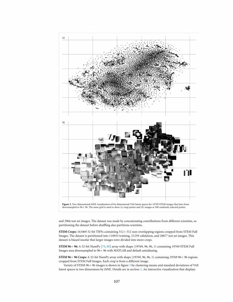
Mach. Learn.: Sci. Technol. 1 (2020) 045003 J M Ede
Figure 3. Two-dimensional tSNE visualization of 64-dimensional VAE latent spaces for 19769 STEM images that have beendownsampled to 96× 96. The same grid is used to show (a) map points and (b) images at 500 randomly selected points.
and 2966 test set images. The dataset was made by concatenating contributions from different scientists, sopartitioning the dataset before shuffling also partitions scientists.
STEMCrops: 161069 32-bit TIFFs containing 512× 512 non-overlapping regions cropped from STEM FullImages. The dataset is partitioned into 110933 training, 21259 validation, and 28877 test set images. Thisdataset is biased insofar that larger images were divided into more crops.
STEM 96× 96: A 32-bit NumPy [79, 80] array with shape [19769, 96, 96, 1] containing 19769 STEM FullImages area downsampled to 96× 96 with MATLAB and default antialiasing.
STEM 96× 96 Crops: A 32-bit NumPy array with shape [19769, 96, 96, 1] containing 19769 96× 96 regionscropped from STEM Full Images. Each crop is from a different image.
Variety of STEM 96× 96 images is shown in figure 3 by clustering means and standard deviations of VAElatent spaces in two dimensions by tSNE. Details are in section 2. An interactive visualization that displays
6
107
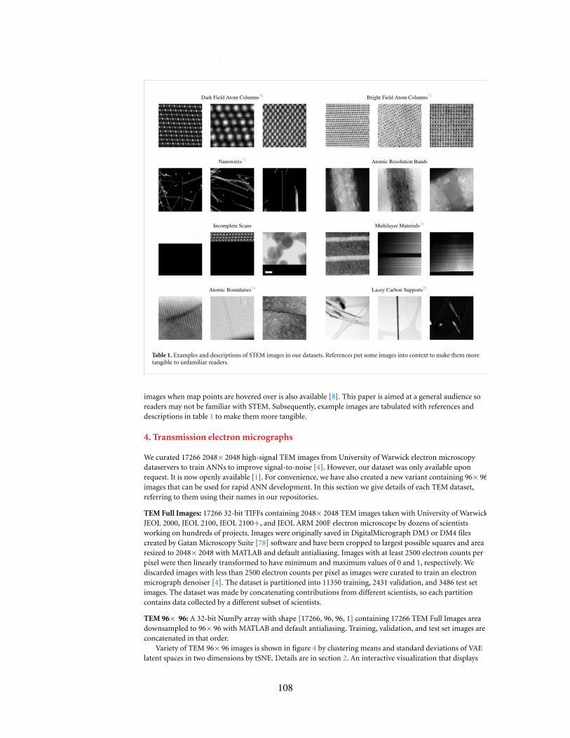
Mach. Learn.: Sci. Technol. 1 (2020) 045003 J M Ede
Table 1. Examples and descriptions of STEM images in our datasets. References put some images into context to make them moretangible to unfamiliar readers.
images when map points are hovered over is also available [8]. This paper is aimed at a general audience soreaders may not be familiar with STEM. Subsequently, example images are tabulated with references anddescriptions in table 1 to make them more tangible.
4. Transmission electronmicrographs
We curated 17266 2048× 2048 high-signal TEM images from University of Warwick electron microscopydataservers to train ANNs to improve signal-to-noise [4]. However, our dataset was only available uponrequest. It is now openly available [1]. For convenience, we have also created a new variant containing 96× 96images that can be used for rapid ANN development. In this section we give details of each TEM dataset,referring to them using their names in our repositories.
TEM Full Images: 17266 32-bit TIFFs containing 2048× 2048 TEM images taken with University of WarwickJEOL 2000, JEOL 2100, JEOL 2100+, and JEOL ARM 200F electron microscope by dozens of scientistsworking on hundreds of projects. Images were originally saved in DigitalMicrograph DM3 or DM4 filescreated by Gatan Microscopy Suite [78] software and have been cropped to largest possible squares and arearesized to 2048× 2048 with MATLAB and default antialiasing. Images with at least 2500 electron counts perpixel were then linearly transformed to have minimum and maximum values of 0 and 1, respectively. Wediscarded images with less than 2500 electron counts per pixel as images were curated to train an electronmicrograph denoiser [4]. The dataset is partitioned into 11350 training, 2431 validation, and 3486 test setimages. The dataset was made by concatenating contributions from different scientists, so each partitioncontains data collected by a different subset of scientists.
TEM 96× 96: A 32-bit NumPy array with shape [17266, 96, 96, 1] containing 17266 TEM Full Images areadownsampled to 96× 96 with MATLAB and default antialiasing. Training, validation, and test set images areconcatenated in that order.
Variety of TEM 96× 96 images is shown in figure 4 by clustering means and standard deviations of VAElatent spaces in two dimensions by tSNE. Details are in section 2. An interactive visualization that displays
7
108

Mach. Learn.: Sci. Technol. 1 (2020) 045003 J M Ede
Figure 4. Two-dimensional tSNE visualization of 64-dimensional VAE latent spaces for 17266 TEM images that have beendownsampled to 96× 96. The same grid is used to show (a) map points and (b) images at 500 randomly selected points.
images when map points are hovered over is also available [8]. This paper is aimed at a general audience soreaders may not be familiar with TEM. Subsequently, example images are tabulated with references anddescriptions in table 2 to make them more tangible.
5. Exit wavefunctions
We simulated 98340 TEM exit wavefunctions to train ANNs to reconstruct phases from amplitudes [3]. Halfof wavefunction information is undetected by conventional TEM as only the amplitude, and not the phase,of an image is recorded. Wavefunctions were simulated at 512× 512 then centre-cropped to 320× 320 toremove simulation edge artefacts. Wavefunctions have been simulated for real physics where Kirklandpotentials [87] for each atom are summed from n= 3 terms, and by truncating Kirkland potentialsummations to n= 1 to simulate an alternative universe where atoms have different potentials.Wavefunctions simulated for an alternate universe can be used to test ANN robustness to simulation physics.
8
109

Mach. Learn.: Sci. Technol. 1 (2020) 045003 J M Ede
Table 2. Examples and descriptions of TEM images in our datasets. References put some images into context to make them moretangible to unfamiliar readers.
For rapid development, we also downsampled n= 3 wavefunctions from 320× 320 to 96× 96. In this sectionwe give details of each exit wavefunction dataset, referring to them using their names in our repositories.
CIFs: 12789 CIFs downloaded from the Crystallography Open Database [88–93] (COD). The CIFs are formaterials published in inorganic chemistry journals. There are 150 New Journal of Chemistry, 1034American Mineralogist, 1998 Journal of the American Chemical Society and 5457 Inorganic Chemistry CIFsused to simulate training set wavefunctions, 1216 Physics and Chemistry of Materials CIFs used to simulatevalidation set wavefunctions, and 2927 Chemistry of Materials CIFs used to simulate test set wavefunctions.In addition, the CIFs have been preprocessed to be input to clTEM wavefunction simulations.
URLs: COD Uniform Resource Locators [94] (URLs) that CIFs were downloaded from.
Wavefunctions: 36324 complex 64-bit NumPy files containing 320× 320 wavefunctions. The wavefunctionsare for a large range of materials and physical hyperparameters. The dataset is partitioned into 24530training, 3399 validation, and 8395 test set wavefunctions. Metadata Javascript Object Notation [95] (JSON)files link wavefunctions to CIFs and contain some simulation hyperparameters.
Wavefunctions Unseen Training: 1544 64-bit NumPy files containing 320× 320 wavefunctions. Thewavefunctions are for training set CIFs and are for a large range of materials and physical hyperparameters.Metadata JSONs link wavefunctions to CIFs and contain some simulation hyperparameters.
Wavefunctions Single: 4825 complex 64-bit NumPy files containing 320× 320 wavefunctions. Thewavefunctions are for a single material, In1.7K2Se8Sn2.28 [96], and a large range of physical hyperparameters.The dataset is partitioned into 3861 training, and 964 validation set wavefunctions. Metadata JSONs linkwavefunctions to CIFs and contain some simulation hyperparameters.
Wavefunctions Restricted: 11870 complex 64-bit NumPy files containing 320× 320 wavefunctions. Thewavefunctions are for a large range of materials and a small range of physical hyperparameters. The dataset is
9
110
Mach. Learn.: Sci. Technol. 1 (2020) 045003 J M Ede
partitioned into 8002 training, 1105 validation, and 2763 test set wavefunctions. Metadata JSON files linkwavefunctions to CIFs and contain some simulation hyperparameters.
Wavefunctions 96× 96: A 32-bit NumPy array with shape [36324, 96, 96, 2] containing 36324wavefunctions. The wavefunctions were simulated for a large range of materials and physicalhyperparameters, and bilinearly downsampled with skimage [47] from 320× 320 to 96× 96 using defaultantialiasing. In Python [97], Real components are at index [...,0], and imaginary components are at index[...,1]. The dataset can be partitioned in 24530 training, 3399 validation, and 8395 test set wavefunctions,which have been concatenated in that order. To be clear, the training subset is at Python indexes [:24530].
Wavefunctions 96× 96 Restricted: A 32-bit NumPy array with shape [11870, 96, 96, 2] containing 11870wavefunctions. The wavefunctions were simulated for a large range of materials and a small range of physicalhyperparameters, and bilinearly downsampled with skimage from 320× 320 to 96× 96 using defaultantialiasing. The dataset can be partitioned in 8002 training, 1105 validation, and 2763 test setwavefunctions, which have been concatenated in that order.
Wavefunctions 96× 96 Single: A 32-bit NumPy array with shape [4825, 96, 96, 2] containing 11870wavefunctions. The wavefunctions were simulated for In1.7K2Se8Sn2.28 and a large range of physicalhyperparameters, and bilinearly downsampled with skimage from 320× 320 to 96× 96 using defaultantialiasing. The dataset can be partitioned in 3861 training, and 964 validation set wavefunctions, whichhave been concatenated in that order.
Wavefunctions n= 1: 37457 complex 64-bit NumPy files containing 320× 320 wavefunctions. Thewavefunctions are for a large range of materials and physical hyperparameters. The dataset is partitioned into25352 training, 3569 validation, and 8563 test set wavefunctions. These wavefunctions are for an alternateuniverse where atoms have different potentials.
Wavefunctions n= 1 Unseen Training: 1501 64-bit NumPy files containing 320× 320 wavefunctions. Thewavefunctions are for training set CIFs and are for a large range of materials and physical hyperparameters.Metadata JSONs link wavefunctions to CIFs and contain some simulation hyperparameters. Thesewavefunctions are for an alternate universe where atoms have different potentials.
Wavefunctions n= 1 Single: 4819 complex 64-bit NumPy files containing 320× 320 wavefunctions. Thewavefunctions are for a single material, In1.7K2Se8Sn2.28, and a large range of physical hyperparameters. Thedataset is partitioned into 3856 training, and 963 validation set wavefunctions. Metadata JSONs linkwavefunctions to CIFs and contain some simulation hyperparameters. These wavefunctions are for analternate universe where atoms have different potentials.
Experimental Focal Series: 1000 experimental focal series. Each series consists of 14 32-bit 512× 512 TEMimages, area downsampled from 4096× 4096 with MATLAB and default antialiasing. The images are in TIFF[98] format. All series were created with a common, quadratically increasing [99] defocus series. However,spatial scales vary and would need to be fitted as part of wavefunction reconstruction.
In detail, exit wavefunctions for a large range of physical hyperparameters were simulated with clTEM[100, 101] for acceleration voltages in 80, 200, 300 kV, material depths uniformly distributed in [5, 100)nm, material widths in [5, 10) nm, and crystallographic zone axes (h, k, l) h, k, l∈ 0, 1, 2. Materials werepadded on all sides with vacuum 0.8 nm wide and 0.3 nm deep to reduce simulation artefacts. Finally, crystaltilts were perturbed by zero-centred Gaussian random variates with 0.1
standard deviations. We used
default values for other clTEM hyperparameters. Simulations for a small range of physical hyperparametersused lower upper bounds that reduced simulation hyperparameter ranges by factors close to 1/4. Allwavefunctions are linearly transformed to have a mean amplitude of 1.
All wavefunctions show atom columns, so tSNE visualizations are provided in supplementaryinformation to conserve space. The visualizations are for Wavefunctions 96× 96, Wavefunctions 96× 96Restricted and Wavefunctions 96× 96 Single.
6. Discussion
The best dataset variant varies for different applications. Full-sized datasets can always be used as otherdataset variants are derived from them. However, loading and processing full-sized examples may bottlenecktraining, and it is often unnecessary. Instead, smaller 512× 512 crops, which can be loaded more quickly thefull-sized images, can often be used to train ANNs to be applied convolutionally [102] to or tiled across [4]full-sized inputs. In addition, our 96× 96 datasets can be used for rapid initial development before scaling up
10
111
Mach. Learn.: Sci. Technol. 1 (2020) 045003 J M Ede
to full-sized datasets, similar to how ANNs might be trained with CIFAR-10 before scaling up to ImageNet.However, subtle application- and dataset-specific considerations may also influence the best dataset choice.For example, an ANN trained with downsampled 96× 96 inputs may not generalize to 96× 96 crops fromfull-sized inputs as downsampling may introduce artifacts [103] and change noise or other datacharacteristics.
In practice, electron microscopists image most STEM and TEM signals at several times their Nyquistrates [77]. This eases visual inspection, decreases sub-Nyquist aliasing [104], improves display on computermonitors, and is easier than carefully tuning sampling rates to capture the minimum data needed to resolvesignals. High sampling may also reveal additional high-frequency information when images are inspectedafter an experiment. However, this complicates ANN development as it means that information per pixel isoften higher in downsampled images. For example, partial scans across STEM images that have beendowsampled to 96× 96 require higher coverages than scans across 96× 96 crops for ANNs to learn tocomplete images with equal performance [5]. It also complicates the comparison of different approaches tocompressed sensing. For example, we suggested that sampling 512× 512 crops at a regular grid of probinglocations outperforms sampling along spiral paths as a subsampling grid can still access mostinformation [5].
Test set performance should be calculated for a standardized dataset partition to ease comparison withother methods. Nevertheless, training and validation partitions can be varied to investigate validationvariance for partitions with different characteristics. Default training and validation sets for STEM and TEMdatasets contain contributions from different scientists that have been concatenated or numbered in order, sonew validation partitions can be selected by concatenating training and validation partitions and moving thewindow used to select the validation set. Similarly, exit wavefunctions were simulated with CIFs fromdifferent journals that were concatenated or numbered sequentially. There is leakage [105, 106] betweentraining, validation and test sets due to overlap between materials published in different journals andbetween different scientists’ work. However, further leakage can be minimized by selecting dataset partitionsbefore any shuffling and, for wavefunctions, by ensuring that simulations for each journal are not splitbetween partitions.
Experimental STEM and TEM image quality is variable. Images were taken by scientists with all levels ofexperience and TEM images were taken on multiple microscopes. This means that our datasets containimages that might be omitted from other datasets. For example, the tSNE visualization for STEM in figure 3includes incomplete scans, ~ 50 blank images, and images that only contain noise. Similarly, the tSNEvisualization for TEM in figure 4 revealed some images where apertures block electrons, and that there aresmall number of unprocessed standard diffraction and convergent beam electron diffraction [107] patterns.Although these conventionally low-quality images would not normally be published, they are important toensure that ANNs are robust for live applications. In addition, inclusion of conventionally low-quality imagesmay enable identification of this type of data. We encourage readers to try our interactive tSNE visualizations[8] for detailed inspection of our datasets.
In this paper, we present tSNE visualizations of VAE latent spaces to show image variety. However, ourVAEs can be directly applied to a wide range of additional applications. For example, successful tSNEclustering of latent spaces suggests that VAEs could be used to create a hash table [108, 109] for an electronmicrograph search engine. VAEs can also be applied to semantic manipulation [110], and clustering in tSNEvisualizations may enable subsets of latent space that generate interesting subsets of data distributions to beidentified. Other applications include using clusters in tSNE visualizations to label data for supervisedlearning, data compression, and anomaly detection [111, 112]. To encourage further development, we havemade our source code and pretrained VAEs openly available [8].
7. Conclusion
We have presented details of and visualizations for large new electron microscopy datasets that are openlyavailable from our new repositories. Datasets have been carefully partitioned into training, validation, andtest sets for machine learning. Further, we provide variants containing 512× 512 crops to reduce data loadingtimes, and examples downsampled to 96× 96 for rapid development. To improve dataset visualization withVAEs, we introduce encoding normalization and regularization, and add an image gradient loss. In addition,we propose extending tSNE to account for encoded standard deviations. Source code, pretrained VAEs,precompiled tSNE binaries, and interactive dataset visualizations are provided in supplementary repositoriesto help users become familiar with our datasets and visualizations. By making our datasets available, we aimto encourage standardization of performance benchmarks in electron microscopy and increase participationof the wider computer science community in electron microscopy research.
11
112
Mach. Learn.: Sci. Technol. 1 (2020) 045003 J M Ede
8. Supplementary Information
Ten additional tSNE visualizations are provided as supplementary information. They are for:
• Extracting 50 principal components by probabilistic PCA for the STEM 96× 96, STEM 96× 96 Crops, TEM96× 96, Wavefunctions 96× 96, Wavefunctions 96× 96 Restricted and Wavefunctions 96× 96 Single data-sets. PCA is a quick and effective method to extract features. As a result, we think that visualizations forPCA are interesting benchmarks.• VAE latent spaces with σ propagation for the STEM 96× 96 Crops dataset. Crops show smaller featuresthan downsampled images.• VAE latent spaces without σ propagation for the STEM 96× 96, STEM 96× 96 Crops and TEM 96× 96datasets. They are comparable to visualizations created with σ propagation.
Interactive versions of tSNE visualizations that display data when map points are hovered over areavailable [8] for every figure. In addition, we propose an algorithm to increase whitespace utilization in tSNEvisualizations by uniformly separating points, and show that our VAEs can be used as the basis of imagesearch engines. Supplementary information is openly available at https://doi.org/10.5281/zenodo.3899740and stacks.iop.org/MLST/1/045003/mmedia.
9. Data Availability
The data that support the findings of this study are openly available athttps://doi.org/10.5281/zenodo.3834197. For additional information contact the corresponding author(J.M.E.).
Acknowledgement
Funding: J.M.E. acknowledges EPSRC EP/N035437/1 and EPSRC Studentship 1917382.
Competing Interests
The author declares no competing interests.
ORCID iD
Jeffrey M Ede https://orcid.org/0000-0002-9358-5364
References
[1] Ede J M 2020 Electron microscopy datasets (Available online at: https://github.com/Jeffrey-Ede/datasets/wiki)[2] FEI C 2010 An introduction to electron microscopy (Available online at: https://www.fei.com/documents/
introduction-to-microscopy-document)[3] Ede J M, Peters J J P, Sloan J and Beanland R 2020 Exit wavefunction reconstruction from single transmission electron
micrographs with deep learning (arXiv:2001.10938)[4] Ede J M and Beanland R 2019 Improving electron micrograph signal-to-noise with an atrous convolutional encoder-decoder
Ultramicroscopy 202 18–25[5] Ede J M and Beanland R 2020 Partial scanning transmission electron microscopy with deep learning Sci. Rep. 10 8332[6] Ede J M and Beanland R 2020 Adaptive learning rate clipping stabilizes learningMach. Learn. Sci. Technol. 1 015011[7] Ede J M 2019 Deep learning supersampled scanning transmission electron microscopy (arXiv:1910.10467)[8] Ede J M 2020 Visualization of electron microscopy datasets with deep learning (Available online at:
https://github.com/Jeffrey-Ede/datasets)[9] Schmidt J, Marques M R, Botti S and Marques M A 2019 Recent advances and applications of machine learning in solid-state
materials science npj Comput. Mater. 5 1–36[10] von Lilienfeld O A 2020 Introducing Machine Learning: Science and TechnologyMach. Learn. Sci. Technol. 1 010201[11] Belianinov A et al 2015 Big data and deep data in scanning and electron microscopies: deriving functionality from
multidimensional data sets Adv. Struct. Chem. Imaging 1 1–25[12] Hornik K, Stinchcombe M and White H 1989 Multilayer feedforward networks are universal approximators Neural Netw. 2
359–66[13] Lin HW, Tegmark M and Rolnick D 2017 Why does deep and cheap learning work so well? J. Stat. Phys. 168 1223–47[14] Raschka S 2018 Model evaluation, model selection and algorithm selection in machine learning (arXiv:1811.12808)[15] Roh Y, Heo G and Whang S E 2019 A survey on data collection for machine learning: A big data-AI integration perspective IEEE
Trans. Knowl. Data Eng. 10.1109/TKDE.2019.2946162[16] Hall S R, Allen F H and Brown I D 1991 The crystallographic information file (CIF): A new standard archive file for
crystallography Acta Crystallogr. Sect. A: Foundations Crystallogr. 47 655–85
12
113
Mach. Learn.: Sci. Technol. 1 (2020) 045003 J M Ede
[17] Baker M 2016 Reproducibility Crisis? Nature 533 353–66[18] Hutson M 2018 Artificial intelligence faces reproducibility crisis Science 359 725–6[19] Iudin A, Korir P K, Salavert-Torres J, Kleywegt G J and Patwardhan A 2016 EMPIAR: A public archive for raw electron
microscopy image data Nat. Methods 13 387[20] Hey T, Butler K, Jackson S and Thiyagalingam J 2020 Machine learning and big scientific data Philosophical Trans. of the Royal
Society A 378 20190054[21] Krizhevsky A, Nair V and Hinton G 2014 The CIFAR-10 dataset (Available online at: http://www:cs:toronto:edu/ kriz/cifar:html)[22] Krizhevsky A and Hinton G 2009 Learning multiple layers of features from tiny images. Tech. Rep., Citeseer[23] LeCun Y, Cortes C and Burges C 2010 MNIST handwritten digit database. AT&T Labs (Available online at:
http://yann.lecun.com/exdb/mnist)[24] Russakovsky O et al 2015 ImageNet large scale visual recognition challenge Int. J. Comput. Vis. 115 211–52[25] Tenenbaum J B, De Silva V and Langford J C 2000 A global geometric framework for nonlinear dimensionality reduction Science
290 2319–23[26] Roweis S T and Saul L K 2000 Nonlinear dimensionality reduction by locally linear embedding Science 290 2323–6[27] Zhang Z and Wang J 2007 MLLE: Modified locally linear embedding using multiple weights Advances in Neural Information
Processing Systems 19: Proc. of the 2006 Conf. pp 1593–600[28] Donoho D L and Grimes C 2003 Hessian eigenmaps: locally linear embedding techniques for high-dimensional data Proc. Natl
Acad. Sci. 100 5591–6[29] Belkin M and Niyogi P 2003 Laplacian eigenmaps for dimensionality reduction and data representation Neural Comput. 15
1373–96[30] Zhang Z and Zha H 2004 Principal manifolds and nonlinear dimensionality reduction via tangent space alignment SIAM J. Sci.
Comput. 26 313–38[31] Buja A et al 2008 Data visualization with multidimensional scaling J. Comput. Graph. Stat. 17 444–72[32] Van Der Maaten L 2014 Accelerating t-SNE using tree-based algorithms J. Mach. Learn. Res. 15 3221–45[33] Maaten L v d and Hinton G 2008 Visualizing data using t-SNE J. Mach. Learn. Res. 9 2579–605[34] Wattenberg M, Viegas F and Johnson I 2016 How to use t-SNE effectively Distill 1 e2[35] Ruder S 2016 An overview of gradient descent optimization algorithms (arXiv:1609.04747)[36] Schubert E and Gertz M 2017 Intrinsic t-stochastic neighbor embedding for visualization and outlier detection Int. Conf. on
Similarity Search and Applications (Berlin: Springer) pp 188–203[37] Halko N, Martinsson P-G and Tropp J A 2011 Finding structure with randomness: Probabilistic algorithms for constructing
approximate matrix decompositions SIAM Rev. 53 217–88[38] Martinsson P-G, Rokhlin V Tygert M 2011 A randomized algorithm for the decomposition of matrices Appl. Comput. Harmon.
Anal. 30 47–68[39] Wall M E, Rechtsteiner A Rocha L M 2003 Singular value decomposition and principal component analysis A Practical Approach
to Microarray Data Analysis (Berlin: Springer) pp 91–109[40] Jolliffe I T and Cadima J 2016 Principal component analysis: A review and recent developments Philosophical Trans. of the Royal
Society A: Mathematical, Physical and Engineering Sciences 374 20150202[41] Dalal N and Triggs B 2005 Histograms of oriented gradients for human detection 2005 IEEE Computer Conf. on Computer Vision
and Pattern Recognition (CVPR’05) IEEE vol 1 pp 886–93[42] Bay H, Ess A, Tuytelaars T Van Gool L 2008 Speeded-Up robust features (SURF) Comput. Vis. Image Underst. 110 346–59[43] Ojala T, Pietikainen M and Maenpaa T 2002 Multiresolution gray-scale and rotation invariant texture classification with local
binary pattern IEEE Trans. Pattern Anal. Mach. Intell. 24 971–87[44] Mallat S G 1989 A Theory for multiresolution signal decomposition: The wavelet representation IEEE Transactions on Pattern
Analysis Mach. Intell. 11 674–93[45] Latif A et al 2019 Content-based image retrieval and feature extraction: a comprehensive reviewMath. Probl. Eng. 2019
10.1155/2019/9658350[46] Minka T P 2001 Automatic choice of dimensionality for PCA Adv Neural Inf Process Syst. 13 598–604[47] Van der Walt S et al 2014 scikit-image: image processing in python PeerJ 2 e453[48] Tschannen M, Bachem O and Lucic M 2018 Recent advances in autoencoder-based representation learning (arXiv:1812.05069)[49] Kramer M A 1991 Nonlinear principal component analysis using autoassociative neural networks AIChE J. 37 233–43[50] Marcelino P 2018 Transfer learning from pre-trained models Towards data science (Available online at:
https://towardsdatascience.com/transfer-learning-from-pre-trained-models-f2393f124751)[51] Ede J M 2018 Kernels, MLPs and autoencoders (Available online at: https://github.com/Jeffrey-Ede/Denoising-
Kernels-MLPs-Autoencoders)[52] Ede J M 2018 Autoencoders, kernels and multilayer perceptrons for electron micrograph restoration and compression
(arXiv:1808.09916)[53] Kingma D P and Welling M 2014 Auto-encoding variational Bayes (arXiv:1312.6114)[54] Kingma D P and Welling M 2019 An introduction to variational autoencoders (arXiv:1906.02691)[55] McCann M T, Jin K H and Unser M 2017 Convolutional neural networks for inverse problems in imaging: A review IEEE Signal
Process. Mag. 34 85–95[56] Krizhevsky A, Sutskever I and Hinton G E 2012 ImageNet classification with deep convolutional neural networks Adv Neural Inf
Process Syst. 25 1097–105[57] Ioffe S and Szegedy C 2015 Batch normalization: accelerating deep network training by reducing internal covariate shift
(arXiv:1502.03167)[58] Nair V and Hinton G E 2010 Rectified linear units improve restricted Boltzmann machines Proc. of the 27th Int. Conf. on Machine
Learning (ICML-10) pp 807–14[59] Higgins I et al 2017 beta-VAE: learning basic visual concepts with a constrained variational framework Int. Conf. on Learning
Representations vol 2 p 6[60] Hu Q and Greene C S 2019 Parameter tuning is a key part of dimensionality reduction via deep variational autoencoders for
single cell RNA transcriptomics Symp. on Biocomputing. Symp. on Biocomputing NIH Public Access vol 24 p 362[61] McIlhagga W 2018 Estimates of edge detection filters in human vision Vis. Res. 153 30–6[62] Larsen A B L, Sønderby S K, Larochelle H and Winther O 2015 Autoencoding beyond pixels using a learned similarity metric
(arXiv:1512.09300)
13
114
Mach. Learn.: Sci. Technol. 1 (2020) 045003 J M Ede
[63] Vairalkar M K and Nimbhorkar S 2012 Edge detection of images using Sobel operator Int. Journal of Emerging Technology andAdvanced Engineering 2 291–3
[64] Kingma D P and Ba J 2014 ADAM: A method for stochastic optimization (arXiv:1412.6980)[65] Zou D, Cao Y, Zhou D and Gu Q 2018 Stochastic gradient descent optimizes over-parameterized deep ReLU networks
(arXiv:1811.08888)[66] Ge R, Kakade S M, Kidambi R and Netrapalli P 2019 The step decay schedule: a near optimal, geometrically decaying learning
rate procedure (arXiv:1904.12838)[67] Chen J and Kyrillidis A 2019 Decaying momentum helps neural network training (arXiv:1910.04952)[68] Oskolkov N 2019 How to tune hyperparameters of tSNE Towards Data Science (Available online at:
https://towardsdatascience.com/how-to-tune-hyperparameters-of-tsne-7c0596a18868)[69] Pedregosa F et al 2011 scikit-learn: machine learning in python J. Mach. Learn. Res. 12 2825–30[70] Van den Bos K H et al 2016 Unscrambling mixed elements using high angle annular dark field scanning transmission electron
microscopy Phys. Rev. Lett. 116 246101[71] Zhou D et al 2016 Sample tilt effects on atom column position determination in ABF-STEM imaging Ultramicroscopy 160 110–17[72] Bu L et al 2016 Surface engineering of hierarchical platinum-cobalt nanowires for efficient electrocatalysis Nat. Commun. 7 1–10[73] Monclus M et al 2018 Effect of layer thickness on the mechanical behaviour of oxidation-strengthened Zr/Nb nanoscale
multilayers J. Mater. Sci. 53 5860–78[74] Pyrz W D et al 2010 Atomic-Level imaging of Mo-V-O complex oxide phase intergrowth, grain boundaries and defects using
HAADF-STEM Proc. Natl Acad. Sci. 107 6152–7[75] McGilvery C M, Goode A E, Shaffer M S and McComb DW 2012 Contamination of holey/lacey carbon films in STEMMicron 43
450–5[76] Seki T, Ikuhara Y and Shibata N 2018 Theoretical framework of statistical noise in scanning transmission electron microscopy
Ultramicroscopy 193 118–25[77] Landau H 1967 Sampling, data transmission and the Nyquist rate Proc. of the IEEE 55 1701–6[78] Gatan microscopy suite 2019 (Available online at: www.gatan.com/products/tem-analysis/gatan-microscopy-suite-software)[79] NPY format 2019 (Available online at: https://docs.scipy.org/doc/numpy/reference/generated/numpy.lib.format.html)[80] Kern R 2007 NEP 1—a simple file format for NumPy arrays (Available online at:
https://numpy.org/neps/nep-0001-npy-format.html)[81] Karlsson G 2001 Thickness measurements of lacey carbon films J. Microsc. 203 326–8[82] InamM et al 2017 1D vs. 2D Shape selectivity in the crystallization-driven self-assembly of polylactide block copolymers Chem.
Sci. 8 4223–30[83] Bendersky L A and Gayle F W 2001 Electron diffraction using transmission electron microscopy J. Res. Natl Inst. Stand. Technol.
106 997[84] Wu Y, Messer B and Yang P 2001 Superconducting MgB2 nanowires Adv. Mater. 13 1487–9[85] Pang B et al 2017 The microstructural characterization of multiferroic LaFeO3-YMnO3 multilayers grown on (001)- and
(111)-SrTiO3 substrates by transmission electron microscopyMaterials 10 839[86] Dong Z et al 2016 Individual particles of cryoconite deposited on the mountain glaciers of the Tibetan Plateau: Insights into
chemical composition and sources Atmos. Environ. 138 114–24[87] Kirkland E J 2010 Advanced computing in electron microscopy (Berlin: Springer Science & Business Media)[88] Quiros M, Gražulis S, Girdzijauskaite S, Merkys A and Vaitkus A 2018 Using SMILES strings for the description of chemical
connectivity in the Crystallography Open Database J. Cheminformatics 10 1–17[89] Merkys A et al 2016 COD:: CIF::Parser: An error-correcting CIF parser for the Perl language J. Appl. Crystallogr. 49 292–301[90] Gražulis S, Merkys A, Vaitkus A and Okulic-Kazarinas M 2015 Computing stoichiometric molecular composition from crystal
structures J. Appl. Crystallogr. 48 85–91[91] Gražulis S et al 2012 Crystallography Open Database (COD): An open-access collection of crystal structures and platform for
world-wide collaboration Nucleic Acids Res. 40 D420–D427[92] Gražulis S et al 2009 Crystallography Open Database – an open-access collection of crystal structures J. Appl. Crystallogr. 42 726–9[93] Downs R T and Hall-Wallace M 2003 The American Mineralogist crystal structure database Am. Mineral. 88 247–50[94] Berners-Lee T, Masinter L and McCahill M 1994 RFC1738: Uniform Resource Locators (URL) RFC[95] ISO/IEC JTC 1/SC 22 2017 International standard ISO/IEC21778: information technology - the JSON data interchange syntax
(Available online at: https://www.iso.org/standard/71616.html)[96] Hwang S-J, Iyer R G, Trikalitis P N, Ogden A G and Kanatzidis M G 2004 Cooling of melts: kinetic stabilization and polymorphic
transitions in the KInSnSe4 System Inorg. Chem. 43 2237–9[97] Python software foundation 2020 Python 3.6 (Available online at: www.python.org)[98] Adobe developers association 1992 et al TIFF Revision 6.0. (Available online at:
www.adobe.io/content/dam/udp/en/open/standards/tiff/TIFF6.pdf)[99] Haigh S, Jiang B, Alloyeau D, Kisielowski C and Kirkland A 2013 Recording low and high spatial frequencies in exit wave
reconstructions Ultramicroscopy 133 26–34[100] Peters J J P and Dyson M A 2019 clTEM (Available online at: https://github.com/JJPPeters/clTEM)[101] Dyson M A 2014 Advances in Computational Methods for Transmission Electron Microscopy Simulation and Image Processing Ph.D.
thesis University of Warwick[102] Zhu J-Y, Park T, Isola P and Efros A A 2017 Unpaired image-to-image translation using cycle-consistent adversarial networks
Proc. of the IEEE Int. Conf. on Computer Vision pp 2223–32[103] MicroImages 2010 Resampling methods. technical Guide (Available online at:
https://www.microimages.com/documentation/TechGuides/77resampling.pdf)[104] Amidror I 2015 Sub-Nyquist artefacts and sampling Moire effects Royal Soc. Open Sci. 2 140550[105] Open data science 2019 How to fix data leakage - your model’s greatest enemy. towards data science (Available online at:
https://medium.com/@ODSC/how-to-fix-data-leakage-your-models-greatest-enemy-e34fa26abac5)[106] Bussola N, Marcolini A, Maggio V, Jurman G and Furlanello C 2019 Not again! Data leakage in digital pathology
(arXiv:1909.06539)[107] Tanaka M 1994 Convergent-beam electron diffraction Acta Crystallogr. Sect. A: Foundations Crystallogr. 50 261–86[108] Patterson N and Wang Y Semantic hashing with variational autoencoders https://pdfs.semanticscholar.org/f2c3/
3951f347b5e0f7ac4946f0672fdb4ca5394b.pdf
14
115
Mach. Learn.: Sci. Technol. 1 (2020) 045003 J M Ede
[109] Jin G, Zhang Y and Lu K 2019 Deep hashing based on VAE-GAN for efficient similarity retrieval Chin. J. Electron. 28 1191–7[110] Klys J, Snell J Zemel R 2018 Learning latent subspaces in variational autoencoders Adv Neural Inf Process Syst. 31 6444–54[111] Yao R, Liu C, Zhang L and Peng P 2019 Unsupervised anomaly detection using variational auto-encoder based feature extraction
2019 IEEE Int. Conf. on Prognostics and Health Management (ICPHM) IEEE pp 1–7[112] Xu H et al 2018 Unsupervised anomaly detection via variational auto-encoder for seasonal KPIs in web applications Proc. of the
2018 World Wide Conf. pp 187–96
15
116

Supplementary Information: Warwick ElectronMicroscopy DatasetsJeffrey M. Ede1,*
1University of Warwick, Department of Physics, Coventry, CV4 7AL, UK*[email protected]
S1 Additional VisualizationsFigure numbers for a variety of two-dimensional tSNE visualisations are tabulated in table S1 to ease comparison. Visualizationsare for the first 50 principal components extracted by a scikit-learn1 implementation of probabilistic PCA, means encoded in64-dimensional VAE latent spaces without modified tSNE losses to account for standard deviations, and means encoded in64-dimensional VAE latent spaces with modified tSNE losses to account for standard deviations. Interactive versions of tSNEvisualizations that display data when map points are hovered over are also available for every visualization2. In addition, oursource code, graph points and datasets are openly available.
Dataset PCA VAE µ VAE µ,σSTEM 96×96 S1 S7 3 (main article)STEM 96×96 Crops S2 S8 S10TEM 96×96 S3 S9 4 (main article)Wavefunctions 96×96 S4 - -Wavefunctions 96×96 Restricted S5 - -Wavefunctions 96×96 Single S6 - -
Table S1. To ease comparison, we have tabulated figure numbers for tSNE visualizations. Visualizations are for principalcomponents, VAE latent space means, and VAE latent space means weighted by standard deviations..
Visualization of complex exit wavefunctions is complicated by the display of their real and imaginary components. However,real and imaginary components are related3, and can be visualized in the same image by displaying them in different colourchannels. For example, we show real and imaginary components in red and blue colour channels, respectively, in figures S4-S6.Note that a couple of extreme points are cropped from some of the tSNE visualizations of principal components in figures S1-S6.However, this only affected ∼0.01% of points and therefore does not have a substantial effect on visualizations. In contrast,tSNE visualizations of VAE latent spaces did not have extreme points.
S2 Uniformly Separated tSNELimitedly, most tSNE visualizations do not fully utilize whitespace. This is problematic as space is often limited in journals,websites and other media. As a result, we propose algorithm 1 to uniformly separate map points. This increases whitespaceutilization while keeping clustered points together. Example applications are shown in figures S11-S13, where images nearestpoints on a regular grid are shown at grid points. Uniformly separating map points removes information about pairwise distancesencoded in the tSNE distributions. However, distances and cluster sizes in tSNE visualizations are not overly meaningful4.Overall, we think that uniformly separated tSNE is an interesting option that could be improved by further development. To thisend, our source code and graph points for uniformly separated tSNE visualizations are openly available2.
S3 Image Search EnginesOur VAEs can be used as the basis of image search engines. To find similar images, we compute Euclidean distances betweenmeans encoded for search inputs and images in the STEM or TEM datasets, then select images at lowest distances. Examplesof top-5 search results for various input images are shown in figure S14 and figure S15 for TEM and STEM, respectively.Search results are most accurate for common images and are less accurate for unusual images. The main difference between theperformance of our search engines and Google, Bing or other commercial image search engines is the result of commercialANNs being trained with over 100× more training data, 3500× more computational resources and larger images c.f. Xception5.
117
However, the performance of our search engines is okay and our VAEs could easily be scaled up. Our source code, pretrainedmodels and VAE encodings for each dataset are openly available2.
Algorithm 1 Two-dimensional Bayesian inverse transformed tSNE. We default to a h = w = 25 grid.
Initialize N two-dimensional tSNE map points, X = x1, ...,xN, where xi = xi1,xi2.Linearly transform dimensions to have values in [0,1],
xi j←xi j−mini(xi j)
maxi(xi j)−mini(xi j). (1)
Divide points into an evenly spaced grid with h×w cells.Compute number of points in each cell, nab, a ∈ [1,h], b ∈ [1,w].Cumulative numbers of points using the recurrent relations,
ca = ca−1 +w
∑b=1
nab , (2)
cb|a = cb−1|a +nab , (3)
where c0 = c0|a = 0.Estimate Bayesian conditional cumulative distribution functions,
Ca = ca/ch , (4)Cb|a = cb|a/ca . (5)
Map grid points, (a−0.5)/h,(b−0.5)/w, to distribution points, (u−0.5)/h,(v−0.5)/w, where u and v are minimumvalues that satisfy
(a−0.5)/h≤Cu , (6)(b−0.5)/w≤Cv|u . (7)
Interpolate uniformly separated grid positions, Y, for X based on pairs of grid and distribution points. We use Clough-Tochercubic Bezier interpolation6.
References1. Pedregosa, F. et al. Scikit-learn: Machine Learning in Python. J. Mach. Learn. Res. 12, 2825–2830 (2011).
2. Ede, J. M. Visualization of Electron Microscopy Datasets with Deep Learning. Online: https://github.com/Jeffrey-Ede/datasets, DOI: 10.5281/zenodo.3834197 (2020).
3. Ede, J. M., Peters, J. J. P., Sloan, J. & Beanland, R. Exit Wavefunction Reconstruction from Single Transmission ElectronMicrographs with Deep Learning. arXiv preprint arXiv:2001.10938 (2020).
4. Wattenberg, M., Viégas, F. & Johnson, I. How to Use t-SNE Effectively. Distill 1, e2 (2016).
5. Chollet, F. Xception: Deep Learning with Depthwise Separable Convolutions. In Proceedings of the IEEE Conference onComputer Vision and Pattern Recognition, 1251–1258 (2017).
6. Alfeld, P. A Trivariate Clough—Tocher Scheme for Tetrahedral Data. Comput. Aided Geom. Des. 1, 169–181 (1984).
S2/S16118
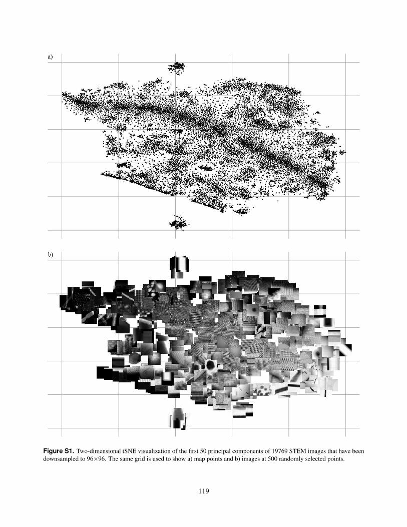
Figure S1. Two-dimensional tSNE visualization of the first 50 principal components of 19769 STEM images that have beendownsampled to 96×96. The same grid is used to show a) map points and b) images at 500 randomly selected points.
S3/S16119
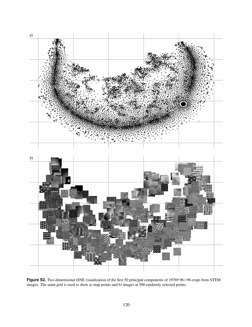
Figure S2. Two-dimensional tSNE visualization of the first 50 principal components of 19769 96×96 crops from STEMimages. The same grid is used to show a) map points and b) images at 500 randomly selected points.
S4/S16120
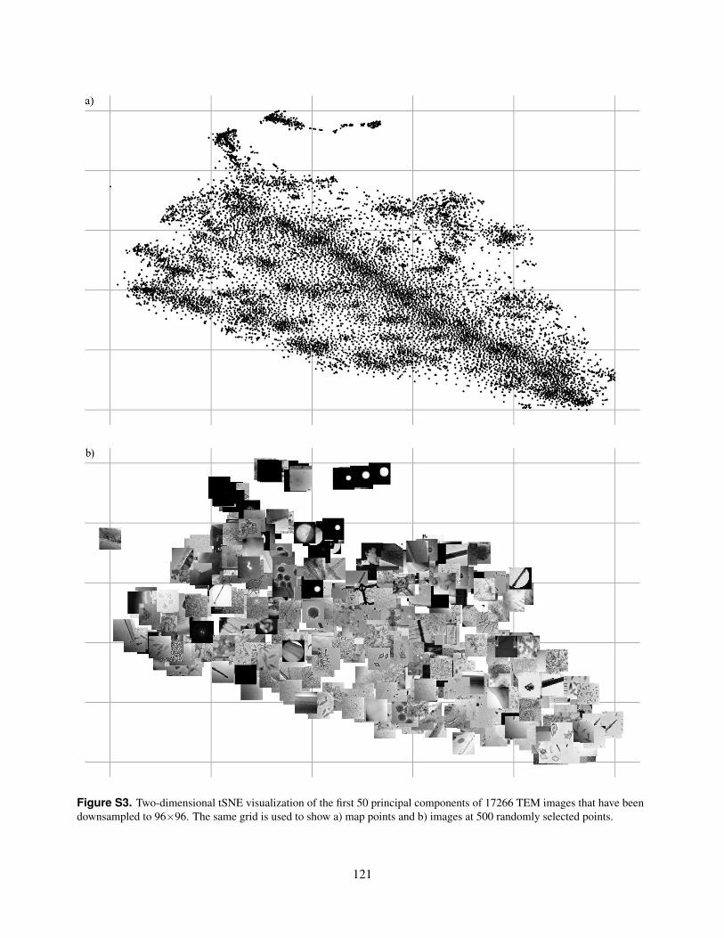
Figure S3. Two-dimensional tSNE visualization of the first 50 principal components of 17266 TEM images that have beendownsampled to 96×96. The same grid is used to show a) map points and b) images at 500 randomly selected points.
S5/S16121
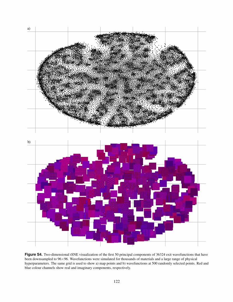
Figure S4. Two-dimensional tSNE visualization of the first 50 principal components of 36324 exit wavefunctions that havebeen downsampled to 96×96. Wavefunctions were simulated for thousands of materials and a large range of physicalhyperparameters. The same grid is used to show a) map points and b) wavefunctions at 500 randomly selected points. Red andblue colour channels show real and imaginary components, respectively.
S6/S16122
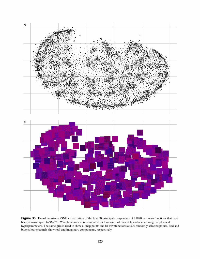
Figure S5. Two-dimensional tSNE visualization of the first 50 principal components of 11870 exit wavefunctions that havebeen downsampled to 96×96. Wavefunctions were simulated for thousands of materials and a small range of physicalhyperparameters. The same grid is used to show a) map points and b) wavefunctions at 500 randomly selected points. Red andblue colour channels show real and imaginary components, respectively.
S7/S16123
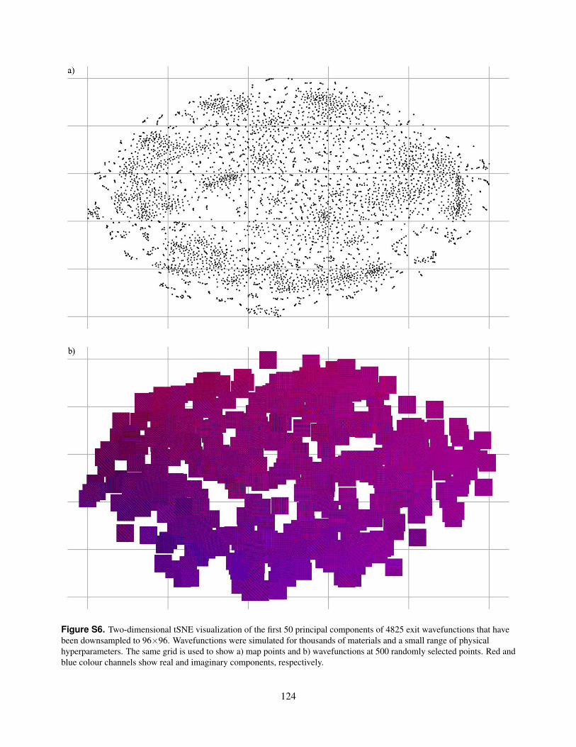
Figure S6. Two-dimensional tSNE visualization of the first 50 principal components of 4825 exit wavefunctions that havebeen downsampled to 96×96. Wavefunctions were simulated for thousands of materials and a small range of physicalhyperparameters. The same grid is used to show a) map points and b) wavefunctions at 500 randomly selected points. Red andblue colour channels show real and imaginary components, respectively.
S8/S16124
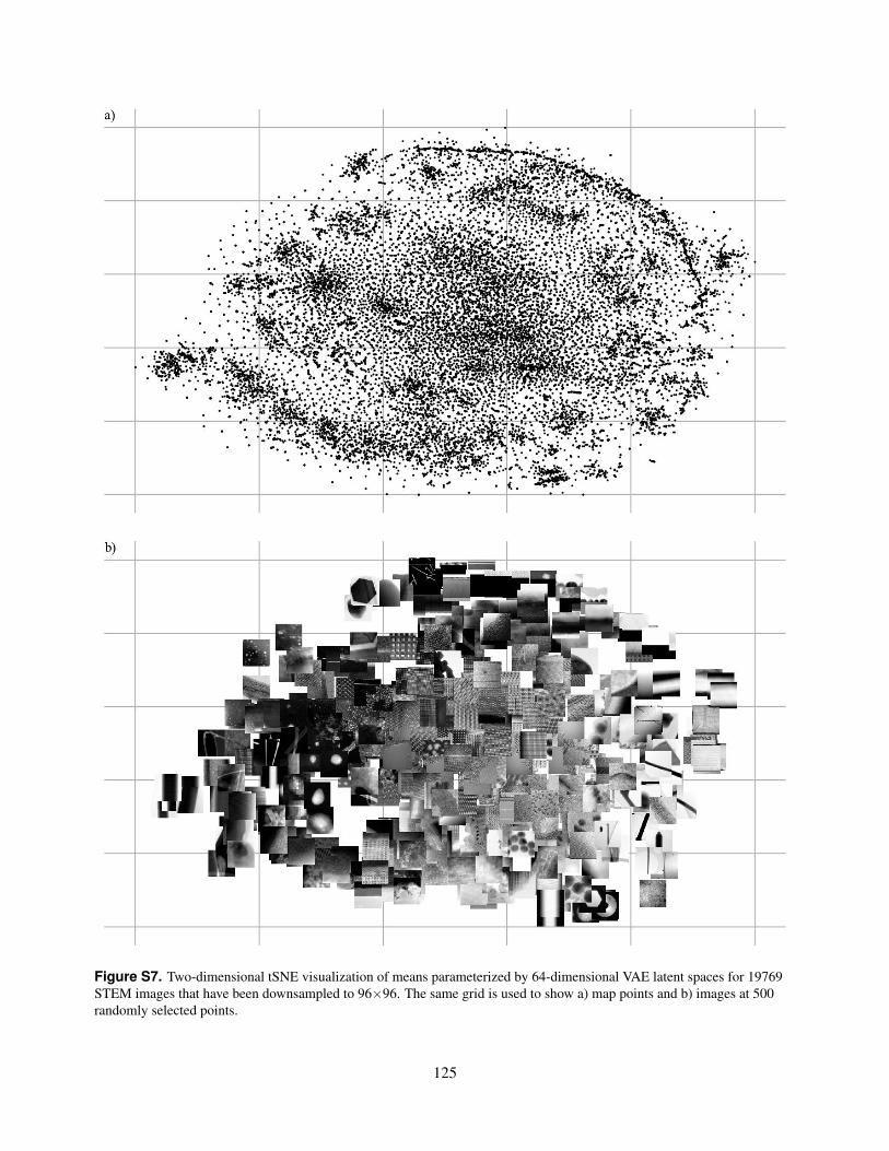
Figure S7. Two-dimensional tSNE visualization of means parameterized by 64-dimensional VAE latent spaces for 19769STEM images that have been downsampled to 96×96. The same grid is used to show a) map points and b) images at 500randomly selected points.
S9/S16125
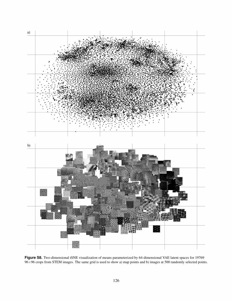
Figure S8. Two-dimensional tSNE visualization of means parameterized by 64-dimensional VAE latent spaces for 1976996×96 crops from STEM images. The same grid is used to show a) map points and b) images at 500 randomly selected points.
S10/S16126
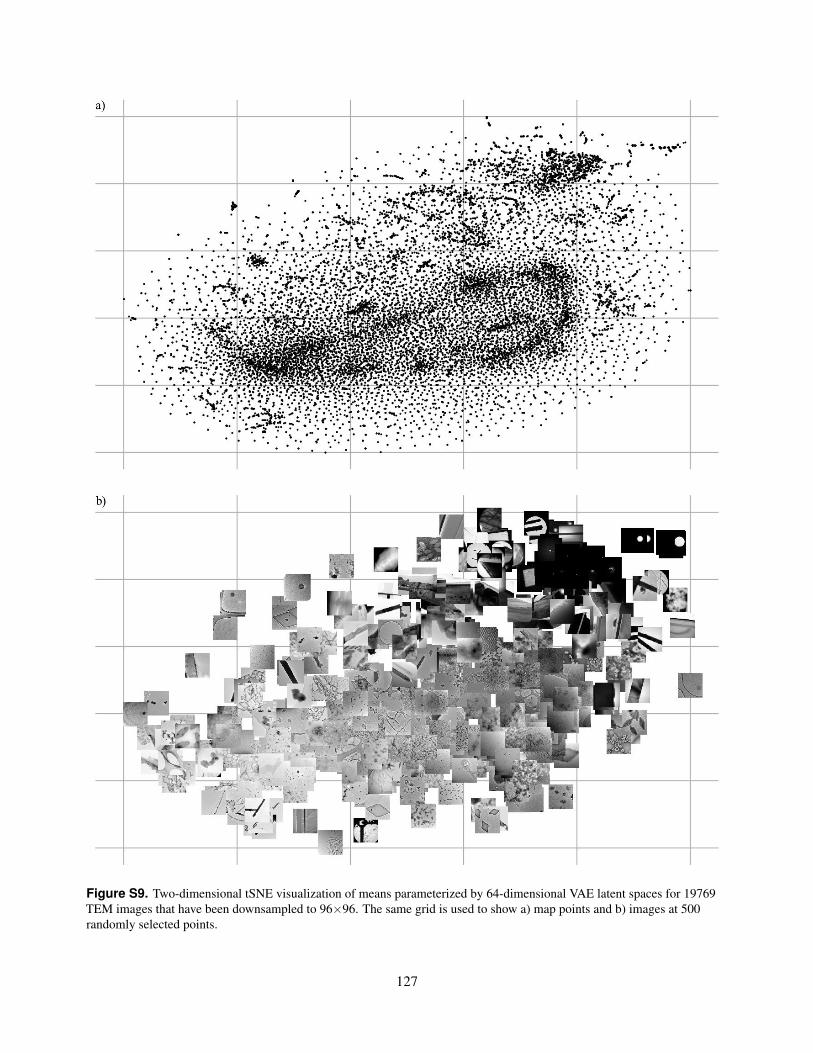
Figure S9. Two-dimensional tSNE visualization of means parameterized by 64-dimensional VAE latent spaces for 19769TEM images that have been downsampled to 96×96. The same grid is used to show a) map points and b) images at 500randomly selected points.
S11/S16127
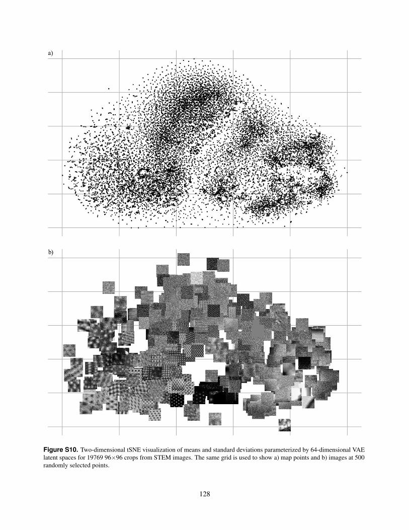
Figure S10. Two-dimensional tSNE visualization of means and standard deviations parameterized by 64-dimensional VAElatent spaces for 19769 96×96 crops from STEM images. The same grid is used to show a) map points and b) images at 500randomly selected points.
S12/S16128
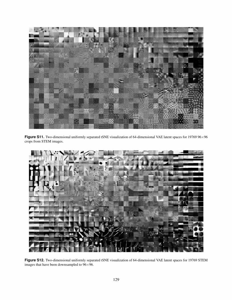
Figure S11. Two-dimensional uniformly separated tSNE visualization of 64-dimensional VAE latent spaces for 19769 96×96crops from STEM images.
Figure S12. Two-dimensional uniformly separated tSNE visualization of 64-dimensional VAE latent spaces for 19769 STEMimages that have been downsampled to 96×96.
S13/S16129

Figure S13. Two-dimensional uniformly separated tSNE visualization of 64-dimensional VAE latent spaces for 17266 TEMimages that have been downsampled to 96×96.
S14/S16130
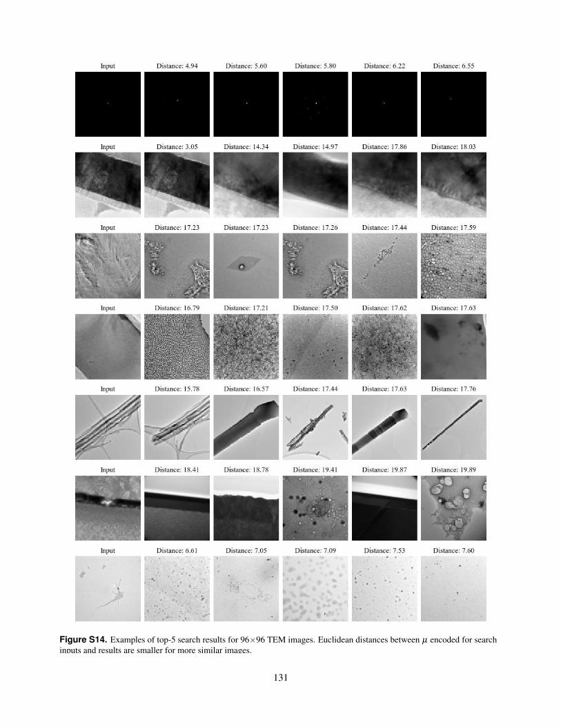
Figure S14. Examples of top-5 search results for 96×96 TEM images. Euclidean distances between µ encoded for searchinputs and results are smaller for more similar images.
S15/S16131

Figure S15. Examples of top-5 search results for 96×96 STEM images. Euclidean distances between µ encoded for searchinputs and results are smaller for more similar images.
S16/S16132
2.2 Amendments and Corrections
There are amendments or corrections to the paper2 covered by this chapter.
Location: Page 4, caption of fig. 2.
Change: “...at 500 randomly selected images...” should say “...at 500 randomly selected data points...”.
2.3 Reflection
This ancillary chapter covers my paper titled “Warwick Electron Microscopy Datasets”2 and associated research
outputs9,13–15. My paper presents visualizations for large new electron microscopy datasets published with our
earlier papers. There are 17266 TEM images curated to train our denoiser6 (ch. 6), 98340 STEM images curated to
train generative adversarial networks (GANs) for compressed sensing4,19 (ch. 4), and 98340 TEM exit wavefunctions
simulated to investigate EWR7 (ch. 7), and derived datasets containing smaller TEM and STEM images that I
created to rapidly prototype of ANNs for adaptive partial STEM5 (ch. 5). To improve visualizations, I developed
new regularization mechanisms for variational autoencoders107–109 (VAEs), which were trained to embed high-
dimensional electron micrographs in low-dimensional latent spaces. In addition, I demonstrate that VAEs can be
used as the basis of electron micrograph search engines. Finally, I provide extensions to t-distributed stochastic
neighbour embedding110–114 (tSNE) and interactive dataset visualizations.
Making our large machine learning datasets openly accessible enables our research to be reproduced115, stan-
dardization of performance comparisons, and dataset reuse in future research. Dissemination of large datasets is
enabled by the internet116,117, for example, through fibre optic118 broadband119,120 or satellite121,122 connections.
Subsequently, there are millions of open access datasets123,124 that can be used for machine learning125,126. Perfor-
mance of ANNs usually increases with increasing training dataset size125, so some machine learning datasets have
millions of examples. Examples of datasets with millions of examples include DeepMind Kinetics127, ImageNet128,
and YouTube 8M129. Nevertheless, our datasets containing tens of thousands of examples are more than sufficient for
initial exploration of deep learning in electron microscopy. For reference, some datasets used for initial explorations
of deep learning for Coronavirus Disease 2019130–132 (COVID-19) diagnosis are 10× smaller133 than WEMD.
There are many data clustering algorithms134–140 that can group data for visualization. However, tSNE is a de
facto default as it often outperforms other algorithms110. For context, tSNE is a variant of stochastic neighbour em-
bedding141 (SNE) where a heavy-tailed Student’s t-distribution is used to measure distances between embedded data
points. Applications of tSNE include bioinformatics142,143, forensic science144,145, medical signal processing146–148,
particle physics149,150, smart electricity metering151, and sound synthesis152. Before tSNE, data is often embedded
in a low-dimensional space to reduce computation, suppress noise, and prevent Euclidean distances used in tSNE
optimization being afflicted by the curse of dimensionality153. For example, the original tSNE paper suggests using
principal component analysis154–157 (PCA) to reduce data dimensionality to 30 before applying tSNE110.
Extensions of tSNE can improve clustering. For example, graphical processing unit accelerated implementations
of tSNE158,159 can speedup clustering 50-700×. Alternatively, approximate tSNE160 (A-tSNE) can trade accuracy
for decreased computation time. Our tSNE visualizations took a couple of hours to optimize on an Intel i7-6700
central processing unit (CPU) as we used 10000 iterations to ensure that clusters stabilized. It follows that accelerated
133
tSNE implementations may be preferable to reduce computation time. Another extension is to adjust distances used
for tSNE optimization with a power transform based on the intrinsic dimension of each point. This can alleviate the
curse of dimensionality for high-dimensional data153; however, it was not necessary for our data as I used VAEs
to reduce image dimensionality to 64 before tSNE. Finally, tSNE early exaggeration (EE), where probabilities
modelling distances in a high-dimensional space are increased, and number of iterations can be automatically tuned
with opt-tSNE161. Tuning can significantly improve visualizations, especially for large datasets with millions of
examples. However, I doubt that opt-tSNE would result in large improvements to clustering as our datasets contain
tens of thousands of examples, where tSNE is effective. Nevertheless, I expect that opt-tSNE could have improved
clustering if I had been aware of it.
Further extensions to tSNE are proposed in my paper2,9. I think that the most useful extension uniformly
separates clustered points based clustering density. Uniformly separated tSNE (US-tSNE) can often double
whitespace utilization, which could make tSNE visualizations more suitable for journals, websites, and other media
where space is limited. However, the increased whitespace utilization comes at the cost of removing information
about the structure of clusters. Further, my preliminary implementation of US-tSNE is limited insofar that Clough-
Tocher cubic Bezier interpolation162 used to map tSNE points to a uniform map is only applied to points within their
convex hull. I also proposed a tSNE extension that uses standard deviations encoded by VAEs to inform clustering
as this appeared to slightly improve clustering. However, I later found that using standard deviations appears to
decrease similarity of nearest neighbours in tSNE visualizations. As a result, I think that how extra information
encoded in standard deviations is used to inform clustering may merit further investigation.
To improve VAE encodings for tSNE, I applied a variant of batch normalization to their latent spaces. This
avoids needing to tune a hyperparameter to balance VAE decoder and Kullback-Leibler (KL) losses, which is
architecture-specific and can be complicated by relative sizes of their gradients varying throughout training. I
also considered adaptive gradient balancing163,164 of losses; however, that would require separate backpropagation
through the VAE generator for each loss, increasing computation. To increase image realism, I added Sobel losses
to mean squared errors (MSEs). Sobel losses often improve realism as human vision is sensitive to edges165. In
addition, Sobel losses require less computation than VAE training with GAN166 or perceptual167 losses. Another
computationally inexpensive approach to improve generated image realism is to train with structural similarity index
measures168 (SSIMs) instead of MSEs169.
My VAEs are used as the basis of my openly accessible electron microscopy search engines. I observe that top-5
search results are usually successful insofar that they contain images that are similar to input images. However,
they often contain some images that are not similar, possibly due to there not being many similar images in our
datasets. Thus, I expect that search results could be improved by increasing dataset size. Increasing input image
size from 96×96 to a couple of hundred pixels and increasing training iterations could also improve performance.
Further, training could be modified to encode binary latent variables for efficient hashing170–175. Finally, I think that
an interesting research direction is to create a web interface for an electron microscopy search engine that indexes
institutional electron microscopy data servers. Such a search engine could enhance collaboration by making it easier
to find electron microscopists working on interesting projects.
An application of my VAEs that is omitted from my paper is that VAE generators could function as portable
electron microscopy image generators. For example, to create training data for machine learning. For comparison,
134
my VAE generators require roughly 0.1% of the storage space needed for my image datasets to store their trainable
parameters. However, I was concerned that a distribution of generated images might be biased by catastrophic
forgetting176. Further, a distribution of generated images could be sensitive to ANN architecture and learning policy,
including when training is stopped177,178. Nevertheless, I expect that data generated from by VAEs could be used for
pretraining to improve ANN robustness179. Overall, I think it will become increasingly practical to use VAEs or
GANs as high-quality data generators as ANN architectures and learning policies are improved.
Perhaps the main limitation of my paper is that I did not introduce my preferred abbreviation, “WEMD”,
for “Warwick Electron Microscopy Datasets”. Further, I did not define “WEMD” in my WEMD preprint13.
Subsequently, I introduced my preferred abbreviation in my review of deep learning in electron microscopy1 (ch. 1).
I also defined an abbreviation, “WLEMD”, for “Warwick Large Electron Microscopy Datasets” in the first version
of the partial STEM preprint18 (ch. 4). Another limitation is that my paper only details datasets that had already
been published, or that were derived from the published datasets. For example, Richard Beanland and I successfully
co-authored an application for funding to simulate tens of thousands of CBED patterns with Felix180, which are not
detailed in my paper. The CBED dataset requires a couple of terabytes of storage and has not been processed for
dissemination. Nevertheless, Richard Beanland1 may be able to provide the CBED dataset upon request.
1Email: [email protected]
135
Chapter 3
Adaptive Learning Rate Clipping StabilizesLearning
3.1 Scientific Paper
This chapter covers the following paper3.
J. M. Ede and R. Beanland. Adaptive Learning Rate Clipping Stabilizes Learning. Machine Learning:
Science and Technology, 1:015011, 2020
136
Mach. Learn.: Sci. Technol. 1 (2020) 015011 https://doi.org/10.1088/2632-2153/ab81e2
OPEN ACCESS
RECEIVED
20 December 2019
REVISED
26 February 2020
ACCEPTED FOR PUBLICATION
20 March 2020
PUBLISHED
28 April 2020
Original Content fromthis work may be usedunder the terms of theCreative CommonsAttribution 4.0 licence.
Any further distributionof this work mustmaintain attribution tothe author(s) and the titleof the work, journalcitation and DOI.
PAPER
Adaptive learning rate clipping stabilizes learning
Jeffrey M Ede1 and Richard BeanlandDepartment of Physics, University of Warwick, Coventry CV4 7AL United Kingdom
E-mail: [email protected] and [email protected]
Keywords:machine learning, optimization, electron microscopy, learning stability
Supplementary material for this article is available online
AbstractArtificial neural network training with gradient descent can be destabilized by ‘bad batches’ withhigh losses. This is often problematic for training with small batch sizes, high order loss functionsor unstably high learning rates. To stabilize learning, we have developed adaptive learning rateclipping (ALRC) to limit backpropagated losses to a number of standard deviations above theirrunning means. ALRC is designed to complement existing learning algorithms: Our algorithm iscomputationally inexpensive, can be applied to any loss function or batch size, is robust tohyperparameter choices and does not affect backpropagated gradient distributions. Experimentswith CIFAR-10 supersampling show that ALCR decreases errors for unstable mean quartic errortraining while stable mean squared error training is unaffected. We also show that ALRC decreasesunstable mean squared errors for scanning transmission electron microscopy supersampling andpartial scan completion. Our source code is available at https://github.com/Jeffrey-Ede/ALRC.
1. Introduction
Loss spikes arise when artificial neural networks (ANNs) encounter difficult examples and can destabilizetraining with gradient descent[1, 2]. Examples may be difficult because an ANN needs more training togeneralize, catastrophically forgot previous learning [3] or because an example is complex or unusual.Whatever the cause, applying gradients backpropagated [4] from high losses results in large perturbations totrainable parameters.
When a trainable parameter perturbation is much larger than others, learning can be destabilized whileparameters adapt. This behaviour is common for ANN training with gradient descent where a large portionof parameters is perturbed at each optimization step. In contrast, biological networks often perturb smallportions of neurons to combine new learning with previous learning. Similar to biological networks, ANNlayers can become more specialized throughout training [5] and specialized capsule networks [6] are beingdeveloped. Nevertheless, ANN loss spikes during optimization are still a common reason for learninginstability. Loss spikes are common for training with small batch sizes, high order loss functions, andunstably high learning rates.
During ANN training by stochastic gradient descent [1] (SGD), a trainable parameter, θt , from step t isupdated to θt+ 1 in step t+ 1. The size of the update is given by the product of a learning rate, η, and thebackpropagated gradient of a loss function with respect to the trainable parameter
θt+1← θt− η∂L
∂θ. (1)
Without modification, trainable parameter perturbations are proportional to the scale of the loss function.Following gradient backpropagation, a high loss spike can cause a large perturbation to a learned parameterdistribution. Learning will then be destabilized while subsequent iterations update trainable parameters backto an intelligent distribution.
1 Author to whom any correspondence should be addressed.
© 2020 The Author(s). Published by IOP Publishing Ltd
137
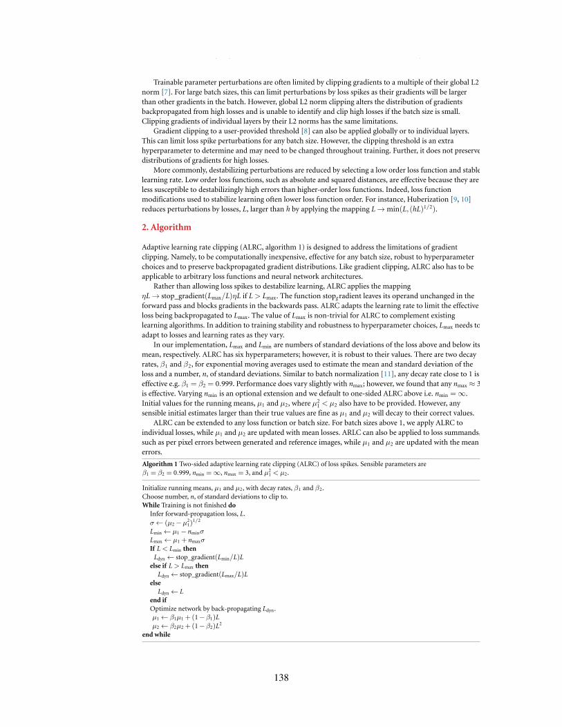
Mach. Learn.: Sci. Technol. 1 (2020) 015011 J M Ede and R Beanland
Trainable parameter perturbations are often limited by clipping gradients to a multiple of their global L2norm [7]. For large batch sizes, this can limit perturbations by loss spikes as their gradients will be largerthan other gradients in the batch. However, global L2 norm clipping alters the distribution of gradientsbackpropagated from high losses and is unable to identify and clip high losses if the batch size is small.Clipping gradients of individual layers by their L2 norms has the same limitations.
Gradient clipping to a user-provided threshold [8] can also be applied globally or to individual layers.This can limit loss spike perturbations for any batch size. However, the clipping threshold is an extrahyperparameter to determine and may need to be changed throughout training. Further, it does not preservedistributions of gradients for high losses.
More commonly, destabilizing perturbations are reduced by selecting a low order loss function and stablelearning rate. Low order loss functions, such as absolute and squared distances, are effective because they areless susceptible to destabilizingly high errors than higher-order loss functions. Indeed, loss functionmodifications used to stabilize learning often lower loss function order. For instance, Huberization [9, 10]reduces perturbations by losses, L, larger than h by applying the mapping L→min(L,(hL)1/2).
2. Algorithm
Adaptive learning rate clipping (ALRC, algorithm 1) is designed to address the limitations of gradientclipping. Namely, to be computationally inexpensive, effective for any batch size, robust to hyperparameterchoices and to preserve backpropagated gradient distributions. Like gradient clipping, ALRC also has to beapplicable to arbitrary loss functions and neural network architectures.
Rather than allowing loss spikes to destabilize learning, ALRC applies the mappingηL→ stop_gradient(Lmax/L)ηL if L> Lmax. The function stopgradient leaves its operand unchanged in theforward pass and blocks gradients in the backwards pass. ALRC adapts the learning rate to limit the effectiveloss being backpropagated to Lmax. The value of Lmax is non-trivial for ALRC to complement existinglearning algorithms. In addition to training stability and robustness to hyperparameter choices, Lmax needs toadapt to losses and learning rates as they vary.
In our implementation, Lmax and Lmin are numbers of standard deviations of the loss above and below itsmean, respectively. ALRC has six hyperparameters; however, it is robust to their values. There are two decayrates, β1 and β2, for exponential moving averages used to estimate the mean and standard deviation of theloss and a number, n, of standard deviations. Similar to batch normalization [11], any decay rate close to 1 iseffective e.g. β1 = β2 = 0.999. Performance does vary slightly with nmax; however, we found that any nmax ≈ 3is effective. Varying nmin is an optional extension and we default to one-sided ALRC above i.e. nmin =∞.Initial values for the running means, µ1 and µ2, where µ2
1 < µ2 also have to be provided. However, anysensible initial estimates larger than their true values are fine as µ1 and µ2 will decay to their correct values.
ALRC can be extended to any loss function or batch size. For batch sizes above 1, we apply ALRC toindividual losses, while µ1 and µ2 are updated with mean losses. ARLC can also be applied to loss summands,such as per pixel errors between generated and reference images, while µ1 and µ2 are updated with the meanerrors.
Algorithm 1 Two-sided adaptive learning rate clipping (ALRC) of loss spikes. Sensible parameters areβ1 = β2 = 0.999, nmin =∞, nmax = 3, and µ2
1 < µ2.
Initialize running means, µ1 and µ2, with decay rates, β1 and β2.Choose number, n, of standard deviations to clip to.While Training is not finished do
Infer forward-propagation loss, L.σ← (µ2−µ2
1)1/2
Lmin← µ1− nminσLmax← µ1 + nmaxσIf L< Lmin thenLdyn← stop_gradient(Lmin/L)Lelse if L> Lmax then
Ldyn← stop_gradient(Lmax/L)Lelse
Ldyn← Lend ifOptimize network by back-propagating Ldyn.µ1← β1µ1 +(1−β1)Lµ2← β2µ2 +(1−β2)L
2
end while
2
138
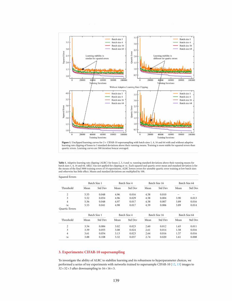
Mach. Learn.: Sci. Technol. 1 (2020) 015011 J M Ede and R Beanland
Figure 1. Unclipped learning curves for 2× CIFAR-10 supersampling with batch sizes 1, 4, 16 and 64 with and without adaptivelearning rate clipping of losses to 3 standard deviations above their running means. Training is more stable for squared errors thanquartic errors. Learning curves are 500 iteration boxcar averaged.
Table 1. Adaptive learning rate clipping (ALRC) for losses 2, 3, 4 and∞ running standard deviations above their running means forbatch sizes 1, 4, 16 and 64. ARLC was not applied for clipping at∞. Each squared and quartic error mean and standard deviation is forthe means of the final 5000 training errors of 10 experiments. ALRC lowers errors for unstable quartic error training at low batch sizesand otherwise has little effect. Means and standard deviations are multiplied by 100.
Squared Errors
Batch Size 1 Batch Size 4 Batch Size 16 Batch Size 64
Threshold Mean Std Dev Mean Std Dev Mean Std Dev Mean Std Dev
2 5.55 0.048 4.96 0.016 4.58 0.010 − −3 5.52 0.054 4.96 0.029 4.58 0.004 3.90 0.0134 5.56 0.048 4.97 0.017 4.58 0.007 3.89 0.016∞ 5.55 0.041 4.98 0.017 4.59 0.006 3.89 0.014
Quartic Errors
Batch Size 1 Batch Size 4 Batch Size 16 Batch Size 64
Threshold Mean Std Dev Mean Std Dev Mean Std Dev Mean Std Dev
2 3.54 0.084 3.02 0.023 2.60 0.012 1.65 0.0113 3.59 0.055 3.08 0.024 2.61 0.014 1.58 0.0164 3.61 0.054 3.13 0.023 2.64 0.016 1.57 0.016∞ 3.88 0.108 3.32 0.037 2.74 0.020 1.61 0.008
3. Experiments: CIFAR-10 supersampling
To investigate the ability of ALRC to stabilize learning and its robustness to hyperparameter choices, weperformed a series of toy experiments with networks trained to supersample CIFAR-10 [12, 13] images to32×32×3 after downsampling to 16×16×3.
3
139
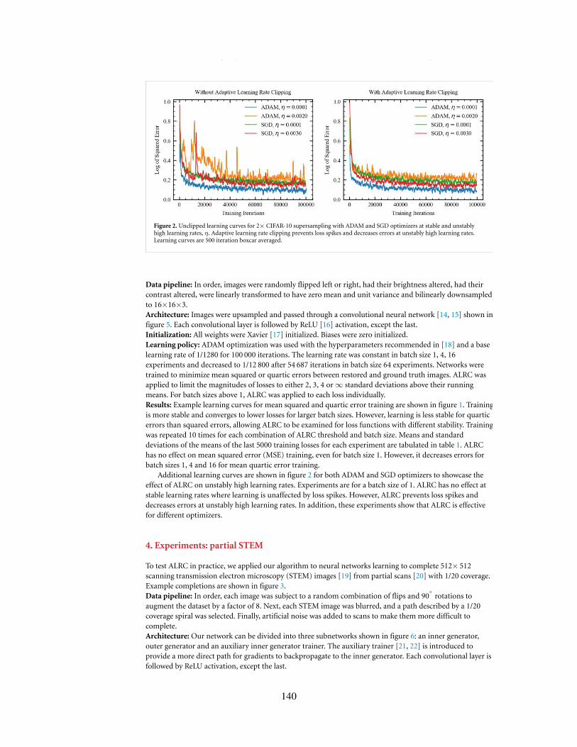
Mach. Learn.: Sci. Technol. 1 (2020) 015011 J M Ede and R Beanland
Figure 2. Unclipped learning curves for 2× CIFAR-10 supersampling with ADAM and SGD optimizers at stable and unstablyhigh learning rates, η. Adaptive learning rate clipping prevents loss spikes and decreases errors at unstably high learning rates.Learning curves are 500 iteration boxcar averaged.
Data pipeline: In order, images were randomly flipped left or right, had their brightness altered, had theircontrast altered, were linearly transformed to have zero mean and unit variance and bilinearly downsampledto 16×16×3.Architecture: Images were upsampled and passed through a convolutional neural network [14, 15] shown infigure 5. Each convolutional layer is followed by ReLU [16] activation, except the last.Initialization: All weights were Xavier [17] initialized. Biases were zero initialized.Learning policy: ADAM optimization was used with the hyperparameters recommended in [18] and a baselearning rate of 1/1280 for 100 000 iterations. The learning rate was constant in batch size 1, 4, 16experiments and decreased to 1/12 800 after 54 687 iterations in batch size 64 experiments. Networks weretrained to minimize mean squared or quartic errors between restored and ground truth images. ALRC wasapplied to limit the magnitudes of losses to either 2, 3, 4 or∞ standard deviations above their runningmeans. For batch sizes above 1, ALRC was applied to each loss individually.Results: Example learning curves for mean squared and quartic error training are shown in figure 1. Trainingis more stable and converges to lower losses for larger batch sizes. However, learning is less stable for quarticerrors than squared errors, allowing ALRC to be examined for loss functions with different stability. Trainingwas repeated 10 times for each combination of ALRC threshold and batch size. Means and standarddeviations of the means of the last 5000 training losses for each experiment are tabulated in table 1. ALRChas no effect on mean squared error (MSE) training, even for batch size 1. However, it decreases errors forbatch sizes 1, 4 and 16 for mean quartic error training.
Additional learning curves are shown in figure 2 for both ADAM and SGD optimizers to showcase theeffect of ALRC on unstably high learning rates. Experiments are for a batch size of 1. ALRC has no effect atstable learning rates where learning is unaffected by loss spikes. However, ALRC prevents loss spikes anddecreases errors at unstably high learning rates. In addition, these experiments show that ALRC is effectivefor different optimizers.
4. Experiments: partial STEM
To test ALRC in practice, we applied our algorithm to neural networks learning to complete 512× 512scanning transmission electron microscopy (STEM) images [19] from partial scans [20] with 1/20 coverage.Example completions are shown in figure 3.Data pipeline: In order, each image was subject to a random combination of flips and 90
rotations to
augment the dataset by a factor of 8. Next, each STEM image was blurred, and a path described by a 1/20coverage spiral was selected. Finally, artificial noise was added to scans to make them more difficult tocomplete.Architecture: Our network can be divided into three subnetworks shown in figure 6: an inner generator,outer generator and an auxiliary inner generator trainer. The auxiliary trainer [21, 22] is introduced toprovide a more direct path for gradients to backpropagate to the inner generator. Each convolutional layer isfollowed by ReLU activation, except the last.
4
140
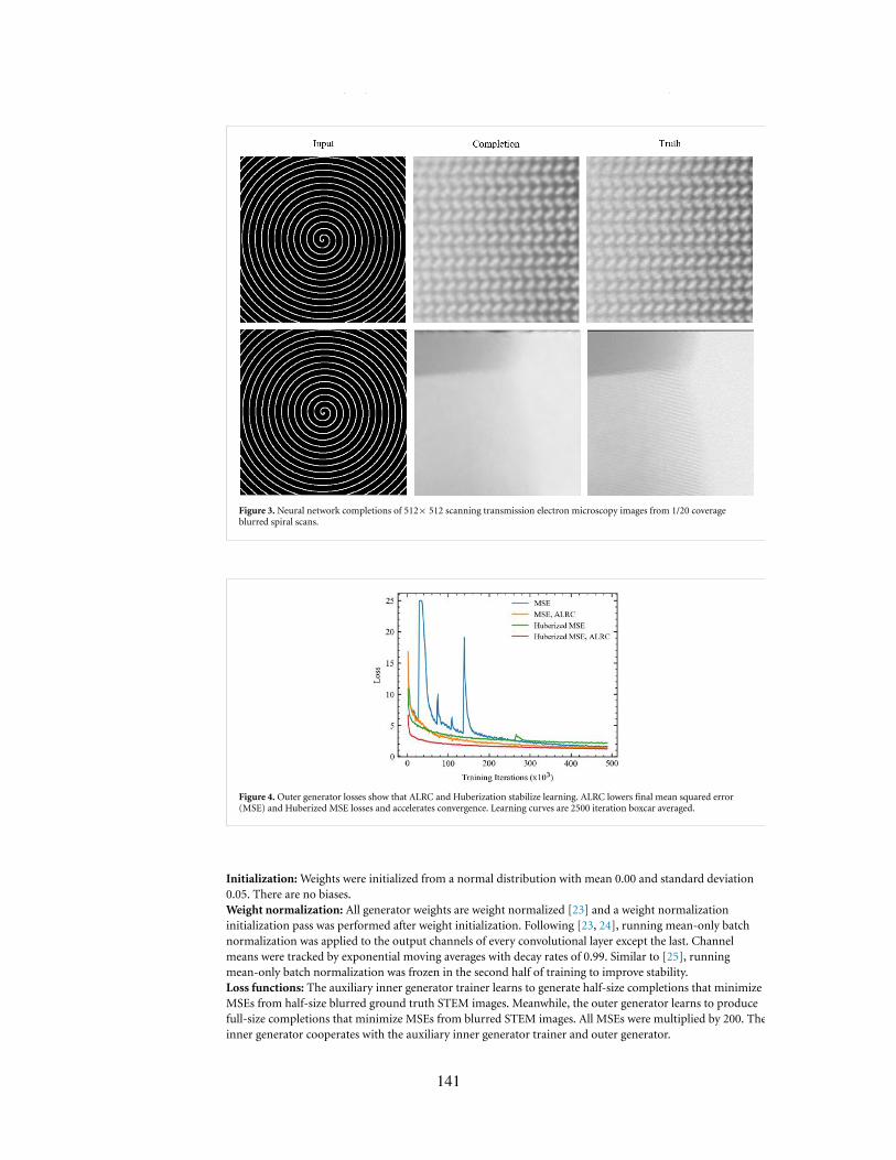
Mach. Learn.: Sci. Technol. 1 (2020) 015011 J M Ede and R Beanland
Figure 3. Neural network completions of 512× 512 scanning transmission electron microscopy images from 1/20 coverageblurred spiral scans.
Figure 4. Outer generator losses show that ALRC and Huberization stabilize learning. ALRC lowers final mean squared error(MSE) and Huberized MSE losses and accelerates convergence. Learning curves are 2500 iteration boxcar averaged.
Initialization:Weights were initialized from a normal distribution with mean 0.00 and standard deviation0.05. There are no biases.Weight normalization: All generator weights are weight normalized [23] and a weight normalizationinitialization pass was performed after weight initialization. Following [23, 24], running mean-only batchnormalization was applied to the output channels of every convolutional layer except the last. Channelmeans were tracked by exponential moving averages with decay rates of 0.99. Similar to [25], runningmean-only batch normalization was frozen in the second half of training to improve stability.Loss functions: The auxiliary inner generator trainer learns to generate half-size completions that minimizeMSEs from half-size blurred ground truth STEM images. Meanwhile, the outer generator learns to producefull-size completions that minimize MSEs from blurred STEM images. All MSEs were multiplied by 200. Theinner generator cooperates with the auxiliary inner generator trainer and outer generator.
5
141

Mach. Learn.: Sci. Technol. 1 (2020) 015011 J M Ede and R Beanland
Table 2.Means and standard deviations of 20 000 unclipped test set MSEs for STEM supersampling networks trained with variouslearning rate clipping algorithms and clipping hyperparameters, n↑ and n↓, above and below, respectively.
Algorithm n↓ n↑ Mean Std
Unchanged ∞ ∞ 0.95 1.33ALRC ∞ 3 0.89 1.68ALRC 3 3 0.92 1.77CLRC(↓), ALRC(↑) 1 3 0.95 2.30DALRC 3 3 0.93 1.57DALRC ∞ 2 0.89 1.51DALRC 2 2 0.91 1.34DALRC 1 2 0.91 1.54
To benchmark ALRC, we investigated training with MSEs, Huberized (h= 1) MSEs, MSEs with ALRCand Huberized (h= 1) MSEs with ALRC before Huberization. Training with both ALRC and Hubarizationshowcases the ability of ALRC to complement another loss function modification.Learning policy: ADAM optimization [18] was used with a constant generator learning rate of 0.0003 and afirst moment of the momentum decay rate, β1 = 0.9, for 250 000 iterations. In the next 250 000 iterations,the learning rate and β1 were linearly decayed in eight steps to zero and 0.5, respectively. The learning rate forthe auxiliary inner generator trainer was two times the generator learning rate; β1 were the same. All trainingwas performed with batch size 1 due to the large model size needed to complete 512× 512 scans.Results: Outer generator losses in figure 4 show that ALRC and Huberization stabilize learning. Further,ALRC accelerates MSE and Huberized MSE convergence to lower losses. To be clear, learning policy wasoptimized for MSE training so direct loss comparison is uncharitable to ALRC.
Algorithm 2 Two-sided constant learning rate clipping (CLRC) to effective losses in [Lmin, Lmax].
Choose effective loss bounds, Lmin and Lmax.While Training is not finished doIf L< Lmin thenLdyn← stop_gradient(Lmin/L)Lelse if L> Lmax thenLdyn← stop_gradient(Lmax/L)LelseLdyn← Lend ifOptimize network by back-propagating Ldyn.
endWhile
Algorithm 3 Two-sided doubly adaptive learning rate clipping (DALRC) of loss spikes. Sensible parameters areβ1 = β↓ = β↑ = 0.999, and n↓ = n↑ = 2.
Initialize running means, µ1, µ↓ and µ↑, with decay rates, β1, β
↓ and β↑.Choose numbers, n, of standard deviations to clip to.While Training is not finisheddoInfer forward-propagation loss, L.Lmin← µ1− n↓µ↓
Lmax← µ1 + n↑µ↑
if L< Lmin thenLdyn← stop_gradient(Lmin/L)Lelse if L> Lmax thenLdyn← stop_gradient(Lmax/L)LelseLdyn← Lend ifOptimize network by back-propagating Ldyn.if L>µ1 thenµ↑← β↑µ↑ +(1−β↑)(L−µ1)else if L<µ1 thenµ↓← β↓µ↓ +(1−β↓)(µ1− L)end ifµ1← β1µ1 +(1−β1)L
endWhile
6
142
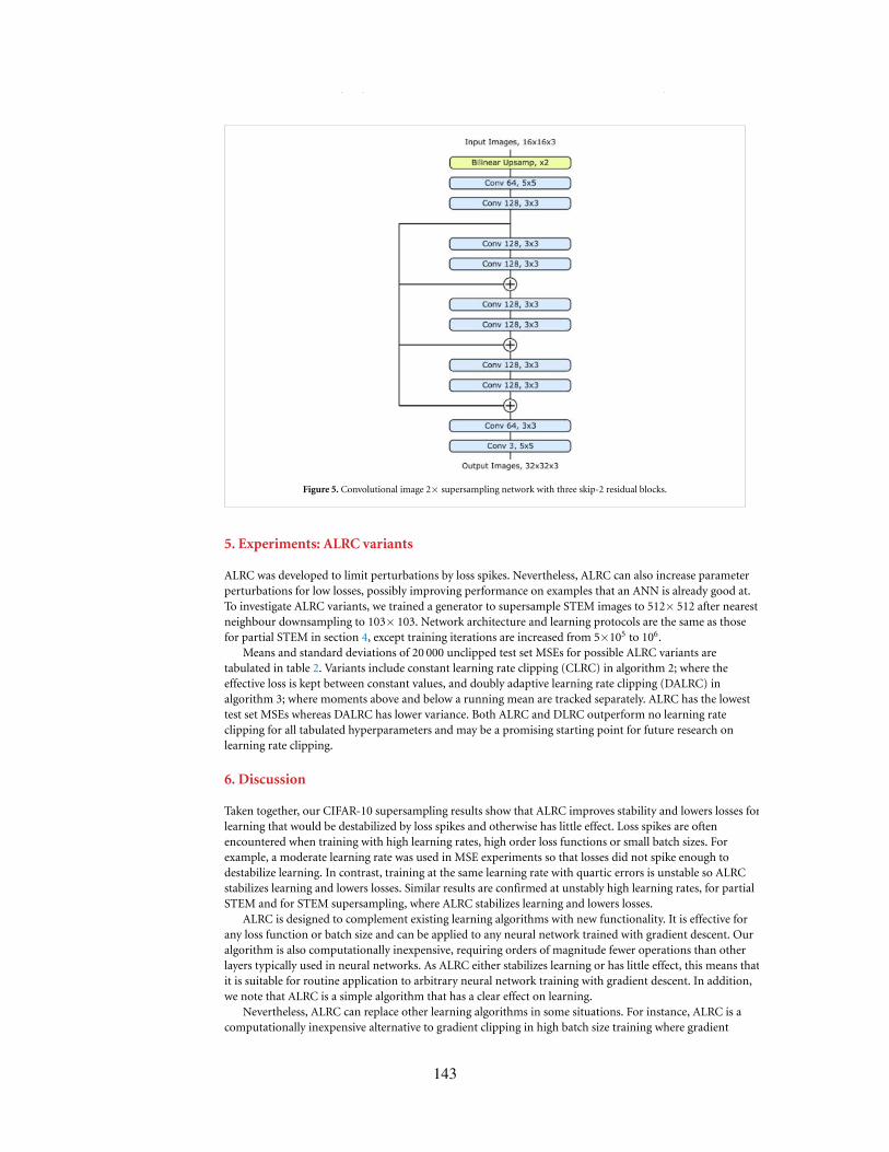
Mach. Learn.: Sci. Technol. 1 (2020) 015011 J M Ede and R Beanland
Figure 5. Convolutional image 2× supersampling network with three skip-2 residual blocks.
5. Experiments: ALRC variants
ALRC was developed to limit perturbations by loss spikes. Nevertheless, ALRC can also increase parameterperturbations for low losses, possibly improving performance on examples that an ANN is already good at.To investigate ALRC variants, we trained a generator to supersample STEM images to 512× 512 after nearestneighbour downsampling to 103× 103. Network architecture and learning protocols are the same as thosefor partial STEM in section 4, except training iterations are increased from 5×10⁵ to 106.
Means and standard deviations of 20 000 unclipped test set MSEs for possible ALRC variants aretabulated in table 2. Variants include constant learning rate clipping (CLRC) in algorithm 2; where theeffective loss is kept between constant values, and doubly adaptive learning rate clipping (DALRC) inalgorithm 3; where moments above and below a running mean are tracked separately. ALRC has the lowesttest set MSEs whereas DALRC has lower variance. Both ALRC and DLRC outperform no learning rateclipping for all tabulated hyperparameters and may be a promising starting point for future research onlearning rate clipping.
6. Discussion
Taken together, our CIFAR-10 supersampling results show that ALRC improves stability and lowers losses forlearning that would be destabilized by loss spikes and otherwise has little effect. Loss spikes are oftenencountered when training with high learning rates, high order loss functions or small batch sizes. Forexample, a moderate learning rate was used in MSE experiments so that losses did not spike enough todestabilize learning. In contrast, training at the same learning rate with quartic errors is unstable so ALRCstabilizes learning and lowers losses. Similar results are confirmed at unstably high learning rates, for partialSTEM and for STEM supersampling, where ALRC stabilizes learning and lowers losses.
ALRC is designed to complement existing learning algorithms with new functionality. It is effective forany loss function or batch size and can be applied to any neural network trained with gradient descent. Ouralgorithm is also computationally inexpensive, requiring orders of magnitude fewer operations than otherlayers typically used in neural networks. As ALRC either stabilizes learning or has little effect, this means thatit is suitable for routine application to arbitrary neural network training with gradient descent. In addition,we note that ALRC is a simple algorithm that has a clear effect on learning.
Nevertheless, ALRC can replace other learning algorithms in some situations. For instance, ALRC is acomputationally inexpensive alternative to gradient clipping in high batch size training where gradient
7
143
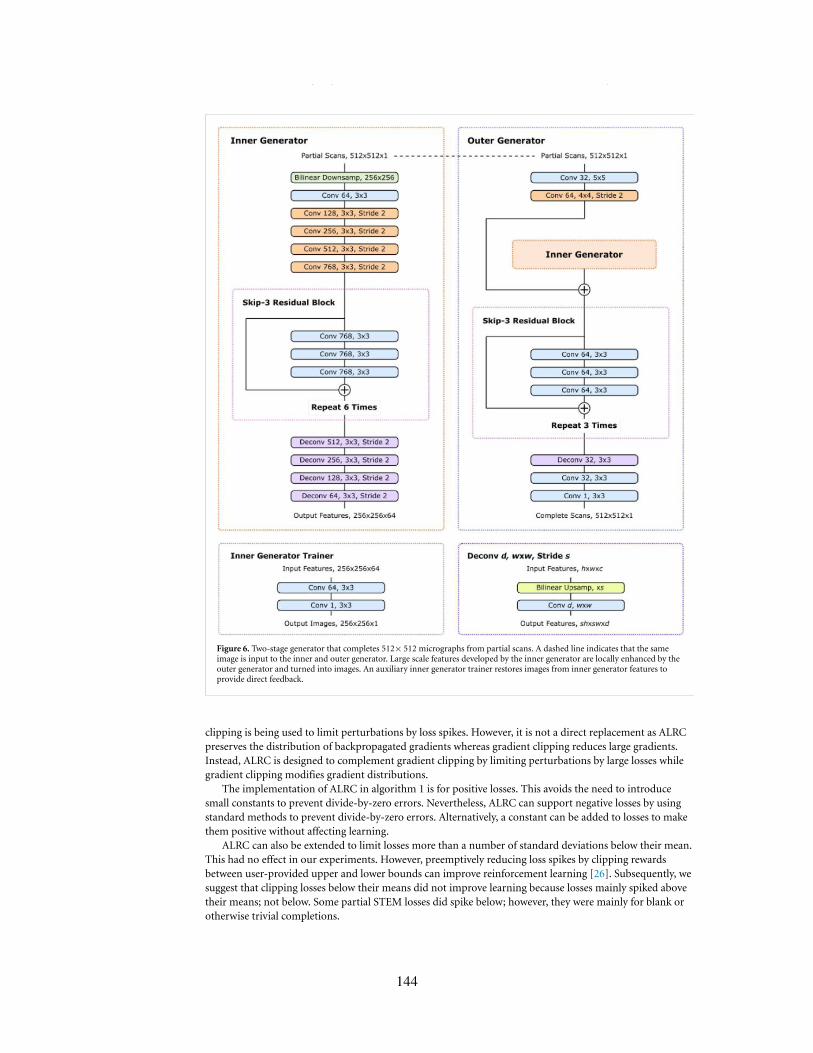
Mach. Learn.: Sci. Technol. 1 (2020) 015011 J M Ede and R Beanland
Figure 6. Two-stage generator that completes 512× 512 micrographs from partial scans. A dashed line indicates that the sameimage is input to the inner and outer generator. Large scale features developed by the inner generator are locally enhanced by theouter generator and turned into images. An auxiliary inner generator trainer restores images from inner generator features toprovide direct feedback.
clipping is being used to limit perturbations by loss spikes. However, it is not a direct replacement as ALRCpreserves the distribution of backpropagated gradients whereas gradient clipping reduces large gradients.Instead, ALRC is designed to complement gradient clipping by limiting perturbations by large losses whilegradient clipping modifies gradient distributions.
The implementation of ALRC in algorithm 1 is for positive losses. This avoids the need to introducesmall constants to prevent divide-by-zero errors. Nevertheless, ALRC can support negative losses by usingstandard methods to prevent divide-by-zero errors. Alternatively, a constant can be added to losses to makethem positive without affecting learning.
ALRC can also be extended to limit losses more than a number of standard deviations below their mean.This had no effect in our experiments. However, preemptively reducing loss spikes by clipping rewardsbetween user-provided upper and lower bounds can improve reinforcement learning [26]. Subsequently, wesuggest that clipping losses below their means did not improve learning because losses mainly spiked abovetheir means; not below. Some partial STEM losses did spike below; however, they were mainly for blank orotherwise trivial completions.
8
144
Mach. Learn.: Sci. Technol. 1 (2020) 015011 J M Ede and R Beanland
7. Conclusions
We have developed ALRC to stabilize the training of ANNs by limiting backpropagated loss perturbations.Our experiments show that ALRC accelerates convergence and lowers losses for learning that would bedestabilized by loss spikes and otherwise has little effect. Further, ALRC is computationally inexpensive, canbe applied to any loss function or batch size, does not affect the distribution of backpropagated gradients andhas a clear effect on learning. Overall, ALRC complements existing learning algorithms and can be routinelyapplied to arbitrary neural network training with gradient descent.
Data Availability
The data that support the findings of this study are openly available. Source code based on TensorFlow[27] isprovided for CIFAR-10 supersampling[28] and partial STEM[29], and both CIFAR-10[12] and STEM[19]datasets are available. For additional information contact the corresponding author (J M E ).
8. Network architecture
ANN architecture for CIFAR-10 experiments is shown in figure 5, and architecture for STEM partial scanand supersampling experiments is shown in figure 6. The components in our networks areBilinear Downsamp,wxw: This is an extension of linear interpolation in one dimension to two dimensions.It is used to downsample images to w×w.Bilinear Upsamp, xs: This is an extension of linear interpolation in one dimension to two dimensions. It isused to upsample images by a factor of s.Conv d,wxw, Stride, x: Convolutional layer with a square kernel of width, w, that outputs d feature channels.If the stride is specified, convolutions are only applied to every xth spatial element of their input, rather thanto every element. Striding is not applied depthwise.+⃝: Circled plus signs indicate residual connections[30] where tensors are added together. Residualconnections help reduce signal attenuation and allow networks to learn perturbative transformations moreeasily.
Acknowledgment
J M E and R B acknowledge EPSRC grant EP/N035437/1 for financial support. In addition, J M Eacknowledges EPSRC Studentship 1917382.
ORCID iD
Jeffrey M Ede https://orcid.org/0000-0002-9358-5364
References
[1] Ruder S 2016 An overview of gradient descent optimization algorithms arXiv:1609.04747[2] Zou D, Cao Y, Zhou D and Gu Q 2018 Stochastic gradient descent optimizes over-parameterized deep ReLU networks
arXiv:1811.08888[3] Pfülb B, Gepperth A, Abdullah S and Kilian A 2018 Catastrophic forgetting: still a problem for DNNs Int. Conf. on Artificial Neural
Networks pp 487–97 Springer[4] Boue L 2018 Deep learning for pedestrians: backpropagation in CNNs arXiv:1811.11987[5] Qin Z, Yu F, Liu C and Chen X 2018 How convolutional neural network see the world-A survey of convolutional neural network
visualization methods arXiv:1804.11191[6] Sabour S, Frosst N and Hinton G E 2017 Dynamic routing between capsules Advances in Neural Information Processing Systems pp
3856–66[7] Bengio Y and Pascanu R 2012 On the difficulty of training recurrent neural networks arXiv:1211.5063[8] Mikolov T 2012 Statistical language models based on neural networks PhD thesis Brno University of Technology[9] Huber P J 1964 Robust estimation of a location parameter The Annals of Mathematical Statistics pp 73–101[10] Meyer G P 2019 An alternative probabilistic interpretation of the Huber loss arXiv:1911.02088[11] Ioffe S and Szegedy C 2015 Batch normalization accelerating deep network training by reducing internal covariate shift
arXiv:1502.03167[12] Krizhevsky A, Nair V and Hinton G 2014 The CIFAR-10 dataset Online (www.cs.toronto.edu/ Kriz/Cifar.html) vol 55[13] Krizhevsky A and Hinton G 2009 Learning multiple layers of features from tiny images Technical Report TR-2009 University of
Toronto[14] McCann M T, Jin K H and Unser M 2017 Convolutional neural networks for inverse problems in imaging: A review IEEE Signal
Process. Mag. 34 85–95[15] Krizhevsky A, Sutskever I and Hinton G E 2012 ImageNet classification with deep convolutional neural networks Advances in
Neural Information Processing Systems pp 1097–105
9
145
Mach. Learn.: Sci. Technol. 1 (2020) 015011 J M Ede and R Beanland
[16] Nair V and Hinton G E 2010 Rectified linear units improve restricted Boltzmann machines in Proc. of the 27th Int. Conf. onMachine Learning (ICML-10) pp 807–14
[17] Glorot X and Bengio Y 2010 Understanding the difficulty of training deep feedforward neural networks Proc. of the Thirteenth Int.Conf. on Artificial Intelligence and Statistics pp 249–56
[18] Kingma D P and Ba J 2014 ADAM: A method for stochastic optimization arXiv:1412.6980[19] Ede J M and STEM Crops Dataset 2019 Online
(https://warwick.ac.uk/fac/sci/physics/research/condensedmatt/microscopy/research/machinelearning)[20] Ede J M and Beanland R 2020 Partial scanning transmission electron microscopy with deep learning arXiv:1910.10467[21] Szegedy C, Liu W, Jia Y, Sermanet P, Reed S, Anguelov D, Erhan D, Vanhoucke V and Rabinovich A 2015 Going deeper with
convolutions Proc. of the Conf. on Computer Vision and Pattern Recognition pp 1–9[22] Szegedy C, Vanhoucke V, Ioffe S, Shlens J and Wojna Z 2016 Rethinking the inception architecture for computer vision Proc. of the
IEEE Conference on Computer Vision and Pattern Recognition pp 2818–26[23] Salimans T and Kingma D P 2016 Weight normalization: A simple reparameterization to accelerate training of deep neural
networks Advances in Neural Information Processing Systems pp 901–9[24] Hoffer E, Banner R, Golan I and Soudry D 2018 Norm matters: efficient and accurate normalization schemes in deep networks
Advances in Neural Information Processing Systems pp 2160–70[25] Chen L-C, Papandreou G, Schroff F and Adam H 2017 Rethinking atrous convolution for semantic image segmentation
arXiv:1706.05587[26] Mnih V et al et al 2015 Human-Level control through deep reinforcement learning Nature 518 529[27] Abadi M et al et al 2016 Tensor flow: A system for large-scale machine learning. OSDI 16 265–83[28] Ede J M and ALRC 2020 Online: (https://github.com/Jeffrey-Ede/ALRC)[29] Ede J M and Partial STEM 2020 Online: (https://github.com/Jeffrey-Ede/partial-STEM)[30] He K, Zhang X, Ren S and Sun J 2016 Deep residual learning for image recognition Proc. of the Conf. on Computer Vision and
Pattern Recognition pp 770–8
10
146
3.2 Amendments and Corrections
There are amendments or corrections to the paper3 covered by this chapter.
Location: Page 3, image in fig. 1.
Change: A title above the top two graphs is cut off. The missing title said “With Adaptive Learning Rate Clipping”,
and is visible in our preprint16.
Location: Last paragraph starting on page 7.
Change: “...inexpensive alternative to gradient clipping in high batch size training where...” should say “...inexpen-
sive alternative to gradient clipping where...”.
3.3 Reflection
This ancillary chapter covers my paper titled “Adaptive Learning Rate Clipping Stabilizes Learning”3 and associated
research outputs16,17. The ALRC algorithm was developed to prevent loss spikes destabilizing training of DNNs
for partial STEM4 (ch. 4). To fit the partial STEM ANN in GPU memory, it was trained with a batch size of 1.
However, using a small batch size results in occasional loss spikes, which meant that it was sometimes necessary to
repeat training to compare performance with earlier experiments where learning had not been destabilized by loss
spikes. I expected that I could adjust training hyperparameters to stabilize learning; however, I had optimized the
hyperparameters and training was usually fine. Thus, I developed ALRC to prevent loss spikes from destabilizing
learning. Initially, ALRC was included as an appendix in the first version of the partial STEM preprint18. However,
ALRC was so effective that I continued to investigate. Eventually, there were too many ALRC experiments to
comfortably fit in an appendix of the partial STEM paper, so I separated ALRC into its own paper.
There are variety of alternatives to ALRC that can stabilize learning. A popular alternative is training with
Huberized losses181,182,
Huber(L) = min(L, (λL)1/2) , (3.1)
where L is a loss and λ is a training hyperparameter. However, I found that Huberized learning continued to be
destabilized by loss spikes. I also considered gradient clipping183–185. However, my DNNs for partial STEM have
many millions of trainable parameters, so computational requirements for gradient clipping are millions of times
higher than applying ALRC to losses. Similarly, rectified ADAM186 (RADAM), can stabilize learning by decreasing
trainable parameter learning rates if adaptive learning rates of an ADAM187 optimizer have high variance. However,
computational requirements of RADAM are also often millions of times higher than ALRC as RADAM adapts
adaptive learning rates for every trainable parameter.
Overall, I think that ALRC merits further investigation. ALRC is computationally inexpensive, can be applied to
any loss function, and appears to either stabilize learning or have no significant effect. Further, ALRC can often
readily improve ANN training that would otherwise be destabilized loss spikes. However, I suspect that ALRC may
slightly decrease performance where learning is not destabilized by loss spikes as ALRC modifies training losses. In
addition, I have only investigated applications of ALRC to mean square and quartic errors per training example of
deep convolutional neural networks (CNNs). Applying ALRC to losses for individual pixels of CNN outputs or
to losses at each step of a recurrent neural network (RNN) may further improve performance. Encouragingly, my
147

initial experiments with ALRC variants3 show that a variety approaches improve training that would otherwise be
destabilized by loss spikes.
148

Chapter 4
Partial Scanning Transmission ElectronMicroscopy with Deep Learning
4.1 Scientific Paper
This chapter covers the following paper4 and its supplementary information10.
J. M. Ede and R. Beanland. Partial Scanning transmission Electron Microscopy with Deep Learning.
Scientific Reports, 10(1):1–10, 2020
J. M. Ede. Supplementary Information: Partial Scanning Transmission Electron Microscopy with Deep
Learning. Online: https://static-content.springer.com/esm/art%3A10.1038%
2Fs41598-020-65261-0/MediaObjects/41598 2020 65261 MOESM1 ESM.pdf, 2020
149
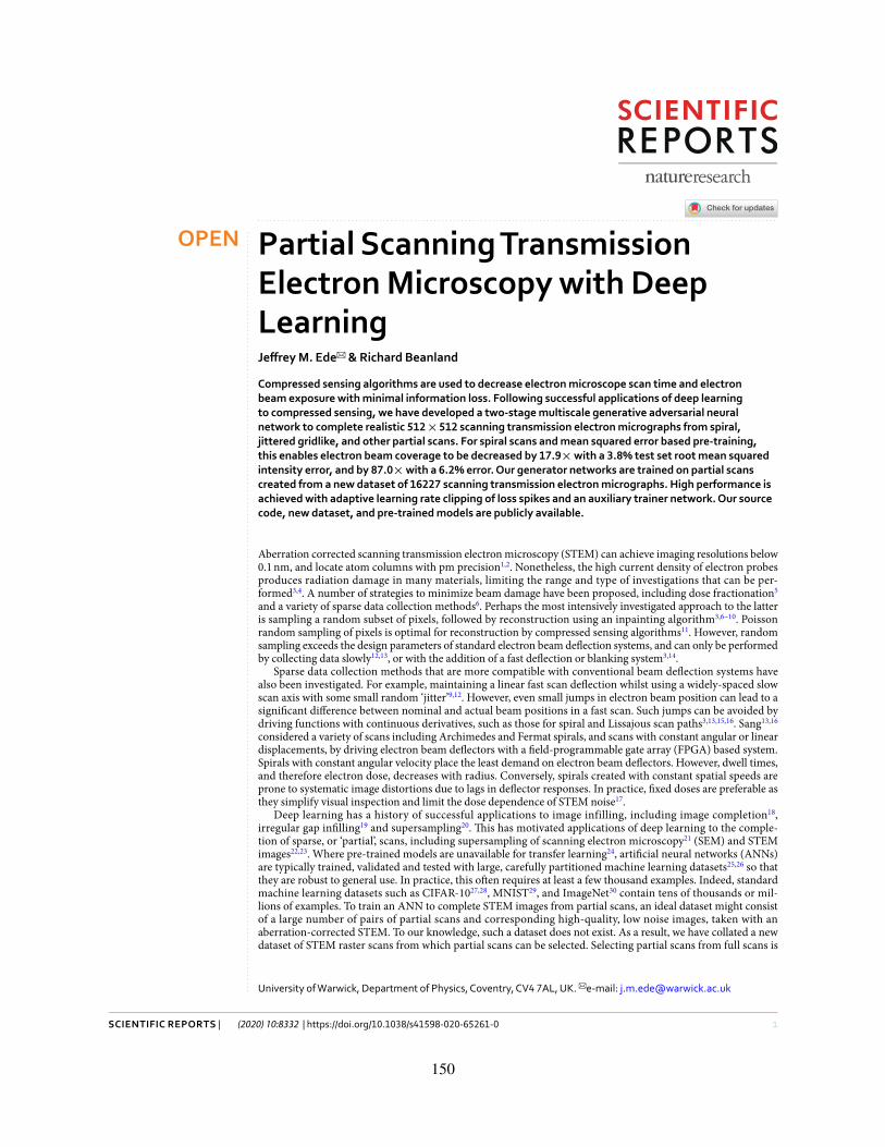
1Scientific RepoRtS | (2020) 10:8332 | https://doi.org/10.1038/s41598-020-65261-0
www.nature.com/scientificreports
partial Scanning transmission electron Microscopy with Deep LearningJeffrey M. ede & Richard Beanland
compressed sensing algorithms are used to decrease electron microscope scan time and electron beam exposure with minimal information loss. Following successful applications of deep learning to compressed sensing, we have developed a two-stage multiscale generative adversarial neural network to complete realistic 512 × 512 scanning transmission electron micrographs from spiral, jittered gridlike, and other partial scans. For spiral scans and mean squared error based pre-training, this enables electron beam coverage to be decreased by 17.9× with a 3.8% test set root mean squared intensity error, and by 87.0× with a 6.2% error. Our generator networks are trained on partial scans created from a new dataset of 16227 scanning transmission electron micrographs. High performance is achieved with adaptive learning rate clipping of loss spikes and an auxiliary trainer network. Our source code, new dataset, and pre-trained models are publicly available.
Aberration corrected scanning transmission electron microscopy (STEM) can achieve imaging resolutions below 0.1 nm, and locate atom columns with pm precision1,2. Nonetheless, the high current density of electron probes produces radiation damage in many materials, limiting the range and type of investigations that can be per-formed3,4. A number of strategies to minimize beam damage have been proposed, including dose fractionation5 and a variety of sparse data collection methods6. Perhaps the most intensively investigated approach to the latter is sampling a random subset of pixels, followed by reconstruction using an inpainting algorithm3,6–10. Poisson random sampling of pixels is optimal for reconstruction by compressed sensing algorithms11. However, random sampling exceeds the design parameters of standard electron beam deflection systems, and can only be performed by collecting data slowly12,13, or with the addition of a fast deflection or blanking system3,14.
Sparse data collection methods that are more compatible with conventional beam deflection systems have also been investigated. For example, maintaining a linear fast scan deflection whilst using a widely-spaced slow scan axis with some small random ‘jitter’9,12. However, even small jumps in electron beam position can lead to a significant difference between nominal and actual beam positions in a fast scan. Such jumps can be avoided by driving functions with continuous derivatives, such as those for spiral and Lissajous scan paths3,13,15,16. Sang13,16 considered a variety of scans including Archimedes and Fermat spirals, and scans with constant angular or linear displacements, by driving electron beam deflectors with a field-programmable gate array (FPGA) based system. Spirals with constant angular velocity place the least demand on electron beam deflectors. However, dwell times, and therefore electron dose, decreases with radius. Conversely, spirals created with constant spatial speeds are prone to systematic image distortions due to lags in deflector responses. In practice, fixed doses are preferable as they simplify visual inspection and limit the dose dependence of STEM noise17.
Deep learning has a history of successful applications to image infilling, including image completion18, irregular gap infilling19 and supersampling20. This has motivated applications of deep learning to the comple-tion of sparse, or ‘partial’, scans, including supersampling of scanning electron microscopy21 (SEM) and STEM images22,23. Where pre-trained models are unavailable for transfer learning24, artificial neural networks (ANNs) are typically trained, validated and tested with large, carefully partitioned machine learning datasets25,26 so that they are robust to general use. In practice, this often requires at least a few thousand examples. Indeed, standard machine learning datasets such as CIFAR-1027,28, MNIST29, and ImageNet30 contain tens of thousands or mil-lions of examples. To train an ANN to complete STEM images from partial scans, an ideal dataset might consist of a large number of pairs of partial scans and corresponding high-quality, low noise images, taken with an aberration-corrected STEM. To our knowledge, such a dataset does not exist. As a result, we have collated a new dataset of STEM raster scans from which partial scans can be selected. Selecting partial scans from full scans is
University of Warwick, Department of Physics, Coventry, CV4 7AL, UK. e-mail: [email protected]
open
150
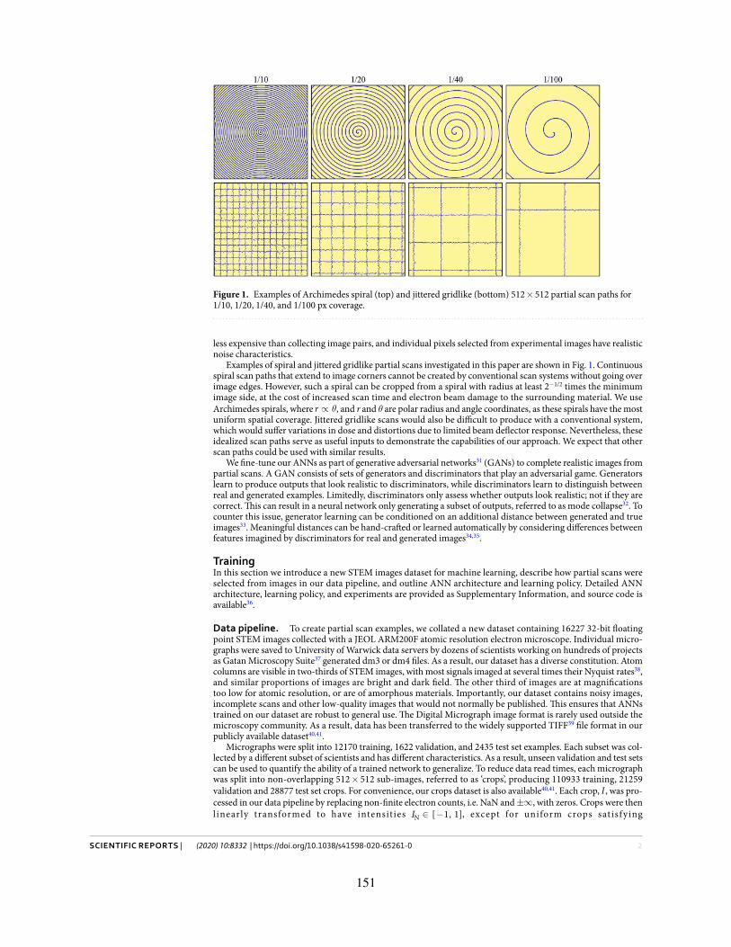
2Scientific RepoRtS | (2020) 10:8332 | https://doi.org/10.1038/s41598-020-65261-0
www.nature.com/scientificreportswww.nature.com/scientificreports/
less expensive than collecting image pairs, and individual pixels selected from experimental images have realistic noise characteristics.
Examples of spiral and jittered gridlike partial scans investigated in this paper are shown in Fig. 1. Continuous spiral scan paths that extend to image corners cannot be created by conventional scan systems without going over image edges. However, such a spiral can be cropped from a spiral with radius at least 2−1/2 times the minimum image side, at the cost of increased scan time and electron beam damage to the surrounding material. We use Archimedes spirals, where θ∝r , and r and θ are polar radius and angle coordinates, as these spirals have the most uniform spatial coverage. Jittered gridlike scans would also be difficult to produce with a conventional system, which would suffer variations in dose and distortions due to limited beam deflector response. Nevertheless, these idealized scan paths serve as useful inputs to demonstrate the capabilities of our approach. We expect that other scan paths could be used with similar results.
We fine-tune our ANNs as part of generative adversarial networks31 (GANs) to complete realistic images from partial scans. A GAN consists of sets of generators and discriminators that play an adversarial game. Generators learn to produce outputs that look realistic to discriminators, while discriminators learn to distinguish between real and generated examples. Limitedly, discriminators only assess whether outputs look realistic; not if they are correct. This can result in a neural network only generating a subset of outputs, referred to as mode collapse32. To counter this issue, generator learning can be conditioned on an additional distance between generated and true images33. Meaningful distances can be hand-crafted or learned automatically by considering differences between features imagined by discriminators for real and generated images34,35.
trainingIn this section we introduce a new STEM images dataset for machine learning, describe how partial scans were selected from images in our data pipeline, and outline ANN architecture and learning policy. Detailed ANN architecture, learning policy, and experiments are provided as Supplementary Information, and source code is available36.
Data pipeline. To create partial scan examples, we collated a new dataset containing 16227 32-bit floating point STEM images collected with a JEOL ARM200F atomic resolution electron microscope. Individual micro-graphs were saved to University of Warwick data servers by dozens of scientists working on hundreds of projects as Gatan Microscopy Suite37 generated dm3 or dm4 files. As a result, our dataset has a diverse constitution. Atom columns are visible in two-thirds of STEM images, with most signals imaged at several times their Nyquist rates38, and similar proportions of images are bright and dark field. The other third of images are at magnifications too low for atomic resolution, or are of amorphous materials. Importantly, our dataset contains noisy images, incomplete scans and other low-quality images that would not normally be published. This ensures that ANNs trained on our dataset are robust to general use. The Digital Micrograph image format is rarely used outside the microscopy community. As a result, data has been transferred to the widely supported TIFF39 file format in our publicly available dataset40,41.
Micrographs were split into 12170 training, 1622 validation, and 2435 test set examples. Each subset was col-lected by a different subset of scientists and has different characteristics. As a result, unseen validation and test sets can be used to quantify the ability of a trained network to generalize. To reduce data read times, each micrograph was split into non-overlapping 512 × 512 sub-images, referred to as ‘crops’, producing 110933 training, 21259 validation and 28877 test set crops. For convenience, our crops dataset is also available40,41. Each crop, I , was pro-cessed in our data pipeline by replacing non-finite electron counts, i.e. NaN and ±∞, with zeros. Crops were then l inearly transformed to have intensit ies ∈ −I [ 1, 1]N , except for uniform crops sat isfying
Figure 1. Examples of Archimedes spiral (top) and jittered gridlike (bottom) 512 × 512 partial scan paths for 1/10, 1/20, 1/40, and 1/100 px coverage.
151
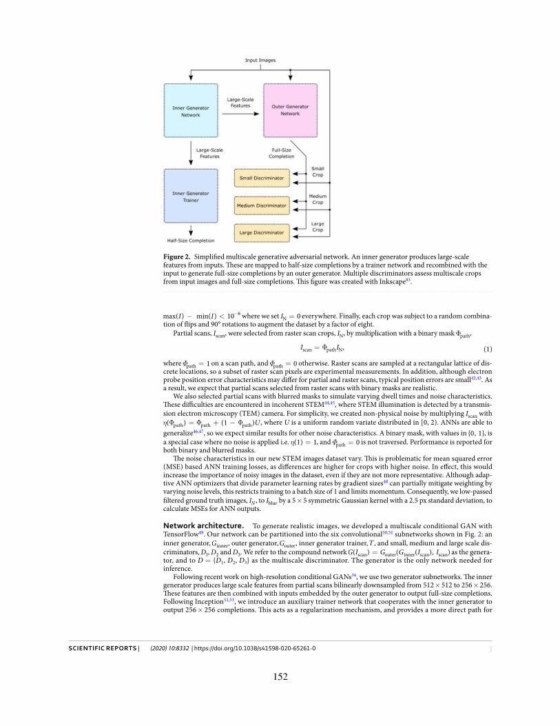
3Scientific RepoRtS | (2020) 10:8332 | https://doi.org/10.1038/s41598-020-65261-0
www.nature.com/scientificreportswww.nature.com/scientificreports/
− < −I Imax( ) min( ) 10 6 where we set =I 0N everywhere. Finally, each crop was subject to a random combina-tion of flips and 90° rotations to augment the dataset by a factor of eight.
Partial scans, Iscan, were selected from raster scan crops, IN, by multiplication with a binary mask Φpath,
= ΦI I , (1)scan path N
where Φ = 1path on a scan path, and Φ = 0path otherwise. Raster scans are sampled at a rectangular lattice of dis-crete locations, so a subset of raster scan pixels are experimental measurements. In addition, although electron probe position error characteristics may differ for partial and raster scans, typical position errors are small42,43. As a result, we expect that partial scans selected from raster scans with binary masks are realistic.
We also selected partial scans with blurred masks to simulate varying dwell times and noise characteristics. These difficulties are encountered in incoherent STEM44,45, where STEM illumination is detected by a transmis-sion electron microscopy (TEM) camera. For simplicity, we created non-physical noise by multiplying Iscan with
U( ) (1 )path path pathη Φ = Φ + − Φ , where U is a uniform random variate distributed in [0, 2). ANNs are able to generalize46,47, so we expect similar results for other noise characteristics. A binary mask, with values in 0, 1, is a special case where no noise is applied i.e. η =(1) 1, and Φ = 0path is not traversed. Performance is reported for both binary and blurred masks.
The noise characteristics in our new STEM images dataset vary. This is problematic for mean squared error (MSE) based ANN training losses, as differences are higher for crops with higher noise. In effect, this would increase the importance of noisy images in the dataset, even if they are not more representative. Although adap-tive ANN optimizers that divide parameter learning rates by gradient sizes48 can partially mitigate weighting by varying noise levels, this restricts training to a batch size of 1 and limits momentum. Consequently, we low-passed filtered ground truth images, IN , to Iblur by a 5 × 5 symmetric Gaussian kernel with a 2.5 px standard deviation, to calculate MSEs for ANN outputs.
Network architecture. To generate realistic images, we developed a multiscale conditional GAN with TensorFlow49. Our network can be partitioned into the six convolutional50,51 subnetworks shown in Fig. 2: an inner generator, Ginner, outer generator, Gouter, inner generator trainer, T , and small, medium and large scale dis-criminators, D1, D2 and D3. We refer to the compound network =G I G G I I( ) ( ( ), )scan outer inner scan scan as the genera-tor, and to D = D1, D2, D3 as the multiscale discriminator. The generator is the only network needed for inference.
Following recent work on high-resolution conditional GANs34, we use two generator subnetworks. The inner generator produces large scale features from partial scans bilinearly downsampled from 512 × 512 to 256 × 256. These features are then combined with inputs embedded by the outer generator to output full-size completions. Following Inception52,53, we introduce an auxiliary trainer network that cooperates with the inner generator to output 256 × 256 completions. This acts as a regularization mechanism, and provides a more direct path for
Figure 2. Simplified multiscale generative adversarial network. An inner generator produces large-scale features from inputs. These are mapped to half-size completions by a trainer network and recombined with the input to generate full-size completions by an outer generator. Multiple discriminators assess multiscale crops from input images and full-size completions. This figure was created with Inkscape83.
152
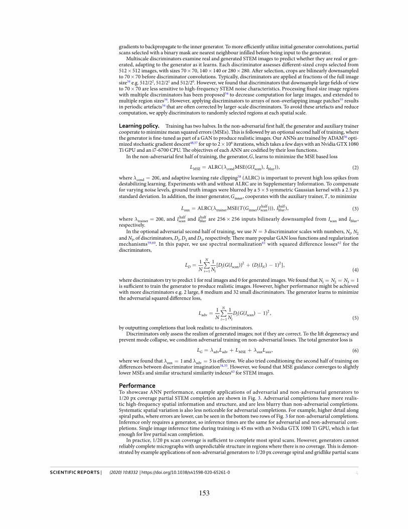
4Scientific RepoRtS | (2020) 10:8332 | https://doi.org/10.1038/s41598-020-65261-0
www.nature.com/scientificreportswww.nature.com/scientificreports/
gradients to backpropagate to the inner generator. To more efficiently utilize initial generator convolutions, partial scans selected with a binary mask are nearest neighbour infilled before being input to the generator.
Multiscale discriminators examine real and generated STEM images to predict whether they are real or gen-erated, adapting to the generator as it learns. Each discriminator assesses different-sized crops selected from 512 × 512 images, with sizes 70 × 70, 140 × 140 or 280 × 280. After selection, crops are bilinearly downsampled to 70 × 70 before discriminator convolutions. Typically, discriminators are applied at fractions of the full image size34 e.g. 512/22, 512/21 and 512/20. However, we found that discriminators that downsample large fields of view to 70 × 70 are less sensitive to high-frequency STEM noise characteristics. Processing fixed size image regions with multiple discriminators has been proposed54 to decrease computation for large images, and extended to multiple region sizes34. However, applying discriminators to arrays of non-overlapping image patches55 results in periodic artefacts34 that are often corrected by larger-scale discriminators. To avoid these artefacts and reduce computation, we apply discriminators to randomly selected regions at each spatial scale.
Learning policy. Training has two halves. In the non-adversarial first half, the generator and auxiliary trainer cooperate to minimize mean squared errors (MSEs). This is followed by an optional second half of training, where the generator is fine-tuned as part of a GAN to produce realistic images. Our ANNs are trained by ADAM56 opti-mized stochastic gradient descent48,57 for up to 2 × 10⁶ iterations, which takes a few days with an Nvidia GTX 1080 Ti GPU and an i7-6700 CPU. The objectives of each ANN are codified by their loss functions.
In the non-adversarial first half of training, the generator, G, learns to minimize the MSE based loss
λ=L G I IALRC( MSE( ( ), )), (2)MSE cond scan blur
where λ = 200cond , and adaptive learning rate clipping58 (ALRC) is important to prevent high loss spikes from destabilizing learning. Experiments with and without ALRC are in Supplementary Information. To compensate for varying noise levels, ground truth images were blurred by a 5 × 5 symmetric Gaussian kernel with a 2.5 px standard deviation. In addition, the inner generator, Ginner, cooperates with the auxiliary trainer, T , to minimize
λ=L T G I IALRC( MSE( ( ( ))), ), (3)aux trainer inner scanhalf
blurhalf
where λ = 200trainer , and Iscanhalf and Iblur
half are 256 × 256 inputs bilinearly downsampled from Iscan and Iblur, respectively.
In the optional adversarial second half of training, we use =N 3 discriminator scales with numbers, N1, N2 and N3, of discriminators, D1, D2 and D3, respectively. There many popular GAN loss functions and regularization mechanisms59,60. In this paper, we use spectral normalization61 with squared difference losses62 for the discriminators,
∑= + −=
LN N
D G I D I1 1 [ ( ( )) ( ( ) 1) ],(4)D
i
N
ii i N
1scan
2 2
where discriminators try to predict 1 for real images and 0 for generated images. We found that = = =N N N 11 2 3 is sufficient to train the generator to produce realistic images. However, higher performance might be achieved with more discriminators e.g. 2 large, 8 medium and 32 small discriminators. The generator learns to minimize the adversarial squared difference loss,
∑= −=
LN N
D G I1 1 ( ( ) 1) ,(5)i
N
iiadv
1scan
2
by outputting completions that look realistic to discriminators.Discriminators only assess the realism of generated images; not if they are correct. To the lift degeneracy and
prevent mode collapse, we condition adversarial training on non-adversarial losses. The total generator loss is
λ λ= + +L L L L , (6)G adv adv MSE aux aux
where we found that λ = 1aux and λ = 5adv is effective. We also tried conditioning the second half of training on differences between discriminator imagination34,35. However, we found that MSE guidance converges to slightly lower MSEs and similar structural similarity indexes63 for STEM images.
performanceTo showcase ANN performance, example applications of adversarial and non-adversarial generators to 1/20 px coverage partial STEM completion are shown in Fig. 3. Adversarial completions have more realis-tic high-frequency spatial information and structure, and are less blurry than non-adversarial completions. Systematic spatial variation is also less noticeable for adversarial completions. For example, higher detail along spiral paths, where errors are lower, can be seen in the bottom two rows of Fig. 3 for non-adversarial completions. Inference only requires a generator, so inference times are the same for adversarial and non-adversarial com-pletions. Single image inference time during training is 45 ms with an Nvidia GTX 1080 Ti GPU, which is fast enough for live partial scan completion.
In practice, 1/20 px scan coverage is sufficient to complete most spiral scans. However, generators cannot reliably complete micrographs with unpredictable structure in regions where there is no coverage. This is demon-strated by example applications of non-adversarial generators to 1/20 px coverage spiral and gridlike partial scans
153
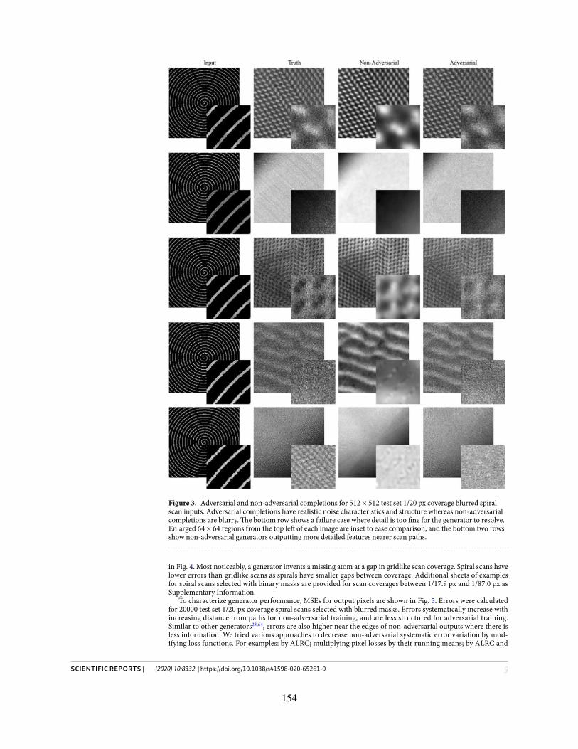
5Scientific RepoRtS | (2020) 10:8332 | https://doi.org/10.1038/s41598-020-65261-0
www.nature.com/scientificreportswww.nature.com/scientificreports/
in Fig. 4. Most noticeably, a generator invents a missing atom at a gap in gridlike scan coverage. Spiral scans have lower errors than gridlike scans as spirals have smaller gaps between coverage. Additional sheets of examples for spiral scans selected with binary masks are provided for scan coverages between 1/17.9 px and 1/87.0 px as Supplementary Information.
To characterize generator performance, MSEs for output pixels are shown in Fig. 5. Errors were calculated for 20000 test set 1/20 px coverage spiral scans selected with blurred masks. Errors systematically increase with increasing distance from paths for non-adversarial training, and are less structured for adversarial training. Similar to other generators23,64, errors are also higher near the edges of non-adversarial outputs where there is less information. We tried various approaches to decrease non-adversarial systematic error variation by mod-ifying loss functions. For examples: by ALRC; multiplying pixel losses by their running means; by ALRC and
Figure 3. Adversarial and non-adversarial completions for 512 × 512 test set 1/20 px coverage blurred spiral scan inputs. Adversarial completions have realistic noise characteristics and structure whereas non-adversarial completions are blurry. The bottom row shows a failure case where detail is too fine for the generator to resolve. Enlarged 64 × 64 regions from the top left of each image are inset to ease comparison, and the bottom two rows show non-adversarial generators outputting more detailed features nearer scan paths.
154
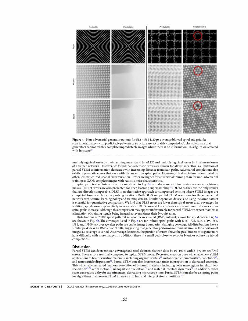
6Scientific RepoRtS | (2020) 10:8332 | https://doi.org/10.1038/s41598-020-65261-0
www.nature.com/scientificreportswww.nature.com/scientificreports/
multiplying pixel losses by their running means; and by ALRC and multiplying pixel losses by final mean losses of a trained network. However, we found that systematic errors are similar for all variants. This is a limitation of partial STEM as information decreases with increasing distance from scan paths. Adversarial completions also exhibit systematic errors that vary with distance from spiral paths. However, spiral variation is dominated by other, less structured, spatial error variation. Errors are higher for adversarial training than for non-adversarial training as GANs complete images with realistic noise characteristics.
Spiral path test set intensity errors are shown in Fig. 6a, and decrease with increasing coverage for binary masks. Test set errors are also presented for deep learning supersampling23 (DLSS) as they are the only results that are directly comparable. DLSS is an alternative approach to compressed sensing where STEM images are completed from a sublattice of probing locations. Both DLSS and partial STEM results are for the same neural network architecture, learning policy and training dataset. Results depend on datasets, so using the same dataset is essential for quantitative comparison. We find that DLSS errors are lower than spiral errors at all coverages. In addition, spiral errors exponentially increase above DLSS errors at low coverages where minimum distances from spiral paths increase. Although this comparison may appear unfavourable for partial STEM, we expect that this is a limitation of training signals being imaged at several times their Nyquist rates.
Distributions of 20000 spiral path test set root mean squared (RMS) intensity errors for spiral data in Fig. 6a are shown in Fig. 6b. The coverages listed in Fig. 6 are for infinite spiral paths with 1/16, 1/25, 1/36, 1/49, 1/64, 1/81, and 1/100 px coverage after paths are cut by image boundaries; changing coverage. All distributions have a similar peak near an RMS error of 0.04, suggesting that generator performance remains similar for a portion of images as coverage is varied. As coverage decreases, the portion of errors above the peak increases as generators have difficulty with more images. In addition, there is a small peak close to zero for blank or otherwise trivial completions.
DiscussionPartial STEM can decrease scan coverage and total electron electron dose by 10–100× with 3–6% test set RMS errors. These errors are small compared to typical STEM noise. Decreased electron dose will enable new STEM applications to beam-sensitive materials, including organic crystals65, metal-organic frameworks66, nanotubes67, and nanoparticle dispersions68. Partial STEM can also decrease scan times in proportion to decreased coverage. This will enable increased temporal resolution of dynamic materials, including polar nanoregions in relaxor fer-roelectrics69,70, atom motion71, nanoparticle nucleation72, and material interface dynamics73. In addition, faster scans can reduce delay for experimenters, decreasing microscope time. Partial STEM can also be a starting point for algorithms that process STEM images e.g. to find and interpret atomic positions74.
Figure 4. Non-adversarial generator outputs for 512 × 512 1/20 px coverage blurred spiral and gridlike scan inputs. Images with predictable patterns or structure are accurately completed. Circles accentuate that generators cannot reliably complete unpredictable images where there is no information. This figure was created with Inkscape83.
155
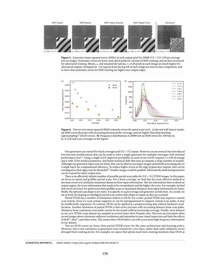
7Scientific RepoRtS | (2020) 10:8332 | https://doi.org/10.1038/s41598-020-65261-0
www.nature.com/scientificreportswww.nature.com/scientificreports/
Our generators are trained for fixed coverages and 512 × 512 inputs. However, recent research has introduced loss function modifications that can be used to train a single generator for multiple coverages with minimal performance loss23. Using a single GAN improves portability as each of our GANs requires 1.3 GB of storage space with 32 bit model parameters, and limits technical debt that may accompany a large number of models. Although our generator input sizes are fixed, they can be tiled across larger images; potentially processing tiles in a single batch for computational efficiency. To reduce higher errors at the edge of generator outputs, tiles can be overlapped so that edges may be discarded64. Smaller images could be padded. Alternatively, dedicated generators can be trained for other output sizes.
There is an effectively infinite number of possible partial scan paths for 512 × 512 STEM images. In this paper, we focus on spiral and gridlike partial scans. For a fixed coverage, we find that the most effective method to decrease errors is to minimize maximum distances from input information. The less information there is about an output region, the more information that needs to be extrapolated, and the higher the error. For example, we find that errors are lower for spiral scans than gridlike scans as maximum distances from input information are lower. Really, the optimal scan shape is not static: It is specific to a given image and generator architecture. As a result, we are actively developing an intelligent partial scan system that adapts to inputs as they are scanned.
Partial STEM has a number of limitations relative to DLSS. For a start, partial STEM may require a custom scan system. Even if a scan system supports or can be reprogrammed to support custom scan paths, it may be insufficiently responsive. In contrast, DLSS can be applied as a postprocessing step without hardware mod-ification. Another limitation of partial STEM is that errors increase with increasing distance from scan paths. Distances from continuous scan paths cannot be decreased without increasing coverage. Finally, most features in our new STEM crops dataset are sampled at several times their Nyquist rates. Electron microscopists often record images above minimum sufficient resolutions and intensities to ease visual inspection and limit the effects of drift75, shot17, and other noise. This means that a DLSS lattice can still access most high frequency information in our dataset.
Test set DLSS errors are lower than partial STEM errors for the same architecture and learning policy. However, this is not conclusive as generators were trained for a few days; rather than until validation errors diverged from training errors. For example, we expect that spirals need more training iterations than DLSS as
Figure 5. Generator mean squared errors (MSEs) at each output pixel for 20000 512 × 512 1/20 px coverage test set images. Systematic errors are lower near spiral paths for variants of MSE training, and are less structured for adversarial training. Means, μ, and standard deviations, σ, of all pixels in each image are much higher for adversarial outputs. Enlarged 64 × 64 regions from the top left of each image are inset to ease comparison, and to show that systematic errors for MSE training are higher near output edges.
Figure 6. Test set root mean squared (RMS) intensity errors for spiral scans in [0, 1] selected with binary masks. (a) RMS errors decrease with increasing electron probe coverage, and are higher than deep learning supersampling23 (DLSS) errors. (b) Frequency distributions of 20000 test set RMS errors for 100 bins in .[0, 0 224] and scan coverages in the legend.
156

8Scientific RepoRtS | (2020) 10:8332 | https://doi.org/10.1038/s41598-020-65261-0
www.nature.com/scientificreportswww.nature.com/scientificreports/
nearest neighbour infilled spiral regions have varying shapes, whereas infilled regions of DLSS grids are square. In addition, limited high frequency information in training data limits one of the key strengths of partial STEM that DLSS lacks: access to high-frequency information from neighbouring pixels. As a result, we expect that partial STEM performance would be higher for signals imaged closer to their Nyquist rates.
To generate realistic images, we fine-tuned partial STEM generators as part of GANs. GANs generate images with more realistic high-frequency spatial components and structure than MSE training. However, GANs focus on semantics; rather than intensity differences. This means that although adversarial completions have realistic characteristics, such as high-frequency noise, individual pixel values differ from true values. GANs can also be difficult to train76,77, and training requires additional computation. Nevertheless, inference time is the same for adversarial and non-adversarial generators after training.
Encouragingly, ANNs are universal approximators78 that can represent79 the optimal mapping from partial scans with arbitrary accuracy. This overcomes the limitations of traditional algorithms where performance is fixed. If ANN performance is insufficient or surpassed by another method, training or development can be con-tinued to achieve higher performance. Indeed, validation errors did not diverge from training errors during our experiments, so we are presenting lower bounds for performance. In this paper, we compare spiral STEM perfor-mance against DLSS. It is the only method that we can rigorously and quantitatively compare against as it used the same test set data. This yielded a new insight into how signals being imaged above their Nyquist rates may affect performance discussed two paragraphs earlier, and highlights the importance of standardized datasets like our new STEM images dataset. As machine learning becomes more established in the electron microscopy commu-nity, we hope that standardized datasets will also become established to standardize performance benchmarks.
Detailed neural network architecture, learning policy, experiments, and additional sheets of examples are pro-vided as Supplementary Information. Further improvements might be made with AdaNet80, Ludwig81, or other automatic machine learning82 algorithms, and we encourage further development. In this spirit, we have made our source code36, a new dataset containing 16227 STEM images40,41, and pre-trained models publicly available. For convenience, new datasets containing 161069 non-overlapping 512 × 512 crops from STEM images used for training, and 19769 antialiased 96 × 96 area downsampled STEM images created for faster ANN development, are also available.
conclusionsPartial STEM with deep learning can decrease electron dose and scan time by over an order of magnitude with minimal information loss. In addition, realistic STEM images can be completed by fine-tuning generators as part of a GAN. Detailed MSE characteristics are provided for multiple coverages, including MSEs per output pixel for 1/20 px coverage spiral scans. Partial STEM will enable new beam sensitive applications, so we have made our source code, new STEM dataset, pre-trained models, and details of experiments available to encourage further investigation. High performance is achieved by the introduction of an auxiliary trainer network, and adaptive learning rate clipping of high losses. We expect our results to be generalizable to SEM and other scan systems.
Data availabilityNew STEM datasets are available on our publicly accessible dataserver40,41. Source code for ANNs and to create images is in a GitHub repository with links to pre-trained models36. For additional information contact the corresponding author (J.M.E.).
Received: 12 February 2020; Accepted: 28 April 2020;Published: xx xx xxxx
References 1. Yankovich, A. B., Berkels, B., Dahmen, W., Binev, P. & Voyles, P. M. High-Precision Scanning Transmission Electron Microscopy at
Coarse Pixel Sampling for Reduced Electron Dose. Adv. Struct. Chem. Imaging 1, 2 (2015). 2. Peters, J. J. P., Apachitei, G., Beanland, R., Alexe, M. & Sanchez, A. M. Polarization Curling and Flux Closures in Multiferroic Tunnel
Junctions. Nat. Commun. 7, 13484 (2016). 3. Hujsak, K., Myers, B. D., Roth, E., Li, Y. & Dravid, V. P. Suppressing Electron Exposure Artifacts: An Electron Scanning Paradigm
with Bayesian Machine Learning. Microsc. Microanal. 22, 778–788 (2016). 4. Egerton, R. F., Li, P. & Malac, M. Radiation Damage in the TEM and SEM. Micron 35, 399–409 (2004). 5. Jones, L. et al. Managing Dose-, Damage- and Data-Rates in Multi-Frame Spectrum-Imaging. Microscopy 67, i98–i113 (2018). 6. Trampert, P. et al. How Should a Fixed Budget of Dwell Time be Spent in Scanning Electron Microscopy to Optimize Image Quality?
Ultramicroscopy 191, 11–17 (2018). 7. Anderson, H. S., Ilic-Helms, J., Rohrer, B., Wheeler, J. & Larson, K. Sparse Imaging for Fast Electron Microscopy. In Computational
Imaging XI, vol. 8657, 86570C (International Society for Optics and Photonics, 2013). 8. Stevens, A., Yang, H., Carin, L., Arslan, I. & Browning, N. D. The Potential for Bayesian Compressive Sensing to Significantly Reduce
Electron Dose in High-Resolution STEM Images. Microscopy 63, 41–51 (2013). 9. Stevens, A. et al. A Sub-Sampled Approach to Extremely Low-Dose STEM. Appl. Phys. Lett. 112, 043104 (2018). 10. Hwang, S., Han, C. W., Venkatakrishnan, S. V., Bouman, C. A. & Ortalan, V. Towards the Low-Dose Characterization of Beam
Sensitive Nanostructures via Implementation of Sparse Image Acquisition in Scanning Transmission Electron Microscopy. Meas. Sci. Technol. 28, 045402 (2017).
11. Candes, E. & Romberg, J. Sparsity and Incoherence in Compressive Sampling. Inverse Probl. 23, 969 (2007). 12. Kovarik, L., Stevens, A., Liyu, A. & Browning, N. D. Implementing an Accurate and Rapid Sparse Sampling Approach for Low-Dose
Atomic Resolution STEM Imaging. Appl. Phys. Lett. 109, 164102 (2016). 13. Sang, X. et al. Dynamic Scan Control in STEM: Spiral Scans. Adv. Struct. Chem. Imaging 2, 6 (2017). 14. Béché, A., Goris, B., Freitag, B. & Verbeeck, J. Development of a Fast Electromagnetic Beam Blanker for Compressed Sensing in
Scanning Transmission Electron Microscopy. Appl. Phys. Lett. 108, 093103 (2016). 15. Li, X., Dyck, O., Kalinin, S. V. & Jesse, S. Compressed Sensing of Scanning Transmission Electron Microscopy (STEM) with
Nonrectangular Scans. Microsc. Microanal. 24, 623–633 (2018).
157
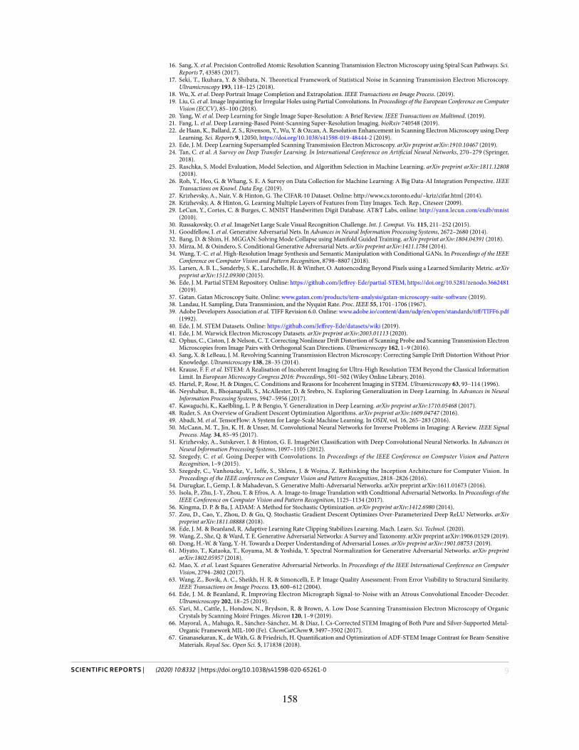
9Scientific RepoRtS | (2020) 10:8332 | https://doi.org/10.1038/s41598-020-65261-0
www.nature.com/scientificreportswww.nature.com/scientificreports/
16. Sang, X. et al. Precision Controlled Atomic Resolution Scanning Transmission Electron Microscopy using Spiral Scan Pathways. Sci. Reports 7, 43585 (2017).
17. Seki, T., Ikuhara, Y. & Shibata, N. Theoretical Framework of Statistical Noise in Scanning Transmission Electron Microscopy. Ultramicroscopy 193, 118–125 (2018).
18. Wu, X. et al. Deep Portrait Image Completion and Extrapolation. IEEE Transactions on Image Process. (2019). 19. Liu, G. et al. Image Inpainting for Irregular Holes using Partial Convolutions. In Proceedings of the European Conference on Computer
Vision (ECCV), 85–100 (2018). 20. Yang, W. et al. Deep Learning for Single Image Super-Resolution: A Brief Review. IEEE Transactions on Multimed. (2019). 21. Fang, L. et al. Deep Learning-Based Point-Scanning Super-Resolution Imaging. bioRxiv 740548 (2019). 22. de Haan, K., Ballard, Z. S., Rivenson, Y., Wu, Y. & Ozcan, A. Resolution Enhancement in Scanning Electron Microscopy using Deep
Learning. Sci. Reports 9, 12050, https://doi.org/10.1038/s41598-019-48444-2 (2019). 23. Ede, J. M. Deep Learning Supersampled Scanning Transmission Electron Microscopy. arXiv preprint arXiv:1910.10467 (2019). 24. Tan, C. et al. A Survey on Deep Transfer Learning. In International Conference on Artificial Neural Networks, 270–279 (Springer,
2018). 25. Raschka, S. Model Evaluation, Model Selection, and Algorithm Selection in Machine Learning. arXiv preprint arXiv:1811.12808
(2018). 26. Roh, Y., Heo, G. & Whang, S. E. A Survey on Data Collection for Machine Learning: A Big Data-AI Integration Perspective. IEEE
Transactions on Knowl. Data Eng. (2019). 27. Krizhevsky, A., Nair, V. & Hinton, G. The CIFAR-10 Dataset. Online: http://www.cs.toronto.edu/~kriz/cifar.html (2014). 28. Krizhevsky, A. & Hinton, G. Learning Multiple Layers of Features from Tiny Images. Tech. Rep., Citeseer (2009). 29. LeCun, Y., Cortes, C. & Burges, C. MNIST Handwritten Digit Database. AT&T Labs, online: http://yann.lecun.com/exdb/mnist
(2010). 30. Russakovsky, O. et al. ImageNet Large Scale Visual Recognition Challenge. Int. J. Comput. Vis. 115, 211–252 (2015). 31. Goodfellow, I. et al. Generative Adversarial Nets. In Advances in Neural Information Processing Systems, 2672–2680 (2014). 32. Bang, D. & Shim, H. MGGAN: Solving Mode Collapse using Manifold Guided Training. arXiv preprint arXiv:1804.04391 (2018). 33. Mirza, M. & Osindero, S. Conditional Generative Adversarial Nets. arXiv preprint arXiv:1411.1784 (2014). 34. Wang, T.-C. et al. High-Resolution Image Synthesis and Semantic Manipulation with Conditional GANs. In Proceedings of the IEEE
Conference on Computer Vision and Pattern Recognition, 8798–8807 (2018). 35. Larsen, A. B. L., Sønderby, S. K., Larochelle, H. & Winther, O. Autoencoding Beyond Pixels using a Learned Similarity Metric. arXiv
preprint arXiv:1512.09300 (2015). 36. Ede, J. M. Partial STEM Repository. Online: https://github.com/Jeffrey-Ede/partial-STEM, https://doi.org/10.5281/zenodo.3662481
(2019). 37. Gatan. Gatan Microscopy Suite. Online: www.gatan.com/products/tem-analysis/gatan-microscopy-suite-software (2019). 38. Landau, H. Sampling, Data Transmission, and the Nyquist Rate. Proc. IEEE 55, 1701–1706 (1967). 39. Adobe Developers Association et al. TIFF Revision 6.0. Online: www.adobe.io/content/dam/udp/en/open/standards/tiff/TIFF6.pdf
(1992). 40. Ede, J. M. STEM Datasets. Online: https://github.com/Jeffrey-Ede/datasets/wiki (2019). 41. Ede, J. M. Warwick Electron Microscopy Datasets. arXiv preprint arXiv:2003.01113 (2020). 42. Ophus, C., Ciston, J. & Nelson, C. T. Correcting Nonlinear Drift Distortion of Scanning Probe and Scanning Transmission Electron
Microscopies from Image Pairs with Orthogonal Scan Directions. Ultramicroscopy 162, 1–9 (2016). 43. Sang, X. & LeBeau, J. M. Revolving Scanning Transmission Electron Microscopy: Correcting Sample Drift Distortion Without Prior
Knowledge. Ultramicroscopy 138, 28–35 (2014). 44. Krause, F. F. et al. ISTEM: A Realisation of Incoherent Imaging for Ultra-High Resolution TEM Beyond the Classical Information
Limit. In European Microscopy Congress 2016: Proceedings, 501–502 (Wiley Online Library, 2016). 45. Hartel, P., Rose, H. & Dinges, C. Conditions and Reasons for Incoherent Imaging in STEM. Ultramicroscopy 63, 93–114 (1996). 46. Neyshabur, B., Bhojanapalli, S., McAllester, D. & Srebro, N. Exploring Generalization in Deep Learning. In Advances in Neural
Information Processing Systems, 5947–5956 (2017). 47. Kawaguchi, K., Kaelbling, L. P. & Bengio, Y. Generalization in Deep Learning. arXiv preprint arXiv:1710.05468 (2017). 48. Ruder, S. An Overview of Gradient Descent Optimization Algorithms. arXiv preprint arXiv:1609.04747 (2016). 49. Abadi, M. et al. TensorFlow: A System for Large-Scale Machine Learning. In OSDI, vol. 16, 265–283 (2016). 50. McCann, M. T., Jin, K. H. & Unser, M. Convolutional Neural Networks for Inverse Problems in Imaging: A Review. IEEE Signal
Process. Mag. 34, 85–95 (2017). 51. Krizhevsky, A., Sutskever, I. & Hinton, G. E. ImageNet Classification with Deep Convolutional Neural Networks. In Advances in
Neural Information Processing Systems, 1097–1105 (2012). 52. Szegedy, C. et al. Going Deeper with Convolutions. In Proceedings of the IEEE Conference on Computer Vision and Pattern
Recognition, 1–9 (2015). 53. Szegedy, C., Vanhoucke, V., Ioffe, S., Shlens, J. & Wojna, Z. Rethinking the Inception Architecture for Computer Vision. In
Proceedings of the IEEE conference on Computer Vision and Pattern Recognition, 2818–2826 (2016). 54. Durugkar, I., Gemp, I. & Mahadevan, S. Generative Multi-Adversarial Networks. arXiv preprint arXiv:1611.01673 (2016). 55. Isola, P., Zhu, J.-Y., Zhou, T. & Efros, A. A. Image-to-Image Translation with Conditional Adversarial Networks. In Proceedings of the
IEEE Conference on Computer Vision and Pattern Recognition, 1125–1134 (2017). 56. Kingma, D. P. & Ba, J. ADAM: A Method for Stochastic Optimization. arXiv preprint arXiv:1412.6980 (2014). 57. Zou, D., Cao, Y., Zhou, D. & Gu, Q. Stochastic Gradient Descent Optimizes Over-Parameterized Deep ReLU Networks. arXiv
preprint arXiv:1811.08888 (2018). 58. Ede, J. M. & Beanland, R. Adaptive Learning Rate Clipping Stabilizes Learning. Mach. Learn. Sci. Technol. (2020). 59. Wang, Z., She, Q. & Ward, T. E. Generative Adversarial Networks: A Survey and Taxonomy. arXiv preprint arXiv:1906.01529 (2019). 60. Dong, H.-W. & Yang, Y.-H. Towards a Deeper Understanding of Adversarial Losses. arXiv preprint arXiv:1901.08753 (2019). 61. Miyato, T., Kataoka, T., Koyama, M. & Yoshida, Y. Spectral Normalization for Generative Adversarial Networks. arXiv preprint
arXiv:1802.05957 (2018). 62. Mao, X. et al. Least Squares Generative Adversarial Networks. In Proceedings of the IEEE International Conference on Computer
Vision, 2794–2802 (2017). 63. Wang, Z., Bovik, A. C., Sheikh, H. R. & Simoncelli, E. P. Image Quality Assessment: From Error Visibility to Structural Similarity.
IEEE Transactions on Image Process. 13, 600–612 (2004). 64. Ede, J. M. & Beanland, R. Improving Electron Micrograph Signal-to-Noise with an Atrous Convolutional Encoder-Decoder.
Ultramicroscopy 202, 18–25 (2019). 65. S’ari, M., Cattle, J., Hondow, N., Brydson, R. & Brown, A. Low Dose Scanning Transmission Electron Microscopy of Organic
Crystals by Scanning Moiré Fringes. Micron 120, 1–9 (2019). 66. Mayoral, A., Mahugo, R., Sánchez-Sánchez, M. & Díaz, I. Cs-Corrected STEM Imaging of Both Pure and Silver-Supported Metal-
Organic Framework MIL-100 (Fe). ChemCatChem 9, 3497–3502 (2017). 67. Gnanasekaran, K., de With, G. & Friedrich, H. Quantification and Optimization of ADF-STEM Image Contrast for Beam-Sensitive
Materials. Royal Soc. Open Sci. 5, 171838 (2018).
158
1 0Scientific RepoRtS | (2020) 10:8332 | https://doi.org/10.1038/s41598-020-65261-0
www.nature.com/scientificreportswww.nature.com/scientificreports/
68. Ilett, M., Brydson, R., Brown, A. & Hondow, N. Cryo-Analytical STEM of Frozen, Aqueous Dispersions of Nanoparticles. Micron 120, 35–42 (2019).
69. Kumar, A., Dhall, R. & LeBeau, J. M. In Situ Ferroelectric Domain Dynamics Probed with Differential Phase Contrast Imaging. Microsc. Microanal. 25, 1838–1839 (2019).
70. Xie, L. et al. Static and Dynamic Polar Nanoregions in Relaxor Ferroelectric Ba(Ti1−xSnx)O3 System at High Temperature. Phys. Rev. B 85, 014118 (2012).
71. Aydin, C. et al. Tracking Iridium Atoms with Electron Microscopy: First Steps of Metal Nanocluster Formation in One-Dimensional Zeolite Channels. Nano Lett. 11, 5537–5541 (2011).
72. Hussein, H. E. et al. Tracking Metal Electrodeposition Dynamics from Nucleation and Growth of a Single Atom to a Crystalline Nanoparticle. ACS Nano 12, 7388–7396 (2018).
73. Chen, S. et al. Atomic Structure and Migration Dynamics of MoS2/LixMoS2 Interface. Nano Energy 48, 560–568 (2018). 74. Ziatdinov, M. et al. Deep Learning of Atomically Resolved Scanning Transmission Electron Microscopy Images: Chemical
Identification and Tracking Local Transformations. ACS Nano 11, 12742–12752 (2017). 75. Jones, L. & Nellist, P. D. Identifying and Correcting Scan Noise and Drift in the Scanning Transmission Electron Microscope.
Microsc. Microanal. 19, 1050–1060 (2013). 76. Salimans, T. et al. Improved Techniques for Training GANs. In Advances in Neural Information Processing Systems, 2234–2242
(2016). 77. Liang, K. J., Li, C., Wang, G. & Carin, L. Generative Adversarial Network Training is a Continual Learning Problem. arXiv preprint
arXiv:1811.11083 (2018). 78. Hornik, K., Stinchcombe, M. & White, H. Multilayer Feedforward Networks are Universal Approximators. Neural Networks 2,
359–366 (1989). 79. Lin, H. W., Tegmark, M. & Rolnick, D. Why does Deep and Cheap Learning Work so Well? J. Stat. Phys. 168, 1223–1247 (2017). 80. Weill, C. et al. AdaNet: A Scalable and Flexible Framework for Automatically Learning Ensembles. arXiv preprint arXiv:1905.00080
(2019). 81. Molino, P., Dudin, Y. & Miryala, S. S. Ludwig: A Type-Based Declarative Deep Learning Toolbox. arXiv preprint arXiv:1909.07930
(2019). 82. He, X., Zhao, K. & Chu, X. AutoML: A Survey of the State-of-the-Art. arXiv preprint arXiv:1908.00709 (2019). 83. Harrington, B. et al. Inkscape 0.92, Online: http://www.inkscape.org/ (2020).
AcknowledgementsThanks go to Julie Robinson for advice on finding publication venues and to Marin Alexe for helpful discussion. J.M.E. and R.B. acknowledge EPSRC grant EP/N035437/1 for financial support. In addition, J.M.E. acknowledges EPSRC Studentship 1917382.
Author contributionsJ.M.E. proposed this research, wrote the code, collated training data, performed experiments and analysis, created repositories, and co-wrote this paper. R.B. supervised and co-wrote this paper.
competing interestsThe authors declare no competing interests.
Additional informationSupplementary information is available for this paper at https://doi.org/10.1038/s41598-020-65261-0.Correspondence and requests for materials should be addressed to J.M.E.Reprints and permissions information is available at www.nature.com/reprints.Publisher’s note Springer Nature remains neutral with regard to jurisdictional claims in published maps and institutional affiliations.
Open Access This article is licensed under a Creative Commons Attribution 4.0 International License, which permits use, sharing, adaptation, distribution and reproduction in any medium or
format, as long as you give appropriate credit to the original author(s) and the source, provide a link to the Cre-ative Commons license, and indicate if changes were made. The images or other third party material in this article are included in the article’s Creative Commons license, unless indicated otherwise in a credit line to the material. If material is not included in the article’s Creative Commons license and your intended use is not per-mitted by statutory regulation or exceeds the permitted use, you will need to obtain permission directly from the copyright holder. To view a copy of this license, visit http://creativecommons.org/licenses/by/4.0/. © The Author(s) 2020
159
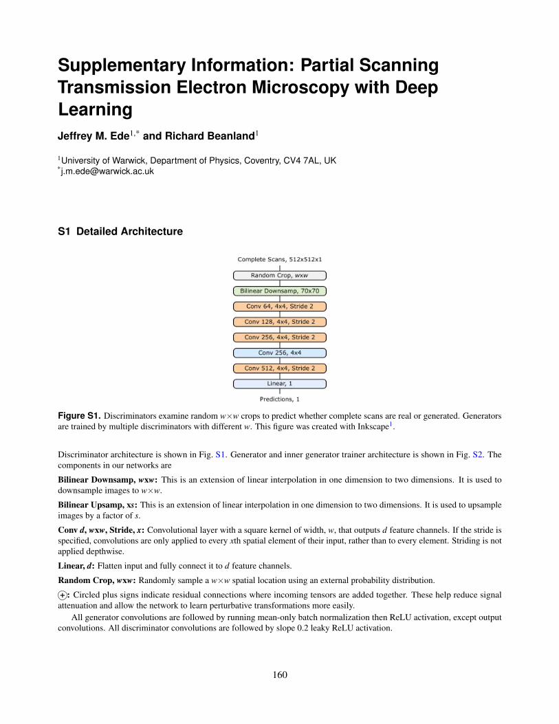
Supplementary Information: Partial ScanningTransmission Electron Microscopy with DeepLearningJeffrey M. Ede1,* and Richard Beanland1
1University of Warwick, Department of Physics, Coventry, CV4 7AL, UK*[email protected]
S1 Detailed Architecture
Figure S1. Discriminators examine random w×w crops to predict whether complete scans are real or generated. Generatorsare trained by multiple discriminators with different w. This figure was created with Inkscape1.
Discriminator architecture is shown in Fig. S1. Generator and inner generator trainer architecture is shown in Fig. S2. Thecomponents in our networks are
Bilinear Downsamp, wxw: This is an extension of linear interpolation in one dimension to two dimensions. It is used todownsample images to w×w.
Bilinear Upsamp, xs: This is an extension of linear interpolation in one dimension to two dimensions. It is used to upsampleimages by a factor of s.
Conv d, wxw, Stride, x: Convolutional layer with a square kernel of width, w, that outputs d feature channels. If the stride isspecified, convolutions are only applied to every xth spatial element of their input, rather than to every element. Striding is notapplied depthwise.
Linear, d: Flatten input and fully connect it to d feature channels.
Random Crop, wxw: Randomly sample a w×w spatial location using an external probability distribution.
+ : Circled plus signs indicate residual connections where incoming tensors are added together. These help reduce signalattenuation and allow the network to learn perturbative transformations more easily.
All generator convolutions are followed by running mean-only batch normalization then ReLU activation, except outputconvolutions. All discriminator convolutions are followed by slope 0.2 leaky ReLU activation.
160

Figure S2. Two-stage generator that completes 512×512 micrographs from partial scans. A dashed line indicates that thesame image is input to the inner and outer generator. Large scale features developed by the inner generator are locally enhancedby the outer generator and turned into images. An auxiliary trainer network restores images from inner generator features toprovide direct feedback. This figure was created with Inkscape1.
S2/S16161
S2 Learning Policy
Optimizer: Training is ADAM2 optimized and has two halves. In the first half, the generator and auxiliary trainer learn tominimize mean squared errors between their outputs and ground truth images. For the quarter of iterations, we use a constantlearning rate η0 = 0.0003 and a decay rate for the first moment of the momentum β1 = 0.9. The learning rate is then stepwisedecayed to zero in eight steps over the second quarter of iterations. Similarly, β1 is stepwise linearly decayed to 0.5 in eightsteps. In an optional second half, the generator and discriminators play an adversarial game conditioned on MSE guidance. Forthe third quarter of iterations, we use η = 0.0001 and β1 = 0.9 for the generator and discriminators. In the final quarter ofiterations, the generator learning rate is decayed to zero in eight steps while the discriminator learning rate remains constant.Similarly, generator and discriminator β1 is stepwise decayed to 0.5 in eight steps.
Experiments with GAN training hyperparameters show that β1 = 0.5 is a good choice3. Our decision to start at β1 = 0.9aims to improve the initial rate of convergence. In the first stage, generator and auxiliary trainer parameters are both updatedonce per training step. In the second stage, all parameters are updated once per training step. In most of our initial experimentswith burred masks, we used a total of 106 training iterations. However, we found that validation errors do not diverge if trainingtime is increased to 2×10⁶ iterations, and used this number for experiments with binary masks. These training iterations arein-line with with other GANs, which reuse datasets containing a few thousand examples for 200 epochs4. The lack of validationdivergence suggests that performance may be substantially improved, and means that our results present lower bounds forperformance. All training was performed with a batch size of 1 due to the large model size needed to complete 512×512 scans.
Adaptive learning rate clipping: To stabilize batch size 1 training, adaptive learning rate clipping5 (ALRC) was developedto limit high MSEs. ALRC layers were initialized with first raw moment µ1 = 25, second raw moment µ2 = 30, exponentialdecay rates β1 = β2 = 0.999, and n = 3 standard deviations.
Input normalization: Partial scans, Iscan, input to the generator are linearly transformed to I′scan = (Iscan + 1)/2, whereI′scan ∈ [0,1]. The generator is trained to output ground truth crops in [0,1], which are linearly transformed to [−1,1]. Generatoroutputs and ground truth crops in [−1,1] are directly input to discriminators.
Weight normalization: All generator parameters are weight normalized6. Running mean-only batch normalization6, 7 isapplied to the output channels of every convolutional layer, except the last. Channel means are tracked by exponential movingaverages with decay rates of 0.99. Running mean-only batch normalization is frozen in the second half of training to improvestability8.
Spectral normalization: Spectral normalization3 is applied to the weights of each convolutional layer in the discriminatorsto limit the Lipschitz norms of the discriminators. We use the power iteration method with one iteration per training step toenforce a spectral norm of 1 for each weight matrix.
Spectral normalization stabilizes training, reduces susceptibility to mode collapse and is independent of rank, encouragingdiscriminators to use more input features to inform decisions3. In contrast, weight normalization6 and Wasserstein weightclipping9 impose more arbitrary model distributions that may only partially match the target distribution.
Activation: In the generator, ReLU10 non-linearities are applied after running mean-only batch normalization. In thediscriminators, slope 0.2 leaky ReLU11 non-linearities are applied after every convolutional layer. Rectifier leakage encouragesdiscriminators to use more features to inform decisions. Our choice of generator and discriminator non-linearities followsrecent work on high-resolution conditional GANs4.
Initialization: Generator weights were initialized from a normal distribution with mean 0.00 and standard deviation 0.05. Toapply weight normalization, an example scan is then propagated through the network. Each layer output is divided by its L2norm and the layer weights assigned their division by the square root of the L2 normalized output’s standard deviation. Thereare no biases in the generator as running mean-only batch normalization would allow biases to grow unbounded c.f. batchnormalization12.
Discriminator weights were initialized from a normal distribution with mean 0.00 and standard deviation 0.03. Discriminatorbiases were zero initialized.
Experience replay: To reduce destabilizing discriminator oscillations13, we used an experience replay14, 15 with 50 examples.Prioritizing the replay of difficult examples can improve learning16, so we only replayed examples with losses in the top 20%.Training examples had a 20% chance to be sampled from the replay.
S3 ExperimentsIn this section, we present learning curves for some of our non-adversarial architecture and learning policy experiments. Duringtraining, each training set example was reused ∼8 times. In comparison, some generative adversarial networks (GANs) aretrained on the same data hundreds of times4. As a result, we did not experience noticeable overfitting. In cases where final
S3/S16162
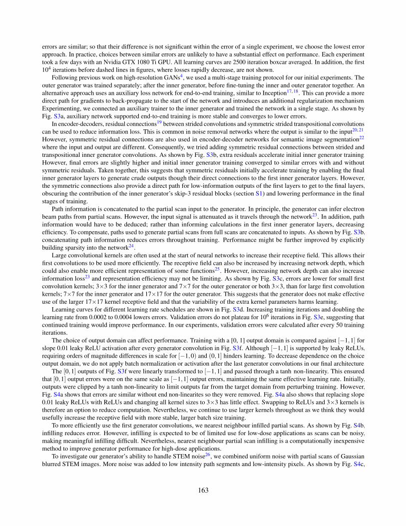
errors are similar; so that their difference is not significant within the error of a single experiment, we choose the lowest errorapproach. In practice, choices between similar errors are unlikely to have a substantial effect on performance. Each experimenttook a few days with an Nvidia GTX 1080 Ti GPU. All learning curves are 2500 iteration boxcar averaged. In addition, the first104 iterations before dashed lines in figures, where losses rapidly decrease, are not shown.
Following previous work on high-resolution GANs4, we used a multi-stage training protocol for our initial experiments. Theouter generator was trained separately; after the inner generator, before fine-tuning the inner and outer generator together. Analternative approach uses an auxiliary loss network for end-to-end training, similar to Inception17, 18. This can provide a moredirect path for gradients to back-propagate to the start of the network and introduces an additional regularization mechanism.Experimenting, we connected an auxiliary trainer to the inner generator and trained the network in a single stage. As shown byFig. S3a, auxiliary network supported end-to-end training is more stable and converges to lower errors.
In encoder-decoders, residual connections19 between strided convolutions and symmetric strided transpositional convolutionscan be used to reduce information loss. This is common in noise removal networks where the output is similar to the input20, 21.However, symmetric residual connections are also used in encoder-decoder networks for semantic image segmentation22
where the input and output are different. Consequently, we tried adding symmetric residual connections between strided andtranspositional inner generator convolutions. As shown by Fig. S3b, extra residuals accelerate initial inner generator training.However, final errors are slightly higher and initial inner generator training converged to similar errors with and withoutsymmetric residuals. Taken together, this suggests that symmetric residuals initially accelerate training by enabling the finalinner generator layers to generate crude outputs though their direct connections to the first inner generator layers. However,the symmetric connections also provide a direct path for low-information outputs of the first layers to get to the final layers,obscuring the contribution of the inner generator’s skip-3 residual blocks (section S1) and lowering performance in the finalstages of training.
Path information is concatenated to the partial scan input to the generator. In principle, the generator can infer electronbeam paths from partial scans. However, the input signal is attenuated as it travels through the network23. In addition, pathinformation would have to be deduced; rather than informing calculations in the first inner generator layers, decreasingefficiency. To compensate, paths used to generate partial scans from full scans are concatenated to inputs. As shown by Fig. S3b,concatenating path information reduces errors throughout training. Performance might be further improved by explicitlybuilding sparsity into the network24.
Large convolutional kernels are often used at the start of neural networks to increase their receptive field. This allows theirfirst convolutions to be used more efficiently. The receptive field can also be increased by increasing network depth, whichcould also enable more efficient representation of some functions25. However, increasing network depth can also increaseinformation loss23 and representation efficiency may not be limiting. As shown by Fig. S3c, errors are lower for small firstconvolution kernels; 3×3 for the inner generator and 7×7 for the outer generator or both 3×3, than for large first convolutionkernels; 7×7 for the inner generator and 17×17 for the outer generator. This suggests that the generator does not make effectiveuse of the larger 17×17 kernel receptive field and that the variability of the extra kernel parameters harms learning.
Learning curves for different learning rate schedules are shown in Fig. S3d. Increasing training iterations and doubling thelearning rate from 0.0002 to 0.0004 lowers errors. Validation errors do not plateau for 106 iterations in Fig. S3e, suggesting thatcontinued training would improve performance. In our experiments, validation errors were calculated after every 50 trainingiterations.
The choice of output domain can affect performance. Training with a [0, 1] output domain is compared against [−1,1] forslope 0.01 leaky ReLU activation after every generator convolution in Fig. S3f. Although [−1,1] is supported by leaky ReLUs,requiring orders of magnitude differences in scale for [−1,0) and (0,1] hinders learning. To decrease dependence on the choiceoutput domain, we do not apply batch normalization or activation after the last generator convolutions in our final architecture.
The [0,1] outputs of Fig. S3f were linearly transformed to [−1,1] and passed through a tanh non-linearity. This ensuredthat [0,1] output errors were on the same scale as [−1,1] output errors, maintaining the same effective learning rate. Initially,outputs were clipped by a tanh non-linearity to limit outputs far from the target domain from perturbing training. However,Fig. S4a shows that errors are similar without end non-linearites so they were removed. Fig. S4a also shows that replacing slope0.01 leaky ReLUs with ReLUs and changing all kernel sizes to 3×3 has little effect. Swapping to ReLUs and 3×3 kernels istherefore an option to reduce computation. Nevertheless, we continue to use larger kernels throughout as we think they wouldusefully increase the receptive field with more stable, larger batch size training.
To more efficiently use the first generator convolutions, we nearest neighbour infilled partial scans. As shown by Fig. S4b,infilling reduces error. However, infilling is expected to be of limited use for low-dose applications as scans can be noisy,making meaningful infilling difficult. Nevertheless, nearest neighbour partial scan infilling is a computationally inexpensivemethod to improve generator performance for high-dose applications.
To investigate our generator’s ability to handle STEM noise26, we combined uniform noise with partial scans of Gaussianblurred STEM images. More noise was added to low intensity path segments and low-intensity pixels. As shown by Fig. S4c,
S4/S16163
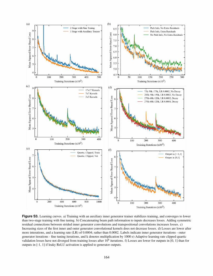
Figure S3. Learning curves. a) Training with an auxiliary inner generator trainer stabilizes training, and converges to lowerthan two-stage training with fine tuning. b) Concatenating beam path information to inputs decreases losses. Adding symmetricresidual connections between strided inner generator convolutions and transpositional convolutions increases losses. c)Increasing sizes of the first inner and outer generator convolutional kernels does not decrease losses. d) Losses are lower aftermore interations, and a learning rate (LR) of 0.0004; rather than 0.0002. Labels indicate inner generator iterations - outergenerator iterations - fine tuning iterations, and k denotes multiplication by 1000 e) Adaptive learning rate clipped quarticvalidation losses have not diverged from training losses after 106 iterations. f) Losses are lower for outputs in [0, 1] than foroutputs in [-1, 1] if leaky ReLU activation is applied to generator outputs.
S5/S16164
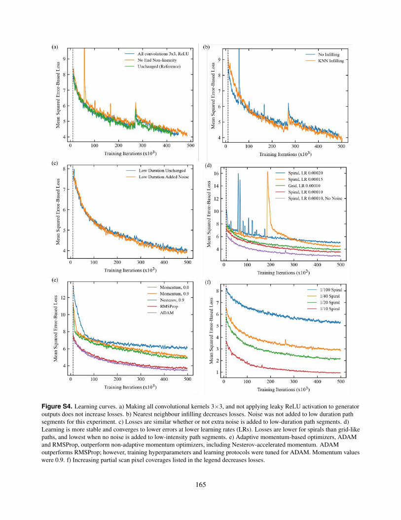
Figure S4. Learning curves. a) Making all convolutional kernels 3×3, and not applying leaky ReLU activation to generatoroutputs does not increase losses. b) Nearest neighbour infilling decreases losses. Noise was not added to low duration pathsegments for this experiment. c) Losses are similar whether or not extra noise is added to low-duration path segments. d)Learning is more stable and converges to lower errors at lower learning rates (LRs). Losses are lower for spirals than grid-likepaths, and lowest when no noise is added to low-intensity path segments. e) Adaptive momentum-based optimizers, ADAMand RMSProp, outperform non-adaptive momentum optimizers, including Nesterov-accelerated momentum. ADAMoutperforms RMSProp; however, training hyperparameters and learning protocols were tuned for ADAM. Momentum valueswere 0.9. f) Increasing partial scan pixel coverages listed in the legend decreases losses.
S6/S16165
Figure S5. Adaptive learning rate clipping stabilizes learning, accelerates convergence and results in lower errors thanHuberisation. Weighting pixel errors with their running or final mean errors is ineffective.
ablating extra noise for low-duration path segments increases performance.Fig. S4d shows that spiral path training is more stable and reaches lower errors at lower learning rates. At the same learning
rate, spiral paths converge to lower errors than grid-like paths as spirals have more uniform coverage. Errors are much lower forspiral paths when both intensity- and duration-dependent noise is ablated.
To choose a training optimizer, we completed training with stochastic gradient descent, momentum, Nesterov-acceleratedmomentum27, 28, RMSProp29 and ADAM2. Learning curves are in Fig. S4e. Adaptive momentum optimizers, ADAM andRMSProp, outperform the non-adaptive optimizers. Non-adaptive momentum-based optimizers outperform momentumlessstochastic gradient decent. ADAM slightly outperforms RMSProp; however, architecture and learning policy were tuned forADAM. This suggests that RMSProp optimization may also be a good choice.
Learning curves for 1/10, 1/20, 1/40 and 1/100 px coverage spiral scans are shown in Fig. S4f. In practice, 1/20 px coverageis sufficient for most STEM images. On average, a non-adversarial generator can complete test set 1/20 px coverage partialscans with a 2.6% root mean squared intensity error. Nevertheless, higher coverage is needed to resolve fine detail in someimages. Likewise, lower coverage may be appropriate for images without fine detail. Consequently, we are developing anintelligent scan system that adjusts coverage based on micrograph content.
Training is performed with a batch size of 1 due to the large network size needed for 512×512 partial scans. However,MSE training is unstable and large error spikes destabilize training. To stabilize learning, we developed adaptive learning rateclipping5 (ALRC) to limit magnitudes of high losses while preserving their initial gradient distributions. ALRC is comparedagainst MSE, Huberised MSE, and weighting each pixel’s error by its Huberised running mean, and fixed final errors in Fig. S5.ALRC results in more stable training with the fastest convergence and lowest errors. Similar improvements have been confirmedfor CIFAR-10 and STEM supersampling with ALRC5.
S4 Additional ExamplesSheets of examples comparing non-adversarial generator outputs and true images are shown in Fig. S6-S12 for 512×512 spiralscans selected with binary masks. True images are blurred by a 5×5 symmetric Gaussian kernel with a 2.5 px standard deviationso that they are the same as the images that generators were trained output. Images are blurred to suppress high-frequencynoise. Examples are presented for 1/17.9, 1/27.3, 1/38.2, 1/50.0, 1/60.5, 1/73.7, and 1/87.0 px coverage, in that order, so thathigher errors become apparent for decreasing coverage with increasing page number. Quantitative performance characteristicsfor each generator are provided in the main article.
S7/S16166
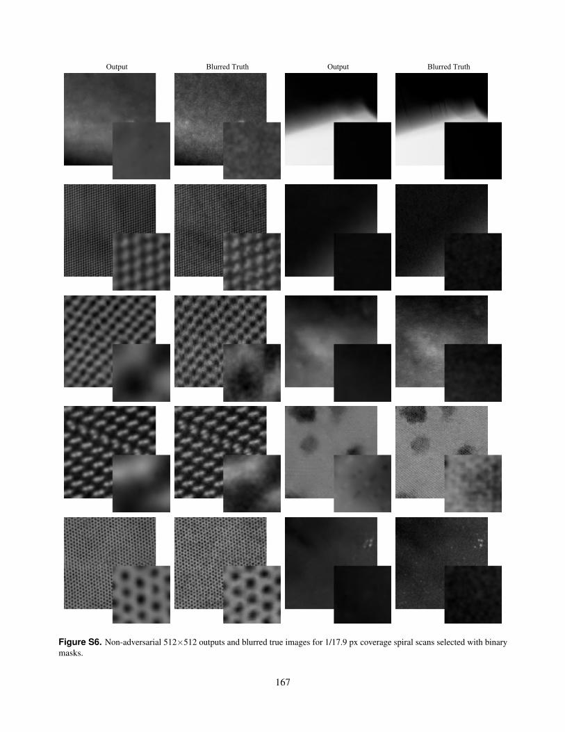
Output Blurred Truth Output Blurred Truth
Figure S6. Non-adversarial 512×512 outputs and blurred true images for 1/17.9 px coverage spiral scans selected with binarymasks.
S8/S16167
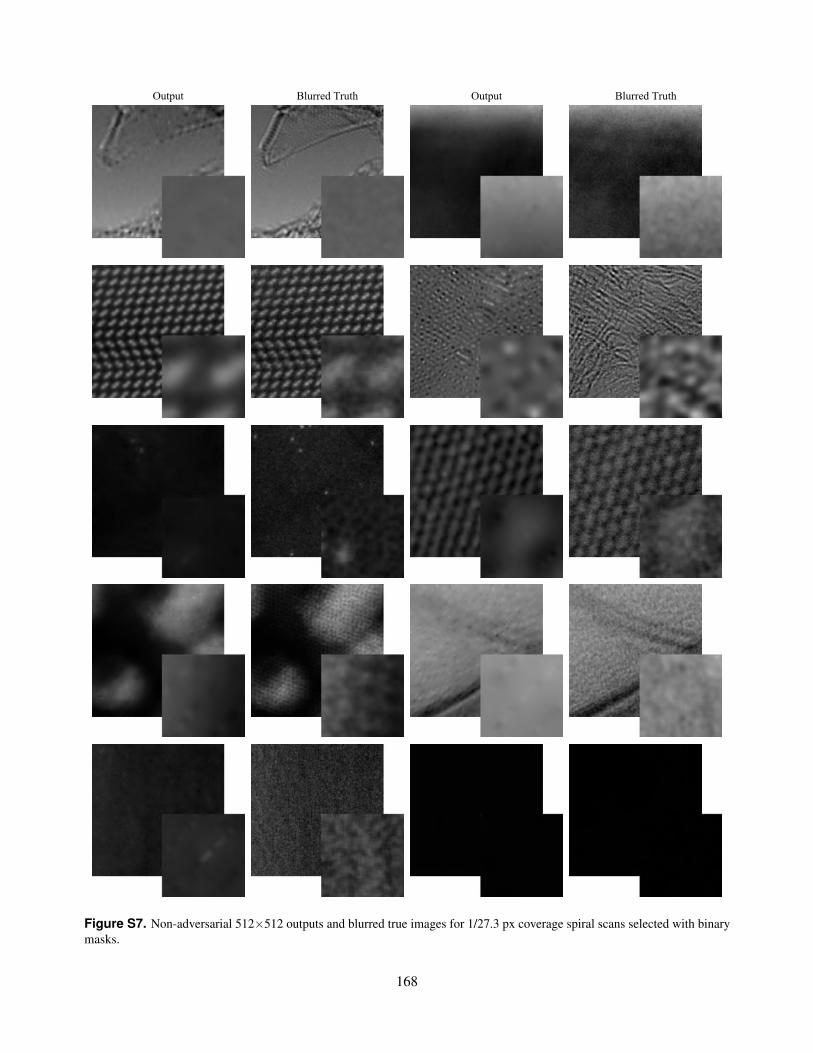
Output Blurred Truth Output Blurred Truth
Figure S7. Non-adversarial 512×512 outputs and blurred true images for 1/27.3 px coverage spiral scans selected with binarymasks.
S9/S16168
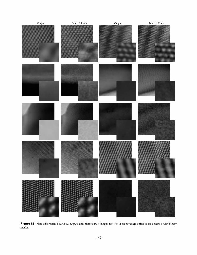
Output Blurred Truth Output Blurred Truth
Figure S8. Non-adversarial 512×512 outputs and blurred true images for 1/38.2 px coverage spiral scans selected with binarymasks.
S10/S16169
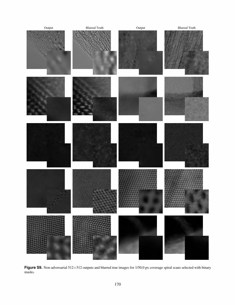
Output Blurred Truth Output Blurred Truth
Figure S9. Non-adversarial 512×512 outputs and blurred true images for 1/50.0 px coverage spiral scans selected with binarymasks.
S11/S16170

Output Blurred Truth Output Blurred Truth
Figure S10. Non-adversarial 512×512 outputs and blurred true images for 1/60.5 px coverage spiral scans selected withbinary masks.
S12/S16171
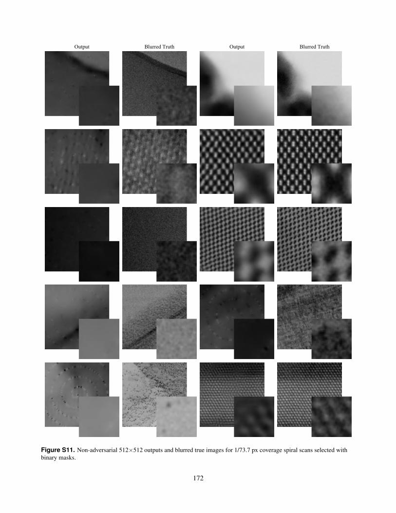
Output Blurred Truth Output Blurred Truth
Figure S11. Non-adversarial 512×512 outputs and blurred true images for 1/73.7 px coverage spiral scans selected withbinary masks.
S13/S16172
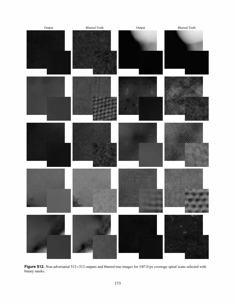
Output Blurred Truth Output Blurred Truth
Figure S12. Non-adversarial 512×512 outputs and blurred true images for 1/87.0 px coverage spiral scans selected withbinary masks.
S14/S16173

References1. Harrington, B. et al. Inkscape 0.92. Online: http://www.inkscape.org/ (2020).
2. Kingma, D. P. & Ba, J. ADAM: A Method for Stochastic Optimization. arXiv preprint arXiv:1412.6980 (2014).
3. Miyato, T., Kataoka, T., Koyama, M. & Yoshida, Y. Spectral Normalization for Generative Adversarial Networks. arXivpreprint arXiv:1802.05957 (2018).
4. Wang, T.-C. et al. High-Resolution Image Synthesis and Semantic Manipulation with Conditional GANs. In Proceedingsof the IEEE Conference on Computer Vision and Pattern Recognition, 8798–8807 (2018).
5. Ede, J. M. & Beanland, R. Adaptive Learning Rate Clipping Stabilizes Learning. Mach. Learn. Sci. Technol. (2020).
6. Salimans, T. & Kingma, D. P. Weight Normalization: A Simple Reparameterization to Accelerate Training of Deep NeuralNetworks. In Advances in Neural Information Processing Systems, 901–909 (2016).
7. Hoffer, E., Banner, R., Golan, I. & Soudry, D. Norm Matters: Efficient and Accurate Normalization Schemes in DeepNetworks. In Advances in Neural Information Processing Systems, 2160–2170 (2018).
8. Chen, L.-C., Papandreou, G., Schroff, F. & Adam, H. Rethinking Atrous Convolution for Semantic Image Segmentation.arXiv preprint arXiv:1706.05587 (2017).
9. Arjovsky, M., Chintala, S. & Bottou, L. Wasserstein Generative Adversarial Networks. In International Conference onMachine Learning, 214–223 (2017).
10. Nair, V. & Hinton, G. E. Rectified Linear Units Improve Restricted Boltzmann Machines. In Proceedings of the 27thInternational Conference on Machine Learning (ICML-10), 807–814 (2010).
11. Maas, A. L., Hannun, A. Y. & Ng, A. Y. Rectifier Nonlinearities Improve Neural Network Acoustic Models. In Proceedingsof the International Conference on Machine Learning, vol. 30, 3 (2013).
12. Ioffe, S. & Szegedy, C. Batch Normalization: Accelerating Deep Network Training by Reducing Internal Covariate Shift.arXiv preprint arXiv:1502.03167 (2015).
13. Liang, K. J., Li, C., Wang, G. & Carin, L. Generative Adversarial Network Training is a Continual Learning Problem.arXiv preprint arXiv:1811.11083 (2018).
14. Pfau, D. & Vinyals, O. Connecting Generative Adversarial Networks and Actor-Critic Methods. arXiv preprintarXiv:1610.01945 (2016).
15. Shrivastava, A. et al. Learning from Simulated and Unsupervised Images through Adversarial Training. arXiv preprintarXiv: 161207828 (2016).
16. Schaul, T., Quan, J., Antonoglou, I. & Silver, D. Prioritized Experience Replay. arXiv preprint arXiv:1511.05952 (2015).
17. Szegedy, C. et al. Going Deeper with Convolutions. In Proceedings of the IEEE Conference on Computer Vision andPattern Recognition, 1–9 (2015).
18. Szegedy, C., Vanhoucke, V., Ioffe, S., Shlens, J. & Wojna, Z. Rethinking the Inception Architecture for Computer Vision.In Proceedings of the IEEE conference on Computer Vision and Pattern Recognition, 2818–2826 (2016).
19. He, K., Zhang, X., Ren, S. & Sun, J. Deep Residual Learning for Image Recognition. In Proceedings of the IEEEConference on Computer Vision and Pattern Recognition, 770–778 (2016).
20. Mao, X.-J., Shen, C. & Yang, Y.-B. Image Restoration using Convolutional Auto-encoders with Symmetric SkipConnections. arXiv preprint arXiv:1606.08921 (2016).
21. Casas, L., Navab, N. & Belagiannis, V. Adversarial Signal Denoising with Encoder-Decoder Networks. arXiv preprintarXiv:1812.08555 (2018).
22. Badrinarayanan, V., Kendall, A. & Cipolla, R. SegNet: A Deep Convolutional Encoder-Decoder Architecture for ImageSegmentation. IEEE Transactions on Pattern Analysis Mach. Intell. 39, 2481–2495 (2017).
23. Zheng, H., Yao, J., Zhang, Y. & Tsang, I. W. Degeneration in VAE: In the Light of Fisher Information Loss. arXiv preprintarXiv:1802.06677 (2018).
24. Graham, B. Spatially-Sparse Convolutional Neural Networks. arXiv preprint arXiv:1409.6070 (2014).
25. Lin, H. W., Tegmark, M. & Rolnick, D. Why does Deep and Cheap Learning Work so Well? J. Stat. Phys. 168, 1223–1247(2017).
S15/S16174
26. Seki, T., Ikuhara, Y. & Shibata, N. Theoretical Framework of Statistical Noise in Scanning Transmission ElectronMicroscopy. Ultramicroscopy 193, 118–125 (2018).
27. Sutskever, I., Martens, J., Dahl, G. & Hinton, G. On the Importance of Initialization and Momentum in Deep Dearning. InInternational Conference on Machine Learning, 1139–1147 (2013).
28. Nesterov, Y. A Method of Solving a Convex Programming Problem with Convergence Rate O(1/k2). In Soviet MathematicsDoklady, vol. 27, 372–376 (1983).
29. Hinton, G., Srivastava, N. & Swersky, K. Neural Networks for Machine Learning Lecture 6a Overview of Mini-BatchGradient Descent (2012).
S16/S16175
4.2 Amendments and Corrections
There are amendments or corrections to the paper4 covered by this chapter.
Location: Reference 13 in the bibliography.
Change: “Sang, X. et al. Dynamic Scan Control in STEM: Spiral Scans. Adv. Struct. Chem. Imaging 2, 6 (2017)”
should say “Sang, X. et al. Dynamic Scan Control in STEM: Spiral Scans. Adv. Struct. Chem. Imaging 2, 1–8
(2016)”.
4.3 Reflection
This chapter covers our paper titled “Partial Scanning Transmission Electron Microscopy with Deep Learning”4 and
associated research outputs10,15,18–21,188, which were summarized by Bethany Connolly189. Our paper presents some
of my investigations into compressed sensing of STEM images. Specifically, it combines results from two of my
arXiv papers about compressed sensing with contiguous paths18 and uniformly spaced grids19 of probing locations.
A third investigation into compressed sensing with a fixed random grid of probing locations was not published as I
think that uniformly spaced grid scans are easier to implement on most scan systems. Further, reconstruction errors
were usually similar for uniformly spaced and fixed random grids with the same coverage. Nevertheless, a paper
I drafted on fixed random grids is openly accessible190. Overall, I think that compressed sensing with DNNs is a
promising approach to reduce electron beam damage and scan time by 10-100× with minimal information loss.
My comparison of spiral and uniformly spaced grid scans with the same ANN architecture, learning policy and
training data indicates that errors are lower for uniformly spaced grids. However, the comparison is not conclusive
as ANNs were trained for a few days, rather than until validation errors plateaued. Further, a fair comparison is
difficult as suitability of architectures and learning policies may vary for different scan paths. Higher performance of
uniformly spaced grids can be explained by content at the focus of most electron micrographs being imaged at 5-10×its Nyquist rate2 (ch. 2). It follows that high-frequency information that is accessible from neighbouring pixels
in contiguous scans is often almost redundant. Overall, I think the best approach may combine both contiguous
and uniform spaced grid scans. For example, a contiguous scan ANN could exploit high-frequency information to
complete an image, which could then be mapped to a higher resolution image by an ANN for uniformly spaced
scans. Indeed, functionality for contiguous and uniformly spaced grid scans could be combined into a single ANN.
Most STEM scan systems can raster uniformly spaced grids of probing locations. However, scan systems
often have to be modified to perform spiral or other custom scans191,192. Modification is not difficult for skilled
programmers. For example, Jonathan Peters1 created a custom scan controller prototype based on my field
programmable gate array193 (FPGA) within one day. Custom scans are often more distorted than raster scans.
However, distortions can be minimized by careful choice of custom scan speed and path shape191. Alternatively,
ANNs can correct electron microscope scan distortions194,195. We planned to use my FPGA to develop an openly
accessible custom scan controller near the end of my PhD; however, progress was stalled by COVID-19 national
lockdowns in the United Kingdom196. As a result, I invested time that we had planned to use for FPGA deployment
to review deep learning in electron microscopy1 (ch. 1).1Email: [email protected]
176
To complete realistic images, generators were trained with MSEs or as part of GANs. However, GANs can
introduce uncertainty into scientific investigation as they can generate realistic outputs, even if scan coverage is too
low to reliably complete a region4. Consequently, investigated reducing uncertainty by adapting scan coverage5
to imaging regions (ch. 5). Alternatively, there are a variety of methods to quantify DNN uncertainty197–203. For
example, uncertainty can be predicted by ANNs204,205, Bayesian uncertainty approximation206–209, or from variance
of bootstrap aggregated210 (bagged) model outputs. To address uncertainty, we present mean errors for 20000 test
images, showing that errors are higher further away from scan paths. However, we do not provide an approach
to quantify uncertainty of individual images, which could be critical to make scientific conclusions. Overall, I
think that further investigation of uncertainty may be necessary before DNNs are integrated into default operating
configurations of electron microscopes.
A GAN could learn to generate any realistic STEM images, rather than outputs that correspond to inputs. To
train GANs to generate outputs that correspond to inputs, I added MSEs between blurred input and output images
to generator losses. Blurring prevented MSEs from strongly suppressing high-frequency noise characteristics. I
also investigated adding distances between features output by discriminator layers for real and generated images to
generator losses48. However, feature distances require more computation than MSEs, and both feature distances
and MSEs result in similar SSIMs190 between completed and true scans. As a result, I do not think that other
computationally inexpensive additional losses, such as SSIMs or mean absolute errors, would substantially improve
performance. Finally, I considered training generators to minimize perceptual losses211. However, most pretrained
models used for feature extraction are not trained on electron micrographs or scientific images. Consequently, I was
concerned that pretrained models might not clearly perceive characteristics specific to electron micrographs, such as
noise.
177
Chapter 5
Adaptive Partial Scanning TransmissionElectron Microscopy with ReinforcementLearning
5.1 Scientific Paper
This chapter covers the following paper5 and its supplementary information11.
J. M. Ede. Adaptive Partial Scanning Transmission Electron Microscopy with Reinforcement Learning.
arXiv preprint arXiv:2004.02786 (under review by Machine Learning: Science and Technology), 2020
J. M. Ede. Supplementary Information: Adaptive Partial Scanning Transmission Electron Microscopy
with Reinforcement Learning. Zenodo, Online: https://doi.org/10.5281/zenodo.43847
08, 2020
178
Adaptive Partial Scanning Transmission ElectronMicroscopy with Reinforcement LearningJeffrey M. Ede1,a
1University of Warwick, Department of Physics, Coventry, CV4 7AL, [email protected]
ABSTRACT
Compressed sensing can decrease scanning transmission electron microscopy electron dose and scan time with minimalinformation loss. Traditionally, sparse scans used in compressed sensing sample a static set of probing locations. However,dynamic scans that adapt to specimens are expected to be able to match or surpass the performance of static scans as staticscans are a subset of possible dynamic scans. Thus, we present a prototype for a contiguous sparse scan system that piece-wise adapts scan paths to specimens as they are scanned. Sampling directions for scan segments are chosen by a recurrentneural network based on previously observed scan segments. The recurrent neural network is trained by reinforcementlearning to cooperate with a feedforward convolutional neural network that completes the sparse scans. This paper presentsour learning policy, experiments, and example partial scans, and discusses future research directions. Source code, pretrainedmodels, and training data is openly accessible at https://github.com/Jeffrey-Ede/adaptive-scans.
Keywords: adaptive scans, compressed sensing, deep learning, electron microscopy, reinforcement learning.
1 Introduction
Most scan systems sample signals at sequences of discrete probing locations. Examples include atomic force microscopy1, 2,computerized axial tomography3, 4, electron backscatter diffraction5, scanning electron microscopy6, scanning Raman spec-troscopy7, scanning transmission electron microscopy8 (STEM) and X-ray diffraction spectroscopy9. In STEM, the high currentdensity of electron probes produces radiation damage in many materials, limiting the range and types of investigations thatcan be performed10, 11. In addition, most STEM signals are oversampled12 to ease visual inspection and decrease sub-Nyquistartefacts13. As a result, a variety of compressed sensing14 algorithms have been developed to enable decreased STEM probing15.In this paper, we introduce a new approach to STEM compressed sensing where a scan system is trained to piecewise adaptpartial scans16 to specimens by deep reinforcement learning17 (RL).
Established compressed sensing strategies include random sampling18–20, uniformly spaced sampling19, 21–23, samplingbased on a model of a sample24, 25, partials scans with fixed paths16, dynamic sampling to minimize entropy26–29 and dynamicsampling based on supervised learning30. Complete signals can be extrapolated from partial scans by an infilling algorithm,estimating their fast Fourier transforms31 or inferred by an artificial neural network16, 23 (ANN). In general, the best samplingstrategy varies for different specimens. For example, uniformly spaced sampling is often better than spiral paths for oversampledSTEM images16. However, sampling strategies designed by humans usually have limited ability to leverage an understandingof physics to optimize sampling. As proposed by our earlier work16, we have therefore developed ANNs to dynamically adaptscan paths to specimens. Expected performance of dynamic scans can always match or surpass expected performance of staticscans as static scan paths are a special case of dynamic scan paths.
Exploration of STEM specimens is a finite-horizon partially observed Markov decision process32, 33 (POMDP) with sparselosses: A partial scan can be constructed from path segments sampled at each step of the POMDP and a loss can be based onthe quality of an scan completion generated from the partial scan with an ANN. Most scan systems support custom scan pathsor can be augmented with a field programmable gate array34, 35 (FPGA) to support custom scan paths. However, there is a delaybefore a scan system can execute or is ready to receive a new command. Total latency can be reduced by using both fewer andlarger steps, and decreasing steps may also reduce distortions due to cumulative errors in probing positions34 after commandsare executed. Command execution can also be delayed by ANN inference. However, inference delay can be minimized byusing a computationally lightweight ANN and inferring future commands while previous commands are executing.
Markov decision processes (MDPs) can be optimized by recurrent neural networks (RNNs) based on long short-termmemory36, 37 (LSTM), gated recurrent unit38 (GRU), or other cells39–41. LSTMs and GRUs are popular as they solve thevanishing gradient problem42 and have consistently high performance40. Small RNNs are computationally inexpensive and
1
arX
iv:2
004.
0278
6v4
[cs
.LG
] 2
2 D
ec 2
020
179
are often applied to MDPs as they can learn to extract and remember state information to inform future decisions. To solvedynamic graphs, an RNN can be augmented with dynamic external memory to create a differentiable neural computer43 (DNC).To optimize a MDP, a discounted future loss, Qt , at step t in a MDP with T steps can be calculated from step losses, Lt , withBellman’s equation,
Qt =T
∑t ′=t
γ t ′−tLt ′ , (1)
where γ ∈ [0,1) discounts future step losses. Equations for RL are often presented in terms of rewards, e.g. rt =−Lt ; however,losses are an equivalent representation that avoids complicating our equations with minus signs. Discounted future lossbackpropagation through time44 (BPTT) enables RNNs to be trained by gradient descent45. However, losses for partial scancompletions are not differentiable with respect to (w.r.t.) RNN actions, (a1, ...,aT ), controlling which path segments aresampled.
Many MDPs have losses that are not differentiable w.r.t. agent actions. Examples include agents directing their vision46, 47,managing resources48, and playing score-based computer games49, 50. Actors can be trained with non-differentiable losses byintroducing a differentiable surrogate51 or critic52 to predict losses that can be backpropagated to actor parameters. Alternatively,non-differentiable losses can be backpropagated to agent parameters if actions are sampled from a differentiable probabilitydistribution46, 53 as training losses given by products of losses and sampling probabilities are differentiable. There are also avariety of alternatives to gradient descent, such as simulated annealing54 and evolutionary algorithms55, that do not requiredifferentiable loss functions. Such alternatives can outperform gradient descent56; however, they usually achieve similar orlower performance than gradient descent for deep ANN training.
2 TrainingIn this section, we outline our training environment, ANN architecture and learning policy. Our ANNs were developed inPython with TensorFlow57. Detailed architecture and learning policy is in supplementary information. In addition, source codeand pretrained models are openly accessible from GitHub58, and training data is openly accessible12, 59.
2.1 EnvironmentTo create partial scans from STEM images, an actor, µ , infers action unit vectors, µ(ht), based on a history, ht =(oi
1,a1, ...,ot ,at),of previous actions, a, and observations, o. To encourage exploration, µ(ht) is rotated to at by Ornstein-Uhlenbeck60 (OU)exploration noise61, εt ,
at =
[cosεt −sinεtsinεt cosεt
]µ(ht) (2)
εt = θ(εavg− εt−1)+σW (3)
where we chose θ = 0.1 to decay noise to εavg = 0, a scale factor, σ = 0.2, to scale a standard normal variate, W , and startnoise ε0 = 0. OU noise is linearly decayed to zero throughout training. Correlated OU exploration noise is recommendedfor continuous control tasks optimized by deep deterministic policy gradients49 (DDPG) and recurrent deterministic policygradients50 (RDPG). Nevertheless, follow-up experiments with twin delayed deep deterministic policy gradients62 (TD3) anddistributed distributional deep deterministic policy gradients63 (D4PG) have found that uncorrelated Gaussian noise can producesimilar results.
An action, at , is the direction to move to observe a path segment, ot , from the position at the end of the previous pathsegment. Partial scans are constructed from complete histories of actions and observations, hT . A simplified partial scan isshown in figure 1. In our experiments, partial scans, s, are constructed from T = 20 straight path segments selected from 96×96STEM images. Each segment has 20 probing positions separated by d = 21/2 px and positions can be outside an image. Thepixels in the image nearest each probing position are sampled, so a separation of d ≥ 21/2 simplied development by preventingsuccessive probing positions in a segment from sampling the same pixel. A separation of d < 21/2 would allow a pixel tosampled more than once by moving diagonally, potentially incentivising orthogonal scan motion to sample more pixels.
Following our earlier work16, 23, 64, we select subsets of pixels from STEM images to create partial scans to train ANNsfor compressed sensing. Selecting a subset of pixels is easier than preparing a large, carefully partitioned and representativedataset65, 66 containing experimental partial scan and full image pairs, and selected pixels have realistic noise characteristics asthey are from experimental images. However, selecting a subset of pixels does not account for probing location errors varyingwith scan shape34. We use a Warwick Electron Microscopy Dataset (WEMD) containing 19769 32-bit 96×96 images croppedand downsampled from full images12, 59. Cropped images were blurred by a symmetric 5×5 Gaussian kernel with a 2.5 px
2/13180
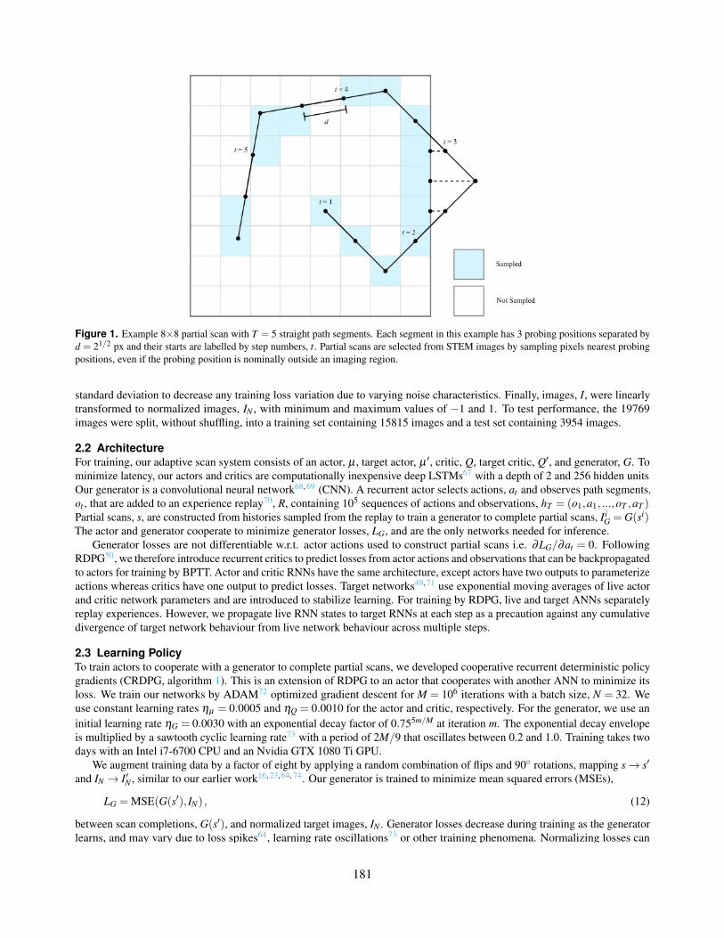
Figure 1. Example 8×8 partial scan with T = 5 straight path segments. Each segment in this example has 3 probing positions separated byd = 21/2 px and their starts are labelled by step numbers, t. Partial scans are selected from STEM images by sampling pixels nearest probingpositions, even if the probing position is nominally outside an imaging region.
standard deviation to decrease any training loss variation due to varying noise characteristics. Finally, images, I, were linearlytransformed to normalized images, IN , with minimum and maximum values of −1 and 1. To test performance, the 19769images were split, without shuffling, into a training set containing 15815 images and a test set containing 3954 images.
2.2 ArchitectureFor training, our adaptive scan system consists of an actor, µ , target actor, µ ′, critic, Q, target critic, Q′, and generator, G. Tominimize latency, our actors and critics are computationally inexpensive deep LSTMs67 with a depth of 2 and 256 hidden units.Our generator is a convolutional neural network68, 69 (CNN). A recurrent actor selects actions, at and observes path segments,ot , that are added to an experience replay70, R, containing 105 sequences of actions and observations, hT = (o1,a1, ...,oT ,aT ).Partial scans, s, are constructed from histories sampled from the replay to train a generator to complete partial scans, Ii
G = G(si).The actor and generator cooperate to minimize generator losses, LG, and are the only networks needed for inference.
Generator losses are not differentiable w.r.t. actor actions used to construct partial scans i.e. ∂LG/∂at = 0. FollowingRDPG50, we therefore introduce recurrent critics to predict losses from actor actions and observations that can be backpropagatedto actors for training by BPTT. Actor and critic RNNs have the same architecture, except actors have two outputs to parameterizeactions whereas critics have one output to predict losses. Target networks49, 71 use exponential moving averages of live actorand critic network parameters and are introduced to stabilize learning. For training by RDPG, live and target ANNs separatelyreplay experiences. However, we propagate live RNN states to target RNNs at each step as a precaution against any cumulativedivergence of target network behaviour from live network behaviour across multiple steps.
2.3 Learning PolicyTo train actors to cooperate with a generator to complete partial scans, we developed cooperative recurrent deterministic policygradients (CRDPG, algorithm 1). This is an extension of RDPG to an actor that cooperates with another ANN to minimize itsloss. We train our networks by ADAM72 optimized gradient descent for M = 106 iterations with a batch size, N = 32. Weuse constant learning rates ηµ = 0.0005 and ηQ = 0.0010 for the actor and critic, respectively. For the generator, we use aninitial learning rate ηG = 0.0030 with an exponential decay factor of 0.755m/M at iteration m. The exponential decay envelopeis multiplied by a sawtooth cyclic learning rate73 with a period of 2M/9 that oscillates between 0.2 and 1.0. Training takes twodays with an Intel i7-6700 CPU and an Nvidia GTX 1080 Ti GPU.
We augment training data by a factor of eight by applying a random combination of flips and 90 rotations, mapping s→ s′
and IN → I′N , similar to our earlier work16, 23, 64, 74. Our generator is trained to minimize mean squared errors (MSEs),
LG = MSE(G(s′), IN) , (12)
between scan completions, G(s′), and normalized target images, IN . Generator losses decrease during training as the generatorlearns, and may vary due to loss spikes64, learning rate oscillations73 or other training phenomena. Normalizing losses can
3/13181
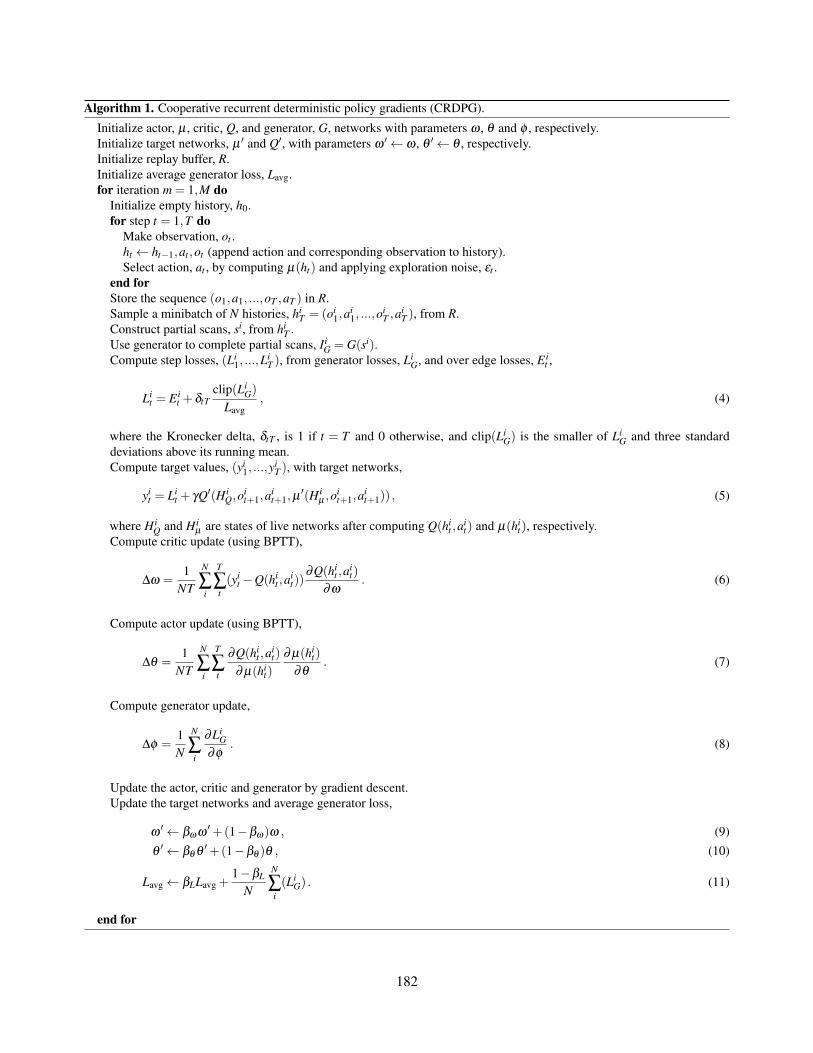
Algorithm 1. Cooperative recurrent deterministic policy gradients (CRDPG).
Initialize actor, µ , critic, Q, and generator, G, networks with parameters ω , θ and φ , respectively.Initialize target networks, µ ′ and Q′, with parameters ω ′← ω , θ ′← θ , respectively.Initialize replay buffer, R.Initialize average generator loss, Lavg.for iteration m = 1,M do
Initialize empty history, h0.for step t = 1,T do
Make observation, ot .ht ← ht−1,at ,ot (append action and corresponding observation to history).Select action, at , by computing µ(ht) and applying exploration noise, εt .
end forStore the sequence (o1,a1, ...,oT ,aT ) in R.Sample a minibatch of N histories, hi
T = (oi1,a
i1, ...,o
iT ,a
iT ), from R.
Construct partial scans, si, from hiT .
Use generator to complete partial scans, IiG = G(si).
Compute step losses, (Li1, ...,L
iT ), from generator losses, Li
G, and over edge losses, E it ,
Lit = E i
t +δtTclip(Li
G)
Lavg, (4)
where the Kronecker delta, δtT , is 1 if t = T and 0 otherwise, and clip(LiG) is the smaller of Li
G and three standarddeviations above its running mean.Compute target values, (yi
1, ...,yiT ), with target networks,
yit = Li
t + γQ′(H iQ,o
it+1,a
it+1,µ
′(H iµ ,o
it+1,a
it+1)) , (5)
where H iQ and H i
µ are states of live networks after computing Q(hit ,a
it) and µ(hi
t), respectively.Compute critic update (using BPTT),
∆ω =1
NT
N
∑i
T
∑t(yi
t −Q(hit ,a
it))
∂Q(hit ,a
it)
∂ω. (6)
Compute actor update (using BPTT),
∆θ =1
NT
N
∑i
T
∑t
∂Q(hit ,a
it)
∂ µ(hit)
∂ µ(hit)
∂θ. (7)
Compute generator update,
∆φ =1N
N
∑i
∂LiG
∂φ. (8)
Update the actor, critic and generator by gradient descent.Update the target networks and average generator loss,
ω ′← βω ω ′+(1−βω)ω , (9)θ ′← βθ θ ′+(1−βθ )θ , (10)
Lavg← βLLavg +1−βL
N
N
∑i(Li
G) . (11)
end for
4/13182
improve RL75, so we divide generator losses used for critic training by their running mean,
Lavg← βLLavg +1−βL
N
N
∑i
LG , (13)
where we chose βL = 0.997 and Lavg is updated at each training iteration.Heuristically, an optimal policy does not go over image edges as there is no information there in our training environment.
To accelerate convergence, we therefore added a small loss penalty, Et = 0.1, at step t if an action results in a probing positionbeing over an image edge. The total loss at each step is
Lt = Et +δtTclip(LG)
Lavg, (14)
where clip(LG) clips losses used for RL to three standard deviations above their running mean. This adaptive loss clippingis inspired by adaptive learning rate clipping64 (ALRC) and reduces learning destabilization by high loss spikes. However,we expect that clipping normalized losses to a fixed threshold71 would achieve similar results. The Kronecker delta, δtT , inequation 14 is 1 if t = T and 0 otherwise, so it only adds the generator loss at the final step, T .
To estimate discounted future losses, Qrlt , for RL, we use a target actor and critic,
Qrlt = Lt + γQ′(ht+1,µ ′(ht+1)) , (15)
where we chose γ = 0.97. Target networks stabilize learning and decrease policy oscillations76–78. The critic is trained tominimize mean squared differences, LQ, between predicted and target losses, and the actor is trained to minimize losses, Lµ ,predicted by the critic,
LQ =1
2T
T
∑t=1
(yt −Q(ht ,at))2 , (16)
Lµ =1T
T
∑t=1
Q(ht ,at) . (17)
Our target actor and critic have trainable parameters ω ′ and θ ′, respectively, that track live parameters, ω and θ , by softupdates49,
ω ′m = βω ω ′m−1 +(1−βω)ωm , (18)θ ′m = βθ θ ′m−1 +(1−βθ )θm , (19)
where we chose βω = βθ = 0.9997. We also investigated hard updates71, where target networks are periodically copied fromlive networks; however, we found that soft updates result in faster convergence and more stable training.
3 ExperimentsIn this section, we present examples of adaptive partial scans and select learning curves for architecture and learning policyexperiments. Examples of 1/23.04 px coverage partial scans, target outputs and generator completions are shown in figure 2 for96×96 crops from test set STEM images. They show both adaptive and spiral scans after flips and rotations to augment data forthe generator. The first actions select a path segment from the middle of image in the direction of a corner. Actors then use thefirst and following observations to inform where to sample the remaining T −1 = 19 path segments. Actors adapt scan paths tospecimens. For example, if an image contains regular atoms, an actor might cover a large area to see if there is a region wherethat changes. Alternatively, if an image contains a uniform region, actors, may explore near image edges and far away from theuniform region to find region boundaries.
The main limitation of our experiments is that generators trained to complete a variety of partial scan paths generated by anactor achieves lower performance than a generate trained to complete partial scans with a fixed path. For example, figure 3(a)shows that generators trained to cooperate with LSTM or GRU actors are outperformed by generators trained with fixed spiralor other scan paths shown in figure 3(b). Spiral paths outperform fixed scan paths; however, we emphasize that paths generatedby actors are designed for individual training data, rather than all training data. Freezing actor training to prevent changes inactor policy does not result in clear improvements in generator performance. Consequently, we think that improvements togenerator architecture or learning policy should be a starting point for further investigation. To find the best practical actor
5/13183
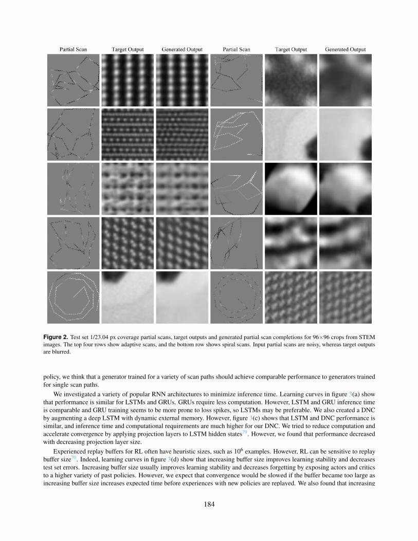
Figure 2. Test set 1/23.04 px coverage partial scans, target outputs and generated partial scan completions for 96×96 crops from STEMimages. The top four rows show adaptive scans, and the bottom row shows spiral scans. Input partial scans are noisy, whereas target outputsare blurred.
policy, we think that a generator trained for a variety of scan paths should achieve comparable performance to generators trainedfor single scan paths.
We investigated a variety of popular RNN architectures to minimize inference time. Learning curves in figure 3(a) showthat performance is similar for LSTMs and GRUs. GRUs require less computation. However, LSTM and GRU inference timeis comparable and GRU training seems to be more prone to loss spikes, so LSTMs may be preferable. We also created a DNCby augmenting a deep LSTM with dynamic external memory. However, figure 3(c) shows that LSTM and DNC performance issimilar, and inference time and computational requirements are much higher for our DNC. We tried to reduce computation andaccelerate convergence by applying projection layers to LSTM hidden states79. However, we found that performance decreasedwith decreasing projection layer size.
Experienced replay buffers for RL often have heuristic sizes, such as 106 examples. However, RL can be sensitive to replaybuffer size70. Indeed, learning curves in figure 3(d) show that increasing buffer size improves learning stability and decreasestest set errors. Increasing buffer size usually improves learning stability and decreases forgetting by exposing actors and criticsto a higher variety of past policies. However, we expect that convergence would be slowed if the buffer became too large asincreasing buffer size increases expected time before experiences with new policies are replayed. We also found that increasing
6/13184
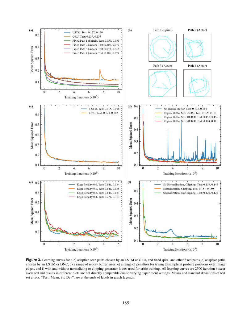
Figure 3. Learning curves for a-b) adaptive scan paths chosen by an LSTM or GRU, and fixed spiral and other fixed paths, c) adaptive pathschosen by an LSTM or DNC, d) a range of replay buffer sizes, e) a range of penalties for trying to sample at probing positions over imageedges, and f) with and without normalizing or clipping generator losses used for critic training. All learning curves are 2500 iteration boxcaraveraged and results in different plots are not directly comparable due to varying experiment settings. Means and standard deviations of testset errors, “Test: Mean, Std Dev”, are at the ends of labels in graph legends.
7/13185
buffer sized decreased the size of small loss oscillations76–78, which have a period near 2000 iterations. However, the size ofloss oscillations does not appear to affect performance.
We found that initial convergence is usually delayed if a large portion of initial actions go outside the imaging region. Thiswould often delay convergence by about 104 iterations before OU noise led to the discovery of better exploration strategiesaway from image edges. Although 104 iterations is only 1% of our 106 iteration learning policy, it often impaired developmentby delaying debugging or evaluation of changes to architecture and learning policy. Augmenting RL losses with subgoal-basedheuristic rewards can accelerate convergence by making problems more tractable80. Thus, we added loss penalties if actors triedto go over image edges, which accelerated initial convergence. Learning curves in figure 3(e) show that over edge penaltiesat each step smaller than Et = 0.2 have a similar effect on performance. Further, performance is lower for higher over edgepenalties, Et ≥ 0.2. We also found that training is more stable if over edge penalties are added at individual steps, rather thanpropagated to past steps as part of a discounted future loss.
Our actor, critic and generator are trained together. It follows that generator losses, which our critic learns to predict,decrease throughout training as generator performance improves. However, normalizing loss sizes usually improves RL75, sowe divide by their running means in equation 14. Learning curves in figure 3(f) show that loss normalization improves learningstability and decreases final errors. Clipping training losses can improve RL71, so we clipped generator losses used for critictraining to 3 standard deviations above their running means. We found that clipping increases test set errors, possibly becausemost training errors are in a similar regime. Thus, we expect that clipping may be more helpful for training with sparser scansas higher uncertainty may increase likelihood of unusually high generator losses.
4 DiscussionThe main limitation of our adaptive scan system is that generator errors are much higher when a generator is trained for avariety of scan paths than when it is trained for a single scan path. However, we expect that generator performance for a varietyof scans could be improved to match performance for single scans by developing a larger neural network with a better learningpolicy. To train actors to cooperate with generators, we developed CRDPG. This is an extension of RDPG50, and RDPG isbased on DDPG49. Alternatives to DDPG, such as TD362 and D4PG63, arguably achieve higher performance, so we expectthat they could form the basis of a future training algorithm. Further, we expect that architecture and learning policy could beimproved by AdaNet81, Ludwig82, or other automatic machine learning83–87 (AutoML) algorithms as AutoML can often matchor surpass the performance of human developers88, 89. Finally, test set losses for a variety of scans appear to be decreasing atthe end of training, so we expect that performance could be improved by increasing training iterations.
After generator performance is improved, we expect the main limitation of our adaptive scan system to be distortions causedby probing position errors. Errors usually depend on scan path shape34 and accumulate for each path segment. Non-linear scandistortions can be corrected by comparing pairs of orthogonal raster scans90, 91, and we expect this method can be extended topartial scans. However, orthogonal scanning would complicate measurement by limiting scan paths to two half scans to avoiddoubling electron dose on beam-sensitive materials. Instead, we propose that a cyclic generator92 could be trained to correctscan distortions and provide a detailed method as supplementary information93. Another limitation is that our generators do notlearn to correct STEM noise94. However, we expect that generators can learn to remove noise, for example, from single noisyexamples95 or by supervised learning74.
To simplify our preliminary investigation, our scan system samples straight path segments and cannot go outside a specifiedimaging region. However, actors could learn to output actions with additional degrees of freedom to describe curves, multiplesuccessive path segments, or sequences of non-contiguous probing positions. Similarly, additional restrictions could beapplied to actions. For example, actions could be restricted to avoid actions that cause high probing position errors. Trainingenvironments could also be modified to allow actors to sample pixels over image edges by loading images larger than partialscan regions. In practice, actors can sample outside a scan region and being able to access extra information outside an imagingregion could improve performance. However, using larger images may slow development by increasing data loading andprocessing times.
Not all scan systems support non-raster scan paths. However, many scan controllers can be augmented with an FPGA toenable custom scan paths34, 35. Recent versions of Gatan DigitalMicrograph support Python96, so our ANNs can be readilyintegrated into existing scan systems. Alternatively, an actor could be synthesized on a scan-controlling FPGA97, 98 to minimizeinference time. There could be hundreds of path segments in a partial scan, so computationally lightweight and parallelizableactors are essential to minimize scan time. We have therefore developed actors based computationally inexpensive RNNs,which can remember state information to inform future decisions. Another approach is to update a partial scan at each stepto be input to feedforward neural network (FNN), such as a CNN, to decide actions. However, we expect that FNNs are lesspractical than RNNs as FNNs may require additional computation to reprocess all past states at each step.
8/13186
5 ConclusionsOur initial investigation demonstrates that actor RNNs can be trained by RL to direct piecewise adaption of contiguous scansto specimens for compressed sensing. We introduce CRDPG to train an RNN to cooperate with a CNN to complete STEMimages from partial scans and present our learning policy, experiments, and example applications. After further development,we expect that adaptive scans will become the most effective approach to decrease electron beam damage and scan time withminimal information loss. Static sampling strategies are a subset of possible dynamic sampling strategies, so the performance ofstatic sampling can always be matched by or outperformed by dynamic sampling. Further, we expect that adaptive scan systemscan be developed for most areas of science and technology, including for the reduction of medical radiation. To encouragefurther investigation, our source code, pretrained models, and training data is openly accessible.
6 Supplementary InformationSupplementary information is openly accessible at https://doi.org/10.5281/zenodo.4384708. Therein, we presentdetailed ANN architecture, additional experiments and example scans, and a new method to correct partial scan distortions.
Data AvailabilityThe data that support the findings of this study are openly available.
AcknowledgementsThanks go to Jasmine Clayton, Abdul Mohammed, and Jeremy Sloan for internal review. The author acknowledges fundingfrom EPSRC grant EP/N035437/1 and EPSRC Studentship 1917382.
Competing InterestsThe author declares no competing interests.
References1. Krull, A., Hirsch, P., Rother, C., Schiffrin, A. & Krull, C. Artificial-Intelligence-Driven Scanning Probe Microscopy.
Commun. Phys. 3, 1–8 (2020).
2. Rugar, D. & Hansma, P. Atomic Force Microscopy. Phys. Today 43, 23–30 (1990).
3. New, P. F., Scott, W. R., Schnur, J. A., Davis, K. R. & Taveras, J. M. Computerized Axial Tomography with the EMIScanner. Radiology 110, 109–123 (1974).
4. Heymsfield, S. B. et al. Accurate Measurement of Liver, Kidney, and Spleen Volume and Mass by Computerized AxialTomography. Annals Intern. Medicine 90, 185–187 (1979).
5. Schwartz, A. J., Kumar, M., Adams, B. L. & Field, D. P. Electron Backscatter Diffraction in Materials Science, vol. 2(Springer, 2009).
6. Vernon-Parry, K. D. Scanning Electron Microscopy: An Introduction. III-Vs Rev. 13, 40–44 (2000).
7. Keren, S. et al. Noninvasive Molecular Imaging of Small Living Subjects Using Raman Spectroscopy. Proc. Natl. Acad.Sci. 105, 5844–5849 (2008).
8. Tong, Y.-X., Zhang, Q.-H. & Gu, L. Scanning Transmission Electron Microscopy: A Review of High Angle Annular DarkField and Annular Bright Field Imaging and Applications in Lithium-Ion Batteries. Chin. Phys. B 27, 066107 (2018).
9. Scarborough, N. M. et al. Dynamic X-Ray Diffraction Sampling for Protein Crystal Positioning. J. Synchrotron Radiat. 24,188–195 (2017).
10. Hujsak, K., Myers, B. D., Roth, E., Li, Y. & Dravid, V. P. Suppressing Electron Exposure Artifacts: An Electron ScanningParadigm with Bayesian Machine Learning. Microsc. Microanal. 22, 778–788 (2016).
11. Egerton, R. F., Li, P. & Malac, M. Radiation Damage in the TEM and SEM. Micron 35, 399–409 (2004).
12. Ede, J. M. Warwick Electron Microscopy Datasets. Mach. Learn. Sci. Technol. 1, 045003 (2020).
13. Amidror, I. Sub-Nyquist Artefacts and Sampling Moiré Effects. Royal Soc. Open Sci. 2, 140550 (2015).
14. Binev, P. et al. Compressed Sensing and Electron Microscopy. In Modeling Nanoscale Imaging in Electron Microscopy,73–126 (Springer, 2012).
9/13187

15. Ede, J. M. Review: Deep Learning in Electron Microscopy. arXiv preprint arXiv:2009.08328 (2020).
16. Ede, J. M. & Beanland, R. Partial Scanning Transmission Electron Microscopy with Deep Learning. arXiv preprintarXiv:1910.10467 (2020).
17. Li, Y. Deep Reinforcement Learning: An Overview. arXiv preprint arXiv:1701.07274 (2017).
18. Hwang, S., Han, C. W., Venkatakrishnan, S. V., Bouman, C. A. & Ortalan, V. Towards the Low-Dose Characterizationof Beam Sensitive Nanostructures via Implementation of Sparse Image Acquisition in Scanning Transmission ElectronMicroscopy. Meas. Sci. Technol. 28, 045402 (2017).
19. Hujsak, K., Myers, B. D., Roth, E., Li, Y. & Dravid, V. P. Suppressing Electron Exposure Artifacts: An Electron ScanningParadigm with Bayesian Machine Learning. Microsc. Microanal. 22, 778–788 (2016).
20. Anderson, H. S., Ilic-Helms, J., Rohrer, B., Wheeler, J. & Larson, K. Sparse Imaging for Fast Electron Microscopy. InComputational Imaging XI, vol. 8657, 86570C (International Society for Optics and Photonics, 2013).
21. Fang, L. et al. Deep Learning-Based Point-Scanning Super-Resolution Imaging. bioRxiv 740548 (2019).
22. de Haan, K., Ballard, Z. S., Rivenson, Y., Wu, Y. & Ozcan, A. Resolution Enhancement in Scanning Electron MicroscopyUsing Deep Learning. Sci. Reports 9, 1–7 (2019).
23. Ede, J. M. Deep Learning Supersampled Scanning Transmission Electron Microscopy. arXiv preprint arXiv:1910.10467(2019).
24. Mueller, K. Selection of Optimal Views for Computed Tomography Reconstruction (2011). US Patent App. 12/842,274.
25. Wang, Z. & Arce, G. R. Variable Density Compressed Image Sampling. IEEE Transactions on Image Process. 19, 264–270(2009).
26. Ji, S., Xue, Y. & Carin, L. Bayesian Compressive Sensing. IEEE Transactions on Signal Process. 56, 2346–2356 (2008).
27. Seeger, M. W. & Nickisch, H. Compressed Sensing and Bayesian Experimental Design. In Proceedings of the 25thInternational Conference on Machine Learning, 912–919 (2008).
28. Braun, G., Pokutta, S. & Xie, Y. Info-Greedy Sequential Adaptive Compressed Sensing. IEEE J. Sel. Top. Signal Process.9, 601–611 (2015).
29. Carson, W. R., Chen, M., Rodrigues, M. R., Calderbank, R. & Carin, L. Communications-Inspired Projection Design withApplication to Compressive Sensing. SIAM J. on Imaging Sci. 5, 1185–1212 (2012).
30. Godaliyadda, G. D. P. et al. A Framework for Dynamic Image Sampling Based on Supervised Learning. IEEE Transactionson Comput. Imaging 4, 1–16 (2017).
31. Ermeydan, E. S. & Cankaya, I. Sparse Fast Fourier Transform for Exactly Sparse Signals and Signals with AdditiveGaussian Noise. Signal, Image Video Process. 12, 445–452 (2018).
32. Saldi, N., Yüksel, S. & Linder, T. Asymptotic Optimality of Finite Model Approximations for Partially Observed MarkovDecision Processes With Discounted Cost. IEEE Transactions on Autom. Control. 65, 130–142 (2019).
33. Jaakkola, T., Singh, S. P. & Jordan, M. I. Reinforcement Learning Algorithm for Partially Observable Markov DecisionProblems. In Advances in Neural Information Processing Systems, 345–352 (1995).
34. Sang, X. et al. Dynamic Scan Control in STEM: Spiral Scans. Adv. Struct. Chem. Imaging 2, 6 (2017).
35. Sang, X. et al. Precision Controlled Atomic Resolution Scanning Transmission Electron Microscopy Using Spiral ScanPathways. Sci. Reports 7, 43585 (2017).
36. Hochreiter, S. & Schmidhuber, J. Long Short-Term Memory. Neural Comput. 9, 1735–1780 (1997).
37. Olah, C. Understanding LSTM Networks. Online: https://colah.github.io/posts/2015-08-Understanding-LSTMs (2015).
38. Cho, K. et al. Learning Phrase Representations Using RNN Encoder-Decoder for Statistical Machine Translation. arXivpreprint arXiv:1406.1078 (2014).
39. Weiss, G., Goldberg, Y. & Yahav, E. On the Practical Computational Power of Finite Precision RNNs for LanguageRecognition. arXiv preprint arXiv:1805.04908 (2018).
40. Jozefowicz, R., Zaremba, W. & Sutskever, I. An Empirical Exploration of Recurrent Network Architectures. In InternationalConference on Machine Learning, 2342–2350 (2015).
41. Bayer, J., Wierstra, D., Togelius, J. & Schmidhuber, J. Evolving Memory Cell Structures for Sequence Learning. InInternational Conference on Artificial Neural Networks, 755–764 (Springer, 2009).
10/13188
42. Pascanu, R., Mikolov, T. & Bengio, Y. On the Difficulty of Training Recurrent Neural Networks. In InternationalConference on Machine Learning, 1310–1318 (2013).
43. Graves, A. et al. Hybrid Computing Using a Neural Network with Dynamic External Memory. Nature 538, 471–476(2016).
44. Werbos, P. J. Backpropagation Through Time: What It Does and How To Do It. Proc. IEEE 78, 1550–1560 (1990).
45. Ruder, S. An Overview of Gradient Descent Optimization Algorithms. arXiv preprint arXiv:1609.04747 (2016).
46. Mnih, V., Heess, N., Graves, A. & Kavukcuoglu, K. Recurrent Models of Visual Attention. In Advances in NeuralInformation Processing Systems, 2204–2212 (2014).
47. Ba, J., Mnih, V. & Kavukcuoglu, K. Multiple Object Recognition with Visual Attention. arXiv preprint arXiv:1412.7755(2014).
48. Vinyals, O. et al. AlphaStar: Mastering the Real-Time Strategy Game StarCraft II. https://deepmind.com/blog/alphastar-mastering-real-time-strategy-game-starcraft-ii/ (2019).
49. Lillicrap, T. P. et al. Continuous Control with Deep Reinforcement Learning. arXiv preprint arXiv:1509.02971 (2015).
50. Heess, N., Hunt, J. J., Lillicrap, T. P. & Silver, D. Memory-Based Control with Recurrent Neural Networks. arXiv preprintarXiv:1512.04455 (2015).
51. Grabocka, J., Scholz, R. & Schmidt-Thieme, L. Learning Surrogate Losses. arXiv preprint arXiv:1905.10108 (2019).
52. Konda, V. R. & Tsitsiklis, J. N. Actor-Critic Algorithms. In Advances in Neural Information Processing Systems,1008–1014 (2000).
53. Zhao, T., Hachiya, H., Niu, G. & Sugiyama, M. Analysis and Improvement of Policy Gradient Estimation. In Advances inNeural Information Processing Systems, 262–270 (2011).
54. Rere, L. R., Fanany, M. I. & Arymurthy, A. M. Simulated Annealing Algorithm for Deep Learning. Procedia Comput. Sci.72, 137–144 (2015).
55. Young, S. R., Rose, D. C., Karnowski, T. P., Lim, S.-H. & Patton, R. M. Optimizing Deep Learning Hyper-ParametersThrough an Evolutionary Algorithm. In Proceedings of the Workshop on Machine Learning in High-PerformanceComputing Environments, 1–5 (2015).
56. Such, F. P. et al. Deep Neuroevolution: Genetic Algorithms are a Competitive Alternative for Training Deep NeuralNetworks for Reinforcement Learning. arXiv preprint arXiv:1712.06567 (2017).
57. Abadi, M. et al. TensorFlow: A System for Large-Scale Machine Learning. In 12th USENIX Symposium on OperatingSystems Design and Implementation (OSDI 16), 265–283 (2016).
58. Ede, J. M. Adaptive Partial STEM Repository. Online: https://github.com/Jeffrey-Ede/adaptive-scans (2020).
59. Ede, J. M. & Beanland, R. Electron Microscopy Datasets. Online: https://github.com/Jeffrey-Ede/datasets/wiki (2020).
60. Uhlenbeck, G. E. & Ornstein, L. S. On the Theory of the Brownian Motion. Phys. Rev. 36, 823 (1930).
61. Plappert, M. et al. Parameter Space Noise for Exploration. arXiv preprint arXiv:1706.01905 (2017).
62. Fujimoto, S., Van Hoof, H. & Meger, D. Addressing Function Approximation Error in Actor-Critic Methods. arXivpreprint arXiv:1802.09477 (2018).
63. Barth-Maron, G. et al. Distributed Distributional Deterministic Policy Gradients. arXiv preprint arXiv:1804.08617 (2018).
64. Ede, J. M. & Beanland, R. Adaptive Learning Rate Clipping Stabilizes Learning. Mach. Learn. Sci. Technol. 1, 015011(2020).
65. Raschka, S. Model Evaluation, Model Selection, and Algorithm Selection in Machine Learning. arXiv preprintarXiv:1811.12808 (2018).
66. Roh, Y., Heo, G. & Whang, S. E. A Survey on Data Collection for Machine Learning: A Big Data-AI IntegrationPerspective. IEEE Transactions on Knowl. Data Eng. (2019).
67. Zaremba, W., Sutskever, I. & Vinyals, O. Recurrent Neural Network Regularization. arXiv preprint arXiv:1409.2329(2014).
68. McCann, M. T., Jin, K. H. & Unser, M. Convolutional Neural Networks for Inverse Problems in Imaging: A Review. IEEESignal Process. Mag. 34, 85–95 (2017).
11/13189
69. Krizhevsky, A., Sutskever, I. & Hinton, G. E. ImageNet Classification with Deep Convolutional Neural Networks. InAdvances in Neural Information Processing Systems, 1097–1105 (2012).
70. Zhang, S. & Sutton, R. S. A Deeper Look at Experience Replay. arXiv preprint arXiv:1712.01275 (2017).
71. Mnih, V. et al. Human-Level Control Through Deep Reinforcement Learning. Nature 518, 529–533 (2015).
72. Kingma, D. P. & Ba, J. ADAM: A Method for Stochastic Optimization. arXiv preprint arXiv:1412.6980 (2014).
73. Smith, L. N. Cyclical Learning Rates for Training Neural Networks. In 2017 IEEE Winter Conference on Applications ofComputer Vision (WACV), 464–472 (IEEE, 2017).
74. Ede, J. M. & Beanland, R. Improving Electron Micrograph Signal-to-Noise with an Atrous Convolutional Encoder-Decoder.Ultramicroscopy 202, 18–25 (2019).
75. van Hasselt, H. P., Guez, A., Hessel, M., Mnih, V. & Silver, D. Learning Values Across Many Orders of Magnitude. InAdvances in Neural Information Processing Systems, 4287–4295 (2016).
76. Czarnecki, W. M. et al. Distilling Policy Distillation. arXiv preprint arXiv:1902.02186 (2019).
77. Lipton, Z. C. et al. Combating Reinforcement Learning’s Sisyphean Curse with Intrinsic Fear. arXiv preprintarXiv:1611.01211 (2016).
78. Wagner, P. A Reinterpretation of the Policy Oscillation Phenomenon in Approximate Policy Iteration. In Advances inNeural Information Processing Systems, 2573–2581 (2011).
79. Jia, Y., Wu, Z., Xu, Y., Ke, D. & Su, K. Long Short-Term Memory Projection Recurrent Neural Network Architectures forPiano’s Continuous Note Recognition. J. Robotics 2017 (2017).
80. Ng, A. Y., Harada, D. & Russell, S. Policy Invariance Under Reward Transformations: Theory and Application to RewardShaping. In International Conference on Machine Learning, vol. 99, 278–287 (1999).
81. Weill, C. et al. AdaNet: A Scalable and Flexible Framework for Automatically Learning Ensembles. arXiv preprintarXiv:1905.00080 (2019).
82. Molino, P., Dudin, Y. & Miryala, S. S. Ludwig: A Type-Based Declarative Deep Learning Toolbox. arXiv preprintarXiv:1909.07930 (2019).
83. He, X., Zhao, K. & Chu, X. AutoML: A Survey of the State-of-the-Art. arXiv preprint arXiv:1908.00709 (2019).
84. Malekhosseini, E., Hajabdollahi, M., Karimi, N. & Samavi, S. Modeling Neural Architecture Search Methods for DeepNetworks. arXiv preprint arXiv:1912.13183 (2019).
85. Jaafra, Y., Laurent, J. L., Deruyver, A. & Naceur, M. S. Reinforcement Learning for Neural Architecture Search: A Review.Image Vis. Comput. 89, 57–66 (2019).
86. Elsken, T., Metzen, J. H. & Hutter, F. Neural Architecture Search: A Survey. arXiv preprint arXiv:1808.05377 (2018).
87. Waring, J., Lindvall, C. & Umeton, R. Automated Machine Learning: Review of the State-of-the-Art and Opportunities forHealthcare. Artif. Intell. Medicine 101822 (2020).
88. Hanussek, M., Blohm, M. & Kintz, M. Can AutoML Outperform Humans? An Evaluation on Popular OpenML DatasetsUsing AutoML Benchmark. arXiv preprint arXiv:2009.01564 (2020).
89. Zoph, B., Vasudevan, V., Shlens, J. & Le, Q. V. Learning Transferable Architectures for Scalable Image Recognition. InProceedings of the IEEE Conference on Computer Vision and Pattern Recognition, 8697–8710 (2018).
90. Ophus, C., Ciston, J. & Nelson, C. T. Correcting Nonlinear Drift Distortion of Scanning Probe and Scanning TransmissionElectron Microscopies from Image Pairs with Orthogonal Scan Directions. Ultramicroscopy 162, 1–9 (2016).
91. Ning, S. et al. Scanning Distortion Correction in STEM Images. Ultramicroscopy 184, 274–283 (2018).
92. Zhu, J.-Y., Park, T., Isola, P. & Efros, A. A. Unpaired Image-to-Image Translation Using Cycle-Consistent AdversarialNetworks. In Proceedings of the IEEE International Conference on Computer Vision, 2223–2232 (2017).
93. Ede, J. M. Supplementary Information: Adaptive Partial Scanning Transmission Electron Microscopy with ReinforcementLearning. Zenodo, Online: https://doi.org/10.5281/zenodo.4384708 (2020).
94. Seki, T., Ikuhara, Y. & Shibata, N. Theoretical Framework of Statistical Noise in Scanning Transmission ElectronMicroscopy. Ultramicroscopy 193, 118–125 (2018).
95. Laine, S., Karras, T., Lehtinen, J. & Aila, T. High-Quality Self-Supervised Deep Image Denoising. In Advances in NeuralInformation Processing Systems, 6968–6978 (2019).
12/13190
96. Miller, B. & Mick, S. Real-Time Data Processing Using Python in DigitalMicrograph. Microsc. Microanal. 25, 234–235(2019).
97. Noronha, D. H., Salehpour, B. & Wilton, S. J. LeFlow: Enabling Flexible FPGA High-Level Synthesis of TensorFlowDeep Neural Networks. In FSP Workshop 2018; Fifth International Workshop on FPGAs for Software Programmers, 1–8(VDE, 2018).
98. Ruan, A., Shi, A., Qin, L., Xu, S. & Zhao, Y. A Reinforcement Learning Based Markov-Decision Process (MDP)Implementation for SRAM FPGAs. IEEE Transactions on Circuits Syst. II: Express Briefs (2019).
13/13191
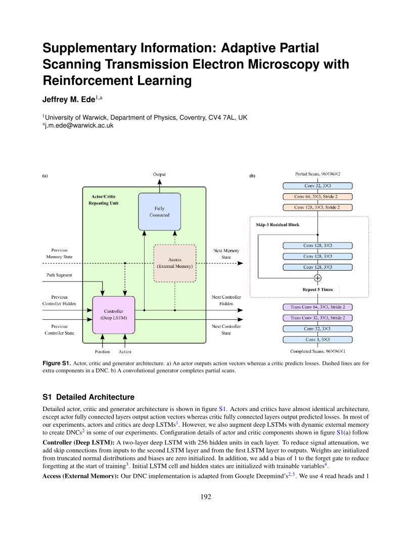
Supplementary Information: Adaptive PartialScanning Transmission Electron Microscopy withReinforcement LearningJeffrey M. Ede1,a
1University of Warwick, Department of Physics, Coventry, CV4 7AL, [email protected]
Figure S1. Actor, critic and generator architecture. a) An actor outputs action vectors whereas a critic predicts losses. Dashed lines are forextra components in a DNC. b) A convolutional generator completes partial scans.
S1 Detailed ArchitectureDetailed actor, critic and generator architecture is shown in figure S1. Actors and critics have almost identical architecture,except actor fully connected layers output action vectors whereas critic fully connected layers output predicted losses. In most ofour experiments, actors and critics are deep LSTMs1. However, we also augment deep LSTMs with dynamic external memoryto create DNCs2 in some of our experiments. Configuration details of actor and critic components shown in figure S1(a) follow.
Controller (Deep LSTM): A two-layer deep LSTM with 256 hidden units in each layer. To reduce signal attenuation, weadd skip connections from inputs to the second LSTM layer and from the first LSTM layer to outputs. Weights are initializedfrom truncated normal distributions and biases are zero initialized. In addition, we add a bias of 1 to the forget gate to reduceforgetting at the start of training3. Initial LSTM cell and hidden states are initialized with trainable variables4.
Access (External Memory): Our DNC implementation is adapted from Google Deepmind’s2, 5. We use 4 read heads and 1
S1192

write head to control access to dynamic external memory, which has 16 slots with a word size of 64.Fully Connected: A dense layer linearly connects inputs to outputs. Weights are initialized from a truncated normal distributionand there are no biases.Conv d, wxw, Stride, x: Convolutional layer with a square kernel of width, w, that outputs d feature channels. If the stride isspecified, convolutions are only applied to every xth spatial element of their input, rather than to every element. Striding is notapplied depthwise.Trans Conv d, wxw, Stride, x: Transpositional convolutional layer with a square kernel of width, w, that outputs d featurechannels. If the stride is specified, convolutions are only applied to every xth spatial element of their input, rather than to everyelement. Striding is not applied depthwise.+ : Circled plus signs indicate residual connections where incoming tensors are added together. Residuals help reduce signalattenuation and allow a network to learn perturbative transformations more easily.The actor and critic cooperate with a convolutional generator, shown in figure S1(b), to complete partial scans. Our generator isconstructed from convolutional layers6 and skip-3 residual blocks7. Each convolutional layer is followed by ReLU8 activationthen batch normalization9, and residual connections are added between activation and batch normalization. The convolutionalweights are Xavier10 initialized and biases are zero initialized.
S2 Additional Regularization
We apply L2 regularization11 to decay generator parameters by a factor, β = 0.99999, at each training iteration. This decay rateis heuristic and the L2 regularization is primarily a precaution against overfitting. Further, adding L2 regularization did nothave a noticeable effect on performance. We also investigated gradient clipping12–15 to a range of static and dynamic thresholdsfor actor and critic training. However, we found that gradient clipping decreases convergence if clipping thresholds are toosmall and otherwise does not have a noticeable effect.
S3 Additional ExperimentsThis section present additional learning curves for architecture and learning policy experiments in figure S2. For example,learning curves in figure S2(a) show that generator training with an exponentially decayed cyclic learning rate16 results infaster convergence and lower final errors than just using an exponentially decayed learning rate. We were concerned that acyclic learning rate might cause generator loss oscillations if the learning rate oscillated too high. Indeed, our investigation ofloss normalization was, in part, to prevent potential generator loss oscillations from destabilizing critic training. However, ourlearning policy results in generator losses that steadily decay throughout training.
To train actors by BPTT, we differentiate losses predicted by critics w.r.t. actor parameters by the chain rule,
∆θ =1
NT
N
∑i
T
∑t
∂Q(hit ,a
it)
∂θ=
1NT
N
∑i
T
∑t
∂Q(hit ,a
it)
∂ µ(hit)
∂ µ(hit)
∂θ. (S1)
An alternative approach is to replace ∂Q(hit ,a
it)/∂ µ(hi
t) with a derivative w.r.t. replayed actions, ∂Q(hit ,a
it)/∂ai
t . This isequivalent to adding noise, stop_gradient(ai
t −µ(hit)), to an actor action, µ(hi
t), where stop_gradient(x) is a function that stopsgradient backpropagation to x. However, learning curves in figure S2(b) show that differentiation w.r.t. live actor actions resultsin faster convergence to lower losses. Results for ∂Q(hi
t ,ait)/∂ai
t are similar if OU exploration noise is doubled.Most STEM signals are imaged at several times their Nyquist rates17. To investigate adaptive STEM performance on signals
imaged close to their Nyquist rates, we downsampled STEM images to 96×96. Learning curves in figure S2(c) show that lossesare lower for oversampled STEM crops. Following, we investigated if MSEs vary for training with different loss metrics byadding a Sobel loss, λSLS, to generator losses. Our Sobel loss is
LS = MSE(S(G(s)),S(IN)) , (S2)
where S(x) computes a channelwise concatenation of horizontal and vertical Sobel derivatives18 of x, and we chose λS = 0.1 toweight the contribution of LS to the total generator loss, LG +λSLS. Learning curves in figure S2(c) show that Sobel losses donot decrease training MSEs for STEM crops. However, Sobel losses decrease MSEs for downsampled STEM images. Thismotivates the exploration of alternative loss functions19 to further improve performance. For example, our earlier work showsthat generator training as part of a generative adversarial network20–23 (GAN) can improve STEM image realism24. Similarly,we expect that generated image realism could be improved by training generators with perceptual losses25.
After we found that adding a Sobel loss can decrease MSEs, we also experimented with other loss functions, such as themaximum MSE of 5×5 regions. Learning curves in figure S2(d) show that MSEs result in faster convergence than maximum
S2/S10193
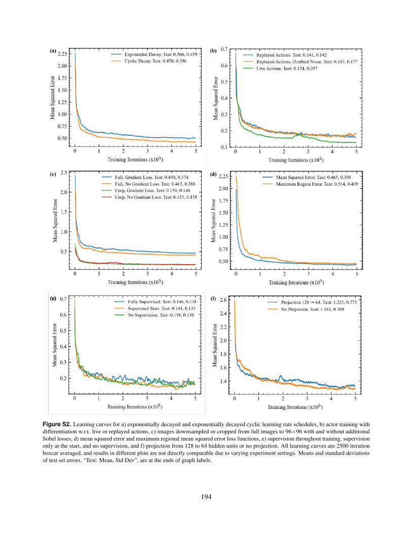
Figure S2. Learning curves for a) exponentially decayed and exponentially decayed cyclic learning rate schedules, b) actor training withdifferentiation w.r.t. live or replayed actions, c) images downsampled or cropped from full images to 96×96 with and without additionalSobel losses, d) mean squared error and maximum regional mean squared error loss functions, e) supervision throughout training, supervisiononly at the start, and no supervision, and f) projection from 128 to 64 hidden units or no projection. All learning curves are 2500 iterationboxcar averaged, and results in different plots are not directly comparable due to varying experiment settings. Means and standard deviationsof test set errors, “Test: Mean, Std Dev”, are at the ends of graph labels.
S3/S10194
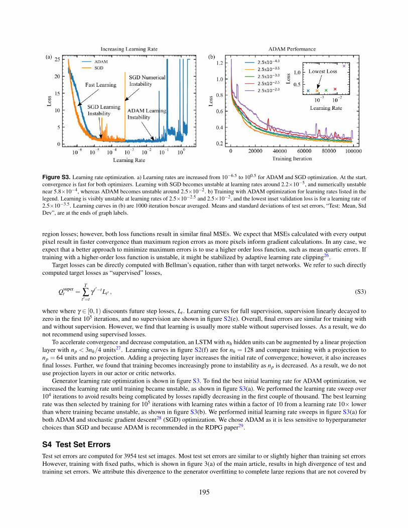
Figure S3. Learning rate optimization. a) Learning rates are increased from 10−6.5 to 100.5 for ADAM and SGD optimization. At the start,convergence is fast for both optimizers. Learning with SGD becomes unstable at learning rates around 2.2×10⁻⁵, and numerically unstablenear 5.8×10⁻⁴, whereas ADAM becomes unstable around 2.5×10⁻². b) Training with ADAM optimization for learning rates listed in thelegend. Learning is visibly unstable at learning rates of 2.5×10−2.5 and 2.5×10⁻², and the lowest inset validation loss is for a learning rate of2.5×10−3.5. Learning curves in (b) are 1000 iteration boxcar averaged. Means and standard deviations of test set errors, “Test: Mean, StdDev”, are at the ends of graph labels.
region losses; however, both loss functions result in similar final MSEs. We expect that MSEs calculated with every outputpixel result in faster convergence than maximum region errors as more pixels inform gradient calculations. In any case, weexpect that a better approach to minimize maximum errors is to use a higher order loss function, such as mean quartic errors. Iftraining with a higher-order loss function is unstable, it might be stabilized by adaptive learning rate clipping26.
Target losses can be directly computed with Bellman’s equation, rather than with target networks. We refer to such directlycomputed target losses as “supervised” losses,
Qsupert =
T
∑t ′=t
γ t ′−tLt ′ , (S3)
where where γ ∈ [0,1) discounts future step losses, Lt . Learning curves for full supervision, supervision linearly decayed tozero in the first 105 iterations, and no supervision are shown in figure S2(e). Overall, final errors are similar for training withand without supervision. However, we find that learning is usually more stable without supervised losses. As a result, we donot recommend using supervised losses.
To accelerate convergence and decrease computation, an LSTM with nh hidden units can be augmented by a linear projectionlayer with np < 3nh/4 units27. Learning curves in figure S2(f) are for nh = 128 and compare training with a projection tonp = 64 units and no projection. Adding a projecting layer increases the initial rate of convergence; however, it also increasesfinal losses. Further, we found that training becomes increasingly prone to instability as np is decreased. As a result, we do notuse projection layers in our actor or critic networks.
Generator learning rate optimization is shown in figure S3. To find the best initial learning rate for ADAM optimization, weincreased the learning rate until training became unstable, as shown in figure S3(a). We performed the learning rate sweep over104 iterations to avoid results being complicated by losses rapidly decreasing in the first couple of thousand. The best learningrate was then selected by training for 105 iterations with learning rates within a factor of 10 from a learning rate 10× lowerthan where training became unstable, as shown in figure S3(b). We performed initial learning rate sweeps in figure S3(a) forboth ADAM and stochastic gradient descent28 (SGD) optimization. We chose ADAM as it is less sensitive to hyperparameterchoices than SGD and because ADAM is recommended in the RDPG paper29.
S4 Test Set ErrorsTest set errors are computed for 3954 test set images. Most test set errors are similar to or slightly higher than training set errors.However, training with fixed paths, which is shown in figure 3(a) of the main article, results in high divergence of test andtraining set errors. We attribute this divergence to the generator overfitting to complete large regions that are not covered by
S4/S10195
fixed scan paths. In comparison, our learning policy was optimized for training with a variety of adaptive scan paths whereoverfitting is minimal. After all 106 training iterations, means and standard deviations (mean, std dev) of test set errors for fixedpaths 2, 3 and 4 are (0.170, 0.182), (0.135, 0.133), and (0.171, 0.184). Instead, we report lower test set errors of (0.106, 0.090),(0.073, 0.045), and (0.106. 0.090), respectively, at 5×10⁵ training iterations, which correspond to early stopping30, 31. Allother test set errors were computed after final training iterations.
S5 Distortion Correction
A limitation of partial STEM is that images are usually distorted by probing position errors, which vary with scan path shape32.Distortions in raster scans can be corrected by comparing series of images33, 34. However, distortion correction of adaptivescans is complicated by more complicated scan path shapes and microscope-specific actor command execution characteristics.We expect that command execution characteristics are almost static. Thus, it follows that there is a bijective mapping betweenprobing locations in distorted adaptive partial scans and raster scans. Subsequently, we propose that distortions could becorrected by a cyclic generative adversarial network35 (GAN). To be clear, this section outlines a possible starting point forfuture research that can be refined or improved upon. The method’s main limitation is that the cyclic GAN would need to betrained or fine-tuned for individual scan systems.
Let Ipartial and Iraster be unpaired partial scans and raster scans, respectively. A binary mask, M, can be constructed to be1 at nominal probing positions in Ipartial and 0 elsewhere. We introduce generators Gp→r(Ipartial) and Gr→p(Iraster,M) to mapfrom partial scans to raster scans and from raster scans to partial scans, respectively. A mask must be input to the partial scangenerator for it to output a partial scan with a realistic distortion field as distortions depend on scan path shape32. Finally, weintroduce discriminators Dpartial and Draster are trained to distinguish between real and generated partial scans and raster scans,respectively, and predict losses that can be used to train generators to create realistic images. In short, partial scans could bemapped to raster scans by minimizing
LGANp→r = Draster(Gp→r(Ipartial)) , (S4)
LGANr→p = Dpartial(MGr→p(Iraster,M)) , (S5)
Lcycler→p = MSE(MGr→p(Gp→r(Ipartial),M), Ipartial) , (S6)
Lcyclep→r = MSE(Gp→r(MGr→p(Iraster,M)), Iraster) , (S7)
Lp→r = LGANp→r +bLcycle
r→p , (S8)
Lr→p = LGANr→p +bLcycle
p→r , (S9)
where Lp→r and Lp→r are total losses to optimize Gp→r and Gp→r, respectively. A scalar, b, balances adversarial andcycle-consistency losses.
S6 Additional ExamplesAdditional sheets of test set adaptive scans are shown in figure S4 and figure S5. In addition, a sheet of test set spiral scans isshown in figure S6. Target outputs were low-pass filtered by a 5×5 symmetric Gaussian kernel with a 2.5 px standard deviationto suppress high-frequency noise.
S5/S10196

Figure S4. Test set 1/23.04 px coverage adaptive partial scans, target outputs, and generated partial scan completions for 96×96 crops fromSTEM images.
S6/S10197
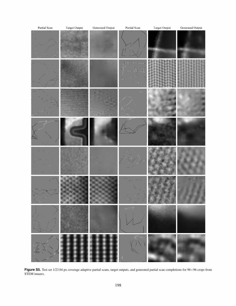
Figure S5. Test set 1/23.04 px coverage adaptive partial scans, target outputs, and generated partial scan completions for 96×96 crops fromSTEM images.
S7/S10198
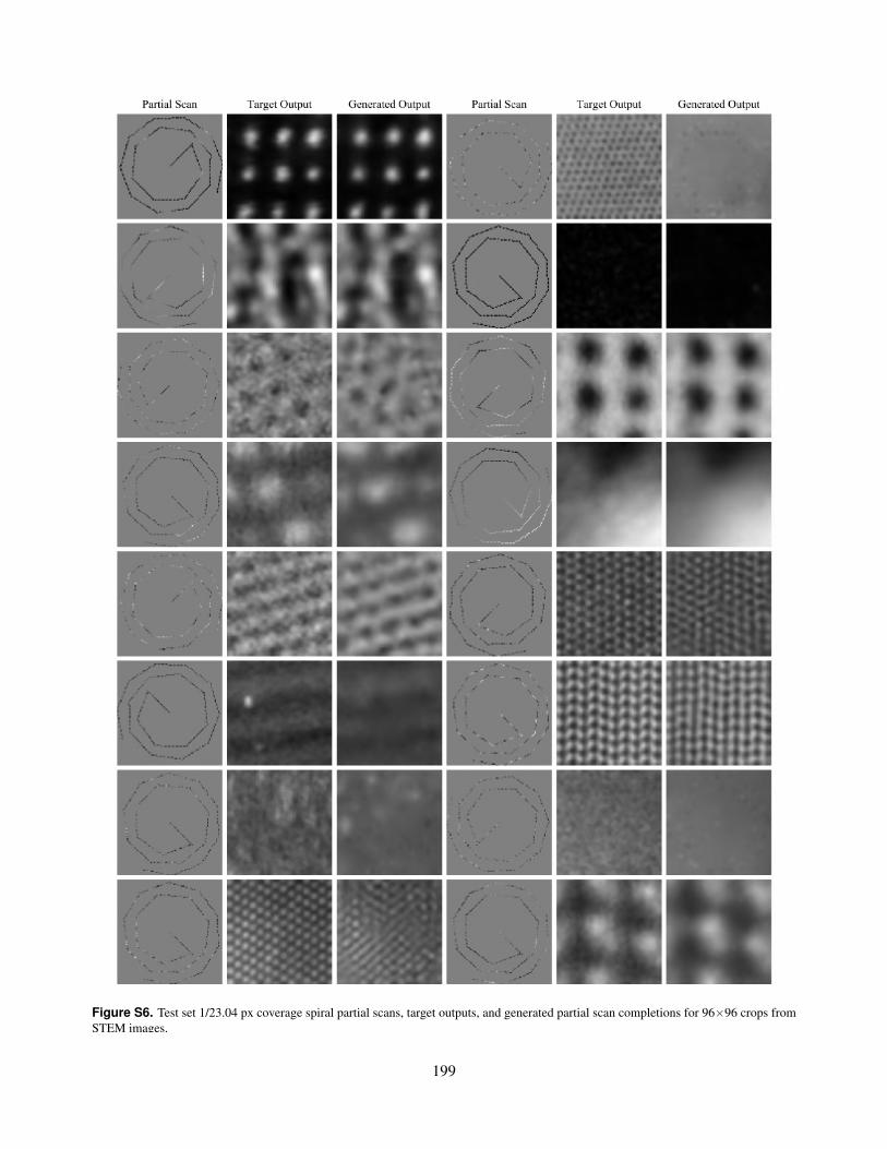
Figure S6. Test set 1/23.04 px coverage spiral partial scans, target outputs, and generated partial scan completions for 96×96 crops fromSTEM images.
S8/S10199
References1. Zaremba, W., Sutskever, I. & Vinyals, O. Recurrent Neural Network Regularization. arXiv preprint arXiv:1409.2329
(2014).
2. Graves, A. et al. Hybrid Computing Using a Neural Network with Dynamic External Memory. Nature 538, 471–476(2016).
3. Jozefowicz, R., Zaremba, W. & Sutskever, I. An Empirical Exploration of Recurrent Network Architectures. In InternationalConference on Machine Learning, 2342–2350 (2015).
4. Pitis, S. Non-Zero Initial States for Recurrent Neural Networks. Online: https://r2rt.com/non-zero-initial-states-for-recurrent-neural-networks.html (2016).
5. DeepMind. Differentiable Neural Computer. Online: https://github.com/deepmind/dnc (2018).
6. Dumoulin, V. & Visin, F. A Guide to Convolution Arithmetic for Deep Learning. arXiv preprint arXiv:1603.07285 (2016).
7. He, K., Zhang, X., Ren, S. & Sun, J. Deep Residual Learning for Image Recognition. CoRR abs/1512.03385 (2015).
8. Nair, V. & Hinton, G. E. Rectified Linear Units Improve Restricted Boltzmann Machines. In Proceedings of the 27thInternational Conference on Machine Learning (ICML-10), 807–814 (2010).
9. Ioffe, S. & Szegedy, C. Batch Normalization: Accelerating Deep Network Training by Reducing Internal Covariate Shift.arXiv preprint arXiv:1502.03167 (2015).
10. Glorot, X. & Bengio, Y. Understanding the Difficulty of Training Deep Feedforward Neural Networks. In Proceedings ofthe Thirteenth International Conference on Artificial Intelligence and Statistics, 249–256 (2010).
11. Kukacka, J., Golkov, V. & Cremers, D. Regularization for Deep Learning: A Taxonomy. arXiv preprint arXiv:1710.10686(2017).
12. Zhang, J., He, T., Sra, S. & Jadbabaie, A. Why Gradient Clipping Accelerates Training: A Theoretical Justification forAdaptivity. arXiv preprint arXiv:1905.11881 (2019).
13. Gorbunov, E., Danilova, M. & Gasnikov, A. Stochastic Optimization with Heavy-Tailed Noise via Accelerated GradientClipping. arXiv preprint arXiv:2005.10785 (2020).
14. Chen, X., Wu, Z. S. & Hong, M. Understanding Gradient Clipping in Private SGD: A Geometric Perspective. arXivpreprint arXiv:2006.15429 (2020).
15. Menon, A. K., Rawat, A. S., Reddi, S. J. & Kumar, S. Can Gradient Clipping Mitigate Label Noise? In InternationalConference on Learning Representations (2019).
16. Smith, L. N. Cyclical Learning Rates for Training Neural Networks. In 2017 IEEE Winter Conference on Applications ofComputer Vision (WACV), 464–472 (IEEE, 2017).
17. Ede, J. M. Warwick Electron Microscopy Datasets. Mach. Learn. Sci. Technol. 1, 045003 (2020).
18. Vairalkar, M. K. & Nimbhorkar, S. Edge Detection of Images Using Sobel Operator. Int. J. Emerg. Technol. Adv. Eng. 2,291–293 (2012).
19. Zhao, H., Gallo, O., Frosio, I. & Kautz, J. Loss Functions for Neural Networks for Image Processing. arXiv preprintarXiv:1511.08861 (2015).
20. Gui, J., Sun, Z., Wen, Y., Tao, D. & Ye, J. A Review on Generative Adversarial Networks: Algorithms, Theory, andApplications. arXiv preprint arXiv:2001.06937 (2020).
21. Saxena, D. & Cao, J. Generative Adversarial Networks (GANs): Challenges, Solutions, and Future Directions. arXivpreprint arXiv:2005.00065 (2020).
22. Pan, Z. et al. Recent Progress on Generative Adversarial Networks (GANs): A Survey. IEEE Access 7, 36322–36333(2019).
23. Wang, Z., She, Q. & Ward, T. E. Generative Adversarial Networks: A Survey and Taxonomy. arXiv preprintarXiv:1906.01529 (2019).
24. Ede, J. M. & Beanland, R. Partial Scanning Transmission Electron Microscopy with Deep Learning. arXiv preprintarXiv:1910.10467 (2020).
25. Grund Pihlgren, G., Sandin, F. & Liwicki, M. Improving Image Autoencoder Embeddings with Perceptual Loss. InInternational Joint Conference on Neural Networks (2020).
S9/S10200
26. Ede, J. M. & Beanland, R. Adaptive Learning Rate Clipping Stabilizes Learning. Mach. Learn. Sci. Technol. 1, 015011(2020).
27. Jia, Y., Wu, Z., Xu, Y., Ke, D. & Su, K. Long Short-Term Memory Projection Recurrent Neural Network Architectures forPiano’s Continuous Note Recognition. J. Robotics 2017 (2017).
28. Ruder, S. An Overview of Gradient Descent Optimization Algorithms. arXiv preprint arXiv:1609.04747 (2016).
29. Heess, N., Hunt, J. J., Lillicrap, T. P. & Silver, D. Memory-Based Control with Recurrent Neural Networks. arXiv preprintarXiv:1512.04455 (2015).
30. Li, M., Soltanolkotabi, M. & Oymak, S. Gradient Descent with Early Stopping is Provably Robust to Label Noise forOverparameterized Neural Networks. In International Conference on Artificial Intelligence and Statistics, 4313–4324(2020).
31. Flynn, T., Yu, K. M., Malik, A., D’Imperio, N. & Yoo, S. Bounding the Expected Run-Time of Nonconvex Optimizationwith Early Stopping. arXiv preprint arXiv:2002.08856 (2020).
32. Sang, X. et al. Dynamic Scan Control in STEM: Spiral Scans. Adv. Struct. Chem. Imaging 2, 6 (2017).
33. Zhang, C., Berkels, B., Wirth, B. & Voyles, P. M. Joint Denoising and Distortion Correction for Atomic Column Detectionin Scanning Transmission Electron Microscopy Images. Microsc. Microanal. 23, 164–165 (2017).
34. Jin, P. & Li, X. Correction of Image Drift and Distortion in a Scanning Electron Microscopy. J. Microsc. 260, 268–280(2015).
35. Zhu, J.-Y., Park, T., Isola, P. & Efros, A. A. Unpaired Image-to-Image Translation Using Cycle-Consistent AdversarialNetworks. In Proceedings of the IEEE International Conference on Computer Vision, 2223–2232 (2017).
S10/S10201
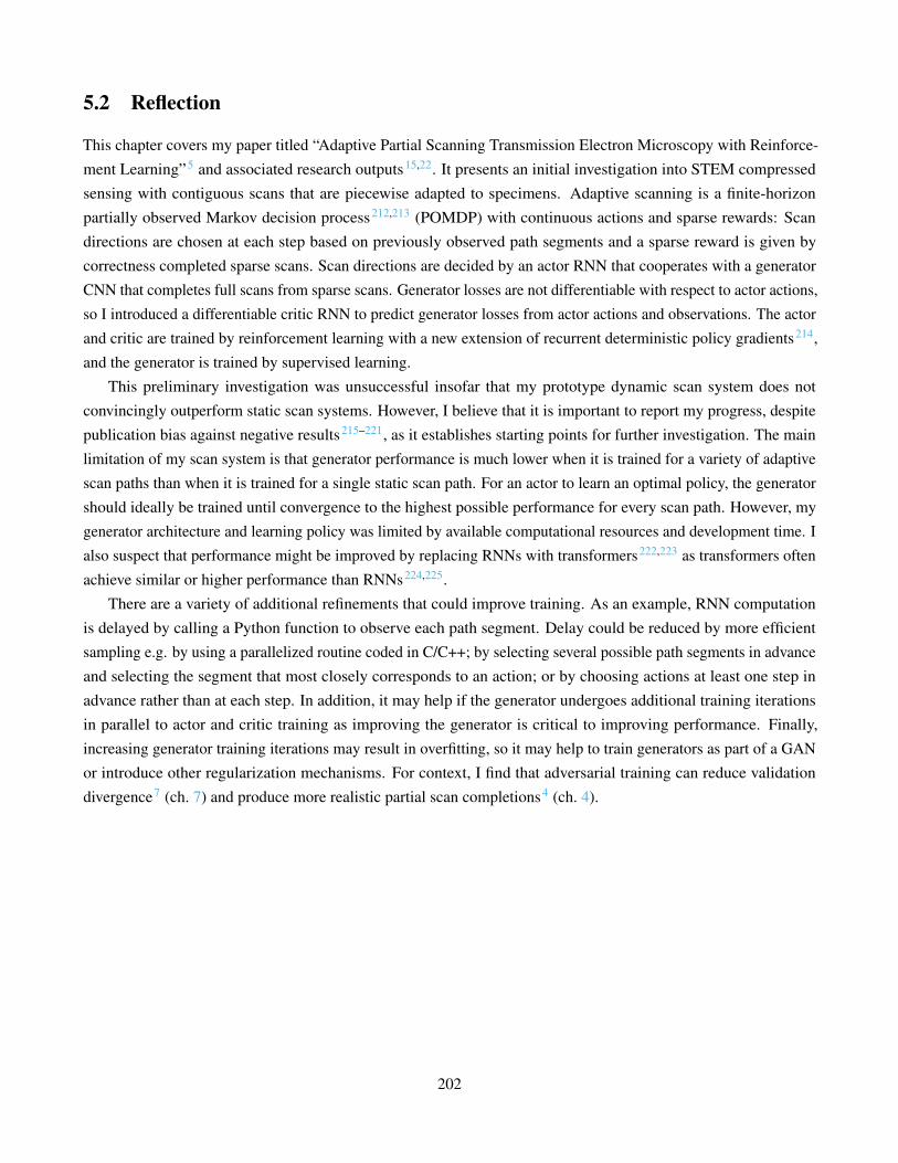
5.2 Reflection
This chapter covers my paper titled “Adaptive Partial Scanning Transmission Electron Microscopy with Reinforce-
ment Learning”5 and associated research outputs15,22. It presents an initial investigation into STEM compressed
sensing with contiguous scans that are piecewise adapted to specimens. Adaptive scanning is a finite-horizon
partially observed Markov decision process212,213 (POMDP) with continuous actions and sparse rewards: Scan
directions are chosen at each step based on previously observed path segments and a sparse reward is given by
correctness completed sparse scans. Scan directions are decided by an actor RNN that cooperates with a generator
CNN that completes full scans from sparse scans. Generator losses are not differentiable with respect to actor actions,
so I introduced a differentiable critic RNN to predict generator losses from actor actions and observations. The actor
and critic are trained by reinforcement learning with a new extension of recurrent deterministic policy gradients214,
and the generator is trained by supervised learning.
This preliminary investigation was unsuccessful insofar that my prototype dynamic scan system does not
convincingly outperform static scan systems. However, I believe that it is important to report my progress, despite
publication bias against negative results215–221, as it establishes starting points for further investigation. The main
limitation of my scan system is that generator performance is much lower when it is trained for a variety of adaptive
scan paths than when it is trained for a single static scan path. For an actor to learn an optimal policy, the generator
should ideally be trained until convergence to the highest possible performance for every scan path. However, my
generator architecture and learning policy was limited by available computational resources and development time. I
also suspect that performance might be improved by replacing RNNs with transformers222,223 as transformers often
achieve similar or higher performance than RNNs224,225.
There are a variety of additional refinements that could improve training. As an example, RNN computation
is delayed by calling a Python function to observe each path segment. Delay could be reduced by more efficient
sampling e.g. by using a parallelized routine coded in C/C++; by selecting several possible path segments in advance
and selecting the segment that most closely corresponds to an action; or by choosing actions at least one step in
advance rather than at each step. In addition, it may help if the generator undergoes additional training iterations
in parallel to actor and critic training as improving the generator is critical to improving performance. Finally,
increasing generator training iterations may result in overfitting, so it may help to train generators as part of a GAN
or introduce other regularization mechanisms. For context, I find that adversarial training can reduce validation
divergence7 (ch. 7) and produce more realistic partial scan completions4 (ch. 4).
202
Chapter 6
Improving Electron MicrographSignal-to-Noise with an Atrous ConvolutionalEncoder-Decoder
6.1 Scientific Paper
This chapter covers the following paper6.
J. M. Ede and R. Beanland. Improving Electron Micrograph Signal-to-Noise with an Atrous Convolu-
tional Encoder-Decoder. Ultramicroscopy, 202:18–25, 2019
203
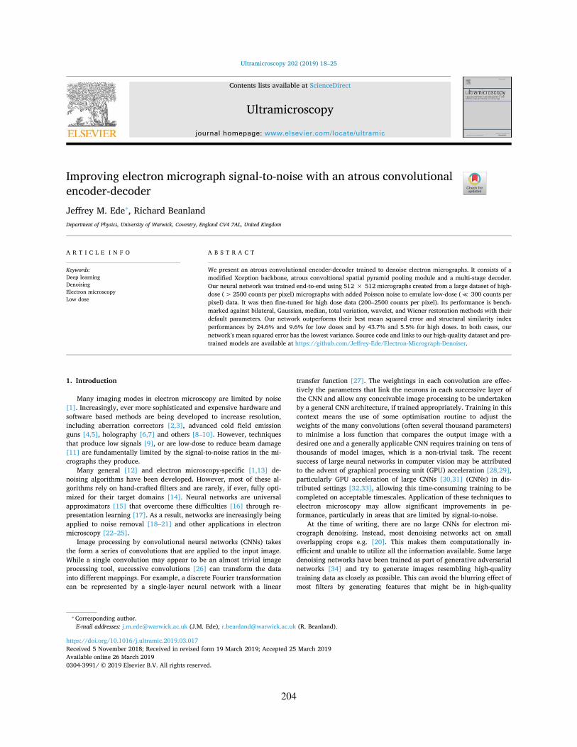
Contents lists available at ScienceDirectUltramicroscopy
journal homepage: www.elsevier.com/locate/ultramic
Improving electron micrograph signal-to-noise with an atrous convolutionalencoder-decoderJeffrey M. Ede⁎, Richard BeanlandDepartment of Physics, University of Warwick, Coventry, England CV4 7AL, United Kingdom
A R T I C L E I N F OKeywords:Deep learningDenoisingElectron microscopyLow dose
A B S T R A C TWe present an atrous convolutional encoder-decoder trained to denoise electron micrographs. It consists of amodified Xception backbone, atrous convoltional spatial pyramid pooling module and a multi-stage decoder.Our neural network was trained end-to-end using 512 × 512 micrographs created from a large dataset of high-dose ( > 2500 counts per pixel) micrographs with added Poisson noise to emulate low-dose ( ≪ 300 counts perpixel) data. It was then fine-tuned for high dose data (200–2500 counts per pixel). Its performance is bench-marked against bilateral, Gaussian, median, total variation, wavelet, and Wiener restoration methods with theirdefault parameters. Our network outperforms their best mean squared error and structural similarity indexperformances by 24.6% and 9.6% for low doses and by 43.7% and 5.5% for high doses. In both cases, ournetwork’s mean squared error has the lowest variance. Source code and links to our high-quality dataset and pre-trained models are available at https://github.com/Jeffrey-Ede/Electron-Micrograph-Denoiser.
1. IntroductionMany imaging modes in electron microscopy are limited by noise[1]. Increasingly, ever more sophisticated and expensive hardware andsoftware based methods are being developed to increase resolution,including aberration correctors [2,3], advanced cold field emissionguns [4,5], holography [6,7] and others [8–10]. However, techniquesthat produce low signals [9], or are low-dose to reduce beam damage[11] are fundamentally limited by the signal-to-noise ratios in the mi-crographs they produce.Many general [12] and electron microscopy-specific [1,13] de-noising algorithms have been developed. However, most of these al-gorithms rely on hand-crafted filters and are rarely, if ever, fully opti-mized for their target domains [14]. Neural networks are universalapproximators [15] that overcome these difficulties [16] through re-presentation learning [17]. As a result, networks are increasingly beingapplied to noise removal [18–21] and other applications in electronmicroscopy [22–25].Image processing by convolutional neural networks (CNNs) takesthe form a series of convolutions that are applied to the input image.While a single convolution may appear to be an almost trivial imageprocessing tool, successive convolutions [26] can transform the datainto different mappings. For example, a discrete Fourier transformationcan be represented by a single-layer neural network with a linear
transfer function [27]. The weightings in each convolution are effec-tively the parameters that link the neurons in each successive layer ofthe CNN and allow any conceivable image processing to be undertakenby a general CNN architecture, if trained appropriately. Training in thiscontext means the use of some optimisation routine to adjust theweights of the many convolutions (often several thousand parameters)to minimise a loss function that compares the output image with adesired one and a generally applicable CNN requires training on tens ofthousands of model images, which is a non-trivial task. The recentsuccess of large neural networks in computer vision may be attributedto the advent of graphical processing unit (GPU) acceleration [28,29],particularly GPU acceleration of large CNNs [30,31] (CNNs) in dis-tributed settings [32,33], allowing this time-consuming training to becompleted on acceptable timescales. Application of these techniques toelectron microscopy may allow significant improvements in pe-formance, particularly in areas that are limited by signal-to-noise.At the time of writing, there are no large CNNs for electron mi-crograph denoising. Instead, most denoising networks act on smalloverlapping crops e.g. [20]. This makes them computationally in-efficient and unable to utilize all the information available. Some largedenoising networks have been trained as part of generative adversarialnetworks [34] and try to generate images resembling high-qualitytraining data as closely as possible. This can avoid the blurring effect ofmost filters by generating features that might be in high-quality
https://doi.org/10.1016/j.ultramic.2019.03.017Received 5 November 2018; Received in revised form 19 March 2019; Accepted 25 March 2019
⁎ Corresponding author.E-mail addresses: [email protected] (J.M. Ede), [email protected] (R. Beanland).
Ultramicroscopy 202 (2019) 18–25
Available online 26 March 20190304-3991/ © 2019 Elsevier B.V. All rights reserved.
T
204

micrographs. However, this means that they are prone to producingundesirable artefacts.This paper presents the deep CNN in Fig. 1 for electron micrographdenoising. Our network architecture and training hyperparameters aresimilar to DeepLab3 [35] and DeepLab3+ [36], with the modificationsdiscussed in [37]. Briefly, image processing starts in a modified Xcep-tion [38] encoder, which spatially downsamples its 512 × 512 input toa 32 × 32 × 728 tensor. These high-level features flow into an atrousspatial pyramid pooling (ASPP) module [35,36] that combines theoutputs of atrous convolutions acting on different spatial scales into a32 × 32 × 256 tensor. A multi-stage decoder then upsamples the richASPP semantics to a 512 × 512 output by combining them with low-level encoder features. This recombination with low-level features helpsto reduce signal attenuaiton. For computational and parameter effi-ciency, most convolutions are depthwise separated into pointwise anddepthwise convolutions [38]; rather than standard convolutions.2. Training
An ideal training dataset might have a wide variety of images and zeronoise, enabling the CNN to be trained by inputting artificially degradedimages and comparing its output with the zero-noise image. Such datasetscan only be produced by simulation (which may be a time-consumingtask), or approximated by experimental data. Here, we used 17,267 elec-tron micrographs saved to University of Warwick data servers by scores ofscientists working on hundreds of projects over several years. The data settherefore has a diverse constitution, including for example phase contrastimages of polymers, diffraction contrast images of semiconductors, highresolution lattice imaging of crystals and a small number of CBED patterns.it is comprised of 32-bit image collected on Gatan SC600 or SC1000 Oriuscameras on JEOL 2000FX, 2100, 2100plus and ARM200F microscopes.Scanning TEM (STEM) images were not included. There are several con-tributions to noise from these charge-coupled device (CCD) cameras, whichform an image of an optically coupled scintillator, including [39]: Poissonnoise, dictated by the size of the detected signal; electrical readout and shotnoise; systematic errors in dark reference, linearity, gain reference, deadpixels or dead columns of pixels (some, but not all, of which is typicallycorrected by averaging in the camera software); and X-ray noise, whichresults in individual pixels having extreme high or low values.In order to minimize the effects of Poisson noise in this dataset weonly included micrographs with mean counts per pixel above 2500. X-
ray noise, typically affecting only 0.05–0.10% of pixels, was left un-corrected. Each micrograph was cropped to 2048 × 2048 and binnedby a factor of two to 1024 × 1024. This increased the mean count perpixel to above 10,000, i.e. a signal-to-(Poisson)noise ratio above 100:1.The effects of systematic errors were mitigated by taking 512 × 512crops at random positions followed by a random combination of flipsand 90∘ rotations (in the process, augmenting the dataset by a factor ofeight). Finally, each image was then scaled to have single-precision (32-bit) pixel values between zero and one.Our dataset was split into 11,350 training, 2431 validation and3486 test micrographs. This was pipelined used the TensorFlow [33]deep learning framework to a replica network on each of a pair ofNvidia GTX 1080 Ti GPUs for training via ADAM [40] optimized syn-chronous stochastic gradient descent [32].To train the network for low doses, Poisson noise was applied toeach 512 × 512 training image after multiplying it by a scale factor,effectively setting the dose in electrons per pixel for a camera withperfect detective quantum efficiency (DQE). These doses were gener-ated by adding 25.0 to numbers, x, sampled from an exponential dis-tribution with probability density function= >f x x x, 1 1 exp , ( , ) ,0
2 (1)where we chose = 75.0. To place this in context, the minimum dose inthis training data is equivalent to only 25 e 2 for a camera with perfectDQE and pixel size size of 5 µm at 50,000 × . These numbers and dis-tribution thus exposed the network to a continuous range of signal-to-noise ratios (most below 10:1) appropriate for typical low-dose electronmicroscopy [41]. After noise application, ground truth training imageswere scaled to have the same mean as their noisy counterparts.After being trained for low-dose applications, the network was fine-tuned for high doses by training it on crops scaled by numbers uni-formly distributed between 200 and 2500. That is, by scale factors forsignal-to-noise ratios between 10 2 :1 and 50:1.The learning curve for our network is shown in Fig. 2. It was trainedto minimize the mean squared error (MSE) between its denoised outputand the original image before the addition of noise. To surpass our low-dose performance benchmarks, our network had to achieve a MSElower than ×7.5 10 ,4 as tabulated in Table 1. Consequently MSEs werescaled by 1000, limiting trainable parameter perturbations by MSEs
Fig. 1. Simplified network showing how features produced by an Xceptionbackbone are processed. Complex high-level features flow into an atrous spatialpyramid pooling module that produces rich semantic information. This iscombined with simple low-level features in a multi-stage decoder to resolvedenoised micrographs.
Fig. 2. Mean squared error (MSE) losses of our neural network during trainingon low dose ( ≪ 300 counts ppx) and fine-tuning for high doses (200–2500counts ppx). Learning rates (LRs) and the freezing of batch normalization areannotated. Validation losses were calculated using one validation example afterevery five training batches.
J.M. Ede and R. Beanland Ultramicroscopy 202 (2019) 18–25
19
205
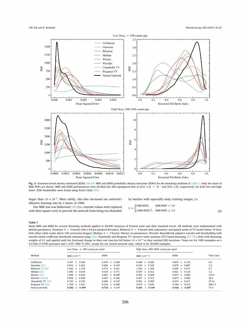
larger than ×1.0 10 3. More subtly, this also increased our network’seffective learning rate by a factor of 1000.Our MSE loss was Huberized [42] (i.e. extreme values were replacedwith their square root) to prevent the network from being too disturbedby batches with especially noisy training images, i.e.
=<
LMSE MSEMSE MSE
1000 , 1000 1.0(1000 ) , 1000 1.01
2 (2)
Fig. 3. Gaussian kernel density estimated (KDE) [48,49] MSE and SSIM probability density functions (PDFs) for the denoising methods in Table 1. Only the starts ofMSE PDFs are shown. MSE and SSIM performances were divided into 200 equispaced bins in [0.0, 1.2] × 10 3 and [0.0, 1.0], respectively, for both low and highdoses. KDE bandwidths were found using Scott’s Rule [50].
Table 1Mean MSE and SSIM for several denoising methods applied to 20,000 instances of Poisson noise and their standard errors. All methods were implemented withdefault parameters. Gaussian: 3 × 3 kernel with a 0.8 px standard deviation. Bilateral: 9 × 9 kernel with radiometric and spatial scales of 75 (scales below 10 havelittle effect while scales above 150 cartoonize images). Median: 3 × 3 kernel. Wiener: no parameters. Wavelet: BayesShrink adaptive wavelet soft-thresholding withwavelet detail coefficient thresholds estimated using [56]. Chambolle and Bregman TV: iterative total-variation (TV) based denoising [57–59], both with denoisingweights of 0.1 and applied until the fractional change in their cost function fell below ×2.0 10 4 or they reached 200 iterations. Times are for 1000 examples on a3.4 GHz i7-6700 processor and 1 GTX 1080 Ti GPU, except for our neural network time, which is for 20,000 examples.Low Dose, ≪ 300 counts per pixel High Dose, 200–2500 counts per pixel
Method MSE ×( 10 )3 SSIM MSE ×( 10 )3 SSIM Time (ms)Unfiltered 4.357 ± 2.558 0.454 ± 0.208 0.508 ± 0.682 0.850 ± 0.123 0.0Gaussian [51] 0.816 ± 0.452 0.685 ± 0.159 0.344 ± 0.334 0.878 ± 0.087 1.0Bilateral [51,52] 1.025 ± 1.152 0.574 ± 0.261 1.243 ± 1.392 0.600 ± 0.271 5.7Median [51] 1.083 ± 0.618 0.618 ± 0.171 0.507 ± 0.512 0.821 ± 0.126 1.2Wiener [53] 1.068 ± 0.546 0.681 ± 0.137 0.402 ± 0.389 0.870 ± 0.085 133.4Wavelet [54,55] 0.832 ± 0.580 0.657 ± 0.186 0.357 ± 0.312 0.875 ± 0.085 42.4Chambolle TV [54] 0.746 ± 0.725 0.680 ± 0.192 0.901 ± 0.909 0.674 ± 0.217 313.6Bregman TV [54] 1.109 ± 1.031 0.544 ± 0.268 4.074 ± 3.025 0.348 ± 0.312 2061.3Neural network 0.562 ± 0.449 0.752 ± 0.147 0.201 ± 0.169 0.926 ± 0.057 77.0
J.M. Ede and R. Beanland Ultramicroscopy 202 (2019) 18–25
20
206
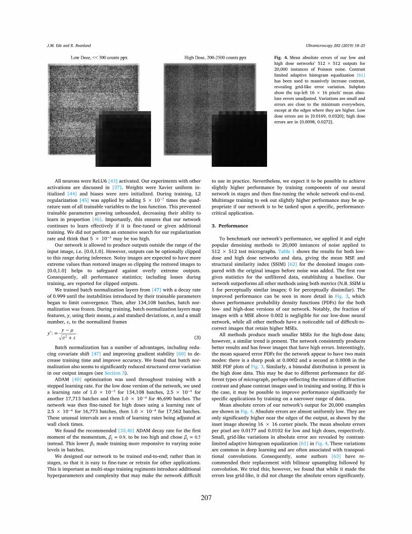
All neurons were ReLU6 [43] activated. Our experiments with otheractivations are discussed in [37]. Weights were Xavier uniform in-itialized [44] and biases were zero initialized. During training, L2regularization [45] was applied by adding 5 × 10 5 times the quad-rature sum of all trainable variables to the loss function. This preventedtrainable parameters growing unbounded, decreasing their ability tolearn in proportion [46]. Importantly, this ensures that our networkcontinues to learn effectively if it is fine-tuned or given additionaltraining. We did not perform an extensive search for our regularizationrate and think that 5 × 10 5 may be too high.Our network is allowed to produce outputs outside the range of theinput image, i.e. [0.0,1.0]. However, outputs can be optionally clippedto this range during inference. Noisy images are expected to have moreextreme values than restored images so clipping the restored images to[0.0,1.0] helps to safeguard against overly extreme outputs.Consequently, all performance statistics; including losses duringtraining, are reported for clipped outputs.We trained batch normalization layers from [47] with a decay rateof 0.999 until the instabilities introduced by their trainable parametersbegan to limit convergence. Then, after 134,108 batches, batch nor-malization was frozen. During training, batch normalization layers mapfeatures, y, using their means, μ and standard deviations, σ, and a smallnumber, ε, to the normalized frames=
+y y µ: .
2 (3)Batch normalization has a number of advantages, including redu-cing covariate shift [47] and improving gradient stability [60] to de-crease training time and improve accuracy. We found that batch nor-malization also seems to significantly reduced structured error variationin our output images (see Section 3).ADAM [40] optimization was used throughout training with astepped learning rate. For the low dose version of the network, we useda learning rate of 1.0 × 10 3 for 134,108 batches, 2.5 × 10 4 foranother 17,713 batches and then 1.0 × 10 4 for 46,690 batches. Thenetwork was then fine-tuned for high doses using a learning rate of2.5 × 10 4 for 16,773 batches, then 1.0 × 10 4 for 17,562 batches.These unusual intervals are a result of learning rates being adjusted atwall clock times.We found the recommended [33,40] ADAM decay rate for the firstmoment of the momentum, = 0.9,1 to be too high and chose = 0.51instead. This lower β1 made training more responsive to varying noiselevels in batches.We designed our network to be trained end-to-end; rather than instages, so that it is easy to fine-tune or retrain for other applications.This is important as multi-stage training regiments introduce additionalhyperparameters and complexity that may make the network difficult
to use in practice. Nevertheless, we expect it to be possible to achieveslightly higher performance by training components of our neuralnetwork in stages and then fine-tuning the whole network end-to-end.Multistage training to eek out slightly higher performance may be ap-propriate if our network is to be tasked upon a specific, performance-critical application.3. Performance
To benchmark our network’s performance, we applied it and eightpopular denoising methods to 20,000 instances of noise applied to512 × 512 test micrographs. Table 1 shows the results for both low-dose and high dose networks and data, giving the mean MSE andstructural similarity index (SSIM) [62] for the denoised images com-pared with the original images before noise was added. The first rowgives statistics for the unfiltered data, establishing a baseline. Ournetwork outperforms all other methods using both metrics (N.B. SSIM is1 for perceptually similar images; 0 for perceptually dissimilar). Theimproved performance can be seen in more detail in Fig. 3, whichshows performance probability density functions (PDFs) for the bothlow- and high-dose versions of our network. Notably, the fraction ofimages with a MSE above 0.002 is negligible for our low-dose neuralnetwork, while all other methods have a noticeable tail of difficult-to-correct images that retain higher MSEs.All methods produce much smaller MSEs for the high-dose data;however, a similar trend is present. The network consistently producesbetter results and has fewer images that have high errors. Interestingly,the mean squared error PDFs for the network appear to have two mainmodes: there is a sharp peak at 0.0002 and a second at 0.0008 in theMSE PDF plots of Fig. 3. Similarly, a bimodal distribution is present inthe high dose data. This may be due to different performance for dif-ferent types of micrograph, perhaps reflecting the mixture of diffractioncontrast and phase contrast images used in training and testing. If this isthe case, it may be possible to improve performance significantly forspecific applications by training on a narrower range of data.Mean absolute errors of our network’s output for 20,000 examplesare shown in Fig. 4. Absolute errors are almost uniformly low. They areonly significantly higher near the edges of the output, as shown by theinset image showing 16 × 16 corner pixels. The mean absolute errorsper pixel are 0.0177 and 0.0102 for low and high doses, respectively.Small, grid-like variations in absolute error are revealed by contrast-limited adaptive histogram equalization [61] in Fig. 4. These variationsare common in deep learning and are often associated with transposi-tional convolutions. Consequently, some authors [63] have re-commended their replacement with bilinear upsampling followed byconvolution. We tried this; however, we found that while it made theerrors less grid-like, it did not change the absolute errors significantly.
Fig. 4. Mean absolute errors of our low andhigh dose networks’ 512 × 512 outputs for20,000 instances of Poisson noise. Contrastlimited adaptive histogram equalization [61]has been used to massively increase contrast,revealing grid-like error variation. Subplotsshow the top-left 16 × 16 pixels’ mean abso-lute errors unadjusted. Variations are small anderrors are close to the minimum everywhere,except at the edges where they are higher. Lowdose errors are in [0.0169, 0.0320]; high doseerrors are in [0.0098, 0.0272].
J.M. Ede and R. Beanland Ultramicroscopy 202 (2019) 18–25
21
207
Instead, we found batch normalization to be a simple and effective wayto reduce structured error variation, likely due to the regularizing effectof its instability. This is evident from the more grid-like errors in thehigh dose version of our network, which was trained for longer afterbatch normalization was frozen. More advanced methods that reduce
structured error variation are discussed in [64] but were not appliedhere.Example applications of our low-dose network being use to removedapplied noise from high-quality 512 × 512 electron micrographs areshown in Fig. 5. In practice, our program may be applied to arbitrarily
Fig. 5. Example applications of the noise-removal network to instances of Poisson noise applied to 512 × 512 crops from high-quality micrographs. Enlarged64 × 64 regions from the top left of each crop are shown to ease comparison.
J.M. Ede and R. Beanland Ultramicroscopy 202 (2019) 18–25
22
208
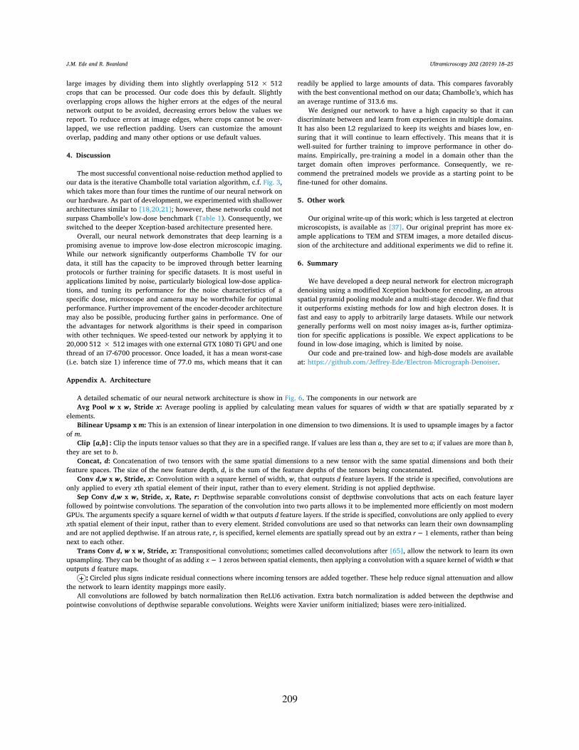
large images by dividing them into slightly overlapping 512 × 512crops that can be processed. Our code does this by default. Slightlyoverlapping crops allows the higher errors at the edges of the neuralnetwork output to be avoided, decreasing errors below the values wereport. To reduce errors at image edges, where crops cannot be over-lapped, we use reflection padding. Users can customize the amountoverlap, padding and many other options or use default values.4. Discussion
The most successful conventional noise-reduction method applied toour data is the iterative Chambolle total variation algorithm, c.f. Fig. 3,which takes more than four times the runtime of our neural network onour hardware. As part of development, we experimented with shallowerarchitectures similar to [18,20,21]; however, these networks could notsurpass Chambolle’s low-dose benchmark (Table 1). Consequently, weswitched to the deeper Xception-based architecture presented here.Overall, our neural network demonstrates that deep learning is apromising avenue to improve low-dose electron microscopic imaging.While our network significantly outperforms Chambolle TV for ourdata, it still has the capacity to be improved through better learningprotocols or further training for specific datasets. It is most useful inapplications limited by noise, particularly biological low-dose applica-tions, and tuning its performance for the noise characteristics of aspecific dose, microscope and camera may be worthwhile for optimalperformance. Further improvement of the encoder-decoder architecturemay also be possible, producing further gains in performance. One ofthe advantages for network algorithms is their speed in comparisonwith other techniques. We speed-tested our network by applying it to20,000 512 × 512 images with one external GTX 1080 Ti GPU and onethread of an i7-6700 processor. Once loaded, it has a mean worst-case(i.e. batch size 1) inference time of 77.0 ms, which means that it can
readily be applied to large amounts of data. This compares favorablywith the best conventional method on our data; Chambolle’s, which hasan average runtime of 313.6 ms.We designed our network to have a high capacity so that it candiscriminate between and learn from experiences in multiple domains.It has also been L2 regularized to keep its weights and biases low, en-suring that it will continue to learn effectively. This means that it iswell-suited for further training to improve performance in other do-mains. Empirically, pre-training a model in a domain other than thetarget domain often improves performance. Consequently, we re-commend the pretrained models we provide as a starting point to befine-tuned for other domains.5. Other work
Our original write-up of this work; which is less targeted at electronmicroscopists, is available as [37]. Our original preprint has more ex-ample applications to TEM and STEM images, a more detailed discus-sion of the architecture and additional experiments we did to refine it.6. Summary
We have developed a deep neural network for electron micrographdenoising using a modified Xception backbone for encoding, an atrousspatial pyramid pooling module and a multi-stage decoder. We find thatit outperforms existing methods for low and high electron doses. It isfast and easy to apply to arbitrarily large datasets. While our networkgenerally performs well on most noisy images as-is, further optimiza-tion for specific applications is possible. We expect applications to befound in low-dose imaging, which is limited by noise.Our code and pre-trained low- and high-dose models are availableat: https://github.com/Jeffrey-Ede/Electron-Micrograph-Denoiser.Appendix A. Architecture
A detailed schematic of our neural network architecture is show in Fig. 6. The components in our network areAvg Pool w x w, Stride x: Average pooling is applied by calculating mean values for squares of width w that are spatially separated by xelements.Bilinear Upsamp x m: This is an extension of linear interpolation in one dimension to two dimensions. It is used to upsample images by a factorof m.Clip [a,b]: Clip the inputs tensor values so that they are in a specified range. If values are less than a, they are set to a; if values are more than b,they are set to b.Concat, d: Concatenation of two tensors with the same spatial dimensions to a new tensor with the same spatial dimensions and both theirfeature spaces. The size of the new feature depth, d, is the sum of the feature depths of the tensors being concatenated.Conv d,w x w, Stride, x: Convolution with a square kernel of width, w, that outputs d feature layers. If the stride is specified, convolutions areonly applied to every xth spatial element of their input, rather than to every element. Striding is not applied depthwise.Sep Conv d,w x w, Stride, x, Rate, r: Depthwise separable convolutions consist of depthwise convolutions that acts on each feature layerfollowed by pointwise convolutions. The separation of the convolution into two parts allows it to be implemented more efficiently on most modernGPUs. The arguments specify a square kernel of width w that outputs d feature layers. If the stride is specified, convolutions are only applied to everyxth spatial element of their input, rather than to every element. Strided convolutions are used so that networks can learn their own downsamplingand are not applied depthwise. If an atrous rate, r, is specified, kernel elements are spatially spread out by an extra r 1 elements, rather than beingnext to each other.Trans Conv d, w x w, Stride, x: Transpositional convolutions; sometimes called deconvolutions after [65], allow the network to learn its ownupsampling. They can be thought of as adding x 1 zeros between spatial elements, then applying a convolution with a square kernel of width w thatoutputs d feature maps.Circled plus signs indicate residual connections where incoming tensors are added together. These help reduce signal attenuation and allowthe network to learn identity mappings more easily.All convolutions are followed by batch normalization then ReLU6 activation. Extra batch normalization is added between the depthwise andpointwise convolutions of depthwise separable convolutions. Weights were Xavier uniform initialized; biases were zero-initialized.
J.M. Ede and R. Beanland Ultramicroscopy 202 (2019) 18–25
23
209

Fig. 6. Architecture of our deep convolutional encoder-decoder for electron micrograph denoising. The entry and middle flows develop high-level features that aresampled at multiple scales by the atrous spatial pyramid pooling module. This produces rich semantic information that is concatenated with low-level entry flowfeatures and resolved into denoised micrographs by the decoder.
J.M. Ede and R. Beanland Ultramicroscopy 202 (2019) 18–25
24
210
Supplementary materialSupplementary material associated with this article can be found, in the online version, at doi:10.1016/j.ultramic.2019.03.017.
References[1] E. Oho, N. Ichise, W.H. Martin, K.-R. Peters, Practical method for noise removal inscanning electron microscopy, Scanning 18 (1) (1996) 50–54.[2] S.J. Pennycook, The impact of stem aberration correction on materials science,Ultramicroscopy 180 (2017) 22–33.[3] M. Linck, P. Hartel, S. Uhlemann, F. Kahl, H. Müller, J. Zach, M. Haider,M. Niestadt, M. Bischoff, J. Biskupek, et al., Chromatic aberration correction foratomic resolution tem imaging from 20 to 80 kv, Phys. Rev. Lett. 117 (7) (2016)076101.[4] F. Houdellier, L. De Knoop, C. Gatel, A. Masseboeuf, S. Mamishin, Y. Taniguchi,M. Delmas, M. Monthioux, M. Hÿtch, E. Snoeck, Development of tem and sem highbrightness electron guns using cold-field emission from a carbon nanotip,Ultramicroscopy 151 (2015) 107–115.[5] T. Akashi, Y. Takahashi, T. Tanigaki, T. Shimakura, T. Kawasaki, T. Furutsu,H. Shinada, H. Müller, M. Haider, N. Osakabe, et al., Aberration corrected 1.2-mvcold field-emission transmission electron microscope with a sub-50-pm resolution,Appl. Phys. Lett. 106 (7) (2015) 074101.[6] H. Adaniya, M. Cheung, C. Cassidy, M. Yamashita, T. Shintake, Development of asem-based low-energy in-line electron holography microscope for individual par-ticle imaging, Ultramicroscopy 188 (2018) 31–40.[7] C.T. Koch, Towards full-resolution inline electron holography, Micron 63 (2014)69–75.[8] A. Feist, N. Bach, N.R. da Silva, T. Danz, M. Möller, K.E. Priebe, T. Domröse,J.G. Gatzmann, S. Rost, J. Schauss, et al., Ultrafast transmission electron micro-scopy using a laser-driven field emitter: femtosecond resolution with a high co-herence electron beam, Ultramicroscopy 176 (2017) 63–73.[9] V. Migunov, H. Ryll, X. Zhuge, M. Simson, L. Strüder, K.J. Batenburg, L. Houben,R.E. Dunin-Borkowski, Rapid low dose electron tomography using a direct electrondetection camera, Sci. Rep. 5 (2015) 14516.[10] Y. Jiang, Z. Chen, Y. Han, P. Deb, H. Gao, S. Xie, P. Purohit, M.W. Tate, J. Park,S.M. Gruner, et al., Electron ptychography of 2d materials to deep sub-ångströmresolution, Nature 559 (7714) (2018) 343.[11] J. Hattne, D. Shi, C. Glynn, C.-T. Zee, M. Gallagher-Jones, M.W. Martynowycz,J.A. Rodriguez, T. Gonen, Analysis of global and site-specific radiation damage incryo-em, Structure (2018).[12] M.C. Motwani, M.C. Gadiya, R.C. Motwani, F.C. Harris, Survey of image denoisingtechniques, Proceedings of GSPX, (2004), pp. 27–30.[13] Q. Zhang, C.L. Bajaj, Cryo-electron microscopy data denoising based on the gen-eralized digitized total variation method, Far East J. Appl. Math. 45 (2) (2010) 83.[14] H.S. Kushwaha, S. Tanwar, K. Rathore, S. Srivastava, De-noising filters for tem(transmission electron microscopy) image of nanomaterials, Advanced Computing& Communication Technologies (ACCT), 2012 Second International Conference on,IEEE, 2012, pp. 276–281.[15] K. Hornik, M. Stinchcombe, H. White, Multilayer feedforward networks are uni-versal approximators, Neural Netw. 2 (5) (1989) 359–366.[16] H.W. Lin, M. Tegmark, D. Rolnick, Why does deep and cheap learning work so well?J. Stat. Phys. 168 (6) (2017) 1223–1247.[17] Y. Bengio, A. Courville, P. Vincent, Representation learning: a review and newperspectives, IEEE Trans. Pattern Anal. Mach. Intell. 35 (8) (2013) 1798–1828.[18] X. Yang, V. De Andrade, W. Scullin, E.L. Dyer, N. Kasthuri, F. De Carlo, D. Gürsoy,Low-dose x-ray tomography through a deep convolutional neural network, Sci. Rep.8 (1) (2018) 2575.[19] T. Remez, O. Litany, R. Giryes, A.M. Bronstein, Deep convolutional denoising oflow-light images, arXiv preprint arXiv:/1701.01687 (2017).[20] X.-J. Mao, C. Shen, Y.-B. Yang, Image restoration using convolutional auto-encoderswith symmetric skip connections, arXiv preprint arXiv:/1606.08921 (2016).[21] K. Zhang, W. Zuo, Y. Chen, D. Meng, L. Zhang, Beyond a Gaussian denoiser: residuallearning of deep cnn for image denoising, IEEE Trans. Image Process. 26 (7) (2017)3142–3155.[22] W. Xu, J.M. LeBeau, A deep convolutional neural network to analyze positionaveraged convergent beam electron diffraction patterns, arXiv preprint arXiv:/1708.00855 (2017).[23] K. Lee, J. Zung, P. Li, V. Jain, H.S. Seung, Superhuman accuracy on the snemi3dconnectomics challenge, arXiv preprint arXiv:/1706.00120 (2017).[24] D. Ciresan, A. Giusti, L.M. Gambardella, J. Schmidhuber, Deep neural networkssegment neuronal membranes in electron microscopy images, Advances in NeuralInformation Processing Systems, (2012), pp. 2843–2851.[25] Y. Zhu, Q. Ouyang, Y. Mao, A deep convolutional neural network approach tosingle-particle recognition in cryo-electron microscopy, BMC Bioinform. 18 (1)(2017) 348.[26] V. Dumoulin, F. Visin, A guide to convolution arithmetic for deep learning, arXivpreprint arXiv:/1603.07285 (2016).[27] R. Velik, Discrete fourier transform computation using neural networks, 2008International Conference on Computational Intelligence and Security, IEEE, 2008,pp. 120–123.[28] J. Schmidhuber, Deep learning in neural networks: an overview, Neural Netw. 61(2015) 85–117.[29] S. Chetlur, C. Woolley, P. Vandermersch, J. Cohen, J. Tran, B. Catanzaro, E.Shelhamer, Cudnn: efficient primitives for deep learning, arXiv preprint arXiv:/1410.0759 (2014).
[30] M.T. McCann, K.H. Jin, M. Unser, A review of convolutional neural networks forinverse problems in imaging, arXiv preprint arXiv:/1710.04011 (2017).[31] W. Liu, Z. Wang, X. Liu, N. Zeng, Y. Liu, F.E. Alsaadi, A survey of deep neuralnetwork architectures and their applications, Neurocomputing 234 (2017) 11–26.[32] J. Chen, X. Pan, R. Monga, S. Bengio, R. Jozefowicz, Revisiting distributed syn-chronous sgd, arXiv preprint arXiv:/1604.00981 (2016).[33] M. Abadi, P. Barham, J. Chen, Z. Chen, A. Davis, J. Dean, M. Devin, S. Ghemawat,G. Irving, M. Isard, et al., Tensorflow: a system for large-scale machine learning.OSDI, 16 (2016), pp. 265–283.[34] Q. Yang, P. Yan, Y. Zhang, H. Yu, Y. Shi, X. Mou, M.K. Kalra, Y. Zhang, L. Sun,G. Wang, Low dose ct image denoising using a generative adversarial network withwasserstein distance and perceptual loss, IEEE Trans. Med. Imaging (2018).[35] L.-C. Chen, G. Papandreou, F. Schroff, H. Adam, Rethinking atrous convolution forsemantic image segmentation, arXiv preprint arXiv:/1706.05587 (2017).[36] L.-C. Chen, Y. Zhu, G. Papandreou, F. Schroff, H. Adam, Encoder-decoder withatrous separable convolution for semantic image segmentation, arXiv preprintarXiv:/1802.02611 (2018).[37] J.M. Ede, Improving electron micrograph signal-to-noise with an atrous convolu-tional encoder-decoder, arXiv preprint arXiv:/1807.11234 (2018).[38] F. Chollet, Xception: deep learning with depthwise separable convolutions, arXivpreprint (2016).[39] J.R. Janesick, Scientific charge-coupled devices(2001).[40] D.P. Kingma, J. Ba, Adam: a method for stochastic optimization, arXiv preprintarXiv:/1412.6980 (2014).[41] G. McMullan, A. Faruqi, D. Clare, R. Henderson, Comparison of optimal perfor-mance at 300kev of three direct electron detectors for use in low dose electronmicroscopy, Ultramicroscopy 147 (2014) 156–163, doi:10.1016/j.ultramic.2014.08.002. URL http://www.sciencedirect.com/science/article/pii/S030439911400151X.[42] P.J. Huber, Robust estimation of a location parameter, Ann. Math. Stat. (1964)73–101.[43] A. Krizhevsky, G. Hinton, Convolutional deep belief networks on cifar-10, Technicalreport, U. Toronto, 2010.[44] X. Glorot, Y. Bengio, Understanding the difficulty of training deep feedforwardneural networks, Proceedings of the Thirteenth International Conference onArtificial Intelligence and Statistics, (2010), pp. 249–256.[45] J. Kukačka, V. Golkov, D. Cremers, Regularization for deep learning: a taxonomy,arXiv preprint arXiv:/1710.10686 (2017).[46] T. Salimans, D.P. Kingma, Weight normalization: A simple reparameterization toaccelerate training of deep neural networks, Advances in Neural InformationProcessing Systems, (2016), pp. 901–909.[47] S. Ioffe, C. Szegedy, Batch normalization: accelerating deep network training byreducing internal covariate shift, arXiv preprint arXiv:/1502.03167 (2015).[48] B.A. Turlach, Bandwidth selection in kernel density estimation: a review, CORE andInstitut de Statistique, Citeseer, 1993.[49] D.M. Bashtannyk, R.J. Hyndman, Bandwidth selection for kernel conditional den-sity estimation, Comput. Stat. Data Anal. 36 (3) (2001) 279–298.[50] D.W. Scott, Multivariate Density Estimation: Theory, Practice, and Visualization,John Wiley & Sons, 2015.[51] G. Bradski, The opencv library, Dr. Dobb’s J. Softw. Tools (2000).[52] C. Tomasi, R. Manduchi, Bilateral filtering for gray and color images, ComputerVision, 1998. Sixth International Conference on, IEEE, 1998, pp. 839–846.[53] E. Jones, T. Oliphant, P. Peterson, et al., SciPy: Open source scientific tools forPython, 2001, [Online; accessed], URL http://www.scipy.org/.[54] S. Van der Walt, J.L. Schönberger, J. Nunez-Iglesias, F. Boulogne, J.D. Warner,N. Yager, E. Gouillart, T. Yu, Scikit-image: image processing in python, PeerJ 2(2014) e453.[55] S.G. Chang, B. Yu, M. Vetterli, Adaptive wavelet thresholding for image denoisingand compression, IEEE Trans. Image Process. 9 (9) (2000) 1532–1546.[56] D.L. Donoho, J.M. Johnstone, Ideal spatial adaptation by wavelet shrinkage,Biometrika 81 (3) (1994) 425–455.[57] A. Chambolle, An algorithm for total variation minimization and applications, J.Math. Imaging Vis. 20 (1–2) (2004) 89–97.[58] T. Goldstein, S. Osher, The split bregman method for l1-regularized problems, SIAMJ. Imaging Sci. 2 (2) (2009) 323–343.[59] P. Getreuer, Rudin-osher-fatemi total variation denoising using split bregman,Image Process. On Line 2 (2012) 74–95.[60] S. Santurkar, D. Tsipras, A. Ilyas, A. Madry, How does batch normalization helpoptimization? (no, it is not about internal covariate shift), arXiv preprint arXiv:/1805.11604 (2018).[61] K. Zuiderveld, Contrast limited adaptive histogram equalization, Graphics Gems(1994) 474–485.[62] Z. Wang, A.C. Bovik, H.R. Sheikh, E.P. Simoncelli, Image quality assessment: fromerror visibility to structural similarity, IEEE Trans. Image Process. 13 (4) (2004)600–612.[63] A. Odena, V. Dumoulin, C. Olah, Deconvolution and checkerboard artifacts, Distill 1(10) (2016) e3.[64] Y. Sugawara, S. Shiota, H. Kiya, Super-resolution using convolutional neural net-works without any checkerboard artifacts, arXiv preprint arXiv:/1806.02658(2018).[65] M.D. Zeiler, D. Krishnan, G.W. Taylor, R. Fergus, Deconvolutional networks (2010).
J.M. Ede and R. Beanland Ultramicroscopy 202 (2019) 18–25
25
211
6.2 Amendments and Corrections
There are amendments or corrections to the paper6 covered by this chapter.
Location: Page 19, text following eqn 1.
Change: “...to only 25 e−2 for a camera...” should say “...to only 25 eA−2
for a camera...”.
Location: Page 21, first paragraph of performance section.
Change: “...structural similarity index (SSIM)...” should say “...structural similarity index measure (SSIM)...”.
6.3 Reflection
This chapter covers our paper titled “Improving Electron Micrograph Signal-to-Noise with an Atrous Convolutional
Encoder-Decoder”6 and associated research outputs15,23,24. Our paper presents a DNN based on Deeplabv3+ that is
trained to remove Poisson noise from TEM images. My DNN is affectionately named “Fluffles” and it is the only
DNN that I have named. Pretrained models and performance characterizations are provided for DNNs trained for
low and high electron doses. We also show that my DNN has lower MSEs, lower MSE variance, higher SSIMs, and
lower or similar SSIM variance to other popular algorithms. We also provide MSE and SSIM distributions, and
visualize errors for each output pixel.
Due to limited available computational resources, DNN training was stopped after it surpassed the performance
of a variety of popular denoising algorithms. However, there are many other denoising algorithms226–228 that might
achieve higher performance, some of which were developed for electron microscopy1. For example, we did not
compare our DNN against block-matching and 3D filtering229,230 (BM3D), which often achieves high-performance.
However, an extensive comparison is complicated by source code not being available for some algorithms. In
addition, we expect that further training would improve performance as validation errors did not diverge from
training errors. For comparison, our DNN was trained for about ten days on two Nvidia GTX 1080 Ti GPUs
whereas Xception231, which is randomly initialized as part of our DNN, was trained for one month on 60 Nvidia
K80 GPUs for ImageNet232 image classification. Indeed, I suspect that restarting DNN training with a pretrained
Xception backbone may more quickly achieve much higher performance than continuing training from my pretrained
models. Finally, sufficiently deep and wide ANNs are universal approximators233–241, so denoising DNNs can
always outperform or match the accuracy of other methods developed by humans.
A few aspects of my DNN architecture and optimization are peculiar as our paper presents some of my earliest
experiments with deep learning. For example, learning rates were stepwise decayed at irregular “wall clock” times.
Further, large decreases in errors when learning rates were decreased may indicate that learning rates were too
high. Another issue is that ReLU6242 activation does not significantly outperform ReLU243,244 activation, so ReLU
is preferable as it requires less computation. Finally, I think that my DNN is too large for electron micrograph
denoising. We justified that training can be continued and provide pretrained models; however, I doubt that training
on the scale of Xception is practical insofar that most electron microscopists do not readily have access to more
than a few GPUs for DNN training. I investigated smaller DNNs, which achieved lower performance. However, I
expect that their performance could have been improved by further optimization of their training and architecture. In
any case, I think that future DNNs for TEM denoising should be developed with automatic machine learning245–249
212
(AutoML) as AutoML can balance accuracy and training time, and can often outperform human developers250,251.
My denoiser has higher errors near output image edges. Higher errors near image edges were also observed
for compressed sensing with spiral4 and uniformly spaced grid19 scans (ch. 4). Indeed, the structured systematic
errors of my denoiser partially motivated my investigations of structured systematic errors in compressed sensing.
To avoid higher errors at output edges, I overlap parts of images that my denoiser is applied to so that edges of
outputs where errors are higher can be discarded. However, discarding parts of denoiser outputs is computationally
inefficient. To reduce structured systematic errors, I tried weighting contributions of output pixel errors to training
losses by multiplying pixel errors by their exponential moving averages4. However, weighting errors did not have
a significant effect. Nevertheless, I expect that higher variation of pixel weights could reduce systematic errors.
Moreover, I propose that weights for output pixel errors could be optimized during DNN training to minimize
structured systematic errors.
213
Chapter 7
Exit Wavefunction Reconstruction from SingleTransmission Electron Micrographs with DeepLearning
7.1 Scientific Paper
This chapter covers the following paper7 and its supplementary information12.
J. M. Ede, J. J. P. Peters, J. Sloan, and R. Beanland. Exit Wavefunction Reconstruction from Single
Transmission Electron Micrographs with Deep Learning. arXiv preprint arXiv:2001.10938 (under
review by Ultramicroscopy), 2020
J. M. Ede, J. J. P. Peters, J. Sloan, and R. Beanland. Supplementary Information: Exit Wavefunction
Reconstruction from Single Transmission Electron Micrographs with Deep Learning. Zenodo, Online:
https://doi.org/10.5281/zenodo.4277357, 2020
214
Exit Wavefunction Reconstruction from Single Transmission ElectronMicrographs with Deep Learning
Jeffrey M. Edea,∗, Jonathan J. P. Petersa, Jeremy Sloana, Richard Beanlanda
aDepartment of Physics, University of Warwick, Coventry, England, CV4 7AL
Abstract
Half of wavefunction information is undetected by conventional transmission electron microscopy (CTEM) as onlythe intensity, and not the phase, of an image is recorded. Following successful applications of deep learning to opticalhologram phase recovery, we have developed neural networks to recover phases from CTEM intensities for newdatasets containing 98340 exit wavefunctions. Wavefunctions were simulated with clTEM multislice propagation for12789 materials from the Crystallography Open Database. Our networks can recover 224×224 wavefunctions in ∼25ms for a large range of physical hyperparameters and materials, and we demonstrate that performance improves as thedistribution of wavefunctions is restricted. Phase recovery with deep learning overcomes the limitations of traditionalmethods: it is live, not susceptible to distortions, does not require microscope modification or multiple images, andcan be applied to any imaging regime. This paper introduces multiple approaches to CTEM phase recovery with deeplearning, and is intended to establish starting points to be improved upon by future research. Source code and links toour new datasets and pre-trained models are available at https://github.com/Jeffrey-Ede/one-shot.
Keywords: deep learning, electron microscopy, exit wavefunction reconstruction
1. Introduction
Information transfer by electron microscope lensesand correctors can be described by wave optics[1]as electrons exhibit wave-particle duality[2, 3]. Ina model electron microscope, a system of condenserlenses directs electrons illuminating a material intoa planar wavefunction, ψinc(r, z), with wavevector, k.Here, z is distance along its optical axis in the electronpropagation direction, described by unit vector z, andr is the position in a plane perpendicular to the opticalaxis. As ψinc(r, z) travels through a material in fig. 1a,it is perturbed to an exit wavefunction, ψexit(r, z), by amaterial potential.
The projected potential of a material in direction z,U(r, z), and corresponding structural information can becalculated from ψexit(r, z)[4, 5]. For example,
U(r) ≈ Im(ψexit(r, z) exp(iϕ) − 〈ψexit(r, z)〉r)λξ sin(πz/ξ)
, (1)
∗Corresponding authorEmail addresses: [email protected] (Jeffrey M.
Ede), [email protected] (Jonathan J. P. Peters),[email protected] (Jeremy Sloan),[email protected] (Richard Beanland)
for a typical crystal system well-approximated bytwo Bloch waves[4]. Here ϕ is a distance betweenBloch wavevectors, λ is the electron wavelength, ξis an extinction distance for two Bloch waves, 〈...〉rdenotes an average with respect to r, and Im(z)is the imaginary part of z. Other applications ofψexit(r, z)[6] include information storage, point spreadfunction deconvolution, improving contrast, aberrationcorrection[7], thickness measurement[8], and electricand magnetic structure determination[9, 10]. Exitwavefunctions can also simplify comparison withsimulations as no information is lost.
In general, the intensity, I(S ), of a measurement withsupport, S , is
I(S ) =
∫
s∈S|ψ(s)|2 ds. (2)
A support is a measurement region, such as anelectron microscope camera[11, 12] element. Half ofwavefunction information is lost at measurement as |ψ|2is a function of amplitude, A > 0, and not phase,θ ∈ [−π, π),
|ψ|2 = |A exp(iθ)|2 = A2| exp(iθ)|2 = A2. (3)
Preprint submitted to Elsevier January 31, 2020
arX
iv:2
001.
1093
8v2
[ee
ss.I
V]
30
Jan
2020
215
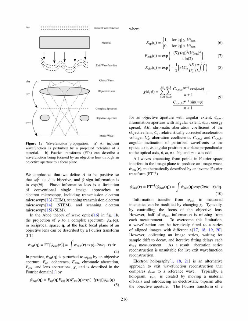
Figure 1: Wavefunction propagation. a) An incidentwavefunction is perturbed by a projected potential of amaterial. b) Fourier transforms (FTs) can describe awavefunction being focused by an objective lens through anobjective aperture to a focal plane.
We emphasize that we define A to be positive sothat |ψ|2 7→ A is bijective, and ψ sign information isin exp(iθ). Phase information loss is a limitationof conventional single image approaches toelectron microscopy, including transmission electronmicroscopy[13] (TEM), scanning transmission electronmicroscopy[14] (STEM), and scanning electronmicroscopy[15] (SEM).
In the Abbe theory of wave optics[16] in fig. 1b,the projection of ψ to a complex spectrum, ψdif(q),in reciprocal space, q, at the back focal plane of anobjective lens can be described by a Fourier transform(FT)
ψdif(q) = FT[ψexit(r)] =
∫ψexit(r) exp(−2πiq · r) dr.
(4)In practice, ψdif(q) is perturbed to ψpert by an objectiveaperture, Eap, coherence, Ecoh, chromatic aberration,Echr, and lens aberrations, χ, and is described in theFourier domain[1] by
ψpert(q) = Eap(q)Ecoh(q)Echr(q) exp(−iχ(q))ψdif(q)(5)
where
Eap(q) =
1, for |q| ≤ kθmax
0, for |q| > kθmax(6)
Ecoh(q) = exp(− (∇χ(q))2(kθcoh)2
4 ln(2)
)(7)
Echr(q) = exp(− 1
2
(πkCc
∆EU∗a
(qk
)2)2)(8)
χ(θ, φ) =
∞∑
n=0
n+1∑
m=0
Cn,m,aθn+1 cos(mφ)n + 1
+
Cn,m,bθn+1 sin(mφ)n + 1
(9)
for an objective aperture with angular extent, θmax,illumination aperture with angular extent, θcoh, energyspread, ∆E, chromatic aberration coefficient of theobjective lens, Cc, relativistically corrected accelerationvoltage, U∗a, aberration coefficients, Cn,m,a and Cn,m,b,angular inclination of perturbed wavefronts to theoptical axis, φ, angular position in a plane perpendicularto the optical axis, θ, m, n ∈ N0, and m + n is odd.
All waves emanating from points in Fourier spaceinterfere in the image plane to produce an image wave,ψimg(r), mathematically described by an inverse Fouriertransform (FT−1)
ψimg(r) = FT−1(ψpert(q)) =
∫ψpert(q) exp(2πiq · r) dq.
(10)Information transfer from ψexit to measured
intensities can be modified by changing χ. Typically,by controlling the focus of the objective lens.However, half of ψexit information is missing fromeach measurement. To overcome this limitation,a wavefunction can be iteratively fitted to a seriesof aligned images with different χ[17, 18, 19, 20].However, collecting an image series, waiting forsample drift to decay, and iterative fitting delays eachψexit measurement. As a result, aberration seriesreconstruction is unsuitable for live exit wavefunctionreconstruction.
Electron holography[1, 18, 21] is an alternativeapproach to exit wavefunction reconstruction thatcompares ψexit to a reference wave. Typically, ahologram, Ihol, is created by moving a materialoff-axis and introducing an electrostatic biprism afterthe objective aperture. The Fourier transform of a
2216
Mollenstedt biprismatic hologram is[1]
FT(Ihol(r)) = FT(1 + |ψexit(r)|2) +
µFT(ψexit(r)) ⊗ δ(q − qc) +
µFT(ψ∗exit(r)) ⊗ δ(q + qc),(11)
where ψ∗exit(r) is the complex conjugate of ψexit(r), |qc|is the carrier frequency of interference fringes, and theircontrast,
µ = |µcoh||µinel||µinst|MTF, (12)
is given by source spatiotemporal coherence, µcoh,inelastic interactions, µinst, instabilities, µinst, andthe modulation transfer function[22], MTF, of adetector. Convolutions with Dirac δ in eqn. 11describe sidebands in Fourier space that can be cropped,centered, and inverse Fourier transformed for liveexit wavefunction reconstruction. However, off-axisholograms are susceptible to distortions and requiremeticulous microscope alignment as phase informationis encoded in interference fringes[1], and croppingFourier space reduces resolution[21].
Artificial neural networks (ANNs) have been trainedto recover phases of optical holograms from singleimages[23]. In general, this is not possible as there arean infinite number of physically possible θ for a given A.However, ANNs are able to leverage an understandingof the physical world to recover θ if the distributionof possible holograms is restricted, for example, tobiological cells. Non-iterative methods that do not useANNs to recover phase information from single imageshave also been developed. However, they are limitedto defocused images in the Fresnel regime[24], or tonon-planar incident wavefunctions in the Fraunhoferregime[25].
One-shot phase recovery with ANNs overcomesthe limitations of traditional methods: it is live, notsusceptible to off-axis holographic distortions, does notrequire microscope modification, and can be appliedto any imaging regime. In addition, ANNs could beapplied to recover phases of images in large databases,long after samples may have been lost or destroyed.In this paper, we investigate the application of deeplearning to one-shot exit wavefunction reconstructionin conventional transmission electron microscopy(CTEM).
2. Exit Wavefunction Datasets
To showcase one-shot exit wavefunctionreconstruction, we generated 98340 exit wavefunctionswith clTEM[27, 28] multislice propagation for 12789
CIFs[29] downloaded from the Crystallography OpenDatabase[30, 31, 32, 33, 34, 35] (COD). Complex 64bit 512×512 wavefunctions were simulated for CTEMwith acceleration voltages in 80, 200, 300 kV, materialdepths along the optical axis uniformly distributedin [5, 100) nm, material widths perpendicular to theoptical axis in [5, 10) nm, and crystallographic zoneaxes (h, k, l) h, k, l ∈ 0, 1, 2. Materials are paddedon all sides with 0.8 nm of vacuum in the imageplane, and 0.3 nm along the optical axis, to reducesimulation artefacts. Finally, crystal tilts to each axiswere perturbed by zero-centered Gaussian randomvariates with standard deviation 0.1. We used defaultvalues for other clTEM hyperparameters.
Multislice exit wavefunction simulations with clTEMare based on [36]. Simulations start with a planarwavefunction, ψ, travelling along a TEM column
ψ (x, y, z) = exp(
2πizλ
), (13)
where x and y are in-plane coordinates, and z is distancetravelled. After passing through a thin specimen, withthickness ∆z, wavefunctions are approximated by
ψ (x, y, z + ∆z) ' exp (iσVz (x, y) ∆z)ψ (x, y, z) (14)
withσ =
2πmeλh2 , (15)
where Vz is the projected potential of the specimen at z,m is relativistic electron mass, e is fundamental electroncharge, and h is Planck’s constant.
For electrons propagating through a thickerspecimen, cumulative phase change can describedby a specimen transmission function, t(x, y, z), so that
ψ (x, y, z + ∆z) = t (x, y, z)ψ (x, y, z) (16)
with
t (x, y, z) = exp
iσz+∆z∫
z
V(x, y, z′
)dz′
. (17)
A thin sample can be divided into multiple thin slicesstacked together using a propagator function, P, to mapwavefunctions between slices. A wavefunction at slicen is mapped to a wavefunction at slice n + 1 by
ψn+1 (x, y)← P (x, y,∆z) ⊗ [tn (x, y)ψn (x, y, )
](18)
where ψ0 is the incident wave in eqn. 13. Simulationswith clTEM are based on OpenCL[37], and use
3217

Dataset n Train Unseen Validation Test TotalMultiple Materials 1 25325 1501 3569 8563 38958Multiple Materials 3 24530 1544 3399 8395 37868Multiple Materials, Restricted 3 8002 - 1105 2763 11870In1.7K2Se8Sn2.28 1 3856 - 963 - 4819In1.7K2Se8Sn2.28 3 3861 - 964 - 4825
Table 1: New datasets containing 98340 wavefunctions simulated with clTEM are split into training, unseen, validation, and testsets. Unseen wavefunctions are simulated for training set materials with different simulation hyperparameters. Kirkland potentialsummations were calculated with n = 3 or truncated to n = 1 terms, and dashes (-) indicate subsets that have not been simulated.Datasets have been made publicly available at [26].
graphical processing units (GPUs) to accelerate fastFourier transform[38] (FFT) based convolutions. Thepropagator is calculated in reciprocal space
P(kx, ky
)= exp
(−iπλk2∆z
), (19)
where kx, ky are reciprocal space coordinates, andk = (k2
x + k2y )1/2. As Fourier transforms are used
to map between reciprocal and real space, propagatorand transmission functions are band limited to decreasealiasing.
Projected atomic potentials are calculated usingKirkland’s parameterization[36], where the projectedpotential of an atom at position, p, in a thin slice is
vp (x, y) = 4π2erBohr
n∑
i
aiK0
(2πrpb1/2
i
)+
2π2erBohr
n∑
i
ci
diexp
−π2r2
p
di
,(20)
where rp = [(x − xp)2 + (y − yp)2]1/2, xp and yp arethe coordinates of the atom, rBohr is the Bohr radius, K0is the modified Bessel function[39], and the parametersai, bi, ci, and di are tabulated for each atom in [36].Nominally, n = 3. However, we also use n = 1 toinvestigate robustness to alternative simulation physics.In effect, simulations with n = 1 are for an alternativeuniverse where atoms have different potentials. Everyatom in a slice contributes to the total projected potential
Vz =∑
p
vp. (21)
After simulation, a 320×320 region was selectedfrom the center of each wavefunction to removeedge artefacts. Each wavefunction was divided byits magnitude to prevent an ANN from inferringinformation from an absolute intensity scale. Inpractice, it is possible to measure an absolute scale;however, it is specific to a microscope and itsconfiguration.
Figure 2: Crystal structure of In1.7K2Se8Sn2.28 projectedalong Miller zone axis [001]. A square outlines a unit cell.
To investigate ANN performance for multiplematerials, we partitioned 12789 CIFs into training,validation, and test sets by journal of publication.There are 8639 training set CIFs: 150 New Journal ofChemistry, 1034 American Mineralogist, 1998 Journalof the American Chemical Society, and 5457 InorganicChemistry. In addition, there are 1216 validation setCIFs published in Physics and Chemistry of Materials,and 2927 test set CIFs published in Chemistry ofMaterials. Wavefunctions were simulated for threerandom sets of hyperparameters for each CIF, exceptfor a small portion of examples that were discardedbecause CIF format or simulation hyperparameters wereunsupported. Partitioning by journal helps to test theability of an ANN to generalize given that wavefunctioncharacteristics are expected to vary with journal.
New simulated wavefunction datasets are tabulated intable 1 and have been made publicly available at [26].In total, 76826 wavefunction have been simulated formultiple materials. To investigate ANN performance as
4218
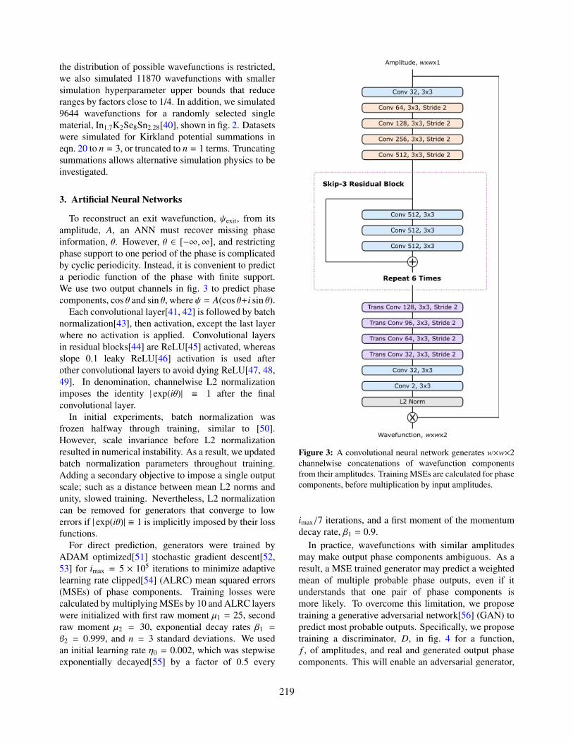
the distribution of possible wavefunctions is restricted,we also simulated 11870 wavefunctions with smallersimulation hyperparameter upper bounds that reduceranges by factors close to 1/4. In addition, we simulated9644 wavefunctions for a randomly selected singlematerial, In1.7K2Se8Sn2.28[40], shown in fig. 2. Datasetswere simulated for Kirkland potential summations ineqn. 20 to n = 3, or truncated to n = 1 terms. Truncatingsummations allows alternative simulation physics to beinvestigated.
3. Artificial Neural Networks
To reconstruct an exit wavefunction, ψexit, from itsamplitude, A, an ANN must recover missing phaseinformation, θ. However, θ ∈ [−∞,∞], and restrictingphase support to one period of the phase is complicatedby cyclic periodicity. Instead, it is convenient to predicta periodic function of the phase with finite support.We use two output channels in fig. 3 to predict phasecomponents, cos θ and sin θ, where ψ = A(cos θ+i sin θ).
Each convolutional layer[41, 42] is followed by batchnormalization[43], then activation, except the last layerwhere no activation is applied. Convolutional layersin residual blocks[44] are ReLU[45] activated, whereasslope 0.1 leaky ReLU[46] activation is used afterother convolutional layers to avoid dying ReLU[47, 48,49]. In denomination, channelwise L2 normalizationimposes the identity | exp(iθ)| ≡ 1 after the finalconvolutional layer.
In initial experiments, batch normalization wasfrozen halfway through training, similar to [50].However, scale invariance before L2 normalizationresulted in numerical instability. As a result, we updatedbatch normalization parameters throughout training.Adding a secondary objective to impose a single outputscale; such as a distance between mean L2 norms andunity, slowed training. Nevertheless, L2 normalizationcan be removed for generators that converge to lowerrors if | exp(iθ)| ≡ 1 is implicitly imposed by their lossfunctions.
For direct prediction, generators were trained byADAM optimized[51] stochastic gradient descent[52,53] for imax = 5 × 10⁵ iterations to minimize adaptivelearning rate clipped[54] (ALRC) mean squared errors(MSEs) of phase components. Training losses werecalculated by multiplying MSEs by 10 and ALRC layerswere initialized with first raw moment µ1 = 25, secondraw moment µ2 = 30, exponential decay rates β1 =
β2 = 0.999, and n = 3 standard deviations. We usedan initial learning rate η0 = 0.002, which was stepwiseexponentially decayed[55] by a factor of 0.5 every
Figure 3: A convolutional neural network generates w×w×2channelwise concatenations of wavefunction componentsfrom their amplitudes. Training MSEs are calculated for phasecomponents, before multiplication by input amplitudes.
imax/7 iterations, and a first moment of the momentumdecay rate, β1 = 0.9.
In practice, wavefunctions with similar amplitudesmay make output phase components ambiguous. As aresult, a MSE trained generator may predict a weightedmean of multiple probable phase outputs, even if itunderstands that one pair of phase components ismore likely. To overcome this limitation, we proposetraining a generative adversarial network[56] (GAN) topredict most probable outputs. Specifically, we proposetraining a discriminator, D, in fig. 4 for a function,f , of amplitudes, and real and generated output phasecomponents. This will enable an adversarial generator,
5219

Figure 4: A discriminator predicts if wavefunctioncomponents were generated by a neural network.
G, to learn to output realistic phases in the context oftheir amplitudes.
There are many popular GAN loss functions andregularization mechanisms[57, 58]. Following [59], weuse mean squared generator, LG, and discriminator, LD,losses, and apply spectral normalization to the weightsof every convolutional layer in the discriminator
LD = (D( f (ψ)) − 1)2 + D( f (G(|ψ|)))2 (22)
LG = (D( f (G(|ψ|)) − 1)2, (23)
where f is a function that parameterizes ψ asthe channelwise concatenation of A cos θ, A sin θ.Multiplying generated phase components by inputted Aconditions wavefunction discrimination on A, ensuringthat the generator learns to output physically probableθ. Other parameterizations; such as the channelwiseconcatenation of A, cos θ, sin θ could also be used.There are no biases in the discriminator.
Concatenation of conditional information todiscriminator inputs and feature channels is investigatedin [60, 61, 62, 63, 64, 65, 66, 67]. Projectiondiscriminators, which calculate inner products ofgenerator outputs and conditional embeddings, arean alternative that achieve higher performance in[68]. However, blind compression to an embeddedrepresentation would reduce wavefunction information,potentially limiting the quality of generatedwavefunctions, and may encourage catastrophicforgetting[69].
Both generator and discriminator training wasADAM optimized for 5 × 10⁵ iterations with base
learning rate ηG = ηD = 0.0002, and first moment ofthe momentum decay, β1 = 0.5. To balance generatorand discriminator learning, we map the discriminatorlearning rate to
η′D =ηD
1 + exp(−m(µD − c)), (24)
where µD is the running mean discrimination forgenerated wavefunctions, D( f (G(|ψ|)), tracked by anexponential moving average with a decay rate of 0.99,and m = 20 and c = 0.5 linearly transform µD.
To augment training data, we selected random w×wcrops from 320×320 wavefunctions. Each crop wasthen subject to random combination of flips and π/2rad rotations to augment our datasets by a factor ofeight. We chose wavefunction size w = 224 fordirect prediction and w = 144 for GANs, where wis smaller for GANs as discriminators add to GPUmemory requirements. ANNs were trained with a batchsize of 24.
4. Experiments
In this section, we investigate phase recovery withANNs as the distribution of wavefunctions is restricted.To directly predict θ for A, we trained ANNs formultiple materials, multiple materials with restrictedsimulation hyperparameters, and In1.7K2Se8Sn2.28. Wealso trained a GAN for In1.7K2Se8Sn2.28 wavefunctions.Experiments are repeated with the summation in eqn. 20truncated from n = 3 to n = 1, to demonstraterobustness to simulation physics.
Distributions of generated phase component meanabsolute errors (MAEs) for sets of 19992 validationexamples are shown in fig. 5, and moments are tabulatedin table 2. We used up to three validation sets,which cumulatively quantify the ability of a network togeneralize to unseen transforms; combinations of flips,rotations and translations, simulation hyperparameters;such as thickness and voltage, and materials. Incomparison, the expected error of the nth momentof phase components, E[|G(|ψ|) − f (θ)|n], where g ∈cos, sin, for uniform random predictions, x ∼U(−1, 1), and uniformly distributed phases, θ ∼U(−π, π), is
E[|x − g(θ)|n] =
1∫
−1
π∫
−πρ(x)ρ(θ)|x − g(θ)|n dθ dx, (25)
where ρ(θ) = 1/2π and ρ(x) = 1/2 are uniformprobability density functions for θ and x, respectively.
6220
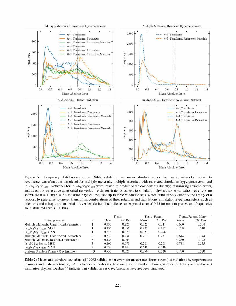
Figure 5: Frequency distributions show 19992 validation set mean absolute errors for neural networks trained toreconstruct wavefunctions simulated for multiple materials, multiple materials with restricted simulation hyperparameters, andIn1.7K2Se8Sn2.28. Networks for In1.7K2Se8Sn2.28 were trained to predict phase components directly; minimising squared errors,and as part of generative adversarial networks. To demonstrate robustness to simulation physics, some validation set errors areshown for n = 1 and n = 3 simulation physics. We used up to three validation sets, which cumulatively quantify the ability of anetwork to generalize to unseen transforms; combinations of flips, rotations and translations, simulation hyperparameters; such asthickness and voltage, and materials. A vertical dashed line indicates an expected error of 0.75 for random phases, and frequenciesare distributed across 100 bins.
Trans. Trans., Param. Trans., Param., Mater.Training Scope n Mean Std Dev Mean Std Dev Mean Std Dev
Multiple Materials, Unrestricted Parameters 1 0.333 0.220 0.525 0.341 0.600 0.334In1.7K2Se8Sn2.28, MSE 1 0.135 0.056 0.205 0.157 0.708 0.310In1.7K2Se8Sn2.28, GAN 1 0.318 0.279 0.321 0.256 - -Multiple Materials, Unrestricted Parameters 3 0.513 0.234 0.717 0.271 0.614 0.344Multiple Materials, Restricted Parameters 3 0.123 0.069 - - 0.260 0.192In1.7K2Se8Sn2.28, MSE 3 0.190 0.079 0.281 0.208 0.768 0.235In1.7K2Se8Sn2.28, GAN 3 0.633 0.244 0.638 0.249 - -Uniform Random Phases (Max Entropy) 1, 3 0.750 0.520 0.750 0.520 0.750 0.520
Table 2: Means and standard deviations of 19992 validation set errors for unseen transforms (trans.), simulations hyperparameters(param.) and materials (mater.). All networks outperform a baseline uniform random phase generator for both n = 1 and n = 3simulation physics. Dashes (-) indicate that validation set wavefunctions have not been simulated.
7221
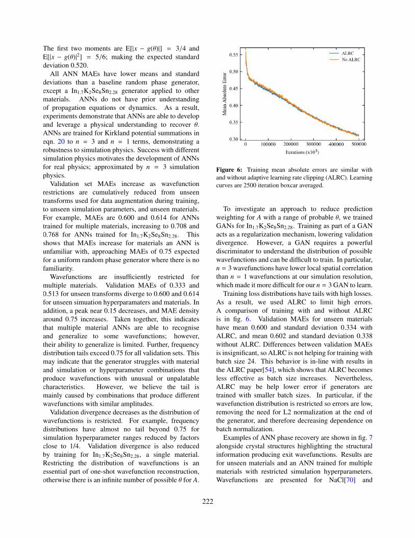
The first two moments are E[|x − g(θ)|] = 3/4 andE[|x − g(θ)|2] = 5/6; making the expected standarddeviation 0.520.
All ANN MAEs have lower means and standarddeviations than a baseline random phase generator,except a In1.7K2Se8Sn2.28 generator applied to othermaterials. ANNs do not have prior understandingof propagation equations or dynamics. As a result,experiments demonstrate that ANNs are able to developand leverage a physical understanding to recover θ.ANNs are trained for Kirkland potential summations ineqn. 20 to n = 3 and n = 1 terms, demonstrating arobustness to simulation physics. Success with differentsimulation physics motivates the development of ANNsfor real physics; approximated by n = 3 simulationphysics.
Validation set MAEs increase as wavefunctionrestrictions are cumulatively reduced from unseentransforms used for data augmentation during training,to unseen simulation parameters, and unseen materials.For example, MAEs are 0.600 and 0.614 for ANNstrained for multiple materials, increasing to 0.708 and0.768 for ANNs trained for In1.7K2Se8Sn2.28. Thisshows that MAEs increase for materials an ANN isunfamiliar with, approaching MAEs of 0.75 expectedfor a uniform random phase generator where there is nofamiliarity.
Wavefunctions are insufficiently restricted formultiple materials. Validation MAEs of 0.333 and0.513 for unseen transforms diverge to 0.600 and 0.614for unseen simuation hyperparamaters and materials. Inaddition, a peak near 0.15 decreases, and MAE densityaround 0.75 increases. Taken together, this indicatesthat multiple material ANNs are able to recogniseand generalize to some wavefunctions; however,their ability to generalize is limited. Further, frequencydistribution tails exceed 0.75 for all validation sets. Thismay indicate that the generator struggles with materialand simulation or hyperparameter combinations thatproduce wavefunctions with unusual or unpalatablecharacteristics. However, we believe the tail ismainly caused by combinations that produce differentwavefunctions with similar amplitudes.
Validation divergence decreases as the distribution ofwavefunctions is restricted. For example, frequencydistributions have almost no tail beyond 0.75 forsimulation hyperparameter ranges reduced by factorsclose to 1/4. Validation divergence is also reducedby training for In1.7K2Se8Sn2.28, a single material.Restricting the distribution of wavefunctions is anessential part of one-shot wavefunction reconstruction,otherwise there is an infinite number of possible θ for A.
Figure 6: Training mean absolute errors are similar withand without adaptive learning rate clipping (ALRC). Learningcurves are 2500 iteration boxcar averaged.
To investigate an approach to reduce predictionweighting for A with a range of probable θ, we trainedGANs for In1.7K2Se8Sn2.28. Training as part of a GANacts as a regularization mechanism, lowering validationdivergence. However, a GAN requires a powerfuldiscriminator to understand the distribution of possiblewavefunctions and can be difficult to train. In particular,n = 3 wavefunctions have lower local spatial correlationthan n = 1 wavefunctions at our simulation resolution,which made it more difficult for our n = 3 GAN to learn.
Training loss distributions have tails with high losses.As a result, we used ALRC to limit high errors.A comparison of training with and without ALRCis in fig. 6. Validation MAEs for unseen materialshave mean 0.600 and standard deviation 0.334 withALRC, and mean 0.602 and standard deviation 0.338without ALRC. Differences between validation MAEsis insignificant, so ALRC is not helping for training withbatch size 24. This behavior is in-line with results inthe ALRC paper[54], which shows that ALRC becomesless effective as batch size increases. Nevertheless,ALRC may be help lower error if generators aretrained with smaller batch sizes. In particular, if thewavefunction distribution is restricted so errors are low,removing the need for L2 normalization at the end ofthe generator, and therefore decreasing dependence onbatch normalization.
Examples of ANN phase recovery are shown in fig. 7alongside crystal structures highlighting the structuralinformation producing exit wavefunctions. Results arefor unseen materials and an ANN trained for multiplematerials with restricted simulation hyperparameters.Wavefunctions are presented for NaCl[70] and
8222

Figure 7: Exit wavefunction reconstruction for unseen NaCl, B3BeLaO7, PbZr0.45Ti0.5503, CdTe, and Si input amplitudes, andcorresponding crystal structures. Phases in [−π, π) rad are depicted on a linear greycale from black to white, and show that outputphases are close to true phases. Wavefunctions are cyclically periodic functions of phase so distances between black and whitepixels are small. Si is a failure case where phase information is not accurately recovered. Miller indices label projection directions.
9223
elemental Si as they are simple materials with widelyrecognised structures. Other materials belong toclasses that are widely investigated: B3BeLaO7[71]is a non-linear optical crystal, PbZr0.45Ti0.5503[72] isferroelectric used in ultrasonic transducers[73] andceramic capacitors[74], and CdTe is a semiconductorused in solar cells[75]. The Si example is also includedas typical failure case for unfamiliar examples. Inthis case, possibly because the Si crystal structure isunusually simple. Additional sheets of example inputphases, generated phases, and true phases for eachANN will be provided as supplementary informationwith the published version of this preprint.
5. Discussion
This paper describes an initial investigation intoCTEM one-shot exit wavefunction reconstruction withdeep learning, and is intended to be a starting point forfuture research. We expect that ANN architecture andlearning policy can be substantially improved; possiblywith AdaNet[76], Ludwig[77], or other automaticmachine learning[78] algorithms, and we encouragefurther investigation. In this spirit, all of our sourcecode[79] (based on TensorFlow[80]), clTEM simulationsoftware[27], and new wavefunction datasets[26] havebeen made publicly available. Training for eachnetwork was stopped after a few days on an Nvidia 1080Ti GPU, and losses were still decreasing. As a result,this paper presents lower bounds for performance.
To demonstrate robustness to simulation physics,Kirkland potential summations in eqn. 20 werecalculated with n = 3, or truncated to n = 1 terms,for different datasets. For further simulations, compiledclTEM versions with n = 1 and n = 3 have beenincluded in our project repository[79]. Source code forclTEM is also available with separate pre-releases[27].Summations with n = 3 approximate experimentalphysics, whereas n = 1 is for an alternative universewith different atom potentials.
Our experiments do not include aberrations ordetector noise. This restricts the distribution ofwavefunctions and makes it easier for ANNs to learn.However, distributions of wavefunctions were lessrestricted than possible in practice, and ANNs canremove noise[81]. As a result, we expect one-shotexit wavefunction to be applicable to experimentalimages. A good starting point for future research maybe materials where the distribution of wavefunctionsis naturally restricted. For example, graphene[82] andother two-dimensional materials[83], select crystals at
atomic resolution[84], or classified images; such asbiological specimens[85, 86] after similar preparation.
Information about materials, expected ranges ofsimulation hyperparameters, and other metadata wasnot input to ANNs. However, this variable informationis readily available and could restrict the distributionof wavefunctions; improving ANN performance.Subsequently, we suggest that metadata embedded byan ANN could be used to modulate information transferthrough a convolutional neural network by conditionalbatch normalization[87]. However, metadata istypically high-dimensional, so this may be impracticalbeyond individual applications.
By default, large amounts of metadata is savedto Digital Micrograph image files (e.g. dm3 anddm4) created by Gatan Microscopy Suite[88] software.Metadata can also be saved to TIFFs[89] or otherimage formats preferred by electron microscopists usingdifferent software. In practice, most of this metadatadescribes microscope settings; such as voltage andmagnification, and may not be sufficient to restrict thedistribution of wavefunctions. Nevertheless, most fileformats support the addition of extra metadata that isreadily known to experimenters. Example informationmay include estimates for stoichiometry, specimenthickness, zone axis, temperature, the microscope andits likely aberration range, and phenomena exhibitedby materials in scientific literature. ANNs have beendeveloped to embed scientific literature[90], so weexpect that it will become possible to include additionalmetadata as a lay description.
In this paper, ANNs are trained to reconstruct ψfrom A, and therefore follow a history of successfuldeep learning applications to accelerated quantummechanics[91, 92]. In contrast, experimental hologramsare integrated over detector supports. Althoughprobability density, |ψ(S )|2, at the mean support, S ,can be factored outside the integral of eqn. 2 if spatialvariation is small, ∇χ → 0, and S is effectivelyinvariant,
I(S ) ≈ |ψ(S )|2∫
s∈Sds, (26)
these restrictions are unrealistic. In practice, we do notthink the distinction is important as ANNs have learnedto recover optical θ from I[23].
To discourage ANNs from gaming their lossfunctions by predicting an average of probable phasecomponents, we propose training GANs. However,GANs are difficult to train[93, 69], and GAN trainingcan take longer than with MSEs. For example, ourvalidation set GAN MAEs are lower than for MSE
10224
training after 5 × 10⁵ iterations. We also foundthat GAN performance can be much lower for somewavefunctions; such as those with low local spatialcorrelation. High performance for large wavefunctionsalso requires powerful discriminators; such as [94], tounderstand their distribution.
Overall, we expect GANs to become less usefulthe more a distribution of wavefunctions is restricted.As the distribution becomes more restricted, a smallerportion of the distribution has similar amplitudes withsubstantially different phases. In part, we expectthis effect already lowers MAEs as distributions arerestricted. Another contribution is restricted physics;which makes networks less reliant on identifyingfeatures. As a result, we expect the main use of GANs inphase recovery to be improving wavefunction realism.
6. Conclusions
We have simulated five new datasets containing98340 CTEM exit wavefunctions with clTEM. Thedatasets have been used to train ANNs to reconstructwavefunctions from single images. In this initialinvestigation, we found that ANN performanceimproves as the distribution of wavefunctions isrestricted. One-shot exit wavefunction reconstructionovercomes the limitations of aberration seriesreconstruction and holography: it is live, does notrequire experimental equipment, and can be appliedas a post-processing step indefinitely after an imageis taken. We expect our results to be generalizable toother types of electron microscopy.
7. Supplementary Information
This work is intended to establish starting points tobe improved on by future research. In this spirit, ournew datasets[26], clTEM simulation software[27], andsource code with links to pre-trained models[79] hasbeen made publicly available.
In appendices, we build on Abbe’s theory of waveoptics to propose a new approach to phase recovery withdeep learning. The idea is that wavefunctions could belearned from large datasets of single images; avoidingthe difficulty and expense of collecting experimentalwavefunctions. Nevertheless, we also introduce a newdataset containing 1000 512×512 experimental focalseries. In addition, a supplementary document will beprovided with the published version of this preprint withsheets of example input amplitudes, output phases, andtrue phases for every ANN featured in this paper.
References
[1] M. Lehmann, H. Lichte, Tutorial on off-axis electronholography, Microscopy and Microanalysis 8 (6) (2002)447–466.
[2] S. Frabboni, G. C. Gazzadi, G. Pozzi, Youngs double-slitinterference experiment with electrons, American Journal ofPhysics 75 (11) (2007) 1053–1055.
[3] G. Matteucci, C. Beeli, An experiment on electronwave–particle duality including a Planck constant measurement,American Journal of Physics 66 (12) (1998) 1055–1059.
[4] M. Lentzen, K. Urban, Reconstruction of the projectedcrystal potential in transmission electron microscopy bymeans of a maximum-likelihood refinement algorithm, ActaCrystallographica Section A: Foundations of Crystallography56 (3) (2000) 235–247.
[5] A. Auslender, M. Halabi, G. Levi, O. Dieguez, A. Kohn,Measuring the mean inner potential of Al2O3 sapphire usingoff-axis electron holography, Ultramicroscopy 198 (2019)18–25.
[6] A. Tonomura, Applications of electron holography, Reviews ofmodern physics 59 (3) (1987) 639.
[7] Q. Fu, H. Lichte, E. Volkl, Correction of aberrations of anelectron microscope by means of electron holography, Physicalreview letters 67 (17) (1991) 2319.
[8] M. McCartney, M. Gajdardziska-Josifovska, Absolutemeasurement of normalized thickness, t/λi, from off-axiselectron holography, Ultramicroscopy 53 (3) (1994) 283–289.
[9] H. S. Park, X. Yu, S. Aizawa, T. Tanigaki, T. Akashi,Y. Takahashi, T. Matsuda, N. Kanazawa, Y. Onose, D. Shindo,et al., Observation of the magnetic flux and three-dimensionalstructure of skyrmion lattices by electron holography, Naturenanotechnology 9 (5) (2014) 337.
[10] R. E. Dunin-Borkowski, T. Kasama, A. Wei, S. L. Tripp, M. J.Hytch, E. Snoeck, R. J. Harrison, A. Putnis, Off-axis electronholography of magnetic nanowires and chains, rings, and planararrays of magnetic nanoparticles, Microscopy research andtechnique 64 (5-6) (2004) 390–402.
[11] G. McMullan, A. Faruqi, R. Henderson, Direct electrondetectors, in: Methods in enzymology, Vol. 579, Elsevier, 2016,pp. 1–17.
[12] G. McMullan, S. Chen, R. Henderson, A. Faruqi, Detectivequantum efficiency of electron area detectors in electronmicroscopy, Ultramicroscopy 109 (9) (2009) 1126–1143.
[13] C. B. Carter, D. B. Williams, Transmission electron microscopy:Diffraction, imaging, and spectrometry, Springer, 2016.
[14] S. J. Pennycook, P. D. Nellist, Scanning transmission electronmicroscopy: imaging and analysis, Springer Science & BusinessMedia, 2011.
[15] J. I. Goldstein, D. E. Newbury, J. R. Michael, N. W. Ritchie,J. H. J. Scott, D. C. Joy, Scanning electron microscopy andX-ray microanalysis, Springer, 2017.
[16] H. Kohler, On Abbe’s theory of image formation in themicroscope, Optica Acta: International Journal of Optics28 (12) (1981) 1691–1701.
[17] A. Lubk, K. Vogel, D. Wolf, J. Krehl, F. Roder, L. Clark,G. Guzzinati, J. Verbeeck, Fundamentals of focal series inlineelectron holography, in: Advances in imaging and electronphysics, Vol. 197, Elsevier, 2016, pp. 105–147.
[18] C. T. Koch, A. Lubk, Off-axis and inline electron holography:A quantitative comparison, Ultramicroscopy 110 (5) (2010)460–471.
[19] C. T. Koch, Towards full-resolution inline electron holography,Micron 63 (2014) 69–75.
[20] S. Haigh, B. Jiang, D. Alloyeau, C. Kisielowski, A. Kirkland,
11225
Recording low and high spatial frequencies in exit wavereconstructions, Ultramicroscopy 133 (2013) 26–34.
[21] C. Ozsoy-Keskinbora, C. Boothroyd, R. Dunin-Borkowski,P. Van Aken, C. Koch, Hybridization approach to in-line andoff-axis (electron) holography for superior resolution and phasesensitivity, Scientific Reports 4 (2014) 7020.
[22] R. S. Ruskin, Z. Yu, N. Grigorieff, Quantitative characterizationof electron detectors for transmission electron microscopy,Journal of structural biology 184 (3) (2013) 385–393.
[23] Y. Rivenson, Y. Zhang, H. Gunaydın, D. Teng, A. Ozcan,Phase recovery and holographic image reconstruction usingdeep learning in neural networks, Light: Science & Applications7 (2) (2018) 17141.
[24] A. Morgan, A. Martin, A. D’Alfonso, C. Putkunz, L. Allen,Direct exit-wave reconstruction from a single defocused image,Ultramicroscopy 111 (9-10) (2011) 1455–1460.
[25] A. Martin, L. Allen, Direct retrieval of a complex wave fromits diffraction pattern, Optics Communications 281 (20) (2008)5114–5121.
[26] J. M. Ede, J. P. P. Peters, R. Beanland, Warwick electronmicroscopy datasets, online: https://warwick.ac.uk/fac/sci/physics/research/condensedmatt/microscopy/research/machinelearning (2019).
[27] J. P. P. Peters, M. A. Dyson, clTEM, online: https://github.com/JJPPeters/clTEM (2019).
[28] M. A. Dyson, Advances in computational methods fortransmission electron microscopy simulation and imageprocessing, Ph.D. thesis, University of Warwick (2014).
[29] S. R. Hall, F. H. Allen, I. D. Brown, The crystallographicinformation file (CIF): a new standard archive file forcrystallography, Acta Crystallographica Section A: Foundationsof Crystallography 47 (6) (1991) 655–685.
[30] M. Quiros, S. Grazulis, S. Girdzijauskaite, A. Merkys,A. Vaitkus, Using SMILES strings for the description ofchemical connectivity in the Crystallography Open Database,Journal of Cheminformatics 10 (1) (May 2018). doi:10.1186/s13321-018-0279-6.
[31] A. Merkys, A. Vaitkus, J. Butkus, M. Okulic-Kazarinas,V. Kairys, S. Grazulis, COD::CIF::Parser: an error-correctingCIF parser for the Perl language, Journal of AppliedCrystallography 49 (1) (Feb 2016). doi:10.1107/S1600576715022396.URL http://dx.doi.org/10.1107/S1600576715022396
[32] S. Grazulis, A. Merkys, A. Vaitkus, M. Okulic-Kazarinas,Computing stoichiometric molecular composition from crystalstructures, Journal of Applied Crystallography 48 (1) (2015)85–91. doi:10.1107/S1600576714025904.URL http://dx.doi.org/10.1107/S1600576714025904
[33] S. Grazulis, A. Daskevic, A. Merkys, D. Chateigner,L. Lutterotti, M. Quiros, N. R. Serebryanaya, P. Moeck, R. T.Downs, A. Le Bail, Crystallography Open Database (COD):an open-access collection of crystal structures and platformfor world-wide collaboration, Nucleic Acids Research 40 (D1)(2012) D420–D427. arXiv:http://nar.oxfordjournals.org/content/40/D1/D420.full.pdf+html,doi:10.1093/nar/gkr900.URL http://nar.oxfordjournals.org/content/40/D1/D420.abstract
[34] S. Grazulis, D. Chateigner, R. T. Downs, A. F. T.Yokochi, M. Quiros, L. Lutterotti, E. Manakova, J. Butkus,P. Moeck, A. Le Bail, Crystallography Open Database– an open-access collection of crystal structures, Journalof Applied Crystallography 42 (4) (2009) 726–729.
doi:10.1107/S0021889809016690.URL http://dx.doi.org/10.1107/S0021889809016690
[35] R. T. Downs, M. Hall-Wallace, The American Mineralogistcrystal structure database, American Mineralogist 88 (2003)247–250.
[36] E. J. Kirkland, Advanced computing in electron microscopy,Springer Science & Business Media, 2010.
[37] J. E. Stone, D. Gohara, G. Shi, OpenCL: A parallelprogramming standard for heterogeneous computing systems,Computing in science & engineering 12 (3) (2010) 66.
[38] K. Moreland, E. Angel, The FFT on a GPU, in: Proceedingsof the ACM SIGGRAPH/EUROGRAPHICS conference onGraphics hardware, Eurographics Association, 2003, pp.112–119.
[39] M. Abramowitz, I. A. Stegun, Handbook of mathematicalfunctions. 1965 (1964).
[40] S.-J. Hwang, R. G. Iyer, P. N. Trikalitis, A. G. Ogden,M. G. Kanatzidis, Cooling of melts: Kinetic stabilization andpolymorphic transitions in the KInSnSe4 system, Inorganicchemistry 43 (7) (2004) 2237–2239.
[41] M. T. McCann, K. H. Jin, M. Unser, Convolutional neuralnetworks for inverse problems in imaging: A review, IEEESignal Processing Magazine 34 (6) (2017) 85–95.
[42] A. Krizhevsky, I. Sutskever, G. E. Hinton, ImageNetclassification with deep convolutional neural networks, in:Advances in neural information processing systems, 2012, pp.1097–1105.
[43] S. Ioffe, C. Szegedy, Batch normalization: Accelerating deepnetwork training by reducing internal covariate shift, arXivpreprint arXiv:1502.03167 (2015).
[44] K. He, X. Zhang, S. Ren, J. Sun, Deep residual learning forimage recognition. CoRR abs/1512.03385 (2015).
[45] V. Nair, G. E. Hinton, Rectified linear units improve restrictedBoltzmann machines, in: Proceedings of the 27th internationalconference on machine learning (ICML-10), 2010, pp. 807–814.
[46] A. L. Maas, A. Y. Hannun, A. Y. Ng, Rectifier nonlinearitiesimprove neural network acoustic models, in: Proc. ICML,Vol. 30, 2013, p. 3.
[47] L. Lu, Y. Shin, Y. Su, G. E. Karniadakis, Dying ReLU andinitialization: Theory and numerical examples, arXiv preprintarXiv:1903.06733 (2019).
[48] S. C. Douglas, J. Yu, Why ReLU units sometimes die: Analysisof single-unit error backpropagation in neural networks, in:2018 52nd Asilomar Conference on Signals, Systems, andComputers, IEEE, 2018, pp. 864–868.
[49] B. Xu, N. Wang, T. Chen, M. Li, Empirical evaluation ofrectified activations in convolutional network, arXiv preprintarXiv:1505.00853 (2015).
[50] L.-C. Chen, Y. Zhu, G. Papandreou, F. Schroff, H. Adam,Encoder-decoder with atrous separable convolution for semanticimage segmentation, in: Proceedings of the Europeanconference on computer vision (ECCV), 2018, pp. 801–818.
[51] D. P. Kingma, J. Ba, ADAM: A method for stochasticoptimization, arXiv preprint arXiv:1412.6980 (2014).
[52] S. Ruder, An overview of gradient descent optimizationalgorithms, arXiv preprint arXiv:1609.04747 (2016).
[53] D. Zou, Y. Cao, D. Zhou, Q. Gu, Stochastic gradientdescent optimizes over-parameterized deep relu networks, arXivpreprint arXiv:1811.08888 (2018).
[54] J. M. Ede, R. Beanland, Adaptive learning rate clippingstabilizes learning, arXiv preprint arXiv:1906.09060 (2019).
[55] R. Ge, S. M. Kakade, R. Kidambi, P. Netrapalli, The step decayschedule: A near optimal, geometrically decaying learning rateprocedure, arXiv preprint arXiv:1904.12838 (2019).
12226

[56] I. Goodfellow, J. Pouget-Abadie, M. Mirza, B. Xu,D. Warde-Farley, S. Ozair, A. Courville, Y. Bengio, Generativeadversarial nets, in: Advances in neural information processingsystems, 2014, pp. 2672–2680.
[57] Z. Wang, Q. She, T. E. Ward, Generative adversarial networks:A survey and taxonomy, arXiv preprint arXiv:1906.01529(2019).
[58] H.-W. Dong, Y.-H. Yang, Towards a deeper understanding ofadversarial losses, arXiv preprint arXiv:1901.08753 (2019).
[59] T. Miyato, T. Kataoka, M. Koyama, Y. Yoshida, Spectralnormalization for generative adversarial networks, arXivpreprint arXiv:1802.05957 (2018).
[60] M. Mirza, S. Osindero, Conditional generative adversarial nets,arXiv preprint arXiv:1411.1784 (2014).
[61] E. L. Denton, S. Chintala, R. Fergus, et al., Deep generativeimage models using a Laplacian pyramid of adversarialnetworks, in: Advances in neural information processingsystems, 2015, pp. 1486–1494.
[62] S. Reed, Z. Akata, X. Yan, L. Logeswaran, B. Schiele, H. Lee,Generative adversarial text to image synthesis, arXiv preprintarXiv:1605.05396 (2016).
[63] H. Zhang, T. Xu, H. Li, S. Zhang, X. Wang, X. Huang, D. N.Metaxas, Stackgan: Text to photo-realistic image synthesis withstacked generative adversarial networks, in: Proceedings of theIEEE International Conference on Computer Vision, 2017, pp.5907–5915.
[64] G. Perarnau, J. Van De Weijer, B. Raducanu, J. M. Alvarez,Invertible conditional GANs for image editing, arXiv preprintarXiv:1611.06355 (2016).
[65] M. Saito, E. Matsumoto, S. Saito, Temporal generativeadversarial nets with singular value clipping, in: Proceedings ofthe IEEE International Conference on Computer Vision, 2017,pp. 2830–2839.
[66] V. Dumoulin, I. Belghazi, B. Poole, O. Mastropietro, A. Lamb,M. Arjovsky, A. Courville, Adversarially learned inference,arXiv preprint arXiv:1606.00704 (2016).
[67] K. Sricharan, R. Bala, M. Shreve, H. Ding, K. Saketh,J. Sun, Semi-supervised conditional gans, arXiv preprintarXiv:1708.05789 (2017).
[68] T. Miyato, M. Koyama, cgans with projection discriminator,arXiv preprint arXiv:1802.05637 (2018).
[69] K. J. Liang, C. Li, G. Wang, L. Carin, Generative adversarialnetwork training is a continual learning problem, arXiv preprintarXiv:1811.11083 (2018).
[70] S. Abrahams, J. Bernstein, Accuracy of an automaticdiffractometer. Measurement of the sodium chloride structurefactors, Acta Crystallographica 18 (5) (1965) 926–932.
[71] X. Yan, S. Luo, Z. Lin, Y. Yue, X. Wang, L. Liu, C. Chen,LaBeB3O7: A new phase-matchable nonlinear optical crystalexclusively containing the tetrahedral XO4 (X=B and Be)anionic groups, Journal of Materials Chemistry C 1 (22) (2013)3616–3622.
[72] Y. Idemoto, H. Yoshikoshi, N. Koura, K. Takeuchi, J. W.Richardson, C. K. Loong, Relation between the crystal structure,physical properties and ferroelectric properties of PbZrxTi1−xO3(x=0.40, 0.45, 0.53) ferroelectric material by heat treatment,Journal of the Ceramic Society of Japan 112 (1301) (2004)40–45.
[73] Y. Chen, X. Bao, C.-M. Wong, J. Cheng, H. Wu, H. Song, X. Ji,S. Wu, PZT ceramics fabricated based on stereolithographyfor an ultrasound transducer array application, CeramicsInternational 44 (18) (2018) 22725–22730.
[74] M. Hikam, I. Irzaman, H. DarmasetiawanArifin,P. Arifin, M. Budiman, M. Barmawi, Pyroelectricproperties of lead zirconium titanate (PbZr0.525Ti0.475O3)
metal-ferroelectric-metal capacitor and its application for IRsensor, Jurnal Sains Materi Indonesia 6 (3) (2018) 23–27.
[75] J. M. Burst, J. N. Duenow, D. S. Albin, E. Colegrove, M. O.Reese, J. A. Aguiar, C.-S. Jiang, M. Patel, M. M. Al-Jassim,D. Kuciauskas, et al., CdTe solar cells with open-circuit voltagebreaking the 1 V barrier, Nature Energy 1 (3) (2016) 1–8.
[76] C. Weill, J. Gonzalvo, V. Kuznetsov, S. Yang, S. Yak,H. Mazzawi, E. Hotaj, G. Jerfel, V. Macko, B. Adlam,M. Mohri, C. Cortes, AdaNet: A scalable and flexibleframework for automatically learning ensembles (2019). arXiv:1905.00080.
[77] P. Molino, Y. Dudin, S. S. Miryala, Ludwig: a type-baseddeclarative deep learning toolbox, arXiv preprintarXiv:1909.07930 (2019).
[78] X. He, K. Zhao, X. Chu, AutoML: A survey of thestate-of-the-art, arXiv preprint arXiv:1908.00709 (2019).
[79] J. M. Ede, One shot exit wavefunction reconstruction,online: https://github.com/Jeffrey-Ede/one-shot (2019).
[80] M. Abadi, P. Barham, J. Chen, Z. Chen, A. Davis, J. Dean,M. Devin, S. Ghemawat, G. Irving, M. Isard, et al., Tensorflow:A system for large-scale machine learning., in: OSDI, Vol. 16,2016, pp. 265–283.
[81] J. M. Ede, R. Beanland, Improving electron micrographsignal-to-noise with an atrous convolutional encoder-decoder,Ultramicroscopy 202 (2019) 18–25.
[82] C. Wang, C. Luo, X. Wu, Characterization and dynamicmanipulation of graphene by in situ transmission electronmicroscopy at atomic scale, Handbook of Graphene: Physics,Chemistry, and Biology (2019) 291.
[83] R. G. Mendes, J. Pang, A. Bachmatiuk, H. Q. Ta, L. Zhao,T. Gemming, L. Fu, Z. Liu, M. H. Rummelii, Electron-drivenin situ transmission electron microscopy of 2D transition metaldichalcogenides and their 2D heterostructures, ACS nano 13 (2)(2019) 978–995.
[84] D. Zhang, Y. Zhu, L. Liu, X. Ying, C.-E. Hsiung, R. Sougrat,K. Li, Y. Han, Atomic-resolution transmission electronmicroscopy of electron beam–sensitive crystalline materials,Science 359 (6376) (2018) 675–679.
[85] M. Lakshman, Application of conventional electron microscopyin aquatic animal disease diagnosis: A review, Journal ofEntomology and Zoology Studies 7 (2019) 470–475.
[86] Y. Ogawa, J.-L. Putaux, Transmission electron microscopy ofcellulose. Part 2: technical and practical aspects, Cellulose26 (1) (2019) 17–34.
[87] E. Perez, H. de Vries, F. Strub, V. Dumoulin, A. Courville,Learning visual reasoning without strong priors, arXiv preprintarXiv:1707.03017 (2017).
[88] Gatan, Gatan microscopy suite, online: www.gatan.com/products/tem-analysis/gatan-microscopy-suite-software (2019).
[89] A. D. Association, et al., TIFF revision 6.0, online:www.adobe.io/content/dam/udp/en/open/standards/tiff/TIFF6.pdf (1992).
[90] V. Tshitoyan, J. Dagdelen, L. Weston, A. Dunn, Z. Rong,O. Kononova, K. A. Persson, G. Ceder, A. Jain, Unsupervisedword embeddings capture latent knowledge from materialsscience literature, Nature 571 (7763) (2019) 95–98.
[91] M. J. Beach, I. De Vlugt, A. Golubeva, P. Huembeli,B. Kulchytskyy, X. Luo, R. G. Melko, E. Merali, G. Torlai,QuCumber: Wavefunction reconstruction with neural networks,arXiv preprint arXiv:1812.09329 (2018).
[92] G. Carleo, K. Choo, D. Hofmann, J. E. Smith, T. Westerhout,F. Alet, E. J. Davis, S. Efthymiou, I. Glasser, S.-H. Lin, et al.,NetKet: A machine learning toolkit for many-body quantum
13227

systems, arXiv preprint arXiv:1904.00031 (2019).[93] T. Salimans, I. Goodfellow, W. Zaremba, V. Cheung,
A. Radford, X. Chen, Improved techniques for training GANs,in: Advances in neural information processing systems, 2016,pp. 2234–2242.
[94] A. Brock, J. Donahue, K. Simonyan, Large scale GANtraining for high fidelity natural image synthesis, arXiv preprintarXiv:1809.11096 (2018).
[95] H. Research, FTSR software, online:www.hremresearch.com/Eng/plugin/FTSREng.html (2019).
[96] MATLAB, version 9.5 (R2018b), The MathWorks Inc., Natick,Massachusetts, 2018.
8. Acknowledgements
Thanks go to Christoph T. Koch for software used tocollect experimental focal series, to David Walker forsuggesting materials in fig. 7, and to Jessica Marshallfor feedback on fig. 7.
Funding: J.M.E. acknowledges EPSRC grantEP/N035437/1 and EPSRC Studentship 1917382for financial support, R.B. acknowledge EPSRCgrant EP/N035437/1 for financial support, J.J.P.P.acknowledges EPSRC grant EP/P031544/1 forfinancial support, and J.S. acknowledges EPSRC grantEP/R019428/1 for financial support.
Appendix A. Sharded Deep Holography
Collecting experimental CTEM holograms with abiprism or focal series reconstruction is expensive:Measuring a large number of representative hologramsis time-intensive, and requires skilled electronmicroscopists to align and operate microscopes.In this context, we propose a new method to reconstructholograms by extracting information from a largeimage database with deep learning. It is based on theidea that individual images are fragments of aberrationseries sampled from an aberration series distribution.To be clear, this section summarizes an idea and isintended to be a starting point for future work.
Let ψexit ∼ Ψexit denote an unknown exitwavefunction, ψexit, sampled from a distribution,Ψexit, c ∼ C denote an unknown contrast transferfunction (CTF), c = ψpert(q)/ψdif(q), sampled froma distribution, C, and m ∼ M denote metadata, m,sampled from a distribution, M, that restricts Ψexit. Theimage wave is
ψimg = FT−1(cFT(ψexit)). (27)
We propose introducing a faux CTF, c′ ∼ C′, to train acycle-consistent generator, G, and discriminator, D, to
predict the exit wave,
ψexit = G(|ψimg|,m). (28)
The faux CTF can be used to generate an imagewavefunction
ψ′img = FT−1(c′FT(ψexit)). (29)
If the faux distribution is realistic, D can be trained todiscriminate between |ψ′img| and |ψimg|. For example, byminimizing the expected value of
LD = D(|ψimg|,m)2 + (D(|ψ′img|,m′) − 1)2, (30)
where m′ , m if metadata describes different CTFs.A cycle-consistent adversarial generator can then betrained to minimize the expected value of
LG = D(|ψ′img|,m)2 +
λ||G(|ψimg|,m) −G(|ψ′img|,m′)||22,(31)
where λ weights the contribution of the adversarial andcycle-consistency losses. The adversarial loss trains thegenerator to produce realistic wavefunctions, whereasthe cycle-consistency loss trains the generator to learnunique solutions.
Alternatively, CTFs could be preserved by mapping
G(|ψ′img|,m)→ FT−1(FT(G(|ψ′img|,m))/c′), (32)
when calculating the L2 norm in eqn. 31. If CTFs arepreserved by this mapping, c′ is a relative; rather thanabsolute, CTF and cc′ is the CTF of ψ′img.
Two of our experimental datasets containing 17267TEM and 16227 STEM images are available withour new wavefunction datasets[26]. However, theimages are unlabelled to anonymise contributors;limiting metadata available to restrict a distribution ofwavefunctions.
Appendix B. Experimental Focal Series
As a potential starting point for experimentalone-shot exit wavefunction reconstruction, we havemade 1000 focal series publicly available[26]. Wehave also made simple focal series reconstruction codeavailable at [79]. Alternatively, refined focal and tiltseries reconstruction (FTSR) software is commerciallyavailable[95]. Each series consists of 14 32-bit512×512 TIFFs, area downsampled from 4096×4096with MATLAB[96] and default antialiasing. Allseries were created with a common, quadraticallyincreasing[20] defocus series. However, spatial scalesvary and must be fitted as part of reconstruction.
14228
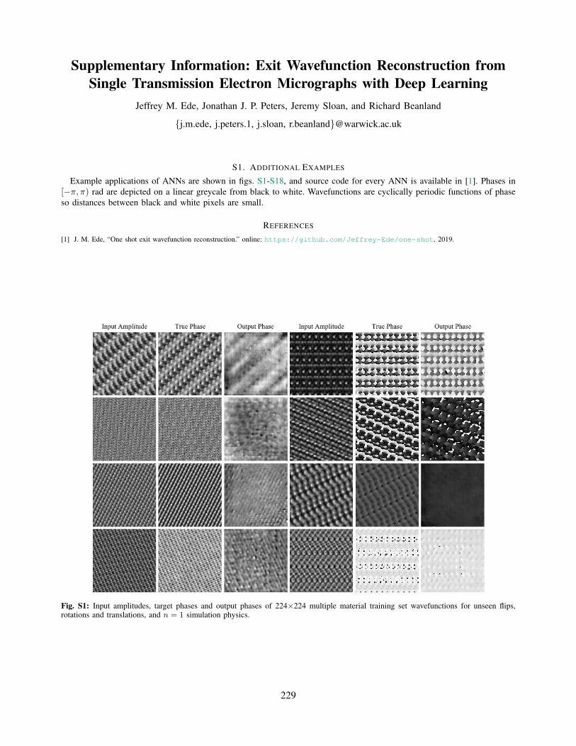
Supplementary Information: Exit Wavefunction Reconstruction fromSingle Transmission Electron Micrographs with Deep Learning
Jeffrey M. Ede, Jonathan J. P. Peters, Jeremy Sloan, and Richard Beanland
j.m.ede, j.peters.1, j.sloan, [email protected]
S1. ADDITIONAL EXAMPLES
Example applications of ANNs are shown in figs. S1-S18, and source code for every ANN is available in [1]. Phases in[−π, π) rad are depicted on a linear greycale from black to white. Wavefunctions are cyclically periodic functions of phaseso distances between black and white pixels are small.
REFERENCES
[1] J. M. Ede, “One shot exit wavefunction reconstruction.” online: https://github.com/Jeffrey-Ede/one-shot, 2019.
Fig. S1: Input amplitudes, target phases and output phases of 224×224 multiple material training set wavefunctions for unseen flips,rotations and translations, and n = 1 simulation physics.
229
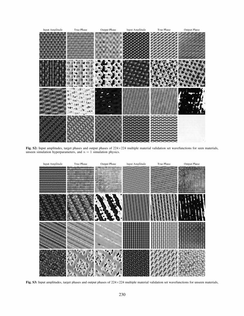
Fig. S2: Input amplitudes, target phases and output phases of 224×224 multiple material validation set wavefunctions for seen materials,unseen simulation hyperparameters, and n = 1 simulation physics.
Fig. S3: Input amplitudes, target phases and output phases of 224×224 multiple material validation set wavefunctions for unseen materials,unseen simulation hyperparameters, and n = 1 simulation physics.
230
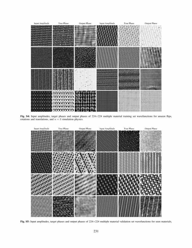
Fig. S4: Input amplitudes, target phases and output phases of 224×224 multiple material training set wavefunctions for unseen flips,rotations and translations, and n = 3 simulation physics.
Fig. S5: Input amplitudes, target phases and output phases of 224×224 multiple material validation set wavefunctions for seen materials,unseen simulation hyperparameters, and n = 3 simulation physics.
231
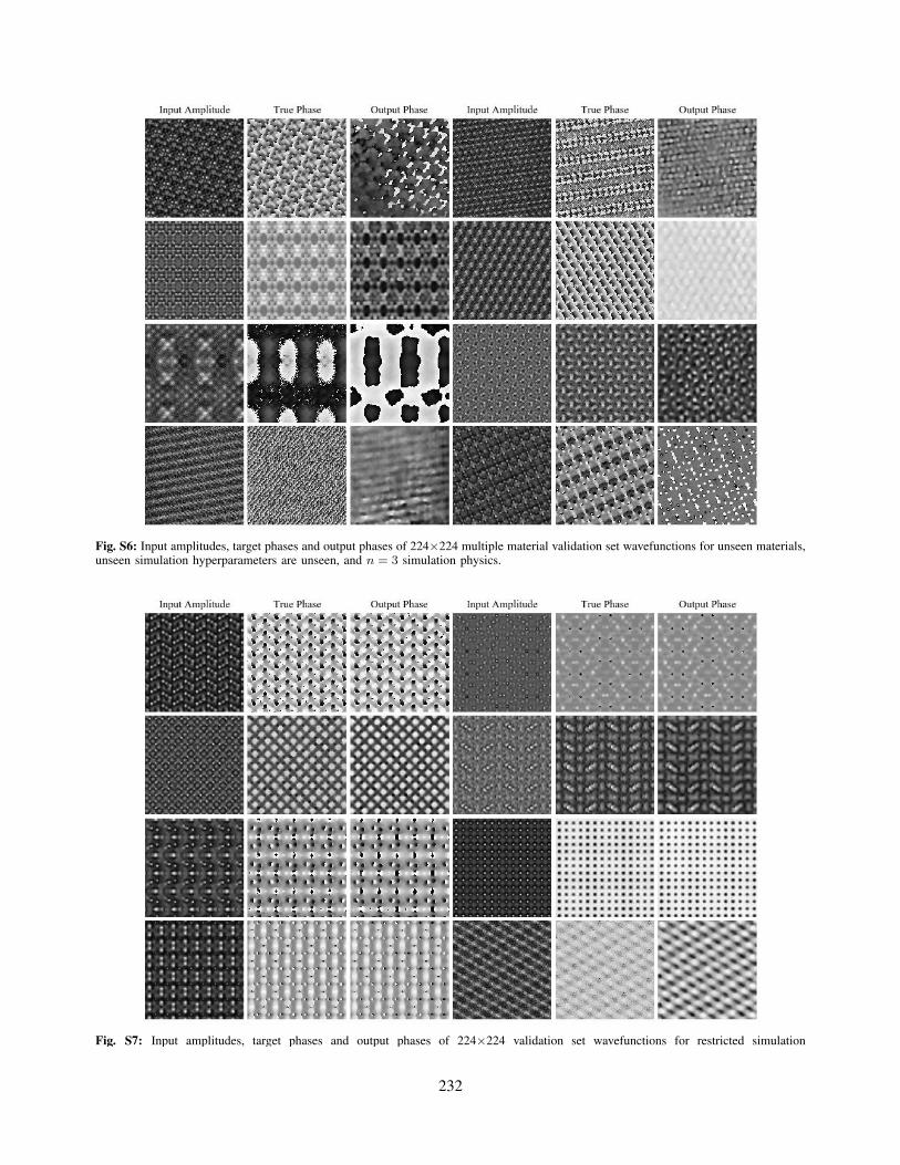
Fig. S6: Input amplitudes, target phases and output phases of 224×224 multiple material validation set wavefunctions for unseen materials,unseen simulation hyperparameters are unseen, and n = 3 simulation physics.
Fig. S7: Input amplitudes, target phases and output phases of 224×224 validation set wavefunctions for restricted simulationhyperparameters, and n = 3 simulation physics.
232
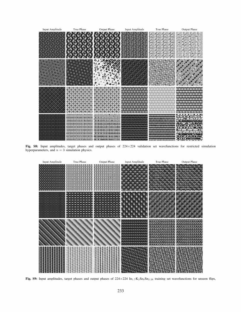
Fig. S8: Input amplitudes, target phases and output phases of 224×224 validation set wavefunctions for restricted simulationhyperparameters, and n = 3 simulation physics.
Fig. S9: Input amplitudes, target phases and output phases of 224×224 In1.7K2Se8Sn2.28 training set wavefunctions for unseen flips,rotations and translations, and n = 1 simulation physics.
233

Fig. S10: Input amplitudes, target phases and output phases of 224×224 In1.7K2Se8Sn2.28 validation set wavefunctions for unseensimulation hyperparameters, and n = 1 simulation physics.
Fig. S11: Input amplitudes, target phases and output phases of 224×224 validation set wavefunctions for unseen simulation hyperparametersand materials, and n = 1 simulation physics. The generator was trained with In1.7K2Se8Sn2.28 wavefunctions.
234
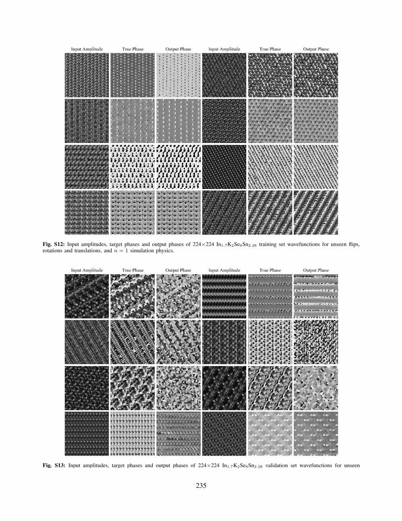
Fig. S12: Input amplitudes, target phases and output phases of 224×224 In1.7K2Se8Sn2.28 training set wavefunctions for unseen flips,rotations and translations, and n = 1 simulation physics.
Fig. S13: Input amplitudes, target phases and output phases of 224×224 In1.7K2Se8Sn2.28 validation set wavefunctions for unseensimulation hyperparameters, and n = 3 simulation physics.
235
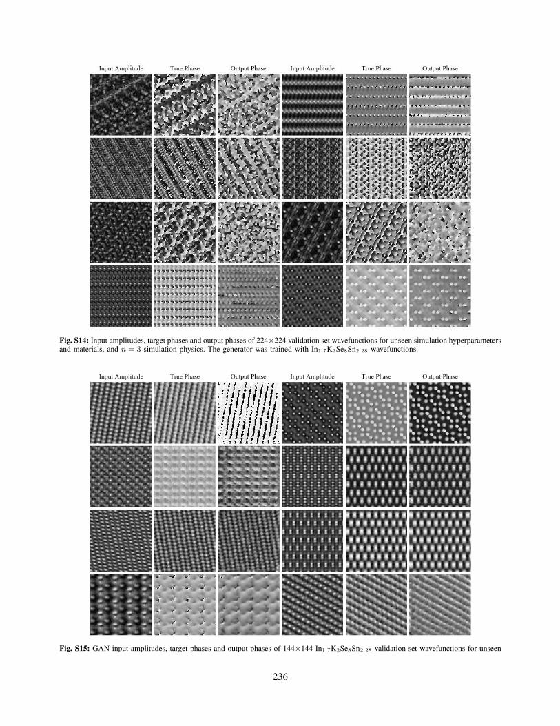
Fig. S14: Input amplitudes, target phases and output phases of 224×224 validation set wavefunctions for unseen simulation hyperparametersand materials, and n = 3 simulation physics. The generator was trained with In1.7K2Se8Sn2.28 wavefunctions.
Fig. S15: GAN input amplitudes, target phases and output phases of 144×144 In1.7K2Se8Sn2.28 validation set wavefunctions for unseenflips, rotations and translations, and n = 1 simulation physics.
236

Fig. S16: GAN input amplitudes, target phases and output phases of 144×144 In1.7K2Se8Sn2.28 validation set wavefunctions for unseensimulation hyperparameters, and n = 1 simulation physics.
Fig. S17: GAN input amplitudes, target phases and output phases of 144×144 In1.7K2Se8Sn2.28 validation set wavefunctions for unseenflips, rotations and translations, and n = 3 simulation physics.
237

Fig. S18: GAN input amplitudes, target phases and output phases of 144×144 In1.7K2Se8Sn2.28 validation set wavefunctions for unseensimulation hyperparameters, and n = 3 simulation physics.
238
7.2 Reflection
This chapter covers our paper titled “Exit Wavefunction Reconstruction from Single Transmission Electron Mi-
crographs with Deep Learning”7 and associated research outputs15,25. At the University of Warwick, EWR is
usually based on iterative focal and tilt series reconstruction (FTSR), so a previous PhD student, Mark Dyson,
GPU-accelerated FTSR252. However, both recording a series of electron micrographs and FTSR usually take several
seconds, so FTSR is unsuitable for live EWR. We have an electrostatic biprism that can be used for live in-line
holography253–255; however, it is not used as we find that in-line holography is more difficult than FTSR. In addition,
in-line holography can require expensive microscope modification if a microscope is not already equipped for it.
Thus, I was inspired by applications of DNNs to predict missing information for low-light vision256,257 to investigate
live application of DNNs to predict missing phases of exit wavefunctions from single TEM images.
A couple of years ago, it was shown that DNNs can recover phases of exit wavefunctions from single optical
micrographs if wavefunctions are constrained by limiting input variety258–260. Similarly, electron propagation
can be described by wave optics261, and optical and electron microscopes have similar arrangements of optical
and electromagnetic lenses, respectively262. Thus, it might be expected that DNNs can recover phases of exit
wavefunctions from single TEM images. However, earlier experiments with optical micrographs were unbeknownst
to us when we started our investigation. Thus, whether DNNs could reconstruct phase information from single
TEM images was contentions as there are infinite possible phases for a given amplitude. Further, previous non-
iterative approaches to TEM EWR were limited to defocused images in the Fresnel regime263 or non-planar incident
wavefunctions in the Fraunhofer regime264.
We were not aware of any large openly accessible datasets containing experimental TEM exit wavefunctions.
Consequently, we simulated exit wavefunctions with clTEM252,265 for a preliminary investigation. Similar to optical
EWR258–260, we found that DNNs can recover the phases of TEM exit wavefunctions if wavefunction variety
is restricted. Limitingly, our simulations are unrealistic insofar they do not include aberrations, specimen drift,
statistical noise, and higher-order simulation physics. However, we have demonstrated that DNNs can learn to
remove noise6 (ch. 6), specimen drifted can be reduced by sample holders266, and aberrations can be minimized by
aberration correctors261,267–269. Moreover, our results present lower bounds for performance as our inputs were far
less restricted than possible in practice.
Curating a dataset of experimental exit wavefunctions to train DNNs to recover their phases is time-consuming
and expensive. Further, data curation became impractical due to a COVID-19 national lockdown in the United
Kingdom196. Instead, we propose a new approach to EWR that uses metadata to inform DNN training with single
images. Our TEM (ch. 6) and STEM (ch. 4) images in WEMD2 are provided as a possible resource to investigate our
proposal. However, metadata is not included in WEMD, which is problematic as performance is expected to increase
with increasing metadata as increasing metadata increasingly restricts probable exit wavefunctions. Nevertheless,
DNNs can reconstruct some metadata from unlabelled electron micrographs270. Another issue is that experimental
WEMD contain images for a range of electron microscope configurations, which would complicate DNN training.
For example, experimental TEM images include bright field, dark field, diffraction and CBED images. However,
data clustering could be applied to partially automate labelling of electron microscope configurations. For example,
I provide pretrained VAEs to embed images for tSNE2 (ch. 2).
239

Chapter 8
Conclusions
This thesis covers a subset of my papers on advances in electron microscopy with deep learning. My review paper
(ch. 1) offers a substantial introduction that sets my work in context. Ancillary chapters then introduce new machine
learning datasets for electron microscopy (ch. 2) and an algorithm to prevent learning instabilty when training large
neural networks with limited computational resources (ch. 3). Finally, we report applications of deep learning to
compressed sensing in STEM with static (ch. 4) and dynamic (ch. 5) scans, improving TEM signal-to-noise (ch. 6),
and TEM exit wavefunction reconstruction (ch. 7). This thesis therefore presents a substantial original contribution
to knowledge which is, in practice, worthy of peer-reviewed publication. This thesis adds to my existing papers by
presenting their relationships, reflections, and holistic conclusions. To encourage further investigation, source code,
pretrained models, datasets, and other research outputs associated with this thesis are openly accessible.
Experiments presented in this thesis are based on unlabelled electron microscopy image data. Thus, this thesis
demonstrates that large machine learning datasets can be valuable without needing to add enhancements, such as
image-level or pixel-level labels, to data. Indeed, this thesis can be characterized as an investigation into applications
of large unlabelled electron microscopy datasets. However, I expect that tSNE clustering based on my pretrained
VAE encodings2 (ch. 2) could ease image-level labelling for future investigations. Most areas of science are facing a
reproducibility crisis115, including artificial intelligence271, which I think is partly due to a perceived lack of value
in archiving data that has not been enhanced. However, this thesis demonstrates that unlabelled data can readily
enable new applications of deep learning in electron microscopy. Thus, I hope that my research will encourage more
extensive data archiving by the electron microscopy community.
My DNNs were developed with TensorFlow272,273 and Python. In addition, recent versions of Gatan Microscopy
Suite (GMS) software274, which is often used to drive electron microscopes, support Python275. Thus, my pretrained
models and source code can be readily integrated into existing GMS software. If a microscope is operated by
alternative software or an older version of GMS that does not support Python, TensorFlow supports many other
programming languages1 which can also interface with my pretrained models, and which may be more readily
integrated. Alternatively, Python code can often be readily embedded in or executed by other programming languages.
To be clear, my DNNs were developed as part of an initial investigation of deep learning in electron microscopy.
Thus, this thesis presents lower bounds for performance that may be improved upon by refining ANN architecture
and learning policy. Nevertheless, my pretrained models can be the initial basis of deep learning software for electron
microscopy.
This thesis includes a variety of experiments to refine ANN architecture and learning policy. As AutoML245–249
has improved since the start of my PhD, I expect that human involvement can be reduced in future investigations
of standard architecture and learning policy variations. However, AutoML is yet to be able to routinely develop
new approaches to machine learning, such as VAE encoding normalization and regularization2 (ch. 2) and ALRC3
240

(ch. 3). Most machine learning experts do not think that a technological singularity, where machines outrightly
surpasses human developers, is likely for at least a couple of decades276. Nonetheless, our increasingly creative
machines are already automating some aspects of software development277,278 and can programmatically describe
ANNs279. Subsequently, I encourage adoption of creative software, like AutoML, to ease development.
Perhaps the most exciting aspect of ANNs is their scalability280,281. Once an ANN has been trained, clones
of the ANN and supporting software can be deployed on many electron microscopes at little or no additional cost
to the developer. All machine learning software comes with technical debt282,283; however, software maintenance
costs are usually far lower than the cost of electron microscopes. Thus, machine learning may be a promising
means to cheaply enhance electron microscopes. As an example, my experiments indicate that compressed sensing
ANNs4 (ch. 4) can increase STEM and other electron microscopy resolution by up to 10× with minimal information
loss. Such a resolution increase could greatly reduce the cost of electron microscopes while maintaining similar
capability. Further, I anticipate that multiple ANNs offering a variety of functionality can be combined into a single-
or multiple-ANN system that simultaneously offers a variety of enhancements, including increased resolution,
decreased noise6 (ch. 6), and phase information7 (ch. 6).
I think the main limitation of this thesis, and deep learning, is that it is difficult to fairly compare different
approaches to DNN development. As an example, I found that STEM compressed sensing with regularly spaced
scans outperforms contiguous scans for the same ANN architecture and learning policy4 (ch. 4). However, such a
performance comparison is complicated by sensitivity of performance to training data, architecture, and learning
policy. As a case in point, I argued that contiguous scans could outperform spiral scans if STEM images were not
oversampled4, which could be the case if partial STEM ANNs are also trained to increase image resolution. In part,
I think ANN development is an art: Most ANN architecture and learning policy is guided by heuristics, and best
approaches to maximize performance are chosen by natural selection284. Due to the complicated nature of most
data, maximum performances that can be achieved with deep learning are not known. However, it follows from the
universal approximator theorem233–241 that minimum errors can, in principle, be achieved by DNNs.
Applying an ANN to a full image usually requires less computation than applying an ANN to multiple image
crops. Processing full images avoids repeated calculations if crops overlap6 (ch. 6) or lower performance near crop
edges where there is less information4,6,19 (ch. 4 and ch. 6). However, it is usually impractical to train large DNNs
to process full electron microscopy images, which are often 1024×1024 or larger, due to limited memory in most
GPUs. This was problematic as one of my original agreements about my research was that I would demonstrate that
DNNs could be applied to large electron microscopy images, which Richard Beanland and I decided were at least
512×512. As a result, most of my DNNs were developed for 512×512 crops from electron micrographs, especially
near the start of my PhD. The combination of large input images and limited available GPU memory restricted
training batch sizes to few examples for large ANNs, so I often trained ANNs with a batch size of 1 and either
weight285 or spectral286 normalization, rather than batch normalization287.
Most of my DNNs leverage an understanding of physics to add extra information to electron microscopy images.
Overt examples include predicting unknown pixels for compressed sensing with static4 (ch. 4) or adaptive5 (ch. 5)
sparse scans, and unknown phase information from image intensities7 (ch. 7). More subtly, improving image
signal-to-noise with an DNN6 (ch. 6) is akin to improving signal-to-noise by increasing numbers of intensity
measurements. Arguably, even search engines based on VAEs2 (ch. 2) add information to images insofar that VAE
241
encodings can be compared to quantify semantic similarities between images. Ultimately, my DNNs add information
to data that could already be understood from physical laws and observations. However, high-dimensional datasets
can be difficult to utilize. Deep learning offers an effective and timely means to both understand high-dimensional
data and leverage that understanding to produce results in a useable format. Thus, I both anticipate and encourage
further investigation of deep learning in electron microscopy.
242
References
[1] J. M. Ede. Review: Deep Learning in Electron Microscopy. arXiv preprint arXiv:2009.08328 (accepted by
Machine Learning: Science and Technology – https://doi.org/10.1088/2632-2153/abd614),
2020.
[2] J. M. Ede. Warwick Electron Microscopy Datasets. Machine Learning: Science and Technology, 1(4):045003,
2020.
[3] J. M. Ede and R. Beanland. Adaptive Learning Rate Clipping Stabilizes Learning. Machine Learning: Science
and Technology, 1:015011, 2020.
[4] J. M. Ede and R. Beanland. Partial Scanning transmission Electron Microscopy with Deep Learning. Scientific
Reports, 10(1):1–10, 2020.
[5] J. M. Ede. Adaptive Partial Scanning Transmission Electron Microscopy with Reinforcement Learning. arXiv
preprint arXiv:2004.02786 (under review by Machine Learning: Science and Technology), 2020.
[6] J. M. Ede and R. Beanland. Improving Electron Micrograph Signal-to-Noise with an Atrous Convolutional
Encoder-Decoder. Ultramicroscopy, 202:18–25, 2019.
[7] J. M. Ede, J. J. P. Peters, J. Sloan, and R. Beanland. Exit Wavefunction Reconstruction from Single
Transmission Electron Micrographs with Deep Learning. arXiv preprint arXiv:2001.10938 (under review by
Ultramicroscopy), 2020.
[8] J. M. Ede. Resume of Jeffrey Mark Ede. Zenodo, Online: https://doi.org/10.5281/zenodo.4
429077, 2021.
[9] J. M. Ede. Supplementary Information: Warwick Electron Microscopy Datasets. Zenodo, Online: https:
//doi.org/10.5281/zenodo.3899740, 2020.
[10] J. M. Ede. Supplementary Information: Partial Scanning Transmission Electron Microscopy with Deep
Learning. Online: https://static-content.springer.com/esm/art%3A10.1038%2Fs4
1598-020-65261-0/MediaObjects/41598 2020 65261 MOESM1 ESM.pdf, 2020.
[11] J. M. Ede. Supplementary Information: Adaptive Partial Scanning Transmission Electron Microscopy with
Reinforcement Learning. Zenodo, Online: https://doi.org/10.5281/zenodo.4384708, 2020.
[12] J. M. Ede, J. J. P. Peters, J. Sloan, and R. Beanland. Supplementary Information: Exit Wavefunction
Reconstruction from Single Transmission Electron Micrographs with Deep Learning. Zenodo, Online:
https://doi.org/10.5281/zenodo.4277357, 2020.
[13] J. M. Ede. Warwick Electron Microscopy Datasets. arXiv preprint arXiv:2003.01113, 2020.
243
[14] J. M. Ede. Source Code for Warwick Electron Microscopy Datasets. Online: https://github.com/J
effrey-Ede/datasets, 2020.
[15] J. M. Ede. Warwick Electron Microscopy Datasets Archive. Online: https://github.com/Jeffrey
-Ede/datasets/wiki, 2020.
[16] J. M. Ede and R. Beanland. Adaptive Learning Rate Clipping Stabilizes Learning. arXiv preprint
arXiv:1906.09060, 2019.
[17] J. M. Ede. Source Code for Adaptive Learning Rate Clipping Stabilizes Learning. Online: https:
//github.com/Jeffrey-Ede/ALRC, 2020.
[18] J. M. Ede and R. Beanland. Partial Scanning Transmission Electron Microscopy with Deep Learning. arXiv
preprint arXiv:1910.10467, 2020.
[19] J. M. Ede. Deep Learning Supersampled Scanning Transmission Electron Microscopy. arXiv preprint
arXiv:1910.10467, 2019.
[20] J. M. Ede. Source Code for Partial Scanning Transmission Electron Microscopy. Online: https://gith
ub.com/Jeffrey-Ede/partial-STEM, 2019.
[21] J. M. Ede. Source Code for Deep Learning Supersampled Scanning Transmission Electron Microscopy.
Online: https://github.com/Jeffrey-Ede/DLSS-STEM, 2019.
[22] J. M. Ede. Source Code for Adaptive Partial Scanning Transmission Electron Microscopy with Reinforcement
Learning. Online: https://github.com/Jeffrey-Ede/adaptive-scans, 2020.
[23] J. M. Ede. Improving Electron Micrograph Signal-to-Noise with an Atrous Convolutional Encoder-Decoder.
arXiv preprint arXiv:1807.11234, 2018.
[24] J. M. Ede. Source Code for Improving Electron Micrograph Signal-to-Noise with an Atrous Convolutional
Encoder-Decoder. Online: https://github.com/Jeffrey-Ede/Electron-Micrograph-D
enoiser, 2019.
[25] J. M. Ede. Source Code for Exit Wavefunction Reconstruction from Single Transmission Electron Micrographs
with Deep Learning. Online: https://github.com/Jeffrey-Ede/one-shot, 2019.
[26] J. M. Ede. Progress Reports of Jeffrey Mark Ede: 0.5 Year Progress Report. Zenodo, Online: https:
//doi.org/10.5281/zenodo.4094750, 2020.
[27] J. M. Ede. Source Code for Beanland Atlas. Online: https://github.com/Jeffrey-Ede/Beanl
and-Atlas, 2018.
[28] J. M. Ede. Thesis Word Counting. Zenodo, Online: https://doi.org/10.5281/zenodo.4321429,
2020.
244
[29] J. M. Ede. Posters and Presentations. Zenodo, Online: https://doi.org/10.5281/zenodo.404
1574, 2020.
[30] J. M. Ede. Autoencoders, Kernels, and Multilayer Perceptrons for Electron Micrograph Restoration and
Compression. arXiv preprint arXiv:1808.09916, 2018.
[31] J. M. Ede. Source Code for Autoencoders, Kernels, and Multilayer Perceptrons for Electron Micrograph
Restoration and Compression. Online: https://github.com/Jeffrey-Ede/Denoising-Ker
nels-MLPs-Autoencoders, 2018.
[32] J. M. Ede. Source Code for Simple Webserver. Online: https://github.com/Jeffrey-Ede/sim
ple-webserver, 2019.
[33] Guide to Examinations for Higher Degrees by Research. University of Warwick Doctoral College, Online:
https://warwick.ac.uk/services/dc/pgrassessments/gtehdr, 2020.
[34] Regulation 38: Research Degrees. University of Warwick Calendar, Online: https://warwick.ac.u
k/services/gov/calendar/section2/regulations/reg38pgr, 2020.
[35] Thesis Writing and Submission. University of Warwick Department of Physics, Online: https://warw
ick.ac.uk/fac/sci/physics/current/postgraduate/regs/thesis, 2020.
[36] A Warwick Thesis Template. University of Warwick Department of Physics, Online: https://warwick.
ac.uk/fac/sci/physics/staff/academic/mhadley/wthesis, 2020.
[37] J. M. Ede. Advances in Electron Microscopy with Deep Learning. arXiv preprint arXiv:2101.01178, 2021.
[38] EPSRC Studentship 1917382: Application of Novel Computing and Data Analysis Methods in Electron
Microscopy. UK Research and Innovation, Online: https://gtr.ukri.org/projects?ref=stu
dentship-1917382, 2020.
[39] EPSRC Grant EP/N035437/1: ADEPT – Advanced Devices by ElectroPlaTing. EPSRC, Online: https:
//gow.epsrc.ukri.org/NGBOViewGrant.aspx?GrantRef=EP/N035437/1, 2016.
[40] A. J. M. Hubert, R. Romer, and R. Beanland. Structure Refinement from ‘Digital’ Large Angle Convergent
Beam Electron Diffraction Patterns. Ultramicroscopy, 198:1–9, 2019.
[41] J. M. Ede. Beanland Atlas Repository. Towards Data Science, Online: https://github.com/Jeffr
ey-Ede/Beanland-Atlas, 2018.
[42] J. L. Hart, S. Liu, A. C. Lang, A. Hubert, A. Zukauskas, C. Canalias, R. Beanland, A. M. Rappe, M. Arredondo,
and M. L. Taheri. Electron-Beam-Induced Ferroelectric Domain Behavior in the Transmission Electron
Microscope: Toward Deterministic Domain Patterning. Physical Review B, 94(17):174104, 2016.
[43] D. Ha. Neural Network Generative Art in Javascript. Online: https://blog.otoro.net/2015/06
/19/neural-network-generative-art, 2015.
245
[44] T. Le. Generate Abstract Random Art with A Neural Network. Medium, Online: https://medium.com
/@tuanle618/generate-abstract-random-art-with-a-neural-network-ecef26f3
dd5f, 2019.
[45] L. A. Gatys, A. S. Ecker, and M. Bethge. Image Style Transfer Using Convolutional Neural Networks. In
Proceedings of the IEEE Conference on Computer Vision and Pattern Recognition, pages 2414–2423, 2016.
[46] L. A. Gatys, A. S. Ecker, and M. Bethge. A Neural Algorithm of Artistic Style. Nature Communications,
2015.
[47] J. Johnson, A. Alahi, and L. Fei-Fei. Perceptual Losses for Real-Time Style Transfer and Super-Resolution.
In European Conference on Computer Vision, pages 694–711. Springer, 2016.
[48] T.-C. Wang, M.-Y. Liu, J.-Y. Zhu, A. Tao, J. Kautz, and B. Catanzaro. High-Resolution Image Synthesis and
Semantic Manipulation with Conditional GANs. In Proceedings of the IEEE Conference on Computer Vision
and Pattern Recognition, pages 8798–8807, 2018.
[49] L.-C. Chen, Y. Zhu, G. Papandreou, F. Schroff, and H. Adam. Encoder-Decoder with Atrous Separable
Convolution for Semantic Image Segmentation. In Proceedings of the European conference on computer
vision (ECCV), pages 801–818, 2018.
[50] F. Jiang, W. Tao, S. Liu, J. Ren, X. Guo, and D. Zhao. An End-to-End Compression Framework Based on
Convolutional Neural Networks. IEEE Transactions on Circuits and Systems for Video Technology, 28(10):
3007–3018, 2017.
[51] C. Guerin. Connecting the Dots: Writing a Doctoral Thesis by Publication. In Research Literacies and
Writing Pedagogies for Masters and Doctoral Writers, pages 31–50. Brill, 2016.
[52] S. Mason, J. E. Morris, and M. K. Merga. Institutional and Supervisory Support for the Thesis by Publication.
Australian Journal of Education, page 0004944120929065, 2020.
[53] V. Lariviere, A. Zuccala, and E. Archambault. The Declining Scientific Impact of Theses: Implications for
Electronic Thesis and Dissertation Repositories and Graduate Studies. Scientometrics, 74(1):109–121, 2008.
[54] 2018 Global State of Peer Review. Publons, Online: https://publons.com/static/Publons-G
lobal-State-Of-Peer-Review-2018.pdf, 2018.
[55] J. P. Tennant. The State of the Art in Peer Review. FEMS Microbiology Letters, 365(19), 2018.
[56] R. Walker and P. Rocha da Silva. Emerging Trends in Peer Review – A Survey. Frontiers in Neuroscience, 9:
169, 2015.
[57] I. Vesper. Peer Reviewers Unmasked: Largest Global Survey Reveals Trends. Nature, 2018.
[58] Z.-Y. Tan, N. Cai, J. Zhou, and S.-G. Zhang. On Performance of Peer Review for Academic Journals: Analysis
Based on Distributed Parallel System. IEEE Access, 7:19024–19032, 2019.
246
[59] T. Ferreras-Fernandez, F. Garcıa-Penalvo, J. A. Merlo-Vega, and H. Martın-Rodero. Providing Open Access
to PhD Theses: Visibility and Citation Benefits. Program, 2016.
[60] M. Kettler. Ways of Disseminating, Tracking Usage and Impact of Electronic Theses and Dissertations
(ETDs). In Conference on Grey Literature and Repositories, page 37, 2016.
[61] B. M. Miller. The Making of Knowledge-Makers in Composition: A Distant Reading of Dissertations. PhD
thesis, City University of New York, 2015.
[62] University of Warwick Physics PhD Theses. Online: https://wrap.warwick.ac.uk/view/thes
es/Department of Physics.html, 2020.
[63] About arXiv. Online: https://arxiv.org/about, 2020.
[64] P. Ginsparg. ArXiv at 20. Nature, 476(7359):145–147, 2011.
[65] G. Pignalberi and M. Dominici. Introduction to LATEX and to Some of its Tools. ArsTEXnica, page 8, 2019.
[66] M. Bransen and G. Schulpen. Pimp Your Thesis: A Minimal Introduction to LATEX. IC/TC, U.S.S. Proton,
Online: https://ussproton.nl/files/careerweeks/20180320-pimpyourthesis.pdf,
2018.
[67] L. Lamport. LATEX: A Document Preparation System: User’s Guide and Reference Manual. Addison-Wesley,
1994.
[68] Creative Commons Attribution 4.0 International (CC BY 4.0). Online: https://creativecommons.
org/licenses/by/4.0, 2020.
[69] M. B. Hoy. Rise of the Rxivs: How Preprint Servers are Changing the Publishing Process. Medical Reference
Services Quarterly, 39(1):84–89, 2020.
[70] N. K. Fry, H. Marshall, and T. Mellins-Cohen. In Praise of Preprints. Microbial Genomics, 5(4), 2019.
[71] E. G. Rodrıguez. Preprints and Preprint Servers as Academic Communication Tools. Revista Cubana de
Informacion en Ciencias de la Salud, 30(1), 2019.
[72] G. C. Banks, J. G. Field, F. L. Oswald, E. H. O’Boyle, R. S. Landis, D. E. Rupp, and S. G. Rogelberg.
Answers to 18 Questions About Open Science Practices. Journal of Business and Psychology, 34(3):257–270,
2019.
[73] N. Fraser, F. Momeni, P. Mayr, and I. Peters. The Relationship Between bioRxiv Preprints, Citations and
Altmetrics. Quantitative Science Studies, 1(2):618–638, 2020.
[74] Z. Wang, W. Glanzel, and Y. Chen. The Impact of Preprints in Library and Information Science: An Analysis
of Citations, Usage and Social Attention Indicators. Scientometrics, pages 1–21, 2020.
247
[75] A. C. Furnival and B. Hubbard. Open Access to Scholarly Communications: Advantages, Policy and
Advocacy. Acceso Abierto a la informacion en las Bibliotecas Academicas de America Latina y el Caribe,
pages 101–120, 2020.
[76] D. Y. Fu and J. J. Hughey. Meta-Research: Releasing a Preprint is Associated with More Attention and
Citations for the Peer-Reviewed Article. Elife, 8:e52646, 2019.
[77] Y. Niyazov, C. Vogel, R. Price, B. Lund, D. Judd, A. Akil, M. Mortonson, J. Schwartzman, and M. Shron.
Open Access Meets Discoverability: Citations to Articles Posted to Academia.edu. PLOS ONE, 11(2):
e0148257, 2016.
[78] M. Klein, P. Broadwell, S. E. Farb, and T. Grappone. Comparing Published Scientific Journal Articles to
Their Pre-Print Versions. International Journal on Digital Libraries, 20(4):335–350, 2019.
[79] C. F. Carneiro, V. G. Queiroz, T. C. Moulin, C. A. Carvalho, C. B. Haas, D. Rayee, D. E. Henshall, E. A. De-
Souza, F. Espinelli, F. Z. Boos, et al. Comparing Quality of Reporting Between Preprints and Peer-Reviewed
Articles in the Biomedical Literature. BioRxiv, page 581892, 2019.
[80] Elsevier Language Editing Services. Online: https://webshop.elsevier.com/language-ed
iting-services, 2020.
[81] IOP Editing Services. Online: https://editing.iopscience.iop.org, 2020.
[82] Springer Nature Author Services. Online: https://authorservices.springernature.com,
2020.
[83] Wiley Editing Services. Online: https://wileyeditingservices.com/en, 2020.
[84] R. Roth. Understanding the Importance of Copyediting in Peer-Reviewed Manuscripts. Science Editor, 42(2):
51, 2019.
[85] ISO 32000-2:2017 Document management — Portable document format — Part 2: PDF 2.0. International
Organization for Standardization, Online: https://www.iso.org/standard/51502.html, 2017.
[86] ISO 32000-2:2008 Document management — Portable document format — Part 1: PDF 1.7. Adobe Systems,
Online: http://wwwimages.adobe.com/www.adobe.com/content/dam/acom/en/devn
et/pdf/pdfs/PDF32000 2008.pdf, 2008.
[87] arXiv License Information. Online: https://arxiv.org/help/license, 2020.
[88] C. B. Clement, M. Bierbaum, K. P. O’Keeffe, and A. A. Alemi. On the Use of ArXiv as a Dataset. arXiv
preprint arXiv:1905.00075, 2019.
[89] S. Eger, C. Li, F. Netzer, and I. Gurevych. Predicting Research Trends from ArXiv. arXiv preprint
arXiv:1903.02831, 2019.
[90] T. Ross-Hellauer. What is Open Peer Review? A Systematic Review. F1000Research, 6, 2017.
248
[91] About OpenReview. Online: https://openreview.net/about, 2020.
[92] D. Soergel, A. Saunders, and A. McCallum. Open Scholarship and Peer Review: a Time for Experimentation.
In International Conference on Machine Learning (ICML 2013) Peer Review Workshop, 2013.
[93] L. Wang and Y. Zhan. A Conceptual Peer Review Model for arXiv and Other Preprint Databases. Learned
Publishing, 32(3):213–219, 2019.
[94] GitHub Profile of Jeffrey Mark Ede. Online: https://github.com/Jeffrey-Ede, 2020.
[95] Zenodo. Online: https://about.zenodo.org, 2020.
[96] R. Lalli. A Brief History of Physics Reviews. Nature Reviews Physics, 1(1):12, 2019.
[97] S. Sengupta, S. Basak, P. Saikia, S. Paul, V. Tsalavoutis, F. Atiah, V. Ravi, and A. Peters. A Review of
Deep Learning with Special Emphasis on Architectures, Applications and Recent Trends. Knowledge-Based
Systems, page 105596, 2020.
[98] A. Shrestha and A. Mahmood. Review of Deep Learning Algorithms and Architectures. IEEE Access, 7:
53040–53065, 2019.
[99] M. Z. Alom, T. M. Taha, C. Yakopcic, S. Westberg, P. Sidike, M. S. Nasrin, M. Hasan, B. C. Van Essen,
A. A. S. Awwal, and V. K. Asari. A State-of-the-Art Survey on Deep Learning Theory and Architectures.
Electronics, 8(3):292, 2019.
[100] Y. LeCun, Y. Bengio, and G. Hinton. Deep Learning. Nature, 521(7553):436–444, 2015.
[101] J. Schmidhuber. Deep Learning in Neural Networks: An Overview. Neural Networks, 61:85–117, 2015.
[102] G. Barbastathis, A. Ozcan, and G. Situ. On the Use of Deep Learning for Computational Imaging. Optica, 6
(8):921–943, 2019.
[103] M. Ge, F. Su, Z. Zhao, and D. Su. Deep Learning Analysis on Microscopic Imaging in Materials Science.
Materials Today Nano, page 100087, 2020.
[104] J. Wei, X. Chu, X.-Y. Sun, K. Xu, H.-X. Deng, J. Chen, Z. Wei, and M. Lei. Machine Learning in Materials
Science. InfoMat, 1(3):338–358, 2019.
[105] G. R. Schleder, A. C. Padilha, C. M. Acosta, M. Costa, and A. Fazzio. From DFT to Machine Learning:
Recent Approaches to Materials Science – A Review. Journal of Physics: Materials, 2(3):032001, 2019.
[106] G. Carleo, I. Cirac, K. Cranmer, L. Daudet, M. Schuld, N. Tishby, L. Vogt-Maranto, and L. Zdeborova.
Machine Learning and the Physical Sciences. Reviews of Modern Physics, 91(4):045002, 2019.
[107] D. P. Kingma and M. Welling. Auto-Encoding Variational Bayes. arXiv preprint arXiv:1312.6114, 2014.
[108] D. P. Kingma and M. Welling. An Introduction to Variational Autoencoders. arXiv preprint arXiv:1906.02691,
2019.
249
[109] C. Doersch. Tutorial on Variational Autoencoders. arXiv preprint arXiv:1606.05908, 2016.
[110] L. v. d. Maaten and G. Hinton. Visualizing Data Using t-SNE. Journal of Machine Learning Research, 9
(Nov):2579–2605, 2008.
[111] G. C. Linderman and S. Steinerberger. Clustering with t-SNE, Provably. SIAM Journal on Mathematics of
Data Science, 1(2):313–332, 2019.
[112] L. van der Maaten. Accelerating t-SNE Using Tree-Based Algorithms. The Journal of Machine Learning
Research, 15(1):3221–3245, 2014.
[113] L. van der Maaten. Barnes-Hut-SNE. arXiv preprint arXiv:1301.3342, 2013.
[114] M. Wattenberg, F. Viegas, and I. Johnson. How to Use t-SNE Effectively. Distill, 1(10):e2, 2016.
[115] M. Baker. Reproducibility Crisis. Nature, 533(26):353–66, 2016.
[116] C. A. of Cyberspace Studies. Development of World Internet. World Internet Development Report 2017:
Translated by Peng Ping, pages 1–19, 2019.
[117] T. Berners-Lee, L. Masinter, and M. McCahill. RFC1738: Uniform Resource Locators (URL). RFC, 1994.
doi: 10.17487/RFC1738.
[118] P. Kaushik, D. P. Singh, and S. Rajpoot. Fibre Optic Communication in 21 st Century. In 2020 International
Conference on Intelligent Engineering and Management (ICIEM), pages 125–129. IEEE, 2020.
[119] E. Mack. The History of Broadband. Geographies of the Internet, pages 63–76, 2020.
[120] L. Abrardi and C. Cambini. Ultra-Fast Broadband Investment and Adoption: A Survey. Telecommunications
Policy, 43(3):183–198, 2019.
[121] M. Graydon and L. Parks. ’Connecting the Unconnected’: A Critical Assessment of US Satellite Internet
Services. Media, Culture & Society, 42(2):260–276, 2020.
[122] C. Kaufmanna, H.-P. Huthb, F. Zeigerb, and M. Schmidta. Performance Evaluation of Internet over Geo-
stationary Satellite for Industrial Applications. In 70th International Astronautical Congress. International
Astronautical Federation, 2019.
[123] D. Castelvecchi. Google Unveils Search Engine for Open Data. Nature, 561(7722):161–163, 2018.
[124] N. Noy. Discovering Millions of Datasets on the Web. The Keyword, Online: https://blog.google/
products/search/discovering-millions-datasets-web, 2020.
[125] C. Sun, A. Shrivastava, S. Singh, and A. Gupta. Revisiting Unreasonable Effectiveness of Data in Deep
Learning Era. In Proceedings of the IEEE International Conference on Computer Vision, pages 843–852,
2017.
250
[126] T. Hey, K. Butler, S. Jackson, and J. Thiyagalingam. Machine Learning and Big Scientific Data. Philosophical
Transactions of the Royal Society A, 378(2166):20190054, 2020.
[127] W. Kay, J. Carreira, K. Simonyan, B. Zhang, C. Hillier, S. Vijayanarasimhan, F. Viola, T. Green, T. Back,
P. Natsev, et al. The Kinetics Human Action Video Dataset. arXiv preprint arXiv:1705.06950, 2017.
[128] O. Russakovsky, J. Deng, H. Su, J. Krause, S. Satheesh, S. Ma, Z. Huang, A. Karpathy, A. Khosla, M. Bern-
stein, et al. ImageNet Large Scale Visual Recognition Challenge. International Journal of Computer Vision,
115(3):211–252, 2015.
[129] S. Abu-El-Haija, N. Kothari, J. Lee, P. Natsev, G. Toderici, B. Varadarajan, and S. Vijayanarasimhan.
YouTube-8M: A Large-Scale Video Classification Benchmark. arXiv preprint arXiv:1609.08675, 2016.
[130] C. Sohrabi, Z. Alsafi, N. O’Neill, M. Khan, A. Kerwan, A. Al-Jabir, C. Iosifidis, and R. Agha. World
Health Organization Declares Global Emergency: A Review of the 2019 Novel Coronavirus (COVID-19).
International Journal of Surgery, 2020.
[131] W. J. Wiersinga, A. Rhodes, A. C. Cheng, S. J. Peacock, and H. C. Prescott. Pathophysiology, Transmission,
Diagnosis, and Treatment of Coronavirus Disease 2019 (COVID-19): A Review. Jama, 324(8):782–793,
2020.
[132] T. Singhal. A Review of Coronavirus Disease-2019 (COVID-19). The Indian Journal of Pediatrics, pages
1–6, 2020.
[133] L. O. Teixeira, R. M. Pereira, D. Bertolini, L. S. Oliveira, L. Nanni, and Y. M. Costa. Impact of Lung
Segmentation on the Diagnosis and Explanation of COVID-19 in Chest X-Ray Images. arXiv preprint
arXiv:2009.09780, 2020.
[134] A. Ghosal, A. Nandy, A. K. Das, S. Goswami, and M. Panday. A Short Review on Different Clustering
Techniques and Their Applications. In Emerging Technology in Modelling and Graphics, pages 69–83.
Springer, 2020.
[135] M. Z. Rodriguez, C. H. Comin, D. Casanova, O. M. Bruno, D. R. Amancio, L. d. F. Costa, and F. A. Rodrigues.
Clustering Algorithms: A Comparative Approach. PlOS ONE, 14(1):e0210236, 2019.
[136] K. Djouzi and K. Beghdad-Bey. A Review of Clustering Algorithms for Big Data. In 2019 International
Conference on Networking and Advanced Systems (ICNAS), pages 1–6. IEEE, 2019.
[137] M. Mittal, L. M. Goyal, D. J. Hemanth, and J. K. Sethi. Clustering Approaches for High-Dimensional
Databases: A Review. Wiley Interdisciplinary Reviews: Data Mining and Knowledge Discovery, 9(3):e1300,
2019.
[138] M. Y. Ansari, A. Ahmad, S. S. Khan, G. Bhushan, et al. Spatiotemporal Clustering: A Review. Artificial
Intelligence Review, pages 1–43, 2019.
251
[139] A. K. Jain, M. N. Murty, and P. J. Flynn. Data Clustering: A Review. ACM Computing Surveys (CSUR), 31
(3):264–323, 1999.
[140] J. A. Lee and M. Verleysen. Nonlinear Dimensionality Reduction. Springer Science & Business Media, 2007.
[141] G. E. Hinton and S. T. Roweis. Stochastic Neighbor Embedding. In Advances in Neural Information
Processing Systems, pages 857–864, 2003.
[142] W. Li, J. E. Cerise, Y. Yang, and H. Han. Application of t-SNE to Human Genetic Data. Journal of
Bioinformatics and Computational Biology, 15(04):1750017, 2017.
[143] I. Wallach and R. Lilien. The Protein–Small-Molecule Database, A Non-Redundant Structural Resource for
the Analysis of Protein-Ligand Binding. Bioinformatics, 25(5):615–620, 2009.
[144] B. M. Devassy and S. George. Dimensionality Reduction and Visualisation of Hyperspectral Ink Data Using
t-SNE. Forensic Science International, page 110194, 2020.
[145] B. Melit Devassy, S. George, and P. Nussbaum. Unsupervised Clustering of Hyperspectral Paper Data Using
t-SNE. Journal of Imaging, 6(5):29, 2020.
[146] P. Gang, W. Zhen, W. Zeng, Y. Gordienko, Y. Kochura, O. Alienin, O. Rokovyi, and S. Stirenko. Dimension-
ality Reduction in Deep Learning for Chest X-Ray Analysis of Lung Cancer. In 2018 Tenth International
Conference on Advanced Computational Intelligence (ICACI), pages 878–883. IEEE, 2018.
[147] J. Birjandtalab, M. B. Pouyan, and M. Nourani. Nonlinear Dimension Reduction for EEG-Based Epileptic
Seizure Detection. In 2016 IEEE-EMBS International Conference on Biomedical and Health Informatics
(BHI), pages 595–598. IEEE, 2016.
[148] W. M. Abdelmoula, B. Balluff, S. Englert, J. Dijkstra, M. J. Reinders, A. Walch, L. A. McDonnell, and B. P.
Lelieveldt. Data-Driven Identification of Prognostic Tumor Subpopulations Using Spatially Mapped t-SNE of
Mass Spectrometry Imaging Data. Proceedings of the National Academy of Sciences, 113(43):12244–12249,
2016.
[149] F. Psihas, E. Niner, M. Groh, R. Murphy, A. Aurisano, A. Himmel, K. Lang, M. D. Messier, A. Radovic, and
A. Sousa. Context-Enriched Identification of Particles with a Convolutional Network for Neutrino Events.
Physical Review D, 100(7):073005, 2019.
[150] E. Racah, S. Ko, P. Sadowski, W. Bhimji, C. Tull, S.-Y. Oh, P. Baldi, et al. Revealing Fundamental Physics
from the Daya Bay Neutrino Experiment Using Deep Neural Networks. In 2016 15th IEEE International
Conference on Machine Learning and Applications (ICMLA), pages 892–897. IEEE, 2016.
[151] F. Gong, F. Bu, Y. Zhang, Y. Yan, R. Hu, and M. Dong. Visual Clustering Analysis of Electricity Data
Based on t-SNE. In 2020 IEEE 5th International Conference on Cloud Computing and Big Data Analytics
(ICCCBDA), pages 234–240. IEEE, 2020.
252
[152] K. McDonald, M. Tan, and Y. Mann. The Infinite Drum Machine. Experiments with Google, Online:
https://experiments.withgoogle.com/drum-machine, 2018.
[153] E. Schubert and M. Gertz. Intrinsic t-Stochastic Neighbor Embedding for Visualization and Outlier Detection.
In International Conference on Similarity Search and Applications, pages 188–203. Springer, 2017.
[154] I. T. Jolliffe and J. Cadima. Principal Component Analysis: A Review and Recent Developments. Philo-
sophical Transactions of the Royal Society A: Mathematical, Physical and Engineering Sciences, 374(2065):
20150202, 2016.
[155] M. E. Wall, A. Rechtsteiner, and L. M. Rocha. Singular Value Decomposition and Principal Component
Analysis. In A Practical Approach to Microarray Data Analysis, pages 91–109. Springer, 2003.
[156] N. Halko, P.-G. Martinsson, and J. A. Tropp. Finding Structure with Randomness: Probabilistic Algorithms
for Constructing Approximate Matrix Decompositions. SIAM Review, 53(2):217–288, 2011.
[157] P.-G. Martinsson, V. Rokhlin, and M. Tygert. A Randomized Algorithm for the Decomposition of Matrices.
Applied and Computational Harmonic Analysis, 30:47–68, 2011.
[158] N. Pezzotti, J. Thijssen, A. Mordvintsev, T. Hollt, B. Van Lew, B. P. Lelieveldt, E. Eisemann, and A. Vilanova.
GPGPU Linear Complexity t-SNE Optimization. IEEE Transactions on Visualization and Computer Graphics,
26(1):1172–1181, 2019.
[159] D. M. Chan, R. Rao, F. Huang, and J. F. Canny. t-SNE-CUDA: GPU-Accelerated t-SNE and its Applications
to Modern Data. In 2018 30th International Symposium on Computer Architecture and High Performance
Computing (SBAC-PAD), pages 330–338. IEEE, 2018.
[160] N. Pezzotti, B. P. Lelieveldt, L. van der Maaten, T. Hollt, E. Eisemann, and A. Vilanova. Approximated and
User Steerable tSNE for Progressive Visual Analytics. IEEE Transactions on Visualization and Computer
Graphics, 23(7):1739–1752, 2016.
[161] A. C. Belkina, C. O. Ciccolella, R. Anno, R. Halpert, J. Spidlen, and J. E. Snyder-Cappione. Automated
Optimized Parameters for t-Distributed Stochastic Neighbor Embedding Improve Visualization and Analysis
of Large Datasets. Nature Communications, 10(1):1–12, 2019.
[162] P. Alfeld. A Trivariate Clough—Tocher Scheme for Tetrahedral Data. Computer Aided Geometric Design, 1
(2):169–181, 1984.
[163] Z. Chen, V. Badrinarayanan, C.-Y. Lee, and A. Rabinovich. GradNorm: Gradient Normalization for Adaptive
Loss Balancing in Deep Multitask Networks. arXiv preprint arXiv:1711.02257, 2017.
[164] I. Malkiel, S. Ahn, V. Taviani, A. Menini, L. Wolf, and C. J. Hardy. Conditional WGANs with Adaptive
Gradient Balancing for Sparse MRI Reconstruction. arXiv preprint arXiv:1905.00985, 2019.
[165] W. McIlhagga. Estimates of Edge Detection Filters in Human Vision. Vision Research, 153:30–36, 2018.
253
[166] A. B. L. Larsen, S. K. Sønderby, H. Larochelle, and O. Winther. Autoencoding Beyond Pixels Using a
Learned Similarity Metric. In International Conference on Machine Learning, pages 1558–1566, 2016.
[167] G. Grund Pihlgren, F. Sandin, and M. Liwicki. Improving Image Autoencoder Embeddings with Perceptual
Loss. In International Joint Conference on Neural Networks, 2020.
[168] Z. Wang, A. C. Bovik, H. R. Sheikh, and E. P. Simoncelli. Image Quality Assessment: From Error Visibility
to Structural Similarity. IEEE Transactions on Image Processing, 13(4):600–612, 2004.
[169] H. Zhao, O. Gallo, I. Frosio, and J. Kautz. Loss Functions for Image Restoration with Neural Networks.
IEEE Transactions on Computational Imaging, 3(1):47–57, 2016.
[170] S. Z. Dadaneh, S. Boluki, M. Yin, M. Zhou, and X. Qian. Pairwise Supervised Hashing with Bernoulli
Variational Auto-Encoder and Self-Control Gradient Estimator. arXiv preprint arXiv:2005.10477, 2020.
[171] N. Patterson and Y. Wang. Semantic Hashing with Variational Autoencoders, 2016.
[172] G. Jin, Y. Zhang, and K. Lu. Deep Hashing Based on VAE-GAN for Efficient Similarity Retrieval. Chinese
Journal of Electronics, 28(6):1191–1197, 2019.
[173] F. Mena and R. Nanculef. A Binary Variational Autoencoder for Hashing. In Iberoamerican Congress on
Pattern Recognition, pages 131–141. Springer, 2019.
[174] D. Shen, Q. Su, P. Chapfuwa, W. Wang, G. Wang, L. Carin, and R. Henao. Nash: Toward End-to-End Neural
Architecture for Generative Semantic Hashing. arXiv preprint arXiv:1805.05361, 2018.
[175] S. Chaidaroon and Y. Fang. Variational Deep Semantic Hashing for Text Documents. In Proceedings of the
40th International ACM SIGIR Conference on Research and Development in Information Retrieval, pages
75–84, 2017.
[176] K. J. Liang, C. Li, G. Wang, and L. Carin. Generative Adversarial Network Training is a Continual Learning
Problem. arXiv preprint arXiv:1811.11083, 2018.
[177] M. Li, M. Soltanolkotabi, and S. Oymak. Gradient Descent with Early Stopping is Provably Robust to Label
Noise for Overparameterized Neural Networks. In International Conference on Artificial Intelligence and
Statistics, pages 4313–4324, 2020.
[178] T. Flynn, K. M. Yu, A. Malik, N. D’Imperio, and S. Yoo. Bounding the Expected Run-Time of Nonconvex
Optimization with Early Stopping. arXiv preprint arXiv:2002.08856, 2020.
[179] D. Hendrycks, K. Lee, and M. Mazeika. Using Pre-Training can Improve Model Robustness and Uncertainty.
arXiv preprint arXiv:1901.09960, 2019.
[180] R. Beanland, K. Evans, and R. A. Roemer. Felix. Online: https://github.com/RudoRoemer/Fe
lix, 2020.
254
[181] G. P. Meyer. An Alternative Probabilistic Interpretation of the Huber Loss. arXiv preprint arXiv:1911.02088,
2019.
[182] P. J. Huber. Robust Estimation of a Location Parameter. The Annals of Mathematical Statistics, pages 73–101,
1964.
[183] P. Seetharaman, G. Wichern, B. Pardo, and J. L. Roux. AutoClip: Adaptive Gradient Clipping for Source
Separation Networks. arXiv preprint arXiv:2007.14469, 2020.
[184] R. Pascanu, T. Mikolov, and Y. Bengio. On the Difficulty of Training Recurrent Neural Networks. In
International Conference on Machine Learning, pages 1310–1318, 2013.
[185] E. Gorbunov, M. Danilova, and A. Gasnikov. Stochastic Optimization with Heavy-Tailed Noise via Acceler-
ated Gradient Clipping. arXiv preprint arXiv:2005.10785, 2020.
[186] L. Liu, H. Jiang, P. He, W. Chen, X. Liu, J. Gao, and J. Han. On the Variance of the Adaptive Learning Rate
and Beyond. arXiv preprint arXiv:1908.03265, 2019.
[187] D. P. Kingma and J. Ba. ADAM: A Method for Stochastic Optimization. arXiv preprint arXiv:1412.6980,
2014.
[188] J. M. Ede. Pixel Subset Super-Compression with a Generative Adversarial Network (Unfinished Manuscript).
Zenodo, Online: https://doi.org/10.5281/zenodo.4072946, 2020.
[189] B. Connolly. Atomic Scale Deep Learning. Towards Data Science, Online: https://towardsdatasci
ence.com/atomic-scale-deep-learning-34238feda632, 2020.
[190] J. M. Ede. Pixel Subset Super-Compression of STEM Images. Online: https://zenodo.org/recor
d/4072946#.X37gMWhKiCo, 2020.
[191] X. Sang, A. R. Lupini, R. R. Unocic, M. Chi, A. Y. Borisevich, S. V. Kalinin, E. Endeve, R. K. Archibald, and
S. Jesse. Dynamic Scan Control in STEM: Spiral Scans. Advanced Structural and Chemical Imaging, 2(1):
1–8, 2016.
[192] X. Sang, A. R. Lupini, J. Ding, S. V. Kalinin, S. Jesse, and R. R. Unocic. Precision Controlled Atomic
Resolution Scanning Transmission Electron Microscopy Using Spiral Scan Pathways. Scientific Reports, 7:
43585, 2017.
[193] S. Gandhare and B. Karthikeyan. Survey on FPGA Architecture and Recent Applications. In 2019 Interna-
tional Conference on Vision Towards Emerging Trends in Communication and Networking (ViTECoN), pages
1–4. IEEE, 2019.
[194] C. Zhang, B. Berkels, B. Wirth, and P. M. Voyles. Joint Denoising and Distortion Correction for Atomic
Column Detection in Scanning Transmission Electron Microscopy Images. Microscopy and Microanalysis,
23(S1):164–165, 2017.
255
[195] P. Jin and X. Li. Correction of Image Drift and Distortion in a Scanning Electron Microscopy. Journal of
Microscopy, 260(3):268–280, 2015.
[196] E. Aspinall. COVID-19 Timeline. British Foreign Policy Group, Online: https://bfpg.co.uk/202
0/04/covid-19-timeline, 2020.
[197] J. Caldeira and B. Nord. Deeply Uncertain: Comparing Methods of Uncertainty Quantification in Deep
Learning Algorithms. arXiv preprint arXiv:2004.10710, 2020.
[198] A. M. Alaa. Uncertainty Quantification in Deep Learning: Literature Survey. Towards Data Science, Online:
https://github.com/ahmedmalaa/deep-learning-uncertainty, 2020.
[199] N. Stahl, G. Falkman, A. Karlsson, and G. Mathiason. Evaluation of Uncertainty Quantification in Deep
Learning. In International Conference on Information Processing and Management of Uncertainty in
Knowledge-Based Systems, pages 556–568. Springer, 2020.
[200] A. Loquercio, M. Segu, and D. Scaramuzza. A General Framework for Uncertainty Estimation in Deep
Learning. IEEE Robotics and Automation Letters, 5(2):3153–3160, 2020.
[201] A. G. Kendall. Geometry and Uncertainty in Deep Learning for Computer Vision. PhD thesis, University of
Cambridge, 2019.
[202] Y. Gal. Uncertainty in Deep Learning. PhD thesis, University of Cambridge, 2016.
[203] C. Rudin. Stop Explaining Black Box Machine Learning Models for High Stakes Decisions and use
Interpretable Models Instead. Nature Machine Intelligence, 1(5):206–215, 2019.
[204] J. van Amersfoort, L. Smith, Y. W. Teh, and Y. Gal. Simple and Scalable Epistemic Uncertainty Estimation
Using a Single Deep Deterministic Neural Network. arXiv preprint arXiv:2003.02037, 2020.
[205] B. Lakshminarayanan, A. Pritzel, and C. Blundell. Simple and Scalable Predictive Uncertainty Estimation
Using Deep Ensembles. In Advances in Neural Information Processing Systems, pages 6402–6413, 2017.
[206] W. J. Maddox, P. Izmailov, T. Garipov, D. P. Vetrov, and A. G. Wilson. A Simple Baseline for Bayesian
Uncertainty in Deep Learning. In Advances in Neural Information Processing Systems, pages 13153–13164,
2019.
[207] M. Teye, H. Azizpour, and K. Smith. Bayesian Uncertainty Estimation for Batch Normalized Deep Networks.
arXiv preprint arXiv:1802.06455, 2018.
[208] A. Kendall and Y. Gal. What Uncertainties Do We Need in Bayesian Deep Learning for Computer Vision? In
Advances in Neural Information Processing Systems, pages 5574–5584, 2017.
[209] Y. Gal and Z. Ghahramani. Dropout as a Bayesian Approximation: Representing Model Uncertainty in Deep
Learning. In International Conference on Machine Learning, pages 1050–1059, 2016.
[210] L. Breiman. Bagging Predictors. Machine Learning, 24(2):123–140, 1996.
256
[211] C. N. d. Santos, Y. Mroueh, I. Padhi, and P. Dognin. Learning Implicit Generative Models by Matching
Perceptual Features. In Proceedings of the IEEE International Conference on Computer Vision, pages
4461–4470, 2019.
[212] N. Saldi, S. Yuksel, and T. Linder. Asymptotic Optimality of Finite Model Approximations for Partially
Observed Markov Decision Processes With Discounted Cost. IEEE Transactions on Automatic Control, 65
(1):130–142, 2019.
[213] T. Jaakkola, S. P. Singh, and M. I. Jordan. Reinforcement Learning Algorithm for Partially Observable
Markov Decision Problems. In Advances in Neural Information Processing Systems, pages 345–352, 1995.
[214] N. Heess, J. J. Hunt, T. P. Lillicrap, and D. Silver. Memory-Based Control with Recurrent Neural Networks.
arXiv preprint arXiv:1512.04455, 2015.
[215] B. D. Earp. The Need for Reporting Negative Results - A 90 Year Update. Journal of clinical and translational
research, 3(Suppl 2):344, 2018.
[216] A. Mlinaric, M. Horvat, and V. Supak Smolcic. Dealing with the Positive Publication Bias: Why You Should
Really Publish Your Negative Results. Biochemia Medica, 27(3):447–452, 2017.
[217] S. B. Nissen, T. Magidson, K. Gross, and C. T. Bergstrom. Publication Bias and the Canonization of False
Facts. eLife, 5:e21451, 2016.
[218] I. Andrews and M. Kasy. Identification of and Correction for Publication Bias. American Economic Review,
109(8):2766–94, 2019.
[219] I. Buvat and F. Orlhac. The Dark Side of Radiomics: On the Paramount Importance of Publishing Negative
Results. Journal of Nuclear Medicine, 60(11):1543–1544, 2019.
[220] H. Sharma and S. Verma. Is Positive Publication Bias Really a Bias, or an Intentionally Created Discrimination
Toward Negative Results? Saudi Journal of Anaesthesia, 13(4):352, 2019.
[221] N. Matosin, E. Frank, M. Engel, J. S. Lum, and K. A. Newell. Negativity Towards Negative Results: A
Discussion of the Disconnect Between Scientific Worth and Scientific Culture, 2014.
[222] A. Vaswani, N. Shazeer, N. Parmar, J. Uszkoreit, L. Jones, A. N. Gomez, Ł. Kaiser, and I. Polosukhin.
Attention is All You Need. In Advances in Neural Information Processing Systems, pages 5998–6008, 2017.
[223] J. Alammar. The Illustrated Transformer. GitHub Blog, Online: http://jalammar.github.io/ill
ustrated-transformer, 2018.
[224] S. Karita, N. Chen, T. Hayashi, T. Hori, H. Inaguma, Z. Jiang, M. Someki, N. E. Y. Soplin, R. Yamamoto,
X. Wang, et al. A Comparative Study on Transformer vs RNN in Speech Applications. In 2019 IEEE
Automatic Speech Recognition and Understanding Workshop (ASRU), pages 449–456. IEEE, 2019.
257
[225] A. Zeyer, P. Bahar, K. Irie, R. Schluter, and H. Ney. A Comparison of Transformer and LSTM Encoder
Decoder Models for ASR. In 2019 IEEE Automatic Speech Recognition and Understanding Workshop
(ASRU), pages 8–15. IEEE, 2019.
[226] B. Goyal, A. Dogra, S. Agrawal, B. Sohi, and A. Sharma. Image Denoising Review: From Classical to
State-of-the-Art Approaches. Information Fusion, 55:220–244, 2020.
[227] A. Girdher, B. Goyal, A. Dogra, A. Dhindsa, and S. Agrawal. Image Denoising: Issues and Challenges.
Available at SSRN 3446627, 2019.
[228] L. Fan, F. Zhang, H. Fan, and C. Zhang. Brief Review of Image Denoising Techniques. Visual Computing for
Industry, Biomedicine, and Art, 2(1):7, 2019.
[229] K. Dabov, A. Foi, V. Katkovnik, and K. Egiazarian. Image Denoising by Sparse 3-D Transform-Domain
Collaborative Filtering. IEEE Transactions on image processing, 16(8):2080–2095, 2007.
[230] M. Lebrun. An Analysis and Implementation of the BM3D Image Denoising Method. Image Processing On
Line, 2:175–213, 2012.
[231] F. Chollet. Xception: Deep Learning with Depthwise Separable Convolutions. In Proceedings of the IEEE
Conference on Computer Vision and Pattern Recognition, pages 1251–1258, 2017.
[232] A. Krizhevsky, I. Sutskever, and G. E. Hinton. ImageNet Classification with Deep Convolutional Neural
Networks. In Advances in Neural Information Processing Systems, pages 1097–1105, 2012.
[233] P. Kidger and T. Lyons. Universal Approximation with Deep Narrow Networks. arXiv preprint
arXiv:1905.08539, 2019.
[234] H. Lin and S. Jegelka. ResNet with One-Neuron Hidden Layers is a Universal Approximator. In Advances in
Neural Information Processing Systems, pages 6169–6178, 2018.
[235] B. Hanin and M. Sellke. Approximating Continuous Functions by ReLU Nets of Minimal Width. arXiv
preprint arXiv:1710.11278, 2017.
[236] Z. Lu, H. Pu, F. Wang, Z. Hu, and L. Wang. The Expressive Power of Neural Networks: A View from the
Width. In Advances in Neural Information Processing Systems, pages 6231–6239, 2017.
[237] A. Pinkus. Approximation Theory of the MLP Model in Neural Networks. Acta Numerica, 8(1):143–195,
1999.
[238] M. Leshno, V. Y. Lin, A. Pinkus, and S. Schocken. Multilayer Feedforward Networks with a Nonpolynomial
Activation Function can Approximate any Function. Neural Networks, 6(6):861–867, 1993.
[239] K. Hornik. Approximation Capabilities of Multilayer Feedforward Networks. Neural Networks, 4(2):251–257,
1991.
258
[240] K. Hornik, M. Stinchcombe, and H. White. Multilayer Feedforward Networks are Universal Approximators.
Neural Networks, 2(5):359–366, 1989.
[241] G. Cybenko. Approximation by Superpositions of a Sigmoidal Function. Mathematics of Control, Signals
and Systems, 2(4):303–314, 1989.
[242] A. Krizhevsky. Convolutional Deep Belief Networks on CIFAR-10. Technical Report, 40(7):1–9, 2010.
[243] V. Nair and G. E. Hinton. Rectified Linear Units Improve Restricted Boltzmann Machines. In Proceedings of
the 27th International Conference on Machine Learning (ICML-10), pages 807–814, 2010.
[244] X. Glorot, A. Bordes, and Y. Bengio. Deep Sparse Rectifier Neural Networks. In Proceedings of the
Fourteenth International Conference on Artificial Intelligence and Statistics, pages 315–323, 2011.
[245] X. He, K. Zhao, and X. Chu. AutoML: A Survey of the State-of-the-Art. arXiv preprint arXiv:1908.00709,
2019.
[246] E. Malekhosseini, M. Hajabdollahi, N. Karimi, and S. Samavi. Modeling Neural Architecture Search Methods
for Deep Networks. arXiv preprint arXiv:1912.13183, 2019.
[247] Y. Jaafra, J. L. Laurent, A. Deruyver, and M. S. Naceur. Reinforcement Learning for Neural Architecture
Search: A Review. Image and Vision Computing, 89:57–66, 2019.
[248] T. Elsken, J. H. Metzen, and F. Hutter. Neural Architecture Search: A Survey. arXiv preprint
arXiv:1808.05377, 2018.
[249] J. Waring, C. Lindvall, and R. Umeton. Automated Machine Learning: Review of the State-of-the-Art and
Opportunities for Healthcare. Artificial Intelligence in Medicine, page 101822, 2020.
[250] M. Hanussek, M. Blohm, and M. Kintz. Can AutoML Outperform Humans? An Evaluation on Popular
OpenML Datasets Using AutoML Benchmark. arXiv preprint arXiv:2009.01564, 2020.
[251] B. Zoph, V. Vasudevan, J. Shlens, and Q. V. Le. Learning Transferable Architectures for Scalable Image
Recognition. In Proceedings of the IEEE Conference on Computer Vision and Pattern Recognition, pages
8697–8710, 2018.
[252] M. A. Dyson. Advances in Computational Methods for Transmission Electron Microscopy Simulation and
Image Processing. PhD thesis, University of Warwick, 2014.
[253] M. Lehmann and H. Lichte. Tutorial on Off-Axis Electron Holography. Microscopy and Microanalysis, 8(6):
447–466, 2002.
[254] C. T. Koch and A. Lubk. Off-Axis and Inline Electron Holography: A Quantitative Comparison. Ultrami-
croscopy, 110(5):460–471, 2010.
259
[255] C. Ozsoy-Keskinbora, C. B. Boothroyd, R. Dunin-Borkowski, P. A. Van Aken, and C. T. Koch. Hybridization
Approach to In-Line and Off-Axis (Electron) Holography for Superior Resolution and Phase Sensitivity.
Scientific Reports, 4:7020, 2014.
[256] F. Almasri and O. Debeir. Robust Perceptual Night Vision in Thermal Colorization. arXiv preprint
arXiv:2003.02204, 2020.
[257] C. Chen, Q. Chen, J. Xu, and V. Koltun. Learning to See in the Dark. In Proceedings of the IEEE Conference
on Computer Vision and Pattern Recognition, pages 3291–3300, 2018.
[258] Y. Rivenson, Y. Zhang, H. Gunaydın, D. Teng, and A. Ozcan. Phase Recovery and Holographic Image
Reconstruction Using Deep Learning in Neural Networks. Light: Science & Applications, 7(2):17141–17141,
2018.
[259] Y. Wu, Y. Rivenson, Y. Zhang, Z. Wei, H. Gunaydin, X. Lin, and A. Ozcan. Extended Depth-of-Field in
Holographic Imaging Using Deep-Learning-Based AutofocUsing and Phase Recovery. Optica, 5(6):704–710,
2018.
[260] A. Sinha, J. Lee, S. Li, and G. Barbastathis. Lensless Computational Imaging Through Deep Learning.
Optica, 4(9):1117–1125, 2017.
[261] H. H. Rose. Optics of High-Performance Electron Microscopes. Science and Technology of Advanced
Materials, 9(1):014107, 2008.
[262] X. Chen, B. Zheng, and H. Liu. Optical and Digital Microscopic Imaging Techniques and Applications in
Pathology. Analytical Cellular Pathology, 34(1, 2):5–18, 2011.
[263] A. J. Morgan, A. V. Martin, A. J. D’Alfonso, C. T. Putkunz, and L. J. Allen. Direct Exit-Wave Reconstruction
from a Single Defocused Image. Ultramicroscopy, 111(9-10):1455–1460, 2011.
[264] A. V. Martin and L. J. Allen. Direct Retrieval of a Complex Wave from its Diffraction Pattern. Optics
Communications, 281(20):5114–5121, 2008.
[265] J. J. P. Peters and M. A. Dyson. clTEM. Online: https://github.com/JJPPeters/clTEM, 2019.
[266] B. H. Goodge, E. Bianco, and H. W. Kourkoutis. Atomic-Resolution Cryo-STEM Across Continuously
Variable Temperature. arXiv preprint arXiv:2001.11581, 2020.
[267] S. J. Pennycook. The Impact of STEM Aberration Correction on Materials Science. Ultramicroscopy, 180:
22–33, 2017.
[268] Q. M. Ramasse. Twenty Years After: How “Aberration Correction in the STEM” Truly Placed a “A
Synchrotron in a Microscope”. Ultramicroscopy, 180:41–51, 2017.
[269] P. Hawkes. Aberration Correction Past and Present. Philosophical Transactions of the Royal Society A:
Mathematical, Physical and Engineering Sciences, 367(1903):3637–3664, 2009.
260
[270] G. H. Weber, C. Ophus, and L. Ramakrishnan. Automated Labeling of Electron Microscopy Images Using
Deep Learning. In Proceedings of MLHPC 2018: Machine Learning in HPC Environments, Held in
conjunction with SC 2018: The International Conference for High Performance Computing, Networking,
Storage and Analysis, pages 26–36. IEEE, 2018.
[271] M. Hutson. Artificial Intelligence Faces Reproducibility Crisis. Science, 359(6377):725–726, 2018.
[272] M. Abadi, P. Barham, J. Chen, Z. Chen, A. Davis, J. Dean, M. Devin, S. Ghemawat, G. Irving, M. Isard, et al.
TensorFlow: A System for Large-Scale Machine Learning. In 12th USENIX Symposium on Operating
Systems Design and Implementation (OSDI 16), pages 265–283, 2016.
[273] M. Abadi, A. Agarwal, P. Barham, E. Brevdo, Z. Chen, C. Citro, G. S. Corrado, A. Davis, J. Dean, M. Devin,
et al. TensorFlow: Large-Scale Machine Learning on Heterogeneous Distributed Systems. arXiv preprint
arXiv:1603.04467, 2016.
[274] Gatan Microscopy Suite Software. Online: www.gatan.com/products/tem-analysis/gatan-
microscopy-suite-software, 2020.
[275] B. Miller and S. Mick. Real-Time Data Processing Using Python in DigitalMicrograph. Microscopy and
Microanalysis, 25(S2):234–235, 2019.
[276] V. C. Muller and N. Bostrom. Future Progress in Artificial Intelligence: A Survey of Expert Opinion. In
Fundamental Issues of Artificial Intelligence, pages 555–572. Springer, 2016.
[277] A. Sarkar and S. Cooper. Towards Game Design via Creative Machine Learning (GDCML). In 2020 IEEE
Conference on Games (CoG), pages 744–751. IEEE, 2020.
[278] M. Guzdial, N. Liao, and M. Riedl. Co-Creative Level Design via Machine Learning. arXiv preprint
arXiv:1809.09420, 2018.
[279] A. Sethi, A. Sankaran, N. Panwar, S. Khare, and S. Mani. DLPaper2Code: Auto-Generation of Code from
Deep Learning Research Papers. arXiv preprint arXiv:1711.03543, 2017.
[280] L. E. Lwakatare, A. Raj, I. Crnkovic, J. Bosch, and H. H. Olsson. Large-Scale Machine Learning Systems in
Real-World Industrial Settings: A Review of Challenges and Solutions. Information and Software Technology,
127:106368, 2020.
[281] P. Gupta, A. Sharma, and R. Jindal. Scalable Machine-Learning Algorithms for Big Data Analytics: A
Comprehensive Review. Wiley Interdisciplinary Reviews: Data Mining and Knowledge Discovery, 6(6):
194–214, 2016.
[282] E. Breck, S. Cai, E. Nielsen, M. Salib, and D. Sculley. The ML Test Score: A Rubric for ML Production
Readiness and Technical Debt Reduction. In 2017 IEEE International Conference on Big Data (Big Data),
pages 1123–1132. IEEE, 2017.
261
[283] D. Sculley, G. Holt, D. Golovin, E. Davydov, T. Phillips, D. Ebner, V. Chaudhary, M. Young, J.-F. Crespo,
and D. Dennison. Hidden Technical Debt in Machine Learning Systems. In Advances in Neural Information
Processing Systems, pages 2503–2511, 2015.
[284] B. R. Johnson and S. K. Lam. Self-Organization, Natural Selection, and Evolution: Cellular Hardware and
Genetic Software. Bioscience, 60(11):879–885, 2010.
[285] T. Salimans and D. P. Kingma. Weight Normalization: A Simple Reparameterization to Accelerate Training
of Deep Neural Networks. In Advances in Neural Information Processing Systems, pages 901–909, 2016.
[286] T. Miyato, T. Kataoka, M. Koyama, and Y. Yoshida. Spectral Normalization for Generative Adversarial
Networks. arXiv preprint arXiv:1802.05957, 2018.
[287] S. Ioffe and C. Szegedy. Batch Normalization: Accelerating Deep Network Training by Reducing Internal
Covariate Shift. arXiv preprint arXiv:1502.03167, 2015.
262

Vita
This vita covers the following resume8.
J. M. Ede. Resume of Jeffrey Mark Ede. Zenodo, Online: https://doi.org/10.5281/zenodo.4429077, 2021
263
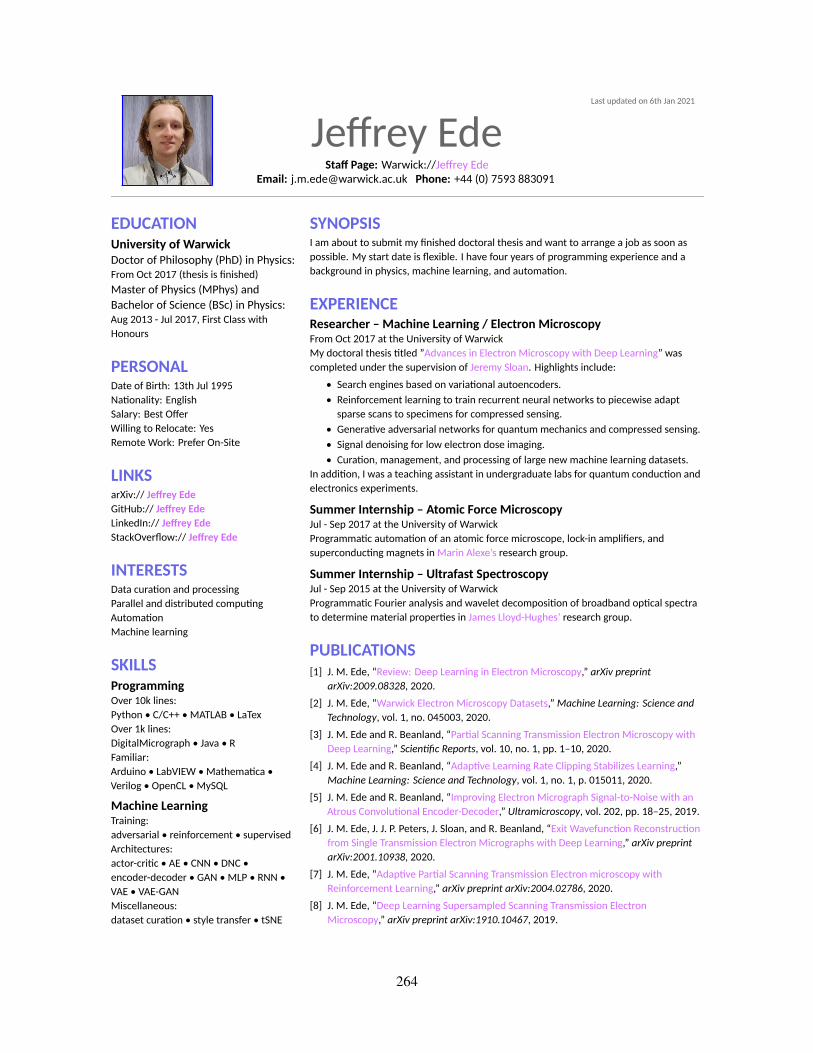
Last updated on 6th Jan 2021
Jeffrey EdeStaff Page: Warwick://Jeffrey Ede
Email: [email protected] Phone: +44 (0) 7593 883091
EDUCATIONUniversity of WarwickDoctor of Philosophy (PhD) in Physics:From Oct 2017 (thesis is finished)Master of Physics (MPhys) andBachelor of Science (BSc) in Physics:Aug 2013 - Jul 2017, First Class withHonours
PERSONALDate of Birth: 13th Jul 1995Nationality: EnglishSalary: Best OfferWilling to Relocate: YesRemote Work: Prefer On-Site
LINKSarXiv:// Jeffrey EdeGitHub:// Jeffrey EdeLinkedIn:// Jeffrey EdeStackOverflow:// Jeffrey Ede
INTERESTSData curation and processingParallel and distributed computingAutomationMachine learning
SKILLSProgrammingOver 10k lines:Python • C/C++ • MATLAB • LaTexOver 1k lines:DigitalMicrograph • Java • RFamiliar:Arduino • LabVIEW • Mathematica •Verilog • OpenCL • MySQL
Machine LearningTraining:adversarial • reinforcement • supervisedArchitectures:actor-critic • AE • CNN • DNC •encoder-decoder • GAN • MLP • RNN •VAE • VAE-GANMiscellaneous:dataset curation • style transfer • tSNE
SYNOPSISI am about to submit my finished doctoral thesis and want to arrange a job as soon aspossible. My start date is flexible. I have four years of programming experience and abackground in physics, machine learning, and automation.
EXPERIENCEResearcher – Machine Learning / Electron MicroscopyFrom Oct 2017 at the University of WarwickMy doctoral thesis titled ”Advances in Electron Microscopy with Deep Learning” wascompleted under the supervision of Jeremy Sloan. Highlights include:
• Search engines based on variational autoencoders.• Reinforcement learning to train recurrent neural networks to piecewise adaptsparse scans to specimens for compressed sensing.
• Generative adversarial networks for quantum mechanics and compressed sensing.• Signal denoising for low electron dose imaging.• Curation, management, and processing of large new machine learning datasets.
In addition, I was a teaching assistant in undergraduate labs for quantum conduction andelectronics experiments.
Summer Internship – Atomic Force MicroscopyJul - Sep 2017 at the University of WarwickProgrammatic automation of an atomic force microscope, lock-in amplifiers, andsuperconducting magnets in Marin Alexe’s research group.
Summer Internship – Ultrafast SpectroscopyJul - Sep 2015 at the University of WarwickProgrammatic Fourier analysis and wavelet decomposition of broadband optical spectrato determine material properties in James Lloyd-Hughes’ research group.
PUBLICATIONS[1] J. M. Ede, “Review: Deep Learning in Electron Microscopy,” arXiv preprint
arXiv:2009.08328, 2020.[2] J. M. Ede, “Warwick Electron Microscopy Datasets,”Machine Learning: Science and
Technology, vol. 1, no. 045003, 2020.[3] J. M. Ede and R. Beanland, “Partial Scanning Transmission Electron Microscopy with
Deep Learning,” Scientific Reports, vol. 10, no. 1, pp. 1–10, 2020.[4] J. M. Ede and R. Beanland, “Adaptive Learning Rate Clipping Stabilizes Learning,”
Machine Learning: Science and Technology, vol. 1, no. 1, p. 015011, 2020.[5] J. M. Ede and R. Beanland, “Improving Electron Micrograph Signal-to-Noise with an
Atrous Convolutional Encoder-Decoder,” Ultramicroscopy, vol. 202, pp. 18–25, 2019.[6] J. M. Ede, J. J. P. Peters, J. Sloan, and R. Beanland, “Exit Wavefunction Reconstruction
from Single Transmission Electron Micrographs with Deep Learning,” arXiv preprintarXiv:2001.10938, 2020.
[7] J. M. Ede, “Adaptive Partial Scanning Transmission Electron microscopy withReinforcement Learning,” arXiv preprint arXiv:2004.02786, 2020.
[8] J. M. Ede, “Deep Learning Supersampled Scanning Transmission ElectronMicroscopy,” arXiv preprint arXiv:1910.10467, 2019.
264
Related Documents