Advances in deep generative modeling for clinical data by Rahul Gopalkrishnan published as: Rahul G. Krishnan BaSc., The University of Toronto (2013) M.S., New York University (2016) Submitted to the Department of Electrical Engineering and Computer Science in partial fulfillment of the requirements for the degree of Doctor of Philosophy in Electrical Engineering and Computer Science at the MASSACHUSETTS INSTITUTE OF TECHNOLOGY September 2020 c ○ Massachusetts Institute of Technology 2020. All rights reserved. Author ................................................................ Department of Electrical Engineering and Computer Science June 30, 2020 Certified by ............................................................ David A. Sontag Associate Professor of Electrical Engineering and Computer Science Thesis Supervisor Accepted by ........................................................... Leslie A. Kolodziejski Professor of Electrical Engineering and Computer Science Chair, Department Committee for Graduate Students

Welcome message from author
This document is posted to help you gain knowledge. Please leave a comment to let me know what you think about it! Share it to your friends and learn new things together.
Transcript
Advances in deep generative modelingfor clinical data
by
Rahul Gopalkrishnanpublished as: Rahul G. Krishnan
BaSc., The University of Toronto (2013)M.S., New York University (2016)
Submitted to the Department of Electrical Engineering and ComputerScience
in partial fulfillment of the requirements for the degree of
Doctor of Philosophyin
Electrical Engineering and Computer Science
at the
MASSACHUSETTS INSTITUTE OF TECHNOLOGY
September 2020
c○ Massachusetts Institute of Technology 2020. All rights reserved.
Author . . . . . . . . . . . . . . . . . . . . . . . . . . . . . . . . . . . . . . . . . . . . . . . . . . . . . . . . . . . . . . . .Department of Electrical Engineering and Computer Science
June 30, 2020
Certified by. . . . . . . . . . . . . . . . . . . . . . . . . . . . . . . . . . . . . . . . . . . . . . . . . . . . . . . . . . . .David A. Sontag
Associate Professor of Electrical Engineering and Computer ScienceThesis Supervisor
Accepted by . . . . . . . . . . . . . . . . . . . . . . . . . . . . . . . . . . . . . . . . . . . . . . . . . . . . . . . . . . .Leslie A. Kolodziejski
Professor of Electrical Engineering and Computer ScienceChair, Department Committee for Graduate Students

2
Advances in deep generative modelingfor clinical data
byRahul Gopalkrishnan
Submitted to the Department of Electrical Engineering and Computer Scienceon June 30, 2020, in partial fulfillment of the
requirements for the degree ofDoctor of Philosophy
inElectrical Engineering and Computer Science
Abstract
The intelligent use of electronic health record data opens up new opportunities toimprove clinical care. Such data have the potential to uncover new sub-types of adisease, approximate the effect of a drug on a patient, and create tools to find patientswith similar phenotypic profiles. Motivated by such questions, this thesis developsnew algorithms for unsupervised and semi-supervised learning of latent variable, deepgenerative models – Bayesian networks parameterized by neural networks.
To model static, high-dimensional data, we derive a new algorithm for inference in deepgenerative models. The algorithm, a hybrid between stochastic variational inferenceand amortized variational inference, improves the generalization of deep generativemodels on data with long-tailed distributions. We develop gradient-based approachesto interpret the parameters of deep generative models, and fine-tune such modelsusing supervision to tackle problems that arise in few-shot learning.
To model longitudinal patient biomarkers as they vary due to treatment we proposeDeep Markov Models (DMMs). We design structured inference networks for variationallearning in DMMs; the inference network parameterizes a variational approximationwhich mimics the factorization of the true posterior distribution. We leverage insightsin pharmacology to design neural architectures which improve the generalizationof DMMs on clinical problems in the low-data regime. We show how to capturestructure in longitudinal data using deep generative models in order to reduce thesample complexity of nonlinear classifiers thus giving us a powerful tool to build riskstratification models from complex data.
Thesis Supervisor: David A. SontagTitle: Associate Professor of Electrical Engineering and Computer Science
3

4
Acknowledgments
To my graduate advisor, David Sontag, thank you for all the patience, wisdomand guidance that you has shown me for the better half of a decade. Your infiniteenthusiasm for research and fearlessness in asking difficult questions, have and continueto inspire me. Interdisciplinary work is hard, but you’ve guided and helped me walkthe tightrope that spans the daunting peaks of research questions that are technicallychallenging and those that can impact people’s lives.
I want to thank all the members of my thesis committee for their feedback on my workand on this thesis. To Pete Szolovitz, I’ve enjoyed our conversations whose topics spanthe gamut from locations for your sabbatical to how you came to study computerscience in medicine. To Matthew Hoffman, thank for showing me the breadth andwidth of how algorithms for probabilistic inference inference can be applied to realproblems; I have learned much from your unerring eye to spot patterns that othersoften miss. To Uri Shalit, thank you for being an excellent office mate, and for everymanner of professional and personal life advice you’ve given me over the years.
I am grateful to the many mentors, collaborators, and colleagues without whom manyof my research ideas would not have reached fruition. Thank you to Lydia Bourouibaand Simone Cenci for introducing me to the world of epidemiological modelling; I hopeto continue to explore the many relationships between statistical learning and fluidmechanics. Thank you to Simone Lacoste Julien, Dawen Liang, Rajesh Ranganth,Li-wei Lehman, Andrew Yee, Narges Razavian, Hendrik Strobelt, Nicolo Fusi andLester Mackey for sharing your knowledge with me. Thank you to all the members ofthe ClinicalML lab: Yoni Halpern, Yacine Jernite, Rachel Hodos, Fredrik Johansson,Irene Chen, Michael Oberst, Monica Agrawal, Zeshan Hussain, Sanjat Kanjilal, ArjunKhandelwal and Christina Ji: your wit, intelligence and humor have made science fun.I look forward to many more collaborations with all of you.
Life doesn’t press pause for a PhD, as my parents keep reminding me, and I wantto thank all my friends, both in and out of school, for keeping me sane through allthe ups and downs of being a PhD student. To Rachel Gubow, Siddharth Krishna,Shravas Rao, Anthony Rossi, Alex Grote and the many other graduate students atNYU, thank you for being part of many adventures in NY. Thank you to KarthikNarasimhan, Ardavan Saeedi, Zoya Bylinksii and Marzyeh Ghassemi for giving me awarm welcome when I first moved to Cambridge. To Isabel Schwarz, Jonathan Ng, andCarmen Reilly, thank you for for being excellent sounding boards for talking through
5

any manner of road bumps in life. To Kate Finegold (and the inimitable Mocha), bothof your smiles make long weeks fly by. To Firas Kamaleddine, Ben Aneesh, AnirudhGanti, Omer Shaeldin, Aniruddha Borah, Ratika Goyal, Inmar Givoni, Mustafa El-hiloand Aniruddha Borah, Zahan Malkani, Ameya Shroff and Arka Bhattacharyya – aftermore than a decade since we parted ways, I’m grateful that you all remain a closepart of my life.
Finally, to my family who have been a bedrock of support throughout my academicjourney. To my father, Vettithuruthil Gopalkrishnan, thank you for teaching meto never stop asking questions, and for teaching me how to weather the harsheststorms in life with a smile. To my mother, Beena Krishnan Nair, thank you for yoursteadfast belief in me, even when my belief in myself faded. And to my sister, RasmiGopalkrishnan, who taught me that living is believing in principles that you’re willingto make sacrifices for. You fill my life with warmth and love. This is for you.
6
When I began my PhD I sought a framework to make sense of the myriad problemsthat people studied in machine learning, which comprises an abundance of ideas thatspan topics in statistics, deep learning, stochastic optimization, linear algebra andcausality. Like others before me, in Bayesian networks, I found the technical machineryto begin to organize all these concepts within a single unifying framework. Doing sohas helped me read, organize and contextualize ideas from a variety of different fields.If there is anything that I have learned over the past several years, it is that progressacross multiple fields will be driven by researchers across the world speaking andunderstanding the same technical language. To that end, discovering, experimentingand contributing to such a unifying framework has been a liberating experience.
7

8
Contents
1 Introduction 29
1.1 Machine learning for healthcare . . . . . . . . . . . . . . . . . . . . . 29
1.2 Challenges in healthcare . . . . . . . . . . . . . . . . . . . . . . . . . 31
1.3 Contributions . . . . . . . . . . . . . . . . . . . . . . . . . . . . . . . 32
2 Background 35
2.1 Random variables and probabilities . . . . . . . . . . . . . . . . . . . 35
2.2 Graphical models . . . . . . . . . . . . . . . . . . . . . . . . . . . . . 37
2.2.1 Structure as domain knowledge . . . . . . . . . . . . . . . . . 38
2.2.2 Independence statements . . . . . . . . . . . . . . . . . . . . . 39
2.3 Bayesian networks . . . . . . . . . . . . . . . . . . . . . . . . . . . . 40
2.3.1 Parameterizations of Bayesian networks . . . . . . . . . . . . . 40
2.3.2 Learning . . . . . . . . . . . . . . . . . . . . . . . . . . . . . . 45
2.3.3 Variational learning of latent variable models . . . . . . . . . . 46
2.4 Learning with automatic differentiation . . . . . . . . . . . . . . . . . 52
2.5 Modeling data with deep generative models . . . . . . . . . . . . . . 53
3 Gradient based introspection in deep generative models 55
9
3.1 Introduction . . . . . . . . . . . . . . . . . . . . . . . . . . . . . . . 55
3.2 Jacobian vectors . . . . . . . . . . . . . . . . . . . . . . . . . . . . . 58
3.3 Evaluation . . . . . . . . . . . . . . . . . . . . . . . . . . . . . . . . . 61
3.3.1 Text data . . . . . . . . . . . . . . . . . . . . . . . . . . . . . 62
3.3.2 Electronic Health Record (EHR) data . . . . . . . . . . . . . . 65
3.3.3 Netflix: Embeddings for movies . . . . . . . . . . . . . . . . . 68
3.4 Discussion . . . . . . . . . . . . . . . . . . . . . . . . . . . . . . . . . 69
4 Representation learning for high-dimensional data 73
4.1 Introduction . . . . . . . . . . . . . . . . . . . . . . . . . . . . . . . . 73
4.2 Setup . . . . . . . . . . . . . . . . . . . . . . . . . . . . . . . . . . . . 75
4.3 Sources of error in variational learning . . . . . . . . . . . . . . . . . 77
4.3.1 Limitations of joint parameter updates . . . . . . . . . . . . . 79
4.4 Improving estimates of variational parameters . . . . . . . . . . . . . 80
4.4.1 Between stochastic and amortized variational inference . . . . 80
4.4.2 Representations for inference networks . . . . . . . . . . . . . 80
4.4.3 Spectral analysis of the Jacobian matrix . . . . . . . . . . . . 81
4.5 Related 2ork . . . . . . . . . . . . . . . . . . . . . . . . . . . . . . . . 82
4.6 Evaluation . . . . . . . . . . . . . . . . . . . . . . . . . . . . . . . . . 84
4.6.1 Setup . . . . . . . . . . . . . . . . . . . . . . . . . . . . . . . 84
4.6.2 Bag-of-words text data . . . . . . . . . . . . . . . . . . . . . . 85
4.6.3 Collaborative filtering . . . . . . . . . . . . . . . . . . . . . . 93
4.7 Discussion . . . . . . . . . . . . . . . . . . . . . . . . . . . . . . . . . 96
5 Supervised fine-tuning of deep generative models 97
10
5.1 Introduction . . . . . . . . . . . . . . . . . . . . . . . . . . . . . . . . 98
5.2 From representation learning to reasoning . . . . . . . . . . . . . . . 100
5.2.1 Data model . . . . . . . . . . . . . . . . . . . . . . . . . . . . 100
5.2.2 Reasoning model . . . . . . . . . . . . . . . . . . . . . . . . . 102
5.2.3 Bayes factor . . . . . . . . . . . . . . . . . . . . . . . . . . . . 102
5.3 Hierarchical models with compound priors . . . . . . . . . . . . . . . 103
5.4 Latent Reasoning Networks . . . . . . . . . . . . . . . . . . . . . . . 105
5.5 Learning . . . . . . . . . . . . . . . . . . . . . . . . . . . . . . . . . . 107
5.6 Evaluation . . . . . . . . . . . . . . . . . . . . . . . . . . . . . . . . . 108
5.6.1 Learning 𝑝(𝑧|𝒬) . . . . . . . . . . . . . . . . . . . . . . . . . . 109
5.6.2 Changing inductive biases at test-time . . . . . . . . . . . . . 110
5.6.3 Modeling high-dimensional data . . . . . . . . . . . . . . . . . 111
5.6.4 Few-shot learning with the Bayes factor . . . . . . . . . . . . 111
5.7 Related work . . . . . . . . . . . . . . . . . . . . . . . . . . . . . . . 113
5.8 Discussion . . . . . . . . . . . . . . . . . . . . . . . . . . . . . . . . . 115
6 Deep Markov Models 117
6.1 Introduction . . . . . . . . . . . . . . . . . . . . . . . . . . . . . . . . 118
6.2 Setup . . . . . . . . . . . . . . . . . . . . . . . . . . . . . . . . . . . . 120
6.3 A factorized variational lower bound . . . . . . . . . . . . . . . . . . 121
6.3.1 Simplifying the lower bounds . . . . . . . . . . . . . . . . . . 123
6.3.2 Analytic forms of the KL divergence . . . . . . . . . . . . . . 125
6.3.3 Learning with gradient ascent . . . . . . . . . . . . . . . . . . 126
6.4 Structured Inference Networks . . . . . . . . . . . . . . . . . . . . . . 127
11
6.5 Deep Markov Models . . . . . . . . . . . . . . . . . . . . . . . . . . . 130
6.6 Evaluation . . . . . . . . . . . . . . . . . . . . . . . . . . . . . . . . . 131
6.6.1 Synthetic data . . . . . . . . . . . . . . . . . . . . . . . . . . . 132
6.6.2 Polyphonic music . . . . . . . . . . . . . . . . . . . . . . . . . 134
6.6.3 EHR Patient Data . . . . . . . . . . . . . . . . . . . . . . . . 138
6.7 Discussion . . . . . . . . . . . . . . . . . . . . . . . . . . . . . . . . . 142
7 Inductive biases for clinical data 145
7.1 Introduction . . . . . . . . . . . . . . . . . . . . . . . . . . . . . . . . 145
7.2 Setup . . . . . . . . . . . . . . . . . . . . . . . . . . . . . . . . . . . . 147
7.2.1 First Order Markov Models (FOMMs) . . . . . . . . . . . . . 148
7.2.2 Gated Recurrent Neural Network (GRUs) . . . . . . . . . . . 149
7.2.3 State Space Models (SSMs) . . . . . . . . . . . . . . . . . . . 150
7.2.4 Missing data . . . . . . . . . . . . . . . . . . . . . . . . . . . . 151
7.2.5 Pharmacokinetic-Pharmacodynamic (PK-PD) models . . . . . 151
7.3 Intervention Effect Functions for clinical data . . . . . . . . . . . . . 153
7.3.1 Capturing lines of therapy with local and global clocks . . . . 154
7.3.2 Domain expert IEF modules for clinical data . . . . . . . . . 155
7.3.3 PK-PD Intervention Effect Function . . . . . . . . . . . . . . 157
7.4 Datasets . . . . . . . . . . . . . . . . . . . . . . . . . . . . . . . . . . 158
7.4.1 Synthetic data . . . . . . . . . . . . . . . . . . . . . . . . . . . 158
7.4.2 Multiple Myleoma - ML-MMRF . . . . . . . . . . . . . . . . . 160
7.5 Evaluation . . . . . . . . . . . . . . . . . . . . . . . . . . . . . . . . . 162
7.5.1 Quantitative analysis . . . . . . . . . . . . . . . . . . . . . . . 163
12
7.5.2 Qualitative Analysis . . . . . . . . . . . . . . . . . . . . . . . 170
7.6 Discussion . . . . . . . . . . . . . . . . . . . . . . . . . . . . . . . . . 175
8 Latent Representations of Privileged Information 177
8.1 Introduction . . . . . . . . . . . . . . . . . . . . . . . . . . . . . . . . 177
8.2 Setup . . . . . . . . . . . . . . . . . . . . . . . . . . . . . . . . . . . . 179
8.3 Privileged Information Variational Autoencoder . . . . . . . . . . . . 180
8.4 Evaluation . . . . . . . . . . . . . . . . . . . . . . . . . . . . . . . . . 183
8.4.1 Synthetic Data . . . . . . . . . . . . . . . . . . . . . . . . . . 183
8.4.2 Evaluation . . . . . . . . . . . . . . . . . . . . . . . . . . . . . 184
8.5 Related work . . . . . . . . . . . . . . . . . . . . . . . . . . . . . . . 187
8.6 Discussion . . . . . . . . . . . . . . . . . . . . . . . . . . . . . . . . . 188
9 Conclusion 191
9.1 Future directions for deep generative modeling . . . . . . . . . . . . . 192
9.2 Future directions for machine learning in healthcare . . . . . . . . . . 194
A Model configurations 197
A.0.1 Pinwheel Dataset . . . . . . . . . . . . . . . . . . . . . . . . . 197
A.0.2 MiniImagenet Dataset . . . . . . . . . . . . . . . . . . . . . . 198
A.0.3 MNIST Dataset . . . . . . . . . . . . . . . . . . . . . . . . . . 199
B Model configurations 201
13

14
List of Figures
1-1 Patient data: Left (clinical observations), Middle (centers of care),Right (treatments provided to patients) . . . . . . . . . . . . . . . . . 30
1-2 Patient data across scales of the human body: From bottom totop, we depict patient data as manifested in the various scales of thehuman body, from micro scale to macro scale. . . . . . . . . . . . . . 30
1-3 Sequential patient data: When tracking the progression of diseases,doctors characterize progression of disease as a function of how thepatient’s clinical observations vary with time. . . . . . . . . . . . . . 31
2-1 Undirected graphical models: Nodes shaded in grey are observed random
variables, while those with a white background denote unobserved or latent
random variables . . . . . . . . . . . . . . . . . . . . . . . . . . . . . . 37
2-2 Directed graphical nodels: Nodes shaded in grey are observed random
variables, while those with a white background denote unobserved or latent
random variables . . . . . . . . . . . . . . . . . . . . . . . . . . . . . . 37
15
2-3 Bayesian networks for supervised and unsupervised Learning: Nodes
shaded in grey are observed random variables, while those with a white back-
ground denote unobserved or latent random variables. On the left is a
Bayesian network for supervised learning where 𝑥 denote the inputs and 𝑦
denote the random variables corresponding to the labels. On the right is
a Bayesian network that characterizes a large class of latent factor models
used in unsupervised learning where 𝑥 is the data being modeled and 𝑧 are
the latent factors (or causes) that influence the data. Under the manifold
hypothesis(Fefferman et al. , 2016), 𝑧 is posited to have a lower-dimensionality
than 𝑥, i.e. the domain of the latent variable 𝑧 is lower-dimensional but
suffices to explain variation in the higher-dimensional 𝑥. . . . . . . . . . . 41
2-4 Convolutional neural networks: On the left is an input image𝑋 that is transformed via parameteric, nonlinear functions (such asconvolutional operations) to yield the vector on the right, a set of classprobabilities corresponding to a distribution over probabilities of eachlabel. . . . . . . . . . . . . . . . . . . . . . . . . . . . . . . . . . . . . 42
2-5 Stochastic Variational Inference (SVI) (Hoffman et al. , 2013) 𝜑 denote
the variational parameters which are optimized prior to deriving gradients
with respect to the model parameters 𝜃 . . . . . . . . . . . . . . . . . . 48
2-6 Amortized Variational Inference (AVI) (Rezende et al. , 2014; Kingma
& Welling, 2014) 𝜑 denotes the parameters of an inference network which
is used to predict the variational parameters that are subsequently used to
evaluate the variational lower bound. . . . . . . . . . . . . . . . . . . . . 49
2-7 Nonlinear factor analysis: The model comprises a single latent variable
𝑧 with the conditional probability 𝑝(𝑥|𝑧) defined by a deep neural network
with parameter 𝜃. On the right, 𝑞𝜑(𝑧|𝑥), the inference network, parameterized
by 𝜑, is used to predict variational parameters used at train and test time
inference. When paired with an inference network, the resulting coupled
model is known as a variational autoencoder. . . . . . . . . . . . . . . . 50
4-1 Learning nonlinear factor analysis with an inference network: [Left]
The generative model contains a single latent variable 𝑧. The conditional
probability 𝑝(𝑥|𝑧; 𝜃) parameterized by a deep neural network. [Right] The
inference network 𝑞𝜑(𝑧|𝑥) is used for inference at train and test time. . . . 74
16
4-2 From patient history to a bag of diagnosis codes: On the left is a
depiction of a patient’s history (outpatient in green and inpatient in red).
On the right is how such a history would appear to machine learning models;
as collections of diagnosis codes. . . . . . . . . . . . . . . . . . . . . . . 74
4-3 Lower bounds in variational learning: To estimate 𝜃, we maximize
a lower bound on log 𝑝(𝑥; 𝜃). ℒ(𝑥; 𝜃, 𝜓(𝑥)) denotes the standard training
objective used by VAEs. The tightness of this bound (relative to ℒ(𝑥; 𝜃, 𝜓*)
depends on the inference network. The x-axis is 𝜃. . . . . . . . . . . . . 78
4-4 Parameter estimation in NFA with a hybrid inference algorithm . 80
4-5 Mechanics of learning: Best viewed in color. (Left and Middle) For
the Wikipedia dataset, we visualize upper bounds on training and held-
out perplexity (evaluated with 𝜓*) viewed as a function of epochs. Items
in the legend corresponds to choices of training method. (Right) Sorted
log-singular values of ∇𝑧 log 𝑝(𝑥|𝑧) on Wikipedia (left) on RCV1 (right) for
different training methods. The x-axis is latent dimension. The legend is
identical to that in Fig. 4-5a. . . . . . . . . . . . . . . . . . . . . . . . 85
4-6 Decrease in perplexity versus sparsity: We plot the relative drop in
perplexity obtained by training with 𝜓* instead of 𝜓(𝑥) against varying levels
of sparsity in the Wikipedia data. On the y-axis, we plot 𝑃[3−𝜓(𝑥)]−𝑃[3−𝜓*]𝑃[3−𝜓(𝑥)]
;
𝑃 denotes the bound on perplexity (evaluated with 𝜓*) and the subscript
denotes the model and method used during training. Each point on the
x-axis is a restriction of the dataset to the top 𝐿 most frequently occurring
words (number of features). . . . . . . . . . . . . . . . . . . . . . . . . 87
4-7 Late versus early optimization of 𝜓(𝑥): Fig. 4-7a (4-7b) denote the
train (held-out) perplexity for three-layered models trained on the Wikipedia
data in the following scenarios: 𝜓* is used for training for the first ten
epochs following which 𝜓(𝑥) is used (denoted “𝜓* then 𝜓(𝑥)”) and vice versa
(denoted “𝜓(𝑥) then 𝜓*”). Fig. 4-7c (Left) depicts the number of singular
values of the Jacobian matrix ∇𝑧 log 𝑝(𝑥|𝑧) with value greater than 1 as a
function of training epochs for each of the two aforementioned methodologies.
Fig. 4-7c (Right) plots the sorted log-singular values of the Jacobian matrix
corresponding to the final model under each training strategy. . . . . . . 88
17
4-8 KL divergence and rare word counts: We plot the values of KL(𝜓(𝑥)‖𝜓*)
versus the number of rare words. We zoom into the plot and reduce the
opacity of the train points to better see the held-out points. The Spearman
𝜌 correlation coefficient is computed between the two across 20, 000 points.
We find a positive correlation. . . . . . . . . . . . . . . . . . . . . . . . 89
4-9 Normalized KL and Rare Word Counts: Fig. 4-9a depicts percentage
of times words appear in the Wikipedia dataset (sorted by frequency). The
dotted line in blue denotes the marker for a word that has a 5% occurrence
in documents. In Fig. 4-9b, 4-9c, we superimpose (1) the normalized (to be
between 0 and 1) values of KL(𝜓(𝑥)‖𝜓*) and (2) the normalized number of
rare words (sorted by value of the KL-divergence) for 20, 000 points (on the
x-axis) randomly sampled from the train and held-out data. . . . . . . . 90
4-10 20Newsgroups - training and held-out bounds: Fig. 4-10a, 4-10b
denotes the train (held-out) perplexity for different models. Fig. 4-10c
depicts the log-singular values of the Jacobian matrix for the trained models. 90
4-11 RCV1 - training and held-out bounds: Fig. 4-11a, 4-11b denotes
the train (held-out) perplexity for different models. Fig. 4-11c depicts the
log-singular values of the Jacobian matrix for the trained models. . . . . 91
4-12 KL annealing vs learning with 𝜓* Fig. 4-12a, 4-12b denotes the train
(held-out) perplexity for different training methods. The suffix at the end
of the model configuration denotes the number of parameter updates that
it took for the KL divergence in Equation 4.2 to be annealed from 0 to 1.
3-𝜓*-50k denotes that it took 50000 parameter updates before −ℒ(𝑥; 𝜃, 𝜓(𝑥))was used as the loss function. Fig. 4-10c depicts the log-singular values of
the Jacobian matrix for the trained models. . . . . . . . . . . . . . . . . 92
4-13 Varying the depth of 𝑞𝜑(𝑧|𝑥): Fig. 4-12a (4-12b) denotes the train
(held-out) perplexity for a three-layer generative model learned with inference
networks of varying depth. The notation q3-𝜓* denotes that the inference
network contained a two-layer intermediate hidden layer ℎ(𝑥) = MLP(𝑥;𝜑0)
followed by 𝜇(𝑥) =𝑊𝜇ℎ(𝑥), log Σ(𝑥) =𝑊log Σℎ(𝑥). . . . . . . . . . . . . 93
18
5-1 Comparing objects in representational space: On the left is a target
set that will be ranked based on similarity to the query 𝑄 (right). The colour
of each object is matched to a distribution in representation space. In orange
is the output of the latent reasoning network – it represents the common
factor of variation shared by 𝒬. The black chair should rank higher than
the black table; here its distribution (in representation space) overlaps more
with the output of the latent reasoning network. . . . . . . . . . . . . . . 98
5-2 Hypothesis testing with deep generative models: (a) The Reason-
ing Model, here, depicting the hypothesis that the set {𝑥𝑡,𝒬 = {𝑥1, 𝑥2}}was generated jointly; (b) the two figures represent the hypothesis that 𝑥𝑡and 𝒬 were generated independently under different realizations of 𝑤 (the
random variable that captures the property shared across datapoints). . . 100
5-3 Latent Reasoning Networks (LRN) and loss function: On the left
is a diagrammatic representation of 𝑝rm(𝑧𝑡|𝒬). On the right is a depiction
of Monte-Carlo sampling (with samples from the LRN) to evaluate Bayes
factor. 𝑥𝑖 is a point similar to those in the query 𝒬 = {𝑥1, 𝑥2, 𝑥3}, while 𝑥𝑛𝑠is not. We suppress subscripts in the figure. . . . . . . . . . . . . . . . . 105
5-4 Qualitative evaluation on pinwheel data: Studying how the latentspace of the data changes over the course of fine-tuning on the synthetic,pinwheel dataset. . . . . . . . . . . . . . . . . . . . . . . . . . . . . . 109
5-5 Qualitative evaluation on MNIST: Studying the effect of fine-tuning the latent space of the data model on MNIST. . . . . . . . . . 112
6-1 Generative Models of Sequential Data: (Top Left) Hidden Markov
Model (HMM), (Top Right) Deep Markov Model (DMM) � denotes the
neural networks used in DMMs for the emission and transition functions.
(Bottom) Recurrent Neural Network (RNN), ♦ denotes a deterministic
intermediate representation. Code for learning DMMs and reproducing our
results may be found at: github.com/clinicalml/structuredinference 119
19
6-2 Structured Inference Networks: MF-LR and ST-LR variational ap-
proximations for a sequence of length 3, using a bi-directional recurrent neural
net (BRNN). The BRNN takes as input the sequence (𝑥1, . . . 𝑥3), and through
a series of non-linearities denoted by the blue arrows it forms a sequence
of hidden states summarizing information from the left and right (ℎleft𝑡 and
ℎright𝑡 ) respectively. Then through a further sequence of non-linearities which
we call the “combiner function” (marked (a) above), and denoted by the
red arrows, it outputs two vectors 𝜇 and Σ, parameterizing the mean and
diagonal covariance of 𝑞𝜑(𝑧𝑡|𝑧𝑡−1, �⃗�) of Eq. 6.5. Samples 𝑧𝑡 are drawn from
𝑞𝜑(𝑧𝑡|𝑧𝑡−1, �⃗�), as indicated by the black dashed arrows. For the structured
variational models ST-LR, the samples 𝑧𝑡 are fed into the computation of
𝜇𝑡+1 and Σ𝑡+1, as indicated by the red arrows with the label (a). The mean-
field model does not have these arrows, and therefore computes 𝑞𝜑(𝑧𝑡|�⃗�). We
use 𝑧0 = 0⃗. The inference network for DKS (ST-R) is structured like that of
ST-LR except without the RNN from the past. . . . . . . . . . . . . . . 130
6-3 Synthetic evaluation: (Top & Bottom) Compiled inference for a fixed
linear GSSM: 𝑧𝑡 ∼ 𝒩 (𝑧𝑡−1 + 0.05, 10), 𝑥𝑡 ∼ 𝒩 (0.5𝑧𝑡, 20). The training set
comprised 𝑁 = 5000 one-dimensional observations of sequence length 𝑇 = 25.
(Top left) RMSE with respect to true 𝑧* that generated the data. (Top
right) Variational bound during training. The results on held-out data are
very similar (see supplementary material). (Bottom four plots) Visualizing
inference in two sequences (denoted (1) and (2)); Left panels show the Latent
Space of variables 𝑧, right panels show the Observations 𝑥. Observations are
generated by the application of the emission function to the posterior shown
in Latent Space. Shading denotes standard deviations. . . . . . . . . . . 133
6-4 Parameter estimation: Learning parameters 𝛼, 𝛽 in a two-dimensional
non-linear GSSM. 𝑁 = 5000, 𝑇 = 25 �⃗�𝑡 ∼ 𝒩 ([0.2𝑧0𝑡−1+tanh(𝛼𝑧1𝑡−1); 0.2𝑧1𝑡−1+
sin(𝛽𝑧0𝑡−1)], 1.0) �⃗�𝑡 ∼ 𝒩 (0.5�⃗�𝑡, 0.1) where �⃗� denotes a vector, [] denotes
concatenation and superscript denotes indexing. . . . . . . . . . . . . . 133
6-5 Inference in a linear SSM on held-out data: Performance ofinference networks on held-out data using a generative model withLinear Emission and Linear Transition . . . . . . . . . . . . . . . . . 134
6-6 Inference in a don-linear SSM: Performance of inference networkstrained with data from a Linear Emission and Non-linear Transition SSM135
20
6-7 Inference on non-linear synthetic data: Visualizing inferenceon training data. Generative Models: (a) Linear Emission and Non-linear Transition 𝑧* denotes the latent variable that generated theobservation. 𝑥 denotes the true data. We compare against the resultsobtained by a smoothed Unscented Kalman Filter (UKF) (Wan & VanDer Merwe, 2000). The column denoted “Observations" denotes theresult of applying the emission function of the respective generativemodel on the posterior estimates shown in the column “Latent Space".The shaded areas surrounding each curve 𝜇 denotes 𝜇± 𝜎 for each plot. 136
6-8 Two samples from the DMM trained on JSB Chorales . . . . . . . . . 137
6-9 DMM for medical data: The DMM (from Fig. 6-1) is augmented with
external actions 𝑢𝑡 representing medications presented to the patient. 𝑧𝑡 is
the latent state of the patient. 𝑥𝑡 are the observations that we model. Since
both 𝑢𝑡 and 𝑥𝑡 are always assumed observed, the conditional distribution
𝑝(𝑢𝑡|𝑥1, . . . , 𝑥𝑡−1) may be ignored during learning. . . . . . . . . . . . . . 140
6-10 Left two plots; Estimating counterfactuals with DMM: The x-axis
denotes the number of 3-month intervals after prescription of Metformin. The
y-axis denotes the proportion of patients (out of a test set size of 800) who,
after their first prescription of Metformin, experienced a high level of A1C.
In each tuple of bar plots at every time step, the left aligned bar plots (green)
represent the population that received diabetes medication while the right
aligned bar plots (red) represent the population that did not receive diabetes
medication. (Rightmost plot) Upper bound on negative-log likelihood for
different DMMs trained on the medical data. (T) denotes “transition”, (E)
denotes “emission”, (L) denotes “linear” and (NL) denotes “non-linear”. . . 141
6-11 Patient data generated by a DMM Samples of a patient generated by
the model. The x-axis denotes time and the y-axis denotes the observations.
The intensity of the color denotes its value between zero and one . . . . . 144
21
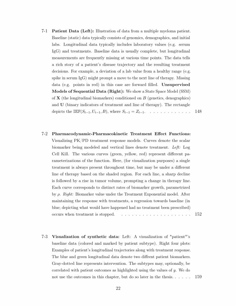
7-1 Patient Data (Left): Illustration of data from a multiple myeloma patient.
Baseline (static) data typically consists of genomics, demographics, and initial
labs. Longitudinal data typically includes laboratory values (e.g. serum
IgG) and treatments. Baseline data is usually complete, but longitudinal
measurements are frequently missing at various time points. The data tells
a rich story of a patient’s disease trajectory and the resulting treatment
decisions. For example, a deviation of a lab value from a healthy range (e.g.
spike in serum IgG) might prompt a move to the next line of therapy. Missing
data (e.g. points in red) in this case are forward filled. Unsupervised
Models of Sequential Data (Right): We show a State Space Model (SSM)
of X (the longitudinal biomarkers) conditioned on 𝐵 (genetics, denographics)
and U (binary indicators of treatment and line of therapy). The rectangle
depicts the IEF(𝑆𝑡−1, 𝑈𝑡−1, 𝐵), where 𝑆𝑡−1 = 𝑍𝑡−1. . . . . . . . . . . . . 148
7-2 Pharmacodynamic-Pharmacokinetic Treatment Effect Functions:
Visualizing PK/PD treatment response models. Curves denote the scalar
biomarker being modeled and vertical lines denote treatment. Left: Log
Cell Kill. The various curves (green, yellow, red) represent different pa-
rameterizations of the function. Here, (for visualization purposes) a single
treatment is always present throughout time, but may be under a different
line of therapy based on the shaded region. For each line, a sharp decline
is followed by a rise in tumor volume, prompting a change in therapy line.
Each curve corresponds to distinct rates of biomarker growth, parametrized
by 𝜌. Right: Biomarker value under the Treatment Exponential model. After
maintaining the response with treatments, a regression towards baseline (in
blue; depicting what would have happened had no treatment been prescribed)
occurs when treatment is stopped. . . . . . . . . . . . . . . . . . . . . 152
7-3 Visualization of synthetic data: Left: A visualization of "patient"’s
baseline data (colored and marked by patient subtype). Right four plots:
Examples of patient’s longitudinal trajectories along with treatment response.
The blue and green longitudinal data denote two diffrent patient biomarkers.
Gray-dotted line represents intervention. The subtypes may, optionally, be
correlated with patient outcomes as highlighted using the values of 𝑦. We do
not use the outcomes in this chapter, but do so later in the thesis. . . . . . 159
22
7-4 Visualizations of learned SSM models: (a) Synthetic: Forward samples
(conditioned only on 𝐵) from SSMPK-PD (o), SSMLinear (x), SSMPK-PD
without local clocks (△), for a single patient. Blue circles (o) denote ground
truth. The markers above the trajectories represent treatments prescribed
across time. (b) ML-MMRF : We visualize the TSNE representations of each
held-out patient’s 𝛼1 parameter (in the TE module) at the start of treatment
and three years in. (c) ML-MMRF : For SSMPK-PD, we visualize weights, 𝛿,
on each domain expert module (LIN, LC, TE) across state space dimensions.
(d) ML-MMRF : Each column is a different biomarker containing forward
samples (conditioned only on 𝐵) from SSMPK-PD (o) and SSMlinear (x) of a
single patient. As in the synthetic samples, blue circles denote ground truth,
and the markers above the trajectories represent treatments prescribed across
time. y-axis shows biomarker levels (normalized to be between -8 and 8). 164
7-5 a) NLL estimates via importance sampling: We estimate the NLL of
SSMPK-PD and SSMLinear for each feature, summed over all time points and
averaged over all patients. b) Condition on 6 months, forward sample
1 year: We show L1 prediction error for forward samples over a 1 year time
window conditioned on 6 months of patient data. At each time point, we
compute the L1 error with the observed biomarker and sum these errors
(excluding predictions for missing biomarker values) over the prediction
window. We employ this procedure for each patient. c) Condition on
6 months, sample forward 2 years: We report L1 error for forward
samples over a 2 year window conditioned on 6 months of patient data. d)
Condition on 2 years, sample forward 1 year: Finally, we report L1
error for forward samples over a 1 year time window conditioned on 2 years
of patient data. . . . . . . . . . . . . . . . . . . . . . . . . . . . . . . 169
7-6 Samples from learned SSM models with differing conditioning strate-
gies: We visualize samples from SSMPK-PD (𝑜) and SSMlinear (x). Each row
corresponds to a single patient, whereas each column represents a different
biomarker for that patient. a): We condition on 6 months of patient data
and forward sample 2 years. b): We condition on 1 year of patient data
and forward sample 1 year. c): We condition on data corresponding to the
patient’s first line of therapy and then forward sample the extent of their
second and third line therapies. The blue circles denote ground truth, and
the markers above the trajectories represent treatments prescribed across time.173
23
7-7 a),b) Heatmaps showing directional derivative of expected longi-
tudinal values: Here, we depict two heatmaps showing the directional
derivatives of the expected longitudinal data with respect to VD (a)) and
RVD (b)), two common first line therapies in multiple myeloma. Red boxes
surround hemoglobin, creatinine, and platelet count, covariates that display
the most differences between the two therapies over time. This analysis
was done on SSMPK-PD. c) Weights on the linear model that maps
treatment to 𝛼1: We visualize the weight matrix of the linear function
that maps the treatment signal to 𝛼1, which varies across the state space
dimension, in SSMPK-PD. . . . . . . . . . . . . . . . . . . . . . . . . . 174
7-8 𝛼1𝑡 Visualizations: We visualize the TSNE representations of each held-
out patient’s 𝛼1 parameter (in TE module used in trained SSMPK-PD) over
multiple time points. . . . . . . . . . . . . . . . . . . . . . . . . . . . 174
8-1 Learning with post-treatment information: (a) prediction of out-
comes from baseline data only. (b) the Privileged Information Variational
Autoencoder (PIVAE) (c) the PIVAE’s inference network. . . . . . . . . . 181
8-2 Visualizing synthetic data: Left: A visualization of patient’s baseline
data (coloured and marked by patient subtype). Each quadrant is annotated
with [subtype] (time-to-death). Right four plots: For patients from each of
the subtypes, an example of their longitudinal trajectories. The solid lines
are trajectories had there been no treatment, while the dotted lines over
time represent trajectories with treatment response. The dashed vertical line
represents the therapy given at a particular point in time. . . . . . . . . . 185
8-3 Synthetic (held-out) data: (a) depicts the delta distribution implied by 𝑍
under a supervised PIVAE while (b)∑︀
𝑛 𝑞(𝑍𝑛|𝑋,𝑈), (c)∑︀
𝑛 𝑝(𝑍𝑛|𝐵,𝑋0, 𝑈0)
visualize the corresponding distributions from an unsupervised PIVAE. (d),
(e) visualize different accuracy metrics comparing the PIVAE to various
baselines. . . . . . . . . . . . . . . . . . . . . . . . . . . . . . . . . . . 185
8-4 Visualizing the learned model (a) Visualization of ℎglobal (each row
corresponds to the averaged, binarized ℎglobal of a patient within a subtype);
(b, c, d, e) for a single patient from each subtype, we sample the patient’s
biomarker from the generative model (conditioned on their baseline data),
where we see a good fit to the ground truth . . . . . . . . . . . . . . . . 187
24
List of Tables
3.1 Jacobian vectors: The functional form of the Jacobian vectors for feature
𝑖 as defined in Eq. 3.3 when 𝑝(𝑥𝑖 = 1|𝑧) is defined as in Eq. 3.1. . . . . . 60
3.2 Word embeddings (nearest neighbors): We visualize nearest neighbors
of word embeddings (excluding plurals of the query) . . . . . . . . . . . . 62
3.3 Word embeddings (polysemy): We visualize the nearest neighbors under
the Jacobian vector induced by the posterior distribution of a document
created based on the context word. . . . . . . . . . . . . . . . . . . . . . 63
3.4 Semantic similarity on text data: A higher number is better. In Table
3.4a, 3.4b, the baseline results are taken from Huang et al. (2012). C&W
uses embeddings from the language model of Collobert & Weston (2008).
Glove corresponds to embeddings by Pennington et al. (2014). 𝜌 corresponds
to Spearman rho-correlation. . . . . . . . . . . . . . . . . . . . . . . . 63
3.5 Discriminative ability of Jacobian vectors: Glove corresponds to
embeddings by (Pennington et al. , 2014). (Stanford Sentiment Treebank)
SST-fine corresponds to the fine grained classification task of predicting one
of eight different sentiments while SST-binary corresponds to predicting a
positive or negative sentiment for the sentence. . . . . . . . . . . . . . . 65
3.6 Medical embeddings (nearest neighbors): Nearest neighbors of some
diagnosis codes (ignoring duplicates). Metformin (and it’s neighbors) are
diabetic drugs. A contour meter measures blood glucose. Spiriva and it’s
neighbors are drugs used for treating chronic obstructive pulmonary disease
(COPD). . . . . . . . . . . . . . . . . . . . . . . . . . . . . . . . . . . 66
25
3.7 Medical analogies: We perform analogical reasoning with embeddings
of medical codes. If we know a drug used to treat a disease, we can use
their relationship in vector space to find unknown drugs associated with a
different disease. Queries take the form Code 1→Code 2 =⇒ Code 3→?.
Sicca syndrome or Sjogren’s disease is an immune disease treated with Evoxac
and Methotrexate is commonly used to treat Rheumatoid Arthiritis. “Leg
Varicosity” denotes the presence of swollen veins under the skin. “Ligation of
angioaccess arteriovenous fistula” denotes the tying of a passage between an
artery and a vein. . . . . . . . . . . . . . . . . . . . . . . . . . . . . . 66
3.8 Medical embeddings (clustering): We visualize some topical clusters
of diagnosis codes. . . . . . . . . . . . . . . . . . . . . . . . . . . . . . 66
3.9 Medical embeddings: Medical Relatedness Measure (MRM) We
evaluating embeddings using medical (NDF-RT and CCS) ontologies. SCUIs
result from the method developed by Choi et al. (2016c) applied to data in
Finlayson et al. (2014). . . . . . . . . . . . . . . . . . . . . . . . . . . 68
3.10 Qualitative evaluation of movie embeddings: We evaluate 𝒥 logmean
using 100 Monte-Carlo samples to perform the evaluation in Tables 3.10a
and 3.10b. . . . . . . . . . . . . . . . . . . . . . . . . . . . . . . . . . 71
4.1 Test perplexity on RCV1: Left: Baselines Legend: LDA (Blei et al. ,
2003), Replicated Softmax (RSM) (Hinton & Salakhutdinov, 2009), Sigmoid
Belief Networks (SBN) and Deep Autoregressive Networks (DARN) (Mnih
& Gregor, 2014), Neural Variational Document Model (NVDM) (Miao et al.
, 2016). 𝐾 denotes the latent dimension in our notation. Right: NFA on
text data with 𝐾 = 100. We vary the features presented to the inference
network 𝑞𝜑(𝑧|𝑥) during learning between: normalized count vectors ( 𝑥∑︀𝑉𝑖=1 𝑥𝑖
,
denoted “norm”) and normalized TF-IDF . . . . . . . . . . . . . . . . . 86
26
4.2 Test perplexity on 20newsgroups: Left: Baselines Legend: LDA
(Blei et al. , 2003), Replicated Softmax (RSM) (Hinton & Salakhutdi-
nov, 2009), Sigmoid Belief Networks (SBN) and Deep Autoregressive Net-
works (DARN) (Mnih & Gregor, 2014), Neural Variational Document Model
(NVDM) (Miao et al. , 2016). 𝐾 denotes the latent dimension in our notation.
Right: NFA on text data with 𝐾 = 100. We vary the features presented
to the inference network 𝑞𝜑(𝑧|𝑥) during learning between: normalized count
vectors ( 𝑥∑︀𝑉𝑖=1 𝑥𝑖
, denoted “norm”) and normalized TF-IDF (denoted “tfidf”)
features. . . . . . . . . . . . . . . . . . . . . . . . . . . . . . . . . . . 91
4.3 Recall and NDCG on recommender systems: “2-𝜓*-tfidf” denotes a
two-layer (one hidden layer and one output layer) generative model. Standard
errors are around 0.002 for ML-20M and 0.001 for Netflix. Runtime: WMF
takes on the order of minutes [ML-20M & Netflix]; CDAE and NFA (𝜓(𝑥))
take 8 hours [ML-20M] and 32.5 hours [Netflix] for 150 epochs; NFA (𝜓*)
takes takes 1.5 days [ML-20M] and 3 days [Netflix]; SLIM takes 3-4 days
[ML-20M] and 2 weeks [Netflix]. . . . . . . . . . . . . . . . . . . . . . . 95
5.1 5-way MiniImagenet task: Accuracies for few-shot learning on the Mini-
Imagenet task. The first row contains our method where higher is better.
. . . . . . . . . . . . . . . . . . . . . . . . . . . . . . . . . . . . . . . 113
6.1 Inference networks: BRNN refers to a Bidirectional RNN and comb.fxn
is shorthand for combiner function. . . . . . . . . . . . . . . . . . . . . . 128
6.2 Comparing inference networks: Test negative log-likelihood on poly-
phonic music of different inference networks trained on a DMM with a fixed
structure (lower is better). The numbers inside parentheses are the variational
bound. . . . . . . . . . . . . . . . . . . . . . . . . . . . . . . . . . . . 137
6.3 Evaluation against baselines: Test negative log-likelihood (lower is
better) on Polyphonic Music Generation dataset. Table Legend: RNN
Boulanger-Lewandowski et al. (2012), LV-RNN Gu et al. (2015), STORN
Bayer & Osendorfer (2014), TSBN, HMSBN Gan et al. (2015). . . . . . . 138
6.4 Experiments with NADE Emission: Test negative log-likelihood (lower
is better) on Polyphonic Music Generation dataset. Table Legend: RNN-
NADE (Boulanger-Lewandowski et al. , 2012) . . . . . . . . . . . . . . . 139
27
7.1 Synthetic data: Lower is better. We report held-out negative log likelihood
(or a bound on it for SSM models) with std. dev. on several model families
to study generalization in the synthetic setting. . . . . . . . . . . . . . . 163
7.2 ML-MMRF: Higher is better. Each number is the fraction (with std. dev.)
of held-out patients for which the model that uses PK-PDIEF has a lower
negative log-likelihood (or bound on it) than a model in the same family that
uses a different IEF. . . . . . . . . . . . . . . . . . . . . . . . . . . . . 163
7.3 Ablation experiments on the synthetic and ML-MMRF datasets:
Top): We study the effect of adding each domain expert module to SSMPK-PD.
We report held-out bounds on negative log likelihood. Bottom): In this
experiment, we study the effect of varying the tunable parameters of the
domain expert modules in the SSM models vs keeping them fixed. . . . . . 166
7.4 Generalization on held-out data in ML-MMRF: Lower is better. For
the FOMM and RNN models, we report negative log-likelihood. For the SSM
models, we report upper bounds on the negative log-likelihood. . . . . . . 167
7.5 Pairwise comparison of models trained on ML-MMRF: Higher is
better. Each number is the fraction (with std. dev.) of held out patients for
which the model that used PK-PDIEF has a lower negative log-likelihood (or
bound on it) than a model in the same family that uses a different IEF. We
report fractions for each fold in ML-MMRF. . . . . . . . . . . . . . . . . 168
B.1 Synthetic Experiments (ReLU was used as the non-linearity) . . . . . 202
B.2 Polyphonic Experiments (Tanh was used as the non-linearity). . . . . 202
B.3 Medical Experiments (Tanh was used as the non-linearity). We describethe “E:NL-T:NL” model. The observations were 48 dimensional of whichthere were 4 lab indicators that we treat separately to perform do-calculus.202
28
Chapter 1
Introduction
1.1 Machine learning for healthcare
The ancient Egyptians, through the ritual practice of mummification, had a coarsegrained but functional understanding of the taxonomy of the human body includingbody parts such as the brain, the heart, the blood and the role they played in keepingus alive. As civilisations evolved over the centuries, so too has our understandingof processes that govern the functioning of human bodies. We now know that thehuman body is among the most complex living organisms. At any point in time, thereare millions of biochemical reactions happening simultaneously in the body, all ofwhich together result in our instantaneous state of being. When one or more of theseprocesses deviate from normalcy, we become ill.
Healthcare, broadly speaking, comprises the myriad of practices, policies and knowledgeto treat our illnesses. The interventions in our present-day healthcare systems havebeen designed with the goal of reverting the state of our body from sick to healthy. Weare constantly improving the way in which we treat diseases as we understand thembetter. Over the last several decades, bolstered by the ready availability of digitalstorage, healthcare institutions have collected, curated and organized patient data.We refer to this collection of data as Electronic Health Records (EHR). EHR dataare collected by hospitals, insurance companies and clinics and record each patient’sinteraction with the healthcare system.
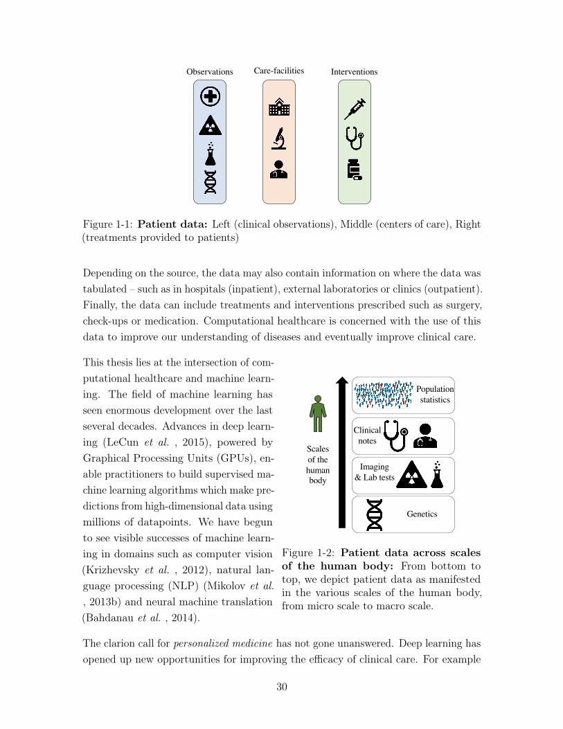
Figure 1-1, depicts the kind of data that is often collected. Clinical data mayinclude diagnosis codes, x-ray imaging, clinical labs and occasionally patient genetics.
29
Observations InterventionsCare-facilities
Figure 1-1: Patient data: Left (clinical observations), Middle (centers of care), Right(treatments provided to patients)
Depending on the source, the data may also contain information on where the data wastabulated – such as in hospitals (inpatient), external laboratories or clinics (outpatient).Finally, the data can include treatments and interventions prescribed such as surgery,check-ups or medication. Computational healthcare is concerned with the use of thisdata to improve our understanding of diseases and eventually improve clinical care.
Genetics
Imaging& Lab tests
Clinicalnotes
Scalesof thehumanbody
Population statistics
Time
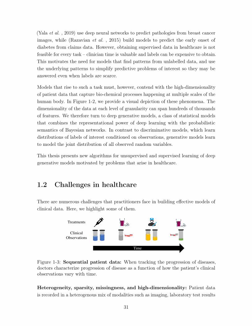
Figure 1-2: Patient data across scalesof the human body: From bottom totop, we depict patient data as manifestedin the various scales of the human body,from micro scale to macro scale.
This thesis lies at the intersection of com-putational healthcare and machine learn-ing. The field of machine learning hasseen enormous development over the lastseveral decades. Advances in deep learn-ing (LeCun et al. , 2015), powered byGraphical Processing Units (GPUs), en-able practitioners to build supervised ma-chine learning algorithms which make pre-dictions from high-dimensional data usingmillions of datapoints. We have begunto see visible successes of machine learn-ing in domains such as computer vision(Krizhevsky et al. , 2012), natural lan-guage processing (NLP) (Mikolov et al., 2013b) and neural machine translation(Bahdanau et al. , 2014).
The clarion call for personalized medicine has not gone unanswered. Deep learning hasopened up new opportunities for improving the efficacy of clinical care. For example
30
(Yala et al. , 2019) use deep neural networks to predict pathologies from breast cancerimages, while (Razavian et al. , 2015) build models to predict the early onset ofdiabetes from claims data. However, obtaining supervised data in healthcare is notfeasible for every task – clinician time is valuable and labels can be expensive to obtain.This motivates the need for models that find patterns from unlabelled data, and usethe underlying patterns to simplify predictive problems of interest so they may beanswered even when labels are scarce.
Models that rise to such a task must, however, contend with the high-dimensionalityof patient data that capture bio-chemical processes happening at multiple scales of thehuman body. In Figure 1-2, we provide a visual depiction of these phenomena. Thedimensionality of the data at each level of granularity can span hundreds of thousandsof features. We therefore turn to deep generative models, a class of statistical modelsthat combines the representational power of deep learning with the probabilisticsemantics of Bayesian networks. In contrast to discriminative models, which learndistributions of labels of interest conditioned on observations, generative models learnto model the joint distribution of all observed random variables.
This thesis presents new algorithms for unsupervised and supervised learning of deepgenerative models motivated by problems that arise in healthcare.
1.2 Challenges in healthcare
There are numerous challenges that practitioners face in building effective models ofclinical data. Here, we highlight some of them.
ClinicalObservations
Treatments
Time
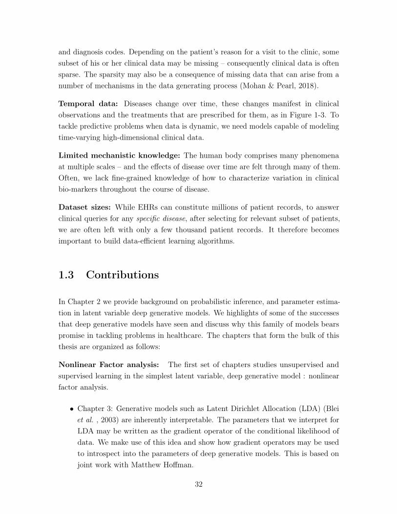
Figure 1-3: Sequential patient data: When tracking the progression of diseases,doctors characterize progression of disease as a function of how the patient’s clinicalobservations vary with time.
Heterogeneity, sparsity, missingness, and high-dimensionality: Patient datais recorded in a heterogenous mix of modalities such as imaging, laboratory test results
31
and diagnosis codes. Depending on the patient’s reason for a visit to the clinic, somesubset of his or her clinical data may be missing – consequently clinical data is oftensparse. The sparsity may also be a consequence of missing data that can arise from anumber of mechanisms in the data generating process (Mohan & Pearl, 2018).
Temporal data: Diseases change over time, these changes manifest in clinicalobservations and the treatments that are prescribed for them, as in Figure 1-3. Totackle predictive problems when data is dynamic, we need models capable of modelingtime-varying high-dimensional clinical data.
Limited mechanistic knowledge: The human body comprises many phenomenaat multiple scales – and the effects of disease over time are felt through many of them.Often, we lack fine-grained knowledge of how to characterize variation in clinicalbio-markers throughout the course of disease.
Dataset sizes: While EHRs can constitute millions of patient records, to answerclinical queries for any specific disease, after selecting for relevant subset of patients,we are often left with only a few thousand patient records. It therefore becomesimportant to build data-efficient learning algorithms.
1.3 Contributions
In Chapter 2 we provide background on probabilistic inference, and parameter estima-tion in latent variable deep generative models. We highlights of some of the successesthat deep generative models have seen and discuss why this family of models bearspromise in tackling problems in healthcare. The chapters that form the bulk of thisthesis are organized as follows:
Nonlinear Factor analysis: The first set of chapters studies unsupervised andsupervised learning in the simplest latent variable, deep generative model : nonlinearfactor analysis.
∙ Chapter 3: Generative models such as Latent Dirichlet Allocation (LDA) (Bleiet al. , 2003) are inherently interpretable. The parameters that we interpret forLDA may be written as the gradient operator of the conditional likelihood ofdata. We make use of this idea and show how gradient operators may be usedto introspect into the parameters of deep generative models. This is based onjoint work with Matthew Hoffman.
32
∙ Chapter 4 studies a failure mode of the canonical learning algorithm for deepgenerative models when modeling high-dimensional data with long-tailed distri-butions. We propose a way to mitigate the underlying pathology encounteredduring learning. This is based on joint work with Dawen Liang and MatthewHoffman.
∙ Chapter 5 depicts how the task of patient similarity may be posed as few-shotlearning. To this end, we give new algorithms to fine-tune deep generativemodels using similarity judgements. This is based on joint work with ArjunKhandelwal, Rajesh Ranganath and David Sontag.
Deep Markov Models: The latter set of chapters studies models for unsupervisedand supervised learning with high-dimensional, time-varying data.
∙ Chapter 6 introduces Deep Markov Models, nonlinear Gaussian state spacemodels where the relationships between random variables are parameterized byneural networks. We propose a variational learning algorithm for the model andshowcase its utility in modeling clinical data. Our work opens up new avenuesfor the use of deep generative models to tackle problems in clinical care. This isbased on joint work with Uri Shalit and David Sontag.
∙ Chapter 7 proposes new neural architectures, inspired by pharmacology, whichwhen used in Deep Markov Models, improve generalization of the model onpatient data. This is based on joint work with Zeshan Hussain and David Sontag.
∙ Chapter 8 develops new methods for how deep generative models may be usedto improve the predictive performance of classifiers by leveraging privilegedinformation: information available at training time, but not at test time. Thisis based on joint work with Zeshan Hussain and David Sontag.
Finally, in Chapter 9, we conclude with a discussion on how the innovations made inthis thesis can drive the next generation of predictive models in healthcare.
33

34

Chapter 2
Background
There are myriad ways to stratify and analyze the collective of methods used inmachine learning. This thesis is best viewed from a probabilistic perspective (Murphy,2012). This chapter is a primer on probability theory, graphical models, and deepgenerative models; the chapter introduces concepts and notation used throughout thisthesis. For a more thorough introduction to random variables, and the statisticalconcepts that this thesis builds on, we refer the reader to (Wasserman, 2013).
2.1 Random variables and probabilities
Random variables are the atoms of machine learning. A random variable, as the wordsuggests, is a variable whose value (corresponding to an event of interest) is unknownbut has the capacity to take multiple different values. The domain of a randomvariable may be discrete (like the side of a die), or continuous (such as how long ithas been since the bus arrived). A probability is the chance of an event occurring,and a probability distribution describes the chances that a random variable takes anyvalue in its domain. 𝑃 (𝑋 = 5) denotes the chances that the random variable 𝑋 hasof taking the assignment 5. A probability of zero denotes that the event cannot occurwhile a probability of one denotes the certainty of an event among all possible choices.Notationally, we will often use 𝑃 (𝑥) in leiu of 𝑃 (𝑋 = 𝑥).
Probabilities may also be defined for multiple random variables; 𝑃 (𝑋 = 𝑥, 𝑌 = 𝑦) isthe joint probability distribution denoting the probability that both random variablestake their assigned values. Similarly, probability distributions of a random variable
35
can also be affected by values taken on by other (typically related) random variables.A conditional probability is the probability of an event occurring given that anotherevent has occurred. For example, the probability of a patient suffering from a heartattack increases conditional on the patient being obese. Two random variables areindependent if conditioning on one has no consequence on the probability of the other.There are a few key rules that probability distributions follow that merit mention atthis junction.
The product rule of probabilities states that the probability of two events can bewritten as the probability of the first event times the probability of the secondevent conditioned on knowing whether or not the first occurred. This rule general-izes to the chain rule of probabilities which may be written as: 𝑃 (𝑋1, 𝑋2, 𝑋3) =
𝑃 (𝑋1)𝑃 (𝑋2|𝑋1)𝑃 (𝑋3|𝑋1, 𝑋2). An immediate consequence of this rule is Bayesrule, which forms the backbone of many inferential tasks. Bayes Rule states that:𝑃 (𝑋|𝑌 ) = 𝑃 (𝑌 |𝑋)𝑃 (𝑋)
𝑃 (𝑌 ); i.e. given access to 𝑃 (𝑌 |𝑋), 𝑃 (𝑋), 𝑃 (𝑌 ), it provides a mecha-
nism by which we may invert conditional probabilities.
The sum rule states that 𝑃 (𝑋 ∪ 𝑌 ) = 𝑃 (𝑋) +𝑃 (𝑌 )−𝑃 (𝑋 ∩ 𝑌 ) where ∪ denotes theunion of events spanned by the random variables 𝑋, 𝑌 and ∩ denotes the intersection ofthe events. For mutually exclusive events, 𝑃 (𝑋 ∪ 𝑌 ) = 𝑃 (𝑋) + 𝑃 (𝑌 ). A consequenceof the sum rule is that the estimation of marginal probabilities 𝑃 (𝑋) can be derivedfrom the joint probability distribution 𝑃 (𝑋, 𝑌 ) as: 𝑃 (𝑋) =
∑︀𝑦 𝑃 (𝑋, 𝑌 = 𝑦) when
𝑌 is discrete (for continuous random variables the sum would be replaced with anintegral).
Finally, a probability density function, pdf for short, is a map from the assignmentof a random variable onto a scalar proportional to the likelihood that the randomvariable takes the chosen assignment. For any event 𝐸, which constitutes values thatthe random variable may take: 𝑃 (𝑋 ∈ 𝐸) =
∫︀𝑥∈𝐸 𝑝(𝑥)𝑑𝑥 i.e. the probability density
function characterizes how often random variable 𝑋 lies in the set 𝐸.
The goal of a probabilistic treatment of machine learning is often to pose questionsof interest to the practitioner using the language of probability; we refer to thesequestions as probabilistic queries. For example, supervised prediction corresponds tothe evaluation of the conditional probability of 𝑌 , a random variable that representsthe label, given covariates 𝑋: 𝑃 (𝑌 |𝑋). Similarly, the goal of unsupervised learning isto approximate 𝑃 (𝑋), where 𝑋 may be a vector valued random variable correspondingto high-dimensional data of interest. Queries from unsupervised models can createnew examples of data by drawing samples via the probabilistic query 𝑃 (𝑋).
36
x1
<latexit sha1_base64="hRS0ddpgxHMAJcuGPZWM1yTuND4=">AAAB6nicbVBNS8NAEJ3Ur1q/qh69LBbBU0lE0WPRi8eK9gPaUDbbTbt0swm7E7GE/gQvHhTx6i/y5r9x2+agrQ8GHu/NMDMvSKQw6LrfTmFldW19o7hZ2tre2d0r7x80TZxqxhsslrFuB9RwKRRvoEDJ24nmNAokbwWjm6nfeuTaiFg94DjhfkQHSoSCUbTS/VPP65UrbtWdgSwTLycVyFHvlb+6/ZilEVfIJDWm47kJ+hnVKJjkk1I3NTyhbEQHvGOpohE3fjY7dUJOrNInYaxtKSQz9fdERiNjxlFgOyOKQ7PoTcX/vE6K4ZWfCZWkyBWbLwpTSTAm079JX2jOUI4toUwLeythQ6opQ5tOyYbgLb68TJpnVe+8enF3Xqld53EU4QiO4RQ8uIQa3EIdGsBgAM/wCm+OdF6cd+dj3lpw8plD+APn8wcOSI2o</latexit>
x2
<latexit sha1_base64="rZqqRJEsDVTa/mx5dMmqIpR8GIA=">AAAB6nicbVDLTgJBEOzFF+IL9ehlIjHxRHYJRo9ELx4xyiOBDZkdemHC7OxmZtZICJ/gxYPGePWLvPk3DrAHBSvppFLVne6uIBFcG9f9dnJr6xubW/ntws7u3v5B8fCoqeNUMWywWMSqHVCNgktsGG4EthOFNAoEtoLRzcxvPaLSPJYPZpygH9GB5CFn1Fjp/qlX6RVLbtmdg6wSLyMlyFDvFb+6/ZilEUrDBNW647mJ8SdUGc4ETgvdVGNC2YgOsGOppBFqfzI/dUrOrNInYaxsSUPm6u+JCY20HkeB7YyoGeplbyb+53VSE175Ey6T1KBki0VhKoiJyexv0ucKmRFjSyhT3N5K2JAqyoxNp2BD8JZfXiXNStmrli/uqqXadRZHHk7gFM7Bg0uowS3UoQEMBvAMr/DmCOfFeXc+Fq05J5s5hj9wPn8AD8yNqQ==</latexit>
x3
<latexit sha1_base64="ucUuJlzTdKE55zbmY9paKxrCXdE=">AAAB6nicbVDLTgJBEOzFF+IL9ehlIjHxRHYVo0eiF48Y5ZHAhswOA0yYnd3M9BrJhk/w4kFjvPpF3vwbB9iDgpV0UqnqTndXEEth0HW/ndzK6tr6Rn6zsLW9s7tX3D9omCjRjNdZJCPdCqjhUiheR4GSt2LNaRhI3gxGN1O/+ci1EZF6wHHM/ZAOlOgLRtFK90/d826x5JbdGcgy8TJSggy1bvGr04tYEnKFTFJj2p4bo59SjYJJPil0EsNjykZ0wNuWKhpy46ezUyfkxCo90o+0LYVkpv6eSGlozDgMbGdIcWgWvan4n9dOsH/lp0LFCXLF5ov6iSQYkenfpCc0ZyjHllCmhb2VsCHVlKFNp2BD8BZfXiaNs7JXKV/cVUrV6yyOPBzBMZyCB5dQhVuoQR0YDOAZXuHNkc6L8+58zFtzTjZzCH/gfP4AEVCNqg==</latexit>
x4
<latexit sha1_base64="QrchNgH7OdLRQMbrSRtNerERkVc=">AAAB6nicbVBNS8NAEJ34WetX1aOXxSJ4KolU9Fj04rGi/YA2lM120i7dbMLuRiyhP8GLB0W8+ou8+W/ctjlo64OBx3szzMwLEsG1cd1vZ2V1bX1js7BV3N7Z3dsvHRw2dZwqhg0Wi1i1A6pRcIkNw43AdqKQRoHAVjC6mfqtR1Sax/LBjBP0IzqQPOSMGivdP/WqvVLZrbgzkGXi5aQMOeq90le3H7M0QmmYoFp3PDcxfkaV4UzgpNhNNSaUjegAO5ZKGqH2s9mpE3JqlT4JY2VLGjJTf09kNNJ6HAW2M6JmqBe9qfif10lNeOVnXCapQcnmi8JUEBOT6d+kzxUyI8aWUKa4vZWwIVWUGZtO0YbgLb68TJrnFa9aubirlmvXeRwFOIYTOAMPLqEGt1CHBjAYwDO8wpsjnBfn3fmYt644+cwR/IHz+QMS1I2r</latexit>
x5
<latexit sha1_base64="hIN1tAdz5fE+0mkT2j9lTqXNEQw=">AAAB6nicbVDLTgJBEOzFF+IL9ehlIjHxRHYNRI9ELx4xyiOBDZkdemHC7OxmZtZICJ/gxYPGePWLvPk3DrAHBSvppFLVne6uIBFcG9f9dnJr6xubW/ntws7u3v5B8fCoqeNUMWywWMSqHVCNgktsGG4EthOFNAoEtoLRzcxvPaLSPJYPZpygH9GB5CFn1Fjp/qlX7RVLbtmdg6wSLyMlyFDvFb+6/ZilEUrDBNW647mJ8SdUGc4ETgvdVGNC2YgOsGOppBFqfzI/dUrOrNInYaxsSUPm6u+JCY20HkeB7YyoGeplbyb+53VSE175Ey6T1KBki0VhKoiJyexv0ucKmRFjSyhT3N5K2JAqyoxNp2BD8JZfXiXNi7JXKVfvKqXadRZHHk7gFM7Bg0uowS3UoQEMBvAMr/DmCOfFeXc+Fq05J5s5hj9wPn8AFFiNrA==</latexit>
x6
<latexit sha1_base64="B9qSbtg2nXHCj8lUHK+7KQvL0fQ=">AAAB6nicbVDLTgJBEOzFF+IL9ehlIjHxRHYNPo5ELx4xyiOBDZkdGpgwO7uZmTWSDZ/gxYPGePWLvPk3DrAHBSvppFLVne6uIBZcG9f9dnIrq2vrG/nNwtb2zu5ecf+goaNEMayzSESqFVCNgkusG24EtmKFNAwENoPRzdRvPqLSPJIPZhyjH9KB5H3OqLHS/VP3olssuWV3BrJMvIyUIEOtW/zq9CKWhCgNE1TrtufGxk+pMpwJnBQ6icaYshEdYNtSSUPUfjo7dUJOrNIj/UjZkobM1N8TKQ21HoeB7QypGepFbyr+57UT07/yUy7jxKBk80X9RBATkenfpMcVMiPGllCmuL2VsCFVlBmbTsGG4C2+vEwaZ2WvUj6/q5Sq11kceTiCYzgFDy6hCrdQgzowGMAzvMKbI5wX5935mLfmnGzmEP7A+fwBFdyNrQ==</latexit>
x7
<latexit sha1_base64="8yJWn5eiMjm0lmOo5aae8jtW8/8=">AAAB6nicbVDLTgJBEOzFF+IL9ehlIjHxRHYNBo9ELx4xyiOBDZkdemHC7OxmZtZICJ/gxYPGePWLvPk3DrAHBSvppFLVne6uIBFcG9f9dnJr6xubW/ntws7u3v5B8fCoqeNUMWywWMSqHVCNgktsGG4EthOFNAoEtoLRzcxvPaLSPJYPZpygH9GB5CFn1Fjp/qlX7RVLbtmdg6wSLyMlyFDvFb+6/ZilEUrDBNW647mJ8SdUGc4ETgvdVGNC2YgOsGOppBFqfzI/dUrOrNInYaxsSUPm6u+JCY20HkeB7YyoGeplbyb+53VSE175Ey6T1KBki0VhKoiJyexv0ucKmRFjSyhT3N5K2JAqyoxNp2BD8JZfXiXNi7JXKV/eVUq16yyOPJzAKZyDB1WowS3UoQEMBvAMr/DmCOfFeXc+Fq05J5s5hj9wPn8AF2CNrg==</latexit>
x8
<latexit sha1_base64="rWnjBZLI0+5M+KjAKjBigOf+kos=">AAAB6nicbVDLTgJBEOzFF+IL9ehlIjHxRHYNRo5ELx4xyiOBDZkdemHC7OxmZtZICJ/gxYPGePWLvPk3DrAHBSvppFLVne6uIBFcG9f9dnJr6xubW/ntws7u3v5B8fCoqeNUMWywWMSqHVCNgktsGG4EthOFNAoEtoLRzcxvPaLSPJYPZpygH9GB5CFn1Fjp/qlX7RVLbtmdg6wSLyMlyFDvFb+6/ZilEUrDBNW647mJ8SdUGc4ETgvdVGNC2YgOsGOppBFqfzI/dUrOrNInYaxsSUPm6u+JCY20HkeB7YyoGeplbyb+53VSE1b9CZdJalCyxaIwFcTEZPY36XOFzIixJZQpbm8lbEgVZcamU7AheMsvr5LmRdmrlC/vKqXadRZHHk7gFM7BgyuowS3UoQEMBvAMr/DmCOfFeXc+Fq05J5s5hj9wPn8AGOSNrw==</latexit>
x9
<latexit sha1_base64="dsuJAUfiD8eC8z5Gyy7I092Wa2U=">AAAB6nicbVDLSgNBEOyNrxhfUY9eBoPgKexKRL0FvXiMaB6QLGF20kmGzM4uM7NiWPIJXjwo4tUv8ubfOEn2oIkFDUVVN91dQSy4Nq777eRWVtfWN/Kbha3tnd294v5BQ0eJYlhnkYhUK6AaBZdYN9wIbMUKaRgIbAajm6nffESleSQfzDhGP6QDyfucUWOl+6fuVbdYcsvuDGSZeBkpQYZat/jV6UUsCVEaJqjWbc+NjZ9SZTgTOCl0Eo0xZSM6wLalkoao/XR26oScWKVH+pGyJQ2Zqb8nUhpqPQ4D2xlSM9SL3lT8z2snpn/pp1zGiUHJ5ov6iSAmItO/SY8rZEaMLaFMcXsrYUOqKDM2nYINwVt8eZk0zspepXx+VylVr7M48nAEx3AKHlxAFW6hBnVgMIBneIU3RzgvzrvzMW/NOdnMIfyB8/kDGmiNsA==</latexit>
x1
<latexit sha1_base64="hRS0ddpgxHMAJcuGPZWM1yTuND4=">AAAB6nicbVBNS8NAEJ3Ur1q/qh69LBbBU0lE0WPRi8eK9gPaUDbbTbt0swm7E7GE/gQvHhTx6i/y5r9x2+agrQ8GHu/NMDMvSKQw6LrfTmFldW19o7hZ2tre2d0r7x80TZxqxhsslrFuB9RwKRRvoEDJ24nmNAokbwWjm6nfeuTaiFg94DjhfkQHSoSCUbTS/VPP65UrbtWdgSwTLycVyFHvlb+6/ZilEVfIJDWm47kJ+hnVKJjkk1I3NTyhbEQHvGOpohE3fjY7dUJOrNInYaxtKSQz9fdERiNjxlFgOyOKQ7PoTcX/vE6K4ZWfCZWkyBWbLwpTSTAm079JX2jOUI4toUwLeythQ6opQ5tOyYbgLb68TJpnVe+8enF3Xqld53EU4QiO4RQ8uIQa3EIdGsBgAM/wCm+OdF6cd+dj3lpw8plD+APn8wcOSI2o</latexit>
x2
<latexit sha1_base64="rZqqRJEsDVTa/mx5dMmqIpR8GIA=">AAAB6nicbVDLTgJBEOzFF+IL9ehlIjHxRHYJRo9ELx4xyiOBDZkdemHC7OxmZtZICJ/gxYPGePWLvPk3DrAHBSvppFLVne6uIBFcG9f9dnJr6xubW/ntws7u3v5B8fCoqeNUMWywWMSqHVCNgktsGG4EthOFNAoEtoLRzcxvPaLSPJYPZpygH9GB5CFn1Fjp/qlX6RVLbtmdg6wSLyMlyFDvFb+6/ZilEUrDBNW647mJ8SdUGc4ETgvdVGNC2YgOsGOppBFqfzI/dUrOrNInYaxsSUPm6u+JCY20HkeB7YyoGeplbyb+53VSE175Ey6T1KBki0VhKoiJyexv0ucKmRFjSyhT3N5K2JAqyoxNp2BD8JZfXiXNStmrli/uqqXadRZHHk7gFM7Bg0uowS3UoQEMBvAMr/DmCOfFeXc+Fq05J5s5hj9wPn8AD8yNqQ==</latexit>
x3
<latexit sha1_base64="ucUuJlzTdKE55zbmY9paKxrCXdE=">AAAB6nicbVDLTgJBEOzFF+IL9ehlIjHxRHYVo0eiF48Y5ZHAhswOA0yYnd3M9BrJhk/w4kFjvPpF3vwbB9iDgpV0UqnqTndXEEth0HW/ndzK6tr6Rn6zsLW9s7tX3D9omCjRjNdZJCPdCqjhUiheR4GSt2LNaRhI3gxGN1O/+ci1EZF6wHHM/ZAOlOgLRtFK90/d826x5JbdGcgy8TJSggy1bvGr04tYEnKFTFJj2p4bo59SjYJJPil0EsNjykZ0wNuWKhpy46ezUyfkxCo90o+0LYVkpv6eSGlozDgMbGdIcWgWvan4n9dOsH/lp0LFCXLF5ov6iSQYkenfpCc0ZyjHllCmhb2VsCHVlKFNp2BD8BZfXiaNs7JXKV/cVUrV6yyOPBzBMZyCB5dQhVuoQR0YDOAZXuHNkc6L8+58zFtzTjZzCH/gfP4AEVCNqg==</latexit>
h1
<latexit sha1_base64="PhPhUBmZf4mysfrvPFsxlILUh3c=">AAAB6nicbVBNS8NAEJ3Ur1q/qh69LBbBU0mkoseiF48V7Qe0oWy2k3bpZhN2N0IJ/QlePCji1V/kzX/jts1BWx8MPN6bYWZekAiujet+O4W19Y3NreJ2aWd3b/+gfHjU0nGqGDZZLGLVCahGwSU2DTcCO4lCGgUC28H4dua3n1BpHstHM0nQj+hQ8pAzaqz0MOp7/XLFrbpzkFXi5aQCORr98ldvELM0QmmYoFp3PTcxfkaV4UzgtNRLNSaUjekQu5ZKGqH2s/mpU3JmlQEJY2VLGjJXf09kNNJ6EgW2M6JmpJe9mfif101NeO1nXCapQckWi8JUEBOT2d9kwBUyIyaWUKa4vZWwEVWUGZtOyYbgLb+8SloXVa9WvbyvVeo3eRxFOIFTOAcPrqAOd9CAJjAYwjO8wpsjnBfn3flYtBacfOYY/sD5/AH12Y2Y</latexit>
h2
<latexit sha1_base64="/w5wC0SQ4C5TQi3e6M/rKSvtWTY=">AAAB6nicbVBNS8NAEJ3Ur1q/qh69LBbBU0lKRY9FLx4r2lpoQ9lsJ+3SzSbsboQS+hO8eFDEq7/Im//GbZuDtj4YeLw3w8y8IBFcG9f9dgpr6xubW8Xt0s7u3v5B+fCoreNUMWyxWMSqE1CNgktsGW4EdhKFNAoEPgbjm5n/+IRK81g+mEmCfkSHkoecUWOl+1G/1i9X3Ko7B1klXk4qkKPZL3/1BjFLI5SGCap113MT42dUGc4ETku9VGNC2ZgOsWuppBFqP5ufOiVnVhmQMFa2pCFz9fdERiOtJ1FgOyNqRnrZm4n/ed3UhFd+xmWSGpRssShMBTExmf1NBlwhM2JiCWWK21sJG1FFmbHplGwI3vLLq6Rdq3r16sVdvdK4zuMowgmcwjl4cAkNuIUmtIDBEJ7hFd4c4bw4787HorXg5DPH8AfO5w/3XY2Z</latexit>
h3
<latexit sha1_base64="F5oBiuXxD+NfN3Uv10U/977PtUk=">AAAB6nicbVBNS8NAEJ3Ur1q/qh69LBbBU0m0oseiF48V7Qe0oWy2m3bpZhN2J0IJ/QlePCji1V/kzX/jts1Bqw8GHu/NMDMvSKQw6LpfTmFldW19o7hZ2tre2d0r7x+0TJxqxpsslrHuBNRwKRRvokDJO4nmNAokbwfjm5nffuTaiFg94CThfkSHSoSCUbTS/ah/3i9X3Ko7B/lLvJxUIEejX/7sDWKWRlwhk9SYrucm6GdUo2CST0u91PCEsjEd8q6likbc+Nn81Ck5scqAhLG2pZDM1Z8TGY2MmUSB7YwojsyyNxP/87ophld+JlSSIldssShMJcGYzP4mA6E5QzmxhDIt7K2EjaimDG06JRuCt/zyX9I6q3q16sVdrVK/zuMowhEcwyl4cAl1uIUGNIHBEJ7gBV4d6Tw7b877orXg5DOH8AvOxzf44Y2a</latexit>
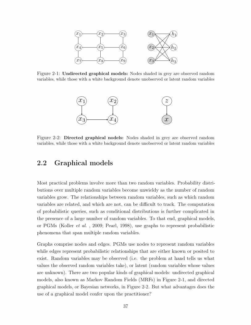
Figure 2-1: Undirected graphical models: Nodes shaded in grey are observed randomvariables, while those with a white background denote unobserved or latent random variables
x1
<latexit sha1_base64="hRS0ddpgxHMAJcuGPZWM1yTuND4=">AAAB6nicbVBNS8NAEJ3Ur1q/qh69LBbBU0lE0WPRi8eK9gPaUDbbTbt0swm7E7GE/gQvHhTx6i/y5r9x2+agrQ8GHu/NMDMvSKQw6LrfTmFldW19o7hZ2tre2d0r7x80TZxqxhsslrFuB9RwKRRvoEDJ24nmNAokbwWjm6nfeuTaiFg94DjhfkQHSoSCUbTS/VPP65UrbtWdgSwTLycVyFHvlb+6/ZilEVfIJDWm47kJ+hnVKJjkk1I3NTyhbEQHvGOpohE3fjY7dUJOrNInYaxtKSQz9fdERiNjxlFgOyOKQ7PoTcX/vE6K4ZWfCZWkyBWbLwpTSTAm079JX2jOUI4toUwLeythQ6opQ5tOyYbgLb68TJpnVe+8enF3Xqld53EU4QiO4RQ8uIQa3EIdGsBgAM/wCm+OdF6cd+dj3lpw8plD+APn8wcOSI2o</latexit>
x2
<latexit sha1_base64="rZqqRJEsDVTa/mx5dMmqIpR8GIA=">AAAB6nicbVDLTgJBEOzFF+IL9ehlIjHxRHYJRo9ELx4xyiOBDZkdemHC7OxmZtZICJ/gxYPGePWLvPk3DrAHBSvppFLVne6uIBFcG9f9dnJr6xubW/ntws7u3v5B8fCoqeNUMWywWMSqHVCNgktsGG4EthOFNAoEtoLRzcxvPaLSPJYPZpygH9GB5CFn1Fjp/qlX6RVLbtmdg6wSLyMlyFDvFb+6/ZilEUrDBNW647mJ8SdUGc4ETgvdVGNC2YgOsGOppBFqfzI/dUrOrNInYaxsSUPm6u+JCY20HkeB7YyoGeplbyb+53VSE175Ey6T1KBki0VhKoiJyexv0ucKmRFjSyhT3N5K2JAqyoxNp2BD8JZfXiXNStmrli/uqqXadRZHHk7gFM7Bg0uowS3UoQEMBvAMr/DmCOfFeXc+Fq05J5s5hj9wPn8AD8yNqQ==</latexit>
x4
<latexit sha1_base64="QrchNgH7OdLRQMbrSRtNerERkVc=">AAAB6nicbVBNS8NAEJ34WetX1aOXxSJ4KolU9Fj04rGi/YA2lM120i7dbMLuRiyhP8GLB0W8+ou8+W/ctjlo64OBx3szzMwLEsG1cd1vZ2V1bX1js7BV3N7Z3dsvHRw2dZwqhg0Wi1i1A6pRcIkNw43AdqKQRoHAVjC6mfqtR1Sax/LBjBP0IzqQPOSMGivdP/WqvVLZrbgzkGXi5aQMOeq90le3H7M0QmmYoFp3PDcxfkaV4UzgpNhNNSaUjegAO5ZKGqH2s9mpE3JqlT4JY2VLGjJTf09kNNJ6HAW2M6JmqBe9qfif10lNeOVnXCapQcnmi8JUEBOT6d+kzxUyI8aWUKa4vZWwIVWUGZtO0YbgLb68TJrnFa9aubirlmvXeRwFOIYTOAMPLqEGt1CHBjAYwDO8wpsjnBfn3fmYt644+cwR/IHz+QMS1I2r</latexit>
x3
<latexit sha1_base64="ucUuJlzTdKE55zbmY9paKxrCXdE=">AAAB6nicbVDLTgJBEOzFF+IL9ehlIjHxRHYVo0eiF48Y5ZHAhswOA0yYnd3M9BrJhk/w4kFjvPpF3vwbB9iDgpV0UqnqTndXEEth0HW/ndzK6tr6Rn6zsLW9s7tX3D9omCjRjNdZJCPdCqjhUiheR4GSt2LNaRhI3gxGN1O/+ci1EZF6wHHM/ZAOlOgLRtFK90/d826x5JbdGcgy8TJSggy1bvGr04tYEnKFTFJj2p4bo59SjYJJPil0EsNjykZ0wNuWKhpy46ezUyfkxCo90o+0LYVkpv6eSGlozDgMbGdIcWgWvan4n9dOsH/lp0LFCXLF5ov6iSQYkenfpCc0ZyjHllCmhb2VsCHVlKFNp2BD8BZfXiaNs7JXKV/cVUrV6yyOPBzBMZyCB5dQhVuoQR0YDOAZXuHNkc6L8+58zFtzTjZzCH/gfP4AEVCNqg==</latexit>
x
<latexit sha1_base64="E+xWb622b2P97o+CO1oWwc/7ors=">AAAB6HicbVDLTgJBEOzFF+IL9ehlIjHxRHYNRo9ELx4hkUcCGzI79MLI7OxmZtZICF/gxYPGePWTvPk3DrAHBSvppFLVne6uIBFcG9f9dnJr6xubW/ntws7u3v5B8fCoqeNUMWywWMSqHVCNgktsGG4EthOFNAoEtoLR7cxvPaLSPJb3ZpygH9GB5CFn1Fip/tQrltyyOwdZJV5GSpCh1it+dfsxSyOUhgmqdcdzE+NPqDKcCZwWuqnGhLIRHWDHUkkj1P5kfuiUnFmlT8JY2ZKGzNXfExMaaT2OAtsZUTPUy95M/M/rpCa89idcJqlByRaLwlQQE5PZ16TPFTIjxpZQpri9lbAhVZQZm03BhuAtv7xKmhdlr1K+rFdK1ZssjjycwCmcgwdXUIU7qEEDGCA8wyu8OQ/Oi/PufCxac042cwx/4Hz+AOjRjQQ=</latexit>
z
<latexit sha1_base64="mBNsSck29HYD+UA8I7CdsBnbA5A=">AAAB6HicbVDLTgJBEOzFF+IL9ehlIjHxRHYNRo9ELx4hkUcCGzI79MLI7OxmZtYECV/gxYPGePWTvPk3DrAHBSvppFLVne6uIBFcG9f9dnJr6xubW/ntws7u3v5B8fCoqeNUMWywWMSqHVCNgktsGG4EthOFNAoEtoLR7cxvPaLSPJb3ZpygH9GB5CFn1Fip/tQrltyyOwdZJV5GSpCh1it+dfsxSyOUhgmqdcdzE+NPqDKcCZwWuqnGhLIRHWDHUkkj1P5kfuiUnFmlT8JY2ZKGzNXfExMaaT2OAtsZUTPUy95M/M/rpCa89idcJqlByRaLwlQQE5PZ16TPFTIjxpZQpri9lbAhVZQZm03BhuAtv7xKmhdlr1K+rFdK1ZssjjycwCmcgwdXUIU7qEEDGCA8wyu8OQ/Oi/PufCxac042cwx/4Hz+AOvZjQY=</latexit>
Figure 2-2: Directed graphical nodels: Nodes shaded in grey are observed randomvariables, while those with a white background denote unobserved or latent random variables
2.2 Graphical models
Most practical problems involve more than two random variables. Probability distri-butions over multiple random variables become unwieldy as the number of randomvariables grow. The relationships between random variables, such as which randomvariables are related, and which are not, can be difficult to track. The computationof probabilistic queries, such as conditional distributions is further complicated inthe presence of a large number of random variables. To that end, graphical models,or PGMs (Koller et al. , 2009; Pearl, 1998), use graphs to represent probabilisticphenomena that span multiple random variables.
Graphs comprise nodes and edges. PGMs use nodes to represent random variableswhile edges represent probabilistic relationships that are either known or posited toexist. Random variables may be observed (i.e. the problem at hand tells us whatvalues the observed random variables take), or latent (random variables whose valuesare unknown). There are two popular kinds of graphical models: undirected graphicalmodels, also known as Markov Random Fields (MRFs) in Figure 2-1, and directedgraphical models, or Bayesian networks, in Figure 2-2. But what advantages does theuse of a graphical model confer upon the practitioner?
37
2.2.1 Structure as domain knowledge
There are several reasons why graphical models have seen tremendous success as atool for probabilistic modelling. First, every graph structure over random variablesimplies a factorization on the joint distribution. For the undirected graphical modelin Figure 2-1 (left), it can be shown that
𝑃 (𝑋1, . . . , 𝑋9) =1
𝑍
∏︁
𝑐𝑖∈𝒞
𝜑𝑖(𝑥𝑐),
where 𝒞 are the set of all cliques in the graph (in this case, all pairs of nodes connectedby an edge), where 𝜑𝑖(𝑥𝑐) denote clique potentials (a function that assigns a scalar toevery assignment taken on by variables in the clique 𝑥𝑐) and 𝑍 is the normalizationconstant. Similarly, for the directed graphical model in Figure 2-2 (left), the jointdistribution over the random variables factorizes as:
𝑃 (𝑋1, . . . , 𝑋4) = 𝑃 (𝑋1)𝑃 (𝑋2)𝑃 (𝑋3|𝑋1)𝑃 (𝑋4|𝑋3, 𝑋2),
An immediate consequence of the factorization of the joint distribution is that prac-tioners need only track parameters associated with each of the clique potentials orconditional probabilities. For example, if all random variables were binary, thenthe joint distribution over random variables in Figure 2-1 (left) would naïvely becharacterized by 29 − 1 = 511 parameters. However, the graphical model has twelvecliques potentials, each of which can be represented via 22−1 = 3 parameters resultingin 36 parameters: an order of magnitude in parameter savings.
Second, the exercise of creating the graphical model is often undertaken in conjunctionwith a domain expert. Doing so forces practitioners to think carefully about selectingthe random variables in the problem, and decide how they are related. For example,the graphical model in Figure 2-1 (left) shows a grid structured model, which impliesthat the random variables exhibit spatial correlations, such as those among pixels inan image.
Finally, the use of a graph allows us to understand and take advantage of structuralproperties of the data generating distribution to simplify the computation of prob-abilistic queries. One concrete way in which they do so is via the simplification ofindependence statements.
38
2.2.2 Independence statements
Once a probabilistic graphical model has been created, we can borrow from the richliterature on graph theory to study the various properties that must hold among thedistributions over random variables in the graph. Key among them are propertiesabout which variables are independent from one another.
Marginal Independence: If there exists no edge between two random variables ina graph, then the random variables are said to be marginally independent. In directedgraphs, there must exist no directed path between two random variables. For example,there are no random variables in Figure 2-1 (left) that are marginally independent ofone another since the graph is connected. 𝑋1 and 𝑋2 in Figure 2-2 (left) are marginallyindependent of one another since one is not a parent of the other. For marginallyindependent random variables, we have that 𝑃 (𝑋1, 𝑋2) = 𝑃 (𝑋1)𝑃 (𝑋2).
Conditional Independence: Conditioning, or observing a random variable’s value,is an important event that has ramifications about the independence properties ofrandom variables in a graph. Conditional independence statements tell us whenobserving a set of random variables renders two random variables independent of oneanother. In Figure 2-1 (left), 𝑋1 |= 𝑋3, 𝑋5, 𝑋6,...,9|𝑋2, 𝑋4 since all the influence that𝑋1 has on the other random variables is via 𝑋2, 𝑋4. Similarly in directed graphicalmodels, Figure 2-2 (left), 𝑋1 |= 𝑋4|𝑋3. For conditionally independent random variables,we have that 𝑃 (𝑋1, 𝑋4|𝑋3) = 𝑃 (𝑋1|𝑋3)𝑃 (𝑋4|𝑋3).
In directed graphical models, there is a special form of conditioning that renders other-wise marginally independent variables dependent. This happens when conditioning ona common child. For example, 𝑋1��|= 𝑋2|𝑋4 in Figure 2-2 (left) where 𝑋4 is a commonchild of both 𝑋1 and 𝑋2. The rationale for this is as follows, consider the following:let 𝑋1 capture whether a sprinkler is on, 𝑋2 represent the probability of rain, and𝑋4 denote the grass being wet. Knowing that the grass is wet means that either thesprinkler was on rendering it less likely to have rained, or vice versa. This phenomenonis referred to as explaining away ; in the aforementioned example, knowing the grass iswet allows rain to explain away the chance of the sprinkler being on and vice versa.
The Markov blanket of a random variable is a set of variables which if conditioned on,render a random variable independent of every other in a graph.
Definition 2.2.1. For any random variables 𝑋, 𝑌 ∈ 𝐺, the Markov Blanket MB(𝑋) ∈
39
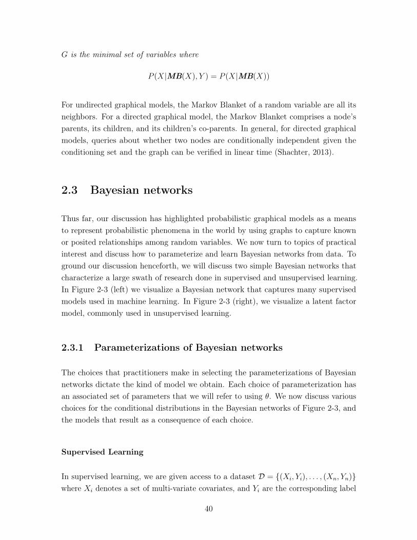
𝐺 is the minimal set of variables where
𝑃 (𝑋|MB(𝑋), 𝑌 ) = 𝑃 (𝑋|MB(𝑋))
For undirected graphical models, the Markov Blanket of a random variable are all itsneighbors. For a directed graphical model, the Markov Blanket comprises a node’sparents, its children, and its children’s co-parents. In general, for directed graphicalmodels, queries about whether two nodes are conditionally independent given theconditioning set and the graph can be verified in linear time (Shachter, 2013).
2.3 Bayesian networks
Thus far, our discussion has highlighted probabilistic graphical models as a meansto represent probabilistic phenomena in the world by using graphs to capture knownor posited relationships among random variables. We now turn to topics of practicalinterest and discuss how to parameterize and learn Bayesian networks from data. Toground our discussion henceforth, we will discuss two simple Bayesian networks thatcharacterize a large swath of research done in supervised and unsupervised learning.In Figure 2-3 (left) we visualize a Bayesian network that captures many supervisedmodels used in machine learning. In Figure 2-3 (right), we visualize a latent factormodel, commonly used in unsupervised learning.
2.3.1 Parameterizations of Bayesian networks
The choices that practitioners make in selecting the parameterizations of Bayesiannetworks dictate the kind of model we obtain. Each choice of parameterization hasan associated set of parameters that we will refer to using 𝜃. We now discuss variouschoices for the conditional distributions in the Bayesian networks of Figure 2-3, andthe models that result as a consequence of each choice.
Supervised Learning
In supervised learning, we are given access to a dataset 𝒟 = {(𝑋𝑖, 𝑌𝑖), . . . , (𝑋𝑛, 𝑌𝑛)}where 𝑋𝑖 denotes a set of multi-variate covariates, and 𝑌𝑖 are the corresponding label
40
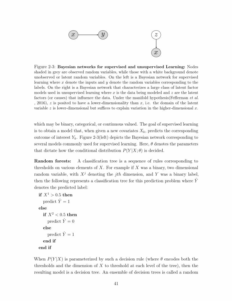
x
<latexit sha1_base64="E+xWb622b2P97o+CO1oWwc/7ors=">AAAB6HicbVDLTgJBEOzFF+IL9ehlIjHxRHYNRo9ELx4hkUcCGzI79MLI7OxmZtZICF/gxYPGePWTvPk3DrAHBSvppFLVne6uIBFcG9f9dnJr6xubW/ntws7u3v5B8fCoqeNUMWywWMSqHVCNgktsGG4EthOFNAoEtoLR7cxvPaLSPJb3ZpygH9GB5CFn1Fip/tQrltyyOwdZJV5GSpCh1it+dfsxSyOUhgmqdcdzE+NPqDKcCZwWuqnGhLIRHWDHUkkj1P5kfuiUnFmlT8JY2ZKGzNXfExMaaT2OAtsZUTPUy95M/M/rpCa89idcJqlByRaLwlQQE5PZ16TPFTIjxpZQpri9lbAhVZQZm03BhuAtv7xKmhdlr1K+rFdK1ZssjjycwCmcgwdXUIU7qEEDGCA8wyu8OQ/Oi/PufCxac042cwx/4Hz+AOjRjQQ=</latexit>
z
<latexit sha1_base64="mBNsSck29HYD+UA8I7CdsBnbA5A=">AAAB6HicbVDLTgJBEOzFF+IL9ehlIjHxRHYNRo9ELx4hkUcCGzI79MLI7OxmZtYECV/gxYPGePWTvPk3DrAHBSvppFLVne6uIBFcG9f9dnJr6xubW/ntws7u3v5B8fCoqeNUMWywWMSqHVCNgktsGG4EthOFNAoEtoLR7cxvPaLSPJb3ZpygH9GB5CFn1Fip/tQrltyyOwdZJV5GSpCh1it+dfsxSyOUhgmqdcdzE+NPqDKcCZwWuqnGhLIRHWDHUkkj1P5kfuiUnFmlT8JY2ZKGzNXfExMaaT2OAtsZUTPUy95M/M/rpCa89idcJqlByRaLwlQQE5PZ16TPFTIjxpZQpri9lbAhVZQZm03BhuAtv7xKmhdlr1K+rFdK1ZssjjycwCmcgwdXUIU7qEEDGCA8wyu8OQ/Oi/PufCxac042cwx/4Hz+AOvZjQY=</latexit>
x
<latexit sha1_base64="E+xWb622b2P97o+CO1oWwc/7ors=">AAAB6HicbVDLTgJBEOzFF+IL9ehlIjHxRHYNRo9ELx4hkUcCGzI79MLI7OxmZtZICF/gxYPGePWTvPk3DrAHBSvppFLVne6uIBFcG9f9dnJr6xubW/ntws7u3v5B8fCoqeNUMWywWMSqHVCNgktsGG4EthOFNAoEtoLR7cxvPaLSPJb3ZpygH9GB5CFn1Fip/tQrltyyOwdZJV5GSpCh1it+dfsxSyOUhgmqdcdzE+NPqDKcCZwWuqnGhLIRHWDHUkkj1P5kfuiUnFmlT8JY2ZKGzNXfExMaaT2OAtsZUTPUy95M/M/rpCa89idcJqlByRaLwlQQE5PZ16TPFTIjxpZQpri9lbAhVZQZm03BhuAtv7xKmhdlr1K+rFdK1ZssjjycwCmcgwdXUIU7qEEDGCA8wyu8OQ/Oi/PufCxac042cwx/4Hz+AOjRjQQ=</latexit>
y
<latexit sha1_base64="0AzN9pSceEkVyYO5YY8D+4ugxy4=">AAAB6HicbVBNS8NAEJ3Ur1q/qh69LBbBU0mkoseiF48t2FpoQ9lsJ+3azSbsboQS+gu8eFDEqz/Jm//GbZuDtj4YeLw3w8y8IBFcG9f9dgpr6xubW8Xt0s7u3v5B+fCoreNUMWyxWMSqE1CNgktsGW4EdhKFNAoEPgTj25n/8IRK81jem0mCfkSHkoecUWOl5qRfrrhVdw6ySrycVCBHo1/+6g1ilkYoDRNU667nJsbPqDKcCZyWeqnGhLIxHWLXUkkj1H42P3RKzqwyIGGsbElD5urviYxGWk+iwHZG1Iz0sjcT//O6qQmv/YzLJDUo2WJRmApiYjL7mgy4QmbExBLKFLe3EjaiijJjsynZELzll1dJ+6Lq1aqXzVqlfpPHUYQTOIVz8OAK6nAHDWgBA4RneIU359F5cd6dj0VrwclnjuEPnM8f6lWNBQ==</latexit>
Figure 2-3: Bayesian networks for supervised and unsupervised Learning: Nodesshaded in grey are observed random variables, while those with a white background denoteunobserved or latent random variables. On the left is a Bayesian network for supervisedlearning where 𝑥 denote the inputs and 𝑦 denote the random variables corresponding to thelabels. On the right is a Bayesian network that characterizes a large class of latent factormodels used in unsupervised learning where 𝑥 is the data being modeled and 𝑧 are the latentfactors (or causes) that influence the data. Under the manifold hypothesis(Fefferman et al., 2016), 𝑧 is posited to have a lower-dimensionality than 𝑥, i.e. the domain of the latentvariable 𝑧 is lower-dimensional but suffices to explain variation in the higher-dimensional 𝑥.
which may be binary, categorical, or continuous valued. The goal of supervised learningis to obtain a model that, when given a new covariates 𝑋𝑘, predicts the correspondingoutcome of interest 𝑌𝑘. Figure 2-3(left) depicts the Bayesian network corresponding toseveral models commonly used for supervised learning. Here, 𝜃 denotes the parametersthat dictate how the conditional distribution 𝑃 (𝑌 |𝑋; 𝜃) is decided.
Random forests: A classification tree is a sequence of rules corresponding tothresholds on various elements of 𝑋. For example if 𝑋 was a binary, two dimensionalrandom variable, with 𝑋𝑗 denoting the 𝑗𝑡ℎ dimension, and 𝑌 was a binary label,then the following represents a classification tree for this prediction problem where 𝑌denotes the predicted label:
if 𝑋1 > 0.5 thenpredict 𝑌 = 1
elseif 𝑋2 < 0.5 then
predict 𝑌 = 0
elsepredict 𝑌 = 1
end ifend if
When 𝑃 (𝑌 |𝑋) is parameterized by such a decision rule (where 𝜃 encodes both thethresholds and the dimension of 𝑋 to threshold at each level of the tree), then theresulting model is a decision tree. An ensemble of decision trees is called a random
41
Figure 2-4: Convolutional neural networks: On the left is an input image𝑋 that istransformed via parameteric, nonlinear functions (such as convolutional operations) toyield the vector on the right, a set of class probabilities corresponding to a distributionover probabilities of each label.
forest.
The choice of parameterization, 𝜃 plays a large role in how well we can learn to makepredictions from data. Linear regression is a model of continuous 𝑌 given covariates𝑋 where 𝑃 (𝑌 |𝑋) = 𝒩 (𝑊 𝑇𝑋 + 𝑏, I). Logistic regression is a model of binary 𝑌
given covariates 𝑋 where 𝑃 (𝑌 |𝑋) = 11+exp(𝑊𝑇𝑋+𝑏)
. In both of the aforementionedmodels, 𝜃 = {𝑊, 𝑏}.
Finally, while the above model families are linear, we may also parameterize 𝑃 (𝑌 |𝑋; 𝜃)
using nonlinear functions. For example, with binary 𝑌 given covariates 𝑋 we canhave 𝑃 (𝑌 |𝑋) = 1
1+exp(𝑓(𝑋;𝜃)). There are many feasible choices for 𝑓 but the one that
we will discuss in detail is where 𝑓(𝑋; 𝜃) is a deep neural network.
Deep neural networks are a class of compositional, differentiable, parameteric functions:𝑓(𝑋; 𝜃) = ℎ𝐾(. . . ℎ2(ℎ1(𝑥; 𝜃1); 𝜃2) . . . ; 𝜃𝐾). Each ℎ𝑘 corresponds to a (potentiallyvector valued) function at layer 𝑘 in the network, and each layer has parameters 𝜃𝑘.The parameters of the model are 𝜃 = {𝜃1, 𝜃2, . . . , 𝜃𝐾}. When ℎ𝑘 is the convolutionaloperation (LeCun et al. , 1998) followed by an elementwise non-linearity, 𝑓(𝑥) is a deepconvolutional network. Figure 2-4 depicts a convolutional neural network. Although,
42
two-layer neural networks can approximate any real-valued function to an arbitraryaccuracy (Cybenko, 1989), practioners have found that deeper neural networks tend toyield better results. Hardware acceleration using Graphical Processing Units (GPUs)has enabled practioners to train neural networks that are hundreds of layers deep. In2012, Krizhevsky et al. (2012) showed that deep convolutional neural networks, whentrained on a large corpus of labelled data, were capable of detecting objects in unseenimages with accuracies as high as 95%. Since then, deep neural networks have foundsuccess as powerful function approximators in diverse domains like models that playAlphaGo (Silver et al. , 2016) and self-driving cars (Bojarski et al. , 2016).
Unsupervised Learning
Unsupervised learning is the umbrella term used to describe a class of methods formodeling the likelihood of data. Given 𝒟 = {𝑋1, 𝑋2, . . . , 𝑋𝑛} samples from someunderlying distribution over data, the goal is to build a model to approximate thetrue data distribution 𝑃 (𝑋). This task is often referred to as density estimation. Theethos of unsupervised learning is that a model which succeeds at density estimationcan only do so by capturing the salient aspects of the dataset 𝒟.
Good unsupervised models of data have several uses. They are used to generatesynthetic data that appears as if it came from the true data distribution. They maybe used for anomaly detection, i.e. given a parameteric model, we can use 𝑃 (𝑋; 𝜃)
to decide the likelihood that a new datapoint �̂� could have come from the true datadistribution. Finally, they may also be used to build exploratory tools of data. Oneway to do so is by using unsupervised models to learn low-dimensional representationsof high-dimensional data.
Recall that Bayesian networks may be used to posit a data generation process for theobserved data. Within that process, one or more of the variables in the network may belatent or unobserved. A common theme in many popular Bayesian networks is to use alow-dimensional, latent random variable as the parent of an observed, high-dimensionalrandom variable. Although we do not directly observe latent variables, their valuesmay be inferred via probabilistic inference from observed data.
There are many widely used latent variable models; here, we discuss two among themto set the stage for the work done in this thesis – both of them share the Bayesiannetwork in Figure 2-3 (right).
43
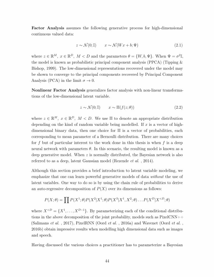
Factor Analysis assumes the following generative process for high-dimensionalcontinuous valued data:
𝑧 ∼ 𝒩 (0; I) 𝑥 ∼ 𝒩 (𝑊𝑥+ 𝑏; Ψ) (2.1)
where 𝑧 ∈ R𝑀 , 𝑥 ∈ R𝐷, 𝑀 < 𝐷 and the parameters 𝜃 = {𝑊, 𝑏,Ψ}. When Ψ = 𝜎2I,the model is known as probabilistic principal component analysis (PPCA) (Tipping &Bishop, 1999). The low-dimensional representations recovered under the model maybe shown to converge to the principal components recovered by Principal ComponentAnalysis (PCA) in the limit 𝜎 → 0.
Nonlinear Factor Analysis generalizes factor analysis with non-linear transforma-tions of the low-dimensional latent variable.
𝑧 ∼ 𝒩 (0; I) 𝑥 ∼ Π(𝑓(𝑧; 𝜃)) (2.2)
where 𝑧 ∈ R𝑀 , 𝑥 ∈ R𝐷, 𝑀 < 𝐷. We use Π to denote an appropriate distributiondepending on the kind of random variable being modelled. If 𝑥 is a vector of high-dimensional binary data, then one choice for Π is a vector of probabilities, eachcorresponding to mean parameter of a Bernoulli distribution. There are many choicesfor 𝑓 but of particular interest to the work done in this thesis is when 𝑓 is a deepneural network with parameters 𝜃. In this scenario, the resulting model is known as adeep generative model. When 𝑧 is normally distributed, the Bayesian network is alsoreferred to as a deep, latent Gaussian model (Rezende et al. , 2014).
Although this section provides a brief introduction to latent variable modeling, weemphasize that one can learn powerful generative models of data without the use oflatent variables. One way to do so is by using the chain rule of probabilities to derivean auto-regressive decomposition of 𝑃 (𝑋) over its dimensions as follows:
𝑃 (𝑋; 𝜃) =∏︁
𝑃 (𝑋1; 𝜃)𝑃 (𝑋2|𝑋1; 𝜃)𝑃 (𝑋3|𝑋1, 𝑋2; 𝜃) . . . 𝑃 (𝑋𝐷|𝑋<𝐷; 𝜃)
where 𝑋<𝐷 = {𝑋1, . . . , 𝑋𝐷−1}. By parameterizing each of the conditional distribu-tions in the above decomposition of the joint probability, models such as PixelCNN++(Salimans et al. , 2017), PixelRNN (Oord et al. , 2016a) and Wavenet (Oord et al. ,2016b) obtain impressive results when modelling high dimensional data such as imagesand speech.
Having discussed the various choices a practitioner has to parameterize a Bayesian
44
network for both supervised and unsupervised learning problems, we turn to thequestion of estimating the parameters, or learning from data.
2.3.2 Learning
There are several guiding principles to learning the parameters of graphical models.We highlight three of them here. In each case, we will assume access to a dataset𝒟 = {𝑋1, 𝑋2, . . . , 𝑋𝑛} where 𝑋𝑖 is the realization (or sample) from a parametericdistribution of random variable 𝑋 driven by an unknown set of parameters 𝜃.
The method of moments reduces the problem of estimating the parameters ofa probability distribution into one of solving a system of equations. This methodrelies on uncovering the parameters governing a distribution via the moments of thedistribution. The 𝑘th moment can be expressed as: 𝜇𝑘 = E[𝑋𝑘]. Intuitively, momentsquantify the shape of a distribution. For example, the first moment of a distribution isthe mean (the average value that random variables under that distribution take), thesecond is the variance (the degree to which the distribution spreads about the mean),the third is the skewness (how tilted the distribution is) and the fourth moment isthe kurtosis (the degree of peakiness of a distribution). For many distributions themoments may be expressed as a function of 𝜃, the parameters of the distribution.Therefore, given (1) sufficiently many expressions of moments of the distributionusing 𝜃 and (2) empirical estimates of each moment obtained using 𝒟, we can solvefor 𝜃 using 𝑘 systems of equations of the form 𝜇𝑘 = E[𝑋𝑘]. The complexity of theparametric distribution dictates the number of moments required to estimate 𝜃. Forsamples drawn from a univariate Bernoulli random variable, a single moment suffices.More moments are necessary to estimate the parameters from distributions impliedunder certain classes of Bayesian networks such as Mixture Models (Anandkumaret al. , 2012), Noisy Or networks (Jernite et al. , 2013; Halpern & Sontag, 2013) andHidden Markov Models (Hsu et al. , 2012).
Comparative density estimation uses comparisons between a model’s predictionand observations from a dataset as a means to estimate model parameters. While theunderlying goal of this methodology is to compare the distribution of data under amodel with the true data distribution, in practice a variety of techniques are used tosidestep our lack of access to the latter, and in some cases the former. For example,(Dziugaite et al. , 2015; Li et al. , 2015b) derive gradient updates to 𝜃 based on howwell the statistics of samples from a Bayesian network compare to the statistics from
45
the data distribution in a Reproducing Kernel Hilbert Space (RKHS). Generativeadversarial networks (Goodfellow et al. , 2014), derive gradients to 𝜃 using an auxiliarymodel (called a discriminator) to decide via classification if the samples under thegenerative model can be distinguished from samples in the dataset. A characteristicfeature of this class of learning algorithms is that it is capable of operating in theabsence of a parametric specification for the distribution of 𝑋. Models that one cansample from, but not necessarily evaluate the likelihood of, are often referred to asimplicit generative models. We refer the reader to (Mohamed & Lakshminarayanan,2016) for an overview of various techniques for learning implicit generative modelsand their relationship to one another.
Maximum likelihood estimation turns parameter estimation into an optimizationproblem. Specifically, given 𝒟, the goal is to solve the following optimization:
max𝜃
𝑁∏︁
𝑖=1
𝑝(𝑋𝑖; 𝜃)
⏟ ⏞ likelihood of observing 𝒟
and find model parameters 𝜃 such that the probability of observing 𝒟 is as high aspossible. In practice, we often use the logarithmic transformation of the probabilitydensity function of the dataset yielding the following optimization problem:
max𝜃
log𝑁∏︁
𝑖=1
𝑝(𝑋𝑖; 𝜃) = max𝜃
𝑁∑︁
𝑖=1
log 𝑝(𝑋𝑖; 𝜃)⏟ ⏞ log-likelihood of 𝒟
2.3.3 Variational learning of latent variable models
For many classes of supervised and unsupervised models discussed above, the log-likelihood is a differentiable function of 𝜃, the model parameters. Consequently,the optimization problem max𝜃
∑︀𝑁𝑖=1 log 𝑝(𝑋𝑖; 𝜃) or max𝜃
∑︀𝑁𝑖=1 log 𝑝(𝑌𝑖|𝑋𝑖; 𝜃) may be
solved via stochastic gradient ascent. But this is not always the case. Learning can bechallenging in latent variable models like those in Figure 2-3 (right) and will be thefocus of this section where we consider learning parameters 𝜃 from a single datapoint𝑋 = 𝑥.
log 𝑝(𝑥; 𝜃) = log
∫︁
𝑧
𝑝(𝑥|𝑧; 𝜃)𝑝(𝑧; 𝜃)𝑑𝑧 (2.3)
46
For models such as linear factor analysis, we can derive an analytic expression for theintegral in Equation 2.3 as a function of the parameters 𝜃.
However, when 𝑝(𝑥|𝑧; 𝜃) is a non-linear function, the integral inside the logarithm isintractable. We therefore must resort to approximations to evaluate the log-likelihood.So how can we learn if the function that we use to evaluate the quality of a models’ fitto data is not tractable? We use a surrogate to the likelihood function, in particular,a lower bound to it. In order to construct a lower bound to the likelihood function,we will require access to an auxillary distribution over the latent variables 𝑞(𝑧).
log 𝑝(𝑥; 𝜃) = log
∫︁
𝑧
𝑝(𝑥, 𝑧; 𝜃)𝑑𝑧 = log
∫︁
𝑧
𝑞(𝑧)𝑝(𝑥, 𝑧; 𝜃)
𝑞(𝑧)𝑑𝑧
≥∫︁
𝑧
𝑞(𝑧) log𝑝(𝑥, 𝑧; 𝜃)
𝑞(𝑧)(2.4)
= E𝑞(𝑧)[log 𝑝(𝑥, 𝑧; 𝜃)] + H(𝑞(𝑧))⏟ ⏞ ℒ(𝑥,𝑞(𝑧);𝜃)
(2.5)
where Equation 2.4 is due to Jensen’s Inequality. The distribution 𝑞(𝑧) is known as thevariational distribution and the lower bound in Equation 2.5 is called the variationallower bound or the evidence lower bound (ELBO). Note that while Equation 2.3 hadan expectation inside the log, Equation 2.5 has the expectation outside. Consequently,as long as we can evaluate the entropy of the variational distribution and the log-probability of the joint distribution log 𝑝(𝑥, 𝑧; 𝜃), we may use Monte-Carlo samplingto obtain an unbiased estimate of the lower-bound. If the resulting estimate isdifferentiable, then we can learn the model parameters via gradient ascent.
The practitioner is free to choose 𝑞(𝑧) and the ELBO is a valid lower bound on thelog-likelihood of data for any choice of 𝑞(𝑧). However, it is easy enough to derive thebest choice for 𝑞(𝑧) by studying at the difference between the log-likelihood and thevariational lower bound:
log 𝑝(𝑥)− ℒ(𝑥, 𝑞(𝑧)) = log 𝑝(𝑥; 𝜃)−∫︁
𝑧
𝑞(𝑧) log𝑝(𝑥, 𝑧)
𝑞(𝑧)
=
∫︁
𝑧
𝑞(𝑧) log 𝑝(𝑥)−∫︁
𝑧
𝑞(𝑧) log𝑝(𝑥, 𝑧)
𝑞(𝑧)
=
∫︁
𝑧
𝑞(𝑧) log𝑝(𝑥)𝑞(𝑧)
𝑝(𝑥, 𝑧)
=
∫︁
𝑧
𝑞(𝑧) log𝑝(𝑥)𝑞(𝑧)
𝑝(𝑧|𝑥)𝑝(𝑥)= KL(𝑞(𝑧)||𝑝(𝑧|𝑥)) (2.6)
47
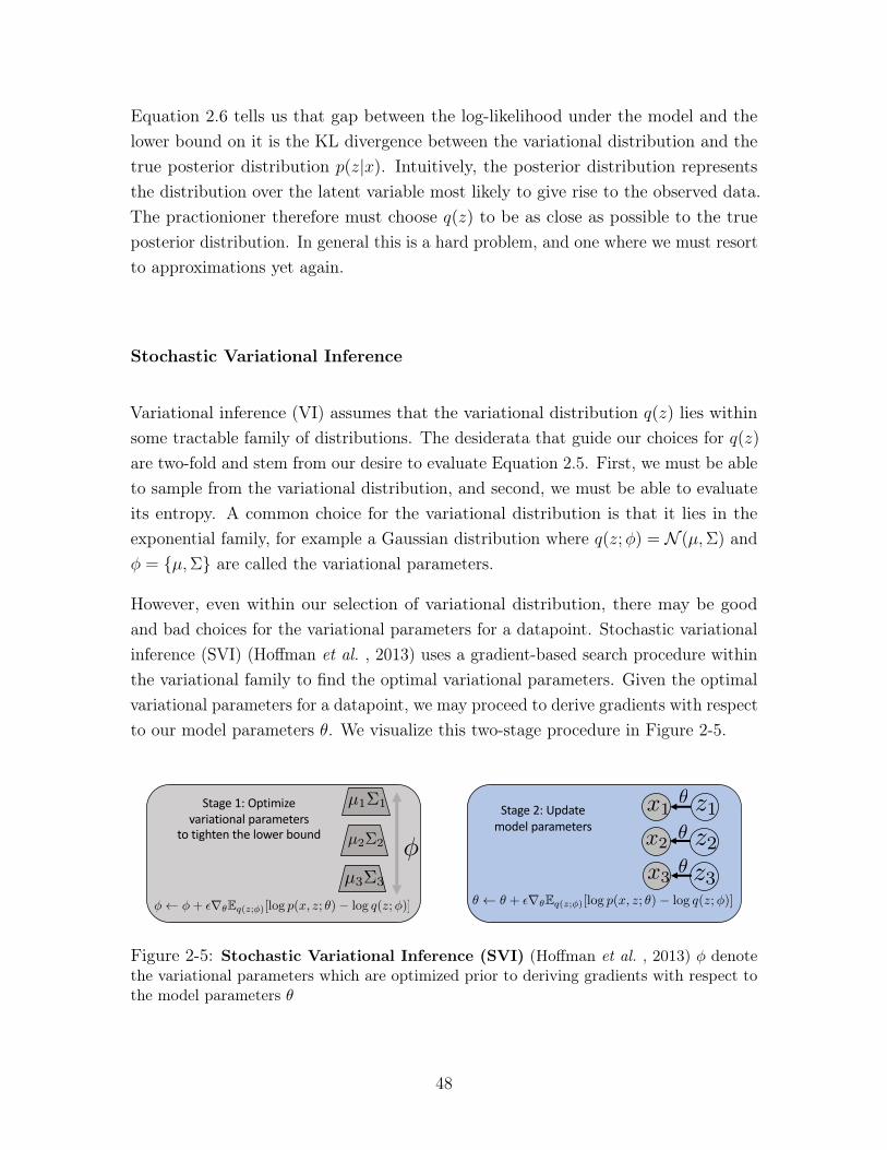
Equation 2.6 tells us that gap between the log-likelihood under the model and thelower bound on it is the KL divergence between the variational distribution and thetrue posterior distribution 𝑝(𝑧|𝑥). Intuitively, the posterior distribution representsthe distribution over the latent variable most likely to give rise to the observed data.The practionioner therefore must choose 𝑞(𝑧) to be as close as possible to the trueposterior distribution. In general this is a hard problem, and one where we must resortto approximations yet again.
Stochastic Variational Inference
Variational inference (VI) assumes that the variational distribution 𝑞(𝑧) lies withinsome tractable family of distributions. The desiderata that guide our choices for 𝑞(𝑧)are two-fold and stem from our desire to evaluate Equation 2.5. First, we must be ableto sample from the variational distribution, and second, we must be able to evaluateits entropy. A common choice for the variational distribution is that it lies in theexponential family, for example a Gaussian distribution where 𝑞(𝑧;𝜑) = 𝒩 (𝜇,Σ) and𝜑 = {𝜇,Σ} are called the variational parameters.
However, even within our selection of variational distribution, there may be goodand bad choices for the variational parameters for a datapoint. Stochastic variationalinference (SVI) (Hoffman et al. , 2013) uses a gradient-based search procedure withinthe variational family to find the optimal variational parameters. Given the optimalvariational parameters for a datapoint, we may proceed to derive gradients with respectto our model parameters 𝜃. We visualize this two-stage procedure in Figure 2-5.
µ1⌃1
<latexit sha1_base64="XcJc816Esyn6ky31dd/dosLchtQ=">AAAB9HicbVBNS8NAEJ34WetX1aOXxSJ4KokU9Fj04rGi/YAmhM120y7d3cTdTaGE/g4vHhTx6o/x5r9x2+agrQ8GHu/NMDMvSjnTxnW/nbX1jc2t7dJOeXdv/+CwcnTc1kmmCG2RhCeqG2FNOZO0ZZjhtJsqikXEaSca3c78zpgqzRL5aCYpDQQeSBYzgo2VAl9koec/sIHAoRdWqm7NnQOtEq8gVSjQDCtffj8hmaDSEI617nluaoIcK8MIp9Oyn2maYjLCA9qzVGJBdZDPj56ic6v0UZwoW9Kgufp7IsdC64mIbKfAZqiXvZn4n9fLTHwd5EymmaGSLBbFGUcmQbMEUJ8pSgyfWIKJYvZWRIZYYWJsTmUbgrf88ippX9a8eq1+X682boo4SnAKZ3ABHlxBA+6gCS0g8ATP8Apvzth5cd6dj0XrmlPMnMAfOJ8/Hn2Rrg==</latexit>
µ2⌃2
<latexit sha1_base64="kL14Z5YngAsUUVG8+NZZMaQtoUg=">AAAB9HicbVDLSgNBEOyNrxhfUY9eBoPgKeyGgB6DXjxGNA/ILsvsZDYZMjO7zswGwpLv8OJBEa9+jDf/xsnjoIkFDUVVN91dUcqZNq777RQ2Nre2d4q7pb39g8Oj8vFJWyeZIrRFEp6oboQ15UzSlmGG026qKBYRp51odDvzO2OqNEvko5mkNBB4IFnMCDZWCnyRhTX/gQ0EDmthueJW3TnQOvGWpAJLNMPyl99PSCaoNIRjrXuem5ogx8owwum05GeappiM8ID2LJVYUB3k86On6MIqfRQnypY0aK7+nsix0HoiItspsBnqVW8m/uf1MhNfBzmTaWaoJItFccaRSdAsAdRnihLDJ5Zgopi9FZEhVpgYm1PJhuCtvrxO2rWqV6/W7+uVxs0yjiKcwTlcggdX0IA7aEILCDzBM7zCmzN2Xpx352PRWnCWM6fwB87nDyGNkbA=</latexit>
µ3⌃3
<latexit sha1_base64="a5nro/iDLWbDJRiqw5Ysst+HgyU=">AAAB9HicbVBNSwMxEJ2tX7V+VT16CRbBU9nVgh6LXjxWtB/QXZZsmm1Dk+yaZAul9Hd48aCIV3+MN/+NabsHbX0w8Hhvhpl5UcqZNq777RTW1jc2t4rbpZ3dvf2D8uFRSyeZIrRJEp6oToQ15UzSpmGG006qKBYRp+1oeDvz2yOqNEvkoxmnNBC4L1nMCDZWCnyRhZf+A+sLHF6G5YpbdedAq8TLSQVyNMLyl99LSCaoNIRjrbuem5pggpVhhNNpyc80TTEZ4j7tWiqxoDqYzI+eojOr9FCcKFvSoLn6e2KChdZjEdlOgc1AL3sz8T+vm5n4OpgwmWaGSrJYFGccmQTNEkA9pigxfGwJJorZWxEZYIWJsTmVbAje8surpHVR9WrV2n2tUr/J4yjCCZzCOXhwBXW4gwY0gcATPMMrvDkj58V5dz4WrQUnnzmGP3A+fwAknZGy</latexit>
Stage 1: Optimizevariational parameters
to tighten the lower bound�
<latexit sha1_base64="JRZt2Euh1LfHOoI6wpWNn5kH6kc=">AAAB7HicbVBNS8NAEJ3Ur1q/qh69LBbBU0mkoMeiF48VTFtoQ9lsN+3SzSbsToQS+hu8eFDEqz/Im//GbZuDtj4YeLw3w8y8MJXCoOt+O6WNza3tnfJuZW//4PCoenzSNkmmGfdZIhPdDanhUijuo0DJu6nmNA4l74STu7nfeeLaiEQ94jTlQUxHSkSCUbSS30/HggyqNbfuLkDWiVeQGhRoDapf/WHCspgrZJIa0/PcFIOcahRM8lmlnxmeUjahI96zVNGYmyBfHDsjF1YZkijRthSShfp7IqexMdM4tJ0xxbFZ9ebif14vw+gmyIVKM+SKLRdFmSSYkPnnZCg0ZyinllCmhb2VsDHVlKHNp2JD8FZfXiftq7rXqDceGrXmbRFHGc7gHC7Bg2towj20wAcGAp7hFd4c5bw4787HsrXkFDOn8AfO5w9s1Y5w</latexit>
x1
<latexit sha1_base64="3c+R7TUljyGse9TtnSD6PbvAzD0=">AAAB6nicbVBNS8NAEJ3Ur1q/qh69LBbBU0mkoMeiF48V7Qe0oWy2k3bpZhN2N2IJ/QlePCji1V/kzX/jts1BWx8MPN6bYWZekAiujet+O4W19Y3NreJ2aWd3b/+gfHjU0nGqGDZZLGLVCahGwSU2DTcCO4lCGgUC28H4Zua3H1FpHssHM0nQj+hQ8pAzaqx0/9T3+uWKW3XnIKvEy0kFcjT65a/eIGZphNIwQbXuem5i/Iwqw5nAaamXakwoG9Mhdi2VNELtZ/NTp+TMKgMSxsqWNGSu/p7IaKT1JApsZ0TNSC97M/E/r5ua8MrPuExSg5ItFoWpICYms7/JgCtkRkwsoUxxeythI6ooMzadkg3BW355lbQuql6tWrurVerXeRxFOIFTOAcPLqEOt9CAJjAYwjO8wpsjnBfn3flYtBacfOYY/sD5/AEN9o2n</latexit>
x2
<latexit sha1_base64="o3wFLFaKyKBrwbQ6JfdiLDWtk1E=">AAAB6nicbVBNS8NAEJ3Ur1q/qh69LBbBU0lKQY9FLx4r2lZoQ9lsN+3SzSbsTsQS+hO8eFDEq7/Im//GbZuDtj4YeLw3w8y8IJHCoOt+O4W19Y3NreJ2aWd3b/+gfHjUNnGqGW+xWMb6IaCGS6F4CwVK/pBoTqNA8k4wvp75nUeujYjVPU4S7kd0qEQoGEUr3T31a/1yxa26c5BV4uWkAjma/fJXbxCzNOIKmaTGdD03QT+jGgWTfFrqpYYnlI3pkHctVTTixs/mp07JmVUGJIy1LYVkrv6eyGhkzCQKbGdEcWSWvZn4n9dNMbz0M6GSFLlii0VhKgnGZPY3GQjNGcqJJZRpYW8lbEQ1ZWjTKdkQvOWXV0m7VvXq1fptvdK4yuMowgmcwjl4cAENuIEmtIDBEJ7hFd4c6bw4787HorXg5DPH8AfO5w8Peo2o</latexit>
x3
<latexit sha1_base64="2usqR2oczGZrEREbzbs5WH3GM8c=">AAAB6nicbVBNS8NAEJ34WetX1aOXxSJ4KokW9Fj04rGi/YA2lM120y7dbMLuRCyhP8GLB0W8+ou8+W/ctjlo64OBx3szzMwLEikMuu63s7K6tr6xWdgqbu/s7u2XDg6bJk414w0Wy1i3A2q4FIo3UKDk7URzGgWSt4LRzdRvPXJtRKwecJxwP6IDJULBKFrp/ql30SuV3Yo7A1kmXk7KkKPeK311+zFLI66QSWpMx3MT9DOqUTDJJ8VuanhC2YgOeMdSRSNu/Gx26oScWqVPwljbUkhm6u+JjEbGjKPAdkYUh2bRm4r/eZ0Uwys/EypJkSs2XxSmkmBMpn+TvtCcoRxbQpkW9lbChlRThjadog3BW3x5mTTPK161Ur2rlmvXeRwFOIYTOAMPLqEGt1CHBjAYwDO8wpsjnRfn3fmYt644+cwR/IHz+QMQ/o2p</latexit>
z1
<latexit sha1_base64="f4JAkaJV4cmKQlTHc1bgJFYupSE=">AAAB6nicbVBNS8NAEJ3Ur1q/qh69LBbBU0mkoMeiF48V7Qe0oWy2k3bpZhN2N0IN/QlePCji1V/kzX/jts1BWx8MPN6bYWZekAiujet+O4W19Y3NreJ2aWd3b/+gfHjU0nGqGDZZLGLVCahGwSU2DTcCO4lCGgUC28H4Zua3H1FpHssHM0nQj+hQ8pAzaqx0/9T3+uWKW3XnIKvEy0kFcjT65a/eIGZphNIwQbXuem5i/Iwqw5nAaamXakwoG9Mhdi2VNELtZ/NTp+TMKgMSxsqWNGSu/p7IaKT1JApsZ0TNSC97M/E/r5ua8MrPuExSg5ItFoWpICYms7/JgCtkRkwsoUxxeythI6ooMzadkg3BW355lbQuql6tWrurVerXeRxFOIFTOAcPLqEOt9CAJjAYwjO8wpsjnBfn3flYtBacfOYY/sD5/AERAo2p</latexit>
z2
<latexit sha1_base64="FqpP9uCOdABFOj14AIByasx7unA=">AAAB6nicbVBNS8NAEJ3Ur1q/qh69LBbBU0lKQY9FLx4r2lZoQ9lsN+3SzSbsToQa+hO8eFDEq7/Im//GbZuDtj4YeLw3w8y8IJHCoOt+O4W19Y3NreJ2aWd3b/+gfHjUNnGqGW+xWMb6IaCGS6F4CwVK/pBoTqNA8k4wvp75nUeujYjVPU4S7kd0qEQoGEUr3T31a/1yxa26c5BV4uWkAjma/fJXbxCzNOIKmaTGdD03QT+jGgWTfFrqpYYnlI3pkHctVTTixs/mp07JmVUGJIy1LYVkrv6eyGhkzCQKbGdEcWSWvZn4n9dNMbz0M6GSFLlii0VhKgnGZPY3GQjNGcqJJZRpYW8lbEQ1ZWjTKdkQvOWXV0m7VvXq1fptvdK4yuMowgmcwjl4cAENuIEmtIDBEJ7hFd4c6bw4787HorXg5DPH8AfO5w8Sho2q</latexit>
z3
<latexit sha1_base64="5/sih4utI9Qflouo3SvzdI1+aqg=">AAAB6nicbVBNS8NAEJ34WetX1aOXxSJ4KokW9Fj04rGi/YA2lM120i7dbMLuRqihP8GLB0W8+ou8+W/ctjlo64OBx3szzMwLEsG1cd1vZ2V1bX1js7BV3N7Z3dsvHRw2dZwqhg0Wi1i1A6pRcIkNw43AdqKQRoHAVjC6mfqtR1Sax/LBjBP0IzqQPOSMGivdP/UueqWyW3FnIMvEy0kZctR7pa9uP2ZphNIwQbXueG5i/Iwqw5nASbGbakwoG9EBdiyVNELtZ7NTJ+TUKn0SxsqWNGSm/p7IaKT1OApsZ0TNUC96U/E/r5Oa8MrPuExSg5LNF4WpICYm079JnytkRowtoUxxeythQ6ooMzadog3BW3x5mTTPK161Ur2rlmvXeRwFOIYTOAMPLqEGt1CHBjAYwDO8wpsjnBfn3fmYt644+cwR/IHz+QMUCo2r</latexit>
Stage 2: Updatemodel parameters
✓
<latexit sha1_base64="IUo58iXthkKcpWuwk5473IAm0y4=">AAAB7XicbVDLSgNBEOz1GeMr6tHLYBA8hV0J6DHoxWME84BkCbOTSTJmdmaZ6RXCkn/w4kERr/6PN//GSbIHTSxoKKq66e6KEiks+v63t7a+sbm1Xdgp7u7tHxyWjo6bVqeG8QbTUpt2RC2XQvEGCpS8nRhO40jyVjS+nfmtJ26s0OoBJwkPYzpUYiAYRSc1uzjiSHulsl/x5yCrJMhJGXLUe6Wvbl+zNOYKmaTWdgI/wTCjBgWTfFrsppYnlI3pkHccVTTmNszm107JuVP6ZKCNK4Vkrv6eyGhs7SSOXGdMcWSXvZn4n9dJcXAdZkIlKXLFFosGqSSoyex10heGM5QTRygzwt1K2IgaytAFVHQhBMsvr5LmZSWoVqr31XLtJo+jAKdwBhcQwBXU4A7q0AAGj/AMr/Dmae/Fe/c+Fq1rXj5zAn/gff4Apj2PLw==</latexit>
✓ ✓ + ✏r✓Eq(z;�)[log p(x, z; ✓)� log q(z;�)]
<latexit sha1_base64="VNSAN2Rev63QgfgbISmA8BF4dAM=">AAACVXicbVFdaxQxFM2Mtdb1o6s++hJchC3qMlMWKvhSKoKPFdy2sBmGTPbObmgmicmdtuswf7IvxX/ii2B2dhFtPRA4nHMuyT0prJIek+RHFN/bur/9YOdh79HjJ093+8+en3hTOwETYZRxZwX3oKSGCUpUcGYd8KpQcFqcf1z5pxfgvDT6Ky4tZBWfa1lKwTFIeV8xXABypqBE7py5pGuBvqEMrJfKaMo0LxTPm7XTUlZxXBRF86nNm2/D7x+YXci9dsqUmVM7vHoblC65966T/kSyvD9IRkkHepekGzIgGxzn/Ws2M6KuQKNQ3PtpmljMGu5QCgVtj9UeLBfnfA7TQDWvwGdN10pLXwdlRkvjwtFIO/XviYZX3i+rIiRXC/nb3kr8nzetsXyfNVLbGkGL9UVlrSgauqqYzqQDgWoZCBdOhrdSseCOCwwf0QslpLdXvktO9kfpeDT+Mh4cHm3q2CEvySsyJCk5IIfkMzkmEyLINfkZRVEc3US/4q14ex2No83MC/IP4t3flP2zvA==</latexit>
� �+ ✏r✓Eq(z;�)[log p(x, z; ✓)� log q(z;�)]
<latexit sha1_base64="5jdeHcfc6eSdmW/aSz7bXarsyWs=">AAACUXicbVFdaxQxFM1O/ahbtas++hJchC3qMiMLCr6USsHHCm5b2AxDJntnJzSTxOSOug7zF33QJ/9HX3xQzEwX0dYLgZNzzuXmnuRWSY9x/H0QbV27fuPm9q3hzu07d3dH9+4fe1M7AXNhlHGnOfegpIY5SlRwah3wKldwkp+97vSTD+C8NPodri2kFV9pWUjBMVDZqGS2lExBgdw585F2V/qEMrBeKqMp0zxXPGsYloC8paziWOZ5c9hmzfvJ51edf69dMGVW1E4+PQ1M79x71lN/LGk2GsfTuC96FSQbMCabOspGX9nSiLoCjUJx7xdJbDFtuEMpFLRDVnuwXJzxFSwC1LwCnzZ9Ii19HJglLYwLRyPt2b87Gl55v67y4OwW8pe1jvyftqixeJk2UtsaQYuLQUWtKBraxUuX0oFAtQ6ACyfDW6koueMCwycMQwjJ5ZWvguPn02Q2nb2djfcPNnFsk4fkEZmQhLwg++QNOSJzIsgXck5+kl+Db4MfEYmiC2s02PQ8IP9UtPMbHKGz6A==</latexit>
Figure 2-5: Stochastic Variational Inference (SVI) (Hoffman et al. , 2013) 𝜑 denotethe variational parameters which are optimized prior to deriving gradients with respect tothe model parameters 𝜃
48
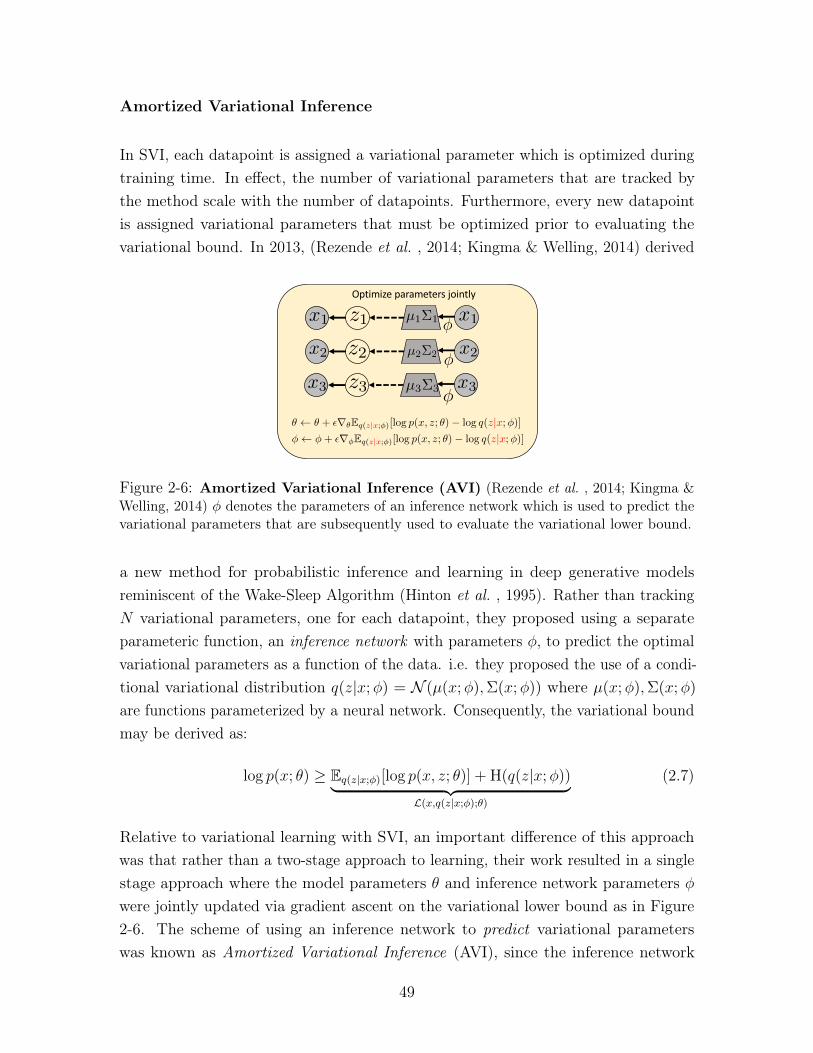
Amortized Variational Inference
In SVI, each datapoint is assigned a variational parameter which is optimized duringtraining time. In effect, the number of variational parameters that are tracked bythe method scale with the number of datapoints. Furthermore, every new datapointis assigned variational parameters that must be optimized prior to evaluating thevariational bound. In 2013, (Rezende et al. , 2014; Kingma & Welling, 2014) derived
x1
<latexit sha1_base64="3c+R7TUljyGse9TtnSD6PbvAzD0=">AAAB6nicbVBNS8NAEJ3Ur1q/qh69LBbBU0mkoMeiF48V7Qe0oWy2k3bpZhN2N2IJ/QlePCji1V/kzX/jts1BWx8MPN6bYWZekAiujet+O4W19Y3NreJ2aWd3b/+gfHjU0nGqGDZZLGLVCahGwSU2DTcCO4lCGgUC28H4Zua3H1FpHssHM0nQj+hQ8pAzaqx0/9T3+uWKW3XnIKvEy0kFcjT65a/eIGZphNIwQbXuem5i/Iwqw5nAaamXakwoG9Mhdi2VNELtZ/NTp+TMKgMSxsqWNGSu/p7IaKT1JApsZ0TNSC97M/E/r5ua8MrPuExSg5ItFoWpICYms7/JgCtkRkwsoUxxeythI6ooMzadkg3BW355lbQuql6tWrurVerXeRxFOIFTOAcPLqEOt9CAJjAYwjO8wpsjnBfn3flYtBacfOYY/sD5/AEN9o2n</latexit>
z1
<latexit sha1_base64="f4JAkaJV4cmKQlTHc1bgJFYupSE=">AAAB6nicbVBNS8NAEJ3Ur1q/qh69LBbBU0mkoMeiF48V7Qe0oWy2k3bpZhN2N0IN/QlePCji1V/kzX/jts1BWx8MPN6bYWZekAiujet+O4W19Y3NreJ2aWd3b/+gfHjU0nGqGDZZLGLVCahGwSU2DTcCO4lCGgUC28H4Zua3H1FpHssHM0nQj+hQ8pAzaqx0/9T3+uWKW3XnIKvEy0kFcjT65a/eIGZphNIwQbXuem5i/Iwqw5nAaamXakwoG9Mhdi2VNELtZ/NTp+TMKgMSxsqWNGSu/p7IaKT1JApsZ0TNSC97M/E/r5ua8MrPuExSg5ItFoWpICYms7/JgCtkRkwsoUxxeythI6ooMzadkg3BW355lbQuql6tWrurVerXeRxFOIFTOAcPLqEOt9CAJjAYwjO8wpsjnBfn3flYtBacfOYY/sD5/AERAo2p</latexit>
x1
<latexit sha1_base64="3c+R7TUljyGse9TtnSD6PbvAzD0=">AAAB6nicbVBNS8NAEJ3Ur1q/qh69LBbBU0mkoMeiF48V7Qe0oWy2k3bpZhN2N2IJ/QlePCji1V/kzX/jts1BWx8MPN6bYWZekAiujet+O4W19Y3NreJ2aWd3b/+gfHjU0nGqGDZZLGLVCahGwSU2DTcCO4lCGgUC28H4Zua3H1FpHssHM0nQj+hQ8pAzaqx0/9T3+uWKW3XnIKvEy0kFcjT65a/eIGZphNIwQbXuem5i/Iwqw5nAaamXakwoG9Mhdi2VNELtZ/NTp+TMKgMSxsqWNGSu/p7IaKT1JApsZ0TNSC97M/E/r5ua8MrPuExSg5ItFoWpICYms7/JgCtkRkwsoUxxeythI6ooMzadkg3BW355lbQuql6tWrurVerXeRxFOIFTOAcPLqEOt9CAJjAYwjO8wpsjnBfn3flYtBacfOYY/sD5/AEN9o2n</latexit>
µ1⌃1
<latexit sha1_base64="XcJc816Esyn6ky31dd/dosLchtQ=">AAAB9HicbVBNS8NAEJ34WetX1aOXxSJ4KokU9Fj04rGi/YAmhM120y7d3cTdTaGE/g4vHhTx6o/x5r9x2+agrQ8GHu/NMDMvSjnTxnW/nbX1jc2t7dJOeXdv/+CwcnTc1kmmCG2RhCeqG2FNOZO0ZZjhtJsqikXEaSca3c78zpgqzRL5aCYpDQQeSBYzgo2VAl9koec/sIHAoRdWqm7NnQOtEq8gVSjQDCtffj8hmaDSEI617nluaoIcK8MIp9Oyn2maYjLCA9qzVGJBdZDPj56ic6v0UZwoW9Kgufp7IsdC64mIbKfAZqiXvZn4n9fLTHwd5EymmaGSLBbFGUcmQbMEUJ8pSgyfWIKJYvZWRIZYYWJsTmUbgrf88ippX9a8eq1+X682boo4SnAKZ3ABHlxBA+6gCS0g8ATP8Apvzth5cd6dj0XrmlPMnMAfOJ8/Hn2Rrg==</latexit>
µ2⌃2
<latexit sha1_base64="kL14Z5YngAsUUVG8+NZZMaQtoUg=">AAAB9HicbVDLSgNBEOyNrxhfUY9eBoPgKeyGgB6DXjxGNA/ILsvsZDYZMjO7zswGwpLv8OJBEa9+jDf/xsnjoIkFDUVVN91dUcqZNq777RQ2Nre2d4q7pb39g8Oj8vFJWyeZIrRFEp6oboQ15UzSlmGG026qKBYRp51odDvzO2OqNEvko5mkNBB4IFnMCDZWCnyRhTX/gQ0EDmthueJW3TnQOvGWpAJLNMPyl99PSCaoNIRjrXuem5ogx8owwum05GeappiM8ID2LJVYUB3k86On6MIqfRQnypY0aK7+nsix0HoiItspsBnqVW8m/uf1MhNfBzmTaWaoJItFccaRSdAsAdRnihLDJ5Zgopi9FZEhVpgYm1PJhuCtvrxO2rWqV6/W7+uVxs0yjiKcwTlcggdX0IA7aEILCDzBM7zCmzN2Xpx352PRWnCWM6fwB87nDyGNkbA=</latexit>
µ3⌃3
<latexit sha1_base64="a5nro/iDLWbDJRiqw5Ysst+HgyU=">AAAB9HicbVBNSwMxEJ2tX7V+VT16CRbBU9nVgh6LXjxWtB/QXZZsmm1Dk+yaZAul9Hd48aCIV3+MN/+NabsHbX0w8Hhvhpl5UcqZNq777RTW1jc2t4rbpZ3dvf2D8uFRSyeZIrRJEp6oToQ15UzSpmGG006qKBYRp+1oeDvz2yOqNEvkoxmnNBC4L1nMCDZWCnyRhZf+A+sLHF6G5YpbdedAq8TLSQVyNMLyl99LSCaoNIRjrbuem5pggpVhhNNpyc80TTEZ4j7tWiqxoDqYzI+eojOr9FCcKFvSoLn6e2KChdZjEdlOgc1AL3sz8T+vm5n4OpgwmWaGSrJYFGccmQTNEkA9pigxfGwJJorZWxEZYIWJsTmVbAje8surpHVR9WrV2n2tUr/J4yjCCZzCOXhwBXW4gwY0gcATPMMrvDkj58V5dz4WrQUnnzmGP3A+fwAknZGy</latexit>
x2
<latexit sha1_base64="o3wFLFaKyKBrwbQ6JfdiLDWtk1E=">AAAB6nicbVBNS8NAEJ3Ur1q/qh69LBbBU0lKQY9FLx4r2lZoQ9lsN+3SzSbsTsQS+hO8eFDEq7/Im//GbZuDtj4YeLw3w8y8IJHCoOt+O4W19Y3NreJ2aWd3b/+gfHjUNnGqGW+xWMb6IaCGS6F4CwVK/pBoTqNA8k4wvp75nUeujYjVPU4S7kd0qEQoGEUr3T31a/1yxa26c5BV4uWkAjma/fJXbxCzNOIKmaTGdD03QT+jGgWTfFrqpYYnlI3pkHctVTTixs/mp07JmVUGJIy1LYVkrv6eyGhkzCQKbGdEcWSWvZn4n9dNMbz0M6GSFLlii0VhKgnGZPY3GQjNGcqJJZRpYW8lbEQ1ZWjTKdkQvOWXV0m7VvXq1fptvdK4yuMowgmcwjl4cAENuIEmtIDBEJ7hFd4c6bw4787HorXg5DPH8AfO5w8Peo2o</latexit>
x3
<latexit sha1_base64="2usqR2oczGZrEREbzbs5WH3GM8c=">AAAB6nicbVBNS8NAEJ34WetX1aOXxSJ4KokW9Fj04rGi/YA2lM120y7dbMLuRCyhP8GLB0W8+ou8+W/ctjlo64OBx3szzMwLEikMuu63s7K6tr6xWdgqbu/s7u2XDg6bJk414w0Wy1i3A2q4FIo3UKDk7URzGgWSt4LRzdRvPXJtRKwecJxwP6IDJULBKFrp/ql30SuV3Yo7A1kmXk7KkKPeK311+zFLI66QSWpMx3MT9DOqUTDJJ8VuanhC2YgOeMdSRSNu/Gx26oScWqVPwljbUkhm6u+JjEbGjKPAdkYUh2bRm4r/eZ0Uwys/EypJkSs2XxSmkmBMpn+TvtCcoRxbQpkW9lbChlRThjadog3BW3x5mTTPK161Ur2rlmvXeRwFOIYTOAMPLqEGt1CHBjAYwDO8wpsjnRfn3fmYt644+cwR/IHz+QMQ/o2p</latexit>
z2
<latexit sha1_base64="FqpP9uCOdABFOj14AIByasx7unA=">AAAB6nicbVBNS8NAEJ3Ur1q/qh69LBbBU0lKQY9FLx4r2lZoQ9lsN+3SzSbsToQa+hO8eFDEq7/Im//GbZuDtj4YeLw3w8y8IJHCoOt+O4W19Y3NreJ2aWd3b/+gfHjUNnGqGW+xWMb6IaCGS6F4CwVK/pBoTqNA8k4wvp75nUeujYjVPU4S7kd0qEQoGEUr3T31a/1yxa26c5BV4uWkAjma/fJXbxCzNOIKmaTGdD03QT+jGgWTfFrqpYYnlI3pkHctVTTixs/mp07JmVUGJIy1LYVkrv6eyGhkzCQKbGdEcWSWvZn4n9dNMbz0M6GSFLlii0VhKgnGZPY3GQjNGcqJJZRpYW8lbEQ1ZWjTKdkQvOWXV0m7VvXq1fptvdK4yuMowgmcwjl4cAENuIEmtIDBEJ7hFd4c6bw4787HorXg5DPH8AfO5w8Sho2q</latexit>
z3
<latexit sha1_base64="5/sih4utI9Qflouo3SvzdI1+aqg=">AAAB6nicbVBNS8NAEJ34WetX1aOXxSJ4KokW9Fj04rGi/YA2lM120i7dbMLuRqihP8GLB0W8+ou8+W/ctjlo64OBx3szzMwLEsG1cd1vZ2V1bX1js7BV3N7Z3dsvHRw2dZwqhg0Wi1i1A6pRcIkNw43AdqKQRoHAVjC6mfqtR1Sax/LBjBP0IzqQPOSMGivdP/UueqWyW3FnIMvEy0kZctR7pa9uP2ZphNIwQbXueG5i/Iwqw5nASbGbakwoG9EBdiyVNELtZ7NTJ+TUKn0SxsqWNGSm/p7IaKT1OApsZ0TNUC96U/E/r5Oa8MrPuExSg5LNF4WpICYm079JnytkRowtoUxxeythQ6ooMzadog3BW3x5mTTPK161Ur2rlmvXeRwFOIYTOAMPLqEGt1CHBjAYwDO8wpsjnBfn3fmYt644+cwR/IHz+QMUCo2r</latexit>
Optimize parameters jointly
�
<latexit sha1_base64="JRZt2Euh1LfHOoI6wpWNn5kH6kc=">AAAB7HicbVBNS8NAEJ3Ur1q/qh69LBbBU0mkoMeiF48VTFtoQ9lsN+3SzSbsToQS+hu8eFDEqz/Im//GbZuDtj4YeLw3w8y8MJXCoOt+O6WNza3tnfJuZW//4PCoenzSNkmmGfdZIhPdDanhUijuo0DJu6nmNA4l74STu7nfeeLaiEQ94jTlQUxHSkSCUbSS30/HggyqNbfuLkDWiVeQGhRoDapf/WHCspgrZJIa0/PcFIOcahRM8lmlnxmeUjahI96zVNGYmyBfHDsjF1YZkijRthSShfp7IqexMdM4tJ0xxbFZ9ebif14vw+gmyIVKM+SKLRdFmSSYkPnnZCg0ZyinllCmhb2VsDHVlKHNp2JD8FZfXiftq7rXqDceGrXmbRFHGc7gHC7Bg2towj20wAcGAp7hFd4c5bw4787HsrXkFDOn8AfO5w9s1Y5w</latexit>
✓ ✓ + ✏r✓Eq(z|x;�)[log p(x, z; ✓)� log q(z|x;�)]
� �+ ✏r�Eq(z|x;�)[log p(x, z; ✓)� log q(z|x;�)]
<latexit sha1_base64="h4BPmoGgvH4LbLaO8pnF+IP63Mk=">AAADD3ictVJNi9RAEO3Er3X8mtWjl8Zhl1nUIZEBhb0siuBxBWd3YTqETk9lptlOOnZXdGZj/oEX/4oXD4p49erNf2Mnk4P7gTcLGl6/qke9KioplLQYBL89/9LlK1evbVzv3bh56/ad/ubdA6tLI2AitNLmKOEWlMxhghIVHBUGeJYoOEyOXzT5w3dgrNT5G1wVEGV8nstUCo6Oije9rW2GC0BOmYIUuTH6Pe2Yh5RBYaXSOWU5TxSPq3WmpizjuEiS6mUdV2+HDGGJrZfKwKyuTj4s611WLOROPWVKz2kxXD462V2Ldx631L9UEWO97QadMtX8L7Lk+P9uKO4PglHQBj0Pwg4MSBf7cf8Xm2lRZpCjUNzaaRgUGFXcoBQK6h4rLRRcHPM5TB3MeQY2qtrmNd1yzIym2riXI23ZvxUVz6xdZYmrbMa2Z3MNeVFuWmL6LKpkXpQIuVg3SktFUdPmOOhMGhCoVg5wYaTzSsWCGy7QnVDPLSE8O/J5cPBkFI5H49fjwd7zbh0b5D55QIYkJE/JHnlF9smECO+j99n76n3zP/lf/O/+j3Wp73Wae+RU+D//AJVY/h0=</latexit>
Figure 2-6: Amortized Variational Inference (AVI) (Rezende et al. , 2014; Kingma &Welling, 2014) 𝜑 denotes the parameters of an inference network which is used to predict thevariational parameters that are subsequently used to evaluate the variational lower bound.
a new method for probabilistic inference and learning in deep generative modelsreminiscent of the Wake-Sleep Algorithm (Hinton et al. , 1995). Rather than tracking𝑁 variational parameters, one for each datapoint, they proposed using a separateparameteric function, an inference network with parameters 𝜑, to predict the optimalvariational parameters as a function of the data. i.e. they proposed the use of a condi-tional variational distribution 𝑞(𝑧|𝑥;𝜑) = 𝒩 (𝜇(𝑥;𝜑),Σ(𝑥;𝜑)) where 𝜇(𝑥;𝜑),Σ(𝑥;𝜑)are functions parameterized by a neural network. Consequently, the variational boundmay be derived as:
log 𝑝(𝑥; 𝜃) ≥ E𝑞(𝑧|𝑥;𝜑)[log 𝑝(𝑥, 𝑧; 𝜃)] + H(𝑞(𝑧|𝑥;𝜑))⏟ ⏞ ℒ(𝑥,𝑞(𝑧|𝑥;𝜑);𝜃)
(2.7)
Relative to variational learning with SVI, an important difference of this approachwas that rather than a two-stage approach to learning, their work resulted in a singlestage approach where the model parameters 𝜃 and inference network parameters 𝜑were jointly updated via gradient ascent on the variational lower bound as in Figure2-6. The scheme of using an inference network to predict variational parameterswas known as Amortized Variational Inference (AVI), since the inference network
49
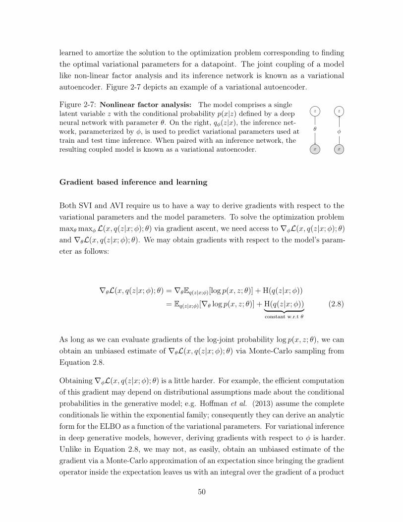
learned to amortize the solution to the optimization problem corresponding to findingthe optimal variational parameters for a datapoint. The joint coupling of a modellike non-linear factor analysis and its inference network is known as a variationalautoencoder. Figure 2-7 depicts an example of a variational autoencoder.
Figure 2-7: Nonlinear factor analysis: The model comprises a singlelatent variable 𝑧 with the conditional probability 𝑝(𝑥|𝑧) defined by a deepneural network with parameter 𝜃. On the right, 𝑞𝜑(𝑧|𝑥), the inference net-work, parameterized by 𝜑, is used to predict variational parameters used attrain and test time inference. When paired with an inference network, theresulting coupled model is known as a variational autoencoder.
𝑧
𝑥
𝜃
𝑧
𝑥
𝜑
Gradient based inference and learning
Both SVI and AVI require us to have a way to derive gradients with respect to thevariational parameters and the model parameters. To solve the optimization problemmax𝜃max𝜑 ℒ(𝑥, 𝑞(𝑧|𝑥;𝜑); 𝜃) via gradient ascent, we need access to ∇𝜑ℒ(𝑥, 𝑞(𝑧|𝑥;𝜑); 𝜃)and ∇𝜃ℒ(𝑥, 𝑞(𝑧|𝑥;𝜑); 𝜃). We may obtain gradients with respect to the model’s param-eter as follows:
∇𝜃ℒ(𝑥, 𝑞(𝑧|𝑥;𝜑); 𝜃) = ∇𝜃E𝑞(𝑧|𝑥;𝜑)[log 𝑝(𝑥, 𝑧; 𝜃)] + H(𝑞(𝑧|𝑥;𝜑))= E𝑞(𝑧|𝑥;𝜑)[∇𝜃 log 𝑝(𝑥, 𝑧; 𝜃)] + H(𝑞(𝑧|𝑥;𝜑))⏟ ⏞
constant w.r.t 𝜃
(2.8)
As long as we can evaluate gradients of the log-joint probability log 𝑝(𝑥, 𝑧; 𝜃), we canobtain an unbiased estimate of ∇𝜃ℒ(𝑥, 𝑞(𝑧|𝑥;𝜑); 𝜃) via Monte-Carlo sampling fromEquation 2.8.
Obtaining ∇𝜑ℒ(𝑥, 𝑞(𝑧|𝑥;𝜑); 𝜃) is a little harder. For example, the efficient computationof this gradient may depend on distributional assumptions made about the conditionalprobabilities in the generative model; e.g. Hoffman et al. (2013) assume the completeconditionals lie within the exponential family; consequently they can derive an analyticform for the ELBO as a function of the variational parameters. For variational inferencein deep generative models, however, deriving gradients with respect to 𝜑 is harder.Unlike in Equation 2.8, we may not, as easily, obtain an unbiased estimate of thegradient via a Monte-Carlo approximation of an expectation since bringing the gradientoperator inside the expectation leaves us with an integral over the gradient of a product
50
of distributions.
To circumvent this issue, (Kingma & Welling, 2014; Rezende et al. , 2014) make useof the reparameterization trick :
E𝑧∼𝒩 (𝜇,Σ)[𝑓(𝑧)] = E𝜖∼𝒩 (0;I)[𝑓(𝜇+𝑅𝜖)]; Σ = 𝑅𝑅𝑇 (2.9)
Crucially, the use of the trick removes the dependence of the expectation on theparameters 𝜑.
∇𝜑ℒ(𝑥, 𝑞(𝑧|𝑥;𝜑); 𝜃) = ∇𝜑E𝑧∼𝑞(𝑧|𝑥;𝜑)[log 𝑝(𝑥, 𝑧; 𝜃)] +∇𝜑H(𝑞(𝑧|𝑥;𝜑))= ∇𝜑E𝑧∼𝒩 (𝜇(𝑥;𝜑),𝑅(𝑥;𝜑)𝑅𝑇 (𝑥;𝜑))[log 𝑝(𝑥, 𝑧; 𝜃)] +∇𝜑H(𝑞(𝑧|𝑥;𝜑))= ∇𝜑E𝜖∼𝒩 (0;I)[log 𝑝(𝑥, 𝜇(𝑥;𝜑) +𝑅(𝑥;𝜑)𝜖; 𝜃)] +∇𝜑H(𝑞(𝑧|𝑥;𝜑))= E𝜖∼𝒩 (0;I)[∇𝜑 log 𝑝(𝑥, 𝜇(𝑥;𝜑) +𝑅(𝑥;𝜑)𝜖; 𝜃)] +∇𝜑H(𝑞(𝑧|𝑥;𝜑))
(2.10)
Where Equation 2.10 now gives us a route to approximate the gradients with respectto 𝜑 via Monte-Carlo sampling.
The reparameterization trick is not the only route to obtain unbiased estimates, andthere is a rich literature surrounding the construction of schemes that permit theapproximation of gradients via Monte-Carlo approximations. When the variationaldistribution is not continuous and/or reparameterizable, one may use the (more generalpurpose) score function estimator (Ranganath et al. , 2013; Mnih & Gregor, 2014) toobtain gradients. Maddison et al. (2016) derive a new family of reparameterizabledistributions, known as the Concrete distribution, that allows for the practitioner toform variational approximations to discrete latent variables. Jankowiak & Obermeyer(2018) derive connections between the reparameterization gradients and solutions ofa transport equation (as in optimal transport). Lee et al. (2018) derive gradientswhen the variational distribution used is non-differentiable. Finally, we refer thereader to Mohamed et al. (2019) for an overview of a variety of techniques to obtainunbiased gradients using Monte-Carlo approximations as well as their use in severalsub-domains of machine learning, with variational inference, being one among them.
51
Overview
We instantiated variational inference as a method for probabilistic inference usedwithin parameter estimation and highlighted Stochastic Variational Inference (SVI)and Amortized Variational Inference. In reality, both are a small part of the richliterature in variational methods for probabilistic inference and we refer the reader to(Jordan et al. , 1999) for a comprehensive overview of the same. Variational inference isnot the only technique capable of approximating the posterior distribution. Techniquessuch as Markov Chain Monte Carlo are capable of drawing samples from the trueposterior distribution in complex latent variable models; however, this remains outsidethe scope of this thesis and we refer the reader to (Neal, 1993) for a broad overview ofMCMC methods for probabilistic inference in graphical models.
2.4 Learning with automatic differentiation
Until now, we have assumed access to the gradients of functions of the log-joint ofthe data and latent variables. But when the conditional probability distributions areparameterized by neural networks, these gradients may be complex, vector valuedfunctions of their inputs. Manually deriving these gradients can prove tedious andcan severely hinder a practitioner’s ability to experiment with different choices ofparameterizations for conditional probabilities in the model. Fortunately, much of themachinery behind the computation of gradients for such functions may be automatedby Automatic Differentiation (AD).
The remarkable successes that deep learning has seen would be all but a pipe dreamwithout automatic differentiation. Academic software such as Theano (Team et al. ,2016) and Torch (Collobert et al. , 2002) led the way for industrial scale frameworkssuch as PyTorch (Paszke et al. , 2017) and Tensorflow (Abadi et al. , 2015) whichallow for deep learning algorithms to scale via the distribution of computation acrossmultiple hardware devices.
At its core, AD allows users to specify a mathematical function in code. The codeis silently instrumented so that when it is executed, intermediate results about theexecution of the function are stored in computer memory. The calculation of derivativesthen proceeds via the chain rule. A thorough review of AD is unnecessary to understandthe context of this thesis and therefore out of scope. However, we point the reader to(Baydin et al. , 2017) for an accessible survey on the topic.
52
2.5 Modeling data with deep generative models
Despite the advances that machine learning has made over the decades, there is muchwe cannot say with certainty.
Inference or parameter estimation? A note on being Bayesian
The background we present on parameter estimation in latent variable models treatlatent variables as first-class citizens whose values we must infer from data. A validquestion then is: why not treat the model parameters 𝜃 as random variables too?Certainly, much of the machinery discussed in the previous sections carries forward andwe can use techniques such as Markov Chain Monte Carlo and Variational Inferenceto pose parameter estimation as probabilistic inference. This is a valid point of viewand for certain problems a desirable one, but one that this thesis does not explore indepth. We refer the reader to (MacKay & Mac Kay, 2003) for an overview of machinelearning from a Bayesian lens.
What makes a good model?
One of the most important question that a modeller must answer is, how to designa probabilistic graphical model. Certainly a good starting point would be to collectall the random variables in the problem at hand – these form the nodes in the graph.Next might be engaging with a domain expert to understand which random variablesare associated with each other, and what drives their association. These form theedges in the graph. However, at this junction, several important questions remain.
Are there latent variables in the problem to consider and account for? How do thelatent variables relate to the observed data, is the interaction linear or non-linear,known or unknown? How can we ever know that we’ve gotten the right model?
There are no right answers to these questions. George Box, a famous statistician iscredited with the saying: “all models are wrong, but some models are useful". Inreality, model development is an iterative process. Machine learning’s successes havebeen as much about using data judiciously as they have been about taking insightsfrom domain experts and operationalizing them with mathematical primitives andincorporating them within graphical models.
53

54
Chapter 3
Gradient based introspection in deepgenerative models
Factor analysis (Spearman, 1904a) is a widely used model in the applied sciences. Thegenerative model assumes the data is a linear function of independent latent variables.In Section 2.3.1 we introduced nonlinear factor analysis where the generative model isparameterized by deep neural networks. When paired with an inference or recognitionnetwork (Hinton et al. , 1995), a parametric function that predicts local variationalparameters from data, such models go by the name of variational autoencoders (VAEs,Kingma et al. , 2014; Rezende et al. , 2014).
One of the reasons that factor analysis has found widespread use is that studying thematrix which maps from the latent variable onto the data characterizes the correlationsthat exist among features. In this chapter, we discuss ways in which we may similarlyintrospect into deep generative models through the use of gradient operators.
3.1 Introduction
The promise of variational autoencoders, and deep generative models, lies in theability to model complex nonlinear data. However it is worth pausing to ask: whatpurpose is served by fitting more powerful generative models? Breiman (2001) arguesthat discriminative modeling falls into two schools of thought: the data modelingand the algorithmic modeling culture. The former advocates the use of models withinterpretable, mechanistic processes while the latter espouses black box techniques
55
with an emphasis on prediction accuracy. Breiman’s arguments also apply to thedivide between deep generative models with complex conditional distributions andsimpler, more interpretable statistical models. Our goal in this chapter will be tobridge this divide.
Consider a classic model such as latent Dirichlet allocation (LDA) (Blei et al. , 2003).It is outperformed in held-out likelihood (Miao et al. , 2016) by deeper generativemodels and assumes a simple probabilistic process for data generation that is unlikelyto hold in reality. Despite its simplicity, its generative semantics lend it a distinctadvantage: interpretability. The word-topic matrix in the LDA allows practitionersto read off what the model has learned about the data. This begs the question weexplore herein: is there a natural way to interpret the generative model when theconditional distributions are parameterized by a deep neural network?
Using unsupervised models of data, there are two kinds of insights one can hope toachieve:
1. Interpreting datapoints: Latent variable models encode our knowledge of thedata generating process within the prior distributions over latent variables. Bystudying variation and patterns in the inferred values of (often low-dimensional)latent variables across a dataset, we may more easily observe salient structurethat exists within a dataset. For example, using T-SNE (Maaten & Hinton, 2008)on the inferred latent representations from a variational autoencoder trained onMNIST (LeCun, 1998) reveals that there are ten clusters, each one correspondingto one of ten digits within the dataset.
2. Interpreting model parameters: Whereas the latent variables may be usedto simplify patterns that differentiate datapoints in a dataset, the parameterswithin latent variable models can also yield insights into patterns that unify databy their inclusion in a dataset. For example, a common use of factor analysisis feature exploration. After learning the generative model in Equation 2.1, wemay inspect the factor loading matrix 𝑊 to study patterns by which featuresof the observation vary according to a latent dimension. By plotting thesefeature representations in latent space we may inspect and discover ambientstructure among features that are shared across all datapoints. This is thepremise underpinning the literature of exploratory factor analysis (Norris &Lecavalier, 2010) and the form of interpretability that we study in this chapter.
Our contribution towards this vision is a simple, easy to implement method to
56
interpret the parameters learned by nonlinear factor analysis. We use the Jacobianof the conditional distribution with respect to latent variables to create embeddings(or Jacobian vectors) of the observational features. Intuitively the Jacobian capturesvariation for each feature of the observations along directions in the vector dimensionallatent space.
Introspection into what the model has learned through the use of embeddings has along history. Landauer et al. (1998) proposed latent semantic analysis, one of theearliest works to create vector space representations of documents. Bengio et al. (2003)and Mikolov et al. (2013a) propose log-linear models to create word-representationsfrom document corpora. Rudolph et al. (2016) describe a family of models to createconditional embeddings where the data are parameterized to lie within the exponentialfamily. In the context of discriminative modeling, Erhan et al. (2009) use gradientinformation to study the patterns with which neurons are activated in a deep neuralnetwork. At the crux of each of the above methods lies the ethos that the inspectionof a model’s parameters via embeddings can yield insights into what the model haslearned about the dataset on hand.
We make use of gradients in the log densities of a statistical model relative to per-datapoint latent variables to capture patterns of interest to practitioners. However,gradient information may also be of use to other downstream models. For example, thederivative of the log-probability of data with respect to the globally shared parametersof a generative model encodes the variability in the input under the generative process.Jaakkola & Haussler (2007) exploit this variability to form a kernel function for adiscriminative classifier using Fisher Score features.1
Generative model: In this chapter, we will consider a generative model of theform shown in Figure 2-7. We observe a set of 𝐷 word-count2 vectors 𝑥1:𝐷, where 𝑥𝑑𝑣denotes the number of times that word index 𝑣 ∈ {1, . . . , 𝑉 } appears in document 𝑑.We assume we are given the total number of words per document 𝑁𝑑 ≡
∑︀𝑣 𝑥𝑑𝑣, and
that 𝑥𝑑 was generated via the following generative process:
𝑧𝑑 ∼ 𝒩 (0, 𝐼); 𝛾(𝑧𝑑) ≡ MLP(𝑧𝑑; 𝜃); (3.1)
𝜇(𝑧𝑑) ≡exp{𝛾(𝑧𝑑)}∑︀𝑣 exp{𝛾(𝑧𝑑)𝑣}
; 𝑥𝑑 ∼ Mult.(𝜇(𝑧𝑑), 𝑁𝑑).
1For some model that parameterizes 𝑝(𝑥; 𝜃), the Fisher score is defined as 𝑈𝑥 = ∇𝜃 log 𝑝(𝑥; 𝜃)2We use word-count in document for the sake of concreteness. Our methodology is generally
applicable to other types of discrete high-dimensional data.
57
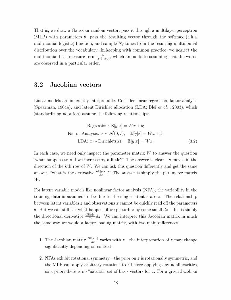
That is, we draw a Gaussian random vector, pass it through a multilayer perceptron(MLP) with parameters 𝜃, pass the resulting vector through the softmax (a.k.a.multinomial logistic) function, and sample 𝑁𝑑 times from the resulting multinomialdistribution over the vocabulary. In keeping with common practice, we neglect themultinomial base measure term 𝑁 !
𝑥1!···𝑥𝑉 !, which amounts to assuming that the words
are observed in a particular order.
3.2 Jacobian vectors
Linear models are inherently interpretable. Consider linear regression, factor analysis(Spearman, 1904a), and latent Dirichlet allocation (LDA; Blei et al. , 2003), which(standardizing notation) assume the following relationships:
Regression: E[𝑦|𝑥] = 𝑊𝑥+ 𝑏;
Factor Analysis: 𝑥 ∼ 𝒩 (0, 𝐼); E[𝑦|𝑥] = 𝑊𝑥+ 𝑏;
LDA: 𝑥 ∼ Dirichlet(𝛼); E[𝑦|𝑥] = 𝑊𝑥. (3.2)
In each case, we need only inspect the parameter matrix 𝑊 to answer the question“what happens to 𝑦 if we increase 𝑥𝑘 a little?” The answer is clear—𝑦 moves in thedirection of the 𝑘th row of 𝑊 . We can ask this question differently and get the sameanswer: “what is the derivative 𝜕E[𝑦|𝑥]
𝜕𝑥?” The answer is simply the parameter matrix
𝑊 .
For latent variable models like nonlinear factor analysis (NFA), the variability in thetraining data is assumed to be due to the single latent state 𝑧. The relationshipbetween latent variables 𝑧 and observations 𝑥 cannot be quickly read off the parameters𝜃. But we can still ask what happens if we perturb 𝑧 by some small 𝑑𝑧—this is simplythe directional derivative 𝜕E[𝑥|𝑧]
𝜕𝑧𝑑𝑧. We can interpret this Jacobian matrix in much
the same way we would a factor loading matrix, with two main differences.
1. The Jacobian matrix 𝜕E[𝑥|𝑧]𝜕𝑧
varies with 𝑧—the interpretation of 𝑧 may changesignificantly depending on context.
2. NFAs exhibit rotational symmetry—the prior on 𝑧 is rotationally symmetric, andthe MLP can apply arbitrary rotations to 𝑧 before applying any nonlinearities,so a priori there is no “natural” set of basis vectors for 𝑧. For a given Jacobian
58
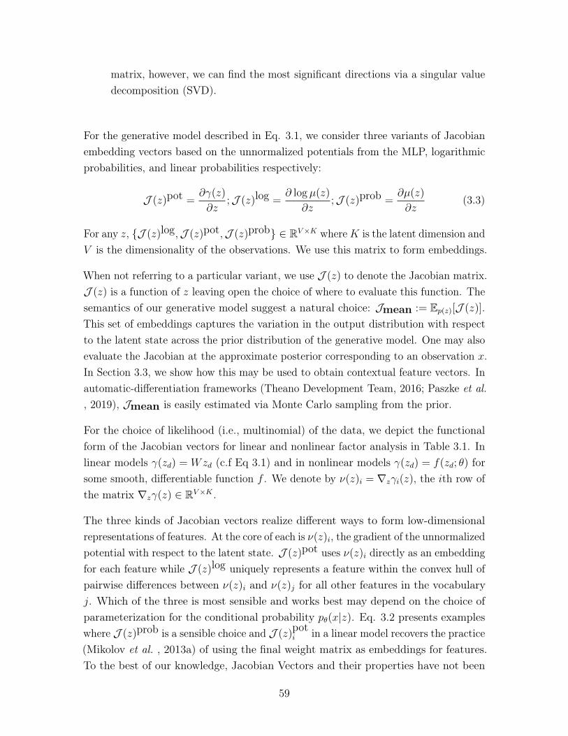
matrix, however, we can find the most significant directions via a singular valuedecomposition (SVD).
For the generative model described in Eq. 3.1, we consider three variants of Jacobianembedding vectors based on the unnormalized potentials from the MLP, logarithmicprobabilities, and linear probabilities respectively:
𝒥 (𝑧)pot =𝜕𝛾(𝑧)
𝜕𝑧;𝒥 (𝑧)log =
𝜕 log 𝜇(𝑧)
𝜕𝑧;𝒥 (𝑧)prob =
𝜕𝜇(𝑧)
𝜕𝑧(3.3)
For any 𝑧, {𝒥 (𝑧)log,𝒥 (𝑧)pot,𝒥 (𝑧)prob} ∈ R𝑉×𝐾 where𝐾 is the latent dimension and𝑉 is the dimensionality of the observations. We use this matrix to form embeddings.
When not referring to a particular variant, we use 𝒥 (𝑧) to denote the Jacobian matrix.𝒥 (𝑧) is a function of 𝑧 leaving open the choice of where to evaluate this function. Thesemantics of our generative model suggest a natural choice: 𝒥mean := E𝑝(𝑧)[𝒥 (𝑧)].This set of embeddings captures the variation in the output distribution with respectto the latent state across the prior distribution of the generative model. One may alsoevaluate the Jacobian at the approximate posterior corresponding to an observation 𝑥.In Section 3.3, we show how this may be used to obtain contextual feature vectors. Inautomatic-differentiation frameworks (Theano Development Team, 2016; Paszke et al., 2019), 𝒥mean is easily estimated via Monte Carlo sampling from the prior.
For the choice of likelihood (i.e., multinomial) of the data, we depict the functionalform of the Jacobian vectors for linear and nonlinear factor analysis in Table 3.1. Inlinear models 𝛾(𝑧𝑑) = 𝑊𝑧𝑑 (c.f Eq 3.1) and in nonlinear models 𝛾(𝑧𝑑) = 𝑓(𝑧𝑑; 𝜃) forsome smooth, differentiable function 𝑓 . We denote by 𝜈(𝑧)𝑖 = ∇𝑧𝛾𝑖(𝑧), the 𝑖th row ofthe matrix ∇𝑧𝛾(𝑧) ∈ R𝑉×𝐾 .
The three kinds of Jacobian vectors realize different ways to form low-dimensionalrepresentations of features. At the core of each is 𝜈(𝑧)𝑖, the gradient of the unnormalizedpotential with respect to the latent state. 𝒥 (𝑧)pot uses 𝜈(𝑧)𝑖 directly as an embeddingfor each feature while 𝒥 (𝑧)log uniquely represents a feature within the convex hull ofpairwise differences between 𝜈(𝑧)𝑖 and 𝜈(𝑧)𝑗 for all other features in the vocabulary𝑗. Which of the three is most sensible and works best may depend on the choice ofparameterization for the conditional probability 𝑝𝜃(𝑥|𝑧). Eq. 3.2 presents exampleswhere 𝒥 (𝑧)prob is a sensible choice and 𝒥 (𝑧)
pot𝑖 in a linear model recovers the practice
(Mikolov et al. , 2013a) of using the final weight matrix as embeddings for features.To the best of our knowledge, Jacobian Vectors and their properties have not been
59

studied in the context of deep generative models.
Table 3.1: Jacobian vectors: The functional form of the Jacobian vectors for feature 𝑖as defined in Eq. 3.3 when 𝑝(𝑥𝑖 = 1|𝑧) is defined as in Eq. 3.1.
Linear Model
𝒥 (𝑧)log𝑖
∑︀𝑗 𝑝(𝑥𝑗 = 1|𝑧)(𝑤𝑖 − 𝑤𝑗)
𝒥 (𝑧)prob𝑖 𝑝(𝑥𝑖 = 1|𝑧)∑︀𝑗 𝑝(𝑥𝑗 = 1|𝑧)(𝑤𝑖 − 𝑤𝑗)
𝒥 (𝑧)pot𝑖 𝑤𝑖
Nonlinear Model
𝒥 (𝑧)log𝑖
∑︀𝑗 𝑝(𝑥𝑗 = 1|𝑧)(∇𝑧𝜈(𝑧)𝑖 − 𝜈(𝑧)𝑗)
𝒥 (𝑧)prob𝑖 𝑝(𝑥𝑖 = 1|𝑧)∑︀𝑗 𝑝(𝑥𝑗 = 1|𝑧)(𝜈(𝑧)𝑖 − 𝜈(𝑧)𝑗)
𝒥 (𝑧)pot𝑖 ∇𝑧𝜈(𝑧)𝑖
Deriving Jacobian vectors Here, we derive the function form of Jacobian vectors.For clarity we provide the generative model under consideration:
𝑧𝑑 ∼ 𝒩 (0, 𝐼); 𝛾(𝑧𝑑) ≡ MLP(𝑧𝑑; 𝜃);
𝜇(𝑧𝑑) ≡exp{𝛾(𝑧𝑑)}∑︀𝑣 exp{𝛾(𝑧𝑑)𝑣}
; 𝑥𝑑 ∼ Multinomial(𝜇(𝑧𝑑), 𝑁𝑑). (3.4)
For simplicity, we derive the functional form of the Jacobian in a linear model, i.e.,where 𝛾(𝑧𝑑) = 𝑊𝑧𝑑 (c.f Eq 3.4). We drop the subscript 𝑑 and denote by 𝛾𝑖(𝑧), the 𝑖thelement of the vector 𝛾(𝑧). Then, we can write the probability of an element as:
𝑝(𝑥𝑖 = 1|𝑧) = exp(𝛾𝑖(𝑧))∑︀𝑗 exp(𝛾𝑗(𝑧))
and 𝛾𝑖(𝑧) = 𝑤𝑇𝑖 𝑧
For linear models, ∇𝑧𝛾𝑖(𝑧) = 𝑤𝑖 directly corresponds to 𝒥 (𝑧)pot. Noting that∇𝑧 exp(𝛾𝑖(𝑧)) = exp(𝛾𝑖(𝑧))∇𝑧𝛾𝑖(𝑧) and ∇𝑧
∑︀𝑗 exp(𝛾𝑗(𝑧)) =
∑︀𝑗 exp(𝛾𝑗(𝑧))∇𝑧𝛾𝑗(𝑧),
we estimate 𝒥 (𝑧)prob as:
60
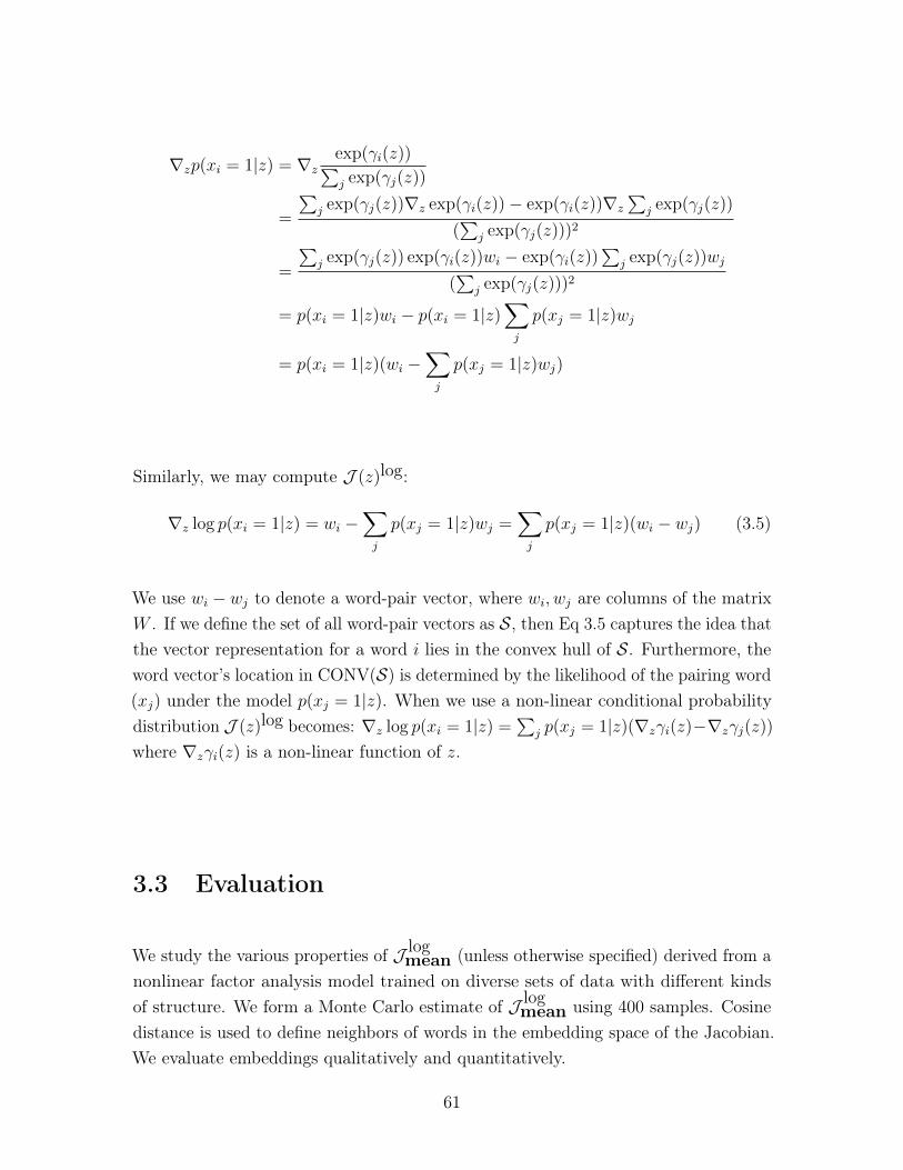
∇𝑧𝑝(𝑥𝑖 = 1|𝑧) = ∇𝑧exp(𝛾𝑖(𝑧))∑︀𝑗 exp(𝛾𝑗(𝑧))
=
∑︀𝑗 exp(𝛾𝑗(𝑧))∇𝑧 exp(𝛾𝑖(𝑧))− exp(𝛾𝑖(𝑧))∇𝑧
∑︀𝑗 exp(𝛾𝑗(𝑧))
(∑︀
𝑗 exp(𝛾𝑗(𝑧)))2
=
∑︀𝑗 exp(𝛾𝑗(𝑧)) exp(𝛾𝑖(𝑧))𝑤𝑖 − exp(𝛾𝑖(𝑧))
∑︀𝑗 exp(𝛾𝑗(𝑧))𝑤𝑗
(∑︀
𝑗 exp(𝛾𝑗(𝑧)))2
= 𝑝(𝑥𝑖 = 1|𝑧)𝑤𝑖 − 𝑝(𝑥𝑖 = 1|𝑧)∑︁
𝑗
𝑝(𝑥𝑗 = 1|𝑧)𝑤𝑗
= 𝑝(𝑥𝑖 = 1|𝑧)(𝑤𝑖 −∑︁
𝑗
𝑝(𝑥𝑗 = 1|𝑧)𝑤𝑗)
Similarly, we may compute 𝒥 (𝑧)log:
∇𝑧 log 𝑝(𝑥𝑖 = 1|𝑧) = 𝑤𝑖 −∑︁
𝑗
𝑝(𝑥𝑗 = 1|𝑧)𝑤𝑗 =∑︁
𝑗
𝑝(𝑥𝑗 = 1|𝑧)(𝑤𝑖 − 𝑤𝑗) (3.5)
We use 𝑤𝑖 − 𝑤𝑗 to denote a word-pair vector, where 𝑤𝑖, 𝑤𝑗 are columns of the matrix𝑊 . If we define the set of all word-pair vectors as 𝒮, then Eq 3.5 captures the idea thatthe vector representation for a word 𝑖 lies in the convex hull of 𝒮. Furthermore, theword vector’s location in CONV(𝒮) is determined by the likelihood of the pairing word(𝑥𝑗) under the model 𝑝(𝑥𝑗 = 1|𝑧). When we use a non-linear conditional probabilitydistribution 𝒥 (𝑧)log becomes: ∇𝑧 log 𝑝(𝑥𝑖 = 1|𝑧) = ∑︀
𝑗 𝑝(𝑥𝑗 = 1|𝑧)(∇𝑧𝛾𝑖(𝑧)−∇𝑧𝛾𝑗(𝑧))
where ∇𝑧𝛾𝑖(𝑧) is a non-linear function of 𝑧.
3.3 Evaluation
We study the various properties of 𝒥 logmean (unless otherwise specified) derived from a
nonlinear factor analysis model trained on diverse sets of data with different kindsof structure. We form a Monte Carlo estimate of 𝒥 log
mean using 400 samples. Cosinedistance is used to define neighbors of words in the embedding space of the Jacobian.We evaluate embeddings qualitatively and quantitatively.
61
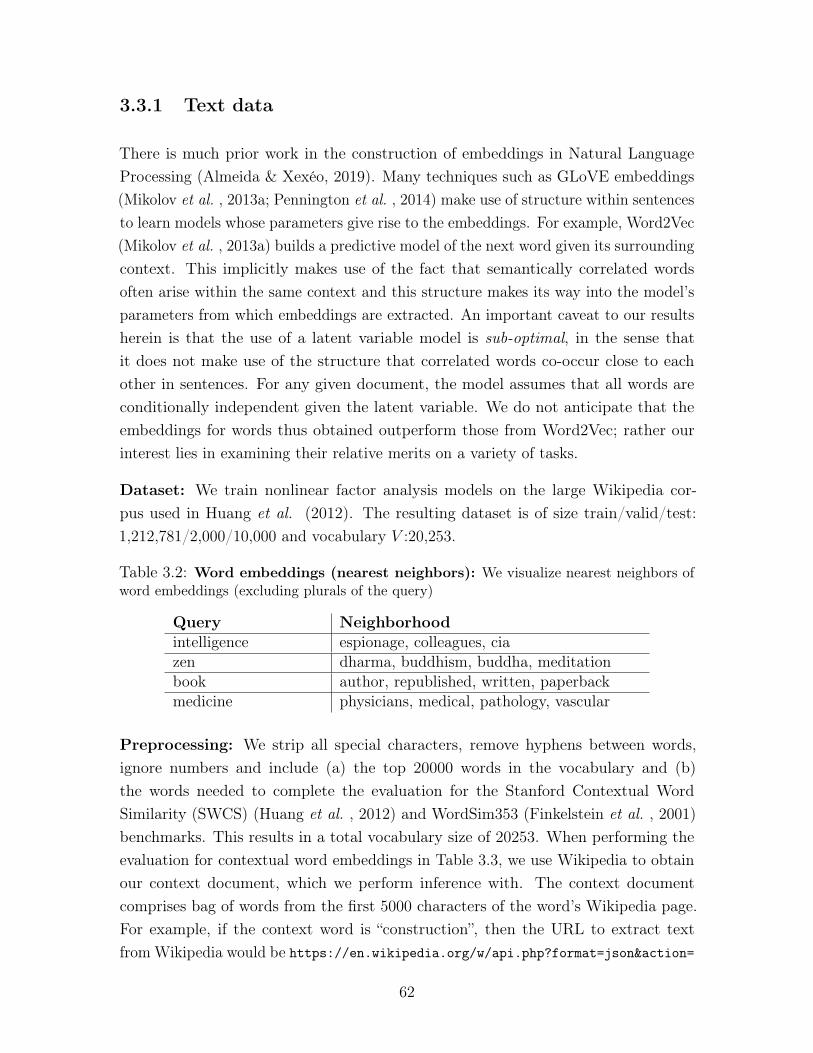
3.3.1 Text data
There is much prior work in the construction of embeddings in Natural LanguageProcessing (Almeida & Xexéo, 2019). Many techniques such as GLoVE embeddings(Mikolov et al. , 2013a; Pennington et al. , 2014) make use of structure within sentencesto learn models whose parameters give rise to the embeddings. For example, Word2Vec(Mikolov et al. , 2013a) builds a predictive model of the next word given its surroundingcontext. This implicitly makes use of the fact that semantically correlated wordsoften arise within the same context and this structure makes its way into the model’sparameters from which embeddings are extracted. An important caveat to our resultsherein is that the use of a latent variable model is sub-optimal, in the sense thatit does not make use of the structure that correlated words co-occur close to eachother in sentences. For any given document, the model assumes that all words areconditionally independent given the latent variable. We do not anticipate that theembeddings for words thus obtained outperform those from Word2Vec; rather ourinterest lies in examining their relative merits on a variety of tasks.
Dataset: We train nonlinear factor analysis models on the large Wikipedia cor-pus used in Huang et al. (2012). The resulting dataset is of size train/valid/test:1,212,781/2,000/10,000 and vocabulary 𝑉 :20,253.
Table 3.2: Word embeddings (nearest neighbors): We visualize nearest neighbors ofword embeddings (excluding plurals of the query)
Query Neighborhoodintelligence espionage, colleagues, ciazen dharma, buddhism, buddha, meditationbook author, republished, written, paperbackmedicine physicians, medical, pathology, vascular
Preprocessing: We strip all special characters, remove hyphens between words,ignore numbers and include (a) the top 20000 words in the vocabulary and (b)the words needed to complete the evaluation for the Stanford Contextual WordSimilarity (SWCS) (Huang et al. , 2012) and WordSim353 (Finkelstein et al. , 2001)benchmarks. This results in a total vocabulary size of 20253. When performing theevaluation for contextual word embeddings in Table 3.3, we use Wikipedia to obtainour context document, which we perform inference with. The context documentcomprises bag of words from the first 5000 characters of the word’s Wikipedia page.For example, if the context word is “construction”, then the URL to extract textfrom Wikipedia would be https://en.wikipedia.org/w/api.php?format=json&action=
62
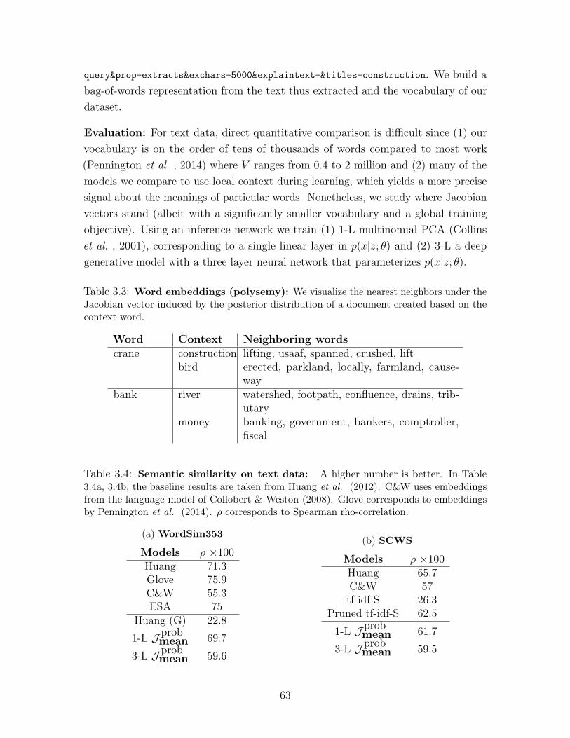
query&prop=extracts&exchars=5000&explaintext=&titles=construction. We build abag-of-words representation from the text thus extracted and the vocabulary of ourdataset.
Evaluation: For text data, direct quantitative comparison is difficult since (1) ourvocabulary is on the order of tens of thousands of words compared to most work(Pennington et al. , 2014) where 𝑉 ranges from 0.4 to 2 million and (2) many of themodels we compare to use local context during learning, which yields a more precisesignal about the meanings of particular words. Nonetheless, we study where Jacobianvectors stand (albeit with a significantly smaller vocabulary and a global trainingobjective). Using an inference network we train (1) 1-L multinomial PCA (Collinset al. , 2001), corresponding to a single linear layer in 𝑝(𝑥|𝑧; 𝜃) and (2) 3-L a deepgenerative model with a three layer neural network that parameterizes 𝑝(𝑥|𝑧; 𝜃).
Table 3.3: Word embeddings (polysemy): We visualize the nearest neighbors under theJacobian vector induced by the posterior distribution of a document created based on thecontext word.
Word Context Neighboring wordscrane construction lifting, usaaf, spanned, crushed, lift
bird erected, parkland, locally, farmland, cause-way
bank river watershed, footpath, confluence, drains, trib-utary
money banking, government, bankers, comptroller,fiscal
Table 3.4: Semantic similarity on text data: A higher number is better. In Table3.4a, 3.4b, the baseline results are taken from Huang et al. (2012). C&W uses embeddingsfrom the language model of Collobert & Weston (2008). Glove corresponds to embeddingsby Pennington et al. (2014). 𝜌 corresponds to Spearman rho-correlation.
(a) WordSim353
Models 𝜌 ×100Huang 71.3Glove 75.9C&W 55.3ESA 75
Huang (G) 22.8
1-L 𝒥 probmean 69.7
3-L 𝒥 probmean 59.6
(b) SCWS
Models 𝜌 ×100Huang 65.7C&W 57tf-idf-S 26.3
Pruned tf-idf-S 62.5
1-L 𝒥 probmean 61.7
3-L 𝒥 probmean 59.5
63
Qualitative analysis In Table 3.2, we visualize some of the nearest neighborsof words using 𝒥 log
mean obtained from models trained on Wikipedia and find thatthe neighbors are semantically sensible. Next, we consider contextual embeddings.Rather than evaluating the Jacobian at 𝐿 points 𝑧1:𝐿 ∼ 𝑝(𝑧), we instead evaluate itat 𝑧1:𝐿 ∼ 𝑞(𝑧|𝑥) for some 𝑥. In Table 3.3, we select three polysemous query wordsalongside “context words” that disambiguate the query’s meaning. For each word-context pair, we create a document comprising a subset of words in the the context’sWikipedia page. Then, we use the inference network to perform posterior inferenceto evaluate 𝒥 log
mean at the corresponding 𝑞(𝑧|𝑥). This yields a set of contextualJacobian vectors. We display the nearest neighbors for each word under differentcontextual Jacobian vectors and find that, while not always perfect, they capturedifferent contextually relevant semantics. Note that other approaches to obtain contextspecific representations (Chen et al. , 2014) explicitly use local context during training– our method does not. Rather the contextual nature of the representation arises dueto the sensitivity of the nonlinear Jacobian vector to the choice of 𝑧. By combiningposterior inference in NFA with our methodology of introspecting the model, oneobtains different context-specific representations.
Quantitative analysis To quantify the amount of semantic content in Jacobianvectors, we evaluate the vector space representations on WordSim353 (Finkelsteinet al. , 2001) and SCWS (Huang et al. , 2012). Each benchmark contains humanannotated measures of similarity between words. The evaluation on the WordSimand SCWS datasets are done by computing the Spearman rank correlation betweenhuman annotated rankings between 1 and 10 and an algorithmically derived measuresof word-pair similarity. We first compute the distances between all word pairs. Ourmeasure of similarity is obtained by subtracting the distances from the maximaldistance across all word pairs. Closest to us in learning procedure is (Huang (G),Table 3.4a), whose model we outperform. On a discriminative task of predictingsentiment on the Stanford Sentiment Treebank Dataset (Socher et al. , 2013), we findthat Jacobian vectors perform only slightly worse than Glove embeddings, despitebeing trained with a much smaller vocabulary. For this task, we do not find muchimprovements in the quality of the embeddings relative to those obtained from asimpler multinomial-PCA model.
To test the discriminative ability of the learned Jacobian vectors, we use the Jacobianvectors as representations for sentiment classification. We evaluate our method onclassifying the sentiment of movie ratings from the Rotten Tomatoes (RT) dataset
64
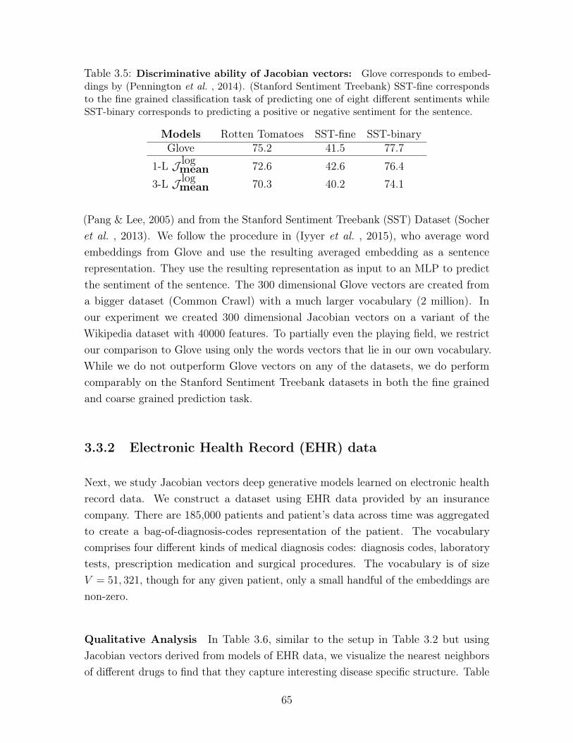
Table 3.5: Discriminative ability of Jacobian vectors: Glove corresponds to embed-dings by (Pennington et al. , 2014). (Stanford Sentiment Treebank) SST-fine correspondsto the fine grained classification task of predicting one of eight different sentiments whileSST-binary corresponds to predicting a positive or negative sentiment for the sentence.
Models Rotten Tomatoes SST-fine SST-binaryGlove 75.2 41.5 77.7
1-L 𝒥 logmean 72.6 42.6 76.4
3-L 𝒥 logmean 70.3 40.2 74.1
(Pang & Lee, 2005) and from the Stanford Sentiment Treebank (SST) Dataset (Socheret al. , 2013). We follow the procedure in (Iyyer et al. , 2015), who average wordembeddings from Glove and use the resulting averaged embedding as a sentencerepresentation. They use the resulting representation as input to an MLP to predictthe sentiment of the sentence. The 300 dimensional Glove vectors are created froma bigger dataset (Common Crawl) with a much larger vocabulary (2 million). Inour experiment we created 300 dimensional Jacobian vectors on a variant of theWikipedia dataset with 40000 features. To partially even the playing field, we restrictour comparison to Glove using only the words vectors that lie in our own vocabulary.While we do not outperform Glove vectors on any of the datasets, we do performcomparably on the Stanford Sentiment Treebank datasets in both the fine grainedand coarse grained prediction task.
3.3.2 Electronic Health Record (EHR) data
Next, we study Jacobian vectors deep generative models learned on electronic healthrecord data. We construct a dataset using EHR data provided by an insurancecompany. There are 185,000 patients and patient’s data across time was aggregatedto create a bag-of-diagnosis-codes representation of the patient. The vocabularycomprises four different kinds of medical diagnosis codes: diagnosis codes, laboratorytests, prescription medication and surgical procedures. The vocabulary is of size𝑉 = 51, 321, though for any given patient, only a small handful of the embeddings arenon-zero.
Qualitative Analysis In Table 3.6, similar to the setup in Table 3.2 but usingJacobian vectors derived from models of EHR data, we visualize the nearest neighborsof different drugs to find that they capture interesting disease specific structure. Table
65
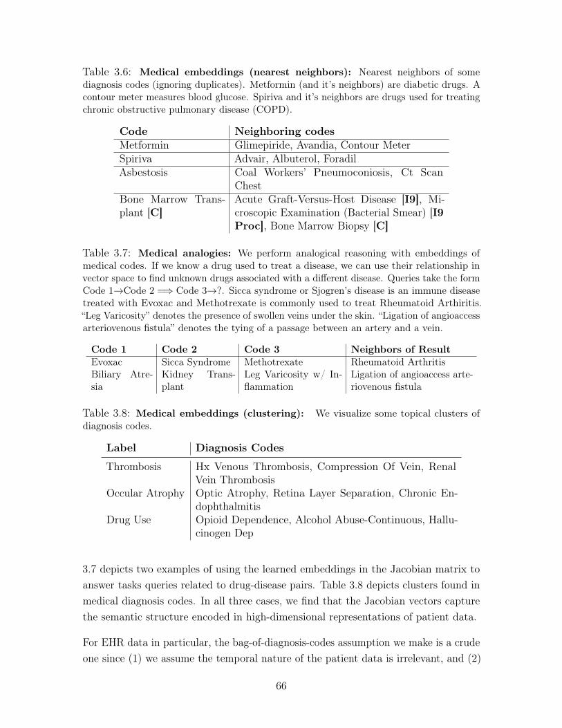
Table 3.6: Medical embeddings (nearest neighbors): Nearest neighbors of somediagnosis codes (ignoring duplicates). Metformin (and it’s neighbors) are diabetic drugs. Acontour meter measures blood glucose. Spiriva and it’s neighbors are drugs used for treatingchronic obstructive pulmonary disease (COPD).
Code Neighboring codesMetformin Glimepiride, Avandia, Contour MeterSpiriva Advair, Albuterol, ForadilAsbestosis Coal Workers’ Pneumoconiosis, Ct Scan
ChestBone Marrow Trans-plant [C]
Acute Graft-Versus-Host Disease [I9], Mi-croscopic Examination (Bacterial Smear) [I9Proc], Bone Marrow Biopsy [C]
Table 3.7: Medical analogies: We perform analogical reasoning with embeddings ofmedical codes. If we know a drug used to treat a disease, we can use their relationship invector space to find unknown drugs associated with a different disease. Queries take the formCode 1→Code 2 =⇒ Code 3→?. Sicca syndrome or Sjogren’s disease is an immune diseasetreated with Evoxac and Methotrexate is commonly used to treat Rheumatoid Arthiritis.“Leg Varicosity” denotes the presence of swollen veins under the skin. “Ligation of angioaccessarteriovenous fistula” denotes the tying of a passage between an artery and a vein.
Code 1 Code 2 Code 3 Neighbors of ResultEvoxac Sicca Syndrome Methotrexate Rheumatoid ArthritisBiliary Atre-sia
Kidney Trans-plant
Leg Varicosity w/ In-flammation
Ligation of angioaccess arte-riovenous fistula
Table 3.8: Medical embeddings (clustering): We visualize some topical clusters ofdiagnosis codes.
Label Diagnosis Codes
Thrombosis Hx Venous Thrombosis, Compression Of Vein, RenalVein Thrombosis
Occular Atrophy Optic Atrophy, Retina Layer Separation, Chronic En-dophthalmitis
Drug Use Opioid Dependence, Alcohol Abuse-Continuous, Hallu-cinogen Dep
3.7 depicts two examples of using the learned embeddings in the Jacobian matrix toanswer tasks queries related to drug-disease pairs. Table 3.8 depicts clusters found inmedical diagnosis codes. In all three cases, we find that the Jacobian vectors capturethe semantic structure encoded in high-dimensional representations of patient data.
For EHR data in particular, the bag-of-diagnosis-codes assumption we make is a crudeone since (1) we assume the temporal nature of the patient data is irrelevant, and (2)
66
combining patient statistics over time renders it difficult for the generative model todisambiguate the correlations between codes that correspond to multiple diseases apatient may suffer from. Despite this, it is interesting that the Jacobian vectors stillcapture much of the meaningful structure among the diagnosis codes.
Quantitative Analysis Choi et al. (2016c) explore different metrics to test whetherthe embedding space of medical diagnosis codes captures medically related conceptswell. We evaluate medical embeddings as follows. MRMNDF-RT (Medical RelatednessMeasure under NDF-RT) leverages a medical database (NDF-RT) to evaluate howgood an embedding space is at answering analogical queries between drugs and diseases.The evaluation (MRMCCS) measures if the neighborhood of the diagnosis codes ismedically coherent using a predefined medical ontology (CCS) as ground truth. Thenumber is a measure of precision, where higher is better.
MRMCCS(𝑉,𝐺): The Agency for Healthcare Research and Quality’s clinical classi-fication software (CCS) collapses the hierarchical ICD9 diagnosis codes into clinicallymeaningful categories. The evaluation on CCS checks whether the nearest neighborsof a disease include other diseases related to it (if they are in the same category in theCCS). Using the ICD9 hierarchy, the authors further split the evaluation task intopredicting neighbors of fine-grained and coarse grained diagnosis codes. For a choiceof granularity 𝐺 ∈ {fine,coarse}, 𝑉 (𝐺) ∈ 𝑉 denotes the subset of ICD9 codes in thevocabulary. I𝐺(𝑣(𝑖)) is one if the 𝑣’s i’th nearest neighbor: 𝑣(𝑖) is in the same groupas 𝑣 according to 𝐺.
MRMCCS(𝑉,𝐺) =1
|𝑉 (𝐺)|∑︁
𝑣∈𝑉 (𝐺)
40∑︁
𝑘=1
I𝐺(𝑣(𝑖))log2(𝑖+ 1)
(3.6)
MRMNDF-RT(𝑉,𝑅): This uses the National Drug File Reference Terminology (NDF-RT) to evaluate analogical reasoning. The NDF-RT provides two kinds of relationships(𝑅) between drugs and diseases: May-Treat (if the drug may be used to treat thedisease) and May-Prevent. Given 𝜑𝐴 as the embedding for a code 𝐴, this test automatesthe evaluation of analogies such as 𝜑Diabetes⏟ ⏞
𝑟
≈ 𝜑Metformin⏟ ⏞ 𝑣
−(𝜑Lung Cancer − 𝜑Tarceva⏟ ⏞ 𝑠
). Here
𝑣 is the query code and 𝑠 is a representation of the relationship we seek. (Metformin isa diabetic drug and Tarceva is used in the treatment of lung cancer.) The evaluationwe perform reports a number proportional to the number of times the neighborhood of𝑣− 𝑠 contains 𝑟 for the best value of 𝑠 (computed from the set of all valid drug-disease
67
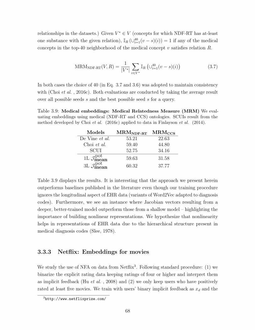
relationships in the datasets.) Given 𝑉 * ∈ 𝑉 (concepts for which NDF-RT has at-leastone substance with the given relation), I𝑅 (∪40𝑖=1(𝑣 − 𝑠)(𝑖)) = 1 if any of the medicalconcepts in the top-40 neighborhood of the medical concept 𝑣 satisfies relation 𝑅.
MRMNDF-RT(𝑉,𝑅) =1
|𝑉 *|∑︁
𝑣∈𝑉 *
I𝑅(︀∪40𝑖=1(𝑣 − 𝑠)(𝑖)
)︀(3.7)
In both cases the choice of 40 (in Eq. 3.7 and 3.6) was adopted to maintain consistencywith (Choi et al. , 2016c). Both evaluations are conducted by taking the average resultover all possible seeds 𝑠 and the best possible seed 𝑠 for a query.
Table 3.9: Medical embeddings: Medical Relatedness Measure (MRM) We eval-uating embeddings using medical (NDF-RT and CCS) ontologies. SCUIs result from themethod developed by Choi et al. (2016c) applied to data in Finlayson et al. (2014).
Models MRMNDF-RT MRMCCS
De Vine et al. 53.21 22.63Choi et al. 59.40 44.80
SCUI 52.75 34.161L 𝒥 pot
mean 59.63 31.583L 𝒥 pot
mean 60.32 37.77
Table 3.9 displays the results. It is interesting that the approach we present hereinoutperforms baselines published in the literature even though our training procedureignores the longitudinal aspect of EHR data (variants of Word2Vec adapted to diagnosiscodes). Furthermore, we see an instance where Jacobian vectors resulting from adeeper, better-trained model outperform those from a shallow model – highlighting theimportance of building nonlinear representations. We hypothesize that nonlinearityhelps in representations of EHR data due to the hierarchical structure present inmedical diagnosis codes (Slee, 1978).
3.3.3 Netflix: Embeddings for movies
We study the use of NFA on data from Netflix3. Following standard procedure: (1) webinarize the explicit rating data keeping ratings of four or higher and interpret themas implicit feedback (Hu et al. , 2008) and (2) we only keep users who have positivelyrated at least five movies. We train with users’ binary implicit feedback as 𝑥𝑑 and the
3http://www.netflixprize.com/
68
vocabulary comprises the set of all movies. The number of training/validation/testusers is 383,435/40,000/40,000 for Netflix (𝑉 : 17,769).
The Netflix dataset comprises movie ratings of 500, 000 users. We treat each user’sratings as a document and model the numbers ascribed to each movie (from 1− 5)as counts drawn from the multinomial distribution parameterized as in Eq. 3.1. Wetrain the three-layer deep generative model on the dataset, evaluate 𝒥mean with 100
samples and consider two distinct methods of evaluating the learned embeddings. Wecluster the movie embeddings (using spectral clustering with cosine distance to obtain100 clusters) and depict some of the clusters in Table 3.10a. We find that clustersexhibit coherent themes such as documentary films, horror and James Bond movies.Other clusters (not displayed) included multiple seasons of the same show such asFriends, WWE wrestling, and Pokemon. In Table 3.10b, we visualize the neighborsof some popular films. In the examples we visualize, the nearest neighbors includesequels, movies from the same franchise or, as in the case of 12 Angry Men, otherdramatic classics.
To compare the effect of using a model to create embeddings versus using the rawdata from a large dataset directly, we evaluated nearest neighbors of movies using asimple baseline. For a query movie, we found all users who gave the movie a rating of3 or above (nominally, they watched and liked the movie). Then, for all those users,we computed the mean ratings they gave to every other movie in the vocabulary andranked them based on the mean ratings. We display the top five movies obtainedusing this approach in Table 3.10c. The query words are the same as in Table 3.10b.For most of the queries, the difference between the two is evident and we simply endup with popular, well-liked movies rather than relevant movies.
3.4 Discussion
This chapter introduced and studied Jacobian Vectors both qualitatively and quanti-tatively. In three different datasets of high-dimensional data, we showed how Jacobianvectors capture semantic structure among features in datasets giving practitioners anew way to perform exploratory analysis of data with deep generative models.
Beyond the construction of embeddings, there are many other uses practiotioners canfind for the gradients in deep generative models. In Chapter 4, we will see how thegradient operator may be used to characterize the quality of a learned generative model
69

and in Chapter 7, we will make use of the Jacobian to interpret what a sequential,deep generative model has learned about the data.
70
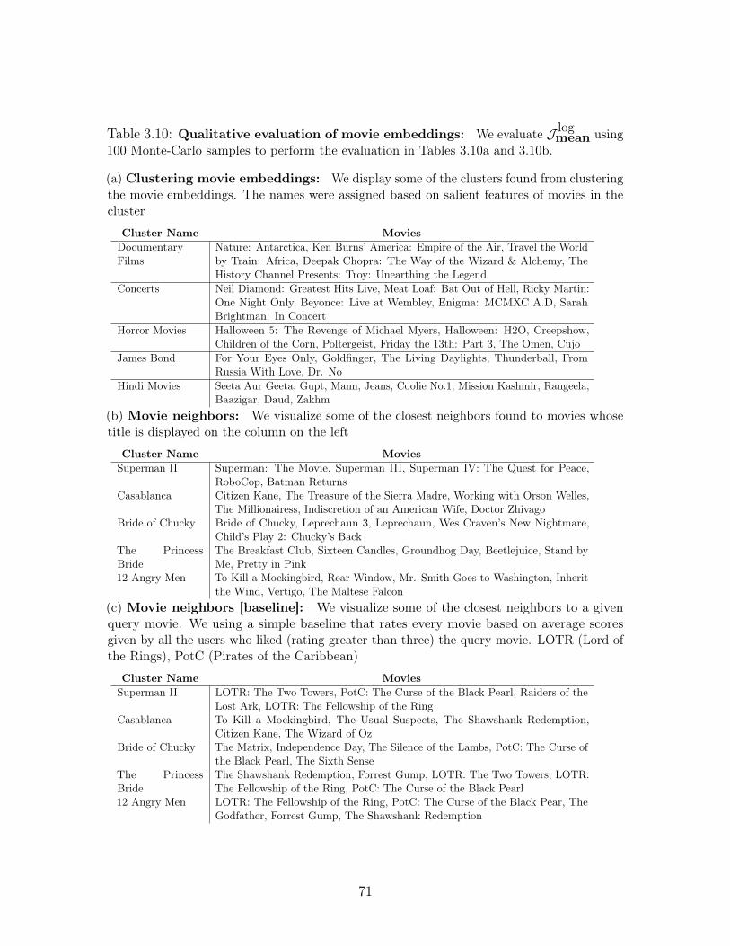
Table 3.10: Qualitative evaluation of movie embeddings: We evaluate 𝒥 logmean using
100 Monte-Carlo samples to perform the evaluation in Tables 3.10a and 3.10b.
(a) Clustering movie embeddings: We display some of the clusters found from clusteringthe movie embeddings. The names were assigned based on salient features of movies in thecluster
Cluster Name MoviesDocumentaryFilms
Nature: Antarctica, Ken Burns’ America: Empire of the Air, Travel the Worldby Train: Africa, Deepak Chopra: The Way of the Wizard & Alchemy, TheHistory Channel Presents: Troy: Unearthing the Legend
Concerts Neil Diamond: Greatest Hits Live, Meat Loaf: Bat Out of Hell, Ricky Martin:One Night Only, Beyonce: Live at Wembley, Enigma: MCMXC A.D, SarahBrightman: In Concert
Horror Movies Halloween 5: The Revenge of Michael Myers, Halloween: H2O, Creepshow,Children of the Corn, Poltergeist, Friday the 13th: Part 3, The Omen, Cujo
James Bond For Your Eyes Only, Goldfinger, The Living Daylights, Thunderball, FromRussia With Love, Dr. No
Hindi Movies Seeta Aur Geeta, Gupt, Mann, Jeans, Coolie No.1, Mission Kashmir, Rangeela,Baazigar, Daud, Zakhm
(b) Movie neighbors: We visualize some of the closest neighbors found to movies whosetitle is displayed on the column on the left
Cluster Name MoviesSuperman II Superman: The Movie, Superman III, Superman IV: The Quest for Peace,
RoboCop, Batman ReturnsCasablanca Citizen Kane, The Treasure of the Sierra Madre, Working with Orson Welles,
The Millionairess, Indiscretion of an American Wife, Doctor ZhivagoBride of Chucky Bride of Chucky, Leprechaun 3, Leprechaun, Wes Craven’s New Nightmare,
Child’s Play 2: Chucky’s BackThe PrincessBride
The Breakfast Club, Sixteen Candles, Groundhog Day, Beetlejuice, Stand byMe, Pretty in Pink
12 Angry Men To Kill a Mockingbird, Rear Window, Mr. Smith Goes to Washington, Inheritthe Wind, Vertigo, The Maltese Falcon
(c) Movie neighbors [baseline]: We visualize some of the closest neighbors to a givenquery movie. We using a simple baseline that rates every movie based on average scoresgiven by all the users who liked (rating greater than three) the query movie. LOTR (Lord ofthe Rings), PotC (Pirates of the Caribbean)
Cluster Name MoviesSuperman II LOTR: The Two Towers, PotC: The Curse of the Black Pearl, Raiders of the
Lost Ark, LOTR: The Fellowship of the RingCasablanca To Kill a Mockingbird, The Usual Suspects, The Shawshank Redemption,
Citizen Kane, The Wizard of OzBride of Chucky The Matrix, Independence Day, The Silence of the Lambs, PotC: The Curse of
the Black Pearl, The Sixth SenseThe PrincessBride
The Shawshank Redemption, Forrest Gump, LOTR: The Two Towers, LOTR:The Fellowship of the Ring, PotC: The Curse of the Black Pearl
12 Angry Men LOTR: The Fellowship of the Ring, PotC: The Curse of the Black Pear, TheGodfather, Forrest Gump, The Shawshank Redemption
71

72
Chapter 4
Representation learning forhigh-dimensional data
4.1 Introduction
Deep generative models, like those highlighted in Chapter 2, learn low-dimensionalrepresentations 𝑧, of high-dimensional random variables 𝑥 from data via unsupervisedlearning. There are many perspectives on how, and why such models learn meaningfulrepresentations. Among them is the perspective that the task of learning a gener-ative model is equivalent to the task of compressing high-dimensional information.Intuitively, to effectively compress high-dimensional data the model must use latentvariables to capture variation in both coarse and fine-grained structure. A more formalview on this perspective can be found in (Honkela & Valpola, 2004) who characterizethe relationship between the compression of information (via an information theoreticconcept known as bits-back coding) and variational learning of latent variable models.However, this perspective is not a guarantee that unsupervised learning of deep gener-ative models will always be successful in learning meaningful representations of data.In this chapter, we take a critical look at the canonical learning algorithm for deepgenerative models and investigate pitfalls that practioners may encounter. We focusour discussion on latent factor models.
The assumption of linearity in factor analysis (FA, Spearman, 1904b) has been relaxedin nonlinear factor analysis (NFA) (Gibson, 1960) and extended across a varietyof domains such as economics (Jones, 2006), signal processing (Jutten, 2003), and
73
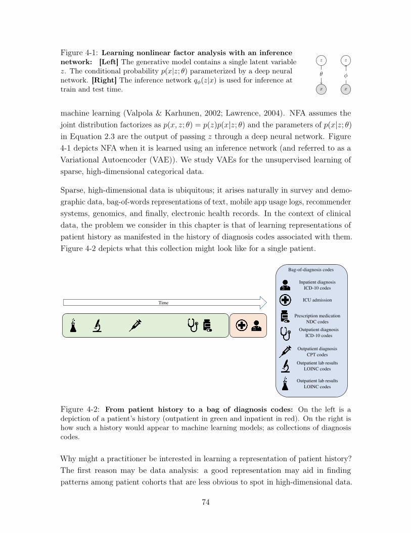
Figure 4-1: Learning nonlinear factor analysis with an inferencenetwork: [Left] The generative model contains a single latent variable𝑧. The conditional probability 𝑝(𝑥|𝑧; 𝜃) parameterized by a deep neuralnetwork. [Right] The inference network 𝑞𝜑(𝑧|𝑥) is used for inference attrain and test time.
𝑧
𝑥
𝜃
𝑧
𝑥
𝜑
machine learning (Valpola & Karhunen, 2002; Lawrence, 2004). NFA assumes thejoint distribution factorizes as 𝑝(𝑥, 𝑧; 𝜃) = 𝑝(𝑧)𝑝(𝑥|𝑧; 𝜃) and the parameters of 𝑝(𝑥|𝑧; 𝜃)in Equation 2.3 are the output of passing 𝑧 through a deep neural network. Figure4-1 depicts NFA when it is learned using an inference network (and referred to as aVariational Autoencoder (VAE)). We study VAEs for the unsupervised learning ofsparse, high-dimensional categorical data.
Sparse, high-dimensional data is ubiquitous; it arises naturally in survey and demo-graphic data, bag-of-words representations of text, mobile app usage logs, recommendersystems, genomics, and finally, electronic health records. In the context of clinicaldata, the problem we consider in this chapter is that of learning representations ofpatient history as manifested in the history of diagnosis codes associated with them.Figure 4-2 depicts what this collection might look like for a single patient.
Time
Inpatient diagnosis ICD-10 codes
Bag-of-diagnosis codes
ICU admission
Prescription medicationNDC codes
Outpatient diagnosis ICD-10 codes
Outpatient diagnosis CPT codes
Outpatient lab results LOINC codes
Outpatient lab results LOINC codes
Figure 4-2: From patient history to a bag of diagnosis codes: On the left is adepiction of a patient’s history (outpatient in green and inpatient in red). On the right ishow such a history would appear to machine learning models; as collections of diagnosiscodes.
Why might a practitioner be interested in learning a representation of patient history?The first reason may be data analysis: a good representation may aid in findingpatterns among patient cohorts that are less obvious to spot in high-dimensional data.
74
The second reason may be to use the representation as a proxy for the high-dimensionaldata in prediction tasks. High-dimensional tabular data, such as collections of patientdiagnosis codes are characterized by a few frequently occurring features and a long tailof rare features. For example, during the course of a patient medical history, we maysee many counts of diagnosis codes and treatments associated with common medicalconditions such as hypertension but fewer codes associated with rare diseases.
When directly learning deep generative models on sparse data, a problem we run intois that the standard amortized variational learning algorithm results in underfitting ;i.e. the learning algorithm fails to utilize the model’s full capacity to model thedata. This is problematic since it severely limits the applicability of this class ofmodels to finding low-dimensional representations of sparse, high-dimensional data. Toexplore, understand and mitigate this phenomena, this chapter explores the followingcontributions to the literature (Krishnan et al. , 2018):
1. We identify a problem with standard VAE training when applied to sparse,high-dimensional data—underfitting. We investigate the underlying causes ofthis phenomenon, and propose modifications to the learning algorithm to addressthese causes. We combine inference networks with an iterative optimizationscheme inspired by Stochastic Variational Inference (SVI) (Hoffman et al. ,2013).
2. We show that our proposed learning algorithm dramatically improves the qualityof the estimated parameters.
3. We empirically study various factors that govern the severity of underfitting andhow the techniques we propose mitigate it.
4. A practical ramification of our work is that improvements in learning NFA onrecommender system data translate to more accurate predictions and betterrecommendations. In contrast, standard VAE training fails to outperform thesimple shallow linear models that still largely dominate the collaborative filteringdomain (Sedhain et al. , 2016).
4.2 Setup
A bag-of-words (or in the context of clinical data, a bag-of-diagnosis codes) represen-tation is one that foregoes the ordering of observed features and instead represents
75
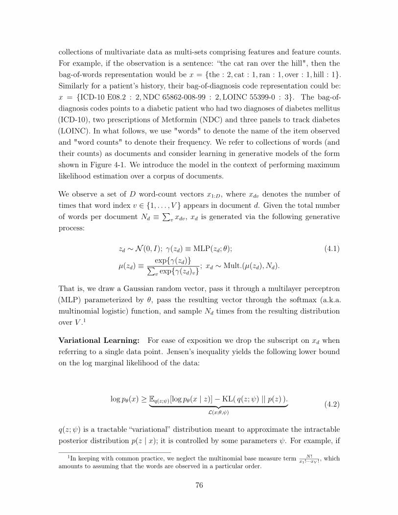
collections of multivariate data as multi-sets comprising features and feature counts.For example, if the observation is a sentence: “the cat ran over the hill", then thebag-of-words representation would be 𝑥 = {the : 2, cat : 1, ran : 1, over : 1, hill : 1}.Similarly for a patient’s history, their bag-of-diagnosis code representation could be:𝑥 = {ICD-10 E08.2 : 2,NDC 65862-008-99 : 2,LOINC 55399-0 : 3}. The bag-of-diagnosis codes points to a diabetic patient who had two diagnoses of diabetes mellitus(ICD-10), two prescriptions of Metformin (NDC) and three panels to track diabetes(LOINC). In what follows, we use "words" to denote the name of the item observedand "word counts" to denote their frequency. We refer to collections of words (andtheir counts) as documents and consider learning in generative models of the formshown in Figure 4-1. We introduce the model in the context of performing maximumlikelihood estimation over a corpus of documents.
We observe a set of 𝐷 word-count vectors 𝑥1:𝐷, where 𝑥𝑑𝑣 denotes the number oftimes that word index 𝑣 ∈ {1, . . . , 𝑉 } appears in document 𝑑. Given the total numberof words per document 𝑁𝑑 ≡
∑︀𝑣 𝑥𝑑𝑣, 𝑥𝑑 is generated via the following generative
process:
𝑧𝑑 ∼ 𝒩 (0, 𝐼); 𝛾(𝑧𝑑) ≡ MLP(𝑧𝑑; 𝜃); (4.1)
𝜇(𝑧𝑑) ≡exp{𝛾(𝑧𝑑)}∑︀𝑣 exp{𝛾(𝑧𝑑)𝑣}
; 𝑥𝑑 ∼ Mult.(𝜇(𝑧𝑑), 𝑁𝑑).
That is, we draw a Gaussian random vector, pass it through a multilayer perceptron(MLP) parameterized by 𝜃, pass the resulting vector through the softmax (a.k.a.multinomial logistic) function, and sample 𝑁𝑑 times from the resulting distributionover 𝑉 .1
Variational Learning: For ease of exposition we drop the subscript on 𝑥𝑑 whenreferring to a single data point. Jensen’s inequality yields the following lower boundon the log marginal likelihood of the data:
log 𝑝𝜃(𝑥) ≥ E𝑞(𝑧;𝜓)[log 𝑝𝜃(𝑥 | 𝑧)]−KL( 𝑞(𝑧;𝜓) || 𝑝(𝑧) ).⏟ ⏞ ℒ(𝑥;𝜃,𝜓)
(4.2)
𝑞(𝑧;𝜓) is a tractable “variational” distribution meant to approximate the intractableposterior distribution 𝑝(𝑧 | 𝑥); it is controlled by some parameters 𝜓. For example, if
1In keeping with common practice, we neglect the multinomial base measure term 𝑁 !𝑥1!···𝑥𝑉 ! , which
amounts to assuming that the words are observed in a particular order.
76
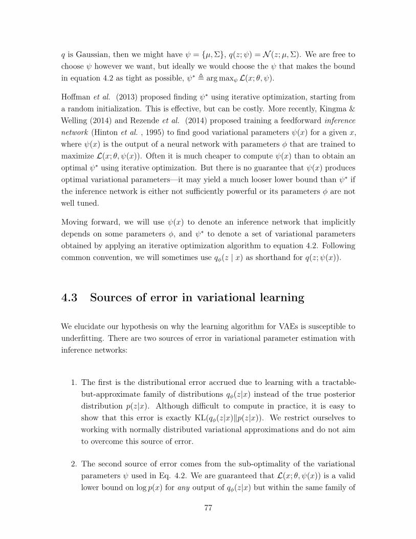
𝑞 is Gaussian, then we might have 𝜓 = {𝜇,Σ}, 𝑞(𝑧;𝜓) = 𝒩 (𝑧;𝜇,Σ). We are free tochoose 𝜓 however we want, but ideally we would choose the 𝜓 that makes the boundin equation 4.2 as tight as possible, 𝜓* , argmax𝜓 ℒ(𝑥; 𝜃, 𝜓).
Hoffman et al. (2013) proposed finding 𝜓* using iterative optimization, starting froma random initialization. This is effective, but can be costly. More recently, Kingma &Welling (2014) and Rezende et al. (2014) proposed training a feedforward inferencenetwork (Hinton et al. , 1995) to find good variational parameters 𝜓(𝑥) for a given 𝑥,where 𝜓(𝑥) is the output of a neural network with parameters 𝜑 that are trained tomaximize ℒ(𝑥; 𝜃, 𝜓(𝑥)). Often it is much cheaper to compute 𝜓(𝑥) than to obtain anoptimal 𝜓* using iterative optimization. But there is no guarantee that 𝜓(𝑥) producesoptimal variational parameters—it may yield a much looser lower bound than 𝜓* ifthe inference network is either not sufficiently powerful or its parameters 𝜑 are notwell tuned.
Moving forward, we will use 𝜓(𝑥) to denote an inference network that implicitlydepends on some parameters 𝜑, and 𝜓* to denote a set of variational parametersobtained by applying an iterative optimization algorithm to equation 4.2. Followingcommon convention, we will sometimes use 𝑞𝜑(𝑧 | 𝑥) as shorthand for 𝑞(𝑧;𝜓(𝑥)).
4.3 Sources of error in variational learning
We elucidate our hypothesis on why the learning algorithm for VAEs is susceptible tounderfitting. There are two sources of error in variational parameter estimation withinference networks:
1. The first is the distributional error accrued due to learning with a tractable-but-approximate family of distributions 𝑞𝜑(𝑧|𝑥) instead of the true posteriordistribution 𝑝(𝑧|𝑥). Although difficult to compute in practice, it is easy toshow that this error is exactly KL(𝑞𝜑(𝑧|𝑥)‖𝑝(𝑧|𝑥)). We restrict ourselves toworking with normally distributed variational approximations and do not aimto overcome this source of error.
2. The second source of error comes from the sub-optimality of the variationalparameters 𝜓 used in Eq. 4.2. We are guaranteed that ℒ(𝑥; 𝜃, 𝜓(𝑥)) is a validlower bound on log 𝑝(𝑥) for any output of 𝑞𝜑(𝑧|𝑥) but within the same family of
77
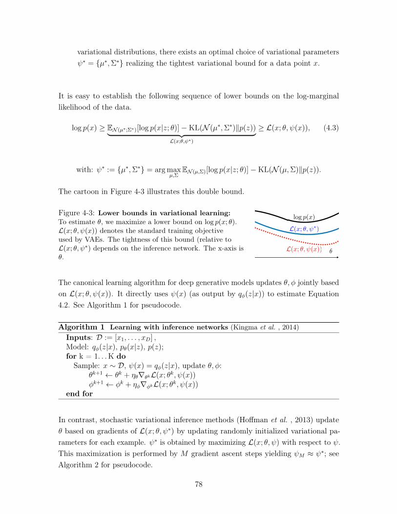
variational distributions, there exists an optimal choice of variational parameters𝜓* = {𝜇*,Σ*} realizing the tightest variational bound for a data point 𝑥.
It is easy to establish the following sequence of lower bounds on the log-marginallikelihood of the data.
log 𝑝(𝑥) ≥ E𝒩 (𝜇*;Σ*)[log 𝑝(𝑥|𝑧; 𝜃)]−KL(𝒩 (𝜇*,Σ*)‖𝑝(𝑧))⏟ ⏞ ℒ(𝑥;𝜃,𝜓*)
≥ ℒ(𝑥; 𝜃, 𝜓(𝑥)), (4.3)
with: 𝜓* := {𝜇*,Σ*} = argmax𝜇,Σ
E𝒩 (𝜇,Σ)[log 𝑝(𝑥|𝑧; 𝜃)]−KL(𝒩 (𝜇,Σ)‖𝑝(𝑧)).
The cartoon in Figure 4-3 illustrates this double bound.
Figure 4-3: Lower bounds in variational learning:To estimate 𝜃, we maximize a lower bound on log 𝑝(𝑥; 𝜃).ℒ(𝑥; 𝜃, 𝜓(𝑥)) denotes the standard training objectiveused by VAEs. The tightness of this bound (relative toℒ(𝑥; 𝜃, 𝜓*) depends on the inference network. The x-axis is𝜃.
log p(x)
L(x; ✓, ⇤)
L(x; ✓, (x)) ✓
The canonical learning algorithm for deep generative models updates 𝜃, 𝜑 jointly basedon ℒ(𝑥; 𝜃, 𝜓(𝑥)). It directly uses 𝜓(𝑥) (as output by 𝑞𝜑(𝑧|𝑥)) to estimate Equation4.2. See Algorithm 1 for pseudocode.
Algorithm 1 Learning with inference networks (Kingma et al. , 2014)Inputs: 𝒟 := [𝑥1, . . . , 𝑥𝐷] ,Model: 𝑞𝜑(𝑧|𝑥), 𝑝𝜃(𝑥|𝑧), 𝑝(𝑧);for k = 1. . . K do
Sample: 𝑥 ∼ 𝒟, 𝜓(𝑥) = 𝑞𝜑(𝑧|𝑥), update 𝜃, 𝜑:𝜃𝑘+1 ← 𝜃𝑘 + 𝜂𝜃∇𝜃𝑘ℒ(𝑥; 𝜃𝑘, 𝜓(𝑥))𝜑𝑘+1 ← 𝜑𝑘 + 𝜂𝜑∇𝜑𝑘ℒ(𝑥; 𝜃𝑘, 𝜓(𝑥))
end for
In contrast, stochastic variational inference methods (Hoffman et al. , 2013) update𝜃 based on gradients of ℒ(𝑥; 𝜃, 𝜓*) by updating randomly initialized variational pa-rameters for each example. 𝜓* is obtained by maximizing ℒ(𝑥; 𝜃, 𝜓) with respect to 𝜓.This maximization is performed by 𝑀 gradient ascent steps yielding 𝜓𝑀 ≈ 𝜓*; seeAlgorithm 2 for pseudocode.
78
Algorithm 2 Learning with Stochastic Variational Inference: 𝑀 : number ofgradient updates to 𝜓.
Inputs: 𝒟 := [𝑥1, . . . , 𝑥𝐷] ,Model: 𝑝𝜃(𝑥|𝑧), 𝑝(𝑧);for k = 1. . . K do
1. Sample: 𝑥 ∼ 𝒟 and initialize: 𝜓0 = 𝜇0,Σ0
2. Approx. 𝜓𝑀 ≈ 𝜓* = argmax𝜓 ℒ(𝑥; 𝜃;𝜓):For 𝑚 = 0, . . . ,𝑀 − 1:
𝜓𝑚+1 = 𝜓𝑚 + 𝜂𝜓𝜕ℒ(𝑥;𝜃𝑘,𝜓𝑚)
𝜕𝜓𝑚
3. Update 𝜃: 𝜃𝑘+1 ← 𝜃𝑘 + 𝜂𝜃∇𝜃𝑘ℒ(𝑥; 𝜃𝑘, 𝜓𝑀)end for
4.3.1 Limitations of joint parameter updates
Alg. (1) updates 𝜃, 𝜑 jointly. During training, the inference network learns to approxi-mate the posterior, and the generative model improves itself using local variationalparameters 𝜓(𝑥) output by 𝑞𝜑(𝑧|𝑥). If the variational parameters 𝜓(𝑥) output bythe inference network are close to the optimal variational parameters 𝜓* (Eq. 4.3),then the updates for 𝜃 are based on a relatively tight lower bound on log 𝑝(𝑥). But inpractice 𝜓(𝑥) may not be a good approximation to 𝜓*.
Both the inference network and generative model are initialized randomly. At thestart of learning, 𝜓(𝑥) is the output of a randomly initialized neural network, and willtherefore be a poor approximation to the optimal parameters 𝜓*. So the gradients usedto update 𝜃 will be based on a very loose lower bound on log 𝑝(𝑥). These gradientsmay push the generative model towards a poor local minimum – previous work hasargued that deep neural networks (which form the conditional probability distributions𝑝𝜃(𝑥|𝑧)) are often sensitive to initialization (Glorot & Bengio, 2010; Larochelle et al., 2009). Even later in learning, 𝜓(𝑥) may yield suboptimal gradients for 𝜃 if theinference network is not powerful enough to find optimal variational parameters forall data points.
Learning in the original SVI scheme does not suffer from this problem, since thevariational parameters are optimized within the inner loop of learning before updatingto 𝜃 (i.e. in Alg. (2)); 𝜕𝜃 is effectively derived using ℒ(𝑥; 𝜃, 𝜓*)). However, this methodrequires potentially an expensive iterative optimization.
This motivates blending the two methodologies for parameter estimation. Rather thanrely entirely on the inference network, we use its output to “warm-start” an SVI-styleoptimization that yields higher-quality estimates of 𝜓*, which in turn should yield
79
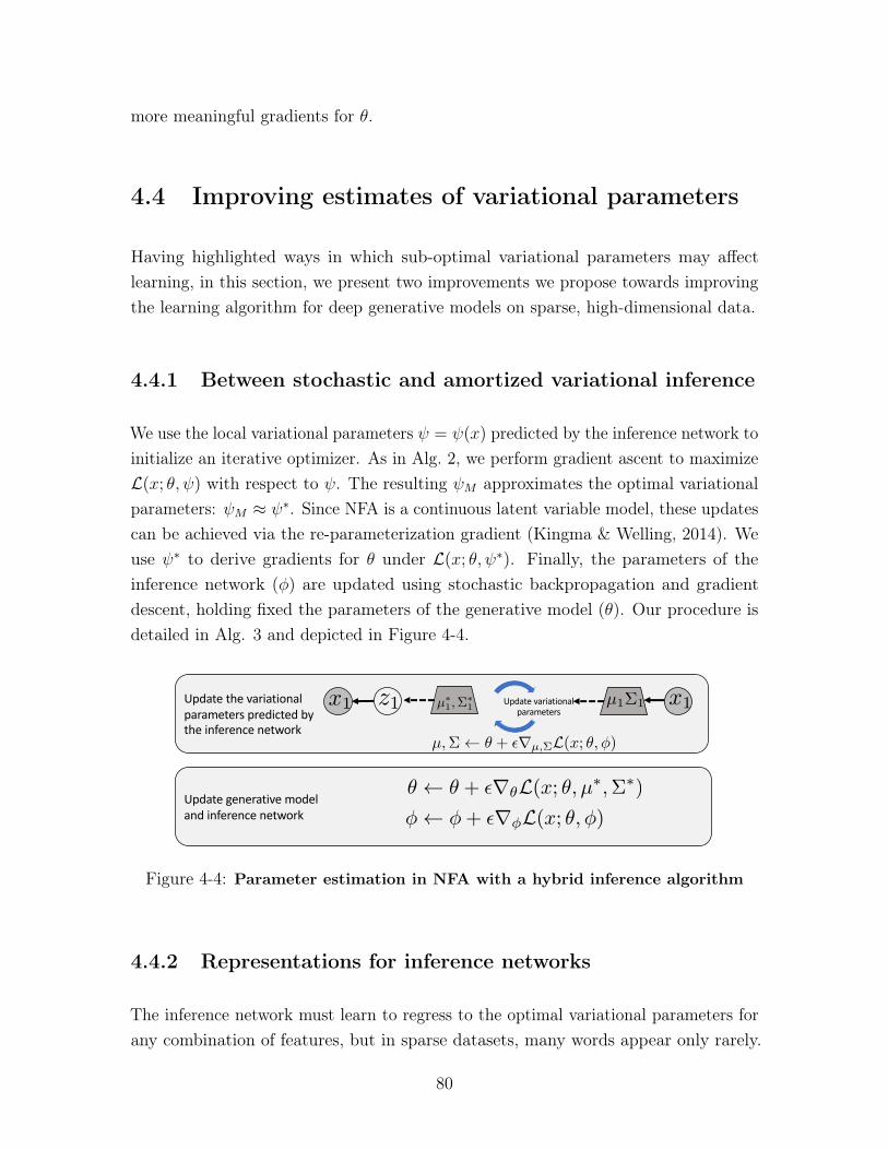
more meaningful gradients for 𝜃.
4.4 Improving estimates of variational parameters
Having highlighted ways in which sub-optimal variational parameters may affectlearning, in this section, we present two improvements we propose towards improvingthe learning algorithm for deep generative models on sparse, high-dimensional data.
4.4.1 Between stochastic and amortized variational inference
We use the local variational parameters 𝜓 = 𝜓(𝑥) predicted by the inference network toinitialize an iterative optimizer. As in Alg. 2, we perform gradient ascent to maximizeℒ(𝑥; 𝜃, 𝜓) with respect to 𝜓. The resulting 𝜓𝑀 approximates the optimal variationalparameters: 𝜓𝑀 ≈ 𝜓*. Since NFA is a continuous latent variable model, these updatescan be achieved via the re-parameterization gradient (Kingma & Welling, 2014). Weuse 𝜓* to derive gradients for 𝜃 under ℒ(𝑥; 𝜃, 𝜓*). Finally, the parameters of theinference network (𝜑) are updated using stochastic backpropagation and gradientdescent, holding fixed the parameters of the generative model (𝜃). Our procedure isdetailed in Alg. 3 and depicted in Figure 4-4.
Update generative modeland inference network
Update the variational parameters predicted by the inference network
x1
<latexit sha1_base64="3c+R7TUljyGse9TtnSD6PbvAzD0=">AAAB6nicbVBNS8NAEJ3Ur1q/qh69LBbBU0mkoMeiF48V7Qe0oWy2k3bpZhN2N2IJ/QlePCji1V/kzX/jts1BWx8MPN6bYWZekAiujet+O4W19Y3NreJ2aWd3b/+gfHjU0nGqGDZZLGLVCahGwSU2DTcCO4lCGgUC28H4Zua3H1FpHssHM0nQj+hQ8pAzaqx0/9T3+uWKW3XnIKvEy0kFcjT65a/eIGZphNIwQbXuem5i/Iwqw5nAaamXakwoG9Mhdi2VNELtZ/NTp+TMKgMSxsqWNGSu/p7IaKT1JApsZ0TNSC97M/E/r5ua8MrPuExSg5ItFoWpICYms7/JgCtkRkwsoUxxeythI6ooMzadkg3BW355lbQuql6tWrurVerXeRxFOIFTOAcPLqEOt9CAJjAYwjO8wpsjnBfn3flYtBacfOYY/sD5/AEN9o2n</latexit>
z1
<latexit sha1_base64="f4JAkaJV4cmKQlTHc1bgJFYupSE=">AAAB6nicbVBNS8NAEJ3Ur1q/qh69LBbBU0mkoMeiF48V7Qe0oWy2k3bpZhN2N0IN/QlePCji1V/kzX/jts1BWx8MPN6bYWZekAiujet+O4W19Y3NreJ2aWd3b/+gfHjU0nGqGDZZLGLVCahGwSU2DTcCO4lCGgUC28H4Zua3H1FpHssHM0nQj+hQ8pAzaqx0/9T3+uWKW3XnIKvEy0kFcjT65a/eIGZphNIwQbXuem5i/Iwqw5nAaamXakwoG9Mhdi2VNELtZ/NTp+TMKgMSxsqWNGSu/p7IaKT1JApsZ0TNSC97M/E/r5ua8MrPuExSg5ItFoWpICYms7/JgCtkRkwsoUxxeythI6ooMzadkg3BW355lbQuql6tWrurVerXeRxFOIFTOAcPLqEOt9CAJjAYwjO8wpsjnBfn3flYtBacfOYY/sD5/AERAo2p</latexit>
x1
<latexit sha1_base64="3c+R7TUljyGse9TtnSD6PbvAzD0=">AAAB6nicbVBNS8NAEJ3Ur1q/qh69LBbBU0mkoMeiF48V7Qe0oWy2k3bpZhN2N2IJ/QlePCji1V/kzX/jts1BWx8MPN6bYWZekAiujet+O4W19Y3NreJ2aWd3b/+gfHjU0nGqGDZZLGLVCahGwSU2DTcCO4lCGgUC28H4Zua3H1FpHssHM0nQj+hQ8pAzaqx0/9T3+uWKW3XnIKvEy0kFcjT65a/eIGZphNIwQbXuem5i/Iwqw5nAaamXakwoG9Mhdi2VNELtZ/NTp+TMKgMSxsqWNGSu/p7IaKT1JApsZ0TNSC97M/E/r5ua8MrPuExSg5ItFoWpICYms7/JgCtkRkwsoUxxeythI6ooMzadkg3BW355lbQuql6tWrurVerXeRxFOIFTOAcPLqEOt9CAJjAYwjO8wpsjnBfn3flYtBacfOYY/sD5/AEN9o2n</latexit>
µ1⌃1
<latexit sha1_base64="XcJc816Esyn6ky31dd/dosLchtQ=">AAAB9HicbVBNS8NAEJ34WetX1aOXxSJ4KokU9Fj04rGi/YAmhM120y7d3cTdTaGE/g4vHhTx6o/x5r9x2+agrQ8GHu/NMDMvSjnTxnW/nbX1jc2t7dJOeXdv/+CwcnTc1kmmCG2RhCeqG2FNOZO0ZZjhtJsqikXEaSca3c78zpgqzRL5aCYpDQQeSBYzgo2VAl9koec/sIHAoRdWqm7NnQOtEq8gVSjQDCtffj8hmaDSEI617nluaoIcK8MIp9Oyn2maYjLCA9qzVGJBdZDPj56ic6v0UZwoW9Kgufp7IsdC64mIbKfAZqiXvZn4n9fLTHwd5EymmaGSLBbFGUcmQbMEUJ8pSgyfWIKJYvZWRIZYYWJsTmUbgrf88ippX9a8eq1+X682boo4SnAKZ3ABHlxBA+6gCS0g8ATP8Apvzth5cd6dj0XrmlPMnMAfOJ8/Hn2Rrg==</latexit>
Update variational parameters
µ⇤1,⌃
⇤1
<latexit sha1_base64="Ozbp3FCKT4ytZCjM78GIivDeJa4=">AAAB+3icbVDLSsNAFJ3UV62vWJduBosgRUoiBV0W3bisaB/QpGEynbRDZyZhZiKW0F9x40IRt/6IO//GaZuFth64cDjnXu69J0wYVdpxvq3C2vrG5lZxu7Szu7d/YB+W2ypOJSYtHLNYdkOkCKOCtDTVjHQTSRAPGemE45uZ33kkUtFYPOhJQnyOhoJGFCNtpMAuezwN3H713LunQ4761cAN7IpTc+aAq8TNSQXkaAb2lzeIccqJ0JghpXquk2g/Q1JTzMi05KWKJAiP0ZD0DBWIE+Vn89un8NQoAxjF0pTQcK7+nsgQV2rCQ9PJkR6pZW8m/uf1Uh1d+RkVSaqJwItFUcqgjuEsCDigkmDNJoYgLKm5FeIRkghrE1fJhOAuv7xK2hc1t16r39Urjes8jiI4BifgDLjgEjTALWiCFsDgCTyDV/BmTa0X6936WLQWrHzmCPyB9fkDRaiTTQ==</latexit>
µ,⌃ ✓ + ✏rµ,⌃L(x; ✓,�)
<latexit sha1_base64="WMCARFnyd66aI4/rg03yk2CGiZA=">AAACPnicbVBNa1NBFJ3XVq3xK9alm6FBqFjCeyWg4KbYjQsXLTZtIRPCfZP7kqHz8Zi5rzU88svc+Bu6c+nGRYu47dLJB1RbDwwczjmXuffkpVaB0vR7srK6du/+g/WHjUePnzx91ny+cRRc5SV2pdPOn+QQUCuLXVKk8aT0CCbXeJyf7s384zP0QTl7SJMS+wZGVhVKAkVp0OwKU22Lz2pkQGgsCLx351zQGAn4Gy6wDEo7y4WFXMOgvolPuTBAYwm6/jTd+vJ+MbMtyrF6PWi20nY6B79LsiVpsSX2B80LMXSyMmhJagihl6Ul9WvwpKTGaUNUAUuQpzDCXqQWDIZ+PT9/yl9FZcgL5+OzxOfq3xM1mBAmJo/J2cbhtjcT/+f1Kire9Wtly4rQysVHRaU5OT7rkg+VR0l6EglIr+KuXI7Bg6TYeCOWkN0++S452mlnnXbnoNPa/bCsY529ZJtsi2XsLdtlH9k+6zLJvrIf7JJdJd+Sn8mv5PciupIsZ16wf5Bc/wENJa+h</latexit>
✓ ✓ + ✏r✓L(x; ✓, µ⇤,⌃⇤)
� �+ ✏r�L(x; ✓,�)
<latexit sha1_base64="EfFfOX8NHpZ1a0wq/ZPmTyaRDo4=">AAACj3icdZHbahsxEIa1mx5SN22c9DI3oqYlSYPZDYYUUopJb1roRUrrJGA5ZlbW2iI6LNJsW7P4dfJAuevbVGvvRXPogODn+0ej0UxWKOkxSf5E8dqjx0+erj9rPd948XKzvbV95m3puBhwq6y7yMALJY0YoEQlLgonQGdKnGdXn2r//KdwXlrzA+eFGGmYGplLDhjQuH3NcCYQ6FumRI7gnP1FG/SOMlF4qayhzECmYFytnAVlGnDGQVVfF7u/j1f0gOnycv+AfZdTDZf7e4y1WDGTtyvX4KG6gf+varD2WuN2J+kmy6D3RdqIDmnidNy+YRPLSy0McgXeD9OkwFEFDiVXYtFipRcF8CuYimGQBrTwo2o5zwV9E8iE5taFY5Au6b83KtDez3UWMuuW/V2vhg95wxLz96NKmqJEYfjqobxUFC2tl0Mn0gmOah4EcCdDr5TPwAHHsMJ6COndL98XZ4fdtNftfet1+ifNONbJDnlNdklKjkiffCanZEB4tBEdRsfRh3grPoo/xv1Vahw1d16RWxF/+QtpkMZg</latexit>
Figure 4-4: Parameter estimation in NFA with a hybrid inference algorithm
4.4.2 Representations for inference networks
The inference network must learn to regress to the optimal variational parameters forany combination of features, but in sparse datasets, many words appear only rarely.
80
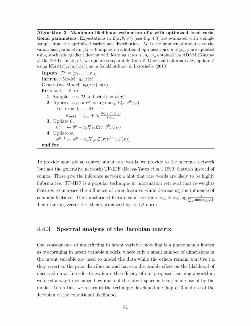
Algorithm 3 Maximum likelihood estimation of 𝜃 with optimized local varia-tional parameters: Expectations in ℒ(𝑥, 𝜃, 𝜓*) (see Eq. 4.3) are evaluated with a singlesample from the optimized variational distribution. 𝑀 is the number of updates to thevariational parameters (𝑀 = 0 implies no additional optimization). 𝜃, 𝜓(𝑥), 𝜑 are updatedusing stochastic gradient descent with learning rates 𝜂𝜃, 𝜂𝜓, 𝜂𝜑 obtained via ADAM (Kingma& Ba, 2014). In step 4, we update 𝜑 separately from 𝜃. One could alternatively, update 𝜑using KL(𝜓(𝑥)𝑀‖𝑞𝜑(𝑧|𝑥)) as in Salakhutdinov & Larochelle (2010).
Inputs: 𝒟 := [𝑥1, . . . , 𝑥𝐷] ,Inference Model: 𝑞𝜑(𝑧|𝑥),Generative Model: 𝑝𝜃(𝑥|𝑧), 𝑝(𝑧),for k = 1. . . K do
1. Sample: 𝑥 ∼ 𝒟 and set 𝜓0 = 𝜓(𝑥)2. Approx. 𝜓𝑀 ≈ 𝜓* = argmax𝜓 ℒ(𝑥; 𝜃𝑘;𝜓),
For 𝑚 = 0, . . . ,𝑀 − 1:𝜓𝑚+1 = 𝜓𝑚 + 𝜂𝜓
𝜕ℒ(𝑥;𝜃𝑘,𝜓𝑚)𝜕𝜓𝑚
3. Update 𝜃,𝜃𝑘+1 ← 𝜃𝑘 + 𝜂𝜃∇𝜃𝑘ℒ(𝑥; 𝜃𝑘, 𝜓𝑀)
4. Update 𝜑,𝜑𝑘+1 ← 𝜑𝑘 + 𝜂𝜑∇𝜑𝑘ℒ(𝑥; 𝜃𝑘+1, 𝜓(𝑥))
end for
To provide more global context about rare words, we provide to the inference network(but not the generative network) TF-IDF (Baeza-Yates et al. , 1999) features instead ofcounts. These give the inference network a hint that rare words are likely to be highlyinformative. TF-IDF is a popular technique in information retrieval that re-weightsfeatures to increase the influence of rarer features while decreasing the influence ofcommon features. The transformed feature-count vector is �̃�𝑑𝑣 ≡ 𝑥𝑑𝑣 log
𝐷∑︀𝑑′ min{𝑥𝑑′𝑣 ,1}
.The resulting vector �̃� is then normalized by its L2 norm.
4.4.3 Spectral analysis of the Jacobian matrix
One consequence of underfitting in latent variable modeling is a phenomenon knownas overpruning in latent variable models, where only a small number of dimensions inthe latent variable are used to model the data while the others remain inactive i.e.they revert to the prior distribution and have no discernible effect on the likelihood ofobserved data. In order to evaluate the efficacy of our proposed learning algorithm,we need a way to visualize how much of the latent space is being made use of by themodel. To do this, we return to the technique developed in Chapter 3 and use of theJacobian of the conditional likelihood.
81
For any vector valued function 𝑓(𝑥) : R𝐾 → R𝑉 , ∇𝑥𝑓(𝑥) is the matrix-valued functionrepresenting the sensitivity of the output to the input. When 𝑓(𝑥) is a deep neuralnetwork, Wang et al. (2016) use the spectra of the Jacobian matrix under variousinputs 𝑥 to quantify the complexity of the learned function. They find that the spectraare correlated with the complexity of the learned function. We adopt their techniquefor studying the utilization of the latent space in deep generative models. In the caseof NFA, we seek to quantify the learned complexity of the generative model. To do so,we compute the Jacobian matrix as 𝒥 (𝑧) = ∇𝑧 log 𝑝(𝑥|𝑧). This is a read-out measureof the sensitivity of the likelihood with respect to the latent dimension.
𝒥 (𝑧) is a matrix valued function that can be evaluated at every point in the latentspace. We evaluate it at the mode of the (unimodal) prior distribution i.e. at 𝑧 = 0⃗.The singular values of the resulting matrix denote how much the log-likelihood changesfrom the origin along the singular vectors lying in latent space. The intensity ofthese singular values (which we plot) is a read-out measure of how many intrinsicdimensions are utilized by the model parameters 𝜃 at the mode of the prior distribution.Our choice of evaluating 𝒥 (𝑧) at 𝑧 = 0⃗ is motivated by the fact that much of theprobability mass in latent space under the NFA model will be placed at the origin.We use the utilization at the mode as an approximation for the utilization acrossthe entire latent space. We visualized the spectral decomposition obtained under aMonte-Carlo approximation to the matrix E[𝒥 (𝑧)] and found it to be similar to thedecomposition obtained by evaluating the Jacobian at the mode. Another possibilityto measure utilization would be using the KL divergence of the prior and the outputof the inference network (as in Burda et al. (2015)).
Unlike in Chapter 3, where we made use of the Jacobian matrix to introspect what thedeep generative model had learned about data, here, we use it as a means to quantifyhow much information about the observations is captured by the generative model.
4.5 Related 2ork
Salakhutdinov & Larochelle (2010) optimize local mean-field parameters from aninference network in the context of learning deep Boltzmann machines. Salimans et al.(2015) explore warm starting MCMC with the output of an inference network.
Previous work has studied the failure modes of learning VAEs. They can be broadlycategorized into two classes. The first aims to improves the utilization of latent
82
variables using a richer posterior distribution (Burda et al. , 2015). However, forsparse data, the limits of learning with a normally distributed 𝑞𝜑(𝑧|𝑥) have barelybeen pushed – our goal is to do so in this work. Further gains may indeed be obtainedwith a richer posterior distribution but the techniques herein can inform work alongthis vein. The second class of methods studies ways to alleviate the underutilization oflatent dimensions due to an overly expressive choice of models for 𝑝(𝑥|𝑧; 𝜃) such as aRecurrent Neural Network (Bowman et al. , 2015; Chen et al. , 2016). This too, is notthe scenario we are in; underfitting of VAEs on sparse data occurs even when 𝑝(𝑥|𝑧; 𝜃)is an MLP. Our study here exposes a third failure mode; one in which learning ischallenging not just because of the objective used in learning but also because of thecharacteristics of the data.
Our work was among the first to study the effects of sub-optimal variational parametersin deep generative models; since then there have been several advances that haveenriched our understanding of limitations of inference networks. Cremer et al. (2018)coin the term amortization gap to refer to the divergence between the variationaldistribution predicted by the inference network and the optimal variational distributionwithin the distributional family. They highlight that limitations in the predictionsof the inference network, rather than the choice of variational family are responsiblefor amortization gaps observed in practice. In our work, we use SVI to update thevariational parameters predicted by the inference network; however our updates tothe parameters of the inference network do not make use of the optimized variationalparameters. Kim et al. (2018) derive gradients of the inference network throughthe computation of optimized variational parameters – they find that doing so yieldsstrong results in building deep generative models of sequence data where 𝑝(𝑥|𝑧; 𝜃) isparameterized by a recurrent neural network. He et al. (2019) propose a simple, yeteffective approach to improve the quality of inference networks, for each update ofthe generative model’s parameters, conduct multiple updates to the parameters of theinference network. Finally, Lucas et al. (2019) perform a case study on probabilisticPCA, a linear factor model, and study how posterior collapse, or the underutilizationof the model’s latent variable, can arise due to the existance of multiple local optimain the log-marginal likelihood.
83
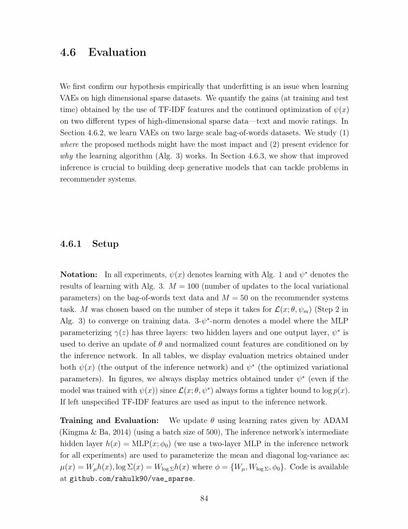
4.6 Evaluation
We first confirm our hypothesis empirically that underfitting is an issue when learningVAEs on high dimensional sparse datasets. We quantify the gains (at training and testtime) obtained by the use of TF-IDF features and the continued optimization of 𝜓(𝑥)on two different types of high-dimensional sparse data—text and movie ratings. InSection 4.6.2, we learn VAEs on two large scale bag-of-words datasets. We study (1)where the proposed methods might have the most impact and (2) present evidence forwhy the learning algorithm (Alg. 3) works. In Section 4.6.3, we show that improvedinference is crucial to building deep generative models that can tackle problems inrecommender systems.
4.6.1 Setup
Notation: In all experiments, 𝜓(𝑥) denotes learning with Alg. 1 and 𝜓* denotes theresults of learning with Alg. 3. 𝑀 = 100 (number of updates to the local variationalparameters) on the bag-of-words text data and 𝑀 = 50 on the recommender systemstask. 𝑀 was chosen based on the number of steps it takes for ℒ(𝑥; 𝜃, 𝜓𝑚) (Step 2 inAlg. 3) to converge on training data. 3-𝜓*-norm denotes a model where the MLPparameterizing 𝛾(𝑧) has three layers: two hidden layers and one output layer, 𝜓* isused to derive an update of 𝜃 and normalized count features are conditioned on bythe inference network. In all tables, we display evaluation metrics obtained underboth 𝜓(𝑥) (the output of the inference network) and 𝜓* (the optimized variationalparameters). In figures, we always display metrics obtained under 𝜓* (even if themodel was trained with 𝜓(𝑥)) since ℒ(𝑥; 𝜃, 𝜓*) always forms a tighter bound to log 𝑝(𝑥).If left unspecified TF-IDF features are used as input to the inference network.
Training and Evaluation: We update 𝜃 using learning rates given by ADAM(Kingma & Ba, 2014) (using a batch size of 500), The inference network’s intermediatehidden layer ℎ(𝑥) = MLP(𝑥;𝜑0) (we use a two-layer MLP in the inference networkfor all experiments) are used to parameterize the mean and diagonal log-variance as:𝜇(𝑥) = 𝑊𝜇ℎ(𝑥), log Σ(𝑥) = 𝑊log Σℎ(𝑥) where 𝜑 = {𝑊𝜇,𝑊log Σ, 𝜑0}. Code is availableat github.com/rahulk90/vae_sparse.
84
4.6.2 Bag-of-words text data
Datasets and Metrics: We study two large text datasets.
1. RCV1 (Lewis et al. , 2004) dataset (train/valid/test: 789,414/5,000/10,000, 𝑉 :10,000). We follow the preprocessing procedure in Miao et al. (2016),
2. Wikipedia corpus used in Huang et al. (2012) (train/test: 1,104,937/100,000and 𝑉 :20,000). We set all words to lowercase, ignore numbers and restrict thedataset to the top 20, 000 frequently occurring words.
We report an upper bound on perplexity (Mnih & Gregor, 2014) given by
exp(− 1
𝑁
∑︁
𝑖
1
𝑁𝑖
log 𝑝(𝑥𝑖))
where log 𝑝(𝑥𝑖) is replaced by Eq 4.2.
To study the utilization of the latent dimension obtained by various training methods,we compute the Jacobian 𝒥 (𝑧) matrix (as ∇𝑧 log 𝑝(𝑥|𝑧)). The singular value spectrumof the Jacobian directly measures the utilization of the latent dimensions in the model.
0 3 6 9 15 20 25 30 35 40 45 50Epochs
1100
1200
1300
1400
1500
1600
Tra
in[P
erp
lexi
ty]
1-ψ(x)
1-ψ∗3-ψ(x)
3-ψ∗
(a) Wikipedia - Training
0 3 6 9 15 20 25 30 35 40 45 50Epochs
1100
1200
1300
1400
1500
1600
Hel
d-o
ut
[Per
ple
xity
] 1-ψ(x)
1-ψ∗3-ψ(x)
3-ψ∗
(b) Wikipedia - Evaluation
0 25 50 75 100−2.5
0.0
2.5
5.0
Log
sin
gula
rva
lues
of∇z
logp(x|z
)
0 25 50 75 100−2.5
0.0
2.5
5.0
Wikipedia RCV1
(c) Log-Singular Values
Figure 4-5: Mechanics of learning: Best viewed in color. (Left and Middle) For theWikipedia dataset, we visualize upper bounds on training and held-out perplexity (evaluatedwith 𝜓*) viewed as a function of epochs. Items in the legend corresponds to choices oftraining method. (Right) Sorted log-singular values of ∇𝑧 log 𝑝(𝑥|𝑧) on Wikipedia (left) onRCV1 (right) for different training methods. The x-axis is latent dimension. The legend isidentical to that in Fig. 4-5a.
Reducing Underfitting: Is underfitting a problem and does optimizing 𝜓(𝑥) withthe use of TF-IDF features help? Table 4.1 confirms both statements.
Between “norm” and “tfidf” (comparing first four rows and second four rows), wefind that the use of TF-IDF features almost always improves parameter estimation.
85
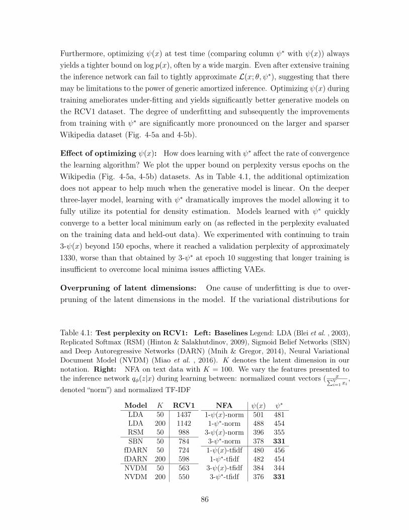
Furthermore, optimizing 𝜓(𝑥) at test time (comparing column 𝜓* with 𝜓(𝑥)) alwaysyields a tighter bound on log 𝑝(𝑥), often by a wide margin. Even after extensive trainingthe inference network can fail to tightly approximate ℒ(𝑥; 𝜃, 𝜓*), suggesting that theremay be limitations to the power of generic amortized inference. Optimizing 𝜓(𝑥) duringtraining ameliorates under-fitting and yields significantly better generative models onthe RCV1 dataset. The degree of underfitting and subsequently the improvementsfrom training with 𝜓* are significantly more pronounced on the larger and sparserWikipedia dataset (Fig. 4-5a and 4-5b).
Effect of optimizing 𝜓(𝑥): How does learning with 𝜓* affect the rate of convergencethe learning algorithm? We plot the upper bound on perplexity versus epochs on theWikipedia (Fig. 4-5a, 4-5b) datasets. As in Table 4.1, the additional optimizationdoes not appear to help much when the generative model is linear. On the deeperthree-layer model, learning with 𝜓* dramatically improves the model allowing it tofully utilize its potential for density estimation. Models learned with 𝜓* quicklyconverge to a better local minimum early on (as reflected in the perplexity evaluatedon the training data and held-out data). We experimented with continuing to train3-𝜓(𝑥) beyond 150 epochs, where it reached a validation perplexity of approximately1330, worse than that obtained by 3-𝜓* at epoch 10 suggesting that longer training isinsufficient to overcome local minima issues afflicting VAEs.
Overpruning of latent dimensions: One cause of underfitting is due to over-pruning of the latent dimensions in the model. If the variational distributions for
Table 4.1: Test perplexity on RCV1: Left: Baselines Legend: LDA (Blei et al. , 2003),Replicated Softmax (RSM) (Hinton & Salakhutdinov, 2009), Sigmoid Belief Networks (SBN)and Deep Autoregressive Networks (DARN) (Mnih & Gregor, 2014), Neural VariationalDocument Model (NVDM) (Miao et al. , 2016). 𝐾 denotes the latent dimension in ournotation. Right: NFA on text data with 𝐾 = 100. We vary the features presented tothe inference network 𝑞𝜑(𝑧|𝑥) during learning between: normalized count vectors ( 𝑥∑︀𝑉
𝑖=1 𝑥𝑖,
denoted “norm”) and normalized TF-IDF
Model 𝐾 RCV1LDA 50 1437LDA 200 1142RSM 50 988SBN 50 784
fDARN 50 724fDARN 200 598NVDM 50 563NVDM 200 550
NFA 𝜓(𝑥) 𝜓*
1-𝜓(𝑥)-norm 501 4811-𝜓*-norm 488 454
3-𝜓(𝑥)-norm 396 3553-𝜓*-norm 378 3311-𝜓(𝑥)-tfidf 480 4561-𝜓*-tfidf 482 454
3-𝜓(𝑥)-tfidf 384 3443-𝜓*-tfidf 376 331
86
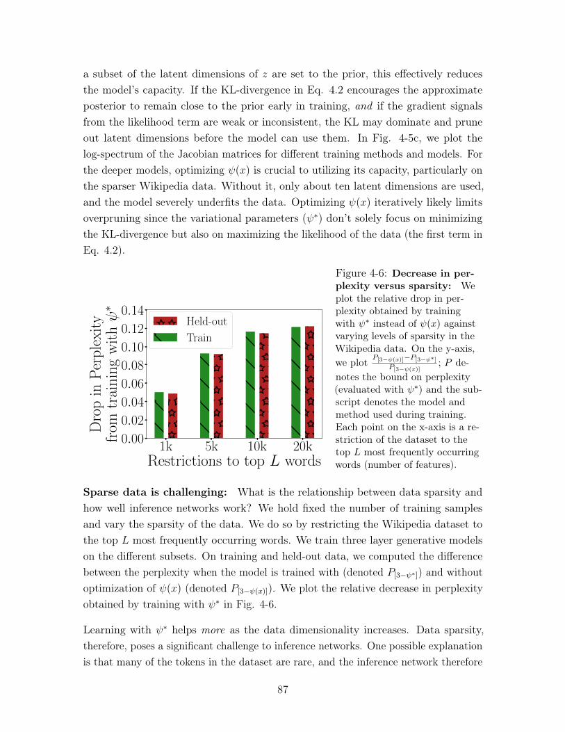
a subset of the latent dimensions of 𝑧 are set to the prior, this effectively reducesthe model’s capacity. If the KL-divergence in Eq. 4.2 encourages the approximateposterior to remain close to the prior early in training, and if the gradient signalsfrom the likelihood term are weak or inconsistent, the KL may dominate and pruneout latent dimensions before the model can use them. In Fig. 4-5c, we plot thelog-spectrum of the Jacobian matrices for different training methods and models. Forthe deeper models, optimizing 𝜓(𝑥) is crucial to utilizing its capacity, particularly onthe sparser Wikipedia data. Without it, only about ten latent dimensions are used,and the model severely underfits the data. Optimizing 𝜓(𝑥) iteratively likely limitsoverpruning since the variational parameters (𝜓*) don’t solely focus on minimizingthe KL-divergence but also on maximizing the likelihood of the data (the first term inEq. 4.2).
1k 5k 10k 20kRestrictions to top L words
0.00
0.02
0.04
0.06
0.08
0.10
0.12
0.14
Dro
pin
Per
ple
xity
from
trai
nin
gw
ithψ∗
Held-out
Train
Figure 4-6: Decrease in per-plexity versus sparsity: Weplot the relative drop in per-plexity obtained by trainingwith 𝜓* instead of 𝜓(𝑥) againstvarying levels of sparsity in theWikipedia data. On the y-axis,we plot 𝑃[3−𝜓(𝑥)]−𝑃[3−𝜓*]
𝑃[3−𝜓(𝑥)]; 𝑃 de-
notes the bound on perplexity(evaluated with 𝜓*) and the sub-script denotes the model andmethod used during training.Each point on the x-axis is a re-striction of the dataset to thetop 𝐿 most frequently occurringwords (number of features).
Sparse data is challenging: What is the relationship between data sparsity andhow well inference networks work? We hold fixed the number of training samplesand vary the sparsity of the data. We do so by restricting the Wikipedia dataset tothe top 𝐿 most frequently occurring words. We train three layer generative modelson the different subsets. On training and held-out data, we computed the differencebetween the perplexity when the model is trained with (denoted 𝑃[3−𝜓*]) and withoutoptimization of 𝜓(𝑥) (denoted 𝑃[3−𝜓(𝑥)]). We plot the relative decrease in perplexityobtained by training with 𝜓* in Fig. 4-6.
Learning with 𝜓* helps more as the data dimensionality increases. Data sparsity,therefore, poses a significant challenge to inference networks. One possible explanationis that many of the tokens in the dataset are rare, and the inference network therefore
87
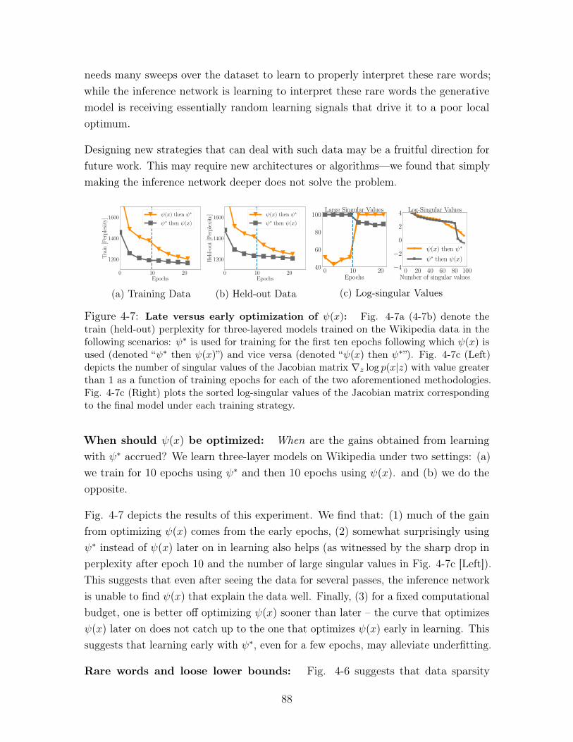
needs many sweeps over the dataset to learn to properly interpret these rare words;while the inference network is learning to interpret these rare words the generativemodel is receiving essentially random learning signals that drive it to a poor localoptimum.
Designing new strategies that can deal with such data may be a fruitful direction forfuture work. This may require new architectures or algorithms—we found that simplymaking the inference network deeper does not solve the problem.
0 10 20Epochs
1200
1400
1600
Tra
in[P
erp
lexi
ty]
ψ(x) then ψ∗
ψ∗ then ψ(x)
(a) Training Data
0 10 20Epochs
1200
1400
1600
Hel
d-o
ut
[Per
ple
xity
] ψ(x) then ψ∗
ψ∗ then ψ(x)
(b) Held-out Data
0 10 20Epochs
40
60
80
100Large Singular Values
0 20 40 60 80 100Number of singular values
−4
−2
0
2
4 Log-Singular Values
ψ(x) then ψ∗
ψ∗ then ψ(x)
(c) Log-singular Values
Figure 4-7: Late versus early optimization of 𝜓(𝑥): Fig. 4-7a (4-7b) denote thetrain (held-out) perplexity for three-layered models trained on the Wikipedia data in thefollowing scenarios: 𝜓* is used for training for the first ten epochs following which 𝜓(𝑥) isused (denoted “𝜓* then 𝜓(𝑥)”) and vice versa (denoted “𝜓(𝑥) then 𝜓*”). Fig. 4-7c (Left)depicts the number of singular values of the Jacobian matrix ∇𝑧 log 𝑝(𝑥|𝑧) with value greaterthan 1 as a function of training epochs for each of the two aforementioned methodologies.Fig. 4-7c (Right) plots the sorted log-singular values of the Jacobian matrix correspondingto the final model under each training strategy.
When should 𝜓(𝑥) be optimized: When are the gains obtained from learningwith 𝜓* accrued? We learn three-layer models on Wikipedia under two settings: (a)we train for 10 epochs using 𝜓* and then 10 epochs using 𝜓(𝑥). and (b) we do theopposite.
Fig. 4-7 depicts the results of this experiment. We find that: (1) much of the gainfrom optimizing 𝜓(𝑥) comes from the early epochs, (2) somewhat surprisingly using𝜓* instead of 𝜓(𝑥) later on in learning also helps (as witnessed by the sharp drop inperplexity after epoch 10 and the number of large singular values in Fig. 4-7c [Left]).This suggests that even after seeing the data for several passes, the inference networkis unable to find 𝜓(𝑥) that explain the data well. Finally, (3) for a fixed computationalbudget, one is better off optimizing 𝜓(𝑥) sooner than later – the curve that optimizes𝜓(𝑥) later on does not catch up to the one that optimizes 𝜓(𝑥) early in learning. Thissuggests that learning early with 𝜓*, even for a few epochs, may alleviate underfitting.
Rare words and loose lower bounds: Fig. 4-6 suggests that data sparsity
88
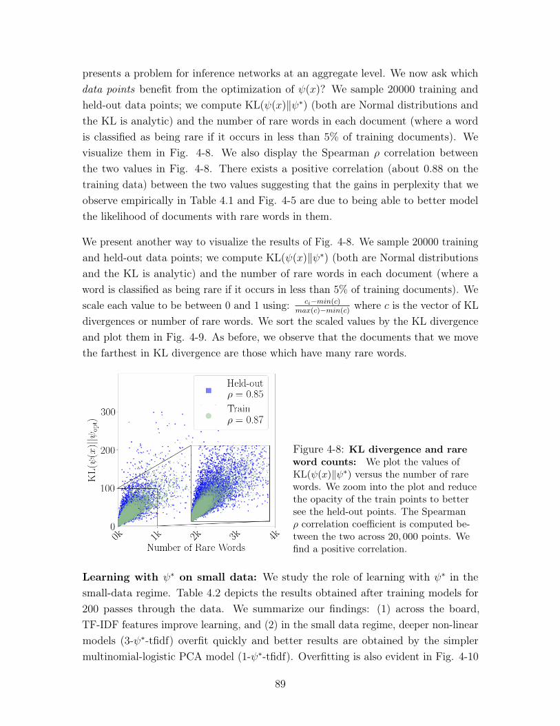
presents a problem for inference networks at an aggregate level. We now ask whichdata points benefit from the optimization of 𝜓(𝑥)? We sample 20000 training andheld-out data points; we compute KL(𝜓(𝑥)‖𝜓*) (both are Normal distributions andthe KL is analytic) and the number of rare words in each document (where a wordis classified as being rare if it occurs in less than 5% of training documents). Wevisualize them in Fig. 4-8. We also display the Spearman 𝜌 correlation betweenthe two values in Fig. 4-8. There exists a positive correlation (about 0.88 on thetraining data) between the two values suggesting that the gains in perplexity that weobserve empirically in Table 4.1 and Fig. 4-5 are due to being able to better modelthe likelihood of documents with rare words in them.
We present another way to visualize the results of Fig. 4-8. We sample 20000 trainingand held-out data points; we compute KL(𝜓(𝑥)‖𝜓*) (both are Normal distributionsand the KL is analytic) and the number of rare words in each document (where aword is classified as being rare if it occurs in less than 5% of training documents). Wescale each value to be between 0 and 1 using: 𝑐𝑖−𝑚𝑖𝑛(𝑐)
𝑚𝑎𝑥(𝑐)−𝑚𝑖𝑛(𝑐) where 𝑐 is the vector of KLdivergences or number of rare words. We sort the scaled values by the KL divergenceand plot them in Fig. 4-9. As before, we observe that the documents that we movethe farthest in KL divergence are those which have many rare words.
Figure 4-8: KL divergence and rareword counts: We plot the values ofKL(𝜓(𝑥)‖𝜓*) versus the number of rarewords. We zoom into the plot and reducethe opacity of the train points to bettersee the held-out points. The Spearman𝜌 correlation coefficient is computed be-tween the two across 20, 000 points. Wefind a positive correlation.
Learning with 𝜓* on small data: We study the role of learning with 𝜓* in thesmall-data regime. Table 4.2 depicts the results obtained after training models for200 passes through the data. We summarize our findings: (1) across the board,TF-IDF features improve learning, and (2) in the small data regime, deeper non-linearmodels (3-𝜓*-tfidf) overfit quickly and better results are obtained by the simplermultinomial-logistic PCA model (1-𝜓*-tfidf). Overfitting is also evident in Fig. 4-10
89
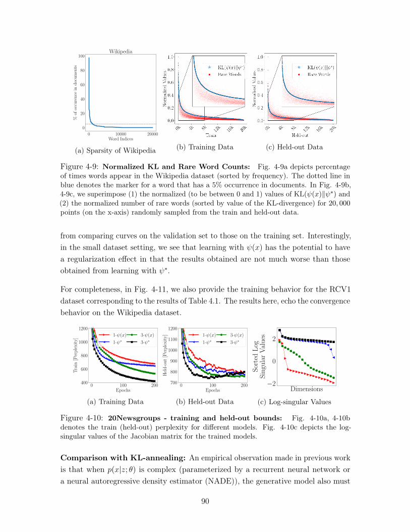
0 10000 20000Word Indices
0
20
40
60
80
100
%of
occu
ren
cein
doc
um
ents
Wikipedia
(a) Sparsity of Wikipedia (b) Training Data (c) Held-out Data
Figure 4-9: Normalized KL and Rare Word Counts: Fig. 4-9a depicts percentageof times words appear in the Wikipedia dataset (sorted by frequency). The dotted line inblue denotes the marker for a word that has a 5% occurrence in documents. In Fig. 4-9b,4-9c, we superimpose (1) the normalized (to be between 0 and 1) values of KL(𝜓(𝑥)‖𝜓*) and(2) the normalized number of rare words (sorted by value of the KL-divergence) for 20, 000points (on the x-axis) randomly sampled from the train and held-out data.
from comparing curves on the validation set to those on the training set. Interestingly,in the small dataset setting, we see that learning with 𝜓(𝑥) has the potential to havea regularization effect in that the results obtained are not much worse than thoseobtained from learning with 𝜓*.
For completeness, in Fig. 4-11, we also provide the training behavior for the RCV1dataset corresponding to the results of Table 4.1. The results here, echo the convergencebehavior on the Wikipedia dataset.
0 100 200Epochs
400
600
800
1000
1200
Tra
in[P
erp
lexi
ty]
1-ψ(x)
1-ψ∗3-ψ(x)
3-ψ∗
(a) Training Data
0 100 200Epochs
700
800
900
1000
1100
1200
Hel
d-o
ut
[Per
ple
xity
] 1-ψ(x)
1-ψ∗3-ψ(x)
3-ψ∗
(b) Held-out Data
Dimensions−2
0
2
Sor
ted
Log
Sin
gula
rV
alu
es
(c) Log-singular Values
Figure 4-10: 20Newsgroups - training and held-out bounds: Fig. 4-10a, 4-10bdenotes the train (held-out) perplexity for different models. Fig. 4-10c depicts the log-singular values of the Jacobian matrix for the trained models.
Comparison with KL-annealing: An empirical observation made in previous workis that when 𝑝(𝑥|𝑧; 𝜃) is complex (parameterized by a recurrent neural network ora neural autoregressive density estimator (NADE)), the generative model also must
90
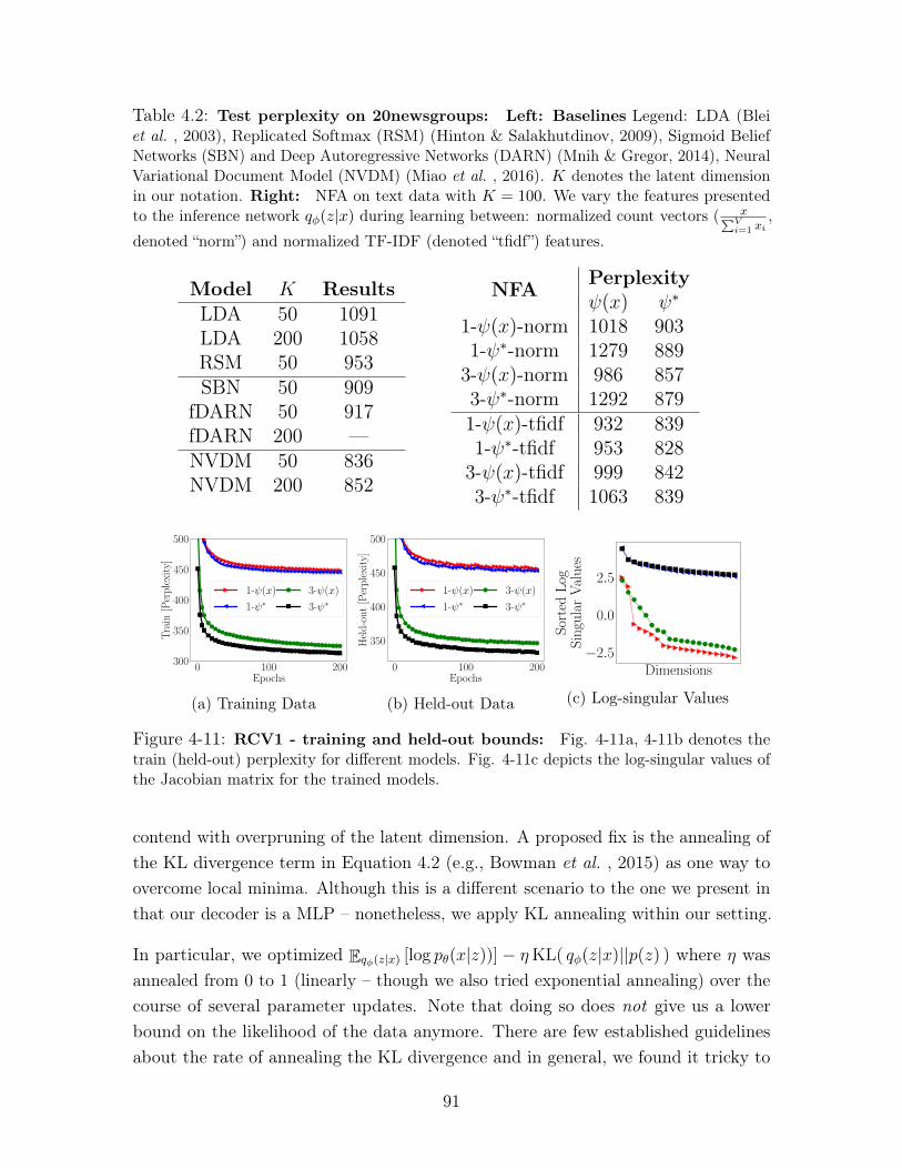
Table 4.2: Test perplexity on 20newsgroups: Left: Baselines Legend: LDA (Bleiet al. , 2003), Replicated Softmax (RSM) (Hinton & Salakhutdinov, 2009), Sigmoid BeliefNetworks (SBN) and Deep Autoregressive Networks (DARN) (Mnih & Gregor, 2014), NeuralVariational Document Model (NVDM) (Miao et al. , 2016). 𝐾 denotes the latent dimensionin our notation. Right: NFA on text data with 𝐾 = 100. We vary the features presentedto the inference network 𝑞𝜑(𝑧|𝑥) during learning between: normalized count vectors ( 𝑥∑︀𝑉
𝑖=1 𝑥𝑖,
denoted “norm”) and normalized TF-IDF (denoted “tfidf”) features.
Model 𝐾 ResultsLDA 50 1091LDA 200 1058RSM 50 953SBN 50 909
fDARN 50 917fDARN 200 —NVDM 50 836NVDM 200 852
NFA Perplexity𝜓(𝑥) 𝜓*
1-𝜓(𝑥)-norm 1018 9031-𝜓*-norm 1279 889
3-𝜓(𝑥)-norm 986 8573-𝜓*-norm 1292 8791-𝜓(𝑥)-tfidf 932 8391-𝜓*-tfidf 953 828
3-𝜓(𝑥)-tfidf 999 8423-𝜓*-tfidf 1063 839
0 100 200Epochs
300
350
400
450
500
Tra
in[P
erp
lexi
ty]
1-ψ(x)
1-ψ∗3-ψ(x)
3-ψ∗
(a) Training Data
0 100 200Epochs
350
400
450
500
Hel
d-o
ut
[Per
ple
xity
]
1-ψ(x)
1-ψ∗3-ψ(x)
3-ψ∗
(b) Held-out Data
Dimensions−2.5
0.0
2.5S
orte
dL
ogS
ingu
lar
Val
ues
(c) Log-singular Values
Figure 4-11: RCV1 - training and held-out bounds: Fig. 4-11a, 4-11b denotes thetrain (held-out) perplexity for different models. Fig. 4-11c depicts the log-singular values ofthe Jacobian matrix for the trained models.
contend with overpruning of the latent dimension. A proposed fix is the annealing ofthe KL divergence term in Equation 4.2 (e.g., Bowman et al. , 2015) as one way toovercome local minima. Although this is a different scenario to the one we present inthat our decoder is a MLP – nonetheless, we apply KL annealing within our setting.
In particular, we optimized E𝑞𝜑(𝑧|𝑥) [log 𝑝𝜃(𝑥|𝑧))] − 𝜂KL( 𝑞𝜑(𝑧|𝑥)||𝑝(𝑧) ) where 𝜂 wasannealed from 0 to 1 (linearly – though we also tried exponential annealing) over thecourse of several parameter updates. Note that doing so does not give us a lowerbound on the likelihood of the data anymore. There are few established guidelinesabout the rate of annealing the KL divergence and in general, we found it tricky to
91
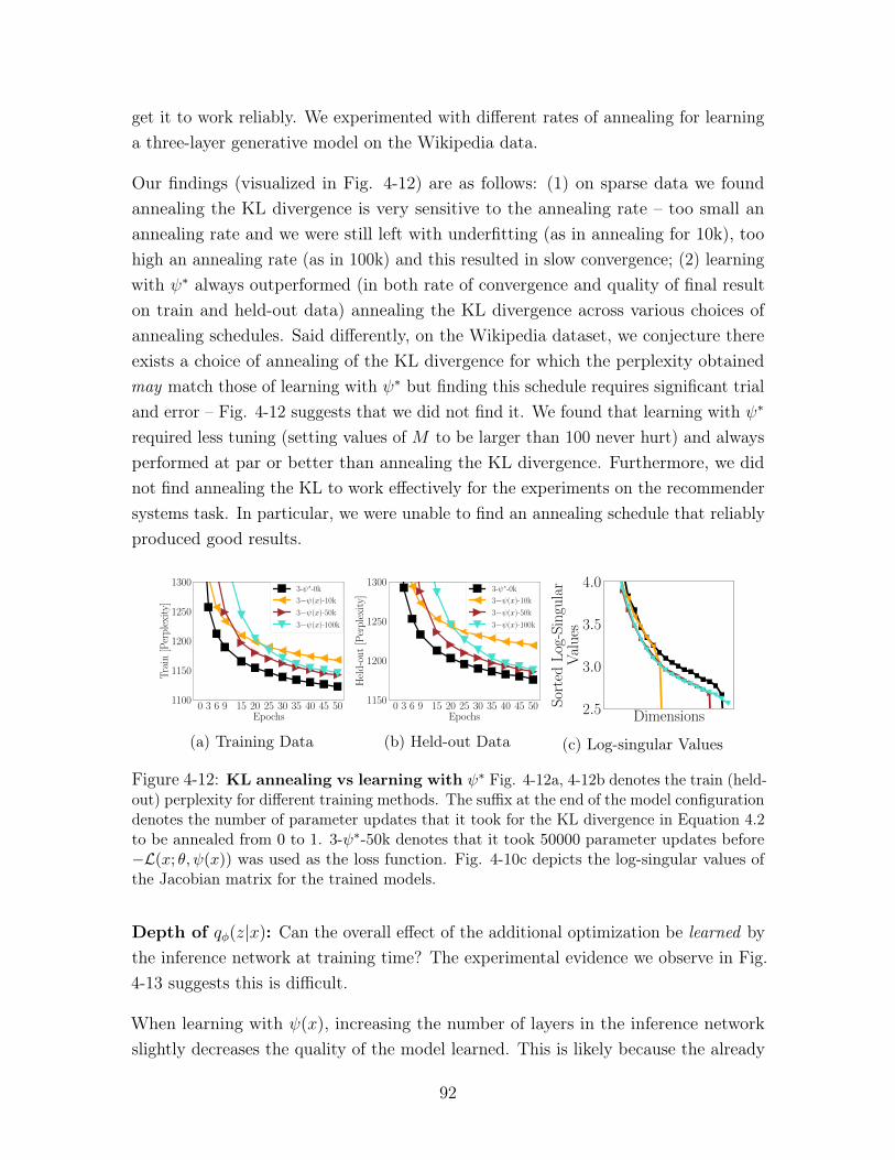
get it to work reliably. We experimented with different rates of annealing for learninga three-layer generative model on the Wikipedia data.
Our findings (visualized in Fig. 4-12) are as follows: (1) on sparse data we foundannealing the KL divergence is very sensitive to the annealing rate – too small anannealing rate and we were still left with underfitting (as in annealing for 10k), toohigh an annealing rate (as in 100k) and this resulted in slow convergence; (2) learningwith 𝜓* always outperformed (in both rate of convergence and quality of final resulton train and held-out data) annealing the KL divergence across various choices ofannealing schedules. Said differently, on the Wikipedia dataset, we conjecture thereexists a choice of annealing of the KL divergence for which the perplexity obtainedmay match those of learning with 𝜓* but finding this schedule requires significant trialand error – Fig. 4-12 suggests that we did not find it. We found that learning with 𝜓*
required less tuning (setting values of 𝑀 to be larger than 100 never hurt) and alwaysperformed at par or better than annealing the KL divergence. Furthermore, we didnot find annealing the KL to work effectively for the experiments on the recommendersystems task. In particular, we were unable to find an annealing schedule that reliablyproduced good results.
0 3 6 9 15 20 25 30 35 40 45 50Epochs
1100
1150
1200
1250
1300
Tra
in[P
erp
lexi
ty]
3-ψ∗-0k
3−ψ(x)-10k
3−ψ(x)-50k
3−ψ(x)-100k
(a) Training Data
0 3 6 9 15 20 25 30 35 40 45 50Epochs
1150
1200
1250
1300
Hel
d-o
ut
[Per
ple
xity
]
3-ψ∗-0k
3−ψ(x)-10k
3−ψ(x)-50k
3−ψ(x)-100k
(b) Held-out Data
Dimensions2.5
3.0
3.5
4.0
Sor
ted
Log
-Sin
gula
rV
alu
es
(c) Log-singular Values
Figure 4-12: KL annealing vs learning with 𝜓* Fig. 4-12a, 4-12b denotes the train (held-out) perplexity for different training methods. The suffix at the end of the model configurationdenotes the number of parameter updates that it took for the KL divergence in Equation 4.2to be annealed from 0 to 1. 3-𝜓*-50k denotes that it took 50000 parameter updates before−ℒ(𝑥; 𝜃, 𝜓(𝑥)) was used as the loss function. Fig. 4-10c depicts the log-singular values ofthe Jacobian matrix for the trained models.
Depth of 𝑞𝜑(𝑧|𝑥): Can the overall effect of the additional optimization be learned bythe inference network at training time? The experimental evidence we observe in Fig.4-13 suggests this is difficult.
When learning with 𝜓(𝑥), increasing the number of layers in the inference networkslightly decreases the quality of the model learned. This is likely because the already
92
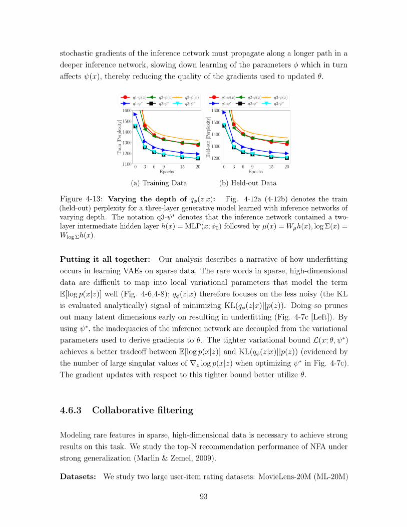
stochastic gradients of the inference network must propagate along a longer path in adeeper inference network, slowing down learning of the parameters 𝜑 which in turnaffects 𝜓(𝑥), thereby reducing the quality of the gradients used to updated 𝜃.
0 3 6 9 15 20Epochs
1100
1200
1300
1400
1500
1600
Tra
in[P
erp
lexi
ty]
q1-ψ(x)
q1-ψ∗q2-ψ(x)
q2-ψ∗q3-ψ(x)
q3-ψ∗
(a) Training Data
0 3 6 9 15 20Epochs
1200
1300
1400
1500
1600
Hel
d-o
ut
[Per
ple
xity
]
q1-ψ(x)
q1-ψ∗q2-ψ(x)
q2-ψ∗q3-ψ(x)
q3-ψ∗
(b) Held-out Data
Figure 4-13: Varying the depth of 𝑞𝜑(𝑧|𝑥): Fig. 4-12a (4-12b) denotes the train(held-out) perplexity for a three-layer generative model learned with inference networks ofvarying depth. The notation q3-𝜓* denotes that the inference network contained a two-layer intermediate hidden layer ℎ(𝑥) = MLP(𝑥;𝜑0) followed by 𝜇(𝑥) =𝑊𝜇ℎ(𝑥), log Σ(𝑥) =𝑊log Σℎ(𝑥).
Putting it all together: Our analysis describes a narrative of how underfittingoccurs in learning VAEs on sparse data. The rare words in sparse, high-dimensionaldata are difficult to map into local variational parameters that model the termE[log 𝑝(𝑥|𝑧)] well (Fig. 4-6,4-8); 𝑞𝜑(𝑧|𝑥) therefore focuses on the less noisy (the KLis evaluated analytically) signal of minimizing KL(𝑞𝜑(𝑧|𝑥)||𝑝(𝑧)). Doing so prunesout many latent dimensions early on resulting in underfitting (Fig. 4-7c [Left]). Byusing 𝜓*, the inadequacies of the inference network are decoupled from the variationalparameters used to derive gradients to 𝜃. The tighter variational bound ℒ(𝑥; 𝜃, 𝜓*)
achieves a better tradeoff between E[log 𝑝(𝑥|𝑧)] and KL(𝑞𝜑(𝑧|𝑥)||𝑝(𝑧)) (evidenced bythe number of large singular values of ∇𝑧 log 𝑝(𝑥|𝑧) when optimizing 𝜓* in Fig. 4-7c).The gradient updates with respect to this tighter bound better utilize 𝜃.
4.6.3 Collaborative filtering
Modeling rare features in sparse, high-dimensional data is necessary to achieve strongresults on this task. We study the top-N recommendation performance of NFA understrong generalization (Marlin & Zemel, 2009).
Datasets: We study two large user-item rating datasets: MovieLens-20M (ML-20M)
93
(Harper & Konstan, 2015) and Netflix2. Following standard procedure: we binarize theexplicit rating data, keeping ratings of four or higher and interpreting them as implicitfeedback (Hu et al. , 2008) and keep users who have positively rated at least fivemovies. We train with users’ binary implicit feedback as 𝑥𝑑; the vocabulary is the setof all movies. The number of training/validation/test users is 116,677/10,000/10,000for ML-20M (𝑉 : 20,108) and 383,435/40,000/40,000 for Netflix (𝑉 : 17,769).
Evaluation and metrics: We train with the complete feedback history fromtraining users, and evaluate on held-out validation/test users. We select modelarchitecture (MLP with 0, 1, 2 hidden layers) from the held-out validation users basedon NDCG@100 and report metrics on the held-out test users. For held-out users, werandomly select 80% of the feedback as the input to the inference network and seehow the other 20% of the positively rated items are ranked based 𝜇(𝑧). We reporttwo ranking-based metrics averaged over all held-out users: Recall@𝑁 and truncatednormalized discounted cumulative gain (NDCG@𝑁) (Järvelin & Kekäläinen, 2002).For each user, both metrics compare the predicted rank of unobserved items withtheir true rank. While Recall@𝑁 considers all items ranked within the first 𝑁 tobe equivalent, NDCG@𝑁 uses a monotonically increasing discount to emphasize theimportance of higher ranks versus lower ones.
Define 𝜋 as a ranking over all the items where 𝜋(𝑣) indicates the 𝑣-th ranked item,I{·} is the indicator function, and 𝑑(𝜋(𝑣)) returns 1 if user 𝑑 has positively rated item𝜋(𝑣). Recall@𝑁 for user 𝑑 is
Recall@𝑁(𝑑, 𝜋) :=𝑁∑︁
𝑣=1
I{𝑑(𝜋(𝑣)) = 1}min(𝑁,
∑︀𝑉𝑣′ I{𝑑(𝜋(𝑣′)) = 1})
.
The expression in the denominator evaluates to the minimum between 𝑁 and thenumber of items consumed by user 𝑑. This normalizes Recall@𝑁 to have a maximum of1, which corresponds to ranking all relevant items in the top 𝑁 positions. Discountedcumulative gain (DCG@𝑁) for user 𝑑 is
DCG@𝑁(𝑑, 𝜋) :=𝑁∑︁
𝑣=1
2I{𝑑(𝜋(𝑣))=1} − 1
log(𝑣 + 1).
NDCG@𝑁 is the DCG@𝑁 normalized by ideal DCG𝑁 , where all the relevant itemsare ranked at the top. We have, NDCG@𝑁 ∈ [0, 1]. As baselines, we consider:
2http://www.netflixprize.com/
94
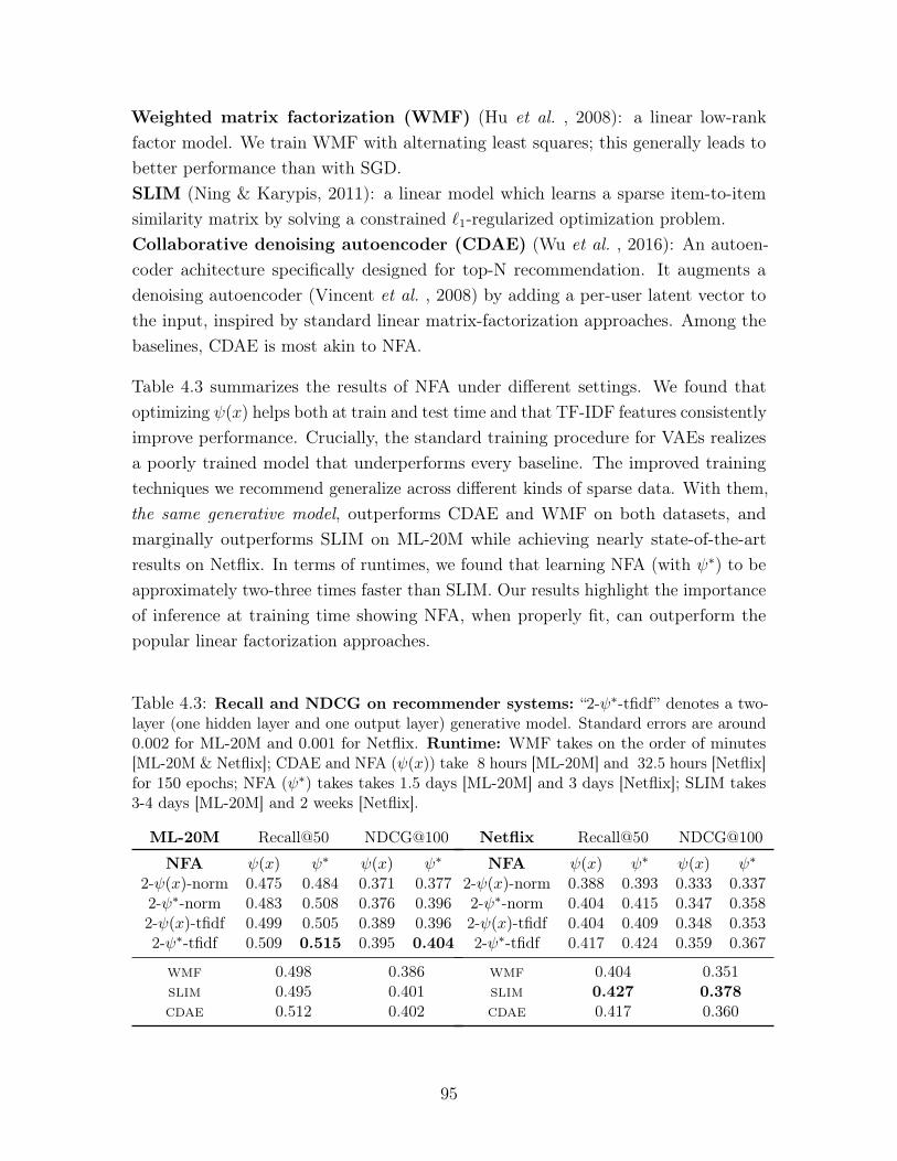
Weighted matrix factorization (WMF) (Hu et al. , 2008): a linear low-rankfactor model. We train WMF with alternating least squares; this generally leads tobetter performance than with SGD.SLIM (Ning & Karypis, 2011): a linear model which learns a sparse item-to-itemsimilarity matrix by solving a constrained ℓ1-regularized optimization problem.Collaborative denoising autoencoder (CDAE) (Wu et al. , 2016): An autoen-coder achitecture specifically designed for top-N recommendation. It augments adenoising autoencoder (Vincent et al. , 2008) by adding a per-user latent vector tothe input, inspired by standard linear matrix-factorization approaches. Among thebaselines, CDAE is most akin to NFA.
Table 4.3 summarizes the results of NFA under different settings. We found thatoptimizing 𝜓(𝑥) helps both at train and test time and that TF-IDF features consistentlyimprove performance. Crucially, the standard training procedure for VAEs realizesa poorly trained model that underperforms every baseline. The improved trainingtechniques we recommend generalize across different kinds of sparse data. With them,the same generative model, outperforms CDAE and WMF on both datasets, andmarginally outperforms SLIM on ML-20M while achieving nearly state-of-the-artresults on Netflix. In terms of runtimes, we found that learning NFA (with 𝜓*) to beapproximately two-three times faster than SLIM. Our results highlight the importanceof inference at training time showing NFA, when properly fit, can outperform thepopular linear factorization approaches.
Table 4.3: Recall and NDCG on recommender systems: “2-𝜓*-tfidf” denotes a two-layer (one hidden layer and one output layer) generative model. Standard errors are around0.002 for ML-20M and 0.001 for Netflix. Runtime: WMF takes on the order of minutes[ML-20M & Netflix]; CDAE and NFA (𝜓(𝑥)) take 8 hours [ML-20M] and 32.5 hours [Netflix]for 150 epochs; NFA (𝜓*) takes takes 1.5 days [ML-20M] and 3 days [Netflix]; SLIM takes3-4 days [ML-20M] and 2 weeks [Netflix].
ML-20M Recall@50 NDCG@100
NFA 𝜓(𝑥) 𝜓* 𝜓(𝑥) 𝜓*
2-𝜓(𝑥)-norm 0.475 0.484 0.371 0.3772-𝜓*-norm 0.483 0.508 0.376 0.3962-𝜓(𝑥)-tfidf 0.499 0.505 0.389 0.3962-𝜓*-tfidf 0.509 0.515 0.395 0.404
wmf 0.498 0.386slim 0.495 0.401cdae 0.512 0.402
Netflix Recall@50 NDCG@100
NFA 𝜓(𝑥) 𝜓* 𝜓(𝑥) 𝜓*
2-𝜓(𝑥)-norm 0.388 0.393 0.333 0.3372-𝜓*-norm 0.404 0.415 0.347 0.3582-𝜓(𝑥)-tfidf 0.404 0.409 0.348 0.3532-𝜓*-tfidf 0.417 0.424 0.359 0.367
wmf 0.404 0.351slim 0.427 0.378cdae 0.417 0.360
95
4.7 Discussion
Studying the failures of learning with inference networks is an important step todesigning more robust neural architectures for inference networks. We show thatavoiding gradients obtained using poor variational parameters is vital to successfullylearning VAEs on sparse data. An interesting question is why inference networks havea harder time turning sparse data into variational parameters compared to images?One hypothesis is that the redundant correlations that exist among pixels (but occurless frequently in features found in sparse data) are more easily transformed into localvariational parameters 𝜓(𝑥) that are, in practice, often reasonably close to 𝜓* duringlearning.
Hjelm et al. explore a similar idea as ours to derive an importance-sampling-basedbound for learning deep generative models with discrete latent variables. They findthat learning with 𝜓* does not improve results on binarized MNIST. This is consistentwith our experience—we find that our secondary optimization procedure helped morewhen learning models of sparse data. Miao et al. learn log-linear models (multinomial-logistic PCA, Collins et al. , 2001) of documents using inference networks. We showthat mitigating underfitting in deeper models yields better results on the benchmarkRCV1 data. Our use of the spectra of the Jacobian matrix of log 𝑝(𝑥|𝑧) to inspectlearned models is inspired by Wang et al. (2016).
96
Chapter 5
Supervised fine-tuning of deepgenerative models
Supervision in machine learning comes in many forms. Although the canonical formof supervised data is in the form of labelled annotations (for each datapoint), thismay not always be the best way to guide learning algorithm. One form of supervisionof interest are pairwise expressions of similarity between datapoints.
A motivating example is the task of patient similarity where a doctor may be interestedin searching a hospital database to find similar patients. For example, a doctor mayhave a set of patients who they believe are similar because they respond rapidly toa treatment. The doctor may be interested in finding other patients who respondsimilarly. In this scenario, the doctor does not prescribe discrete labels to every patient,but rather identifies similar patients based on how much they satisfy a clinical criteriasuch as their response to treatment.
We build algorithms to tackle such a problem by way of analogy to few-shot learning.In few-shot learning, a learner is given access to sets of datapoints that are assumedto be similar. At test time, the learner is given a target datapoint and multiple querysets. Each query set, comprising one or more datapoints, is a candidate to be identifiedas being most similar to the target.
To make the analogy to healthcare precise, the target datapoint may comprise patientdata from a new patient and the query sets may comprise pre-defined sets of patients,each exhibiting known phenotypic characteristics. The goal of the learner is to identifywhich set of phenotypic characteristic the new patient is most similar to. In this
97
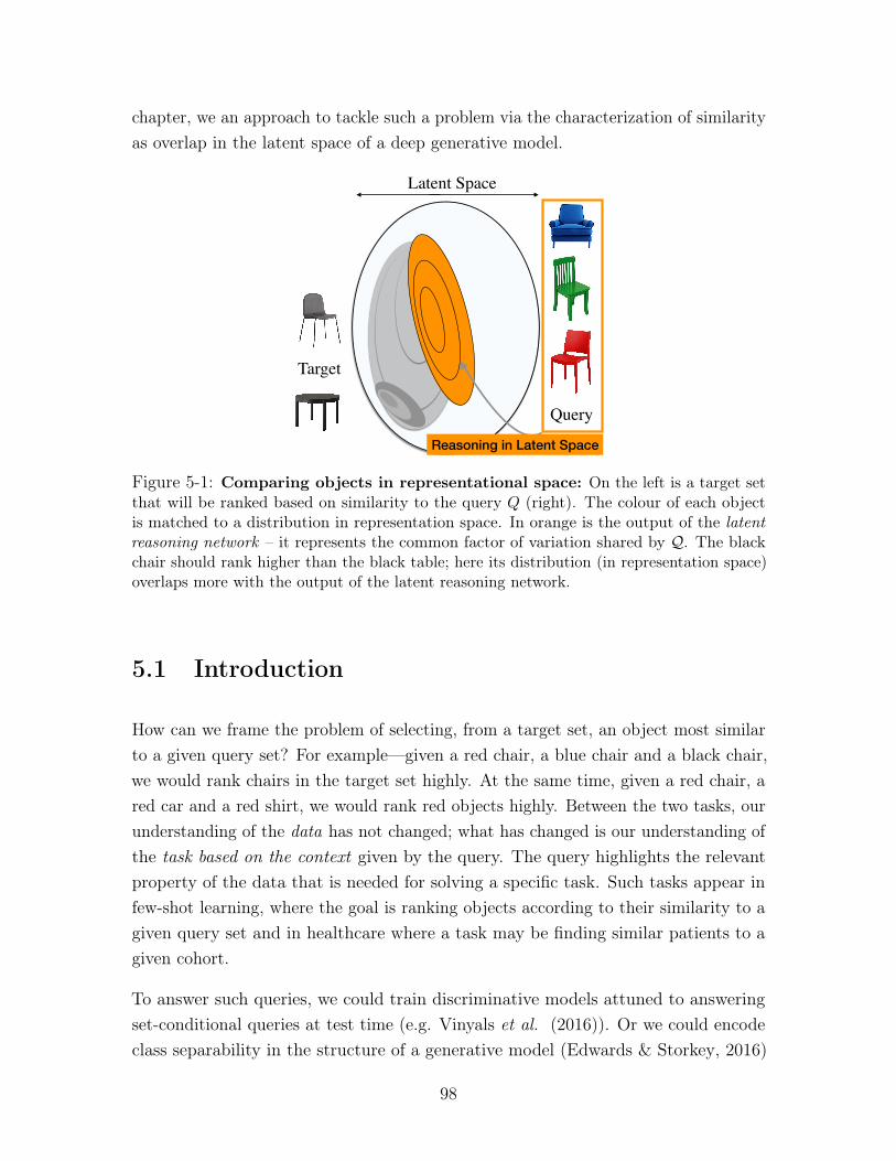
chapter, we an approach to tackle such a problem via the characterization of similarityas overlap in the latent space of a deep generative model.
Latent Space
Query
Target
Reasoning in Latent Space
Figure 5-1: Comparing objects in representational space: On the left is a target setthat will be ranked based on similarity to the query 𝑄 (right). The colour of each objectis matched to a distribution in representation space. In orange is the output of the latentreasoning network – it represents the common factor of variation shared by 𝒬. The blackchair should rank higher than the black table; here its distribution (in representation space)overlaps more with the output of the latent reasoning network.
5.1 Introduction
How can we frame the problem of selecting, from a target set, an object most similarto a given query set? For example—given a red chair, a blue chair and a black chair,we would rank chairs in the target set highly. At the same time, given a red chair, ared car and a red shirt, we would rank red objects highly. Between the two tasks, ourunderstanding of the data has not changed; what has changed is our understanding ofthe task based on the context given by the query. The query highlights the relevantproperty of the data that is needed for solving a specific task. Such tasks appear infew-shot learning, where the goal is ranking objects according to their similarity to agiven query set and in healthcare where a task may be finding similar patients to agiven cohort.
To answer such queries, we could train discriminative models attuned to answeringset-conditional queries at test time (e.g. Vinyals et al. (2016)). Or we could encodeclass separability in the structure of a generative model (Edwards & Storkey, 2016)
98
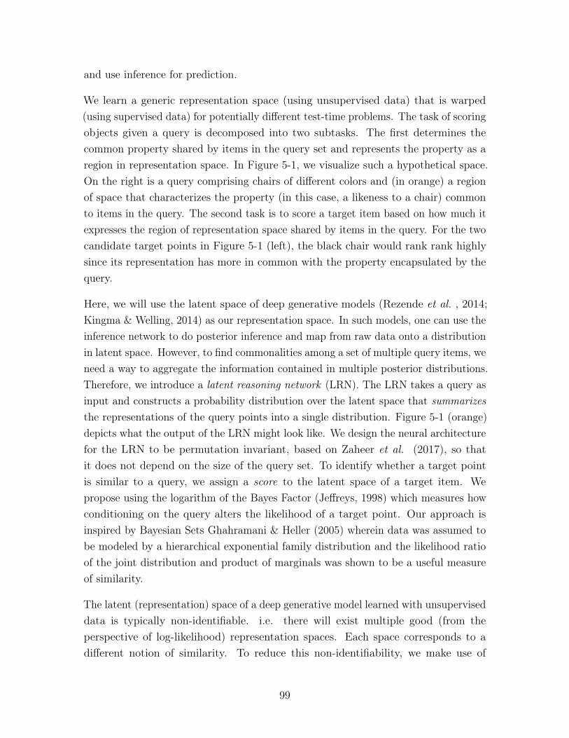
and use inference for prediction.
We learn a generic representation space (using unsupervised data) that is warped(using supervised data) for potentially different test-time problems. The task of scoringobjects given a query is decomposed into two subtasks. The first determines thecommon property shared by items in the query set and represents the property as aregion in representation space. In Figure 5-1, we visualize such a hypothetical space.On the right is a query comprising chairs of different colors and (in orange) a regionof space that characterizes the property (in this case, a likeness to a chair) commonto items in the query. The second task is to score a target item based on how much itexpresses the region of representation space shared by items in the query. For the twocandidate target points in Figure 5-1 (left), the black chair would rank rank highlysince its representation has more in common with the property encapsulated by thequery.
Here, we will use the latent space of deep generative models (Rezende et al. , 2014;Kingma & Welling, 2014) as our representation space. In such models, one can use theinference network to do posterior inference and map from raw data onto a distributionin latent space. However, to find commonalities among a set of multiple query items, weneed a way to aggregate the information contained in multiple posterior distributions.Therefore, we introduce a latent reasoning network (LRN). The LRN takes a query asinput and constructs a probability distribution over the latent space that summarizesthe representations of the query points into a single distribution. Figure 5-1 (orange)depicts what the output of the LRN might look like. We design the neural architecturefor the LRN to be permutation invariant, based on Zaheer et al. (2017), so thatit does not depend on the size of the query set. To identify whether a target pointis similar to a query, we assign a score to the latent space of a target item. Wepropose using the logarithm of the Bayes Factor (Jeffreys, 1998) which measures howconditioning on the query alters the likelihood of a target point. Our approach isinspired by Bayesian Sets Ghahramani & Heller (2005) wherein data was assumed tobe modeled by a hierarchical exponential family distribution and the likelihood ratioof the joint distribution and product of marginals was shown to be a useful measureof similarity.
The latent (representation) space of a deep generative model learned with unsuperviseddata is typically non-identifiable. i.e. there will exist multiple good (from theperspective of log-likelihood) representation spaces. Each space corresponds to adifferent notion of similarity. To reduce this non-identifiability, we make use of
99
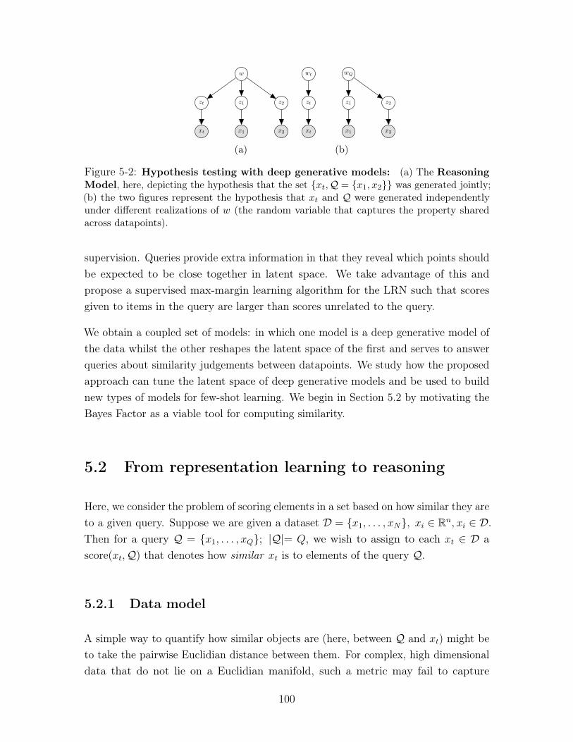
𝑥𝑡 𝑥1 𝑥2
𝑧𝑡 𝑧1 𝑧2
𝑤
(a)
𝑥𝑡
𝑧𝑡
𝑤𝑡
𝑥1 𝑥2
𝑧1 𝑧2
𝑤𝑄
(b)
Figure 5-2: Hypothesis testing with deep generative models: (a) The ReasoningModel, here, depicting the hypothesis that the set {𝑥𝑡,𝒬 = {𝑥1, 𝑥2}} was generated jointly;(b) the two figures represent the hypothesis that 𝑥𝑡 and 𝒬 were generated independentlyunder different realizations of 𝑤 (the random variable that captures the property sharedacross datapoints).
supervision. Queries provide extra information in that they reveal which points shouldbe expected to be close together in latent space. We take advantage of this andpropose a supervised max-margin learning algorithm for the LRN such that scoresgiven to items in the query are larger than scores unrelated to the query.
We obtain a coupled set of models: in which one model is a deep generative model ofthe data whilst the other reshapes the latent space of the first and serves to answerqueries about similarity judgements between datapoints. We study how the proposedapproach can tune the latent space of deep generative models and be used to buildnew types of models for few-shot learning. We begin in Section 5.2 by motivating theBayes Factor as a viable tool for computing similarity.
5.2 From representation learning to reasoning
Here, we consider the problem of scoring elements in a set based on how similar they areto a given query. Suppose we are given a dataset 𝒟 = {𝑥1, . . . , 𝑥𝑁}, 𝑥𝑖 ∈ R𝑛, 𝑥𝑖 ∈ 𝒟.Then for a query 𝒬 = {𝑥1, . . . , 𝑥𝑄}; |𝒬|= 𝑄, we wish to assign to each 𝑥𝑡 ∈ 𝒟 ascore(𝑥𝑡,𝒬) that denotes how similar 𝑥𝑡 is to elements of the query 𝒬.
5.2.1 Data model
A simple way to quantify how similar objects are (here, between 𝒬 and 𝑥𝑡) might beto take the pairwise Euclidian distance between them. For complex, high dimensionaldata that do not lie on a Euclidian manifold, such a metric may fail to capture
100
interesting regularity between data.
Alternatively, we can use a latent variable model to construct a representation of data.The latent variable then becomes a low-dimensional sufficient statistic for the raw datawhen quantifying similarity. The simplest latent variable model we will consider hasthe following generative process: 𝑧 ∼ 𝑝dm(𝑧); 𝑥 ∼ 𝑝dm(𝑥; 𝑓(𝑧; 𝜃)) where 𝑝dm(𝑧) isa simple distribution such as 𝒩 (0, 𝐼). The use of MLPs in the conditional distributionsallow the model to fit highly complex data despite the use of a simple prior. When 𝑓is parameterized by a Multi-Layer Perceptron (MLP), the resulting model is a deepgenerative model. We will refer to this model (Kingma & Welling, 2014; Rezende et al., 2014) as the Data Model (with probabilities denoted with subscript dm).
The generative process assumes datapoints are drawn independently. Using variationalinference with an inference network (Hinton et al. , 1995) to approximate the posteriordistribution, 𝑝rm(𝑧|𝑥), the model can be learned by maximizing a lower bound onthe log-likelihood of the data.
log 𝑝dm(𝑥; 𝜃) ≥ E𝑞dm(𝑧|𝑥;𝜑)
[︀log 𝑝dm(𝑥|𝑧; 𝜃))
]︀(5.1)
−KL( 𝑞dm(𝑧|𝑥;𝜑)||𝑝dm(𝑧) ) = ℒ(𝑥; 𝜃, 𝜑),
With a Gaussian distribution as the variational approximation: 𝑞dm(𝑧|𝑥;𝜑) ∼𝒩 (𝜇𝜑(𝑥),Σ𝜑(𝑥)) where 𝜇𝜑(𝑥),Σ𝜑(𝑥) are (differentiable, parametric, with parame-ters 𝜑) functions of the observation 𝑥. As before, Eq. 5.1 is differentiable in 𝜃, 𝜑
(Kingma & Welling, 2014; Rezende et al. , 2014) and the model parameters (𝜃, 𝜑) canbe learned via gradient ascent on ℒ(𝑥; 𝜃, 𝜑).
With the variational approximation, 𝑞dm(𝑧|𝑥;𝜑), to map from data to latent space,would computing overlap in the posterior distributions of points in 𝒬 and 𝑥𝑡 sufficeto identify similar points? The answer is sometimes. While unsupervised learningwill tend to put similar points together, the notion of similarity encoded in the latentspace need not correspond to the notion of similarity required for a task at test time.We require a way to guide the structure of the latent space to be better suited for atask.
101
5.2.2 Reasoning model
Introducing hierarchy into the generative process is one way to guide the structureof latent variables. In Figure 5-2 (b) is a simple hierarchical model that makesexplicit the insight that similar datapoints should have similar latent spaces. Itdefines the following generative process for a set of similar objects 𝒬: 𝑝rm(𝒬) =∫︀𝑤
∫︀𝑧𝑝rm(𝑤)
∏︀𝑄𝑞=1 𝑝rm(𝑧𝑞|𝑤)𝑝rm(𝑥𝑞|𝑧𝑞). The random variable 𝑤 defines the context
of 𝒬. It may denote the label or class identity of points in 𝒬 but more broadly is arepresentation of the properties that points in 𝒬 satisfy. For notational convenienceand because we can express reasoning about similarity as a probabilistic query in thismodel, we refer to it as the Reasoning Model.
The Neural Statistician (Edwards & Storkey, 2016) uses KL(𝑝(𝑤|𝑥𝑡)||𝑝(𝑤|𝒬)) toquantify the similarity between 𝑥𝑡 and 𝒬 in a model similar to the one in Figure 5-2(b). In this work, we pose the estimation of similarity between objects as hypothesistesting in a hierarchical deep generative model. The conditional independences inFigure 5-2 (b) enforce that 𝑥𝑡 is independent of 𝑤 given 𝑧𝑡, i.e. the per-data-pointlatent variables serve as a sufficient statistic to quantify comparisons between multipledatapoints. The conditional density 𝑝(𝑥𝑡|𝑧𝑡) is a map from the representation spaceto the data while 𝑝(𝑧𝑡|𝑤) dictates how the latent space of a datapoint behaves as afunction of property encoded in 𝑤.
5.2.3 Bayes factor
To score the similarity between two objects (in this case 𝑥𝑡 and set 𝒬) under theReasoning Model, we turn to the likelihood ratio between the joint distribution of 𝑥𝑡and 𝒬 and the product of their marginals. If 𝑥𝑡 and 𝒬 are drawn from the same jointdistribution, then there exists a random variable 𝑤 that governs the distribution of thelatent spaces 𝑧𝑡, 𝑧1, . . . , 𝑧𝑄. With slight abuse of notation1, Figure 5-2 (a) depicts thisscenario when 𝒬 = {𝑥1, 𝑥2}. If 𝑥𝑡 and 𝒬 are not similar, then their latent spaces willhave different distributions, and they are children of different realizations of 𝑤 (seeFigure 5-2 (b)). With that in mind, the score function we use to measure similarity isgiven by (Bayes Factor):
𝑝(𝑥𝑡,𝒬)𝑝(𝑥𝑡)𝑝(𝒬)
=𝑝(𝑥𝑡|𝒬)𝑝(𝑥𝑡)
= score(𝑥𝑡,𝒬) (5.2)
1We re-use Figure 5-2 to denote both the instantiation of a hypothesis and the generative process
102
The log-score is the pointwise mutual information (Fano, 1949), a measure of associationthat is frequently used in applications such as natural language processing (Church &Hanks, 1990). The Bayes Factor normalizes the posterior predictive density of thetarget point conditioned on the query by the target’s marginal likelihood under themodel. It also has an information theoretic interpretation. Letting ℎ(𝑥) = − log 𝑝(𝑥)
denote the self-information (or surprisal), then log score(𝑥𝑡,𝒬) = ℎ(𝑥𝑡) − ℎ(𝑥𝑡|𝒬)intuitively denotes the surprise (quantified in nats or bits) from observing 𝑥𝑡 whenhaving already observed 𝒬.
Similarity in Latent Space: Equation 5.2 captures an intuitive notion of similaritybut evaluating 𝑝(𝑥𝑡), the marginal density of the target, is typically intractable (exceptin hierarchical models that lie in the exponential family (Ghahramani & Heller, 2005)).Furthermore, an importance sampling based Monte-Carlo estimator for 𝑝(𝑥𝑡) willinvolve a high-dimensional integral in the data 𝑥𝑡. We therefore propose the followingdecomposition of the score function that evaluates the Bayes Factor in the targetdatapoint’s (lower dimensional) latent space:
𝑝rm(𝑥𝑡|𝒬)𝑝rm(𝑥𝑡)
=1
𝑝rm(𝑥𝑡)
∫︁
𝑧𝑡
𝑝rm(𝑥𝑡, 𝑧𝑡|𝒬) (5.3)
=1
𝑝rm(𝑥𝑡)
∫︁
𝑧𝑡
𝑝rm(𝑥𝑡|𝑧𝑡)𝑝rm(𝑧𝑡|𝒬)
=1
𝑝rm(𝑥𝑡)
∫︁
𝑧𝑡
𝑝rm(𝑧𝑡|𝑥𝑡)𝑝rm(𝑥𝑡)
𝑝rm(𝑧𝑡)𝑝rm(𝑧𝑡|𝒬)
=
∫︁
𝑧𝑡
𝑝rm(𝑧𝑡|𝑥𝑡)𝑝rm(𝑧𝑡)⏟ ⏞
Relative Posterior Likelihood
𝑝rm(𝑧𝑡|𝒬)⏟ ⏞ Latent Reasoning Network
.
The estimator above formalizes the intuition for comparing points laid out in Section5.1. The query-conditional posterior-predictive density over the latent space of thetarget datapoint, 𝑝rm(𝑧𝑡|𝒬), reasons about points in the query and represents themas a density in latent space, The Relative Posterior Likelihood, 𝑝rm(𝑧𝑡|𝑥𝑡)
𝑝rm(𝑧𝑡)scores
how likely the target point is to have come from the relevant part of latent space.
5.3 Hierarchical models with compound priors
To compute the ratio 𝑝rm(𝑧𝑡|𝑥𝑡)𝑝rm(𝑧𝑡)
, we need to marginalize 𝑤𝑡. However, under certainassumptions about the conditional distributions in the Reasoning Model, we will
103
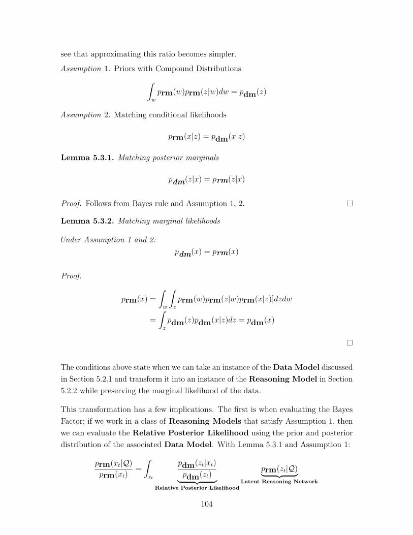
see that approximating this ratio becomes simpler.
Assumption 1. Priors with Compound Distributions∫︁
𝑤
𝑝rm(𝑤)𝑝rm(𝑧|𝑤)𝑑𝑤 = 𝑝dm(𝑧)
Assumption 2. Matching conditional likelihoods
𝑝rm(𝑥|𝑧) = 𝑝dm(𝑥|𝑧)
Lemma 5.3.1. Matching posterior marginals
𝑝dm(𝑧|𝑥) = 𝑝rm(𝑧|𝑥)
Proof. Follows from Bayes rule and Assumption 1, 2.
Lemma 5.3.2. Matching marginal likelihoods
Under Assumption 1 and 2:𝑝dm(𝑥) = 𝑝rm(𝑥)
Proof.
𝑝rm(𝑥) =
∫︁
𝑤
∫︁
𝑧
𝑝rm(𝑤)𝑝rm(𝑧|𝑤)𝑝rm(𝑥|𝑧)]𝑑𝑧𝑑𝑤
=
∫︁
𝑧
𝑝dm(𝑧)𝑝dm(𝑥|𝑧)𝑑𝑧 = 𝑝dm(𝑥)
The conditions above state when we can take an instance of the Data Model discussedin Section 5.2.1 and transform it into an instance of the Reasoning Model in Section5.2.2 while preserving the marginal likelihood of the data.
This transformation has a few implications. The first is when evaluating the BayesFactor; if we work in a class of Reasoning Models that satisfy Assumption 1, thenwe can evaluate the Relative Posterior Likelihood using the prior and posteriordistribution of the associated Data Model. With Lemma 5.3.1 and Assumption 1:
𝑝rm(𝑥𝑡|𝒬)𝑝rm(𝑥𝑡)
=
∫︁
𝑧𝑡
𝑝dm(𝑧𝑡|𝑥𝑡)𝑝dm(𝑧𝑡)⏟ ⏞
Relative Posterior Likelihood
𝑝rm(𝑧𝑡|𝒬)⏟ ⏞ Latent Reasoning Network
104
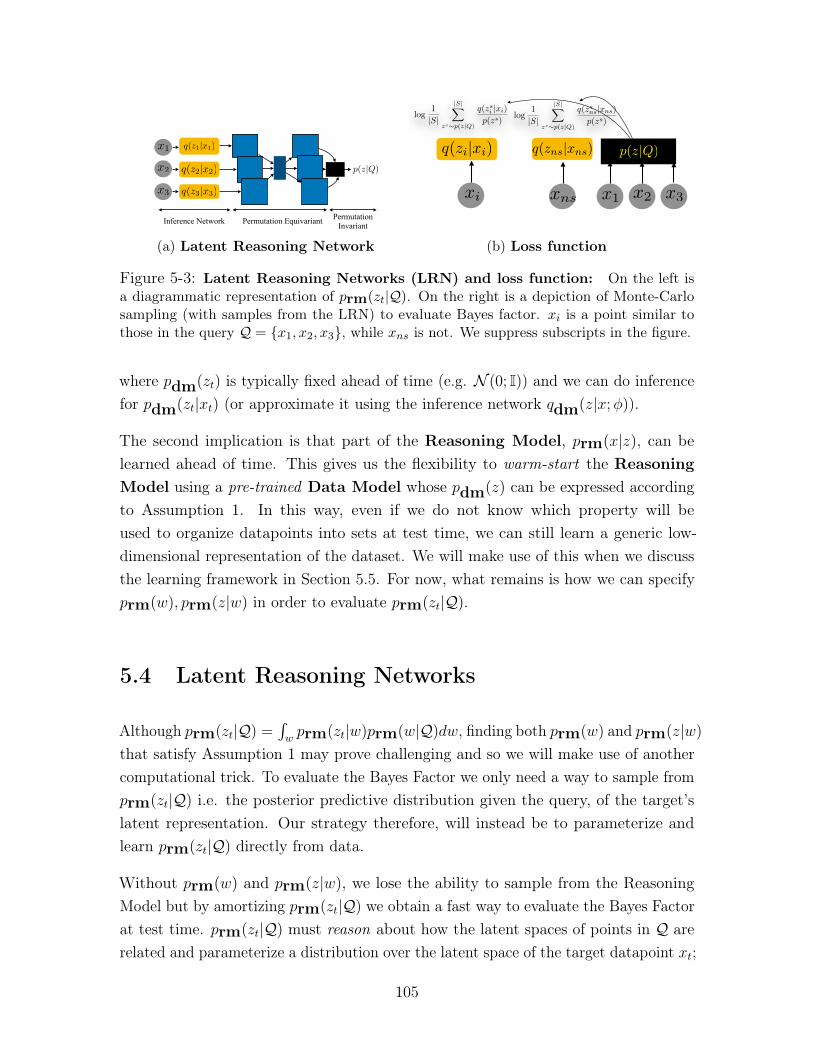
x1
x2
x3
q(z1|x1)
q(z2|x2)
q(z3|x3)
p(z|Q)
Inference Network Permutation InvariantPermutation Equivariant
(a) Latent Reasoning Network
x1 x2xi xns
q(zns|xns)q(zi|xi)
log1
|S|
|S|X
zs⇠p(z|Q)
q(zsns|xns)
p(zs)log
1
|S|
|S|X
zs⇠p(z|Q)
q(zsi |xi)
p(zs)
p(z|Q)
x3<latexit sha1_base64="l/zb7Fkfb1j3hLpXFHaq4Ct5MIc=">AAAB6XicbVBNS8NAEJ3Ur1q/qh69LBbBU0lVUG9FLx4rGltoQ9lsJ+3SzSbsbsQS+hO8eFDx6j/y5r9x2+agrQ8GHu/NMDMvSATXxnW/ncLS8srqWnG9tLG5tb1T3t170HGqGHosFrFqBVSj4BI9w43AVqKQRoHAZjC8nvjNR1Sax/LejBL0I9qXPOSMGivdPXVPu+WKW3WnIIuklpMK5Gh0y1+dXszSCKVhgmrdrrmJ8TOqDGcCx6VOqjGhbEj72LZU0gi1n01PHZMjq/RIGCtb0pCp+nsio5HWoyiwnRE1Az3vTcT/vHZqwgs/4zJJDUo2WxSmgpiYTP4mPa6QGTGyhDLF7a2EDaiizNh0SjaE2vzLi8Q7qV5W3duzSv0qT6MIB3AIx1CDc6jDDTTAAwZ9eIZXeHOE8+K8Ox+z1oKTz+zDHzifP3wpjXU=</latexit><latexit sha1_base64="l/zb7Fkfb1j3hLpXFHaq4Ct5MIc=">AAAB6XicbVBNS8NAEJ3Ur1q/qh69LBbBU0lVUG9FLx4rGltoQ9lsJ+3SzSbsbsQS+hO8eFDx6j/y5r9x2+agrQ8GHu/NMDMvSATXxnW/ncLS8srqWnG9tLG5tb1T3t170HGqGHosFrFqBVSj4BI9w43AVqKQRoHAZjC8nvjNR1Sax/LejBL0I9qXPOSMGivdPXVPu+WKW3WnIIuklpMK5Gh0y1+dXszSCKVhgmrdrrmJ8TOqDGcCx6VOqjGhbEj72LZU0gi1n01PHZMjq/RIGCtb0pCp+nsio5HWoyiwnRE1Az3vTcT/vHZqwgs/4zJJDUo2WxSmgpiYTP4mPa6QGTGyhDLF7a2EDaiizNh0SjaE2vzLi8Q7qV5W3duzSv0qT6MIB3AIx1CDc6jDDTTAAwZ9eIZXeHOE8+K8Ox+z1oKTz+zDHzifP3wpjXU=</latexit><latexit sha1_base64="l/zb7Fkfb1j3hLpXFHaq4Ct5MIc=">AAAB6XicbVBNS8NAEJ3Ur1q/qh69LBbBU0lVUG9FLx4rGltoQ9lsJ+3SzSbsbsQS+hO8eFDx6j/y5r9x2+agrQ8GHu/NMDMvSATXxnW/ncLS8srqWnG9tLG5tb1T3t170HGqGHosFrFqBVSj4BI9w43AVqKQRoHAZjC8nvjNR1Sax/LejBL0I9qXPOSMGivdPXVPu+WKW3WnIIuklpMK5Gh0y1+dXszSCKVhgmrdrrmJ8TOqDGcCx6VOqjGhbEj72LZU0gi1n01PHZMjq/RIGCtb0pCp+nsio5HWoyiwnRE1Az3vTcT/vHZqwgs/4zJJDUo2WxSmgpiYTP4mPa6QGTGyhDLF7a2EDaiizNh0SjaE2vzLi8Q7qV5W3duzSv0qT6MIB3AIx1CDc6jDDTTAAwZ9eIZXeHOE8+K8Ox+z1oKTz+zDHzifP3wpjXU=</latexit>
(b) Loss function
Figure 5-3: Latent Reasoning Networks (LRN) and loss function: On the left isa diagrammatic representation of 𝑝rm(𝑧𝑡|𝒬). On the right is a depiction of Monte-Carlosampling (with samples from the LRN) to evaluate Bayes factor. 𝑥𝑖 is a point similar tothose in the query 𝒬 = {𝑥1, 𝑥2, 𝑥3}, while 𝑥𝑛𝑠 is not. We suppress subscripts in the figure.
where 𝑝dm(𝑧𝑡) is typically fixed ahead of time (e.g. 𝒩 (0; I)) and we can do inferencefor 𝑝dm(𝑧𝑡|𝑥𝑡) (or approximate it using the inference network 𝑞dm(𝑧|𝑥;𝜑)).
The second implication is that part of the Reasoning Model, 𝑝rm(𝑥|𝑧), can belearned ahead of time. This gives us the flexibility to warm-start the ReasoningModel using a pre-trained Data Model whose 𝑝dm(𝑧) can be expressed accordingto Assumption 1. In this way, even if we do not know which property will beused to organize datapoints into sets at test time, we can still learn a generic low-dimensional representation of the dataset. We will make use of this when we discussthe learning framework in Section 5.5. For now, what remains is how we can specify𝑝rm(𝑤), 𝑝rm(𝑧|𝑤) in order to evaluate 𝑝rm(𝑧𝑡|𝒬).
5.4 Latent Reasoning Networks
Although 𝑝rm(𝑧𝑡|𝒬) =∫︀𝑤𝑝rm(𝑧𝑡|𝑤)𝑝rm(𝑤|𝒬)𝑑𝑤, finding both 𝑝rm(𝑤) and 𝑝rm(𝑧|𝑤)
that satisfy Assumption 1 may prove challenging and so we will make use of anothercomputational trick. To evaluate the Bayes Factor we only need a way to sample from𝑝rm(𝑧𝑡|𝒬) i.e. the posterior predictive distribution given the query, of the target’slatent representation. Our strategy therefore, will instead be to parameterize andlearn 𝑝rm(𝑧𝑡|𝒬) directly from data.
Without 𝑝rm(𝑤) and 𝑝rm(𝑧|𝑤), we lose the ability to sample from the ReasoningModel but by amortizing 𝑝rm(𝑧𝑡|𝒬) we obtain a fast way to evaluate the Bayes Factorat test time. 𝑝rm(𝑧𝑡|𝒬) must reason about how the latent spaces of points in 𝒬 arerelated and parameterize a distribution over the latent space of the target datapoint 𝑥𝑡;
105
this distribution must characterize the property represented by points in 𝒬. Therefore,we refer to this amortizated, parameteric posterior-predictive distribution as a LatentReasoning Network. Since we do not know the functional form of this distribution wewill parameterize it as a non-linear function of the query 𝒬.
To construct the LRN, we require neural architectures capable of operating over sets.We make use of two primitives for such neural architectures proposed by Zaheer et al.(2017). These functions operate over sets of vectors 𝒬 = {𝑥1, . . . , 𝑥𝑄}, 𝑥𝑞 ∈ R𝑛. We
will use the notation R𝑛×|𝒬| to denote a set of size |𝒬| where each element is an𝑛-dimensional vector. We design the LRN, with the following three properties:
A] Parameter Sharing: We share parameters between the inference network ofthe Data Model and the LRN. A direct consequence of this choice is that the LRNnow has the ability to change the way inference is done in the Data model. The firststage of the LRN uses the inference network of the Data Model to map from the set𝒬 to a set of each point’s variational parameters
B] Exchangeability: The output of the LRN must not depend on the order ofelements in 𝒬. We achieve this by using the functions proposed by (Zaheer et al. ,2017): 𝑔 : R𝑛×|𝒬| → R𝑚×|𝒬| is a permutation equivariant function that maps from setsof 𝑛 dimensional vectors to sets of 𝑚 dimensional vectors while ensuring that if theinput elements were permuted, then the output elements would also be permuted
identically. The form of 𝑔 is given by 𝑔(𝒬) =[︁𝜌(︁𝑊 eq
1 𝑥𝑞 +𝑊 eq2 (
∑︀𝑞′ 𝑥𝑞′)
)︁]︁|𝒬|
𝑞=1where
𝑊 eq1 ∈ R𝑚×𝑛, 𝑊 eq
2 ∈ R𝑚×𝑛 and 𝜌 is an elementwise nonlinearity. We use compositionsof the function 𝑔 in the second stage of the LRN to learn about how the variationalparameters between points in 𝒬 relate to one-another and map to a set of intermediaterepresentations.
C] Distributions in latent space: The network must parameterize a validdensity in latent space; this is satisfied by construction. To go from the set ofintermediate representations to the parameters of 𝑝(𝑧𝑡|𝒬), we leverage the followingpermutation invariant function: 𝑓(𝒬) = 𝜌
(︁∑︀𝑞(𝑊
inv𝑥𝑞 + 𝑏))︁, 𝑓 : R𝑛×|𝒬| → R𝑚 where
𝑊 inv ∈ R𝑚×𝑛, 𝑏 ∈ R𝑚 are linear operators and 𝜌 is an elementwise non-linearity.
With 𝜇(𝒬; 𝛾, 𝜑),Σ(𝒬; 𝛾, 𝜑) as parameteric functions of set 𝒬, we can express theprobability distribution 𝑝rm(𝑧𝑡|𝒬; 𝛾, 𝜑) = 𝒩 (𝜇(𝒬; 𝛾, 𝜑),Σ(𝒬; 𝛾, 𝜑)). 𝛾 denotes theparameters of the permutation equivariant and invariant layers while 𝜑 represent theparameters shared with 𝑞dm(𝑧|𝑥;𝜑). We visualize the LRN in Figure 5-3a.
106
5.5 Learning
The learning procedure we use is based on a combination of doing unsupervisedlearning to learn a good representation alongside a supervised max-margin loss toground the representation for a specific task. We discuss each separately and thenhighlight how they are combined.
Unsupervised Learning: Since we use Reasoning Models that satisfy As-sumption 1, 2, we make use of the transformation between the Data Model andReasoning Model in Section 5.3. We maximize the likelihood of a given datasetusing the lower-bound in Equation 5.1. A consequence of doing variational learning ofthe Data Model is that we can use 𝑞dm(𝑧|𝑥;𝜑) to approximate the Bayes Factor.
Max-Margin Learning: We expect that the Bayes Factor in Equation 5.3 takesa high value when the target point 𝑥𝑡 is similar to 𝒬 and a low value when 𝑥𝑡 isdissimilar to 𝒬. But how do we know what points form 𝒬? This will depend on thetest-time task. We assume we are given labels that define the property encompassedin sets of datapoints.
Assumption 3. For 𝐿 datapoints in 𝒟, we have 𝒴 = {𝑦𝑥1 , . . . , 𝑦𝑥𝐿}, 𝑦𝑙 ∈ {1, . . . , 𝐾}where 𝑦𝑥𝑖 is the label for 𝑥𝑖 that takes one of 𝐾 unique labels. We define N𝒬
𝑥𝑖=
{𝑥𝑘 𝑠.𝑡. 𝑦𝑥𝑘 ∈ 𝒴 & 𝑦𝑥𝑘 = 𝑦𝑥𝑖}, N̸𝑄𝑥𝑖
= {𝑥𝑘 𝑠.𝑡. 𝑦𝑥𝑘 ∈ 𝒴 & 𝑦𝑥𝑘 ̸= 𝑦𝑥𝑖} to be sets ofdatapoints that have the same label as 𝑥𝑖 and those that do not.
We will assume that a point can only have a single label. Here, the labels characterizethe property we want to base our similarity judgements on. Therefore, learn theparameters of 𝑝(𝑧𝑡|𝒬; 𝛾, 𝜑) using the following (supervised) loss function:
ℒmm(𝑥; 𝛾, 𝜑) = E𝒬∼N𝒬𝑥E𝒬𝑛𝑠∼N ̸𝑄
𝑥
1
|𝒬𝑛𝑠|∑︁
𝑥𝑛𝑠∈𝒬𝑛𝑠
max(log score(𝑥𝑛𝑠,𝒬)
− log score(𝑥,𝒬) + Δ, 0). (5.4)
The loss function maximizes the difference between the log-Bayes Factor for pointsthat lie within the set 𝒬 and those that do not (they lie in 𝒬𝑛𝑠). The log score(𝑥,𝒬),in Equation 5.3, is evaluated via Monte-Carlo sampling and the log-sum-exp trick.The expectation is differentiable with respect to 𝛾, 𝜑 via the reparameterization trick(Kingma & Welling, 2014; Rezende et al. , 2014). For the margin Δ we use themean-squared-error between the the posterior means of 𝑥, 𝑥𝑛𝑠. We provide a visualdepiction of how the loss is evaluated using the LRN in Figure 5-3.
107
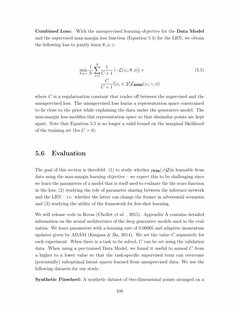
Combined Loss: With the unsupervised learning objective for the Data Modeland the supervised max-margin loss function (Equation 5.4) for the LRN, we obtainthe following loss to jointly learn 𝜃, 𝜑, 𝛾:
min𝜃.𝜑.𝛾
1
𝑁
𝑁∑︁
𝑖=1
1
𝐶 + 1[−ℒ(𝑥𝑖; 𝜃, 𝜑)] + (5.5)
𝐶
𝐶 + 1I[𝑥𝑖 ∈ 𝒴 ]ℒmm(𝑥𝑖; 𝛾, 𝜑)
where 𝐶 is a regularization constant that trades off between the supervised and theunsupervised loss. The unsupervised loss learns a representation space constrainedto lie close to the prior while explaining the data under the generative model. Themax-margin loss modifies this representation space so that dissimilar points are keptapart. Note that Equation 5.5 is no longer a valid bound on the marginal likelihoodof the training set (for 𝐶 > 0).
5.6 Evaluation
The goal of this section is threefold: (1) to study whether 𝑝rm(𝑧|𝒬)is learnable fromdata using the max-margin learning objective – we expect this to be challenging sincewe learn the parameters of a model that is itself used to evaluate the the score functionin the loss; (2) studying the role of parameter sharing between the inference networkand the LRN – i.e. whether the latter can change the former in adversarial scenarios;and (3) studying the utility of the framework for few-shot learning.
We will release code in Keras (Chollet et al. , 2015). Appendix A contains detailedinformation on the neural architectures of the deep generative models used in the eval-uation. We learn parameters with a learning rate of 0.00005 and adaptive momentumupdates given by ADAM (Kingma & Ba, 2014). We set the value 𝐶 separately foreach experiment. When there is a task to be solved, 𝐶 can be set using the validationdata. When using a pre-trained Data Model, we found it useful to anneal 𝐶 froma higher to a lower value so that the task-specific supervised term can overcome(potentially) suboptimal latent spaces learned from unsupervised data. We use thefollowing datasets for our study:
Synthetic Pinwheel: A synthetic dataset of two-dimensional points arranged on a
108
−10 0 10−20
−15
−10
−5
0
5
10
15
Raw Data
−2 0 20
1
2
3
4
Aggregate Posterior
−2 0 20.0
0.2
0.4
0.6
0.8
1.0
1.2
1.4
Samples from p(z|Q)
−2 0 20.0
0.2
0.4
0.6
0.8
1.0
1.2
1.4
Samples from p(z|Q)p(z|Q) p(z|Q)p(z|Q) p(z|Q)
(a) Data and aggregate poste-rior: (Top Left) Pinwheel data;(Top right) Aggregate posterior den-sity of a learned (unconditional) deepgenerative model coloured by classmembership. (Bottom row) Samplingfrom 𝑝rm(𝑧|𝒬) where the colour de-notes the class membership of pointsin 𝒬.
−15 −10 −5 0 5 10 15−20
−15
−10
−5
0
5
10
15
Scatter Plot [Relabelled]
−3 −2 −1 0 1 2 30.0
0.5
1.0
1.5
2.0
2.5
3.0
3.5
4.0Epoch 1
−3 −2 −1 0 1 2 30.0
0.5
1.0
1.5
2.0
2.5
3.0
3.5
Epoch 5
−3 −2 −1 0 1 2 30.00
0.25
0.50
0.75
1.00
1.25
1.50
1.75
Epoch 40
(b) Learning dynamics: (Top left)Visualization of adversarially labelleddata (relative to the learned aggre-gate posterior in Figure 5-4a (topright)). The remaining plots are classcoloured visualizations of the aggre-gate posterior (during training) whileallowing the LRN to fine-tune the la-tent space of the DGM.
Figure 5-4: Qualitative evaluation on pinwheel data: Studying how the latentspace of the data changes over the course of fine-tuning on the synthetic, pinwheeldataset.
pinwheel taken from the work of Johnson et al. (2016). We depict the raw data inFigure 5-4a. The dataset is created with five labels.
MNIST digits: 50000 black and white images of handwritten digits (LeCun, 1998).
MiniImagenet: A subsampled set of images taken from the Imagenet repository setupfor the task of k-shot learning by Vinyals et al. (2016). We use the train-validate-testsplit kindly provided by Ravi & Larochelle (2016).
5.6.1 Learning 𝑝(𝑧|𝒬)
As a sanity check, we begin by first training a deep generative model (without labelsand using a one-dimensional latent space) on the Pinwheel dataset. We visualize theraw-data and learned aggregate posterior
∑︀𝑥 𝑞dm(𝑧|𝑥;𝜑) in Figure 5-4a (top row).
We see that the unsupervised learning alone induces class separation in the aggregateposterior distribution. Using the learned model, we hold fixed parameters: 𝜃, 𝜑 and
109
learn the parameters 𝛾 of the LRN using the loss function in 5.4 with 𝐶 = 2000. Weform a kernel density estimate of samples from 𝑝rm(𝑧|𝒬) using randomly constructedsets of points derived from the red and green clusters. In Figure 5-4a (bottom row),we see that samples from the LRN correspond to regions of the latent space associatedwith 𝒬. On synthetic examples, the LRN finds regions of latent space correspondingto points from a query 𝒬.
5.6.2 Changing inductive biases at test-time
Previously, we worked with a model where the structure of the latent space (as seenin the aggregate posterior distribution) formed during unsupervised learning coincidedwith how points were grouped into sets. Here, we study what happens where thenotion of which points are similar changes at test time. We relabel the pinwheeldataset so that the yellow and orange points form one class while the green, red andblue form the other (see Figure 5-4b, top left). This corresponds to an adversariallabelling of the data since we use a deep generative model in which points in the sameclass are far apart in the learned latent space. If we keep 𝜃, 𝜑 fixed then 𝑝rm(𝑧|𝒬)(whose output is parameterized as a unimodal Gaussian distribution) cannot capturethe relevant subspace.
We have two choices here; we can either consider richer parameterizations for 𝑝rm(𝑧|𝒬)that are capable of capturing multi-modal structure in the latent space using techniquesproposed by Rezende & Mohamed (2015), or we can instead allow the 𝑝rm(𝑧|𝒬) tochange the underlying latent space of the generative model by back-propagatingthrough the parameters of the inference network. Here, we opt for the latter, thoughthe former is an avenue for future work.
We minimize Equation 5.5 while annealing the constant 𝐶 from 1000 → 1 linearlythrough the course of training. To gain insight into the learning dynamics of theLRN during training, we visualize the aggregate posterior of the generative model (viathe fine-tuned inference network) in Figure 5-4b through the course of training. Therole of this adversarial scenario is to highlight two important points (1) unsupervisedlearning is typically unidentifiable and may not learn a representation appropriate toall tasks and (2) learning with the latent reasoning network can overcome a suboptimal(relative to the task at hand) representation and transform it to a more suitable one.
110
5.6.3 Modeling high-dimensional data
Inducing diversity in latent space: Moving beyond low-dimensional data, westudy learning LRNs on MNIST digits. We use a Data Model with a two-dimensionallatent space for this experiment. We begin by training the model in a fully unsupervisedmanner and visualize the learned latent space in the form of the aggregate posterior(Figure 5-5a [left]). Although there is some class separability, we find that theunsupervised learning algorithm concentrates much of the probability mass together.
We re-learn the same model with the loss in Equation 5.5 where 𝐶 is set to 3000 (andannealed to 1). We again visualize the new aggregate posterior distribution of theData Model in Figure 5-5a (middle and right). When learning with Equation 5.5, theinference network uses more of the latent space in the model because the max-marginloss pushes points in different classes further apart.
Qualitative Analysis of MNIST digits: To validate our method, we providevisualizations on the MNIST dataset. We select a handful of labelled examples 𝒬(Figure 5-5b, left) and visualize both their posterior means and samples from 𝑝(𝑧|𝒬)(Figure 5-5b, middle). Then, for each sample from 𝑝rm(𝑧|𝒬), we evaluate the fine-tuned 𝑝dm(𝑥|𝑧) and visualize the images in Figure 5-5b (right). We see that thegenerative model fine-tuned with the learning algorithm retains its ability to generatemeaningful samples.
5.6.4 Few-shot learning with the Bayes factor
The task of k-shot learning is to identify the class an object came from given a singleexample from 5 other classes (1-shot, 5-way). In the 5-shot, 5-way task. there are5 examples provided from each of the 5 potential classes. We use an LRN with adeep-discriminative model to obtain near state of the art performance in few-shotlearning on the MiniImagenet dataset.
Following (Bauer et al. , 2017), who show that discriminative models alone formpowerful baselines for this task on this dataset, we pretrain an 18 layer Resnet (Heet al. , 2016) convolutional neural network to predict class labels at training time.We use early stopping on a validation set based on the nearest neighbor performanceof the learned embeddings (obtained from the final layer of the ResNet) to identifythe best model. Building a good generative model of the images in MiniImagenetis difficult and so instead, we use the fixed embeddings as a 256 dimensional proxy
111
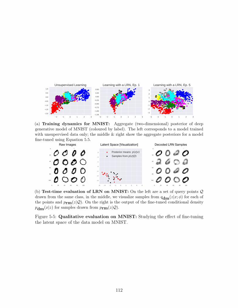
−2 −1 0 1 2 3
−2.0
−1.5
−1.0
−0.5
0.0
0.5
1.0
Unsupervised Learning
−3 −2 −1 0 1 2 3−1.25
−1.00
−0.75
−0.50
−0.25
0.00
0.25
0.50
Learning with a LRN, Ep. 1
−3 −2 −1 0 1 2 3
−3
−2
−1
0
1
2
3
Learning with a LRN, Ep. 5
(a) Training dynamics for MNIST: Aggregate (two-dimensional) posterior of deepgenerative model of MNIST (coloured by label). The left corresponds to a model trainedwith unsupervised data only; the middle & right show the aggregate posteriors for a modelfine-tuned using Equation 5.5.
Latent Space [Visualization] Decoded LRN SamplesRaw Images
(b) Test-time evaluation of LRN on MNIST: On the left are a set of query points 𝒬drawn from the same class, in the middle, we visualize samples from 𝑞dm(𝑧|𝑥;𝜑) for each ofthe points and 𝑝rm(𝑧|𝒬). On the right is the output of the fine-tuned conditional density𝑝dm(𝑥|𝑧) for samples drawn from 𝑝rm(𝑧|𝒬).
Figure 5-5: Qualitative evaluation on MNIST: Studying the effect of fine-tuningthe latent space of the data model on MNIST.
112
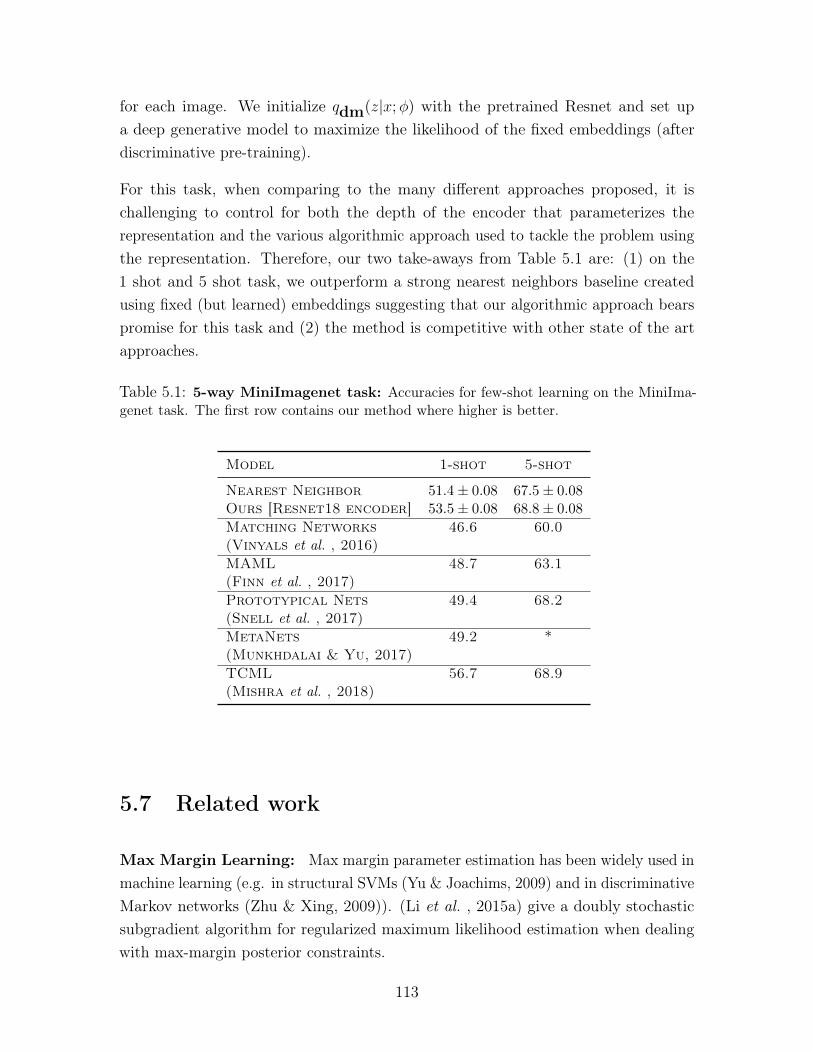
for each image. We initialize 𝑞dm(𝑧|𝑥;𝜑) with the pretrained Resnet and set upa deep generative model to maximize the likelihood of the fixed embeddings (afterdiscriminative pre-training).
For this task, when comparing to the many different approaches proposed, it ischallenging to control for both the depth of the encoder that parameterizes therepresentation and the various algorithmic approach used to tackle the problem usingthe representation. Therefore, our two take-aways from Table 5.1 are: (1) on the1 shot and 5 shot task, we outperform a strong nearest neighbors baseline createdusing fixed (but learned) embeddings suggesting that our algorithmic approach bearspromise for this task and (2) the method is competitive with other state of the artapproaches.
Table 5.1: 5-way MiniImagenet task: Accuracies for few-shot learning on the MiniIma-genet task. The first row contains our method where higher is better.
Model 1-shot 5-shot
Nearest Neighbor 51.4± 0.08 67.5± 0.08Ours [Resnet18 encoder] 53.5± 0.08 68.8± 0.08
Matching Networks 46.6 60.0(Vinyals et al. , 2016)MAML 48.7 63.1(Finn et al. , 2017)Prototypical Nets 49.4 68.2(Snell et al. , 2017)MetaNets 49.2 *(Munkhdalai & Yu, 2017)TCML 56.7 68.9(Mishra et al. , 2018)
5.7 Related work
Max Margin Learning: Max margin parameter estimation has been widely used inmachine learning (e.g. in structural SVMs (Yu & Joachims, 2009) and in discriminativeMarkov networks (Zhu & Xing, 2009)). (Li et al. , 2015a) give a doubly stochasticsubgradient algorithm for regularized maximum likelihood estimation when dealingwith max-margin posterior constraints.
113
(Zaheer et al. , 2017) experiment with max-margin learning using a variant of theDeepSets model to predict a scalar score conditioned on a set. While (Zaheer et al., 2017) cite the estimator in (Ghahramani & Heller, 2005) as motivation for theirmodel, they do not explicitly use, parameterize, or differentiate through the BayesFactor in a generative model of data.
Inductive Transfer and Metric Learning: Lake et al. (2013) use probabilisticinference in a hierarchical model to classify unseen examples by their probability ofbeing in a new class. Instead of the Bayes Factor, they use the posterior predictiveobtained via the use of a MCMC algorithm to score target points relative to a query.(Ghahramani & Heller, 2005) evaluate the Bayes factor analytically in exponentialfamily distributions. What we gain in for sacrificing tractability is the ability towork within a richer class of models. Though not motivated within the context of ahierarchical model, (Engel et al. , 2018) use an adversarial loss to recognize regions oflatent space that correspond to points with a specified class.
Vinyals et al. (2016) learn a parametric K-nearest neighbor classifiers to predictwhether a target item is within the same class as 𝑘-others. (Snell et al. , 2017)associate a point with a prototype within a set and use it to answer whether an objectis in the same class as others. (Bauer et al. , 2017) show that the features from aResNet (He et al. , 2016) model already provide a powerful feature representation inwhich a k-nearest neighbor classifier performs remarkably well. The Neural Statistician(Edwards & Storkey, 2016) learns a model similar 2 to the Reasoning Model inFigure 5-2 (b) by maximizing the likelihood of sets 𝒬. Their method does not use theBayes Factor to score items; it also does not permit easy initialization with pre-trainedData Models since the full model is trained with queries.
We tune the latent space of a deep generative model to enhance class separability fortest time tasks. By contrast, meta learning algorithms learn to tune the parametersof an algorithm or a model. (Finn et al. , 2017) prime the parameters of a neuralnetwork to have high accuracy at test time using second order gradient information.
Our work has close parallels with metric-learning; here the metric learned lies inthe latent space of a deep generative model. (Bar-Hillel et al. , 2005) proposedRelevant Component Analysis, an optimization problem that jointly performs (linear)dimensionality reduction and learns a Mahalanobis metric using queries.
2Their model does not enforce the conditional independence statement 𝑥𝑡 || 𝒬|𝑧𝑡
114
5.8 Discussion
We seek good, task-specific inductive biases to quantify how similar a point is to aset. We give new theoretical and practical constructs towards this goal. We breakup the problem into two parts: learn a good representation and tune the learnedrepresentation for a specific notion of similarity. Using the latent space in a deepgenerative model as our representation, we use the Bayes Factor to quantify similarity.
We derive conditions under which there exists an equivalence between a generativemodel where data are generated independently and a hierarchical model that jointlygenerates sets of (similar) points. Using this insight, we derive a differentiable estimatorfor the Bayes Factor; the estimator poses the comparison between a point and a set asoverlap in latent space. With the Bayes Factor as a differentiable scoring mechanism,we give a max-margin learning algorithm capable of changing the inductive bias ofa (potentially pre-trained) deep generative model. To evaluate the Bayes Factor, wepropose a neural architecture for a latent reasoning network : a set conditional densitythat amortizes the posterior predictive distribution of a hierarchical model.
Our approach has limitations. By directly parameterizing the posterior predictivedensity, and not the prior 𝑝rm(𝑤) and conditional 𝑝rm(𝑧|𝑤), we lose the ability tosample points from the hierarchical generative model. Working with a set of modelsin which Assumption 1 holds may implicitly only find posterior predictive densitiesunder relatively simple model families of 𝑝rm(𝑤) and 𝑝rm(𝑧|𝑤). Finally, enforcingthat property identity in 𝑤 is conditionally independent of the data 𝑥, given therepresentation 𝑧, may make for a challenging learning problem – 𝑧 has to representboth the property and variability in the property conditional distribution of the data.
An avenue of future work is leveraging vast amounts of unlabeled data for representationlearning informed by a small amount of supervision to guide either during learning, orafter learning, the structured of the learned space. Yet another interesting directionwould be to learn LRNs that parameterize distributions over hierarchies of latentvariables.
115

116
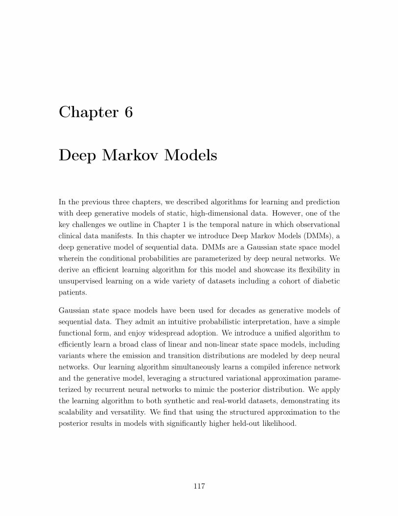
Chapter 6
Deep Markov Models
In the previous three chapters, we described algorithms for learning and predictionwith deep generative models of static, high-dimensional data. However, one of thekey challenges we outline in Chapter 1 is the temporal nature in which observationalclinical data manifests. In this chapter we introduce Deep Markov Models (DMMs), adeep generative model of sequential data. DMMs are a Gaussian state space modelwherein the conditional probabilities are parameterized by deep neural networks. Wederive an efficient learning algorithm for this model and showcase its flexibility inunsupervised learning on a wide variety of datasets including a cohort of diabeticpatients.
Gaussian state space models have been used for decades as generative models ofsequential data. They admit an intuitive probabilistic interpretation, have a simplefunctional form, and enjoy widespread adoption. We introduce a unified algorithm toefficiently learn a broad class of linear and non-linear state space models, includingvariants where the emission and transition distributions are modeled by deep neuralnetworks. Our learning algorithm simultaneously learns a compiled inference networkand the generative model, leveraging a structured variational approximation parame-terized by recurrent neural networks to mimic the posterior distribution. We applythe learning algorithm to both synthetic and real-world datasets, demonstrating itsscalability and versatility. We find that using the structured approximation to theposterior results in models with significantly higher held-out likelihood.
117
6.1 Introduction
Models of sequence data such as hidden Markov models (HMMs) and recurrent neuralnetworks (RNNs) are widely used in machine translation, speech recognition, andcomputational biology. Linear and non-linear Gaussian state space models (GSSMs,Fig. 6-1) are used in applications including robotic planning and missile tracking.However, despite huge progress over the last decade, efficient learning of non-linearmodels from complex high dimensional time-series remains a major challenge. Ourpaper proposes a unified learning algorithm for a broad class of GSSMs, and weintroduce an inference procedure that scales easily to high dimensional data, compilingapproximate (and where feasible, exact) inference into the parameters of a neuralnetwork.
In engineering and control, the parametric form of the GSSM model is often known,with typically a few specific parameters that need to be fit to data. The mostcommonly used approaches for these types of learning and inference problems areoften computationally demanding, e.g. dual extended Kalman filter (Wan & Nelson,1997), expectation maximization (Briegel & Tresp, 1999; Ghahramani & Roweis,1999) or particle filters (Schön et al. , 2011). Our compiled inference algorithm caneasily deal with high-dimensions both in the observed and the latent spaces, withoutcompromising the quality of inference and learning.
When the parametric form of the model is unknown, we propose learning DeepMarkov Models (DMM), a class of generative models where linear emission andtransition distributions are replaced with complex multi-layer perceptrons (MLPs).These are GSSMs that retain the Markovian structure of HMMs, but leverage therepresentational power of deep neural networks to model complex high dimensionaldata. If one augments a DMM model such as the one presented in Fig. 6-1 with edgesfrom the observations 𝑥𝑡 to the latent states of the following time step 𝑧𝑡+1, then theDMM can be seen to be similar to, though more restrictive than, stochastic RNNs(Bayer & Osendorfer, 2014) and variational RNNs (Chung et al. , 2015).
Our learning algorithm performs stochastic gradient ascent on a variational lower boundof the likelihood. Instead of introducing variational parameters for each data point,we compile the inference procedure at the same time as learning the generative model.This idea was originally used in the wake-sleep algorithm for unsupervised learning(Hinton et al. , 1995), and has since led to state-of-the-art results for unsupervisedlearning of deep generative models (Kingma & Welling, 2014; Mnih & Gregor, 2014;
118
𝑧1 𝑧2 . . .
𝑥1 𝑥2
𝑧1 𝑧2 . . .
𝑥1 𝑥2
d
d d
d ℎ1 ℎ2 . . .
𝑥1 𝑥2
Figure 6-1: Generative Models of Sequential Data: (Top Left) Hidden MarkovModel (HMM), (Top Right) Deep Markov Model (DMM) � denotes the neural networksused in DMMs for the emission and transition functions. (Bottom) Recurrent Neural Network(RNN), ♦ denotes a deterministic intermediate representation. Code for learning DMMs andreproducing our results may be found at: github.com/clinicalml/structuredinference
Rezende et al. , 2014).
Specifically, we introduce a new family of structured inference networks, parameterizedby recurrent neural networks, and evaluate their effectiveness in three scenarios: (1)when the generative model is known and fixed, (2) in parameter estimation whenthe functional form of the model is known and (3) for learning deep Markov models.By looking at the structure of the true posterior, we show both theoretically andempirically that inference for a latent state should be performed using information fromits future, as opposed to recent work which performed inference using only informationfrom the past Chung et al. (2015); Gan et al. (2015); Gregor et al. (2015), and thata structured variational approximation outperforms mean-field based approximations.Our approach may easily be adapted to learning more general generative models, forexample models with edges from observations to latent states.
Finally, we learn a Deep Markov Model on a polyphonic music dataset and on adataset of electronic health records (a complex high dimensional setting with missingdata). We use the model learned on health records to ask queries such as “what wouldhave happened to patients had they not received treatment”, and show that our modelcorrectly identifies the way certain medications affect a patient’s health.
Related Work: Learning GSSMs with MLPs for the transition distribution wasconsidered by Raiko & Tornio (2009). They approximate the posterior with non-lineardynamic factor analysis Valpola & Karhunen (2002), which scales quadratically withthe observed dimension and is impractical for large-scale learning.
Recent work has considered variational learning of time-series data using structuredinference or recognition networks. Archer et al. propose using a Gaussian approxima-tion to the posterior distribution with a block-tridiagonal inverse covariance. Johnsonet al. use a conditional random field as the inference network for time-series models.Concurrent to our own work, Fraccaro et al. also learn sequential generative models
119
using structured inference networks parameterized by recurrent neural networks.
Bayer & Osendorfer and Fabius & van Amersfoort create a stochastic variant ofRNNs by making the hidden state of the RNN at every time step be a function ofindependently sampled latent variables. Chung et al. apply a similar model to speechdata, sharing parameters between the RNNs for the generative model and the inferencenetwork. Gan et al. learn a model with discrete random variables, using a structuredinference network that only considers information from the past, similar to Chunget al. and Gregor et al. ’s models. In contrast to these works, we use informationfrom the future within a structured inference network, which we show to be preferableboth theoretically and practically. Additionally, we systematically evaluate the impactof the different variational approximations on learning.
Watter et al. construct a first-order Markov model using inference networks. However,their learning algorithm is based on data tuples over consecutive time steps. Thismakes the strong assumption that the posterior distribution can be recovered basedon observations at the current and next time-step. As we show, for generative modelslike the one in Fig. 6-1, the posterior distribution at any time step is a function of allfuture (and past) observations.
6.2 Setup
Gaussian State Space Models: We consider both inference and learning in a classof latent variable models given by: We denote by 𝑧𝑡 a vector valued latent variable andby 𝑥𝑡 a vector valued observation. A sequence of such latent variables and observationsis denoted �⃗�, �⃗� respectively.
𝑧𝑡 ∼ 𝒩 (G𝛼(𝑧𝑡−1,Δ𝑡), S𝛽(𝑧𝑡−1,Δ𝑡)) (Transition) (6.1)
𝑥𝑡 ∼ Π(F𝜅(𝑧𝑡)) (Emission) (6.2)
We assume that the distribution of the latent states is a multivariate Gaussian with amean and covariance which are differentiable functions of the previous latent stateand Δ𝑡 (the time elapsed of time between 𝑡− 1 and 𝑡). The multivariate observations𝑥𝑡 are distributed according to a distribution Π (e.g., independent Bernoullis if thedata is binary) whose parameters are a function of the corresponding latent state 𝑧𝑡.Collectively, we denote by 𝜃 = {𝛼, 𝛽, 𝜅} the parameters of the generative model.
120
Eq. 6.1 subsumes a large family of linear and non-linear Gaussian state space models.For example, by setting G𝛼(𝑧𝑡−1) = 𝐺𝑡𝑧𝑡−1, S𝛽 = Σ𝑡,F𝜅 = 𝐹𝑡𝑧𝑡, where 𝐺𝑡, Σ𝑡 and 𝐹𝑡
are matrices, we obtain linear state space models. The functional forms and initialparameters for G𝛼, S𝛽,F𝜅 may be pre-specified.
Variational Learning: Using recent advances in variational inference we optimizea variational lower bound on the data log-likelihood. We will make use of an inferencenetwork or recognition network Hinton et al. (1995); Kingma & Welling (2014); Mnih& Gregor (2014); Rezende et al. (2014), a neural network which approximates theintractable posterior. This is a parametric conditional distribution that is optimizedto perform inference. Throughout this paper we will use 𝜃 to denote the parametersof the generative model, and 𝜑 to denote the parameters of the inference network.
For the remainder of this section, we consider learning in a Bayesian network whosejoint distribution factorizes as: 𝑝(𝑥, 𝑧) = 𝑝𝜃(𝑧)𝑝𝜃(𝑥|𝑧). The posterior distribution𝑝𝜃(𝑧|𝑥) is typically intractable. Using the well-known variational principle, we positan approximate posterior distribution 𝑞𝜑(𝑧|𝑥) to obtain the following lower bound onthe marginal likelihood:
log 𝑝𝜃(𝑥) ≥ E𝑞𝜑(𝑧|𝑥)
[log 𝑝𝜃(𝑥|𝑧)]−KL( 𝑞𝜑(𝑧|𝑥)||𝑝𝜃(𝑧) ), (6.3)
where the inequality is by Jensen’s inequality. Kingma & Welling; Rezende et al. usea neural net (with parameters 𝜑) to parameterize 𝑞𝜑. The challenge in the resultingoptimization problem is that the lower bound in Eq. 6.3 includes an expectationw.r.t. 𝑞𝜑, which implicitly depends on the network parameters 𝜑. When using aGaussian variational approximation 𝑞𝜑(𝑧|𝑥) ∼ 𝒩 (𝜇𝜑(𝑥),Σ𝜑(𝑥)), where 𝜇𝜑(𝑥),Σ𝜑(𝑥)
are parametric functions of the observation 𝑥, this difficulty is overcome by usingstochastic backpropagation: a simple transformation allows one to obtain unbiasedMonte Carlo estimates of the gradients of E𝑞𝜑(𝑧|𝑥) [log 𝑝𝜃(𝑥|𝑧)] with respect to 𝜑. TheKL term in Eq. 6.3 can be estimated similarly since it is also an expectation. Whenthe prior 𝑝𝜃(𝑧) is normally distributed, the KL and its gradients may be obtainedanalytically.
6.3 A factorized variational lower bound
We leverage stochastic backpropagation to learn generative models given by Eq. 6.1,corresponding to the graphical model in Fig. 6-1. Our insight is that for the purpose
121
of inference, we can use the Markov properties of the generative model to guide usin deriving a structured approximation to the posterior. Specifically, the posteriorfactorizes as:
𝑝(�⃗�|�⃗�) = 𝑝(𝑧1|�⃗�)𝑇∏︁
𝑡=2
𝑝(𝑧𝑡|𝑧𝑡−1, 𝑥𝑡, . . . , 𝑥𝑇 ). (6.4)
To see this, use the independence statements implied by the graphical model in Fig.6-1 to note that 𝑝(�⃗�|�⃗�), the true posterior, factorizes as:
𝑝(�⃗�|�⃗�) = 𝑝(𝑧1|�⃗�)𝑇∏︁
𝑡=2
𝑝(𝑧𝑡|𝑧𝑡−1, �⃗�)
Now, we notice that 𝑧𝑡 || 𝑥1, . . . , 𝑥𝑡−1|𝑧𝑡−1, yielding the desired result. The significanceof Eq. 6.4 is that it yields insight into the structure of the exact posterior for the classof models laid out in Fig. 6-1.
We directly mimic the structure of the posterior with the following factorization ofthe variational approximation:
𝑞𝜑(�⃗�|�⃗�) = 𝑞𝜑(𝑧1|𝑥1, . . . , 𝑥𝑇 )𝑇∏︁
𝑡=2
𝑞𝜑(𝑧𝑡|𝑧𝑡−1, 𝑥𝑡, . . . , 𝑥𝑇 ) (6.5)
s.t. 𝑞𝜑(𝑧𝑡|𝑧𝑡−1, 𝑥𝑡, . . . , 𝑥𝑇 ) ∼𝒩 (𝜇𝜑(𝑧𝑡−1, 𝑥𝑡, . . . , 𝑥𝑇 ),Σ𝜑(𝑧𝑡−1, 𝑥𝑡, . . . , 𝑥𝑇 ))
where 𝜇𝜑 and Σ𝜑 are functions parameterized by neural nets. Although 𝑞𝜑 has theoption to condition on all information across time, Eq. 6.4 suggests that in fact itsuffices to condition on information from the future and the previous latent state. Theprevious latent state serves as a summary statistic for information from the past.
Exact Inference: We can match the factorization of the true posterior using theinference network but using a Gaussian variational approximation for the approximateposterior over each latent variable (as we do) limits the expressivity of the inferentialmodel, except for the case of linear dynamical systems where the posterior distributionis Normally distributed. However, one could augment our proposed inference networkwith recent innovations that improve the variational approximation to allow for multi-modality Rezende & Mohamed (2015); Tran et al. (2016). Such modifications couldyield black-box methods for exact inference in time-series models, which we leave forfuture work.
Deriving a variational lower bound: For a generative model (with parameters
122
𝜃) and an inference network (with parameters 𝜑), we are interested in max𝜃 log 𝑝𝜃(�⃗�).For ease of exposition, we instantiate the derivation of the variational bound for asingle data point �⃗� though we learn 𝜃, 𝜑 from a corpus.
The lower bound in Eq. 6.3 has an analytic form of the KL term only for the simplestof transition models G𝛼, S𝛽 between 𝑧𝑡−1 and 𝑧𝑡 (Eq. 6.1). One could estimate thegradient of the KL term by sampling from the variational model, but that resultsin high variance estimates and gradients. We use a different factorization of the KLterm (obtained by using the prior distribution over latent variables), leading to thevariational lower bound we use as our objective function:
ℒ(�⃗�; (𝜃, 𝜑)) =𝑇∑︁
𝑡=1
E𝑞𝜑(𝑧𝑡|�⃗�)
[log 𝑝𝜃(𝑥𝑡|𝑧𝑡)] (6.6)
−KL(𝑞𝜑(𝑧1|�⃗�)||𝑝𝜃(𝑧1))−𝑇∑︁
𝑡=2
E𝑞𝜑(𝑧𝑡−1|�⃗�)
[KL(𝑞𝜑(𝑧𝑡|𝑧𝑡−1, �⃗�)||𝑝𝜃(𝑧𝑡|𝑧𝑡−1))] .
The key point is the resulting objective function has more stable analytic gradients.Without the factorization of the KL divergence in Eq. 6.6, we would have to estimateKL(𝑞(�⃗�|�⃗�)||𝑝(�⃗�)) via Monte-Carlo sampling, since it has no analytic form. In contrast,in Eq. 6.6 the individual KL terms do have analytic forms. Section 6.3.1 simplifiesthe lower bound we use during learning while Section 6.3.2 derives the analytic formsfor the KL divergence term in the simplification.
6.3.1 Simplifying the lower bounds
We can derive the bound on the likelihood ℒ(�⃗�; (𝜃, 𝜑)) as follows:
log 𝑝𝜃(�⃗�) ≥∫︁
�⃗�
𝑞𝜑(�⃗�|�⃗�) log𝑝𝜃(�⃗�)𝑝𝜃(�⃗�|�⃗�)𝑞𝜑(�⃗�|�⃗�)
𝑑�⃗� = E𝑞𝜑(�⃗�|�⃗�)
[log 𝑝𝜃(�⃗�|�⃗�)]−KL(𝑞𝜑(�⃗�|�⃗�)||𝑝𝜃(�⃗�))
( Using 𝑥𝑡 || 𝑥¬𝑡|𝑧𝑡 )
=𝑇∑︁
𝑡=1
E𝑞𝜑(𝑧𝑡|�⃗�)
[log 𝑝𝜃(𝑥𝑡|𝑧𝑡)]−KL(𝑞𝜑(�⃗�|�⃗�)||𝑝𝜃(�⃗�)) = ℒ(�⃗�; (𝜃, 𝜑)) (6.7)
In the following we omit the dependence of 𝑞 on �⃗�, and omit the subscript 𝜑. Wecan show that the KL divergence between the approximation to the posterior and the
123
prior simplifies as:
KL(𝑞(𝑧1, . . . , 𝑧𝑇 )||𝑝(𝑧1, . . . , 𝑧𝑇 )) =∫︁
𝑧1
. . .
∫︁
𝑧𝑇
𝑞(𝑧1) . . . 𝑞(𝑧𝑇 |𝑧𝑇−1) log𝑝(𝑧1, . . . , 𝑧𝑇 )
𝑞(𝑧1)..𝑞(𝑧𝑇 |𝑧𝑇−1)
(Factorization of the variational distribution)
=
∫︁
𝑧1
. . .
∫︁
𝑧𝑇
𝑞(𝑧1) . . . 𝑞(𝑧𝑇 |𝑧𝑇−1) log𝑝(𝑧1)𝑝(𝑧2|𝑧1) . . . 𝑝(𝑧𝑇 |𝑧𝑇−1)
𝑞(𝑧1) . . . 𝑞(𝑧𝑇 |𝑧𝑇−1)
(Factorization of the prior)
=
∫︁
𝑧1
. . .
∫︁
𝑧𝑇
𝑞(𝑧1) . . . 𝑞(𝑧𝑇 |𝑧𝑇−1) log𝑝(𝑧1)
𝑞(𝑧1)+
𝑇∑︁
𝑡=2
∫︁
𝑧1
. . .
∫︁
𝑧𝑇
𝑞(𝑧1) . . . 𝑞(𝑧𝑇 |𝑧𝑇−1) log𝑝(𝑧𝑡|𝑧𝑡−1)
𝑞(𝑧𝑡|𝑧𝑡−1)
=
∫︁
𝑧1
𝑞(𝑧1) log𝑝(𝑧1)
𝑞(𝑧1)+
𝑇∑︁
𝑡=2
∫︁
𝑧𝑡−1
∫︁
𝑧𝑡
𝑞(𝑧𝑡) log𝑝(𝑧𝑡|𝑧𝑡−1)
𝑞(𝑧𝑡|𝑧𝑡−1)
(Each expectation over 𝑧𝑡 is constant for 𝑡 /∈ {𝑡, 𝑡− 1})
= KL(𝑞(𝑧1)||𝑝(𝑧1)) +𝑇∑︁
𝑡=2
E𝑞(𝑧𝑡−1)
[KL(𝑞(𝑧𝑡|𝑧𝑡−1)||𝑝(𝑧𝑡|𝑧𝑡−1))]
For evaluating the marginal likelihood on the test set, we can use the followingMonte-Carlo estimate:
𝑝(�⃗�) u1
𝑆
𝑆∑︁
𝑠=1
𝑝(�⃗�|�⃗�(𝑠))𝑝(�⃗�(𝑠))𝑞(�⃗�(𝑠)|�⃗�) �⃗�(𝑠) ∼ 𝑞(�⃗�|�⃗�) (6.8)
This may be derived in a manner akin to the one depicted in Appendix E in Rezendeet al. (2014) or Appendix D in Kingma & Welling (2014).
The log likelihood on the test set is computed using:
log 𝑝(�⃗�) u log1
𝑆
𝑆∑︁
𝑠=1
exp log
[︂𝑝(�⃗�|�⃗�(𝑠))𝑝(�⃗�(𝑠))
𝑞(�⃗�(𝑠)|�⃗�)
]︂(6.9)
Eq. 6.9 may be computed in a numerically stable manner using the log-sum-exp trick.
124
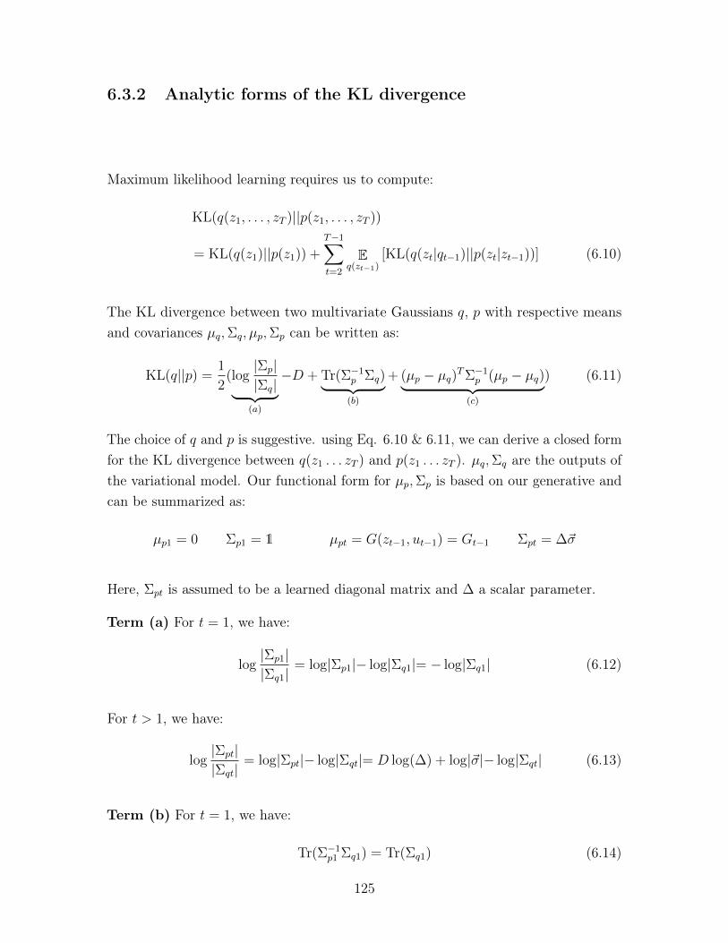
6.3.2 Analytic forms of the KL divergence
Maximum likelihood learning requires us to compute:
KL(𝑞(𝑧1, . . . , 𝑧𝑇 )||𝑝(𝑧1, . . . , 𝑧𝑇 ))
= KL(𝑞(𝑧1)||𝑝(𝑧1)) +𝑇−1∑︁
𝑡=2
E𝑞(𝑧𝑡−1)
[KL(𝑞(𝑧𝑡|𝑞𝑡−1)||𝑝(𝑧𝑡|𝑧𝑡−1))] (6.10)
The KL divergence between two multivariate Gaussians 𝑞, 𝑝 with respective meansand covariances 𝜇𝑞,Σ𝑞, 𝜇𝑝,Σ𝑝 can be written as:
KL(𝑞||𝑝) = 1
2(log|Σ𝑝||Σ𝑞|⏟ ⏞
(𝑎)
−𝐷 + Tr(Σ−1𝑝 Σ𝑞)⏟ ⏞ (𝑏)
+(𝜇𝑝 − 𝜇𝑞)𝑇Σ−1𝑝 (𝜇𝑝 − 𝜇𝑞)⏟ ⏞
(𝑐)
) (6.11)
The choice of 𝑞 and 𝑝 is suggestive. using Eq. 6.10 & 6.11, we can derive a closed formfor the KL divergence between 𝑞(𝑧1 . . . 𝑧𝑇 ) and 𝑝(𝑧1 . . . 𝑧𝑇 ). 𝜇𝑞,Σ𝑞 are the outputs ofthe variational model. Our functional form for 𝜇𝑝,Σ𝑝 is based on our generative andcan be summarized as:
𝜇𝑝1 = 0 Σ𝑝1 = 1 𝜇𝑝𝑡 = 𝐺(𝑧𝑡−1, 𝑢𝑡−1) = 𝐺𝑡−1 Σ𝑝𝑡 = Δ�⃗�
Here, Σ𝑝𝑡 is assumed to be a learned diagonal matrix and Δ a scalar parameter.
Term (a) For 𝑡 = 1, we have:
log|Σ𝑝1||Σ𝑞1|
= log|Σ𝑝1|− log|Σ𝑞1|= − log|Σ𝑞1| (6.12)
For 𝑡 > 1, we have:
log|Σ𝑝𝑡||Σ𝑞𝑡|
= log|Σ𝑝𝑡|− log|Σ𝑞𝑡|= 𝐷 log(Δ) + log|�⃗�|− log|Σ𝑞𝑡| (6.13)
Term (b) For 𝑡 = 1, we have:
Tr(Σ−1𝑝1 Σ𝑞1) = Tr(Σ𝑞1) (6.14)
125
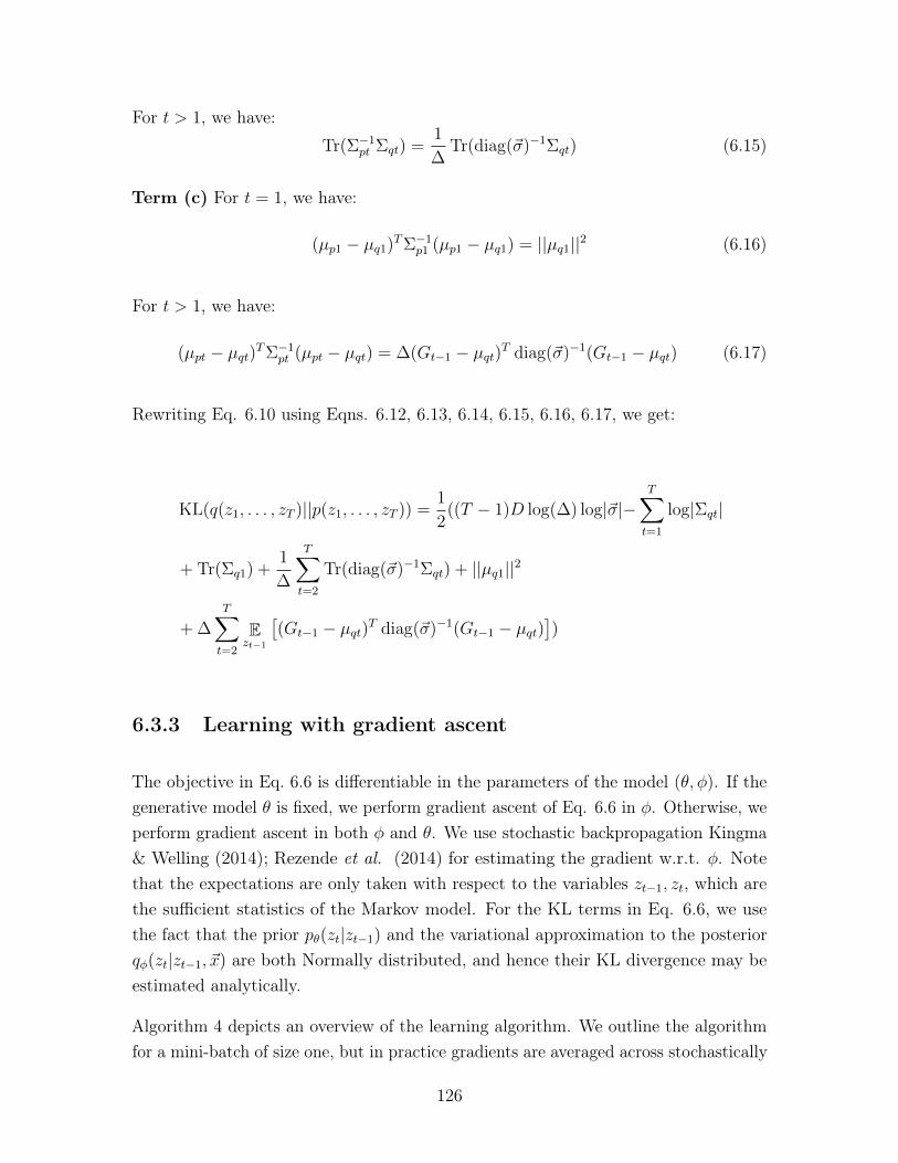
For 𝑡 > 1, we have:
Tr(Σ−1𝑝𝑡 Σ𝑞𝑡) =
1
ΔTr(diag(�⃗�)−1Σ𝑞𝑡) (6.15)
Term (c) For 𝑡 = 1, we have:
(𝜇𝑝1 − 𝜇𝑞1)𝑇Σ−1𝑝1 (𝜇𝑝1 − 𝜇𝑞1) = ||𝜇𝑞1||2 (6.16)
For 𝑡 > 1, we have:
(𝜇𝑝𝑡 − 𝜇𝑞𝑡)𝑇Σ−1𝑝𝑡 (𝜇𝑝𝑡 − 𝜇𝑞𝑡) = Δ(𝐺𝑡−1 − 𝜇𝑞𝑡)𝑇 diag(�⃗�)−1(𝐺𝑡−1 − 𝜇𝑞𝑡) (6.17)
Rewriting Eq. 6.10 using Eqns. 6.12, 6.13, 6.14, 6.15, 6.16, 6.17, we get:
KL(𝑞(𝑧1, . . . , 𝑧𝑇 )||𝑝(𝑧1, . . . , 𝑧𝑇 )) =1
2((𝑇 − 1)𝐷 log(Δ) log|�⃗�|−
𝑇∑︁
𝑡=1
log|Σ𝑞𝑡|
+ Tr(Σ𝑞1) +1
Δ
𝑇∑︁
𝑡=2
Tr(diag(�⃗�)−1Σ𝑞𝑡) + ||𝜇𝑞1||2
+Δ𝑇∑︁
𝑡=2
E𝑧𝑡−1
[︀(𝐺𝑡−1 − 𝜇𝑞𝑡)𝑇 diag(�⃗�)−1(𝐺𝑡−1 − 𝜇𝑞𝑡)
]︀)
6.3.3 Learning with gradient ascent
The objective in Eq. 6.6 is differentiable in the parameters of the model (𝜃, 𝜑). If thegenerative model 𝜃 is fixed, we perform gradient ascent of Eq. 6.6 in 𝜑. Otherwise, weperform gradient ascent in both 𝜑 and 𝜃. We use stochastic backpropagation Kingma& Welling (2014); Rezende et al. (2014) for estimating the gradient w.r.t. 𝜑. Notethat the expectations are only taken with respect to the variables 𝑧𝑡−1, 𝑧𝑡, which arethe sufficient statistics of the Markov model. For the KL terms in Eq. 6.6, we usethe fact that the prior 𝑝𝜃(𝑧𝑡|𝑧𝑡−1) and the variational approximation to the posterior𝑞𝜑(𝑧𝑡|𝑧𝑡−1, �⃗�) are both Normally distributed, and hence their KL divergence may beestimated analytically.
Algorithm 4 depicts an overview of the learning algorithm. We outline the algorithmfor a mini-batch of size one, but in practice gradients are averaged across stochastically
126
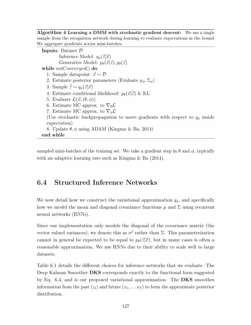
Algorithm 4 Learning a DMM with stochastic gradient descent: We use a singlesample from the recognition network during learning to evaluate expectations in the bound.We aggregate gradients across mini-batches.
Inputs: Dataset 𝒟Inference Model: 𝑞𝜑(�⃗�|�⃗�)Generative Model: 𝑝𝜃(�⃗�|�⃗�), 𝑝𝜃(�⃗�)
while 𝑛𝑜𝑡𝐶𝑜𝑛𝑣𝑒𝑟𝑔𝑒𝑑() do1. Sample datapoint: �⃗� ∼ 𝒟2. Estimate posterior parameters (Evaluate 𝜇𝜑,Σ𝜑)3. Sample ^⃗𝑧 ∼ 𝑞𝜑(�⃗�|�⃗�)4. Estimate conditional likelihood: 𝑝𝜃(�⃗�|^⃗𝑧) & KL5. Evaluate ℒ(�⃗�; (𝜃, 𝜑))6. Estimate MC approx. to ∇𝜃ℒ7. Estimate MC approx. to ∇𝜑ℒ(Use stochastic backpropagation to move gradients with respect to 𝑞𝜑 insideexpectation)8. Update 𝜃, 𝜑 using ADAM (Kingma & Ba, 2014)
end while
sampled mini-batches of the training set. We take a gradient step in 𝜃 and 𝜑, typicallywith an adaptive learning rate such as Kingma & Ba (2014).
6.4 Structured Inference Networks
We now detail how we construct the variational approximation 𝑞𝜑, and specificallyhow we model the mean and diagonal covariance functions 𝜇 and Σ using recurrentneural networks (RNNs).
Since our implementation only models the diagonal of the covariance matrix (thevector valued variances), we denote this as 𝜎2 rather than Σ. This parameterizationcannot in general be expected to be equal to 𝑝𝜃(�⃗�|�⃗�), but in many cases is often areasonable approximation. We use RNNs due to their ability to scale well to largedatasets.
Table 6.1 details the different choices for inference networks that we evaluate. TheDeep Kalman Smoother DKS corresponds exactly to the functional form suggestedby Eq. 6.4, and is our proposed variational approximation. The DKS smoothesinformation from the past (𝑧𝑡) and future (𝑥𝑡, . . . 𝑥𝑇 ) to form the approximate posteriordistribution.
127
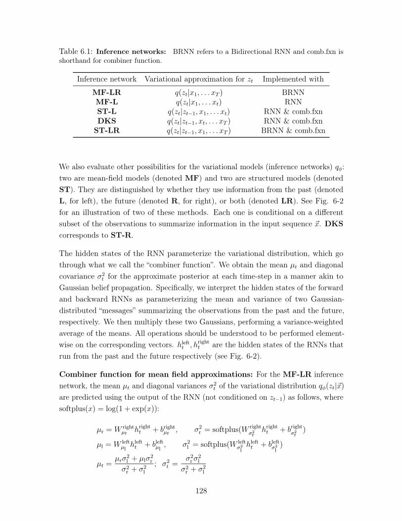
Table 6.1: Inference networks: BRNN refers to a Bidirectional RNN and comb.fxn isshorthand for combiner function.
Inference network Variational approximation for 𝑧𝑡 Implemented with
MF-LR 𝑞(𝑧𝑡|𝑥1, . . . 𝑥𝑇 ) BRNNMF-L 𝑞(𝑧𝑡|𝑥1, . . . 𝑥𝑡) RNNST-L 𝑞(𝑧𝑡|𝑧𝑡−1, 𝑥1, . . . 𝑥𝑡) RNN & comb.fxnDKS 𝑞(𝑧𝑡|𝑧𝑡−1, 𝑥𝑡, . . . 𝑥𝑇 ) RNN & comb.fxn
ST-LR 𝑞(𝑧𝑡|𝑧𝑡−1, 𝑥1, . . . 𝑥𝑇 ) BRNN & comb.fxn
We also evaluate other possibilities for the variational models (inference networks) 𝑞𝜑:two are mean-field models (denoted MF) and two are structured models (denotedST). They are distinguished by whether they use information from the past (denotedL, for left), the future (denoted R, for right), or both (denoted LR). See Fig. 6-2for an illustration of two of these methods. Each one is conditional on a differentsubset of the observations to summarize information in the input sequence �⃗�. DKScorresponds to ST-R.
The hidden states of the RNN parameterize the variational distribution, which gothrough what we call the “combiner function”. We obtain the mean 𝜇𝑡 and diagonalcovariance 𝜎2
𝑡 for the approximate posterior at each time-step in a manner akin toGaussian belief propagation. Specifically, we interpret the hidden states of the forwardand backward RNNs as parameterizing the mean and variance of two Gaussian-distributed “messages” summarizing the observations from the past and the future,respectively. We then multiply these two Gaussians, performing a variance-weightedaverage of the means. All operations should be understood to be performed element-wise on the corresponding vectors. ℎleft
𝑡 , ℎright𝑡 are the hidden states of the RNNs that
run from the past and the future respectively (see Fig. 6-2).
Combiner function for mean field approximations: For the MF-LR inferencenetwork, the mean 𝜇𝑡 and diagonal variances 𝜎2
𝑡 of the variational distribution 𝑞𝜑(𝑧𝑡|�⃗�)are predicted using the output of the RNN (not conditioned on 𝑧𝑡−1) as follows, wheresoftplus(𝑥) = log(1 + exp(𝑥)):
𝜇r = 𝑊 right𝜇r ℎright
𝑡 + 𝑏right𝜇r , 𝜎2
r = softplus(𝑊 right𝜎2r
ℎright𝑡 + 𝑏right
𝜎2r)
𝜇l = 𝑊 left𝜇lℎleft𝑡 + 𝑏left𝜇l
, 𝜎2l = softplus(𝑊 left
𝜎2lℎleft𝑡 + 𝑏left𝜎2
l)
𝜇𝑡 =𝜇r𝜎
2l + 𝜇l𝜎
2r
𝜎2r + 𝜎2
l; 𝜎2
𝑡 =𝜎2
r𝜎2l
𝜎2r + 𝜎2
l
128
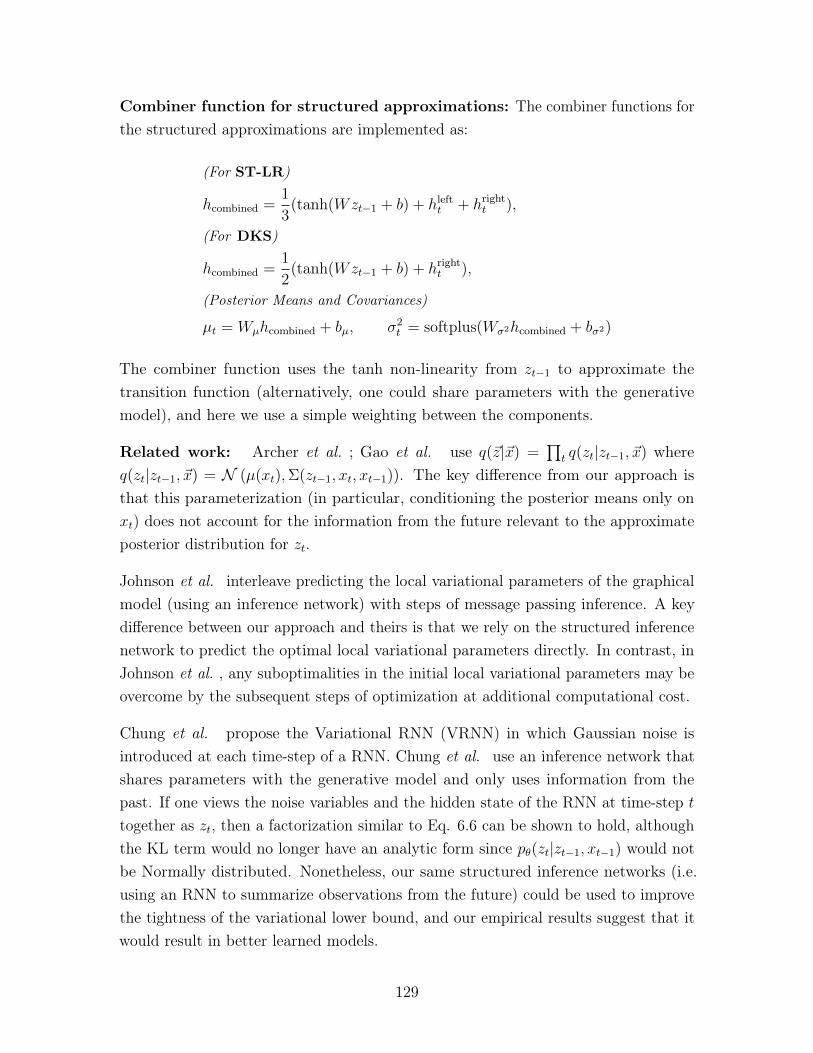
Combiner function for structured approximations: The combiner functions forthe structured approximations are implemented as:
(For ST-LR)
ℎcombined =1
3(tanh(𝑊𝑧𝑡−1 + 𝑏) + ℎleft
𝑡 + ℎright𝑡 ),
(For DKS)
ℎcombined =1
2(tanh(𝑊𝑧𝑡−1 + 𝑏) + ℎright
𝑡 ),
(Posterior Means and Covariances)
𝜇𝑡 = 𝑊𝜇ℎcombined + 𝑏𝜇, 𝜎2𝑡 = softplus(𝑊𝜎2ℎcombined + 𝑏𝜎2)
The combiner function uses the tanh non-linearity from 𝑧𝑡−1 to approximate thetransition function (alternatively, one could share parameters with the generativemodel), and here we use a simple weighting between the components.
Related work: Archer et al. ; Gao et al. use 𝑞(�⃗�|�⃗�) =∏︀
𝑡 𝑞(𝑧𝑡|𝑧𝑡−1, �⃗�) where𝑞(𝑧𝑡|𝑧𝑡−1, �⃗�) = 𝒩 (𝜇(𝑥𝑡),Σ(𝑧𝑡−1, 𝑥𝑡, 𝑥𝑡−1)). The key difference from our approach isthat this parameterization (in particular, conditioning the posterior means only on𝑥𝑡) does not account for the information from the future relevant to the approximateposterior distribution for 𝑧𝑡.
Johnson et al. interleave predicting the local variational parameters of the graphicalmodel (using an inference network) with steps of message passing inference. A keydifference between our approach and theirs is that we rely on the structured inferencenetwork to predict the optimal local variational parameters directly. In contrast, inJohnson et al. , any suboptimalities in the initial local variational parameters may beovercome by the subsequent steps of optimization at additional computational cost.
Chung et al. propose the Variational RNN (VRNN) in which Gaussian noise isintroduced at each time-step of a RNN. Chung et al. use an inference network thatshares parameters with the generative model and only uses information from thepast. If one views the noise variables and the hidden state of the RNN at time-step 𝑡together as 𝑧𝑡, then a factorization similar to Eq. 6.6 can be shown to hold, althoughthe KL term would no longer have an analytic form since 𝑝𝜃(𝑧𝑡|𝑧𝑡−1, 𝑥𝑡−1) would notbe Normally distributed. Nonetheless, our same structured inference networks (i.e.using an RNN to summarize observations from the future) could be used to improvethe tightness of the variational lower bound, and our empirical results suggest that itwould result in better learned models.
129
𝑥1 𝑥2 𝑥3
ℎleft1 ℎleft
2 ℎleft3Forward RNN
ℎright1 ℎright
2 ℎright3Backward RNN
(𝜇1,Σ1) (𝜇2,Σ2) (𝜇3,Σ3)Combiner function
(a) (a) (a)
𝑧1 𝑧2 𝑧30⃗
Figure 6-2: Structured Inference Networks: MF-LR and ST-LR variational approx-imations for a sequence of length 3, using a bi-directional recurrent neural net (BRNN).The BRNN takes as input the sequence (𝑥1, . . . 𝑥3), and through a series of non-linearitiesdenoted by the blue arrows it forms a sequence of hidden states summarizing informationfrom the left and right (ℎleft
𝑡 and ℎright𝑡 ) respectively. Then through a further sequence of
non-linearities which we call the “combiner function” (marked (a) above), and denoted by thered arrows, it outputs two vectors 𝜇 and Σ, parameterizing the mean and diagonal covarianceof 𝑞𝜑(𝑧𝑡|𝑧𝑡−1, �⃗�) of Eq. 6.5. Samples 𝑧𝑡 are drawn from 𝑞𝜑(𝑧𝑡|𝑧𝑡−1, �⃗�), as indicated by theblack dashed arrows. For the structured variational models ST-LR, the samples 𝑧𝑡 are fedinto the computation of 𝜇𝑡+1 and Σ𝑡+1, as indicated by the red arrows with the label (a).The mean-field model does not have these arrows, and therefore computes 𝑞𝜑(𝑧𝑡|�⃗�). We use𝑧0 = 0⃗. The inference network for DKS (ST-R) is structured like that of ST-LR exceptwithout the RNN from the past.
6.5 Deep Markov Models
Following Raiko et al. (2006), we apply the ideas of deep learning to non-linearcontinuous state space models. When the transition and emission function have anunknown functional form, we parameterize G𝛼, S𝛽,F𝜅 from Eq. 6.1 with deep neuralnetworks. See Fig. 6-1 (right) for an illustration of the graphical model.
Emission function: We parameterize the emission function F𝜅 using a two-layer MLP(multi-layer perceptron), MLP(𝑥,NL1,NL2) = NL2(𝑊2NL1(𝑊1𝑥+ 𝑏1) + 𝑏2)), whereNL denotes non-linearities such as ReLU, sigmoid, or tanh units applied element-wise
130
to the input vector. For modeling binary data,
F𝜅(𝑧𝑡) = sigmoid(𝑊emissionMLP(𝑧𝑡,ReLU,ReLU) + 𝑏emission)
parameterizes the mean probabilities of independent Bernoullis.
Gated transition function: We parameterize the transition function from 𝑧𝑡 to 𝑧𝑡+1
using a gated transition function inspired by Gated Recurrent Units (Chung et al. ,2014), instead of an MLP. Gated recurrent units (GRUs) are a neural architecture thatparameterizes the recurrence equation in the RNN with gating units to control theflow of information from one hidden state to the next, conditioned on the observation.Unlike GRUs, in the DMM, the transition function is not conditional on any of theobservations. All the information must be encoded in the completely stochastic latentstate. To achieve this goal, we create a Gated Transition Function. We would like themodel to have the flexibility to choose a linear transition for some dimensions whilehaving a non-linear transitions for the others. We adopt the following parameterization,where I denotes the identity function and ⊙ denotes element-wise multiplication:
𝑔𝑡 = MLP(𝑧𝑡−1,ReLU, sigmoid) (Gating Unit)
ℎ𝑡 = MLP(𝑧𝑡−1,ReLU, I) (Proposed mean)
(Transition Mean G𝛼 and S𝛽)
𝜇𝑡(𝑧𝑡−1) = (1− 𝑔𝑡)⊙ (𝑊𝜇𝑝𝑧𝑡−1 + 𝑏𝜇𝑝) + 𝑔𝑡 ⊙ ℎ𝑡𝜎2𝑡 (𝑧𝑡−1) = softplus(𝑊𝜎2
𝑝ReLU(ℎ𝑡) + 𝑏𝜎2
𝑝)
Note that the mean and covariance functions both share the use of ℎ𝑡. In ourexperiments, we initialize 𝑊𝜇𝑝 to be the identity function and 𝑏𝜇𝑝 to 0. The parametersof the emission and transition function form the set 𝜃.
6.6 Evaluation
We use Adam Kingma & Ba (2014) with a learning rate of 0.0008 to train the DMM.In the models we trained, the hidden dimension was set to be 100 for the emissiondistribution and 200 in the transition function. We typically used RNN sizes from oneof {400, 600} and a latent dimension of size 100. We study the inference algorithmand the model on three datasets.
131
6.6.1 Synthetic data
Dataset: We consider simple linear and non-linear GSSMs. To train the inferencenetworks we use 𝑁 = 5000 datapoints of length 𝑇 = 25. We consider both oneand two dimensional systems for inference and parameter estimation. We compareour results using the training value of the variational bound ℒ(�⃗�; (𝜃, 𝜑)) (Eq. 6.6)
and the RMSE =√︁
1𝑁
1𝑇
∑︀𝑁𝑖=1
∑︀𝑇𝑡=1[𝜇𝜑(𝑥𝑖,𝑡)− 𝑧*𝑖,𝑡]2, where 𝑧* correspond to the true
underlying 𝑧’s that generated the data.
Compiling exact inference: We seek to understand whether inference networkscan accurately compile exact posterior inference into the network parameters 𝜑 forlinear GSSMs when exact inference is feasible. For this experiment we optimize Eq.6.6 over 𝜑, while 𝜃 is fixed to a synthetic distribution given by a one-dimensionalGSSM. We compare results obtained by the various approximations we propose tothose obtained by an implementation of Kalman smoothing (Duckworth, 2016) whichperforms exact inference. Fig. 6-3 (top and middle) depicts our results. The proposedDKS (i.e., ST-R) and ST-LR outperform the mean-field based variational methodMF-L that only looks at information from the past. MF-LR, however, is often ableto catch up when it comes to RMSE, highlighting the role that information fromthe future plays when performing posterior inference, as is evident in the posteriorfactorization in Eq. 6.4. Both DKS and ST-LR converge to the RMSE of the exactSmoothed KF, and moreover their lower bound on the likelihood becomes tight.
Approximate inference and parameter estimation: Here, we experiment withapplying the inference networks to synthetic non-linear generative models as well asusing DKS for learning a subset of parameters within a fixed generative model. Onsynthetic non-linear datasets (see supplemental material) we find, similarly, that thestructured variational approximations are capable of matching the performance ofinference using a smoothed Unscented Kalman Filter Wan & Van Der Merwe (2000)on held-out data. Finally, Fig. 6-4 illustrates a toy instance where we successfullyperform parameter estimation in a synthetic, two-dimensional, non-linear GSSM.
Experimental setup: We used an RNN size of 40 in the inference networks usedfor the synthetic experiments.
Linear SSMs: Fig. 6-5 (N=500, T=25) depicts the performance of inference networks,only now using held out data to evaluate the RMSE and the upper bound. We findthat the results echo those in the training set, and that on unseen data points,the inference networks, particularly the structured ones, are capable of generalizing
132
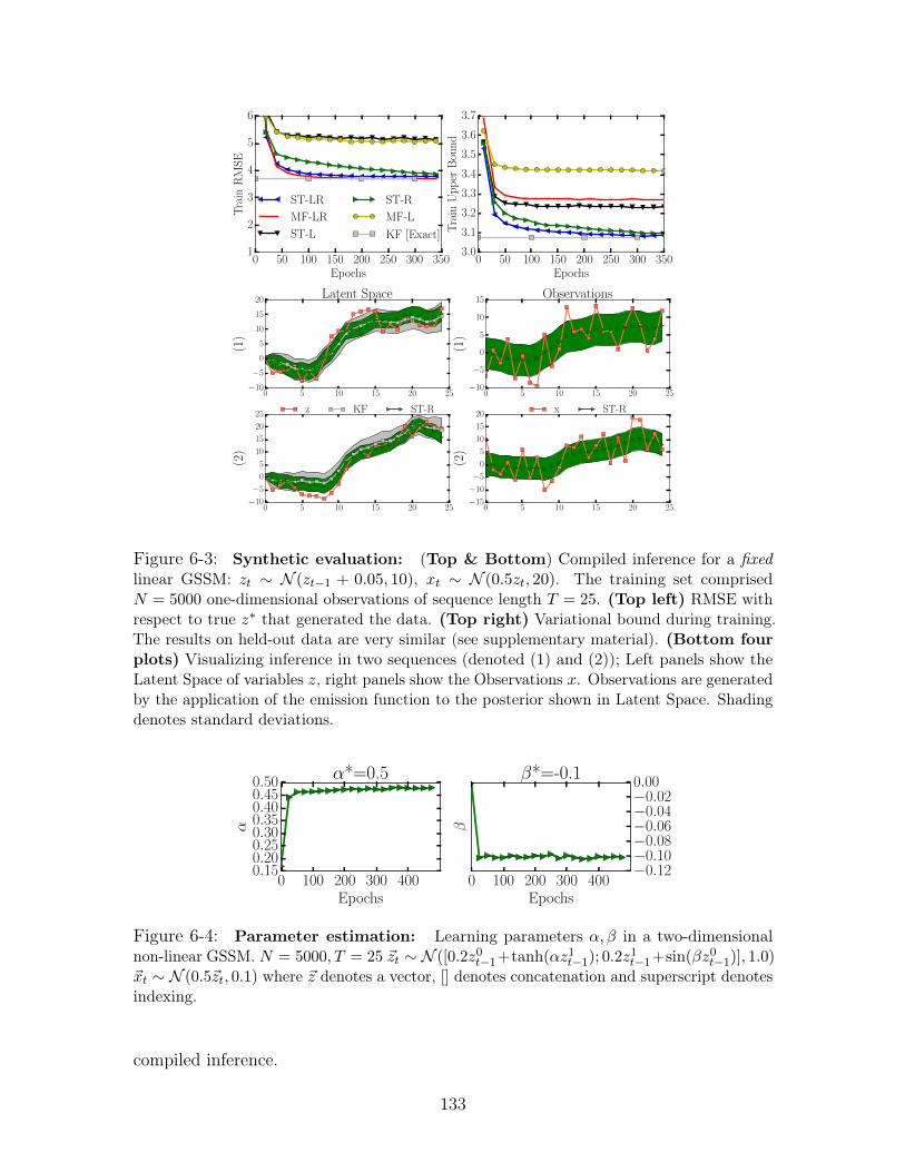
0 50 100 150 200 250 300 350Epochs
1
2
3
4
5
6
Tra
inR
MS
E
ST-LR
MF-LR
ST-L
ST-R
MF-L
KF [Exact]
0 50 100 150 200 250 300 350Epochs
3.0
3.1
3.2
3.3
3.4
3.5
3.6
3.7
Tra
inU
pp
erB
oun
d
0 5 10 15 20 25−10
−5
0
5
10
15
20
(1)
Latent Space
0 5 10 15 20 25−10
−5
0
5
10
15
(1)
Observations
0 5 10 15 20 25−10
−5
0
5
10
15
20
25
(2)
z KF ST-R
0 5 10 15 20 25−15
−10
−5
0
5
10
15
20
(2)
x ST-R
Figure 6-3: Synthetic evaluation: (Top & Bottom) Compiled inference for a fixedlinear GSSM: 𝑧𝑡 ∼ 𝒩 (𝑧𝑡−1 + 0.05, 10), 𝑥𝑡 ∼ 𝒩 (0.5𝑧𝑡, 20). The training set comprised𝑁 = 5000 one-dimensional observations of sequence length 𝑇 = 25. (Top left) RMSE withrespect to true 𝑧* that generated the data. (Top right) Variational bound during training.The results on held-out data are very similar (see supplementary material). (Bottom fourplots) Visualizing inference in two sequences (denoted (1) and (2)); Left panels show theLatent Space of variables 𝑧, right panels show the Observations 𝑥. Observations are generatedby the application of the emission function to the posterior shown in Latent Space. Shadingdenotes standard deviations.
0 100 200 300 400Epochs
0.150.200.250.300.350.400.450.50
α
α*=0.5
0 100 200 300 400Epochs
−0.12−0.10−0.08−0.06−0.04−0.020.00
β
β*=-0.1
Figure 6-4: Parameter estimation: Learning parameters 𝛼, 𝛽 in a two-dimensionalnon-linear GSSM. 𝑁 = 5000, 𝑇 = 25 �⃗�𝑡 ∼ 𝒩 ([0.2𝑧0𝑡−1+tanh(𝛼𝑧1𝑡−1); 0.2𝑧
1𝑡−1+sin(𝛽𝑧0𝑡−1)], 1.0)
�⃗�𝑡 ∼ 𝒩 (0.5�⃗�𝑡, 0.1) where �⃗� denotes a vector, [] denotes concatenation and superscript denotesindexing.
compiled inference.
133
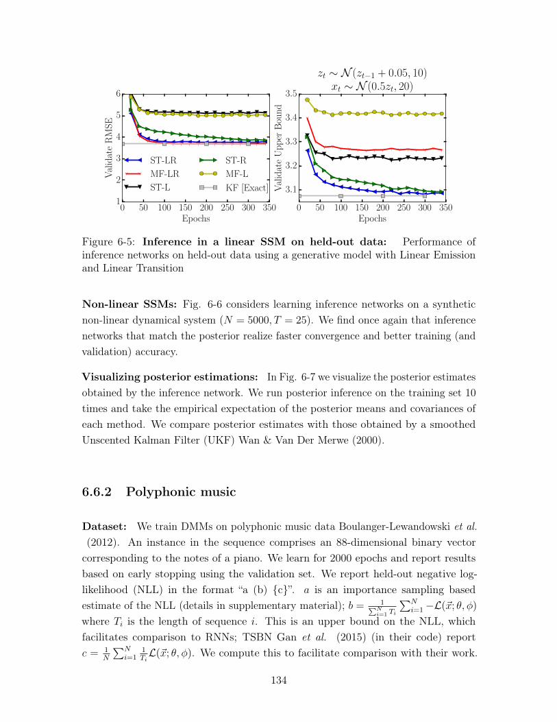
0 50 100 150 200 250 300 350Epochs
1
2
3
4
5
6
Val
idat
eR
MS
E
ST-LR
MF-LR
ST-L
ST-R
MF-L
KF [Exact]
0 50 100 150 200 250 300 350Epochs
3.1
3.2
3.3
3.4
3.5
Val
idat
eU
pp
erB
oun
d
zt ∼ N (zt−1 + 0.05, 10)xt ∼ N (0.5zt, 20)
Figure 6-5: Inference in a linear SSM on held-out data: Performance ofinference networks on held-out data using a generative model with Linear Emissionand Linear Transition
Non-linear SSMs: Fig. 6-6 considers learning inference networks on a syntheticnon-linear dynamical system (𝑁 = 5000, 𝑇 = 25). We find once again that inferencenetworks that match the posterior realize faster convergence and better training (andvalidation) accuracy.
Visualizing posterior estimations: In Fig. 6-7 we visualize the posterior estimatesobtained by the inference network. We run posterior inference on the training set 10
times and take the empirical expectation of the posterior means and covariances ofeach method. We compare posterior estimates with those obtained by a smoothedUnscented Kalman Filter (UKF) Wan & Van Der Merwe (2000).
6.6.2 Polyphonic music
Dataset: We train DMMs on polyphonic music data Boulanger-Lewandowski et al.(2012). An instance in the sequence comprises an 88-dimensional binary vector
corresponding to the notes of a piano. We learn for 2000 epochs and report resultsbased on early stopping using the validation set. We report held-out negative log-likelihood (NLL) in the format “a (b) {c}”. 𝑎 is an importance sampling basedestimate of the NLL (details in supplementary material); 𝑏 = 1∑︀𝑁
𝑖=1 𝑇𝑖
∑︀𝑁𝑖=1−ℒ(�⃗�; 𝜃, 𝜑)
where 𝑇𝑖 is the length of sequence 𝑖. This is an upper bound on the NLL, whichfacilitates comparison to RNNs; TSBN Gan et al. (2015) (in their code) report𝑐 = 1
𝑁
∑︀𝑁𝑖=1
1𝑇𝑖ℒ(�⃗�; 𝜃, 𝜑). We compute this to facilitate comparison with their work.
134
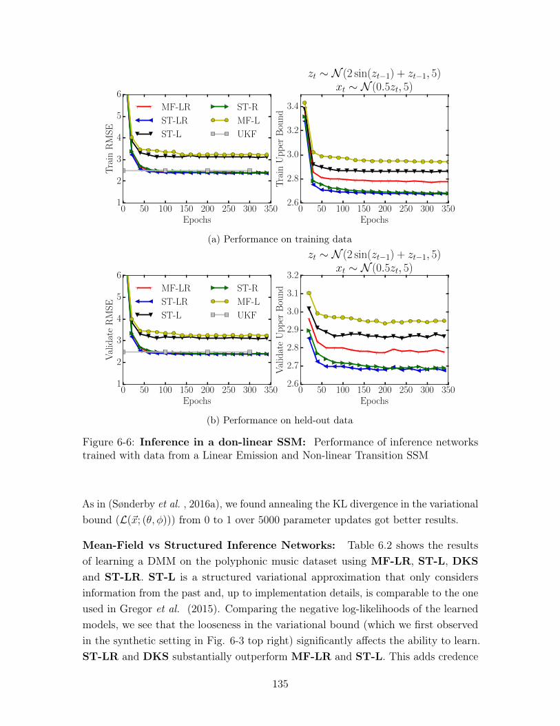
0 50 100 150 200 250 300 350Epochs
1
2
3
4
5
6
Tra
inR
MS
EMF-LR
ST-LR
ST-L
ST-R
MF-L
UKF
0 50 100 150 200 250 300 350Epochs
2.6
2.8
3.0
3.2
3.4
Tra
inU
pp
erB
oun
d
zt ∼ N (2 sin(zt−1) + zt−1, 5)xt ∼ N (0.5zt, 5)
(a) Performance on training data
0 50 100 150 200 250 300 350Epochs
1
2
3
4
5
6
Val
idat
eR
MS
E
MF-LR
ST-LR
ST-L
ST-R
MF-L
UKF
0 50 100 150 200 250 300 350Epochs
2.6
2.7
2.8
2.9
3.0
3.1
3.2V
alid
ate
Up
per
Bou
nd
zt ∼ N (2 sin(zt−1) + zt−1, 5)xt ∼ N (0.5zt, 5)
(b) Performance on held-out data
Figure 6-6: Inference in a don-linear SSM: Performance of inference networkstrained with data from a Linear Emission and Non-linear Transition SSM
As in (Sønderby et al. , 2016a), we found annealing the KL divergence in the variationalbound (ℒ(�⃗�; (𝜃, 𝜑))) from 0 to 1 over 5000 parameter updates got better results.
Mean-Field vs Structured Inference Networks: Table 6.2 shows the resultsof learning a DMM on the polyphonic music dataset using MF-LR, ST-L, DKSand ST-LR. ST-L is a structured variational approximation that only considersinformation from the past and, up to implementation details, is comparable to the oneused in Gregor et al. (2015). Comparing the negative log-likelihoods of the learnedmodels, we see that the looseness in the variational bound (which we first observedin the synthetic setting in Fig. 6-3 top right) significantly affects the ability to learn.ST-LR and DKS substantially outperform MF-LR and ST-L. This adds credence
135
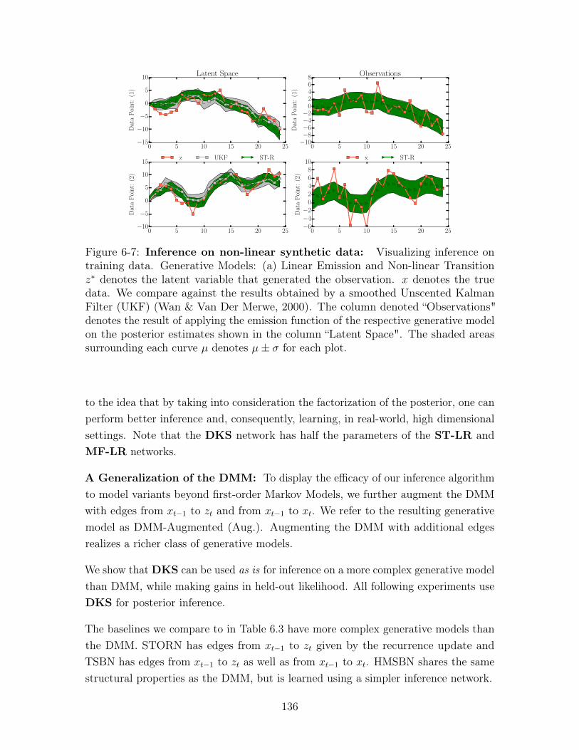
0 5 10 15 20 25−15
−10
−5
0
5
10
Dat
aP
oint
:(1
)
Latent Space
0 5 10 15 20 25−10−8−6−4−2
02468
Dat
aP
oint
:(1
)
Observations
0 5 10 15 20 25−10
−5
0
5
10
15
Dat
aP
oint
:(2
)
z UKF ST-R
0 5 10 15 20 25−6−4−2
02468
10
Dat
aP
oint
:(2
)
x ST-R
Figure 6-7: Inference on non-linear synthetic data: Visualizing inference ontraining data. Generative Models: (a) Linear Emission and Non-linear Transition𝑧* denotes the latent variable that generated the observation. 𝑥 denotes the truedata. We compare against the results obtained by a smoothed Unscented KalmanFilter (UKF) (Wan & Van Der Merwe, 2000). The column denoted “Observations"denotes the result of applying the emission function of the respective generative modelon the posterior estimates shown in the column “Latent Space". The shaded areassurrounding each curve 𝜇 denotes 𝜇± 𝜎 for each plot.
to the idea that by taking into consideration the factorization of the posterior, one canperform better inference and, consequently, learning, in real-world, high dimensionalsettings. Note that the DKS network has half the parameters of the ST-LR andMF-LR networks.
A Generalization of the DMM: To display the efficacy of our inference algorithmto model variants beyond first-order Markov Models, we further augment the DMMwith edges from 𝑥𝑡−1 to 𝑧𝑡 and from 𝑥𝑡−1 to 𝑥𝑡. We refer to the resulting generativemodel as DMM-Augmented (Aug.). Augmenting the DMM with additional edgesrealizes a richer class of generative models.
We show that DKS can be used as is for inference on a more complex generative modelthan DMM, while making gains in held-out likelihood. All following experiments useDKS for posterior inference.
The baselines we compare to in Table 6.3 have more complex generative models thanthe DMM. STORN has edges from 𝑥𝑡−1 to 𝑧𝑡 given by the recurrence update andTSBN has edges from 𝑥𝑡−1 to 𝑧𝑡 as well as from 𝑥𝑡−1 to 𝑥𝑡. HMSBN shares the samestructural properties as the DMM, but is learned using a simpler inference network.
136
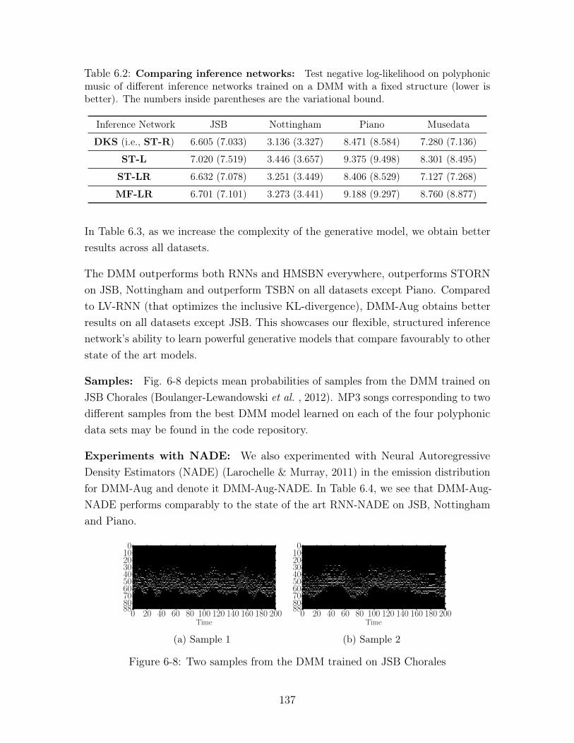
Table 6.2: Comparing inference networks: Test negative log-likelihood on polyphonicmusic of different inference networks trained on a DMM with a fixed structure (lower isbetter). The numbers inside parentheses are the variational bound.
Inference Network JSB Nottingham Piano Musedata
DKS (i.e., ST-R) 6.605 (7.033) 3.136 (3.327) 8.471 (8.584) 7.280 (7.136)
ST-L 7.020 (7.519) 3.446 (3.657) 9.375 (9.498) 8.301 (8.495)
ST-LR 6.632 (7.078) 3.251 (3.449) 8.406 (8.529) 7.127 (7.268)
MF-LR 6.701 (7.101) 3.273 (3.441) 9.188 (9.297) 8.760 (8.877)
In Table 6.3, as we increase the complexity of the generative model, we obtain betterresults across all datasets.
The DMM outperforms both RNNs and HMSBN everywhere, outperforms STORNon JSB, Nottingham and outperform TSBN on all datasets except Piano. Comparedto LV-RNN (that optimizes the inclusive KL-divergence), DMM-Aug obtains betterresults on all datasets except JSB. This showcases our flexible, structured inferencenetwork’s ability to learn powerful generative models that compare favourably to otherstate of the art models.
Samples: Fig. 6-8 depicts mean probabilities of samples from the DMM trained onJSB Chorales (Boulanger-Lewandowski et al. , 2012). MP3 songs corresponding to twodifferent samples from the best DMM model learned on each of the four polyphonicdata sets may be found in the code repository.
Experiments with NADE: We also experimented with Neural AutoregressiveDensity Estimators (NADE) (Larochelle & Murray, 2011) in the emission distributionfor DMM-Aug and denote it DMM-Aug-NADE. In Table 6.4, we see that DMM-Aug-NADE performs comparably to the state of the art RNN-NADE on JSB, Nottinghamand Piano.
0 20 40 60 80 100 120 140 160 180 200Time
0102030405060708088
(a) Sample 1
0 20 40 60 80 100 120 140 160 180 200Time
0102030405060708088
(b) Sample 2
Figure 6-8: Two samples from the DMM trained on JSB Chorales
137
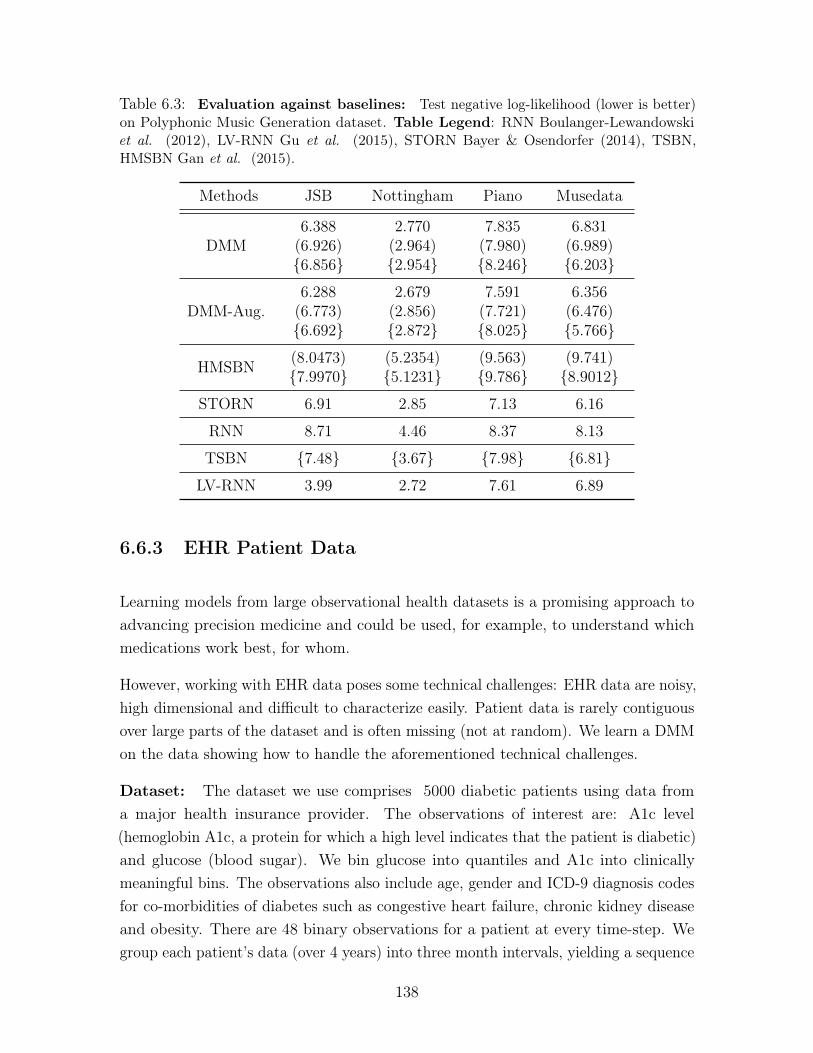
Table 6.3: Evaluation against baselines: Test negative log-likelihood (lower is better)on Polyphonic Music Generation dataset. Table Legend: RNN Boulanger-Lewandowskiet al. (2012), LV-RNN Gu et al. (2015), STORN Bayer & Osendorfer (2014), TSBN,HMSBN Gan et al. (2015).
Methods JSB Nottingham Piano Musedata
DMM6.388
(6.926){6.856}
2.770(2.964){2.954}
7.835(7.980){8.246}
6.831(6.989){6.203}
DMM-Aug.6.288
(6.773){6.692}
2.679(2.856){2.872}
7.591(7.721){8.025}
6.356(6.476){5.766}
HMSBN (8.0473){7.9970}
(5.2354){5.1231}
(9.563){9.786}
(9.741){8.9012}
STORN 6.91 2.85 7.13 6.16
RNN 8.71 4.46 8.37 8.13
TSBN {7.48} {3.67} {7.98} {6.81}
LV-RNN 3.99 2.72 7.61 6.89
6.6.3 EHR Patient Data
Learning models from large observational health datasets is a promising approach toadvancing precision medicine and could be used, for example, to understand whichmedications work best, for whom.
However, working with EHR data poses some technical challenges: EHR data are noisy,high dimensional and difficult to characterize easily. Patient data is rarely contiguousover large parts of the dataset and is often missing (not at random). We learn a DMMon the data showing how to handle the aforementioned technical challenges.
Dataset: The dataset we use comprises 5000 diabetic patients using data froma major health insurance provider. The observations of interest are: A1c level(hemoglobin A1c, a protein for which a high level indicates that the patient is diabetic)and glucose (blood sugar). We bin glucose into quantiles and A1c into clinicallymeaningful bins. The observations also include age, gender and ICD-9 diagnosis codesfor co-morbidities of diabetes such as congestive heart failure, chronic kidney diseaseand obesity. There are 48 binary observations for a patient at every time-step. Wegroup each patient’s data (over 4 years) into three month intervals, yielding a sequence
138
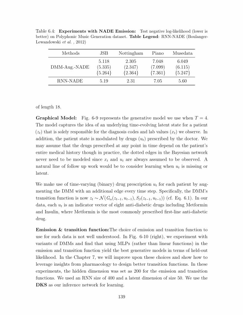
Table 6.4: Experiments with NADE Emission: Test negative log-likelihood (lower isbetter) on Polyphonic Music Generation dataset. Table Legend: RNN-NADE (Boulanger-Lewandowski et al. , 2012)
Methods JSB Nottingham Piano Musedata
DMM-Aug.-NADE5.118
(5.335){5.264}
2.305(2.347){2.364}
7.048(7.099){7.361}
6.049(6.115){5.247}
RNN-NADE 5.19 2.31 7.05 5.60
of length 18.
Graphical Model: Fig. 6-9 represents the generative model we use when 𝑇 = 4.The model captures the idea of an underlying time-evolving latent state for a patient(𝑧𝑡) that is solely responsible for the diagnosis codes and lab values (𝑥𝑡) we observe. Inaddition, the patient state is modulated by drugs (𝑢𝑡) prescribed by the doctor. Wemay assume that the drugs prescribed at any point in time depend on the patient’sentire medical history though in practice, the dotted edges in the Bayesian networknever need to be modeled since 𝑥𝑡 and 𝑢𝑡 are always assumed to be observed. Anatural line of follow up work would be to consider learning when 𝑢𝑡 is missing orlatent.
We make use of time-varying (binary) drug prescription 𝑢𝑡 for each patient by aug-menting the DMM with an additional edge every time step. Specifically, the DMM’stransition function is now 𝑧𝑡 ∼ 𝒩 (G𝛼(𝑧𝑡−1, 𝑢𝑡−1), S𝛽(𝑧𝑡−1, 𝑢𝑡−1)) (cf. Eq. 6.1). In ourdata, each 𝑢𝑡 is an indicator vector of eight anti-diabetic drugs including Metforminand Insulin, where Metformin is the most commonly prescribed first-line anti-diabeticdrug.
Emission & transition function:The choice of emission and transition function touse for such data is not well understood. In Fig. 6-10 (right), we experiment withvariants of DMMs and find that using MLPs (rather than linear functions) in theemission and transition function yield the best generative models in terms of held-outlikelihood. In the Chapter 7, we will improve upon these choices and show how toleverage insights from pharmacology to design better transition functions. In theseexperiments, the hidden dimension was set as 200 for the emission and transitionfunctions. We used an RNN size of 400 and a latent dimension of size 50. We use theDKS as our inference network for learning.
139
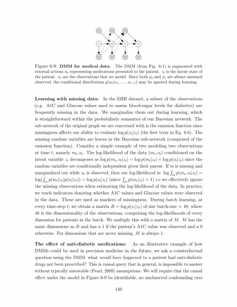
𝑧1
𝑢1
𝑥1
𝑧2
𝑢2
𝑥2
𝑧3
𝑢3
𝑥3
𝑧4
𝑥4
Figure 6-9: DMM for medical data: The DMM (from Fig. 6-1) is augmented withexternal actions 𝑢𝑡 representing medications presented to the patient. 𝑧𝑡 is the latent state ofthe patient. 𝑥𝑡 are the observations that we model. Since both 𝑢𝑡 and 𝑥𝑡 are always assumedobserved, the conditional distribution 𝑝(𝑢𝑡|𝑥1, . . . , 𝑥𝑡−1) may be ignored during learning.
Learning with missing data: In the EHR dataset, a subset of the observations(e.g. A1C and Glucose values used to assess blood-sugar levels for diabetics) arefrequently missing in the data. We marginalize them out during learning, whichis straightforward within the probabilistic semantics of our Bayesian network. Thesub-network of the original graph we are concerned with is the emission function sincemissingness affects our ability to evaluate log 𝑝(𝑥𝑡|𝑧𝑡) (the first term in Eq. 6.6). Themissing random variables are leaves in the Bayesian sub-network (comprised of theemission function). Consider a simple example of two modeling two observationsat time 𝑡, namely 𝑚𝑡, 𝑜𝑡. The log-likelihood of the data (𝑚𝑡, 𝑜𝑡) conditioned on thelatent variable 𝑧𝑡 decomposes as log 𝑝(𝑚𝑡, 𝑜𝑡|𝑧𝑡) = log 𝑝(𝑚𝑡|𝑧𝑡) + log 𝑝(𝑜𝑡|𝑧𝑡) since therandom variables are conditionally independent given their parent. If 𝑚 is missing andmarginalized out while 𝑜𝑡 is observed, then our log-likelihood is: log
∫︀𝑚𝑝(𝑚𝑡, 𝑜𝑡|𝑧𝑡) =
log(∫︀𝑚𝑝(𝑚𝑡|𝑧𝑡)𝑝(𝑜𝑡|𝑧𝑡)) = log 𝑝(𝑜𝑡|𝑧𝑡) (since
∫︀𝑚𝑝(𝑚𝑡|𝑧𝑡) = 1) i.e we effectively ignore
the missing observations when estimating the log-likelihood of the data. In practice,we track indicators denoting whether A1C values and Glucose values were observedin the data. These are used as markers of missingness. During batch learning, atevery time-step 𝑡, we obtain a matrix 𝐵 = log 𝑝(𝑥𝑡|𝑧𝑡) of size batch-size × 48, where48 is the dimensionality of the observations, comprising the log-likelihoods of everydimension for patients in the batch. We multiply this with a matrix of 𝑀 . 𝑀 has thesame dimensions as 𝐵 and has a 1 if the patient’s A1C value was observed and a 0
otherwise. For dimensions that are never missing, 𝑀 is always 1.
The effect of anti-diabetic medications: As an illustrative example of howDMMs could be used in precision medicine in the future, we ask a counterfactualquestion using the DMM: what would have happened to a patient had anti-diabeticdrugs not been prescribed? This is causal query that in general, is impossible to answerwithout typically untestable (Pearl, 2009) assumptions. We will require that the causaleffect under the model in Figure 6-9 be identifiable, no unobserved confounding over
140
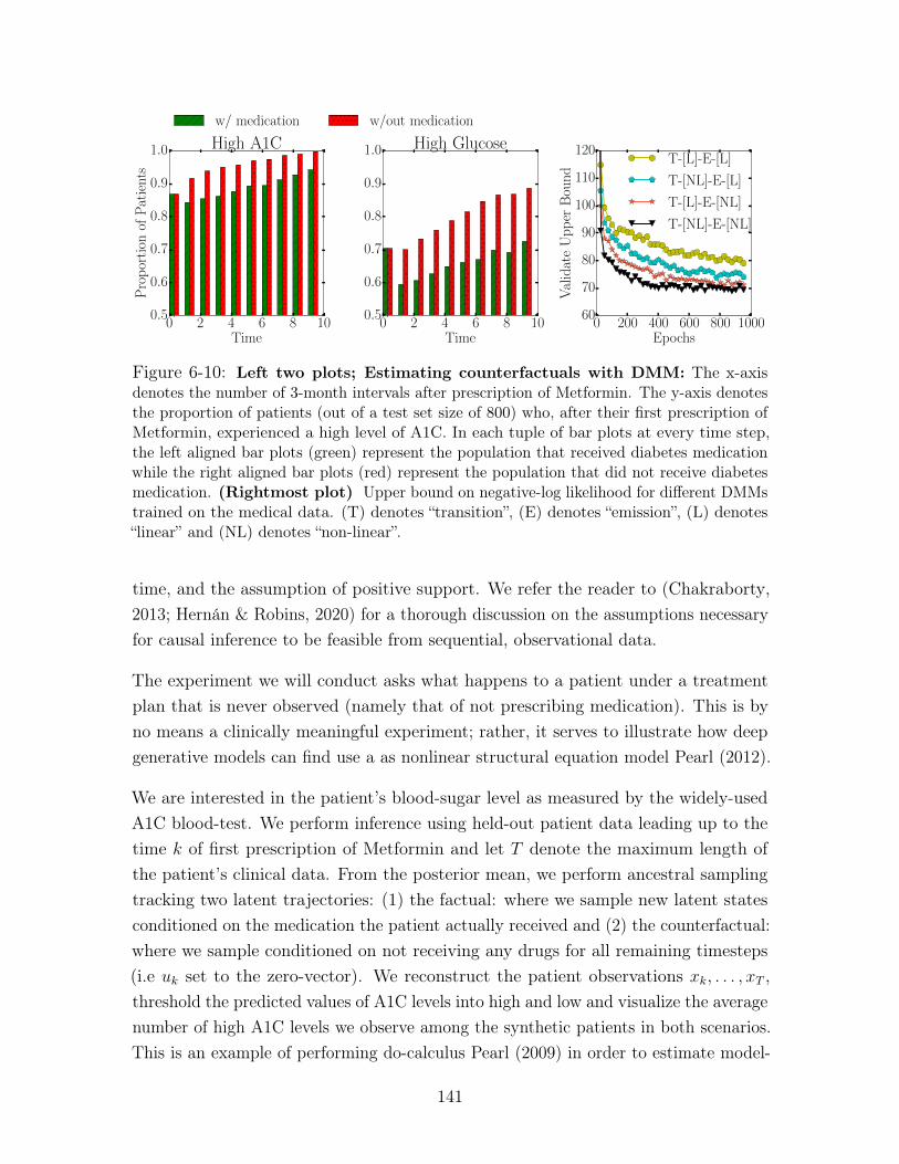
0 2 4 6 8 10Time
0.5
0.6
0.7
0.8
0.9
1.0P
rop
orti
onof
Pat
ient
sHigh A1C
w/ medication w/out medication
0 2 4 6 8 10Time
0.5
0.6
0.7
0.8
0.9
1.0 High Glucose
0 200 400 600 800 1000Epochs
60
70
80
90
100
110
120
Val
idat
eU
pp
erB
oun
d
T-[L]-E-[L]
T-[NL]-E-[L]
T-[L]-E-[NL]
T-[NL]-E-[NL]
Figure 6-10: Left two plots; Estimating counterfactuals with DMM: The x-axisdenotes the number of 3-month intervals after prescription of Metformin. The y-axis denotesthe proportion of patients (out of a test set size of 800) who, after their first prescription ofMetformin, experienced a high level of A1C. In each tuple of bar plots at every time step,the left aligned bar plots (green) represent the population that received diabetes medicationwhile the right aligned bar plots (red) represent the population that did not receive diabetesmedication. (Rightmost plot) Upper bound on negative-log likelihood for different DMMstrained on the medical data. (T) denotes “transition”, (E) denotes “emission”, (L) denotes“linear” and (NL) denotes “non-linear”.
time, and the assumption of positive support. We refer the reader to (Chakraborty,2013; Hernán & Robins, 2020) for a thorough discussion on the assumptions necessaryfor causal inference to be feasible from sequential, observational data.
The experiment we will conduct asks what happens to a patient under a treatmentplan that is never observed (namely that of not prescribing medication). This is byno means a clinically meaningful experiment; rather, it serves to illustrate how deepgenerative models can find use a as nonlinear structural equation model Pearl (2012).
We are interested in the patient’s blood-sugar level as measured by the widely-usedA1C blood-test. We perform inference using held-out patient data leading up to thetime 𝑘 of first prescription of Metformin and let 𝑇 denote the maximum length ofthe patient’s clinical data. From the posterior mean, we perform ancestral samplingtracking two latent trajectories: (1) the factual: where we sample new latent statesconditioned on the medication the patient actually received and (2) the counterfactual:where we sample conditioned on not receiving any drugs for all remaining timesteps(i.e 𝑢𝑘 set to the zero-vector). We reconstruct the patient observations 𝑥𝑘, . . . , 𝑥𝑇 ,threshold the predicted values of A1C levels into high and low and visualize the averagenumber of high A1C levels we observe among the synthetic patients in both scenarios.This is an example of performing do-calculus Pearl (2009) in order to estimate model-
141
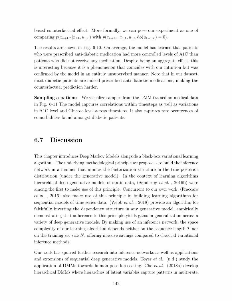
based counterfactual effect. More formally, we can pose our experiment as one ofcomparing 𝑝(𝑥𝑘+1:𝑇 |𝑥1:𝑘, 𝑢1:𝑇 ) with 𝑝(𝑥𝑘+1:𝑇 |𝑥1:𝑘, 𝑢1:𝑡, do(𝑢𝑘+1:𝑇 ) = 0).
The results are shown in Fig. 6-10. On average, the model has learned that patientswho were prescribed anti-diabetic medication had more controlled levels of A1C thanpatients who did not receive any medication. Despite being an aggregate effect, thisis interesting because it is a phenomenon that coincides with our intuition but wasconfirmed by the model in an entirely unsupervised manner. Note that in our dataset,most diabetic patients are indeed prescribed anti-diabetic medications, making thecounterfactual prediction harder.
Sampling a patient: We visualize samples from the DMM trained on medical datain Fig. 6-11 The model captures correlations within timesteps as well as variationsin A1C level and Glucose level across timesteps. It also captures rare occurrences ofcomorbidities found amongst diabetic patients.
6.7 Discussion
This chapter introduces Deep Markov Models alongside a black-box variational learningalgorithm. The underlying methodological principle we propose is to build the inferencenetwork in a manner that mimics the factorization structure in the true posteriordistribution (under the generative model). In the context of learning algorithmshierarchical deep generative models of static data, (Sønderby et al. , 2016b) wereamong the first to make use of this principle. Concurrent to our own work, (Fraccaroet al. , 2016) also make use of this principle in building learning algorithms forsequential models of time-series data. (Webb et al. , 2018) provide an algorithm forfaithfully inverting the dependency structure in any generative model, empiricallydemonstrating that adherence to this principle yields gains in generalization across avariety of deep generative models. By making use of an inference network, the spacecomplexity of our learning algorithm depends neither on the sequence length 𝑇 noron the training set size 𝑁 , offering massive savings compared to classical variationalinference methods.
Our work has spurred further research into inference networks as well as applicationsand extensions of sequential deep generative models. Toyer et al. (n.d.) study theapplication of DMMs towards human pose forecasting. Che et al. (2018a) develophierarchical DMMs where hierarchies of latent variables capture patterns in multi-rate,
142

high-dimensional time-series data. Finally, Zhi-Xuan et al. (2020) extend DMMsto learn unified, time-varying representations of multi-modal data. An open sourceimplementation of DMMs is also available in the probabilistic programming packagePyro (Bingham et al. , 2019).
143
1 2 3 4 5 6 7 8 9 10 11 12 13 14 15 16 17 18
0 < A1C < 5.5
5.5 < A1C < 6.0
6.0 < A1C < 6.5
6.5 < A1C < 7.0
7.0 < A1C < 8.0
8.0 < A1C < 9.0
9.0 < A1C < 10.0
10.0 < A1C < 19.0
0 < GLUC. < 92.0
92.0 < GLUC. < 102.0
102.0 < GLUC. < 113.0
113.0 < GLUC. < 135.0
135.0 < GLUC. < 989.0
18 < AGE < 49.0
49.0 < AGE < 57.0
57.0 < AGE < 63.0
63.0 < AGE < 70.0
70.0 < AGE < 98.0
GENDER IS FEMALE
COVERAGE
DIABETES WO CMP NT ST UNCNTR
DIABETES WO CMP NT ST UNCNTRL
DIABETES WO CMP UNCNTRLD
GOUT NOS
OBESITY NOS
MORBID OBESITY
ANEMIA IN CHR KIDNEY DIS
OBSTRUCTIVE SLEEP APNEA
MALIGNANT HYPERTENSION
BENIGN HYP HT DIS W/O HF
HYP HRT DIS NOS W/O HF
CORONARY ATH UNSP VSL NTV/GFT
Figure 6-11: Patient data generated by a DMM Samples of a patient generated by themodel. The x-axis denotes time and the y-axis denotes the observations. The intensity ofthe color denotes its value between zero and one
144
Chapter 7
Inductive biases for clinical data
In Chapter 6 we showed how to make use of structure in the graphical model toderive learning algorithms for nonlinear state space models of clinical data. To makepredictions from longitudinal data or deconstruct salient structure within, we needgood sequential models. However, modeling longitudinal observations in the presenceof time-varying interventions is challenging. In this chapter, we study whether wecan improve upon the use of multi-layer perceptrons in the conditional probabilitydistributions of DMMs.
Models parameterize intervention effect functions (IEFs), which determine how themodel responds to an intervention, in different ways. A common choice, that we madein the previous chapter, for high-dimensional data is to use neural networks. However,datasets in healthcare can be small, leaving such approaches prone to overfitting. Weshow how to make deep learning practical in the low-data regime by building newneural architectures inspired by ideas from pharmacology. In doing so, we show howpractitioners can use domain knowledge and patterns in time-varying interventions toconstruct IEFs. In various non-linear, sequential models of disease progression, acrossboth synthetic and real-world data, our proposed IEF yields dramatic improvementsin generalization where other representation learning approaches overfit.
7.1 Introduction
Deep generative models capture changes in high-dimensional, longitudinal observationsusing time-varying hidden representations, such as Recurrent Neural Networks (RNNs)
145
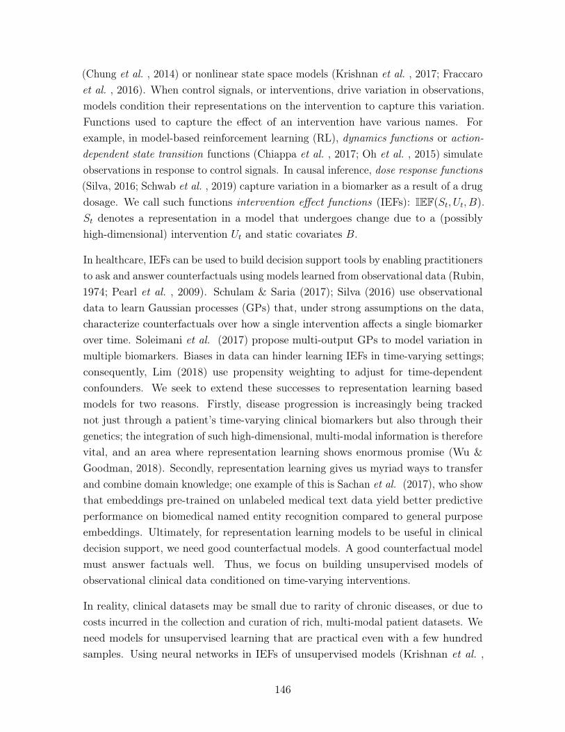
(Chung et al. , 2014) or nonlinear state space models (Krishnan et al. , 2017; Fraccaroet al. , 2016). When control signals, or interventions, drive variation in observations,models condition their representations on the intervention to capture this variation.Functions used to capture the effect of an intervention have various names. Forexample, in model-based reinforcement learning (RL), dynamics functions or action-dependent state transition functions (Chiappa et al. , 2017; Oh et al. , 2015) simulateobservations in response to control signals. In causal inference, dose response functions(Silva, 2016; Schwab et al. , 2019) capture variation in a biomarker as a result of a drugdosage. We call such functions intervention effect functions (IEFs): IEF(𝑆𝑡, 𝑈𝑡, 𝐵).𝑆𝑡 denotes a representation in a model that undergoes change due to a (possiblyhigh-dimensional) intervention 𝑈𝑡 and static covariates 𝐵.
In healthcare, IEFs can be used to build decision support tools by enabling practitionersto ask and answer counterfactuals using models learned from observational data (Rubin,1974; Pearl et al. , 2009). Schulam & Saria (2017); Silva (2016) use observationaldata to learn Gaussian processes (GPs) that, under strong assumptions on the data,characterize counterfactuals over how a single intervention affects a single biomarkerover time. Soleimani et al. (2017) propose multi-output GPs to model variation inmultiple biomarkers. Biases in data can hinder learning IEFs in time-varying settings;consequently, Lim (2018) use propensity weighting to adjust for time-dependentconfounders. We seek to extend these successes to representation learning basedmodels for two reasons. Firstly, disease progression is increasingly being trackednot just through a patient’s time-varying clinical biomarkers but also through theirgenetics; the integration of such high-dimensional, multi-modal information is thereforevital, and an area where representation learning shows enormous promise (Wu &Goodman, 2018). Secondly, representation learning gives us myriad ways to transferand combine domain knowledge; one example of this is Sachan et al. (2017), who showthat embeddings pre-trained on unlabeled medical text data yield better predictiveperformance on biomedical named entity recognition compared to general purposeembeddings. Ultimately, for representation learning models to be useful in clinicaldecision support, we need good counterfactual models. A good counterfactual modelmust answer factuals well. Thus, we focus on building unsupervised models ofobservational clinical data conditioned on time-varying interventions.
In reality, clinical datasets may be small due to rarity of chronic diseases, or due tocosts incurred in the collection and curation of rich, multi-modal patient datasets. Weneed models for unsupervised learning that are practical even with a few hundredsamples. Using neural networks in IEFs of unsupervised models (Krishnan et al. ,
146
2017; Lipton et al. , 2015) for such data risks overfitting. One may overcome thelimited-data problem by using domain expertise; for example, in model-based RL, Du& Narasimhan (2019); Scholz et al. (2014) use the physics of how objects interact todesign the dynamics function. This approach can reduce sample complexity, but relieson domain knowledge. We seek to understand what the correct domain knowledge isin settings where it is not easily obtainable and difficult to formalize, and how oneshould leverage it when building IEFs for unsupervised models of disease progression.
This chapter makes several contributions towards both machine learning and itsapplications to healthcare. First, we propose a novel neural architecture for an IEF,PK-PDIEF, that blends mathematical models from pharmacology with deep learning.The IEF is flexible and leverages unique structure in the treatments prescribed tochronically ill patients. Second, we show that the incorporation of domain knowledgein unsupervised models of high-dimensional clinical data aids generalization in the lowdata regime. We study the use of PK-PDIEF in three unsupervised models (on bothsynthetic and real-world patient data) and find strong differential improvements ingeneralization conferred from the use of PK-PDIEF when data is scarce. Qualitatively,the neural architecture is interpretable, and captures known clinical knowledge regard-ing the treatment effect. Third, we release code for the PK-PDIEF and the ML-MMRFdataset, which is a curated, pre-processed subset of the CoMMpass study (MultipleMyeloma Research Foundation & others, 2011) set up for the machine learning andhealthcare communities to study these and other questions.
7.2 Setup
To ground our discussion, we focus on IEFs tailored for clinical data of chronically illpatients. Chronic diseases (e.g. cancer, heart disease) are those which require long-term medical attention and result in one or more organ systems being compromised.The progression of chronic disease is tracked via clinical biomarkers whose evolution isinfluenced by static factors like age, genetics and medical history. Patient data for thosesuffering from such diseases may be very limited, making these disease cohorts idealfor studying questions about the generalization of unsupervised models in the low-dataregime. Patients suffering from such diseases tend to have pre-determined scheduleswhere their progress is measured and treatments are prescribed. We therefore turn todiscrete-time models as a reasonable approximation of the underlying data generatingprocess. We review three models of sequential data conditioned on interventions and
147
highlight the IEF within each one.
Notation: Let 𝐵 ∈ R𝐽 denote baseline data that are static, i.e. individual-specificcovariates. Let U = {𝑈0, . . . , 𝑈𝑇−1}; 𝑈𝑡 ∈ R𝐿 be a sequence of 𝐿 dimensionalinterventions for an individual. An element of 𝑈𝑡 may be binary, to denote prescriptionof a drug, or real-valued, to denote the dosage. Let X = {𝑋1, . . . , 𝑋𝑇}; 𝑋𝑡 ∈ R𝑀
denote the sequence of real-valued, 𝑀 dimensional clinical biomarkers. An elementof 𝑋𝑡 may denote a serum lab value or blood count, which is used by clinicians tomeasure organ function as a proxy for disease severity. We assume access to a dataset𝒟 = {(X1,U1, 𝐵1), . . . , (X𝑁 ,U𝑁 , 𝐵𝑁)}. Unless required, we ignore the superscriptdenoting the index of the datapoint and denote concatenation with []. The goal of ourwork is to build models of X conditioned on U, 𝐵. We denote the parameters of amodel by 𝜃, which may comprise weight matrices or the parameters of functions thatindex 𝜃. Each model will have an IEF(𝑆𝑡−1, 𝑈𝑡−1, 𝐵).
Line 1Line 2Line 3+
BortezomibLenalidomide
SerumIgG
U: Treatments
X: Biomarkers
B: BaselineCovariates
Time
𝐵
𝑍1
𝑈1
𝑍2
𝑈2
𝑍3
𝑋1 𝑋2 𝑋3
Figure 7-1: Patient Data (Left): Illustration of data from a multiple myeloma patient.Baseline (static) data typically consists of genomics, demographics, and initial labs. Longitu-dinal data typically includes laboratory values (e.g. serum IgG) and treatments. Baselinedata is usually complete, but longitudinal measurements are frequently missing at varioustime points. The data tells a rich story of a patient’s disease trajectory and the resultingtreatment decisions. For example, a deviation of a lab value from a healthy range (e.g. spikein serum IgG) might prompt a move to the next line of therapy. Missing data (e.g. points inred) in this case are forward filled. Unsupervised Models of Sequential Data (Right):We show a State Space Model (SSM) of X (the longitudinal biomarkers) conditioned on 𝐵(genetics, denographics) and U (binary indicators of treatment and line of therapy). Therectangle depicts the IEF(𝑆𝑡−1, 𝑈𝑡−1, 𝐵), where 𝑆𝑡−1 = 𝑍𝑡−1.
7.2.1 First Order Markov Models (FOMMs)
FOMMs assume observations are conditionally independent of the past given theprevious observation, intervention and baseline covariates:
𝑝(X|U, 𝐵) =∏︀𝑇
𝑡=1 𝑝(𝑋𝑡|𝑋𝑡−1, 𝑈𝑡−1, 𝐵);𝑋𝑡 ∼ 𝒩 (𝜇𝜃(𝑋𝑡−1, 𝑈𝑡−1, 𝐵),Σ𝜃(𝑋𝑡−1, 𝑈𝑡−1, 𝐵)),
148
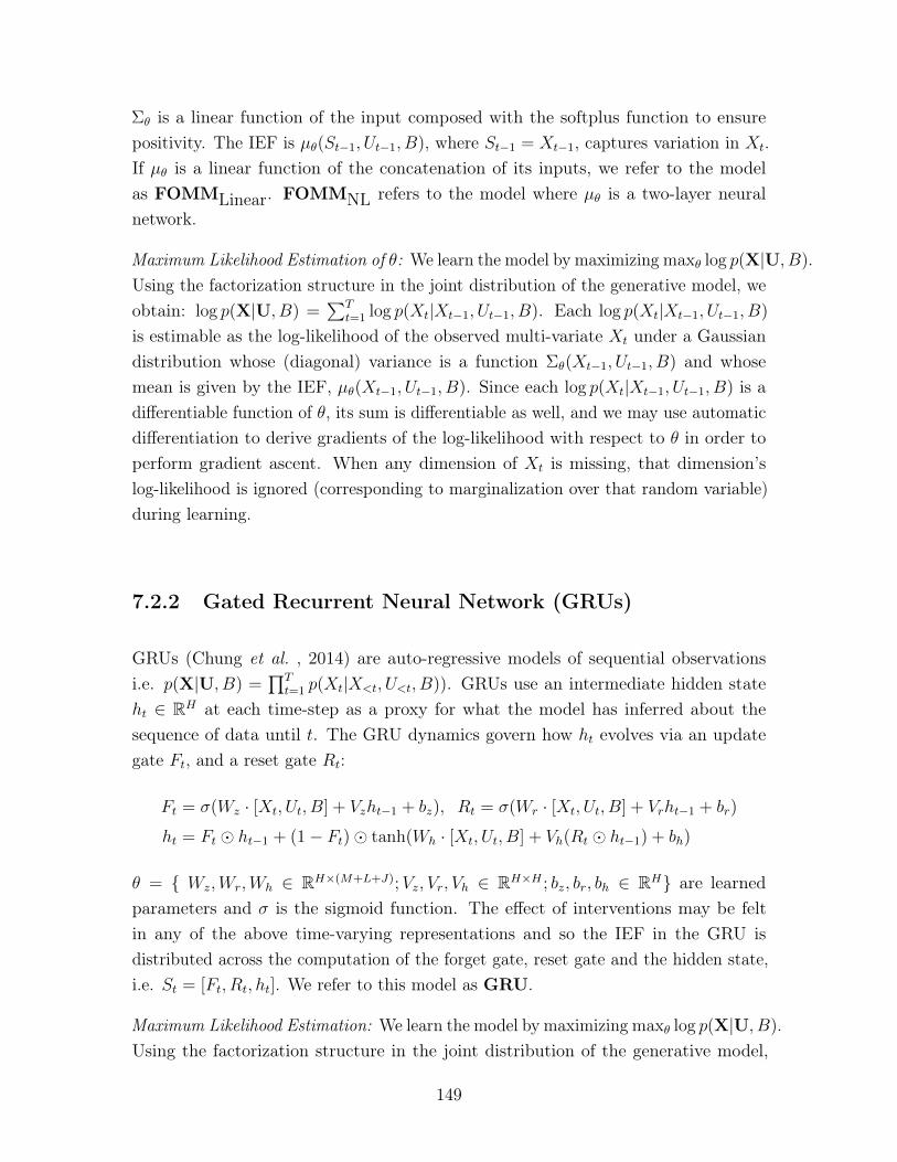
Σ𝜃 is a linear function of the input composed with the softplus function to ensurepositivity. The IEF is 𝜇𝜃(𝑆𝑡−1, 𝑈𝑡−1, 𝐵), where 𝑆𝑡−1 = 𝑋𝑡−1, captures variation in 𝑋𝑡.If 𝜇𝜃 is a linear function of the concatenation of its inputs, we refer to the modelas FOMMLinear. FOMMNL refers to the model where 𝜇𝜃 is a two-layer neuralnetwork.
Maximum Likelihood Estimation of 𝜃: We learn the model by maximizing max𝜃 log 𝑝(X|U, 𝐵).Using the factorization structure in the joint distribution of the generative model, weobtain: log 𝑝(X|U, 𝐵) =
∑︀𝑇𝑡=1 log 𝑝(𝑋𝑡|𝑋𝑡−1, 𝑈𝑡−1, 𝐵). Each log 𝑝(𝑋𝑡|𝑋𝑡−1, 𝑈𝑡−1, 𝐵)
is estimable as the log-likelihood of the observed multi-variate 𝑋𝑡 under a Gaussiandistribution whose (diagonal) variance is a function Σ𝜃(𝑋𝑡−1, 𝑈𝑡−1, 𝐵) and whosemean is given by the IEF, 𝜇𝜃(𝑋𝑡−1, 𝑈𝑡−1, 𝐵). Since each log 𝑝(𝑋𝑡|𝑋𝑡−1, 𝑈𝑡−1, 𝐵) is adifferentiable function of 𝜃, its sum is differentiable as well, and we may use automaticdifferentiation to derive gradients of the log-likelihood with respect to 𝜃 in order toperform gradient ascent. When any dimension of 𝑋𝑡 is missing, that dimension’slog-likelihood is ignored (corresponding to marginalization over that random variable)during learning.
7.2.2 Gated Recurrent Neural Network (GRUs)
GRUs (Chung et al. , 2014) are auto-regressive models of sequential observationsi.e. 𝑝(X|U, 𝐵) = ∏︀𝑇
𝑡=1 𝑝(𝑋𝑡|𝑋<𝑡, 𝑈<𝑡, 𝐵)). GRUs use an intermediate hidden stateℎ𝑡 ∈ R𝐻 at each time-step as a proxy for what the model has inferred about thesequence of data until 𝑡. The GRU dynamics govern how ℎ𝑡 evolves via an updategate 𝐹𝑡, and a reset gate 𝑅𝑡:
𝐹𝑡 = 𝜎(𝑊𝑧 · [𝑋𝑡, 𝑈𝑡, 𝐵] + 𝑉𝑧ℎ𝑡−1 + 𝑏𝑧), 𝑅𝑡 = 𝜎(𝑊𝑟 · [𝑋𝑡, 𝑈𝑡, 𝐵] + 𝑉𝑟ℎ𝑡−1 + 𝑏𝑟)
ℎ𝑡 = 𝐹𝑡 ⊙ ℎ𝑡−1 + (1− 𝐹𝑡)⊙ tanh(𝑊ℎ · [𝑋𝑡, 𝑈𝑡, 𝐵] + 𝑉ℎ(𝑅𝑡 ⊙ ℎ𝑡−1) + 𝑏ℎ)
𝜃 = { 𝑊𝑧,𝑊𝑟,𝑊ℎ ∈ R𝐻×(𝑀+𝐿+𝐽);𝑉𝑧, 𝑉𝑟, 𝑉ℎ ∈ R𝐻×𝐻 ; 𝑏𝑧, 𝑏𝑟, 𝑏ℎ ∈ R𝐻} are learnedparameters and 𝜎 is the sigmoid function. The effect of interventions may be feltin any of the above time-varying representations and so the IEF in the GRU isdistributed across the computation of the forget gate, reset gate and the hidden state,i.e. 𝑆𝑡 = [𝐹𝑡, 𝑅𝑡, ℎ𝑡]. We refer to this model as GRU.
Maximum Likelihood Estimation: We learn the model by maximizing max𝜃 log 𝑝(X|U, 𝐵).Using the factorization structure in the joint distribution of the generative model,
149
we obtain: log 𝑝(X|U, 𝐵) = ∑︀𝑇𝑡=1 log 𝑝(𝑋𝑡|𝑋<𝑡, 𝑈<𝑡, 𝐵). At each point in time the
hidden state of the GRU, ℎ𝑡, summarizes 𝑋<𝑡, 𝑈<𝑡, 𝐵. Thus, the model assumes𝑋𝑡 ∼ 𝒩 (𝜇𝜃(ℎ𝑡),Σ𝜃(ℎ𝑡)).
At each point in time, log 𝑝(𝑋𝑡|𝑋<𝑡, 𝑈<𝑡, 𝐵) is the log-likelihood of a multi-variateGaussian distribution which depends on 𝜃. As before, we may use automatic dif-ferentiation to derive gradients of the log-likelihood with respect to 𝜃 in order toperform gradient ascent. When any dimension of 𝑋𝑡 is missing, that dimension’slog-likelihood is ignored (corresponding to marginalization over that random variable)during learning.
7.2.3 State Space Models (SSMs)
SSMs capture longer-term dependencies in sequential data via a time-varying latentstate, as in Figure 7-1 (right). 𝑍𝑡 is a low-dimensional representation of the high-dimensional 𝑋𝑡. We experiment with Deep Markov Models (Krishnan et al. , 2017):
𝑝(X|U, 𝐵) =
∫︁
𝑍
𝑇∏︁
𝑡=1
𝑝(𝑍𝑡|𝑍𝑡−1, 𝑈𝑡−1, 𝐵; 𝜃)𝑝(𝑋𝑡|𝑍𝑡; 𝜃)𝑑𝑍
𝑍𝑡 ∼ 𝒩 (𝜇𝜃(𝑍𝑡−1, 𝑈𝑡−1, 𝐵),Σ𝑡𝜃(𝑍𝑡−1, 𝑈𝑡−1, 𝐵)), 𝑋𝑡 ∼ 𝒩 (𝜅𝜃(𝑍𝑡),Σ
𝑒𝜃(𝑍𝑡))
Σ𝑡𝜃,Σ𝑒𝜃, 𝜅𝜃(𝑍𝑡) are linear functions of a concatenation of their inputs composed with the
softplus function to ensure positivity. The IEF is 𝜇𝜃(𝑆𝑡−1, 𝑈𝑡−1, 𝐵), where 𝑆𝑡−1 = 𝑍𝑡−1.SSMLinear and SSMNL refer to models where 𝜇𝜃 is linear and non-linear (two-layerneural network), respectively.
Maximum Likelihood Estimation: We learn the model by maximizing max𝜃 log 𝑝(X|U, 𝐵).Using the factorization structure in the joint distribution of the generative model, weobtain: log 𝑝(X|U, 𝐵) =
∑︀𝑇𝑡=1 log 𝑝(𝑋𝑡|𝑋𝑡−1, 𝑈𝑡−1, 𝐵). Each log 𝑝(𝑋𝑡|𝑋𝑡−1, 𝑈𝑡−1, 𝐵)
is estimable as the log-likelihood of the observed multi-variate 𝑋𝑡 under a Gaussiandistribution whose (diagonal) variance is a function Σ𝜃(𝑋𝑡−1, 𝑈𝑡−1, 𝐵) and whosemean is given by the IEF, 𝜇𝜃(𝑋𝑡−1, 𝑈𝑡−1, 𝐵). Since each log 𝑝(𝑋𝑡|𝑋𝑡−1, 𝑈𝑡−1, 𝐵) is adifferentiable function of 𝜃, its sum is differentiable as well, and we may use automaticdifferentiation to derive gradients of the log-likelihood with respect to 𝜃 in order toperform gradient ascent. When any dimension of 𝑋𝑡 is missing, that dimension’slog-likelihood is ignored (corresponding to marginalization over that random variable)during learning.
150
7.2.4 Missing data
Clinical biomarkers may not always be observed. When a variable in the conditioningset is missing, e.g. 𝑋𝑡−1 when evaluating the FOMM’s IEF 𝜇𝜃, we use a proxy for 𝑋𝑡−1
obtained via forward-fill imputation. In Figure 7-1 (left), the dots in red for serumIgG are forward filled from their previous values. When evaluating the likelihood, if𝑋𝑡 is missing, we marginalize it out, i.e. it does not contribute towards the likelihoodof the data. We assume that U, 𝐵 are always observed.
7.2.5 Pharmacokinetic-Pharmacodynamic (PK-PD) models
To gain improvements in sample complexity when doing unsupervised learning in low-data regimes, we need domain expertise to parameterize IEF(𝑆𝑡−1, 𝑈𝑡−1, 𝐵). We turn tothe pharmacokinetics (PK) & pharmacodynamics (PD) literature. Pharmacokineticsis concerned with how drugs move in the body, and pharmacodynamics studies thebody’s response to drugs. We review three PK-PD models in this section.
PK-PD models typically comprise two components: the first is a proxy for diseaseburden, and the second is the treatment effect, or rather the effect that treatmenthas on disease burden. Disease burden, denoted 𝑆(𝑡), is quantified in different waysdepending on the disease. Models of chronic disease progression might track a singleclinical biomarker as a proxy for disease burden. We will denote the effect of treatmentby 𝐸(𝑡). Unless otherwise specified, the quantities we describe in this section arereal-valued scalars, which may be constrained to be positive.
Linear A linear model is one of the simplest disease progression models that is usedfor tracking the dynamics of tumor volume 𝑆(𝑡) (Klein, 2009):
𝑆(𝑡) = 𝑆(0) + (𝛼 + 𝐸(𝑡)) · 𝑡,
Here 𝐸(𝑡) is the scalar, real-valued treatment dose. Linear models have also beenbeen used successfully to describe progression of biomarkers in neurological disorderssuch as Alzheimer’s disease (Doyle et al. , 2014), and Huntington’s disease (Warner &Sampaio, 2016).
151
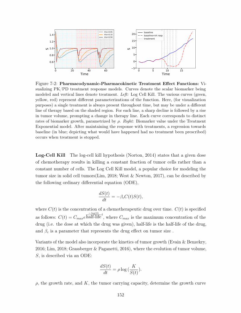
0 20 40 60Time
0.6
0.8
1.0
1.2
1.4
S
rho=0.05rho=0.10rho=0.50
0 5 10 15Time
5
0
5
10
15
20
S
baselinebaseline+trt resptreatment
Figure 7-2: Pharmacodynamic-Pharmacokinetic Treatment Effect Functions: Vi-sualizing PK/PD treatment response models. Curves denote the scalar biomarker beingmodeled and vertical lines denote treatment. Left: Log Cell Kill. The various curves (green,yellow, red) represent different parameterizations of the function. Here, (for visualizationpurposes) a single treatment is always present throughout time, but may be under a differentline of therapy based on the shaded region. For each line, a sharp decline is followed by a risein tumor volume, prompting a change in therapy line. Each curve corresponds to distinctrates of biomarker growth, parametrized by 𝜌. Right: Biomarker value under the TreatmentExponential model. After maintaining the response with treatments, a regression towardsbaseline (in blue; depicting what would have happened had no treatment been prescribed)occurs when treatment is stopped.
Log-Cell Kill The log-cell kill hypothesis (Norton, 2014) states that a given doseof chemotherapy results in killing a constant fraction of tumor cells rather than aconstant number of cells. The Log Cell Kill model, a popular choice for modeling thetumor size in solid cell tumors(Lim, 2018; West & Newton, 2017), can be described bythe following ordinary differential equation (ODE),
𝑑𝑆(𝑡)
𝑑𝑡= −𝛽𝑐𝐶(𝑡)𝑆(𝑡),
where 𝐶(𝑡) is the concentration of a chemotherapeutic drug over time. 𝐶(𝑡) is specified
as follows: 𝐶(𝑡) = 𝐶𝑚𝑎𝑥𝑒− log(2)
half-life 𝑡, where 𝐶𝑚𝑎𝑥 is the maximum concentration of thedrug (i.e. the dose at which the drug was given), half-life is the half-life of the drug,and 𝛽𝑐 is a parameter that represents the drug effect on tumor size .
Variants of the model also incorporate the kinetics of tumor growth (Evain & Benzekry,2016; Lim, 2018; Grassberger & Paganetti, 2016), where the evolution of tumor volume,𝑆, is described via an ODE:
𝑑𝑆(𝑡)
𝑑𝑡= 𝜌 log (
𝐾
𝑆(𝑡)).
𝜌, the growth rate, and 𝐾, the tumor carrying capacity, determine the growth curve
152
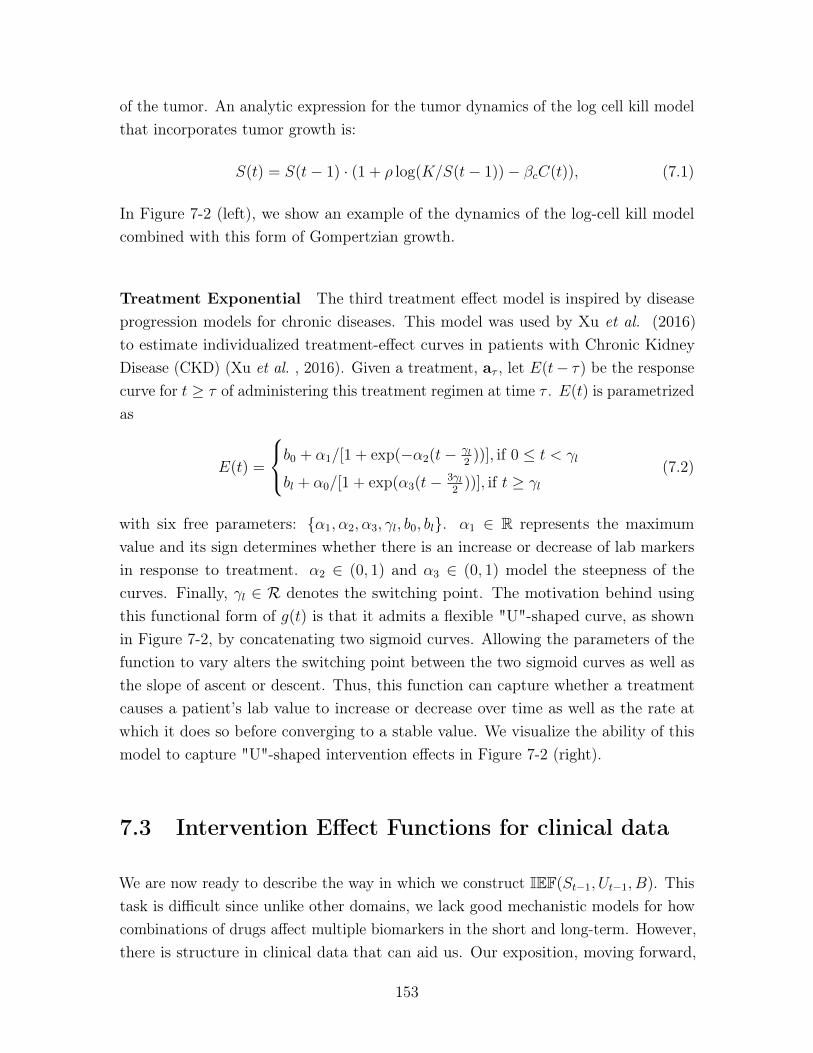
of the tumor. An analytic expression for the tumor dynamics of the log cell kill modelthat incorporates tumor growth is:
𝑆(𝑡) = 𝑆(𝑡− 1) · (1 + 𝜌 log(𝐾/𝑆(𝑡− 1))− 𝛽𝑐𝐶(𝑡)), (7.1)
In Figure 7-2 (left), we show an example of the dynamics of the log-cell kill modelcombined with this form of Gompertzian growth.
Treatment Exponential The third treatment effect model is inspired by diseaseprogression models for chronic diseases. This model was used by Xu et al. (2016)to estimate individualized treatment-effect curves in patients with Chronic KidneyDisease (CKD) (Xu et al. , 2016). Given a treatment, a𝜏 , let 𝐸(𝑡− 𝜏) be the responsecurve for 𝑡 ≥ 𝜏 of administering this treatment regimen at time 𝜏 . 𝐸(𝑡) is parametrizedas
𝐸(𝑡) =
⎧⎨⎩𝑏0 + 𝛼1/[1 + exp(−𝛼2(𝑡− 𝛾𝑙
2))], if 0 ≤ 𝑡 < 𝛾𝑙
𝑏𝑙 + 𝛼0/[1 + exp(𝛼3(𝑡− 3𝛾𝑙2))], if 𝑡 ≥ 𝛾𝑙
(7.2)
with six free parameters: {𝛼1, 𝛼2, 𝛼3, 𝛾𝑙, 𝑏0, 𝑏𝑙}. 𝛼1 ∈ R represents the maximumvalue and its sign determines whether there is an increase or decrease of lab markersin response to treatment. 𝛼2 ∈ (0, 1) and 𝛼3 ∈ (0, 1) model the steepness of thecurves. Finally, 𝛾𝑙 ∈ ℛ denotes the switching point. The motivation behind usingthis functional form of 𝑔(𝑡) is that it admits a flexible "U"-shaped curve, as shownin Figure 7-2, by concatenating two sigmoid curves. Allowing the parameters of thefunction to vary alters the switching point between the two sigmoid curves as well asthe slope of ascent or descent. Thus, this function can capture whether a treatmentcauses a patient’s lab value to increase or decrease over time as well as the rate atwhich it does so before converging to a stable value. We visualize the ability of thismodel to capture "U"-shaped intervention effects in Figure 7-2 (right).
7.3 Intervention Effect Functions for clinical data
We are now ready to describe the way in which we construct IEF(𝑆𝑡−1, 𝑈𝑡−1, 𝐵). Thistask is difficult since unlike other domains, we lack good mechanistic models for howcombinations of drugs affect multiple biomarkers in the short and long-term. However,there is structure in clinical data that can aid us. Our exposition, moving forward,
153
will focus on chronic diseases. First, we recognize that treatments for chronic diseasesare not given in isolation but are often prescribed as parts of contiguous plans oftreatment known as lines of therapy. Second, chronic diseases, despite differences inhow they manifest, may share similarities in mechanisms behind how drugs affect theirprogression. To that end, we posit that functions known to capture the mechanisticeffect of drugs contain knowledge we can transfer to design IEFs for chronic diseaseswhere we lack good mechanistic knowledge. We will refer to IEFs for diseases withknown mechanisms as domain expert modules and propose a neural architecturethat trades off between them. Our architecture does so by using data to guide howimportant a domain expert is in deciding how a representation varies over time. Toour knowledge, both of the above have not been studied in the context of unsupervisedlearning of high-dimensional clinical data. We will use Figure 7-1 (left), which depictsdata from a patient suffering from a chronic disease, as a guide in our discussion.
7.3.1 Capturing lines of therapy with local and global clocks
Many representation learning based approaches (Choi et al. , 2016b; Krishnan et al., 2017; Choi et al. , 2016a; Lipton et al. , 2015) use binary or continuous indicatorsto designate the prescription or dosage of drugs in 𝑈𝑡. However, chronic diseases aretreated with more than one drug (combination therapy) following clinically acceptedguidelines known as lines of therapy. For example, first line therapies often representcombinations prioritized due to their efficacy in clinical trials; subsequent lines maybe decided by clinician experience. Lines of therapy index treatment plans thatspan multiple time-steps and are often laid out by clinicians at first diagnosis. Weincorporate line of therapy as one-hot vectors in 𝑈𝑡[: 𝐾] ∀𝑡 where 𝐾 is the maximalline of therapy. In doing so, we implicitly capture the clinician’s intention whenprescribing drug combinations.
Lines of therapy typically change when drug combinations fail, or due to adverseside effects. In Figure 7-1 (left), the doctor may change the line of therapy once thecombinations of drugs cease to be effective in modulating the behavior of serum IgG.By using line of therapy, an IEF(𝑆𝑡−1, 𝑈𝑡−1, 𝐵) can infer vital information such as howlong a patient has been on a line in the representation 𝑆𝑡. We conjecture, however,that using line of therapy is not enough in a low-data setting. Neural Turing MachinesGraves et al. (2014) can learn to count occurrences of observations in their history,but may fail when data is at a premium. (Che et al. , 2018b) use time since the lastobservation to help RNNs learn well when data is missing. (Koutnik et al. , 2014)
154
partition the hidden states in an RNNs so they are updated at different time-scales.To explicitly enforce our IEFs can capture time since change in line of therapy, we useclocks to track the time elapsed since an event.
We augment our interventional vector, 𝑈𝑡, with two more dimensions. A global clock,𝑔𝑐, captures time elapsed since 𝑇 = 0, i.e. 𝑈𝑡[𝐾] = gc𝑡 = 𝑡. A local clock, 𝑙𝑐, capturestime elapsed since a line of therapy began; i.e. 𝑈𝑡[𝐾 + 1] = lc𝑡 = 𝑡 − 𝑝𝑡 where 𝑝𝑡denotes the index of time when the line last changed. IEF(𝑆𝑡−1, 𝑈𝑡−1, 𝐵) can, byusing the local clock, modulate 𝑆𝑡 to capture patterns such as: the longer a lineof therapy is deployed, the less or (more) effective it may be. For the patient inFigure 7-1 (left), we can see that the first dimension of U denoting line of therapywould be [0, 0, 0, 0, 1, 1, 2, 2, 2]. Line 0 was used four times, line 1 used twice, line2 used thrice. Then 𝑝 = [0, 0, 0, 0, 4, 4, 6, 6, 6, 6], 𝑔𝑐 = [0, 1, 2, 3, 4, 5, 6, 7, 8, 9] and𝑙𝑐 = [0, 1, 2, 3, 0, 1, 0, 1, 2, 3]. Next, we highlight how these clocks are put to use.
7.3.2 Domain expert IEF modules for clinical data
There are a few challenges, though, to the use of PK-PD models in parameterizingIEF(𝑆𝑡−1, 𝑈𝑡−1, 𝐵). First, PK-PD models are often constructed to quantify doseresponse for physiological markers at the micro-scale, such as the evolution of thevolume of a non-small cell lung tumor (Geng et al. , 2017). However, such markersmay not be among the multivariate biomarkers used to characterize disease progressionin clinical practice. We hypothesize that given suitably diverse observations in 𝑋𝑡,one or more of the dimensions of the representation 𝑆𝑡 can implicitly capture thevalue of the unobserved physiological marker. Second, PK-PD models are oftenunivariate, modeling how a single marker changes in response to variation in the drug.Our work designs functions to generalize PK-PD models to work with multivariaterepresentations, 𝑆𝑡−1. The final challenge is knowing which PK-PD models to makeuse of. We describe three new IEFs, each using PK-PD dynamics of a different disease,designed to capture properties we may expect in representations of chronic diseasedata.
Saturated Linear: (Klein, 2009) study the use of linear functions in characterizingdose-responses in solid cancerous tumors. To allow for the representations we use toincrease or decrease as a linear function of the treatments and the line of therapy, we
155
propose the use of a (bounded) linear effect.
𝑔1(𝑆𝑡−1, 𝑈𝑡−1, 𝐵) = LIN(𝑆𝑡−1, 𝑈𝑡−1, 𝐵) = 𝑆𝑡−1 ⊙ tanh(𝑏lin +𝑊lin[𝑈𝑡−1, 𝐵]) (7.3)
where 𝑏lin ∈ R𝑄,𝑊lin ∈ R𝑄×(𝐿+𝐽).
Log-Cell Kill: The log-cell kill model is a classical model of tumor volume in solidcell tumors (Lim, 2018; West & Newton, 2017). It is derived from the log-cell killhypothesis, which states that administering a dose of chemotherapy kills a constantfraction of tumor cells regardless of the size of the tumor. While chronic diseasesmay not have a single observation that characterizes the organ system (akin to tumorvolume), we hypothesize that representations, 𝑆𝑡, of the observed clinical biomarkersmay benefit from mimicking the dynamics exhibited by tumor volume when exposedto chemotherapeutic agents. Therefore, we design the following IEF:
𝑔2(𝑆𝑡−1, 𝑈𝑡−1, 𝐵) = LC(𝑆𝑡−1, 𝑈𝑡−1, 𝐵) = 𝑆𝑡−1 ⊙ (1− 𝜌 log(𝑆2𝑡−1)− 𝛽 exp(−𝛿 · lc𝑡−1)),
(7.4)
where 𝛽 = tanh(𝑊𝑙𝑐𝑈𝑡−1 + 𝑏𝑙𝑐). 𝑊𝑙𝑐 ∈ R𝑄×𝐿, 𝑏𝑙𝑐 ∈ R𝑄, 𝛿 ∈ R𝑄 and 𝜌 ∈ R𝑄 are learned.
Treatment Exponential: (Xu et al. , 2016) propose a Bayesian nonparametericmodel of creatinine, a marker of kidney function, in patients suffering from ChronicKidney Disease. The model can track the dynamics of creatinine due to treatment,but is limited to operating on a single biomarker. We extend their IEF to modelinghigh dimensional representations, 𝑆𝑡, making use of information in the lines of therapyvia the clocks (Section 7.3.1). We refer to this as the Treatment Exponential IEF.
𝑔3(𝑆𝑡−1, 𝑈𝑡−1, 𝐵) = TE(·) =
⎧⎨⎩𝑏0 + 𝛼1,𝑡−1/[1 + exp(−𝛼2,𝑡−1(lc𝑡−1 − 𝛾𝑙
2))], if 0 ≤ lc𝑡−1 < 𝛾𝑙
𝑏𝑙 + 𝛼0,𝑡−1/[1 + exp(𝛼3,𝑡−1(lc𝑡−1 − 3𝛾𝑙2))], if lc𝑡−1 ≥ 𝛾𝑙
(7.5)
The parameters of this model have meaning. 𝛼1,𝑡−1 = 𝑊𝑑[𝑆𝑡−1, 𝑈𝑡−1, 𝐵] + 𝑏𝑑, where𝑊𝑑 ∈ R𝑄×(𝑄+𝐿+𝐽), 𝑏𝑑 ∈ R𝑄 is used to control whether TE is positive or negative.𝛼2,𝑡−1, 𝛼3,𝑡−1, and 𝛾𝑙 control the steepness and duration of the effect. We restrict thesecharacteristics to be similar for drugs administered under the same strategy (or lineof therapy). Thus, we parameterize: [𝛼2, 𝛼3, 𝛾]𝑡−1 = 𝜎(𝑊𝑒 · 𝑈𝑡−1[0] + 𝑏𝑒). If there arethree lines of therapy, 𝑊𝑒 ∈ R3×3, 𝑏𝑒 ∈ R3 and the biases, 𝑏0 ∈ R𝑄 and 𝑏𝑙 ∈ R𝑄, arelearned. Finally, 𝛼0,𝑡−1 = (𝛼1,𝑡−1 + 2𝑏0 − 𝑏𝑙)/(1 + exp(−𝛼3,𝑡−1𝛾/2)) will ensure thatthe effect peaks at 𝑡 = lc𝑡 + 𝛾.
156
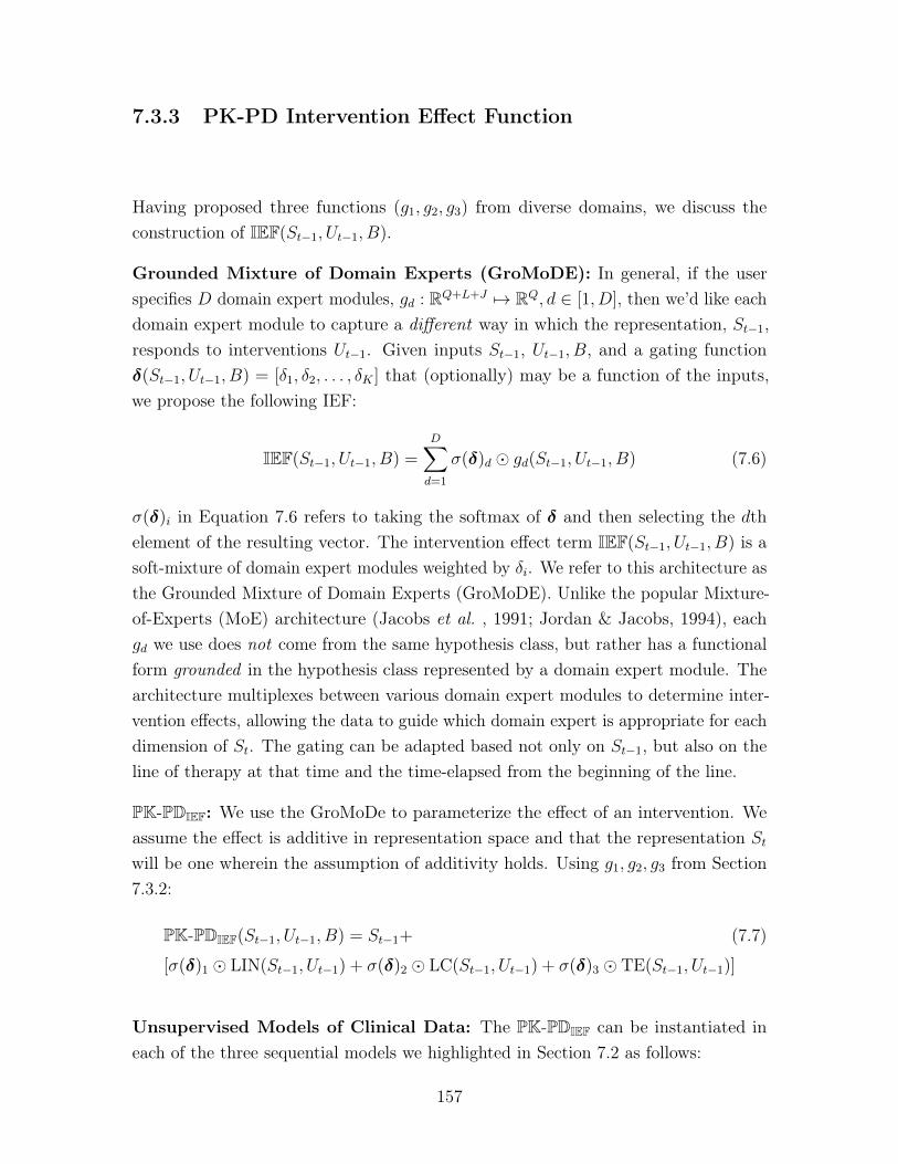
7.3.3 PK-PD Intervention Effect Function
Having proposed three functions (𝑔1, 𝑔2, 𝑔3) from diverse domains, we discuss theconstruction of IEF(𝑆𝑡−1, 𝑈𝑡−1, 𝐵).
Grounded Mixture of Domain Experts (GroMoDE): In general, if the userspecifies 𝐷 domain expert modules, 𝑔𝑑 : R𝑄+𝐿+𝐽 ↦→ R𝑄, 𝑑 ∈ [1, 𝐷], then we’d like eachdomain expert module to capture a different way in which the representation, 𝑆𝑡−1,responds to interventions 𝑈𝑡−1. Given inputs 𝑆𝑡−1, 𝑈𝑡−1, 𝐵, and a gating function𝛿(𝑆𝑡−1, 𝑈𝑡−1, 𝐵) = [𝛿1, 𝛿2, . . . , 𝛿𝐾 ] that (optionally) may be a function of the inputs,we propose the following IEF:
IEF(𝑆𝑡−1, 𝑈𝑡−1, 𝐵) =𝐷∑︁
𝑑=1
𝜎(𝛿)𝑑 ⊙ 𝑔𝑑(𝑆𝑡−1, 𝑈𝑡−1, 𝐵) (7.6)
𝜎(𝛿)𝑖 in Equation 7.6 refers to taking the softmax of 𝛿 and then selecting the 𝑑thelement of the resulting vector. The intervention effect term IEF(𝑆𝑡−1, 𝑈𝑡−1, 𝐵) is asoft-mixture of domain expert modules weighted by 𝛿𝑖. We refer to this architecture asthe Grounded Mixture of Domain Experts (GroMoDE). Unlike the popular Mixture-of-Experts (MoE) architecture (Jacobs et al. , 1991; Jordan & Jacobs, 1994), each𝑔𝑑 we use does not come from the same hypothesis class, but rather has a functionalform grounded in the hypothesis class represented by a domain expert module. Thearchitecture multiplexes between various domain expert modules to determine inter-vention effects, allowing the data to guide which domain expert is appropriate for eachdimension of 𝑆𝑡. The gating can be adapted based not only on 𝑆𝑡−1, but also on theline of therapy at that time and the time-elapsed from the beginning of the line.
PK-PDIEF: We use the GroMoDe to parameterize the effect of an intervention. Weassume the effect is additive in representation space and that the representation 𝑆𝑡
will be one wherein the assumption of additivity holds. Using 𝑔1, 𝑔2, 𝑔3 from Section7.3.2:
PK-PDIEF(𝑆𝑡−1, 𝑈𝑡−1, 𝐵) = 𝑆𝑡−1+ (7.7)
[𝜎(𝛿)1 ⊙ LIN(𝑆𝑡−1, 𝑈𝑡−1) + 𝜎(𝛿)2 ⊙ LC(𝑆𝑡−1, 𝑈𝑡−1) + 𝜎(𝛿)3 ⊙ TE(𝑆𝑡−1, 𝑈𝑡−1)]
Unsupervised Models of Clinical Data: The PK-PDIEF can be instantiated ineach of the three sequential models we highlighted in Section 7.2 as follows:
157
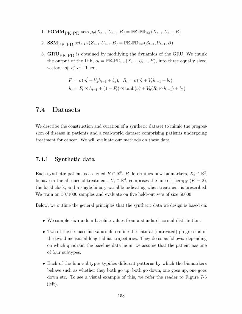
1. FOMMPK-PD sets 𝜇𝜃(𝑋𝑡−1, 𝑈𝑡−1, 𝐵) = PK-PDIEF(𝑋𝑡−1, 𝑈𝑡−1, 𝐵)
2. SSMPK-PD sets 𝜇𝜃(𝑍𝑡−1, 𝑈𝑡−1, 𝐵) = PK-PDIEF(𝑍𝑡−1, 𝑈𝑡−1, 𝐵)
3. GRUPK-PD is obtained by modifying the dynamics of the GRU. We chunkthe output of the IEF, 𝑜𝑡 = PK-PDIEF(𝑋𝑡−1, 𝑈𝑡−1, 𝐵), into three equally sizedvectors: 𝑜𝑓𝑡 , 𝑜𝑟𝑡 , 𝑜ℎ𝑡 . Then,
𝐹𝑡 = 𝜎(𝑜𝑓𝑡 + 𝑉𝑧ℎ𝑡−1 + 𝑏𝑧), 𝑅𝑡 = 𝜎(𝑜𝑟𝑡 + 𝑉𝑟ℎ𝑡−1 + 𝑏𝑟)
ℎ𝑡 = 𝐹𝑡 ⊙ ℎ𝑡−1 + (1− 𝐹𝑡)⊙ tanh(𝑜ℎ𝑡 + 𝑉ℎ(𝑅𝑡 ⊙ ℎ𝑡−1) + 𝑏ℎ)
7.4 Datasets
We describe the construction and curation of a synthetic dataset to mimic the progres-sion of disease in patients and a real-world dataset comprising patients undergoingtreatment for cancer. We will evaluate our methods on these data.
7.4.1 Synthetic data
Each synthetic patient is assigned 𝐵 ∈ R6. 𝐵 determines how biomarkers, 𝑋𝑡 ∈ R2,behave in the absence of treatment. 𝑈𝑡 ∈ R4, comprises the line of therapy (𝐾 = 2),the local clock, and a single binary variable indicating when treatment is prescribed.We train on 50/1000 samples and evaluate on five held-out sets of size 50000.
Below, we outline the general principles that the synthetic data we design is based on:
∙ We sample six random baseline values from a standard normal distribution.
∙ Two of the six baseline values determine the natural (untreated) progression ofthe two-dimensional longitudinal trajectories. They do so as follows: dependingon which quadrant the baseline data lie in, we assume that the patient has oneof four subtypes.
∙ Each of the four subtypes typifies different patterns by which the biomarkersbehave such as whether they both go up, both go down, one goes up, one goesdown etc. To see a visual example of this, we refer the reader to Figure 7-3(left).
158
2 0 23
2
1
0
1
2
3 [S0] (y=3)
[S1] (y=10)
[S2] (y=12)
[S3] (y=5)
Baseline data labelled by [subtype] & (time-to-event)
0 10 20Time
10
0
10
20
Subtype 0
0 10 20Time
10
0
10
20
Subtype 1
0 10 20Time
10
0
10
20
Subtype 2
0 10 20Time
10
0
10
20
Subtype 3
Figure 7-3: Visualization of synthetic data: Left: A visualization of "patient"’s baselinedata (colored and marked by patient subtype). Right four plots: Examples of patient’slongitudinal trajectories along with treatment response. The blue and green longitudinaldata denote two diffrent patient biomarkers. Gray-dotted line represents intervention. Thesubtypes may, optionally, be correlated with patient outcomes as highlighted using the valuesof 𝑦. We do not use the outcomes in this chapter, but do so later in the thesis.
Baseline The generative process for the baseline covariates is 𝐵 ∼ 𝒩 (0; I);𝐵 ∈ R6.
Treatments (Interventions): There is a single drug (denoted by a binary randomvariable) that may be withheld (in the first line of therapy) or prescribed in the secondline of therapy. 𝑑𝑖 ∼ Unif.[0, 18] denotes when the single drug is administered (andthe second line of treatment begins). 𝑑𝑖 is the point at which the local clock resets.We can summarize the generative process for the treatments as follows:
𝑑 ∼ Unif.[0, 18]
line𝑡 = 0 if 𝑡 < 𝑑 and 1 otherwise
𝑙𝑐𝑡[0] = 1 if 𝑡 < 𝑑 and 0 otherwise
𝑙𝑐𝑡[1] = 0 if 𝑡 < 𝑑 and 1 otherwise (7.8)
where 𝑙𝑐𝑡[0], 𝑙𝑐𝑡[1] denote the one-hot encoding for line of therapy. Next we describethe intervention effect function that we use. The functional form of TE(·) is re-statedbelow for convenience,
TE(lc𝑡) =
⎧⎨⎩𝑏0 + 𝛼1/[1 + exp(−𝛼2(lc𝑡 − 𝛾𝑙
2))], if 0 ≤ lc𝑡 < 𝛾𝑙
𝑏𝑙 + 𝛼0/[1 + exp(𝛼3(lc𝑡 − 3𝛾𝑙2))], if lc𝑡 ≥ 𝛾𝑙
(7.9)
The parameters that we use to generate the data are: 𝛼2 = 0.6, 𝛼3 = 0.6, 𝛾𝑙 =
2, 𝑏𝑙 = 3, and 𝛼1 = [10, 5,−5,−10], which we vary based on patient subtype. We set𝛼0 = (𝛼1 + 2𝑏0 − 𝑏𝑙)/(1 + exp(−𝛼3𝛾𝑙)/2) to ensure that the treatment effect peaks at𝑡 = lc𝑡 + 𝛾𝑙 and 𝑏0 = −𝛼1/(1 + exp(𝛼2 · 𝛾𝑙/2)) for attaining TE(0) = 0.
159
Biomarkers: We are now ready to describe the full generative process of the longitu-dinal biomarkers.
Recall: 𝐵1...,6 ∼ 𝒩 (0; 𝐼),
𝑓𝑑(𝑡) = 2− 0.05𝑡− 0.005𝑡2, 𝑓𝑢(𝑡) = −1 + 0.0001𝑡+ 0.005𝑡2,
𝑋1(𝑡);𝑋2(𝑡) = (7.10)⎧⎪⎪⎪⎪⎪⎪⎪⎪⎪⎪⎪⎪⎪⎪⎪⎪⎪⎨⎪⎪⎪⎪⎪⎪⎪⎪⎪⎪⎪⎪⎪⎪⎪⎪⎪⎩
𝑓𝑑(𝑡) + TE(lc𝑡) +𝒩 (0, 0.25); 𝑓𝑑(𝑡) + TE(lc𝑡)
+𝒩 (0, 0.25), 𝐵1 ≥ 0, 𝐵2 ≥ 0 if subtype 1
𝑓𝑑(𝑡) + TE(lc𝑡) +𝒩 (0, 0.25); 𝑓𝑢(𝑡) + TE(lc𝑡)
+𝒩 (0, 0.25), 𝐵1 ≥ 0, 𝐵2 < 0 if subtype 2
𝑓𝑢(𝑡) + TE(lc𝑡) +𝒩 (0, 0.25); 𝑓𝑑(𝑡) + TE(lc𝑡)
+𝒩 (0, 0.25), 𝐵1 < 0, 𝐵2 ≥ 0 if subtype 3
𝑓𝑢(𝑡) + TE(lc𝑡) +𝒩 (0, 0.25); 𝑓𝑢(𝑡) + TE(lc𝑡)
+𝒩 (0, 0.25), 𝐵1 < 0, 𝐵2 < 0 if subtype 4,
Intuitively, the above generative process captures the idea that without any effect oftreatment, the biomarkers follow the patterns implied by the subtype (encoded in thefirst two dimensions of the baseline data). However the effect of interventions is feltmore prominently after the 𝑑, the random variable denoting time at which treatmentwas prescribed.
7.4.2 Multiple Myleoma - ML-MMRF
Multiple myeloma is a rare and incurable plasma cell cancer with nearly 30, 000 newcases every year in the United States. The Multiple Myeloma Research Foundation(MMRF) CoMMpass study releases de-identified clinical data for 1143 patients sufferingfrom multiple myeloma, an incurable plasma cell cancer. We will release code thatpre-processes features from the CoMMpass study files to construct ML-MMRF, apublicly available dataset with clinical and interventional data alongside rich geneticprofiles of patients.
Inclusion Criteria: All patients are aligned to the start of treatment, which ismade according to current standard of care (not random assignment). To enroll in
160
the CoMMpass study, patients must be newly diagnosed with symptomatic multiplemyeloma, which coincides with the start of treatment. Patients must be eligible fortreatment with an immunomodulator or a proteasome inhibitor, two of the mostcommon first line drugs, and they must begin treatment within 30 days of the baselinebone marrow evaluation (Multiple Myeloma Research Foundation & others, 2011).
Features
Genomic Data: RNA-sequencing of CD38+ bone marrow cells was available for769 patients. Samples were collected at initiation into the study, pre-treatment. Forthese patients, we used the Seurat package version 2.3.4 Butler et al. (2018) in R toidentify variable genes, and we then limit downstream analyses to these genes. Weuse principal component analysis (PCA) to further reduce the dimensionality of thedata, and the projection of each patient’s gene expression on to the first 40 principalcomponents serves as the genetic features used in our model.
Baseline Data 𝐵: Baseline data includes genetic PCA scores, lab values at thepatient’s first visit, gender, age, and the revised ISS stage. The baseline data alsoincludes binary variables detailing the patient’s myeloma subtype, including whetheror not they have heavy chain myeloma, are IgG type, IgA type, IgM type, kappa type,or lambda type. Additionally, the following labs are measured at baseline, as wellas longitudinally at subsequent visits: absolute neutrophil count (x109/l), albumin(g/l), blood urea nitrogen (mmol/l), calcium (mmol/l), serum creatinine (umol/l),glucose (mmol/l), hemoglobin (mmol/l), serum kappa (mg/dl), serum m protein (g/dl),platelet count x109/l, total protein (g/dl), white blood count x109/l, serum iga (g/l),serum igg (g/l), serum igm (g/l), serum lambda (mg/dl).
Longitudinal Data 𝑋: Longitudinal data is measured approximately every 2 monthsand includes lab values and treatment information. The biomarkers are real-valuednumbers whose values evolve over time. They include: absolute neutrophil count(x109/l), albumin (g/l), blood urea nitrogen (mmol/l), calcium (mmol/l), serumcreatinine (umol/l), glucose (mmol/l), hemoglobin (mmol/l), serum kappa (mg/dl),serum m protein (g/dl), platelet count x109/l, total protein (g/dl), white blood countx109/l, serum iga (g/l), serum igg (g/l), serum igm (g/l), serum lambda (mg/dl).
Treatment information 𝑈 : This includes the line of therapy (we group all linesbeyond line 3 as line 3+) the patient is on at a given point in time, and the local clockdenoting the time elapsed since the last line of therapy. We also include the following
161
treatments as (binary, indicating prescription) features in our model: lenalidomide,dexamethasone, cyclophosphamide, carfilzomib, bortezomib. The aforementioned arethe top five drugs by frequency in the MMRF dataset.
Data processing
Longitudinal biomarkers X: Labs are first clipped to five times the median valueto correct for outliers or data errors in the registry. They are then normalized totheir healthy ranges (obtained via a literature search) as (unnormalized labs - healthyminimum value) / (healthy maximum value - healthy minimum value), and thenmultiplied by a scaling factor of lab-dependent scaling factor to ensure that mostvalues lie within the range [−8, 8]. This dataset has significant missingness, with∼ 66% of the longitudinal markers missing. In addition, there is right censorship inthe dataset, with around 25% of patients getting censored over time. Missing valuesare represented as zeros but a separate mask tensor where 1 denotes observed and 0
denotes missing is used to marginalize out missing variables during learning.
Baseline 𝐵: The biomarkers in the baseline are clipped to five times their medianvalues. Patients without gene expression data (in the PCA features) are assignedthe average normalized PCA score of their 5 nearest neighbors, using the Minkowskidistance metric calculated on FISH features, ISS stage, and age.
Our results are obtained using 5-fold cross evaluation (60/20/20 split) with cohortsbalanced on age and overall survival time. As a representative example, one fold has439 train, 211 validation, and 301 test examples. The median length in each of thesesets is 11-12 time steps. There is missingness in the biomarkers, with 66% of theobservations missing.
7.5 Evaluation
We answer the following questions: What benefits does PK-PDIEF confer upon unsu-pervised models of clinical data? Which model families benefit the most? How doesthe GroMoDE architecture aid with introspection into the model’s functionality? Westudy these questions on two datasets in the low-data regime (∼ 100-1000 samples),where little prior work exists. The data faithfully represent the multi-modal natureby which chronic disease progression is tracked in the clinic.
162
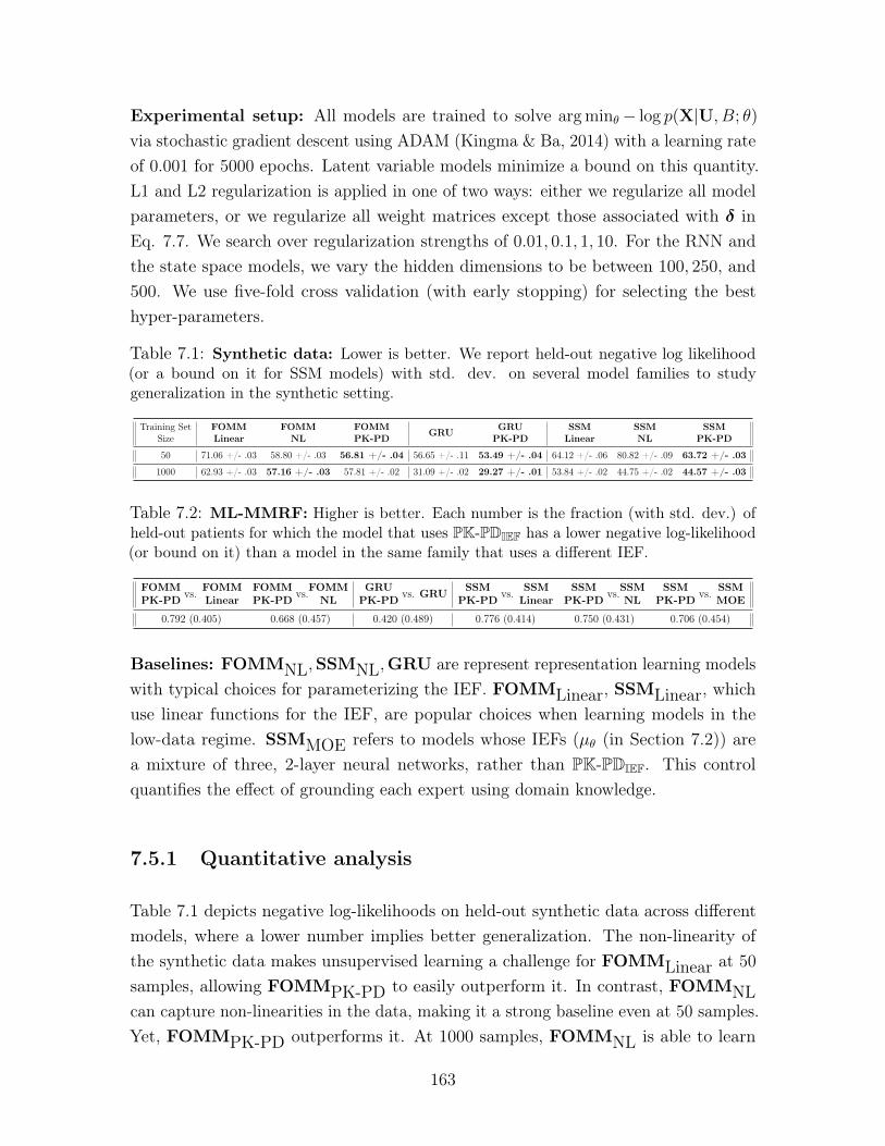
Experimental setup: All models are trained to solve argmin𝜃− log 𝑝(X|U, 𝐵; 𝜃)via stochastic gradient descent using ADAM (Kingma & Ba, 2014) with a learning rateof 0.001 for 5000 epochs. Latent variable models minimize a bound on this quantity.L1 and L2 regularization is applied in one of two ways: either we regularize all modelparameters, or we regularize all weight matrices except those associated with 𝛿 inEq. 7.7. We search over regularization strengths of 0.01, 0.1, 1, 10. For the RNN andthe state space models, we vary the hidden dimensions to be between 100, 250, and500. We use five-fold cross validation (with early stopping) for selecting the besthyper-parameters.
Table 7.1: Synthetic data: Lower is better. We report held-out negative log likelihood(or a bound on it for SSM models) with std. dev. on several model families to studygeneralization in the synthetic setting.
Training SetSize
FOMMLinear
FOMMNL
FOMMPK-PD GRU GRU
PK-PDSSM
LinearSSMNL
SSMPK-PD
50 71.06 +/- .03 58.80 +/- .03 56.81 +/- .04 56.65 +/- .11 53.49 +/- .04 64.12 +/- .06 80.82 +/- .09 63.72 +/- .03
1000 62.93 +/- .03 57.16 +/- .03 57.81 +/- .02 31.09 +/- .02 29.27 +/- .01 53.84 +/- .02 44.75 +/- .02 44.57 +/- .03
Table 7.2: ML-MMRF: Higher is better. Each number is the fraction (with std. dev.) ofheld-out patients for which the model that uses PK-PDIEF has a lower negative log-likelihood(or bound on it) than a model in the same family that uses a different IEF.
FOMMPK-PD vs. FOMM
LinearFOMMPK-PD vs.FOMM
NLGRU
PK-PD vs. GRU SSMPK-PD vs. SSM
LinearSSM
PK-PD vs.SSMNL
SSMPK-PD vs. SSM
MOE
0.792 (0.405) 0.668 (0.457) 0.420 (0.489) 0.776 (0.414) 0.750 (0.431) 0.706 (0.454)
Baselines: FOMMNL,SSMNL,GRU are represent representation learning modelswith typical choices for parameterizing the IEF. FOMMLinear, SSMLinear, whichuse linear functions for the IEF, are popular choices when learning models in thelow-data regime. SSMMOE refers to models whose IEFs (𝜇𝜃 (in Section 7.2)) area mixture of three, 2-layer neural networks, rather than PK-PDIEF. This controlquantifies the effect of grounding each expert using domain knowledge.
7.5.1 Quantitative analysis
Table 7.1 depicts negative log-likelihoods on held-out synthetic data across differentmodels, where a lower number implies better generalization. The non-linearity ofthe synthetic data makes unsupervised learning a challenge for FOMMLinear at 50samples, allowing FOMMPK-PD to easily outperform it. In contrast, FOMMNLcan capture non-linearities in the data, making it a strong baseline even at 50 samples.Yet, FOMMPK-PD outperforms it. At 1000 samples, FOMMNL is able to learn
163
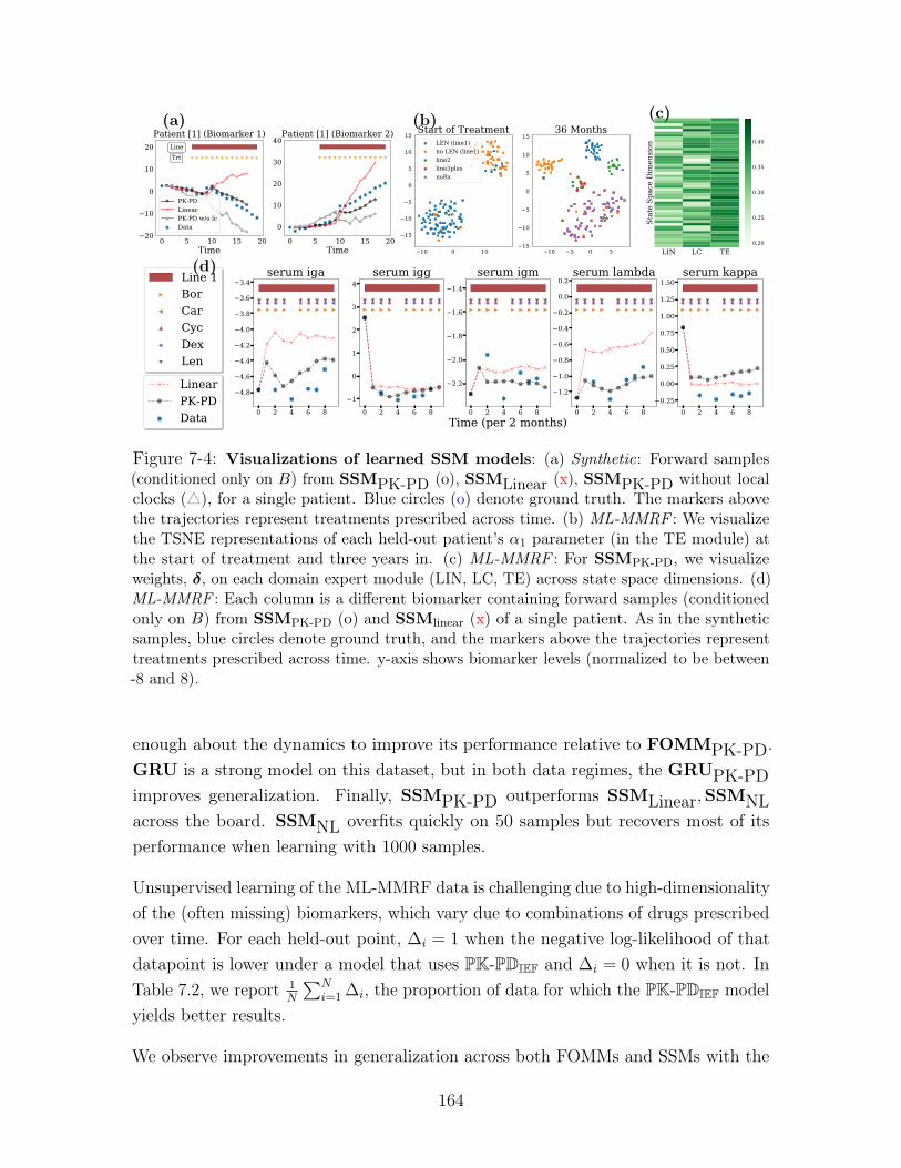
0 5 10 15 20Time
20
10
0
10
20 LineTrt
Patient [1] (Biomarker 1)
PK-PDLinearPK-PD w/o lcData
0 5 10 15 20Time
0
10
20
30
40Patient [1] (Biomarker 2)
(a)
10 0 10
15
10
5
0
5
10
15Start of Treatment
10 5 0 515
10
5
0
5
10
1536 Months
LEN (line1)no LEN (line1)line2line3plusnoRx
(b)
LIN LC TE
Stat
e Sp
ace
Dim
ensi
on
0.20
0.25
0.30
0.35
0.40
(c)
(d)
Figure 7-4: Visualizations of learned SSM models: (a) Synthetic: Forward samples(conditioned only on 𝐵) from SSMPK-PD (o), SSMLinear (x), SSMPK-PD without localclocks (△), for a single patient. Blue circles (o) denote ground truth. The markers abovethe trajectories represent treatments prescribed across time. (b) ML-MMRF : We visualizethe TSNE representations of each held-out patient’s 𝛼1 parameter (in the TE module) atthe start of treatment and three years in. (c) ML-MMRF : For SSMPK-PD, we visualizeweights, 𝛿, on each domain expert module (LIN, LC, TE) across state space dimensions. (d)ML-MMRF : Each column is a different biomarker containing forward samples (conditionedonly on 𝐵) from SSMPK-PD (o) and SSMlinear (x) of a single patient. As in the syntheticsamples, blue circles denote ground truth, and the markers above the trajectories representtreatments prescribed across time. y-axis shows biomarker levels (normalized to be between-8 and 8).
enough about the dynamics to improve its performance relative to FOMMPK-PD.GRU is a strong model on this dataset, but in both data regimes, the GRUPK-PDimproves generalization. Finally, SSMPK-PD outperforms SSMLinear,SSMNLacross the board. SSMNL overfits quickly on 50 samples but recovers most of itsperformance when learning with 1000 samples.
Unsupervised learning of the ML-MMRF data is challenging due to high-dimensionalityof the (often missing) biomarkers, which vary due to combinations of drugs prescribedover time. For each held-out point, Δ𝑖 = 1 when the negative log-likelihood of thatdatapoint is lower under a model that uses PK-PDIEF and Δ𝑖 = 0 when it is not. InTable 7.2, we report 1
𝑁
∑︀𝑁𝑖=1 Δ𝑖, the proportion of data for which the PK-PDIEF model
yields better results.
We observe improvements in generalization across both FOMMs and SSMs with the
164
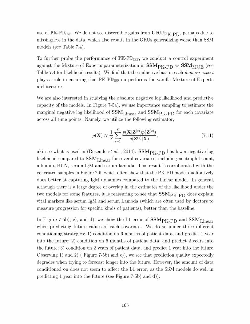
use of PK-PDIEF. We do not see discernible gains from GRUPK-PD, perhaps due tomissingness in the data, which also results in the GRUs generalizing worse than SSMmodels (see Table 7.4).
To further probe the performance of PK-PDIEF, we conduct a control experimentagainst the Mixture of Experts parameterization in SSMPK-PD vs SSMMOE (seeTable 7.4 for likelihood results). We find that the inductive bias in each domain expertplays a role in ensuring that PK-PDIEF outperforms the vanilla Mixture of Expertsarchitecture.
We are also interested in studying the absolute negative log likelihood and predictivecapacity of the models. In Figure 7-5a), we use importance sampling to estimate themarginal negative log likelihood of SSMLinear and SSMPK-PD for each covariateacross all time points. Namely, we utilize the following estimator,
𝑝(X) ≈ 1
𝑆
𝑆∑︁
𝑠=1
𝑝(X|Z(𝑠))𝑝(Z(𝑠))
𝑞(Z(𝑠)|X), (7.11)
akin to what is used in (Rezende et al. , 2014). SSMPK-PD has lower negative loglikelihood compared to SSMLinear for several covariates, including neutrophil count,albumin, BUN, serum IgM and serum lambda. This result is corroborated with thegenerated samples in Figure 7-6, which often show that the PK-PD model qualitativelydoes better at capturing IgM dynamics compared to the Linear model. In general,although there is a large degree of overlap in the estimates of the likelihood under thetwo models for some features, it is reassuring to see that SSMPK-PD does explainvital markers like serum IgM and serum Lambda (which are often used by doctors tomeasure progression for specific kinds of patients), better than the baseline.
In Figure 7-5b), c), and d), we show the L1 error of SSMPK-PD and SSMLinearwhen predicting future values of each covariate. We do so under three differentconditioning strategies: 1) condition on 6 months of patient data, and predict 1 yearinto the future; 2) condition on 6 months of patient data, and predict 2 years intothe future; 3) condition on 2 years of patient data, and predict 1 year into the future.Observing 1) and 2) ( Figure 7-5b) and c)), we see that prediction quality expectedlydegrades when trying to forecast longer into the future. However, the amount of dataconditioned on does not seem to affect the L1 error, as the SSM models do well inpredicting 1 year into the future (see Figure 7-5b) and d)).
165
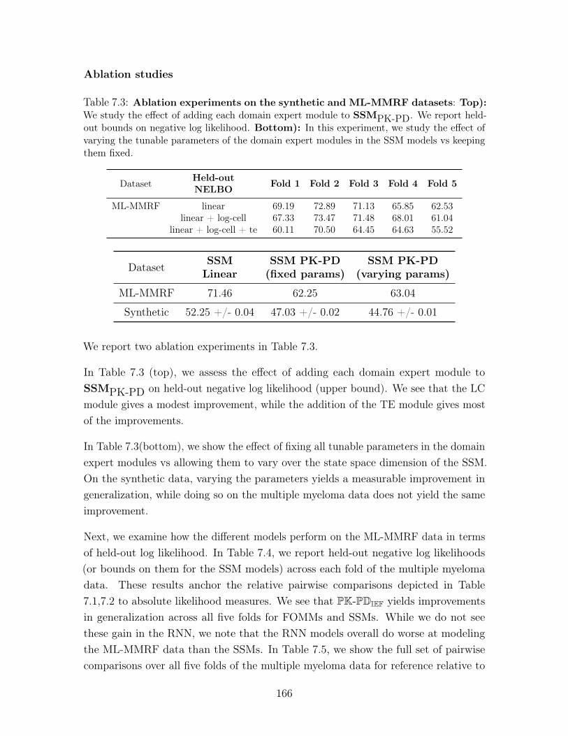
Ablation studies
Table 7.3: Ablation experiments on the synthetic and ML-MMRF datasets: Top):We study the effect of adding each domain expert module to SSMPK-PD. We report held-out bounds on negative log likelihood. Bottom): In this experiment, we study the effect ofvarying the tunable parameters of the domain expert modules in the SSM models vs keepingthem fixed.
Dataset Held-outNELBO Fold 1 Fold 2 Fold 3 Fold 4 Fold 5
ML-MMRF linear 69.19 72.89 71.13 65.85 62.53linear + log-cell 67.33 73.47 71.48 68.01 61.04
linear + log-cell + te 60.11 70.50 64.45 64.63 55.52
Dataset SSMLinear
SSM PK-PD(fixed params)
SSM PK-PD(varying params)
ML-MMRF 71.46 62.25 63.04
Synthetic 52.25 +/- 0.04 47.03 +/- 0.02 44.76 +/- 0.01
We report two ablation experiments in Table 7.3.
In Table 7.3 (top), we assess the effect of adding each domain expert module toSSMPK-PD on held-out negative log likelihood (upper bound). We see that the LCmodule gives a modest improvement, while the addition of the TE module gives mostof the improvements.
In Table 7.3(bottom), we show the effect of fixing all tunable parameters in the domainexpert modules vs allowing them to vary over the state space dimension of the SSM.On the synthetic data, varying the parameters yields a measurable improvement ingeneralization, while doing so on the multiple myeloma data does not yield the sameimprovement.
Next, we examine how the different models perform on the ML-MMRF data in termsof held-out log likelihood. In Table 7.4, we report held-out negative log likelihoods(or bounds on them for the SSM models) across each fold of the multiple myelomadata. These results anchor the relative pairwise comparisons depicted in Table7.1,7.2 to absolute likelihood measures. We see that PK-PDIEF yields improvementsin generalization across all five folds for FOMMs and SSMs. While we do not seethese gain in the RNN, we note that the RNN models overall do worse at modelingthe ML-MMRF data than the SSMs. In Table 7.5, we show the full set of pairwisecomparisons over all five folds of the multiple myeloma data for reference relative to
166
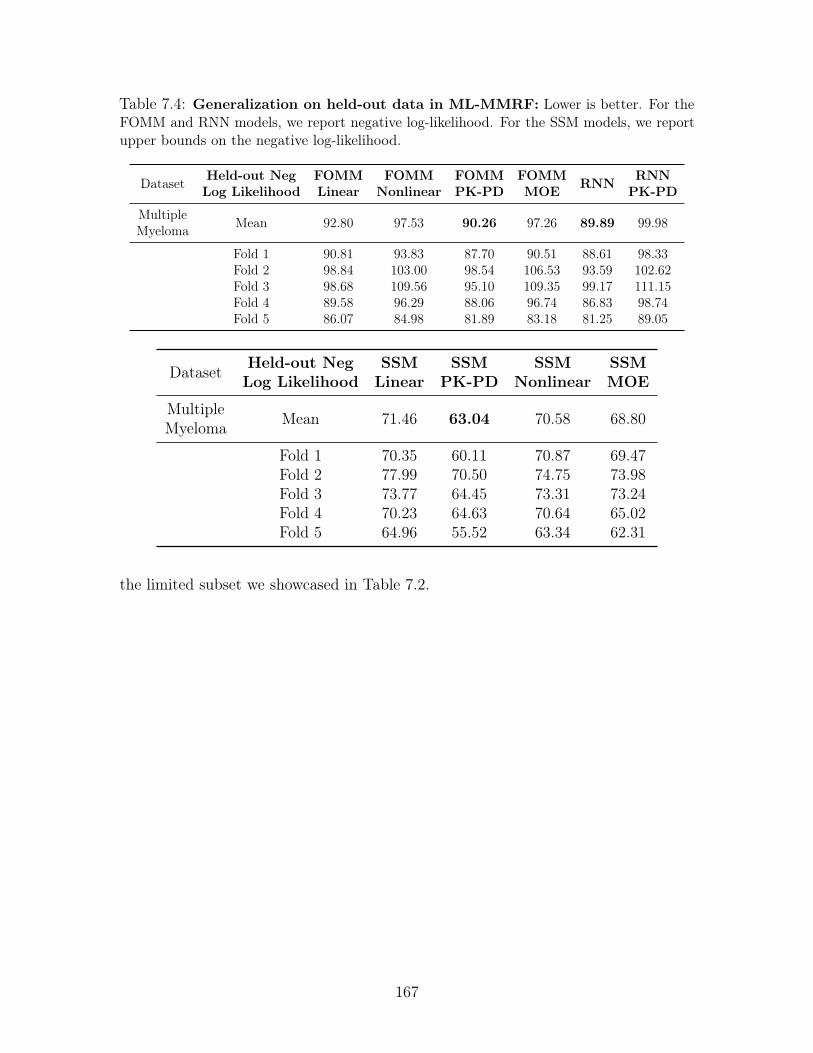
Table 7.4: Generalization on held-out data in ML-MMRF: Lower is better. For theFOMM and RNN models, we report negative log-likelihood. For the SSM models, we reportupper bounds on the negative log-likelihood.
Dataset Held-out NegLog Likelihood
FOMMLinear
FOMMNonlinear
FOMMPK-PD
FOMMMOE RNN RNN
PK-PD
MultipleMyeloma Mean 92.80 97.53 90.26 97.26 89.89 99.98
Fold 1 90.81 93.83 87.70 90.51 88.61 98.33Fold 2 98.84 103.00 98.54 106.53 93.59 102.62Fold 3 98.68 109.56 95.10 109.35 99.17 111.15Fold 4 89.58 96.29 88.06 96.74 86.83 98.74Fold 5 86.07 84.98 81.89 83.18 81.25 89.05
Dataset Held-out NegLog Likelihood
SSMLinear
SSMPK-PD
SSMNonlinear
SSMMOE
MultipleMyeloma Mean 71.46 63.04 70.58 68.80
Fold 1 70.35 60.11 70.87 69.47Fold 2 77.99 70.50 74.75 73.98Fold 3 73.77 64.45 73.31 73.24Fold 4 70.23 64.63 70.64 65.02Fold 5 64.96 55.52 63.34 62.31
the limited subset we showcased in Table 7.2.
167
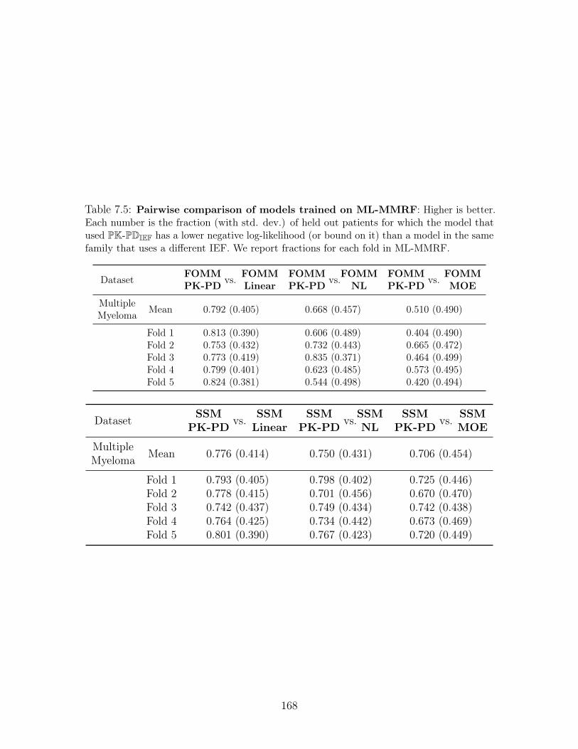
Table 7.5: Pairwise comparison of models trained on ML-MMRF: Higher is better.Each number is the fraction (with std. dev.) of held out patients for which the model thatused PK-PDIEF has a lower negative log-likelihood (or bound on it) than a model in the samefamily that uses a different IEF. We report fractions for each fold in ML-MMRF.
Dataset FOMMPK-PD vs. FOMM
LinearFOMMPK-PD vs.FOMM
NLFOMMPK-PD vs. FOMM
MOE
MultipleMyeloma Mean 0.792 (0.405) 0.668 (0.457) 0.510 (0.490)
Fold 1 0.813 (0.390) 0.606 (0.489) 0.404 (0.490)Fold 2 0.753 (0.432) 0.732 (0.443) 0.665 (0.472)Fold 3 0.773 (0.419) 0.835 (0.371) 0.464 (0.499)Fold 4 0.799 (0.401) 0.623 (0.485) 0.573 (0.495)Fold 5 0.824 (0.381) 0.544 (0.498) 0.420 (0.494)
Dataset SSMPK-PD vs. SSM
LinearSSM
PK-PD vs.SSMNL
SSMPK-PD vs. SSM
MOE
MultipleMyeloma Mean 0.776 (0.414) 0.750 (0.431) 0.706 (0.454)
Fold 1 0.793 (0.405) 0.798 (0.402) 0.725 (0.446)Fold 2 0.778 (0.415) 0.701 (0.456) 0.670 (0.470)Fold 3 0.742 (0.437) 0.749 (0.434) 0.742 (0.438)Fold 4 0.764 (0.425) 0.734 (0.442) 0.673 (0.469)Fold 5 0.801 (0.390) 0.767 (0.423) 0.720 (0.449)
168
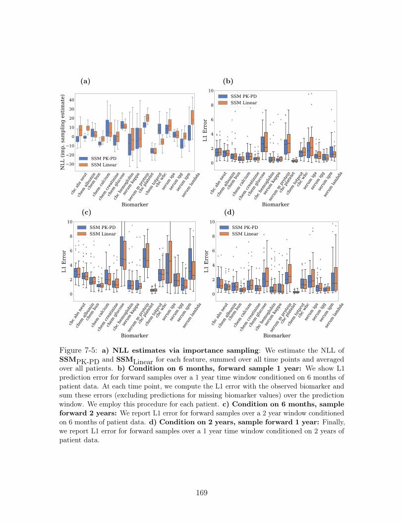
cbc a
bs n
eut
chem
alb
umin
chem
bun
chem
calci
um
chem
crea
tinin
e
chem
glu
cose
cbc h
emog
lobi
n
seru
m k
appa
seru
m m
pro
tein
cbc p
late
let
chem
totp
rot
cbc w
bcse
rum
iga
seru
m ig
gse
rum
igm
seru
m la
mbd
a
Biomarker
30
20
10
0
10
20
30
40
NLL
(im
p. s
ampl
ing
estim
ate)
SSM PK-PDSSM Linear
(a)
cbc a
bs n
eut
chem
alb
umin
chem
bun
chem
calci
um
chem
crea
tinin
e
chem
glu
cose
cbc h
emog
lobi
n
seru
m k
appa
seru
m m
pro
tein
cbc p
late
let
chem
totp
rot
cbc w
bcse
rum
iga
seru
m ig
gse
rum
igm
seru
m la
mbd
a
Biomarker
0
2
4
6
8
10
L1 E
rror
SSM PK-PDSSM Linear
(b)
cbc a
bs n
eut
chem
alb
umin
chem
bun
chem
calci
um
chem
crea
tinin
e
chem
glu
cose
cbc h
emog
lobi
n
seru
m k
appa
seru
m m
pro
tein
cbc p
late
let
chem
totp
rot
cbc w
bcse
rum
iga
seru
m ig
gse
rum
igm
seru
m la
mbd
a
Biomarker
0
2
4
6
8
10
L1 E
rror
SSM PK-PDSSM Linear
(c)cb
c abs
neu
tch
em a
lbum
inch
em b
unch
em ca
lcium
chem
crea
tinin
e
chem
glu
cose
cbc h
emog
lobi
n
seru
m k
appa
seru
m m
pro
tein
cbc p
late
let
chem
totp
rot
cbc w
bcse
rum
iga
seru
m ig
gse
rum
igm
seru
m la
mbd
aBiomarker
0
2
4
6
8
10
L1 E
rror
SSM PK-PDSSM Linear
(d)
Figure 7-5: a) NLL estimates via importance sampling: We estimate the NLL ofSSMPK-PD and SSMLinear for each feature, summed over all time points and averagedover all patients. b) Condition on 6 months, forward sample 1 year: We show L1prediction error for forward samples over a 1 year time window conditioned on 6 months ofpatient data. At each time point, we compute the L1 error with the observed biomarker andsum these errors (excluding predictions for missing biomarker values) over the predictionwindow. We employ this procedure for each patient. c) Condition on 6 months, sampleforward 2 years: We report L1 error for forward samples over a 2 year window conditionedon 6 months of patient data. d) Condition on 2 years, sample forward 1 year: Finally,we report L1 error for forward samples over a 1 year time window conditioned on 2 years ofpatient data.
169
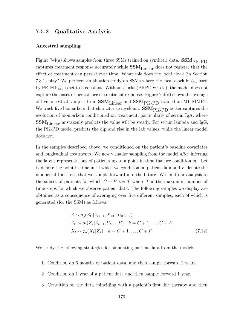
7.5.2 Qualitative Analysis
Ancestral sampling
Figure 7-4(a) shows samples from three SSMs trained on synthetic data. SSMPK-PDcaptures treatment response accurately while SSMLinear does not register that theeffect of treatment can persist over time. What role does the local clock (in Section7.3.1) play? We perform an ablation study on SSMs where the local clock in 𝑈𝑡, usedby PK-PDIEF, is set to a constant. Without clocks (PKPD w/o lc), the model does notcapture the onset or persistence of treatment response. Figure 7-4(d) shows the averageof five ancestral samples from SSMLinear and SSMPK-PD trained on ML-MMRF.We track five biomarkers that characterize myeloma. SSMPK-PD better captures theevolution of biomarkers conditioned on treatment, particularly of serum IgA, whereSSMLinear mistakenly predicts the value will be steady. For serum lambda and IgG,the PK-PD model predicts the dip and rise in the lab values, while the linear modeldoes not.
In the samples described above, we conditioned on the patient’s baseline covariatesand longitudinal treatments. We now visualize sampling from the model after inferringthe latent representations of patients up to a point in time that we condition on. Let𝐶 denote the point in time until which we condition on patient data and 𝐹 denote thenumber of timesteps that we sample forward into the future. We limit our analysis tothe subset of patients for which 𝐶 + 𝐹 <= 𝑇 where 𝑇 is the maximum number oftime steps for which we observe patient data. The following samples we display areobtained as a consequence of averaging over five different samples, each of which isgenerated (for the SSM) as follows:
𝑍 ∼ 𝑞𝜑(𝑍𝐶 |𝑍𝐶−1, 𝑋1:𝐶 , 𝑈0:𝐶−1)
𝑍𝑘 ∼ 𝑝𝜃(𝑍𝑘|𝑍𝑘−1, 𝑈𝑘−1, 𝐵) 𝑘 = 𝐶 + 1, . . . , 𝐶 + 𝐹
𝑋𝑘 ∼ 𝑝𝜃(𝑋𝑘|𝑍𝑘) 𝑘 = 𝐶 + 1, . . . , 𝐶 + 𝐹 (7.12)
We study the following strategies for simulating patient data from the models.
1. Condition on 6 months of patient data, and then sample forward 2 years,
2. Condition on 1 year of a patient data and then sample forward 1 year,
3. Condition on the data coinciding with a patient’s first line therapy and then
170
forward sample until the end of their third line therapy.
In Figure 7-6, we show additional samples from SSMPK-PD when conditioning ondiffering amounts of data. Overall, in all three cases, SSMPK-PD models treatmentresponse better than a linear baseline. For 1. (Figure 7-6a)), we see that SSMPK-PDcorrectly captures that the serum IgA value remains steady while SSMLinear predictsan upward trend. For 2. (Figure 7-6b)), SSMPK-PD does well in modeling down-trends, as in serum IgA and serum IgM. For 3. (Figure 7-6c)), we similarly see thatSSMPK-PD captures the down-trending serum IgA and serum IgM during the secondline therapy.
Interpreting what the model has learned about multiple myeloma
Do the models learn known clinical relationships between interventions and observa-tions? On SSMPK-PD, we analyze this via the sensitivity function ∇𝑈𝑡−1E𝑍𝑡(𝑋𝑡|𝑍𝑡).This presents another use case wherein gradients of a deep generative model maybe used for In Figure 7-7a) and b) show how changes in two combination therapies,Lenalidomide, Bortezomib, Dexamethasone (RVD) and Bortezomib, Dexamethasone(VD) respectively are associated with changes in clinical lab markers. (a) RVD isassociated with a decrease in hemoglobin and platelet values, two known side effectsof the treatment (Kumar et al. , 2012). (b) We observe a diminished effect of VDon hemoglobin, platelets and creatinine. Indeed, VD is given in favor of RVD whentrying to avoid side effects (Jacobus et al. , 2016).
Figure 7-4(c) visualizes the gates 𝜎(𝛿) from SSMPK-PD trained on ML-MMRF.The highest weighted component is the treatment exponential model followed by thelog-cell kill model for many of the latent state dimensions. This result tells us (a) thatno single domain expert is responsible for the dynamics of all the latent dimensionsand (b) the treatment exponential IEF appears to have the largest weights acrossseveral dimensions.
Knowing that 𝛼1𝑡 in the treatment exponential IEF drives much of the variation inrepresentation, we perform TSNE (Maaten & Hinton, 2008) on each held-out patient’shigh-dimensional 𝛼1𝑡 at two time points in Figure 7-4(b). This analysis shows howvariation in 𝛼1𝑡, and consequently the dimensions of the latent representation, aredriven by treatment. Early on, the representations segregate by lenalidomine (afirst-line therapy), whereas for patients who make it through three years of treatment,
171
the line of therapy drives the representation. The PK-PDIEF thus admits a hierarchicaldecomposition of information that aids in interpreting the model’s dynamics.
In Figure 7-8, we perform TSNE (Maaten & Hinton, 2008) on each held-out patient’shigh-dimensional 𝛼1𝑡 vector (obtained from SSMPK-PD trained on ML-MMRF) atmultiple time points, expanding on the two time points that were shown in Figure7-4. Overall, we gain a richer understanding of how the variation in 𝛼1𝑡 is driven bytreatment. As we saw before, the representations segregate by presence of lenalidomidein initial therapy. Later, they segregate by line of therapy; finally, most patients aretaken off treatment.
In Figure 7-7c), we show the how treatments in 𝑈𝑡 play a role in 𝛼1𝑡 by visualizingthe weights of the linear model that maps from treatment signal to 𝛼1. This resultshowcases how this parameter varies as a function of treatment.
An important point to note in these plots is that as 𝑇 increases, the number of patientsdecreases due to right censoring in the ML-MMRF dataset.
172
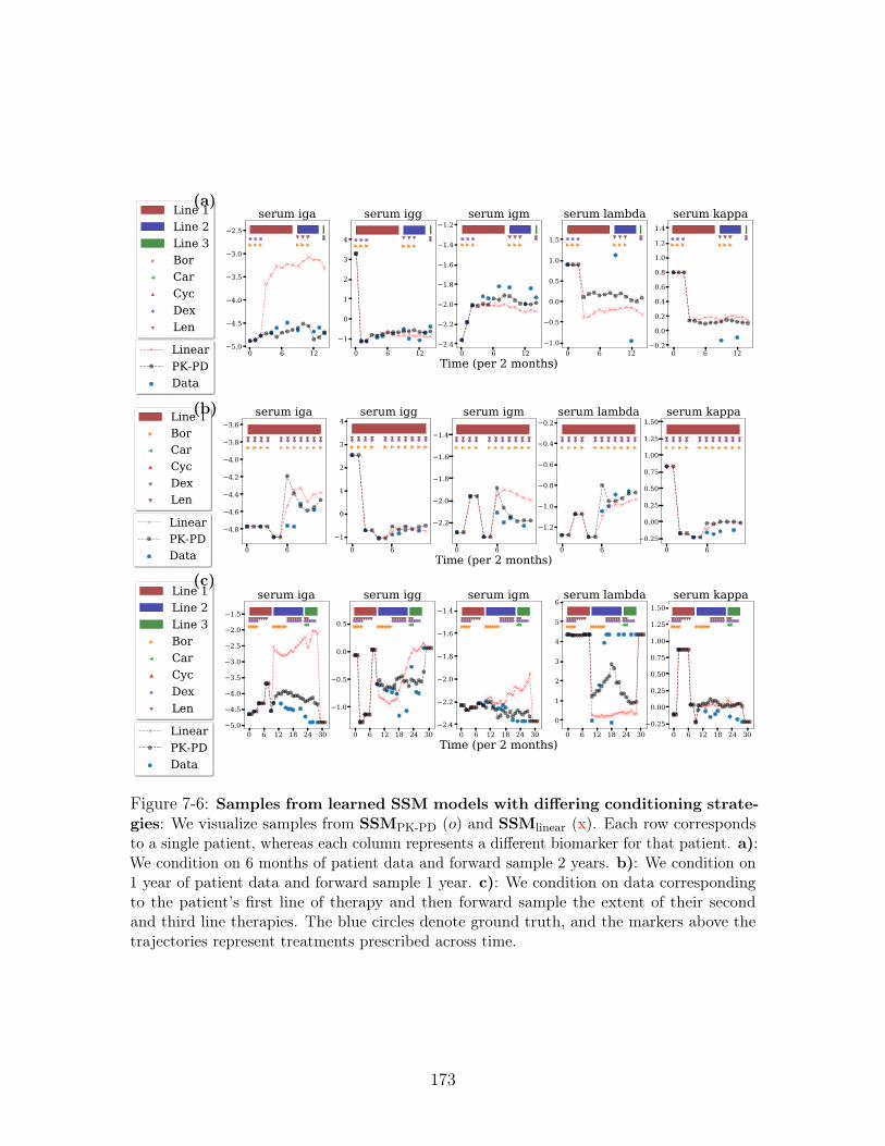
(a)
(b)
(c)
Figure 7-6: Samples from learned SSM models with differing conditioning strate-gies: We visualize samples from SSMPK-PD (𝑜) and SSMlinear (x). Each row correspondsto a single patient, whereas each column represents a different biomarker for that patient. a):We condition on 6 months of patient data and forward sample 2 years. b): We condition on1 year of patient data and forward sample 1 year. c): We condition on data correspondingto the patient’s first line of therapy and then forward sample the extent of their secondand third line therapies. The blue circles denote ground truth, and the markers above thetrajectories represent treatments prescribed across time.
173
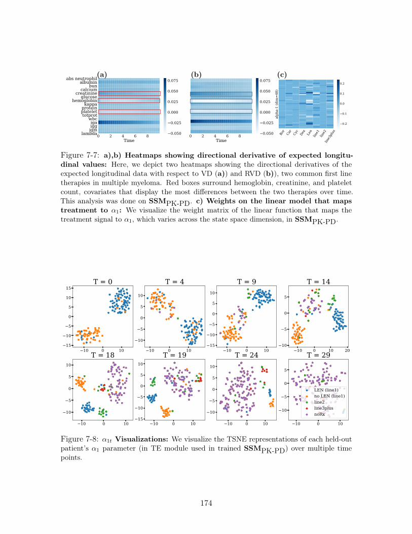
0 2 4 6 8Time
abs neutrophilalbumin
buncalcium
creatinineglucose
hemoglobinkappa
proteinplatelettotprot
wbcigaiggigm
lambda 0 2 4 6 8Time
0.050
0.025
0.000
0.025
0.050
0.075
0.050
0.025
0.000
0.025
0.050
0.075(a) (b)
Bor
Car
Cyc
Dex
Len
line1
line2
line3
plus
alph
a-1
(dim
=48
)
0.2
0.1
0.0
0.1
0.2
(c)
Figure 7-7: a),b) Heatmaps showing directional derivative of expected longitu-dinal values: Here, we depict two heatmaps showing the directional derivatives of theexpected longitudinal data with respect to VD (a)) and RVD (b)), two common first linetherapies in multiple myeloma. Red boxes surround hemoglobin, creatinine, and plateletcount, covariates that display the most differences between the two therapies over time.This analysis was done on SSMPK-PD. c) Weights on the linear model that mapstreatment to 𝛼1: We visualize the weight matrix of the linear function that maps thetreatment signal to 𝛼1, which varies across the state space dimension, in SSMPK-PD.
10 0 1015
10
5
0
5
10
15T = 0
10 0 10
10
5
0
5
10
T = 4
10 0 1015
10
5
0
5
10
T = 9
10 0 10 2010
5
0
5
T = 14
10 0 10
10
5
0
5
10
T = 18
10 0 1015
10
5
0
5
10
T = 19
10 0 10
10
5
0
5
10
T = 24
10 0 10
10
5
0
5
T = 29
LEN (line1)no LEN (line1)line2line3plusnoRx
Figure 7-8: 𝛼1𝑡 Visualizations: We visualize the TSNE representations of each held-outpatient’s 𝛼1 parameter (in TE module used in trained SSMPK-PD) over multiple timepoints.
174
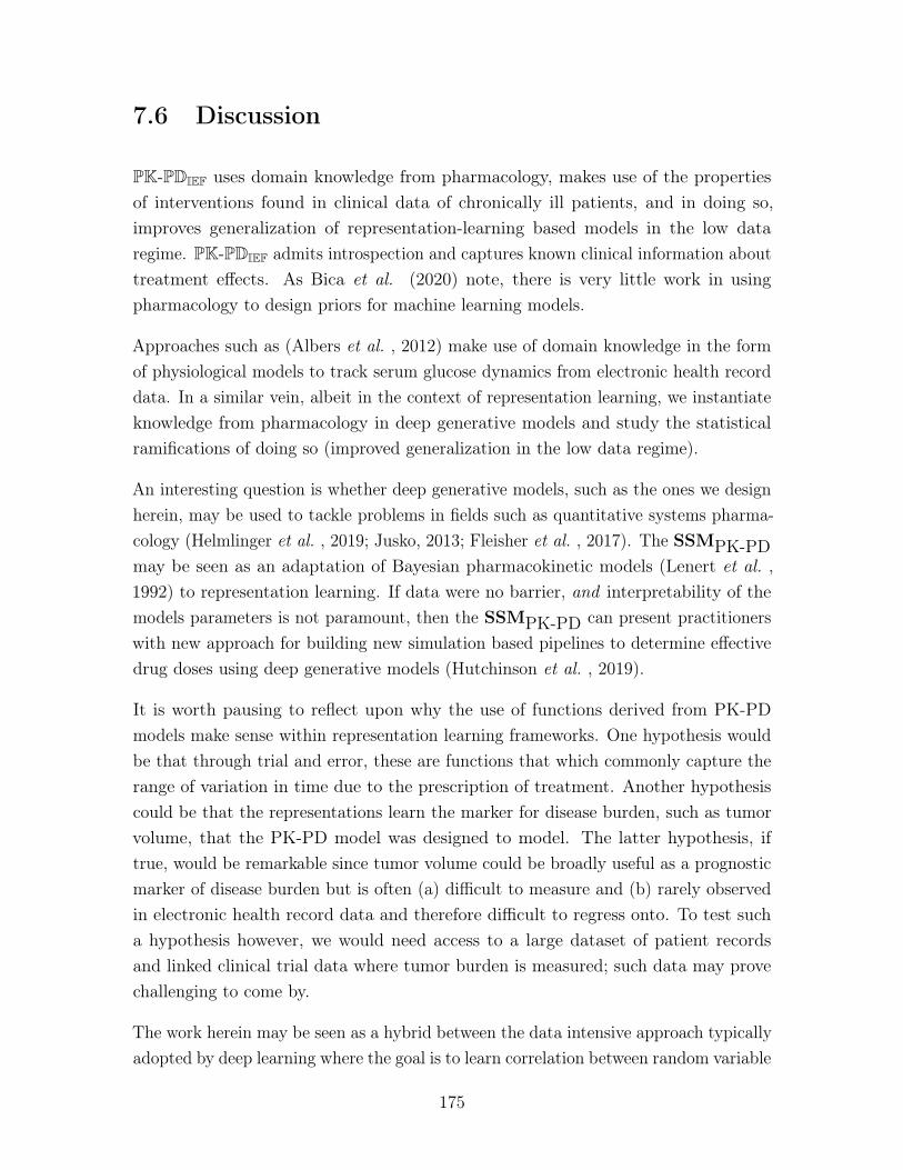
7.6 Discussion
PK-PDIEF uses domain knowledge from pharmacology, makes use of the propertiesof interventions found in clinical data of chronically ill patients, and in doing so,improves generalization of representation-learning based models in the low dataregime. PK-PDIEF admits introspection and captures known clinical information abouttreatment effects. As Bica et al. (2020) note, there is very little work in usingpharmacology to design priors for machine learning models.
Approaches such as (Albers et al. , 2012) make use of domain knowledge in the formof physiological models to track serum glucose dynamics from electronic health recorddata. In a similar vein, albeit in the context of representation learning, we instantiateknowledge from pharmacology in deep generative models and study the statisticalramifications of doing so (improved generalization in the low data regime).
An interesting question is whether deep generative models, such as the ones we designherein, may be used to tackle problems in fields such as quantitative systems pharma-cology (Helmlinger et al. , 2019; Jusko, 2013; Fleisher et al. , 2017). The SSMPK-PDmay be seen as an adaptation of Bayesian pharmacokinetic models (Lenert et al. ,1992) to representation learning. If data were no barrier, and interpretability of themodels parameters is not paramount, then the SSMPK-PD can present practitionerswith new approach for building new simulation based pipelines to determine effectivedrug doses using deep generative models (Hutchinson et al. , 2019).
It is worth pausing to reflect upon why the use of functions derived from PK-PDmodels make sense within representation learning frameworks. One hypothesis wouldbe that through trial and error, these are functions that which commonly capture therange of variation in time due to the prescription of treatment. Another hypothesiscould be that the representations learn the marker for disease burden, such as tumorvolume, that the PK-PD model was designed to model. The latter hypothesis, iftrue, would be remarkable since tumor volume could be broadly useful as a prognosticmarker of disease burden but is often (a) difficult to measure and (b) rarely observedin electronic health record data and therefore difficult to regress onto. To test sucha hypothesis however, we would need access to a large dataset of patient recordsand linked clinical trial data where tumor burden is measured; such data may provechallenging to come by.
The work herein may be seen as a hybrid between the data intensive approach typicallyadopted by deep learning where the goal is to learn correlation between random variable
175

from scratch, and the approach made use of in knowledge-based systems (Szolovits,1986, 1982; Szolovits et al. , 1988; Patil & Schwartz, 1982) where relationships betweenrandom variables are prescribed. The issue with the former is that in data poorregimes, learning functional relationships is hard; the issue with the latter is that itcan be brittle and sensitive to potential model misspecification. By grounding thefunctional forms of the functions in a knowledge based system, whilst still making useof data to guide the learning of relationships, we seek to obtain the benefits of bothparadigms.
176
Chapter 8
Latent Representations of PrivilegedInformation
Chapter 6 introduced Deep Markov Models and Chapter 7 introduced interventioneffect functions, which when used in Deep Markov Models, improved generalization ofdeep generative models trained on clinical data. An important question to ask at thisjuncture is what can good unsupervised models of sequential, clinical data be usedfor?
A motivating example we consider is the problem of building risk stratification tools forrare diseases. In such problems, we are data limited due to the frequency by which thedisease manifests in the general population. In this chapter, we show that if one hasaccess to a model that can uncover patterns in time-varying data, then, by making useof the inferred patterns, we can reduce the sample complexity of supervised learning.Our approach opens a new set of algorithmic techniques to learn risk prediction modelsfrom high-dimensional data when labelled data is scarce.
8.1 Introduction
Accurate models for predicting patient risk can have a large impact on clinical care andpractice. For diseases with no known cure, risk prediction models can guide ongoingcare and help clinicians and patients plan future therapy development (Razavian et al., 2015; Chen & Asch, 2017). In the selection of patient cohorts for clinical trials, riskstratification tools can ensure a new drug’s effect is validated on a diverse group of
177
people through cohort selection (Shivade et al. , 2013). A common approach to patientrisk stratification is to collect labelled patient data prior to treatment (baseline data)and to regress onto an outcome of interest such as death or progression-event for adisease. Approaches based on deep neural networks along these lines can work well,and success stories abound (Gulshan et al. , 2016; Razavian et al. , 2015). But suchmodels are data-hungry. What happens when data is scarce?
In this work, we make use of privileged information (Vapnik & Vashist, 2009):information (features) available during training but not available for prediction at testtime. In clinical settings, privileged data is often available but is rarely used for taskof risk stratification. For example, such information can take the form of prescribedmedications and patient treatment response as measured in terms of longitudinalbiomarkers relevant to the disease. This work aims to achieve two goals: (a) to buildmodels that capture the progression of a disease as observed in privileged data, and (b)to learn representations from such models that contain information vital to buildingaccurate risk stratification models when data is scarce.
It is known that patients respond differently to the same medication. This heterogeneityin response to medication can be driven by a patient’s underlying genetics as wellas their past medical history. The key assumption that we will make here is thatcharacterizing this heterogeneity can yield insight into disease progression and aidprediction of patient outcomes. To operationalize these insights, we propose thePrivileged Information Variational Autoencoder (PIVAE), a deep generative modelwhich uses a latent variable to model the statistical variation in treatment effect thatremains constant across time. The model predicts patient outcomes of interest usingthe latent variable while conditioning on baseline patient covariates.
Why should we expect gains from using privileged information? In the low-data regime,there can be a high degree of uncertainty in the decision boundary for a prediction taskfrom baseline data alone. Intuitively, a representation of post-treatment observationsmay decrease uncertainty by providing a different view of the prediction problem andconsequently improve accuracy. Building on learning using privileged information(LuPI), our work serves as a case-study for how clinical domain knowledge can beutilized to make deep learning in healthcare practical in the low data regime.
In this chapter we introduce the Privileged Information VAE (PIVAE), a conditionaldeep generative model designed to capture statistical patterns in the effect of treatment(or control signals) on a time-varying, multi-variate longitudinal sequences. We usethe PIVAE to form a representation of privileged data, which can be used to improve
178
predictive performance for outcomes of interest in the low-data regime.
8.2 Setup
We begin by presenting background on learning risk prediction and learning usingprivileged information.
Survival analysis. Survival analysis (Cox, 2018) is a popular tool used used toestimate the time to a patient outcome of interest 𝑌 conditional on some covariates𝑋 when the outcomes are censored (or unobserved). Censoring occurs if an patientoutcome is unknown due to incomplete information or if the patient leaves beforethe end of the study. The survival analysis literature spans the gamut of non-parametric models such as the Kaplan-Meier model (Kaplan & Meier, 1958), semi-parametric models such as the the Cox-proportional hazards model (Cox, 1972) andfully parameteric models such as the Weibull distribution (Klein & Moeschberger,2006). To learn parameteric survival models via maximum likelihood we denote abinary indication of censorship as 𝐶. In this setting, it is common to combine a logsurvival function sf for censored events with a model log likelihood of observed eventsusing the binary censorship variable 𝐶 (Klein & Moeschberger, 2006) and maximize:
log 𝑝(𝑌 |𝑋,𝐶) = (1− 𝐶) log 𝑝(𝑌 |𝑋) + 𝐶 log sf(𝑌 |𝑋) (8.1)
Learning using privileged information (LuPI). In most machine learning prob-lems, the training data used for model development, the validation data used forhyperparameter tuning, and test data for evaluation all comprise the same set ofcovariates and labels. With LUPI, at training time, we have access to privilegedinformation not available at validation or test time. Prior work in support vectormachine classification has shown that privileged information such as slack variables orrelated correcting functions can improve learning(Vapnik & Vashist, 2009). Similarresults have been seen for problems in multi-class learning (Wang et al. , 2018).
179
8.3 Privileged Information Variational Autoencoder
We seek a risk stratification tool for a single disease of interest. Such tools are oftenbuilt by using pre-treatment data (i.e. data about a patient prior to undergoingtherapy) to regress onto an outcome that characterizes patient risk (such as the timeto death). For rare diseases, this learning problem will typically lie in the low-dataregime which limits the use of more data-hungry non-linear models.
Fortunately, at training time, in addition to pre-treatment data, we often have post-treatment data available. We will assume the latter is in the form of longitudinaltrajectories of treatments and their subsequent effects on bio-markers that trackdisease progression. Such patient trajectories are often available when building riskprediction models from Electronic Medical Record (EMR), registry or claims data.This is privileged information that we will leverage to build our risk prediction models.
The central hypothesis of this work is twofold: first, that we can learn a representationof privileged information which characterizes the progression of disease; and second,that the representation provides a different view of the pre-treatment data that iseasier to correlate with patient outcomes.
But what principle guides the representation we seek? It is well known that there isheterogeneity in the way a disease manifests itself and that a disease that we refer toby a single name, could comprise many different sub-types. For example, Ahlqvistet al. (2018) describes five different subgroups within diabetes and demonstratesthat patient outcomes vary by subgroup. We use privileged information to uncoverthis latent subgroup. We seek a representation such that closeness in representationspace corresponds to similarity in progression patterns, and, we hypothesize, patientoutcomes of interest.
(Privileged) longitudinal data, 𝑈,𝑋: For patients in the training set, we assumethat we have access to a sequence of multivariate interventions 𝑈 = (𝑈1, . . . , 𝑈𝑇−1)
and multivariate, post-treatment biomarkers 𝑋 = (𝑋1, . . . , 𝑋𝑇 ) for 𝑇 > 0. Thebiomarkers may be any combination of real-valued (e.g. laboratory measurements ofproteins), categorical (e.g. responses to survey data) or binary-valued (indications ofcomorbidities). The PIVAE will seek to build representations, 𝑍, of these (privileged)time-varying biomarkers.
Baseline data, 𝐵, corresponds to patient features prior to the start of therapy, usedin the prediction task—these are the only data available at test time. The set 𝐵
180
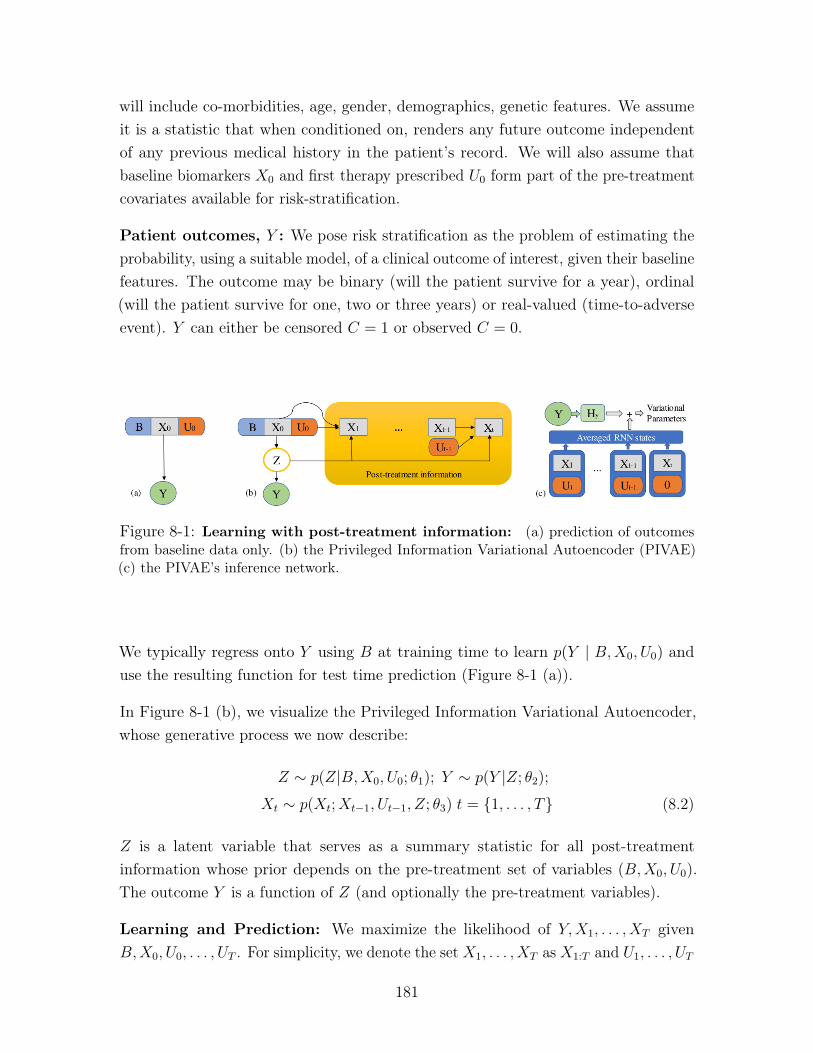
will include co-morbidities, age, gender, demographics, genetic features. We assumeit is a statistic that when conditioned on, renders any future outcome independentof any previous medical history in the patient’s record. We will also assume thatbaseline biomarkers 𝑋0 and first therapy prescribed 𝑈0 form part of the pre-treatmentcovariates available for risk-stratification.
Patient outcomes, 𝑌 : We pose risk stratification as the problem of estimating theprobability, using a suitable model, of a clinical outcome of interest, given their baselinefeatures. The outcome may be binary (will the patient survive for a year), ordinal(will the patient survive for one, two or three years) or real-valued (time-to-adverseevent). 𝑌 can either be censored 𝐶 = 1 or observed 𝐶 = 0.
Figure 8-1: Learning with post-treatment information: (a) prediction of outcomesfrom baseline data only. (b) the Privileged Information Variational Autoencoder (PIVAE)(c) the PIVAE’s inference network.
We typically regress onto 𝑌 using 𝐵 at training time to learn 𝑝(𝑌 | 𝐵,𝑋0, 𝑈0) anduse the resulting function for test time prediction (Figure 8-1 (a)).
In Figure 8-1 (b), we visualize the Privileged Information Variational Autoencoder,whose generative process we now describe:
𝑍 ∼ 𝑝(𝑍|𝐵,𝑋0, 𝑈0; 𝜃1); 𝑌 ∼ 𝑝(𝑌 |𝑍; 𝜃2);𝑋𝑡 ∼ 𝑝(𝑋𝑡;𝑋𝑡−1, 𝑈𝑡−1, 𝑍; 𝜃3) 𝑡 = {1, . . . , 𝑇} (8.2)
𝑍 is a latent variable that serves as a summary statistic for all post-treatmentinformation whose prior depends on the pre-treatment set of variables (𝐵,𝑋0, 𝑈0).The outcome 𝑌 is a function of 𝑍 (and optionally the pre-treatment variables).
Learning and Prediction: We maximize the likelihood of 𝑌,𝑋1, . . . , 𝑋𝑇 given𝐵,𝑋0, 𝑈0, . . . , 𝑈𝑇 . For simplicity, we denote the set 𝑋1, . . . , 𝑋𝑇 as 𝑋1:𝑇 and 𝑈1, . . . , 𝑈𝑇
181
as 𝑈1:𝑇 . For a single patient:
log 𝑝(𝑋1:𝑇 , 𝑌 |𝐵,𝑋0, 𝑈0:𝑇 , 𝐶)
= log
∫︁
𝑍
𝑝(𝑋1:𝑇 , 𝑌, 𝑍|𝐵,𝑋0, 𝑈0:𝑇 )
= log
∫︁
𝑍
𝑝(𝑋1:𝑇 |𝑍,𝑋0, 𝑈0:𝑇 )𝑝(𝑍|𝐵,𝑋0, 𝑈0)𝑝(𝑌 |𝑍,𝐶)
= log
∫︁
𝑍
𝑞(𝑍|𝑌,𝑋1:𝑇 , 𝑈1:𝑇 ;𝜑)
𝑇∏︁
𝑡=1
𝑝(𝑋𝑡|𝑋𝑡−1, 𝑍, 𝑈𝑡−1)𝑝(𝑍|𝐵,𝑋0, 𝑈0)
𝑞(𝑍|𝑌,𝑋1:𝑇 , 𝑈1:𝑇 ;𝜑)𝑝(𝑌 |𝑍,𝐶)
≥ E𝑞(𝑍|𝑌,𝑋1:𝑇 ,𝑈1:𝑇 ;𝜑)
[︃𝑇∑︁
𝑡=1
log 𝑝(𝑋𝑡|𝑋𝑡−1, 𝑍, 𝑈𝑡−1)
+ log 𝑝(𝑌 |𝑍,𝐶)]︂
−KL(𝑞(𝑍|𝑌,𝑋1:𝑇 , 𝑈1:𝑇 ;𝜑)||𝑝(𝑍|𝐵,𝑋0, 𝑈0)) (8.3)
where log 𝑝(𝑌 |𝑍,𝐶) is estimated as in Equation 8.1.
The inference network for the model is depicted in Figure 8-1 (c). A recurrent neural net-work uses the concatenation of treatments and interventions in addition to a represen-tation of the outcome to parameterize the variational distribution 𝑞(𝑍|𝑌,𝑋1:𝑇 , 𝑈1:𝑇 ;𝜑).
At test time, 𝑋1, . . . , 𝑋𝑇 , 𝑈1, . . . , 𝑈𝑇 are unobserved and we approximate the predictionfunction 𝑃 (𝑌 |𝐵,𝑈0, 𝑋0) =
∫︀𝑍𝑝(𝑌 |𝑍)𝑝(𝑍|𝐵,𝑈0, 𝑋0) for prediction.
Overview: It is worth giving pause to why the PIVAE is a good fit for the problemat hand.
Our first goal was to learn a representation of privileged information. The PIVAE doesthis by modeling the likelihood of privileged data as a function of the latent variable𝑍. At training time, the privileged data are observed and probabilistic inference (viaan inference network) is used to infer 𝑍 by maximizing a lower bound on the loglikelihood of the observed data. At prediction time, the privileged information isunobserved. However, as leaves in a Bayesian network, they may be ignored and aMonte-Carlo approximation to the prior-predictive (in this case, a marginalization oflatent variable 𝑍) is used to predict the outcome 𝑌 .
Our second goal was to build a model wherein the representation learned yielded
182
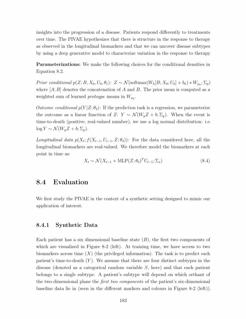
insights into the progression of a disease. Patients respond differently to treatmentsover time. The PIVAE hypothesizes that there is structure in the response to therapyas observed in the longitudinal biomarkers and that we can uncover disease subtypesby using a deep generative model to characterize variation in the response to therapy.
Parameterizations: We make the following choices for the conditional densities inEquation 8.2.
Prior conditional 𝑝(𝑍;𝐵,𝑋0, 𝑈0, 𝜃1): 𝑍 ∼ 𝒩 (softmax(𝑊ℎ[𝐵;𝑋0;𝑈0] + 𝑏ℎ) *𝑊𝜇𝑝 ; Σ𝑝)
where [𝐴;𝐵] denotes the concatenation of 𝐴 and 𝐵. The prior mean is computed as aweighted sum of learned protoype means in 𝑊𝜇𝑝 .
Outcome conditional 𝑝(𝑌 |𝑍; 𝜃2): If the prediction task is a regression, we parameterizethe outcome as a linear function of 𝑍: 𝑌 ∼ 𝒩 (𝑊𝑦𝑍 + 𝑏; Σ𝑦). When the event istime-to-death (positive, real-valued number), we use a log normal distribution: i.e.log 𝑌 ∼ 𝒩 (𝑊𝑦𝑍 + 𝑏; Σ𝑦).
Longitudinal data 𝑝(𝑋𝑡; 𝑓(𝑋𝑡−1, 𝑈𝑡−1, 𝑍; 𝜃3)): For the data considered here, all thelongitudinal biomarkers are real-valued. We therefore model the biomarkers at eachpoint in time as:
𝑋𝑡 ∼ 𝒩 (𝑋𝑡−1 + MLP(𝑍; 𝜃3)𝑇𝑈𝑡−1; Σ𝑥) (8.4)
8.4 Evaluation
We first study the PIVAE in the context of a synthetic setting designed to mimic ourapplication of interest.
8.4.1 Synthetic Data
Each patient has a six dimensional baseline state (𝐵), the first two components ofwhich are visualized in Figure 8-2 (left). At training time, we have access to twobiomarkers across time (𝑋) (the privileged information). The task is to predict eachpatient’s time-to-death (𝑌 ). We assume that there are four distinct subtypes in thedisease (denoted as a categorical random variable 𝑆, here) and that each patientbelongs to a single subtype. A patient’s subtype will depend on which orthant ofthe two-dimensional plane the first two components of the patient’s six-dimensionalbaseline data lie in (seen in the different markers and colours in Figure 8-2 (left)).
183
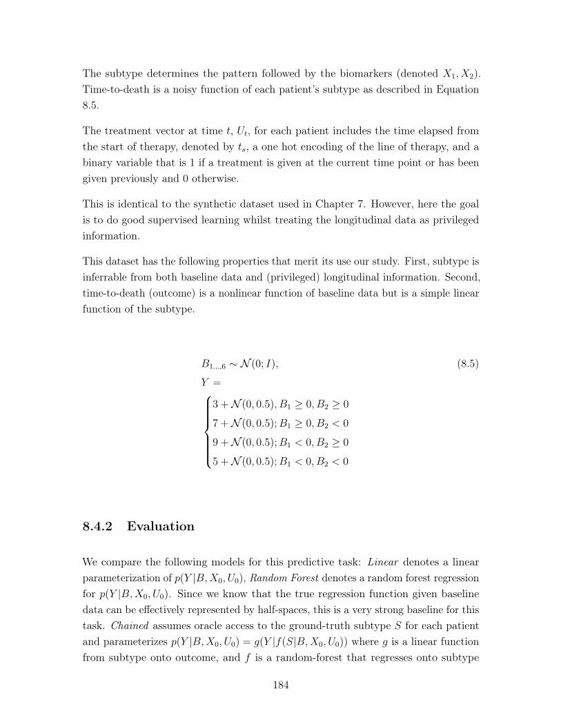
The subtype determines the pattern followed by the biomarkers (denoted 𝑋1, 𝑋2).Time-to-death is a noisy function of each patient’s subtype as described in Equation8.5.
The treatment vector at time 𝑡, 𝑈𝑡, for each patient includes the time elapsed fromthe start of therapy, denoted by 𝑡𝑠, a one hot encoding of the line of therapy, and abinary variable that is 1 if a treatment is given at the current time point or has beengiven previously and 0 otherwise.
This is identical to the synthetic dataset used in Chapter 7. However, here the goalis to do good supervised learning whilst treating the longitudinal data as privilegedinformation.
This dataset has the following properties that merit its use our study. First, subtype isinferrable from both baseline data and (privileged) longitudinal information. Second,time-to-death (outcome) is a nonlinear function of baseline data but is a simple linearfunction of the subtype.
𝐵1...,6 ∼ 𝒩 (0; 𝐼), (8.5)
𝑌 =⎧⎪⎪⎪⎪⎪⎨⎪⎪⎪⎪⎪⎩
3 +𝒩 (0, 0.5), 𝐵1 ≥ 0, 𝐵2 ≥ 0
7 +𝒩 (0, 0.5);𝐵1 ≥ 0, 𝐵2 < 0
9 +𝒩 (0, 0.5);𝐵1 < 0, 𝐵2 ≥ 0
5 +𝒩 (0, 0.5);𝐵1 < 0, 𝐵2 < 0
8.4.2 Evaluation
We compare the following models for this predictive task: Linear denotes a linearparameterization of 𝑝(𝑌 |𝐵,𝑋0, 𝑈0), Random Forest denotes a random forest regressionfor 𝑝(𝑌 |𝐵,𝑋0, 𝑈0). Since we know that the true regression function given baselinedata can be effectively represented by half-spaces, this is a very strong baseline for thistask. Chained assumes oracle access to the ground-truth subtype 𝑆 for each patientand parameterizes 𝑝(𝑌 |𝐵,𝑋0, 𝑈0) = 𝑔(𝑌 |𝑓(𝑆|𝐵,𝑋0, 𝑈0)) where 𝑔 is a linear functionfrom subtype onto outcome, and 𝑓 is a random-forest that regresses onto subtype
184
2 0 23
2
1
0
1
2
3 [S0] (y=3)
[S1] (y=7)
[S2] (y=9)
[S3] (y=5)
Baseline data labelled by [subtype] & (time-to-event)
0 10 20Time
10
0
10
20 Subtype 0
0 10 20Time
10
0
10
20 Subtype 1
0 10 20Time
10
0
10
20 Subtype 2
0 10 20Time
10
0
10
20 Subtype 3
Figure 8-2: Visualizing synthetic data: Left: A visualization of patient’s baseline data(coloured and marked by patient subtype). Each quadrant is annotated with [subtype](time-to-death). Right four plots: For patients from each of the subtypes, an example oftheir longitudinal trajectories. The solid lines are trajectories had there been no treatment,while the dotted lines over time represent trajectories with treatment response. The dashedvertical line represents the therapy given at a particular point in time.
5 0 5 10
10
5
0
5
10
15
(a) TRVAE [sup] p(z|[B, X0, A0])
4 2 0 2 42
0
2
4
6
(b) TRVAE [unsup] q(z|[X, A])S[0] (6.0)S[1] (6.0)S[2] (6.0)S[3] (6.0)
3 2 1 0 1 2
2
1
0
1
2
3
4
(c) TRVAE [unsup] p(z|[B, X0, A0])
25 50 75 100
150
200
# samples
0
2
4
6
8
10(d) Mean Squared Error
25 50 75 100
150
200
# samples
0.0
0.2
0.4
0.6
0.8
1.0(e) R2 Score
LinearRandom ForestChained (oracle)TRVAE [sup]TRVAE [unsup]
Figure 8-3: Synthetic (held-out) data: (a) depicts the delta distribution implied by 𝑍under a supervised PIVAE while (b)
∑︀𝑛 𝑞(𝑍𝑛|𝑋,𝑈), (c)
∑︀𝑛 𝑝(𝑍𝑛|𝐵,𝑋0, 𝑈0) visualize the
corresponding distributions from an unsupervised PIVAE. (d), (e) visualize different accuracymetrics comparing the PIVAE to various baselines.
from baseline data. This is an approximation to the best achievable regression model.PIVAE [supervised] (denoted with [sup]) corresponds to learning the PIVAE in a fullysupervised manner. i.e. via minimizing a Maximum A-Posteriori approximation toE𝑝(𝑍|𝐵,𝑋0,𝑈0)[− log 𝑝(𝑌 |𝑍,𝐶)]. PIVAE [unsupervised] (denoted with [unsup]) learns bymaximizing Equation 8.2.
How do the different methods compare to one another? We evaluate performanceon mean square error (MSE) and 𝑅2 (coefficient of determination) as a function ofthe number of training samples while keeping fixed the number of held-out dataat 300 points. We conduct a hyperparameter search over the number of latentdimension (4, 10), number of hidden dimensions in 𝑝(𝑌 |𝑍,𝐶) (10, 50) and learningrates (1𝑒− 3, 8𝑒− 3) identically for PIVAE [sup] and PIVAE [unsup] and selected thebest model using mean square error on held-out data as the metric.
In Figure 8-3 (d,e) we see that the linear models, as expected, perform poorly (since
185
the outcome is not linear in the input). (Note that the MSE for the linear modelsis >30, so therefore are not shown in the plot). Both random forests and PIVAE[sup] do well when the number of training samples exceeds one-hundred but theirperformance degrades in the low-data regime. In contrast, PIVAE [unsup], matchesthe performance (in MSE and 𝑅2) of an oracle regression model with access to thetrue underlying subtype.
What advantage does using of privileged information confer upon PIVAE [unsup]relative to PIVAE [sup] in the small data regime? To answer this question we train,on 25 patients, a supervised and unsupervised version of the PIVAE where 𝑍 istwo-dimensional. When PIVAE [sup] is via a MAP approximation to
E𝑝(𝑍|𝐵,𝑋0,𝑈0)[− log 𝑝(𝑌 |𝑍,𝐶)]
, we obtain a delta-distribution 𝑝(𝑍|𝐵,𝑋0, 𝑈0)). In Figure 8-3 (a) we visualizethis distribution evaluated on a held-out set. Although the PIVAE [sup] has be-gun to separate out patients with varying outcome times, learning about subtypestructure, in the low-data regime, is difficult from baseline data alone. The samerepresentation 𝑝(𝑍|𝐵,𝑋0, 𝑈0) for PIVAE [unsup] is plotted in Figure 8-3 (c) wherewe see that the model has successfully learned to map from baseline data ontofour distinct regions corresponding to subtype – why has this happened? Notethat the learning signal for 𝑝(𝑍|𝐵,𝑋0, 𝑈0) is derived from the minimization ofKL(𝑞(𝑍|𝑌,𝑋1:𝑇 , 𝑈1:𝑇 ;𝜑)||𝑝(𝑍|𝐵,𝑋0, 𝑈0)) (Equation 8.2). We plot the aggregate pos-terior distribution in Figure 8-3 (b) which reveals that the inference network hasused privileged information to uncover the latent subtype. The minimization of KLdivergence consequently transfers this knowledge onto 𝑝(𝑍|𝐵,𝑋0, 𝑈0), allowing themodel to generalize effectively at test time. Note that the functions used in PIVAE[sup] and PIVAE [unsup] are identical in their structure and number of parameters,what differs is that at training time, the privileged information is used to construct aview on data which when leveraged by the latter allows it to generalize better. This,in effect, validates the utility of privileged information in the small data regime.
To inspect what the PIVAE [unsup] (trained on 25 patients) learns, in Figure 8-4 (a)we visualize values of ℎglobal in matrix form. Across all patients within a subtype,we average the estimates of ℎglobal, binarize the result and insert it into a row of thematrix visualized in the plot. We find that the global structure learned by the modelcorresponds to the four patterns of variation exhibited by the biomarkers for eachsubtype. We forward sample the longitudinal data from the model and visualize the
186
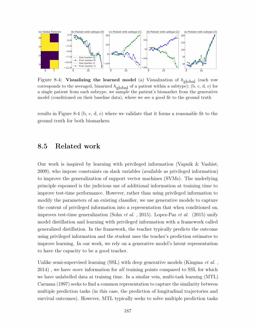
0 1
0
1
2
3
(a) Global Patterns
0 1012.5
10.0
7.5
5.0
2.5
0.0
2.5(b) Patient with subtype [0]
Data [marker 0]Pred. [marker 0]Data [marker 1]Pred. [marker 1]
0 10
10
0
10
20(c) Patient with subtype [1]
0 1020
10
0
10
(d) Patient with subtype [2]
0 10
0
5
10
15
20(e) Patient with subtype [3]
Figure 8-4: Visualizing the learned model (a) Visualization of ℎglobal (each rowcorresponds to the averaged, binarized ℎglobal of a patient within a subtype); (b, c, d, e) fora single patient from each subtype, we sample the patient’s biomarker from the generativemodel (conditioned on their baseline data), where we see a good fit to the ground truth
results in Figure 8-4 (b, c, d, e) where we validate that it forms a reasonable fit to theground truth for both biomarkers.
8.5 Related work
Our work is inspired by learning with privileged information (Vapnik & Vashist,2009), who impose constraints on slack variables (available as privileged information)to improve the generalization of support vector machines (SVMs). The underlyingprinciple espoused is the judicious use of additional information at training time toimprove test-time performance. However, rather than using privileged information tomodify the parameters of an existing classifier, we use generative models to capturethe content of privileged information into a representation that when conditioned on,improves test-time generalization (Sohn et al. , 2015). Lopez-Paz et al. (2015) unifymodel distillation and learning with privileged information with a framework calledgeneralized distillation. In the framework, the teacher typically predicts the outcomeusing privileged information and the student uses the teacher’s prediction estimates toimprove learning. In our work, we rely on a generative model’s latent representationto have the capacity to be a good teacher.
Unlike semi-supervised learning (SSL) with deep generative models (Kingma et al. ,2014) , we have more information for all training points compared to SSL for whichwe have unlabelled data at training time. In a similar vein, multi-task learning (MTL)Caruana (1997) seeks to find a common representation to capture the similarity betweenmultiple prediction tasks (in this case, the prediction of longitudinal trajectories andsurvival outcomes). However, MTL typically seeks to solve multiple prediction tasks
187
at test time.
There is a rich history of jointly modeling longitudinal data and clinical outcomes(Wu et al. , 2012). Unsupervised sequential models have been used to model diseaseslike Chronic Kidney disease (Futoma et al. , 2016; Wang et al. , 2014b) and modelingmobile health drug-use (Dempsey et al. , 2017). In addition to modeling sequentialdata, Ranganath et al. (2015) use a time-varying latent variable to parameterizethe hazard function while predicting outcomes for heart patients. Schulam & Saria(2016) propose a conditional Bayesian network that models the progression of a singlebiomarker as a function of other observed data. They use latent variables as proxiesfor the observed set of biomarkers. Our work differs from theirs in our explicit desireto use heterogeneity in treatment effect as the means by which we uncover patterns indata.
Gabler et al. (2009) discuss the importance of explicitly accounting for treatmentheterogeneity, particularly in the context of designing and evaluating clinical trials.Smolenski et al. (2017) study the heterogeneity in the context of patients treatedfor depression via video-conference. In child psychology, Mertens et al. (2017) studyheterogeneity of response to therapy for problematic behavior. To the best of ourknowledge, we are not aware of other work that uses deep generative models to capturetreatment heterogeneity.
8.6 Discussion
This chapter proposes the Privileged Information Variational Autoencoder. The modelcaptures representations of subtype in longitudinal patient data while correcting forthe effect of treatments. We show how the model’s latent representations can serveboth as a diagnostic tool to understand how disease behave as well as improve thepredictive performance of risk prediction tools.
Although our method is most useful at providing predictive gains in the low-dataregime, there are limitations to the model and care must be taken in its use for buildingrisk-prediciton models. First, within the prediction problem must exist a degree ofcorrelation between the variation in privileged information and the outcome of interest.In such scenarios, the information captured in the latent variable be correlated tothe outcome and provide a kind of supervision to the risk-prediction model thanthe outcome alone. Second, designing good deep generative models of privileged
188

information often requires domain knowledge for the problem at hand. Validatingthe approach by building a new risk prediction model on a real world dataset is animportant direction for future work.
189

190
Chapter 9
Conclusion
We are constantly discovering new ways to measure phenomena occurring at a varietyof scales in the human body. As we do so, our notions of healthy and diseased changes.While our understanding of the mechanisms that drive change over time in the humanbody is constantly improving, there is much we do not know. In the absence of detailedmechanistic knowledge about the data generating processes that drive, we conjecturein this thesis that deep generative models, given sufficient data, may prove a capablesurrogate as a computational modeling tool for clinical questions of interest.
This thesis develops supervised, and unsupervised learning algorithms for modelsof high-dimensional data designed to tackle some of the challenges that arise in thecontext of healthcare. We return to the challenges highlighted in Chapter 1 andoutline how some of the work in this thesis addresses them.
Heterogeneity, sparsity, missingness, and high-dimensionality: This thesismakes use of latent variable deep generative models to capture patterns in high-dimensional data. When the data comes from long-tailed distributions, as they oftendo for problems in healthcare, deep generative models may underfit. In Chapter 4(Krishnan et al. , 2018) we investigate and remedy this pathology. Being able to fitthese models well means that we can make use of the innovations in Chapter 3 toinvestigate the parameters of the model and understand the correlations that existamong features in high-dimensional data.
Temporal data: As diseases progress in a patient they manifest changes in clinicalobservations which then prompt changes in downstream treatment. Deep markovmodels (Krishnan et al. , 2017), in Chapter 6, are a flexible model family that
191
practitioners can use for unsupervised learning of such data. The black-box variationallearning algorithm we derive can be scaled up to learn DMMs from millions ofdatapoints through the use of GPUs.
Limited mechanistic knowledge: When modeling patient data from rare diseases,DMMs may overfit. In Chapter 7, we combine ideas from pharmacology with deeplearning and design new neural architectures for use in the conditional probabilitydistributions of DMMs. We show that this judicious use of domain knowledge improvesthe generalization of DMMs when data is scarce.
Dataset sizes: In Chapter 8 we show how deep generative models may be usedto capture salient structure in post-treatment, privileged information and in doingso learn representations that can reduce the sample complexity of risk stratificationmodels that make predictions using pre-treatment data. Chapter 5 shows how tofine-tune deep generative models with a little bit of supervision so that datapointsthat are similar have similar latent representations.
9.1 Future directions for deep generative modeling
Inference as prediction The idea of posing an optimization problem, such asprobabilistic inference in a graphical model, as prediction has roots that go back atleast to the wake-sleep algorithm (Hinton et al. , 1995). However, there remain manyquestions of a statistical nature that arise from such a transformation. Statisticallearning theory tells us about how well classifiers generalize when applied to unseendata. Little is known about whether such results may be extended to characterizethe generalization of inference networks. For amortized variational inference to findfooting within the statistical modeling workflow, we need ways to quantify the samplecomplexity, and generalization of the coupled systems comprising the deep generativemodel and the inference network. Such results will be necessary to trust the predictionsobtained from inference networks when deployed to tackle real-world problems indomains such as healthcare.
Disentangled representation learning and identifiability The ability of deepgenerative models to model complex log likelihoods has led researchers to questionwhether this class of models can identify factors of variation in a dataset. In thecontext of MNIST, a disentangled model will map digit identity to some subset of the
192
latent variables and digit style to others.
Several studies (Siddharth et al. , 2017; Kingma et al. , 2014) make use of supervision tocontrol the information content captured by different latent variables – this is a powerfulapproach when supervision is available. Others claim that disentanglement may beobtained in a purely unsupervised manner, usually via some form of regularization onthe inference network (Higgins et al. , 2016; Kim & Mnih, 2018; Chen et al. , 2018).However, the above studies leave open a crucial question: does there exist a couplingof model and learning algorithm that guarantees disentanglement independent ofthe dataset? Fortunately, and unsurprisingly, Locatello et al. (2019) show that inthe absence of assumptions about the inductive biases of the generative model orthe datasets that it is trained on, disentangled representation learning is impossible.Where does that leave us?
One of the most promising directions for future research towards the goal of disentan-gled representation learning is building deep generative models with identifiable latentrepresentations. Classical identifiability is a statistical property of a model under whichit is possible to uniquely determine the model parameters after observing an infinitenumber of observations. However deep generative models typically rely on conditionalprobability distributions defined using overparameterized neural networks renderingthe unique identification of parameters improbable. Indeed one of the rationales behindthe successes of neural networks is that overparameterization is crucial to learningsuch models via stochastic gradient based methods(Allen-Zhu et al. , 2019). But ifwe cannot identify the parameters of the model, perhaps we may identify the latentrepresentations uniquely given infinite data. One of the pioneering works towardsthis end is that of (Khemakhem et al. , 2020) who make use of results from nonlinearindependent component analysis (ICA) (Hyvarinen & Morioka, 2017; Hyvärinen &Pajunen, 1999; Hyvarinen et al. , 2019) to derive identifiability results for variationalautoencoders. The extension of such results towards Deep Markov Models presentsan intriguing opportunity to learn identifiable non-linear state space models wherewe can uniquely determine low-dimensional patient trajectories for high-dimensional,time-varying patient data.
Deep generative models with tractable likelihoods In this thesis, we madeuse of latent variable models for unsupervised learning. Furthermore, we assumedthat latent variables had a lower dimensionality than the data. Dinh et al. (2016)present an alternative approach to unsupervised learning with latent variables. They
193
assume the latent variable has the same dimensionality of the data, and the generativeprocess comprises iterated, parameteric, transformations, each of which is constrainedto be volume preserving. The resulting model has a tractable and differentiable log-likelihood and one can perform exact probabilistic inference by inverting each of thetransformations in the generative model to obtain the posterior distribution. Althoughsuch models yield competitive results on image datasets, it would be interesting tostudy their utility on tabular datasets such as those found in electronic health recorddata.
The use of parameteric, volume preserving transformations has seen use not just indensity estimation, but also in variational inference. Indeed, one of the canonical waysin which the complexity of the inference network may be improved is via normalizingflows. We refer the reader to (Kobyzev et al. , 2019; Papamakarios et al. , 2019) for acomprehensive review of such methods.
9.2 Future directions for machine learning in health-care
In addition to the above methodological directions for future work, much remains tobe done before we can answer some of the most pressing questions posed by clinicalinformatics.
Multi-scale, multi-modal deep generative models Over the next decade, med-ical institutions will collect a large amount of fine-grained data about the human bodyacross different scales. At the micro scale, the collection of RNA and DNA sequencingdata will give us a view into the cellular health of a patient. At the macro scale, thecompilation of diagnosis codes, medical images and procedures will offer insights intothe health of a patient’s organ system. At the population scale, infection counts andcommunity wellness data aggregated by non-governmental agencies will characterizethe general health of large groups of people. Building hierarchical models of data atmultiple scales and multiple modalities is a rich area for innovative applications ofdeep generative models (Shi et al. , 2019; Wu & Goodman, 2018; Wang et al. , 2014a),and new algorithms for inference and learning.
Success in this arena can inform solutions to new prediction problems that cannotsolely be answered using data at a single scale. For example, a model looking to
194
predict how likely a patient is to contract a life threatening C.difficile infection mightrequire a patient’s medical history at the macro scale, as well as the prevailing ratesof infection in the hospital ward at the population scale.
Inductive biases for clinical data Hierarchical models are only part of the solutionto decision making with multi-modal, multi-scale data. The other part of the solutionlies in developing new parameterizations for the conditional probability distributionsused in deep generative models. Many problems in healthcare will be fundamentallydata limited, either due to the nature of the disease or due to socio-technical constraintson data access. Good inductive biases can prove crucial in building models thatgeneralize well in the low-data regime. In Chapter 7, we saw the dramatic improvementsobtained from the use of a judiciously chosen intervention effect function. Comingup with good neural architectures for deep neural networks that parameterize modelsof data such as lab results, x-rays, DNA and immunomics will no doubt require theexpertise of pharmacologists, radiologists, geneticists and immunologists.
Disease progression Disease progression modeling (Cook & Bies, 2016) encom-passes the use of discrete (Sukkar et al. , 2012) or continuous-time (Wang et al. , 2014b)statistical models to uncover patterns in longitudinal patient data. The ability of deepgenerative models to model data from millions of patients, each one with a potentiallyhigh-dimensional set of covariates, means that we are no longer computationallylimited in which diseases we choose to study. Making use of sequential deep generativemodels to subtype low-dimensional patient trajectories (while correcting for variationin biomarkers due to treatments) can give clinicians insights into strata that existwithin their patient populations. Characterizing the strata may then reveal known orunknown aspects of the disease, or give clinicians new ways to group patients.
Causal Inference There are several opportunities wherein the innovations withinthis thesis can play a role towards tackling problems of a causal nature. The onewe highlight is the use of deep generative models as structural equation models(Pearl, 2012). Under the appropriate conditions where the sequential causal effect isidentifiable (Pearl et al. , 2009), the DMM may be viewed as a structural equationmodel and be used to ask counterfactual queries of how patients behave under varioustreatment plans. Such a tool can give clinicians the ability to gauge the success ofa chosen longitudinal treatment plan not just in terms of the primary biomarkers
195
used to characterize disease burden, but also in terms of biomarkers that characterizerelated comorbidities.
Clinical Deployment On a more humbling note, while there many known unknownsin the application of machine learning for problems in healthcare, there are a far greaternumber of unknown unknowns. The careful deployment, study and characterizationof decision support tools powered by machine learning is vital to shed light on whatproblems remain to be characterized before patients and doctors can make use of theinsights learned from data.
196
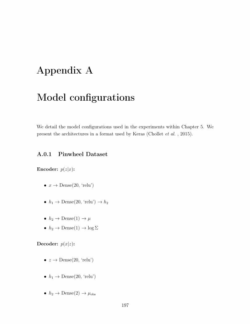
Appendix A
Model configurations
We detail the model configurations used in the experiments within Chapter 5. Wepresent the architectures in a format used by Keras (Chollet et al. , 2015).
A.0.1 Pinwheel Dataset
Encoder: 𝑝(𝑧|𝑥):
∙ 𝑥→ Dense(20, ‘relu’)
∙ ℎ1 → Dense(20, ‘relu’) → ℎ2
∙ ℎ2 → Dense(1) → 𝜇
∙ ℎ2 → Dense(1) → log Σ
Decoder: 𝑝(𝑥|𝑧):
∙ 𝑧 → Dense(20, ‘relu’)
∙ ℎ1 → Dense(20, ‘relu’)
∙ ℎ2 → Dense(2) → 𝜇obs
197
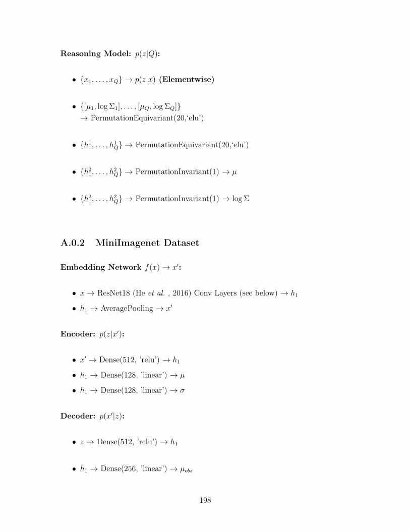
Reasoning Model: 𝑝(𝑧|𝑄):
∙ {𝑥1, . . . , 𝑥𝑄} → 𝑝(𝑧|𝑥) (Elementwise)
∙ {[𝜇1, log Σ1], . . . , [𝜇𝑄, log Σ𝑄]}→ PermutationEquivariant(20,‘elu’)
∙ {ℎ11, . . . , ℎ1𝑄} → PermutationEquivariant(20,‘elu’)
∙ {ℎ21, . . . , ℎ2𝑄} → PermutationInvariant(1) → 𝜇
∙ {ℎ21, . . . , ℎ2𝑄} → PermutationInvariant(1) → log Σ
A.0.2 MiniImagenet Dataset
Embedding Network 𝑓(𝑥)→ 𝑥′:
∙ 𝑥→ ResNet18 (He et al. , 2016) Conv Layers (see below) → ℎ1
∙ ℎ1 → AveragePooling → 𝑥′
Encoder: 𝑝(𝑧|𝑥′):
∙ 𝑥′ → Dense(512, ’relu’) → ℎ1
∙ ℎ1 → Dense(128, ’linear’) → 𝜇
∙ ℎ1 → Dense(128, ’linear’) → 𝜎
Decoder: 𝑝(𝑥′|𝑧):
∙ 𝑧 → Dense(512, ’relu’) → ℎ1
∙ ℎ1 → Dense(256, ’linear’) → 𝜇𝑜𝑏𝑠
198
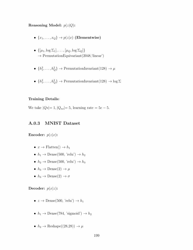
Reasoning Model: 𝑝(𝑧|𝑄):
∙ {𝑥1, . . . , 𝑥𝑄} → 𝑝(𝑧|𝑥) (Elementwise)
∙ {[𝜇1, log Σ1], . . . , [𝜇𝑄, log Σ𝑄]}→ PermutationEquivariant(2048,‘linear’)
∙ {ℎ21, . . . , ℎ2𝑄} → PermutationInvariant(128) → 𝜇
∙ {ℎ21, . . . , ℎ2𝑄} → PermutationInvariant(128) → log Σ
Training Details:
We take |𝑄𝑠|= 1, |𝑄𝑛𝑠|= 5, learning rate = 5𝑒− 5.
A.0.3 MNIST Dataset
Encoder: 𝑝(𝑧|𝑥):
∙ 𝑥→ Flatten() → ℎ1
∙ ℎ1 → Dense(500, ’relu’) → ℎ2
∙ ℎ2 → Dense(500, ’relu’) → ℎ3
∙ ℎ3 → Dense(2) → 𝜇
∙ ℎ3 → Dense(2) → 𝜎
Decoder: 𝑝(𝑥|𝑧):
∙ 𝑧 → Dense(500, ’relu’) → ℎ1
∙ ℎ1 → Dense(784, ’sigmoid’) → ℎ2
∙ ℎ2 → Reshape((28,28)) → 𝜇
199
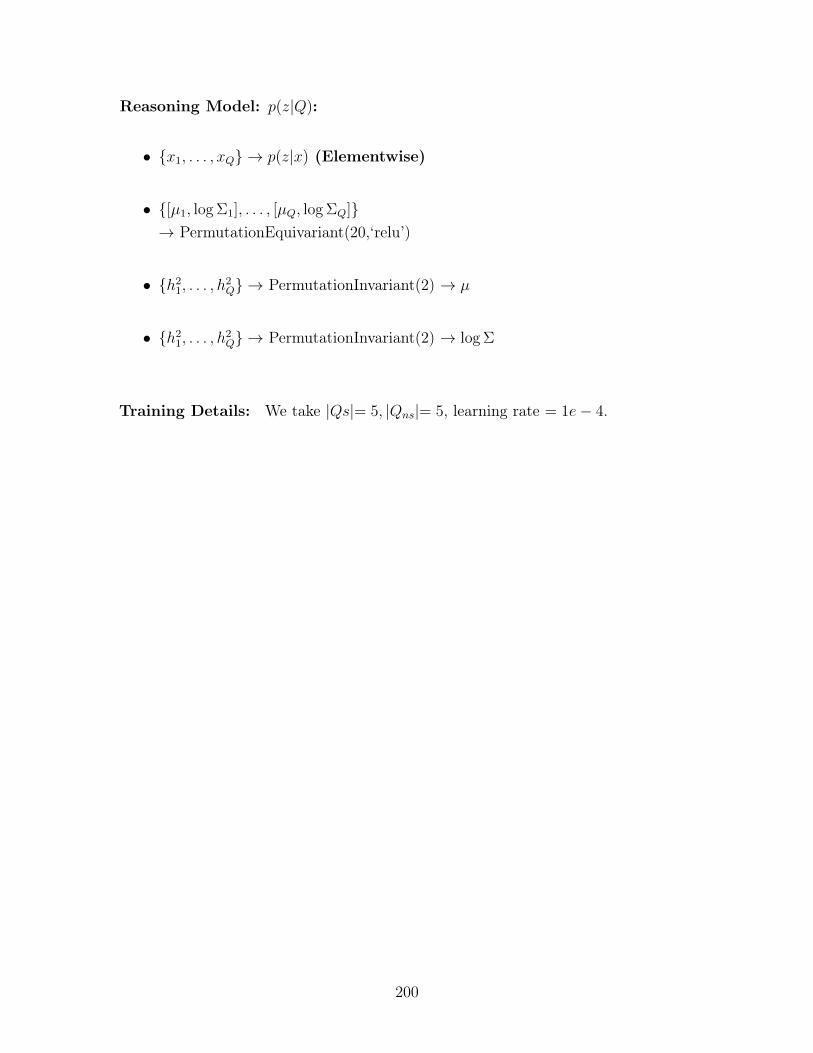
Reasoning Model: 𝑝(𝑧|𝑄):
∙ {𝑥1, . . . , 𝑥𝑄} → 𝑝(𝑧|𝑥) (Elementwise)
∙ {[𝜇1, log Σ1], . . . , [𝜇𝑄, log Σ𝑄]}→ PermutationEquivariant(20,‘relu’)
∙ {ℎ21, . . . , ℎ2𝑄} → PermutationInvariant(2) → 𝜇
∙ {ℎ21, . . . , ℎ2𝑄} → PermutationInvariant(2) → log Σ
Training Details: We take |𝑄𝑠|= 5, |𝑄𝑛𝑠|= 5, learning rate = 1𝑒− 4.
200
Appendix B
Model configurations
We detail the model configurations used in the experiments within Chapter 6.
In each instance, we detail the model architecture used in the generative model(comprising a transition and emission function) as well as the model used for posteriorinference. “L” denotes a linear layer with the values in parenthesis denoting thedimensions of the transformation. “NL” denotes the application of a non-linearity(specified in the caption). Since parameters in the model are shared across time, wedescribe the architecture at a single time-step. The row denoted “Inference” is thearchitecture used for performing inference. In the case of the bidirectional RNN, weconcatenate the outputs from the forward and reverse RNN to perform predictionof the posterior means and log covariances. The recognition network predicts theposterior mean and log-covariance. The two quantities are predicted with a sharedbase network feeding into a separate final linear layer (i.e the last linear layer in therow “Inference” is different for the function used to predict the posterior mean and theposterior log-covariance). Square braces indicate a vector concatenation operation.
Table B.1 describes the model architecture used in the synthetic experiments. Wedetail the architectures used for inference in “MF-LR” and “ST-LR”. The other inferencealgorithms involve different structures in the LSTM-RNN module but are otherwiseidentical. The “combiner function” is detailed by the mapping from [ℎ𝑡; 𝑧𝑡−1]→𝜇𝑞.
Table B.2 describes the architecture used for the polyphonic dataset and in Table B.3,we describe the architecture used for experiments on medical data.
201
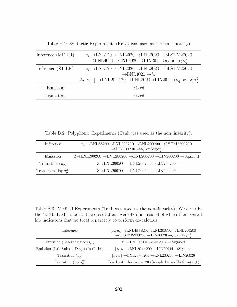
Table B.1: Synthetic Experiments (ReLU was used as the non-linearity)
Inference (MF-LR) 𝑥𝑡 →LNL120→LNL2020 →LNL2020 →bLSTM22020→LNL4020 →LNL2020 →LIN201 →𝜇𝑞 or log 𝜎2
𝑞
Inference (ST-LR) 𝑥𝑡 →LNL120→LNL2020 →LNL2020 →bLSTM22020→LNL4020 →ℎ𝑡
[ℎ𝑡; 𝑧𝑡−1] →LNL20+120 →LNL2020→LIN201 →𝜇𝑞 or log 𝜎2𝑞
Emission Fixed
Transition Fixed
Table B.2: Polyphonic Experiments (Tanh was used as the non-linearity).
Inference 𝑥𝑡 →LNL88200→LNL200200 →LNL200200 →LSTM2200200→LIN200200 →𝜇𝑞 or log 𝜎2
𝑞
Emission Z→LNL200200 →LNL200200 →LNL200200 →LIN200200 →Sigmoid
Transition (𝜇𝑝) Z→LNL200200 →LNL200200 →LIN200200
Transition (log 𝜎2𝑝) Z→LNL200200 →LNL200200 →LIN200200
Table B.3: Medical Experiments (Tanh was used as the non-linearity). We describethe “E:NL-T:NL” model. The observations were 48 dimensional of which there were 4lab indicators that we treat separately to perform do-calculus.
Inference [𝑥𝑡;𝑢𝑡] →LNL48+8200→LNL200300 →LNL200200→bLSTM2200200 →LIN40020 →𝜇𝑞 or log 𝜎2
𝑞
Emission (Lab Indicators 𝑖𝑡 ) 𝑧𝑡 →LNL20200 →LIN2004 →Sigmoid
Emission (Lab Values, Diagnosis Codes) [𝑧𝑡; 𝑖𝑡] →LNL20+4200 →LIN20044 →Sigmoid
Transition (𝜇𝑝) [𝑧𝑡;𝑢𝑡] →LNL20+8200 →LNL200200 →LIN20020
Transition (log 𝜎2𝑝) Fixed with dimension 20 (Sampled from Uniform(-1,1)
202
Bibliography
Abadi, Martín, Agarwal, Ashish, Barham, Paul, Brevdo, Eugene, Chen, Zhifeng,Citro, Craig, Corrado, Greg S., Davis, Andy, Dean, Jeffrey, Devin, Matthieu,Ghemawat, Sanjay, Goodfellow, Ian, Harp, Andrew, Irving, Geoffrey, Isard, Michael,Jia, Yangqing, Jozefowicz, Rafal, Kaiser, Lukasz, Kudlur, Manjunath, Levenberg,Josh, Mané, Dandelion, Monga, Rajat, Moore, Sherry, Murray, Derek, Olah, Chris,Schuster, Mike, Shlens, Jonathon, Steiner, Benoit, Sutskever, Ilya, Talwar, Kunal,Tucker, Paul, Vanhoucke, Vincent, Vasudevan, Vijay, Viégas, Fernanda, Vinyals,Oriol, Warden, Pete, Wattenberg, Martin, Wicke, Martin, Yu, Yuan, & Zheng,Xiaoqiang. 2015. TensorFlow: Large-Scale Machine Learning on HeterogeneousSystems. Software available from tensorflow.org.
Ahlqvist, Emma, Storm, Petter, Käräjämäki, Annemari, Martinell, Mats, Dorkhan,Mozhgan, Carlsson, Annelie, Vikman, Petter, Prasad, Rashmi B, Aly, Dina Mansour,Almgren, Peter, et al. . 2018. Novel subgroups of adult-onset diabetes and theirassociation with outcomes: a data-driven cluster analysis of six variables. TheLancet Diabetes & endocrinology, 6(5), 361–369.
Albers, David J, Hripcsak, George, & Schmidt, Michael. 2012. Population physiology:leveraging electronic health record data to understand human endocrine dynamics.PLoS One, 7(12), e48058.
Allen-Zhu, Zeyuan, Li, Yuanzhi, & Liang, Yingyu. 2019. Learning and generalizationin overparameterized neural networks, going beyond two layers. Pages 6158–6169of: Advances in neural information processing systems.
Almeida, Felipe, & Xexéo, Geraldo. 2019. Word embeddings: A survey. arXiv preprintarXiv:1901.09069.
Anandkumar, Animashree, Hsu, Daniel, & Kakade, Sham M. 2012. A method ofmoments for mixture models and hidden Markov models. Pages 33–1 of: Conferenceon Learning Theory.
Archer, Evan, Park, Il Memming, Buesing, Lars, Cunningham, John, & Paninski,Liam. 2015. Black box variational inference for state space models. arXiv preprintarXiv:1511.07367.
Baeza-Yates, Ricardo, Ribeiro-Neto, Berthier, et al. . 1999. Modern informationretrieval. Vol. 463. ACM press New York.
203
Bahdanau, Dzmitry, Cho, Kyunghyun, & Bengio, Yoshua. 2014. Neural machinetranslation by jointly learning to align and translate. arXiv preprint arXiv:1409.0473.
Bar-Hillel, Aharon, Hertz, Tomer, Shental, Noam, & Weinshall, Daphna. 2005. Learn-ing a mahalanobis metric from equivalence constraints. JMLR.
Bauer, Matthias, Rojas-Carulla, Mateo, Bartłomiej Świątkowski, Jakub, Schölkopf,Bernhard, & Turner, Richard E. 2017. Discriminative k-shot learning using proba-bilistic models. arXiv preprint arXiv:1706.00326.
Baydin, Atılım Günes, Pearlmutter, Barak A, Radul, Alexey Andreyevich, & Siskind,Jeffrey Mark. 2017. Automatic differentiation in machine learning: a survey. TheJournal of Machine Learning Research, 18(1), 5595–5637.
Bayer, Justin, & Osendorfer, Christian. 2014. Learning stochastic recurrent networks.arXiv preprint arXiv:1411.7610.
Bengio, Yoshua, Ducharme, Réjean, Vincent, Pascal, & Jauvin, Christian. 2003. Aneural probabilistic language model. JMLR.
Bica, Ioana, Alaa, Ahmed M, Lambert, Craig, & van der Schaar, Mihaela. 2020. Fromreal-world patient data to individualized treatment effects using machine learning:Current and future methods to address underlying challenges. Clinical Pharmacology& Therapeutics.
Bingham, Eli, Chen, Jonathan P, Jankowiak, Martin, Obermeyer, Fritz, Pradhan,Neeraj, Karaletsos, Theofanis, Singh, Rohit, Szerlip, Paul, Horsfall, Paul, & Good-man, Noah D. 2019. Pyro: Deep universal probabilistic programming. The Journalof Machine Learning Research, 20(1), 973–978.
Blei, David M, Ng, Andrew Y, & Jordan, Michael I. 2003. Latent dirichlet allocation.Journal of machine Learning research, 3(Jan), 993–1022.
Bojarski, Mariusz, Del Testa, Davide, Dworakowski, Daniel, Firner, Bernhard, Flepp,Beat, Goyal, Prasoon, Jackel, Lawrence D, Monfort, Mathew, Muller, Urs, Zhang,Jiakai, et al. . 2016. End to end learning for self-driving cars. arXiv preprintarXiv:1604.07316.
Boulanger-Lewandowski, Nicolas, Bengio, Yoshua, & Vincent, Pascal. 2012. Modelingtemporal dependencies in high-dimensional sequences: Application to polyphonicmusic generation and transcription. arXiv preprint arXiv:1206.6392.
Bowman, Samuel R, Vilnis, Luke, Vinyals, Oriol, Dai, Andrew M, Jozefowicz, Rafal, &Bengio, Samy. 2015. Generating sentences from a continuous space. arXiv preprintarXiv:1511.06349.
Breiman, Leo. 2001. Statistical modeling: The two cultures. Statistical Science.
204
Briegel, Thomas, & Tresp, Volker. 1999. Fisher scoring and a mixture of modesapproach for approximate inference and learning in nonlinear state space models.Pages 403–409 of: Advances in Neural Information Processing Systems.
Burda, Yuri, Grosse, Roger, & Salakhutdinov, Ruslan. 2015. Importance weightedautoencoders. arXiv preprint arXiv:1509.00519.
Butler, A., Hoffman, P., Smibert, P., Papalexi, E., & Satija, R. 2018. Integratingsingle-cell transcriptomic data across different conditions, technologies, and species.Nature biotechnology 36.5.
Caruana, Rich. 1997. Multitask learning. Machine learning, 28(1), 41–75.
Chakraborty, Bibhas. 2013. Statistical methods for dynamic treatment regimes.Springer.
Che, Zhengping, Purushotham, Sanjay, Li, Guangyu, Jiang, Bo, & Liu, Yan. 2018a.Hierarchical deep generative models for multi-rate multivariate time series. Pages784–793 of: International Conference on Machine Learning.
Che, Zhengping, Purushotham, Sanjay, Cho, Kyunghyun, Sontag, David, & Liu, Yan.2018b. Recurrent neural networks for multivariate time series with missing values.Scientific reports, 8(1), 1–12.
Chen, Jonathan H, & Asch, Steven M. 2017. Machine learning and prediction inmedicine—beyond the peak of inflated expectations. The New England journal ofmedicine, 376(26), 2507.
Chen, Ricky TQ, Li, Xuechen, Grosse, Roger B, & Duvenaud, David K. 2018. Isolat-ing sources of disentanglement in variational autoencoders. Pages 2610–2620 of:Advances in Neural Information Processing Systems.
Chen, Xi, Kingma, Diederik P, Salimans, Tim, Duan, Yan, Dhariwal, Prafulla, Schul-man, John, Sutskever, Ilya, & Abbeel, Pieter. 2016. Variational lossy autoencoder.arXiv preprint arXiv:1611.02731.
Chen, Xinxiong, Liu, Zhiyuan, & Sun, Maosong. 2014. A Unified Model for WordSense Representation and Disambiguation. In: EMNLP.
Chiappa, Silvia, Racaniere, Sébastien, Wierstra, Daan, & Mohamed, Shakir. 2017.Recurrent environment simulators. arXiv preprint arXiv:1704.02254.
Choi, Edward, Bahadori, Mohammad Taha, Schuetz, Andy, Stewart, Walter F, & Sun,Jimeng. 2016a. Doctor ai: Predicting clinical events via recurrent neural networks.Pages 301–318 of: Machine Learning for Healthcare Conference.
Choi, Edward, Bahadori, Mohammad Taha, Sun, Jimeng, Kulas, Joshua, Schuetz,Andy, & Stewart, Walter. 2016b. Retain: An interpretable predictive model forhealthcare using reverse time attention mechanism. Pages 3504–3512 of: Advancesin Neural Information Processing Systems.
205
Choi, Youngduck, Yi-I Chiu, Chill, & Sontag, David. 2016c. Learning Low-DimensionalRepresentations of Medical Concepts. In: AMIA.
Chollet, François, et al. . 2015. Keras. https://github.com/keras-team/keras.
Chung, Junyoung, Gulcehre, Caglar, Cho, KyungHyun, & Bengio, Yoshua. 2014.Empirical evaluation of gated recurrent neural networks on sequence modeling.arXiv preprint arXiv:1412.3555.
Chung, Junyoung, Kastner, Kyle, Dinh, Laurent, Goel, Kratarth, Courville, Aaron C,& Bengio, Yoshua. 2015. A recurrent latent variable model for sequential data.Pages 2980–2988 of: Advances in neural information processing systems.
Church, Kenneth Ward, & Hanks, Patrick. 1990. Word association norms, mutualinformation, and lexicography. Computational linguistics.
Collins, Michael, Dasgupta, Sanjoy, & Schapire, Robert E. 2001. A generalization ofprincipal component analysis to the exponential family. In: NIPS.
Collobert, Ronan, & Weston, Jason. 2008. A unified architecture for natural languageprocessing: Deep neural networks with multitask learning. In: ICML.
Collobert, Ronan, Bengio, Samy, & Mariéthoz, Johnny. 2002. Torch: a modularmachine learning software library. Tech. rept. Idiap.
Cook, Sarah F, & Bies, Robert R. 2016. Disease progression modeling: key conceptsand recent developments. Current pharmacology reports, 2(5), 221–230.
Cox, David R. 1972. Regression models and life-tables. Journal of the Royal StatisticalSociety: Series B (Methodological), 34(2), 187–202.
Cox, David Roxbee. 2018. Analysis of survival data. Routledge.
Cremer, Chris, Li, Xuechen, & Duvenaud, David. 2018. Inference Suboptimalityin Variational Autoencoders. Pages 1078–1086 of: International Conference onMachine Learning.
Cybenko, George. 1989. Approximation by superpositions of a sigmoidal function.Mathematics of control, signals and systems, 2(4), 303–314.
De Vine, Lance, Zuccon, Guido, Koopman, Bevan, Sitbon, Laurianne, & Bruza, Peter.2014. Medical semantic similarity with a neural language model. In: CIKM.
Dempsey, Walter H, Moreno, Alexander, Scott, Christy K, Dennis, Michael L,Gustafson, David H, Murphy, Susan A, & Rehg, James M. 2017. iSurvive: An Inter-pretable, Event-time Prediction Model for mHealth. Pages 970–979 of: InternationalConference on Machine Learning.
Dinh, Laurent, Sohl-Dickstein, Jascha, & Bengio, Samy. 2016. Density estimationusing real nvp. arXiv preprint arXiv:1605.08803.
206
Doyle, Orla M, Westman, Eric, Marquand, Andre F, Mecocci, Patrizia, Vellas, Bruno,Tsolaki, Magda, Kłoszewska, Iwona, Soininen, Hilkka, Lovestone, Simon, Williams,Steve CR, et al. . 2014. Predicting progression of Alzheimer’s disease using ordinalregression. PloS one, 9(8).
Du, Yilun, & Narasimhan, Karthic. 2019. Task-Agnostic Dynamics Priors for DeepReinforcement Learning. Pages 1696–1705 of: International Conference on MachineLearning.
Duckworth, D. 2016. Kalman filter, kalman smoother, and em library for python.
Dziugaite, Gintare Karolina, Roy, Daniel M, & Ghahramani, Zoubin. 2015. Traininggenerative neural networks via maximum mean discrepancy optimization. arXivpreprint arXiv:1505.03906.
Edwards, Harrison, & Storkey, Amos. 2016. Towards a neural statistician. arXivpreprint arXiv:1606.02185.
Engel, Jesse, Hoffman, Matthew, & Roberts, Adam. 2018. Latent Constraints: Learn-ing to Generate Conditionally from Unconditional Generative Models. In: ICLR.
Erhan, Dumitru, Bengio, Yoshua, Courville, Aaron, & Vincent, Pascal. 2009. Visualiz-ing higher-layer features of a deep network.
Evain, Simon, & Benzekry, Sebastien. 2016. Mathematical modeling of tumor andmetastatic growth when treated with sunitinib.
Fabius, Otto, & van Amersfoort, Joost R. 2014. Variational recurrent auto-encoders.arXiv preprint arXiv:1412.6581.
Fano, Robert M. 1949. The transmission of information. The MIT Press.
Fefferman, Charles, Mitter, Sanjoy, & Narayanan, Hariharan. 2016. Testing themanifold hypothesis. Journal of the American Mathematical Society, 29(4), 983–1049.
Finkelstein, Lev, Gabrilovich, Evgeniy, Matias, Yossi, Rivlin, Ehud, Solan, Zach,Wolfman, Gadi, & Ruppin, Eytan. 2001. Placing search in context: The conceptrevisited. In: WWW.
Finlayson, Samuel G, LePendu, Paea, & Shah, Nigam H. 2014. Building the graph ofmedicine from millions of clinical narratives. Scientific data.
Finn, Chelsea, Abbeel, Pieter, & Levine, Sergey. 2017. Model-agnostic meta-learningfor fast adaptation of deep networks. ICML.
Fleisher, Brett, Brown, Ashley N, & Ait-Oudhia, Sihem. 2017. Application of pharma-cometrics and quantitative systems pharmacology to cancer therapy: The exampleof luminal a breast cancer. Pharmacological Research, 124, 20–33.
207
Fraccaro, Marco, Sønderby, Søren Kaae, Paquet, Ulrich, & Winther, Ole. 2016.Sequential neural models with stochastic layers. Pages 2199–2207 of: Advances inneural information processing systems.
Futoma, Joseph, Sendak, Mark, Cameron, C Blake, & Heller, Katherine. 2016. ScalableModeling of Multivariate Longitudinal Data for Prediction of Chronic Kidney DiseaseProgression. arXiv preprint arXiv:1608.04615.
Gabler, Nicole B, Duan, Naihua, Liao, Diana, Elmore, Joann G, Ganiats, Theodore G,& Kravitz, Richard L. 2009. Dealing with heterogeneity of treatment effects: is theliterature up to the challenge? Trials, 10(1), 43.
Gan, Zhe, Li, Chunyuan, Henao, Ricardo, Carlson, David E, & Carin, Lawrence. 2015.Deep temporal sigmoid belief networks for sequence modeling. Pages 2467–2475 of:Advances in Neural Information Processing Systems.
Gao, Yuanjun, Archer, Evan W, Paninski, Liam, & Cunningham, John P. 2016. Lineardynamical neural population models through nonlinear embeddings. Pages 163–171of: Advances in neural information processing systems.
Geng, Changran, Paganetti, Harald, & Grassberger, Clemens. 2017. Prediction oftreatment response for combined chemo-and radiation therapy for non-small celllung cancer patients using a bio-mathematical model. Scientific reports, 7(1), 1–12.
Ghahramani, Zoubin, & Heller, Katherine A. 2005. Bayesian sets. In: NIPS.
Ghahramani, Zoubin, & Roweis, Sam T. 1999. Learning nonlinear dynamical systemsusing an EM algorithm. Pages 431–437 of: Advances in neural information processingsystems.
Gibson, WA. 1960. Nonlinear factors in two dimensions. Psychometrika, 25(4),381–392.
Glorot, Xavier, & Bengio, Yoshua. 2010. Understanding the difficulty of training deepfeedforward neural networks. In: AISTATS.
Goodfellow, Ian, Pouget-Abadie, Jean, Mirza, Mehdi, Xu, Bing, Warde-Farley, David,Ozair, Sherjil, Courville, Aaron, & Bengio, Yoshua. 2014. Generative adversarialnets. Pages 2672–2680 of: Advances in neural information processing systems.
Grassberger, C, & Paganetti, H. 2016. Methodologies in the modeling of combinedchemo-radiation treatments. Physics in Medicine & Biology, 61(21), R344.
Graves, Alex, Wayne, Greg, & Danihelka, Ivo. 2014. Neural Turing Machines. arXivpreprint arXiv:1410.5401.
Gregor, Karol, Danihelka, Ivo, Graves, Alex, Rezende, Danilo Jimenez, & Wierstra,Daan. 2015. Draw: A recurrent neural network for image generation. arXiv preprintarXiv:1502.04623.
208
Gu, Shixiang, Ghahramani, Zoubin, & Turner, Richard E. 2015. Neural adaptivesequential monte carlo. Pages 2629–2637 of: Advances in Neural InformationProcessing Systems.
Gulshan, V, Peng, L, Coram, M, & et al. 2016. Development and validation of adeep learning algorithm for detection of diabetic retinopathy in retinal fundusphotographs. JAMA, 316(22), 2402–2410.
Halpern, Yoni, & Sontag, David. 2013. Unsupervised Learning of Noisy-Or BayesianNetworks. Page 272 of: Uncertainty in Artificial Intelligence. Citeseer.
Harper, F Maxwell, & Konstan, Joseph A. 2015. The MovieLens Datasets: Historyand Context. ACM Transactions on Interactive Intelligent Systems (TiiS).
He, Junxian, Spokoyny, Daniel, Neubig, Graham, & Berg-Kirkpatrick, Taylor. 2019.Lagging inference networks and posterior collapse in variational autoencoders. arXivpreprint arXiv:1901.05534.
He, Kaiming, Zhang, Xiangyu, Ren, Shaoqing, & Sun, Jian. 2016. Deep residuallearning for image recognition. In: CVPR.
Helmlinger, Gabriel, Sokolov, Victor, Peskov, Kirill, Hallow, Karen M, Kosinsky, Yuri,Voronova, Veronika, Chu, Lulu, Yakovleva, Tatiana, Azarov, Ivan, Kaschek, Daniel,et al. . 2019. Quantitative Systems Pharmacology: An Exemplar Model-BuildingWorkflow With Applications in Cardiovascular, Metabolic, and Oncology DrugDevelopment. CPT: pharmacometrics & systems pharmacology, 8(6), 380–395.
Hernán, Miguel, & Robins, Jamie. 2020. Causal Inference: What If. Boca Raton:Chapman & Hall/CRC.
Higgins, Irina, Matthey, Loic, Pal, Arka, Burgess, Christopher, Glorot, Xavier,Botvinick, Matthew, Mohamed, Shakir, & Lerchner, Alexander. 2016. beta-vae:Learning basic visual concepts with a constrained variational framework.
Hinton, Geoffrey E, & Salakhutdinov, Ruslan R. 2009. Replicated softmax: anundirected topic model. Pages 1607–1614 of: Advances in Neural InformationProcessing Systems.
Hinton, Geoffrey E, Dayan, Peter, Frey, Brendan J, & Neal, Radford M. 1995. The"wake-sleep" algorithm for unsupervised neural networks. Science, 268(5214), 1158–1161.
Hjelm, R Devon, Cho, Kyunghyun, Chung, Junyoung, Salakhutdinov, Russ, Calhoun,Vince, & Jojic, Nebojsa. 2016. Iterative Refinement of Approximate Posterior forTraining Directed Belief Networks. In: NIPS.
Hoffman, Matthew D, Blei, David M, Wang, Chong, & Paisley, John. 2013. Stochasticvariational inference. The Journal of Machine Learning Research, 14(1), 1303–1347.
209
Honkela, Antti, & Valpola, Harri. 2004. Variational learning and bits-back coding:an information-theoretic view to Bayesian learning. IEEE transactions on NeuralNetworks, 15(4), 800–810.
Hsu, Daniel, Kakade, Sham M, & Zhang, Tong. 2012. A spectral algorithm forlearning hidden Markov models. Journal of Computer and System Sciences, 78(5),1460–1480.
Hu, Yifan, Koren, Yehuda, & Volinsky, Chris. 2008. Collaborative filtering for implicitfeedback datasets. Pages 263–272 of: 2008 Eighth IEEE International Conferenceon Data Mining. Ieee.
Huang, Eric H., Socher, Richard, Manning, Christopher D., & Ng, Andrew Y. 2012.Improving Word Representations via Global Context and Multiple Word Prototypes.In: ACL.
Hutchinson, Lucy, Steiert, Bernhard, Soubret, Antoine, Wagg, Jonathan, Phipps,Alex, Peck, Richard, Charoin, Jean-Eric, & Ribba, Benjamin. 2019. Models andMachines: How Deep Learning Will Take Clinical Pharmacology to the Next Level.CPT: pharmacometrics & systems pharmacology, 8(3), 131–134.
Hyvärinen, Aapo, & Pajunen, Petteri. 1999. Nonlinear independent componentanalysis: Existence and uniqueness results. Neural networks, 12(3), 429–439.
Hyvarinen, Aapo, Sasaki, Hiroaki, & Turner, Richard. 2019. Nonlinear ICA usingauxiliary variables and generalized contrastive learning. Pages 859–868 of: The22nd International Conference on Artificial Intelligence and Statistics.
Hyvarinen, AJ, & Morioka, Hiroshi. 2017. Nonlinear ICA of temporally dependentstationary sources. Proceedings of Machine Learning Research.
Iyyer, Mohit, Manjunatha, Varun, Boyd-Graber, Jordan, & Daumé III, Hal. 2015.Deep Unordered Composition Rivals Syntactic Methods for Text Classification. In:ACL.
Jaakkola, Tommi S, & Haussler, David. 2007. Exploiting generative models indiscriminative classifiers. In: NIPS.
Jacobs, Robert A, Jordan, Michael I, Nowlan, Steven J, & Hinton, Geoffrey E. 1991.Adaptive mixtures of local experts. Neural computation, 3(1), 79–87.
Jacobus, SJ, Rajkumar, S Vincent, Weiss, M, Stewart, Alexander Keith, Stadt-mauer, EA, Callander, NS, Dreosti, Lydia M, Lacy, MQ, & Fonseca, Rafael. 2016.Randomized phase III trial of consolidation therapy with bortezomib–lenalidomide–Dexamethasone (VRd) vs bortezomib–dexamethasone (Vd) for patients with multi-ple myeloma who have completed a dexamethasone based induction regimen. Bloodcancer journal, 6(7), e448–e448.
210
Jankowiak, Martin, & Obermeyer, Fritz. 2018. Pathwise Derivatives Beyond the Repa-rameterization Trick. Pages 2235–2244 of: International Conference on MachineLearning.
Järvelin, K., & Kekäläinen, J. 2002. Cumulated gain-based evaluation of IR techniques.ACM Transactions on Information Systems (TOIS), 20(4), 422–446.
Jeffreys, Harold. 1998. The Theory of Probability. OUP Oxford.
Jernite, Yacine, Halpern, Yonatan, & Sontag, David. 2013. Discovering hidden variablesin noisy-or networks using quartet tests. Pages 2355–2363 of: Advances in NeuralInformation Processing Systems.
Johnson, Matthew, Duvenaud, David K, Wiltschko, Alex, Adams, Ryan P, & Datta,Sandeep R. 2016. Composing graphical models with neural networks for struc-tured representations and fast inference. Pages 2946–2954 of: Advances in neuralinformation processing systems.
Jones, Christopher S. 2006. A nonlinear factor analysis of S&P 500 index optionreturns. The Journal of Finance, 61(5), 2325–2363.
Jordan, Michael I, & Jacobs, Robert A. 1994. Hierarchical mixtures of experts andthe EM algorithm. Neural computation, 6(2), 181–214.
Jordan, Michael I, Ghahramani, Zoubin, Jaakkola, Tommi S, & Saul, Lawrence K.1999. An introduction to variational methods for graphical models. Machine learning,37(2), 183–233.
Jusko, William J. 2013. Moving from basic toward systems pharmacodynamic models.Journal of pharmaceutical sciences, 102(9), 2930–2940.
Jutten, C. 2003. Advances in nonlinear blind source separation. Pages 245–256 of:4th Int. Symp. on Independent Component Analysis and Blind Signal Separation(ICA2003), Nara.
Kaplan, Edward L, & Meier, Paul. 1958. Nonparametric estimation from incompleteobservations. Journal of the American statistical association, 53(282), 457–481.
Khemakhem, Ilyes, Kingma, Diederik, Monti, Ricardo, & Hyvarinen, Aapo. 2020.Variational autoencoders and nonlinear ica: A unifying framework. Pages 2207–2217of: International Conference on Artificial Intelligence and Statistics.
Kim, Hyunjik, & Mnih, Andriy. 2018. Disentangling by Factorising. Pages 2649–2658of: International Conference on Machine Learning.
Kim, Yoon, Wiseman, Sam, Miller, Andrew, Sontag, David, & Rush, Alexander. 2018.Semi-Amortized Variational Autoencoders. Pages 2678–2687 of: InternationalConference on Machine Learning.
211
Kingma, Diederik P, & Ba, Jimmy. 2014. Adam: A method for stochastic optimization.arXiv preprint arXiv:1412.6980.
Kingma, Diederik P., & Welling, Max. 2014. Auto-encoding variational bayes. In:Proceedings of the International Conference on Learning Representations (ICLR),vol. 2.
Kingma, Diederik P, Mohamed, Shakir, Rezende, Danilo Jimenez, & Welling, Max.2014. Semi-supervised learning with deep generative models. In: Advances in NeuralInformation Processing Systems.
Klein, Christoph A. 2009. Parallel progression of primary tumours and metastases.Nature Reviews Cancer, 9(4), 302–312.
Klein, John P, & Moeschberger, Melvin L. 2006. Survival analysis: techniques forcensored and truncated data. Springer Science & Business Media.
Kobyzev, Ivan, Prince, Simon, & Brubaker, Marcus A. 2019. Normalizing flows:Introduction and ideas. arXiv preprint arXiv:1908.09257.
Koller, Daphne, Friedman, Nir, & Bach, Francis. 2009. Probabilistic graphical models:principles and techniques. The MIT Press.
Koutnik, Jan, Greff, Klaus, Gomez, Faustino, & Schmidhuber, Juergen. 2014. AClockwork RNN. Pages 1863–1871 of: International Conference on MachineLearning.
Krishnan, Rahul G, Shalit, Uri, & Sontag, David. 2017. Structured Inference Networksfor Nonlinear State Space Models. In: AAAI.
Krishnan, Rahul G, Liang, Dawen, & Hoffman, Matthew. 2018. On the challenges oflearning with inference networks on sparse, high-dimensional data. In: Proceedingsof the Twenty-first Conference on Artificial Intelligence and Statistics.
Krizhevsky, Alex, Sutskever, Ilya, & Hinton, Geoffrey E. 2012. Imagenet classificationwith deep convolutional neural networks. Pages 1097–1105 of: Advances in neuralinformation processing systems.
Kumar, Shaji, Flinn, Ian, Richardson, Paul G, Hari, Parameswaran, Callander, Natalie,Noga, Stephen J, Stewart, A Keith, Turturro, Francesco, Rifkin, Robert, Wolf,Jeffrey, et al. . 2012. Randomized, multicenter, phase 2 study (EVOLUTION) ofcombinations of bortezomib, dexamethasone, cyclophosphamide, and lenalidomidein previously untreated multiple myeloma. Blood, The Journal of the AmericanSociety of Hematology, 119(19), 4375–4382.
Lake, Brenden M, Salakhutdinov, Ruslan R, & Tenenbaum, Josh. 2013. One-shotlearning by inverting a compositional causal process. In: NIPS.
212
Landauer, Thomas K, Foltz, Peter W, & Laham, Darrell. 1998. An introduction tolatent semantic analysis. Discourse processes.
Larochelle, Hugo, & Murray, Iain. 2011. The neural autoregressive distributionestimator. Pages 29–37 of: Proceedings of the Fourteenth International Conferenceon Artificial Intelligence and Statistics.
Larochelle, Hugo, Bengio, Yoshua, Louradour, Jérôme, & Lamblin, Pascal. 2009.Exploring strategies for training deep neural networks. Journal of machine learningresearch, 10(Jan), 1–40.
Lawrence, Neil D. 2004. Gaussian process latent variable models for visualisation ofhigh dimensional data. Pages 329–336 of: Advances in neural information processingsystems.
LeCun, Yann. 1998. The MNIST database of handwritten digits. http://yann. lecun.com/exdb/mnist/.
LeCun, Yann, Bottou, Léon, Bengio, Yoshua, & Haffner, Patrick. 1998. Gradient-based learning applied to document recognition. Proceedings of the IEEE, 86(11),2278–2324.
LeCun, Yann, Bengio, Yoshua, & Hinton, Geoffrey. 2015. Deep learning. nature,521(7553), 436–444.
Lee, Wonyeol, Yu, Hangyeol, & Yang, Hongseok. 2018. Reparameterization gradientfor non-differentiable models. Pages 5553–5563 of: Advances in Neural InformationProcessing Systems.
Lenert, Leslie A, Lurie, Jon, Sheiner, Lewis B, Coleman, Robert, Klostermann,Heidrun, & Blaschke, Terrence F. 1992. Advanced computer programs for drugdosing that combine pharmacokinetic and symbolic modeling of patients. Computersand biomedical research, 25(1), 29–42.
Lewis, David D, Yang, Yiming, Rose, Tony G, & Li, Fan. 2004. Rcv1: A newbenchmark collection for text categorization research. Journal of machine learningresearch, 5(Apr), 361–397.
Li, Chongxuan, Zhu, Jun, Shi, Tianlin, & Zhang, Bo. 2015a. Max-margin deepgenerative models. Pages 1837–1845 of: Advances in neural information processingsystems.
Li, Yujia, Swersky, Kevin, & Zemel, Rich. 2015b. Generative moment matchingnetworks. Pages 1718–1727 of: International Conference on Machine Learning.
Lim, Bryan. 2018. Forecasting treatment responses over time using recurrent marginalstructural networks. Pages 7483–7493 of: Advances in Neural Information ProcessingSystems.
213
Lipton, Zachary C, Kale, David C, Elkan, Charles, & Wetzell, Randall. 2015. Learningto diagnose with LSTM recurrent neural networks. arXiv preprint arXiv:1511.03677.
Locatello, Francesco, Bauer, Stefan, Lucic, Mario, Raetsch, Gunnar, Gelly, Sylvain,Schölkopf, Bernhard, & Bachem, Olivier. 2019. Challenging common assumptionsin the unsupervised learning of disentangled representations. Pages 4114–4124 of:international conference on machine learning.
Lopez-Paz, David, Bottou, Léon, Schölkopf, Bernhard, & Vapnik, Vladimir. 2015.Unifying distillation and privileged information. arXiv preprint arXiv:1511.03643.
Lucas, James, Tucker, George, Grosse, Roger B, & Norouzi, Mohammad. 2019. Don’tBlame the ELBO! A Linear VAE Perspective on Posterior Collapse. Pages 9403–9413of: Advances in Neural Information Processing Systems.
Maaten, Laurens van der, & Hinton, Geoffrey. 2008. Visualizing data using t-SNE.Journal of machine learning research, 9(Nov), 2579–2605.
MacKay, David JC, & Mac Kay, David JC. 2003. Information theory, inference andlearning algorithms. Cambridge university press.
Maddison, Chris J, Mnih, Andriy, & Teh, Yee Whye. 2016. The concrete distribution: Acontinuous relaxation of discrete random variables. arXiv preprint arXiv:1611.00712.
Marlin, Benjamin M, & Zemel, Richard S. 2009. Collaborative prediction and rankingwith non-random missing data. Pages 5–12 of: Proceedings of the third ACMconference on Recommender systems.
Mertens, Esther CA, Deković, Maja, Asscher, Jessica J, & Manders, Willeke A. 2017.Heterogeneity in response during multisystemic therapy: Exploring subgroups andpredictors. Journal of abnormal child psychology, 45(7), 1285–1295.
Miao, Yishu, Yu, Lei, & Blunsom, Phil. 2016. Neural Variational Inference for TextProcessing. In: International Conference on Machine Learning (ICML).
Mikolov, Tomas, Sutskever, Ilya, Chen, Kai, Corrado, Greg S, & Dean, Jeff. 2013a.Distributed representations of words and phrases and their compositionality. Pages3111–3119 of: Advances in neural information processing systems.
Mikolov, Tomas, Chen, Kai, Corrado, Greg, & Dean, Jeffrey. 2013b. Efficient estimationof word representations in vector space. arXiv preprint arXiv:1301.3781.
Mishra, Nikhil, Rohaninejad, Mostafa, Chen, Xi, & Abbeel, Pieter. 2018. Meta-learningwith temporal convolutions. ICLR.
Mnih, Andriy, & Gregor, Karol. 2014. Neural variational inference and learning inbelief networks. arXiv preprint arXiv:1402.0030.
Mohamed, Shakir, & Lakshminarayanan, Balaji. 2016. Learning in implicit generativemodels. arXiv preprint arXiv:1610.03483.
214
Mohamed, Shakir, Rosca, Mihaela, Figurnov, Michael, & Mnih, Andriy. 2019. Montecarlo gradient estimation in machine learning. arXiv preprint arXiv:1906.10652.
Mohan, Karthika, & Pearl, Judea. 2018. Graphical models for processing missing data.arXiv preprint arXiv:1801.03583.
Multiple Myeloma Research Foundation & others. 2011. Relating clinical outcomes inmultiple myeloma to personal assessment of genetic profile (CoM-Mpass). ClinicalTrials website. https: // clinicaltrials. gov/ ct2/ show/ NCT01454297 .
Munkhdalai, Tsendsuren, & Yu, Hong. 2017. Meta networks. ICML.
Murphy, Kevin P. 2012. Machine Learning: A Probabilistic Perspective. MIT Press.
Neal, Radford M. 1993. Probabilistic inference using Markov chain Monte Carlomethods. Department of Computer Science, University of Toronto Toronto, ON,Canada.
Ning, Xia, & Karypis, George. 2011. Slim: Sparse linear methods for top-n recom-mender systems. Pages 497–506 of: 2011 IEEE 11th International Conference onData Mining. IEEE.
Norris, Megan, & Lecavalier, Luc. 2010. Evaluating the use of exploratory factoranalysis in developmental disability psychological research. Journal of autism anddevelopmental disorders, 40(1), 8–20.
Norton, Larry. 2014. Cancer log-kill revisited. American Society of Clinical OncologyEducational Book, 34(1), 3–7.
Oh, Junhyuk, Guo, Xiaoxiao, Lee, Honglak, Lewis, Richard L, & Singh, Satinder.2015. Action-conditional video prediction using deep networks in atari games. Pages2863–2871 of: Advances in neural information processing systems.
Oord, Aaron van den, Kalchbrenner, Nal, & Kavukcuoglu, Koray. 2016a. Pixelrecurrent neural networks. arXiv preprint arXiv:1601.06759.
Oord, Aaron van den, Dieleman, Sander, Zen, Heiga, Simonyan, Karen, Vinyals, Oriol,Graves, Alex, Kalchbrenner, Nal, Senior, Andrew, & Kavukcuoglu, Koray. 2016b.Wavenet: A generative model for raw audio. arXiv preprint arXiv:1609.03499.
Pang, Bo, & Lee, Lillian. 2005. Seeing stars: Exploiting class relationships for sentimentcategorization with respect to rating scales. In: ACL.
Papamakarios, George, Nalisnick, Eric, Rezende, Danilo Jimenez, Mohamed, Shakir,& Lakshminarayanan, Balaji. 2019. Normalizing flows for probabilistic modelingand inference. arXiv preprint arXiv:1912.02762.
Paszke, Adam, Gross, Sam, Chintala, Soumith, Chanan, Gregory, Yang, Edward,DeVito, Zachary, Lin, Zeming, Desmaison, Alban, Antiga, Luca, & Lerer, Adam.2017. Automatic differentiation in pytorch.
215
Paszke, Adam, Gross, Sam, Massa, Francisco, Lerer, Adam, Bradbury, James, Chanan,Gregory, Killeen, Trevor, Lin, Zeming, Gimelshein, Natalia, Antiga, Luca, Desmai-son, Alban, Kopf, Andreas, Yang, Edward, DeVito, Zachary, Raison, Martin, Tejani,Alykhan, Chilamkurthy, Sasank, Steiner, Benoit, Fang, Lu, Bai, Junjie, & Chintala,Soumith. 2019. PyTorch: An Imperative Style, High-Performance Deep LearningLibrary. Pages 8024–8035 of: Wallach, H., Larochelle, H., Beygelzimer, A., dAlcheBuc, F., Fox, E., & Garnett, R. (eds), Advances in Neural Information ProcessingSystems 32. Curran Associates, Inc.
Patil, Ramesh S., Peter Szolovits, & Schwartz, William B. 1982. Modeling knowledgeof the patient in acid-base and electrolyte disorders. Pages 345—348 of: ArtificialIntelligence in Medicine.
Pearl, Judea. 1998. Graphical models for probabilistic and causal reasoning. Pages367–389 of: Quantified representation of uncertainty and imprecision. Springer.
Pearl, Judea. 2009. Causality. Cambridge university press.
Pearl, Judea. 2012. The causal foundations of structural equation modeling. Tech. rept.University of California, Los Angeles, Department of Computer Science.
Pearl, Judea, et al. . 2009. Causal inference in statistics: An overview. Statisticssurveys, 3, 96–146.
Pennington, Jeffrey, Socher, Richard, & Manning, Christopher D. 2014. Glove: GlobalVectors for Word Representation. In: EMNLP.
Raiko, Tapani, & Tornio, Matti. 2009. Variational Bayesian learning of nonlinearhidden state-space models for model predictive control. Neurocomputing, 72(16-18),3704–3712.
Raiko, Tapani, Tornio, Matti, Honkela, Antti, & Karhunen, Juha. 2006. Stateinference in variational Bayesian nonlinear state-space models. Pages 222–229 of:International Conference on Independent Component Analysis and Signal Separation.Springer.
Ranganath, Rajesh, Gerrish, Sean, & Blei, David M. 2013. Black box variationalinference. arXiv preprint arXiv:1401.0118.
Ranganath, Rajesh, Perotte, Adler J, Elhadad, Noémie, & Blei, David M. 2015. TheSurvival Filter: Joint Survival Analysis with a Latent Time Series. In: Uncertaintyin Artificial Intelligence.
Ravi, Sachin, & Larochelle, Hugo. 2016. Optimization as a model for few-shot learning.In: ICLR.
Razavian, Narges, Blecker, Saul, Schmidt, Ann Marie, Smith-McLallen, Aaron, Nigam,Somesh, & Sontag, David. 2015. Population-level prediction of type 2 diabetes fromclaims data and analysis of risk factors. Big Data, 3(4), 277–287.
216
Rezende, Danilo Jimenez, & Mohamed, Shakir. 2015. Variational inference withnormalizing flows. arXiv preprint arXiv:1505.05770.
Rezende, Danilo Jimenez, Mohamed, Shakir, & Wierstra, Daan. 2014. Stochasticbackpropagation and approximate inference in deep generative models. arXivpreprint arXiv:1401.4082.
Rubin, Donald B. 1974. Estimating causal effects of treatments in randomized andnonrandomized studies. Journal of educational Psychology, 66(5), 688.
Rudolph, Maja R, Ruiz, Francisco JR, Mandt, Stephan, & Blei, David M. 2016.Exponential Family Embeddings. In: NIPS.
Sachan, Devendra Singh, Xie, Pengtao, Sachan, Mrinmaya, & Xing, Eric P. 2017.Effective use of bidirectional language modeling for transfer learning in biomedicalnamed entity recognition. arXiv preprint arXiv:1711.07908.
Salakhutdinov, Ruslan, & Larochelle, Hugo. 2010. Efficient learning of deep Boltzmannmachines. Pages 693–700 of: Proceedings of the thirteenth international conferenceon artificial intelligence and statistics.
Salimans, Tim, Kingma, Diederik, & Welling, Max. 2015. Markov chain monte carloand variational inference: Bridging the gap. Pages 1218–1226 of: InternationalConference on Machine Learning.
Salimans, Tim, Karpathy, Andrej, Chen, Xi, & Kingma, Diederik P. 2017. Pixel-cnn++: Improving the pixelcnn with discretized logistic mixture likelihood andother modifications. arXiv preprint arXiv:1701.05517.
Scholz, Jonathan, Levihn, Martin, Isbell, Charles, & Wingate, David. 2014. A physics-based model prior for object-oriented mdps. Pages 1089–1097 of: InternationalConference on Machine Learning.
Schön, Thomas B, Wills, Adrian, & Ninness, Brett. 2011. System identification ofnonlinear state-space models. Automatica, 47(1), 39–49.
Schulam, Peter, & Saria, Suchi. 2016. Integrative analysis using coupled latent variablemodels for individualizing prognoses. The Journal of Machine Learning Research,17(1), 8244–8278.
Schulam, Peter, & Saria, Suchi. 2017. Reliable decision support using counterfactualmodels. Pages 1697–1708 of: Advances in Neural Information Processing Systems.
Schwab, Patrick, Linhardt, Lorenz, Bauer, Stefan, Buhmann, Joachim M, & Karlen,Walter. 2019. Learning counterfactual representations for estimating individualdose-response curves. arXiv preprint arXiv:1902.00981.
Sedhain, Suvash, Menon, Aditya Krishna, Sanner, Scott, & Braziunas, Darius. 2016.On the effectiveness of linear models for one-class collaborative filtering. In: ThirtiethAAAI Conference on Artificial Intelligence.
217
Shachter, Ross D. 2013. Bayes-ball: The rational pastime (for determining irrelevanceand requisite information in belief networks and influence diagrams). arXiv preprintarXiv:1301.7412.
Shi, Yuge, Siddharth, N, Paige, Brooks, & Torr, Philip. 2019. Variational mixture-of-experts autoencoders for multi-modal deep generative models. Pages 15718–15729of: Advances in Neural Information Processing Systems.
Shivade, Chaitanya, Raghavan, Preethi, Fosler-Lussier, Eric, Embi, Peter J, Elhadad,Noemie, Johnson, Stephen B, & Lai, Albert M. 2013. A review of approaches toidentifying patient phenotype cohorts using electronic health records. Journal ofthe American Medical Informatics Association, 21(2), 221–230.
Siddharth, Narayanaswamy, Paige, Brooks, Van de Meent, Jan-Willem, Desmaison,Alban, Goodman, Noah, Kohli, Pushmeet, Wood, Frank, & Torr, Philip. 2017.Learning disentangled representations with semi-supervised deep generative models.Pages 5925–5935 of: Advances in Neural Information Processing Systems.
Silva, Ricardo. 2016. Observational-interventional priors for dose-response learning.Pages 1561–1569 of: Advances in Neural Information Processing Systems.
Silver, David, Huang, Aja, Maddison, Chris J, Guez, Arthur, Sifre, Laurent, VanDen Driessche, George, Schrittwieser, Julian, Antonoglou, Ioannis, Panneershelvam,Veda, Lanctot, Marc, et al. . 2016. Mastering the game of Go with deep neuralnetworks and tree search. nature, 529(7587), 484.
Slee, Vergil N. 1978. The International classification of diseases: ninth revision (ICD-9).Annals of Internal Medicine.
Smolenski, Derek J, Pruitt, Larry D, Vuletic, Simona, Luxton, David D, & Gahm,Gregory. 2017. Unobserved heterogeneity in response to treatment for depressionthrough videoconference. Psychiatric rehabilitation journal, 40(3), 303.
Snell, Jake, Swersky, Kevin, & Zemel, Richard. 2017. Prototypical networks forfew-shot learning. In: NIPS.
Socher, Richard, Perelygin, Alex, Wu, Jean Y, Chuang, Jason, Manning, Christopher D,Ng, Andrew Y, Potts, Christopher, et al. . 2013. Recursive deep models for semanticcompositionality over a sentiment treebank. In: EMNLP.
Sohn, Kihyuk, Lee, Honglak, & Yan, Xinchen. 2015. Learning structured outputrepresentation using deep conditional generative models. Pages 3483–3491 of:Advances in neural information processing systems.
Soleimani, Hossein, Subbaswamy, Adarsh, & Saria, Suchi. 2017. Treatment-responsemodels for counterfactual reasoning with continuous-time, continuous-valued inter-ventions. In: 33rd Conference on Uncertainty in Artificial Intelligence, UAI 2017.AUAI Press Corvallis.
218
Sønderby, Casper Kaae, Raiko, Tapani, Maaløe, Lars, Sønderby, Søren Kaae, &Winther, Ole. 2016a. How to train deep variational autoencoders and probabilisticladder networks. In: 33rd International Conference on Machine Learning (ICML2016).
Sønderby, Casper Kaae, Raiko, Tapani, Maaløe, Lars, Sønderby, Søren Kaae, &Winther, Ole. 2016b. Ladder variational autoencoders. Pages 3738–3746 of: Ad-vances in neural information processing systems.
Spearman, Charles. 1904a. "General Intelligence," objectively determined and mea-sured. The American Journal of Psychology.
Spearman, Charles. 1904b. "General Intelligence" Objectively Determined and Mea-sured. American Journal of Psychology, 15(2), 201–293.
Sukkar, Rafid, Katz, Elyse, Zhang, Yanwei, Raunig, David, & Wyman, Bradley T.2012. Disease progression modeling using hidden Markov models. Pages 2845–2848of: Annual International Conference of the IEEE Engineering in Medicine andBiology Society. IEEE.
Szolovits, Peter. 1982. Artificial intelligence methods for medical expert systems. In:In Proc. Amer. Med. Informatics Assn. Congress . AMIA.
Szolovits, Peter. 1986. Knowledge-based systems: A survey. Pages 339–352 of: OnKnowledge Base Management Systems. Springer.
Szolovits, Peter, Patil, Ramesh S, & Schwartz, William B. 1988. Artificial intelligencein medical diagnosis. Annals of internal medicine, 108(1), 80–87.
Team, The Theano Development, Al-Rfou, Rami, Alain, Guillaume, Almahairi, Amjad,Angermueller, Christof, Bahdanau, Dzmitry, Ballas, Nicolas, Bastien, Frédéric,Bayer, Justin, Belikov, Anatoly, et al. . 2016. Theano: A Python framework forfast computation of mathematical expressions. arXiv preprint arXiv:1605.02688.
Theano Development Team. 2016. Theano: A Python framework for fast computationof mathematical expressions. arXiv e-prints.
Tipping, Michael E, & Bishop, Christopher M. 1999. Probabilistic principal componentanalysis. Journal of the Royal Statistical Society: Series B (Statistical Methodology),61(3), 611–622.
Toyer, Sam, Cherian, Anoop, Han, Tengda, & Gould, Stephen. Human pose forecastingvia deep markov models. Pages 1–8 of: 2017 International Conference on DigitalImage Computing: Techniques and Applications (DICTA). IEEE.
Tran, Dustin, Ranganath, Rajesh, & Blei, David. 2016. The variational Gaussianprocess. In: International Conference on Representation Learning.
219
Valpola, Harri, & Karhunen, Juha. 2002. An unsupervised ensemble learning methodfor nonlinear dynamic state-space models. Neural computation, 14(11), 2647–2692.
Vapnik, Vladimir, & Vashist, Akshay. 2009. A new learning paradigm: Learning usingprivileged information. Neural networks, 22(5-6), 544–557.
Vincent, Pascal, Larochelle, Hugo, Bengio, Yoshua, & Manzagol, Pierre-Antoine. 2008.Extracting and composing robust features with denoising autoencoders. Pages1096–1103 of: Proceedings of the 25th international conference on Machine learning.
Vinyals, Oriol, Blundell, Charles, Lillicrap, Tim, Wierstra, Daan, et al. . 2016. Match-ing networks for one shot learning. Pages 3630–3638 of: Advances in NeuralInformation Processing Systems.
Wan, Eric A, & Nelson, Alex T. 1997. Dual Kalman filtering methods for nonlinearprediction, smoothing and estimation. Pages 793–799 of: Advances in neuralinformation processing systems.
Wan, Eric A, & Van Der Merwe, Rudolph. 2000. The unscented Kalman filter fornonlinear estimation. Pages 153–158 of: Adaptive Systems for Signal Processing,Communications, and Control Symposium 2000. AS-SPCC. The IEEE 2000. IEEE.
Wang, Bo, Mezlini, Aziz M, Demir, Feyyaz, Fiume, Marc, Tu, Zhuowen, Brudno,Michael, Haibe-Kains, Benjamin, & Goldenberg, Anna. 2014a. Similarity networkfusion for aggregating data types on a genomic scale. Nature methods, 11(3), 333.
Wang, Shangfei, Chen, Shiyu, Chen, Tanfang, & Shi, Xiaoxiao. 2018. Learning withprivileged information for multi-label classification. Pattern Recognition, 81, 60–70.
Wang, Shengjie, Mohamed, Abdel-rahman, Caruana, Rich, Bilmes, Jeff, Plilipose,Matthai, Richardson, Matthew, Geras, Krzysztof, Urban, Gregor, & Aslan, Ozlem.2016. Analysis of deep neural networks with extended data jacobian matrix. Pages718–726 of: International Conference on Machine Learning.
Wang, Xiang, Sontag, David, & Wang, Fei. 2014b. Unsupervised learning of diseaseprogression models. Pages 85–94 of: Proceedings of the 20th ACM SIGKDDinternational conference on Knowledge discovery and data mining.
Warner, JH, & Sampaio, C. 2016. Modeling Variability in the Progression of Hunting-ton’s Disease A Novel Modeling Approach Applied to Structural Imaging Markersfrom TRACK-HD. CPT: pharmacometrics & systems pharmacology, 5(8), 437–445.
Wasserman, Larry. 2013. All of statistics: a concise course in statistical inference.Springer Science & Business Media.
Watter, Manuel, Springenberg, Jost, Boedecker, Joschka, & Riedmiller, Martin. 2015.Embed to control: A locally linear latent dynamics model for control from rawimages. Pages 2746–2754 of: Advances in neural information processing systems.
220
Webb, Stefan, Golinski, Adam, Zinkov, Rob, Siddharth, N, Rainforth, Tom, Teh,Yee Whye, & Wood, Frank. 2018. Faithful inversion of generative models foreffective amortized inference. Pages 3070–3080 of: Advances in Neural InformationProcessing Systems.
West, Jeffrey, & Newton, Paul K. 2017. Chemotherapeutic dose scheduling based ontumor growth rates provides a case for low-dose metronomic high-entropy therapies.Cancer research, 77(23), 6717–6728.
Wu, Lang, Liu, Wei, Yi, Grace Y, & Huang, Yangxin. 2012. Analysis of longitudinaland survival data: joint modeling, inference methods, and issues. Journal ofProbability and Statistics, 2012.
Wu, Mike, & Goodman, Noah. 2018. Multimodal generative models for scalableweakly-supervised learning. Pages 5575–5585 of: Advances in Neural InformationProcessing Systems.
Wu, Yao, DuBois, Christopher, Zheng, Alice X, & Ester, Martin. 2016. Collabora-tive denoising auto-encoders for top-n recommender systems. Pages 153–162 of:Proceedings of the Ninth ACM International Conference on Web Search and DataMining.
Xu, Yanbo, Xu, Yanxun, & Saria, Suchi. 2016. A Bayesian nonparametric approachfor estimating individualized treatment-response curves. Pages 282–300 of: MachineLearning for Healthcare Conference.
Yala, Adam, Schuster, Tal, Miles, Randy, Barzilay, Regina, & Lehman, Constance.2019. A deep learning model to triage screening mammograms: a simulation study.Radiology, 293(1), 38–46.
Yu, Chun-Nam John, & Joachims, Thorsten. 2009. Learning structural svms withlatent variables. In: ICML. ACM.
Zaheer, Manzil, Kottur, Satwik, Ravanbakhsh, Siamak, Poczos, Barnabas, Salakhut-dinov, Ruslan R, & Smola, Alexander J. 2017. Deep sets. Pages 3391–3401 of:Advances in Neural Information Processing Systems.
Zhi-Xuan, Tan, Soh, Harold, & Ong, Desmond C. 2020. Factorized inference in DeepMarkov Models for incomplete multimodal time series. In: Association for theAdvancement of Artificial Intelligence.
Zhu, Jun, & Xing, Eric P. 2009. Maximum entropy discrimination Markov networks.Journal of Machine Learning Research, 10(Nov), 2531–2569.
221
Related Documents


![Deep Generative Modelsslwang/generative_model.pdf · minimization." Advances in Neural Information Processing Systems. 2016. [6] Denton, Emily L., Soumith Chintala, and Rob Fergus.](https://static.cupdf.com/doc/110x72/5ec69a7025ea1f1b6d46a0be/deep-generative-models-slwanggenerativemodelpdf-minimization-advances.jpg)


![Unsupervised Deep Generative Hashing · 2018. 6. 12. · SHEN, LIU, SHAO: UNSUPERVISED DEEP GENERATIVE HASHING 3. networks [41] provide an illustrative way to build a deep generative](https://static.cupdf.com/doc/110x72/60bd3fc4d406e337444b10cc/unsupervised-deep-generative-2018-6-12-shen-liu-shao-unsupervised-deep-generative.jpg)


