Welcome message from author
This document is posted to help you gain knowledge. Please leave a comment to let me know what you think about it! Share it to your friends and learn new things together.
Transcript


ADVANCES INCODING THEORY AND
CRYPTOGRAPHY
Series on Coding Theory and Cryptology
Editors: Harald Niederreiter (National University of Singapore, Singapore) andSan Ling (Nanyang Technological University, Singapore)
Published
Vol. 1 Basics of Contemporary Cryptography for IT PractitionersB. Ryabko and A. Fionov
Vol. 2 Codes for Error Detectionby T. Kløve
Vol. 3 Advances in Coding Theory and Cryptographyeds. T. Shaska et al.
EH - Advs in Coding Theory.pmd 5/15/2007, 6:05 PM2

N E W J E R S E Y • L O N D O N • S I N G A P O R E • B E I J I N G • S H A N G H A I • H O N G K O N G • TA I P E I • C H E N N A I
World Scientific
Series on Coding Theory and Cryptology – Vol. 3
Editors
ADVANCES INCODING THEORY AND
CRYPTOGRAPHY
T. Shaska
W. C. Huffman
D. Joyner
V. Ustimenko
Oakland University, USA
Loyola University, USA
US Naval Academy, USA
The University of Maria Curie Sklodowska, Poland
Library of Congress Cataloging-in-Publication DataAdvances in coding theory and cryptography / editors T. Shaska ... [et al.].
p. cm. -- (Series on coding theory and cryptology ; vol. 3)Includes bibliographical references.ISBN-13: 978-981-270-701-7ISBN-10: 981-270-701-81. Coding theory--Congresses. 2. Cryptography--Congresses. I. Shaska, Tanush. II. VloraConference in Coding Theory and Cryptography (2007 : Vlorë, Albania) III. Applications ofComputer Algebra Conference (2007 : Oakland University)
QA268.A38 2007003'.54--dc22
2007018079
British Library Cataloguing-in-Publication DataA catalogue record for this book is available from the British Library.
For photocopying of material in this volume, please pay a copying fee through the CopyrightClearance Center, Inc., 222 Rosewood Drive, Danvers, MA 01923, USA. In this case permission tophotocopy is not required from the publisher.
All rights reserved. This book, or parts thereof, may not be reproduced in any form or by any means,electronic or mechanical, including photocopying, recording or any information storage and retrievalsystem now known or to be invented, without written permission from the Publisher.
Copyright © 2007 by World Scientific Publishing Co. Pte. Ltd.
Published by
World Scientific Publishing Co. Pte. Ltd.
5 Toh Tuck Link, Singapore 596224
USA office: 27 Warren Street, Suite 401-402, Hackensack, NJ 07601
UK office: 57 Shelton Street, Covent Garden, London WC2H 9HE
Printed in Singapore.
EH - Advs in Coding Theory.pmd 5/15/2007, 6:05 PM1

May 10, 2007 8:8 WSPC - Proceedings Trim Size: 9in x 6in ws-procs9x6
v
PREFACE
Due to the increasing importance of digital communications, the area ofresearch in coding theory and cryptography is broad and fast developing. Inthis book there are presented some of the latest research developments in thearea. The book grew as a combination of two research conferences organizedin the area: the Vlora Conference in Coding Theory and Cryptography heldin Vlora, Albania during May 26-27, 2007, and the special session on codingtheory as part of the Applications of Computer Algebra conference, heldduring July 19-22, Oakland University, Rochester, MI, USA.
The Vlora Conference in Coding Theory and Cryptography is part ofVlora Conference Series which is a series of conferences organized yearly inthe city of Vlora sometime in the period April 25 - May 30. The conferenceis 3-4 days long and focuses on some special topic each year. The topicof the 2007 conference was coding theory and cryptography. The Vloraconference series will host a Nato Advanced Study Institute during theyear 2008 with the theme New Challenges in Digital Communications. Moreinformation of the conferences organized by the Vlora group can be foundat http://www.albmath.org/vlconf.
Applications of Computer Algebra (ACA) is a series of conferences de-voted to promoting the applications and development of computer algebraand symbolic computation. Topics include computer algebra and symboliccomputation in engineering, the sciences, medicine, pure and applied math-ematics, education, communication and computer science. Occasionally theACA conferences have special sessions on coding theory and cryptography.
I especially want to thank A. Elezi who shared with me the burdens oforganizing the Vlora Conference in Coding Theory and Cryptography, theparticipants of the conference in Vlora, and the Department of Mathematicsand Informatics at the Technological University of Vlora for helping hostthe conference.
Also, my thanks go to the Department of Mathematics and Statisticsat Oakland University for hosting the Applications of Computer Algebraconference. Without their financial and administrative support such a con-ference would not be possible. My special thanks go to J. Nachman for

May 10, 2007 8:8 WSPC - Proceedings Trim Size: 9in x 6in ws-procs9x6
vi
sharing with me all the burdens of organizing such a big conference. I wantto thank also the co-organizers of the coding theory session D. Joyner andC. Shor and all the participants of this session.
There are fourteen papers in this book which cover a wide range of topicsand 26 authors from institutions across North America and Europe. I wantto thank all the authors for their contributions to this volume. Finally,my special thanks go to my co-editors W. C. Huffman, D. Joyner, and V.Ustimenko for their continuous support and excellent editorial job. It wastheir efforts which made the publication of this book possible.
T. Shaska

May 10, 2007 8:8 WSPC - Proceedings Trim Size: 9in x 6in ws-procs9x6
vii
LIST OF AUTHORS
T. L. Alderson – University of New Brunswick,M. Borges-Quintana – Universidad de Oriente, Santiago de Cuba, CubaM. A. Borges-Trenard – Universidad de Oriente, Santiago de Cuba, Cuba
Saint John, NB., E2L 4L5, CanadaI. G. Bouykliev – Institute of Mathematics and Informatics,
Veliko Tarnovo, BulgariaJ. Brevik – California State University, Long Beach, CA, USAD. Coles – Bloomsburg University, Bloomsburg PA, USAM. J. Jacobson, Jr. – University of Calgary, Calgary, CanadaD. Joyner – US Naval Academy, Annapolis, ML, USAX. Hou – University of South Florida, Tampa, FL, USAJ. D. Key – Clemson University, Clemson SC, USAJ. L. Kim – University of Louisville, Louisville, KY, USAA. Ksir – US Naval Academy, Annapolis, ML, USAJ. B. Little – College of the Holy Cross, Worcester, MA, USAE. Martinez-Moro – Universidad de Valladolid, Valladolid, SpainK. Mellinger – University of Mary Washington,
Fredericksburg, VA, USAM. E. O’Sullivan – San Diego State University, San Diego, CA, USAE. Previato – Institut Mittag-Leffler, Djursholm, Sweden
Boston University, Boston, MA USAR. Scheidler – University of Calgary, Calgary, CanadaP. Seneviratne – Clemson University, Clemson, SC, USAT. Shaska – Oakland University, Rochester, MI, USAC. Shor – Bates College, Lewiston, ME, USAA. Stein – University of Wyoming, Laramie, WY, USAW. Traves – US Naval Academy, Annapolis, ML, USAV. Ustimenko – The University of Maria Curie-Sklodowska,
Lublin, POLANDH. N. Ward – University of Virginia, Charlottesville, VA, USAR. Wolski – University of California, Santa Barbara, CA, USA

May 10, 2007 8:8 WSPC - Proceedings Trim Size: 9in x 6in ws-procs9x6
This page intentionally left blankThis page intentionally left blank

May 15, 2007 6:54 WSPC/Trim Size: 9in x 6in for Proceedings contents
ix
CONTENTS
Preface v
List of authors vii
The key equation for codes from order domains
J. B. Little 1
A Grobner representation for linear codes
M. Borges-Quintana, M. A. Borges-Trenard
and E. Martınez-Moro 17
Arcs, minihypers, and the classification of three-dimensional
Griesmer codes
H. N. Ward 33
Optical orthogonal codes from Singer groups
T. L. Alderson and K. E. Mellinger 51
Codes over Fp2 and Fp × Fp, lattices, and theta functions
T. Shaska and C. Shor 70
Goppa codes and Tschirnhausen modules
D. Coles and E. Previato 81
Remarks on s-extremal codes
J.-L. Kim 101
Automorphism groups of generalized Reed-Solomon codes
D. Joyner, A. Ksir and W. Traves 114

May 15, 2007 6:54 WSPC/Trim Size: 9in x 6in for Proceedings contents
x
About the code equivalence
I. G. Bouyukliev 126
Permutation decoding for binary self-dual codes from the graph
Qn where n is even
J. D. Key and P. Seneviratne 152
The sum-product algorithm on small graphs
M. E. O’Sullivan, J. Brevik and R. Wolski 160
On the extremal graph theory for directed graphs and its
cryptographical applications
V. A. Ustimenko 181
Fast arithmetic on hyperelliptic curves via continued fraction
expansions
M. J. Jacobson, Jr., R. Scheidler and A. Stein 200
The number of inequivalent binary self-orthogonal codes of
dimension 6
X.-D. Hou 244

May 10, 2007 8:8 WSPC - Proceedings Trim Size: 9in x 6in ws-procs9x6
1
The key equation for codes from order domains
John B. Little
Department of Mathematics and Computer Science,
College of the Holy Cross,
Worcester, MA 01610, USAE-mail: [email protected]
We study a sort of analog of the key equation for decoding Reed-Solomon and
BCH codes and identify a key equation for all codes from order domains which
have finitely-generated value semigroups (the field of fractions of the order do-main may have arbitrary transcendence degree, however). We provide a natural
interpretation of the construction using the theory of Macaulay’s inverse sys-
tems and duality. O’Sullivan’s generalized Berlekamp-Massey-Sakata (BMS)decoding algorithm applies to the duals of suitable evaluation codes from these
order domains. When the BMS algorithm does apply, we will show how it can
be understood as a process for constructing a collection of solutions of our keyequation.
Keywords: order domain, key equation, Berlekamp-Massey-Sakata algorithm
1. Introduction
The theory of error control codes constructed using ideas from algebraic ge-ometry (including the geometric Goppa and related codes) has undergone aremarkable extension and simplification with the introduction of codes con-structed from order domains. This development has been largely motivatedby the structures utilized in the Berlekamp-Massey-Sakata decoding algo-rithm with Feng-Rao-Duursma majority voting for unknown syndromes.
The order domains, see [1–4], form a class of rings having many of thesame properties as the rings R = ∪∞m=0L(mQ) underlying the one-pointgeometric Goppa codes constructed from curves. The general theory givesa common framework for these codes, n-dimensional cyclic codes, as well asmany other Goppa-type codes constructed from varieties of dimension > 1.Moreover, O’Sullivan has shown in [5] that the Berlekamp-Massey-Sakatadecoding algorithm (abbreviated as the BMS algorithm in the following)and the Feng-Rao procedure extend in a natural way to a suitable class of

May 10, 2007 8:8 WSPC - Proceedings Trim Size: 9in x 6in ws-procs9x6
2
codes in this much more general setting.For the Reed-Solomon codes, the Berlekamp-Massey decoding algorithm
can be phrased as a method for solving a key equation. For a Reed-Solomoncode with minimum distance d = 2t+ 1, the key equation has the form
fS ≡ g mod 〈X2t〉. (1)
Here S is a known univariate polynomial in X constructed from the errorsyndromes, and f, g are unknown polynomials in X. If the error vector esatisfies wt(e) ≤ t, there is a unique solution (f, g) with deg(f) ≤ t, anddeg(g) < deg(f) (up to a constant multiple). The polynomial f is known asthe error locator because its roots give the inverses of the error locations;the polynomial g is known as the error evaluator because the error valuescan be determined from values of g at the roots of f , via the Forney formula.
O’Sullivan has introduced a generalization of this key equation for one-point geometric Goppa codes from curves in [6] and shown that the BMSalgorithm can be modified to compute the analogs of the error-evaluatorpolynomial together with error locators.
Our main goal in this article is to identify an analog of the key equa-tion Eq. (1) for codes from general order domains, and to give a naturalinterpretation of these ideas in the context of Macaulay’s inverse systemsfor ideals in a polynomial ring (see [7–10]) and the theory of duality. Wewill only consider order domains whose value semigroups are finitely gen-erated. In these cases, the ring R can be presented as an affine algebraR ∼= F[X1, . . . , Xs]/I, where the ideal I has a Grobner basis of a very par-ticular form (see [3]). Although O’Sullivan has shown how more generalorder domains arise naturally from valuations on function fields, it is notclear to us how our approach applies to those examples. On the positiveside, by basing all constructions on algebra in polynomial rings, all codesfrom these order domains can be treated in a uniform way, Second, we alsopropose to study the relation between the BMS algorithm and the processof solving this key equation in the cases where BMS is applicable.
Our key equation generalizes the key equation for n-dimensional cycliccodes studied by Chabanne and Norton in [12]. Results on the algebraicbackground for their construction appear in [13]. See also [14] for connec-tions with the more general problem of finding shortest linear recurrences,and [15] for a generalization giving a key equation for codes over commu-tative rings.
The present article is organized as follows. In Section 2 we will brieflyreview the definition of an order domain, evaluation codes and dual evalu-

May 10, 2007 8:8 WSPC - Proceedings Trim Size: 9in x 6in ws-procs9x6
3
ation codes. Section 3 contains a quick summary of the basics of Macaulayinverse systems and duality. In Section 4 we introduce the key equation andrelate the BMS algorithm to the process of solving this equation.
2. Codes from Order Domains
In this section we will briefly recall the definition of order domains andexplain how they can be used to construct error control codes. We will usethe following formulation.
Definition 2.1. Let R be a Fq-algebra and let (Γ,+,) be a well-orderedsemigroup. We assume the ordering is compatible with the semigroup oper-ation in the sense that if a b and c is arbitrary in Γ, then a+c b+c. Anorder function on R is a surjective mapping ρ : R→ −∞ ∪ Γ satisfying:
(1) ρ(f) = −∞⇔ f = 0,(2) ρ(cf) = ρ(f) for all f ∈ R, all c 6= 0 in Fq,(3) ρ(f + g) maxρ(f), ρ(g),(4) if ρ(f) = ρ(g) 6= −∞, then there exists c 6= 0 in Fq such that ρ(f) ≺
ρ(f − cg),(5) ρ(fg) = ρ(f) + ρ(g).
We call Γ the value semigroup of ρ.
Axioms 1 and 5 in this definition imply that R must be an integral domain.In the cases where the transcendence degree of R over Fq is at least 2, a ringR with one order function will have many others too. For this reason anorder domain is formally defined as a pair (R, ρ) where R is an Fq-algebraand ρ is an order function on R. However, from now on, we will only useone particular order function on R at any one time. Hence we will oftenomit it in refering to the order domain, and we will refer to Γ as the valuesemigroup of R. Several constructions of order domains are discussed in [3]and [4].
The most direct way to construct codes from an order domain givenby a particular presentation R ∼= Fq[X1, . . . , Xs]/I is to generalize Goppa’sconstruction in the case of curves.
Let XR be the variety V (I) ⊂ As and let
XR(Fq) = P1, . . . , Pn
be the set of Fq-rational points on XR. Define an evaluation mapping
ev : R → Fnq
f 7→ (f(P1), . . . , f(Pn))

May 10, 2007 8:8 WSPC - Proceedings Trim Size: 9in x 6in ws-procs9x6
4
Let V ⊂ R be any finite-dimensional vector subspace. Then the imageev(V ) ⊆ Fn
q will be a linear code in Fnq . One can also consider the dual code
ev(V )⊥.Of particular interest here are the codes constructed as follows (see
[5]). Let R be an order domain whose value semigroup Γ can be put intoorder-preserving one-to-one correspondence with Z≥0. We refer to such Γ asArchimedean value semigroups because it follows that for all nonconstantf ∈ R and all g ∈ R there is some n ≥ 1 such that ρ(fn) ρ(g). Thisproperty is equivalent to saying that the corresponding valuation of K =QF (R) has rank 1. O’Sullivan gives a necessary and sufficient condition forthis property when is given by a monomial order on Zr
≥0 in [2], Example1.3. Let ∆ be the ordered basis of R with ordering by ρ-value. Let ` ∈ Nand let V` be the span of the first ` elements of ∆. In this way, we obtainevaluation codes Ev` = ev(V`) and dual codes C` = Ev⊥` for all `.
O’Sullivan’s generalized BMS algorithm is specifically tailored for thislast class of codes from order domains with Γ Archimedean. If the C` codesare used to encode messages, then the Ev` codes describe the parity checksand the syndromes used in the decoding algorithm.
3. Preliminaries on Inverse Systems
A natural setting for our formulation of a key equation for codes from or-der domains is the theory of inverse systems of polynomial ideals originallyintroduced by Macaulay. There are several different versions of this the-ory. For modern versions using the language of differentiation operators,see [9, 10]. Here, we will summarize a number of more or less well-knownresults, using an alternate formulation of the definitions that works in anycharacteristic. A reference for this approach is [8].
Let k be a field, let S = k[X1, . . . , Xs] and let T be the formal powerseries ring k[[X−1
1 , . . . , X−1s ]] in the inverse variables. T is an S-module
under a mapping
c : S × T → T
(f, g) 7→ f · g,
sometimes called contraction, defined as follows. First, given monomials Xα
in S and X−β in T , Xα ·X−β is defined to be Xα−β if this is in T , and 0otherwise. We then extend by linearity to define c : S × T → T .
Let Homk(S, k) be the usual linear dual vector space. It is a standard
May 10, 2007 8:8 WSPC - Proceedings Trim Size: 9in x 6in ws-procs9x6
5
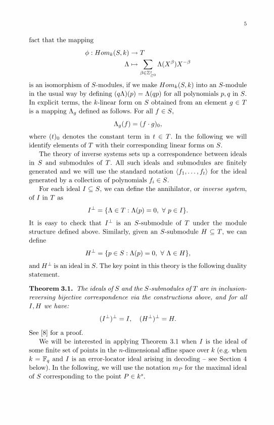
fact that the mapping
φ : Homk(S, k)→ T
Λ 7→∑
β∈Zs≥0
Λ(Xβ)X−β
is an isomorphism of S-modules, if we make Homk(S, k) into an S-modulein the usual way by defining (qΛ)(p) = Λ(qp) for all polynomials p, q in S.In explicit terms, the k-linear form on S obtained from an element g ∈ Tis a mapping Λg defined as follows. For all f ∈ S,
Λg(f) = (f · g)0,
where (t)0 denotes the constant term in t ∈ T . In the following we willidentify elements of T with their corresponding linear forms on S.
The theory of inverse systems sets up a correspondence between idealsin S and submodules of T . All such ideals and submodules are finitelygenerated and we will use the standard notation 〈f1, . . . , ft〉 for the idealgenerated by a collection of polynomials fi ∈ S.
For each ideal I ⊆ S, we can define the annihilator, or inverse system,of I in T as
I⊥ = Λ ∈ T : Λ(p) = 0, ∀ p ∈ I.
It is easy to check that I⊥ is an S-submodule of T under the modulestructure defined above. Similarly, given an S-submodule H ⊆ T , we candefine
H⊥ = p ∈ S : Λ(p) = 0, ∀ Λ ∈ H,
and H⊥ is an ideal in S. The key point in this theory is the following dualitystatement.
Theorem 3.1. The ideals of S and the S-submodules of T are in inclusion-reversing bijective correspondence via the constructions above, and for allI,H we have:
(I⊥)⊥ = I, (H⊥)⊥ = H.
See [8] for a proof.We will be interested in applying Theorem 3.1 when I is the ideal of
some finite set of points in the n-dimensional affine space over k (e.g. whenk = Fq and I is an error-locator ideal arising in decoding – see Section 4below). In the following, we will use the notation mP for the maximal idealof S corresponding to the point P ∈ ks.

May 10, 2007 8:8 WSPC - Proceedings Trim Size: 9in x 6in ws-procs9x6
6
Theorem 3.2. Let P1, . . . , Pt be points in ks and let
I = mP1 ∩ · · · ∩mPt .
The submodule of T corresponding to I has the form
H = I⊥ = (mP1)⊥ ⊕ · · · ⊕ (mPt
)⊥.
Proof. In Proposition 2.6 of [11], Geramita shows that (I∩J)⊥ = I⊥+J⊥
for any pair of ideals. The idea is that I⊥ and J⊥ can be constructed degreeby degree, so the corresponding statement from the linear algebra of finite-dimensional vector spaces applies. The equality (I + J)⊥ = I⊥ ∩ J⊥ alsoholds from linear algebra (and no finite-dimensionality is needed). The sumin the statement of the Lemma is a direct sum since mPi
+ ∩j 6=imPj= S,
hence (mPi)⊥ ∩ Σj 6=i(mPj )
⊥ = 0.
We can also give a concrete description of the elements of (mP )⊥.
Theorem 3.3. Let P = (a1, . . . , as) ∈ As over k, and let Li be the coordi-nate hyperplane Xi = ai containing P .
(1) (mP )⊥ is the cyclic S-submodule of T generated by
hP =∑
u∈Zs≥0
PuX−u,
where if u = (u1, . . . , us), Pu denotes the product au11 · · · aus
s (Xu eval-uated at P ).
(2) f · hP = f(P )hP for all f ∈ S, and the submodule (mP )⊥ is a one-dimensional vector space over k.
(3) Let ILibe the ideal 〈Xi− ai〉 in S (the ideal of Li). Then (ILi
)⊥ is thesubmodule of T generated by hLi
=∑∞
j=0 ajiX
−ji .
(4) In T , we have hP =∏s
i=1 hLi.
Proof. (1) First, if f ∈ mP , and g ∈ S is arbitrary then
Λg·hP(f) = (f · (g · hP ))0 = ((fg) · hP )0 = f(P )g(P ) = 0.
Hence the S-submodule 〈hP 〉 is contained in (mP )⊥. Conversely, if h ∈(mP )⊥, then for all f ∈ mP ,
0 = Λh(f) = (f · h)0.
An easy calculation using all f of the form f = xβ − aβ ∈ mP shows thath = chP for some constant c. Hence (mP )⊥ = 〈hP 〉.

May 10, 2007 8:8 WSPC - Proceedings Trim Size: 9in x 6in ws-procs9x6
7
(2) The second claim follows by a direct computation of the contractionproduct f · hp.
(3) Let f ∈ ILi (so f vanishes at all points of the hyperplane Li), andlet g ∈ S be arbitrary. Then
Λg·hLi(f) = (f · (g · hLi))0 = ((fg) · hLi)0
= f(0, . . . , 0, ai, 0, . . . , 0)g(0, . . . , 0, ai, 0, . . . , 0) = 0,
since the only nonzero terms in the product ((fg) · hLi) come from mono-
mials in fg containing only the variable Xi. Hence 〈hLi〉 ⊂ T is contained
in I⊥Li. Then we show the other inclusion as in the proof of (1).
(4) We have mP = IL1 + · · ·+ILs. Hence (mP )⊥ = (IL1)
⊥∩· · ·∩(ILs)⊥,
and the claim follows. We note that a more explicit form of this equationcan be derived by the formal geometric series summation formula:
hP =∑
u∈Zs≥0
PuX−u =s∏
i=1
11− ai/Xi
=s∏
i=1
hLi .
Both the polynomial ring S and the formal power series ring T can beviewed as subrings of the field of formal Laurent series in the inverse vari-ables,
K = k((X−11 , . . . , X−1
s )),
which is the field of fractions of T . Hence the (full) product fg for f ∈ Sand g ∈ T is an element of K. The contraction product f · g is a projectionof fg into T ⊂ K. We can also consider the projection of fg into S+ =〈X1, . . . , Xs〉 ⊂ S ⊂ K under the linear projection with kernel spanned byall monomials not in S+. We will denote this by (fg)+.
4. The Key Equation and its Relation to the BMSAlgorithm
Let C be one of the codes C = ev(V ) or ev(V )⊥ constructed from anorder domain R ∼= Fq[X1, . . . , Xs]/I. Consider an error vector e ∈ Fn
q
(where entries are indexed by the elements of the set XR(Fq)). In theusual terminology, the error-locator ideal corresponding to e is the idealIe ⊂ Fq[X1, . . . , Xs] defining the set of error locations:
Ie = f ∈ Fq[X1, . . . , Xs] : f(P ) = 0, ∀ P s.t. eP 6= 0.
We will use a slightly different notation and terminology in the followingbecause we want to make a systematic use of the observation that this ideal

May 10, 2007 8:8 WSPC - Proceedings Trim Size: 9in x 6in ws-procs9x6
8
depends only on the support of e, not on the error values. Indeed, manydifferent error vectors yield the same ideal defining the error locations. Forthis reason we will introduce E = P : eP 6= 0, and refer to the error-locator ideal for any e with supp(e) = E as IE .
For each monomial Xu ∈ Fq[X1, . . . , Xs], we let
Eu = 〈e, ev(Xu)〉 =∑
P∈XR(Fq)
ePPu (2)
be the corresponding syndrome of the error vector. (As in Theorem 3.3, Pu
is shorthand notation for the evaluation of the monomial Xu at P .)In the practical decoding situation, of course, for a code C = ev(V )⊥
where V is a subspace of R spanned by some set of monomials, only theEu for the Xu in a basis of V are initially known from the received word.
In addition, the elements of the ideal I+〈Xq1−X1, . . . , X
qs−Xs〉 defining
the set XR(Fq) give relations between the Eu. Indeed, the Eu for u in theordered basis ∆ for R with all components ≤ q−1 determine all the others,and these syndromes still satisfy additional relations. Thus the Eu are, ina sense, highly redundant.
To package the syndromes into a single algebraic object, following [12],we define the syndrome series
Se =∑
u∈Zs≥0
EuX−u
in the formal power series ring T = Fq[[X−11 , . . . , X−1
s ]]. (This depends bothon the set of error locations E and on the error values.) As in Section 3, wehave a natural interpretation for Se as an element of the dual space of thering S = Fq[X1, . . . , Xs].
The following expression for the syndrome series Se will be fundamental.We substitute from Eq. (2) for the syndrome Eu and change the order ofsummation to obtain:
Se =∑
u∈Zn≥0
EuX−u =
∑u∈Zn
≥0
∑P∈XR(Fq)
ePPuX−u
=∑
P∈XR(Fq)
eP
∑u∈Zn
≥0
PuX−u =∑
P∈XR(Fq)
ePhP ,
where hP is the generator of (mP )⊥ from Theorem 3.3. The sum heretaking the terms with eP 6= 0, gives the decomposition of Se in the directsum expression for I⊥E as in Theorem 3.2.
The first statement in the following Theorem is well-known; it is a trans-lation of the standard fact that error-locators give linear recurrences on the
May 10, 2007 8:8 WSPC - Proceedings Trim Size: 9in x 6in ws-procs9x6
9
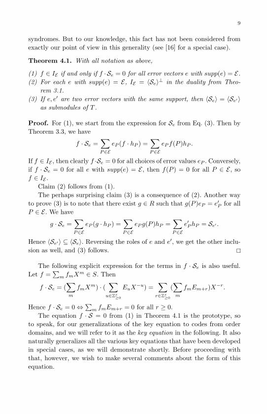
syndromes. But to our knowledge, this fact has not been considered fromexactly our point of view in this generality (see [16] for a special case).
Theorem 4.1. With all notation as above,
(1) f ∈ IE if and only if f · Se = 0 for all error vectors e with supp(e) = E.(2) For each e with supp(e) = E, IE = 〈Se〉⊥ in the duality from Theo-
rem 3.1.(3) If e, e′ are two error vectors with the same support, then 〈Se〉 = 〈Se′〉
as submodules of T .
Proof. For (1), we start from the expression for Se from Eq. (3). Then byTheorem 3.3, we have
f · Se =∑P∈E
eP (f · hP ) =∑P∈E
eP f(P )hP .
If f ∈ IE , then clearly f ·Se = 0 for all choices of error values eP . Conversely,if f · Se = 0 for all e with supp(e) = E , then f(P ) = 0 for all P ∈ E , sof ∈ IE .
Claim (2) follows from (1).The perhaps surprising claim (3) is a consequence of (2). Another way
to prove (3) is to note that there exist g ∈ R such that g(P )eP = e′P for allP ∈ E . We have
g · Se =∑P∈E
eP (g · hP ) =∑P∈E
eP g(P )hP =∑P∈E
e′PhP = Se′ .
Hence 〈Se′〉 ⊆ 〈Se〉. Reversing the roles of e and e′, we get the other inclu-sion as well, and (3) follows.
The following explicit expression for the terms in f · Se is also useful.Let f =
∑m fmX
m ∈ S. Then
f · Se = (∑m
fmXm) · (
∑u∈Zs
≥0
EuX−u) =
∑r∈Zs
≥0
(∑m
fmEm+r)X−r.
Hence f · Se = 0⇔∑
m fmEm+r = 0 for all r ≥ 0.The equation f · S = 0 from (1) in Theorem 4.1 is the prototype, so
to speak, for our generalizations of the key equation to codes from orderdomains, and we will refer to it as the key equation in the following. It alsonaturally generalizes all the various key equations that have been developedin special cases, as we will demonstrate shortly. Before proceeding withthat, however, we wish to make several comments about the form of thisequation.

May 10, 2007 8:8 WSPC - Proceedings Trim Size: 9in x 6in ws-procs9x6
10
Comparing the equation f ·Se = 0 with the familiar form Eq. (1), severaldifferences may be apparent. First, note that the syndrome series Se willnot be entirely known from the received word in the decoding situation.The same is true in the Reed-Solomon case, of course. The polynomial S inthe congruence in Eq. (1) involves only the known syndromes, and Eq. (1)is derived by accounting for the other terms in the full syndrome series.With a truncation of Se in our situation we would obtain a similar type ofcongruence (see the discussion following Eq. (8) below, for instance). It isapparently somewhat rare, however, that the portion of Se known from thereceived word suffices for decoding up to half the minimum distance of thecode.
Another difference is that there is no apparent analog of the error-evaluator polynomial g from Eq. (1) in the equation f · Se = 0. The way toobtain error evaluators in this situation is to consider the “purely positiveparts” (fSe)+ for certain solutions of our key equation.
We now turn to several examples that show how our key equation relatesto several special cases that have appeared in the literature.
Example 4.1. We begin by providing more detail on the precise relationbetween Theorem 4.1, part (1) in the case of a Reed-Solomon code andthe usual key equation from Eq. (1). These codes are constructed from theorder domain R = Fq[X] (where Γ = Z≥0 and ρ is the degree mapping).The key equation Eq. (1) applies to the code Ev` = ev(V`), where V` =Span1, X,X2, . . . , X`−1, and the evaluation takes place at all Fq-rationalpoints on the affine line, omitting 0.
Our key equation in this case is closely related to, but not preciselythe same, as Eq. (1). The reason for the difference is that Theorem 4.1 isapplied to the dual code C` = Ev⊥` rather than Ev`. Starting from Eq. (3)and using the formal geometric series summation formula as in Theorem 3.3part (4), we can write:
Se =∑P∈E
eP
∑u≥0
PuX−u = X
∑P∈E eP
∏Q∈E,Q 6=P (X −Q)∏
P∈E(X − P ).
Hence, in this formulation, Se = Xq/p, where p is the generator of theactual error locator ideal (not the ideal of the inverses of the error locations).Moreover if we take f = p in Theorem 4.1, then
(pSe)+ = Xq (3)
gives an analog of the error evaluator. There are no “mixed terms” in theproducts fSe in this one-variable situation.

May 10, 2007 8:8 WSPC - Proceedings Trim Size: 9in x 6in ws-procs9x6
11
Example 4.2. The key equation for s-dimensional cyclic codes introducedby Chabanne and Norton in [12] has the form
σSe =
(s∏
i=1
Xi
)g, (4)
where σ =∏s
i=1 σi(Xi), and σi is the univariate generator of the eliminationideal IE∩Fq[Xi]. Our version of the Reed-Solomon key equation from Eq. (3)is a special case of Eq. (4). Moreover, Eq. (4) is clearly the special case ofTheorem 4.1, part (1) for these codes where f = σ is the particular errorlocator polynomial
∏si=1 σi(Xi) ∈ IE . For this special choice of error locator,
σ · Se = 0, and (σSe)+ = (∏s
i=1Xi) g for some polynomial g. We see thatSe can be written as
Se =∑P
ePhP =
(s∏
i=1
Xi
)∑P
eP1∏s
i=1(Xi −Xi(P )),
and the product σSe = (σSe)+ reduces to a polynomial (again, there areno “mixed terms”).
Example 4.3. We now turn to the key equation for one-point geometricGoppa codes introduced by O’Sullivan in [6]. Let X be a smooth curveover Fq of genus g, and consider one-point codes constructed from R =∪∞m=0L(mQ) for some point Q ∈ X (Fq), O’Sullivan’s key equation has theform:
fωe = φ. (5)
Here ωe is the syndrome differential, which can be expressed as
ωe =∑
P∈X (Fq)
ePωP,Q,
where ωP,Q is the differential of the third kind on Y with simple poles atP and Q, no other poles, and residues resP (ωP,Q) = 1, resQ(ωP,Q) = −1.For any f ∈ R, we have
resQ(fωe) =∑P
eP f(P ),
the syndrome of e corresponding to f . (We only defined syndromes formonomials above; taking a presentation R = Fq[X1, . . . , Xs]/I, however,any f ∈ R can be expressed as a linear combination of monomials and thesyndrome of f is defined accordingly.) The right-hand side of Eq. (5) isalso a differential. In this situation, Eq. (5) furnishes a key equation in the

May 10, 2007 8:8 WSPC - Proceedings Trim Size: 9in x 6in ws-procs9x6
12
following sense: f is an error locator (i.e. f is in the ideal of R correspondingto IE) if and only if φ has poles only at Q. In the special case that (2g−2)Qis a canonical divisor (the divisor of zeroes of some differential of the firstkind ω0 on X ), Eq. (5) can be replaced by the equivalent equation foe = g,where oe = ωe/ω0 and g = φ/ω0 are rational functions on X . Since ω0 iszero only at Q, the key equation is now that f is an error locator if andonly if Eq. (5) is satisfied for some g ∈ R.
For instance, when X is a smooth plane curve V (F ) over Fq definedby F ∈ Fq[X,Y ], with a single smooth point Q at infinity, then it is truethat (2g − 2)Q is canonical. O’Sullivan shows in Example 4.2 of [6] (usinga slightly different notation) that
oe =∑
P∈X (Fq)
ePHP , (6)
where if P = (a, b), then HP = F (a,Y )(X−a)(Y−b) . This is a function with a pole
of order 1 at P , a pole of order 2g − 1 at Q, and no other poles.To relate this to our approach, note that we may assume from the start
that Q = (0 : 1 : 0) and that F is taken in the form
F (X,Y ) = Xβ − cY α +G(X,Y )
for some relatively prime α < β generating the value semigroup at Q. Everyterm in G has (α, β)-weight less than αβ. First we rearrange to obtain
HP =F (a, Y )
(X − a)(Y − b)=
(aβ −Xβ) + F (X,Y ) + (G(a, Y )−G(X,Y ))(X − a)(Y − b)
The F (X,Y ) term in the numerator does not depend on P . We can collectthose terms in the sum Eq. (6) and factor out the F (X,Y ). We will seeshortly that those terms can in fact be ignored. The G(a, Y )−G(X,Y ) inthe numerator furnish terms that go into the error evaluator g here. Theremaining portion is
−(Xβ − aβ)(X − a)(Y − b)
= −Xβ−1
Y
β−1∑i=0
∞∑j=0
aibj
XiY j.
The sum here looks very much like that defining our hP from Theorem 3.3,except that it only extends over the monomials in complement of 〈LT (F )〉.Call this last sum h′P . As noted before the full series hP (and consequentlyS) are redundant. For example, every ideal contained in mP (for instancethe ideal I = 〈F 〉 defining the curve), produces relations between the co-efficients. From the duality theorem, Theorem 3.1, we have that I ⊂ mP
implies (mP )⊥ ⊂ I⊥, so F · hP = 0.
May 10, 2007 8:8 WSPC - Proceedings Trim Size: 9in x 6in ws-procs9x6
13
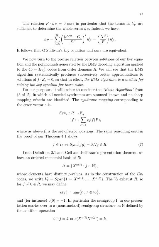
The relation F · hP = 0 says in particular that the terms in h′P aresufficient to determine the whole series hP . Indeed, we have
hP =∞∑
i=0
((cY α −G)
Xβ
)i
h′P =(Xβ
F
)h′P .
It follows that O’Sullivan’s key equation and ours are equivalent.
We now turn to the precise relation between solutions of our key equa-tion and the polynomials generated by the BMS decoding algorithm appliedto the C` = Ev⊥` codes from order domains R. We will see that the BMSalgorithm systematically produces successively better approximations tosolutions of f · Se = 0, so that in effect, the BMS algorithm is a method forsolving the key equation for these codes.
For our purposes, it will suffice to consider the “Basic Algorithm” from§3 of [5], in which all needed syndromes are assumed known and no sharpstopping criteria are identified. The syndrome mapping corresponding tothe error vector e is
Syne : R → Fq
f 7→∑P∈E
eP f(P ),
where as above E is the set of error locations. The same reasoning used inthe proof of our Theorem 4.1 shows
f ∈ IE ⇔ Syne(fg) = 0,∀g ∈ R. (7)
From Definition 2.1 and Geil and Pellikaan’s presentation theorem, wehave an ordered monomial basis of R:
∆ = Xα(j) : j ∈ N,
whose elements have distinct ρ-values. As in the construction of the Ev`
codes, we write V` = Span1 = Xα(1), . . . , Xα(`). The V` exhaust R, sofor f 6= 0 ∈ R, we may define
o(f) = min` : f ∈ V`,
and (for instance) o(0) = −1. In particular the semigroup Γ in our presen-tation carries over to a (nonstandard) semigroup structure on N defined bythe addition operation
i⊕ j = k ⇔ o(Xα(i)Xα(j)) = k.

May 10, 2007 8:8 WSPC - Proceedings Trim Size: 9in x 6in ws-procs9x6
14
Given f ∈ R, one defines
span(f) = min` : ∃g ∈ V` s.t. Syne(fg) 6= 0fail(f) = o(f)⊕ span(f).
When f ∈ IE , span(f) = fail(f) =∞.The BMS algorithm, then, is an iterative process which produces a
Grobner basis for IE with respect to a certain monomial order >. Thestrategy is to maintain data structures for all m ≥ 1 as follows. The ∆m
are an increasing sequence of sets of monomials, converging to the monomialbasis for IE as m→∞, and δm is the set of maximal elements of ∆m withrespect to > (the “interior corners of the footprint”). Similarly, we considerthe complement Σm of ∆m, and σm, the set of minimal elements of Σm
(the “exterior corners”). For sufficiently large m, the elements of σm willbe the leading terms of the elements of the Grobner basis of IE , and Σm
will be the set of monomials in LT>(IE).For eachm, the algorithm also produces collections of polynomials Fm =
fm(s) : s ∈ σm and Gm = gm(c) : c ∈ δm satisfying:
o(fm(s)) = s, fail(fm(s)) > m
span(gm(c)) = c, fail(gm(c)) ≤ m.
In the limit as m→∞, by Eq. (7), the Fm yield the Grobner basis for IE .We record the following simple observation.
Theorem 4.2. With all notation as above, suppose f ∈ R satisfies o(f) =s, fail(f) > m. Then
f · Se ≡ 0 mod Ws,m,
where Ws,m is the Fq-vector subspace of the formal power series ring T
spanned by the X−α(j) such that s⊕ j > m.
Proof. By the definition, fail(f) > m means that Syne(fXα(k)) = 0 forall k with o(f) ⊕ k ≤ m. By the definitions of Se and the contractionproduct, Syne(fXα(k)) is exactly the coefficient of X−α(k) in f · Se.
The subspace Ws,m in Theorem 4.2 depends on s = o(f). In our situ-ation, though, note that if s′ = maxo(f) : f ∈ Fm, then Theorem 4.2implies
f · Se ≡ 0 mod Ws′,m (8)

May 10, 2007 8:8 WSPC - Proceedings Trim Size: 9in x 6in ws-procs9x6
15
for all f = fm(s) in Fm. Moreover, only finitely many terms from Se enterinto any one of these congruences, so Eq. (8) is, in effect, a sort of generalanalog of Eq. (1).
The fm(s) from Fm can be understood as approximate solutions of keyequation (where the goodness of the approximation is determined by thesubspaces Ws′,m, a decreasing chain, tending to 0 in T , as m → ∞).The BMS algorithm thus systematically constructs better and better ap-proximations to solutions of the key equation. O’Sullivan’s stopping criteria(see [5]) show when further steps of the algorithm make no changes. TheFeng-Rao theorem shows that any additional syndromes needed for this canbe determined by the majority-voting process when wt(e) ≤ bdF R(C`)−1
2 c.We conclude by noting that O’Sullivan has also shown in [6] that, for
codes from curves, the BMS algorithm can be slightly modified to computeerror locators and error evaluators simultaneously in the situation studiedin Example 4.3. The same is almost certainly true in our general setting,although we have not worked out all the details.
Acknowledgements
Thanks go to Mike O’Sullivan and Graham Norton for comments on anearlier version prepared while the author was a visitor at MSRI. Researchat MSRI is supported in part by NSF grant DMS-9810361.
References
[1] T. Høholdt, R. Pellikaan, and J. van Lint, Algebraic Geometry Codes, in:Handbook of Coding Theory, W. Huffman and V. Pless, eds. (Elsevier, Am-sterdam, 1998), 871-962.
[2] M. O’Sullivan, New Codes for the Berlekamp-Massey-Sakata Algorithm, Fi-nite Fields Appl. 7 (2001), 293-317.
[3] O. Geil and R. Pellikaan, On the Structure of Order Domains, Finite FieldsAppl. 8 (2002), 369-396.
[4] J. Little, The Ubiquity of Order Domains for the Construction of ErrorControl Codes, Advances in Mathematics of Communications 1 (2007), 151-171.
[5] M. O’Sullivan, A Generalization of the Berlekamp-Massey-Sakata Algo-rithm, preprint, 2001.
[6] M. O’Sullivan, The key equation for one-point codes and efficient error eval-uation, J. Pure Appl. Algebra 169 (2002), 295-320.
[7] F.S. Macaulay, Algebraic Theory of Modular Systems, Cambridge Tracts inMathematics and Mathematical Physics, v. 19, (Cambridge University Press,Cambridge, UK, 1916).
May 10, 2007 8:8 WSPC - Proceedings Trim Size: 9in x 6in ws-procs9x6
16
[8] D.G. Northcott, Injective envelopes and inverse polynomials, J. LondonMath. Soc. (2) 8 (1974), 290-296.
[9] J. Emsalem and A. Iarrobino, Inverse System of a Symbolic Power, I, J.Algebra 174 (1995), 1080-1090.
[10] B. Mourrain, Isolated points, duality, and residues J. Pure Appl. Algebra117/118 (1997), 469-493.
[11] A. Geramita, Inverse systems of fat points, Waring’s problem, secant vari-eties of Veronese varieties and parameter spaces for Gorenstein ideals, TheCurves Seminar at Queen’s (Kingston, ON) X (1995), 2–114.
[12] H. Chabanne and G. Norton, The n-dimensional key equation and a decodingapplication, IEEE Trans. Inform Theory 40 (1994), 200-203.
[13] G.H. Norton, On n-dimensional Sequences. I, II, J. Symbolic Comput. 20(1995), 71-92, 769-770.
[14] G.H. Norton, On Shortest Linear Recurrences, J. Symbolic Comput. 27(1999), 323-347.
[15] G.H. Norton and A. Salagean, On the key equation over a commutative ring,Designs, Codes and Cryptography 20 (2000), 125-141.
[16] J. Althaler and A. Dur, Finite linear recurring sequences and homogeneousideals, Appl. Algebra. Engrg. Comm. Comput. 7 (1996), 377-390.

May 10, 2007 8:8 WSPC - Proceedings Trim Size: 9in x 6in ws-procs9x6
17
A Grobner representation for linear codes
M. Borges-Quintana∗ and M. A. Borges-Trenard∗∗
Departamento de Matematicas, Universidad de Oriente,
Santiago de Cuba, Cuba∗ E-mail: [email protected]
∗∗ E-mail: [email protected]
E. Martınez-Moro
Departamento de Matematica Aplicada,
Universidad de Valladolid
Valladolid, SpainE-mail: [email protected]
This work explains the role of Moller algorithm and Grobner technology in
the description of linear codes. We survey several results of the authors about
FGLM techniques applied to linear codes as well as some results concerningthe structure of the code.
Keywords: Linear code; Moller algorithm; Grobner representation.
1. Introduction
In this paper we survey several results of the authors about the nice roleof Grobner bases technology and Moller FGLM techniques (FGLM standsfor Faugere, Gianni, Lazard and Mora, see [7]) applied to linear codes overfinite fields. This work is intended as an attempt to clarify and summa-rize as well as unify several previous works of the authors [3–5]. We followTeo Mora’s approach for the presentation of Grobner bases theory [15] andstudy how this theory can describe several combinatorial properties of linearcodes. Section 2 contains a brief summary of Moller algorithm and relatedconcepts. In the third section we set up the notation and terminology of thestructures associated to a linear code. In section 4 we will look more closelyat those structures and we will indicate the resemblances with the Grobnerbases technology, with special emphasis on the binary case. Although it isnot the main goal of this survey, in section 5 we point out several directionsof how these techniques can be used to derive solutions for several cod-

May 10, 2007 8:8 WSPC - Proceedings Trim Size: 9in x 6in ws-procs9x6
18
ing theory problems such that gradient decoding, combinatorial problems,minimal codeword bases, etc.
2. Moller’s algorithm
No attempt has been made here to develop the whole theory of Molleralgorithm. We will touch only a few aspects of the theory useful for ourpaper. For a thorough treatment of Grobner bases we refer the reader to[15] and for a recent survey on Moller algorithm and FGLM techniques werefer to [16].
As usual we will denote by X the finite set of variables x1, . . . , xn andif a = (a1, . . . , an) ∈ Nn we will denote xa = xa1
1 . . . xann . Let P = F[X] the
polynomial ring over the field F and T = xa | a ∈ Nn the set of terms.Let ≺ be a Notherian semigroup ordering on the set T (this is called eitherterm ordering or admissible ordering), for each f =
∑τ∈T c(f, τ)τ ∈ P we
write T(f) = max≺τ ∈ T | c(f, τ) 6= 0 and lc(f) = c(f,T(f)) for theleading term and leading coefficient of f respectively.
If F ⊆ P then T(F ) = T(f) | f ∈ F and for each ideal I ⊂ P weconsider the semigroup ideal T(I) and the Grobner escalier N(I) = I\T(I).It is well known that P ∼= I
⊕spanF (N(I)) as F-vector spaces, which in
turn gives a unique canonical form for each element f ∈ P
Can(f, I,≺) =∑
τ∈N(I)
c(f, τ,≺)τ ∈ spanF (N(I)) (1)
such that f − Can(f, I,≺) ∈ I.Let G≺(I) denote the unique minimal basis of T≺(I), a set G ⊆ I is
said to be a Grobner basis of the ideal I with respect to (w.r.t. for short)the ordering ≺ if the set T≺(G) generates T≺(I) as a semigroup ideal. Thereduced Grobner basis of the ideal I w.r.t. ≺ is the set
Red≺(I) = τ − Can(τ, I,≺) | τ ∈ G≺(I) , (2)
and the border basis of I w.r.t. ≺ is
Bor≺(I) = τ − Can(τ, I,≺) | τ ∈ B≺(I) , (3)
thus the border basis of the ideal I is a Grobner basis of I that containsthe reduced Grobner basis.
An ideal I ⊂ P is zero-dimensional if dimF(P/I) < ∞ where dimFdenotes the dimension as F vector space. From now on we will make the as-sumption that our ideal I is zero-dimensional. The following representationwill play a central role in the paper

May 10, 2007 8:8 WSPC - Proceedings Trim Size: 9in x 6in ws-procs9x6
19
Definition 2.1 (Grobner representation). Let I ⊂ P be a zero-dimensional ideal and s = dimF(P/I). A Grobner representation of I isthe assignment of
(1) a set N = τ1, . . . , τs ⊆ N≺(I)(2) and a set of square matrices
φ =φ(r) =
(ar
ij
)si,j=1
| r = 1, . . . , n , arij ∈ F
such that
P/I = spanF(N), τixr ≡Is∑
j=1
arijτj ∀ 1 ≤ i ≤ s, 1 ≤ r ≤ n.
We call φ the matphi structure and φ(r) the matphi matrices. Theyfirst appear in [7] in a procedure to describe the multiplication structure inthe quotient algebra P/I. Note that φ is independent of the particular setN of representatives of P/I we have chosen. For each f ∈ P the Grobnerdescription of f in terms of the Grobner representation (N,φ) is
Rep(f,N) = (γ(f, τ1), . . . , γ(f, τs)) ∈ Fs
such that f −∑s
i=1 γ(f, τi)τi ∈ I.We write P∗ = HomF(P,F) to denote the vector space of all linear
functionals ` : P → F. P∗ is a P-module defined by the product
(` · f)(g) = `(fg) ` ∈ P∗, f, g ∈ P
where
`(f) =∑τ∈T
c(f, τ)`(τ).
Two ordered sets L = `1, . . . , `r ⊂ P∗, q = q1, . . . , qs ⊂ P are said tobe triangular if r = s and `i(qj) = 0 for all i < j. For each F-vector spaceL ⊆ P∗ we define the ideal P(L) = g ∈ P | `(g) = 0, ∀` ∈ L.
Proposition 2.1 (Moller’s theorem). Let ≺ be any term ordering andL = `1, . . . , `s ⊂ P∗ be a set of functionals such that I = P(L)is a zero-dimensional ideal. Then there are a r ∈ N, an order idealN = τ1, . . . , τr ⊂ T and two ordered subsets
Λ = λ1, . . . , λr ⊂ L, q = q1, . . . , qr ⊂ P
such that
(1) r = deg(I) = dimF (spanF(L)).
May 10, 2007 8:8 WSPC - Proceedings Trim Size: 9in x 6in ws-procs9x6
20
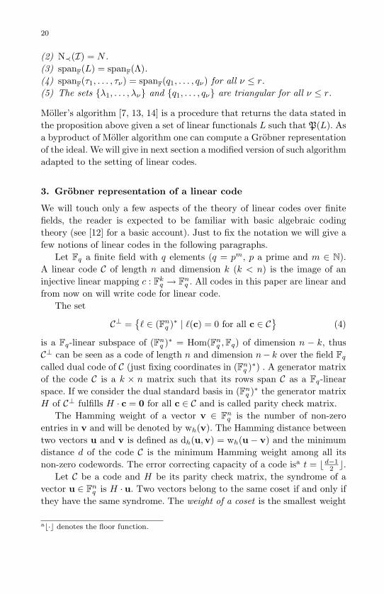
(2) N≺(I) = N .(3) spanF(L) = spanF(Λ).(4) spanF(τ1, . . . , τν) = spanF(q1, . . . , qν) for all ν ≤ r.(5) The sets λ1, . . . , λν and q1, . . . , qν are triangular for all ν ≤ r.
Moller’s algorithm [7, 13, 14] is a procedure that returns the data stated inthe proposition above given a set of linear functionals L such that P(L). Asa byproduct of Moller algorithm one can compute a Grobner representationof the ideal. We will give in next section a modified version of such algorithmadapted to the setting of linear codes.
3. Grobner representation of a linear code
We will touch only a few aspects of the theory of linear codes over finitefields, the reader is expected to be familiar with basic algebraic codingtheory (see [12] for a basic account). Just to fix the notation we will give afew notions of linear codes in the following paragraphs.
Let Fq a finite field with q elements (q = pm, p a prime and m ∈ N).A linear code C of length n and dimension k (k < n) is the image of aninjective linear mapping c : Fk
q → Fnq . All codes in this paper are linear and
from now on will write code for linear code.The set
C⊥ =` ∈ (Fn
q )∗ | `(c) = 0 for all c ∈ C
(4)
is a Fq-linear subspace of (Fnq )∗ = Hom(Fn
q ,Fq) of dimension n − k, thusC⊥ can be seen as a code of length n and dimension n− k over the field Fq
called dual code of C (just fixing coordinates in (Fnq )∗) . A generator matrix
of the code C is a k × n matrix such that its rows span C as a Fq-linearspace. If we consider the dual standard basis in (Fn
q )∗ the generator matrixH of C⊥ fulfills H · c = 0 for all c ∈ C and is called parity check matrix.
The Hamming weight of a vector v ∈ Fnq is the number of non-zero
entries in v and will be denoted by wh(v). The Hamming distance betweentwo vectors u and v is defined as dh(u,v) = wh(u− v) and the minimumdistance d of the code C is the minimum Hamming weight among all itsnon-zero codewords. The error correcting capacity of a code isa t = bd−1
2 c.Let C be a code and H be its parity check matrix, the syndrome of a
vector u ∈ Fnq is H · u. Two vectors belong to the same coset if and only if
they have the same syndrome. The weight of a coset is the smallest weight
ab·c denotes the floor function.

May 10, 2007 8:8 WSPC - Proceedings Trim Size: 9in x 6in ws-procs9x6
21
of a vector in the coset and any vector of smallest weight in the coset iscalled a coset leader. Every coset of a weight at most t has a unique cosetleader thus the equation
H · u = H · e
has a unique minimal weight solution e among the coset leaders of the codeC for each u ∈ B(C, t) called the error vector of u where
B(C, t) =u ∈ Fn
q | ∃c ∈ C such that dh(u, c) ≤ t.
If we fix α a root of an irreducible polynomial of degree m over Fp wecan represent any element of Fq as a0 +a1α+ · · ·+am−1α
m−1 with ai ∈ Fp
for all i. Let T be the set of terms, i.e., the free commutative monoidgenerated by the nm variables X = x11, . . . , x1m, . . . , xn1, . . . , xnm, andconsider the morphism of monoids from T onto Fn
q :
ψ : T →Fnq
xij 7→(0, . . . , 0, αj−1︸ ︷︷ ︸i
, 0, . . . , 0)
and, by morphism extension,n∏
i=1
m∏j=1
xβij
ij 7→((∑m
j=1 β1jαj−1), . . . ,
(∑mj=1 βnjα
j−1))
(5)
We say that∏n
i=1
∏mj=1 x
βij
ij ∈ T is in standard representation if βij < p
for all i, j.A code C defines an equivalence relation RC in Fn
q given by
(u,v) ∈ RC ⇔ u− v ∈ C. (6)
This relation can be translated to xa,xb ∈ T as follows
xa ≡C xb ⇔ (ψ(xa), ψ(xb)) ∈ RC ⇔ ξC(xa) = ξC(xb) (7)
where ξC(xa) = H ·ψ(xa) is the transition from the monoid T to the set ofsyndromes associated to the word u through ψ.
The support of xa ∈ T will be the set of variables in X that divide xa
and is denoted by supp(xa) whereas the indexb of xa is defined as
ind(xa) = i | ∃j ∈ 1, . . . ,m such that xij ∈ supp(xa) . (8)
For the sake of simplicity in notation from now on we write the set of nmvariables as xk, where k = (i− 1)m+ j instead of xij .
bNote that this definition for elements in T corresponds to the definition of support ofthe corresponding vector in Fn
q .

May 10, 2007 8:8 WSPC - Proceedings Trim Size: 9in x 6in ws-procs9x6
22
Definition 3.1 (Error vector ordering). We say that xa is less thanxb w.r.t. the error-vector ordering, and denote it by xa ≺e xb, if one of thefollowing conditions holds:
(1) |ind(xa)| < |ind(xb)|.(2) |ind(xa)| = |ind(xb)| and xa ≺ad xb, where ≺ad denotes an arbitrary
but fixed admissible ordering on T .
Note that the error vector ordering is a total degree compatible orderingon T but in general it is not admissible (the multiplicative property ofadmissible orderings sometimes fails). For example let the vector space F7
3
and ≺ad be the degree reverse lexicographical ordering, we have
x1x5 ≺e x3x7 but x1x5x7 e x3x27.
Anyway the error vector ordering still shares two important properties ofadmissible orderings
(1) 1 ≺e xa for all a 6= 0.(2) xa ≺e xaxi for all i = 1, . . . , n.
The two properties above will allow us to construct a Grobner represen-tation of a code using a sort of Moller algorithm as an analogue of theGrobner representation of a zero-dimensional ideal in Definition 2.1.
Definition 3.2 (Grobner representation of a code). Let C be a Fq-linear code of dimension k. A Grobner representation of C is the assignmentof
• a set N = τ1, . . . , τqn−k ⊆ T• and a function φ : N ×X → N (the function Matphi)
such that
(1) 1 ∈ N .(2) If τ1, τ2 ∈ N and τ1 6= τ2 then ξC(τ1) 6= ξC(τ2).(3) For all τ ∈ N \ 1 there exist x ∈ X such that τ = τ ′x and τ ′ ∈ N .(4) ξC(φ(τ, xi)) = ξC(τxi).
Note that N has as many elements as different syndromes has code C andcondition (2) states that two different elements in N have different syn-drome. The function φ gives us a multiplicative structure that is inde-pendent of the particular set N of representative elements of the cosetsdetermined by the code (i.e. φ can be seen as a function on the cosets ofthe code).
May 10, 2007 8:8 WSPC - Proceedings Trim Size: 9in x 6in ws-procs9x6
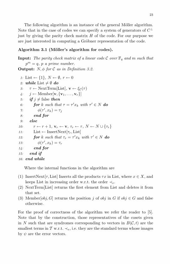
23
The following algorithm is an instance of the general Moller algorithm.Note that in the case of codes we can specify a system of generators of C⊥
just by giving the parity check matrix H of the code. For our purpose weare just interested in computing a Grobner representation of the code.
Algorithm 3.1 (Moller’s algorithm for codes).
Input: The parity check matrix of a linear code C over Fq and m such thatpm = q, p a prime number.
Output: N,φ for C as in Definition 3.2.
1: List← 1, N ← ∅, r ← 02: while List 6= ∅ do
3: τ ← NextTerm[List], v← ξC(τ)4: j ← Member[v, v1, . . . ,vr]5: if j 6= false then
6: for k such that τ = τ ′xk with τ ′ ∈ N do
7: φ(τ ′, xk) = τj8: end for
9: else
10: r ← r + 1, vr ← v, τr ← τ , N ← N ∪ τr11: List← InsertNext[τr,List]12: for k such that τr = τ ′xk with τ ′ ∈ N do
13: φ(τ ′, xk) = τr14: end for
15: end if
16: end while
Where the internal functions in the algorithm are
(1) InsertNext[τ,List] Inserts all the products τx in List, where x ∈ X, andkeeps List in increasing order w.r.t. the order ≺e.
(2) NextTerm[List] returns the first element from List and deletes it fromthat set.
(3) Member[obj,G] returns the position j of obj in G if obj ∈ G and falseotherwise.
For the proof of correctness of the algorithm we refer the reader to [5].Note that by the construction, those representatives of the cosets givenin N such that are syndromes corresponding to vectors in B(C, t) are thesmallest terms in T w.r.t. ≺e, i.e. they are the standard terms whose imagesby ψ are the error vectors.

May 10, 2007 8:8 WSPC - Proceedings Trim Size: 9in x 6in ws-procs9x6
24
An important byproduct of this construction is the following theoremthat allows us to compute the error correcting capability of a code (see [5]for a proof)
Theorem 3.1. Let List be the list of words in Step 3 of the previous algo-rithm and let τ be the first element analyzed by NextTerm[List] such that τdoes not belong to N and τ is in standard representation. Then
t = |ind(τ)| − 1. (9)
Note that we do not need to run the whole algorithm in order to computesuch element τ in the theorem above, we just need to compute the first one.
Example 3.1. Consider the binary linear code C in F62 with generator
matrix:
G =
1 0 0 1 1 10 1 0 1 0 10 0 1 0 1 1
.
The set of codewords isC = (0, 0, 0, 0, 0, 0), (1, 0, 1, 1, 0, 0), (1, 1, 0, 0, 1, 0), (0, 1, 0, 1, 0, 1)
(0, 0, 1, 0, 1, 1), (1, 1, 1, 0, 0, 1), (0, 1, 1, 1, 1, 0), (1, 0, 0, 1, 1, 1).Let ≺ad be the degree reverse lexicographical ordering induced by x1 ≺
x2 ≺ . . . ≺ x6. Running Algorithm 3.1 it computes
N = 1, x1, x2, x3, x4, x5, x6, x1x6
and φ is represented as a matrix of positions (pointer matrix) as follows
[ [[0, 0, 0, 0, 0, 0], 1, [2, 3, 4, 5, 6, 7]],[[1, 0, 0, 0, 0, 0], 1, [1, 6, 5, 4, 3, 8]],
[[0, 1, 0, 0, 0, 0], 1, [6, 1, 8, 7, 2, 5]],[[0, 0, 1, 0, 0, 0], 1, [5, 8, 1, 2, 7, 6]],
[[0, 0, 0, 1, 0, 0], 1, [4, 7, 2, 1, 8, 3]],[[0, 0, 0, 0, 1, 0], 1, [3, 2, 7, 8, 1, 4]],
[[0, 0, 0, 0, 0, 1], 1, [8, 5, 6, 3, 4, 1]],[[1, 0, 0, 0, 0, 1], 0, [7, 4, 3, 6, 5, 2]] ]
where in each triple the first entry correspond to the elements ψ(τ) whereτ ∈ N (τ = N [i]), the second entry is 1 if ψ(τ) ∈ B(C, t) or 0 otherwise,and the third component points to the values φ(τ, xj), for j = 1, . . . , 6.
4. Reduced and border bases
Following the analogy between the Grobner representation of a code C andthe Grobner representation of an ideal presented in section 2 we will con-sider the border basis of the code C w.r.t. the error vector ordering ≺e given

May 10, 2007 8:8 WSPC - Proceedings Trim Size: 9in x 6in ws-procs9x6
25
by the set of binomials
Bor≺e(C) = τx− τ ′ | τ, τ ′ ∈ N,x ∈ X, τx 6= τ ′, ξC(τx) = ξC(τ ′) . (10)
Note that this set is closely related with the structure matphi since
Bor≺e(C) = τx− φ(τ, x) | τ ∈ N,x ∈ X \ 0 , (11)
i.e., the border basis of the code C w.r.t. ≺e contains all the binomialscorresponding to the non trivial pairs (τx, φ(τ, x)) ∈ RC .
As in every Grobner bases technology, we will define a reduction to theset of canonical forms in N by the following statement
Definition 4.1 (One step reduction). Let N,φ be as in Definition 3.2for a code C and τ ∈ N , x ∈ X, we say that φ(τ, x) is the canonical formof τx, i.e. τx reduces in one step to φ(τ, x).
This reduction definition can be extended to the set T as follows: Let xa =xi1 . . . xik
∈ T , xij≺e xik
for all j ≤ k − 1 and consider the recursivefunction
Can≺e: T −→ N
1 7→ 1xa 7→ φ(Can≺e(xi1 . . . xik−1), xik
).(12)
where the initial case is the empty word represented by 1. The elementCan≺e
(xa) ∈ N with the same syndrome as xa since
ξC (Can≺e(xi1 . . . xik
)) = ξC(φ(Can≺e
(xi1xi2 . . . xik−1), xik
))= ξC
(Can≺e(xi1xi2 . . . xik−1)xik
)= ξC
(Can≺e
(xi1xi2 . . . xik−1))
+ ξC(xik)
(13)
where the second equality in (13) holds by the definition of φ and the thirdone due to the additivity of ξC , and we now compute by recursion
ξC (Can≺e(xi1 . . . xik)) = ξC (Can≺e(1)xi1xi2 . . . xik
) = ξC (xi1xi2 . . . xik)
thus both syndromes are equal. It remains to prove that Can≺eis well de-
fined for all the elements on T by the recurrence in (12), but this followsfrom steps 10 and 11 in Algorithm 3.1. Note that the recurrence proce-dure we just have described is just recursive applications of border basisreduction.
Finally we introduce the notion of reduced basis for the code C as follows
Definition 4.2 (Reduced basis of a code). The reduced basis in F[X]for the code C w.r.t the ordering ≺e is a set Red≺e
(C) ⊆ Bor≺e(C) such
that

May 10, 2007 8:8 WSPC - Proceedings Trim Size: 9in x 6in ws-procs9x6
26
(1) For all (τ, x) ∈ N × X such that τx ∈ T (Bor≺e), there exists τ1 ∈
T (Red≺e(C)) such that τ1 | τx.
(2) Given τ1, τ2 ∈ T (Red≺e(C)) then τ1 - τ2 and τ2 - τ1.
Note that in the first case in definition above we have that τx 6= φ(τ, x),i.e. τx /∈ N . Note also that although the definitions of reduced Grobnerbasis and reduced basis of a code are very similar in general the reducedbasis of a code can not be used for an effective reduction process due to thenon admissibility of the ordering ≺e (see Example 3.2 in [5]). However, thestructure of Grobner representation always works and by this way we havean effective reduction process for any code. In the binary case, the reducedbasis can be used as well.
4.1. Binary codes
We will make the assumption that we are working with a code C definedover the field with two elements F2 during the rest of this section. Considerthe binomial ideal
I(C) := 〈τ1 − τ2 | (ψ(τ1), ψ(τ2)) ∈ RC〉 ⊂ F[X] (14)
where F is an arbitrary field. In the binary case we have that x2i − 1 ∈ I(C),
for all xi ∈ X and it follows from Theorem 3.1 that if the code corrects atleast one error we have x2
i−1 ∈ Red≺e(C), i.e. all the variables xi correspond
to canonical forms. If the code has 0 correcting capability there exists atleast one xi such that it is not a canonical form, and x2
i − 1 ∈ Red≺e(C) orxi ∈ T(Red≺e
(C)), for each xi thus all the other elements of T(Red≺e(C))
will be standard words (i.e. the exponent of each variable is at most one).By the above discussion in the case of standard words, the order ≺e and
the total degree term ordering are exactly the same. So, the reduced basisof the code w.r.t. ≺e will be exactly the reduced Grobner basis of I(C) w.r.t.the total degree term ordering related to the same admissible ordering usedfor defining ≺e, thus in this case (binary case) the reduced basis of a codecan be used for a effective (Notherian) reduction process.
Example 4.1. If we consider the same code as in Example 3.1 then wehave that the reduced basis is
Red≺e(C) = x2
1 − 1, x22 − 1, x2
3 − 1, x24 − 1, x2
5 − 1, x26 − 1,
x1x2 − x5, x1x3 − x4, x1x4 − x3, x1x5 − x2,
x2x3 − x1x6, x2x4 − x6, x2x5 − x1, x2x6 − x4,
x3x4 − x1, x3x5 − x6, x3x6 − x5,
x4x5 − x1x6, x4x6 − x2, x5x6 − x3.

May 10, 2007 8:8 WSPC - Proceedings Trim Size: 9in x 6in ws-procs9x6
27
5. Applications
Although it is not our purpose in this paper to fully describe the applica-tions of the Grobner representation of a linear code we present here severalessential facts. All this applications are implemented in GAP [8] using thepackage GBLA-LC [6].
5.1. Gradient decoding
Complete decoding [12] for a linear block code has proved to be an NP-hard computational problem [2], i.e. it is unlikely that a polynomial time(space) complete decoding algorithm can be found. In the literature sev-eral attempts have been made to improve the syndrome decoding idea fora general linear code. Usually they look for a smaller structure than thesyndrome table to perform the decoding, the main idea is finding for eachcoset the smaller weight of the words in that coset instead of storing thecandidate error vector (see for example the Step-by-Step algorithm in [17]or the test set decoding in [1], in particular those based on zero-neighborsand zero-guards [9–11]). Following the notation in [1] we will call theseprocedures gradient decoding algorithms.
In the same fashion we use the reduction given by the structures com-puted above matphi or the border basis to give a procedure to decode anyarbitrary linear code. Also we give a step further for binary codes wherethe reduction given by the reduced basis is Notherian (i.e. it can be usedfor decoding) and the reduced basis is often smaller than matphi.
The theorem below, is independent of whether we used matphi or borderbasis for reduction in any linear code or the reduced basis in a binary code.
Theorem 5.1 (See [5]). Let C be a linear code. Let τ ∈ T and τ ′ ∈ N
its corresponding canonical form. If wh(ψ(τ ′)) ≤ t then ψ(τ ′) is the errorvector corresponding to ψ(τ). Otherwise, if wh(ψ(τ ′)) > t, ψ(τ) containsmore than t errors. (t is the error correcting capability)
Proof. Note that each element has one and only one canonical form. Ifψ(τ) ∈ B(C, t) then it follows that wh(ψ(τ ′)) ≤ t, that is, ψ(τ ′) is theerror vector, and ψ(τ) − ψ(τ ′) is the codeword corresponding to ψ(τ). Ifψ(τ) /∈ B(C, t) it is clear that ψ(τ ′) /∈ B(C, t) (they both have the samesyndrome), therefore if wh(ψ(τ ′)) > t means that we had more than t
errors.
Note that the decoding procedure derived from Theorem 5.1 is a com-

May 10, 2007 8:8 WSPC - Proceedings Trim Size: 9in x 6in ws-procs9x6
28
plete decoding procedure, that is it always finds the codeword that is closestto the received vector. The procedure can be modified to an incomplete de-coding (bounded-distance decoding) procedure in order to further reducethe decoding computation needed.
Example 5.1. We consider the code defined in Example 3.1 and its mat-phi, and the reduced basis showed in Example 4.1.
Decoding process using matphi.
(1) If y ∈ B(C, t)y = (1, 1, 0, 1, 1, 0); wy := x1x2x4x5; φ(1, x1) = x1;φ(x1, x2) = x5; φ(x5, x4) = x2x3; φ(x2x3, x5) = x4, this meanswh(ψ(x4)) = 1, then the codeword corresponding to y is c =y − ψ(x4) = (1, 1, 0, 0, 1, 0).
(2) If y /∈ B(C, t)y = (0, 1, 0, 0, 1, 1); wy := x2x5x6; φ(1, x2) = x2; φ(x2, x5) = x1;φ(x1, x6) = x2x3, thus, wh(ψ(x2x3)) > 1; consequently, we reportan error in the transmission process, in this case the reader cancheck that the vector y is outside the set B(C, 1) for the set C givenin Example 3.1. Note that we could also give the value y−ψ(x2x3)as a result; this could be useful for applications of codes when itis necessary to always give a result.
Using the reduced basis for decoding Let us work with the same twocases above. By w
g−→ v we mean w is reduced to v modulo the binomialg of the reduced basis.
(1) x1x2x4x5x1x2−x5−→ x4x
25, x4x
25
x25−1−→ x4.
(2) x2x5x6x2x5−x1−→ x1x6.
The following result gives us the “worst case” complexity of our decodingprocedure
Proposition 5.1.
Preprocessing (Moller’s algorithm for codes) Algorithm 3.1 performsO(mnqn−k) iterations.
Decoding For any linear code the reduction to the candidate error vectoris performed in O(mn(p − 1)) applications of the matrix matphi orborder basis reduction.
Computing the error correction capability Algorithm 3.1 computesthe error correcting capability of a linear code after at most m·n·S(t+1)

May 10, 2007 8:8 WSPC - Proceedings Trim Size: 9in x 6in ws-procs9x6
29
iterations where
S(l) =l∑
i=0
(n
i
)(q − 1)i.
We refer the reader to [5] for a proof of this proposition. Note that thealgorithm we refer for computing the error correction capability is the onederived from Theorem 3.1 ,i.e. run Moller’s algorithm until one element inthe theorem is found.
5.2. Permutation equivalent codes
Let C be a code of length n over Fq and let σ ∈ Sn, where Sn denotes thesymmetric group of degree n, we define:
σ(C) = (yσ−1(i))ni=1 | (yi)n
i=1 ∈ C,
and we say that C and σ(C) are permutation-equivalent or σ-equivalent andwe denote it by C ∼ σ(C).
The problem of finding whether two codes are permutation equivalent ornot is studied in several places in the literature (see [19] and the referencestherein). In [18] the authors proved that the Code Equivalence Problem
is not an NP-complete problem, but it is at least as hard as the Graph
Isomorphism Problem. We transform the problem using a combinatorialdefinition of permutation equivalent matphi as
Definition 5.1 (Permutation equivalent matphi). Let φ : N ×X −→N and φ? : N? ×X −→ N? be two matphi functions. Then φ ∼ φ? if andonly if the following two conditions hold:
(1) There exists a σ ∈ Sn such that N? = σ(N), and(2) For all v ∈ N and i = 1, . . . ,mn we have φ?(σ(v), σ(xi)) = σ(φ(v, xi)).
Our contribution to determine if two codes are permutation equivalent ornot is stated in the following theorem
Theorem 5.2. Let φ be a matphi function for the code C, and φ? a matphifor a code C?. Then C ∼ C? ⇐⇒ φ ∼ φ?.
See [5] for a proof. In that paper several heuristic and incremental proce-dures are shown for dealing with the Code Equivalence Problem (some ofthem are implemented in the package GBLA-LC [6]).
In the binary case we can make use of the reduced basis. The main ideais the following, if two codes are equivalent then, under the appropriate

May 10, 2007 8:8 WSPC - Proceedings Trim Size: 9in x 6in ws-procs9x6
30
permutation, words of the same weight must be sent to each other. Notealso, that it will be used only the level t + 1 of the reduced bases, whichis the first interesting level, from level 1 to t all the elements are canonicalforms (we define level l of a reduced basis as the set of binomials of thereduced basis which their maximal terms have cardinal of the set of indicesequal to l). The number of elements at this level can be large for big codesbut it is considerable smaller than the whole basis. Note that the samereasoning by levels could be used for checking the permutation equivalenceof two matphis, thus, it is possible to use a part of a big structure and notthe whole object.
5.3. Grobner codewords for binary codes
During this section all codes C are binary, i.e. defined over the field withtwo elements F2 and we will work with an error term ordering such that itis a degree compatible monomial ordering ≺dc and x1 ≺dc x2 ≺dc . . . . LetTd (f) denote the total degree of the polynomial f and let G = Red≺dc
(C)be the reduced basis of the binomial ideal associated to the code in (14)w.r.t. ≺dc. For each element in g = τ1 − τ2 ∈ I(C) we define cg as thecodeword associated to the binomial, i.e. cg = ψ(τ1)+ψ(τ2). We define theset of Grobner words of the code C w.r.t. ≺dc as the set
CG =cg ∈ C | g ∈ G \
x2
i − 1n
i=1
. (15)
From Section 5.1 we know that this set can be used to perform a gradientdecoding procedure in the code, we will show two further combinatorialproperties of this set (See [3] for the proofs).
Proposition 5.2 (Codewords of minimal weight). Let c be a code-word of minimal weight d.
(1) If d is odd then there exists g ∈ G such that c = cg and Td (g) = t+ 1.(2) If d is even then either there exists g ∈ G such that c = cg and Td (g) =
t + 1 or there exist g1, g2 ∈ G such that c = cg1 + cg2 = ψ(τ1) +ψ(τ2), where g1 = τ1 − τ , g2 = τ2 − τ (τ1 = T (g1), τ2 = T (g2), τ =Can(g1, G) = Can(g2, G)), with t+ 1 = Td (g1) = Td (g2).
A codeword c is called minimal if does not exist c1 ∈ C \ c such thatsupp(xc1) ⊂ supp(xc). Then we have the following result for a set ofGrobner codewords.
Proposition 5.3. The elements of the set CG of Grobner codewords areminimal codewords of the code C.

May 10, 2007 8:8 WSPC - Proceedings Trim Size: 9in x 6in ws-procs9x6
31
Proposition 5.4 (Decomposition of a codeword). Any codeword c ∈C can be decomposed as a sum of the form c =
∑li=1 cgi
, where cgi∈ CG,
wh(cgi) ≤ wh(c), and
Td (gi) ≤[(wh(c)− 1)
2
]+ 1, for all i = 1, . . . , l.
Using the connection between the set of cycles in graph and binary codes[3, 17] the propositions above enable us to compute all the minimal cyclesof a graph according to their lengths and a minimal cycle basis (see [3] forfurther details).
Example 5.2. The set of Grobner codewords for the code of the Exam-ple 3.1 and the reduced basis of Example 4.1 is
CG =
(1, 1, 0, 0, 1, 0), (1, 0, 1, 1, 0, 0), (0, 1, 0, 1, 0, 1),(1, 1, 1, 0, 0, 1), (1, 0, 0, 1, 1, 1)
.
By Proposition 5.2 and taking into account that d = 3 and the codewordsof minimal weight of C are (1, 1, 0, 0, 1, 0),(1, 0, 1, 1, 0, 0),(0, 1, 0, 1, 0, 1).Let c = (0, 1, 1, 1, 1, 0) /∈ CG. Applying Proposition 5.4 we get
c = cg1 + cg2 = (1, 1, 0, 0, 1, 0) + (1, 0, 1, 1, 0, 0).
Acknowledgments
The authors wish to express their gratitude to Teo Mora for many helpfulsuggestions. They also want to thank David Joyner for his active interestin the publication of this survey. This work has been partially conductedduring the Special Semester on Grobner Bases, February 1— July 31, 2006organized by RICAM, Austrian Academy of Sciences, and RISC, JohannesKepler University, Linz, Austria.
References
[1] A. Barg. Complexity issues in coding theory. In Handbook of Coding Theory,Elsevier Science, vol. 1, 1998.
[2] E. Berlekamp, R. McEliece, H. van Tilborg. On the inherent intractabilityof certain coding problems. IEEE Trans. Inform. Theory, IT-24, 384–386,1978.
[3] M. Borges-Quintana, M. A. Borges-Trenard, P. Fitzpatrick and E. Martınez-Moro. On Grobner basis and combinatorics for binary codes. Appl. AlgebraEngrg. Comm. Comput., 1–13 (Submitted, 2006).

May 10, 2007 8:8 WSPC - Proceedings Trim Size: 9in x 6in ws-procs9x6
32
[4] M. Borges-Quintana, M. A. Borges-Trenard and E. Martınez-Moro. A gen-eral framework for applying FGLM techniques to linear codes. In AAAECC16, Lecture Notes in Comput. Sci., Springer, Berlin, vol. 3857, 76–86, 2006
[5] M. Borges-Quintana, M. A. Borges-Trenard and E. Martınez-Moro. On aGrobner bases structure associated to linear codes. J. Discrete Math. Sci.Cryptogr., 1–41 (To appear, 2007).
[6] M. Borges-Quintana, M. A. Borges-Trenard and E. Martınez-Moro. GBLA-LC: Grobner basis by linear algebra and codes. International Congress ofMathematicians 2006 (Madrid), Mathematical Software, EMS (Ed), 604–605, 2006. Avaliable at http://www.math.arq.uva.es/~edgar/GBLAweb/.
[7] J.C. Faugere, P. Gianni, D. Lazard, T. Mora. Efficient Computation of Zero-Dimensional Grobner Bases by Change of Ordering. J. Symbolic Comput.,vol. 16(4), 329–344, 1993.
[8] The GAP Group. GAP – Groups, Algorithms, and Programming, Version4.4.9, 2006. http://www.gap-system.org.
[9] Y. Han. A New Decoding Algorithm for Complete Decoding of Linear BlockCodes. SIAM J. Discrete Math., vol. 11(4), 664–671, 1998.
[10] Y. Han, C. Hartmann. The zero-guards algorithm for general minimum-distance decoding problems. IEEE Trans. Inform. Theory, vol. 43, 1655–1658, 1997.
[11] L. Levitin, C. Hartmann. A new approach to the general minimum distancedecoding problem: the zero-neighbors algorithm. IEEE Trans. Inform. The-ory, vol. 31, 378–384, 1985.
[12] F.J. MacWilliams, N.J.A. Sloane. The theory of error-correcting codes. PartsI, II. (3rd repr.). North-Holland Mathematical Library, North- Holland (El-sevier), vol. 16, 1985.
[13] M.G. Marinari, H.M. Moller. Grobner Bases of Ideals Defined by Functionalswith an Application to Ideals of Projective Points.Appl. Algebra Engrg.Comm. Comput., vol. 4, 103–145, 1993.
[14] H.M. Moller, B. Buchberger. The construction of multivariate polynomialswith preassigned zeros. Lecture Notes Comp. Sci., Springer-Verlag, vol. 144,24–31, 1982.
[15] T. Mora. Solving polynomial equation systems II. Macaulay’s paradigm andGrobner technology. Encyclopedia of Mathematics and its Applications,Cambridge University Press, vol. 99, 2005.
[16] T. Mora. A survey on Combinatorial Duality Approach to Zero-dimensionalIdeals 1: Moller Algorithm and the FGLM problem. Submitted to the spe-cial volumen Grobner Bases, Coding, and Cryptography RISC Book Series(Springer, Heidelberg).
[17] W. W. Peterson, E. J. Jr. Weldon. Error-Correcting Codes (2nd ed.). MITPress, Cambridge, Massachusetts, London, England, 1972.
[18] E. Petrank, R. M. Roth. Is code equivalence easy to decide? IEEE Trans.Inform. Theory, vol. 43(5), 1602–1604, 1997.
[19] N. Sendrier. Finding the permutation between equivalent linear codes: thesupport splitting algorithm. IEEE Trans. Inform. Theory, vol. 46(4), 1193–1203, 2000.

May 10, 2007 8:8 WSPC - Proceedings Trim Size: 9in x 6in ws-procs9x6
33
Arcs, minihypers, and the classification of three-dimensionalGriesmer codes
Harold N. Ward
Department of Mathematics,University of Virginia
Charlottesville, VA 22904, USA
E-mail: [email protected]
We survey background material involved in the geometric description of codes.Arcs and minihypers figure prominently, appearing here as multisets. We re-
prove several results, but our main goal is setting the stage for a recent mini-
hyper approach to the classification of three-dimensional codes meeting theGriesmer bound.
1. Introduction
Ray Hill and the author [20] recently began a systematic classification ofcertain three-dimensional codes meeting the Griesmer bound. We employedminihypers as the basis for the classification, mainly because of a naturalinductive process inherent within that framework. But we were pleasantlysurprised by the variety of geometric structures that arise in the descriptionof some of the key minihypers. The present paper outlines the minihyperframework, presenting background, concepts, and vocabulary. It also givesproofs of several related geometric and coding results, most of which areknown. The final section contains examples of the classification that wascarried out in the cited paper. The references given are not meant to beexhaustive, but they are intended to provide access to an extensive litera-ture.
2. Codes and the Griesmer bound
The subject of this paper is linear codes and developments centering on theGriesmer bound. The alphabet for the codes is the finite field Fq of prime-power size q. Traditionally, an [n, k]q code is a k-dimensional subspace ofthe ambient space Fn
q of words of length n. When the minimum weight d
May 10, 2007 8:8 WSPC - Proceedings Trim Size: 9in x 6in ws-procs9x6
34
of the code is specified, the code parameters are displayed as [n, k, d]q. Alinear code is usually presented as the row space of an n-columned matrixof rank k, a generator matrix for the code. We shall shortly give a geometricpresentation for codes that will be a major theme of the paper.
Given the field and two of the code parameters, one can seek to maximizeor minimize the third, as the case may be. Thus a distance-optimal codeis one for which d is as large as possible for given n and k, while a length-optimal code is one with smallest n, given k and d. Finding codes displayingthe extremes has been a major activity in coding theory. We shall be mostinterested in length-optimal codes, usually simply called optimal codes.The guiding bound for them is the Griesmer bound, proved for q = 2 byGriesmer [14] and for general q by Solomon and Stiffler [29].
Theorem 2.1. (Griesmer bound) For an [n, k, d]q code,
n ≥ gq(k, d) = d+⌈d
q
⌉+ . . .+
⌈d
qk−1
⌉.
A code meeting the Griesmer bound is called a Griesmer code.There is a formula for gq(k, d) that will be useful later (Hill [18]): for
a vector space V over Fq, let PG(V ) be the projective space based on V ,whose points are the 1-dimensional subspaces of V . We denote PG(Ft+1
q ) byPG(t, q), or simply Πt if q is understood. The number of points in PG(t, q)is θt := (qt+1−1)/(q−1) = qt + . . .+1. Note that θ0 = 1 and θi+1 = qθi +1;we set θ−1 = 0 (some authors write vt+1 for θt). Now let
⌈d/qk−1
⌉= δ,
and expand δqk−1 − d base q as∑k−2
i=0 δiqi, with 0 ≤ δi ≤ q − 1. Then
d = δqk−1 −∑k−2
i=0 δiqi, and
gq(k, d) = δθk−1 −k−2∑i=0
δiθi. (1)
3. Codes and multisets
The alternative description of codes we shall use was presented by Assmusand Mattson [1] at the beginning of the development of algebraic codingtheory. For a recent exposition of this idea aimed at codes over rings, seeWood [34]. Let Fk
q be construed as the message space for a code. Then letλ1, . . . , λn, the coding functionals, be n members of the vector-space dual(Fk
q )∗ of Fkq ; we shall identify (Fk
q )∗ with Fkq itself. Message v is encoded as
λ(v) = (λ1(v), . . . , λn(v)), and the image λ(Fkq ) in Fn
q is the correspondingcode. If v1, . . . ,vk is a basis of Fk
q , then the k × n matrix [λj(vi)] is a

May 10, 2007 8:8 WSPC - Proceedings Trim Size: 9in x 6in ws-procs9x6
35
generator matrix of the code. The λi must satisfy the coding axiom: λ is tobe one-to-one. A code is called full length if none of the λi is the 0-functional.Permuting and scaling the λi replaces λ(Fk
q ) with a monomially equivalentcode. Thus as far as the weight structure of the code is concerned, only thepoints 〈λi〉 in Πk−1 = PG(k − 1, q) ( = PG((Fk
q )∗)) are of significance.Let L be the multiset in Πk−1 comprising the 〈λi〉: the members of
L are the 〈λi〉, but with multiplicities. More formally, L is the mappingΠk−1 → N for which L(P ) is the number of times point P appears in thelist 〈λ1〉 , . . . , 〈λn〉. Two such multisets L and L′ correspond to (monomially)equivalent codes exactly when there is a projectivity τ of Πk−1 (inducedby a linear transformation) with L′ = L τ , making L and L′ projectivelyequivalent. We can use the notation C(L) for the code λ(Fk
q ) if we bear inmind that L determines a code only to equivalence. As we wish to concen-trate on the connection between multisets and codes, we shall assume thatall codes are full-length.
Several authors have investigated this use of multisets in coding theory,among them Dodunekov and Simonis [11], Hamada (cited later), Landjev[25], and Storme [30]. The classic paper by Calderbank and Kantor [9]explores connections between codes with just two non-zero weights andvarious geometric structures.
3.1. Arcs
Let A be any multiset in Πt for some t. The multiplicity of point P isA(P ), and we let max(A) and min(A) denote the maximum and minimumof the A(P ). If max(A) = 1, we shall refer to A as a set. (The code C(L)is sometimes called projective if L is a set.) For a subset X of Πt, letA(X) =
∑P :P∈X A(P ), the strength of X. Thus for the multiset L of an
[n, k]q code, n = L(Πk−1). Moreover, if v ∈ Fkq , v 6= 0, then the weight of
the corresponding codeword c = λ(v) is wt(c) = n−L(c⊥), where c⊥ is thehyperplane in Πk−1 comprising the points 〈λ〉 for which λ(v) = 0. We canthink of the message space in projective terms, too: the nonzero vectorsin the projective point 〈v〉, v 6= 0, give codewords in the correspondingpoint 〈λ(v)〉 all having the same weight. If the code is an [n, k, d]q code,then for all hyperplanes H, L(H) ≤ n− d, with equality for some H (everyH has the form c⊥ for some c). Such a multiset L is called an (n, n − d)-arc (Landjev [25]). There is a one-to-one correspondence between classes ofprojectively equivalent (n, n− d)-arcs and classes of equivalent codes.
Here is the Griesmer bound in the language of arcs:

May 10, 2007 8:8 WSPC - Proceedings Trim Size: 9in x 6in ws-procs9x6
36
Proposition 3.1. Let K be an (n, r)-arc in Πt = PG(t, q): K(Πt) = n andK(H) ≤ r for all hyperplanes H, with equality for some H. Suppose thatd ≤ n− r. Then
n ≥ d+⌈d
q
⌉+ . . .+
⌈d
qt
⌉. (2)
Proof. Let J be a t− 2 subspace in Πt (J is the empty set if t = 1). Then
n = K(Πt) =∑
H:J⊂H
K(H)− qK(J) ≤ (q + 1)r − qK(J),
the sum over the q + 1 hyperplanes H containing J . Thus K(J) ≤ r −(n− r)/q ≤ r − d/q. If H is a hyperplane with K(H) = r, this means thatK|H is an (r, r′)-arc in Πt−1 for some r′ ≤ r − d/q; so r − r′ ≥ dd/qe. Asda/(bc)e = dda/be /ce in general, we obtain r ≥ dd/qe + . . . + dd/qte byinduction (at t = 1, n ≤ (q + 1)r), which gives the stated inequality.
Of course, for arcs one expects an upper bound on n, and that is what(2) really is: with d = n− r, the inequality becomes⌈
n− rq
⌉+ . . .+
⌈n− rqt
⌉≤ r.
If n > r, this gives the elementary lower bound (n− r)/q + (t− 1) ≤ r, orn ≤ (q+1)r− (t−1)q. If K is a set, then r ≤ θt−1. Thus at t = 2, arcs withr = q + 2 must be multisets. For them, the bound is n ≤ q2 + q + 2, sincen = q2+q+2 gives q+1 on the left and n = q2+q+3 gives q+3. The paperby Ball et al. [3] contains an extensive study of (q2 +q+2, q+2)-arcs in Π2.Bounds for arcs that are sets have been widely investigated, and Hirschfeldand Storme [22] provide a recent survey.
3.2. Combinations
If A and B are multisets in Πt, the function combination aA+bB (a, b ∈ Q)makes sense as a multiset if its values are always in N. However, as Wood[34] observes, one can usefully define “virtual codes” whose multisets areunrestricted functions to Q. The empty multiset N has N (P ) = 0 for allP , and the set Πt itself, denoted by P, has P(P ) = 1 for all P . If L and L′are multisets for two codes C and C ′ of the same dimension, then L + L′is the multiset for a code denoted C|C ′ that has as generator matrix thejuxtaposition of those for C and C ′, the matrices being set up relative tothe same basis of the message space. For m > 0, mL corresponds to the

May 10, 2007 8:8 WSPC - Proceedings Trim Size: 9in x 6in ws-procs9x6
37
m-fold replication m×C = C| . . . |C of C. In particular, mP represents anm-fold replicated simplex code, all of whose nonzero words have the sameweight. Linear codes with this property are called constant weight linearcodes. As will be shown in Corollary 4.1, these replicated simplex codes arethe only full-length constant weight linear codes (Assmus and Mattson [1];Bonisoli [6]).
4. Minihypers
An (f, h)-minihyper in Πt is a multiset M for which M(Πt) = f andM(H) ≥ h for all hyperplanes H, with equality for some H. Minihyperswere defined by Hamada and Tamari [17] and have been used extensivelyby Hamada and others for classifying Griesmer codes (see, for example, thesurveys by Hamada [15, 16] and the one by Storme [30]). If K is an (n, r)-arcin Πt with max(K) ≤ m, then M = mP − K is an (mθt − n,mθt−1 − r)-minihyper. When L is the arc for an [n, k]q code and b = max(L), M =bP−L presents the functionals (as projective points) that must be omittedfrom b copies of (Fk
q )∗ to define the code. Such a structure is closely relatedto the concept of an anticode introduced by Farrell (see, for example, Farrell[12] and MacWilliams and Sloane [27], Chapter 17, Section 6). Conversely,ifM is an (f, h)-minihyper in Πk−1 and m ≥ max(M), then L = mP −Mdefines an (n, n − d)-arc with n = mθk−1 − f and d = n − (mθk−2 − h) =mqk−1 − f + h. The shortest corresponding code C0 comes from takingm to be max(M), and the other codes have the form C0|S, where S is areplicated simplex code.
Here are some results for codes proved in the language of minihypers,based on this preliminary observation: letM be an (f, h)-minihyper in Πt,t ≥ 1, and let P ∈ Πt. Then∑
H:P∈H
M(H) = θt−1M(P ) + θt−2
∑Q6=P
M(Q) = qt−1M(P ) + θt−2f, (3)
H in the left sum running through the hyperplanes containing P .
Proposition 4.1. Suppose that the weights of all nonzero words in an[n, k]q code C are congruent modulo ∆, for some ∆ relatively prime to q.Then C is equivalent to (∆×C0)|S for a code C0 and a replicated simplexcode S.
Proof. Let wt(c) ≡ w(mod ∆) for all nonzero c in C. WithM = bP −L,b = max(L) as above,M(c⊥) = bθk−2−n+wt(c), so thatM(H) ≡ bθk−2−n + w(mod∆) for all hyperplanes H. Then (3) implies that qt−1M(P )

May 10, 2007 8:8 WSPC - Proceedings Trim Size: 9in x 6in ws-procs9x6
38
is constant mod∆, and as ∆ and q are relatively prime, M(P ) itself isconstant mod∆. The same is then true for L(P ): L(P ) = xP ∆ + y, yindependent of P (y < ∆). Defining L0 by P → xP , we have L = ∆L0 +yPand we take C0 = C(L0), S = C(yP). (If all xP are 0, then there is no codeC0.)
The special case that w = 0, when all word weights are divisible by ∆(and y = 0), was proved in Ward [31] and reproved in Dodunekov andSimonis [11] in the arc framework. As a corollary of Proposition 4.1 weobtain the Assmus-Mattson-Bonisoli theorem:
Corollary 4.1. A full-length constant-weight linear code is equivalent to areplicated simplex code.
Proof. The hypothesis of the proposition is satisfied for any ∆ relativelyprime to q, the field size. For ∆ > n, there can be no term ∆× C0, and Cmust be equivalent to S.
We also obtain a slight generalization of Corollary 2 in Delsarte [10]:
Corollary 4.2. Let a code C over Fq have exactly two nonzero codewordweights. Suppose that min(L) = 0 for the arc L of C, and that C is nota replicated code (these conditions hold if C is projective). Then the twoweights differ by a power of the prime dividing q.
Proof. If the difference between the weights had a factor ∆ relatively primeto q, the two weights would be congruent mod ∆. Then the hypothesis im-plies that y = 0 in Proposition 4.1. But now the non-replication assumptionrequires ∆ = 1.
4.1. The Hamada bound
Hamada [15] presented a bound for minihypers that are sets and describedthe generalization to multisets. We shall prove this generalization in detailand mention some connections. We need the following numerical arrange-ment: given q, let e ≥ 0 be fixed. For any a ≥ 0, write a =
∑ei=0 aiθi, where
ae = ba/θec and for j < e, aj =⌊(a−
∑ei=j+1 aiθi)/θj
⌋. We express this
(e+1)-term θ-expansion as a = [ae, ae−1, . . . , a0]. The expansion has theseproperties: ae ≥ 0; 0 ≤ aj ≤ q for j < e; and if aj = q for some j < e, thenaj−1 = . . . = a0 = 0. The mapping a→ [ae, ae−1, . . . , a0] is one-to-one from
May 10, 2007 8:8 WSPC - Proceedings Trim Size: 9in x 6in ws-procs9x6
39
N onto the set of lists of length e+1 having these three properties. Numericalorder corresponds to lexicographic order (denoted ≺) of the (e + 1)-termθ-expansions. If a = [ae, . . . , a0], then a + 1 = [ae, . . . , a0 + 1] if none ofae−1, . . . , a0 is q; but if a = [ae, . . . , ai, q, 0, . . . 0] (possibly with no zerosafter the q), then a+ 1 = [ae, . . . , ai + 1, 0, . . . , 0], with one more zero.
Theorem 4.1. (Hamada bound) LetM be an (f, h)-minihyper in PG(t, q),and let the t-term θ-expansion of h be h = [ht−1, . . . , h0]. Then
f ≥ f(h) = [ht−1, . . . , h0, 0] (a (t+ 1) term θ-expansion)
= qh+t−1∑i=0
hi.
Proof. That f(h) = qh+∑t−1
i=0 hi follows from the relation θi+1 = qθi +1.For the proof of the bound, induct on t. At t = 1, h = [h]. The hyperplanesare just the points, for whichM(P ) ≥ h. Then f ≥ (q + 1)h = [h, 0].
For t ≥ 2, let J be a (t − 2)-subspace in PG(t, q). Summing over theq + 1 hyperplanes H containing J , we obtain
f =∑
H:J⊂H
M(H)− qM(J) ≥ (q + 1)h− qM(J).
The bound will be established if there is a J for which (q+1)h− qM(J) ≥[ht−1, . . . , h0, 0], which simplifies to [ht−1, . . . , h1] ≥ M(J) (the left sideis a (t − 1)-term θ-expansion). Thus suppose that [ht−1, . . . , h1] < M(J)for all J . Let H be a hyperplane, and let
[h′t−2, . . . , h
′0
]be the minimum
of the M(J) for J ⊂ H; [ht−1, . . . , h1] ≺[h′t−2, . . . , h
′0
]. By induction,
M(H) ≥[h′t−2, . . . , h
′0, 0]. But [ht−1, . . . , h1] ≺
[h′t−2, . . . , h
′0
]implies that
[ht−1, . . . , h1, h0] ≺[h′t−2, . . . , h
′0, 0]; that is, h <M(H). As this holds for
all hyperplanes H, the fact thatM(H) = h for some H is contradicted.
This corollary was also given in Hamada [15]:
Corollary 4.3. Let f = [ht−1, . . . , h0, h−1], and let h = [ht−1, . . . , h0].Suppose that M is a multiset in Πt for which M(Πt) = f and M(H) ≥ h
for all hyperplanes H. Then M is an (f, h)-minihyper.
Proof. M is an (f, h′)-minihyper for some h′ ≥ h, and we need h′ = h.Let h′ =
[h′t−1, . . . , h
′0
], so that f(h′) =
[h′t−1, . . . , h
′0, 0]. By the theorem,
f(h′) ≤ f , which reads[h′t−1, . . . , h
′0, 0] [ht−1, . . . , h0, h−1] for the θ-
expansions. If h < h′, then [ht−1, . . . , h0] ≺[h′t−1, . . . , h
′0
]; but, as above,
that implies the contradiction [ht−1, . . . , h0, h−1] ≺[h′t−1, . . . , h
′0, 0].

May 10, 2007 8:8 WSPC - Proceedings Trim Size: 9in x 6in ws-procs9x6
40
The Hamada bound can be applied to multiarcs: let K be an (n, r)-arcin PG(t, q), and let b = max(K); thus b ≥ dr/θt−1e. Then bP − K is a(bθt − n, bθt−1 − r)-minihyper, so that bθt − n ≥ f(bθt−1 − r); that is, n ≤bθt−f(bθt−1−r). Write bθt−1−r = (b−dr/θt−1e)θt−1+(dr/θt−1e θt−1−r).Let the (t−1)-term θ-expansion of dr/θt−1e θt−1−r be [rt−2, . . . , r0]. Sincedr/θt−1e θt−1− r < θt−1, we have rt−2 ≤ q. Thus the t-term θ-expansion of(b−dr/θt−1e)θt−1 +(dr/θt−1e θt−1− r) is [b− dr/θt−1e , rt−2, . . . , r0]. Then
f(bθt−1 − r) = q(bθt−1 − r) + (b− dr/θt−1e) +t−2∑i=0
ri
= bθt − qr − dr/θt−1e+t−2∑i=0
ri.
In the resulting inequality, b disappears:
Proposition 4.2. If K is an (n, r)-arc in PG(t, q), then n ≤ qr+dr/θt−1e−∑t−2i=0 ri. Here dr/θt−1e θt−1 − r = [rt−2, . . . , r0].
This bound should be compared with the elementary bound n ≤ (q+1)r−(t− 1)q obtained after Proposition 3.1.
How does the Hamada bound relate to the Griesmer bound? The arc Lof a full-length [n, k, d]q code is an (n, n − d)-arc in PG(k − 1, q) (we takek ≥ 3), and with r = n− d, the bound inequality in Proposition 4.2 can bewritten as
0 ≤ q(n− d)− n+ d(n− d)/θk−2e −k−3∑i=0
ri,
with d(n− d)/θk−2e θk−2 − (n − d) = [rk−3, . . . , r0]. For fixed q, k, and d,the right-hand side of the inequality is a nondecreasing function R(n) of n,as one verifies by examining the change from n to n+1; the delicate point isthe effect in the t-term θ-expansion of a when a changes to a+1 as coveredby the formulas before Theorem 4.1. From (1), gq(k, d) = δθk−1−
∑k−2i=0 δiθi
when d = δqk−1−∑k−2
i=0 δiqi. Then gq(k, d)− d = δθk−2−
∑k−2i=1 δiθi−1 and
d(gq(k, d)− d)/θk−2e = δ, so that [rk−3, . . . , r0] = [δk−2, . . . , δ1]. With this,R(gq(k, d)) comes out to be δ0, correctly nonnegative. But for n = gq(k, d)−1, [rk−3, . . . , r0] = [δk−2, . . . , δ1 + 1], since each δi is actually at most q− 1.Thus d(n− d)/θk−2e is still δ, and R(n) = R(gq(k, d)) − q = δ0 − q < 0.So gq(k, d) is the smallest value of n for which the inequality holds, in linewith the Griesmer bound.
Let L be the arc for an [n, k, d]q Griesmer code, C. With b = max(L),M = bP −L is the (f, h)-minihyper (a Griesmer minihyper) for this code.
May 10, 2007 8:8 WSPC - Proceedings Trim Size: 9in x 6in ws-procs9x6
41
We give the parameters f and h explicitly. If d = δqk−1 −∑k−2
i=0 δiqi, then
n = gq(k, d) = δθk−1 −∑k−2
i=0 δiθi, from the preceding paragraph. Since∑k−2i=0 δiθi < θk−1, we have dn/θk−1e = δ; and since f = M(Πk−1) =
bθk−1 − n ≥ 0, it follows that b ≥ δ. If L(〈λ〉) = b, let C ′ be the short-ened code whose coordinate functionals are the restrictions to kerλ of thecoordinate functionals of C that are not in 〈λ〉. (In conventional terms,C ′ consists of the words of C that have zeros at the positions indexedby members of 〈λ〉, with those positions then deleted.) Then C ′ is an[n − b, k − 1, d′]q code with d′ ≥ d. The Griesmer bound for C ′ givesn − b ≥
∑k−2i=0
⌈d/qi
⌉= n −
⌈d/qk−1
⌉, so that b ≤
⌈d/qk−1
⌉= δ. Con-
sequently b = δ (this argument is adapted from Hill [18]). Thus withh = bθk−2 − (n − d), then since n − d = δθk−2 −
∑k−2i=1 δiθi−1 (again from
the preceding paragraph), we have
f =k−2∑i=0
δiθi = [δk−2, . . . , δ0] and h =k−2∑i=1
δiθi−1 = [δk−2, . . . , δ1] .
4.2. Achievement of the Griesmer bound
The following theorem guides the search for optimal codes.
Theorem 4.2. Let k and q be fixed. Then for sufficiently large d, [n, k, d]qGriesmer codes exist.
Finding the cases for which Griesmer codes do not exist for given q andk thus is a finite problem, upon which much effort has been put. The twosurveys Hill [18] and Hill and Kolev [19] cover background and the stateof affairs at their publication dates. Maruta [28] illustrates the kind ofinformation sought for particular values of k. A web server maintained byA. E. Brouwer [7] provides up-to-date lower and upper bounds for distance-optimal codes, substantiated by references, from which bounds for length-optimal codes can be inferred. We give a proof of Theorem 4.2 adapted fromBaumert and McEliece [5] (which uses ideas in Solomon and Stiffler [29]),which, however, provides only a crude lower bound for d. Hill [18] presentsconstructions due to Belov and others for Griesmer codes that lower thebound on d; indeed, much of Hamada’s work has been in the direction ofgeneralizing these constructions by using minihypers.
Proof. In Πk−1, let T be a subspace of projective dimension t ≤ k − 1as a minihyper PT : PT is the characteristic function of T . If T ⊆ H for a
May 10, 2007 8:8 WSPC - Proceedings Trim Size: 9in x 6in ws-procs9x6
42
hyperplane H, then PT (H) = θt; while if T * H, H ∩ T is a (t− 1)-spaceand PT (H) = θt−1. Thus PT is a (θt, θt−1)-minihyper (the second entry is0 when t = 0). Now suppose that d = δqk−1−
∑k−2i=0 δiq
i, with the δi fixed,but δ not prescribed. Let M =
∑k−2i=0 δiPi, where Pi = PTi , Ti a subspace
of dimension i. Then M(Πk−1) =∑k−2
i=0 δiPi(Πk−1) =∑k−2
i=0 δiθi; and fora hyperplane H, M(H) =
∑k−2i=0 δiPi(H) ≥
∑k−2i=0 δiθi−1 =
∑k−2i=1 δiθi−1.
By Corollary 4.3,M is a (∑k−2
i=0 δiθi,∑k−2
i=1 δiθi−1)-minihyper (which is nothard to prove directly). If δ ≥ max(M), then δP −M is an (n, n− d′)-arcwith n = δθk−1 −
∑k−2i=0 δiθi and
d′ = n− (δθk−2 −k−2∑i=1
δiθi−1) = δqk−1 −k−2∑i=0
δiqi = d.
So C(δP −M) is a desired [gq(k, d), k, d]q Griesmer code. Now M(P ) ≤∑k−2i=0 δi ≤ (k − 1)(q − 1). Therefore this construction works for δ ≥ (k −
1)(q − 1) and so for d ≥ (k − 1)(q − 1)qk−1.
When δ = 1,M is required to be a set, and if it is to be a sum of certainPi, the corresponding subspaces must be disjoint. A number of authors havesought constructions of such M; see, for example, the paper of Ferret andStorme [13] that surveys and improves earlier work.
5. Divisibility
If all the word weights of a linear code share a common divisor ∆ > 1, thecode is called divisible (by ∆), and ∆ is a divisor of the code. GeneralizedReed-Muller codes and formally self-dual codes covered by the Gleason-Pierce theorem are prominent examples; see the survey by Ward [33]. Thistheorem from Ward [32] generalizes an earlier theorem of Dodunekov forbinary codes:
Theorem 5.1. If the minimum weight of a Griesmer code over Fp, p aprime, is divisible by pe, then the code itself is divisible by pe.
The following generalizing conjecture appears in Ward [33] (where it isproved for q = 4):
Conjecture 5.1. Let C be a Griesmer code over Fq whose minimum weightis divisible by pe ≥ q, p the prime dividing q. Then C is divisible by pe+1/q.
If L is the (n, n − d)-arc in Πk−1 of a (full-length) [n, k, d]q code di-visible by ∆, then as in Proposition 4.1, the strengths of all hyperplanes

May 10, 2007 8:8 WSPC - Proceedings Trim Size: 9in x 6in ws-procs9x6
43
will be congruent mod ∆, and the same will be true of the correspondingminihyper. But such congruence properties of geometrical objects are morewidespread than just those inherited from codes. Polynomial methods haveled to many of these properties, as surveyed, for example, by Ball [2]. For in-stance, Landjev [25] proves Theorem 5.1 (but not–alas—its generalization)with polynomial methods. Theorem 5.1 of Ball et al. [3], which concerns(q2+q+2, q+2)-arcs in PG(2, q), q a power of the prime p, has a polynomialproof of the fact that if the number of points with multiplicity 2 is morethan (q − 1)pe−1, then the line strengths are all congruent to q2 + q + 2mod pe (2 is the maximum point multiplicity for such an arc). These arcscorrespond to [q2 + q+2, 3, q2]q codes, which, though distance-optimal, arenot Griesmer codes. And perhaps most famously, Ball, Blokhuis, and Maz-zocca [4] used the polynomial approach to show that in PG(2, q) with q
odd, there are no sets that are (n, r)-arcs, with r < q, meeting the boundn ≤ (q + 1)r − q with equality. (At r = q, the complement of a line is suchan arc.)
6. Three-dimensional Griesmer codes
For k = 1, Griesmer codes, like all codes, are trivial. At k = 2, withd = δq − δ0 and n = δ(q + 1) − δ0, the corresponding arc is an (n, δ)-arc.Such an arc can be created, for example, by initially assigning multiplicity δto all q+1 points and then lowering the multiplicity by 1 at δ0 of them–thisis actually an example of a Belov construction!
For k = 3, the situation is totally different. Here d = δq2− δ1q− δ0 andn = δq2 + (δ − δ1)q + δ − δ1 − δ0. The arc is an (n, δq + δ − δ1)-arc andthe minihyper has parameters (δ1(q + 1) + δ0, δ1). As pointed out earlier,arcs in Π2 have been studied intensively. Our paper, Hill and Ward [20],is meant to initiate a classification of Griesmer codes for k = 3 from theminihyper viewpoint. It was inspired in part by the work of Jones et al. [24]on four-dimensional divisible Griesmer codes over F8. One of the results ofthat paper was that there is no [93, 4, 80]8 code; it can be shown that sucha code would have to be divisible by 4, in line with Conjecture 5.1. Provingnonexistence required some analysis of [92, 3, 80]8 subcodes, but only theweight distributions of these codes were needed. There are four differentdistribution possibilities, each of which corresponds to at least one code.It is thus of interest to characterize the actual codes, whose minihypershave parameters (54, 6). In our general analysis we focused on (x(q+1), x)-minihypers (δ1 = x, δ0 = 0), with x < q. We did this in part because ofthe divisibility aspects mentioned below, and in part because in existence

May 10, 2007 8:8 WSPC - Proceedings Trim Size: 9in x 6in ws-procs9x6
44
questions for higher dimensional Griesmer codes, it is frequently the casethat key values of d are multiples of q. This is so because solutions forthese cases often lead to solutions for a sequence of codes with minimumdistances going down from d. Three-dimensional codes will be involved inan analysis based on induction in dimension.
In our work, two important aspects came into play: minihypers that are“orphans” and divisibility.
6.1. Orphans
If Mi is a (fi, hi)-minihyper in Πt for i = 1, 2, then their sum is an (f1 +f2, h)-minihyper for some h ≥ h1 +h2. Hence in classifying minihypers, onecould begin by looking for indecomposable minihypers (a term suggestedby Ivan Landjev), those not the sum of two “smaller” minihypers. Evenwith the indecomposable minihypers in hand, to projective equivalence,one would have to deal with possible ways of adding representatives of theequivalence classes. The simplest instance is that one of the minihypers isthe characteristic function of a subspace. Thus in Π2, let l be a line and letPl be its characteristic function, a (q+1, 1)-minihyper. Then the move fromM to M + Pl might be referred to as “adding a line.” Coining a phrase,we call M + Pl a child of its parent M, and now the emphasis shifts toclassifying orphans, minihypers with no parents. The status of orphanagefor a minihyper puts extra constraints on its geometric structure.
If M is an (x(q + 1), x)-minihyper, then min(M) = 0, since otherwisex(q+1) =M(Π2) ≥ q2 +q+1, contradicting the standing assumption thatx < q. Let P be a point withM(P ) = 0. AsM(l) ≥ x for each of the q+1lines l on P and
∑l:P∈lM(l) = x(q + 1), it can only be thatM(l) = x for
each such line. Thus ifM(l) > x for some line l, then l has no 0-point on it.If, in fact,M(l) ≥ x+q, then each point P on l hasM(P ) > 0. Such anMwill not be an orphan, for the following reason: let M′ =M−Pl (so thatM =M′ +Pl). ThenM′ is an ((x− 1)(q+ 1), x− 1)-minihyper. This is sobecauseM′(l) ≥ x−1; and for any other line l′,M′(l′) =M(l′)−1 ≥ x−1.Since M(l′) = x for some line l′ 6= l, we have M′(l′) = x − 1. Thereforein seeking orphans, we may assume that M(l) < x + q for all lines l. Weinclude the empty minihyper N for convenience; each Pl is a child of N .
6.2. Divisibility
The second aspect also puts extra constraints on the geometric structure ofthe minihypers, namely divisibility again. The codes corresponding to an

May 10, 2007 8:8 WSPC - Proceedings Trim Size: 9in x 6in ws-procs9x6
45
(x(q + 1), x)-minihyper M in Π2 are [δq2 + (δ − x)q + δ − x, 3, (δq − x)q]qGriesmer codes. For a nonzero codeword c,M(c⊥) = x(q+1)−δq2+wt(c).So divisibility of all values wt(c) by a divisor q0 of q2 implies that all linestrengths (the hyperplanes are lines) are congruent to x(q + 1) mod q0.
For example, when q is a prime, the fact that q divides d givesM(l) ≡x(q + 1) ≡ x(mod q), by Theorem 5.1. IfM were an orphan, thenM(l) <x + q and the congruence would force M(l) = x. In the present case, (3)reads
x(q + 1) =∑l:P∈l
M(l) = qM(P ) + x(q + 1),
making M(P ) = 0 for all P and soM = N . That is:
Theorem 6.1. If q is a prime, then there are no orphan (x(q + 1), x)-minihypers (x < q) in Π2 other than N . In other words, each (x(q+1), x)-minihyper is a sum of lines.
If p is the prime dividing q and pe|x (so pe < q), then peq divides theminimum weight of the corresponding code. Assuming that Conjecture 5.1is true, we would get that the code is divisible by pe+1, and then M(l) ≡x(mod pe+1) for all lines l. But in fact this congruence is true–never mindthe conjecture–because the polynomial proof in Ball et al. [3] mentionedafter Conjecture 5.1 can be invoked with appropriate changes. Having thecongruence in hand, we can strengthen Theorem 6.1:
Theorem 6.2. Suppose that M is a nonempty orphan (x(q + 1), x)-minihyper in Π2 and p is the prime dividing q. Then x > q − q/p.
(There is an analogous theorem in the paper by Landjev and Honold [26];this paper develops multiset ideas for codes defined over chain rings.) Wecan also bound line strengths and point multiplicities more sharply:
Proposition 6.1. Let M be a nonempty orphan (x(q + 1), x)-minihyperin Π2 and suppose that x ≤ y < q with pe|y. Theni) M(l) ≤ x+ q − pe+1 for each line l, andii) maxM≤ x− pe+1.
Both Theorem 6.2 and Proposition 6.1 are proved using an observationlike that at the end of Subsection 6.1: suppose that M is an (x(q + 1), x)-minihyper, and let l0 be a line withM(l0) = x. If x ≤ y < q, letM′ =M+(y−x)Pl′ for a chosen line l′ different from l0. ThenM′(l) =M(l)+(y−x)for l 6= l′, whileM′(l′) =M(l′)+(y−x)(q+1). ThusM′(l) ≥ y for all lines

May 10, 2007 8:8 WSPC - Proceedings Trim Size: 9in x 6in ws-procs9x6
46
l, and since M′(l0) = y, M′ is a (y(q + 1), y)-minihyper. Now if pe < q,then M′(l) ≡ y(mod pe+1) if and only if M(l) ≡ x(mod pe+1), a transferof congruences.
6.3. The [92, 3, 80]8 codes
As pointed out, the [92, 3, 80]8 Griesmer codes correspond to (54, 6)-minihypers in PG(2, 8). Since 80 = 2×82−6×8, so that δ = 2, maxM = 2for a corresponding minihyper M. Thus if M is a sum of lines, no threeare concurrent and their configuration is a (6, 2)-arc in the dual plane Π∗
2
of Π2. To projective equivalence, there are five such arcs (Hirschfeld [21],Section 14.6): one comprises six lines (as dual points) on a conic in the dualplane and a second five lines on a conic plus its nucleus (line). The remain-ing three are complete–they cannot be augmented to (7, 2)-arcs. They areprojectively distinct, but they are equivalent under collineations inducedby semilinear transformations that involve the automorphisms of F8. Sothere are five monomially inequivalent corresponding codes.
The “oldest” (smallest x) orphan minihyper is N , and by Theorem6.2, the next oldest could have x = 8 − 8/2 + 1 = 5. For a minihyper,two counts are important: ai is the number of lines of strength i (i-lines),the sequence of ai forming the spectrum of the minihyper; and pj is thenumber of points of multiplicity j (j-points). These numbers are connectedby standard equations derived by counting arguments (generally double-counting arguments!). Examination of the possibilities for the number ofi-lines on a j-point is also an important ingredient in the analysis. Thereis indeed a (45, 5) orphan minihyper, H1 (in the notation of Hill and Ward[20]). By Proposition 6.1, max(H1) ≤ 5 − 4 = 1 (from y = 6); so H1
is a set. It has the spectrum a5 = 63, a9 = 10; and p0 = 28, p1 = 45.It follows quickly that the ten 9-lines form a dual hyperoval, a (10, 2)-arcin Π∗
2. This is projectively unique (Hirschfeld [21], Section 14.6 again): itconsists of the nine lines of a dual conic and the nucleus. However, H1 hasthree inequivalent children, according as the added line is a line of the conic,the nucleus, or one of the remaining 63 lines (and all line choices here areprojectively equivalent).
The final code corresponds to the unique orphan (54, 6)-minihyper, H2.Its spectrum is a6 = 61, a10 = 12; and p0 = 22, p1 = 48, p2 = 3. The three2-points are collinear on a 6-line, l. Each of the them is on four additional6-lines. Moreover, any point of intersection of two of these twelve lines thatgo through two different 2-points is on a 6-line through the third 2-point.This means that l and the twelve additional 6-lines form a dual projective

May 10, 2007 8:8 WSPC - Proceedings Trim Size: 9in x 6in ws-procs9x6
47
triad (Hirschfeld [21], p. 335), which is also projectively unique. We shallreturn to H2 shortly.
We have now described the minihypers for nine distinct [92, 3, 80]8codes.
6.4. Duality
The possibility of introducing configurations in some sense dual to givenones seems implicit from the beginning, where the arc for a code is actu-ally set up in the dual of the message space. In their fundamental paper,Brouwer and van Eupen [8] showed how to obtain new codes from old byconstructing arcs in the projective space of the message space itself (geo-metrically dual configurations have been known for centuries, of course).The points of these arcs were certain points 〈v〉, with multiplicities, chosenby the weights of their codewords λ(v). Dodunekov and Simonis [11] elab-orated upon the framework that Brouwer and van Eupen set up, and thatelaboration was invoked, for example, by Jaffe and Simonis [23], to producea number of codes better than any previously known. Duality also playsa role in the paper of Calderbank and Kantor [9] cited. However, as Jaffeand Simonis point out, the choice of which codewords to use in creating adual is something of an art: “A key problem is to understand why the dualtransform method . . . produces good codes so often.”
To illustrate the idea, we show how a natural dual for H2 produces an-other orphan minihyper, labeled H7 in our paper, with parameters (63, 7).In the analysis of a minihyper, one assigns a complexion to a line, thedescription of how many points of given multiplicity lie on the line. A con-venient short-hand is a symbol aαbβ . . . indicating that the line contains αa-points, β b-points, and so on. A similar notation is used for points to de-scribe the strengths of the lines on them. First we give the line complexionsfor H2, along with the multiplicities used for the dual structure. (The typenames suggest the number of 0-points on the lines.)
line strength line type complexion number dual multiplicity6 s 2306 (the line l) 1 36 f 211404 12 16 t 1603 48 110 z 2118 12 0
Then here are the point complexions, multiplicities, and strengths as linesin the dual. We have also identified how many lines there are of each type

May 10, 2007 8:8 WSPC - Proceedings Trim Size: 9in x 6in ws-procs9x6
48
on the point.
point multiplicity complexion line names number dual strength2 10465 z4s1f4 3 71 10267 z2f1t6 48 70 69 f3t6 16 90 69 s1t8 6 11
The thirteen points s and f in the dual form a projective triad. The typef points are collinear in fours with the type s point, the three lines ofcollinearity in the dual being the 2-points in the original.
Acknowledgment
My thanks go to Ray Hill for his hospitality and mathematical insightswhile we completed the paper Hill and Ward [20]. I am also grateful to Rayand to Cary Huffman for reading this manuscript.
References
[1] E. F. Assmus, Jr., and H. F. Mattson, Error-correcting codes: an axiomaticapproach. Information and Control 6 (1963), 315–330.
[2] Simeon Ball, Polynomials in finite geometries. Surveys in Combinatorics,1999 (Canterbury), 17–35, London Math. Soc. Lecture Note Ser., 267, Cam-bridge Univ. Press, Cambridge, 1999.
[3] Simeon Ball, Ray Hill, Ivan Landjev, and Harold Ward, On (q2+q+2, q+2)-arcs in the projective plane PG(2, q). Des. Codes Cryptogr. 24 (2001), no.2, 205–224.
[4] Simeon Ball, Aart Blokhuis, and Francesco Mazzocca, Maximal arcs in De-sarguesian planes of odd order do not exist. Combinatorica 17 (1997), no.1, 31–41.
[5] L. D. Baumert and R. J. McEliece, A note on the Griesmer bound. IEEETrans. Information Theory IT-19 (1973), no. 1, 134–135.
[6] Arrigo Bonisoli, Every equidistant linear code is a sequence of dual Hammingcodes. Ars Combin. 18 (1984), 181–186.
[7] A. E. Brouwer, http://www.win.tue.nl/~aeb/voorlincod.html[8] A. E. Brouwer and M. van Eupen, The correspondence between projective
codes and 2-weight codes. Des. Codes Cryptogr. 11 (1997), no. 3, 261–266.[9] R. Calderbank and W. M. Kantor, The geometry of two-weight codes. Bull.
London Math. Soc. 18 (1986), no. 2, 97–122.[10] Ph. Delsarte, Weights of linear codes and strongly regular normed spaces.
Discrete Math. 3 (1972), 47–64.[11] Stefan Dodunekov and Juriaan Simonis, Codes and projective multisets.
Electron. J. Combin. 5 (1998), Research Paper 37.

May 10, 2007 8:8 WSPC - Proceedings Trim Size: 9in x 6in ws-procs9x6
49
[12] P. G. Farrell, An introduction to anticodes. Algebraic Coding Theory andApplications, 180–229, Lectures from the Summer School held at the Inter-national Centre for Mechanical Sciences (CISM), Udine, July 1978, Editedby Giuseppe Longo, CISM Courses and Lectures, 258, Springer-Verlag, Vi-enna, 1979.
[13] S. Ferret and Leo Storme, Minihypers and linear codes meeting the Griesmerbound: improvements to results of Hamada, Helleseth and Maekawa. Des.Codes Cryptogr. 25 (2002), no. 2, 143–162.
[14] J. H. Griesmer, A bound for error-correcting codes. IBM J. Res. Develop. 4(1960), 532–542.
[15] Noboru Hamada, A characterization of some [n, k, d; q]-codes meeting theGriesmer bound using a minihyper in a finite projective geometry. DiscreteMath. 116 (1993), no. 1-3, 229–268.
[16] Noboru Hamada, A survey of recent work on characterization of minihy-pers in PG(t, q) and nonbinary linear codes meeting the Griesmer bound. J.Combin. Inform. System Sci. 18 (1993), no. 3-4, 161–191.
[17] Noboru Hamada and Fumikazu Tamari, On a geometrical method of con-struction of maximal t-linearly independent sets. J. Combin. Theory Ser. A25 (1978), no. 1, 14–28.
[18] Ray Hill, Optimal linear codes. Cryptography and Coding, II (Cirencester,1989), 75–104, Inst. Math. Appl. Conf. Ser. New Ser., 33, Oxford Univ.Press, New York, 1992.
[19] Ray Hill and Emil Kolev, A survey of recent results on optimal linear codes.Combinatorial Designs and Their Applications (Milton Keynes, 1997), 127–152, Chapman & Hall/CRC Res. Notes Math., 403, Chapman & Hall/CRC,Boca Raton, FL, 1999.
[20] Ray Hill and Harold N. Ward, A geometric approach to classifying Griesmercodes, Des. Codes Cryptogr., to appear.
[21] J. W. P. Hirschfeld, Projective Geometries over Finite Fields. Second edition.Oxford Mathematical Monographs. The Clarendon Press, Oxford UniversityPress, New York, 1998.
[22] J. W. P. Hirschfeld and Leo Storme, The packing problem in statistics,coding theory and finite projective spaces: update 2001. Finite Geometries,201–246, Dev. Math., 3, Kluwer Acad. Publ., Dordrecht, 2001.
[23] David B. Jaffe and Juriaan Simonis, New binary linear codes which are dualtransforms of good codes. IEEE Trans. Inform. Theory 45 (1999), no. 6,2136–2137.
[24] Chris Jones, Angela Matney, and Harold Ward, Optimal four-dimensionalcodes over GF(8). Electron. J. Combin. 13 (2006), no. 1, Research Paper 43.
[25] I. N. Landjev, The geometric approach to linear codes. Finite Geometries,247–256, Dev. Math., 3, Kluwer Acad. Publ., Dordrecht, 2001.
[26] I. Landjev and T. Honold, Arcs in projective Hjelmslev planes. DiscreteMath. Appl. 11 (2001), no.1, 53–70.
[27] F. J. MacWilliams and N. J. A. Sloane, The Theory of Error-CorrectingCodes. North-Holland Mathematical Library, Vol. 16. North-Holland Pub-lishing Co., Amsterdam-New York-Oxford, 1977.

May 10, 2007 8:8 WSPC - Proceedings Trim Size: 9in x 6in ws-procs9x6
50
[28] Tatsuya Maruta, On the minimum length of q-ary linear codes of dimensionfour. Discrete Math. 208/209 (1999), 427–435.
[29] G. Solomon and J. J. Stiffler, Algebraically punctured cyclic codes. Infor-mation and Control 8 (1965) 170–179.
[30] Leo Storme, Linear codes meeting the Griesmer bound, minihypers and ge-ometric applications. Matematiche (Catania) 59 (2004), no. 1-2, 367–392(2006).
[31] Harold N. Ward, Divisible codes. Arch. Math. (Basel) 36 (1981), no. 6, 485–494.
[32] Harold N. Ward, Divisibility of codes meeting the Griesmer bound. J. Com-bin. Theory Ser. A 83 (1998), no. 1, 79–93.
[33] Harold N. Ward, Divisible codes—a survey. Serdica Math. J. 27 (2001), no.4, 263–278.
[34] Jay A. Wood, The structure of linear codes of constant weight. Trans. Amer.Math. Soc. 354 (2002), no. 3, 1007–1026.

May 10, 2007 8:8 WSPC - Proceedings Trim Size: 9in x 6in ws-procs9x6
51
Optical orthogonal codes from Singer groups
T. L. Alderson
Mathematical Sciences
University of New Brunswick
Saint John, NB.E2L 4L5, Canada
E-mail: [email protected]
www.unbsj.ca
Keith E. Mellinger
Department of MathematicsUniversity of Mary Washington
Fredericksburg, VA, 22401, USA
E-mail: [email protected]
We construct some new families of optical orthogonal codes that are asymptot-
ically optimal. In particular, for any prescribed value of λ, we construct infinite
families of (n, w, λ)-OOCs that in each case are asymptotically optimal. Ourconstructions rely on various techniques in finite projective spaces involving
normal rational curves and Singer groups. These constructions generalize and
improve previous constructions of OOCs, in particular, those from conics [1]and arcs [2].
Keywords: optical orthogonal codes; Singer cycles; cyclically permutable con-
stant weight codes; normal rational curves.
1. Introduction
There is interest in applying code-division multiple-access (CDMA) tech-niques to optical networks (OCDMA) and the codes used in an OCDMAsystem are called optical orthogonal codes. An (n,w, λa, λc)-optical orthog-onal code (OOC) is a family of binary sequences (codewords) of length n,and constant hamming weight w satisfying the following two conditions:

May 10, 2007 8:8 WSPC - Proceedings Trim Size: 9in x 6in ws-procs9x6
52
• (auto-correlation property) for any codeword c = (c0, c1, . . . , cn−1) and
for any integer 1 ≤ t ≤ n− 1, there holdsn−1∑i=1
cici+t ≤ λa
• (cross-correlation property) for any two distinct codewords c, c′ and for
any integer 0 ≤ t ≤ n− 1, there holdsn−1∑i=0
cic′i+t ≤ λc
where each subscript is reduced modulo n.As stated above, an application of optical orthogonal codes is to op-
tical CDMA communication systems where binary codewords with strongcorrelation properties are required (see Refs. 3–5 for more details). Subse-quently, OOCs have been used for multimedia transmissions in networks us-ing fiber-optics [6]. Optical orthogonal codes have also been called cyclicallypermutable constant weight codes in the construction of protocol sequencesfor multiuser collision channels without feedback [7]. Mathematically, OOCshave been studied in their own right because of their connection to vari-ous problems that arise naturally in combinatorics. For instance, there isa fundamental equivalence between optimal OOCs and maximum cyclict-difference packings [8].
An (n,w, λa, λc)-OOC with λa = λc is denoted an (n,w, λ)-OOC. Thenumber of codewords is the size of the code. For fixed values of n, w, λa andλc, the largest size of an (n,w, λa, λc)-OOC is denoted Φ(n,w, λa, λc). An(n,w, λa, λc)-OOC of size Φ(n,w, λa, λc) is said to be optimal. In applica-tions, optimal OOCs facilitate the largest possible number of asynchronoususers to transmit information efficiently and reliably. From the JohnsonBound for constant weight codes it follows [4] that
Φ(n,w, λ) ≤⌊
1w
⌊n− 1w − 1
⌊n− 2w − 2
⌊· · ·⌊n− λw − λ
⌋⌋· · ·⌋. (1)
Much of the literature is restricted to (n,w, λ)-OOCs. If C is an(n,w, λa, λc)-OOC with λa 6= λc then we obtain a bound on the size ofC by taking λ = maxλa, λc in (1). Alternatively, Yang and Fuja [9] dis-cuss OOCs with λa > λc and a corresponding bound is established. Thecodes we construct in Sections 3, 4 and 5 all have λa = λc and, as such, (1)seems the only applicable bound.
We now carefully define the concept of an OOC being asymptoticallyoptimal. Let F be an infinite family of OOCs of varying length n with λa =λc. For any (n,w, λ)-OOC C ∈ F containing at least one codeword, thenumber of codewords in C is denoted by M(n,w, λ) and the correspondingJohnson bound is denoted by J(n,w, λ).

May 10, 2007 8:8 WSPC - Proceedings Trim Size: 9in x 6in ws-procs9x6
53
Definition 1.1. The family F is called asymptotically optimal if
limn→∞
M(n,w, λ)J(n,w, λ)
= 1. (2)
For λ = 1, 2 there are many constructions of (asymptotically) optimalfamilies of (n,w, λ)-OOCs. For λ > 2 however, constructive examples seemrelatively scarce. In Ref. 1, 2, 10, 11, methods of projective geometry aresuccessfully employed to provide asymptotically optimal families of OOCswith λ ≥ 2. In the present work we generalize the previous constructions. Inparticular, for each prescribed λ ≥ 2 we provide several new asymptoticallyoptimal families of OOCs (Theorems 3.3, 5.1 and Corollaries 4.1, 4.2, 5.1,and 5.2). The codes constructed in Theorem 5.1 have the same or similarparameters to those constructed in Ref. 1 yet compare more favorably withthe Johnson Bound (JB). For instance, Table 1 shows how the sizes of someof our codes compare to some previously known codes. We remark that theconstruction given in Ref. 1 is a special case of our Corollary 4.1 by takingk = 3. We also mention that the construction provided in Corollary 4.2 isa strict improvement to the main results of Ref. 2.
Table 1. Comparison of constructions of (n, 9, λ)-OOCs
n λ |C| JB |C|/JB Reference
585 2 456 673 0.6775631501 1, Proposition 6
511 2 448 510 0.8784313727 Theorem 5.1 (k = 3, q = 8)
4681 3 14450752 33845825 0.4269581846 2, Theorem 94681 3 14479433 33845825 0.4278055860 Corollary 4.2 (k = 4, q = 8)
2. Preliminaries
As our work relies heavily on the structure of finite projective spaces, westart with a short overview of the fundamental concepts needed. We letPG(k, q) represent the finite projective geometry of dimension k and orderq. Due to a result of Veblen and Young in the early 1900s, all finite projectivespaces of dimension not equal to two are equivalent up to the order. Thespace PG(k, q) can be modeled easily with the vector space of dimension k+1 over the finite field GF (q). In this model, the one-dimensional subspacesrepresent the points, two-dimensional subspaces represent lines, etc. Usingthis model, it is not hard to show by elementary counting that the numberof points of PG(k, q) is given by θ(k, q) = qk+1−1
q−1 . We will continue to usethe symbol θ(k, q) to represent this number.

May 10, 2007 8:8 WSPC - Proceedings Trim Size: 9in x 6in ws-procs9x6
54
The Fundamental Theorem of Projective Geometry states that the fullautomorphism group of PG(k, q) is the group PΓL(k + 1, q) of semilin-ear transformations acting on the underlying vector space. The subgroupPGL(k + 1, q) ∼= GL(k + 1, q)/Z0 (where Z0 represents the center of thegroup GL(k+1, q)) of projective linear transformations is easily modeled bymatrices and will be referred to in some of our discussions. A Singer groupis a cyclic group acting sharply transitively on the points and hyperplanesof PG(k, q), and the generator of such a group is known as a Singer cycle.Singer groups are known to exists in projective spaces of any order anddimension.
Another property that will provide some assistance is the principle ofduality. For any result about points of PG(k, q), there is always a corre-sponding result about hyperplanes (subspaces, or flats, of dimension k−1).More generally, for any result dealing with flats of PG(k, q), replacing eachreference to an m-flat, m < k, with a reference to a (k−m−1)-flat, yields acorresponding dual statement that has the same truth value. For instance,a result about a set of points of PG(k, q), no three of which are collinear,could be rewritten dually about a set of hyperplanes of PG(k, q), no threeof which meet in a common (k − 2)-flat.
Chung, Salehi, and Wei [4] provide a method for constructing (n,w, 1)-OOCs using lines of the projective geometry PG(k, q). As our methodsmay be viewed as a generalization of this construction, we describe thetechnique in detail. The idea makes use of a Singer cycle that is most easilyunderstood by modeling a finite projective space using a finite field. If welet ω be a primitive element of GF (qk+1), the points of Σ = PG(k, q) can berepresented by the field elements ω0 = 1, ω, ω2, . . . , ωn−1 where n = qk+1−1
q−1 .Hence, in a natural way a point set A of PG(k, q) corresponds to a binaryn-tuple (or codeword) (a0, a1, . . . , an−1) where ai = 1 if and only if ωi ∈ A.
Recall that the non-zero elements ofGF (qk+1) form a cyclic group undermultiplication. Moreover, it is not hard to show that multiplication by ω in-duces an automorphism, or collineation, on the associated projective spacePG(k, q). Denote by φ the collineation of Σ defined by ωi 7→ ωi+1. The mapφ clearly acts transitively on the points (and dually on the hyperplanes) ofΣ. It is important to note that if A is a point set of Σ corresponding tothe codeword c = (a0, a1, . . . , an−1), then φ induces a cyclic shift on thecoordinates of c. Furthermore, φ is a Singer cycle for PG(k, q).
For each line ` of Σ = PG(k, q), consider its orbit O` under φ. We sayO` is a full orbit if it has size n = θ(k, q). Let L(k, q) denote the numberof full line orbits. A variety of techniques for determining L(k, q) exist in
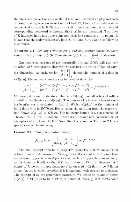
May 10, 2007 8:8 WSPC - Proceedings Trim Size: 9in x 6in ws-procs9x6
55
the literature; in sections 4,5 of Ref. 3 Bird and Keedwell employ methodsof design theory, whereas in section 5 of Ref. 12, Ebert et. al. take a moregeometrical approach. If O` is a full orbit, then a representative line andcorresponding codeword is chosen. Short orbits are discarded. Two linesof Σ intersect in at most one point and each line contains q + 1 points. Itfollows that the codewords satisfy both λa ≤ 1 and λc ≤ 1 and the followingis obtained.
Theorem 2.1. For any prime power q and any positive integer k, thereexists a (θ(k, q), q + 1, 1)-OOC consisting of L(k, q) =
⌊qk−1q2−1
⌋codewords.
Our new constructions of asymptotically optimal OOCs will also relyon orbits of Singer groups. However, we consider the orbits of flats of vary-
ing dimension. As such, we let[k + 1d+ 1
]q
denote the number of d-flats in
PG(k, q). Elementary counting can be used to show that[k + 1d+ 1
]q
=(qk+1 − 1)(qk+1 − q) · · · (qk+1 − qd)(qd+1 − 1)(qd+1 − q) · · · (qd+1 − qd)
≈ q(k−d)(d+1).
Moreover, it is well understood that in PG(k, q), not all orbits of d-flatsare full orbits (having size θ(k, q)). The number of orbits of d-flats of vary-ing lengths was investigated in Ref. 13. We let Nq(d, k) be the number offull d-flat orbits in PG(k, q). Hence, using the notation from the construc-tion above, Nq(1, k) ≡ L(k, q). The following lemma is a consequence ofTheorem 2.1 of Ref. 13 and shall prove useful in our new constructions ofasymptotically optimal OOCs. Note that the count in Theorem 2.1 is aspecial case of the following.
Lemma 2.1. Using the notation above,
Nq(d, k) =
⌊1
θ(k, q)
[k + 1d+ 1
]q
⌋≈ q(k−d−1)d.
The final concept from finite projective geometry that we make use ofis that of an arc. An m-arc in PG(d, q) is a collection of m > d points thatmeets some hyperplane in d points and meets no hyperplane in as manyas d + 1 points. It follows that if K is an m-arc in PG(d, q) then no d + 1points of K lie on a hyperplane, no d lie on a (d − 2)-flat,..., no 3 lie ona line. An arc is called complete if it is maximal with respect to inclusion.The concept of an arc generalizes naturally. We define an m-arc of degreer (≥ d) in PG(d, q) to be a set of m points of PG(d, q) that meets some

May 10, 2007 8:8 WSPC - Proceedings Trim Size: 9in x 6in ws-procs9x6
56
hyperplane in r points and meets no hyperplane in as many as r+1 points.Hence, arcs of degree d are simply arcs. In the plane PG(2, q), for instance,an arc of degree 2 is simply an arc, and an arc of degree 3 (also known as acubic arc) is a set of points that intersects at least one line in 3 points andintersects no line in as many as 4 points. There is a great deal of literatureregarding the connection between arcs and other classes of error-correctingcodes including low-density parity-check codes [14] and MDS codes [15].
In PG(2, q), a (non-degenerate) conic is a (q + 1)-arc and elementarycounting shows that this arc is complete when q is odd. In fact, a well-known result of Segre says that every complete arc of PG(2, q), q odd, is aconic. The (q + 2)-arcs (hyperovals) exist in PG(2, q) if q is even and theyare necessarily complete. Conics are a special case of the so called normalrational curves. A rational curve Cn of order n in PG(d, q) is a set of points
P (t) = (g0(t0, t1), . . . , gd(t0, t1)) | t0, t1 ∈ GF (q)
where each gi is a binary form of degree n and the highest common factorof g0, g1, . . . , gd is 1. The curve Cn may also be written
P (t) = (f0(t), . . . , fd(t)) | t ∈ GF (q) ∪ ∞ (3)
where fi(t) = gi(1, t).
Definition 2.1. A normal rational curve (NRC) in PG(d, q), 2 ≤ d ≤ q−2is a rational curve (of order d) projectively equivalent to
(1, t, . . . , td) | t ∈ GF (q) ∪ (0, . . . , 0, 1).
It is well-known that an NRC is, in fact, a (q+1)-arc. If C is an NRC inPG(d, q) then the subgroup of PGL(d+1, q) leaving C fixed is (isomorphicto) PGL(2, q) (see Ref. 16 Theorem 27.5.3). It follows that if ν(d, q) denotesthe number of distinct normal rational curves in PG(d, q) then
ν(d, q) =|PGL(d+ 1, q)||PGL(2, q)|
=(qd+1 − 1)(qd+1 − q) · · · (qd+1 − qd)
(q2 − 1)(q2 − q)(4)
The following is a well known property of NRCs (see Ref. 17).
Theorem 2.2. For 2 ≤ d ≤ q − 2, a (d + 3)-arc in PG(d, q) is containedin a unique normal rational curve.
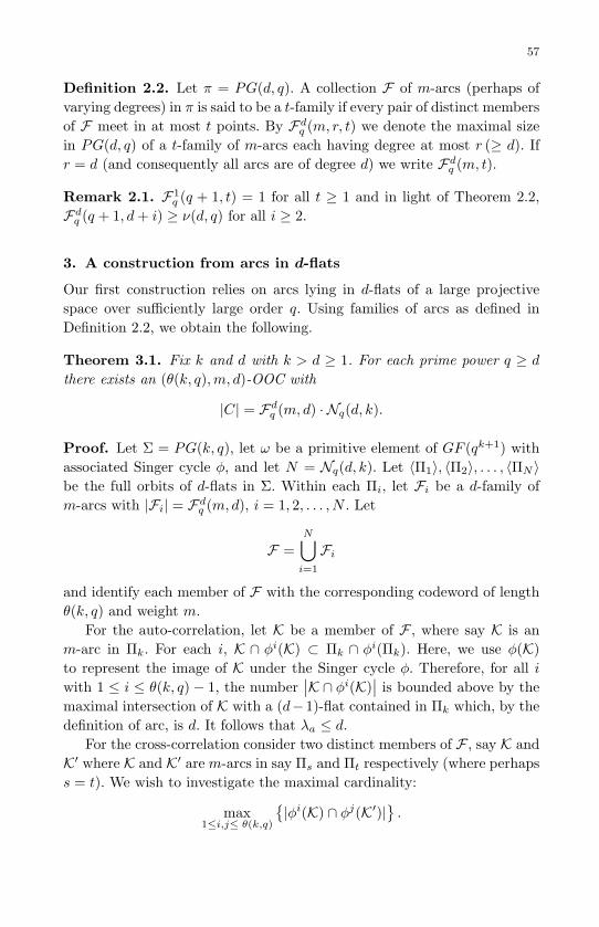
May 10, 2007 8:8 WSPC - Proceedings Trim Size: 9in x 6in ws-procs9x6
57
Definition 2.2. Let π = PG(d, q). A collection F of m-arcs (perhaps ofvarying degrees) in π is said to be a t-family if every pair of distinct membersof F meet in at most t points. By Fd
q (m, r, t) we denote the maximal sizein PG(d, q) of a t-family of m-arcs each having degree at most r (≥ d). Ifr = d (and consequently all arcs are of degree d) we write Fd
q (m, t).
Remark 2.1. F1q (q + 1, t) = 1 for all t ≥ 1 and in light of Theorem 2.2,
Fdq (q + 1, d+ i) ≥ ν(d, q) for all i ≥ 2.
3. A construction from arcs in d-flats
Our first construction relies on arcs lying in d-flats of a large projectivespace over sufficiently large order q. Using families of arcs as defined inDefinition 2.2, we obtain the following.
Theorem 3.1. Fix k and d with k > d ≥ 1. For each prime power q ≥ d
there exists an (θ(k, q),m, d)-OOC with
|C| = Fdq (m, d) · Nq(d, k).
Proof. Let Σ = PG(k, q), let ω be a primitive element of GF (qk+1) withassociated Singer cycle φ, and let N = Nq(d, k). Let 〈Π1〉, 〈Π2〉, . . . , 〈ΠN 〉be the full orbits of d-flats in Σ. Within each Πi, let Fi be a d-family ofm-arcs with |Fi| = Fd
q (m, d), i = 1, 2, . . . , N . Let
F =N⋃
i=1
Fi
and identify each member of F with the corresponding codeword of lengthθ(k, q) and weight m.
For the auto-correlation, let K be a member of F , where say K is anm-arc in Πk. For each i, K ∩ φi(K) ⊂ Πk ∩ φi(Πk). Here, we use φ(K)to represent the image of K under the Singer cycle φ. Therefore, for all iwith 1 ≤ i ≤ θ(k, q)− 1, the number
∣∣K ∩ φi(K)∣∣ is bounded above by the
maximal intersection of K with a (d−1)-flat contained in Πk which, by thedefinition of arc, is d. It follows that λa ≤ d.
For the cross-correlation consider two distinct members of F , say K andK′ where K and K′ are m-arcs in say Πs and Πt respectively (where perhapss = t). We wish to investigate the maximal cardinality:
max1≤i,j≤ θ(k,q)
|φi(K) ∩ φj(K′)|
.

May 10, 2007 8:8 WSPC - Proceedings Trim Size: 9in x 6in ws-procs9x6
58
We have that φi(K) ∩ φj(K′) ⊆ φi(Πs) ∩ φj(Πt). If s 6= t then φi(Πs)and φj(Πt) are in different orbits of d-flats, implying that φi(Πs) ∩ φj(Πt)is contained in a (d − 1)-flat. If s = t but i 6= j, then φi(Πs) 6= φj(Πs),implying that φi(Πs)∩φj(Πs) is still contained in a (d− 1)-flat. Therefore,by definition of an arc in PG(d, q), φi(K)∩φj(K′) must have cardinality atmost d. It follows that λc ≤ d.
The following appears in Ref. 2; for the sake of completeness we includea proof.
Theorem 3.2. In π = PG(d, q), d ≥ 2, there exists a d-family F of (q+1)-arcs where |F| = (qd+1 − q2)(qd+1 − q3) · · · (qd+1 − qd).
Proof. Consider π = PG(d, q) as a (Baer) subspace of Π = PG(d, q2). LetΠ∗ = Π \ π. Choose a point P = (α0, α1, . . . , αd) ∈ Π∗.
With reference to Equation (3), consider the collection of NRCs in Πhaving polynomial coefficients in GF (q). Denote by XP the number of suchNRCs containing P . Note that any such NRC intersects π in an NRC of π.To determine XP , we count ordered pairs (N , Q) where N is an NRC of Πover GF (q) and Q is a point of N in Π∗. This gives us the following.
|PGL(d+ 1, q)||PGL(2, q)|
[(q2+1)−(q+1)] =[(
(q2)d+1 − 1q2 − 1
)−(
(q)d+1 − 1q − 1
)]XP .
After some simplification we arrive at
XP = (qd+1 − q2)(qd+1 − q3) · · · (qd+1 − qd).
Let C be an NRC in Π over GF (q) containing P . Then the point P q =(αq
0, αq1, . . . , α
qd) conjugate to P is also contained in C (and is also in Π∗). As
such, any two of the NRCs counted above have at most d common points inπ. Hence, by restricting to the intersection of these NRCs with π we havea d-family of (q + 1)-arcs in π having size XP .
Corollary 3.1. If q is a prime power, then in PG(d, q), the maximum sizeof a d-family of (q + 1)-arcs, denoted by Fd
q (q + 1, d) satisfies
Fdq (q + 1, d) ≥ (qd+1 − q2)(qd+1 − q3) · · · (qd+1 − qd).

May 10, 2007 8:8 WSPC - Proceedings Trim Size: 9in x 6in ws-procs9x6
59
Theorem 3.3. Fix k and d with k > d ≥ 2. For each prime power q ≥ d
there exists a (θ(k, q), q + 1, d)-OOC C with
|C| ≥ (qd+1− q2)(qd+1− q3) · · · (qd+1− qd) ·
⌊1
θ(k, q)
[k + 1d+ 1
]q
⌋≈ qkd−d−1
Proof. Follows from Theorem 3.1, Corollary 3.1 and Lemma 2.1.
Now fix k > d ≥ 1 and consider the infinite family of (θ(k, q), q + 1, d)-OOCs constructed as in Theorem 3.3. The Johnson Bound for these codesis
J(θ(k, q), q + 1, d) =⌊
1q+1
⌊θ(k,q)−1
q
⌊θ(k,q)−2
q−1
⌊· · ·⌊
θ(k,q)−dq+1−d
⌋⌋⌋≈ qkd−d−1.
With reference to Definition 1.1 we see that the codes constructed as inTheorem 3.3 satisfy the following limit:
limn→∞
M(n,w, λ)J(n,w, λ)
= 1.
Hence, we obtain the following.
Theorem 3.4. Each infinite family of OOCs in Theorem 3.3 is asymptot-ically optimal.
4. A construction from arcs of higher degree
We now show that for d > 1 it is possible to improve the codes constructedabove. Again, we rely on families of arcs lying in certain flats of a large pro-jective space with sufficiently large order q. For this construction, however,we vary the dimension of the flats where the arcs lie.
Theorem 4.1. Fix k and d with k > d ≥ 1. For each prime power q ≥ d
and for each m > d there exists a (θ(k, q),m, d)-OOC C with
|C| =d∑
i=1
F iq(m, d, d) · Nq(i, k).
Proof. Let Σ = PG(k, q). For fixed s, 1 ≤ s ≤ d, let Ns = Nq(s, k),the number of full orbits of s-flats in PG(k, q). For each s, 1 ≤ s ≤ d letΠs,1,Πs,2, . . . ,Πs,Ns
be s-flats chosen one from each of the full s-flat orbits

May 10, 2007 8:8 WSPC - Proceedings Trim Size: 9in x 6in ws-procs9x6
60
under φ. In each Πs,t 1 ≤ s ≤ d, 1 ≤ t ≤ Ns let Fs,t be a d-family of m-arcseach of degree at most d with |Fs,t| = Fs
q (m, d, d).Let
F =⋃s,t
Fs,t.
Identify each member of F with the corresponding codeword of lengthθ(k, q) and weight m. We claim that the code C comprised of all such code-words is a (θ(k, q),m, d)-OOC. That C is of constant weight m is clear.
The auto-correlation, λa = d:Let K be a member of F , say K ∈ Fs,t is an m-arc of degree r (≤ d) in thes-flat Π, 1 ≤ s ≤ d, and 〈Π〉 is a full orbit under φ. It suffices to show
|φi(K) ∩ φj(K)| ≤ d, for all i 6= j, 1 ≤ i, j ≤ θ(k, q).
For any i, j, i 6= j, 1 ≤ i, j ≤ θ(k, q), since 〈Π〉 is a full orbit, φi(Π) 6= φj(Π)which implies that
dim(φi(Π) ∩ φj(Π)
)≤ s− 1.
Therefore, since φi(K)∩φj(K) ⊂ φi(K)∩(φi(Π) ∩ φj(Π)
)and since φi(Π)∩
φj(Π) is at most an (s−1)-flat, we are computing the maximum size of theintersection of an m-arc of degree r lying in an s-flat with an (s − 1)-flat.It follows that
|φi(K) ∩ φj(K)| ≤ |φi(K) ∩(φi(Π) ∩ φj(Π)
)| ≤ r
by the definition of an arc of degree r. Since r ≤ d we have λa ≤ d.
The cross-correlation, λc = d:Let K 6= K′ ∈ F where K ∈ Fs,t is an m-arc of degree r ≤ d in the s-flatΠ, 〈Π〉 a full orbit and K′ ∈ Fs′,t′ is an m-arc of degree r′ ≤ d in the s′-flatΠ′, 〈Π′〉 a full orbit. It suffices to show
|φi(K) ∩ φj(K′)| ≤ d, for all i, j, 1 ≤ i, j ≤ θ(k, q).
For any i, j, 1 ≤ i, j ≤ θ(k, q), either s = s′ or, without loss of generality,s′ < s. If s′ < s then dim(φi(Π)∩ φj(Π′)) ≤ s′ < s and therefore (as in thefirst part of the proof)
|φi(K) ∩ φj(K′)| ≤ r ≤ d.

May 10, 2007 8:8 WSPC - Proceedings Trim Size: 9in x 6in ws-procs9x6
61
If s = s′ we consider two cases:Case 1: Π = Π′. In this case Π,Π′ ∈ Fs,t. Therefore if i = j, then (by defini-tion of a d-family) |φi(K)∩φj(K′)| ≤ d. If i 6= j then dim
(φi(Π) ∩ φj(Π)
)≤
s− 1 whence
|φi(K) ∩ φj(K′)| ≤ r ≤ d.
Case 2: Π 6= Π′. In this case 〈Π〉 6= 〈Π′〉, so φi(Π) 6= φj(Π′) and againdim
(φi(Π) ∩ φj(Π)
)≤ s− 1 whence
|φi(K) ∩ φj(K′)| ≤ r ≤ d.
It follows that λc ≤ d.
If we use the 2-family of arcs (in this case, conics) in the plane as inTheorem 3.2, and embed into the ambient space PG(k, q), we obtain thefollowing asymptotically optimal class of OOCs.
Corollary 4.1. For k > 2 and for each prime power q ≥ 2 there exists a(θ(k, q), q + 1, 2)-OOC C with
|C| = (q3 − q2) · Nq(2, k) +Nq(1, k)
= (q3 − q2) ·
⌊1
θ(k,q)
[k + 1
3
]q
⌋+
⌊1
θ(k,q)
[k + 1
2
]q
⌋(5)
codewords.
Remark 4.1. For k = 3 above, we get the main result of Ref. 1.
Table 2 compares some of the classes of codes constructed as in Corollary4.1 with the number of codes given by the Johnson Bound.
Table 2. Values ofM(n,w,λ)J(n,w,λ)
, n = θ(k, q),
w = q + 1, λ = 2
q k = 3 k = 4 k = 5
7 0.6404255318 0.6330472103 0.6318161869
11 0.7546353523 0.7521739130 0.7519103045121 0.9754142500 0.9754115290 0.9754115020
343 0.9912792665 0.9912791440 0.9912791434
1721 0.9982578413 0.9982575034 0.9982578401
Teaming the result of Theorem 4.1 with the construction in Theorem3.2 for large families of arcs we can improve upon the codes constructed as

May 10, 2007 8:8 WSPC - Proceedings Trim Size: 9in x 6in ws-procs9x6
62
in Theorem 3.3. That is, codes of the same parameters and of larger sizeresult. Indeed, fix d, let our ambient space be PG(k, q), k > d, and considerthe full Singer orbits of flats of dimension d or less. For our first class ofcodewords, we take a d-family of arcs in a representative d-flat from eachfull d-flat orbit. As in Corollary 3.1 we have
Fdq (q + 1, d, d) ≥ (qd+1 − q2)(qd+1 − q3) · · · (qd+1 − qd).
For our second class of codewords, we look at the (d − 1)-flats. In theconstruction outlined in Theorem 4.1 a d-family of arcs of degree d in arepresentative (d− 1)-flat from each full orbit is used. For such families, ageneral construction yielding a family of significant size appears difficult.However, a (d−1)-family of arcs in PG(d−1, q) is easily constructed (as inTheorem 3.2) and may be considered (perhaps rather trivially) as a d-familyof arcs of degree at most d. That is,
Fd−1q (q+1, d, d) ≥ Fd−1
q (q+1, d−1, d−1) ≥ (qd−q2)(qd−q3) · · · (qd−qd−1).
For subsequent classes of codewords, we consider in turn the (d−i)-flats,for each i ≥ 2. By Theorem 2.2 the collection of all NRCs in a (d − i)-flati ≥ 2 is a (d− i+2)-family of arcs (of degree (d− i)). Hence again we arriveat an ostensibly loose lower bound:
Fd−iq (q + 1, d, d) ≥ ν(d− i, q) for each i ≥ 2.
Putting all of these classes of codewords together establishes the following.
Corollary 4.2. For k > d ≥ 3 and for each prime power q ≥ d there existsa (θ(k, q), q + 1, d)-OOC C consisting of
Nq(d, k) ·dY
i=2
(qd+1 − qi) +Nq(d− 1, k) ·d−1Yi=2
(qd − qi) +
d−2Xi=1
ν(i, q) · Nq(i, k)
=
$1
θ(k, q)
k + 1d + 1
q
%·
dYi=2
(qd+1 − qi) +
$1
θ(k, q)
k + 1
d
q
%·d−1Yi=2
(qd − qi)
+Pd−2
i=1
ν(i, q) ·
$k + 1i + 1
q
%!
(6)
codewords.
Remark 4.2. Taking k = d + 1 in the above yields codes of the sameparameters as those constructed in Ref. 2. Moreover, the size of the codesconstructed in Ref. 2 correspond to the first and last terms in the expansion(6). Consequently, for λ > 2 we obtain a strict improvement to the mainconstruction of (n,w, λ)-OOCs in Ref. 2.

May 10, 2007 8:8 WSPC - Proceedings Trim Size: 9in x 6in ws-procs9x6
63
Tables 3 and 4 compare some of the classes of codes constructed as inCorollary 4.2 with the number of codes given by the Johnson Bound.
Table 3. Values ofM(n,w,λ)J(n,w,λ)
, n = θ(k, q),
w = q + 1, λ = 3
q k = 4 k = 5 k = 6
7 0.3723672313 0.3778141740 0.378801968811 0.5503002252 0.5542495934 0.5546309684
121 0.9512311850 0.9512954758 0.9512960102
343 0.9826092131 0.9826175386 0.98261756231721 0.9965177060 0.9965180418 0.9965180423
Table 4. Values ofM(n,w,λ)J(n,w,λ)
, n = θ(k, q),
w = q + 1, λ = 5
q k = 6 k = 7 k = 8
7 0.0663583530 0.0677297426 0.0679268867
11 0.2100588301 0.2118051740 0.2119642548
121 0.8822149212 0.8822751817 0.8822756800
343 0.9570511656 0.9570593005 0.95705932421721 0.9913154765 0.9913158107 0.9913158117
5. Affine constructions
For our final construction, we will work in the finite affine space AG(k, q).Our basic technique follows the work of Ref. 18 where the authors use d-flatsof AG(k, q) to construct some OOCs, some of which are optimal. One wayto model AG(d, k) is to simply start in the projective space PG(d, k) anddelete any hyperplane Σ. The remaining points form the points of AG(d, k)and the flats of AG(d, q) are simply the flats of PG(d, k) with any pointsof Σ deleted.
It is well-known that AG(d, q) does not admit a Singer group in thesame fashion as PG(d, q). However, we can still apply the same generaltechniques as above. One way to model AG(k, q) is with a k-dimensionalvector space over GF (q). In this model, the vectors represent the affinepoints. The finite field GF (qk) is one example of such a vector space. As thenon-zero field elements of GF (qk) form a cyclic group under multiplication,we can obtain a similar group (to that of a Singer group of PG(d, q)) bysimply removing the point corresponding to the zero element of GF (qk).

May 10, 2007 8:8 WSPC - Proceedings Trim Size: 9in x 6in ws-procs9x6
64
Briefly, let Σ = AG(k, q) and denote by 0 the zero vector in Σ. Take α to bea primitive element of GF (qk). Just as in the projective case, each nonzerovector in Σ corresponds in the natural way to αj for some j, 0 ≤ j ≤ qk−2.Denote by φ the (Singer-like) mapping of Σ defined by φ(αj) = αj+1 andφ(0) = 0. Hence, for all of our constructions below, our code lengths willbe of the form qk−1 where the coordinates of the codewords correspond tothe non-zero elements of the finite field GF (qk) (see e.g. Ref. 19). Just asin the previous sections, we will make use of certain families of arcs lyingin AG(k, q).
Definition 5.1. Let π = AG(d, q). A collection F of m-arcs (perhaps ofvarying degrees) in π is said to be a t-family if every pair of distinct membersof F meet in at most t points. By Ed
q (m, r, t) we denote maximal size inAG(d, q) of a t-family of m-arcs each having degree at most r (≥ d). If r = d
(and consequently all arcs are of degree d) we write Edq (m, t).
Consider the space AG(k, q) with the origin removed, and consider the d-flats that do not contain the origin as a point. We wish to count the numberof full orbits of these d-flats under the action of the group described aboveon the points of AG(d, q) minus the origin. We letMq(d, k) be the numberof such full d-flat orbits in AG(k, q). It follows from Theorem 8 of Ref. 19that
Mq(d, k) =qk−d − 1qd − 1
·[k
d
]q
=(qk−1 − 1)(qk−2 − 1) · · · (qk−d − 1)
(qd − 1)(qd−1 − 1) · · · (q − 1).
Theorem 5.1. For each prime power q ≥ 2 there exists a (qk−1, q+1, 2)-OOC C with
|C| = (q3 − q2)Mq(2, k).
Proof. Our technique is exactly as in Theorem 3.1. We consider a familyof (q + 1)-arcs lying in a plane π of AG(k, q) not containing the origin. Weonly need to show that the 2-family of (q+ 1)-arcs of PG(2, q) constructedin Theorem 3.2 can still be constructed in AG(2, q).
Let Π = PG(2, q2) and let π ∼= PG(2, q) be the natural Baer subplaneof Π consisting of the set of points whose homogeneous coordinates lie inthe subfield GF (q) of the field GF (q2). Let P be any point of Π \ π. Asin Theorem 3.2, there are q3 − q2 arcs of Π, the family F , that meet theBaer subplane π in a sub-arc of size q + 1. We refer to these sub-arcs asGF (q)-arcs. Now, consider the line PP q, that is, the line joining P with isconjugate point P q. It’s a simple consequence of the classical theory that

May 10, 2007 8:8 WSPC - Proceedings Trim Size: 9in x 6in ws-procs9x6
65
this line meets the subplane π in a Baer subline. Since the points P and P q
both lie on each of the arcs of F , it follows that no other points of the linePP q lie on any of the GF (q)-arcs. Hence, if we remove the Baer subline ofPP q lying in π from the Baer subplane π, we are left with an isomorphiccopy of AG(2, q) containing a set of q3 − q2 arcs, pairwise meeting in atmost two points.
We now embed the affine plane AG(2, q) in AG(k, q) and associate witheach arc of the family a codeword. The results on auto and cross correlationnow follow as in Theorem 3.1.
We can increase the number of codewords in the code above by addingthe lines of AG(2, q) as additional codewords. In AG(2, q), however, linescontain q points. Hence, in order to keep our codewords of constant weight,we start by removing one point (randomly) from each arc of the family F .Using these q-arcs together with the lines of AG(2, q) gives us the following.
Corollary 5.1. For k > 2 and for each prime power q ≥ 2 there exists a(qk − 1, q, 2)-OOC C with
|C| = (q3 − q2)Mq(2, k) +Mq(1, k).
Just as with the projective case, the construction above generalizes nat-urally. The proof of the following is entire similar to that of Theorem 4.1.
Theorem 5.2. Fix k and d with k > d ≥ 1. For each prime power q ≥ d
and for each m > d there exists a (qk − 1,m, d)-OOC C with
|C| =d∑
i=1
E iq(m, d, d) · Mq(i, k).
We now establish some lower bounds on E iq(m, d, d), i ≤ d.
Lemma 5.1. In AG(d, q), d ≥ 2, there exists a d-family F0 of (q− d+ 3)-arcs with |F0| = (qd+1 − q2)(qd+1 − q3) · · · (qd+1 − qd).
Proof. As in Theorem 5.1, consider π = PG(d, q) as a (Baer) subspaceof Π = PG(d, q2) and choose a point P of Π outside of π. As discussedin Theorem 3.2, there are (qd+1 − q2)(qd+1 − q3) · · · (qd+1 − qd) NRCs (thefamily F) passing through P and meeting π in a sub-arc, and this collec-tion of (q + 1)-arcs forms a d-family of GF (q)-arcs in π. The line PP q ofΠ meets π in a Baer subline l0. Now consider any (d − 1)-flat, say π0, ofπ that contains the line l0. The hyperplane π0 extends to a hyperplane of

May 10, 2007 8:8 WSPC - Proceedings Trim Size: 9in x 6in ws-procs9x6
66
the entire space Π that contains the points P and P q. By the definition ofarc, any of the arcs in our family F meet this (d− 1)-flat of Π in at most dpoints, two of which are P and P q. Hence, if we delete the hyperplane π0
from π, we delete at most d− 2 points from any arc of the family F . Thisgives us a family of arcs we call F0. For any arc of F not meeting π0 ind− 2 points, we (randomly) remove points so that each arc of F0 has size(q+1)− (d−2) = q−d+3. Hence, every member of F0 is a (q−d+3)-arc.
From Lemma 5.1 we have
Edq (q − d+ 3, d, d) ≥ (qd+1 − q2)(qd+1 − q3) · · · (qd+1 − qd).
Moreover, an analysis similar to that preceding Corollary 4.2 yields
Ed−1q (q − d+ 3, d, d) ≥ Ed−1
q (q − d+ 3, d− 1, d− 1)≥ (qd − q2)(qd − q3) · · · (qd − qd−1),
and
Ed−iq (q − d+ 3, d, d) ≥ ν(d− i, q) for each i ≥ 2
which, with Theorem 5.2, establishes the following.
Corollary 5.2. For k > d ≥ 3 and for each prime power q ≥ d there existsa (qk − 1, q − d+ 3, d)-OOC C consisting of
Mq(d, k) ·d∏
i=2
(qd+1−qi)+Mq(d−1, k) ·d−1∏i=2
(qd−qi)+d−2∑i=1
(ν(i, q) ·Mq(i, k)
)codewords.
As discussed before Corollary 4.2, we can potentially increase the num-ber of codewords by using arcs of higher degree. In particular, if there existsa t-family F of m-arcs of degree r in PG(d, q), then there would exist at-family F0 of (m− r)-arcs of degree r in AG(d, q). Such a family F0 couldpotentially be larger than the family described in Lemma 5.1 which wouldlead to larger codes. In addition, notice in the constructions above that wewere forced to remove some points from our arcs for the sole purpose ofmaintaining a constant codeword weight. Avoiding this might improve theparameters of our codes.
Tables 5, 6, and 7 compare some of the classes of codes constructed asin Corollary 5.2 with the number of codes given by the Johnson Bound.Of particular note are the codes for λ = 2 (Table 5) whose ratio with theJohnson bound is extremely close to 1.

May 10, 2007 8:8 WSPC - Proceedings Trim Size: 9in x 6in ws-procs9x6
67
Table 5. Values ofM(n,w,λ)J(n,w,λ)
, n = qk − 1,
w = q + 1, λ = 2
q k = 3 k = 4 k = 5
7 0.8621700881 0.9804586940 0.9972032137
11 0.9104589917 0.9918766332 0.9992610944
121 0.9917366568 0.9999317079 0.9999994356343 0.9970845975 0.9999915002 0.9999999753
1721 0.9994189427 0.9999996625 0.9999999997
Table 6. Values ofM(n,w,λ)J(n,w,λ)
, n = qk−1, w = q,
λ = 3
q k = 4 k = 5 k = 6
7 0.2960072911 0.3428831335 0.3497386757
11 0.4885791465 0.5365032592 0.5409140118121 0.9432368020 0.9510961860 0.9511611465
343 0.9797276160 0.9825922863 0.9826006382
1721 0.9959379975 0.9965170310 0.9965173675
Table 7. Values ofM(n,w,λ)J(n,w,λ)
, n = qk − 1,
w = q − 2, λ = 5
q k = 6 k = 7 k = 8
8 0.0023607860 0.0026977534 0.0027405412
11 0.0307547138 0.0338295282 0.0341113883
121 0.7894584074 0.7960372276 0.7960916016343 0.9210483659 0.9237414898 0.9237493411
1721 0.9838383895 0.9844103884 0.9844107212
Note: Our code construction for the tables above involves d-families of(q − d + 3)-arcs. To avoid trivial arcs we considered only values of q forwhich q − d+ 3 > d.
6. Conclusion
We have exhibited a very general construction of optical orthogonal codesthat gives rise to a robust class of asymptotically optimal codes. Our codesgeneralize and improve the prior constructions involving conics [1] andarcs [2] by expanding the families of intersecting arcs and by working inhigher dimensional projective spaces. One next step might be to considersubgeometries PG(k, q) embedded in PG(k, qn) and use large families ofarcs in these subgeometries to find other classes of OOCs whose size ap-proaches that given by the Johnson Bound.
In the last section of Ref. 18 the authors discuss the possibility of OOCs

May 10, 2007 8:8 WSPC - Proceedings Trim Size: 9in x 6in ws-procs9x6
68
with different weight classes. In the constructions of Section 5, points werearbitrarily removed from certain arcs for the sole purpose of maintaininga constant codeword weight. Hence, the methods of Section 5 provide aconstruction for large non-constant weight codes with strong auto and crosscorrelations properties. The investigation into bounds on the size of suchOOCs with different weight classes seems an interesting problem as well.
Acknowledgments
The first author acknowledges support from the N.S.E.R.C. of Canada. Thesecond author acknowledges support by a Jepson Fellowship from the Uni-versity of Mary Washington and National Security Agency grant #H98230-06-1-0080
References
[1] Miyamoto, Nobuko and Mizuno, Hirobumi and Shinohara, Satoshi, Opticalorthogonal codes obtained from conics on finite projective planes, FiniteFields Appl., 10, 2004, no. 3, 405–411.
[2] Alderson, T.L., Optical Orthogonal Codes and Arcs in PG(d, q), FiniteFields Appl., to appear.
[3] Bird, C. M. and Keedwell, A. D., Design and applications of optical orthog-onal codes—a survey, Bull. Inst. Combin. Appl., 11, 1994, 21–44.
[4] Chung, Fan R. K. and Salehi, Jawad A. and Wei, Victor K., Optical orthog-onal codes: design, analysis, and applications, IEEE Trans. Inform. Theory,35, 1989, 3, 595–604.
[5] Healy, Timothy J., Coding and decoding for code division multiple usercommunication systems, IEEE Trans. Comm., Institute of Electrical andElectronics Engineers. Transactions on Communications, 33, 1985, 4, 310–316.
[6] Maric, S. V and Moreno, O. and Corrada, C., Multimedia transmissionin fiber-optic LANs using optical CDMA, J. Lightwave Technol., 14, 1996,2149–2153.
[7] Nguyen, Q. A and Gyorfi, Laszlo and Massey, James L., Constructions ofbinary constant-weight cyclic codes and cyclically permutable codes, IEEETrans. Inform. Theory, 38, 1992, 3, 940–949.
[8] Fuji-Hara, Ryoh and Miao, Ying, Optical orthogonal codes: their boundsand new optimal constructions, IEEE Trans. Inform. Theory, 46, 2000, 7,2396–2406.
[9] Yang, Guu-chang and Fuja, Thomas E., Optical orthogonal codes with un-equal auto- and cross-correlation constraints, IEEE Trans. Inform. Theory,41, 1, 1995, 96-106.
[10] Alderson, T.L. and Mellinger, Keith E., Constructions of optical orthogonalcodes from finite geometry, to appear .

May 10, 2007 8:8 WSPC - Proceedings Trim Size: 9in x 6in ws-procs9x6
69
[11] Alderson, T.L. and Mellinger, Keith E., Optical orthogonal codes from arcsin root subspaces, to appear .
[12] Ebert, G. L. and Metsch, K. and Szonyi, T., Caps embedded in Grassman-nians, Geom. Dedicata, 70, 1998, 2, 181–196.
[13] Drudge, Keldon, On the orbits of Singer groups and their subgroups, Elec-tron. J. Combin., 9, 2002, 1, 10 pp.
[14] Droms, Sean V. and Mellinger, Keith E. and Meyer, Chris, LDPC codesgenerated by conics in the classical projective plane, Des. Codes Cryptogr.,40, 2006, 3, 343–356.
[15] Alderson, T.L. and Bruen, A. A. and Silverman, R., Maximum distanceseparable codes and arcs in projective spaces, J. Combin. Theory Ser. A, toappear .
[16] Hirschfeld, J. W. P. and Thas, J. A., General Galois geometries, OxfordMathematical Monographs, The Clarendon Press Oxford University Press,New York, 1991, xiv+407.
[17] Thas, Joseph A., Projective geometry over a finite field, Handbook of inci-dence geometry, 295–347, North-Holland, Amsterdam, 1995.
[18] Omrani, R. and Moreno, O. and Kumar, P.V., Improved Johnson bounds foroptical orthogonal codes with λ > 1 and some optimal constructions, Proc.Int. Symposium on Information Theory, 2005, 259–263.
[19] Rao, C. Radhakrishna, Cyclical generation of linear subspaces in finite ge-ometries, Combinatorial Mathematics and its Applications (Proc. Conf.,Univ. North Carolina, Chapel Hill, N.C., 1967), 515–535, Univ. North Car-olina Press, 1969.

May 10, 2007 8:8 WSPC - Proceedings Trim Size: 9in x 6in ws-procs9x6
70
Codes over Fp2 and Fp × Fp, lattices, and theta functions
T. Shaska ∗
367 Science and Engineering Building,
Department of Mathematics and Statistics,
Oakland University,Rochester, MI, 48309.
Email: [email protected]
C. Shor
Department of Mathematics,
Bates College,3 Andrews Road,
Lewiston, ME, 04240.
Email: [email protected]
Let ` > 0 be a square free integer and OK the ring of integers of the imaginaryquadratic field K = Q(
√−`). Codes C over K determine lattices Λ`(C) over
rings OK/pOK . The theta functions θΛ`(C) of such lattices are known to
determine the symmetrized weight enumerator swe(C) for small primes p =2, 3; see [1, 10].
In this paper we explore such constructions for any p. If p - ` then the ring
R := OK/pOK is isomorphic to Fp2 or Fp × Fp. Given a code C over R wedefine new theta functions on the corresponding lattices. We prove that the
theta series θΛ`(C) can be written in terms of the complete weight enumerator
of C and that θΛ`(C) is the same for almost all `. Furthermore, for large enough
`, there is a unique complete weight enumerator polynomial which corresponds
to θΛ`(C).
Keywords: codes, lattices, theta functions
1. Introduction
Let ` > 0 be a square free integer, K = Q(√−`) be the imaginary quadratic
field, and OK its ring of integers. Codes, Hermitian lattices, and their theta-functions over rings R := OK/pOK , for small primes p, have been studiedby many authors, see [1, 7, 8] among others. In [1], an explicit description
∗Partially supported by a NATO grant
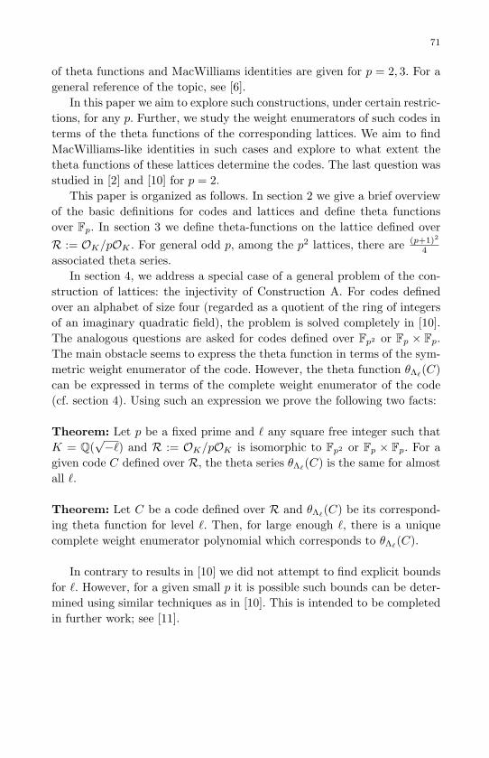
May 10, 2007 8:8 WSPC - Proceedings Trim Size: 9in x 6in ws-procs9x6
71
of theta functions and MacWilliams identities are given for p = 2, 3. For ageneral reference of the topic, see [6].
In this paper we aim to explore such constructions, under certain restric-tions, for any p. Further, we study the weight enumerators of such codes interms of the theta functions of the corresponding lattices. We aim to findMacWilliams-like identities in such cases and explore to what extent thetheta functions of these lattices determine the codes. The last question wasstudied in [2] and [10] for p = 2.
This paper is organized as follows. In section 2 we give a brief overviewof the basic definitions for codes and lattices and define theta functionsover Fp. In section 3 we define theta-functions on the lattice defined overR := OK/pOK . For general odd p, among the p2 lattices, there are (p+1)2
4
associated theta series.In section 4, we address a special case of a general problem of the con-
struction of lattices: the injectivity of Construction A. For codes definedover an alphabet of size four (regarded as a quotient of the ring of integersof an imaginary quadratic field), the problem is solved completely in [10].The analogous questions are asked for codes defined over Fp2 or Fp × Fp.The main obstacle seems to express the theta function in terms of the sym-metric weight enumerator of the code. However, the theta function θΛ`
(C)can be expressed in terms of the complete weight enumerator of the code(cf. section 4). Using such an expression we prove the following two facts:
Theorem: Let p be a fixed prime and ` any square free integer such thatK = Q(
√−`) and R := OK/pOK is isomorphic to Fp2 or Fp × Fp. For a
given code C defined over R, the theta series θΛ`(C) is the same for almost
all `.
Theorem: Let C be a code defined over R and θΛ`(C) be its correspond-
ing theta function for level `. Then, for large enough `, there is a uniquecomplete weight enumerator polynomial which corresponds to θΛ`
(C).
In contrary to results in [10] we did not attempt to find explicit boundsfor `. However, for a given small p it is possible such bounds can be deter-mined using similar techniques as in [10]. This is intended to be completedin further work; see [11].

May 10, 2007 8:8 WSPC - Proceedings Trim Size: 9in x 6in ws-procs9x6
72
2. Preliminaries
Let ` > 0 be a square free integer and K = Q(√−`) be the imaginary
quadratic field with discriminant dK . Recall that
dK =
−` if ` ≡ 3 mod 4,
−4` otherwise.
Let OK be the ring of integers of K. A lattice Λ over K is an OK-submoduleof Kn of full rank. The Hermitian dual is defined by
Λ∗ = x ∈ Kn | x · y ∈ OK , for all y ∈ Λ, (1)
where x · y :=∑n
i=1 xiyi and y denotes component-wise complex conju-gation. In the case that Λ is a free OK - module, for every OK basisv1, v2, ...., vn we can associate a Gram matrix G(Λ) given by G(Λ) =(vi · vj)n
i,j=1 and the determinant detΛ := det(G) defined up to squaresof units in OK . If Λ = Λ∗ then Λ is Hermitian self-dual (or unimodular)and integral if and only if Λ ⊂ Λ∗. An integral lattice has the propertyΛ ⊂ Λ∗ ⊂ 1
detΛΛ. An integral lattice is called even if x ·x ≡ 0 mod 2 for allx ∈ Λ, and otherwise it is odd. An odd unimodular lattice is called a Type1 lattice and even unimodular lattice is called a Type 2 lattice.
The theta series of a lattice Λ in Kn is given by
θΛ(τ) =∑z∈Λ
eπiτz·z,
where τ ∈ H = z ∈ C : Im(z) > 0.Usually we let q = eπiτ . Then, θΛ(q) =∑z∈Λ q
z·z. The one dimensional theta series (or Jacobi’s theta series) andits shadow are given by
θ3(q) =∑n∈Z
qn2, θ2(q) =
∑n∈ 1
2+Z
qn2.
Let ` ≡ 3 mod 4 and d be a positive number such that ` = 4d − 1. Then,−` ≡ 1 mod 4. This implies that the ring of integers is OK = Z[ω`], whereω` = −1+
√−`
2 and ω2` + ω` + d = 0. The principal norm form of K is given
by
Qd(x, y) = |x− yω`|2 = x2 + xy + dy2. (2)
The structure of OK/pOK depends on the value of ` modulo p. For (ap )
the Legendre symbol,
OK/pOK =
Fp × Fp if (−`
p ) = 1,
Fp2 if (−`p ) = −1,
Fp + uFp with u2 = 0 if p | `.(3)

May 10, 2007 8:8 WSPC - Proceedings Trim Size: 9in x 6in ws-procs9x6
73
We will concern ourselves with the cases where p - `.
2.1. Theta functions over Fp
Let q = eπiτ . For integers a and b and a prime p, let Λa,b denote the latticea− bω` + pOK . The theta series associated to this lattice is
θΛa,b(q) =
∑m,n∈Z
q|a+mp−(b+np)ω`|2
=∑
m,n∈ZqQd(mp+a,np+b)
=∑
m,n∈Zqp2Qd(m+a/p,n+b/p).
(4)
For a prime p and an integer j, consider the theta series
θp,j(q) :=∑
n∈ j2p +Z
qn2. (5)
Note that θp,j(q) = θp,k(q) if and only if j ≡ ±k mod 2p.The theta series of Λa,b can be written in terms of these series. In par-
ticular,
θΛa,b(q) = θp,b(qp2`)θp,2a+b(qp2
) + θp,b+p(qp2`)θp,2a+b+p(qp2). (6)
The proof of this fact is similar to the proof of Lemma 2.1 in [5].
Lemma 2.1. For any integers a, b,m, n, if the ordered pair (m,n) iscomponent-wise congruent modulo p to one of
(a, b), (−a,−b), (a+ b,−b), (−a− b, b),
then
θΛm,n(q) = θΛa,b
(q)
Proof. We prove this by supposing either
θp,n(q) = θp,b(q) and θp,2m+n(q) = θp,2a+b(q) (7)
or
θp,n(q) = θp,b+p(q) and θp,2m+n(q) = θp,2a+b+p(q). (8)
From Eq. 7, we have four subcases corresponding to n ≡ ±b mod 2pand 2m+ n ≡ ±(2a+ b) mod 2p. If n ≡ b mod 2p, one finds that m ≡ a

May 10, 2007 8:8 WSPC - Proceedings Trim Size: 9in x 6in ws-procs9x6
74
mod p or m ≡ −a− b mod p. If n ≡ −b mod 2p, one finds that m ≡ a+ b
mod p or m ≡ −a mod p.From Eq. 8, we have four subcases as well, corresponding to n ≡ ±(b+p)
mod 2p and 2m + n ≡ ±(2a + b + p) mod 2p. If n ≡ b + p mod 2p, theneither m ≡ a mod p or m ≡ −a − b mod p. And if n ≡ −b − p mod 2p,then either m ≡ a+ b mod p or m ≡ −a mod p.
Therefore, if n ≡ b mod p, then m ≡ a mod p or m ≡ −a− b mod p.If n ≡ −b mod p, then m ≡ a+ b mod p or m ≡ −a mod p.
Remark 2.1. Notice that in the case of p = 2, there are 4 lattices Λa,b
corresponding to choices of a and b modulo 2. One finds that θΛ0,1(q) =θΛ1,1(q) (which is given as Eq. (3.9) in Lemma 3.1 of [2]), so there are 3associated theta series.
Remark 2.2. In the case of p = 3, among the 9 lattices, one finds that
θΛ0,1(q) = θΛ2,1(q) = θΛ1,2(q) = θΛ0,2(q),
θΛ1,1(q) = θΛ2,2(q), and
θΛ1,0(q) = θΛ2,0(q),
giving a total of 4 associated theta series.For general odd p, among the p2 lattices, there are (p+1)2
4 associatedtheta series.
3. Theta functions of codes over R
Let p - ` and
R := OK/pOK =a+ bω : a, b ∈ Fp, ω
2 + ω + d = 0.
A linear code C of length n over R is an R-submodule of Rn. The dualis defined as C⊥ = u ∈ Rn : u · v = 0 for all v ∈ C. If C = C⊥ then C isself-dual. We define
Λ`(C) := x ∈ OnK : ρ`(x) ∈ C,
where ρ` : OK → OK/pOK → R . In other words, Λ`(C) consists of allvectors in On
K which when taken mod pOK componentwise are in ρ−1` (C).
This method of lattice construction is known as Construction A.For 0 ≤ a, b ≤ p − 1, let ra+pb = a − bω, so R =
r0, . . . , rp2−1
. For
a codeword u = (u1, . . . , un) ∈ Rn and ri ∈ R, we define the countingfunction
ni(u) := #i : ui = ri.

May 10, 2007 8:8 WSPC - Proceedings Trim Size: 9in x 6in ws-procs9x6
75
The complete weight enumerator of the R code C is the polynomial
cweC(z0, z1, . . . , zp2−1) =∑u∈C
zn0(u)0 z
n1(u)1 . . . z
np2−1(u)
p2−1 . (9)
We can use this polynomial to find the theta function of the lattice Λ`(C).
Lemma 3.1. Let C be a code defined over R and cweC its complete weightenumerator as above. Then,
θΛ`(C)(q) = cweC(θΛ0,0(q), θΛ1,0(q), . . . , θΛp−1,p−1(q))
Proof. Since
θΛ`(C)(q) =∑
z∈Λ`(C)
qz·z,
one has
θΛ`(C)(q) =∑u∈C
θΛ`(u)(q),
=∑u∈C
∑x∈u+pOn
K
qx·x,
=∑u∈C
n∏j=1
∑x∈uj+pOK
qx·x (for u = (u1, . . . , un)),
=∑u∈C
n∏j=1
θuj+pOK(q),
=∑u∈C
p2−1∏i=0
(θri+pOK(q))ni(u) (where ra+pb = a− bω` ∈ OK),
= cweC(θr0+pOK(q), θr1+pOK
(q), . . . , θrp2−1+pOK(q)),
= cweC(θΛ0,0(q), θΛ1,0(q), . . . , θΛp−1,p−1(q)),
which completes the proof.
3.1. A MacWilliams identity
Let C⊥ be the dual code to C. From Theorem 4.1 of [1] one has the followingMacWilliams identity:
Theorem 3.1. Let χ : (R,+) → (C∗,×) be a character of the additivegroup of R whose restriction to any nonzero left ideal of R is nontrivial.

May 10, 2007 8:8 WSPC - Proceedings Trim Size: 9in x 6in ws-procs9x6
76
Then
cweC⊥(z0, . . . , zp2−1) =1p2cweC(M(z0, . . . , zp2−1)),
where M is the matrix defined by
M = (χ(rirj))0≤i≤p−1,0≤j≤p−1.
To apply this theorem, we need an appropriate character. Define χ byχ(a + bω) = e2πib/p. Any non-zero ideal I ⊂ R contains an element ofR − 0, 1, . . . , p− 1, so there is some a + bω ∈ I with b 6= 0, meaning χacts non-trivially on I. A calculation shows that
(a+ bω)(s+ tω) = (as− at+ btd) + (bt− as)ω,
so χ((a+bω)(s+ tω)) = e(bs−at)2πi/p. This is independent of d, so we obtainthe same MacWilliams identity for codes over Fp2 and Fp × Fp.
In the case of p = 2, for example, such identities can be made explicit;see [2] and [1] among others.
3.2. A generalization of the symmetric weight enumerator
polynomial
In [2], for p = 2, the symmetric weight enumerator polynomial sweC of acode C over a ring or field of cardinality 4 is defined to be
sweC(X,Y, Z) = cweC(X,Y, Z, Z).
For ΛC(q) the lattice obtained from C by Construction A, by Theorem 5.2of [2], one can then write
θΛ`(C)(q) = sweC(θΛ0,0(q), θΛ1,0(q), θΛ0,1(q)).
These theta functions are referred to as Ad(q), Cd(q), and Gd(q) in [2] and[10].
For p > 2, however, there are (p+1)2
4 (which is larger than 3) thetafunctions associated to the various lattices, so our analog of the symmetricweight enumerator polynomial has more than 3 variables.
Example 3.1. For p = 3, from Remark 2.2, we have four theta functionscorresponding to the lattices Λa,b, namely
θΛ0,0(q), θΛ1,0(q), θΛ1,1(q), θΛ0,1(q).
If we define the “symmetric weight enumerator for p = 3” to be
sweC(X,Y, Z,W ) = cweC(X,Y, Y, Z,W,Z, Z, Z,W ),

May 10, 2007 8:8 WSPC - Proceedings Trim Size: 9in x 6in ws-procs9x6
77
then one finds that
θΛ`C(q) = cweC(θΛ0,0(q), θΛ1,0(q), . . . , θΛ2,2(q)), (10)
= sweC(θΛ0,0(q), θΛ1,0(q), θΛ1,1(q), θΛ0,1(q)). (11)
Finding such an explicit relation between the theta function and thesymmetric weight enumerator polynomial for larger p seems difficult. Wesuggest the following problem:
Problem 1. Define an symmetric weight enumerator, analogous to thep = 2 case, for codes defined over R for p > 3. Write a MacWilliamsidentity for the symmetric weight enumerator and determine an explicitrelation between the symmetric weight enumerator and theta functions.
4. The injectivity of construction A
For a fixed prime p, let R = OK/pOK and C be a linear code over R oflength n and dimension k. An admissible level ` is an integer ` such thatR is isomorphic to Fp2 or Fp × Fp. For an admissible `, let Λ`(C) be thecorresponding lattice as in the previous section. Then, the level ` thetafunction θΛ`(C)(τ) of the lattice Λ`(C) is determined by the completeweight enumerator cweC of C, evaluated on the theta functions defined oncosets of OK/pOK . We consider the following questions:
i) How do the theta functions θΛ`(C)(τ) of the same code C differ fordifferent levels `?
ii) Can non-equivalent codes give the same theta functions for all levels`?
Next we see how this can be made explicit for the case p = 2.
4.1. The case p = 2
For p = 2 case these questions are fully answered in [10]. We have thefollowing:
Theorem 4.1 (Thm. 1, [10]). Let p = 2 and C be a code defined overR. For all admissible `, `′ such that ` > `′, the following holds
θΛ`(C) = θΛ`′ (C) +O(q
`′+14 ).

May 10, 2007 8:8 WSPC - Proceedings Trim Size: 9in x 6in ws-procs9x6
78
Let C be a code of length n defined over R and θΛ`(C) be its corre-
sponding theta function for level `. Let f(x, y, z) ∈ F [x, y, z] where F isa field of transcendental degree δ. We say that f(x, y, z) is in a family ofpolynomials of dimension δ.
Theorem 4.2 (Thm. 2, [10]). Let p = 2 and C be a code of length n
defined over R and θΛ`(C) be its corresponding theta function for level `.
Then the following hold:
i) For ` < 2(n+1)(n+2)n − 1 there is a δ-dimensional family of symmetrized
weight enumerator polynomials corresponding to θΛ`(C), where
δ ≥ (n+1)(n+2)2 − n(`+1)
4 − 1.ii) For ` ≥ 2(n+1)(n+2)
n − 1 and n < `+14 there is a unique symmetrized
weight enumerator polynomial which corresponds to θΛ`(C).
Example 4.1. There are two non isomorphic codes
C3,2 = ω < [0, 1, 1] > +(ω + 1) < [0, 1, 1] >⊥
C3,3 = ω < [0, 0, 1] > +(ω + 1) < [0, 0, 1] >⊥ .
with symmetrized weight enumerator polynomials
sweC3,2(X,Y, Z) = X3 +X2Z +XY 2 + 2XZ2 + Y 2Z + 2Z3
sweC3,3(X,Y, Z) = X3 + 3X2Z + 3XZ2 + Z3
Both these codes give the following theta function for level ` = 7:
θ = 1 + 6q2 + 24q4 + 56q6 + 114q8 + 168q10 + 280q12 + 294q14 + · · ·
However, when ` = 15, we are in the second case of the above theorem.Two non equivalent codes cannot give the same theta function for ` = 15and n = 3. Explicit details are given in [10].
The above results were obtained by using the explicit expression oftheta in terms of the symmetric weight enumerator valuated on the thetafunctions of the cosets. Hence, a solution to Problem 1 most likely wouldlead to obtaining such results for all p > 2 and admissible `. In this paperwe use the complete weight enumerator polynomial to get similar results.
4.2. The case p > 2
Let C be a code defined over R for a fixed p > 2. Let the complete weightenumerator of C be the degree n polynomial
cweC = f(x0, . . . , xr)

May 10, 2007 8:8 WSPC - Proceedings Trim Size: 9in x 6in ws-procs9x6
79
for r = p2 − 1. Then from Lemma 3.1 we have that
θΛ`(C)(τ) = f(θΛ0,0(τ), . . . , θΛp−1,p−1(τ))
for a given `. First we want to address how θΛ`(C)(τ) and θΛ`′ (C)(τ) differfor different ` and `′. We have the following:
Theorem 4.3. Let C be a code defined over R. For all admissible `, `′ thefollowing holds
θΛ`(C)− θΛ`′ (C) =
s∑i=0
aiqs
for some ai ∈ Z and s ∈ Z+.
Corollary 4.1. Let p be a fixed prime and ` any square free integer suchthat K = Q(
√−`) and R := OK/pOK is isomorphic to Fp2 or Fp × Fp.
For a given code C defined over R, the theta series θΛ`(C) is the same for
almost all `.
Theorem 4.4. Let C be a code defined over R and θΛ`(C) be its cor-
responding theta function for level `. Then, for large enough `, there isa unique complete weight enumerator polynomial which corresponds toθΛ`
(C).
The proofs of Theorems 4.3 and 4.4 are provided in [11] where explicitbounds for ` are provided for small p.
Acknowledgment
Some of the ideas of this paper originated during visits of the first author atThe University of Maria Curie Sklodowska, Lublin, Poland. The first authorwants to thank the faculty of the Department of Computer Science in Lublinfor their hospitality. The paper was presented at the Vlora Conference onAlgebra, Coding Theory, and Cryptography.
References
[1] C. Bachoc, Applications of coding theory to the construction of modularlattices. J. Combin. Theory Ser. A 78 (1997), no. 1, 92–119.
[2] K. S. Chua, Codes over GF(4) and F2 × F2 and Hermitian lattices overimaginary quadratic fields. Proc. Amer. Math. Soc. 133 (2005), no. 3, 661–670 (electronic).

May 10, 2007 8:8 WSPC - Proceedings Trim Size: 9in x 6in ws-procs9x6
80
[3] J. H. Conway, N. J. A. Sloane, Sphere packings, lattices and groups. Sec-ond edition. Grundlehren der Mathematischen Wissenschaften [FundamentalPrinciples of Mathematical Sciences], 290. Springer-Verlag, New York, 1993.xliv+679 pp. ISBN: 0-387-97912-3
[4] H. H. Chan, K. S. Chua and P. Sole, Seven-modular lattices and a septicbase Jacobi identity, J. Number Theory, volume 99, 2003, 2, pg. 361–372,
[5] H. H. Chan, K. S. Chua and P. Sole, Quadratic iterations to π associatedwith elliptic functions to the cubic and septic base, Trans. AMS 355, 2003,pg. 1505-1520.
[6] W. Ebeling, Lattices and codes, a course partially based on lectures by F.Hirzenbruch, Vieweg (Braunschweig) 1994.
[7] F. J. MacWilliams, N. J. A. Sloane, The theory of error-correcting codes.II. North-Holland Mathematical Library, Vol. 16. North-Holland PublishingCo., Amsterdam-New York-Oxford, 1977. pp. i–ix and 370–762.
[8] F. J. MacWilliams, N. J. A. Sloane, The theory of error-correcting codes.I. North-Holland Mathematical Library, Vol. 16. North-Holland PublishingCo., Amsterdam-New York-Oxford, 1977. pp. i–xv and 1–369.
[9] N. J. A. Sloane, Codes over GF(4) and complex lattices. Information theory(Proc. Internat. CNRS Colloq., Cachan, 1977) (French), pp. 273–283, Colloq.Internat. CNRS, 276, CNRS, Paris, 1978.
[10] T. Shaska and S. Wijesiri, Codes over rings of size four, Hermitian lattices,and corresponding theta functions, Proc. Amer. Math. Soc., (2007), to ap-pear.
[11] T. Shaska, C. Shor, and S. Wijesiri, Codes, modular lattices, and correspond-ing theta functions, work in progress.

May 10, 2007 8:8 WSPC - Proceedings Trim Size: 9in x 6in ws-procs9x6
81
Goppa codes and Tschirnhausen modules
Drue Coles
Department of Mathematics, Computer Science, and Statistics,
Bloomsburg University,
Bloomsburg PA 17815, USAE-mail: [email protected]
Emma Previato
Institut Mittag-Leffler
S-18262 Djursholm, Sweden
Permanent:Department of Mathematics and Statistics,
Boston University, Boston MA 02215-2411
E-mail: [email protected]
We review the use of rank-2 vector bundles in error-correcting coding theory,introduce the issue of maximal subbundles in this context and give an explicit
example of rank-2 bundles naturally associated to an elliptic subcover of the
Klein curve. We also describe how codes on curves (and therefore certain as-sociated rank-2 bundles and their maximal subbundles) can be formulated in
terms of adeles.
Keywords: Goppa codes; Vector bundles; Klein curve.
Introduction
Goppa codes (more properly, geometric Goppa codes, for the earliest codesintroduced by Goppa were still associated with rational functions on theline) provide a fertile area of interaction between coding theory and al-gebraic geometry, specifically algebraic curves over finite fields. Goppa’soriginal idea is based on the explicit representation of the space of sectionsof a line bundle over the curve, and deep issues regarding ‘curves with manypoints’ and asymptotic bounds on the genus and ramification of towers ofcurves have been brought up in view of this application, cf. [9] for a briefsurvey. More recently, rank-2 vector bundles over the curve have been in-terpreted as error-correcting devices [4–6, 12] but not so explicitly. Theirline subbundles of highest possible degree are of particular interest for de-

May 10, 2007 8:8 WSPC - Proceedings Trim Size: 9in x 6in ws-procs9x6
82
coding, and our goal in this small note is to initiate a study of these objectsin the finite field setting.
Higher-rank vector bundles (meaning higher than 1, for line bundles arequite different and better-known objects) come with a concept of “max-imal subbundle” for which we refer to the paper [15] although it madeearlier appearances (Corrado Segre 1889), since degrees of subbundles canbe be related to the self-intersection numbers of sections of the bundle pro-jectivized fiberwise into a ruled surface. We restrict attention to rank-2bundles, and for these, a maximal subbundle is a line subbundle of largestpossible degree. There has been enormous activity on the topic of maxi-mal subbundles in algebraic geometry, which we do not reference here, andthis prompts our proposed line of research. On one hand, the results of[15] are given over an algebraically closed field of characteristic zero. Evenfrom the pure viewpoint of algebraic geometry, it would be worth extendingthe study to any characteristic, and in addition, restricting the analysis tofinite fields. In the same vein as counting (rational) points on curves andpoints of Brill-Noether loci, we propose to count the number of maximalsubbundles. Here we give but one example. We decided to use the Kleincurve X as a test case, in part because it is so full of beautiful uniqueproperties among curves of genus 3 (small enough yet highly non-trivial),and partly because its large number of automorphisms has already madeit popular in coding theory. Over the finite field F8 the Klein quartic has24 points, hence it attains Serre’s improvement of the Hasse-Weil bound,|#X(Fq)− (q + 1)| ≤ g[2√q].
As regards the link with error-correcting, a weakness might be that thebundles which correspond to correctable messages are unstable, hence theirmaximal subbundles have very large degree, too large, roughly speaking, tobe interesting in algebraic geometry (except perhaps for the suggestions of[12], to the effect of blowing up unstable strata). Our present result concernsbundles whose maximal subbundles have degree zero, yet we regard it aswork towards a potential link with coding theory, for example pursuing thesuggestion in [12], that is to look at stable points whose lack of correctability(exceeding the distance from a unique codeword) is not too large, so thaterror-correction is possible in practice (“For practical purposes this wouldbe almost as good as unique decoding (...) one is then interested in maximalsublinebundles”). Other potential uses of stable bundles are discussed inSection 1.
We adopt three approaches which we believe to be new. The first usesthe ideas of [15] to construct all rank-2 bundles with largest-dimensional
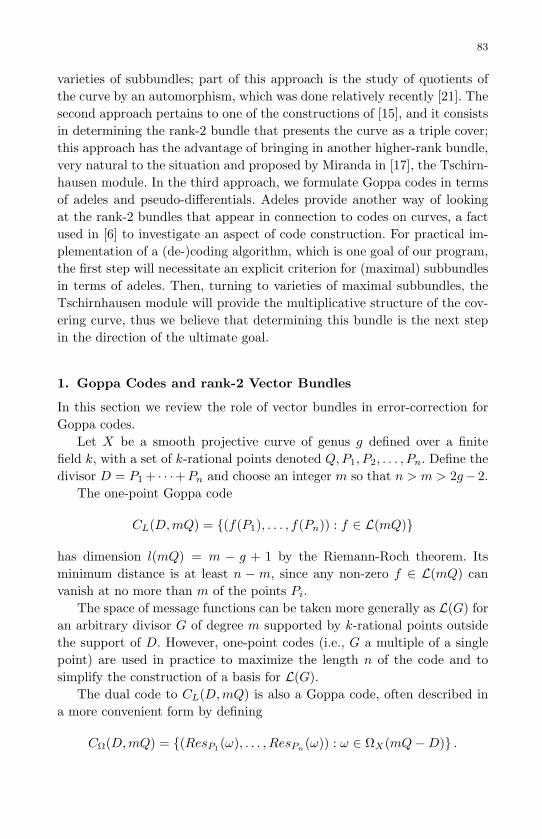
May 10, 2007 8:8 WSPC - Proceedings Trim Size: 9in x 6in ws-procs9x6
83
varieties of subbundles; part of this approach is the study of quotients ofthe curve by an automorphism, which was done relatively recently [21]. Thesecond approach pertains to one of the constructions of [15], and it consistsin determining the rank-2 bundle that presents the curve as a triple cover;this approach has the advantage of bringing in another higher-rank bundle,very natural to the situation and proposed by Miranda in [17], the Tschirn-hausen module. In the third approach, we formulate Goppa codes in termsof adeles and pseudo-differentials. Adeles provide another way of lookingat the rank-2 bundles that appear in connection to codes on curves, a factused in [6] to investigate an aspect of code construction. For practical im-plementation of a (de-)coding algorithm, which is one goal of our program,the first step will necessitate an explicit criterion for (maximal) subbundlesin terms of adeles. Then, turning to varieties of maximal subbundles, theTschirnhausen module will provide the multiplicative structure of the cov-ering curve, thus we believe that determining this bundle is the next stepin the direction of the ultimate goal.
1. Goppa Codes and rank-2 Vector Bundles
In this section we review the role of vector bundles in error-correction forGoppa codes.
Let X be a smooth projective curve of genus g defined over a finitefield k, with a set of k-rational points denoted Q,P1, P2, . . . , Pn. Define thedivisor D = P1 + · · ·+Pn and choose an integer m so that n > m > 2g− 2.
The one-point Goppa code
CL(D,mQ) = (f(P1), . . . , f(Pn)) : f ∈ L(mQ)
has dimension l(mQ) = m − g + 1 by the Riemann-Roch theorem. Itsminimum distance is at least n − m, since any non-zero f ∈ L(mQ) canvanish at no more than m of the points Pi.
The space of message functions can be taken more generally as L(G) foran arbitrary divisor G of degree m supported by k-rational points outsidethe support of D. However, one-point codes (i.e., G a multiple of a singlepoint) are used in practice to maximize the length n of the code and tosimplify the construction of a basis for L(G).
The dual code to CL(D,mQ) is also a Goppa code, often described ina more convenient form by defining
CΩ(D,mQ) = (ResP1(ω), . . . , ResPn(ω)) : ω ∈ ΩX(mQ−D) .

May 10, 2007 8:8 WSPC - Proceedings Trim Size: 9in x 6in ws-procs9x6
84
The fact that CL(D,mQ) and CΩ(D,mQ) are dual codes is a conse-quence of the residue theorem, which states the sum of residues of a differ-ential over all points is zero.
Requiring m > 2g − 2 makes computing the dimension of L(mQ) andhence of the code CL(D,mQ) a simple application of the Riemann-Rochtheorem. We actually want m > 2g so that the rational map ϕ : X → Pm−g
determined by the complete linear system |mQ| is guaranteed to be anembedding.
Since the rows of a generator matrix for CL(D,mQ) are obtained byevaluating the functions of a basis for L(mQ) at P1, . . . , Pn, we can viewthe columns as points ϕ(Pi) on the curve in Pm−g. These columns are paritychecks for the dual code CΩ(D,mQ), so a corrupted codeword of the dualis in effect a linear combination of some of the points ϕ(Pi), namely thosepoints at which errors occurred. More explicitly, if H denotes the paritycheck matrix and y = (c+e) a received word, with codeword c ∈ CΩ(D,mQ)and error vector e, then Hy = H(c + e) = He, and the received wordy = e1 · ϕ(P1) + · · · + en · ϕ(Pn) can be viewed as a point in the j-secantvariety of the curve in Pm−g, where j = |i : ei 6= 0|.
We call A =∑
ei 6=0 Pi the error divisor. The received word y = c+ e issaid to be correctable if degA < (d− 1)/2, where d = m− 2g+ 2 is a lowerbound on the mimimum distance, since in this case the received word iscloser to the transmitted codeword c than to any other codeword.
We also consider an error vector (e) as a point in H0(X,ΩC(mQ−D))∗,and then identify it with the isomorphism class of a rank-2 extension E ofthe form
0→ OX → E → OX(D −mQ)→ 0
in a standard way through
H0(X,Ω(mQ−D))∗ ∼= H1(X,OX(mQ−D))∼= ExtOX
(OX ,OX(mQ−D))∼= ExtOX
(OX(D −mQ),OX).
Lange and Narasimhan [15] showed that s(E)(:=degE − 2max(degL),where L is a subbundle of E) is determined by the smallest integer j suchthat (e) is contained in the j-secant variety of the curve. Applying theirresults to our situation and with our notation, we get that A is the errordivisor for a correctable word if and only if OX(D−mQ−A) is the unique

May 10, 2007 8:8 WSPC - Proceedings Trim Size: 9in x 6in ws-procs9x6
85
maximal subbundle of E. This abstract connection between decoding andmaximal subbundles of rank-2 extensions was first noticed by Johnsen [12].
A decoding algorithm based on this idea would determine the rank-2bundle E corresponding to the syndrome He = Hy of the received wordy = c + e, in concrete form for instance as a transition matrix, and thencompute its unique maximal subbundle OX(D−mQ−A). One might thenexpect to extract the error divisor A and so obtain the error positions(and then the actual error values via simple linear algebra), but with acaveat: we cannot distinguish OX(D −mQ − A) from OX(D −mQ − A′)when A ∼ A′, so the most that can be guaranteed about the error divisorcomputed by such an algorithm without additional assumptions (such asthe number of errors being less than the gonality of the curve) is that it islinearly equivalent to the true error divisor.
We note that for correctable words, the associated bundle E is neces-sarily unstable [12]. Still, computing maximal subbundles of stable E’s inour extension space may be useful for decoding. If the number of errors ina word y exceeds the error correction capacity of the code, it may happenthat there are several codewords of precisely equal Hamming distance fromy. In that case, finding maximal subbundles amounts to producing a smalllist of candidate error divisors, though the issue of linear equivalence dis-cussed above applies here as well. There is a vast coding theory literatureon list decoding, as it is called.
The study of stable rank-2 bundles on curves with many maximal sub-bundles defined over a finite field may, in addition to its inherent interest,have a coding theory application, since for particular code parameters themaximum possible number of closest codewords to a given (uncorrectable)word may not be known. This point was discussed in [4], where it was alsoobserved that the recent discovery of families of Goppa codes with expo-nentially many minimum weight codewords [1] is somewhat related: thisresult says that for a certain code there is a Hamming sphere of radius dcentered at 0 with a huge number of codewords on its boundary; a stablebundle with many maximal subbundles (over the base field) would describea Hamming sphere of radius greater than d centered at an uncorrectableword with a huge number of codewords on its boundary. One possible wayto find rank-2 bundles with lots of maximal subbundles over a finite fieldis to construct examples with infinitely many in the algebraic closure andthen count the ones defined over the base field. We turn to this constructionnext.

May 10, 2007 8:8 WSPC - Proceedings Trim Size: 9in x 6in ws-procs9x6
86
2. The Klein Curve as Cover
In this section, which is composed of old-and-new facts about the Kleincurve, we recall some results that were given in characteristic zero in theoriginal references; however, they hold in our more general situation pro-vided the characteristic of the base field k is not 2, 3 or 7 (the divisors of168 which is the order of AutX in any other characteristic), and providedk contains a seventh root of unity, as noted in the text, because the resultswe use are obtained by algebraic operations defined over the integers.
The two most familiar ways (for a third one cf. 2.4) to write an algebraicequation for Klein’s curve X are:
s7 = t(1− t)2,
x31x2 + x3
2x0 + x30x1 = 0.
Klein, already in his original definition [14] of the unique curve of genus3 that has the maximal number of automorphisms, presented it at first asa modular curve, then as a (canonical) plane quartic. This double featurealready exhibits the curve as a cover, on one hand, a (7 : 1) cover of P1,on the other, true of every non-hyperelliptic curve of genus 3, as a (3 :1) trigonal cover in a 1-dimensional manifold way. More surprisingly, [3,VIII.75] shows that the Jacobian of the curve is isomorphic as a complexmanifold (without principal polarization) to the product of three ellipticcurves; more precisely, using the (7 : 1) cover, Baker computes the periodmatrix
Z =
− 18 + 3
√7i
8 − 14 −
√7i4 − 3
8 +√
7i8
− 14 −
√7i4
12 +
√7i2 − 1
4 −√
7i4
− 38 +
√7i8 − 1
4 −√
7i4
78 + 3
√7i
8
.As observed in [22], all entries lie in the field generated (over the field k ofdefinition of the curve, k = Q, e.g.) by the character of the representationinduced on the differentials of the first kind by the automorphism groupof the curve. But another interesting phenomenon occurs: Jac(X) = C3/Λ,where Λ is the lattice corresponding to [I Z], is actually isomorphic to theproduct of 3 elliptic curves. Indeed, Baker shows that it can be brought byan integral (but not unimodular) transformation into diagonal form:1 0 0 1+i
√7
4 0 00 1 0 0 2 1+i
√7
4 00 0 1 0 0 2 1+i
√7
4
.

May 10, 2007 8:8 WSPC - Proceedings Trim Size: 9in x 6in ws-procs9x6
87
He also remarks that this transformation does not give us an algebraic mapfrom X to an elliptic curve; for that we use recent work [21], which gives abit more: the three elliptic curves are isomorphic as opposed to 2-isogenousas in Baker’s decomposition.
We recall some notation and standard facts from [21]. The followingthree elements generate the automorphism group of X, which is isomor-phic to PSL2(F7): σ(x0, x1, x2) = (x1, x2, x0) of order 3, τ(x0, x1, x2) =(x1 + µ1x2 + 1
µ3x0, µ1x1 + 1
µ3x2 + x0,
1µ3x1 + x2 + µ1x0
)of order 2 and
ε(x0, x1, x2) = (x0, ζx1, ζ5x2) of order 7, where ζ is a primitive 7th root
of 1 and we let µi = ζi + ζ−i.
Proposition 2.1. [21] The quotient of X by σi, i = 0, 1, 2 gives three(canonically isomorphic) elliptic curves Ti with Weierstrass equations:
Ti : y2 + 3ζ4ixy + ζ5iy = x3 − 2ζ2ix− 3ζ3i, i = 0, 1, 2,
with the (3 : 1)-morphisms X → Ti given by φi(x1, x2) = (−wi, vi) where
wi = x+ ζ6i 1y
+ ζ4i y
x, vi = y + ζ6i 1
x+ ζ2ix
y.
Given that the above result is algebraic, we can simply replace Q[ζ] by afinite field that contains a seventh root of unity, and keep the notation ζ for aprimitive one. In fact, it is quite interesting and non-tivial to find AutX overan algebraically closed field of any characteristic. This was accomplished in[30–32]: if the characteristic is p 6= 3, 7 the group is again GL(3, 2). Forp = 3 (resp. p = 7), the group properly contains GL(3, 2) and is of order6048 (resp. 672). It is thus not true (as had also been observed earlier) thatthe Hurwitz bound 84(g − 1) holds for the number of automorphisms of acurve of genus g (> 1), if the characteristic is not zero; a bound does exist,modified by the contribution of wild ramification in the Riemann-Hurwitzformula, has degree 4 in g, and it is known which curves attain it.
Our program is now the study of maximal subbundles in positive char-acteristic. Following the seminal article [15], for a rank-2 (algebraic) vectorbundle over a curve X of genus g, we define the numerical invariant:
s(E) = degE − 2max(degL),
where L is a line-subbundle of E. By definition, the degree of E and s(E)have the same parity. It is known that s(E) ≤ g, and the study in [15]addresses the case s(E) > 0 (equivalent to E being a stable bundle) ors(E) ≥ 0 (semi-stable). The relevant geometric object then is M(E), thesubvariety of maximal subbundles. This variety can be identified canonically

May 10, 2007 8:8 WSPC - Proceedings Trim Size: 9in x 6in ws-procs9x6
88
with the space of minimal sections of the ruled surface P(E), minimal inthe sense of having smallest self-intersection number. Let us also denoteby M(d) the moduli space of stable bundles of rank 2 and degree d over acurve X of genus g ≥ 2, and by M(d, s) its stratification into locally closedsubsets according to the value of the invariant s(E). For generic E, M(E)is smooth and projective and its dimension is described in terms of the rankand degree of E and the genus of X. It has exactly the Chern numbers ofan etale cover of the symmetric product SnX, where n = dimM(E) [20].In particular, for the general bundle, s(E) = g if the degree of E has thesame parity as the genus, and s(E) = g − 1 otherwise. When s(E) = g,the variety of maximal subbundles of E is a curve, but when s(E) = g− 1,it is generically a finite number of points. It is this number that in thecase of positive characteristic could conceivably be smaller, in the casethe field is not algebraically closed and the subbundle as a variety is notrational over the field of definition, or perhaps larger, as is the case forthe number of automorphisms, due to the wild-ramification contribution inthe Riemann-Hurwitz formula, in view of the fact that in [15] a manifoldof maximal line subbundles are identified by using covering maps. Thenumber of subbundles does have a topological-degree significance, becauseof the cited result [20] which computes it as a Chern number, 2g times aCastelnuovo number, but so does the number of inflections of a plane curve;in point of fact, the Klein curve is the “funny curve” in characteristic 3, andall of its points are inflections [11, Exercise IV.2.4]. It is also interesting tonote that the dimension of M(E) can jump, as in the following example [20,Remark 1.5]: the general bundle E with trivial determinant on a curve ofgenus 3 has a finite number of maximal subbundles, 23 = 8, since s(E) =g−1 as we recalled. But M(E) is isomorphic to the curve for the 64 bundlesE = κ−1 ⊗ V , where κ is a theta characteristic and V is the unique stablerank-2 bundle whose determinant is the canonical bundle, and whose spaceof sections has the maximal possible dimH0(X,V ) = 3. In fact, in thisprogrammatic note we focus on such ‘richest’ case only, namely s(E) =g − 1(= 2 in our case) and dimM(E)=1, strictly larger than for generalE. In [15] it is determined exactly which E have this property, providing anegative answer to a conjecture of M. Maruyama, to the effect of dimM(E)being zero for all, not merely general, bundles that have s(E) ≤ g − 1.
Proposition 2.2 (after 15, Theorem 5.1). Every degree-2 cover X →T of an elliptic curve gives a g-dimensional subvariety of M(d, 2), whered is an even number, for all of whose points E, dimM(E) = 1. If X is ofgenus 3, any trigonality of X gives a 3-dimensional subvariety of M(d, 2)
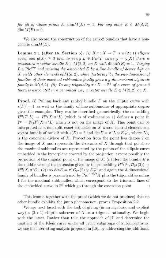
May 10, 2007 8:8 WSPC - Proceedings Trim Size: 9in x 6in ws-procs9x6
89
for all of whose points E, dimM(E) = 1. For any other E ∈ M(d, 2),dimM(E) = 0.
We also record the construction of the rank-2 bundles that have a non-generic dimM(E):
Lemma 2.1 (after 15, Section 5). (i) If π : X → T is a (2 : 1) ellipticcover and g(X) ≥ 3 then to every L ∈ PicgT where g = g(X) there isassociated a vector bundle E ∈M(2, 2) on X with dimM(E) = 1. VaryingL ∈ PicgT and twisting the associated E by a line bundle of degree d−2
2 onX yields other elements of M(d, 2), while ‘factoring’ by the one-dimensionalfamilies of their maximal subbundles finally gives a g-dimensional algebraicfamily in M(d, 2). (ii) To any trigonality π : X → P1 of a curve of genus 3there is associated in a canonical way a vector bundle E ∈M(2, 2) on X.
Proof. (i) Pulling back any rank-2 bundle F on the elliptic curve withs(F ) = 1 as well as the family of line subbundles of appropriate degreegives the examples. They can be described geometrically: the embeddingH0(T,L) → H0(X,π∗L) (which is of codimension 1) defines a point inPg = P(H0(X,π∗L) which is not on the image of X. This point can beinterpreted as a non-split exact sequence on X whose central element is avector bundle of rank 2 with s(E) = 2 and detE = π∗L⊗K−1
X , where KX
is the canonical divisor of X. Projection from the point has degree 2 onthe image of X and represents the 2-secants of X through that point, sothe maximal subbundles are represented by the points of the elliptic curveembedded in the hyperplane covered by the projection, except possibly theprojection of the singular point of the image of X. (ii) Here the bundle E isthe middle term of the extension given by the embedding H0(P1,OP1(2))→H0(X,π∗OP1(2)) so detE = π∗OP1(2)⊗K−1
X and again the 3-dimensionalfamily of bundles is parametrized by Picd−2/2X plus the trigonalities minus1 for the maximal subbundles, which correspond to the trisecant lines ofthe embedded curve in P3 which go through the extension point.
This lemma together with the proof (which we do not produce) that noother bundle exhibits the jump phenomenon, proves Proposition 2.2.
We are next faced with the task of giving (in an algebraic and explicitway) a (2 : 1) elliptic subcover of X or a trigonal rationality. We beginwith the latter. Rather than take the approach of [7] and determine thequotient of the Klein curve under all cyclic subgroups of automorphisms,we use the interesting analysis proposed in [18], by addressing the additional

May 10, 2007 8:8 WSPC - Proceedings Trim Size: 9in x 6in ws-procs9x6
90
question: given a trigonality obtained by projecting a smooth plane quarticto a line from a point on it, when is this cover Galois? We take this pointof view because we find it potentially interesting to give an addendum toKowalevski’s early result: she proved that a plane quartic is a (2 : 1) coverof an elliptic curve if and only if four of its 28 bitangents are concurrent,as we recall in Prop. 2.4.
The gonality of a curve is the smallest possible degree of the functionfield of the curve over a rational field of one variable. We now adapt state-ments from [18], which assumes the field of definition k to be algebraicallyclosed of characteristic zero. For our purposes we assume that all maps aredefined over k in case k isn’t algebraically closed (such as a finite field). TheKlein curve is not hyperelliptic, hence it is trigonal. For a plane smooth m-gonal curve of degree d the gonality is d−1 and any extensionK/k(t), whereK is the function field of the curve and k(t) is any rational field of degree1, corresponds to an (m : 1) projection from a point of the curve onto aline [18]. In [18], the authors determine the following objects pertaining toa smooth quartic (such as our Klein curve – in fact, their worked-out ex-ample is the Fermat curve, whose automorphism group [33] has order 96):for P ∈ X, the projection of X from P to a line is a degree-3 cover, and theGalois group as well as the genus of the corresponding cover are calculated,together with the (finite) number of points P for which the cover is Galois.
Proposition 2.3 (after 18, Theorem 2.1). For any smooth plane quar-tic X and any point P ∈ X, the projection from P to a line corresponds toa field extension that does not depend on the line, and if we call g(P ) thegenus of the smooth curve whose function field is the Galois closure of thefield extension corresponding to the projection and P a Galois point whenthe extension is Galois, then: g(P )=3,6,7,8,9, or 10, with g(P ) =10 for thegeneral point, with Galois group isomorphic to S3. The number of Galoispoints can be 0,1, or 4, and it is zero for a general quartic.
In [18], part of the criterion for P to be a Galois point is that P be a2-inflection point. In particular, for the Klein curve, none exists, since theinflections are all distinct and comprise the 24 Weierstrass points, so noneof the trigonal covers is Galois.
Similar issues are treated in [18] for the case P /∈ X, there being morecases to analyze and slightly less complete results. The Klein curve doesadmit a double cover to an elliptic curve. Indeed, as noted in [14], thereare 21 subgroups of order 2 of AutX, each corresponding to a collineation;the centers of projection give (4 : 1) maps of X to a line which factor

May 10, 2007 8:8 WSPC - Proceedings Trim Size: 9in x 6in ws-procs9x6
91
through an elliptic curve, the ramification given by the four bitangents toX through the center (each bitangent contains three centers so that thereare 21×4
3 = 28 bitangents). We note however that none of the 4-gonal coversgiven by projection from P /∈ X of the Klein (unlike the Fermat!) quarticare Galois either; the 21 elliptic subfields of K(X) fixed by involutions areone orbit under AutX [16].
It seems worth recalling Kowalevski’s criterion for a smooth plane quar-tic to be a (2 : 1) elliptic cover, which again is proved in characteristic zero.Her proof was analytic, a contribution to the theory of reduction, part ofher dissertation supervised by Weierstrass. An algebraic proof is given in[8], as part of the properties of Weierstrass points of curves with involution.
Proposition 2.4 (Chap. III, Art. 71, 72, 76 in [3]). A canonicallyembedded plane curve of genus 3 admits a (2 : 1) cover to an elliptic curveif and only if four of its bitangents are concurrent, equivalently in suitablecoordinates it has an equation:
(z2 − φ2)2 = 4xy(ax+ by)(cx+ dy),
with φ2 a homogeneous for of degree 2 in x, y.
Here the bitangents are patently represented by the linear forms x, y, ax+byand cx+dy, whose cross-ratio is an invariant of the elliptic curve. Note theanalogy with genus one: an elliptic curve is the Fermat curve if and onlyif it can be represented as a plane cubic with three concurrent bitangents,the projection from their common point being Galois. As recalled above,Klein’s curve can be written in this way by virtue of its automorphisms oforder two. An actual geometric model of the elliptic curve together withthe (2 : 1) projection can be found by embedding X in P3 via the divisor ofdegree 6 that pulls back an L ∈ Pic3T , precisely as in Lemma 2.1, obtainingan extension E to be viewed as a point in P3 and projecting the image ofX from that point to a plane; Baker (loc. cit. in Prop. 2.4) states this factconcretely presenting the image of X as a space sextic with equations:
z2 − φ2 = xt, xt2 = 4y(ax+ by)(cx+ dy),
as obtained by sending [x, y, z] 7→ [x, y, z, t] ∼ [1, y/x, z/x, (z2 − φ2)/x2] bythe pole-divisor map of 3P1 + 3P2, P1 and P2 being the points of contactof the bitangent x = 0.
Remark. One subtle issue that we do not address in this note is the fol-lowing. A classical result reprised and refined in [13] says that if an abeliansurface has more than two elliptic subgroups, then it has infinitely many;

May 10, 2007 8:8 WSPC - Proceedings Trim Size: 9in x 6in ws-procs9x6
92
[13] shows also that it has finitely many ones for each bounded degree (thedegree can be taken to be the intersection number with any fixed ampledivisor). In our case, we would ask how many genuinely distinct (ellip-tic) subcovers the Klein curve has, in particular over each finite field. Wenote that much current work is devoted to classifying subcovers of Her-mitian curves (of key interest in the area of Goppa codes), for examplein [7] a classification is given of the quotients of Hermitian curves by allprime-order automorphisms. For the genus-2 case, an explicit detection ofisogenous/isomorphic degree-2 and degree-3 subcovers, as well as partialresults for higher degree, is given in [24–27].
Summary. Let X be the Klein curve. For each fixed determinant, therank-2 bundles E ∈ M(2, 2) with dimM(E) = 1 correspond to a givenelliptic-hyperelliptic map or trigonality. The 64 points E mentioned abovethat exhibit the jump phenomenon as regards dimM(E) [20] have fixed(even-degree) determinant. It follows from the above construction that eachmap gives rise to one bundle; the 21 subgroups of order 2 of AutX comewith three maps each (each group of 4 concurrent bitangents gives an el-liptic curve and each bitangent contains three centers), so we recover the64 = 21× 3 + [one trigonality] bundles of [20], on which AutX acts bypermutations. To compute the number of these bundles over a finite fieldFq, one of our goals, first we fix a determinant of degree d that is an el-ement of PicdX(Fq) (there exists one for each degree, and the number ofdistinct ones is independent of the degree [19, Chap. 3]), then there areas many bundles (semistable and with that determinant), with ‘too manysubbundles’, as there are points of order 2 in Pic0X(Fq), found [19] (sincethe Jacobian splits) by splitting the characteristic p in Z[
√−7].
Example. Consider the Klein curve X defined by x31x2 + x3
2x0 + x30x1 = 0
over F8 = F2[β]/(β3 +β+1). Since the characteristic is 2, we cannot expectthe same situation as in characteristic zero, in fact there are no odd theta-characteristics since the tangent line at any point is an inflectionary tangent.However, the maximal-subbundle geometry survives. Fix coordinates sothat on the line at infinity z = 0, parametrized as [a, b], P∞ = [1, 0] and letπ : X → P1 be the projection from Q3 = [0, 0, 1] to the line at infinity, sothat 2P∞ pulls back to 6Q1, where Q1 = [1, 0, 0].
Let ϕ : P1 → P2 denote the embedding [a, b] 7→ [1, a/b, a2/b2]. Thedivisor map ϕ6Q1 : X → P3 that makes the following diagram commute isgiven by [a, b, c] 7→ [1, a/b, a2/b2, ab/c2].
The injection H0(P1, 2P∞)π∗
→ H0(X, 6Q1) corresponds to the point
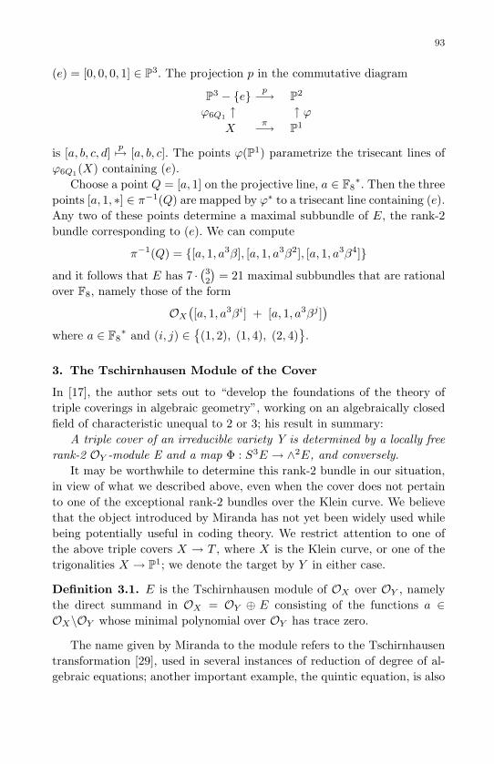
May 10, 2007 8:8 WSPC - Proceedings Trim Size: 9in x 6in ws-procs9x6
93
(e) = [0, 0, 0, 1] ∈ P3. The projection p in the commutative diagram
P3 − e p−→ P2
ϕ6Q1 ↑ ↑ ϕX
π−→ P1
is [a, b, c, d]p7→ [a, b, c]. The points ϕ(P1) parametrize the trisecant lines of
ϕ6Q1(X) containing (e).Choose a point Q = [a, 1] on the projective line, a ∈ F8
∗. Then the threepoints [a, 1, ∗] ∈ π−1(Q) are mapped by ϕ∗ to a trisecant line containing (e).Any two of these points determine a maximal subbundle of E, the rank-2bundle corresponding to (e). We can compute
π−1(Q) = [a, 1, a3β], [a, 1, a3β2], [a, 1, a3β4]
and it follows that E has 7 ·(32
)= 21 maximal subbundles that are rational
over F8, namely those of the form
OX
([a, 1, a3βi] + [a, 1, a3βj ]
)where a ∈ F8
∗ and (i, j) ∈(1, 2), (1, 4), (2, 4)
.
3. The Tschirnhausen Module of the Cover
In [17], the author sets out to “develop the foundations of the theory oftriple coverings in algebraic geometry”, working on an algebraically closedfield of characteristic unequal to 2 or 3; his result in summary:
A triple cover of an irreducible variety Y is determined by a locally freerank-2 OY -module E and a map Φ : S3E → ∧2E, and conversely.
It may be worthwhile to determine this rank-2 bundle in our situation,in view of what we described above, even when the cover does not pertainto one of the exceptional rank-2 bundles over the Klein curve. We believethat the object introduced by Miranda has not yet been widely used whilebeing potentially useful in coding theory. We restrict attention to one ofthe above triple covers X → T , where X is the Klein curve, or one of thetrigonalities X → P1; we denote the target by Y in either case.
Definition 3.1. E is the Tschirnhausen module of OX over OY , namelythe direct summand in OX = OY ⊕ E consisting of the functions a ∈OX\OY whose minimal polynomial over OY has trace zero.
The name given by Miranda to the module refers to the Tschirnhausentransformation [29], used in several instances of reduction of degree of al-gebraic equations; another important example, the quintic equation, is also

May 10, 2007 8:8 WSPC - Proceedings Trim Size: 9in x 6in ws-procs9x6
94
related to curves [10]. The conventional way to perform a Tschirnhausentransformation is to allow a substitution y = xm+rm−1x
m−1+. . .+r1x+r0,in order to simultaneously eliminate (by using the r’s as free parameters)intermediate terms of any nth- (say) degree equationa. In the case of aquintic, to bring it to Bring-Jerrard form: x5 + ax+ b, with y =
∑4j=0 ajx
j
one has to solve three equations of degrees 1, 2, and 3 in the coefficients ofthe original equation. In this case [10] it is possible to intersect suitable hy-persurfaces in P4 and find solutions by solving equations of degree at mostfour. Bring’s curve is then of genus four and can be explicitly uniformizedas it possesses sufficiently many automorphisms, in particular a (12 : 1)(Galois) cover to an elliptic curve. This provides a solution to the generalquintic in terms of modular forms of weight −2.
With this motivation, Miranda defines the Tschirnhausen module of thetriple cover X → Y to be the submodule E in the decomposition of localk-algebras (where k is an algebraically closed field of characteristic unequalto 2 or 3), or sheaves, OX = OY ⊕E consisting of the elements a ∈ OX\OY
whose minimal polynomial is trace free.In our situation, for the map in Prop. 2.1 given explicitly as above, the
module consists of the elements 23a−a
σ−aσ2, for all a in the function field
of X that are not σ-invariant; is is enough to take a = x, y to span themodule and the map σ is given explicitly: x 7→ y 7→ z 7→ x so x projects to23x− y− z and y to 2
3y− z−x. This would provide actual equations for thecorresponding divisor; however, we give a more theoretic way to identify it.
Miranda computes the ramification and branch locus of the triple cover:the branch locus in Y is a divisor whose associated line bundle is (∧2E)−2 soby the Riemann-Hurwitz formula (which has no inertia components underthe assumptions we made on the characteristic), 2g(X) − 2 = 3(2g(Y ) −2) + degree(∧2E). In conclusion, in our case E has degree 4. Atiyah [2]gave a description of all the semistable bundles over an elliptic curve, butwe are further restricted in our situation: the cover is by construction aGalois cover, and Miranda shows that E splits into the sum of two eigenlinebundles: f∗OX = OY ⊕ L−1 ⊕M−1, E = L−1 ⊕M−1, where L−1, M−1
are the eigenspaces for σ, σ2. Since there are exactly two σ-fixed points onX, namely p1 = [1, ε, ε2] and p2 = [1, ε2, ε] where ε is a primitive third rootof 1, the bundles L and M are O(−2pi).
The trigonality, however, is never Galois as we saw. To compute the
aWe acknowledge this clear and clever exemplification due to Titus Pierzas III postedon the web: A New Way To Derive The Bring-Jerrard Quintic in Radicals,
www.geocities.com/titus−piezas/Tschirnhausen.pdf.
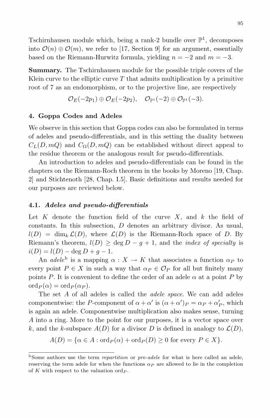
May 10, 2007 8:8 WSPC - Proceedings Trim Size: 9in x 6in ws-procs9x6
95
Tschirnhausen module which, being a rank-2 bundle over P1, decomposesinto O(n) ⊕ O(m), we refer to [17, Section 9] for an argument, essentiallybased on the Riemann-Hurwitz formula, yielding n = −2 and m = −3.
Summary. The Tschirnhausen module for the possible triple covers of theKlein curve to the elliptic curve T that admits multiplication by a primitiveroot of 7 as an endomorphism, or to the projective line, are respectively
OE(−2p1)⊕OE(−2p2), OP1(−2)⊕OP1(−3).
4. Goppa Codes and Adeles
We observe in this section that Goppa codes can also be formulated in termsof adeles and pseudo-differentials, and in this setting the duality betweenCL(D,mQ) and CΩ(D,mQ) can be established without direct appeal tothe residue theorem or the analogous result for pseudo-differentials.
An introduction to adeles and pseudo-differentials can be found in thechapters on the Riemann-Roch theorem in the books by Moreno [19, Chap.2] and Stichtenoth [28, Chap. I.5]. Basic definitions and results needed forour purposes are reviewed below.
4.1. Adeles and pseudo-differentials
Let K denote the function field of the curve X, and k the field ofconstants. In this subsection, D denotes an arbitrary divisor. As usual,l(D) = dimk L(D), where L(D) is the Riemann-Roch space of D. ByRiemann’s theorem, l(D) ≥ degD − g + 1, and the index of specialty isi(D) = l(D)− degD + g − 1.
An adeleb is a mapping α : X → K that associates a function αP toevery point P ∈ X in such a way that αP ∈ OP for all but finitely manypoints P . It is convenient to define the order of an adele α at a point P byordP (α) = ordP (αP ).
The set A of all adeles is called the adele space. We can add adelescomponentwise: the P -component of α+α′ is (α+α′)P = αP +α′P , whichis again an adele. Componentwise multiplication also makes sense, turningA into a ring. More to the point for our purposes, it is a vector space overk, and the k-subspace A(D) for a divisor D is defined in analogy to L(D),
A(D) = α ∈ A : ordP (α) + ordP (D) ≥ 0 for every P ∈ X.
bSome authors use the term repartition or pre-adele for what is here called an adele,reserving the term adele for when the functions αP are allowed to lie in the completion
of K with respect to the valuation ordP .
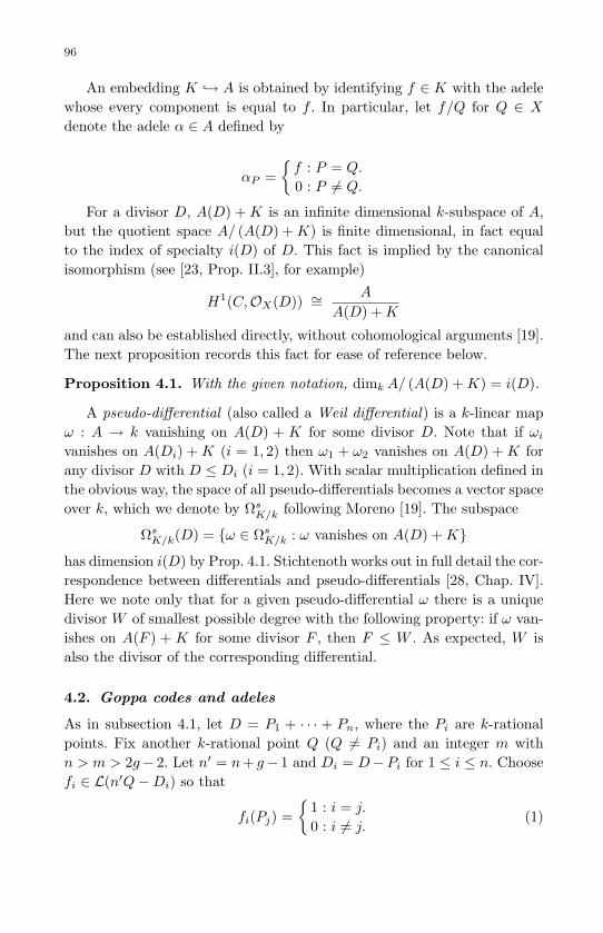
May 10, 2007 8:8 WSPC - Proceedings Trim Size: 9in x 6in ws-procs9x6
96
An embedding K → A is obtained by identifying f ∈ K with the adelewhose every component is equal to f . In particular, let f/Q for Q ∈ X
denote the adele α ∈ A defined by
αP =f : P = Q.
0 : P 6= Q.
For a divisor D, A(D) +K is an infinite dimensional k-subspace of A,but the quotient space A/ (A(D) +K) is finite dimensional, in fact equalto the index of specialty i(D) of D. This fact is implied by the canonicalisomorphism (see [23, Prop. II.3], for example)
H1(C,OX(D)) ∼=A
A(D) +K
and can also be established directly, without cohomological arguments [19].The next proposition records this fact for ease of reference below.
Proposition 4.1. With the given notation, dimk A/ (A(D) +K) = i(D).
A pseudo-differential (also called a Weil differential) is a k-linear mapω : A → k vanishing on A(D) + K for some divisor D. Note that if ωi
vanishes on A(Di) +K (i = 1, 2) then ω1 + ω2 vanishes on A(D) +K forany divisor D with D ≤ Di (i = 1, 2). With scalar multiplication defined inthe obvious way, the space of all pseudo-differentials becomes a vector spaceover k, which we denote by Ωs
K/k following Moreno [19]. The subspace
ΩsK/k(D) = ω ∈ Ωs
K/k : ω vanishes on A(D) +K
has dimension i(D) by Prop. 4.1. Stichtenoth works out in full detail the cor-respondence between differentials and pseudo-differentials [28, Chap. IV].Here we note only that for a given pseudo-differential ω there is a uniquedivisor W of smallest possible degree with the following property: if ω van-ishes on A(F ) + K for some divisor F , then F ≤ W . As expected, W isalso the divisor of the corresponding differential.
4.2. Goppa codes and adeles
As in subsection 4.1, let D = P1 + · · · + Pn, where the Pi are k-rationalpoints. Fix another k-rational point Q (Q 6= Pi) and an integer m withn > m > 2g− 2. Let n′ = n+ g− 1 and Di = D−Pi for 1 ≤ i ≤ n. Choosefi ∈ L(n′Q−Di) so that
fi(Pj) =
1 : i = j.
0 : i 6= j.(1)
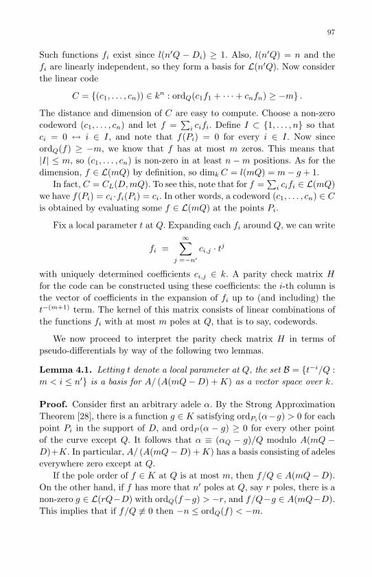
May 10, 2007 8:8 WSPC - Proceedings Trim Size: 9in x 6in ws-procs9x6
97
Such functions fi exist since l(n′Q − Di) ≥ 1. Also, l(n′Q) = n and thefi are linearly independent, so they form a basis for L(n′Q). Now considerthe linear code
C = (c1, . . . , cn)) ∈ kn : ordQ(c1f1 + · · ·+ cnfn) ≥ −m .
The distance and dimension of C are easy to compute. Choose a non-zerocodeword (c1, . . . , cn) and let f =
∑i cifi. Define I ⊂ 1, . . . , n so that
ci = 0 ↔ i ∈ I, and note that f(Pi) = 0 for every i ∈ I. Now sinceordQ(f) ≥ −m, we know that f has at most m zeros. This means that|I| ≤ m, so (c1, . . . , cn) is non-zero in at least n −m positions. As for thedimension, f ∈ L(mQ) by definition, so dimk C = l(mQ) = m− g + 1.
In fact, C = CL(D,mQ). To see this, note that for f =∑
i cifi ∈ L(mQ)we have f(Pi) = ci ·fi(Pi) = ci. In other words, a codeword (c1, . . . , cn) ∈ Cis obtained by evaluating some f ∈ L(mQ) at the points Pi.
Fix a local parameter t at Q. Expanding each fi around Q, we can write
fi =∞∑
j =−n′
ci,j · tj
with uniquely determined coefficients ci,j ∈ k. A parity check matrix H
for the code can be constructed using these coefficients: the i-th column isthe vector of coefficients in the expansion of fi up to (and including) thet−(m+1) term. The kernel of this matrix consists of linear combinations ofthe functions fi with at most m poles at Q, that is to say, codewords.
We now proceed to interpret the parity check matrix H in terms ofpseudo-differentials by way of the following two lemmas.
Lemma 4.1. Letting t denote a local parameter at Q, the set B = t−i/Q :m < i ≤ n′ is a basis for A/ (A(mQ−D) +K) as a vector space over k.
Proof. Consider first an arbitrary adele α. By the Strong ApproximationTheorem [28], there is a function g ∈ K satisfying ordPi(α−g) > 0 for eachpoint Pi in the support of D, and ordP (α − g) ≥ 0 for every other pointof the curve except Q. It follows that α ≡ (αQ − g)/Q modulo A(mQ −D)+K. In particular, A/ (A(mQ−D) +K) has a basis consisting of adeleseverywhere zero except at Q.
If the pole order of f ∈ K at Q is at most m, then f/Q ∈ A(mQ−D).On the other hand, if f has more that n′ poles at Q, say r poles, there is anon-zero g ∈ L(rQ−D) with ordQ(f−g) > −r, and f/Q−g ∈ A(mQ−D).This implies that if f/Q 6≡ 0 then −n ≤ ordQ(f) < −m.
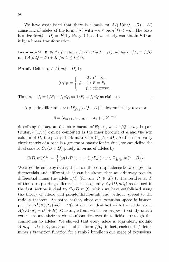
May 10, 2007 8:8 WSPC - Proceedings Trim Size: 9in x 6in ws-procs9x6
98
We have established that there is a basis for A/(A(mQ − D) + K)consisting of adeles of the form f/Q with −n ≤ ordQ(f) < −m. The basishas size i(mQ −D) = |B| by Prop. 4.1, and we clearly can obtain B fromit by a linear transformation.
Lemma 4.2. With the functions fi as defined in (1), we have 1/Pi ≡ fi/Q
mod A(mQ−D) +K for 1 ≤ i ≤ n.
Proof. Define αi ∈ A(mQ−D) by
(αi)P =
0 : P = Q.
fi + 1 : P = Pi.
fi : otherwise.
Then αi − fi = 1/Pi − fi/Q, so 1/Pi ≡ fi/Q as claimed.
A pseudo-differential ω ∈ ΩsK/k(mQ−D) is determined by a vector
a = (am+1, am+2, . . . , an′) ∈ kn′−m
describing the action of ω on elements of B; i.e., ω : t−i/Q 7→ ai. In par-ticular, ω(1/Pi) can be computed as the inner product of a and the i-thcolumn of H, the parity check matrix for CL(D,mQ). And since a paritycheck matrix of a code is a generator matrix for its dual, we can define thedual code to CL(D,mQ) purely in terms of adeles by
C(D,mQ)⊥ =
(ω(1/P1), . . . , ω(1/Pn)) : ω ∈ ΩsK/k(mQ−D)
We close the circle by noting that from the correspondence between pseudo-differentials and differentials it can be shown that an arbitrary pseudo-differential maps the adele 1/P (for any P ∈ X) to the residue at P
of the corresponding differential. Consequently, CΩ(D,mQ) as defined inthe first section is dual to CL(D,mQ), which we have established usingthe theory of adeles and pseudo-differentials and without appeal to theresidue theorem. As noted earlier, since our extension space is isomor-phic to H1(X,OX(mQ − D)), it can be identified with the adelic spaceA/(A(mQ − D) + K). One angle from which we propose to study rank-2extensions and their maximal subbundles over finite fields is through thisconnection to adeles. We showed that every adele is equivalent, moduloA(mQ−D) +K, to an adele of the form f/Q; in fact, each such f deter-mines a transition function for a rank-2 bundle in our space of extensions.

May 10, 2007 8:8 WSPC - Proceedings Trim Size: 9in x 6in ws-procs9x6
99
Acknowledgements
Both authors are thankful for partial research-travel support under NSAgrant MDA904-03-1-0119 [any opinions, findings, and conclusions or rec-ommendations expressed in this material are those of the authors and donot necessarily reflect the views of the National Security Agency]. E.P. iscurrently benefiting from the scholarly atmosphere of the Institut Mittag-Leffler in the Moduli Spaces program and is deeply grateful for the hospi-tality extended to her.
References
[1] A. Ashikhmin, A. Barg, S. Vladut, Linear codes with exponentially manylight vectors, J. Combin. Theory Ser. A 96 (2001), no. 2, 396-399.
[2] M.F. Atiyah, Vector bundles over an elliptic curve, Proc. London Math. Soc.(3) 7 (1957), 414–452.
[3] H.F. Baker, An introduction to the theory of multiply-periodic functions. Uni-versity Press XVI , Cambridge, 1907.
[4] T. Bouganis and D. Coles, A geometric view of decoding AG codes, in Appliedalgebra, algebraic algorithms and error-correcting codes (Toulouse, 2003), pp.180–190, Lecture Notes in Comput. Sci., 2643, Springer, Berlin, 2003.
[5] D. Coles, Vector bundles and codes on the Hermitian curve, IEEE Trans.Inform. Theory 51 (2005), no. 6, 2113–2120.
[6] D. Coles, On constructing AG codes without basis functions for Riemann-Roch spaces, in Lecture Notes in Comput. Sci., 3857, Springer, 2006, pp.108–117.
[7] A. Cossidente, G. Korchmaros and F. Torres, Curves of large genus coveredby the Hermitian curve, Comm. Algebra 28 (2000), no. 10, 4707–4728.
[8] H.M. Farkas and I. Kra, Branched two-sheeted covers, Israel J. Math. bf 74(1991), no. 2-3, 169–197.
[9] G. van der Geer, Curves over finite fields and codes, in European Congressof Mathematics, Vol. II (Barcelona, 2000), pp. 225–238, Progr. Math., 202,Birkhauser, Basel, 2001.
[10] M.L. Green, On the analytic solution of the equation of fifth degree, Com-positio Math. 37 (1978), no. 3, 233–241.
[11] R. Hartshorne, Algebraic geometry, Graduate Texts in Mathematics, No. 52.Springer-Verlag, New York-Heidelberg, 1977.
[12] T. Johnsen, Rank two bundles on algebraic curves and decoding of Goppacodes, Int. J. Pure Appl. Math. 4 (2003), no. 1, 33–45.
[13] E. Kani, Elliptic curves on abelian surfaces, Manuscripta Math. 84 (1994),no. 2, 199–223.
[14] F. Klein, On the order-seven transformation of elliptic functions, in Math.Sci. Res. Inst. Publ., 35, The eightfold way, pp. 287–331, Cambridge Univ.Press, Cambridge, 1999.
[15] H. Lange and S. Narasimhan, Maximal subbundles of rank two vector bun-dles on curves, Math. Ann. 266 (1983), no. 1, 55–72.

May 10, 2007 8:8 WSPC - Proceedings Trim Size: 9in x 6in ws-procs9x6
100
[16] K. Magaard, S. Shpectorov and H. Volklein, A GAP package for braid orbitcomputation and applications, Experiment. Math. 12 (2003), no. 4, 385–393.
[17] R. Miranda, Triple covers in algebraic geometry, Amer. J. Math. 107 (1985),no. 5, 1123–1158.
[18] K. Miura and H. Yoshihara, Field Theory for Function Fields of Plane Quar-tic Curves, J. Algebra 226 (2000), no. 1, 283–294.
[19] C. Moreno, Algebraic Curves Over Finite Fields, Cambridge Univ. Press,1991.
[20] W.M. Oxbury, Varieties of maximal line subbundles, Math. Proc. CambridgePhilos. Soc. 129 (2000), no. 1, 9–18.
[21] D.T. Prapavessi, On the Jacobian of the Klein curve, Proc. Amer. Math.Soc. 122 (1994), no. 4, 971–978.
[22] H.E. Rauch and J. Lewittes, The Riemann surface of Klein with 168 auto-morphisms, in Problems in Analysis (papers dedicated to Salomon Bochner,1969), Princeton Univ. Press, Princeton, NJ, 1970, pp. 297–308.
[23] J.-P. Serre, Algebraic Groups and Class Fields, Springer Graduate Texts inMathematics, 1988.
[24] T. Shaska, Curves of genus 2 with (N, N) decomposable Jacobians, J. Sym-bolic Comput. 31 (2001), no. 5, 603–617.
[25] T. Shaska, Genus 2 curves with (3, 3)-split Jacobian and large automorphismgroup, in: Algorithmic number theory (Sydney, 2002), 205–218, Lecture Notesin Comput. Sci., 2369, Springer, Berlin, 2002.
[26] T. Shaska, Genus 2 fields with degree 3 elliptic subfields, Forum Math. 16(2004), no. 2, 263–280.
[27] T. Shaska and H. Volklein, Elliptic subfields and automorphisms of genus 2function fields, in: Algebra, arithmetic and geometry with applications (WestLafayette, IN, 2000), 703–723, Springer, Berlin, 2004.
[28] H. Stichtenoth, Algebraic Function Fields and Codes, Springer-Verlag 1993.[29] E.W. von Tschirnhaus, Acta Eruditorium (1683).[30] S. Tuffery, Automorphismes d’ordre 3 et 7 sur une courbe de genre 3, Expo-
sition. Math. 11 (1993), no. 2, 159–162.[31] S. Tuffery, Les automorphismes des courbes de genre 3 de caracteristique 2,
C. R. Acad. Sci. Paris Ser. I Math. 321 (1995), no. 2, 205–210.[32] S. Tuffery, Deformations de courbes avec action de groupe. II, Forum Math.
8 (1996), no. 2, 205–218.[33] P. Tzermias, The group of automorphisms of the Fermat curve, J. Number
Theory 53 (1995), no. 1, 173–178.

May 10, 2007 8:8 WSPC - Proceedings Trim Size: 9in x 6in ws-procs9x6
101
Remarks on s-extremal codes
Jon-Lark Kim
Department of Mathematics,
University of Louisville,
Louisville, KY 40292, USAE-mail: [email protected]
www.math.louisville.edu/∼jlkim
We study s-extremal codes over F4 or over F2. A Type I self-dual code over F4
or over F2 of length n and minimum distance d is s-extremal if the minimumweight of its shadow is largest possible. The purpose of this paper is to give
some results which are missing in a series of papers by Bachoc and Gaborit [2],
by Gaborit [6], and by Bautista, et. al. [1]. In particular, we give an explicitformula for the numbers of the first four nonzero weights of an s-extremal code
over F4. We improve a bound on the length for which there exists an s-extremal
code over F4 (res. F2) with even minimum distance d (resp. d ≡ 0 (mod 4)),and give codes related to s-extremal binary codes.
Keywords: Additive self-dual codes; Ninary self-dual codes; s-extremal codes.
1. Introduction
Binary self-dual codes have been of great interest since the beginning ofthe coding theory partly because many good linear block codes are eitherself-orthogonal or self-dual. Furthermore, they have nice properties; in par-ticular, the weight enumerator of a binary self-dual code is invariant undera certain finite group, which often restricts the minimum distance of sucha code. We refer to the chapter of self-dual codes [12] for a full discussionof self-dual codes.
It was Conway and Sloane [4] who introduced the notion of the shadowof a binary self-dual code in order to get additional constraints in the weightenumerator of a singly-even binary self-dual code C. The shadow S of C isdefined as
S := C⊥0 \ C.
Let d be the minimum distance of C and s the minimum weight of S.Bachoc and Gaborit [2] showed that 2d + s ≤ n
2 + 4, except in the case
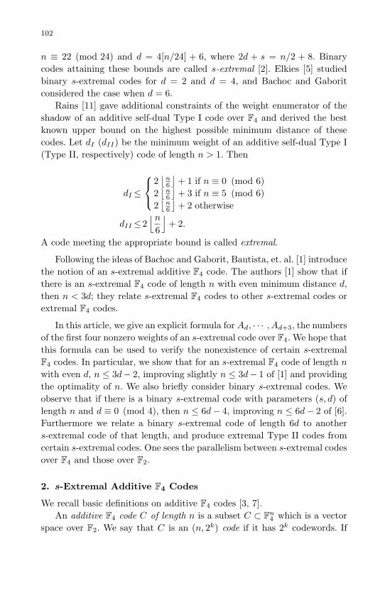
May 10, 2007 8:8 WSPC - Proceedings Trim Size: 9in x 6in ws-procs9x6
102
n ≡ 22 (mod 24) and d = 4[n/24] + 6, where 2d + s = n/2 + 8. Binarycodes attaining these bounds are called s-extremal [2]. Elkies [5] studiedbinary s-extremal codes for d = 2 and d = 4, and Bachoc and Gaboritconsidered the case when d = 6.
Rains [11] gave additional constraints of the weight enumerator of theshadow of an additive self-dual Type I code over F4 and derived the bestknown upper bound on the highest possible minimum distance of thesecodes. Let dI (dII) be the minimum weight of an additive self-dual Type I(Type II, respectively) code of length n > 1. Then
dI ≤
2⌊
n6
⌋+ 1 if n ≡ 0 (mod 6)
2⌊
n6
⌋+ 3 if n ≡ 5 (mod 6)
2⌊
n6
⌋+ 2 otherwise
dII ≤2⌊n
6
⌋+ 2.
A code meeting the appropriate bound is called extremal.
Following the ideas of Bachoc and Gaborit, Bautista, et. al. [1] introducethe notion of an s-extremal additive F4 code. The authors [1] show that ifthere is an s-extremal F4 code of length n with even minimum distance d,then n < 3d; they relate s-extremal F4 codes to other s-extremal codes orextremal F4 codes.
In this article, we give an explicit formula for Ad, · · · , Ad+3, the numbersof the first four nonzero weights of an s-extremal code over F4. We hope thatthis formula can be used to verify the nonexistence of certain s-extremalF4 codes. In particular, we show that for an s-extremal F4 code of length nwith even d, n ≤ 3d− 2, improving slightly n ≤ 3d− 1 of [1] and providingthe optimality of n. We also briefly consider binary s-extremal codes. Weobserve that if there is a binary s-extremal code with parameters (s, d) oflength n and d ≡ 0 (mod 4), then n ≤ 6d− 4, improving n ≤ 6d− 2 of [6].Furthermore we relate a binary s-extremal code of length 6d to anothers-extremal code of that length, and produce extremal Type II codes fromcertain s-extremal codes. One sees the parallelism between s-extremal codesover F4 and those over F2.
2. s-Extremal Additive F4 Codes
We recall basic definitions on additive F4 codes [3, 7].An additive F4 code C of length n is a subset C ⊂ Fn
4 which is a vectorspace over F2. We say that C is an (n, 2k) code if it has 2k codewords. If
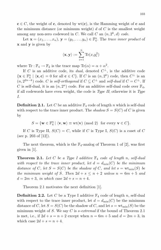
May 10, 2007 8:8 WSPC - Proceedings Trim Size: 9in x 6in ws-procs9x6
103
c ∈ C, the weight of c, denoted by wt(c), is the Hamming weight of c andthe minimum distance (or minimum weight) d of C is the smallest weightamong any non-zero codeword in C. We call C an (n, 2k, d) code.
Let x = (x1, . . . , xn), y = (y1, . . . , yn) ∈ Fn4 . The trace inner product of
x and y is given by
〈x,y〉 :=n∑
i=1
Tr(xiy2i )
where Tr : F4 → F2 is the trace map Tr(α) = α+ α2.If C is an additive code, its dual, denoted C⊥, is the additive code
x ∈ Fn4 | 〈x, c〉 = 0 for all c ∈ C. If C is an (n, 2k) code, then C⊥ is an
(n, 22n−k) code. C is self-orthogonal if C ⊆ C⊥ and self-dual if C = C⊥. IfC is self-dual, it is an (n, 2n) code. For an additive self-dual code over F4,if all codewords have even weight, the code is Type II; otherwise it is TypeI.
Definition 2.1. Let C be an additive F4 code of length n which is self-dualwith respect to the trace inner product. The shadow S = S(C) of C is givenby
S = w ∈ Fn4 | 〈v,w〉 ≡ wt(v) (mod 2) for every v ∈ C.
If C is Type II, S(C) = C, while if C is Type I, S(C) is a coset of C(see p. 203 of [12]).
The next theorem, which is the F4-analog of Theorem 1 of [2], was firstgiven in [1].
Theorem 2.1. Let C be a Type I additive F4 code of length n, self-dualwith respect to the trace inner product, let d = dmin(C) be the minimumdistance of C, let S = S(C) be the shadow of C, and let s = wtmin(S) bethe minimum weight of S. Then 2d + s ≤ n + 2 unless n = 6m + 5 andd = 2m+ 3, in which case 2d+ s = n+ 4.
Theorem 2.1 motivates the next definition [1].
Definition 2.2. Let C be a Type I additive F4 code of length n, self-dualwith respect to the trace inner product, let d = dmin(C) be the minimumdistance of C, let S = S(C) be the shadow of C, and let s = wtmin(S) be theminimum weight of S. We say C is s-extremal if the bound of Theorem 2.1is met, i.e., if 2d+ s = n+ 2 except when n = 6m+ 5 and d = 2m+ 3, inwhich case 2d+ s = n+ 4.

May 10, 2007 8:8 WSPC - Proceedings Trim Size: 9in x 6in ws-procs9x6
104
Remark 2.1. It is interesting to note that the weight enumerator of any s-extremal code is uniquely determined and can be explicitly computed fromthe values of n and d (or n and s) [1].
Gleason’s Theorem for additive F4-codes holds as follows; see [1, 9, 11]for details.
Theorem 2.2. Let C be an additive F4 code of length n which is self-dualwith respect to the trace inner product. Let S = S(C) be the shadow of C,and let C(x, y) and S(x, y) be the homogeneous weight enumerators of Cand S, respectively. Then
S(x, y) =1|C|
C(x+ 3y, y − x),
and there are polynomials
P (X,Y ) =bn
2 c∑i=0
uiXn−2iY i and Q(X,Y ) =
bn2 c∑
i=0
viXn−2iY i
over R such that
C(x, y) = P (x+ y, x2 + 3y2) = Q(x+ y, y(x− y))
and
S(x, y) = P (2y, x2 + 3y2) = Q(2y,y2 − x2
2).
Certain coefficients of P (x, y) and Q(x, y) are 0 as follows; see [1] fordetails.
Lemma 2.1. Let C be an additive F4 code of length n which is self-dualwith respect to the trace inner product. Let S = S(C) be the shadow ofC. Every vector in S has weight congruent to n modulo 2. Moreover, ifwe let s = wtmin(S) be the minimum weight of S and write s = n − 2r,then the coefficients ui and vi in the polynomials P (X,Y ) and Q(X,Y ) ofTheorem 2.2 are 0 for r + 1 ≤ i ≤ bn
2 c.
Let C be an s-extremal F4 code of length n with minimum distance dand the minimum weight s of the shadow of C. In what follows, we derivean explicit formula for Ad, · · ·Ad+3, where Ai is the number of codewordsin C of weight i.
Using the second equation of C(x, y) in Theorem 2.2 and Lemma 2.1,we have

May 10, 2007 8:8 WSPC - Proceedings Trim Size: 9in x 6in ws-procs9x6
105
C(1, y) = 1 +Adyd +Ad+1y
d+1 +Ad+2yd+2 +Ad+3y
d+3 + · · ·
=d−1∑i=0
vi(1 + y)n−2i(y(1− y))i.
Dividing both sides by (1 + y)n, we get
1(1 + y)n
(1 +Adyd +Ad+1y
d+1 +Ad+2yd+2 +Ad+3y
d+3 + . . . )
=d−1∑i=0
vi
(y(1− y)(1 + y)2
)i
.
Write f(y) = 1(1+y)n and g(y) = y(1−y)
(1+y)2 . Then we have
d−1∑i=0
vigi(y) = f(y) + f(y)Ady
d + · · ·+ f(y)Ad+3yd+3 +O(yd+4). (1)
We expand f(y) as a power series of y as follows.
f(y) =1
(1 + y)n=
∞∑i=0
(−1)i
(n+ i− 1
i
)yi
= 1− ny +(n+ 1
2
)y2 −
(n+ 2
3
)y3 +O(y4).
We plug this in Equation (1) to get the following lemma.
Lemma 2.2. Under the above notations,d−1∑i=0
vigi(y) = f(y) +Ad
1− ny +
(n+ 1
2
)y2 −
(n+ 2
3
)y3 +O(y4)
yd
+Ad+1
1− ny +
(n+ 1
2
)y2 −
(n+ 2
3
)y3 +O(y4)
yd+1
+ · · ·= f(y) +Ady
d + −nAd +Ad+1 yd+1
+Ad
(n+ 1
2
)− nAd+1 +Ad+2
yd+2
+−Ad
(n+ 2
3
)+Ad+1
(n+ 1
2
)− nAd+2 +Ad+3
yd+3
+O(yd+4).

May 10, 2007 8:8 WSPC - Proceedings Trim Size: 9in x 6in ws-procs9x6
106
Our next step is to rewrite gi(y) for i ≥ d as a power series in y. Sinceg(y) = y(1−y)
(1+y)2 , we have
gd(y) =yd(1− y)d
(1 + y)2d
= yd
d∑j=0
(−1)j
(d
j
)yj
( ∞∑i=0
(−1)i
(2d+ i− 1
i
)yi
)
= yd − 3dyd+1 +(
d
2
)+ d
(2d1
)+(
2d+ 12
)yd+2
+−(d
3
)−(d
2
)(2d1
)− d(
2d+ 12
)−(
2d+ 23
)yd+3
+O(yd+4).
Similarly we obtain the following.
gd+1(y) = yd+1 +−(d+ 1
1
)−(
2d+ 21
)yd+2
+(
2d+ 32
)+(d+ 1
1
)(2d+ 2
1
)+(d+ 1
2
)yd+3
+O(yd+4),
gd+2(y) = yd+2 +−(
2d+ 41
)−(d+ 2
1
)yd+3 +O(yd+4),
gd+3(y) = yd+3 +O(yd+4).
Now we can rewrite yi for i = d, d+ 1, d+ 2, d+ 3 in terms of gi(y) andO(yd+4) as follows.
yd+3 = gd+3(y) +O(yd+4),
yd+2 = gd+2(y) +(
d+ 21
)+(
2d+ 41
)gd+3(y) +O(yd+4),
yd+1 = gd+1(y) +(
d+ 11
)+(
2d+ 21
)gd+2(y)
+ (3d+ 3)(3d+ 6)gd+3(y)
−(
2d+ 32
)+(d+ 1
1
)(2d+ 2
1
)+(d+ 1
2
)gd+3(y) +O(yd+4),

May 10, 2007 8:8 WSPC - Proceedings Trim Size: 9in x 6in ws-procs9x6
107
yd = gd(y) + 3dgd+1(y)
+
3d(3d+ 3)−(d
2
)− d(
2d1
)−(
2d+ 12
)gd+2(y)
+ 3d(3d+ 3)(3d+ 6)gd+3(y)
− 3d(
2d+ 32
)+ (d+ 1)(2d+ 2) +
(d+ 1
2
)gd+3(y)
− (3d+ 6)(
d
2
)+ d
(2d1
)+(
2d+ 12
)gd+3(y)
+(
d
3
)+(d
2
)(2d1
)+ d
(2d+ 1
2
)+(
2d+ 23
)gd+3(y)
+O(yd+4).
Now let κi be the coefficient of gi(y) in
f(y) =∑i≥0
κig(y)i
Then we plug the above calculations in Lemma 2.2 to obtain the follow-ing relation between κi and Ai’s.
Lemma 2.3.Under the notations as above,
(i) κd = −Ad,
(ii) κd+1 = −((3d− n)Ad +Ad+1),
(iii) κd+2 = −12Ad(9d2 + 17d− 6dn− 5n+ n2)
−Ad+1(3d+ 3− n)−Ad+2,
(iv) κd+3 = −Ad
92d3 +
512d2 + 37d+ n(−9
2d2 − 35
2d− 13)
−Ad
(3d+ 6)
(n+ 1
2
)−(n+ 2
3
)−Ad+1
92d2 +
352d+ 13− n(3d+ 6) +
(n+ 1
2
)−Ad+2(3d+ 6− n)−Ad+3.
On the other hand, we can evaluate κi using the Burman-LagrangeTheorem. We recall the Burman-Lagrange Theorem (as stated in [11]): If

May 10, 2007 8:8 WSPC - Proceedings Trim Size: 9in x 6in ws-procs9x6
108
f(x) and g(x) are formal power series with g(0) = 0 and g′(0) 6= 0 and thecoefficients κi are defined by
f(x) =∑i≥0
κig(x)i,
then
κi =1i
(coefficient of xi−1 in f ′(x)
(x
g(x)
)i).
Our functions f(y) and g(y) satisfy these hypotheses, and we have
κd =1d
(coefficient of yd−1 in f ′(y)
(y
g(y)
)d)
=1d
(coefficient of yd−1 in
(−n
(1 + y)n+1
)((1 + y)2
1− y
)d)
=−nd
(coefficient of yd−1 in
1(1 + y)n−3d+1(1− y2)d
).
Similarly we obtain the following.
κd+1 =−nd+ 1
(coefficient of yd in
1(1 + y)n−3d−2(1− y2)d+1
)κd+2 =
−nd+ 2
(coefficient of yd+1 in
1(1 + y)n−3d−5(1− y2)d+2
)κd+3 =
−nd+ 3
(coefficient of yd+2 in
1(1 + y)n−3d−8(1− y2)d+3
)
Corollary 2.1. If d is even and n = 3d− 1 then there is no s-extremal F4
code.
Proof. If n = 3d−1, then κd = −nd
(coefficient of yd−1 in 1
(1−y2)d
). Hence
κd = 0 as d is even. Then by (i) of Lemma 2.3, Ad = 0, which is a contra-diction.
Note that an s-extremal code of length n with minimum distance d mustsatisfy n ≥ 3d−5, and that if d is even, 3d−4 ≤ n < 3d [1]. Hence we havethe following.
Corollary 2.2. An s-extremal code of length n with even minimum dis-tance d must satisfy n = 3d− 4, 3d− 3, or 3d− 2.
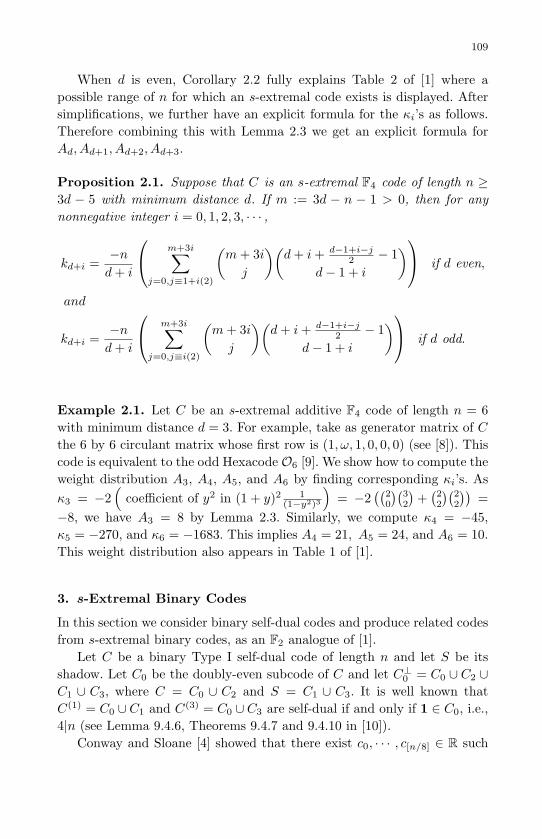
May 10, 2007 8:8 WSPC - Proceedings Trim Size: 9in x 6in ws-procs9x6
109
When d is even, Corollary 2.2 fully explains Table 2 of [1] where apossible range of n for which an s-extremal code exists is displayed. Aftersimplifications, we further have an explicit formula for the κi’s as follows.Therefore combining this with Lemma 2.3 we get an explicit formula forAd, Ad+1, Ad+2, Ad+3.
Proposition 2.1. Suppose that C is an s-extremal F4 code of length n ≥3d − 5 with minimum distance d. If m := 3d − n − 1 > 0, then for anynonnegative integer i = 0, 1, 2, 3, · · · ,
kd+i =−nd+ i
m+3i∑j=0,j≡1+i(2)
(m+ 3ij
)(d+ i+ d−1+i−j
2 − 1d− 1 + i
) if d even,
and
kd+i =−nd+ i
m+3i∑j=0,j≡i(2)
(m+ 3ij
)(d+ i+ d−1+i−j
2 − 1d− 1 + i
) if d odd.
Example 2.1. Let C be an s-extremal additive F4 code of length n = 6with minimum distance d = 3. For example, take as generator matrix of Cthe 6 by 6 circulant matrix whose first row is (1, ω, 1, 0, 0, 0) (see [8]). Thiscode is equivalent to the odd Hexacode O6 [9]. We show how to compute theweight distribution A3, A4, A5, and A6 by finding corresponding κi’s. Asκ3 = −2
(coefficient of y2 in (1 + y)2 1
(1−y2)3
)= −2
((20
)(32
)+(22
)(22
))=
−8, we have A3 = 8 by Lemma 2.3. Similarly, we compute κ4 = −45,κ5 = −270, and κ6 = −1683. This implies A4 = 21, A5 = 24, and A6 = 10.This weight distribution also appears in Table 1 of [1].
3. s-Extremal Binary Codes
In this section we consider binary self-dual codes and produce related codesfrom s-extremal binary codes, as an F2 analogue of [1].
Let C be a binary Type I self-dual code of length n and let S be itsshadow. Let C0 be the doubly-even subcode of C and let C⊥0 = C0 ∪ C2 ∪C1 ∪ C3, where C = C0 ∪ C2 and S = C1 ∪ C3. It is well known thatC(1) = C0 ∪C1 and C(3) = C0 ∪C3 are self-dual if and only if 1 ∈ C0, i.e.,4|n (see Lemma 9.4.6, Theorems 9.4.7 and 9.4.10 in [10]).
Conway and Sloane [4] showed that there exist c0, · · · , c[n/8] ∈ R such

May 10, 2007 8:8 WSPC - Proceedings Trim Size: 9in x 6in ws-procs9x6
110
that:
C(x, y) =[n/8]∑i=0
ci(x2 + y2)n2−4ix2y2(x2 − y2)2i, (2)
S(x, y) =[n/8]∑i=0
ci(−1)i2n2−6i(xy)
n2−4i(x4 − y4)2i. (3)
Applying the Burman-Lagrange Theorem to certain transformed equationsof the above equations, Bachoc and Gaborit [2] introduced a notion of ans-extremal binary code; for details see [2].
Theorem 3.1. Let C be a binary Type I self-dual code of length n andminimum distance d, and let S be its shadow of minimum weight s. Then2d+ s ≤ 4+ n
2 , unless n ≡ 22 (mod 24) and d = 4[n/24]+6, in which case2d+ s = 8 + n
2 .
Definition 3.1. A binary Type I code meeting the above bound is calleds-extremal.
When d ≡ 0 (mod 4), the length of a s-extremal code is bounded by 6das follows.
Theorem 3.2. Let C be an s-extremal code with parameters (s, d) of lengthn. If d ≡ 0 (mod 4), then n < 6d (i.e., n ≤ 6d− 2).
Following the proof of the above theorem in [6], we have that for anybinary s-extremal code,
Ad =n
d
(coefficient of yd−2 in
1(1 + y2)
n2−3d+1(1− y4)d
).
In particular, if n = 6d − 2, then n2 − 3d + 1 = 0. Further if d ≡ 0
(mod 4) then d − 2 ≡ 2 (mod 4). Therefore Ad = 0, which is impossible.Therefore we obtain the following.
Proposition 3.1. Let C be an s-extremal code with parameters (s, d) oflength n. If d ≡ 0 (mod 4), then n ≤ 6d− 4.
Codes related to s-extremal additive F4 codes are described in Propo-sitions 7.1 and 7.3 in [1], whose proofs however contain minor errors. Weshow that this can be done analogously for binary s-extremal codes in thefollowing propositions. We include the proofs for completeness.
Proposition 3.2. Let C be a binary s-extremal code of length n and min-imum distance d satisfying 2d+ s = 4+ n
2 . If d ≡ 2 (mod 4) and s = d+4,

May 10, 2007 8:8 WSPC - Proceedings Trim Size: 9in x 6in ws-procs9x6
111
then C(1) and C(3) are also s-extremal with minimum distance d′ = d + 2and the minimum shadow weight s′ = d.
Proof. Since d ≡ 2 (mod 4), n2 = 3d is congruent to 2 (mod 4). Thus
all weights in S are congruent to 2 (mod 4) (by Theorem 9.4.7 [10] or bylooking at the powers of y in Equation (3)). Thus both C(1) and C(3) areType I self-dual codes; self-duality follows as 4|n. We may assume that C1
contains a vector x of minimum weight s. There are two possibilities ford(C0): Either d(C0) = d+ 2 or d(C0) > d+ 2.
If d(C0) > d + 2, then d(C0) ≥ d + 6 as C0 is doubly-even. So in thiscase, the minimum distance of C(1) is d′ = mind(C0), d(C1) = min≥d+ 6, s = d+ 4. The shadow of C(1) is C2 ∪ C3, and its minimum weightis s′ = mind(C2), d(C3) = mind,≥ s = d. As 2d′ + s′ = 2(d+ 4) + d =3d+ 8 = n
2 + 8, n must be congruent to 22 (mod 24). This contradicts thecondition that n
2 ≡ 2 (mod 4).Thus we have d(C0) = d+2. Following the above arguments, we obtain
d′ = d+ 2 and s′ = d. As 2d′ + s′ = 2(d+ 2) + d = 3d+ 4 = n2 + 4, C(1) is
s-extremal.As d(C0) = d + 2, one can show that C(3) is s-extremal in a similar
manner.
Proposition 3.3. Let C be a binary s-extremal code of length n = 24µ+8and minimum distance d. If d ≡ 2 (mod 4) and s = d + 2, then both C(1)
and C(3) are extremal Type II codes with minimum distance d + 2. More-over the weight enumerators of C1 and C3 are the same and are explicitlydetermined.
Proof. As n2 ≡ 0 (mod 4), 4|n and all weights in S are doubly-even. So
C(1) and C(3) are Type II. Since d(S) = s, the minimum distance of C(i) ismind(C0), d(Ci) ≥ s for i = 1, 3, and either d(C1) = s or d(C3) = s, butnot necessarily both. We know that d(C0) ≥ d + 2 = s as d ≡ 2 (mod 4)and C0 is doubly-even. So d(C(i)) = mind(C0), d(Ci) ≥ s for i = 1, 3.Since 2d+s = 4+ n
2 = 12µ+8 and d = s−2, we have 2(s−2)+s = 12µ+8implying s = 4µ+4. As extremal Type II codes of length n = 24µ+8 haveminimum weight at most 4µ+4, d(C(i)) must be s = d+2 and each d(C(i))is extremal.
Finally note that the weight enumerator of a binary extremal Type IIcode is uniquely determined by its length and that the weight enumeratorof C0 is explicitly determined by that of C. Thus the weight enumerator ofC1 and C3 are the same and are explicitly determined.

May 10, 2007 8:8 WSPC - Proceedings Trim Size: 9in x 6in ws-procs9x6
112
4. Conclusion
We have obtained results concerning both s-extremal F4 codes and s-extremal binary codes. In particular, we find an explicit formula forAd, · · · , Ad+3 of an s-extremal F4 code. This formula is of use for knowinga possible weight distribution of an s-extremal F4 code. Furthermore, thisformula might be used for the upper bound on the length of an s-extremalF4 code when its minimum distance is odd. For example, suppose that thereexists an s-extremal F4 code with odd d and n = 3d + 2. Then κd+1 = 0from Proposition 2.1. Hence Ad+1 = 2Ad by Lemma 2.3. All the weightenumerators of s-extremal F4 codes [1] do not have this relation. On theother hand we remark that one can obtain a formula for Ad, · · · , Ad+3 of abinary s-extremal code in an analogous manner.
We also have improved a bound on the length for which there exists ans-extremal code over F4 or over F2 with even minimum distance, and gavebinary s-extremal or extremal codes constructed from binary s-extremalcodes.
Acknowledgments
The author would like to thank Professor W. Cary Huffman and Dr.Sunghyu Han for invaluable comments on the submitted manuscript, inparticular for suggesting improved proofs of Propositions 3.2 and 3.3. Theauthor acknowledges support by a Project Completion Grant from the Uni-versity of Louisville.
References
[1] E.P. Bautista, P. Gaborit, J.-L. Kim, and J.L. Walker, s-extremal additive F4
codes, Advances in Mathematics of Communication, 1 111-130 (2007).[2] C. Bachoc and P. Gaborit, Designs and self-dual codes with long shadows, J.
Combin. Theory Ser. A, 105 15–34 (2004).[3] A. R. Calderbank, E. M. Rains, P. W. Shor, and N. J. A. Sloane. Quantum
error correction via codes over GF (4), IEEE Trans. Inform. Theory, 44 1369–1387 (1998).
[4] J. H. Conway and N. J. A. Sloane, A new upper bound on the minimal dis-tance of self-dual codes, IEEE Trans. Inform. Theory, 36 1319–1333 (1990).
[5] N. D. Elkies, Lattices and codes with long shadows, Math. Res. Lett., 2 643–651 (1995).
[6] P. Gaborit, A bound for certain s-extremal lattices and codes, preprint. avail-able at http://www.unilim.fr/pages perso/philippe.gaborit/
[7] P. Gaborit, W. C. Huffman, J.-L. Kim, and V. Pless, On additive GF(4)codes, in Codes and association schemes (Piscataway, NJ, 1999), volume 56
May 10, 2007 8:8 WSPC - Proceedings Trim Size: 9in x 6in ws-procs9x6
113
of DIMACS Ser. Discrete Math. Theoret. Comput. Sci., pages 135–149. Amer.Math. Soc., Providence, RI, 2001.
[8] T. A. Gulliver and J.-L. Kim, Circulant based extremal additive self-dualcodes over GF(4), IEEE Trans. Inform. Theory, 50 359–366 (2004).
[9] G. Hohn, Self-dual codes over the Kleinian four group, Math. Ann., 327 227–255 (2003).
[10] W. C. Huffman and V. S. Pless, Fundamentals of Error-correcting Codes.Cambridge: Cambridge University Press, 2003.
[11] E. M. Rains, Shadow bounds for self-dual codes, IEEE Trans. Inform. The-ory, 44 134–139 (1998).
[12] E. M. Rains and N. J. A. Sloane, Self-dual codes, in Handbook of CodingTheory, ed. V. S. Pless and W. C. Huffman. Amsterdam: Elsevier, pp. 177–294, 1998.

May 10, 2007 8:8 WSPC - Proceedings Trim Size: 9in x 6in ws-procs9x6
114
Automorphism groups of generalized Reed-Solomon codes
David Joyner, Amy Ksir, Will Traves
Mathematics Dept.
U.S. Naval Academy
Annapolis, MD 21402E-mails: [email protected], [email protected], [email protected]
We look at AG codes associated to P1, re-examining the problem of determin-
ing their automorphism groups (originally investigated by Dur in 1987 using
combinatorial techniques) using recent methods from algebraic geometry. Weclassify those finite groups that can arise as the automorphism group of an
AG code and give an explicit description of how these groups appear. We give
examples of generalized Reed-Solomon codes with large automorphism groupsG, such as G = PSL(2, q), and explicitly describe their G-module structure.
Keywords: generalized Reed-Solomon codes, permutation automorphism
groups, algebraic-geometric codes, G-modules
1. Introduction
Reed-Solomon codes are popular in applications because fast encoding anddecoding algorithms are known for them. For example, they are used incompact discs (more details can be found in §5.6 in Huffman and Pless [4]).
In this paper we study which groups can arise as automorphism groupsof a related collection of codes, the algebraic geometry (AG) codes on P1.These codes are monomially equivalent to generalized Reed-Solomon (GRS)codes. Their automorphism groups were first studied by Dur [2] in 1987using combinatorial techniques. Huffman [3] gives an excellent expositionof Dur’s original work. In this paper, using recent methods from algebraicgeometry (due to Brandt and Stichenoth [12], Valentini and Madan [14],Kontogeorgis [9]), we present a method for computing GRS codes with“large” permutation automorphism groups. In contrast to Dur’s results, weindicate exactly how these automorphism groups can be obtained.
The paper is organized as follows. In section 2 we review some back-ground on AG codes and GRS codes. In section 3 we review some knownresults on automorphisms of AG codes, and then prove our main result,

May 10, 2007 8:8 WSPC - Proceedings Trim Size: 9in x 6in ws-procs9x6
115
characterizing the automorphism groups of AG codes. In section 4 we usethese results to give examples of codes with large automorphism groups.In section 5, we discuss the structure of these group representations asG-modules, in some cases determining it explicitly.
2. AG codes and GRS codes
We recall some well-known background on AG codes and GRS codes.Let X be a smooth projective curve over a field F and let F denote
a separable algebraic closure of F . We will generally take F to be finiteof order q. Let F (X) denote the function field of X (the field of rationalfunctions on X). Recall that a divisor on X is a formal sum, with integercoefficients, of places of F (X). We will denote the group of divisors on X
by Div(X). The rational points of X are the places of degree 1, and the setof rational points is denoted X(F ).
AG codes associated to a divisor D are constructed from the Riemann-Roch space
L(D) = LX(D) = f ∈ F (X)× | div(f) +D ≥ 0 ∪ 0,
where div(f) denotes the (principal) divisor of the function f ∈ F (X). TheRiemann-Roch space is a finite dimensional vector space over F , whosedimension is given by the Riemann-Roch theorem.
Let P1, ..., Pn ∈ X(F ) be distinct points and E = P1+...+Pn ∈ Div(X).Assume these divisors have disjoint support, supp(D) ∩ supp(E) = ∅. LetC(D,E) denote the AG code
C(D,E) = (f(P1), ..., f(Pn)) | f ∈ L(D). (1)
This is the image of L(D) under the evaluation map
evalE : L(D)→ Fn,
f 7−→ (f(P1), ..., f(Pn)).(2)
The following is well-known (a proof can be found in Joyner and Ksir [7]).
Lemma 2.1. If deg(D) > deg(E), then evalE is injective.
In this paper, we restrict to the case where X is the projective line P1
over F . In this case, if degD ≥ 0 then dimL(D) = degD+1, and otherwisedimL(D) = 0. Thus we will be interested in the case where degD ≥ 0.

May 10, 2007 8:8 WSPC - Proceedings Trim Size: 9in x 6in ws-procs9x6
116
In the special case when D is a positive integer multiple of the point atinfinity, then this construction gives a Reed-Solomon code. More generally,
C = (α1f(P1), ..., αnf(Pn)) | f ∈ L(` · ∞),
is called a generalized Reed-Solomon code (or GRS code), whereα1, ..., αn is a fixed set of non-zero elements in F (called “multipliers”).
In fact, for a more general D, this construction gives a code which ismonomially equivalent to a GRS code, and which furthermore is MDS (thatis, n + 1 = k + d, where n is the length, k is the dimension, and d is theminimum distance of the code). We say that two codes C,C ′ of length n aremonomially equivalent if there is an element of the group of monomialmatrices Monn(F ) – those matrices with precisely one non-zero entry ineach row and column – (acting in the natural way on Fn) sending C to C ′
(as F -vector spaces).
Lemma 2.2. Let X = P1/F , D be any divisor of positive degree on X, andlet E = P1 + . . .+Pn, where P1, . . . , Pn are points in X(F ) and n > degD.Let C(D,E) be the AG code constructed as above. Then C(D,E) is anMDS code which is monomially equivalent to a GRS code (with all scalarsαi = 1).
Proof. This is well-known (see for example Stichtenoth [11], §II.2), butwe give the details for convenience. C(D,E) has length n and dimensionk = deg(D)+1. By Theorem 13.4.3 of Huffman and Pless [4], its minimumdistance d satisfies
n− deg(D) ≤ d,
and the Singleton bound says that
d ≤ n+ 1− k = n− deg(D).
Therefore, d = n+ 1− k, and this shows that C(D,E) is MDS.The monomial equivalence follows from the fact that on P1, all divisors
of a given positive degree are (rationally) equivalent, so D is rationallyequivalent to deg(D) · ∞. Thus there is a rational function h on X suchthat
D = deg(D) · ∞+ div(h).
Then for any f ∈ L(D), fh is in L(deg(D) · ∞). Thus there is a map
M : C(D,E)→ C(deg(D) · ∞, E)
(f(P1), . . . , f(Pn)) 7→ (fh(P1), . . . , fh(Pn))

May 10, 2007 8:8 WSPC - Proceedings Trim Size: 9in x 6in ws-procs9x6
117
which is linear and whose matrix is diagonal with diagonal entriesh(P1), . . . , h(Pn). In particular, M is a monomial matrix, so C(D,E) andthe GRS code C(deg(D) · ∞, E) are monomially equivalent.
Remark 2.1. The spectrum of a code of length n is the list[A0, A1, ..., An], where Ai denotes the number of codewords of weight i.The dual code of a linear code C ⊂ Fn is the dual of C as a vector spacewith respect to the Hamming inner product on Fn, denoted C⊥. We say Cis formally self-dual if the spectrum of C⊥ is the same as that of C. Thespectrum of any MDS code is known (see §7.4 in Huffman and Pless [4]),and as a consequence of this we have the following
Aj =(n
j
)(q − 1)
j−d∑i=0
(−1)i
(j − 1i
)qj−d−i, d ≤ j ≤ n,
where q is the order of the finite field F . The following is an easy conse-quence of this and the fact that the dual code of an MDS code is MDS: if Cis a GRS code with parameters [n, k, d] satisfying n = 2k then C is formallyself-dual. We will see later some examples of formally self-dual codes withlarge automorphism groups.
3. Automorphisms
The action of a finite group G ⊂ Aut(X) on F (X) is defined by restrictionto G of the map
ρ : Aut(X) −→ Aut(F (X)),g 7−→ (f 7−→ fg)
where fg(x) = (ρ(g)(f))(x) = f(g−1(x)).Note that Y = X/G is also smooth and the quotient map
ψ : X → Y (3)
yields an identification F (Y ) = F (X)G := f ∈ F (X) | fg = f, ∀ g ∈ G.Of course, G also acts on the group Div(X) of divisors of X. If g ∈
Aut(X) and dP ∈ Z, for places P of F (X), then g(∑
P dPP ) =∑
P dP g(P ).It is easy to show that div(fg) = g(div(f)). Because of this, if div(f)+D ≥ 0then div(fg) + g(D) ≥ 0, for all g ∈ Aut(X). In particular, if the action ofG on X leaves D ∈ Div(X) stable then G also acts on L(D). We denotethis action by
ρ : G→ Aut(L(D)).

May 10, 2007 8:8 WSPC - Proceedings Trim Size: 9in x 6in ws-procs9x6
118
Now suppose that E = P1 + . . . + Pn is also stabilized by G. In otherwords, G acts on the set supp(E) = P1, . . . , Pn by permutation. Thenthe group G acts on C(D,E) by g ∈ G sending c = (f(P1), ..., f(Pn)) ∈ Cto c′ = (f(g−1(P1)), ..., f(g−1(Pn))), where f ∈ L(D).
Remark 3.1. Observe that this map sending c 7−→ c′, denoted φ(g),is well-defined. This is clearly true if evalE is injective. In case evalEis not injective, suppose c is also represented by f ′ ∈ L(D), so c =(f ′(P1), ..., f ′(Pn)) ∈ C. Since G acts on the set supp(E) by permu-tation, for each Pi, g−1(Pi) = Pj for some j. Then f(g−1(Pi)) =f(Pj) = f ′(Pj) = f ′(g−1(Pi)), so (f(g−1(P1)), ..., f(g−1(Pn))) =(f ′(g−1(P1)), ..., f ′(g−1(Pn))). Therefore, φ(g) is well-defined.
The permutation automorphism group of the code C, denotedPerm(C), is the subgroup of the symmetric group Sn (acting in the naturalway on Fn) which preserves the set of codewords. More generally, we saytwo codes C and C ′ of length n are permutation equivalent if there is anelement of Sn sending C to C ′ (as F -vector spaces). The automorphismgroup of the code C, denoted Aut(C), is the subgroup of the group ofmonomial matrices Monn(F ) (acting in the natural way on Fn) which pre-serves the set of codewords. Thus the permutation automorphism group ofC is a subgroup of the full automorphism group.
The map φ induces a homomorphism of G into the automorphism groupof the code. The image of the map
φ : G→ Aut(C)g 7−→ φ(g)
(4)
is contained in Perm(C).Define AutD,E(X) to be the subgroup of Aut(X) which preserves the
divisors D and E.When does a group of permutation automorphisms of the code C induce
a group of automorphisms of the curve X? Permutation automorphisms ofthe code C(D,E) induce curve automorphisms whenever D is very ampleand the degree of E is large enough. Under these conditions, the groupsAutD,E(X) and PermC are isomorphic.
Theorem 3.1. (Joyner and Ksir [6]) Let X be an algebraic curve, D be avery ample divisor on X, and P1, . . . , Pn be a set of points on X disjointfrom the support of D. Let E = P1 + . . .+Pn be the associated divisor, andC = C(D,E) the associated AG code. Let G be the group of permutationautomorphisms of C. Then there is an integer r ≥ 1 such that if n >

May 10, 2007 8:8 WSPC - Proceedings Trim Size: 9in x 6in ws-procs9x6
119
r ·deg(D), then G can be lifted to a group of automorphisms of the curve Xitself. This lifting defines a group homomorphism ψ : PermC → Aut(X).Furthermore, the lifted automorphisms will preserve D and E, so the imageof ψ will be contained in AutD,E(X).
Remark 3.2. An explicit upper bound on r can be determined (see Joyner-Ksir [6]). In the case where X = P1, r = 2. In addition, any divisor ofpositive degree on P1 is very ample. Therefore, as long as degD > 0 andn > 2 deg(D), the groups Perm(C) and AutD,E(X) will be isomorphic.
Now we would like to describe all possible finite groups of automor-phisms of P1. Valentini and Madan [14] give a very explicit list of possibleautomorphisms of the associated function field F (X) and their ramifica-tions.
Proposition 3.1. (Valentini and Madan [14]) Let F be finite field of orderq = pk. Let G be a nontrivial finite group of automorphisms of F (X) fixingF elementwise and let E = F (X)G be the fixed field of G. Let r be thenumber of ramified places of E in the extension F (X)/E and e1, . . . , er thecorresponding ramification indices. Then G is one of the following groups,with F (X)/E having one of the associated ramification behaviors:
(1) Cyclic group of order relatively prime to p with r = 2, e1 = e2 = |G0|.(2) Dihedral group Dm of order 2m with p = 2, (p,m) = 1, r = 2, e1 = 2,
e2 = m, or p 6= 2, (p,m) = 1, r = 3, e1 = e2 = 2, e3 = m.(3) Alternating group A4 with p 6= 2, 3, r = 3, e1 = 2, e2 = e3 = 3.(4) Symmetric group S4 with p 6= 2, 3, r = 3, e1 = 2, e2 = 3, e3 = 4.(5) Alternating group A5 with p = 3, r = 2, e1 = 6, e2 = 5, or p 6= 2, 3, 5,
r = 3, e1 = 2, e2 = 3, e3 = 5.(6) Elementary Abelian p-group with r = 1, e = |G0|.(7) Semidirect product of an elementary Abelian p-group of order q with a
cyclic group of order m with m|(q − 1), r = 2, e1 = |G0|, e2 = m.(8) PSL(2, q), with p 6= 2, q = pm, r = 2, e1 = q(q−1)
2 , e2 = (q+1)2 .
(9) PGL(2, q), with q = pm, r = 2, e1 = q(q − 1), e2 = q + 1.
The following result of Brandt can be found in §4 of Kontogeorgis andAntoniadis [8]. It provides a more detailed explanation of the group actionon P1 than the previous Proposition, giving the orbits explicitly in eachcase.
Notation: In the result below, let i =√−1. Also, if S ⊂ T then let T −S
denote the subset of elements of T not in S.

May 10, 2007 8:8 WSPC - Proceedings Trim Size: 9in x 6in ws-procs9x6
120
Proposition 3.2. (Brandt [1]) If the characteristic p of the algebraicallyclosed field of constants F is zero or p > 5 then the possible automorphismgroups of the projective line are given by the following list.
(1) Cyclic group of order δ.(2) Dδ = 〈σ, τ〉, (δ, p) = 1 where σ(x) = ξx , τ(x) = 1/x, ξ is a primitive
δ-th root of one. The possible orbits of the Dδ action are B∞ = 0,∞,B− = roots of xδ−1, B+ = roots of xδ +1, Ba = roots of x2δ +xδ + 1, where a ∈ F − ±2.
(3) A4 = 〈σ, µ〉, σ(x) = −x , µ(x) = ix+1x−1 , i2 = −1. The possi-
ble orbits of the action are the following sets: B0 = 0,∞,±1,±i,B1 = roots of x4 − 2i
√3x2 + 1, B2 = roots of x4 − 2i
√3x2 + 1,
Ba = roots of∏3
i=1(x4 + aix
2 + 1), where a1 ∈ F − ±2,±2i√
3,a2 = 2a1+12
2−a1, a3 = 2a1−12
2+a1.
(4) S4 = 〈σ, µ〉, σ(x) = ix, µ(x) = ix+1x−1 , i2 = −1. The possible orbits of the
action are the following sets: B0 = 0,∞,±1,±i, B1 = roots of x8+14x4+1, B2 = roots of (x4+1)(x8−34x4+1), Ba = roots of (x8+14x4 + 1)3 − a(x5 − x)4, a ∈ F − 108.
(5) A5 = 〈σ, ρ〉, σ(x) = ξx, µ(x) = − x+bbx+1 , where ξ is a primitive fifth root
of one and b = −i(ξ4 + ξ), i2 = −1. The possible orbits of the actionare the following sets: B∞ = 0,∞∪roots of f0(x) := x10 +11ix5 +1, B0 = roots of f1(x) := x20 − 228ix15 − 494x10 − 228ix5 + 1,B∗0 = roots of x30 + 522ix25 + 10005x20 − 10005x10 − 522ix5 − 1,Ba = roots of f1(x)3 − af0(x)5, where a ∈ F − −1728i.
(6) Semidirect products of elementary Abelian groups with cyclic groups:(Z/pZ× ...×Z/pZ)×Z/mZ of order ptm, where m|(pt−1). Suppose wehave an embedding of a field of order pt into k. Assume GF (pt) containsall the m-th roots of unity. The possible orbits of the action are thefollowing sets: B∞ = ∞, B0 = roots of f(x) := x
∏(pt−1)/mj=1 (xm −
bj), where bj are selected so that all the elements of the additive groupZ/pZ × ... × Z/pZ (t times), when viewed as elements in F , are rootsof f(x), Ba = roots of f(x)m − a, where a ∈ F −B0.
(7) PSL(2, pt) = 〈σ, τ, φ〉, σ(x) = ξ2x , τ(x) = −1/x, φ(x) = x + 1,where ξ is a primitive m = pt − 1 root of one. The orbits of the actionare B∞ = ∞, roots of xm − x. B0 = roots of (xm − x)m−1 + 1,Ba = roots of ((xm−x)m−1 +1)(m+1)/2−a(xm−x)m(m−1)/2, wherea ∈ F×.
(8) PGL(2, pt) = 〈σ, τ, φ〉, σ(x) = ξx , τ(x) = 1/x, φ(x) = x + 1, whereξ is a primitive m = pt − 1 root of one. The orbits of the action are
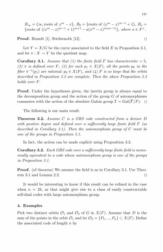
May 10, 2007 8:8 WSPC - Proceedings Trim Size: 9in x 6in ws-procs9x6
121
B∞ = ∞, roots of xm − x. B0 = roots of (xm − x)m−1 + 1, Ba =roots of ((xm − x)m−1 + 1)m+1 − a(xm − x)m(m−1), where a ∈ F×.
Proof. Brandt [1], Stichtenoth [12].
Let Y = X/G be the curve associated to the field E in Proposition 3.1,and let π : X → Y be the quotient map.
Corollary 3.1. Assume that (1) the finite field F has characteristic > 5,(2) π is defined over F , (3) for each p1 ∈ X(F ), all the points p0 in thefiber π−1(p1) are rational: p0 ∈ X(F ), and (4) F is so large that the orbitsdescribed in Proposition 3.2 are complete. Then the above Proposition 3.2holds over F .
Proof. Under the hypotheses given, the inertia group is always equal tothe decomposition group and the action of the group G of automorphismscommutes with the action of the absolute Galois group Γ = Gal(F/F ).
The following is our main result.
Theorem 3.2. Assume C is a GRS code constructed from a divisor Dwith positive degree and defined over a sufficiently large finite field F (asdescribed in Corollary 3.1). Then the automorphism group of C must beone of the groups in Proposition 3.1.
In fact, the action can be made explicit using Proposition 3.2.
Corollary 3.2. Each GRS code over a sufficiently large finite field is mono-mially equivalent to a code whose automorphism group is one of the groupsin Proposition 3.1.
Proof. (of theorem) We assume the field is as in Corollary 3.1. Use Theo-rem 3.1 and Lemma 2.2.
It would be interesting to know if this result can be refined in the casewhen n = 2k, as that might give rise to a class of easily constructableself-dual codes with large automorphism group.
4. Examples
Pick two distinct orbits O1 and O2 of G in X(F ). Assume that D is thesum of the points in the orbit O1 and let O2 = P1, ..., Pn ⊂ X(F ). Definethe associated code of length n by

May 10, 2007 8:8 WSPC - Proceedings Trim Size: 9in x 6in ws-procs9x6
122
C = (f(P1), ..., f(Pn)) | f ∈ L(D) ⊂ Fn.
This code has a G-action, by g ∈ G sending (f(P1), ..., f(Pn)) to(f(g−1P1), ..., f(g−1Pn)), so is a G-module. Indeed, by construction, theaction of G is by permuting the coordinates of C.
Example 4.1. Let F be a finite field of characteristic > 5 which contains
(1) all 4th and 5th roots of unity, (2) all the roots of x10 + 11ix5 + 1, (3) all
the roots B0 of x20 − 228ix15 − 494x10 − 228ix5 + 1, and (4) all the roots B∗0 of
x30+522ix25+10005x20−10005x10−522ix5−1. Furthermore, let B∞ = 0,∞∪roots of x10 +11ix5 +1. Let E =
PP∈B0
P and let D =P
P∈B∗0∪B∞P . Then
deg(E) = 20 and deg(D) = 42. Then C = C(D, E) is a formally self-dual code
with parameters n = 42, k = 21, d = 22, and automorphism group A5.
This follows from (5) of Proposition 3.2 and Remark 2.1.
Example 4.2. Let F = GF (q) be a finite field of characteristic p > 5 for which
q ≡ 1 (mod 8) and for which F contains (1) all the roots of xq−1 − x, and (2)
all the roots B1 of ((xq−1 − x)q−2 + 1)q/2 − (xq−1 − x)(q−1)(q−2)/2. If B∞ =
∞, roots of xq−1 − x, then let D =(q−1)(q−2)
4
PP∈B∞
P , E =P
P∈B1P ,
and C = C(D, E). Then C is a formally self-dual code with parameters n =q(q−1)(q−2)
2 , k = n/2, d = n + 1 − k, and permutation automorphism group
G = PSL(2, q).
This follows from (7) of Proposition 3.2.
5. Structure of the representations
We study the possible representations of finite groups G on the codesC(D,E). As noted in Lemma 3.1, when E is large enough, this is thesame as the representation of G on L(D). Therefore we study the possiblerepresentations of G on L(D). For simplicity we will restrict to the casewhere the support of D is rational, i.e. D =
∑si=1 aiPi, where P1, . . . , Ps
are rational points on P1.We can give the representation explicitly by finding a basis for L(D).
For a divisor D with rational support on X = P1, it is easy to find a basisfor L(D), as follows. Let ∞ = [1 : 0] ∈ X denote the point correspondingto the localization F [x](1/x), and [p : 1] denote the point corresponding tothe localization F [x](x−p), for p ∈ F . For notational simplicity, let
mP (x) =
x, P = [1 : 0] =∞,1
(x−p) , P = [p : 1].

May 10, 2007 8:8 WSPC - Proceedings Trim Size: 9in x 6in ws-procs9x6
123
Then mP (x) is a rational function with a simple pole at the point P , andno other poles.
Lemma 5.1. Let D =∑s
i=1 aiPi be a divisor with rational support onX = P1, so ai ∈ Z and Pi ∈ X(F ) for 0 ≤ i ≤ s.
(a) If D is effective, then
1,mPi(x)k | 1 ≤ k ≤ ai, 1 ≤ i ≤ s
is a basis for L(D).(b) If D is not effective but deg(D) ≥ 0, then D can be written as D =
D1 + D2, where D1 is effective and deg(D2) = 0. Let q(x) ∈ L(D2)(which is a 1-dimensional vector space) be any non-zero element. LetD1 =
∑si=1 aiPi. Then
q(x),mPi(x)kq(x) | 1 ≤ k ≤ ai, 1 ≤ i ≤ s
is a basis for L(D).(c) If deg(D) < 0, then L(D) = 0.
Proof. This is an easy application of the Riemann-Roch theorem. Notethat the first part appears as Lemma 2.4 in Lorenzini [10].
By the Riemann-Roch theorem, L(D) has dimension degD + 1 ifdeg(D) ≥ 0 and otherwise L(D) = 0, proving part (c) and the exis-tence of q(x) in part (b). For part (a), since mPi
(x)k has a pole of orderk at Pi and no other poles, it will be in L(D) if and only if k ≤ ai. Simi-larly, for part (b), mPi
(x)k will be in L(D1) if and only if k ≤ ai; thereforemPi
(x)kq(x) will be in L(D1 +D2) = L(D) under the same conditions. Ineach of parts (a) and (b), the set of functions given is linearly independent,so by a dimension count must form a basis for L(D).
Now let G be a finite group acting on X = P1 and let D be a divisorwith rational support, stabilized by G. Let S = supp(D) and let
S = S1 ∪ S2 ∪ ... ∪ Sm
be the decomposition of S into primitive G-sets. Then we can write D as
D =m∑
k=1
akSk =m∑
k=1
ak
s∑i=1
Pik,
where for each k, P1k . . . Psk are the points in the orbit Sk. Then G will actby a permutation on the points P1k . . . Psk in each orbit, and therefore onthe corresponding functions mPsk
(x).
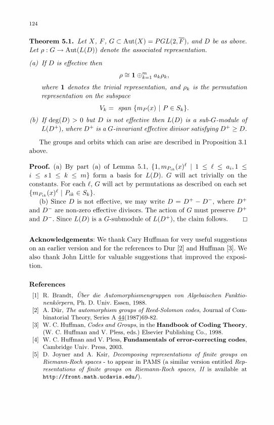
May 10, 2007 8:8 WSPC - Proceedings Trim Size: 9in x 6in ws-procs9x6
124
Theorem 5.1. Let X, F , G ⊂ Aut(X) = PGL(2, F ), and D be as above.Let ρ : G→ Aut(L(D)) denote the associated representation.
(a) If D is effective then
ρ ∼= 1⊕mk=1 akρk,
where 1 denotes the trivial representation, and ρk is the permutationrepresentation on the subspace
Vk = span mP (x) | P ∈ Sk.
(b) If deg(D) > 0 but D is not effective then L(D) is a sub-G-module ofL(D+), where D+ is a G-invariant effective divisor satisfying D+ ≥ D.
The groups and orbits which can arise are described in Proposition 3.1above.
Proof. (a) By part (a) of Lemma 5.1, 1,mPik(x)` | 1 ≤ ` ≤ ai, 1 ≤
i ≤ s 1 ≤ k ≤ m form a basis for L(D). G will act trivially on theconstants. For each `, G will act by permutations as described on each setmPik
(x)` | Pik ∈ Sk.(b) Since D is not effective, we may write D = D+ − D−, where D+
and D− are non-zero effective divisors. The action of G must preserve D+
and D−. Since L(D) is a G-submodule of L(D+), the claim follows.
Acknowledgements: We thank Cary Huffman for very useful suggestionson an earlier version and for the references to Dur [2] and Huffman [3]. Wealso thank John Little for valuable suggestions that improved the exposi-tion.
References
[1] R. Brandt, Uber die Automorphismengruppen von Algebaischen Funktio-nenkorpern, Ph. D. Univ. Essen, 1988.
[2] A. Dur, The automorphism groups of Reed-Solomon codes, Journal of Com-binatorial Theory, Series A 44(1987)69-82.
[3] W. C. Huffman, Codes and Groups, in the Handbook of Coding Theory,(W. C. Huffman and V. Pless, eds.) Elsevier Publishing Co., 1998.
[4] W. C. Huffman and V. Pless, Fundamentals of error-correcting codes,Cambridge Univ. Press, 2003.
[5] D. Joyner and A. Ksir, Decomposing representations of finite groups onRiemann-Roch spaces - to appear in PAMS (a similar version entitled Rep-resentations of finite groups on Riemann-Roch spaces, II is available athttp://front.math.ucdavis.edu/).
May 10, 2007 8:8 WSPC - Proceedings Trim Size: 9in x 6in ws-procs9x6
125
[6] ——, Automorphism groups of some AG codes, IEEE Trans. Info. Theory,vol 52, July 2006, pp 3325-3329.
[7] ——, Modular representations on some Riemann-Roch spaces of modularcurves X(N), in Computational Aspects of Algebraic Curves, (Editor:T. Shaska) Lecture Notes in Computing, WorldScientific, 2005.
[8] A. Kontogeorgis and J. Antoniadis, On cyclic covers of the projective line,Manuscripta Mathematica Volume 121, Number 1 / September, 2006.
[9] A. Kontogeorgis, The group of automorphisms of cyclic extensions of rationalfunction fields, Journal of Algebra , Volume 216, June 1999, p 665-706.
[10] D. Lorenzini, An invitation to arithmetic geometry, Grad. Studies inMath, AMS, 1996.
[11] H. Stichtenoth, Algebraic function fields and codes, Springer-Verlag,1993.
[12] ——, Algebraische Funktionenkorper einer Variablen, Vorlesungenaus dem Fachbereich Mathematik der Universitt Essen [Lecture Notes inMathematics at the University of Essen], vol. 1, Universitat Essen Fachbere-ich Mathematik, Essen, 1978.
[13] M. A. Tsfasman and S. G. Vladut, Algebraic-geometric codes, Mathe-matics and its Applications, Kluwer Academic Publishers, Dordrechet 1991.
[14] C. R. Valentini and L. M. Madan, A Hauptsatz of L. E. Dickson and ArtinSchreier extensions, J. Reine Angew. Math., Volume 318, 1980., 156-177.
May 10, 2007 8:8 WSPC - Proceedings Trim Size: 9in x 6in ws-procs9x6
126
About the code equivalence
Iliya G. Bouyukliev∗
Institute of Mathematics and Informatics,
Bulgarian Academy of Sciences,
P.O.Box 323, 5000 Veliko Tarnovo, BulgariaE-mail: [email protected]
In this paper we discuss an algorithm for code equivalence. We reduce the
equivalence test for linear codes to a test for isomorphism of binary matrices.
Keywords: Code equivalence, automorphism group, algorithm, canonical form
1. Introduction
In this paper, we consider the algorithm for equivalence which is imple-mented in the current version of the package Q − Extension [3]. Mainly,this package can be used for classification of linear codes over small fields.Actually, we reduce, as many other algorithms do, the equivalence test forlinear codes to a test for isomorphism of binary matrices or bipartite graphs.This allows us to use the developed algorithm for many other combinatorialobjects - nonlinear codes, combinatorial designs, Hadamard matrices, etc.
The paper is organized in the following way: In section 2 we give somemain definitions related to the code equivalence and the isomorphism ofbinary matrices. We also show how to transform the problem of code equiv-alence to the problem of isomorphism of binary matrices. In section 3, wepresent an important part of the mathematical base of the algorithm. Sec-tion 4 contains the main algorithm with detailed pseudo code. In the endof the section we give some additional invariants.
∗Partially supported by the Bulgarian National Science Fund under Contract No MM1304/2003
May 10, 2007 8:8 WSPC - Proceedings Trim Size: 9in x 6in ws-procs9x6
127
2. Codes and binary matrices
2.1. Equivalence of linear codes
Let Fnq be the n-dimensional vector space over the finite field Fq. The Ham-
ming distance between two vectors of Fnq is defined as the number of coor-
dinates in which they differ. A q-ary linear [n, k, d]q code is a k-dimensionallinear subspace of Fn
q with minimum distance d. A generator matrix G ofa linear [n, k] code C is any matrix of rank k (over Fq) with rows from C.
Definition 2.1. We say that two linear [n, k]q codes C1 and C2 are equiv-alent, if the codewords of C2 can be obtained from the codewords of C1
via a finite sequence of transformations of the following types:
(1) permutation of coordinate positions;(2) multiplication of the elements in a given position by a non-zero
element of Fq;(3) application of a field automorphism to the elements in all coordinate
positions.
An automorphism of a linear code C is a finite sequence of transforma-tions of type (1)–(3), which maps each codeword of C onto a codeword ofC. The set of automorphisms of a code C forms a group which is called theautomorphism group of the code C and denoted by Aut(C).
This definition is well motivated as the transformations (1)–(3) preservethe Hamming distance and the linearity (for more details see [5, Chapter7.3]). The problem of equivalence of codes has been considered in many pa-pers. We distinguish the works of Leon [7] and Sendrier [11]. The complexityof the Code Equivalence Problem is studied in [10].
The algorithm proposed by Sendrier [11] directly uses generator matricesof the linear codes. It works only for codes with specific properties andcannot be used in the general case.
Let C be a linear code over a field with q > 2 elements. In our algorithm,we use a subset D of C which is stable under the action of Aut(C) andgenerates C as a vector space. If the vector d ∈ D then the vectors λd forλ ∈ Fq \ 0 are also in D. Let D′ = d′1, d′2, . . . , d′K be a subset of Dsuch that no two vectors d′i, d
′j ∈ D′ are proportional for i 6= j, and for any
vector d ∈ D there is a constant λ ∈ Fq \ 0 for which λd ∈ D′.Let A′′ be the matrix with rows d′1, d
′2, . . . , d
′K . We associate to any
element d′i,j the matrix

May 10, 2007 8:8 WSPC - Proceedings Trim Size: 9in x 6in ws-procs9x6
128
D′i,j =
d′i,j α2d
′i,j . . . αq−1d
′i,j
α2d′i,j α2
2 · d′i,j . . . α2αq−1d′i,j
. . . . . . . . . . . .
αq−1d′i,j α2αq−1d
′i,j . . . α2
q−1d′i,j
,
where Fq \ 0 = 1, α2, . . . , αq−1. In this way we obtain a q-ary (K(q −1) + n)× n(q − 1) matrix A′
A′ =
D′1,1 D′
1,2 . . . D′1,n
D′2,1 D′
2,2 . . . D′2,n
. . . . . . . . . . . .
D′K,1 D′
K,2 . . . D′K,n
11 . . . 1 00 . . . 0 . . . 00 . . . 000 . . . 0 11 . . . 1 . . . 00 . . . 0. . . . . . . . . . . .
00 . . . 0︸ ︷︷ ︸ 00 . . . 0︸ ︷︷ ︸ . . . 11 . . . 1︸ ︷︷ ︸q − 1 q − 1 q − 1
From this matrix we easily obtain the binary (K(q− 1) + n)× n(q− 1)
matrix A such that
ai,j = 1 ⇐⇒ a′i,j = 1, ai,j = 0 otherwise. (1)
For large enough values of K, Aut(A) will be isomorphic to Aut(C) (seedefinitions 2.3 and 2.4). The last n rows guarantee that an automorphismσ will map any block of q−1 columns of A (which corresponds to a columnof A′′) to another block of q − 1 columns.
So we reduce our code equivalence problem to an isomorphism test ofbinary matrices. Moreover, by the permutation which gives an isomorphismof the binary matrices, we can find the coefficients in point (2) in the defi-nition for equivalence of q-ary codes and the field automorphism when q isa power of a prime (see section 2.3).
2.2. Isomorphism of binary matrices
Let us denote by Ω the set of all binary m × n matrices. We define anordering in the set Fn
2 as follows: For a = (α1, α2, . . . , αn) ∈ Fn2 and b =
(β1, β2, . . . , βn) ∈ Fn2 we have a < b ⇐⇒ α1 = β1, . . . , αj−1 = βj−1,
αj < βj for some j ≤ n. We use it to define a sorted matrix.
Definition 2.2. A sorted matrix is a matrix with rows a1, a2, . . . , am
such that a1 ≥ a2 ≥ · · · ≥ am.

May 10, 2007 8:8 WSPC - Proceedings Trim Size: 9in x 6in ws-procs9x6
129
Obviously, we can correspond to any matrix A ∈ Ω a sorted matrixAsort in a unique way.
We consider the action of the group Sn on the columns of a matrixA ∈ Ω. If σ ∈ Sn, we denote by Aσ the matrix obtained from A after thepermutation of the columns. If the columns of A are b1, b2, . . . , bn then thecolumns of Aσ are σ(b1) = b1σ, σ(b2) = b2σ, . . . , σ(bn) = bnσ. Similarly,we consider the action of Sm on the rows of A. For τ ∈ Sm, we denoteby τA the matrix obtained from A after the permutation of the rows. Ifa1, a2, . . . , am are the rows of A then the rows of τA are τ(a1) = a1τ ,τ(a2) = a2τ , . . . , τ(am) = amτ . Obviously, for any matrix A ∈ Ω, there is apermutation γ ∈ Sm such that the sorted matrix Asort = γA.
Definition 2.3. Two matrices of the same size are isomorphic if therows of the second one can be obtained from the rows of the first one by apermutation of the columns.
This definition is based on the natural action of the symmetric group Sn
on the set of columns for all elements in Ω. Obviously, the matrices A andB from the set Ω are isomorphic, or A ∼ B, if their corresponding sortedmatrices are isomorphic. This fact allows us to consider only the sortedmatrices in Ω.
Any permutation of the columns of A which maps the rows of A intorows of the same matrix, is called an automorphism of A. The set of allautomorphisms of A is a subgroup of the symmetric group Sn and we denoteit by Aut(A).
The following definition (equivalent to definition 2.3 ) is based on theaction of the symmetric group Sn on the set of columns and the action ofthe symmetric group Sm on the set of rows to all elements in Ω.
Definition 2.4. Two matrices of the same size are isomorphic if thesecond one can be obtained from the first one by a permutation of thecolumns and the rows.
We prefer the first one because it is similar to the usual code equivalencedefinition. Considering the sorted matrices, we have A ∼ B if there existsa permutation σ ∈ Sn such that Bsort = (Aσ)sort.
We consider two main problems.
Problem 2.1. Is there a permutation σ ∈ Sn such that for given binarymatrices A and B, Bsort = (Aσ)sort?
May 10, 2007 8:8 WSPC - Proceedings Trim Size: 9in x 6in ws-procs9x6
130
Problem 2.2. For a given binary matrix A, compute a set of generatorsfor the automorphism group of A.
The definition for isomorphism of binary matrices allows us to considerthe set Ω as a union of equivalence classes. Matrices which are isomorphicbelong to the same equivalence class. Every matrix of an equivalence classcan serve as a representative for this equivalence class. In many cases, acanonical representative is used, which is selected based on some specificconditions. This canonical representative is intended to easily make thedistinction between distinct equivalence classes. Practically, it reduces theisomorphism testing of matrices to comparing matrices. More precisely, wecan define the canonical representative map as follows:
Definition 2.5. A canonical representative map is a function ρ: Ω 7→Ω which satisfies the following two properties:
1. for all X ∈ Ω it holds that ρ(X) ∼ X,2. for all X,Y ∈ Ω it holds that X ∼ Y implies ρ(X) = ρ(Y ).
We say that the matrix X is in canonical form if ρ(X) = X.
We consider ordering in the set of all binary m × n matrices. For thematrices A = (a1, a2, . . . , am)t and B = (b1, b2, . . . , bm)t we have A <
B ⇐⇒ a1 = b1, . . . , aj−1 = bj−1, aj < bj for some j ≤ m. For any twomatrices A and B we can say A < B, A > B or A = B.
Now we will present a way to choose a canonical representative. Forthe canonical representative of the class of equivalence of the matrix A wecan take the matrix B such that Bsort ≥ (Aσ)sort for any permutationσ ∈ Sn. It is easy to define the canonical representative in this way butquite complicated to find it. Of course, we can try all permutations inSn. Using comparison of matrices, we can define ordering for the elementsin Sn with respect to a binary matrix A: γ1 < γ2 with respect to A if(Aγ1)sort < (Aγ2)sort. The general idea of a class of algorithms includingours is to find a minimal (or maximal) element in the set Π of permutations,which depends on the matrix A, where Π has a much smaller number ofelements than Sn.
Definition 2.6. Let A1, A2, . . . , As be all different m× n binary matriceswhich are isomorphic to the matrix in canonical form B. Let σi ∈ Sn be apermutation of the columns of the matrix Ai such that (Aiσi)sort = Bsort,i = 1, . . . , s. We call the permutation σi a canonical labeling map forthe matrix Ai defined by B.

May 10, 2007 8:8 WSPC - Proceedings Trim Size: 9in x 6in ws-procs9x6
131
As Aiτ = B ∀τ ∈ σiAut(B), the map σi is not unique except whenAut(B) = id. A canonical labeling of the columns of the matrix Ai is(σi(1), σi(2), . . . , σi(n)).
An important computational problem is the following:
Problem 2.3. For a given binary matrix A compute the canonical form B
and a canonical labeling σ ∈ Sn such that Bsort = (Aσ)sort.
The aim of our work is to present an algorithm which defines a spe-cific canonical representative map and gives a solution of the three definedproblems.
Problems 1,2, and 3, are connected with the graph isomorphism prob-lem. First of all, any binary matrix can be considered as a bipartite graph.In the case of a bipartite graph, the set of vertices is decomposed into twodisjoint colored sets (columns and rows) such that no two graph verticeswithin the same set are adjacent. Hence, solving the isomorphism problemsfor bipartite graphs and binary matrices is the same.
In other hand, any graph can be made bipartite by replacing each edgeby two edges connected with a new vertex. And any two graphs are isomor-phic if and only if the transformed bipartite graphs are. Theoretical resultsfor the graph isomorphism problem can be found in [1], [4].
Next, we briefly describe some of the basic setup and give pseudo-codefor the algorithm. For further details see [8].
2.3. The connection between equivalence of linear codes and
isomorphism of binary matrices
Let C be a linear code over a field with q > 2 elements and A be thecorresponding binary (K(q− 1) + n)× n(q− 1) matrix as presented in (1).To any automorphism ϕ of C there corresponds a permutation σϕ fromAut(A) in the following way:
(1) If ϕ is a permutation of the coordinate positions, the permutation σϕ
is the same ϕ which acts on the blocks of q− 1 columns correspondingto the coordinates of C.
(2) If ϕ is a multiplication of the elements in a given position, say i, by anonzero element α ∈ Fq, σϕ is a permutation of the columns in the blockof q − 1 columns corresponding to the position i. This permutation,considered as an element of the symmetric group Sq−1, depends onlyon α; that’s why we denote it by σ(α). So for all nonzero elements of Fq
we can collect corresponding permutations and from the permutation

May 10, 2007 8:8 WSPC - Proceedings Trim Size: 9in x 6in ws-procs9x6
132
easily find the element. Moreover, the set Yq = σ(α) | α ∈ Fq \ 0forms a cyclic subgroup of Sq−1 of order q − 1.
(3) The case when ϕ is a field automorphism is more complicated. Thenthe corresponding permutation σϕ is a permutation of the columns inthe blocks. As in the previous case, it can be considered as an elementof Sq−1 and depends only on the field automorphism. As we know, theGalois group of a finite field with q = ps elements is a cyclic group oforder s; that’s why the set Xq of the corresponding permutations inSq−1 forms a cyclic group of order s.
(4) When ϕ is a finite sequence of the transformations of the three types,then σϕ is the product of the corresponding permutations of thecolumns in A.
Example 2.1. Let C be a quaternary code and F4 = 0, 1, x, x2, x3 = 1.We associate the elements of the field with binary 3 × 3 matrices in thefollowing way:
0 7−→
000000000
, 1 7−→
100001010
, x 7−→
001010100
, x2 7−→
010100001
. (2)
It is easy to see that the multiplication by x corresponds to the permu-tation (132) of the columns in any of these blocks, and the multiplicationby x2 corresponds to the permutation (123). The only nontrivial automor-phism of the field maps the element a ∈ F4 to its conjugate a = a2. We canrepresent it as the permutation (23) of the columns combined with the samepermutation of the rows. So the transposition (12) = (23)(132) correspondsto the field automorphism combined with a multiplication by x.
Example 2.2. Let consider the field F5 = Z5. Then
1→
1000001001000001
, 2→
0010000110000100
, 3→
0100100000010010
, 4→
0001010000101000
. (3)
In this case we have Y5 = id, σ(2) = (1342), σ(4) = (14)(23), σ(3) =(1243).
Proposition 2.1. If the codes C and C ′ are equivalent, then the corre-sponding matrices A and A′ are isomorphic. Moreover, if C ′ = φ(C) thenσ = σφ is a composition of a permutation of the n blocks of q − 1 columns

May 10, 2007 8:8 WSPC - Proceedings Trim Size: 9in x 6in ws-procs9x6
133
corresponding to the coordinates of the codes, and permutations from a cosetτYq, where τ ∈ Xq.
Proposition 2.2. If there is a permutation σ ∈ Sn(q−1) such that(Aσ)sort = (A′)sort, this permutation is a composition of a permutationof the n blocks of q − 1 columns corresponding to the coordinates of thecodes, and permutations from a coset τYq, where τ ∈ Xq, then the codes Cand C ′ are equivalent.
Proof. The permutation of the n blocks corresponds to a permutation ofthe coordinates of C. A permutation from the coset τYq corresponds to afield automorphism followed by a multiplication of the elements in a givenposition by a nonzero element of the field.
If the matrices A and A′ are isomorphic, they have the same canon-ical form B. As Bsort = (Aτ)sort = (A′τ ′)sort for some permutations τand τ ′, we can take σ = τ(τ ′)−1 to be the isomorphism. Obtaining thecanonical form of the matrices, we find also their automorphism groups. Ifthe automorphism groups Aut(A) and Aut(A′) of two isomorphic matricesconsist only of permutations as described in the proposition, then the cor-responding codes are equivalent. Really, from the structure of the matrices,it follows that a permutation ϕ, such that ϕ(A) = A′, maps any block ofA into a block of A′. Moreover, if τ ∈ Sq−1, τ 6∈ Yq, then τσ(α)τ−1 6∈ Yq.Hence, if ϕ is not of the type as described in the proposition, the groupAut(A′) will also contain elements which are not of this type - but this isnot the case.
Proposition 2.3. Let C be a linear code over Fq and A be the correspond-ing binary (K(q − 1) + n) × n(q − 1) matrix as presented in Eq. (1). Ifall automorphisms of A are of the type described in Proposition 2.2, thenAut(C) ∼= Aut(A).
3. Orbits, partitions, invariants
3.1. Orbits
The group Aut(A) splits the columns of A into disjoint sets O1, O2, . . . , Ok
called orbits. Two columns a1 and b1 are in the same orbit if and onlyif there is an automorphism σ ∈ Aut(A) such that σ(a1) = b1. All au-tomorphisms γ ∈ Aut(A) for which γ(a1) = a1 form a group Aut(Aa1)called the stabilizer of a1. All the automorphisms which map a1 to b1
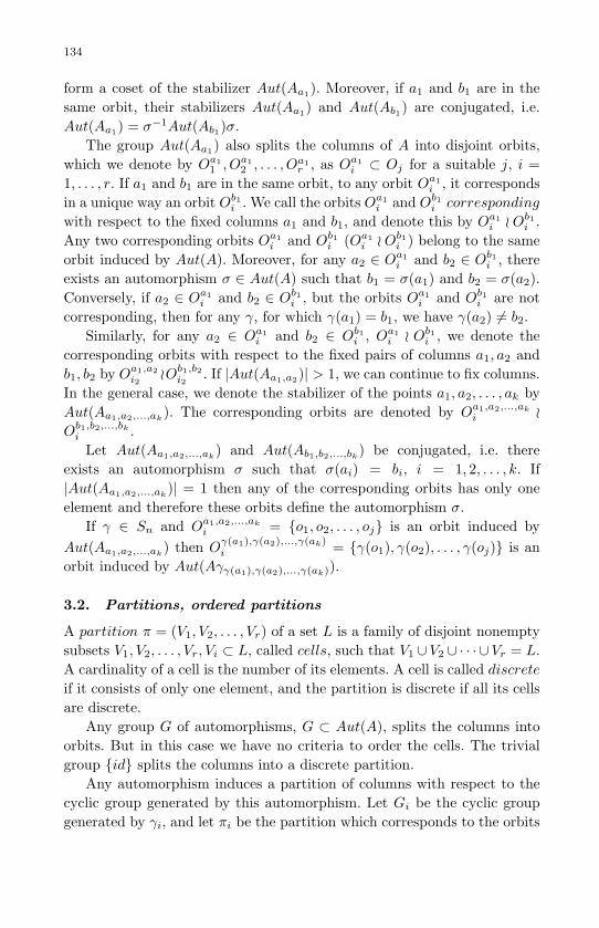
May 10, 2007 8:8 WSPC - Proceedings Trim Size: 9in x 6in ws-procs9x6
134
form a coset of the stabilizer Aut(Aa1). Moreover, if a1 and b1 are in thesame orbit, their stabilizers Aut(Aa1) and Aut(Ab1) are conjugated, i.e.Aut(Aa1) = σ−1Aut(Ab1)σ.
The group Aut(Aa1) also splits the columns of A into disjoint orbits,which we denote by Oa1
1 , Oa12 , . . . , Oa1
r , as Oa1i ⊂ Oj for a suitable j, i =
1, . . . , r. If a1 and b1 are in the same orbit, to any orbit Oa1i , it corresponds
in a unique way an orbit Ob1i . We call the orbits Oa1
i and Ob1i corresponding
with respect to the fixed columns a1 and b1, and denote this by Oa1i oO
b1i .
Any two corresponding orbits Oa1i and Ob1
i (Oa1i oO
b1i ) belong to the same
orbit induced by Aut(A). Moreover, for any a2 ∈ Oa1i and b2 ∈ Ob1
i , thereexists an automorphism σ ∈ Aut(A) such that b1 = σ(a1) and b2 = σ(a2).Conversely, if a2 ∈ Oa1
i and b2 ∈ Ob1i , but the orbits Oa1
i and Ob1i are not
corresponding, then for any γ, for which γ(a1) = b1, we have γ(a2) 6= b2.Similarly, for any a2 ∈ Oa1
i and b2 ∈ Ob1i , Oa1
i o Ob1i , we denote the
corresponding orbits with respect to the fixed pairs of columns a1, a2 andb1, b2 by Oa1,a2
i2oOb1,b2
i2. If |Aut(Aa1,a2)| > 1, we can continue to fix columns.
In the general case, we denote the stabilizer of the points a1, a2, . . . , ak byAut(Aa1,a2,...,ak
). The corresponding orbits are denoted by Oa1,a2,...,ak
i oOb1,b2,...,bk
i .
Let Aut(Aa1,a2,...,ak) and Aut(Ab1,b2,...,bk
) be conjugated, i.e. thereexists an automorphism σ such that σ(ai) = bi, i = 1, 2, . . . , k. If|Aut(Aa1,a2,...,ak
)| = 1 then any of the corresponding orbits has only oneelement and therefore these orbits define the automorphism σ.
If γ ∈ Sn and Oa1,a2,...,ak
i = o1, o2, . . . , oj is an orbit induced byAut(Aa1,a2,...,ak
) then Oγ(a1),γ(a2),...,γ(ak)i = γ(o1), γ(o2), . . . , γ(oj) is an
orbit induced by Aut(Aγγ(a1),γ(a2),...,γ(ak)).
3.2. Partitions, ordered partitions
A partition π = (V1, V2, . . . , Vr) of a set L is a family of disjoint nonemptysubsets V1, V2, . . . , Vr, Vi ⊂ L, called cells, such that V1 ∪V2 ∪ · · · ∪Vr = L.A cardinality of a cell is the number of its elements. A cell is called discreteif it consists of only one element, and the partition is discrete if all its cellsare discrete.
Any group G of automorphisms, G ⊂ Aut(A), splits the columns intoorbits. But in this case we have no criteria to order the cells. The trivialgroup id splits the columns into a discrete partition.
Any automorphism induces a partition of columns with respect to thecyclic group generated by this automorphism. Let Gi be the cyclic groupgenerated by γi, and let πi be the partition which corresponds to the orbits

May 10, 2007 8:8 WSPC - Proceedings Trim Size: 9in x 6in ws-procs9x6
135
of Gi, i = 1, 2. The orbits of the group G, generated by γ1 and γ2, form anew partition π, and we can find it in the following rule using π1 and π2.If there are two columns which are in different cells Vi and Vj in πl1 and inthe same cell in πl2 , l1, l2 = 1, 2, then the columns of Vi and Vj haveto be in one cell in π.
An ordered partition is a partition, for which Vi < Vj or Vi > Vj for anyi 6= j. We will write the ordered partitions in increasing order, i.e. Vi < Vj
for i < j.Let π = (V1, V2, . . . , Vr) is a partition and γ ∈ Sn. Then γ(π) =
(γ(V1), γ(V2), . . . , γ(Vr)) where γ(Vj) = (γ(a1), γ(a2), . . . , γ(ai)) for Vj =[a1, a2, . . . , ai].
3.3. Definition of invariants
An invariant of the columns of a matrix A with respect to the group Aut(A)is a function f1 which maps any column to an element of an ordered setM (for example Z), as f1(ci) = mi, mi ∈ M , such that if σ(ci) = cj ,σ ∈ Aut(A), then f1(ci) = f1(cj). Moreover, f1(c) has the same value asf1(γ(c)) with respect to γAut(Aγ)γ−1 for any permutation γ ∈ Sn.
The invariant f1 induces an ordered partition of the set of columns ofthe matrix , as f1(ci) = f1(cj)⇔ ci, cj ∈ Vp, f1(ci) < f1(cj)⇔ ci ∈ Vp, cj ∈Vq for p < q. This ordered partition can be considered as:
- arranging the columns in groups - any cell consists of the columns inone or more orbits.
- reordering the columns with respect to the cells and their order. If thepartition is discrete, it defines a permutation of the columns in A.
- we can choose a cell as special. For example this could be the firstlargest cell.
The group Aut(A) stabilizes the defined partition π1. We define in-variants with respect to the stabilizer Aut(Aa1,a2,...,ak
) of the columnsa1, a2, . . . , ak in the following way.
Definition 3.1. Let πk = (V1, V2, . . . , Vrk) be an ordered partition such
that σ(πk) = πk for any σ ∈ Aut(Aa1,a2,...,ak−1) and ak be a column in thespecial cell Vjs
. An invariant of the columns of a matrix A with respect tothe group Aut(Aa1,a2,...,ak−1,ak
) and the ordered partition πk is a functionfk+1, which maps any column to an element of M , such that:
1. fk+1(ak) < fk+1(b) for all b ∈ Vjs\ ak.
2. fk+1(a) < fk+1(b) for any a ∈ Vi, b ∈ Vj , where Vi, Vj ∈ πk, i < j.3. fk+1(a) = fk+1(b) when a and b are in the same orbit with respect

May 10, 2007 8:8 WSPC - Proceedings Trim Size: 9in x 6in ws-procs9x6
136
to the stabilizer Aut(Aa1,a2,...,ak). Moreover, fk+1(a) = fk+1(γ(a)) with
respect to γAut((Aγ)γ(a1),γ(a2),...,γ(ak))γ−1 and γ(πk) for any γ ∈ Sn.
Definition 3.2. We call the set of invariants F strong if the columns indifferent orbits have different values in M .
Let F = f1, f2, f3, . . . be a set of invariants. To obtain a discrete par-tition, induced by F and the matrix A, we can use the following algorithm:
00]disc part(inp A:binary matrix; F:set of invariants; π0:partition;00] out k:number of fixed columns;00] π1, π2, . . . , πk:partitions;00] w:array of cells; v:vector of fixed columns );00] var00] i: integer; v: vector;01] begin02] i := 1;03] v[i] := 0;04] inv act; using f1 and π0 find π1 = (V1, V2 . . . , Vr1) and Vs1 ;
Vs1 is a ”special” cell 05] w[1]:=Vs1 ;06] while πi is not discrete do07] begin08] choose ai from Vsi ;09] fix(ai); (V1, . . . , Vsi , . . . , Vri) go to (V1, . . . , ai, Vsi \ ai, . . . , Vri) 10] v[i] := ai;11] i := i + 1;12] inv act; using fi find πi = (V1, V2, . . . , Vri) and Vsi ; 13] w[i]:=Vsi ;14] end;15] k := i;16] end;
We use the following notations in the algorithms: inp - input variables,out - output variables, inp out - variables, used as input and output (theychange in the corresponding algorithm).
After acting with f1 on the columns of the input partition π0, the algo-rithm obtains (step 4) a partition induced by f1 and a special cell Vs1 . If thepartition obtained is not discrete, the algorithm chooses a column from thespecial cell, and collects this column in v[i]. In row 9, the algorithm fixesthe chosen column, i.e. it splits the special cell Vsi
in the partition π1 intotwo cells. The first one is discrete and contains only the fixed column. Inrow 12, using the invariant fi, the algorithm obtains the next partition. Inthe end, the variable k keeps the number of fixed columns and the numberof levels, and w keeps the special cells in the different levels.

May 10, 2007 8:8 WSPC - Proceedings Trim Size: 9in x 6in ws-procs9x6
137
We call a position of a cell Vl in the partition πj =(V1, . . . , Vl−1, Vl, . . . , Vr) the number |V1| + |V2| + · · · + |Vl−1| + 1. Fromthe definition 3.1, it follows that any cell Vi in the partition πj consists ofordered cells in the partition πj+1 and the position of the first one is thesame as the position of Vi.
The set v of fixed columns in steps one, two, etc., and the algorithmdisc part define in a unique way an ordered partition. We call the set v thevector of the fixed columns.
If we choose different columns ai from the special cell Vsi, the algorithm
disc part determines different discrete partitions. Let us denote by Π theset of all different discrete partitions which can be generated using thealgorithm disc part. Let πk = (V1, V2 . . . , Vri) ∈ Π be a discrete partition.This means that any cell is discrete, ri = n, and πk = ([ci1 ], [ci2 ], . . . , [cin
]),where cj are columns in A.
3.4. Properties of partitions induced by invariants
Let A be a binary matrix and F be a set of invariants.
Proposition 3.1. Let the stabilizers Aut(Aa1,...,ak) and Aut(Ab1,...,bk
) beconjugate and the orbits Oa1,...,ak
i1and Ob1,...,bk
i1be corresponding (Oa1,...,ak
i1o
Ob1,...,bk
i1). If Oa1,...,ak
i1belongs to the special cell, then Ob1,...,bk
i1also belongs
to the special cell but after fixing b1, b2, . . . , bk.
Proof. Let f2(d) = mi1 ∈ M where d is a column in Oa1i1
or in anotherorbit in the special cell. By point 2 in definition 3.1, the value of f2 willbe also mi1 for the columns in the corresponding orbits. This means thatthese corresponding orbits form a special cell after fixing b1. For k > 1, theproposition can be proved trivially by induction with respect to the numberof fixed columns.
Corollary 3.1. Let π′ and π′′ be two partitions obtained in the row 12 ofdisc part and their corresponding vectors of fixed columns v′ and v′′ havek elements. If there exists an automorphism σ such that v′′ = σ(v′), thenπ′′ = σ(π′). If π ∈ Π and σ ∈ Aut(A) then σ(π) ∈ Π.
The discrete partition πk = ([ci1 ], [ci2 ], . . . , [cin]) determines the permu-
tation of the columns πk = (1→ ci1 , 2→ ci2 , . . . , n→ cin). Conversely, forany permutation we have a unique discrete partition.
We compare discrete partitions πA and πB of the matrices A and B,respectively, in the following way: πA < πB ⇔ (AπA)sort < (BπB)sort,

May 10, 2007 8:8 WSPC - Proceedings Trim Size: 9in x 6in ws-procs9x6
138
πA πB ⇔ (AπA)sort = (BπB)sort.
Lemma 3.1. Consider the matrices A and B = Aτ for τ ∈ Sn and thesets ΠA and ΠB of all discrete partitions obtained for A and B using thealgorithm disc part. Then there is an one-to-one correspondence betweenΠA and ΠB. Moreover, for any discrete partition πA ∈ ΠA there is a discretepartition πB ∈ ΠB such that πB πA.
Proof. Let πA = ([ci1 ], [ci2 ], . . . , [cin]) be a discrete partition in ΠA with
vector of the fixed columns v. From the properties of the orbits and def-inition 3.1, it follows that τ(v) = (τ(v1), τ(v2), . . . , τ(vk)) is the vector ofthe fixed columns of the partition τ(πA) = ([τ(ci1)], [τ(ci2)], . . . , [τ(cin
)]).Actually, the columns cil
and τ(cil) are the same, l = 1, 2, . . . , n. From
proposition 3.1, it follows that τ(πA) ∈ ΠB . Hence πA τ(πA) with re-spect to the definition given above.
For a fixed column a, we call the position of the corresponding discretecell in the partition a position of this column. So if we fix a column a, itsposition is not changed until the end of the procedure, where we obtain adiscrete partition. In the algorithm disc part, we can obtain not only thevector of fixed columns v, but also the vector of their positions vp.
The comparing of the discrete partitions helps us to define a canonicaldiscrete partition.
Lemma 3.2. The maximal discrete partition c in Π such that c maxπj ;πj ∈ Π, which we call canonical, determines a permutation c
which is a canonical labeling map for A.
Proof. It follows from the definition for canonical labeling map and lemma3.1.
Proposition 3.2. Two discrete partitions γ1 = ([ci1 ], [ci2 ], . . . , [cin ]) andγ2 = ([cj1 ], [cj2 ], . . . , [cjn
]), for which γ1 γ2, define an automorphismσ = (ci1 → cj1 , ci2 → cj2 , . . . , cin
→ cjn), which is σ = γ1 · γ−1
2 .
Proof. γ1 γ2 ⇒ (Aγ1)sort = (Aγ2)sort.
Lemma 3.3. Two discrete partitions π′ and π′′ in Π with vectors of fixedcolumns v′ and v′′ of length k are equal (π′ π′′) if and only if v′j and
v′′j belong to corresponding orbits for any j ≤ k (if v′j ∈ Ov′1,...,v′j−1j and
v′′j ∈ Ov′′1 ,...,v′′j−1j for j ≤ k, then O
v′1,...,v′j−1j oOv′′1 ,...,v′′j−1
j ).
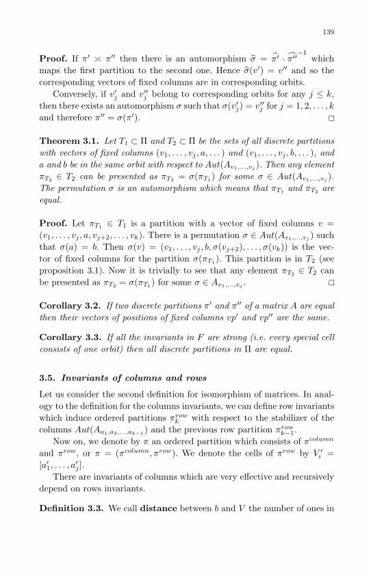
May 10, 2007 8:8 WSPC - Proceedings Trim Size: 9in x 6in ws-procs9x6
139
Proof. If π′ π′′ then there is an automorphism σ = π′ · π′′−1
whichmaps the first partition to the second one. Hence σ(v′) = v′′ and so thecorresponding vectors of fixed columns are in corresponding orbits.
Conversely, if v′j and v′′j belong to corresponding orbits for any j ≤ k,then there exists an automorphism σ such that σ(v′j) = v′′j for j = 1, 2, . . . , kand therefore π′′ = σ(π′).
Theorem 3.1. Let T1 ⊂ Π and T2 ⊂ Π be the sets of all discrete partitionswith vectors of fixed columns (v1, . . . , vj , a, . . . ) and (v1, . . . , vj , b, . . . ), anda and b be in the same orbit with respect to Aut(Av1,...,vj ). Then any elementπT2 ∈ T2 can be presented as πT2 = σ(πT1) for some σ ∈ Aut(Av1,...,vj
).The permutation σ is an automorphism which means that πT1 and πT2 areequal.
Proof. Let πT1 ∈ T1 is a partition with a vector of fixed columns v =(v1, . . . , vj , a, vj+2, . . . , vk). There is a permutation σ ∈ Aut(Av1,...,vj
) suchthat σ(a) = b. Then σ(v) = (v1, . . . , vj , b, σ(vj+2), . . . , σ(vk)) is the vec-tor of fixed columns for the partition σ(πT1). This partition is in T2 (seeproposition 3.1). Now it is trivially to see that any element πT2 ∈ T2 canbe presented as πT2 = σ(πT1) for some σ ∈ Av1,...,vj .
Corollary 3.2. If two discrete partitions π′ and π′′ of a matrix A are equalthen their vectors of positions of fixed columns vp′ and vp′′ are the same.
Corollary 3.3. If all the invariants in F are strong (i.e. every special cellconsists of one orbit) then all discrete partitions in Π are equal.
3.5. Invariants of columns and rows
Let us consider the second definition for isomorphism of matrices. In anal-ogy to the definition for the columns invariants, we can define row invariantswhich induce ordered partitions πrow
k with respect to the stabilizer of thecolumns Aut(Aa1,a2,...,ak−1) and the previous row partition πrow
k−1.Now on, we denote by π an ordered partition which consists of πcolumn
and πrow, or π = (πcolumn, πrow). We denote the cells of πrow by V ′i =[a′1, . . . , a
′j ].
There are invariants of columns which are very effective and recursivelydepend on rows invariants.
Definition 3.3. We call distance between b and V the number of ones in

May 10, 2007 8:8 WSPC - Proceedings Trim Size: 9in x 6in ws-procs9x6
140
a row b and the columns in a set V and denote d(b, V ). Similarly, we definedistance between a column b and a set of rows V .
Now we consider an invariant which is based on the following trivialfact.
Lemma 3.4. Let us consider the set Vcolumn of columns of a binary matrixwhich consists of one or a few orbits with respect to a group of automor-phisms G. Then a necessary condition two rows a and b from the set ofrows Vrows to be in the same orbit with respect to G is d(a, Vcolumn) =d(b, Vcolumn). Similarly, this works for two columns and a set of rows.
This claim is also true in the case when G is a stabilizer of columnsAut(Aa1,a2,...,ak
) ⊂ Aut(A).We give an example to show how to use lemma 3.4 to obtain an invariant
and the induced by it partition. We denote by R an ordered partition ofrows or columns, which we use for comparing. Actually, R can be an orderedpartition of some of the rows and columns (not of all rows and columns) oreven the empty set.
Example 3.1. Let us consider the matrix
A = 〈1111000, 0101100, 0010110, 0001011, 1000111, 1100010, 0110001〉
In the beginning, we have the trivial partition of the columns
πcolumn = Rcolumn = (V1), V1 = [1, 2, 3, 4, 5, 6, 7],
and the trivial partition of the rows πrow = Rrow = (V ′1), for V ′1 =[1′, 2′, 3′, 4′, 5′, 6′, 7′].
The number of ones in the rows is 1′− 4, 2′− 3, 3′− 3, 4′− 3, 5′− 4, 6′−3, 7′−3, or d(1′, V1) = 4, d(1′, V1) = 4, d(2′, V1) = 3, d(3′, V1) = 3, d(4′, V1) = 3,
d(5′, V1) = 4, d(6′, V1) = 3, d(7′, V1) = 3. This means that the set of the rowshas at least 2 orbits with respect to Aut(A). The number of ones in therows (or the distance to the set of all columns V1) induces the followingordered partition: πrow = (V ′1 , V
′2) = ([2′, 3′, 4′, 6′, 7′], [1′, 5′]).
In the second step we use the obtained partition πrow as Rrow and com-pare the distances from the columns to the cells of Rrow. So we obtain thefollowing distances from the columns to the cells of Rrow:
1 2 3 4 5 6 7d(∗, V ′1) 1 3 2 2 2 3 2d(∗, V ′2) 2 1 1 1 1 1 1

May 10, 2007 8:8 WSPC - Proceedings Trim Size: 9in x 6in ws-procs9x6
141
These distances induce the next ordered partition of the columns.πcolumn = (V1, V2, V3) = ([1], [3, 4, 5, 7], [2, 6]). In the third step, we com-pare the distances between the rows and the obtained πcolumn:
1′ 2′ 3′ 4′ 5′ 6′ 7′
d(∗, V1) 1 0 0 1 1 1 0d(∗, V2) 2 2 2 2 2 1 2d(∗, V3) 1 1 1 1 1 2 1
Hence, after this step we have
πrow = (V ′1 , V′2 , V
′3) = ([2′, 3′, 4′, 7′], [6′], [1′, 5′]).
In step 4, for the columns we obtain following distances
1 2 3 4 5 6 7d(∗, V ′1) 0 2 2 2 2 2 2d(∗, V ′2) 1 1 0 0 0 1 0d(∗, V ′3) 2 1 1 1 1 2 1
There is no new splitting of cells and therefore the process stops. Wecan generalize all the calculations for the columns in the following way:to any column we correspond in a unique way a polynomial with integercoefficients:
f(1) = 1 + Y (1 + 2x) + Y 2(x+ 2x2)
f(2) = f(6) = 1 + Y (3 + x) + Y 2(2 + x+ x2)
f(3) = f(4) = f(5) = f(7) = 1 + Y (2 + x) + Y 2(2 + x2)
The coefficients for Y 0 is one because all the columns are in the samecell in the beginning. The coefficients for Y and Y 2 depend on the distancesto the corresponding cells of Rcolumn in the steps two and four.
Actually, we repeat some of the calculations in this procedure. In steptwo, we look for distances between all columns and the rows in the set[2′, 3′, 4′, 6′, 7′]. In step 4, we look for the distances to [2′, 3′, 4′, 7′] and [6′].It is clear that in step 4 we can obtain the same splitting of columns if wecompute only the distances to the cell [6′] or to cell of rows [2′, 3′, 4′, 7′].Generally, it is necessary to calculate the distances to all cells except one.

May 10, 2007 8:8 WSPC - Proceedings Trim Size: 9in x 6in ws-procs9x6
142
We skip the first largest cell (with maximum cardinality) for efficiency. Ifthere is only one cell, there is no reason to compare again with it.
To obtain the final partition of columns and rows, we use the followingalgorithm:
stable(inp A:bin mat; inp out π:partition; inp πh:partition; inp copy:string);00] var i: integer;00] πcolumns, πrows: partition; πhcolumns, πhrows: partition;01] begin02] init πcolumns and πrows using π;03] init Rcolumns and Rrows using πh;04] split(inp out: πrows, inp: Rcolumns, out: Rrows, inp: copy);05] copy:=’some’;06] split(inp out: πcolumns, inp: Rrows, out: Rcolumns, inp: copy );07] while not ((|Rcolumns| = 0) and (|Rrows| = 0)) do08] begin10] split(inp out: πrows, inp: Rcolumns, out: Rrows, inp: copy);11] split(inp out: πcolumns, inp: Rrows, out: Rcolumns, inp: copy);12] end;13] πcolumns and πrows form π;14] end;
Split partitions πrows with respect to Rcolumns and copy the result inRrows, which will be used in the next step to partition the columns.
split(inp out π:partition of rows (or columns);
inp Rnow:partition of columns (or rows);out Rnext:partition of rows (or columns);
inp copy:string );
beginRnext:=(); empty for every cell V in π dobegin
partition V in V1, . . . , Vg such that a ∈ Vi and b ∈ Vj for i < j ⇔d(a, Rnow
r ) = d(b, Rnowr ) for r = 1, . . . , l − 1, and d(a, Rnow
l ) < d(b, Rnowl ) for some l
replace V in π with V1, . . . , Vg in that order;
if copy = ’every’ then
add all V1, . . . , Vg in Rnext in that order else copy=’some’ add all V1, . . . , Vg without Vt (Vt is the first largest cell) in Rnext in that order;
end;
end;
The algorithm stable has four parameters. The first one is the binarymatrix which we consider. The second one is the input partition whosecells the algorithm will split depending on the distances to the cells ofthe ordered partition πh. The final result (output of the algorithm) is alsowritten in π. The parameter some takes two values: ’some’ and ’every’.

May 10, 2007 8:8 WSPC - Proceedings Trim Size: 9in x 6in ws-procs9x6
143
The algorithm stable skips the mentioned above additional calculationswhen the parameter ’copy’ has the value ’some’.
The partition π1 = (V column1 , . . . , V column
s1 , . . . , V columnr1 ; V row
1 , . . . , V rowr′1
),which we have obtained as a result of the algorithm stable(A, π, πh =π, copy =′ every′), can be considered as induced by the invariant f1. Wecan find the special cell V column
s1as it is said in the definition.
This algorithm can be used to obtain the partition, induced by f2, inthe following way: Let fix a1 in π1, i.e. π2 = (V column
1 , . . . , [a1], V columns1
\a1, . . . , V column
r1;V row
1 , . . . , V rowr′1
) and πh = ([a1]). Then we run the algo-rithm stable with parameters (A, π := π2, πh, copy =′ some′). The processcontinues until the step when we obtain a discrete partition.
The suggested algorithm is proper to be used in rows 4 and 12 in thealgorithm disc part in the following form:
inv act(inp out π:partition; inp πh:partition; out sp cell:cell; inp copy:string);begin
stable(inp:A, inp out:π, inp:πh, inp:copy);find a special cell sp cell;
end;
In the first step of the algorithm disc part, row 4, the parameters ofinv act have to be πh = π and copy = every, and in the other steps ofdisc part, in row 12, the parameter πh is a partition with one cell andit has only one column - this is the last fixed column. In all these stepscopy = some.
Let A be a matrix without repeated rows. It is easy to see that anydiscrete partition for the columns leads to a discrete partition of the rows.If the matrix A contains repeated rows, a discrete partition of the columnsleads to a partition of the rows with discrete cells or cells with repeatedrows. Without lost of generality, we can split a cell with repeated rows intodiscrete cells. Hence, as an output of the algorithm disc part we obtaina discrete partition of the columns and of the rows. Thus, we have thefollowing lemma:
Lemma 3.5. Any discrete partition of the columns obtained by disc partdefines in a unique way a discrete partition of the rows.
Remark 3.1. The ordered discrete partitions obtained with the algorithmdisc part, which uses in rows 4 and 12 the algorithm inv act, allows us tocompare binary matrices instead of sorted binary matrices.
Remark 3.2. This type of invariant is related to ’equitable partition’ or
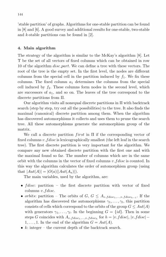
May 10, 2007 8:8 WSPC - Proceedings Trim Size: 9in x 6in ws-procs9x6
144
’stable partition’ of graphs. Algorithms for one-stable partition can be foundin [8] and [6]. A good survey and additional results for one-stable, two-stableand k-stable partitions can be found in [2].
4. Main algorithm
The strategy of the algorithm is similar to the McKay’s algorithm [8]. LetΥ be the set of all vectors of fixed columns which can be obtained in row10 of the algorithm disc part. We can define a tree with these vectors. Theroot of the tree is the empty set. In the first level, the nodes are differentcolumns from the special cell in the partition induced by f1. We fix thesecolumns. The fixed column a1 determines the columns from the specialcell induced by f2. These columns form nodes in the second level, whichare successors of a1, and so on. The leaves of the tree correspond to thediscrete partitions from Π.
Our algorithm visits all nonequal discrete partitions in Π with backtracksearch (step by step, try out all the possibilities) to the tree. It also finds themaximal (canonical) discrete partition among them. When the algorithmhas discovered automorphisms it collects and uses them to prune the searchtree. All these automorphisms generate the automorphism group of thematrix.
We call a discrete partition first in Π if the corresponding vector offixed columns v fdisc is lexicographically smallest (the left leaf in the searchtree). The first discrete partition is very important for the algorithm. Wecompare any new obtained discrete partition with the first one and withthe maximal found so far. The number of columns which are in the sameorbit with the columns in the vector of fixed columns v fdisc is counted. Inthis way the algorithm calculates the order of automorphism group (usingthat |Aut(A)| = |O(a)||Aut(Aa)|).
The main variables, used by the algorithm, are:
• fdisc: partition – the first discrete partition with vector of fixedcolumns v fdisc.• orbits: partition – The orbits of G, G ≤ Av fdisc1,...,v fdisch−1 . If the
algorithm has discovered the automorphisms γ1, . . . , γl, this partitionconsists of cells which correspond to the orbits of the group G ≤ Aut(A)with generators γ1, . . . , γl. In the beginning G = id. Then in somesteps G coincides with Av fdisc1,...,v fdisch
for h = |v fdisc|, |v fdisc|−1, . . . , 1. In the end of the algorithm G = Aut(A).• k: integer – the current depth of the backtrack search.

May 10, 2007 8:8 WSPC - Proceedings Trim Size: 9in x 6in ws-procs9x6
145
• h: integer – shows the smallest depth reached by the backtrack search.The algorithm looks for the columns which are in the same orbit withv fdisc[h] with respect to Aut(Av fdisc1,...,v fdisch−1) in the special cellw[h]. In the beginning h = |v fdisc| − 1. After visiting all columns inthe nondiscrete special cell obtained in the process of generating of thefirst discrete partition, h takes values h− 1 and so on.• sp cell: cell – the special cell obtained after the action of the corre-
sponding invariant.• w: array of cells – If k > h, w[k] consists of the first columns (with
smallest index) from the orbits of Aut(Av1,v2,...,vk−1) which are in thespecial cell. If k ≤ h, then w[k] consists of all columns from the specialcell.• tree: array of integers – tree[k] shows the number of columns in w[k]
which are visited so far.• π: array of partitions – π[k] is the current partition with vector of fixed
columns v.• cdisc: partition – keeps the maximal discrete partition to the current
point of the execution (candidate for canonical) with vector of fixedpoints v cdisc.• ind: integer – the number of columns in the orbit ofAut(Av fdisc1,...,v fdisch−1), which contains v fdisc[h].
• size: integer – The order of the group Aut(Av fdisc1,...,v fdisch). In the
end size = |Aut(A)|.• list of aut contains discovered generators of the automorphism groupAut(A).
• πh: partition with one cell with one element v[k − 1].
00]canon(inp A:bin mat; inp: π0:partition; out: cdisc:partition;);00]var orbits, fdisc, πh: partition;
00] π: array of partitions;00] w: array of cells;
00] sp cell: cell;
00] k, size, ind, h: integer;00] tree, v, v fdisc, v cdisc: array of integer;
00] γ: automorphism;00] list of aut;00]begin01] gen f(inp: π0; out: π, k, w, v);
02] fdisc := π[k];03] v fdisc := v;04] v cdisc := v;05] cdisc := π[k];
06] k := k − 1; orbits = ([1], [2], . . . , [n]);
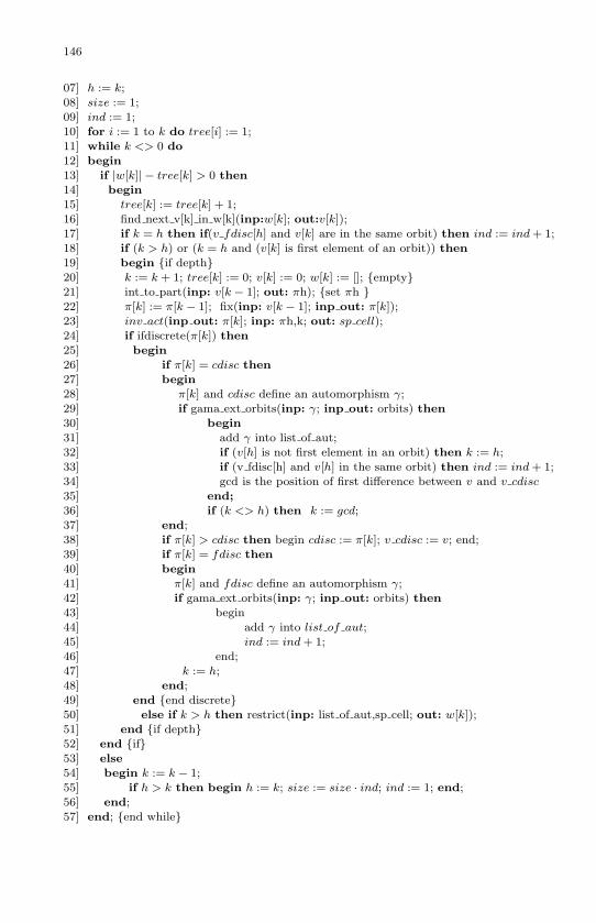
May 10, 2007 8:8 WSPC - Proceedings Trim Size: 9in x 6in ws-procs9x6
146
07] h := k;08] size := 1;
09] ind := 1;
10] for i := 1 to k do tree[i] := 1;11] while k <> 0 do
12] begin
13] if |w[k]| − tree[k] > 0 then14] begin
15] tree[k] := tree[k] + 1;
16] find next v[k] in w[k](inp:w[k]; out:v[k]);17] if k = h then if(v fdisc[h] and v[k] are in the same orbit) then ind := ind + 1;
18] if (k > h) or (k = h and (v[k] is first element of an orbit)) then
19] begin if depth20] k := k + 1; tree[k] := 0; v[k] := 0; w[k] := []; empty21] int to part(inp: v[k − 1]; out: πh); set πh 22] π[k] := π[k − 1]; fix(inp: v[k − 1]; inp out: π[k]);
23] inv act(inp out: π[k]; inp: πh,k; out: sp cell);
24] if ifdiscrete(π[k]) then25] begin
26] if π[k] = cdisc then
27] begin28] π[k] and cdisc define an automorphism γ;
29] if gama ext orbits(inp: γ; inp out: orbits) then
30] begin31] add γ into list of aut;
32] if (v[h] is not first element in an orbit) then k := h;33] if (v fdisc[h] and v[h] in the same orbit) then ind := ind + 1;
34] gcd is the position of first difference between v and v cdisc
35] end;36] if (k <> h) then k := gcd;
37] end;
38] if π[k] > cdisc then begin cdisc := π[k]; v cdisc := v; end;39] if π[k] = fdisc then
40] begin
41] π[k] and fdisc define an automorphism γ;42] if gama ext orbits(inp: γ; inp out: orbits) then
43] begin
44] add γ into list of aut;45] ind := ind + 1;
46] end;47] k := h;
48] end;
49] end end discrete50] else if k > h then restrict(inp: list of aut,sp cell; out: w[k]);51] end if depth52] end if53] else
54] begin k := k − 1;
55] if h > k then begin h := k; size := size · ind; ind := 1; end;56] end;
57] end; end while

May 10, 2007 8:8 WSPC - Proceedings Trim Size: 9in x 6in ws-procs9x6
147
58]end;
In row 1 the algorithm finds the first discrete partition. The proceduredisc part can be used as gen f after changing row 08 (choose ai from Vsi
)with 08| choose ai – the column with smallest index in Vsi .
The discrete partition, obtained in row 1, is the first discrete and max-imal discrete partition cdisc in this step with a vector of fixed columnsv fdisc = v cdisc (rows 2-5).
While the current level is not 0 (row 11) the backtrack search continues.If the number of columns in w[k] is bigger than the number of the visitedcolumns in w[k] (tree[k]), we continue with the next element in w[k] (rows15, 16, with the procedure find next v[k] in w[k]).
If k > h, or k = h and v[k] is the first element of an orbit, the algorithmcontinues in depth. In the case when k = h but v[k] is not the first elementof an orbit, the next partition is defined by the vector of fixed columns(v[1], . . . , v[k − 1], v[k]). But the algorithm already has passed all discretepartitions which are defined by the vector of fixed columns (v[1], . . . , v[k−1], v[k]f , . . . ), where v[k]f is the first in the same orbit. By theorem 3.1, wecan skip the current v[k].
Using the last fixed column as the only column in the partition πh, theprevious known partition π[k − 1] after fixing the same column (row 22,procedure fix), and inv act, the algorithm obtains the next partition andthe next special cell. If the obtained partition is discrete, the algorithmcompares it with the current maximal cdisc (row 28) and fdisc (row 39).
In the first comparing we have two cases. If the algorithm has discoveredan automorphism, and this automorphism gives new (extended) orbits, thenit is collected in list of aut. We check whether the element v[h] is first inany of the new orbits. If not, the backtracking jumps to the level h, becausethe first element is already passed (v fdisc[1] = v[1], . . . , v fdisc[h − 1] =v[h − 1]). If yes, it jumps to the level of the first difference between v andv cdisc. If the current discrete partition π[k] is bigger than cdisc, the algo-rithm takes π[k] as maximal (or canonical). In the second comparing, if thealgorithm discovers an automorphism, the backtracking jumps to the levelh. The discovered automorphisms, which fix the columns v[1], . . . , v[k− 1],form a group G. If the obtained partition is not discrete, the algorithmputs all columns from the special cell sp cell (row 23), which are first el-ements in orbits with respect to G, in w[k] (with procedure restrict(inp:list of aut,sp cell; out: w[k]) ).

May 10, 2007 8:8 WSPC - Proceedings Trim Size: 9in x 6in ws-procs9x6
148
4.1. Additional invariants
There are two general strategies to improve the efficiency of the main algo-rithm. The first one is to cut the part of the search tree which correspondsto the set of vectors Υ. The next example is based on the fact that the setsof vectors of positions Ψ′ and Ψ′′ corresponding to vectors of fixed columnsΥ′ and Υ′′ for the matrices A and γ(A), γ ∈ Sn, are equal: Ψ′ = Ψ′′.
We can redefine the canonical partition to be c maxπj , πj ∈ Π′,where Π′ is the set of discrete partitions which have lexicographically largestvector of positions of fixed columns.
In the main algorithm, we have to compare the vector of positions vp,corresponding to v, with the vector vpf of the positions of the first discretepartition fdisc and the vector of positions vpc of the discrete partitionwhich is a candidate for maximal cdisc. If the current vp coincides withvpf or vpc, the backtrack search continues - the algorithm expects an auto-morphism. If vp[k] <> vpf [k] and vp[k] < vpc[k], the backtracking jumpsin the previous level. Another similar approach can be found in [8].
The other strategy is to use proper invariants, which will help us todecrease the number of the discrete partitions in Π. This happens when thenumber of the orbits in the special cells are smaller than before. In fact, ifevery spacial cell consists of only one orbit, the algorithm visits only j + 1discrete partitions to obtain j generators of the automorphism group. Thenumber of possible generators is bounded by n − 1 (n is the number ofcolumns). To do this, we can use stronger invariants. Unfortunately, suchinvariants usually are computationally expensive. There are two options:
If we consider structures with a small group, we use an additional in-variant in lower level. We call this level pointed. If we expect structureswith a large group, we use an additional invariant in levels which dependon given parameters - for example the size of the largest cell in the currentpartition (we use as pointed levels the levels in which this size is smallerthan a given constant). To use additional invariants, we redefine inv act:
inv act(inp out π: partition; inp πh: partition; k: integer; out sp cell:cell);
beginif k is in a pointed level thenbegin
partition the special cell sp cell in πh using additional invariants
stable(inp A: bin mat; inp out π: partition; inp πh: partition; inp copy: string );end else
stable(inp A: bin mat; inp out π: partition; inp πh; partition; inp copy: string );find a special cell sp cell;
end;

May 10, 2007 8:8 WSPC - Proceedings Trim Size: 9in x 6in ws-procs9x6
149
The pointed levels are input for the main algorithm and depend onthe user. There are no special cell in the beginning. To use an additionalinvariant in the first level, we consider the set of all columns of the matrixas a special cell. Of course, we have to use the redefined inv act in theprocedure disc part.
The difference here is that we use as an input partition for comparing πhin stable not only the fixed column but the partition obtained after splittingthe special cell using the additional invariants. Now we describe the typeof the additional invariants which we use. Let’s consider the following 8× 8matrix
1000111001101001010011100101010110010101101100100111001010101001
This matrix has the same number of ones in any row and column, so
we can expect that all columns are in the same orbit. But this is not true.If we consider the sum of the first, third and forth columns, we obtaininv = (1, 1, 0, 1, 2, 3, 2, 2). To this vector, we correspond the polynomial
Y x3 + Y 2x3 + Y 3x,
such that Y axb shows that inv has b elements equal to a. Then we calculatethe sums of the first column with all pairs of two other columns. So weobtain
inv1(Y, x) = Y (12x3 + 9x4) + Y 2(12x3 + 9x4) + Y 3(12x)
which is the sum of the corresponding polynomials. With(n3
)×m operations,
we can have similar polynomials for all columns. In this way we obtain
inv1 = inv2 = Y (12x3 + 9x4) + Y 2(12x3 + 9x4) + Y 3(12x)
and
inv3 = inv4 = · · · = inv8 =Y (8x3 + 9x4 + 2x6)
+ Y 2(8x3 + 9x4 + 2x6) + Y 3(8x+ 12x2)
These polynomials split the set of all columns (with respect to the lex-icographic ordering of the corresponding vectors) in two cells and define

May 10, 2007 8:8 WSPC - Proceedings Trim Size: 9in x 6in ws-procs9x6
150
π = ([3, 4, 5, 6, 7, 8], [1, 2]). This means that we have at least two orbits. Wecall this type of invariants additional ’sum’ invariants with complexity 3 inlevel 1. For the graph invariants you can see [9].
Remark 4.1. Additional invariants are necessary only in cases when thematrix A has a very specific structure. For example, when A is an incidencematrix of a combinatorial design. This algorithm can be used also in thecase when we have coloring of the columns.Then the initial partition willdepend on the coloring.
5. Efficiency and storage requirements
About the efficiency of the algorithm stable for graphs, which is an impor-tant part of the main algorithm, we refer to [8]. The efficiency of the mainalgorithm depends on the size and the structure of the automorphism groupand the cardinality of the set of discrete partitions Π. The author does notknow a reasonable theoretical bound for this cardinality.
As we mentioned, this implementation needs m × n units of memory(for the matrix A), which is less than (m+n)× (m+n) units - the memoryused for the corresponding graph. This fact helps us to use easily variableswhich need a lot of memory. These variables are: 1) partitions of the rowsand columns π1, π2, . . . , πk. Of course, k ≤ n, but if we consider matrixwithout repeated columns k will be much smaller; 2) the set of specialcells w - only for columns; 3) the obtained automorphisms. Actually, wekeep the orbits of the columns with respect to the cyclic group generatedby the corresponding automorphism. This can be realized with two arrayswith length n (see [6]). 4) the first discrete partition fdisc and the currentmaximal partition cdisc. For any of them we need two arrays with lengthn+m.
References
[1] L. Babai, Automorphism groups, isomorphism, reconstruction, Handbook ofCombinatorics (R. L. Graham, M. Grotschel, and L. Lovasz, Eds.), Vol. II,North-Holland, Amsterdam, pp. 1447–1540, (1995).
[2] O. Bastert, Stabilization Procedures and Applications, Zentrum Mathe-matik, Technische Universitat Munchen, (2000).
[3] I. Bouyukliev and J. Simonis, Some new results for optimal ternary linearcodes, IEEE Trans. Inform. Theory, vol. 48, No. 4, pp. 981-985, (2002).
[4] M. Goldberg, The graph isomorphism problem, Handbook of Graph Theory(J. L. Gross and J. Yellen, Eds.), CRC Press, pp. 68-78, (2004).
[5] P. Kaski and P. R. Ostergard, Classification Algorithms for Codes and De-signs, Springer, (2006).

May 10, 2007 8:8 WSPC - Proceedings Trim Size: 9in x 6in ws-procs9x6
151
[6] W. Kocay, On writing isomorphism programs, Computational and Construc-tive Design Theory (ed. W. D. Wallis), Kluwer, pp. 135-175, (1996).
[7] J. Leon, Computing automorphism groups of error-correcting codes, IEEETrans. Inform. Theory, vol. 28, pp. 496-511, (1982).
[8] B. McKay, Practical graph isomorphism, Congressus Numerantium, 30, pp.45–87, (1981).
[9] B. McKay, nauty user’s guide (version 1.5). Technical Report TR-CS-90-02,Computer Science Department, Australian National University, (1990).
[10] E. Petrank and R. Roth; Is code equivalence easy to decide? IEEE Trans.Inform. Theory, vol. 43, pp. 1602–1604, (1997).
[11] N. Sendrier, The Support Splitting Algorithm, IEEE Trans, Info. Theory,vol. 46, pp. 1193-1203, (2000).

May 10, 2007 8:8 WSPC - Proceedings Trim Size: 9in x 6in ws-procs9x6
152
Permutation decoding for binary self-dual codes from the graphQn where n is even.
J. D. Key
Department of Mathematical SciencesClemson University
Clemson SC 29634, U.S.A.
E-mail: [email protected]://www.ces.clemson.edu/˜ keyj
P. Seneviratne
Department of Mathematical SciencesClemson University
Clemson SC 29634, U.S.A.
The binary self-dual [2n, 2n−1, n]2 codes from the adjacency matrices of the
n-cubes Qn, where n ≥ 6 and is even, are examined and 2- and 3-PD-sets ofsize n2n are found.
Keywords: graphs, codes, permutation decoding
1. Introduction
For n ≥ 2, the graph with vertices the 2n vectors of Fn2 and two vertices
adjacent if their coordinates differ in precisely one place, is called the n-cube, denoted by Qn. We examine the binary code obtained from the rowspan of an adjacency matrix for Qn over the field F2, and show that when nis even it is self-dual and can be used for permutation decoding. Our mainresult obtaining 3-PD-sets is as follows:
Theorem 1.1. For n even and n ≥ 8, let
Tn = T (w)ti | w ∈ Fn2 , 1 ≤ i ≤ n,
where T (w) is the translation by w ∈ Fn2 , ti = (i, n) for i < n is a trans-
position in the symmetric group Sn, and tn is the identity map. Then Tn
is a 3-PD-set of size n2n for the self-dual [2n, 2n−1, n]2 code Cn from an

May 10, 2007 8:8 WSPC - Proceedings Trim Size: 9in x 6in ws-procs9x6
153
adjacency matrix for the n-cube Qn, with the information set
I = [0,1, . . . ,2n−1 − 3,2n − 2,2n − 1].
This is proved in Section 4, with the notation for Tn and I given in Section 3.Background definitions and notions are in Section 2 and general propertiesof the graph Qn, the symmetric design obtained from it, and its binarycodes, are in Section 3.
2. Background and terminology
The notation for designs and codes is as in [1]. An incidence structureD = (P,B,J ), with point set P, block set B and incidence J is a t-(v, k, λ) design, if |P| = v, every block B ∈ B is incident with precisely k
points, and every t distinct points are together incident with precisely λ
blocks. The design is symmetric if it has the same number of points andblocks. The code CF of the design D over the finite field F is the spacespanned by the incidence vectors of the blocks over F . If Q is any subsetof P, then we will denote the incidence vector of Q by vQ. If Q = Pwhere P ∈ P, then we will write vP instead of the more cumbersome vP.Thus CF =
⟨vB |B ∈ B
⟩, and is a subspace of FP , the full vector space of
functions from P to F .All the codes here are linear codes, and the notation [n, k, d]q will be
used for a q-ary code C of length n, dimension k, and minimum weight d,where the weight wt(v) of a vector v is the number of non-zero coordinateentries. The distance d(u, v) between two vectors u, v is the number ofplaces in which they differ, i.e. wt(u − v). A generator matrix for Cis a k × n matrix made up of a basis for C, and the dual code C⊥ is theorthogonal under the standard inner product (, ), i.e. C⊥ = v ∈ Fn|(v, c) =0 for all c ∈ C. A check matrix for C is a generator matrix for C⊥. Theall-one vector will be denoted by , and is the vector with all entries equalto 1. Two linear codes of the same length and over the same field areisomorphic if they can be obtained from one another by permuting thecoordinate positions. An automorphism of a code C is an isomorphismfrom C to C. The automorphism group will be denoted by Aut(C). Anycode is isomorphic to a code with generator matrix in so-called standardform, i.e. the form [Ik |A]; a check matrix then is given by [−AT | In−k].The first k coordinates are the information symbols and the last n − kcoordinates are the check symbols.
The graphs, Γ = (V,E) with vertex set V and edge set E, discussedhere are undirected with no loops. A graph is regular if all the vertices

May 10, 2007 8:8 WSPC - Proceedings Trim Size: 9in x 6in ws-procs9x6
154
have the same valency. The adjacency matrix A of a graph of order n isan n× n matrix with entries aij such that aij = 1 if vertices vi and vj areadjacent, and aij = 0 otherwise.
Permutation decoding was first developed by MacWilliams [7] andinvolves finding a set of automorphisms of a code called a PD-set. Themethod is described fully in MacWilliams and Sloane [8, Chapter 16, p. 513]and Huffman [4, Section 8]. In [5] and [6] the definition of PD-sets wasextended to that of s-PD-sets for s-error-correction:
Definition 2.1. If C is a t-error-correcting code with information set Iand check set C, then a PD-set for C is a set S of automorphisms of Cwhich is such that every t-set of coordinate positions is moved by at leastone member of S into the check positions C.
For s ≤ t an s-PD-set is a set S of automorphisms of C which is suchthat every s-set of coordinate positions is moved by at least one memberof S into C.
That a PD-set will fully use the error-correction potential of the codefollows easily and is proved in Huffman [4, Theorem 8.1]. That an s-PD-setwill correct s errors follows in the same way (see [5, Result 2.3]).
The algorithm for permutation decoding is as follows: we have a t-error-correcting [n, k, d]q code C with check matrix H in standard form. Thus thegenerator matrix G = [Ik|A] and H = [−AT |In−k], for some A, and the firstk coordinate positions correspond to the information symbols. Any vectorv of length k is encoded as vG. Suppose x is sent and y is received and atmost s errors occur, where s ≤ t. Let S = g1, . . . , gm be an s-PD-set.Compute the syndromes H(ygi)T for i = 1, . . . ,m until an i is found suchthat the weight of this vector is s or less. Compute the codeword c that hasthe same information symbols as ygi and decode y as cg−1
i .
3. Binary codes of cubic graphs
For n ≥ 2 let Qn denote the n-cube (see [9]) and Dn the symmetric 1-designobtained by defining the 2n vertices (i.e. vectors in Fn
2 ) to be the points P,and a block v for every point (vector) v by
v = w | w ∈ P and w adjacent to v in Qn.
Then Dn is a 1-(2n, n, n) symmetric design with the property that twodistinct blocks meet in zero or two points and similarly any two distinctpoints are together on zero or two blocks.

May 10, 2007 8:8 WSPC - Proceedings Trim Size: 9in x 6in ws-procs9x6
155
We will use the following notation: for r ∈ Z and 0 ≤ r ≤ 2n − 1, ifr =
∑ni=1 ri2
i−1 is the binary representation of r, let r = (r1, . . . , rn) bethe corresponding vector in Fn
2 , i.e. point in P.The complement of v ∈ P will be denoted by vc. Thus vc(i) = 1 + v(i)
for 1 ≤ i ≤ n, where v(i) denotes the ith coordinate entry of v. Similarly,for α ∈ F2, αc = α+ 1. Clearly vc = v + 2n − 1.
The binary code Cn of the design Dn is the same as the row span over F2
of an adjacency matrix forQn, and for n even and n ≥ 4, it is a [2n, 2n−1, n]2self-dual code. Before showing this, we show why the case for n odd is notof interest.
Proposition 3.1. For n odd, the binary code Cn of Dn is the full spaceF2n
.
Proof: For n odd, it can be verified directly that
v(x1,...,xn) = v(x1,...,(xn)c) +n−1∑i=1
v(x1,...,(xi)c,...,xn−1,xn)
for all choices of x = (x1, . . . , xn). Thus Cn contains all the vectors of weight1 and is the full space.
The automorphism group of the design and of the code contains (prop-erly, for n ≥ 4) the automorphism group TSn = T o Sn of the graph(see [9]), where T is the translation group of order 2n and Sn is the sym-metric group acting on the n coordinate positions of the points v ∈ P. Wewill write, for each w ∈ P, T (w) for the automorphism of Cn defined by thetranslation on Fn
2 given by T (w) : v 7→ v +w for each v ∈ Fn2 . The identity
map will be denoted by ι = T (0). Then T = T (w) | w ∈ P.
Lemma 3.1. The group TSn acts imprimitively on the points of the designDn for n ≥ 4 with v, vc, for each v ∈ Fn
2 , a block of imprimitivity.
Proof: We need only show that for g ∈ TSn, and any v ∈ Fn2 , vcg = (vg)c,
which will make the set v, vc a block of imprimitivity. Clearly TSn istransitive on points. For g ∈ Sn the assertion is clear. If g is the translationT (u), where T (u) : v 7→ v+u, then vcg = vcT (u) = v+2n − 1+u = vT (u)+2n − 1 = (vg)c. Thus for any g ∈ TSn and any v ∈ Fn
2 , vcg = (vg)c.
For each i such that 1 ≤ i < n let ti = (i, n) ∈ Sn, i.e. the automorphismof Cn defined by the transposition of the coordinate positions. For n ≥ 4

May 10, 2007 8:8 WSPC - Proceedings Trim Size: 9in x 6in ws-procs9x6
156
let
Pn = ti | 1 ≤ i ≤ n− 1 ∪ ι (1)
Tn = TPn. (2)
Since the translation group T is normalized by Sn, elements of the formT (w)tiT (u) are all in Tn, i.e. σ−1T (u)σ = T (uσ−1), so that for transposi-tions t, tT (u) = T (ut)t.
Proposition 3.2. For n even, n ≥ 4, Cn is a [2n, 2n−1, n]2 self-dual codewith
I = [0,1, . . . ,2n−1 − 3,2n − 2,2n − 1]
as an information set.
Proof: Using the natural ordering for the points and blocks, the incidencematrix for Qn has the form
Bn =
Bn−2 I2n−2 I2n−2 0I2n−2 Bn−2 0 I2n−2
I2n−2 0 Bn−2 I2n−2
0 I2n−2 I2n−2 Bn−2
(3)
where Bn−2 is the incidence matrix of the graph Qn−2. It is easy to provethat the matrix has rank 2n−1 and it can be shown by induction that theminimum weight is n. That the code is self-dual follows from the earlierobservation that blocks meet in 0, 2 or n points.
To show that I is an information set, let B∗n be the first 2n−1 rows of Bn.Clearly B∗n has rank 2n−1 and generates the same code as Bn. We want toswitch the column indexed by 2n−1 − 2 with that indexed by 2n − 2, andthe column indexed by 2n−1 − 1 with that indexed by 2n − 1. Notice that2n−1 − 2 ∈ 2n−1 − 1, so the 2×2 submatrix of B∗n from the (2n−1−2)th and
(2n−1−1)th rows and columns has the form[
0 11 0
], while the corresponding
2 × 2 submatrix from the same rows but the last two columns is just I2.Thus the column interchanges described will give the information set I.
If I is as in the proposition, the corresponding check set is C. We willwrite
I1 = [0,1, . . . ,2n−1 − 3] (4)
C1 = [2n−1,2n−1 + 1, . . . ,2n − 3] (5)
I2 = [2n − 2,2n − 1] (6)
C2 = [2n−1 − 2,2n−1 − 1] (7)

May 10, 2007 8:8 WSPC - Proceedings Trim Size: 9in x 6in ws-procs9x6
157
and
a = 2n − 2 = (0, 1, . . . , 1, 1) , b = 2n − 1 = (1, 1, . . . , 1, 1) (8)
A = 2n−1 − 2 = (0, 1, . . . , 1, 0) , B = 2n−1 − 1 = (1, 1, . . . , 1, 0) (9)
Notice that the points a and b are placed in I in order to have points andtheir complements in I since under any automorphism g ∈ TSn of thedesign, if vg = w then vcg = wc, by Lemma 3.1. Thus we have ac = 1 andbc = 0, Ac = 1 + 2n−1, Bc = 2n−1, and v + vc = b for any vector v ∈ P.
4. 3-PD-sets
In this section we prove the main result, Theorem 1.1, obtaining 3-PD-sets. Since the minimum weight is n, the code cannot correct three errorsif n < 8. However the proof of the theorem holds for n = 4, 6 as well.
Proof of Theorem 1.1: Let T = x, y, z be a set of three points in P.We need to show that there is an element in Tn that maps T into C. Weconsider the various possibilities for the points in T . If T ⊆ C then use ι.Thus suppose at least one of the points is in I and, by using a translation,suppose that one of the points, say z, is 0. If T ⊆ I, then T (2n−1) willwork. Now we consider the other cases.
(1) x ∈ I1, y ∈ C1Then there are ix, iy such that 2 ≤ ix, iy ≤ n − 1 such that x(ix) =y(iy) = 0. If ix = iy = i, then T ti ⊆ I, unless yti ∈ A,B, sotiT (2n−1) will work unless yti ∈ A,B. If yti = A, then y(1) = y(i) =0, y(j) = 1 otherwise. If x(1) = 0, then t1T (2n−1) will work. If x(1) = 1,then take any j 6= 1, i, n, and use T (2j−1)tiT (2n−1). If yti = B, theny(i) = 0 and y(j) = 1 otherwise. Here we can take any j 6= 1, i, n, anduse T (2j−1)tiT (2n−1).If x and y have no common zero, then if y = xc, so that x+ y = b, wecan use T (x)T (2n−1). If x(i) = y(i) = 1, where 1 ≤ i ≤ n − 1, thentiT (2n−1 − 1) can be used.
(2) x ∈ I1, y ∈ C2Since x ∈ I1, x(i) = 0 for some i such that 2 ≤ i ≤ n−1. If there is a jsuch that j 6= i and 2 ≤ j ≤ n− 1 with x(j) = 0, then T (2i−1 + 2n−1)can be used.If there is no such j, then either x(1) = x(i) = x(n) = 0 and x(j) = 1for j 6∈ 1, i, n, or x(i) = x(n) = 0 and x(j) = 1 for j 6∈ i, n. Ineither case, take j 6= i, 2 ≤ j ≤ n − 1. Then the map T (2j−1 + 2n−1)can be used.

May 10, 2007 8:8 WSPC - Proceedings Trim Size: 9in x 6in ws-procs9x6
158
(3) x ∈ I2, y ∈ C1(a) x = a: since y ∈ C1, there is a j such that 2 ≤ j ≤ n − 1 with
y(j) = 0. If y(i) = 1 for i 6= j and 1 ≤ i ≤ n, or if y(1) = 0 andy(i) = 1 for i 6= j and 2 ≤ i ≤ n, then T (A) will work. If there isan i 6= j such that y(i) = y(j) = 0 where 2 ≤ i, j ≤ n − 1, thentjT (2n−1) can be used.
(b) x = b: this follows exactly as in the x = a case except that in thefirst two cases for y use T (B) instead of T (A).
(4) x ∈ I2, y ∈ C2(a) x = a, y = A: use T (a)t2T (2n−1).(b) x = a, y = B: use tn−1T (B).(c) x = b, y = A: use tn−1T (B).(d) x = b, y = B: use t1T (1 + 2n−1).
(5) x, y ∈ C
(a) x, y ∈ C1: if x+ y = B then T (B) will work. Otherwise x(i) = y(i)for some i such that 1 ≤ i ≤ n − 1. Again T (B) will work unlessx or y are (0, . . . , 0, 1) or (1, 0, . . . , 0, 1). If x = (0, . . . , 0, 1) theny(i) = 0 for some i such that 2 ≤ i ≤ n−1. Then tiT (2n−1) can beused unless y(j) = 1 for all j 6= i, or y(1) = y(i) = 0 and y(j) = 1for j 6= 1, i; in these cases tiT (2i−1 + 2n−1) can be used. The samearguments hold if x = (1, 0, . . . , 0, 1).
(b) x ∈ C1, y ∈ C2: since x ∈ C1, there is a j such that 2 ≤ j ≤ n − 1with x(j) = 0. Then tjT (2j−1 + 2n−1) can be used.
(c) x, y ∈ C2: T (2n−2 + 2n−1) will work.
This completes all the cases and proves the theorem.
Note that this result also shows that the set Tn is a 2-PD-set for Cn
for n = 6. However, this set Tn with this information set I will not givea 4-PD-set, since it is quite easy to verify that the set of four points0,2,2n − 2,2n−1 − 1 cannot be moved by any element of Tn into thecheck positions.
5. Discussion
The automorphism group of the symmetric 1-design is much larger thanthat of the graph. In particular, it will contain any invertible n× n matrixover F2 with the property that the sum of any two of its rows has weight2. In fact, if v ∈ P has an even number of entries equal to 1, then the
May 10, 2007 8:8 WSPC - Proceedings Trim Size: 9in x 6in ws-procs9x6
159
matrix A having for rows the points in v, will be be an automorphism ofDn that also preserves the blocks of imprimitivity. If v has an odd numberof entries equal to 1, it will not be invertible. There are also other, non-linear, automorphisms, of the design, and that also preserve these blocks ofimprimitivity, as is indicated by computations with Magma [2, 3].
It is possible to arrange more interchanges so that more instances of apoint and its complement in the information set occur. Thus s-PD-sets fors > 3 seem possible in general.
References
[1] E. F. Assmus, Jr and J. D. Key. Designs and their Codes. Cambridge: Cam-bridge University Press, 1992. Cambridge Tracts in Mathematics, Vol. 103(Second printing with corrections, 1993).
[2] W. Bosma, J. Cannon, and C. Playoust. The Magma algebra system I: Theuser language. J. Symb. Comp., 24, 3/4:235–265, 1997.
[3] J. Cannon, A. Steel, and G. White. Linear codes over finite fields. In J. Cannonand W. Bosma, editors, Handbook of Magma Functions, pages 3951–4023.Computational Algebra Group, Department of Mathematics, University ofSydney, 2006. V2.13, http://magma.maths.usyd.edu.au/magma.
[4] W. Cary Huffman. Codes and groups. In V. S. Pless and W. C. Huffman,editors, Handbook of Coding Theory, pages 1345–1440. Amsterdam: Elsevier,1998. Volume 2, Part 2, Chapter 17.
[5] J. D. Key, T. P. McDonough, and V. C. Mavron. Partial permutation decodingof codes from finite planes. European J. Combin., 26:665–682, 2005.
[6] Hans-Joachim Kroll and Rita Vincenti. PD-sets related to the codes of someclassical varieties. Discrete Math., 301:89–105, 2005.
[7] F. J. MacWilliams. Permutation decoding of systematic codes. Bell SystemTech. J., 43:485–505, 1964.
[8] F. J. MacWilliams and N. J. A. Sloane. The Theory of Error-CorrectingCodes. Amsterdam: North-Holland, 1983.
[9] Gordon Royle. Colouring the cube. Preprint.

May 10, 2007 8:8 WSPC - Proceedings Trim Size: 9in x 6in ws-procs9x6
160
The Sum-Product Algorithm on Small Graphs
M. E. O’Sullivan
Dept. of Mathematics and Statistics
San Diego State University
San Diego, CA, 92182-7720E-mail: [email protected]
J. Brevik
Dept. of Mathematics and Statistics
California State University, Long Beach
Long Beach, CA, 90840E-mail: [email protected]
R. Wolski
Dept. of Computer Science University of CaliforniaSanta Barbara, CA 75275-0338
E-mail: [email protected]
Keywords: Sum-product algorithm, low-density parity-check codes, finite
length bipartite graphs.
1. Introduction
One of the great achievements in coding theory in the last decade or sohas been the discovery that iterative decoding methods, such as the sum-product algorithm, can be used to achieve Shannon capacity; see [7, 11].Although there are provable asymptotic results for the performance of thesum-product algorithm, there is little that can be said for finite lengthcodes. In this article we focus on very simple cases for which we can deriveexact formulas for convergence of the sum-product algorithm. By estab-lishing some simple, but provable, results we hope to build a foundationfor further algebraic analysis. These examples may also enhance the intu-itive understanding of the algorithm and thereby yield improved heuristicmethods for code construction.
Given a binary matrix H, the sum-product algorithm is defined by us-

May 10, 2007 8:8 WSPC - Proceedings Trim Size: 9in x 6in ws-procs9x6
161
ing the bipartite graph of H. It is to be expected that the sum-productalgorithm will yield better decoding performance on some bipartite graphsthan on others. What makes one graph (or, equivalently, matrix) betterthan another? Several properties have been proposed, some of them basedon other decoding algorithms. Short cycles in the bipartite graph of theparity-check matrix are considered problematic; see [16]. The reasoning isthat inaccurate received estimates of bit values passed to the decoding al-gorithm are self-reinforcing in the presence of short cycles. Recent worksuggests that short cycles are particularly problematic when the degrees ofthe nodes involved are low; see [14]. An erasure correction algorithm thatis similar to belief propagation fails exactly when it arrives at a stoppingset; see [1]. These sets also seem to foil the belief-propagation algorithm.The experiments by MacKay and Postol in [8] with the Margulis group-theoretic construction led them to attribute decoding failure in the errorfloor region to near-codewords. These are vectors v such that Hv has lowweight. Richardson in [10] calls near-codewords trapping sets; he also seesthem as a cause of error floors. Pseudo-codewords arise from codewords in acode for a covering graph of the bipartite graph of the check matrix; see [6].The closure of the set of pseudo-codewords is a polytope in Rn where n isthe dimension of the code. The articles [4, 15] investigate their relevance forsum-product decoding. Pseudo-codewords are directly relevant in anotherapproach to decoding due to Feldman [2, 3] that uses linear programming.This algorithm attempts to maximize a linear functional over the polytopeof pseudo-codewords, and the vertices of the polytope are the possible solu-tions to the problem. Bipartite graphs with good expansion properties wereshown to be asymptotically good for a low-complexity decoding algorithmpresented in [12].
In the simple cases that we examine, pseudo-codewords, near-codewordsand stopping sets do not play a role and expansion is not meaningful becausethe graphs are very small. We do see a difference between graphs thatare very similar, but differ in one aspect, the existence of short cycles.The difference in performance of the sum-product algorithm yields somesurprises.
Section 2 introduces the bipartite graphs under investigation and someexperiments with the performance of the sum-product algorithm. In Sec-tion 3 we give our algebraic analysis of the sum-product algorithm for arestricted set of bipartite graphs, those in which all check nodes have de-gree 2. Section 4 applies our algebraic results to the bipartite graphs ofSection 2 and explains the differences in performance therein.

May 10, 2007 8:8 WSPC - Proceedings Trim Size: 9in x 6in ws-procs9x6
162
2. Experimental Results
Figures 1 and 3 show several bipartite graphs. Following common practice,the circular nodes (shaded) are called bit nodes and the square nodes arecalled check nodes. A code is defined by allowing bit nodes to take valuesin Z/2, such that each check node is connected to an even number of 1s.It is readily seen that all the codes defined by these graphs are repetitioncodes, that is, codes whose only two codewords are the vector of repeated0s and that of repeated 1s.
Consider the two graphs in Figure 1, each of which determines the rep-etition code of length four. The em 4-Choose-2 graph is constructed bycreating one check for each two element subset of the four bit nodes. As wewill show in the next section, the Two-to-One graph is a two-to-one coverof the complete bipartite graph on 2 bit-nodes and 3 check-nodes (in fact,it is the unique connected cover).
Fig. 1. Two graphs defining the repetition code of length four. Two-to-One on the left,
and 4-Choose-2 on the right.
Figure 2 shows the performance of the sum-product algorithm on eachgraph, for each of two different termination criteria. The “fine” case used athreshold of 10−20, while the “coarse” case used a threshold of 10−3. It isevident that the 4-Choose-2 graph has superior performance, and that it isless affected by the degradation of performance under a coarser threshold.It would be tempting to attribute the superior performance to the largergirth of the 4-Choose-2 graph.
Consider the three graphs in Figure 3, which are all 3-to-1 covers of thecomplete bipartite graph on 2 bit-nodes and 3 check-nodes. One can showthat any connected 3-to-1 cover is one of these three. One of the graphs hasgirth 8, one has three 4-cycles, and one has two 4-cycles.
Figure 4 shows the performance of the sum-product algorithm on thesegraphs, for the same two termination criteria as used above. Perhaps sur-

May 10, 2007 8:8 WSPC - Proceedings Trim Size: 9in x 6in ws-procs9x6
163
4 5 6 7 8 9 10 1110
−7
10−6
10−5
10−4
10−3
10−2
10−1
Eb/N0 [dB]
Bit
erro
r ra
te
4choose2fine4choose2coarse2to1 fine2to1 coarse
Fig. 2. The performance of the sum-product algorithm on the graphs in Figure 1, using
two different termination criteria.
prisingly, the performance of the sum-product algorithm is the same whenthe threshold is fine. On the other hand, with a coarse threshold we seegreater degradation of performance corresponding to a greater number of4-cycles.
In the following sections we will derive formulas for convergence which

May 10, 2007 8:8 WSPC - Proceedings Trim Size: 9in x 6in ws-procs9x6
164
Fig. 3. Three graphs defining the repetition code of length 6. From the top No 4-cycles,
Two 4-cycles, and Three 4-cycles.
will explain the performance in these examples.
3. Analysis of the Sum-Product Algorithm
The principal goal of this section is to develop our algebraic analysis ofthe sum-product algorithm for graphs on which all check nodes have de-gree 2. One may readily check that the code defined by such a graph isa repetition code. We start with a discussion of maps of bipartite graphs,including covering maps and automorphisms. We then present the versionof the sum-product algorithm that we use and show how it is affected by anautomorphism. Finally we show that the algorithm simplifies dramaticallywhen all check nodes have degree 2.
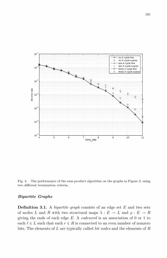
May 10, 2007 8:8 WSPC - Proceedings Trim Size: 9in x 6in ws-procs9x6
165
4 5 6 7 8 9 10 1110
−7
10−6
10−5
10−4
10−3
10−2
10−1
Eb/N0 [dB]
Bit
erro
r ra
te
no 4−cycle fineno 4−cycle coarsetwo 4−cycle finetwo 4−cycle coarsethree 4−cycle finethree 4−cycle coarse
Fig. 4. The performance of the sum-product algorithm on the graphs in Figure 3, using
two different termination criteria.
Bipartite Graphs
Definition 3.1. A bipartite graph consists of an edge set E and two setsof nodes L and R with two structural maps λ : E → L and ρ : E → R
giving the ends of each edge E. A codeword is an association of 0 or 1 toeach ` ∈ L such that each r ∈ R is connected to an even number of nonzerobits. The elements of L are typically called bit nodes and the elements of R
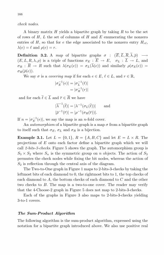
May 10, 2007 8:8 WSPC - Proceedings Trim Size: 9in x 6in ws-procs9x6
166
check nodes.
A binary matrix H yields a bipartite graph by taking R to be the setof rows of H, L the set of columns of H and E enumerating the nonzeroentries of H, so that for e the edge associated to the nonzero entry Hr`,λ(e) = ` and ρ(e) = r.
Definition 3.2. A map of bipartite graphs σ : (E,L,R, λ, ρ) −→(E,L,R, λ, ρ) is a triple of functions σE : E → E, σL : L → L, andσR : R → R such that λ(σE(e)) = σL(λ(e)) and similarly ρ(σE(e)) =σR(ρ(e)).
We say σ is a covering map if for each e ∈ E, ` ∈ L, and r ∈ R,
|σ−1E (e)| = |σ−1
L (`)|= |σ−1
R (r)|
and for each ` ∈ L and r ∈ R we have
|λ−1(`)| = |λ−1(σL(`))| and
|ρ−1(r)| = |ρ−1(σR(r))|.
If n = |σ−1E (e)|, we say the map is an n-fold cover.
An automorphism of a bipartite graph is a map σ from a bipartite graphto itself such that σE , σL and σR is a bijection.
Example 3.1. Let L = 0, 1, R = A,B,C and let E = L × R. Theprojections of E onto each factor define a bipartite graph which we willcall 2-bits-3-checks. Figure 5 shows the graph. The automorphism group isS3 × S2 where Sn is the symmetric group on n objects. The action of S3
permutes the check nodes while fixing the bit nodes, whereas the action ofS2 is reflection through the central axis of the diagram.
The Two-to-One graph in Figure 1 maps to 2-bits-3-checks by taking theleftmost bits of each diamond to 0, the rightmost bits to 1, the top checks ofeach diamond to A, the bottom checks of each diamond to C and the othertwo checks to B. The map is a two-to-one cover. The reader may verifythat the 4-Choose-2 graph in Figure 5 does not map to 2-bits-3-checks.
Each of the graphs in Figure 3 also maps to 2-bits-3-checks yielding3-to-1 covers.
The Sum-Product Algorithm
The following algorithm is the sum-product algorithm, expressed using thenotation for a bipartite graph introduced above. We also use positive real

May 10, 2007 8:8 WSPC - Proceedings Trim Size: 9in x 6in ws-procs9x6
167
A
0 1B
C
Fig. 5. The bipartite graph 2-bits-3-checks.
numbers to represent the probability distributions in the algorithm. Theinput data for bit ` is the “odds” that the actual intended or transmittedvalue for that bit was 1, expressed as the likelihood ratio u` = p`(1)/p`(0).Likewise, the messages along the edges of the graph produced by the al-gorithm are expressed as the odds of 1. The algorithm uses the transformfrom the “odds of 1” domain to the difference domain in which a probabilitydistribution p is represented as p(0)−p(1), which is in the interval [−1,+1].The function s : R ∪ ∞ −→ R ∪ ∞ defined by s(x) = 1−x
1+x transformsfrom one domain to the other. Notice that s(s(x)) = x. In the literature,the ratio p(0)/p(1) is sometimes used rather than p(1)/p(0). We prefer thelatter, since with this notation the same function s is used to translate ineach direction.
Algorithm 3.1 (Sum-Product Algorithm).
Input: For each ` ∈ L, u` ∈ (0,∞). Termination criteria ε > 0.Data Structures: For each e ∈ E, xe, ye ∈ (0,∞).Initialization: Set ye ← 1 for all e ∈ E.
Algorithm:
Bit-To-Check Step: For each e ∈ E, set
xe ← uλ(e)
∏f :λ(f)=λ(e)
f 6=e
yf
Check-To-Bit Step: For each e ∈ E, set
ye ← s
∏f :ρ(f)=ρ(e)
f 6=e
s(xf )

May 10, 2007 8:8 WSPC - Proceedings Trim Size: 9in x 6in ws-procs9x6
168
New Estimate Step: Set
u` ← u`
∏e∈λ−1(l)
ye
Termination and Output: If either u` < ε or u` > 1/ε for all ` ∈ L
then output the hard decision based on u`: Vector w ∈ FL such that
w` =
1 if u` > 1
0 else
When analyzing the algorithm it will sometimes prove useful to indicatethe iteration using a superscript. Thus for example, we will sometimes write
x(t+1)e ← uλ(e)
∏f :λ(f)=λ(e)
f 6=e
y(t)f
Let σ be an automorphism of the bipartite graph. Then the update stepof the algorithm says that
xσE(e) ← uλ(σE(e))
∏f :λ(f)=λ(σE(e))
f 6=σE(e)
yf
Since f ∈ E : λ(f) = λ(σE(e)) = σE(f) : f ∈ E, λ(f) = λ(e), andsince λσE = σLλ the update may be rewritten
xσE(e) ← uσL(λ(e))
∏f :λ(f)=λ(e)
f 6=e
yσE(f) (1)
Proposition 3.1. Let σ be an automorphism of the graph and suppose thatuσL(`) = u` for all ` ∈ L. Then xe = xσ(e) and ye = yσ(e) at each iterationof the algorithm.
Proof. At initialization y(0)e = y
(0)σE(e) for all e ∈ E since ye(0) = 1. We
proceed by induction assuming that the statement holds at iteration t.
x(t+1)σE(e) = uσL(λ(e))
∏f :λ(f)=λ(e)
f 6=e
y(t)σE(f) (2)
= uλ(e)
∏f :λ(f)=λ(e)
f 6=e
y(t)f (3)
= x(t+1)e (4)
The analogous argument is used to show that y(t+1)σ(e) = y
(t+1)e .

May 10, 2007 8:8 WSPC - Proceedings Trim Size: 9in x 6in ws-procs9x6
169
Reduction of the SPA to a local sum algorithm when check
nodes have degree 2
We now restrict attention to a fixed bipartite graph in which each checknode has degree 2. We will also assume that the graph is connected. Onemay readily check that the code defined by such a graph is a repetitioncode. The sum-product algorithm simplifies dramatically because at thecheck to bit step there is only one term in the product.
Proposition 3.2. If all right nodes have degree 2, then then all edge mes-sages are monomials in the u`.
Proof. Clearly, at initialization y(0)e = 1 is a monomial as claimed. If all
y(t)e are monomial then all x(t+1)
e are as well, since the bit-to-check step justinvolves multiplication. Each right node has degree 2, so the product in thecheck-to-bit step has only one term. Since s is an involution, y(t+1)
e = x(t+1)e′
where e′ is the unique edge distinct from e sharing the same right node.Thus we may establish the proposition by induction.
Notation 3.1. For an edge e let e′ be the unique edge, distinct from e,with ρ(e) = ρ(e′). Let us use ae ∈ NL to denote the (vector of) exponentsappearing in xe so xe =
∏`∈L u
ae,`
` . We will abbreviate this product as asuae . When we want to specify the tth iteration we will write a
(t)e .
Let 0 ∈ NL be the zero vector and let δ` ∈ NL be the vector which is 1in the `th component and 0 otherwise.
We may reduce the sum-product algorithm to an algorithm that com-putes the exponents of the input data u` for each edge e. Note that nonotation is needed for ye since it is equal to xe′ .
Algorithm 3.2 (Local Sum Algorithm).
Data Structures: For each e ∈ E, ae,∈ NL.Initialization: Set ae ← 0 for all e ∈ E.
Algorithm: Set
ae ← δλ(e) +∑
f :λ(f)=λ(e)f 6=e
af ′ (5)
Since a is a vector of integers doubly indexed by e ∈ E and ` ∈ L, wecan consider a as an element of the vector space C|E||L| of dimension |E||L|over the complex numbers C.

May 10, 2007 8:8 WSPC - Proceedings Trim Size: 9in x 6in ws-procs9x6
170
Our update function is a linear inhomogeneous map on this space, theinhomogenous part coming from the term δλ(e). The homogeneous part ofthe map is represented by the matrix M , defined as follows.
M (e,`),(f,m) =
1 if λ(e) = λ(f ′), f ′ 6= e, and ` = m
0 else(6)
We can write the local sum algorithm in a homogeneous way by using a“dummy” variable to supply the necessary δλ(e) terms. To this end, defineT ∈ C|E||L| such that
T e,l =
1 if λ(e) = l
0 else(7)
Let
M =[M T
0T 1
](8)
Then [a(t)
1
]= M
[a(t−1)
1
](9)
We have thus reduced analysis of the sum-product algorithm in ourrestricted case to the problem of understanding the dynamics of the matrixM .
Proposition 3.3. Suppose that all check nodes have degree 2. Let xe = uae
and let a be the concatenation of the exponent vectors ae. Then at iterationt, [
a(t)
1
]= M
t[01
](10)
We can use the automorphism group of the bipartite graph to reduce thedimensionality of the problem. Consider an automorphism σ of the graph.From (1) we have
xσE(e) ← uσL(λ(e))
∏f :λ(f)=λ(e)
f 6=e
yσE(f)
= uσL(λ(e))
∏f :λ(f)=λ(e)
f 6=e
xσE(f ′)

May 10, 2007 8:8 WSPC - Proceedings Trim Size: 9in x 6in ws-procs9x6
171
where ρ(f ′) = ρ(f), so
aσE(e) ← δσL(λ(e)) +∑
f :λ(f)=λ(e)f 6=e
aσE(f ′) (11)
Proposition 3.4. Let σ be an automorphism of a bipartite graph in whichall checks have degree 2. At any iteration of the local sum algorithm,
aσE(e),σL(`) = ae,l
Proof. At initialization, the claim is immediate. We proceed by induction.From the algorithm,
a(t+1)e,` =
∑f :λ(f)=λ(e)
f 6=e
a(t)f ′,` +
1 if λ(e) = `
0 else
From the action of σ in (11) we have
a(t+1)σE(e),σL(`) =
(δσL(λ(e))
)σL(`)
+∑
f :λ(f)=λ(e)f 6=e
a(t)σE(f ′),σL(`)
Using the induction hypothesis and observing that σL(λ(e)) = σL(`) if andonly if λ(e) = ` we have
a(t+1)σE(e),σL(`) =
∑f :λ(f)=λ(e)
f 6=e
a(t)f ′,` +
1 if λ(e) = `
0 else
= a(t+1)e,`
As a consequence of this proposition we may compute just the exponentsae for one edge from each orbit under the automorphism group of thebipartite graph. The exponent for any edge f may be obtained by applyingan appropriate automorphism to the representative from the orbit of f .Instead of using the update matrix (6) we may simplify to a matrix N
with one representative edge for each orbit. The entries in N must bederived from (5) replacing af ′ with some aσ(g) for g the representative forthe orbit of f ′ and σ an automorphism taking g to f ′.

May 10, 2007 8:8 WSPC - Proceedings Trim Size: 9in x 6in ws-procs9x6
172
4. Examples
In this section we solve the following question for a number of bipartitegraphs in which all check nodes have degree 2: Under what conditions on theinput values u` will all values xe in the sum-product algorithm converge to0 (or to∞)? In these examples, we ignore termination criteria and examinethe convergence behavior of the infinite sequence x(t)
e , t = 1, 2, ...Our method is to identify a set of representatives for the edge set E
under the action of the automorphism of the graph. Let a be the vector ofexponents indexed by these representatives and by ` ∈ L. We derive theupdate matrix N using one representative from each equivalence class. Wethen have a dynamical system: for
N =[N T
0T 1
](12)
we have [a(t)
1
]= N
t[01
](13)
Except for one case, that of a simple cycle, we will write[01
]=∑t
i=1 wi
as a sum of eigenvectors of N . Let µi be the eigenvalue associated to wi.Then [
a(t)
1
]=
t∑i=1
µtiwi (14)
We can determine convergence from the fact that for large t the eigenvectorswith largest eigenvalues will dominate.
A cycle of length 2m
Consider a cycle of length 2m with both bit nodes and check nodes enumer-ated from 0 to m−1. Let b+ and bi be the edges such that λ(b+) = λ(bi) = b
and ρ(b+) = b, ρ(b−) = b−1 mod m. It is clear that the symmetry group isthe dihedral group Dm and that it is transitive on edges. For the reflectionaround bit node 0 we have from Proposition 3.4, a0+,` = a0−,−` (computing−` modulo m). For rotation by 1 the proposition says
a(k+1)+,l+1 = ak+,l
a(k+1)−,l+1 = ak−,l
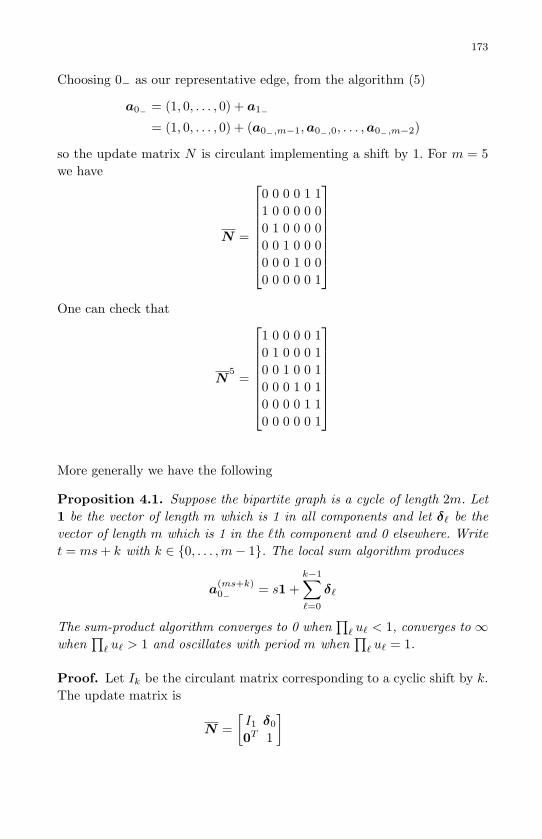
May 10, 2007 8:8 WSPC - Proceedings Trim Size: 9in x 6in ws-procs9x6
173
Choosing 0− as our representative edge, from the algorithm (5)
a0− = (1, 0, . . . , 0) + a1−
= (1, 0, . . . , 0) + (a0−,m−1,a0−,0, . . . ,a0−,m−2)
so the update matrix N is circulant implementing a shift by 1. For m = 5we have
N =
0 0 0 0 1 11 0 0 0 0 00 1 0 0 0 00 0 1 0 0 00 0 0 1 0 00 0 0 0 0 1
One can check that
N5
=
1 0 0 0 0 10 1 0 0 0 10 0 1 0 0 10 0 0 1 0 10 0 0 0 1 10 0 0 0 0 1
More generally we have the following
Proposition 4.1. Suppose the bipartite graph is a cycle of length 2m. Let1 be the vector of length m which is 1 in all components and let δ` be thevector of length m which is 1 in the `th component and 0 elsewhere. Writet = ms+ k with k ∈ 0, . . . ,m− 1. The local sum algorithm produces
a(ms+k)0−
= s1 +k−1∑`=0
δ`
The sum-product algorithm converges to 0 when∏
` u` < 1, converges to ∞when
∏` u` > 1 and oscillates with period m when
∏` u` = 1.
Proof. Let Ik be the circulant matrix corresponding to a cyclic shift by k.The update matrix is
N =[I1 δ0
0T 1
]

May 10, 2007 8:8 WSPC - Proceedings Trim Size: 9in x 6in ws-procs9x6
174
One can prove by induction that for 0 ≤ k < m
Nms+k
=[I s10T 1
][Ik∑k−1
`=0 δ`
0T 1
]
=
[Ik s1 +
∑k−1`=0 δ`
0T 1
]
Thus ams+k0−
= s1 +∑k−1
`=0 δ`. Since x0− = ua0− = (u0 · · ·um−1)s∏k−1
`=0 u`,the converge properties are easily verified.
2 bits n checks
As noted earlier the automorphism group of this graph is S3 × S2. Thereis only a single orbit for the edges under this group action, so we mayreduce analysis of the sum-product algorithm to the consideration of asingle edge e. Proposition 3.4 shows that all edges leaving the same bithave the same vector of exponents. Edges connected to different bit nodesdiffer by transposition of the entries. That is, for e an edge with λ(e) = 0and f an edge with λ(e) = 1 we have af = (ae,1,ae,0). The update of thealgorithm is a
(t+1)e = 2af + (1, 0) = (a(t)
e,1,a(t)e,0) + (1, 0). Using e as the
representative edge, in the matrix equation (12) we have
N =
0 2 12 0 00 0 1
The eigenvalues of N are 2,−2, and 1, with respective eigenvectors
w1 =
110
,w2 =
1−10
, and w3 =
− 13
− 23
1
. The initial vector is
a(0) =
001
=12w1 −
16w2 + w3

May 10, 2007 8:8 WSPC - Proceedings Trim Size: 9in x 6in ws-procs9x6
175
We can calculate
a(t) =12· 2tw1 −
16(−2)tw2 + w3
=
2t−1 − 16 (−2)t − 1
3
2t−1 + 16 (−2)t − 2
3
1
=
2t−1
32t+1−2
3
1
, t even
2t+1−1
32t−2
3
1
, t odd.
Thus, for t even, the message passed by bit 0 at the tth iteration is
u− 1
30 u
− 23
1 · (u0u21)
2t
3 ,
which tends toward 0 if u0u21 < 1 and toward ∞ if u0u
21 > 1. On the other
hand, when t is odd, the message looks like
u− 1
30 u
− 23
1 · (u20u1)
2t
3 ,
and this quantity tends toward 0 if u20u1 < 1 and toward ∞ if u2
0u1 > 1.We see that these conditions are symmetric with respect to u0 and u1
and therefore the sum-product algorithm
• converges to the codeword [0, 0] if u20u1 and u0u
21 are both less than 1;
• converges to the codeword [1, 1] if u20u1 and u0u
21 are both greater than
1;• fails to converge if u2
1u2 < 1 < u1u22 or u2
1u2 < 1 < u1u22.
These results generalize in straightforward way. We will say that twopositive real numbers have the same parity when they are either both lessthan 1 or both greater than 1.
Proposition 4.2. Suppose the bipartite graph has 2 bit nodes and m checknodes. Then the sum-product algorithm converges when u0u
m−11 and
um−10 u1 have the same parity and it divirges otherwise.
4-Choose-2
The symmetry group in this case is S4 and is transitive on edges. Let usenumerate the bits from 0 to 3, going left to right, and identify the edgesby an ordered pair of bits. Then edge (0, 1) is the edge from 0 to the checkfor the pair 0, 1. Let a be the vector of exponents for the edge (0, 1). The
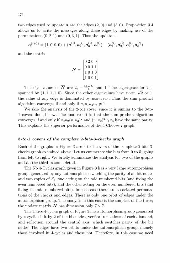
May 10, 2007 8:8 WSPC - Proceedings Trim Size: 9in x 6in ws-procs9x6
176
two edges used to update a are the edges (2, 0) and (3, 0). Proposition 3.4allows us to write the messages along these edges by making use of thepermutations (0, 2, 1) and (0, 3, 1). Thus the update is
a(t+1) = (1, 0, 0, 0) + (a(t)1 ,a
(t)2 ,a
(t)0 ,a
(t)3 ) + (a(t)
1 ,a(t)3 ,a
(t)2 ,a
(t)0 )
and the matrix
N =
0 2 0 00 0 1 11 0 1 01 0 0 1
The eigenvalues of N are 2, − 1±
√7i
2 and 1. The eigenspace for 2 isspanned by (1, 1, 1, 1, 0). Since the other eigenvalues have norm
√2 or 1,
the value at any edge is dominated by u0u1u2u3. Thus the sum productalgorithm converges if and only if u0u1u2u3 6= 1.
We skip the analysis of the 2-to1 cover, since it is similar to the 3-to-1 covers done below. The final result is that the sum-product algorithmconverges if and only if u0u2(u1u3)2 and (u0u2)2u1u3 have the same parity.This explains the superior performance of the 4-Choose-2 graph.
3-to-1 covers of the complete 2-bits-3-checks graph
Each of the graphs in Figure 3 are 3-to-1 covers of the complete 2-bits-3-checks graph examined above. Let us enumerate the bits from 0 to 5, goingfrom left to right. We briefly summarize the analysis for two of the graphsand do the third in some detail.
The No 4-Cycles graph given in Figure 3 has a very large automorphismgroup, generated by any automorphism switching the parity of all bit nodesand two copies of S3, one acting on the odd numbered bits (and fixing theeven numbered bits), and the other acting on the even numbered bits (andfixing the odd numbered bits). In each case there are associated permuta-tions of the checks and edges. There is only one orbit of edges under theautomorphism group. The analysis in this case is the simplest of the three;the update matrix N has dimension only 7× 7.
The Three 4-cycles graph of Figure 3 has automorphism group generatedby a cyclic shift by 2 of the bit nodes, vertical reflections of each diamond,and reflection around the central axis, which switches parity of the bitnodes. The edges have two orbits under the automorphism group, namelythose involved in 4-cycles and those not. Therefore, in this case we need

May 10, 2007 8:8 WSPC - Proceedings Trim Size: 9in x 6in ws-procs9x6
177
only keep track of two 6-vectors, which we will take to emanate from bit 0,and the update matrix N has dimension 13× 13.
The Two 4-cycles graph given in Figure 3, has automorphisms generatedby σ, the 180-degree rotation around the center; τ , which interchanges thefirst and second bits, the third and fourth bits, and the fifth and sixth bits(and performs the necessary permutations of the checks and edges), and π,which interchanges the two checks on the far left of the graph and theirattendant edges.
The edges of this graph form 4 orbits under its automorphism group,which we can take to be the upper and lower edges from bit 0 and the middleand lower edges from bit 3. The update matrix N is therefore 25× 25, thefirst 24 dimensions coming from the exponents along the respective edgesand, as in previous examples, the last one “driving” the dynamical systemby adding 1 to the respective bits’ exponents at each time step. We candescribe the matrix as follows: Label the vectors of exponents for the ui
along the edges as follows: a along the upper edge from bit 0; b along thelower edge from bit 0; c along the lower edge from bit 3; and d along thehorizontal edge from bit 3. The updating rule is then as follows, where ′
denotes updated values:
(a0,a1,a2,a3,a4,a5)′ = (a1 + c0 + 1,a0 + c1,a3 + c2,
a2 + c3,a5 + c4,a4 + c5)
(b0, b1, b2, b3, b4, b5)′ = (2a1 + 1, 2a0, 2a3, 2a2, 2a5, 2a4)
(c0, c1, c2, c3, c4, c5)′ = (b4 + d1, b5 + d0, b2 + d3,
d2, b0 + d5, b1 + d4)
(d0,d1,d2,d3,d4,d5)′ = (b0 + b4, b1 + b5, 2b2, 2b3, b0 + b4, b1 + b5)
From these equations one derives the 25× 25 transition matrix N .For each of the three graphs the eigenvalues have norm 2,
√2 or 1. The
initial vector (0, 0, 0, ..., 1) can be decomposed into a sum of eigenvectorsas 1
6w2 + 118w−2 + other terms, where w2 = (1, 1, 1, ..., 1, 1, 0) has eigen-
value 2, w−2 = (1,−1, 1,−1, ..., 1,−1, 0) has eigenvalue −2 and the otherterms involve eigenvectors associated to smaller eigenvalues. Therefore, asthe system evolves, these two terms dominate. At odd iterations, the sig-nificant terms look like 2t · 1
9 (1, 2, 1, 2...1, 2, 0) and at even iterations like2t · 19 (2, 1, 2, 1, ..., 2, 1, 0). Thus, if (u0u2u4)(u1u3u5)2 and (u0u2u4)2(u1u3u5)have the same parity the sum-product algorithm will converge; otherwise, itwill diverge. This explains why the performance curves under the stringentcriterion given in Figure 4 are the same for the three graphs. The algorithm

May 10, 2007 8:8 WSPC - Proceedings Trim Size: 9in x 6in ws-procs9x6
178
under the stringent criterion reflects the convergence behavior of the infi-nite sequences, which are identical. This is somewhat surprising given thepresence of multiple 4-cycles in two of them and desirable “large girth” inthe third.
Degradation of performance with the coarse termination
criterion
We now consider the difference in performance for the three graphs un-der the less stringent termination criterion. Let us write the initial vector(0, 0, . . . , 1) as 1
6w2 + 118w−2 + w√
2 + w1, where w√2 is the contribution
from all eigenvectors associated to eigenvalues of norm√
2 and w1 is thecontribution from the eigenvectors associated to eigenvalues of norm 1. Con-sider inputs u0, . . . , u5 such that (u0u2u4)(u1u3u5)2 and (u0u2u4)2(u1u3u5)have the same parity, say both < 1, so that the sum-product algorithm con-verges. The sum-product algorithm will terminate early and be incorrect,when at iteration t, some of the u(t)
` are larger than 103 and others areless than 10−3. For this to happen some of the u` must be larger than 1,and their contribution at the locations `′ where u(t)
`′ > 103 must be un-usually high. We have u`′ = u
Pλ(e)=l′ ae and, at iteration t, each a
(t)e is
some subvector of Nt(w2 +w−2 +w√
2 +w1) (subject to a permutation of
indices). The contribution from uNt(w2+w−2) is either (u0u2u4)(u1u3u5)2
or (u0u2u4)2(u1u3u5) for each of the graphs. Thus early termination is dueto the contribution from N
tw√
2. The difference in performance is due tothe different dynamics for this expression in the three graphs.
For the No 4-cycle graph the vector of exponents for u2t+s1 is
(−2)t(0, 2/3, 0,−1/3, 0,−1/3). Thus u may be greater than 103 when u1
is large and u3 and u5 are small, or vice-versa. The situation at other bitnodes is similar. For the Three 4-cycle graph the vector of exponents at bitnode 1 behaves more chaotically.
(0, 2/3, 0,−1/3, 0,−1/3) at iteration 0
(1, 2/3, 0,−1/3,−1,−1/3) at iteration 2
(−1,−10/3, 0, 5/3, 1, 5/3) at iteration 4
(−3, 2/3, 0,−1/3, 3, 1/3) at iteration 6
The exact cause of inferior performance for the Three 4-cycle graph isnot obvious, but we think two things play a role. First, the L1-norm of thevector of exponents for u` is larger for the Three 4-cycle graph. Second,
May 10, 2007 8:8 WSPC - Proceedings Trim Size: 9in x 6in ws-procs9x6
179
the chaotic variation of the vector of exponents for u` means that there aremore conditions that can lead to early, and incorrect, termination.
5. Concluding Remarks
Although the examples considered in this article are very simple and do notdefine codes of practical interest, there are several interesting results andsome properties that may have relevance for realistic codes.
We remark that the usual explanations for decoding failure seem irrel-evant for these graphs. For each of the examples the only stopping sets aretrivial, either the empty set or the entire set. One does find near-codewordsof different weights for the different graphs in Figures 5 and 3, but theydon’t appear to be directly related to the convergence criteria reportedhere. Expansion hardly makes sense with such small graphs. The polytopeof pseudo-codewords is simply a line segment generated by the all 0 code-word and the all 1 codeword, so the only extremal pseudo-codewords arein fact codewords. Thus pseudo-codewords do not explain decoding failure.These properties may be associated with decoding failure on large graphs,but these examples suggest they are not a cause, but rather correlated tosome deeper causative phenomenon.
One explanation for pseudo-codewords causing decoding failure is thatthe sum-product algorithm on a given graph may be affected by codewordsin a covering graph. Our examples suggest the reverse effect, the sum-product algorithm on the covering graphs of 2-bits-3-checks seem to haveinherited the convergence behavior of their base graph. Furthermore, the4-Choose-2 graph shows that one can do better than a covering graph. Itwould be interesting to see if this effect can be proven, whether for bipartitegraphs with all check nodes of degree 2, or more generally. If so, this suggestsan inherent weakness in the low-density matrices constructed in severalarticles, e.g. [5, 9, 13], using a block matrix of circulants. It also presents achallenge to find other algebraic methods for constructing bipartite graphs.
References
[1] C. Di, D. Proietti, I. E. Teletar, T. J. Richardson, and R. L. Urbanke. Fi-nite length analysis of low-density parity-check codes on the binary erasurechannel. IEEE Trans. Inform. Theory, 48(6):1570–1579, 2002.
[2] Jon Feldman. Decoding Error-Correcting Codes via Linear Programming.PhD thesis, Massachusetts Institute of Technology, 2003.
[3] Jon Feldman, M. J. Wainwright, and D. R. Karger. Using linear program-ming to decode linear codes. IEEE Trans. Inform. Theory, 51(3):954–972,Mar. 2005.

May 10, 2007 8:8 WSPC - Proceedings Trim Size: 9in x 6in ws-procs9x6
180
[4] G. D. Forney, R. Koetter, F. R.Kschischang, and A. Reznik. On the effectiveweights of pseudocodewords for codes defined on graphs with cycles. In Proc.IMA workshop on codes systems and graphical models, pages 101–112, 2001.
[5] M. P. C. Fossorier. Quasi-cyclic, low-density parity-check codes from circu-lant permutation matrices. IEEE Trans. Inform. Theory, 50(8):1788–1793,2004.
[6] R. Koetter and P. O. Vontobel. Graph covers and iterative decoding of finitelength codes. In Proc. 3rd Int. Conf. on Turbo Codes and Related Topics,pages 75–82, Sept. 2003.
[7] D. J. C. MacKay. Good error-correcting codes based on very sparse matrices.IEEE Trans. Inform. Theory, 45(2):399–431, 1999.
[8] David J. C. MacKay and M. J. Postol. Weaknesses of Margulis andRamanujan–Margulis low-density parity-check codes. In Proceedings ofMFCSIT2002, Galway, volume 74 of Electronic Notes in Theoretical Com-puter Science. Elsevier, 2003.
[9] M. E. O’Sullivan. Algebraic construction of sparse matrices with large girth.IEEE Trans. Inform. Theory, 52:718–727, 2006.
[10] T. Richardson. Error floors of LDPC codes. In Proc. of the 42-th AnnualAllerton Conference on Communication, Control, and Computing, pages1426–1435, 2004.
[11] T. Richardson, A. Shokrollahi, and R. Urbanke. Design of capacity-approaching irregular low-density parity-check codes. IEEE Trans. Inform.Theory, 47(2):619–639, 2001.
[12] M. Sipser and D. A. Spielman. Expander codes. IEEE Trans. Inform. The-ory, 42(6, part 1):1710–1722, 1996.
[13] R. M. Tanner. On graph constructions for LDPC codes by quasi-cyclic ex-tensions. In M. Blaum, P. Farrell, and H. C. .A. van Tilborg, editors, Infor-mation, Coding and Mathematics, pages 209–219. Kluwer Academic, 2002.
[14] T. Tian, C. Jones, J. Villasenor, and R. Wesel. Selective avoidance of cyclesin irregular ldpc code construction. IEEE Trans. on Comm., 52(8):1242–1247, Aug. 2004.
[15] P. O. Vontobel and R. Koetter. Lower bounds on the minimum pseudo-weight of linear codes. In 2004 IEEE Int. Symp. Infor. Theory, page 70,2004.
[16] N. Wiberg. Codes and Decoding on General Graphs. PhD thesis, LinkopingUniversity, Sweden, 1996.

May 10, 2007 8:8 WSPC - Proceedings Trim Size: 9in x 6in ws-procs9x6
181
On the extremal graph theory for directed graphs and itscryptographical applications
V. A. Ustimenko
University of Maria Curie-Sklodowska,Lublin, Poland,
E-mail: [email protected]
The paper is devoted to the graph based cryptography. The girth of a directed
graph (girth indicator) is defined via its smallest commutative diagram. Theanalogue of Erdøos’s Even Circuit Theorem for directed graphs allows to es-
tablish upper bound on the size of directed graphs with a fixed girth indicator.
Size of members of infinite family of directed regular graphs of high girth isclose to an upper bound.
Finite automata related to members of such a family of algebraic graphs
over chosen commutative ring can be used effectively for the design of cryp-tographical algorithm for different problems of data security (stream ciphers,
data base encryption, public key mode an digital signatures).
The explicit construction of infinite family of algebraic graphs of high girthdefined over the arbitrarily chosen ring is given. Some results on their proper-
ties, based on theoretical studies or software implementations are given.
Keywords: Extremal graph theory, directed graphs of large girth, algebraicgraphs over commutative rings, graph based cryptography, coding theory
1. Introduction
One of the important direction in the classical extremal graph theory isstudies of the greatest number of edges ex(v, d) = ex(v, C3, . . . C2d) ofgraphs on v vertices without cycles Ct of length t = 3, 4, . . . , d . It is knownthat ex(v, C3, . . . , C2d) ≤ O(v1+1/d) (see [3]). Similar problem for directedgraphs (roughly, finite automata) has been motivated by applications tocryptography and other areas of computer science.
We use term binary relation graph for the graph Γ of irreflexive binaryrelation φ over finite set V such that for each v ∈ V sets x|(x, v) ∈ φ andx|(v, x) ∈ φ have same cardinality.
We say that the pair of passes a = x0 → x1 → · · · → xs = b, s ≥ 1 anda = y0 → y1 → · · · → yt = b, t ≥ 1 form an (s, t)-commutative diagram

May 10, 2007 8:8 WSPC - Proceedings Trim Size: 9in x 6in ws-procs9x6
182
Os,t if xi 6= yj for 0 < i < s, 0 < j < t. Without loss of generality we assumes ≥ t and refer to the number s as the rank of Os,t. The directed cycle withs arrows we denote as Os,0. The minimal parameter s = max(s, t) of thecommutative diagram Os,t with s+ t ≥ 3 in the binary relation graph Γ wecall the girth indicator of the Γ and denote it as gi(Γ).
Let E = Ed(v) = Ex(v,Os,t, s + t ≥ 3|2 ≤ s ≤ d) be the maximal size(number of arrows) of the binary relation graphs with the girth indicator> d.
Notice , that the size of symmetric irreflexive relation is the double of thesize of corresponding simple graph. because undirected edge of the simplegraph corresponds to two arrows of O2,0. In [27] the following bound hasbeen obtained
Ed(v) ≤ v1+1/d +O(v) (1)
Via explicit constructions we find out that for d = 2, 3, 4, 5 and 6 the bound(1) is sharp up to magnitude.
It indicates that studies of extremal properties of graphs of binary re-lations with the high girth indicator and studies of ex(v, C3, . . . , Cn) arefar from being equivalent. Really, the sharpness of the ex(v, n) for n = 8and n = 12 are old open problems (similar to cases of cycles C8 and C12 inErdos’ Even Circuit Theorem).
The girth of the simple graph is the minimal length of its minimal cycles.The infinite family of k-regular graphs Γi of fixed degree k is the family ofgraphs of large girth if the size of its members is close to exv, C3, c4, . . . , Cn,i.e. girth of Γi of order vi is clogk−1(vi), where c is independent on i con-stant. They turned out to be very useful in networking (see [2]).
The idea to use simple graphs of large girth in cryptography had beenwidely explored, in particular see [10], [19], [20], [22]-[26], [28]-[29].
The definitions of family of graphs of large girth for the class of irreflex-ive binary relation graphs formulated in [28], where more general encryptionscheme for the ”potentially infinite” text based on the graphs of binary re-lations with special ”rainbow-like” coloring of arrows has been proposed(see section 2 of current paper for all details). In fact, a family of k-regularbinary relation graphs Γi, i = 1, . . . is a family of graphs of large girth ifthe size of its members is close to the bound (1).
For the encryption purpose we identify the vertex of the graph withthe plaintext, encryption procedure corresponds to the chain of adjacentvertices starting from the plaintext, the information on such chain is givenby the sequence of colors (passwords). We assume that the end of the chain

May 10, 2007 8:8 WSPC - Proceedings Trim Size: 9in x 6in ws-procs9x6
183
is the ciphertext.The important feature of such encryption is the resistance to attacks,
when adversary intercepts the pair plaintext - ciphertext. It is true becausethe best algorithm of finding the pass between given vertices (by Dijkstra,see [6] and latest modifications) has complexity nlnn where n is the orderof the graph, i.e. the size of the plainspace. The situation is similar to thechecking of the primality of Fermat’s numbers 22m
+ 1: if the input givenby the string of binary digits, then the problem is polynomial, but if theinput is given by just a parameter m, then the task is NP-complete.
We have an encryption scheme with the flexible length of the password(length of the chain). If graphs are connected then we can convert eachpotentially infinite plaintext into the chosen string ”as fast as it is possible”.
Finally, in the case of ”algebraic graphs” (see [1]) with the special”rainbow-like” coloring (symbolic rainbow-like graphs of section 3) thereis an option to use symbolic computations in the implementation of graphbased algorithm. We can create public rules symbolically and use the abovealgorithm as public key tool (for the example of implementation look at[24]).
The first explicit examples of families with large girth with arbitrarylarge valency were given by Margulis. The constructions were Cayley graphsXp,q of group SL2(Zq) with respect to special sets of q + 1 generators,p and q are primes congruent to 1 mod 4. The family of Xp,q is not afamily of algebraic graphs because the neighborhood of each vertex is notan algebraic variety over Fq. For each p, graphs Xp,q, where q is runningvia appropriate primes, form a family of small world graph of unboundeddiameter (see [15]-
The first family of connected algebraic graphs over Fq of large girthand arbitrarily large degree had been constructed in [13]. These graphsCD(k, q), k is an integer ≥ 2 and q is odd prime power had been constructedas connected component of graphs D(k, q) defined earlier. For each q graphsCD(k, q), k ≥ 2 form a family of large girth with γ = 4/3logq−1q.
Some new examples of simple algebraic graphs of large girth and arbi-trary large degree the reader can find in [29].
[17]).

May 10, 2007 8:8 WSPC - Proceedings Trim Size: 9in x 6in ws-procs9x6
184
2. Binary relations, related rainbow-like graphs andalgorithms
2.1. Binary relations and special colorings
Let Φ be an irreflexive binary relation over the set V , i.e. Φ ∈ V × V andfor each v pair (v, v) is not the element of Φ.
We say that u is the neighbor of v if (v, u) ∈ Φ. Recall, that we use termbinary relation graph for the graph Γ of irreflexive binary relation φ overfinite set V such that for each v ∈ V sets x|(x, v) ∈ φ and x|(v, x) ∈ φhave the same cardinality. It is a directed graph without loops and multipleedges.
Let Γ be the graph of binary relation. The pass between vertices a and bis the sequence a = x0 → x1 → . . . xs = b of length s, where xi, i = 0, 1, . . . sare distinct vertices.
We shall use a term the family of algebraic graphs for the family ofgraphs Γ(K), where K belongs to some infinite class F of commutativerings, such that the neighborhood of each vertex of Γ(K) and the vertexset itself are quasi-projective varieties over K of dimension ≥ 1 (see [1]).
Such a family can be treated as special Turing machine with the internaland external alphabet K.
We say that the graph Γ of binary relation Φ has a rainbow-like coloringover the set of colors C if for each v, v ∈ V we have a coloring function ρv,which is a bijection from the neighborhood St(v) of v onto C, such thatthe operator Nc(v) of taking the neighbor of v with color c is the bijectionof V onto V .
We say that the rainbow like coloring ρ is invertible if there is a rainbow-like coloring of Φ−1 over C ′ such that Nc
−1 = N ′c′ for some color c′ ∈ C ′.
Example 2.1. (Cayley graphs)Let G be the group and S be subset of distinct generators, then the
binary relation φ = (g1, g2)|gi ∈ G, i = 1, 2, g1g2−1 ∈ S admits therainbow like coloring ρ(g1, g2) = g1g2
−1
This rainbow like coloring is invertible because the inverse graph φ−1 =(g2, g1)|g1g2−1 ∈ S admits the rainbow-like coloring ρ
′(g2, g1) = g2g1
−1 ∈S−1.
Example 2.2. (Parallelotopic graphs and latin squares)Let G be the graph with the coloring µ : V (G)→ C of the set of vertices
V (G) into colors from C such that the neighborhood of each vertex lookslike rainbow, i.e. consists of |C| vertices of different colors. In case of pair
May 10, 2007 8:8 WSPC - Proceedings Trim Size: 9in x 6in ws-procs9x6
185
(G,µ) we shall refer to G as parallelotopic graph with the local projectionµ (see [20], [22] and further references).
It is obvious that parallelotopic graphs are k-regular with k = |C|. IfC ′ is a subset of C, then induced subgraph GC′ of G which consists of allvertices with colors from C ′ is also a parallelotopic graph. It is clear thatconnected component of the parallelotopic graph is also a parallelotopicgraph.
The arc of the graph G is a sequence of vertices v1, . . . , vk such thatviIvi+1 for i = 1, . . . , k − 1 and vi 6= vi+2 for i = 1, . . . , k − 2. If v1, . . . , vk
is an arc of the parallelotopic graph (G,µ) then µ(vi) 6= µ(vi+2) for i =1, . . . , k − 2.
Let + be the latin square defined on the set of colors C. Let us assumethat ρ(u, v) = µ(u) − µ(v). The operator Nc(u) of taking the neighbor ofthe color is invertible, Nc
−1 = N−c, where −c is the opposite for c elementin the latin square. It means that ρ is invertible rainbow like coloring.
Example 2.3. The class of sparse parallelotopic bipartite graphs can begiven by the following incidence structure defined over finite field Fq in [27].
Let P = (x1, . . . , xn)|xi ∈ Fq and L = [y1, . . . , yn]|yi ∈ Fq bethe sets of points and lines. The point (x1, . . . , xn) is incident to the line[y1, y2, . . . , yn]|yi ∈ Fq] if and only if xi − yi = xk(i)yl(i), i = 2, 3, . . . , n,where parameters k(i) < i, l(i) < i are chosen for each value of i. We candefine the coloring µ((x1, . . . xn) = x1, µ([y1, . . . , yn]) = y1 and obtain theparallelotopic graph. The choice of the field addition + as an appropriatelatin square allows us to define an effective finite automaton: the operatorof taking the neighbor of chosen color require 2n− 1 field operations.
2.2. General symmetric algorithm
Let us consider the encryption algorithm corresponding to the graph Γ withthe chosen invertible rainbow-like coloring of edges. Let ρ(u, v) be the colorof arrow u → v, C is the totality of colors and Nc(u) is the operator oftaking the neighbor of u with the color c.
The password is the string of colors (c1, c2, . . . , cs) and the encryp-tion procedure is the composition Nc1 × Nc2 . . . Ncs
of bijective mapsNci
: V (Γ) → V (Γ) . So if the plaintext v ∈ V (Γ) is given, then theencryption procedure corresponds to the following chain: x0 = v → x1 =Nc1(x0) → x2 = Nc2(x1) → · · · → xs = Ncs
(xs−1) = u in the graph. Thevertex u is the ciphertext.
Let N ′c′(Nc(v)) = v for each v ∈ V (Γ). The decryption procedure corre-

May 10, 2007 8:8 WSPC - Proceedings Trim Size: 9in x 6in ws-procs9x6
186
sponds to the composition of maps N ′c′s
, N ′c′s−1
, . . . , N ′c′1
. The above schemegives a symmetric encryption algorithm with flexible length of the password(key). Let A(Γ, ρ, s) be the above encryption scheme.
Examples 1 and 2 demonstrate that each known infinite family of graphsof large girth of unbounded degree can be used for the development of theencryption algorithm according to the above scheme; see [28] or [29] for thedetails.
2.3. Symbolic computations and public keys
Let K be the commutative ring. Recall that graph Γ is the algebraic graphover K if the set of vertices V (Γ) and the neighborhood of each vertex u
are algebraic quasi-projective varieties over the ring K; see [1].In the case of symbolic invertible rainbow-like graph (Γ, ρ, ρ′), the vertex
set V (Γ) and the neighborhoods of each vertex are open algebraic varietiesin Zariski topology as well as the color set C, maps N(c, v) = Nc(u) andN ′(c, v) = N ′
c(u) are polynomial maps from C × V (Γ) onto V (Γ).In the case of symbolic rainbow-like graph the encryption as above with
the key (t1, t2, . . . , tk) is given by some polynomial map from Ck×V (Γ)→V (Γ). We can treat ti, i = 1, . . . , k as symbolic variables.
The specializations ti = αi ∈ K give the public key map P : V (Γ) →V (Γ). Like in the known example of polynomial encryption proposed byImai and Matsumoto (see [16]) and its modifications by J. Patarin (see[12]) we can combine P with two invertible affine transformations T1 andT2 (bijective polynomial maps of degree 1) and work with the public mapQ = T1PT2.
Let us use the characters Alice and Bob from books on Cryptography(see, for instance [11], [12]), where Bob is a public user and Alice is a keyholder. So she knows the string t1, . . . , , ts, the graph and affine transfor-mations T1 and T2. She can decrypt via consecutive applications of T2
−1,N ′
t′k, N ′
t′k−1, . . . N′t1 and T1
−1.The public user Bob has the encryption mapQ only. He can encrypt, but
the decryption is hard task because (1) Q is the polynomial map of degree≥ 2 from many variables. (2) Even in the case, when Bob knows T1, T2 andthe graph Γ. The problem of finding the pass between the plaintext vertexand the ciphertext vertex has complexity nlnn, where n = |V (Γ)| is thesize of plainspace. So Bob is not able to decrypt if the plainspace is largeenough.

May 10, 2007 8:8 WSPC - Proceedings Trim Size: 9in x 6in ws-procs9x6
187
2.4. Coding theory, other applications
The theory of distance transitive graphs is the theoretical basis for codingtheory problems dealing with the problem of error detection and error cor-rection (see [4], [5]). Some applications (not only in Coding Theory, but inComplexity Studies and Parallel Computing) require the expansion prop-erties of the graphs (see [2], [8] and further references). For instance, errorcorrecting codes by Tanner [18] use expansion properties of finite gener-alized polygons, which are both distance-regular and expanding graphs.In the paper [7] Tanner’s idea (see [13]) had been implemented to graphsCD(k, q) which are not distance regular, but have good expansion prop-erties. We suggest to use the encryption based on the graphs X(p, q) offixed degree q + 1. They form the family of graphs of large girth (girth= 4/3logq(v)), family of small world graphs (diameter = 4/3logq(v) + 2,family of expanding graphs (the second largest eigenvalue is bounded by2√q [14], so it is the Ramanujan case).
3. The incidence structures defined over commutative rings
We define the family of graphs D(k,K), where k > 2 is positive integer andK is a commutative ring (see [20], [29]), such graphs have been consideredin [13] for the case K = Fq. Let P and L be two copies of Cartesian powerKN , where K is the commutative ring and N is the set of positive integernumbers. Elements of P will be called points and those of L lines.
To distinguish points from lines we use parentheses and brackets, forx ∈ V , we write (x) ∈ P or [x] ∈ L. It will also be advantageous to adoptthe notation for co-ordinates of points and lines introduced in [20] for thecase of general commutative ring K:
(p) = (p0,1, p1,1, p1,2, p2,1, p2,2, p′2,2, p2,3, . . . , pi,i, p
′i,i, pi,i+1, pi+1,i, . . .),
[l] = [l1,0, l1,1, l1,2, l2,1, l2,2, l′2,2, l2,3, . . . , li,i, l
′i,i, li,i+1, li+1,i, . . .].
The elements of P and L can be thought as infinite ordered tuples of el-ements from K, such that only finite number of components are differentfrom zero.
We now define an incidence structure (P,L, I) as follows. We say thatthe point (p) is incident with the line [l], and we write (p)I[l], if the following
May 10, 2007 8:8 WSPC - Proceedings Trim Size: 9in x 6in ws-procs9x6
188
relations between their co-ordinates hold:
li,i − pi,i = l1,0pi−1,i
l′i,i − p′i,i = li,i−1p0,1
li,i+1 − pi,i+1 = li,ip0,1
li+1,i − pi+1,i = l1,0p′i,i
(2)
These four relations are defined for i ≥ 1, p′1,1 = p1,1, l′1,1 = l1,1). Thisincidence structure (P,L, I) we denote by D(K) and identify it with thebipartite incidence graph of (P,L, I), which has the vertex set P ∪ L andedge set consisting of all pairs (p), [l] for which (p)I[l].
For each positive integer k ≥ 2 we obtain an incidence structure(Pk, Lk, Ik) as follows. First, Pk and Lk are obtained from P and L, re-spectively, by simply projecting each vector onto its k initial coordinateswith respect to the above order. The incidence Ik is then defined by impos-ing the first k−1 incidence equations and ignoring all others. The incidencegraph corresponding to the structure (Pk, Lk, Ik) is denoted by D(k,K).
To facilitate notation in future results, it will be convenient for us todefine p−1,0 = l0,−1 = p1,0 = l0,1 = 0, p0,0 = l0,0 = −1, p′0,0 = l′0,0 = −1,and to assume that (6) are defined for i ≥ 0.
Notice that for i = 0, the four conditions (1) are satisfied by everypoint and line, and, for i = 1, the first two equations coincide and givel1,1 − p1,1 = l1,0p0,1.
The incidence relation is motivated by the linear interpretation ofLie geometries in terms of their Lie algebras [22] . Let us define the”root subgroups” Uα, where the ”root” α belongs to the root systemRoot = (1, 0), (0, 1), (1, 1), (1, 2), (2, 1), (2, 2), (2, 2)′ . . . , (i, i), (i, i)′, (i, i +1), (i+ 1, i) . . . . The ”root system above” contains all real and imaginaryroots of the Kac-Moody Lie Algebra A1 with the symmetric Cartan matrix(see [9]). We just double the imaginary roots (i, i) by introducing (i, i)′.
Remark 3.1. For K = Fq the following statement had been formulated in[13]. Let k ≥ 6, t =
[k+24
], and let
u = (uα, u11, · · · , utt, u′tt, ut,t+1, ut+1,t, · · · )
be a vertex of D(k,K) (α ∈ (1, 0), (0, 1), it does not matter whether u isa point or a line). For every r, 2 ≤ r ≤ t, let
ar = ar(u) =∑
i=0,r
(uiiu′r−i,r−i − ui,i+1ur−i,r−i−1),
and a = a(u) = (a2, a3, · · · , at).

May 10, 2007 8:8 WSPC - Proceedings Trim Size: 9in x 6in ws-procs9x6
189
Proposition 3.1. (i) The classes of equivalence relation τ = (u, v)|a(u) =a(v) are connected components of graph D(n,K), where n ≥ 2 and K bethe ring with unity of odd characteristic.
(ii) For any t − 1 ring elements xi ∈ K), 2 ≤ t ≥ [(k + 2)/4], thereexists a vertex v of D(k,K) for which
a(v) = (x2, . . . , xt) = (x).
(3i) The equivalence class C for the equivalence relation τ on the setKn ∪Kn is isomorphic to the affine variety Kt ∪Kt , t = [4/3n] + 1 forn = 0, 2, 3 mod 4, t = [4/3n] + 2 for n = 1 mod 4.
Remark 3.2. Let K be the general commutative ring and C be the equiv-alence class on τ on the vertex set D(K) (D(n,K), then the induced sub-graph, with the vertex set C is the union of several connected componentsof D(K) (D(n,K)).
Without loss of generality we may assume that the vertex v of C(n,K)satisfies to conditions a2(v) = 0, . . . at(v) = 0. We can find the values ofcomponents v′i,i) from this system of equations and eliminate them. Thuswe can identify P and L with elements of Kt, where t = [3/4n] + 1 forn = 0, 2, 3 mod 4, and t = [3/4n] + 2 for n = 1 mod 4.
We shall use notation C(t,K) (C(K)) for the induced subgraph ofD(n,K) with the vertex set C.
Remark 3.3. IfK = Fq, q is odd, then the graph C(t, k) coincides with theconnected component CD(n, q) of the graph D(n, q) (see [29] and furtherreferences), graph C(Fq) is a q-regular tree. In other cases the questionon the connectivity of C(t,K) is open. It is clear that g(C(t, Fq)) is ≥2[2t/3] + 4.
Proposition 3.2. Projective limit of graphs D(n,K) (graphs C(t,K),CD(n,K) ) with respect to standard morphisms of D(n + 1,K) ontoD(n,K) (their restrictions on induced subgraphs) equals to D(K) (C(K).
If K is an integrity domain, then D(K) and CD(K) are forests. Let Cbe the connected component, i.e a tree.
We define the parallelotopic coloring of the graphs C(t,K)), D(n,K),C(K) and D(K) by formulae µ(p1,0, p1,1, . . . ) = p1,0, µ([l0,1, l1,1, . . . ]) =l0,1.
Let us consider the directed flag graphs F (t,K) and E(n,K) of thetactical configurations C(t,K) and D(n,K), respectively. The vertex set ofF (t,K) (E(n,K)) is a totality of flags f = (([l], (p)), where (p)I[l] in the

May 10, 2007 8:8 WSPC - Proceedings Trim Size: 9in x 6in ws-procs9x6
190
C(t,K) (D((n,K), respectively), we have f1 → f2 for f1 = ([l1], (p1)), f2 =([l2], (p2)) if [l2]I(p1) ,[l1] 6= [l2], (p1) 6= (p2). We can consider the symbolicinvertible rainbow-like coloring ρ(f1, f2) of F (t,K) ( E(t,K)) defined onthe color set K∗ ×K∗ by the following rule:
Let f1 = ([l1], (p1)), f2 = ([l2], (p2)) form the arrow in F (t,K) (E(t,K)).So, [l2]I(p1). We assume that ρ(f1, f2) = (l11,0 − l21,0, p
10,1 − l20,1).
If K is finite, then the cardinality of the color set is (|K| − 1)2. LetRegK be the totality of regular elements, i.e. not zero divisors of the ringK. Let us delete all arrows with color (x, y), where one of the elements xand y is not a zero divisor for F (t,K) and E(t,K). New graph RF (t,K)and RE(t,K) are the symbolic rainbow-like graphs over the set of colors(RegK)2. The following statement can be found in [28].
Theorem 3.1. The girth indicator gi of the symbolic rainbow like graphRF (t, k) are g ≥ 1/3t.
Corollary 3.1. Let K be a finite such that k = |RegK| ≥ 2. Then graphsRF (t,K), t = 1, 2, . . . form the family of symbolic rainbow-like graphs oflarge girth of degree k2.
4. Symmetric encryption, algorithms related to graphsRF (n, K)
We can apply the general scheme of symmetric encryption to the paral-lelotopic graphs RF (t,K) or RE(n,K) from the previous section. Otheroptions are based on the fact that RE(n,K) and E(n,K) are the envelop-ing graph for RF (t,K) and the description of ”connectivity invariants”ai(u), i ≥ 2 of D(n,K).
The information on the vertex f = (p), [l], (p)I[l] can be given bythe list of coordinates (p1,0, p1,1, . . . ) of the point (p) and the parallelotopiccolor l0,1 of the line [l]. Obviously, (p) and [l] are in the same connectedcomponent of the graph D(n,K). So we can think of ai((p)), i ≥ 2 asconnectivity invariants of the graph RE(n,K).
Let Root be the list of all roots related to D(n,K) and Ω = Root −(0, 1) be the list of the indexes of components of the tuple (p). Let ai(p),i = 2, 3, . . . , t be the list of connectivity invariants. We choose two subsetsJ = i1, i2, . . . il and J ′ = j1, . . . , Jm , |J∩J ′| = 0 of the set 2, 3, . . . , t,l +m ≤ t− 1. So we have 3t−1 options to make a choice of (J, J ′). Let
Fj(x1, x2, . . . , xd), d = t− l −m− 1, j = 1, 2

May 10, 2007 8:8 WSPC - Proceedings Trim Size: 9in x 6in ws-procs9x6
191
be the polynomial maps from Kd into K. The pair (J, J ′) and functions Fi,i = 1, 2 form the ”internal key” of our encryption algorithm.
Let us choose the ”external key” in the form of the pair (b),=(b1, . . . , bd), c, where b ∈ Kd and c ∈ Reg(K)s for some even integer1 ≤ s < gi− 1. If the ring K is finite, then we have |K|d|RegK|s options toform the external password for chosen parameter s.
4.1. The encryption algorithm
Let
∆(J) = (i, i)|i ∈ J∆(J ′) = (i, i)|i ∈ J ′Root′ = Root− J ∪ J ′
(3)
The plainspace is the totality of functions f : Root′ → K. So theplainspace is the string of characters from the alphabet K.
Step 1. We will form the vertex of the graph E(n,K) by the follow-ing rule: form the point (p) such that pα = f(α) for α ∈ Root′. For theα ∈ ∆(J) ∪ ∆(J ′) values pα (α = (i, i) or α = (i, i)′) will be computedconsequently from the equations ai(p) = bi, i ∈ J ∪ J ′, [l] be the neighbor-ing line for (p) with the parallelotopic color f((0, 1)). We form the vertexv = ((p), [l]) of the graph E(n,K).
Step 2. Let Rt1,t2(u) be the operator of taking the neighbor of the vertexu = (p), [l]) of the parallelotopic color (p1,0 + t1, l0,1 + t2), where ti ∈ K,i = 1, 2. Let s1, s2, . . . , sd be the list of elements of the complement forJ ∪ J ′. We compute RF1(as1 (p),...,asd
)(p),F2(as1 (p),...,asd)(p) = v0.
Step 3. Apply the composition of operators Rc1,c2 , . . . , Rcs−1,csto the
vertex v0. In fact, we use here the general encryption scheme for the graphRE(n,K) in case of the plaintext v0). Let ((h), [g]) be the resulting vertex.Assume that the information on this pair is given by function z : Root→ K,such that z((0, 1)) = g0,1 and zα = hα for α 6= (0, 1).
Step 4. The ciphertext is the restriction z′ of the function z ontoRoot−∆(J) ∪∆(J ′).
Step 5. We combine polynomial map τ : f → z′ as above with two

May 10, 2007 8:8 WSPC - Proceedings Trim Size: 9in x 6in ws-procs9x6
192
invertible sparse affine transformations A and B by taking the compositionAτB.
4.2. Decryption procedure
Step 1. Let u be the ciphertext. We form the vertex ((p′), [l′]) of the graphRE(n,K) from the function y = B−1(U) by the following rule: p′α = y(α)for α ∈ Root′, for the α ∈ ∆(J) ∪∆(J ′) values p′α (α = (i, i) or α = (i, i)′)will be computed consequently from the equations
ai(p′) = bi, , i ∈ J ∪ J′.
The line [l′] be the neighboring line for (p′) with the parallelotopic colory((0.1). We form the vertex
vertex v′ = ((p′), [l′]) of the graph RE(n,K)−1.
Step 2. Let R′t1,t2(u) be the operator of taking the neighbor of thevertex u = ((p), [l]) in the graph E(n,K)−1 of the parallelotopic color(p1,0 = t1, l0,1 + t2), where ti ∈ RegK, i = 1, 2. Let s1, s2, . . . sd
be the list of elements of the complement for J ∪ J ′. We computeR−F1(as1 (p′),...,asd
(p′)),−F2(as1 (p′),...,asd(p′))(v′) = v′0.
Step 3. Apply the composition of operators R′−cs−1,−ccs, . . . ,−Rc1,c2 to
the vertex v′0. In fact, we use here the general decryption scheme for thegraph RE(n,K) in case of the ciphertext v′0).
Step 4. Let ((h′), [g′]) be the resulting vertex. Assume that the in-formation on this pair is given by function z1 : Root → K, such thatz((0, 1)) = g′0,1 and zα = h′α for α 6= (0, 1). We take the restriction z′1 ofthe function z1 onto Root−∆(J) ∪∆(J ′).
Step 5. Compute the plaintext A−1(z′1).
Let us denote the above symmetric encryption algorithm asAlg(F1, F2, A,B).
Proposition 4.1. (i) Let us keep the internal password fixed. Then differ-ent external passwords correspond to distinct ciphertext.
(ii) If the values of F1(as1(p), . . . , asd(p)) and F2(as1(p), . . . , asd
(p))(Step 2) are regular elements and B = A−1 of the ciphertext is always
different from the plaintext.

May 10, 2007 8:8 WSPC - Proceedings Trim Size: 9in x 6in ws-procs9x6
193
Proof. Let us consider the transformation Alg(E,E, F1, F2), where E isthe identity map. Steps 1 and 2 do not depend on the external alphabet.The encryption procedure corresponds to the directed pass in the graphRE(n,K) of the length less than the girth indicator. So the property (i)holds. The affine transformations A and B are bijections, so the property(i) is true for the Alg(A,B, F1, F2).
If the condition of (ii) holds then steps 2 and 3 of Alg(E,E, F1, F2)correspond to the directed pass in the graph RE(n,K) of the length lessthen the girth indicator. So this transformation have no fixed points. Themap Alg(A,A−1, F1, F2) is conjugate with Alg(E,E, F1, F2).
Remark 4.1. In fact we can use conditions F1(as1(p), . . . , asd(p)) ×
F2(as1(p), . . . , asd(p)) 6= 0 or Fi(as1(p), . . . , asd
(p)) = 0 for some i insteadof condition of (ii) for the above statement.
We say that functions A,B, Fi, i = 1, 2 are sparse if their computationrequires O(n) operations of the ring K.
Proposition 4.2. (i) Let the complexity of transformations A,B, Fi, i =1, 2. If max(|J |, |J ′|) is bounded by independent on n constant, then thesymmetric encryption as above requires O(n) ring operations.
(ii) For each positive integer m there is a choice of functions Fi, i = 1, 2,such that the degree of polynomial encryption map is ≥ m.
(iii) If functions F1 and F2 are constants, then the encryptiontransformation of Alg(E,E, F1, F2) sending (l0,1, p1,0, p1,1, . . . , pα, . . . ) into(l′0,1, p
′1,0, p
′1,1, . . . , p
′α, . . . ) ’ is a triangular map of kind l′0,1 → l′0,1 + c,
p′α → pα + fα(l0,1, p1,0, p1,1, . . . , pα). So the value of p′alpha depends compo-nents pβ such that β < α according to the natural order on the root set.
Remark 4.2. The properties (i) and (iii) of the statement above allowto use Alg(E,E, c1, c2 as a stream cipher for ”changing data on the fly”(telecommunications, encryption CD’s with movies and etc). If we keepthe external password fixed, then change of the single character pα of theplaintext lead to change of characters p′β of ciphertext with β ≥ α.
Remark 4.3. In the case of the root set with the highest roots (l, l), (l, l)′
such that l is not an element of J and J ′, Fi(as1(p), . . . , asd(p)), i = 1, 2 are
linear combinations of as1(p), . . . , asd(p) containing terms kiai(p), ki 6= 0
change of single character of the ciphertext lead to change with the proba-bility close to 1 each character of the ciphertext. It justifies use of nontrivial

May 10, 2007 8:8 WSPC - Proceedings Trim Size: 9in x 6in ws-procs9x6
194
F1 and F2 for the self-coding in case of encryption of large file (data bases,Geological Information Systems, etc).
4.3. Examples
1) In the practically important case of the ring K = Z2n (sizes of theASKEE and binary alphabets are 27 and 28, respectively) the RegK isthe totality of odd residues modulo 2n, all values of functions of kind2f(x1, x2, . . . , xn) + 1 are regular elements. So if Fi, i = 1, 2 belong tothis set, then the ciphertext for Alg(A,A−1, F1, F2) is always different fromeach plaintext.
2) In the case of K = z2k+1, the value of Euler function φ(2k+1) givingus the number of regular elements of the ring is ≥ k, because of all evenresidues are regular, values of functions of kind 2f(x1, . . . , xn) either areregular or zero, So if Fi, i = 1, 2 belong to this set, then the ciphertext forAlg(A,A−1, F1, F2) is always different from each plaintext.
3) In the case of the integer domain RegK coincides with the K − 0any transformation Alg(A,A−1, F1, F2) has no fixed points.
5. Public keys
We can use the following modification of the encryption Alg(A,B, F1, F2)with subsets J = i1, i2, . . . , il and J ′ = j1, . . . , jm , |J ∩ J ′| = 0 of theset 2, 3, . . . , t, l +m ≤ t− 1. Recall that Fi, i = 1, 2 depend on variables(x1, x2, . . . , xd), d = t− l −m− 1.
Let us choose the ”dynamical external key” in the form of the pairb = (b1, . . . bd) ∈ Kd and c = (f1(x1, x2, . . . , xd), . . . , fs(x1, . . . , xd)), wheres is even integer and fi are polynomial maps from Kd into K.
We have to complete Step 1 and 2 without any changes. After computa-tion of ”numerical password” c′ = (f1(as1(p), . . . , asd
(p)) = (c′1, . . . , c′d)
and complete modified Step 3 i. e. apply the composition of operatorsRc′1,c′2
, . . . , Rc′s−1,c′sto the vertex v0. In fact, we use here the general en-
cryption scheme for the graph E(n,K) in case of the plaintext v0).After we conduct remaining steps 4 and 5 without any changes.The new algorithm Alg(E(n, k), A,B, F1, F2, f1, . . . , fs) defines the
polynomial map of the free module Kr, r = |Root − J ∪ J | into itself.We have to create (say with ”Mathematica” or ”Maple”) the public rule:
y1 = P1(x1, . . . , xr), . . . , yr = Pr(x1, . . . , xr).

May 10, 2007 8:8 WSPC - Proceedings Trim Size: 9in x 6in ws-procs9x6
195
The public user Bob can use it for the encryption procedure. If parameters and degrees of polynomials F1, F2, f1, . . . , fs are sufficiently large then heis not able to find the inverse map.
The key holder Alice use information on the graph E(n,K), matri-ces A, B, sets J, J ′, functions F1, F2 and external key i. e. string bof elements of the ring K and sequences of functions f1, . . . , fs. Thatis why she can use modified decryption scheme of Alg(A,B, F1, F2) ,where the only modification is the computation of ”numerical password”c = (f1(as1(p), . . . , asd
(p)) = (c1, . . . , cd) for the restriction p of the outputof Step 2 onto the set Root(0, 1).
If values functions F1, F2, f1, . . . , fs are regular elements then the plain-text and the ciphertext of Alg(E(n, k), E,E, F1, F2, f1, . . . , fs) are at thedistance s/2 + 1 in the graph RE(n,K). If s/2 + 1 is ≤ gi, then the cipher-text is always different from the plaintext.
6. Other algebraic parallelotopic graphs
The algorithm Alg(E,E, F1, F2) with empty sets Jand J can be easilygeneralized on the arbitrary algebraic parallelotopic graph G(K) over ringK with the color set M and coloring function µ. We can assume thatM = M(K) is the open quasi-algebraic variety over the commutative ringK. Let V (K) be the vertex set of G and g : V (K)→ Kl be the connectivityinvariant of the graph i. e. function which is constant on vertices fromthe same connected component. Let Ra(v) be the operator of taking theneighbor of the vertex v ∈ V (G) of the color a ∈ M . Let hi(x, y), x ∈ M ,y ∈ M , i = 1, . . . , s be polynomial maps from M ×Kl → M such thateach equation of kind hi(x, b) = c has unique solution in variable x. Wedefine the following invertible procedure τ : v → v1 = Rh1(µ(v),g(v)(v) →Rh2(µ(v1),g(v) → Rhs(µ(vs−1),g(v). The transformation AτB, where A and Bare sparse invertible polynomial automorphisms of V (G), can be used forvarious cryptographical problems.
If L(x, y) be the latin squire on M , which is a polynomial map fromM×M → M , then we can take hi = L(φi(x), y), where φi are polynomialautomorphisms of open variety M .
The reader can find examples of parallelotopic graphs over the set ofcolors Km of high girth for each commutative ring K and each positiveinteger m ≥ 2.
We can consider more general graphs RF 2s(t,K) (RE2s(t,K)), whichvertices are chains (p1), [l1], . . . , (ps), [ls] of old graph Ct(K) (D(n,K),respectively) such that ρ(pi) − ρ(pi−1), i = 2, 3, . . . , s and ρ(li) −
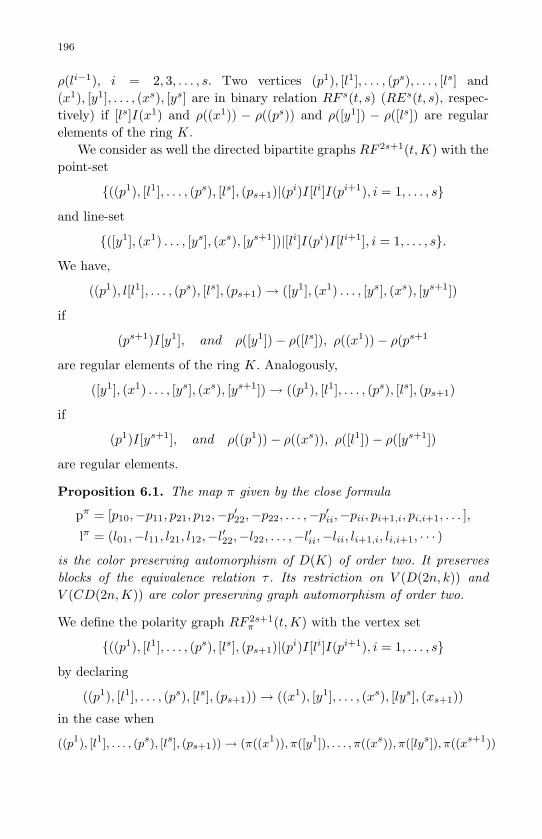
May 10, 2007 8:8 WSPC - Proceedings Trim Size: 9in x 6in ws-procs9x6
196
ρ(li−1), i = 2, 3, . . . , s. Two vertices (p1), [l1], . . . , (ps), . . . , [ls] and(x1), [y1], . . . , (xs), [ys] are in binary relation RF s(t, s) (REs(t, s), respec-tively) if [ls]I(x1) and ρ((x1)) − ρ((ps)) and ρ([y1]) − ρ([ls]) are regularelements of the ring K.
We consider as well the directed bipartite graphs RF 2s+1(t,K) with thepoint-set
((p1), [l1], . . . , (ps), [ls], (ps+1)|(pi)I[li]I(pi+1), i = 1, . . . , s
and line-set
([y1], (x1) . . . , [ys], (xs), [ys+1])|[li]I(pi)I[li+1], i = 1, . . . , s.
We have,
((p1), l[l1], . . . , (ps), [ls], (ps+1)→ ([y1], (x1) . . . , [ys], (xs), [ys+1])
if
(ps+1)I[y1], and ρ([y1])− ρ([ls]), ρ((x1))− ρ(ps+1
are regular elements of the ring K. Analogously,
([y1], (x1) . . . , [ys], (xs), [ys+1])→ ((p1), [l1], . . . , (ps), [ls], (ps+1)
if
(p1)I[ys+1], and ρ((p1))− ρ((xs)), ρ([l1])− ρ([ys+1])
are regular elements.
Proposition 6.1. The map π given by the close formula
pπ = [p10,−p11, p21, p12,−p′22,−p22, . . . ,−p′ii,−pii, pi+1,i, pi,i+1, . . . ],
lπ = (l01,−l11, l21, l12,−l′22,−l22, . . . ,−l′ii,−lii, li+1,i, li,i+1, · · · )
is the color preserving automorphism of D(K) of order two. It preservesblocks of the equivalence relation τ . Its restriction on V (D(2n, k)) andV (CD(2n,K)) are color preserving graph automorphism of order two.
We define the polarity graph RF 2s+1π (t,K) with the vertex set
((p1), [l1], . . . , (ps), [ls], (ps+1)|(pi)I[li]I(pi+1), i = 1, . . . , s
by declaring
((p1), [l1], . . . , (ps), [ls], (ps+1))→ ((x1), [y1], . . . , (xs), [lys], (xs+1))
in the case when
((p1), [l1], . . . , (ps), [ls], (ps+1)) → (π((x1)), π([y1]), . . . , π((xs)), π([lys]), π((xs+1))

May 10, 2007 8:8 WSPC - Proceedings Trim Size: 9in x 6in ws-procs9x6
197
Corollary 6.1. Let K be a finite such that k = |RegK| ≥ 2. Thengraphs RF s(t,K) (RF 2s+1
π (t,K)), t = 1, 2, . . . form the family of symbolicrainbow-like graphs of large girth of degree ks (k2s+1, respectively).
Password length 3000 6000 9000m5 915 1760 260610 1830 3520 521115 2745 5280 781520 3666 7053 10440
7. Remarks on implementation
In our package for symmetric encryption we used the rings Z28 and F28 ,same field as in the new U.S. Advanced Encryption Standard (AES). In fact,our crypto-system works primarily with bytes (8 bits), represented from theright as: b7b6b5b4b3b2b1b0. The 8-bit elements of the field are regardedas polynomials with coefficients in the field F2: b7x7 + b6x6 + b5x5 +b4x4 + b3x3 + b2x2 + b1x1 + b0. The field elements will be denoted bytheir sequence of bits, using two hexadecimal digits. . We eight irreduciblepolynomial (a polynomial that cannot be factored into the product of twosimpler polynomials). As for the AES, we use the following irreducible poly-nomial: m(x) = x8+x4+x3+x+1 = 0x11b(hex). The intermediate productof the two polynomial we first generate a multiplication table for the 256elements and once any multiplication of elements in the F28 , we use theloaded multiplication table for efficiency reasons.
To evaluate the performance of our algorithm (F28), we use measurethe encryption time for our method for different size of data files and usingdifferent password lengths of keys (in bytes). It shows also that for passwordof length 10 our algorithm is capable to encrypt at speed as fast as 2kilo-bytes per millisecond. Together with the traditional table below, wejust write the close formula T = 2nk, T - time, n, k are dimensions ofthe plainspace and the keyspace as vector spaces over the chosen field,
in the directed graph RF 2s+1(t, K). The following statement is immediate
corollary from Theorem 3.

May 10, 2007 8:8 WSPC - Proceedings Trim Size: 9in x 6in ws-procs9x6
198
respectively. Our program is written in Java and it runs on Pentium 4,1GHZ. The better performance on better computers we get via C or C++version.
Our algorithm uses binary code, it may encrypt any data type. We havedeveloped a prototype software written in Java. We hope that our softwarecan be a very attractive tool for reliable security of virtual organization(e-learning, e-business, etc ...). We used families of graphs RE(k,K), K ∈Z28 , F28, D(k, F28). Because of the use of loaded multiplication table thespeed of computation does not depend on the choice of the family.
Remark. Case of rings Z2s . Let us assume that the password and theplaintext are numbers written base 2 (binary code). To encrypt we makingtwo steps: first is the conversion of the plaintext and the key into stringsof residues mod Z2s (numbers n and k base 2s), second is our algorithmon symmetric mode with the numerical key. The complexity of first stepO(log2(n))+Olog2(k) does not depend on parameter s (see [11]). The com-plexity of second step is approximately 2nk2−2s because the key (plaintext)is the string of length k2−s (n−2s, respectively. So the algorithm in case ofs = 32 (s = 64) works 16 times (64 times, respectively) faster then in cases = 8 evaluated by table below.
References
[1] N. Biggs, Algebraic Graph Theory (2nd ed), Cambridge, University Press,1993.
[2] F. Bien, Constructions of telephone networks by group representations, No-tices Amer. Mah. Soc., 36 (1989), 5-22.
[3] B. Bollobas, Extremal Graph Theory, Academic Press, London, 1978.[4] A. Brower, A. Cohen, A. Nuemaier, Distance regular graphs, Springer, Berlin,
1989.[5] P. J. Cameron and J.H. van Lint, Graphs, Codes and Designs, London. Math.
Soc. Lecture Notes, 43, Cambridge (1980).[6] E. Dijkstra, A note on two problems in connection with graphs, Num. Math.,
1 (1959), 269-271.[7] P. S. Guinard and J.Lodge, Tanner Type Codes Arizing from Large Girth
Graphs, Communications Research Centre, Canada , Reprint GUI94, 2006.[8] S. Hoory, N. Linial, and A.Wigderson, Expander graphs and their applications,
Bulletin (New Series) of AMS, volume 43, N4, 439-461,[9] V. Kac. Infinite dimensional Lie algebras, Birkhauser, Boston, 1983.[10] Yu. Khmelevsky , V. A. Ustimenko, Practical aspects of the Informational
Systems reengineering, The South Pacific Journal of Natural Science, volume21, 2003, www.usp.ac.fj(spjns).
[11] N. Koblitz, A Course in Number Theory and Cryptography, Second Edition,Springer, 1994, 237 p.

May 10, 2007 8:8 WSPC - Proceedings Trim Size: 9in x 6in ws-procs9x6
199
[12] N. Koblitz, Algebraic aspects of Cryptography, in Algorithms and Compu-tations in Mathematics, v. 3, Springer, 1998.
[13] F. Lazebnik, V. Ustimenko and A.J.Woldar, A new series of dense graphsof high girth, Bulletin of the AMS 32 (1) (1995), 73-79.
[14] A. Lubotsky, R. Philips, P. Sarnak, Ramanujan graphs, J. Comb. Theory,115, N 2., (1989), 62-89.
[15] G. A. Margulis, Explicit construction of graphs without short cycles and lowdensity codes, Combinatorica, 2, (1982), 71-78.
[16] G. Margulis, Explicit group-theoretical constructions of combinatorialschemes and their application to desighn of expanders and concentrators,Probl. Peredachi Informatsii, 24, N1, 51-60. English translation publ. Journalof Problems of Information transmission (1988), 39-46.
[17] M. Margulis, Arithmetic groups and graphs without short cycles, 6th Intern.Symp. on Information Theory, Tashkent, abstracts, vol. 1, 1984, pp. 123-125(in Russion).
[18] R.Michael Tanner. A recursive approach to low complexity codes, IEEE Transon Info.Th., IT, 27(5):533-547, Sept. 1981.
[19] A. Tousene, V. Ustimenko, Graph Based Private Key Crypto System, Inter-national Journal on Computer Research, Nova Science Publisher, volume 13(2006), issue 4, 12p.
[20] V. A. Ustimenko, Coordinatisation of regular tree and its quotients, in”Voronoi’s impact on modern science”, eds P. Engel and H. Syta, book 2,National Acad. of Sci, Institute of Matematics, 1998, 228p.
[21] V. A. Ustimenko, On the varieties of parabolic subgroups, their generaliza-tions and combinatorial applications, Acta Applicandae Mathematicae, 52(1998), 223-238.
[22] V. Ustimenko, Graphs with Special Arcs and Cryptography, Acta Applican-dae Mathematicae, 2002, vol. 74, N2, 117-153.
[23] V. Ustimenko, CRYPTIM: Graphs as tools for symmetric encryption, InLecture Notes in Comput. Sci., 2227, Springer, New York, 2001.
[24] V. Ustimenko, Maximality of affine group and hidden graph cryptsystems,Journal of Algebra and Discrete Mathematics, October, 2004, v.10, pp. 51-65.
[25] V. A. Ustimenko, D. Sharma, CRYPTIM: system to encrypt text and imagedata, Proceedings of International ICSC Congress on Intelligent Systems 2000,Wollongong, 2001, 11pp.
[26] V. Ustimenko, A. Touzene, CRYPTALL:system to encrypt all types of data,Notices of the Kiev-Mohyla Academy, v 23, June , 2004, pp. 12-15.
[27] V. Ustimenko, On the extremal binary relation graphs of high girth, Proceed-ings of the Conference on infinite particle systems, Kazimerz- Dolny, 2006,World Scientific Publ.(to appear).
[28] V. Ustimenko, On the graph based cryptography and symbolic computations,Serdica Journal of Computing, Proceedings of the International Conference,ACA 2006, Warna, Bugaria (to appear).
[29] V. Ustimenko. On linguistic Dynamical Systems, Graphs of Large Girth andCryptography, Journal of Mathematical Sciences, Springer, vol.140, N3 (2007)pp. 412-434.

May 10, 2007 8:8 WSPC - Proceedings Trim Size: 9in x 6in ws-procs9x6
200
Fast arithmetic on hyperelliptic curves via continued fractionexpansions
M. J. Jacobson, Jr.
Department of Computer Science, University of Calgary,2500 University Drive NW, Calgary, Alberta, Canada T2N 1N4
E-mail: [email protected]
R. Scheidler∗
Department of Mathematics and Statistics, University of Calgary,
2500 University Drive NW, Calgary, Alberta, Canada T2N 1N4
E-mail: [email protected]
A. Stein
Department of Mathematics, University of Wyoming1000 E. University Avenue, Laramie, WY 82071-3036, USA
Email: [email protected]
In this paper, we present a new algorithm for computing the reduced sum of
two divisors of an arbitrary hyperelliptic curve. Our formulas and algorithmsare generalizations of Shanks’s NUCOMP algorithm, which was suggested ear-
lier for composing and reducing positive definite binary quadratic forms. Our
formulation of NUCOMP is derived by approximating the irrational contin-ued fraction expansion used to reduce a divisor by a rational continued frac-
tion expansion, resulting in a relatively simple and efficient presentation of
the algorithm as compared to previous versions. We describe a novel, unifiedframework for divisor reduction on an arbitrary hyperelliptic curve using the
theory of continued fractions, and derive our formulation of NUCOMP based
on these results. We present numerical data demonstrating that our versionof NUCOMP is more efficient than Cantor’s algorithm for most hyperelliptic
curves, except those of very small genus defined over small finite fields.
Keywords: Hyperelliptic curve, reduced divisor, continued fraction expansion,infrastructure, Cantor’s algorithm, NUCOMP
∗The research of the first two authors is supported by NSERC of Canada.

May 10, 2007 8:8 WSPC - Proceedings Trim Size: 9in x 6in ws-procs9x6
201
1. Introduction and Motivation
Divisor addition and reduction is one of the fundamental operations re-quired for a number of problems and applications related to hyperellipticcurves. The group law of the Jacobian can be realized by this operation,and as such, applications ranging from computing the structure of the divi-sor class group to cryptographic protocols depend on it. Furthermore, thespeed of algorithms for solving discrete logarithm problems on hyperellipticcurves, particularly of medium and large size genus, depend on a fast com-putation of the group law. There has been a great deal of work on findingefficient algorithms for this operation (see for instance [5]).
Cantor’s algorithm [2] is a generic algorithm that allows this opera-tion to be explicitly computed. It works by first adding the two divisorsand subsequently reducing the sum. One drawback of this approach, andmost algorithms derived from it, is that one has to deal with intermedi-ate operands of double size. That is, while the basis polynomials of thetwo starting divisors and the final reduced divisor have degree at most g,where g is the genus of the curve, the divisor sum has a basis consistingof two polynomials whose degree is usually as large as 2g, and reductiononly gradually reduces the degrees back down to g. This greatly reducesthe speed of the operation, and it is highly desirable to be able to performdivisor addition and reduction without having to compute with quantitiesof double size.
The group operation of the class group of positive definite binaryquadratic forms, composition and reduction, suffers from the same problemof large intermediate operands. In 1988, Shanks [13] devised a solution tothis problem, an algorithm he called NUCOMP. The idea behind this algo-rithm is to stop the composition process before completion and apply a typeof intermediate reduction before computing the composed form. Insteadof using the rather expensive continued fraction algorithm that producesthe aforementioned intermediate operands of double size, the reduction isperformed using the much less costly extended Euclidean Algorithm. Thecoefficients are only computed once the form is reduced or almost reduced.As a result, the sizes of the intermediate operands are significantly smaller,and the binary quadratic form produced by NUCOMP is very close to beingreduced.
In [11], van der Poorten generalized NUCOMP to computing with idealsin the infrastructure of a real quadratic number field by showing how therelative generator corresponding to the output can be recovered. Jacobsonand van der Poorten [6] presented numerical evidence for the efficiency
May 10, 2007 8:8 WSPC - Proceedings Trim Size: 9in x 6in ws-procs9x6
202
of their version of NUCOMP. They also sketched an adaptation of thismethod to arithmetic in the class group and infrastructure of a hyperellipticcurve. Their computational results indicated that their version of NUCOMPwas more efficient than Cantor’s algorithm for moderately small genera(between genus 5 and 10), and that the relative efficiency improved as boththe genus and size of the ground field increase. However, a formal analysisand description of NUCOMP in the hyperelliptic curve setting was notprovided.
Shanks’s formulation of NUCOMP, as well as the treatments in [11]and [6], are based on the arithmetic of binary quadratic forms. In [8], theauthors described NUCOMP in terms of ideal arithmetic in real quadraticnumber fields. They provided a clear and complete description of NUCOMPin terms of continued fraction expansions of real quadratic irrationalitiesand, in addition, showed how to optimize the formulas in this context.
In this paper, we provide a unified description of NUCOMP for divisorarithmetic on the three different possible models of a hyperelliptic curve:imaginary, real, and unusual [3]. We generalize the results in [8], describ-ing and deriving NUCOMP in terms of continued fraction expansions inall three settings. Furthermore, we explain NUCOMP purely in terms ofdivisor arithmetic, also incorporating the infrastructure arithmetic of a realhyperelliptic curve. Our formulation of NUCOMP is complete and some-what simpler than that in [6], and its relation to Cantor’s algorithm ismore clear. In addition, we prove its correctness and a number of relatedresults, including the fact that the output is in most cases reduced, andis in the worst case only one step away from being reduced. The end re-sult, supported by computational results, is that our improved formulationof NUCOMP offers performance improvements over Cantor’s algorithm foreven smaller genera than indicated in [6].
We begin in Sec. 2 with an overview of continued fractions, and explaindivisor arithmetic on hyperelliptic curves and its connection to continuedfractions in Sec. 3–Sec. 5. Based on this foundation, we describe divisoraddition and reduction as well as NUCOMP in Sec. 6–Sec. 10. We concludewith numerical results in Sec. 11, including a discussion of the efficiency ofour two different versions of NUCOMP as given in Sec. 9.

May 10, 2007 8:8 WSPC - Proceedings Trim Size: 9in x 6in ws-procs9x6
203
2. Continued Fraction Expansions
For brevity, we write the symbolic expression
s0 +1
s1 +1
. . .sn +
1αn+1
as [s0, s1, . . . , sn, αn+1]. If we wish to leave the end of the expression unde-termined, we simply write [s0, s1, . . . ].
Let k be any field, k[t] the ring of polynomials in the indeterminate t withcoefficients in k, and k(t) the field of rational functions in t with coefficientsin k. It is well-known that the completion of k(t) with respect to the placeat infinity of k(t) (corresponding to the discrete valuation “denominatordegree minus numerator degree”) is the field k〈t−1〉 of Puiseux series in t−1;that is, any non-zero element in k〈t−1〉 is of the form
α =d∑
i=−∞ait
i ,
where d ∈ Z, ai ∈ k for i ≤ d, and ad 6= 0. Define
bαc =d∑
i=0
aiti , sgn(α) = ad , deg(α) = d . (2.1)
Also, define b0c = 0 and deg(0) = −∞.Let n ≥ 0, s0, s1, . . . , sn a sequence of polynomials in k[t], and α ∈
k〈t−1〉 non-zero. Then the expression
α = [s0, s1, . . . , sn, αn+1] (2.2)
is referred to as the (ordinary) continued fraction expansion of α with partialquotients s0, s1, . . . , sn. It uniquely defines a Puiseux series αn+1 ∈ k〈t−1〉where α0 = α and αi+1 = (αi − si)−1 for 0 ≤ i ≤ n. If we set
A−2 = 0 , A−1 = 1 , Ai = siAi−1 +Ai−2 ,
B−2 = 1 , B−1 = 0 , Bi = siBi−1 +Bi−2 ,(2.3)
for 0 ≤ i ≤ n, then Ai/Bi = [s0, s1, . . . , si] for 0 ≤ i ≤ n − 1. SinceAiBi−1 − Ai−1Bi = (−1)i−1 for −1 ≤ i ≤ n, Ai and Bi are coprime for−2 ≤ i ≤ n.
If si = qi with qi = bαic for i ≥ 0, then Eq. (2.2) is the well-known regu-lar continued fraction expansion of α. Here, the partial quotients q0, q1, . . .

May 10, 2007 8:8 WSPC - Proceedings Trim Size: 9in x 6in ws-procs9x6
204
are uniquely determined by α, and deg(qi) ≥ 1 for all i ∈ N. The rationalfunction Ai/Bi = [q0, q1, . . . , qi] is the i-th convergent of α. This term ismotivated by the well-known inequalities
deg(α− Ai
Bi
)≤ − deg(BiBi+1) < −2 deg(Bi) (2.4)
for all i ≥ 0. The following result is also well-known:
Lemma 2.1. Let α ∈ k〈t−1〉, E, F ∈ k[t] with αF 6= 0 and gcd(E,F ) = 1.If
deg(α− E
F
)< −2 deg(F ) ,
then E/F is a convergent in the regular continued fraction expansion of α.
Throughout this paper, we reserve the symbols qi and qi for the quo-tients of a regular continued fraction expansion; for arbitrary partial quo-tients, we use the symbol si. To distinguish expansions of rational functionsfrom those of Puiseux series, we henceforth use the convention that partialquotients and convergents relating to expansions of rational functions areequipped with a “ˆ” symbol, whereas quantities pertaining to expansionsof Puiseux series do not have this symbol.
One of the main ideas underlying NUCOMP is to approximate the reg-ular continued fraction expansion of a Puiseux series by that of a rationalfunction “close” to it. We then expect the convergents, and hence the twoexpansions, to agree up to a certain point:
Theorem 2.1. Let α ∈ k〈t−1〉 and α ∈ k(t) be non-zero, and write α =E/F with E,F ∈ k[t]. Let qi (0 ≤ i ≤ m) and ri (−1 ≤ i ≤ m) be thesequences of quotients and remainders, respectively, obtained by applying theEuclidean Algorithm to α; that is, r−2 = E, r−1 = F, ri−2 = qiri−1+ri withqi = bri−2/ri−1c for 0 ≤ i ≤ m, so rm−1 = gcd(E,F ) and rm = 0. If thereexists n ∈ Z, −1 ≤ n ≤ m− 1, such that 2 deg(rn) > deg(F 2(α− α)), thenthe first n+2 partial quotients in the regular continued fraction expansionsof α and α are equal.
Proof. Let α = [q0, q1, . . . , qm, . . .] be the regular continued fraction expan-sion of α. The regular continued fraction expansion of α is obviously α =[q0, q1, . . . , qm]. Then Ai/Bi = [q0, q1, . . . , qi] and Ai/Bi = [q0, q1, . . . , qi]are the i-th convergents of α and α, respectively. We wish to prove thatqi = qi for 0 ≤ i ≤ n+ 1.
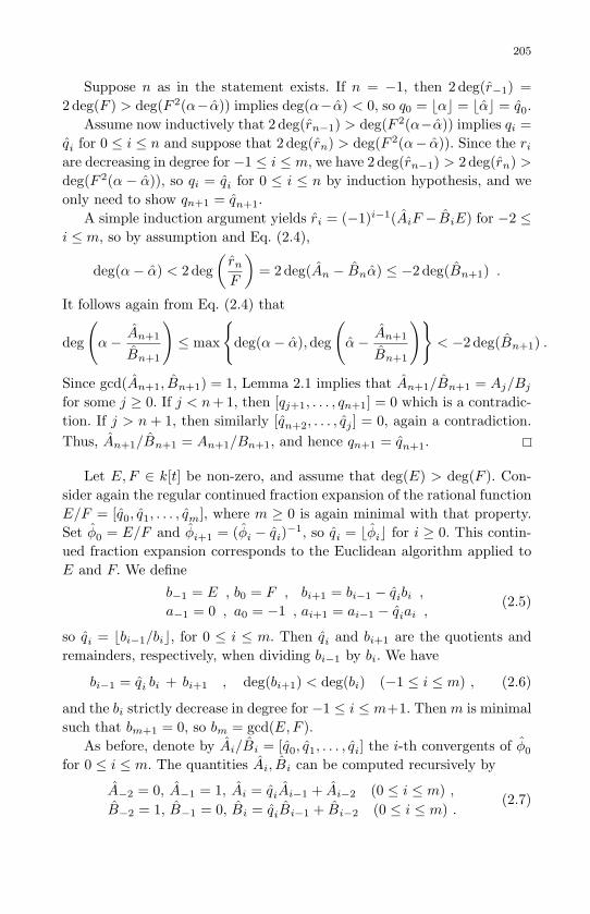
May 10, 2007 8:8 WSPC - Proceedings Trim Size: 9in x 6in ws-procs9x6
205
Suppose n as in the statement exists. If n = −1, then 2 deg(r−1) =2 deg(F ) > deg(F 2(α− α)) implies deg(α− α) < 0, so q0 = bαc = bαc = q0.
Assume now inductively that 2 deg(rn−1) > deg(F 2(α−α)) implies qi =qi for 0 ≤ i ≤ n and suppose that 2 deg(rn) > deg(F 2(α− α)). Since the riare decreasing in degree for −1 ≤ i ≤ m, we have 2 deg(rn−1) > 2 deg(rn) >deg(F 2(α − α)), so qi = qi for 0 ≤ i ≤ n by induction hypothesis, and weonly need to show qn+1 = qn+1.
A simple induction argument yields ri = (−1)i−1(AiF − BiE) for −2 ≤i ≤ m, so by assumption and Eq. (2.4),
deg(α− α) < 2 deg(rn
F
)= 2deg(An − Bnα) ≤ −2 deg(Bn+1) .
It follows again from Eq. (2.4) that
deg
(α− An+1
Bn+1
)≤ max
deg(α− α),deg
(α− An+1
Bn+1
)< −2 deg(Bn+1) .
Since gcd(An+1, Bn+1) = 1, Lemma 2.1 implies that An+1/Bn+1 = Aj/Bj
for some j ≥ 0. If j < n+ 1, then [qj+1, . . . , qn+1] = 0 which is a contradic-tion. If j > n + 1, then similarly [qn+2, . . . , qj ] = 0, again a contradiction.Thus, An+1/Bn+1 = An+1/Bn+1, and hence qn+1 = qn+1.
Let E,F ∈ k[t] be non-zero, and assume that deg(E) > deg(F ). Con-sider again the regular continued fraction expansion of the rational functionE/F = [q0, q1, . . . , qm], where m ≥ 0 is again minimal with that property.Set φ0 = E/F and φi+1 = (φi − qi)−1, so qi = bφic for i ≥ 0. This contin-ued fraction expansion corresponds to the Euclidean algorithm applied toE and F. We define
b−1 = E , b0 = F , bi+1 = bi−1 − qibi ,
a−1 = 0 , a0 = −1 , ai+1 = ai−1 − qiai ,(2.5)
so qi = bbi−1/bic, for 0 ≤ i ≤ m. Then qi and bi+1 are the quotients andremainders, respectively, when dividing bi−1 by bi. We have
bi−1 = qi bi + bi+1 , deg(bi+1) < deg(bi) (−1 ≤ i ≤ m) , (2.6)
and the bi strictly decrease in degree for −1 ≤ i ≤ m+1. Then m is minimalsuch that bm+1 = 0, so bm = gcd(E,F ).
As before, denote by Ai/Bi = [q0, q1, . . . , qi] the i-th convergents of φ0
for 0 ≤ i ≤ m. The quantities Ai, Bi can be computed recursively by
A−2 = 0, A−1 = 1, Ai = qiAi−1 + Ai−2 (0 ≤ i ≤ m) ,B−2 = 1, B−1 = 0, Bi = qiBi−1 + Bi−2 (0 ≤ i ≤ m) .
(2.7)

May 10, 2007 8:8 WSPC - Proceedings Trim Size: 9in x 6in ws-procs9x6
206
Then induction yields ai = (−1)i−1Ai−1 for −1 ≤ i ≤ m+ 1; in particular,we see that the ai increase in degree for −1 ≤ i ≤ m+ 1. We also obtain
b−1 = (−1)i(ai−1bi − aibi−1) (0 ≤ i ≤ m+ 1) . (2.8)
We require the following basic degree properties later on:
Lemma 2.2.
(a) deg(bi) = deg(bi−1)− deg(qi) ≤ deg(bi−1)− 1 (0 ≤ i ≤ m) .(b) deg(ai) = deg(ai−1) + deg(qi−1) ≥ deg(ai−1) + 1 (1 ≤ i ≤ m+ 1) .(c) deg(bi) ≤ deg(b−1)− i− 1 (−1 ≤ i ≤ m+ 1) .(d) deg(ai) ≥ i (0 ≤ i ≤ m+ 1) .(e) deg(ai) + deg(bi−1) = deg(b−1) (0 ≤ i ≤ m+ 1) .
Proof. Since deg(qi) ≥ 1 for 0 ≤ i ≤ m by Eq. (2.6), (a) and (b) followfrom Eq. (2.5). Parts (c) and (d) can then be obtained from (a) and (b),respectively, using induction. Finally, since deg(aibi−1) > deg(ai−1bi) by(a) and (b), (e) now follows from Eq. (2.8).
3. Hyperelliptic Curves
We employ an algebraic framework of hyperelliptic curves based on thetreatments of function fields given in [12], [17], and [4], as opposed to amore geometric treatment. Let k be a finite field of order q. Following [3],we define a hyperelliptic function field of genus g ∈ N to be a quadraticextension of genus g over the rational function field k(u), and a hyperellipticcurve of genus g over k to be a plane, smootha, absolutely irreducible, affinecurve C over k whose function field k(C) is hyperelliptic of genus g. Thecurve C and its function field are called imaginary, unusual, or real, if theplace at infinity of k(u) is ramified, inert, or split in k(C), respectively.Then C is of the form
C : v2 + h(u)v = f(u) , (3.1)
where f, h ∈ k[u], h = 0 if k has odd characteristic, h is monic if k has evencharacteristic, and every irreducible factor in k[u] of h is a simple factor of f ;in particular, f is squarefree if k has odd characteristic. Then the functionfield of C is k(C) = k(u, v) and its maximal order is the integral domaink[C] = k[u, v], the coordinate ring of C over k. The different signatures atinfinity can easily be distinguished as follows:
aA hyperelliptic curve does have singularities at infinity if it is not elliptic, i.e. g ≥ 2

May 10, 2007 8:8 WSPC - Proceedings Trim Size: 9in x 6in ws-procs9x6
207
(1) C is imaginary if deg(f) = 2g+1, and if deg(h) ≤ g if k has character-istic 2;
(2) C is unusual if the following holds: if k has odd characteristic, thendeg(f) = 2g + 2 and sgn(f) is a non-square in k, whereas if k hascharacteristic 2, then deg(h) = g + 1, deg(f) = 2g + 2 and the leadingcoefficient of f is not of the form e2 + e for any e ∈ k∗.
(3) C is real if the following holds: if k has odd characteristic, then deg(f) =2g + 2 and sgn(f) is a square in k, whereas if k has characteristic 2,then deg(h) = g + 1, and either deg(f) ≤ 2g + 1, or deg(f) = 2g + 2and the leading coefficient of f is of the form e2 + e for some e ∈ k∗.
In some literature sources, unusual curves are counted among the imaginaryones, as there is a unique place in k(C) lying above the place at infinity ofk(u) for both models. Note also that an unusual curve over k is real over aquadratic extension of k; whence the term “unusual”.
It is well-known that the places of k(u) are given by the monic irreduciblepolynomials in k[u] together with the place at infinity of k(u). Define S to bethe set of places of k(C) lying above the place at infinity of k(u), and writeS = ∞ if C is imaginary or unusual, and S = ∞1,∞2 if C is real. Thenthe places of k(C) are the prime ideals lying above the places of k(u) (thefinite places) together with the elements of S (the infinite places). To everyplace p of k(C) corresponds a normalized additive valuation νp on k(C)and a discrete valuation ring Op = α ∈ k(C) | νp(α) ≥ 0; for brevity, wewrite νi = ν∞i (i = 1, 2) if C is real. The degree deg(p) of a place p is thefield extension degree deg(p) = [Op/p : k]. Note that deg(∞) = 1 if C isimaginary, deg(∞) = 2 if C is unusual, and deg(∞1) = deg(∞2) = 1 if C isreal. The norm of a finite place p is the polynomial N(p) = Pdeg(p) ∈ k[u],where P is the unique place of k(u) lying below p.
For any place p of k(C), denote by k(C)p the completion of k(C) withrespect to p. Then it is easy to see that the completions k(C)S of k(C) withrespect to the places in S are, respectively,
k(C)S =
k(C)∞ = k〈u−1/2〉 if C is imaginary ,
k(C)∞ = k′〈u−1〉 if C is unusual ,k(C)∞1 = k(C)∞2 = k〈u−1〉 if C is real ,
where k′ = k(sgn(v)) is a quadratic extension of k. For C imaginary orunusual, the embedding of k(C) into k(C)S is unique, whereas for the realcase, we have two embeddings of k(C) into k〈u−1〉. Here, we number theindices so that ν1(v) ≤ ν2(v), and choose the embedding with deg(α) =−ν1(α) for all α ∈ k(C).

May 10, 2007 8:8 WSPC - Proceedings Trim Size: 9in x 6in ws-procs9x6
208
To unify our discussion over all hyperelliptic models, we henceforth in-terpret elements in k(C) as series in powers of u−1, where in the imaginarycase, the exponents of these powers are half integers. All degrees of functionfield elements are then taken with respect to u; more exactly, we set
deg(α) = degu(α) =
−ν∞(α)/2 if C is imaginary ,−ν∞(α) if C is unusual ,−ν1(α) = −ν2(α) if C is real ,
for α ∈ k(C). Here, if α = a + bv ∈ k(C) with a, b ∈ k(u), then α =a − b(v + h) is the conjugate of α. Note that for imaginary curves, deg(α)can be a half integer. The following properties are easily seen:
Lemma 3.1.
(a) If C is imaginary, then deg(v) = deg(v + h) = g + 1/2.(b) If C is unusual or real with deg(f) = 2g+2, then deg(v) = deg(v+h) =
g + 1.(c) If C is real and deg(f) ≤ 2g+ 1, then deg(v) = g+ 1 and deg(v+h) =
deg(f)− (g + 1) ≤ g.
A divisor b is a formal sum D =∑
p νp(D)p where p runs through allthe places of k(C) and νp(D) = 0 for all but finitely many places p. Thesupport supp(D) of D is the set of places for which νp(D) 6= 0, and thedegree of D is deg(D) =
∑p νp(D) deg(p); this agrees with the notion of
degree of a place. A divisor whose support is disjoint from S is a finitedivisor. Every divisor D of k(C) can be written uniquely as a sum of twodivisors
D = DS +DS where DS is finite and supp(D) ⊆ S .
The norm map extends naturally to all finite divisors DS via Z-linearity,and we can now define the norm of any divisor D to be N(D) = N(DS).
For two divisors D1 and D2 of k(C), we write D1 ≥ D2 if νp(D1) ≥νp(D2) for all places p of k(C). With this notation, we see that k[C] is theset of all α ∈ k(C) with div(α)S ≥ 0 and its unit group k[C]∗ consists ofexactly those α ∈ k(C) with div(α)S = 0.
bAn equivalent geometric definition of a divisor (defined over k) that is frequently used inthe literature on hyperelliptic curves is as follows: it is a formal sum D =
PP νP (D)P
that is invariant under the Galois action of k, where P runs through all the points
on C with coordinates in some algebraic closure of k. The degree of D is then simplyPP νP (D).
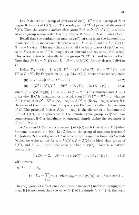
May 10, 2007 8:8 WSPC - Proceedings Trim Size: 9in x 6in ws-procs9x6
209
Let D denote the group of divisors of k(C), D0 the subgroup of D ofdegree 0 divisors of k(C), and P the subgroup of D0 of principal divisors ofk(C). Then the degree 0 divisor class group Pic0 = D0/P of k(C) is a finiteAbelian group whose order h is the (degree 0 divisor) class number of C.
Recall that the conjugation map on k(C), arising from the hyperellipticinvolution on C, maps each element α = a+ bv ∈ k(C) with a, b ∈ k(u) toα = a− b(v+h). This map thus acts on all the finite places of k(C) as wellas on S via ∞ =∞ if C is imaginary or unusual and ∞1 =∞2 if C is real.This action extends naturally to the groups D, D0, P, and hence to Pic0.
Note that N(D) = N(D) and D+D = div(N(D)) for any degree 0 divisorD.
Define DS = DS | D ∈ D, DS = DS | D ∈ D, PS = P ∩ DS , andPS = P∩DS . By Proposition 14.1, p. 243, of [12], there are exact sequences
(0)→ k∗ → k[C]∗ → PS → (0) , (3.2)
(0)→ (DS ∩D0)/PS → Pic0 → DS/PS → Z/fZ→ (0) , (3.3)
where f = gcddeg(p) | p ∈ S, so f = 2 if C is unusual and f = 1otherwise. If C is imaginary or unusual, then DS ∩D0 = PS = 0, whereasif C is real, then DS∩D0 = 〈∞1−∞2〉 and PS = 〈R(∞1−∞2)〉, where R isthe order of the divisor class of ∞1−∞2 in Pic0 and is called the regulatorof C. The principal divisor R(∞1 − ∞2) is the divisor of a fundamentalunit of k(C), i.e. a generator of the infinite cyclic group k[C]∗/k∗. Forcompleteness, if C is imaginary or unusual, simply define the regulator ofC to be R = 1.
A fractional k[C]-ideal is a subset f of k(C) such that df is a k[C]-idealfor some non-zero d ∈ k[u]. Let I denote the group of non-zero fractionalk[C]-ideals, H the subgroup of I of non-zero principal fractional k[C]-ideals(which we write as (α) for α ∈ k(C)∗), C = I/H the ideal class group ofk(C), and h′ = |C| the ideal class number of k(C). There is a naturalisomorphism
Φ : DS → I, DS 7→ α ∈ k(C)∗ | div(α)S ≥ DS (3.4)
with inverse
Φ−1 : I → DS
f 7→ DS =∑p 6∈S
mpp where mp = minνp(α) | α ∈ f non-zero .
The conjugate f of a fractional ideal f is the image of f under the conjugationmap. If f is non-zero, then the norm N(f) of f is simply N(Φ−1(f)), the norm

May 10, 2007 8:8 WSPC - Proceedings Trim Size: 9in x 6in ws-procs9x6
210
of the finite divisor corresponding to f under Φ−1, with Φ given by Eq. (3.4).Note that ff is the principal fractional ideal generated by N(f).
The isomorphism Φ extends to an isomorphism from the factor groupDS/PS onto the ideal class group C (see p. 401 of [4] and Theorem 14.5,p. 247, of [12]). Thus, we have h = Rh′/f by Eq. (3.3). The Hasse-Weilbounds (
√q − 1)2g ≤ h ≤ (
√q + 1)2g imply h ∼ qg, and for real curves, we
generally expect that h′ is small and hence R ≈ h. The isomorphism Φ inEq. (3.4) can further be extended to the group D0, or a subgroup thereof,as follows.
3.1. Imaginary Curves
Since deg(∞) = 1 in this case, every degree 0 divisor of k(C) can be writtenuniquely in the form D = DS − deg(DS)∞. Hence, every degree 0 divisorD is uniquely determined by DS , and the isomorphism in Eq. (3.4) extendsnaturally to an isomorphism D0 → I.
3.2. Unusual Curves
Here, deg(∞) = 2, so every degree 0 divisor D of k(C) can be writtenas D = DS − (deg(DS)/2)∞ and must have deg(DS) even. Again, everydegree 0 divisor D is uniquely determined by DS . Thus, Φ as given inEq. (3.4) extends to an isomorphism from D0 onto the group of fractionalideals whose norm have even degree.
3.3. Real Curves
If C is real, then deg(∞1) = deg(∞2) = 1, so every degree 0 divisor of k(C)can be uniquely written in the form
D = DS − deg(DS)∞2 + ν1(D)(∞1 −∞2) .
Hence, every degree 0 divisor D is uniquely determined by DS and ν1(D).Here, Φ extends to an isomorphism from the subgroup of D0 of degree 0divisors D with ν1(D) = 0 onto I.
We conclude this section with the observation that the choice of thetranscendental element u determines the signature at infinity (ramified,inert, or split) and hence the set S of places lying above infinity. So theideal class group C, its order h′, and the regulator R depend on the modelof C (imaginary, unusual, or real), whereas the genus g, the divisor groupsD, D0 and P, as well as the degree 0 divisor class group Pic0 and its orderh are model-independent.

May 10, 2007 8:8 WSPC - Proceedings Trim Size: 9in x 6in ws-procs9x6
211
4. Reduced Ideals and Divisors
Some of the material in this and the next section can be found in [2], [5],and [7]. As before, let C : v2 + h(u)v = f(u) be a hyperelliptic curveof genus g over a finite field k. The maximal order k[C] of k(C) is anintegral domain and a k[u]-module of rank 2 with k[u]-basis 1, v. Thenon-zero integral ideals in k[C] are exactly the k[u]-modules of the forma = k[u]SQ+k[u]S(P+v) where P,Q, S ∈ k[u] and Q divides f+hP−P 2.
Here, S and Q are unique up to factors in k∗ and P is unique moduloQ. For brevity, write a = S(Q,P ). An ideal a = S(Q,P ) is primitive ifS ∈ k∗, in which case we simply take S = 1 and write a = (Q,P ). Aprimitive ideal a is reduced if degQ ≤ g. The basis Q,P of a primitiveideal a = (Q,P ) is adapted if deg(P ) < deg(Q) and reduced if C is real anddeg(P−h−v) < deg(Q) < deg(P+v); the latter is only possible if C is real.In practice, it is common to have reduced divisors given in adapted form forimaginary and unusual curves and in reduced (or possibly adapted) formfor real curves.
A divisor D of k(C) is effective if D ≥ 0. An effective finite divisor DS
is semi-reduced c if there does not exist any subset U ⊆ supp(DS) suchthat
∑p∈U νp(DS)p is the divisor of a polynomial in k[u], and reduced if
in addition deg(DS) ≤ g. Under the isomorphism in Eq. (3.4), effectivefinite divisors of k(C) map to integral k[C]-ideals, semi-reduced divisorsto primitive ideals, and reduced divisors to reduced ideals. Analogous tothe ideal notation, we write DS = (Q,P ) for the semi-reduced divisor ofk(C) corresponding to the primitive k[C]-ideal a = (Q,P ) under Φ, andrefer to the polynomials Q and P as a basis of DS ; note that N(DS) =N(a) = sgn(Q)−1Q. It is easy to see that the conjugation map of k(C) actson semi-reduced and reduced divisors DS = (Q,P ) via DS = (Q,−P − h).
Up to now, we have only defined the notions of reduced and semi-reducedfor finite divisors. We simply extend this notion to arbitrary degree 0 divi-sors of k(C) by declaring a degree 0 divisor D to be (semi-)reduced if DS
is (semi-)reduced. We then say that a semi-reduced divisor D is in adaptedor reduced form if DS is given by an adapted or reduced basis, respectively.
We would like to represent degree 0 divisor classes via reduced divisors.In the imaginary case, this is well-known, but we repeat it briefly here forcompleteness; for the other two hyperelliptic curve models, it is less simple.In particular, for the unusual case, reduced divisors need not exist in some
cFor geometric and ideal-independent definitions of the notions of semi-reduced andreduced divisors, see for example [2] or [5].

May 10, 2007 8:8 WSPC - Proceedings Trim Size: 9in x 6in ws-procs9x6
212
divisor classes, so we will have to allow divisors D with deg(DS) = g + 1when representing elements in Pic0. For simplicity, we will say that a degree0 divisor D in a given class C ∈ Pic0 has minimal norm if D is semi-reducedand deg(N(E)) ≥ deg(N(D)) for every semi-reduced divisor E ∈ C.We willsee that if C is imaginary, unusual with g even, or real, then D will alwaysbe reduced, otherwise (C unusual and g odd), we have deg(N(D)) ≤ g+1.
4.1. Imaginary Curves
Here, it is well-known that reduced divisors are pairwise inequivalent (see[2]), and every degree 0 divisor class in Pic0, and hence every ideal class inC, has exactly one reduced representative.
4.2. Unusual Curves
Again, reduced degree 0 divisors are pairwise inequivalent, and every degree0 divisor class contains at most one reduced divisor. Those classes that donot contain any reduced divisor contain exactly q + 1 pairwise equivalentsemi-reduced divisors D with deg(DS) = g+1 (see p. 183 of [1]). Note thatthis can only occur if g is odd, so in this case, the norm of a reduced divisormust have degree ≤ g−1. Hence if g is even, then in complete analogy to theimaginary case, every divisor class does in fact have a unique representative.In order to represent divisor classes without reduced divisors, i.e. with q+1pairwise equivalent divisors of minimal norm of degree g + 1, for g odd, afast equivalence test or a systematic efficient way to identity a distinguisheddivisor of minimal norm in a given degree 0 divisor class are required.
4.3. Real Curves
By Proposition 4.1 of [10], every degree 0 divisor class of k(C) contains auniqued reduced divisor D such that 0 ≤ deg(DS) + ν1(D) ≤ g, or equiva-lently, −g ≤ ν2(D) ≤ 0. Using these reduced representatives for arithmeticin Pic0 is somewhat slower that for imaginary curves, so we concentrateinstead on reduced divisors D = DS − deg(DS)∞2 with ν1(D) = 0. By thePaulus-Ruck result cited above, these divisors are pairwise inequivalent,so every degree 0 divisor class of k(C) contains at most one such reduceddivisor.
dThe proposition as stated in [10] reads “0 ≤ ν1(D) ≤ g − deg(DS)”. The correctstatement is “0 ≤ deg(DS) + ν1(D) ≤ g”.

May 10, 2007 8:8 WSPC - Proceedings Trim Size: 9in x 6in ws-procs9x6
213
Rather than examining degree 0 divisor classes, we now consider idealclasses of k(C). Recall that the isomorphism Φ defined in Eq. (3.4) can beextend to an isomorphism from the set D ∈ D0 | ν1(D) = 0 onto I. Forany non-zero fractional ideal f, set D(f) = Φ−1(f) to be the divisor with nosupport at ∞1 corresponding to f; note that f is reduced if and only if D(f)is reduced. Let C be any ideal class of k(C), and define the set
RC = D(a) | a ∈ C reduced .
By our above remarks, all the divisors in RC are reduced and pairwiseinequivalent even though the corresponding ideals are all equivalent. Sincethe basis polynomials of a reduced divisor or ideal have bounded degree,RC is a finite set.
We now fix any reduced ideal a ∈ C; for example, if C is the principalideal class, then we always chose a = (1) to be the trivial ideal. Then forevery b ∈ C, there exists α ∈ k(C)∗ with b = (α)a; if a = (1), then α
is in fact a generator of b. By multiplying α with a suitable power of afundamental unit of k(C), or equivalently, adding a suitable multiple ofR(∞1 − ∞2) to its divisor, we may assume that −R < ν1(α) ≤ 0, orequivalently, 0 ≤ deg(α) < R. Then we define the distance of the divisorD(b) (with respect to D(a)) to be δ(D(b)) = deg(α). It follows that the setRC is ordered by distance, and if we set D1 = D(a) and rC = |RC|, thenwe can write
RC = D1, D2, . . . , DrC
and δi = δ(Di), with 0 = δ1 < δ2 < · · · < δrC < R. The set RC is calledthe infrastructure of C; we will motivate this term later on. Note that if Cis the principal class and b ∈ C, D(b) and D(b) both belong to RC, andδ(D(b)) = R+ deg(D(b)S)− δ(D(b)) if b is nontrivial.
5. Reduction and Baby Steps
We continue to assume that we have a hyperelliptic curve C given byEq. (3.1). Our goal is to develop a unified framework for reduction on allhyperelliptic curves. We begin with the standard approach for reduction onimaginary curves — which we however apply to any hyperelliptic curve —and then link this technique to the traditional continued fractions methodfor real curves.
Starting with polynomials R0, S0 such that deg(R0) < deg(S0) and S0
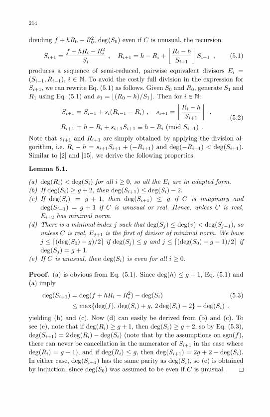
May 10, 2007 8:8 WSPC - Proceedings Trim Size: 9in x 6in ws-procs9x6
214
dividing f + hR0 −R20, deg(S0) even if C is unusual, the recursion
Si+1 =f + hRi −R2
i
Si, Ri+1 = h−Ri +
⌊Ri − hSi+1
⌋Si+1 , (5.1)
produces a sequence of semi-reduced, pairwise equivalent divisors Ei =(Si−1, Ri−1), i ∈ N. To avoid the costly full division in the expression forSi+1, we can rewrite Eq. (5.1) as follows. Given S0 and R0, generate S1 andR1 using Eq. (5.1) and s1 = b(R0 − h)/S1c. Then for i ∈ N:
Si+1 = Si−1 + si(Ri−1 −Ri) , si+1 =⌊Ri − hSi+1
⌋,
Ri+1 = h−Ri + si+1Si+1 ≡ h−Ri (mod Si+1) .(5.2)
Note that si+1 and Ri+1 are simply obtained by applying the division al-gorithm, i.e. Ri − h = si+1Si+1 + (−Ri+1) and deg(−Ri+1) < deg(Si+1).Similar to [2] and [15], we derive the following properties.
Lemma 5.1.
(a) deg(Ri) < deg(Si) for all i ≥ 0, so all the Ei are in adapted form.(b) If deg(Si) ≥ g + 2, then deg(Si+1) ≤ deg(Si)− 2.(c) If deg(Si) = g + 1, then deg(Si+1) ≤ g if C is imaginary and
deg(Si+1) = g + 1 if C is unusual or real. Hence, unless C is real,Ei+2 has minimal norm.
(d) There is a minimal index j such that deg(Sj) ≤ deg(v) < deg(Sj−1), sounless C is real, Ej+1 is the first of divisor of minimal norm. We havej ≤ d(deg(S0)− g)/2e if deg(Sj) ≤ g and j ≤ d(deg(S0)− g − 1)/2e ifdeg(Sj) = g + 1.
(e) If C is unusual, then deg(Si) is even for all i ≥ 0.
Proof. (a) is obvious from Eq. (5.1). Since deg(h) ≤ g + 1, Eq. (5.1) and(a) imply
deg(Si+1) = deg(f + hRi −R2i )− deg(Si) (5.3)
≤ maxdeg(f), deg(Si) + g, 2 deg(Si)− 2 − deg(Si) ,
yielding (b) and (c). Now (d) can easily be derived from (b) and (c). Tosee (e), note that if deg(Ri) ≥ g+ 1, then deg(Si) ≥ g+ 2, so by Eq. (5.3),deg(Si+1) = 2 deg(Ri)− deg(Si) (note that by the assumptions on sgn(f),there can never be cancellation in the numerator of Si+1 in the case wheredeg(Ri) = g + 1), and if deg(Ri) ≤ g, then deg(Si+1) = 2g + 2 − deg(Si).In either case, deg(Si+1) has the same parity as deg(Si), so (e) is obtainedby induction, since deg(S0) was assumed to be even if C is unusual.

May 10, 2007 8:8 WSPC - Proceedings Trim Size: 9in x 6in ws-procs9x6
215
Suppose deg(Sj) ≤ deg(v) < deg(Sj−1) as in part (d) of Lemma 5.1. IfC is imaginary, or C is unusual with deg(Sj) ≤ g, then Ej+1 is the uniquereduced divisor in the class of D1. If C is unusual and deg(Sj) = g + 1,(g odd), then the other q semi-reduced divisors equivalent to Ej+1 whosenorm have degree g + 1 can be obtained from Ej+1 as follows (see also [1]for the case where q is odd).
Proposition 5.1. Let C given by Eq. (3.1) be unusual of odd genus g andE = (S,R) a semi-reduced divisor with deg(R) ≤ deg(S) = g+ 1. Then theq + 1 divisors in the divisor class of E whose norm have degree g + 1 aregiven by E and Ea = (Sa, Ra) for a ∈ Fq where
Ra = h−R+ aS, Sa =f + hRa −R2
a
S. (5.4)
Proof. Since Ea = E+div((Ra+v)/S) for all a ∈ Fq, all Ea are equivalentto E. Furthermore, deg(Ra) ≤ g + 1 and hence deg(Sa) = g + 1, since theconditions on sgn(f) prevent cancellation of leading terms in the numeratorof Sa. So it only remains to show that E and and all the Ea are pairwisedistinct. To that end, we prove that equality among any two of these q+ 1divisors leads to a sequence of divisibility conditions that yield a singularpoint on C.
So fix a ∈ Fq and suppose that Ea = E or Ea = Eb for some b ∈ Fq\a.We first claim that
Sa and S differ by a constant factor in Fq . (5.5)
This is clear if Ea = E, so suppose Ea = Eb with b ∈ Fq, b 6= a. Then Sa
and Sb differ by a constant factor, and Ra ≡ Rb (mod Sa). By Eq. (5.4),Ra ≡ Rb (mod S), so since deg(Ra − Rb) = deg(Sa) = deg(S) = g + 1, wesee that Sa and S must also differ by a constant factor in Fq.
Next, we claim that
S divides 2R− h . (5.6)
If Ea = E, then R ≡ Ra (mod S). On the other hand, Ra ≡ h−R (mod S)by Eq. (5.4), so R ≡ h− R (mod S), proving Eq. (5.6). Suppose now thatEa = Eb for some b ∈ Fq distinct from a. Then Sa and Sb differ by aconstant factor, so by Eq. (5.5), both differ from S by a constant factor.Now a simple calculation yields Sa−Sb = (a− b)(2R−h− (a+ b)S). Sincea 6= b and S divides the left hand side of this equality, S must again divide2R− h.

May 10, 2007 8:8 WSPC - Proceedings Trim Size: 9in x 6in ws-procs9x6
216
Our next assertion is that
S2 divides f + hR−R2 . (5.7)
By Eq. (5.4) and Eq. (5.6), Ra ≡ h−R ≡ R (mod S). Since deg(Ra−R) ≤g + 1 = deg(S), there exists ca ∈ Fq with Ra = R + caS. Substituting intoEq. (5.4) yields SSa = f + hR − R2 + caS(h − 2R − caS). By Eq. (5.5),S2 divides the left hand side of this equality. Invoking Eq. (5.6), we obtainEq. (5.7).
Our fourth and final claim is that
S divides f ′ + hR′ , (5.8)
where f ′ denotes the derivative of f with respect to u; similarly for R′.To prove this claim, we simply observe that taking derivatives in Eq. (5.7)implies that S divides f ′ + h′R+ hR′ − 2RR′ = f ′ + hR′ +R′(h− 2R), soEq. (5.8) now follows from Eq. (5.6).
Now let r be a root of S in some algebraic closure of k. Then Eq. (5.6)–Eq. (5.8) easily imply that (r,−R(r)) is a singular point on C, a contra-diction. So no two among the divisors E and Ea (a ∈ Fq) can be be equal,proving the proposition.
We now relate Eq. (5.1) to a regular continued fraction expansion, whichis the usual approach to reduction on real curves. Let P,Q ∈ k[u] with Q
non-zero and Q dividing f + hP − P 2, and let s0, s1, . . . be a sequence ofpolynomials in k[u]. Set P0 = P, Q0 = Q, and
Pi+1 = h− Pi + siQi, Qi+1 =f + hPi+1 − P 2
i+1
Qi, (5.9)
for i ≥ 0. If we set φi = (Pi + v)/Qi, then φi+1 = (φi − si)−1, soφ0 = [s0, s1, . . . , si, φi+1] for all i ≥ 0. Thus, Eq. (5.9) determines a con-tinued fraction expansion of φ0 in the completion k(C)S . It is clear thatEq. (5.9) defines a sequenceDi = (Qi−1, Pi−1) of semi-reduced divisors withcorresponding primitive ideals ai. The operation Di → Di+1 is referred toas a baby or reduction stepe.
Set θ1 = 1 and θi =∏i−1
j=1 φ−1j for i ≥ 2. Since φiφi = −Qi−1/Qi, it is
easy to see that Q0θiθi = (−1)i−1Qi−1. Thus
θi =i−1∏j=1
φ−1
j = (−1)i−1Qi−1
Q0θi= (−1)i−1Qi−1
Q0
i−1∏j=1
φj . (5.10)
eNote that Eq. (5.4) is a special case of Eq. (5.9), with si = a ∈ Fq . However, in thiscase, the recursion only alternates between E and Ea.

May 10, 2007 8:8 WSPC - Proceedings Trim Size: 9in x 6in ws-procs9x6
217
Then ai+1 = (φ−1
i )ai and hence ai = (θi)a1, for i ∈ N. Therefore, the idealsai are all equivalent, so baby steps preserve ideal equivalence.
If we choose si in Eq. (5.9) to be si = qi = bφic, i.e. the quotient inthe regular continued fraction expansion of φ0 in k(C)S , then we have thebaby steps
qi =⌊Pi + v
Qi
⌋, Pi+1 = h−Pi + qiQi, Qi+1 =
f + hPi+1 − P 2i+1
Qi. (5.11)
If deg(Qi) > deg(v), then qi = bPi/Qic. It is now easy to deduce that if jis as in part (d) of Lemma 5.1 and Si, Ri are defined as in Eq. (5.1), then
qi = bPi/Qic ∈ k[u], Pi+1 = h−Ri, Qi+1 = Si+1 , (5.12)
for 0 ≤ i < j. Therefore, for this range of indices, Eq. (5.11) is equivalent toEq. (5.1) and hence produces the same sequence of divisors. For imaginaryand unusual curves, we will only consider baby steps as in Eq. (5.11) in therange 0 ≤ i < j. For C real, baby steps as in Eq. (5.11) can be performedbeyond that range as well. However, for i ≥ j, qj 6= bPj/Qjc, so Eq. (5.12)is false. Here, if we use Eq. (5.11) to compute the sequence Di+1 = (Qi, Pi),starting with i = j, then Di+1 is reduced for i > j. We have deg(Pj+1 −h− v) ≤ g, deg(Pj+1 + v) = g + 1, and for i ≥ j + 2, Di+1 = (Qi, Pi) is inreduced form.
We now see that for all hyperelliptic curves, there exists an index l ≥0 such that Eq. (5.11) repeatedly applied to D1 = (Q0, P0) produces areduced divisor Dl+1, if one exists, after l ≤ d(deg(Q0) − g)/2e steps. IfC is unusual, g is odd, and the class of D1 contains no reduced divisor,then Eq. (5.11) produces a divisor Dl+1 whose norm has degree g+ 1 afterl ≤ d(deg(Q0)−g−1)/2e steps. In the imaginary and unusual scenarios, wehave l = j with j as in part (d) of Lemma 5.1; for C real, we have l = j+1.For 0 ≤ i < l, Eq. (5.11) is equivalent to
qi =⌊Pi + eiv
Qi
⌋, ei =
1 if C real, deg(Qi) = g + 1,0 otherwise,
Pi+1 = h− Pi + qiQi, Qi+1 =f + hPi+1 − P 2
i+1
Qi.
(5.13)
Again, the recursion in Eq. (5.13) can be made more efficient for i ≥ 1, i.e.for all but the first baby step. Given Q0 and P0, we compute Q1 and P1
using Eq. (5.13). Then for i ∈ N:
qi =⌊Pi + beivc
Qi
⌋, ri ≡ Pi + beivc (mod Qi) ,
Pi+1 = h+ beivc − ri , Qi+1 = Qi−1 + qi(ri − ri−1) .(5.14)

May 10, 2007 8:8 WSPC - Proceedings Trim Size: 9in x 6in ws-procs9x6
218
As before, the first line in Eq. (5.14) is equivalent to applying the divisionalgorithm in order to compute polynomials qi and ri such that Pi +beivc =qiQi + ri and deg(ri) < deg(Qi).
Suppose now that C is real. If we repeatedly apply Eq. (5.11), orequivalently, Eq. (5.14), starting with a reduced divisor D1 = D(a) forsome reduced ideal a of k(C), then we can generate the entire infrastruc-ture RC = Di | 1 ≤ i ≤ rC of the ideal class C containing a. Here,Di = D(ai) where ai = (θi)a with θi as in Eq. (5.10), so the distance of Di
is δi = deg(θi). In particular, θrC is a fundamental unit of k(C) of positivedegree, and deg(θrC) = R is the regulator of k(C).
We conclude this section by showing how to compute the distancesδi = δ(Di). By Eq. (5.10), the distance satisfies
δi = deg(θi) = deg(Qi−1)− deg(Q0) +i−1∑j=1
deg(qj) (5.15)
for i ∈ N. Since φi = (Pi − h − v)/Qi = −Qi−1/(Pi + v) and δi+1 − δi =−deg(φi) = deg(Pi + v) − deg(Qi−1) = g + 1 − deg(Qi−1) by Eq. (5.10),we have 1 ≤ δi+1 − δi ≤ g if Di is non-zero, and δi+1 = g + 1 if Di = 0, inwhich case C is the principal class.
6. Giant Steps and the Idea of NUCOMP
As before, let C be given by Eq. (3.1), and let D′ = (Q′, P ′), D′′ = (Q′′, P ′′)be two semi-reduced divisors of k(C). Then it is well-known that there existsa semi-reduced divisor D = (Q,P ) in the divisor class of the sum D′ +D′′
that can be computed as follows.
S = gcd(Q′, Q′′, P ′ + P ′′ − h) = V Q′ +WQ′′ +X(P ′ + P ′′ − h) ,
Q =Q′Q′′
S2, (6.1)
P = P ′′ + UQ′′
Swith U ≡W (P ′ − P ′′) +XR′′ (mod Q′/S) ,
where U, V,W,X ∈ k[u], deg(U) < deg(Q′/S), and R′′ = (f + hP ′′ −P ′′
2)/Q′′. Note that D is in adapted form if deg(P ′′) < deg(Q).Since S tends to have very small degree (usually S = 1), we expect
degQ ≈ degQ′ + degQ′′; in particular, even if D′ and D′′ have minimalnorm, thenD will generally not have minimal norm. We now apply repeatedbaby steps as in Eq. (5.14) to P0 = P and Q0 = Q until we obtain a divisorof minimal norm. The first divisor thus obtained is defined to be D′⊕D′′.
The operation (D′, D′′)→ D′⊕D′′ is called a giant step.

May 10, 2007 8:8 WSPC - Proceedings Trim Size: 9in x 6in ws-procs9x6
219
6.1. Imaginary Curves
Here, D′⊕D′′ is the unique reduced divisor in the class of D′ + D′′, andthe algorithm above is Cantor’s algorithm [2]. Thus, the group operationon Pic0 can be performed efficiently via reduced representatives.
6.2. Unusual Curves
In this case, if g is even, then everything is completely analogous to theimaginary setting. However, if g is odd, then D′⊕D′′ may or may notbe reduced, so the set of reduced divisors is no longer closed under theoperation ⊕ . However, as mentioned earlier, if we could either performfast equivalence testing, or efficiently and systematically identify a distin-guished divisor D with deg(DS) = g+1 in every divisor class that containsno reduced divisor, then we could perform arithmetic in Pic0 via thesedistinguished representatives plus reduced representatives if they exist.
6.3. Real Curves
Suppose D′ and D′′ are reduced, and D′ ∈ RC′ , D′′ ∈ RC′′ for suitable
ideal classes C′,C′′ of k(C). Then D′⊕D′′ ∈ RC′C′′ . In particular, if C′′
is the principal ideal class, then D′⊕D′′ ∈ RC′ , and we have
δ(D′⊕D′′) = δ(D′) + δ(D′′)− δ with 0 ≤ δ ≤ 2g . (6.2)
Here, distances in the principal class are taken with respect to D1 = 0, anddistances in C′ with respect to some some suitable first divisor. The “errorterm” δ in Eq. (6.2) is linear in g and hence very small compared to the twodistances δ(D′) and δ(D′′). The quantity δ in Eq. (6.2) can be efficientlycomputed as part of the giant step.
Suppose now that D′ = (Q′, P ′) and D′′ = (Q′′, P ′′) are two divisors ofminimal norm. A giant step as described above finds the divisor D′⊕D′′
in two steps. First set D1 = (Q,P ) with P and Q given by Eq. (6.1); Qand P have degree approximately 2g, i.e. double size. Then apply repeatedbaby steps as in Eq. (5.14) to D1 until the first divisor Dl+1 = D′⊕D′′ ofminimal norm is obtained; by Lemma 5.1, we have l ≤ dg/2e for all threecurve models, so this takes at most dg/2e such steps. The reduction processproduces a sequence of semi-reduced divisors Di+1 = (Qi, Pi), 0 ≤ i ≤ l, viathe continued fraction expansion of φ = (P +v)/Q = [q0, q1, . . . , ql, φl+1]. Itslowly shrinks the degrees of the Qi and Pi again to original size, reducingthem by about 2 in each step by Lemma 5.1. The obvious disadvantage

May 10, 2007 8:8 WSPC - Proceedings Trim Size: 9in x 6in ws-procs9x6
220
of this method is that the polynomials Qi, Pi have large degree while i issmall, and are costly to compute.
NUCOMP is an algorithm for computing D′⊕D′′ that eliminates thesecostly baby steps on large operands. The idea of NUCOMP is to performarithmetic on polynomials of much smaller degree. Instead of computing Qas well as the Qi and Pi explicitly via the continued fraction expansion ofφ, one computes sequences of polynomials ai, bi, ci, and di such that
Qi = (−1)i(bi−1ci−1 − ai−1di−1)
Pi = (−1)i(bi−2ci−1 − ai−1di−2) + P ′′ .
Only two basis coefficients Qn+2 and Pn+2 are evaluated at the end in orderto obtain a divisor Dn+3. Here, the value of n is determined by the propertythat an, bn, cn, and dn have approximately equal degree of about g/2. Moreexactly, we will have l = n+ 2 or n+ 3, i.e. D′⊕D′′ = Dn+3 or Dn+4.
The key observation is that φ = U/(Q′/S), with U as given in Eq. (6.1),is a very good rational approximation of φ = (P+v)/Q, and that the contin-ued fraction expansion of φ
−1is given by Q′/(SU) = [q1, q2, . . . , qn+1, . . .].
Note that deg(U) < deg(Q′/S) ≤ g (or possibly g+ 1), so all quantities in-volved are of small degree. The polynomials ai, bi, ci, and di are computedrecursively along with the continued fraction expansion of Q′/(SU) whichis basically the extended Euclidean algorithm applied to Q′/S and U ; infact, the bi are the remainders obtained in this Euclidean division process.Alternatively, only the ai and bi are computed recursively, and cn−1, dn−1,
and dn are then obtained from these two sequences; this approach turnsout to employ polynomials of smaller degree (as c0 and d0 have large de-gree), but requires an extra full division by Q′/S. We describe the detailsof NUCOMP in the next two sections.
7. NUCOMP
Let D′ = (Q′, P ′) and D′′ = (Q′′, P ′′) be two divisors of minimal norm,and let P,Q, S, U be defined as in Eq. (6.1). We assume that
deg(P ′′) ≤ g + 1 < deg(Q) . (7.1)
The first inequality in Eq. (7.1) is equivalent to deg(P ′′ + v) ≤ g + 1,and holds if D′′ is given in adapted or reduced form. While it can alwaysbe achieved by reducing P modulo Q, for example, we will see that thiswill generally not be necessary, i.e. usually NUCOMP outputs a divisor
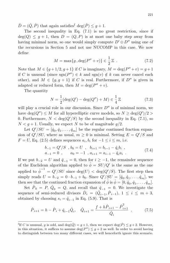
May 10, 2007 8:8 WSPC - Proceedings Trim Size: 9in x 6in ws-procs9x6
221
D = (Q, P ) that again satisfiesf deg(P ) ≤ g + 1.The second inequality in Eq. (7.1) is no great restriction, since if
deg(Q) ≤ g + 1, then D = (Q,P ) is at most one baby step away fromhaving minimal norm, so one would simply compute D′⊕D′′ using one ofthe recursions in Section 5 and not use NUCOMP in this case. We nowdefine
M = maxg ,deg(P ′′ + v) ∈ 12
Z . (7.2)
Note that M ∈ g+1/2, g+1 if C is imaginary, M = deg(P ′′+ v) = g+1if C is unusual (since sgn(P ′′) ∈ k and sgn(v) /∈ k can never cancel eachother), and M ∈ g, g + 1 if C is real. Furthermore, if D′′ is given inadapted or reduced form, then M = deg(P ′′ + v).
The quantity
N =12(deg(Q′)− deg(Q′′) +M) ∈ 1
4Z (7.3)
will play a crucial role in our discussion. Since D′′ is of minimal norm, wehave deg(Q′′) ≤M for all hyperelliptic curve models, so N ≥ deg(Q′)/2 >0. Furthermore, N < deg(Q′/S) by the second inequality in Eq. (7.1), soN < g + 1. Usually, we expect N to be of magnitude g/2.
Let Q′/SU = [q0, q1, . . . , qm] be the regular continued fraction expan-sion of Q′/SU, where as usual, m ≥ 0 is minimal. Setting E = Q′/S andF = U, Eq. (2.5) defines sequences ai, bi for −1 ≤ i ≤ m, i.e.
b−1 = Q′/S , b0 = U , bi+1 = bi−1 − qibi ,
a−1 = 0 , a0 = −1 , ai+1 = ai−1 − qiai .(7.4)
If we put b−2 = U and q−1 = 0, then for i ≥ −1, the remainder sequenceof the Euclidean algorithm applied to φ = SU/Q′ is the same as the oneapplied to φ
−1= Q′/SU since deg(U) < deg(Q′/S). The first step then
simply reads U = b−2 = 0 · b−1 + b0. Since Q′/SU = [q0, q1, . . . , qm], wethen see that the continued fraction expansion of φ is φ = [0, q0, q1, . . . , qm].
Set P 0 = P, Q0 = Q, and recall that q−1 = 0. We investigate thesequence of semi-reduced divisors Di = (Qi−1, P i−1), 1 ≤ i ≤ m + 3,obtained by choosing si = qi−1 in Eq. (5.9). That is
P i+1 = h− P i + qi−1Qi, Qi+1 =f + hP i+1 − P
2
i+1
Qi
, (7.5)
fIf C is unusual, g is odd, and deg(Q) = g +1, then we expect deg(P ) ≤ g +2. However,in this situation, it suffices to assume deg(P ′′) ≤ g + 2 as well. In order to avoid having
to distinguish between too many different cases, we will henceforth ignore this scenario.

May 10, 2007 8:8 WSPC - Proceedings Trim Size: 9in x 6in ws-procs9x6
222
for 0 ≤ i ≤ m+1. To facilitate the computation of P i, Qi, we proceed as in[8] and introduce two more sequences of polynomials ci, di, −1 ≤ i ≤ m+1as follows.
c−1 =Q′′
S, c0 =
P − P ′
b−1, ci+1 = ci−1 − qici,
d−1 = P ′ + P ′′ − h, d0 =d−1b0 − SR′′
b−1, di+1 = di−1 − qidi,
(7.6)
for 0 ≤ i ≤ m.We point out an interesting symmetry between the sequencesbi and ci, −1 ≤ i ≤ m + 1; namely, reversing the roles of D′ and D′′ inEq. (6.1) results in a swap of these two sequences. An easy induction yields
ci =1b−1
(biQ′′
S+ ai(P ′ − P ′′)
), (7.7)
di =1b−1
(bi(P ′ + P ′′ − h) + aiSR′′) , (7.8)
for −1 ≤ i ≤ m+ 1. Using induction simultaneously on both formulas, weobtain
Qi = (−1)i(bi−1ci−1 − ai−1di−1) , (7.9)
P i = (−1)i(bi−2ci−1 − ai−1di−2) + P ′′ , (7.10)
for 0 ≤ i ≤ m+ 2.As outlined above, we wish to determine a point up to which the divisors
Di+1 = (Qi, Pi) with P0 = P , Q0 = Q, and Pi, Qi given by Eq. (5.13)or equivalently, by Eq. (5.11) or Eq. (5.14) are identical to the divisorsDi+1 = (Qi, P i) with P i, Qi given by Eq. (7.5) or equivalently, by Eq. (7.9)and Eq. (7.10). Clearly, D1 = D1 by definition, so our goal is to find amaximal index n ≥ −1 that guarantees Qi = Qi and Pi = P i, and henceDi+1 = Di+1, for 0 ≤ i ≤ n+ 2 (see Theorem 7.1). Such an index will haveto satisfy n ≤ m to ensure that the polynomials Qi, P i as given in Eq. (7.5)are in fact defined. Our next task will then be to see how many baby stepsif any we need to apply to the last divisor Dn+3 = (Qn+2, Pn+2) to obtainthe divisor D′⊕D′′.
Theorem 7.1. Let D′ = (Q′, P ′), D′′ = (Q′′, P ′′) be two divisors, and letP and Q be given by Eq. (6.1). Set P0 = P 0 = P, Q0 = Q0 = Q, and definePi, Qi (i ∈ N) by Eq. (5.11), P i, Qi (1 ≤ i ≤ m + 2) by Eq. (7.5), and bi(−1 ≤ i ≤ m+1) by Eq. (7.4). Then there exists n ∈ Z, −1 ≤ n ≤ m, such

May 10, 2007 8:8 WSPC - Proceedings Trim Size: 9in x 6in ws-procs9x6
223
that deg(bn) > N, with N as in Eq. (7.3). Furthermore,
qi = qi−1 (0 ≤ i ≤ n+ 1) ,
Pi = P i (0 ≤ i ≤ n+ 2) ,
Qi = Qi (0 ≤ i ≤ n+ 2) .
Proof. We already observed that deg(b−1) = deg(Q′/S) > N, so sincedeg(bi) decreases as i increases, there must exist n ≥ −1 with deg(bn) > N.
Since deg(bm+1) = −∞ < N, we must have n ≤ m. So n as specified aboveexists and all the quantities qi−1, P i, Qi above are in fact well-defined.
Set φ = (P + v)/Q and φ = SU/Q′. Then φ = [q0, q1, . . .] with qi =(Pi + v)/Qi is the continued fraction expansion of φ in a suitable field ofPuiseux series; also, recall that φ = [q−1, q0, . . . , qm] where q−1 = 0. Wewish to applyg Theorem 2.1 to φ and φ. Since φ − φ = (P ′′ + v)/Q, wehave b2−1(φ − φ) = Q′(P ′′ + v)/Q′′. The definition of N implies 2N ≥deg(Q′(P ′′ + v)/Q′′), so
2 deg(bn) > 2N ≥ deg(b2−1(φ− φ)
). (7.11)
Seth r−2 = U, r−1 = Q′/S, and ri = ri−2−qi−1ri−1 for 0 ≤ i ≤ m+1. Thenri = bi for −1 ≤ i ≤ m+1, so the ri are the remainders when applying theEuclidean algorithm to E = U and F = Q′/S. By Theorem 2.1, Eq. (7.11)implies that qi = qi−1 for 0 ≤ i ≤ n + 1. Now P0 = P 0, Q0 = Q0, andinductively by Eq. (5.11) and Eq. (7.5),
Pi+1 = h− Pi + qiQi = h− P i + qi−1Qi = P i+1 ,
Qi+1 =f + hPi+1 − P 2
i+1
Qi=f + hP i+1 − P
2
i+1
Qi
= Qi+1 ,
for 0 ≤ i ≤ n+ 1.
Corollary 7.1. With the notation of Theorem 7.1, we have Di = Di for1 ≤ i ≤ n+ 3.
gAlthough the degrees in Theorem 2.1 are taken with respect to u1/2 if C is imaginary,
the statement still holds if degrees are taken with respect to u as is done here, since this
only changes both sides of the degree inequality in Theorem 2.1 by a factor of 2.hNote that the indices of the partial quotients qi in the definition of the ri are offset
by 1 compared to the proof of Theorem 2.1 because here, the continued fraction in
question is φ = [q−1, q0, q1, . . . , qm] (with q−1 = 0), whereas in Theorem 2.1, it is
φ = [q0, q1, . . . , qm].

May 10, 2007 8:8 WSPC - Proceedings Trim Size: 9in x 6in ws-procs9x6
224
Since deg(bi) is a decreasing sequence for −1 ≤ i ≤ m+ 1, there existsa unique index n with −1 ≤ n ≤ m such that
deg(bn) > N ≥ deg(bn+1) , (7.12)
with N as in Eq. (7.3). By Corollary 7.1, Di = Di for 1 ≤ i ≤ n+ 3.
8. Giant Steps with NUCOMP
We now show that Dn+3 is at most one baby step away from being reducedif C is imaginary or real, and always has minimal norm if C is unusual.Furthermore, Dn+2 never has minimal norm. Note that this implies that ifDn+3 actually has minimal norm, then Dn+3 = D′⊕D′′.
Substituting Eq. (7.7) and Eq. (7.8) into Eq. (7.9) yields
Qi =(−1)i
b−1
(Q′′
Sb2i−1 + (h− 2P ′′)ai−1bi−1 − SR′′a2
i−1
)(8.1)
for 0 ≤ i ≤ m+2. For brevity, we define sequences of rational functions ui,
vi, wi via
ui =Q′′
b−1Sb2i , vi =
h− 2P ′′
b−1aibi , wi =
SR′′
b−1a2
i , (8.2)
for −1 ≤ i ≤ m+ 1, where as before, R′′ = (f + hP ′′ − P ′′2)/Q′′. Then
(−1)i+1Qi+1 = ui + vi + wi (1 ≤ i ≤ m+ 1) . (8.3)
Note that ui decreases and wi increases in degree as i increases. Further-more, ui, vi, wi satisfy the following properties:
Lemma 8.1. Let N and n be given by Eq. (7.3) and Eq. (7.12), respec-tively, and define
L = deg(Q′′R′′) = deg(f + hP ′′ − P ′′2)= deg(P ′′ + v) + deg(P ′′ − h− v) .
(8.4)
Then we have the following:
(a) deg(vi) ≤ g for −1 ≤ i ≤ m+ 1.(b) deg(wi) = L− deg(ui−1) for 0 ≤ i ≤ m+ 1.(c) deg(un+1) ≤M < deg(ui) for −1 ≤ i ≤ n.(d) deg(wi) ≤ deg(P ′′ − h− v)− 1 ≤ g for −1 ≤ i ≤ n+ 1.

May 10, 2007 8:8 WSPC - Proceedings Trim Size: 9in x 6in ws-procs9x6
225
Proof. Since deg(h − 2P ′′) ≤ g + 1, (a) can be derived using Lemma 2.2(e) and (b), since
deg(vi) = deg(ai) + deg(bi) + deg(h− 2P ′′)− deg(b−1)
= deg(ai)− deg(ai+1) + deg(h− 2P ′′) ≤ −1 + (g + 1) = g
for 0 ≤ i ≤ m+ 1. The definition of ui−1 as well as Eq. (8.4) and part (e)of Lemma 2.2 imply
deg(wi) = 2 deg(ai) + deg(S) + deg(R′′)− deg(b−1)
= deg(b−1)− 2 deg(bi−1) + deg(S) + L− deg(Q′′)
= L− deg(ui−1)
for 0 ≤ i ≤ m+ 1, whence follows (b). For (c), we note that
deg(ui) = 2 deg(bi) + deg(Q′′/S)− deg(b−1)
= deg(Q′′/Q′) + 2 deg(bi)
= M − 2N + 2 deg(bi)
for −1 ≤ i ≤ m+1. We then see from Eq. (7.2) and Eq. (7.3) that deg(ui) ≤M if and only if deg(bi) ≤ N. Part (c) now follows from Eq. (7.12). For(d), we note that deg(w−1) = −∞, and for 0 ≤ i ≤ n + 1, by Eq. (8.4),Eq. (7.2), and parts (b) and (c),
deg(wi) = L− deg(ui−1) < L−M≤ L− deg(P ′′ + v) = deg(P ′′ − h− v) .
Corollary 8.1. Let N and n be given by Eq. (7.3) and Eq. (7.12), respec-tively. Then the following holds.
(a) deg(Qi+1) = deg(ui) ≥ g + 2 for −1 ≤ i ≤ n.(b) deg(Qn+2) ≤M + 1 ≤ g + 1.(c) deg(Qn+2) ≤ g if and only if deg(bn+1) < N or M < g + 1.
Proof. Parts (a) and (b) immediately follow from Eq. (8.3) as well asparts (a), (c), and (d) of Lemma 8.1. For part (c) of the Corollary, notethat deg(un+1) = M − 2(N − deg(bn+1)), so deg(Qn+2) = g+ 1 if and onlyif deg(un+1) = g+ 1, which in turn holds if and only if deg(bn+1) = N andM = g + 1.
We now determine how to obtain the divisor D′⊕D′′ using NUCOMP.First, we recall that Eq. (7.5), or equivalently, Eq. (7.10) and Eq. (7.9),define a sequence of divisors Di+1 = (Qi, P i) for 0 ≤ i ≤ n + 2. If C

May 10, 2007 8:8 WSPC - Proceedings Trim Size: 9in x 6in ws-procs9x6
226
is imaginary or real and deg(Qn+2) = g + 1, then we define the divisorDn+4 = (Qn+3, Pn+3) where
qn+2 =
⌊Pn+2 + en+2v
Qn+2
⌋with en+2 =
1 if C is real ,0 if C is imaginary ,
Pn+3 = h− Pn+2 + qn+2Qn+2, Qn+3 =f + hPn+3 − P 2
n+3
Qn+2
.
(8.5)
so Pn+3 and Qn+3 are obtained by applying Eq. (5.13) to Pn+2 = Pn+2
and Qn+2 = Qn+2. For brevity, we define the integer
K = deg(Q′′) + deg(Q′)− g . (8.6)
Then we can determine D′⊕D′′ as follows.
Proposition 8.1. Let N, n, and K be given by Eq. (7.3), Eq. (7.12), andEq. (8.6), respectively. Then the following holds.
(a) If C is unusual, then D′⊕D′′ = Dn+3.
(b) If C is imaginary or real and deg(P ′′+v) < g+1, then D′⊕D′′ = Dn+3.
(c) If C is imaginary or real and deg(P ′′ + v) = g + 1, then D′⊕D′′ =Dn+3 if K is even. If K is odd, then D′⊕D′′ = Dn+3 and only ifdeg(Qn+2) ≤ g, or equivalently, deg(bn+1) < N, otherwise D′⊕D′′ =Dn+4.
Proof. Note that deg(P ′′+v) < g+1 if and only ifM < g+1, and deg(P ′′+v) = g+1 if and only ifM = g+1.We now use the definition ofD′⊕D′′ andinvoke Corollary 7.1. Then parts (a) and (b) follow immediately from parts(a) and (c) of Corollary 8.1, respectively. For part (c) of the Proposition,we have M = deg(P ′′ + v) = g + 1, so D′⊕D′′ = Dn+3 if and only ifdeg(Qn+2) ≤ g, which by part (c) of Corollary 8.1 holds if and only ifdeg(bn+1) < N. Now if K is even, then 2N = K + 1 + 2(g− deg(Q′′)) is aninteger and odd, and 2 deg(bn) is even, so we must have deg(bn+1) < N. IfK is odd and deg(Qn+2) = g + 1, then Dn+3 is not reduced, so it sufficesto prove that Dn+4 is reduced.
To that end, note that by Eq. (8.5), deg(Pn+3 − h − en+2v) <
deg(Qn+2) = g + 1. If C is imaginary, then this implies deg(Pn+3) ≤ g,
whereas if C is real, then deg(Pn+3−h−v) ≤ g. In either case, deg(Qn+3) ≤2g + 1− deg(Qn+2) = g by Eq. (8.5), so Dn+4 is reduced.
Remark 8.1. We note that if C is imaginary or real, deg(P ′′ + v) =g + 1, and K as given in Eq. (8.6) is odd, then we will almost always have

May 10, 2007 8:8 WSPC - Proceedings Trim Size: 9in x 6in ws-procs9x6
227
D′⊕D′′ = Dn+4, i.e. it is very unlikely that Dn+3 is reduced. In fact,under these conditions, if Dn+3 is reduced, then it is easy to show thatdeg(bn+1) ≤ N − 1 and deg(bn) ≥ N + 1, so
deg(bn)− deg(bn+1) ≥ 2 . (8.7)
If bn+1 = 0, then bn = gcd(Q′/S, U), so Eq. (8.7) would imply that Q′/Sand U have a non-trivial common factor which is highly unlikely. If bn+1 6=0, then Eq. (8.7) implies deg(qn+1) ≥ 2. But all but the first partial quotientin a regular continued fraction expansion are expected to have degree 1 withvery high probability.
To compute the relative distance δ = δ(D′)+ δ(D′′)− δ(D′⊕D′′) usingNUCOMP in the case where C is real, let a, a′, a′′ be the reduced idealscorresponding to the divisors D′⊕D′′, D′, D′′, respectively. Then a =(S/θ)a′a′′ where θ = θi with a1 = a′a′′, ai = a, and i = n + 3 or n + 4 byProposition 8.1. Setting d = deg(S)− deg(θn+3), we obtain by Eq. (5.10),Eq. (6.1), and Theorem 7.1,
d = deg(S)−
deg(Qn+2)− deg(Q0) +n+2∑j=1
deg(qj)
= deg(Q′) + deg(Q′′)− deg(S)− deg(Qn+2)−
n∑j=0
deg(qj)− deg(qn+2) .
If D′⊕D′′ = Dn+3, then δ = d, and if D′⊕D′′ = Dn+4, then δ =d − deg(qn+3) with qn+3 = b(Pn+3 + v)/Qn+3c, so deg(qn+3) = g + 1 −deg(Qn+3).
We now give upper bounds on the index n of Eq. (7.12).
Theorem 8.1. Let N, n and K be defined by Eq. (7.3), Eq. (7.12) andEq. (8.6), respectively. Then the following holds:
(a) If K is even, then n ≤ (K − 4)/2 and D′⊕D′′ = Dn+3 is reduced.(b) If K is odd, then we have the following:
(a) If C is unusual, then n ≤ (K − 5)/2 and D′⊕D′′ = Dn+3.
(b) If C is imaginary or real and deg(P ′′ + v) < g + 1, then n ≤(K − 3)/2 and D′⊕D′′ = Dn+3.
(c) If C is imaginary or real and deg(P ′′ + v) = g + 1, thenn ≤ (K − 5)/2, and D′⊕D′′ = Dn+3 if and only if deg(bn+1) <N, otherwise D′⊕D′′ = Dn+4.

May 10, 2007 8:8 WSPC - Proceedings Trim Size: 9in x 6in ws-procs9x6
228
Proof. From Lemma 2.2 (c), Eq. (7.3), Eq. (7.12), and Eq. (8.6), we obtain
n ≤ deg(b−1)− deg(bn)− 1 < deg(Q′)−N − 1 =12(K −M + g)− 1 .
If K is even, then as before, deg(bn+1) < N, which holds if and only ifdeg(Qn+2) < M, or equivalently, deg(Qn+2) ≤ g. Thus, Dn+3 is reduced,and we simply use M ≥ g to obtain n < K/2− 1 and hence n ≤ (K− 4)/2.
Suppose now that K is odd. Then all the claims in Theorem 8.1 exceptfor the bounds on n follow from Proposition 8.1. If deg(P ′′ + v) < g + 1,then we again use M ≥ g to obtain n ≤ (K − 3)/2. If deg(P ′′ + v) = g + 1then M = g+1, yielding n ≤ (K−5)/2. Note that this includes the unusualscenario.
Remark 8.2. The bounds in Theorem (8.1) can also be derived as follows.If D′⊕D′′ = Dl+1, then by our remarks just before Eq. (5.13), l ≤ dK/2eif deg(Ql) ≤ g, and l ≤ d(K − 1)/2e if deg(Ql) = g + 1 for C unusual andg odd. Now distinguish between the cases l = n + 2 and l = n + 3 usingProposition 8.1.
In lieu of Remark 8.1, we see that in the imaginary and real cases,D′⊕D′′ can usually be found in (K − 4)/2 “NUCOMP steps” if K is evenand in either (K−3)/2 NUCOMP steps or (K−5)/2 NUCOMP steps plusone reduction step if K is odd. Furthermore, if D′ and D′′ have minimalnorm, then we expect that deg(Q′) = deg(Q′′). This degree will generallybe equal to g if C is imaginary, unusual with g even, or real, and tends to beequal to g+ 1 if C is unusual and g odd. In the latter case, we expect thatthe norm of D′⊕D′′ again has degree g + 1. We thus obtain the followingCorollary:
Corollary 8.2. Let N, n and K be defined by Eq. (7.3), Eq. (7.12) andEq. (8.6), respectively, and assume that
• M = deg(P ′′ + v) = g + 1.• deg(Q′) = deg(Q′′) = g if C is imaginary, unusual with g even, or real.• deg(Q′) = deg(Q′′) = g + 1 if C is unusual and g odd.• deg(bn)− deg(bn+1) = 1.
Then the following holds:
(a) If g is even, then D′⊕D′′ = Dn+3 is reduced and n ≤ (g − 4)/2.(b) If g is odd and C is unusual, then D′⊕D′′ = Dn+3 and n ≤ (g− 3)/2.(c) If g is odd and C is imaginary or real, then D′⊕D′′ = Dn+4 and
n ≤ (g − 5)/2.

May 10, 2007 8:8 WSPC - Proceedings Trim Size: 9in x 6in ws-procs9x6
229
Proof. Since deg(Q′) = deg(Q′′), g has the same parity as K. If g is even,or g is odd and C is imaginary or real, then deg(Q′) = deg(Q′′) = g, soK = g. The bounds on n for these cases now again follow immediately fromTheorem 8.1. If g is odd and C is unusual, then K = 2(g + 1)− g = g + 2,so (K − 5)/2 = (g − 3)/2.
In all three cases of Corollary 8.2, as pointed out in Sec. 6, D′⊕D′′ isreached after at most dg/2e steps; these are all NUCOMP steps except incase (c), where all but the last step are NUCOMP steps and the last stepis a baby step.
Finally, recall our assumption Eq. (7.1) that deg(P ′′ + v) ≤ g + 1.We argue that if D′⊕D′′ = (Q, P ), then we generally have deg(P ) ≤g + 1 as well if C is imaginary or real. If P = Pn+3, then we saw thatdeg(Pn+3−h−v) ≤ g, so deg(P ) ≤ g if C is imaginary and deg(P ) ≤ g+1if C is real. Suppose now that P = Pn+2, so deg(Qn+2) ≤ g, implyingdeg(un+1) ≤ g by Eq. (8.3) and Lemma 8.1. Since gcd(Q′/S, U) is verylikely to have small degree (usually the gcd is 1), it is highly improbablethat bn+1 = 0. Therefore, qn+1 is defined, and from part (a) of Lemma 2.2and the definition of ui, we see that
deg(Qn+1) = deg(un) = 2 deg(qn+1) + deg(un+1) ≤ 2 deg(qn+1) + g .
It follows from Eq. (5.13) and part (a) of Corollary 8.1 that Pn+2 = h −Pn+1 +bPn+1/Qn+1cQn+1, so deg(Pn+2) ≤ deg(Qn+1)−1 ≤ 2 deg(qn+1)+g − 1. Since qn+1, as the partial quotient of a continued fraction expan-sion, is expected to have degree 1, we obtain deg(Pn+2) ≤ g + 1 with highprobability.
Note that if C is unusual, then we may have deg(Pn+2) ≤ g+ 2, but allthe proofs in Sec. 8 can be easily adjusted to work for this case under theassumption deg(P ′′) ≤ g + 2. We omit the details of this reasoning.
If we impose stronger conditions than Eq. (7.1) on P ′′, then P need notsatisfy the same conditions. For example, if D′′ is given in adapted form,then D′⊕D′′ will usually not be in adapted form. Similarly, if C is real andD′′ is in reduced form, then D′⊕D′′ will generally not be in reduced form.In this case, if the application requires the basis Q, P to be of a particularform, then a suitable multiple of Q will need to be added to P . However, wepoint out that in many applications, the above question does not even playa role. For example, if we apply NUCOMP repeatedly to a starting divisorD′′ = (Q′′, P ′′), say to generate a “scalar product” D′′⊕D′′⊕ · · · ⊕D′′
computed as part of a cryptographic protocol, then it is sufficient to ensurethat deg(P ′′) ≤ g + 1 once at the beginning of the computation.

May 10, 2007 8:8 WSPC - Proceedings Trim Size: 9in x 6in ws-procs9x6
230
9. NUCOMP Algorithms
The basic strategy of the NUCOMP algorithm is as follows. Suppose weare given two divisors D′ = (Q′, P ′) and D′′ = (Q′′, P ′′) of minimal normwith deg(P ′′) ≤ g + 1; for reasons of efficiency, we will also input thepolynomials R′ = (f+hP ′−P ′2)/Q′ and R′′ = (f+hP ′′−P ′′2)/Q′′. Beginby computing S,U as in Eq. (6.1). If deg(Q′)+deg(Q′′)−2 deg(S) ≤ g+1,then the divisor D = (Q,P ) defined in Eq. (6.1) is at most one step awayfrom having minimal norm, so simply compute Q and P as in Eq. (6.1)and, if necessary, apply one reduction step — Eq. (5.2) if C is imaginaryor Eq. (5.14) otherwise — to D = (Q,P ) to obtain D′⊕D′′.
Suppose now that deg(Q′) + deg(Q′′) − 2 deg(S) ≥ g + 2. Then wesimultaneously compute the sequences bi, ai, ci, di for −1 ≤ i ≤ n+ 1; thisis what we referred to as“NUCOMP steps” in the previous section. Finally,recover Pn+2 and Qn+2 using Eq. (7.10) and Eq. (7.9) and, if necessary,apply one iteration of Eq. (5.14) to Pn+2, Qn+2 to obtain D′⊕D′′. Wedescribe this method in algorithmic form below.
Algorithm 9.1. NUCOMP (original)
Input: (Q′, P ′, R′), (Q′′, P ′′, R′′) with Q′R′ = f + hP ′ − P ′2 and Q′′R′′ =f +hP ′′−P ′′2, representing two semi-reduced divisors D′ and D′′ of minimal
norm.
Output: (Q, P , R) representing D′⊕D′′ with QR = f + hP − P2.
(1) // Compute D′ +D′′
(a) Compute S1,W1 ∈ F[u] such that S1 = gcd(Q′, Q′′) = V1Q′+W1Q
′′.
(b) IF S1 = 1 THEN S := S1 = 1, X := 0, W := W1, GOTO (d).
(c) Compute S,W2, X ∈ F[u] such that S = gcd(S1, P′ + P ′′ − h) =
W2S1 +X(P ′ + P ′′ − h). Put W := W1W2.
(d) Put b−1 := Q′/S and U :≡W (P ′ − P ′′) +XR′′ (mod b−1).
(2) IF deg(Q′) + deg(Q′′)− 2 deg(S) ≤ g + 1 THEN // at most one baby
step
(a) Put
Q :=Q′Q′′
S2, P := P ′′ + U
Q′′
S(mod Q), R :=
f + hP − P 2
Q.
(b) IF deg(Q) = g + 1 AND C is imaginary THEN
Q := R , P := h− P (mod Q) , R :=f + hP − P
2
Q.

May 10, 2007 8:8 WSPC - Proceedings Trim Size: 9in x 6in ws-procs9x6
231
(c) IF deg(Q) = g + 1 AND C is real THEN
(i) Put P := P , Q := Q
(ii) q := b(P + v)/Qc.(iii) P := h− P + qQ.
(iv) Q := R+ q(P − P ), R := Q.
(d) RETURN(Q,P,R)
(3) // Now apply NUCOMP
(a) b0 := U, a−1 := 0, a0 := 1.(b) c−1 := Q′′/S, P = P ′′ + UQ′′/S, c0 := (P − P ′)/b−1.
(c) d−1 := P ′ + P ′′ − h, d0 := (d−1b0 − SR′′)/b−1.
(d) i := 0, N := (deg(Q′)− deg(Q′′) + maxg,deg(P ′′ + v))/2.(4) While deg(bi) > N do
(a) qi := bbi−1/bic, bi+1 := bi−1 (mod bi). // Division with remainder
(b) ai+1 := ai−1 − qiai.
(c) ci+1 := ci−1 − qici.
(d) di+1 := di−1 − qidi.
(e) i := i+ 1.
(5) // Now i = n+ 1, so deg(bn+1) ≤ N < deg(bn).
(a) Qi+1 := (−1)i+1(bici − aidi) // Qi+1 = Qn+2.
(b) Pi+1 := (−1)i+1(bi−1ci − aidi−1) + P ′′ // Pi+1 = Pn+2.
(c) Ri+1 := (−1)i−1(ai−1di−1 − bi−1ci−1) // Ri+1 = Rn+2 = Qn+1
(d) IF C is imaginary or real and deg(Qi+1) = g + 1 THEN
i. IF C is imaginary, qi+1 := bPi+1/Qi+1cELSE qi+1 := b(Pi+1 + v)/Qi+1c
ii. Pi+2 := h− Pi+1 + qi+1Qi+1.
iii. Qi+2 := Ri+1 + qi+1(Pi+1 − Pi+2).iv. Ri+2 := Qi+1.
v. i := i+ 1.
(e) put Q := Qi+1, P := Pi+1, R := Ri+1.
(f) RETURN(Q, P , R).
There is an alternative version of this algorithm that is aimed at keepingthe size of the intermediate operands low. In the context of binary quadraticforms, this idea is originally due to Atkin. Instead of computing all foursequences, we only compute bi, ai for −1 ≤ i ≤ n+ 1. Then compute cn+1,
dn and dn+1 using Eq. (7.7) and Eq. (7.8), and finally, Pn+2 and Qn+2
using Eq. (7.10) and Eq. (7.9). Since N ≈ g/2, we expect bn and bn+1

May 10, 2007 8:8 WSPC - Proceedings Trim Size: 9in x 6in ws-procs9x6
232
to have approximate degree g/2. By Lemma 2.2 (e), we thus also expectdeg(an+1) ≈ g/2, and Eq. (7.7) and Eq. (7.8) show that cn+1, dn and dn+1
also have approximate degree g/2. So all operands have very small degree;only the numerators in Eq. (7.7) for i = n + 1 and Eq. (7.8) for i = n
and i = n + 1 have degree ≈ 3g/2. These degrees are much smaller thanthose of the numerators of c0 and d0 which are roughly 2g. On the otherhand, the computation of cn+1, dn and dn+1 requires three divisions by b−1,
compared to only two such divisions required for computing c0 and d0. Weagain present this technique algorithmically below.
Algorithm 9.2. NUCOMP (small operands)
Input: (Q′, P ′, R′), (Q′′, P ′′, R′′) with Q′R′ = f + hP ′ − P ′2 and Q′′R′′ =f +hP ′′−P ′′2, representing two semi-reduced divisors D′ and D′′ of minimal
norm.
Output: (Q, P , R) representing D′⊕D′′ with QR = f + hP − P2.
(1) // Compute D′ +D′′
(a) Compute S1,W1 ∈ F[u] such that S1 = gcd(Q′, Q′′) = V1Q′+W1Q
′′.
(b) IF S1 = 1 THEN S := S1 = 1, X := 0, W := W1, GOTO (d).
(c) Compute S,W2, X ∈ F[u] such that S = gcd(S1, P′ + P ′′ − h) =
W2S1 +X(P ′ + P ′′ − h). Put W := W1W2.
(d) Put b−1 := Q′/S and U :≡W (P ′ − P ′′) +XR′′ (mod b−1).
(2) IF deg(Q′) + deg(Q′′)− 2 deg(S) ≤ g + 1 THEN // at most one baby
step
(a) Put
Q :=Q′Q′′
S2, P := P ′′ + U
Q′′
S(mod Q), R :=
f + hP − P 2
Q.
(b) IF deg(Q) = g + 1 AND C is imaginary THEN
Q := R , P := h− P (mod Q) , R :=f + hP − P
2
Q.
(c) IF deg(Q) = g + 1 AND C is real THEN
(i) Put P := P , Q := Q
(ii) q := b(P + v)/Qc.(iii) P := h− P + qQ.
(iv) Q := R+ q(P − P ), R := Q.
(d) RETURN(Q, P , R)
(3) // Now apply NUCOMP
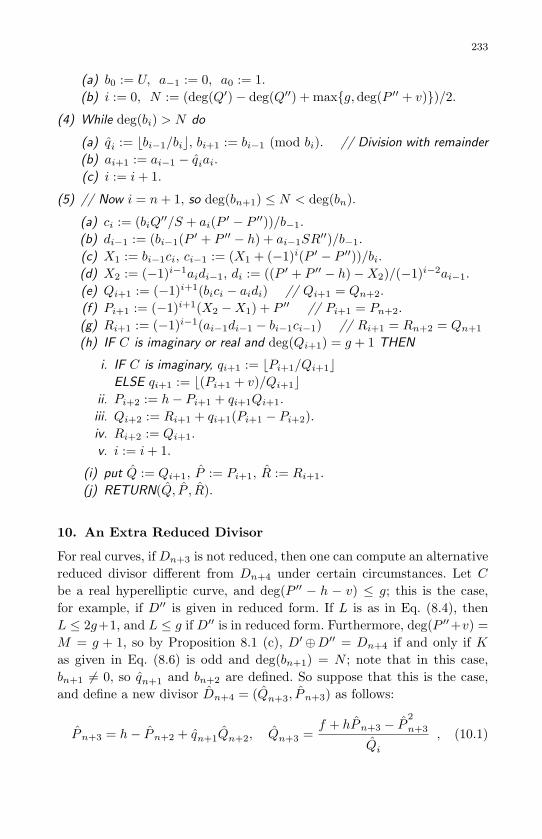
May 10, 2007 8:8 WSPC - Proceedings Trim Size: 9in x 6in ws-procs9x6
233
(a) b0 := U, a−1 := 0, a0 := 1.(b) i := 0, N := (deg(Q′)− deg(Q′′) + maxg,deg(P ′′ + v))/2.
(4) While deg(bi) > N do
(a) qi := bbi−1/bic, bi+1 := bi−1 (mod bi). // Division with remainder
(b) ai+1 := ai−1 − qiai.
(c) i := i+ 1.
(5) // Now i = n+ 1, so deg(bn+1) ≤ N < deg(bn).
(a) ci := (biQ′′/S + ai(P ′ − P ′′))/b−1.
(b) di−1 := (bi−1(P ′ + P ′′ − h) + ai−1SR′′)/b−1.
(c) X1 := bi−1ci, ci−1 := (X1 + (−1)i(P ′ − P ′′))/bi.(d) X2 := (−1)i−1aidi−1, di := ((P ′ + P ′′ − h)−X2)/(−1)i−2ai−1.
(e) Qi+1 := (−1)i+1(bici − aidi) // Qi+1 = Qn+2.
(f) Pi+1 := (−1)i+1(X2 −X1) + P ′′ // Pi+1 = Pn+2.
(g) Ri+1 := (−1)i−1(ai−1di−1 − bi−1ci−1) // Ri+1 = Rn+2 = Qn+1
(h) IF C is imaginary or real and deg(Qi+1) = g + 1 THEN
i. IF C is imaginary, qi+1 := bPi+1/Qi+1cELSE qi+1 := b(Pi+1 + v)/Qi+1c
ii. Pi+2 := h− Pi+1 + qi+1Qi+1.
iii. Qi+2 := Ri+1 + qi+1(Pi+1 − Pi+2).iv. Ri+2 := Qi+1.
v. i := i+ 1.
(i) put Q := Qi+1, P := Pi+1, R := Ri+1.
(j) RETURN(Q, P , R).
10. An Extra Reduced Divisor
For real curves, if Dn+3 is not reduced, then one can compute an alternativereduced divisor different from Dn+4 under certain circumstances. Let Cbe a real hyperelliptic curve, and deg(P ′′ − h − v) ≤ g; this is the case,for example, if D′′ is given in reduced form. If L is as in Eq. (8.4), thenL ≤ 2g+1, and L ≤ g if D′′ is in reduced form. Furthermore, deg(P ′′+v) =M = g + 1, so by Proposition 8.1 (c), D′⊕D′′ = Dn+4 if and only if Kas given in Eq. (8.6) is odd and deg(bn+1) = N ; note that in this case,bn+1 6= 0, so qn+1 and bn+2 are defined. So suppose that this is the case,and define a new divisor Dn+4 = (Qn+3, Pn+3) as follows:
Pn+3 = h− Pn+2 + qn+1Qn+2, Qn+3 =f + hPn+3 − P
2
n+3
Qi
, (10.1)
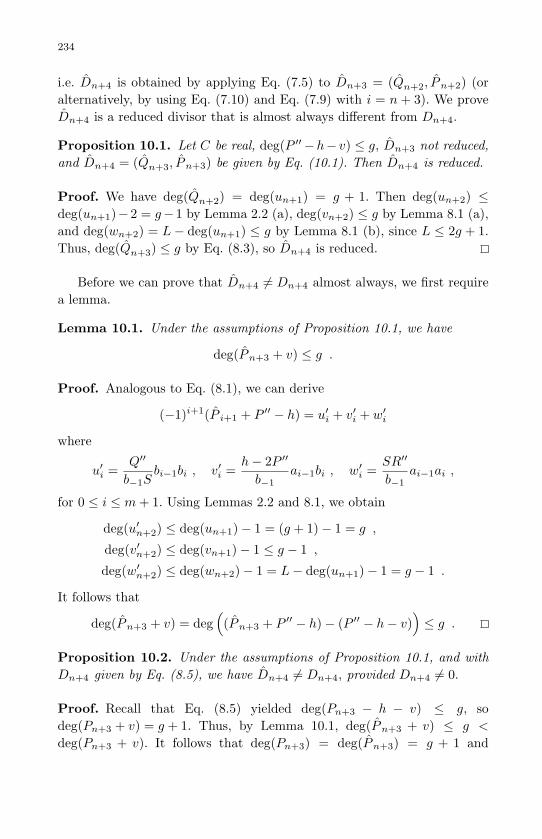
May 10, 2007 8:8 WSPC - Proceedings Trim Size: 9in x 6in ws-procs9x6
234
i.e. Dn+4 is obtained by applying Eq. (7.5) to Dn+3 = (Qn+2, Pn+2) (oralternatively, by using Eq. (7.10) and Eq. (7.9) with i = n + 3). We proveDn+4 is a reduced divisor that is almost always different from Dn+4.
Proposition 10.1. Let C be real, deg(P ′′−h− v) ≤ g, Dn+3 not reduced,and Dn+4 = (Qn+3, Pn+3) be given by Eq. (10.1). Then Dn+4 is reduced.
Proof. We have deg(Qn+2) = deg(un+1) = g + 1. Then deg(un+2) ≤deg(un+1)−2 = g−1 by Lemma 2.2 (a), deg(vn+2) ≤ g by Lemma 8.1 (a),and deg(wn+2) = L− deg(un+1) ≤ g by Lemma 8.1 (b), since L ≤ 2g + 1.Thus, deg(Qn+3) ≤ g by Eq. (8.3), so Dn+4 is reduced.
Before we can prove that Dn+4 6= Dn+4 almost always, we first requirea lemma.
Lemma 10.1. Under the assumptions of Proposition 10.1, we have
deg(Pn+3 + v) ≤ g .
Proof. Analogous to Eq. (8.1), we can derive
(−1)i+1(P i+1 + P ′′ − h) = u′i + v′i + w′i
where
u′i =Q′′
b−1Sbi−1bi , v′i =
h− 2P ′′
b−1ai−1bi , w′i =
SR′′
b−1ai−1ai ,
for 0 ≤ i ≤ m+ 1. Using Lemmas 2.2 and 8.1, we obtain
deg(u′n+2) ≤ deg(un+1)− 1 = (g + 1)− 1 = g ,
deg(v′n+2) ≤ deg(vn+1)− 1 ≤ g − 1 ,
deg(w′n+2) ≤ deg(wn+2)− 1 = L− deg(un+1)− 1 = g − 1 .
It follows that
deg(Pn+3 + v) = deg((Pn+3 + P ′′ − h)− (P ′′ − h− v)
)≤ g .
Proposition 10.2. Under the assumptions of Proposition 10.1, and withDn+4 given by Eq. (8.5), we have Dn+4 6= Dn+4, provided Dn+4 6= 0.
Proof. Recall that Eq. (8.5) yielded deg(Pn+3 − h − v) ≤ g, sodeg(Pn+3 + v) = g + 1. Thus, by Lemma 10.1, deg(Pn+3 + v) ≤ g <
deg(Pn+3 + v). It follows that deg(Pn+3) = deg(Pn+3) = g + 1 and

May 10, 2007 8:8 WSPC - Proceedings Trim Size: 9in x 6in ws-procs9x6
235
Pn+3 6= Pn+3. Now Pn+3 − Pn+3 = sQn+2 with s = qn+1 − qn+2. Sincedeg(Qn+2) = g + 1, we must have s ∈ F∗q .
By way of contradiction, assume that Dn+4 = Dn+4 6= 0. Then Qn+3
and Qn+3 differ by a factor in k∗, and Qn+3 divides Pn+3−Pn+3 = sQn+2.
Since s ∈ F∗q , we see that Qn+3 divides Qn+2. By Eq. (8.5) and Eq. (10.1),we have
Qn+2(Qn+3 −Qn+3) = (f + hPn+3 − P2
n+3)− (f + hPn+3 − P 2n+3)
= (Pn+3 − Pn+3)(h− Pn+3 − Pn+3)
= sQn+2(h− 2Pn+3 − sQn+2) ,
so Qn+3 divides h−2Pn+3. Now Dn+4 6= 0 forces Qn+3 to be non-constant.Let r be a root of Qn+3 in some algebraic closure of k. Then we can use rea-soning analogous to the proof of Proposition 5.1 to infer that (r,−Pn+3(r))is a singular point on C, a contradiction.
Remark 10.1. Let an+3, an+4 and an+4 be the reduced ideals corre-sponding to Dn+3, Dn+4, and Dn+4, respectively. Then (Qn+2)an+4 =(Pn+3 + v)an+3 and (Qn+2)an+4 = (Pn+3 + v)an+3. If we now take dis-tances with respect to some starting divisor and set δn+4 = δ(Dn+4) andδn+4 = δ(Dn+4), then we have δn+4 = δn+4 + δ with
δ = deg(Pn+3 + v)− deg(Pn+3 + v) .
Since deg(Pn+3 +v) = g+1 > deg(Pn+3 +v), we have δ ≥ 1. Furthermore,since deg(Pn+3 + v) = deg(Pn+3 − h− v) = g + 1,
Pn+3 + v
Pn+3 + v=
(Pn+3 + v)(Pn+3 − h− v)Qn+2Qn+3
,
and deg(Qn+3) ≥ 1, we have δ ≤ 2(g+1)−(g+1)−1 = g. In summary, 1 ≤δ ≤ g, so Dn+4 and Dn+4 are not far from each other in the infrastructureof the appropriate ideal class. In general, we expect deg(Qn+3) = g andhence δ = 1, so Dn+4 and Dn+4 are neighbors.
11. Numerical Results
The following numerical experiments were performed on a Pentium IV 2.4GHz computer running Linux. We used the computer algebra library NTL[14] for finite field and polynomial arithmetic and the GNU C++ compilerversion 3.4.3.

May 10, 2007 8:8 WSPC - Proceedings Trim Size: 9in x 6in ws-procs9x6
236
11.1. Binary Exponentiation
In order to test the efficiency of our versions of NUCOMP, we implementedroutines for binary exponentiation using Cantor’s algorithm in Eq. (6.1),NUCOMP (Algorithm 9.1), and NUCOMP with small operands (Algo-rithm 9.2). All three algorithms were implemented using real, imaginary,and unusual curves defined over prime finite fields Fp and characteristic 2finite fields F2n .
Table 11.1-11.5 contain the ratio of runtimes for binary exponentiationusing Algorithm 9.1 (NUCOMP using recurrences to compute ci and di)divided by the runtime using Algorithm 9.2 (NUCOMP using formulasto compute the final values of ci and di). For each genus and field sizelisted, 1000 binary exponentiations were performed with random 100-bitexponents. The same 1000 exponents were used for both algorithms andfor all genera and finite field sizes. The divisors produced by NUCOMPwere normalized; adapted basis was used for imaginary and unusual curvesand reduced basis was used for real curves [5]. The data clearly show thatAlgorithm 9.1 is more efficient that Algorithm 9.2 for g < 10 approximately,but that Algorithm 9.2 is ultimately more efficient as g grows.
Table 11.1. Exponentiation ratios (Alg 9.1 / Alg 9.2) over Fp, imaginary.
log2 pg 2 4 8 16 32 64 128 256 512
2 0.9839 0.9012 0.8983 0.9037 0.9038 0.8909 0.9110 0.9140 0.89763 0.8703 0.9471 0.9289 0.8934 0.9523 0.9659 0.9503 0.9568 0.95914 0.9619 0.9342 0.9266 0.9662 0.9503 0.9514 0.9634 0.9644 0.96725 0.9693 0.9550 0.9518 0.9576 0.9567 0.9474 0.9327 0.9341 0.93186 0.9754 0.9548 0.9631 0.9624 0.9378 0.9467 0.9413 0.9442 0.94347 0.9407 0.9530 0.9608 0.9561 0.9518 0.9532 0.9559 0.9592 0.96138 0.9726 0.9663 0.9666 0.9600 0.9576 0.9668 0.9785 0.9641 0.96719 0.9751 0.9764 0.9840 0.9776 0.9645 0.9760 0.9947 0.9710 0.978410 0.9793 0.9708 0.9817 0.9724 0.9629 0.9746 0.9976 0.9775 0.986411 0.9853 0.9792 0.9854 0.9877 0.9705 0.9839 1.0067 0.9875 0.997412 0.9983 0.9969 0.9971 0.9875 0.9777 0.9907 0.9924 0.9917 1.002313 0.9851 1.0084 1.0000 0.9963 0.9874 0.9993 0.9986 1.0024 1.010214 1.0126 1.0039 1.0049 0.9988 0.9845 1.0010 1.0003 1.0038 1.013015 1.0143 1.0085 1.0102 1.0097 0.9913 1.0079 1.0076 1.0103 1.020420 1.0823 1.1033 1.1029 1.1017 1.0670 1.1102 1.0568 1.0710 1.086625 1.1003 1.1185 1.1137 1.1203 1.1103 1.1187 1.0718 1.0988 1.089630 1.0872 1.0908 1.0927 1.0895 1.1152 1.1107 1.0839 1.0946 1.1129
Table 11.6–11.10 contain the ratio of runtimes for binary exponenti-ation using Cantor’s algorithm as compared to that using the faster ofAlgorithm 9.1 or Algorithm 9.2. Again, for each genus and field size listed,1000 binary exponentiations were performed with random 100-bit expo-nents. The same 1000 exponents were used for both algorithms and for allgenera and finite field sizes. The data clearly show that NUCOMP out-performs Cantor’s algorithm except for very small genera and finite fieldsizes, and that its relative performance improves as both the genus and

May 10, 2007 8:8 WSPC - Proceedings Trim Size: 9in x 6in ws-procs9x6
237
Table 11.2. Exponentiation ratios (Alg 9.1 / Alg 9.2) over Fp, real.
log2 pg 2 4 8 16 32 64 128 256 512
2 0.8661 0.8743 0.9368 0.9557 0.8414 0.8766 0.8830 0.8859 0.87613 0.8579 0.9149 0.9163 0.9216 0.8967 0.8996 0.8924 0.8761 0.88514 0.9395 0.9647 0.9485 0.9582 0.9533 0.9545 0.9633 0.9648 0.96945 0.9294 0.9209 0.9335 0.9489 0.9629 0.9661 0.9652 0.9695 0.97266 0.9477 0.9397 0.9595 0.9523 0.9636 0.9566 0.9499 0.9535 0.95707 0.8635 0.9431 0.9466 0.9370 0.9644 0.9606 0.9580 0.9586 0.95958 0.9349 0.9667 0.9684 0.9860 0.9869 0.9793 1.0003 0.9783 0.97819 0.9549 0.9723 0.9683 0.9561 0.9859 0.9818 0.9997 0.9774 0.978810 0.9522 0.9963 0.9913 0.9820 0.9968 0.9942 1.0116 0.9857 0.996211 0.9540 0.9645 0.9854 0.9874 0.9966 0.9975 0.9957 0.9902 0.999212 0.9726 0.9872 0.9960 0.9809 1.0166 1.0098 1.0058 1.0011 1.013013 0.9806 0.9948 0.9926 0.9941 1.0191 1.0148 1.0078 1.0018 1.010514 0.9883 1.0135 1.0023 0.9989 1.0239 1.0197 1.0171 1.0139 1.023715 0.9807 0.9989 1.0117 1.0071 1.0229 1.0226 1.0168 1.0127 1.020920 1.0995 1.1180 1.1156 1.1109 1.1063 1.1291 1.0692 1.0856 1.093225 1.0968 1.1090 1.1164 1.1060 1.0847 1.1100 1.0745 1.0784 1.098930 1.0981 1.1088 1.1149 1.1068 1.0980 1.1066 1.0863 1.0979 1.1258
Table 11.3. Exponentiation ratios (Alg 9.1 / Alg 9.2) over Fp, unusual.
log2 pg 2 4 8 16 32 64 128 256 512
2 0.9108 0.8800 0.8571 0.8910 0.8969 0.8896 0.9069 0.9082 0.90193 0.9175 1.0081 1.0161 1.0109 0.9715 0.9466 0.9658 0.9583 0.96494 0.9504 1.0290 1.0311 0.9967 0.9552 0.9542 0.9614 0.9603 0.96605 0.9684 0.9690 0.9853 0.9844 0.9730 0.9486 0.9475 0.9439 0.94916 0.9649 0.9626 0.9862 0.9731 0.9584 0.9471 0.9418 0.9368 0.93897 0.9816 1.0212 1.0139 0.9620 0.9854 0.9705 0.9868 0.9672 0.97248 0.9929 0.9867 0.9911 0.9980 0.9775 0.9666 0.9782 0.9590 0.96299 0.9938 0.9981 1.0131 0.9832 1.0047 0.9870 1.0063 0.9792 0.989910 1.0000 0.9982 0.9964 1.0017 0.9959 0.9834 0.9993 0.9729 0.985411 1.0000 1.0235 1.0103 1.0072 1.0228 1.0015 1.0012 0.9924 1.005812 1.0048 1.0046 1.0085 1.0014 1.0163 0.9956 0.9953 0.9851 0.997513 1.0000 1.0077 1.0243 1.0024 1.0362 0.9985 1.0101 1.0058 1.018414 0.9960 1.0245 1.0037 1.0070 1.0313 1.0101 1.0034 0.9958 1.009915 1.0094 1.0301 1.0370 1.0321 1.0448 1.0145 1.0176 1.0184 1.026420 1.1394 1.1789 1.1526 1.1262 1.1024 1.1000 1.0621 1.0671 1.088425 1.1014 1.1103 1.1209 1.1168 1.0860 1.1069 1.0716 1.0799 1.098130 1.0932 1.1047 1.1064 1.1018 1.0939 1.1108 1.0799 1.0885 1.1068
Table 11.4. Exponentiation ratios (Alg 9.1 / Alg 9.2) over F2n , imaginary.
log2 pg 2 4 8 16 32 64 128 256 512
2 0.9308 0.9002 0.8891 0.8889 0.8976 0.8744 0.9006 0.8880 0.88713 0.9622 0.9511 0.9547 0.9514 0.9446 0.9440 0.9600 0.9571 0.95854 0.9507 0.9395 0.9480 0.9507 0.9528 0.9592 0.9663 0.9613 0.96105 0.9682 0.9436 0.9396 0.9557 0.9443 0.9440 0.9396 0.9356 0.93436 0.9661 0.9544 0.9468 0.9528 0.9519 0.9530 0.9469 0.9474 0.94587 0.9819 0.9620 0.9674 0.9662 0.9681 0.9669 0.9611 0.9644 0.96228 0.9881 0.9663 0.9653 0.9693 0.9725 0.9780 0.9693 0.9691 0.96889 1.0071 0.9929 0.9868 0.9853 0.9920 0.9890 0.9807 0.9830 0.982010 1.0026 1.0011 0.9864 0.9917 0.9918 0.9891 0.9872 0.9878 0.987611 1.0205 0.9981 1.0046 1.0010 0.9947 0.9960 0.9960 0.9986 0.996412 1.0272 1.0124 1.0193 1.0137 1.0019 0.9984 1.0016 1.0042 1.002213 1.0341 1.0191 1.0311 1.0249 1.0116 1.0092 1.0118 1.0060 1.014814 1.0441 1.0311 1.0322 1.0242 1.0145 1.0081 1.0148 1.0181 1.018715 1.0504 1.0311 1.0415 1.0324 1.0208 1.0133 1.0190 1.0221 1.021620 1.1072 1.1263 1.1350 1.1218 1.1051 1.0890 1.0923 1.0893 1.088525 1.1624 1.1662 1.1724 1.1556 1.1337 1.1104 1.1119 1.1203 1.114630 1.1869 1.1797 1.1930 1.1826 1.1419 1.1375 1.1335 1.1337 1.1309
finite field size increase. The findings are consistent with those presentedin [6], but our improved versions of NUCOMP presented here out-performCantor’s algorithm for even smaller genera and finite field sizes than in [6].

May 10, 2007 8:8 WSPC - Proceedings Trim Size: 9in x 6in ws-procs9x6
238
Table 11.5. Exponentiation ratios (Alg 9.1 / Alg 9.2) over F2n , real
log2 pg 2 4 8 16 32 64 128 256 512
2 0.9249 0.8800 0.8630 0.8604 0.8649 0.8603 0.8816 0.8737 0.87253 0.8406 0.8562 0.8682 0.8670 0.8710 0.8910 0.8613 0.8745 0.87234 0.9331 0.9424 0.9480 0.9561 0.9524 0.9526 0.9561 0.9614 0.96185 0.9217 0.9480 0.9562 0.9596 0.9600 0.9526 0.9614 0.9668 0.96656 0.9471 0.9655 0.9548 0.9628 0.9574 0.9711 0.9444 0.9503 0.95047 0.9557 0.9580 0.9531 0.9511 0.9588 0.9574 0.9462 0.9512 0.95068 0.9765 0.9776 0.9781 0.9750 0.9819 0.9800 0.9711 0.9737 0.97599 0.9761 0.9709 0.9752 0.9799 0.9729 0.9705 0.9701 0.9701 0.967610 0.9891 1.0057 1.0019 0.9996 0.9970 0.9857 0.9868 0.9892 0.995211 0.9810 0.9962 1.0070 0.9997 0.9920 0.9849 0.9866 0.9905 0.991012 1.0080 1.0064 1.0220 1.0158 1.0081 0.9958 1.0006 1.0082 1.008513 1.0029 1.0162 1.0208 1.0120 1.0041 0.9845 1.0009 1.0093 1.008214 1.0243 1.0326 1.0379 1.0284 1.0162 0.9981 1.0093 1.0214 1.021515 1.0228 1.0329 1.0327 1.0270 1.0175 1.0016 1.0111 1.0182 1.017620 1.1270 1.1450 1.1401 1.1737 1.1256 1.0984 1.0998 1.0968 1.093725 1.1456 1.1565 1.1748 1.1471 1.0596 1.1021 1.1083 1.1207 1.104930 1.1672 1.1757 1.1822 1.1820 1.1477 1.1239 1.1288 1.1374 1.1328
Table 11.6. Exponentiation ratios (NUCOMP / Cantor) over Fp, imaginary.
log2 pg 2 4 8 16 32 64 128 256 512
2 1.0991 1.0504 1.0743 1.0432 0.9308 0.9141 0.9242 0.8847 0.84473 1.0662 1.0707 1.0609 1.0140 0.9523 0.9419 0.9008 0.8865 0.86524 1.0632 1.0607 1.0390 1.0158 0.9309 0.9286 0.9068 0.8582 0.85405 1.0766 1.0376 1.0350 1.0194 0.9120 0.9046 0.8865 0.8571 0.86426 1.0931 1.0462 1.0150 1.0056 0.8888 0.8963 0.8452 0.8594 0.85737 1.0235 0.9865 0.9679 0.9583 0.8692 0.8755 0.8310 0.8558 0.85868 0.9924 0.9349 0.9414 0.9268 0.8532 0.8697 0.8237 0.8500 0.84249 0.9557 0.9212 0.9212 0.9273 0.8405 0.8588 0.8144 0.8472 0.842010 0.9423 0.8975 0.8961 0.8910 0.8275 0.8451 0.8078 0.8402 0.833411 0.9538 0.8968 0.8981 0.9046 0.8128 0.8407 0.7921 0.8371 0.833312 0.9441 0.9043 0.8991 0.8918 0.8075 0.8332 0.8047 0.8278 0.823513 0.9361 0.9320 0.9035 0.9063 0.8060 0.7857 0.7995 0.8184 0.814814 0.9308 0.9038 0.8971 0.8981 0.7926 0.7821 0.8035 0.8184 0.807115 0.9135 0.8747 0.8704 0.8694 0.7851 0.7715 0.8043 0.8130 0.805920 0.8255 0.7956 0.7861 0.7989 0.7536 0.7242 0.7910 0.7843 0.776925 0.7949 0.7662 0.7693 0.7727 0.7208 0.7398 0.7854 0.7943 0.775930 0.7921 0.7714 0.7730 0.7716 0.7157 0.7372 0.7743 0.7616 0.7588
Table 11.7. Exponentiation ratios (NUCOMP / Cantor) over Fp, real.
log2 pg 2 4 8 16 32 64 128 256 512
2 0.8943 1.1268 1.2192 1.2763 1.0659 1.0987 1.0872 1.0731 1.08353 1.0449 1.1497 1.1165 1.1330 1.0503 1.0515 1.0434 1.0376 1.05004 1.0745 1.1081 1.0932 1.0784 1.0169 1.0137 1.0150 0.9847 1.00605 1.0549 1.0659 1.0300 1.0570 0.9635 0.9771 0.9650 0.9664 0.97876 1.0507 1.0124 1.0350 1.0327 0.9444 0.9555 0.9243 0.9540 0.95697 0.9705 0.9525 0.9231 0.9209 0.9144 0.9309 0.8950 0.9289 0.95128 0.9724 0.9539 0.9426 0.9338 0.9094 0.9195 0.8816 0.9244 0.92549 0.9591 0.9179 0.9028 0.9023 0.8726 0.8876 0.8608 0.8913 0.901310 0.9105 0.9056 0.8818 0.8877 0.8625 0.8879 0.8642 0.8933 0.895511 0.9396 0.9043 0.9159 0.9145 0.8402 0.8596 0.8415 0.8836 0.886212 0.9668 0.9341 0.9149 0.9135 0.8356 0.8536 0.8512 0.8832 0.874513 0.9581 0.9128 0.8856 0.8942 0.8047 0.7877 0.8201 0.8637 0.856014 0.9596 0.9098 0.8782 0.8912 0.8051 0.7874 0.8205 0.8502 0.847115 0.9356 0.8696 0.8640 0.8670 0.7789 0.7656 0.8037 0.8425 0.838720 0.8065 0.7549 0.7519 0.7638 0.7463 0.7275 0.8110 0.8108 0.800825 0.7717 0.7303 0.7215 0.7186 0.6996 0.7124 0.7818 0.7842 0.772330 0.7651 0.7337 0.7270 0.7392 0.6873 0.7212 0.7687 0.7749 0.7801
11.2. Key Exchange
We also ran numerous examples of the key exchange protocols describedin [7], again using both real and imaginary curves and Fp (p prime) and F2n
as base fields. The genus of our curves ranged from 2 to 6 and the underlying
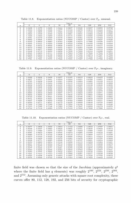
May 10, 2007 8:8 WSPC - Proceedings Trim Size: 9in x 6in ws-procs9x6
239
Table 11.8. Exponentiation ratios (NUCOMP / Cantor) over Fp, unusual.
log2 pg 2 4 8 16 32 64 128 256 512
2 1.0438 1.1079 1.0435 1.0444 0.9607 0.9345 0.9257 0.8955 0.87493 1.0500 1.0649 1.0506 1.0377 0.9102 0.8970 0.8815 0.8443 0.84174 1.1220 1.0905 1.0576 1.0565 0.9182 0.9301 0.9102 0.8782 0.86985 1.0824 1.0539 1.0030 1.0216 0.8861 0.8631 0.8382 0.8535 0.84656 1.1224 1.0404 1.0259 1.0419 0.9115 0.8951 0.8580 0.8769 0.87447 1.0081 0.9179 0.9309 0.9179 0.8604 0.8461 0.8158 0.8424 0.83128 0.9882 0.9695 0.9654 0.9900 0.8668 0.8647 0.8342 0.8627 0.85269 0.9340 0.8902 0.8883 0.8784 0.8286 0.8274 0.7986 0.8336 0.827410 0.9245 0.9151 0.9224 0.9308 0.8523 0.8396 0.8182 0.8484 0.842411 0.9641 0.9075 0.8642 0.8858 0.8033 0.8117 0.8016 0.8177 0.816412 0.9570 0.8997 0.8892 0.9055 0.8215 0.8265 0.8166 0.8258 0.833813 0.9615 0.8977 0.8662 0.8828 0.7821 0.7650 0.7964 0.8115 0.802614 0.9448 0.8719 0.8652 0.8858 0.7839 0.7699 0.8104 0.8328 0.825115 0.8945 0.8203 0.8111 0.8306 0.7663 0.7389 0.7822 0.7945 0.785820 0.8458 0.8234 0.8108 0.8250 0.7220 0.7456 0.8074 0.7927 0.799625 0.7964 0.7660 0.7606 0.7656 0.7252 0.7429 0.7942 0.7901 0.782230 0.7781 0.7591 0.7575 0.7622 0.7055 0.7307 0.7769 0.7766 0.7682
Table 11.9. Exponentiation ratios (NUCOMP / Cantor) over F2n , imaginary.
log2 pg 2 4 8 16 32 64 128 256 512
2 1.0068 0.9696 0.9498 0.9257 0.9185 0.8919 0.8824 0.8433 0.82053 0.9857 0.9757 0.9401 0.9244 0.9244 0.9251 0.8789 0.8951 0.88554 0.9725 0.9638 0.9448 0.9301 0.9056 0.9204 0.9285 0.9102 0.91105 0.9916 0.9705 0.9404 0.9360 0.9115 0.9153 0.9192 0.9035 0.90086 0.9632 0.9479 0.9248 0.9155 0.8915 0.9025 0.9132 0.9045 0.90357 0.9688 0.9248 0.9083 0.9050 0.8855 0.8761 0.9181 0.9161 0.91588 0.9305 0.9110 0.8928 0.8903 0.8866 0.9096 0.9263 0.9237 0.92479 0.9245 0.8985 0.8799 0.8902 0.8766 0.8926 0.9061 0.9079 0.909810 0.8890 0.8843 0.8809 0.8907 0.8715 0.8823 0.8937 0.8971 0.899611 0.8932 0.8695 0.8777 0.8780 0.8640 0.8776 0.8865 0.8938 0.895512 0.8744 0.8581 0.8621 0.8593 0.8666 0.8798 0.8811 0.8852 0.890513 0.8551 0.8623 0.8401 0.8469 0.8537 0.8696 0.8678 0.8759 0.877814 0.8407 0.8298 0.8202 0.8332 0.8492 0.8669 0.8676 0.8751 0.880215 0.8220 0.8171 0.8041 0.8173 0.8430 0.8609 0.8649 0.8750 0.880520 0.7449 0.7362 0.7399 0.7625 0.7950 0.8106 0.8316 0.8481 0.853625 0.7015 0.7089 0.7146 0.7263 0.7585 0.7847 0.8059 0.8174 0.827030 0.6744 0.7118 0.6993 0.7078 0.7419 0.7632 0.7839 0.7996 0.8131
Table 11.10. Exponentiation ratios (NUCOMP / Cantor) over F2n , real.
log2 pg 2 4 8 16 32 64 128 256 512
2 0.9277 1.0896 1.0930 1.0854 1.1152 1.0998 1.0653 1.0787 1.06613 0.8948 0.9597 0.9860 0.9622 0.9695 0.9791 0.9640 0.9824 0.98144 1.0213 1.0360 1.0375 1.0274 1.0267 1.0252 1.0289 1.0421 1.04405 0.9587 0.9672 0.9630 0.9505 0.9372 0.9295 0.9499 0.9516 0.94916 0.9989 0.9776 0.9743 0.9838 0.9718 0.9715 0.9689 0.9777 0.97907 0.9370 0.9193 0.9025 0.9126 0.8990 0.9041 0.9311 0.9413 0.94248 0.9534 0.9439 0.9222 0.9379 0.9365 0.9476 0.9650 0.9785 0.98429 0.9008 0.8771 0.8685 0.8928 0.8707 0.8727 0.8891 0.8954 0.896310 0.9053 0.8863 0.8854 0.9142 0.9098 0.9115 0.9252 0.9384 0.949111 0.8601 0.8518 0.8504 0.8713 0.8624 0.8595 0.8755 0.8838 0.887012 0.8878 0.8679 0.8589 0.8705 0.8938 0.9006 0.9154 0.9220 0.930113 0.8377 0.8230 0.8171 0.8281 0.8478 0.8476 0.8675 0.8729 0.877014 0.8393 0.8258 0.8206 0.8384 0.8659 0.8783 0.8863 0.8957 0.903115 0.7970 0.7775 0.7800 0.7942 0.8204 0.8423 0.8548 0.8594 0.865920 0.7221 0.7313 0.7312 0.7552 0.7968 0.8291 0.8311 0.8548 0.863825 0.6565 0.6298 0.6678 0.6954 0.7907 0.7356 0.7520 0.7756 0.801030 0.6576 0.6649 0.6722 0.6936 0.7353 0.7663 0.7823 0.8043 0.8187
finite field was chosen so that the size of the Jacobian (approximately qg
where the finite field has q elements) was roughly 2160, 2224, 2256, 2384,
and 2512. Assuming only generic attacks with square root complexity, thesecurves offer 80, 112, 128, 192, and 256 bits of security for cryptographic

May 10, 2007 8:8 WSPC - Proceedings Trim Size: 9in x 6in ws-procs9x6
240
protocols based on the corresponding discrete logarithm problem. NIST [9]currently recommends these five levels of security for key establishment inU.S. Government applications. Although the use of curves with genus 3 andlarger for cryptographic purposes is questionable, we nevertheless includedtimes for higher genus as our main goal is to provide a relative comparisonbetween our formulation of NUCOMP with Cantor’s algorithm.
For curves defined over Fp, we chose a random prime p of appropriatelength such that pg had the required bit length, and for curves over F2n
we chose the minimal value of n with gn greater than or equal to the re-quired bit length. For each genus and finite field, we randomly selected 2000curves and executed Diffie–Hellman key exchange twice for each curve, onceusing Cantor’s algorithm and once using our version of NUCOMP (Algo-rithm 9.1). We used Algorithm 9.1 as opposed to Algorithm 9.2, becauseour previous experiments indicated that it is more efficient for low genuscurves. The random exponents used had 160, 224, 256, 384, and 512 bits,respectively, ensuring that the number of bits of security corresponds tothe five levels recommended by NIST (again, considering only generic at-tacks). In order to provide a fair comparison, the same sequence of randomexponents was used for each run of the key exchange protocol.
Table 11.11 contains the average CPU time in seconds for each version ofthe protocol using real and imaginary curves over Fp and F2n . The columnslabeled “Cantor” contain the runtimes when using Cantor’s algorithm, andthose labeled “NC” the runtimes when using NUCOMP. The times for anyprecomputations, as described in [7], are not included. We also give theratios of the average time spent for key exchange using NUCOMP versusthat using Cantor’s algorithm in Table 11.12. Clearly, in almost all cases,NUCOMP offers a fairly significant performance improvement as opposedto Cantor’s algorithm, even for genus as low as 2.
12. Conclusions
Our results indicate that NUCOMP does provide an improvement for di-visor arithmetic in hyperelliptic curves except for the smallest examples interms of genus and finite field size. They also show that both versions ofNUCOMP, Algorithm 9.1 and Algorithm 9.2, are useful. Nevertheless, acareful complexity analysis and further numerical experiments are requiredto compare NUCOMP and Cantor’s algorithm more precisely.
There are a number of possible improvements to NUCOMP that needto be investigated. For example, our remarks at the end of Sec. 8 indicatethat basis normalization need not be done when NUCOMP is used as a

May 10, 2007 8:8 WSPC - Proceedings Trim Size: 9in x 6in ws-procs9x6
241
Table 11.11. Key exchange timings over Fp and F2n (in seconds).
Security Fp F2nlevel Imaginary Real Imaginary Real
(in bits) g Cantor NC Cantor NC Cantor NC Cantor NC
2 0.0322 0.0290 0.0324 0.0306 0.0320 0.0282 0.0282 0.02913 0.0382 0.0350 0.0390 0.0363 0.0342 0.0320 0.0322 0.0317
80 4 0.0492 0.0438 0.0487 0.0438 0.0443 0.0404 0.0403 0.03825 0.0466 0.0435 0.0483 0.0444 0.0611 0.0601 0.0560 0.05636 0.0124 0.0124 0.0123 0.0122 0.0737 0.0705 0.0667 0.0658
2 0.0562 0.0498 0.0554 0.0520 0.0585 0.0505 0.0511 0.05223 0.0737 0.0649 0.0707 0.0660 0.0692 0.0627 0.0624 0.0636
112 4 0.0723 0.0651 0.0730 0.0648 0.0691 0.0630 0.0622 0.05985 0.0938 0.0875 0.0937 0.0867 0.0846 0.0822 0.0776 0.07816 0.1182 0.1076 0.1171 0.1048 0.1032 0.0977 0.0946 0.0919
2 0.0667 0.0593 0.0663 0.0625 0.0692 0.0594 0.0598 0.06113 0.0870 0.0771 0.0847 0.0790 0.0807 0.0732 0.0730 0.0734
128 4 0.0904 0.0806 0.0906 0.0806 0.0791 0.0723 0.0697 0.06675 0.1129 0.1044 0.1124 0.1037 0.0989 0.0957 0.0899 0.09096 0.1354 0.1224 0.1318 0.1181 0.1192 0.1129 0.1090 0.1063
2 0.1439 0.1235 0.1375 0.1290 0.1620 0.1348 0.1369 0.13953 0.1617 0.1436 0.1577 0.1480 0.1652 0.1484 0.1472 0.1486
192 4 0.1832 0.1609 0.1793 0.1615 0.1743 0.1642 0.1537 0.15055 0.2313 0.2114 0.2210 0.2069 0.2190 0.2147 0.1964 0.19856 0.2247 0.2053 0.2242 0.2019 0.1912 0.1795 0.1726 0.1677
2 0.2517 0.2127 0.2303 0.2182 0.3037 0.2556 0.2540 0.25933 0.2920 0.2538 0.2825 0.2633 0.3417 0.3129 0.3025 0.3106
256 4 0.2875 0.2537 0.2771 0.2505 0.3015 0.2815 0.2664 0.26225 0.3662 0.3375 0.3557 0.3341 0.3693 0.3599 0.3338 0.33446 0.3968 0.3577 0.3792 0.3446 0.3555 0.3456 0.3185 0.3120
Table 11.12. Key exchange ratios over Fp and F2n .
Security levelg 80 112 128 192 256
2 0.8999 0.8869 0.8890 0.8585 0.84543 0.9153 0.8804 0.8866 0.8882 0.8693
Fp 4 0.8916 0.9004 0.8919 0.8781 0.8825imaginary 5 0.9329 0.9332 0.9242 0.9140 0.9214
6 0.9984 0.9102 0.9038 0.9135 0.9015
2 0.9435 0.9383 0.9429 0.9383 0.94773 0.9305 0.9342 0.9323 0.9384 0.9321
Fp 4 0.9000 0.8867 0.8895 0.9008 0.9041real 5 0.9197 0.9255 0.9229 0.9363 0.9391
6 0.9905 0.8947 0.8961 0.9007 0.9088
2 0.8800 0.8621 0.8579 0.8320 0.84173 0.9364 0.9066 0.9074 0.8984 0.9157
F2n 4 0.9132 0.9125 0.9144 0.9420 0.9336imaginary 5 0.9829 0.9718 0.9677 0.9803 0.9744
6 0.9558 0.9467 0.9475 0.9388 0.9722
2 1.0334 1.0222 1.0225 1.0190 1.02063 0.9855 1.0181 1.0067 1.0097 1.0270
F2n 4 0.9493 0.9616 0.9567 0.9796 0.9840real 5 1.0046 1.0065 1.0112 1.0106 1.0016
6 0.9870 0.9707 0.9753 0.9717 0.9796
component for binary exponentiation, because the degree of P will generallybe at most g + 1 at the end of NUCOMP. Not performing normalizationsaves one division with remainder at the cost of the inputs to subsequentapplications of NUCOMP having slightly larger degrees. In addition, theresults in Sec. 10 indicate that in some cases, it is possible to perform oneextra NUCOMP step to guarantee that the output of NUCOMP is reducedwithout having to perform a continued fraction step. Further investigationand analysis is required to determine which of these options is the mostefficient in practice.

May 10, 2007 8:8 WSPC - Proceedings Trim Size: 9in x 6in ws-procs9x6
242
Our data also indicate that using NUCOMP is more efficient than Can-tor’s algorithm for cryptographic key exchange using low genus hyperellip-tic curves, for both imaginary and real models, However, explicit formulasbased on Cantor’s algorithm have been developed for divisor arithmetic oncurves of genus 2, 3, and 4 (see [5] for a partial survey and references). NU-COMP, as presented in this paper, is generic in the sense that it works forany genus and as such does not compete in terms of performance with theseexplicit formulas. Given that NUCOMP out-performs Cantor’s algorithm,it is conceivable that some of the ideas used in NUCOMP can be applied toimprove the explicit formulas. This, as well as the open problems mentionedabove, is the subject of on-going research.
References
[1] E. Artin, Quadratische Korper im Gebiete der hoheren Kongruenzen. Math.Zeitschr. 19 (1924), 153–206.
[2] D. G. Cantor, Computing in the Jacobian of a hyperelliptic curve, Math.Comp. 48 (1987), 95–101.
[3] A. Enge, How to distinguish hyperelliptic curves in even characteristic.Public-Key Cryptography and Computational Number Theory. De Gruyter(Berlin), 2001, 49–58.
[4] H. Hasse, Algebraic Number Theory, Springer, Berlin 2002.[5] M. J. Jacobson, Jr., A. J. Menezes, and A. Stein, Hyperelliptic curves and
cryptography, in High Primes and Misdemeanors: Lectures in Honour of the60th Birthday of Hugh Cowie Williams, Fields Inst. Comm. 41, AmericanMathematical Society, 2004, 255–282.
[6] M. J. Jacobson., Jr. and A. J. van der Poorten, Computational aspects ofNUCOMP, Proc. ANTS-V, Lect. Notes Comp. Sci. 2369, Springer (NewYork), 2002, 120–133.
[7] M. J. Jacobson, Jr., R. Scheidler, and A. Stein, Cryptographic protocolson real and imaginary hyperelliptic curves, submitted to Advances Math.Comm., 2006.
[8] M. J. Jacobson, Jr., R. Scheidler and H. C. Williams, An improved realquadratic field based key exchange procedure. J. Cryptology 19 (2006), 211–239.
[9] National Institute of Standards and Technology (NIST), Recommendationon key establishment schemes, NIST Special Publication 800-56, January2003.
[10] S. Paulus and H.-G. Ruck, Real and imaginary quadratic representations ofhyperelliptic function fields, Math. Comp. 68 (1999), 1233–1241.
[11] A. J. van der Poorten, A note on NUCOMP. Math. Comp. 72 (2003), 1935–1946.
[12] M. Rosen, Number Theory in Function Fields, Springer, New York 2002.[13] D. Shanks, On Gauss and composition I, II. In Proc. NATO ASI on Number
Theory and Applications, Kluwer Academic Press 1989, 163–204.

May 10, 2007 8:8 WSPC - Proceedings Trim Size: 9in x 6in ws-procs9x6
243
[14] V. Shoup, NTL: A library for doing number theory. Software, 2001. Availableat http://www.shoup.net.ntl.
[15] A. Stein. Sharp upper bounds for arithmetics in hyperelliptic function fields.J. Ramanujan Math. Soc. 16 (2001), 1–86.
[16] A. Stein and H. C. Williams, Some methods for evaluating the regulator ofa real quadratic function field. Experiment. Math. 8 (1999), 119–133.
[17] H. Stichtenoth, Algebraic Function Fields and Codes. Springer, Berlin 1993.
May 10, 2007 8:8 WSPC - Proceedings Trim Size: 9in x 6in ws-procs9x6
244
The number of inequivalent binary self-orthogonal codes ofdimension 6
Xiang-dong Hou
Department of Mathematics, University of South FloridaTampa, FL 33620, USA
E-mail: [email protected]
We announce an explicit formula for the number of inequivalent binary self-
orthogonal codes of dimension 6 and arbitrary length. Formulas for dimension≤ 5 have been obtained in a previous paper.
Keywords: Binary self-orthogonal code, Equivalence, General linear group, The
symmetric group.
1. Introduction
Let F2 be the binary field and let 〈·, ·〉 denote the usual inner product ofFn
2 . An [n, k] binary code is a k-dimensional subspace C of Fn2 ; C is self-
orthogonal if C ⊂ C⊥, where C⊥ = x ∈ Fn2 : 〈x, y〉 = 0 for all y ∈ C.
Self-dual codes are [2k, k] self-orthogonal codes.Let Sn denote the symmetric group on 1, . . . , n. Sn acts on Fn
2 bypermuting its coordinates. Call two codes C1, C2 ⊂ Fn
2 equivalent if thereexists σ ∈ Sn such that C2 = Cσ
1 . Self-orthogonality of codes is preservedunder this equivalence. Classification of self-orthogonal codes, especially, ofself-dual codes, has been a focus of attention since the early days of codingtheory; see Pless [7], Pless and Sloane [8], Conway and Pless [1], Conway,Pless and Sloane [2], and Huffman [5]. Complete classifications of self-dualcodes are known up to length 32 [2].
Let Ψk,n denote the number of inequivalent [n, k] self-orthogonal codes.We are interested in the computation of Ψk,n. More precisely, to what extentcan Ψk,n be explicitly determined? In a recent paper [4], we introduced analgorithm which essentially says that for a given moderate k, it is possibleto find an explicit formula for Ψk,n that holds for all n. In fact, formulas forΨk,n with k ≤ 5 have been found in [4]. The main purpose of the presentpaper is to announce the formula for Ψ6,n. The result consists of a master

May 10, 2007 8:8 WSPC - Proceedings Trim Size: 9in x 6in ws-procs9x6
245
formula and forty sub formulas which are ingredients of the master formula.In Section 2, we describe the method of computation. The master formula isthe Cauchy-Frobenius lemma, i.e., Burnside’s lemma, applied to an actionby the group GL(6,F2) × Sn on a certain set of 6 × n matrices over F2.The sub formulas count numbers of matrices fixed by representatives fromthe conjugacy classes of GL(6,F2) ×Sn. We tabulate the sub formulas inTable 2 of the appendix. In Table 4 of the appendix, one can find the valuesof Ψk,n with k ≤ 6 and n ≤ 40.
Knowing the value of Ψk,n is a big advantage if we try to classify all [n, k]self-orthogonal codes. Without knowing Ψk,n beforehand, the algorithm toclassify [n, k] self-orthogonal codes relies on the mass formula, see [6, §9.7.1].This algorithm consists of two types of steps: (i) search for an inequivalentcode, (ii) computation of the order of the automorphism group of the newlyfound inequivalent code. The purpose of type (ii) steps is to check if thelist of inequivalent codes already found is complete. However, if Ψk,n isknown beforehand, type (ii) steps are not needed. All we have to do is tofind Ψk,n pairwise inequivalent [n, k] self-orthogonal codes (by whatevermethod). For example, classification of [16, 6] self-orthogonal codes seemsquite an undertaking. (To the author’s knowledge, this classification is notknown.) However, the problem becomes more feasible when reformulatedas “find 153 (= Ψ6,16) pairwise inequivalent [16, 6] self-orthogonal codes”.
2. Method of Computation
The method for computing Ψk,n has been laid out in [4]. Since all detailsare available in 4, we only outline the approach here.
Let Ψ≤k,n be the number of inequivalent self-orthogonal codes in Fn2
with dimension ≤ k. Since
Ψk,n = Ψ≤k,n −Ψ≤k−1,n,
it suffices to compute Ψ≤k−1,n and Ψ≤k,n. (Since Ψ≤5,n has been de-termined in [4], for the purpose of this paper, we only need to deter-mine Ψ≤6,n.) Let Mk×n be the set of all k × n matrices over F2 and letSk×n = X ∈Mk×n : XXT = 0. The group GL(k,F2)×Sn acts on Sk×n
by
X(A,P ) = A−1XP, (A,P ) ∈ GL(k,F2)×Sn, X ∈ Sk×n.
(Here, a permutation in Sn is treated an n× n permutation matrix.) Thenumber Ψ≤k,n is precisely the number of GL(k,F2) × Sn-orbits in Sk×n.
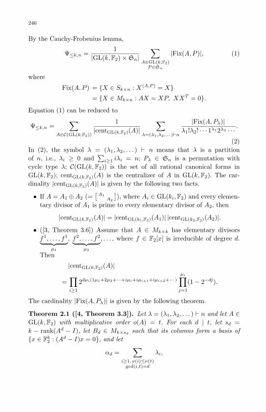
May 10, 2007 8:8 WSPC - Proceedings Trim Size: 9in x 6in ws-procs9x6
246
By the Cauchy-Frobenius lemma,
Ψ≤k,n =1
|GL(k,F2)×Sn|∑
A∈GL(k,F2)P∈Sn
|Fix(A,P )|, (1)
where
Fix(A,P ) = X ∈ Sk×n : X(A,P ) = X= X ∈Mk×n : AX = XP, XXT = 0.
Equation (1) can be reduced to
Ψ≤k,n =∑
A∈C(GL(k,F2))
1|centGL(k,F2)(A)|
∑λ=(λ1,λ2,... )`n
|Fix(A,Pλ)|λ1!λ2! · · · 1λ12λ2 · · ·
.
(2)In (2), the symbol λ = (λ1, λ2, . . . ) ` n means that λ is a partitionof n, i.e., λi ≥ 0 and
∑i≥1 iλi = n; Pλ ∈ Sn is a permutation with
cycle type λ; C(GL(k,F2)) is the set of all rational canonical forms inGL(k,F2); centGL(k,F2)(A) is the centralizer of A in GL(k,F2). The car-dinality |centGL(k,F2)(A)| is given by the following two facts.
• If A = A1 ⊕A2 (=[
A1A2
]), where Ai ∈ GL(ki,F2) and every elemen-
tary divisor of A1 is prime to every elementary divisor of A2, then
|centGL(k,F2)(A)| = |centGL(k1,F2)(A1)| |centGL(k2,F2)(A2)|.
• ([3, Theorem 3.6]) Assume that A ∈ Mk×k has elementary divisorsf1, . . . , f1︸ ︷︷ ︸
µ1
, f2, . . . , f2︸ ︷︷ ︸µ2
, . . . , where f ∈ F2[x] is irreducible of degree d.
Then
|centGL(k,F2)(A)|
=∏i≥1
2dµi(1µ1+2µ2+···+iµi+iµi+1+iµi+2+··· )µi∏
j=1
(1− 2−dj).
The cardinality |Fix(A,Pλ)| is given by the following theorem.
Theorem 2.1 ([4, Theorem 3.3]). Let λ = (λ1, λ2, . . . ) ` n and let A ∈GL(k,F2) with multiplicative order o(A) = t. For each d | t, let sd =k − rank(Ad − I), let Bd ∈ Mk×sd
such that its columns form a basis ofx ∈ Fk
2 : (Ad − I)x = 0, and let
αd =∑
i≥1, ν(i)≤ν(t)gcd(i,t)=d
λi,

May 10, 2007 8:8 WSPC - Proceedings Trim Size: 9in x 6in ws-procs9x6
247
where ν is the 2-adic order. Then
|Fix(A,Pλ)| = 2P
ν(i)>ν(t) sgcd(i,t)λi · n(A),
where n(A) is the number of sequences of matrices (Yd)d|t with Yd ∈Msd×αd
and ∑d|t
d−1∑j=0
AjBdYdYTd B
Td (Aj)T = 0.
The computation of n(A) is complicated but is not out of reach for amoderate k. An algorithm for computing n(A) is detailed in [4, Algorthim3.4]. The algorithm is based on the predictable behavior of binary quadraticforms. In [4], one can also find many examples of step-by-step execution ofthis algorithm.
The following additional facts greatly simplify the computation of|Fix(A,Pλ)| for many A.
• ([4, Lemma 3.7 and Eq. (3.25)]) |Fix(Ik, Pλ)| is known.• ([4, Corollary 3.10]) Let f1, . . . , ft ∈ F2[x]\x be irreducible such thatf1, f∗1 , . . . , ft, f
∗t are pairwise disjoint, where f∗i is the reciprocal
polynomial of fi. Let A = A1 ⊕ · · · ⊕ At ∈ GL(k,F2), where Ai ∈GL(ki,F2) and the elementary divisors of Ai are powers of fi or f∗i .Then
|Fix(A,Pλ)| =t∏
i=1
|Fix(Ai, Pλ)|. (3)
• ([4, Lemma 3.11]) Let f ∈ F2[x] \ x be an irreducible polyno-mial which is not self-reciprocal. Let t be the smallest positive inte-ger such that f | xt − 1. Let A ∈ GL(k,F2) have elementary divisorsf1, . . . , f1︸ ︷︷ ︸
µ1
, . . . , fs, . . . , fs︸ ︷︷ ︸µs
and let λ = (λ1, λ2, . . . ) ` n. Then
|Fix(A,Pλ)| = 2deg fP
j≥1 λjt
Pl≥1 µl minl,2ν(j).
We now turn to the case k = 6. GL(6,F2) has 60 rational canonicalforms A1, . . . , A60. Their elementary divisors and the cardinalities of theircentralizers are given in Table 1 of the appendix. Formulas for |Fix(Ai, Pλ)|,1 ≤ i ≤ 60, are computed by the method outlined above. The resultsare contained in Table 2 of the appendix. It is common that for severalAi, |Fix(Ai, Pλ)| share the same formula. As a result, Table 2 contains 40formulas instead of 60. All computations in this project were done usingMathematica [9].
May 10, 2007 8:8 WSPC - Proceedings Trim Size: 9in x 6in ws-procs9x6
248
Remarks.
(i) Since the amount of computation (mostly symbolic) in this project isvery large and since the result is very intricate, there is a natural con-cern about the possible errors in the computation. To have a strongassurance for the correctness of the formulas in Table 2, we have usedthem to compute the values of Ψ≤6,n for n ≤ 40 (Table 3 of the ap-pendix). If any of those formulas for |Fix(Ai, Pλ)| had gone wrong, mostlikely, the results of Ψ≤6,n coming out of the master formula would nothave been integers. The results of Ψ≤6,n have turned out to be integers.
(ii) It is possible to simplify the computation and presentation of Ψ≤k,n.The idea is to further exploit (3) in order to express Ψ≤k,n in termsof functions that are reusable. We will discuss this idea in details else-where. In fact, there do not seem to be insurmountable obstacles in thecomputation of Ψ≤k,n with reasonably larger k’s.
Appendix. Tables
The appendix consists of four tables. Table 1 contains the information ofC(GL(6,F2)) = A1, . . . , A60, the set of rational canonical forms inGL(6,F2). Table 2 contains the formulas for |Fix(Ai, Pλ)|, 1 ≤ i ≤ 60.In Table 2, λ = (λ1, λ2, . . . ) and
λa,b =∑
i≡a (mod b)
λi for 0 ≤ a < b.
The function δ : 0, 1, . . . → 0, 1 is defined by
δ(x) =
0 if x = 0,
1 if x > 0.
Tables 3 and 4 give the values of Ψ≤k,n and Ψk,n with k ≤ 6 and n ≤ 40.Portions of Tables 3 and 4 with k ≤ 5 are from [4].
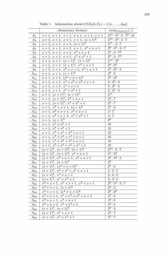
May 10, 2007 8:8 WSPC - Proceedings Trim Size: 9in x 6in ws-procs9x6
249
Table 1. Information about C(GL(6, F2) = A1, . . . , A60
elementary divisors |centGL(6,F2)( )|A1 x + 1, x + 1, x + 1, x + 1, x + 1, x + 1 215 · 34 · 5 · 72 · 31A2 x + 1, x + 1, x + 1, x + 1, (x + 1)2 215 · 32 · 5 · 7A3 x + 1, x + 1, x + 1, (x + 1)3 211 · 3 · 7A4 x + 1, x + 1, x + 1, x + 1, x2 + x + 1 26 · 33 · 5 · 7A5 x + 1, x + 1, x + 1, x3 + x + 1 23 · 3 · 72
A6 x + 1, x + 1, x + 1, x3 + x2 + 1 23 · 3 · 72
A7 x + 1, x + 1, (x + 1)2, (x + 1)2 214 · 32
A8 x + 1, x + 1, (x + 1)2, x2 + x + 1 26 · 32
A9 x + 1, x + 1, x2 + x + 1, x2 + x + 1 23 · 33 · 5A10 x + 1, x + 1, (x + 1)4 28 · 3A11 x + 1, x + 1, (x2 + x + 1)2 23 · 32
A12 x + 1, x + 1, x4 + x3 + x2 + x + 1 2 · 32 · 5A13 x + 1, x + 1, x4 + x + 1 2 · 32 · 5A14 x + 1, x + 1, x4 + x3 + 1 2 · 32 · 5A15 x + 1, (x + 1)2, (x + 1)3 211
A16 x + 1, (x + 1)2, x3 + x + 1 23 · 7A17 x + 1, (x + 1)2, x3 + x2 + 1 23 · 7A18 x + 1, x2 + x + 1, (x + 1)3 24 · 3A19 x + 1, x2 + x + 1, x3 + x + 1 3 · 7A20 x + 1, x2 + x + 1, x3 + x2 + 1 3 · 7A21 x + 1, (x + 1)5 26
A22 x + 1, x5 + x2 + 1 31
A23 x + 1, x5 + x3 + 1 31
A24 x + 1, x5 + x3 + x2 + x + 1 31
A25 x + 1, x5 + x4 + x2 + x + 1 31
A26 x + 1, x5 + x4 + x3 + x + 1 31
A27 x + 1, x5 + x4 + x3 + x2 + 1 31
A28 (x + 1)2, (x + 1)2, (x + 1)2 212 · 3 · 7A29 (x + 1)2, (x + 1)2, x2 + x + 1 25 · 32
A30 (x + 1)2, x2 + x + 1, x2 + x + 1 23 · 32 · 5A31 (x + 1)2, (x + 1)4 28
A32 (x + 1)2, (x2 + x + 1)2 23 · 3A33 (x + 1)2, x4 + x3 + x2 + x + 1 2 · 3 · 5A34 (x + 1)2, x4 + x + 1 2 · 3 · 5A35 (x + 1)2, x4 + x3 + 1 2 · 3 · 5A36 x2 + x + 1, x2 + x + 1, x2 + x + 1 26 · 34 · 5 · 7A37 x2 + x + 1, (x + 1)4 23 · 3A38 x2 + x + 1, (x2 + x + 1)2 26 · 32
A39 x2 + x + 1, x4 + x3 + x2 + x + 1 32 · 5A40 x2 + x + 1, x4 + x + 1 32 · 5A41 x2 + x + 1, x4 + x3 + 1 32 · 5A42 (x + 1)3, (x + 1)3 29 · 3A43 (x + 1)3, x3 + x + 1 22 · 7A44 (x + 1)3, x3 + x2 + 1 22 · 7
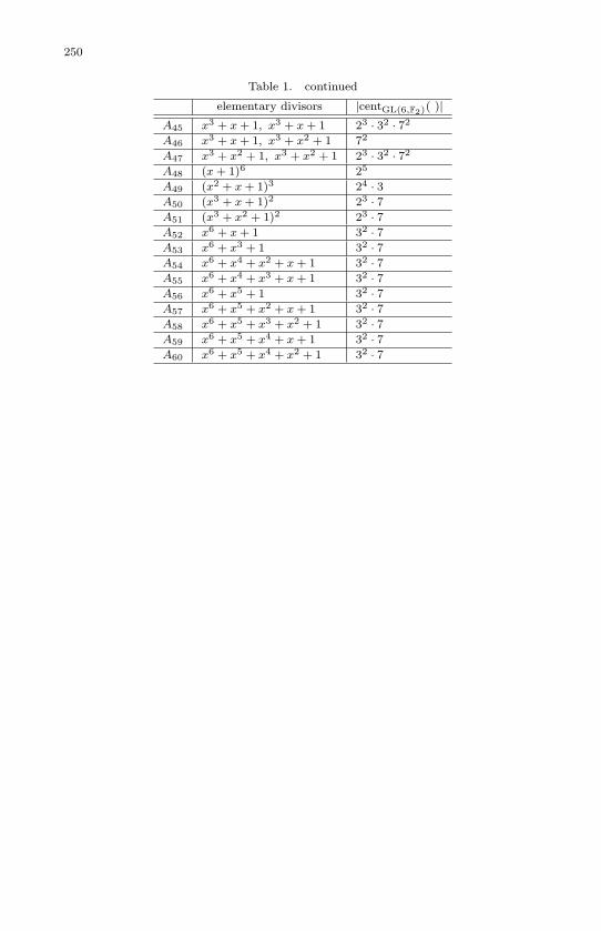
May 10, 2007 8:8 WSPC - Proceedings Trim Size: 9in x 6in ws-procs9x6
250
Table 1. continued
elementary divisors |centGL(6,F2)( )|A45 x3 + x + 1, x3 + x + 1 23 · 32 · 72
A46 x3 + x + 1, x3 + x2 + 1 72
A47 x3 + x2 + 1, x3 + x2 + 1 23 · 32 · 72
A48 (x + 1)6 25
A49 (x2 + x + 1)3 24 · 3A50 (x3 + x + 1)2 23 · 7A51 (x3 + x2 + 1)2 23 · 7A52 x6 + x + 1 32 · 7A53 x6 + x3 + 1 32 · 7A54 x6 + x4 + x2 + x + 1 32 · 7A55 x6 + x4 + x3 + x + 1 32 · 7A56 x6 + x5 + 1 32 · 7A57 x6 + x5 + x2 + x + 1 32 · 7A58 x6 + x5 + x3 + x2 + 1 32 · 7A59 x6 + x5 + x4 + x + 1 32 · 7A60 x6 + x5 + x4 + x2 + 1 32 · 7
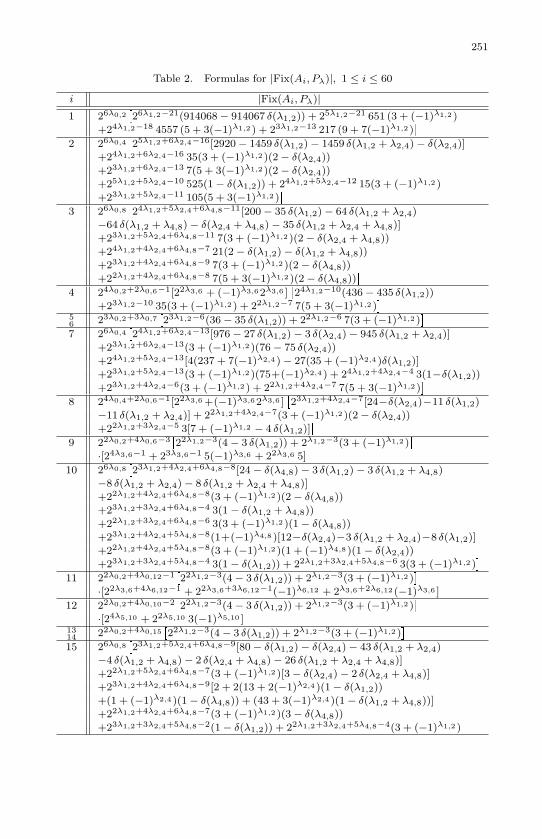
May 10, 2007 8:8 WSPC - Proceedings Trim Size: 9in x 6in ws-procs9x6
251
Table 2. Formulas for |Fix(Ai, Pλ)|, 1 ≤ i ≤ 60
i |Fix(Ai, Pλ)|1 26λ0,2
26λ1,2−21(914068− 914067 δ(λ1,2)) + 25λ1,2−21 651 (3 + (−1)λ1,2 )
+24λ1,2−18 4557 (5 + 3(−1)λ1,2 ) + 23λ1,2−13 217 (9 + 7(−1)λ1,2 )
2 26λ0,425λ1,2+6λ2,4−16[2920− 1459 δ(λ1,2)− 1459 δ(λ1,2 + λ2,4)− δ(λ2,4)]
+24λ1,2+6λ2,4−16 35(3 + (−1)λ1,2 )(2− δ(λ2,4))
+23λ1,2+6λ2,4−13 7(5 + 3(−1)λ1,2 )(2− δ(λ2,4))
+25λ1,2+5λ2,4−10 525(1− δ(λ1,2)) + 24λ1,2+5λ2,4−12 15(3 + (−1)λ1,2 )
+23λ1,2+5λ2,4−11 105(5 + 3(−1)λ1,2 )
3 26λ0,824λ1,2+5λ2,4+6λ4,8−11[200− 35 δ(λ1,2)− 64 δ(λ1,2 + λ2,4)
−64 δ(λ1,2 + λ4,8)− δ(λ2,4 + λ4,8)− 35 δ(λ1,2 + λ2,4 + λ4,8)]
+23λ1,2+5λ2,4+6λ4,8−11 7(3 + (−1)λ1,2 )(2− δ(λ2,4 + λ4,8))
+24λ1,2+4λ2,4+6λ4,8−7 21(2− δ(λ1,2)− δ(λ1,2 + λ4,8))
+23λ1,2+4λ2,4+6λ4,8−9 7(3 + (−1)λ1,2 )(2− δ(λ4,8))
+22λ1,2+4λ2,4+6λ4,8−8 7(5 + 3(−1)λ1,2 )(2− δ(λ4,8))
4 24λ0,2+2λ0,6−1[22λ3,6 + (−1)λ3,62λ3,6 ]24λ1,2−10(436− 435 δ(λ1,2))
+23λ1,2−10 35(3 + (−1)λ1,2 ) + 22λ1,2−7 7(5 + 3(−1)λ1,2 )
56 23λ0,2+3λ0,7
23λ1,2−6(36− 35 δ(λ1,2)) + 22λ1,2−6 7(3 + (−1)λ1,2 )
7 26λ0,424λ1,2+6λ2,4−13[976− 27 δ(λ1,2)− 3 δ(λ2,4)− 945 δ(λ1,2 + λ2,4)]
+23λ1,2+6λ2,4−13(3 + (−1)λ1,2 )(76− 75 δ(λ2,4))
+24λ1,2+5λ2,4−13[4(237 + 7(−1)λ2,4 )− 27(35 + (−1)λ2,4 )δ(λ1,2)]
+23λ1,2+5λ2,4−13(3 + (−1)λ1,2 )(75+(−1)λ2,4 ) + 24λ1,2+4λ2,4−4 3(1−δ(λ1,2))
+23λ1,2+4λ2,4−6(3 + (−1)λ1,2 ) + 22λ1,2+4λ2,4−7 7(5 + 3(−1)λ1,2 )
8 24λ0,4+2λ0,6−1[22λ3,6 +(−1)λ3,62λ3,6 ]23λ1,2+4λ2,4−7[24−δ(λ2,4)−11 δ(λ1,2)
−11 δ(λ1,2 + λ2,4)] + 22λ1,2+4λ2,4−7(3 + (−1)λ1,2 )(2− δ(λ2,4))
+22λ1,2+3λ2,4−5 3[7 + (−1)λ1,2 − 4 δ(λ1,2)]
9 22λ0,2+4λ0,6−322λ1,2−3(4− 3 δ(λ1,2)) + 2λ1,2−3(3 + (−1)λ1,2 )
·[24λ3,6−1 + 23λ3,6−1 5(−1)λ3,6 + 22λ3,6 5]
10 26λ0,823λ1,2+4λ2,4+6λ4,8−8[24− δ(λ4,8)− 3 δ(λ1,2)− 3 δ(λ1,2 + λ4,8)
−8 δ(λ1,2 + λ2,4)− 8 δ(λ1,2 + λ2,4 + λ4,8)]
+22λ1,2+4λ2,4+6λ4,8−8(3 + (−1)λ1,2 )(2− δ(λ4,8))
+23λ1,2+3λ2,4+6λ4,8−4 3(1− δ(λ1,2 + λ4,8))
+22λ1,2+3λ2,4+6λ4,8−6 3(3 + (−1)λ1,2 )(1− δ(λ4,8))
+23λ1,2+4λ2,4+5λ4,8−8(1+(−1)λ4,8 )[12−δ(λ2,4)−3 δ(λ1,2 + λ2,4)−8 δ(λ1,2)]
+22λ1,2+4λ2,4+5λ4,8−8(3 + (−1)λ1,2 )(1 + (−1)λ4,8 )(1− δ(λ2,4))
+23λ1,2+3λ2,4+5λ4,8−4 3(1− δ(λ1,2)) + 22λ1,2+3λ2,4+5λ4,8−6 3(3 + (−1)λ1,2 )
11 22λ0,2+4λ0,12−122λ1,2−3(4− 3 δ(λ1,2)) + 2λ1,2−3(3 + (−1)λ1,2 )
·[22λ3,6+4λ6,12−1 + 22λ3,6+3λ6,12−1(−1)λ6,12 + 2λ3,6+2λ6,12 (−1)λ3,6 ]
12 22λ0,2+4λ0,10−222λ1,2−3(4− 3 δ(λ1,2)) + 2λ1,2−3(3 + (−1)λ1,2 )
·[24λ5,10 + 22λ5,10 3(−1)λ5,10 ]1314 22λ0,2+4λ0,15
22λ1,2−3(4− 3 δ(λ1,2)) + 2λ1,2−3(3 + (−1)λ1,2 )
15 26λ0,823λ1,2+5λ2,4+6λ4,8−9[80− δ(λ1,2)− δ(λ2,4)− 43 δ(λ1,2 + λ2,4)
−4 δ(λ1,2 + λ4,8)− 2 δ(λ2,4 + λ4,8)− 26 δ(λ1,2 + λ2,4 + λ4,8)]
+22λ1,2+5λ2,4+6λ4,8−7(3 + (−1)λ1,2 )[3− δ(λ2,4)− 2 δ(λ2,4 + λ4,8)]
+23λ1,2+4λ2,4+6λ4,8−9[2 + 2(13 + 2(−1)λ2,4 )(1− δ(λ1,2))
+(1 + (−1)λ2,4 )(1− δ(λ4,8)) + (43 + 3(−1)λ2,4 )(1− δ(λ1,2 + λ4,8))]
+22λ1,2+4λ2,4+6λ4,8−7(3 + (−1)λ1,2 )(3− δ(λ4,8))
+23λ1,2+3λ2,4+5λ4,8−2(1− δ(λ1,2)) + 22λ1,2+3λ2,4+5λ4,8−4(3 + (−1)λ1,2 )

May 10, 2007 8:8 WSPC - Proceedings Trim Size: 9in x 6in ws-procs9x6
252
Table 2. continued
i |Fix(Ai, Pλ)|1617 23λ0,4+3λ0,7
22λ1,2+3λ2,4−4[8− 3 δ(λ1,2)− δ(λ2,4)− 3 δ(λ1,2 + λ2,4)]
+2λ1,2+2λ2,4−3(3 + (−1)λ1,2 )
18 22λ0,6+4λ0,8−1[22λ3,6 +(−1)λ3,62λ3,6 ]22λ1,2+3λ2,4+4λ4,8−4[8−δ(λ2,4+λ4,8)
−δ(λ1,2)− 2 δ(λ1,2 + λ4,8)− 2 δ(λ1,2 + λ2,4)− δ(λ1,2 + λ2,4 + λ4,8)]
+2λ1,2+2λ2,4+4λ4,8−4(3 + (−1)λ1,2 )(2− δ(λ4,8))
1920 2λ0,1+2λ0,6+3λ0,7−2(2− δ(λ1,2))[22λ3,6 + (−1)λ3,62λ3,6 ]
21 26λ0,1622λ1,2+3λ2,4+5λ4,8+6λ8,16−5[8− δ(λ1,2)− 2 δ(λ1,2 + λ2,4)− δ(λ4,8)
−δ(λ1,2 + λ4,8)− 2 δ(λ1,2 + λ2,4 + λ4,8)]
+2λ1,2+2λ2,4+5λ4,8+6λ8,16−4(3 + (−1)λ1,2 )(1− δ(λ4,8 + λ8,16))
+22λ1,2+3λ2,4+4λ4,8+6λ8,16−5(1 + (−1)λ4,8 )[4− 2 δ(λ1,2 + λ8,16)
−δ(λ2,4 + λ8,16)− δ(λ1,2 + λ2,4 + λ8,16)]
+2λ1,2+2λ2,4+4λ4,8+6λ8,16−4(3 + (−1)λ1,2 )
22p
272λ0,1+5λ0,31−1(2− δ(λ1,2))
28 26λ0,423λ1,2+6λ2,4−12[1184− 35 δ(λ2,4)− 7 δ(λ1,2)− 1141 δ(λ1,2 + λ2,4)]
+22λ1,2+6λ2,4−7 7(3 + (−1)λ1,2 )(1− δ(λ2,4))
+23λ1,2+5λ2,4−12 7(3 + (−1)λ2,4 )(8− 7 δ(λ1,2))
+23λ1,2+4λ2,4−5 7(1− δ(λ1,2)) + 22λ1,2+4λ2,4−7 7(3 + (−1)λ1,2 )
29 24λ0,4+2λ0,6−1[22λ3,6 + (−1)λ3,62λ3,6 ]
·22λ1,2+4λ2,4−6[16− 3 δ(λ2,4)− 3 δ(λ1,2)− 9 δ(λ1,2 + λ2,4)]
+22λ1,2+3λ2,4−6(3 + (−1)λ2,4 )(4− 3 δ(λ1,2)) + 2λ1,2+2λ2,4−3(3 + (−1)λ1,2 )
30 2λ1,2+2λ0,2+4λ0,6−5[4− δ(λ1,2)− δ(λ2,4)− δ(λ1,2 + λ2,4)]
·[24λ3,6−1 + 23λ3,6−1 5(−1)λ3,6 + 22λ3,6 5]
31 26λ0,822λ1,2+4λ2,4+6λ4,8−7[16− δ(λ1,2)− δ(λ2,4)− 5 δ(λ1,2 + λ2,4)−δ(λ4,8)
−δ(λ1,2 + λ4,8)− δ(λ2,4 + λ4,8)− 5 δ(λ1,2 + λ2,4 + λ4,8)]
+22λ1,2+3λ2,4+6λ4,8−6[(1 + (−1)λ2,4 )(1− δ(λ4,8))
+(5 + (−1)λ2,4 )(1− δ(λ1,2 + λ4,8))]
+22λ1,2+4λ2,4+5λ4,8−6(1 + (−1)λ4,8 )[4− δ(λ1,2)− δ(λ2,4)− 2 δ(λ1,2 + λ2,4)]
+22λ1,2+3λ2,4+5λ4,8−5[1 + (2 + (−1)λ2,4 )(1− δ(λ1,2))]
+2λ1,2+2λ2,4+4λ4,8−3(3 + (−1)λ1,2 )
32 2λ1,2+2λ0,2+4λ0,12−3[4− δ(λ1,2)− δ(λ2,4)− δ(λ1,2 + λ2,4)]
·[22λ3,6+4λ6,12−1 + 22λ3,6+3λ6,12−1(−1)λ6,12 + 2λ3,6+2λ6,12 (−1)λ3,6 ]
33 2λ1,2+2λ0,2+4λ0,10−4[4− δ(λ1,2)− δ(λ2,4)− δ(λ1,2 + λ2,4)]
·[24λ5,10 + 22λ5,10 3(−1)λ5,10 ]3435 2λ1,2+2λ0,2+4λ0,15−2[4− δ(λ1,2)− δ(λ2,4)− δ(λ1,2 + λ2,4)]
36 26λ0,626λ3,6−9 + 25λ3,6−9 21(−1)λ3,6 + 24λ3,6−8 105 + 23λ3,6−6 35(−1)λ3,6
37 22λ0,6+4λ0,8−1[22λ3,6 + (−1)λ3,62λ3,6 ]2λ1,2+2λ2,4+4λ4,8−3[4− δ(λ4,8)
−δ(λ1,2 + λ2,4)− δ(λ1,2 + λ2,4 + λ4,8)]
+2λ1,2+2λ2,4+3λ4,8−3(1 + (−1)λ4,8 )(2− δ(λ1,2)− δ(λ2,4))
38 26λ0,12 [24λ3,6+6λ6,12−5 + 23λ3,6+6λ6,12−5(−1)λ3,6
+24λ3,6+5λ6,12−5(−1)λ6,12 + 23λ3,6+5λ6,12−5(−1)λ3,6+λ6,12
+23λ3,6+4λ6,12−2(−1)λ3,6 + 22λ3,6+4λ6,12−3 5]
39 22λ0,6+4λ0,10−3[22λ3,6 + (−1)λ3,62λ3,6 ][24λ5,10 + 22λ5,10 3(−1)λ5,10 ]4041 22λ0,6+4λ0,15−1[22λ3,6 + (−1)λ3,62λ3,6 ]

May 10, 2007 8:8 WSPC - Proceedings Trim Size: 9in x 6in ws-procs9x6
253
Table 2. continued
i |Fix(Ai, Pλ)|42 26λ0,8
22λ1,2+4λ2,4+6λ4,8−6[16− 3 δ(λ1,2 + λ2,4)− 3 δ(λ1,2 + λ4,8)
−3 δ(λ2,4 + λ4,8)− 6 δ(λ1,2 + λ2,4 + λ4,8)]
+22λ1,2+3λ2,4+5λ4,8−6[3 + (−1)λ2,4+λ4,8
+3(1− δ(λ1,2))(2 + (−1)λ2,4 + (−1)λ4,8 )]
+2λ1,2+2λ2,4+4λ4,8−3(3 + (−1)λ1,2 )
4344 2λ1,2+2λ2,4+3λ0,4+3λ0,7−2[4− δ(λ1,2 + λ2,4)− δ(λ1,2 + λ4,8)− δ(λ2,4+λ4,8)]4547 26λ0,7
46 26λ0,14 [26λ7,14−3 + 23λ7,14−3 7]
48 26λ0,162λ1,2+2λ2,4+4λ4,8+6λ8,16−3[4− δ(λ1,2 + λ2,4 + λ4,8)
−δ(λ1,2 + λ2,4 + λ8,16)− δ(λ4,8 + λ8,16)] + 2λ1,2+2λ2,4+3λ4,8+5λ8,16−3
·[(1 + (−1)λ4,8+λ8,16 )(1− δ(λ1,2)) + ((−1)λ4,8 + (−1)λ8,16 )(1− δ(λ2,4))]
49 26λ0,24 [22λ3,6+4λ6,12+6λ12,24−2 + 22λ3,6+3λ6,12+5λ12,24−2(−1)λ6,12+λ12,24
+2λ3,6+2λ6,12+4λ12,24−1(−1)λ3,6 ]5051 23λ0,7+3λ0,14
5255p
59
26λ0,63
53 26λ0,18 [26λ9,18−3 + 23λ9,18−3(−1)λ9,18 7]5460 26λ0,21
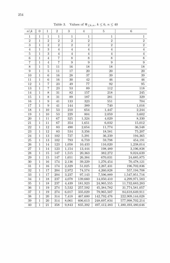
May 10, 2007 8:8 WSPC - Proceedings Trim Size: 9in x 6in ws-procs9x6
254
Table 3. Values of Ψ≤k,n, k ≤ 6, n ≤ 40
n\k 0 1 2 3 4 5 6
1 1 1 1 1 1 1 1
2 1 2 2 2 2 2 2
3 1 2 2 2 2 2 2
4 1 3 4 4 4 4 4
5 1 3 4 4 4 4 4
6 1 4 7 8 8 8 8
7 1 4 7 9 9 9 9
8 1 5 11 16 18 18 18
9 1 5 11 17 20 20 20
10 1 6 16 28 37 39 39
11 1 6 16 30 42 46 46
12 1 7 23 49 77 92 95
13 1 7 23 53 89 112 118
14 1 8 31 82 157 218 245
15 1 8 31 89 187 281 329
16 1 9 41 133 323 551 704
17 1 9 41 144 389 740 1,016
18 1 10 53 210 654 1,447 2,244
19 1 10 53 229 804 2,059 3,602
20 1 11 67 325 1,324 4,029 8,330
21 1 11 67 354 1,651 6,032 15,012
22 1 12 83 490 2,654 11,774 36,548
23 1 12 83 534 3,356 18,581 75,207
24 1 13 102 727 5,291 36,239 194,365
25 1 13 102 793 6,759 59,798 454,191
26 1 14 123 1,058 10,433 116,020 1,238,014
27 1 14 123 1,154 13,444 198,489 3,196,838
28 1 15 147 1,515 20,363 382,272 9,024,639
29 1 15 147 1,651 26,384 670,031 24,685,875
30 1 16 174 2,136 39,229 1,276,454 70,478,121
31 1 16 174 2,329 51,025 2,267,431 196,702,836
32 1 17 204 2,972 74,574 4,260,828 557,194,708
33 1 17 204 3,237 97,143 7,596,889 1,547,951,716
34 1 18 237 4,078 139,660 14,050,410 4,299,971,583
35 1 18 237 4,439 181,923 24,965,555 11,732,683,283
36 1 19 274 5,532 257,592 45,384,782 31,774,581,057
37 1 19 274 6,017 335,029 79,965,507 84,618,649,911
38 1 20 314 7,418 467,600 142,792,476 222,909,144,028
39 1 20 314 8,061 606,613 248,697,834 577,998,702,214
40 1 21 358 9,843 835,392 497,412,483 1,480,493,480,646

May 10, 2007 8:8 WSPC - Proceedings Trim Size: 9in x 6in ws-procs9x6
255
Table 4. Values of Ψk,n, k ≤ 6, n ≤ 40
n\k 0 1 2 3 4 5 6
1 1 0 0 0 0 0 0
2 1 1 0 0 0 0 0
3 1 1 0 0 0 0 0
4 1 2 1 0 0 0 0
5 1 2 1 0 0 0 0
6 1 3 3 1 0 0 0
7 1 3 3 2 0 0 0
8 1 4 6 5 2 0 0
9 1 4 6 6 3 0 0
10 1 5 10 12 9 2 0
11 1 5 10 14 12 4 0
12 1 6 16 26 28 15 3
13 1 6 16 30 36 23 6
14 1 7 23 51 75 61 27
15 1 7 23 58 98 94 48
16 1 8 32 92 190 228 153
17 1 8 32 103 245 351 276
18 1 9 43 157 444 793 797
19 1 9 43 176 575 1,255 1,543
20 1 10 56 258 999 2,705 4,301
21 1 10 56 287 1,297 4,381 8,980
22 1 11 71 407 2,164 9,120 24,774
23 1 11 71 451 2,822 15,225 56,626
24 1 12 89 625 4,564 30,948 158,126
25 1 12 89 691 5,966 53,039 394,393
26 1 13 109 935 9,375 105,587 1,121,994
27 1 13 109 1,031 12,290 185,045 2,998,349
28 1 14 132 1,368 18,848 361,909 8,642,367
29 1 14 132 1,504 24,733 643,647 24,015,844
30 1 15 158 1,962 37,093 1,237,225 69,201,667
31 1 15 158 2,155 48,696 2,216,406 194,435,405
32 1 16 187 2,768 71,602 4,186,254 552,933,880
33 1 16 187 3,033 93,906 7,499,746 1,540,354,827
34 1 17 219 3,841 135,582 13,910,750 4,285,921,173
35 1 17 219 4,202 177,484 24,783,632 11,707,717,728
36 1 18 255 5,258 252,060 45,127,190 31,729,196,275
37 1 18 255 5,743 329,012 79,630,478 84,538,684,404
38 1 19 294 7,104 460,182 142,324,876 222,766,351,552
39 1 19 294 7,747 598,552 248,091,221 577,750,004,380
40 1 20 337 9,485 825,549 496,577,091 1,479,996,068,163
May 10, 2007 8:8 WSPC - Proceedings Trim Size: 9in x 6in ws-procs9x6
256
References
[1] J. H. Conway and V. Pless, On the enumeration of self-dual codes, J. Combin.Theory A 28, 26 – 53 (1980).
[2] J. H. Conway, V. Pless, and N. J. A. Sloane, The binary self-dual codes oflength up to 32: a revised enumeration, J. Combin. Theory A 60, 183 – 195(1992).
[3] X. Hou, GL(m, 2) acting on R(r, m)/R(r − 1, m), Discrete Math. 149, 99 –122 (1996).
[4] X. Hou, On the number of inequivalent binary self-orthogonal codes, IEEETrans. Inform. Theory, to appear.
[5] W. C. Huffman, On the classification and enumeration of self-dual codes,Finite Fields Appl. 11, 451 – 490 (2005).
[6] W. C. Huffman and V. Pless, Fundamentals of Error-Correcting Codes (Cam-bridge University Press, Cambridge, 2003).
[7] V. Pless, A classification of self-orthogonal codes over GF(2), Discrete Math.3, 209 – 246 (1972).
[8] V. Pless and N. J. A. Sloane, On the classification and enumeration of self-dual codes, J. Combin. Theory A 18, 313 – 335 (1975).
[9] Mathematica, Wolfram Research, Inc. Champaign, IL,http://www.wolfram.com/
Related Documents