Advanced Statistics - Paolo Coletti

Advanced Statistics

Page 1

Advanced Statistics Paolo Coletti – A.Y. 2010/11 – Free University of Bolzano Bozen

Table of Contents

1. Statistical inference ................................................................................................................ 2 1.1 Population and sampling .............................................................................................................................................. 2

2. Data organization ................................................................................................................... 4 2.1 Variable’s measure ....................................................................................................................................................... 4 2.2 SPSS .............................................................................................................................................................................. 4 2.3 Data description ........................................................................................................................................................... 5

3. Statistical tests ........................................................................................................................ 7 3.1 Example ........................................................................................................................................................................ 7 3.2 Null and alternative hypothesis .................................................................................................................................. 11 3.3 Type I and type II error ............................................................................................................................................... 11 3.4 Significance ................................................................................................................................................................. 12 3.5 Accept and reject ........................................................................................................................................................ 12 3.6 Tails and critical regions ............................................................................................................................................. 13 3.7 Parametric and non‐parametric test .......................................................................................................................... 15 3.8 Prerequisites ............................................................................................................................................................... 15

4. Tests ..................................................................................................................................... 16 4.1 Student’s t test for one variable ................................................................................................................................. 16 4.2 Student’s t test for two populations ........................................................................................................................... 16 4.3 Student’s t test for paired data .................................................................................................................................. 18 4.4 F test ........................................................................................................................................................................... 19 4.5 One‐way analysis of variance (ANOVA) ...................................................................................................................... 20 4.6 Jarque‐Bera test.......................................................................................................................................................... 22 4.7 Kolmogorov‐Smirnov test ........................................................................................................................................... 22 4.8 Sign test ...................................................................................................................................................................... 23 4.9 Mann‐Whitney (Wilcoxon rank sum) test .................................................................................................................. 26 4.10 Wilcoxon signed rank test .......................................................................................................................................... 28 4.11 Kruskal‐Wallis test ...................................................................................................................................................... 30 4.12 Pearson’s correlation coefficient ................................................................................................................................ 32 4.13 Spearman's rank correlation coefficient..................................................................................................................... 34 4.14 Multinomial experiment ............................................................................................................................................. 36

5. Which test to use? ................................................................................................................ 41 6. Regression model ................................................................................................................. 43 6.1 The least squares approach ........................................................................................................................................ 43 6.2 Statistical inference .................................................................................................................................................... 46 6.3 Multivariate and non linear regression model ........................................................................................................... 47 6.4 Multivariate statistical inference ................................................................................................................................ 48 6.5 Qualitative independent variables ............................................................................................................................. 49 6.6 Qualitative dependent variable .................................................................................................................................. 50 6.7 Problems of regression models .................................................................................................................................. 51

Advanced Statistics

Page 2

1. Statistical inference Statistic is the science of data. This involves collecting, classifying, summarizing, organizing,

analyzing, and interpreting numerical information. A population is a set of units (usually people, objects, transactions, etc.) that we are interested in studying. A sample is a subset of units of a population, whose elements are called cases or, when dealing with people, subjects. A statistical inference is an estimate, prediction, or some other generalization about a population based on information contained in a sample.

For example, we may introduce a variable which models the temperature at midday in January. Clearly this is a random variable, since the temperature fluctuates randomly day by day and, moreover, temperatures of the future days cannot be even determined now. However, from this random variables we have data, measurements done in the past. In statistics people deal with observations or, in other words, realizations, , , ..., of a random variable . That is, each of is a random variable that has the same probability distribution as its originating random variable . It characterizes the th performance of the stochastic experiment determined by the random

variable . Given this information, we want to characterize the distribution of or some of its characteristics, like the expected value. In the simplest cases, we can even establish via theoretical considerations the shape of the distribution and then try to estimate from the data its parameters.

In other words, statistical inference concerns the problem of inferring properties of an unknown distribution from data generated by that distribution. The most common type of inference involves approximating the unknown distribution by choosing a distribution from a restricted family of distributions. Generally the restricted family of distributions is specified parametrically. For the temperature example we can assume that be normally distributed with a known variance σ and an expected value to be determined. Among all normal distribution with this variance we want to find the one which is the most likely candidate for having produced the finite sequence , , ..., of temperature observed in the past days.

Making inference about parameters of a distribution, people deal with statistic or estimates. Any function , , … , of the observations is called a statistic. For example, the sample

mean ∑ is a common statistic, typically used to estimate the expected value. The

sample variance ∑ is another useful estimate. Being a function of random

variables, a statistic is a random variable itself. Consequently we may, and will, talk about its distribution.

1.1 Population and sampling

A statistical research can analyze data from the entire population or only on a sample. The population is the set of all objects for which we want to infer information or relations. In this case, data set is complete and statistical research simply describes the situation without going on to any other objective and without using any statistical test. When data are instead available only on a sample, a subset of the population, statistical research analyses whether information and relations found on the sample can be extended on the entire population from which the sample comes from or they are valid only for that particular sample choice.

Therefore, sample choice is a very important and delicate issue in statistical researches. Many

Advanced Statistics

Page 3

statistical methods let us extend results (estimates or tests’ results) found on the sample to the population, provided that sample is a random sample, a sample whose elements are randomly extracted from the population without any influence from the researcher, from previously taken sample’s elements or from other factors. Building such a sample, however, is a difficult task since a perfectly random selection is almost a utopia. For example, any random sampling on people will necessarily include people who are unwilling to give information, who have disappeared, and who lie; these people cannot be excluded nor replaced with others, because otherwise the sample would not be random anymore. A previously random sample with excluded elements can screw the estimates: in our example, problematic people are typically old and with low education, thus unbalancing our sample in favor of young and educated subjects.

A common strategy to build a sample which behaves like a random sample is the stratified sampling. With this method, the sample is chosen respecting the proportions of the variables which are believed to be important for the analysis and which are believed to be able to influence the analysis results. For example, if we analyze people we should take care to build a sample which reflects the sex proportions, age, education and income distribution, the residence (towns, suburbs, countryside) proportions, etc. In this way, the sample will reflect exactly the population at least for what the considered variables are concerned. Whenever a person is not available for answering, we replace him with another one with the same variables’ values. Obviously these variables must be chosen with care and with a look at previous studies on the same topic, balancing their number since too few variables will create a badly stratified sample, while a too many will make sample creation and people’s substitution very difficult.

Another aspect is the sample size. Obviously, the larger the sample the better. However, this relation is not direct, i.e. doubling the sample size does not yield doubly better results. The relation in

many statistical tests goes approximately like √ , which means that we need to quadruple the sample size to get doubly better results. In any case, it is much more important to have a random or well stratified sample rather than a numerous sample. Quality is much better than quantity.

A common mistake related to sample size is supposing that it should be proportional to the population. This is, at least for all the test analyzed in this book, false: for large populations, test’s results depend only on the absolute size and not on the proportion. Thus, a population of 1000 with a sample of 20 does not yield better results compared to a population of 5000 with a sample of 20.

Advanced Statistics

Page 4

2. Data organization 2.1 Variable’s measure

In a statistical research we face basically three types of variables:

scale variables are fully numerical variables with an intrinsic mathematical meaning. For example, a temperature or a length are scale variables since they are numeric and any mathematical operation on these variables makes sense. Also a count is a numerical variable, even though it has restrictions (cannot be negative and is integer), because it makes sense to perform mathematical operations on it. However, numerical codes such as phone numbers or identification codes are not scale variables even though they seem numeric, since no mathematical operation makes sense on them and the number is used only as a code;

nominal variables represent categories such as sex, nationality, degree course, plant’s type. These variables divide the population into groups. Variables such as identification number are nominal since they divide the sample into categories, even though each case is a single category;

ordinal variables are a midway between nominal and scale variables. They represent categories which do not have a mathematical meaning (even though many times categories are identified by numbers, such as in a questionnaire’s answers) but these categories have an ordinal meaning, i.e. can be put in order. Typical examples are questionnaire’s answers such that “very bad”, “bad”, “good”, “very good”, or some time issues such as “first year”, “second year”, “third year”.

Ordinal and nominal variables, often referred to as categorical, are used in SPSS in two ways: as variables by themselves, such as in multinomial experiments (see section 4.14) and, more often, as a way to split the sample into groups to perform tests on two or more populations, such as Student T test for two populations (see section 4.2), ANOVA (see section 4.5), Mann‐Whitney (see section 4.9) and Kruskal‐Wallis (see section 4.11).

2.1.1 Grouping

It is also a common procedure to degrade scale variable them to ordinal variables, arbitrarily fixing intervals or bins and grouping the cases into their appropriate bin. For example, an age variable expressed in years can be degraded to an ordinal variable dividing the subjects into “young”, up to 25, “adult”, from 26 to 50, “old”, from 51 to 70, “very old”, 71 and over. The new variables that we obtain are suited for different statistical tests which open up more possibilities. However, any grouping procedure reduces the information that we have introducing arbitrary decisions in the data and possible biases. For example, if our sample has a very large count for people of age 26, the previous arbitrary choice of 25 as a limit for “young” group has put many people, who are more similar to 25 years old people rather than to 50 years old people, into the “adult” group.

SPSS: Transform Recode into Different Variables

2.2 SPSS

SPSS means Statistical Package for Social Sciences and it is a program to organize statistical data and perform statistical research. SPSS organizes data in a sheet called Data View which is a database table, more or less like Excel’s tables. Each case is represented by an horizontal lines and identified very often by the first variable which is an ID number. Variables instead use vertical

Advanced Statistics

Page 5

columns. Unlike Excel and like database tables, SPSS data table is extremely well structured and each variable has a lot of features. These features are found in Variable View sheet:

Name: feel free to use any meaningful name, but without special characters and without spaces. When data have many variables it is a good idea to indicate names as v_ followed by a number (it will be possible to indicate a human readable name later).

Type: numeric is the most common type. String should be used only for completely free text, while categorical variables should be numeric with a number corresponding to each category (it will be possible to indicate a human readable name later); a common mistake is using a string variable for a categorical variable, which has the impact that SPSS will refuse to perform certain operations with that variable.

Width and decimals

Label: this is the variable’s label which will appear in charts and tables instead of the variable’s name.

Values: this feature represents the association between values and categories. It is used for categorical variables, which, as said before, should use numbers for each category. In this field values’ labels can be assigned and in charts and tables these labels will appear instead of numbers. Obviously scale variables should not receive values’ labels.

Missing: whenever a variable’s value is unknown for a certain case a special numeric code should be used, traditionally a negative number (if the variable has only positive numbers) or the largest possible number such as 9999. If this number is inserted here among the missing values, SPSS will simply ignore that case whenever that variable is involved in any operation. It is also possible, in Data View, to clear the cell completely and SPSS will indicate it with a dot which is a system‐missing number (same effect as missing value).

Measure: variable’s measure must be carefully indicated, since it will have implications on which operations may be done on the variable.

SPSS has four basic menus:

Transform: this menu lets us build new variables or modify existing ones, usually working on a case by case base, thus performing only horizontal operations. Very useful are commands: o compute, which build a new variable, typically scale, using mathematical operations; o recode, which build a new variable, typically categorical, using recoding;

Data: this menu lets you rearrange your data in a more global way. Very useful are the commands: o split, splits the file using a nominal or ordinal variable in such a way to be able to analyze it

automatically in groups; o select, lets us filter out some temporarily undesired cases; o weight, lets us weight the cases using a variable whenever each case represents several cases

with the same data (all the statistics will use a new sample size based on the weights);

Analyze: this menu is the core of SPSS with all the statistical tests and models;

Graphs: this is the menu to create charts.

2.3 Data description

SPSS offers a variety of numerical and graphical tools to quickly describe data. The choice of the tool depends on variable’s measure:

Advanced Statistics

Page 6

SPSS: Analyze Descriptive Statistics Frequencies Frequencies is indicated as a description for a single categorical variable, while for a scale variable frequency table becomes too long and full of single cases. However, it is always a good idea to start any statistical research with frequencies for every variable, including scale ones, to spot out data entry mistakes which are very common in statistical data.

SPSS: Graphs Chart Builder Pie/Polar Pie chart is indicated as a graph for a single nominal and ordinal variable.

SPSS: Graphs Chart Builder Bar Pie charts are indicated as a graph for a single categorical variable. Using colors and three‐dimensionality they work also for two or even three nominal and ordinal variables.

SPSS: Analyze Descriptive Statistics Descriptives Descriptive statistics (mean, median, standard deviation, minimum, maximum, range, skewness, kurtosis) is indicated as a description for a single scale variable and usually it does not make sense for categorical variables.

SPSS: Graphs Chart Builder Histogram Histogram is indicated as a graph for a single scale variable. Variable values are grouped into bins for the variable representation. The choice of binning influences the histogram.

SPSS: Graphs Chart Builder Boxplot Boxplot is indicated as a graph for a single scale variable. The central line represents the median and the box represents the central 50% of the variable’s distribution on the sample. Boxplots may be used also to compare the values of a scale variable by groups of a categorical variable.

SPSS: Analyze Descriptive Statistics Crosstabs Contingency table (see section 4.14.2) is indicated as a description for two categorical variables.

SPSS: Analyze Compare Means Means Means comparison is a way to compare the means of a scale variable for groups of a categorical variable, usually followed by Student’s T test or ANOVA (see sections 4.2 and 4.5).

SPSS: Analyze Correlate Bivariate Bivariate correlation (see sections 4.12 and 4.13) is a description for the linear relation between two scale variables.

SPSS: Graphs Chart Builder Scatter/Dot Scatterplot is indicated as a graph for two scale variables.

Advanced Statistics

Page 7

3. Statistical tests Statistical tests are inference tools which are able to tell us the probability with which results

obtained on the sample can be extended to the population.

Every statistical test has these features:

the null hypothesis H0 and its contradictory hypothesis H1. It is very important that these hypotheses are built without looking at the sample;

a sample of observations , , . . . , and a population, to which we want to extend information and relations found on the sample;

prerequisites, special assumptions which are necessary to perform the test. Among these assumptions there is always, even though we will not repeat it every time, that data must come from a random sample;

the statistic , , . . . , , a function calculated on the data, whose value determines the result of the test;

a statistic’s distribution from which we can obtain the test’s significance. When using statistical computer programs, significance is automatically provided by the program next to the statistic’s value;

significance, also called p‐value, from which we can deduct whether accepting or rejecting null hypothesis.

3.1 Example

In order to show all the elements of a statistical test, we run through a very simple example and we will, later, analyze the theoretical aspects of all the test’s steps.

We want to study the age of Internet users. Age is a random variable for which we do not have any idea of the distribution nor its parameters. However, we make the hypothesis that age is a continuous random variable with an expected value. We want to check whether the expected value is 35 years or not. We formulate the test’s hypotheses:

H0: E age 35 H1: E age 35

Of this random variable the only thing we know are the observations on a random sample of 100 users, which are: 25; 26; 27; 28; 29; 30; 31; 30; 33; 34; 35; 36; 37; 38; 30; 30; 41; 42; 43; 44; 45; 46; 47; 48; 49; 50; 51; 52; 20; 54; 55; 56; 57; 20; 20; 20; 30; 31; 32; 33; 34; 35; 36; 37; 38; 39; 40; 41; 42; 43; 44; 45; 46; 47; 48; 49; 50; 20; 21; 22; 23; 24; 25; 26; 27; 28; 29; 30; 31; 32; 33; 34; 35; 36; 37; 38; 39; 40; 35; 36; 37; 35; 36; 37; 35; 36; 37; 35; 36; 37; 35; 36; 37; 35; 36; 37; 35; 36; 37; 35.

Now we calculate the age average on the sample, age 36.2, which is an estimation for the expected value. We compare this result with the 35 of the H0 hypothesis and we find a difference of 1.2. At this point, we ask ourselves whether this difference is large enough, implying that the expected value is not 35 and thus H0 must be rejected, or is small and can be caused by an unlucky choice of the sample and therefore H0 must be accepted.

This conclusion in a statistical research cannot be drawn from a subjective decision whether the difference is large or small. It is taken using formal arguments and therefore we must rely on this

Advanced Statistics

Page 8

statistic function:

age hypothesized expected value

sample variance⁄

It is noteworthy to look at this statistic numerator. When the average of age is very close to the hypothesized expected value, the statistic will be close to 0. On the other hand, when the two quantities are very different, compared to the sample standard deviation, the statistic is very large. Statistic’s value is also influenced by the sample’s number of elements : the larger is the sample, the larger the statistic.

Summing up, considering that in our case the sample standard deviation is 8.57, statistic is 1.40. The situation is therefore

At this point we ask ourselves where is exactly the point which separated the “H0 true” zone from the “H0 false” zone. To find it out, we calculate the probability to obtain an even worse result than the one we have got now. The meaning of “worse” in this situation is “worse for H0”, therefore any result

larger than 1.40 or smaller than – 1.40. We use central limit theorem which guarantees us that, if is large enough and if the hypothesized expected value is the real expected value of the

distribution (i.e. H0 is true), our statistic has a standard normal distribution. In fact, the only reason why we have built this statistic instead of using directly the difference at the numerator is because we know the statistic’s distribution. Therefore we know that the probability of getting a value larger than

1.40 or smaller than – 1.40 is1 16%. This value is called significance or p‐value.

If significance is large it means that, supposing H0 to be true and taking another random

sample, the probability of obtaining a worse result is large and therefore the result that we have

1 This value can be calculated through normal distribution tables or using English Microsoft Excel function NORMDIST(‐1.4;0;1;TRUE) which gives the area under the normal distribution on the left of ‐1.4, equal to 8%. Area on the right of +1.4 is obviously the same.

‐3 ‐2 ‐1 0 1 2 3+1.4‐1.4

H0 probably false

0

H0 probably true

+1.40

H0 probably false

Advanced Statistics

Page 9

obtained can be considered to be really close to 0, something which pushes us to accept the idea that H0 is true. When, instead, significance is small, it means that if we suppose that H0 is true we have a small probability of getting such a bad result, something which pushes us to believe that H0 be false. In the example’s situation we have a significance of 16%, which usually is considered large (the chosen cut point is typically 5%) and therefore we accept H0.

A slightly different method, which yields to the same result, is fixing the cut point a priori, let’s say 5%, and finding the corresponding critical value after which the statistic is in the rejection region. In our case, considering two areas of 2.5% on the left and on the right side, the critical value for a standard normal distribution is2 1.96.

At this point the situation is

The first method gives us an immediate and straightforward answer and in fact is the one typically used by computer programs. The second method instead is more suited for one‐tailed tests and is easier to apply if a computer is not available.

An example of a one‐tailed test is the situation when we want to check whether the expected value of the age is smaller or larger than 35. We write the hypotheses in this way:


In this case, the difference of 1.2 between sample average and 35, since it is positive, leads us to strongly believe that H0 be true. In fact, now the situation of the statistic is different from before, i.e.

2 This value can be calculated through normal distribution tables or using English Microsoft Excel NORMINV(2.5%;0;1) which gives the critical value –1.96 for which the area under the normal distribution on the left of it is 2.5%. Due to symmetricity of the distribution, critical value on the right is obviously +1.96.

‐3 ‐2 ‐1 0 1 2 3+1.96‐1.96

H0 probably false H0 probably false

0

H0 probably true

+1.40 +1.96 ‐1.96

Advanced Statistics

Page 10

In fact here we do not have any doubt since the statistic value falls right in the middle of the “H0 true” area.

Writing however the hypotheses in this way:


In this case, the situation of the statistic is

and here we have the same problem of determining whether 1.40 is close to 0 or far away from it. As usual, to determine it we have two methods. The first one calculates the probability of getting a worse result, where worse means “worse for H0”. In this situation, however, a worse result is larger

than 1.40, while results smaller than – 1.40 are strongly in favor of H0. The statistic is always distributed like a standard normal, under the hypothesis that H0 be true,

and the area, thus the significance, is 8%. Using the second method the critical value is not 1.96 anymore, but3 1.64. The critical region is larger than before, since now the 5% is all concentrated on the left part.

3 This value can be calculated through normal distribution tables or using English Microsoft Excel NORMINV(5%;0;1) which gives the critical value –1.64 for which the area under the normal distribution on the left of it is 5%. Due to symmetricity of the distribution, critical value on the right is obviously +1.64.

‐3 ‐2 ‐1 0 1 2 3+1.4

H0 probably false H0 probably true

0

H0 probably true

+1.40 +1.64

H0 probably true

0

H0 probably true

+1.40

H0 probably false

H0 probably false

0

H0 probably true

+1.40

H0 probably true

Advanced Statistics

Page 11

3.2 Null and alternative hypothesis

The hearth of a statistical test is null hypothesis H0, which represents the information that we are officially trying to extend from the sample to the population4. It is important that the null hypothesis gives us additional information, since we need to suppose it to be true and use its information to know the statistic’s distribution. If, in the previous example, the null hypothesis had not given us the additional information that the real expected value be 35, we could not use the fact that that statistic function be normally distributed. Therefore, the null hypothesis must always contain an equality, while strict inequalities are reserved for H1. When the test is one‐tailed, we write the null hypothesis in the form of a non‐strict inequality such as E age 35 for practical purposes, but theoretically we should write the equality E age 35 and simply not take into account the E age 35 possibility.

For example, usable hypotheses are “E 35” or “distribution of is exponential” or even “ and are independent”. On the other hand, hypotheses such as “E 35” or “distribution of is not exponential” are not acceptable. Also “ and are dependent” is not acceptable, since it

does not provide us with any information on how they are dependent.

Together with null hypothesis we always write alternative hypothesis H1, which is the logical contradiction of null hypothesis.

3.3 Type I and type II error

Once the statistic is calculated we must take a decision: accept H0 or reject H0. When H0 is rejected, we face one of the two following situations:

null hypothesis is really false and we rejected it: very good;

null hypothesis is really true and we rejected it: we committed a type I error.

If we accept H0, we face one of the two following situations:

null hypothesis is really false and we accepted it: we committed a type II error;

null hypothesis is really true and we rejected it: very good.

There are two different types of errors that we may commit when taking a decision after a statistical test and it would be wonderful if we could reduce at the same time the probability of committing both errors. Unfortunately, the only method to reduce the probability to commit both errors is taking a large sample, hopefully taking the entire population. This thing is clearly not feasible in many situations where gathering data is very expensive.

There is a method to reduce probability of committing a type I error: rejecting only in the situations where H0 is evidently false. In this way a type I error will be very rare since we are rejecting in very few situations. Unfortunately, if we reject with parsimony, we will accept very often and this means committing a lot of type II errors. Same thing if, vice versa, we reject too much: we will commit very few type II errors but many type I errors.

Thus, we must decide which error is the more severe one and try to concentrate on reducing the probability of committing it. Every statistical research concentrates on type I errors, trying to

4 As we will see later, it is instead H1 the information that we will be able to extend to the population, while, unfortunately, it is never possible to extend H0.

Advanced Statistics

Page 12

reduce the probability of committing them under a significance level usually 5% or 1%. Using an example drawn from a juridical situation:

H0: suspect deserves 0 years of prison (suspect is innocent)

H1: suspect deserves > 0 years of prison (suspect is guilty)

In this case, a type I error means condemning an innocent, while a type II error means an innocent verdict for a guilty. It is common belief that in this case a type I error should be avoided at all cost, while a type II error be acceptable.

The reason why statistical tests concentrate their attention on avoiding type I errors derived from the historical development of science which takes as correct the current theories (H0) and tries to minimize the error to destroy, by mistake, a well‐established theory in favor of new theories (H1). It is therefore a conservative approach. For example:

H0: heart pumps blood

H1: heart does not pump blood

A type I error in this case would be a disaster since it would mean rejecting the correct hypothesis that blood is pumped by hearǘ, giving us no other clue since H1 carries only a negative information.

3.4 Significance

Significance or p‐value is the probability of committing a type I error. This probability is calculated assuming that H0 be true and comparing the value of the statistic that we calculate on our sample’s data with the statistic’s distribution. A small significance means that if we reject we have only a small probability of committing a mistake, and therefore we will reject. A large significance means that if we reject we are facing a large probability of committing a mistake, and therefore we will accept H0.

Another equivalent definition for the significance is the probability of obtaining, taking another random sample, an equal or worse statistic’s value under the hypothesis that H0 be true. A small significance means that the statistic’s value is really bad and therefore we will reject H0. A large significance means that the statistic’s value is much better than what we expected and therefore we will accept H0.

Since we try to minimize type I errors, we will fix a very small significance level under which null hypothesis is rejected, usually 5% or 1%. In this way, probability of a type I error is low and when we reject we are almost sure that H0 is really false.

Confidence is equal to 100% minus the significance.

3.5 Accept and reject

At the end of the statistical test we must decide whether accepting or rejecting:

if significance is above the significance level (usually 5% or 1%), we accept H0;

if significance is below the significance level, we reject H0.

It is very important to underline the fact that when we reject we are almost sure that H0 is false, since we are keeping type I errors under a small significance level. However, when we accept we may not say that H0 be true, since we do not have any estimation on type II errors. Therefore, rejecting is a sure thing, while accepting is a “no answer” and from it we are not allowed to draw any conclusion.

Advanced Statistics

Page 13

This approach is called falsification, since we are only able to falsify H0 and never to prove it. If we need to prove that H0 be true, we must rewrite the hypotheses and put the information we want to extend to the population in the H1 hypothesis instead, perform the test again and hope to reject.

Another important effect that we must underline is the sample size. When sample size is extremely small, data are almost random and probability of committing type I error is very large. Therefore significance is very large and, using the traditional small significance levels, we will accept. Therefore a statistical test with few data automatically accepts everything, since it does not have enough data to prove that H0 be false. Again, accepting must never imply that H0 be true.

3.5.1 Paradox

Using the falsification approach we can, through a smart choice of null hypotheses, accept two contradictory null hypotheses. Using as sample the one of the previous example and formulating the hypotheses


we accept E age 35 with a significance level of 5%. Using instead these hypotheses


we accept E age 36 with a significance level of 5%. We have thus accepted two hypotheses which say different and contradictory things. This is only an apparent paradox, since accepting does not mean that they are true but only that they might be true. Therefore, for the population from which our sample is extracted, the expected value might be 35 or 36 (or many other close values, such as 35.3, 36.5, 37, etc.). This is due to a relatively small size of the sample; if we increase the sample size, the interval of values for which we accept would decrease.

3.6 Tails and critical regions

Statistical tests where the null hypothesis contains an equality and alternative hypothesis a not equality are two‐tailed tests. Statistical tests where the null hypothesis contains a non‐strict inequality and alternative hypothesis a strict inequality are one‐tailed tests, such as


The name of these tests comes from the number of critical regions. A critical region is an area for which null hypothesis is rejected when the statistic’s value falls in that area, according to the second method that we have seen in the example 3.1. The number of critical regions, which usually are far away from the center of the distribution and therefore are called tails, determines the name of the test two‐tailed or one‐tailed.

two‐tailed test

critical region critical region

0

+C –C

Advanced Statistics

Page 14

one‐tailed test with critical region on the right one‐tailed test with critical region on the left

The point where the critical region starts is called critical value and is usually calculated from tables of the statistic’s distribution. In the two‐tailed test the two regions are always symmetric, while for one‐tailed test we face the problem of determining on which side is the rejection region.

In order to find where the critical region is in one‐tailed tests, we try to see what happens if we have an extremely large positive value for the statistic. If such an extremely large positive value (which, being very large, is for sure in the right tail) is not in favor of null hypothesis, it means that the right tail is not in favor of null hypothesis and therefore it is the rejection region. Otherwise, if this extremely large value of the statistic is in favor of the null hypothesis, the right region is not a rejection region and the critical region is on the left. For example, we consider example 3.1


and we use the same statistic age

sample variance⁄. When this statistic’s value is positive and

extremely large, it means that the average of age is much more than the hypothesized expected value and this is a clear indication that the real expected value is much larger than 35. This is in contradiction with null hypothesis which says that expected value must be smaller or equal to 35. Therefore a positive value of the statistic, on the right tail, is contradicting null hypothesis and this means that right tail is a critical region.

Considering instead hypotheses

H0: E age 35 H1: E age 35,

when the statistic’s value is positive and extremely large, it means that the average of age is much more than the hypothesized expected value and this is a clear indication that the real expected value is much larger than 35. This is exactly what the null hypothesis says. Therefore a positive value of the statistic, on the right tail, is in favor of the null hypothesis and this means that right tail is not critical region. Therefore the critical region is on the left.

Some important features to note on critical values:

decreasing significance level implies that critical value goes away from 0. This is evident if we consider the fact that decreasing the significance level we are even more afraid of type I errors

critical region

0 – 1.41

critical region

0 +1.41

critical region

0 – C

critical region

0

+C

Advanced Statistics

Page 15

and therefore we reject with much more care, thus reducing the rejection zone;

the critical value of a one‐tailed test is always closer to 0 than the critical value of two‐tailed tests. This is because the critical tail of a one‐tailed test must contain the probability that for a two‐tailed test in split in two regions and therefore the zone must be larger;

for each two‐tailed test there are two corresponding one‐tailed tests. One of them has the statistic’s value completely on the other side of the rejection region, therefore for this one we always accept. This is the reason why using the significance method to determine whether accepting or rejecting can be misleading for one‐tailed tests, since it is not evident whether the test has an obvious accept verdict or not.

3.7 Parametric and nonparametric test

There are parametric and non‐parametric statistical tests. A parametric test implies that the distribution in question is known up to a parameter or several parameters. For example, it is believed that many natural phenomena are normally distributed. Estimating and of the phenomenon is a parametric statistical problem, because the shape of the distribution, a normal one, is known up to these two parameters. On the other hand, non‐parametric test do not rely on any underlying assumptions about the probability distribution of the sampled population. For example, we may deal with continuous distribution without specifying its shape.

Non‐parametric tests are also appropriate when the data are non‐numerical in nature but can be ranked, thus becoming rank tests. For example, taste‐testing foods we can say we like product A better than product B, and B better than C, but we cannot obtain exact quantitative values for the respective measurements. Other examples are tests where the statistic is not calculated on sample’s values but on the relative positions of the values in their set.

3.8 Prerequisites

Each test, especially parametric ones, may have prerequisites which are necessary for the statistic to be distributed in a known way (and thus for us to calculate its significance).

A typical prerequisite for many parametric tests is that the sample comes from a certain distribution. To verify it:

if data are not individual measures but are averages of many data, the central limit theorem guarantees us that they are approximately normally distributed;

if data are measures of a natural phenomena, they are often affected by random errors which are normally distributed;

we can hypothesize that data comes from a certain distribution if we have theoretical reasons to do it;

we can plot the histogram of the data to have a hint on the original population’s distribution, if the sample size is large enough;

we can perform specific statistical tests to check the population’s distribution, such as Kolmogorov‐Smirnov or Jarque‐Bera tests for normality.

Every test has as a prerequisite that the sample be a random sample, even though we will not indicate it.

Advanced Statistics

Page 16

4. Tests 4.1 Student’s t test for one variable

Prerequisites: variable normally distributed (if sample variance is used).

H0: expected value =

Statistic: n

m

/ variancesampleor population

average sample

Statistic’s distribution: Student’s t with 1 degrees of freedom; when 30 standard normal.

SPSS: Analyze Compare Means One‐Sample T Test

William “Student” Gosset

(1886‐1937)

Student’s t test is the one we have already seen in the example in its large sample version. It is a test which involves a single random variable and checks whether its expected value is or not.

For example, taking 32 and a sample of 10 elements: 25; 26; 27; 28; 29; 30; 30; 31; 33; 34

H0: E 32 H1: E 32

Sample average is 29.3 and sample standard deviation is 2.91. Statistic is therefore – 2.94 and its significance is5 1.7%. H0 is rejected since 1.7% is below significance level; this means that extracting another sample of 10 elements from a distribution with an expected value equal to 32, we have a very small probability of getting such bad results. We can thus say that expected value is not 32.

As we can easily see, Student’s t test for one variable is exactly the test version of the average confidence interval.

4.2 Student’s t test for two populations

Prerequisites: two populations A and B and the variable must be distributed normally on the two populations

H0: expected value on population A = expected value on population B

Statistic:

BA

BA

nnn

n n 112

varianceB populationor sample1A variance populationor sample1

average B sample averageA sample

Statistic’s distribution: Student’s t with 2 degrees of freedom; when 31 standard normal.

SPSS: Analyze Compare Means Means SPSS: Analyze Compare Means Independent‐Samples T Test

5 Significance can be calculated in two ways. (1) Using Student’s t distribution table. (2) Using English Microsoft Excel function TDIST(2.94;9;2) which gives us the sum of the two tails areas, those on the left of ‐2.94 and on the right of +2.94.

Advanced Statistics

Page 17

This test is used whenever we have two populations and one variable calculated on this population and we want to check whether the expected value of the variable changes on the populations.

For example, we want to test

H0: E height for male E height for female H1: E height for male E height for female

We take a sample of 10 males (180; 175; 160; 180; 175; 165; 185; 180; 185; 190) e 8 female (170; 175; 160; 160; 175; 165; 165; 180). We suppose that male’s and female’s heights are normally distributed with the same variance. Male’s sample average is 177.5 while for female it is 168.75. Statistic’s value is 2.18. Since it is one‐tailed test we draw the graph to have a clear idea where does the statistic fall.

If the statistic were extremely large, this would be strongly in contradiction with H0 and therefore rejection region in on the right.

Critical value for one‐tailed test is6 1.76 and therefore we reject. Using instead the significance method, after having checked that statistic does not fall on the “H0 true” area, we get

7 a significance of 2.2% and therefore we reject, meaning that male population has an expected height significantly larger than female population.

6 Critical value can be calculated in two ways. (1) Using English Microsoft Excel function TINV(5%;16), which gives us the critical value for the two‐tailed test, therefore probability split into 2.5% and 2.5%. For one‐tailed test probability must be doubled, TINV(10%;16), since in this way it would be split into 5% and 5%. (2) Using Student’s t distribution table.

7 Significance can be calculated in four ways. (1) Using one of the statistical t tests (Zweistichproben t test) in the Data Analysis tookpak in Microsoft Excel, choosing among known variances (in this case populations’ variances have to be indicated explicitly), equal and unknown, different and unknown (in these latter two cases populations’ variances are estimated from sample data automatically by Excel), which gives us statistic’s value and its significance. (2) Using English Microsoft Excel function TTEST which gives us the significance directly from the data, choosing type=2 if we suppose equal variances or type=3 if we suppose different variances. (3) Using English Microsoft Excel function TDIST(2.18;16;1) which gives us the area of one of the two tails. (4) Using Student’s t distribution table.


0

H0 probably true

+1.76 +2.18

0

H0 probably true

+2.18

Advanced Statistics

Page 18

4.3 Student’s t test for paired data

Prerequisites: two variables and on the same population and – must be normally distributed

H0: E E , which means E –E

The test can also be performed with null hypothesis: H0: E – E

Statistic: we use – as variable and we perform Student’s t test for one variable

Statistic’s distribution: same as Student’s t test for one variable

SPSS: Analyze Compare Means Paired‐Samples T Test

This test is used whenever we have a single population and two variables calculated on this population and we want to check whether the expected value of these two variables is different.

For example, we want to test whether population’s income in a country has changed. We take a sample of 10 people’s income and then we take the same 10 subjects’ income the next year

Income 2010 (thousands €)

Income 2011 (thousands €)

Difference 2010 – 2011

20 21 ‐1

23 23 0

34 36 ‐2

53 50 +3

43 40 +3

45 44 +1

36 12 +24

76 80 ‐4

44 45 ‐1

12 15 ‐3

Two things are very important here. The subjects must be exactly the same, no replacement is clearly possible. When calculating the difference the sign is important, so it is a good idea to clearly write what is subtracted from what, especially for one‐tailed tests.

Hypotheses are:

H0: E income for 2010 – E income for 2011 0 H1: E income for 2010 – E income for 2011 0

Sample average for the difference is 2.0 and sample standard deviation is 8.07. Statistic is 0.78 with8 a significance of 45.3%. H0 is thus accepted. This does not mean that income has remained the same, but simply that our data are not able to prove that it has changed.

8 Significance can be calculated in four ways. (1) With the Student’s t test for one variable formula using m=0. (2) Using English Microsoft Excel function TTEST which gives us the significance directly from the data, choosing type=1. (3) Using the statistical t test (Zweistichproben t test bei abhängig Stichproben) in the Data Analysis tookpak in Microsoft Excel, which gives us statistic’s value and its significance. (4) Using Student’s t distribution table.

Advanced Statistics

Page 19

4.4 F test

Prerequisites: two populations A and B and the variable must be distributed normally on the two populations

H0: Var on population A = Var on population B

Statistic: sample A variance/sample B variance

Statistic distribution: Fisher’s F distribution with – 1 and – 1 degrees of freedom

George Waddel Snedecor (1881‐1974)

Ronald Fisher

(1890‐1962)

The name of this test was coined by Snedecor in honor of Fisher. It checks the variances of two populations. It is interesting to note that, unlike all the other tests, statistic’s best value for H0 is 1 and not 0. Since F distribution is only positive and not symmetric, special care must be taken into account on the statistic’s position when calculating the significance since it can be misleading. In particular, the opposing statistic’s value is not the opposite but the reciprocal.

For example, supposing that height for male and female is normally distributed, we test

H0: Var height for male Var height for female H1: Var height for male Var height for female.

We use the previous sample and we get a sample variance of 84.7 for male and 55.4 for female. Statistic is thus 1.53. Degrees of freedom are 9 and 7. The two critical values are9 4.82 and

.0.21 and therefore we accept H0. Using the significance method, after having checked that the

statistic is on the right of 1, we get an area of 29% for the right part and therefore significance is 58%.

9 Calculation of critical values or significance can be done in different ways. (1) Using the statistical F test (Zwei‐Stichproben F‐Test) in the Data Analysis tookpak in Microsoft Excel, which gives us statistic’s value and its significance. (2) Using English Microsoft Excel function FTEST which gives us the significance directly from the data. This method can be misleading when statistic is on the left of 1. (3) Using English Microsoft Excel function FDIST(1.53;9;7) which gives us the area of the right tail. (4) Using English Microsoft Excel function FINV(2.5%;9;7) and 1/FINV(2.5%;9;7) to get the two critical values. Pay attention to the inverted degrees of freedom for the second calculation. (5) Using F distribution table, which however usually provides only the critical values.

1

critical region critical region

4.82 1.53 0 0.21

Advanced Statistics

Page 20

4.5 Oneway analysis of variance (ANOVA)

Prerequisites: populations, variable is normally distributed on every population with the same variance

H0: expected value of the variable is the same on all populations

Statistic: Variance Between

Variance Within∑ ∑ ∑

Statistic distribution: Fisher’s F distribution with degrees of freedom equal to – 1 and –

SPSS: Analyze Compare Means Means SPSS: Analyze Compare Means One‐Way ANOVA

This test is the equivalent of Student’s t test for two unpaired populations when the populations are more than two. We note that if only one population has an expected value different from the other, the test rejects. Therefore, a rejection guarantees us that populations do not have the same expected value but does not tell us which populations are different and how. Optimal statistic value for H0 is 0 and, since F distribution has only positive values, this test has only the right tail.

For example, we have heights for young (180; 170; 150; 160; 170), adults (170; 160; 165) and old (155; 160; 160; 165; 175; 165) and we want to check

H0: E height for young E height for adults E height for old H1: at least one of the E height is different from the others

We suppose heights are normally distributed with the same variance. From data we get a sample average of 166 for young, 165 for adults and 163.3 for old. Now we ask ourselves whether these differences are large enough to say that there are differences among populations’ expected values or not.

The origins of the analysis of variance lie in the splitting of sample’s variance in this way10:

10 Variance ∑ ∑ ∑ ∑ ∑ ∑ ∑

2 ∑ ∑ ∑ ∑

Advanced Statistics

Page 21

Variance1 1

We now define the sample’s variance between groups as a measure of the averages variations between values of different groups

variance between111

and the sample’s variance within group as a measure of the variations among values of the same group

variance within1 1

The idea behind the test is to compare these two measures: if the variance between is much larger than the variance within, it means that at least one population is significantly different from the others, while if the variance between is not large compared to the variance within it means that variations due to a change in the population have the same size as variations due to other effects and can thus be considered negligible. Simplifying the 1/ the statistic is

variance betweenvariance within

11

1

which is distributed as a Fisher’s F distribution with 1 and degrees of freedom. Rejection region is clearly on the right, since that area is the one where Variance Between is much larger than Variance Within.

Going back to our example, statistic’s value is . ⁄

. /0.136 with degrees of freedom

2 and 11 and a significance11 of 87.4% and therefore we accept.

∑ ∑ ∑ ∑ ∑

∑ ∑ ∑ 0

11 Significance can be calculated in different ways. (1) Using the one‐way ANOVA (ANOVA: Einfaktorielle Varianzanalyse) in the Data Analysis tookpak in Microsoft Excel, which gives us statistic’s value and its significance. (2) Using English Microsoft Excel function FDIST(0.136;2;12) which gives us the area of the right tail. (3) Using F distribution table, which usually provides the right side critical values.

Advanced Statistics

Page 22

4.6 JarqueBera test

Prerequisites: none.

H0: variable follows a normal distribution

Statistic:

4

Kurtosis sampleskewness sample

6

22n

Statistic distribution: Jarque‐Bera distribution. When 2000, chi square distribution with 2 degrees of freedom.

Carlos Jarque Anil Bera

This test checks whether a variable is distributed, on the population, according to a normal distribution. It uses the fact that a normal distribution has always a skewness and a Kurtosis of 0. Its statistic is clearly equal to 0 if the sample’s data have a skewness and Kurtosis of 0 and increases if these measures are different from 0. The statistic is multiplied by , meaning that if we have many data they must have display very small skewness and Kurtosis to get a low statistic’s value.

Sample’s skewness and sample’s Kurtosis are calculated as

1

1

1

13.

4.7 KolmogorovSmirnov test

Prerequisites: none.

H0: variable follows a known distribution

Statistic: supnumber of sample data

, where

is the cumulative distribution of the known r.v.

Statistic distribution: Kolmogorov distribution

SPSS: Analyze Nonparametric Tests One Sample

Andrey Kolmogorov (1903‐1987)

Vladimir Ivanovich Smirnov

(1887‐1974)

This is a rank test which checks whether a variable is distributed, on the population, according to a known distribution specified by the researcher. The test for each calculates the the difference between the percentage of sample’s data smaller than this and the probability of getting a value smaller than from the known distribution. Clearly, if sample’s data are distributed according to the known distribution, these differences are very small for every since the percentage of smaller values reflects exactly the probability of finding smaller values. The statistic is defined as the maximum, for all the , of these differences.

For example, we want to check whether data 3; 4; 5; 8; 9; 10; 11; 11; 13; 14 come from a

N 9; 25 distribution. For 2 , number of sample data

N 9;25 2 |0 0.05| 0.05 ; for

3 , number of sample data

N 9;25 3 |0 0.08| 0.08 ; for 4 , number of sample data

N 9;25 4 |0.1 0.12| 0.02; for 5 , number of sample dataN 9;25 5 |0.2 0.16|

Advanced Statistics

Page 23

0.04 and so on. Obviously, this calculation is not done only for integer values but for all values and doing it manually is, in many cases, a very hard task. In this case, the maximum is 0.21 obtained for a value of immediately after 11. Its significance is much larger than 5% and therefore we accept.

4.8 Sign test

Prerequisites: continuous distribution.

H0: median is

Statistic: outcomes on the left or on the right of

Statistic distribution: B ; 50% ; for 10 . . ·

√ . ·~N 0; 1

SPSS: Analyze Nonparametric Tests One Sample

Sign test is a rank test which tests the central tendency of a probability distribution. It is used to decide on whether the population median equals or not the hypothesized value.

Consider the example when 8 independent observations of a random variable having a continuous distribution are 0.78, 0.51, 3.79, 0.23, 0.77, 0.98, 0.96, 0.89. We have to decide whether the distribution median is equal to 1.00. We formulate the two hypotheses:

H0: 1.00 H1: 1.00

If the null hypothesis is true, we expect approximately half of the measurements to fall on each side of the hypothesized median. If the alternative is true, there will be significantly more than half on one of the sides. Thus, our test statistic will be either or . These two quantities denote the number of observations falling below and above 1.00 . Since was assumed to have a continuous distribution, P 1.00 0. In other words, every observation falls either below of above 1.00, never hitting this value itself. Consequently, 8. In practice it can be that an observation is exactly 1.00. In this situation, since this observation is strongly in favor of H0 hypothesis, we will consider it to belong to when is larger and to when is larger.

Note that this choice of test statistic does not require having exact values of the observations. In fact, it is enough to know whether each observation is larger or smaller than 1.00. To the contrary, the corresponding small sample parametric test (which is the Student’s t test for one variable) requires exact values in order to calculate the sample’s average and variance.

Now we take and consider the significance of this test. This is the probability (assuming that H0 is true) of observing a value of the test statistic that is at least as contradictory to the null hypothesis, and thus supportive to the alternative hypothesis, as the actual one computed from the sample data. In our case 7. There are two more contradictory outcomes of the experiment: when 8, the case when all observations have fallen on the same side of the hypothesized median, and when 0. And there is a result which is as contradictory as the one we have,

1. Thus significance equals P 7 P 8 P 1 P 0 .

Note that the distribution of has a binomial distribution B 8; 0.5 . Indeed, if we suppose that H0 is correct, having an outcome on the left of 1.00 is an event with probability 50%. And having outcomes on the left of 1.00 on a total of 8 independent observations is a binomial with 50% and 8. Therefore, remembering that

Advanced Statistics

Page 24

P B ;!

! ! 1

we can calculate12 P 7 P 8 0.035. Remembering that the binomial distribution in the particular case of 50% is symmetric and therefore P 1 P 0 P 7P 8 , we get that significance is 7%. Setting a significance level of 5%, we accept null hypothesis meaning that our data are not able to support the hypothesis that median is not 1.00.

The corresponding one‐tailed test is used to decide on whether the distribution median equals to the hypothesized value or falls below/exceeds it. Referring to the set of data considered above, the corresponding two mutually exclusive hypotheses read, for example:

H0: 1.00 H1: 1.00

As test statistic we choose . In order to find out where is the rejection region, we note that when our statistic is huge the observations falling below 1 will be more numerous than the ones exceeding 1 and this is in favor with the alternative hypothesis. Thus the zone on the right is the rejection region, while the zone on the left, where is small, is not a rejection region. Because 7, there is only one more contradictory to H0 outcome is 8. Thus the significance equals P 7 P 8 . The random variable has always a binomial distribution whose probability of a success is 1/2 and we conclude that the significance is P B 8; 50% 7P B 8; 50% 8 3.5%.

Thus, when H0 is true, the probability to face an outcome as contradictory as the actually observed one or an outcome more contradictory to H0, equals 3.5%. Consequently, the sample data suggest that if we reject H0 we may be wrong in only 3.5% of the cases.

Note that, as compared with the two‐tailed test, now the probability of type I error is two times smaller although the sample information remains the same. This is not surprising because the one‐tailed test starts from a more precise guess, it starts with the implicit hypothesis that can never be larger than 0.

If we make the other one‐tailed test instead:

H0: 1.00 H1: 1.00,

if we take as statistic, in order to find out where is the rejection region, we note that when our statistic is huge the observations falling below 1 will be more numerous than the ones exceeding 1 and this is in favor with the null hypothesis. Therefore larger values of the statistic are all in favor of

12 These quantities can be much easily calculated in two different ways: (1) using binomial distribution cumulative tables, which give directly P B ; and in our case P(B(8;50%)=7) + P(B(8;50%)=8) = 100% – P(B(8;50%)≤6); (2) using English Microsoft Excel function 100% – BINOMDIST(6;8;50%;TRUE) which gives us 100% – P(B(8;50%)≤6).


4

H0 probably true

7

Advanced Statistics

Page 25

H0. Therefore the rejection region is now for small values of the statistic

Without even calculating the significance, it is evident that we must accept H0. In any case, the worse cases are 6, 5, 4, 3, 2, 1 and 0. Therefore, P 7P B 8; 50% 7 0.996.

Recall that the normal distribution provides a good approximation for the binomial distribution when the sample size is large (usually 10). Thus, using the central limit theorem, we may use N 0.5 ; 0.25 to approximate the distribution of our statistic. Using standardization

0.5 ·

√0.25 ·~N 0; 1 ,

where is our statistic or . Due to technical reasons13 a correction of 0.5 is applied to the formula

0.5 0.5 ·

√0.25 ·~N 0; 1 ,

For example, we have a sample of 30 elements with 18 elements on the left of 2.00 and 12 elements on the right of 2.00 and we want to test

H0: median 2.00 H1: median 2.00.

13 A technical problem which arises whenever we try to approximate a discrete distribution (B ; 50% in our case) with a continuous one (N 0.5 ; 0.25 in our case). Discrete probability distribution does not have any probability for non integer values, while continuous one does.

Therefore we have to decide what to do with the values between 12 and 13, where the binomial distribution does not exists, however the normal distribution has a consistent probability. We take a compromise, taking for the normal approximations all the values up to 12.5. Therefore we add a 0.5 to the previous formula. It is always an addition whenever we are on the left tail, while it is clearly a subtraction whenever we are on the right tail and have thus a sign:

. . ·

√ . ·~N 0; 1

H0 probably true H0 probably false

4

H0 probably true

7

Advanced Statistics

Page 26

We take as statistic . Since it is a one‐tailed test we have to see where the rejection region is. Supposing a very large value for the statistic, i.e. 30, this means that probably the median is much larger than the hypothesized value and this is in favor of H0. Therefore, rejection region is not for large statistic’s value and it is on the other side, the left one. Values more or equal contradictory to H0 are thus 12. Using the exact calculation yields to P B 30; 50% 12 18.07%, while using approximated calculation14 we have

P N 0; 112 0.5 0.5 · 30

√0.25 · 30P N 0; 1 0.9129 18.06%.

In both cases we accept, meaning that our sample data are not able to prove that H0 be wrong.

4.9 MannWhitney (Wilcoxon rank sum) test

Prerequisites: the two probability distributions are continuous

H0: position of distribution for population A = position of distribution for population B

Statistic: sum of ranks of the smaller group

Statistic distribution: Wilcoxon rank sum table or ⁄

⁄N 0; 1 when sample is large

and tables are not available

Alternative statistic: sum of ranks of the smaller group minus 1 /2, where is the size of the smaller group

Alternative statistic distribution: Mann‐Whitney table or ⁄

⁄N 0; 1 when sample

is large and tables are not available

SPSS: Analyze Nonparametric Tests Independent Samples

Suppose two independent random samples are to be used to compare two populations and we are unwilling to make assumptions about the form of the underlying population probability distributions (and therefore we cannot perform Student’s t test for two populations) or we may be unable to obtain exact values of the sample measurements. If the data can be ranked in order of magnitude, the Mann‐Whitney test (also called Wilcoxon rank sum test) can be used to test the hypothesis that the probabilities distributions associated with the two populations are identical.

For example, suppose six economists who work for the government and seven who work for universities are randomly selected, and each one is asked to predict next year's inflation. The objective of the study is to compare the government economists' predictions to those of the university economists. Assume the government economists have given: 3.1, 4.8, 2.3, 5.6, 0.0, 2.9. The university economists have suggested instead the following values: 4.4, 5.8, 3.9, 8.7, 6.3, 10.5, 10.8. That is, there is a random variable equal to the next year's inflation given by a governmental economist. Asking governmental economists about their prediction, we observe independent outcomes, , of . As well, there is another random variable equal to the next year's inflation given by a university economist. Approaching a university economist concerning his forecast of the

14 The probability of a normal distribution can be calculated in two ways: (1) looking into a standard normal distribution table; (2) using English Microsoft Excel function NORMDIST(‐2.5/SQRT(0.25*30);0;1;TRUE).

Advanced Statistics

Page 27

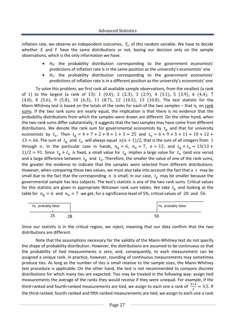
inflation rate, we observe an independent outcomes, , of this random variable. We have to decide whether and have the same distributions or not, basing our decision only on the sample observations, which is the only information we have.

H0: the probability distribution corresponding to the government economists’ predictions of inflation rate is in the same position as the university’s economists’ one

H1: the probability distribution corresponding to the government economists’ predictions of inflation rate is in a different position as the university’s economists’ one

To solve this problem, we first rank all available sample observations, from the smallest (a rank of 1) to the largest (a rank of 13): 1 0.0 , 2 2.3 , 3 2.9 , 4 3.1 , 5 3.9 , 6 4.4 , 7 4.8 , 8 5.6 , 9 5.8 , 10 6.3 , 11 8.7 , 12 10.5 , 13 10.8 . The test statistic for the Mann‐Whitney test is based on the totals of the ranks for each of the two samples – that is, on rank sums. If the two rank sums are nearly equal, the implication is that there is no evidence that the probability distributions from which the samples were drawn are different. On the other hand, when the two rank sums differ substantially, it suggests that the two samples may have come from different distributions. We denote the rank sum for governmental economists by and that for university

economists by . Then 4 7 2 8 1 3 25 and 6 9 5 11 10 1213 66. The sum of and will always equal 1 /2, that is the sum of all integers from 1 through . In the particular case in hands, 6 , 7 , 13 , and 13 131 /2 91. Since is fixed, a small value for implies a large value for (and vice versa)

and a large difference between and . Therefore, the smaller the value of one of the rank sums,

the greater the evidence to indicate that the samples were selected from different distributions. However, when comparing these two values, we must also take into account the fact that a may be small due to the fact that the corresponding is small; in our case, g may be smaller because the

governmental sample has less subjects. The test’s statistic is any of the two rank sums. Critical values for this statistic are given in appropriate Wilcoxon rank sum tables. We take g and looking at the

table for 6 and 7 we get, for a significance level of 5%, critical values of 28 and 56.

Since our statistic is in the critical region, we reject, meaning that our data confirm that the two distributions are different.

Note that the assumptions necessary for the validity of the Mann‐Whitney test do not specify the shape of probability distribution. However, the distributions are assumed to be continuous so that the probability of tied measurements is zero, and, consequently, to each measurement can be assigned a unique rank. In practice, however, rounding of continuous measurements may sometimes produce ties. As long as the number of ties is small relative to the sample sizes, the Mann‐Whitney test procedure is applicable. On the other hand, the test is not recommended to compare discrete distributions for which many ties are expected. Ties may be treated in the following way: assign tied measurements the average of the ranks they would receive if they were unequal. For example, if the

third‐ranked and fourth‐ranked measurements are tied, we assign to each one a rank of 3.5. If the third‐ranked, fourth‐ranked and fifth‐ranked measurements are tied, we assign to each one a rank


56 25 28

Advanced Statistics

Page 28

of 4.

Returning to our example, we may formulate the question more exactly: is it true that the university economists' predictions tend to be higher than the predictions of the governmental economists? In other words, is the density shifted to the right with respect to density ? Conceptually this shift equals the systematic component in the difference between the predictions of a generic university economist and a generic government economist. That is:

H0: the probability distribution corresponding to the government economists’ predictions of inflation rate is in the same position or shifted to the right with respect to the university’s economists’ one

H1: the probability distribution corresponding to the government economists’ predictions of inflation rate is shifted to the left with respect to the university’s economists’ one

We have to find out the rejection region. We take g as statistic and suppose that its value is very

large. This means that governmental economists make predictions with larger ranks and thus with higher values than university’s economists. This is strongly in favor of H0 and therefore rejection region is on the other side, the left one. Critical values are different and they are, for a significance level of 5%, 30 and 54. Statistic falls in the rejection region and thus our data confirms that governmental predictions are shifted to the left.

When sample size, or , is larger than 10, tables do not provide us with critical values anymore. In these cases statistic distribution can be approximated with a normal distribution

1 2⁄

1 12⁄N 0; 1 .

4.10 Wilcoxon signed rank test

Prerequisites: the difference is a random variable having a continuous probability distribution.

H0: position of distribution for variable A = position of distribution for variable B

Statistic: sum of ranks of differences

Statistic distribution: Wilcoxon signed rank table or ⁄

⁄N 0; 1

when sample is large and tables are not available

SPSS: Analyze Nonparametric Tests Related Samples Frank Wilcoxon (1892‐1965)

Rank tests can also be employed to compare two probability distributions when a paired difference design is used. For example, consumer preferences for two competing products are often compared by analyzing the responses in a random sample of consumers who are asked to rate both

H0 probably true H0 probably false H0 probably true

54 25 30

Advanced Statistics

Page 29

products. Thus, the ratings have been paired on each consumer. Consider for example a situation

when 10 students have been asked to compare the teaching ability of two professors, say

and . Each of the students grades the teaching ability on a scale from 1 to 10, with higher grades implying better teaching. The results of the experiment are as follows:

student sign of rank of

1 6 4 2 2 + 5

2 8 5 3 3 + 7.5

3 4 5 ‐1 1 – 2

4 9 8 1 1 + 2

5 4 1 3 3 + 7.5

6 7 9 ‐2 2 – 5

7 6 2 4 4 + 9

8 5 3 2 2 + 5

9 6 7 ‐1 1 – 2

10 8 2 6 6 + 10

Here and are the grades assigned by each Student’s to professor and . Since this

is a paired difference experiment, we analyze the differences between the measurements. Examining the differences allows removing a possible common causality behind these ratings. In fact, the fourth and the sixth students seem to have given higher than other students’ ratings to both professors.

This rank test requires that we calculate the ranks of the absolute values of the differences between the measurements. Since there are ties, the tied absolute differences are assigned the average of the ranks they would receive if they were unequal but successive measurements. For example, the absolute value 3 appears two times. If these were unequal measurements, their ranks

would have been 8 and 7. Thus the rank for 3 equals 7.5. In the same way, the rank for 2

equals 5, the rank for 1 is 2. After the absolute differences are ranked, the sum of

the ranks of the positive differences of the original measurements, , and the sum of the ranks of the negative measurements, , are computed. In our case: 5 7.5 2 7.5 9 5 1046 and 2 5 2 9. Now we are ready to test the non‐parametric hypotheses:

H0: the probability distributions of the ratings for professor is in the same position

as the one for professor , 1 2 H1: the probability distributions of the ratings for professor is in a different

position as the one for professor , 1 2

As the test statistic we use any . The more the difference between and , the greater the evidence to indicate that the two probability distributions differ in location. Note that also for this test the sum of is fixed and equal to 1 /2. Left critical value is tabulated, while right critical value can be found for symmetricity. In our case, we take for example which is 8. The left critical value, for a significance level of 5%, is 8. The other critical value is 1 /2 8 558 47.


27.5

H0 probably true

47 9 8

46

Advanced Statistics

Page 30

As it can be seen in the schema, this test is perfectly symmetric and when one falls into the central region, the other automatically does the same. Vice versa, when one falls into a rejection region, the other falls into the other rejection region. In our example we accept and therefore our data are not able to prove that the two distributions are different.

Obviously, also for this test we have one‐tailed versions. This is performed in the usual way, taking care to choose one statistic and decide which the rejection region for that statistic is.

Since we have assumed that the distribution of a difference is continuous, there may not be differences which are exactly 0. However, in practice, they may occur due to rounding: in such cases, we must decide whether assigning their rank to or to . For the two‐tailed test there is no solution. Since a difference of 0 is in favor of H0 hypothesis, assigning it to either statistic can unbalance the situation and push in favor of H1. Moreover, a difference of 0 is strongly in favor of H0, but it would have the smaller rank. So, the two‐tailed test cannot be performed at all if we have any 0 difference. However, the one tailed test can be performed. For example:

H0: the probability distributions of the ratings for professor is in the same position or

shifted to the left with respect to the one for professor , 1 2 , 1 2 0 H1: the probability distributions of the ratings for professor is shifted to the right

with respect to the one for professor , 1 2 , 1 2 0

A difference of 0 is in favor of H0 hypothesis which includes also all the negative differences. Therefore, any 0 difference’s rank is assigned, with these hypotheses, to .

When 25 statistic’s tables are not available anymore. Statistic’s distribution can be approximated with:

1 4⁄

1 2 1 24⁄N 0; 1 ,

where it is better to take as statistic the smaller between and , since usually standard normal distribution tables provide the area on the left.

4.11 KruskalWallis test

Prerequisites: there are 5 or more measurements in each sample; the probability distributions from which the samples are drawn are continuous

H0: position of distribution of populations is the same

Statistic: ∑ 3 1

Statistic distribution: chi square distribution with 1 degrees of freedom

SPSS: Analyze Nonparametric Tests Independent Samples

William Henry Kruskal

(1919‐2005)

Wilson Allen Wallis

(1912‐1998)

The Kruskal‐Wallis test is the Mann‐Whitney test when more than two populations are involved. Its corresponding parametric test is the Analysis of Variance.

For example, a health administrator wants to compare the unoccupied bed space for three

Advanced Statistics

Page 31

hospitals. She randomly selects 10 different days from the records of each hospital and lists the number of unoccupied beds for each day. Just as with two independent samples, we base our comparison on the rank sums for these three sets of data. Ties are treated as in the Mann‐Whitney test by assigning the average value of the ranks to each of the tied observations:

Hospital 1 Hospital 2 Hospital 3

Beds Rank Beds Rank Beds Rank

6 5 34 25 13 9.5

38 27 28 19 35 26

3 2 42 30 19 15

17 13 13 9.5 4 3

11 8 40 29 29 20

30 21 31 22 0 1

15 11 9 7 7 6

16 12 32 23 33 24

25 17 39 28 18 14

5 4 27 18 24 16

120 210.5 134.5We test

H0: the probability distributions of the number of unoccupied beds have the same position for all three hospitals

H1: at least one of the hospitals has probability position different with respect to the others.

The test statistic, called , is ∑ , where denotes the number of distributions

involved, is the number of measurements available for the th distribution, is the

corresponding rank sum, / is the mean rank for population and . . . /

⁄ (remembering that the sum of ranks is fixed, as for Mann‐Whitney and

Wilcoxon tests) is the mean rank for the whole population. As it can be seen from the formula, this statistic measures the extent to which the ranks differ with respect to the average rank. Note that statistic is always non‐negative. It takes on the value zero if and only if all samples have the same

mean rank, that is for all . This statistic becomes increasingly large as the distance between

a sample mean rank and the mean rank for the whole population grows.

However, the formula that is used for practical calculations is an easier one15:

121

3 1

In our case 3, 10 and 30. is . .

3 · 31

15 ∑ ∑ 2 ∑ 2

∑ 1 ∑ ∑ ∑ 1 ∑

1 24 12 1 1 2 3 1

Advanced Statistics

Page 32

6.097.

The statistic’s distribution is, under the hypothesis that the null hypothesis is true, approximately a chi square distribution with 1 degrees of freedom. This approximation is adequate as long as each of the sample sizes is at least 5. Chi square distribution has only one tail on the right and thus the rejection region for the test is located in the right tail. In our case 3, so we are dealing with a chi square distribution with 2 degrees of freedom. Using the significance method, we find16 a significance of 4.74% which means that we reject. Using the critical region method with 5% significance level, we get a critical value of 5.99.

4.12 Pearson’s correlation coefficient

Prerequisites: coupled data

H0: Corr ,

Statistic: ·√

√

Statistic distribution: Student’s t with 2 degrees of freedom

SPSS: Analyze Correlate Bivariate

Karl Pearson (1857‐1936)

Consider two random variables, and , of which we have only couples of outcomes, ; . It is important that the outcomes that we have are in couples, since we are interesting in

estimating the correlation between the two variables. We use as estimator the Pearson’s correlation coefficient which is defined, through the introduction of the (sum of squares) quantity, as

·

∑

∑ · ∑

∑

·.

As it can be seen from the formulas, quantities have two equivalent definitions, of which the latter is easier to use in practical calculations while the former is more useful for theoretical considerations. In particular, we can immediately observe from the second definition that and

are strictly positive and therefore the square root and the denominator are well defined. In the

particular case when all the or all the have the same value, the corresponding quantity becomes 0 and the Pearson correlation coefficient is no more defined. This is a very rare case and corresponds to the situation when there are only constant outcomes for random variable or ; clearly, from constant outcomes we can not estimate anything concerning the behavior of random variables.

⁄ is the estimation of the variance of random variable , while ⁄ is the

16 Significance can be calculated in two different ways. (1) Using English Microsoft Excel function CHIDIST(6.097;2) which gives us the area of the left tail. (2) Using chi square distribution table, which usually provides the left side critical values.


6.097 5.99 0

Advanced Statistics

Page 33

estimation of the variance of random variable and ⁄ is the estimation for Cov , . Since

the correlation is exactly Corr ,Cov ,

Var ·Var, Pearson’s correlation coefficient is the

estimation for the correlation.

The sign of is determined only by the sign of . It can moreover be easily

demonstrated17 that · and therefore the value of must lie between – 1 and 1, independently from how large or small are the numbers and . In other words, is a scaleless variable. A value of near or equal to zero is interpreted as little or no correlation between and . In contrast, the closer comes to 1 or 1, the stronger is the correlation of these

variables. Positive values of imply a positive correlation between and . That is, if one increases, the other one increases as well. Negative values of imply a negative correlation. In fact, and move in the opposite directions: when increases, decreases and vice versa. In sum,

this coefficient of correlation reveals whether there is a common tendency in moves of and .

We have a test to check whether Corr X, Y is different from 0, meaning that there is a linear relation between random variables and . This test uses the fact that statistic

· √ 2

√1

is distributed like a Student’s t distribution with 2 degrees of freedom. We remind the fact that independence implies zero correlation but not vice versa: therefore, when the correlation is different from 0, we are sure that the two random variables are dependent.

For example, suppose we have these 11 couples of data

2 3 4 3 5 6 7 3 1 3 4

5 5 7 5 7 7 14 5 3 1 12

we get 4 9 16 9 25 36 49 9 1 9 16 11 · 3.7 30.18 ,

10 15 28 15 35 42 98 15 3 3 48 11 · 3.7 · 6.5 47.36 and

138.73. Therefore .

√ . · .0.732 with 11 couples of data and the value of our statistic

is . ·√

√ .3.223 and a significance, for the two‐tailed test, of 1.04% . Therefore, taking a

significance level of 5%, 11 couples of data with Pearson’s correlation coefficient of 0.732 are enough to prove that the correlation is different from 0 and therefore the two variables are not independent.

17 This fact obtains by applying the Cauchy‐Schwarz inequality, | | || || || ||, to the ‐vectors and with and .

Advanced Statistics

Page 34

4.13 Spearman's rank correlation coefficient

Prerequisites: coupled ranked data or coupled data from continuous distributions

H0: ranks are uncorrelated

Statistic: Spearman’s rank correlation coefficient

Statistic distribution: Spearman table

SPSS: Analyze Correlate Bivariate Charles Spearman(1863‐1945)

The Spearman's rank correlation coefficient is the non parametric version of the Pearson’s correlation coefficient.

Taking the same data of the previous example,

2 3 4 3 5 6 7 3 1 3 4

5 5 7 5 7 7 14 5 3 1 12

this time instead of taking the values, we assign ranks. It is important that ranks be assigned independently for and , yet maintaining the coupled position of the data:

2 4.5 7.5 4.5 9 10 11 4.5 1 4.5 7.5

4.5 4.5 8 4.5 8 8 11 4.5 2 1 10

The Spearman’s rank correlation coefficient, , is calculated exactly as Pearson’s correlation coefficient:

Where, exactly as for Pearson’s correlation coefficient,

· · ,

1

The value of always falls between 1 and 1, with 1 indicating perfect positive correlation and 1 for perfect negative correlation. The closer falls to 1 or 1 , the greater the correlation between the ranks. Conversely, the nearer is to 0, the less the correlation.

For Spearman’s rank correlation we have, however, additional information since the values used in the calculation must be integer numbers between 1 and . Therefore, through mathematical calculations, we can derive18 an alternative formula valid only when there are not tied

18 Starting from the consideration that ∑ 1 2 3 1 we can obtain a

simplification ∑ ∑ and ∑

∑ . Moreover, since ∑ 1 2 3 1

Advanced Statistics

Page 35

ranks:

16

n 1 .

where , the difference between the rank of the th measurement in the first set and

the rank of the th measurement in the second set. We can see that if all ranks are identical, that is,

for every , then 1. We must take care to remember that this formula is valid only

when there are no tied ranks.

Returning to our example, we see that

2.5 0 0.5 0 1 2 0 0 1 3.5 2.5 31,

consequently, 1 6 · 31 11 · 11 1⁄ 0.859. The fact that is close to 1 indicates that the rankings given by the two magazines tend to agree, but the agreement is not perfect.

If the sets of ranks are formed by values taken by independent realizations of random

variables and , the Spearman's rank correlation coefficient may be used for testing

whether the value of Corr , is different from 0. The statistic is the coefficient itself. In the previous example, with 11 and a significance level of 5% we have a critical value of 0.623,

and therefore we reject, meaning that the ranks are correlated and there is a relation between the order of the two variables.

Spearman’s rank correlation coefficient can be used, as every other rank test, in all the situations where effective measures are not available and only ranks are provided. Suppose ten new car models are evaluated by two consumer magazines and each magazine ranks the braking system of the cars from 1 (best) to 10 (worst). We want to determine whether the magazines' ranks are related. If they are, we may conclude that these rankings contain useful information about the breaking system. Otherwise, if the rankings given by the two magazines are not related, we should not regard these ranking as containing useful information since they are contradictory and we do not know which one to use. Let the ranks given by the two magazines be as follows:

Car model 1 2 3 4 5 6 7 8 9 10

we see that . Finally, taking into account that

, we obtain ∑ ∑

∑ ∑ ∑

∑ . Consequently, ∑

1 ∑ .


0

H0 probably true

0.623

– 0.623

0.859

Advanced Statistics

Page 36

Rank given by magazine 1 4 1 9 5 2 10 7 3 6 8

Rank given by magazine 2 5 2 10 6 1 9 7 3 4 8

In this case data are already ranked and the coefficient can be calculated directly.

4.14 Multinomial experiment

Many business analyses consist of enumerating the number of occurrences of some event. For example, we may count the number of consumers who choose each of the three brands of coffee, or the number of sales made by each of five automobile salespeople during a month. When there is a single scale to classify data, as in all examples above, we have a one dimensional classification. In some cases we may collect the count data characterizing several factors. For example, we may be interested in investigating whether the color of automobile purchased is related to the sex of the buyer. In this case we are dealing with a two dimensional classification. The corresponding data constitute a contingency table. Count data are traditionally analyzed using tables.

4.14.1 One dimensional classification

Prerequisites: · 5 for all

H0: for all or, equivalently, · for all

Statistic: table’s chi square ∑ ·

·,

Statistic distribution: chi square with 1 degrees of freedom

SPSS: Analyze Nonparametric tests One Sample

The properties of the one dimensional multinomial experiment are as follows:

the experiment consists of identical trials; the trials are independent; there are possible outcomes to each trial; the probabilities of the outcomes, denoted by , , ..., , remain the same from trial to

trial, where 1 (therefore there is no other possible outcome outside the ones we are considering);

the random variables of interest are the counts , , ..., in each of the cells.

For example, suppose a large supermarket chain conducts a consumer preference survey by recording the brand of bread purchased by customers in its stores. Assume the chain carries three brands of bread, A, B and C. The brand preferences of a random sample of 150 consumers are observed, and the resulting count data are as follows: A: 61, B: 53, C: 36. Do these data indicate that a preference exists for any of these brands?

Our consumer preference survey satisfies the properties of a multinomial experiment. The experiment consists in randomly sampling 150 buyers from a large population of consumers containing an unknown proportion who prefer brand A, a proportion who prefer brand B, and a proportion who prefer the store brand, C. Approaching a buyer concerning his preference, we perform a single trial that can result in one of three outcomes: the consumer prefers brand A, B or C. Probabilities of these outcomes are , , and , respectively. The buyer's preference of any single consumer in the sample does not affect the preference of another. Consequently, the trials are

Advanced Statistics

Page 37

independent. The recorded data are the numbers of buyers in each of the consumer preference categories. Thus, the consumer preference survey satisfies the five properties of a multinomial experiment.

Note that we may talk about the proportions , , as probabilities because in a population consisting totally of agents, prefer brand A, opt for brand B, and for brand C. Consequently, the probability to choose randomly a customer who buys A, B, C will be correspondingly / , / and / . That is why we may talk about as a proportion as well as about a probability. The three probabilities , , are unknown and we want to use the survey data to make inferences about their size.

The general form for a test of a hypothesis concerning multinomial probabilities is as follows:

H0: , , ..., , where , , ..., represent the hypothesized values of the multinomial probabilities ( 1/3 in the above example with three types of bread)

H1: at least one of the multinomial probabilities does not equal its hypothesized value, in other words, there is an such that the corresponding actual probability does not coincide with its hypothesized value , .

We build a table of observed counts and a table of predicted counts ·

A B C A B C

61 53 36 50 50 50

observed counts predicted counts

under H0 hypothesis

The test statistic is the table’s chi square, a measure calculated as

·

·,

where are called observed counts, . . . is the total sample size. This statistic is distributed as a chi square distribution with 1 degrees of freedom. Observing the chi square statistic, it is evident that when the observed numbers are very different from the predicted counts, · , the value of the statistic is very large, while when the observed numbers coincides with the

predicted ones the statistic is zero. Therefore, rejection region is only on the right. This test works only if the predicted counts are all · 5, while it is not important that the observed ones be at least 5.

In our particular example, · /

· /

· /

· /

· /

· /6.52. Since here

3 , we are dealing with a chi square distribution with 2 degrees of freedom. Statistic’s significance is19 3.84% and therefore we reject, meaning that consumers’ preferences are not

19 Significance can be calculated in different ways: (1) using English Microsoft Excel function CHIDIST(6.52;2) which gives us the probability of the right tail of chi square distribution; (2) looking into chi square tables which usually provide critical values for different significance levels; (3) using English Microsoft Excel function CHIINV(5%;2) which gives us the critical value corresponding to 5% significance level; (4) test can be performed also using English Microsoft Excel function CHITEST which, given the observed table and the predicted table, gives us the value of chi square statistic and then using CHIDIST significance can be found.

Advanced Statistics

Page 38

uniform and that there is at least one type of bread that has a probability different from 1/3. If we want to use the critical regions method, critical value for 5% is 5.99 and therefore 6.52 is in the rejection region which for this test is always on the right.

As another example, using the same data we want to check whether the bread’s probabilities follow a 40%, 40%, 20% distribution:

H0: 40% and 40% and 20% H1: 40% or 40% or 20%.

The observed and predicted tables are

A B C A B C

61 53 36 60 60 30

observed counts predicted counts

under H0 hypothesis

and 1.43 with a significance of 48.8%. Therefore we accept,

meaning that our sample is not able to prove that consumers’ preference is not 40%, 40%, 20%.

4.14.2 Two dimensional contingency table

Prerequisites: · / 5 for all ,

H0: classifications are independent

Statistic: table’s chi square ∑ ∑ · /

· /,

Statistic distribution: chi square with 1 1 degrees of freedom

SPSS: Analyze Descriptive Statistics Crosstabs Statistics Chi‐square

Suppose, for example, that an automobile magazine is interested in determining the relationship between the size and manufacturer of newly purchased automobiles. One thousand recent buyers of cars made in Germany are randomly sampled, and each purchase is classified with respect to the size (small, intermediate, and large) and manufacturer of the automobile (Volkswagen, BMW, Opel, Mercedes). The data are summarized in the two‐way table:

Size\Manufacturer VW BMW Opel Mercedes Totals

Small 157 65 181 10 413

Intermediate 126 82 142 46 396

Large 58 45 60 28 191

Totals 341 192 383 84 1000

This table is called a contingency table.

SPSS: Analyze Descriptive Statistics Crosstabs

It presents multinomial count data classified in two dimensions, namely automobile size and manufacturer. Each count is indicated with , , where the first index is referred to the row, the size, and the second index to the column, the manufacturer. We also indicate with the rows’ totals and with the columns’ totals, and these quantities are called marginal counts. The sample size is and coincides with the grand total, in our case 1000.

Advanced Statistics

Page 39


Small 1,1 1,2 1,3 1,4 1

Intermediate 2,1 2,2 2,3 2,4 2

Large 3,1 3,2 3,3 3,4 3

Totals 1 2 3 4

This is a multinomial experiment with a total of 1000 trials, 3 · 4 12 cells or possible outcomes, and probabilities for the cells. If the 1000 recent buyers are randomly chosen,

the trials are considered independent and the probabilities are viewed as remaining constant from

trial to trial. We also define the marginal probabilities for rows and columns as and .

In a two dimensional classification experiment usually we are interested in checking whether

one variable can influence the other. It may be helpful calculating the row percentages , and

column percentages , as follow:


Small 38.0% 15.7% 43.8% 2.4% 100.0%

Intermediate 31.8% 20.7% 35.9% 11.6% 100.0%

Large 30.4% 23.6% 31.4% 14.7% 100.0%

Size\Manufacturer VW BMW Opel Mercedes

Small 46.0% 33.9% 47.3% 11.9%

Intermediate 37.0% 42.7% 37.1% 54.8%

Large 17.0% 23.4% 15.7% 33.3%

Totals 100.0% 100.0% 100.0% 100.0%

Using row percentages we can show, for example, that among all small cars only 2.4% are produced by Mercedes compared to Opel which has 43.8% of the market. Using column percentages instead we see that among all Mercedes cars 11.9% are small compared to 33.3% of large ones.

SPSS: Analyze Descriptive Statistics Crosstabs Cells

Therefore, in a two dimensional classification experiment we are not interested in whether the observed counts follow a predetermined distribution, since they are also influenced by the marginal counts (which depends on our sample’s choice). We instead test whether the two classifications, manufacturer and size in our example, are independent.

H0: row variable and column variable are independent, i.e. ·

H1: row variable and column variable are dependent, i.e. there is a couple , for which ·.

That is, if we know which size car a buyer will choose, does this information give us a clue about the manufacturer of the car that is going to be bought? In a probabilistic sense we know that independence of events and implies P P · P . Similarly, in the contingency table analysis, if the two classifications are independent, the probability that an item is classified in any particular cell of the table is a product of the corresponding marginal probabilities. Thus, under the hypothesis of independence, we must have: · , · and so forth. To test

Advanced Statistics

Page 40

the hypothesis of independence, we use the same reasoning as in the one‐dimensional tests. First we calculate the predicted count in each cell assuming that the null hypothesis of independence is true, multiplying by the cell predicted probability · · · · ⁄ · ⁄ ⁄ . In

our example


Small 413∙341/1000 413∙192/1000 413∙383/1000 413∙84/1000 413

Intermediate 396∙341/1000 396∙192/1000 396∙383/1000 396∙84/1000 396

Large 191∙341/1000 191∙192/1000 191∙383/1000 191∙84/1000 191

Totals 341 192 383 84 1000


Small 140.8 79.3 158.2 34.6 413

Intermediate 135.0 76.0 151.7 33.5 396

Large 65.1 36.7 73.2 16.0 191

Totals 341 192 383 84 1000

As it can be seen, marginal counts have remained the same.

We use the chi square statistic to compare the observed and predicted counts in each cell of

the contingency table .

.

.

.

.

.

.

.

.

..

.

.

.

.

.

.

.

.

.

.

.

.

.45.81. Degrees

of freedom are 3 1 · 4 1 6 , significance is 20 0.000003% : therefore we reject the hypothesis of independence and we conclude that the size and manufacturer of a car selected by a purchaser are dependent events. Using instead the critical regions method, for a significance level of 5% we get a critical value of 12.59 and therefore the statistic value falls into the rejection region.

20 Significance can be found and test can be performed in different ways: (1) using English Microsoft Excel function CHIDIST(45.81;6) which gives us the probability of the right tail of chi square distribution; (2) looking into chi square tables which usually provide critical values for different significance levels; (3) using English Microsoft Excel function CHIINV(5%;6) which gives us the critical value corresponding to 5% significance level; (4) test can be performed also using English Microsoft Excel function CHITEST which, given the observed table and the predicted table (which must be manually built), gives us the value of chi square statistic and then using CHIDIST significance can be found.

Advanced Statistics

Page 41

5. Which test to use? While for some data situation it is evident which statistical test to use, such as for example

multinomial experiments or when facing with a single distribution, when having to compare two distributions there are several tests that may be used, according to what we want to check.

Mann‐Whitney test check whether two distributions have the same position or not. We use it when we have two sets of data and we are simply interested into testing whether they come from distributions in the same position or not. Student’s t test for two populations is a test for the same situation but which tests whether the expected values of the distributions are the same and does not test their position.

Wilcoxon signed rank test checks whether two distributions of paired data have the same position. It can be used only when data are paired and it analyses the difference case with case (intra‐case, inside the same case). Same thing for Student’s t test for paired data, which analyses the difference between expected values of the two samples on a case by case basis.

Spearman rank correlation coefficient checks whether two distributions of paired data have the same order or a perfectly reverse order. It does not matter whether the data come from similar distribution or not, the important thing is that they are in order. It can be used only when data are paired and when we are simply interested in the order. Pearson correlation coefficient applies to the same situation, but checking the effective data’s values and not the order.

There are however many cases where all the tests can be performed. Some theoretical examples:

if data are in perfect reverse order (1, 2, 3, 4, 5 and 5, 4, 3, 2, 1), Spearman is equal to 1 (H0 rejected, therefore orders are related) indicating that the order is reversed while Mann‐Whitney test and Wilcoxon signed rank test accept H0 indicating that data may be in the same position;

if data are perfectly shifted (1, 2, 3, 4, 5 and 3, 4, 5, 6, 7), Wilcoxon signed rank test and Mann‐Whitney test reject H0 indicating that data do not have the same position while Spearman is equal to 1 (H0 rejected, therefore orders are related) indicating that the order is the same.

Some more practical examples for non parametric tests, which are however valid also for the corresponding parametric tests provided their prerequisites are satisfied.

Given two students and their exams' grades on the same 6 economics subjects, which one will you hire for a position in a bank? Data are paired so we can use all three tests. However, we are not interested whether the two students have the same order or not, but simply whether their two distributions have the same position or not (and, if we want to do also one‐tailed tests, whether one of the two students has exams' grades shifted to the right). For example, suppose that grades are 30 29 28 27 26 25 and

25 26 27 28 29 30: in this case for us the two students are equivalent, but Spearman is – 1 (H0 rejected, therefore orders are related) indicating that the order is reversed, while Mann‐Whitney and Wilcoxon tests both accept indicating that data may come from the same position. Suppose instead that grades are 30 29 28 27 26 25 and 25 24 23 22 21 20: in this case the first student is evidently the best. Spearman is 1 (H0 rejected, therefore orders are related) indicating that the order is the same, while Mann‐Whitney and Wilcoxon tests both reject indicating that data

Advanced Statistics

Page 42

come from different position. So the best choice here is Mann‐Whitney test, followed by Wilcoxon signed rank test since the differences exam by exam are not important. Spearman is not good here since we are not interested in the order.

Given two subjects and the grades given to the same 6 students, how can you test whether subject B has marks which have been inflated? Data are paired so we can use all three tests. However, we are not interested whether the two exams have the same order or not (because it can happen that a student is good in a subject but bad in another, due to personal preferences), but we are interested whether their distribution have the same position. For example, suppose that grades are 30 29 28 27 26 25 and 25 26 27 28 29 30: in this case, even though the same student got different grades, for each student who has got high grade in A and low in B there is another who compensate with a low grade in A and high in B (and this is not an indication that grades have been inflated, but simply that students good in A are not good in B, due to personal preferences). So subject B has not been inflated. Spearman is

– 1 (H0 rejected, therefore orders are related) indicating that marks are in the reverse order, an information which is totally useless here, while the two Wilcoxon tests do not reject indicating that marks may come from the same distribution. Suppose instead that grades are 25 24 23 22 21 20 and 30 29 28 27 26 25: in this case exam’s grades are evidently inflated. Spearman is 1 (H0 rejected, therefore orders are related) indicating that marks are in the same order, an useless information, while Mann‐Whitney and Wilcoxon tests both reject, indicating that marks’ distribution do not have the same position. So the best choice here is Mann‐Whitney test, followed by Wilcoxon signed rank test since the differences subject by subject are not important. Spearman is not good here. If, on the other hand, we want to concentrate the attention on the grades inflation subject by subject, Wilcoxon signed rank test is the best choice, followed by Mann‐Whitney test.

Given two subjects and the grades given to the same 6 students, how can you test whether grades are consistent? Data are paired so we can use all three tests. Consistent here means that good students in one subject are also good in the other. So in this case we are interested in discovering whether grades have the same order or not. For example, suppose that grades are 30 29 28 27 26 25 and 25 26 27 28 29 30: in this case it is clear that good students in first subject are bad in the second.

Spearman is – 1 (H0 rejected, therefore orders are related) indicating that the order is different while the two Wilcoxon tests do not reject indicating that marks may come from the same distribution, a useless information in this case. Suppose instead that grades are 25 24 23 22 21 20 and 30 29 28 27 26 25: in this case, even though second exam’s grades are evidently inflated, at least good students in first exam are still the best ones in the second. Spearman is 1 (H0 rejected, therefore orders are related) indicating that the order is the same, while Mann‐Whitney and Wilcoxon tests both reject indicating that data have different positions. Therefore Spearman is the best choice, and Mann‐Whitney and Wilcoxon tests are not appropriate.

Given two subjects and the grades given to 4 students for subject A and to 8 students (including the previous 4) for subject B, how can you test whether subject B has marks which have been inflated? Data are paired only for the first 4. So using Wilcoxon signed rank test implies taking very few subjects and looking at the table with 4 cases we see that we must always accept. Therefore Mann‐Whitney test with 4/8 subjects is the only test possible here.

Advanced Statistics

Page 43

6. Regression model An important consideration in merchandising a product is the amount of money spent on

advertising. Suppose you want to model the monthly sales revenue of a store as a function of the monthly advertising expenditure. First, you have to decide whether an exact relationship exists between these two variables. That is, whether it is possible to state the exact monthly revenue if the amount spent on advertising is known. We are going to study a situation when this is not possible. There are several reasons. First, sales depend on many variables other than advertising expenditure: time of year, the state of the general economy, inventory, and price structure. These variables can be included, along with the monthly advertising expenditure, in a model, but then it is still unlikely that we would be able to predict the monthly sales exactly. This happens due to random phenomena that cannot be predicted with certainty. For example, people may stop buying microwave appliances because of new findings concerning the harmful effects of electromagnetic radiation.

If we were to construct a model that hypothesized an exact relationship between variables, it would be called a deterministic model. For example, if we believe that , the monthly sales revenue, will be exactly 5 times , the monthly advertising expenditure, we write 5 . This deterministic relationship implies that can always be determined when is known. There is no allowance for error in this prediction. If, on the other hand, we believe that there will be unexplained variation in monthly sales – perhaps caused by important but not included variables or by random phenomena – we discard the deterministic model and use a model that accounts for this random error. This probabilistic model includes both a deterministic component and a random error component. For example, if we hypothesized that the sales is related to advertising expenditure by 5random error, we are hypothesizing a probabilistic relationship between and .

In general the deterministic component may be any function of several variables. The simplest probabilistic model employs a linear function of one independent variable as its deterministic component. Here is called the dependent variable, is the independent or predictor variable and is the random error term. The latter is supposed to have zero mean and finite variance, i.e. to randomly fluctuate around a null value. Then E

E implying that expected value of follows a straight line . The Greek symbols and are the model’s parameters. They are not known and we have to estimate them from the available data.

The most common uses of a probabilistic model for making inferences can be divided into two categories. The first is the use of a probabilistic model for estimating the value of for a specific value of which is in the set of our data. The second use of the model usually entails predicting a value for corresponding to a new (that is, which is not in the set of data we are dealing with) value of .

6.1 The least squares approach

Given coupled observations , , we now want to find estimates for the parameters which fits to this set of data the best. We start with choosing a mathematical model . Plotting the above couples in a Cartesian plane, we obtain the scatterplot corresponding to this data set. It is very unusual that all points belong to the same straight line. If it does not seem to be possible to have a single straight line passing through all of the couples, we may try to look for a

Advanced Statistics

Page 44

straight line which deviates the least from them. As a measure for the deviation we may consider the sum of squared distances between the observed couples and the couples predicted by the line

∑ ∑ . This is the essence of the least squares approach, which tries to find estimates for parameters for which this quantity is the minimum possible value21.

Estimates are / and (remembering from section 4.12 on page 32

the definitions of ). The straight line given by the linear function is called the least

squares line or regression line. The value can be considered as a prediction or estimate for .

SPSS: Analyze Regression Linear

Since the numerators in the expressions for and Pearson’s correlation coefficient (see

section 4.12 on page 32) are identical, we see that 0 if and only if 0 and that has the

same sign as .

Note that, dividing by , we are assuming that 0. In fact, is equal to zero only when all the x values are identical, a case where it is clearly impossible to estimate basing on

21 In formal terms, given 2 couples , , we consider the following function of two arguments ,∑ . This is, in fact, a sum of squared deviations of actually observed values from the quantities

assigned to points by the linear function . We want to find a couple of values and such that this quantity has the minimum possible value (note that is always positive and it is 0 only when all the

, lie on a line). In order to find this minimum we derive the function with respect to and : ∑

∑ 2 1 2n and ∑ ∑ 2

1 2 1 0 1 1 2. Equating the above partial derivatives to zero, we obtain

0

0

The first equation implies that . Substituting this expression in the second equation, we get ∑

∑ 0 , and, remembering from section 4.12 on page 29 the definitions of ,

/ and .

Advanced Statistics

Page 45

.

The simplest way to measure the quality of the linear model is to evaluate the contribution of in predicting . We define the sum of squares of errors

,

which is a measure of how close to 0 our errors are. However, this quantity depends strongly on the scale we are using: if we divide all our numbers by 10, this quantity would be reduced by 100! In order to have a scale invariant measure we introduce

1

which belongs to 0; 1 and is called coefficient of determination. It is interpreted as the proportion of the total sample variability around that has been explained by the linear relationship

between and . The difference shows how much the total variability

(when is not involved at all) has been reduced by using the best possible (in the least square sense) linear approximation. Dividing by , we get the proportion of this reduction as measured against

. Obviously, the larger is , the better is the linear approximation. Indeed, a larger implies a

smaller . In other words, a smaller deviation of predictions from actually observed . For example, 0.6 means that the sum of squares of deviations of predicted values from actually observed ones has been reduced by 60% by using the least squares linear predictions instead of

.

It can be easily demonstrated22 that coefficient of determination is the square of Pearson’s correlation coefficient.

1

This implies also that , and are either all 0 or all different from 0.

22 The expression for implies that ∑ ∑ ∑

∑ 2 ∑ ∑ 2

. Indeed, we have demonstrated above that ∑ , but the remaining terms may be treated

analogously. Inserting here / , we get 2 . Hence,

1 .

Advanced Statistics

Page 46

6.2 Statistical inference

So far all calculations have been done without any hypothesis concerning the nature of the dependence between the variables in question. Now we want to turn to the distributions used to evaluate the quality of the least squares estimates obtained above. This calls for more assumptions about the structure of the data:

whenever we consider a value we have the following relation . The values and are deterministic and unknown to us. are independent (meaning that is independent from for ) observations of a random variable

normally distributed as N 0; , with zero expected value and a fixed variance (the same for all ).

The values , are called the residuals. They are the estimates for the outcomes of random variable . It is interesting to note that residuals have the following feature

0

which automatically implies that any can be written as a function of the others. Therefore are not independent.

Prerequisites: are independent observations of a random variable ~N 0;

R² = 0.9799

0

2

4

6

8

10

12

14

16

18

0 2 4 6 8 10 12 14 16 18 20

R² = 0.0044

0

1

2

3

4

5

6

7

8

0 1 2 3 4 5 6 7 8 9 10 11 12

Advanced Statistics

Page 47

H0:

Statistic: √ 2·

2

Statistic distribution: Student’s t with 2 degrees of freedom. For 31 standard normal distribution.


Arguing about the usefulness of the simple linear regression model, we want to test whether

, of whom we only have the estimation , is equal to zero or not. Indeed, when 0, the deterministic part of the model does not change as varies and therefore the model is totally useless since does not depend on . Therefore, we test:

H0: 0 H1: 0.

The statistic we use is

√ 2 ·

which has the Student’s t distribution with 2 degrees of freedom. When we reject the null hypothesis, we are sure that the slope of the regression line is not zero and therefore there is a deterministic influence of independent variable over dependent variable. On the other hand, when we accept the null hypothesis we are not able to prove that is different from zero and we can not argue whether there is an influence or not.

6.3 Multivariate and non linear regression model

We may also assume that the dependent variable is a function of independent arguments. For example, we may try to model the dependence of the annual revenue of a firm

running supermarkets not only from the advertising expenditure , but also from the money

invested in the infrastructure of its shops. Trying to recover a relationship between and ,

1, 2, … , , we can assume that it takes a linear form . Searching for the best values for such coefficients, we can attempt to use again the least

squares approach23 to estimate the coefficients.


23 Introducing , , … , ∑ and looking for a minimum point,

, , … , of this function of 1 parameters , , … , . As in the case of the simple linear model, the 1 estimates , , … , are obtained as a unique solution to a system of 1 linear equations

, , … , 0

, , … , 0

Advanced Statistics

Page 48

The quality of this approximation may be assessed by looking at the multiple coefficient of determination defined always as

1

As before, it is interpreted as the ratio of the explained variability to the total variability. Hence the larger is this value, the better fits this linear function to the set of data in question. For multivariate regression models there is no alternative formula and no easy relation with Pearson’s correlation coefficients. However, it is still often called .

The coefficient has the same meaning as before: it is the predicted value of when all the

are equal to 0. Instead, each coefficient is the increment of when the corresponding

increments by 1 unit and at the same time all the other , ,…, , ,… , maintain the same value. Thus each for 1 can be seen as the effect of its independent variable on the dependent variable.

In the previous models we have always looked for a linear relation between dependent and independent variables. There are cases, however, where theoretical reasons or the scatterplot itself suggest a non linear relation. For example, the relation may be polynomial

or logarithmic part ln or exponential e or any complex combination of functions. Clearly, the more complex the function the more coefficients are

necessary to be estimated. Estimates , , ..., may be obtained by the least squares approach as well.

Quadratic model: Logarithmic model ln SPSS: Analyze Regression Curve Estimation / Nonlinear

6.4 Multivariate statistical inference

Prerequisites: are independent observations of a random variable ~N 0;

H0: for all 0

Statistic: 1

1

Statistic distribution: Fisher’s F with and 1 degrees of freedom.

SPSS: Analyze Regression Curve Estimation / Linear / Nonlinear

y = 0.9857ln(x) + 5.9685d = 0.8566

‐1

0

1

2

3

4

5

6

7

0 0,1 0,2 0,3 0,4 0,5 0,6 0,7 0,8 0,9 1

Advanced Statistics

Page 49

Since the dependent variable now is written as a linear function of independent

variables , , ... , , the model is also termed as a general linear model. Now it is explicitly postulated that the unknown deterministic part is a linear function with unknown coefficients. The

value of determines the contribution of the independent variable and is the intercept.

We define exactly as in the previous case the residuals and we make the same assumptions as before. Now we can test the usefulness of the model

H0: 0 H1: there is at least a 0 for which 0.

The statistic we use is

1 11

which is distributed as a Fisher’s F with and 1 degrees of freedom with only a rejection region on the right. Note that when we reject we know that at least one coefficient is not zero but we do not know which one.

6.5 Qualitative independent variables

People distinguish between two types of data: qualitative and quantitative ones. Quantitative data are recorded in a meaningful numerical scale, whereas qualitative data are measured on a non‐numerical or categorical scale. Thus, the Gross Domestic Product, number of sold items, kilowatt per hours of electricity used per day are all examples of quantitative variables. On the other hand, the gender, race, job title, and style of packing are all examples of qualitative variables. The possible values of a qualitative independent variable are referred to as category. For example, the style of packing might have three possible levels: A, B, and C. Even if we designate these values arbitrarily as 1, 2, and 3, then the numbers still represent categories and the variable is still qualitative.

Let us look at regression models with qualitative independent variables. Suppose we want to estimate the mean operating cost per kilometer of cars as a function of the car's manufacturer. Let there be three manufacturers of interest, which we identify as A, B and C. Then the automobile manufacturer is a single qualitative independent variable with three categories, A, B and C. Note that, as always with a quantitative independent variable, we cannot attach a quantitative measure to a given category. Even if we were to call the manufacturers 1, 2, and 3, the numbers would simply be identifiers of the manufacturers and would have no meaningful quantitative interpretation. Our objective is to write a single equation to predict the cost per kilometer based on car’s brand. This can

be done as follows: E, where

1 if the car is manufactured by B, 0 if the car is not manufactured by B;

1 if the car is manufactured by C, 0 if the car is not manufactured by C;

The variables and are not meaningful independent variables as they are in the case of the model with quantitative independent variables. Instead, they are dummy variables that make the model work.

Advanced Statistics

Page 50

To understand the meanings of the coefficients, let 0. This condition means that the car is manufactured by A (neither B nor C is manufacturing; hence it must be A). Then the model becomes

· 0 · 0 .

Thus, . Taking the expected value, E for cars manufactured by A. Therefore is the expected value for the cost of cars manufactured by A. Now suppose we want to represent the

mean cost per kilometer for manufacturer B. Then we should let 1 and 0:

E · 1 · 0 .

We have that E produced by B E produced by A . Therefore this coefficient is the expected difference of cost when switching from A to B. Similarly, E produced by CE produced by A .

Note that we are able to describe three categories of the qualitative variable with only two dummy variables. This is because the base level (manufacturer A, in this case) is accounted for the intercept . In general therefore for each qualitative variable we require an amount of dummy variables equal to the categories minus 1.

Since a model with dummy variables is a multivariate regression model, everything we said concerning usefulness tests also applies here. Moreover, it can be freely mixed with quantitative linear and non linear model’s components.

SPSS: dummy variables are handled automatically if variables are nominal or ordinal

6.6 Qualitative dependent variable

It is also possible to build a regression model with a qualitative dependent variable, provided that it has only two categories arbitrarily indicated with 0 and 1. The difficulty of this model is the

fact that the right side of the model’s term , , … , provides continuous values while

the left side has only two possible values. For example a linear regression model would yield silly results, larger than 1 or smaller than 0, such as

Therefore instead of using , , … , as estimation function, we use its logit

1

1 , ,…,.

The function on the right side now goes from 0 to 1. Its shape is much better suited for interpolating values which are always 0 or 1:

y = 0,0494x + 0,1986R² = 0,3682

0

1

0 5 10 15 20

Advanced Statistics

Page 51

Values between 0 and 1 can be interpreted as the probability for the dependent variable to take value 1.

SPSS: Analyze Regression Binary Logistic

6.7 Problems of regression models

6.7.1 Number of observations

In order to work correctly, the least squares approach needs a number of observations that is at least equal to the number of parameters it needs to estimate. If this condition is not satisfied, the linear equations system does not have a unique solution and thus parameters’ estimates cannot be determined. In practice however, the number of observations must be much larger than the number of parameters: as an empirical rule, observations should be at least 10 times the number of parameters used by the model. This is because whenever we add a parameter to the model we get always a larger ; this seems to indicate that the new model is better, but it is only more complex, i.e. it is simulating reality not simplifying it but simply auto adapting itself. If we build a regression model to understand reality and not simulating it, keeping the model simple must be our priority.

6.7.2 Multicollinearity

Multicollinearity exists in a multivariate regression model when one or more of the independent variables used in regression depend in a deterministic way on each other. In this case the corresponding independent variables contribute redundant information. For example, suppose

we want to construct a model to predict the fuel cost of a truck as a function of its load and the

power of its engine. Clearly, these two variables are dependent since usually a powerful truck

carries huge loads. Although both and contribute information for the prediction of fuel cost, the contributions are tautological and in the model coefficients will not reflect the effect of each independent variable.

A simple way to detect multicollinearity is to calculate the Pearson’s correlation coefficient between each pair of independent variables in the model. When a calculated value differs significantly from zero, the variables in question are related and a multicollinearity problem exists.

6.7.3 Dependent errors and DurbinWatson test

As we have seen in section 6.2, residuals are dependent. Residuals are the estimations of the outcomes of random variable , which in order to perform usefulness tests, must be all independent. Since their estimates are dependent, we may legitimately argue that the independence hypothesis may not hold. In fact, there are many practical situations where it does not hold, in particular when the observed cases are taken at different times, since cyclical component of a time series may result

0

1

0 5 10 15 20

Advanced Statistics

Page 52

in deviations from the secular trend that tend to cluster alternately on the positive and negative sides of the trend. For example, if our dependent variable is the monthly Gross Domestic Product of a country, its cases are taken at different times and their values may be influenced by cyclical fluctuations which, not predicted by the deterministic side of the model, end up influencing the errors which are therefore no more independent.

Prerequisites: ~N 0;

H0: are independent

Statistic: ∑ 11 1

2

∑ 12

Statistic distribution: Durbin‐Watson’s table

SPSS: Analyze Regression Linear Statistics

Supposing now that the observations are taken at different times, and thus using as case index, we want to test

H0: and are not autocorrelated for every

H1: and are autocorrelated for at least a

The statistic is ∑

∑ and takes values from 0 to 4. Value 0 corresponds to a situation

where all the are constant, and thus a perfect correlation. On the other hand, when ,

we have ∑

∑

∑

∑ 4, which therefore corresponds to a perfect negative correlation.

A value of 2 is the uncorrelation’s value, where H0 is accepted. Critical values are found in Durbin‐Watson’s table.

For example, if we get a Durbin‐Watson’s statistic value of 3.8 for 15 and 3 (multivariate model with 3 independent variables) we get a critical value of 0.814. This means that

the right critical value is 4– 0.814 3.186 and therefore we reject. This means that errors are autocorrelated.

If we manage to prove that the autocorrelation is not zero, then automatically and are correlated and thus (since independence implies zero correlation) they cannot be independent and usefulness’ test cannot be performed since hypotheses do not hold true.

On the other hand, if the autocorrelation is zero, we cannot directly deduce that and are independent (since zero correlation does not imply independence). However, when assumption ~N 0; holds, zero correlation does imply independence. Therefore, if null hypothesis is

accepted, we can hope that errors be independent.

In any case, even with dependent errors, the regression model continues to work and the determination coefficient continues to have its meaning. The only thing than cannot be performed is the usefulness test.


2

H0 probably true

4 – 0.814

+0.814 3.8 0 4

Advanced Statistics

Page 53

6.7.4 Heteroskedasticity

Let the errors in a simple linear regression model have a varying variance, that is even though all of them are independent and normally distributed with zero expected value, they come

from random variables with a different variance . Usually this happens whenever the data come from observations which vary a lot in size, as it is the case when our cases are firms of different sizes, or when data come from aggregated values, such as averages or sums.

In the case when we are able to know a priori the values , we may build a new model for which errors’ variances are the same. If we divide the model, written for each , by , we get

and calling , , it becomes

1

which is a particular multivariate regression model with two independent variables, and , and

no intercept. If we calculate the variance of we get that they are all the same:

Var Var1Var 1.

Therefore we can use the new model, which does not present the heteroskedasticity problem, to estimate and then multiply by to get the estimations.

Since in practice the value of the standard deviation of errors is unknown, it is common to divide the regression model by a scale quantity which represent an estimate of the standard deviation, for example the size of the firm (number of employees or total budget).

A typical case where the scaling factor is known are aggregated data with heteroskedasticity. Let be the observation on the th case in the th group, and consider the following regression

If we do not have the cases’ single values but only aggregate observations on each group are available, then these expressions are summed over cases, that is

Here ∑ , ∑ , ∑ . If the original errors , those referred to

cases, satisfy our assumptions, i.e. are independent identically distributed with expected value 0 and variance , then the errors we use in the model are still independent identically distributed with expected value 0 but with variance since

Var Var

Var .

This means that the errors in our aggregated model are now heteroskedastic. However, we know

their variances . Hence, we have to divide the model by and perform the ordinary

Advanced Statistics

Page 54

least squares estimates on the transformed equation. In practice, in this case we do not know the

value of but we may simply divide by , a value that we know since it is the number of firms in

every sector. We will get a model with constant errors’ variance .

In any case, even with dependent errors, the regression model continues to work and the determination coefficient continues to have its meaning. The only thing than cannot be done is the usefulness problem.

Advanced Statistics - Paolo Coletti

Documents