Advanced Quantum Mechanics 2 lecture 3 Schemes of Quantum Mechanics Yazid Delenda D´ epartement des Sciences de la mati` ere Facult´ e des Sciences - UHLB http://theorique05.wordpress.com/f411 Batna, 16 Novembre 2014 (http://theorique05.wordpress.com/f411) Advanced Quantum Mechanics 2 - lecture 3 1 / 32

Welcome message from author
This document is posted to help you gain knowledge. Please leave a comment to let me know what you think about it! Share it to your friends and learn new things together.
Transcript

Advanced Quantum Mechanics 2lecture 3
Schemes of Quantum Mechanics
Yazid Delenda
Departement des Sciences de la matiereFaculte des Sciences - UHLB
http://theorique05.wordpress.com/f411
Batna, 16 Novembre 2014
(http://theorique05.wordpress.com/f411) Advanced Quantum Mechanics 2 - lecture 3 1 / 32

Quantisation schemes of quantum mechanics Examples
Position and momentum in the Heisenberg picture:
The position and momentum operators are time-independent in theSchrodinger picture, and their commutator is [x, p] = i~.In the Heisenberg picture the time evolution of the position operator is:
dx(t)
dt=i
~[H, x(t)]
Note that the Hamiltonian in the Schrodinger picture is the same as theHamiltonian in the Heisenberg picture, since
H(t) = U †HU = U †UH = 1H = H
Considering the Hamiltonian of a free particle:
H =p2
2m=p2(t)
2m
(http://theorique05.wordpress.com/f411) Advanced Quantum Mechanics 2 - lecture 3 2 / 32

Quantisation schemes of quantum mechanics Examples
Position and momentum in the Heisenberg picture:
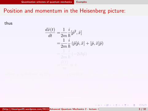
thus
dx(t)
dt=
1
2m
i
~[p2, x]
=1
2m
i
~(p[p, x] + [p, x]p)
=1
2m
i
~(−2i~p)
=p(t)
m≡ v
where v is defined as the velocity operator. The momentum of operator onthe other hand satisfies:
dp(t)
dt=i
~[H, p] =
i
~2m[p2, p] = 0⇒ p(t) = p(0) = p
i.e. the momentum operator is conserved, so the classical picture ofconservation of momentum of a free particle is maintained.
(http://theorique05.wordpress.com/f411) Advanced Quantum Mechanics 2 - lecture 3 3 / 32
Quantisation schemes of quantum mechanics Examples
Position and momentum in the Heisenberg picture:
thus
dx(t)
dt=
1
2m
i
~[p2, x]
=1
2m
i
~(p[p, x] + [p, x]p)
=1
2m
i
~(−2i~p)
=p(t)
m≡ v
where v is defined as the velocity operator. The momentum of operator onthe other hand satisfies:
dp(t)
dt=i
~[H, p] =
i
~2m[p2, p] = 0⇒ p(t) = p(0) = p
i.e. the momentum operator is conserved, so the classical picture ofconservation of momentum of a free particle is maintained.
(http://theorique05.wordpress.com/f411) Advanced Quantum Mechanics 2 - lecture 3 3 / 32

Quantisation schemes of quantum mechanics Examples
Position and momentum in the Heisenberg picture:So now going back to the position operator we can write (sincemomentum is conserved):
x(t) = x(0) +p
mt
The commutator of position and momentum is therefore:
[x(t), p(t)] = [x(0) + pt/m, p(0)] = [x(0), p(0)] + [p(0), p(0)]t/m = i~
so at any time the commutator of the position and momentum isconserved.Note that this commutator also is maintained even if the particleis not free, provided that the commutator is evaluated at equal time:
[x(t), p(t)] = [U †xU , U †pU ] = (U †xU U †pU − U †pU U †xU)
= U †(xp− px)U = i~U †U = i~
(http://theorique05.wordpress.com/f411) Advanced Quantum Mechanics 2 - lecture 3 4 / 32

Quantisation schemes of quantum mechanics Path integrals
Introduction:
The main problem with standard scheme of quantization is thequantization of classical systems with constraints (which are basically allimportant classical systems).Constraint is a limitation imposed on possiblevalues of co-ordinates.In classical physics constraints can be written as:
φ(p, q) = 0,
where φ(p, q) are some functions of p and q.Example: the motion on a sphere in three dimensions has Hamiltonian:
H(p, q) =
3∑i=1
p2i /2m+ V (q),
with the constraint: ∑j
q2j = R2
(http://theorique05.wordpress.com/f411) Advanced Quantum Mechanics 2 - lecture 3 5 / 32
Quantisation schemes of quantum mechanics Path integrals
Introduction:
where R is the radius of the sphere. Then, the coordinates qi withi = 1 · · · 3, are “over-complete” basis in which Hamiltonian is simple.Whenwe reduce the basis to complete one and remove one of the co-ordinatesusing the constraint, we arrive at very cumbersome Hamiltonian which isquite difficult to quantize.There are many ways how we can choose “complete” set of co-ordinatesfor a system with constraints which provide different (usually awkward)classical and quantum Hamiltonians.Dirac developed quite a few methods to deal with constraints in thestandard scheme.It was, however, Richard alertFeynmann, who solved theproblem by developing path integral formulation of quantum mechanics.
(http://theorique05.wordpress.com/f411) Advanced Quantum Mechanics 2 - lecture 3 6 / 32

Quantisation schemes of quantum mechanics Path integrals
The formalism of path integrals
Consider the time evolution of states:
|ψ(t)〉 = U(t, t0)|ψ(t0)〉where the evolution operator is linear. Projecting onto the bra 〈x|:
〈x|ψ(t)〉 = ψ(x, t) =〈x|U(t, t0)|ψ(t0)〉 = 〈x|U(t, t0)1|ψ(t0)〉
=
∫〈x|U(t, t0)|x0〉〈x0|ψ(t0)〉dx0
where 〈x|U(t, t0)|x0〉 are the matrix elements for the evolution operator inthe position representation.We write this as:
ψ(x, t) =
∫K(x, t, x0, t0)ψ(x0, 0)dx0
K(x, t, x0, t0) =〈x|U(t, t0)|x0〉where K(x, t, x0, t0) is known as the propagator.
(http://theorique05.wordpress.com/f411) Advanced Quantum Mechanics 2 - lecture 3 7 / 32

Quantisation schemes of quantum mechanics Path integrals
The formalism of path integrals
It represents the amplitude that a particle propagates from point x0 attime t0 to the point x at time t.Alternatively it represents the probabilityamplitude that a particle which was at time t0 at position x0 to be foundat a later time t at position x, since |x〉 is an eigenstate of positionoperator. It is also called a Green’s function since it satisfies the initialcondition:
K(x, t0, x0, t0) = δ(x− x0)Writing:
K(x, t, x0, t0) =〈x| exp(− i~(t− t0)H
)|x0〉
=〈x| exp(− i~tH
)exp
(+i
~t0H
)|x0〉
=〈x, t|x0, t0〉
(http://theorique05.wordpress.com/f411) Advanced Quantum Mechanics 2 - lecture 3 8 / 32
Quantisation schemes of quantum mechanics Path integrals
The formalism of path integralswhere |x0, t0〉 = exp(iHt0/~)|x0〉 and similarly |x, t〉 = exp(iHt/~)|x〉,are the time-dependent eigenstates of the position operator
x(t) = eiHt/~xe−iHt/~ with eigenvalue x: x(t)|x, t〉 = x|x, t〉,thus theseeigenstates form a complete basis and satisfy the completeness relation,which allows us to write:
K(x, t, x0, t0) =〈x, t|1|x0, t0〉
=
∫〈x, t|x1, t1〉〈x1, t1|x0, t0〉dx1
=
∫K(x, t, x1, t1)K(x1, t1, x0, t0)dx1
which is known as the Markovian property of quantum evolution. In shortthe probability amplitude for the transition |x0, t0〉 → |x, t〉 is equal to thesum over all products of probability amplitudes for intermediate transitions|x0, t0〉 → |x1, t1〉 and |x1, t1〉 → |x, t〉.
(http://theorique05.wordpress.com/f411) Advanced Quantum Mechanics 2 - lecture 3 9 / 32

Quantisation schemes of quantum mechanics Path integrals
The formalism of path integrals
x
t
x0
x
x1t0
t1
t Sum over all x1
Inserting a further unit we write:
K(x, t, x0, t0) =
∫〈x, t|1|x1, t1〉〈x1, t1|x0, t0〉dx1
=
∫〈x, t|x2, t2〉〈x2, t2|x1, t1〉〈x1, t1|x0, t0〉dx2dx1
=
∫K(x, t, x2, t2)K(x2, t2, x1, t1)K(x1, t1, x0, t0)dx2dx1
(http://theorique05.wordpress.com/f411) Advanced Quantum Mechanics 2 - lecture 3 10 / 32
Quantisation schemes of quantum mechanics Path integrals
The formalism of path integrals
x
t
x0
x
x1t0t1
t
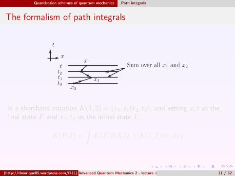
Sum over all x1 and x2 t2
In a shorthand notation K(1, 2) = 〈x1, t1|x2, t2〉, and setting x, t as thefinal state F and x0, t0 as the initial state I:
K(F, I) =
∫K(F, 2)K(2, 1)K(1, I)dx1dx2
(http://theorique05.wordpress.com/f411) Advanced Quantum Mechanics 2 - lecture 3 11 / 32

Quantisation schemes of quantum mechanics Path integrals
The formalism of path integrals
x
t
x0
x
x1t0t1
t
Sum over all x1 and x2 t2
In a shorthand notation K(1, 2) = 〈x1, t1|x2, t2〉, and setting x, t as thefinal state F and x0, t0 as the initial state I:
K(F, I) =
∫K(F, 2)K(2, 1)K(1, I)dx1dx2
(http://theorique05.wordpress.com/f411) Advanced Quantum Mechanics 2 - lecture 3 11 / 32

Quantisation schemes of quantum mechanics Path integrals
The formalism of path integrals
If we keep inserting unities and intermediate time steps we can write:
K(x, t, x0, t0) =
∫K(x, t, xn−1, tn−1) · · ·K(x2, t2, x1, t1)
×K(x1, t1, x0, t0)dxn−1 · · · dx2dx1We can think of the time interval [t0, t] as being divided into Ntime-intervals of length δt,so t− t0 = Nδt and we define tM = t0 +Mδtand tN = t. We thus express the propagator as:
K(F, I) =
∫K(N,N − 1)K(N − 1, N − 2) · · ·K(2, 1)K(1, 0)
× dxN−1dxN−2 · · · dx2dx1
=
∫ (N−1∏M=0
K(M + 1,M)
)N−1∏q=1
dxq
with I ≡ 0 and F ≡ N and where we have:(http://theorique05.wordpress.com/f411) Advanced Quantum Mechanics 2 - lecture 3 12 / 32

Quantisation schemes of quantum mechanics Path integrals
The formalism of path integrals
K(M + 1,M) =〈xM+1, tM+1|xM , tM 〉
=〈xM+1| exp(− i~(tM+1 − tM )H
)|xM 〉
where in fact the time interval between two adjacent instances istM+1− tM = δt.Now as this time interval δt→ 0 (and so N →∞ keepingt− t0 finite –recall δt = (t− t0)/N) we can express the propagatorK(M + 1,M) in the following way by expanding to first order in δt:
K(M + 1,M) =〈xM+1|(1− i
~(tM+1 − tM )H
)|xM 〉
=〈xM+1|xM 〉 −i
~(tM+1 − tM )〈xM+1|H|xM 〉
(http://theorique05.wordpress.com/f411) Advanced Quantum Mechanics 2 - lecture 3 13 / 32

Quantisation schemes of quantum mechanics Path integrals
The formalism of path integrals
The first term 〈xM+1|xM 〉 = δ(xM+1 − xM ), which we can also write inFourier space as:
〈xM+1|xM 〉 =∫〈xM+1|pM 〉〈pM |xM 〉dpM
=
∫1
(√2π~)n
eixM+1pM/~ 1
(√2π~)n
e−ixMpM/~dpM
=1
(2π~)n
∫ei(xM+1−xM )pM/~dpM
with n the number of dimensions of space.The second term is just thematrix element of the Hamiltonian in the position representation, forwhich we can write :
〈xM+1|1H|xM 〉 =∫〈xM+1|pM 〉〈pM |H|xM 〉dpM
(http://theorique05.wordpress.com/f411) Advanced Quantum Mechanics 2 - lecture 3 14 / 32
Quantisation schemes of quantum mechanics Path integrals
The formalism of path integrals
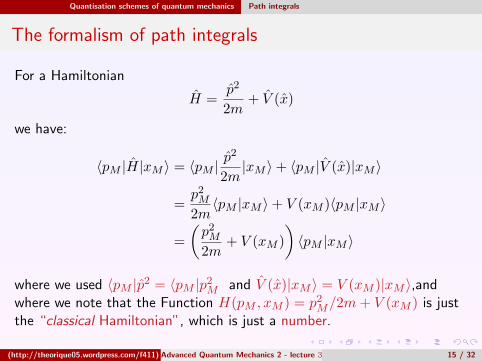
For a Hamiltonian
H =p2
2m+ V (x)
we have:
〈pM |H|xM 〉 = 〈pM |p2
2m|xM 〉+ 〈pM |V (x)|xM 〉
=p2M2m〈pM |xM 〉+ V (xM )〈pM |xM 〉
=
(p2M2m
+ V (xM )
)〈pM |xM 〉
where we used 〈pM |p2 = 〈pM |p2M and V (x)|xM 〉 = V (xM )|xM 〉,andwhere we note that the Function H(pM , xM ) = p2M/2m+ V (xM ) is justthe “classical Hamiltonian”, which is just a number.
(http://theorique05.wordpress.com/f411) Advanced Quantum Mechanics 2 - lecture 3 15 / 32

Quantisation schemes of quantum mechanics Path integrals
The formalism of path integrals
For a Hamiltonian
H =p2
2m+ V (x)
we have:
〈pM |H|xM 〉 = 〈pM |p2
2m|xM 〉+ 〈pM |V (x)|xM 〉
=p2M2m〈pM |xM 〉+ V (xM )〈pM |xM 〉
=
(p2M2m
+ V (xM )
)〈pM |xM 〉
where we used 〈pM |p2 = 〈pM |p2M and V (x)|xM 〉 = V (xM )|xM 〉,andwhere we note that the Function H(pM , xM ) = p2M/2m+ V (xM ) is justthe “classical Hamiltonian”, which is just a number.
(http://theorique05.wordpress.com/f411) Advanced Quantum Mechanics 2 - lecture 3 15 / 32

Quantisation schemes of quantum mechanics Path integrals
The formalism of path integrals
So substituting back we get:
〈xM+1|H|xM 〉 =∫〈xM+1|pM 〉
(p2M/2m+ V (xM )
)〈pM |xM 〉dpM
=1
(2π~)n
∫ei(xM+1−xM )pM/~H(pM , xM )dpM
Thus going back to the propagator K(M + 1,M) we see that it is writtenin Fourier space as:
K(M + 1,M) = 〈xM+1|xM 〉 −i
~(tM+1 − tM )〈xM+1|H|xM 〉
=1
(2π~)n
∫ei(xM+1−xM )pM/~dpM
− i
~(tM+1 − tM )
1
(2π~)n
∫ei(xM+1−xM )pM/~H(pM , xM )dpM
=1
(2π~)n
∫ei(xM+1−xM )pM/~(1− i
~(tM+1 − tM )H(pM , xM ))dpM
(http://theorique05.wordpress.com/f411) Advanced Quantum Mechanics 2 - lecture 3 16 / 32

Quantisation schemes of quantum mechanics Path integrals
The formalism of path integrals
Restoring the exponential to first order in δt we get
K(M + 1,M) =1
(2π~)n
∫exp (i(xM+1 − xM )pM/~)
exp
(− i~(tM+1 − tM )H(pM , xM )
)dpM
=1
(2π~)n
∫exp
(i
~[(xM+1 − xM )pM − (tM+1 − tM )H(pM , xM )]
)dpM
=1
(2π~)n
∫exp
(i
~
[xM+1 − xM
δtpM −H(pM , xM )
]δt
)dpM
Putting this expression into the master relation and setting N →∞ andδt→ 0 we finally arrive at our expression for the propagator:
(http://theorique05.wordpress.com/f411) Advanced Quantum Mechanics 2 - lecture 3 17 / 32

Quantisation schemes of quantum mechanics Path integrals
The formalism of path integrals
K(F, I) = limN→∞
∫ N−1∏q=1
dxq
×(N−1∏M=0
dpM(2π~)n
exp
[i
~
[xM+1 − xM
δtpM −H(pM , xM )
]δt
])
= limN→∞
∫ N−1∏q=1
dxq
(N−1∏M=0
dpM(2π~)n
)
× exp
[i
~
N−1∑k=0
[xk+1 − xk
δtpk −H(pk, xk)
]δt
]
=
∫Dx Dp
(2π~)nexp
[i
~
∫ t
t0
(xp−H(p, x)) dt
](http://theorique05.wordpress.com/f411) Advanced Quantum Mechanics 2 - lecture 3 18 / 32

Quantisation schemes of quantum mechanics Path integrals
The formalism of path integrals
K(F, I) =
∫Dx Dp
(2π~)nexp
[i
~
∫ t
t0
Ldt
]=
∫Dx Dp
(2π~)nexp
[i
~S]
where
Dx ≡ limN→∞
N−1∏q=1
dxq
Dp(2π~)n
≡ limN→∞
N−1∏M=0
dpM(2π~)n
(http://theorique05.wordpress.com/f411) Advanced Quantum Mechanics 2 - lecture 3 19 / 32
Quantisation schemes of quantum mechanics Path integrals
The formalism of path integrals
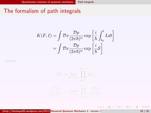
K(F, I) =
∫Dx Dp
(2π~)nexp
[i
~
∫ t
t0
Ldt
]=
∫Dx Dp
(2π~)nexp
[i
~S]
where
Dx ≡ limN→∞
N−1∏q=1
dxq
Dp(2π~)n
≡ limN→∞
N−1∏M=0
dpM(2π~)n
(http://theorique05.wordpress.com/f411) Advanced Quantum Mechanics 2 - lecture 3 19 / 32

Quantisation schemes of quantum mechanics Path integrals
The formalism of path integrals
and where L = xp−H(p, x) is the classical Lagrangian associated withthe classical potential V (x)and S =
∫ tt0L(x, x, t)dt is the corresponding
action.Note that this Lagrangian and classical.So the physical sense of the path integral formulation of quantummechanics is transparent.The amplitude of transition from one point inspace to another is simply obtained by calculating the amplitudes from “allpossible paths” that connect these two points and summing over all theamplitudes.
(http://theorique05.wordpress.com/f411) Advanced Quantum Mechanics 2 - lecture 3 20 / 32

Quantisation schemes of quantum mechanics Path integrals
The formalism of path integrals
x
t
x0
x
t0t1
t
Sum over all trajectoriest2
The paths get smooth as t → 0
Now the amplitude for each path is simply exp(iS/~), with S is just theclassical action for the corresponding path.Essentially we know that inclassical physics there is only one possible path that the particleundergoes,which is the one that extremises the action,but in quantummechanics each of these paths is possible and contributes to theprobability of getting there.
(http://theorique05.wordpress.com/f411) Advanced Quantum Mechanics 2 - lecture 3 21 / 32

Quantisation schemes of quantum mechanics Path integrals
The formalism of path integrals
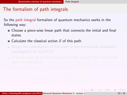
So the path integral formalism of quantum mechanics works in thefollowing way:
Choose a piece-wise linear path that connects the initial and finalstates.
Calculate the classical action S of this path
Assign the contribution of this path to the transitional probability(propagator) as exp(iS/~)Integrate over all possible trajectories that connect the initial pointwith the final point.
The propagator (amplitude of transition F → I) is
K(F, I) =
∫Dx Dp
(2π~)nexp
[i
~S]
(http://theorique05.wordpress.com/f411) Advanced Quantum Mechanics 2 - lecture 3 22 / 32
Quantisation schemes of quantum mechanics Path integrals
The formalism of path integrals
So the path integral formalism of quantum mechanics works in thefollowing way:
Choose a piece-wise linear path that connects the initial and finalstates.
Calculate the classical action S of this path
Assign the contribution of this path to the transitional probability(propagator) as exp(iS/~)Integrate over all possible trajectories that connect the initial pointwith the final point.
The propagator (amplitude of transition F → I) is
K(F, I) =
∫Dx Dp
(2π~)nexp
[i
~S]
(http://theorique05.wordpress.com/f411) Advanced Quantum Mechanics 2 - lecture 3 22 / 32

Quantisation schemes of quantum mechanics Path integrals
The formalism of path integrals
The main advantage of this scheme is that any classical Hamiltonian withany constraints can be easily quantized (constraints can be incorporatedinto “normalization factor”). Furthermore the transition to classicalphysics is obvious: as ~→ 0 the only contributions which maximise theaction S are important.However the disadvantage of the scheme is that itis mathematically ambiguous.
(http://theorique05.wordpress.com/f411) Advanced Quantum Mechanics 2 - lecture 3 23 / 32
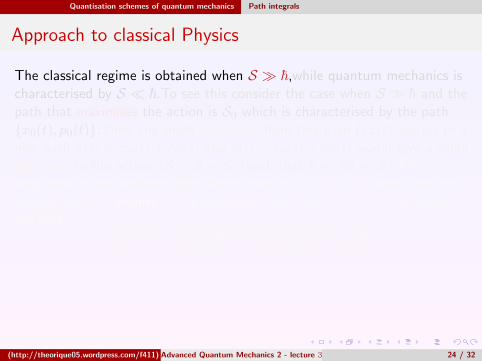
Quantisation schemes of quantum mechanics Path integrals
Approach to classical Physics
The classical regime is obtained when S � ~,while quantum mechanics ischaracterised by S � ~.To see this consider the case when S � ~ and thepath that maximises the action is S0 which is characterised by the path{x0(t), p0(t)}.Then any small deviations from this path (δx(t), δp(t)) to anew path x(t) = x0(t) + δx(t) and p(t) = p0(t) + δp(t) would give a smalldeviation to the action δS = S − S0 (such that ~� δS � S).Theamplitude of the deviated path would then be eiS0/~eiδS/~.Now since onesweeps over the vicinity of the extremum and since δS/~� 1 we easilysee that
〈eiδS/~〉 = 〈cos(δS/~) + i sin(δS/~)〉 = 0
(http://theorique05.wordpress.com/f411) Advanced Quantum Mechanics 2 - lecture 3 24 / 32

Quantisation schemes of quantum mechanics Path integrals
Approach to classical Physics
so on average the contribution from these neighbouring paths are justzero, since: 〈cos(δS/~)〉 = 0 and 〈sin(δS/~)〉 = 0.We clearly see thatthere is only one path that contributes in this regime and it is the classicaltrajectory that maximises the action.The action being extremum means that δS = 0 which leads to theEuler-Lagrange equations of motion.
(http://theorique05.wordpress.com/f411) Advanced Quantum Mechanics 2 - lecture 3 25 / 32

Quantisation schemes of quantum mechanics Path integrals
Example: A free classical particle
Consider a free classical particle travelling in 1D from initial positionI(x0, t0) to a final point F (x, t) along a straight path whose length is Land the time interval is T = t− t0.The speed of the particle is
v =L
T=x− x0t− t0
The classical momentum is p = mv = mL/T and the Hamiltonian isH = p2/2m therefore the classical action (which is extremum) is:
S =
∫ f
i(pv −H)dt =
∫ f
i(mL
T
L
T− 1
2m
m2L2
T 2)dt =
mL2
2T
The propagator is thus (in this classical limit):
K(F, I) = C exp
(imL2
2T~
)which is the classical form of the propagator.
(http://theorique05.wordpress.com/f411) Advanced Quantum Mechanics 2 - lecture 3 26 / 32
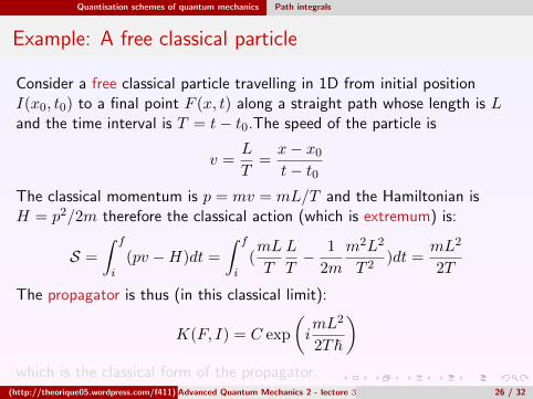

Quantisation schemes of quantum mechanics Path integrals
Example: A free classical particle
We can express the action alternatively as:
S
~=xp
~− Ht
~= kx− ωt
with H/~ = E/~ = ω and p/~ = k. Thus the propagator reads
K(F, I) = C exp (−i(ωt− kx))
which is the wave equation of plane waves.
(http://theorique05.wordpress.com/f411) Advanced Quantum Mechanics 2 - lecture 3 27 / 32

Quantisation schemes of quantum mechanics Path integrals
Example: A free classical particle
Let us consider some examples and see if they are classical or quantumsystems:
Scanning electromagnetic microscope:Typical energies of the electronin the SEM are of order E ∼ 3 eV, and distances are of order L ∼ 5cm.Putting numbers in we find:
S =mL2
2T=mvL
2=pL
2=
√2meEL
2
so S/~ ∼ 1010, which means that this system is classical.
Electron in quantum well: Typical energies are 3 meV and distancesinvlolved are of order L ∼ 1 nm,so S/~ ∼ 0.6. Hence this system is aquantum one.
(http://theorique05.wordpress.com/f411) Advanced Quantum Mechanics 2 - lecture 3 28 / 32

Quantisation schemes of quantum mechanics Path integrals
Borh quantisation and tunneling
Consider the energy levels in the potential well problem.The classicalaction for the trajectory between edges of the well is as usualS =
∫Ldt.To consider the contributions from various paths we must
consider the phase contributions to the amplitude as being exp(niS/~) asthe particle bounces off the walls of the well n times.Thus we see thatunless the action satisfies S = 2π~m, with m being an integer, then thecontribution to the amplitude would be zero.This then leads to thequantisation of energy levels (Bohr quantisation).
(http://theorique05.wordpress.com/f411) Advanced Quantum Mechanics 2 - lecture 3 29 / 32

Quantisation schemes of quantum mechanics Path integrals
Borh quantisation and tunneling
1 2
Consider the tunneling between two wells as shown in the figure.Nowinside the well as the energy of the tunneling particle is conserved itsenergy inside the barrier is negative which means it has an imaginarymomentum,thus its action is imaginary.The contribution from thetrajectories of the particle through the barrier will thus be realexponentially decaying functions:
exp(iS/~)→ exp(−S ′/~)(http://theorique05.wordpress.com/f411) Advanced Quantum Mechanics 2 - lecture 3 30 / 32

Quantisation schemes of quantum mechanics Path integrals
Borh quantisation and tunneling
with S ′ being real.Thus we have by summing over paths T exp(−S ′/~)with T accounting for the degenerate trajectories,i.e. those trajectories inwhich the particle remains within the well barrier an infinitely long time.Sothe total propagator would be written:
C1eiS/~ + C2Te
−S′/~
So when the degeneracy factor is large enough then these terms would giveequivalent contributions, which is true if T ∼ exp(+S ′/~).The tunnelingof the particle through the barrier in this case would be more probable.
(http://theorique05.wordpress.com/f411) Advanced Quantum Mechanics 2 - lecture 3 31 / 32
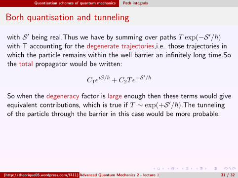

Quantisation schemes of quantum mechanics Path integrals
Conclusions
Different schemes of quantisation of quantum mechanics are:
Orthodox (Copenhagen) version: Advantages: well developedformalism, excellent for 1D and 2D simple (one-body) quantumsystems.Disadvantage: problems with quantisation and measurements
Modern version (Hilbert space Dirac notations): Advantages:mathematically sound, good for many-body systems (condensedmatter physics).Disadvantage: still problems with quantisation andmeasurements
Path Integrals: Advantages: physically transparent, ideal forelementary particles and quantum fields.Disadvantage:mathematically vulnerable
(http://theorique05.wordpress.com/f411) Advanced Quantum Mechanics 2 - lecture 3 32 / 32
Related Documents


![Quantum Mechanics relativistic quantum mechanics (RQM) · Quantum Mechanics_ relativistic quantum mechanics (RQM) ... [2] A postulate of quantum mechanics is that the time evolution](https://static.cupdf.com/doc/110x72/5b6dfe707f8b9aed178e053e/quantum-mechanics-relativistic-quantum-mechanics-rqm-quantum-mechanics-relativistic.jpg)