Advanced Modelling in Biology PrimerThis primer is meant to be a guide as well as a starting point for the student taking Advanced Biological Modelling and is not meant to supplant

Advanced Modelling in Biology Primer

Imperial College London

Spring 2009

Introduction and TopicsCovered

Introduction

This primer is meant to be a guide as well as a starting point for the studenttaking Advanced Biological Modelling and is not meant to supplant lectures.The reason for developing such a primer was intended to make the course moreexciting and relevant to todays algorithms and methods giving both a foundationto what is being done in different fields and allowing for further reading intotopics that you might be more interested in.

Given that this is only a one semester course taught two hours every week,it is impossible to expect to cover every topic and application, yet resourcesare available both here and on the internet if one wanted to go deeper into anysubject.

The topics covered in this primer and corresponding lectures are listed below,but are subject to revision. A website is also dedicated to this course which hasmost of the information covered in this primer as well as many other links tovarious sources on the internet if any subject is still unclear to you or if youdesire further reading.

The website can be found at:

http://openwetware.org/wiki/User:Johnsy/Advanced_Modelling_in_Biology

Optimization

• Introduction to optimization: definitions and concepts, standard formu-lation. Convexity. Combinatorial explosion and computationally hardproblems.

• Least squares solution: pseudo-inverse; multivariable case. Applications:data fitting.

• Constrained optimization:

– Linear equality constraints: Lagrange multipliers

– Linear inequality constraints: Linear programming. Simplex algo-rithm. Applications.

1

• Gradient methods: steepest descent; dissipative gradient dynamics; im-proved gradient methods.

• Heuristic methods:

– Simulated annealing: Continuous version; relation to stochastic dif-ferential equations.

– Neural networks: General architectures; nonlinear units; back-propagation;applications and relation to least squares.

• Combinatorial optimization: hard problems, enumeration, combinatorialexplosion. Examples and formulation.

• Heuristic algorithms: simulated annealing (discrete version); evolutionary(genetic) algorithms. Applications.

Discrete Systems

• Linear difference equations: general solution; auto-regressive models; re-lation to z-transform and Fourier analysis.

• Nonlinear maps: fixed points; stability; bifurcations. Poincar section.Cobweb analysis. Examples: logistic map in population dynamics (period-doubling bifurcation and chaos); genetic populations.

• Control and optimization in maps. Applications: management of fisheries.

Advanced Topics (Networks & Chaos)

• Networks in biology: graph theoretical concepts and properties; randomgraphs; deterministic, constructive graphs; small-worlds; scale-free graphs.Applications in biology, economics, sociology, engineering.

• Nonlinear control in biology: recurrence plots and embeddings; projectiononto the stable manifolds; stabilization of unstable periodic orbits andanti-control. Applications to physiological monitoring.

2

Contents

1 Optimization 41.1 What do we mean when we say optimization? . . . . . . . . . . . 41.2 Standard Optimization vs. Combinatorial Optimization . . . . . 41.3 The Traveling Salesman Problem . . . . . . . . . . . . . . . . . . 51.4 Dimensionality and Finding Minima . . . . . . . . . . . . . . . . 61.5 Steepest Descent and Newton’s Method for Optimization . . . . 61.6 Combinatorial Optimization with Greedy Algorithms . . . . . . . 91.7 Formulating a Combinatorial Optimization Problem . . . . . . . 91.8 Simulated Annealing . . . . . . . . . . . . . . . . . . . . . . . . . 101.9 Genetic/Evolutionary Algorithms . . . . . . . . . . . . . . . . . . 121.10 Constrained Optimization . . . . . . . . . . . . . . . . . . . . . . 131.11 Example: Linear Programming . . . . . . . . . . . . . . . . . . . 141.12 Standard Least Squares Optimization . . . . . . . . . . . . . . . 16

1.12.1 Example: Standard Least Squares for a Straight Line Fit 171.13 Total Least Squares, Singular Value Decomposition, and Princi-

pal Component Analysis . . . . . . . . . . . . . . . . . . . . . . . 181.14 Artificial Neural Networks . . . . . . . . . . . . . . . . . . . . . . 20

2 Discrete Systems 222.1 What is a discrete system? . . . . . . . . . . . . . . . . . . . . . 222.2 How do we solve difference equations? . . . . . . . . . . . . . . . 222.3 What are the behaviors of the solution xt = x0r

t? . . . . . . . . 232.4 Higher Order Difference Equations . . . . . . . . . . . . . . . . . 242.5 Fourier Analysis and Discrete Time Analysis . . . . . . . . . . . 252.6 Cobweb Analysis . . . . . . . . . . . . . . . . . . . . . . . . . . . 262.7 Logistic Maps . . . . . . . . . . . . . . . . . . . . . . . . . . . . . 27

3

Chapter 1

Optimization

1.1 What do we mean when we say optimiza-tion?

The general formulation for any optimization problem is this: We want to mini-mize a function f(x), known as our cost or objective function, subject to a seriesof constraints (e.g. gi(x) = 0 and hi(x) < 0).

f(x) is a function in the general sense, meaning that it can be either con-tinuous or discrete. A continuous function f(x) is one which is defined for allvalues of x. A discrete function is one which is only defined for a discrete inputset xi = [x1, x2, . . . ].

Figure 1.1: Continuous vs. Discrete Functions

It is easy to think of f(x) as a black box having an output for any giveninput.

1.2 Standard Optimization vs. Combinatorial

Optimization

Standard optimization, simply put, is optimization which deals with functionswhere the output is continuous (both variables and functions are continuous).On the other hand, combinatorial optimization deals with functions where theoutput is a discrete set. Remember that the fact that it is discrete does not

4

1.3. The Traveling Salesman Problem

mean that it is not infinite! It is also important to note that calculus does notapply to combinatorial problems, making them more difficult to analyze.

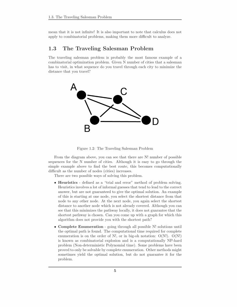
1.3 The Traveling Salesman Problem

The traveling salesman problem is probably the most famous example of acombinatorial optimization problem. Given N number of cities that a salesmanhas to visit, in what sequence do you travel through each city to minimize thedistance that you travel?

Figure 1.2: The Traveling Salesman Problem

From the diagram above, you can see that there are N! number of possiblesequences for the N number of cities. Although it is easy to go through thesimple example above to find the best route, this becomes computationallydifficult as the number of nodes (cities) increases.

There are two possible ways of solving this problem.

• Heuristics - defined as a “trial and error” method of problem solving.Heuristics involves a lot of informal guesses that tend to lead to the correctanswer, but are not guaranteed to give the optimal solution. An exampleof this is starting at one node, you select the shortest distance from thatnode to any other node. At the next node, you again select the shortestdistance to another node which is not already covered. Although you cansee that this minimizes the pathway locally, it does not guarantee that theshortest pathway is chosen. Can you come up with a graph for which thisalgorithm does not provide you with the shortest path?

• Complete Enumeration - going through all possible N! solutions untilthe optimal path is found. The computational time required for completeenumeration is on the order of N!, or in big-oh notation: O(N!). O(N!)is known as combinatorial explosion and is a computationally NP-hardproblem (Non-deterministic Polynomial time). Some problems have beenproved to only be solvable by complete enumeration. Other methods mightsometimes yield the optimal solution, but do not guarantee it for theproblem.

5

1.4. Dimensionality and Finding Minima

1.4 Dimensionality and Finding Minima

Let’s now review some basic calculus involved in finding extrema in a function.Recall that for a one dimensional system, we calculate the derivative of a func-tion f(x) to find the minimum, given a continuous and differentiable function:

df

dx= 0 (1.1)

To ensure that we have a minimum, we look to the second derivative, suchthat

d2f

dx2> 0 (1.2)

Remember that the second derivative must be positive since for a minimumto occur, the gradient of the function must go from being negative to positive.

The first derivative tells us if there is a change in the monotonicity of thefunction while the second derivative guarantees us the minimum. From a twodimensional system, f(x, y), we also can look to the gradient and the secondderivative (this time, the Hessian) such that:

∇f = 0 (1.3)

And that:

H =

(d2fdx2

d2fdxdy

d2fdxdy

d2fdy2

)> 0 (1.4)

The condition above is known as positive definite (all elements in thematrix are positive), and this guarantees that we have a minimum. H is alsopositive definite if the following condition exists:

xT Hx > 0, ∀x (1.5)

The function is also positive definite if the eigenvalues of H are both positivefor symmetric matrices (usually this matrix will be symmetric). The eigenvaluesbeing positive is related to the function being convex in both directions. Recallthat if one eigenvalue is positive and the other negative, then the point is asaddle node.

1.5 Steepest Descent and Newton’s Method forOptimization

Let us return to our problem of continuous optimization where we want tominimize the function f(x), now given that it is positive definite. Althoughit is easy to look at a graph and find the minimum, what tools are availablein Matlab which will allow us to perform optimization without using graphicalmethods? There are two main methods for approaching optimization which youwill explore more in the problem sets.

6

1.5. Steepest Descent and Newton’s Method for Optimization

• fsolve() function in Matlab is an implementation of the steepest descentmethod and finds the zeros of a function (so one must supply the derivativeof a function to obtain an extremum)

• ode45() function performs the analysis over time of a function if we candefine the function to be minimized in terms of a potential function (andsimilar to fsolve(), the gradient of the function must also be supplied)

On using ode45() for optimization:

• Let f(x) be our energy function such that if we integrate dxdt = −∇f with

respect to time, then we are assured that our energy function will decreasealong all trajectories.

• We must supply ode45() with an initial condition to run and with thismethod, we are guaranteed a minimum, but not necessarily the globalminimum. Only if the function is convex that we are guaranteed a globalminimum and hence convex functions are easier to optimize than non-convex functions.

How do you know which function to use when you are performing youroptimization? Let’s consider the similarities and differences between fsolve()and ode45() to get a better idea of how they work and how they can be useful.

Similarities between fsolve() and ode45():

• Both must be supplied the gradient function in order to work

• Both must sample many initial conditions, in fact an infinite number ofthem, to guarantee that the global minimum is achieved. This is particu-larly important for energy functions with very narrow wells.

• Both take large time steps if possible to maximize the change in gradientand speed up calculations

Differences between fsolve() and ode45():

• The output of fsolve() is the x value at which an extremum occurs

• The output of ode45() is a time trace of the x value as time progressesand it is the final value of x over time which determines the value at whichthe extremum occurs. See below for an explanation as to why this is thecase.

• The time steps of ode45() can be changed to suit the needs of the user,which is not available for fsolve().

Convex functions - functions in which for all points in x that our Hessian ispositive definite (will only have one extremum for the entire function). Convex-ity is the result of the variables and if we can redefine the variables such thatour function becomes convex, then this makes optimization much easier.

In the computer, steepest descent is performed by the Euler method of in-tegration given our function:

dx

dt= −∇f (1.6)

7

1.5. Steepest Descent and Newton’s Method for Optimization

The Euler method expands out the differential to give:

xt+1 = xt − (∇f)δt (1.7)

The computer adjusts δt to make it more efficient to reach the minimum andwill minimize ∇f as much as possible until it reaches a given tolerance value(ε) such that:

‖ xt+1 − xt ‖< ε (1.8)

When using ode45(), the computer integrates using the above Euler’s methodand evaluates the derivative after every time step. When the derivative equalsto zero, then xt+1 = xt and the value of x will stop changing and be constantover time. This is why when we use ode45() to obtain our extrema, then wemust take the final value of x to be the point where the extremum occurs.

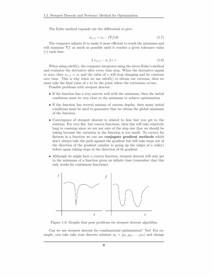
Possible problems with steepest descent:

• If the function has a very narrow well with the minimum, then the initialconditions must be very close to the minimum to achieve optimization

• If the function has several minima of various depths, then many initialconditions must be used to guarantee that we obtain the global minimumof the function.

• Convergence of steepest descent is related to how fast you get to thesolution. For very flat, but convex functions, then this will take relativelylong to converge since we are not sure of the step size that we should betaking because the variation in the function is too small. To correct forflatness in a function we can use conjugate gradient methods whichdon’t always take the path against the gradient but will take steps out ofthe direction of the gradient (similar to going up the ridges of a valley)before again taking steps in the direction of th gradient.

• Although we might have a convex function, steepest descent will only getto the minimum of a function given an infinite time (remember that thisonly works for continuous functions).

Figure 1.3: Graphs that pose problems for steepest descent algorithm

Can we use steepest descent for combinatorial optimization? Yes! For ex-ample, you take take your discrete solution x0 = [μ1, μ2, . . . , μN ] and change

8

1.6. Combinatorial Optimization with Greedy Algorithms

Figure 1.4: The probability of a jump occuring is related to the Boltzmanndistribution

the state of each μ that minimizes the cost function. In effect, steepest descentis similar to a greedy algorithm in that it can minimize each μ locally in an at-tempt to minimize the cost function globally. The only difference between usingsteepest descent instead of simulated annealing with is that we allow upwardchanges in energy for simulated annealing and not for steepest descent.

1.6 Combinatorial Optimization with Greedy Al-

gorithms

For discrete sets in combinatorial problems, we utilize greedy algorithms whichtakes a starting condition and looks to it’s nearest neighbors and minimizes thatdistance before continuing. Remember that without complete enumeration, thiswill not necessarily give the best solution and may get caught in large distanceslater on in the algorithm. This algorithm minimizes locally in an attempt tominimize globally and this is no longer an O(N!) problem anymore, making itcomputationally easier than complete enumeration. A good example of a greedyalgorithm is Dijkstra’s algorithm for finding the minimum pathway through anetwork. Other minimum tree spanning algorithms include Kruskal’s or Prim’sAlgorithm.

1.7 Formulating a Combinatorial OptimizationProblem

Although it is easy to see how we can optimize combinatorial problems, it maybe more difficult to formulate the problem in terms of equations which we want

9

1.8. Simulated Annealing

to minimize. For an example, consider a circuit design where we are given Ncircuits to be divided into two different connected chips. The traffic matrix Ais the interchip cost matrix or our “energy” look up table in the form:

Aij =

⎡⎢⎣

a11 · · · a1n

.... . .

...an1 · · · ann

⎤⎥⎦ (1.9)

We first define the state for each circuit being either μ = ±1 where if thevalue of μ = +1, then it is on the first chip, and if the value of μ = −1, then itis on the second chip.

The state of the system will be given by the list of all the circuits: [μ1, . . . , μn].It can be seen that there are 2n possible solutions for the circuit design.

But what exactly do we want to optimize? First, we want to reduce theinterchip traffic, or the energy required to transfer information between chips.All related chips (as defined by a very low value in the matrix A) would ideallybe together on one chip by having only a very limited number of connectionsbetween the two chips. Second, we would like to make the size of each chiproughly equivalent. We don’t want it such that all the circuits are contained onone chip while the other chip only has a few circuits.

How do we first deal with the interchip traffic? Because we defined eachcircuit to having a state of ±1, this makes it relatively easy. If they are on thesame chip, then μi −μj = 0 and we can formulate the total cost of the functionas:

utraffic =12

∑i,j

(μi − μj

2)2Aij (1.10)

Now to deal with the sizes of both chips, we can just sum up the values ofthe -1 and +1. If they are the same size, then the sum will be equal to 0.

usize = (∑

μi)2 (1.11)

The total cost function that we now want to minimize is:

utotal =12

∑i,j

(μi − μj

2)2Aij + (

∑μi)2 (1.12)

We can also give different weightings (λ) to each cost value to change theimportance of the size of the chips or the interchip traffic by multiplying witha factor:

utotal =12

∑i,j

(μi − μj

2)2Aij + λ(

∑μi)2 (1.13)

1.8 Simulated Annealing

This method attempts to correct for the presence of several minima and is aheuristic algorithm for non-convex problems derived from materials physics. Weslightly adapt the Newton method by including a random term which will causeour function to sometimes go against the gradient.

10

1.8. Simulated Annealing

xt+1 = xt − (∇u)δt + αw(0, σ) (1.14)

• w(0, σ) is a randomly generated number from a normal distribution withmean centered at zero and a standard deviation σ.

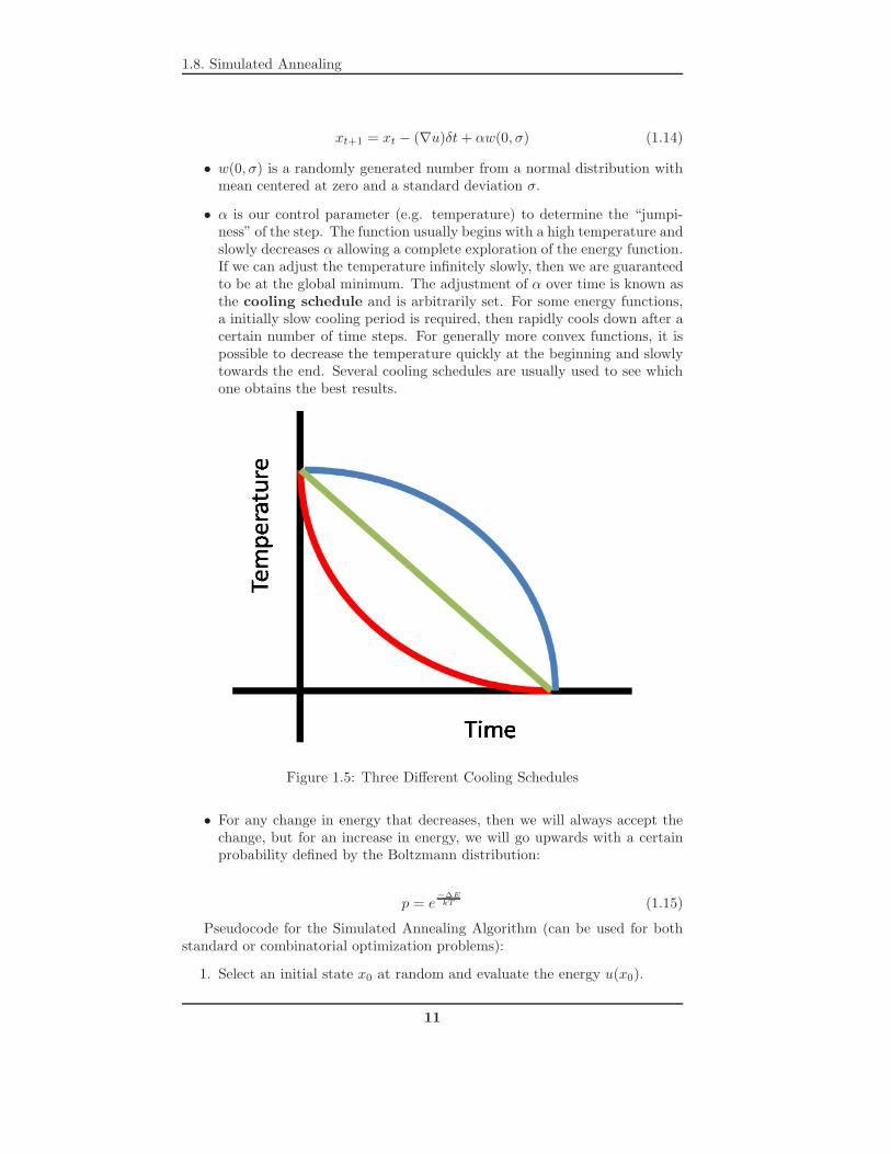
• α is our control parameter (e.g. temperature) to determine the “jumpi-ness” of the step. The function usually begins with a high temperature andslowly decreases α allowing a complete exploration of the energy function.If we can adjust the temperature infinitely slowly, then we are guaranteedto be at the global minimum. The adjustment of α over time is known asthe cooling schedule and is arbitrarily set. For some energy functions,a initially slow cooling period is required, then rapidly cools down after acertain number of time steps. For generally more convex functions, it ispossible to decrease the temperature quickly at the beginning and slowlytowards the end. Several cooling schedules are usually used to see whichone obtains the best results.

Figure 1.5: Three Different Cooling Schedules

• For any change in energy that decreases, then we will always accept thechange, but for an increase in energy, we will go upwards with a certainprobability defined by the Boltzmann distribution:

p = e−ΔE

kT (1.15)

Pseudocode for the Simulated Annealing Algorithm (can be used for bothstandard or combinatorial optimization problems):

1. Select an initial state x0 at random and evaluate the energy u(x0).

11

1.9. Genetic/Evolutionary Algorithms

2. Select x1, the next state at random and evaluate the energy u(x1).

3. Accept the change if the cost function is decreased

4. Otherwise, accept the change with a probability p = e−ΔE

kT , where δE isthe difference in energy between the new state and the previous state

5. Decrease T (temperature) according to the cooling schedule

6. Repeat steps 2 - 5 until we reach the desired number of time steps

An example of simulated annealing from Lawrence David at MIT:Imagine that there is a large hilly region with several peaks and valleys and

one small fish. You, God, suddenly made it rain very hard and the entire regionwas filled with water (remember Noah and the ark?). Now because the waterlevel is quite high, the fish can explore almost every part of the region. However,now that you’ve finished cleansing the land of all the sinners, you want to reducethe water level so that man can once again survive. You slowly reduce the waterlevel. The fish however, wants to live as long as possible so will tend to exploreall the places until he has found the lowest point in the region. By reducingthe water level, the fish sometimes can get stuck in local valleys (minima), butif we can reduce the water very slowly, then the fish will eventually be able toseek out the lowest valley and survive.

Now you might be asking what this is all about? But this is similar tothe simulated annealing problem in that the water level is equivalent to thetemperature and the highest point is what our Boltzmann probability maximumthat we can jump. As God, you control the cooling schedule until your fishreaches the global minimum.

1.9 Genetic/Evolutionary Algorithms

This method is only for combinatorial problems and was inspired by genetics.Evolutionary algorithms are generally faster and get around some of the prob-lems found in simulated annealing. Instead of minimizing an energy function,we maximize a “fitness” when we use evolutionary algorithms. The advantagesof using this algorithm over simulated annealing are the parallelism (fasterbecause you are considering several solutions at each step) and the increasedexploration of state space with “reproduction/crossovers” and “mutations”(ie random factors) of each solution. Remember that this is a heuristic algorithmand that there are no guarantees that the optimal solution will be found.

We first define our function u in state space with a discrete set of solutions.

1. Start out with a population of randomly generated solutions (initial guesses)of size P

2. Reproduction - take random pairs of parents and create their offspring(generating a total of P + P/2 solutions), reproduction is achieved throughmutating the strands and then performing crossovers.

• Mutation - Mutate each solution with a given probability at eachlocation

12

1.10. Constrained Optimization

• Crossover - Move entire portions of the solution to different posi-tions from the two randomly selected parent solutions

3. Rank the population according to their energy u(x)

4. Eliminate (Selection) the bottom P/2 to optimize u(x) leaving again apopulation of size P.

5. Repeat from the reproduction step until you have achieved the number oftime steps that are desired.

Pseudocode for an Evolutionary Algorithm:

generation = 0;initialize populationwhile generation < max_generationfor i from 1 to population_sizeselect two parentscrossover parents to produce a childmutate child with certain probabilitycalculate the fitness of each individual in populationend foreliminate the bottom P/2 membersgeneration++update current population

end while

1.10 Constrained Optimization

If we have constraints that are in the form of equalities, then we want to useLagrange multipliers to solve for the solution. An example of this is to findout which distribution yields maximum entropy.

Below is adapted from the Wikipedia page on Lagrange Multipliers:Suppose we wish to find the discrete probability distribution with maximal

information entropy. Then

f(p1, p2, . . . , pn) = −n∑

k=1

pk log2 pk (1.16)

Of course, the sum of these probabilities equals 1, so our constraint is

n∑k=1

pk = 1 (1.17)

We can use Lagrange multipliers to find the point of maximum entropy(depending on the probabilities). For all k from 1 to n, we require that

∂

∂pk(f + λ(

n∑k=1

pk − 1)) = 0 (1.18)

(see that∑n

k=1 pk−1 = 0 allowing us to do the above operation) which gives

13

1.11. Example: Linear Programming

∂

∂pk

(−

n∑k=1

pk log2 pk + λ(n∑

k=1

pk − 1)

)= 0 (1.19)

Carrying out the differentiation of these n equations, we get

−(

1ln 2

+ log2 pk

)+ λ = 0 (1.20)

If we now solve for pk:

pk = 21

ln 2−λ (1.21)

This shows that all pi are constant and equal (because they depend on λonly). By using the constraint

∑k pk = 1, we find

pk =1n

(1.22)

Hence, the uniform distribution is the distribution with the greatest entropy.If the constraints are in the form of inequalities, then we want to use linear

programming (used in the field of operations research and pioneered by Dantzigwith the Simplex Algorithm). Because all our constraints are linear, then thefeasible region is a convex polytope, so that the optimal solution will be at one ofthe vertices. This can be expanded to N-dimensions, except now, we cannot usea graphical method for solving. However, since we only care about the verticesof the polytope, we can go through each vertex in turn to maximize the costfunction. This is known as the Simplex Algorithm which efficiently checkseach of the vertices in our polytope until an optimal solution is found. First, wefind one vertex and check if it’s optimal. Then, we change one of the variables toget the next vertex and move on to increase the cost function maximally. Checkeach vertex to see if it is optimal until you have maximized the cost function.Computationally, the Simplex Algorithm is also combinatorial (ie O(N C N-m))where N is the number of variables and m is the number of inequalities.

1.11 Example: Linear Programming

The Problem:You are managing a farm that has 45 Ha in surface and you want to split

your cultivated surface between wheat (W) and corn (C). The amount of laborthat you can use is limited at 100 workers. Each hectare of wheat requires 3workers while each hectare of corn requires 2 workers. The amount of fertilizerneeded is 20 kg per hectare of wheat and 40 kg per hectare of corn. You canonly use up to 1200 kg of fertilizer. When you go to the market, for each hectareof wheat, you will get a profit of $200 while each hectare of corn returns $300.

The Solution:The first thing to do in any linear programming problem is to identify the

constraints and the cost function that we wish to maximize. In the aboveproblem, there are three limitations to the total amount of wheat and corn thatcan be grown: land, labor and fertilizer limitations. Let us first consider theland limitations. The total number of hectares of wheat (W) and corn (C) mustbe less than or equal to 45. Writing this as an inequality (Constraint 1):

14

1.11. Example: Linear Programming

W + C ≤ 45 (1.23)For the labor limitations, we cannot exceed 100 workers (Constraint 2):

3W + 2C ≤ 100 (1.24)For the fertilizer limitations, we cannot exceed 1200 kg of fertilizer (Con-

straint 3):

20W + 40C ≤ 1200 (1.25)And finally, our cost/profit function which we wish to maximize:

Profit = 200W + 300C (1.26)Since this is only a two dimensional problem, we can solve this using a

graphical method. We plot all of the constraints to come up with a feasibleregion, or the region of solutions which the problem satisfies all of the conditions.

Figure 1.6: Linear Programming Example

With a graphical method, it is easy to see that the optimal solution will occurat (20,20), the last point which the profit function touches of the polytope ifyou continue moving it upwards keeping the same slope. This corresponds tofarming 20 hectares each of wheat and corn. Although we have not optimallyused all of the land, we have maximized the profit given the conditions.

Is the upper right corner of the polytope always the optimal point of opera-tion? By no means is this the optimal point at which to operate. The optimalpoint is determined by the profit function. For example, if the profit for eachhectare of corn is only $1 while the profit for wheat is $200, then it is easy tosee that we should produce all wheat (corresponding to the upper left point ofthe polytope.

15

1.12. Standard Least Squares Optimization

1.12 Standard Least Squares Optimization

Least Squares Optimization is used for data fitting given one or more inde-pendent variables and one dependent variable. We establish the relationshipbetween the variables either by a theoretical relationship or by observation andwe wish to know which “line” best describes the data obtained from experimen-tation. For standard least squares, this problem has an analytical solution.

We have a collection of N points (xi, yi) and we have strong belief thatthis dependency is linear. We must assume that x is an independent variableand that there is no error involved with the measurement of this parameter.We would like to find out the coefficients of the following equation that bestdescribes the data.

y = a0 + a1x (1.27)

For the least squares method, we optimize the distance between the predictedline and the actual points that we have. We have a overdetermined system(a system where we have too few variables for the number of equations) whichwe can write in matrix form below:

y =

⎛⎜⎝

y1

...yN

⎞⎟⎠ = a0

⎛⎜⎝

1...1

⎞⎟⎠+ a1

⎛⎜⎝

x1

...xN

⎞⎟⎠ =

⎛⎜⎝

1 x1

......

1 xN

⎞⎟⎠(

a0

a1

)= Xa (1.28)

The error function is now the difference between the predicted values andthe observed values:

e = yi − yi (1.29)

For the least squares optimization we would like to minimize eT e

eT e = (yi − yi)T (yi − yi)

= yT y − yT y − yT y + yT y (1.30)

But we know that y = Xa, so substituting, we get:

E = eT e = (Xa)T (Xa) − (Xa)T y − yT (Xa) + yT y

= aT XT Xa− aT XT y − yT Xa + yT y (1.31)

To minimize the error, we want ∇Ea = 0:

∇Ea = 2XT Xa− 2XT y = 0

a = (XT X)−1XT y (1.32)

This can be expanded into N variables, each with a linear dependence. Theresult of this is that it will find the best hyperplane in m − 1 dimensions if wehave m number of independent variables.

16

1.12. Standard Least Squares Optimization

Let us compare the above with a determined system where there are enoughequations to find the coefficients exactly.

y1 = a0 + a1x1 (1.33)y2 = a0 + a1x2 (1.34)

We can easily rewrite this in matrix form:

�y =[y1

y2

]=[1 x1

1 x2

] [a0

a1

]= �X�a (1.35)

Now we can see to solve for the coefficients, we can just take the inversematrix of X :

�a = ( �X)−1�y (1.36)

Compared to the overdetermined system above calculated for the standardleast squares, we can see a similarity between the matrices inverted. Becausewe are “inverting” a rectangular matrix for the least squares method and nota square matrix, we call this the pseudoinverse. (Note that the inverse of amatrix can only be taken on a square matrix)

Pseudoinverse = (XT X)−1XT

In Matlab, this is implemented by the function pinv().

1.12.1 Example: Standard Least Squares for a StraightLine Fit

If we reinvert the matrix, we obtain that

XT Xa = XT y (1.37)

Let us take the four points (0,0), (1,8), (3,8), and (4,20) and perform stan-dard least squares to find the line which best fits the points (minimizes thevertical error).

X =

⎡⎢⎢⎣1 01 11 31 4

⎤⎥⎥⎦ (1.38)

y =

⎡⎢⎢⎣

08820

⎤⎥⎥⎦ (1.39)

Performing the calculations:

XT X =[1 1 1 10 1 3 4

]⎡⎢⎢⎣1 01 11 31 4

⎤⎥⎥⎦ =

[4 88 26

](1.40)

and

17

1.13. Total Least Squares, Singular Value Decomposition, and PrincipalComponent Analysis

XT y =[1 1 1 10 1 3 4

]⎡⎢⎢⎣08820

⎤⎥⎥⎦ =

[36112

](1.41)

The system is then solved with[4 88 26

] [a0

a1

]=[

36112

](1.42)

By solving the system of equations, we obtain that[a0

a1

]=[14

](1.43)

Hence the best fit line through the points is y = 1 + 4x. Below shows thebest fit line with the four points.

Figure 1.7: Linear Least Squares Example

1.13 Total Least Squares, Singular Value De-composition, and Principal Component Anal-

ysis

Total least squares is a method to finding the best fit curve given that we don’tknow the independent and dependent variables of the system. For example,given several different parameters that one is looking at, we are unsure of whichvariables depend on the other. In effect, total least squares finds the best fitline such that the error minimized is the perpendicular distance between the

18

1.13. Total Least Squares, Singular Value Decomposition, and PrincipalComponent Analysis

measured point and the optimal line (as opposed to the vertical distance instandard least squares).

Figure 1.8: Total Least Squares Method utilizing the perpendicular distancebetween the point and the best-fit line

Singular Value Decomposition (SVD) yields the covariance matrix betweenthe variables that we have and the matrix of principle components from whichwe can perform Principal Component Analysis. Singular value decompositionis equivalent to the diagonalization of rectangular matrices and typically yield aseries of ranked numbers. The largest of these values are known as the principalcomponents of the system and allow us to determine which of the variablesare most strongly correlated to one another. For example, given 5 variablesand our SVD yields that 2 of the variables are much higher than the other, wehave 2 principal components which should be sufficient to describe the trendsin the data and the other variables have little or no correlation to what is beingobserved. Using PCA allows us to discard redundant variables in our systemleaving what is known as the lower rank approximation to the system.

The decomposition of a matrix X yields the following:

X = UΣV T (1.44)

Where U and V are unitary matrices and σ is the matrix with the singularvalues. Usually, the singular value decomposition is preformed on the matrix ofthe variables with the mean subtracted from all the data points and not usuallyon the raw data. This allows an easier interpretation of the decomposition. Thecovariance matrix can then be calculated from the altered data and the singularvalues correspond to the eigenvalues of this n × n covariance matrix (with nnumber of variables).

To obtain the lower rank approximation, we reduce the number of rows ofσ such that it becomes an r × r matrix, where r is the number of variables.

19

1.14. Artificial Neural Networks

The reconstructed values of X now take into account only the singular valueswith the highest value and discard those with lower values that are may notbe pertinent to explaining the trendline. For example, you might have singularvalues of 200, 100, 1 and 0.5. In this case, if you wanted to reduce the numberof variables in the problem, the lower rank approximation would be a 2 × 2matrix with only singular values of 200 and 100. The variables that correspondto these highest singular values are your principal components of the system.

1.14 Artificial Neural Networks

Optimization within artificial neural networks can also be a challenging prob-lem. We first define a neural network through the perceptron, or a series ofinputs, hidden nodes, and outputs in a funnel like structure which allow fastcomputation of certain types of problems. Connections exist between layers butdo not exist within layers. Each edge contains a weight by which the input fromthe previous layer is multiplied to obtain the next layer.

Figure 1.9: An example of a perceptron

Given that the input into the perceptron is x0, what will our output be withthe two hidden layers above? Consider the first hidden layer. The input intothe first hidden layer is:

χIl×1 = W I

l×n�xn×1 (1.45)

We apply a non-linear function f(x) at the hidden layer such that the outputfrom the first layer and the input into the second hidden layer is:

χIIp×1 = W II

p×lf(χI) (1.46)

Similarly, our output of the perceptron is:

20

1.14. Artificial Neural Networks

y = W III1×pf(χII) (1.47)

It can be seen that these are nested expressions, so if we want to express theoutput in terms of the input and the weightings, we obtain the equation:

y = W III1×pf(W II

p×lf(W Il×nxn×1)) (1.48)

The output is a nested series of functions that are weighted by each nodein the system. This is usually a non-trivial solution and very non-linear. Theweights of the edges are usually obtained through “learning”, or taking severalknown inputs and outputs and allowing the weights of each to change such thatthe known output is obtained. The three types of learning are used and arederived from biological heuristics: the Hebbian Rule, the Darwinian Rule, andSteepest Descent.

The Hebbian Rule (potentiation) is based upon the theory that synapsesthat are used most are strengthened, ie the weights of those edges are higherbased on how many times they are used in the learning sequence.

The Darwinian rule initially assigns random weights to each edge and evolvesthem over time to minimize the error in the output.

Steepest descent attempts to minimize the error function similar to the steep-est descent methods described earlier. We can define our desired output as:

y = W IIIf(W IIf(W I�x)) (1.49)

The error involved between the desired output and the observed output ycan be minimized with the function:

E =∥∥y − y

∥∥2 (1.50)

All that is required now is to optimize dEdW by following the decrease in the

gradient to obtain the weights that give the minimum error.An implementation of this method is known as back propagation, where we

first start from the output and calculate and minimize the local errors involvedto find the best weights. Although back propagation is not a biological example,it is a heuristic algorithm that tends to work when training neural networks.

21

Chapter 2

Discrete Systems

2.1 What is a discrete system?

Discrete systems are systems with non-continuous outputs with the result foreach time step being determined by the previous time step. The equivalentto differential equations (continuous systems) in discrete system are known asdifference equations such as the one shown below. Since the difference equationtells us about the next time step, it is known as a 1st order difference equation.

xt+1 = rxt (2.1)

This is the discrete equivalent of the differential equation:

dx

dt= rx (2.2)

Discrete systems are found in nature, for example in biology where repro-duction occurs at discrete time steps. Also, sampling at discrete time intervalsof a continuous system gives us discreteness.

2.2 How do we solve difference equations?

1) By guessing (ansatz - German for ”guess”)Let us assume that the solution is in the form

xt = Aβt (2.3)

Then substituting into the difference equation, we get

Aβt+1 = rAβt (2.4)

r = β (2.5)

And hence the solution to the difference equation is

xt = x0rt (2.6)

2) Z-transforms - the discrete equivalent to the Laplace transform, an orga-nized way to find solutions

22

2.3. What are the behaviors of the solution xt = x0rt?

2.3 What are the behaviors of the solution xt =x0r

t?

There are 4 different regimes, depending on the value of r.

• If r > 1, then xt approaches infinity.

• If 0 < r < 1, then xt approaches zero.

• If −1 < r < 0, then xt approaches zero in an oscillatory manner.

• If r < −1, then xt approaches infinity in an oscillatory manner.

Figure 2.1: Plots of a discrete equations over time

Remember that if we have non-linear systems, it is difficult to obtain theglobal stability analysis of the problem, however, we can see from the abovedifferent behaviors that we can generalize it into stable and unstable behaviorsas shown in the table below.

Stability Analysisr States Stability|r| < 1 Stable|r| > 1 Unstabler = 1 Liapunov Stable

23

2.4. Higher Order Difference Equations

What does Liapunov stability imply? The fixed point is neither stable (goestowards the fixed point) nor unstable (goes away from the fixed point), but thetrajectory is bounded. This is similar to a limit cycle or a center in continuousdifferential equations.

2.4 Higher Order Difference Equations

A second order difference equations would tell us about the state of the systemtwo time steps away, for example:

xt+2 = axt+1 + bxt (2.7)

How do we go about solving this system? We again solve by guessing forthe correct solution. We have our initial guess again as xt = Art. Substitutinginto our original equation, we get:

Art+2 = aArt+1 + bArt (2.8)

The characteristic equation for this system is

r2 − ar − b = 0 (2.9)

Solving for r

r± =a ±√

a2 + 4b

2(2.10)

Hence, our general solution will be the sum of all possible solutions, just likein second order differential equations

xt = Art+ + Brt

− (2.11)

We can then solve for A and B with our initial conditions.For the stability of the system, we know that for the system not to blow up

to infinity, |r+|, |r−| < 1. For this condition to be met, the following conditionmust be satisfied (can be solve for by setting r = 1).

b < 1 − a (2.12)

Furthermore, we can generalize this solution for an N-dimensional system:

a0xt+N + a1xt+N−1 + · · · + aN = 0 (2.13)

We again make the guess that our solution is in the form xt = Art, substitute,and obtain our characteristic polynomial to be:

α0rN + α1r

N−1 + · · · + αN = 0 (2.14)

The roots of our polynomial give the values of r and they must all satisfy|r| < 1 for the entire system to be stable. With the root of the equation being:{r∗1 , . . . , r∗N}, our general solution becomes:

xt =N∑

i=1

Ai(r∗i )t (2.15)

24

2.5. Fourier Analysis and Discrete Time Analysis

Solving these difference equations is non-trivial and computationally diffi-cult. There are criteria (see Schur or Jury) to check to see if the parameterswill lead to a stable conditions (which check to see if the roots are within theunit circle). We can only solve by hand to a maximum of 4 dimensions. Withhigher order dimensions, a computer becomes necessary to establish the rootsof the equation.

2.5 Fourier Analysis and Discrete Time Analy-sis

We can first motivate this by an example. Let us consider a single sinusoid inthe time domain.

y(t) = Asin(ωt) (2.16)

Is it possible to write this function in terms of a difference equation? Con-sider the time steps t and t + 1 for a sinusoidal function:

yt = Asin(ωt) (2.17)yt±1 = Asin(ω(t ± 1))

= A[sin(ωt)cos(ω) ± sin(ω)cos(ωt)] (2.18)

If we now add yt+1 and yt−1 we obtain:

yt+1 + yt−1 = 2Acos(ω)sin(ωt)= 2cos(ω)yt (2.19)

Hence we can conclude that:

yt+1 = 2cos(ω)yt − yt−1 (2.20)

We can see that a sinusoid function in the time domain can be expressedin terms of a second order difference equation. In general, if we have a sum ofN sinusoidal waves making up our function, we can write this as a differenceequations with 2N terms. In mathematical terms, this can be expressed as:

yt =N∑

m=1

amsin(mωt + φm)

≡

yt+2N =2N−1∑m=0

bmyt−m (2.21)

Recall that the first equation above is just the Fourier transform of a func-tion in time domain. Hence, for any function in the time domain, this can bewritten as either a series of sinusoids using Fourier transform or as a difference

25

2.6. Cobweb Analysis

equation with two terms to each Fourier term. We can also see that the coef-ficients obtained from performing the Fourier transform are directly related tothe coefficients of the difference equation that is generated.

The process of going from the time domain to the difference equation isknown as Linear Discrete Time Analysis, since we can see that we obtain a lineardifference equation from a sinusoidal function. This is analogous to gettinga linear second order differential equation when we are considering the samesinusoid when we do continuous differentiation.

2.6 Cobweb Analysis

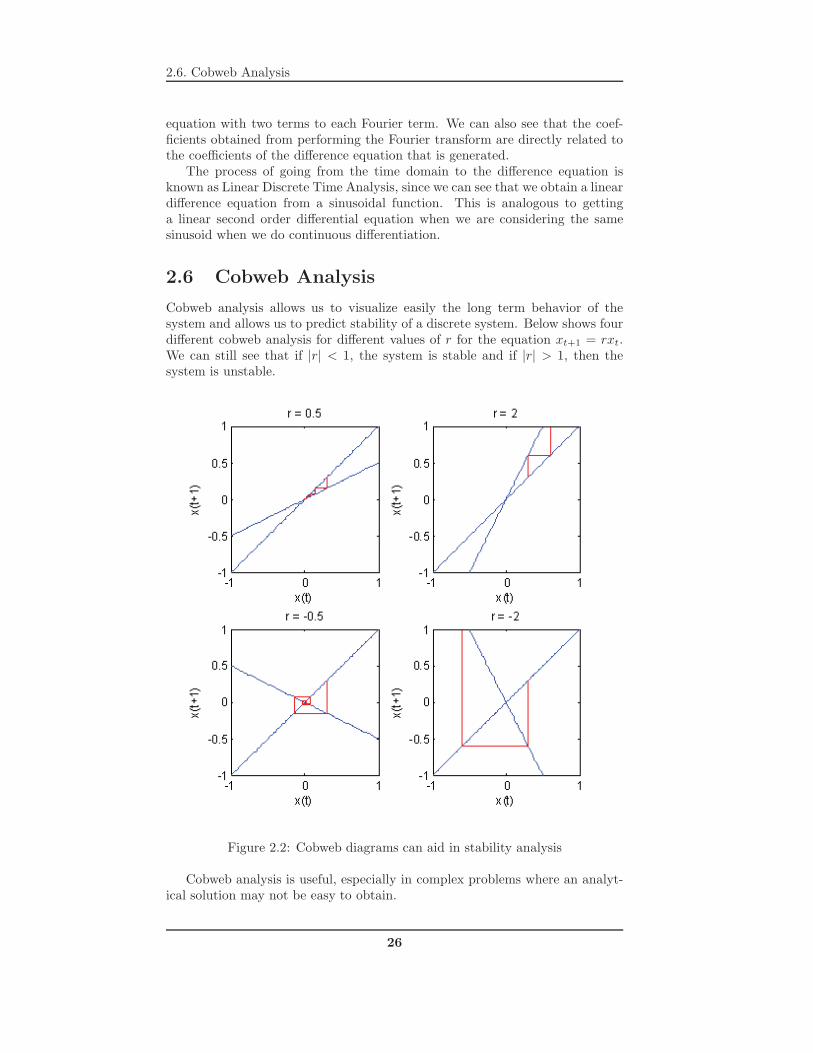
Cobweb analysis allows us to visualize easily the long term behavior of thesystem and allows us to predict stability of a discrete system. Below shows fourdifferent cobweb analysis for different values of r for the equation xt+1 = rxt.We can still see that if |r| < 1, the system is stable and if |r| > 1, then thesystem is unstable.

Figure 2.2: Cobweb diagrams can aid in stability analysis

Cobweb analysis is useful, especially in complex problems where an analyt-ical solution may not be easy to obtain.

26

2.7. Logistic Maps

2.7 Logistic Maps

Let us now consider the logistic map equation as an example of how linearstability analysis is preformed on difference equations/systems.

xt+1 = rxt(1 − xt) (2.22)

Where 0 < r < 4 are the boundaries set.First, to find the fixed points, we set xt+1 = xt to obtain the two fixed

points:

x∗t = 0, 1 − 1

r(2.23)

For linear stability analysis, we need that∣∣∣ dfdxt

∣∣∣ < 1

f(xt) = xt+1 = rxt(1 − xt) (2.24)df

dxt= r − 2rxt (2.25)

Now evaluating at the fixed points

f ′(x∗t = 0) = r (2.26)

f ′(x∗t = 1 − 1

r) = −r + 2 (2.27)

Hence, the stability of the x∗t = 0 fixed point is stable if 0 < r < 1 (recall

that we are bounded between 0 < r < 4 for our system). The stability of thex∗

t = 1 − 1r fixed point is stable for 1 < r < 3.

After r = 3, we see that the system is unstable and that there are nofixed points. In fact, we will oscillate between fixed points and observe what isknown as period doubling in our system. How do we calculate these fixed pointsanalytically? If we have a period 2 oscillation, that means that

xt+2 = xt (2.28)

And from our function, we know that

xt+1 = f(xt) (2.29)

And by substitution

xt+2 = f(xt+1) = f(f(xt)) (2.30)

In general, to solve for p period solutions, we want that

xt+p = xt (2.31)

And we can solve

xt+p = f(f...f(f(xt)))p (2.32)

27

2.7. Logistic Maps

Returning back to our period-2 oscillations, we substitute our logistic equa-tion into the xt+2 equation

xt+2 = f(f(xt)) = r[rxt(1 − xt)][1 − rxt(1 − xt)] (2.33)

We now set this equal to xt and solve for the fixed points. As it can be seenthat both our initial fixed points are fixed points of this system with two furtherfixed points being added. The two new fixed points are the points around whichthe system oscillates.

The bifurcations occur when the looking at the difference plot and seeingwhen you get more crossings on the graph. As the value of r is increased, thebifurcations occur more closely. After a certain value of r, you can get a pointwhere there are no period solutions exist and this is the point where chaosemerges. Within the chaotic region, numerical analysis has yielded windows ofperiodicity such as period-3 oscillations, but quickly become chaotic again as ris changed.

With the analysis above, we can easily see that a fixed point is actually aperiod-1 solution to our system.

28