ADVANCED MISSION DESIGN: INTERPLANETARY SUPER HIGHWAY TRAJECTORY METHOD A Dissertation by HYERIM KIM Submitted to the Office of Graduate and Professional Studies of Texas A&M University in partial fulfillment of the requirements for the degree of DOCTOR OF PHILOSOPHY Chair of Committee, David C. Hyland Committee Members, Srinivas Rao Vadali Tom Pollock Lucas Macri Head of Department, Rodney Bowersox August 2015 Major Subject: Aerospace Engineering Copyright 2015 Hyerim Kim

Welcome message from author
This document is posted to help you gain knowledge. Please leave a comment to let me know what you think about it! Share it to your friends and learn new things together.
Transcript

ADVANCED MISSION DESIGN: INTERPLANETARY SUPER HIGHWAY
TRAJECTORY METHOD
A Dissertation
by
HYERIM KIM
Submitted to the Office of Graduate and Professional Studies of
Texas A&M University
in partial fulfillment of the requirements for the degree of
DOCTOR OF PHILOSOPHY
Chair of Committee, David C. Hyland
Committee Members, Srinivas Rao Vadali
Tom Pollock
Lucas Macri
Head of Department, Rodney Bowersox
August 2015
Major Subject: Aerospace Engineering
Copyright 2015 Hyerim Kim

ii
ABSTRACT
Near-future space missions demand the delivery of massive payloads to deep
space destinations. Given foreseeable propulsion technology, this is feasible only if we
can design trajectories that require the smallest possible propulsive energy input. This
research aims to design interplanetary space missions by using new low-energy
trajectory methods that take advantage of natural dynamics in the solar system. This
energy efficient trajectory technology, called the Interplanetary Super Highway (IPSH),
allows long duration space missions with minimum fuel requirements. To develop the
IPSH trajectory design method, invariant manifolds of the three-body problem are used.
The invariant manifolds, which are tube-like structures that issue from the periodic orbits
around the L1 and L2 Lagrangian points, can be patched together to achieve voyages of
immense distances while the spacecraft expends little or no energy. This patched three-
body method of trajectory design is fairly well developed for impulsive propulsion. My
research is dedicated to advance its capabilities by extending it to continuous, low-thrust,
high specific impulse propulsion methods.
The IPSH trajectory design method would be useful in designing many types of
interplanetary missions. As one of its applications, my research is focused on Near-Earth
Asteroids (NEAs) rendezvous mission design for exploration, mitigation, and mining.
Asteroids have many valuable resources such as minerals and volatiles, which can be
brought back to Earth or used in space for propulsion systems or space habitats and
stations. Transportation to and from asteroids will require relatively massive vehicles

iii
capable of sustaining crew for long durations while economizing on propellant mass.
Thus, in the design of advanced NEA rendezvous missions, developing new technology
for low cost trajectories will play a key role.
In a second application study, the solar sail mission for Mars exploration is
considered. By using solar radiation pressure, solar sails provide propulsive power. This
thrust affects the three-body system dynamics such that the Sun-Mars L1 and L2
Lagrangian points are shifted toward the Sun and the geometry of the invariant
manifolds around L1 and L2 points is changed. By taking advantage of these features, a
low-thrust trajectory for Mars exploration is developed.

iv
ACKNOWLEDGEMENTS
I would like to thank Dr. David C. Hyland for his contributions and exceptional
mentorship through the course of this research. He has motivated and encouraged me
with valuable discussions on this topic.
Also I would like to thank to my colleagues who have consistently helped my
graduate study at Texas A&M University: Shen Ge, Micaela Landivar, Richard
Margulieux, Julie Sandberg, Neha Satak, Russell Trahan, and Brian Young.
Finally, thanks to my mother and father for their infinite support and to my
wonderful husband for his unconditional trust and love.

v
NOMENCLATURE
BCM Bi-Circular Model
C Jacobi Integral
CCM Concentric Circular Model
DCM Differential Correction Method
E Energy Integral
f Solar Sail Factor
GEO Geosynchronous Equatorial Orbit
Isp Specific Impulse
IPSH Interplanetary Super Highway
LEO Low Earth Orbit
NEA Near-Earth Asteroid
PCR3BP Planar Circular Restricted 3-Body Problem
rh Hill Radius
S/C Spacecraft
STM State Transition Matrix
U Pseudo-Potential Energy Function
�� Effective Potential Energy Function
μ Mass Parameter

vi
TABLE OF CONTENTS
Page
ABSTRACT ....................................................................................................................... ii
ACKNOWLEDGEMENTS ...............................................................................................iv
NOMENCLATURE ........................................................................................................... v
TABLE OF CONTENTS ..................................................................................................vi
LIST OF FIGURES ........................................................................................................ viii
LIST OF TABLES ............................................................................................................ x
1. INTRODUCTION .......................................................................................................... 1
1.1 Historical Contributions ....................................................................................... 1 1.2 Problem Statement ............................................................................................... 3
2. BACKGROUND: MATHEMATICAL MODEL .......................................................... 5
2.1 The N-Body Problem ........................................................................................... 5 2.2 Normalized Units ................................................................................................. 6 2.3 Equation of Motion for PCR3BP ......................................................................... 8 2.4 Equilibrium Points in PCR3BP .......................................................................... 11 2.5 Energy State Dynamics: Jacobi Constant, Hill’s Region ................................... 13
3. DESIGN TRAJECTORY WITH GEOMETRY OF N-BODY PROBLEM ............... 15
3.1 Invariant Manifolds ............................................................................................ 15 3.2 1-D Search Technique ........................................................................................ 19
3.2.1 Linearization in the Vicinity of L1 and L2 points ........................................ 19 3.2.2 Geometry of Solutions with the Eigen State Analysis ................................ 20
3.2.3 Centerline of Invariant Manifolds ............................................................... 22
3.2.4 Symmetries of Homoclinic and Heteroclinic Orbits ................................... 24 3.3 Preliminary Design for NEA Rendezvous Mission ........................................... 26
3.3.1 4-Body Dynamics for Coupled Two 3-Body Systems ................................ 29
4. DESIGN TRAJECTORY FROM EARTH TO MARS ............................................... 33
4.1 Investigation for Omni-directional Solar Sail Power ......................................... 34 4.2 Limited Case of 4-Body Problem ....................................................................... 38

vii
4.2.1 Equations of Motion for the Limited Case of 4 Body Problem .................. 38 4.2.2 Energy State and Eigen State for the Limited Case of 4-Body Problem .... 43
4.3 Transfer Trajectory from Earth to Mars with Solar Sail .................................... 52
5. SUMMARY AND FUTURE WORK .......................................................................... 57
REFERENCES ................................................................................................................. 59
viii
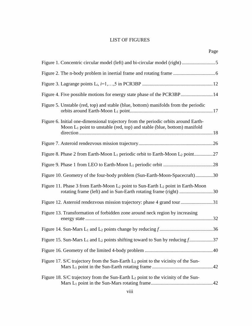
LIST OF FIGURES
Page
Figure 1. Concentric circular model (left) and bi-circular model (right) ........................... 5
Figure 2. The n-body problem in inertial frame and rotating frame .................................. 6
Figure 3. Lagrange points Li, i=1,…,5 in PCR3BP ......................................................... 12
Figure 4. Five possible motions for energy state phase of the PCR3BP .......................... 14
Figure 5. Unstable (red, top) and stable (blue, bottom) manifolds from the periodic
orbits around Earth-Moon L1 point ................................................................... 17
Figure 6. Initial one-dimensional trajectory from the periodic orbits around Earth-
Moon L1 point to unstable (red, top) and stable (blue, bottom) manifold
direction ............................................................................................................ 18
Figure 7. Asteroid rendezvous mission trajectory ............................................................ 26
Figure 8. Phase 2 from Earth-Moon L1 periodic orbit to Earth-Moon L2 point ............... 27
Figure 9. Phase 1 from LEO to Earth-Moon L1 periodic orbit ........................................ 28
Figure 10. Geometry of the four-body problem (Sun-Earth-Moon-Spacecraft) .............. 30
Figure 11. Phase 3 from Earth-Moon L2 point to Sun-Earth L2 point in Earth-Moon
rotating frame (left) and in Sun-Earth rotating frame (right) ........................... 30
Figure 12. Asteroid rendezvous mission trajectory: phase 4 grand tour .......................... 31
Figure 13. Transformation of forbidden zone around neck region by increasing
energy state ....................................................................................................... 32
Figure 14. Sun-Mars L1 and L2 points change by reducing f ........................................... 36
Figure 15. Sun-Mars L1 and L2 points shifting toward to Sun by reducing f ................... 37
Figure 16. Geometry of the limited 4-body problem ....................................................... 40
Figure 17. S/C trajectory from the Sun-Earth L2 point to the vicinity of the Sun-
Mars L1 point in the Sun-Earth rotating frame ................................................. 42
Figure 18. S/C trajectory from the Sun-Earth L2 point to the vicinity of the Sun-
Mars L1 point in the Sun-Mars rotating frame .................................................. 42

ix
Figure 19. Close up of the trajectory near the Sun-Mars L1 point in the Sun-Mars
rotating frame .................................................................................................... 43
Figure 20. Forbidden zone for the Sun-Earth-S/C system in the Sun-Earth rotating
frame when f = 1 and ESE = -1.50045 ............................................................... 44
Figure 21. Forbidden zone for the Sun-Earth-S/C system in the Sun-Earth rotating
frame when f = 0.83 and ESE = -1.32482 .......................................................... 44
Figure 22. Forbidden zones when f is decreasing with fixed energy ESE = -1.50045
(f = 1 (left), f = 0.9999 (middle), f = 0.9991 (right)) ........................................ 46
Figure 23. Forbidden zones when ESE is increasing with fixed f = 1 (ESE = -1.50045
(left), ESE = -1.50023 (middle), ESE = -1.50001 (right)) ................................... 46
Figure 24. Forbidden zones with different f and energy ESE (f = 1, ESE = -1.5001
(left), f = 0.9, ESE = -1.3933 (middle), f = 0.82, ESE = -1.31(right)) ................. 46
Figure 25. S/C trajectory from the Sun-Mars L2 point into unstable manifolds to
the exterior realm .............................................................................................. 50
Figure 26. S/C trajectory from the Sun-Mars L2 point into unstable manifolds to
the interior realm ............................................................................................... 50
Figure 27. S/C trajectory from the Sun-Mars L2 point into stable manifolds to the
exterior realm .................................................................................................... 51
Figure 28. S/C trajectory from the Sun-Mars L2 point into stable manifolds to the
interior realm .................................................................................................... 51
Figure 29. S/C trajectory from the Sun-Earth L2 point to the Sun-Mars L1 point in
the Sun-Earth rotating frame ............................................................................ 53
Figure 30. S/C trajectory from the Sun-Earth L2 point to the Sun-Mars L1 point in
the Sun-Mars rotating frame ............................................................................. 54
Figure 31. Transfer trajectory from Sun-Earth L2 point to Mars in Sun-Mars
rotating frame .................................................................................................... 55

x
LIST OF TABLES
Page
Table 1. The dimensional units of fundamental quantities in the solar system ................ 8
Table 2. Initial conditions for unstable and stable manifolds........................................... 18
Table 3. Summary of cost for NEAs rendezvous mission ............................................... 32
Table 4. Summary of cost for transfer trajectory from Earth to Mars ............................. 56

1
1. INTRODUCTION
Over the last half-century, many successful space missions have been launched.
Most interplanetary mission trajectories have been designed through the traditional conic
solution with the dynamical principles of the 2-body problem. For example, a Hohmann
transfer, which is one of the simple solutions for the 2-body problem, has been used in
many successful missions. However, it is not always practical and has limits in hardware
capabilities and cost. By increasing the demand for new design technology which meets
complex mission scenarios and economical requirements of using minimum fuel, many
investigations have focused on low-energy trajectory methods. The Interplanetary Super
Highway (IPSH) trajectory method, one of the well-known low-thrust trajectory
methods, was developed based on the Circular Restricted 3-BodyProblem (CR3BP) [1].
The CR3BP can take advantage of natural dynamics using invariant manifolds which
can connect around Lagrangian points like a chain of tunnels [1-4]. This dissertation
explores the dynamics of CR3BP and is focused on designing energy efficient
trajectories for interplanetary missions.
1.1 Historical Contributions
One of the remarkable contributions to the 3-body problem was started by two
mathematicians, Leonhard Euler (1767) and Joseph-Louis Lagrange (1772) with
identification of five equilibrium points in the restricted 3-body problem. Euler proposed
the restricted 3-body problem in a rotating frame [5]. This model became the basic

2
foundation of recent researches on CR3BP. He discovered three collinear points (L1, L2,
L3) first and then Lagrange defined two equilateral points (L4, L5) later. Those five
equilibrium points are commonly known as “Lagrangian points” or “libration points”.
An object in the vicinity of Lagrangian points will be in a state of equilibrium [6]. These
points have a significant role in the transfer trajectory design since the existence of
periodic orbits and the tunnels around the points are discovered in later work.
Another significant contribution was made by Carl Gustave Jacob Jacobi (1836)
who discovered the Jacobi constant. His works focused on the integral of motion in the
3-body problem [7]. By extending Jacobi’s work, George William Hill (1878) modeled
the lunar orbit considering the effect of Sun. He demonstrated that the existence of
regions which limit the motion of third body depends on the energy level [8]. These
region called Hill’s curves of zero velocity defined the realms of the forbidden zone
where the third body cannot enter.
One of the innovative approaches to CR3BP was developed by Henri Poincare in
the 19th century. He studied a natural motion of PCR3BP in its qualitative aspects with a
surface section method called the Poincare section [9]. Based on these advances and the
advent of modern computers, several space missions have been designed and launched
based on 3-body problem. The first one was the ISEE-3 mission which transferred a
spacecraft to a periodic orbit around Sun-Earth L1 point in 1978 [10, 11]. After that
numerical techniques were combined with CR3BP by many researchers in the 1990s.
Especially, the design algorithms developed by Wilson, Barden, and Howell were
implemented in the Genesis Discovery mission which was launched in 2001 [12].

3
Collecting a sample of solar wind particles, the spacecraft reached the Sun-Earth L1 orbit
and came back to Earth with significantly low thrust. The Genesis mission manifested
the usefulness of low energy transfer trajectories associated with invariant manifolds
around Lagrangian points.
1.2 Problem Statement
Various techniques for low thrust trajectory design were proposed and developed
over the last few decades. Among them, interplanetary transfer trajectory design
methods associated with the invariant manifolds around Lagrangian points are one of the
noted energy efficient trajectory design methods. In the restricted 3-body system
formulation it is assumed that two massive particles move in their circular orbits while a
third body of negligible mass freely moves around them in the same orbit plane without
affecting the motion of two massive bodies. This simplified situation, called the Planar
Circular Restricted 3-Body Problem (PCR3BP), leads us to fruitful insights into the
motion of three bodies. By understanding of dynamics and energy states of 3-body
system, a reasonably tractable mathematical model can be defined for the PCR3BP.
However it is still challenging to obtain the solutions of transfer trajectory designs. A
large amount of computationally precise effort is needed due to the high sensitivity of
trajectories to initial conditions. To deal with this complex control problem, many
different types of efficient tools were studied by Belbruno [13, 14], Howell [15], and Lo
[1-4]. To find a systematically general and simple solution of PCR3BP, this research has
focused on developing a new design approach, called 1-D search techniques in PCR3BP.

4
Furthermore, the results of this work may offer insight for the global structure of
invariant manifolds and possibilities of advanced trajectory design.
The basic background of the PCR3BP is introduced in Section 2 to provide the
foundations of this study. The mathematical model of PCR3BP is developed based on
the work of Conley [16] and W. S. Koon [1]. The energy states of the PCR3BP including
the Jacobi integral and Hill’s region are also discussed.
In Section 3, the invariant manifolds are investigated to understand the geometry
of the multi-body problem. We developed the 1-D search method associated with the
dynamics of PCR3BP. To compare with the 1-D search method, the general numerical
method, specifically the differential correction method (DCM), is also reviewed. The
results of preliminary trajectory design for NEA rendezvous mission are presented.
In Section 4, we explore the special case of the 4-body problem which can be
useful for Mars exploration. Assuming the use of solar sails, we studied the resulting
changes in the natural motion and geometric structure in the restricted 4-body problem.
A sample transfer trajectory from Earth to Mars is presented.
In Section 5, we make concluding remarks and discuss recommendations for
further investigations.

5
2. BACKGROUND: MATHEMATICAL MODEL
2.1 The N-Body Problem
Suppose that there are three bodies m1, m2, and m3 all executing circular motions
in the same plane. Then typical motions can be described in two ways. First, when m2
and m3 move in circular orbits around m1 as a center, as shown on the left in Figure 1,
we call this Concentric Circular Model (CCM) [1]. This model can be applied to any
interplanetary system within the solar system, such as the Sun-Earth-Mars system.
Second, consider m2 and m3 to be in relatively small circular motions about their
barycenter and that the m2-m3 barycenter is in a large circular orbit about m1. This
situation, shown on the right in Figure 1, is called the Bi-Circular Model (BCM) [1].
This model can be applied to planet-satellite system with the Sun such as Sun-Earth-
Moon system. For Near Earth Asteroid (NEA) mission design, the BCM will be
considered to produce an Earth to Asteroid trajectory via the Earth-Moon system to the
Sun-Earth system. The CCM will be considered to describe the Sun-Earth-Mars system.
Figure 1. Concentric circular model (left) and bi-circular model (right)

6
To describe the motion of the third body, m3 effectively, let us explore the
reference frames in the three-body system. In Figure 2, assume that the inertial frame is
the X-Y plane which is the orbital plane of the two primaries. Since those two bodies are
constantly moving, it is inconvenient to formulate the equation of motion for m3 in the
inertial frame. Let us consider the m1-m2 rotating reference frame which is consist of the
x-y plane in Figure 2. Note that the x-y frame rotates with the angular velocity of the
primaries with respect to the X-Y frame. The transformation from inertial to rotating
frame can be helpful to represent the equation of motion in PCR3BP.
Figure 2. The n-body problem in inertial frame and rotating frame
2.2 Normalized Units
For the three-body problem in this research, the system units were used as non-
dimensional quantities. By generalizing the equation of motion with the normalized unit,

7
it is more convenient to describe the motion of bodies composing different systems. The
fundamental parameters to be normalized in the system are length L, mass M, and time t.
The unit of length, L is defined as the distance between the two primary bodies, m1 and
m2, i.e. L = 𝑑1 + 𝑑2 in Figure 2. The unit of mass, M is defined as the summation of
mass, M = 𝑚1 +𝑚2. The unit of time, t can be calculated assuming the orbital period of
m1 and m2, called T, is 2π. So the conversion of those fundamental quantities into the
normalized unit can be described as:
d′ = Ld (2.1a)
t′ =𝑇
2𝜋𝑡 (2.1b)
where d′, t′ are the dimensional units and d, t are the non-dimensional units for
length and time respectively. Especially the mass parameter, μ can be represented as:
μ =𝑚2
𝑚1+𝑚2 (2.2)
In the case that 𝑚1 is larger than 𝑚2, the non-dimensional mass of the first and
second primaries are expressed as:
μ1 = 1 − μ, μ2 = μ (2.3)
Note that the mass parameter μ and dimensional values of length L, velocity V,
and the orbital period T in various interplanetary systems are shown in Table 1. Those
values are provided from the Jet Propulsion Laboratory’s solar system dynamics website
[1].
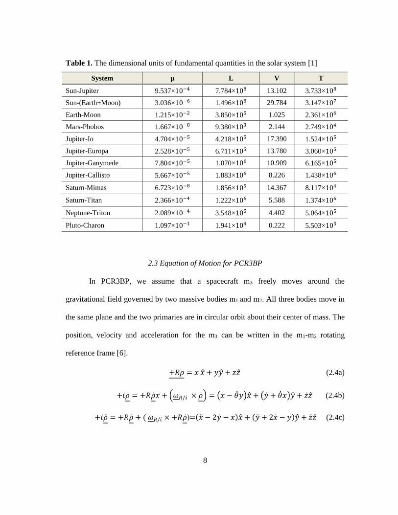
8
Table 1. The dimensional units of fundamental quantities in the solar system [1]
System µ L V T
Sun-Jupiter 9.537×10⁻⁴ 7.784×10⁸ 13.102 3.733×10⁸
Sun-(Earth+Moon) 3.036×10⁻⁶ 1.496×10⁸ 29.784 3.147×10⁷
Earth-Moon 1.215×10⁻² 3.850×10⁵ 1.025 2.361×10⁶
Mars-Phobos 1.667×10⁻⁸ 9.380×10³ 2.144 2.749×10⁴
Jupiter-Io 4.704×10⁻⁵ 4.218×10⁵ 17.390 1.524×10⁵
Jupiter-Europa 2.528×10⁻⁵ 6.711×10⁵ 13.780 3.060×10⁵
Jupiter-Ganymede 7.804×10⁻⁵ 1.070×10⁶ 10.909 6.165×10⁵
Jupiter-Callisto 5.667×10⁻⁵ 1.883×10⁶ 8.226 1.438×10⁶
Saturn-Mimas 6.723×10⁻⁸ 1.856×10⁵ 14.367 8.117×10⁴
Saturn-Titan 2.366×10⁻⁴ 1.222×10⁶ 5.588 1.374×10⁶
Neptune-Triton 2.089×10⁻⁴ 3.548×10⁵ 4.402 5.064×10⁵
Pluto-Charon 1.097×10⁻¹ 1.941×10⁴ 0.222 5.503×10⁵
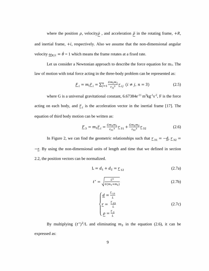
2.3 Equation of Motion for PCR3BP
In PCR3BP, we assume that a spacecraft m3 freely moves around the
gravitational field governed by two massive bodies m1 and m2. All three bodies move in
the same plane and the two primaries are in circular orbit about their center of mass. The
position, velocity and acceleration for the m3 can be written in the m1-m2 rotating
reference frame [6].
+𝑅𝜌 = 𝑥 �� + 𝑦�� + 𝑧�� (2.4a)
+𝑖�� = +𝑅��𝑥 + (𝜔𝑅/𝑖 × 𝜌) = (�� − ��𝑦)�� + (�� + ��𝑥)�� + ���� (2.4b)
+𝑖�� = +𝑅�� + ( 𝜔𝑅/𝑖 ×+𝑅��)=(�� − 2�� − 𝑥)�� + (�� + 2�� − 𝑦)�� + ���� (2.4c)
9
where the position 𝜌, velocity�� , and acceleration �� in the rotating frame, +𝑅,
and inertial frame, +𝑖, respectively. Also we assume that the non-dimensional angular
velocity 𝜔𝑅/𝑖 = 𝜃 = 1 which means the frame rotates at a fixed rate.
Let us consider a Newtonian approach to describe the force equation for m3. The
law of motion with total force acting in the three-body problem can be represented as:
𝐹 𝑖 = 𝑚𝑖�� 𝑖 = ∑𝐺𝑚𝑖𝑚𝑗
𝑟𝑖𝑗3𝑟 𝑖𝑗
𝑛𝑗=1 (𝑖 ≠ 𝑗, 𝑛 = 3) (2.5)
where G is a universal gravitational constant, 6.67384e-11 m3kg-1s-2, F is the force
acting on each body, and �� 𝑖 is the acceleration vector in the inertial frame [17]. The
equation of third body motion can be written as:
𝐹 3 = 𝑚3�� 𝑖 =𝐺𝑚3𝑚1
𝑟313𝑟 31 +
𝐺𝑚3𝑚2
𝑟323𝑟 32 (2.6)
In Figure 2, we can find the geometric relationships such that 𝑟 31 = −d, 𝑟 32 =
−r. By using the non-dimensional units of length and time that we defined in section
2.2, the position vectors can be normalized.
L = 𝑑1 + 𝑑2 = 𝑟 12 (2.7a)
𝑡∗ = √𝐿3
𝐺(𝑚1+𝑚2) (2.7b)
{
𝑑 =
𝑟 13
𝐿
𝑟 = 𝑟 23
𝐿
𝜌 =𝑟 3
𝐿
(2.7c)
By multiplying (𝑡∗)2/L and eliminating 𝑚3 in the equation (2.6), it can be
expressed as:
10
𝑑2(𝑟 3 𝐿⁄ )
𝑑(𝑡 𝑡 ∗⁄ )2 =
𝐺𝑚1
𝑟313((𝑡∗)2
𝐿) 𝑟 31 +
𝐺𝑚2
𝑟323𝑟 32 (
(𝑡∗)2
𝐿) (2.8)
To the above equation, we can apply the equation (2.7c). Then, the Newton’s law
of motion can be described as:
𝑑2𝜌
𝑑𝜏2=
𝐺𝑚1(𝑡∗)2
𝑟313𝑑 +
𝐺𝑚2(𝑡∗)2
𝑟323𝑟 (2.9)
where the position vector 𝑟 3 = 𝜌 and the non-dimensional time is defined as
𝜏 = 𝑡 𝑡 ∗⁄ . Then 𝑡
∗ can be substituted using the equation (2.7b). The acceleration vector,
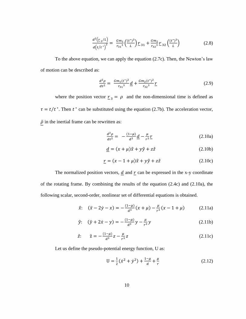
�� in the inertial frame can be rewritten as:
𝑑2𝜌
𝑑𝜏2= −
(1−𝜇)
𝑑3𝑑 −
𝜇
𝑟3𝑟 (2.10a)
𝑑 = (𝑥 + 𝜇)�� + 𝑦�� + 𝑧�� (2.10b)
𝑟 = (𝑥 − 1 + 𝜇)�� + 𝑦�� + 𝑧�� (2.10c)
The normalized position vectors, 𝑑 and 𝑟 can be expressed in the x-y coordinate
of the rotating frame. By combining the results of the equation (2.4c) and (2.10a), the
following scalar, second-order, nonlinear set of differential equations is obtained.
��: (�� − 2�� − 𝑥) = −(1−𝜇)
𝑑3(𝑥 + 𝜇) −
𝜇
𝑟3(𝑥 − 1 + 𝜇) (2.11a)
��: (�� + 2�� − 𝑦) = −(1−𝜇)
𝑑3𝑦 −
𝜇
𝑟3𝑦 (2.11b)
��: z = −(1−𝜇)
𝑑3𝑧 −
𝜇
𝑟3𝑧 (2.11c)
Let us define the pseudo-potential energy function, U as:
U =1
2(��2 + ��2) +
1−𝜇
𝑑+𝜇
𝑟 (2.12)

11
Then we can derive the equations of motion for m3 relative to the m1-m2 rotating
reference frame in non-dimensional coordinates.
�� − 2�� =𝜕𝑈
𝜕𝑥 (2.13a)
�� + 2�� =𝜕𝑈
𝜕𝑦 (2.13b)
�� =𝜕𝑈
𝜕𝑧 (2.13c)
Also the above equation can be expressed in the first-order form. By considering
the planar circular motion on x-y plane, we can obtain the simplified equation of motion
for the PCR3BP.
�� = 𝑣𝑥 (2.14a)
�� = 𝑣𝑦 (2.14b)
𝑣�� = 2𝑣𝑦 −𝜕��
𝜕𝑥+ 𝐹𝑥 (2.14c)
𝑣�� = −2𝑣𝑥 −𝜕��
𝜕𝑦+ 𝐹𝑦 (2.14d)
where the effective potential �� = −1
2(𝑥2 + 𝑦2) −
1−𝜇
𝑟1−
𝜇
𝑟2 ; 𝑟1 =
√(𝑥 + 𝜇)2 + 𝑦2 , 𝑟2 = √(𝑥 − 1 + 𝜇)2 + 𝑦2 ; Fx, Fy = x, y components of thrust.
2.4 Equilibrium Points in PCR3BP
To find equilibrium points in the PCR3BP, we assume that both velocity and
acceleration relative to the rotating frame are zero. Let us set the right-hand sides of
equation (2.14) to zero, i.e. �� = �� = 𝑣�� = 𝑣�� = 0 and Fx = Fy = 0. Then the position of
the equilibrium points in the PCR3BP can be determined: 1) three unstable points on the

12
x-axis, called L1, L2, and L3, form a collinear formation solution 2) two stable points,
called L4 and L5, form an equilateral triangle solution. These five equilibrium points,
commonly referred as the Lagrange points, are illustrated in Figure 3.
Figure 3. Lagrange points Li, i=1,…,5 in PCR3BP
If the third body, m3, is placed at the equilibrium points with zero velocity, it
will remain at rest in the rotating frame. Therefore these points are useful for various
space missions as a connecting hub or observing destination. Especially, the existence of
the periodic orbit around the L1 and L2 points is an important feature to IPSH trajectory
design method. More details will be discussed in following section in this paper.
To calculate the collinear equilibrium points, the critical condition for the
effective potential function �� is:
𝑑
𝑑𝑥(��(𝑥, 0)) = −𝑥 +
1−𝜇
(𝑥−𝜇)2+
𝜇
(𝑥−1+𝜇)2= 0 (2.15)

13
Let the position x be δ + 1 − μ where the separated distance from the second
primary, δ is negative for the L1 point and positive for the L2 point. By substituting δ +
1 − μ for x making δ the unknown, the equation (2.15) can be represented as:
𝐿1: δ = − (𝜇(1+𝛿)2+(1−𝜇)𝛿4
(1+𝛿)2+2(1−𝜇))
1
3≅ −𝑟ℎ = −(
𝜇
3)1/3 (2.16a)
𝐿2: δ = (𝜇(1+𝛿)2−(1−𝜇)𝛿4
(1+𝛿)2+2(1−𝜇))
1
3≅ 𝑟ℎ = (
𝜇
3)1/3 (2.16b)
Where rh, denotes the Hill radius, which is the radius of the Hill’s region in the
PCR3BP. Equations (2.16) represent iterative sequences wherein, starting at zero,
successive values of δ are substituted into the right-hand sides to generate the next
iterates. These sequences are rapidly convergent.
2.5 Energy State Dynamics: Jacobi Constant, Hill’s Region
The motion of the particle, m3, is impossible when its kinetic energy is negative.
This impenetrable area, called the forbidden zone, can be calculated by the energy
integral of motion, E (C=-2E, C is Jacobi integral). This energy integral can exist since
the equation of motion for the PCR3BP are Hamiltonian and time independent. The
energy integral can be expressed as a function of the position and velocities.
𝐸 =1
2(𝑥2 + 𝑦2) + �� (2.17)
Based on this energy level, we can divide the phase space of the PCR3BP into
five possible cases. As seen in Figure 4, a projection of the energy surface, called the
Hill’s region, can be plotted in the blue zone, while the forbidden realm is shown in red
zone. The five cases are divided based on a critical energy levels Ei i=1,..,5 which

14
correspond to the energy of a particle at rest at the Lagrange point Li, i=1,…,5. For
example, the spacecraft m3 cannot move between the m1 and m2 regions due to lower
energy than E1. By increasing the energy level, the neck region between m1 and m2
regions will be opened up. If the energy of spacecraft is slightly above E2 such as case 3,
m3 can move around the realm of m1 and m2, even the exterior realm too.
Figure 4. Five possible motions for energy state phase of the PCR3BP
15
3. DESIGN TRAJECTORY WITH GEOMETRY OF N-BODY PROBLEM
3.1 Invariant Manifolds
The investigation of invariant manifolds was developed by the French
mathematician Henri Poincare who was dedicated to the study of abstract dynamical
stability of systems in the late 19th century [9]. Based on his mathematical foundation,
later researchers focused on mapping the geometry of the N-body system. A geometrical
view for the N-body system considers the set of all possible states of the system in the
phase space. Among the possible sets of trajectories, one can discern trajectory sets that
trace out all the points in a connected subspace of phase space. Such a set is called an
invariant manifold, which is a cylinder type tube structure winding around the
equilibrium points in the N-body system. Particles can be transported through the
invariant manifolds between large regions of the energy surface by winding around the
periodic orbits near L1 and L2, called Lyapunov orbits. The characteristics of the
invariant manifolds issuing from the periodic orbits is investigated in this section.
To generate invariant manifolds, it is necessary to do numerical computation.
First the traditional computation method is examined briefly, then an advanced but
simple method is addressed in detail. Commonly the Differential Correction Method
(DCM) used to generate the Lyapunov orbit and associated manifolds are accurate
enough for space mission design. This method consists in successive approximations
using the State Transition Matrix (STM) along with a reference trajectory [19, 20]. For
the first period of a Lyapunov orbit, the STM is called the monodromy matrix, Φ. The

16
eigenvalues and eigenvectors of the monodromy matrix determine the characteristics of
the local geometry in the system. Given the eigenvectors of the monodromy matrix, the
initial guess of the stable manifold, 𝑋𝑠 and unstable manifold, 𝑋𝑢 can be described as:
𝑋𝑠 = 𝑥0 + 𝑑𝑉𝑠 (3.1a)
𝑋𝑢 = 𝑥0 + 𝑑𝑉𝑢 (3.1b)
where 𝑉𝑠 and 𝑉𝑢 denote the stable and unstable eigenvectors, respectively, of the
monodromy matrix at point 𝑥0, and d is initial displacement. By integrating the equation
of motion for PCR3BP with the different initial positions along the periodic orbit, the
local approximation of the stable and unstable manifolds can be calculated. As an
example, let us consider the Lyapunov orbit around the Earth-Moon L1 point [21]. In
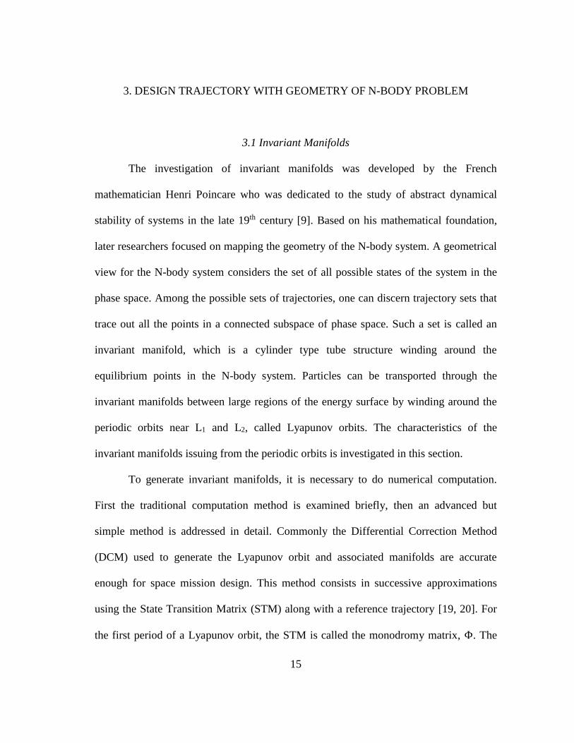
Figure 5, both unstable (red) and stable (blue) manifolds are illustrated. Both manifolds
which are departing (unstable) and approaching (stable) to the periodic orbits are
generated by the position components for 50 different points along the orbits.
The Eigen-basis of the system dynamics can provide simple portraits of the
Lyapunov orbits. By following the centerline of the invariant manifolds, the global form
of these tubes can be simply mapped. Let us assume that the radius of the Lyapunov
orbit approaches zero. Then the resulting one-dimensional paths imply the proper initial
conditions to the interior and exterior realm. These trajectories are the minimum energy
paths within the tubes. By taking a small perturbation in the direction of the eigenvector,
the initial one-dimensional trajectory initially following the periodic orbit enclosing the
Lagrange point evolves to form tube-like surface, as illustrated in Figure 6. Two sets of
17
initial conditions respectively with the interior and exterior directions for the stable and
unstable manifolds are shown in Table 2. Note that 𝛼 is very small positive constant.
Figure 5. Unstable (red, top) and stable (blue, bottom) manifolds from the periodic
orbits around Earth-Moon L1 point
18
Figure 6. Initial one-dimensional trajectory from the periodic orbits around Earth-
Moon L1 point to unstable (red, top) and stable (blue, bottom) manifold direction
Table 2. Initial conditions for unstable and stable manifolds
Initial Conditions
Unstable manifold to
the exterior realm (�� 𝑦 𝑣𝑥 𝑣𝑦)𝑡=0 = 𝛼[1 −𝜎 𝜆 −𝜆𝜎]
Unstable manifold to
the interior realm (�� 𝑦 𝑣𝑥 𝑣𝑦)𝑡=0 = 𝛼[−1 𝜎 −𝜆 𝜆𝜎]
Stable manifold to
the exterior realm (�� 𝑦 𝑣𝑥 𝑣𝑦)𝑡=0 = 𝛼[1 𝜎 𝜆 𝜆𝜎]
Stable manifold to
the interior realm (�� 𝑦 𝑣𝑥 𝑣𝑦)𝑡=0 = 𝛼[−1 −𝜎 −𝜆 −𝜆𝜎]

19
3.2 1-D Search Technique
Let us define the centerline of invariant manifolds as the limiting case where the
tube width and the extent of the boundary Lyapunov orbit approach zero. In PCR3BP,
one can express the equation of motion for m3 in second-order differential equation
form:
�� − 2�� =𝜕��
𝜕𝑥 (3.2a)
�� + 2�� =𝜕��
𝜕𝑦 (3.2b)
where �� =1
2(𝑥2 + 𝑦2) +
1−𝜇
𝑟1+
𝜇
𝑟2, 𝑟1 = √(𝑥 + 𝜇)2 + 𝑦2, 𝑟2 =
√(𝑥 − 1 + 𝜇)2 + 𝑦2.
3.2.1 Linearization in the Vicinity of L1 and L2 points
To describe the geometry of invariant manifolds in three-body dynamics, we can
simply consider the equations of motion linearized near the equilibrium points. Consider
that 𝑥 = 𝑥𝐿 + 𝜉, where 𝑥𝐿 represents the L1 or L2 point, 𝜉 is relatively small. Then we
can express the equation of motion for m3 in terms of 𝜉 and y:
�� − 2�� =𝜕��
𝜕𝑥 (3.3a)
�� + 2�� =𝜕��
𝜕𝑦 (3.3b)
This can also be rewritten in the first-order form such that:
�� = 𝑣𝑥 (3.4a)
�� = 𝑣𝑦 (3.4b)

20
𝑣�� = 2𝑣𝑦 −𝜕��
𝜕𝜉(𝑥𝐿 + 𝜉, 𝑦) (3.4c)
𝑣�� = −2𝑣𝑥 −𝜕𝑈
𝜕𝑦(𝑥𝐿 + 𝜉, 𝑦) (3.4d)
To linearize the above equations, the second-order partial derivative of the
pseudo potential, U, can be calculated. Then we can expand 𝜕��
𝜕𝜉, 𝜕��
𝜕𝑦 about 𝜉 = 0, 𝑦 = 0.
Therefore the linearized first-order form of the equations of motion for PCR3BP
become:
�� = 𝑣𝑥 (3.5a)
�� = 𝑣𝑦 (3.5b)
𝑣�� = 2𝑣𝑦 + 𝑎𝑥 (3.5c)
𝑣�� = −2𝑣𝑥 − 𝑏𝑦 (3.5d)
where a = − (𝜕2��
𝜕𝑥2) = 1 +
2(1−𝜇)
|𝑥𝐿+𝜇|3+
2𝜇
|𝑥𝐿−1+𝜇|3, 𝑏 = −(
𝜕2��
𝜕𝑦2) =
(1−𝜇)
|𝑥𝐿+𝜇|3+
𝜇
|𝑥𝐿−1+𝜇|3− 1. To simplify the equation, we can define a new term, ��:
�� =(1−𝜇)
|𝑥𝐿+𝜇|3+
𝜇
|𝑥𝐿−1+𝜇|3 (3.6)
Then a = 1 + 2�� , 𝑏 = �� − 1, x = 𝑥𝐿 + ��, and �� ≪ 𝑟ℎ. The energy integral E*
represents the energy surface that passes through the equilibrium points.
𝐸∗ =1
2(𝑣𝑦
2 + 𝑣𝑦2 − 𝑎𝑥2 + 𝑏𝑦2) (3.7)
3.2.2 Geometry of Solutions with the Eigen State Analysis
The linearized equation of motion around the L1 or L2 points, the equation (3.5),
can be represented in matrix form:

21
𝑑
𝑑𝑡(
��𝑦𝑣𝑥𝑣𝑦
) = [
0 0 1 00 0 0 1𝑎0
0−𝑏
0 2−2 0
](
��𝑦𝑣𝑥𝑣𝑦
) (3.8)
By adopting the Eigenvectors as the new coordinate system, we can better
understand the geometry of the phase space. The Eigen state can be calculated
straightforwardly from the above matrix forms, �� = 𝐴𝑋.
When setting det (𝐴 − 𝜆𝐼) = 0, the characteristic equation is found to be:
𝜆4 + 𝜆2(2 − ��) + (1 + �� − 2��2) = 0 (3.9)
Then the eigenvalue of the linearized equations are of the form ±𝜆 and ±𝑖𝜐.
𝜆1,2 = ± [��−2+√9��2−8��
2]1/2
= ±𝜆 (3.10a)
𝜆3,4 = ±𝑖 [2−��−√9��2−8��
2]1/2
= ±𝑖𝜐 (3.10b)
The eigenvectors, 𝜐 = (𝑢1, 𝑢2, 𝑤1, 𝑤2) can be calculated from the relations with
the eigenvalues: 𝐴𝜐 = 𝜆𝜐. The corresponding eigenvectors can be expressed in matrix
form:
[𝑢1 𝑢2 𝑤1 𝑤2] = [
1 1 1 1−𝜎 𝜎 −𝑖𝜏 𝑖𝜏𝜆−𝜆𝜎
−𝜆−𝜆𝜎
𝑖𝜐 −𝑖𝜐𝜐𝜏 𝜐𝜏
] (3.11)
where σ =2𝜆
𝜆2+𝑏> 0 , 𝜏 = − (
𝜐2+𝑎
2𝜐) < 0. Then the linearized equation of
motion near the libration points can be expressed in the new coordinate system
(𝜉, 𝜂, 𝜁1, 𝜁2):

22
(
��𝑦𝑣𝑥𝑣𝑦
) = [
1 1 1 1−𝜎 𝜎 −𝑖𝜏 𝑖𝜏𝜆−𝜆𝜎
−𝜆−𝜆𝜎
𝑖𝜐 −𝑖𝜐𝜐𝜏 𝜐𝜏
](
𝜉𝜂𝜁1𝜁2
) (3.12)
In these Eigen state coordinates, the differential equation can simply described in
new coordinate system (𝜉, 𝜂, 𝜁1, 𝜁2):
�� = 𝜆𝜉 (3.13a)
�� = −𝜆𝜂 (3.13 b)
𝜁1 = 𝜐𝜁2 (3.13 c)
𝜁2 = −𝜐𝜁1 (3.13d)
E = λξη +υ
2(𝜁1
2 + 𝜁22) (3.14)
The solution can be conveniently written as:
𝜉(𝑡) = 𝜉0𝑒𝜆𝑡
𝜂(𝑡) = 𝜂0𝑒−𝜆𝑡
𝜁1(𝑡) = 𝜁10𝑐𝑜𝑠𝜐𝑡 + 𝜁20𝑠𝑖𝑛𝜐𝑡
𝜁2(𝑡) = 𝜁20𝑐𝑜𝑠𝜐𝑡 − 𝜁10𝑠𝑖𝑛𝜐𝑡
(3.15)
3.2.3 Centerline of Invariant Manifolds
The unstable manifolds winding around the Lyapunov orbits in L1 or L2 points
would be in the form:
(
𝜉𝑦𝑣𝑥𝑣𝑦
) = 𝛼𝑒𝜆𝑡 (
1−𝜎𝜆−𝜆𝜎
) + 2𝑅𝑒 [𝛽𝑒𝑖𝜈𝑡 (
1−𝑖𝜏𝑖𝜈𝜈𝜏
)] (3.16)
Note that |𝛽| determines the radius of the manifold tube. By letting the radius
approach zero, |𝛽| → 0, the exact solution for the initial conditions can be obtained. The
23
resulting one-dimensional path, called the centerline of the tube, implies the proper
initial conditions needed for entry into the interior or exterior realm. These trajectories
are the minimum energy paths within the tubes. The trajectory can be described in the
linearized approximation:
(
𝜉𝑦𝑣𝑥𝑣𝑦
) = 𝛼𝑒𝜆𝑡 (
1−𝜎𝜆−𝜆𝜎
) + 𝐻.𝑂. 𝑇. (𝛼 > 0) (3.17)
With these initial conditions, we can use the full nonlinear equation of motion to
determine a centerline of the invariant manifolds. The equation of motion can be applied
to calculate the centerline of tube as the solution for the second-order differential
equations. Let us define new independent variable, 𝑠 ≡ 𝑒𝜆𝑡. This can be easily expressed
as:
𝑑
𝑑𝑡=
𝑑𝑠
𝑑𝑡
𝑑
𝑑𝑠=
𝑑
𝑑𝑡[𝑒𝜆𝑡]
𝑑
𝑑𝑠= 𝜆𝑠
𝑑
𝑑𝑠 (3.18)
Then the equations of motion can be expressed in (𝜉, 𝑦, 𝑣𝑥, 𝑣𝑦) coordinates with
the new variable, s, as:
𝑑𝜉
𝑑𝑠=
1
𝜆𝑠𝑣𝑥 (3.19a)
𝑑𝑦
𝑑𝑠=
1
𝜆𝑠𝑣𝑦 (3.19b)
𝑑𝑣𝑥
𝑑𝑠=
2
𝜆𝑠𝑣𝑦 −
1
𝜆𝑠
𝜕��
𝜕𝜉(𝑥𝐿 + 𝜉, 𝑦) (3.19c)
𝑑𝑣𝑦
𝑑𝑠= −
2
𝜆𝑠𝑣𝑥 −
1
𝜆𝑠
𝜕��
𝜕𝑦(𝑥𝐿 + 𝜉, 𝑦) (3.19d)
Note that the initial condition can be obtained at s = 1.

24
(
𝜉𝑦𝑣𝑥𝑣𝑦
) = 𝛼(
1−𝜎𝜆−𝜆𝜎
) (3.20)
The above equations demonstrate the existence of the centerline in the invariant
manifolds. To set up the initial condition summarized in Table 2, the centerlines of
unstable and stable manifolds for both exterior and interior realms can be calculated.
3.2.4 Symmetries of Homoclinic and Heteroclinic Orbits
One of the important characteristics of invariant manifolds is the existence of the
trajectories, called the homoclinic orbits, which are symmetric about the x-axis. The
homoclinic orbits in both the interior and exterior realms was investigated by Conley
(1968) and McGehee (1969) [16, 22]. Homoclinic orbits start from and return to the
same Lagrange point, while Heteroclinic orbits connect two different Lagrange points.
Through the heteroclinic orbits, which are linked with the invariant manifolds of the L1
and L2 Lyapunov orbits in the neck region, the homoclinic orbits in interior and exterior
realms can be connected to each other. To examine the symmetry of the homoclinic
orbits, let us bring back the equations of motion in the first-order form.
�� = 𝑣𝑥 (3.21a)
�� = 𝑣𝑦 (3.21b)
𝑣�� = 2𝑣𝑦 + 𝑥 −2(1−𝜇)(𝑥+𝜇)
𝑟13+2𝜇(𝑥−1+𝜇)
𝑟23 (3.21c)
𝑣�� = −2𝑣𝑥 + 𝑦 −(1−𝜇)
𝑟13−
𝜇
𝑟23 (3.21d)
where 𝑟1 = √(𝑥 + 𝜇)2 + 𝑦2 and 𝑟2 = √(𝑥 − 1 + 𝜇)2 + 𝑦2.

25
To validate the symmetry on the x-axis, we can transform the variables: y = −y
and t = −t. Then the equation of motion can be represented as:
𝑑𝑥
𝑑��= −𝑣𝑥 (3.22a)
𝑑��
𝑑��= 𝑣𝑦 (3.22b)
𝑑𝑣𝑥
𝑑��= −(2𝑣𝑦 + 𝑥 −
2(1−𝜇)(𝑥+𝜇)
𝑟13+2𝜇(𝑥−1+𝜇)
𝑟23) (3.22c)
𝑑𝑣𝑦
𝑑��= −(−2𝑣𝑥 − �� +
(1−𝜇)
𝑟13�� +
𝜇
𝑟23��) (3.22d)
where 𝑟1 = √(𝑥 + 𝜇)2 + ��2 and 𝑟2 = √(𝑥 − 1 + 𝜇)2 + ��2. When we assume
that ��𝑥 = −𝑣𝑥, the equations (3.22) match exactly with the equations (3.21). Hence, the
equations (3.22) with initial conditions, (𝑥0, −𝑦0, −𝑣𝑥0, 𝑣𝑦0), are a mirror image of the
trajectory which is generated by the equations (3.21) with initial conditions,
(𝑥0, 𝑦0, 𝑣𝑥0, 𝑣𝑦0). Expressed in the x-y plane, this homoclinic orbit shows the symmetry
about the x-axis. In a similar manner, the heteroclinic orbits associated with the L1 and
L2 Lyapunov orbits are approximately symmetric about the y-axis with small μ.
By combining the symmetric homoclinic and heteroclinic orbits, the interior and
exterior realms of the PCR3BP can be connected. Therefore, using the centerline of the
invariant manifolds and their symmetries, a sequence of one-dimensional searches
allows us to design the trajectory around the Lagrange points.

26
3.3 Preliminary Design for NEA Rendezvous Mission
As one of the 1-D search technique applications, Near-Earth Asteroids (NEAs)
rendezvous mission design is considered. Since NEAs continually pose a threat to the
safety of Earth, NEAs exploration and mitigation are crucial tasks for defending our
planet. There is also a huge possibility of extracting valuable materials from asteroids.
They have many valuable resources that can be brought back to Earth or used in space
for spacecraft propulsion systems or space habitations. To find fuel-optimized
trajectories to NEAs, the IPSH method is fully exploited to transfer from the Earth-
Moon system to the Sun-Earth system. As in Figure 7, the overall mission trajectory is
divided into four phases: Phase 1) LEO orbit to the Lyapunov orbit around Earth-Moon
L1 point; Phase 2) Earth-Moon L1 Lyapunov orbit to Earth-Moon L2 point; Phase 3)
Earth-Moon L2 point to Sun-Earth L2 point; and Phase 4) Sun-Earth L2 point to NEA.
Figure 7. Asteroid rendezvous mission trajectory

27
Computationally, it is more convenient to generate the symmetric heteroclinic
orbit between Lyapunov orbit in Earth-Moon L1 point and Earth-Moon L2 point in the
neck region. Therefore we started in the neck region of the Earth-Moon system to
generate the trajectory of phase 2 first by integrating the equations in reverse time and
starting from the Earth-Moon L2 point stable manifold. A 1 metric ton (1MT) spacecraft
using ion engines with the specific impulse, Isp = 3000 s, can take the centerline of
unstable manifolds to the interior realm at the Earth-Moon L2 point using negligible
thrust. Note that the appropriate initial perturbations for the unstable manifolds to the
interior realm are used from Table 2. Then, as seen in Figure 8, the S/C encircles the
Moon twice and then reaches to the Earth-Moon L1 point in 43.7 days. To obtain the
outward bound trajectory, we simply start at the Earth-Moon L1 Lyapunov orbit and
integrate in forward time.
Figure 8. Phase 2 from Earth-Moon L1 periodic orbit to Earth-Moon L2 point

28
When the S/C reaches the Lyapunov orbit of the Earth-Moon L1 point, the
trajectory to Earth (LEO/GEO) can be generated in reverse time. The Earth-Moon L1
point has been chosen as a connecting place for phase 1 because it results in the
maximum number of opportunities to take on supplies, exchange crew or deal with
emergencies. With the initial conditions for stable manifolds to the interior realm at the
Earth-Moon L1 periodic orbit, the S/C slowly spirals back into the Earth. As seen in
Figure 9, a small amount (0.24 N) of kick-start thrust is necessary for 4.2 months,
consuming 96 kg of fuel. The total trip time is 156 days (5.2 months), which is longer
than the traditional transfer methods like Hohmann Transfer, but the total ∆V is
significantly reduced to 2.698 km/s. Through the Lyapunov orbit in Earth-Moon L1
point, which is the crucial link between phase 1 and phase 2, the S/C can travel from the
interior realm to the exterior realm of the Earth-Moon system.
Figure 9. Phase 1 from LEO to Earth-Moon L1 periodic orbit

29
3.3.1 4-Body Dynamics for Coupled Two 3-Body Systems
Now we can proceed to investigate the trajectory of phase 3, which is to connect
from the Earth-Moon L2 point to the Sun-Earth L2 point. To consider the transfer
trajectory from the Earth-Moon system to the Sun-Earth system, the four-body dynamics
are implemented as two coupled three-body problems [1]. The four bodies, Sun-Earth-
Moon-S/C, can be split in two perturbed three-body problems as Sun-Earth-Spacecraft
(CCM) perturbed by the Moon and Earth-Moon-Spacecraft (BCM) perturbed by the
Sun. The geometry of the four-body problem [1] is illustrated in Figure 10. The
equations of motion for this four-body problem can be described as:
�� = 𝑢 (3.23a)
�� = 𝑣 (3.23b)
�� = 𝑥 + 2𝑣 − 𝐶𝐸(𝑥 + 𝜇𝑀) − 𝐶𝐸(𝑥 − 𝜇𝐸) − 𝐶𝑠(𝑥 − 𝑥𝑆) − 𝛼𝑆𝑥𝑆 (3.23c)
�� = 𝑦 − 2𝑢 − 𝐶𝐸𝑦 − 𝐶𝑀𝑦 − 𝐶𝑠(𝑦 − 𝑦𝑆) − 𝛼𝑆𝑦𝑆 (3.23d)
where 𝐶𝑖 =𝜇𝑖
𝑟𝑖3 𝑓𝑜𝑟 𝑖 = 𝐸,𝑀, 𝑆 , 𝛼𝑆 =
𝑚𝑆
𝛼𝑆3 .
In Figure 11, the thrust-free trajectory obtained via a one-dimensional search of
the correct phasing of the Earth-Moon L2 departure is shown in the Earth-Moon rotating
frame (left) and the Sun-Earth rotating frame (right). For 39.4 days, the S/C travels the
immense distance from unstable manifolds to the exterior realm without fuel
expenditure.

30
Figure 10. Geometry of the four-body problem (Sun-Earth-Moon-Spacecraft)
Figure 11. Phase 3 from Earth-Moon L2 point to Sun-Earth L2 point in Earth-
Moon rotating frame (left) and in Sun-Earth rotating frame (right)
Phase 4 is the trajectory, called the Grand Tour [23, 24], from the Sun-Earth L2
point via Near-Earth Asteroids which visit both regions that are ~0.15 AU below and
above the Earth’s orbit, and then back to the original point. During the segment of the

31
trajectory indicated by the red line in Figure 12, the S/C departs from Sun-Earth L2 point
through the unstable manifold to the exterior realm direction by executing a small thrust,
0.264N for 138 days. The small increment of the thrust changes the energy state of the
system so that the neck region of the forbidden zone opens outward as you can see in
Figure 13. Therefore the S/C can enter the internal region of the Sun-Earth system. By
passing through the interior realm, the S/C coasts along the blue line in Figure 12. When
it approached to the wall of forbidden zone, the S/C can be pushed in the opposite
direction with a second small thrust, 0.264N for another 138 days. Finally, it can travel
the unpowered return trajectory in the exterior realm (sky-blue line) and back to the Sun-
Earth L2 point. During this 9.2 months grand tour to reach NEAs, the total ∆V is 5.708
km/s which consumes 214.06 kg of fuel mass. The summary of total trip time and ∆V is
shown in Table 3.
Figure 12. Asteroid rendezvous mission trajectory: phase 4 grand tour

32
Figure 13. Transformation of forbidden zone around neck region by increasing
energy state
Table 3. Summary of cost for NEAs rendezvous mission
TOF [days]
∆𝐕 [𝐤𝐦/𝐬]
Phase 1: LEO to Earth-Moon L1 156 2.698
Phase 2: Earth-Moon L1 to L2 43.7 0
Phase 3: Earth-Moon L2 to Sun-Earth L2 39.4 0
Phase 4: Grand Tour 604.5 5.708
Total 843.6 (=2.3 yrs) 8.406

33
4. DESIGN TRAJECTORY FROM EARTH TO MARS
By using the low-energy trajectory method, ISPH, a novel design of a solar sail
mission for Mars exploration can be developed. Invariant manifolds, which are winding
around the Lagrangian points, can be helpful to transfer a spacecraft with almost no fuel
consumption. This energy efficient method makes Mars exploration mission more
attainable. Moreover, the topology of invariant manifolds can be transformed by
deploying solar sails. Solar sails provide a propulsive power using solar radiation
pressure. Assuming the sail is isotropic, that is, it produces a radiation force equivalent
to a spherical reflector, and the effect of the solar sail on the system dynamics is to
modify the gravitational constant of the Sun, while the centrifugal force in the rotating
frame remains the same. Therefore, the Sun-Mars L1 and L2 Lagrangian points will be
shifted toward the Sun and the geometry of the invariant manifolds around L1 and L2
points will be changed. By taking advantage of these features, a low-thrust trajectory for
Mars exploration is developed.
The PCR3BP will be considered since Earth and Mars are nearly co-planar
planets. The first stage is the trajectory from Earth to Sun-Earth L2 point. When the
spacecraft reaches Sun-Earth L2 point, the solar sail can be launched with a slight nudge
into the invariant manifold leading to the exterior realm. At this second stage, the
spacecraft leaves the neck regions and obtains an extra acceleration from the solar
radiation pressure force. Meantime the centrifugal force, Fc has to be conserved for the
three bodies. Let define a factor, 𝑓 = (𝐹𝑚1)𝑓𝑖𝑛𝑎𝑙 (𝐹𝑚1)𝑖𝑛𝑖𝑡𝑖𝑎𝑙⁄ , where Fm1 is the Sun’s

34
gravitational force and f = 1 means no solar sail effect as an initial state. When f becomes
close to zero, Sun’s gravitational force will be cancelled by increasing the solar radiation
pressure force, FSRP. The acceleration depends on the reflectivity of the solar sail
material and also its size. Assume that the solar sail is large enough to cancel Sun’s
gravitational force by solar pressure here. Then the Sun-Mars Lagrangian points move
toward the Sun as f becomes smaller. Also the configuration of invariant manifolds for
Sun-Mars system will be changed along with the Lagrangian points. Here we can get an
advantage by reducing the distances of the L1 and L2 points from the Sun. It means that
the positions of the Sun-Mars L1 and L2 points can be closer to the spacecraft, which is
near Sun-Earth L2 point. At the last stage, the spacecraft can transfer to the approached
Sun-Mars L1 point with a small thrust.
4.1 Investigation for Omni-directional Solar Sail Power
Consider a spacecraft moving around under the massive m1 and m2 gravitational
fields. Assume that the three bodies are in the same plane and that m1 and m2 are around
in a circular orbit about their center of mass. The equations of motion for the three-body
problem can be described as:
𝑚1𝑥1 =−𝐺𝑚1𝑚2
|𝑥1−𝑥2|3(𝑥1 − 𝑥2) (4.1a)
𝑚2𝑥2 =𝐺𝑚1𝑚2
|𝑥1−𝑥2|3(𝑥1 − 𝑥2) (4.1b)
𝑚�� = 𝑓𝐺𝑚1𝑚
|𝑥−𝑥2|3(𝑥1 − 𝑥) +
𝐺𝑚2𝑚
|𝑥−𝑥2|3(𝑥2 − 𝑥) + 𝐹 (4.1c)

35
where the solar sail factor is 𝑓 = (𝐹𝑚1)𝑓𝑖𝑛𝑎𝑙 (𝐹𝑚1)𝑖𝑛𝑖𝑡𝑖𝑎𝑙⁄ , which will affect the
equations of motion only for m1, Fm1 is the Sun’s gravity force, and F is an additional
thrust. Alternatively the equations of motion can be written as:
�� − 2�� = −𝜕��
𝜕𝑥 (4.2a)
�� + 2�� = −𝜕��
𝜕𝑦 (4.2b)
where the effective potential �� = −1
2(𝑥2 + 𝑦2) − 𝑓
1−𝜇
𝑟1−
𝜇
𝑟2; 𝑟1 =
√(𝑥 + 𝜇)2 + 𝑦2; 𝑟2 = √(𝑥 − 1 + 𝜇)2 + 𝑦2. For the advanced approach to describe the
motion of this Sun-Mars system, the four body dynamics of Sun, Earth, Mars, and
spacecraft can be considered later. To calculate L1 and L2 positions, the equilibrium
points need to be solved. The PCR3BP allows five equilibrium point solutions, which
are including the collinear equilibria on the x-axis (y=0) L1, and L2.
For L1 and 𝑥 < (1 − 𝜇): 𝑓(1−𝜇)
(𝑥+𝜇)2−
𝜇
(𝑥−1+𝜇)2− 𝑥 = 0 (4.3a)
For L2 and 𝑥 > (1 − 𝜇), (𝑥 − 1 + 𝜇) > 0: 𝑓(1−𝜇)
(𝑥+𝜇)2+
𝜇
(𝑥−1+𝜇)2− 𝑥 = 0 (4.3b)
By using 𝑥 = 𝛿 + 1 − 𝜇, the equations can be expressed in 𝛿. Equation (4.3)
defines recursive sequences obtained by successive substitution of 𝛿 into the right hand
side. The infinite sequences are convergent.
L1: 𝛿 = −(𝜇(1+𝛿)2+(1−𝜇)𝛿2(1−𝑓+𝛿2)
(1+𝛿)2+2(1−𝜇))1/3
(4.4a)
L2: 𝛿 = √(𝜇−𝛿3)
(1−𝜇)+ 𝑓
𝛿2
(1+𝛿)2 (4.4b)

36
As seen in Figure 14, both the distances of Sun-Mars L1 and L2 points from the
Sun decrease from their initial state by reducing the solar sail factor f. It means that the
Sun-Mars L1 and L2 points can shift toward the Sun. The factor f can be changed by the
solar sail effect, dragging the Sun-Mars L1 point near the spacecraft that is around the
Sun-Earth L2 point. It is like docking the spacecraft over the Sun-Mars L1 point. The
configuration of the invariant manifolds around the Sun-Mars L1 and L2 points will be
transformed, since it is formed with Lyapunov orbit around the L1 and L2 points.
Therefore, the Sun-Mars L1 point can meet the Sun-Earth L2 point around f = 0.291. The
forbidden zone, which is inaccessible for a given energy, and its neck region are shown
in Figure 15.
Figure 14. Sun-Mars L1 and L2 points change by reducing f

37
Figure 15. Sun-Mars L1 and L2 points shifting toward to Sun by reducing f
The change of the invariant manifold structure in the four-body system by
reducing f will be studied in a geometrical view. This framework of tube dynamics leads
us to find intersected regions between Sun-Earth manifolds systems and the Sun-Mars
system. Based on the previous research done by German and Frabcesco [25-27], two
circular restricted three-body systems with similar mass parameters cannot approach one
another even in developing the manifolds for a long integration time. Therefore various
researchers designed the transfer trajectory from one system to another combining with
the traditional differential correction method, or shooting method. However, the system-
to-system trajectory design directly through manifolds can possibly be done by this
research with solar sail effect. We will explore the limited case of 4-body problem and
design advanced transfer trajectories with significantly reduced ∆𝑉 compared with
previous work.

38
4.2 Limited Case of 4-Body Problem
Consider a simple case of a 4 body problem with Sun-Earth-Mars-S/C system. It
can be divided into two 3-body models with specific assumptions. First, the two
components of the models are the planar circular restricted 3-body problems with Sun-
Earth-S/C systems and Sun-Mars-S/C systems. Second, the Sun is at the origin of the 4-
body problem. In this case, the circular orbits of the Earth and Mars are described
proportionally with their semi-major axes and orbital periods. These assumptions have a
limit of mathematical precision with errors of the order of since has different values
for each case of Earth and Mars. However, the difference is small enough (less than
3x10⁻⁶) to be ignored. Simply using these assumptions to the limited case of 4-body
model, a basic tractable formulation can be developed. This can be a guideline of 4-body
dynamics to enhance understanding of the mathematical and geometrical framework to
describe the modification of the structure for the 4-body system due to the effects of the
solar sail. The results show that system-to-system transfer trajectories can be designed
by changing the configuration of the invariant manifolds.
4.2.1 Equations of Motion for the Limited Case of 4 Body Problem
Assume the Sun is at the origin when the Earth and Mars are on their circular
orbits. To describe this limited 4-body problem in the Sun-Earth rotating frame, let us
define the dimensionless quantities for position x, time t, mass parameter .
𝑥 =��
|𝑟��|(4.5)
where �� is the position vector of S/C and 𝑟�� is the position vectors of Earth.

39
𝑡 = ��Ω (4.6)
where �� is time and Ω is angular velocity of Sun-Earth rotating frame, Ω = √𝑚𝑠𝐺
|𝑟𝐸|3
𝜇𝐸 =𝑚𝐸
𝑚𝑆, 𝜇𝑀 =
𝑚𝑀
𝑚𝑆 (4.7)
Where mS, mE, mM are the mass of the Sun, Earth and Mars respectively. Note
that 𝜇𝐸 and 𝜇𝑀 are the mass parameters for the Sun-Earth system and the Sun-Mars
system. Since the distance between the Sun and the Earth is set to unity, the relative
position and angular velocity of Mars can be calculated in the Sun-Earth rotating frame.
𝑟 =|𝑟��|
|𝑟��|= 1.5235 (4.8)
𝜔𝑀 = 1 −𝑇𝑀
𝑇𝐸= 0.5317 (4.9)
where 𝑟�� is the position vectors of Mars, 𝜔𝑀 is angular velocity of Mars, 𝑇𝐸 and
𝑇𝑀 are the orbital periods of the Earth and Mars, respectively. With these dimensionless
components, the equations of motion of the limited 4-body problem can be expressed in
x-y plane.
�� = 2�� + 𝑥 − 𝑓𝑥
𝑅3+ 𝜇𝐸
(1−𝑥)
𝑅𝐸3 + 𝜇𝑀
(𝑟𝑥−𝑥)
𝑅𝑀3 + 𝐹𝑥 (4.10a)
�� = −2�� + 𝑦 − 𝑓𝑦
𝑅3+ 𝜇𝐸
𝑦
𝑅𝐸3 + 𝜇𝑀
(𝑟𝑦−𝑦)
𝑅𝑀3 + 𝐹𝑦 (4.10b)
where R, RE, RM are the distances between the Sun and S/C, Earth, and Mars,
respectively: R = √𝑥2 + 𝑦2, 𝑅𝐸 = √(1 − 𝑥)2 + 𝑦2, 𝑅𝑀 = √(𝑟𝑥 − 𝑥)2 + (𝑟𝑦−𝑦)2. The
position of Mars can be described in terms of rx and ry: 𝑟𝑥 = 𝑟𝑐𝑜𝑠(−𝜔𝑀𝑡 + 𝜑0), ∶ 𝑟𝑦 =
𝑟𝑠𝑖𝑛(−𝜔𝑀𝑡 + 𝜑0) with 𝜑0 is the initial phase angle of Mars. The factor by which the
solar sail decreases the solar gravitational parameter is denoted by f. The external force
40
divided by the S/C mass is expressed in two components, Fx and Fy. In Figure 16, the
geometry of 4-body systems is shown.
Figure 16. Geometry of the limited 4-body problem
Let us investigate the existence of the force-free Lagrange points, 𝑥𝐸∗, 𝑥𝑀
∗ in the
limited 4-body problem. For the Sun-Earth system, the Sun-Earth Lagrange points can
be calculated when 𝜇𝑀 = 0.
𝑥𝐸∗ = 1 + 𝛿 (4.11a)
For L1: 𝛿 ← − (1
3[𝜇𝐸(1 + 𝛿)
2 + 3𝛿4 + 𝛿5 + 𝛿2])3
(4.11b)
For L2: 𝛿 ← √𝜇𝐸 + 𝑓𝛿2
(1+𝛿)2− 𝛿3 (4.11c)
To get the distance from the origin of the Sun-Mars Lagrange points, solve δ
after replacing 𝜇𝐸 by 𝜇𝑀 in the equation (4.11).

41
𝑥𝑀∗ = 𝑟(1 + 𝛿) (4.12a)
For L1: 𝛿 ← − (1
3[𝜇𝑀(1 + 𝛿)
2 + 3𝛿4 + 𝛿5 + 𝛿2])3
(4.12b)
For L2: 𝛿 ← √𝜇𝑀 + 𝑓𝛿2
(1+𝛿)2− 𝛿3 (4.12c)
Note that the x-y position of the Sun-Mars L1 and L2 points can be expressed in
the Sun-Earth rotating frame.
(𝑥𝑀∗)𝑆𝐸 = 𝑥𝑀
∗cos (−𝜔𝑀𝑡 + 𝜑0) (4.13a)
(𝑦𝑀∗)𝑆𝐸 = 𝑦𝑀
∗sin (−𝜔𝑀𝑡 + 𝜑0) (4.13a)
For the example trajectory, we can assume that the initial phase angle of Mars is
𝜑0 = 4.4139 = 252.9°. The mission scenario is: First, the solar sail is deployed at the
Sun-Earth L2 point and embarks onto the unstable manifolds to the exterior realm.
Second, the value of the solar sail factor, f is decreased in proportion to the mission time
starting from f = 1 to 0.83. By applying those conditions to the equation of motion
(4.10), the trajectory from the Sun-Earth L2 point to the vicinity of the Sun-Mars L1
point can be obtained. The trajectories in the Sun-Earth and Sun-Mars rotating frame are
shown in Figures 17 and 18. As the factor f is changed, both the Sun-Earth and Sun-
Mars Lagrange points are shifted toward to the Sun. Since the factor f is decreased
discretely in three steps from 1 to 0.83, discontinuous points in the motions of Sun-Earth
L1 and L2 points can be found in Figure 18. Interestingly, there is a bounce back motion
of S/C trajectory in the vicinity of the Sun-Mars L1 point. In Figure 19, the Sun-Mars L1
point is moved toward to the Sun while the factor f is decreased. Then the S/C penetrates
a little beyond the Sun-Mars L1 point but turns back to the interior realm of the Sun-

42
Mars system again. It is necessary to investigate the energy state and the eigen state
analysis of this resulting motion with the factor f.
Figure 17. S/C trajectory from the Sun-Earth L2 point to the vicinity of the Sun-
Mars L1 point in the Sun-Earth rotating frame
Figure 18. S/C trajectory from the Sun-Earth L2 point to the vicinity of the Sun-
Mars L1 point in the Sun-Mars rotating frame

43
Figure 19. Close up of the trajectory near the Sun-Mars L1 point in the Sun-Mars
rotating frame
4.2.2 Energy State and Eigen State for the Limited Case of 4-Body Problem
To understand the bounce back motion with decreasing f, let us explore the
geometry of the system near the neck region. The energy integral for the Sun-Earth-S/C
system in the Sun-Earth rotating frame can be expressed in:
𝐸𝑆𝐸 =1
2(𝜈𝑥
2 + 𝜈𝑦2) −
1
2(𝑥2 + 𝑦2) −
𝑓
𝑅−𝜇𝐸
𝑅𝐸 (4.14)
The spacecraft can move around the interior and exterior realms through the neck
region near the L1 and L2 points when the energy level of the system is between E2 and
E3. It is this case 3 (𝐸2 ≤ 𝐸 ≤ 𝐸3) which is one of the typical energy regimes of the
PCR3BP (See Figure 4). Let us take the value of ESE = -1.50045 while the factor f is 1.
This value of the energy is just enough to open the neck regions slightly as seen in

44
Figure 20. However if we put f = 0.83 and use ESE = -1.32482 to maintain the neck
region open, the forbidden zone is entirely shifted to the left side of the Earth in Figure
21. It means that the energy state of the system can be affected by changing the value of
the factor f.
Figure 20. Forbidden zone for the Sun-Earth-S/C system in the Sun-Earth rotating
frame when f = 1 and ESE = -1.50045
Figure 21. Forbidden zone for the Sun-Earth-S/C system in the Sun-Earth rotating
frame when f = 0.83 and ESE = -1.32482

45
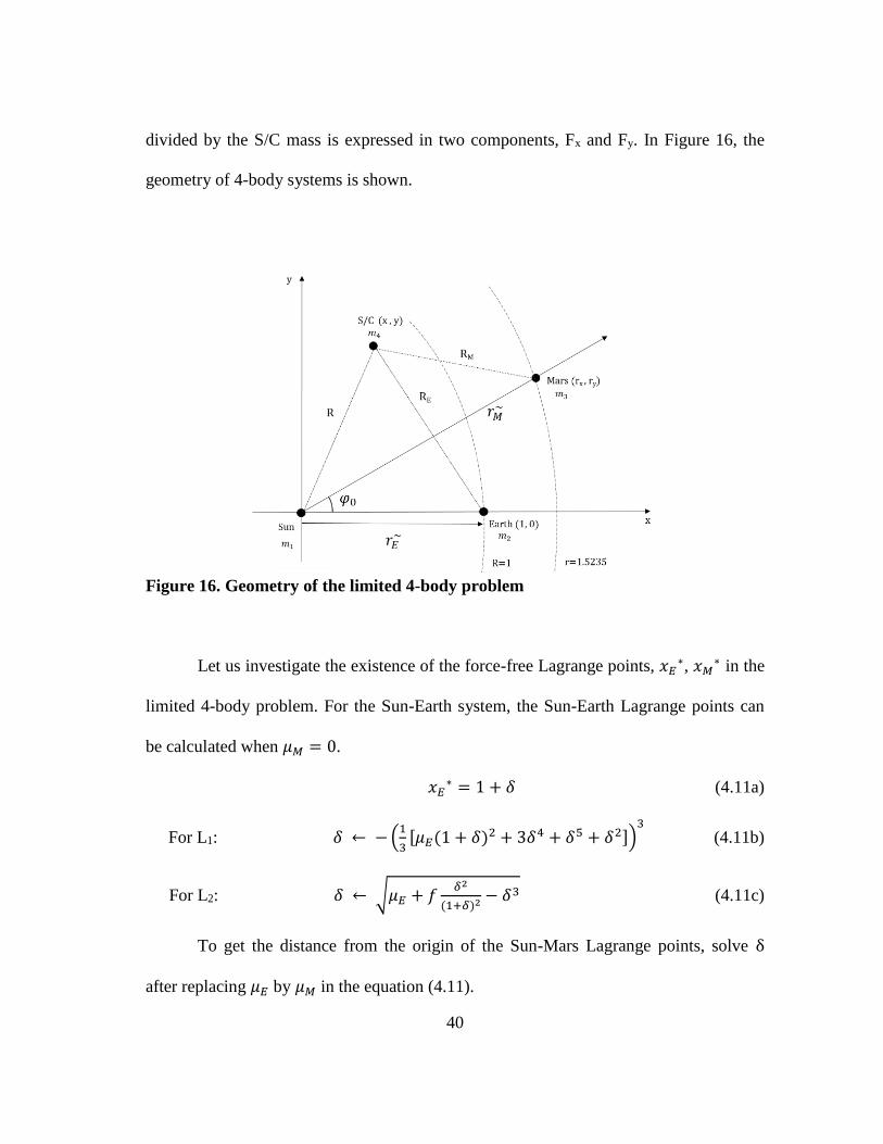
To investigate the relationship between the energy integral and the solar sail
factor f, we can fix one parameter and change the other one. In Figure 22, the factor f is
decreased from 1 to 0.9991 while the value of energy is set to ESE = -1.50045. The neck
region with two throats is closed so that the S/C cannot move from the interior to the
exterior realm. Also the thickness of the forbidden zone is increased when the factor f is
decreased. It means that the required energy limit to maintain the neck region open in the
energy state phase is increased by reducing the solar sail factor f. In Figure 23, the
energy ESE is increased from -1.50045 to -1.50001 while the factor f is kept at1. Then the
forbidden zone becomes thinner and is shifted to the left slightly while the neck region
opens widely upwards. The two throats of the neck region are reduced to one throat at
ESE = -1.50001 and then entirely disappear when ESE is larger than -1.3. Therefore 1) the
critical limits of the energy level to open the neck region are increased while the factor f
is decreased and 2) the entire forbidden zone is shifted slightly toward the Sun’s
direction while ESE is increased. In Figure 24, the forbidden zone can keep a neck region
open by increasing the energy ESE over the critical limits while the solar sail factor f is
decreasing.
46
Figure 22. Forbidden zones when f is decreasing with fixed energy ESE = -1.50045 (f
= 1 (left), f = 0.9999 (middle), f = 0.9991 (right))
Figure 23. Forbidden zones when ESE is increasing with fixed f = 1 (ESE = -1.50045
(left), ESE = -1.50023 (middle), ESE = -1.50001 (right))
Figure 24. Forbidden zones with different f and energy ESE (f = 1, ESE = -1.5001
(left), f = 0.9, ESE = -1.3933 (middle), f = 0.82, ESE = -1.31(right))

47
To further investigate the bounce back motion with decreasing f, we can examine
the eigen states of the limited case of 4-body system. Assume linearization near the Sun-
Mars L1 and L2 points. Then the equation of motion can be simplified by following the
steps of eigen-analysis previously discussed in section 3.2 (see equation 3.8).
𝑑
𝑑𝑡(
��𝑦𝑣𝑥𝑣𝑦
) = [
0 0 1 00 0 0 1𝑎0
0−𝑏
0 2−2 0
](
��𝑦𝑣𝑥𝑣𝑦
) (4.15)
where x = 𝑥𝐿 + ��, and �� ≪ 𝑟ℎ. Then the energy integral for the Sun-Mars
System:
𝐸𝑆−𝑀 =1
2(𝑣𝑦
2 + 𝑣𝑦2) + ��(𝑥, 𝑦)
=1
2(𝑣𝑦
2 + 𝑣𝑦2) −
1
2(𝑥2 + 𝑦2) −
𝑓
𝑅−𝜇𝑀
𝑅𝑀 (4.16)
Eigenvectors and eigenvalues can be calculated with parameter ��.
a = −𝜕2��
𝜕𝑥2|𝑥=𝑥𝐿, 𝑦=0
= 1 +2𝑓
|𝑥𝐿|3+
2𝜇𝑀
|𝑥𝐿−1|3= 1 + 2�� (4.17a)
𝑏 = −𝜕2��
𝜕𝑦2|𝑥=𝑥𝐿, 𝑦=0
=𝑓
|𝑥𝐿|3+
𝜇𝑀
|𝑥𝐿−1|3− 1 = �� − 1 (4.17b)
�� =𝑓
|𝑥𝐿|3+
𝜇𝑀
|𝑥𝐿−1|3 (4.17c)
Eigenvalues and corresponding eigenvectors are:
𝜆1,2 = ± [��−2+√9��2−8��
2]1/2
= ±𝜆 (4.18a)
𝜆3,4 = ±𝑖 [2−��+√9��2−8��
2]1/2
= ±𝑖𝜐 (4.18b)
48
[𝑢1 𝑢2 𝑤1 𝑤2] = [
1 1 1 1−𝜎 𝜎 −𝑖𝜏 𝑖𝜏𝜆−𝜆𝜎
−𝜆−𝜆𝜎
𝑖𝜐 −𝑖𝜐𝜐𝜏 𝜐𝜏
] (4.18c)
σ =2𝜆
𝜆2+𝑏> 0 , 𝜏 = −(
𝜐2+𝑎
2𝜐) < 0 (4.18d)
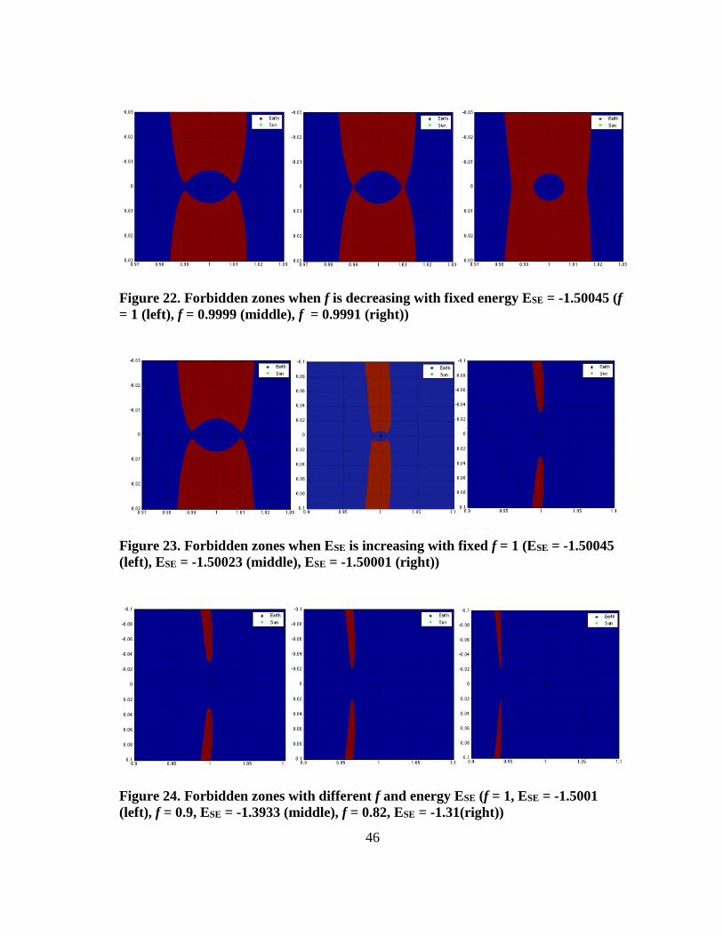
Based on the obtained eigenvectors, we can describe the equation of motion for
the limited 4-body problem into the first-order form. It is useful to track the contour of
the Lyapunov orbit around the Lagrange points. By using the 1-D search technique, the
global structure of the invariant manifolds can be mapped simply. Let us explore the
significant changes in the configuration of the invariant manifolds when the factor f is
decreased. As an example, we tracked the centerline of the invariant manifolds near the
Sun-Mars L2 point while the factor f is decreased. The initial conditions for each case of
unstable and stable manifolds can be obtained from the calculated eigenvalues in the
equation 4.18. For case 1, we assumed that the spacecraft left in the exterior realm
direction through unstable manifolds starting at the Sun-Mars L2 point. The initial
condition for the case 1 is (�� 𝑦 𝑣𝑥 𝑣𝑦)𝑡=0 = 𝛼[1 −𝜎 𝜆 −𝜆𝜎] so that the S/C
can follow the centerline of the unstable manifolds. As seen in Figure 25, the S/C
trajectories with different value of f are shown in Sun-Mars rotating frame. When the
factor f is 1, meaning no solar sail effect, the S/C travels like a shape of a scallop shell
around the forbidden zone and coms back to the starting point. By deploying the solar
sail so that it reduced the value of the factor f, the size of the scallop shell gets bigger.
Also a number of the bounce back motion by hitting the forbidden zone barrier is
reduced during the one cycle of motion. This behavior can be explained by the

49
relationship between the energy integral and the factor f. When f is decreased, the criteria
of the energy level for E2 and E3 are increased. So when the energy level of the entire
system still remains the same with no additional thrust, the thickness of the forbidden
zone is increased. That increases the size of scallop shell trajectory since the S/C hits the
forbidden zone barrier and bounces off slowly during the one cycle of the motion. In
Figure 25, the outer radius of the S/C trajectories are increased from 1 to 1.5 by reducing
the factor f. For case 2, the S/C follows the centerline of the unstable manifolds to the
interior realm direction at Sun-Mars L2 point. The initial condition for case 2 is
(�� 𝑦 𝑣𝑥 𝑣𝑦)𝑡=0 = 𝛼[−1 𝜎 −𝜆 𝜆𝜎]. In Figure 26, when the factor f is 1, the
S/C flies near Mars many times to reach the Sun-Mars L1 point. As f is decreased slowly,
the S/C trajectory is trapped in a halo orbit between Mars and the Sun-Mars L2 point. So
the S/C cannot connect with the Sun-Mars L1 point. For case 3, we assumed that the S/C
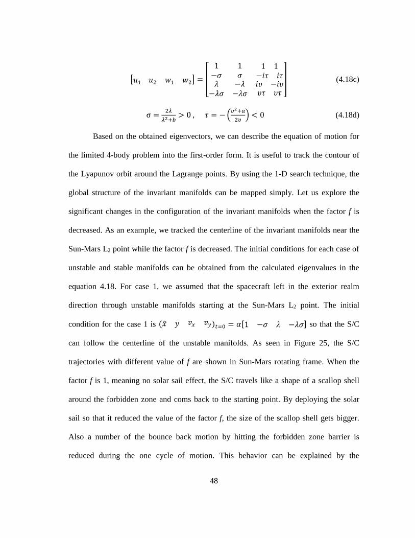
left in the exterior realm direction through stable manifolds starting at Sun-Mars L2
point. The initial condition for the case 3 is (�� 𝑦 𝑣𝑥 𝑣𝑦)𝑡=0 = 𝛼[1 𝜎 𝜆 𝜆𝜎]
while time direction is -1. The S/C trajectories are quite similar to the case 1 as you can
see in Figure 27. However, the S/C starts to fly in the opposite direction of case 1. For
the last case, the S/C travels through stable manifolds to the interior realm direction
starting at the Sun-Mars L2 point. The initial condition for case 4 is
(�� 𝑦 𝑣𝑥 𝑣𝑦)𝑡=0 = 𝛼[−1 −𝜎 −𝜆 −𝜆𝜎] while time direction is -1. The S/C
trajectories also show the same behaviors of case 2, but in the opposite direction. In
Figure 28, the S/C captured in a halo orbit between Mars and the Sun-Mars L2 point
when the factor f is below 0.99.

50
Figure 25. S/C trajectory from the Sun-Mars L2 point into unstable manifolds to
the exterior realm
Figure 26. S/C trajectory from the Sun-Mars L2 point into unstable manifolds to the
interior realm
51
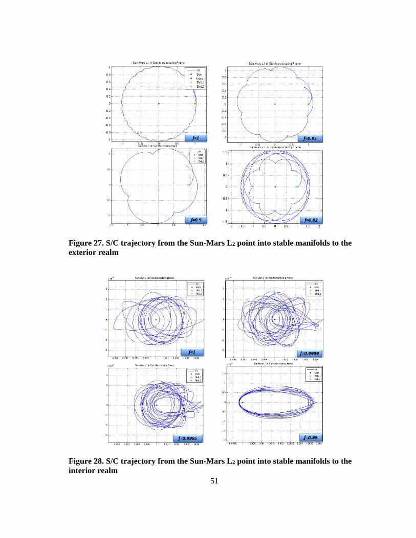
Figure 27. S/C trajectory from the Sun-Mars L2 point into stable manifolds to the
exterior realm
Figure 28. S/C trajectory from the Sun-Mars L2 point into stable manifolds to the
interior realm
52
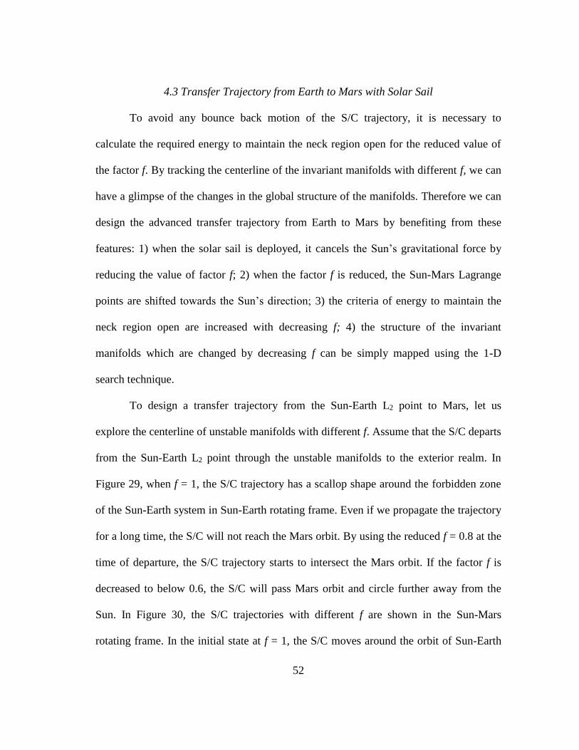
4.3 Transfer Trajectory from Earth to Mars with Solar Sail
To avoid any bounce back motion of the S/C trajectory, it is necessary to
calculate the required energy to maintain the neck region open for the reduced value of
the factor f. By tracking the centerline of the invariant manifolds with different f, we can
have a glimpse of the changes in the global structure of the manifolds. Therefore we can
design the advanced transfer trajectory from Earth to Mars by benefiting from these
features: 1) when the solar sail is deployed, it cancels the Sun’s gravitational force by
reducing the value of factor f; 2) when the factor f is reduced, the Sun-Mars Lagrange
points are shifted towards the Sun’s direction; 3) the criteria of energy to maintain the
neck region open are increased with decreasing f; 4) the structure of the invariant
manifolds which are changed by decreasing f can be simply mapped using the 1-D
search technique.
To design a transfer trajectory from the Sun-Earth L2 point to Mars, let us
explore the centerline of unstable manifolds with different f. Assume that the S/C departs
from the Sun-Earth L2 point through the unstable manifolds to the exterior realm. In
Figure 29, when f = 1, the S/C trajectory has a scallop shape around the forbidden zone
of the Sun-Earth system in Sun-Earth rotating frame. Even if we propagate the trajectory
for a long time, the S/C will not reach the Mars orbit. By using the reduced f = 0.8 at the
time of departure, the S/C trajectory starts to intersect the Mars orbit. If the factor f is
decreased to below 0.6, the S/C will pass Mars orbit and circle further away from the
Sun. In Figure 30, the S/C trajectories with different f are shown in the Sun-Mars
rotating frame. In the initial state at f = 1, the S/C moves around the orbit of Sun-Earth
53
L2 points. But when f = 0.9, it starts to show the bounce back motions by hitting the
forbidden zone of Sun-Mars system. Especially there are rewind points of the S/C
trajectory when f = 0.85. The S/C flies to the Sun-Mars L2 point and comes back near the
Sun-Earth L2 point again when f = 0.8. This retro trajectory can be useful to transfer to
Mars.
Figure 29. S/C trajectory from the Sun-Earth L2 point to the Sun-Mars L1 point in
the Sun-Earth rotating frame

54
Figure 30. S/C trajectory from the Sun-Earth L2 point to the Sun-Mars L1 point in
the Sun-Mars rotating frame
55
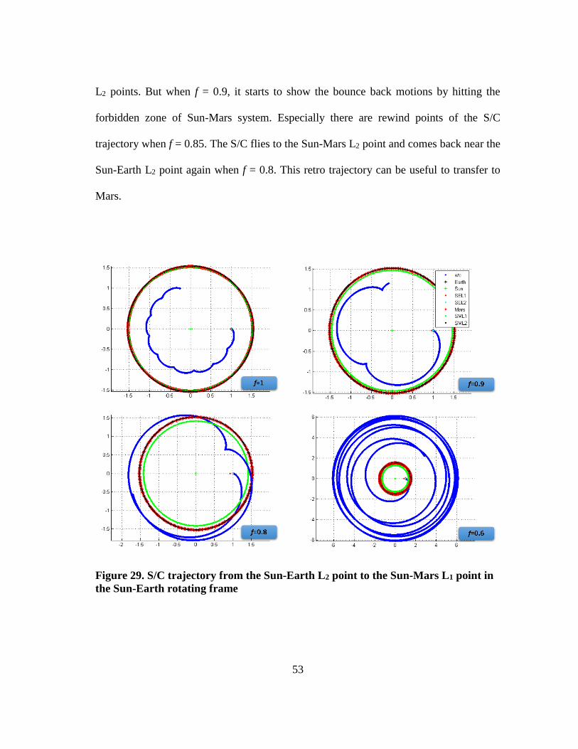
By taking advantage of the work described above, an example trajectory from the
Sun-Earth L2 point to Mars can be designed. In this case, we assume that the S/C departs
from Earth to the Sun-Earth L2 point via the Earth-Moon system as in the NEA
rendezvous mission described in section 3.3. The initial conditions of the S/C remain the
same: the mass of S/C is 1 MT and the specific impulse, Isp is 3000s. As you can see in
Figure 31, the S/C escapes from the Sun-Earth L2 point through the unstable manifolds
to the exterior realm and starts to deploy the solar sails. For 1.05 years (=384.3 days), the
S/C coasts along the manifolds and then f is reduced to 0.9. By reducing f, the Sun-Mars
Lagrange points are moved toward the Sun and the structure of the manifolds is also
changed. After travelling 74.45 days, the factor f is reduced to 0.80085. Then the S/C
flies over the Sun-Mars L2 point and turns back toward Mars. The S/C approaches to
Mars less than 0.0001396 AU (=2,090 km), below than the Martian geostationary orbit
altitude of 13,634 km.
Figure 31. Transfer trajectory from Sun-Earth L2 point to Mars in Sun-Mars
rotating frame

56
The time of flight for the retro trajectory is 829.6 days. Therefore the total flight
time of the transfer trajectory from Earth to Mars is approximately 2.93 years and the
energy consumption is only 2.698 km/s. This interesting retro trajectory is achieved
without fuel expenditure by using the interplanetary super highway method with solar
sail. The summary of the cost is shown in Table 4.
Table 4. Summary of cost for transfer trajectory from Earth to Mars
TOF [days]
∆𝐕 [𝐤𝐦/𝐬]
Earth to Sun-Earth L2 point 239.1 2.698
Sun-Earth L2 point to Mars
f = 1 384.3 0
f = 0.9 74.45 0
f = 0.80085 370.8 0
829.6 0
Total 1068.7 (=2.93 yrs) 2.698

57
5. SUMMARY AND FUTURE WORK
The overall purpose of this paper is to develop advanced mission design with
interplanetary transfer trajectory methods which can provide the minimum fuel cost for
complex and long duration space missions. To develop this new low-energy trajectory
method, called IPSH method, the dynamical properties of the PCR3BP were considered.
Also it was essential to explore the characteristics of the invariant manifolds winding
around the Lagrange points in the three-body system. With understanding of dynamical
symmetries and energy state dynamics, computationally simplified methods for IPSH
trajectory designs can be achieved. A simple method, called 1-D search technique, can
depict the centerline of the invariant manifolds issuing from the periodic orbits around
the Lagrange points. It allows us to see at a glance the global structure of the invariant
manifolds. For a meaningful design exercise, NEAs rendezvous mission was discussed
in four phases. In phase 1, a 1MT spacecraft slowly spiraled away from Earth LEO to
Earth-Moon L1 point by using small thrust. Then the S/C followed the thrust-free
trajectory to reach Earth-Moon L2 point in phase 2. By considering four-body dynamics
into two segments of three-body dynamics, the system-to-system transfer trajectory from
Earth-Moon L2 point to Sun-Earth L2 point were described in phase 3. Lastly, the S/C
travelled the grand tour of the NEAs by executing small burns and coasting
stable/unstable manifolds and returned back to Sun-Earth L2 point. The total trip time is
843.6 days with ∆V = 8.406 km/s.
58
For a second application study, the Mars exploration mission with solar sail was
considered. The propulsive power obtained from the solar sail can affect the three-body
dynamics by changing the geometry of invariant manifolds near the Lagrange points. A
limited case for four-body system was formulated with Earth, Mars, and S/C while Sun
is at origin. The significant changes in energy state and manifold structure due to the
solar sail factor f were investigated in depth. Therefore, we found that those changes can
be useful to design energy efficient trajectories for various interplanetary space mission.
As an example, a thrust-free trajectory from the Sun-Earth L2 point to Mars was
developed.
This research contributed to broaden the understanding of the natural dynamics
of the solar system and to design advanced transfer trajectories with significantly
reduced ∆V. The developed 1-D search technique can efficiently reveal the geometrical
framework for the whole tube-structure of the invariant manifolds based on the
centerline. With extended research on the general solution of the multi-body problem
and the effect of solar sails, it can be possible to develop an advanced design tool of low-
thrust trajectory for various interplanetary space missions.

59
REFERENCES
[1] W. S. Koon, M. W. Lo, J. E. Marsden and S. D. Ross, Dynamical Systems, the Three-
Body Problem, and Space Mission Design, Berlin, Springer, 2008
[2] M. W. Lo, “The Interplanetary Superhighway and the Origins Program,” Aerospace
Conference Proceedings, IEEE, Vol. 7, pp. 7-3543, 2002
[3] W. S. Koon, M. W. Lo, J. E. Marsden and S. D. Ross, “Shoot the Moon,” AAS 00-
166, AAS/AIAA Astrodynamics Specialist Conference, 2000
[4] S. D. Ross, “Cylindrical Manifolds and Tube Dynamics in the Restricted Three-Body
Problem,” Ph.D. Dissertation, California Institute of Technology, 2004
[5] V. G. Szebehely, Adventures in Celestial Mechanics, a First Course in the Theory
of Orbits, Austin, University of Texas Press, 1989
[6] H. Schaub and J. L. Junkins, Analytical Mechanics of Space Systems, Reston, VA,
AIAA, 2nd ed., 2009.
[7] V. G. Szebehely, Theory of Orbits, Academic Press, New York, 1967
[8] G. W. Hill, “Mr. Hill’s Researches in the Lunar Theory,” Monthly Notices of the
Royal Astronautical Society, Vol. 39, pp. 258-261, November 1879
[9] J. Barrow-Green, Poincare and the Three Body Problem, Providence RI, American
Mathematical Society, History of Mathematics, Vol. 2, 1997
[10] R. W. Farquhar, D. P. Muhonen, C. R. Newman, and H. S. Heuberger, “Trajectories
and Orbital Maneuvers for the First Libration-Point Satellite,” Journal of
Guidance and Control, Vol. 3, pp. 549-554, November-December 1980

60
[11] R. W. Farquhar, “The Flight of ISEE-3/ICE: Origins, Mission History, and a
Legacy,” AIAA Paper 98-4464, AIAA/AAS Astrodynamics Specialist Conference
and Exhibit, August 1998
[12] K. C. Howell, B. T. Barden, R. S. Wilson, and M. W. Lo, “Trajectory Design Using
a Dynamical Systems Approach with Applications to Genesis,”, Advances in the
Astronautical Sciences, Vol. 97, Part II, pp.1665-1684, 1997
[13] E. A. Belbruno, Capture Dynamics and Chaotic Motions in Celestial Mechanics,
Princeton, NJ, Princeton University Press, 2004
[14] E. A. Belbruno and J. K. Miller, “Sun-Perturbed Earth-to-Moon Transfers with
Ballistic Capture,” Journal of Guidance, Control, and Dynamics, Vol. 16, No. 4, pp. 770-
775, 1993.
[15] B. T. Barden and K. C. Howell, “Fundamental Motions Near the Collinear
Libration Points and Their Transitions,” Journal of the Astronautical Sciences, Vol. 46,
No.4, pp. 361-378, 1998
[16] C. C. Conley, “Low Energy Transit Orbits in the Restricted Three-Body Problem,”
SIAM J. Appl. Math., Vol. 16, pp. 732–746, 1968
[17] J. E. Prussing and B. A. Conway, Orbital Mechanics, Oxford, Oxford University
Press, 1993
[18] M. W. Lo and S. D. Ross, The Lunar L1 Gateway: Portal to the Stars and Beyond,
Pasadena, CA: Jet Propulsion Laboratory, National Aeronautics and Space
Administration, 2001

61
[19] K. C. Howell, B. T. Barden and M. W. Lo, “Application of Dynamical Systems
Theory to Trajectory Design for a Lagrange Point Mission,” Journal of Astronautial
Sciences, Vol. 45, No. 1, pp. 161-178, 1977
[20] R. R. Rausch, “Earth to Halo Orbit Transfer Trajectories”, M.S. Thesis, School of
Aeronautics and Astronautics, Purdue University, 2005
[21] J. D. Mireles James, “Celestial Mechanics Notes Set 5: Symmetric Periodic Orbits
of the Circular Restricted Three Body Problem and their Stable and Unstable
Manifolds,” Rutgers University, 2006
[22] R. McGehee, “Some Homoclinic Orbits for the Restricted Three-Body Problem,”
Ph.D. Dissertation, University of Wisconsin, Madison, 1969
[23] G. Gomez, W. S. Koon, M. W. Lo, J. E. Marsden, J. Masdemont, and S. D. Ross,
“Invariant Manifolds, the Spatial Three-Body Problem and Space Mission Design,”
AAS 01-301, AAS Conference, August 2001
[24] D. B. Kanipe, D. C. Hyland, “Investigation of the Potential for Human Travel into
Deep Space Using Current, or Imminently, Available Technology,” AIAA 2014-4238,
AIAA Space 2014 Conference, August 4-7, 2014
[25] G. P. Alonso, “The Design of System-to-System Transfer Arcs using Invariant
Manifolds in the Multi-body Problem”, Ph.D. Dissertation, Purdue University, 2006
[26] F. Topputo, M. Vasile and A. E. Finzi, “Combining Two and Three-Body
Dynamics for Low Energy Transfer Trajectories of Practical Interest,” Proceedings of
the 55th International Astronautical Congress, pp. 584-596, 2004

62
[27] J. Lu, M. Zhang, Q. Lu, “Transfer Trajectory Design for Mars Exploration,”
International Journal of Astronomy and Astrophysics, Vol. 3, No. 2A, pp. 5-16, 2013
Related Documents