Advanced Macroeconomics II Lecture 1 Stochastic Dynamic Programming Isaac Baley UPF & Barcelona GSE January 7, 2016 1 / 38

Welcome message from author
This document is posted to help you gain knowledge. Please leave a comment to let me know what you think about it! Share it to your friends and learn new things together.
Transcript

Advanced Macroeconomics II
Lecture 1
Stochastic Dynamic Programming
Isaac Baley
UPF & Barcelona GSE
January 7, 2016
1 / 38

Introduction
• Stochastic dynamic programming is a very useful tool to think and solve a
lot of economic problems.
• We review the theory of dynamic programming and extend to include
uncertainty.
• Straightforward extension of what you did in Advanced Macro I.
• References:
I Acemoglu (2009), Ch. 16.
I Adda and Cooper (2003), Ch 2-3.
I Ljungquvist and Sargent (2014), Ch 3-4.
I Stokey, Lucas, and Prescott (1989), Ch 3-4 (deterministic), 7-9
(stochastic with measure theory).
2 / 38
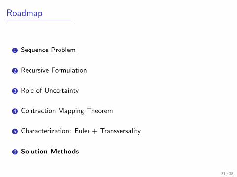
Roadmap
1 Sequence Problem
2 Recursive Formulation
3 Role of Uncertainty
4 Contraction Mapping Theorem
5 Characterization: Euler + Transversality
6 Solution Methods
3 / 38
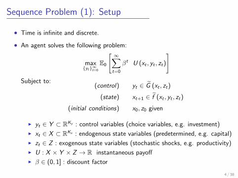
Sequence Problem (1): Setup
• Time is infinite and discrete.
• An agent solves the following problem:
max{yt}∞t=0
E0
[ ∞∑t=0
βt U (xt , yt , zt)
]Subject to:
(control) yt ∈ G̃ (xt , zt)
(state) xt+1 ∈ f̃ (xt , yt , zt)
(initial conditions) x0, z0 given
I yt ∈ Y ⊂ RKy : control variables (choice variables, e.g. investment)
I xt ∈ X ⊂ RKx : endogenous state variables (predetermined, e.g. capital)
I zt ∈ Z : exogenous state variables (stochastic shocks, e.g. productivity)
I U : X × Y × Z → R instantaneous payoff
I β ∈ (0, 1] : discount factor
4 / 38
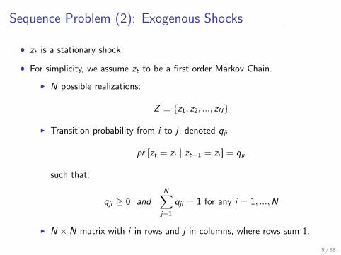
Sequence Problem (2): Exogenous Shocks
• zt is a stationary shock.
• For simplicity, we assume zt to be a first order Markov Chain.
I N possible realizations:
Z ≡ {z1, z2, ..., zN}
I Transition probability from i to j , denoted qji
pr [zt = zj | zt−1 = zi ] = qji
such that:
qji ≥ 0 andN∑j=1
qji = 1 for any i = 1, ...,N
I N × N matrix with i in rows and j in columns, where rows sum 1.
5 / 38
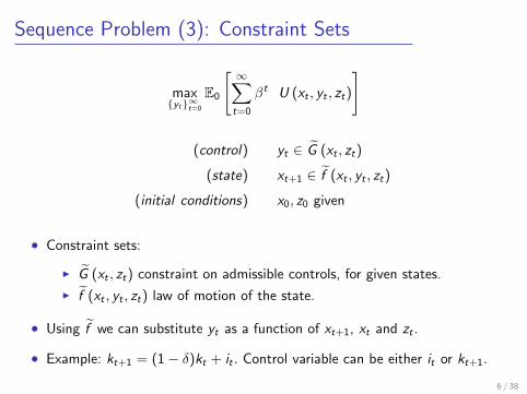
Sequence Problem (3): Constraint Sets
max{yt}∞t=0
E0
[ ∞∑t=0
βt U (xt , yt , zt)
]
(control) yt ∈ G̃ (xt , zt)
(state) xt+1 ∈ f̃ (xt , yt , zt)
(initial conditions) x0, z0 given
• Constraint sets:
I G̃ (xt , zt) constraint on admissible controls, for given states.
I f̃ (xt , yt , zt) law of motion of the state.
• Using f̃ we can substitute yt as a function of xt+1, xt and zt .
• Example: kt+1 = (1− δ)kt + it . Control variable can be either it or kt+1.
6 / 38
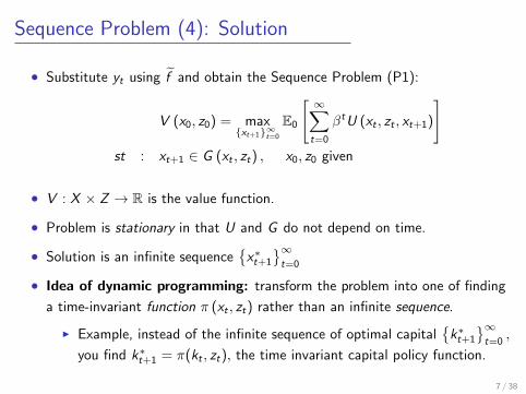
Sequence Problem (4): Solution
• Substitute yt using f̃ and obtain the Sequence Problem (P1):
V (x0, z0) = max{xt+1}∞t=0
E0
[ ∞∑t=0
βtU (xt , zt , xt+1)
]st : xt+1 ∈ G (xt , zt) , x0, z0 given
• V : X × Z → R is the value function.
• Problem is stationary in that U and G do not depend on time.
• Solution is an infinite sequence{x∗t+1
}∞t=0
• Idea of dynamic programming: transform the problem into one of finding
a time-invariant function π (xt , zt) rather than an infinite sequence.
I Example, instead of the infinite sequence of optimal capital{k∗t+1
}∞t=0
,
you find k∗t+1 = π(kt , zt), the time invariant capital policy function.
7 / 38
Roadmap
1 Sequence Problem
2 Recursive Formulation
3 Role of Uncertainty
4 Contraction Mapping Theorem
5 Characterization: Euler + Transversality
6 Solution Methods
8 / 38
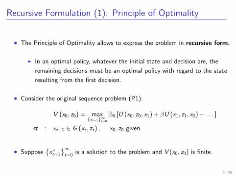
Recursive Formulation (1): Principle of Optimality
• The Principle of Optimality allows to express the problem in recursive form.
I In an optimal policy, whatever the initial state and decision are, the
remaining decisions must be an optimal policy with regard to the state
resulting from the first decision.
• Consider the original sequence problem (P1):
V (x0, z0) = max{xt+1}∞t=0
E0 [U (x0, z0, x1) + βU (x1, z1, x2) + . . . ]
st : xt+1 ∈ G (xt , zt) , x0, z0 given
• Suppose{x∗t+1
}∞t=0
is a solution to the problem and V (x0, z0) is finite.
9 / 38
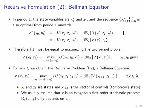
Recursive Formulation (2): Bellman Equation
• In period 1, the state variables are x∗1 and z1, and the sequence{x∗t+1
}∞t=0
is
also optimal from period 1 onwards:
V ∗ (x0, z0) = U (x0, z0, x∗1 ) + βE0 [U (x∗1 , z1, x
∗2 ) + . . . ]
= U (x0, z0, x∗1 ) + βE0 [V (x∗1 , z1)]
• Therefore P1 must be equal to maximizing the two period problem:
V (x0, z0) = maxx1=π(x0,z0)
U (x0, z0, x1) + βE0 [V (x1, z1)] , x0, z0 given
• For any t, we obtain the Recursive Problem (P2), a Bellman Equation:
V (xt , zt) = maxxt+1=π(xt ,zt)
{U (xt , zt , xt+1) + βEt [V (xt+1, zt+1)]} ∀x ∈ X
I xt and zt are states and xt+1 is the vector of controls (tomorrow’s state)
I We usually assume that z is an exogenous first order stochastic process:
Et (zt+1) only depends on zt .
10 / 38
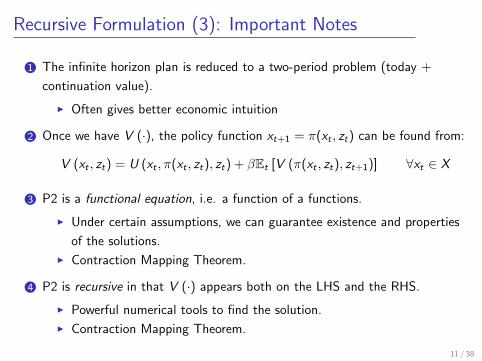
Recursive Formulation (3): Important Notes
1 The infinite horizon plan is reduced to a two-period problem (today +
continuation value).
I Often gives better economic intuition
2 Once we have V (·), the policy function xt+1 = π(xt , zt) can be found from:
V (xt , zt) = U (xt , π(xt , zt), zt) + βEt [V (π(xt , zt), zt+1)] ∀xt ∈ X
3 P2 is a functional equation, i.e. a function of a functions.
I Under certain assumptions, we can guarantee existence and properties
of the solutions.
I Contraction Mapping Theorem.
4 P2 is recursive in that V (·) appears both on the LHS and the RHS.
I Powerful numerical tools to find the solution.
I Contraction Mapping Theorem.
11 / 38
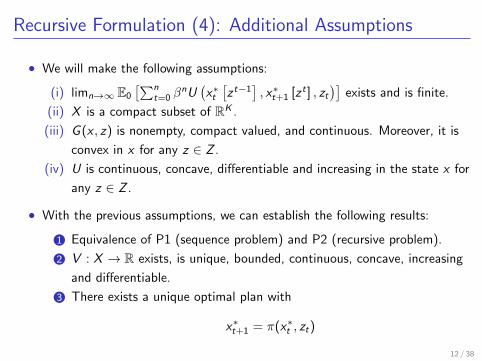
Recursive Formulation (4): Additional Assumptions
• We will make the following assumptions:
(i) limn→∞ E0
[∑nt=0 β
nU(x∗t[z t−1
], x∗t+1 [z t ] , zt
)]exists and is finite.
(ii) X is a compact subset of RK .
(iii) G (x , z) is nonempty, compact valued, and continuous. Moreover, it is
convex in x for any z ∈ Z .
(iv) U is continuous, concave, differentiable and increasing in the state x for
any z ∈ Z .
• With the previous assumptions, we can establish the following results:
1 Equivalence of P1 (sequence problem) and P2 (recursive problem).
2 V : X → R exists, is unique, bounded, continuous, concave, increasing
and differentiable.
3 There exists a unique optimal plan with
x∗t+1 = π(x∗t , zt)
12 / 38
Roadmap
1 Sequence Problem
2 Recursive Formulation
3 Role of Uncertainty
4 Contraction Mapping Theorem
5 Characterization: Euler + Transversality
6 Solution Methods
13 / 38
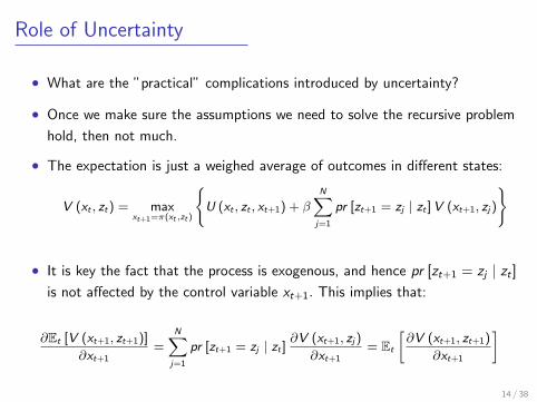
Role of Uncertainty
• What are the ”practical” complications introduced by uncertainty?
• Once we make sure the assumptions we need to solve the recursive problem
hold, then not much.
• The expectation is just a weighed average of outcomes in different states:
V (xt , zt) = maxxt+1=π(xt ,zt )
{U (xt , zt , xt+1) + β
N∑j=1
pr [zt+1 = zj | zt ]V (xt+1, zj)
}
• It is key the fact that the process is exogenous, and hence pr [zt+1 = zj | zt ]is not affected by the control variable xt+1. This implies that:
∂Et [V (xt+1, zt+1)]
∂xt+1=
N∑j=1
pr [zt+1 = zj | zt ]∂V (xt+1, zj)
∂xt+1= Et
[∂V (xt+1, zt+1)
∂xt+1
]
14 / 38
Roadmap
1 Sequence Problem
2 Recursive Formulation
3 Role of Uncertainty
4 Contraction Mapping Theorem
5 Characterization: Euler + Transversality
6 Solution Methods
15 / 38
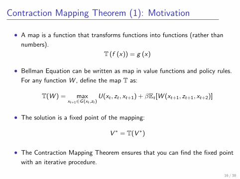
Contraction Mapping Theorem (1): Motivation
• A map is a function that transforms functions into functions (rather than
numbers).
T (f (x)) = g (x)
• Bellman Equation can be written as map in value functions and policy rules.
For any function W , define the map T as:
T(W ) = maxxt+1∈G(xt ,zt)
U(xt , zt , xt+1) + βEt [W (xt+1, zt+1, xt+2)]
• The solution is a fixed point of the mapping:
V ∗ = T(V ∗)
• The Contraction Mapping Theorem ensures that you can find the fixed point
with an iterative procedure.
16 / 38
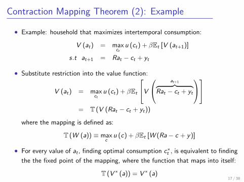
Contraction Mapping Theorem (2): Example
• Example: household that maximizes intertemporal consumption:
V (at) = maxct
u (ct) + βEt [V (at+1)]
s.t at+1 = Rat − ct + yt
• Substitute restriction into the value function:
V (at) = maxct
u (ct) + βEt
V at+1︷ ︸︸ ︷Rat − ct + yt
= T (V (Rat − ct + yt))
where the mapping is defined as:
T (W (a)) ≡ maxc
u (c) + βEt [W (Ra− c + y)]
• For every value of at , finding optimal consumption c∗t , is equivalent to finding
the the fixed point of the mapping, where the function that maps into itself:
T (V ∗ (a)) = V ∗ (a)17 / 38
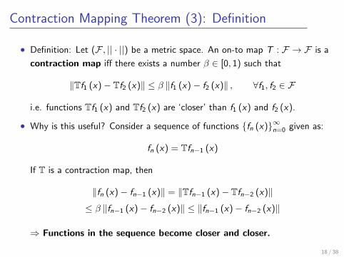
Contraction Mapping Theorem (3): Definition
• Definition: Let (F , || · ||) be a metric space. An on-to map T : F → F is a
contraction map iff there exists a number β ∈ [0, 1) such that
‖Tf1 (x)− Tf2 (x)‖ ≤ β ‖f1 (x)− f2 (x)‖ , ∀f1, f2 ∈ F
i.e. functions Tf1 (x) and Tf2 (x) are ‘closer’ than f1 (x) and f2 (x).
• Why is this useful? Consider a sequence of functions {fn (x)}∞n=0 given as:
fn (x) = Tfn−1 (x)
If T is a contraction map, then
‖fn (x)− fn−1 (x)‖ = ‖Tfn−1 (x)− Tfn−2 (x)‖
≤ β ‖fn−1 (x)− fn−2 (x)‖ ≤ ‖fn−1 (x)− fn−2 (x)‖
⇒ Functions in the sequence become closer and closer.
18 / 38
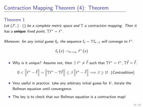
Contraction Mapping Theorem (4): Theorem
Theorem 1Let (F , || · ||) be a complete metric space and T a contraction mapping. Then it
has a unique fixed point, Tf ∗ = f ∗.
Moreover, for any initial guess f0, the sequence fn = Tfn−1 will converge to f ∗.
fn (x)→n→∞ f ∗ (x)
• Why is it unique? Assume not, then ∃ f ∗ 6= f̃ such that Tf ∗ = f ∗, Tf̃ = f̃ .
0 <∥∥∥f ∗ − f̃
∥∥∥ =∥∥∥Tf ∗ − Tf̃
∥∥∥ ≤ β ∥∥∥f ∗ − f̃∥∥∥ =⇒ β ≥ 1! (Contradition)
• Very useful in practice: take any arbitrary initial guess for V , iterate the
Bellman equation until convergence.
• The key is to check that our Bellman equation is a contraction map!
19 / 38
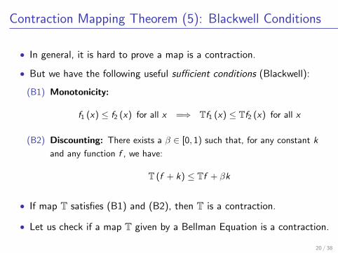
Contraction Mapping Theorem (5): Blackwell Conditions
• In general, it is hard to prove a map is a contraction.
• But we have the following useful sufficient conditions (Blackwell):
(B1) Monotonicity:
f1 (x) ≤ f2 (x) for all x =⇒ Tf1 (x) ≤ Tf2 (x) for all x
(B2) Discounting: There exists a β ∈ [0, 1) such that, for any constant k
and any function f , we have:
T (f + k) ≤ Tf + βk
• If map T satisfies (B1) and (B2), then T is a contraction.
• Let us check if a map T given by a Bellman Equation is a contraction.
20 / 38
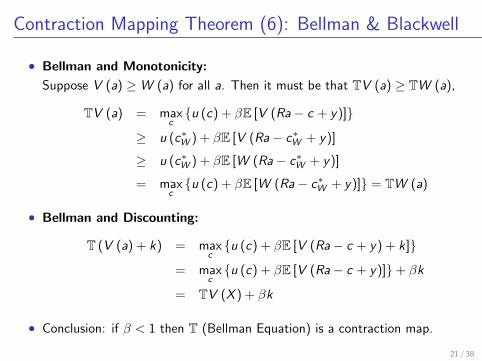
Contraction Mapping Theorem (6): Bellman & Blackwell
• Bellman and Monotonicity:
Suppose V (a) ≥W (a) for all a. Then it must be that TV (a) ≥ TW (a),
TV (a) = maxc{u (c) + βE [V (Ra− c + y)]}
≥ u (c∗W ) + βE [V (Ra− c∗W + y)]
≥ u (c∗W ) + βE [W (Ra− c∗W + y)]
= maxc{u (c) + βE [W (Ra− c∗W + y)]} = TW (a)
• Bellman and Discounting:
T (V (a) + k) = maxc{u (c) + βE [V (Ra− c + y) + k]}
= maxc{u (c) + βE [V (Ra− c + y)]}+ βk
= TV (X ) + βk
• Conclusion: if β < 1 then T (Bellman Equation) is a contraction map.
21 / 38
Roadmap
1 Sequence Problem
2 Recursive Formulation
3 Role of Uncertainty
4 Contraction Mapping Theorem
5 Characterization: Euler + Transversality
6 Solution Methods
22 / 38
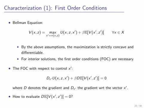
Characterization (1): First Order Conditions
• Bellman Equation:
V (x , z) = maxx′=π(x,z)
U(x , z , x ′) + βE[V (x ′, z ′)] ∀x ∈ X
I By the above assumptions, the maximization is strictly concave and
differentiable.
I For interior solutions, the first order conditions (FOC) are necessary.
• The FOC with respect to control x ′:
Dx′U(x , z , x ′) + βDE[V (x ′, z ′)] = 0
where D denotes the gradient and Dx′ the gradient wrt the vector x ′.
• How to evaluate DE[V (x ′, z ′)] = 0?
23 / 38
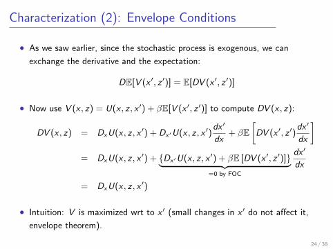
Characterization (2): Envelope Conditions
• As we saw earlier, since the stochastic process is exogenous, we can
exchange the derivative and the expectation:
DE[V (x ′, z ′)] = E[DV (x ′, z ′)]
• Now use V (x , z) = U(x , z , x ′) + βE[V (x ′, z ′)] to compute DV (x , z):
DV (x , z) = DxU(x , z , x ′) + Dx′U(x , z , x ′)dx ′
dx+ βE
[DV (x ′, z ′)
dx ′
dx
]= DxU(x , z , x ′) + {Dx′U(x , z , x ′) + βE [DV (x ′, z ′)]}︸ ︷︷ ︸
=0 by FOC
dx ′
dx
= DxU(x , z , x ′)
• Intuition: V is maximized wrt to x ′ (small changes in x ′ do not affect it,
envelope theorem).
24 / 38
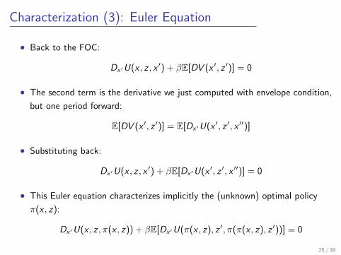
Characterization (3): Euler Equation
• Back to the FOC:
Dx′U(x , z , x ′) + βE[DV (x ′, z ′)] = 0
• The second term is the derivative we just computed with envelope condition,
but one period forward:
E[DV (x ′, z ′)] = E[Dx′U(x ′, z ′, x ′′)]
• Substituting back:
Dx′U(x , z , x ′) + βE[Dx′U(x ′, z ′, x ′′)] = 0
• This Euler equation characterizes implicitly the (unknown) optimal policy
π(x , z):
Dx′U(x , z , π(x , z)) + βE[Dx′U(π(x , z), z ′, π(π(x , z), z ′))] = 0
25 / 38
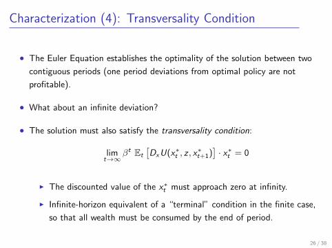
Characterization (4): Transversality Condition
• The Euler Equation establishes the optimality of the solution between two
contiguous periods (one period deviations from optimal policy are not
profitable).
• What about an infinite deviation?
• The solution must also satisfy the transversality condition:
limt→∞
βt Et
[DxU(x∗t , z , x
∗t+1)
]· x∗t = 0
I The discounted value of the x∗t must approach zero at infinity.
I Infinite-horizon equivalent of a “terminal” condition in the finite case,
so that all wealth must be consumed by the end of period.
26 / 38
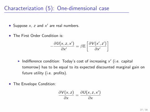
Characterization (5): One-dimensional case
• Suppose x , z and x ′ are real numbers.
• The First Order Condition is:
−∂U(x , z , x ′)
∂x ′= βE
[∂V (x ′, z ′)
∂x ′
]
I Indifference condition: Today’s cost of increasing x ′ (i.e. capital
tomorrow) has to be equal to its expected discounted marginal gain on
future utility (i.e. profits).
• The Envelope Condition:
∂V (x , z)
∂x=∂U(x , z , x ′)
∂x
27 / 38
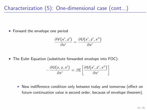
Characterization (5): One-dimensional case (cont...)
• Forward the envelope one period
∂V (x ′, z ′)
∂x ′=∂U(x ′, z ′, x ′′)
∂x ′
• The Euler Equation (substitute forwarded envelope into FOC):
−∂U(x , z , x ′)
∂x ′= βE
[∂U(x ′, z ′, x ′′)
∂x ′
]
I New indifference condition only between today and tomorrow (effect on
future continuation value is second order, because of envelope theorem).
28 / 38
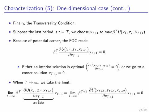
Characterization (5): One-dimensional case (cont...)
• Finally, the Transversality Condition.
• Suppose the last period is t = T , we choose xT+1 to maxβTU(xT , zT , xT+1)
• Because of potential corner, the FOC reads:
βT ∂U(xT , zT , xT+1)
∂xT+1xT+1 = 0
I Either an interior solution is optimal(∂U(xT ,zT ,xT+1)
∂xT+1= 0)
or we go to a
corner solution xT+1 = 0.
• When T →∞, we take the limit:
limT→∞
βT ∂U(xT , zT , xT+1)
∂xT+1︸ ︷︷ ︸use Euler
xT+1 = limT→∞
βT+1 ∂U(xT+1, zT+1, xT+2)
∂xT+1xT+1 = 0
29 / 38
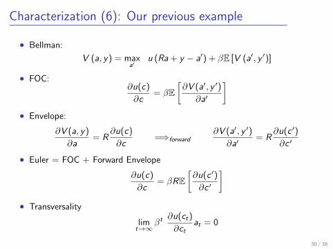
Characterization (6): Our previous example
• Bellman:
V (a, y) = maxa′
u (Ra + y − a′) + βE [V (a′, y ′)]
• FOC:∂u(c)
∂c= βE
[∂V (a′, y ′)
∂a′
]• Envelope:
∂V (a, y)
∂a= R
∂u(c)
∂c=⇒forward
∂V (a′, y ′)
∂a′= R
∂u(c ′)
∂c ′
• Euler = FOC + Forward Envelope
∂u(c)
∂c= βRE
[∂u(c ′)
∂c ′
]• Transversality
limt→∞
βt ∂u(ct)
∂ctat = 0
30 / 38
Roadmap
1 Sequence Problem
2 Recursive Formulation
3 Role of Uncertainty
4 Contraction Mapping Theorem
5 Characterization: Euler + Transversality
6 Solution Methods
31 / 38
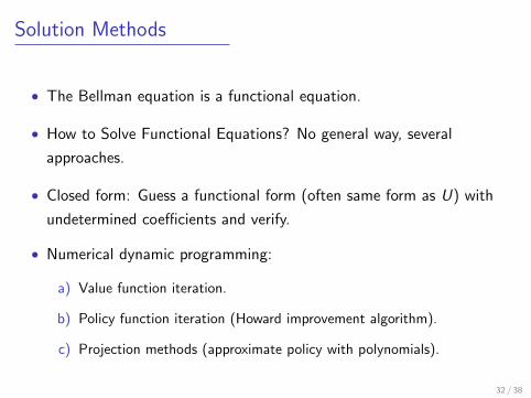
Solution Methods
• The Bellman equation is a functional equation.
• How to Solve Functional Equations? No general way, several
approaches.
• Closed form: Guess a functional form (often same form as U) with
undetermined coefficients and verify.
• Numerical dynamic programming:
a) Value function iteration.
b) Policy function iteration (Howard improvement algorithm).
c) Projection methods (approximate policy with polynomials).
32 / 38
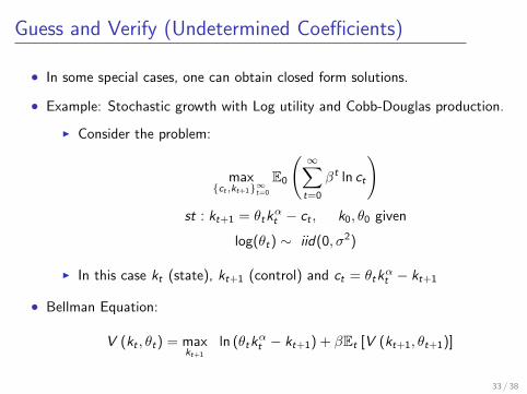
Guess and Verify (Undetermined Coefficients)
• In some special cases, one can obtain closed form solutions.
• Example: Stochastic growth with Log utility and Cobb-Douglas production.
I Consider the problem:
max{ct ,kt+1}∞t=0
E0
( ∞∑t=0
βt ln ct
)st : kt+1 = θtk
αt − ct , k0, θ0 given
log(θt) ∼ iid(0, σ2)
I In this case kt (state), kt+1 (control) and ct = θtkαt − kt+1
• Bellman Equation:
V (kt , θt) = maxkt+1
ln (θtkαt − kt+1) + βEt [V (kt+1, θt+1)]
33 / 38
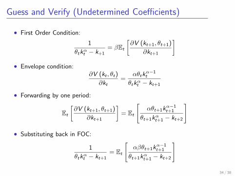
Guess and Verify (Undetermined Coefficients)
• First Order Condition:
1
θtkαt − k+1= βEt
[∂V (kt+1, θt+1)
∂kt+1
]• Envelope condition:
∂V (kt , θt)
∂kt=
αθtkα−1t
θtkαt − kt+1
• Forwarding by one period:
Et
[∂V (kt+1, θt+1)
∂kt+1
]= Et
[αθt+1k
α−1t+1
θt+1kαt+1 − kt+2
]
• Substituting back in FOC:
1
θtkαt − kt+1= Et
[αβθt+1k
α−1t+1
θt+1kαt+1 − kt+2
]
34 / 38
Guess and Verify (Undetermined Coefficients)
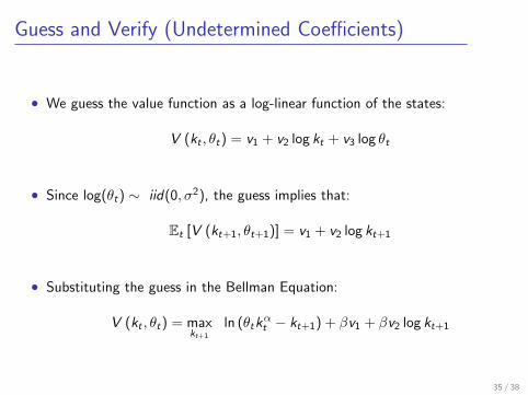
• We guess the value function as a log-linear function of the states:
V (kt , θt) = v1 + v2 log kt + v3 log θt
• Since log(θt) ∼ iid(0, σ2), the guess implies that:
Et [V (kt+1, θt+1)] = v1 + v2 log kt+1
• Substituting the guess in the Bellman Equation:
V (kt , θt) = maxkt+1
ln (θtkαt − kt+1) + βv1 + βv2 log kt+1
35 / 38
Guess and Verify (Undetermined Coefficients)
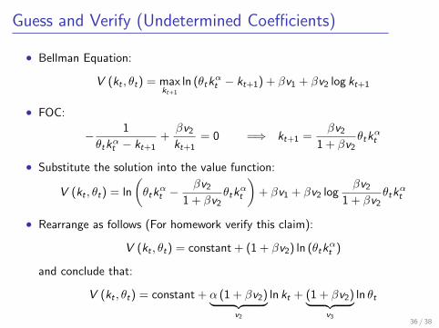
• Bellman Equation:
V (kt , θt) = maxkt+1
ln (θtkαt − kt+1) + βv1 + βv2 log kt+1
• FOC:
− 1
θtkαt − kt+1+βv2kt+1
= 0 =⇒ kt+1 =βv2
1 + βv2θtk
αt
• Substitute the solution into the value function:
V (kt , θt) = ln
(θtk
αt −
βv21 + βv2
θtkαt
)+ βv1 + βv2 log
βv21 + βv2
θtkαt
• Rearrange as follows (For homework verify this claim):
V (kt , θt) = constant + (1 + βv2) ln (θtkαt )
and conclude that:
V (kt , θt) = constant + α (1 + βv2)︸ ︷︷ ︸v2
ln kt + (1 + βv2)︸ ︷︷ ︸v3
ln θt
36 / 38
Guess and Verify (Undetermined Coefficients)
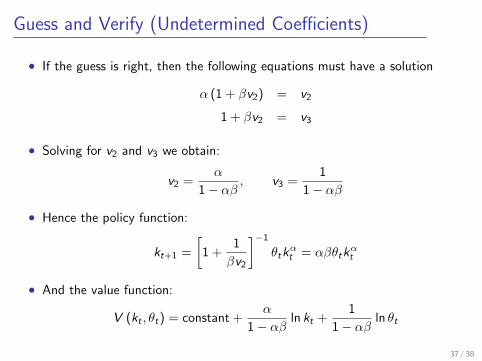
• If the guess is right, then the following equations must have a solution
α (1 + βv2) = v2
1 + βv2 = v3
• Solving for v2 and v3 we obtain:
v2 =α
1− αβ, v3 =
1
1− αβ
• Hence the policy function:
kt+1 =
[1 +
1
βv2
]−1θtk
αt = αβθtk
αt
• And the value function:
V (kt , θt) = constant +α
1− αβln kt +
1
1− αβln θt
37 / 38
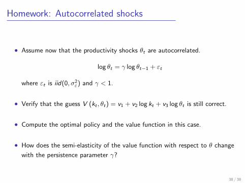
Homework: Autocorrelated shocks
• Assume now that the productivity shocks θt are autocorrelated.
log θt = γ log θt−1 + εt
where εt is iid(0, σ2ε) and γ < 1.
• Verify that the guess V (kt , θt) = v1 + v2 log kt + v3 log θt is still correct.
• Compute the optimal policy and the value function in this case.
• How does the semi-elasticity of the value function with respect to θ change
with the persistence parameter γ?
38 / 38
Related Documents