CPA CERTIFIED PUBLIC ACCOUNTANTS PART III SECTION 5 ADVANCED FINANCIAL MANAGEMENT STUDY TEXT Revised on: July 2019 KASNEB JULY 2018 SYLLABUS Page 1

Welcome message from author
This document is posted to help you gain knowledge. Please leave a comment to let me know what you think about it! Share it to your friends and learn new things together.
Transcript

CPA
CERTIFIED PUBLIC ACCOUNTANTS
PART III
SECTION 5
ADVANCED FINANCIAL MANAGEMENT
STUDY TEXT
Revised on: July 2019
KASNEB JULY 2018 SYLLABUS
Page 1
SYLLABUS PAPER NO.15 ADVANCED FINANCIAL MANAGEMENT
GENERAL OBJECTIVE This paper is intended to equip the candidate with knowledge, skills and attitudes that will enable
him/her to apply advanced financial management techniques in an organisation.
15.0LEARNING OUTCOMES A candidate who passes this paper should be able to:
- Evaluate advanced capital budgeting decisions
- Design an optimal capital structure for an organisation
- Predict corporate failure
- Apply derivatives in financial risk management
- Apply financial management skills in the public sector
- Understand concepts of corporate restructuring and re-organisation
- Apply valuation techniques in real estate finance
CONTENT
15.1Advanced capital budgeting decision
- Incorporating risk/uncertainty in capital investment decisions
- Nature and measurement of risk and uncertainty
- Techniques of handling risk: sensitivity analysis, scenario analysis, decision trees, simulation
analysis, utility analysis, risk adjusted discounting rate(radr) and certainty equivalent method
- Incorporating capital rationing in capital investment appraisal
- Incorporating inflation in capital investment appraisal
- Evaluation of projects of unequal lives
- The real options-strategic investment option, timing option, abandonment option and the
replacement option
- Common capital budgeting pitfalls
15.2Portfolio theory and analysis:
- The modern portfolio theory: background of the theory; portfolio expected return; the actual
and weighted portfolio risk; derivation of efficient sets; the capital market line (CML) model
and its applications, the mean variance dominance rule; short comings of portfolio theory
- Capital Asset Pricing Model-CAPM : background of the theory; assumptions; beta estimation
- beta coefficient of an individual asset and that of a portfolio and the interpretation of the
result; security market line(SML) model and its applications; conceptual differences between
portfolio theory and capital asset pricing model
- Shortcomings of the capital asset pricing model
- The Arbitrage pricing model (APM) and other multifactor models: background of the theory;
conceptual differences between the Capital asset pricing model and the Arbitrage pricing
model; application of the Arbitrage pricing model, shortcomings of Arbitrage pricing model;
Pastor Stambaugh model
- Evaluation of portfolio performance: Treynor’s measure, Sharpe’s measure, Jensen’s
measure, appraisal ratio measure, information ratio, Modigliani and Modigliani (M2)
15.3Advanced financing decision
- The nature of financing decision, principle objectives of making financing decision
Page 2
- Overview of cost of capital: meaning and relevance of cost of capital: the firm’s overall cost
of capital; weighted average cost of capital (WACC) and weighted marginal cost of capital
(WMCC) ; analysis of breakpoints in weighted marginal cost of capital schedule
- Capital structure theories: nature of capital structure and factors influencing the firm’s capital
structure; traditional theories of capital structure - assumptions of the theories, Net income
theory and Net operating income theory; Franco Modigliani and Merton Miller’s propositions
- MM without taxes, MM with corporation taxes, MM with corporation and personal tax rates
and MM with taxes and financial distress costs; other theories of capital structure; the pecking
order theory and Trade-off theory determination of the firm’s optimal capital structure using
the Hamada model, CAPM and WACC
- Special topics in financing decision: analysis of operating profit (EBIT)/EPS at point of
indifference in firm’s earnings; establishing the range of operating profit within which each
financing option; leverage and risk; operating leverage and operating risk, financial leverage
and financial risk, combined leverage and total risk; quantifying leverage using the degree of
operating leverage, degree of financial leverage and degree of combined leverage
- Long term financing decisions; bond refinancing decision, lease-buy evaluation and the rights
issues
- Impact of financing on investment decisions - the concept of adjusted present value (APV)
15.4Mergers and acquisitions
- Nature of mergers and acquisitions
- Reasons of mergers and acquisitions
- Acquisition and Mergers verses organic growth
- Valuation of acquisitions and mergers
- Prediction of a takeover target
- Defence tactics against hostile takeovers
- Financing of mergers and acquisitions
- Analysis of combined operating profit (EBIT) and post-acquisition earning per share at the
point of indifference in firms earnings under various financing options.
- Determination of range of combined operating profit.
- Regulatory frame work for mergers and acquisitions
- Reasons why there are failed mergers and acquisitions
- Mergers and acquisitions in a global context
15.5Corporate restructuring and re-organisation
- Background on restructuring and re organisation
- Indicators/symptoms of restructuring
- Considerations in designing an appropriate restructuring programme
- Financial reconstruction: forms of financial reconstruction; impact of financial reconstruction
on share price; impact of financial reconstruction on the weighted Average cost of capital
(WACC)
- Portfolio reconstruction: various ways of unbundling a firm: divestment, de-merger, spin-off,
liquidation, sell-offs, equity curve outs, strategic alliances, management buyout, leveraged
buyouts and the management buy-ins.
- The relevance of the various forms of portfolio reconstruction
- Organisational reconstruction: The nature and benefits of this form of restructuring; models of
predicting corporate failure; Multiple discriminant analysis (Z-Score model), Beaver failure
ratio, Argenti model, Taffler’s model
- Causes of financial distress
Page 3
- Forms of financial distress and solutions to financial distress
15.6Derivatives in financial risk management
- The meaning, nature and importance of derivative instruments: futures, forwards, options and
swaps
- Pricing and valuations of derivatives: futures, forwards, options and swaps
- Types of risks: operational risks, political risks, economic risks, fiscal risks, regulatory risks,
currency risks and interest rate risks
- Foreign currency risk management: Types of forex risks, hedging currency risks, forward
contracts, money market hedge, currency options, currency futures and currency swaps
- Interest rate risks: Term structure of interest rates, forward rate agreement, interest rate
futures, interest rate swaps, interest rate options
15.7International financial management
- International investments
- International financial markets
- International financial institutions
- Methods of financing international trade
- International parity conditions: Interest rate parity, purchasing power parity and International
fisher effect
- International arbitrage: locational arbitrage, triangular arbitrage and covered interest arbitrage
- Divided policy for multinationals
- International debt instruments: International bonds (euro bond), certificate of deposits,
securitisation of loans, commercial paper
- Availability and timing of remittances
- Transfer pricing: impact on taxes and dividends
15.8Real estate finance
- Overview of real estate business - nature of real estate business, legal and economic
framework and participants in real estate business in Kenya
- Valuation approaches (income, cost and sales comparison approaches)
- REITS: types; advantages and disadvantages; valuation: net asset value per share (NAVPS);
use of funds from operations (FFO), adjusted funds from operations (AFFO) in REIT
valuation
- Instruments of real estate financing - mortgages, lien, title, mortgage requirements and
mortgage clauses
- Rights in case of debt - default and its consequence, equity of redemption, foreclosure,
statutory redemptions
- Mortgage and financial markets: demand for funds in mortgage market, disintermediation
effects, primary and secondary mortgage market, mortgage market and cost of money, role of
central bank and the role of government in mortgage markets
- Savings and loan association - classification, state accounts, insurers. Mortgage backed bonds
and services
15.9 Emerging issues and trends
Page 4
CONTENT PAGE
Topic 1: Advanced capital budgeting decision…………………………….…….…6
Topic 2: Portfolio theory and analysis…………………………………………..…69
Topic 4: Advanced financing decision……………………………………………112
Topic 4: Mergers and acquisitions………………………………………..…….…186
Topic 5: Corporate restructuring and re-organisation…………….………….……217
Topic 6: Derivatives in financial risk management……………………….………228
Topic 7: International financial management………………………………..……283
Topic 8: Real estate finance……………………………………………….…....…306
Page 5
CHAPTER ONE
ADVANCED CAPITAL BUDGETING DECISION
CHAPTER KEY OBJECTIVES
To be able to understand the following with regard to capital budgeting decisions;-
1. Incorporating risk/uncertainty in capital investment decisions
2. Nature and measurement of risk and uncertainty
3. Techniques of handling risk: sensitivity analysis, scenario analysis, decision trees, simulation
analysis, utility analysis, risk adjusted discounting rate(RADR) and certainty equivalent method
4. Incorporating capital rationing in capital investment appraisal
5. Incorporating inflation in capital investment appraisal
6. Evaluation of projects of unequal lives
7. The real options-strategic investment option, timing option, abandonment option and the
replacement option
8. Common capital budgeting pitfalls
1.1 INTRODUCTION
These decisions involve investing of a company’s funds in long term projects that are more beneficial
to the firm i.e. projects that aim at maximisation of shareholders’ wealth or value of the firm. It is the
process of determining viability of projects.
Capital investment refers to the real act of expenditure that involves allocation of capital/resources
the available company projects.
Capital Budgeting refers to the process of planning and evaluating the profitability/viability of the
available projects to be undertaken with an aim of implementing the most profitable i.e. the project
that would maximise the value of the firm/shareholders wealth.
Importance of capital budgeting.
Most projects involve a heavy investment of funds, which may lead to significant losses if not
properly planned.
Such decisions would affect the long-term growth of the firm. Profitable projects would increase
the value of the firm and the shareholders’ wealth, which is the main objective of any company.
Such decisions are largely irreversible and if reversed it will be at a substantial loss.
1.2 INCORPORATING RISK/UNCERTAINTY IN CAPITAL INVESTMENT
DECISIONS
Investment Decisions under Uncertainty/Risk
Investment appraisal faces the following problems;
The decisions made are based on forecasted cash flows
Page 6
The forecasted cash flows are subject to uncertainty
This uncertainty has to be reflected in financial evaluations
Risk
This refers to a quantifiable possible outcome that has some associated probabilities because of the
past data that is available about such circumstances. Its the possibility of a firm’s earnings fluctuating
through time
Uncertainty
This refers to unquantifiable possible outcome that cannot be measured using mathematical models
techniques since it does not have any associated probability i.e. the investor has no past data of such
assurances e.g. A project being implemented for the first time.
Uncertainty is more difficult to plan, for obvious reasons. Uncertainty can be dealt with in project
appraisal in several ways.
In investment appraisal three areas of concern includes –
- The projects economic life
- Forecasted cash flows and their associated probabilities
- The discount factor/firms cost of capital
Three methods are available for use when incorporating risk in capital budgeting i.e.
1. Expected monetary value
2. Standard Deviation
3. Coefficient of variation
Expected Monetary Value
The expected value is a weighted average of the expected cash flows of a project.
It is determined by the value of cash flow and the associated probabilities.
Expected Value = ∑Return × Probability
The higher the Expected value, the lower the risk a project has.
Standard Deviation
This measures the spread of data around the expected value.
The higher the standard deviation, the hire the risk a project has since cash flows can deviate more
from the actual return.
Three methods are available in calculating the standard deviation (SD) depending on variables
provided.
1. When probabilities are provided;
Page 7
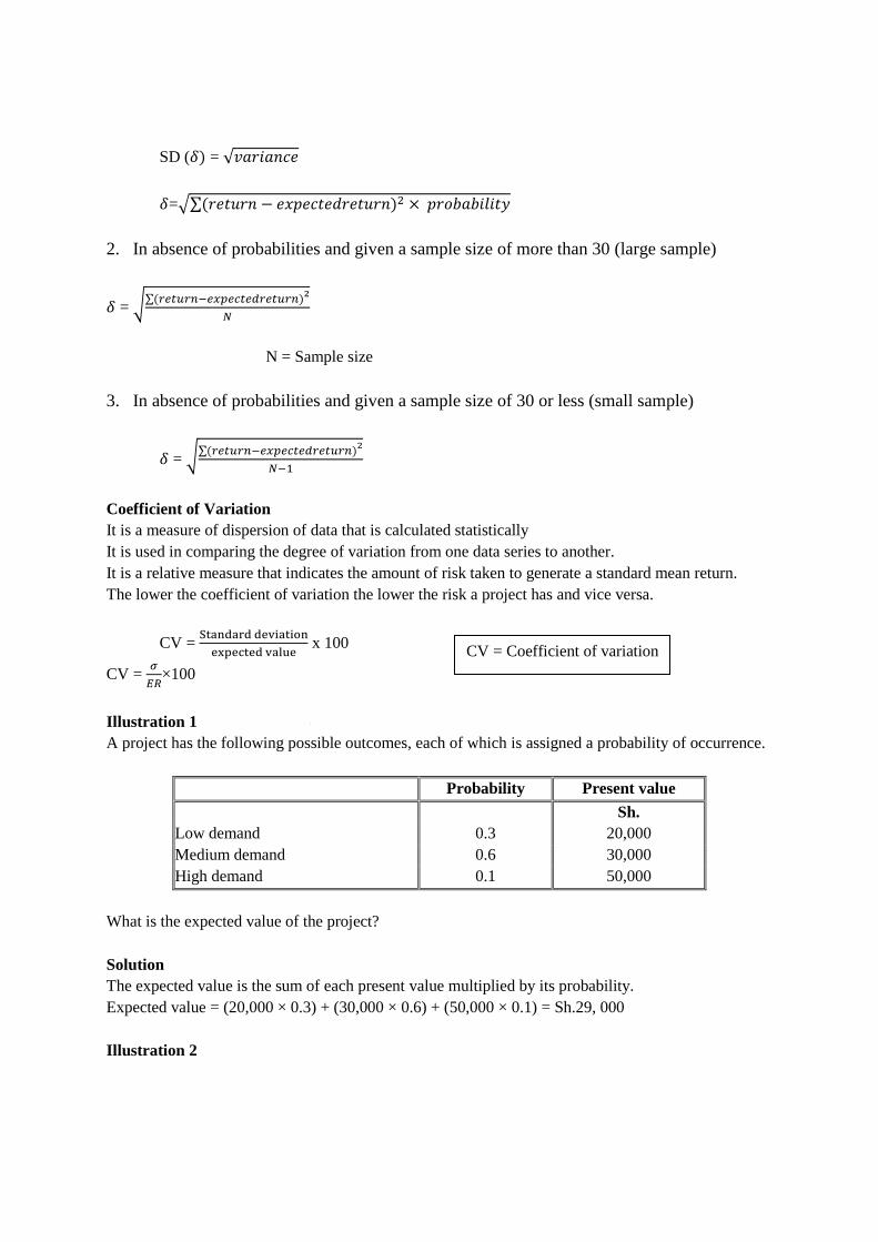
SD (𝛿) = √𝑣𝑎𝑟𝑖𝑎𝑛𝑐𝑒
𝛿=√∑(𝑟𝑒𝑡𝑢𝑟𝑛 − 𝑒𝑥𝑝𝑒𝑐𝑡𝑒𝑑𝑟𝑒𝑡𝑢𝑟𝑛)2 × 𝑝𝑟𝑜𝑏𝑎𝑏𝑖𝑙𝑖𝑡𝑦
2. In absence of probabilities and given a sample size of more than 30 (large sample)
𝛿 = √∑(𝑟𝑒𝑡𝑢𝑟𝑛−𝑒𝑥𝑝𝑒𝑐𝑡𝑒𝑑𝑟𝑒𝑡𝑢𝑟𝑛)
2
𝑁
N = Sample size
3. In absence of probabilities and given a sample size of 30 or less (small sample)
𝛿 = √∑(𝑟𝑒𝑡𝑢𝑟𝑛−𝑒𝑥𝑝𝑒𝑐𝑡𝑒𝑑𝑟𝑒𝑡𝑢𝑟𝑛)
2
𝑁−1
Coefficient of Variation
It is a measure of dispersion of data that is calculated statistically
It is used in comparing the degree of variation from one data series to another.
It is a relative measure that indicates the amount of risk taken to generate a standard mean return.
The lower the coefficient of variation the lower the risk a project has and vice versa.
CV = Standard deviation
expected value x 100
CV = 𝜎
𝐸𝑅×100
Illustration 1
A project has the following possible outcomes, each of which is assigned a probability of occurrence.
Probability Present value
Sh.
Low demand 0.3 20,000
Medium demand 0.6 30,000
High demand 0.1 50,000
What is the expected value of the project?
Solution
The expected value is the sum of each present value multiplied by its probability.
Expected value = (20,000 × 0.3) + (30,000 × 0.6) + (50,000 × 0.1) = Sh.29, 000
Illustration 2
CV = Coefficient of variation
Page 8
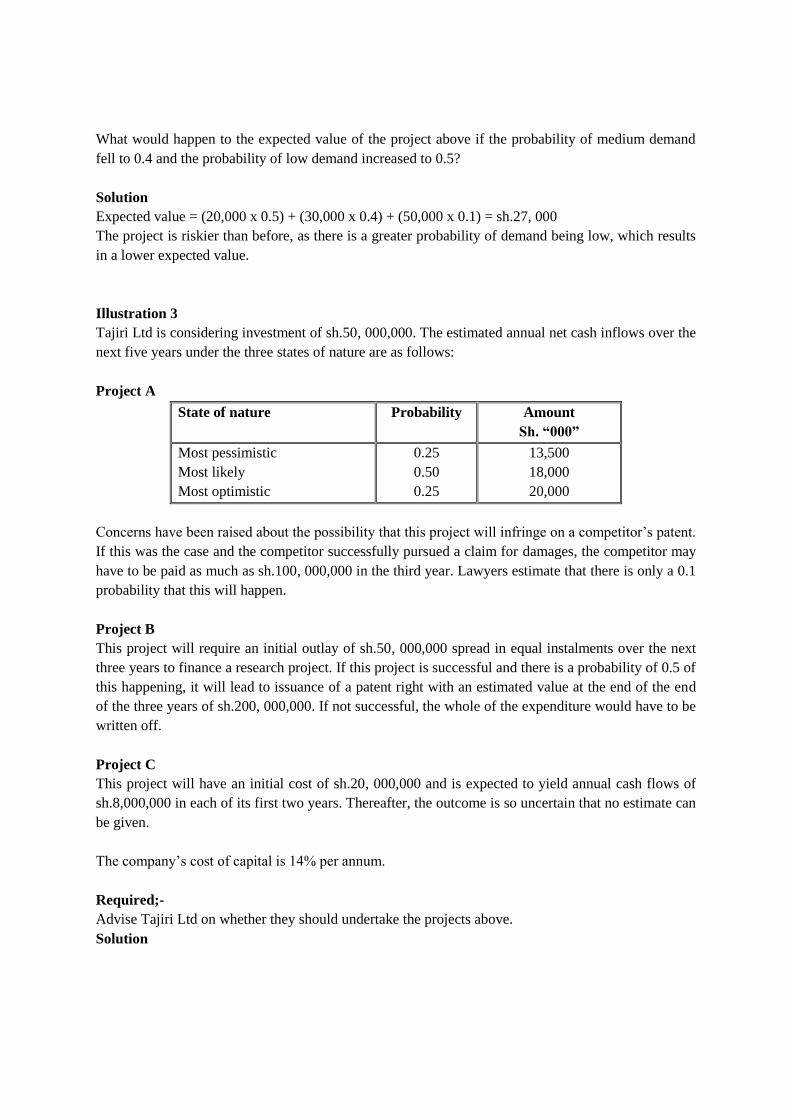
What would happen to the expected value of the project above if the probability of medium demand
fell to 0.4 and the probability of low demand increased to 0.5?
Solution
Expected value = (20,000 x 0.5) + (30,000 x 0.4) + (50,000 x 0.1) = sh.27, 000
The project is riskier than before, as there is a greater probability of demand being low, which results
in a lower expected value.
Illustration 3
Tajiri Ltd is considering investment of sh.50, 000,000. The estimated annual net cash inflows over the
next five years under the three states of nature are as follows:
Project A
State of nature Probability Amount
Sh. “000”
Most pessimistic
Most likely
Most optimistic
0.25
0.50
0.25
13,500
18,000
20,000
Concerns have been raised about the possibility that this project will infringe on a competitor’s patent.
If this was the case and the competitor successfully pursued a claim for damages, the competitor may
have to be paid as much as sh.100, 000,000 in the third year. Lawyers estimate that there is only a 0.1
probability that this will happen.
Project B
This project will require an initial outlay of sh.50, 000,000 spread in equal instalments over the next
three years to finance a research project. If this project is successful and there is a probability of 0.5 of
this happening, it will lead to issuance of a patent right with an estimated value at the end of the end
of the three years of sh.200, 000,000. If not successful, the whole of the expenditure would have to be
written off.
Project C
This project will have an initial cost of sh.20, 000,000 and is expected to yield annual cash flows of
sh.8,000,000 in each of its first two years. Thereafter, the outcome is so uncertain that no estimate can
be given.
The company’s cost of capital is 14% per annum.
Required;-
Advise Tajiri Ltd on whether they should undertake the projects above.
Solution
Page 9
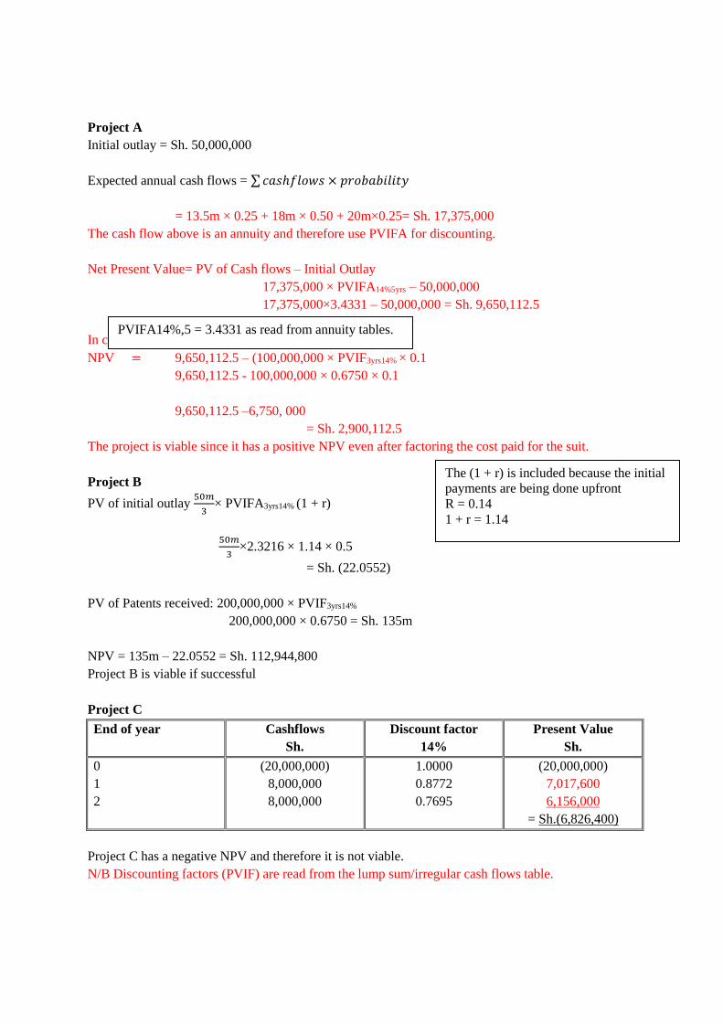
Project A
Initial outlay = Sh. 50,000,000
Expected annual cash flows = ∑ 𝑐𝑎𝑠ℎ𝑓𝑙𝑜𝑤𝑠 × 𝑝𝑟𝑜𝑏𝑎𝑏𝑖𝑙𝑖𝑡𝑦
= 13.5m × 0.25 + 18m × 0.50 + 20m×0.25= Sh. 17,375,000
The cash flow above is an annuity and therefore use PVIFA for discounting.
Net Present Value= PV of Cash flows – Initial Outlay
17,375,000 × PVIFA14%5yrs – 50,000,000
17,375,000×3.4331 – 50,000,000 = Sh. 9,650,112.5
In case the competitor succeeds in the suit
NPV = 9,650,112.5 – (100,000,000 × PVIF3yrs14% × 0.1
9,650,112.5 - 100,000,000 × 0.6750 × 0.1
9,650,112.5 –6,750, 000
= Sh. 2,900,112.5
The project is viable since it has a positive NPV even after factoring the cost paid for the suit.
Project B
PV of initial outlay 50𝑚
3× PVIFA3yrs14% (1 + r)
50𝑚
3×2.3216 × 1.14 × 0.5
= Sh. (22.0552)
PV of Patents received: 200,000,000 × PVIF3yrs14%
200,000,000 × 0.6750 = Sh. 135m
NPV = 135m – 22.0552 = Sh. 112,944,800
Project B is viable if successful
Project C
End of year Cashflows
Sh.
Discount factor
14%
Present Value
Sh.
0
1
2
(20,000,000)
8,000,000
8,000,000
1.0000
0.8772
0.7695
(20,000,000)
7,017,600
6,156,000
= Sh.(6,826,400)
Project C has a negative NPV and therefore it is not viable.
N/B Discounting factors (PVIF) are read from the lump sum/irregular cash flows table.
The (1 + r) is included because the initial
payments are being done upfront
R = 0.14
1 + r = 1.14
PVIFA14%,5 = 3.4331 as read from annuity tables.
Page 10
1.3 ADVANCED TECHNIQUES OF HANDLING RISK
1. Sensitivity Analysis
The focus in this case is determining the effect on NPV due to a a change in a given decision variable
holding other factors constant. Variables are changed one at a time.
The concept of sensitivity analysis involves posing a question “what if” example
What if sales volume falls by 10%, will the NPV remain positive.
For investment decisions to change from Accept to Reject NPV should be less than 0 and the
variables must change by the sensitivity margin.
Sensitivity analysis is divided into two:
1) Breakeven point sensitivity analysis
2) Impact analysis
Weaknesses of sensitivity analysis
These are as follows;-
1. The method requires that changes in each key variable are isolated. However,
management is more interested in the combination of the effects of changes in two or
more key variables.
2. Looking at factors in isolation is unrealistic since they are often interdependent.
3. Sensitivity analysis does not examine the probability that any particular variation in costs
or revenues might occur.
4. Critical factors may be those over which managers have no control.
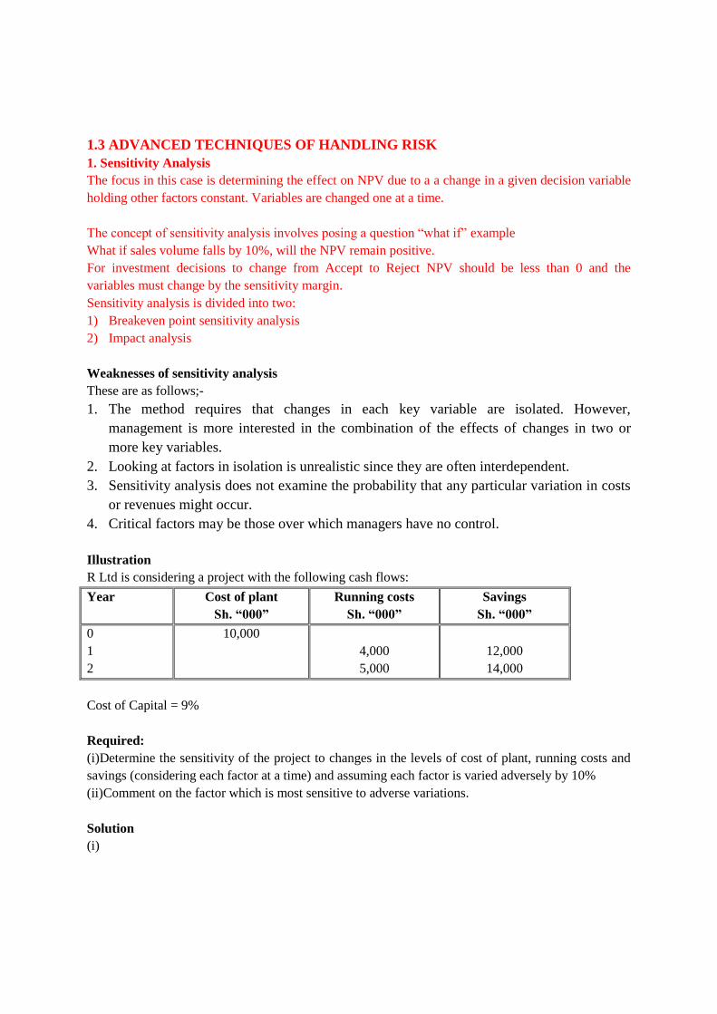
Illustration
R Ltd is considering a project with the following cash flows:
Year Cost of plant
Sh. “000”
Running costs
Sh. “000”
Savings
Sh. “000”
0
1
2
10,000
4,000
5,000
12,000
14,000
Cost of Capital = 9%
Required:
(i)Determine the sensitivity of the project to changes in the levels of cost of plant, running costs and
savings (considering each factor at a time) and assuming each factor is varied adversely by 10%
(ii)Comment on the factor which is most sensitive to adverse variations.
Solution
(i)
Page 11
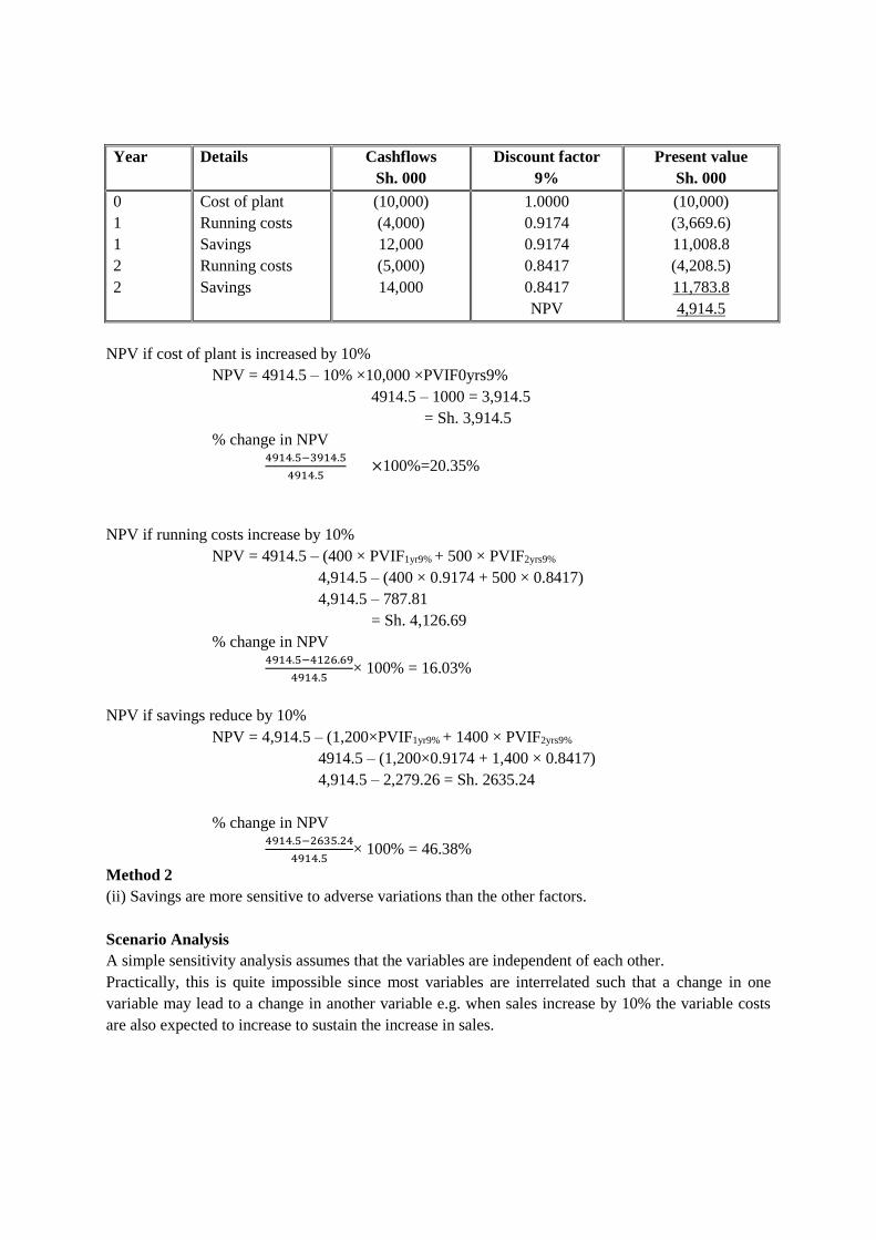
Year Details Cashflows
Sh. 000
Discount factor
9%
Present value
Sh. 000
0
1
1
2
2
Cost of plant
Running costs
Savings
Running costs
Savings
(10,000)
(4,000)
12,000
(5,000)
14,000
1.0000
0.9174
0.9174
0.8417
0.8417
NPV
(10,000)
(3,669.6)
11,008.8
(4,208.5)
11,783.8
4,914.5
NPV if cost of plant is increased by 10%
NPV = 4914.5 – 10% ×10,000 ×PVIF0yrs9%
4914.5 – 1000 = 3,914.5
= Sh. 3,914.5
% change in NPV
4914.5−3914.5
4914.5 ×100%=20.35%
NPV if running costs increase by 10%
NPV = 4914.5 – (400 × PVIF1yr9% + 500 × PVIF2yrs9%
4,914.5 – (400 × 0.9174 + 500 × 0.8417)
4,914.5 – 787.81
= Sh. 4,126.69
% change in NPV
4914.5−4126.69
4914.5× 100% = 16.03%
NPV if savings reduce by 10%
NPV = 4,914.5 – (1,200×PVIF1yr9% + 1400 × PVIF2yrs9%
4914.5 – (1,200×0.9174 + 1,400 × 0.8417)
4,914.5 – 2,279.26 = Sh. 2635.24
% change in NPV
4914.5−2635.24
4914.5× 100% = 46.38%
Method 2
(ii) Savings are more sensitive to adverse variations than the other factors.
Scenario Analysis
A simple sensitivity analysis assumes that the variables are independent of each other.
Practically, this is quite impossible since most variables are interrelated such that a change in one
variable may lead to a change in another variable e.g. when sales increase by 10% the variable costs
are also expected to increase to sustain the increase in sales.
Page 12
Scenario analysis therefore considers all these variables changing simultaneously to give a particular
scenario to the managers.
This behavioural approach is used instead of sensitivity analysis to evaluate the impact of various
circumstances in decision-making.
It normally provides three different types of scenarios, that is
Worst Case Scenario
This is a pessimistic view of likelihood of future variables to change to the worst.
Base Case/Average Scenario
This represents the average and most likely of each variable. It represents what the analyst
believes that is most likely to occur.
Best Case Scenario
This is an optimistic view of the likely future events and it represents the best reasonable
estimates of each occurrence.
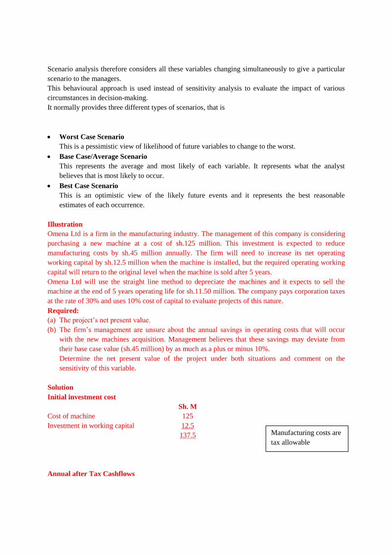
Illustration
Omena Ltd is a firm in the manufacturing industry. The management of this company is considering
purchasing a new machine at a cost of sh.125 million. This investment is expected to reduce
manufacturing costs by sh.45 million annually. The firm will need to increase its net operating
working capital by sh.12.5 million when the machine is installed, but the required operating working
capital will return to the original level when the machine is sold after 5 years.
Omena Ltd will use the straight line method to depreciate the machines and it expects to sell the
machine at the end of 5 years operating life for sh.11.50 million. The company pays corporation taxes
at the rate of 30% and uses 10% cost of capital to evaluate projects of this nature.
Required:
(a) The project’s net present value.
(b) The firm’s management are unsure about the annual savings in operating costs that will occur
with the new machines acquisition. Management believes that these savings may deviate from
their base case value (sh.45 million) by as much as a plus or minus 10%.
Determine the net present value of the project under both situations and comment on the
sensitivity of this variable.
Solution
Initial investment cost
Sh. M
Cost of machine
Investment in working capital
125
12.5
137.5
Annual after Tax Cashflows
Manufacturing costs are
tax allowable
Page 13
Sh. M
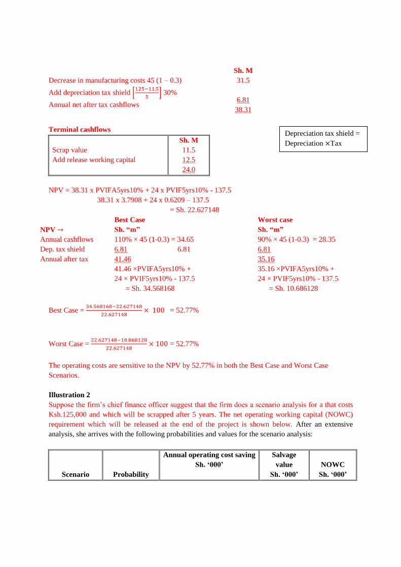
Decrease in manufacturing costs 45 (1 – 0.3)
Add depreciation tax shield [125−11.5
5] 30%
Annual net after tax cashflows
31.5
6.81
38.31
Terminal cashflows
Scrap value
Add release working capital
Sh. M
11.5
12.5
24.0
NPV = 38.31 x PVIFA5yrs10% + 24 x PVIF5yrs10% - 137.5
38.31 x 3.7908 + 24 x 0.6209 – 137.5
= Sh. 22.627148
NPV →
Best Case
Sh. “m”
Worst case
Sh. “m”
Annual cashflows
Dep. tax shield
Annual after tax
110% × 45 (1-0.3) = 34.65
6.81 6.81
41.46
90% × 45 (1-0.3) = 28.35
6.81
35.16
41.46 ×PVIFA5yrs10% +
24 × PVIF5yrs10% - 137.5
= Sh. 34.568168
35.16 ×PVIFA5yrs10% +
24 × PVIF5yrs10% - 137.5
= Sh. 10.686128
Best Case = 34.568168−22.627148
22.627148× 100 = 52.77%
Worst Case = 22.627148−10.868128
22.627148× 100 = 52.77%
The operating costs are sensitive to the NPV by 52.77% in both the Best Case and Worst Case
Scenarios.
Illustration 2
Suppose the firm’s chief finance officer suggest that the firm does a scenario analysis for a that costs
Ksh.125,000 and which will be scrapped after 5 years. The net operating working capital (NOWC)
requirement which will be released at the end of the project is shown below. After an extensive
analysis, she arrives with the following probabilities and values for the scenario analysis:
Scenario
Probability
Annual operating cost saving
Sh. ‘000’
Salvage
value
Sh. ‘000’
NOWC
Sh. ‘000’
Depreciation tax shield =
Depreciation ×Tax
Page 14
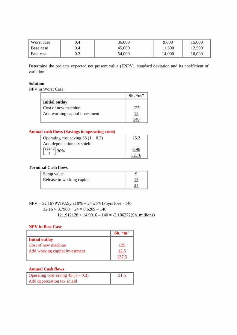
Worst case
Base case
Best case
0.4
0.4
0.2
36,000
45,000
54,000
9,000
11,500
14,000
15,000
12,500
10,000
Determine the projects expected net present value (ENPV), standard deviation and its coefficient of
variation.
Solution
NPV in Worst Case
Sh. “m”
Initial outlay
Cost of new machine
Add working capital investment
125
15
140
Annual cash flows (Savings in operating costs)
Operating cost saving 36 (1 – 0.3)
Add depreciation tax shield
[125−9
5] 30%
25.2
6.96
32.16
Terminal Cash flows
Scrap value
Release in working capital
9
15
24
NPV = 32.16×PVIFA5yrs10% + 24 x PVIF5yrs10% - 140
32.16 × 3.7908 + 24 × 0.6209 – 140
121.912128 + 14.9016 – 140 = -3.186272(Sh. millions)
NPV in Best Case
Sh. “m”
Initial outlay
Cost of new machine
Add working capital investment
125
12.5
137.5
Annual Cash flows
Operating cost saving 45 (1 – 0.3)
Add depreciation tax shield
31.5
Page 15
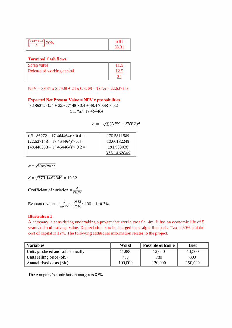
[125−11.5
5] 30% 6.81
38.31
Terminal Cash flows
Scrap value
Release of working capital
11.5
12.5
24
NPV = 38.31 x 3.7908 + 24 x 0.6209 – 137.5 = 22.627148
Expected Net Present Value = NPV x probabilities
-3.186272×0.4 + 22.627148 ×0.4 + 48.440568 × 0.2
Sh. “m” 17.464464
𝜎 = √∑(𝑁𝑃𝑉 − 𝐸𝑁𝑃𝑉)2
(-3.186272 – 17.464464)2× 0.4 =
(22.627148 – 17.464464)2×0.4 =
(48.440568 – 17.464464)2× 0.2 =
170.5811589
10.66132248
191.903038
373.1462849
𝜎 = √𝑉𝑎𝑟𝑖𝑎𝑛𝑐𝑒
𝛿 = √373.1462849 = 19.32
Coefficient of variation = 𝜎
𝐸𝑁𝑃𝑉
Evaluated value = 𝜎
𝐸𝑁𝑃𝑉 =
19.32
17.46× 100 = 110.7%
Illustration 1
A company is considering undertaking a project that would cost Sh. 4m. It has an economic life of 5
years and a nil salvage value. Depreciation is to be charged on straight line basis. Tax is 30% and the
cost of capital is 12%. The following additional information relates to the project.
Variables Worst Possible outcome Best
Units produced and sold annually
Units selling price (Sh.)
Annual fixed costs (Sh.)
11,000
750
100,000
12,000
780
120,000
13,500
800
150,000
The company’s contribution margin is 85%
Page 16
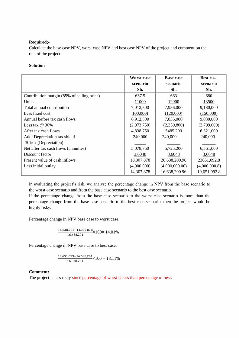
Required;-
Calculate the base case NPV, worst case NPV and best case NPV of the project and comment on the
risk of the project.
Solution
Worst case
scenario
Sh.
Base case
scenario
Sh.
Best case
scenario
Sh.
Contribution margin (85% of selling price)
Units
Total annual contribution
Less fixed cost
Annual before tax cash flows
Less tax @ 30%
After tax cash flows
Add: Depreciation tax shield
30% x (Depreciation)
Net after tax cash flows (annuities)
Discount factor
Present value of cash inflows
Less initial outlay
637.5
11000
7,012,500
100,000)
6,912,500
(2,073,750)
4,838,750
240,000
_____
5,078,750
3.6048
18,307,878
(4,000,000)
14,307,878
663
12000
7,956,000
(120,000)
7,836,000
(2,350,800)
5485,200
240,000
______
5,725,200
3.6048
20,638,200.96
(4,000,000.00)
16,638,200.96
680
13500
9,180,000
(150,000)
9,030,000
(2,709,000)
6,321,000
240,000
______
6,561,000
3.6048
23651,092.8
(4,000,000.8)
19,651,092.8
In evaluating the project’s risk, we analyse the percentage change in NPV from the base scenario to
the worst case scenario and from the base case scenario to the best case scenario.
If the percentage change from the base case scenario to the worst case scenario is more than the
percentage change from the base case scenario to the best case scenario, then the project would be
highly risky.
Percentage change in NPV base case to worst case.
16,638,201−14,307,878
16,638,201×100= 14.01%
Percentage change in NPV base case to best case.
19,651,093−16,638,201
16,638,201×100 = 18.11%
Comment:
The project is less risky since percentage of worst is less than percentage of best.
Page 17
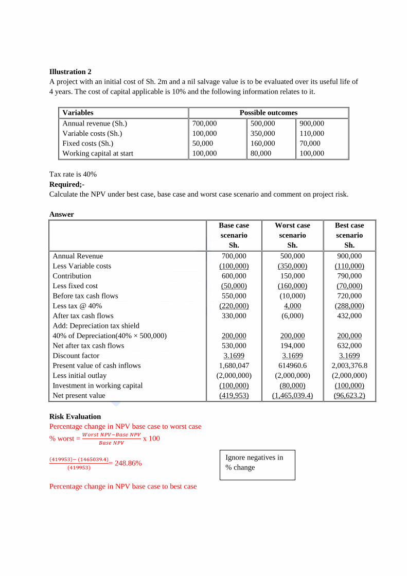
Illustration 2
A project with an initial cost of Sh. 2m and a nil salvage value is to be evaluated over its useful life of
4 years. The cost of capital applicable is 10% and the following information relates to it.
Variables Possible outcomes
Annual revenue (Sh.)
Variable costs (Sh.)
Fixed costs (Sh.)
Working capital at start
700,000
100,000
50,000
100,000
500,000
350,000
160,000
80,000
900,000
110,000
70,000
100,000
Tax rate is 40%
Required;-
Calculate the NPV under best case, base case and worst case scenario and comment on project risk.
Answer
Base case
scenario
Sh.
Worst case
scenario
Sh.
Best case
scenario
Sh.
Annual Revenue
Less Variable costs
Contribution
Less fixed cost
Before tax cash flows
Less tax @ 40%
After tax cash flows
Add: Depreciation tax shield
40% of Depreciation(40% × 500,000)
Net after tax cash flows
Discount factor
Present value of cash inflows
Less initial outlay
Investment in working capital
Net present value
700,000
(100,000)
600,000
(50,000)
550,000
(220,000)
330,000
200,000
530,000
3.1699
1,680,047
(2,000,000)
(100,000)
(419,953)
500,000
(350,000)
150,000
(160,000)
(10,000)
4,000
(6,000)
200,000
194,000
3.1699
614960.6
(2,000,000)
(80,000)
(1,465,039.4)
900,000
(110,000)
790,000
(70,000)
720,000
(288,000)
432,000
200,000
632,000
3.1699
2,003,376.8
(2,000,000)
(100,000)
(96,623.2)
Risk Evaluation
Percentage change in NPV base case to worst case
% worst = 𝑊𝑜𝑟𝑠𝑡 𝑁𝑃𝑉−𝐵𝑎𝑠𝑒 𝑁𝑃𝑉
𝐵𝑎𝑠𝑒 𝑁𝑃𝑉 x 100
(419953)− (1465039.4)
(419953)= 248.86%
Percentage change in NPV base case to best case
Ignore negatives in
% change
Page 18
% best case = 𝐵𝑒𝑠𝑡 𝑁𝑃𝑉−𝐵𝑎𝑠𝑒 𝑁𝑃𝑉
𝐵𝑎𝑠𝑒 𝑁𝑃𝑉
(419,953)− (96,623.2)
(419,953)= 77%
Comment:
The project is highly risky since percentage of worst is more than percentage of best.
3. Simulation Analysis
To simulate is to imitate. It involves conducting of a series of trial and error experiments. Where there
is a large number of random variables in an investment decision, simulation analysis may provide a
more satisfactory results in evaluating that project provided. Simulation can only apply when the
probability distribution of projects variables is given and a large number of trials are conducted to
reach a steady state.
Monte Carlo simulation and investment appraisal
Monte Carlo method
This section provides a brief outline of the Monte Carlo method in investment appraisal. The method
appeared in 1949 and is widely used in situations involving uncertainty. The method amounts to
adopting a particular probability distribution for the uncertain (random) variables that affect the NPV
and then using simulations to generate values of the random variables.
The basic idea is to generate through simulation thousands of values for the parameters or variables of
interest and use those variables to derive the NPV for each possible simulated outcome.
From the resulting values we can derive the distribution of the NPV.
Basic steps
1) Identify probabilistic variables
2) Determine cumulative probabilities
3) Assign RN – Ranges
NB: The Ranges will contain digits that correspond to the decimal places of probabilities i.e. if a
series has:
1) 1 decimal place probabilities that we use 1 digit (0 – 9)
2) 2 decimal places – 2 digits (00 – 99)
3) 3 decimal places – 2 digits (000 – 999)
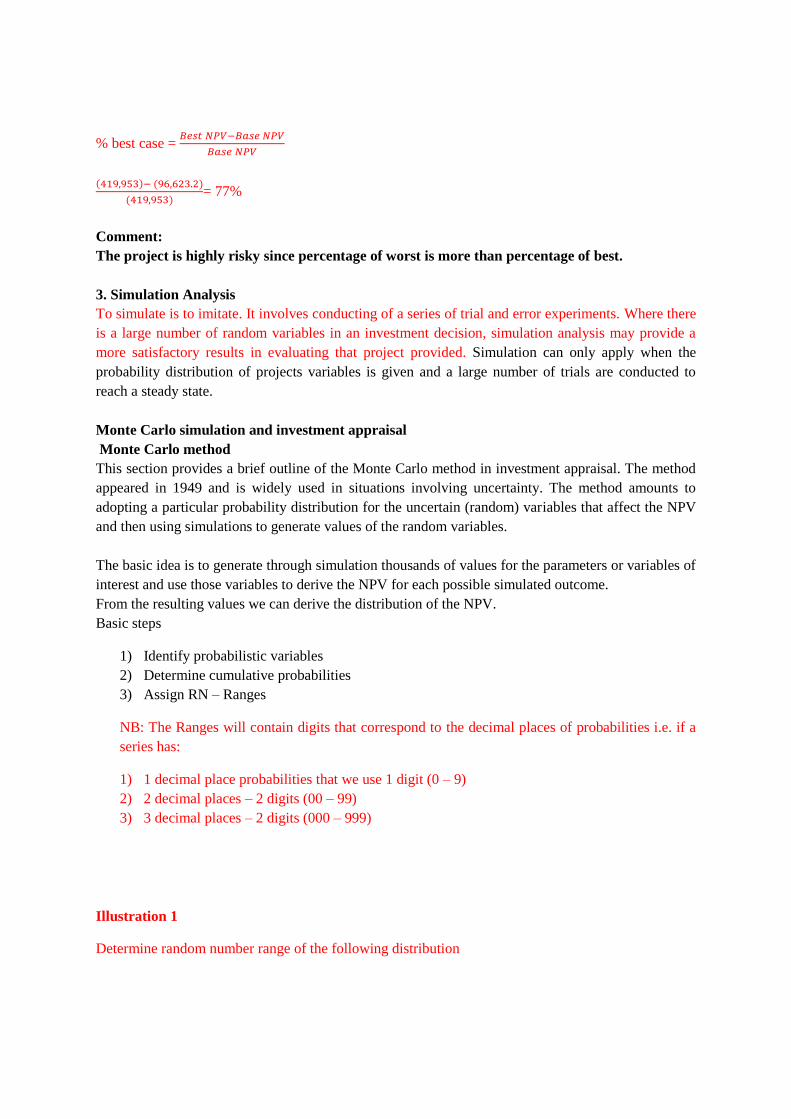
Illustration 1
Determine random number range of the following distribution
Page 19
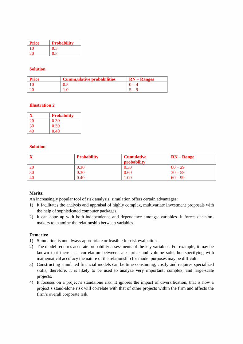
Price Probability
10
20
0.5
0.5
Solution
Price Cumm,ulative probabilities RN – Ranges
10
20
0.5
1.0
0 – 4
5 – 9
Illustration 2
X Probability
20
30
40
0.30
0.30
0.40
Solution
X Probability Cumulative
probability
RN – Range
20
30
40
0.30
0.30
0.40
0.30
0.60
1.00
00 – 29
30 – 59
60 – 99
Merits:
An increasingly popular tool of risk analysis, simulation offers certain advantages:
1) It facilitates the analysis and appraisal of highly complex, multivariate investment proposals with
the help of sophisticated computer packages.
2) It can cope up with both independence and dependence amongst variables. It forces decision-
makers to examine the relationship between variables.
Demerits:
1) Simulation is not always appropriate or feasible for risk evaluation.
2) The model requires accurate probability assessments of the key variables. For example, it may be
known that there is a correlation between sales price and volume sold, but specifying with
mathematical accuracy the nature of the relationship for model purposes may be difficult.
3) Constructing simulated financial models can be time-consuming, costly and requires specialized
skills, therefore. It is likely to be used to analyze very important, complex, and large-scale
projects.
4) It focuses on a project’s standalone risk. It ignores the impact of diversification, that is how a
project’s stand-alone risk will correlate with that of other projects within the firm and affects the
firm’s overall corporate risk.
Page 20
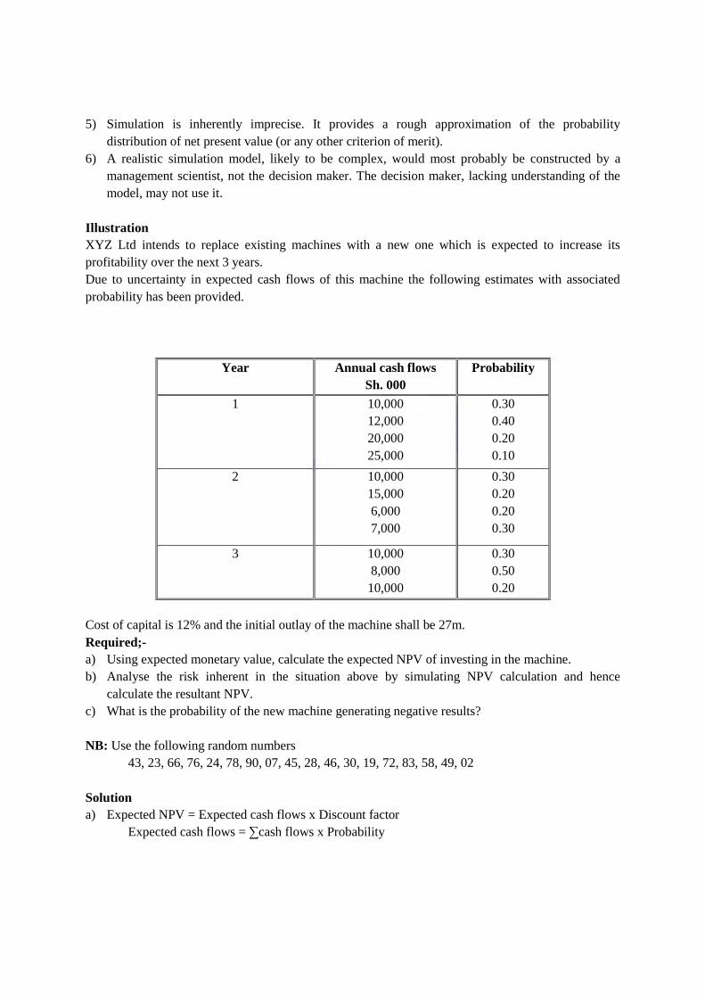
5) Simulation is inherently imprecise. It provides a rough approximation of the probability
distribution of net present value (or any other criterion of merit).
6) A realistic simulation model, likely to be complex, would most probably be constructed by a
management scientist, not the decision maker. The decision maker, lacking understanding of the
model, may not use it.
Illustration
XYZ Ltd intends to replace existing machines with a new one which is expected to increase its
profitability over the next 3 years.
Due to uncertainty in expected cash flows of this machine the following estimates with associated
probability has been provided.
Year Annual cash flows
Sh. 000
Probability
1
10,000
12,000
20,000
25,000
0.30
0.40
0.20
0.10
2
10,000
15,000
6,000
7,000
0.30
0.20
0.20
0.30
3 10,000
8,000
10,000
0.30
0.50
0.20
Cost of capital is 12% and the initial outlay of the machine shall be 27m.
Required;-
a) Using expected monetary value, calculate the expected NPV of investing in the machine.
b) Analyse the risk inherent in the situation above by simulating NPV calculation and hence
calculate the resultant NPV.
c) What is the probability of the new machine generating negative results?
NB: Use the following random numbers
43, 23, 66, 76, 24, 78, 90, 07, 45, 28, 46, 30, 19, 72, 83, 58, 49, 02
Solution
a) Expected NPV = Expected cash flows x Discount factor
Expected cash flows = ∑cash flows x Probability
Page 21
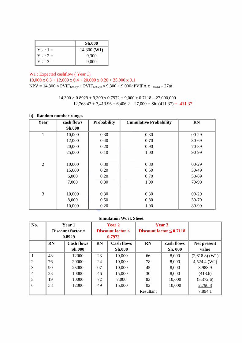
Sh.000
Year 1 =
Year 2 =
Year 3 =
14,300 (W1)
9,300
9,000
W1 : Expected cashflow ( Year 1)
10,000 x 0.3 + 12,000 x 0.4 + 20,000 x 0.20 + 25,000 x 0.1
NPV = 14,300 × PVIF12%1yr + PVIF12%2yr × 9,300 + 9,000×PVIFA x 12%3yr – 27m
14,300 × 0.8929 + 9,300 x 0.7972 + 9,000 x 0.7118 – 27,000,000
12,768.47 + 7,413.96 + 6,406.2 – 27,000 = Sh. (411.37) = -411.37
b) Random number ranges
Year cash flows
Sh.000
Probability Cumulative Probability RN
1
2
3
10,000
12,000
20,000
25,000
10,000
15,000
6,000
7,000
10,000
8,000
10,000
0.30
0.40
0.20
0.10
0.30
0.20
0.20
0.30
0.30
0.50
0.20
0.30
0.70
0.90
1.00
0.30
0.50
0.70
1.00
0.30
0.80
1.00
00-29
30-69
70-89
90-99
00-29
30-49
50-69
70-99
00-29
30-79
80-99
Simulation Work Sheet
No. Year 1
Discount factor =
0.8929
Year 2
Discount factor <
0.7972
Year 3
Discount factor ≤ 0.7118
RN Cash flows
Sh.000
RN Cash flows
Sh.000
RN cash flows
Sh. 000
Net present
value
1
2
3
4
5
6
43
76
90
28
19
58
12000
20000
25000
10000
10000
12000
23
24
07
46
72
49
10,000
10,000
10,000
15,000
7,000
15,000
66
78
45
30
83
02
Resultant
8,000
8,000
8,000
8,000
10,000
10,000
(2,618.8) (W1)
4,524.4 (W2)
8,988.9
(418.6)
(5,372.6)
2,790.8
7,894.1
Page 22
NPV
W1: 12,000 × 0.8929 + 100,000 × 0.7972 + 8,000 × 0.7118 – 27,000 = 2618.8
W2: 20,000 × 0.8929 + 10,000×0.7972 + 8,000×0.7118 – 27,000 = 4524.4
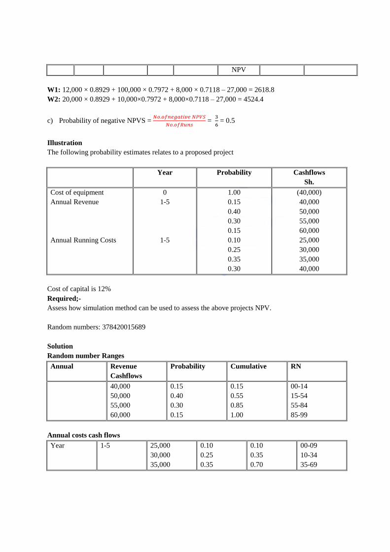
c) Probability of negative NPVS = 𝑁𝑜.𝑜𝑓𝑛𝑒𝑔𝑎𝑡𝑖𝑣𝑒 𝑁𝑃𝑉𝑆
𝑁𝑜.𝑜𝑓𝑅𝑢𝑛𝑠 =
3
6 = 0.5
Illustration
The following probability estimates relates to a proposed project
Year Probability Cashflows
Sh.
Cost of equipment
Annual Revenue
Annual Running Costs
0
1-5
1-5
1.00
0.15
0.40
0.30
0.15
0.10
0.25
0.35
0.30
(40,000)
40,000
50,000
55,000
60,000
25,000
30,000
35,000
40,000
Cost of capital is 12%
Required;-
Assess how simulation method can be used to assess the above projects NPV.
Random numbers: 378420015689
Solution
Random number Ranges
Annual Revenue
Cashflows
Probability Cumulative RN
40,000
50,000
55,000
60,000
0.15
0.40
0.30
0.15
0.15
0.55
0.85
1.00
00-14
15-54
55-84
85-99
Annual costs cash flows
Year 1-5 25,000
30,000
35,000
0.10
0.25
0.35
0.10
0.35
0.70
00-09
10-34
35-69
Page 23
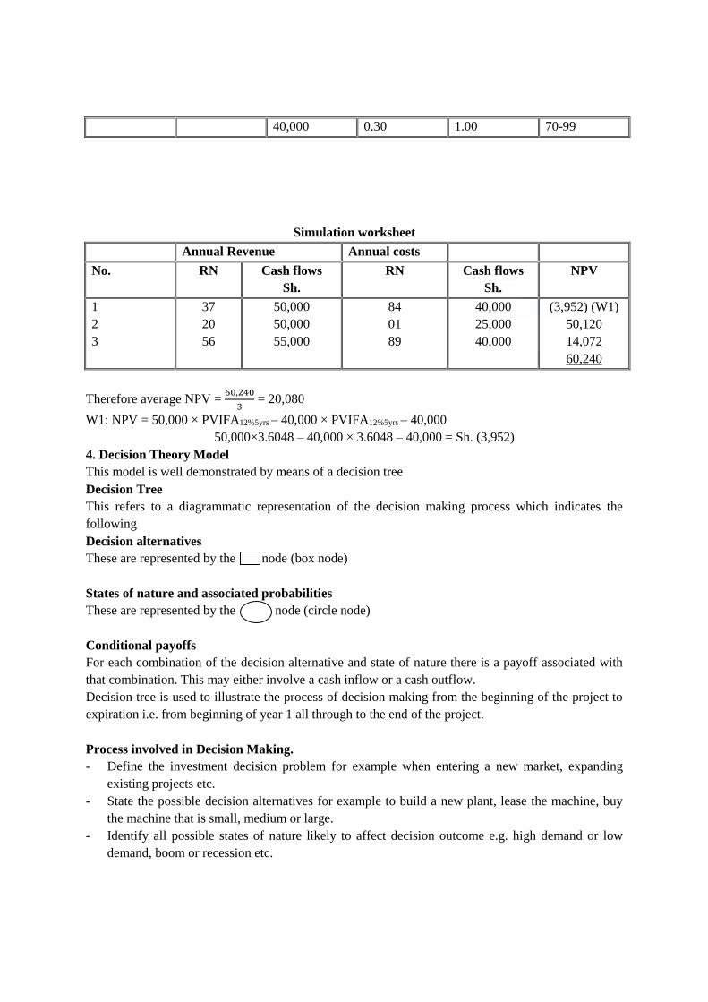
40,000 0.30 1.00 70-99
Simulation worksheet
Annual Revenue Annual costs
No. RN Cash flows
Sh.
RN Cash flows
Sh.
NPV
1
2
3
37
20
56
50,000
50,000
55,000
84
01
89
40,000
25,000
40,000
(3,952) (W1)
50,120
14,072
60,240
Therefore average NPV = 60,240
3 = 20,080
W1: NPV = 50,000 × PVIFA12%5yrs – 40,000 × PVIFA12%5yrs – 40,000
50,000×3.6048 – 40,000 × 3.6048 – 40,000 = Sh. (3,952)
4. Decision Theory Model
This model is well demonstrated by means of a decision tree
Decision Tree
This refers to a diagrammatic representation of the decision making process which indicates the
following
Decision alternatives
These are represented by the node (box node)
States of nature and associated probabilities
These are represented by the node (circle node)
Conditional payoffs
For each combination of the decision alternative and state of nature there is a payoff associated with
that combination. This may either involve a cash inflow or a cash outflow.
Decision tree is used to illustrate the process of decision making from the beginning of the project to
expiration i.e. from beginning of year 1 all through to the end of the project.
Process involved in Decision Making.
- Define the investment decision problem for example when entering a new market, expanding
existing projects etc.
- State the possible decision alternatives for example to build a new plant, lease the machine, buy
the machine that is small, medium or large.
- Identify all possible states of nature likely to affect decision outcome e.g. high demand or low
demand, boom or recession etc.
Page 24
- Estimate the probabilities associated with different states of nature identified above.
- Estimate conditional payoff for each combination of decision alternative and states of nature.
- Draw the decision tree.
- Calculate the expected value/expected monetary value of each of the alternatives available.
- Calculate the NPV of each of the available options we use the rollback technique in calculating
the resultant NPV of the project at hand i.e. we start from the furthest year then calculate NPV in
backward scenario up to year 0.
Merits
The sensitivity analysis has the following advantages:
It compels the decision maker to identify the variables affecting the cash flow forecasts
which helps in understanding the investment project in totality.
It identifies the critical variables for which special actions can be taken.
It guides the decision maker to concentrate on relevant variables for the project.
Demerits:
The sensitivity analysis suffers from following limitations:
The range of values suggested by the technique may not be consistent. The terms
‘optimistic’ and ‘pessimistic’ could mean different things to different people.
It fails to focus on the interrelationship between variables. The study of variability of one
factor at a time, keeping other variables constant may not much sense. For example, sales
volume may be related to price and cost. One cannot study the effect of change in price
keeping quantity constant.
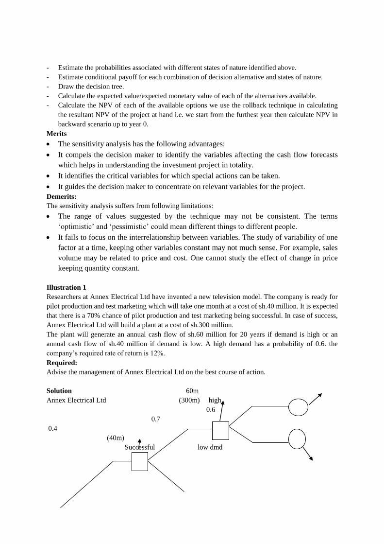
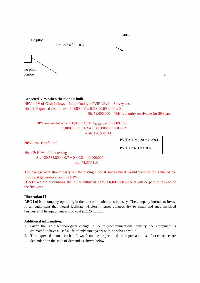
Illustration 1
Researchers at Annex Electrical Ltd have invented a new television model. The company is ready for
pilot production and test marketing which will take one month at a cost of sh.40 million. It is expected
that there is a 70% chance of pilot production and test marketing being successful. In case of success,
Annex Electrical Ltd will build a plant at a cost of sh.300 million.
The plant will generate an annual cash flow of sh.60 million for 20 years if demand is high or an
annual cash flow of sh.40 million if demand is low. A high demand has a probability of 0.6. the
company’s required rate of return is 12%.
Required:
Advise the management of Annex Electrical Ltd on the best course of action.
Solution 60m
Annex Electrical Ltd (300m) high
0.6
0.7
0.4
(40m)
Successful low dmd
Page 25
40m
Do pilot
Unsuccessful 0.3
no pilot
ignore 0
Expected NPV when the plant is built
NPV = PV of Cash Inflows – Initial Outlay x PVIF12%,1 – Survey cost
Note 1: Expected cash flows =60,000,000 x 0.6 + 40,000,000 x 0.4
= Sh. 52,000,000 – This is annuity receivable for 20 years.
NPV successful = 52,000,000 x PVIFA12%20yrs – 300,000,000
52,000,000 x 7.4694 – 300,000,000 x 0.8929
= Sh. 120,538,800
NPV unsuccessful = 0
Node 2: NPV of Pilot testing
Sh. 120,538,800 x 0.7 + 0 x 0.3 – 40,000,000
= Sh. 44,377,160
The management should carry out the testing since if successful it would increase the value of the
firm i.e. it generates a positive NPV.
HINT: We are discounting the initial outlay of Kshs.300,000,000 since it will be paid at the end of
the first year.
Illustration II
ABC Ltd is a company operating in the telecommunications industry. The company intends to invest
in an equipment that would facilitate wireless internet connectivity to small and medium-sized
businesses. The equipment would cost sh.125 million.
Additional information:
1. Given the rapid technological change in the telecommunications industry, the equipment is
estimated to have a useful life of only three years with no salvage value.
2. The expected annual cash inflows from the project and their probabilities of occurrence are
dependent on the state of demand as shown below:
PVIFA 12%, 20 = 7.4694
PVIF 12%, 1 = 0.8929
Page 26
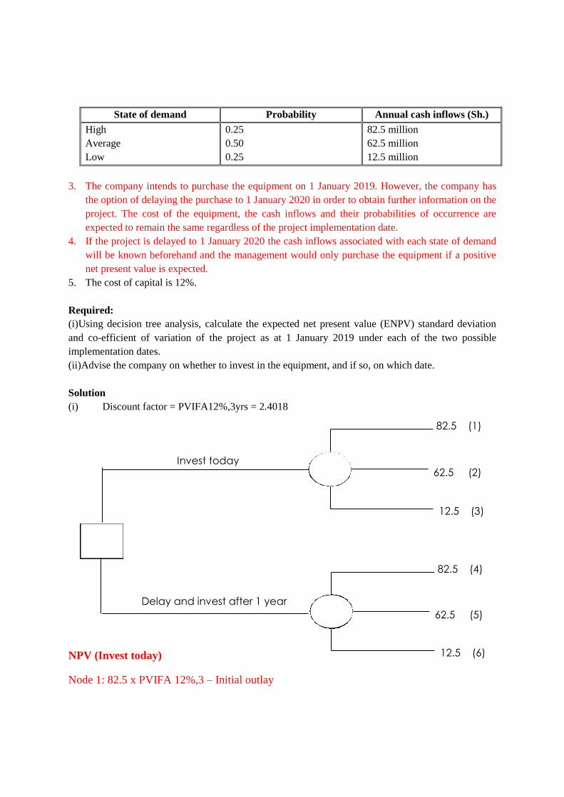
State of demand Probability Annual cash inflows (Sh.)
High
Average
Low
0.25
0.50
0.25
82.5 million
62.5 million
12.5 million
3. The company intends to purchase the equipment on 1 January 2019. However, the company has
the option of delaying the purchase to 1 January 2020 in order to obtain further information on the
project. The cost of the equipment, the cash inflows and their probabilities of occurrence are
expected to remain the same regardless of the project implementation date.
4. If the project is delayed to 1 January 2020 the cash inflows associated with each state of demand
will be known beforehand and the management would only purchase the equipment if a positive
net present value is expected.
5. The cost of capital is 12%.
Required:
(i)Using decision tree analysis, calculate the expected net present value (ENPV) standard deviation
and co-efficient of variation of the project as at 1 January 2019 under each of the two possible
implementation dates.
(ii)Advise the company on whether to invest in the equipment, and if so, on which date.
Solution
(i) Discount factor = PVIFA12%,3yrs = 2.4018
NPV (Invest today)
Node 1: 82.5 x PVIFA 12%,3 – Initial outlay
82.5 (1)
62.5 (2)
12.5 (3)
82.5 (4)
62.5 (5)
12.5 (6)
Invest today
Delay and invest after 1 year
Page 27
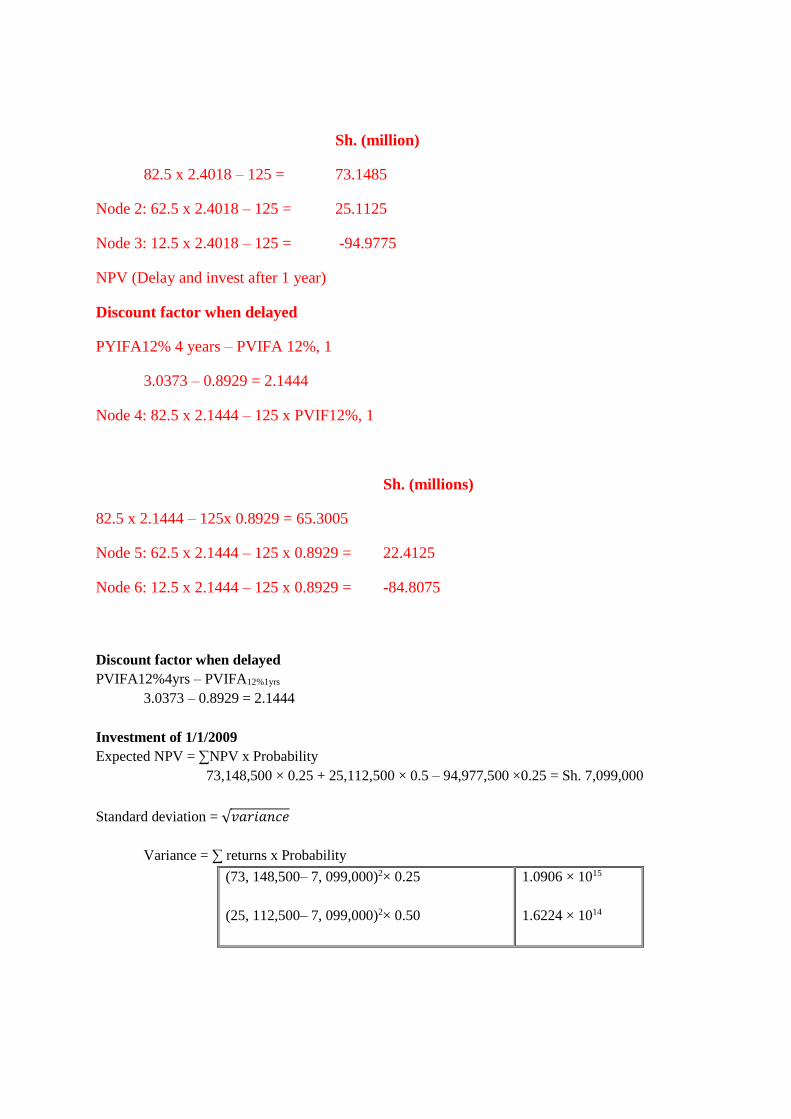
Sh. (million)
82.5 x 2.4018 – 125 = 73.1485
Node 2: 62.5 x 2.4018 – 125 = 25.1125
Node 3: 12.5 x 2.4018 – 125 = -94.9775
NPV (Delay and invest after 1 year)
Discount factor when delayed
PYIFA12% 4 years – PVIFA 12%, 1
3.0373 – 0.8929 = 2.1444
Node 4: 82.5 x 2.1444 – 125 x PVIF12%, 1
Sh. (millions)
82.5 x 2.1444 – 125x 0.8929 = 65.3005
Node 5: 62.5 x 2.1444 – 125 x 0.8929 = 22.4125
Node 6: 12.5 x 2.1444 – 125 x 0.8929 = -84.8075
Discount factor when delayed
PVIFA12%4yrs – PVIFA12%1yrs
3.0373 – 0.8929 = 2.1444
Investment of 1/1/2009
Expected NPV = ∑NPV x Probability
73,148,500 × 0.25 + 25,112,500 × 0.5 – 94,977,500 ×0.25 = Sh. 7,099,000
Standard deviation = √𝑣𝑎𝑟𝑖𝑎𝑛𝑐𝑒
Variance = ∑ returns x Probability
(73, 148,500– 7, 099,000)2× 0.25
(25, 112,500– 7, 099,000)2× 0.50
1.0906 × 10¹⁵
1.6224 × 10¹⁴
Page 28
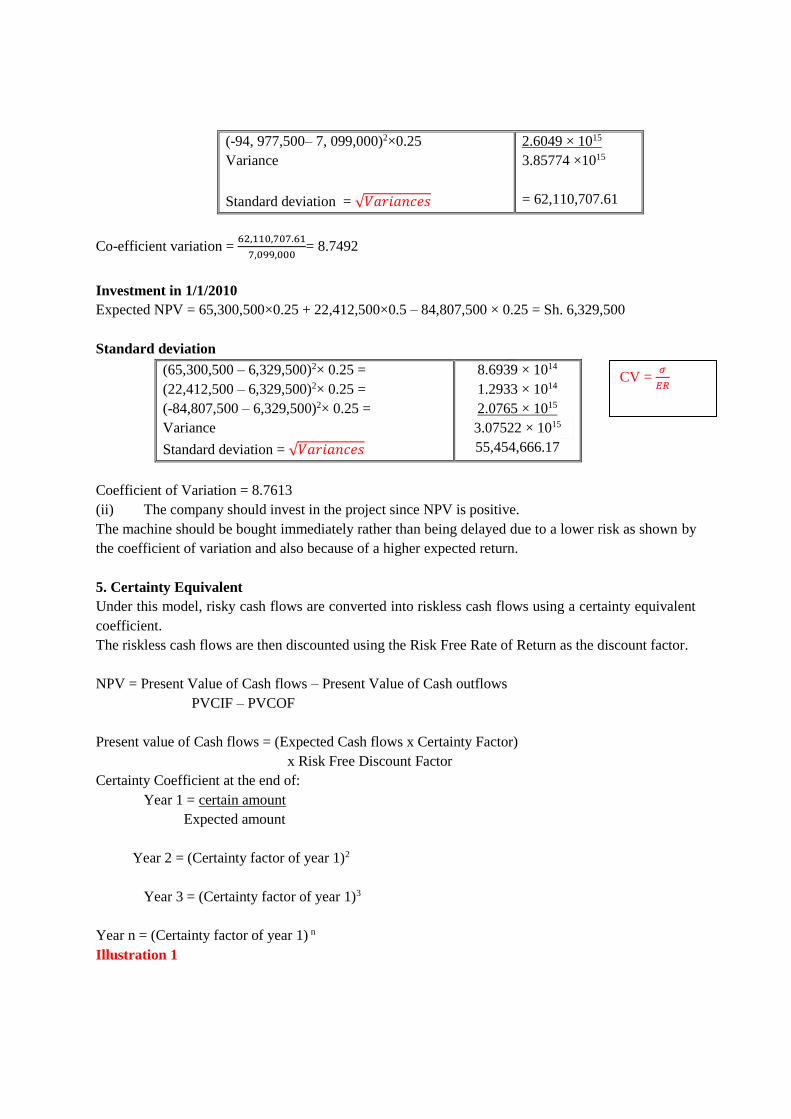
(-94, 977,500– 7, 099,000)2×0.25
Variance
Standard deviation = √𝑉𝑎𝑟𝑖𝑎𝑛𝑐𝑒𝑠
2.6049 × 10¹⁵
3.85774 ×1015
= 62,110,707.61
Co-efficient variation = 62,110,707.61
7,099,000= 8.7492
Investment in 1/1/2010
Expected NPV = 65,300,500×0.25 + 22,412,500×0.5 – 84,807,500 × 0.25 = Sh. 6,329,500
Standard deviation
(65,300,500 – 6,329,500)2× 0.25 =
(22,412,500 – 6,329,500)2× 0.25 =
(-84,807,500 – 6,329,500)2× 0.25 =
Variance
Standard deviation = √𝑉𝑎𝑟𝑖𝑎𝑛𝑐𝑒𝑠
8.6939 × 10¹⁴
1.2933 × 10¹⁴
2.0765 × 10¹⁵
3.07522 × 10¹⁵
55,454,666.17
Coefficient of Variation = 8.7613
(ii) The company should invest in the project since NPV is positive.
The machine should be bought immediately rather than being delayed due to a lower risk as shown by
the coefficient of variation and also because of a higher expected return.
5. Certainty Equivalent
Under this model, risky cash flows are converted into riskless cash flows using a certainty equivalent
coefficient.
The riskless cash flows are then discounted using the Risk Free Rate of Return as the discount factor.
NPV = Present Value of Cash flows – Present Value of Cash outflows
PVCIF – PVCOF
Present value of Cash flows = (Expected Cash flows x Certainty Factor)
x Risk Free Discount Factor
Certainty Coefficient at the end of:
Year 1 = certain amount
Expected amount
Year 2 = (Certainty factor of year 1)2
Year 3 = (Certainty factor of year 1)3
Year n = (Certainty factor of year 1) n
Illustration 1
CV = 𝜎
𝐸𝑅
Page 29
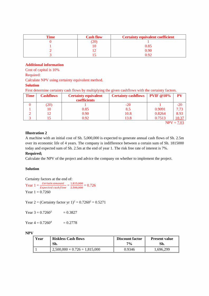
Time Cash flow Certainty equivalent coefficient
0
1
2
3
(20)
10
12
15
1
0.85
0.90
0.92
Additional information
Cost of capital is 10%
Required:
Calculate NPV using certainty equivalent method.
Solution
First determine certainty cash flows by multiplying the given cashflows with the certainty factors.
Time Cashflows Certainty equivalent
coefficients
Certainty cashflows PVIF @10% PV
0
1
2
3
(20)
10
12
15
1
0.85
0.90
0.92
-20
8.5
10.8
13.8
1
0.9091
0.8264
0.7513
-20
7.73
8.93
10.37
NPV = 7.03
Illustration 2
A machine with an initial cost of Sh. 5,000,000 is expected to generate annual cash flows of Sh. 2.5m
over its economic life of 4 years. The company is indifference between a certain sum of Sh. 1815000
today and expected sum of Sh. 2.5m at the end of year 1. The risk free rate of interest is 7%.
Required;
Calculate the NPV of the project and advice the company on whether to implement the project.
Solution
Certainty factors at the end of:
Year 1 = 𝐶𝑒𝑟𝑡𝑎𝑖𝑛 𝑎𝑚𝑜𝑢𝑛𝑡
𝐸𝑥𝑝𝑒𝑐𝑡𝑒𝑑 𝑐𝑎𝑠ℎ𝑓𝑙𝑜𝑤 =
1,815,000
2,500,000 = 0.726
Year 1 = 0.7260
Year 2 = (Certainty factor yr 1)2 = 0.72602 = 0.5271
Year 3 = 0.72603 = 0.3827
Year 4 = 0.72604 = 0.2778
NPV
Year Riskless Cash flows
Sh.
Discount factor
7%
Present value
Sh.
1 2,500,000 × 0.726 = 1,815,000 0.9346 1,696,299
Page 30

2
3
4
2,500,000 × 0.5271 = 1,317,750
2,500,000 × 0.3827 = 956,750
2,500,000 × 0.2778 = 694,500
0.8734
0.8163
0.7629
1,150,922.85
780,995.025
529,834.05
Present value of cash inflows
Less initial/Outlay
NPV
4,158,050.925
(5,000,000,000)
(841,949.075)
Illustration 3
David Majimbo is evaluating a project with a one year life and expected cash flow of sh. 5,000,000
receivable at year end. Shareholders require a return of 12%. The risk free rate is 6%.
Required:
Certainty equivalent coefficient. Interpret your result.
Solution
Present value of cash inflows = cash flows x CEC x Risk Free Discount Factor.
Present Value of cash inflows = 5,000,000 × PVIF12%1yr
5,000,000 × 0.8929 = Sh. 4,464,500
Expected Cash flows = 5,000,000
Risk Free Rate of Return = 6%
4,464,500 = [5,000,000x] ×PVIF6%1yr x CEC
4,464,500 = 5,000,000x × 0.9434 x CEC
Therefore CEC = 0.9465
Certainty Equivalent Coefficient = 0.9465
The management is at indifference whether to receive an uncertain amount of Sh. 5,000,000 after one
year or to receive (Sh. 0.9465 of 5,000,000) = Sh. 4.732500 today.
Merits of certainty equivalent
1) It is simple to calculate.
2) It is conceptually superior to time-adjusted discount rate approach because it incorporates risk by
modifying the cash flows which are subject to risk.
Demerits of certainty equivalent
1) This method explicitly recognizes risk, but the procedure for reducing the forecast of cash flows is
implicit and likely to be inconsistent from one investment to another.
2) The forecaster expecting reduction that will be made in his forecast, may inflate them in
anticipation. This will no longer give forecasts according to “best estimate”.
Page 31
3) If forecast have to pass through several layers of management, the effect may be to greatly
exaggerate the original forecast or to make it ultra conservative.
4) By focusing explicit attention only on the gloomy outcomes, chances are increased for passing by
some good investments.
6. Risk Adjusted Discount Rates (RADR)
Under this model, the discount factors for different projects are determined which are used in
calculating the NPV of the specific projects based on their risk level.
Traditionally, the same discount factor fact is used when evaluating different projects irrespective of
the difference in their level of risks.
Different projects are always affected by different factors which may not be similar to the risks of the
company hence the need to use Risk Adjusted Discount Factors/Discount factors when evaluating the
risks.
Decision Rule:
The risk adjusted approach can be used for both NPV and IRR.
If NPV method is used for evaluation, the NPV would be calculated using risk adjusted rate. If
NPV is positive, the proposal would qualify for acceptance, if it is negative, the proposal would
be rejected.
In case of IRR, the IRR would be compared with the risk adjusted required rate of return. If the
‘IRR’ exceeds risk adjusted rate, the proposal would be accepted, otherwise not.
Merits of risk adjusted discount rates
1) It is simple to calculate and easy to understand.
2) It has a great deal of intuitive appeal for risk-averse businessman.
3) It incorporates an attitude towards uncertainty.
Demerits of risk adjusted discount rates
1) The determination of appropriate discount rates keeping in view the differing degrees of risk is
arbitrary and does not give objective results.
2) Conceptually this method is incorrect since it adjusts the required rate of return. As a matter fact it
is the future cash flows which are subject to risk.
3) This method results in compounding of risk over time, thus it assumes that risk necessarily
increases with time which may not be correct in all cases.
4) The method presumes that investors are averse to risk, which is true in most cases. However,
there are risk seeker investors and are prepared to pay premium for taking risk and for them
discount rate should be reduced rather than increased with increase in risk.
Thus, this approach can be best described as a crude method of incorporating risk into capital
budgeting.
Illustration
Page 32
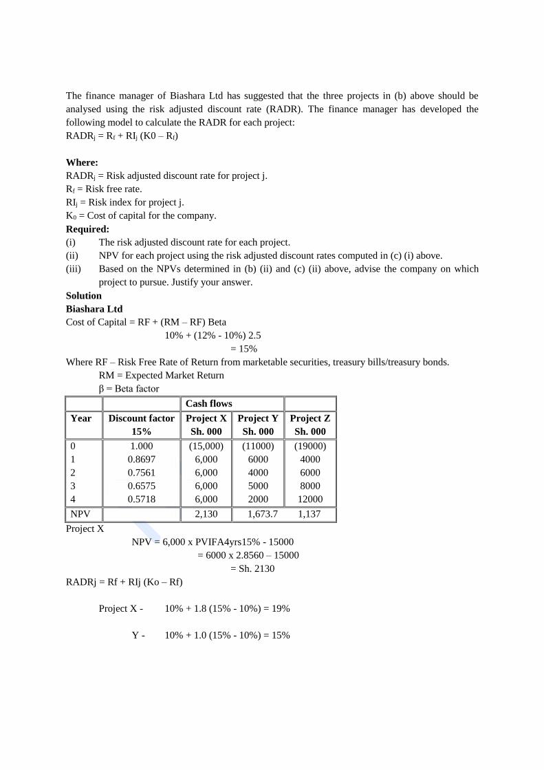
The finance manager of Biashara Ltd has suggested that the three projects in (b) above should be
analysed using the risk adjusted discount rate (RADR). The finance manager has developed the
following model to calculate the RADR for each project:
RADRj = Rf + RIj (K0 – Rf)
Where:
RADRj = Risk adjusted discount rate for project j.
Rf = Risk free rate.
RIj = Risk index for project j.
K0 = Cost of capital for the company.
Required:
(i) The risk adjusted discount rate for each project.
(ii) NPV for each project using the risk adjusted discount rates computed in (c) (i) above.
(iii) Based on the NPVs determined in (b) (ii) and (c) (ii) above, advise the company on which
project to pursue. Justify your answer.
Solution
Biashara Ltd
Cost of Capital = RF + (RM – RF) Beta
10% + (12% - 10%) 2.5
= 15%
Where RF – Risk Free Rate of Return from marketable securities, treasury bills/treasury bonds.
RM = Expected Market Return
β = Beta factor
Cash flows
Year Discount factor
15%
Project X
Sh. 000
Project Y
Sh. 000
Project Z
Sh. 000
0
1
2
3
4
1.000
0.8697
0.7561
0.6575
0.5718
(15,000)
6,000
6,000
6,000
6,000
(11000)
6000
4000
5000
2000
(19000)
4000
6000
8000
12000
NPV 2,130 1,673.7 1,137
Project X
NPV = 6,000 x PVIFA4yrs15% - 15000
= 6000 x 2.8560 – 15000
= Sh. 2130
RADRj = Rf + RIj (Ko – Rf)
Project X - 10% + 1.8 (15% - 10%) = 19%
Y - 10% + 1.0 (15% - 10%) = 15%
Page 33
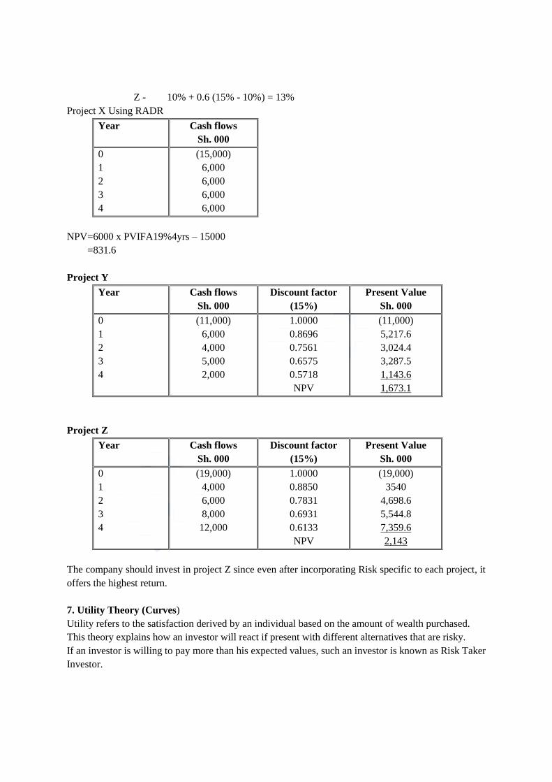
Z - 10% + 0.6 (15% - 10%) = 13%
Project X Using RADR
Year Cash flows
Sh. 000
0
1
2
3
4
(15,000)
6,000
6,000
6,000
6,000
NPV=6000 x PVIFA19%4yrs – 15000
=831.6
Project Y
Year Cash flows
Sh. 000
Discount factor
(15%)
Present Value
Sh. 000
0
1
2
3
4
(11,000)
6,000
4,000
5,000
2,000
1.0000
0.8696
0.7561
0.6575
0.5718
NPV
(11,000)
5,217.6
3,024.4
3,287.5
1,143.6
1,673.1
Project Z
Year Cash flows
Sh. 000
Discount factor
(15%)
Present Value
Sh. 000
0
1
2
3
4
(19,000)
4,000
6,000
8,000
12,000
1.0000
0.8850
0.7831
0.6931
0.6133
NPV
(19,000)
3540
4,698.6
5,544.8
7,359.6
2,143
The company should invest in project Z since even after incorporating Risk specific to each project, it
offers the highest return.
7. Utility Theory (Curves)
Utility refers to the satisfaction derived by an individual based on the amount of wealth purchased.
This theory explains how an investor will react if present with different alternatives that are risky.
If an investor is willing to pay more than his expected values, such an investor is known as Risk Taker
Investor.
Page 34
If an investor is willing to pay less than his expected return value, such an investor is known as
Risk Averse Investor.
In case the investor is willing to pay the same amount as his expected return, such an investor is
known as a Risk Neutral Investor.
As regards the attitude of individual investors towards risk, they can be classified in three categories. ·
Risk-averse investors attach lower utility to increasing wealth i.e. for a given wealth or return, they
prefer less risk to more risk. ·
Risk-neutral investors attach same utility to increasing or decreasing wealth i.e. they are indifferent to
less or more risk for a given wealth or return.
Risk-seeking investors attach more utility to the potential of additional wealth to the loss from the
possible loss from the decrease in wealth. I.e. for earning a given wealth or return, they are prepared
to assume higher risk. It is well established by many empirical studies that individuals are generally
risk averse and demonstrate a decreasing marginal utility for money function.
1.3 INCORPORATING CAPITAL RATIONING IN CAPITAL INVESTMENT
APPRAISAL
Capital rationing implies investment in projects within limited capital resources. It is the process of
allocating money among different projects, where the amount of money to be invested is limited.
Companies ration their capital and investments among different opportunities as countries use
rationing of food. In case of capital rationing, the company may not be able to invest in all profitable
projects.
Types of capital rationing
1. Internal/Soft Capital Rationing
In this case the decisions of the management leads to the company not being able to raise all the
required funds necessary for undertaking all profitable projects examples.
(i)Issue of additional shares to the public may be avoided so as not to dilute the firm’s earnings per
share.
(ii)Issue of additional debt may be avoided so as not to increase the firm’s gearing/financial risk.
(iii)Use of debt finance may be avoided so as not to increase the fixed finance costs inform of
interests.
(iv)The management may opt to maintain their investments at a level that can only be financed by
internally generated funds.
2. External/Hard capital rationing
It arises due to external factors which are beyond the control of the management, i.e. the firm is
unable to raise all the required funds due to the restrictions from the financial markets among other
external factors for example;
i) Raising of funds from the public through ordinary shares or debentures is not possible for a
company that is not listed (Quoted at the securities market).
ii) Raising of funds through debt may be difficult for a firm without collateral to pledge a security.
iii) The existing shareholders/investors may be unwilling to increase their investments to the firm.
Page 35
iv) The existing contractual obligations may prohibit the firm from raising additional funds from
other sources.
v) Government policies with respect to regulations of financial markets may prevent the firm from
additional borrowing through an increase in minimum lending rates.
Profitability Index = 𝑃𝑉𝑜𝑓𝑐𝑎𝑠ℎ 𝑖𝑛 𝑓𝑙𝑜𝑤𝑠
𝐼𝑛𝑖𝑡𝑖𝑎𝑙 𝑐𝑜𝑠𝑡 𝑜𝑢𝑡𝑙𝑎𝑦
Single period capital rationing (one period capital rationing)
It is where the limitation of fund is not expected to extend beyond the current financial year.
This is applicable when limits are placed on the availability of finance for positive NPV for one year
only and capital is freely available in all the rest of periods.
There are some additional assumptions in single period rationing which are very important to consider
here which include:
(i) If a firm does not undertake a project `now'the period of capital scarcity, the opportunity is lost
in other words, the project cannot be deferred until the capital is available.
(ii) The outcome of each project is known with certainty so that the choice between the projects is not
affected by considerations of risk.
(iii) The projects are divisible. This means that we can undertake 50% of project A and 50% of project B.
The basic approach will be to rank the projects in such in such a way that NPV can be maximised
from the use of available finances using profitability indices
Ranking the projects using NPV will be incorrect in this scenario because NPV basis will lead to
select the ‘big’ projects, each of which has a high individual NPV but which have a lower NPV than a
large number of smaller projects with lower individual NPVs.
Therefore, ranking should be made in terms of Profitability index
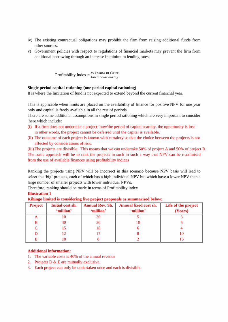
Illustration 1
Kihingo limited is considering five project proposals as summarised below;
Project Initial cost sh.
‘million’
Annual Rev. Sh.
‘million’
Annual fixed cost sh.
‘million’
Life of the project
(Years)
A
B
C
D
E
10
30
15
12
18
20
30
18
17
8
5
10
6
8
2
3
5
4
10
15
Additional information:
1. The variable costs is 40% of the annual revenue
2. Projects D & E are mutually exclusive.
3. Each project can only be undertaken once and each is divisible.
Page 36
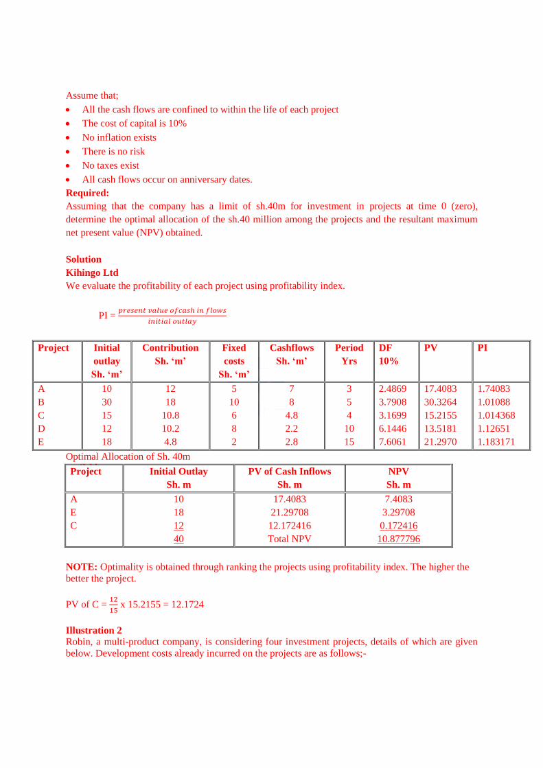
Assume that;
All the cash flows are confined to within the life of each project
The cost of capital is 10%
No inflation exists
There is no risk
No taxes exist
All cash flows occur on anniversary dates.
Required:
Assuming that the company has a limit of sh.40m for investment in projects at time 0 (zero),
determine the optimal allocation of the sh.40 million among the projects and the resultant maximum
net present value (NPV) obtained.
Solution
Kihingo Ltd
We evaluate the profitability of each project using profitability index.
PI = 𝑝𝑟𝑒𝑠𝑒𝑛𝑡 𝑣𝑎𝑙𝑢𝑒 𝑜𝑓𝑐𝑎𝑠ℎ 𝑖𝑛 𝑓𝑙𝑜𝑤𝑠
𝑖𝑛𝑖𝑡𝑖𝑎𝑙 𝑜𝑢𝑡𝑙𝑎𝑦
Project Initial
outlay
Sh. ‘m’
Contribution
Sh. ‘m’
Fixed
costs
Sh. ‘m’
Cashflows
Sh. ‘m’
Period
Yrs
DF
10%
PV PI
A
B
C
D
E
10
30
15
12
18
12
18
10.8
10.2
4.8
5
10
6
8
2
7
8
4.8
2.2
2.8
3
5
4
10
15
2.4869
3.7908
3.1699
6.1446
7.6061
17.4083
30.3264
15.2155
13.5181
21.2970
1.74083
1.01088
1.014368
1.12651
1.183171
Optimal Allocation of Sh. 40m available
Project Initial Outlay
Sh. m
PV of Cash Inflows
Sh. m
NPV
Sh. m
A
E
C
10
18
12
40
17.4083
21.29708
12.172416
Total NPV
7.4083
3.29708
0.172416
10.877796
NOTE: Optimality is obtained through ranking the projects using profitability index. The higher the
better the project.
PV of C = 12
15 x 15.2155 = 12.1724
Illustration 2
Robin, a multi-product company, is considering four investment projects, details of which are given
below. Development costs already incurred on the projects are as follows;-
Page 37
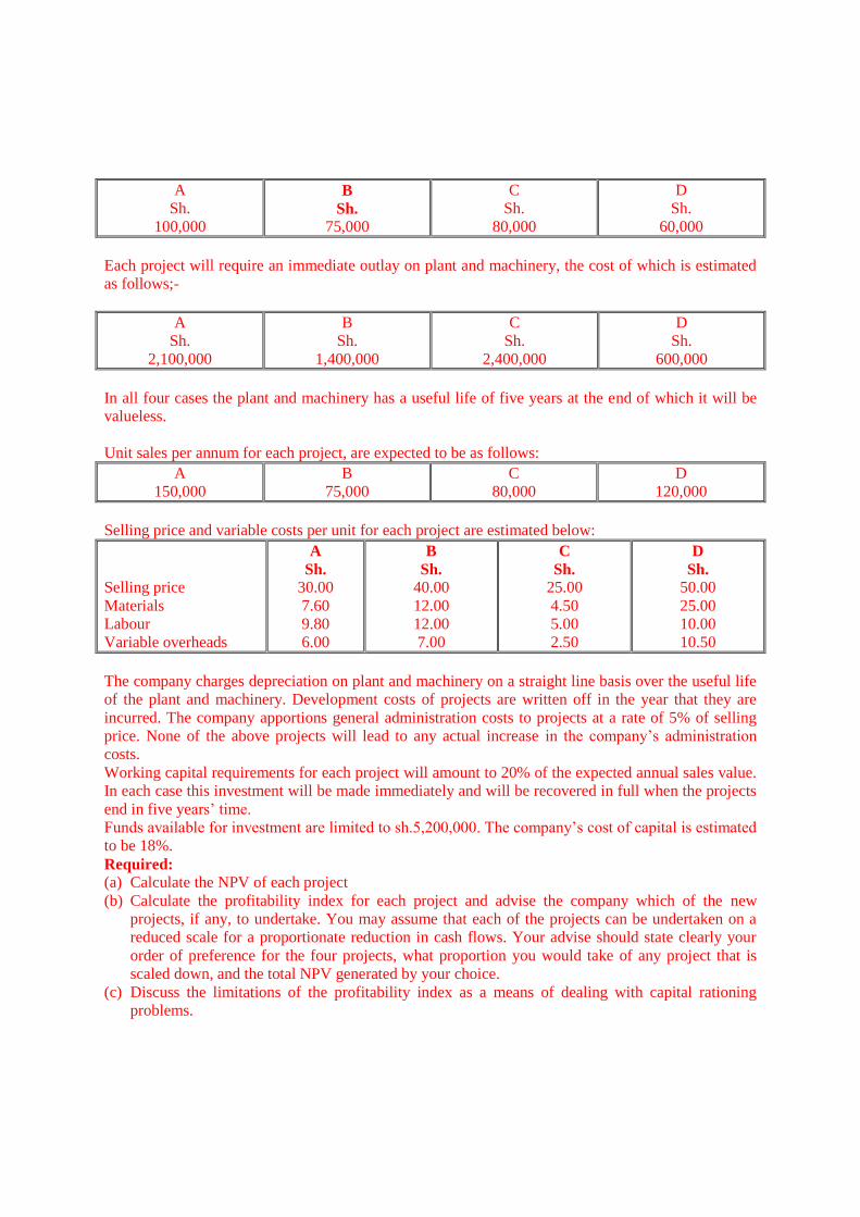
A
Sh.
100,000
B
Sh.
75,000
C
Sh.
80,000
D
Sh.
60,000
Each project will require an immediate outlay on plant and machinery, the cost of which is estimated
as follows;-
A
Sh.
2,100,000
B
Sh.
1,400,000
C
Sh.
2,400,000
D
Sh.
600,000
In all four cases the plant and machinery has a useful life of five years at the end of which it will be
valueless.
Unit sales per annum for each project, are expected to be as follows:
A
150,000
B
75,000
C
80,000
D
120,000
Selling price and variable costs per unit for each project are estimated below:
Selling price
Materials
Labour
Variable overheads
A
Sh.
30.00
7.60
9.80
6.00
B
Sh.
40.00
12.00
12.00
7.00
C
Sh.
25.00
4.50
5.00
2.50
D
Sh.
50.00
25.00
10.00
10.50
The company charges depreciation on plant and machinery on a straight line basis over the useful life
of the plant and machinery. Development costs of projects are written off in the year that they are
incurred. The company apportions general administration costs to projects at a rate of 5% of selling
price. None of the above projects will lead to any actual increase in the company’s administration
costs.
Working capital requirements for each project will amount to 20% of the expected annual sales value.
In each case this investment will be made immediately and will be recovered in full when the projects
end in five years’ time.
Funds available for investment are limited to sh.5,200,000. The company’s cost of capital is estimated
to be 18%.
Required:
(a) Calculate the NPV of each project
(b) Calculate the profitability index for each project and advise the company which of the new
projects, if any, to undertake. You may assume that each of the projects can be undertaken on a
reduced scale for a proportionate reduction in cash flows. Your advise should state clearly your
order of preference for the four projects, what proportion you would take of any project that is
scaled down, and the total NPV generated by your choice.
(c) Discuss the limitations of the profitability index as a means of dealing with capital rationing
problems.
Page 38
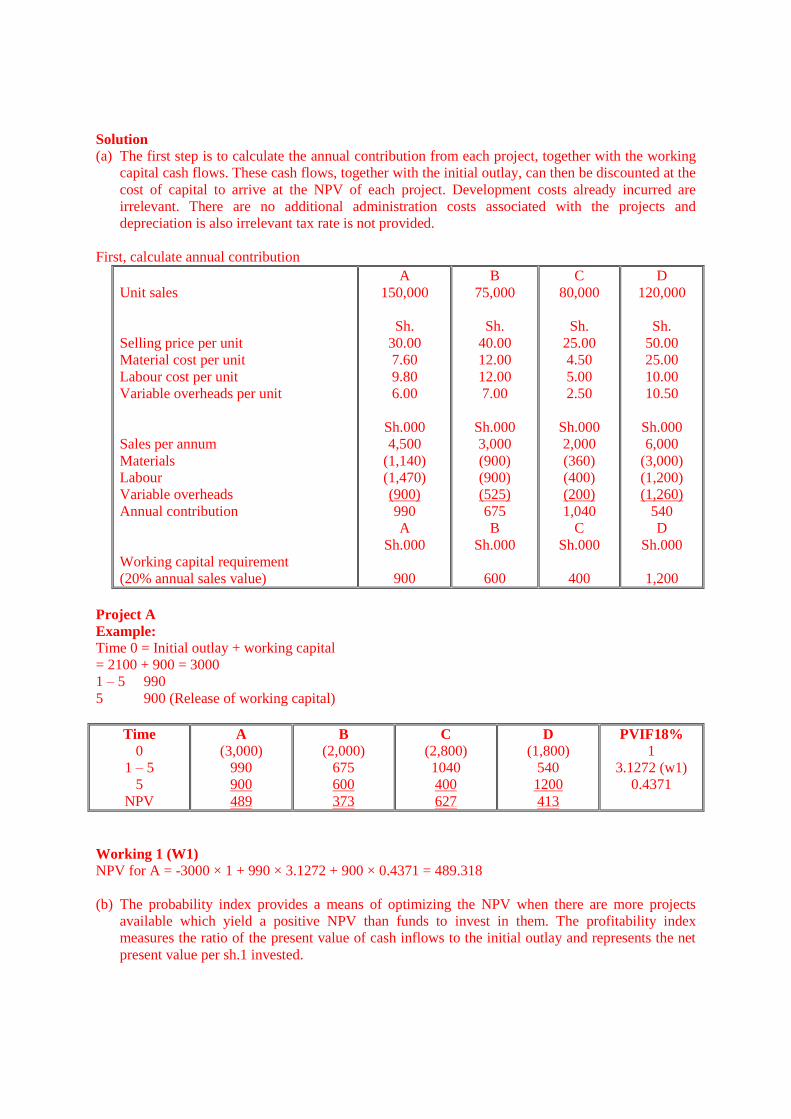
Solution
(a) The first step is to calculate the annual contribution from each project, together with the working
capital cash flows. These cash flows, together with the initial outlay, can then be discounted at the
cost of capital to arrive at the NPV of each project. Development costs already incurred are
irrelevant. There are no additional administration costs associated with the projects and
depreciation is also irrelevant tax rate is not provided.
First, calculate annual contribution
Unit sales
Selling price per unit
Material cost per unit
Labour cost per unit
Variable overheads per unit
Sales per annum
Materials
Labour
Variable overheads
Annual contribution
Working capital requirement
(20% annual sales value)
A
150,000
Sh.
30.00
7.60
9.80
6.00
Sh.000
4,500
(1,140)
(1,470)
(900)
990
A
Sh.000
900
B
75,000
Sh.
40.00
12.00
12.00
7.00
Sh.000
3,000
(900)
(900)
(525)
675
B
Sh.000
600
C
80,000
Sh.
25.00
4.50
5.00
2.50
Sh.000
2,000
(360)
(400)
(200)
1,040
C
Sh.000
400
D
120,000
Sh.
50.00
25.00
10.00
10.50
Sh.000
6,000
(3,000)
(1,200)
(1,260)
540
D
Sh.000
1,200
Project A
Example:
Time 0 = Initial outlay + working capital
= 2100 + 900 = 3000
1 – 5 990
5 900 (Release of working capital)
Time
0
1 – 5
5
NPV
A
(3,000)
990
900
489
B
(2,000)
675
600
373
C
(2,800)
1040
400
627
D
(1,800)
540
1200
413
PVIF18%
1
3.1272 (w1)
0.4371
Working 1 (W1)
NPV for A = -3000 × 1 + 990 × 3.1272 + 900 × 0.4371 = 489.318
(b) The probability index provides a means of optimizing the NPV when there are more projects
available which yield a positive NPV than funds to invest in them. The profitability index
measures the ratio of the present value of cash inflows to the initial outlay and represents the net
present value per sh.1 invested.
Page 39
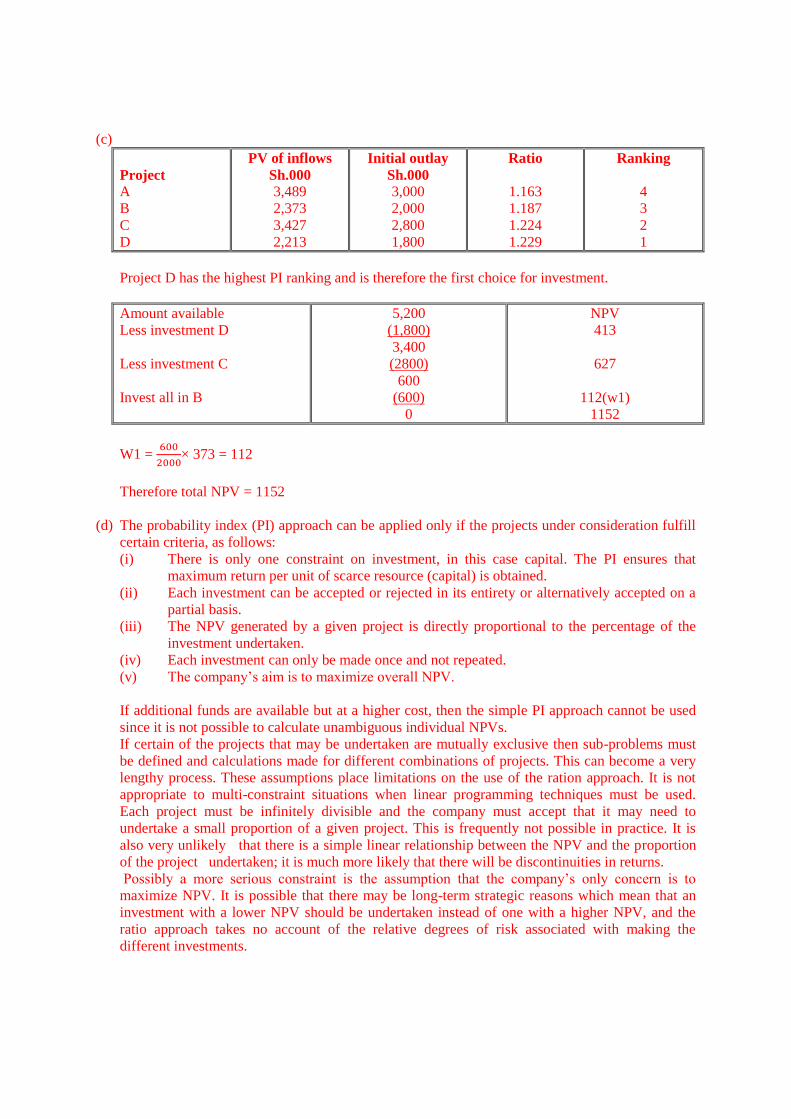
(c)
Project
A
B
C
D
PV of inflows
Sh.000
3,489
2,373
3,427
2,213
Initial outlay
Sh.000
3,000
2,000
2,800
1,800
Ratio
1.163
1.187
1.224
1.229
Ranking
4
3
2
1
Project D has the highest PI ranking and is therefore the first choice for investment.
Amount available
Less investment D
Less investment C
Invest all in B
5,200
(1,800)
3,400
(2800)
600
(600)
0
NPV
413
627
112(w1)
1152
W1 = 600
2000× 373 = 112
Therefore total NPV = 1152
(d) The probability index (PI) approach can be applied only if the projects under consideration fulfill
certain criteria, as follows:
(i) There is only one constraint on investment, in this case capital. The PI ensures that
maximum return per unit of scarce resource (capital) is obtained.
(ii) Each investment can be accepted or rejected in its entirety or alternatively accepted on a
partial basis.
(iii) The NPV generated by a given project is directly proportional to the percentage of the
investment undertaken.
(iv) Each investment can only be made once and not repeated.
(v) The company’s aim is to maximize overall NPV.
If additional funds are available but at a higher cost, then the simple PI approach cannot be used
since it is not possible to calculate unambiguous individual NPVs.
If certain of the projects that may be undertaken are mutually exclusive then sub-problems must
be defined and calculations made for different combinations of projects. This can become a very
lengthy process. These assumptions place limitations on the use of the ration approach. It is not
appropriate to multi-constraint situations when linear programming techniques must be used.
Each project must be infinitely divisible and the company must accept that it may need to
undertake a small proportion of a given project. This is frequently not possible in practice. It is
also very unlikely that there is a simple linear relationship between the NPV and the proportion
of the project undertaken; it is much more likely that there will be discontinuities in returns.
Possibly a more serious constraint is the assumption that the company’s only concern is to
maximize NPV. It is possible that there may be long-term strategic reasons which mean that an
investment with a lower NPV should be undertaken instead of one with a higher NPV, and the
ratio approach takes no account of the relative degrees of risk associated with making the
different investments.
Page 40
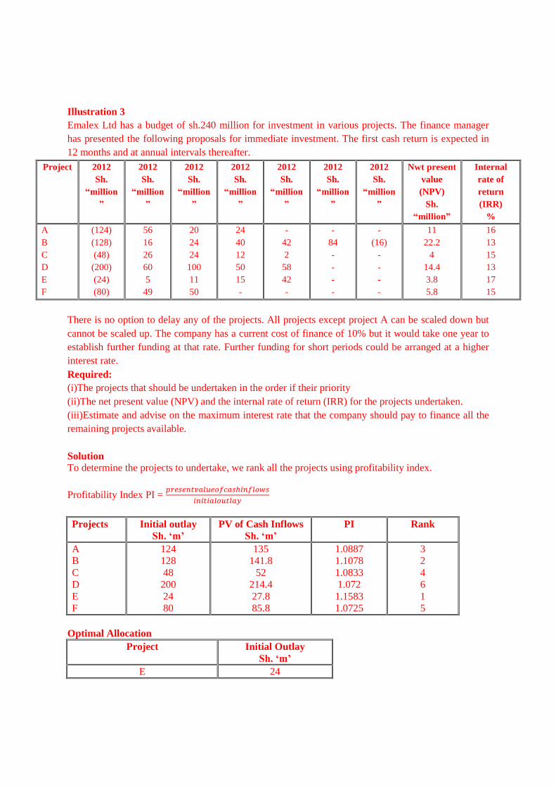
Illustration 3
Emalex Ltd has a budget of sh.240 million for investment in various projects. The finance manager
has presented the following proposals for immediate investment. The first cash return is expected in
12 months and at annual intervals thereafter.
Project 2012
Sh.
“million
”
2012
Sh.
“million
”
2012
Sh.
“million
”
2012
Sh.
“million
”
2012
Sh.
“million
”
2012
Sh.
“million
”
2012
Sh.
“million
”
Nwt present
value
(NPV)
Sh.
“million”
Internal
rate of
return
(IRR)
%
A
B
C
D
E
F
(124)
(128)
(48)
(200)
(24)
(80)
56
16
26
60
5
49
20
24
24
100
11
50
24
40
12
50
15
-
-
42
2
58
42
-
-
84
-
-
-
-
-
(16)
-
-
-
-
11
22.2
4
14.4
3.8
5.8
16
13
15
13
17
15
There is no option to delay any of the projects. All projects except project A can be scaled down but
cannot be scaled up. The company has a current cost of finance of 10% but it would take one year to
establish further funding at that rate. Further funding for short periods could be arranged at a higher
interest rate.
Required:
(i)The projects that should be undertaken in the order if their priority
(ii)The net present value (NPV) and the internal rate of return (IRR) for the projects undertaken.
(iii)Estimate and advise on the maximum interest rate that the company should pay to finance all the
remaining projects available.
Solution
To determine the projects to undertake, we rank all the projects using profitability index.
Profitability Index PI = 𝑝𝑟𝑒𝑠𝑒𝑛𝑡𝑣𝑎𝑙𝑢𝑒𝑜𝑓𝑐𝑎𝑠ℎ𝑖𝑛𝑓𝑙𝑜𝑤𝑠
𝑖𝑛𝑖𝑡𝑖𝑎𝑙𝑜𝑢𝑡𝑙𝑎𝑦
Projects Initial outlay
Sh. ‘m’
PV of Cash Inflows
Sh. ‘m’
PI Rank
A
B
C
D
E
F
124
128
48
200
24
80
135
141.8
52
214.4
27.8
85.8
1.0887
1.1078
1.0833
1.072
1.1583
1.0725
3
2
4
6
1
5
Optimal Allocation
Project Initial Outlay
Sh. ‘m’
E 24
Page 41
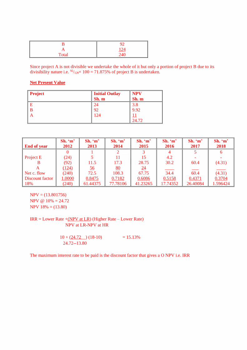
B
A
Total
92
124
240
Since project A is not divisible we undertake the whole of it but only a portion of project B due to its
divisibility nature i.e. 92/128× 100 = 71.875% of project B is undertaken.
Net Present Value
Project Initial Outlay
Sh. m
NPV
Sh. m
E
B
A
24
92
124
3.8
9.92
11
24.72
NPV = (13.801756)
NPV @ 10% = 24.72
NPV 18% = (13.80)
IRR = Lower Rate +(NPV at LR) (Higher Rate – Lower Rate)
NPV at LR-NPV at HR
10 + (24.72 ) (18-10) = 15.13%
24.72--13.80
The maximum interest rate to be paid is the discount factor that gives a O NPV i.e. IRR
End of year
Sh. ‘m’
2012
Sh. ‘m’
2013
Sh. ‘m’
2014
Sh. ‘m’
2015
Sh. ‘m’
2016
Sh. ‘m’
2017
Sh. ‘m’
2018
Project E
B
A
Net c. flow
Discount factor
18%
0
(24)
(92)
(124)
(240)
1.0000
(240)
1
5
11.5
56
72.5
0.8475
61.44375
2
11
17.3
80
108.3
0.7182
77.78106
3
15
28.75
24
67.75
0.6086
41.23265
4
4.2
30.2
____
34.4
0.5158
17.74352
5
-
60.4
___
60.4
0.4371
26.40084
6
-
(4.31)
____
(4.31)
0.3704
1.596424
Page 42
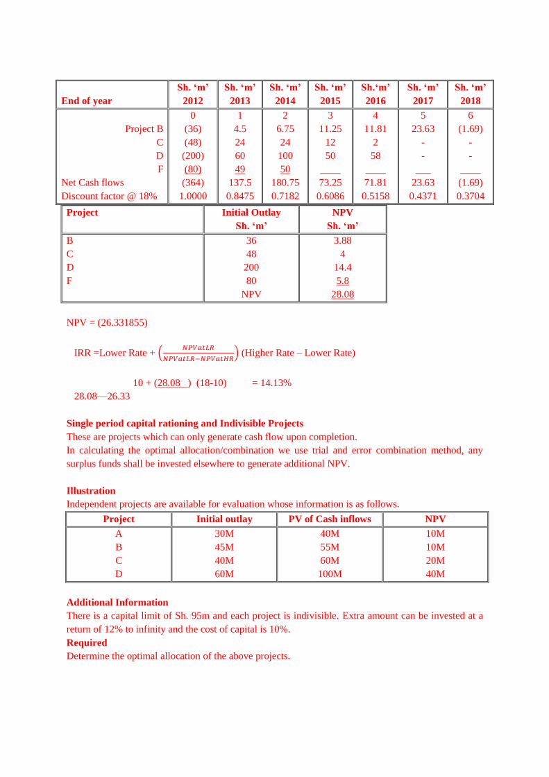
Project Initial Outlay
Sh. ‘m’
NPV
Sh. ‘m’
B
C
D
F
36
48
200
80
NPV
3.88
4
14.4
5.8
28.08
NPV = (26.331855)
IRR =Lower Rate + (𝑁𝑃𝑉𝑎𝑡𝐿𝑅
𝑁𝑃𝑉𝑎𝑡𝐿𝑅−𝑁𝑃𝑉𝑎𝑡𝐻𝑅) (Higher Rate – Lower Rate)
10 + (28.08 ) (18-10) = 14.13%
28.08—26.33
Single period capital rationing and Indivisible Projects
These are projects which can only generate cash flow upon completion.
In calculating the optimal allocation/combination we use trial and error combination method, any
surplus funds shall be invested elsewhere to generate additional NPV.
Illustration
Independent projects are available for evaluation whose information is as follows.
Project Initial outlay PV of Cash inflows NPV
A
B
C
D
30M
45M
40M
60M
40M
55M
60M
100M
10M
10M
20M
40M
Additional Information
There is a capital limit of Sh. 95m and each project is indivisible. Extra amount can be invested at a
return of 12% to infinity and the cost of capital is 10%.
Required
Determine the optimal allocation of the above projects.
End of year
Sh. ‘m’
2012
Sh. ‘m’
2013
Sh. ‘m’
2014
Sh. ‘m’
2015
Sh.‘m’
2016
Sh. ‘m’
2017
Sh. ‘m’
2018
Project B
C
D
F
Net Cash flows
Discount factor @ 18%
0
(36)
(48)
(200)
(80)
(364)
1.0000
1
4.5
24
60
49
137.5
0.8475
2
6.75
24
100
50
180.75
0.7182
3
11.25
12
50
____
73.25
0.6086
4
11.81
2
58
____
71.81
0.5158
5
23.63
-
-
___
23.63
0.4371
6
(1.69)
-
-
____
(1.69)
0.3704
Page 43
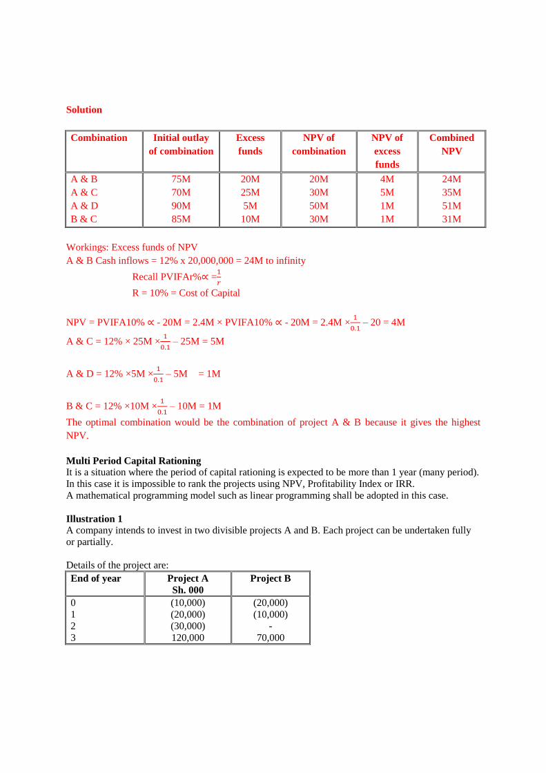
Solution
Combination Initial outlay
of combination
Excess
funds
NPV of
combination
NPV of
excess
funds
Combined
NPV
A & B
A & C
A & D
B & C
75M
70M
90M
85M
20M
25M
5M
10M
20M
30M
50M
30M
4M
5M
1M
1M
24M
35M
51M
31M
Workings: Excess funds of NPV
A & B Cash inflows = 12% x 20,000,000 = 24M to infinity
Recall PVIFAr%∝ =1
𝑟
R = 10% = Cost of Capital
NPV = PVIFA10% ∝ - 20M = 2.4M × PVIFA10% ∝ - 20M = 2.4M ×1
0.1 – 20 = 4M
A & C = 12% × 25M ×1
0.1 – 25M = 5M
A & D = 12% ×5M ×1
0.1 – 5M = 1M
B & C = 12% ×10M ×1
0.1 – 10M = 1M
The optimal combination would be the combination of project A & B because it gives the highest
NPV.
Multi Period Capital Rationing
It is a situation where the period of capital rationing is expected to be more than 1 year (many period).
In this case it is impossible to rank the projects using NPV, Profitability Index or IRR.
A mathematical programming model such as linear programming shall be adopted in this case.
Illustration 1
A company intends to invest in two divisible projects A and B. Each project can be undertaken fully
or partially.
Details of the project are:
End of year Project A
Sh. 000
Project B
0
1
2
3
(10,000)
(20,000)
(30,000)
120,000
(20,000)
(10,000)
-
70,000
Page 44
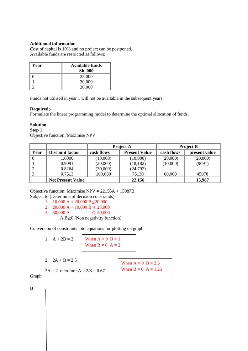
Additional information
Cost of capital is 10% and no project can be postponed.
Available funds are restricted as follows:
Year Available funds
Sh. 000
0
1
2
25,000
30,000
20,000
Funds not utilised in year 1 will not be available in the subsequent years.
Required;-
Formulate the linear programming model to determine the optimal allocation of funds.
Solution
Step 1
Objective function /Maximise NPV
Project A Project B
Year Discount factor cash flows Present Value cash flows present value
0
1
2
3
1.0000
0.9091
0.8264
0.7513
(10,000)
(20,000)
(30,000)
100,000
(10,000)
(18,182)
(24,792)
75130
(20,000)
(10,000)
-
60,000
(20,000)
(9091)
-
45078
Net Present Value 22,156 15,987
Objective function: Maximise NPV = 22156A + 15987B
Subject to (Determine of decision constraints)
1. 10,000 A + 20,000 B≤20,000
2. 20,000 A + 10,000 B ≤ 25,000
3. 30,000 A ≤ 20,000
A,B≥0 (Non negativity function)
Conversion of constraints into equations for plotting on graph
1. A + 2B = 2
2. 2A + B = 2.5
3A = 2 therefore A = 2/3 = 0.67
Graph
B
When A = 0 B = 1
When B = 0 A = 2
When A = 0 B = 2.5
When B = 0 A = 1.25
Page 45
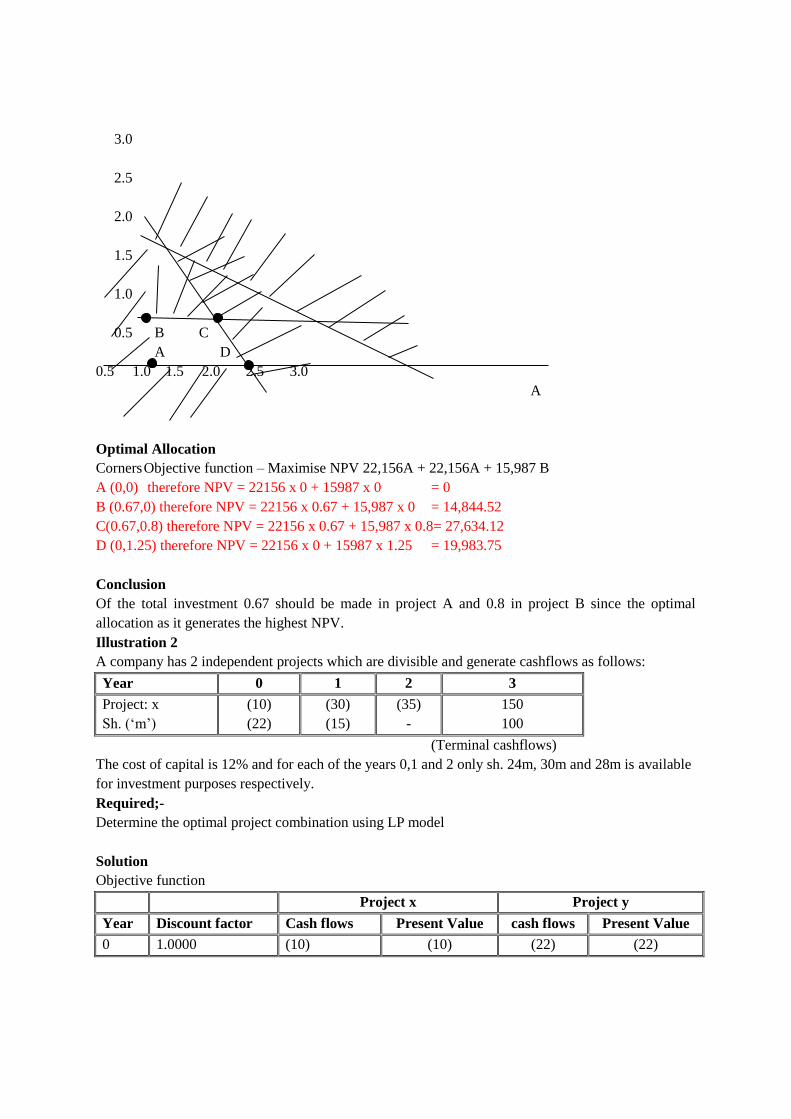
3.0
2.5
2.0
1.5
1.0
0.5 B C
A D
0.5 1.0 1.5 2.0 2.5 3.0
A
Optimal Allocation
Corners Objective function – Maximise NPV 22,156A + 22,156A + 15,987 B
A (0,0) therefore NPV = 22156 x 0 + 15987 x 0 = 0
B (0.67,0) therefore NPV = 22156 x 0.67 + 15,987 x 0 = 14,844.52
C(0.67,0.8) therefore NPV = 22156 x 0.67 + 15,987 x 0.8= 27,634.12
D (0,1.25) therefore NPV = 22156 x 0 + 15987 x 1.25 = 19,983.75
Conclusion
Of the total investment 0.67 should be made in project A and 0.8 in project B since the optimal
allocation as it generates the highest NPV.
Illustration 2
A company has 2 independent projects which are divisible and generate cashflows as follows:
Year 0 1 2 3
Project: x
Sh. (‘m’)
(10)
(22)
(30)
(15)
(35)
-
150
100
(Terminal cashflows)
The cost of capital is 12% and for each of the years 0,1 and 2 only sh. 24m, 30m and 28m is available
for investment purposes respectively.
Required;-
Determine the optimal project combination using LP model
Solution
Objective function
Project x Project y
Year Discount factor Cash flows Present Value cash flows Present Value
0 1.0000 (10) (10) (22) (22)
Page 46
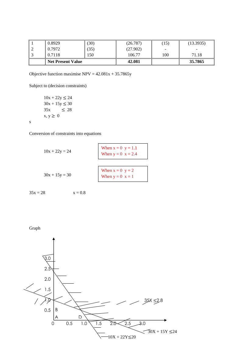
1
2
3
0.8929
0.7972
0.7118
(30)
(35)
150
(26.787)
(27.902)
106.77
(15)
-
100
(13.3935)
-
71.18
Net Present Value 42.081 35.7865
Objective function maximise NPV = 42.081x + 35.7865y
Subject to (decision constraints)
10x + 22y ≤ 24
30x + 15y ≤ 30
35x ≤ 28
x, y ≥ 0
s
Conversion of constraints into equations
10x + 22y = 24
30x + 15y = 30
35x = 28 x = 0.8
Graph
0 0.5 1.0 1.5 2.0 2.5 3.0
3.0
2.5
2.0
1.5
1.0
0.5
0
B
C A D
10X + 22Y≤20
30X + 15Y ≤24
35X ≤2.8
When x = 0 y = 1.1
When y = 0 x = 2.4
When x = 0 y = 2
When y = 0 x = 1
Page 47
Optimal Allocation
Corners objective function maximise NPV (42.081x + 35.7865)
A (0,0) = 0
B (0,8.0) 0.8 x 42.081 + 0 x 35.7865 = 33.6648
C (0.6,0.8) 0.6 x 42.081 + 0.8 x 35.7865 = 53.8778
D (0,1.1) 0 x 42.081 + 1.1 x 35.7865 = 39.36515
Conclusion
Of the total investment 0.6m should be made in project x and 0.8m in project y since it is the optimal
allocation.
1.4 INCORPORATING INFLATION IN CAPITAL INVESTMENT APPRAISAL
INVESTMENT DECISION UNDER INFLATION
Inflation is the general increase in the price of goods and services.
Inflation can either be general or specific inflation.
General inflation affects the overall investors required rate of return.
Specific inflation only affects individual cash flows components.
Dealing with inflation in Net Present Value calculation two methods are used:
Real Method
Money Method/nominal
Real method
Under this method, cash flows are not inflated but the discount factor cost of capital /money rate is
adjusted to be the rate of return using the fisher formula
Using fisher formula (1 + r) (1 + i) = (1 + m) where
r = real rate of return
i = Inflation rate
m = money market rate of return /cost of capital
Make r the subject of the formulae
Page 48
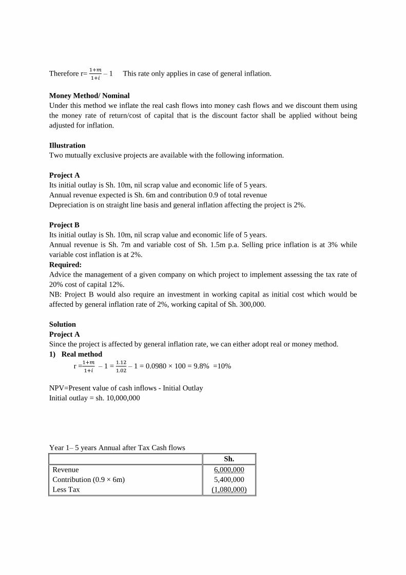
Therefore r= 1+𝑚
1+𝑖 – 1 This rate only applies in case of general inflation.
Money Method/ Nominal
Under this method we inflate the real cash flows into money cash flows and we discount them using
the money rate of return/cost of capital that is the discount factor shall be applied without being
adjusted for inflation.
Illustration
Two mutually exclusive projects are available with the following information.
Project A
Its initial outlay is Sh. 10m, nil scrap value and economic life of 5 years.
Annual revenue expected is Sh. 6m and contribution 0.9 of total revenue
Depreciation is on straight line basis and general inflation affecting the project is 2%.
Project B
Its initial outlay is Sh. 10m, nil scrap value and economic life of 5 years.
Annual revenue is Sh. 7m and variable cost of Sh. 1.5m p.a. Selling price inflation is at 3% while
variable cost inflation is at 2%.
Required:
Advice the management of a given company on which project to implement assessing the tax rate of
20% cost of capital 12%.
NB: Project B would also require an investment in working capital as initial cost which would be
affected by general inflation rate of 2%, working capital of Sh. 300,000.
Solution
Project A
Since the project is affected by general inflation rate, we can either adopt real or money method.
1) Real method
r =1+𝑚
1+𝑖 – 1 =
1.12
1.02 – 1 = 0.0980 × 100 = 9.8% =10%
NPV=Present value of cash inflows - Initial Outlay
Initial outlay = sh. 10,000,000
Year 1– 5 years Annual after Tax Cash flows
Sh.
Revenue
Contribution (0.9 × 6m)
Less Tax
6,000,000
5,400,000
(1,080,000)
Page 49
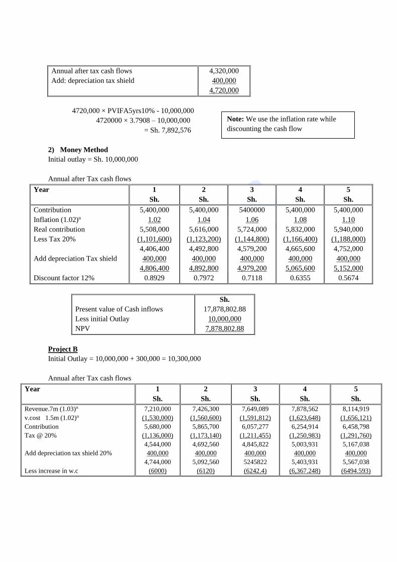
Annual after tax cash flows
Add: depreciation tax shield
4,320,000
400,000
4,720,000
4720,000 × PVIFA5yrs10% - 10,000,000
4720000 × 3.7908 – 10,000,000
= Sh. 7,892,576
2) Money Method
Initial outlay = Sh. 10,000,000
Annual after Tax cash flows
Year 1
Sh.
2
Sh.
3
Sh.
4
Sh.
5
Sh.
Contribution
Inflation (1.02)n
Real contribution
Less Tax 20%
Add depreciation Tax shield
Discount factor 12%
5,400,000
1.02
5,508,000
(1,101,600)
4,406,400
400,000
4,806,400
0.8929
5,400,000
1.04
5,616,000
(1,123,200)
4,492,800
400,000
4,892,800
0.7972
5400000
1.06
5,724,000
(1,144,800)
4,579,200
400,000
4,979,200
0.7118
5,400,000
1.08
5,832,000
(1,166,400)
4,665,600
400,000
5,065,600
0.6355
5,400,000
1.10
5,940,000
(1,188,000)
4,752,000
400,000
5,152,000
0.5674
Present value of Cash inflows
Less initial Outlay
NPV
Sh.
17,878,802.88
10,000,000
7,878,802.88
Project B
Initial Outlay = 10,000,000 + 300,000 = 10,300,000
Annual after Tax cash flows
Year 1
Sh.
2
Sh.
3
Sh.
4
Sh.
5
Sh.
Revenue.7m (1.03)n
v.cost 1.5m (1.02)n
Contribution
Tax @ 20%
Add depreciation tax shield 20%
Less increase in w.c
7,210,000
(1,530,000)
5,680,000
(1,136,000)
4,544,000
400,000
4,744,000
(6000)
7,426,300
(1,560,600)
5,865,700
(1,173,140)
4,692,560
400,000
5,092,560
(6120)
7,649,089
(1,591,812)
6,057,277
(1,211,455)
4,845,822
400,000
5245822
(6242.4)
7,878,562
(1,623,648)
6,254,914
(1,250,983)
5,003,931
400,000
5,403,931
(6,367.248)
8,114,919
(1,656,121)
6,458,798
(1,291,760)
5,167,038
400,000
5,567,038
(6494.593)
Note: We use the inflation rate while
discounting the cash flow
Page 50
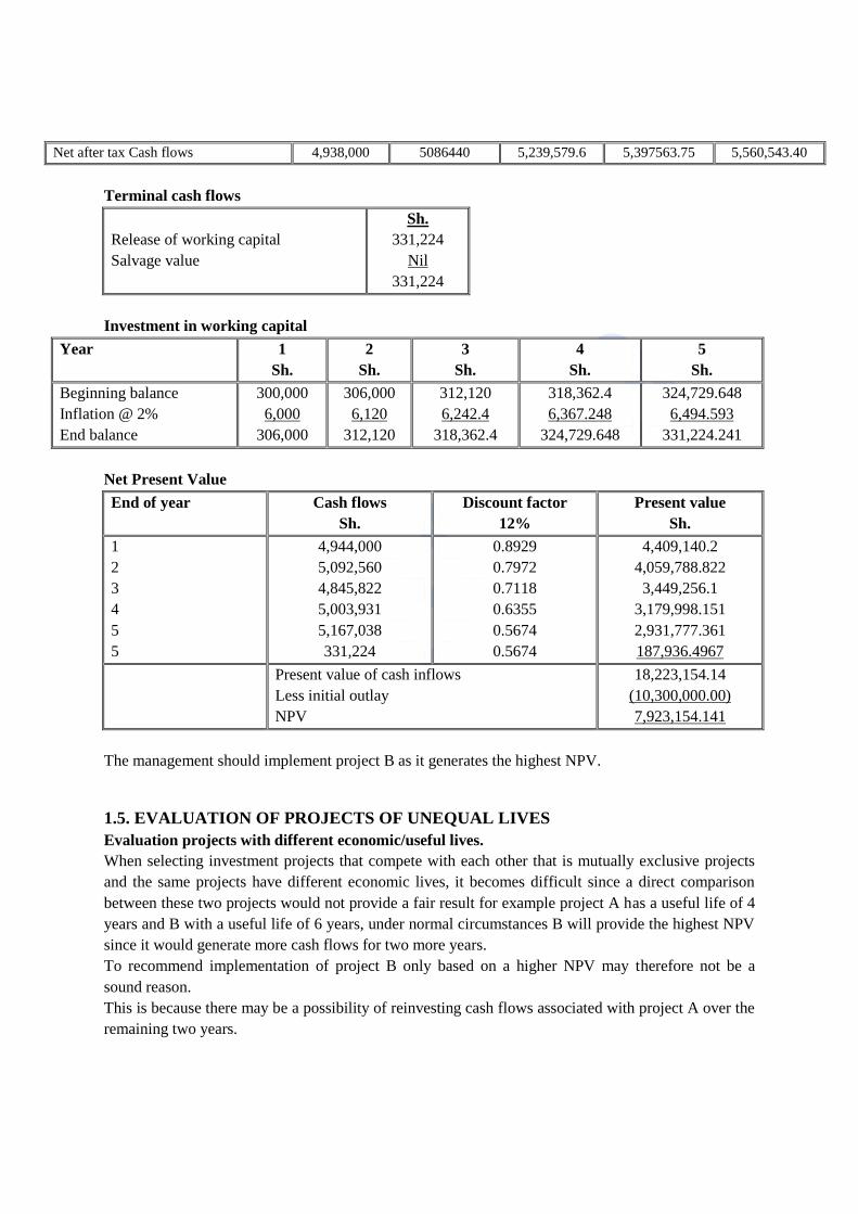
Net after tax Cash flows 4,938,000 5086440 5,239,579.6 5,397563.75 5,560,543.40
Terminal cash flows
Release of working capital
Salvage value
Sh.
331,224
Nil
331,224
Investment in working capital
Year 1
Sh.
2
Sh.
3
Sh.
4
Sh.
5
Sh.
Beginning balance
Inflation @ 2%
End balance
300,000
6,000
306,000
306,000
6,120
312,120
312,120
6,242.4
318,362.4
318,362.4
6,367.248
324,729.648
324,729.648
6,494.593
331,224.241
Net Present Value
End of year Cash flows
Sh.
Discount factor
12%
Present value
Sh.
1
2
3
4
5
5
4,944,000
5,092,560
4,845,822
5,003,931
5,167,038
331,224
0.8929
0.7972
0.7118
0.6355
0.5674
0.5674
4,409,140.2
4,059,788.822
3,449,256.1
3,179,998.151
2,931,777.361
187,936.4967
Present value of cash inflows
Less initial outlay
NPV
18,223,154.14
(10,300,000.00)
7,923,154.141
The management should implement project B as it generates the highest NPV.
1.5. EVALUATION OF PROJECTS OF UNEQUAL LIVES
Evaluation projects with different economic/useful lives.
When selecting investment projects that compete with each other that is mutually exclusive projects
and the same projects have different economic lives, it becomes difficult since a direct comparison
between these two projects would not provide a fair result for example project A has a useful life of 4
years and B with a useful life of 6 years, under normal circumstances B will provide the highest NPV
since it would generate more cash flows for two more years.
To recommend implementation of project B only based on a higher NPV may therefore not be a
sound reason.
This is because there may be a possibility of reinvesting cash flows associated with project A over the
remaining two years.
Page 51
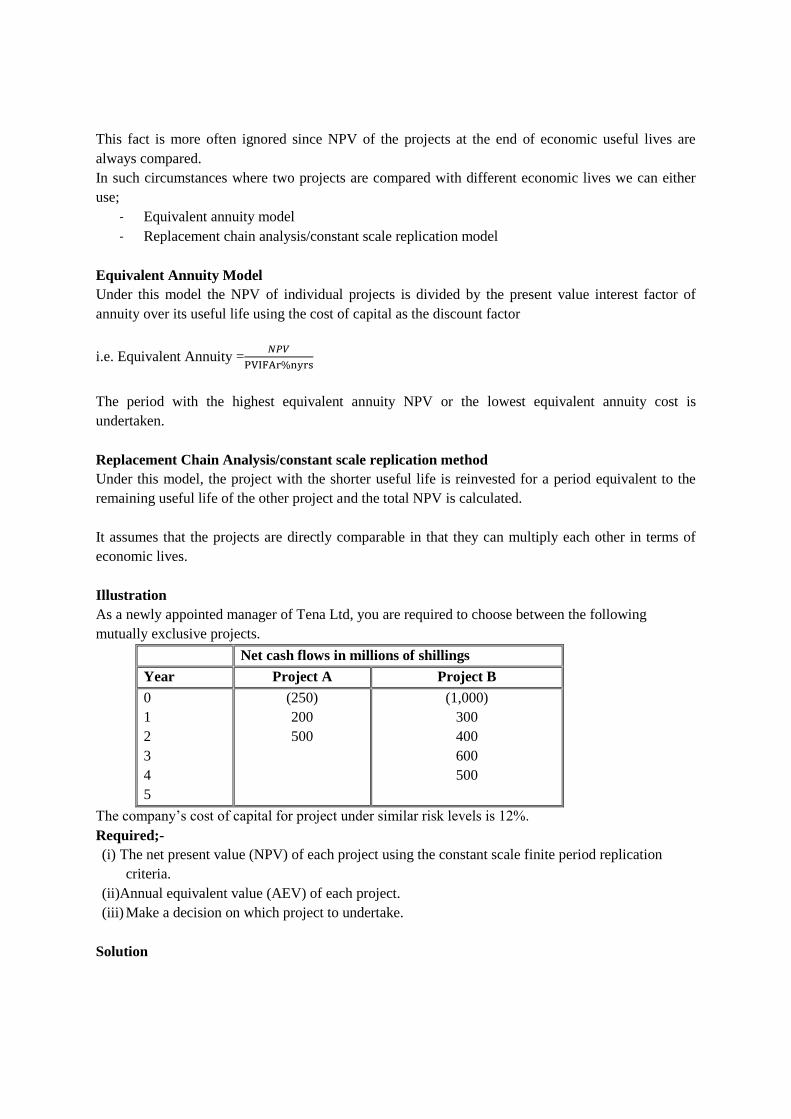
This fact is more often ignored since NPV of the projects at the end of economic useful lives are
always compared.
In such circumstances where two projects are compared with different economic lives we can either
use;
- Equivalent annuity model
- Replacement chain analysis/constant scale replication model
Equivalent Annuity Model
Under this model the NPV of individual projects is divided by the present value interest factor of
annuity over its useful life using the cost of capital as the discount factor
i.e. Equivalent Annuity =𝑁𝑃𝑉
PVIFAr%nyrs
The period with the highest equivalent annuity NPV or the lowest equivalent annuity cost is
undertaken.
Replacement Chain Analysis/constant scale replication method
Under this model, the project with the shorter useful life is reinvested for a period equivalent to the
remaining useful life of the other project and the total NPV is calculated.
It assumes that the projects are directly comparable in that they can multiply each other in terms of
economic lives.
Illustration
As a newly appointed manager of Tena Ltd, you are required to choose between the following
mutually exclusive projects.
Net cash flows in millions of shillings
Year Project A Project B
0
1
2
3
4
5
(250)
200
500
(1,000)
300
400
600
500
The company’s cost of capital for project under similar risk levels is 12%.
Required;-
(i) The net present value (NPV) of each project using the constant scale finite period replication
criteria.
(ii)Annual equivalent value (AEV) of each project.
(iii) Make a decision on which project to undertake.
Solution
Page 52
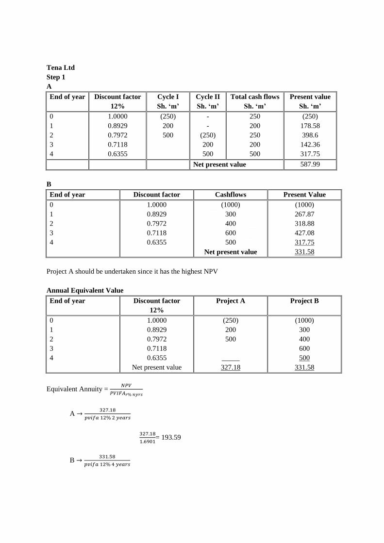
Tena Ltd
Step 1
A
End of year Discount factor
12%
Cycle I
Sh. ‘m’
Cycle II
Sh. ‘m’
Total cash flows
Sh. ‘m’
Present value
Sh. ‘m’
0
1
2
3
4
1.0000
0.8929
0.7972
0.7118
0.6355
(250)
200
500
-
-
(250)
200
500
250
200
250
200
500
(250)
178.58
398.6
142.36
317.75
Net present value 587.99
B
End of year Discount factor Cashflows Present Value
0
1
2
3
4
1.0000
0.8929
0.7972
0.7118
0.6355
(1000)
300
400
600
500
Net present value
(1000)
267.87
318.88
427.08
317.75
331.58
Project A should be undertaken since it has the highest NPV
Annual Equivalent Value
End of year Discount factor
12%
Project A Project B
0
1
2
3
4
1.0000
0.8929
0.7972
0.7118
0.6355
Net present value
(250)
200
500
_____
327.18
(1000)
300
400
600
500
331.58
Equivalent Annuity = 𝑁𝑃𝑉
𝑃𝑉𝐼𝐹𝐴𝑟% 𝑛𝑦𝑟𝑠
A →327.18
𝑝𝑣𝑖𝑓𝑎 12% 2 𝑦𝑒𝑎𝑟𝑠
327.18
1.6901= 193.59
B →331.58
𝑝𝑣𝑖𝑓𝑎 12% 4 𝑦𝑒𝑎𝑟𝑠
Page 53
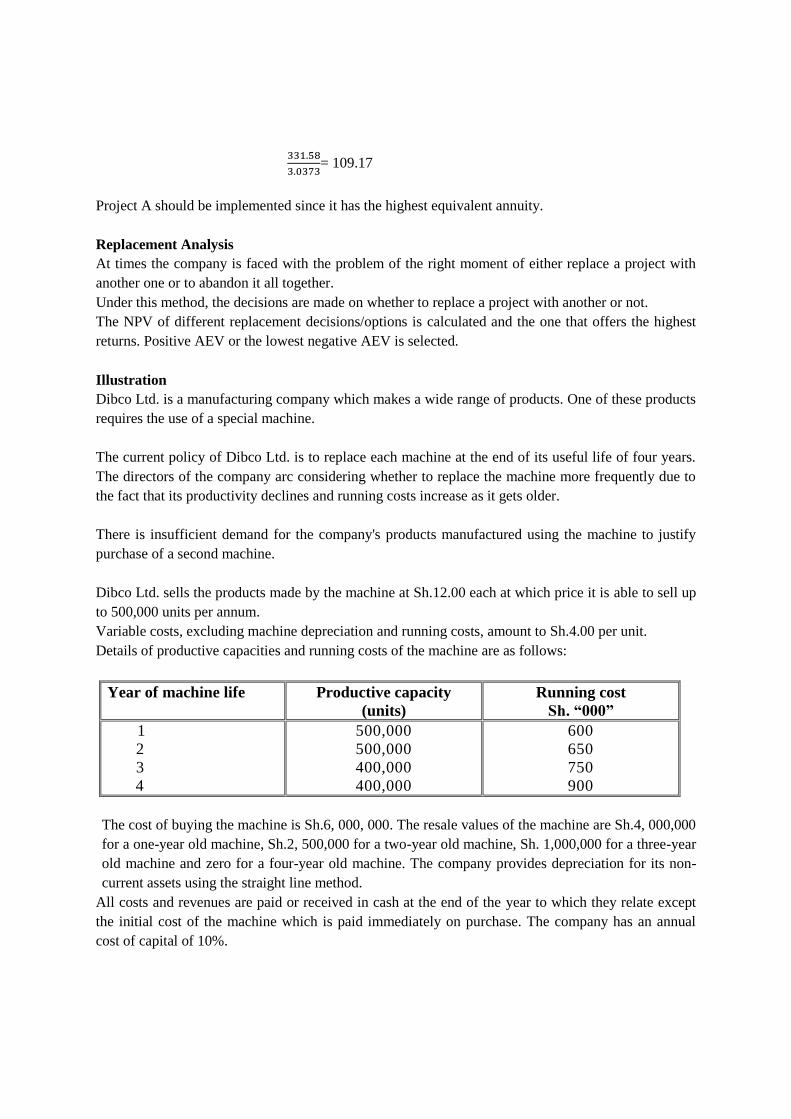
331.58
3.0373= 109.17
Project A should be implemented since it has the highest equivalent annuity.
Replacement Analysis
At times the company is faced with the problem of the right moment of either replace a project with
another one or to abandon it all together.
Under this method, the decisions are made on whether to replace a project with another or not.
The NPV of different replacement decisions/options is calculated and the one that offers the highest
returns. Positive AEV or the lowest negative AEV is selected.
Illustration
Dibco Ltd. is a manufacturing company which makes a wide range of products. One of these products
requires the use of a special machine.
The current policy of Dibco Ltd. is to replace each machine at the end of its useful life of four years.
The directors of the company arc considering whether to replace the machine more frequently due to
the fact that its productivity declines and running costs increase as it gets older.
There is insufficient demand for the company's products manufactured using the machine to justify
purchase of a second machine.
Dibco Ltd. sells the products made by the machine at Sh.12.00 each at which price it is able to sell up
to 500,000 units per annum.
Variable costs, excluding machine depreciation and running costs, amount to Sh.4.00 per unit.
Details of productive capacities and running costs of the machine are as follows:
Year of machine life Productive capacity
(units)
Running cost
Sh. “000”
1
2
3
4
500,000
500,000
400,000
400,000
600
650
750
900
The cost of buying the machine is Sh.6, 000, 000. The resale values of the machine are Sh.4, 000,000
for a one-year old machine, Sh.2, 500,000 for a two-year old machine, Sh. 1,000,000 for a three-year
old machine and zero for a four-year old machine. The company provides depreciation for its non-
current assets using the straight line method.
All costs and revenues are paid or received in cash at the end of the year to which they relate except
the initial cost of the machine which is paid immediately on purchase. The company has an annual
cost of capital of 10%.
Page 54
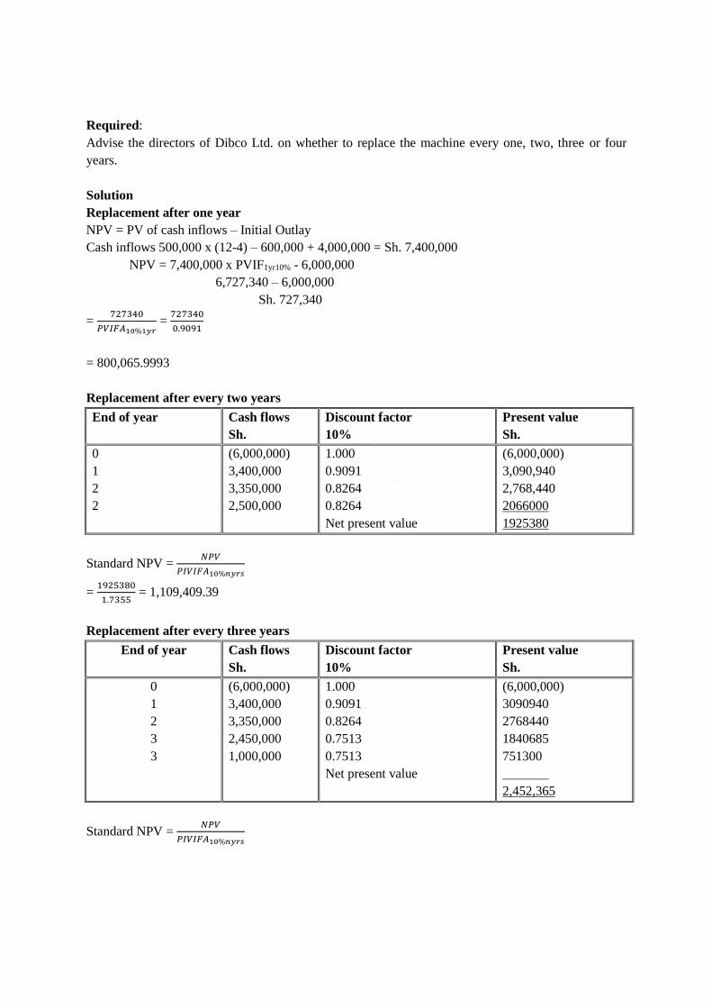
Required:
Advise the directors of Dibco Ltd. on whether to replace the machine every one, two, three or four
years.
Solution
Replacement after one year
NPV = PV of cash inflows – Initial Outlay
Cash inflows 500,000 x (12-4) – 600,000 + 4,000,000 = Sh. 7,400,000
NPV = 7,400,000 x PVIF1yr10% - 6,000,000
6,727,340 – 6,000,000
Sh. 727,340
= 727340
𝑃𝑉𝐼𝐹𝐴10%1𝑦𝑟 =
727340
0.9091
= 800,065.9993
Replacement after every two years
End of year Cash flows
Sh.
Discount factor
10%
Present value
Sh.
0
1
2
2
(6,000,000)
3,400,000
3,350,000
2,500,000
1.000
0.9091
0.8264
0.8264
Net present value
(6,000,000)
3,090,940
2,768,440
2066000
1925380
Standard NPV = 𝑁𝑃𝑉
𝑃𝐼𝑉𝐼𝐹𝐴10%𝑛𝑦𝑟𝑠
= 1925380
1.7355 = 1,109,409.39
Replacement after every three years
End of year Cash flows
Sh.
Discount factor
10%
Present value
Sh.
0
1
2
3
3
(6,000,000)
3,400,000
3,350,000
2,450,000
1,000,000
1.000
0.9091
0.8264
0.7513
0.7513
Net present value
(6,000,000)
3090940
2768440
1840685
751300
_______
2,452,365
Standard NPV = 𝑁𝑃𝑉
𝑃𝐼𝑉𝐼𝐹𝐴10%𝑛𝑦𝑟𝑠
Page 55
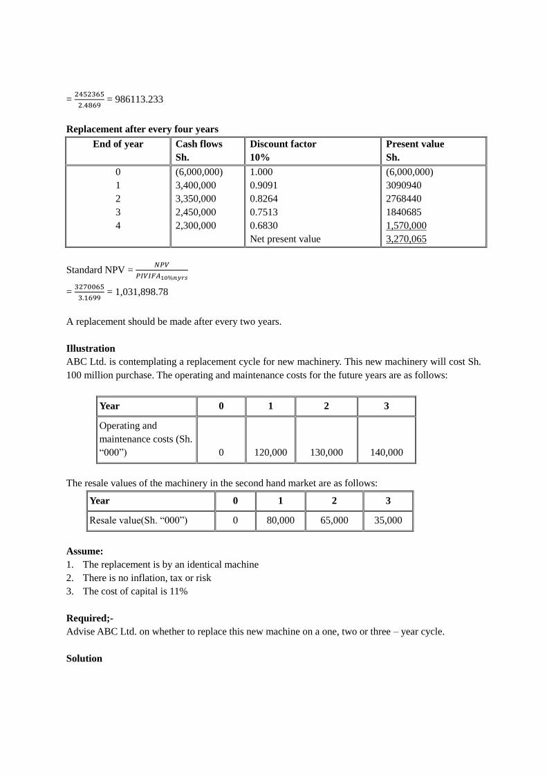
= 2452365
2.4869 = 986113.233
Replacement after every four years
End of year Cash flows
Sh.
Discount factor
10%
Present value
Sh.
0
1
2
3
4
(6,000,000)
3,400,000
3,350,000
2,450,000
2,300,000
1.000
0.9091
0.8264
0.7513
0.6830
Net present value
(6,000,000)
3090940
2768440
1840685
1,570,000
3,270,065
Standard NPV = 𝑁𝑃𝑉
𝑃𝐼𝑉𝐼𝐹𝐴10%𝑛𝑦𝑟𝑠
= 3270065
3.1699 = 1,031,898.78
A replacement should be made after every two years.
Illustration
ABC Ltd. is contemplating a replacement cycle for new machinery. This new machinery will cost Sh.
100 million purchase. The operating and maintenance costs for the future years are as follows:
Year 0 1 2 3
Operating and
maintenance costs (Sh.
“000”) 0 120,000 130,000 140,000
The resale values of the machinery in the second hand market are as follows:
Year 0 1 2 3
Resale value(Sh. “000”) 0 80,000 65,000 35,000
Assume:
1. The replacement is by an identical machine
2. There is no inflation, tax or risk
3. The cost of capital is 11%
Required;-
Advise ABC Ltd. on whether to replace this new machine on a one, two or three – year cycle.
Solution
Page 56
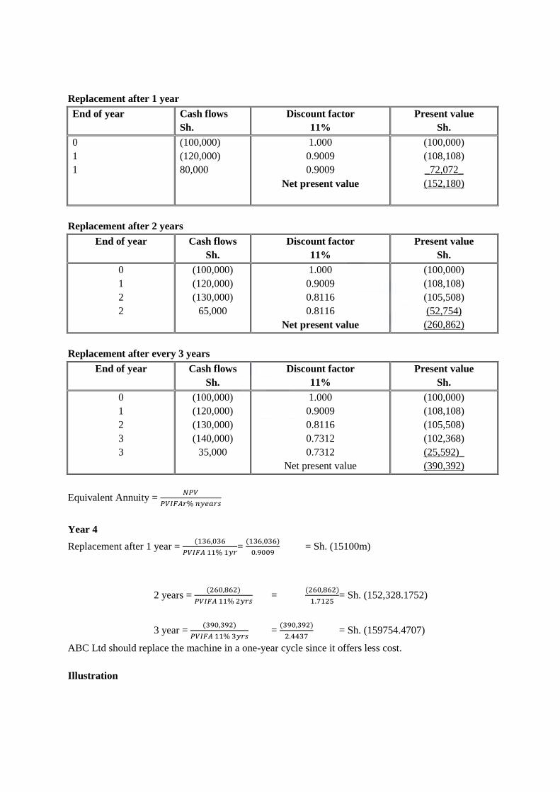
Replacement after 1 year
End of year Cash flows
Sh.
Discount factor
11%
Present value
Sh.
0
1
1
(100,000)
(120,000)
80,000
1.000
0.9009
0.9009
Net present value
(100,000)
(108,108)
_72,072_
(152,180)
Replacement after 2 years
End of year Cash flows
Sh.
Discount factor
11%
Present value
Sh.
0
1
2
2
(100,000)
(120,000)
(130,000)
65,000
1.000
0.9009
0.8116
0.8116
Net present value
(100,000)
(108,108)
(105,508)
(52,754)
(260,862)
Replacement after every 3 years
End of year Cash flows
Sh.
Discount factor
11%
Present value
Sh.
0
1
2
3
3
(100,000)
(120,000)
(130,000)
(140,000)
35,000
1.000
0.9009
0.8116
0.7312
0.7312
Net present value
(100,000)
(108,108)
(105,508)
(102,368)
(25,592)_
(390,392)
Equivalent Annuity = 𝑁𝑃𝑉
𝑃𝑉𝐼𝐹𝐴𝑟% 𝑛𝑦𝑒𝑎𝑟𝑠
Year 4
Replacement after 1 year = (136,036
𝑃𝑉𝐼𝐹𝐴 11% 1𝑦𝑟 =
(136,036)
0.9009 = Sh. (15100m)
2 years = (260,862)
𝑃𝑉𝐼𝐹𝐴 11% 2𝑦𝑟𝑠 =
(260,862)
1.7125= Sh. (152,328.1752)
3 year = (390,392)
𝑃𝑉𝐼𝐹𝐴 11% 3𝑦𝑟𝑠 =
(390,392)
2.4437 = Sh. (159754.4707)
ABC Ltd should replace the machine in a one-year cycle since it offers less cost.
Illustration
Page 57

Cosmos is evaluating two investments as follows: -
This is an investment in new machinery to produce a recently developed product. The cost of the
machinery which is payable immediately is sh.1.5 million, and the scrap value of the machinery at the
end of four years is expected to be sh.100,000. Capital allowances (tax-allowable depreciation) can be
claimed on this investment on a 25% reducing balance basis. Information on future returns from the
investment has been forecast to be as follows: -
Year 1 2 3 4
Sales volume(units/year)
Selling price (sh. unit)
Variable cost (sh. unit)
Fixed costs (sh./year)
50,000
20.00
10.00
105,000
95,000
24.00
11.00
115,000
140,000
23.00
12.00
125,000
75,000
23.00
12.50
125,000
This information must be adjusted to allow for selling price inflation of 4% per year and variable cost
inflation of 2.5% per year. Fixed costs, which are wholly attributable to the project, have already been
adjusted for inflation. Ridag Co pays profit tax of 30% per year one year in arrears.
Project 2
Cosmos plans to replace an existing machine and must choose between two machines. Machine 1 has
an initial cost of sh.200, 000 and will have a scrap value of sh. 25,000 after four years. Machine 2 has
an initial cost of sh.225, 000 and will have a scrap value of sh.50, 000 after three years. Annual
maintenance costs of the two machines are as follows:
Year 1 2 3 4
Machine 1 (sh./year)
Machine 2 (sh./year)
25,000
15,000
29,000
20,000
32,000
25,000
35,000
Where relevant, all information relating to Project 2 has already been adjusted to include expected
future inflation.
Taxation and capital allowances must be ignored in relation to Machine 1 and Machine 2.
Other information
Cosmos has a nominal before tax weighted average cost of 12% and a nominal after-tax weighted
average cost of capital of 7%.
Required;-
(i)Calculate the net present value of Project 1 and comment on whether this project is financially
acceptable to Cosmos Company.
(ii)Calculate the equivalent annual costs of Machine 1 and Machine 2 and discuss which machine
should be purchased.
(iii)Critically discuss the use of sensitivity analysis and probability as ways of including risk in the
investment appraisal process, referring in your answer to the relative effectiveness of each method.
Page 58
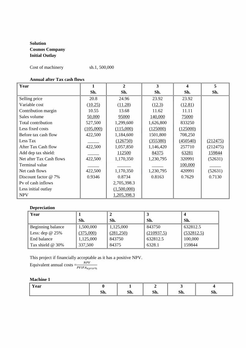
Solution
Cosmos Company
Initial Outlay
Cost of machinery sh.1, 500,000
Annual after Tax cash flows
Year 1
Sh.
2
Sh.
3
Sh.
4
Sh.
5
Sh.
Selling price
Variable cost
Contribution margin
Sales volume
Total contribution
Less fixed costs
Before tax cash flow
Less Tax
After Tax Cash flow
Add dep tax shield:
Net after Tax Cash flows
Terminal value
Net cash flows
Discount factor @ 7%
Pv of cash inflows
Less initial outlay
NPV
20.8
(10.25)
10.55
50,000
527,500
(105,000)
422,500
_____
422,500
_____
422,500
_____
422,500
0.9346
24.96
(11.28)
13.68
95000
1,299,600
(115,000)
1,184,600
(126750)
1,057,850
112500
1,170,350
______
1,170,350
0.8734
2,705,398.3
(1,500,000)
1,205,398.3
23.92
(12.3)
11.62
140,000
1,626,800
(125000)
1501,800
(355380)
1,146,420
84375
1,230,795
_____
1,230,795
0.8163
23.92
(12.81)
11.11
75000
833250
(125000)
708,250
(450540)
257710
63281
320991
100,000
420991
0.7629
(212475)
(212475)
159844
(52631)
_____
(52631)
0.7130
Depreciation
Year 1
Sh.
2
Sh.
3
Sh.
4
Sh.
Beginning balance
Less: dep @ 25%
End balance
Tax shield @ 30%
1,500,000
(375,000)
1,125,000
337,500
1,125,000
(281,250)
843750
84375
843750
(210937.5)
632812.5
6328.1
632812.5
(532812.5)
100,000
159844
This project if financially acceptable as it has a positive NPV.
Equivalent annual costs =𝑁𝑃𝑉
𝑃𝑉𝐼𝐹𝐴𝑛𝑦𝑟𝑠𝑟%
Machine 1
Year 0
Sh.
1
Sh.
2
Sh.
3
Sh.
4
Sh.
Page 59
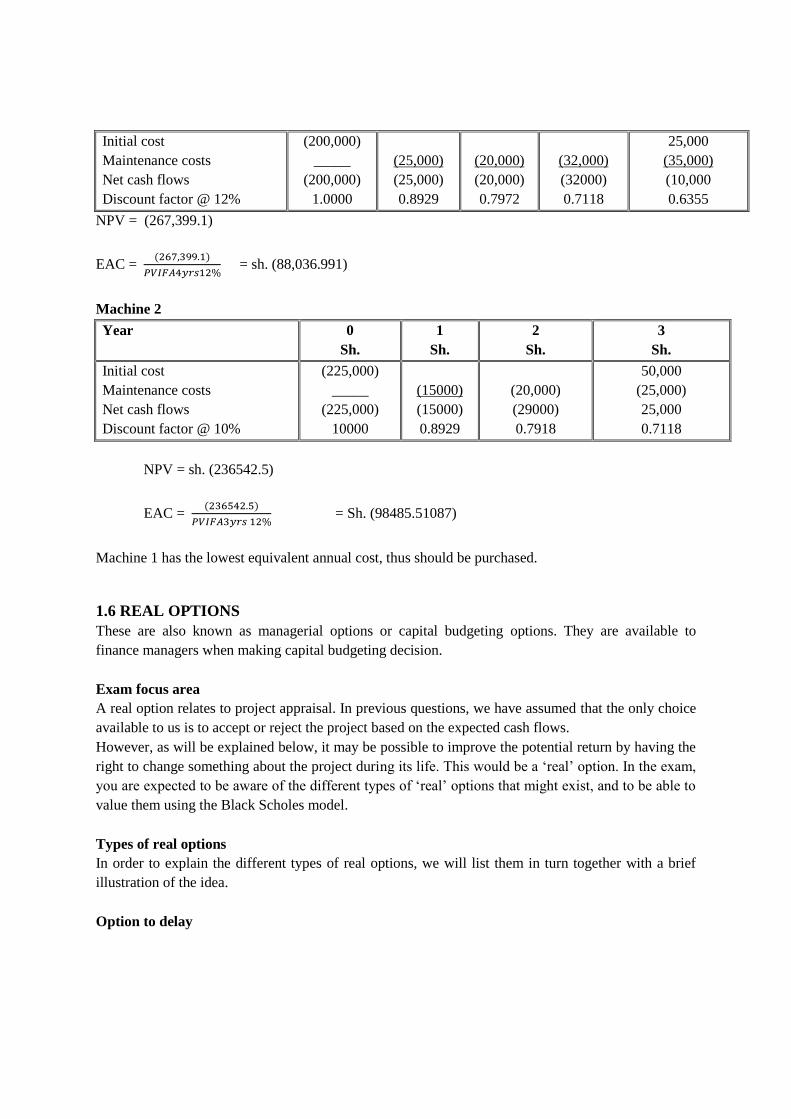
Initial cost
Maintenance costs
Net cash flows
Discount factor @ 12%
(200,000)
_____
(200,000)
1.0000
(25,000)
(25,000)
0.8929
(20,000)
(20,000)
0.7972
(32,000)
(32000)
0.7118
25,000
(35,000)
(10,000
0.6355
NPV = (267,399.1)
EAC = (267,399.1)
𝑃𝑉𝐼𝐹𝐴4𝑦𝑟𝑠12% = sh. (88,036.991)
Machine 2
Year 0
Sh.
1
Sh.
2
Sh.
3
Sh.
Initial cost
Maintenance costs
Net cash flows
Discount factor @ 10%
(225,000)
_____
(225,000)
10000
(15000)
(15000)
0.8929
(20,000)
(29000)
0.7918
50,000
(25,000)
25,000
0.7118
NPV = sh. (236542.5)
EAC = (236542.5)
𝑃𝑉𝐼𝐹𝐴3𝑦𝑟𝑠 12% = Sh. (98485.51087)
Machine 1 has the lowest equivalent annual cost, thus should be purchased.
1.6 REAL OPTIONS
These are also known as managerial options or capital budgeting options. They are available to
finance managers when making capital budgeting decision.
Exam focus area
A real option relates to project appraisal. In previous questions, we have assumed that the only choice
available to us is to accept or reject the project based on the expected cash flows.
However, as will be explained below, it may be possible to improve the potential return by having the
right to change something about the project during its life. This would be a ‘real’ option. In the exam,
you are expected to be aware of the different types of ‘real’ options that might exist, and to be able to
value them using the Black Scholes model.
Types of real options
In order to explain the different types of real options, we will list them in turn together with a brief
illustration of the idea.
Option to delay
Page 60
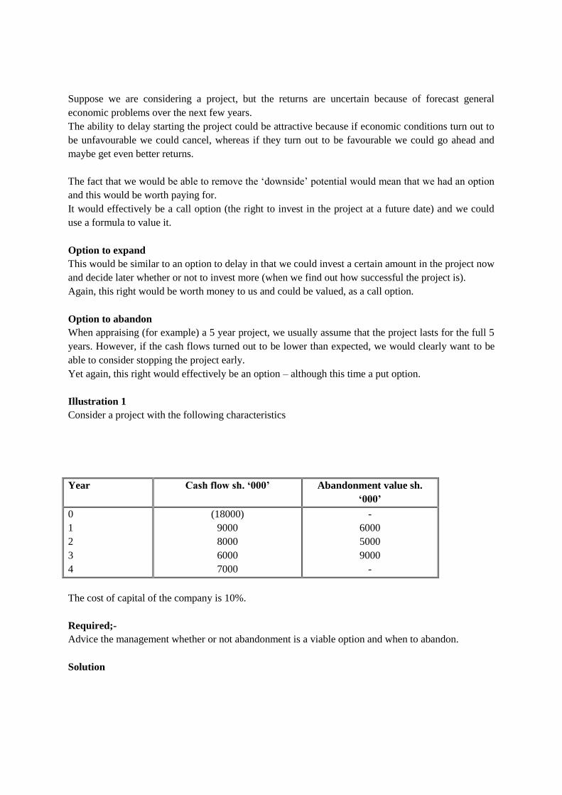
Suppose we are considering a project, but the returns are uncertain because of forecast general
economic problems over the next few years.
The ability to delay starting the project could be attractive because if economic conditions turn out to
be unfavourable we could cancel, whereas if they turn out to be favourable we could go ahead and
maybe get even better returns.
The fact that we would be able to remove the ‘downside’ potential would mean that we had an option
and this would be worth paying for.
It would effectively be a call option (the right to invest in the project at a future date) and we could
use a formula to value it.
Option to expand
This would be similar to an option to delay in that we could invest a certain amount in the project now
and decide later whether or not to invest more (when we find out how successful the project is).
Again, this right would be worth money to us and could be valued, as a call option.
Option to abandon
When appraising (for example) a 5 year project, we usually assume that the project lasts for the full 5
years. However, if the cash flows turned out to be lower than expected, we would clearly want to be
able to consider stopping the project early.
Yet again, this right would effectively be an option – although this time a put option.
Illustration 1
Consider a project with the following characteristics
Year Cash flow sh. ‘000’ Abandonment value sh.
‘000’
0
1
2
3
4
(18000)
9000
8000
6000
7000
-
6000
5000
9000
-
The cost of capital of the company is 10%.
Required;-
Advice the management whether or not abandonment is a viable option and when to abandon.
Solution
Page 61
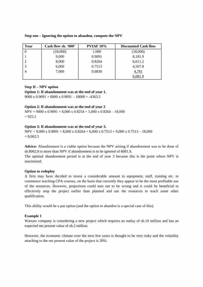
Step one – Ignoring the option to abandon, compute the NPV
Year Cash flow sh. ‘000’ PVIAF 10% Discounted Cash flow
0
1
2
3
4
(18,000)
9,000
8,000
6,000
7,000
1.000
0.9091
0.8264
0.7513
0.6830
(18,000)
8,181.9
6,611.2
4,507.8
4,781
6,081.9
Step II – NPV option
Option 1: If abandonment was at the end of year 1.
9000 x 0.9091 + 6000 x 0.9091 – 18000 = -4363.5
Option 2: If abandonment was at the end of year 2
NPV = 9000 x 0.9091 + 8,000 x 0.8254 + 5,000 x 0.8264 – 18,000
= 925.1
Option 3: If abandonment was at the end of year 3.
NPV = 9,000 x 0.9091 + 8,000 x 0.8264 + 6,000 x 0.7513 + 9,000 x 0.7513 – 18,000
= 8,062.5
Advice: Abandonment is a viable option because the NPV arising if abandonment was to be done of
sh.8062.8 is more than NPV if abandonment is to be ignored of 6081.9.
The optimal abandonment period is at the end of year 3 because this is the point where NPV is
maximized.
Option to redeploy
A firm may have decided to invest a considerable amount in equipment, staff, training etc. to
commence teaching CPA courses, on the basis that currently they appear to be the most profitable use
of the resources. However, projections could turn out to be wrong and it could be beneficial to
effectively stop the project earlier than planned and use the resources to teach some other
qualification.
This ability would be a put option (and the option to abandon is a special case of this).
Example 1
Warsaw company is considering a new project which requires an outlay of sh.10 million and has an
expected net present value of sh.2 million.
However, the economic climate over the next few years is thought to be very risky and the volatility
attaching to the net present value of the project is 20%.
Page 62

Warsaw is able to delay commencing the project for three years.
The risk free rate of interest is 6% p.a.
Estimate the value of the option to delay the start of the project for three years, using the
Black Scholes option pricing model.
Solution
P = current P.V. of project = sh.12 M [NPV = PV – Initial outlay therefore PV = NPV + Initial outlay)
E = capital expenditure = sh.10M
t = 3 years
r = 6%
σ = 20%
d1=𝐼𝑛(𝑃/𝐸)+(𝑟+0.5𝜎2)𝑇
𝜎√𝑇
d1 = 𝐼𝑛(
12
10)+ (0.06+0.5 𝑥(0.2)2)𝑥 3
0.20 𝑥√3
= 0.1823+0.24
0.3464 = 1.22
d2 = 1.22 – 0.2 x √3 = 0.87
N(d1) = 0.5 + 0.3888 = 0.8888
N(d2) = 0.5 + 0.3078 = 0.8078
C = Pnd1- 𝐸𝑛𝑑2
𝑒𝑟𝑡
C= 12 x 0.8888 – 10 × 0.8078
𝑒0.06×3
= sh.3.92M
Therefore the total project value = NPV of project without option value + Option value
= 2 + 3.92 = sh.5.92m
Strategic Investment option – This is where the management undertakes a project irrespective of the
net present value since undertaking the project can give rise to new opportunities.
REPLACEMENT ANALYSIS
Decision regarding replacement of an existing asset with another is based on the net present value and
internal rate of return of the incremental cash flows, i.e. the difference between periodic net cash
flows if the existing asset is kept and the periodic net cash flows if the asset is replaced.
In capital budgeting and engineering economics, the existing asset is called the defender and the asset,
which is proposed to replace the defender, is called the challenger. Estimation of incremental cash
C = Value of a call option
Page 63
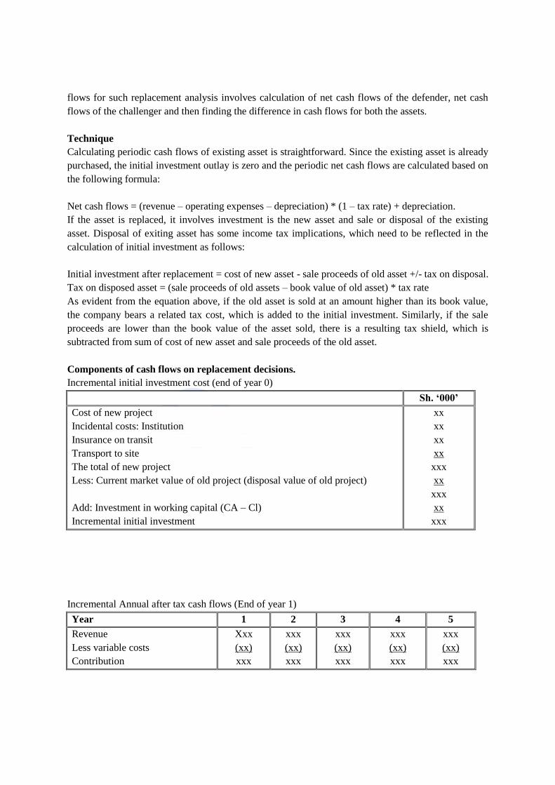
flows for such replacement analysis involves calculation of net cash flows of the defender, net cash
flows of the challenger and then finding the difference in cash flows for both the assets.
Technique
Calculating periodic cash flows of existing asset is straightforward. Since the existing asset is already
purchased, the initial investment outlay is zero and the periodic net cash flows are calculated based on
the following formula:
Net cash flows = (revenue – operating expenses – depreciation) * (1 – tax rate) + depreciation.
If the asset is replaced, it involves investment is the new asset and sale or disposal of the existing
asset. Disposal of exiting asset has some income tax implications, which need to be reflected in the
calculation of initial investment as follows:
Initial investment after replacement = cost of new asset - sale proceeds of old asset +/- tax on disposal.
Tax on disposed asset = (sale proceeds of old assets – book value of old asset) * tax rate
As evident from the equation above, if the old asset is sold at an amount higher than its book value,
the company bears a related tax cost, which is added to the initial investment. Similarly, if the sale
proceeds are lower than the book value of the asset sold, there is a resulting tax shield, which is
subtracted from sum of cost of new asset and sale proceeds of the old asset.
Components of cash flows on replacement decisions.
Incremental initial investment cost (end of year 0)
Sh. ‘000’
Cost of new project
Incidental costs: Institution
Insurance on transit
Transport to site
The total of new project
Less: Current market value of old project (disposal value of old project)
Add: Investment in working capital (CA – Cl)
Incremental initial investment
xx
xx
xx
xx
xxx
xx
xxx
xx
xxx
Incremental Annual after tax cash flows (End of year 1)
Year 1 2 3 4 5
Revenue
Less variable costs
Contribution
Xxx
(xx)
xxx
xxx
(xx)
xxx
xxx
(xx)
xxx
xxx
(xx)
xxx
xxx
(xx)
xxx
Page 64
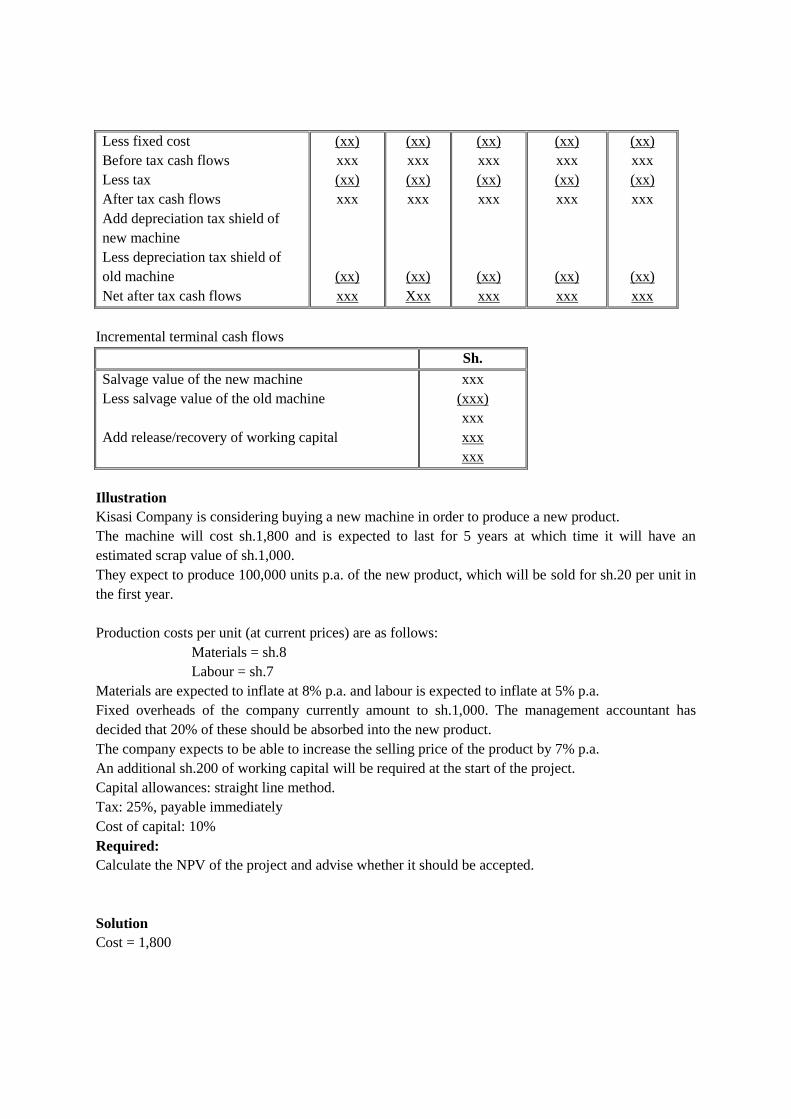
Less fixed cost
Before tax cash flows
Less tax
After tax cash flows
Add depreciation tax shield of
new machine
Less depreciation tax shield of
old machine
Net after tax cash flows
(xx)
xxx
(xx)
xxx
(xx)
xxx
(xx)
xxx
(xx)
xxx
(xx)
Xxx
(xx)
xxx
(xx)
xxx
(xx)
xxx
(xx)
xxx
(xx)
xxx
(xx)
xxx
(xx)
xxx
(xx)
xxx
(xx)
xxx
Incremental terminal cash flows
Sh.
Salvage value of the new machine
Less salvage value of the old machine
Add release/recovery of working capital
xxx
(xxx)
xxx
xxx
xxx
Illustration
Kisasi Company is considering buying a new machine in order to produce a new product.
The machine will cost sh.1,800 and is expected to last for 5 years at which time it will have an
estimated scrap value of sh.1,000.
They expect to produce 100,000 units p.a. of the new product, which will be sold for sh.20 per unit in
the first year.
Production costs per unit (at current prices) are as follows:
Materials = sh.8
Labour = sh.7
Materials are expected to inflate at 8% p.a. and labour is expected to inflate at 5% p.a.
Fixed overheads of the company currently amount to sh.1,000. The management accountant has
decided that 20% of these should be absorbed into the new product.
The company expects to be able to increase the selling price of the product by 7% p.a.
An additional sh.200 of working capital will be required at the start of the project.
Capital allowances: straight line method.
Tax: 25%, payable immediately
Cost of capital: 10%
Required:
Calculate the NPV of the project and advise whether it should be accepted.
Solution
Cost = 1,800
Page 65
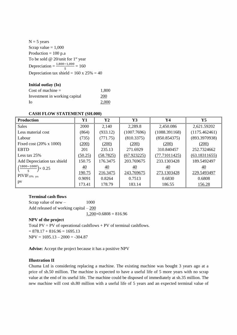
N = 5 years
Scrap value = 1,000
Production = 100 p.a
To be sold @ 20/unit for 1st year
Depreciation = 1,800−1,000
5 = 160
Depreciation tax shield = 160 x 25% = 40
Initial outlay (Io)
Cost of machine = 1,800
Investment in working capital 200
Io 2,000
CASH FLOW STATEMENT (SH.000)
Production Y1 Y2 Y3 Y4 Y5
Sales
Less material cost
Labour
Fixed cost (20% x 1000)
EBTD
Less tax 25%
Add Depreciation tax shield
(1800−1000
5)× 0.25
PIVIF10% yrs
pv
2000
(864)
(735)
(200)
201
(50.25)
150.75
40
190.75
0.9091
173.41
2,140
(933.12)
(771.75)
(200)
235.13
(58.7825)
176.3475
40
216.3475
0.8264
178.79
2,289.8
(1007.7696)
(810.3375)
(200)
271.6929
(67.923225)
203.769675
40
243.769675
0.7513
183.14
2,450.086
(1088.391168)
(850.854375)
(200)
310.840457
(77.71011425)
233.1303428
40
273.1303428
0.6830
186.55
2,621.59202
(1175.462461)
(893.3970938)
(200)
252.7324662
(63.18311655)
189.5492497
40
229.5493497
0.6808
156.28
Terminal cash flows
Scrap value of new – 1000
Add released of working capital – 200
1,200×0.6808 = 816.96
NPV of the project
Total PV = PV of operational cashflows + PV of terminal cashflows.
= 878.17 + 816.96 = 1695.13
NPV = 1695.13 – 2000 = -304.87
Advise: Accept the project because it has a positive NPV
Illustration II
Chuma Ltd is considering replacing a machine. The existing machine was bought 3 years ago at a
price of sh.50 million. The machine is expected to have a useful life of 5 more years with no scrap
value at the end of its useful life. The machine could be disposed of immediately at sh.35 million. The
new machine will cost sh.80 million with a useful life of 5 years and an expected terminal value of
Page 66
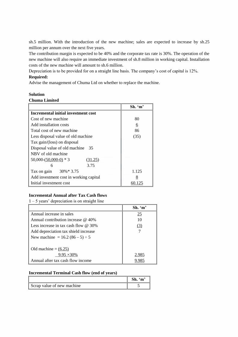
sh.5 million. With the introduction of the new machine; sales are expected to increase by sh.25
million per annum over the next five years.
The contribution margin is expected to be 40% and the corporate tax rate is 30%. The operation of the
new machine will also require an immediate investment of sh.8 million in working capital. Installation
costs of the new machine will amount to sh.6 million.
Depreciation is to be provided for on a straight line basis. The company’s cost of capital is 12%.
Required:
Advise the management of Chuma Ltd on whether to replace the machine.
Solution
Chuma Limited
Incremental Annual after Tax Cash flows
1 – 5 years’ depreciation is on straight line
Sh. ‘m’
Annual increase in sales
Annual contribution increase @ 40%
Less increase in tax cash flow @ 30%
Add depreciation tax shield increase
New machine = 16.2 (86 – 5) ÷ 5
Old machine = (6.25)
9.95 ×30%
Annual after tax cash flow income
25
10
(3)
7
2.985
9.985
Incremental Terminal Cash flow (end of years)
Sh. ‘m’
Scrap value of new machine 5
Sh. ‘m’
Incremental initial investment cost
Cost of new machine
Add installation costs
Total cost of new machine
Less disposal value of old machine
Tax gain/(loss) on disposal
Disposal value of old machine 35
NBV of old machine
50,000-(50,000-0) * 3 (31.25)
6 3.75
Tax on gain 30%* 3.75
Add investment cost in working capital
Initial investment cost
80
6
86
(35)
1.125
8
60.125
Page 67

Less scrap value of old machine
Add release of working capital
(0)
8
13
Net Present Value = PV of Cash inflows – Initial Outlays
= 9.985×PVIFA 5yrs12% + 13 ×PVIF 5 yrs 12% - 60.125
9.985×3.6048 + 13 ×0.5674 – 60.125
35.993928 + 7.3762 – 60.125 = (Sh. 16.754872m)
Chuma Ltd should not replace the machine, as it would result into a negative NPV thus minimising
the shareholders’ wealth.
Page 68

CHAPTER TWO
PORTFOLIO THEORY AND ANALYSIS CHAPTER KEY OBJECTIVES
To be able to understand the following
1. The modern portfolio theory: background of the theory; portfolio expected return; the actual and
weighted portfolio risk; derivation of efficient sets; the capital market line (CML) model and its
applications, the mean variance dominance rule; short comings of portfolio theory
2. Capital Asset Pricing Model-CAPM : background of the theory; assumptions; beta estimation -
beta coefficient of an individual asset and that of a portfolio and the interpretation of the result;
security market line(SML) model and its applications; conceptual differences between portfolio
theory and capital asset pricing model
3. Shortcomings of the capital asset pricing model
4. The Arbitrage pricing model (APM) and other multifactor models: background of the theory;
conceptual differences between the Capital asset pricing model and the Arbitrage pricing model;
application of the Arbitrage pricing model, shortcomings of Arbitrage pricing model; Pastor
Stambaugh model
5. Evaluation of portfolio performance: Treynor’s measure, Sharpe’s measure, Jensen’s measure,
appraisal ratio measure, information ratio, Modigliani and Modigliani (M2)
2.1 THE MODERN PORTFOLIO THEORY
A portfolio refers to a combination of investments held together by an investor in a firm.
Portfolio may include:
- Financial assets /securities e.g. ordinary shares, preference shares, debentures or bonds.
- Physical/tangible assets i.e. equipment, real estate etc.
An investor shall combine the assets with the main objectives of minimising the overall risk and
maximising total returns.
A company will always experience two types of risk i.e.
- Financial risk
- Business risk
Financial Risk
It is the risk associated with the use of debt/capital with fixed returns in the company’s capital
structure.
It is also known as gearing/leverage risk and is measured by use of gearing ratio i.e.
Gearing Ratio = 𝐶𝑊𝐹𝑅
𝐶𝑊𝐹𝑅+𝐶𝑊𝑉𝑅× 100
Page 69
CWFR – Capital with fixed returns (long term debt /debentures
CWVR – Capital with variable returns (ordinary shares i.e. common equity capital)
Business Risk/Operating Risk
This is a combination of;
a) Unsystematic Risk
b) Systematic Risk
Unsystematic Risk
It is a risk that is unique to individual firms in the industry and can be eliminated/reduced through
diversification of investment portfolio.
Due to its diversifiable nature, it is therefore not incorporated in investment appraisal since a company
can avoid it e.g. poor employee remuneration, industrial strikes, poor marketing.
Unsystematic risk factors don't affect everyone; indeed, their impact may be unique to an individual
company or restricted to a small number of companies, with some being winners and some being
losers. For example, the weather – if we have a wet summer then raincoat manufacturers will benefit
but sunglasses manufacturers will suffer. However, for the majority of businesses, it will not make
any difference. Overall, the stock market is unlikely to be affected much by the weather.
Can be measured by the standard deviation
Systematic Risk
It refers to variability in returns of securities cash flows due to factors that affect the firms in the
industry e.g. political instability, inflation, higher lending rates etc.
Due to its undiversifiable nature, it is therefore incorporated in investment appraisal and it is
measured using beta factor 𝛽.
Systematic risk will affect all companies in the same way (although to varying degrees). For example,
the vast majority of companies suffer in a recession but not necessarily to the same extent – e.g.
house-builders typically suffer more than bakers do.
This explains why diversification works, typically there will be winners and losers regarding a
particular risk factor but when combined in a portfolio, the impact is cancelled out. Diversification
can almost eliminate unsystematic risk, but since all investments are affected in the same way by
macroeconomic i.e. systematic factors, the systematic risk of the portfolio remains.
The ability of investors to diversify away unsystematic risk by holding portfolios consisting of a
number of different shares is the cornerstone of portfolio theory.
Page 70
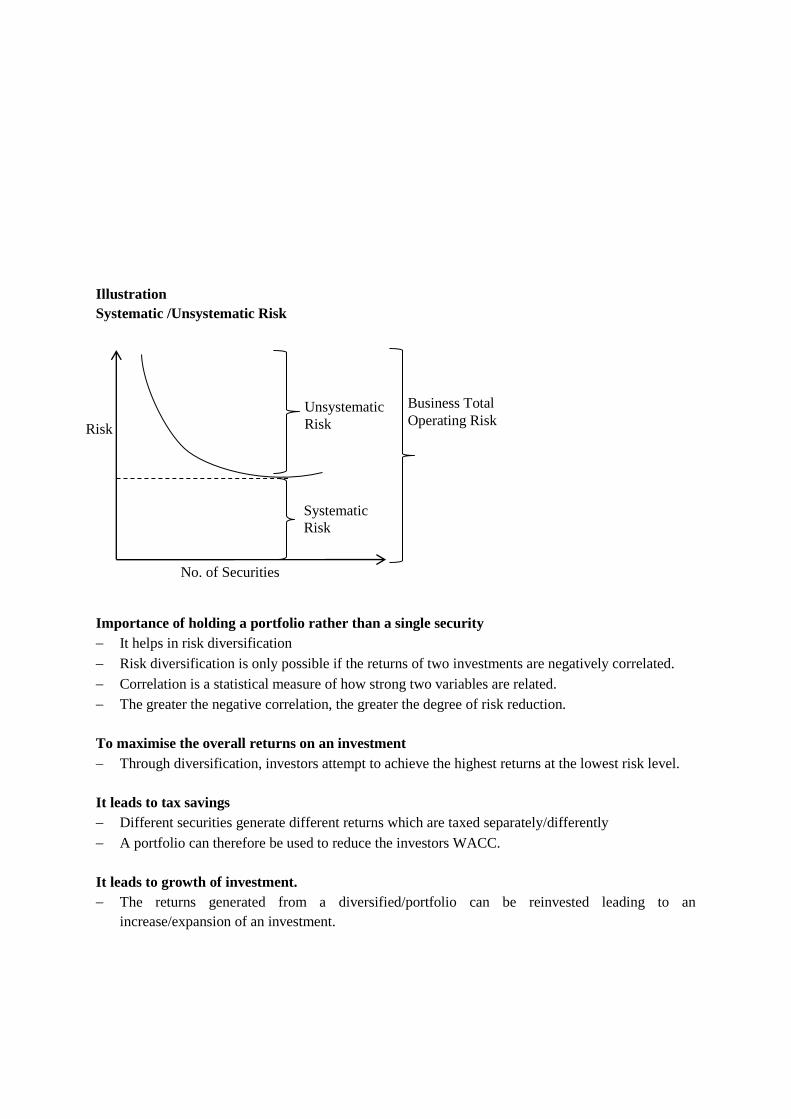
Illustration
Systematic /Unsystematic Risk
Importance of holding a portfolio rather than a single security
It helps in risk diversification
Risk diversification is only possible if the returns of two investments are negatively correlated.
Correlation is a statistical measure of how strong two variables are related.
The greater the negative correlation, the greater the degree of risk reduction.
To maximise the overall returns on an investment
Through diversification, investors attempt to achieve the highest returns at the lowest risk level.
It leads to tax savings
Different securities generate different returns which are taxed separately/differently
A portfolio can therefore be used to reduce the investors WACC.
It leads to growth of investment.
The returns generated from a diversified/portfolio can be reinvested leading to an
increase/expansion of an investment.
Unsystematic
Risk
Systematic
Risk
No. of Securities
Risk
Business Total
Operating Risk
Page 71
It promotes marketability and liquidity of an investor’s assets.
Securities in the portfolio tend to have a ready market due to its publicity and can therefore be
easily converted into cash without losing value.
Weaknesses of Portfolio Theory
1. It considers total risk as measured by standard deviation. In real sense, some risk is diversified
once a portfolio is formed.
2. It uses historical data in analysing the portfolios.
More so, the associated probabilities are not objectively determined.
3. It ignores economies of scale that may arise if more securities are combined together.
It only incorporates the risk reduction and the maximisation of returns.
4. It uses indifference curves in measuring the satisfaction of investors (investors utility) which is
not always practical. It is too theoretical.
5. It assumes that all investors are risk averse such that they would only be willing to increase their
investments if they are promised some returns.
6. It assumes that all projects are divisible. But in reality some projects are indivisible.
Factors Affecting Efficiency of a Good Portfolio
i) Number of securities forming the portfolio
The large the number of securities, the more efficient the portfolio would be.
ii) Correlation between securities in the portfolio i.e. how related the securities in a portfolio are.
iii) The proportions/weight of each security in the portfolio.
In measuring correlation between returns of two securities, co-variance is used.
COV (A, B) = ∑ (RA – ERA) (RB – ERB) P
COV (A, B) = Co-variance between securities A & B
ERA Expected Returns of Security A
ERB Expected Returns of Security B
RA Returns of A
RB Returns of B
Covariance would be negative for a negative correlation (Good portfolio) and it would be positive for
a positive correlation (Inefficient portfolio).
To measure the strength of the association between returns of different securities, we use correlation
coefficient ℓ (A,B)
ℓ(A,B) = 𝐶𝑂𝑉 (𝐴,𝐵)
𝛿𝐴𝑥𝛿𝐵
NB
(i) If ℓ (A,B) is negative, risk would be reduced when a portfolio is formed.
(ii) If ℓ A,B is positive, portfolio formation would not reduce the risk.
Page 72
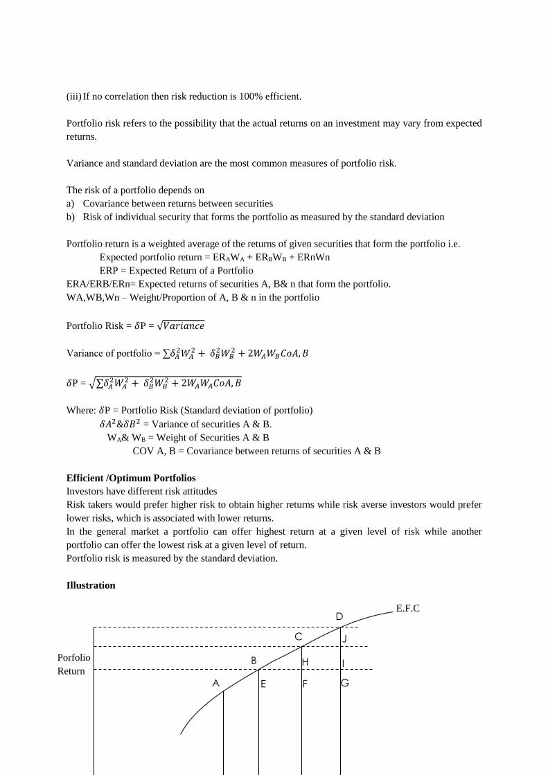
(iii) If no correlation then risk reduction is 100% efficient.
Portfolio risk refers to the possibility that the actual returns on an investment may vary from expected
returns.
Variance and standard deviation are the most common measures of portfolio risk.
The risk of a portfolio depends on
a) Covariance between returns between securities
b) Risk of individual security that forms the portfolio as measured by the standard deviation
Portfolio return is a weighted average of the returns of given securities that form the portfolio i.e.
Expected portfolio return = ERAWA + ERBWB + ERnWn
ERP = Expected Return of a Portfolio
ERA/ERB/ERn= Expected returns of securities A, B& n that form the portfolio.
WA,WB,Wn – Weight/Proportion of A, B & n in the portfolio
Portfolio Risk = 𝛿P = √𝑉𝑎𝑟𝑖𝑎𝑛𝑐𝑒
Variance of portfolio = ∑𝛿𝐴2𝑊𝐴
2 + 𝛿𝐵2𝑊𝐵
2 + 2𝑊𝐴𝑊𝐵𝐶𝑜𝐴, 𝐵
𝛿P = √∑𝛿𝐴2𝑊𝐴
2 + 𝛿𝐵2𝑊𝐵
2 + 2𝑊𝐴𝑊𝐴𝐶𝑜𝐴, 𝐵
Where: 𝛿P = Portfolio Risk (Standard deviation of portfolio)
𝛿𝐴2&𝛿𝐵2 = Variance of securities A & B.
WA& WB = Weight of Securities A & B
COV A, B = Covariance between returns of securities A & B
Efficient /Optimum Portfolios
Investors have different risk attitudes
Risk takers would prefer higher risk to obtain higher returns while risk averse investors would prefer
lower risks, which is associated with lower returns.
In the general market a portfolio can offer highest return at a given level of risk while another
portfolio can offer the lowest risk at a given level of return.
Portfolio risk is measured by the standard deviation.
Illustration
A
B
C
D
J
I
G
H
F E
E.F.C
Porfolio
Return
Page 73
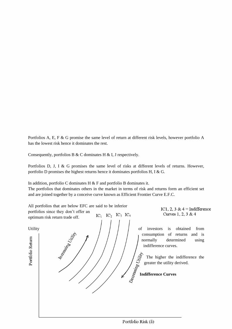
Portfolios A, E, F & G promise the same level of return at different risk levels, however portfolio A
has the lowest risk hence it dominates the rest.
Consequently, portfolios B & C dominates H & I, J respectively.
Portfolios D, J, I & G promises the same level of risks at different levels of returns. However,
portfolio D promises the highest returns hence it dominates portfolios H, I & G.
In addition, portfolio C dominates H & F and portfolio B dominates it.
The portfolios that dominates others in the market in terms of risk and returns form an efficient set
and are joined together by a conceive curve known as Efficient Frontier Curve E.F.C.
All portfolios that are below EFC are said to be inferior
portfolios since they don’t offer an
optimum risk return trade off.
Utility of investors is obtained from
consumption of returns and is
normally determined using
indifference curves.
The higher the indifference the
greater the utility derived.
Indifference Curves
Page 74
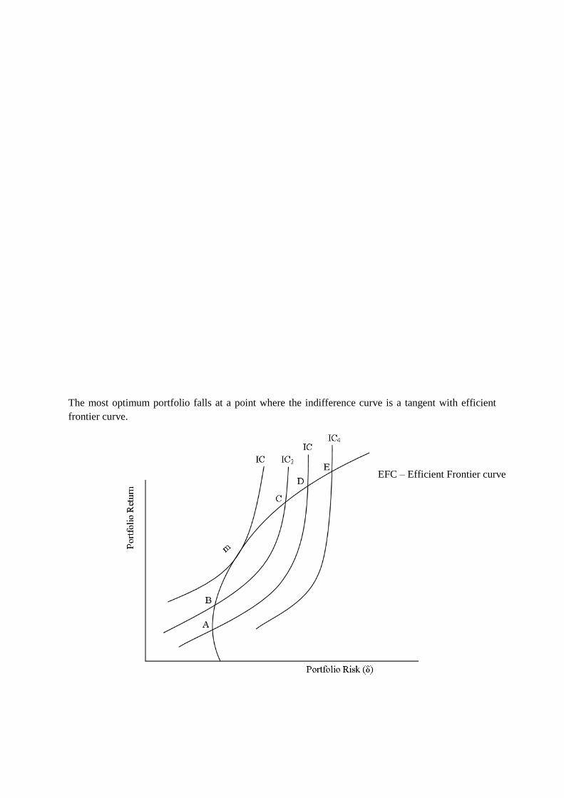
The most optimum portfolio falls at a point where the indifference curve is a tangent with efficient
frontier curve.
EFC – Efficient Frontier curve
Page 75
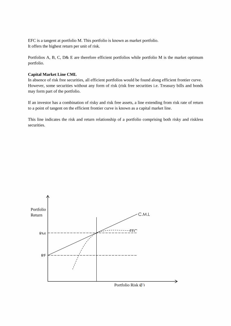
EFC is a tangent at portfolio M. This portfolio is known as market portfolio.
It offers the highest return per unit of risk.
Portfolios A, B, C, D& E are therefore efficient portfolios while portfolio M is the market optimum
portfolio.
Capital Market Line CML
In absence of risk free securities, all efficient portfolios would be found along efficient frontier curve.
However, some securities without any form of risk (risk free securities i.e. Treasury bills and bonds
may form part of the portfolio.
If an investor has a combination of risky and risk free assets, a line extending from risk rate of return
to a point of tangent on the efficient frontier curve is known as a capital market line.
This line indicates the risk and return relationship of a portfolio comprising both risky and riskless
securities.
Portfolio Risk ( )
Portfolio
Return C.M.L
EFC
RF
RM
Page 76
The difference between expected market return and risk free rate of return is the extra return an
investor receives for accepting additional risks (Risk Premium)
The capital market line equation is an equation in the form of y = a + bx
Where
Y = dependent variable required rate of return
A – y when x = 0, risk free rate
B – gradient Δ𝑦
Δ𝑥,
The Risk Premium/Unit of Risk can be determined by calculating the gradient of capital market line
i.e.
Gradient = ∆𝑦
∆𝑥 ,
𝑅𝑀−𝑅𝐹
𝛿𝑚
Risk Premium = 𝑅𝑀−𝑅𝐹
𝛿𝑚
% of Risk Premium = [𝑅𝑀−𝑅𝐹
𝛿𝑀] 𝛿𝑃
Required Returns = RF + Risk Premium
Required Portfolio Return = RF + [𝑅𝑀−𝑅𝐹
𝛿𝑀] 𝛿𝑃
RF – Risk Free Rate of Return
RM – Required Market Return
𝛿𝑀 – Standard deviation of the market
𝛿𝑃 – Standard deviation of the portfolio
The above equation is known as Capital Market Line Equation.
Conclusion
If a portfolio falls above the capital market line such portfolio is undervalued.
If a portfolio falls below the capital market line, such portfolio is overvalued.
If a portfolio falls along the capital market line, such portfolio is correctly valued.
An undervalued portfolio is a super-efficient portfolio overvalued portfolio is an inefficient portfolio
while correctly portfolio is efficient portfolio.
Illustration
An investor has the choice of the following share investments:
Share
Risk (σ) Expected return
Page 77
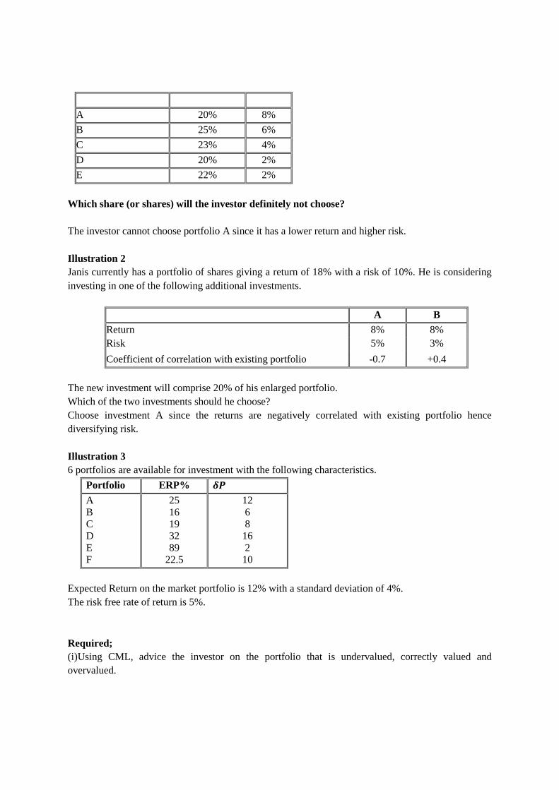
A 20% 8%
B 25% 6%
C 23% 4%
D 20% 2%
E 22% 2%
Which share (or shares) will the investor definitely not choose?
The investor cannot choose portfolio A since it has a lower return and higher risk.
Illustration 2
Janis currently has a portfolio of shares giving a return of 18% with a risk of 10%. He is considering
investing in one of the following additional investments.
A B
Return 8% 8%
Risk 5% 3%
Coefficient of correlation with existing portfolio -0.7 +0.4
The new investment will comprise 20% of his enlarged portfolio.
Which of the two investments should he choose?
Choose investment A since the returns are negatively correlated with existing portfolio hence
diversifying risk.
Illustration 3
6 portfolios are available for investment with the following characteristics.
Portfolio ERP% 𝜹𝑷
A
B
C
D
E
F
25
16
19
32
89
22.5
12
6
8
16
2
10
Expected Return on the market portfolio is 12% with a standard deviation of 4%.
The risk free rate of return is 5%.
Required;
(i)Using CML, advice the investor on the portfolio that is undervalued, correctly valued and
overvalued.
Page 78

(ii)In case of an inefficient portfolio in (i) above, determine the standard deviation that should be
achieved for efficiency to be arrived at.
Solution
CML = RF + [𝑅𝑀−𝑅𝐹
𝛿𝑀] 𝛿𝑃
Required Return ERP Comment
A = 5 + [12−5
4] 12 = 26%
B = 5 + [12−5
4] 6 = 15.5%
C = 5 + [12−5
4] 8 = 19%
D = 5 + [12−5
4] 16 = 33%
E = 5 + [12−5
4] 2 = 8.5%
F = 5 + [12−5
4] 10 =22.5%
25%
16%
19%
32%
8.9%
22.5%
Overvalued
Undervalued
Correctly valued
Overvalued
Undervalued
Correctly valued
Portfolios A and D are inefficient since they are overvalued. The standard deviation of these
portfolios that would make them efficient is:
A 5 + [12−5
4] x = 25
5 + 175x = 25 𝛿𝑃 1.75𝑥
1.75 =
25−5
1.75 x = 11.43%
D 5 + [12−5
4] x = 32 𝛿𝑃
1.75𝑥
1.75 =
32 −5
1.75 = x = 15.43%
Mean-Variance Analysis
Mean-variance analysis is the process of weighing risk, expressed as variance, against expected
return. Investors use mean-variance analysis to make decisions about which financial instruments to
invest in, based on how much risk they are willing to take on in exchange for different levels of
reward. Mean-variance analysis allows investors to find the biggest reward at a given level of risk or
the least risk at a given level of return.
Page 79
Return per unit of risk = 𝐸𝑥𝑝𝑒𝑐𝑡𝑒𝑑 𝑝𝑜𝑟𝑡𝑓𝑜𝑙𝑖𝑜 𝑟𝑒𝑡𝑢𝑟𝑛
𝑆𝑡𝑎𝑛𝑑𝑎𝑟𝑑 𝑑𝑒𝑣𝑖𝑎𝑡𝑖𝑜𝑛 𝑜𝑓 𝑝𝑜𝑟𝑡𝑓𝑜𝑙𝑖𝑜
Minimum variance portfolio
Definition: A minimum variance portfolio indicates a well-diversified portfolio that consists of
individually risky assets, which are hedged when traded together, resulting in the lowest possible risk
for the rate of expected return.
If we want to find the exact minimum variance portfolio allocation for these two assets, we can use
the following equation:
Wx = 𝜹𝟐𝒚−𝑪𝒐𝒗𝒙𝒚
𝜹𝟐𝒙+𝜹𝟐𝒚−𝟐𝑪𝒐𝒗𝒙𝒚
Illustration
a) Mr Akili Mingi holds the following portfolio of four risky assets and a deposit in a risk free asset.
The table below shows the respective portfolio weightings and the current returns on the assets,
together with their beta coefficients.
Asset Weighting (%) Current
returns (%)
Beta coefficient
A
B
C
D
Risk - free asset
20
10
15
25
30
12.0
18.0
14.0
8.0
5.0
1.5
2.0
1.2
0.9
0.0
The overall return on the market portfolio of risky assets is 11 % and this is expected to continue for
the foreseeable future.
Required:
(i)The portfolio current return and the portfolio beta.
(ii)Determine the assets which are inefficient, efficient or super-efficient.
(iii)In view of your answer in (a)(ii) above, predict how the future asset values and, hence, their rates
of return would behave as the market moves towards full equilibrium.
b) A fund is split between two securities X and Y. The following data relate to these securities:
Variance for asset Y = σy2= 297.6
Covariance (COVx, y) =54
Variance for asset X = σ2x= 10
Required:
The proportions that an extremely risk-averse individual would place in a portfolio comprising assets
X and Y to obtain a minimum standard deviation.
Page 80
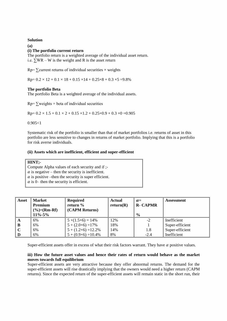
Solution
(a)
(i) The portfolio current return
The portfolio return is a weighted average of the individual asset return.
i.e. ∑WR – W is the weight and R is the asset return
Rp= ∑current returns of individual securities × weights
Rp= 0.2 × 12 + 0.1 × 18 + 0.15 ×14 + 0.25×8 + 0.3 ×5 =9.8%
The portfolio Beta
The portfolio Beta is a weighted average of the individual assets.
Rp= ∑weights × beta of individual securities
Rp= 0.2 × 1.5 + 0.1 × 2 + 0.15 ×1.2 + 0.25×0.9 + 0.3 ×0 =0.905
0.905<1
Systematic risk of the portfolio is smaller than that of market portfolios i.e. returns of asset in this
portfolio are less sensitive to changes in returns of market portfolio. Implying that this is a portfolio
for risk averse individuals.
(ii) Assets which are inefficient, efficient and super-efficient
HINT;-
Compute Alpha values of each security and if ;-
𝛼 is negative – then the security is inefficient.
𝛼 is positive –then the security is super efficient.
𝛼 is 0– then the security is efficient.
Asset Market
Premium
(%)=(Rm-Rf)
11%-5%
Required
return %
(CAPM Returns)
Actual
return(R)
𝜶=
R- CAPMR
%
Assessment
A
B
C
D
6%
6%
6%
6%
5 +(1.5×6) = 14%
5 + (2.0×6) =17%
5 + (1.2×6) =12.2%
5 + (0.9×6) =10.4%
12%
18%
14%
8%
-2
1
1.8
-2.4
Inefficient
Super-efficient
Super-efficient
Inefficient
Super-efficient assets offer in excess of what their risk factors warrant. They have 𝛼 positive values.
iii) How the future asset values and hence their rates of return would behave as the market
moves towards full equilibrium
Super-efficient assets are very attractive because they offer abnormal returns. The demand for the
super-efficient assets will rise drastically implying that the owners would need a higher return (CAPM
returns). Since the expected return of the super-efficient assets will remain static in the short run, their
Page 81
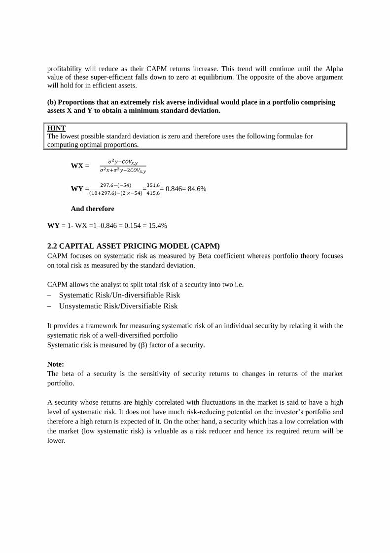
profitability will reduce as their CAPM returns increase. This trend will continue until the Alpha
value of these super-efficient falls down to zero at equilibrium. The opposite of the above argument
will hold for in efficient assets.
(b) Proportions that an extremely risk averse individual would place in a portfolio comprising
assets X and Y to obtain a minimum standard deviation.
HINT
The lowest possible standard deviation is zero and therefore uses the following formulae for
computing optimal proportions.
WX = 𝜎2𝑦−𝐶𝑂𝑉𝑥,𝑦
𝜎2𝑥+𝜎2𝑦−2𝐶𝑂𝑉𝑥,𝑦
WY =297.6−(−54)
(10+297.6)−(2 ×−54)=
351.6
415.6= 0.846= 84.6%
And therefore
WY = 1- WX =10.846 = 0.154 = 15.4%
2.2 CAPITAL ASSET PRICING MODEL (CAPM)
CAPM focuses on systematic risk as measured by Beta coefficient whereas portfolio theory focuses
on total risk as measured by the standard deviation.
CAPM allows the analyst to split total risk of a security into two i.e.
Systematic Risk/Un-diversifiable Risk
Unsystematic Risk/Diversifiable Risk
It provides a framework for measuring systematic risk of an individual security by relating it with the
systematic risk of a well-diversified portfolio
Systematic risk is measured by (β) factor of a security.
Note:
The beta of a security is the sensitivity of security returns to changes in returns of the market
portfolio.
A security whose returns are highly correlated with fluctuations in the market is said to have a high
level of systematic risk. It does not have much risk-reducing potential on the investor’s portfolio and
therefore a high return is expected of it. On the other hand, a security which has a low correlation with
the market (low systematic risk) is valuable as a risk reducer and hence its required return will be
lower.
Page 82
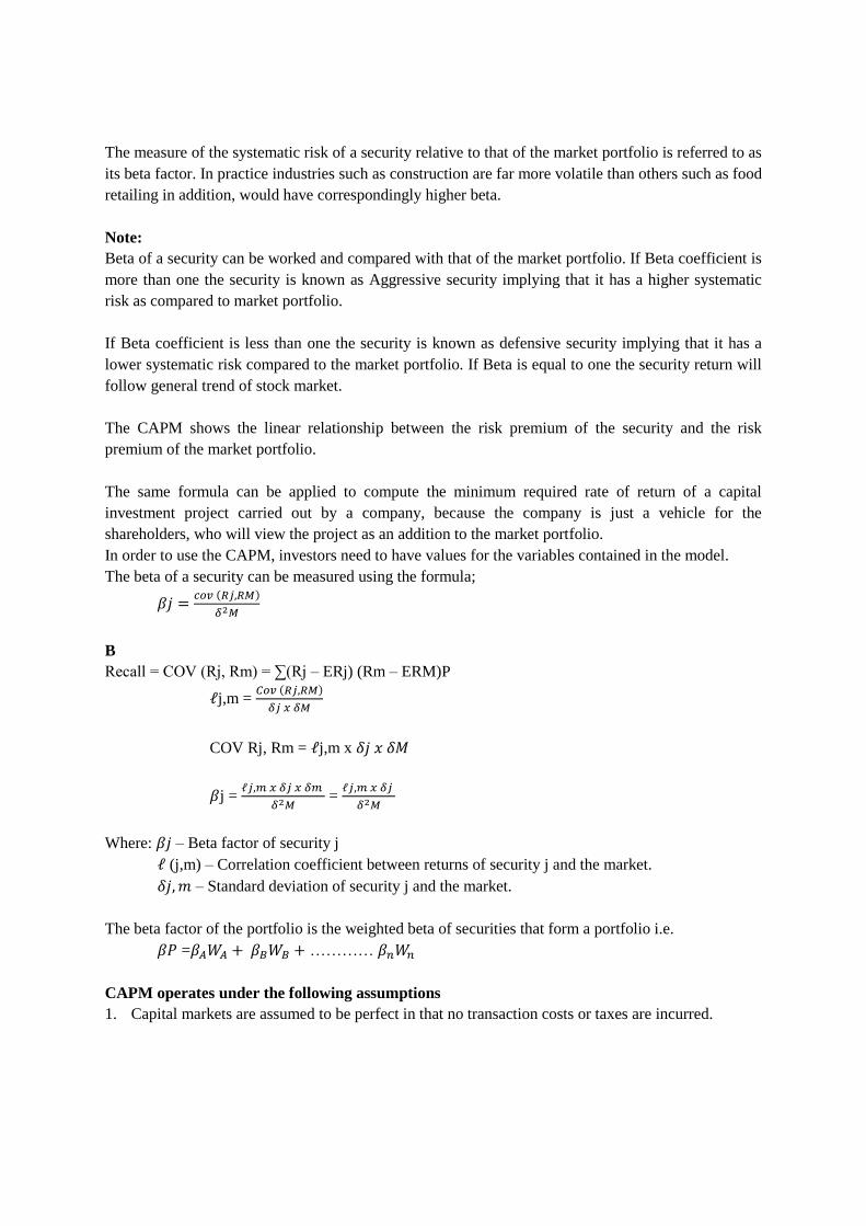
The measure of the systematic risk of a security relative to that of the market portfolio is referred to as
its beta factor. In practice industries such as construction are far more volatile than others such as food
retailing in addition, would have correspondingly higher beta.
Note:
Beta of a security can be worked and compared with that of the market portfolio. If Beta coefficient is
more than one the security is known as Aggressive security implying that it has a higher systematic
risk as compared to market portfolio.
If Beta coefficient is less than one the security is known as defensive security implying that it has a
lower systematic risk compared to the market portfolio. If Beta is equal to one the security return will
follow general trend of stock market.
The CAPM shows the linear relationship between the risk premium of the security and the risk
premium of the market portfolio.
The same formula can be applied to compute the minimum required rate of return of a capital
investment project carried out by a company, because the company is just a vehicle for the
shareholders, who will view the project as an addition to the market portfolio.
In order to use the CAPM, investors need to have values for the variables contained in the model.
The beta of a security can be measured using the formula;
𝛽𝑗 =𝑐𝑜𝑣 (𝑅𝑗,𝑅𝑀)
𝛿2𝑀
B
Recall = COV (Rj, Rm) = ∑(Rj – ERj) (Rm – ERM)P
ℓj,m = 𝐶𝑜𝑣 (𝑅𝑗,𝑅𝑀)
𝛿𝑗 𝑥 𝛿𝑀
COV Rj, Rm = ℓj,m x 𝛿𝑗 𝑥 𝛿𝑀
𝛽j = ℓ𝑗,𝑚 𝑥 𝛿𝑗 𝑥 𝛿𝑚
𝛿2𝑀 =
ℓ𝑗,𝑚 𝑥 𝛿𝑗
𝛿2𝑀
Where: 𝛽𝑗 – Beta factor of security j
ℓ (j,m) – Correlation coefficient between returns of security j and the market.
𝛿𝑗, 𝑚 – Standard deviation of security j and the market.
The beta factor of the portfolio is the weighted beta of securities that form a portfolio i.e.
𝛽𝑃 =𝛽𝐴𝑊𝐴 + 𝛽𝐵𝑊𝐵 + ………… 𝛽𝑛𝑊𝑛
CAPM operates under the following assumptions
1. Capital markets are assumed to be perfect in that no transaction costs or taxes are incurred.
Page 83
2. Capital markets are assumed to be efficient in that security prices reflects all available
information.
3. Investors are assumed to be risk averse i.e. they would only take additional risk if they are assured
of adequate compensation.
4. Investment decisions are based on a single time period.
5. Expected returns of the portfolio are assumed to be normally distributed i.e. they take the form of
a straight line equation y = mx + c
RF = [Rm – Rf] 𝛽P
6. Investors are assumed to lend and borrow at risk free rate of return.
7. CAPM is a single factor model.
8. It is assumed that systematic risk is the only relevant risk since unsystematic risks has been
eliminated through portfolio building (diversification)
9. Investors expectations are homogeneous i.e. similar and identical in all aspects.
The implications of CAPM for project appraisal
1. If the shareholders of a company are well-diversified, then their shares in this
company are just part of their overall portfolio.
2. If the company is to invest the shareholders’ money in a new project, then the project
should be appraised in the same way as the shareholders themselves would appraise
the investment if they were invested their money in it directly.
3. If they were investing directly, then they would base their required return simply on
the β of that investment (not on how it related to any particular other investment in
their portfolio).
Therefore, when the company is appraising a new project they should calculate the β of
the project, determine the required return for that β, and appraise the project at that
required return.
Using CAPM in investment appraisal
The CAPM produces a required return based on the expected return of the market E(rm), the risk-free
interest rate (Rf) and the variability of project returns relative to the market returns (β). Its main
advantage when used for investment appraisal is that it produces a discount rate which is based on the
systematic risk of the individual investment. It can be used to compare projects of all different risk
classes and is therefore superior to an NPV approach which uses only one discount rate for all
projects, regardless of their risk.
The model was developed with respect to securities; by applying it to an investment within the firm,
the company is assuming that the shareholder wishes investments to be evaluated as if they were
securities in the capital market and thus assumes that all shareholders will hold diversified portfolios
and will not look to the company to achieve diversification for them.
Example
Required return
Page 84
Panda is all-equity financed. It wishes to invest in a project with an estimated beta of 1.5. The project
has significantly different business risk characteristics from Panda’s current operations. The project
requires an outlay of sh.10,000 and will generate expected returns of sh.12,000.
The market rate of return is 12% and the risk-free rate of return is 6%.
Required:
Estimate the minimum return that Panda will require from the project and assess whether the project
is worthwhile, based on the figures you are given.
Solution
We do not need to know Panda’s current weighted average cost of capital, as the new project has
different business characteristics from its current operations. Instead we use the capital asset pricing
model so that;
Required return = RF + (ERM – RF)Be
= 6 + (12 – 6)1.5 = 15%
Expected return = 12,000−10,000
10,000= 20%
Thus the project is worthwhile; as expected return exceeds required return i.e. the Alpha value is
positive (α)
α= ER – CAPMRs
= 20% - 15% = 5%
Limitations of using CAPM in investment decisions
The greatest practical problems with the use of the CAPM in investment decisions are as follows.
(a) It is hard to estimate returns on projects under different economic environments, market returns
under different economic environments and the probabilities of the various environments.
(b) The CAPM is really just a single period model. Few investment projects last for one year only and
to extend the use of the return estimated from the model to more than one time period would
require both project performance relative to the market and the economic environment to be
reasonably stable.
In theory, it should be possible to apply the CAPM for each time period, thus arriving at
successive discount rates, one for each year of the project’s life. In practice, this would exacerbate
the estimation problems mentioned above and also make the discounting process much more
cumbersome.
(c) It may be hard to determine the risk-free rate of return. Government securities are usually taken to
be risk-free, but the return on these securities varies according to their term to maturity.
(d) Some experts have argued that betas calculated using complicated statistical techniques often
overestimate high betas, and underestimate how betas, particularly for small companies.
Security Market Line (S.M.L)
Page 85
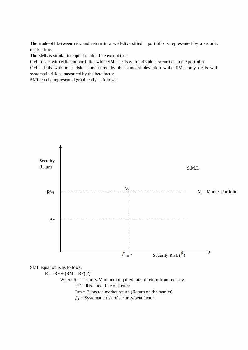
The trade-off between risk and return in a well-diversified portfolio is represented by a security
market line.
The SML is similar to capital market line except that:
CML deals with efficient portfolios while SML deals with individual securities in the portfolio.
CML deals with total risk as measured by the standard deviation while SML only deals with
systematic risk as measured by the beta factor.
SML can be represented graphically as follows:
SML equation is as follows:
Rj = RF + (RM – RF) 𝛽𝑗
Where Rj = security/Minimum required rate of return from security.
RF = Risk free Rate of Return
Rm = Expected market return (Return on the market)
𝛽𝑗 = Systematic risk of security/beta factor
Security Risk ( )
Security
Return S.M.L
M
RF
RM
M = Market Portfolio
= 1
Page 86
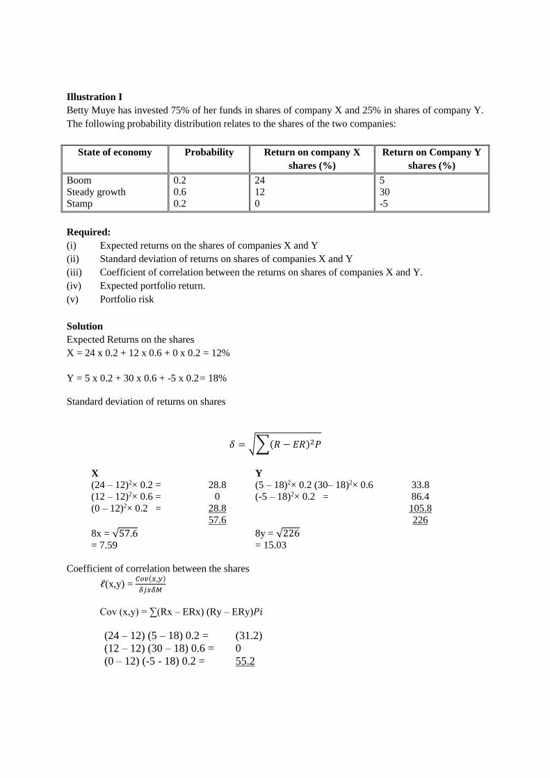
Illustration I
Betty Muye has invested 75% of her funds in shares of company X and 25% in shares of company Y.
The following probability distribution relates to the shares of the two companies:
State of economy Probability Return on company X
shares (%)
Return on Company Y
shares (%)
Boom
Steady growth
Stamp
0.2
0.6
0.2
24
12
0
5
30
-5
Required:
(i) Expected returns on the shares of companies X and Y
(ii) Standard deviation of returns on shares of companies X and Y
(iii) Coefficient of correlation between the returns on shares of companies X and Y.
(iv) Expected portfolio return.
(v) Portfolio risk
Solution
Expected Returns on the shares
X = 24 x 0.2 + 12 x 0.6 + 0 x 0.2 = 12%
Y = 5 x 0.2 + 30 x 0.6 + -5 x 0.2 = 18%
Standard deviation of returns on shares
𝛿 = √∑(𝑅 − 𝐸𝑅)2𝑃
X Y
(24 – 12)2× 0.2 =
(12 – 12)2× 0.6 =
(0 – 12)2× 0.2 =
28.8
0
28.8
57.6
(5 – 18)2× 0.2 (30– 18)2× 0.6
(-5 – 18)2× 0.2 =
33.8
86.4
105.8
226
8x = √57.6
= 7.59
8y = √226
= 15.03
Coefficient of correlation between the shares
ℓ(x,y) = 𝐶𝑜𝑣(𝑥,𝑦)
𝛿𝑗𝑥𝛿𝑀
Cov (x,y) = ∑(Rx – ERx) (Ry – ERy)𝑃𝑖
(24 – 12) (5 – 18) 0.2 =
(12 – 12) (30 – 18) 0.6 =
(0 – 12) (-5 - 18) 0.2 =
(31.2)
0
55.2
Page 87

24
ℓ(x,y) = 24
7.59 𝑥 15.03 = 0.21
ERP = ER x Wx + ERyWy
12 x 0.75 + 18 x 0.25 = 13.5%
𝛿P = √∑𝛿𝑥2𝑊𝑥2 + 𝛿𝑦2 𝑊𝑦2 + 2𝑊𝑥𝑊𝑦x 𝐶𝑜𝑋, 𝑌
√7.592 × 0.752 + 15.032 × 0.252 + 2 × 0.75 × 0.25 × 0.21
√32.405 + 14.119 + 0.079= 6.83
Illustration 2
a. The correlation coefficient between security S and that of the market is 0.96. the variance of
security is 4.36. determine the beta of security S if the variance of the market returns is 2.16.
b. If the risk free rate of return is 10% and the expected returns of the market is 14%, determine the
required rate of return of security S.
Solution
(a) 𝛽 = ℓ(𝑆,𝑀)𝑥 𝛿𝑆
𝛿𝑀
0.96 𝑥 √4.36
√2.16 = 1.3639
(b) RB = RF + (RM – RF)𝛽
10 + [14 – 10] 1.3639 = 15.4556%
Illustration 3
Galaxy Limited is an all equity financed company with a cost of capital of 18.5%. The
company is considering the following-capital investment projects:
Project Initial outlay
Sh. ‘000’
Expected cash flows in
one year.
Sh. ‘000’
Beta
A
B
C
D
1,000
1,000
1,500
2,000
1,095
1,130
1,780
2,385
0.3
0.5
1.0
1.5
Page 88
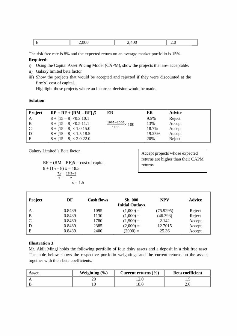
E 2,000 2,400 2.0
The risk free rate is 8% and the expected return on an average market portfolio is 15%.
Required:
i) Using the Capital Asset Pricing Model (CAPM), show the projects that are- acceptable.
ii) Galaxy limited beta factor
iii) Show the projects that would be accepted and rejected if they were discounted at the
firm's1 cost of capital.
Highlight those projects where an incorrect decision would be made.
Solution
Project RP = RF + [RM – RF] 𝜷 ER ER Advice
A
B
C
D
E
8 + [15 – 8] ×0.3 10.1
8 + [15 – 8] ×0.5 11.1
8 + [15 – 8] × 1.0 15.0
8 + [15 – 8] × 1.5 18.5
8 + [15 – 8] × 2.0 22.0
1095−1000
1000× 100
9.5%
13%
18.7%
19.25%
20%
Reject
Accept
Accept
Accept
Reject
Galaxy Limited’s Beta factor
RF + (RM – RF)𝛽 = cost of capital
8 + (15 – 8) x = 18.5
7𝑥
7 =
18.5−8
7
x = 1.5
Project
DF
Cash flows
Sh. 000
Initial Outlays
NPV
Advice
A
B
C
D
E
0.8439
0.8439
0.8439
0.8439
0.8439
1095
1130
1780
2385
2400
(1,000) =
(1,000) =
(1,500) =
(2,000) =
(2000) =
(75.9295)
(46.393)
2.142
12.7015
25.36
Reject
Reject
Accept
Accept
Accept
Illustration 3
Mr. Akili Mingi holds the following portfolio of four risky assets and a deposit in a risk free asset.
The table below shows the respective portfolio weightings and the current returns on the assets,
together with their beta coefficients.
Asset Weighting (%) Current returns (%) Beta coefficient
A
B
20
10
12.0
18.0
1.5
2.0
Accept projects whose expected
returns are higher than their CAPM
returns
Page 89
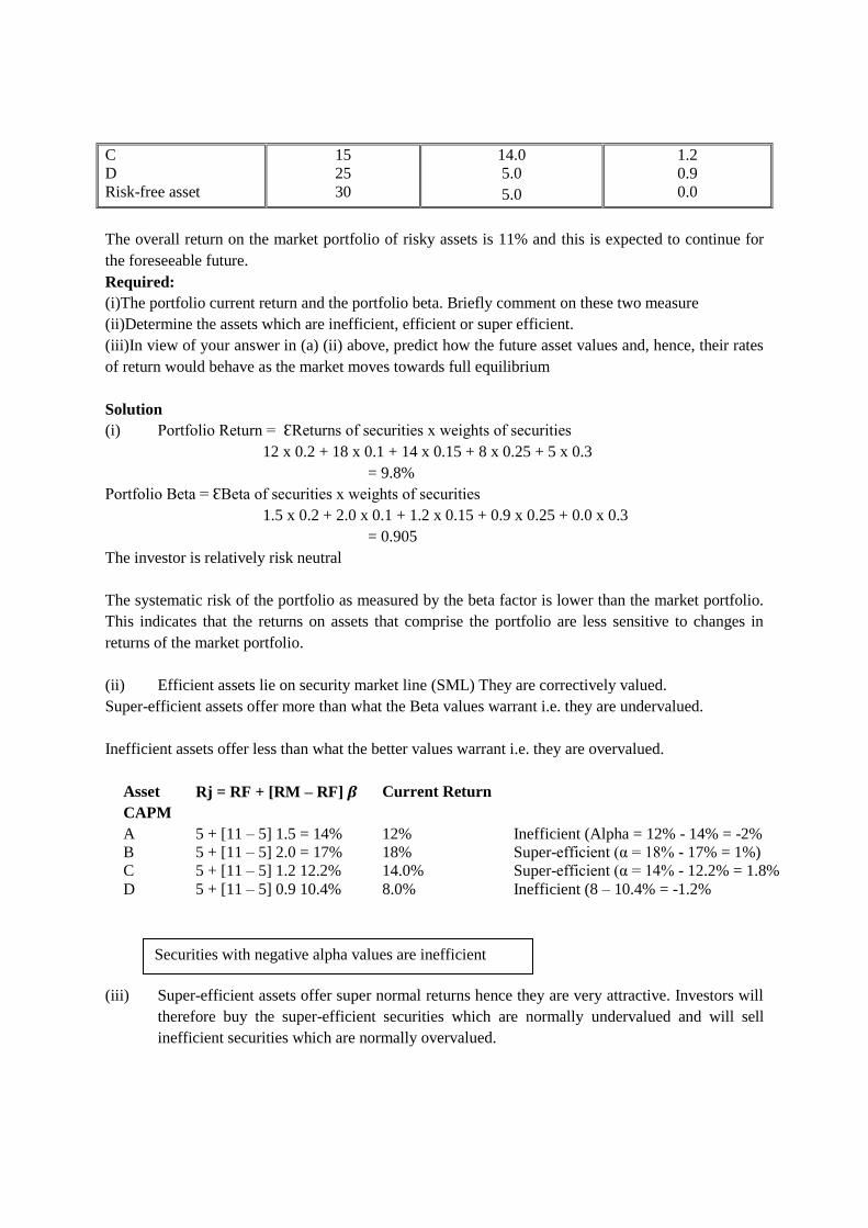
C
D
Risk-free asset
15
25
30
14.0
5.0
5.0
1.2
0.9
0.0
The overall return on the market portfolio of risky assets is 11% and this is expected to continue for
the foreseeable future.
Required:
(i)The portfolio current return and the portfolio beta. Briefly comment on these two measure
(ii)Determine the assets which are inefficient, efficient or super efficient.
(iii)In view of your answer in (a) (ii) above, predict how the future asset values and, hence, their rates
of return would behave as the market moves towards full equilibrium
Solution
(i) Portfolio Return = ԐReturns of securities x weights of securities
12 x 0.2 + 18 x 0.1 + 14 x 0.15 + 8 x 0.25 + 5 x 0.3
= 9.8%
Portfolio Beta = ԐBeta of securities x weights of securities
1.5 x 0.2 + 2.0 x 0.1 + 1.2 x 0.15 + 0.9 x 0.25 + 0.0 x 0.3
= 0.905
The investor is relatively risk neutral
The systematic risk of the portfolio as measured by the beta factor is lower than the market portfolio.
This indicates that the returns on assets that comprise the portfolio are less sensitive to changes in
returns of the market portfolio.
(ii) Efficient assets lie on security market line (SML) They are correctively valued.
Super-efficient assets offer more than what the Beta values warrant i.e. they are undervalued.
Inefficient assets offer less than what the better values warrant i.e. they are overvalued.
Asset
CAPM
Rj = RF + [RM – RF] 𝜷 Current Return
A
B
C
D
5 + [11 – 5] 1.5 = 14%
5 + [11 – 5] 2.0 = 17%
5 + [11 – 5] 1.2 12.2%
5 + [11 – 5] 0.9 10.4%
12%
18%
14.0%
8.0%
Inefficient (Alpha = 12% - 14% = -2%
Super-efficient (α = 18% - 17% = 1%)
Super-efficient (α = 14% - 12.2% = 1.8%
Inefficient (8 – 10.4% = -1.2%
(iii) Super-efficient assets offer super normal returns hence they are very attractive. Investors will
therefore buy the super-efficient securities which are normally undervalued and will sell
inefficient securities which are normally overvalued.
Securities with negative alpha values are inefficient
Page 90
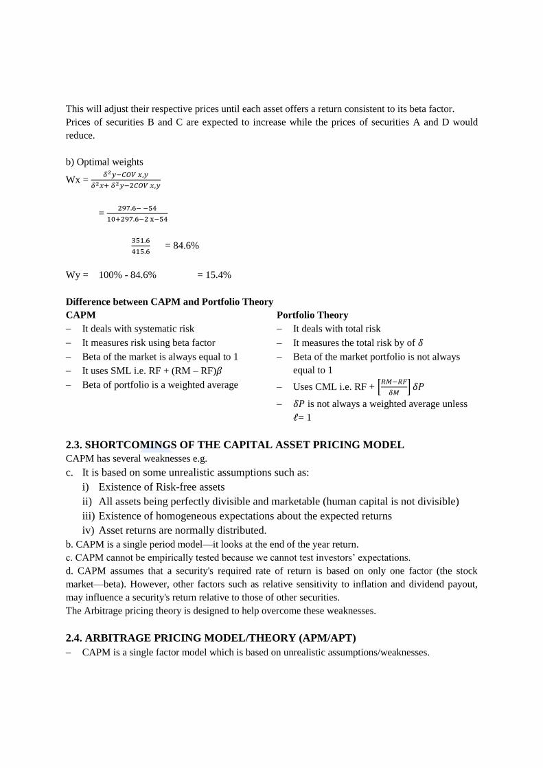
This will adjust their respective prices until each asset offers a return consistent to its beta factor.
Prices of securities B and C are expected to increase while the prices of securities A and D would
reduce.
b) Optimal weights
Wx = 𝛿2𝑦−𝐶𝑂𝑉 𝑥,𝑦
𝛿2𝑥+ 𝛿2𝑦−2𝐶𝑂𝑉 𝑥,𝑦
= 297.6− −54
10+297.6−2 x−54
351.6
415.6 = 84.6%
Wy = 100% - 84.6% = 15.4%
Difference between CAPM and Portfolio Theory
CAPM Portfolio Theory
It deals with systematic risk
It measures risk using beta factor
Beta of the market is always equal to 1
It uses SML i.e. RF + (RM – RF)𝛽
Beta of portfolio is a weighted average
It deals with total risk
It measures the total risk by of 𝛿
Beta of the market portfolio is not always
equal to 1
Uses CML i.e. RF + [𝑅𝑀−𝑅𝐹
𝛿𝑀] 𝛿𝑃
𝛿𝑃 is not always a weighted average unless
ℓ= 1
2.3. SHORTCOMINGS OF THE CAPITAL ASSET PRICING MODEL
CAPM has several weaknesses e.g.
c. It is based on some unrealistic assumptions such as:
i) Existence of Risk-free assets
ii) All assets being perfectly divisible and marketable (human capital is not divisible)
iii) Existence of homogeneous expectations about the expected returns
iv) Asset returns are normally distributed.
b. CAPM is a single period model—it looks at the end of the year return.
c. CAPM cannot be empirically tested because we cannot test investors’ expectations.
d. CAPM assumes that a security's required rate of return is based on only one factor (the stock
market—beta). However, other factors such as relative sensitivity to inflation and dividend payout,
may influence a security's return relative to those of other securities.
The Arbitrage pricing theory is designed to help overcome these weaknesses.
2.4. ARBITRAGE PRICING MODEL/THEORY (APM/APT)
CAPM is a single factor model which is based on unrealistic assumptions/weaknesses.
Page 91
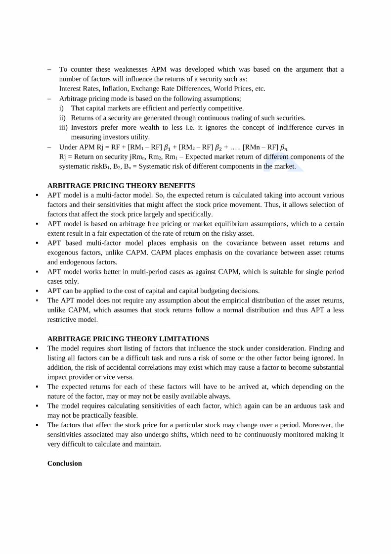
To counter these weaknesses APM was developed which was based on the argument that a
number of factors will influence the returns of a security such as:
Interest Rates, Inflation, Exchange Rate Differences, World Prices, etc.
Arbitrage pricing mode is based on the following assumptions;
i) That capital markets are efficient and perfectly competitive.
ii) Returns of a security are generated through continuous trading of such securities.
iii) Investors prefer more wealth to less i.e. it ignores the concept of indifference curves in
measuring investors utility.
Under APM Rj = RF + [RM1 – RF] 𝛽1 + [RM2 – RF] 𝛽2 + ….. [RMn – RF] 𝛽𝑛
Rj = Return on security jRmn, Rm2, Rm1 – Expected market return of different components of the
systematic riskB1, B2, Bn = Systematic risk of different components in the market.
ARBITRAGE PRICING THEORY BENEFITS
APT model is a multi-factor model. So, the expected return is calculated taking into account various
factors and their sensitivities that might affect the stock price movement. Thus, it allows selection of
factors that affect the stock price largely and specifically.
APT model is based on arbitrage free pricing or market equilibrium assumptions, which to a certain
extent result in a fair expectation of the rate of return on the risky asset.
APT based multi-factor model places emphasis on the covariance between asset returns and
exogenous factors, unlike CAPM. CAPM places emphasis on the covariance between asset returns
and endogenous factors.
APT model works better in multi-period cases as against CAPM, which is suitable for single period
cases only.
APT can be applied to the cost of capital and capital budgeting decisions.
The APT model does not require any assumption about the empirical distribution of the asset returns,
unlike CAPM, which assumes that stock returns follow a normal distribution and thus APT a less
restrictive model.
ARBITRAGE PRICING THEORY LIMITATIONS
The model requires short listing of factors that influence the stock under consideration. Finding and
listing all factors can be a difficult task and runs a risk of some or the other factor being ignored. In
addition, the risk of accidental correlations may exist which may cause a factor to become substantial
impact provider or vice versa.
The expected returns for each of these factors will have to be arrived at, which depending on the
nature of the factor, may or may not be easily available always.
The model requires calculating sensitivities of each factor, which again can be an arduous task and
may not be practically feasible.
The factors that affect the stock price for a particular stock may change over a period. Moreover, the
sensitivities associated may also undergo shifts, which need to be continuously monitored making it
very difficult to calculate and maintain.
Conclusion
Page 92
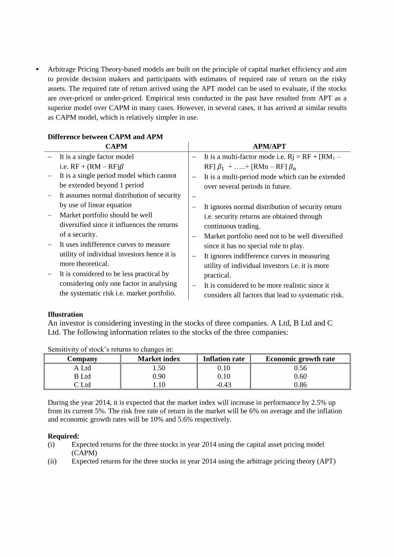
Arbitrage Pricing Theory-based models are built on the principle of capital market efficiency and aim
to provide decision makers and participants with estimates of required rate of return on the risky
assets. The required rate of return arrived using the APT model can be used to evaluate, if the stocks
are over-priced or under-priced. Empirical tests conducted in the past have resulted from APT as a
superior model over CAPM in many cases. However, in several cases, it has arrived at similar results
as CAPM model, which is relatively simpler in use.
Difference between CAPM and APM
CAPM APM/APT
It is a single factor model
i.e. RF + (RM – RF)𝛽
It is a single period model which cannot
be extended beyond 1 period
It assumes normal distribution of security
by use of linear equation
Market portfolio should be well
diversified since it influences the returns
of a security.
It uses indifference curves to measure
utility of individual investors hence it is
more theoretical.
It is considered to be less practical by
considering only one factor in analysing
the systematic risk i.e. market portfolio.
It is a multi-factor mode i.e. Rj = RF + [RM1 –
RF] 𝛽1 + …..+ [RMn – RF] 𝛽𝑛
It is a multi-period mode which can be extended
over several periods in future.
It ignores normal distribution of security return
i.e. security returns are obtained through
continuous trading.
Market portfolio need not to be well diversified
since it has no special role to play.
It ignores indifference curves in measuring
utility of individual investors i.e. it is more
practical.
It is considered to be more realistic since it
considers all factors that lead to systematic risk.
Illustration
An investor is considering investing in the stocks of three companies. A Ltd, B Ltd and C
Ltd. The following information relates to the stocks of the three companies:
Sensitivity of stock’s returns to changes in:
Company Market index Inflation rate Economic growth rate
A Ltd
B Ltd
C Ltd
1.50
0.90
1.10
0.10
0.10
-0.43
0.56
0.60
0.86
During the year 2014, it is expected that the market index will increase in performance by 2.5% up
from its current 5%. The risk free rate of return in the market will be 6% on average and the inflation
and economic growth rates will be 10% and 5.6% respectively.
Required:
(i) Expected returns for the three stocks in year 2014 using the capital asset pricing model
(CAPM)
(ii) Expected returns for the three stocks in year 2014 using the arbitrage pricing theory (APT)
Page 93

ADVANCED FINANCIAL MANA
(iii) State the reason why an investor would get different return estimates in (b)(i) and (b)(ii)
above.
Solution
(i) Expected returns of the stocks using CAPM
ERj = Rf + (Rm – Rf) 𝛽𝑖
ERA = 6 + (7.5 – 6) 1.5 = 8.25%
ERB = 6 + (7.5 – 6) 0.90 = 7.35%
ERC = 6 + (7.5 – 6) 1.1 = 7.65%
Rf is the Risk free rate; Rm is the Return on the market;𝛽𝑖 is the Sensitivity of the asset’s return which
is represented by Beta.
(ii)Expected returns of the stocks using the arbitrage pricing theory (APT)
HINT;
APT is a multiples factor model.
APT returns = Rf + (Ri – Rf) 𝛽𝑖 + (RE – Rf) 𝛽𝑒
ERA = 6 + (10 – 6) -0.1 + (5.6 – 6) 0.56 + (7.5-6)1.5 = 7.626%
ERB = 6 + (10 – 6) 0.1+ (5.6 – 6) 0.6 + (7.5-6)0.9 = 7.51%
ERC = 6 + (10 – 6) -0.43 + (5.6 – 6) 0.86 + (7.5-6)1.1 = 5.59%
E(R1) is the assets’ expected; 𝛽𝑖 is the Sensitivity of the asset’s return to a particular factor rate of
return.
(iii) Why an investor will get different return estimates
CAPM is a single factor model that assumes that the only factors that affects portfolio returns is the
market factor (market returns) whereas APT brings on board many factors. These differences in terms
of variables used wil yield different results.
The Fama-French Model
One of the critiques on CAPM was that it seemed to fail to explain why small cap stocks tended to
outperform large cap stocks. Eugene Fama and Kenneth French researched this issue and introduced a
new model, an extended form of CAPM, called Fama-French Model (FFM). FFM includes the
following factors:
RMRF – Stands for the difference between market return and risk free return, as in CAPM.
SMB – Stands for small minus big, thus is a size factor. It is estimated as the difference between
average return on three small-cap portfolios minus average return on three large-cap portfolios.
Thus, SMB represents a return premium over the large cap stocks.
HML – Stands for high minus low, the average return on two high book-to-market portfolios
minus the average return on two low book-to-market portfolios. This factor accounts for the value
NOTE:Ri = Rf + Beta (market) x RMRF + Beta
(size) x SMB + Beta (value) x HML
Page 94
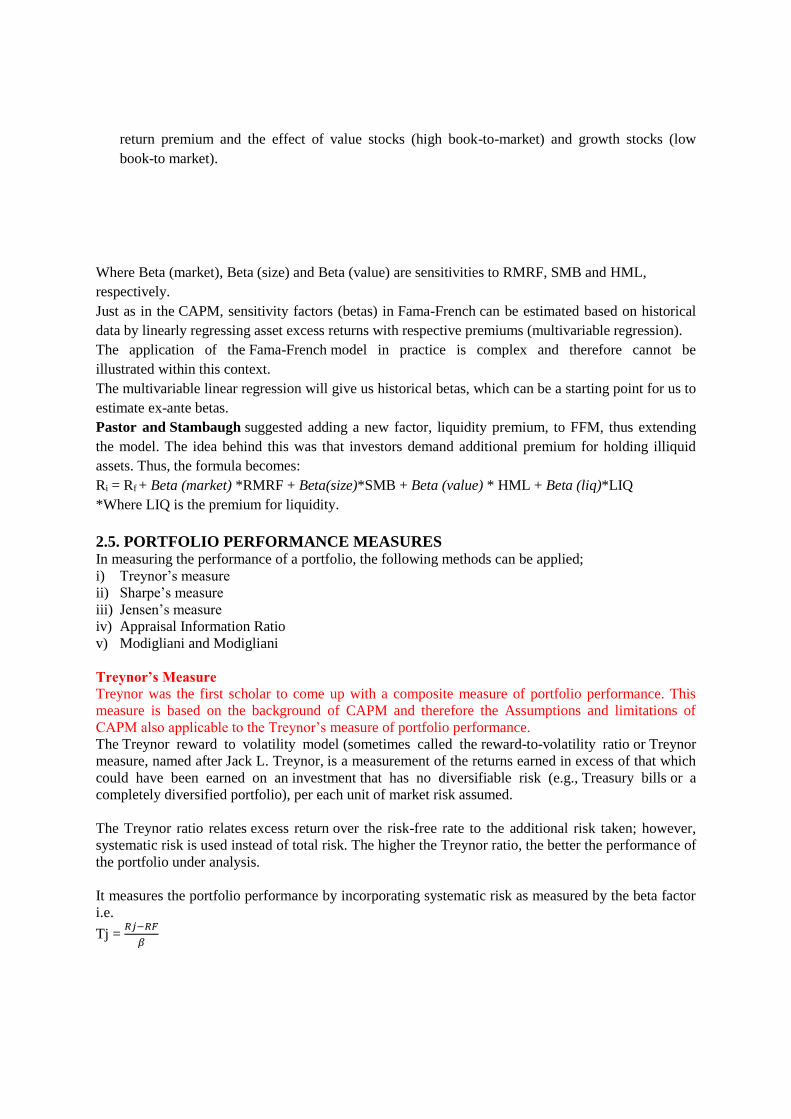
return premium and the effect of value stocks (high book-to-market) and growth stocks (low
book-to market).
Where Beta (market), Beta (size) and Beta (value) are sensitivities to RMRF, SMB and HML,
respectively.
Just as in the CAPM, sensitivity factors (betas) in Fama-French can be estimated based on historical
data by linearly regressing asset excess returns with respective premiums (multivariable regression).
The application of the Fama-French model in practice is complex and therefore cannot be
illustrated within this context.
The multivariable linear regression will give us historical betas, which can be a starting point for us to
estimate ex-ante betas.
Pastor and Stambaugh suggested adding a new factor, liquidity premium, to FFM, thus extending
the model. The idea behind this was that investors demand additional premium for holding illiquid
assets. Thus, the formula becomes:
Ri = Rf + Beta (market) *RMRF + Beta(size)*SMB + Beta (value) * HML + Beta (liq)*LIQ
*Where LIQ is the premium for liquidity.
2.5. PORTFOLIO PERFORMANCE MEASURES In measuring the performance of a portfolio, the following methods can be applied;
i) Treynor’s measure
ii) Sharpe’s measure
iii) Jensen’s measure
iv) Appraisal Information Ratio
v) Modigliani and Modigliani
Treynor’s Measure
Treynor was the first scholar to come up with a composite measure of portfolio performance. This
measure is based on the background of CAPM and therefore the Assumptions and limitations of
CAPM also applicable to the Treynor’s measure of portfolio performance.
The Treynor reward to volatility model (sometimes called the reward-to-volatility ratio or Treynor
measure, named after Jack L. Treynor, is a measurement of the returns earned in excess of that which
could have been earned on an investment that has no diversifiable risk (e.g., Treasury bills or a
completely diversified portfolio), per each unit of market risk assumed.
The Treynor ratio relates excess return over the risk-free rate to the additional risk taken; however,
systematic risk is used instead of total risk. The higher the Treynor ratio, the better the performance of
the portfolio under analysis.
It measures the portfolio performance by incorporating systematic risk as measured by the beta factor
i.e.
Tj = 𝑅𝑗−𝑅𝐹
𝛽
Page 95

Tj = Treynor’s measure of security
Rj = E Returns of security on the market
RF = Risk Free Rate of Return
𝛽𝑗 = Systematic Risk/Beta factor of security
This measure is compared with a similar measure of the market portfolio for analysis purposes i.e.
Tm = 𝑅𝑚−𝑅𝐹
𝛽𝑚
Recall:
𝛽𝑚 = 1
[Rm – RF] = Risk Premium
Tm = Risk Premium
Analysis
If Tj is more than the Tm, it indicates a superior performance
If Tj is less than Tm, (Tj< Tm) it indicates an inferior performance
If Tj is equal to Tm it indicates an efficient performance
Sharpe’s Measure
The Sharpe ratio is defined as the risk premium of the portfolio per unit of total risk in the portfolio.
Risk premium calculated by subtracting risk-free returns from the portfolio returns. The risk-free
returns are measured as the risk-free interest rate of Treasury bonds.
It measures portfolio performance by use of total risk as measured by 𝛿 i.e.
𝛿𝑗 = 𝑅𝑗−𝑅𝐹
𝛿𝑗
Sj = Sharpe’s measure of security
𝛿𝑗 = Standard deviation of security j
Rj = E returns of security in the market
RF = risk free rate of return
For evaluation purposes, a Sharpe’s measure of a security is compared with a similar or measure of
the market portfolio
Sm = 𝑅𝑚−𝑅𝐹
𝛿𝑚
Analysis
If Sj>Sm, it indicates a superior performance
If Sj<Sm, it indicates an inferior performance
If Sj = Sm, it indicates an efficient performance
Jensen’s Measure
the Jensen's measure is a risk-adjusted performance measure that represents the average return on
a portfolio or investment, above or below that predicted by the capital asset pricing model (CAPM),
given the portfolio's or investment's beta and the average market return. This metric is also commonly
referred to as Jensen's alpha, or simply alpha.
With an assumption that capital markets are efficient and perfect, CAPM becomes accurate in
estimating returns of a portfolio.
Jensen’s measure uses Alpha values (𝛼) in measuring portfolio performance.
Page 96
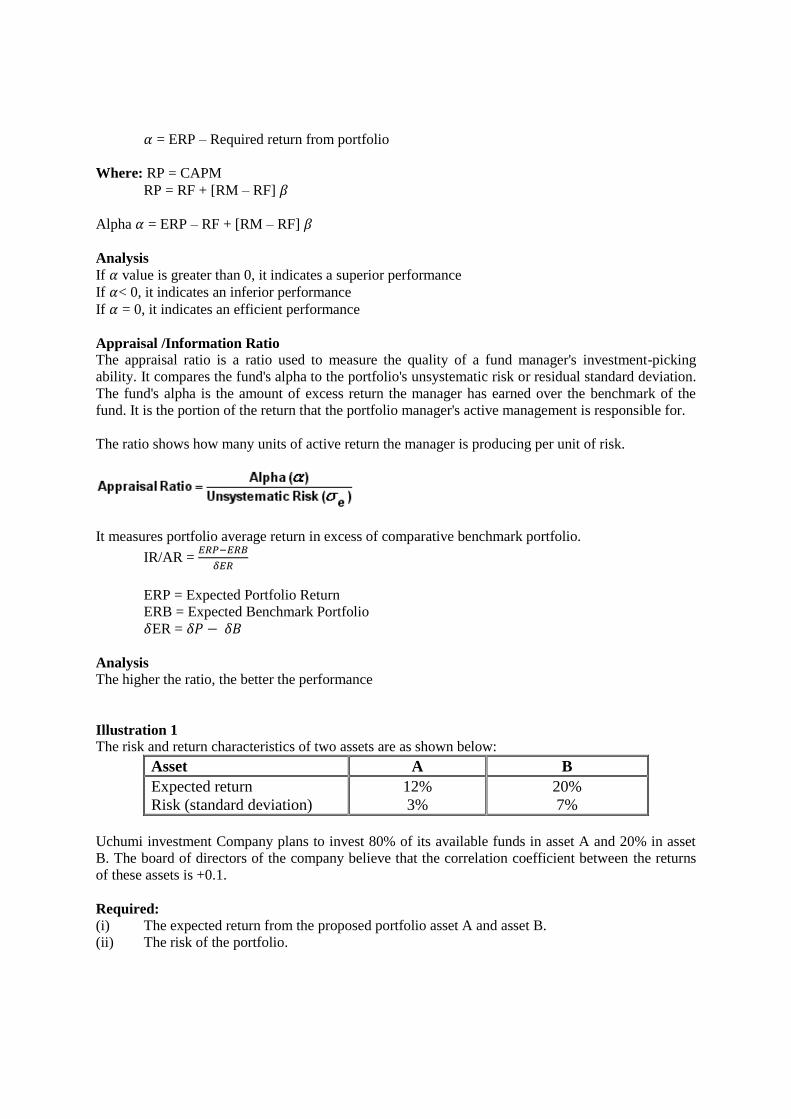
𝛼 = ERP – Required return from portfolio
Where: RP = CAPM
RP = RF + [RM – RF] 𝛽
Alpha 𝛼 = ERP – RF + [RM – RF] 𝛽
Analysis
If 𝛼 value is greater than 0, it indicates a superior performance
If 𝛼< 0, it indicates an inferior performance
If 𝛼 = 0, it indicates an efficient performance
Appraisal /Information Ratio
The appraisal ratio is a ratio used to measure the quality of a fund manager's investment-picking
ability. It compares the fund's alpha to the portfolio's unsystematic risk or residual standard deviation.
The fund's alpha is the amount of excess return the manager has earned over the benchmark of the
fund. It is the portion of the return that the portfolio manager's active management is responsible for.
The ratio shows how many units of active return the manager is producing per unit of risk.
It measures portfolio average return in excess of comparative benchmark portfolio.
IR/AR = 𝐸𝑅𝑃−𝐸𝑅𝐵
𝛿𝐸𝑅
ERP = Expected Portfolio Return
ERB = Expected Benchmark Portfolio
𝛿ER = 𝛿𝑃 − 𝛿𝐵
Analysis
The higher the ratio, the better the performance
Illustration 1
The risk and return characteristics of two assets are as shown below:
Asset A B
Expected return
Risk (standard deviation)
12%
3%
20%
7%
Uchumi investment Company plans to invest 80% of its available funds in asset A and 20% in asset
B. The board of directors of the company believe that the correlation coefficient between the returns
of these assets is +0.1.
Required:
(i) The expected return from the proposed portfolio asset A and asset B.
(ii) The risk of the portfolio.
Page 97

(iii) Comment on your calculations in part (c) (ii) above in the context of the risk-reducing effects
of diversification.
(iv) Suppose the correlation coefficient between the returns of asset A and asset B was -1.0.
Demonstrate how Uchumi Investment Company could invest its funds in order to obtain a
zero-risk portfolio.
Solution
(i) The expected return from the proposed portfolio asset A and asset B.
ER = RAWA + RBWB
12% ×80% + 20% × 20% = 13.6%
(ii) The risk of the portfolio.
Risk of the portfolio = 𝛿P = √𝛿𝐴2𝑊𝐴
2 + 𝛿𝐵2𝑊𝐵
2 + 2𝑊𝐴𝑊𝐴𝐶𝑜𝐴, 𝐵
COV A,B = ℓA,B x 𝛿A x 𝛿B
0.1 x 0.3 x 7 = 2.1%
= √32 × 0.82 + 72 × 0.22 + 2 × 0.8 × 0.2 × 2.1
= 2.90%
(iii)Comment on your calculations in part (c) (ii) above in the context of the risk-reducing effects
of diversification.
Through diversification the overall risk of the portfolio reduces to 2.90% as compared to a higher risk
of 3% for assets A and 7% for asset B.
Weighted σP = WAσA + WBσB = 0.8 x 3% + 0.2 x 7% = 3.8%
The risk has reduced from 3.8% to 2.9%
(iv)
To calculate the proportions investment of types of assets in a portfolio we use the minimum weight
formula i.e.
Wx = 𝛿2𝑦−𝐶𝑂𝑉 𝑥,𝑦
𝛿2𝑥 𝛿2𝑦−2𝐶𝑂𝑉 𝑋,𝑌
Wy = 1 – Wx
WA = 𝛿2𝑦−𝐶𝑂𝑉 𝐴,𝐵
𝛿2𝐴 + 𝛿2𝐵 −2𝐶𝑂𝑉 𝐴,𝐵
COV A,B = ℓ A,B x 𝛿A x 𝛿B
-0.1 x 3 x 7 = -21
72−−21
32+ 72−2∗−21 =
70
100
PAB = Correlation
Coefficient between A & B
Page 98
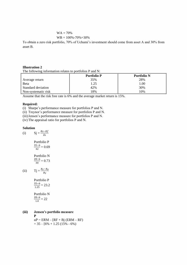
WA = 70%
WB = 100%-70%=30%
To obtain a zero risk portfolio, 70% of Uchumi’s investment should come from asset A and 30% from
asset B.
Illustration 2
The following information relates to portfolios P and N:
Average return
Beta
Standard deviation
Non-systematic risk
Portfolio P
35%
1.25
42%
18%
Portfolio N
28%
1.00
30%
10%
Assume that the risk free rate is 6% and the average market return is 15%.
Required:
(i) Sharpe’s performance measure for portfolios P and N.
(ii) Treynor’s performance measure for portfolios P and N.
(iii) Jensen’s performance measure for portfolios P and N.
(iv) The appraisal ratio for portfolios P and N.
Solution
(i) Sj = 𝑅𝑠−𝑅𝑓
𝛿𝑠
Portfolio P 35−6
42 = 0.69
Portfolio N 28−6
30 = 0.73
(ii) Tj = 𝑅𝑇−𝑅𝐹
𝐵𝑇
Portfolio P 35−6
1.25 = 23.2
Portfolio N 28−6
1.0 = 22
(iii) Jensen’s portfolio measure
P
αP = ERM – [RF + Bj (ERM – RF)
= 35 – [6% + 1.25 (15% - 6%)
Page 99
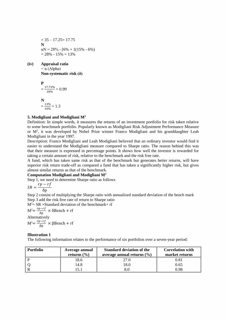
= 35 – 17.25= 17.75
N
αN = 28% - [6% + 1(15% - 6%)
= 28% - 15% = 13%
(iv) Appraisal ratio
= α (Alpha)
Non-systematic risk (δ)
P
= 17.75%
18% = 0.99
N
= 13%
10% = 1.3
5. Modigliani and Modigliani M2
Definition: In simple words, it measures the returns of an investment portfolio for risk taken relative
to some benchmark portfolio. Popularly known as Modigliani Risk Adjustment Performance Measure
or M2, it was developed by Nobel Prize winner Franco Modigliani and his granddaughter Leah
Modigliani in the year 1997.
Description: Franco Modigliani and Leah Modigliani believed that an ordinary investor would find it
easier to understand the Modigliani measure compared to Sharpe ratio. The reason behind this was
that their measure is expressed in percentage points. It shows how well the investor is rewarded for
taking a certain amount of risk, relative to the benchmark and the risk free rate.
A fund, which has taken same risk as that of the benchmark but generates better returns, will have
superior risk return trade-off as compared a fund that has taken a significantly higher risk, but gives
almost similar returns as that of the benchmark.
Computation Modigliani and Modigliani M2
Step 1, we need to determine Sharpe ratio as follows
𝑆𝑅 =𝑟𝑝 − 𝑟𝑓
δp
Step 2 consist of multiplying the Sharpe ratio with annualized standard deviation of the bench mark
Step 3 add the risk free rate of return to Sharpe ratio
M2= SR ×Standard deviation of the benchmark+ rf
M2=𝑟𝑝−𝑟𝑓
δp × δBench + rf
Alternatively
M2=𝑟𝑝−𝑟𝑓
βp × βBench + rf
Illustration 1
The following information relates to the performance of six portfolios over a seven-year period:
Portfolio Average annual
returns (%)
Standard deviation of the
average annual returns (%)
Correlation with
market returns
P
Q
R
18.6
14.8
15.1
27.0
18.0
8.0
0.81
0.65
0.98
Page 100
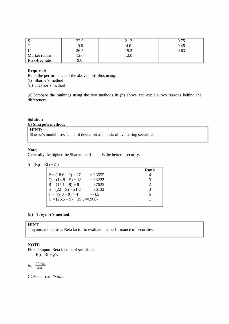
S
T
U
Market return
Risk-free rate
22.0
-9.0
26.5
12.0
9.0
21.2
4.0
19.3
12.0
0.75
0.45
0.63
Required:
Rank the performance of the above portfolios using:
(i) Sharpe’s method
(ii) Treynor’s method
(c)Compare the rankings using the two methods in (b) above and explain two reasons behind the
differences.
Solution
(i) Sharpe’s method:
HINT;
Sharpe’s model uses standard deviation as a basis of evaluating securities.
Note;
Generally the higher the Sharpe coefficient is the better a security.
S= (Rp – Rf) ÷ 𝛿p
(ii) Treynor’s method:
HINT
Treynors model uses Beta factor to evaluate the performance of securities.
NOTE
First compute Beta factors of securities
Tp= Rp - Rf ÷ 𝛽D
𝛽s =𝐶𝑂𝑉𝑆𝑀
𝛿𝑚2
COVsm =rsm 𝛿𝑠𝛿𝑚
P = (18.6 – 9) ÷ 27 =0.3555
Q = (14.8 – 9) ÷ 18 =0.3222
R = (15.1 – 9) ÷ 8 =0.7625
S = (22 – 9) ÷ 21.2 =0.6132
T = (-9.0 – 9) ÷ 4 =-4.5
U = (26.5 – 9) ÷ 19.3=0.9067
Rank
4
5
2
3
6
1
Page 101
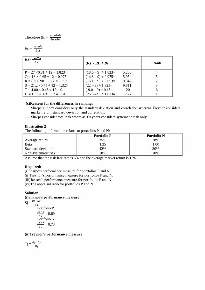
Therefore Bs = 𝑟𝑠𝑚𝛿𝑠𝛿𝑠
𝛿𝑚𝑥𝛿𝑚
𝛽s = 𝑟𝑠𝑚𝛿𝑠
𝛿𝑚
𝜷𝒔= 𝒓𝒔𝒎𝝈𝒎
𝝈𝒎
(Rs - Rf) ÷ 𝜷s
Rank
P = 27 ×0.81 ÷ 12 = 1.823
Q = 18 × 0.65 ÷ 12 = 0.975
R = 8 × 0.98 ÷ 12 = 0.653
S = 21.2 ×0.75 ÷ 12 = 1.325
T = 4.00 × 0.45 ÷ 12 = 0.1
U = 19.3×0.63 ÷ 12 = 1.013
(18.6 – 9) ÷ 1.823= 5.266
(14.8 – 9) ÷ 0.975= 5.95
(15.1 – 9) ÷ 0.653= 9.342
(22 – 9) ÷ 1.325= 9.811
(-9.0 – 9) ÷ 0.15= -120
(26.5 – 9) ÷ 1.013= 17.27
4
5
2
3
6
1
(c)Reasons for the differences in ranking:
Sharpe’s index considers only the standard deviation and correlation whereas Treynor considers
market return standard deviation and correlation.
Sharpes consider total risk where as Treynors considers systematic risk only.
Illustration 2
The following information relates to portfolios P and N:
Average return
Beta
Standard deviation
Non-systematic risk
Portfolio P
35%
1.25
42%
18%
Portfolio N
28%
1.00
30%
10%
Assume that the risk free rate is 6% and the average market return is 15%.
Required:
(i)Sharpe’s performance measure for portfolios P and N.
(ii)Treynor’s performance measure for portfolios P and N.
(iii)Jensen’s performance measure for portfolios P and N.
(iv)The appraisal ratio for portfolios P and N.
Solution
(i)Sharpe’s performance measure
Sj = 𝑅𝑠−𝑅𝑓
𝛿𝑠
Portfolio P 35−6
42 = 0.69
Portfolio N 28−6
30 = 0.73
(ii)Treynor’s performance measure
Tj = 𝑅𝑇−𝑅𝐹
𝐵𝑇
Page 102

Portfolio P 35−6
1.25 = 23.2
Portfolio N 28−6
1.0 = 22
(iii)Jensen’s performance measure
Jensen’s portfolio measure
P
αP = ERM – [RF + Bj (ERM – RF)
= 35 – [6% + 1.25 (15% - 6%)
= 35 – 17.25
= 17.75
N
αN = 28% - [6% + 1(15% - 6%)
= 28% - 15%
= 13%
(iv)Jensen’s performance measure
Appraisal ratio
= α (Alpha)
Non-systematic risk (δ)
P
= 17.75%
18% = 0.99
N
= 13%
10% = 1.3
EXAM PRACTISE QUESTIONS
Question 1
The risk and return characteristics of two assets are as shown below:
Asset A B
Expected return
Risk (standard deviation)
12%
3%
20%
7%
Uchumi investment Company plans to invest 80% of its available funds in asset A and 20% in asset
B. The board of directors of the company believe that the correlation coefficient between the returns
of these assets is +0.1.
Required:
(i)The expected return from the proposed portfolio asset A and asset B.
(ii)The risk of the portfolio.
(iii)Comment on your calculations in part (c) (ii) above in the context of the risk-reducing effects of
diversification.
(iv)Suppose the correlation coefficient between the returns of asset A and asset B was -1.0.
Demonstrate how Uchumi Investment Company could invest its funds in order to obtain a zero-risk
portfolio.
Page 103

Solution
(i)The expected return from the proposed ER = RAWA + RBWB 12% × 80% + 20% × 20%= 13.6%
(ii)The risk of the portfolio
Risk of the portfolio = 𝛿P = √𝛿𝐴2𝑊𝐴
2 + 𝛿𝐵2𝑊𝐵
2 + 2𝑊𝐴𝑊𝐴𝐶𝑜𝐴, 𝐵
COV A,B = ℓA,B x 𝛿A x 𝛿B
0.1 x 0.3 x 7 = 2.1%
= √32 × 0.82 + 72 × 0.22 + 2 × 0.8 × 0.2 × 2.1= 2.90%
(iii)Comment on your calculations in part (c) (ii) above
Through diversification the overall risk of the portfolio reduces to 2.90% as compared to a
higher risk of 3% for assets A and 7% for asset B.
Weighted σP = WAσA + WBσB = 0.8 x 3% + 0.2 x 7% = 3.8%
The risk has reduced from 3.8% to 2.9%
(iv)How Uchumi Investment Company could invest its funds in order to obtain a zero-risk
portfolio. To calculate the proportions investment of types of assets in a portfolio we use the minimum
weight formula i.e.
Wx = 𝛿2𝑦−𝐶𝑂𝑉 𝑥,𝑦
𝛿2𝑥 𝛿2𝑦−2𝐶𝑂𝑉 𝑋,𝑌
Wy = 1 – Wx
WA = 𝛿2𝑦−𝐶𝑂𝑉 𝐴,𝐵
𝛿2𝐴 + 𝛿2𝐵 −2𝐶𝑂𝑉 𝐴,𝐵
COV A,B = ℓ A,B x 𝛿A x 𝛿B
-0.1 x 3 x 7 = -21
72−−21
32+ 72−2∗−21 =
70
100
WA = 70%
WB = 100%-70%=30%
To obtain a zero risk portfolio, 70% of Uchumi’s investment should come from asset A and 30% from
asset B.
Question 2
PAB = Correlation
Coefficient between A & B
Page 104
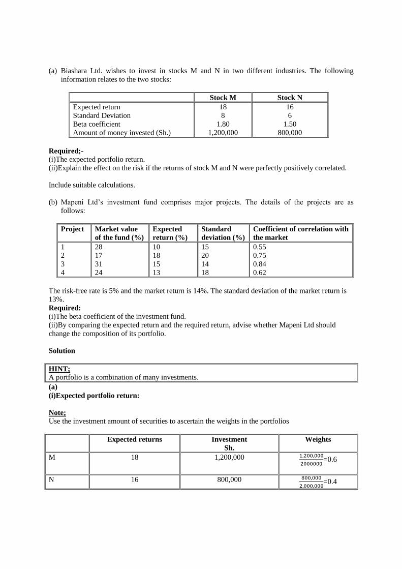
(a) Biashara Ltd. wishes to invest in stocks M and N in two different industries. The following
information relates to the two stocks:
Stock M Stock N
Expected return
Standard Deviation
Beta coefficient
Amount of money invested (Sh.)
18
8
1.80
1,200,000
16
6
1.50
800,000
Required;-
(i)The expected portfolio return.
(ii)Explain the effect on the risk if the returns of stock M and N were perfectly positively correlated.
Include suitable calculations.
(b) Mapeni Ltd’s investment fund comprises major projects. The details of the projects are as
follows:
Project Market value
of the fund (%)
Expected
return (%)
Standard
deviation (%)
Coefficient of correlation with
the market
1
2
3
4
28
17
31
24
10
18
15
13
15
20
14
18
0.55
0.75
0.84
0.62
The risk-free rate is 5% and the market return is 14%. The standard deviation of the market return is
13%.
Required:
(i)The beta coefficient of the investment fund.
(ii)By comparing the expected return and the required return, advise whether Mapeni Ltd should
change the composition of its portfolio.
Solution
HINT;
A portfolio is a combination of many investments.
(a)
(i)Expected portfolio return:
Note;
Use the investment amount of securities to ascertain the weights in the portfolios
Expected returns Investment
Sh.
Weights
M 18 1,200,000 1,200,000
2000000=0.6
N 16 800,000 800,000
2,000,000=0.4
Page 105

2,000,000
E (Rp) = (WM ERM+ (WNE(RN) = (0.6×18) + (0.4×16) = 17.2%
(ii)If the returns of stocks are perfectly positively correlated, the returns are expected to move in the
same direction. However, more importantly, a perfect positive correlation is interpreted to mean that
there is 0% risk reduction through building of such a portfolio. Therefore, building a portfolio whose
stock returns are perfectly positively correlated renders portfolio building meaningless.
In order to justify this argument, we need to determine the 0% risk reduction through portfolio
building as follows:
0% risk reduction = 𝑊𝑒𝑖𝑔ℎ𝑡𝑒𝑑𝛿𝑝–𝐴𝑐𝑡𝑢𝑎𝑙𝛿𝑝
Weighted dp
Weighted portfolio risk (𝛿p)
= (wm𝛿m) + (wn𝛿n)= (0.6×8) + (0.4×6) = 7.2
Actual portfolio risk (𝛿p)
Note;
First determine COVMN =rMN𝛿M𝛿N
rMN = correlation coefficient between M and N= 1 since the securities are perfectly positively related.
HINT;
Perfectly positively correlated securities have a correlation coefficient of 1
Therefore COVMN =1×8×6 =48
Actual 𝜹p
𝛿2p =Wm2𝛿M2 + Wn2𝛿n2 + 2COVMNWMWN
=0.62 × 82 + 0.42 × 62 + 2×48×0.6×0.4=51.84
𝛿p=√51.84 =7.2
% risk reduced=𝑤𝛿𝑝−𝐴𝛿𝑃
𝑊𝛿𝑃=
7.2−7.2
7.2 × 100= 0%
Where;-
W𝛿p = weighted standard deviation of a portfolio.
A𝛿p = Atual
(b)
(i)The investment fund’s Beta coefficient:
Beta of an individual asset (𝛽j)
Page 106

BJ =𝐶𝑂𝑉𝑗,𝑚
𝛿𝑚2 = 𝑟𝑗𝑚×𝛿𝑗×𝛿𝑚
𝛿𝑚×𝛿𝑚
Project 1
B1 = 𝑟𝑗𝑚.𝛿𝑗
𝛿𝑚=
0.55 ×15
13 =0.635
Project 2
B2 = =𝑟2𝑚 .𝛿2
𝛿𝑚 =
0.75 ×20
13 =1.154
Project 3
B3 = =𝑟3,𝑚 .𝛿3
𝛿𝑚 =
0.84 ×14
13 =0.905
Project 4
B3 = =𝑟4,𝑚 .𝛿4
𝛿𝑚 =
0.62×18
13 =0.86
Investment fund’s beta Coefficient (Bp)
HINT
For w=weights, use the market values of funds (%). E.g. project 1 =28%, W1 =0.28
Bp = (W1𝛽1) + (W2𝛽2) + (W3𝛽3) + (W4𝛽4)
= [0.28×0.635] + [0.17×1.154] + [0.31×0.905] + [0.24×0.86] = 0.861
E (portfolio return) = E Rp
E Rp = [(0.28 × 10) + (0.17×18) + (0.31×15) + (0.24×13)] = 13.63%
Required portfolio return (Rp)
HINT;
Use the CAPM to determine the required rate of return of each project.
CAPMRs= Rf + (Erm – Rf) 𝛽s
Project Required return % Weights
1
2
3
4
R1 = 5 + (14.5)0.635
R2 = 5 + (14-5)1.154
R3 = 5 + (14-5)0.905
R4 = 5 + (14-5)0.86
10.72
15.39
13.15
12.74
0.28
0.17
0.31
0.24
Page 107
Rp = [0.28×10.72) + (0.17×15.39) + (0.31×13.15) + (0.24×12.74)] = 12.75%
Portfolio is profitable because is expected rate of return is greater than the required rate of return.
Thus, there is no need to change the composition of this portfolio.
The Jensens Alpha value= ERp –CAPM Rp
𝛼p= ERp –CAPM Rp= 13.63% -12.75% =0.88%
= it is positive implying that the portfolio is profitable i.e. it’s undervalued.
Illustration 3
a) In most cases, the assumption is that investors are risk-averse, that is, they like returns and dislike
risk.
With reference to the above statement, explain why it is argued that only systematic risk and not
total risk is important.
b) In the context of portfolio theory, explain the meaning of "beta coefficient".
c) The following data have been provided with respect to three shares traded on the Nairobi
Securities Exchange (NSE):
Share A Share B Share C
Risk-free rate of return
Beta coefficient
Return on the NSE index
12%
1.340
0.185
12%
1.000
0.185
12%
0.750
0.185
Required:
i) Interpret the beta coefficients of shares A, B and C.
ii) Using the capital asset pricing model (CAPM), compute the expected return on shares A, B
and C.
d) The following information relates to portfolios P and N:
Portfolio P Portfolio N
Average return
Beta
Standard deviation
Non-systematic risk
35%
1.25
42%
18%
28%
1.00
30%
10%
Assume that the risk free rate is 6% and the average market return is 15%.
Required:
i) Sharpe's performance measure for portfolios P and N.
ii) Treynor's performance measure for portfolios P and N.
iii) Jensen's performance measure for portfolios P and N.
iv) The appraisal ratio for portfolios P and N.
Solution
(a)Explain why it is argued that only systematic risk and not total risk is important.
Page 108
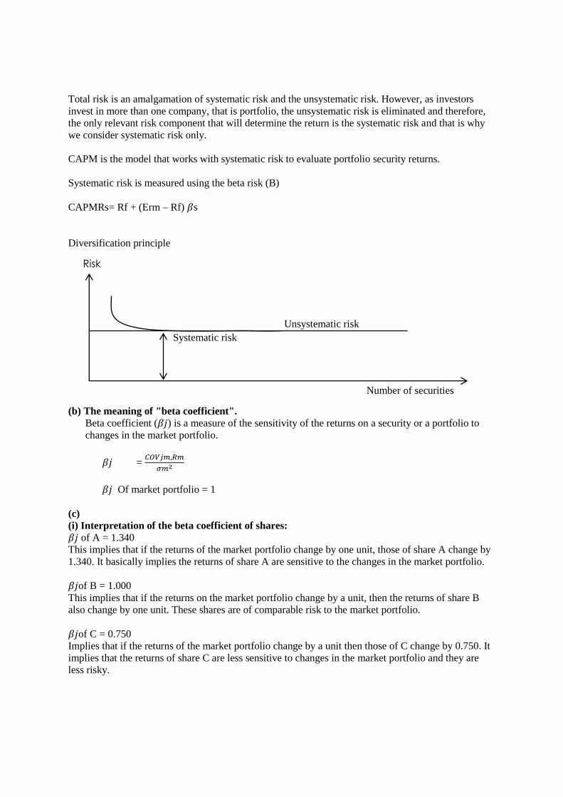
Total risk is an amalgamation of systematic risk and the unsystematic risk. However, as investors
invest in more than one company, that is portfolio, the unsystematic risk is eliminated and therefore,
the only relevant risk component that will determine the return is the systematic risk and that is why
we consider systematic risk only.
CAPM is the model that works with systematic risk to evaluate portfolio security returns.
Systematic risk is measured using the beta risk (B)
CAPMRs= Rf + (Erm – Rf) 𝛽s
Diversification principle
(b) The meaning of "beta coefficient".
Beta coefficient (𝛽𝑗) is a measure of the sensitivity of the returns on a security or a portfolio to
changes in the market portfolio.
𝛽𝑗 = 𝐶𝑂𝑉𝑗𝑚,𝑅𝑚
𝜎𝑚2
𝛽𝑗 Of market portfolio = 1
(c)
(i) Interpretation of the beta coefficient of shares:
𝛽𝑗 of A = 1.340
This implies that if the returns of the market portfolio change by one unit, those of share A change by
1.340. It basically implies the returns of share A are sensitive to the changes in the market portfolio.
𝛽𝑗of B = 1.000
This implies that if the returns on the market portfolio change by a unit, then the returns of share B
also change by one unit. These shares are of comparable risk to the market portfolio.
𝛽𝑗of C = 0.750
Implies that if the returns of the market portfolio change by a unit then those of C change by 0.750. It
implies that the returns of share C are less sensitive to changes in the market portfolio and they are
less risky.
Unsystematic risk
Number of securities
Systematic risk
Risk
Page 109
(ii)Using CAPM, the expected return is given by:
HINT;
CAPM uses the systematic (beta factor) to evaluate security returns.
CAPM Rj = Rf + (Rm – Rf) 𝛽𝑖
CAPM Returns of eachsecurity
Share A
Share B
Share C
=
=
=
12 + (18.5 – 12)1.34 =
12 + (18.5 – 12) 1 =
12 + (18.5 – 12)0.75 =
20.71%
18.5 %
16.875 %
(d)
(i) Sharpe's performance measure for portfolios P and N.
HINT;
Sharpe’s model uses standard deviations to evaluate performance of securities.
Sharpe measure SP = 𝐸𝑅−𝑅𝑓
𝛿𝑝 =
0.35−0.06
0.42= 0.690
SN = 0.28−0.06
0.30= 0.733
(ii)Treynor's performance measure for portfolios P and N.
HINT;
Treynors model uses beta factors to evaluate performance of securities.
Treynor’s measure
TP= 𝐸𝑅𝑝−𝑅𝑓
𝛽𝑝 =
0.35−0.06
1.25= 0.232
TN= 0.28−0.06
1 = 0.22
(iii) Jensen's performance measure for portfolios P and N.
HINT;
First step in evaluation of Jensens values is to determine the returns by use of CAPM model.
CAPM RP=Rf + (Rm – Rf)𝛽𝑗
CAPM RP=0.06 + (0.15 – 0.06) 1.25=0.1725
CAPM RN=0.06 + (0.15 – 0.06) 1 = 0.15
𝛼j =ERj – CAPM Rj
Note
ERj is the expected return = average return
Page 110

ERp =0.35
ERN =0.28
𝛼P= 0.35 – 0.1725= 0.1775=17.75%
𝛼N=0.28 – 0.15= 0.13=13%
(iv) The appraisal ratio/information ratio
Appraisal ratio (AP) = 𝐸𝑥𝑐𝑒𝑠𝑠𝑟𝑒𝑡𝑢𝑟𝑛
𝐸𝑥𝑐𝑒𝑠𝑠𝑠𝑡𝑑𝑑𝑣𝑛
HINT;-
For appraisal Ratio model we must be given a benchmark security.
ERB is the return from benchmark security.
𝛿B= Standard deviation benchmark.
Excess return = ERs – ERB
Excess standard deviation = δs – δB
Appraisal ratio (AP) = 𝐸𝑅𝑠−𝐸𝑅𝐵
δs –δB
HINT;-
If benchmark is not given use that of the market portfolio to ascertain the appraisal ratio.
The 𝛿 of the market portfolio (𝛿m) is not provided and therefore the equation given above is irrelevant.
See this!
AP for portfolio P = 35−15
42 –δm
Alternatively the AP ratio can be ascertained as follows
AP = 𝐸𝑅𝑠−𝐸𝑅𝑚
Non−systematic Risk of the security
AP for portfolio P = 35−15
18 = 1.1
AP for portfolio N = 28−15
10 = 1.3
Page 111
CHAPTER THREE
ADVANCED FINANCING DECISION CHAPTER KEY OJECTIVES
To be able to understand the following;-
1. The nature of financing decision, principle objectives of making financing decision
2. Overview of cost of capital: meaning and relevance of cost of capital: the firm’s overall cost of
capital; weighted average cost of capital (WACC) and weighted marginal cost of capital (WMCC)
; analysis of breakpoints in weighted marginal cost of capital schedule
3. Capital structure theories: nature of capital structure and factors influencing the firm’s capital
structure; traditional theories of capital structure - assumptions of the theories, Net income theory
and Net operating income theory; Franco Modigliani and Merton Miller’s propositions - MM
without taxes, MM with corporation taxes, MM with corporation and personal tax rates and MM
with taxes and financial distress costs; other theories of capital structure; the pecking order theory
and Trade-off theory determination of the firm’s optimal capital structure using the Hamada
model, CAPM and WACC
4. Special topics in financing decision: analysis of operating profit (EBIT)/EPS at point of
indifference in firm’s earnings; establishing the range of operating profit within which each
financing option; leverage and risk; operating leverage and operating risk, financial leverage and
financial risk, combined leverage and total risk; quantifying leverage using the degree of
operating leverage, degree of financial leverage and degree of combined leverage
5. Long term financing decisions; bond refinancing decision, lease-buy evaluation and the rights
issues
6. Impact of financing on investment decisions - the concept of adjusted present value (APV)
3.1. NATURE AND SIGNIFICANCE OF FINANCING DECISIONS This refers to the decisions that involve the manner in which the company is expected to raise funds
that are required to finance all profitable projects.
The required amount should always be raised in the most economical way and from the most
economic sources.
In raising the required finances to undertake all profitable projects, the company can utilise common
equity capital, preference share capital or long term debts/debentures.
The cost of raising the required amount is known as the Weighted Average Cost of Capital. This is the
cost of funds utilised to finance the existing projects.
Therefore, financial decisions refer to decisions concerning financial matters of a business concern.
Decisions regarding magnitude of funds to be invested to enable a firm to accomplish its ultimate
goal, kind of assets to be acquired, pattern of capitalization, pattern of distribution of firms, income
and similar other matters are included in financial decisions
The principle objective of making financing decision is to minimize on the cost of borrowing.
Other objectives include
Ensuring that funds are made available within the correct length of time
Ensuring that funds raised are utilised in a more effective manner.
Once the objective have been attained it is possible to achieve the firms objective of wealth
maximization and profit maximum
Page 112
3.2. OVERVIEW OF COST OF CAPITAL
Cost of capital is an integral part of investment decision as it is used to measure the worth of
investment proposal provided by the business concern. It is used as a discount rate in determining the
present value of future cash flows associated with capital projects. Cost of capital is also called as cut-
off rate, target rate, hurdle rate and required rate of return. When the firms are using different sources
of finance, the finance manager must take careful decision with regard to the cost of capital; because
it is closely associated with the value of the firm and the earning capacity of the firm.
Meaning of Cost of Capital
Cost of capital is the rate of return that a firm must earn on its project investments to maintain its
market value and attract funds. Cost of capital is the required rate of return on its investments which
belongs to equity, debt and retained earnings. If a firm fails to earn return at the expected rate, the
market value of the shares will fall and it will result in the reduction of overall wealth of the
shareholders. It is the minimum required rate of return to providers of capital
Significance of cost of capital
Investment Evaluation:
The primary objective of determining the cost of capital is to evaluate a project. Various methods used
in investment decisions require the cost of capital as the cut-off rate. Under net present value method,
profitability index and benefit-cost ratio method the cost of capital is used as the discounting rate to
determine present value of cash flows. Similarly, a project is accepted if its internal rate of return is
higher than its cost of capital. Hence, cost of capital provides a rational mechanism for making the
optimum investment decision.
Designing Debt Policy
The cost of capital influences the financing policy decision, i.e. the proportion of debt and equity in
the capital structure. Optimal capital structure of a firm can maximize the shareholders’ wealth
because an optimal capital structure logically follows the objective of minimization of overall cost of
capital of the firm. Thus while designing the appropriate capital structure of a firm cost of capital is
used as the yardstick to determine its optimality.
Project Appraisal:
The cost of capital is also used to evaluate the acceptability of a project. If the internal rate of return of
a project is more than its cost of capital, the project is considered profitable. The composition of
assets, i.e. fixed and current, is determined by the cost of capital. The composition of assets, which
earns return higher than cost of capital, is accepted.
In measuring top management performance
It is used as a yard stick in measuring top management performance this is done by comparing return
if the actual return is more than the or equal to the minimum required rate of return the management
would be doing best their jobs otherwise they would doing worst their job.
Overall cost of capital
Page 113
The firm's overall cost of capital is based on the weighted average of the costs of equity capital debt
capital and preference shares capital.
The component costs are the cost of equity (Ke) cost of preference shares (Kp), cost of debt (Kd)
Cost of equity
It is the minimum return that should be obtained from the projects that are fully financed by common
equity capital so as to raise cash flows required to pay back to ordinary shareholders. It is therefore
the minimum rate of return required by ordinary shareholders.
Common equity capital is made up of external equity (ordinary shares) and internal equity (Retained
earnings).
The cost of equity in both cases in calculated in the same way except that in case of calculation costs,
such costs would only affect ordinary shares i.e.
Ke (without floatation costs) would be:
Ke = 𝐷𝑜 (1+𝑔)
𝑃𝑜+ 𝑔
Where
Ke – Cost of equity/minimum rate of return required by ordinary shareholders
Do – Current year’s dividend/Dividends just paid/Dividend for the year just ended
g – Annual growth rate in dividend
Po – Current market price of share/intrinsic value per share
In case the dividend doesn’t grow
Ke = 𝐷𝑜
𝑃𝑜−𝐹
Where D1 = Next year’s dividends/Dividends to be paid in a year’s time/Expected dividends
D1 = Do (1 + g)
Ke = 𝐷𝑜 (1+𝑔)
𝑃𝑜−𝐹+ 𝑔 or
𝐷1
𝑃𝑜−𝐹+ 𝑔
In case of floatation costs
Ke (Retained Earnings) = 𝐷𝑜 (1+𝑔)
𝑃𝑜+ 𝑔 or
𝐷1
𝑃𝑜+ 𝑔
Ke (Ordinary shares) = 𝐷𝑜 (1+𝑔)
𝑃𝑜−𝑓+ 𝑔 or
𝐷1
𝑃𝑜−𝑓+ 𝑔
Page 114
Where f = Floatation/issue costs
Illustration
The current market value of ordinary shares of Ujuzi Ltd is Sh. 45. The company has just paid a
dividend of Sh. 5 which grows at annual rate of 8% p.a. ordinary shares attract a floatation cost of 5%
Required;-
Calculate the cost of equity assuming
Solution
Ke (Retained Earnings) = 𝐷1
𝑃𝑜+ 𝑔=
5(1.08)
45 + 0.08 = 0.2 ×100 = 20%
Ke (Ordinary Shares) = 𝐷1
𝑃𝑜−𝑓+ 𝑔=
5(1.08)
45−2.25 + 0.08 = 0.2063×100 = 20.63%
NOTE: Retained earnings do not have floatation costs.
Floatation cost of ordinary shares = 5% x 45 = 2.25
Illustration
A company expects to pay a dividend of Sh. 12 in the coming years on its shares currently selling for
Sh. 60.The past information about the earnings per share for the current year are as analysed below.
The retention ratio is 20%.
Year EPS (Sh.) DPS 80%
2015
2014
2013
2012
2011
2010
14
11
10.5
9.5
8.0
7.0
11.2
8.8
8.4
7.6
6.4
5.6
Note: Retained ratio + Dividend payout ratio = 1
Required
Calculate Ke
Solution
Ke = 𝐷𝑜 (1+𝑔)
𝑃𝑜−𝐹+ 𝑔
D0(1 + g) = D1
Where D1 = Expected dividend = 12
Ke = 12
60 + 0.15
g = √𝑙𝑎𝑡𝑒𝑠𝑡 𝐷.𝑃.𝑆
𝐸𝑎𝑟𝑙𝑖𝑒𝑠𝑡 𝐷.𝑃.𝑆
𝑛 = √
11.2
5.6
5
= 1.15 – 1 = 0.15 = 15%
Page 115
= 0.35 x 100 = 35%
Note: The growth rate of dividends is not given and therefore we shall first ascertain it.
Illustration
The dividend yield of a company is 12% and the expected dividend is Sh. 10. Currently the company
pays a dividend of Sh. 9.5.
Calculate Ke
Solution
Dividend Yield = 𝐷𝑃𝑆
𝑀𝑃𝑆
0.12 = 9.5
𝑥
0.12x = 9.5
x = 9.5
0.12
x = 79.17
x = market price per share = P0
Determine growth rate as follows:
D1 = Do (1 + g)
10 = 9.5 (1 + g)
10 = 9.5 + 9.5g
10 – 9.5 = 9.5g
0.5 = 9.5g therefore g = 0.5
9.5 = 0.05
g = 0.05 × 100 = 5%
Note: D1 = Expected dividend = 10
Ke = 𝐷1
𝑃𝑜+ 𝑔=
10
79.17 + 0.05 = 0.1763 x 100 = 17.63%
Cost of Preference Shares (Kp)
It is the minimum rate of return that should be obtained from the projects that are fully financed by
preference share capital so as to generate sufficient cash flows required to pay back to preference
shareholders.
It is therefore the minimum rate of return required by preference shareholders.
Kp is the discount factor that equate the present value of expected dividends to the current market
value per preference share i.e.
Page 116
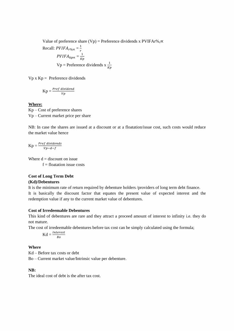
Value of preference share (Vp) = Preference dividends x PVIFAr%,∝
Recall: 𝑃𝑉𝐼𝐹𝐴𝑟%∝ = 1
𝑟
𝑃𝑉𝐼𝐹𝐴𝑘𝑝∝ = 1
𝐾𝑝
Vp = Preference dividends x 1
𝐾𝑝
Vp x Kp = Preference dividends
Kp = 𝑃𝑟𝑒𝑓 𝑑𝑖𝑣𝑖𝑑𝑒𝑛𝑑
𝑉𝑝
Where:
Kp – Cost of preference shares
Vp – Current market price per share
NB: In case the shares are issued at a discount or at a floatation/issue cost, such costs would reduce
the market value hence
Kp = 𝑃𝑟𝑒𝑓 𝑑𝑖𝑣𝑖𝑑𝑒𝑛𝑑𝑠
𝑉𝑝−𝑑−𝑓
Where d = discount on issue
f = floatation issue costs
Cost of Long Term Debt
(Kd)/Debentures
It is the minimum rate of return required by debenture holders /providers of long term debt finance.
It is basically the discount factor that equates the present value of expected interest and the
redemption value if any to the current market value of debentures.
Cost of Irredeemable Debentures
This kind of debentures are rare and they attract a proceed amount of interest to infinity i.e. they do
not mature.
The cost of irredeemable debentures before tax cost can be simply calculated using the formula;
Kd = 𝐼𝑛𝑡𝑒𝑟𝑒𝑠𝑡
𝐵𝑜
Where
Kd – Before tax costs or debt
Bo – Current market value/Intrinsic value per debenture.
NB:
The ideal cost of debt is the after tax cost.
Page 117
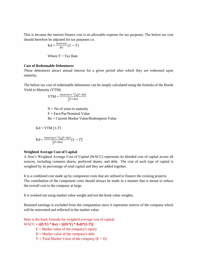
This is because the interest finance cost is an allowable expense for tax purposes. The before tax cost
should therefore be adjusted for tax purposes i.e.
Kd = 𝐼𝑛𝑡𝑒𝑟𝑒𝑠𝑡
𝐵𝑜(1 − 𝑇)
Where T = Tax Rate
Cost of Redeemable Debentures
These debentures attract annual interest for a given period after which they are redeemed upon
maturity.
The before tax cost of redeemable debentures can be simply calculated using the formula of the Bonds
Yield to Maturity (YTM)
YTM = 𝐼𝑛𝑡𝑒𝑟𝑒𝑠𝑡+ 1 𝑛⁄ [𝐹−𝐵𝑜]
1
2[𝐹+𝐵𝑜]
N = No of years to maturity
F = Face/Par/Nominal Value
Bo = Current Market Value/Redemption Value
Kd = YTM [1-T]
Kd = 𝐼𝑛𝑡𝑒𝑟𝑒𝑠𝑡+ 1 𝑛⁄ [𝐹−𝐵𝑜]
1
2[𝐹+𝐵𝑜]
[1 − 𝑇]
Weighted Average Cost of Capital
A firm’s Weighted Average Cost of Capital (WACC) represents its blended cost of capital across all
sources, including common shares, preferred shares, and debt. The cost of each type of capital is
weighted by its percentage of total capital and they are added together.
It is a combined cost made up by component costs that are utilised to finance the existing projects.
The contribution of the component costs should always be made in a manner that is meant to reduce
the overall cost to the company at large.
It is worked out using market value weight and not the book value weights.
Retained earnings is excluded from the computation since it represents reserve of the company which
will be reinvested and reflected in the market value.
Here is the basic formula for weighted average cost of capital:
WACC = ((E/V) * Ke) + [((D/V) * Kd)*(1-T)]
E = Market value of the company's equity
D = Market value of the company's debt
V = Total Market Value of the company (E + D)
Page 118
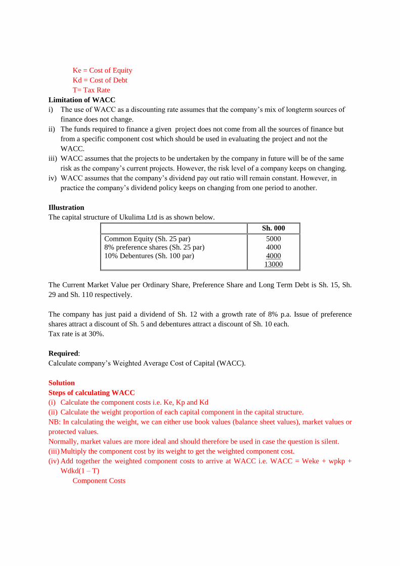
Ke = Cost of Equity
Kd = Cost of Debt
T= Tax Rate
Limitation of WACC
i) The use of WACC as a discounting rate assumes that the company’s mix of longterm sources of
finance does not change.
ii) The funds required to finance a given project does not come from all the sources of finance but
from a specific component cost which should be used in evaluating the project and not the
WACC.
iii) WACC assumes that the projects to be undertaken by the company in future will be of the same
risk as the company’s current projects. However, the risk level of a company keeps on changing.
iv) WACC assumes that the company’s dividend pay out ratio will remain constant. However, in
practice the company’s dividend policy keeps on changing from one period to another.
Illustration
The capital structure of Ukulima Ltd is as shown below.
Sh. 000
Common Equity (Sh. 25 par)
8% preference shares (Sh. 25 par)
10% Debentures (Sh. 100 par)
5000
4000
4000
13000
The Current Market Value per Ordinary Share, Preference Share and Long Term Debt is Sh. 15, Sh.
29 and Sh. 110 respectively.
The company has just paid a dividend of Sh. 12 with a growth rate of 8% p.a. Issue of preference
shares attract a discount of Sh. 5 and debentures attract a discount of Sh. 10 each.
Tax rate is at 30%.
Required:
Calculate company’s Weighted Average Cost of Capital (WACC).
Solution
Steps of calculating WACC
(i) Calculate the component costs i.e. Ke, Kp and Kd
(ii) Calculate the weight proportion of each capital component in the capital structure.
NB: In calculating the weight, we can either use book values (balance sheet values), market values or
protected values.
Normally, market values are more ideal and should therefore be used in case the question is silent.
(iii) Multiply the component cost by its weight to get the weighted component cost.
(iv) Add together the weighted component costs to arrive at WACC i.e. WACC = Weke + wpkp +
Wdkd(1 – T)
Component Costs
Page 119
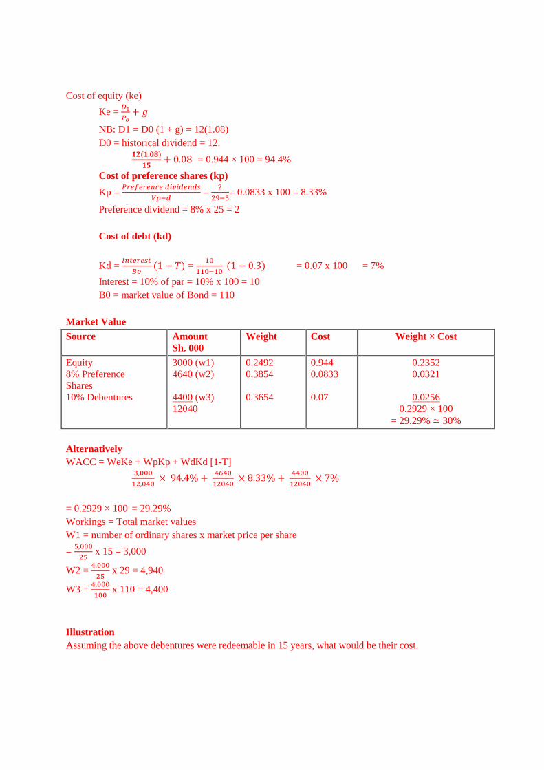
Cost of equity (ke)
Ke = 𝐷1
𝑃𝑜+ 𝑔
NB: D1 = D0 (1 + g) = 12(1.08)
D0 = historical dividend = 12.
𝟏𝟐(𝟏.𝟎𝟖)
𝟏𝟓+ 0.08 = 0.944 × 100 = 94.4%
Cost of preference shares (kp)
Kp = 𝑃𝑟𝑒𝑓𝑒𝑟𝑒𝑛𝑐𝑒 𝑑𝑖𝑣𝑖𝑑𝑒𝑛𝑑𝑠
𝑉𝑝−𝑑 =
2
29−5= 0.0833 x 100 = 8.33%
Preference dividend = 8% x 25 = 2
Cost of debt (kd)
Kd = 𝐼𝑛𝑡𝑒𝑟𝑒𝑠𝑡
𝐵𝑜(1 − 𝑇) =
10
110−10 (1 − 0.3) = 0.07 x 100 = 7%
Interest = 10% of par = 10% x 100 = 10
B0 = market value of Bond = 110
Market Value
Source Amount
Sh. 000
Weight Cost Weight × Cost
Equity
8% Preference
Shares
10% Debentures
3000 (w1)
4640 (w2)
4400 (w3)
12040
0.2492
0.3854
0.3654
0.944
0.0833
0.07
0.2352
0.0321
0.0256
0.2929 × 100
= 29.29% ≃ 30%
Alternatively
WACC = WeKe + WpKp + WdKd [1-T]
3,000
12,040 × 94.4% +
4640
12040 × 8.33% +
4400
12040 × 7%
= 0.2929 × 100 = 29.29%
Workings = Total market values
W1 = number of ordinary shares x market price per share
= 5,000
25 x 15 = 3,000
W2 = 4,000
25 x 29 = 4,940
W3 = 4,000
100 x 110 = 4,400
Illustration
Assuming the above debentures were redeemable in 15 years, what would be their cost.
Page 120
Solution
First compute the yield to maturity
Yield to maturity (YTM) = 𝐼𝑛𝑡𝑒𝑟𝑒𝑠𝑡+
1
𝑛 (𝐹−𝐵𝑜)
1
2 (𝐹+𝐵𝑜)
Formular for redeemable debentures
Where
F = face value
B0 = market value of bond less costs to sell = 110 – 10 = 100
T = Tax
10+ 0
1
2 (100+100)
10+ −01
2 𝑥 200
= 10%
After tax cost (kd (1 + T) = 10% (1 – 0.3) = 7%
NB: When the debentures or preference shares are selling at par, their before tax cost would be the
coupon rate.
Marginal Cost of Capital (MCC)
It is the cost of incremental new funds that are used to undertake the firm’s new projects i.e. it is a
futuristic cost.
WACC is the cost incurred by the company to raise funds that are used to implement existing projects
i.e. it is a historical cost.
In calculating WMCC, marginal book value weights are used.
The marginal weights are the proportions of capital components calculated from the optimal capital
structure.
Retained earnings is included in the computation because it must be utilised up to a point of
exhaustion before raising additional finance through issue of ordinary share.
Breakpoint
It is the level of total financing (100%) at which amount available from a cheaper source in a given
capital component are fully utilised.
Breakpoint arises when a given capital component can generate more than one source of capital e.g.
from equity we can get retained earnings and ordinary shares.
A breakpoint will occur if there is an increase in the cost of capital.
Breakpoint for retained earnings = 𝑟𝑒𝑡𝑎𝑖𝑛𝑒𝑑 𝑒𝑎𝑟𝑛𝑖𝑛𝑔𝑠
optimal equity proportion
Page 121
Breakpoint for Debt capital= 𝐶ℎ𝑒𝑎𝑝𝑒𝑟 𝑑𝑒𝑏𝑡𝑠
optimal debt proportion
Illustration
Mapema Ltd has the following capital structure which it considers optimal:
Source of capital Amount
Sh. “million”
Ordinary share capital
Preference share capital
Long term debt
Total
90.0
22.5
37.5
150.0
Mapema Ltd expects an after tax income of sh.5,143,000 in the next financial year. The company has
a policy of 30% of its earnings as dividends. Investors expect dividends to grow at an annual rate of
9% indefinitely. The dividends paid by the company were sh.5.40 per share. The company’s ordinary
shares currently sell on the stock market at sh.90 per share. The company can obtain additional
financing in the financial markets as follows:
Long-term debt
Up to sh.7.5 million of long-term debt can be obtained at an interest rate of 12%; long-term debt in the
range of sh.7.5 million to sh.15 million must carry an interest rate of 14%; and all long-term debt over
sh.15 million will have an interest rate of 16%. The corporate tax rate is 30% and interest on long-
term debt is tax allowable.
Ordinary shares
New ordinary shares of up to sh.18 million can be raised at sh.81 per share. To issue additional shares
above sh.18 million floatation cost of sh.18 per share must be incurred.
Preference shares
New preference shares with a par value of sh.100 can be issued and the dividend rate is 11%.
However, a floatation cost of 5% of the par value per share must be incurred for all preference shares
up to sh.11.25 million. Additional preference shares (above sh.11.25 million) can be raised at a
floatation cost of sh.10 per share.
The investment opportunities available to the company are as shown below:
Investment Outlay
Sh.
Annual net cash flow
Sh.
Life (years) Internal rate of
return (IRR)
(%)
I
II
III
IV
V
15,000,000
15,000,000
15,000,000
30,000,000
30,000,000
3,286,800
4,731,630
3,255,270
5,684,220
8,141,760
7
5
8
10
6
12.0
17.4
14.2
16.0
?
Required:
(a) Determine the break points in the marginal cost of capital (MCC) schedule.
Page 122
(b) Calculate the weighted average cost of capital (WACC) in the intervals between the break points
in the MCC schedule.
(c) Calculate the internal rate of return (IRR) for project V.
(d) Construct an investment opportunity curve (IOC) marginal cost of capital (MCC) schedule and
indicate which project(s) should be accepted or rejected.
Solution
(a) Weights (obtained from the capital structure)
Weight of Equity = 90
150 x 100 = 60%
Weight of Preference share capital = 22.5
150 x 100 = 15%
Weight of Debt =37.5
150 x 100 = 25%
Equity
Retained earnings = 70% x 5143,000 = 3,600,100
Breakpoint of retained earnings = 𝐴𝑚𝑜𝑢𝑛𝑡
𝑊𝑒𝑖𝑔ℎ𝑡 𝑜𝑓 𝑒𝑞𝑢𝑖𝑡𝑦
= 3600100
0.6= 6,000,167 ksh
Breakpoint (ordinary share upto 18,000,000) = 𝐶𝑢𝑚𝑢𝑙𝑎𝑡𝑖𝑣𝑒 𝑎𝑚𝑜𝑢𝑛𝑡
𝑊𝑒𝑖𝑔ℎ𝑡 𝑜𝑓 𝑑𝑒𝑏𝑡
= 18000000+3600100
0.6
= 36,000167 kshs
Breakpoint (for ordinary shares beyond 18000000). The upper limit is not provided
There if no limit and therefore there is no breakpoint.
Breakpoint of debts (weight of debt = 25%
Breakpoint (upto 7,500,000) = 𝐶𝑢𝑚𝑢𝑙𝑎𝑡𝑖𝑣𝑒 𝑎𝑚𝑜𝑢𝑛𝑡
𝑊𝑒𝑖𝑔ℎ𝑡 𝑜𝑓 𝑒𝑞𝑢𝑖𝑡𝑦
= 7,500,000
25% = 30m
Breakpoint (7.5m up to 15m) = 15,000,000
25% = 60m
Breakpoint (Above 15m) = No limit and therefore no break point.
Breakpoint of preference (weight of preference = 15%)
Breakpoint (up to 11.25m) = 11,250,000
15% = 75,000,000 Ksh
Breakpoint (preference above 11.25m) = No limit, no break point.
(b) WACC
Cost of Equity = 𝐷𝑜 (1+𝑔)
𝑃𝑜−𝑑+ 𝑔
1) Cost of (ke1)
Retained Earnings = 5.40 (1.09)
90+ 0.09
0.0654 + 0.09 = 0.1554 x 100
= 15.54%
2) Cost of (ke2) up to ksh.18,000,000
Page 123
Ordinary Shares = 5.40 (1.09)
81+ 0.09
0.0727 + 0.09 = 0.1627 × 100 = 16.27%
3) Cost of ordinary shares above 18,000,000 (ke3)
= 5.4(1.09)
(90−18) + 0.09= 0.17175 = 17.2%
Cost of Long term debt = 𝐼𝑛𝑡𝑒𝑟𝑒𝑠𝑡
𝐵𝑜[1 − 𝑇] = cost before tax (I – T)
12% long term debt (kd1) = 0.12 (1 – 0.3)
= 0.084 x 100 = 8.4%
14% long term debt (kd2)= 0.14 (0.7)
= 0.098 x 100 = 9.8%
16% long term debt (kd3) = 0.16 (0.7)
= 0.112 x 100 = 11.2%
Preferences Shares = 𝑃𝑟𝑒𝑓𝑒𝑟𝑒𝑛𝑐𝑒 𝑑𝑖𝑣𝑖𝑑𝑒𝑛𝑑𝑠
𝑉𝑝−𝑑𝑓
Upto 11.25m (Floatation cost = 5% x 100 = 5)
Kp1 = 11
100−5 = 0.1158 x 100 = 11.58%
Over 11.25m (Floatation cost = 10)
Kp2 = 11
100−10 = 0.1222 x 100 = 12.22%
Summary
Equity
Bp1 = 6,000,167 ke1 = 15.54%
Bp2 = 36,000,167 ke2 = 16.27%
Ke3 = 17.2%
Debt
Bp1 = 30,000,000
Bp2 = 60m
Kd1 = 8.4%
Kd2 = 9.8%
Kd3 = 11.2%
Preference
Bp1 = 75,000,000
Kp1 = 11.58%
Kp2 = 12.22%
Preference dividend = 11% of par value
11% × 100 = 11
Page 124
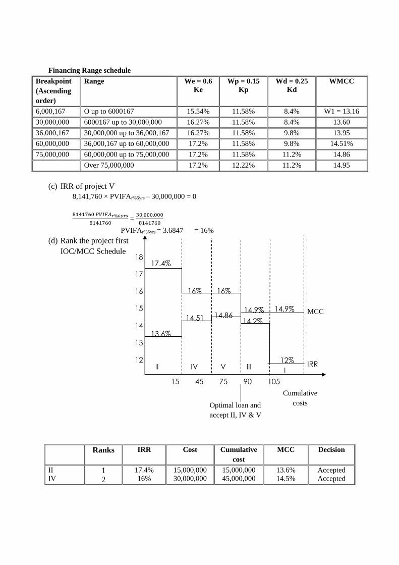
Financing Range schedule
Breakpoint
(Ascending
order)
Range We = 0.6
Ke
Wp = 0.15
Kp
Wd = 0.25
Kd
WMCC
6,000,167 O up to 6000167 15.54% 11.58% 8.4% W1 = 13.16
30,000,000 6000167 up to 30,000,000 16.27% 11.58% 8.4% 13.60
36,000,167 30,000,000 up to 36,000,167 16.27% 11.58% 9.8% 13.95
60,000,000 36,000,167 up to 60,000,000 17.2% 11.58% 9.8% 14.51%
75,000,000 60,000,000 up to 75,000,000 17.2% 11.58% 11.2% 14.86
Over 75,000,000 17.2% 12.22% 11.2% 14.95
(c) IRR of project V
8,141,760 × PVIFAr%6yrs – 30,000,000 = 0
8141760 𝑃𝑉𝐼𝐹𝐴𝑟%6𝑦𝑟𝑠
8141760 =
30,000,000
8141760
PVIFAr%6yrs = 3.6847 = 16%
(d) Rank the project first
IOC/MCC Schedule
Ranks IRR Cost Cumulative
cost
MCC Decision
II
IV 1
2
17.4%
16%
15,000,000
30,000,000
15,000,000
45,000,000
13.6%
14.5%
Accepted
Accepted
18
17
16
15
14
13
12
15 45 75 90 105
II IV V III I
Optimal loan and
accept II, IV & V
Cumulative
costs
IRR 12%
13.6%
14.51
16% 16%
14.9% 14.9%
14.2%
17.4%
14.86 MCC
Page 125
V
III
I
3
4
5
16%
14.2%
12%
30,000,000
15,000,000
15,000,000
75,000,000
90,000,000
105,000,000
14.86%
14.95%
14.95%
Accepted
Rejected
Rejected
The projects whose IRR is more than MCC are accepted hence projects II, IV and V should be
implemented. The optimal amount to be borrowed to finance the 3 projects is Ksh.7,000,000.
Capital Structure Financing Decisions
Capital structure is the mix of debt, preference share capital and equity that is used by a firm to
finance its long term investment activities.
The capital structure decisions are always aimed at maximising the value of the firm and minimising
the overall cost of capital (WACC).
Normally, the optimal capital structure should be planned for by each company. This mix of debt and
equity minimises the cost of capital (WACC) and maximises the shareholders’ wealth/value of the
firm.
OPTIMUM CAPITAL STRUCTURE
Optimum capital structure is the capital structure at which the weighted average cost of capital is
minimum and thereby the value of the firm is maximum. Optimum capital structure may be defined as
the capital structure or combination of debt and equity that leads to the maximum value of the firm.
Objectives of Capital Structure Decision of capital structure aims at the following two important
objectives:
1. Maximize the value of the firm.
2. Minimize the overall cost of capital
Factors that influence capital structure decisions/financing decisions.
Component cost
Some firms could avoid equity due to its high cost as compared to debt.
Debt is always expected to be less expensive since it is more secure from the investments point of
view hence they would demand a lower return compared to equity. Moreover, the company saves
some tax due to interest associated with debt.
Availability of Assets to Pledge as Security
Companies that have disposable assets that can be pledged as collateral for a loan can increase their
capital structure by raising more debt unlike a company without such a facility.
Tax rate
Page 126
Firms that operate in economics of higher taxes can have tax advantage of the system and use more of
debt in their capital structure to save some taxes from the interest known as interest tax shield i.e. the
finance cost is a tax-deductible expense.
Manager’s attitude to risk
Risk takers would always aim to expand which will be financed by increasing the capital structure. At
times, the management that are risk takers may even opt to raise more funds through debt due to fewer
procedures involved.
Risk averse management may not increase their capital structure since they would be too reluctant to
expand more so increase their debt due to the fear of financial gearing risk.
Growth stage of the Firm.
Any company has to raise more funds so as to support/finance its expansion/growth in terms of
revenue and total assets.
Flexibility
A capital structure that can be easily altered/changed with a minimum cost and delays shall be
adopted by many companies.
CAPITAL STRUCTURE THEORIES Some commentators believe that an optimal mix of finance exists at which the company’s cost of
capital will be minimized.
When we consider the capital structure decision, the question arises of whether there is an optimal
mix of equity and debt which a company should try to achieve. Under the traditional view there is an
optimal capital mix at which the average cost of capital, weighted according to the different forms of
capital employed, is minimized.
However, the alternative view of Modigliani and Miller is that the firm’s overall weighted average
cost of capital is not influenced by changes in its capital structure.
Different theories were formulated in different years with the aim of understanding the effect of debt.
Financing in the company’s capital structure.
They include:
i) Traditional Theories
ii) Net Income Theory (NI)
iii) Net Operating Income Approach Theory (NOI)
iv) Modigliani and Miller (MM) Prepositions
TRADITIONAL THEORY
Under the traditional theory of cost of capital, the cost declines initially and then rises as gearing
increases. The optimal capital structure will be the point at which WACC is lowest.
The traditional view of structure is that there is an optimal capital structure and the company can
increase its total value by a suitable use of debt finance in its capital structure.
The assumptions on which this theory is based are as follows:
Page 127
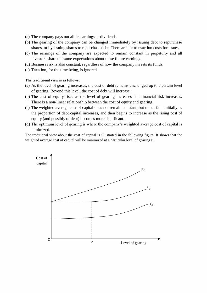
(a) The company pays out all its earnings as dividends.
(b) The gearing of the company can be changed immediately by issuing debt to repurchase
shares, or by issuing shares to repurchase debt. There are not transaction costs for issues.
(c) The earnings of the company are expected to remain constant in perpetuity and all
investors share the same expectations about these future earnings.
(d) Business risk is also constant, regardless of how the company invests its funds.
(e) Taxation, for the time being, is ignored.
The traditional view is as follows:
(a) As the level of gearing increases, the cost of debt remains unchanged up to a certain level
of gearing. Beyond this level, the cost of debt will increase.
(b) The cost of equity rises as the level of gearing increases and financial risk increases.
There is a non-linear relationship between the cost of equity and gearing.
(c) The weighted average cost of capital does not remain constant, but rather falls initially as
the proportion of debt capital increases, and then begins to increase as the rising cost of
equity (and possibly of debt) becomes more significant.
(d) The optimum level of gearing is where the company’s weighted average cost of capital is
minimized.
The traditional view about the cost of capital is illustrated in the following figure. It shows that the
weighted average cost of capital will be minimized at a particular level of gearing P.
Ke
K0
Kd
Level of gearing 0
Cost of
capital
P
Page 128
Where
Ke is the cost of equity in the geared company
Kd is the cost of debt
K0 is the weighted average cost of capital
The traditional view is that the weighted average cost of capital, when plotted against the level of
gearing is saucer shaped. The optimum capital structure is where the weighted average cost of capital
is lowest, at point P.
Conclusion
Traditional theory therefore, states that there exists a capital structure which maximise the value of a
firm and minimises the cost of capital (WACC) at an optimal debt level.
PECKING ORDER THEORY
Pecking order theory has been developed as an alternative to traditional theory. It states that firms will
prefer retained earnings to any other source of finance, and then will choose debt, and last of all
equity.
The order of preference will be:
Retained earnings
Straight debt
Convertible debt
Preference shares
Equity shares
Reasons for following pecking order
(a) It is easier to use retained earnings than go to the trouble of obtaining external finance and have to
live up to the demands of external finance providers.
(b) There are no issue costs if retained earnings are used, and the issue costs of debt are lower than
those of equity.
(c) Investors prefer a safer security, which is debt with its guaranteed income and priority on
liquidation.
(d) Some managers believe that debt issues have a better signalling effect than equity because the
market believes that managers are better informed about shares’ true worth than the market itself
is. Their view is the market will interpret debt issues as a sign of confidence, that businesses are
confident of making sufficient profits to fulfil their obligations on debt and that they believe that
the shares are undervalued.
By contrast the market will interpret equity issues as a measure of last resort that managers believe
that equity is currently overvalued and hence are trying to achieve high proceeds whilst they can.
However an issue of debt may imply a similar lack of confidence to an issue of equity; managers may
issue debt when they believe that the cost of debt is low due to the market underestimating the risk of
default and hence undervaluing, the risk premium in the cost of debt. If the market recognizes this
lack of confidence, it is likely to respond by raising the cost of debt.
Page 129
The main consequence in this situation will be to reinforce a preference for using retained earnings
first. However debt (particularly less risky, secured debt) will be the next source as the market feels
more confident about valuing it than more risky debt or equity.
Behavioural theories
This theory states that the company shall always aim at maintaining a capital structure that is closely
related to that of an average firm in the industry.
Benchmark Theory
This theory suggests that firms will identify a trader or another company in the market and adopt a
similar capital structure.
Post Experience Concept
It is an important influence in the capital structure which is based on accumulative knowledge and
experience about the past that the managers will select an optimal capital structure that will give them
less trouble i.e. higher returns and lower costs.
Traditional and Static Trade-Off Theory
Static trade off view develops the traditional theory and states that firms will always aim from an ideal
capital structure and will issue debt and equity depending on their current needs and preferences e.g.
A company can issue redeemable debt so as to take advantage of the tax savings on interest and also
to invest in a profitable project after which it would redeem the debt so as to move back to its optimal
capital structure in the long run.
Practical implications of the static-trade-off theory
1. Firms with low distress costs should load up on debt to get the tax shield (these are firms with
mostly tangible assets; Example: airlines, real estate holding companies).
2. Firms with high distress costs (firms with mostly intangible assets) should follow more
conservative debt financing policies; Example: high-tech companies).
3. Firms with a high probability of financial distress should go for capital structures that minimize
the costs of financial distress:
- Avoid too much debt
- If need debt, go for an easy-to-reorganize debt structure: – Banks rather than many
bondholders – Few rather than many banks – Few rather than many classes of debt.
Problems with the static trade-off theory
1. Ignores potential gains from market imperfections
Opportunities to issue securities on favorable terms (e.g., government guarantees)
Demand for certain securities that are not available in the market.
2. Ignores information problems
3. Ignores incentive effects of leverage — LBO example
4. Firms do not seem to have well-defined debt ratios.
Page 130
Generally, the capital structure theories have the following assumptions:
1. There are no corporate taxes.
2. The firms use only 2 sources of financing namely perpetual debts and equity shares
3. The firms pay 100% of the earnings as dividend. This means that the dividend pay-out ratio is
100% and there are no earnings that are retained by the firms.
4. The total assets are given which do not change and the investment decisions are assumed to be
constant.
5. Business risk is constant over time and it is assumed that it is independent of the capital structure.
6. The firm has a perpetual life.
7. The firms earnings before interest and taxes are not expected to grow.
8. The firms total financing remains constant. The firms degree of leverage can be altered either by
selling shares and to retire the debt using the proceeds or by raising more debt and reduce the
equity financing.
9. All the investors are assumed to have the same subjective probability distribution of the future
expected operating profits for a given firm.
NET INCOME APPROACH (NI)
Net Income theory was introduced by David Durand. According to this approach, the capital
structure decision is relevant to the valuation of the firm. This means that a change in the financial
leverage will automatically lead to a corresponding change in the overall cost of capital as well as the
total value of the firm. According to Net income approach, if the financial leverage (debt) increases,
the weighted average cost of capital decreases and the value of the firm and the market price of the
equity shares increases. Similarly, if the financial leverage decreases, the weighted average cost of
capital increases and the value of the firm and the market price of the equity shares decreases.
Net income approach also:
Portrays the influence of leverage/gearing on the value of the firm i.e. how debt affects the value of
the firm.
Leverage is associated with the use of debt in the capital structure.
Cost of debt is always identified to be cheaper than equity which means that debt would reduce the
overall (WACC) cost of capital and increase the total value of the firm.
Net income is based on the following assumptions: -
i) The company is financed by only 2 types of capital i.e. debt and equity.
ii) The company operates in an environment of no taxes
iii) All earnings are paid out as dividends i.e. Dividend Pay Out Ratio = 100% (EPS = DPS)
iv) Debt is always cheaper than equity
v) The use of debt in the capital structure does not change the risk attitude of the investor.
Recall: (For a non-growth firm)
Ke = 𝐷1
𝑃𝑜
Ke = 𝐸𝑃𝑆
𝑃𝑜[𝑃𝑎𝑦𝑜𝑢𝑡 𝑟𝑎𝑡𝑖𝑜 = 100%] When payout ratio = 100%
Then dividends per share = EPS
Page 131
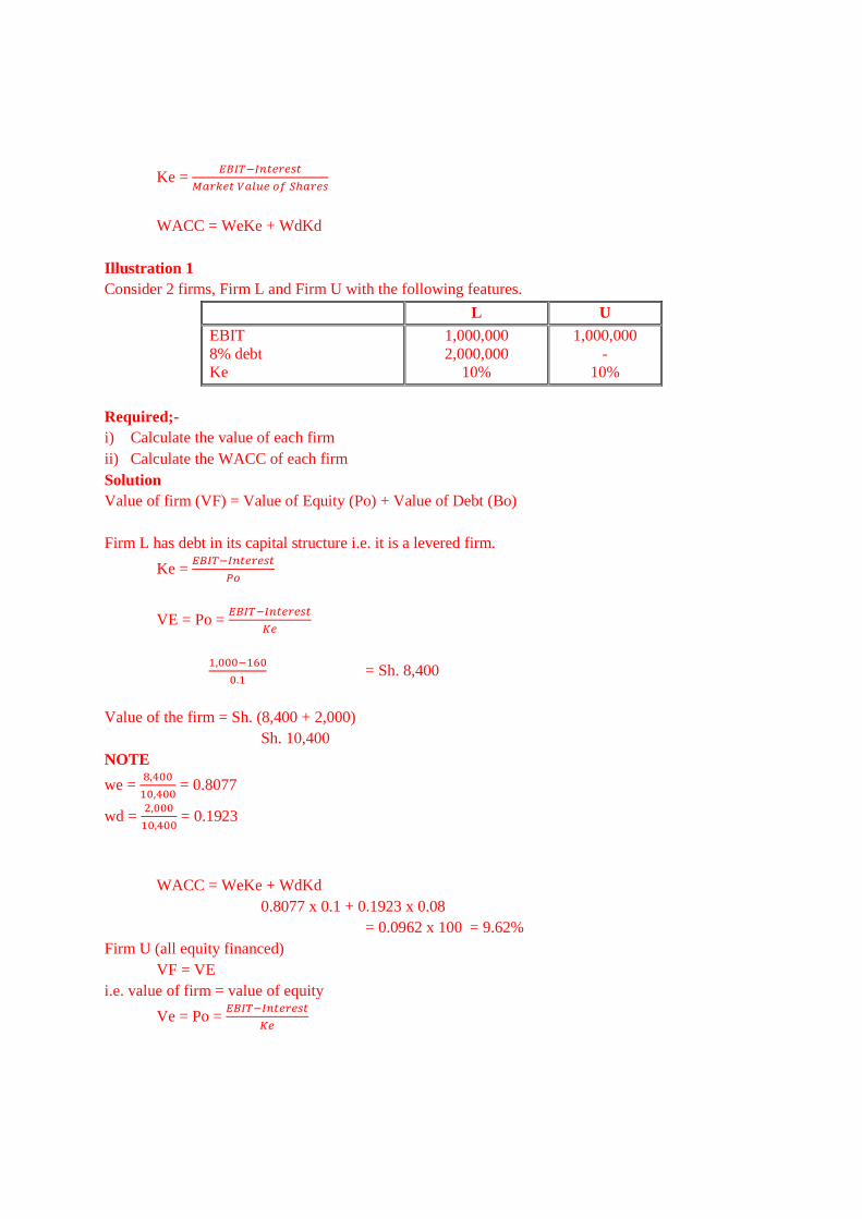
Ke = 𝐸𝐵𝐼𝑇−𝐼𝑛𝑡𝑒𝑟𝑒𝑠𝑡
𝑀𝑎𝑟𝑘𝑒𝑡 𝑉𝑎𝑙𝑢𝑒 𝑜𝑓 𝑆ℎ𝑎𝑟𝑒𝑠
WACC = WeKe + WdKd
Illustration 1
Consider 2 firms, Firm L and Firm U with the following features.
L U
EBIT
8% debt
Ke
1,000,000
2,000,000
10%
1,000,000
-
10%
Required;-
i) Calculate the value of each firm
ii) Calculate the WACC of each firm
Solution
Value of firm (VF) = Value of Equity (Po) + Value of Debt (Bo)
Firm L has debt in its capital structure i.e. it is a levered firm.
Ke = 𝐸𝐵𝐼𝑇−𝐼𝑛𝑡𝑒𝑟𝑒𝑠𝑡
𝑃𝑜
VE = Po = 𝐸𝐵𝐼𝑇−𝐼𝑛𝑡𝑒𝑟𝑒𝑠𝑡
𝐾𝑒
1,000−160
0.1 = Sh. 8,400
Value of the firm = Sh. (8,400 + 2,000)
Sh. 10,400
NOTE
we = 8,400
10,400 = 0.8077
wd = 2,000
10,400 = 0.1923
WACC = WeKe + WdKd
0.8077 x 0.1 + 0.1923 x 0.08
= 0.0962 x 100 = 9.62%
Firm U (all equity financed)
VF = VE
i.e. value of firm = value of equity
Ve = Po = 𝐸𝐵𝐼𝑇−𝐼𝑛𝑡𝑒𝑟𝑒𝑠𝑡
𝐾𝑒
Page 132
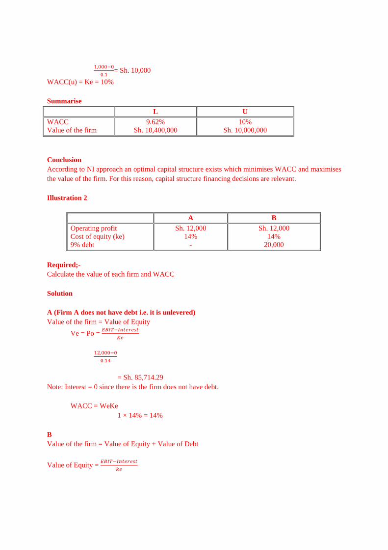
1,000−0
0.1= Sh. 10,000
WACC(u) = Ke = 10%
Summarise
L U
WACC
Value of the firm
9.62%
Sh. 10,400,000
10%
Sh. 10,000,000
Conclusion
According to NI approach an optimal capital structure exists which minimises WACC and maximises
the value of the firm. For this reason, capital structure financing decisions are relevant.
Illustration 2
A B
Operating profit
Cost of equity (ke)
9% debt
Sh. 12,000
14%
-
Sh. 12,000
14%
20,000
Required;-
Calculate the value of each firm and WACC
Solution
A (Firm A does not have debt i.e. it is unlevered)
Value of the firm = Value of Equity
Ve = Po = 𝐸𝐵𝐼𝑇−𝐼𝑛𝑡𝑒𝑟𝑒𝑠𝑡
𝐾𝑒
12,000−0
0.14
= Sh. 85,714.29
Note: Interest = 0 since there is the firm does not have debt.
WACC = WeKe
1 × 14% = 14%
B
Value of the firm = Value of Equity + Value of Debt
Value of Equity = 𝐸𝐵𝐼𝑇−𝐼𝑛𝑡𝑒𝑟𝑒𝑠𝑡
𝑘𝑒
Page 133
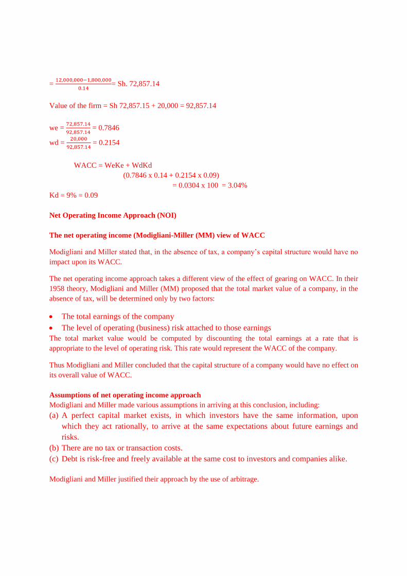
= 12,000,000−1,800,000
0.14= Sh. 72,857.14
Value of the firm = Sh 72,857.15 + 20,000 = 92,857.14
we = 72,857.14
92,857.14 = 0.7846
wd = 20,000
92,857.14 = 0.2154
WACC = WeKe + WdKd
(0.7846 x 0.14 + 0.2154 x 0.09)
= 0.0304 x 100 = 3.04%
Kd = 9% = 0.09
Net Operating Income Approach (NOI)
The net operating income (Modigliani-Miller (MM) view of WACC
Modigliani and Miller stated that, in the absence of tax, a company’s capital structure would have no
impact upon its WACC.
The net operating income approach takes a different view of the effect of gearing on WACC. In their
1958 theory, Modigliani and Miller (MM) proposed that the total market value of a company, in the
absence of tax, will be determined only by two factors:
The total earnings of the company
The level of operating (business) risk attached to those earnings
The total market value would be computed by discounting the total earnings at a rate that is
appropriate to the level of operating risk. This rate would represent the WACC of the company.
Thus Modigliani and Miller concluded that the capital structure of a company would have no effect on
its overall value of WACC.
Assumptions of net operating income approach
Modigliani and Miller made various assumptions in arriving at this conclusion, including:
(a) A perfect capital market exists, in which investors have the same information, upon
which they act rationally, to arrive at the same expectations about future earnings and
risks.
(b) There are no tax or transaction costs.
(c) Debt is risk-free and freely available at the same cost to investors and companies alike.
Modigliani and Miller justified their approach by the use of arbitrage.
Page 134
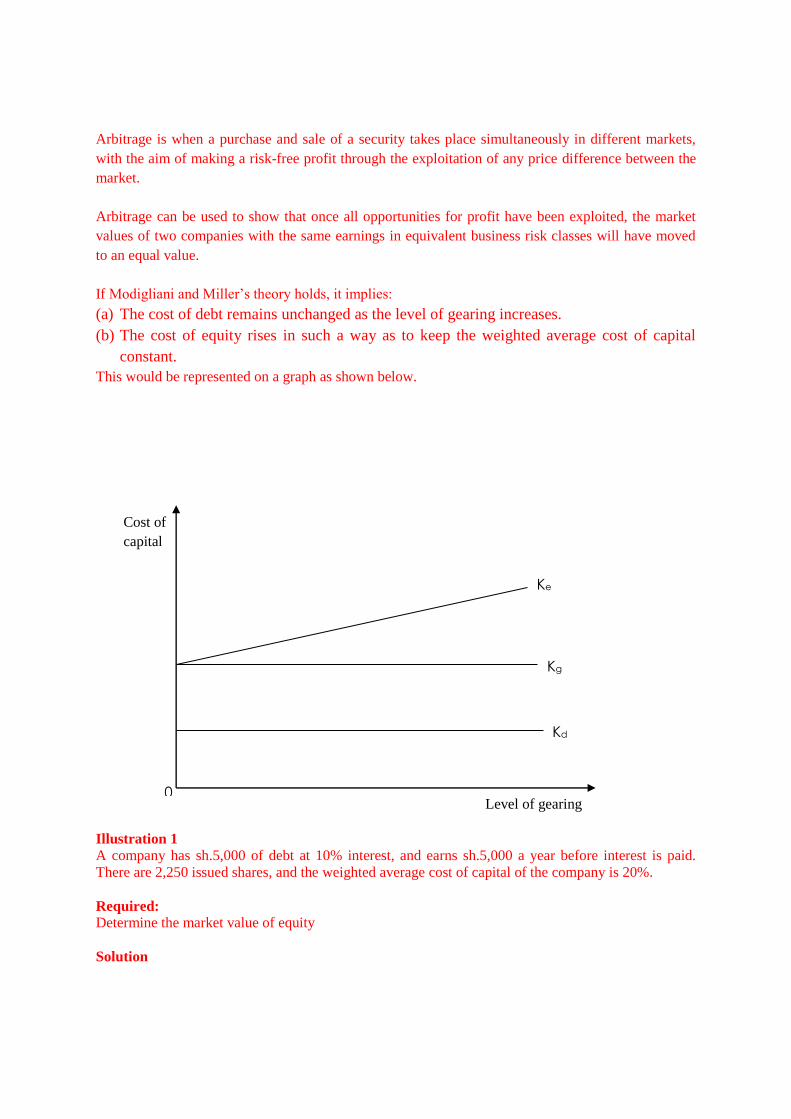
Arbitrage is when a purchase and sale of a security takes place simultaneously in different markets,
with the aim of making a risk-free profit through the exploitation of any price difference between the
market.
Arbitrage can be used to show that once all opportunities for profit have been exploited, the market
values of two companies with the same earnings in equivalent business risk classes will have moved
to an equal value.
If Modigliani and Miller’s theory holds, it implies:
(a) The cost of debt remains unchanged as the level of gearing increases.
(b) The cost of equity rises in such a way as to keep the weighted average cost of capital
constant.
This would be represented on a graph as shown below.
Illustration 1
A company has sh.5,000 of debt at 10% interest, and earns sh.5,000 a year before interest is paid.
There are 2,250 issued shares, and the weighted average cost of capital of the company is 20%.
Required:
Determine the market value of equity
Solution
Ke
Kg
Kd
Level of gearing 0
Cost of
capital
Page 135
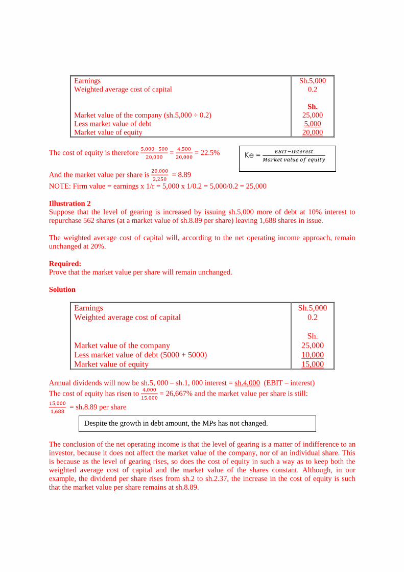
Earnings
Weighted average cost of capital
Market value of the company (sh.5,000 ÷ 0.2)
Less market value of debt
Market value of equity
Sh.5,000
0.2
Sh.
25,000
5,000
20,000
The cost of equity is therefore 5,000−500
20,000 =
4,500
20,000 = 22.5%
And the market value per share is 20,000
2,250 = 8.89
NOTE: Firm value = earnings x 1/r = 5,000 x 1/0.2 = 5,000/0.2 = 25,000
Illustration 2
Suppose that the level of gearing is increased by issuing sh.5,000 more of debt at 10% interest to
repurchase 562 shares (at a market value of sh.8.89 per share) leaving 1,688 shares in issue.
The weighted average cost of capital will, according to the net operating income approach, remain
unchanged at 20%.
Required:
Prove that the market value per share will remain unchanged.
Solution
Earnings
Weighted average cost of capital
Market value of the company
Less market value of debt (5000 + 5000)
Market value of equity
Sh.5,000
0.2
Sh.
25,000
10,000
15,000
Annual dividends will now be sh.5, 000 – sh.1, 000 interest = sh.4,000 (EBIT – interest)
The cost of equity has risen to 4,000
15,000 = 26,667% and the market value per share is still:
15,000
1,688 = sh.8.89 per share
The conclusion of the net operating income is that the level of gearing is a matter of indifference to an
investor, because it does not affect the market value of the company, nor of an individual share. This
is because as the level of gearing rises, so does the cost of equity in such a way as to keep both the
weighted average cost of capital and the market value of the shares constant. Although, in our
example, the dividend per share rises from sh.2 to sh.2.37, the increase in the cost of equity is such
that the market value per share remains at sh.8.89.
Ke = 𝐸𝐵𝐼𝑇−𝐼𝑛𝑡𝑒𝑟𝑒𝑠𝑡
𝑀𝑎𝑟𝑘𝑒𝑡 𝑣𝑎𝑙𝑢𝑒 𝑜𝑓 𝑒𝑞𝑢𝑖𝑡𝑦
Despite the growth in debt amount, the MPs has not changed.
Page 136
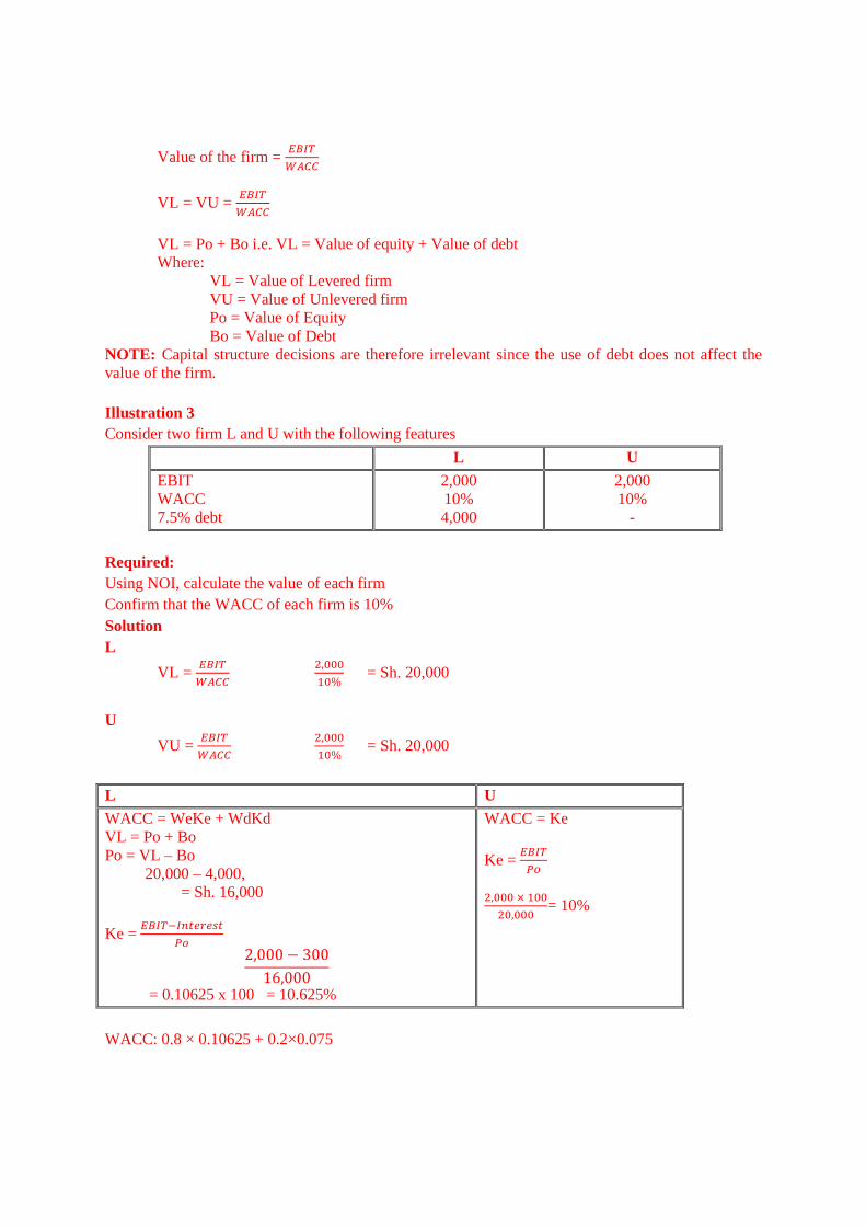
Value of the firm = 𝐸𝐵𝐼𝑇
𝑊𝐴𝐶𝐶
VL = VU = 𝐸𝐵𝐼𝑇
𝑊𝐴𝐶𝐶
VL = Po + Bo i.e. VL = Value of equity + Value of debt
Where:
VL = Value of Levered firm
VU = Value of Unlevered firm
Po = Value of Equity
Bo = Value of Debt
NOTE: Capital structure decisions are therefore irrelevant since the use of debt does not affect the
value of the firm.
Illustration 3
Consider two firm L and U with the following features
L U
EBIT
WACC
7.5% debt
2,000
10%
4,000
2,000
10%
-
Required:
Using NOI, calculate the value of each firm
Confirm that the WACC of each firm is 10%
Solution
L
VL = 𝐸𝐵𝐼𝑇
𝑊𝐴𝐶𝐶
2,000
10% = Sh. 20,000
U
VU = 𝐸𝐵𝐼𝑇
𝑊𝐴𝐶𝐶
2,000
10% = Sh. 20,000
L U
WACC = WeKe + WdKd
VL = Po + Bo
Po = VL – Bo
20,000 – 4,000,
= Sh. 16,000
Ke = 𝐸𝐵𝐼𝑇−𝐼𝑛𝑡𝑒𝑟𝑒𝑠𝑡
𝑃𝑜
2,000 − 300
16,000
= 0.10625 x 100 = 10.625%
WACC = Ke
Ke = 𝐸𝐵𝐼𝑇
𝑃𝑜
2,000 × 100
20,000= 10%
WACC: 0.8 × 0.10625 + 0.2×0.075
Page 137
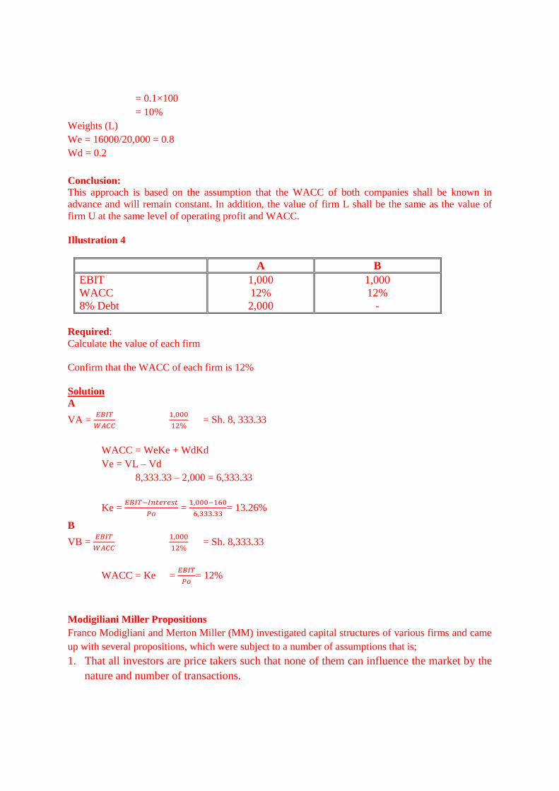
= 0.1×100
= 10%
Weights (L)
We = 16000/20,000 = 0.8
Wd = 0.2
Conclusion:
This approach is based on the assumption that the WACC of both companies shall be known in
advance and will remain constant. In addition, the value of firm L shall be the same as the value of
firm U at the same level of operating profit and WACC.
Illustration 4
A B
EBIT
WACC
8% Debt
1,000
12%
2,000
1,000
12%
-
Required:
Calculate the value of each firm
Confirm that the WACC of each firm is 12%
Solution
A
VA = 𝐸𝐵𝐼𝑇
𝑊𝐴𝐶𝐶
1,000
12% = Sh. 8, 333.33
WACC = WeKe + WdKd
Ve = VL – Vd
8,333.33 – 2,000 = 6,333.33
Ke = 𝐸𝐵𝐼𝑇−𝐼𝑛𝑡𝑒𝑟𝑒𝑠𝑡
𝑃𝑜 =
1,000−160
6,333.33= 13.26%
B
VB = 𝐸𝐵𝐼𝑇
𝑊𝐴𝐶𝐶
1,000
12% = Sh. 8,333.33
WACC = Ke = 𝐸𝐵𝐼𝑇
𝑃𝑜= 12%
Modigiliani Miller Propositions
Franco Modigliani and Merton Miller (MM) investigated capital structures of various firms and came
up with several propositions, which were subject to a number of assumptions that is;
1. That all investors are price takers such that none of them can influence the market by the
nature and number of transactions.
Page 138
2. Investors and companies can borrow and lend at the same market rate or return.
Some companies operate in environment of taxes while others in environment of no taxes.
3. No brokerage and other transaction costs are available that can prevent the process of
buying and selling securities that is capital markets are perfect.
4. All investors are rational and aim at maximising their market value.
The MM view is that:
Their view is based on the belief that the value of a company depends upon the future operating
income generated by its assets. The way in which this income is split between returns to debt holders
and returns to equity should make no difference to the total value of the firm (equity plus Debt). Thus,
the total value of the firm will not change with gearing, and WACC is to remain constant at all levels
of gearing it follows that any benefit from the use of cheaper debt finance must be exactly offset by
the increase in the cost of equity.
The essential point made by MM is that a firm should be indifferent between all possible capital
structures. This is at odds with the beliefs of the traditionalists.
MM supported their case by demonstrating that market pressures (Arbitrage) will ensure that two
companies identical in every aspect apart from their gearing level will have the same overall MV.
This proof is outside the syllabus.
Companies which operate in the same type of business and which have similar operating risks must
have the same total value, irrespective of their capital structures.
MM came up with the following propositions
MMI: Without corporation taxes
This theory is identical to NOI (Net operating income)
It states that the capital structure of a firm does not influence its value simply because the value of
firm is calculated by dividing the operating profit (EBIT) by Overall Cost of Capital (WACC) i.e. VL
= VU = 𝐸𝐵𝐼𝑇
𝑊𝐴𝐶𝐶
Conclusion:
MM under mm1 proposition argued that in absence of taxes the existence of debt in the capital
structure does not affect the value of a firm hence capital structure decisions are irrelevant.
Arbitrage Process
Arbitrage mechanism arises when investors take advantage of the difference in price of securities in
different firms.
They sell their investment in the overvalued firms and invest in the undervalued firms; the process,
which eventually stabilises the prices hence a price equilibrium, is achieved.
The following steps are followed in arbitrage process:
1. An investor sell his /her investment in equity of overvalued firm (Levered firm).
Page 139
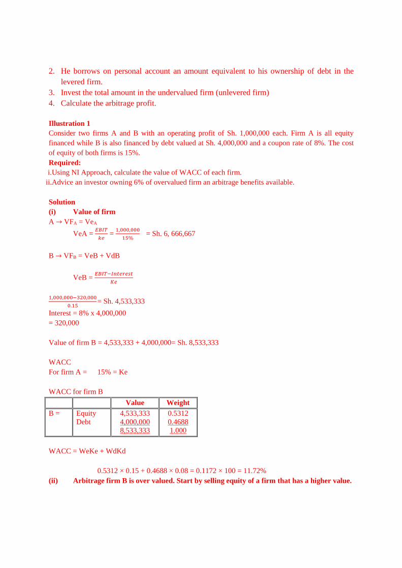
2. He borrows on personal account an amount equivalent to his ownership of debt in the
levered firm.
3. Invest the total amount in the undervalued firm (unlevered firm)
4. Calculate the arbitrage profit.
Illustration 1
Consider two firms A and B with an operating profit of Sh. 1,000,000 each. Firm A is all equity
financed while B is also financed by debt valued at Sh. 4,000,000 and a coupon rate of 8%. The cost
of equity of both firms is 15%.
Required:
i. Using NI Approach, calculate the value of WACC of each firm.
ii.Advice an investor owning 6% of overvalued firm an arbitrage benefits available.
Solution
(i) Value of firm
A → VFA = VeA
VeA = 𝐸𝐵𝐼𝑇
𝑘𝑒 =
1,000,000
15% = Sh. 6, 666,667
B → VFB = VeB + VdB
VeB = 𝐸𝐵𝐼𝑇−𝐼𝑛𝑡𝑒𝑟𝑒𝑠𝑡
𝐾𝑒
1,000,000−320,000
0.15 = Sh. 4,533,333
Interest = 8% x 4,000,000
= 320,000
Value of firm B = 4,533,333 + 4,000,000= Sh. 8,533,333
WACC
For firm A = 15% = Ke
WACC for firm B
Value Weight
B = Equity
Debt
4,533,333
4,000,000
8,533,333
0.5312
0.4688
1.000
WACC = WeKe + WdKd
0.5312 × 0.15 + 0.4688 × 0.08 = 0.1172 × 100 = 11.72%
(ii) Arbitrage firm B is over valued. Start by selling equity of a firm that has a higher value.
Page 140
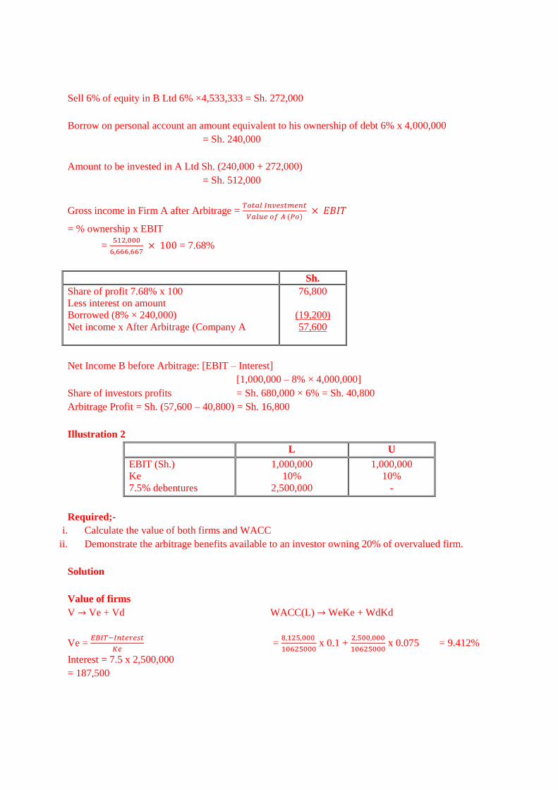
Sell 6% of equity in B Ltd 6% ×4,533,333 = Sh. 272,000
Borrow on personal account an amount equivalent to his ownership of debt 6% x 4,000,000
= Sh. 240,000
Amount to be invested in A Ltd Sh. (240,000 + 272,000)
= Sh. 512,000
Gross income in Firm A after Arbitrage = 𝑇𝑜𝑡𝑎𝑙 𝐼𝑛𝑣𝑒𝑠𝑡𝑚𝑒𝑛𝑡
𝑉𝑎𝑙𝑢𝑒 𝑜𝑓 𝐴 (𝑃𝑜) × 𝐸𝐵𝐼𝑇
= % ownership x EBIT
= 512,000
6,666,667 × 100 = 7.68%
Sh.
Share of profit 7.68% x 100 Less interest on amount
Borrowed (8% × 240,000) Net income x After Arbitrage (Company A
76,800
(19,200) 57,600
Net Income B before Arbitrage: [EBIT – Interest]
[1,000,000 – 8% × 4,000,000]
Share of investors profits = Sh. 680,000 × 6% = Sh. 40,800
Arbitrage Profit = Sh. (57,600 – 40,800) = Sh. 16,800
Illustration 2
L U
EBIT (Sh.)
Ke
7.5% debentures
1,000,000
10%
2,500,000
1,000,000
10%
-
Required;-
i. Calculate the value of both firms and WACC
ii. Demonstrate the arbitrage benefits available to an investor owning 20% of overvalued firm.
Solution
Value of firms
V → Ve + Vd WACC(L) → WeKe + WdKd
Ve = 𝐸𝐵𝐼𝑇−𝐼𝑛𝑡𝑒𝑟𝑒𝑠𝑡
𝐾𝑒 =
8,125,000
10625000 x 0.1 +
2,500,000
10625000 x 0.075 = 9.412%
Interest = 7.5 x 2,500,000
= 187,500
Page 141
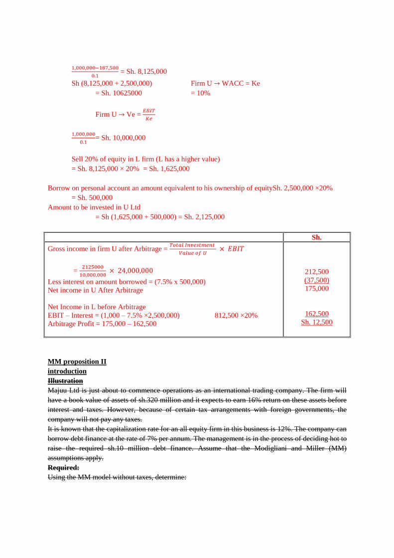
1,000,000−187,500
0.1 = Sh. 8,125,000
Sh (8,125,000 + 2,500,000) Firm U → WACC = Ke
= Sh. 10625000 = 10%
Firm U → Ve = 𝐸𝐵𝐼𝑇
𝐾𝑒
1,000,000
0.1 = Sh. 10,000,000
Sell 20% of equity in L firm (L has a higher value)
= Sh. 8,125,000 × 20% = Sh. 1,625,000
Borrow on personal account an amount equivalent to his ownership of equitySh. 2,500,000 ×20%
= Sh. 500,000
Amount to be invested in U Ltd
= Sh (1,625,000 + 500,000) = Sh. 2,125,000
Sh.
Gross income in firm U after Arbitrage = 𝑇𝑜𝑡𝑎𝑙 𝐼𝑛𝑣𝑒𝑠𝑡𝑚𝑒𝑛𝑡
𝑉𝑎𝑙𝑢𝑒 𝑜𝑓 𝑈 × 𝐸𝐵𝐼𝑇
= 2125000
10,000,000 × 24,000,000
Less interest on amount borrowed = (7.5% x 500,000) Net income in U After Arbitrage
Net Income in L before Arbitrage
EBIT – Interest = (1,000 – 7.5% ×2,500,000) 812,500 ×20%
Arbitrage Profit = 175,000 – 162,500
212,500 (37,500) 175,000
162,500
Sh. 12,500
MM proposition II
introduction
Illustration
Majuu Ltd is just about to commence operations as an international trading company. The firm will
have a book value of assets of sh.320 million and it expects to earn 16% return on these assets before
interest and taxes. However, because of certain tax arrangements with foreign governments, the
company will not pay any taxes.
It is known that the capitalization rate for an all equity firm in this business is 12%. The company can
borrow debt finance at the rate of 7% per annum. The management is in the process of deciding hot to
raise the required sh.10 million debt finance. Assume that the Modigliani and Miller (MM)
assumptions apply.
Required:
Using the MM model without taxes, determine:
Page 142
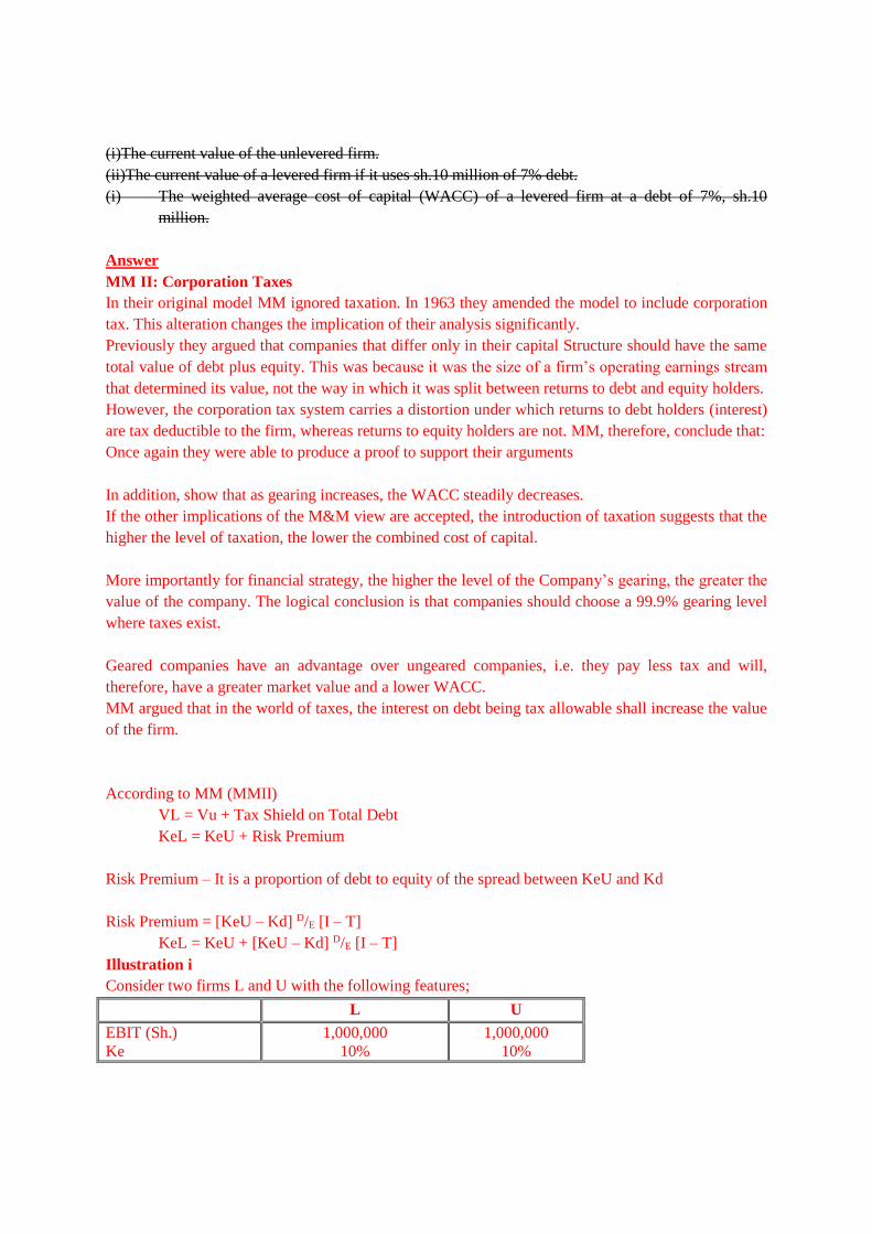
(i)The current value of the unlevered firm.
(ii)The current value of a levered firm if it uses sh.10 million of 7% debt.
(i) The weighted average cost of capital (WACC) of a levered firm at a debt of 7%, sh.10
million.
Answer
MM II: Corporation Taxes
In their original model MM ignored taxation. In 1963 they amended the model to include corporation
tax. This alteration changes the implication of their analysis significantly.
Previously they argued that companies that differ only in their capital Structure should have the same
total value of debt plus equity. This was because it was the size of a firm’s operating earnings stream
that determined its value, not the way in which it was split between returns to debt and equity holders.
However, the corporation tax system carries a distortion under which returns to debt holders (interest)
are tax deductible to the firm, whereas returns to equity holders are not. MM, therefore, conclude that:
Once again they were able to produce a proof to support their arguments
In addition, show that as gearing increases, the WACC steadily decreases.
If the other implications of the M&M view are accepted, the introduction of taxation suggests that the
higher the level of taxation, the lower the combined cost of capital.
More importantly for financial strategy, the higher the level of the Company’s gearing, the greater the
value of the company. The logical conclusion is that companies should choose a 99.9% gearing level
where taxes exist.
Geared companies have an advantage over ungeared companies, i.e. they pay less tax and will,
therefore, have a greater market value and a lower WACC.
MM argued that in the world of taxes, the interest on debt being tax allowable shall increase the value
of the firm.
According to MM (MMII)
VL = Vu + Tax Shield on Total Debt
KeL = KeU + Risk Premium
Risk Premium – It is a proportion of debt to equity of the spread between KeU and Kd
Risk Premium = [KeU – Kd] D/E [I – T]
KeL = KeU + [KeU – Kd] D/E [I – T]
Illustration i
Consider two firms L and U with the following features;
L U
EBIT (Sh.)
Ke
1,000,000
10%
1,000,000
10%
Page 143
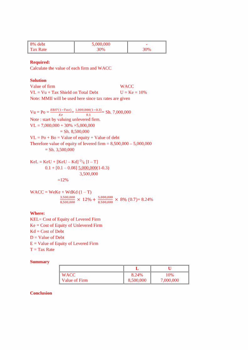
8% debt
Tax Rate
5,000,000
30%
-
30%
Required:
Calculate the value of each firm and WACC
Solution
Value of firm WACC
VL = Vu + Tax Shield on Total Debt U = Ke = 10%
Note: MMII will be used here since tax rates are given
Vu = Po = 𝐸𝐵𝐼𝑇(1−𝑇𝑎𝑥)
𝐾𝑒=
1,000,000(1−0.3)
0.1= Sh. 7,000,000
Note : start by valuing unlevered firm.
VL = 7,000,000 + 30% ×5,000,000
= Sh. 8,500,000
VL = Po + Bo = Value of equity + Value of debt
Therefore value of equity of levered firm = 8,500,000 – 5,000,000
= Sh. 3,500,000
KeL = KeU + [KeU – Kd] D/E [I – T]
0.1 + [0.1 – 0.08] 5,000,000(1-0.3)
3,500,000
=12%
WACC = WeKe + WdKd (1 – T)
3,500,000
8,500,000 × 12% +
5,000,000
8,500,000 × 8% (0.7)= 8.24%
Where:
KEL= Cost of Equity of Levered Firm
Ke = Cost of Equity of Unlevered Firm
Kd = Cost of Debt
D = Value of Debt
E = Value of Equity of Levered Firm
T = Tax Rate
Summary
L U
WACC
Value of Firm
8.24%
8,500,000
10%
7,000,000
Conclusion
Page 144
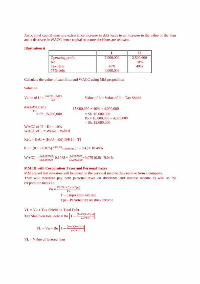
An optimal capital structure exists since increase in debt leads to an increase in the value of the firm
and a decrease in WACC hence capital structure decisions are relevant.
Illustration ii
L U
Operating profit
Ke
Tax Rate
75% debt
2,000,000
-
40%
4,000,000
2,500,000
10%
40%
Calculate the value of each firm and WACC using MM proposition
Solution
Value of U = 𝐸𝐵𝐼𝑇(1−𝑇𝑎𝑥)
𝐾𝑒 Value of L = Value of U + Tax Shield
2,500,000(1−0.4)
0.1 15,000,000 + 40% × 4,000,000
= Sh. 15,000,000 = Sh. 16,600,000
Po = 16,600,000 – 4,000,000
= Sh. 12,600,000
WACC of U = Ke = 10%
WACC of L = WeKe + WdKd
KeL = KeU + (KeU – Kd) D/E [I – T]
0.1 + (0.1 – 0.075) 4,000,000/12,600,000 [1 – 0.4] = 10.48%
WACC = 12,600,000
16,600,000×0.1048 +
4,000,000
16,600,000×0.075 (0.6)= 9.04%
MM III with Corporation Taxes and Personal Taxes
MM argued that investors will be taxed on the personal income they receive from a company.
They will therefore pay both personal taxes on dividends and interest income as well as the
corporation taxes i.e.
Vu = 𝐸𝐵𝐼𝑇(𝐼−𝑇)(𝐼−𝑇𝑝𝑠)
𝐾𝑒
T – Corporation tax rate
Tps – Personal tax on stock income
VL = Vu + Tax Shield on Total Debt
Tax Shield on total debt = Bo [1 −(𝐼−𝑇)(𝐼−𝑇𝑝𝑠)
𝐼−𝑇𝑃𝐷]
VL = Vu + Bo [1 −(𝐼−𝑇)(𝐼−𝑇𝑝𝑠)
𝐼−𝑇𝑃𝐷]
VL – Value of levered firm
Page 145
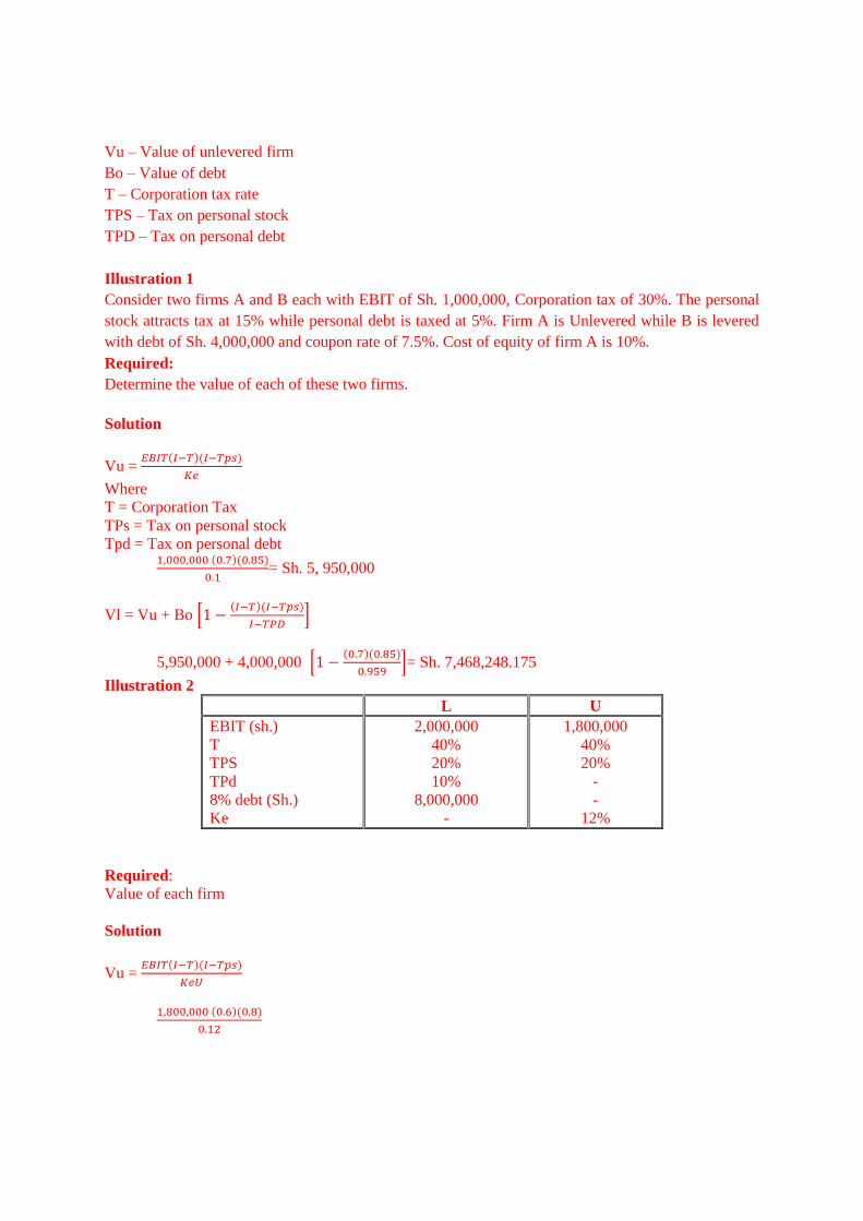
Vu – Value of unlevered firm
Bo – Value of debt
T – Corporation tax rate
TPS – Tax on personal stock
TPD – Tax on personal debt
Illustration 1
Consider two firms A and B each with EBIT of Sh. 1,000,000, Corporation tax of 30%. The personal
stock attracts tax at 15% while personal debt is taxed at 5%. Firm A is Unlevered while B is levered
with debt of Sh. 4,000,000 and coupon rate of 7.5%. Cost of equity of firm A is 10%.
Required:
Determine the value of each of these two firms.
Solution
Vu = 𝐸𝐵𝐼𝑇(𝐼−𝑇)(𝐼−𝑇𝑝𝑠)
𝐾𝑒
Where
T = Corporation Tax
TPs = Tax on personal stock
Tpd = Tax on personal debt
1,000,000 (0.7)(0.85)
0.1= Sh. 5, 950,000
Vl = Vu + Bo [1 −(𝐼−𝑇)(𝐼−𝑇𝑝𝑠)
𝐼−𝑇𝑃𝐷]
5,950,000 + 4,000,000 [1 −(0.7)(0.85)
0.959]= Sh. 7,468,248.175
Illustration 2
L U
EBIT (sh.)
T
TPS
TPd
8% debt (Sh.)
Ke
2,000,000
40%
20%
10%
8,000,000
-
1,800,000
40%
20%
-
-
12%
Required:
Value of each firm
Solution
Vu = 𝐸𝐵𝐼𝑇(𝐼−𝑇)(𝐼−𝑇𝑝𝑠)
𝐾𝑒𝑈
1,800,000 (0.6)(0.8)
0.12
Page 146
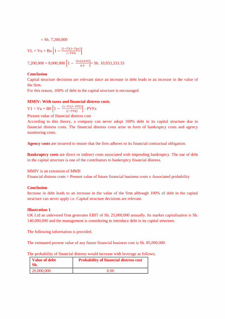
= Sh. 7,200,000
VL = Vu + Bo [1 −(𝐼−𝑇)(𝐼−𝑇𝑝𝑠)
𝐼−𝑇𝑃𝐷]
7,200,000 + 8,000,000 [1 − (0.6)(0.8)
0.9]= Sh. 10,933,333.33
Conclusion
Capital structure decisions are relevant since an increase in debt leads to an increase in the value of
the firm.
For this reason, 100% of debt in the capital structure is encouraged.
MMIV: With taxes and financial distress costs.
V1 = Vu + B0 [1 − (1−𝑇)(𝐼−𝑇𝑃𝑆)
(𝐼−𝑇𝑃𝑑)] - PVFx
Present value of financial distress cost
According to this theory, a company can never adopt 100% debt in its capital structure due to
financial distress costs. The financial distress costs arise in form of bankruptcy costs and agency
monitoring costs.
Agency costs are incurred to ensure that the firm adheres to its financial contractual obligation.
Bankruptcy costs are direct or indirect costs associated with impending bankruptcy. The use of debt
in the capital structure is one of the contributors to bankruptcy financial distress.
MMIV is an extension of MMII
Financial distress costs = Present value of future financial business costs x Associated probability
Conclusion
Increase in debt leads to an increase in the value of the firm although 100% of debt in the capital
structure can never apply i.e. Capital structure decisions are relevant.
Illustration 1
UK Ltd an unlevered firm generates EBIT of Sh. 25,000,000 annually. Its market capitalisation is Sh.
140,000,000 and the management is considering to introduce debt in its capital structure.
The following information is provided.
The estimated present value of any future financial business cost is Sh. 85,000,000.
The probability of financial distress would increase with leverage as follows;
Value of debt
Sh.
Probability of financial distress cost
20,000,000 0.00
Page 147
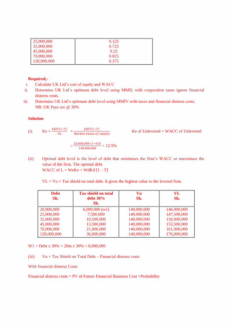
25,000,000
35,000,000
45,000,000
70,000,000
120,000,000
0.125
0.725
0.25
0.025
0.375
Required;-
i. Calculate UK Ltd’s cost of equity and WACC
ii. Determine UK Ltd’s optimum debt level using MMII; with corporation taxes ignore financial
distress costs.
iii. Determine UK Ltd’s optimum debt level using MMIV with taxes and financial distress costs.
NB: UK Pays tax @ 30%
Solution
(i) Ke = 𝐸𝐵𝐼𝑇(𝐼−𝑇)
𝑃𝑜 =
𝐸𝐵𝐼𝑇(𝐼−𝑇)
𝑀𝑎𝑟𝑘𝑒𝑡 𝑣𝑎𝑙𝑢𝑒 𝑜𝑓 𝑒𝑞𝑢𝑖𝑡𝑦 Ke of Unlevered = WACC of Unlevered
= 25,000,000 (1−0.3)
140,000,000 = 12.5%
(ii) Optimal debt level is the level of debt that minimises the firm’s WACC or maximises the
value of the firm. The optimal debt
WACC of L = WeKe + WdKd [1 – T]
VL = Vu + Tax shield on total debt. It gives the highest value to the levered firm.
Debt
Sh.
Tax shield on total
debt 30%
Sh.
Vu
Sh.
VL
Sh.
20,000,000
25,000,000
35,000,000
45,000,000
70,000,000
120,000,000
6,000,000 (w1)
7,500,000
10,500,000
13,500,000
21,000,000
36,000,000
140,000,000
140,000,000
140,000,000
140,000,000
140,000,000
140,000,000
146,000,000
147,500,000
150,000,000
153,500,000
161,000,000
176,000,000
W1 = Debt x 30% = 20m x 30% = 6,000,000
(iii) Vu + Tax Shield on Total Debt – Financial distress costs
With financial distress Costs
Financial distress costs = PV of Future Financial Business Cost ×Probability
Page 148
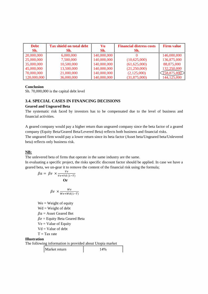
Debt
Sh.
Tax shield on total debt
Sh.
Vu
Sh.
Financial distress costs
Sh.
Firm value
20,000,000
25,000,000
35,000,000
45,000,000
70,000,000
120,000,000
6,000,000
7,500,000
10,500,000
13,500,000
21,000,000
36,000,000
140,000,000
140,000,000
140,000,000
140,000,000
140,000,000
140,000,000
0
(10,625,000)
(61,625,000)
(21,250,000)
(2,125,000)
(31,875,000)
146,000,000
136,875,000
88,875,000
132,250,000
158,875,000
144,125,000
Conclusion
Sh. 70,000,000 is the capital debt level
3.4. SPECIAL CASES IN FINANCING DECISIONS
Geared and Ungeared Beta
The systematic risk faced by investors has to be compensated due to the level of business and
financial activities.
A geared company would pay a higher return than ungeared company since the beta factor of a geared
company (Equity Beta/Geared Beta/Levered Beta) reflects both business and financial risks.
The ungeared firm would pay a lower return since its beta factor (Asset beta/Ungeared beta/Unlevered
beta) reflects only business risk.
NB:
The unlevered beta of firms that operate in the same industry are the same.
In evaluating a specific project, the risks specific discount factor should be applied. In case we have a
geared beta, we un-gear it to remove the content of the financial risk using the formula;
𝛽𝑎 = 𝛽𝑒 ×𝑉𝑒
𝑉𝑒+𝑉𝑑 (1−𝑇)
Or
𝛽𝑒 ×𝑊𝑒
𝑊𝑒+𝑊𝑑(1−𝑇)
We = Weight of equity
Wd = Weight of debt
𝛽𝑎 = Asset Geared Bet
𝛽𝑒 = Equity Beta Geared Beta
Ve = Value of Equity
Vd = Value of debt
T = Tax rate
Illustration
The following information is provided about Utopia market
Market return 14%
Page 149
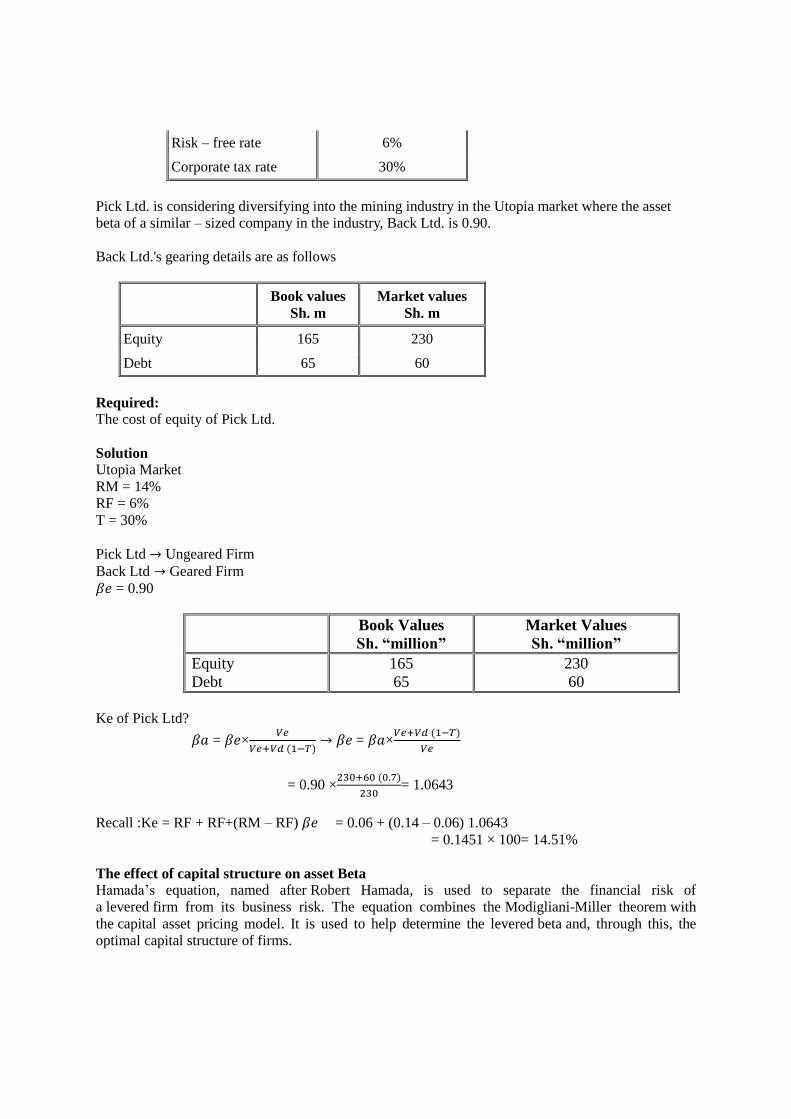
Risk – free rate 6%
Corporate tax rate 30%
Pick Ltd. is considering diversifying into the mining industry in the Utopia market where the asset
beta of a similar – sized company in the industry, Back Ltd. is 0.90.
Back Ltd.'s gearing details are as follows
Book values
Sh. m
Market values
Sh. m
Equity 165 230
Debt 65 60
Required:
The cost of equity of Pick Ltd.
Solution
Utopia Market
RM = 14%
RF = 6%
T = 30%
Pick Ltd → Ungeared Firm
Back Ltd → Geared Firm
𝛽𝑒 = 0.90
Book Values
Sh. “million”
Market Values
Sh. “million”
Equity
Debt
165
65
230
60
Ke of Pick Ltd?
𝛽𝑎 = 𝛽𝑒×𝑉𝑒
𝑉𝑒+𝑉𝑑 (1−𝑇)→ 𝛽𝑒 = 𝛽𝑎×
𝑉𝑒+𝑉𝑑 (1−𝑇)
𝑉𝑒
= 0.90 ×230+60 (0.7)
230= 1.0643
Recall :Ke = RF + RF+(RM – RF) 𝛽𝑒 = 0.06 + (0.14 – 0.06) 1.0643
= 0.1451 × 100= 14.51%
The effect of capital structure on asset Beta
Hamada’s equation, named after Robert Hamada, is used to separate the financial risk of
a levered firm from its business risk. The equation combines the Modigliani-Miller theorem with
the capital asset pricing model. It is used to help determine the levered beta and, through this, the
optimal capital structure of firms.
Page 150

Hamada’s equation relates the beta of a levered firm (a firm financed by both debt and equity) to that
of its unlevered (i.e., a firm which has no debt) counterpart. It has proved useful in several areas of
finance, including capital structuring, portfolio management and risk management, to name just a few.
It is used to determine the cost of capital of a levered firm based on the cost of capital of comparable
firms. Here, the comparable firms would be the ones having similar business risk and, thus, similar
unlevered betas as the firm of interest.
The Beta factor is a Quantitative income of systematic risk in a well-diversified portfolio. This
measure is also affected by capital structure.
Increase in debt will lead to an increase in the value of Beta factor due increase in financial risk hence
leading to increase in systematic risk.
The relationship between financial risk and systematic risk of a company can be expressed in the
following model.
Beu = 𝐵𝑒𝐿
1+ 𝐷
𝐸 (1−𝑇)
Where;-
Beu = Beta equity of unlevered firm
BeL = Beta factor of equity of a levered firm.
S = total market value of debt
E = total market value of equity
Thus if the above equation is rearranged
BeL = Beu [1 + 𝐷
𝐸 (1 – T)]
This model is known as the Hamada model
NB: In Some case debt capital is considered to be a risk free security since debenture holders receive a
fixed annual interest income. In this case, debt is considered a risk free security and its beta
coefficient is equal to zero
The equation is often wrongly thought to hold in general. However, there are several
key assumptions behind the Hamada equation:
1. The Hamada formula is based on Modigliani and Miller’s formulation of the tax shield values
for constant debt, i.e. when the dollar amount of debt is constant over time. The formula cannot
be used when a firm’s debt amount fluctuates. If the firm is assumed to rebalance its debt-to-
equity ratio continuously, the Hamada equation is replaced with the Harris-Pringle equation; if
the firm rebalances only periodically, such as once a year, the Miles-Ezzell equation is the one to
be used.
2. The beta of debt βD equals zero. This is the case if debt capital has negligible risk that interest
and principal payments will not be made when owed. The timely interest payments imply that
tax deductions on the interest expense will also be realized—in the period in which the interest is
paid.
3. The discount rate used to calculate the tax shield is assumed to be equal to the cost of debt
capital (thus, the tax shield has the same risk as debt). This and the constant debt assumption in
(1) imply that the tax shield is proportionate to the market value of debt: Tax Shield = T×D.
Page 151
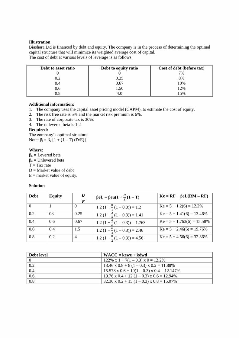
Illustration Biashara Ltd is financed by debt and equity. The company is in the process of determining the optimal
capital structure that will minimize its weighted average cost of capital.
The cost of debt at various levels of leverage is as follows:
Debt to asset ratio
0
0.2
0.4
0.6
0.8
Debt to equity ratio
0
0.25
0.67
1.50
4.0
Cost of debt (before tax)
7%
8%
10%
12%
15%
Additional information:
1. The company uses the capital asset pricing model (CAPM), to estimate the cost of equity.
2. The risk free rate is 5% and the market risk premium is 6%.
3. The rate of corporate tax is 30%.
4. The unlevered beta is 1.2
Required:
The company’s optimal structure
Note: βl = βu [1 + (1 – T) (D/E)]
Where:
βL = Levered beta
βu = Unlevered beta
T = Tax rate
D = Market value of debt
E = market value of equity.
Solution
Debt Equity 𝑫
𝑬 βeL = βeu(1 +
𝑫
𝑬 (1 – T) Ke = RF + βeL(RM – RF)
0 1 0 1.2 (1 + 0
1 (1 – 0.3)) = 1.2 Ke = 5 + 1.2(6) = 12.2%
0.2 08 0.25 1.2 (1 + 2
8 (1 – 0.3)) = 1.41 Ke = 5 + 1.41(6) = 13.46%
0.4 0.6 0.67 1.2 (1 + 4
6 (1 – 0.3)) = 1.763 Ke = 5 + 1.763(6) = 15.58%
0.6 0.4 1.5 1.2 (1 + 6
4 (1 – 0.3)) = 2.46 Ke = 5 + 2.46(6) = 19.76%
0.8 0.2 4 1.2 (1 + 8
2 (1 – 0.3)) = 4.56 Ke = 5 + 4.56(6) = 32.36%
Debt level WACC = kewe + kdwd
0 122% x 1 + 7(1 – 0.3) x 0 = 12.2%
0.2 13.46 x 0.8 + 8 (1 – 0.3) x 0.2 = 11.88%
0.4 15.578 x 0.6 + 10(1 – 0.3) x 0.4 = 12.147%
0.6 19.76 x 0.4 + 12 (1 – 0.3) x 0.6 = 12.94%
0.8 32.36 x 0.2 + 15 (1 – 0.3) x 0.8 = 15.07%
Page 152
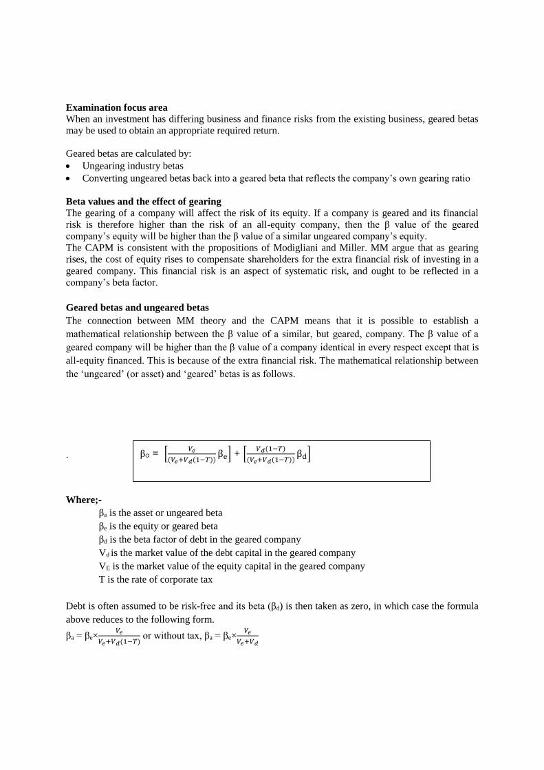
Examination focus area
When an investment has differing business and finance risks from the existing business, geared betas
may be used to obtain an appropriate required return.
Geared betas are calculated by:
Ungearing industry betas
Converting ungeared betas back into a geared beta that reflects the company’s own gearing ratio
Beta values and the effect of gearing
The gearing of a company will affect the risk of its equity. If a company is geared and its financial
risk is therefore higher than the risk of an all-equity company, then the β value of the geared
company’s equity will be higher than the β value of a similar ungeared company’s equity.
The CAPM is consistent with the propositions of Modigliani and Miller. MM argue that as gearing
rises, the cost of equity rises to compensate shareholders for the extra financial risk of investing in a
geared company. This financial risk is an aspect of systematic risk, and ought to be reflected in a
company’s beta factor.
Geared betas and ungeared betas
The connection between MM theory and the CAPM means that it is possible to establish a
mathematical relationship between the β value of a similar, but geared, company. The β value of a
geared company will be higher than the β value of a company identical in every respect except that is
all-equity financed. This is because of the extra financial risk. The mathematical relationship between
the ‘ungeared’ (or asset) and ‘geared’ betas is as follows.
.
Where;-
βa is the asset or ungeared beta
βe is the equity or geared beta
βd is the beta factor of debt in the geared company
Vd is the market value of the debt capital in the geared company
VE is the market value of the equity capital in the geared company
T is the rate of corporate tax
Debt is often assumed to be risk-free and its beta (βd) is then taken as zero, in which case the formula
above reduces to the following form.
βa = βe×𝑉𝑒
𝑉𝑒+𝑉𝑑(1−𝑇) or without tax, βa = βe×
𝑉𝑒
𝑉𝑒+𝑉𝑑
βa = [𝑉𝑒
(𝑉𝑒+𝑉𝑑(1−𝑇))βe] + [
𝑉𝑑(1−𝑇)
(𝑉𝑒+𝑉𝑑(1−𝑇))βd]
Page 153
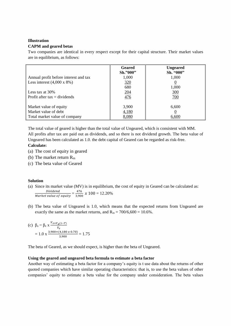
Illustration
CAPM and geared betas
Two companies are identical in every respect except for their capital structure. Their market values
are in equilibrium, as follows:
Annual profit before interest and tax
Less interest (4,000 x 8%)
Less tax at 30%
Profit after tax = dividends
Market value of equity
Market value of debt
Total market value of company
Geared
Sh.”000”
1,000
320
680
204
476
3,900
4,180
8,080
Ungeared
Sh. “000”
1,000
0
1,000
300
700
6,600
0
6,600
The total value of geared is higher than the total value of Ungeared, which is consistent with MM.
All profits after tax are paid out as dividends, and so there is not dividend growth. The beta value of
Ungeared has been calculated as 1.0. the debt capital of Geared can be regarded as risk-free.
Calculate:
(a) The cost of equity in geared
(b) The market return Rm
(c) The beta value of Geared
Solution
(a) Since its market value (MV) is in equilibrium, the cost of equity in Geared can be calculated as: 𝐷𝑖𝑣𝑖𝑑𝑒𝑛𝑑
𝑀𝑎𝑟𝑘𝑒𝑡 𝑣𝑎𝑙𝑢𝑒 𝑜𝑓 𝑒𝑞𝑢𝑖𝑡𝑦 =
476
3,900 𝑥 100 = 12.20%
(b) The beta value of Ungeared is 1.0, which means that the expected returns from Ungeared are
exactly the same as the market returns, and Rm = 700/6,600 = 10.6%.
(c) βa = βe x 𝑉𝑒+𝑉𝑑(1−𝑇)
𝑉𝑒
= 1.0 x 3,900+(4,180 𝑥 0.70)
3,900 = 1.75
The beta of Geared, as we should expect, is higher than the beta of Ungeared.
Using the geared and ungeared beta formula to estimate a beta factor
Another way of estimating a beta factor for a company’s equity is t use data about the returns of other
quoted companies which have similar operating characteristics: that is, to use the beta values of other
companies’ equity to estimate a beta value for the company under consideration. The beta values
Page 154
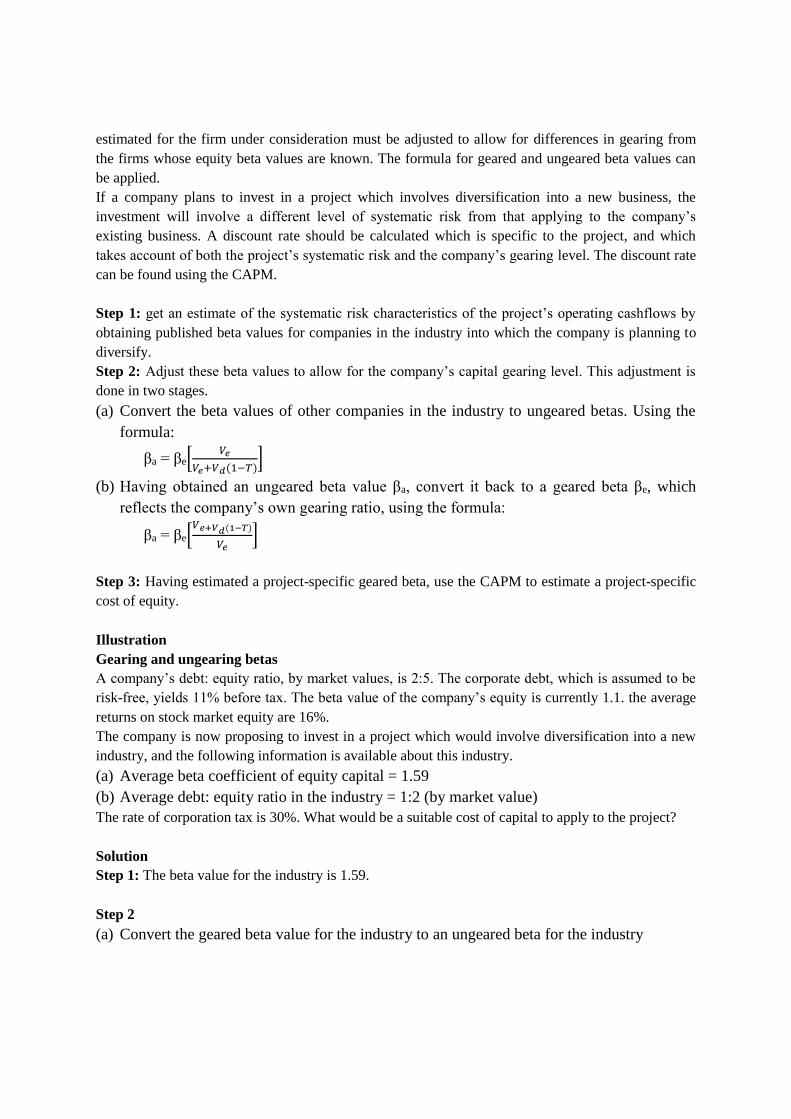
estimated for the firm under consideration must be adjusted to allow for differences in gearing from
the firms whose equity beta values are known. The formula for geared and ungeared beta values can
be applied.
If a company plans to invest in a project which involves diversification into a new business, the
investment will involve a different level of systematic risk from that applying to the company’s
existing business. A discount rate should be calculated which is specific to the project, and which
takes account of both the project’s systematic risk and the company’s gearing level. The discount rate
can be found using the CAPM.
Step 1: get an estimate of the systematic risk characteristics of the project’s operating cashflows by
obtaining published beta values for companies in the industry into which the company is planning to
diversify.
Step 2: Adjust these beta values to allow for the company’s capital gearing level. This adjustment is
done in two stages.
(a) Convert the beta values of other companies in the industry to ungeared betas. Using the
formula:
βa = βe[𝑉𝑒
𝑉𝑒+𝑉𝑑(1−𝑇)]
(b) Having obtained an ungeared beta value βa, convert it back to a geared beta βe, which
reflects the company’s own gearing ratio, using the formula:
βa = βe[𝑉𝑒+𝑉𝑑(1−𝑇)
𝑉𝑒]
Step 3: Having estimated a project-specific geared beta, use the CAPM to estimate a project-specific
cost of equity.
Illustration
Gearing and ungearing betas
A company’s debt: equity ratio, by market values, is 2:5. The corporate debt, which is assumed to be
risk-free, yields 11% before tax. The beta value of the company’s equity is currently 1.1. the average
returns on stock market equity are 16%.
The company is now proposing to invest in a project which would involve diversification into a new
industry, and the following information is available about this industry.
(a) Average beta coefficient of equity capital = 1.59
(b) Average debt: equity ratio in the industry = 1:2 (by market value)
The rate of corporation tax is 30%. What would be a suitable cost of capital to apply to the project?
Solution
Step 1: The beta value for the industry is 1.59.
Step 2
(a) Convert the geared beta value for the industry to an ungeared beta for the industry
Page 155
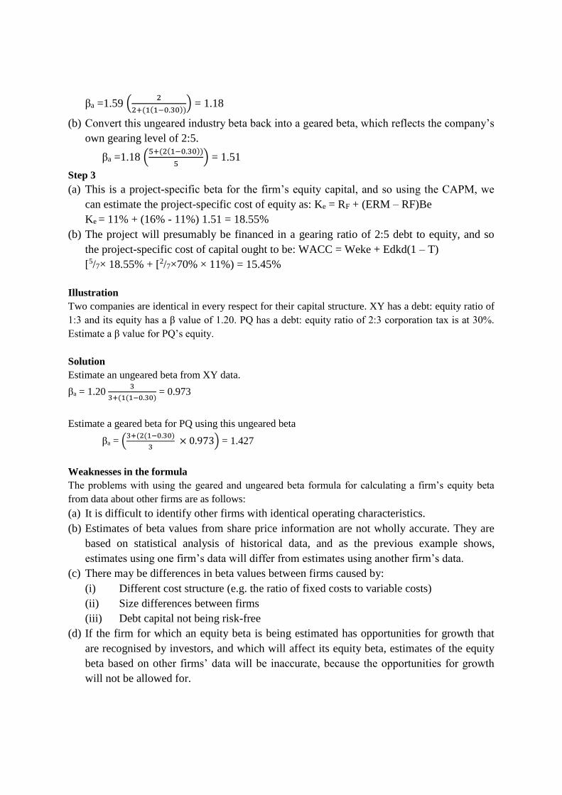
βa =1.59 (2
2+(1(1−0.30))) = 1.18
(b) Convert this ungeared industry beta back into a geared beta, which reflects the company’s
own gearing level of 2:5.
βa =1.18 (5+(2(1−0.30))
5) = 1.51
Step 3
(a) This is a project-specific beta for the firm’s equity capital, and so using the CAPM, we
can estimate the project-specific cost of equity as: Ke = RF + (ERM – RF)Be
Ke = 11% + (16% - 11%) 1.51 = 18.55%
(b) The project will presumably be financed in a gearing ratio of 2:5 debt to equity, and so
the project-specific cost of capital ought to be: WACC = Weke + Edkd(1 – T)
[5/7× 18.55% + [2/7×70% × 11%) = 15.45%
Illustration
Two companies are identical in every respect for their capital structure. XY has a debt: equity ratio of
1:3 and its equity has a β value of 1.20. PQ has a debt: equity ratio of 2:3 corporation tax is at 30%.
Estimate a β value for PQ’s equity.
Solution
Estimate an ungeared beta from XY data.
βa = 1.20 3
3+(1(1−0.30) = 0.973
Estimate a geared beta for PQ using this ungeared beta
βa = (3+(2(1−0.30)
3 × 0.973) = 1.427
Weaknesses in the formula
The problems with using the geared and ungeared beta formula for calculating a firm’s equity beta
from data about other firms are as follows:
(a) It is difficult to identify other firms with identical operating characteristics.
(b) Estimates of beta values from share price information are not wholly accurate. They are
based on statistical analysis of historical data, and as the previous example shows,
estimates using one firm’s data will differ from estimates using another firm’s data.
(c) There may be differences in beta values between firms caused by:
(i) Different cost structure (e.g. the ratio of fixed costs to variable costs)
(ii) Size differences between firms
(iii) Debt capital not being risk-free
(d) If the firm for which an equity beta is being estimated has opportunities for growth that
are recognised by investors, and which will affect its equity beta, estimates of the equity
beta based on other firms’ data will be inaccurate, because the opportunities for growth
will not be allowed for.
Page 156
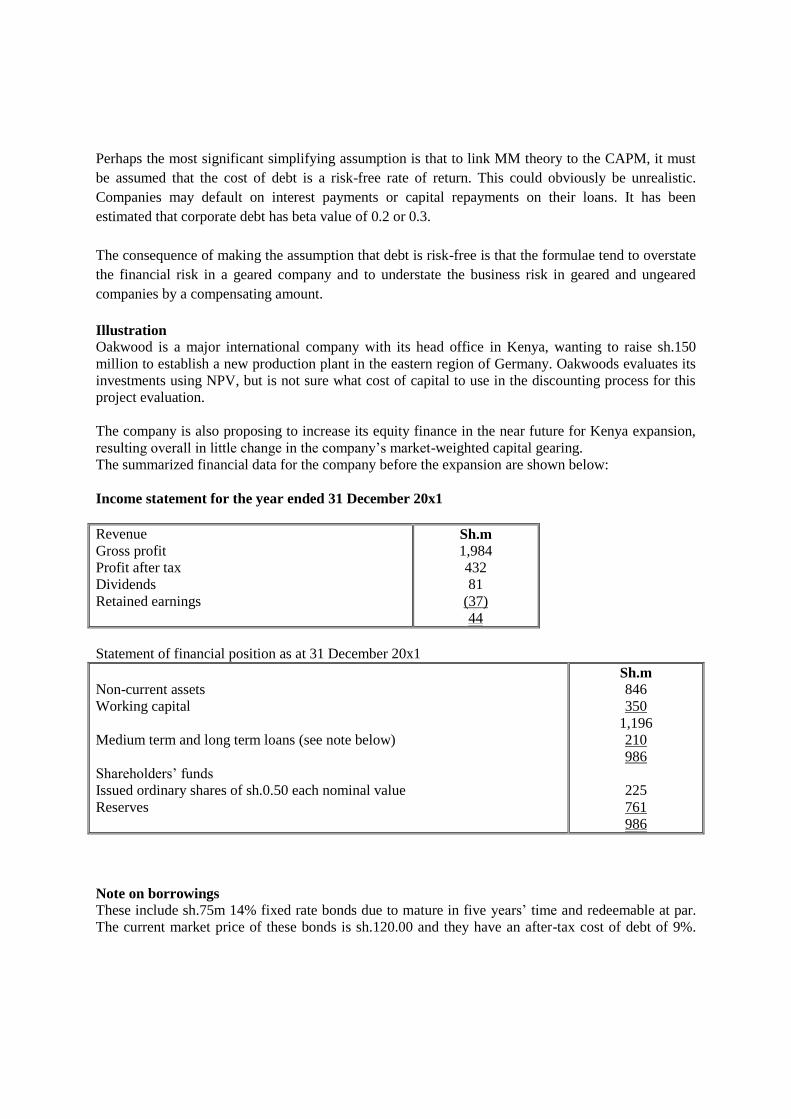
Perhaps the most significant simplifying assumption is that to link MM theory to the CAPM, it must
be assumed that the cost of debt is a risk-free rate of return. This could obviously be unrealistic.
Companies may default on interest payments or capital repayments on their loans. It has been
estimated that corporate debt has beta value of 0.2 or 0.3.
The consequence of making the assumption that debt is risk-free is that the formulae tend to overstate
the financial risk in a geared company and to understate the business risk in geared and ungeared
companies by a compensating amount.
Illustration
Oakwood is a major international company with its head office in Kenya, wanting to raise sh.150
million to establish a new production plant in the eastern region of Germany. Oakwoods evaluates its
investments using NPV, but is not sure what cost of capital to use in the discounting process for this
project evaluation.
The company is also proposing to increase its equity finance in the near future for Kenya expansion,
resulting overall in little change in the company’s market-weighted capital gearing.
The summarized financial data for the company before the expansion are shown below:
Income statement for the year ended 31 December 20x1
Revenue
Gross profit
Profit after tax
Dividends
Retained earnings
Sh.m
1,984
432
81
(37)
44
Statement of financial position as at 31 December 20x1
Non-current assets
Working capital
Medium term and long term loans (see note below)
Shareholders’ funds
Issued ordinary shares of sh.0.50 each nominal value
Reserves
Sh.m
846
350
1,196
210
986
225
761
986
Note on borrowings
These include sh.75m 14% fixed rate bonds due to mature in five years’ time and redeemable at par.
The current market price of these bonds is sh.120.00 and they have an after-tax cost of debt of 9%.
Page 157
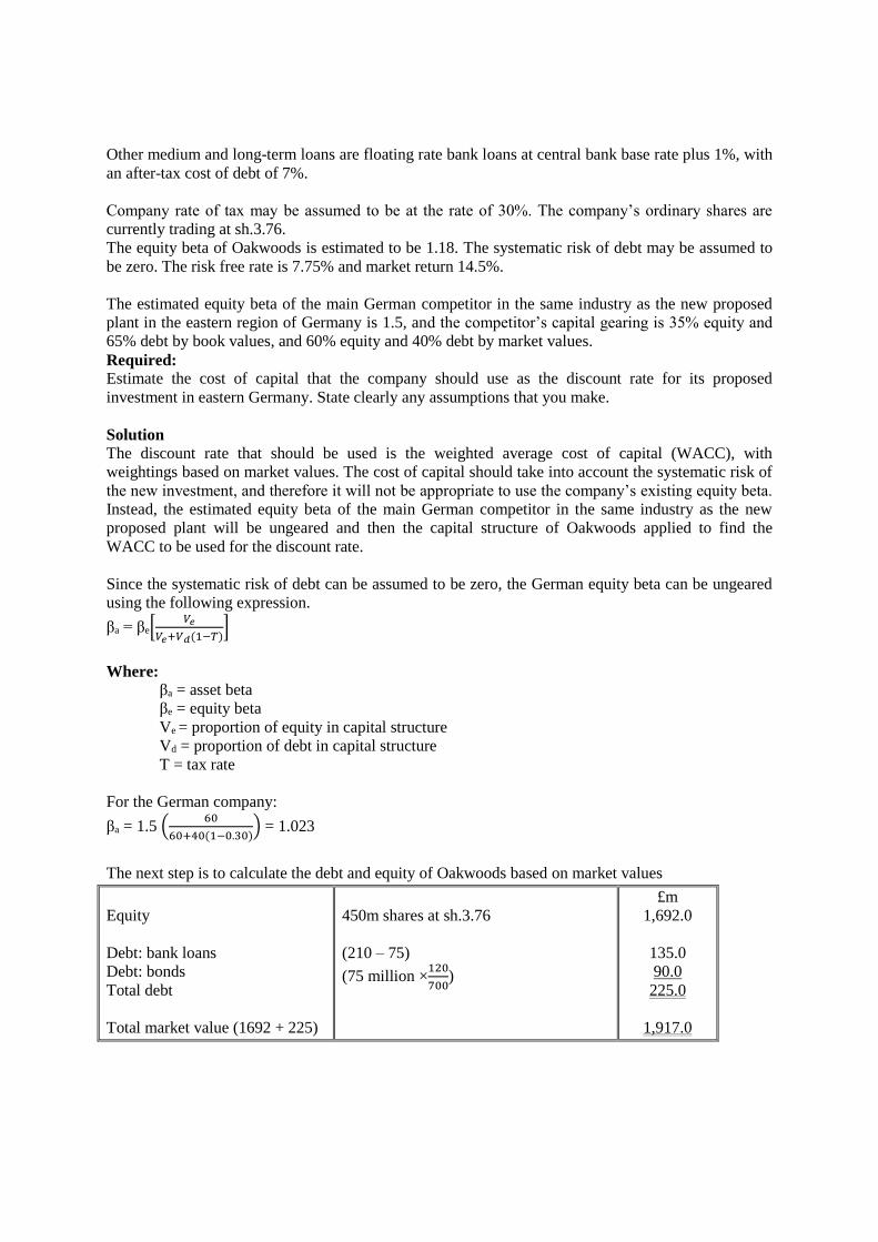
Other medium and long-term loans are floating rate bank loans at central bank base rate plus 1%, with
an after-tax cost of debt of 7%.
Company rate of tax may be assumed to be at the rate of 30%. The company’s ordinary shares are
currently trading at sh.3.76.
The equity beta of Oakwoods is estimated to be 1.18. The systematic risk of debt may be assumed to
be zero. The risk free rate is 7.75% and market return 14.5%.
The estimated equity beta of the main German competitor in the same industry as the new proposed
plant in the eastern region of Germany is 1.5, and the competitor’s capital gearing is 35% equity and
65% debt by book values, and 60% equity and 40% debt by market values.
Required:
Estimate the cost of capital that the company should use as the discount rate for its proposed
investment in eastern Germany. State clearly any assumptions that you make.
Solution
The discount rate that should be used is the weighted average cost of capital (WACC), with
weightings based on market values. The cost of capital should take into account the systematic risk of
the new investment, and therefore it will not be appropriate to use the company’s existing equity beta.
Instead, the estimated equity beta of the main German competitor in the same industry as the new
proposed plant will be ungeared and then the capital structure of Oakwoods applied to find the
WACC to be used for the discount rate.
Since the systematic risk of debt can be assumed to be zero, the German equity beta can be ungeared
using the following expression.
βa = βe[𝑉𝑒
𝑉𝑒+𝑉𝑑(1−𝑇)]
Where:
βa = asset beta
βe = equity beta
Ve = proportion of equity in capital structure
Vd = proportion of debt in capital structure
T = tax rate
For the German company:
βa = 1.5 (60
60+40(1−0.30)) = 1.023
The next step is to calculate the debt and equity of Oakwoods based on market values
Equity
Debt: bank loans
Debt: bonds
Total debt
Total market value (1692 + 225)
450m shares at sh.3.76
(210 – 75)
(75 million ×120
700)
£m
1,692.0
135.0
90.0
225.0
1,917.0
Page 158
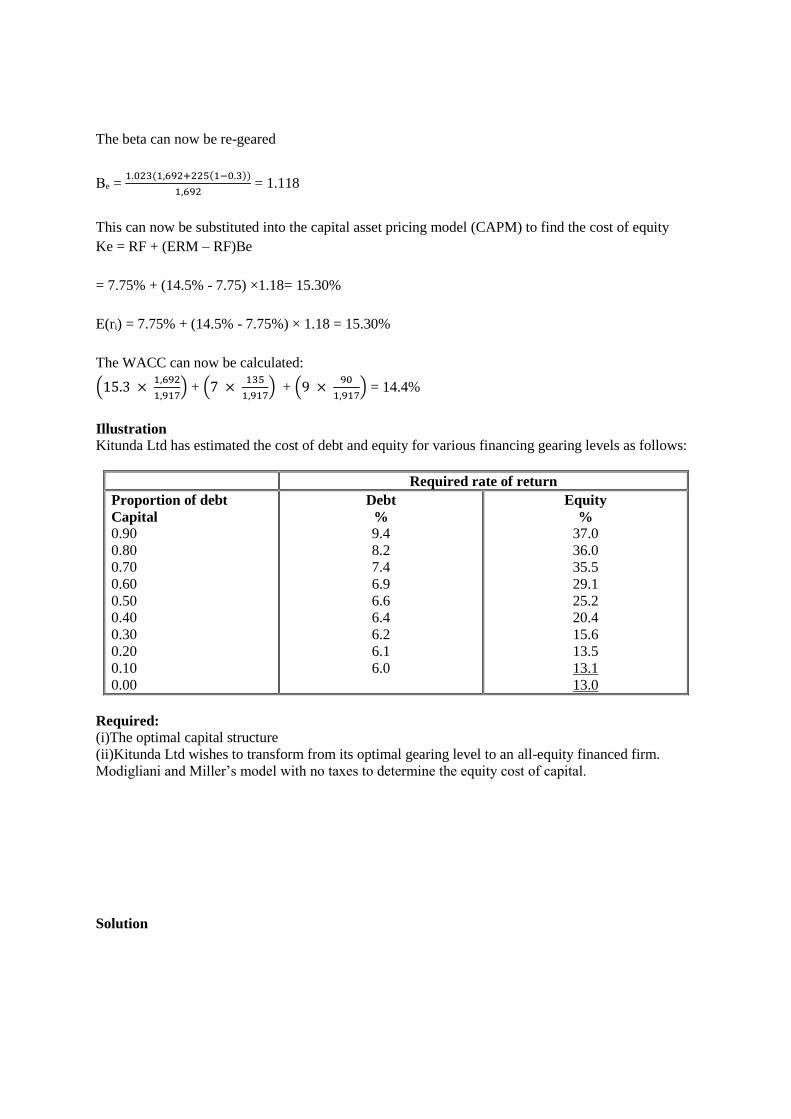
The beta can now be re-geared
Βe = 1.023(1,692+225(1−0.3))
1,692 = 1.118
This can now be substituted into the capital asset pricing model (CAPM) to find the cost of equity
Ke = RF + (ERM – RF)Be
= 7.75% + (14.5% - 7.75) ×1.18= 15.30%
E(ri) = 7.75% + (14.5% - 7.75%) × 1.18 = 15.30%
The WACC can now be calculated:
(15.3 × 1,692
1,917) + (7 ×
135
1,917) + (9 ×
90
1,917) = 14.4%
Illustration
Kitunda Ltd has estimated the cost of debt and equity for various financing gearing levels as follows:
Required rate of return
Proportion of debt
Capital
0.90
0.80
0.70
0.60
0.50
0.40
0.30
0.20
0.10
0.00
Debt
%
9.4
8.2
7.4
6.9
6.6
6.4
6.2
6.1
6.0
Equity
%
37.0
36.0
35.5
29.1
25.2
20.4
15.6
13.5
13.1
13.0
Required:
(i)The optimal capital structure
(ii)Kitunda Ltd wishes to transform from its optimal gearing level to an all-equity financed firm.
Modigliani and Miller’s model with no taxes to determine the equity cost of capital.
Solution
Page 159
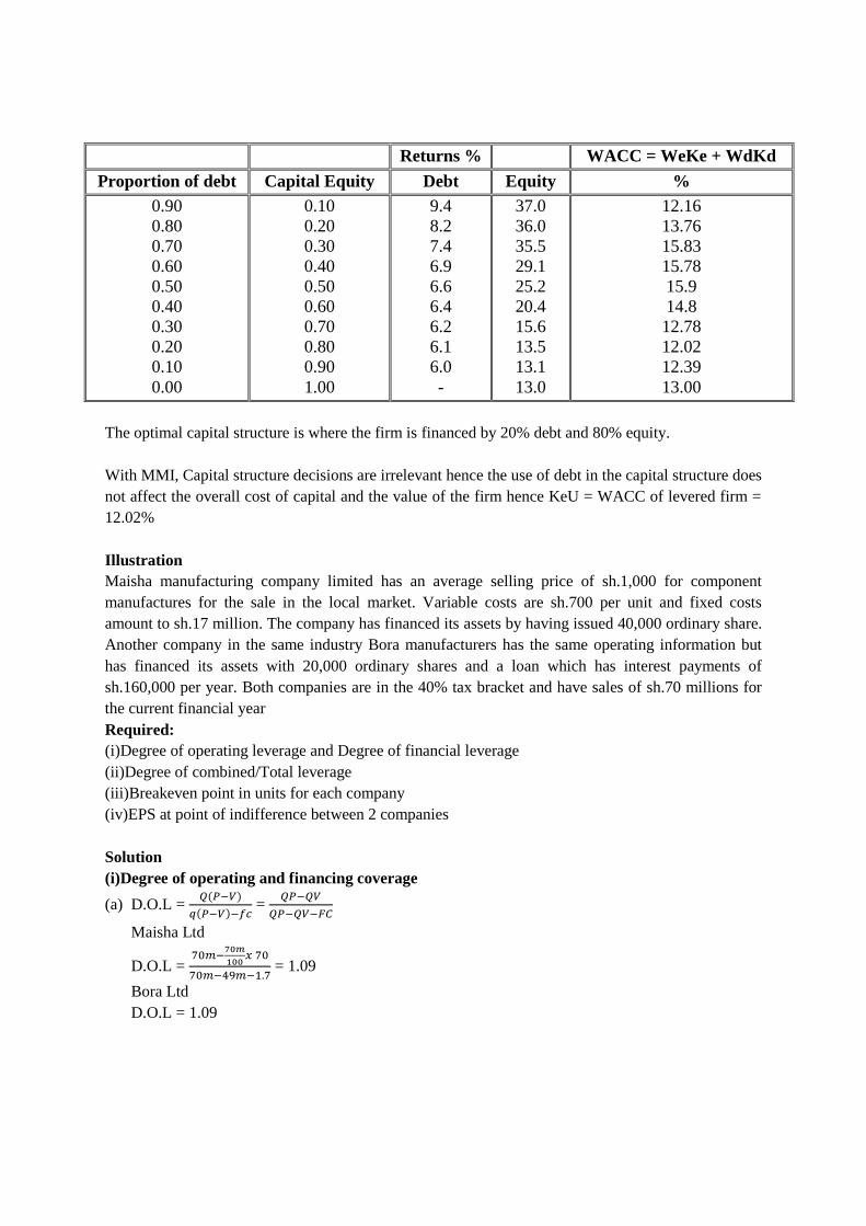
Returns % WACC = WeKe + WdKd
Proportion of debt Capital Equity Debt Equity %
0.90
0.80
0.70
0.60
0.50
0.40
0.30
0.20
0.10
0.00
0.10
0.20
0.30
0.40
0.50
0.60
0.70
0.80
0.90
1.00
9.4
8.2
7.4
6.9
6.6
6.4
6.2
6.1
6.0
-
37.0
36.0
35.5
29.1
25.2
20.4
15.6
13.5
13.1
13.0
12.16
13.76
15.83
15.78
15.9
14.8
12.78
12.02
12.39
13.00
The optimal capital structure is where the firm is financed by 20% debt and 80% equity.
With MMI, Capital structure decisions are irrelevant hence the use of debt in the capital structure does
not affect the overall cost of capital and the value of the firm hence KeU = WACC of levered firm =
12.02%
Illustration
Maisha manufacturing company limited has an average selling price of sh.1,000 for component
manufactures for the sale in the local market. Variable costs are sh.700 per unit and fixed costs
amount to sh.17 million. The company has financed its assets by having issued 40,000 ordinary share.
Another company in the same industry Bora manufacturers has the same operating information but
has financed its assets with 20,000 ordinary shares and a loan which has interest payments of
sh.160,000 per year. Both companies are in the 40% tax bracket and have sales of sh.70 millions for
the current financial year
Required:
(i)Degree of operating leverage and Degree of financial leverage
(ii)Degree of combined/Total leverage
(iii)Breakeven point in units for each company
(iv)EPS at point of indifference between 2 companies
Solution
(i)Degree of operating and financing coverage
(a) D.O.L = 𝑄(𝑃−𝑉)
𝑞(𝑃−𝑉)−𝑓𝑐 =
𝑄𝑃−𝑄𝑉
𝑄𝑃−𝑄𝑉−𝐹𝐶
Maisha Ltd
D.O.L = 70𝑚−
70𝑚
100𝑥 70
70𝑚−49𝑚−1.7 = 1.09
Bora Ltd
D.O.L = 1.09
Page 160
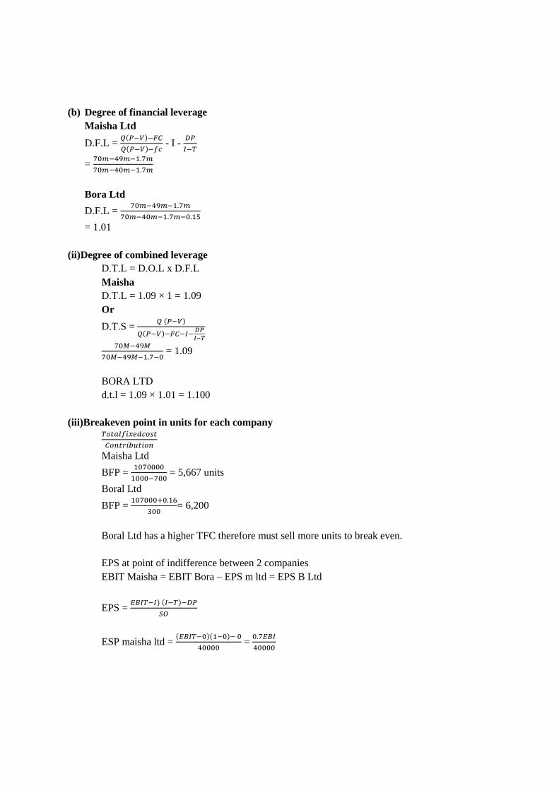
(b) Degree of financial leverage
Maisha Ltd
D.F.L = 𝑄(𝑃−𝑉)−𝐹𝐶
𝑄(𝑃−𝑉)−𝑓𝑐 - I -
𝐷𝑃
𝐼−𝑇
= 70𝑚−49𝑚−1.7𝑚
70𝑚−40𝑚−1.7𝑚
Bora Ltd
D.F.L = 70𝑚−49𝑚−1.7𝑚
70𝑚−40𝑚−1.7𝑚−0.15
= 1.01
(ii)Degree of combined leverage
D.T.L = D.O.L x D.F.L
Maisha
D.T.L = 1.09 × 1 = 1.09
Or
D.T.S = 𝑄 (𝑃−𝑉)
𝑄(𝑃−𝑉)−𝐹𝐶−𝐼−𝐷𝑃
𝐼−𝑇
70𝑀−49𝑀
70𝑀−49𝑀−1.7−0 = 1.09
BORA LTD
d.t.l = 1.09 × 1.01 = 1.100
(iii)Breakeven point in units for each company 𝑇𝑜𝑡𝑎𝑙𝑓𝑖𝑥𝑒𝑑𝑐𝑜𝑠𝑡
𝐶𝑜𝑛𝑡𝑟𝑖𝑏𝑢𝑡𝑖𝑜𝑛
Maisha Ltd
BFP = 1070000
1000−700 = 5,667 units
Boral Ltd
BFP = 107000+0.16
300= 6,200
Boral Ltd has a higher TFC therefore must sell more units to break even.
EPS at point of indifference between 2 companies
EBIT Maisha = EBIT Bora – EPS m ltd = EPS B Ltd
EPS = 𝐸𝐵𝐼𝑇−𝐼) (𝐼−𝑇)−𝐷𝑃
𝑆𝑂
ESP maisha ltd = (𝐸𝐵𝐼𝑇−0)(1−0)− 0
40000 =
0.7𝐸𝐵𝐼
40000
Page 161
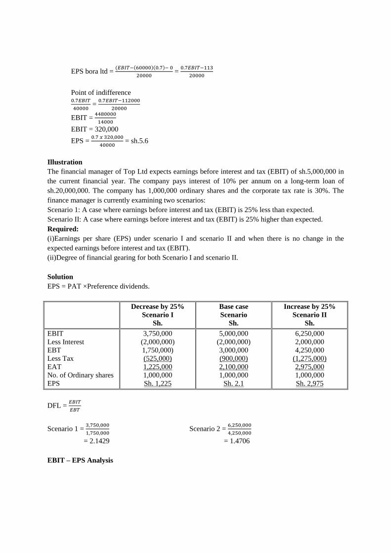
EPS bora ltd = (𝐸𝐵𝐼𝑇−(60000)(0.7)− 0
20000 =
0.7𝐸𝐵𝐼𝑇−113
20000
Point of indifference 0.7𝐸𝐵𝐼𝑇
40000 =
0.7𝐸𝐵𝐼𝑇−112000
20000
EBIT = 4480000
14000
EBIT = 320,000
EPS = 0.7 𝑥 320,000
40000 = sh.5.6
Illustration
The financial manager of Top Ltd expects earnings before interest and tax (EBIT) of sh.5,000,000 in
the current financial year. The company pays interest of 10% per annum on a long-term loan of
sh.20,000,000. The company has 1,000,000 ordinary shares and the corporate tax rate is 30%. The
finance manager is currently examining two scenarios:
Scenario 1: A case where earnings before interest and tax (EBIT) is 25% less than expected.
Scenario II: A case where earnings before interest and tax (EBIT) is 25% higher than expected.
Required:
(i)Earnings per share (EPS) under scenario I and scenario II and when there is no change in the
expected earnings before interest and tax (EBIT).
(ii)Degree of financial gearing for both Scenario I and scenario II.
Solution
EPS = PAT ×Preference dividends.
Decrease by 25%
Scenario I
Sh.
Base case
Scenario
Sh.
Increase by 25%
Scenario II
Sh.
EBIT
Less Interest
EBT
Less Tax
EAT
No. of Ordinary shares
EPS
3,750,000
(2,000,000)
1,750,000)
(525,000)
1,225,000
1,000,000
Sh. 1,225
5,000,000
(2,000,000)
3,000,000
(900,000)
2,100,000
1,000,000
Sh. 2.1
6,250,000
2,000,000
4,250,000
(1,275,000)
2,975,000
1,000,000
Sh. 2,975
DFL = 𝐸𝐵𝐼𝑇
𝐸𝐵𝑇
Scenario 1 = 3,750,000
1,750,000 Scenario 2 =
6,250,000
4,250,000
= 2.1429 = 1.4706
EBIT – EPS Analysis
Page 162
The EBIT-EPS approach to capital structure is a tool businesses use to determine the best ratio of debt
and equity that should be used to finance the business' assets and operations.
At its core, the EBIT-EPS approach is a way to mathematically project how a balance sheet's structure
will affect a company's earnings.
The basic concept of the EBIT-EPS approach
To understand how the EBIT-EPS method works, first we must understand the two primary metrics
involved, EBIT and EPS.
EBIT refers to a company's earnings before interest and taxes. This metric strip out the impact of
interest and taxes, showing an investor or manager how a company is performing excluding the
impacts of the balance sheet's composition. In terms of EBIT, it does not matter if a company is
overloaded with debt or has no loans at all. EBIT will be the same either way.
EPS stands for earnings per share, which is the profit the company generates including the impact of
interest and tax obligations. EPS is particularly helpful to investors because it measures profits on a
per share basis. If a company's total profit is soaring but its profit per share is declining, that is a bad
thing for the investor owning a fixed number of shares. EPS captures this dynamic in a simple, easy to
understand way.
The ratio between these two metrics can show investors and management how the bottom line results,
the company's EPS, relates to its performance independent of its capital structure, its EBIT.
For example, let us say a company wants to maintain stable EPS but is considering taking out a new
loan to grow its balance sheet. In order for EPS to remain stable, the company's EBIT must also
increase at least as much as the new interest expense from the debt. If EBIT increases the same as the
next interest expense, then EPS should remain stable, assuming no change in taxes.
This analysis involves the use of different financing options in the company and the effect of such use
on the firm’s EPS
Recall: EPS = 𝑃𝐴𝑇 & 𝑃𝑟𝑒𝑓𝑒𝑟𝑒𝑛𝑐𝑒 𝑑𝑖𝑣𝑖𝑑𝑒𝑛𝑑𝑠
𝑂𝑟𝑑𝑖𝑛𝑎𝑟𝑦 𝑆ℎ𝑎𝑟𝑒𝑠
𝐸𝐵𝐼𝑇−𝐼𝑛𝑡𝑒𝑟𝑒𝑠𝑡 (𝐼−𝑇)−𝑃𝑟𝑒𝑓𝑒𝑟𝑒𝑛𝑐𝑒 𝐷𝑖𝑣𝑖𝑑𝑒𝑛𝑑𝑠
𝑁𝑜.𝑜𝑓 𝑂𝑟𝑑𝑖𝑛𝑎𝑟𝑦 𝑆ℎ𝑎𝑟𝑒𝑠
Breakeven Point/Indifference Point
This refers to the level of EBIT of which the EPS of different financing options will be the same.
3.5. LONG TERM FINANCING DECISIONS
Bond refinancing decision, lease-buy evaluation and the rights issues
Rights Issue
Page 163
This is an offer given to existing shareholders of a company to acquire additional shares. They are on
a prorate basis and usually given at a discount. (subscription price) prices are usually set below the
prevailing market price.
Reasons for issuing shares at a discount
1. To make issues attractive to existing shareholders
2. To compensate existing shareholders to accept bearing additional shares.
3. To ensure that between the announcement days and issue day the offer price is still below the
market price.
4. Create value for the right.
Dates of rights issue
1) Announcement date. The date when the management announces to the shareholders the intention
to have rights issue.
2) Registration of members date. The date when each member appearing in the register is called
upon to take the rights issue.
NB: between these 2 dates, the shares sell at cum-rights price (price before rights issue)
3) Issue date. Date on which shares are issued. After registration of members date, shares sell at
ex-rights price (price after rights issue).
Note:
After issue date, shares ell without cum-rights or ex-rights up to expiry date. After expiry date,
existing shareholders cannot acquire the rights.
In rights issue, the financial manager has to consider:
Engaging a dealer-manager or broker-dealer to manage the offering process
Selling group and broker-dealer participation
Subscription price per new share
Number of new shares to be sold
The value of rights vs. trading price of the subscription rights
The effect of rights on the value of the current share
The effect of rights to shareholders of record and new shareholders and rights holders
Reasons for a Rights Issue
When a company is planning an expansion of its operations, it may require a huge amount of
capital. Instead of opting for debt, they may like to go for equity to avoid fixed payments of
interest. To raise equity capital, a rights issue may be a faster way to achieve the objective.
A project where debt/loan funding may not be available/suitable or expensive usually makes a
company raise capital through a rights issue.
Companies looking to improve their debt to equity ratio or looking to buy a new company may
opt for funding via the same route.
Page 164

Sometimes troubled companies may issue shares to pay off debt in order to improve their
financial health.
Computations
So = Number of shares before rights issue
S = Number of shares to be issued to raise desired funds.
Ps = Price at which the rights shares are sold (subscription or offer price)
Po = Price of shares before rights issue (cum-rights price)
Pr = Price of shares after rights issue (ex-right price)
N = Number of rights required to acquire one new share.
R = Theoretical value of a right i.e. market price at which each of the rights is assumed to sell at.
Formulae
(i)Number of shares to be issued to raise desired funds (s)
S = 𝑑𝑒𝑠𝑖𝑟𝑒𝑑𝑓𝑢𝑛𝑑𝑠
𝑃𝑟𝑖𝑐𝑒 (𝑃𝑠)
(ii)Number of rights required to acquire one new share (N)
N = 𝑆0
𝑆
(iii)Theoretical ex-right price (Px)
a) Px = (𝑃0𝑥𝑆0+(𝑃𝑠𝑥𝑆)
𝑆0+ 𝑆
b) Px = Ps + (P0 + Ps) 𝑁
𝑁+1
c) Px = N x P0 = xx 1
𝑥𝑥x Ps = xx
xx
= xxx
(iv)Theoretical value of a right (price at which the right is selling) (R)
a) R = P0 – Px
b) R = (𝑃𝑥−𝑃𝑠)
𝑁
Note: R (cum right) = R (ex right)
Illustration
Mhusika Ltd is an all equity financed company with a market capitalization of sh.720,000,000. The
company intends to raise Sh.120,000,000 through a rights issue to finance a new project. The current
market price per share of the company prior to announcement of the rights issue is sh.30. The
proposed offer price is sh.25.The new project is expected to generate cash flows of sh.16,800,000 per
annum to perpetuity. For the year just ended, the company paid a dividend per share of sh.2.83. The
project’s cash flows and dividends per share have an equal growth rate of 6% per annum.
Required:
Page 165

(i)The cum-right market price per share on announcement of the rights issue but just before the issue
is made.
(ii)Assuming there is an investor who has 3000 shares determine the effect of right issue on his
wealth.
Solution
(i)Cum rights MPs = Current MPS – NPV Per Share of the project
Ks = 𝑑0(1+𝑔)
𝑝0 x 100 + g =
2.83(1+6%)
30× 100 + 6% = 10% + 6%
Ks = 16% - cost of equity/capital
NPV = (𝐴𝑥𝐼
𝑟%) - I0 (discounting annuities received to perpetuity)
= (16,800,000 ×𝐼
16%) - 120,000,000
= -1,500,000
NPV per share = −15,000,000
2,400,000 = -0.625
Therefore cum rights MPS = 30 + (-0.625)= 29.375
(1) S = 𝐷𝑒𝑠𝑖𝑟𝑒𝑑𝑓𝑢𝑛𝑑
𝑆𝑢𝑏𝑠𝑐𝑟𝑖𝑝𝑡𝑖𝑜𝑛𝑝𝑟𝑖𝑐𝑒
𝑜𝑓𝑓𝑒𝑟𝑝𝑟𝑖𝑐𝑒 (𝑅𝑠
S = No. of ordinary shares to be issued to raised desired fund.
(2) N = 𝑆0
𝑆
S0 = existing number of ordinary shares
N = Number of rights per share
(3) Px = (𝑃0𝑥𝑆0+(𝑃𝑠𝑥𝑆)
𝑆0+ 𝑆
Px = ex-right price
P0 = cum right price
Ps = offer price
Or
Px = Ps + (Po – Ps) 𝑛
𝑛+1
(4) R = P0 – Px
R = Value of the right at the open market
Or
R cum right = 𝑃0−𝑃𝑠
𝑛+1
Or
R ex right = 𝑃𝑥−𝑃𝑠
𝑛
Theoretical ex-right MPS
Px = (𝑃0𝑥𝑆0+(𝑃𝑠𝑥𝑆)
𝑆0+ 𝑆 S =
120000000
25 = 4800000
Page 166
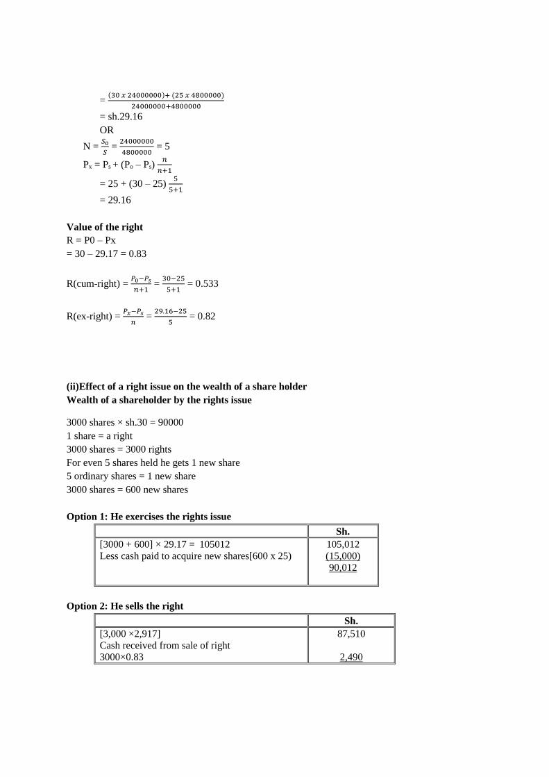
= (30 𝑥 24000000)+ (25 𝑥 4800000)
24000000+4800000
= sh.29.16
OR
N = 𝑆0
𝑆 =
24000000
4800000 = 5
Px = Ps + (Po – Ps) 𝑛
𝑛+1
= 25 + (30 – 25) 5
5+1
= 29.16
Value of the right
R = P0 – Px
= 30 – 29.17 = 0.83
R(cum-right) = 𝑃0−𝑃𝑠
𝑛+1 =
30−25
5+1 = 0.533
R(ex-right) = 𝑃𝑥−𝑃𝑠
𝑛 =
29.16−25
5 = 0.82
(ii)Effect of a right issue on the wealth of a share holder
Wealth of a shareholder by the rights issue
3000 shares × sh.30 = 90000
1 share = a right
3000 shares = 3000 rights
For even 5 shares held he gets 1 new share
5 ordinary shares = 1 new share
3000 shares = 600 new shares
Option 1: He exercises the rights issue
Sh.
[3000 + 600] × 29.17 = 105012
Less cash paid to acquire new shares[600 x 25)
105,012 (15,000) 90,012
Option 2: He sells the right
Sh.
[3,000 ×2,917] Cash received from sale of right
3000×0.83
87,510
2,490
Page 167
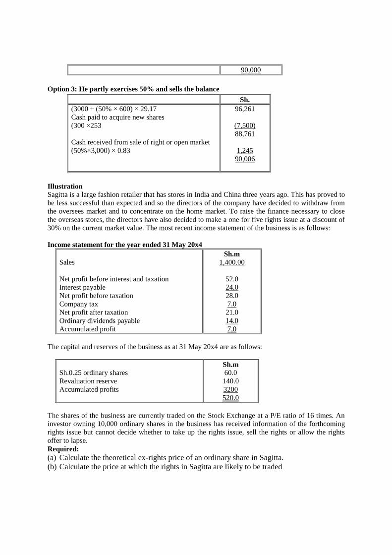
90,000
Option 3: He partly exercises 50% and sells the balance
Sh.
(3000 + (50% × 600) × 29.17 Cash paid to acquire new shares
(300 ×253
Cash received from sale of right or open market
(50%×3,000) × 0.83
96,261
(7,500) 88,761
1,245 90,006
Illustration
Sagitta is a large fashion retailer that has stores in India and China three years ago. This has proved to
be less successful than expected and so the directors of the company have decided to withdraw from
the oversees market and to concentrate on the home market. To raise the finance necessary to close
the overseas stores, the directors have also decided to make a one for five rights issue at a discount of
30% on the current market value. The most recent income statement of the business is as follows:
Income statement for the year ended 31 May 20x4
Sales
Net profit before interest and taxation
Interest payable
Net profit before taxation
Company tax
Net profit after taxation
Ordinary dividends payable
Accumulated profit
Sh.m
1,400.00
52.0
24.0
28.0
7.0
21.0
14.0
7.0
The capital and reserves of the business as at 31 May 20x4 are as follows:
Sh.0.25 ordinary shares
Revaluation reserve
Accumulated profits
Sh.m
60.0
140.0
3200
520.0
The shares of the business are currently traded on the Stock Exchange at a P/E ratio of 16 times. An
investor owning 10,000 ordinary shares in the business has received information of the forthcoming
rights issue but cannot decide whether to take up the rights issue, sell the rights or allow the rights
offer to lapse.
Required:
(a) Calculate the theoretical ex-rights price of an ordinary share in Sagitta.
(b) Calculate the price at which the rights in Sagitta are likely to be traded
Page 168
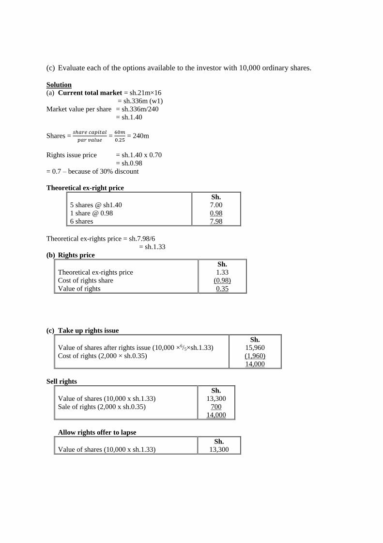
(c) Evaluate each of the options available to the investor with 10,000 ordinary shares.
Solution
(a) Current total market = sh.21m×16
= sh.336m (w1)
Market value per share = sh.336m/240
= sh.1.40
Shares = 𝑠ℎ𝑎𝑟𝑒 𝑐𝑎𝑝𝑖𝑡𝑎𝑙
𝑝𝑎𝑟 𝑣𝑎𝑙𝑢𝑒 =
60𝑚
0.25 = 240m
Rights issue price = sh.1.40 x 0.70
= sh.0.98
= 0.7 – because of 30% discount
Theoretical ex-right price
5 shares @ sh1.40
1 share @ 0.98
6 shares
Sh.
7.00
0.98
7.98
Theoretical ex-rights price = sh.7.98/6
= sh.1.33
(b) Rights price
Theoretical ex-rights price
Cost of rights share
Value of rights
Sh.
1.33
(0.98)
0.35
(c) Take up rights issue
Value of shares after rights issue (10,000 ×6/5×sh.1.33)
Cost of rights (2,000 × sh.0.35)
Sh.
15,960
(1,960)
14,000
Sell rights
Value of shares (10,000 x sh.1.33)
Sale of rights (2,000 x sh.0.35)
Sh.
13,300
700
14,000
Allow rights offer to lapse
Value of shares (10,000 x sh.1.33) Sh.
13,300
Page 169
If the investor either takes up the rights issue or sells his rights then his wealth will remain the same.
The difference is that if he takes up the rights issue he will maintain his relative shareholding but if he
sells his rights his percentage shareholding will fall, although he will gain sh.700 in cash.
However if the investor allows the rights to lapse his wealth will decrease by sh.700.
Bond refinancing/Bond refunding
A company may issue bonds of a time when the rates of interest are relatively high. During periods of
declining rates of interest a company may file itself with a fixed rates of interest were high.
The company will have to make a decision as whether to:
(1) Retrieve existing bond by calling back/repaying / original bond holders back their money.
(2) It is economical to issue a new bond
If existing bond is callable (redeemable) the company can sell or issue a new bond and use the cash
proceeds to retire the existing bond.
The process is known as bond refinancing/bond refunding)
Refunding is done due to the following reasons:
(i)Long-term debt usually have fixed interest charges therefore a company can wish to minimize
financing cost by retrieving existing bonds which are expensive.
(ii)Where existing bonds were issued with restrictive covenants which are not favorable to the firm,
the management can wish to retire such bond and avoid such restrictions.
(iii)Where a company has idle cash which can be used to retire the existing bond.
The following cash flows are considered under bond refinancing:
(i)Premium on refund (Call premium)
The holder of the existing bond which is redeemed prematurely will require a premium from the
company because they are denied certain benefits in future (returns). This premium is penalty payable
by the company and it is usually expressed as a percentage of the par value of the bond. However the
premium on refund is treated as a one of a tax allowable expense in the year of refund.
(ii)Interest charge during the overlapping period
Generally the firm will first issue a new less expensive bond, complete processing of the new bond
before refunding the existing bond holders their money so as to ensure the company do not suffer
from financial distress. During this period the company will pay interest charges on both old and new
bond.
The interest charge payable on the old bond is known as overlapping interest and it is treated as a one
of tax allowable expense.
(iii)Discount on the issue of bond
Page 170

When a bond either new or old realizes cash flows which are less than its par value the difference is
known as a discount. This discount is amortized or written off on a straight line basis over the
maturity period of the bond. Therefore at the time of refunding the existing bond will be unamortized
discount cost which will be treated as a one of tax allowable expense. Therefore it will generate a tax
shield benefit.
(iv)Floatation cost (issue cost)
The bond will always have issue cost which are amortized or written off on a straight line basis over
the life of the bond. For old bond there will always be unamortized floatation cost at time of
refunding. This is treated as one of tax allowable expense which will generate a tax shield benefit.
(v)Interest cost savings
This result from differential interest rate between existing and the new bond. They are usually
discounted using after tax rate of interest of the new bond. Bond refinancing is analyzed in capital
budgeting framework.
Illustration 1
Safaricom Limited issued a sh.100 million per value, 10 year bond, five years ago. The bond was
issued at a 2% discount and issuing costs amounted to sh.2 million.
Due to the decline in Treasury bill rates in the recent past, interest rates in the money market have
been failing presenting favorable opportunities for refinancing.
A financial analysts engaged by the company to assess the possibility of refinancing the debt reports
that a new sh.100 million par value, 12 percent, 5 year bond can be issued by the company. Issuing
costs for the new bond will be 5 per cent of the par value and a discount of 3 per cent will have to be
given to attract investors.
The old bond can be redeemed at 10 per cent premium and in addition, two months interest penalty
will have to be paid on redemption.
All bond issue expenses (including the interest penalty) are amortized on a straight-line basis over the
life of the bond and are allowable for corporate tax purposes.
The applicable corporate tax rate is 40 per cent and the after tax cost of debt to the company is
approximately 7%.
Required:
(a) Cash investment required for the refinancing decision.
(b) Annual cash benefits (savings) of the refinancing decision.
(c) (i) Net present Value (NPV) of the refinancing decision.
(ii) Is it worthwhile to issue a new bond to replace the existing bond? Explain
Solution
(a) Cash investment required for the refinancing
Call premium (110% × 100,000) – 100000
Overlapping interest (2/12×14/100× 100,000)
Discount issue of new bond (3% × 100,000)
Floatation on cost (5% x 100,000)
Sh. 000
10,000
2,333.3
12,333.3
5,000
Page 171
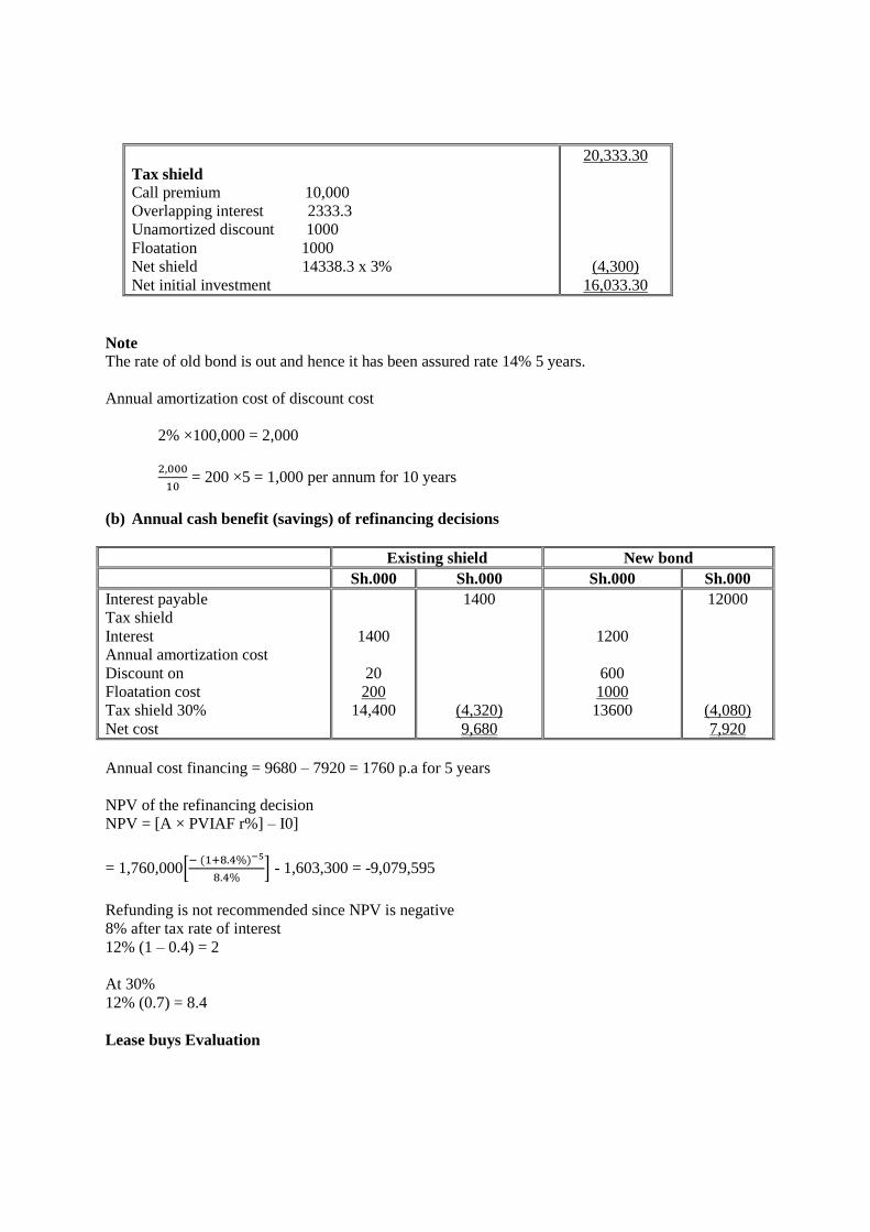
Tax shield
Call premium 10,000
Overlapping interest 2333.3
Unamortized discount 1000
Floatation 1000
Net shield 14338.3 x 3%
Net initial investment
20,333.30
(4,300)
16,033.30
Note
The rate of old bond is out and hence it has been assured rate 14% 5 years.
Annual amortization cost of discount cost
2% ×100,000 = 2,000
2,000
10 = 200 ×5 = 1,000 per annum for 10 years
(b) Annual cash benefit (savings) of refinancing decisions
Existing shield New bond
Sh.000 Sh.000 Sh.000 Sh.000
Interest payable
Tax shield
Interest
Annual amortization cost
Discount on
Floatation cost
Tax shield 30%
Net cost
1400
20
200
14,400
1400
(4,320)
9,680
1200
600
1000
13600
12000
(4,080)
7,920
Annual cost financing = 9680 – 7920 = 1760 p.a for 5 years
NPV of the refinancing decision
NPV = [A × PVIAF r%] – I0]
= 1,760,000[− (1+8.4%)−5
8.4%] - 1,603,300 = -9,079,595
Refunding is not recommended since NPV is negative
8% after tax rate of interest
12% (1 – 0.4) = 2
At 30%
12% (0.7) = 8.4
Lease buys Evaluation
Page 172
Lease or buy decision involves applying capital budgeting principles to determine if leasing as asset is
a better option than buying it.
Leasing in a contractual arrangement in which a company (the lessee) obtains an asset from another
company (the lessor) against periodic payments of lease rentals. It may typically also involve an
option to transfer the ownership of the asset to the lessee at the end of the lease.
Buying the asset involves purchase of the asset with company’s own funds or arranging a loan to
finance the purchase.
In finding out whether leasing is better than buying, we need to find out the periodic cash flows under
both the options and discount them using the after-tax cost of debt to see where does the present value
of the cost of leasing stands as compared to the present value of the cost of buying. The alternative
with lower present value of cash outflows is selected.
Types of leases
1. Capital Lease:
This is also called ‘financial lease’. A capital lease is a long-term arrangement, which is non-
cancelable. The lessee is obligated to pay lease rent until the expiry of lease period. The period of
lease agreement generally corresponds to the useful life of the asset concern.
A long-term lease in which the lessee must record the leased item as an asset on his/her balance sheet
and record the present value of the lease payments as debt. Additionally, the lessor must record the
lease as a sale on his/her own balance sheet. A capital lease may last for several years and is not
cancelable. It is treated as a sale for tax purposes.
2. Operating Lease:
Contrary to capital lease, the period of operating lease is shorter and it is often concealable at the
option of lessee with prior notice. Hence, operating lease is also called as an ‘Open end Lease
Arrangement.’ The lease term is shorter than the economic life of the asset. Thus, the lessor does not
recover its investment during the first lease period. Some of the examples of operating lease are
leasing of copying machines, certain computer hardware, world processors, automobiles, etc.
There is some criticism too labeled against capital leasing and operating leasing. Let us give the
arguments given by the proponents and opponents regarding the two types of equipment leasing. It is
argued that a firm knowing about the possible obsolescence of high technology equipment may not
want to purchase any equipment. Instead, it will prefer to go for operating lease to avoid the possible
risk of obsolescence. There is one difference between an operating lease and capital/financial lease.
Operating lease is short-term and cancelable by the lessee. It is also called as an ‘Open end Lease
Agreement’. In case of a financial lease, the risk of equipment obsolescence is shifted to the lessee
rather than on the lessor.
The reason is that it is a long-term and non-cancelable agreement or contract. Hence, lessee is
required to make rental payments even after obsolescence of equipment. On the other hand, it is said
that in operating lease, the risk of loss shifts from lessee to lessor.
This reasoning is not correct because if the lessor is concerned about the possible obsolescence, he
will certainly compensate for this risk by charging higher lease rentals. In fact, it is more or less a
‘war of wits’ only.
3. Sale and Leaseback:
Page 173
It is a sub-part of finance lease. Under a sale and leaseback arrangement, a firm sells an asset to
another party who in turn leases it back to the firm. The asset is usually sold at the market value on
the day. The firm, thus, receives the sales price in cash, on the one hand, and economic use of the
asset sold, on the other.
Yes, the firm is obliged to make periodic rental payments to the lessor. Sale and leaseback
arrangement is beneficial for both lessor and lessee. While the former gets tax benefits due to
depreciation, the latter has immediate cash inflow, which improves his liquidity position.
In fact, such arrangement is popular with companies facing short-term liquidity crisis. However,
under this arrangement, the assets are not physically exchanged but it all happens in records only.
This is nothing but a paper transaction. Sale and lease back transaction is suitable for those assets,
which are not subjected to depreciation but appreciation, say for example, land.
4. Leveraged Leasing:
A special form of leasing has become very popular in recent years. This is known as Leveraged
Leasing. This is popular in the financing of “big-tickets” assets such as aircraft, oilrigs and railway
equipment’s. In contrast to earlier mentioned three types of leasing, three parties are involved in case
of leveraged lease arrangement – Lessee, Lessor and the lender.
Leveraged leasing can be defined as a lease arrangement in which the lessor provides an equity
portion (say 25%) of the leased asset is cost and the third-party lenders provide the balance of the
financing. The lessor, the owner of the asset is entitled to depreciation allowance associated with the
asset
Illustration
ABC Ltd a small manufacturing firm, wishes to acquire a new machine that costs sh.30,000.
Arrangements can be made to lease or purchase the machine. The firm is in the 40% tax bracket. The
firm has gathered the following information about the two alternatives:
Purchase ABC Ltd can finance the purchase of the machine with a 10%, 6 year loan requiring annual
end of year installment. The machine would be depreciated using the reducing balance method. It
would have a salvage value of sh.6,000 after 5 years. The company would pay sh.1,200 per year for a
service contract that covers all maintenance costs. The firm plans to keep the machine and use it
beyond its 5 year recovery period.
Lease: ABC Ltd would obtain a 5 year lease requiring annual end-of-lease payments of sh.10,000.
The lessor would pay all maintenance costs. Insurance and other costs will be borne by the lease.
ABC Ltd would be given the right to exercise its option to purchase the machine for sh.3,000 at the
end of the lease term.
Required:
Advise ABC Ltd on which alternative to take using suitable computations.
Solution
Borrow to Purchase
Interest on loan [1 – T]
Depreciation tax shield
Initial outlay
Terminal cash flows
Maintenance costs [1 – T]
Page 174
Lease
Annual lease rentals [1 – T]
Option to buy
Purchase
Periodic Instalment = Amount of loan
PVIFAnyrsKd
30,000
PVIFA6yrs10%
30,000
4,3535
= Sh. 6,888.16
Loan Amortisation Schedule
Year Beginning balance
Sh.
Instalment
Sh.
Interest @ 10%
Sh.
Principal
Sh.
End balance
Sh.
1
2
3
4
5
6
30,000
26,112
21,835.2
17,130.72
11,955.792
6,263.3712
6,888
6,888
6,888
6,888
6,888
6,888
3,000
2,611.2
2,183.52
1,713.072
1,195.5792
626.33712
3888
4,276.8
4,704.48
5,174.928
5,692.4208
6,261.66288
26112
21835.2
17130.72
11955.792
6263.3712
NIL
Depreciation
Year Sh.
1
Sh.
2
Sh.
3
Sh.
4
Sh.
5
Beginning balance
Depreciation @ 20%
End balance
Tax shield @ 40%
30,000
(6,000)
24,000
2,400
24,000
(4,800)
19,200
1,920
19,200
(3,840)
15,360
1,536
15,360
(3,072)
12,288
1,228.8
12,288
(6,288)
6,000
2,515.2
Year
%
0
Sh.
1
Sh.
2
Sh.
3
Sh.
4
Sh.
5
Sh.
6
Sh.
Initial outlay
Interest [1-T]
Maintenance costs
Dep. tax shield
Net cash flows
Discount factor
(30,000)
-
-
____
(30,000)
1,000
(1800)
(7200)
2400
(120)
0.9091
(1566.72)
(720)
1920
(366.72)
0.8264
(1310.112)
(720)
1536
(494.112)
0.7513
(1027.8432)
(720)
1228.8
(519.0432)
0.6830
6000
(717.34752)
(720)
2515.2
1077.85248
0.6209
(375.802)
(375.802)
0.5645
NPV = Sh. (30,680.784)
Lease Option
Annual lease payments: 10,000 (1 – 0.4) = Sh. 6000
Purchase price Sh. 3,000
NPV = 6000 x PVIFA5yrs10% + 3000 x PVIF5yrs10%
Page 175
6000 x 3.7908 + 3000 x 0.6209
= Sh. (24,607.5)
ABC Ltd should implement the lease option as it offers the least cost.
Illustration 2
The management of a company has decided to acquire Machine X which costs sh.63,000 and has an
operational life of four years. The expected scrap value would be zero. Tax is payable at 30% on
operating cash flows one year in arrears. Tax-allowable depreciation is available at 25% a year on a
reducing balance basis.
Suppose that the company has the opportunity either to purchase the machine or to lease it under a
finance lease arrangement, at an annual rent of sh.20,000 for four years, payable at the end of each
year.
The company can borrow to finance the acquisition at 10%. Should the company lease or buy the
machine?
Solution
Working
Tax-allowable depreciation
Year
1
2
3
4
(25% of sh.63,000)
(75% of sh.15,750)
(75% of sh.11,813)
(sh.63,000 – sh.36,422)
Sh.
15,750
11,813
8,859
36,422
26,578
Note: 75% of sh.15, 750 is also 25% × (63,000 – 15,750).
The financing decision will be appraised by discounting the relevant cash flows at the after-tax cost of
borrowing, which is 10% ×70% = 7%.
(a) Purchase option
Year
0
2
3
4
5
Item
Cost of machine
Tax saved from tax-allowable depreciation
30% × sh.15,750
30% × sh.11,813
30%×sh.8,859
30% ×sh.26,578
Cash
flow
Sh.
(63,000)
4,725
3,544
2,658
7,973
Discount
factor 7%
1,000
0.873
0.816
0.763
0.713
Present
value
Sh.
(63,000)
4,125
2,892
2,028
5,685
(48,270)
(b) Leasing option
It is assumed that the lease payments are tax allowable in full
Year Item Cash Discount Present
Page 176
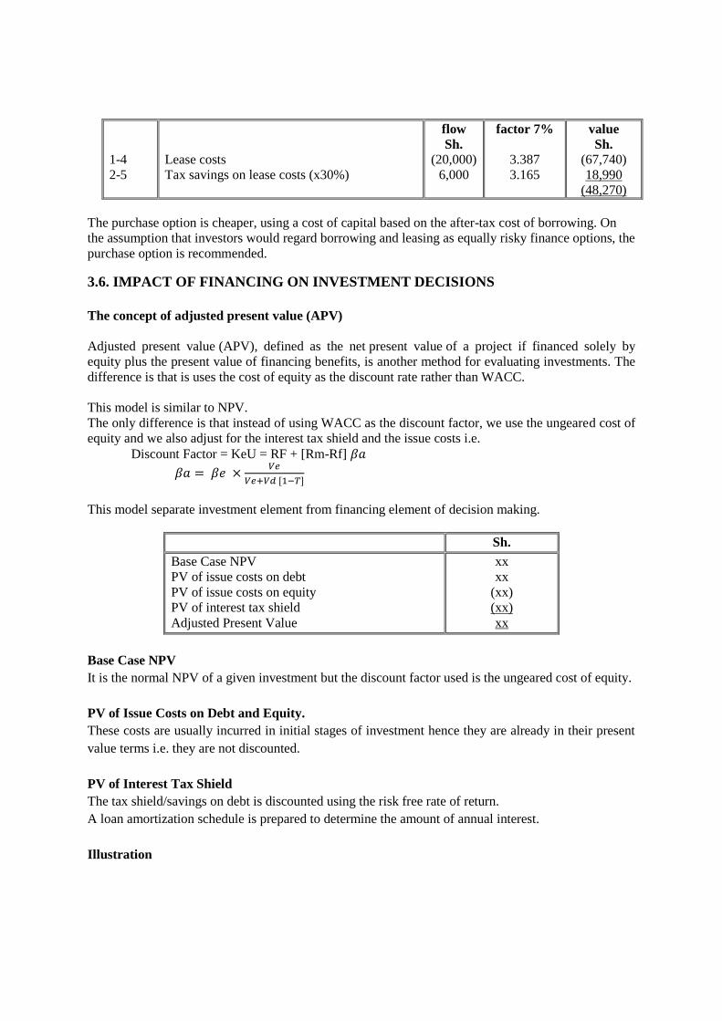
1-4
2-5
Lease costs
Tax savings on lease costs (x30%)
flow
Sh.
(20,000)
6,000
factor 7%
3.387
3.165
value
Sh.
(67,740)
18,990
(48,270)
The purchase option is cheaper, using a cost of capital based on the after-tax cost of borrowing. On
the assumption that investors would regard borrowing and leasing as equally risky finance options, the
purchase option is recommended.
3.6. IMPACT OF FINANCING ON INVESTMENT DECISIONS
The concept of adjusted present value (APV)
Adjusted present value (APV), defined as the net present value of a project if financed solely by
equity plus the present value of financing benefits, is another method for evaluating investments. The
difference is that is uses the cost of equity as the discount rate rather than WACC.
This model is similar to NPV.
The only difference is that instead of using WACC as the discount factor, we use the ungeared cost of
equity and we also adjust for the interest tax shield and the issue costs i.e.
Discount Factor = KeU = RF + [Rm-Rf] 𝛽𝑎
𝛽𝑎 = 𝛽𝑒 ×𝑉𝑒
𝑉𝑒+𝑉𝑑 [1−𝑇]
This model separate investment element from financing element of decision making.
Sh.
Base Case NPV
PV of issue costs on debt
PV of issue costs on equity
PV of interest tax shield
Adjusted Present Value
xx
xx
(xx)
(xx)
xx
Base Case NPV
It is the normal NPV of a given investment but the discount factor used is the ungeared cost of equity.
PV of Issue Costs on Debt and Equity.
These costs are usually incurred in initial stages of investment hence they are already in their present
value terms i.e. they are not discounted.
PV of Interest Tax Shield
The tax shield/savings on debt is discounted using the risk free rate of return.
A loan amortization schedule is prepared to determine the amount of annual interest.
Illustration
Page 177
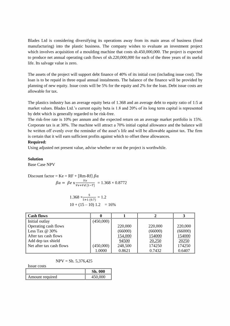
Blades Ltd is considering diversifying its operations away from its main areas of business (food
manufacturing) into the plastic business. The company wishes to evaluate an investment project
which involves acquisition of a moulding machine that costs sh.450,000,000. The project is expected
to produce net annual operating cash flows of sh.220,000,000 for each of the three years of its useful
life. Its salvage value is zero.
The assets of the project will support debt finance of 40% of its initial cost (including issue cost). The
loan is to be repaid in three equal annual instalments. The balance of the finance will be provided by
planning of new equity. Issue costs will be 5% for the equity and 2% for the loan. Debt issue costs are
allowable for tax.
The plastics industry has an average equity beta of 1.368 and an average debt to equity ratio of 1:5 at
market values. Blades Ltd.’s current equity beta is 1.8 and 20% of its long term capital is represented
by debt which is generally regarded to be risk-free.
The risk-free rate is 10% per annum and the expected return on an average market portfolio is 15%.
Corporate tax is at 30%. The machine will attract a 70% initial capital allowance and the balance will
be written off evenly over the reminder of the asset’s life and will be allowable against tax. The firm
is certain that it will earn sufficient profits against which to offset these allowances.
Required:
Using adjusted net present value, advise whether or not the project is worthwhile.
Solution
Base Case NPV
Discount factor = Ke = RF + [Rm-Rf] 𝛽𝑎
𝛽𝑎 = 𝛽𝑒 x𝑉𝑒
𝑉𝑒+𝑉𝑑 [1−𝑇] = 1.368 × 0.8772
1.368 ×5
5+1 (0.7) = 1.2
10 + (15 – 10) 1.2 = 16%
Cash flows 0 1 2 3
Initial outlay
Operating cash flows
Less Tax @ 30%
After tax cash flows
Add dep tax shield
Net after tax cash flows
(450,000)
(450,000)
1.0000
220,000
(66000)
154,000
94500
248,500
0.8621
220,000
(66000)
154000
20,250
174250
0.7432
220,000
(66000)
154000
20250
174250
0.6407
NPV = Sh. 5,376,425
Issue costs
Sh. 000
Amount required 450,000
Page 178
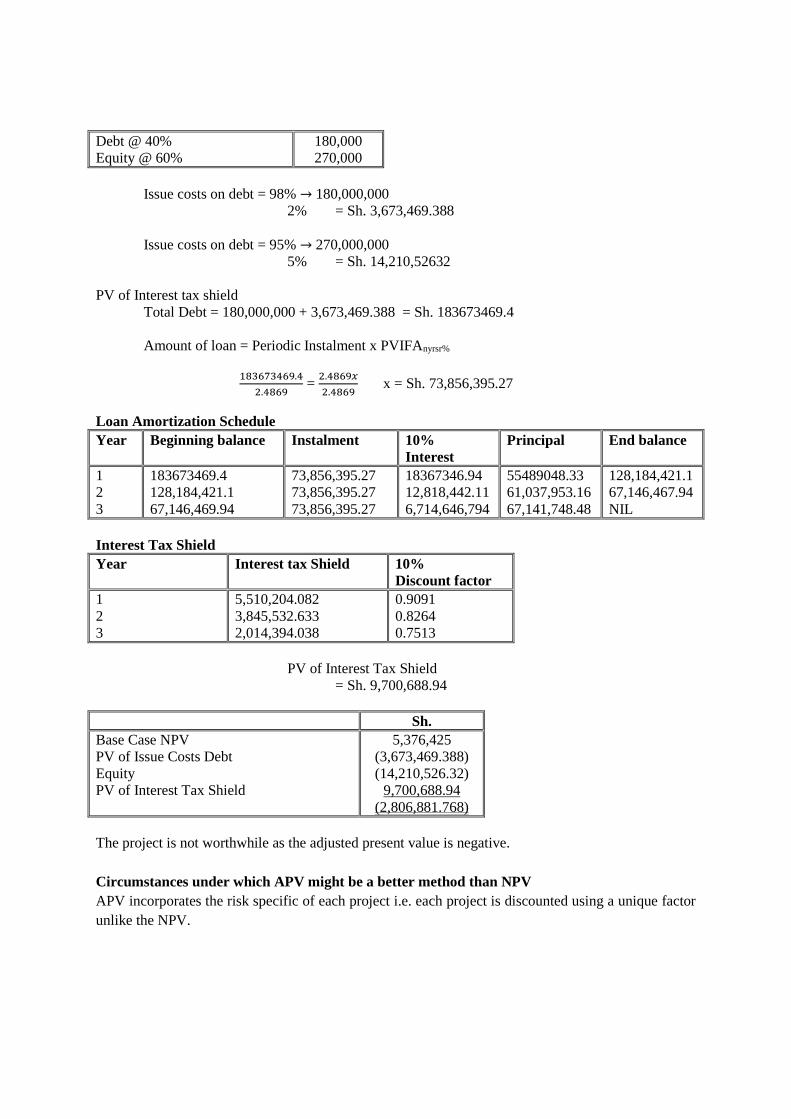
Debt @ 40%
Equity @ 60%
180,000
270,000
Issue costs on debt = 98% → 180,000,000
2% = Sh. 3,673,469.388
Issue costs on debt = 95% → 270,000,000
5% = Sh. 14,210,52632
PV of Interest tax shield
Total Debt = 180,000,000 + 3,673,469.388 = Sh. 183673469.4
Amount of loan = Periodic Instalment x PVIFAnyrsr%
183673469.4
2.4869 =
2.4869𝑥
2.4869 x = Sh. 73,856,395.27
Loan Amortization Schedule
Year Beginning balance Instalment 10%
Interest
Principal End balance
1
2
3
183673469.4
128,184,421.1
67,146,469.94
73,856,395.27
73,856,395.27
73,856,395.27
18367346.94
12,818,442.11
6,714,646,794
55489048.33
61,037,953.16
67,141,748.48
128,184,421.1
67,146,467.94
NIL
Interest Tax Shield
Year Interest tax Shield 10%
Discount factor
1
2
3
5,510,204.082
3,845,532.633
2,014,394.038
0.9091
0.8264
0.7513
PV of Interest Tax Shield
= Sh. 9,700,688.94
Sh.
Base Case NPV
PV of Issue Costs Debt
Equity
PV of Interest Tax Shield
5,376,425
(3,673,469.388)
(14,210,526.32)
9,700,688.94
(2,806,881.768)
The project is not worthwhile as the adjusted present value is negative.
Circumstances under which APV might be a better method than NPV
APV incorporates the risk specific of each project i.e. each project is discounted using a unique factor
unlike the NPV.
Page 179
APV appreciates the difference in the risk levels between the firms existing projects and future
projects unlike NPV. Some discount factor WACC is used to discount all projects of a firm when
using NPV approach.
APV appreciates the fact that the different companies are affected by the financial risk in different
levels depending on the proportion of debt in the capital structure i.e. it eliminates the financial risk by
ungearing the geared beta.
The APV method suggests that it is possible to calculate an adjusted cost of capital for use in project
appraisal, as well as indicating how the NPV of a project can be increased or decreased by project
financing effects.
Evaluate the project as if it was all equity financed
Make adjustments to allow for the effects of the financing method
Arguments against using the WACC
New investments undertaken by a company might have different business risk characteristics from the
company's existing operations. Consequently, the return required by investors might go up (or down)
if the investments are undertaken, because their business risk is perceived to be higher (or lower).
The finance that is raised to fund a new investment might substantially change the capital structure
and the perceived financial risk of investing in the company. Depending on whether the project is
financed by equity or by debt capital, the perceived financial risk of the entire company might change.
This must be taken into account when appraising investments.
Many companies raise floating rate debt capital as well as fixed interest debt capital. With floating
rate debt capital, the interest rate is variable, and is altered every three or six months or so in line with
changes in current market interest rates. The cost of debt capital will therefore fluctuate as market
conditions vary. Floating rate debt is difficult to incorporate into a WACC computation, and the best
that can be done is to substitute an 'equivalent' fixed interest debt capital cost in place of the floating
rate debt cost.
PRACTICE EXAMINATION QUESTIONS
Illustration 1
The managers of Kawaida Ltd are investigating a potential sh.25,000,000 investment. The investment
would be a diversification away from existing mainstream activities into the food manufacturing
industry. Sh.6,000,000 of the investment would be financed by internal funds, sh.10,000,000 by a
rights issue and sh.9,000,000 by long term loans. The investment is expected to generate pretax net
cash flows of approximately sh.5,000,000 per year for a period of ten years. The residual value at the
end of year 10 is forecast to be sh.5,000,000 after tax. As the investment is in an area that the
Page 180
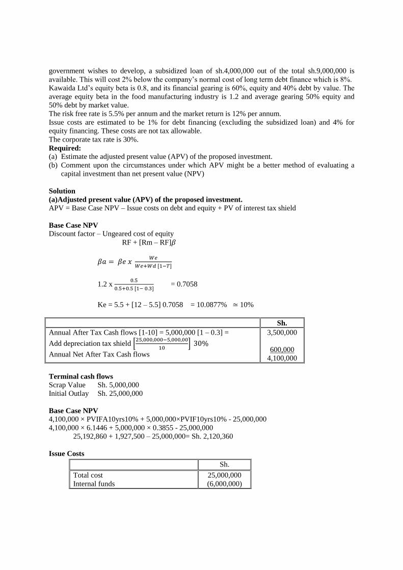
government wishes to develop, a subsidized loan of sh.4,000,000 out of the total sh.9,000,000 is
available. This will cost 2% below the company’s normal cost of long term debt finance which is 8%.
Kawaida Ltd’s equity beta is 0.8, and its financial gearing is 60%, equity and 40% debt by value. The
average equity beta in the food manufacturing industry is 1.2 and average gearing 50% equity and
50% debt by market value.
The risk free rate is 5.5% per annum and the market return is 12% per annum.
Issue costs are estimated to be 1% for debt financing (excluding the subsidized loan) and 4% for
equity financing. These costs are not tax allowable.
The corporate tax rate is 30%.
Required:
(a) Estimate the adjusted present value (APV) of the proposed investment.
(b) Comment upon the circumstances under which APV might be a better method of evaluating a
capital investment than net present value (NPV)
Solution
(a)Adjusted present value (APV) of the proposed investment.
APV = Base Case NPV – Issue costs on debt and equity + PV of interest tax shield
Base Case NPV
Discount factor – Ungeared cost of equity
RF + [Rm – RF]𝛽
𝛽𝑎 = 𝛽𝑒 𝑥 𝑊𝑒
𝑊𝑒+𝑊𝑑 [1−𝑇]
1.2 x 0.5
0.5+0.5 [1− 0.3] = 0.7058
Ke = 5.5 + [12 – 5.5] 0.7058 = 10.0877% ≃ 10%
Sh.
Annual After Tax Cash flows [1-10] = 5,000,000 [1 – 0.3] =
Add depreciation tax shield [25,000,000−5,000,00
10] 30%
Annual Net After Tax Cash flows
3,500,000
600,000
4,100,000
Terminal cash flows
Scrap Value Sh. 5,000,000
Initial Outlay Sh. 25,000,000
Base Case NPV
4,100,000 × PVIFA10yrs10% + 5,000,000×PVIF10yrs10% - 25,000,000
4,100,000 × 6.1446 + 5,000,000 × 0.3855 - 25,000,000
25,192,860 + 1,927,500 – 25,000,000= Sh. 2,120,360
Issue Costs
Sh.
Total cost
Internal funds
25,000,000
(6,000,000)
Page 181
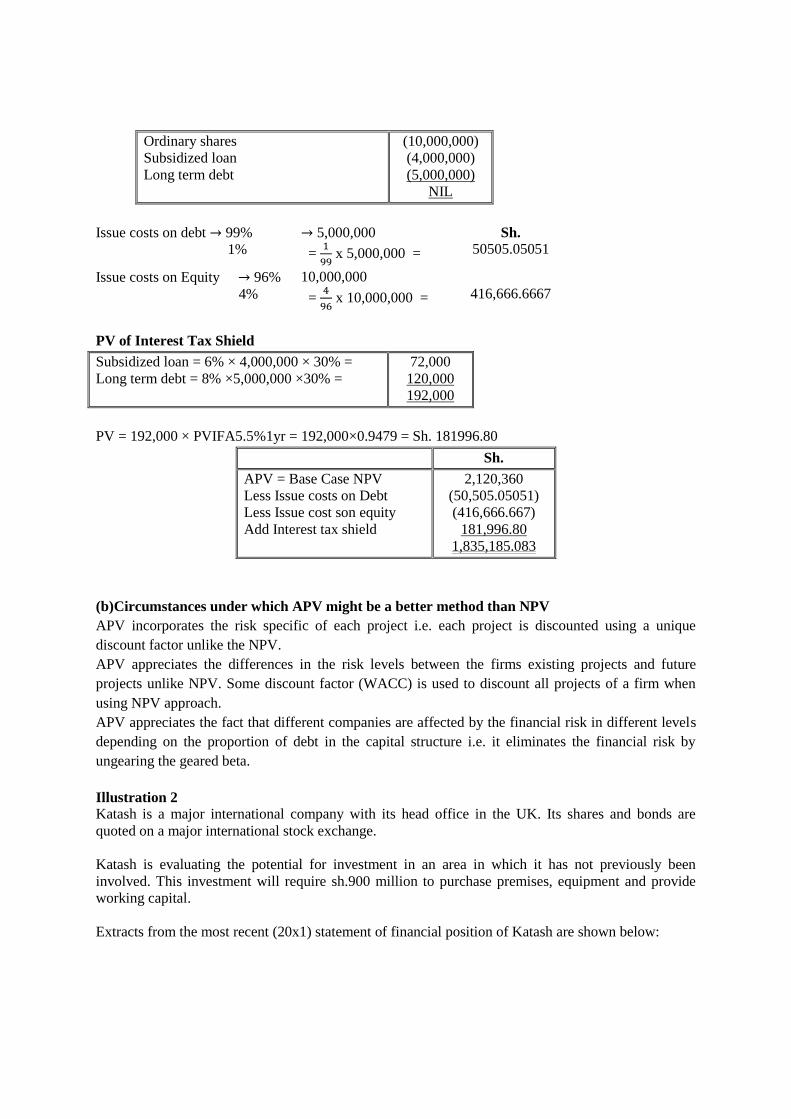
Ordinary shares
Subsidized loan
Long term debt
(10,000,000)
(4,000,000)
(5,000,000)
NIL
Issue costs on debt → 99%
1%
→ 5,000,000
= 1
99 x 5,000,000 =
Sh.
50505.05051
Issue costs on Equity → 96%
4%
10,000,000
= 4
96 x 10,000,000 =
416,666.6667
PV of Interest Tax Shield
Subsidized loan = 6% × 4,000,000 × 30% =
Long term debt = 8% ×5,000,000 ×30% =
72,000
120,000
192,000
PV = 192,000 × PVIFA5.5%1yr = 192,000×0.9479 = Sh. 181996.80
Sh.
APV = Base Case NPV
Less Issue costs on Debt
Less Issue cost son equity
Add Interest tax shield
2,120,360
(50,505.05051)
(416,666.667)
181,996.80
1,835,185.083
(b)Circumstances under which APV might be a better method than NPV
APV incorporates the risk specific of each project i.e. each project is discounted using a unique
discount factor unlike the NPV.
APV appreciates the differences in the risk levels between the firms existing projects and future
projects unlike NPV. Some discount factor (WACC) is used to discount all projects of a firm when
using NPV approach.
APV appreciates the fact that different companies are affected by the financial risk in different levels
depending on the proportion of debt in the capital structure i.e. it eliminates the financial risk by
ungearing the geared beta.
Illustration 2
Katash is a major international company with its head office in the UK. Its shares and bonds are
quoted on a major international stock exchange.
Katash is evaluating the potential for investment in an area in which it has not previously been
involved. This investment will require sh.900 million to purchase premises, equipment and provide
working capital.
Extracts from the most recent (20x1) statement of financial position of Katash are shown below:
Page 182
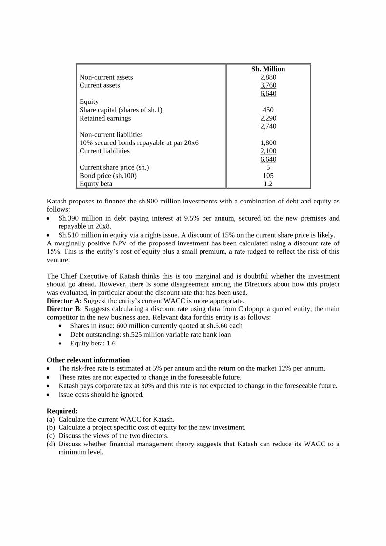
Non-current assets
Current assets
Equity
Share capital (shares of sh.1)
Retained earnings
Non-current liabilities
10% secured bonds repayable at par 20x6
Current liabilities
Current share price (sh.)
Bond price (sh.100)
Equity beta
Sh. Million
2,880
3,760
6,640
450
2,290
2,740
1,800
2,100
6,640
5
105
1.2
Katash proposes to finance the sh.900 million investments with a combination of debt and equity as
follows:
Sh.390 million in debt paying interest at 9.5% per annum, secured on the new premises and
repayable in 20x8.
Sh.510 million in equity via a rights issue. A discount of 15% on the current share price is likely.
A marginally positive NPV of the proposed investment has been calculated using a discount rate of
15%. This is the entity’s cost of equity plus a small premium, a rate judged to reflect the risk of this
venture.
The Chief Executive of Katash thinks this is too marginal and is doubtful whether the investment
should go ahead. However, there is some disagreement among the Directors about how this project
was evaluated, in particular about the discount rate that has been used.
Director A: Suggest the entity’s current WACC is more appropriate.
Director B: Suggests calculating a discount rate using data from Chlopop, a quoted entity, the main
competitor in the new business area. Relevant data for this entity is as follows:
Shares in issue: 600 million currently quoted at sh.5.60 each
Debt outstanding: sh.525 million variable rate bank loan
Equity beta: 1.6
Other relevant information
The risk-free rate is estimated at 5% per annum and the return on the market 12% per annum.
These rates are not expected to change in the foreseeable future.
Katash pays corporate tax at 30% and this rate is not expected to change in the foreseeable future.
Issue costs should be ignored.
Required:
(a) Calculate the current WACC for Katash.
(b) Calculate a project specific cost of equity for the new investment.
(c) Discuss the views of the two directors.
(d) Discuss whether financial management theory suggests that Katash can reduce its WACC to a
minimum level.
Page 183
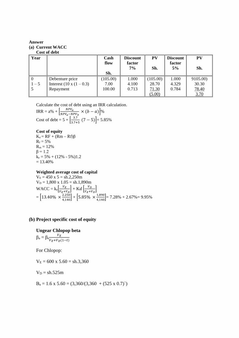
Answer
(a) Current WACC
Cost of debt
Year Cash
flow
Sh.
Discount
factor
7%
PV
Sh.
Discount
factor
5%
PV
Sh.
0
1 – 5
5
Debenture price
Interest (10 x (1 – 0.3)
Repayment
(105.00)
7.00
100.00
1.000
4.100
0.713
(105.00)
28.70
71.30
(5.00)
1.000
4.329
0.784
9105.00)
30.30
78.40
3.70
Calculate the cost of debt using an IRR calculation.
IRR = a% + [𝑁𝑃𝑉𝑎
𝑁𝑃𝑉𝑎−𝑁𝑃𝑉𝑏 × (𝑏 − 𝑎)]%
Cost of debt = 5 + [3.7
3.7+5 (7 − 5)]= 5.85%
Cost of equity
Ke = RF + (Rm – Rf)β
Rf = 5%
Rm = 12%
β = 1.2
ke = 5% + (12% - 5%)1.2
= 13.40%
Weighted average cost of capital
VE = 450 x 5 = sh.2,250m
VD = 1,800 x 1.05 = sh.1,890m
WACC = ke[𝑉𝐸
𝑉𝐸+𝑉𝐷] + K𝑑 [
𝑉𝐷
𝑉𝐸+𝑉𝐷]
= [13.40% ×2.250
4,140] + [5.85% ×
1,890
4,140]= 7.28% + 2.67%= 9.95%
(b) Project specific cost of equity
Ungear Chlopop beta
βa = βe𝑉𝐸
𝑉𝐸+𝑉𝐷(1−𝑡)
For Chlopop:
VE = 600 x 5.60 = sh.3,360
VD = sh.525m
Βa = 1.6 x 5.60 = (3,360/(3,360 + (525 x 0.7)`)
Page 184

= 1.44
Re-gearing
VE = sh.510m
VD = sh.390m
βe = βa𝑉𝐸+𝑉𝐷(1−𝑡
𝑉𝐸
βe =1.44 x 510+(390 ×0.7)
510 = 2.211
Cost of equity
ke = Rf + (Rm – Rf)β
= 5% + (12% - 5%) 2.211 = 20.48%
Page 185

CHAPTER FOUR
MERGERS AND ACQUISITIONS
CHAPTER KEY OBJECTIVES
To be able to understand the following; 1. Nature of mergers and acquisitions
2. Reasons of mergers and acquisitions
3. Acquisition and Mergers verses organic growth
4. Valuation of acquisitions and mergers
5. Prediction of a takeover target
6. Defence tactics against hostile takeovers
7. Financing of mergers and acquisitions
8. Analysis of combined operating profit (EBIT) and post-acquisition earning per share at the point
of indifference in firms earnings under various financing options.
9. Determination of range of combined operating profit.
10. Regulatory frame work for mergers and acquisitions
11. Reasons why there are failed mergers and acquisitions
12. Mergers and acquisitions in a global context
NATURE OF MERGERS AND ACQUISITIONS
A merger refers to a combination of two or more firms, which are almost equally strong. Upon
merging, the initial firms will lose their original identity and a completely new firm is formed.
Mergers are usually based on the core competencies of firms. For example, two companies with
similar core competencies in marketing may merge to strengthen their overall competitive position.
Alternatively, two firms may merge to combine complementary core competencies. For example, a
firm possesses a competency in its marketing may merge with a firm that has good brand name. The
overall reason for a merger is to take advantage of benefits of synergy.
Acquisition or takeover on the other hand arises when the firm being taken loses its identity where as
the acquiring firm maintains its identity. The acquiring firm is known as the Predator while the firm
being acquired is known as Target.
Types of Mergers
There are three merges, which include:
Vertical Merger
This arises when two firms combine, which are complimentary to each other i.e. two components
which depend on one another combine to form one.
The main objective of this merger is to control the market and to ensure there is constant supply of
raw materials due to elimination of any problems associated with negotiation and coordination with
supplies i.e. A car processing company merging with another company that manufactures spare parts.
Four principal advantages are associated with vertical related acquisitions:
Vertical chain economies may result from eliminating production steps, reducing overhead
costs, and coordinating distribution activities to attain greater synergy.
Page 186
Vertical chain innovations refer to improvements or innovations that may be transferred or
share among the corporation's business units in the distribution channel.
A final advantage is a combination of vertical chain economies and chain innovations.
Horizontal Merger
It involves a merger between two companies that are in the same industry and at the same production
level e.g. a merger between two companies providing accounting services, insurance services (ICEA
Lion Group)
The objective of this merger is to eliminate competition, increase the market share and achieve
economies of scale.
The airline industry provides good examples of horizontal mergers. In December 2013 American
Airways and US Airways merged to create the world's biggest airline, American Airlines. The deal
brought American Airways out of the state of bankruptcy that it had been in since 2011. Since 2005
mergers have reduced the numbers of the US's major airlines from nine to four.
Such mergers made it easier for the individual airlines to gain access to routes that would otherwise
have been expensive and difficult to obtain.
There are several reasons for engaging in horizontal integration. Some of these are:
One of the primary reasons is to increase market share. Along with increasing revenues,
larger market share provides the company with greater leverage to deal with its suppliers and
customers. Greater market share should also lower the firm's costs through scale economies.
Increased size enables the firm to promote its products and services more efficiently to larger
audience and may permit greater access to channels of distribution.
Finally, horizontal integration can result in increased operational flexibility.
Conglomerate Merger It is a merger between two firms that are independent of one another and they are in separate business
lines.
The aim of this merger is risk diversification and maximisation of the overall returns
The objectives of takeovers or mergers
Takeovers or mergers should increase shareholders wealth via:
(1) Acquiring the target company that is undervalued
(2) Synergistic benefits:
(a) Economic efficiency gains
i. economies of scale (volume related savings)
ii. economies of scope (complementary resources)
(b) Financial synergy
i. reduced total risk will not benefit well-diversified shareholders (the systematic
risk is not reduced by diversification) but reducing total risk may reduce
insolvency risks and hence borrowing costs
ii. increased asset backing may bolster borrowing capacity
iii. exploiting tax losses sooner
Page 187
(c) Market power
i. acquiring monopolistic powers (e.g. eliminate competition)
ii. acquisition of a scarce resource
iii. dynamic management
iv. innovative product
v. cash mountain
vi. to enter a new market quickly 3. Predator issues on takeover
(1) The investment decision
a) How much is the target worth to the predator?
b) Are the target shareholders willing to sell?
c) What economic / industry and company assumptions underlie the valuation?
BENEFITS OF MERGERS AND ACQUISITIONS
(i) Risk diversification
A company is able to diversify its risk especially through conglomerate mergers. This specifically
arises when the returns of the two firms are perfectly negatively correlated.
(ii) Tax Savings
A company that generates supernormal profits and operates in a high tax regime can acquire another
company that is loss making which would lead to a reduction of profits hence reducing the tax
liability.
(iii) Management efficiency
This is where the predator acquires the target to take over its efficient management team. It is mostly
practical in a horizontal merger.
(iv)Synergy savings
These are additional benefits associated with economies of scale after mergers and acquisitions. The
combined company eliminates some costs, which are duplicative in nature.
There are three types of synergy i.e.
a) Operational synergy
It results from the savings that come in when the company mergers the operations of the two firms i.e.
a reduction in operating expenses.
b) Management synergy
This arises when the company gains some efficiency through combination of the management teams.
c) Financial Synergy
It results in less volatile cash flows, which are less risky. This is because after merging the asset base
of the combined company increases, which minimises the default, risk and reduces the cost of capital.
(v) It helps in maintaining the market control
A company may opt to merge with other to protect itself from the possibility of a hostile takeover.
Merging may also lead to controlling of the market and eliminating any sort of competition.
(vi) Asset Backing
Page 188
The predator acquires a target together with its assets, which leads to a wider asset base of the
combined company.
This makes it cheaper for the company to operate in the end
(viii) Asset break up value
An undervalues firm (target) can be brought and its assets broken into pieces to realise capital gains.
Advantages of mergers as an expansion strategy
As an expansion, strategy mergers are thought to provide a quicker way of acquiring productive
capacity and intangible assets and accessing overseas markets.
There are four main advantages that have been put forward in the literature and these are summarised
below.
(i) Speed
The acquisition of another company is a quicker way of implementing a business plan, as the
company acquires another organisation that is already in operation. An acquisition also allows a
company to reach a certain optimal level of production much quicker than through organic growth.
Acquisition as a strategy for expansion is particularly suitable for management with rather short time
horizons.
(ii) Lower cost
An acquisition may be a cheaper way of acquiring productive capacity than through organic growth.
An acquisition can take place for instance through an exchange of shares which does not have an
immediate impact on the financial resources of the firm.
(iii) Acquisition of intangible assets
A firm through an acquisition will acquire not only tangible assets but also intangible assets, such as
brand recognition, reputation, customer loyalty and intellectual property, which are more difficult to
achieve with organic growth.
(iv) Access to overseas markets
When a company wants to expand its operations in an overseas market, acquiring a local firm may be
the only option of breaking into the overseas market.
MERGERS AND ACQUISITIONS AS A METHOD OF CORPORATE EXPANSION
Although growth strategy through acquisition requires high premiums, it is widely used by
corporations as an alternative to internal organic growth.
Companies may decide to increase the scale of their operations through a strategy of internal organic
growth by investing money to purchase or create assets and product lines internally.
Alternatively, companies may decide to grow by buying other companies in the market thus acquiring
ready-made tangible and intangible assets and product lines. Which is the right strategy? The decision
is one of the most difficult the financial manager has to face.
The right answer is not easy to arrive at. Organic growth in areas where the company has been
successful and has expertise may present few risks but it can be slow, expensive or sometimes
impossible. On the other hand, acquisitions require high premiums that make the creation of value
Page 189
difficult. Irrespective of the merits of a growth strategy by acquisition or not, the fact remains that this
is used by corporations extensively.
Disadvantages of mergers as an expansion strategy
An expansion strategy through acquisition is associated with exposure to a higher
level of business and financial risk.
The risks associated with expansion through acquisitions are:
(i) Exposure to business risk
Acquisitions normally represent large investments by the bidding company and account for a large
proportion of its financial resources. If the acquired company does not perform as well as it was
envisaged, then the effect on the acquiring firm may be catastrophic.
(ii) Exposure to financial risk
During the acquisition process, the acquiring firm may have less than complete information on the
target company, and there may exist aspects that have been kept hidden from outsiders.
(iii) Acquisition premium
When a company acquires another company, it normally pays a premium over its present market
value. This premium is normally justified by the management of the bidding company as necessary
for the benefits that will accrue from the acquisition. However, too large a premium may render the
acquisition unprofitable.
(iv) Managerial competence
When a firm is acquired, which is large relative to the acquiring firm, the management of the
acquiring firm may not have the experience or ability to deal with operations on the new larger scale,
even if the acquired company retains its own management.
(v) Integration problems
Most acquisitions are beset with problems of integration, as each company has its own culture, history
and ways of operation.
(vi) Market power
The impact on market power is one of the most important aspects of an acquisition. By acquiring
another firm, in a horizontal merger, the competition in the industry is reduced and the company may
be able to charge higher prices for its products. However, competition regulation may prevent this
type of acquisition.
Developing an acquisition strategy
The main reason behind strategy for acquiring a target firm includes the target being undervalued or
to diversify operations in order to reduce risk.
Not all firms considering the acquisition of a target firm have acquisition strategies and, even if they
do, they do not always stick to them. We are going to look at a number of different motives for an
acquisition in this section. A coherent acquisition strategy should be based on one of these motives.
Page 190
(i) Acquire undervalued firms
This is one of the main reasons for firms becoming targets for acquisition. If a predator recognises
that a firm has been undervalued by the market it can take advantage of this discrepancy by
purchasing the firm at a 'bargain' price. The difference between the real value of the target firm and
the price paid can then be seen as a 'surplus' which is also known as goodwill.
For this strategy to work, the predator firm must be able to fulfil three things.
a. Find firms that are undervalued
This might seem to be an obvious point but in practice it is not easy to have such superior knowledge
ahead of other predators. The predator would either have to have access to better information than
that available to other market players, or have superior analytical tools to those used by competitors.
b. Access to necessary funds
It is one thing being able to identify firms that are undervalued – it is quite another obtaining the
funds to acquire them. Traditionally, larger firms tend to have better access to capital markets and
internal funds than smaller firms. A history of success in identifying and acquiring undervalued firms
will also make funds more accessible and future acquisitions easier.
c. Skills in executing the acquisition
There are no gains to be made from driving the share price up in the process of acquiring an
undervalued firm. For example, suppose the estimated value of a target firm is sh.500 million and the
current market price is sh.400 million. In acquiring this firm, the predator will have to pay a premium.
If this premium exceeds 25% of the current market price (the difference between estimated value and
current market price divided by current market price) then the price paid will actually exceed the
estimated value. No value would thus be created by the predator.
(ii) Diversify to reduce risk
Firm-specific risk (unsystematic risk) can be reduced by holding a diversified portfolio. This is
another potential acquisition strategy. Predator firms' managers believe that they may reduce earnings
volatility and risk – and increase potential value – by acquiring firms in other industries.
Evaluating the corporate and competitive
Nature of a given acquisition proposal
We have discussed so far the reasons why a company may opt for growth by acquisition instead of
organic growth and the three main types of mergers. We should not of course lose sight of the fact
that expansion either by organic growth or by acquisitions is only undertaken if it leads to an increase
in the wealth of the shareholders. This happens when the merger or acquisition creates synergies
which either increase revenues or reduce costs, or when the management of the acquiring company
can manage the assets of the target company better than the incumbent management, thus creating
additional value for the new owners over and above the current market value of the company. We
Page 191
look at some of the aspects that will have an impact on the competitive position of the firm and its
profitability in a given acquisition proposal.
VALUATION OF ACQUISITIONS AND MERGERS In a merger or acquisition transaction, valuation is essentially the price that one party will pay for the
other, or the value that one side will give up to make the transaction work. Valuations can be made via
appraisals or the price of the firm’s stock if it is a public company, but at the end of the day, valuation
is often a negotiated number.
Valuation is often a combination of cash flow and the time value of money. A business’s worth is in
part a function of the profits and cash flow it can generate. As with many financial transactions, the
time value of money is also a factor. How much is the buyer willing to pay and at what rate of interest
should they discount the other firm’s future cash flows?
Both sides in an M&A deal will have different ideas about the worth of a target company: its seller
will tend to value the company at as high of a price as possible, while the buyer will try to get the
lowest price that he can.
There are, however, many legitimate ways to value companies. The most common method is to look
at comparable companies in an industry, but dealmakers employ a variety of other methods and tools
when assessing a target company. Here are just a few of them:
1. Discounted Cash Flow (DCF) - A key valuation tool in M&A, discounted cash flow analysis
determines a company's current value according to its estimated future cash flows. Forecasted free
cash flows (net income + depreciation/amortization - capital expenditures - change in working capital)
are discounted to a present value using the company's weighted average costs of capital (WACC).
Admittedly, DCF is tricky to get right, but few tools can rival this valuation method.
Illustration
A company has prepared a forecast of the future cash flows. The cash flows are expected to be
sh.4.5M in the first year, sh.8.1M in the second year, sh.11.7M in the third year, and thereafter to
increase at the rate of 4% per year.
The company has debt with a market value of sh.50M, and the relevant cost of capital is 10%.
Calculate the value of the firm and the value of the equity.
Solution
Free cash flow
Discounting factor @10%
Present value
1
4.5
0.909
4.091
2
8.1
0.826
6.691
3
11.7
0.751
s8.787
4 - ∞
202.8
0.751
152.303
Total
171.872m
Page 192
Value of the firm = Total P.V. = Sh.171.872M
Value of the equity = 171.872 - 50 = Sh.121.872M
Calculation of 4 - ∞ :
Using the dividend valuation formula (which can be used for any inflating perpetuity) PV at time 3
= 11.7 × 1.04 / (0.10 - 0.04)= 202.8
Illustration
Double Limited is contemplating acquiring Tatu Limited. The following information relates to Tatu
Limited for the next five years.
Year 1
Sh. “m”
Year 2
Sh. “m”
Year 3
Sh. “m”
Year 4
Sh. “m”
Year 5
Sh. “m”
Net sales
Cost of sales
Selling and adm. expenses
Interest expenses
10,050
735
100
40
1,260
882
120
50
1,510
1,057
130
70
1,740
1,218
150
90
1,910
1,337
160
110
Additional information;-
1. After the fifth year, the cash flows available to Double Limited from Tatu Limited are expected to
grow by 10% per annum in perpetuity.
2. Tatu Limited will retain Sh.40, 000,000 for internal expansion every year.
3. The cost of capital can be assumed to be 18%.
4. The applicable corporate tax rate is 30%.
Required:
i) The estimated annual cash flows of Tatu Limited.
ii) The-maximum amount that Double Limited would be willing to pay to acquire Tatu Limited.
Solution
(i)The estimated annual cash flows of Tatu Limited.
Year 1
Sh. “m”
2
Sh. “m”
3
Sh. “m”
4
Sh. “m”
5
Sh. “m”
PBT
Less Tax @ 30%
PAT
Less R/E
Dividends
9175
(2,752.5)
6,422.5
(40)
6,382.5
208
(62.4)
145.6
(40)
105.6
253
(75.9)
177.1
(40)
137.1
282
(84.6)
197.4
(40)
157.4
303
(90.9)
212.1
(40)
172.1
Cash flow 4 = 𝐶𝑎𝑠ℎ𝑓𝑙𝑜𝑤 3(1+𝑔)
𝑘𝑒−𝑔
Page 193
After year = 𝐷6
𝐾𝑒−𝑔 =
𝐷5 (1+𝑔)
𝐾𝑒−𝑔 =
172.1 (1.1)
0.18−0.1 =
189.31
0.08 = Sh. 2366.375 “m”
Year Sh. “m”
Expected Cash flow
18%
Discount factor
PV
1
2
3
4
5
5
6,382.5
105.6
137.1
157.4
172.1
2,366.375
0.8475
0.7182
0.6086
0.5158
0.4371
2.4371
5409.17
75.84
83.44
81.19
75.22
1034.34
1,471.12997
Maximum amount that Double Ltd is willing to pay
Maximum amount to be paid by Double Ltd = Intrinsic value of Tatu Ltd
Illustration- Calculation of free cash flows
EBIT
Less: Taxation
Add: Depreciation
Operating cash flow
Less: Amounts needed to replace non-current assets
(unless told otherwise, assume equal to the level of depreciation)
Less: Any additional non-current asset expenditure
Less: Incremental working capital expenditure
Free cash flow
X
(X)
X
X
(X)
(X)
(X)
X
Illustration
Calculate the free cash flow given the following information:
Operating profit (EBIT)
Depreciation
Increase in working capital
Cost of new non-current assets
Interest paid
Loans repaid
Tax paid
Sh.
720
288
120
36
12
48
336
Solution
EBIT
Depreciation
Taxation
Operating cash flow
Sh.
720
288
(336)
672
Page 194
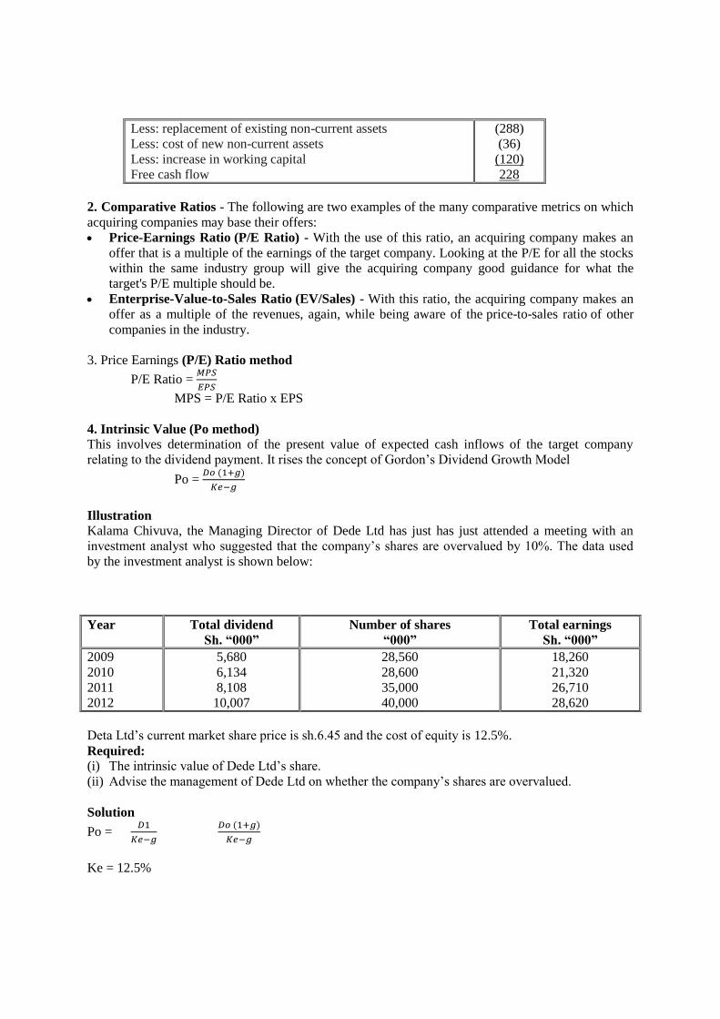
Less: replacement of existing non-current assets
Less: cost of new non-current assets
Less: increase in working capital
Free cash flow
(288)
(36)
(120)
228
2. Comparative Ratios - The following are two examples of the many comparative metrics on which
acquiring companies may base their offers:
Price-Earnings Ratio (P/E Ratio) - With the use of this ratio, an acquiring company makes an
offer that is a multiple of the earnings of the target company. Looking at the P/E for all the stocks
within the same industry group will give the acquiring company good guidance for what the
target's P/E multiple should be.
Enterprise-Value-to-Sales Ratio (EV/Sales) - With this ratio, the acquiring company makes an
offer as a multiple of the revenues, again, while being aware of the price-to-sales ratio of other
companies in the industry.
3. Price Earnings (P/E) Ratio method
P/E Ratio = 𝑀𝑃𝑆
𝐸𝑃𝑆
MPS = P/E Ratio x EPS
4. Intrinsic Value (Po method)
This involves determination of the present value of expected cash inflows of the target company
relating to the dividend payment. It rises the concept of Gordon’s Dividend Growth Model
Po = 𝐷𝑜 (1+𝑔)
𝐾𝑒−𝑔
Illustration
Kalama Chivuva, the Managing Director of Dede Ltd has just has just attended a meeting with an
investment analyst who suggested that the company’s shares are overvalued by 10%. The data used
by the investment analyst is shown below:
Year Total dividend
Sh. “000”
Number of shares
“000”
Total earnings
Sh. “000”
2009
2010
2011
2012
5,680
6,134
8,108
10,007
28,560
28,600
35,000
40,000
18,260
21,320
26,710
28,620
Deta Ltd’s current market share price is sh.6.45 and the cost of equity is 12.5%.
Required:
(i) The intrinsic value of Dede Ltd’s share.
(ii) Advise the management of Dede Ltd on whether the company’s shares are overvalued.
Solution
Po = 𝐷1
𝐾𝑒−𝑔
𝐷𝑜 (1+𝑔)
𝐾𝑒−𝑔
Ke = 12.5%
Page 195
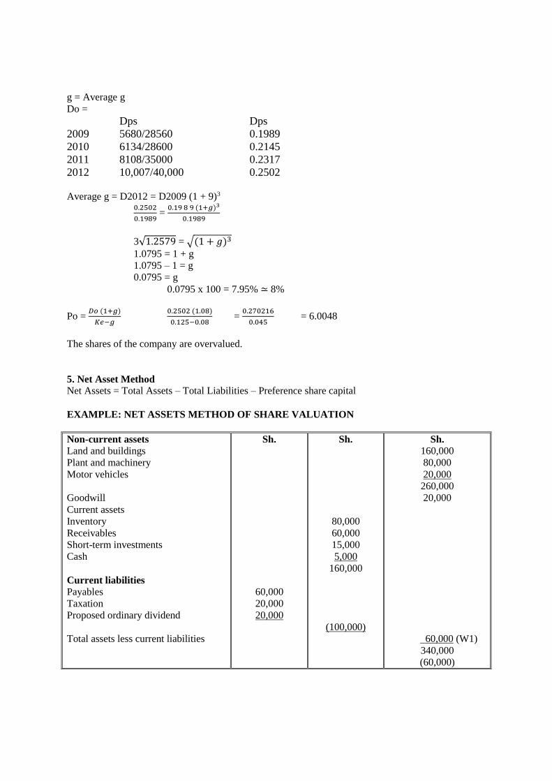
g = Average g
Do =
Dps Dps
2009
2010
2011
2012
5680/28560
6134/28600
8108/35000
10,007/40,000
0.1989
0.2145
0.2317
0.2502
Average g = D2012 = D2009 (1 + 9)3
0.2502
0.1989 =
0.19 8 9 (1+𝑔)3
0.1989
3√1.2579 = √(1 + 𝑔)3
1.0795 = 1 + g
1.0795 – 1 = g
0.0795 = g
0.0795 x 100 = 7.95% ≃ 8%
Po = 𝐷𝑜 (1+𝑔)
𝐾𝑒−𝑔
0.2502 (1.08)
0.125−0.08 =
0.270216
0.045 = 6.0048
The shares of the company are overvalued.
5. Net Asset Method
Net Assets = Total Assets – Total Liabilities – Preference share capital
EXAMPLE: NET ASSETS METHOD OF SHARE VALUATION
Non-current assets
Land and buildings
Plant and machinery
Motor vehicles
Goodwill
Current assets
Inventory
Receivables
Short-term investments
Cash
Current liabilities
Payables
Taxation
Proposed ordinary dividend
Total assets less current liabilities
Sh.
60,000
20,000
20,000
Sh.
80,000
60,000
15,000
5,000
160,000
(100,000)
Sh.
160,000
80,000
20,000
260,000
20,000
60,000 (W1)
340,000
(60,000)
Page 196
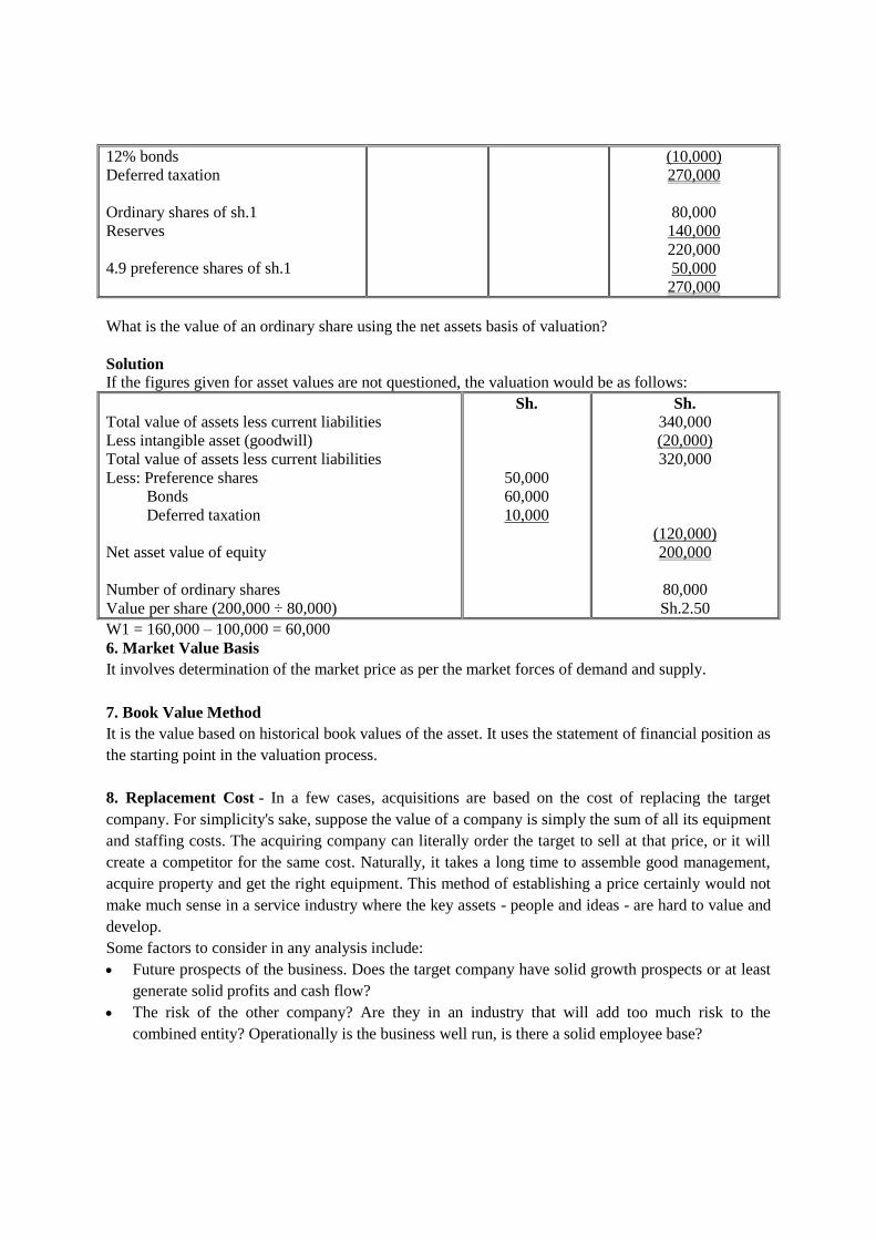
12% bonds
Deferred taxation
Ordinary shares of sh.1
Reserves
4.9 preference shares of sh.1
(10,000)
270,000
80,000
140,000
220,000
50,000
270,000
What is the value of an ordinary share using the net assets basis of valuation?
Solution
If the figures given for asset values are not questioned, the valuation would be as follows:
Total value of assets less current liabilities
Less intangible asset (goodwill)
Total value of assets less current liabilities
Less: Preference shares
Bonds
Deferred taxation
Net asset value of equity
Number of ordinary shares
Value per share (200,000 ÷ 80,000)
Sh.
50,000
60,000
10,000
Sh.
340,000
(20,000)
320,000
(120,000)
200,000
80,000
Sh.2.50
W1 = 160,000 – 100,000 = 60,000
6. Market Value Basis
It involves determination of the market price as per the market forces of demand and supply.
7. Book Value Method
It is the value based on historical book values of the asset. It uses the statement of financial position as
the starting point in the valuation process.
8. Replacement Cost - In a few cases, acquisitions are based on the cost of replacing the target
company. For simplicity's sake, suppose the value of a company is simply the sum of all its equipment
and staffing costs. The acquiring company can literally order the target to sell at that price, or it will
create a competitor for the same cost. Naturally, it takes a long time to assemble good management,
acquire property and get the right equipment. This method of establishing a price certainly would not
make much sense in a service industry where the key assets - people and ideas - are hard to value and
develop.
Some factors to consider in any analysis include:
Future prospects of the business. Does the target company have solid growth prospects or at least
generate solid profits and cash flow?
The risk of the other company? Are they in an industry that will add too much risk to the
combined entity? Operationally is the business well run, is there a solid employee base?
Page 197
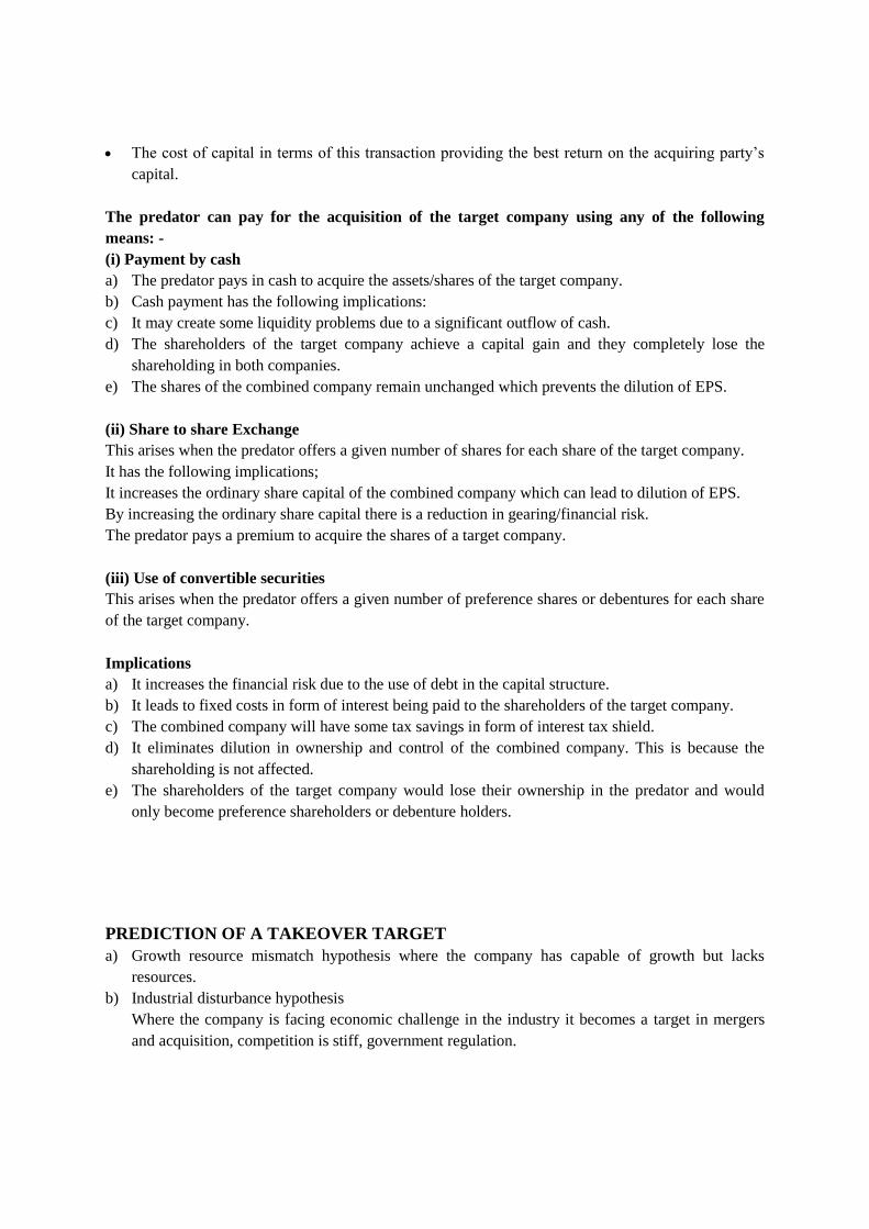
The cost of capital in terms of this transaction providing the best return on the acquiring party’s
capital.
The predator can pay for the acquisition of the target company using any of the following
means: -
(i) Payment by cash
a) The predator pays in cash to acquire the assets/shares of the target company.
b) Cash payment has the following implications:
c) It may create some liquidity problems due to a significant outflow of cash.
d) The shareholders of the target company achieve a capital gain and they completely lose the
shareholding in both companies.
e) The shares of the combined company remain unchanged which prevents the dilution of EPS.
(ii) Share to share Exchange
This arises when the predator offers a given number of shares for each share of the target company.
It has the following implications;
It increases the ordinary share capital of the combined company which can lead to dilution of EPS.
By increasing the ordinary share capital there is a reduction in gearing/financial risk.
The predator pays a premium to acquire the shares of a target company.
(iii) Use of convertible securities
This arises when the predator offers a given number of preference shares or debentures for each share
of the target company.
Implications
a) It increases the financial risk due to the use of debt in the capital structure.
b) It leads to fixed costs in form of interest being paid to the shareholders of the target company.
c) The combined company will have some tax savings in form of interest tax shield.
d) It eliminates dilution in ownership and control of the combined company. This is because the
shareholding is not affected.
e) The shareholders of the target company would lose their ownership in the predator and would
only become preference shareholders or debenture holders.
PREDICTION OF A TAKEOVER TARGET
a) Growth resource mismatch hypothesis where the company has capable of growth but lacks
resources.
b) Industrial disturbance hypothesis
Where the company is facing economic challenge in the industry it becomes a target in mergers
and acquisition, competition is stiff, government regulation.
Page 198
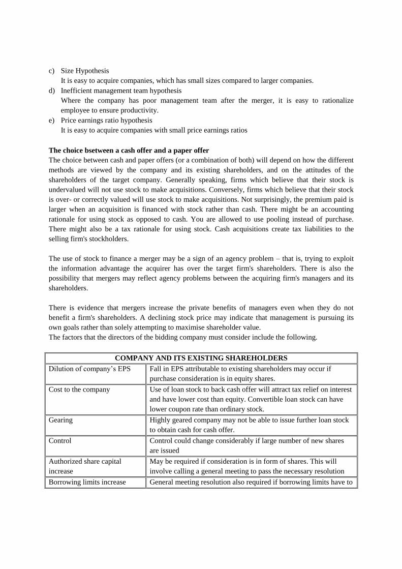
c) Size Hypothesis
It is easy to acquire companies, which has small sizes compared to larger companies.
d) Inefficient management team hypothesis
Where the company has poor management team after the merger, it is easy to rationalize
employee to ensure productivity.
e) Price earnings ratio hypothesis
It is easy to acquire companies with small price earnings ratios
The choice bsetween a cash offer and a paper offer
The choice between cash and paper offers (or a combination of both) will depend on how the different
methods are viewed by the company and its existing shareholders, and on the attitudes of the
shareholders of the target company. Generally speaking, firms which believe that their stock is
undervalued will not use stock to make acquisitions. Conversely, firms which believe that their stock
is over- or correctly valued will use stock to make acquisitions. Not surprisingly, the premium paid is
larger when an acquisition is financed with stock rather than cash. There might be an accounting
rationale for using stock as opposed to cash. You are allowed to use pooling instead of purchase.
There might also be a tax rationale for using stock. Cash acquisitions create tax liabilities to the
selling firm's stockholders.
The use of stock to finance a merger may be a sign of an agency problem – that is, trying to exploit
the information advantage the acquirer has over the target firm's shareholders. There is also the
possibility that mergers may reflect agency problems between the acquiring firm's managers and its
shareholders.
There is evidence that mergers increase the private benefits of managers even when they do not
benefit a firm's shareholders. A declining stock price may indicate that management is pursuing its
own goals rather than solely attempting to maximise shareholder value.
The factors that the directors of the bidding company must consider include the following.
COMPANY AND ITS EXISTING SHAREHOLDERS
Dilution of company’s EPS Fall in EPS attributable to existing shareholders may occur if
purchase consideration is in equity shares.
Cost to the company Use of loan stock to back cash offer will attract tax relief on interest
and have lower cost than equity. Convertible loan stock can have
lower coupon rate than ordinary stock.
Gearing Highly geared company may not be able to issue further loan stock
to obtain cash for cash offer.
Control Control could change considerably if large number of new shares
are issued
Authorized share capital
increase
May be required if consideration is in form of shares. This will
involve calling a general meeting to pass the necessary resolution
Borrowing limits increase General meeting resolution also required if borrowing limits have to
Page 199
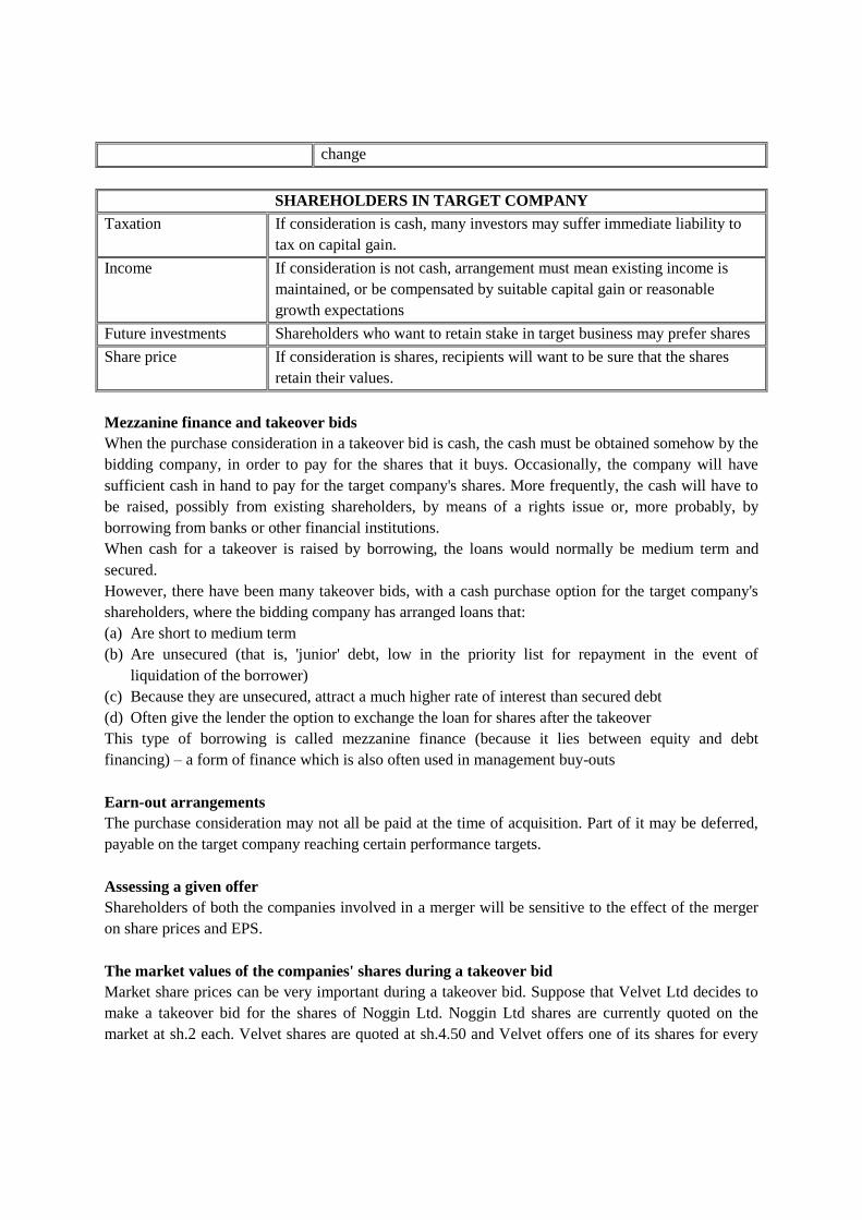
change
SHAREHOLDERS IN TARGET COMPANY
Taxation If consideration is cash, many investors may suffer immediate liability to
tax on capital gain.
Income If consideration is not cash, arrangement must mean existing income is
maintained, or be compensated by suitable capital gain or reasonable
growth expectations
Future investments Shareholders who want to retain stake in target business may prefer shares
Share price If consideration is shares, recipients will want to be sure that the shares
retain their values.
Mezzanine finance and takeover bids
When the purchase consideration in a takeover bid is cash, the cash must be obtained somehow by the
bidding company, in order to pay for the shares that it buys. Occasionally, the company will have
sufficient cash in hand to pay for the target company's shares. More frequently, the cash will have to
be raised, possibly from existing shareholders, by means of a rights issue or, more probably, by
borrowing from banks or other financial institutions.
When cash for a takeover is raised by borrowing, the loans would normally be medium term and
secured.
However, there have been many takeover bids, with a cash purchase option for the target company's
shareholders, where the bidding company has arranged loans that:
(a) Are short to medium term
(b) Are unsecured (that is, 'junior' debt, low in the priority list for repayment in the event of
liquidation of the borrower)
(c) Because they are unsecured, attract a much higher rate of interest than secured debt
(d) Often give the lender the option to exchange the loan for shares after the takeover
This type of borrowing is called mezzanine finance (because it lies between equity and debt
financing) – a form of finance which is also often used in management buy-outs
Earn-out arrangements
The purchase consideration may not all be paid at the time of acquisition. Part of it may be deferred,
payable on the target company reaching certain performance targets.
Assessing a given offer
Shareholders of both the companies involved in a merger will be sensitive to the effect of the merger
on share prices and EPS.
The market values of the companies' shares during a takeover bid
Market share prices can be very important during a takeover bid. Suppose that Velvet Ltd decides to
make a takeover bid for the shares of Noggin Ltd. Noggin Ltd shares are currently quoted on the
market at sh.2 each. Velvet shares are quoted at sh.4.50 and Velvet offers one of its shares for every
Page 200
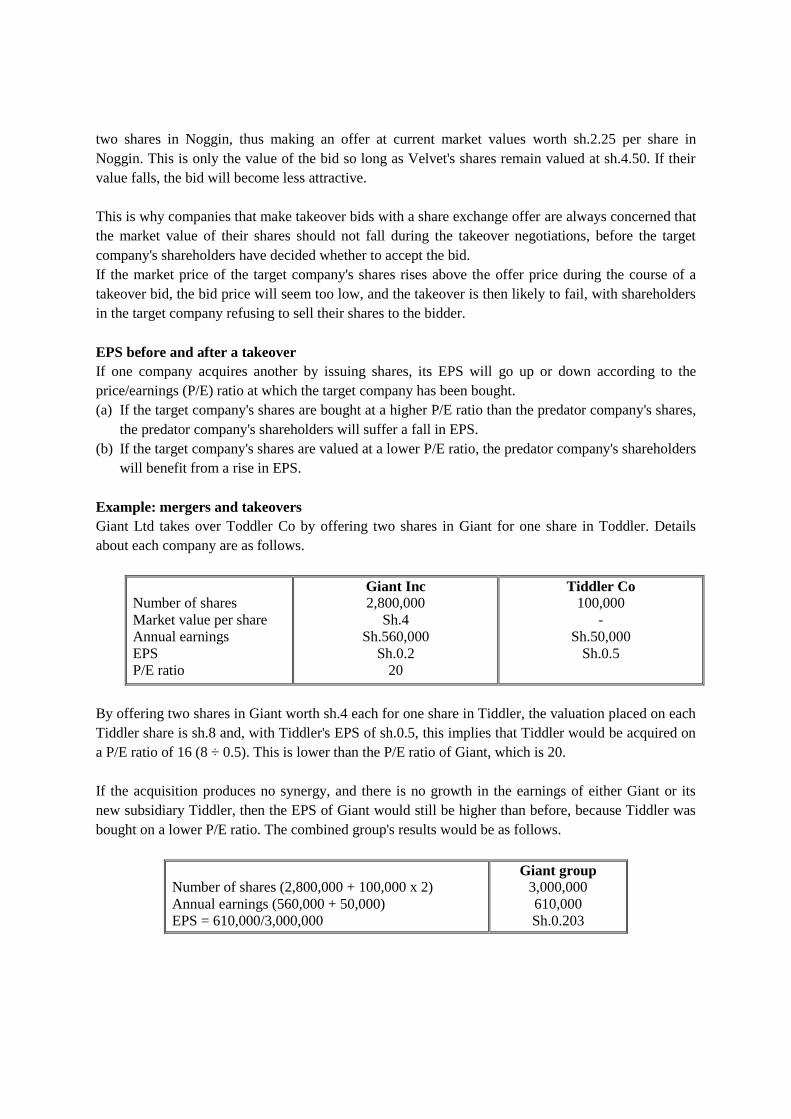
two shares in Noggin, thus making an offer at current market values worth sh.2.25 per share in
Noggin. This is only the value of the bid so long as Velvet's shares remain valued at sh.4.50. If their
value falls, the bid will become less attractive.
This is why companies that make takeover bids with a share exchange offer are always concerned that
the market value of their shares should not fall during the takeover negotiations, before the target
company's shareholders have decided whether to accept the bid.
If the market price of the target company's shares rises above the offer price during the course of a
takeover bid, the bid price will seem too low, and the takeover is then likely to fail, with shareholders
in the target company refusing to sell their shares to the bidder.
EPS before and after a takeover
If one company acquires another by issuing shares, its EPS will go up or down according to the
price/earnings (P/E) ratio at which the target company has been bought.
(a) If the target company's shares are bought at a higher P/E ratio than the predator company's shares,
the predator company's shareholders will suffer a fall in EPS.
(b) If the target company's shares are valued at a lower P/E ratio, the predator company's shareholders
will benefit from a rise in EPS.
Example: mergers and takeovers
Giant Ltd takes over Toddler Co by offering two shares in Giant for one share in Toddler. Details
about each company are as follows.
Number of shares
Market value per share
Annual earnings
EPS
P/E ratio
Giant Inc
2,800,000
Sh.4
Sh.560,000
Sh.0.2
20
Tiddler Co
100,000
-
Sh.50,000
Sh.0.5
By offering two shares in Giant worth sh.4 each for one share in Tiddler, the valuation placed on each
Tiddler share is sh.8 and, with Tiddler's EPS of sh.0.5, this implies that Tiddler would be acquired on
a P/E ratio of 16 (8 ÷ 0.5). This is lower than the P/E ratio of Giant, which is 20.
If the acquisition produces no synergy, and there is no growth in the earnings of either Giant or its
new subsidiary Tiddler, then the EPS of Giant would still be higher than before, because Tiddler was
bought on a lower P/E ratio. The combined group's results would be as follows.
Number of shares (2,800,000 + 100,000 x 2)
Annual earnings (560,000 + 50,000)
EPS = 610,000/3,000,000
Giant group
3,000,000
610,000
Sh.0.203
Page 201
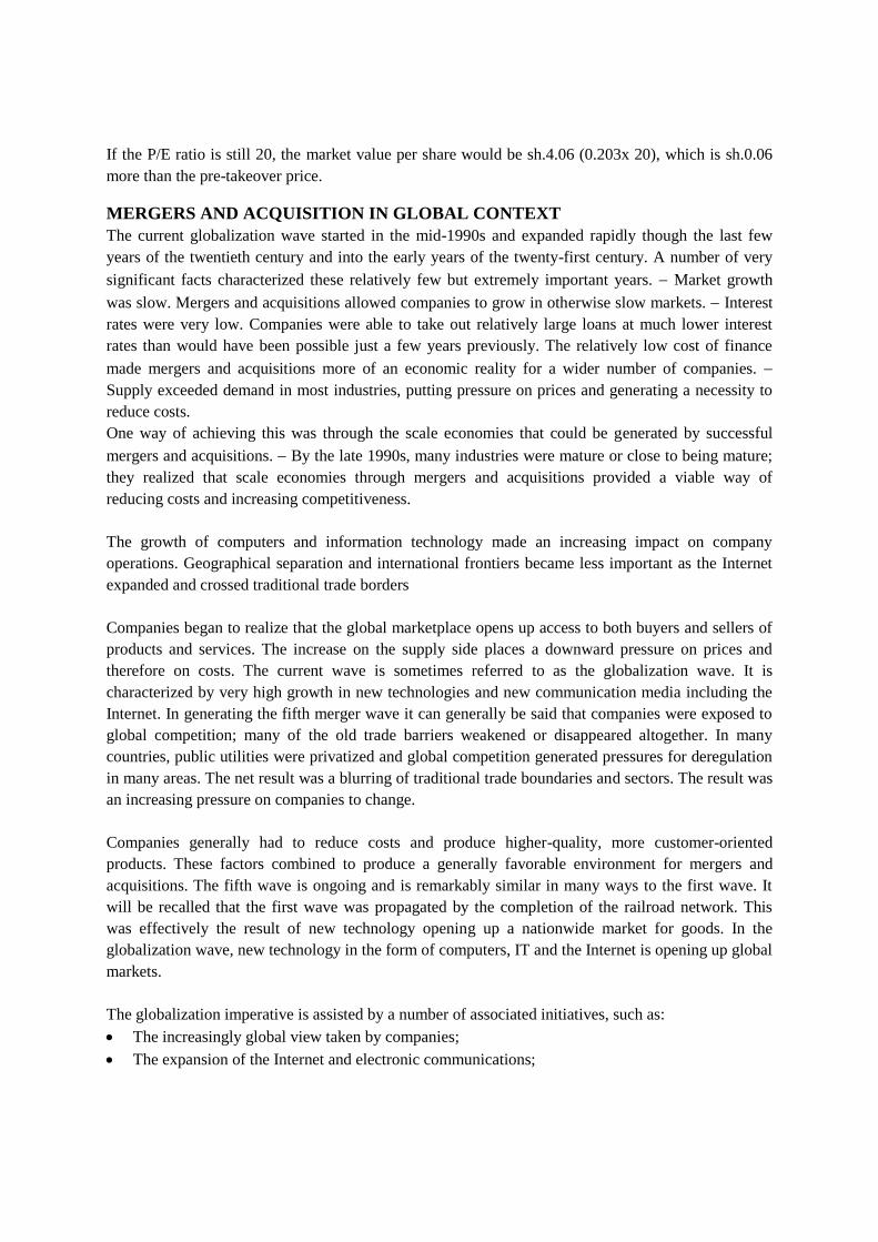
If the P/E ratio is still 20, the market value per share would be sh.4.06 (0.203x 20), which is sh.0.06
more than the pre-takeover price.
MERGERS AND ACQUISITION IN GLOBAL CONTEXT
The current globalization wave started in the mid-1990s and expanded rapidly though the last few
years of the twentieth century and into the early years of the twenty-first century. A number of very
significant facts characterized these relatively few but extremely important years. Market growth
was slow. Mergers and acquisitions allowed companies to grow in otherwise slow markets. Interest
rates were very low. Companies were able to take out relatively large loans at much lower interest
rates than would have been possible just a few years previously. The relatively low cost of finance
made mergers and acquisitions more of an economic reality for a wider number of companies.
Supply exceeded demand in most industries, putting pressure on prices and generating a necessity to
reduce costs.
One way of achieving this was through the scale economies that could be generated by successful
mergers and acquisitions. By the late 1990s, many industries were mature or close to being mature;
they realized that scale economies through mergers and acquisitions provided a viable way of
reducing costs and increasing competitiveness.
The growth of computers and information technology made an increasing impact on company
operations. Geographical separation and international frontiers became less important as the Internet
expanded and crossed traditional trade borders
Companies began to realize that the global marketplace opens up access to both buyers and sellers of
products and services. The increase on the supply side places a downward pressure on prices and
therefore on costs. The current wave is sometimes referred to as the globalization wave. It is
characterized by very high growth in new technologies and new communication media including the
Internet. In generating the fifth merger wave it can generally be said that companies were exposed to
global competition; many of the old trade barriers weakened or disappeared altogether. In many
countries, public utilities were privatized and global competition generated pressures for deregulation
in many areas. The net result was a blurring of traditional trade boundaries and sectors. The result was
an increasing pressure on companies to change.
Companies generally had to reduce costs and produce higher-quality, more customer-oriented
products. These factors combined to produce a generally favorable environment for mergers and
acquisitions. The fifth wave is ongoing and is remarkably similar in many ways to the first wave. It
will be recalled that the first wave was propagated by the completion of the railroad network. This
was effectively the result of new technology opening up a nationwide market for goods. In the
globalization wave, new technology in the form of computers, IT and the Internet is opening up global
markets.
The globalization imperative is assisted by a number of associated initiatives, such as:
The increasingly global view taken by companies;
The expansion of the Internet and electronic communications;
Page 202
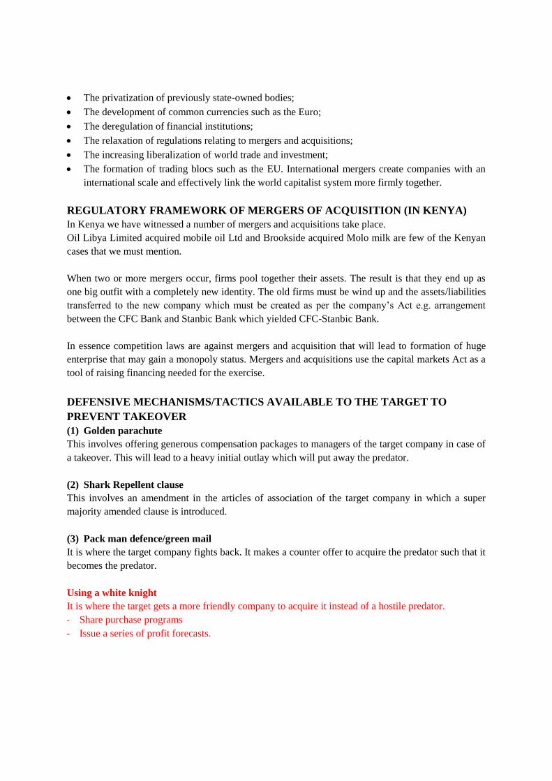
The privatization of previously state-owned bodies;
The development of common currencies such as the Euro;
The deregulation of financial institutions;
The relaxation of regulations relating to mergers and acquisitions;
The increasing liberalization of world trade and investment;
The formation of trading blocs such as the EU. International mergers create companies with an
international scale and effectively link the world capitalist system more firmly together.
REGULATORY FRAMEWORK OF MERGERS OF ACQUISITION (IN KENYA)
In Kenya we have witnessed a number of mergers and acquisitions take place.
Oil Libya Limited acquired mobile oil Ltd and Brookside acquired Molo milk are few of the Kenyan
cases that we must mention.
When two or more mergers occur, firms pool together their assets. The result is that they end up as
one big outfit with a completely new identity. The old firms must be wind up and the assets/liabilities
transferred to the new company which must be created as per the company’s Act e.g. arrangement
between the CFC Bank and Stanbic Bank which yielded CFC-Stanbic Bank.
In essence competition laws are against mergers and acquisition that will lead to formation of huge
enterprise that may gain a monopoly status. Mergers and acquisitions use the capital markets Act as a
tool of raising financing needed for the exercise.
DEFENSIVE MECHANISMS/TACTICS AVAILABLE TO THE TARGET TO
PREVENT TAKEOVER
(1) Golden parachute
This involves offering generous compensation packages to managers of the target company in case of
a takeover. This will lead to a heavy initial outlay which will put away the predator.
(2) Shark Repellent clause
This involves an amendment in the articles of association of the target company in which a super
majority amended clause is introduced.
(3) Pack man defence/green mail
It is where the target company fights back. It makes a counter offer to acquire the predator such that it
becomes the predator.
Using a white knight
It is where the target gets a more friendly company to acquire it instead of a hostile predator.
- Share purchase programs
- Issue a series of profit forecasts.
Page 203

- Use of the poison pill – the target undertakes a suicidal act which will make it unattractive. Such
suicidal act may be getting more debts hence increasing the financial risk of the firm hence making
it attractive.
Disposal of Crown Jewels
It is where the target company identifies and sells off the most attractive portion of its business so as
to make the target less attractive to predators e.g. Mpesa is the crown jewel of Safaricom.
Seeking legal Redress
The target can go to court on competition laws basis. They will claim that the predator will become a
monopoly upon acquisition of the target.
Additional Defensive mechanism
Use of dividend policy – the company can pay higher dividends compared to other years. This will
convince the shareholders hold on to their shares thinking that the dividends paid are sustainable in
future. This makes the share price to increase and make them expensive to buy.
-
CAUSES OF FAILED MERGERS AND ACQUISITIONS
(a) Poor strategic planning
The strategies and objectives of the two companies may differ and conflict with one another.
(b) Cultural and social differences
If the two companies have a wider difference in their cultures and strategy values than a merger will
fail miserably.
(c) Inadequate due diligence
Due diligence is like a watchdog within the process of mergers and acquisitions and unless it is well
applied, the acquisition may cause serious problem.
(d) Poor management integration
Implementation of post mergers objectives may be impossible if the combined management teams are
not well integrated.
(e) Overpricing of the Target Company
If the predator pays too much for the acquisition it may lead to heavy cash outflows which may be
difficult to be recovered.
(f) Excessive Optimism
If the predator is too optimistic and over ambitious on its projections about the target company, poor
decisions may be made within the process.
PRACTICE QUESTIONS
Question 1
M Ltd wants to acquire N Ltd and the financial data of the two companies is as follows:
Page 204
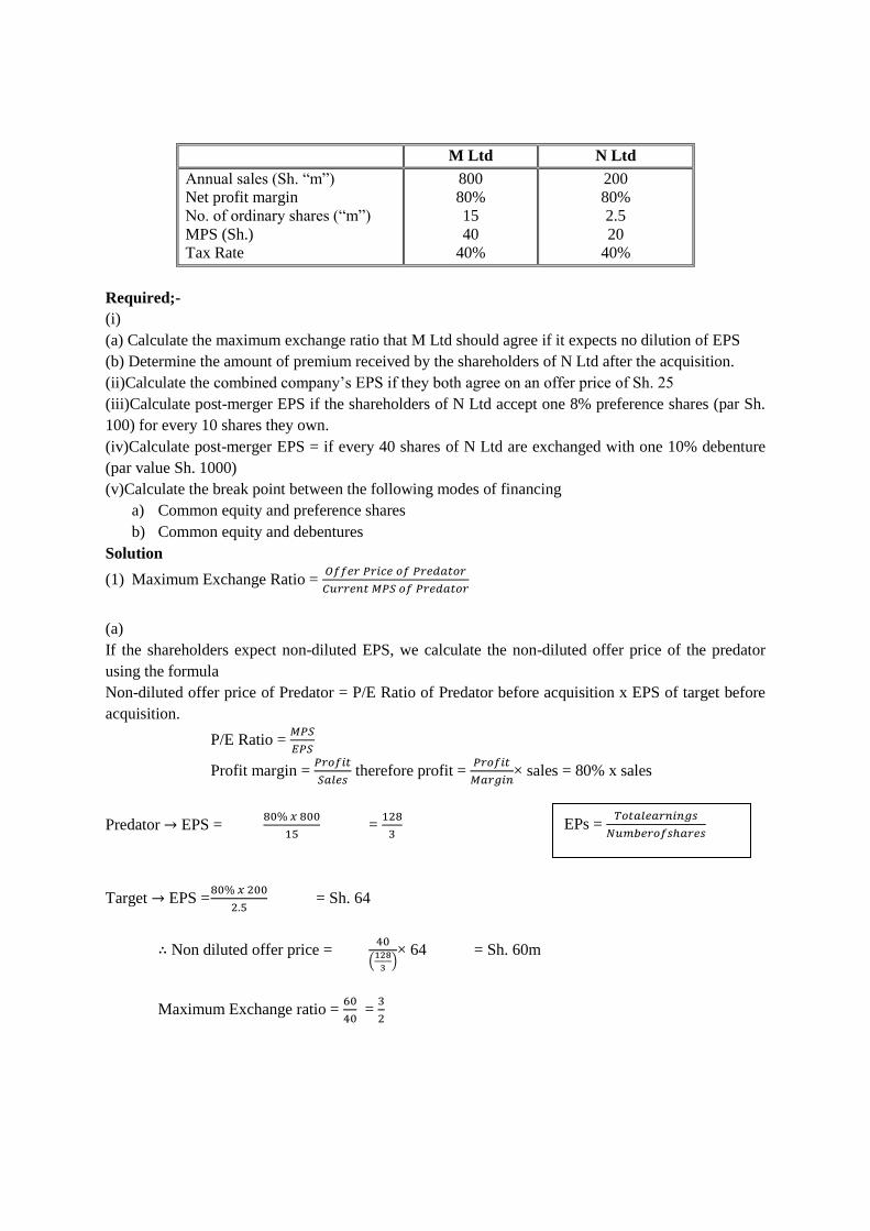
M Ltd N Ltd
Annual sales (Sh. “m”)
Net profit margin
No. of ordinary shares (“m”)
MPS (Sh.)
Tax Rate
800
80%
15
40
40%
200
80%
2.5
20
40%
Required;-
(i)
(a) Calculate the maximum exchange ratio that M Ltd should agree if it expects no dilution of EPS
(b) Determine the amount of premium received by the shareholders of N Ltd after the acquisition.
(ii)Calculate the combined company’s EPS if they both agree on an offer price of Sh. 25
(iii)Calculate post-merger EPS if the shareholders of N Ltd accept one 8% preference shares (par Sh.
100) for every 10 shares they own.
(iv)Calculate post-merger EPS = if every 40 shares of N Ltd are exchanged with one 10% debenture
(par value Sh. 1000)
(v)Calculate the break point between the following modes of financing
a) Common equity and preference shares
b) Common equity and debentures
Solution
(1) Maximum Exchange Ratio = 𝑂𝑓𝑓𝑒𝑟 𝑃𝑟𝑖𝑐𝑒 𝑜𝑓 𝑃𝑟𝑒𝑑𝑎𝑡𝑜𝑟
𝐶𝑢𝑟𝑟𝑒𝑛𝑡 𝑀𝑃𝑆 𝑜𝑓 𝑃𝑟𝑒𝑑𝑎𝑡𝑜𝑟
(a)
If the shareholders expect non-diluted EPS, we calculate the non-diluted offer price of the predator
using the formula
Non-diluted offer price of Predator = P/E Ratio of Predator before acquisition x EPS of target before
acquisition.
P/E Ratio = 𝑀𝑃𝑆
𝐸𝑃𝑆
Profit margin = 𝑃𝑟𝑜𝑓𝑖𝑡
𝑆𝑎𝑙𝑒𝑠 therefore profit =
𝑃𝑟𝑜𝑓𝑖𝑡
𝑀𝑎𝑟𝑔𝑖𝑛× sales = 80% x sales
Predator → EPS = 80% 𝑥 800
15 =
128
3
Target → EPS = 80% 𝑥 200
2.5 = Sh. 64
∴ Non diluted offer price = 40
(128
3)× 64 = Sh. 60m
Maximum Exchange ratio = 60
40 =
3
2
EPs = 𝑇𝑜𝑡𝑎𝑙𝑒𝑎𝑟𝑛𝑖𝑛𝑔𝑠
𝑁𝑢𝑚𝑏𝑒𝑟𝑜𝑓𝑠ℎ𝑎𝑟𝑒𝑠
Page 205

M Ltd is offering 3 of its shares for every 2 share of N Ltd
Method 2
Exchange ratio = 𝐸𝑃𝑠 𝑜𝑓 𝑡𝑎𝑟𝑔𝑒𝑡
𝐸𝑃𝑠 𝑜𝑓 𝑝𝑟𝑒𝑑𝑎𝑡𝑜𝑟 =
64
(128
3) =
3
2
(b) Premium per share = Offer Price of Predator – Current MPS of Target
60 – 20 = Sh. 40
Therefore total premium = 40 x 2.5m = 100m
(ii)
Post-merger EPs if the offer price = sh.25
Determine the normal exchange ratio first
Exchange ratio (ER) = 𝑂𝑓𝑓𝑒𝑟 𝑝𝑟𝑖𝑐𝑒 𝑜𝑓 𝑃𝑟𝑒𝑑𝑎𝑡𝑜𝑟
𝐶𝑢𝑟𝑟𝑒𝑛𝑡 𝑀𝑃𝑆 𝑜𝑓 𝑃𝑟𝑒𝑑𝑎𝑡𝑜𝑟
= 25
40 =
5
8
Post-merger EPs = 𝐸1+𝐸2− 𝑝𝑟𝑒𝑓 𝐷𝑖𝑣
𝑆1+𝑆2 ×𝐸𝑅
E1 = 80% x 200 = 640
E2 = 80% × 200 = 160
640+160
15+2.5 ×5
8
= 48.30
E1 = profit after tax
(iii)Post-Merger EPS for 8% preference shares
First determine preference share value given out.
10 ordinary shares = 100
2.5m = ? 2.5𝑚 ×100
10 = 25m
Therefore preference dividends = 8% x 25m = 2m
Post Acquisition = 𝐸1+𝐸2− 𝑝𝑟𝑒𝑓𝐷𝑖𝑣
𝑆1+𝑆2𝑥𝐸𝑅 ×𝐸𝑅
= 640+160−2
15+2.5 ×0 = 53.2
ER for preference shares and
debenture financed acquisitions is
zero
Page 206

(iv)Post-merger EPS for 10% debentures
40 shares of N ltd = 1000
2.5m = ? 2.5𝑚 ×1000
40 = 62.5m
Total Interest = 10% x 62.5m = 6.25m
Post Acquisition EPS = 𝐸1+𝐸2− 𝑖𝑛𝑡𝑒𝑟𝑒𝑠𝑡 (𝐼−𝑇)
𝑆1+𝑆2 ×𝐸𝑅
= 640+160−6.25 ×0.6
15+2.5 ×0
= 53.08
(v)Break point – It is the level of EBIT at which EPS at different financing options will be the same
(a)
Equity and Preference shares
EPS (Equity) = 𝐸𝐵𝐼𝑇 [1−0.4]
15+2.5×5
8
= 𝐸𝐵𝐼𝑇−0.4 𝐸𝐵𝐼𝑇
16.5625 =
0.6𝐸𝐵𝐼𝑇
16.5625
EPS (preference shares)
EPS = 𝐸𝐵𝐼𝑇 (𝐼−𝑇)− 𝑝𝑟𝑒𝑓 𝐷𝑖𝑣𝑖𝑑𝑒𝑛𝑑
𝑆1+𝑆2×𝐸𝑅
EPS = 0.6𝐸𝐵𝐼𝑇−𝑝𝑟𝑒𝑓𝑒𝑟𝑒𝑛𝑐𝑒 𝐷𝑖𝑣𝑖𝑑𝑒𝑛𝑑𝑠
15+2.5×0
EPS = 0.6𝐸𝐵𝐼𝑇−2𝑚
15
At indifference point:
EPS Equity = EPS preference
0.6𝐸𝐵𝐼𝑇
16.5625 =
0.6𝐸𝐵𝐼𝑇−2𝑚
15
0.6EBIT x 15 = 16.5626 (0.6EBIT – 2m)
9EBIT = 9.9375EBIT – 33.125
9EBIT – 9.9375EBIT = 33.125m
HINT: T = 0.4
I – T = 1 – 0.4 = 0.6
Page 207
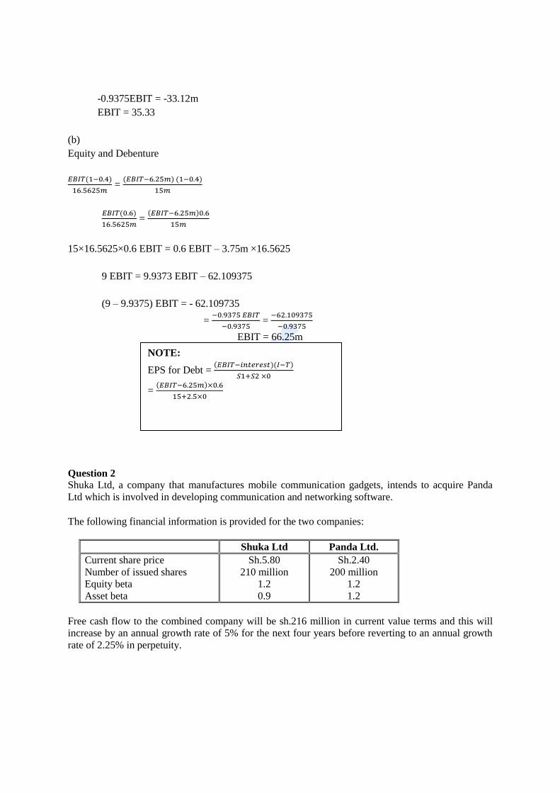
-0.9375EBIT = -33.12m
EBIT = 35.33
(b)
Equity and Debenture
𝐸𝐵𝐼𝑇(1−0.4)
16.5625𝑚 =
(𝐸𝐵𝐼𝑇−6.25𝑚) (1−0.4)
15𝑚
𝐸𝐵𝐼𝑇(0.6)
16.5625𝑚 =
(𝐸𝐵𝐼𝑇−6.25𝑚)0.6
15𝑚
15×16.5625×0.6 EBIT = 0.6 EBIT – 3.75m ×16.5625
9 EBIT = 9.9373 EBIT – 62.109375
(9 – 9.9375) EBIT = - 62.109735
= −0.9375 𝐸𝐵𝐼𝑇
−0.9375 =
−62.109375
−0.9375
EBIT = 66.25m
Question 2
Shuka Ltd, a company that manufactures mobile communication gadgets, intends to acquire Panda
Ltd which is involved in developing communication and networking software.
The following financial information is provided for the two companies:
Shuka Ltd Panda Ltd.
Current share price
Number of issued shares
Equity beta
Asset beta
Sh.5.80
210 million
1.2
0.9
Sh.2.40
200 million
1.2
1.2
Free cash flow to the combined company will be sh.216 million in current value terms and this will
increase by an annual growth rate of 5% for the next four years before reverting to an annual growth
rate of 2.25% in perpetuity.
NOTE:
EPS for Debt = (𝐸𝐵𝐼𝑇−𝑖𝑛𝑡𝑒𝑟𝑒𝑠𝑡)(𝐼−𝑇)
𝑆1+𝑆2 ×0
= (𝐸𝐵𝐼𝑇−6.25𝑚)×0.6
15+2.5×0
Page 208

The combined operations of the companies will result in cash savings of sh.20 million per year for the
next four years.
The debt to equity ratio of the combined company will be 4:6 in market value terms and it is expected
that the combined company’s cost of debt will be 4.55%.
Corporation tax of 30% applies to the company. The current risk-free rate is 2% and the market risk
premium is 7%. It can be assumed that the combined company’s asset beta is the weighted average of
the respective company’s asset betas.
Required:
Estimate the additional equity value created by combining the two companies’ base on free cash
flows.
Solution
Sh. “m”
Combined Asset Beta
Value of Shuka = 5.8 × 40 =
Value of Panda 24×200 =
1,218
480
1,698
Weighted Asset Beta = 0.9 ×1218
1698 + 1.2 ×
480
1698 = 0.9848
𝛽𝑎 = 𝛽𝑒 + 𝑊𝑒
𝑊𝑒+𝑊𝑑 [1−𝑇] 𝛽𝑒 =
𝛽𝑜 × 𝑉𝑒+𝑉𝑑 [1−𝑇]
𝑉𝑒
0.9848 × 4+6 (0.7)
6 = 1.44
Ke = RF + [Rm – RF)𝛽
2 + 7 × 1.44 = 12.088%
Kd 4.55%
WACC = 6
10× 12.088 +
4
10×4.55 (1 – 0.3)= 8.53%
Present Value of Combined Cash flows
Year Expected Cash flows Discount factor
8.53%
PV
Sh. “m”
1
2
3
4
216 (1.05)1 = 226.8
216 (1.05)2 = 238.14
216 (1.05)3 = 250.047
216 (1.05)4 = 262.0.5
4274.80
0.9214
0.8490
0.7823
0.7208
0.7208
208.97
202.18
195.61
189.25
3,081.28
3,877.29
Kd must be adjusted for tax
Page 209
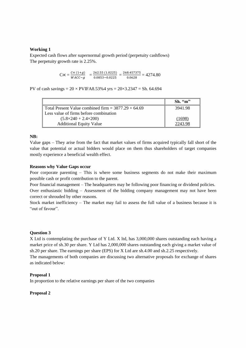
Working 1
Expected cash flows after supernormal growth period (perpetuity cashflows)
The perpetuity growth rate is 2.25%.
C∝ = 𝐶∝ (1+𝑔)
𝑊𝐴𝐶𝐶−𝑔 =
262.55 (1.0225)
0.0853−0.0225 =
268.457375
0.0628 = 4274.80
PV of cash savings = 20 × PVIFA8.53%4 yrs = 20×3.2347 = Sh. 64.694
Sh. “m”
Total Present Value combined firm = 3877.29 + 64.69
Less value of firms before combination
(5.8×240 + 2.4×200)
Additional Equity Value
3941.98
(1698)
2243.98
NB:
Value gaps – They arise from the fact that market values of firms acquired typically fall short of the
value that potential or actual bidders would place on them thus shareholders of target companies
mostly experience a beneficial wealth effect.
Reasons why Value Gaps occur
Poor corporate parenting – This is where some business segments do not make their maximum
possible cash or profit contribution to the parent.
Poor financial management – The headquarters may be following poor financing or dividend policies.
Over enthusiastic bidding – Assessment of the bidding company management may not have been
correct or shrouded by other reasons.
Stock market inefficiency – The market may fail to assess the full value of a business because it is
“out of favour”.
Question 3
X Ltd is contemplating the purchase of Y Ltd. X ltd, has 3,000,000 shares outstanding each having a
market price of sh.30 per share. Y Ltd has 2,000,000 shares outstanding each giving a market value of
sh.20 per share. The earnings per share (EPS) for X Ltd are sh.4.00 and sh.2.25 respectively.
The managements of both companies are discussing two alternative proposals for exchange of shares
as indicated below:
Proposal 1
In proportion to the relative earnings per share of the two companies
Proposal 2
Page 210
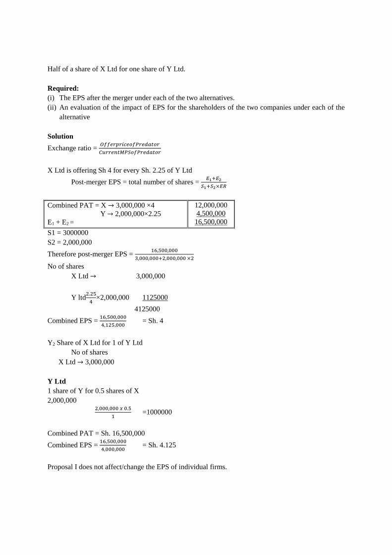
Half of a share of X Ltd for one share of Y Ltd.
Required:
(i) The EPS after the merger under each of the two alternatives.
(ii) An evaluation of the impact of EPS for the shareholders of the two companies under each of the
alternative
Solution
Exchange ratio = 𝑂𝑓𝑓𝑒𝑟𝑝𝑟𝑖𝑐𝑒𝑜𝑓𝑃𝑟𝑒𝑑𝑎𝑡𝑜𝑟
𝐶𝑢𝑟𝑟𝑒𝑛𝑡𝑀𝑃𝑆𝑜𝑓𝑃𝑟𝑒𝑑𝑎𝑡𝑜𝑟
X Ltd is offering Sh 4 for every Sh. 2.25 of Y Ltd
Post-merger EPS = total number of shares = 𝐸1+𝐸2
𝑆1+𝑆2×𝐸𝑅
Combined PAT = X → 3,000,000 ×4
Y → 2,000,000×2.25
E1 + E2 =
12,000,000
4,500,000
16,500,000
S1 = 3000000
S2 = 2,000,000
Therefore post-merger EPS = 16,500,000
3,000,000+2,000,000 ×2
No of shares
X Ltd → 3,000,000
Y ltd2.25
4×2,000,000 1125000
4125000
Combined EPS = 16,500,000
4,125,000 = Sh. 4
Y2 Share of X Ltd for 1 of Y Ltd
No of shares
X Ltd → 3,000,000
Y Ltd
1 share of Y for 0.5 shares of X
2,000,000
2,000,000 𝑥 0.5
1 =1000000
Combined PAT = Sh. 16,500,000
Combined EPS = 16,500,000
4,000,000 = Sh. 4.125
Proposal I does not affect/change the EPS of individual firms.
Page 211
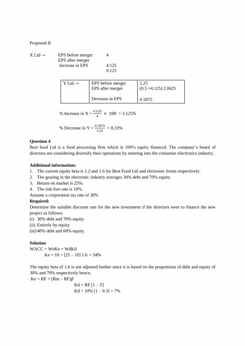
Proposed II
X Ltd → EPS before merger
EPS after merger
Increase in EPS
4
4.125
0.125
Y Ltd → EPS before merger
EPS after merger
Decrease in EPS
2.25
(0.5 ×4.125) 2.0625
0.1875
% Increase in X = 0.125
4 × 100 = 3.125%
% Decrease in Y = 0.1875
2.25 = 8.33%
Question 4
Best food Ltd is a food processing firm which is 100% equity financed. The company’s board of
directors are considering diversify their operations by entering into the consumer electronics industry.
Additional information:
1. The current equity beta is 1.2 and 1.6 for Best Food Ltd and electronic forms respectively.
2. The gearing in the electronic industry averages 30% debt and 70% equity.
3. Return on market is 25%.
4. The risk free rate is 10%.
Assume a corporation tax rate of 30%
Required:
Determine the suitable discount rate for the new investment if the directors were to finance the new
project as follows:
(i) 30% debt and 70% equity
(ii) Entirely by equity
(iii) 40% debt and 60% equity.
Solution
WACC = WeKe + WdKd
Ke = 10 + [25 – 10] 1.6 = 34%
The equity beta of 1.6 is not adjusted further since it is based on the proportions of debt and equity of
30% and 70% respectively hence;
Ke = RF + [Rm – RF)𝛽
Kd = RF [1 – T]
Kd = 10% [1 – 0.3] = 7%
Page 212

WACC = 70%×0.34 + 30% × 0.07 = 25.9%
𝛽𝑎 = 𝛽𝑒 × 𝑊𝑒
𝑊𝑒 + 𝑊𝑑 [1 − 𝑇]
1.6 + 0.7
0.7+0.3 [0.70]= 1.23
Ke = 10 + [25 – 10] = 28.45%
𝛽𝑒 = 𝛽𝑎+𝑊𝑑 [1−𝑇]
𝑊𝑒
We regear the ungeared beta as per the proportions of debt and equity of 40% and 60%
= 1.23 𝑥 0.6+0.4 [0.7]
0.6 = 1.804
Ke = 10 + [25 – 10] 1.804 = 37.06%
WACC = WeKe + WdKd
60% × 0.3706 + 40% ×0.07 = 25.036%
Question 5
Mijengo Ltd, a company engaged in real estate development, intends to acquire Saruji Ltd, a
manufacturer of high quality cement.
Mijengo Ltd proposes to pay for the acquisition using one of the following three methods:
Method 1
A cash offer of sh.10 per share of Saruj Ltd.
Method 2
An offer of three of Mijengo Ltd’s shares for two of Saruji Ltd’s share.
Method 3
An offer of a 2% coupon bond, sh.100 par at the same yield to maturity as Mijengo Ltd’s existing
bond, in exchange for 8 Saruji Ltd shares. The bond will be redeemed in three years at par.
The latest financial statements of the two companies are as follows:
Mijengo Ltd
Sh. “000”
Saruji Ltd
Sh. “000”
Revenue
Profit before tax
Taxation
Dividends
88,410
12,380
(2,480)
9,900
(5,400)
9,360
1,560
(310)
1,250
(550)
Page 213
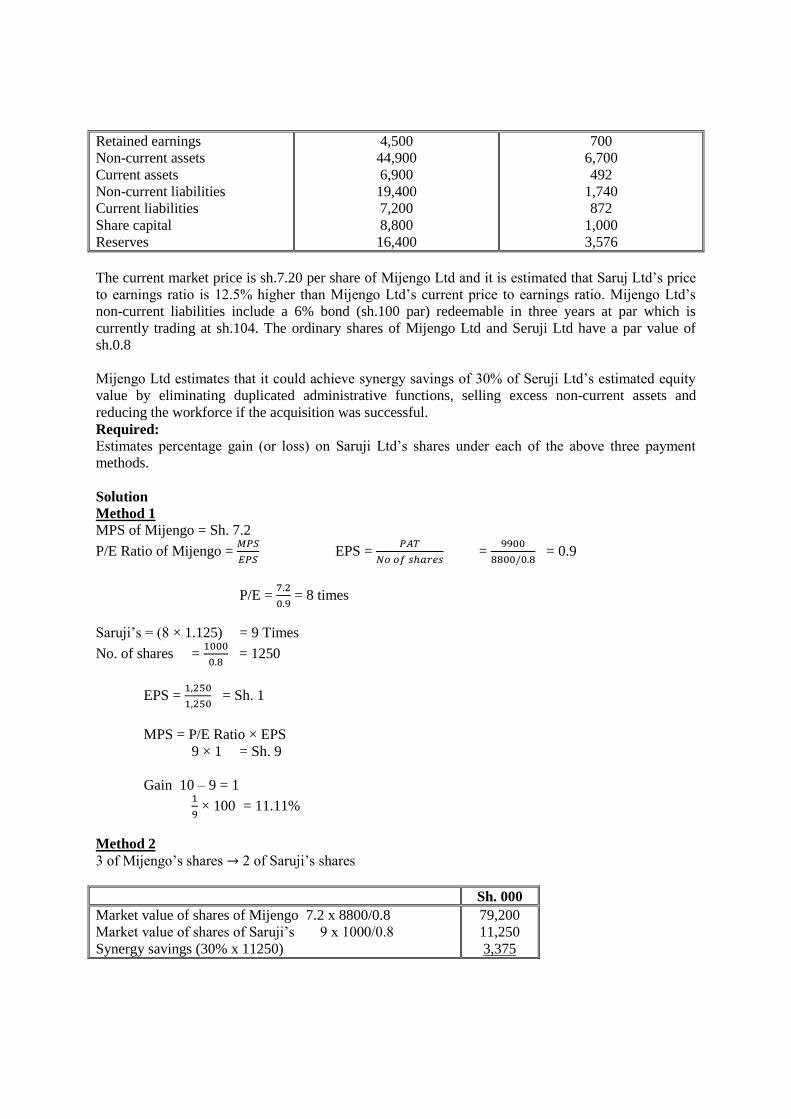
Retained earnings
Non-current assets
Current assets
Non-current liabilities
Current liabilities
Share capital
Reserves
4,500
44,900
6,900
19,400
7,200
8,800
16,400
700
6,700
492
1,740
872
1,000
3,576
The current market price is sh.7.20 per share of Mijengo Ltd and it is estimated that Saruj Ltd’s price
to earnings ratio is 12.5% higher than Mijengo Ltd’s current price to earnings ratio. Mijengo Ltd’s
non-current liabilities include a 6% bond (sh.100 par) redeemable in three years at par which is
currently trading at sh.104. The ordinary shares of Mijengo Ltd and Seruji Ltd have a par value of
sh.0.8
Mijengo Ltd estimates that it could achieve synergy savings of 30% of Seruji Ltd’s estimated equity
value by eliminating duplicated administrative functions, selling excess non-current assets and
reducing the workforce if the acquisition was successful.
Required:
Estimates percentage gain (or loss) on Saruji Ltd’s shares under each of the above three payment
methods.
Solution
Method 1
MPS of Mijengo = Sh. 7.2
P/E Ratio of Mijengo = 𝑀𝑃𝑆
𝐸𝑃𝑆 EPS =
𝑃𝐴𝑇
𝑁𝑜 𝑜𝑓 𝑠ℎ𝑎𝑟𝑒𝑠 =
9900
8800/0.8 = 0.9
P/E = 7.2
0.9 = 8 times
Saruji’s = (8 × 1.125) = 9 Times
No. of shares = 1000
0.8 = 1250
EPS = 1,250
1,250 = Sh. 1
MPS = P/E Ratio × EPS
9 × 1 = Sh. 9
Gain 10 – 9 = 1
1
9 × 100 = 11.11%
Method 2
3 of Mijengo’s shares → 2 of Saruji’s shares
Sh. 000
Market value of shares of Mijengo 7.2 x 8800/0.8
Market value of shares of Saruji’s 9 x 1000/0.8
Synergy savings (30% x 11250)
79,200
11,250
3,375
Page 214
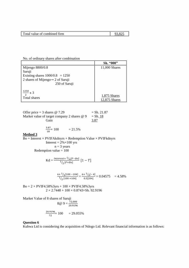
Total value of combined firm 93,825
No. of ordinary shares after combination
Sh. “000”
Mijengo 8800/0.8
Saruji
Existing shares 1000/0.8 = 1250
2 shares of Mijengo→ 2 of Saruji
250 of Saruji
1250
2 x 3
Total shares
11,000 Shares
1,875 Shares
12,875 Shares
Offer price = 3 shares @ 7.29 = Sh. 21.87
Market value of target company 2 shares @ 9 = Sh. 18
Gain 3.87
3.87
18× 100 = 21.5%
Method 3
Bo = Interest × PVIFAkdnyrs + Redemption Value × PVIFkdnyrs
Interest = 2%×100 yrs
n = 3 years
Redemption value = 100
Kd = 𝐼𝑛𝑡𝑒𝑟𝑒𝑠𝑡+ 1 𝑛⁄ [𝐹−𝐵𝑜]
12⁄ [𝐹+𝐵𝑜]
[1 − 𝑇]
6+ 1 3⁄ [100 −104]
12⁄ [100 +104]
= 6+ 1 3⁄ [− 4]
0.5[204] = 0.04575 = 4.58%
Bo = 2 × PVIF4.58%3yrs + 100 × PVIF4.58%3yrs
2 × 2.7448 + 100 × 0.8743=Sh. 92.9196
Market Value of 8 shares of Saruji
8@ 9 = 72,000
20.9196
20.9196
72× 100 = 29.055%
Question 6
Kubwa Ltd is considering the acquisition of Ndogo Ltd. Relevant financial information is as follows:
Page 215
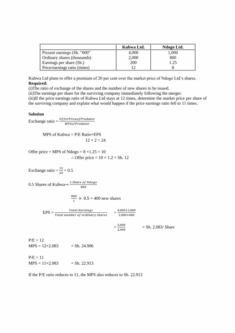
Kubwa Ltd. Ndogo Ltd.
Present earnings (Sh. “000”
Ordinary shares (thousands)
Earnings per share (Sh.)
Price/earnings ratio (times)
4,000
2,000
200
12
1,000
800
1.25
8
Kubwa Ltd plans to offer a premium of 20 per cent over the market price of Ndogo Ltd’s shares.
Required:
(i)The ratio of exchange of the shares and the number of new shares to be issued.
(ii)The earnings per share for the surviving company immediately following the merger.
(iii)If the price earnings ratio of Kubwa Ltd stays at 12 times, determine the market price per share of
the surviving company and explain what would happen if the price earnings ratio fell to 11 times.
Solution
Exchange ratio = 𝑂𝑓𝑓𝑒𝑟𝑃𝑟𝑖𝑐𝑒𝑜𝑓𝑃𝑟𝑒𝑑𝑎𝑡𝑜𝑟
𝑀𝑃𝑆𝑜𝑓𝑃𝑟𝑒𝑑𝑎𝑡𝑜𝑟
MPS of Kubwa = P/E Ratio×EPS
12 × 2 = 24
Offer price = MPS of Ndogo = 8 ×1.25 = 10
∴ Offer price = 10 × 1.2 = Sh. 12
Exchange ratio = 12
24 = 0.5
0.5 Shares of Kubwa→1 𝑆ℎ𝑎𝑟𝑒 𝑜𝑓 𝑁𝑑𝑜𝑔𝑜
800
800
1 × 0.5 = 400 new shares
EPS = 𝑇𝑜𝑡𝑎𝑙 𝐸𝑎𝑟𝑛𝑖𝑛𝑔𝑠
𝑇𝑜𝑡𝑎𝑙 𝑛𝑢𝑚𝑏𝑒𝑟 𝑜𝑓 𝑜𝑟𝑑𝑖𝑛𝑎𝑟𝑦 𝑠ℎ𝑎𝑟𝑒𝑠 =
4,000+1,000
2,000+400
= 5,000
2,400 = Sh. 2.083/ Share
P/E = 12
MPS = 12×2.083 = Sh. 24.996
P/E = 11
MPS = 11×2.083 = Sh. 22.913
If the P/E ratio reduces to 11, the MPS also reduces to Sh. 22.913
Page 216
CHAPTER FIVE
CORPORATE RESTRUCTURING AND RE-
ORGANISATION CHAPTER KEY OBJECTIVES
To be able to understand the following;-
1. Background on restructuring and re organisation
2. Indicators/symptoms of restructuring
3. Considerations in designing an appropriate restructuring programme
4. Financial reconstruction: forms of financial reconstruction; impact of financial reconstruction on
share price; impact of financial reconstruction on the weighted Average cost of capital (WACC)
5. Portfolio reconstruction: various ways of unbundling a firm: divestment, de-merger, spin-off,
liquidation, sell-offs, equity curve outs, strategic alliances, management buyout, leveraged
buyouts and the management buy-ins.
6. The relevance of the various forms of portfolio reconstruction
7. Organisational reconstruction: The nature and benefits of this form of restructuring; models of
predicting corporate failure; Multiple discriminant analysis (Z-Score model), Beaver failure ratio,
Argenti model, Taffler’s model
8. Causes of financial distress
9. Forms of financial distress and solutions to financial distress
5.1 BACKGROUND ON RESTRUCTURING AND RE ORGANISATION
Restructuring can mean
A process of reorganizing a company’s ownership, legal, or operation structure for the betterment of
the company or to increase its profits in the market.
It can also imply a change in the ownership, demerger, or change in the business like a buyout or a
bankruptcy.
Three other terms can imply its meaning: financial restructuring, debt restructuring and corporate
restructuring.
Reorganization is taking control of a bankrupt or financially unstable firm by restating its assets and
liabilities. It involves discussions with creditors about repayment so that the recurrence of the
financial debts is minimized. Reorganization can also refer to the sale or merger of a company that
involves a change in ownership, legal and management level changes, as well as a change in stocks. A
court-supervised formal process restructures a company’s finances after it faces bankruptcy. During
the period when a company files for bankruptcy and the court reviews it, the company is saved from
the creditors.
Reorganization can also occur to take advantage of any changed tax regulations. This brings about
legal as well as corporate structural changes to the firm involved. One of the aims of reorganization is
Page 217
to repay creditors as much of the debt amount as possible, and also restructure the company’s
management, operations, and finances keeping in mind that the same problem (of bankruptcy) does
not reoccur.
Differences between restructuring and reorganization:
Restructuring is done to make an organization profitable or to make it reach thecurrent market
standards. Reorganization is needed to stabilize a company that is facing bankruptcy.
A legal and financial advisor or a new CEO is hired to take care of a company during restructuring.
During reorganization, the entire process takes place under the supervision of the court to take care of
legal and management structural changes.
Summary:
1. Restructuring ensures that a company becomes more effective and better organized.
It focuses on the core business and takes care of changed strategic and financial plans.
2. Reorganization makes sure that new opportunities are opened up, there is a rise in
Profits and updated legal and financial protections are given to companies during trying times.
5.2 INDICATORS OF FINANCIAL DISTRESS
Financial and operating deficiencies pointing to financial distress include:
Significant decline in stock price
Reduction in dividend payments
Sharp increase in the cost of capital
Inability to obtain further financing
Inability to meet past—due obligations
Poor financial reporting system
Movement into business areas unrelated to the company's basic business
Failure to control costs
High degree of competition
Ways to avoid financial problems include:
Merging with another financially stronger similar company. Will a merger aid in financing, lower
overall operating costs, synergy and efficiency, and program expansion?
Restructuring the organization.
Selling off unproductive assets.
Deferring the payment of bills.
Discarding programs and activities that are no longer financially viable.
Implementing a cost reduction program, including layoffs and attrition. However, will this
eliminate programs that will be hard to start up again? Are we getting rid of scarce talent? Such
cuts are referred to as irreversible reductions, which in the end may not be wise.
Increasing service fees.
Increasing fundraising efforts and contributions.
Applying for grants.
Page 218
Stimulating contracts.
5.3. FORMS OF FINANCIAL DISTRESS
(a) Technical insolvency;- a firm is enabled to pay its debts but this happens temporarily. A company
is unable to meet its current debts and this may be temporary and subject to remedy.
(b) Insolvency is bankruptcy;- Company liabilities exceed the assets.
(c) Legal bankruptcy;- The Company files for liquation under the company’s Act.
(d) Economic failure;-Firm’s revenues are insufficient to cover cost as well as cost of capital.
(e) Business Failure;-A firm terminates its operations either partially or fully.
Companies restructure for a variety of reasons:
To reduce costs.
To concentrate on key products or accounts.
To incorporate new technology.
To make better use of talent.
To improve competitive advantage.
To spin off a subsidiary company.
To merge with another company.
To decrease or consolidate debt
5.4 CONSIDERATIONS IN DESIGNING AN APPROPRIATE RESTRUCTURING
PROGRAMME
Companies may embark on organizational restructuring after changes in vision and strategy, or in
hopes of cutting costs by revitalizing processes or pruning parts of the company. When it is done, a
small business will have a new organizational structure and a changed workforce. The influence of the
human resources department on job design, assignments and training can have a lasting impact on the
strategic success of the new organizational structure.
Workforce Characteristics
Human resources should influence the strategic choices leading to restructuring. To develop strategy,
the owner must consider the company’s competitive position, including employees’ strengths and
weaknesses. HR supplies the owner with a workplace assessment -- a thorough inventory of the
employees’ skills and other characteristics such as talent, turnover, education and experience. The
inventory is compared against the strategies under consideration to calculate how well the company’s
workforce can enact them. Once strategy is chosen, HR then evaluates how it must transform the
company’s workforce to fill the company’s needs in the context of the restructuring and strategy.
Organizational Structure
Organizational structure determines job scope, working relationships and resource sharing, so it has a
profound impact on how business is done. Keeping the company’s strategy at the center of structural
decisions allows HR to make the best choices. For instance, if a small business wants to focus on fine,
custom-built products, the organizational structure must promote individual accomplishment instead
of mass production.
Page 219
Job Design
Business Review” listed job design and talent choice as most critical in implementing new
organizational structure. HR must reassess the tasks and workflows needed to effectively do business
and compare those to the organization’s existing jobs and processes. Positions may stay the same,
change or be removed. Some tasks may require new positions. Considerations when designing jobs
include how specialized a job should be, how much authority an employee needs to accomplish work
and how much supervision is needed.
Redeployments and Cuts
HR should consult the workforce assessment to match people to transformed and new positions. For
jobs requiring skills and experience that workers don’t yet have, human resources must rely on
aptitude and personality tests to predict how likely it is that an employee candidate can succeed.
Cutting jobs requires compliance with state and federal laws. HR also should implement a consistent,
objective procedure for choosing the employees who will be cut, and provide them with an appeals
process, a financial cushion to soften the blow and outplacement support to help them find new
employment.
Reengagement
Restructuring is an unsettling process for employees. HR must make sure that the remaining
employees are primed to be successful in their new situations. Workers must be thoroughly trained for
new or changed positions. They must also be re-motivated, which requires insight into employee
attitudes. Motivation surveys can provide answers on the best approach for your business.
5.5. PORTFOLIO RECONSTRUCTION
Unbundling
Is a portfolio restructuring strategy, which involves the disposal and sale of assets, facilities,
production lines, subsidiaries, divisions or product units.
Unbundling can be voluntary or it can be forced on a company. A company may voluntarily
decide to divest part of its business for strategic, financial or organisational reasons. An
involuntary unbundling, on the other hand, may take place for regulatory or financial reasons.
The main forms of unbundling are:
Divestments
Demergers
Sell-offs
Spin-offs
Carve-outs
Management buy-outs
Divestment
Page 220
It is the action or process of selling off subsidiary business interests or investments. Divestment
is the partial or complete sale or disposal of physical and organisational assets in order to free
funds for investment in other areas of strategic interest.
In a divestment, the company ceases the operation of a particular activity in order to concentrate
on other activities. The rationale for divestment is normally to reduce costs or to increase return
on assets.
Demergers
It is the separation of a large company into two or more smaller organizations. A demerger is the
splitting up of corporate bodies into two or more separate bodies, to ensure that share prices reflect
the true value of underlying operations.
In demergers existing shareholders are given shares in each of the two separate businesses – control
is maintained
For example, the BCD Group might demerge by splitting into two independently operating
companies BC Ltd and D Ltd. Existing shareholders are given a stake in each of the new separate
companies.
Advantages of demergers
Demergers lead to greater operational efficiency and greater opportunity to realise value from the
separate entities for example a two-division company with one loss-making division and one profit-
making, fast-growing division may be better off splitting the two divisions. The profitable division
may acquire a valuation well in excess of its contribution to the merged company.
Even if both divisions are profit making, a demerger may still have benefits. Management can focus
on creating value for both companies individually and implementing a suitable financial structure for
each company. The full value of each company may then become appropriate.
Shareholders will continue to own both companies, which means that the diversification of their
portfolio will remain unchanged.
The ability to raise extra finance, especially debt finance, to support new investments and expansion
may be reduced.
Disadvantages of demergers
The process may be expensive.
It leads to a loss of economies of scale
Economies of scale may be lost, where the demerged parts of the business had operations (and
skills) in common, to which economies of scale applied.
The smaller companies, resulting from a demerger will have a lower status and will lose the
group’s bargaining power with banks etc.
Page 221
There may be higher overhead costs as a percentage of revenue, resulting from the ability to raise
extra finance, especially debt finance, to support new investments and expansion may be reduced.
Sell-Offs
A sell-off is the disposal of part of a company to a third party, generally for cash.
Under a ‘sell-off’, at least part of the business will be sold to a third party. Control of the business
sold is lost.
Spin-offs
A subsidiary of a parent company that has been sold off, creating a new company.
In a spin-off, a new company is created from an existing company, whose shares are owned by the
shareholders of the original company which is making the distribution of assets.
In a spin-off:
1. There is no change in the ownership of assets, as the shareholders own the same proportion of
shares in the new company as they did in the old company.
2. Assets of the part of the business to be separated off are transferred into the new company, which
will usually have different management from the old company.
Carve-outs
Also known as split off IPO (initial public offering). It is a type of corporate re-organization in which
a company creates a new subsidiary and subsequently offers it to the public. The parent company will
retain a significant shareholding in the new company. A carve-out is the creation of a new company,
by detaching parts of the company and selling the shares of the new company to the public.
Management Buyout (MBO) and Management Buy In (MBI)
MBO is the purchase of a controlling share in a company by its executive directors or managers.
Management Buy in (MBI)
This is a purchase of shares in a company by managers who are not employed by it. It occurs when a
manager or a management team from outside the company raises the company necessary finance,
buys it and becomes the company’s new management.
Unbundling and firm value
The main effect of unbundling on the value of the firm comes through changes in the return on assets
and the asset beta.
Effect on growth rate
The impact of unbundling on the value of the firm is accessed through one of the valuation models
that we have considered in previous chapters. For example, the growth rate following a restructuring
can be calculated from the formula g = b×re.
Page 222
When firms divest themselves of existing investments, they affect their expected return on assets, as
good projects increase the projected return and bad projects reduce the return – and any investment
decision taken by firms affects their riskiness and therefore the asset beta.
Illustration
A firm is expected to divest itself of unrelated divisions, which have historically had lower returns.
Because of the divestment, the return on equity is expected to increase from 10% to 15%. The
firm’s retention ratio is 50%.
Answer
Before the restructuring the growth rate is equal to:
g = b ×re
g = 0.5 × 0.10 = 0.05 or 5%
After the restructuring the growth rate is equal to:
g = 0.5 ×0.15 = 7.5%
The restructuring has increased the growth rate from 5% to 7.5%.
PREDICTING CORPORATE FAILURE
Corporate failure is always expected when a company starts to show some symptoms/signs of
financial distress.
These symptoms include:
Continuous decrease in profit margins which lead to inability of the firm to maintain and
stabilise its MPS.
High overdraft facilities to finance expansions
Overreliance in borrowing funds which increases the financial gearing risk.
Poor credit rating
High employee turnover.
In predicting corporate failure the firm can use;
(1) Altman’s Z Score Model
This model calculates the ratios from the financial statement of the firm in question, multiplies them
with some constants and the results are added together.
Illustration 1
The following are the summarized financial statements of Shida Products Ltd, which is facing
financial difficulties:
Income statement for the year ended 31 December 2013:
Turnover
Earnings before interest and tax (EBIT)
Interest
Sh. “000”
1,209,000
84,000
(39,000)
Note b = retention ratio = 50%
Page 223
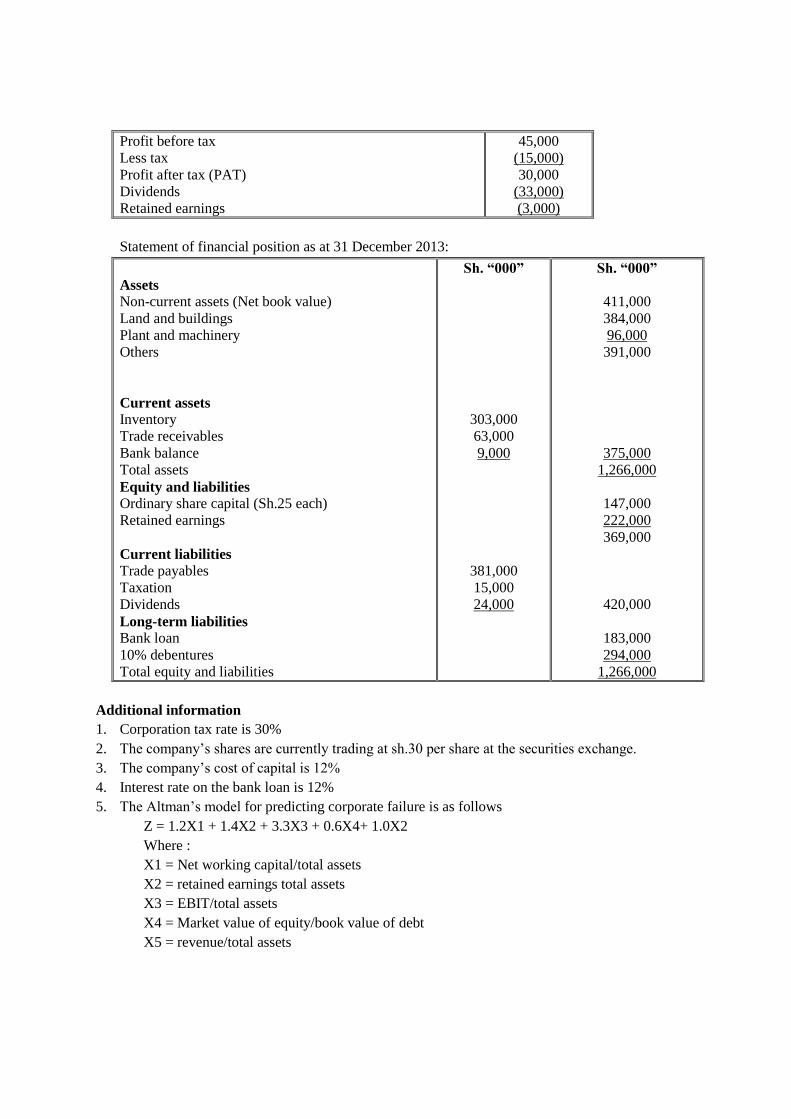
Profit before tax
Less tax
Profit after tax (PAT)
Dividends
Retained earnings
45,000
(15,000)
30,000
(33,000)
(3,000)
Statement of financial position as at 31 December 2013:
Assets
Non-current assets (Net book value)
Land and buildings
Plant and machinery
Others
Current assets
Inventory
Trade receivables
Bank balance
Total assets
Equity and liabilities
Ordinary share capital (Sh.25 each)
Retained earnings
Current liabilities
Trade payables
Taxation
Dividends
Long-term liabilities
Bank loan
10% debentures
Total equity and liabilities
Sh. “000”
303,000
63,000
9,000
381,000
15,000
24,000
Sh. “000”
411,000
384,000
96,000
391,000
375,000
1,266,000
147,000
222,000
369,000
420,000
183,000
294,000
1,266,000
Additional information
1. Corporation tax rate is 30%
2. The company’s shares are currently trading at sh.30 per share at the securities exchange.
3. The company’s cost of capital is 12%
4. Interest rate on the bank loan is 12%
5. The Altman’s model for predicting corporate failure is as follows
Z = 1.2X1 + 1.4X2 + 3.3X3 + 0.6X4+ 1.0X2
Where :
X1 = Net working capital/total assets
X2 = retained earnings total assets
X3 = EBIT/total assets
X4 = Market value of equity/book value of debt
X5 = revenue/total assets
Page 224
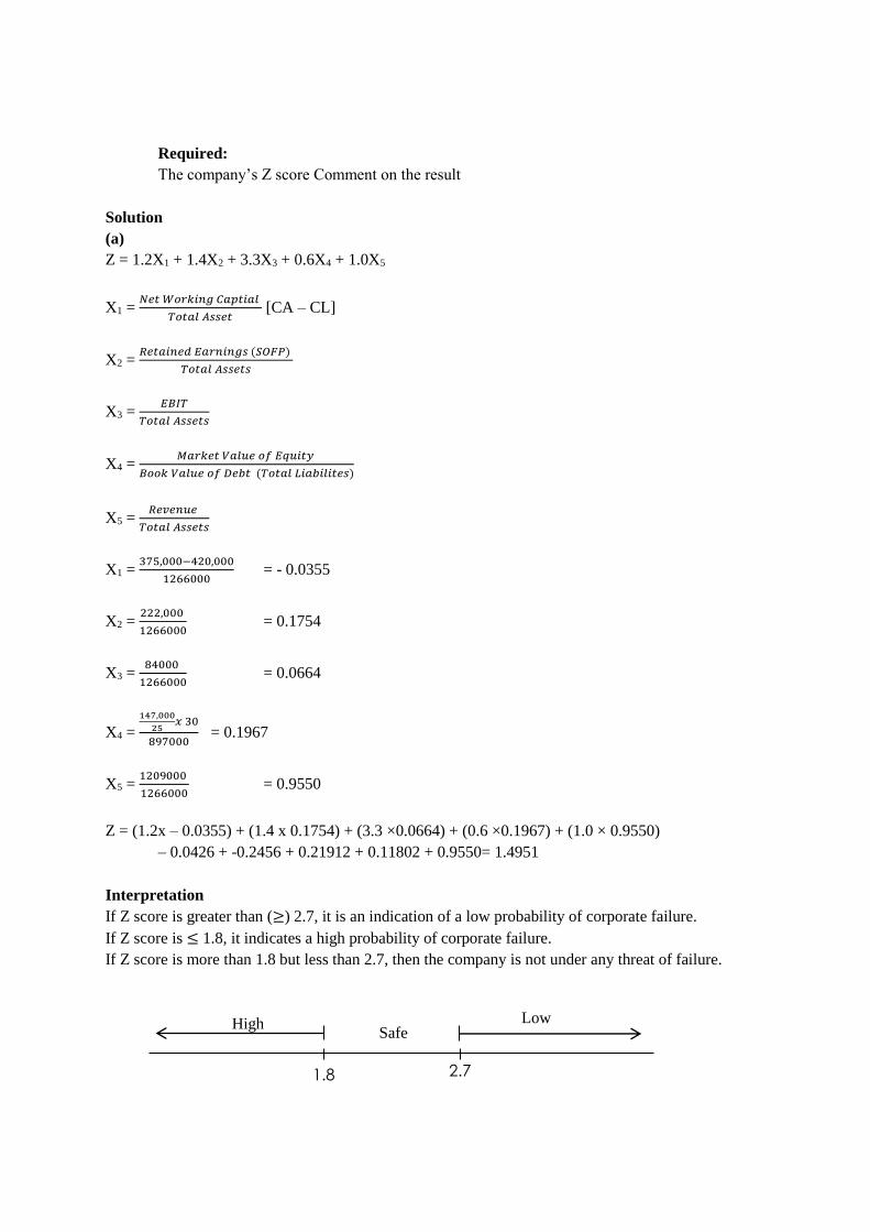
Required:
The company’s Z score Comment on the result
Solution
(a)
Z = 1.2X1 + 1.4X2 + 3.3X3 + 0.6X4 + 1.0X5
X1 = 𝑁𝑒𝑡 𝑊𝑜𝑟𝑘𝑖𝑛𝑔 𝐶𝑎𝑝𝑡𝑖𝑎𝑙
𝑇𝑜𝑡𝑎𝑙 𝐴𝑠𝑠𝑒𝑡 [CA – CL]
X2 = 𝑅𝑒𝑡𝑎𝑖𝑛𝑒𝑑 𝐸𝑎𝑟𝑛𝑖𝑛𝑔𝑠 (𝑆𝑂𝐹𝑃)
𝑇𝑜𝑡𝑎𝑙 𝐴𝑠𝑠𝑒𝑡𝑠
X3 = 𝐸𝐵𝐼𝑇
𝑇𝑜𝑡𝑎𝑙 𝐴𝑠𝑠𝑒𝑡𝑠
X4 = 𝑀𝑎𝑟𝑘𝑒𝑡 𝑉𝑎𝑙𝑢𝑒 𝑜𝑓 𝐸𝑞𝑢𝑖𝑡𝑦
𝐵𝑜𝑜𝑘 𝑉𝑎𝑙𝑢𝑒 𝑜𝑓 𝐷𝑒𝑏𝑡 (𝑇𝑜𝑡𝑎𝑙 𝐿𝑖𝑎𝑏𝑖𝑙𝑖𝑡𝑒𝑠)
X5 = 𝑅𝑒𝑣𝑒𝑛𝑢𝑒
𝑇𝑜𝑡𝑎𝑙 𝐴𝑠𝑠𝑒𝑡𝑠
X1 = 375,000−420,000
1266000 = - 0.0355
X2 = 222,000
1266000 = 0.1754
X3 = 84000
1266000 = 0.0664
X4 =
147,000
25𝑥 30
897000 = 0.1967
X5 = 1209000
1266000 = 0.9550
Z = (1.2x – 0.0355) + (1.4 x 0.1754) + (3.3 ×0.0664) + (0.6 ×0.1967) + (1.0 × 0.9550)
– 0.0426 + -0.2456 + 0.21912 + 0.11802 + 0.9550= 1.4951
Interpretation
If Z score is greater than (≥) 2.7, it is an indication of a low probability of corporate failure.
If Z score is ≤ 1.8, it indicates a high probability of corporate failure.
If Z score is more than 1.8 but less than 2.7, then the company is not under any threat of failure.
High Low Safe
1.8 2.7
Page 225
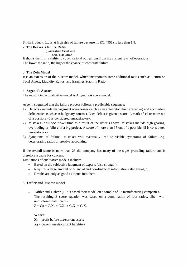
Shida Products Ltd is at high risk of failure because its Z(1.4951) is less than 1.8.
2. The Beaver’s failure Ratio
= 𝑂𝑝𝑒𝑟𝑎𝑡𝑖𝑛𝑔 𝐶𝑎𝑠ℎ𝑓𝑙𝑜𝑤𝑠
𝑇𝑜𝑡𝑎𝑙 𝐿𝑖𝑎𝑏𝑖𝑙𝑖𝑡𝑖𝑒𝑠
It shows the firm’s ability to cover its total obligations from the current level of operations.
The lower the ratio, the higher the chance of corporate failure
3. The Zeta Model
It is an extension of the Z score model, which incorporates some additional ratios such as Return on
Total Assets, Liquidity Ratios, and Earnings Stability Ratio.
4. Argenti’s A score
The most notable qualitative model is Argent is A score model.
Argenti suggested that the failure process follows a predictable sequence:
1) Defects - include management weaknesses (such as an autocratic chief executive) and accounting
deficiencies (such as n budgetary control). Each defect is given a score. A mark of 10 or more out
of a possible 45 is considered unsatisfactory.
2) Mistakes - will occur over time as a result of the defects above. Mistakes include high gearing,
overtrading or failure of a big project. A score of more than 15 out of a possible 45 is considered
unsatisfactory.
3) Symptoms of failure - mistakes will eventually lead to visible symptoms of failure, e.g.
deteriorating ratios or creative accounting.
If the overall score is more than 25 the company has many of the signs preceding failure and is
therefore a cause for concern.
Limitations of qualitative models include:
Based on the subjective judgment of experts (also strength).
Requires a large amount of financial and non-financial information (also strength).
Results are only as good as inputs into them.
5. Taffler and Tishaw model
Taffler and Tishaw (1977) based their model on a sample of 92 manufacturing companies.
The resulting Z score equation was based on a combination of four ratios, albeit with
undisclosed coefficients:
Z = Co + C1X1 + C2X2 + C3X3 + C4X4
Where:
X1 = profit before tax/current assets
X2 = current assets/current liabilities
Page 226

X3 = current liabilities/total assets (
X4 = no credit interval
The percentages reveal a guide to the relative weightings of the ratios.
CAUSES OF FINANCIAL DISTRESS
Financial distress occurs when an organization is unable to pay its creditors and lenders. This
condition is more likely when a business is highly leveraged, its per-unit profit level is
low, its breakeven point is high, or its sales are sensitive to economic declines.
Because of this condition, other parties will typically engage in the following actions:
Suppliers insist on the return on any unpaid inventory
Suppliers require that any additional payments be made with cash on delivery (COD) terms
Suppliers start to charge interest and penalties on overdue payables
Lenders will not extend any additional loans
Customers cancel their orders or do not place new orders
Competitors try to steal away customers
To get out of the situation, managers may be forced to sell assets on a rush basis, lend their own
money to the firm, and eliminate discretionary expenditures.
Financial distress is common just before a business declares bankruptcy.
Page 227
CHAPTER SIX
DERIVATIVES IN FINANCIAL RISK MANAGEMENT
CHAPTER KEY OBJECTIVES
To be able to understand the following;- 1. The meaning, nature and importance of derivative instruments: futures, forwards, options and
swaps
2. Pricing and valuations of derivatives: futures, forwards, options and swaps
3. Types of risks: operational risks, political risks, economic risks, fiscal risks, regulatory risks,
currency risks and interest rate risks.
4. Foreign currency risk management: Types of forex risks, hedging currency risks, forward
contracts, money market hedge, currency options, currency futures and currency swaps
5. Interest rate risks: Term structure of interest rates, forward rate agreement, interest rate futures,
interest rate swaps, interest rate options.
6.1. THE MEANING, NATURE AND IMPORTANCE OF DERIVATIVE
INSTRUMENTS: FUTURES, FORWARDS, OPTIONS AND SWAPS
A derivative is a financial security with a value that is reliant upon or derived from an underlying
asset or group of assets. The derivative itself is a contract between two or more parties based upon the
asset or assets. Its price is determined by fluctuations in the underlying asset. The most common
underlying assets include stocks, bonds, commodities, currencies, interest rates and market indexes.
Derivatives can either be traded over-the-counter (OTC) or on an exchange. OTC derivatives
constitute the greater proportion of derivatives in existence and are unregulated, whereas derivatives
traded on exchanges are standardized. OTC derivatives generally have greater risk for
the counterparty than do standardized derivatives.
Derivatives are used for the following:
Hedge or to mitigate risk in the underlying, by entering into a derivative contract whose value moves
in the opposite direction to their underlying position and cancels part or all of it out
Create option ability where the value of the derivative is linked to a specific condition or event
(e.g., the underlying reaching a specific price level)
Obtain exposure to the underlying where it is not possible to trade in the underlying
Provide leverage (or gearing), such that a small movement in the underlying value can cause a
large difference in the value of the derivative of a specified range, reaches a certain level
Switch asset allocations between different asset classes Speculate and make a profit if the value
of the underlying asset moves the way they expect (e.g. moves in a given direction, stays in or out
without disturbing the underlying assets, as part of transition management
Avoid paying taxes. For example, an equity swap allows an investor to receive steady payments,
e.g. based on a standard rate, while avoiding paying capital gains tax and keeping the stock
Page 228
6.2. PRICING AND VALUATIONS OF DERIVATIVES: FUTURES, FORWARDS,
OPTIONS AND SWAPSVALUATION OF OPTIONS
Option is a contract that gives one party the option to enter into a transaction either at a specific time
in the future or within a specific future period at a price that is agreed when the contract is issued Or
Options are financial contracts which gives the buyer a right but not an obligation to buy a specified
number of securities at some time in future at a predetermined price known as Exercise price.
Exercise price
The exercise or strike price is the price at which the future transaction will take place.
Premium
Premium is the price paid by the option buyer to the seller, or writer, for the right to buy or
sell the underlying shares.
There are two types of options i.e. (i) Call Option
(ii) Put Option
Call Option
It is the financial contract that gives the buyer a right but not an obligation to buy a specified number
of securities at some time in future at a predetermined price.
Put option
It is an option which gives the seller the right but not the obligation to sell a given number of
securities at some time in future at a predetermined price.
European, American and Bermudan options
A European option can only be exercised at expiration, whereas an American option can be exercised
any time prior to expiration. A Bermudan option is an option where early exercise is restricted to
certain dates during the life of the option. It derives its name from the fact that its exercise
characteristics are somewhere between those of the American and the European style of options and
the island of Bermuda lies between America and Europe.
Long and short positions
When an investor buys an option the investor is setting up a long position, and when the investor sells
an option the investor has a short position.
Price quotations
It should be noted that, for simplicity, only one price is quoted for each option in the national
newspapers. In practice, there will always be two prices quoted for each option, i.e. a bid and an offer
price.
Profiles of call options at expiration
Page 229
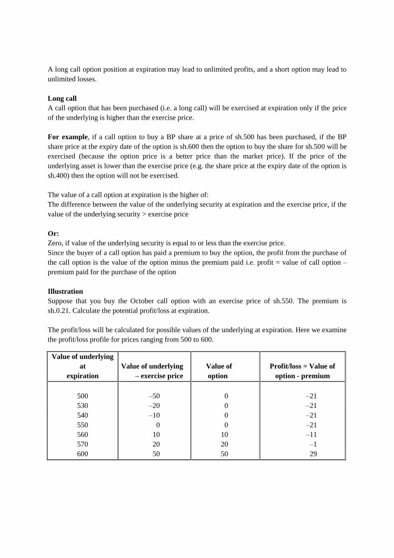
A long call option position at expiration may lead to unlimited profits, and a short option may lead to
unlimited losses.
Long call
A call option that has been purchased (i.e. a long call) will be exercised at expiration only if the price
of the underlying is higher than the exercise price.
For example, if a call option to buy a BP share at a price of sh.500 has been purchased, if the BP
share price at the expiry date of the option is sh.600 then the option to buy the share for sh.500 will be
exercised (because the option price is a better price than the market price). If the price of the
underlying asset is lower than the exercise price (e.g. the share price at the expiry date of the option is
sh.400) then the option will not be exercised.
The value of a call option at expiration is the higher of:
The difference between the value of the underlying security at expiration and the exercise price, if the
value of the underlying security > exercise price
Or:
Zero, if value of the underlying security is equal to or less than the exercise price.
Since the buyer of a call option has paid a premium to buy the option, the profit from the purchase of
the call option is the value of the option minus the premium paid i.e. profit = value of call option –
premium paid for the purchase of the option
Illustration
Suppose that you buy the October call option with an exercise price of sh.550. The premium is
sh.0.21. Calculate the potential profit/loss at expiration.
The profit/loss will be calculated for possible values of the underlying at expiration. Here we examine
the profit/loss profile for prices ranging from 500 to 600.
Value of underlying
at
expiration
Value of underlying
– exercise price
Value of
option
Profit/loss = Value of
option - premium
500 –50 0 –21
530 –20 0 –21
540 –10 0 –21
550 0 0 –21
560 10 10 –11
570 20 20 –1
600 50 50 29
Page 230
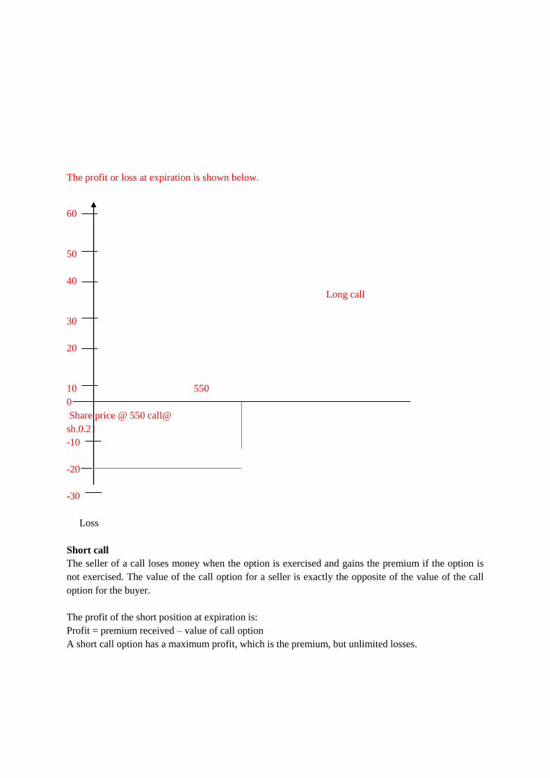
The profit or loss at expiration is shown below.
60
50
40
Long call
30
20
10 550
0
Share price @ 550 call@
sh.0.21
-10
-20
-30
Loss
Short call
The seller of a call loses money when the option is exercised and gains the premium if the option is
not exercised. The value of the call option for a seller is exactly the opposite of the value of the call
option for the buyer.
The profit of the short position at expiration is:
Profit = premium received – value of call option
A short call option has a maximum profit, which is the premium, but unlimited losses.
Page 231
Profiles of put options at expiration
The maximum profit from a long put position and the maximum loss from a short put position occurs
when the price of the underlying becomes zero.
Long put
A put that has been purchased (i.e. a long put) will be exercised at expiration only if the price of the
underlying asset is lower than the exercise price of the option. The value of the option when exercised
is the difference between the exercise price and the value of the underlying.
The profit from a long position is the difference between the value of the option at expiration and the
premium paid.
Short put
The seller of a put loses money when the option is exercised and gains the premium if the option is
not exercised. The value of the put option for a seller is exactly the opposite of the value of the put
option for the buyer.
The profit of the short position at expiration is:
Profit = premium received – value of put option
The maximum profit for the writer of a put option is the premium paid which occurs when the put
option is not exercised (that is, when the value at expiration = 0). This happens when the value of
the underlying at expiration is greater than the exercise price.
The profit will be zero when the value of the underlying at expiration is equal to the sum of the
exercise price and the premium paid.
The highest loss occurs when the value of the underlying = 0. The maximum loss will be equal to
the exercise price.
Determinants of option values
Introduction
Options are financial instruments whose value changes all the time. The value of a call or a put
option at expiration was derived earlier. In this section we shall identify the factors that affect the
price of an option prior to expiration.
The exercise price
The higher the exercise price, the lower the probability that a call will be exercised. So call prices
will decrease as the exercise prices increase. For the put, the effect runs in the opposite direction.
A higher exercise price means that there is higher probability that the put will be exercised. So the
put price increases as the exercise price increases.
The price of the underlying
As the current stock price goes up, there is a higher probability that the call will be in the money. As a
result, the call price will increase. The effect will be in the opposite direction for a put. As the stock
Page 232
price goes up, there is a lower probability that the put will be in the money. So the put price will
decrease.
The volatility of the underlying
Both the call and put will increase in price as the underlying asset becomes more volatile. The buyer
of the option receives full benefit of favourable outcomes but avoids the unfavourable ones (option
price value has zero value).
The time to expiration
Both calls and puts will benefit from increased time to expiration. The reason is that there is more
time for a big move in the stock price. But there are some effects that work in the opposite direction.
As the time to expiration increase, the present value (PV) of the exercise price decreases. This will
increase the value of the call and decrease the value of the put. Also, as the time to expiration
increases, there is a greater amount of time for the stock price to be reduced by a cash dividend. This
reduces the call value but increases the put value.
The interest rate
The higher the interest rate, the lower the PV of the exercise price. As a result, the value of the call
will increase. The opposite is true for puts. The decrease in the PV of the exercise price will adversely
affect the price of the put option.
The intrinsic and time value
The price of an option has two components; intrinsic value and time value. Intrinsic value is the
value of the option if it was exercised now.
Call options: Intrinsic value (at time t) = underlying's current price – call strike price
Put options: Intrinsic value (at time t) = put strike price – underlying's current price.
The difference between the market price of an option and its intrinsic value is the time value of the
option. Buyers of ATM or OTM options are simply buying time value, which decreases as an option
approaches expiration. The more time an option has until expiration, the greater the option's chance
of ending up ITM and the larger its time value. On the expiration day the time value of an option is
zero and all an option is worth is its intrinsic value. It's either ITM, or it isn't.
Using the black Scholes option in pricing model
The black-Scholes model predicts the value of an option for given values of its determinants.
The payoffs at expiration for a call option were derived earlier as:
HINT: If the intrinsic value is positive, the option is in the money (ITM). If the intrinsic value
is zero, the option is at the money (ATM) and if the intrinsic value is negative, the option is out
of the money (OTM).
Page 233
The difference between the value of the underlying at expiration and the exercise price (where
value of underlying > exercise price)
Or:
Zero (where value of underlying ≤ exercise price)
The expected value of the payoff will depend on the probability that the option will be on the money,
which we do not know. The value of the call option today will be the PV of the expected payoff at
expiration. Apart from the probability to be ITM we also need to specify a discount factor, which will
reflect the risk of the option. The problem of option valuation concerned financial specialists for a
long time until Black, Scholes and Merton resolved the problem.
Holding shares in a company is similar to holding a call option because if the debt in the
company exceeds the asset value then the shareholders can walk away (due to limited
liability) whereas if the assets exceed the debts then the shareholders will continue in the
business in order to get the surplus.
Therefore, Black-Scholes may be used to value this ‘option’.
We would use the formula as normal, with
P = The fair value of the firm’s assets
E = Exercise price
r = The risk free rate of interest
t = The time to maturity
σ = The standard deviation of the value of the assets
In valuation of options, we use the Black Scholes Model using Black Scholes Model
Vc = 𝑃𝑁𝑑1 − 𝐸𝑁𝑑2
𝑒𝑟𝑡
Where P = Spot Price/Current Market Price
E = Exercise Price
e = Euler’s Function
Nd1& Nd2 = Normal Distribution probabilities of D1& D2
r = Risk free rate of Return
t = Time in years
Page 234

d1 = 𝐼𝑛 (𝑃
𝐸⁄ )+ [𝑟+ 𝜎2
2⁄ ] 𝑡
𝛿 √𝑡
d2 = d1 - 𝜎 √𝑡
Value of European put options
The value of a European put option can be calculated by using the put call parity relationship which is
given to you in the exam formulae sheet
Put = C – P+ 𝐸
𝑒𝑟𝑡
where C is the value of call option
and P = spot price
E = Exercise price
Value of American call options
Although American options can be exercised any time during their lifetime, it is never
optimal to exercise an option earlier. The value of an American option will therefore
be the same as the value of an equivalent European option and the Black-Scholes
model can be used to calculate its price.
Illustration 1
Consider the situation where the stock price 6 months from the expiration of an option is Sh.42, the
exercise price of the option is Sh.40, the risk-free interest rate is 10% p.a. and the volatility is 20%
p.a. This means P = 42, E = 40, r = 0.1, 𝜎= 0.2, t = 0.5.
𝑑1=𝐿𝑛(
42
40)+(0.1+
0.22
2)0.5
0.2√0.5=0.7693
𝑑2=0.7693-0.2 x √0.5= 0.63
The values of the standard normal cumulative probability distribution N(d1) and N(d2) can be found
from the normal distribution tables which you can find in the Mathematical Tables appendix at the
end of this Study Text.
The text at the bottom of your normal distribution table says:
Note: If d1> 0, add 0.5 to the relevant number above. If d1< 0, subtract the relevant number above
from 0.5.'
d2 = d1 - 𝜎√𝑇
Page 235

So here, because d1 = 0.77, then N (d1) = 0.2794 + 0.5 = 0.7794.
On the same basis, N (d2) = N(0.63) = 0.7357
where the 0.7357 is calculated as 0.2357 from the table + 0.5 (because d2 is a positive number).
Hence if the option is a European call, its value is given by:
c = (42 x 0.7794) – (40 × 0.7357)
1.051= 4.74ert = e0.1x0.5 = e0.05 = 1.051
If the option is a European put, its value is given by:
Put = C – P + 𝐸
𝑒𝑟𝑡 = 4.74 – 42 + 40
1.051 = 0.8
Exam focus
The Black Scholes Option Pricing Model
The formulae that Black and Scholes developed are as follows:
Call option:
c=PN(d1)−𝐸𝑁(𝑑2)
𝑒𝑟𝑡
Where
d1=𝐼𝑛(𝑃/𝐸)+(𝑟+0.5𝜎2)𝑡
𝜎√𝑡
d2 =d1−s √𝑡
Put option:
VP = C – P+ 𝐸
𝑒𝑟𝑡
Where:
VP = value of put option
C = call option value
P = the current share price
E = the exercise price of the option
e = the exponential constant
r = the annual risk free rate of interest
t = the time (in years) until expiry of the option
σ = the share price volatility
N(d) = the probability that a deviation of less than d will occur in a normal distribution.
Illustration 2
Current share price is sh.290.
Page 236

Exercise price sh.260 in 6 months’ time.
Risk free rate of interest is 6% p.a.
Standard deviation of rate of return on share is 40%
Required;-
What is the value of a call option?
Solution
d1=𝐼𝑛(𝑃/𝐸)+(𝑟+0.5𝜎2)𝑇
𝜎√𝑡
d1 = 𝐼𝑛(
290
260)+ (0.06+
0.4
2
2)×0.5
0.4√0.5 = 0.6335
d2 = 0.6335 – 0.4 x √0.5 = 0.3507
n(d1) = 0.5 + 0.2357 = 0.7357
n(d2) = 0.5 + 0.1368 = 0.6368
Option price = Pnd1 – 𝐸𝑛𝑑2
𝑒𝑟𝑡
Option price = 290 x 0.7357 – 260 × 0.6368
𝑒0.06×0.5 = sh.52.7
Illustration 3
Current share price is sh.150
Exercise price sh.180 in 3 months.
Risk free rate of interest is 10% p.a.
Standard deviation of rate of return on share is 40%
Required:
What is the value of a call option?
Solution
d1 = 𝐼𝑛(
150
180)+ (0.1+
0.4
2
2)𝑥 0.25
0.4√0.25 = -0.6866
d2 = -0.6866 – 0.4√0.25 = -0.8866
n(d1) = 0.5 - 0.2549 = 0.2451
n(d2) = 0.5 - 0.3133 = 0.1867
Option price = 150 x 0.2451 – 180 × 0.1867
𝑒0.1×0.25 = 3.989 = 4
The use of options
One use of options is as a way of rewarding managers of a company in a way that motivates them to
increase the share price.
By giving call options to the managers, it becomes very much in their interest to take decisions that
increase the share price.
Very often these options are not traded options and therefore the formula in the previous section can
be used to place a value on them.
Speculators also deal in options. The reason for this is that if (for example) you expect the price of a
share to increase, then you could make money simply by buying shares and then selling them at the
P = 290
E = 260
r = 0.06
σ = 0.4
T = 6/12 = 0.5
Page 237

later, higher, price. As alternative, however, would be to buy call options. As the share price increases
then so too will the option price.
The financial manager is not a speculator. Consider, however, the following situation – the company
currently has an investment in shares in another company. They intend to sell the shares in six months
time, and expect the price to increase. They are however worried in case they are wrong and the price
should fall. How can they protect the company against the possible fall? If the share price were to fall,
then so too would the value of call options. In order to profit out of the fall the company will need to
sell call options now (and would be able to buy them later and make a profit, should the price fall).
This hedging is known as a ‘delta hedge’. The slight problem is that the change in the option price
will not be the same as the change in the share price and therefore we need to be able to calculate how
many options to deal in. We will cover the arithmetic shortly, but first we need to consider the
Greeks!
The Greeks
From day to day the price of an option will change. It will change due to changes in all the factors
discussed above.
Black and Scholes also produced formulae to measure the rate of change in the options price with
changes in each of the factors listed. You do not need to know the formulae, but you need to be aware
of the names given to each of the measures, and they are as follows:
Delta
The rate at which the option price changes with the share price (=N(d1))
Theta
The rate at which the option price changes with the passing of time.
Vega
The rate at which the option price changes with changes in the volatility of the share
Rho
The rate at which the option price changes with changes in the risk-free interest rate
Gamma
The rate at which delta changes
Note: you need to know about the relevance of delta. This is because in the very short term, delta
enables us to predict the effect on the option price of movements in the share price. It will be equal to
N(d1), and we can use it to decide how many options we need to trade in to protect ourselves against
movements in the share price.
The Delta Hedge
If you own shares and you are worried that the share price might fall, then sell some call options. As
the share price falls, so will the value of the options. (You can buy back at a profit).
Page 238

The problem is to decide how many call options we need to sell.
Illustration 4
Current share price is sh.150
Call option exercise price is sh.180 in 3 months
Risk free interest rate is 10% p.a.
Standard deviation of rate of return on share is 40%
Martin owns 1,000 shares.
Devise a delta hedge to protect against change in the share price
Solution
Number of options = number of shares/nd1
N(d1) = 0.2451 (illustration 3 above)
Number of options = 1,000
0.2451 = 4,080
Therefore the investor should sell 4080 options.
Devise a delta hedge to protect against changes in the share price.
The problem with a delta hedge is that our answer to example 4 will only protect us in the very short
term. The reason for this is that over a longer term changes in the other factors will also affect the
option price. For this reason the delta hedge will have to be continuously reviewed and changes made
(which is why the other Greeks are of importance to a trader in options). You will not be expected to
deal with this but you can be expected to be aware of the problem (and therefore of the other Greeks).
Limitations of Black-Scholes Option Pricing Model
1. This model can only apply on European Bonds and not American Bonds
European Bonds would only be expected upon maturity while American Bonds can be exercised
at any time during the option period.
2. It assumes that the markets are perfect such that there are no transaction costs and taxes.
3. It assumes that risk free rate of return is known in advance and remains constant.
4. It assumes that the company does not distribute all its earnings as dividends i.e. No dividends are
paid out.
Exam practice question
Illustration
(a) Briefly discuss the meaning and importance of the following terms as used in option pricing:
(i) Delta
(ii) Theta
(iii) Vega
(iv) Rho
(v) Gamma
(b) Assume that your company has invested in 100,000 shares of Usaidizi Ltd, a manufacturer of
light bulbs. You are concerned about the recent volatility in Usaidizi Ltd share price until winter
in three months time, but do not wish to sell the shares at present.
No dividends are due to the paid by Usaidizi Ltd during the next three months.
Market data:
Page 239
Usaidizi Ltd current share price sh.20
Call option exercise price: sh.22
Time to expiry 3 months
Volatility of Usaidizi Ltd shares 50% (standard deviation per year)
Assume that option contracts are for the purchase or sale of units of 1,000 shares.
Required:
(i)Devise a delta hedge that is expected to protect investment against changes in the share price until
the weather changes. Delta may be estimated using Nd1.
(ii)Comment on whether such hedge is likely to be totally successful.
Answer
Delta = 𝐶ℎ𝑎𝑛𝑔𝑒𝑖𝑛𝐶𝑎𝑙𝑙𝑂𝑝𝑡𝑖𝑜𝑛𝑃𝑟𝑖𝑐𝑒
𝐶ℎ𝑎𝑛𝑔𝑒𝑖𝑛𝑃𝑟𝑖𝑐𝑒𝑜𝑓𝑡ℎ𝑒𝑆ℎ𝑎𝑟𝑒𝑠
This measures the gradient of the option value at any point in time or price point. As the share price
falls towards zero, delta should always falls towards zero. The delta calculation, can be used to
determine the amount of the underlying shares that the writer of the option position should hold in
order to hedge the risk of the option position.
Theta
This represents a change in an options price over time. The time premium element in an option price
will diminish towards zero. Many options have the greatest time premium and thus greatest theta.
Theta can be used to judge how the option price will reduce as maturity approaches.
Vega
This represents the sensitivity of an options price in its implied volatility. It is measured as the change
in the value of an option from a 1% change in its volatility. Long term options have larger Vegas than
short term options.
Rho
This measures sensitivity to the interest rate. It is the derivative of the option value with respect to the
risk price interest rate.
Gamma
This measures the rate of change in delta with respect to changes in the underlying price. All long
options have positive Gamma and vice versa.
Although you will not need the formulae for each of these, you may need to know about
the relevance of delta. This is because in the very short term, delta enables us to predict
Page 240
the effect on the option price of movements in the share price. It will be equal to N(d1),
and we can use it to decide how many options we need to trade in to protect ourselves
against movements in the share price.
6.3. FOREIGN EXCHANGE RISK MANAGEMENT
Globalisation has served to increase the amount of foreign trade, which has in turn increased the
amount of foreign currency transactions that companies have. Any dealings in foreign currency
present the problem of the risk of changes in exchange rates.
Types of risk
(a) Transaction risk
This is the risk that a transaction in a foreign currency at one exchange rate is settled at another rate
(because the rate has changed). It is this risk that the financial manager may attempt to manage and
forms most of the work in the rest of this chapter.
(b) Translation (or accounting) risk
This relates to the exchange profits or losses that result from converting foreign currency balances for
the purposes of preparing the accounts.
These are of less relevance to the financial manager, because they are book entries as opposed to
actual cash flows.
(c) Economic risk
This refers to the change in the present value of future cash flows due to unexpected movements in
foreign exchange rates. E.g. raw material imports increasing in cost.
Exchange rates
The exchange rate on a given day is known as the spot rate and two prices are quoted, depending on
whether we are buying or selling the currency – the difference is known as the spread.
In the examination, the way exchange rates are quoted is always the amount of the first mentioned
currency that is equal to one of the second mentioned currency.
For example, suppose we are given an exchange rate as follows:
$/£ 1.6250 – 1.6310
In this quote, the first number (1.6250) is the exchange rate if we are buying the first mentioned
currency ($’s), and (1.6310) is the rate if we are selling the first mentioned currency ($.’s).
(Alternatively, if you prefer, the first number is the rate at which the bank will sell us $.’s and the
second number the rate at which the bank will buy $.’s from us. It is up to you how you choose to
remember it, but it is vital that you get the arithmetic correct!)
NOTE
Direct and indirect currency quotes
A direct quote is the amount of domestic currency which is equal to one foreign currency unit. For
direct quotes banks buy low and sell high in order to make a profit.
An indirect quote is the amount of foreign currency, which is equal to one domestic currency unit. For
indirect quotes, banks buy high and sell low in order to make a profit.
Bid and offer prices
The bid price is the rate at which the bank is willing to buy currency.
The offer (or ask) price is the rate at which the bank is willing to sell the currency.
If an importer has to pay a foreign supplier in a foreign currency, they might ask their bank to sell
them the required amount of the currency. For example, suppose that a bank’s customer, a Kenyan
trading company, has imported goods for which it must now pay $10,000.
(a) In order to pay the bill, the company must obtain (buy) $10,000 from the bank. In other words, the
bank will sell $10,000 to the company.
Page 241

(b) When the bank agrees to sell $10,000 to the company, it will tell the company what the spot
rate of exchange will be for the transaction. If the bank’s selling rate (know as the ‘offer’ or ‘
ask’ price) is, say, sh.100 per dollar for the currency, the bank will charge the company:
$10,000 x 100sh/$ = sh.1,000,000
If a Kenyan exporting company receives sh.10,000 from a customer , the company will want to
sell the dollars to obtain Kenyan shillings (its home currency ). The bank will therefore buy the
dollars at a quoted bid price. If the bank quotes a bid price of, say, sh.1.99 for the currency the
bank will pay the exporter:
$10,000 x 99 = shs.990,000
Note that the bank buys the dollars for less than it sells them – in other words , it makes a net
profit on the transactions . In this case the net profit is sh.10,000. If you are undecided between
which price is the bid price and which the offer price is, remember that the bank’s customer will
always be offered the worse rate. An exporter will pay a high price for the foreign currency and
an importer will receive a low price . Just think what happens when you buy currency for a
holiday and then sell it back when you come home.
Illustration i– indirect Quotes
If you come back to the UK from a holiday in the US with spare dollars, and you are told the
spread of $/£ rates is 1.8500 – 1.8700, will you have to pay the bank $1.85 or $1.87 to obtain £1?
Solution
You will have to pay the higher price, $1.87 to obtain £1?
The higher rate will be the buying rate since this is an indirect quotation
Illustration II
Calculate how many dollars an exporter would receive or how many dollars an importer would
pay, in each of the following situations, if they were to exchange currency at the spot rate.
(a) A US exporter receives a payment from a Danish customer of 150,000 kroners.
(b) A US importer buys goods from a Japanese supplier and pays 1 million yen.
Danish Kr/$ 9.4240 – 9.5380
Japanese Yen/$ 203.650 – 205.781
Solution
These are indirect quotes and therefore the bank will buy high.
(a) The bank is being asked to buy the Danish kroners and will buy at the higher rate of 9.
5380 kr/$ 150,000
9.5380 = $15,726.57 in exchange
(b) The bank is being asked to sell the yen to the importer and will charge for the currency: 1,000,000
203.650 = $4,910.39
Illustration 3
A ltd, a UK based company, receives $100,000 from a customer in the US.
The exchange rate is $/£ 1.6250 – 1.6310.
How many £’s will A plc receive?
This is an indirect quote and therefore the bank will
sell low in order to make a profit.
Page 242
Solution
This is an indirect quote and therefore the bank will buy at a higher rate.
$.100,000 ÷ 1.6310 = £61,312
Illustration 4
Jimjam is a company based in India, where the currency is the Indian Rupee (IR). They owe money to
a supplier in Ruritania, where the currency is Ruritanian Dollars (R$.). The amount owing is R$.
240,000.
The current exchange rate is IR/R$. 8.6380 – 9.2530
How many Indian Rupees will Jimjam have to pay?
Solution
8.6380 – 9.2530 IR/R
240,000 ×9.2530 = IR 2,220,720
This is an indirect quote and therefore the bank will sell at a higher rate.
Hedging techniques
Internal hedging techniques include leading and lagging, invoicing in home currency, matching.
Leading and lagging
Leading involves accelerating payments to avoid potential additional costs due to currency rate
movements.
Lagging is the practice of delaying payments if currency rate movements are expected to make the
later payment cheaper.
Companies might try to use lead payments (payments in advance) or lagged payments (delayed
payments) in order to take advantage of foreign rate movements.
Illustration
Williams Ltd-a company based in the US – imports goods from the UK. The company is due to make
a payment of £500,000 to a UK supplier in two month’s time. The current exchange rate is as follows.
£0.6450 = $1
(a) If the dollar is expected to appreciate against sterling by 2% in the next month and by a further
1% in the second month, what would be Williams Ltd strategy in terms of leading and lagging
and by how much would the company benefit from this strategy?
(b) If the dollar was to depreciate against sterling by 2% in the next month and by a further 1% in the
second month, how would Williams Ltd strategy probably change and what would the resulting
benefit be?
Solution
NOTE: Williams can either pay at the end of the
first month or second month
Page 243
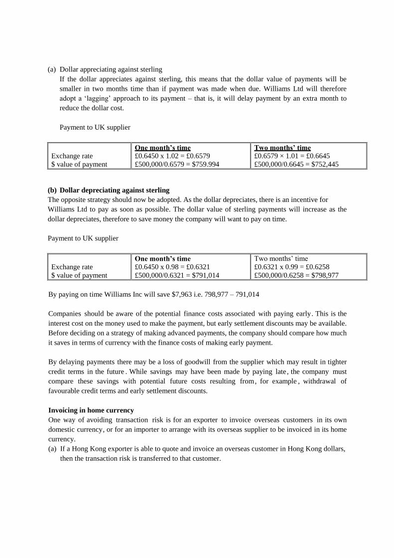
(a) Dollar appreciating against sterling
If the dollar appreciates against sterling, this means that the dollar value of payments will be
smaller in two months time than if payment was made when due. Williams Ltd will therefore
adopt a ‘lagging’ approach to its payment – that is, it will delay payment by an extra month to
reduce the dollar cost.
Payment to UK supplier
Exchange rate
$ value of payment
One month’s time
£0.6450 x 1.02 = £0.6579
£500,000/0.6579 = $759.994
Two months’ time
£0.6579 × 1.01 = £0.6645
£500,000/0.6645 = $752,445
(b) Dollar depreciating against sterling
The opposite strategy should now be adopted. As the dollar depreciates, there is an incentive for
Williams Ltd to pay as soon as possible. The dollar value of sterling payments will increase as the
dollar depreciates, therefore to save money the company will want to pay on time.
Payment to UK supplier
Exchange rate
$ value of payment
One month’s time
£0.6450 x 0.98 = £0.6321
£500,000/0.6321 = $791,014
Two months’ time
£0.6321 x 0.99 = £0.6258
£500,000/0.6258 = $798,977
By paying on time Williams Inc will save $7,963 i.e. 798,977 – 791,014
Companies should be aware of the potential finance costs associated with paying early. This is the
interest cost on the money used to make the payment, but early settlement discounts may be available.
Before deciding on a strategy of making advanced payments, the company should compare how much
it saves in terms of currency with the finance costs of making early payment.
By delaying payments there may be a loss of goodwill from the supplier which may result in tighter
credit terms in the future . While savings may have been made by paying late , the company must
compare these savings with potential future costs resulting from, for example , withdrawal of
favourable credit terms and early settlement discounts.
Invoicing in home currency
One way of avoiding transaction risk is for an exporter to invoice overseas customers in its own
domestic currency, or for an importer to arrange with its overseas supplier to be invoiced in its home
currency.
(a) If a Hong Kong exporter is able to quote and invoice an overseas customer in Hong Kong dollars,
then the transaction risk is transferred to that customer.
Page 244
(b) If a Hong Kong importer is able to arrange with its overseas supplier to be invoiced in Hong Kong
dollars, then the transaction risk is transferred to that supplier.
Matching receipts and payments
A company can reduce or eliminate its transaction risk exposure by matching receipts and payments.
Wherever possible, a company that expects to make payments and have receipts in the same foreign
currency should plan to offset its payments against its receipts in that currency. The process of
matching is made simpler by having foreign currency accounts with a bank.
Offsetting (matching payments against receipts) will be cheaper than arranging a forward contract to
buy currency and another forward contract to sell the currency, provided that:
Receipts occur before payments
The time difference between receipts and payments in the currency is not too long
Any differences between the amounts receivable and the amounts payable in a given currency may be
covered by a forward exchange contract (covered later in this chapter) to buy or sell the amount of the
difference.
Management of barriers
An overseas government may place restrictions on remittances. This means that the amount of profit
that can be sent back to the parent company is limited. This may be achieved through exchange
controls or limits on the amounts that can be remitted. These barriers can be avoided/mitigated by the
following methods.
(a) Charge overseas subsidiary companies additional head office overhead charges.
(b) Subsidiary companies can lend the equivalent of the dividend to the parent company.
(c) Subsidiary companies can make payments to the parent company in the form of royalties, patents,
management fees or other charges.
(d) Increase the transfer prices paid by the subsidiary to the parent company
(e) The overseas subsidiary can lend money to another subsidiary requiring funds in the same
country. In return the parent company will receive the loan amount in the home country from the
other parent company. This method is sometimes known as parallel loans.
Foreign governments may put measures in place to stop the above methods being used.
Forward contracts
What is a forward contract?
A forward exchange contract is:
(a) An immediately firm and binding contract, e.g. between a bank and its customer which must be
exercised regardless of the spot rate at the time of exercise
(b) For the purchase or sale of a specified quantity of a stated foreign currency
(c) At a rate of exchange fixed at the time the contract is made
(d) For performance (delivery of the currency and payment for it) at a future time which is agreed
when making the contract (this future time will be either a specified date, or any time between
two specified dates)
Page 245
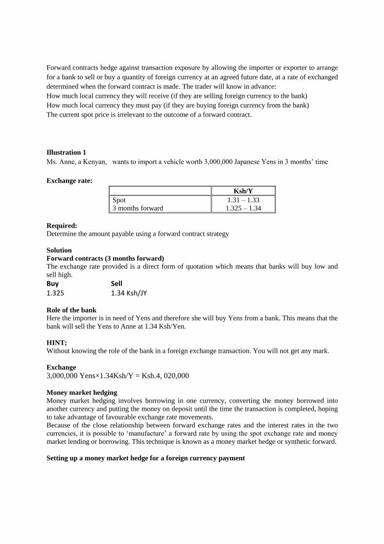
Forward contracts hedge against transaction exposure by allowing the importer or exporter to arrange
for a bank to sell or buy a quantity of foreign currency at an agreed future date, at a rate of exchanged
determined when the forward contract is made. The trader will know in advance:
How much local currency they will receive (if they are selling foreign currency to the bank)
How much local currency they must pay (if they are buying foreign currency from the bank)
The current spot price is irrelevant to the outcome of a forward contract.
Illustration 1
Ms. Anne, a Kenyan, wants to import a vehicle worth 3,000,000 Japanese Yens in 3 months’ time
Exchange rate:
Ksh/Y
Spot
3 months forward
1.31 – 1.33
1.325 – 1.34
Required: Determine the amount payable using a forward contract strategy
Solution
Forward contracts (3 months forward)
The exchange rate provided is a direct form of quotation which means that banks will buy low and
sell high.
Buy Sell 1.325 1.34 Ksh/JY
Role of the bank
Here the importer is in need of Yens and therefore she will buy Yens from a bank. This means that the
bank will sell the Yens to Anne at 1.34 Ksh/Yen.
HINT;
Without knowing the role of the bank in a foreign exchange transaction. You will not get any mark.
Exchange
3,000,000 Yens×1.34Ksh/Y = Ksh.4, 020,000
Money market hedging
Money market hedging involves borrowing in one currency, converting the money borrowed into
another currency and putting the money on deposit until the time the transaction is completed, hoping
to take advantage of favourable exchange rate movements.
Because of the close relationship between forward exchange rates and the interest rates in the two
currencies, it is possible to ‘manufacture’ a forward rate by using the spot exchange rate and money
market lending or borrowing. This technique is known as a money market hedge or synthetic forward.
Setting up a money market hedge for a foreign currency payment
Page 246
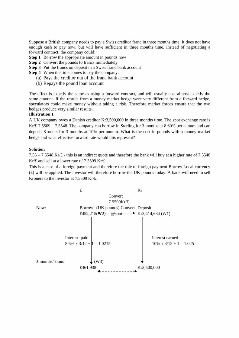
Suppose a British company needs to pay a Swiss creditor franc in three months time. It does not have
enough cash to pay now, but will have sufficient in three months time, instead of negotiating a
forward contract, the company could:
Step 1 Borrow the appropriate amount in pounds now
Step 2 Convert the pounds to francs immediately
Step 3 Put the francs on deposit in a Swiss franc bank account
Step 4 When the time comes to pay the company:
(a) Pays the creditor out of the franc bank account
(b) Repays the pound loan account
The effect is exactly the same as using a forward contract, and will usually cost almost exactly the
same amount. If the results from a money market hedge were very different from a forward hedge,
speculators could make money without taking a risk. Therefore market forces ensure that the two
hedges produce very similar results.
Illustration 1
A UK company owes a Danish creditor Kr3,500,000 in three months time. The spot exchange rate is
Kr/£ 7.5509 – 7.5548. The company can borrow in Sterling for 3 months at 8.60% per annum and can
deposit Kroners for 3 months at 10% per annum. What is the cost in pounds with a money market
hedge and what effective forward rate would this represent?
Solution
7.55 – 7.5548 Kr/£ - this is an indirect quote and therefore the bank will buy at a higher rate of 7.5548
Kr/£ and sell at a lower rate of 7.5509 Kr/£.
This is a case of a foreign payment and therefore the rule of foreign payment Borrow Local currency
(£) will be applied. The investor will therefore borrow the UK pounds today. A bank will need to sell
Kroners to the investor at 7.5509 Kr/£.
£ Kr
Convert
7.5509Kr/£
Now: Borrow (UK pounds) Convert Deposit
£452,215(W2) @spot Kr3,414,634 (W1)
Interest paid Interest earned
8.6% x 3/12 + 1 = 1.0215 10% x 3/12 + 1 = 1.025
3 months’ time: (W3)
£461,938 Kr3,500,000
Page 247

W1= 3,500,000
1.025 = Kr/£ 3414634
W2 = 3414634
7.5509 = £452,215
W3 = 452,215 (1.0215) = £461,938
Setting up a money market hedge for a foreign currency receipt
A similar technique can be used to cover a foreign currency receipt from a debtor. To manufacture a
forward exchange rate, follow the steps below:
Step 1 Borrow an appropriate amount in the foreign currency today
Step 2 Convert it immediately to home currency
Step 3 Place it on deposit in the home currency
Step 4 When the debtor’s cash is received:
(a) Repay the foreign currency loan
(b) Take the cash from the home currency deposit account
Illustration 2
A UK company owed SFr 2,500,000 in three months time by a Swiss company. The spot exchange
rate is SFr/£2.2498 – 2.2510. The company can deposit in Sterling for 3 months at 8.00% per annum
and can borrow Swiss Francs for 3 months at 7.00% per annum. What is the receipt in pounds with a
money market hedge and what effective forward rate would this represent?
Answer
2.2498 – 2.2510SFR/£
This is an indirect quote and therefore bank will buy high and sell low. The bank will buy at 2.2510
SFR/£ since this is a foreign receipt the investor will borrow a foreign denominated loan i.e. a loan
denominated in SFR.
S Fr £
Convert
7.5509
Now: Borrow convert Deposit
S Fr 2,457,003 @spot £1,091,516
2.2510 SFR/£
Interest paid Interest earned
7% x 3/12 + 1 = 1.0175 8% x 3/12 + 1 = 1.02
3 months’ time:
S Fr £1,113,546
2,500,000
Page 248
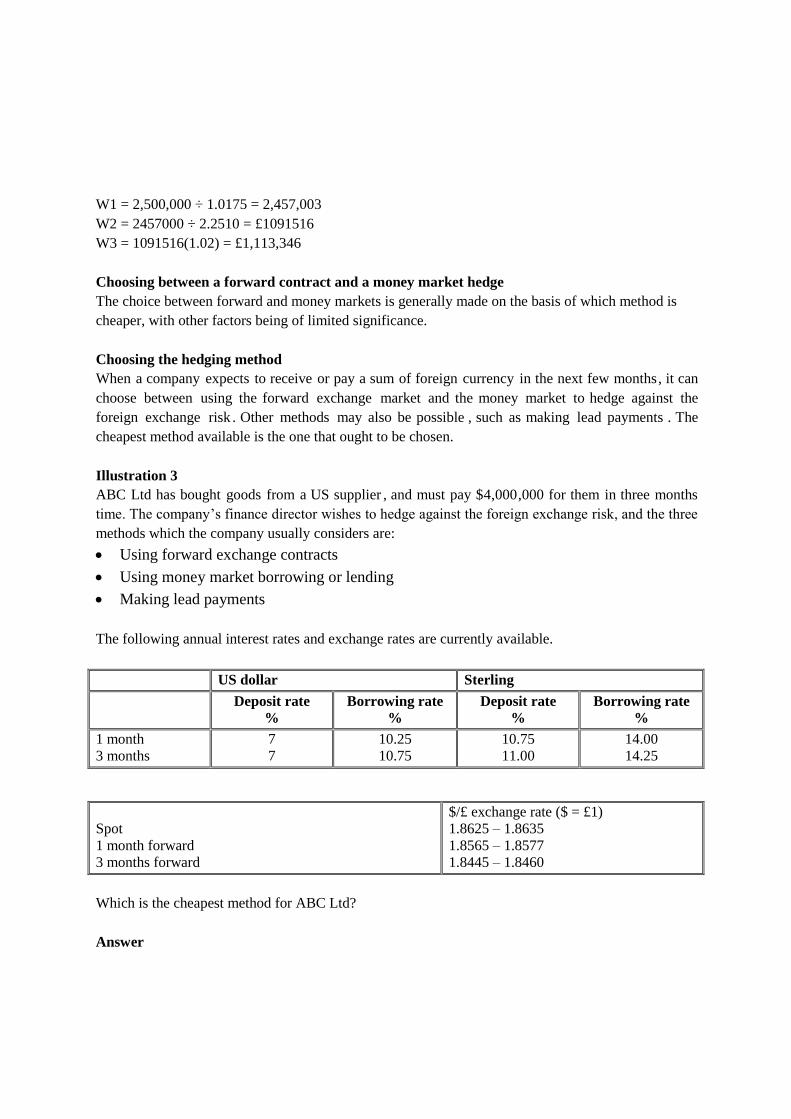
W1 = 2,500,000 ÷ 1.0175 = 2,457,003
W2 = 2457000 ÷ 2.2510 = £1091516
W3 = 1091516(1.02) = £1,113,346
Choosing between a forward contract and a money market hedge
The choice between forward and money markets is generally made on the basis of which method is
cheaper, with other factors being of limited significance.
Choosing the hedging method
When a company expects to receive or pay a sum of foreign currency in the next few months, it can
choose between using the forward exchange market and the money market to hedge against the
foreign exchange risk . Other methods may also be possible , such as making lead payments . The
cheapest method available is the one that ought to be chosen.
Illustration 3
ABC Ltd has bought goods from a US supplier , and must pay $4,000,000 for them in three months
time. The company’s finance director wishes to hedge against the foreign exchange risk, and the three
methods which the company usually considers are:
Using forward exchange contracts
Using money market borrowing or lending
Making lead payments
The following annual interest rates and exchange rates are currently available.
US dollar Sterling
Deposit rate
%
Borrowing rate
%
Deposit rate
%
Borrowing rate
%
1 month
3 months
7
7
10.25
10.75
10.75
11.00
14.00
14.25
Spot
1 month forward
3 months forward
$/£ exchange rate ($ = £1)
1.8625 – 1.8635
1.8565 – 1.8577
1.8445 – 1.8460
Which is the cheapest method for ABC Ltd?
Answer
Page 249
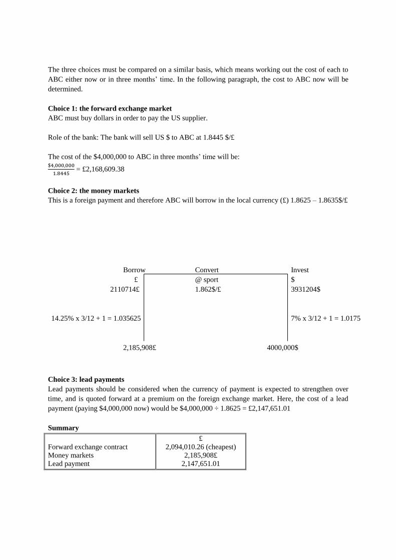
The three choices must be compared on a similar basis, which means working out the cost of each to
ABC either now or in three months’ time. In the following paragraph, the cost to ABC now will be
determined.
Choice 1: the forward exchange market
ABC must buy dollars in order to pay the US supplier.
Role of the bank: The bank will sell US $ to ABC at 1.8445 $/£
The cost of the $4,000,000 to ABC in three months’ time will be: $4,000,000
1.8445 = £2,168,609.38
Choice 2: the money markets
This is a foreign payment and therefore ABC will borrow in the local currency (£) 1.8625 – 1.8635$/£
Choice 3: lead payments
Lead payments should be considered when the currency of payment is expected to strengthen over
time, and is quoted forward at a premium on the foreign exchange market. Here, the cost of a lead
payment (paying $4,000,000 now) would be $4,000,000 ÷ 1.8625 = £2,147,651.01
Summary
Forward exchange contract
Money markets
Lead payment
£
2,094,010.26 (cheapest)
2,185,908£
2,147,651.01
Borrow Convert Invest
£ @ sport $
2110714£ 1.862$/£ 3931204$
14.25% x 3/12 + 1 = 1.035625 7% x 3/12 + 1 = 1.0175
2,185,908£ 4000,000$
Page 250
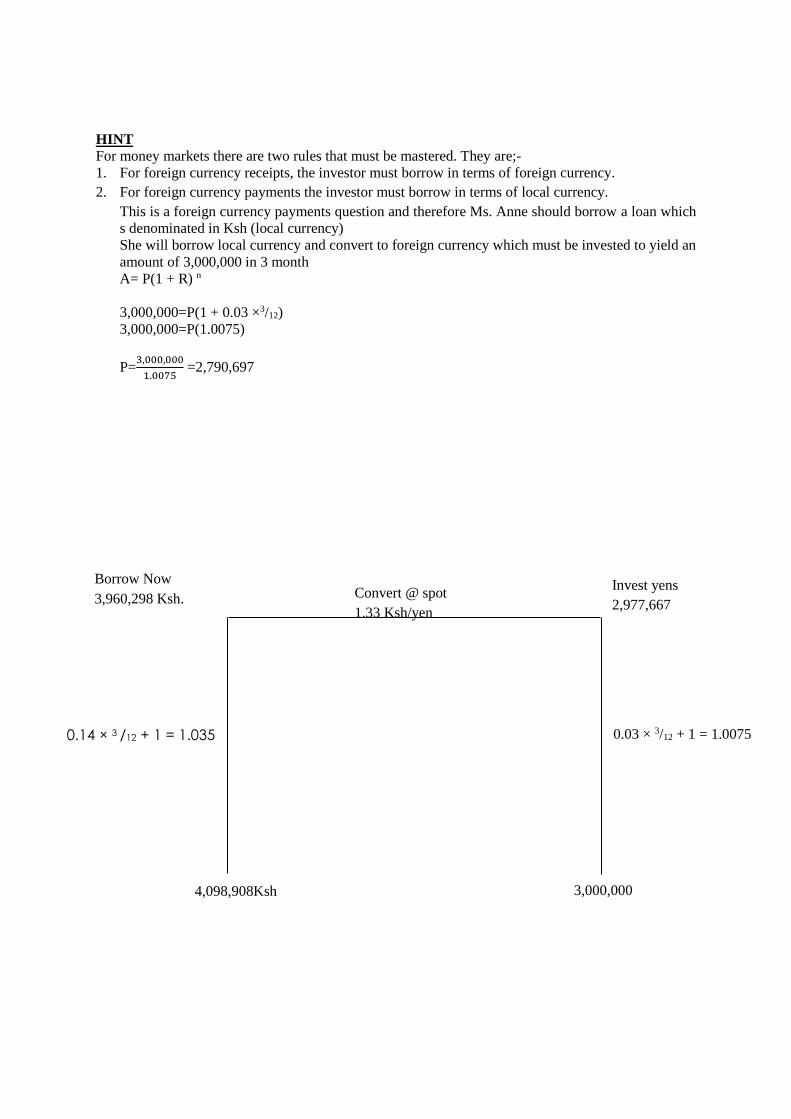
HINT
For money markets there are two rules that must be mastered. They are;-
1. For foreign currency receipts, the investor must borrow in terms of foreign currency.
2. For foreign currency payments the investor must borrow in terms of local currency.
This is a foreign currency payments question and therefore Ms. Anne should borrow a loan which
s denominated in Ksh (local currency)
She will borrow local currency and convert to foreign currency which must be invested to yield an
amount of 3,000,000 in 3 month
A= P(1 + R) n
3,000,000=P(1 + 0.03 ×3/12)
3,000,000=P(1.0075)
P=3,000,000
1.0075 =2,790,697
4,098,908Ksh
3,000,000
0.03 × 3/12 + 1 = 1.0075 0.14 × 3 /12 + 1 = 1.035
Borrow Now
3,960,298 Ksh. Convert @ spot
1.33 Ksh/yen
Invest yens
2,977,667
Page 251
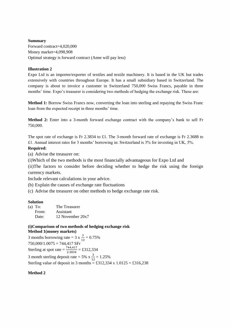
Summary
Forward contract=4,020,000
Money market=4,098,908
Optimal strategy is forward contract (Anne will pay less)
Illustration 2
Expo Ltd is an importer/exporter of textiles and textile machinery. It is based in the UK but trades
extensively with countries throughout Europe. It has a small subsidiary based in Switzerland. The
company is about to invoice a customer in Switzerland 750,000 Swiss Francs, payable in three
months’ time. Expo’s treasurer is considering two methods of hedging the exchange risk. These are:
Method 1: Borrow Swiss Francs now, converting the loan into sterling and repaying the Swiss Franc
loan from the expected receipt in three months’ time.
Method 2: Enter into a 3-month forward exchange contract with the company’s bank to sell Fr
750,000.
The spot rate of exchange is Fr 2.3834 to £1. The 3-month forward rate of exchange is Fr 2.3688 to
£1. Annual interest rates for 3 months’ borrowing in: Switzerland is 3% for investing in UK, 5%.
Required:
(a) Advise the treasurer on:
(i)Which of the two methods is the most financially advantageous for Expo Ltd and
(ii)The factors to consider before deciding whether to hedge the risk using the foreign
currency markets.
Include relevant calculations in your advice.
(b) Explain the causes of exchange rate fluctuations
(c) Advise the treasurer on other methods to hedge exchange rate risk.
Solution
(a) To: The Treasurer
From: Assistant
Date: 12 November 20x7
(i)Comparison of two methods of hedging exchange risk
Method 1(money markets)
3 months borrowing rate = 3 x 3
12 = 0.75%
750,000/1.0075 = 744,417 SFr
Sterling at spot rate = 744,417
2.3834 = £312,334
3 month sterling deposit rate = 5% x 3
12 = 1.25%
Sterling value of deposit in 3 months = £312,334 x 1.0125 = £316,238
Method 2
Page 252
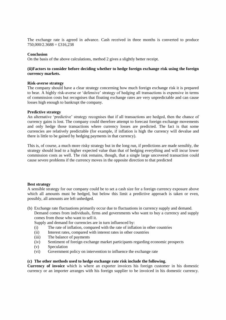
The exchange rate is agreed in advance. Cash received in three months is converted to produce
750,000/2.3688 = £316,238
Conclusion
On the basis of the above calculations, method 2 gives a slightly better receipt.
(ii)Factors to consider before deciding whether to hedge foreign exchange risk using the foreign
currency markets.
Risk-averse strategy
The company should have a clear strategy concerning how much foreign exchange risk it is prepared
to bear. A highly risk-averse or ‘defensive’ strategy of hedging all transactions is expensive in terms
of commission costs but recognises that floating exchange rates are very unpredictable and can cause
losses high enough to bankrupt the company.
Predictive strategy
An alternative ‘predictive’ strategy recognises that if all transactions are hedged, then the chance of
currency gains is lost. The company could therefore attempt to forecast foreign exchange movements
and only hedge those transactions where currency losses are predicted. The fact is that some
currencies are relatively predictable (for example, if inflation is high the currency will devalue and
there is little to be gained by hedging payments in that currency).
This is, of course, a much more risky strategy but in the long run, if predictions are made sensibly, the
strategy should lead to a higher expected value than that of hedging everything and will incur lower
commission costs as well. The risk remains, though, that a single large uncovered transaction could
cause severe problems if the currency moves in the opposite direction to that predicted
Best strategy
A sensible strategy for our company could be to set a cash size for a foreign currency exposure above
which all amounts must be hedged, but below this limit a predictive approach is taken or even,
possibly, all amounts are left unhedged.
(b) Exchange rate fluctuations primarily occur due to fluctuations in currency supply and demand.
Demand comes from individuals, firms and governments who want to buy a currency and supply
comes from those who want to sell it.
Supply and demand for currencies are in turn influenced by:
(i) The rate of inflation, compared with the rate of inflation in other countries
(ii) Interest rates, compared with interest rates in other countries
(iii) The balance of payments
(iv) Sentiment of foreign exchange market participants regarding economic prospects
(v) Speculation
(vi) Government policy on intervention to influence the exchange rate
(c) The other methods used to hedge exchange rate risk include the following.
Currency of invoice which is where an exporter invoices his foreign customer in his domestic
currency or an importer arranges with his foreign supplier to be invoiced in his domestic currency.
Page 253
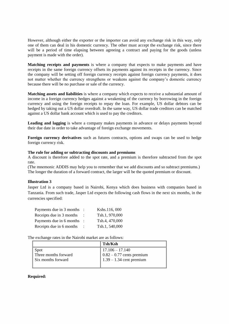
However, although either the exporter or the importer can avoid any exchange risk in this way, only
one of them can deal in his domestic currency. The other must accept the exchange risk, since there
will be a period of time elapsing between agreeing a contract and paying for the goods (unless
payment is made with the order).
Matching receipts and payments is where a company that expects to make payments and have
receipts in the same foreign currency offsets its payments against its receipts in the currency. Since
the company will be setting off foreign currency receipts against foreign currency payments, it does
not matter whether the currency strengthens or weakens against the company’s domestic currency
because there will be no purchase or sale of the currency.
Matching assets and liabilities is where a company which expects to receive a substantial amount of
income in a foreign currency hedges against a weakening of the currency by borrowing in the foreign
currency and using the foreign receipts to repay the loan. For example, US dollar debtors can be
hedged by taking out a US dollar overdraft. In the same way, US dollar trade creditors can be matched
against a US dollar bank account which is used to pay the creditors.
Leading and lagging is where a company makes payments in advance or delays payments beyond
their due date in order to take advantage of foreign exchange movements.
Foreign currency derivatives such as futures contracts, options and swaps can be used to hedge
foreign currency risk.
The rule for adding or subtracting discounts and premiums
A discount is therefore added to the spot rate, and a premium is therefore subtracted from the spot
rate.
(The mnemonic ADDIS may help you to remember that we add discounts and so subtract premiums.)
The longer the duration of a forward contract, the larger will be the quoted premium or discount.
Illustration 3
Jasper Ltd is a company based in Nairobi, Kenya which does business with companies based in
Tanzania. From such trade, Jasper Ltd expects the following cash flows in the next six months, in the
currencies specified:
Payments due in 3 months : Kshs.116, 000
Receipts due in 3 months : Tsh.1, 970,000
Payments due in 6 months : Tsh.4, 470,000
Receipts due in 6 months : Tsh.1, 540,000
The exchange rates in the Nairobi market are as follows:
Tsh/Ksh
Spot
Three months forward
Six months forward
17.106 – 17.140
0.82 – 0.77 cents premium
1.39 – 1.34 cent premium
Required:
Page 254
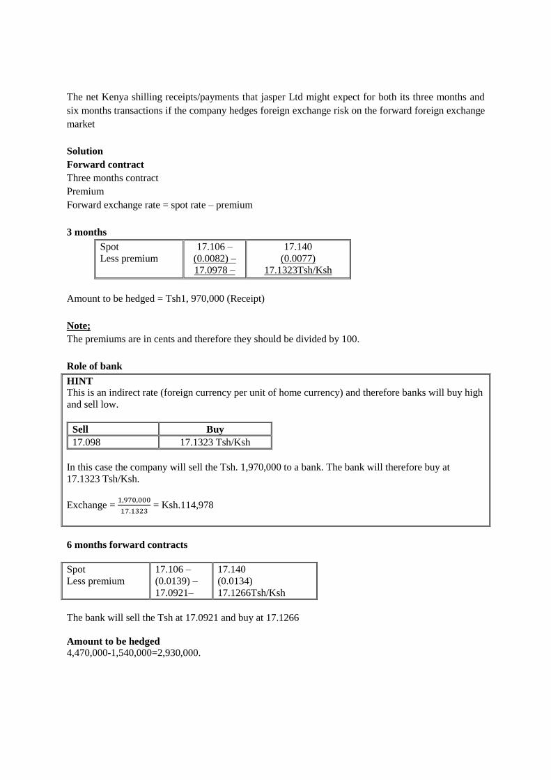
The net Kenya shilling receipts/payments that jasper Ltd might expect for both its three months and
six months transactions if the company hedges foreign exchange risk on the forward foreign exchange
market
Solution
Forward contract
Three months contract
Premium
Forward exchange rate = spot rate – premium
3 months
Spot
Less premium
17.106 –
(0.0082) –
17.0978 –
17.140
(0.0077)
17.1323Tsh/Ksh
Amount to be hedged = Tsh1, 970,000 (Receipt)
Note;
The premiums are in cents and therefore they should be divided by 100.
Role of bank
HINT
This is an indirect rate (foreign currency per unit of home currency) and therefore banks will buy high
and sell low.
Sell Buy
17.098 17.1323 Tsh/Ksh
In this case the company will sell the Tsh. 1,970,000 to a bank. The bank will therefore buy at
17.1323 Tsh/Ksh.
Exchange = 1,970,000
17.1323 = Ksh.114,978
6 months forward contracts
Spot
Less premium
17.106 –
(0.0139) –
17.0921–
17.140
(0.0134)
17.1266Tsh/Ksh
The bank will sell the Tsh at 17.0921 and buy at 17.1266
Amount to be hedged
4,470,000-1,540,000=2,930,000.
Page 255

Role of bank
HINT
Since the Kenyan investor is in need of the above Tsh to meet the obligation, he has to get them from
a bank and therefore the bank will be selling them at 17.0921 Tsh/Ksh.
The bank will sell @ 17.0921 Tsh/Ksh.
Exchange = 2,930,000
17.0921 = Ksh.171,424
For foreign receipts borrow foreign (Tsh)
Illustration 3
A UK company is due to pay $200,000 in 1 month’s time.
Spot $/£ 1.4820 – 1.4905
1 month forward $/£ 1.4910 – 1.4970
If X contracts 1 month forward, how much will it have to pay in 1 months time (in £’s)?
Solution
1.4910 – 1.4970 $/£
200,000 ÷ 1.4910 = £134,138
Therefore the bank will sell at 1.4910 $/£
More often, forward rates are quoted as difference from spot. The difference is expressed in the
smaller units of currency (e.g. cents, in the case of the US), and is expressed as a premium or a
discount depending on whether we should deduct or add the discount to the spot rate.
Illustration 4
A UK firm is due to receive $150,000 in 3 months’ time.
Spot $/£ 1.5326 – 1.5385
3m forward 0.62 – 0.51 cents premium
How much will Y receive?
Answer
Premium is always subtracted from the spot rate
Forward rate = 1.5385 – 0.0051 = 1.5334
150,000 ÷ 1.5334 = £97,822
Illustration 5
A US company is due to pay $200,000 in 2 months time.
Spot $./£ 1.6582 – 1.6623
2m forward 0.83 – 0.92 cents discount
How much will Z pay?
The quote given is an indirect
quote and therefore the Bank
will buy the 150,000$ at a higher
rate of 1.5385 less 0.51 cents
premium.
Page 256
Divide the cents by i.e. to convert them to dollars
Add the discount to the spot rate to convert it to the forward rate.
Solution
Since the US Company is in need of UK £ the Bank will sell the £ to the company at 1.6623 +
0.92/100 = 1.6715$/£
200,000 ÷ 1.6715 = 119,653£
Money market hedging
This approach involves converting the foreign currency at the current spot, which therefore makes
future changes in the exchange rate irrelevant. However, if we are (for example) not going to receive
the foreign currency for 3 months, then how can we convert the money today? The answer is that we
borrow foreign currency now at fixed interest, on the strength of the future receipt.
Currency futures
A currency future is a standardized contract to buy or sell a fixed amount of currency at a fixed rate at
a fixed future date.
Buying the futures contract means receiving the contract currency.
Selling the futures contract means supplying the contract currency.
Features of currency futures
Futures are standardized contracts that are traded on an organized exchange, such as the Chicago
Mercantile Exchange and London International Financial Futures and Options Exchange. They fix the
exchange rate for a set amount of currency for a specified time period.
When entering into a foreign exchange futures contract, no one is actually buying or selling anything
– the participants are agreeing to buy or sell currencies on pre-agreed terms at a specified future date
if the contract is allowed to reach maturity, which it rarely does. Futures are a derivative (their value
derives from movements in the spot rate).
Futures are generally more liquid and have less credit risk than forward contracts, as organized
exchanges have clearing houses that guarantee that all traders in the futures market will honour their
obligations.
Futures contracts are assumed to mature at the end of either March, June, September or December.
One of their limitations is that currencies can only be bought or sold on exchanges for US dollars.
EXAM FOCUS AREA
Buy 1.6582 – Sell 1.6623 $/£
Page 257
If we buy a sterling futures contract it is a binding contract to buy pounds at a fixed rate on a fixed
date. This is similar to a forward rate, but there are two major differences:
1) delivery dates for futures contracts occur only on 4 dates a year – the ends of March,
June, September and December.
2) futures contracts are traded and can be bought and sold from / to others during the period
up to the delivery date.
For these two reasons, most futures contracts are sold before the delivery date – speculators use them
as a way of gambling on exchange rates. They buy at one price and sell later – hopefully at a higher
price. To buy futures does not involve paying the full price – the speculator gives a deposit (called the
margin) and later when the future is sold the margin is returned plus any profit on the deal or less and
loss. The deal must be completed by the delivery date at the latest. In this way it is possible to gamble
on an increase in the exchange rate. However, it is also possible to make a profit if the exchange rate
falls! To do this the speculator will sell a future at today’s price (even though he has nothing to sell)
and then buy back later at a (hopefully) lower price. Again, at the start of the deal he has to put
forward a margin which is returned at the end of the deal plus any profit and less any loss.
The role of the financial manager is not to speculate with the company’s cash, but he can make use of
a futures deal in order to ‘cancel’ (or hedge against) the risk of a commercial transaction.
Illustration 1
R is in the US and needs £800,000 on 10 August.
Spot today (12 June) is: $/£ 1.5526 – 1.5631
September $/£ futures are available. The price today (12 June) is 1.5580.
Show the outcome of using a futures hedge (assuming that the spot and the futures prices both
increase by 0.02).
Solution
If converted at spot on 10 August:
800,000 × 1.5631 = $1,250,480
In 3 months time, spot = 1.5726 – 1.5831(0.02 added to the spot)
futures: 1.5780 (= 1.5580 + 0.02)
Underlying transaction at spot:
800,000 × 1.5831 = $1,266,480
Profits on futures
800,000 × (1.5780 – 1.5580) = 16,000
Net payments $1,250,480
Page 258

Note:
1) The futures price on any day is not the same as the spot exchange rate on that date. They are two
different things and the futures prices are quoted on the futures exchanges. More importantly, the
movement in the futures price over a period is unlikely to be exactly the same as the movement in
the actual exchange rate. The futures market is efficient and prices do move very much in line
with exchange rates, but the movements are not the same (unlike in the simple example above).
We will illustrate the effect of this shortly.
2) In practice any deal in futures must be in units of a fixed size (you will be given the size in the
examination). It is therefore not always possible to enter into a deal of precisely the same amount
as the underlying transaction whose risk we are trying to hedge against.
ILLUSTRATION 2
It is 10 September 2004.
T plc expects to receive $1,200,000, on 12 November 2004
The spot rate (on 10 September) is $/£ 1.5020 – 1.5110
Futures prices (on 10 September) are:
$./£ (£62,500) contracts.
September 1.5035
December 1.5045
March 1.5054
On 12 November 2004:
Spot: $./£ 1.5100 – 1.5190
December futures: 1.5120
Show the outcome of the futures hedge.
Solution
Futures: BUY
December (at 1.5045)
Number of contracts = 1,200,000 ÷ 1.5045 ÷ 62,500 = 13
On 10 September:
Underlying transaction at spot:
1,200,000 ÷ 1.5190 (mote 1) £789,993
Profits on futures
13 × £62,500 × (1.5120 – 1.5045) = $6,094 ÷ 1.5190 (note 2) 4,012
Net receipt = £789,993 + 4012 £794,005
Notes:
Note 1: The company will receive $ and sell them to bank. The bank will buy at 1.5190$/£
Note 2: The profit on futures is dollars which will be sold to a bank at the prevailing rate therefore the
bank will sell them at `.5`90$/£.
Page 259

Ticks
The price of a currency future moves in ticks. A tick is the smallest movement in the exchange rate
and is normally four decimal places.
Tick value = size of futures contract x tick size
For example, if a futures contract is for £62,500 and the tick size is $0.0001, the tick value is $6.25.
(Note that the tick size and tick value are always quoted in US dollars).
What this means is that for every $0.0001 movement in the price, the company will make a profit or
loss of $6.25. if the exchange rate moves by $0.004 in the company’s favour – which is 40 ticks
(0.004/0.0001) – the profit made will be 40 x $6.25 = $250 per contract.
Example of futures contract specifications-including tick size and tick value-are given below
Currency Contract size Price quotation Tick size Tick value per
contract
British pound £62,500 US$/£1 $0.0001 $6.25
Canadian dollar C$100,000 US$/C$1 $0.0001 $10.00
Euro €125,00 US$€1 $0.0001 $12.50
Japanese yen ¥12,500,000 US$/¥100 $0.000001 $12.50
Swiss franc SFr125,000 US$/SFr1 $0.0001 $12.50
Australian dollar A$100,000 US$/A$1 $0.0001 $12.50
You will usually be given the contract size in the exam.
Basic risk
Basis risk is the risk that the price of a currency future will vary from the price of the underlying asset
(the spot rate).
Basis is the difference between the spot and the futures price.
Basis risk is the risk that the price of a futures contract will vary from the spot rate as expiry of the
contract approaches. It is assumed that the difference between the spot rate and futures price (the
basis) falls over time but there is a risk that basis will not decrease in this predictable way (which will
create an imperfect hedge). There is no basis risk when a contract is held to maturity.
In order to manage basis risk it is important to choose a currency future with the closest maturity date
to the actual transaction. This reduces the unexpired basis when the transaction is closed out.
Margins and marking to market
There are two types of margin – initial margin and variation margin
Page 260
An initial margin is similar to a deposit. When a currency futures is set up, the company would be
required to deposit some cash (the initial margin) with the futures exchange in a margin account – this
acts as security against the company defaulting on its trading obligations. This money will remain in
the margin account as long as the currency futures remain open.
We mentioned above the process of calculating the profit or loss on a contract when there is
movement in the exchange rate. This profit or loss is received into or paid from the margin account on
a daily basis rather than in one large amount when the contract matures. This procedure is known as
marking to market.
The futures exchange monitors the margin account on a daily basis. The company will be required to
maintain a minimum balance on its margin account this is called a ‘maintenance margin’. If the
company is making significant losses so that the company’s balance on their margin account drops
beneath the maintenance margin then extra funds will be demanded by the futures exchange. The
demand for extra payment is called a ‘margin call’ and the extra payment is called a ‘variation
margin’. This practice creates uncertainty, as the company will not know in advance the extent (if
any) of such margin payments.
Choosing between forward contracts and futures contracts
Although a foreign exchange futures contract is conceptually similar to a forward foreign exchange
contract, there are important differences between the two instruments.
A futures market hedge attempts to achieve the same result as a forward contract that is, to fix the
exchange rate in advance for a future foreign currency payment or receipt. As we have seen, hedge
inefficiencies mean that a futures contract can only fix the exchange rate subject to a margin of error.
Forward contracts are agreed ‘over the counter’ between a bank and its customer. Futures contracts
are standardized and traded on futures exchanges. This results in the following advantages and
disadvantages.
Advantages of currency futures
(a) Transaction costs should be lower than forward contracts.
(b) The exact date of receipt or payment of the currency does not have to be known, because the other
words, the futures hedge gives the equivalent of an option forward contract, limited only by the
expiry date of the contract.
(c) Because future contracts are traded on exchange regulated markets, counterparty risk should be
reduced and buying and selling contracts should be easy.
Disadvantages of currency futures
(a) The contracts cannot be tailored to the user’s exact requirements.
(b) Hedge inefficiencies are caused by having to deal in a whole number of contracts and by basis
risk.
(c) Only a limited number of currencies are the subject of futures contracts (although the number of
currencies is growing , especially with the rapid development of Asian economies)
Page 261
(d) The procedure for converting between two currencies, neither of which is the US dollar, is twice
as complex for futures as for a forward contract.
(e) Using the market will involve various costs, including brokers fees.
Illustration
ABC Ltd, a company based in the UK imports and exports to the US. 1 May it signs three agreements,
all of which are to be settled on 31 October.
(a) A sale to a US customer of goods for $205,500
(b) A sale to another US customer for £550,000
(c) A purchase from a US supplier for $875,000
On 1 May the spot rate is $1,5500-1.5520 = £1 and the October forward rate is at a premium of 4.00 –
3.95 cents per pound. Sterling futures contracts are trading at the following prices.
Sterling futures (IMM) contract size £62,500
Contract settlement date
Jun
Sep
Dec
Contract price $ per £1
1.5370
1.5180
1.4970
Tick size is $6.25
Required;-
(a) Calculate the net amount receivable or payable in pounds if the transactions are covered on the
forward market.
(b) Demonstrate how a futures hedge could be set up and calculate the result of the futures hedge if,
by 31 October, the spot market price for dollars has moved to 1.5800 – 1.5820.
Solution
(a) Before covering any transactions with forward or futures contracts, match receipts against
payments. The sterling receipt does not need to be hedged. The dollar receipt can be matched
against the payment, giving a net payment of $669,500 on 31 October.
The appropriate spot rate for buying dollars on 1 May (bank sells low) is 1.5500. The forward rate for
October is spot – premium = 1.5500 – 0.0400 = 1.5100 $/£
Using a forward contract, the sterling cost of the dollar payment will be 669,500/1.5100 = £443,377.
The net cash received on 31 October will therefore be £550,000 – 443,377 = £106,623.
(b) Step 1 Setup
(a) Which contract?
December contracts
(b) Type of contract
875,000 – 205000 = 669,500
Page 262
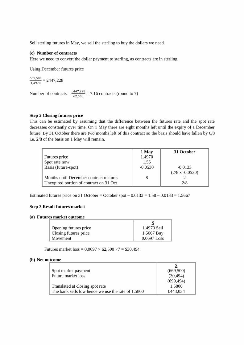
Sell sterling futures in May, we sell the sterling to buy the dollars we need.
(c) Number of contracts
Here we need to convert the dollar payment to sterling, as contracts are in sterling.
Using December futures price
669,500
1,4970 = £447,228
Number of contracts = £447,228
62,500 = 7.16 contracts (round to 7)
Step 2 Closing futures price
This can be estimated by assuming that the difference between the futures rate and the spot rate
decreases constantly over time. On 1 May there are eight months left until the expiry of a December
future. By 31 October there are two months left of this contract so the basis should have fallen by 6/8
i.e. 2/8 of the basis on 1 May will remain.
Futures price
Spot rate now
Basis (future-spot)
Months until December contract matures
Unexpired portion of contract on 31 Oct
1 May
1.4970
1.55
-0.0530
8
31 October
-0.0133
(2/8 x -0.0530)
2
2/8
Estimated futures price on 31 October = October spot – 0.0133 = 1.58 – 0.0133 = 1.5667
Step 3 Result futures market
(a) Futures market outcome
Opening futures price
Closing futures price
Movement
$
1.4970 Sell
1.5667 Buy
0.0697 Loss
Futures market loss = 0.0697 × 62,500 ×7 = $30,494
(b) Net outcome
Spot market payment
Future market loss
Translated at closing spot rate
The bank sells low hence we use the rate of 1.5800
$
(669,500)
(30,494)
(699,494)
1.5800
£443,034
Page 263

Currency options
Currency options protect against adverse exchange rate movements while allowing the investor to
take advantage of favorable exchange rate movements. They are particularly useful in situations
where the cash flow is not certain to occur (e.g. when tendering for overseas contracts).
Introduction
A currency option is an agreement involving a right, but not an obligation, to buy or sell a certain
amount of currency at a stated rate of exchange (the exercise price) at some time in the future.
A forward exchange contract is an agreement to buy or sell a given quantity of foreign exchange
which must be carried out because it is a binding contract. However, some exporters might be
uncertain about the amount of currency they will earn in several months time.
An alternative method of obtaining foreign exchange cover, which overcomes most of this problem, is
the currency option. A currency option does not have to be exercised instead, when the date for
exercising the option arrives, the importer or exporter can either exercise the option or let the option
lapse.
The exercise price for the option may be the same as the current spot rate, or it may be more favorable
or less favorable to the option holder than the current spot rate.
As with other types of option, buying a currency option involves paying a premium, which is the most
buyer of the option can lose. The level of option premiums depends on the following factors.
The exercise price
The maturity of the option
The volatility of exchange and interest rates.
Interest rate differentials, affecting how much banks charge
Basic terminology
This section covers the basic terminology that you will frequently see in questions relating to currency
options. Make sure you understand the meaning of each of the terms, as this will help you to interpret
questions and make decisions regarding different types of options.
Call option – the right to buy (the contract currency)
Put option – the right to sell (the contract currency)
A call option gives the buyer of the option the right to buy the underlying currency at a fixed rate of
exchange (and the seller of the option would be required to sell the underlying currency at that rate)
A put option gives the buyer of the option the right to sell the underlying currency at a fixed rate of
exchange (and the seller of the option would be required to buy the underlying currency at the rate).
Exercise price – the price at which the future transaction will take place
The exercise price is also known as the strike price, it is the price with which the prevailing spot rate
should be compared in order to determine whether the option should be exercised or not.
In the money – where the option strike price is more favorable than the current spot rate
At the money – where the option strike price is equal to the current spot rate.
Out of the money – where the option strike price is less favorable than the current spot rate.
For example, if a German company holds a call option to purchase £ with a strike price of £0.9174 =
€1 and the current spot rate is £0.9200 = €1, the option is out of the money, as the current spot rate is
more favorable than the option strike price.
Page 264
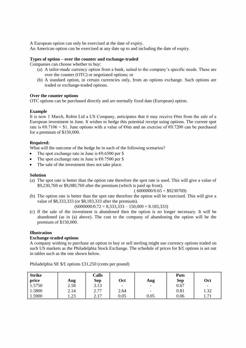
A European option can only be exercised at the date of expiry.
An American option can be exercised at any date up to and including the date of expiry.
Types of option – over the counter and exchange-traded
Companies can choose whether to buy:
(a) A tailor-made currency option from a bank, suited to the company’s specific needs. These are
over the counter (OTC) or negotiated options; or
(b) A standard option, in certain currencies only, from an options exchange. Such options are
traded or exchange-traded options.
Over the counter options
OTC options can be purchased directly and are normally fixed date (European) option.
Example
It is now 1 March, Robin Ltd a US Company, anticipates that it may receive €6m from the sale of a
European investment in June. It wishes to hedge this potential receipt using options. The current spot
rate is €0.7106 = $1. June options with a value of €6m and an exercise of €0.7200 can be purchased
for a premium of $150,000.
Required:
What will the outcome of the hedge be in each of the following scenarios?
The spot exchange rate in June is €0.6500 per $
The spot exchange rate in June is €0.7500 per $
The sale of the investment does not take place.
Solution
(a) The spot rate is better than the option rate therefore the spot rate is used. This will give a value of
$9,230,769 or $9,080,769 after the premium (which is paid up front).
( 6000000/0.65 = $9230769)
(b) The option rate is better than the spot rate therefore the option will be exercised. This will give a
value of $8,333,333 (or $8,183,333 after the premium).
(6000000/0.72 = 8,333,333 – 150,000 = 8.183,333)
(c) If the sale of the investment is abandoned then the option is no longer necessary. It will be
abandoned (as in (a) above). The cost to the company of abandoning the option will be the
premium of $150,000.
Illustration
Exchange-traded options
A company wishing to purchase an option to buy or sell sterling might use currency options traded on
such US markets as the Philadelphia Stock Exchange. The schedule of prices for $/£ options is set out
in tables such as the one shown below.
Philadelphia SE $/£ options £31,250 (cents per pound)
Strike
price
1.5750
1.5800
1.5900
Aug
2.58
2.14
1.23
Calls
Sep
3.13
2.77
2.17
Oct
-
2.64
0.05
Aug
-
-
0.05
Puts
Sep
0.67
0.81
0.06
Oct
-
1.32
1.71
Page 265

1.6000
1.6100
1.6200
0.50
0.15
-
1.61
1.16
0.81
0.32
0.93
1.79
0.32
0.93
1.79
1.50
2.05
2.65
2.18
2.69
3.30
Note the following points
(a) What it the contract size?
The contract size is £31,250
(b) What is the meaning of the numbers under each month?
This is the cost in cents per £ (remember that the market is the US) – for example, September call at a
strike price of $1.6100 will cost 1.16/100$/£ x £31,250 = $362.50
(c) What is a put US$ per £ option?
This is the option to sell £ (e.g. UK importer having to sell £ to obtain $ to pay a US supplier).
(d) Why is an August call at $1.5800 more expensive than an August call at $1.5900?
$1.5800 is a better rate than $1.5900 therefore to secure such a rate will be more expensive.
(e) Why is a call option exercisable in September more expensive than a call option exercisable in
August but with the same strike price?
This is because there is a longer period until the exercise date and it is therefore more likely that
exercising the option will be beneficial. The difference also reflects the market’s view of the direction
in which the exchange rate is likely to move between the two dates.
Traded vs OTC options
Both types of options have advantages over the other – the choice of option will depend on particular
requirements.
Advantages of traded option
(a) Traded options are standard sizes and are thus tradable with means they can be sold on to other
parties if not required. OTC options are designed for a specific purpose and are therefore unlikely
to be suitable for another party.
(b) Traded options are more flexible in that they cover a period of time (American options, whereas
OTC options are fixed date (European options).
Advantages of OTC options
(a) OTC options can be agreed for a longer period than the standard two-year maximum offered by
traded options. This gives greater flexibility and protection from currency movements in the
longer term should the transaction require it.
(b) OTC options are tailored specifically for a particular transaction, ensuring maximum protection
from currency movements. As traded options are of a standard size, the full amount of the
transaction may not be hedged, as fractions of options are not available.
Choosing the correct type of option
The vast majority of option examples which we consider are concerned with hedgers who purchase
options in order to reduce risk. We are seldom concerned with option writers who sell options.
So, given that we are normally going to purchase options, should we purchase puts or calls?
Page 266
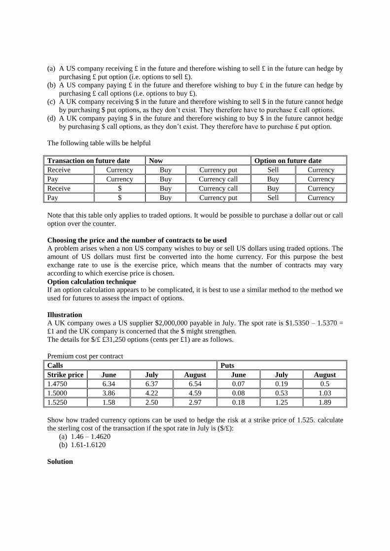
(a) A US company receiving £ in the future and therefore wishing to sell £ in the future can hedge by
purchasing £ put option (i.e. options to sell £).
(b) A US company paying £ in the future and therefore wishing to buy £ in the future can hedge by
purchasing £ call options (i.e. options to buy £).
(c) A UK company receiving $ in the future and therefore wishing to sell $ in the future cannot hedge
by purchasing $ put options, as they don’t exist. They therefore have to purchase £ call options.
(d) A UK company paying $ in the future and therefore wishing to buy $ in the future cannot hedge
by purchasing $ call options, as they don’t exist. They therefore have to purchase £ put option.
The following table wills be helpful
Transaction on future date Now Option on future date
Receive Currency Buy Currency put Sell Currency
Pay Currency Buy Currency call Buy Currency
Receive $ Buy Currency call Buy Currency
Pay $ Buy Currency put Sell Currency
Note that this table only applies to traded options. It would be possible to purchase a dollar out or call
option over the counter.
Choosing the price and the number of contracts to be used
A problem arises when a non US company wishes to buy or sell US dollars using traded options. The
amount of US dollars must first be converted into the home currency. For this purpose the best
exchange rate to use is the exercise price, which means that the number of contracts may vary
according to which exercise price is chosen.
Option calculation technique
If an option calculation appears to be complicated, it is best to use a similar method to the method we
used for futures to assess the impact of options.
Illustration
A UK company owes a US supplier $2,000,000 payable in July. The spot rate is $1.5350 – 1.5370 =
£1 and the UK company is concerned that the $ might strengthen.
The details for $/£ £31,250 options (cents per £1) are as follows.
Premium cost per contract
Calls Puts
Strike price June July August June July August
1.4750 6.34 6.37 6.54 0.07 0.19 0.5
1.5000 3.86 4.22 4.59 0.08 0.53 1.03
1.5250 1.58 2.50 2.97 0.18 1.25 1.89
Show how traded currency options can be used to hedge the risk at a strike price of 1.525. calculate
the sterling cost of the transaction if the spot rate in July is ($/£):
(a) 1.46 – 1.4620
(b) 1.61-1.6120
Solution
Page 267
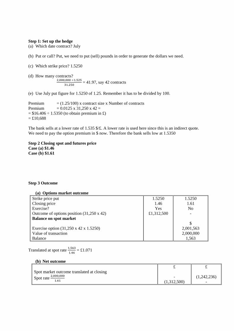
Step 1: Set up the hedge
(a) Which date contract? July
(b) Put or call? Put, we need to put (sell) pounds in order to generate the dollars we need.
(c) Which strike price? 1.5250
(d) How many contracts? 2,000,000 ÷1.525
31.250 = 41.97, say 42 contracts
(e) Use July put figure for 1.5250 of 1.25. Remember it has to be divided by 100.
Premium = (1.25/100) x contract size x Number of contracts
Premium = 0.0125 x 31,250 x 42 =
= $16.406 ÷ 1.5350 (to obtain premium in £)
= £10,688
The bank sells at a lower rate of 1.535 $/£. A lower rate is used here since this is an indirect quote.
We need to pay the option premium in $ now. Therefore the bank sells low at 1.5350
Step 2 Closing spot and futures price
Case (a) $1.46
Case (b) $1.61
Step 3 Outcome
(a) Options market outcome
Strike price put
Closing price
Exercise?
Outcome of options position (31,250 x 42)
Balance on spot market
Exercise option (31,250 x 42 x 1.5250)
Value of transaction
Balance
1.5250
1.46
Yes
£1,312,500
1.5250
1.61
No
-
$
2,001,563
2,000,000
1,563
Translated at spot rate 1,563
1.46 = £1.071
(b) Net outcome
Spot market outcome translated at closing
Spot rate 2,000,000
1.61
£
-
(1,312,500)
£
(1,242,236)
-
Page 268
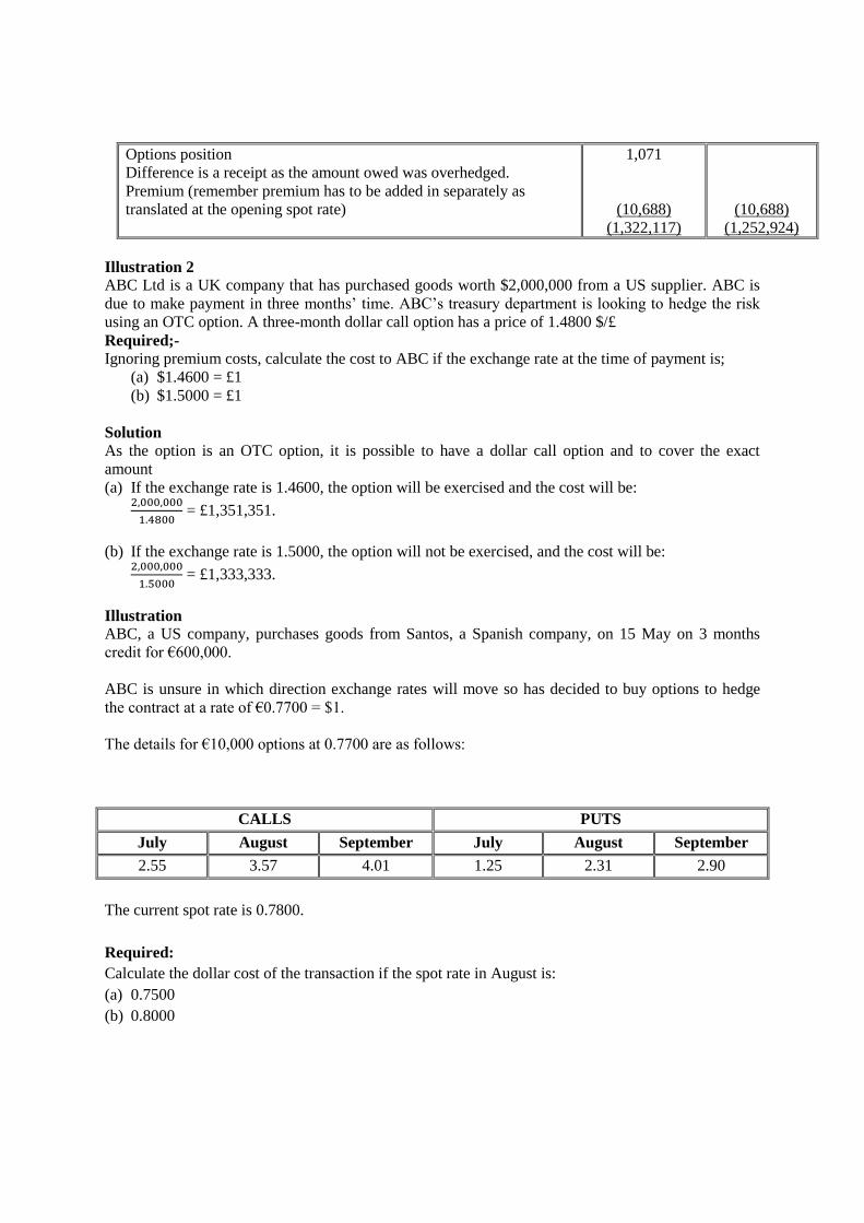
Options position
Difference is a receipt as the amount owed was overhedged.
Premium (remember premium has to be added in separately as
translated at the opening spot rate)
1,071
(10,688)
(1,322,117)
(10,688)
(1,252,924)
Illustration 2
ABC Ltd is a UK company that has purchased goods worth $2,000,000 from a US supplier. ABC is
due to make payment in three months’ time. ABC’s treasury department is looking to hedge the risk
using an OTC option. A three-month dollar call option has a price of 1.4800 $/£
Required;-
Ignoring premium costs, calculate the cost to ABC if the exchange rate at the time of payment is;
(a) $1.4600 = £1
(b) $1.5000 = £1
Solution
As the option is an OTC option, it is possible to have a dollar call option and to cover the exact
amount
(a) If the exchange rate is 1.4600, the option will be exercised and the cost will be: 2,000,000
1.4800 = £1,351,351.
(b) If the exchange rate is 1.5000, the option will not be exercised, and the cost will be: 2,000,000
1.5000 = £1,333,333.
Illustration
ABC, a US company, purchases goods from Santos, a Spanish company, on 15 May on 3 months
credit for €600,000.
ABC is unsure in which direction exchange rates will move so has decided to buy options to hedge
the contract at a rate of €0.7700 = $1.
The details for €10,000 options at 0.7700 are as follows:
CALLS PUTS
July August September July August September
2.55 3.57 4.01 1.25 2.31 2.90
The current spot rate is 0.7800.
Required:
Calculate the dollar cost of the transaction if the spot rate in August is:
(a) 0.7500
(b) 0.8000
Page 269
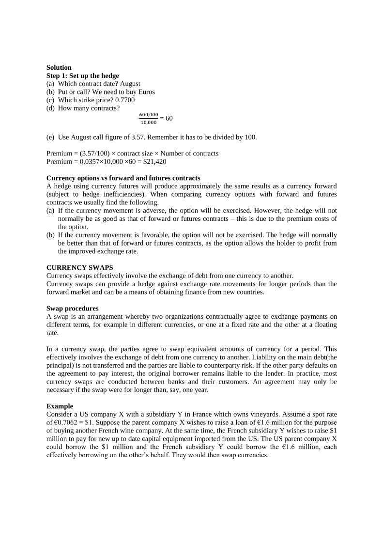
Solution
Step 1: Set up the hedge
(a) Which contract date? August
(b) Put or call? We need to buy Euros
(c) Which strike price? 0.7700
(d) How many contracts? 600,000
10,000 = 60
(e) Use August call figure of 3.57. Remember it has to be divided by 100.
Premium = (3.57/100) × contract size × Number of contracts
Premium = 0.0357×10,000 ×60 = $21,420
Currency options vs forward and futures contracts
A hedge using currency futures will produce approximately the same results as a currency forward
(subject to hedge inefficiencies). When comparing currency options with forward and futures
contracts we usually find the following.
(a) If the currency movement is adverse, the option will be exercised. However, the hedge will not
normally be as good as that of forward or futures contracts – this is due to the premium costs of
the option.
(b) If the currency movement is favorable, the option will not be exercised. The hedge will normally
be better than that of forward or futures contracts, as the option allows the holder to profit from
the improved exchange rate.
CURRENCY SWAPS
Currency swaps effectively involve the exchange of debt from one currency to another.
Currency swaps can provide a hedge against exchange rate movements for longer periods than the
forward market and can be a means of obtaining finance from new countries.
Swap procedures
A swap is an arrangement whereby two organizations contractually agree to exchange payments on
different terms, for example in different currencies, or one at a fixed rate and the other at a floating
rate.
In a currency swap, the parties agree to swap equivalent amounts of currency for a period. This
effectively involves the exchange of debt from one currency to another. Liability on the main debt(the
principal) is not transferred and the parties are liable to counterparty risk. If the other party defaults on
the agreement to pay interest, the original borrower remains liable to the lender. In practice, most
currency swaps are conducted between banks and their customers. An agreement may only be
necessary if the swap were for longer than, say, one year.
Example
Consider a US company X with a subsidiary Y in France which owns vineyards. Assume a spot rate
of €0.7062 = $1. Suppose the parent company X wishes to raise a loan of €1.6 million for the purpose
of buying another French wine company. At the same time, the French subsidiary Y wishes to raise $1
million to pay for new up to date capital equipment imported from the US. The US parent company X
could borrow the $1 million and the French subsidiary Y could borrow the €1.6 million, each
effectively borrowing on the other’s behalf. They would then swap currencies.
Page 270
Benefits of swaps
(a) Flexibility
Swaps are easy to arrange and are flexible since they can be arranged in any size and are reversible.
(b) Cost
Transaction costs are low, only amounting to legal fees, since there is no commission or premium to
be paid.
(c) Market avoidance
The parties can obtain the currency they require without subjecting themselves to the uncertainties of
the foreign exchange markets.
(d) Access to finance
The company can gain access to debt finance in another country and currency where it is little known,
and consequently has a poorer credit rating, than it could obtain if it arranged the currency loan itself.
(e) Financial restructuring
Currency swaps may be used to restructure the currency base of the company’s liabilities. This may
be important where the company is trading overseas and receiving revenues in foreign currencies, but
its borrowings are denominated in the currency of its home country. Currency swaps therefore provide
a means of reducing exchange rate exposure.
(f) Conversion of debt type
At the same time as exchanging currency, the company may also be able to convert fixed rate debt to
floating rate or vice versa. Thus it may obtain some of the benefits of an interest rate swap in addition
to achieving the other purposes of a currency swap.
(g) Liquidity improvement
A currency swap could be used to absorb excess liquidity in one currency which is not needed
immediately, to create funds in another where there is a need.
Disadvantages of swaps
(a) Risk of default by the other party to the swap (counterparty risk)
If one party became unable to meet its swap payment obligations, this could mean that the other party
risked having to make them itself.
(b) Position or market risk
A company whose main business lies outside the field of finance should not increase financial risk in
order to make speculative gains.
(c) Sovereign risk
There may be a risk of political disturbances or exchange controls in the country whose currency is
being used for a swap.
(d) Arrangement fees
Swaps have arrangement fees payable to third parties. Although these may appear to be cheap, this is
because the intermediary accepts no liability for the swap. (However, the third party does suffer some
spread risk, as it warehouses one side of the swap until it is matched with the other, and then
undertakes a temporary hedge on the futures market.)
Page 271
Example
Step 1 ABC, a UK company, wishes to invest in Germany. It borrows £20 million from its bank and
pays interest at 5%. To invest in Germany, the £20 million will be converted into euros at a spot rate
of €1.50 = £1. The earnings from the German investment will be in euros, but ABC will have to pay
interest on the swap. The company arranges to swap the £20 million for €30 million with Gordonbear,
a company in the euro currency zone. Gordonbear is thus the counterparty in this transaction. Interest
of 6% is payable on the €30 million. ABC can use the €30 million it receives to invest in Germany.
Step 2 Each year when interest is due:
(a) ABC receives from its German investment cash remittances of €1.8 million (€30 million × 6%)
(b) ABC passes this €1.8 million to Gordonbear so that Gordonbear can settle its interest liability
(c) Gordonbear passes to ABC £1 million (£20 million × 5%)
(d) ABC settles its interest liability of £1 million with its lender
Step 3 At the end of the useful life of the investment the original payments are reversed, with ABC
paying back the €30 million it originally received and receiving back from Gordonbear the £20
million. ABC uses this £20 million to repay the loan it originally received from its UK lender.
6.4. INTEREST RATE RISK
Factors influencing interest rate risk include:
Fixed rate versus floating rate debt
The term of the loan
Interest rate risk is the risk to the profitability or value of a company resulting from changes in
interest rates.
Managing a debt portfolio
Corporate treasurers will be responsible for managing the company's debt portfolio; that is, in
deciding how a company should obtain its short-term funds so as to:
(a) Be able to repay debts as they mature
(b) Minimise any inherent risks, notably invested foreign exchange risk, in the debts the company
owes and is owed
There are a number of situations in which a company might be exposed to risk from interest rate
movements.
Risks from interest rate movements
(a) Fixed rate versus floating rate debt
A company can get caught paying higher interest rates by having fixed rather than floating rate debt,
or floating rather than fixed rate debt, as market interest rates change.
Interest rate risk management
Page 272
If the organisation faces interest rate risk, it can seek to hedge the risk. Alternatively, where the
magnitude of the risk is immaterial in comparison with the company's overall cash flows or appetite
for risks, one option is to do nothing. The company then accepts the effects of any movement in
interest rates which occur.
The company may also decide to do nothing if risk management costs are excessive, both in terms of
the costs of using derivatives and the staff resources required to manage risk effectively. Appropriate
products may not be available and of course the company may consider hedging unnecessary, as it
believes that the chances of an adverse movement are remote.
Bear in mind the possibility that a company may take the decision to do nothing to reduce interest rate
risk – it is a situation you should consider when answering exam questions.
The company's tax situation may also be a significant determinant of its decision whether or not to
hedge risk. If hedging is likely to reduce variability of earnings, this may have tax advantages if the
company faces a higher rate of tax for higher earnings levels. The directors may also be unwilling to
undertake hedging because of the need to monitor the arrangements, and the requirements to fulfill the
disclosure requirements of International Financial Reporting Standards.
Question
Hedging
Explain what is meant by hedging in the context of interest rate risk.
Solution
Hedging is a means of reducing risk. Hedging involves coming to an agreement with another party
who is prepared to take on the risk that you would otherwise bear. The other party may be willing to
take on that risk because it would otherwise bear an opposing risk which may be 'matched' with your
risk; alternatively, the other party may be a speculator who is willing to bear the risk in return for the
prospect of making a profit. In the case of interest rates, a company with a variable rate loan clearly
faces the risk that the rate of interest will increase in the future as a result of changing market
conditions which cannot now be predicted.
Many financial instruments have been introduced in recent years to help corporate treasurers to hedge
the risks of interest rate movements. These instruments include forward rate agreements, financial
futures, interest rate swaps and options.
Interest rate risk management techniques
Methods of reducing interest rate risk include the following.
Netting – aggregating all positions, assets and liabilities, and hedging the net exposure
Smoothing – maintaining a balance between fixed and floating rate borrowing
Matching – matching assets and liabilities to have a common interest rate
Pooling
Forward rate agreements (FRAs)
Interest rate futures
Page 273
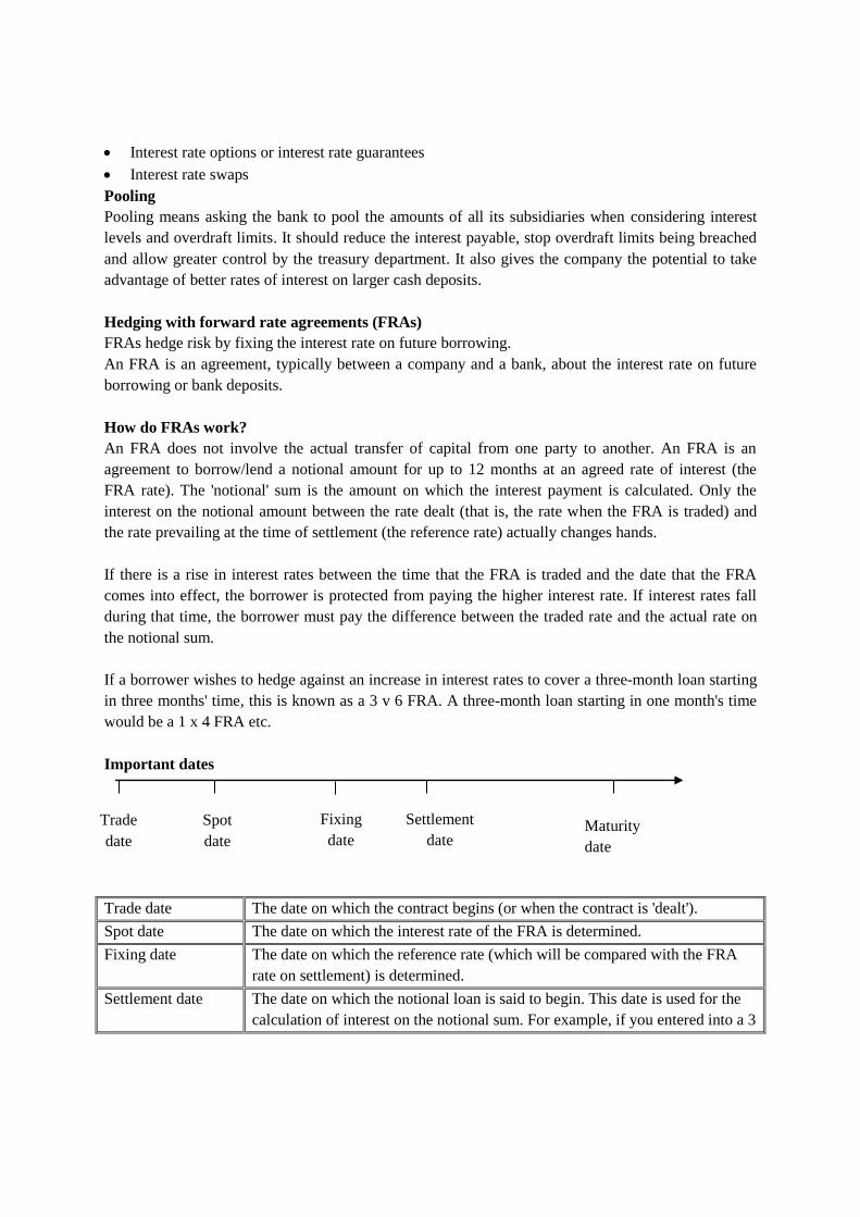
Interest rate options or interest rate guarantees
Interest rate swaps
Pooling
Pooling means asking the bank to pool the amounts of all its subsidiaries when considering interest
levels and overdraft limits. It should reduce the interest payable, stop overdraft limits being breached
and allow greater control by the treasury department. It also gives the company the potential to take
advantage of better rates of interest on larger cash deposits.
Hedging with forward rate agreements (FRAs)
FRAs hedge risk by fixing the interest rate on future borrowing.
An FRA is an agreement, typically between a company and a bank, about the interest rate on future
borrowing or bank deposits.
How do FRAs work?
An FRA does not involve the actual transfer of capital from one party to another. An FRA is an
agreement to borrow/lend a notional amount for up to 12 months at an agreed rate of interest (the
FRA rate). The 'notional' sum is the amount on which the interest payment is calculated. Only the
interest on the notional amount between the rate dealt (that is, the rate when the FRA is traded) and
the rate prevailing at the time of settlement (the reference rate) actually changes hands.
If there is a rise in interest rates between the time that the FRA is traded and the date that the FRA
comes into effect, the borrower is protected from paying the higher interest rate. If interest rates fall
during that time, the borrower must pay the difference between the traded rate and the actual rate on
the notional sum.
If a borrower wishes to hedge against an increase in interest rates to cover a three-month loan starting
in three months' time, this is known as a 3 v 6 FRA. A three-month loan starting in one month's time
would be a 1 x 4 FRA etc.
Important dates
Trade date The date on which the contract begins (or when the contract is 'dealt').
Spot date The date on which the interest rate of the FRA is determined.
Fixing date The date on which the reference rate (which will be compared with the FRA
rate on settlement) is determined.
Settlement date The date on which the notional loan is said to begin. This date is used for the
calculation of interest on the notional sum. For example, if you entered into a 3
Trade
date
Spot
date
Fixing
date
Settlement
date Maturity
date
Page 274
v 6 FRA, this would be 3 months after the spot date.
Maturity date The date on which the notional loan expires. For example, in a 3 v 6 FRA, this
would be 3 months after the settlement date.
Illustration
It is 30 June. Lynn will need a $10 million 6-month fixed rate loan from 1 October. Lynn wants to
hedge using an FRA. The relevant FRA rate is 6% on 30 June.
What is the result of the FRA and the effective loan rate if the 6-month FRA benchmark rate has
moved to:
(a) 5%?
(b) 9%?
Solution
(a) At 5%, because interest rates have fallen, Lynn will pay the bank:
FRA payment $10 million x (6% - 5%) x 6/12
Payment on underlying loan 5% x $10 million x 6/12
Net payment on loan
$
(50,000)
(250,000)
(300,000)
(b) At 9%, because interest rates have risen, the bank will pay Lynn:
FRA (received) $10 million x (9% - 6%) × 6/12
Payment on underlying loan 9% × $10 million × 6/12
Net payment on loan
$
150,000
(450,000)
(300,000)
Effective interest rate on loan = 6%
Advantages of FRAs
(a) Protection provided
An FRA would protect the borrower from adverse interest rate movements above the rate negotiated.
(b) Flexibility
FRAs are flexible; they can in theory be arranged for any amounts and any duration, although they are
normally for amounts of over $1 million.
(c) Cost
FRAs may well be free and will in any case cost little.
Disadvantages of FRAs
(a) Rate available
The rate the bank will set for the FRA will reflect expectations of future interest rate movements. If
interest rates are expected to rise, the bank may set a higher rate than the rate currently available.
(b) Falling interest rate
The borrower will not be able to take advantage if interest rates fall unexpectedly.
Page 275
(c) Term of FRA
The FRA will terminate on a fixed date.
(d) Binding agreement
FRAs are binding agreements so are less easy to sell to other parties.
INTEREST RATE FUTURES
Interest rate futures can be used to hedge against interest rate changes between the current date and
the date at which the interest rate on the lending or borrowing is set. Borrowers sell futures to hedge
against interest rate rises. Lenders buy futures to hedge against interest rate falls.
Futures contracts
We covered currency futures in the previous chapter so you should be familiar with how they work.
Interest rate futures are similar to currency futures in that they are used to hedge against movements in
the underlying (in this case, interest rates).
Interest rate futures are a similar method of hedging to FRAs, except that the terms, amounts and
periods are standardised. For example, a company can contract to buy (or sell) $100,000 of a notional
30-year bond bearing an 8% coupon in, say, 6 months' time at an agreed price. The basic principles
behind such a decision are:
(a) The futures price is likely to vary with changes in interest rates. This acts as a hedge against
adverse interest rate movements. We will illustrate this in an example shortly.
(b) The outlay to buy futures is much less than for buying the financial instrument itself.
Borrowing and lending
Borrowers will wish to hedge against an interest rate rise by:
Selling futures now
Buying futures on the day that the interest rate is fixed
Lenders will wish to hedge against the possibility of falling interest rates by:
Borrowing futures now
Lending futures on the date that the actual lending starts
Pricing futures contracts
The pricing of an interest rate futures contract is determined by prevailing interest rates
For short-term futures, if 3-month interest rates are 8%, a 3-month futures contract will be priced
at 92 i.e. (100 - 8).
If interest rates are 11%, the contract price will be 89 i.e. (100 - 11).
This decrease in price, or value, of the contract reflects the reduced attractiveness of a fixed rate
deposit in a time of rising interest rates.
Page 276

The price of long-term futures reflects market prices of the underlying bonds. A price of $100 equals
par.
The interest rate is implied in the price. If a long-term 10% futures contract has a price of $114.00, the
implied interest rate on long-term bonds is approximately 100/114 × 10% = 8.8%.
Illustration
ABC has taken a 3-month $1,000,000 eurodollar loan with interest payable of 8%, the loan being due
for rollover on 31 March. At 1 January, the company treasurer considers that interest rates are likely
to rise in the near future. The futures price is 91 representing a yield of 9%. Given a standard contract
size of $1,000,000, the company sells a eurodollar 3-month contract to hedge against interest on the 3-
month loan required at 31 March (to sell a contract is to commit the seller to take a deposit). At 31
March the spot interest rate is 11%.
What is the cost saving to ABC?
Solution
The company will buy back the future on 31 March at 89 (100 - 11). The cost saving is the profit on
the futures contract.
$1,000,000 x (91 - 89) x 3/12 = $5,000
The hedge has effectively reduced the net annual interest cost by 2%. Instead of a cost of 11% at 31
March ($27,500) for a 3-month loan, the net cost is $22,500 ($27,500 - $5,000), a 9% annual cost.
Use of interest rate futures
The seller of a futures contract does not have to own the underlying instrument. However, the seller
may need to deliver it on the contract's delivery date if the buyer requires it. Many, but not all, interest
rate contracts are settled for cash rather than by delivery of the underlying instrument.
Interest rate futures offer an attractive means of speculation for some investors, because there is no
requirement that buyers and sellers should actually be lenders and borrowers (respectively) of the
nominal amounts of the contracts.
Basis risk
Basis risk also occurs for interest rate futures.
If a firm takes a position in the futures contract with a view to closing out the contract before its
maturity, there is still likely to be basis. The firm can only estimate what effect this will have on the
11% × 1000,000 ×3/12 = 2700$
Page 277

hedge. 'Basis risk' refers to the problem that the basis may result in an imperfect hedge. The basis will
be zero at the maturity date of the contract.
The basis risk can be calculated as the difference between the futures price and the current price ('cash
market' price) of the underlying security.
Example: basis and basis risk
To give an example, if 3-month Base rate is 7% and the September price of the 3-month sterling
future is 92.70 now (at the end of March, say) then the basis is:
(100 – 7) 93.00
Futures (92.70)
0.30%
Or 30 basis points
In the exam, you might be given other price information and have to calculate the closing futures
price from it.
A further cause of basis risk for interest rates is that there are significantly more possible actual
interest rates than there are standard contracts. Therefore management may wish to calculate the
correlation between the futures price movement and the underlying price movement. This can be used
to calculate hedging ratios which can be used to determine the overall number of contracts required.
Delta hedging can also be used to reduce this risk.
Setting up a futures hedge
The procedure for setting up an interest rate futures hedge is similar to that for currency futures. The
following example illustrates the process.
Illustration
Panda has taken a 6-month $10,000,000 loan with interest payable of 8%, the loan being due for
rollover on 31 March. At 1 January, the company treasurer considers that interest rates are likely to
rise in the near future. The futures price is 91 representing a yield of 9%. Given a standard contract
size of $1,000,000, the company sells a dollar 3-month contract to hedge against interest on the 3-
month loan required at 31
March (to sell a contract is to commit the seller to take a deposit). At 31 March the interest rate is
11% and the futures price had fallen to 88.50.
Required;-
Demonstrate how futures can be used to hedge against interest rate movements.
Solution
The following steps should be taken.
Setup
(a) What contract: 3-month contract
Page 278
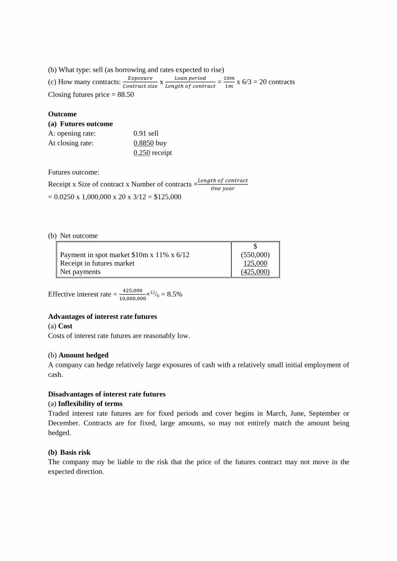
(b) What type: sell (as borrowing and rates expected to rise)
(c) How many contracts: 𝐸𝑥𝑝𝑜𝑠𝑢𝑟𝑒
𝐶𝑜𝑛𝑡𝑟𝑎𝑐𝑡 𝑠𝑖𝑧𝑒 x
𝐿𝑜𝑎𝑛 𝑝𝑒𝑟𝑖𝑜𝑑
𝐿𝑒𝑛𝑔𝑡ℎ 𝑜𝑓 𝑐𝑜𝑛𝑡𝑟𝑎𝑐𝑡 =
10𝑚
1𝑚 x 6/3 = 20 contracts
Closing futures price = 88.50
Outcome
(a) Futures outcome
A: opening rate: 0.91 sell
At closing rate: 0.8850 buy
0.250 receipt
Futures outcome:
Receipt x Size of contract x Number of contracts ×𝐿𝑒𝑛𝑔𝑡ℎ 𝑜𝑓 𝑐𝑜𝑛𝑡𝑟𝑎𝑐𝑡
𝑂𝑛𝑒 𝑦𝑒𝑎𝑟
= 0.0250 x 1,000,000 x 20 x 3/12 = $125,000
(b) Net outcome
Payment in spot market $10m x 11% x 6/12
Receipt in futures market
Net payments
$
(550,000)
125,000
(425,000)
Effective interest rate = 425,000
10,000,000×12/6 = 8.5%
Advantages of interest rate futures
(a) Cost
Costs of interest rate futures are reasonably low.
(b) Amount hedged
A company can hedge relatively large exposures of cash with a relatively small initial employment of
cash.
Disadvantages of interest rate futures
(a) Inflexibility of terms
Traded interest rate futures are for fixed periods and cover begins in March, June, September or
December. Contracts are for fixed, large amounts, so may not entirely match the amount being
hedged.
(b) Basis risk
The company may be liable to the risk that the price of the futures contract may not move in the
expected direction.
Page 279
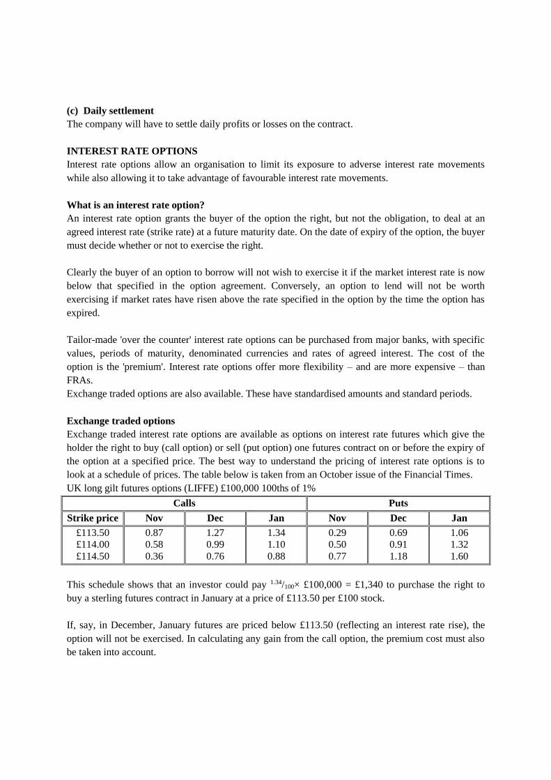
(c) Daily settlement
The company will have to settle daily profits or losses on the contract.
INTEREST RATE OPTIONS
Interest rate options allow an organisation to limit its exposure to adverse interest rate movements
while also allowing it to take advantage of favourable interest rate movements.
What is an interest rate option?
An interest rate option grants the buyer of the option the right, but not the obligation, to deal at an
agreed interest rate (strike rate) at a future maturity date. On the date of expiry of the option, the buyer
must decide whether or not to exercise the right.
Clearly the buyer of an option to borrow will not wish to exercise it if the market interest rate is now
below that specified in the option agreement. Conversely, an option to lend will not be worth
exercising if market rates have risen above the rate specified in the option by the time the option has
expired.
Tailor-made 'over the counter' interest rate options can be purchased from major banks, with specific
values, periods of maturity, denominated currencies and rates of agreed interest. The cost of the
option is the 'premium'. Interest rate options offer more flexibility – and are more expensive – than
FRAs.
Exchange traded options are also available. These have standardised amounts and standard periods.
Exchange traded options
Exchange traded interest rate options are available as options on interest rate futures which give the
holder the right to buy (call option) or sell (put option) one futures contract on or before the expiry of
the option at a specified price. The best way to understand the pricing of interest rate options is to
look at a schedule of prices. The table below is taken from an October issue of the Financial Times.
UK long gilt futures options (LIFFE) £100,000 100ths of 1%
Calls Puts
Strike price Nov Dec Jan Nov Dec Jan
£113.50
£114.00
£114.50
0.87
0.58
0.36
1.27
0.99
0.76
1.34
1.10
0.88
0.29
0.50
0.77
0.69
0.91
1.18
1.06
1.32
1.60
This schedule shows that an investor could pay 1.34/100× £100,000 = £1,340 to purchase the right to
buy a sterling futures contract in January at a price of £113.50 per £100 stock.
If, say, in December, January futures are priced below £113.50 (reflecting an interest rate rise), the
option will not be exercised. In calculating any gain from the call option, the premium cost must also
be taken into account.
Page 280
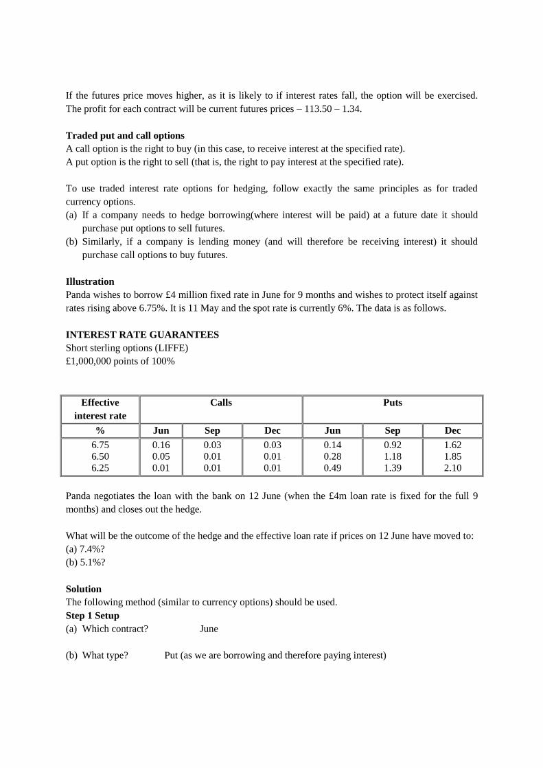
If the futures price moves higher, as it is likely to if interest rates fall, the option will be exercised.
The profit for each contract will be current futures prices – 113.50 – 1.34.
Traded put and call options
A call option is the right to buy (in this case, to receive interest at the specified rate).
A put option is the right to sell (that is, the right to pay interest at the specified rate).
To use traded interest rate options for hedging, follow exactly the same principles as for traded
currency options.
(a) If a company needs to hedge borrowing(where interest will be paid) at a future date it should
purchase put options to sell futures.
(b) Similarly, if a company is lending money (and will therefore be receiving interest) it should
purchase call options to buy futures.
Illustration
Panda wishes to borrow £4 million fixed rate in June for 9 months and wishes to protect itself against
rates rising above 6.75%. It is 11 May and the spot rate is currently 6%. The data is as follows.
INTEREST RATE GUARANTEES
Short sterling options (LIFFE)
£1,000,000 points of 100%
Effective
interest rate
Calls Puts
% Jun Sep Dec Jun Sep Dec
6.75
6.50
6.25
0.16
0.05
0.01
0.03
0.01
0.01
0.03
0.01
0.01
0.14
0.28
0.49
0.92
1.18
1.39
1.62
1.85
2.10
Panda negotiates the loan with the bank on 12 June (when the £4m loan rate is fixed for the full 9
months) and closes out the hedge.
What will be the outcome of the hedge and the effective loan rate if prices on 12 June have moved to:
(a) 7.4%?
(b) 5.1%?
Solution
The following method (similar to currency options) should be used.
Step 1 Setup
(a) Which contract? June
(b) What type? Put (as we are borrowing and therefore paying interest)
Page 281
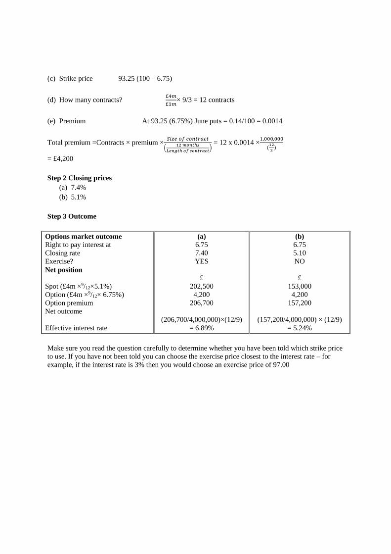
(c) Strike price 93.25 (100 – 6.75)
(d) How many contracts? £4𝑚
£1𝑚× 9/3 = 12 contracts
(e) Premium At 93.25 (6.75%) June puts = 0.14/100 = 0.0014
Total premium =Contracts × premium ×𝑆𝑖𝑧𝑒 𝑜𝑓 𝑐𝑜𝑛𝑡𝑟𝑎𝑐𝑡
(12 𝑚𝑜𝑛𝑡ℎ𝑠
𝐿𝑒𝑛𝑔𝑡ℎ 𝑜𝑓 𝑐𝑜𝑛𝑡𝑟𝑎𝑐𝑡) = 12 x 0.0014 ×
1,000,000
(12
3)
= £4,200
Step 2 Closing prices
(a) 7.4%
(b) 5.1%
Step 3 Outcome
Options market outcome
Right to pay interest at
Closing rate
Exercise?
Net position
Spot (£4m ×9/12×5.1%)
Option (£4m ×9/12× 6.75%)
Option premium
Net outcome
Effective interest rate
(a)
6.75
7.40
YES
£
202,500
4,200
206,700
(206,700/4,000,000)×(12/9)
= 6.89%
(b)
6.75
5.10
NO
£
153,000
4,200
157,200
(157,200/4,000,000) × (12/9)
= 5.24%
Make sure you read the question carefully to determine whether you have been told which strike price
to use. If you have not been told you can choose the exercise price closest to the interest rate – for
example, if the interest rate is 3% then you would choose an exercise price of 97.00
Page 282

CHAPTER SEVEN
INTERNATIONAL FINANCIAL MANAGEMENT CHAPTER KEY OBJECTIVES
To be able to understand the following;- 1. International investments
2. International financial markets
3. International financial institutions
4. Methods of financing international trade
5. International parity conditions: Interest rate parity, purchasing power parity and International
fisher effect
6. International arbitrage: locational arbitrage, triangular arbitrage and covered interest arbitrage
7. Divided policy for multinationals
8. International debt instruments: International bonds (euro bond), certificate of deposits,
securitization of loans, commercial paper
9. Availability and timing of remittances
10. Transfer pricing: impact on taxes and dividends
7.1. INTERNATIONAL FINANCIAL MARKET It exists in every economy to ensure efficient transfer of resource from surplus economic unit to
deficit economic units. The principal participants are large multinational corporations which can
accept and lend credit in various currencies. This market is regulated by various authorities who
ensure market safety and efficiency.
International money market can be distinguished from the domestic money market by the kind of
transactions which is carried out.
Definitions
Arbitrageurs – Arbitrageurs seek to earn risk-less profits by taking advantage of differences in
exchange rates among countries.
Traders – Traders engage in the export or import of goods to a number of countries. They operate
in the foreign exchange market because exporters receive foreign currencies which they have to
convert into local currencies, and importers make payments in foreign currencies which they
purchase by exchanging the local currency. They also operate in the foreign exchange market to
hedge their risk.
Hedgers – Multinational firms have their operations in a number of countries and their assets and
liabilities are designated in foreign currencies. The foreign exchange rates fluctuations can cause
diminution in the home currency value of their assets and liabilities. They operate in the foreign
exchange market as hedgers to protect themselves against the risk of fluctuations in the foreign
exchange rates.
Speculators – Speculators are guided purely by the profit motive. They trade in foreign
currencies to benefit from the exchange rate fluctuations. They take risks in the hope of making
profits.
EXCHANGE RATE DETERMINATION
Influences on exchange rate
(a) Rates of inflation in different countries
Page 283
(b) Interest rates in different countries
(c) Economic and political prospects
(d) The balance of payments
Importantly, expectations concerning changes to the above will affect the exchange rate before
changes actually occur.
Government approaches to exchange rate management
(a) Fixed exchange rate systems
The government and the monetary authorities operate in the foreign exchange markets to ensure that
the rate of exchange remains fixed.
This approach reduces the currency risk faced by companies and hence encourages a higher level of
international trade.
However, keeping the exchange rate fixed places constraints on government policy.
(b) Floating exchange rate systems
Under this approach, the government has no obligation to maintain the rate of exchange and leaves its
determination to market forces. There are 2 types of floating exchange rate systems:
(i)Free floating exchange rates
Here, the exchange rate is left entirely to market forces. However, governments do not like to leave it
entirely up to market forces due to the effect of the exchange rate on other economic factors. More
common is managed floating.
(ii)Managed floating
Under this approach, the government allows the exchange rate to fluctuate between very large bands
but intervenes if the currency looks like moving outside of these bands.
From 1944 to 1971, a system of fixed exchange rates existed (known as the Bretton Woods system).
This collapsed in 1971 and most countries moved to a system of floating exchange rates. The G7
group of countries now operate to manage their exchange rates and attempt to endure reasonable
stability.
Predicting future exchange rates
One important influence on exchange rates is the relative inflation rates between two countries.
The Purchasing Power Parity theory uses inflation rates to predict the future movement in
exchange rates. It states that identical goods should sell at the same price when converted
into the same currency. As the local currency prices changes with inflation then the
exchange rate should change to keep the relative price the same.
7.2. INTERNATIONAL PARITY CONDITIONS
Purchasing power parity
Purchasing power parity theory states that the exchange rate between two currencies is the same in
equilibrium when the purchasing power of currency is the same in each country.
Purchasing power parity theory predicts that the exchange value of foreign currency depends on the
relative purchasing power of each currency in its own country and that spot exchange rates will vary
over time according to relative price changes.
Page 284
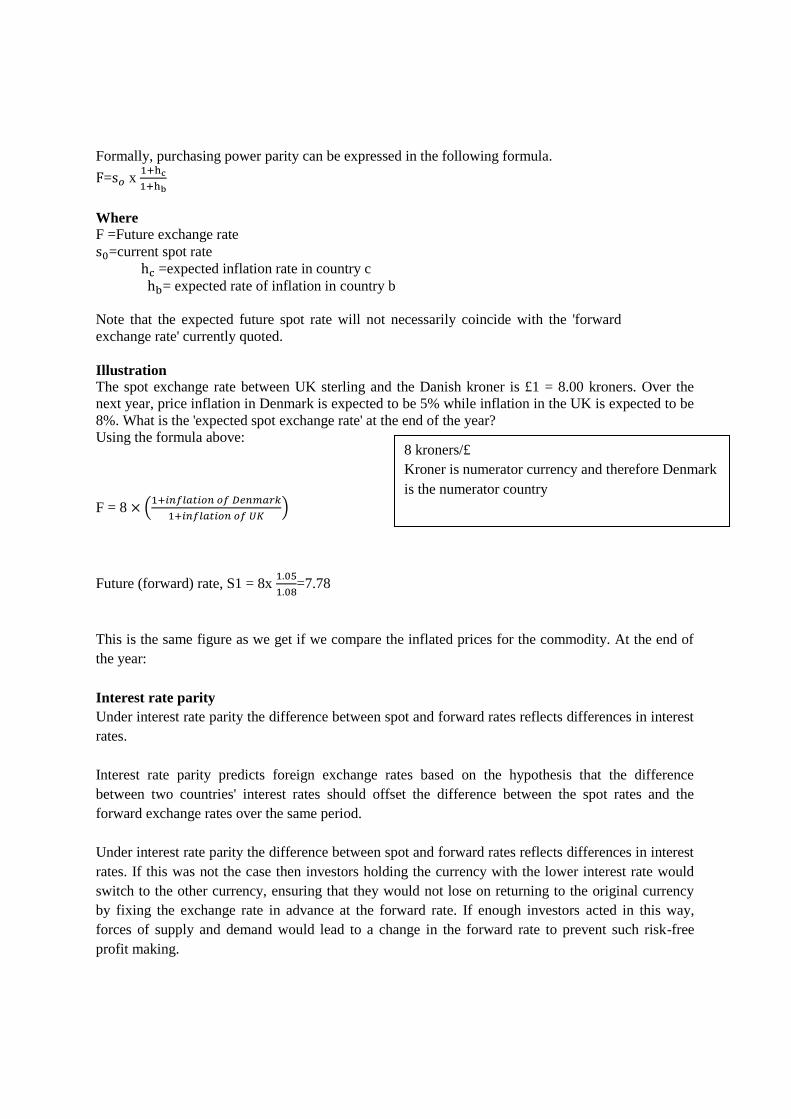
Formally, purchasing power parity can be expressed in the following formula.
F=s𝑜 x 1+hc
1+hb
Where
F =Future exchange rate
s0=current spot rate
hc =expected inflation rate in country c
hb= expected rate of inflation in country b
Note that the expected future spot rate will not necessarily coincide with the 'forward
exchange rate' currently quoted.
Illustration
The spot exchange rate between UK sterling and the Danish kroner is £1 = 8.00 kroners. Over the
next year, price inflation in Denmark is expected to be 5% while inflation in the UK is expected to be
8%. What is the 'expected spot exchange rate' at the end of the year?
Using the formula above:
F = 8 × (1+𝑖𝑛𝑓𝑙𝑎𝑡𝑖𝑜𝑛 𝑜𝑓 𝐷𝑒𝑛𝑚𝑎𝑟𝑘
1+𝑖𝑛𝑓𝑙𝑎𝑡𝑖𝑜𝑛 𝑜𝑓 𝑈𝐾)
Future (forward) rate, S1 = 8x 1.05
1.08=7.78
This is the same figure as we get if we compare the inflated prices for the commodity. At the end of
the year:
Interest rate parity
Under interest rate parity the difference between spot and forward rates reflects differences in interest
rates.
Interest rate parity predicts foreign exchange rates based on the hypothesis that the difference
between two countries' interest rates should offset the difference between the spot rates and the
forward exchange rates over the same period.
Under interest rate parity the difference between spot and forward rates reflects differences in interest
rates. If this was not the case then investors holding the currency with the lower interest rate would
switch to the other currency, ensuring that they would not lose on returning to the original currency
by fixing the exchange rate in advance at the forward rate. If enough investors acted in this way,
forces of supply and demand would lead to a change in the forward rate to prevent such risk-free
profit making.
8 kroners/£
Kroner is numerator currency and therefore Denmark
is the numerator country
Page 285
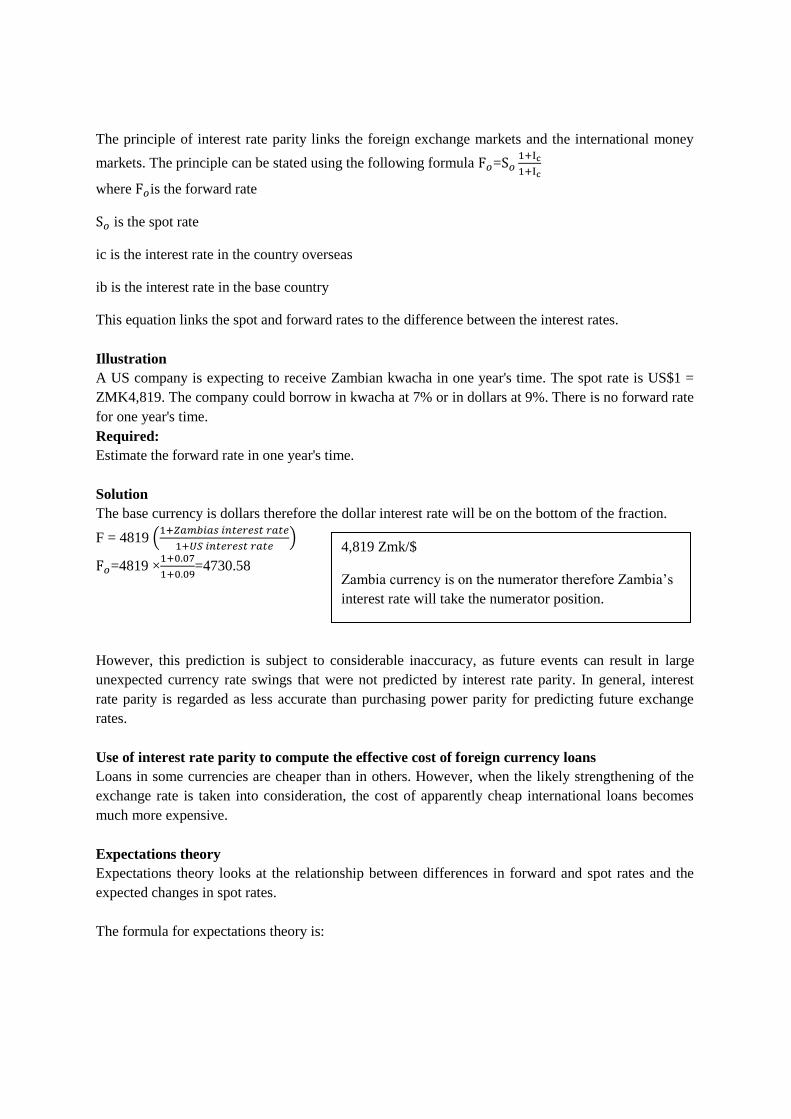
The principle of interest rate parity links the foreign exchange markets and the international money
markets. The principle can be stated using the following formula F𝑜=S𝑜1+Ic
1+Ic
where F𝑜is the forward rate
S𝑜 is the spot rate
ic is the interest rate in the country overseas
ib is the interest rate in the base country
This equation links the spot and forward rates to the difference between the interest rates.
Illustration
A US company is expecting to receive Zambian kwacha in one year's time. The spot rate is US$1 =
ZMK4,819. The company could borrow in kwacha at 7% or in dollars at 9%. There is no forward rate
for one year's time.
Required:
Estimate the forward rate in one year's time.
Solution
The base currency is dollars therefore the dollar interest rate will be on the bottom of the fraction.
F = 4819 (1+𝑍𝑎𝑚𝑏𝑖𝑎𝑠 𝑖𝑛𝑡𝑒𝑟𝑒𝑠𝑡 𝑟𝑎𝑡𝑒
1+𝑈𝑆 𝑖𝑛𝑡𝑒𝑟𝑒𝑠𝑡 𝑟𝑎𝑡𝑒)
F𝑜=4819 ×1+0.07
1+0.09=4730.58
However, this prediction is subject to considerable inaccuracy, as future events can result in large
unexpected currency rate swings that were not predicted by interest rate parity. In general, interest
rate parity is regarded as less accurate than purchasing power parity for predicting future exchange
rates.
Use of interest rate parity to compute the effective cost of foreign currency loans
Loans in some currencies are cheaper than in others. However, when the likely strengthening of the
exchange rate is taken into consideration, the cost of apparently cheap international loans becomes
much more expensive.
Expectations theory
Expectations theory looks at the relationship between differences in forward and spot rates and the
expected changes in spot rates.
The formula for expectations theory is:
4,819 Zmk/$
Zambia currency is on the numerator therefore Zambia’s
interest rate will take the numerator position.
Page 286
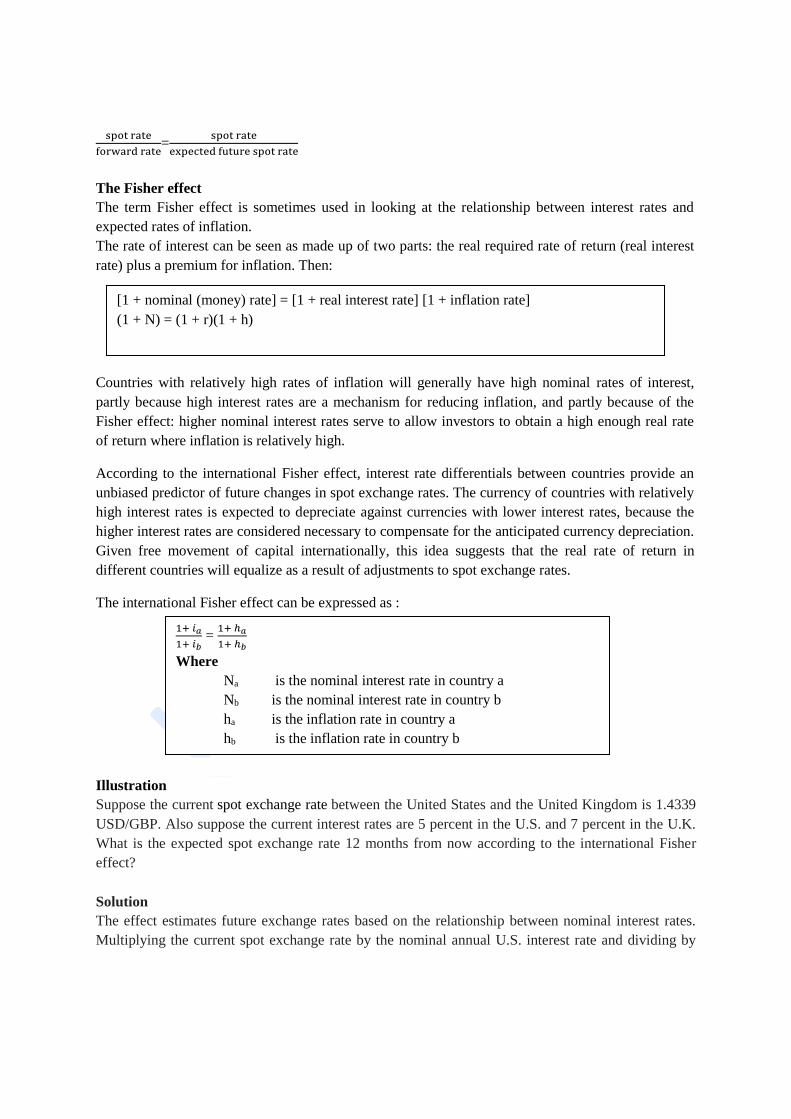
spot rate
forward rate=
spot rate
expected future spot rate
The Fisher effect
The term Fisher effect is sometimes used in looking at the relationship between interest rates and
expected rates of inflation.
The rate of interest can be seen as made up of two parts: the real required rate of return (real interest
rate) plus a premium for inflation. Then:
Countries with relatively high rates of inflation will generally have high nominal rates of interest,
partly because high interest rates are a mechanism for reducing inflation, and partly because of the
Fisher effect: higher nominal interest rates serve to allow investors to obtain a high enough real rate
of return where inflation is relatively high.
According to the international Fisher effect, interest rate differentials between countries provide an
unbiased predictor of future changes in spot exchange rates. The currency of countries with relatively
high interest rates is expected to depreciate against currencies with lower interest rates, because the
higher interest rates are considered necessary to compensate for the anticipated currency depreciation.
Given free movement of capital internationally, this idea suggests that the real rate of return in
different countries will equalize as a result of adjustments to spot exchange rates.
The international Fisher effect can be expressed as :
Illustration
Suppose the current spot exchange rate between the United States and the United Kingdom is 1.4339
USD/GBP. Also suppose the current interest rates are 5 percent in the U.S. and 7 percent in the U.K.
What is the expected spot exchange rate 12 months from now according to the international Fisher
effect?
Solution
The effect estimates future exchange rates based on the relationship between nominal interest rates.
Multiplying the current spot exchange rate by the nominal annual U.S. interest rate and dividing by
[1 + nominal (money) rate] = [1 + real interest rate] [1 + inflation rate]
(1 + N) = (1 + r)(1 + h)
1+ 𝑖𝑎
1+ 𝑖𝑏 =
1+ ℎ𝑎
1+ ℎ𝑏
Where
Na is the nominal interest rate in country a
Nb is the nominal interest rate in country b
ha is the inflation rate in country a
hb is the inflation rate in country b
Page 287

the nominal annual U.K. interest rate yields the estimate of the spot exchange rate 12 months from
now:
= $1.4339 ×1+5%
1+7%=$1.4071
Cross rates
Given the exchange rate of two currencies, we can find the exchange rate of the third currency.
Illustration 1
The US dollar-Thai baht exchange rate is: US$ 0.02339/Baht, and the US dollar-Indian rupee
exchange rate is: US$0.02538/INR. Suppose that INR is not quoted against Thai baht. What is the
Baht/INR exchange rate?
Solution
One Indian rupee costs US$ 0.02538 while one baht costs US$ 0.02339. Thus one Indian rupee should
cost: 0.02538/0.02339 = Baht 1.085. that is:
𝑈𝑆$ 0.02538
𝐼𝑁𝑅÷
𝑈𝑆$ 0.02339
𝐵𝑎ℎ𝑡 =
𝑈𝑆$ 0.02538
𝑈𝑆$ 0.02339×
𝐵𝑎ℎ𝑡
𝐼𝑁𝑅=
𝐵𝑎ℎ𝑡 1.085
𝐼𝑁𝑅 Baht 1.085/inr
A cross rate is an exchange rate between the currencies of two countries that are not quoted against
each other, but are quoted against one common currency. Currencies of many countries are not freely
traded in the forex market. Therefore, all currencies are not quoted against each other. Most
currencies are, however, quoted against the US dollar.
Illustration II
Suppose that German DM is selling for $0.62 and the buying rate for the French franc (FF) is $0.17,
what is the FF/DM cross-rate?
Solution 𝑈𝑆$0.62
𝐷𝑀×
𝐹𝐹
𝑈𝑆$0.17 =
𝐹𝐹 3.65
𝐷𝑀
7.3. INTERNATIONAL ARBITRAGE This arises when an investor takes advantage of the difference in the interest rate in
different countries so as to earn a riskless return profit.
The term international arbitrage refers to the practice of simultaneously buying and
selling a foreign security on two different exchanges. International arbitrage is profitable
when pricing inefficiencies occur due to factors such as timing and exchange rates.
Types of Arbitrage
Triangular Arbitrage
Triangular arbitrage is the result of a discrepancy between three foreign currencies that occurs when
the currency's exchange rates do not exactly match up. These opportunities are rare and
Page 288
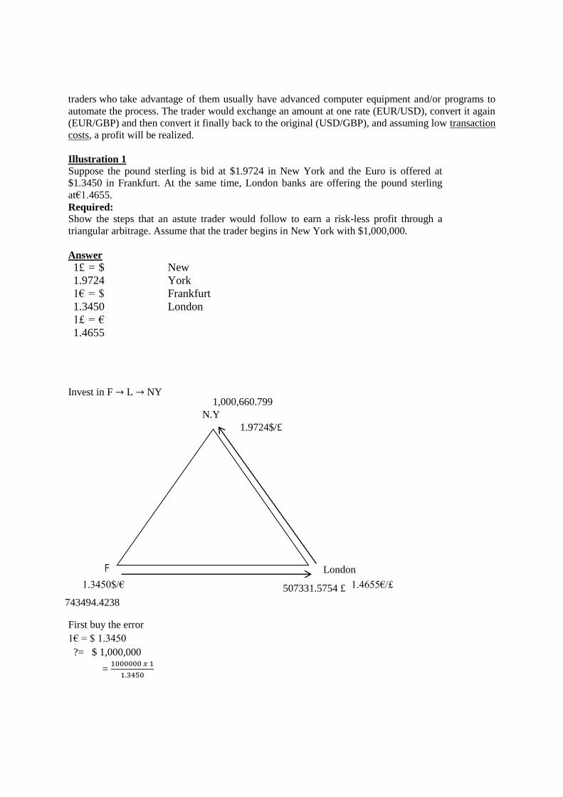
traders who take advantage of them usually have advanced computer equipment and/or programs to
automate the process. The trader would exchange an amount at one rate (EUR/USD), convert it again
(EUR/GBP) and then convert it finally back to the original (USD/GBP), and assuming low transaction
costs, a profit will be realized.
Illustration 1
Suppose the pound sterling is bid at $1.9724 in New York and the Euro is offered at
$1.3450 in Frankfurt. At the same time, London banks are offering the pound sterling
at€1.4655.
Required:
Show the steps that an astute trader would follow to earn a risk-less profit through a
triangular arbitrage. Assume that the trader begins in New York with $1,000,000.
Answer
1£ = $
1.9724
1€ = $
1.3450
1£ = €
1.4655
New
York
Frankfurt
London
Invest in F → L → NY
First buy the error
1€ = $ 1.3450
?= $ 1,000,000
= 1000000 𝑥 1
1.3450
N.Y
London F
743494.4238
507331.5754 £
1,000,660.799
1.9724$/£
1.3450$/€ 1.4655€/£
Page 289
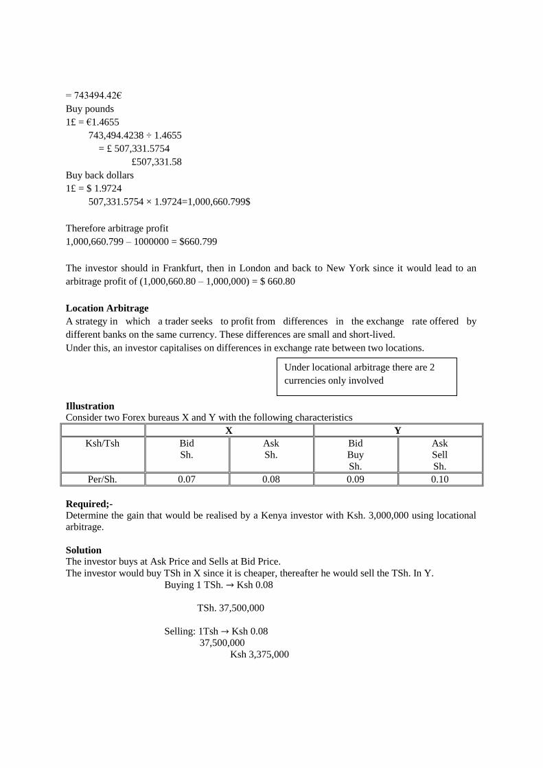
= 743494.42€
Buy pounds
1£ = €1.4655
743,494.4238 ÷ 1.4655
= £ 507,331.5754
£507,331.58
Buy back dollars
1£ = $ 1.9724
507,331.5754 × 1.9724=1,000,660.799$
Therefore arbitrage profit
1,000,660.799 – 1000000 = $660.799
The investor should in Frankfurt, then in London and back to New York since it would lead to an
arbitrage profit of (1,000,660.80 – 1,000,000) = $ 660.80
Location Arbitrage
A strategy in which a trader seeks to profit from differences in the exchange rate offered by
different banks on the same currency. These differences are small and short-lived.
Under this, an investor capitalises on differences in exchange rate between two locations.
Illustration
Consider two Forex bureaus X and Y with the following characteristics
X Y
Ksh/Tsh Bid
Sh.
Ask
Sh.
Bid
Buy
Sh.
Ask
Sell
Sh.
Per/Sh. 0.07 0.08 0.09 0.10
Required;-
Determine the gain that would be realised by a Kenya investor with Ksh. 3,000,000 using locational
arbitrage.
Solution
The investor buys at Ask Price and Sells at Bid Price.
The investor would buy TSh in X since it is cheaper, thereafter he would sell the TSh. In Y.
Buying 1 TSh. → Ksh 0.08
TSh. 37,500,000
Selling: 1Tsh → Ksh 0.08
37,500,000
Ksh 3,375,000
Under locational arbitrage there are 2
currencies only involved
Page 290
Arbitrage Profit
(3,375,000 – 3,000,000) = Ksh. 375,000
Covered Interest Arbitrage
Covered interest arbitrage is a strategy in which an investor uses a forward contract to hedge against
exchange rate risk. Covered interest rate arbitrages the practice of using favorable interest rate
differentials to invest in a higher-yielding currency, and hedging the exchange risk through a forward
currency contract.
It relates to investing in a foreign country that offers a higher interest rate in comparison to the
domestic currency.
Illustration
An investor has Ksh. 10,000,000 to invest for 6 months. The current spot rate of Ush. Is Ksh. 0.06.
The 6 months’ forward rate of Ush. is Ksh 0.09 and the interest rate in Kenya is 15% and in Uganda
is 25%.
Required;-
Calculate the gains from covered interest arbitrage.
Solution
We convert the Ksh into Ush at the spot rate (current rate) since the interest rate in UG is more
attractive in comparison to Ke.
If 1Ush → Ksh 0.06
10m
= Ush 166,666,666.10
Interest earned in UG 25% ×6/12×166,666,666.70
= Ush. 20,833,333.33
Total Investment after 6 months
= 166,666,666.70 + 20,833,333.33 = Ush 187,500,000,000
We convert the total amount into Ksh using forward rate.
If 1Ush → Ksh 0.09
187,500,000
= Ksh. 16,875,000
Investment in Kenya
10,000,000 + 15% ×6/12× 10,000,000 = Ksh. 10,750,000
Arbitrage Profit
Ksh (16,875,000 – 10,750,000)
= Ksh. 6,125,000
Page 291
International borrowing
Borrowing markets are becoming increasingly internationalised, particularly for larger companies.
Companies are able to borrow long-term funds on the Eurocurrency (money) markets and on the
markets for Eurobonds. These markets are collectively called 'Euromarkets'. Large companies can
also borrow on the syndicated loan market where a syndicate of banks provides medium- to long-term
currency loans.
If a company is receiving income in a foreign currency or has a long-term investment overseas, it can
try to limit the risk of adverse exchange rate movements by matching. It can take out a long-term loan
and use the foreign currency receipts to repay the loan.
Syndicated loans
A syndicated loan is a loan offered by a group of lenders (a 'syndicate') to a single borrower
A syndicated loan is a loan put together by a group of lenders (a 'syndicate') for a single borrower.
Banks or other institutional lenders may be unwilling (due to excessive risk) or unable to provide the
total amount individually but may be willing to work as part of a syndicate to supply the requested
funds. Given that many syndicated loans are for very large amounts, the risk of even one single
borrower defaulting could be disastrous for an individual lender. Sharing the risk is likely to be more
attractive for investors.
Each syndicate member will contribute an agreed percentage of the total funds and receive the same
percentage of the repayments.
Originally, syndicated loans were limited to international organisations for acquisitions and other
investments of similar importance and amounts. This was mainly due to the following.
Elimination of foreign exchange risk – borrowers may be able to reduce exchange rate risk by
spreading the supply of funds between a numbers of different international lenders.
7.4. INTERNATIONAL FINANCIAL INSTITUTIONS
1. International monetary fund (IMF)
The IMF aims to:
1. promote international monetary co-operation and facilitate international payments
2. provide support to countries with temporary balance of payments problems
3. provide for the orderly growth of international money through the Special Drawing
Rights (SDR) scheme
Page 292
The IMF achieves (b) by short to medium term loans financed by quota contributions from all
members. The IMF only makes loans if deflationary policies are followed. IMF facilities are often a
pre-requisite to get help from the World Bank and private banks.
2. The international bank for reconstruction and development (the World Bank)
This was created to rebuild Europe after World War 2. The World Bank provides long- term loans to
government on commercial terms for capital projects . The major source of funds is borrowing via
commercial bond issues.
3. The Bank for International Settlements
This is the Central Bankers Bank, based in Basle. It takes deposits and provides loans to central banks
on commercial terms. Its major achievement has been to co-ordinate internationally agreed world
capital adequacy standards for countries.
International trade financing is required especially to get funds to carry out international trade operations.
Depending on the types and attributes of financing , there are five major methods of transactions in
international trade.
7.5. INTERNATIONAL TRADE PAYMENT METHODS
The five major processes of transaction in international trade are the following –
(1) Prepayment
Prepayment occurs when the payment of a debt or installment payment is done before the due date. A
prepayment can include the entire balance or any upcoming part of the entire payment paid in advance of
the due date. In prepayment, the borrower is obligated by a contract to pay for the due amount.
(2) Letter of Credit
A Letter of Credit is a letter from a bank that guarantees that the payment due by the buyer to a seller will
be made timely and for the given amount. In case the buyer cannot make payment, the bank will cover the
entire or remaining portion of the payment.
(3) Drafts
Sight Draft − It is a kind of bill of exchange , where the exporter owns the title to the transported goods
until the importer acknowledges and pays for them. Sight drafts are usually found in case of air shipments
and ocean shipments for financing the transactions of goods in case of international trade.
Time Draft − It is a type of foreign cheque guaranteed by the bank. However, it is not payable in full until
the duration of time after it is obtained and accepted . In fact, time drafts are a short-term credit vehicle
used for financing goods’ transactions in international trade.
(4) Consignment
It is an arrangement to leave the goods in the possession of another party to sell. Typically, the party that
sells receives a good percentage of the sale. Consignments are used to sell a variety of products including
artwork , clothing , books , etc. Recently , consignment dealers have become quite trendy , such as those
offering specialty items, infant clothing, and luxurious fashion items.
(5) Open Account
Page 293
Open account is a method of making payments for various trade transactions. In this arrangement, the
supplier ships the goods to the buyer. After receiving and checking the concerned shipping documents, the
buyer credits the supplier's account in their own books with the required invoice amount.
The account is then usually settled periodically; say monthly, by sending bank drafts by the buyer, or
arranging through wire transfers and air mails in favor of the exporter.
TRADE FINANCE METHODS
The most popular trade financing methods are the following –
(1) Accounts Receivable Financing
It is a special type of asset-financing arrangement. In such an arrangement, a company utilizes the
receivables – the money owed by the customers – as a collateral in getting a finance.
In this type of financing, the company gets an amount that is a reduced value of the total receivables owed
by customers. The time-frame of the receivables exert a large influence on the amount of financing. For
older receivables, the company will get less financing. It is also, referred to as "factoring".
(2) Letters of Credit
Letters of Credit are one of the oldest methods of trade financing.
(3) Banker’s Acceptance
A banker’s acceptance (BA) is a short-term debt instrument that is issued by a firm that guarantees
payment by a commercial bank. BAs are used by firms as a part of the commercial transaction. These
instruments are like T-Bills and are used in case of money market funds.
(4) Working Capital Finance
Working capital finance is a process termed as the capital of a business and is used in its daily trading
operations. It is calculated as the current assets minus the current liabilities. For many firms, this is fully
made up of trade debtors (bills outstanding) and the trade creditors (the bills the firm needs to pay).
(5) Forfeiting
Forfeiting is the purchase of the amount importers owes the exporter at a discounted value by paying cash.
The forfeiter that is the buyer of the receivables then becomes the party the importer is obligated to pay the
debt.
(6) Countertrade
It is a form of international trade where goods are exchanged for other goods, in place of hard currency.
Countertrade is classified into three major categories – barter, counter-purchase, and offset.
Barter is the oldest countertrade process. It involves the direct receipt and offer of goods and services
having an equivalent value.
In a counter-purchase, the foreign seller contractually accepts to buy the goods or services obtained
from the buyer's nation for a defined amount.
Page 294
In an offset arrangement, the seller assists in marketing the products manufactured in the buying
country. It may also allow a portion of the assembly of the exported products for the manufacturers to
carry out in the buying country.
Financing an overseas subsidiary
Once the decision is taken by a multinational company to start overseas operations in any of the forms
that have been discussed in the previous section, there is a need to decide on the source of funds for
the proposed expansion. There are some differences in methods of financing the parent company
itself and the foreign subsidiaries. The parent company itself is more likely than companies, which
have no foreign interests to raise finance in a foreign currency, or in its home currency from foreign
sources.
The need to finance a foreign subsidiary raises the following questions.
How much equity capital should the parent company put into the subsidiary?
Should the subsidiary be allowed to retain a large proportion of its profits to build up its equity
reserves, or not?
Should the parent company hold 100% of the equity of the subsidiary, or should it try to create a
minority shareholding, perhaps by floating the subsidiary on the country's domestic stock exchange?
Should the subsidiary be encouraged to borrow as much long-term debt as it can, for example by
raising large bank loans? If so, should the loans be in the domestic currency of the subsidiary's
country, or should it try to raise a foreign currency loan?
Should the subsidiary be listed on the local stock exchange, raising funds from the local equity
markets?
Should the subsidiary be encouraged to minimise its working capital investment by relying heavily on
trade credit?
The method of financing a subsidiary will give some indication of the nature and length of time of the
investment that the parent company is prepared to make. A sizeable equity investment (or long-term
loans from the parent company to the subsidiary) would indicate a long-term investment by the parent
company.
Choice of finance for an overseas investment
The choice of the source of funds will depend on:
The local finance costs and any subsidies which may be available
Taxation systems of the countries in which the subsidiary is operating; different tax rates can favour
borrowing in high tax regimes, and no borrowing elsewhere
Any restrictions on dividend remittances
Page 295
The possibility of flexibility in repayments which may arise from the parent/subsidiary relationship
Tax-saving opportunities may be maximised by structuring the group and its subsidiaries in such a
way as to take the best advantage of the different local tax systems.
Because subsidiaries may be operating with a guarantee from the parent company, different gearing
structures may be possible. Thus, a subsidiary may be able to operate with a higher level of debt that
would be acceptable for the group as a whole.
Parent companies should also consider the following factors.
1. Reduced systematic risk. There may be a small incremental reduction in systematic risk from
investing abroad due to the segmentation of capital markets.
2. Access to capital. Obtaining capital from foreign markets may increase liquidity, lower costs and
make it easier to maintain optimum gearing.
3. Agency costs. These may be higher due to political risk, market imperfections and complexity,
leading to a higher cost of capital.
Costs and benefits of alternative sources of finance for multinational companies (MNCs)
Multinational companies will have access to international debt facilities, such as Eurobonds and
syndicated loans.
Multinational companies (MNCs) fund their investments from retained earnings, the issue of new
equity or the issue of new debt. Equity and debt funding can be secured by accessing both domestic
and overseas capital markets. Thus MNCs have to make decisions not only about their capital
structure as measured by the debt/equity
DIVIDEND POLICY FOR MULTINATIONALS
Retained earnings are an important source of finance for both long and short-term purposes. They
have no issue costs, they are flexible (they don't need to be applied for or repaid) and they don't result
in a dilution of control.
However, for any company, the decision to use retained earnings as a source of finance will have a
direct impact on the amount of dividends it will pay to shareholders.
The key question is if a company chooses to fund a new investment by a cut in the dividend what will
the impact be on existing shareholders and the share price of the company?
Or put another way, does dividend policy affect shareholder wealth?
Theories of dividend policies
There are three main theories concerning what impact a cut in the dividend will have on a company
and its shareholders.
Dividend irrelevancy theory
The dividend irrelevancy theory put forward by Modigliani &Miller (M&M) argues that in a perfect
capital market (no taxation, no transaction costs, no market imperfections), existing shareholders will
only be concerned about increasing their wealth, but will be indifferent as to whether that increase
comes in the form of a dividend or through capital growth.
Page 296
As a result, a company can pay any level of dividend, with any funds shortfall being met through a
new equity issue, provided it is investing in all available positive NPV projects.
If they need cash, then any investor requiring a dividend could "manufacture" their own by selling
part of their shareholding. Equally, any shareholder wanting retentions when a dividend is paid can
buy more shares with the dividend received.
Most of the criticism of M&M's theory surrounding the assumption of a perfect capital market.
Residual theory
This theory is closely related to M&Ms but recognizes the costs involved in raising new finance.
It argues that dividends themselves are important but the pattern of them is not.
The market value of a share will equal the present value of the future cash flows. The residual theory
argues that provided the present value of the dividend stream remains the same, the timing of the
dividend payments is irrelevant.
It follows that only after a firm has invested in all positive NPV projects should a dividend be paid if
there are any funds remaining. Retentions should be used for project finance with dividends as a
residual.
However, this theory still takes some assumptions that may not be deemed realistic. This includes no
taxation and no market imperfections.
Dividend relevance
Practical influences, including market imperfections, mean that changes in dividend policy,
particularly reductions in dividends paid, can have an adverse effect on shareholder wealth:
Reductions in dividend can convey 'bad news' to shareholders (dividend signalling)
Changes in dividend policy, particularly reductions, may conflict with investor liquidity
requirements (selling shares to 'manufacture dividends' is not a costless alternative to being
paid the dividend).
Changes in dividend policy may upset investor tax planning (e.g. income v capital gain if
shares are sold). Companies may have attracted a certain clientele of shareholders precisely
because of their preference between income and growth
As a result companies tend to adopt a stable dividend policy and keep shareholders informed of any
changes.
Practical influences on dividend policy
Before developing a particular dividend policy, a company must consider the following:
Legal position
Many countries will place legal restrictions on the amount of dividend that can be paid out relative to
a company's earnings.
In addition, governments have operated policies of dividend restraint over various periods.
Page 297
Profitability
Profit is obviously an essential requirement for dividends. All other things being equal, the more
stable the profit the greater the proportion that can be safely paid out as dividends. If profits are
volatile it is unwise to commit the firm to a higher dividend payout ratio.
Inflation
In periods of inflation, paying out dividends based on historic cost profits can lead to erosion of the
operating capacity of the business. For example, insufficient funds may be retained for future asset
replacement. Current cost accounting recalculates profit taking into consideration inflation, asset
values and capital maintenance. Firms would then ensure that the dividend is limited to the CCA
profit.
Growth
Rapidly growing companies commonly pay very low dividends, the bulk of earnings being retained to
finance expansion.
Control
The use of internally generated funds does not alter ownership or control. This can be advantageous
particularly in family owned firms.
Liquidity
Sufficient liquid funds need to be available to pay the dividend.
Tax
The personal tax position of investors may put them in a position of preferring either dividend income
or capital gains though growing share prices. If the clientele of investors in the company have a clear
preference for one or the other, the company should be wary of altering dividend policy and upsetting
investors.
Other sources of finance
If a firm has limited access to other sources of funds, retained earnings become a very important
source of finance. Dividends will therefore tend to be small. This situation is commonly experienced
by unquoted companies that have very limited access to external finance
These factors limit the 'dividend capacity' of the firm.
Dividend capacity
This can be simply defined as the ability at any given time of a firm's ability to pay dividends to its
shareholders. This will clearly have a direct impact on a company's ability to implement its dividend
policy (i.e. can the company actually pay the dividend it would like to).
Page 298
Legally, the firm's dividend capacity is determined by the amount of accumulated distributable profits.
However, more practically, the dividend capacity can be calculated as the Free Cash Flow to Equity
(after reinvestment), since in practice, the level of cash available will be the main driver of how much
the firm can afford to pay out.
Dividend policies
In practice, there are a number of commonly adopted dividend policies:
Stable dividend policy
Constant payout ratio
Zero dividend policy
Residual approach to dividends.
Stable dividend policy
Paying a constant or constantly growing dividend each year:
offers investors a predictable cash flow
reduces management opportunities to divert funds to non-profitable activities
works well for mature firms with stable cash flows.
However, there is a risk that reduced earnings would force a dividend cut with all the associated
difficulties.
Constant payout ratio
Paying out a constant proportion of equity earnings:
Maintains a link between earnings, reinvestment rate and dividend flow but
Cash flow is unpredictable for the investor
Gives no indication of management intention or expectation.
Zero dividend policy
All surplus earnings are invested back into the business. Such a policy:
Is common during the growth phase
Should be reflected in increased share price.
When growth opportunities are exhausted (no further positive NPV projects are available):
cash will start to accumulate
a new distribution policy will be required.
Residual dividend policy
A dividend is paid only if no further positive NPV projects available. This may be popular for firms:
in the growth phase
Without easy access to alternative sources of funds.
However:
Page 299
Cash flow is unpredictable for the investor
Gives constantly changing signals regarding management expectations.
International dividend policy
When deciding how much cash to distribute to shareholders, company directors must keep in mind
that the firm's objective is to maximise shareholder value.
The dividend payout policy should be based on investor preferences for cash dividends now or
capital gains in future from enhanced share value resultant from re-investment into projects
with a positive NPV.
Many types of multinational company shareholder (for example, institutions such as pension funds
and insurance companies ) rely on dividends to meet current expenses and any instability in
dividends would seriously affect them.
An additional factor for multinationals is that they have more than one dividend policy to
consider:
Dividends to external shareholders.
Dividends between group companies, facilitating the movement of profits and funds within the
group.
Probably the most common policy adopted by multinationals for external shareholders is a variant on
stable dividend policy. Most companies go for a stable, but rising, dividend per share:
Dividends lag behind earnings, but are maintained even when earnings fall below the dividend level
, as happens when production is lost for several months during a major industrial dispute. This
was referred to as a 'ratchet' pattern of dividends.
This policy has the advantage of not signaling 'bad news ' to investors . Also if the increases in
dividend per share are not too large it should not seriously upset the firm's clientele of investors
by disturbing their tax position.
A policy of a constant payout ratio is seldom used by multinationals because of the tremendous
fluctuations in dividend per share that it could bring:
Many firms, however, might work towards a long-run target payout percentage smoothing out
the peaks and troughs each year.
If sufficiently smoothed the pattern would be not unlike the ratchet pattern demonstrated
above.
The residual approach to dividends contains a lot of financial common sense:
If positive NPV projects are available, they should be adopted, otherwise funds should be
returned to shareholders.
This avoids the unnecessary transaction costs involved in paying shareholders a dividend and
then asking for funds from the same shareholders (via a rights issue) to fund a new project.
The major problem with the residual approach to dividends is that it can lead to large
fluctuations in dividends, which could signal bad news to investors.
Page 300

INTERNATIONAL DEBT INSTRUMENTS
A debt instrument is a paper or electronic obligation that enables the issuing party to raise funds by
promising to repay a lender in accordance with terms of a contract. Types of debt instruments include
notes, bonds, debentures, certificates, mortgages, leases or other agreements between a lender and a
borrower.
These instruments provide a way for market participants to easily transfer the ownership of debt
obligations from one party to another.
INTERNATIONAL BONDS (EURO BOND)
A euro-bond is an international bond that is denominated in a currency not native to the country where
it is issued. Also called external bond; "external bonds which, strictly, are neither eurobonds nor
foreign bonds would also include: foreign currency denominated domestic bonds…"It can be
categorised according to the currency in which it is issued. London is one of the centers of the
eurobond market, with Luxembourg being the primary listing center[3] for these instruments.
Eurobonds may be traded throughout the world—for example in Singapore or Tokyo.
Eurobonds are named after the currency they are denominated in. For example, Euro-
yen and Eurodollar bonds are denominated in Japanese yen and American dollars respectively.
Eurobonds were originally in bearer bond form, payable to the bearer and were also free
of withholding tax. The bank paid the holder of the coupon the interest payment due. Usually, no
official records were kept. The word euro-bond was originally created by Julius Strauss
Certificate Of Deposit A certificate of deposit is an agreement to deposit money for a fixed period with a bank that will pay
interest. The period for investing can vary for three months, six months, one year or five years. You
will receive a higher interest rate for the longer time commitment. You promise to leave all the
money, plus the interest, with the bank for the entire term.
In effect, you are lending the bank your money in return for interest. The CD is a promissory note that
the bank issues you. That's how banks acquire the cash they need to make loans. The interest you
receive is less than the pay earns for lending it out. That's how banks earn a profit. But you earn a
higher interest rate than you would for an interest-bearing checking account. That because you can't
withdraw the funds for the agreed-upon time.
Three Advantages
There are three advantages to CDs. First, your funds are safe. The Federal Deposit Insurance
Corporation insures CDs up to $250,000. The federal government guarantees you will never lose your
principal. For that reason, they have less risk than bonds, stocks or other more volatile investments.
Second, they offer higher interest rates than interest-bearing checking and savings account. They also
offer higher interest rates than other safe investments, such as money-market accounts or money
market funds.
You can shop around for the best rate. Small banks will offer better rates because they need the funds.
Online-only banks will offer higher rates than brick and mortar banks because their costs are lower.
Three Disadvantages
Page 301
CDs have three disadvantages. The main disadvantage is that your money is tied up for the life of the
certificate. You pay a penalty if you need to withdraw your money before the term is up.
The second disadvantage is that you could miss out on investment opportunities that occur while your
money is tied up. For example, you run the risk that interest rates will go up on other products during
your term. If it looks like interest rates are rising, you can get a no-penalty CD. It allows you to get
your money back without charge any time after the first six days. They pay more than a money
market, but less than a regular CD. (Source: "Certificates of Deposit," Ally Bank.)
The third problem is that CDs don't pay enough to keep up with the rate of inflation. If you only
invest in CDs, you'll lose your standard of living over time. The best way to keep ahead of inflation is
with stock investing, but that is risky. You could lose total investment. You could get a slightly higher
return without risk with Treasury Inflation Protected Securities or I-Bonds. Their disadvantage is that
you'll lose money if there is deflation.
Securitization of loans
Securitization is the financial practice of pooling various types of contractual debt such as residential
mortgages, commercial mortgages, auto loans or credit card debt obligations (or other non-debt assets
which generate receivables) and selling their related cash flows to third party investors as securities,
which may be described as bonds, pass-through securities, or collateralized debt obligations (CDOs).
Investors are repaid from the principal and interest cash flows collected from the underlying debt and
redistributed through the capital structure of the new financing . Securities backed by mortgage
receivables are called mortgage -backed securities (MBS), while those backed by other types of
receivables are asset-backed securities (ABS).
Commercial paper
A Commercial Paper (CP) is an unsecured , short -term debt instrument issued by a corporation ,
typically for the financing of accounts receivable, inventories and meeting short-term liabilities.
Maturities on commercial paper rarely range any longer than 270 days. The debt is usually issued a
discount, reflecting prevailing market interest rates.
In Kenya, Commercial Paper is regulated by the Capital Markets Authority (CMA) whose published
draft (Guidelines for Issuance of Corporate Bonds and Commercial Paper ) offers directives ,
procedures and qualifications for issuance.
Who Can Issue Commercial Paper?
Since Commercial Paper is an unsecured promissory note , any company issuing the paper must
represent a good credit risk. Commercial Paper issuers are typically household names and have a
substantial net worth. Commercial Paper is not for small companies. Investors must be willing to buy
unsecured Commercial Paper based on the company’s reputation and review of the company’s
financial position. Without a very strong reputation, the dealers of Commercial Paper (known as
Placement Agents) would not be able to successfully sell this product.
Guarantor institutions are often large banks or insurance companies and must meet the Capital
Markets Authority guidelines.
Page 302

AVAILABILITY AND TIMING OF REMITTANCES
A remittance is a transfer of money by a foreign worker to an individual in their home country.
Money sent home by migrants competes with international aid as one of the largest financial inflows
to developing countries.
Each year, billions of dollars are sent by migrant workers to their home countries, with some
estimates putting the total value of remittances at more than $200 billion. For some countries,
remittances make up a sizable portion of GDP. How do remittances work, and what are some of the
pitfalls that developing countries face when dealing with such large inflows of cash?
Remittances are funds transferred from migrants to their home country. They are the private savings
of workers and families that are spent in the home country for food, clothing and other expenditures,
and which drive the home economy. For many developing nations, remittances from citizens working
abroad provide an import source of much-needed funds. In some cases, funds from remittances
exceed aide sent from the developed world, and are only exceeded by foreign direct investment
Many developing countries have difficulty borrowing money, just as a first-time home buyer might
have difficulty obtaining a mortgage. Developing nations – the sort that are most likely to rely on
remittances – tend to have less stable governments and are less likely to repay the debt or not go
into default. While organizations such as the World Bank can provide funding, these funds often come
with strings attached. For governments in the developing world, this may simply be too much of a
step on sovereignty, especially if power is being held by a thread.
Remittances give countries the ability to fund development their own way; however, like a teenager
flush with cash from a first job, developing countries first have to understand just what it takes to
effectively use remittance funds. If it is to efficiently use these funds the country must first develop
policies that promote smart, stable growth, and to ensure that growth is not solely concentrated in the
cities.
It is difficult to track how remittance funds are spent because they are private transfers. Some
economists believe that recipients use the funds to purchase necessities such as food, clothing and
housing, which ultimately won't spur development because these purchases are not investments in the
strictest sense (buying a shirt is not the same as investing in a shirt production factory). Other
economists believe that funds from abroad help develop a domestic financial system. While
remittances can be sent through wire transfer businesses, they can also be sent to banks and
other financial institutions. Depending on restrictions on the movement of capital around the country,
these funds can not only help individuals pay for the consumption of goods and services, but can also
be used to make loans to businesses if they are saved rather than spent. Some banks may even seek to
establish branches abroad to make the transfer of remittances easier.
Remittance Problems
While remittances are an important lifeline in many developing countries, they can also foster a
dependency on outside flows of capital instead of prompting developing countries to create
Page 303
sustainable, local economies. The more a country depends on inflows of funds from remittances, the
more that it will be dependent on the global economy staying healthy.
Remittance flows can be negatively impacted by a downturn in the global economy. Workers
employed abroad may lose their job if they are in heavily-cyclical industries, such as construction, and
may have to stop sending remittances. This has a two-pronged effect. First, the home country may see
a significant portion of its income dry up, and thus not be able to fund projects or continue
development. Second, workers who moved abroad may move back home, exacerbating the problem
by increasing the demand for services on an already strapped economy.
Macroeconomic Effects
Large inflows in foreign currency can cause the domestic currency to appreciate, often referred to
as Dutch Disease. This in turn makes the country's exports less price competitive, since goods become
more expensive to other countries as the domestic currency rises. Because the domestic currency is
valued higher, consumption of imports begins to rise. This can snuff out the domestic industries of
developing countries. The inflow of cash, however, can also help the recipient country reduce
its balance of payments.
TRANSFER PRICING; IMPACT ON TAXES AND DIVIDENDS
Transfer pricing refers to value attached to transfer of goods or services between related parties.
Thus, transfer pricing can be defined as the price paid for goods transferred from one economic unit to
another, assuming that the two units involved are situated in different countries, but belong to the
same multinational firm.
Arm’s length principle applied to transfer pricing and attribution of profits to pe The arm’s length principle is applied both in the context of transfer pricing and attribution of profits.
Such an application makes no distinction between a branch or a subsidiary through which an MNE
carries on business in a country. A functionally separate entity approach as a working hypothesis
underlying the application of the arm’s length principle, is found in almost all tax treaties.
Transfer price is not arm’s length price
Transfer price is the price charged in a transaction. The term ‘transfer price’ is used to describe the
actual price charged between the associated enterprises in an international transaction. Transfer
pricing issues arise when entities of multinational corporations resident in different jurisdictions
transfer property or provide services to one another. These entities do not deal at arm’s length and,
thus, transactions between these entities may not be subject to ordinary market forces. Where the
transfer price is different from the price which would have been charged if the enterprises were not
associated and the difference gives rise the tax advantage, the tax is calculated on the basis of arm’s
length price.
Aims and Objective of Transfer Pricing:
1. Transfer pricing minimizes the tax burden or arranging direction of cash flow:
Page 304
Transfer price, as aforesaid, refers to the value attached to transfer of goods, services, and technology
between related entities such as parent and subsidiary corporations and also between the parties which
are controlled by a common entity. Its essence being that the pricing is not set by an independent
transferor and transferee in an arm’s length transaction. Transaction between them is not governed by
open market considerations.
2. Transfer pricing results in shifting profits:
Whatever the reason for fixing a transfer price which is not arm’s length, the result is the shift of
profit. The effect is that the profit appropriately attributable to one jurisdiction is shifted to another
jurisdiction. The main object is to avoid tax as also to withdraw profits leaving very little for the local
participation to share. Other object is avoidance of foreign exchange restrictions.
3. Shifting of Profits- Tax avoiding not the only object:
Transfer between the enterprises under the same control and management, of goods, commodities,
merchandise, raw material, stock, or services is made at a price which is not dictated by the market
but controlled by such considerations such as:
- To reduce profits artificially so that tax effect is reduced in a specific country;
- To facilitate decentralization of production so that efforts are directed to concentrate profits in
the State of production where there is no or least competition;
- To remit profits more than the ceilings imposed for repatriation;
- To use it as an effective tool to exploit the fluctuation in foreign exchange to advantage.
Page 305

CHAPTER EIGHT
REAL ESTATE FINANCE CHAPTER KEY OBJECTIVES
To be able to understand the following 1. Overview of real estate business - nature of real estate business, legal and economic framework
and participants in real estate business in Kenya
2. Valuation approaches (income, cost and sales comparison approaches)
3. REITS: types; advantages and disadvantages; valuation: net asset value per share (NAVPS); use
of funds from operations (FFO), adjusted funds from operations (AFFO) in REIT valuation
4. Instruments of real estate financing - mortgages, lien, title, mortgage requirements and mortgage
clauses
5. Rights in case of debt - default and its consequence, equity of redemption, foreclosure, statutory
redemptions
6. Mortgage and financial markets: demand for funds in mortgage market, disintermediation effects,
primary and secondary mortgage market, mortgage 7. market and cost of money, role of central bank and the role of government in mortgage markets
8. Savings and loan association - classification, state accounts, insurers. Mortgage backed bonds and
services
8.1. OVERVIEW OF REAL ESTATE BUSINESS This topic concentrates on valuation of real estate. The focus is on the three valuation approaches used
for appraisal purposes , especially the income approach . Make sure you can calculate the value of a
property using the direct capitalization method and the discounted cash flow method . Make certain
you understand the relationship between the capitalization rate and the discount rate. Finally ,
understand the investment characteristics and risks involved with estate investments.
FORMS OF REAL ESTATE
There are four basic forms of real estate investment that can be described in terms of a two-
dimensional quadrant . In the first dimension , the investment can be described in terms of public or
private markets. In the private market, ownership usually involves a direct investment like purchasing
property or lending money to a purchaser. Direct investments can be solely owned or indirectly owned
through partnerships or commingled real estate funds (CREF ). The public market does not involve
direct investment ; rather, ownership involves securities that serve as claims on the underlying assets.
Public real estate investment includes ownership of a real estate investment trust (REIT), a real estate
operating company (REOC), and mortgage-backed securities.
The second dimension describes whether an investment involves debt or equity. An equity investor has
an ownership interest in real estate or securities of an entity that owns real estate . Equity investors
control decisions such as borrowing money, property management and the exit strategy.
A debt investor is a lender that owns a mortgage or mortgage securities . Usually , the mortgage is
collateralized (secured) by the underlying real estate. In this case, the lender has a superior claim over,
an equity investor in the event of default. Since the lender must be repaid first, the value of an equity
investor’s interest is equal to the value of the property less the outstanding debt.
Page 306
Each of the basic forms has its own risk, expected returns, regulations, legal issues and market
structure.
Real estate must be actively managed. Private real estate investment requires property management
expertise on the part of the owner or a property management company. In the case of a REIT or
REOC, the real estate is professionally managed; thus, investors need no property management
expertise.
Equity investors usually require a higher rate of return than mortgage lenders because of higher risk.
As previously discussed, lenders have superior claim in the event of default. As financial leverage
(use of debt financing) increases, return requirements of both lenders and equity investors increase as
a result of higher risk.
Typically, lenders expect to receive returns from promised cash flows and do not participate in the
appreciation of the underlying property. Equity investors expect to receive an income stream as a
result of renting the property and the appreciation of value over time.
Figure1 summarizes the basic forms of real estate investment and can be used to identify the
investment that best meets an investor’s objectives.
Basic forms of Real Estate Investment
Debt Equity
Private Mortgages Direct investments such as sole ownership,
partnerships and other forms of commingled
funds
Public Mortgage-backed securities Shares of REITs and REOCs
REAL ESTATE CHARACTERISTICS
Real estate investment differs from other asset classes, like stocks and bonds, and can complicate
measurement and performance assessment.
Heterogeneity. Bonds from a particular issue are alike, as are stocks of a specific company. However
, no two properties are exactly the same because of location , size, age, construction materials ,
tenants and lease terms.
High unit value. Because real estate is indivisible, the unit value is significantly higher than
stocks and bonds, which makes it difficult to construct a diversified portfolio.
Active management . Investors in stocks and bonds are not necessarily involved in the day-to-day
management of the companies . Private real estate investment requires active property
management by the owner or a property management company.
Property management involves maintenance, negotiating leases, and collection of rents. In either
case, property management costs must be considered.
High transaction costs. Buying and selling real estate is costly because it involves appraisers,
lawyers, brokers and construction personnel.
Depreciation and desirability. Buildings wear out over time. Also, buildings may become less
desirable because of location, design or obsolescence.
Cost and availability of debt capital. Because of the high costs to acquire and develop real estate,
property values are impacted by the level of interest rates and availability of debt capital . Real
estate values are usually lower when interest rates are high and debt is scarce.
Lack of liquidity. Real estate is illiquid. It takes time to market and complete the sale of property.
Page 307
Difficulty in determining price. Stocks and bonds of public firms usually trade in active
markets. However, because of heterogeneity and low transaction volume, appraisals are usually
necessary to assess real estate values. Even then, appraised values are often based on similar, not
identical, properties. The combination of limited market participants and lack of knowledge of the
local markets makes it difficult for an outsider to value property. As a result, the market is less
efficient.
NOTE: The market for REITs has expanded to overcome many of the problems involved with direct
investment. Shares of a REIT are actively traded and are more likely to reflect market value. In
addition, investing in a REIT can provide exposure to a diversified real estate portfolio. Finally,
investors don’t need property management expertise because the REIT manages the property.
PROPERTY CLASSIFICATIONS
Real estate is commonly classified as residential or non-residential. Residential real estate includes
single-family (owner-occupied) homes and multi-family properties, such as apartments. Residential
real estate purchased with the intent to produce income is usually considered commercial real estate
property.
Non-residential real estate includes commercial properties, other than multi-family properties and
other properties such as farmland and timberland.
Commercial real estate is usually classified by its end use and includes multi-family, office,
industrial/warehouse, retail, hospitality and other types of properties such as marking facilities,
restaurants and recreational properties. A mixed-use development is a property that serves more than
one end user.
REASONS TO INVEST IN REAL ESTATE
Current income. Investors may expect to earn income from collecting rents and after paying
operating expenses, financing costs, and taxes.
Capital appreciation;-Investors usually expect values to increase over time, which forms part of
their total return.
Inflation hedge;-During inflation, investors expect both rents and property values to rise.
Diversification;-Real estate, especially private equity investment, is less than perfectly correlated
with the returns of stocks and bonds. Thus, adding private real estate investment to a portfolio can
reduce risk relative to the expected return.
Tax benefits;-In some countries, real estate investors receive favorable tax treatment.
PRINCIPAL RISKS
1) Business conditions. Numerous economic factors – such as gross domestic product (GDP).
Employment, household income, interest rates and inflation – affect the rental market.
2) New property lead time. Market conditions can change significantly while approvals are
obtained, while the property is completed, and when the property is fully leased. During the lead
time, if market conditions weaken, the resultant lower demand affects rents and vacancy resulting
in lower returns.
3) Cost and availability of capital. Real estate must compete with other investments for capital. As
previously discussed, demand for real estate is reduced when debt capital is scarce and interest
rates are high. Conversely, demand is higher when debt capital is easily obtained and interest rates
Page 308
are low. Thus, real estate prices can be affected by capital market forces without changes in
demand form tenants.
4) Unexpected inflation. Some leases provide inflation protection by allowing owners to increase
rent or pass through expenses because of inflation. Real estate values may not keep up with
inflation when markets are weak and vacancy rates are high.
5) Demographic factors. The demand for real estate is affected by the size and age distribution of
the local market population, the distribution of socioeconomic groups, and new household
formation rates.
6) Lack of liquidity. Because of the size and complexity of most real estate transactions, buyers and
lenders usually perform due diligence, which takes time and is costly. A quick sale will typically
require a significant discount.
7) Environmental issues. Because of the size and complexity of most real estate transactions,
buyers and lenders usually perform due diligence, which takes time and is costly. A quick sale
will typically require a significant discount.
8) Environmental issues. Real estate values can be significantly reduced when a property has been
contaminated by a prior owner or adjacent property owner.
9) Availability of information. A lack of information when performing property analysis increases
risk. The availability of data depends on the country, but generally more information is available
as real estate investments become more global.
10) Management expertise. Property managers and asset managers must make important operational
decisions – such as negotiating leases, property maintenance, marketing and renovating the
property – when necessary.
11) Leverage. The use of debt (leverage) to finance a real estate purchase is measured by the loan-to-
value (LTV) ratio. Higher LTV results in higher leverage and, thus, higher risk because lenders
have a superior claim in the event of default. With leverage, a small decrease in net operating
income (NOI) negatively magnifies the amount of cash flow available to equity investors after
debt service.
In most cases, risks that can be identified are hedged using insurance. In other cases, risk can be
shifted to the tenants. For example, a lease agreement could require the tenant to reimburse any
unexpected operating expenses.
The role of Real Estate in a Portfolio
Real estate investment has both bond-like and stock-like characteristics. Leases are contractual
agreements that usually call for periodic rental payments, similar to the coupon payments of a bond.
When a lease expires, there is uncertainty regarding renewal and future rental rates. This uncertainty
is affected by the availability of competing space, tenant profitability, and the state of the overall
economy, just as stock prices are affected by the same factors. As a result, the risk/return profile of
real estate as an asset class is usually between the risk/return profiles of stocks and bonds.
Role of Leverage in real Estate investment
So far, our discussion of valuation has ignored debt financing. Earlier we determined that the level of
interest rates and the availability of debt capital impact real estate prices. However, the percentage of
debt and equity used by an investor to finance real estate does not affect the property’s value.
Investors use debt financing (leverage) to increase returns. As long as the investment return is greater
than the interest paid to lenders, there is positive leverage and returns are magnified. Of course,
leverage can work in reverse. Because of the greater uncertainty involved with debt financing, risk is
higher since lenders have a superior claim to cash flow.
Commercial property types
Page 309
The basic property types used to create a low-risk portfolio include office, industrial/warehouse,
retail, and multi-family. Some investors include hospitality properties (hotels and motels) even though
the properties are considered riskier since leases are not involved and performance is highly correlated
with the business cycle.
It is important to know that with all property types, location is critical in determining value.
Office Demand is heavily dependent on job growth, especially in industries that are heavy users of office
space like finance and insurance. The average length of office leases varies globally.
In a gross lease, the owner is responsible for the operating expenses, and in a net lease, the tenant is
responsible. In a net lease, the tenant bears the risk if the actual operating experiences are greater than
expected. As a result, rent under a net lease is lower than a gross lease.
Some leases combine features from both gross and net leases. For example, the owner might pay the
operating expenses in the first year of the lease. Thereafter, any increase in the expenses is passed
through to the tenant. In a multi-tenant building, the expenses are usually prorated based on square
footage.
Understanding how leases are structured is imperative in analyzing real estate investments.
Industrial
Demand is heavily dependent on the overall economy. Demand is also affected by import/export
activity of the economy. Net leases are common.
Retail
Demand is heavily dependent on consumer spending. Consumer spending is affected by the overall
economy, job growth, population growth, and savings rates. Retail lease terms vary by the quality of
the property as well as the size and importance of the tenant. For example, an anchor tenant may
receive favorable lease terms to attract them to the property. In turn, the anchor tenant will draw other
tenants to the property.
Multi-family
Demand depends on population growth, especially in the age demographic that typically rents
apartments. The age demographic can vary by country, type of property and locale. Demand is also
affected by the cost of buying versus the cost of renting, which is measured by the ratio of home price
to rents. As home prices rise, there is a shift toward renting. An increase in interest rates will also
make buying more expensive.
The real estate industry encompasses the many facets of property, including development, appraisal,
marketing, selling, leasing, and management of commercial, industrial, residential, and agricultural
properties. This industry can fluctuate depending on the national and local economies, although it
remains somewhat consistent because people always need homes and businesses always need office
space.
Real estate economics is the application of economic techniques to real estate markets. It tries to
describe, explain, and predict patterns of prices, supply, and demand. The closely related field
of housing economics is narrower in scope, concentrating on residential real estate markets, while the
Page 310
research of real estate trends focuses on the business and structural changes affecting the industry.
Both draw on partial equilibrium analysis (supply and demand), urban economics, spatial economics,
extensive research, surveys, and finance .
Real Estate Law The law recognizes three types of property. Personal property consists of moveable items, such as
furniture. Intangible property refers to ownership that does not have a physical existence but that may
be represented by a physical item, such as a stock certificate. Real estate refers to land, as well as
anything permanently attached to the land, such as buildings and other structures. Some people use
the term “real property” to refer to land without structures.
Limits on Ownership Lawyers often refer to real estate as a “bundle of rights” extending to the center of the earth and up to
the heavens. Certain “sticks” may be separated from the bundle by the owner’s intentional actions.
For example, an owner might grant an easement or acquire property that is subject to an easement,
and thereby give up the right to exclude people from that part of the property. Similarly, an owner
might buy property in a subdivision that is subject to covenants that restrict how the owner can use the
property. In some splaces, owners can sell the subsurface rights to their land, so that one owner might
own and live on the surface, while another has the right to mine minerals below the surface.
Real estate law is closely tied to other areas of law. For example, contract law governs the sale of real
estate and requires that such contracts be in writing. States dictate special inheritance laws for real
estate. There are even specific types of crimes and torts that apply to real estate. For example, trespass
refers to entering the land of another without authority to do so, and it can be a crime or the subject of
a civil lawsuit. Real estate is also subject to special provisions in family law, such as the rights of a
spouse in the marital home.
OVERVIEW OF REAL ESTATE MARKETS
The main participants in real estate markets are:
1) Owner/user: These people are both owners and tenants. They purchase houses
or commercial property as an investment and also to live in or utilize as a business.
2) Owner: These people are pure investors. They do not consume the real estate that they
purchase. Typically, they rent out or lease the property to someone else.
3) Renter: These people are pure consumers.
4) Developers: These people prepare raw land for building, which results in new products
for the market.
5) Renovators: These people supply refurbished buildings to the market.
6) Facilitators: This group includes banks, real estate brokers, lawyers, and others that
facilitate the purchase and sale of real estate.
Characteristics of Real estate markets include:
1) Durability. Real estate is durable. A building can last for decades or even centuries, and
the land underneath it is practically indestructible. Because of this, real estate markets are
modelled as a stock/flow market.
2) Heterogeneity. Every unit of real estate is unique in terms of its location, the building,
and it’s financing. This makes pricing difficult, increases search costs, creates information
asymmetry, and greatly restricts substitutability.
Page 311

3) High transaction costs. Buying and/or moving into a home costs much more than most
types of transactions. The costs include search costs, real estate fees, moving costs, legal
fees, land transfer taxes, and deed registration fees
4) Long time delays. The market adjustment process is subject to time delays due to the
length of time it takes to finance, design, and construct new supply and due to the
relatively slow rate of change of demand.
5) Immobility. Real estate is locational immobile (save for mobile homes, but the land
underneath them is still immobile). Consumers come to the good rather than the good
going to the consumer. Because of this, there can be no physical marketplace.
REAL ESTATE FINANCING
There are different ways of real estate financing: governmental and commercial sources and
institutions. A homebuyer or builder can obtain financial aid from savings and loan associations,
commercial banks, savings banks, mortgage bankers and brokers, life insurance companies, credit
unions, individual investors, and builders.
1) Savings and loan associations The most important purpose of these institutions is to make mortgage loans on residential property.
These organizations, which also are known as savings associations, building and loan
associations, cooperative banks . As home-financing institutions, they give primary attention to
single-family residences and are equipped to make loans in this area.
2) Commercial banks Due to changes in banking laws and policies, commercial banks are increasingly active in home
financing. In acquiring mortgages on real estate, these institutions follow two main practices:
Some banks maintain active and well-organized departments whose primary function is to compete
actively for real estate loans. In areas lacking specialized real estate financial institutions, these banks
become the source for residential and farm mortgage loans.
3) Savings bank These depository financial institutions are licenced by Central Bank. They primarily accept consumer
deposits, and make home mortgage loans.
4) Mortgage bankers and brokers Mortgage bankers are companies or individuals that originate mortgage loans, sell them to other
investors, service the monthly payments, and may act as agents to dispense funds for taxes and
insurance.
Mortgage brokers present homebuyers with loans from a variety of loan sources. Their income comes
from the lender making the loan, just like with any other bank.
5) Credit unions People who share a common bond— for example, employees of a company, labor union, or religious
group, organize these cooperative financial institutions. Some credit unions offer home loans in
addition to other financial services.
6) Real estate investment trusts
Page 312
REITs, like savings and loan associations, are committed to real estate lending, can, and do serve the
national real estate market, although some specialization has occurred in their activities.
How to Value a Real Estate Investment Property
Estimating the value of real estate is necessary for a variety of endeavors, including financing, sales
listing, investment analysis, property insurance and taxation. However, for most people, determining
the asking or purchase price of a piece of real property is the most useful application of real
estate valuation. This article will provide an introduction to the basic concepts and methods of real
estate valuation, particularly as it pertains to sales.
Value Technically speaking, a property's value is defined as the present worth of future benefits arising from
the ownership of the property. Unlike many consumer goods that are quickly used, the benefits of real
property are generally realized over a long period. Therefore, an estimate of a property's value must
take into consideration economic and social trends, as well as governmental controls or regulations
and environmental conditions that may influence the four elements of value.
1) Demand: The desire or need for ownership supported by the financial means to satisfy the desire
2) Utility: The ability to satisfy future owners' desires and needs
3) Scarcity: The finite supply of competing properties
4) Transferability: The ease with which ownership rights are transferred
Value versus Cost and Price
Value is not necessarily equal to cost or price. Cost refers to actual expenditures – on materials, for
example, or labor. Price, on the other hand, is the amount that someone pays for something. While
cost and price can affect value, they do not determine value. The sales price of a house might be
sh.15, 000,000, but the value could be significantly higher or lower. For instance, if a new owner finds
a serious flaw in the house, such as a faulty foundation, the value of the house could be lower than the
price.
Market Value
An appraisal is an opinion or estimate regarding the value of a particular property as of a specific date.
Appraisal reports are used by businesses, government agencies, individuals, investors and mortgage
companies when making decisions regarding real estate transactions. The goal of an appraisal is to
determine a property's market value – the most probable price that the property will bring in a
competitive and open market.
REAL ESTATE APPRAISALS
Since commercial real estate transactions are infrequent, appraisals are used to estimate value or
assess changes in value over time in order to measure performance. In most cases, the focus of an
appraisal is market value; that is, the most probable sales price a typical investor is willing to pay.
VALUATION APPROACHES
Appraisers use three different approaches to value real estate: the cost approach, the sales comparison
approach and the income approach.
The premises of the cost approach is that a buyer would not pay more for a property than it would cost
to purchase land to construct a comparable building. Consequently, under the cost approach, value is
derived by adding the value of the land to the current replacement cost of a new building less
adjustments for estimated depreciation and obsolescence. Because of the difficulty in measuring
Page 313
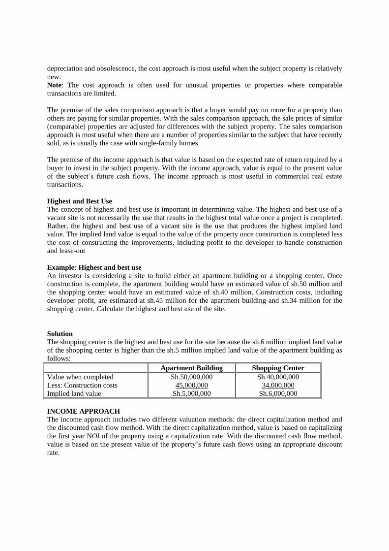
depreciation and obsolescence, the cost approach is most useful when the subject property is relatively
new.
Note: The cost approach is often used for unusual properties or properties where comparable
transactions are limited.
The premise of the sales comparison approach is that a buyer would pay no more for a property than
others are paying for similar properties. With the sales comparison approach, the sale prices of similar
(comparable) properties are adjusted for differences with the subject property. The sales comparison
approach is most useful when there are a number of properties similar to the subject that have recently
sold, as is usually the case with single-family homes.
The premise of the income approach is that value is based on the expected rate of return required by a
buyer to invest in the subject property. With the income approach, value is equal to the present value
of the subject’s future cash flows. The income approach is most useful in commercial real estate
transactions.
Highest and Best Use
The concept of highest and best use is important in determining value. The highest and best use of a
vacant site is not necessarily the use that results in the highest total value once a project is completed.
Rather, the highest and best use of a vacant site is the use that produces the highest implied land
value. The implied land value is equal to the value of the property once construction is completed less
the cost of constructing the improvements, including profit to the developer to handle construction
and lease-out
Example: Highest and best use
An investor is considering a site to build either an apartment building or a shopping center. Once
construction is complete, the apartment building would have an estimated value of sh.50 million and
the shopping center would have an estimated value of sh.40 million. Construction costs, including
developer profit, are estimated at sh.45 million for the apartment building and sh.34 million for the
shopping center. Calculate the highest and best use of the site.
Solution
The shopping center is the highest and best use for the site because the sh.6 million implied land value
of the shopping center is higher than the sh.5 million implied land value of the apartment building as
follows:
Apartment Building Shopping Center
Value when completed
Less: Construction costs
Implied land value
Sh.50,000,000
45,000,000
Sh.5,000,000
Sh.40,000,000
34,000,000
Sh.6,000,000
INCOME APPROACH
The income approach includes two different valuation methods: the direct capitalization method and
the discounted cash flow method. With the direct capitalization method, value is based on capitalizing
the first year NOI of the property using a capitalization rate. With the discounted cash flow method,
value is based on the present value of the property’s future cash flows using an appropriate discount
rate.
Page 314
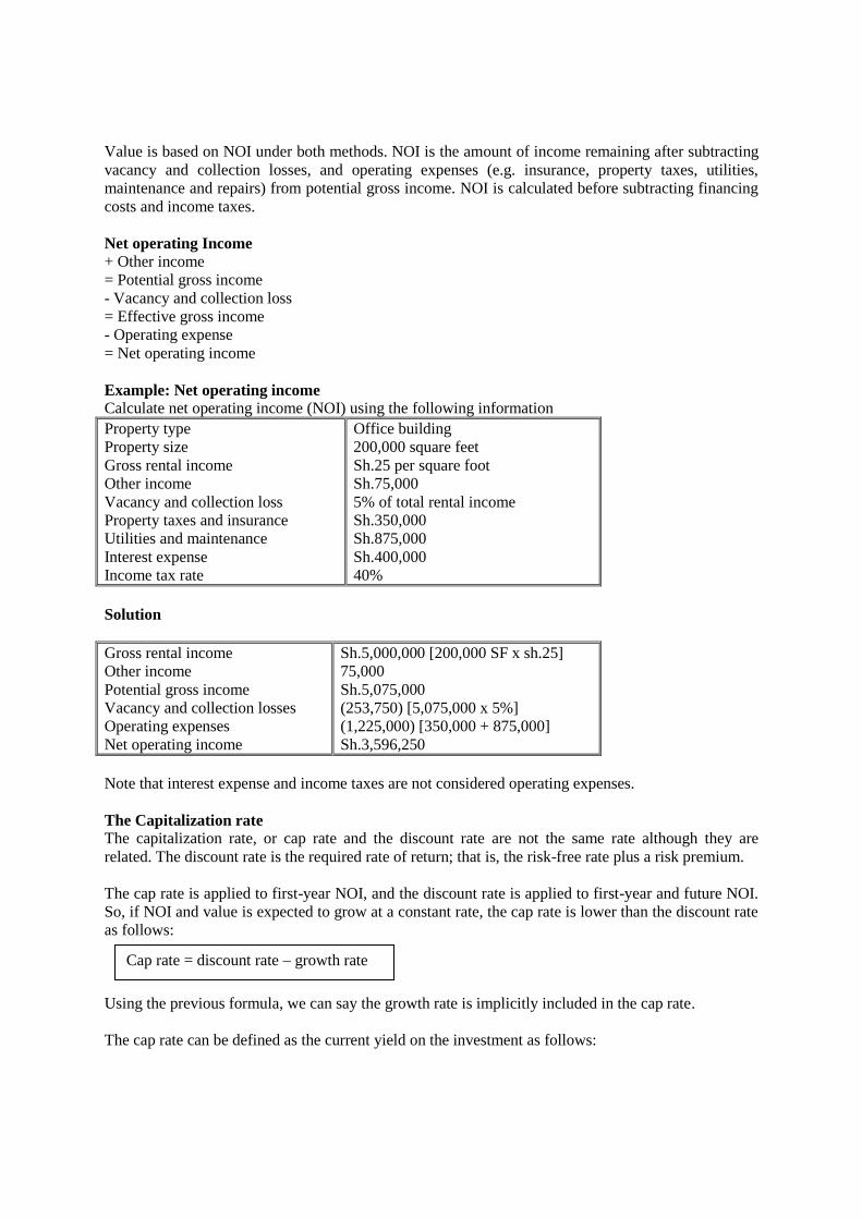
Value is based on NOI under both methods. NOI is the amount of income remaining after subtracting
vacancy and collection losses, and operating expenses (e.g. insurance, property taxes, utilities,
maintenance and repairs) from potential gross income. NOI is calculated before subtracting financing
costs and income taxes.
Net operating Income
+ Other income
= Potential gross income
- Vacancy and collection loss
= Effective gross income
- Operating expense
= Net operating income
Example: Net operating income
Calculate net operating income (NOI) using the following information
Property type
Property size
Gross rental income
Other income
Vacancy and collection loss
Property taxes and insurance
Utilities and maintenance
Interest expense
Income tax rate
Office building
200,000 square feet
Sh.25 per square foot
Sh.75,000
5% of total rental income
Sh.350,000
Sh.875,000
Sh.400,000
40%
Solution
Gross rental income
Other income
Potential gross income
Vacancy and collection losses
Operating expenses
Net operating income
Sh.5,000,000 [200,000 SF x sh.25]
75,000
Sh.5,075,000
(253,750) [5,075,000 x 5%]
(1,225,000) [350,000 + 875,000]
Sh.3,596,250
Note that interest expense and income taxes are not considered operating expenses.
The Capitalization rate
The capitalization rate, or cap rate and the discount rate are not the same rate although they are
related. The discount rate is the required rate of return; that is, the risk-free rate plus a risk premium.
The cap rate is applied to first-year NOI, and the discount rate is applied to first-year and future NOI.
So, if NOI and value is expected to grow at a constant rate, the cap rate is lower than the discount rate
as follows:
Using the previous formula, we can say the growth rate is implicitly included in the cap rate.
The cap rate can be defined as the current yield on the investment as follows:
Cap rate = discount rate – growth rate
Page 315
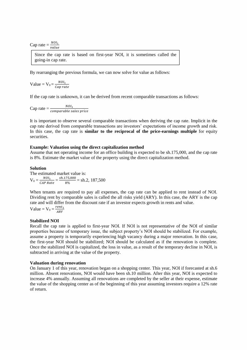
Cap rate = 𝑁𝑂𝐼1
𝑣𝑎𝑙𝑢𝑒
By rearranging the previous formula, we can now solve for value as follows:
Value = V0 = 𝑁𝑂𝐼1
𝐶𝑎𝑝 𝑟𝑎𝑡𝑒
If the cap rate is unknown, it can be derived from recent comparable transactions as follows:
Cap rate = 𝑁𝑂𝐼1
𝑐𝑜𝑚𝑝𝑎𝑟𝑎𝑏𝑙𝑒 𝑠𝑎𝑙𝑒𝑠 𝑝𝑟𝑖𝑐𝑒
It is important to observe several comparable transactions when deriving the cap rate. Implicit in the
cap rate derived from comparable transactions are investors’ expectations of income growth and risk.
In this case, the cap rate is similar to the reciprocal of the price-earnings multiple for equity
securities.
Example: Valuation using the direct capitalization method
Assume that net operating income for an office building is expected to be sh.175,000, and the cap rate
is 8%. Estimate the market value of the property using the direct capitalization method.
Solution
The estimated market value is:
V0 = 𝑁𝑂𝐼1
𝐶𝐴𝑃 𝑅𝑎𝑡𝑒 =
𝑠ℎ.175,000
8% = sh.2, 187,500
When tenants are required to pay all expenses, the cap rate can be applied to rent instead of NOI.
Dividing rent by comparable sales is called the all risks yield (ARY). In this case, the ARY is the cap
rate and will differ from the discount rate if an investor expects growth in rents and value.
Value = V0 = 𝑟𝑒𝑛𝑡1
𝐴𝑅𝑌
Stabilized NOI
Recall the cap rate is applied to first-year NOI. If NOI is not representative of the NOI of similar
properties because of temporary issue, the subject property’s NOI should be stabilized. For example,
assume a property is temporarily experiencing high vacancy during a major renovation. In this case,
the first-year NOI should be stabilized; NOI should be calculated as if the renovation is complete.
Once the stabilized NOI is capitalized, the loss in value, as a result of the temporary decline in NOI, is
subtracted in arriving at the value of the property.
Valuation during renovation
On January 1 of this year, renovation began on a shopping center. This year, NOI if forecasted at sh.6
million. Absent renovations, NOI would have been sh.10 million. After this year, NOI is expected to
increase 4% annually. Assuming all renovations are completed by the seller at their expense, estimate
the value of the shopping center as of the beginning of this year assuming investors require a 12% rate
of return.
Since the cap rate is based on first-year NOI, it is sometimes called the
going-in cap rate.
Page 316
Solution
The value of the shopping center after renovation is: 𝑠𝑡𝑎𝑏𝑖𝑙𝑖𝑧𝑒𝑑 𝑁𝑂𝐼
𝐶𝐴𝑃 𝑅𝑎𝑡𝑒 =
10,000,000
(12%−4%) = sh.125,000,000
Using the financial calculator, the present value of the temporary decline in NOI during renovation is:
PV of loss = 4,000,000 x PVIF12% 4000000 x 0.8929 = sh.3, 571,429
(In the previous computation, we are assuming that all rent is received at the end of the year for
simplicity).
The total value of the shopping center is:
Value after renovations
Loss in value during renovations
Total value
Sh.125,000,000
(3,571,429)
Sh.121,428,571
Discounted cash flow method
Recall from our earlier discussion, we determined the growth rate is implicitly included in the cap rate
as follows:
Cap rate = discount rate – growth rate
Rearranging the above formula we get:
Discount rate = cap rate + growth rate
So, we can say the investor’s rate of return includes the return on first-year NOI (measured by the cap
rate) and the growth in income and value over time (measured by the growth rate).
Value = V0 = 𝑁𝑂𝐼1
(𝑟−𝑔) =
𝑁𝑂𝐼1
𝐶𝑎𝑝 𝑟𝑎𝑡𝑒
Where:
r = rate required by equity investors for similar properties
g = growth rate of NOI (assumed to be constant)
r – g = cap rate
If no growth is expected in NOI, then the cap rate and the discount rate are the same. In this case,
value is calculated just like any perpetuity.
Terminal Cap Rate
Using the discounted cash flow (DCF) method, investors usually project NOI for a specific holding
period and the property value at the end of the holding period rather than projecting NOI into infinity.
Unfortunately, estimating the property value at the end of the holding period, known as the terminal
value (also known as reversion or resale), is challenging. However, since the terminal value is just the
Note: This equation should look very familiar to you because its just a modified version of
the constant growth dividend discount model, also known as the Gordon growth model, from
the equity valuation portion of the curriculum.
Renovations = 10m – 6m = 4m
Page 317
present value of the NOI received by the next investor, we can use the direct capitalization method to
estimate the value of the property when sold. In this case, we need to estimate the future NOI and a
future cap rate, known as the terminal or residual cap rate.
Since the terminal value occurs in the future, it must be discounted to present. Thus, the value of the
property is equal to the present value of NOI over the holding period and the present value of the
terminal value.
Example: Valuation with terminal value
Because of existing leases, the NOI of a warehouse is expected to be sh.1 million per year over the
next four years. Beginning in the fifth year, NOI is expected to increase to sh.1.2 million and grow at
3% annually thereafter. Assuming investors require a 13% return, calculate the value of the property
today assuming the warehouse is sold after four years.
Solution
The present value of the NOI over the holding period is:
N = 4; = 13%Cash flow p.a = 1,000,000; PV = 1,000,000 × PVIFA 13%, 4
PV = 1,000,000 × 2.9745 = 2,974,500
The terminal value after four years is:
V4 = 𝑁𝑂𝐼4
𝐶𝑎𝑝 𝑟𝑎𝑡𝑒 =
𝑠ℎ.1,200,000
(13%−3%) = sh.12, 000,000
The present value of the terminal value is:
Therefore through total PV = 2,974,500 + 12,000,000 × PVIF13%,4
= 2,974,500 + 12,000,000×0.6133 = 10,334,100
Example: Allocation of operating expenses
Total operating expensed for a multi-tenant office building are 30% fixed and 70% variable. If the
100,000 square foot building was fully occupied, operating expenses would total sh.6 per square foot.
The building is currently 90% occupied. If the total operating expenses are allocated to the occupied
space, calculate the operating expense per occupied square foot.
Solution
If the building is fully occupied, total operating expenses would be sh.600,000 (100,000 x sh.6 per
SF). Fixed and variable operating expenses would be:
Fixed Sh.180, 000 (600,000 × 30%)
Variable Sh.420, 000 (600,000 × 70%)
Total Sh.600, 000
Thus variable operating expenses are sh.4.20 per square foot (sh.420, 000/100,000 SF) if the building
is fully occupied. Since the building is 90% occupied, total operating expenses are:
Fixed Sh.180, 000
Variable 378,000 (100,000 SF × 90% per SF)
Total sh. 558,000
Note = Met operating income
Page 318
So, operating expenses per occupied square foot are sh.6.20 (558,000 total operating expenses /
90,000 occupied SF)
Cost Approach
The premise behind the cost approach is that a buyer is unlikely to pay more for a property than it
would cost to purchase land and build a comparable building. The cost approach involves estimating
the market value of the land, estimating the replacement cost of the building and adjusting for
depreciation and obsolescence. The cost approach is often used for unusual properties or properties
where comparable transactions are limited.
Following are the steps involved with applying the cost approach
Step 1: Estimate the market value of the land. The value of the land is estimated separately, often
using the sales comparison approach.
Step 2: Estimate the building’s replacement cost. Replacement cost is based on current construction
costs and standards and should any builder/developer’s profit.
Step 3: Deduct depreciation including physical deterioration, functional obsolescence, locational
obsolescence and economic obsolescence. Physical deterioration is related to the building’s age and
occurs as a result of normal wear and tear over time. Physical deterioration can be curable or
incurable. An item is curable if the benefit of fixing the problem is at least as must as the cost of cure.
For example, replacing the roof will likely increase the value of the building by at least as must as the
cost of the roof. The cost of fixing curable items is subtracted from replacement cost.
An item is incurable if the problem is not economically feasible to remedy. For example, the cost of
fixing a structural problem might exceed the benefit of the example, the cost of fixing a structural
problem might exceed the benefit of the repair. Since an incurable defect would not be fixed,
depreciation can be estimated based on the effective age of the property relative to its total economic
life. For example, the physical depreciation of a property with an effective age of 30 years and a 50-
year total economic life is 60% (30 years effective age / 50 year economic life). To avoid double
Note: Depreciation for appraisal purposes is not the same as depreciation used for financial
reporting or tax reporting purposes. Financial depreciation and tax depreciation involves the
allocation of original cost over time. For appraisal purposes, depreciation represents an actual
decline in value.
Note: replacement cost refers to the cost of a building having the same utility but constructed
with modern building materials. Reproduction cost refers to the cost of reproducing an exact
replica of the building using the same building materials, architectural design and quality of
construction. Replacement cost is usually more relevant for appraisal purposes because
reproduction cost may be uneconomical.
Page 319
counting, the age/life ratio is multiplied by and deducted from replacement cost minus the cost of
fixing curable items.
Functional obsolescence is the loss in value resulting from defects in design that impairs a building’s
utility. For example, a building might have a bad floor plan. As a result of functional obsolescence,
NOI is usually lower than it otherwise would be because of lower rent or higher operating expenses.
Functional obsolescence can be estimated by capitalizing the decline in NOI.
Locational obsolescence occurs when the location is no longer optimal. For example, five years after
a luxury apartment complex is completed, a prison is built down the street making the location of the
apartment complex less desirable. As a result, lower rental rates will decrease the value of the
complex. Care must be taken in deducting the loss in value because part of the loss is likely already
reflected in the market value of the land.
Economic obsolescence occurs when new construction is not feasible under current economic
conditions. This can occur when rental rates are not sufficient to support the property. Consequently,
the replacement cost of the subject property exceeds the value of a new building if it was developed.
Example: The cost approach
Heavenly Towers is a 200,000 square foot high-rise apartment building located in the downtown area.
The building has an effective age of 10 years, while its total economic life is estimated at 40 year. The
building has a structural problem that is not feasible to repair. The building also needs a new roof at a
cost of sh.1, 000,000. The new roof will increase the value of the building by sh.300, 000
The bedrooms in each apartment are too small and the floor plans are awkward. As a result of the
poor design, rents are sh.400, 000 a year lower than competing properties.
When Heavenly Towers was original built, it was located across the street from a park. Five year ago,
the city converted the park to a sewage treatment plant. The negative impact on rents is estimated at
sh.600, 000 a year.
Due to recent construction of competing properties, vacancy rates have increased significantly
resulting in a loss of an estimated value of sh.1, 200,000
The cost of replace Heavenly Towers is estimated at sh.400 per square foot plus builder profit of
sh.5,000,000. The market value of the land is estimated at sh.20,000,000. An appropriate cap rate is
8%. Using the cost approach, estimate the value of heavenly Towers.
Note: The effective age and the actual age can differ as a result of above norrmal or below
normal wear and tear. Incurable items increase the effective age of the property.
Page 320
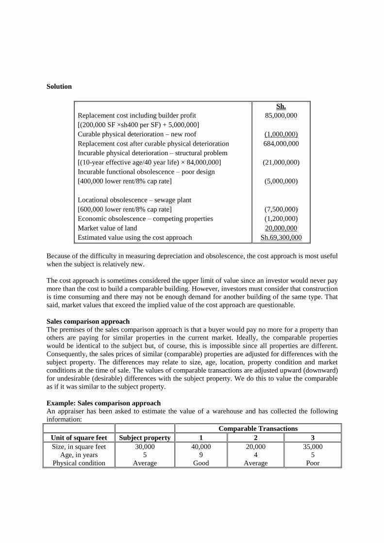
Solution
Replacement cost including builder profit
[(200,000 SF ×sh400 per SF) + 5,000,000]
Curable physical deterioration – new roof
Replacement cost after curable physical deterioration
Incurable physical deterioration – structural problem
[(10-year effective age/40 year life) × 84,000,000]
Incurable functional obsolescence – poor design
[400,000 lower rent/8% cap rate]
Locational obsolescence – sewage plant
[600,000 lower rent/8% cap rate]
Economic obsolescence – competing properties
Market value of land
Estimated value using the cost approach
Sh.
85,000,000
(1,000,000)
684,000,000
(21,000,000)
(5,000,000)
(7,500,000)
(1,200,000)
20,000,000
Sh.69,300,000
Because of the difficulty in measuring depreciation and obsolescence, the cost approach is most useful
when the subject is relatively new.
The cost approach is sometimes considered the upper limit of value since an investor would never pay
more than the cost to build a comparable building. However, investors must consider that construction
is time consuming and there may not be enough demand for another building of the same type. That
said, market values that exceed the implied value of the cost approach are questionable.
Sales comparison approach
The premises of the sales comparison approach is that a buyer would pay no more for a property than
others are paying for similar properties in the current market. Ideally, the comparable properties
would be identical to the subject but, of course, this is impossible since all properties are different.
Consequently, the sales prices of similar (comparable) properties are adjusted for differences with the
subject property. The differences may relate to size, age, location, property condition and market
conditions at the time of sale. The values of comparable transactions are adjusted upward (downward)
for undesirable (desirable) differences with the subject property. We do this to value the comparable
as if it was similar to the subject property.
Example: Sales comparison approach
An appraiser has been asked to estimate the value of a warehouse and has collected the following
information:
Comparable Transactions
Unit of square feet Subject property 1 2 3
Size, in square feet
Age, in years
Physical condition
30,000
5
Average
40,000
9
Good
20,000
4
Average
35,000
5
Poor
Page 321
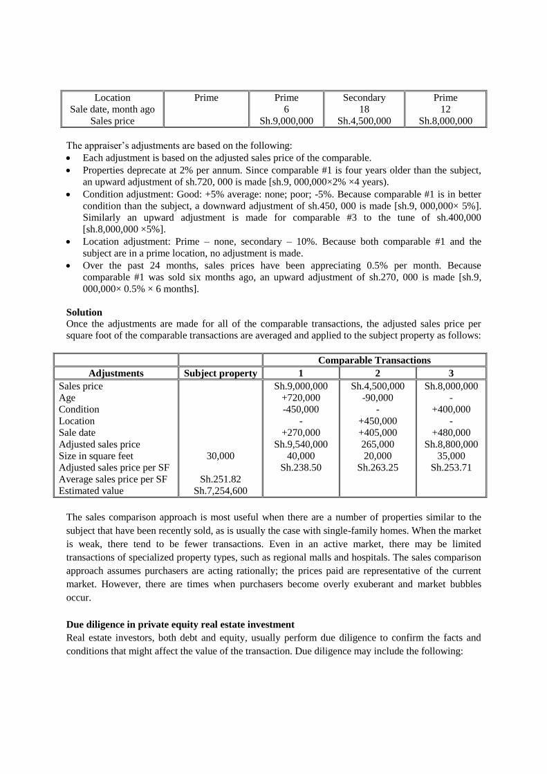
Location
Sale date, month ago
Sales price
Prime Prime
6
Sh.9,000,000
Secondary
18
Sh.4,500,000
Prime
12
Sh.8,000,000
The appraiser’s adjustments are based on the following:
Each adjustment is based on the adjusted sales price of the comparable.
Properties deprecate at 2% per annum. Since comparable #1 is four years older than the subject,
an upward adjustment of sh.720, 000 is made [sh.9, 000,000×2% ×4 years).
Condition adjustment: Good: +5% average: none; poor; -5%. Because comparable #1 is in better
condition than the subject, a downward adjustment of sh.450, 000 is made [sh.9, 000,000× 5%].
Similarly an upward adjustment is made for comparable #3 to the tune of sh.400,000
[sh.8,000,000 ×5%].
Location adjustment: Prime – none, secondary – 10%. Because both comparable #1 and the
subject are in a prime location, no adjustment is made.
Over the past 24 months, sales prices have been appreciating 0.5% per month. Because
comparable #1 was sold six months ago, an upward adjustment of sh.270, 000 is made [sh.9,
000,000× 0.5% × 6 months].
Solution
Once the adjustments are made for all of the comparable transactions, the adjusted sales price per
square foot of the comparable transactions are averaged and applied to the subject property as follows:
Comparable Transactions
Adjustments Subject property 1 2 3
Sales price
Age
Condition
Location
Sale date
Adjusted sales price
Size in square feet
Adjusted sales price per SF
Average sales price per SF
Estimated value
30,000
Sh.251.82
Sh.7,254,600
Sh.9,000,000
+720,000
-450,000
-
+270,000
Sh.9,540,000
40,000
Sh.238.50
Sh.4,500,000
-90,000
-
+450,000
+405,000
265,000
20,000
Sh.263.25
Sh.8,000,000
-
+400,000
-
+480,000
Sh.8,800,000
35,000
Sh.253.71
The sales comparison approach is most useful when there are a number of properties similar to the
subject that have been recently sold, as is usually the case with single-family homes. When the market
is weak, there tend to be fewer transactions. Even in an active market, there may be limited
transactions of specialized property types, such as regional malls and hospitals. The sales comparison
approach assumes purchasers are acting rationally; the prices paid are representative of the current
market. However, there are times when purchasers become overly exuberant and market bubbles
occur.
Due diligence in private equity real estate investment
Real estate investors, both debt and equity, usually perform due diligence to confirm the facts and
conditions that might affect the value of the transaction. Due diligence may include the following:
Page 322
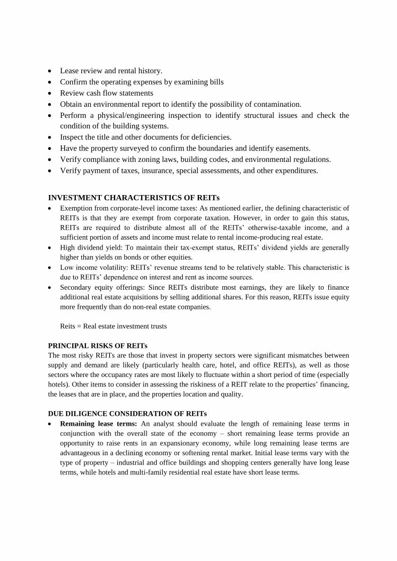
Lease review and rental history.
Confirm the operating expenses by examining bills
Review cash flow statements
Obtain an environmental report to identify the possibility of contamination.
Perform a physical/engineering inspection to identify structural issues and check the
condition of the building systems.
Inspect the title and other documents for deficiencies.
Have the property surveyed to confirm the boundaries and identify easements.
Verify compliance with zoning laws, building codes, and environmental regulations.
Verify payment of taxes, insurance, special assessments, and other expenditures.
INVESTMENT CHARACTERISTICS OF REITs
Exemption from corporate-level income taxes: As mentioned earlier, the defining characteristic of
REITs is that they are exempt from corporate taxation. However, in order to gain this status,
REITs are required to distribute almost all of the REITs’ otherwise-taxable income, and a
sufficient portion of assets and income must relate to rental income-producing real estate.
High dividend yield: To maintain their tax-exempt status, REITs’ dividend yields are generally
higher than yields on bonds or other equities.
Low income volatility: REITs’ revenue streams tend to be relatively stable. This characteristic is
due to REITs’ dependence on interest and rent as income sources.
Secondary equity offerings: Since REITs distribute most earnings, they are likely to finance
additional real estate acquisitions by selling additional shares. For this reason, REITs issue equity
more frequently than do non-real estate companies.
Reits = Real estate investment trusts
PRINCIPAL RISKS OF REITs
The most risky REITs are those that invest in property sectors were significant mismatches between
supply and demand are likely (particularly health care, hotel, and office REITs), as well as those
sectors where the occupancy rates are most likely to fluctuate within a short period of time (especially
hotels). Other items to consider in assessing the riskiness of a REIT relate to the properties’ financing,
the leases that are in place, and the properties location and quality.
DUE DILIGENCE CONSIDERATION OF REITs
Remaining lease terms: An analyst should evaluate the length of remaining lease terms in
conjunction with the overall state of the economy – short remaining lease terms provide an
opportunity to raise rents in an expansionary economy, while long remaining lease terms are
advantageous in a declining economy or softening rental market. Initial lease terms vary with the
type of property – industrial and office buildings and shopping centers generally have long lease
terms, while hotels and multi-family residential real estate have short lease terms.
Page 323
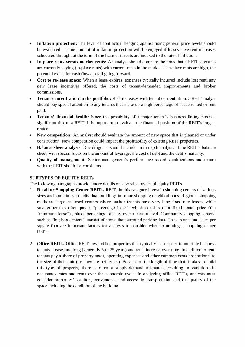
Inflation protection: The level of contractual hedging against rising general price levels should
be evaluated – some amount of inflation protection will be enjoyed if leases have rent increases
scheduled throughout the term of the lease or if rents are indexed to the rate of inflation.
In-place rents versus market rents: An analyst should compare the rents that a REIT’s tenants
are currently paying (in-place rents) with current rents in the market. If in-place rents are high, the
potential exists for cash flows to fall going forward.
Cost to re-lease space: When a lease expires, expenses typically incurred include lost rent, any
new lease incentives offered, the costs of tenant-demanded improvements and broker
commissions.
Tenant concentration in the portfolio: Risk increases with tenant concentration; a REIT analyst
should pay special attention to any tenants that make up a high percentage of space rented or rent
paid.
Tenants’ financial health: Since the possibility of a major tenant’s business failing poses a
significant risk to a REIT, it is important to evaluate the financial position of the REIT’s largest
renters.
New competition: An analyst should evaluate the amount of new space that is planned or under
construction. New competition could impact the profitability of existing REIT properties.
Balance sheet analysis: Due diligence should include an in-depth analysis of the REIT’s balance
sheet, with special focus on the amount of leverage, the cost of debt and the debt’s maturity.
Quality of management: Senior management’s performance record, qualifications and tenure
with the REIT should be considered.
SUBTYPES OF EQUITY REITs
The following paragraphs provide more details on several subtypes of equity REITs.
1. Retail or Shopping Center REITs. REITs in this category invest in shopping centers of various
sizes and sometimes in individual buildings in prime shopping neighborhoods. Regional shopping
malls are large enclosed centers where anchor tenants have very long fixed-rate leases, while
smaller tenants often pay a “percentage lease,” which consists of a fixed rental price (the
“minimum lease”) , plus a percentage of sales over a certain level. Community shopping centers,
such as “big-box centers,” consist of stores that surround parking lots. These stores and sales per
square foot are important factors for analysts to consider when examining a shopping center
REIT.
2. Office REITs. Office REITs own office properties that typically lease space to multiple business
tenants. Leases are long (generally 5 to 25 years) and rents increase over time. In addition to rent,
tenants pay a share of property taxes, operating expenses and other common costs proportional to
the size of their unit (i.e. they are net leases). Because of the length of time that it takes to build
this type of property, there is often a supply-demand mismatch, resulting in variations in
occupancy rates and rents over the economic cycle. In analyzing office REITs, analysts must
consider properties’ location, convenience and access to transportation and the quality of the
space including the condition of the building.
Page 324
3. Residential (Multi-family) REITs. This category of REITs invests in rental apartments. Demand
for rental apartments tends to be stable; however, lease periods are short (usually one year), so
rental income fluctuates over time as competing properties are constructed. Variables that will
affect rental income include the overall strength of the local economy and any move-in
inducements offered. Factors to consider when analyzing a residential REIT include local
demographic trends, availability of alternatives (i.e. home ownership), any rent controls imposed
by the local government, and factors related to the portfolio properties themselves, such as the age
of the properties and how appealing they are to renters in the local market compared to other
competing properties. Additionally, because rents are typically based on a gross lease, the impact
of rising costs must be considered (under a gross lease, operating costs are paid by the landlord).
Examples include rising fuel or energy costs, taxes and maintenance costs.
4. Health Care REITs. Health care REITs invest in hospitals, nursing homes, retirement homes,
rehab centers and medical office buildings. REITs in many countries are barred from operating
this kind of business themselves. In order to participate in this property sector while maintaining
their tax-free status, REITs rent properties to health care providers. Leases in this sector are
usually net leases. Health care REITs are relatively unaffected by the overall economy. However,
other factors are important, such as government funding of health care, demographic shifts, new
construction versus demand, increases in the cost of insurance and the potential for lawsuits by
residents.
5. Industrial REITs. Industrial REITs own properties used in activities such as manufacturing,
warehousing and distribution. The value of industrial properties is relatively stable and less
cyclical compared to the value of other types of properties, due to long leases (5 to 25 years)
which smoothes rental income. In analyzing industrial REITs, an analyst needs to closely examine
the local market for industrial properties; new properties coming on to the market and the demand
for such space by tenants will affect the value of existing properties. Location and availability of
transportation links (airports, roads and ports) are also important consideration for industrial
REITs.
6. Hotel REITs. A hotel REIT (like a health care REIT) usually leases properties to management
companies, so the REIT receives only passive rental income. Hotels are exposed to revenue
volatility driven by changes in business and leisure travel, and the sector’s cyclical nature is
intensified by a lack of long-term leases. In analyzing hotel REITs, analysts compare a number of
statistics against industry averages (operating profit margins, occupancy rates and average room
rates). One key metric that is closely followed is RevPAR, the revenue per available room, which
is calculated by multiplying the average occupancy rate by the average room rate. Other closely-
watched variables are the level of margins, forward bookings, and food and beverage sales.
Expenses related to maintaining the properties are also closely monitored. Because of the time lag
associated with bringing new hotel properties on-line (up to three years), the cyclical nature of
demand needs to be considered. Because of the uncertainty in income, the use of high amounts of
leverage in financing hotel properties is risky.
Page 325
7. Storage REITs. Properties owned by storage REITs rent self-storage lockers (also known
as mini-warehouses) to individuals and small businesses. Space is rented to users on a
monthly basis and under a gross lease. In analyzing storage REITs, it is important to look
at the local factors that drive demand for storage, such as housing sales, new business
start-ups, demographic trends in the surrounding area, as well as any other competing
facilities that are under construction. Seasonal demand should also be considered.
8. Diversified REITs. Diversified REITs own more than one category of REIT. While they
are uncommon in North America, some investors in Europe and Asia are drawn to the
diversified nature of these REITs. Because diversified REITs hold a range of property
types, when analyzing this class of REIT it is especially important to evaluate
management’s background in the kinds of real estate invested in.
Characteristics of REIT property subtypes
REIT
Type
Economic Value
Determinant
Investment
Characteristics
Principal Risks Due Diligence Considerations
Retail Retail sales
growth
Job creation
Stable revenue
stream over the
short term
Depends on consumer
spending
Per-square-foot sales and
rental rates
Office Job creation
New space
supply vs.
demand
Long (5-25 yrs)
lease terms
Stable year-to-year
income
Changes in office
vacancy and rental
rates
New space under construction
Quality of office space
(location, condition of
building, and so on)
Residential Population
growth
Job creation
One-year leases
Stable demand
Competition
Inducements
Regional economy
Inflation in operating
costs
Demographics and income
trends
Age and competitive appeal
Cost of home ownership
Rent controls
Health
care Population
growth
New space
supply vs
demand
REITs lease
facilities to health
care providers
Leases are usually
net leases
Demographics
Government funding
Construction cycles
Financial condition of
operators
Tenant litigation
Operating trends
Government funding trends
Litigation settlements
Insurance costs
Competitors’ new facilities vs
demand
Industrial Retail sales
growth
Population
growth
Less cyclical than
some other REIT
types
5-25 year net leases
Change in income
and values are slow
Shifts in the
composition of local
and national industrial
bases and trade
Trends in tenants’
requirements
Obsolescence of existing
space
Need for new types of space
Proximity to transportation
Trends in local supply and
Page 326
Justify the use of net asset value per share (NAVPS) in REIT valuation and estimate NAVPS
based on forecasted cash net operating income.
NAVPS is the (per-share) amount by which assets exceed liabilities, using current market values
rather than accounting book values. NAVPS is generally considered the appropriate measure of the
fundamental value of REITs (and REOCs). If the market price of a REIT varies from VAVPS, this is
seen as a sign of over or undervaluation.
Estimating NAVPS Based on Forecasted Cash Net Operating Income
In the absence of the reliable appraisal, analysts will estimate the value of operating real estate by
capitalizing the net operating income. This process first requires the calculation of a market required
rate of return, known as the capitalization rate (“cap rate”) based on the prices of comparable recent
transactions that have taken place in the market.
Capitalization rate = 𝑛𝑒𝑡 𝑜𝑝𝑒𝑟𝑎𝑡𝑖𝑛𝑔 𝑖𝑛𝑐𝑜𝑚𝑒
𝑝𝑟𝑜𝑝𝑒𝑟𝑡𝑦 𝑣𝑎𝑙𝑢𝑒
Note that the net operating income (NOI) refers to the expected income in the coming year. Once a
cap rate for the market has been determined, this cap be used to capitalize the NOI:
Property value = 𝑛𝑒𝑡 𝑜𝑝𝑒𝑟𝑎𝑡𝑖𝑛𝑔 𝑖𝑛𝑐𝑜𝑚𝑒
𝑐𝑎𝑝𝑖𝑡𝑎𝑙𝑖𝑧𝑎𝑡𝑖𝑜𝑛 𝑟𝑎𝑡𝑒
In the example below, we show how NAVPS is calculated by capitalizing a rental stream. First,
estimated first-year NOI is capitalized using a market cap rate. Next, we add the value of other
tangible assets and subtract the value of liabilities to find total net asset value. Net asset value divided
by the number of outstanding shares gives us NAVPS.
Example: Computing NAVPS
Vinny Custone, CPA, is undertaking a valuation of the Anyco Shopping Center REIT, Ltd. Given the
following financial data for Anyco, estimate NAVPS based on forecasted cash net operating income.
demand
Hotel Job creation
New space
supply vs.
demand
Variable income
Sector is cyclical
because it is not
protected by long-
term leases
Exposed to business-
cycle
Changes in business
and leisure travel
Exposure to travel
disruptions
Occupancy, room rate and
operating profit margins vs
industry averages
Revenue per available room
(RevPAR)
Trends in forward bookings
Maintenance expenditures
New construction in local
market
Financial leverage
Storage Population
growth
Job creation
Space is rented
under gross leases
and on a monthly
basis
Ease of entry can lead
to overbuilding.
Construction of new
competitive facilities
Trends in housing sales
Demographic trends
New business start-up activity
Seasonal trends in demand for
storage facilities that can be
significant in some markets
Page 327
Select Anyco Shopping Center REIT, Ltd Financial Information (in millions)
Last 12 months NOI
Cash and equivalents
Accounts receivable
Total debt
Other liabilities
Non-cash rents
Full-year adjustment for acquisitions
Land held for future development
Prepaid/Other assets (excluding intangibles)
Estimate of next 12 months in NOI
Cap rate based on recent comparable transactions
Shares outstanding
Sh.80
Sh.20
Sh.15
Sh.250
Sh.50
Sh.2
Sh.1
Sh.10
Sh.5
1.25%
8.0%
15
Solution
Last 12 months NOI
- Non-cash rents + Full-year adjustment for acquisitions2
= Pro forma cash NOI for last 12 months + Next 12 months growth in NOI @1.25%/yr)3
= Estimated next 12 months cash NOI
+ Cap rate4
= Estimated value of operating real estate5
+ Cash and equivalent6
+ Land held for future development
+ Accounts receivable
+ Prepaid/other assets (excluding intangibles
)
= Estimated gross asset value
Total debt7
Other liabilities
= Net asset value
+ Share outstanding
= Net asset value per share8
Sh.80
Sh.2
Sh.1
Sh.79
Sh.1
Sh.80
8.0%
Sh.1,000
Sh.20
Sh.10
Sh.15
Sh.5
Sh.1,050
Sh.250
Sh.50
Sh.750
15
Sh.50.00
Note:
1) Non-cash rent (difference between average contractual rent and cash rent paid) is removed.
2) NOI is increased to represent full-year rent for properties acquired during the year.
3) Cash NOI is expected to increase by 1.25% over the next year.
4) Cap rate is based on recent transactions for comparable properties.
5) Operating real estate value = expected next 12 month cash NOI / 8% capitalization rate.
6) Add the book value of other assets; cash , accounts receivable, land for future development,
prepaid expenses, and so on. Certain intangibles such as goodwill deferred financing expenses
and deferred tax assets, if given are ignored.
7) Debt and other liabilities are subtracted to get to net asset value.
8) NAVPS = NAV/number of outstanding shares.
Page 328
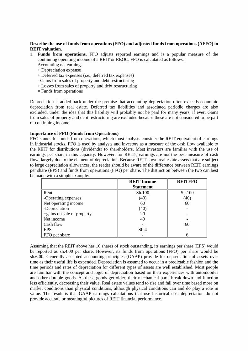
Describe the use of funds from operations (FFO) and adjusted funds from operations (AFFO) in
REIT valuation.
1. Funds from operations. FFO adjusts reported earnings and is a popular measure of the
continuing operating income of a REIT or REOC. FFO is calculated as follows:
Accounting net earnings
+ Depreciation expense
+ Deferred tax expenses (i.e., deferred tax expenses)
- Gains from sales of property and debt restructuring
+ Losses from sales of property and debt restructuring
= Funds from operations
Depreciation is added back under the premise that accounting depreciation often exceeds economic
depreciation from real estate. Deferred tax liabilities and associated periodic charges are also
excluded, under the idea that this liability will probably not be paid for many years, if ever. Gains
from sales of property and debt restructuring are excluded because these are not considered to be part
of continuing income.
Importance of FFO (Funds from Operations)
FFO stands for funds from operations, which most analysts consider the REIT equivalent of earnings
in industrial stocks. FFO is used by analysts and investors as a measure of the cash flow available to
the REIT for distributions (dividends) to shareholders. Most investors are familiar with the use of
earnings per share in this capacity. However, for REITs, earnings are not the best measure of cash
flow, largely due to the element of depreciation. Because REITs own real estate assets that are subject
to large depreciation allowances, the reader should be aware of the difference between REIT earnings
per share (EPS) and funds from operations (FFO) per share. The distinction between the two can best
be made with a simple example:
REIT Income
Statement
REITFFO
Rent
-Operating expenses
Net operating income
-Depreciation
+gains on sale of property
Net income
Cash flow
EPS
FFO per share
Sh.100
(40)
60
(40)
20
40
-
Sh.4
-
Sh.100
(40)
60
-
-
-
60
-
6
Assuming that the REIT above has 10 shares of stock outstanding, its earnings per share (EPS) would
be reported as sh.4.00 per share. However, its funds from operations (FFO) per share would be
sh.6.00. Generally accepted accounting principles (GAAP) provide for depreciation of assets over
time as their useful life is expended. Depreciation is assumed to occur in a predictable fashion and the
time periods and rates of depreciation for different types of assets are well established. Most people
are familiar with the concept and logic of depreciation based on their experiences with automobiles
and other durable goods. As these goods get older, their mechanical parts break down and function
less efficiently, decreasing their value. Real estate values tend to rise and fall over time based more on
market conditions than physical conditions, although physical conditions can and do play a role in
value. The result is that GAAP earnings calculations that use historical cost depreciation do not
provide accurate or meaningful pictures of REIT financial performance.
Page 329
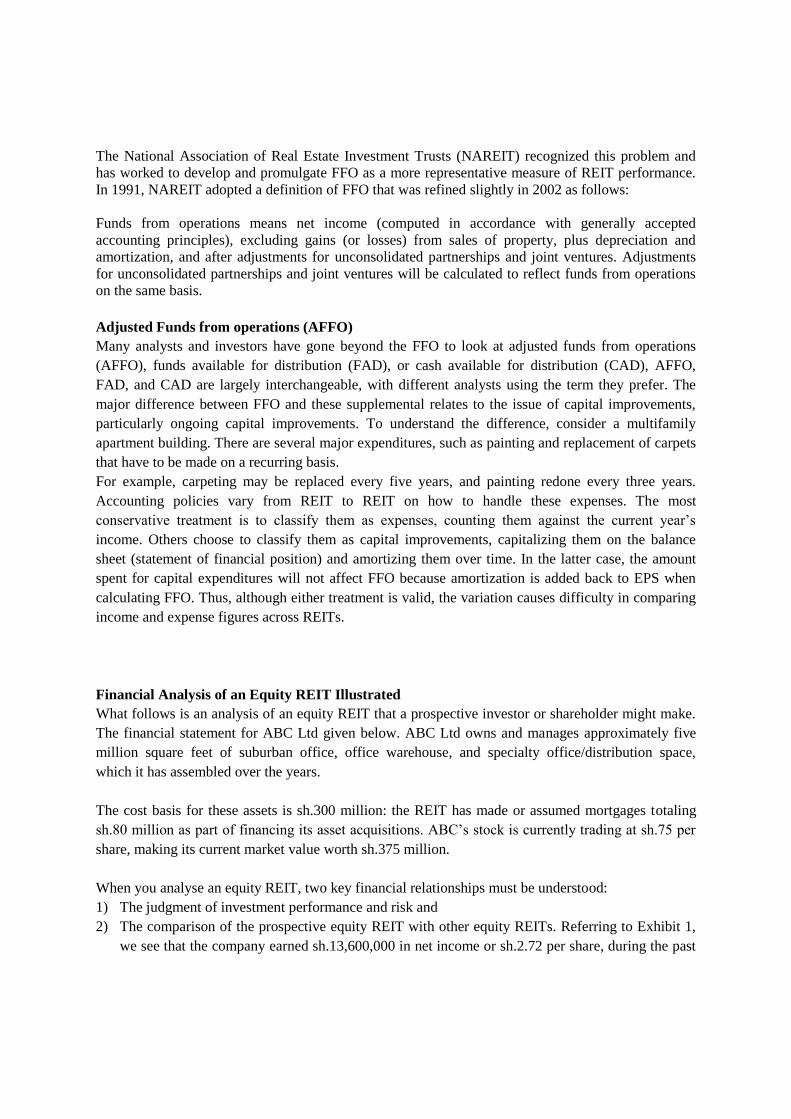
The National Association of Real Estate Investment Trusts (NAREIT) recognized this problem and
has worked to develop and promulgate FFO as a more representative measure of REIT performance.
In 1991, NAREIT adopted a definition of FFO that was refined slightly in 2002 as follows:
Funds from operations means net income (computed in accordance with generally accepted
accounting principles), excluding gains (or losses) from sales of property, plus depreciation and
amortization, and after adjustments for unconsolidated partnerships and joint ventures. Adjustments
for unconsolidated partnerships and joint ventures will be calculated to reflect funds from operations
on the same basis.
Adjusted Funds from operations (AFFO)
Many analysts and investors have gone beyond the FFO to look at adjusted funds from operations
(AFFO), funds available for distribution (FAD), or cash available for distribution (CAD), AFFO,
FAD, and CAD are largely interchangeable, with different analysts using the term they prefer. The
major difference between FFO and these supplemental relates to the issue of capital improvements,
particularly ongoing capital improvements. To understand the difference, consider a multifamily
apartment building. There are several major expenditures, such as painting and replacement of carpets
that have to be made on a recurring basis.
For example, carpeting may be replaced every five years, and painting redone every three years.
Accounting policies vary from REIT to REIT on how to handle these expenses. The most
conservative treatment is to classify them as expenses, counting them against the current year’s
income. Others choose to classify them as capital improvements, capitalizing them on the balance
sheet (statement of financial position) and amortizing them over time. In the latter case, the amount
spent for capital expenditures will not affect FFO because amortization is added back to EPS when
calculating FFO. Thus, although either treatment is valid, the variation causes difficulty in comparing
income and expense figures across REITs.
Financial Analysis of an Equity REIT Illustrated
What follows is an analysis of an equity REIT that a prospective investor or shareholder might make.
The financial statement for ABC Ltd given below. ABC Ltd owns and manages approximately five
million square feet of suburban office, office warehouse, and specialty office/distribution space,
which it has assembled over the years.
The cost basis for these assets is sh.300 million: the REIT has made or assumed mortgages totaling
sh.80 million as part of financing its asset acquisitions. ABC’s stock is currently trading at sh.75 per
share, making its current market value worth sh.375 million.
When you analyse an equity REIT, two key financial relationships must be understood:
1) The judgment of investment performance and risk and
2) The comparison of the prospective equity REIT with other equity REITs. Referring to Exhibit 1,
we see that the company earned sh.13,600,000 in net income or sh.2.72 per share, during the past
Page 330
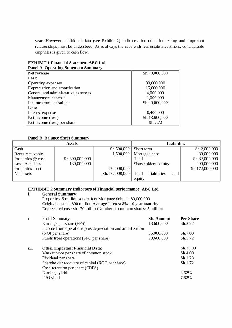
year. However, additional data (see Exhibit 2) indicates that other interesting and important
relationships must be understood. As is always the case with real estate investment, considerable
emphasis is given to cash flow.
EXHIBIT 1 Financial Statement ABC Ltd
Panel A. Operating Statement Summary
Net revenue
Less:
Operating expenses
Depreciation and amortization
General and administrative expenses
Management expense
Income from operations
Less:
Interest expense
Net income (loss)
Net income (loss) per share
Sh.70,000,000
30,000,000
15,000,000
4,000,000
1,000,000
Sh.20,000,000
6,400,000
Sh.13,600,000
Sh.2.72
Panel B. Balance Sheet Summary
Assets Liabilities
Cash
Rents receivable
Properties @ cost
Less: Acc.depr.
Properties – net
Net assets
Sh.300,000,000
130,000,000
Sh.500,000
1,500,000
170,000,000
Sh.172,000,000
Short term
Mortgage debt
Total
Shareholders’ equity
Total liabilities and
equity
Sh.2,000,000
80,000,000
Sh.82,000,000
90,000,000
Sh.172,000,000
EXHIBBIT 2 Summary Indicators of Financial performance: ABC Ltd
i. General Summary:
Properties: 5 million square feet Mortgage debt: sh.80,000,000
Original cost: sh.300 million Average Interest 8%, 10 year maturity
Depreciated cost: sh.170 million Number of common shares: 5 million
ii. Profit Summary:
Earnings per share (EPS)
Income from operations plus depreciation and amortization
(NOI per share)
Funds from operations (FFO per share)
iii. Other important Financial Data:
Market price per share of common stock
Dividend per share
Shareholder recovery of capital (ROC per share)
Cash retention per share (CRPS)
Earnings yield
FFO yield
Sh. Amount
13,600,000
35,000,000
28,600,000
Per Share
Sh.2.72
Sh.7.00
Sh.5.72
Sh.75.00
Sh.4.00
Sh.1.28
Sh.1.72
3.62%
7.62%
Page 331
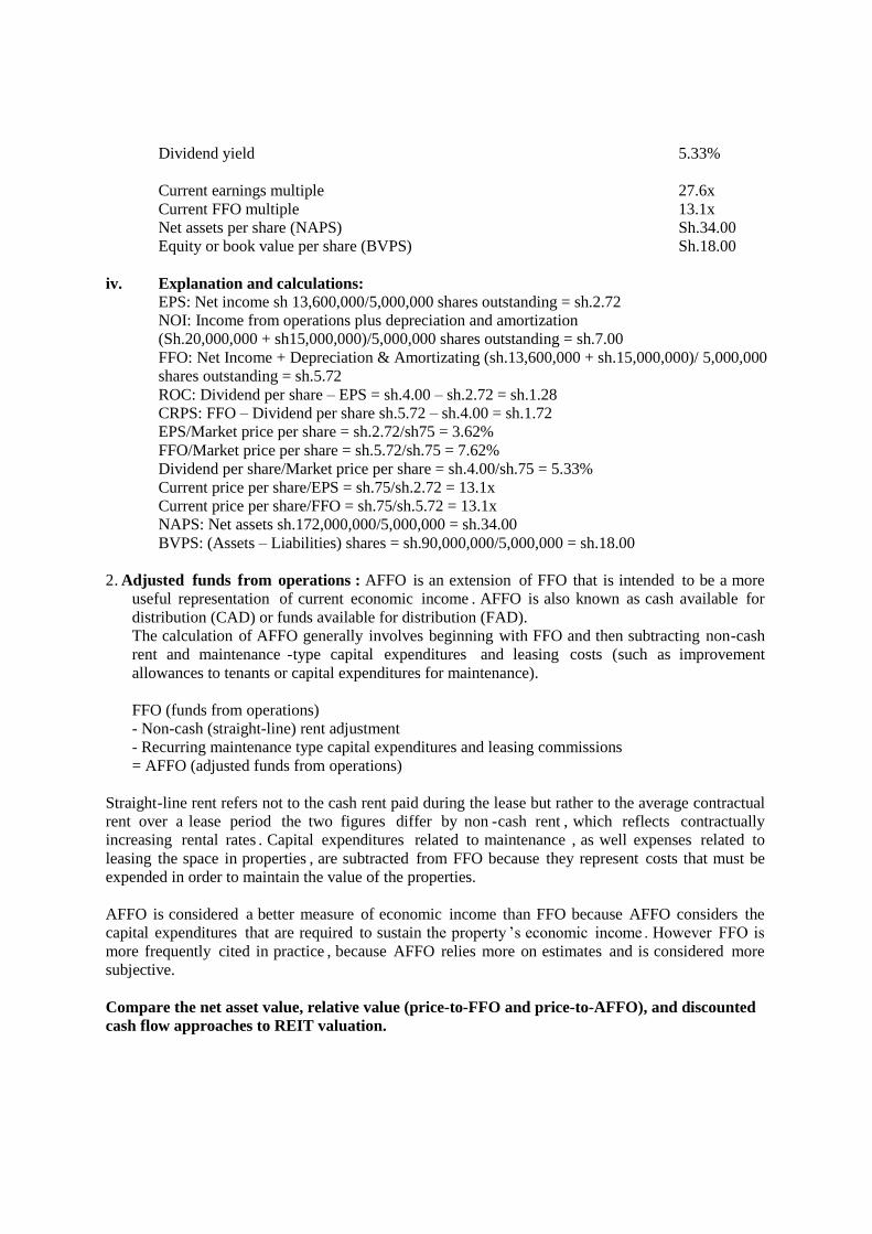
Dividend yield
Current earnings multiple
Current FFO multiple
Net assets per share (NAPS)
Equity or book value per share (BVPS)
5.33%
27.6x
13.1x
Sh.34.00
Sh.18.00
iv. Explanation and calculations:
EPS: Net income sh 13,600,000/5,000,000 shares outstanding = sh.2.72
NOI: Income from operations plus depreciation and amortization
(Sh.20,000,000 + sh15,000,000)/5,000,000 shares outstanding = sh.7.00
FFO: Net Income + Depreciation & Amortizating (sh.13,600,000 + sh.15,000,000)/ 5,000,000
shares outstanding = sh.5.72
ROC: Dividend per share – EPS = sh.4.00 – sh.2.72 = sh.1.28
CRPS: FFO – Dividend per share sh.5.72 – sh.4.00 = sh.1.72
EPS/Market price per share = sh.2.72/sh75 = 3.62%
FFO/Market price per share = sh.5.72/sh.75 = 7.62%
Dividend per share/Market price per share = sh.4.00/sh.75 = 5.33%
Current price per share/EPS = sh.75/sh.2.72 = 13.1x
Current price per share/FFO = sh.75/sh.5.72 = 13.1x
NAPS: Net assets sh.172,000,000/5,000,000 = sh.34.00
BVPS: (Assets – Liabilities) shares = sh.90,000,000/5,000,000 = sh.18.00
2. Adjusted funds from operations : AFFO is an extension of FFO that is intended to be a more
useful representation of current economic income . AFFO is also known as cash available for
distribution (CAD) or funds available for distribution (FAD).
The calculation of AFFO generally involves beginning with FFO and then subtracting non-cash
rent and maintenance -type capital expenditures and leasing costs (such as improvement
allowances to tenants or capital expenditures for maintenance).
FFO (funds from operations)
- Non-cash (straight-line) rent adjustment
- Recurring maintenance type capital expenditures and leasing commissions
= AFFO (adjusted funds from operations)
Straight-line rent refers not to the cash rent paid during the lease but rather to the average contractual
rent over a lease period the two figures differ by non -cash rent , which reflects contractually
increasing rental rates . Capital expenditures related to maintenance , as well expenses related to
leasing the space in properties , are subtracted from FFO because they represent costs that must be
expended in order to maintain the value of the properties.
AFFO is considered a better measure of economic income than FFO because AFFO considers the
capital expenditures that are required to sustain the property ’s economic income . However FFO is
more frequently cited in practice , because AFFO relies more on estimates and is considered more
subjective.
Compare the net asset value, relative value (price-to-FFO and price-to-AFFO), and discounted
cash flow approaches to REIT valuation.
Page 332
REITs and REOCs are valued using several different approaches.
Net asset value per share: The net asset value method of valuation can be used either to generate an
absolute valuation or as part of a relative valuation approach. Note, however, that net asset value is an
indication of a REIT’s assets to a buyer in the private market, which can be quite different from the
value public market investors would attach to the REIT. For this reason, there have historically been
significant differences (i.e. premiums or discounts) between NAV estimates and the prices at which
REITs actually trade.
Relative value (price-to-FFO and price-to-AFFO): There are three key factors that impact that
price-to-FFO and price-to-AFFO of REITs and REOCs:
1. Expectations for growth of FFO or AFFO.
2. The level of risks inherent in the underlying real estate.
3. Risk related to the firm’s leverage and access to capital.
Discounted cash flow approach: Dividend discount and discounted cash flow models of valuation
are appropriate for use with REITs and REOCs, because these two investment structures typically pay
dividends and thereby return a high proportion of their income to investors. DDM and DCF are used
in private real estate in the same way that they are used to value stocks in general. For dividend
discount models, an analyst will typically develop near-term, medium-term, and long-term growth
forecasts and then use these values as the basis for two-or three-stage dividend discount models. To
build a discounted cash flow model, analysts will generally create intermediate-term cash flow
projections plus a terminal value that is developed using historical cash flow multiples.
INSTRUMENTS OF REAL ESTATE FINANCE 1. Encumbrance—right or interest in a property held by one who is not the legal owner of the
property
2. Lien—financial encumbrance; a charge against a specific property wherein the property is made
the security for the performance of a certain act, usually the repayment of a debt – Voluntary
liens and involuntary liens.
Note: Relative valuation using NAVPS is essentially comparing NAVPS to the market price of a
REIT (or REOC) share. If, in general, the market is trading at a premium to NAVPS, a value
investor would select the investments with the lowest premium (everything else held constant).
Note: We discuss dividend discount models extensively in the study session on
equity valuation. Similar to price multiples in equity valuation, price multiples
here depend on growth rate and risk. The first factor (above) focuses on growth
rate, while the second and third factors above focus on risk.
Page 333
Title and lien theories – Equitable rights – Title theory in which lender’s rights are superior to
borrower’s – Redemption right – Statutory redemption period – Lien theory recognizes the rights of
lenders in collateral property being equitable rights, while borrowers retain their legal rights in the
property.
Debtor’s Rights After Default
After the buyer defaults, the secured party must give notice to the debtor of any plan to dispose of the
collateral. In a consumer goods transaction, the notice must contain the following information:
a. A description of the debtor and the secured party;
b. A description of the collateral;
c. A description of the manner in which the secured party will dispose of the collateral;
d. A statement that the debtor is entitled to an accounting of the unpaid indebtedness and the cost of
any accounting;
e. A statement of the time and place of the sale, if the sale is open to the public
f. A description of any liability for amounts the debtor may still owe after the disposition of the
collateral;
g. The telephone number the debtor may contact in order to find out the amount that must be paid to
the secured party to redeem the collateral; and A telephone number or mailing address the debtor
may use to obtain further information concerning the disposition of collateral and the amount
owed to the secured party.
Disintermediation
Disintermediation is a long word with a short, but scary meaning - the removal of the intermediary in
a transaction.
For real estate, it is the word that asks the question: in these digital days, do a property seller and a
buyer really need an agent to connect and mediate the selling of a property? When you can upload a
property to a portal, and that portal will alert buyers to new listings that meet their criteria, what is the
real value a real estate agent adds to the deal?
The common response is that agents offer a value-added service, ensuring that vendors not only sell,
but sell at the best price with the least stress. They are a concierge service to help and guide vendors
through their property journey and the key decisions that will be required to get the best result.
Essentially, what this means is that disintermediation of the real estate industry has started and is
happening now. And here’s why: the service that too many agents still offer their clients is not good
enough.
Two Mortgage Markets
Robinson is looking to buy a home, but he needs a loan. Whether he realizes it or not, he'll be entering
the primary mortgage market to do business. The primary mortgage market is where loans are created.
However, there is another mortgage market that Robinson won't be dealing with directly, but that will
still have an impact on his loan. We call this market the secondary mortgage market, which is where
lenders can sell their loans to interested parties. Let's look a bit closer at each of these mortgage
markets to see how they work.
Primary Mortgage Market
Robinson will be heading to the primary mortgage market where borrowers and mortgage originators
meet and negotiate to create a mortgage loan. It is where loans are originated. Loan origination is a
fancy word for the process of creating a new loan.
Page 334

Many different parties participate in the primary mortgage market. Borrowers obviously are in the
market looking for money, but there are also several types of loan originators who will work with the
borrower to create a real estate loan.
Originators include mortgage brokers, mortgage bankers, commercial banks and credit unions.
A mortgage broker is someone who brings together borrowers, like Robinson, and lenders who want
to loan money. A mortgage banker is a person or institution that specializes in providing mortgage
loans and usually sells them soon after. Your typical commercial banks, like your typical hometown
bank, and credit unions also originate mortgage loans.
Robinson ends up working with one of the large commercial banks in town. His loan officer helps
him through the origination process, and he is approved for a loan sufficient to buy the house he
wants. Several months after closing, Robinson gets a bit of a surprise in the mail. His bank has sent
him notice that his loan has been sold to someone else who he now has to pay instead.
Secondary Mortgage Market
Robinson’s lender, his bank, never intended to keep the loan. It used warehouse lending to obtain the
funds for the loan. Warehouse lenders are financial institutions that loan money to mortgage
originators. In other words, the bank borrowed money from the warehouse lender to turn around and
loan it to Robinson.
Importantly, the bank is making its money off the loan origination fees rather than from holding the
loan for the interest. An origination fee is generally a percentage of the loan value paid to the
originator, somewhat like a sales commission. The bank sold Robinson's loan as quickly as possible
so it could pay back the warehouse lender, which frees up its credit with the warehouse lender for
more loans to earn more origination fees.
Where does the bank sell Robinson's loan? The loans are sold on the secondary mortgage market,
where the mortgage originators, like KCB bank, can sell their loans to investors or mortgage
aggregators. A mortgage aggregator is someone who buys a bunch of mortgages and securitizes them,
or turns them into a security. The mortgage aggregator securitizes them into mortgage-backed
securities (MBS), which are sold to investors much the same way an investor may buy a corporate or
municipal bond. While a corporate bond involves investing in a corporate debt, and a municipal bond
is about investing in government debt, a mortgage-backed security is about investing in mortgage
debt. In a sense, the investor becomes the lender, and her investment does well or poorly depending
upon whether borrowers of the mortgage loans underlying the MBS, like Robinson, pay on their loans
or default.
So we have a situation where a lot of money is at stake and one of the parties is much more
sophisticated than the other. I think most reasonable people would agree that some regulation is useful
in such a situation, particularly if regulation is designed to protect the borrower.
Minimum Mortgage requirements
A mortgage involves a transfer of an interest in real estate from the property owner to the lender.
Accordingly, the statute of frauds requires that it must be in writing. The vast volume of mortgage
lending today is institutional lending, and institutional mortgages are standardized, formal documents.
There is, however, no specific form required for a valid mortgage. Indeed, although most mortgages
are formal documents, a valid mortgage document are:
1. Wording that appropriately expresses the intent of the parties to create a security interest in real
property for the benefit of the mortgage and
Page 335
2. Other items required by state law.
In the Kenyan mortgage law has traditionally been within the jurisdiction of state law; by and large,
mortgages continue to be governed primarily by state law. Thus, to be enforceable, a mortgage must
meet requirements imposed by the law of the state in which the property offered as security is located.
Whether a printed form of mortgage instrument is used or a lawyer draws up a special form, the
following subjects should always be included:
1. Appropriate identification of mortgagor and mortgagee.
2. Proper description of the property serving as security for the loan.
3. Covenants of seisin and warranty.
4. Provision for release of dower rights.
5. Any other desired covenants and contractual agreements.
All of the terms and contractual agreements included in the note can be included in the mortgage as
well as making reference to the note in the mortgage document.
Although the bulk of mortgage law remains within the jurisdiction of state law, a wide range of
government regulations also are operative in the area of mortgage law. Moreover, in recent years, the
national government has acted to directly preempt the law in a number of areas (e.g. establishing
conditions for allowing prepayment of the mortgage debt and for setting prepayment penalties). This
has been particularly true in legislation affecting residential mortgages. Commercial property lending
and mortgages have generally been exempted from such federal legislation.
In addition, the federal government has exerted a strong but indirect influence on mortgage
transactions by means of its sponsorship of the agencies and quasi-private institutions that support
and, for all practical purposes, constitute the secondary market for residential mortgages.
Important Mortgage Clauses
It is beyond the scope of this chapter to discuss all the clauses and covenants that might be found in a
mortgage document. We will mention some of the more important clauses, however, so that the reader
gains an appreciation of the effect these clauses may have on the position of the borrower and lender.
Funds for Taxes and Insurance
This clause requires the mortgagor to pay amounts needed to cover property taxes and property fire
and casualty insurance, plus mortgage insurance premiums, if required by the lender, in monthly
installments in advance of when they are due unless such payments are prohibited by state law. The
purpose of this clause is to enable the mortgagee to pay these charges out of money provided by the
mortgagor when they become due instead of relying on the mortgagor to make timely payments on his
own. The mortgagee is thereby better able to protect his or her security interest against liens for taxes,
which normally have priority over the first mortgage, and against lapses in insurance coverage. Such
funds may be held in an escrow or trust account for the mortgagor.
Charges and Liens
This clause requires the mortgagor to pay all taxes, assessments, charges, and claims assessed against
the property that have priority over the mortgage and to pay all leasehold payments, if applicable. The
reason for this clause is that the mortgagee’s security interest can be wiped out if these claims, or
liens, are not paid or discharged, since they generally can attain priority over the interests of the
mortgagee. For example, if taxes and assessments are not paid, a first mortgage on the property can be
Page 336

wiped out at a sale to satisfy the tax lien, unless the mortgagee is either the successful bidder at the tax
sale or pays the tax due to keeping the property from being sold at the tax sale.
Hazard Insurance
This clause requires the mortgagor to obtain and maintain insurance against loss or damage to the
property caused by fire and other hazards, such as windstorms, hail, explosion, and smoke. In effect,
this clause acknowledges that the mortgagee as well as the mortgagor has an insurable interest in the
mortgaged property. The mortgagee’s insurable interest is the amount of the mortgage debt.
Preservation and Maintenance of the Property
This clause obligates the mortgagor to maintain the property in good condition and to not engage in or
permit acts of waste. This clause recognizes that the mortgagee has a valid interest in preventing the
mortgaged property from deteriorating to the extent that the collateral value of the property is
impaired.
Transfer of property or a Beneficial Interest in Borrower
This clause, known as the due-on-sale clause, allows the mortgagee to accelerate the debt (i.e. to take
action to make the outstanding loan balance plus accrued interest immediately due and payable) when
the property, or some interest in the property, is transferred without the written consent of the
mortgagee. The purpose of the due-on-sale clause is to enable the mortgagee to protect his or her
security interest by approving any new owner. The clause may also permit the mortgage to increase
the interest rate on the loan to current market rates. This, of course, reduces the possibility of the new
owner assuming a loan with an attractive interest rate.
Why government regulation is necessary
Since the average consumer is not as financially sophisticated as their lender, they will have a harder
time understanding everything in the very large stack of documents that accompanies the typical
mortgage. Therefore, this opens borrowers up to the possibility of being taken advantage of in a
transaction.
Borrower’s Rights to Reinstate
This clause deals with the mortgagor’s right to reinstate the original repayment terms in the note after
the mortgagee has caused an acceleration of the debt. It gives the mortgagor the right to have
foreclosure proceedings discontinued at any time before a judgment is entered enforcing the mortgage
(i.e. before a decree for the sale of the property is given) if the mortgagor does the following:
1. Pays to the mortgagee all sums which would then be due had no acceleration occurred.
2. Cures any default of any other covenants or agreements.
3. Pays all expenses incurred by the lender in enforcing its mortgage.
4. Takes such action as the mortgagee may reasonably require to ensure that the mortgagee’s rights
in the property and the mortgagor’s obligations to pay are unchanged.
Right of Entry: Lender in Possession
This clause provides that upon acceleration or an abandonment of the property, the land (or a
judicially appointed receiver) may enter the property to protect the security. The lender may collect
rents until the mortgage is foreclosed. Rents collected must be applied first to the costs of managing
and operating the property, and then to the mortgage debt, real estate taxes, insurance, and other
obligations of the mortgagor as specified in the mortgage.
Future Advances
Page 337
While it is expected that a mortgage will always state the total amount of the debt it is expected to
secure, this amount may be in the nature of the forecast of the total debt to be incurred in installments.
In other words, a mortgage may cover future advances as well as current advances. For example, a
mortgage may be so written that it will protect several successive loans under a general line of credit
extended by the mortgagee to the mortgagor. In case the total amount cannot be forecasted with
accuracy, at least the general nature of the advances or loans must be apparent from the wording of
the mortgage.
As an illustration of a mortgage for future advances, sometimes called an open-end mortgage,
consider the form of construction loans. Here, the borrower arranges in advance with a mortgagee for
a total amount, usually definitely stated in the mortgage, which will be advanced, in stages, under the
mortgage to meet the part of the costs of construction as it progresses. As the structure progresses, the
mortgagor has the right to call upon the mortgagee for successive advances on the loan. All
improvements become security under the terms of the mortgage as they are constructed.
Subordination Clause
By means of this clause, a first mortgage holder agrees to make its mortgage junior in priority to the
mortgage of another lender. A subordination clause might be used in situations where the seller
provides financing by taking back a mortgage from the buyer, and the buyer also intends to obtain a
mortgage from a bank or other financial institution, usually to develop or construct an improvement.
Financial institutions will generally require that their loans have first mortgage priority. Consequently,
the seller must agree to subordinate the priority of the mortgage to the bank loan. This ensures that
even if the seller’s mortgage is recorded before the bank loan, it will be subordinate to the bank loan.
The Auction process
The auction process is important to understand (1) because of possible delays between the time that
foreclosure and sale occur and (2) because other bidders are likely to be present at auction. Because of
possible delays, investors must make a judgment as to if, or when, the property will actually be sold
before expending funds on extensive legal or market research. Generally, the auction process be
described under three categories. For example, in states following the lien theory of mortgages,
foreclosures generally require a civil action (lawsuit) against the borrower-owner who is in default. A
court hearing is held and a judicial declaration must be made terminating the property owner’s
equitable rights. This is followed by an order directing the auctioneer to conduct an auction. In some
cases, as a part of the civil action, delays may be requested by the borrower for many reasons. This
may prolong the time from foreclosure to actual sale.
In summary, under all the systems, there may be opportunities for borrowers to bring legal action to
delay the foreclosure-and-sale process. These range from claims that the lender and/or trustee did not
give the borrower proper notice of default, challenges regarding action pending against the borrower,
bankruptcies, and so forth. In short, if the sale of the property at auction is delayed, the investor (1)
may expend time and money on title search, (2) may have to wait even longer until the auction
actually occurs, and (3) may not be a successful bidder when the auction occurs. These examples
represent some of the costs and risks associated with the business of investing in distressed properties.
Illustration
Pricing Mortgage-Backed Bonds (MBBs)
To illustrate how mortgage-backed bonds are priced by issuers when negotiating with underwriters,
we assume that sh.200 million of MBBs will be issued against a sh.300 million pool of mortgages, in
Page 338

denominations of sh.10,000 for a period of 10 years. The bonds will carry a coupon, or interest rate, of
8 percent, payable annually, based on the quality of the mortgage security in trust, the
overcollateralization, and the creditworthiness of the issuer (and/or credit enhancement provided by
the issuer). We assume that the securities receive a rating of Aaa or AAA. To determine the price at
which the security will be offered on the rating of issue, we must discount the present value of the
future interest payments and return date of issue, we must discount the present value of the future
interest payments and return of principal at the market rate of return demanded by investors (who will
purchase them from underwriters). This rate is obviously a reflection of the riskiness of the bond
relative to other securities and the yields on comparable securities in the market place.
In our example, the price of the security is determined by finding the present value of a stream of
sh.800 interest payments (made annually for 10 years, plus the return of sh.10,000 in principal at the
end of the 10th year). Assuming that the issuer, in concert with the underwriters, agrees that the rate of
return that will be required to sell the bonds is 9 percent, then the price will be established as follows:
Solution
Price = 800 × PVIFA9%, 10 + 10,000 × PVIF9%, 10
PVIFA9%, 10 = 1−(1+0.09)−10
0.09 = 6.4177
PVIF9%, 10 = (1 + 0.09)-10 = 0.4224
Therefore price = 800 x 6.4177 + 10,000 x 0.4224
= Ksh.9358.16
Hence, the bond would be priced at a discount of sh.642, or at 93.58 percent of par value (sh.10,000),
resulting in a yield to maturity of 9 percent.
Subsequent Prices
The bonds referred to will be traded after they are issued and, although the prices at which they trade
will no longer affect funds received by the issuer, these prices are important to investors as well as
issuers who plan to make additional security offerings. For example, if we assume that two years after
issue the required rate of return is again 9 percent, then the bond price would be:
Answer
i = 9%
n = 8
Interest per annum
PMT = sh.800
FV = sh.10,000
Therefore price = 800 x PVIFA 9%,8 + 10,000 x PVIF9%,8
PVIFA9%,8 = 1−(1+0.09)−8
0.09 = 5.5348
PVIF9%,8 = (1.09)-8 = 0.5019
PV = 800 × 5.5348 + 10,000 × 0.5019 = sh.9,447
Zero Coupon Mortgage-Backed Bonds
In some cases, bonds issued against mortgages will carry zero coupons or will not earn any interest.
These MBBs accrue interest until the principal amount is returned at maturity. To illustrate, we
Page 339
assume the bond in our previous example is to be issued with a zero coupon, but interest is to be
accrued at 8 percent until maturity. At maturity, the par value of the security will be redeemed for
sh.10,000. If, however, at the time of issue, the rate of return demanded by investors in these
securities is 8 percent, then the security will be priced as follows:
Answer
i = 8%
n = 10
Annual interest = 0 (zero coupon)
Future value = sh.10,000
PV = 10000 x PVIF8%,10
PVIF8%,10 = (1 + 0.08)-10 = 0.4632
Therefore PV = 10,000 x 0.4632 = 4632
Based on this result, the security would be priced to sell at sh.4,632, or 46.32 percent of par value at
maturity (sh.10,000).
Types of REITs
The two principal types of publicly traded real estate trusts are equity trusts and mortgage trusts. Prior
to 2010. There was a third classification, hybrid REITs, which generally consisted of REITs with a
mix of equal and debt real estate investments. As of December 17, 2010, NAREIT discontinued
tracking these REITs, as only four hybrid REITs remained at that time. There are also REITs that are
public companies but are not listed on an exchange or traded over the counter, which are generally
called “private” REITs.
The difference between assets held by the equity trust and those held by the mortgage trust is fairly
obvious. The equity trust acquires property interests, while the mortgage trust purchases mortgage
obligations and thus becomes a creditor with mortgage liens given priority to equity holders.
Equity REITs
Most REITs specialize by property type; some specialize by geographical location. Others specialize
by both property type and location. Not all REITs specialize; some diversify by both property type
and geographic location. Specialization implies a concentration of effort to create a comparative
advantage. REITs and analysts generally use the term specialization to cover a fairly broad range of
concentration. In reality, specialization is a matter of degree. The extent to which a REIT is
specialized impacts the risks associated with ownership of the REIT. Therefore, it is important to
determine how specialized an individual REIT is in comparison with other REITs, in order to assess
relative risks. For individual REIT is in comparison with other REITs, in order to assess relative risks.
For purposes of description, equity trusts have generally been down by property type specialization.
The National Association of Real Estate Investment Trusts (NAREIT) divides equity REITS into the
following property types:
1. Industrial/Office. These REITs are further subdivided into those that own industrial, office, or a
mix of office and industrial properties. Some analysts further segregate these REITs by property
location (i.e. whether they are in central business district (CBD) or suburban locations, whether
they specialize in medical office properties).
2. Retail. These REITs are further subdivided into those that own strip centers, regional malls and
free-standing retail properties.
Page 340
3. Residential. These REITs are further subdivided into those that own multifamily apartments and
manufactured home commodities.
4. Diversified. These REITs own a variety of property types, or own properties of one type that is
not otherwise categorized, such as single-family rental housing data centers, or prisons.
5. Lodging/Resorts. There REITs primarily own hotels, motels and resorts.
6. Health Care. These REITs specialize in owning hospitals, seniors housing, medical office and
related health care facilities that are leased back to private health care providers who operate such
facilities. This is a highly specialized form of REIT and one which many do not consider to be a
“trust, real estate-backed” security.
REITs may also be categorized by other variables, including duration of the trust, or finite-life versus
non-finite-life REITs. A finite-life (or self-liquidating) REIT is undertaken with the goal of disposing
of its assets and distributing all proceeds to shareholders by a specified date. These REITs were
instituted in response to the criticism of many investors that the prices of REIT shares tended to
behave more like shares of common stock; that is, they were based on current and expected future
earnings instead of the underlying real estate value of the REIT. Hence, by the establishment of a
terminal distribution date, it is argued that REIT share prices would more closely match asset values
because investors could make better estimates of the terminal value of the underlying properties. This,
it is argued, is not the case with nonfinite-life REITs, which reinvest any sale and financing proceeds
in new or existing properties and tend to operate more like a going concern, as opposed to an
investment conduit. One potential problem with finite-life
Public non-listed REITs
Although most REITs trade on one of the established securities markets, there is no requirement that
REITs be publicly traded. REITs that are not listed on an exchange or traded over-the-counter are
called public non-listed REITs. These REITs are public companies, but are not listed.
The real estate investment trust (REIT) system was born in the United States in 1960 and REIT
markets later opened in the Netherlands, Austria and Puerto Rico. The Japanese REIT market was
launched on the TSE in March 2001, making Japan the thirteen country in the world to launch a REIT
market.
This chapter focuses on REITs, which have become the dominant fund real estate securitization
product in the world today. The following is a summary of overseas REIT structures that are currently
being used and analyzed of characteristics, common areas, and differences of the respective systems.
INSTRUMENTS OF REAL ESTATE FINANCING
Lenders, whether banks or individual sellers, typically require the persons who are borrowing money
in order to finance the purchase of real estate to sign a "note" and a "security instrument." A note is a
written, unconditional promise to pay a certain sum of money at a certain time or within a certain
period of time.
MORTGAGES The concept of mortgage lending originated in England under Anglo-Saxon law. Originally, a
borrower (mortgagor) who needed to finance the purchase of land was forced to convey title to the
property to the lender (mortgagee) to ensure payment of the debt. If the obligation was not paid, the
borrower automatically forfeited the land to the creditor, who was already the legal owner of the
property.
Page 341
Through the years, English courts began to acknowledge that a mortgage was only a security
device and the borrower was the true owner of the real estate. Under this concept, real estate --
including fixtures and items attached to the land - was given as security for the payment of a
debt.
Upon gaining independence from England, the original 13 colonies adopted the English laws as
their own basic body of law. From their inception, American courts of equity considered a
mortgage as a voluntary lien on real estate given to secure the payment of a debt or the
performance of an obligation.
Promissory Note
The promissory note, referred to simply as a note, is a contract between a borrower, the obligor, and a
lender, the obligee. It establishes the amount of the debt, the terms of repayment and the interest rate.
Mortgage Instrument
The mortgage is a separate agreement from the promissory note.
Whereas the note is evidence of a debt and a promise to pay, the mortgage provides security
(collateral) that the lender can sell if the note is not paid. The technical term for this is hypothecation.
Hypothecation means the borrower retains the right to possess and use the property while it serves
as collateral.
In contrast, pledging means to give up possession of the property to the lender while it serves as
collateral.
An example of pledging is the loan made by a pawn shop. The shop holds the collateral until the loan
is repaid. The term "pledge" is often incorrectly used to describe a hypothecation.
The mortgage is a contract and must, therefore, meet the minimum requirements of any contract in
order to be valid.
The agreement must clearly identify the property to be held as collateral as well as the lender
(mortgagee) and the borrower (mortgagor); however, the note and mortgage are signed only by
the borrower.
The mortgage document must clearly indicate that it is security for a debt by referring to the
promissory note. Specific provisions which set forth the lender's rights and the borrower's
obligations arising from the debt may appear in either the mortgage or the note, or possibly both.
LIEN
In lien theory states, the borrower takes the legal title to the property while a lender holds a mortgage
lien over it. A lienis a non-possessory security interest in a piece of property. In the case of a
mortgage lien, it is an interest that a lender holds in real property that does not involve possession, but
the property carries the encumbrance of the mortgage lien for the life of the loan.
If the borrower attempts to sell the property before satisfying the debt, the mortgage lien will show up
as a cloud on the title. The lien entitles the lender to step in and claim a portion of the proceeds
sufficient to satisfy what is left of the loan before releasing the lien, which will clear the title and
allow the sale to go forward.
TITLE
Page 342
In title theory states, a lender holds the actual legal title to a piece of real estate for the life of the loan
while the borrower/mortgagor holds the equitable title. When the sale of the real estate goes through,
the seller actually transfers the property to the lender, who then grants equitable title to the borrower.
This means that the borrower can occupy and use the property, but the lender has legal ownership
over it.
In title theory states, a lender can simply step in and take possession of the property if a borrower
defaults on the loan. Since the lender already technically owns the property, the lender simply revokes
the borrower’s equitable title and reclaims the property.
MORTGAGE CLAUSES
Although provisions differ somewhat depending on state law, local custom, and the needs of the
parties, mortgage contracts typically contain the following:
Defeasance Clause
Alienation Clause
Escalation Clause
Condemnation Clause
Subordination Clause
Defeasance Clause
A defeasance clause in the mortgage allows the borrower to "defeat" the mortgage by paying off the
debt. The mortgage is thereby cancelled, divesting the lender of any interest and restoring the
borrower to his full rights of ownership.
Alienation Clause
An alienation clause, also known as a due-on-sale clause, allows the lender to demand the entire
loan balance due if title to the property is transferred (alienated) or, in some cases, upon change of
possession.
In effect, this provision gives the lender the option of:
Approving any buyer who wants to assume a loan.
Calling the note immediately due and payable
This provision is designed to give the lender the opportunity to eliminate a loan with a low rate of
interest. The alienation clause is considered to be a lender's best protection in times of rising
interest rates.
Escalation Clause
Although the agreed upon interest rate is stated in the note, it may be changed at some time in the
future if the mortgage contract or note contains an escalation or escalator clause.
Some lenders reserve the right to escalate the interest rate if the property is not used by the
borrower as his primary residence, but the escalation or escalator clause generally will apply upon
assumption of the loan.
Condemnation Clause
Page 343
The condemnation clause states that if all or any part of the property is taken through eminent domain,
any money so received is to be used to satisfy the note.
Subordination Clause
A security instrument may or may not contain a subordination clause. A subordination clause is a
clause in which the holder of a mortgage permits a subsequent mortgage to take priority.
Subordination is waiving prior rights in favor of another.
This clause provides that if a prior mortgage is paid off or renewed, the junior mortgage will
continue in its subordinate position and will not automatically become a higher or first
mortgage.
A subordination clause is usually standard in a junior mortgage, since the junior mortgagee gets
a higher interest rate and is often not concerned about the inferior mortgage position.
EQUITY OF REDEMPTION
The equity of redemption refers to the right of a mortgagor in law to redeem his or her property once
the debt secured by the mortgage has been discharged.
FORECLOSURE
Default is the borrower's failure to comply with all provisions in the mortgage contract and the
promissory note. Noncompliance generally occurs because the borrower is delinquent or behind on
his payments. The lender's remedy for a borrower's default is foreclosure.
Foreclosure is a legal procedure whereby the mortgaged property is either sold to a third party or
transferred to the lender in order to satisfy the debt. Most lenders are not anxious to foreclose their
mortgages because the process is expensive and generally results in bad public relations. Whenever
possible, lenders prefer to arrange a new payment program for the borrower rather than enforcing
their rights of foreclosure.
STATUTORY REDEMPTIONS
Statutory redemption is the right of a mortgagor to regain ownership of property after foreclosure. A
mortgagor is a person orparty who borrows money from a mortgagee to purchase property.
The arrangement between a mortgagor and mortgagee iscalled a mortgage. Foreclosure is the terminat
ion of rights to property bought with a mortgage. Most foreclosures occur whenthe mortgagor fails to
make mortgage payments to the mortgagee.
After foreclosing a mortgage, the mortgagee may sell theproperty at a foreclosure sale. Statutory rede
mption gives a mortgagor a certain period of time, usually one year, to pay theamount that the propert
y was sold for at the foreclosure sale. If the mortgagor pays the
entire foreclosure sale price before theend of one year after the foreclosure sale, or within the statutory
redemption period, the mortgagor can keep the property.
Page 344
Related Documents