Advanced Fiber Sensing Technologies using Microstructures and Vernier Effect André Rodrigues Delgado Coelho Gomes Doctoral Program in Physics Department of Physics and Astronomy 2021 Supervisor Orlando José dos Reis Frazão, Invited Assistant Professor, FCUP Co-supervisor Hartmut Bartelt, Leibniz IPHT

Welcome message from author
This document is posted to help you gain knowledge. Please leave a comment to let me know what you think about it! Share it to your friends and learn new things together.
Transcript
Advanced Fiber
Sensing Technologies
using Microstructures
and Vernier EffectAndré Rodrigues Delgado Coelho GomesDoctoral Program in PhysicsDepartment of Physics and Astronomy
2021
Supervisor Orlando José dos Reis Frazão, Invited Assistant Professor, FCUP
Co-supervisor Hartmut Bartelt, Leibniz IPHT

Faculty of Sciences of the University of Porto
Advanced Fiber Sensing Technologies
using Microstructures and Vernier Effect
Andre Rodrigues Delgado Coelho Gomes
Dissertation submitted to the Faculty of Sciences of the University of Porto for the
degree of Ph.D in Physics
This dissertation was conducted under the supervision of
Prof. Dr. Orlando Jose dos Reis Frazao
Invited Assistant Professor at the Department of Physics and Astronomy, Faculty of Sci-
ences, University of Porto, and Researcher at the Centre for Applied Photonics, INESC
TEC, Portugal
and
Prof. Dr. Hartmut Bartelt
Full Professor (Emeritus) at the Faculty of Physics and Astronomy, Friedrich-Schiller
University Jena, and Researcher at the Leibniz Institute of Photonic Technology, Germany


Declaration
I hereby declare that this submission is my own work and that, to the best of my knowledge
and belief, it contains no material previously published or written by another person nor
material which to a substantial extent has been accepted for the award of any other
degree or diploma of the university or other institute of higher learning, except where due
acknowledgment has been made in the text.
Andre Rodrigues Delgado Coelho Gomes
2021
vi
Bolsa de investigacao da Fundacao para a Ciencia e a Tecnologia com a referencia
SFRH/BD/129428/2017, financiada no ambito do POCH - Programa Operacional Capital
Humano, comparticipada pelo Fundo Social Europeu e por fundos nacionais do MCTES.
vii
”Auch ist das Suchen und Irren gut, denn durch Suchen und Irren lernt man. Und
zwar lernt man nicht blos die Sache, sondern den ganzen Umfang.”
Johann Wolfgang von Goethe
“Searching and erring is also good, because through searching and erring one
learns. And you don’t just learn the ‘thing’, but the whole scope.”
“Pesquisar e errar tambem e bom, porque atraves da pesquisa e do erro aprende-se.
E nao se aprende apenas a ‘coisa’, mas todo o ambito.”

Acknowledgments
First of all, I am deeply grateful to my supervisor, Professor Orlando Frazao, for all the
advice, support, and friendship during these years. Since I first had the opportunity to
work under his supervision, back in 2015, he always took special care of my personal
development, as a researcher and has a human being. His knowledge, challenges, and
willingness to pursue new ideas were key to the success of my work and career. Thanks
to him, I had plenty of opportunities and adventures that made me grow, leave my mark,
and be were I am today.
A very special gratitude also goes to my co-supervisor, Professor Hartmut Bartelt, who
provided all the support during my time at the Leibniz IPHT, in Germany. Even though
he was about to retire, he didn’t refuse to embrace me as his student and was always
ready to guide and advise me. He always took special care of my work and for many
times he enlightened me during our fruitful conversations about my new results and new
discoveries.
My journey was shared with colleagues and friends from the Centre of Applied Photonics,
INESC TEC: Ricardo Andre, Rita Ribeiro, Luıs Coelho, Nuno Silva, Diana Guimaraes,
Susana Silva, Duarte Viveiros, Prof. Paulo Marques, Prof. Ariel Guerreiro, Prof. Pedro
Jorge, Prof. Antonio Pereira Leite, Prof. Carla Rosa, Prof. Manuel Marques, Dr. Ireneu
Dias, and our dear Luısa Mendonca, who provided me support, care, and interesting
scientific and non-scientific dicussions. A special thanks to my university friends and
colleagues: Catarina Monteiro, Miguel Ferreira, Joao Maia, and Vıtor Amorim (with
whom I shared this journey since the 12th grade), for all the good times we had, for all
the pranks, and for all the suffering we endure during these years.
I thank Prof. Jose Luıs Santos for being our mentor and adviser at the SPIE Student
Chapter. To SPIE for providing funding and support to our Student Chapter, of which I
had the pleasure to belong to and to be officer. Thanks to all the colleagues that helped
in organizing all the wonderful events during these last years.
I would also like to acknowledge Fundacao para a Ciencia e Tecnologia for my PhD schol-
arship (SFRH/BD/129428/2017), which allowed me to realize my work between INESC
TEC, in Portugal, and the Leibniz Institute of Photonic Technology, in Germany.
From the Leibniz Institute of Photonic Technology (IPHT), a special thanks to Martin
Becker, who was the first person I’ve met when I first arrived to the institute during my
x
Masters, and who was always my contact person, a guide, and a friend. I am especially
grateful to Manfred Rothhardt and to the Passive Fiber Modules, for allowing me to do
my research with them, providing all the facilities, equipment, support, and collaboration.
During my stay at IPHT, I was able to collaborate with many different groups. My
thanks go to Jan Dellith, for all the time spent teaching me and providing me support
on the use of the focused ion beam and scanning electron microscope systems. To Jorg
Bierlich and Jens Kobelke, for providing new fibers, for all the interesting discussions, and
for always being willing to cooperate and help. To Tina Eschrich, for all the time spent
teaching me and providing me support on the use of the Vytran.
A special thanks also goes Professor Markus Schmidt, for receiving me in his group and
allowing me to perform very interesting and challenging projects in parallel with my work
for the PhD. It allowed me to experience and face new topics, and involved me in fruitful
discussions. For that I am also thankful to the Fiber Photonics group: Jiangbo Zhao
(Tim), Shiqi Jiang, Ramona Scheibinger, Kay Schaarschmidt, Bumjoon Jang, Jisoo Kim,
Saher Junaid, Malte Plidschun, Xue Qi, Mona Nissen, Tilman Luhder, Ronny Forster,
Torsten Wieduwilt, Henrik Schneidewind, Hartmut Lehman, and Matthias Zeisberger, for
all the meetings, discussions, and experiences shared during this time.
Thanks to all my friends and colleagues from IPHT: Ivo Leite, Sergey Turtaev, Maria
Chernysheva, Dirk Boonzajer Flaes, Yang Du, Professor Tomas Cizmar, Hana Cizmarova,
Oguzhan Kara, Benjamin Rudolf, Ron Fatobene Ando, and especially Ravil Idrisov and
Beatriz Silveira, for all the support, advise, discussions, and experiences shared inside and
outside the institute. A very special gratitude goes to my friend Marta Ferreira, not only
for all the guidance, inspiration, and collaboration at work (even very busy, she helped
me and joined forces to develop interesting research work), but also for all the mutual
complain moments about having to climb the “mountain”, for all the hikes, the cooking
and baking, and the chocolate breaks (very important to feed the brain and to be very
productive... except on fridays!).
At last, but not least, to all my Family, especially my parents, for supporting me through
all these years and for always being there for me.


Abstract
The work presented in this PhD dissertation intends to explore and develop advanced
sensing technologies in optical fiber. The sensing elements were designed to possess en-
hanced sensing capabilities, in particular the ability to achieve high sensitivity values. The
developed structures were based on two main components: the creation of interferometric
microstructures in optical microfibers and microfiber probes, and the application of the
optical Vernier effect.
Taking advantage of the small dimensions of optical microfibers and their properties,
different microstructured interferometers were combined with them to form sensing struc-
tures. One of the works combined a microfiber knot resonator with a Mach-Zehnder inter-
ferometer, both embedded in the same optical microfiber. The sensor was characterized in
temperature and refractive index of liquids. The combined response of the two interfero-
metric structures allowed to achieve simultaneous measurements of these two parameters,
solving the common cross-sensitivity problem.
Competences in the use of focused ion beam technology were also acquired during the
PhD programme. This technology was used to microfabricate interferometric structures
in optical microfiber probes and to open access holes for liquids in specialty fibers. In this
context, a Fabry-Perot interferometer was milled in a multimode optical microfiber probe
for enhanced temperature sensing. The presence of multiple modes in the interferometric
structure generated a beat signal at the output. The envelope modulation presented
enhanced sensitivity in comparison with the normal sensing Fabry-Perot interferometer.
The application of the optical analog of the Vernier effect to optical fiber sensing in-
terferometers has recently shown a huge potential to improve their performance. The use
of two interferometers with slightly detuned interferometric frequencies introduces an en-
velope modulation to the output spectrum with increased sensitivity. A detailed analysis
on the optical Vernier effect and its properties is included in this dissertation. The study
and application of the optical Vernier effect during this PhD led to the discovery of an
extension of the concept and new ways to surpass its limitations.
For the first time, the existence of optical harmonics of the Vernier effect was demon-
strated, theoretically and experimentally. By increasing harmonically the optical path
length of the reference interferometer by an integer multiple of the optical path length of
the sensing interferometer, additional magnification proportional to the harmonic order
xiv
could be obtained. The configurations of the effect in parallel and in series have been
experimentally demonstrated. The parallel configuration consisted of two Fabry-Perot in-
terferometers made of a hollow capillary tube and was characterized for applied strain.
The series configuration explored a complex case of optical Vernier effect, where both
interferometers act as sensors and, therefore, no reference is used. The structure also con-
sisted of two Fabry-Perot interferometers, in this case a hollow microsphere and a section
of a multimode fiber. Simultaneous measurement of applied strain and temperature with
high sensitivity was achieved.
Lastly, two sensing configurations were specially designed and characterized to mea-
sure properties of liquids, in this case the refractive index and viscosity. The first sensor
combined different techniques and concepts developed during the PhD. The structure com-
bined an extreme case of optical Vernier effect in a few-mode Fabry-Perot interferometer
made from a hollow capillary tube, together with focused ion beam milling to open access
holes for the liquid. The extreme optical Vernier effect allowed to achieve giant magnifica-
tion factors, an order of magnitude beyond the expected limit of the conventional optical
Vernier effect, whilst preserving a measurable size of the envelope modulation. When ap-
plied to liquid sensing, the result is a giant refractometric sensitivity for a refractive index
around water. The second sensing structure explored a different way to post-process the
hollow capillary tube to form a small-size probe with an access hole for liquids. Through
interferometric measurements of the liquid displacement inside the probe, the viscosity of
the liquid could be determined.
Most of the works reported in this dissertation can still be further improved. Moreover,
the studies here presented related with the optical Vernier effect and its variants provide
a launching pad for the development of a new generation of highly sensitive sensors.


Resumo
O trabalho apresentado nesta dissertacao de doutoramento pretende explorar e desenvolver
tecnologias sensoras avancadas em fibra optica. Os elementos sensores foram desenhados
para possuırem capacidades sensoras aprimoradas, em particular a capacidade de atingir
altos valores de sensibilidade. As estruturas desenvolvidas foram baseadas em duas com-
ponentes principais: a criacao de microestruturas interferometricas em microfibras opticas
e sondas em microfibra, e a aplicacao do efeito optico de Vernier.
Aproveitando as pequenas dimensoes das microfibras opticas e as suas propriedades,
diferentes interferometros microestruturados foram combinados com elas para formar es-
truturas sensoras. Um dos trabalhos combinou um no ressonador em microfibra com um
interferometro de Mach-Zehnder, ambos incorporados na mesma microfibra optica. O
sensor foi caracterizado em temperature e ındice de refracao de lıquidos. A resposta com-
binada das duas estruturas interferometricas permitiu atingir medicoes simultaneas destes
dois parametros, resolvendo o problema comum da sensibilidade cruzada.
Competencias no uso da tecnologia de feixe de ioes focado tambem foram adquiridas
durante o programa de doutoramento. Esta tecnologia foi usada para microfabricar estru-
turas interferometricas em sondas de microfibra optica e para abrir orifıcios de acesso para
lıquidos em fibras especiais. Neste contexto, um interferometro de Fabry-Perot foi fresado
numa sonda de microfibra optica para detecao aprimorada de temperatura. A presenca
de multiplos modos na estrutura interferometrica gerou um sinal de batimento na saıda.
A modulacao envolvente apresentou uma sensibilidade melhorada em comparacao com o
interferometro sensor de Fabry-Perot normal.
A aplicacao do analogico optico do efeito de Vernier a interferometros sensores em fibra
optica demonstrou recentemente um enorme potencial para melhorar o seu desempenho.
O uso de dois interferometros com frequencias interferometricas ligeiramente desafinadas
introduz uma modulacao envolvente no espectro de saıda com sensibilidade aumentada.
Uma analise detalhada do efeito optico de Vernier e das suas propriedades esta incluıda
nesta dissertacao. O estudo e aplicacao do efeito optico de Vernier durante este doutora-
mento levaram a descoberta de uma extensao do conceito e de novas formas de superar as
suas limitacoes.
Pela primeira vez foi demonstrada, teoricamente e experimentalmente, a existencia de
harmonicos opticos do efeito de Vernier. Ao aumentar harmonicamente o caminho optico
xviii
do interferometro de referencia por um um multiplo inteiro do caminho optico do interfe-
rometro sensor, uma magnificacao adicional proporcional a ordem do harmonico pode ser
obtida. As configuracoes do efeito em paralelo e em serie foram demonstradas experimen-
talmente. A configuracao em paralelo consistiu em dois interferometros de Fabry-Perot
feitos de um tubo capilar oco e foi caracterizada em deformacao. A configuracao em
serie explorou um caso complexo do efeito optico de Vernier, onde ambos os interferome-
tros atuam como sensores e, portanto, nenhuma referencia e usada. A estrutura tambem
consistiu em dois interferometros de Fabry-Perot, neste caso uma microesfera oca e uma
seccao de fibra multimodo. Medicao simultanea de deformacao aplicada e temperatura
com alta sensibilidade foi alcancada.
Por fim, duas configuracoes sensoras foram especialmente desenhadas e caracterizadas
para medir propriedades de lıquidos, neste caso o ındice de refracao e a viscosidade. O
primeiro sensor combinou diferentes tecnicas e conceitos desenvolvidos durante o doutora-
mento. A estrutura combinou um caso extremo do efeito optico de Vernier num interfero-
metro de Fabry-Perot de poucos modos feito a partir de um tubo capilar oco, juntamente
com maquinacao por feixe de ioes focado para abrir orifıcios de acesso para o lıquido. O
efeito optico de Vernier extremo permitiu alcancar fatores de magnificacao gigantes, uma
ordem de magnitude alem do limite esperado para o efeito optico de Vernier convenci-
onal, preservando ao mesmo tempo um tamanho mensuravel da modulacao envolvente.
Quando aplicado a detecao de lıquidos, o resultado e uma sensibilidade refractometrica
gigante para um ındice de refracao em torno da agua. A segunda estrutura sensora ex-
plorou uma forma diferente de pos-processar o tubo capilar oco para formar uma sonda
de tamanho pequeno com um orifıcio de acesso para lıquidos. Atraves de medidas inter-
ferometricas da deslocacao do lıquido dentro da sonda, a viscosidade do lıquido pode ser
determinada.
A maioria dos trabalhos reportados nesta dissertacao ainda pode ser melhorada. Alem
disso, os estudos aqui apresentados relacionados com o efeito optico de Vernier e as suas
variantes fornecem uma plataforma de lancamento para o desenvolvimento de uma nova
geracao de sensores altamente sensıveis.


Contents
Contents xxiii
List of Figures xxxv
List of Tables xxxvii
Nomenclature xxxix
1. Introduction 1
1.1. Motivation and Objectives . . . . . . . . . . . . . . . . . . . . . . . . . . . . 2
1.2. Dissertation Overview . . . . . . . . . . . . . . . . . . . . . . . . . . . . . . 3
1.3. Main Contributions . . . . . . . . . . . . . . . . . . . . . . . . . . . . . . . . 4
1.4. List of Publications . . . . . . . . . . . . . . . . . . . . . . . . . . . . . . . . 5
2. Overview on Optical Microfibers and Sensing Microstructures 9
2.1. Introduction . . . . . . . . . . . . . . . . . . . . . . . . . . . . . . . . . . . . 9
2.2. Optical Microfibers and Microfiber Probes . . . . . . . . . . . . . . . . . . . 10
2.2.1. Structure . . . . . . . . . . . . . . . . . . . . . . . . . . . . . . . . . 11
2.2.2. Fabrication Techniques . . . . . . . . . . . . . . . . . . . . . . . . . 12
2.3. Interferometric Sensing Structures . . . . . . . . . . . . . . . . . . . . . . . 14
2.3.1. Microfiber Knot Resonator . . . . . . . . . . . . . . . . . . . . . . . 15
2.3.2. Mach-Zehnder Interferometer . . . . . . . . . . . . . . . . . . . . . . 17
2.3.3. Fabry-Perot Interferometer . . . . . . . . . . . . . . . . . . . . . . . 18
2.4. Microstructuring Fiber Probes with a Focused Ion Beam . . . . . . . . . . . 20
2.4.1. Overview on the Focused Ion Beam . . . . . . . . . . . . . . . . . . 20
2.4.2. Focused Ion Beam Milling of Optical Fibers . . . . . . . . . . . . . . 21
2.4.3. Sample Preparation . . . . . . . . . . . . . . . . . . . . . . . . . . . 23
2.5. Conclusion . . . . . . . . . . . . . . . . . . . . . . . . . . . . . . . . . . . . 24
3. Microstructured Sensing Devices with Optical Microfibers 25
3.1. Introduction . . . . . . . . . . . . . . . . . . . . . . . . . . . . . . . . . . . . 25
3.2. Microfiber Knot Resonator combined with Mach-Zehnder Interferometer . . 25
3.2.1. Principle and Fabrication . . . . . . . . . . . . . . . . . . . . . . . . 26
xxii
3.2.2. Experimental Setup and Characterization . . . . . . . . . . . . . . . 29
3.2.3. Discussion . . . . . . . . . . . . . . . . . . . . . . . . . . . . . . . . . 34
3.3. FIB-Structured Multimode Fiber Probe . . . . . . . . . . . . . . . . . . . . 35
3.3.1. Fabrication . . . . . . . . . . . . . . . . . . . . . . . . . . . . . . . . 36
3.3.2. Principle . . . . . . . . . . . . . . . . . . . . . . . . . . . . . . . . . 38
3.3.3. Temperature Characterization . . . . . . . . . . . . . . . . . . . . . 42
3.3.4. Discussion . . . . . . . . . . . . . . . . . . . . . . . . . . . . . . . . . 43
3.4. Conclusion . . . . . . . . . . . . . . . . . . . . . . . . . . . . . . . . . . . . 45
4. Optical Vernier Effect in Fiber Interferometers 47
4.1. Introduction . . . . . . . . . . . . . . . . . . . . . . . . . . . . . . . . . . . . 47
4.2. Mathematical Description . . . . . . . . . . . . . . . . . . . . . . . . . . . . 48
4.2.1. Free Spectral Range . . . . . . . . . . . . . . . . . . . . . . . . . . . 53
4.2.2. Magnification Factor (M -Factor) . . . . . . . . . . . . . . . . . . . . 56
4.2.3. Series vs Parallel Configuration . . . . . . . . . . . . . . . . . . . . . 60
4.3. State-of-the-Art Applications and Configurations . . . . . . . . . . . . . . . 61
4.3.1. Single-Type Fiber Configurations . . . . . . . . . . . . . . . . . . . . 62
4.3.2. Hybrid Fiber Configurations . . . . . . . . . . . . . . . . . . . . . . 69
4.4. Conclusion . . . . . . . . . . . . . . . . . . . . . . . . . . . . . . . . . . . . 73
5. Optical Harmonic Vernier Effect 75
5.1. Introduction . . . . . . . . . . . . . . . . . . . . . . . . . . . . . . . . . . . . 75
5.2. Mathematical Description . . . . . . . . . . . . . . . . . . . . . . . . . . . . 76
5.2.1. Traditional Vernier Envelope (Upper Envelope) . . . . . . . . . . . . 79
5.2.2. Internal Envelopes . . . . . . . . . . . . . . . . . . . . . . . . . . . . 82
5.2.3. M -Factor . . . . . . . . . . . . . . . . . . . . . . . . . . . . . . . . . 83
5.3. Simulation . . . . . . . . . . . . . . . . . . . . . . . . . . . . . . . . . . . . . 86
5.4. Parallel vs Series Configuration . . . . . . . . . . . . . . . . . . . . . . . . . 91
5.5. Limitations . . . . . . . . . . . . . . . . . . . . . . . . . . . . . . . . . . . . 95
5.6. Conclusion . . . . . . . . . . . . . . . . . . . . . . . . . . . . . . . . . . . . 97
6. Demonstration and Applications of Optical Harmonic Vernier Effect 99
6.1. Introduction . . . . . . . . . . . . . . . . . . . . . . . . . . . . . . . . . . . . 99
6.2. Parallel Configuration . . . . . . . . . . . . . . . . . . . . . . . . . . . . . . 99
6.2.1. Introduction . . . . . . . . . . . . . . . . . . . . . . . . . . . . . . . 99
6.2.2. Fabrication and Experimental Setup . . . . . . . . . . . . . . . . . . 100
6.2.3. Characterization . . . . . . . . . . . . . . . . . . . . . . . . . . . . . 102
6.2.4. Demonstration of the Optical Harmonic Vernier Effect Enhancement 105
6.3. Series Configuration . . . . . . . . . . . . . . . . . . . . . . . . . . . . . . . 107
6.3.1. Introduction . . . . . . . . . . . . . . . . . . . . . . . . . . . . . . . 107
xxiii
6.3.2. Fabrication . . . . . . . . . . . . . . . . . . . . . . . . . . . . . . . . 108
6.3.3. Complex Optical Harmonic Vernier Effect . . . . . . . . . . . . . . . 112
6.3.4. Characterization in Strain and Temperature . . . . . . . . . . . . . . 114
6.3.5. Simultaneous Measurement of Strain and Temperature . . . . . . . . 116
6.3.6. Considerations about the Optical Harmonic Vernier Effect Enhance-
ment . . . . . . . . . . . . . . . . . . . . . . . . . . . . . . . . . . . . 117
6.4. Conclusion . . . . . . . . . . . . . . . . . . . . . . . . . . . . . . . . . . . . 120
7. Advanced Fiber Sensors based on Microstructures for Liquid Media 123
7.1. Introduction . . . . . . . . . . . . . . . . . . . . . . . . . . . . . . . . . . . . 123
7.2. Giant Refractometric Sensivity based on Extreme Optical Vernier Effect . . 124
7.2.1. Introduction . . . . . . . . . . . . . . . . . . . . . . . . . . . . . . . 124
7.2.2. Working Principle . . . . . . . . . . . . . . . . . . . . . . . . . . . . 125
7.2.3. Fabrication . . . . . . . . . . . . . . . . . . . . . . . . . . . . . . . . 127
7.2.4. Simulation (Proof-of-Concept) . . . . . . . . . . . . . . . . . . . . . 132
7.2.5. Characterization . . . . . . . . . . . . . . . . . . . . . . . . . . . . . 139
7.3. Viscometer based on Hollow Capillary Tube . . . . . . . . . . . . . . . . . . 144
7.3.1. Introduction . . . . . . . . . . . . . . . . . . . . . . . . . . . . . . . 144
7.3.2. Fabrication . . . . . . . . . . . . . . . . . . . . . . . . . . . . . . . . 144
7.3.3. Principle and Experimental Setup . . . . . . . . . . . . . . . . . . . 145
7.3.4. Characterization . . . . . . . . . . . . . . . . . . . . . . . . . . . . . 150
7.4. Conclusion . . . . . . . . . . . . . . . . . . . . . . . . . . . . . . . . . . . . 156
8. Conclusions and Final Remarks 159
Bibliography 165
A. Water Refractive Index 188
B. Summary of Optical Vernier Effect Configurations 191
C. Vernier Envelope Extraction Methods 195
D. Calibration Curves for Sucrose Solutions 199

List of Figures
Figure 2.1. Structure of an optical microfiber. 1: Transition region (down-taper);
2: Taper waist; 3: Transition region (up-taper). . . . . . . . . . . . . . 11
Figure 2.2. Schematic of an optical microfiber fabrication setup using a gas flame. . 13
Figure 2.3. Schematic of an optical microfiber fabrication setup using a CO2 laser. 14
Figure 2.4. Schematic of a microfiber knot resonator. In the coupling region, light
is split between the ring and the output. . . . . . . . . . . . . . . . . . 15
Figure 2.5. Schematic of a fiber Mach-Zehnder interferometer. Light is split be-
tween the two arms and recoupled via two fiber couplers. . . . . . . . . 17
Figure 2.6. Schematic of a fiber Fabry-Perot interferometer using two cleaved fiber
end faces. Adapted from [1]. . . . . . . . . . . . . . . . . . . . . . . . . 18
Figure 2.7. (a) Schematic of the FIB milling. The accelerated gallium ions remove
material from the substrate, resulting in sputtered ions and secondary
electrons. (b) Positioning of the SEM in relation to the FIB at the
Tescan Lyra XMU system. The ion beam is tilted by 55º in relation to
the electron beam. . . . . . . . . . . . . . . . . . . . . . . . . . . . . . . 20
Figure 2.8. Example of FIB milling applied to optical fiber probes for scanning
near-field optical microscopy. Schematic adapted from [2]. . . . . . . . 22
Figure 2.9. Example of FIB-milled FPIs in optical microfibers. (a) Two FPIs (an
air cavity and a silica cavity) in a single microfiber probe. Adapted
from [3]. (b) Ultra-short FPI in a microfiber probe. Adapted from [4]. . 23
Figure 3.1. Schematic of the two main structures: a microfiber knot resonator
(MKR) and a Mach-Zehnder interferometer (MZI). Illustration of the
main modes in the microfiber with a slightly abrupt transition region,
when immersed in water. The fundamental mode of the single-mode
fiber is coupled preferentially to the fundamental mode, LP01, and to
the higher order mode, LP02, of the microfiber. The co-propagation
and interference between these two modes forms the MZI. (Not drawn
to scale.) . . . . . . . . . . . . . . . . . . . . . . . . . . . . . . . . . . . 27
xxvi
Figure 3.2. Schematic of the sensing structure. The sensing structure consists of an
MKR made from an 8.6µm-diameter microfiber with slightly abrupt
transition regions. On the right: profile of the two main modes with
higher intensity excited in the microfiber waist region (LP01 and LP02),
when surrounded by water at 44 °C, at a wavelength of 1550 nm. . . . . 28
Figure 3.3. Diagram of the experimental setup. The sensor was fixed onto a glass
substrate and immersed in a water reservoir. The water temperature is
regulated with a hot plate and simultaneously monitored by an external
thermometer. . . . . . . . . . . . . . . . . . . . . . . . . . . . . . . . . . 29
Figure 3.4. (a) Transmission spectrum of the sensing structure in water at 44 °C.
The red line corresponds to the Mach-Zehnder interferometer compo-
nent, filtered by means of a low-pass filter (cutoff frequency: 0.5 nm-1).
The spectral region inside the dashed box is magnified in (b). The
minima marked with an arrow are originated from the mode LP02. . . 30
Figure 3.5. (a) Transmission spectra of the sensing structure, in water, at different
temperatures: 50 °C and 38 °C. The shaded region is magnified in (b).
The red line corresponds to the Mach-Zehnder interferometer compo-
nent, filtered by means of a low-pass filter (cutoff frequency: 0.5 nm-1).
(b) Zoom-in of the transmission spectra, in water, at four different
temperatures. . . . . . . . . . . . . . . . . . . . . . . . . . . . . . . . . 31
Figure 3.6. Wavelength shift as a function of water temperature variation (only
due to thermo-optic effect) for both components, the microfiber knot
resonator (MKR) and the Mach-Zehnder interferometer (MZI), after
removing the temperature sensitivity in air (thermal expansion). The
inner plot shows the measured values before extracting the temperature
behavior in air. . . . . . . . . . . . . . . . . . . . . . . . . . . . . . . . 32
Figure 3.7. Wavelength shift as a function of water refractive index variations for
both components, the microfiber knot resonator (MKR) and the Mach-
Zehnder interferometer (MZI). . . . . . . . . . . . . . . . . . . . . . . . 33
Figure 3.8. Schematic of the fabrication process by focused ion beam milling. (a)
Step 1: fiber tip cleavage and milling of a small air cavity. (b) Step 2:
edge and cavity side polishing. (c) Appearance of the final structure.
(d) Scanning electron microscope image of the final fabricated struc-
ture. The structure is composed of a 60.2µm-long silica cavity with a
2.7µm-long air gap. . . . . . . . . . . . . . . . . . . . . . . . . . . . . 36
Figure 3.9. (a) Schematic of the interrogation system. The microfiber probe is
monitored in reflection by means of an optical circulator. (b) Reflection
spectrum of the microfiber tip, before and after milling. . . . . . . . . . 37
xxvii
Figure 3.10. Reflection spectrum of the microfiber tip in a broader wavelength range.
The upper and lower envelope modulations are traced with a dashed
line. Intensity represented in a linear scale. . . . . . . . . . . . . . . . . 38
Figure 3.11. (a) Fast Fourier transform of the reflection spectrum from figure 3.10.
Inset: filtered spectrum correspondent to a single FPI. Filtered re-
flection spectrum from the (b) lower frequency region and (c) higher
frequency region. (d) Superposition of the reflection spectrum for the
two filtered regions and experimental measured reflection spectrum. . 40
Figure 3.12. (a) Reflection spectrum at two distinct temperatures. The position of
the envelope node, marked with an arrow, was monitored during the
experiment. (b) Wavelength shift of the envelope node as a function
of temperature. The slope corresponds to a temperature sensitivity of
(=654± 19) pm/°C. . . . . . . . . . . . . . . . . . . . . . . . . . . . . . 42
Figure 3.13. Stability measurements: 10 measurements at two distinct tempera-
tures, 89.54 °C and 94.51 °C. . . . . . . . . . . . . . . . . . . . . . . . . 43
Figure 4.1. Bar chart of the number of publications on the optical Vernier effect
for fiber sensing along the years. It shows an increase of publications in
the last year, especially in 2019. ?The publications were only counted
until October 2020. . . . . . . . . . . . . . . . . . . . . . . . . . . . . . 48
Figure 4.2. Schematic illustration of the experimental setup. The sensing interfer-
ometer (FPI1) and the reference interferometer (FPI2) are separated
by means of a 50/50 fiber coupler. Light is reflected at both interfaces
of the capillary tube, M1 and M2. The length of the interferometer (L)
is given by the length of the capillary tube. . . . . . . . . . . . . . . . 49
Figure 4.3. Simulated reflected spectrum with the fundamental Vernier effect. The
upper Vernier envelope is traced with a dashed line. . . . . . . . . . . . 53
Figure 4.4. FFT of the simulated reflected spectrum from figure 4.3, expressed as
a function of half of the optical path length. . . . . . . . . . . . . . . . 54
Figure 4.5. Schematic of the spectral response of two FPIs (1 and 2). The wave-
lengths of the different peaks are labeled as λmk , where m = 1, 2 is the
number of the interferometer and k is the number of the peak. . . . . 55
Figure 4.6. M -factor and FSR of the Vernier envelope as a function of the detuning
(∆) of the reference interferometer (FPI2) from the sensing interferom-
eter (FPI1). Based on equations 4.28 and 4.26, where λ10 and λ1k were
assumed as the Vernier envelope peaks from figure 4.3 (1379.32 nm and
1481.52 nm, respectively). . . . . . . . . . . . . . . . . . . . . . . . . . 58

xxviii
Figure 4.7. Simulated reflected spectrum with the fundamental Vernier effect. (a)
Initial situation: OPL1 = 100µm (figure 4.3). (b) Final situation:
OPL1 = 100.2µm. The Vernier envelope shifted by 27.62 nm. . . . . . 59
Figure 4.8. (a) Simulated shift of the individual sensing FPI. (b) Zoom of the
Vernier spectrum from figure 4.7. . . . . . . . . . . . . . . . . . . . . . 60
Figure 4.9. Fabry-Perot interferometer configuration: (a) in parallel; (b) in series
(physically connected or separated). . . . . . . . . . . . . . . . . . . . . 62
Figure 4.10. (a) Mach-Zehnder interferometers in series. Mach-Zehnder interferom-
eters in parallel: (b) within the same fiber, or (c) physically separated. 64
Figure 4.11. (a) Sagnac interferometers in series. (b) Single Sagnac interferometer
with two polarization maintaining fibers (PMFs) spliced with an angle
shift between their fast axes. . . . . . . . . . . . . . . . . . . . . . . . . 66
Figure 4.12. Michelson interferometers in parallel. The structure consists of a ta-
pered triple-core fiber spliced to a dual-side-hole fiber. Adapted from [5]. 67
Figure 4.13. (a) Microfiber coupler with birefringence. (b) Microfiber couplers in
parallel. (c) Microfiber couplers in series. . . . . . . . . . . . . . . . . . 68
Figure 4.14. Microfiber knot resonators in series. Adapted from [6]. . . . . . . . . . 69
Figure 4.15. Combination of a Fabry-Perot interferometer in series with a Mach-
Zehnder interferometer. . . . . . . . . . . . . . . . . . . . . . . . . . . . 70
Figure 4.16. Combination of a Fabry-Perot interferometer in series with a Sagnac
interferometer. (a) Fabry-Perot interferometer used in transmission.
(b) Fabry-Perot interferometer applied in reflection. . . . . . . . . . . . 71
Figure 4.17. Combination of a Fabry-Perot interferometer in series with a θ-shaped
microfiber knot resonator. Adapted from [7]. . . . . . . . . . . . . . . . 72
Figure 4.18. Combination of a Sagnac interferometer with a Mach-Zehnder interfer-
ometer. Adapted from [8]. . . . . . . . . . . . . . . . . . . . . . . . . . 72
Figure 5.1. Illustration of the optical harmonic Vernier effect. The novel concept of
harmonics of the Vernier effect shows that it is, in fact, possible to use
two interferometers with very different frequencies as the Vernier scale.
The result is a complex harmonic response with enhanced magnification
properties. . . . . . . . . . . . . . . . . . . . . . . . . . . . . . . . . . . 75
Figure 5.2. Illustration of the reference FPI dimensioning for the fundamental opti-
cal Vernier effect and for the first three harmonic orders. The detuning
(∆) is the same in every situation. . . . . . . . . . . . . . . . . . . . . 77
xxix
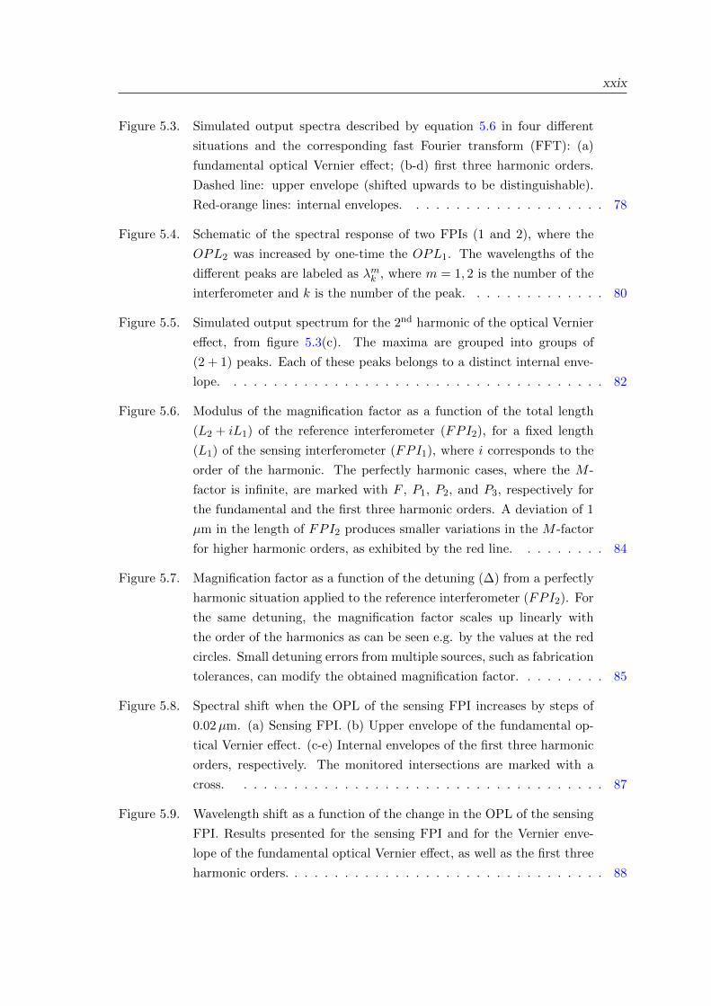
Figure 5.3. Simulated output spectra described by equation 5.6 in four different
situations and the corresponding fast Fourier transform (FFT): (a)
fundamental optical Vernier effect; (b-d) first three harmonic orders.
Dashed line: upper envelope (shifted upwards to be distinguishable).
Red-orange lines: internal envelopes. . . . . . . . . . . . . . . . . . . . 78
Figure 5.4. Schematic of the spectral response of two FPIs (1 and 2), where the
OPL2 was increased by one-time the OPL1. The wavelengths of the
different peaks are labeled as λmk , where m = 1, 2 is the number of the
interferometer and k is the number of the peak. . . . . . . . . . . . . . 80
Figure 5.5. Simulated output spectrum for the 2nd harmonic of the optical Vernier
effect, from figure 5.3(c). The maxima are grouped into groups of
(2 + 1) peaks. Each of these peaks belongs to a distinct internal enve-
lope. . . . . . . . . . . . . . . . . . . . . . . . . . . . . . . . . . . . . . 82
Figure 5.6. Modulus of the magnification factor as a function of the total length
(L2 + iL1) of the reference interferometer (FPI2), for a fixed length
(L1) of the sensing interferometer (FPI1), where i corresponds to the
order of the harmonic. The perfectly harmonic cases, where the M -
factor is infinite, are marked with F , P1, P2, and P3, respectively for
the fundamental and the first three harmonic orders. A deviation of 1
µm in the length of FPI2 produces smaller variations in the M -factor
for higher harmonic orders, as exhibited by the red line. . . . . . . . . 84
Figure 5.7. Magnification factor as a function of the detuning (∆) from a perfectly
harmonic situation applied to the reference interferometer (FPI2). For
the same detuning, the magnification factor scales up linearly with
the order of the harmonics as can be seen e.g. by the values at the red
circles. Small detuning errors from multiple sources, such as fabrication
tolerances, can modify the obtained magnification factor. . . . . . . . . 85
Figure 5.8. Spectral shift when the OPL of the sensing FPI increases by steps of
0.02µm. (a) Sensing FPI. (b) Upper envelope of the fundamental op-
tical Vernier effect. (c-e) Internal envelopes of the first three harmonic
orders, respectively. The monitored intersections are marked with a
cross. . . . . . . . . . . . . . . . . . . . . . . . . . . . . . . . . . . . . 87
Figure 5.9. Wavelength shift as a function of the change in the OPL of the sensing
FPI. Results presented for the sensing FPI and for the Vernier enve-
lope of the fundamental optical Vernier effect, as well as the first three
harmonic orders. . . . . . . . . . . . . . . . . . . . . . . . . . . . . . . . 88
xxx
Figure 5.10. Spectral shift when the OPL of the sensing FPI increases by steps of
0.02 mm. Sensing FPI used in the (a) fundamental effect; (b) 1st har-
monic; and (c) 2nd harmonic. (d) Upper envelope of the fundamental
effect. Internal envelopes of the (e) 1st harmonic; and (f) 2nd harmonic.
The monitored intersections are marked with a cross. . . . . . . . . . . 89
Figure 5.11. Schematic of a series configuration, where the first interferometer (FPI1)
is a hollow capillary tube of length L1 and the second interferometer
(FPI2) is a section of SMF of length L2. . . . . . . . . . . . . . . . . . 91
Figure 5.12. Simulated output spectra: (a-c) parallel configuration; (d-f) series con-
figuration. The fundamental optical Vernier effect, as well as the first
two harmonic orders are represented in both cases. . . . . . . . . . . . . 94
Figure 5.13. Simulated output spectrum for the 4th harmonic of the optical Vernier
effect. (a) Poor resolution spectrum: resolution of 500 pm. (b) Full res-
olution spectrum: resolution of 1 pm. The position of the intersections
between internal envelopes are marked with dashed lines. . . . . . . . . 96
Figure 6.1. Micrograph of the experimental fiber sensing interferometer (FPI1)
and the three different reference interferometers (FPI2) used to excite
the first three harmonic orders of the optical Vernier effect. The length
of the reference interferometers scale with the harmonic order, i, and
depend on the length of the sensing interferometer (L1). All reference
interferometers also present a detuning (∆). . . . . . . . . . . . . . . . 100
Figure 6.2. Schematic illustration of the experimental setup. The sensing interfer-
ometer (FPI1) and the reference interferometer (FPI2) are separated
by means of a 3db fiber coupler. A supercontinuum laser source is con-
nected to the input and the reflected signal from the device is measured
at the output with an optical spectrum analyzer. Strain is only applied
to FPI1, keeping FPI2 as a stable reference. . . . . . . . . . . . . . . . 101
Figure 6.3. Experimental output spectrum and corresponding fast Fourier trans-
form (FFT). (a) Individual sensing interferometer (FPI1). (b-d) First
three harmonic orders. Red-orange lines: internal envelopes. . . . . . . 103
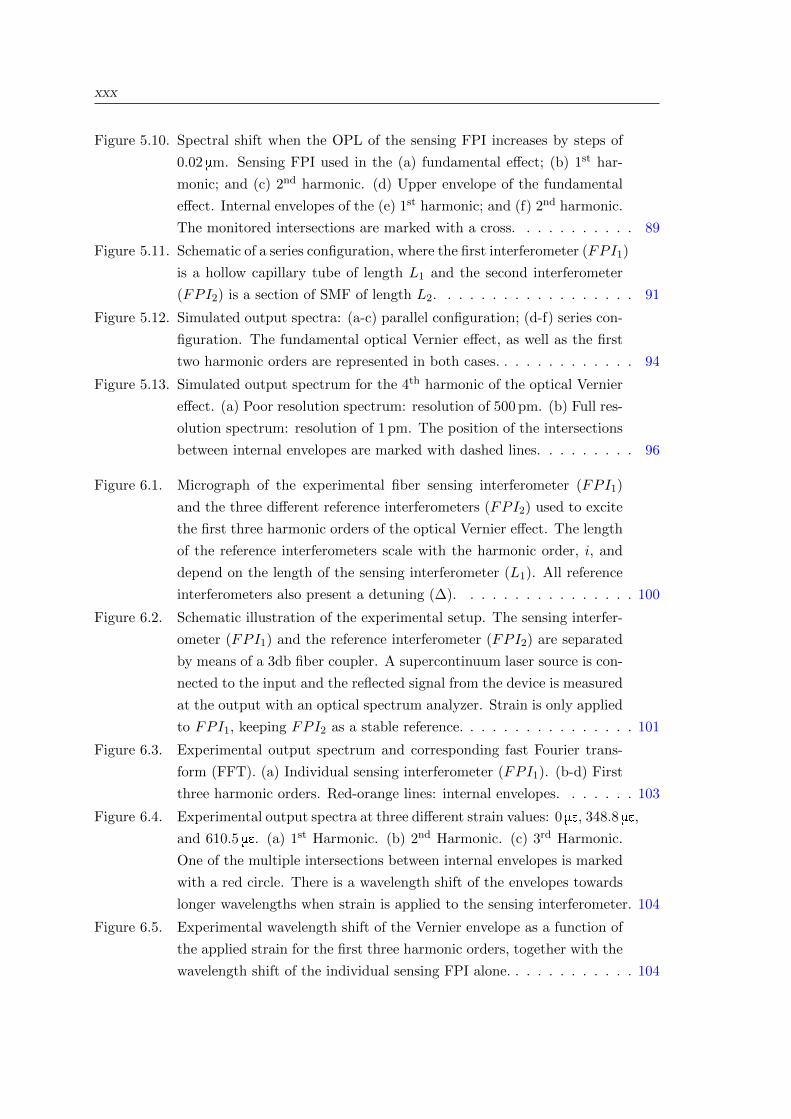
Figure 6.4. Experimental output spectra at three different strain values: 0 me, 348.8 me,
and 610.5 me. (a) 1st Harmonic. (b) 2nd Harmonic. (c) 3rd Harmonic.
One of the multiple intersections between internal envelopes is marked
with a red circle. There is a wavelength shift of the envelopes towards
longer wavelengths when strain is applied to the sensing interferometer. 104
Figure 6.5. Experimental wavelength shift of the Vernier envelope as a function of
the applied strain for the first three harmonic orders, together with the
wavelength shift of the individual sensing FPI alone. . . . . . . . . . . . 104
xxxi
Figure 6.6. Phase shift of the Vernier envelope as a function of the applied strain
for the first three harmonic orders. The sensitivity values are given by
the slope of the linear fit. . . . . . . . . . . . . . . . . . . . . . . . . . . 106
Figure 6.7. Schematic of the sensing structure consisting of two Fabry-Perot inter-
ferometers (FPIs) in series. FPI1 is a hollow microsphere with length
L1. FPI2 is a section of multimode fiber with length L2, followed by a
hollow capillary tube. The three interfaces are marked as M1, M2, and
M3, respectively with reflection coefficients R1, R2, and R3. . . . . . . . 108
Figure 6.8. Fabrication steps: (a) cleaving an MMF spliced to an SMF; (b) air
bubble formation; (c) cleaving of the second MMF; (d) splice with a
hollow capillary tube; (e) micrograph of the final structure. . . . . . . . 109
Figure 6.9. Reflected spectrum at three different fabrication stages. (a) Hollow
microsphere (FPI1), with an FSR of 6.4 nm. (b) Hollow microsphere
plus cleaved MMF (FPI1 + FPI2). The fundamental Vernier effect is
introduced with an envelope FSR of 56.8 nm. (c) Hollow capillary tube
spliced to the MMF with a small pre-tension. The Vernier envelope
FSR increased to 72.2 nm. Internal envelopes indicated by red/orange
lines. . . . . . . . . . . . . . . . . . . . . . . . . . . . . . . . . . . . . . 110
Figure 6.10. Reflected spectrum of the fabricated structure. The response corre-
sponds to the first harmonic of the Vernier effect in a series configuration.112
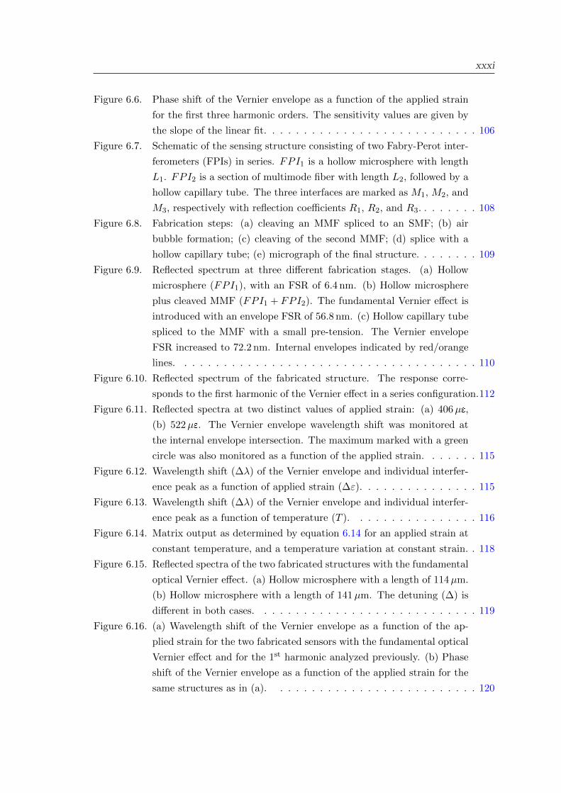
Figure 6.11. Reflected spectra at two distinct values of applied strain: (a) 406µe,
(b) 522µe. The Vernier envelope wavelength shift was monitored at
the internal envelope intersection. The maximum marked with a green
circle was also monitored as a function of the applied strain. . . . . . . 115
Figure 6.12. Wavelength shift (∆λ) of the Vernier envelope and individual interfer-
ence peak as a function of applied strain (∆ε). . . . . . . . . . . . . . . 115
Figure 6.13. Wavelength shift (∆λ) of the Vernier envelope and individual interfer-
ence peak as a function of temperature (T ). . . . . . . . . . . . . . . . 116
Figure 6.14. Matrix output as determined by equation 6.14 for an applied strain at
constant temperature, and a temperature variation at constant strain. . 118
Figure 6.15. Reflected spectra of the two fabricated structures with the fundamental
optical Vernier effect. (a) Hollow microsphere with a length of 114µm.
(b) Hollow microsphere with a length of 141µm. The detuning (∆) is
different in both cases. . . . . . . . . . . . . . . . . . . . . . . . . . . . 119
Figure 6.16. (a) Wavelength shift of the Vernier envelope as a function of the ap-
plied strain for the two fabricated sensors with the fundamental optical
Vernier effect and for the 1st harmonic analyzed previously. (b) Phase
shift of the Vernier envelope as a function of the applied strain for the
same structures as in (a). . . . . . . . . . . . . . . . . . . . . . . . . . 120
xxxii
Figure 7.1. Schematic of the working principle. A complex envelope modulation is
produced from the overlap between two Vernier cases (associated with
two propagating modes in the sensing FPI. Some envelope intersection
points show enhanced sensitivity, expressed qualitatively by the size of
the arrow. The Vernier spectra are purely for explanation purposes,
their visibilities were adjusted to be visually more perceptive and do
not reflect the real case. . . . . . . . . . . . . . . . . . . . . . . . . . . . 126
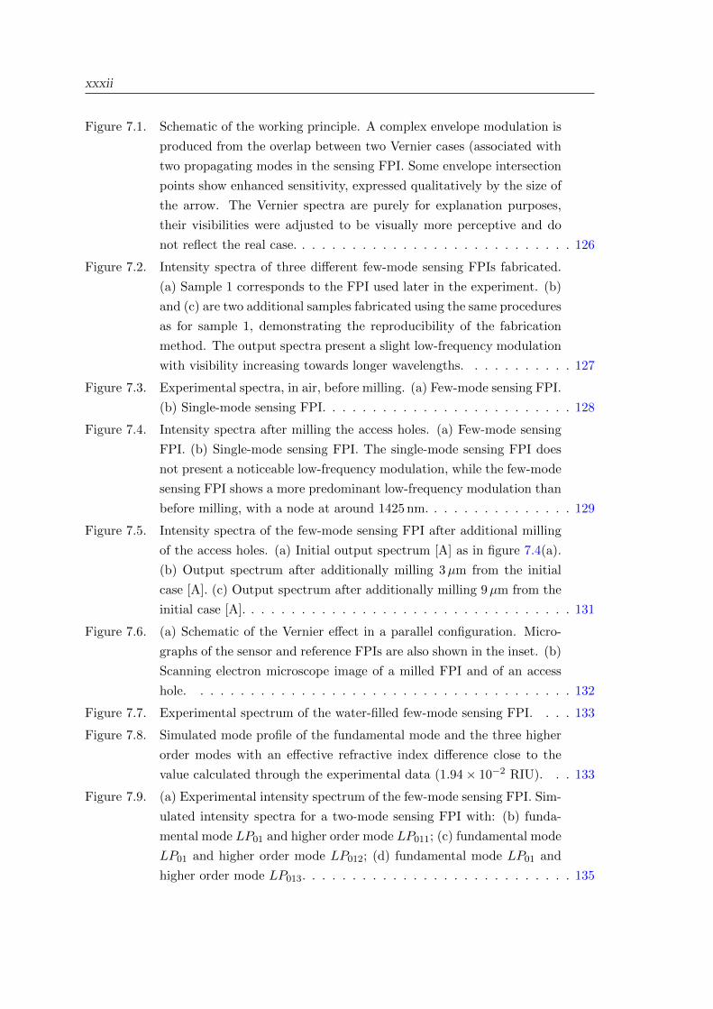
Figure 7.2. Intensity spectra of three different few-mode sensing FPIs fabricated.
(a) Sample 1 corresponds to the FPI used later in the experiment. (b)
and (c) are two additional samples fabricated using the same procedures
as for sample 1, demonstrating the reproducibility of the fabrication
method. The output spectra present a slight low-frequency modulation
with visibility increasing towards longer wavelengths. . . . . . . . . . . 127
Figure 7.3. Experimental spectra, in air, before milling. (a) Few-mode sensing FPI.
(b) Single-mode sensing FPI. . . . . . . . . . . . . . . . . . . . . . . . . 128
Figure 7.4. Intensity spectra after milling the access holes. (a) Few-mode sensing
FPI. (b) Single-mode sensing FPI. The single-mode sensing FPI does
not present a noticeable low-frequency modulation, while the few-mode
sensing FPI shows a more predominant low-frequency modulation than
before milling, with a node at around 1425 nm. . . . . . . . . . . . . . . 129
Figure 7.5. Intensity spectra of the few-mode sensing FPI after additional milling
of the access holes. (a) Initial output spectrum [A] as in figure 7.4(a).
(b) Output spectrum after additionally milling 3µm from the initial
case [A]. (c) Output spectrum after additionally milling 9µm from the
initial case [A]. . . . . . . . . . . . . . . . . . . . . . . . . . . . . . . . . 131
Figure 7.6. (a) Schematic of the Vernier effect in a parallel configuration. Micro-
graphs of the sensor and reference FPIs are also shown in the inset. (b)
Scanning electron microscope image of a milled FPI and of an access
hole. . . . . . . . . . . . . . . . . . . . . . . . . . . . . . . . . . . . . . 132
Figure 7.7. Experimental spectrum of the water-filled few-mode sensing FPI. . . . 133
Figure 7.8. Simulated mode profile of the fundamental mode and the three higher
order modes with an effective refractive index difference close to the
value calculated through the experimental data (1.94× 10⁻² RIU). . . 133
Figure 7.9. (a) Experimental intensity spectrum of the few-mode sensing FPI. Sim-
ulated intensity spectra for a two-mode sensing FPI with: (b) funda-
mental mode LP01 and higher order mode LP011; (c) fundamental mode
LP01 and higher order mode LP012; (d) fundamental mode LP01 and
higher order mode LP013. . . . . . . . . . . . . . . . . . . . . . . . . . . 135
xxxiii
Figure 7.10. Magnification factor and envelope free spectral range (FSR) for a single
mode sensing interferometer as a function of the mode effective refrac-
tive index. . . . . . . . . . . . . . . . . . . . . . . . . . . . . . . . . . . 137
Figure 7.11. Comparison between the Vernier effect with a single mode and a two-
mode sensing FPI. (a) Simulated Vernier spectrum for a sensing FPI
with the fundamental mode (LP01). The Vernier spectrum has a high
magnification factor, but an envelope too large to be measured. (b)
Simulated Vernier spectrum for a sensing FPI with the higher order
mode (LP012), before and after applying a refractive index variation of
8 × 10⁻⁵ RIU to the sensing FPI mode. The Vernier envelope is mea-
surable but has a lower magnification factor (lower wavelength shift).
(c) Simulated Vernier spectrum for a two-mode sensing FPI, before
and after applying the same a refractive index variation to the sensing
FPI modes. The Vernier envelope is measurable, yet the magnification
factor is still high (larger wavelength shift than the single mode case). . 138
Figure 7.12. Experimental Vernier spectra for a few-mode water-filled sensing FPI at
different values of water refractive index. The internal Vernier envelope
intersection, marked with an arrow, is traced and monitored during the
characterization. . . . . . . . . . . . . . . . . . . . . . . . . . . . . . . 140
Figure 7.13. (a) Wavelength shift as a function of water refractive index varia-
tions for different configurations: individual sensing FPI, experimental
Vernier effect for a single mode sensing FPI, simulated Vernier effect
for a two-mode sensing FPI, and experimental Vernier effect for a few-
mode sensing FPI. The M -factor achieved by the Vernier effect with a
few-mode sensing FPI is an order of magnitude higher than the Vernier
effect with a single mode sensing FPI. (b) Zoom in of the experimental
few-mode case and of the simulated two-mode case. . . . . . . . . . . . 141
Figure 7.14. Experimental Vernier spectra for the single mode water-filled sensing
FPI at different values of water refractive index. The internal Vernier
envelope intersection, marked with an arrow, is traced and monitored
during the characterization. . . . . . . . . . . . . . . . . . . . . . . . . . 142
Figure 7.15. Experimental intensity spectra for single mode water-filled sensing FPI,
before and after a water refractive index variation of 7.6× 10⁻⁴ RIU. . 143
Figure 7.16. Schematic of the fabrication process. The probe is fabricated using
three simple steps: (a) splice between the hollow capillary tube and the
input SMF; (b) hollow capillary tube cleavage; (c) electric discharges
on the tube edge. (d) Final structure, together with a micrograph of
the sensing head. . . . . . . . . . . . . . . . . . . . . . . . . . . . . . . 145
xxxiv
Figure 7.17. Schematic diagram of the sensor operation. (a) Immersion in the liquid
to be measured. The liquid enters the air cavity (b) Removal from the
liquid. This step is performed when no more liquid is entering the
cavity. (c) Liquid evacuation. The air cavity length increases due to
the liquid evacuation. . . . . . . . . . . . . . . . . . . . . . . . . . . . . 146
Figure 7.18. Micrograph of the sensing head immersed in liquid. The fluid fills
partially the air cavity, creating a reflective interface. . . . . . . . . . . 146
Figure 7.19. Reflected intensity as a function of time, at 1550 nm, for a sucrose
solution with a refractive index of 1.415 and a viscosity of 12.102 mPas.
The fluid displacement inside the cavity causes fast oscillations in the
intensity signal, happening especially during the dipping and removing
processes. . . . . . . . . . . . . . . . . . . . . . . . . . . . . . . . . . . . 147
Figure 7.20. Fluid displacement as a function of time converted from the intensity
signal of figure 7.19. The region marked with the orang arrow is used
to determine the viscosity. . . . . . . . . . . . . . . . . . . . . . . . . . 149
Figure 7.21. Reflected intensity as a function of time, at 1550 nm, for two sucrose
solutions of distinct viscosities: 1.887 mPa.s and 12.102 mPa.s. Higher
viscosity solutions produce slower intensity oscillations. . . . . . . . . . 151
Figure 7.22. Fluid displacement as a function of time for sucrose solutions with
different viscosities. Solutions of higher viscosity tend to have a more
non-linear displacement inside the cavity. . . . . . . . . . . . . . . . . . 152
Figure 7.23. Fluid viscosity as a function of the fluid evacuation velocity. The result
can be divided into two regimes: low viscosity (up to around 4 mPa.s)
and high viscosity (starting from around 4 mPa.s. . . . . . . . . . . . . 153
Figure 7.24. Three different measurements for two solutions with distinct viscosi-
ties: 2.10 mPa.s and 9.95 mPa.s. The measurements show a good
reproducibility with a standard deviation of 42 nm and 105 nm for the
two cases, respectively. . . . . . . . . . . . . . . . . . . . . . . . . . . . 154
Figure 7.25. Fluid displacement as a function of time for 47%wt/wt sucrose solution
at different temperatures. The viscosity changes due to temperature
variations are also detected by the sensing structure, producing distinct
responses. . . . . . . . . . . . . . . . . . . . . . . . . . . . . . . . . . . . 155
Figure 7.26. Fluid displacement as a function of time for different access hole diam-
eters. The same sucrose solution with a viscosity of 3.0 mPa.s was used
in all cases. The fluid displacement tends to be slower and non-linear
for smaller access holes. . . . . . . . . . . . . . . . . . . . . . . . . . . . 155
Figure A.1. Refractive index of water as a function of temperature, at a wavelength
of 632.8 nm. The data points correspond to the values of table A.1. . . 189
xxxv
Figure C.1. Spectrum from figure 5.5 represented in the frequency domain. The
maxima are marked with a dot and colored according to the respective
internal envelope. . . . . . . . . . . . . . . . . . . . . . . . . . . . . . . 195
Figure C.2. Spectrum from figure 5.5 represented in the frequency domain after
fitting the internal envelopes according to equation C.1. . . . . . . . . . 196
Figure D.1. Viscosity as a function of the sucrose concentration. The data points
can be found at [9]. . . . . . . . . . . . . . . . . . . . . . . . . . . . . . 199
Figure D.2. Viscosity as a function of the refractive index of the sucrose solution.
The data points can be found at [10]. . . . . . . . . . . . . . . . . . . . 200
Figure D.3. Viscosity as a function of the temperature for a sucrose solution with
a concentration of 47 %m/m. The data points can be found at [11]. . . 201

List of Tables
Table 3.1. Parameters used in the CO2 laser system to fabricate the microfiber.
The CO2 laser setup can be found in chapter 2 in figure 2.3. . . . . . . . 27
Table 3.2. Table of comparison between different configurations. NL stands for
non-linear response. . . . . . . . . . . . . . . . . . . . . . . . . . . . . . . 44
Table 5.1. Overview of the simulated results. . . . . . . . . . . . . . . . . . . . . . . 88
Table 5.2. Overview of the simulated results. . . . . . . . . . . . . . . . . . . . . . . 90
Table 6.1. Overview of the experimental results for the first three harmonic orders.
First group: Experimental results. Second group: M -factor via two def-
initions (equations 5.21 and 4.29) are approximately the same. Third
group: M -factor for each harmonic order compared with the M -factor
for the fundamental optical Vernier effect (M0). It shows the i + 1 im-
provement factor with the order of the harmonic. . . . . . . . . . . . . . 107
Table 6.2. Post-Processing – Splicer Parameters. . . . . . . . . . . . . . . . . . . . . 109
Table A.1. Refractive index of water as a function of temperature, at a wavelength
of 632.8 nm [12]. . . . . . . . . . . . . . . . . . . . . . . . . . . . . . . . . 188
Table B.1. Summary of the optical Vernier effect configurations using single-type FPI.191
Table B.2. Summary of the optical Vernier effect configurations using single-type
FPI (continuation). . . . . . . . . . . . . . . . . . . . . . . . . . . . . . . 192
Table B.3. Summary of the optical Vernier effect configurations using other single-
type interferometers, as well as hybrid configurations. . . . . . . . . . . . 193

Nomenclature
DCF Double-Core Fiber
DSHF Dual Side-Hole Fiber
DSO Dimethyl Silicone Oil
FBG Fiber Bragg Grating
FFT Fast Fourier Transform
FIB Focused Ion Beam
FMF Few-Mode Fiber
FSR Free Spectral Range
GIF Graded-Index Fiber
HCF Hollow-Core Fiber
HC-PCF Hollow-Core Photonic Crystal Fiber
Hi-Bi High-Birefringent
IFFT Inverse Fast Fourier Transform
LC Liquid Crystal
LMAF Large Mode Area Fiber
MKR Microfiber Knot Resonator
MZI Mach-Zehnder Interferometer
OSA Optical Spectrum Analyzer
PCF Photonic Crystal Fiber
PM-PCF Polarization Maintaining Photonic Crystal Fiber
RIU Refractive Index Units

xl
SEM Scanning Electron Microscope
SHF Side-Hole Fiber
SHTECF Single Hole Twin Eccentric Cores Fiber
SI Sagnac Interferometer
SMF Single Mode Fiber
SNOM Scanning Near-Field Optical Microscopy
TCF Triple-Core Fiber


Chapter 1.
Introduction
The beginning of optical fibers life history take us back to the 20’s, where the first optical
fibers were produced. Initially, they were used to guide light at short distances for illumi-
nation purposes. The concept of clad fiber (a core protected by a cladding with a lower
refractive index) only appeared in the 50’s [13]. At that time, the idea of transferring
information through optical fibers was growing. However, losses were limiting the trans-
mission of information over long distances through optical fibers. In 1966, Prof. Charles
Kao, together with George Hockham, proposed glass fibers as a possible low-loss optical
waveguide for a new form of communication medium [14]. The idea of optical fiber com-
munications was then born, reason why Kao received the Nobel Prize in 2009. Henceforth,
optical fibers became a topic of extensive research, opening with it new research fields.
One of them is the use of optical fibers, not as a communication medium, but as a sensing
device.
For telecommunications, a basic fiber structure such as a clad fiber (core, cladding) is
sufficient. For sensing applications, a similar fiber structure by itself can also act as a
sensor, yet more complex and special optical fiber structures are attractive and desirable,
providing many different and additional features. Over the years, several different types of
optical fiber sensing structures were created and tested for measuring physical, chemical,
and biochemical parameters. Some traditional examples are fiber Bragg gratings, Mach-
Zehnder interferometers, Fabry-Perot interferometers, multimode fiber devices, fiber loop
mirrors, among others.
Nowadays, the fast development in different fields of research that make use of optical
sensing is creating new challenges also in the field of optical fiber sensing. There is an
increasing demand for miniaturized sensing structures, especially with the capability of
achieving higher sensitivities and resolutions than what current conventional fiber sensors
can provide. Hence, it is necessary to explore alternative options for advanced fiber sensing
structures that meet the state-of-the-art demands.
Optical microfibers opened new doors to the study and development of new and en-
hanced sensors. Due to their properties and small size, optical microfibers are a good
2 Chapter 1. Introduction
platform for the creation of miniaturized sensing structures. Additionally, optical mi-
crofibers can also be microstructured by means of different post-processing techniques,
in order to create special and complex sensing devices, designed to have improved sensi-
tivity to certain parameters. The creation of microstructures in optical microfibers and
microfiber probes are explored in this dissertation.
The optical Vernier effect has recently shown its huge potential to greatly enhance
the sensitivity and resolution of optical fiber sensors. Although it can be challenging
to understand and apply, the optical Vernier effect is a tool that provides impressive
improvements in sensing performance. This effect is also a case of study of this dissertation.
This chapter provides an overview on the motivation and objectives of this work, followed
by a description of the dissertation structure. Finally, the main contributions to the field
are presented, as well as the list of publications that resulted from this PhD.
1.1. Motivation and Objectives
The motivation for the research activities developed in the context of the PhD program
consisted of performing an original study on new advanced optical fiber sensing technolo-
gies relying on microstructures and optical Vernier effect. This includes the combination
of different techniques and concepts learned over these last years to achieve new and inno-
vative sensing structures in optical fibers with enhanced sensing performances. Naturally,
the desire of learning new concepts and acquire new skills and competences in this field
was also a driving force towards the success of the research activities that culminated in
this dissertation. Another major motivation was the opportunity to test and try out my
own ideas, as well as to solve different challenges and find new solutions for problems
and difficulties that constantly emerged as the research activities progressed. Finally, a
personal motivation was to give my contribution and make relevant developments in the
field of optical fiber sensing, in particular on the application of the optical Vernier effect
to fiber sensing interferometers.
The main objectives of the research activities developed during the PhD program con-
sisted in:
� Modeling, fabrication, and characterization of advanced interferometric optical fiber
sensors based on microstructures;
� Acquiring competences in using the focused ion beam technology to create sens-
ing microstructures in optical microfiber probes, as well as to open access holes in
specialty fibers for liquid sensing inside the fiber;
� Studying and further developing the concept of optical Vernier effect as a tool to
enhance the performance of optical fiber sensing interferometers;
1.2. Dissertation Overview 3
� Creating a new generation of optical fiber microsensors of high sensitivity for different
applications, including sensing in liquid media.
1.2. Dissertation Overview
This dissertation is organized in 8 chapters that take the the reader on a journey through
advanced interferometric sensing configurations based on microstructures in optical mi-
crofibers and on the optical Vernier effect.
Chapter 1 provides a brief introduction to the research subject and clarifies the motiva-
tion, the goals, and the structure of this dissertation. It also includes the main contribu-
tions to the research area and publications that resulted from it.
Chapter 2 presents an introductory overview on optical microfibers and sensing interfer-
ometers that will be used along the dissertation. This chapter also explores the application
of focused ion beam milling to optical microfiber probes, together with the necessary sam-
ple preparation.
Chapter 3 proposes two interferometric microstructured sensing devices with optical
microfibers and microfiber probes for enhanced sensing capabilities. The first combines
a microfiber knot resonator with a Mach-Zehnder interferometer embedded in the same
microfiber for simultaneous measurement of refractive index and temperature. The second
device consists of a Fabry-Perot interferometer microfabricated with a focused ion beam
in a multimode microfiber probe for enhanced temperature sensing.
Chapter 4 is dedicated to the optical Vernier effect for optical fiber interferometers. The
fundamentals of the effect are introduced and explored, using a parallel configuration as
the starting point. This chapter presents important discussions regarding the different
properties of the effect from a fiber sensing perspective, and an extensive state-of-the-art
review on the different configurations and applications of the optical Vernier effect.
Chapter 5 describes the new concept of optical harmonic Vernier effect for optical fiber
interferometers. The mathematical description and the new properties that arise from
introducing harmonics to the optical Vernier effect, especially the increase in sensing sen-
sitivity, are here addressed. Simulations that demonstrate the mechanics and properties
of the effect are also presented. This chapter also includes important discussions related
with the difference between the two main configurations: parallel and series, and with the
limitations of this concept.
Chapter 6 is dedicated to the experimental demonstration of the optical harmonic
Vernier effect for both, the parallel and the series configuration. In a first approach,
the parallel configuration is addressed using Fabry-Perot interferometers based on hollow
capillary tubes. This work has a strong focus on validating the properties of the effect
deduced theoretically in the previous chapter. In the second part, a more specific and
complex case of the effect based on a series configuration using a hollow microsphere and
4 Chapter 1. Introduction
a section of multimode fiber is explored. In this case, both interferometers are physically
connected without a separation while, simultaneously, there is no reference interferometer.
Additionally, simultaneous measurement of two parameters using this last configuration
is also demonstrated.
Chapter 7 presents two advanced sensing configurations based on microstructures for
measuring liquid media. It combines different concepts and techniques to achieve novel
optical fiber sensing devices with enhanced performances. The first configuration explores
an extreme case of optical Vernier effect based on a few-mode Fabry-Perot interferometer,
made from a hollow capillary tube. At the same time, focused ion beam milling is used to
open access holes on the Fabry-Perot interferometer, enabling it to be filled with liquids.
A giant refractometric sensitivity and huge magnification factors, that are impossible to be
achieved with the conventional optical Vernier effect, are demonstrated here to be possible
through the extreme optical Vernier effect. As for the second configuration, a section of
hollow capillary tube is post-processed using electric arc to create a microprobe with a
small access hole for viscosity measurement of liquids. The viscosity is obtained through
the analysis of a two-wave interferometric signal that changes in time proportionally to
the liquid displacement inside the optical fiber probe.
Chapter 8 summarizes the main results obtained during the PhD and reanalyzes the
initial objectives. At last, the opportunities for future work emerging from the research
presented in this dissertation are also discussed.
1.3. Main Contributions
From the works presented in this dissertation, it is the author’s opinion that the following
main contributions to the field stand out. First, a more compact and novel hybrid sensing
structure combining a microfiber knot resonator with a Mach-Zehnder interferometer using
microfibers is presented. The novelty here is the structure, where the Mach-Zehnder in-
terferometer is created using a single microfiber, the same as used to create the microfiber
knot resonator, containing two propagating modes, instead of relying on two separated
microfibers to create the two arms of the Mach-Zehnder interferometer. Second, the use
of focused ion beam to mill Fabry-Perot cavities in microfiber probes is not new, however
using a multimode fiber to make the milled Fabry-Perot multimode and introduce the
Vernier effect is. Third, the post-processing of a capillary tube led to the development of
a small size viscometer probe that only requires tiny volumes (picoliters) to perform the
measurement. At last, the works related with the optical Vernier effect represent a large
contribution to the field, providing a deeper understanding and control of the effect. The
existence of optical harmonics of the Vernier effect was demonstrated for the first time,
to the best of the author’s knowledge, theoretically and experimentally. The work repre-
sents a paradigm shift that required the development of a new mathematical description
1.4. List of Publications 5
to correctly describe the novel properties and behaviors of this extended concept of the
optical Vernier effect. The optical harmonics of the Vernier effect are a new tool that
other researchers can use from now on, not just applied to Fabry-Perot interferometers, as
demonstrated in this dissertation, but also to other different types of interferometers and
for other applications. The combination of a hollow microsphere and a multimode fiber
section, together with harmonics of the Vernier effect allowed simultaneous measurement
of two parameters with high sensitivity. A novel extreme optical Vernier effect is also
demonstrated, leading to giant refractometric sensitivity values and huge magnification
factors, which are otherwise impossible to achieve with state-of-the-art optical Vernier
effect.
1.4. List of Publications
From the activities developed within this PhD resulted a total of 7 publications as a first
author in scientific journals (1 of them under revision and 1 review paper to be submitted)
7 communications in national/international conferences, and 1 book chapter. Besides, four
additional papers as first authors, including two invited paper, and three as co-author were
also published as a result of work and collaborations outside the scope of this dissertation,
as well as one communication in international conferences. The list of publications as first
author is presented next.
Scientific Journal Publications
1. A. D. Gomes, H. Bartelt, and O. Frazao, “Optical Vernier effect: recent advances
and developments,”Laser and Photonics Reviews, 2021. doi: 10.1002/lpor.202000588
2. A. D. Gomes, J. Zhao, A. Tuniz, and M. A. Schmidt, Direct observation of modal
hybridization in nanofluidic fiber [Invited],” Optical Materials Express 11(2), 559,
2020. doi: 10.1364/OME.413199 [15]
3. A. D. Gomes, J. Kobelke, J. Bierlich, J. Dellith, M. Rothhardt, H. Bartelt, and O.
Frazao, “Giant refractometric sensitivity by combining extreme optical Vernier effect
and modal interference,”Scientific Reports 10(1), 19313, 2020. doi: 10.1038/s41598-
020-76324-7 [16]
4. P. Robalinho, A. D. Gomes, and O. Frazao, “Colossal enhancement of strain sen-
sitivity using the push-pull deformation method in interferometry,” IEEE Sensors
Journal 21(4), 4623-4627, 2020. doi: 10.1109/JSEN.2020.3033581 [17]
5. P. Robalinho, A. D. Gomes, and O. Frazao, “High enhancement strain sensor based
on Vernier effect using 2-fiber loop mirrors,” IEEE Photonics Technology Letters
32(18), 1139-1142, 2020. doi: 10.1109/LPT.2020.3014695 [18]
6 Chapter 1. Introduction
6. A. D. Gomes, M. S. Ferreira, J. Bierlich, J. Kobelke, M. Rothhardt, H. Bartelt,
and O. Frazao, “Hollow microsphere combined with optical harmonic Vernier effect
for strain and temperature discrimination,” Journal of Optics and Laser Technology
(127), 106198, 2020. doi: 10.1016/j.optlastec.2020.106198 [19]
7. A. D. Gomes, M. S. Ferreira, J. Bierlich, J. Kobelke, M. Rothhardt, H. Bartelt, and
O. Frazao, “Optical harmonic Vernier effect: a new tool for high performance inter-
ferometric fibre sensors,”MDPI Sensors 19(24), 5431, 2019. doi: 10.3390/s19245431
[20]
8. A. D. Gomes, M. Becker, J. Dellith, M. I. Zibaii, H. Latifi, M. Rothhardt, H.
Bartelt, and O. Frazao, “Multimode Fabry–Perot interferometer probe based on
Vernier effect for enhanced temperature sensing,” MDPI Sensors 19(3), 453, 2019.
doi: 10.3390/s19030453 [21]
9. A. D. Gomes, J. Kobelke, J. Bierlich, K. Schuster, H. Bartelt, and O. Frazao,
“Optical fiber probe viscometer based on hollow capillary tube,”Journal of Lightwave
Technology 37(18), 4456-4461, 2019. doi: 10.1109/JLT.2019.2890953 [22]
10. B. Silveira, A. D. Gomes, M. Becker, H. Schneidewind, and O. Frazao,“Bunimovich
stadium-like resonator for randomized fiber laser operation,” MDPI Photonics 5(3),
17, 2018. doi: 10.3390/photonics5030017 [23]
11. A. D. Gomes, C. S. Monteiro, B. Silveira, and O. Frazao, “A brief review of
new fiber microsphere geometries,” MDPI Fibers 6(3), 48, 2018. (invited) doi:
10.3390/fib6030048 [24]
12. A. D. Gomes, F. Karami, M. I. Zibaii, H. Latifi, and O. Frazao, “Multipath in-
terferometer polished microsphere for enhanced temperature sensing,” IEEE Sensors
Letters 2(2), 1-4, 2018. doi: 10.1109/LSENS.2018.2819365 [25]
13. A. D. Gomes, B. Silveira, J. Dellith, M. Becker, M. Rothhardt, H. Bartelt, and
O. Frazao, “Cleaved silica microsphere for temperature sensing,” IEEE Photonics
Technology Letters 30(9), 797-800, 2018. doi: 10.1109/LPT.2018.2817566 [26]
14. A. D. Gomes and O. Frazao, “Microfiber knot with taper interferometer for tem-
perature and refractive index discrimination,” IEEE Photonics Technology Letters
29(8), 1517-1520, 2017. doi: 10.1109/LPT.2017.2735185 [27]
Communications in National/International Conferences
1. A. D. Gomes, M. S. Ferreira, J. Bierlich, J. Kobelke, M. Rothhardt, H. Bartelt,
and O. Frazao, “Challenging the limits of interferometric fiber sensor sensitivity with
1.4. List of Publications 7
the optical harmonic Vernier effect,” 27th International Conference on Optical Fiber
Sensors (OFS-27), Alexandria, Virginia, USA, 2020. [Accepted but postponed to
2022]
2. A. D. Gomes, M. Becker, J. Dellith, M. I. Zibaii, H. Latifi, M. Rothhardt, H.
Bartelt, and O. Frazao, “Enhanced temperature sensing with Vernier effect on fiber
probe based on multimode Fabry-Perot interferometer,” IV International Conference
on Applications of Optics and Photonics (AOP2019), Lisbon, Portugal, 2019. (3 rd
place best student paper, awarded by SPIE) doi:10.1117/12.2527399 [28]
3. A. D. Gomes, J. Kobelke, J. Bierlich, K. Schuster, and O. Frazao, “Optical fiber
probe for viscosity measurements,” 26th International Conference on Optical Fiber
Sensors (OFS-26), Lausanne, Switzerland, 2018. doi: 10.1364/OFS.2018.TuE8 [29]
4. A. D. Gomes, C. S. Monteiro, J. Kobelke, J. Bierlich, K. Schuster, H. Bartelt, and
O. Frazao, “Interferometro de duas ondas em sonda de fibra optica para medicao
de viscosidade”, 21ª Conferencia Nacional de Fısica, Universidade da Beira Interior,
Portugal, 2018.
5. A. D. Gomes, B. Silveira, F. Karami, M. I. Zibaii, H. Latifi, J. Dellith, M. Becker,
M. Rothhardt, H. Bartelt, and O. Frazao, “Multi-path interferometer structures
with microspheres,” SPIE Optics & Photonics 2018, Interferometry XIX, San Diego,
California, United States, 2018. doi: 10.1117/12.2319082 [30]
6. A. D. Gomes and O.Frazao, “Simultaneous measurement of temperature and re-
fractive index based on microfiber knot resonator integrated in an abrupt taper
Mach-Zehnder interferometer,” III International Conference on Applications of Op-
tics and Photonics (AOP2017), Faro, Portugal, 2017. doi: 10.1117/12.2275813 [31]
7. A. D. Gomes and O. Frazao, “Microfiber knot resonator as sensors: a review,” 5th
International Conference on Photonics, Optics and Laser Technology (Photoptics
2017), Porto, Portugal, 2017. doi: 10.5220/0006264803560364 [32]
Book Chapters
1. A. D. Gomes and O. Frazao, “Microfiber knot resonators for sensing applications”,
Optics, Photonics and Laser Technology 2017, Springer Series in Optical Sciences
vol. 222, 145-163, Springer Nature Switzerland AG, 2019. doi: 10.1007/978-3-030-
12692-6 7 / ISBN: 978-3-030-12691-9 [33]

Chapter 2.
Overview on Optical Microfibers and
Sensing Microstructures
2.1. Introduction
Optical fiber tapers were initially developed in the late 20th century, in the context of
optical fiber communication. Their main purpose was to fabricate single mode fiber cou-
plers [34–36]. Since then, optical fiber tapers were continuously studied and applied, not
just in the fields of optical communication, but also for optical fiber sensing.
Optical microfibers by themselves can already be a sensing structure [37]. Their small
size and guidance properties provide a great interaction between the propagating light
and the external environment. Nevertheless, different sensing microstructures can ad-
ditionally be fabricated in optical microfibers, increasing their versatility and range of
applications [3, 38, 39]. These sensing microstructures can be interferometers created ei-
ther by manipulating the optical microfiber [38], or through microfabrication techniques
like femtosecond laser inscription [40] and ablation [41] or focused ion beam milling [4,42].
This chapter intends to provide an insight on optical microfibers, sensing interferometers,
and microfabrication techniques used across the dissertation. First, the properties and the
structure of optical microfibers are explored, as well as some fabrication techniques used
to produce them. Then, a small overview on different interferometric sensing structures
is presented. Here, it is intended to provide some background knowledge on the different
interferometric structures that will later appear in the dissertation. A small state-of-the-
art description of the application of such structures, especially to optical microfibers and
microfiber probes, is also included. The last section of the chapter explores the focused
ion beam technology as a microfabrication technique to create microstructures in optical
microfiber probes. This section also contains an important discussion regarding the sample
preparation necessary to apply the technique to optical fibers.
10 Chapter 2. Overview on Optical Microfibers and Sensing Microstructures
2.2. Optical Microfibers and Microfiber Probes
Optical microfibers are optical fibers tapered down from typical fiber diameters of e.g.
125µm to diameters of few micrometers (around 1 µm - in the order of the wavelength of
light propagating along the fiber), or even to diameters of hundreds of nanometers, the so
called nanofibers. The fabrication of optical microfibers consists of heating the fiber to its
softening point while stretching it to decrease its diameter, obtaining a narrow stretched
filament linked to the rest of the non-stretched fiber through a transition region. By
finding a balance between parameters such as the heating source and the stretching, optical
microfibers with different taper transition regions can be fabricated: linear, parabolic,
sinusoidal, polynomial, or others [43].
Microfibers with dimensions close to 1µm present new properties: low optical loss [44],
outstanding mechanical flexibility [45, 46], tight optical confinement [47], large waveguide
dispersion [48], and large interaction with the external environment through their large
evanescent field [49]. This last property is of great value for sensing applications, since the
larger the interaction with the external medium, the more sensitive the structure tends to
be.
Due to the huge scale down (e.g. from 125µm to around 1µm), and also to the high
temperatures subjected during the production, the doping of the optical fiber core is
diffused to the cladding and disappears. Hence, optical microfibers and nanofibers present
a high index contrast: the microfiber itself acts as a core for light guidance while the
external medium acts as a cladding (usually nfiber � nsurroundingmedium, where n is the
refractive index).
Microfibers with larger diameters can support multimode propagation, being the fun-
damental mode predominantly confined within the microfiber. However, when talking
about optical microfibers with diameters close to 1 µm or nanofibers, where the diameter
is much smaller than the propagated radiation wavelength (d� λ), only the fundamental
mode is propagated along the structure. This mode then propagates mostly outside of
the micro/nanofiber due to the large evanescent field [50]. The single mode condition for
optical fibers is defined by the generalized frequency (V ), also known as the V -number,
in this case given by [48]:
V = 2πa
λ0
√(n2fiber − n2external) ≈ 2.405, (2.1)
where a is the radius of the micro/nanofiber, λ0 is the propagation wavelength (in vacuum),
nfiber is the refractive index of the micro/nanofiber, and nexternal is refractive index of the
external medium. For a microfiber in air with a propagation wavelength of 1550 nm,
considering the refractive index of the microfiber equal to the refractive index of silica
(1.444 at 1550 nm [51]), the single mode condition occurs for a diameter of around 1.14 µm.
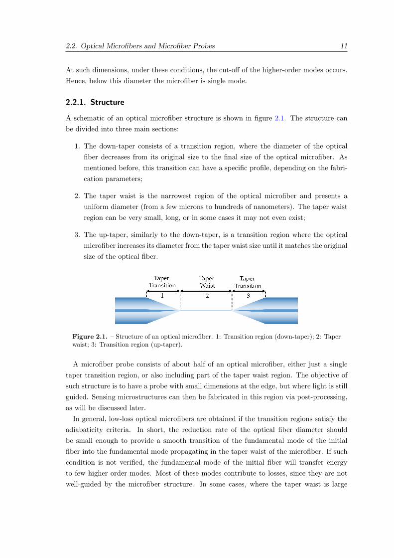
2.2. Optical Microfibers and Microfiber Probes 11
At such dimensions, under these conditions, the cut-off of the higher-order modes occurs.
Hence, below this diameter the microfiber is single mode.
2.2.1. Structure
A schematic of an optical microfiber structure is shown in figure 2.1. The structure can
be divided into three main sections:
1. The down-taper consists of a transition region, where the diameter of the optical
fiber decreases from its original size to the final size of the optical microfiber. As
mentioned before, this transition can have a specific profile, depending on the fabri-
cation parameters;
2. The taper waist is the narrowest region of the optical microfiber and presents a
uniform diameter (from a few microns to hundreds of nanometers). The taper waist
region can be very small, long, or in some cases it may not even exist;
3. The up-taper, similarly to the down-taper, is a transition region where the optical
microfiber increases its diameter from the taper waist size until it matches the original
size of the optical fiber.
Figure 2.1. – Structure of an optical microfiber. 1: Transition region (down-taper); 2: Taperwaist; 3: Transition region (up-taper).
A microfiber probe consists of about half of an optical microfiber, either just a single
taper transition region, or also including part of the taper waist region. The objective of
such structure is to have a probe with small dimensions at the edge, but where light is still
guided. Sensing microstructures can then be fabricated in this region via post-processing,
as will be discussed later.
In general, low-loss optical microfibers are obtained if the transition regions satisfy the
adiabaticity criteria. In short, the reduction rate of the optical fiber diameter should
be small enough to provide a smooth transition of the fundamental mode of the initial
fiber into the fundamental mode propagating in the taper waist of the microfiber. If such
condition is not verified, the fundamental mode of the initial fiber will transfer energy
to few higher order modes. Most of these modes contribute to losses, since they are not
well-guided by the microfiber structure. In some cases, where the taper waist is large
12 Chapter 2. Overview on Optical Microfibers and Sensing Microstructures
enough to support multimode propagation, some of these higher order modes might still
propagate along the microfiber, which can be useful for sensing as it will be discussed in
the next chapter.
The adiabaticity criteria corresponds to an approximate boundary between an optimal
adiabatic taper and a lossy taper. In a more concrete way, the adiabaticity criteria is
verified when the beat length between the fundamental mode (LP01) and the next higher
order local mode is smaller than the local variation of the taper diameter in relation to
the propagation direction [43,52]: ∣∣∣∣drdz∣∣∣∣ < r (β1 − β2)
2π, (2.2)
where r = r (z) is the local cladding radius, z is the propagation direction, β1 = β1 (z)
and β2 = β2 (z) are the local propagation constants of the fundamental mode (LP01) and
the next higher order mode. The smaller the final diameter targeted for the taper waist,
the longer the transition regions should be to obtain a low-loss microfiber. However, it
might happen that the final length of the microfiber is larger than what the fabrication
equipment might be able to produce, due to the need for longer transition regions. There-
fore, each fabrication setup imposes a limitation on the fabrication parameters of very
small microfiber, being necessary to adapt the fabrication conditions (diameter, length,
adiabaticity).
Next, the fabrication techniques to produce optical microfibers will be addressed, as
well as some advantages and disadvantages of each method.
2.2.2. Fabrication Techniques
The typical techniques used to fabricate optical microfibers are similar to each other and
the main difference between them relies on the heating source. There are different heating
sources which are normally associated with the name of a specific tapering technique. The
heating source can be a gas flame [49, 53], an electric arc created by electrodes as in a
splicing machine [54, 55] or in a 3SAE Ring of Fire [56], a focused CO2 laser [57, 58], a
microheater [59,60], or even a heating filament as used in commercial machines such as the
VYTRAN - Glass Processing Workstation [61, 62]. However, not all of these techniques
can achieve optical microfibers with diameters of around 1 mm or even below.
Traditional electric arc discharge methods, as in a fusion splicer, are not able to produce
microfibers with diameters of around 1 mm. The electric arc from a fusion splicer does not
provide the necessary temperature uniformity to reach such small dimensions, and the heat
transfer rate to the fiber is slow [57]. Some of these issues are overcomed in equipment
such as the 3SAE Ring of Fire, where a plasma is created using three electrodes, providing
a controllable thermal profile in three dimensions [56].
A common fabrication method is the flame-brush technique, using a hydrogen flame
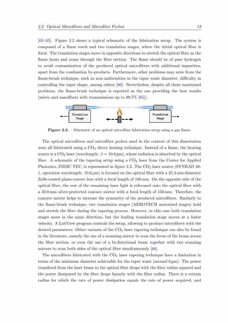
2.2. Optical Microfibers and Microfiber Probes 13
[63–65]. Figure 2.2 shows a typical schematic of the fabrication setup. The system is
composed of a flame torch and two translation stages, where the initial optical fiber is
fixed. The translation stages move in opposite directions to stretch the optical fiber as the
flame heats and scans through the fiber section. The flame should be of pure hydrogen
to avoid contamination of the produced optical microfibers with additional impurities,
apart from the combustion by-products. Furthermore, other problems may arise from the
flame-brush technique, such as non-uniformities in the taper waist diameter, difficulty in
controlling the taper shape, among others [60]. Nevertheless, despite all these mentioned
problems, the flame-brush technique is reported as the one providing the best results
(micro and nanofibers with transmissions up to 99.7% [65]).
Figure 2.2. – Schematic of an optical microfiber fabrication setup using a gas flame.
The optical microfibers and microfiber probes used in the context of this dissertation
were all fabricated using a CO2 direct heating technique. Instead of a flame, the heating
source is a CO2 laser (wavelength: λ = 10.6 mm), whose radiation is absorbed by the optical
fiber. A schematic of the tapering setup using a CO2 laser from the Center for Applied
Photonics, INESC TEC, is represented in figure 2.3. The CO2 laser source (SYNRAD 48-
1, operation wavelength: 10.6µm) is focused on the optical fiber with a 25.4 mm-diameter
ZnSe-coated plano-convex lens with a focal length of 100 mm. On the opposite side of the
optical fiber, the rest of the remaining laser light is refocused onto the optical fiber with
a 50.8 mm silver-protected concave mirror with a focal length of 150 mm. Therefore, the
concave mirror helps to increase the symmetry of the produced microfibers. Similarly to
the flame-brush technique, two translation stages (AEROTECH motorized stages) hold
and stretch the fiber during the tapering process. However, in this case both translation
stages move in the same direction, but the leading translation stage moves at a faster
velocity. A LabView program controls the setup, allowing to produce microfibers with the
desired parameters. Other variants of the CO2 laser tapering technique can also be found
in the literature, namely the use of a scanning mirror to scan the focus of the beam across
the fiber section, or even the use of a bi-directional beam together with two scanning
mirrors to scan both sides of the optical fiber simultaneously [66].
The microfibers fabricated with the CO2 laser tapering technique have a limitation in
terms of the minimum diameter achievable for the taper waist (around 6 mm). The power
transfered from the laser beam to the optical fiber drops with the fiber radius squared and
the power dissipated by the fiber drops linearly with the fiber radius. There is a certain
radius for which the rate of power dissipation equals the rate of power acquired, and
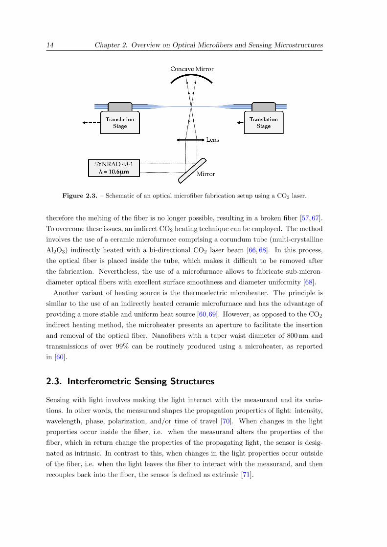
14 Chapter 2. Overview on Optical Microfibers and Sensing Microstructures
Figure 2.3. – Schematic of an optical microfiber fabrication setup using a CO2 laser.
therefore the melting of the fiber is no longer possible, resulting in a broken fiber [57,67].
To overcome these issues, an indirect CO2 heating technique can be employed. The method
involves the use of a ceramic microfurnace comprising a corundum tube (multi-crystalline
Al2O3) indirectly heated with a bi-directional CO2 laser beam [66, 68]. In this process,
the optical fiber is placed inside the tube, which makes it difficult to be removed after
the fabrication. Nevertheless, the use of a microfurnace allows to fabricate sub-micron-
diameter optical fibers with excellent surface smoothness and diameter uniformity [68].
Another variant of heating source is the thermoelectric microheater. The principle is
similar to the use of an indirectly heated ceramic microfurnace and has the advantage of
providing a more stable and uniform heat source [60,69]. However, as opposed to the CO2
indirect heating method, the microheater presents an aperture to facilitate the insertion
and removal of the optical fiber. Nanofibers with a taper waist diameter of 800 nm and
transmissions of over 99% can be routinely produced using a microheater, as reported
in [60].
2.3. Interferometric Sensing Structures
Sensing with light involves making the light interact with the measurand and its varia-
tions. In other words, the measurand shapes the propagation properties of light: intensity,
wavelength, phase, polarization, and/or time of travel [70]. When changes in the light
properties occur inside the fiber, i.e. when the measurand alters the properties of the
fiber, which in return change the properties of the propagating light, the sensor is desig-
nated as intrinsic. In contrast to this, when changes in the light properties occur outside
of the fiber, i.e. when the light leaves the fiber to interact with the measurand, and then
recouples back into the fiber, the sensor is defined as extrinsic [71].
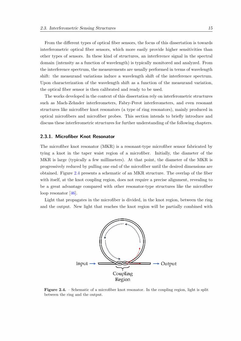
2.3. Interferometric Sensing Structures 15
From the different types of optical fiber sensors, the focus of this dissertation is towards
interferometric optical fiber sensors, which more easily provide higher sensitivities than
other types of sensors. In these kind of structures, an interference signal in the spectral
domain (intensity as a function of wavelength) is typically monitored and analyzed. From
the interference spectrum, the measurements are usually performed in terms of wavelength
shift: the measurand variations induce a wavelength shift of the interference spectrum.
Upon characterization of the wavelength shift as a function of the measurand variation,
the optical fiber sensor is then calibrated and ready to be used.
The works developed in the context of this dissertation rely on interferometric structures
such as Mach-Zehnder interferometers, Fabry-Perot interferometers, and even resonant
structures like microfiber knot resonators (a type of ring resonators), mainly produced in
optical microfibers and microfiber probes. This section intends to briefly introduce and
discuss these interferometric structures for further understanding of the following chapters.
2.3.1. Microfiber Knot Resonator
The microfiber knot resonator (MKR) is a resonant-type microfiber sensor fabricated by
tying a knot in the taper waist region of a microfiber. Initially, the diameter of the
MKR is large (typically a few millimeters). At that point, the diameter of the MKR is
progressively reduced by pulling one end of the microfiber until the desired dimensions are
obtained. Figure 2.4 presents a schematic of an MKR structure. The overlap of the fiber
with itself, at the knot coupling region, does not require a precise alignment, revealing to
be a great advantage compared with other resonator-type structures like the microfiber
loop resonator [46].
Light that propagates in the microfiber is divided, in the knot region, between the ring
and the output. New light that reaches the knot region will be partially combined with
Figure 2.4. – Schematic of a microfiber knot resonator. In the coupling region, light is splitbetween the ring and the output.
16 Chapter 2. Overview on Optical Microfibers and Sensing Microstructures
the light that previously traveled in the ring towards the output, while feeding at the same
time the ring. For specific wavelengths, called the resonant wavelengths (λres), light that
enters the ring is in phase with the one already traveling in it, resulting in accumulation
of light in the ring. As a consequence, light at those resonant wavelengths gets trapped
inside the ring, producing a dip in the transmission spectrum [33].
The distance between two adjacent resonant wavelengths (λres1 and λres2 ) in the MKR
transmission spectrum, known as the free spectral range (FSR), is defined as:
FSRMKR = λres1 − λres2 =λres1 λres2
neffL=λres1 λres2
2πrneff, (2.3)
where neff is the effective refractive index of the microfiber and L is the cavity length,
which for an MKR is given by the perimeter of the ring (L = 2πr, where r is the radius of
the ring). The dependence of the FSR in the radius of the ring can be very useful, since
one can tune the FSR by adjusting the diameter of the MKR.
The FSR is an important quantity for sensing applications, along with the sensitivity
of the structure to a certain measurand. In general, the FSR imposes a limitation in the
measurement range. The wavelength shift of a resonance dip due to a certain physical or
chemical measurand must be smaller than the FSR. Otherwise, the new position of the
resonance dip will overlap the position of a different resonance dip at a previous value of
the measured parameter. In other words, if the spectrum shifts by a FSR, the positions
of the resonance dips overlap and are indistinguishable from the previous state.
The transmission spectrum of a microfiber knot resonator can be, from a different point
of view, similar to that of a Fabry-Perot cavity. The cavity in the MKR structure is the
ring and the mirrors can be seen as the knot coupling region. In a Fabry-Perot cavity with
high reflectance mirrors, light travels longer in the cavity before leaving it. In an MKR,
the high reflectance mirrors correspond to a greater coupling of light between adjacent
fibers in the knot structure, increasing the amount of light accumulated in the ring. A
larger coupling efficiency in the knot region is achieved by using microfibers with small
diameters in the taper waist region (ideally around 1 to 2µm), which present a larger
evanescent field.
The MKR has been widely studied as a sensing element, due to its large evanescent
field that interacts with the external medium and also to the resonant property. The
use of MKRs to measure different parameters, by means of the wavelength shift of a
resonance dip, was demonstrated in the literature. The measured parameters include
temperature [38,72,73], concentration of sodium chloride [74], refractive index (RI) [6,75],
and others. For refractive index sensing, a simple MKR embedded in a Sagnac loop
reflector was proposed by Lim et al. [75], achieving a sensitivity of 30.49 nm/refractive
index units (RIU) in a refractive index range from 1.334-1.348. In 2014, a Teflon-coated
MKR was demonstrated to have a sensitivity of 30.5 nm/RIU between 1.3322 and 1.3412
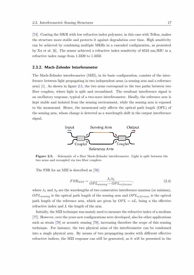
2.3. Interferometric Sensing Structures 17
[74]. Coating the MKR with low refractive index polymers, in this case with Teflon, makes
the structure more stable and protects it against degradation over time. High sensitivity
can be achieved by combining multiple MKRs in a cascaded configuration, as presented
by Xu et al. [6]. The sensor achieved a refractive index sensitivity of 6523 nm/RIU in a
refractive index range from 1.3320 to 1.3350.
2.3.2. Mach-Zehnder Interferometer
The Mach-Zehnder interferometer (MZI), in its basic configuration, consists of the inter-
ference between light propagating in two independent arms (a sensing arm and a reference
arm) [1]. As shown in figure 2.5, the two arms correspond to the two paths between two
fiber couplers, where light is split and recombined. The resultant interference signal is
an oscillatory response, typical of a two-wave interferometer. Ideally, the reference arm is
kept stable and isolated from the sensing environment, while the sensing arm is exposed
to the measurand. Hence, the measurand only affects the optical path length (OPL) of
the sensing arm, whose change is detected as a wavelength shift in the output interference
signal.
Figure 2.5. – Schematic of a fiber Mach-Zehnder interferometer. Light is split between thetwo arms and recoupled via two fiber couplers.
The FSR for an MZI is described as [76]:
FSRMZI =λ1λ2
OPLsensing −OPLreference, (2.4)
where λ1 and λ2 are the wavelengths of two consecutive interference maxima (or minima),
OPLsensing is the optical path length of the sensing arm and OPLreference is the optical
path length of the reference arm, which are given by OPL = nL, being n the effective
refractive index and L the length of the arm.
Initially, the MZI technique was mainly used to measure the refractive index of a medium
[77]. However, over the years new configurations were developed, also for other applications
such as strain [78] or acoustic sensing [79], increasing therefore the scope of this sensing
technique. For instance, the two physical arms of the interferometer can be condensed
into a single physical arm. By means of two propagating modes with different effective
refractive indices, the MZI response can still be generated, as it will be presented in the
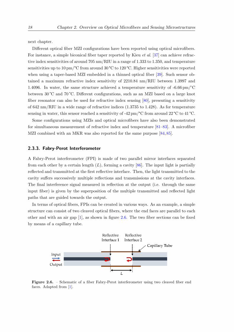
18 Chapter 2. Overview on Optical Microfibers and Sensing Microstructures
next chapter.
Different optical fiber MZI configurations have been reported using optical microfibers.
For instance, a simple biconical fiber taper reported by Kieu et al. [37] can achieve refrac-
tive index sensitivities of around 705 nm/RIU in a range of 1.333 to 1.350, and temperature
sensitivities up to 10 pm/°C from around 30 °C to 120 °C. Higher sensitivities were reported
when using a taper-based MZI embedded in a thinned optical fiber [39]. Such sensor ob-
tained a maximum refractive index sensitivity of 2210.84 nm/RIU between 1.3997 and
1.4096. In water, the same structure achieved a temperature sensitivity of -6.66 pm/°C
between 30 °C and 70 °C. Different configurations, such as an MZI based on a large knot
fiber resonator can also be used for refractive index sensing [80], presenting a sensitivity
of 642 nm/RIU in a wide range of refractive indices (1.3735 to 1.428). As for temperature
sensing in water, this sensor reached a sensitivity of -42 pm/°C from around 22 °C to 41 °C.
Some configurations using MZIs and optical microfibers have also been demonstrated
for simultaneous measurement of refractive index and temperature [81–83]. A microfiber
MZI combined with an MKR was also reported for the same purpose [84,85].
2.3.3. Fabry-Perot Interferometer
A Fabry-Perot interferometer (FPI) is made of two parallel mirror interfaces separated
from each other by a certain length (L), forming a cavity [86]. The input light is partially
reflected and transmitted at the first reflective interface. Then, the light transmitted to the
cavity suffers successively multiple reflections and transmissions at the cavity interfaces.
The final interference signal measured in reflection at the output (i.e. through the same
input fiber) is given by the superposition of the multiple transmitted and reflected light
paths that are guided towards the output.
In terms of optical fibers, FPIs can be created in various ways. As an example, a simple
structure can consist of two cleaved optical fibers, where the end faces are parallel to each
other and with an air gap [1], as shown in figure 2.6. The two fiber sections can be fixed
by means of a capillary tube.
Figure 2.6. – Schematic of a fiber Fabry-Perot interferometer using two cleaved fiber endfaces. Adapted from [1].
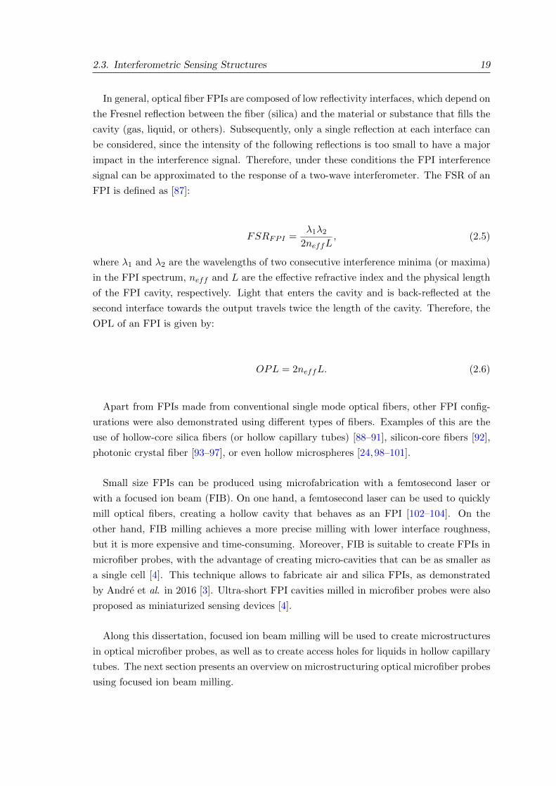
2.3. Interferometric Sensing Structures 19
In general, optical fiber FPIs are composed of low reflectivity interfaces, which depend on
the Fresnel reflection between the fiber (silica) and the material or substance that fills the
cavity (gas, liquid, or others). Subsequently, only a single reflection at each interface can
be considered, since the intensity of the following reflections is too small to have a major
impact in the interference signal. Therefore, under these conditions the FPI interference
signal can be approximated to the response of a two-wave interferometer. The FSR of an
FPI is defined as [87]:
FSRFPI =λ1λ2
2neffL, (2.5)
where λ1 and λ2 are the wavelengths of two consecutive interference minima (or maxima)
in the FPI spectrum, neff and L are the effective refractive index and the physical length
of the FPI cavity, respectively. Light that enters the cavity and is back-reflected at the
second interface towards the output travels twice the length of the cavity. Therefore, the
OPL of an FPI is given by:
OPL = 2neffL. (2.6)
Apart from FPIs made from conventional single mode optical fibers, other FPI config-
urations were also demonstrated using different types of fibers. Examples of this are the
use of hollow-core silica fibers (or hollow capillary tubes) [88–91], silicon-core fibers [92],
photonic crystal fiber [93–97], or even hollow microspheres [24,98–101].
Small size FPIs can be produced using microfabrication with a femtosecond laser or
with a focused ion beam (FIB). On one hand, a femtosecond laser can be used to quickly
mill optical fibers, creating a hollow cavity that behaves as an FPI [102–104]. On the
other hand, FIB milling achieves a more precise milling with lower interface roughness,
but it is more expensive and time-consuming. Moreover, FIB is suitable to create FPIs in
microfiber probes, with the advantage of creating micro-cavities that can be as smaller as
a single cell [4]. This technique allows to fabricate air and silica FPIs, as demonstrated
by Andre et al. in 2016 [3]. Ultra-short FPI cavities milled in microfiber probes were also
proposed as miniaturized sensing devices [4].
Along this dissertation, focused ion beam milling will be used to create microstructures
in optical microfiber probes, as well as to create access holes for liquids in hollow capillary
tubes. The next section presents an overview on microstructuring optical microfiber probes
using focused ion beam milling.
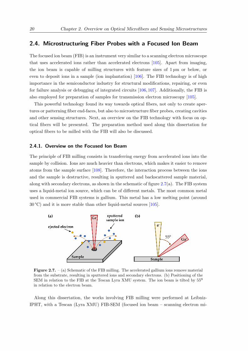
20 Chapter 2. Overview on Optical Microfibers and Sensing Microstructures
2.4. Microstructuring Fiber Probes with a Focused Ion Beam
The focused ion beam (FIB) is an instrument very similar to a scanning electron microscope
that uses accelerated ions rather than accelerated electrons [105]. Apart from imaging,
the ion beam is capable of milling structures with feature sizes of 1 µm or below, or
even to deposit ions in a sample (ion implantation) [106]. The FIB technology is of high
importance in the semiconductor industry for structural modifications, repairing, or even
for failure analysis or debugging of integrated circuits [106, 107]. Additionally, the FIB is
also employed for preparation of samples for transmission electron microscopy [105].
This powerful technology found its way towards optical fibers, not only to create aper-
tures or patterning fiber end-faces, but also to microstructure fiber probes, creating cavities
and other sensing structures. Next, an overview on the FIB technology with focus on op-
tical fibers will be presented. The preparation method used along this dissertation for
optical fibers to be milled with the FIB will also be discussed.
2.4.1. Overview on the Focused Ion Beam
The principle of FIB milling consists in transferring energy from accelerated ions into the
sample by collision. Ions are much heavier than electrons, which makes it easier to remove
atoms from the sample surface [108]. Therefore, the interaction process between the ions
and the sample is destructive, resulting in sputtered and backscattered sample material,
along with secondary electrons, as shown in the schematic of figure 2.7(a). The FIB system
uses a liquid-metal ion source, which can be of different metals. The most common metal
used in commercial FIB systems is gallium. This metal has a low melting point (around
30 °C) and it is more stable than other liquid-metal sources [105].
Figure 2.7. – (a) Schematic of the FIB milling. The accelerated gallium ions remove materialfrom the substrate, resulting in sputtered ions and secondary electrons. (b) Positioning of theSEM in relation to the FIB at the Tescan Lyra XMU system. The ion beam is tilted by 55ºin relation to the electron beam.
Along this dissertation, the works involving FIB milling were performed at Leibniz-
IPHT, with a Tescan (Lyra XMU) FIB-SEM (focused ion beam – scanning electron mi-
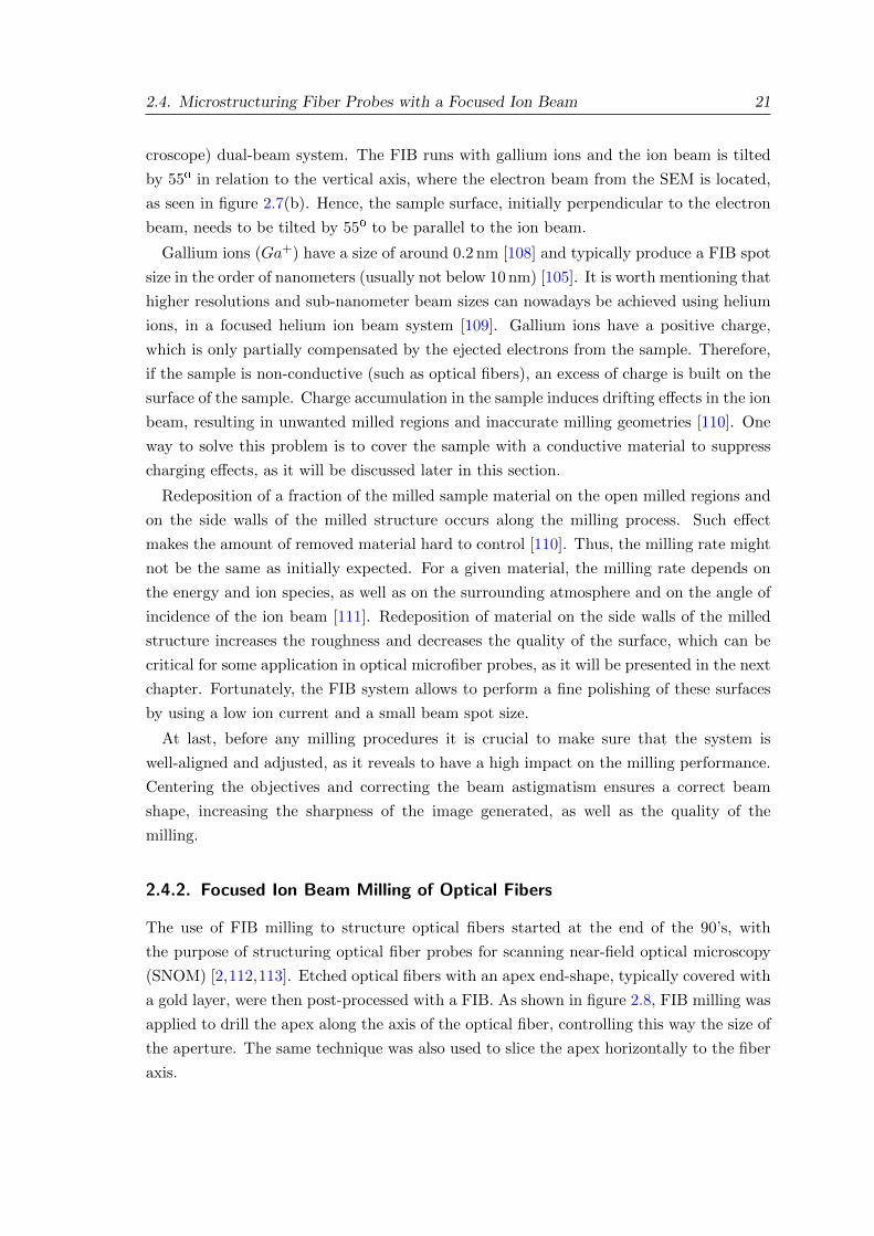
2.4. Microstructuring Fiber Probes with a Focused Ion Beam 21
croscope) dual-beam system. The FIB runs with gallium ions and the ion beam is tilted
by 55º in relation to the vertical axis, where the electron beam from the SEM is located,
as seen in figure 2.7(b). Hence, the sample surface, initially perpendicular to the electron
beam, needs to be tilted by 55º to be parallel to the ion beam.
Gallium ions (Ga+) have a size of around 0.2 nm [108] and typically produce a FIB spot
size in the order of nanometers (usually not below 10 nm) [105]. It is worth mentioning that
higher resolutions and sub-nanometer beam sizes can nowadays be achieved using helium
ions, in a focused helium ion beam system [109]. Gallium ions have a positive charge,
which is only partially compensated by the ejected electrons from the sample. Therefore,
if the sample is non-conductive (such as optical fibers), an excess of charge is built on the
surface of the sample. Charge accumulation in the sample induces drifting effects in the ion
beam, resulting in unwanted milled regions and inaccurate milling geometries [110]. One
way to solve this problem is to cover the sample with a conductive material to suppress
charging effects, as it will be discussed later in this section.
Redeposition of a fraction of the milled sample material on the open milled regions and
on the side walls of the milled structure occurs along the milling process. Such effect
makes the amount of removed material hard to control [110]. Thus, the milling rate might
not be the same as initially expected. For a given material, the milling rate depends on
the energy and ion species, as well as on the surrounding atmosphere and on the angle of
incidence of the ion beam [111]. Redeposition of material on the side walls of the milled
structure increases the roughness and decreases the quality of the surface, which can be
critical for some application in optical microfiber probes, as it will be presented in the next
chapter. Fortunately, the FIB system allows to perform a fine polishing of these surfaces
by using a low ion current and a small beam spot size.
At last, before any milling procedures it is crucial to make sure that the system is
well-aligned and adjusted, as it reveals to have a high impact on the milling performance.
Centering the objectives and correcting the beam astigmatism ensures a correct beam
shape, increasing the sharpness of the image generated, as well as the quality of the
milling.
2.4.2. Focused Ion Beam Milling of Optical Fibers
The use of FIB milling to structure optical fibers started at the end of the 90’s, with
the purpose of structuring optical fiber probes for scanning near-field optical microscopy
(SNOM) [2,112,113]. Etched optical fibers with an apex end-shape, typically covered with
a gold layer, were then post-processed with a FIB. As shown in figure 2.8, FIB milling was
applied to drill the apex along the axis of the optical fiber, controlling this way the size of
the aperture. The same technique was also used to slice the apex horizontally to the fiber
axis.
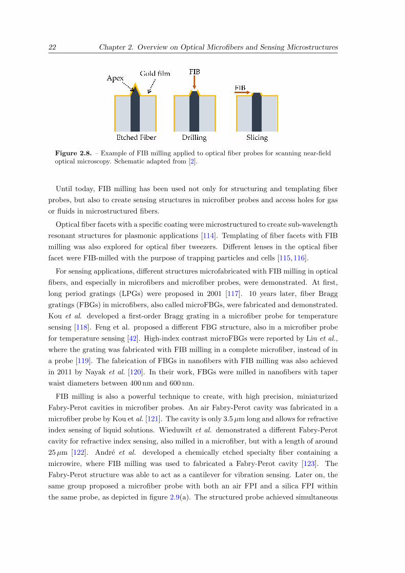
22 Chapter 2. Overview on Optical Microfibers and Sensing Microstructures
Figure 2.8. – Example of FIB milling applied to optical fiber probes for scanning near-fieldoptical microscopy. Schematic adapted from [2].
Until today, FIB milling has been used not only for structuring and templating fiber
probes, but also to create sensing structures in microfiber probes and access holes for gas
or fluids in microstructured fibers.
Optical fiber facets with a specific coating were microstructured to create sub-wavelength
resonant structures for plasmonic applications [114]. Templating of fiber facets with FIB
milling was also explored for optical fiber tweezers. Different lenses in the optical fiber
facet were FIB-milled with the purpose of trapping particles and cells [115,116].
For sensing applications, different structures microfabricated with FIB milling in optical
fibers, and especially in microfibers and microfiber probes, were demonstrated. At first,
long period gratings (LPGs) were proposed in 2001 [117]. 10 years later, fiber Bragg
gratings (FBGs) in microfibers, also called microFBGs, were fabricated and demonstrated.
Kou et al. developed a first-order Bragg grating in a microfiber probe for temperature
sensing [118]. Feng et al. proposed a different FBG structure, also in a microfiber probe
for temperature sensing [42]. High-index contrast microFBGs were reported by Liu et al.,
where the grating was fabricated with FIB milling in a complete microfiber, instead of in
a probe [119]. The fabrication of FBGs in nanofibers with FIB milling was also achieved
in 2011 by Nayak et al. [120]. In their work, FBGs were milled in nanofibers with taper
waist diameters between 400 nm and 600 nm.
FIB milling is also a powerful technique to create, with high precision, miniaturized
Fabry-Perot cavities in microfiber probes. An air Fabry-Perot cavity was fabricated in a
microfiber probe by Kou et al. [121]. The cavity is only 3.5µm long and allows for refractive
index sensing of liquid solutions. Wieduwilt et al. demonstrated a different Fabry-Perot
cavity for refractive index sensing, also milled in a microfiber, but with a length of around
25µm [122]. Andre et al. developed a chemically etched specialty fiber containing a
microwire, where FIB milling was used to fabricated a Fabry-Perot cavity [123]. The
Fabry-Perot structure was able to act as a cantilever for vibration sensing. Later on, the
same group proposed a microfiber probe with both an air FPI and a silica FPI within
the same probe, as depicted in figure 2.9(a). The structured probe achieved simultaneous
2.4. Microstructuring Fiber Probes with a Focused Ion Beam 23
measurement of refractive index of liquid solutions and temperature [3]. Refractive index
sensing with ultra-short Fabry-Perot cavities milled with a FIB, as presented in figure
2.9(b), were demonstrated by Warren-Smith et al. [4].
Figure 2.9. – Example of FIB-milled FPIs in optical microfibers. (a) Two FPIs (an air cavityand a silica cavity) in a single microfiber probe. Adapted from [3]. (b) Ultra-short FPI in amicrofiber probe. Adapted from [4].
More complex fiber sensing devices combining FIB milling were also reported. A mi-
crofiber knot resonator combined with a Mach-Zehnder interferometer, milled with a FIB
in the same microfiber, was shown by Gomes et al. [124]. Warren-Smith et al. reported
a direct core structuring of exposed core fibers with FIB milling [125]. The application of
FIB milling to fabricate asymmetric microspheres was demonstrated in 2018 by Gomes et
al. [24,26]. These microspheres generate a random signal that can be analyzed to retrieve
information regarding temperature variations.
At last, FIB milling was used to open access holes for gas and fluids in specialty fibers,
such as in photonic crystal fibers or in multi-hole step-index fibers [110]. Gomes et al. also
demonstrated an acetone evaporation and water vapor detection sensor using a caterpillar-
like microstructured fiber [126]. FIB milling was applied to open access holes for the gas
vapor to circulate inside the microstructured fiber.
2.4.3. Sample Preparation
Using FIB and/or SEM in optical fibers requires a prior sample preparation to eliminate
charging effects. In this dissertation the optical fibers were initially mounted and fixed
in an aluminium holder with a droplet of carbon glue (DOTITE XC-12, Fujikura Kasei
Co., LtD Tokyo, Japan). The sample holder is conductive and the carbon glue ensures a
good electrical contact between the holder and the fiber, which will then be coated with a
conductive film to suppress surface charges. The optical fiber can be coated with different
materials, such as gold, platinum, tantalum, carbon, and others. It is useful to deposit
a conductive film of a material with a low milling rate, avoiding its fast removal during
the milling process and the need to redeposit a new film. All the FIB-milled optical fibers
along this dissertation were coated with a carbon film. In general, carbon is more stable
and presents a lower milling rate compared with other conductive films, such as platinum
or gold. With this, only a few nanometers of carbon coating are necessary, instead of a
24 Chapter 2. Overview on Optical Microfibers and Sensing Microstructures
few tens of nanometers, having a lesser impact in the final performance of the structure
(ex. inducing losses through light absorption).
The optical fiber samples were carbon-coated by means of a LEICA EM ACE600. This
system allows to tilt the stage for a better positioning of the sample in relation to the carbon
source. Moreover, the stage can also rotate during the deposition process to provide a good
coating distribution, not just on the top of the sample, but also on the sides.
At last, the milled optical fiber samples can be removed from the holder using acetone
to dissolve the carbon glue. Additional cleaning can also be performed using an ultrasonic
bath with acetone, removing parts of the dissolved carbon glue that attached to the milled
region.
2.5. Conclusion
Optical microfibers and microfiber probes are a useful platform to achieve miniaturized
sensors. Their properties, combined with different post-processing techniques, allows to
create distinct sensing interferometers with potential to attain high sensitivities.
An introductory overview of three distinct fiber interferometric configurations was here
presented, providing a basic background for a more comprehensive understanding of the
following chapters. The microfiber knot resonator has improved light-environment inter-
action due to the its resonant property. The Mach-Zehnder interferometer relies on the
phase shift induced by the measurand in one of the arms. This effect can be very sensitive
to small variations in parameters such as the refractive index or concentration of certain
compounds in solutions, which is indirectly related with the refractive index. The response
of a Fabry-Perot interferometer is measured in reflection (the input and the output fiber
is the same), which is extremely useful to incorporate in microfiber probes. As here dis-
cussed, this kind of structures can be fabricated by means of femtosecond laser ablation
or focused ion beam milling.
Much of the work in this dissertation makes use of focused ion beam milling to create
sensing structures in microfiber probes and to open access holes in hollow capillary tubes.
Therefore, this chapter also provided a brief introduction to the principle of focused ion
beam milling, with strong focus on optical fiber applications.
The next chapter explores the development of microstructured sensing devices in optical
microfibers and microfiber probes. Different techniques and sensing interferometers here
introduced are combined together, creating novel sensing structures with enhanced sensing
capabilities.
Chapter 3.
Microstructured Sensing Devices
with Optical Microfibers
3.1. Introduction
This chapter explores the study and development of microstructured sensors based on op-
tical microfibers. The objective is to create small sensing devices with enhanced sensing
capabilities, such as simultaneous measurement of physical quantities or enhanced sensi-
tivity to a certain measurand. In the first section, a complete optical microfiber is struc-
tured to combine two different sensing configurations into a single and compact optical
sensing device. This approach intents to create a versatile sensor that allows simultane-
ous measurement of refractive index and temperature, solving this way the problem of
cross-sensitivity. On the other hand, the second section explores the use of a multimode
microfiber probe to achieve enhanced sensitivity to temperature. At the same time, the
work trends towards the miniaturization of fiber sensing devices for point measurements.
Here, only half of a microfiber is used to create a small size sensing probe with a small
footprint. Additionally, this work also explores microfabrication with a focused ion beam
to post-process the microfiber probe.
3.2. Microfiber Knot Resonator combined with Mach-Zehnder
Interferometer
Cross-sensitivity is a common problem in the domain of optical fiber sensors that needs to
be solved, especially when using the fiber sensing element outside of a stable and controlled
environment. In most cases, apart from the measurand, the measurement signal is also
influenced by different outside parameters. In fiber sensing interferometers, variations
of these external physical quantities induce similar wavelength shifts as the measurand,
making it rather complicated, or nearly impossible, to determine exactly the response of
the target measurand. When measuring a certain quantity, undesired variations of other
26 Chapter 3. Microstructured Sensing Devices with Optical Microfibers
additional parameters introduce an error in the measurement, leading to inaccurate results.
Fluctuations of temperature turned out to be one of the most problematic cases of cross-
sensitivity. Physical parameters are temperature dependent, and the sensing structure
itself may also change due to temperature effects (either by thermal expansion or thermo-
optic effect). Consequently, different fiber sensing configurations and techniques had to
be developed to compensate for possible temperature fluctuations [81, 127–131]. On a
basic level, a simple thermometer could be used to monitor in real time the temperature
fluctuations, using these values to compensate and correct the final response of the fiber
sensor. However, in real applications the use of an external thermometer is inconvenient.
As an alternative approach, it is possible to incorporate a temperature sensor inside
the optical fiber together with a different sensing structure, for instance, by multiplexing
a fiber sensing interferometer with a fiber Bragg grating (FBG) [132]. The FBG was,
and still is, extensively studied and applied to monitor temperature variations in different
environments [133, 134]. A different way to compensate for temperature fluctuations in-
volves the combination of two fiber interferometers with distinct responses to temperature
and to the target measurand. As a drawback, the optical signal of the sensing structure
becomes more complex, requiring additional signal processing. Nevertheless, simultaneous
measurement of both measurands is then enabled by means of a matrix method [135].
Enlightened by this last concept, this section explores the combination of two distinct
interferometric structures within a single optical microfiber: a microfiber knot resonator
(MKR) and a Mach-Zehnder interferometer (MZI). The aim of such sensing device is to
enable simultaneous measurement of refractive index variations of liquid solutions and
temperature variations. A key aspect of the following configuration, as will be further
explained later on this section, is a slight structural modification of the microfiber during
the fabrication process. This allows the Mach-Zehnder interferometer to be embedded in
the microfiber, forming a compact structure.
3.2.1. Principle and Fabrication
The base of the structure consists of a microfiber knot resonator made from an optical
microfiber. As discussed in the previous chapter 2, the MKR produces resonance dips
in the transmission spectrum due light being trapped in the MKR ring. Now, the trick
consists of fabricating the microfiber with a slightly abrupt transition region. In such
case, a few other modes are excited in the microfiber. These modes co-propagate with an
effective refractive index different than the fundamental mode one, hence accumulating
a phase difference. Then, in the knot region, the modes interfere due to the inherent
curvature of the microfiber, creating a Mach-Zehnder interferometer whose response is
susceptible to refractive index variations of the surrounding environment. A schematic of
the two main structures are depicted in figure 3.1.
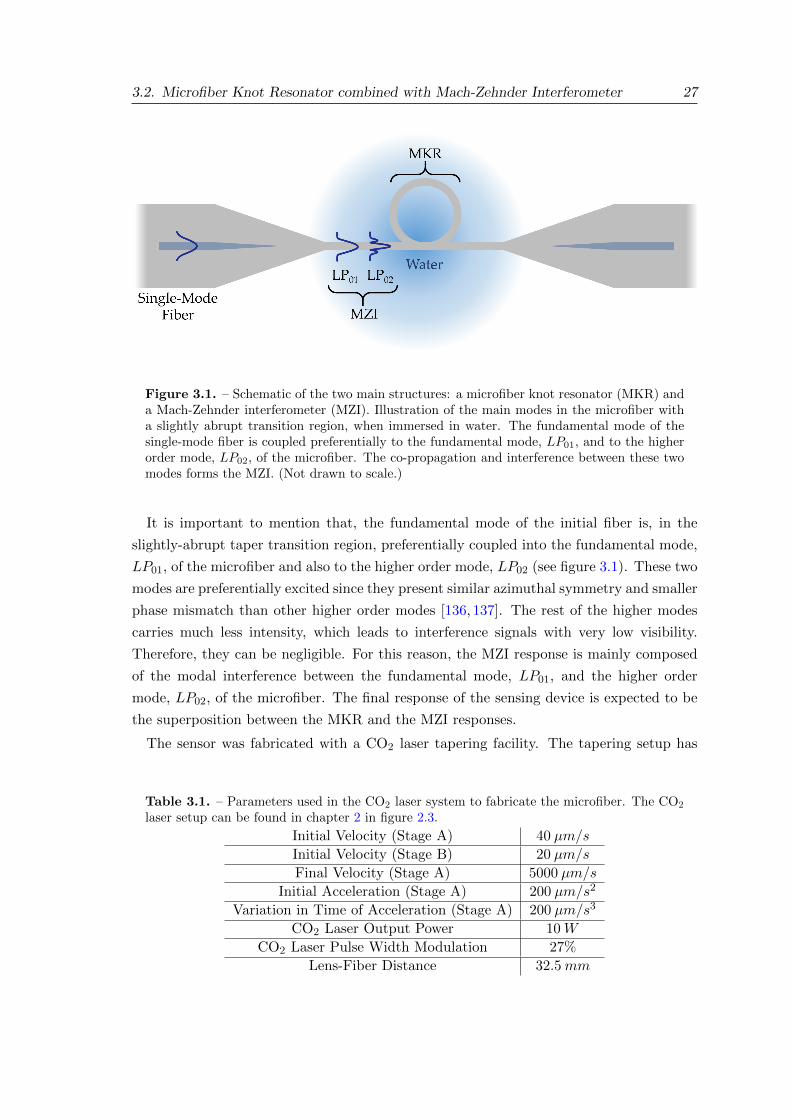
3.2. Microfiber Knot Resonator combined with Mach-Zehnder Interferometer 27
Figure 3.1. – Schematic of the two main structures: a microfiber knot resonator (MKR) anda Mach-Zehnder interferometer (MZI). Illustration of the main modes in the microfiber witha slightly abrupt transition region, when immersed in water. The fundamental mode of thesingle-mode fiber is coupled preferentially to the fundamental mode, LP01, and to the higherorder mode, LP02, of the microfiber. The co-propagation and interference between these twomodes forms the MZI. (Not drawn to scale.)
It is important to mention that, the fundamental mode of the initial fiber is, in the
slightly-abrupt taper transition region, preferentially coupled into the fundamental mode,
LP01, of the microfiber and also to the higher order mode, LP02 (see figure 3.1). These two
modes are preferentially excited since they present similar azimuthal symmetry and smaller
phase mismatch than other higher order modes [136, 137]. The rest of the higher modes
carries much less intensity, which leads to interference signals with very low visibility.
Therefore, they can be negligible. For this reason, the MZI response is mainly composed
of the modal interference between the fundamental mode, LP01, and the higher order
mode, LP02, of the microfiber. The final response of the sensing device is expected to be
the superposition between the MKR and the MZI responses.
The sensor was fabricated with a CO2 laser tapering facility. The tapering setup has
Table 3.1. – Parameters used in the CO2 laser system to fabricate the microfiber. The CO2
laser setup can be found in chapter 2 in figure 2.3.
Initial Velocity (Stage A) 40 µm/s
Initial Velocity (Stage B) 20 µm/s
Final Velocity (Stage A) 5000 µm/s
Initial Acceleration (Stage A) 200 µm/s2
Variation in Time of Acceleration (Stage A) 200 µm/s3
CO2 Laser Output Power 10W
CO2 Laser Pulse Width Modulation 27%
Lens-Fiber Distance 32.5mm
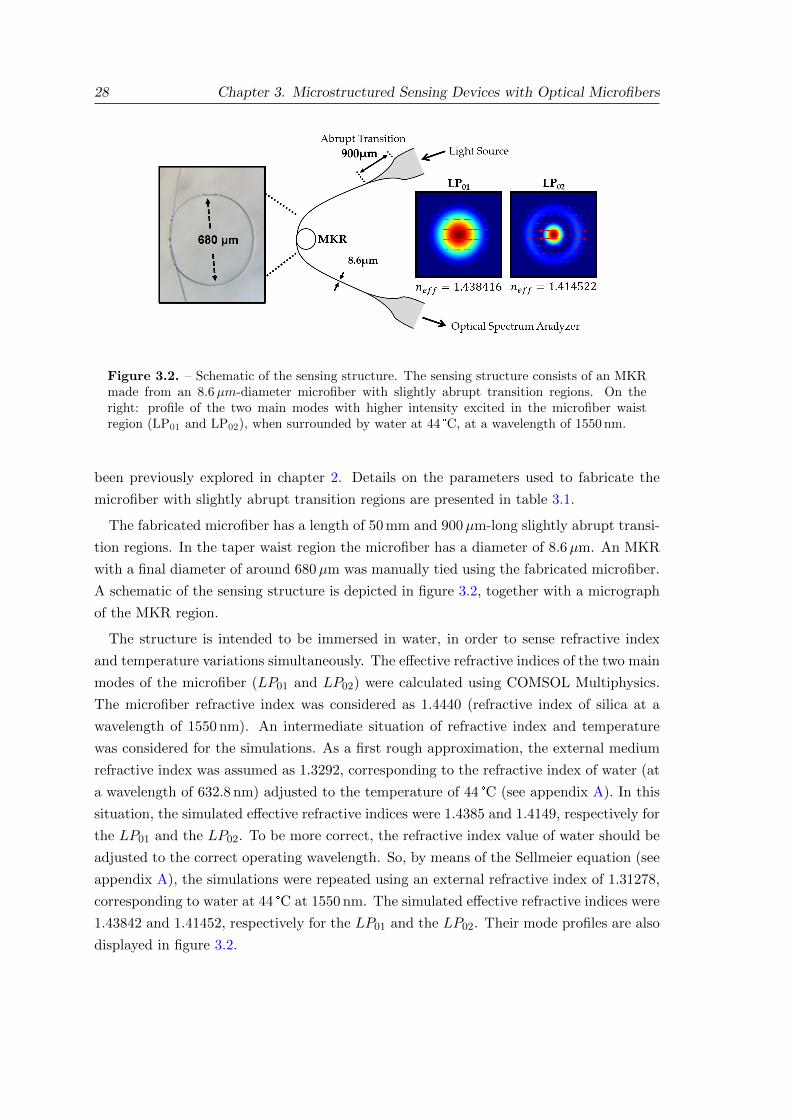
28 Chapter 3. Microstructured Sensing Devices with Optical Microfibers
Figure 3.2. – Schematic of the sensing structure. The sensing structure consists of an MKRmade from an 8.6µm-diameter microfiber with slightly abrupt transition regions. On theright: profile of the two main modes with higher intensity excited in the microfiber waistregion (LP01 and LP02), when surrounded by water at 44 °C, at a wavelength of 1550 nm.
been previously explored in chapter 2. Details on the parameters used to fabricate the
microfiber with slightly abrupt transition regions are presented in table 3.1.
The fabricated microfiber has a length of 50 mm and 900µm-long slightly abrupt transi-
tion regions. In the taper waist region the microfiber has a diameter of 8.6µm. An MKR
with a final diameter of around 680µm was manually tied using the fabricated microfiber.
A schematic of the sensing structure is depicted in figure 3.2, together with a micrograph
of the MKR region.
The structure is intended to be immersed in water, in order to sense refractive index
and temperature variations simultaneously. The effective refractive indices of the two main
modes of the microfiber (LP01 and LP02) were calculated using COMSOL Multiphysics.
The microfiber refractive index was considered as 1.4440 (refractive index of silica at a
wavelength of 1550 nm). An intermediate situation of refractive index and temperature
was considered for the simulations. As a first rough approximation, the external medium
refractive index was assumed as 1.3292, corresponding to the refractive index of water (at
a wavelength of 632.8 nm) adjusted to the temperature of 44 °C (see appendix A). In this
situation, the simulated effective refractive indices were 1.4385 and 1.4149, respectively for
the LP01 and the LP02. To be more correct, the refractive index value of water should be
adjusted to the correct operating wavelength. So, by means of the Sellmeier equation (see
appendix A), the simulations were repeated using an external refractive index of 1.31278,
corresponding to water at 44 °C at 1550 nm. The simulated effective refractive indices were
1.43842 and 1.41452, respectively for the LP01 and the LP02. Their mode profiles are also
displayed in figure 3.2.
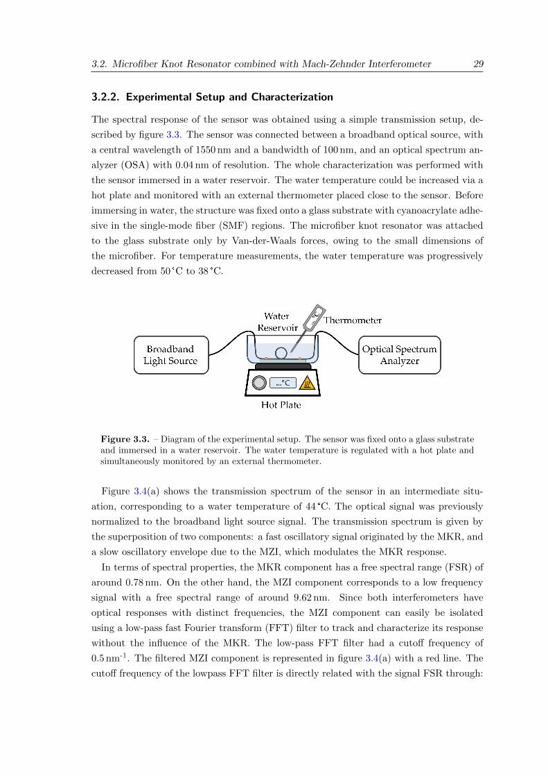
3.2. Microfiber Knot Resonator combined with Mach-Zehnder Interferometer 29
3.2.2. Experimental Setup and Characterization
The spectral response of the sensor was obtained using a simple transmission setup, de-
scribed by figure 3.3. The sensor was connected between a broadband optical source, with
a central wavelength of 1550 nm and a bandwidth of 100 nm, and an optical spectrum an-
alyzer (OSA) with 0.04 nm of resolution. The whole characterization was performed with
the sensor immersed in a water reservoir. The water temperature could be increased via a
hot plate and monitored with an external thermometer placed close to the sensor. Before
immersing in water, the structure was fixed onto a glass substrate with cyanoacrylate adhe-
sive in the single-mode fiber (SMF) regions. The microfiber knot resonator was attached
to the glass substrate only by Van-der-Waals forces, owing to the small dimensions of
the microfiber. For temperature measurements, the water temperature was progressively
decreased from 50 °C to 38 °C.
Figure 3.3. – Diagram of the experimental setup. The sensor was fixed onto a glass substrateand immersed in a water reservoir. The water temperature is regulated with a hot plate andsimultaneously monitored by an external thermometer.
Figure 3.4(a) shows the transmission spectrum of the sensor in an intermediate situ-
ation, corresponding to a water temperature of 44 °C. The optical signal was previously
normalized to the broadband light source signal. The transmission spectrum is given by
the superposition of two components: a fast oscillatory signal originated by the MKR, and
a slow oscillatory envelope due to the MZI, which modulates the MKR response.
In terms of spectral properties, the MKR component has a free spectral range (FSR) of
around 0.78 nm. On the other hand, the MZI component corresponds to a low frequency
signal with a free spectral range of around 9.62 nm. Since both interferometers have
optical responses with distinct frequencies, the MZI component can easily be isolated
using a low-pass fast Fourier transform (FFT) filter to track and characterize its response
without the influence of the MKR. The low-pass FFT filter had a cutoff frequency of
0.5 nm-1. The filtered MZI component is represented in figure 3.4(a) with a red line. The
cutoff frequency of the lowpass FFT filter is directly related with the signal FSR through:
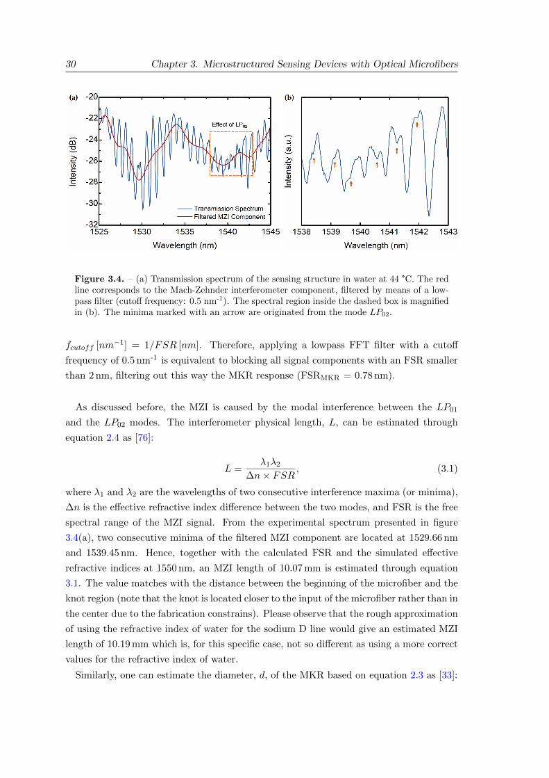
30 Chapter 3. Microstructured Sensing Devices with Optical Microfibers
Figure 3.4. – (a) Transmission spectrum of the sensing structure in water at 44 °C. The redline corresponds to the Mach-Zehnder interferometer component, filtered by means of a low-pass filter (cutoff frequency: 0.5 nm-1). The spectral region inside the dashed box is magnifiedin (b). The minima marked with an arrow are originated from the mode LP02.
fcutoff [nm−1] = 1/FSR [nm]. Therefore, applying a lowpass FFT filter with a cutoff
frequency of 0.5 nm-1 is equivalent to blocking all signal components with an FSR smaller
than 2 nm, filtering out this way the MKR response (FSRMKR = 0.78 nm).
As discussed before, the MZI is caused by the modal interference between the LP01
and the LP02 modes. The interferometer physical length, L, can be estimated through
equation 2.4 as [76]:
L =λ1λ2
∆n× FSR, (3.1)
where λ1 and λ2 are the wavelengths of two consecutive interference maxima (or minima),
∆n is the effective refractive index difference between the two modes, and FSR is the free
spectral range of the MZI signal. From the experimental spectrum presented in figure
3.4(a), two consecutive minima of the filtered MZI component are located at 1529.66 nm
and 1539.45 nm. Hence, together with the calculated FSR and the simulated effective
refractive indices at 1550 nm, an MZI length of 10.07 mm is estimated through equation
3.1. The value matches with the distance between the beginning of the microfiber and the
knot region (note that the knot is located closer to the input of the microfiber rather than in
the center due to the fabrication constrains). Please observe that the rough approximation
of using the refractive index of water for the sodium D line would give an estimated MZI
length of 10.19 mm which is, for this specific case, not so different as using a more correct
values for the refractive index of water.
Similarly, one can estimate the diameter, d, of the MKR based on equation 2.3 as [33]:
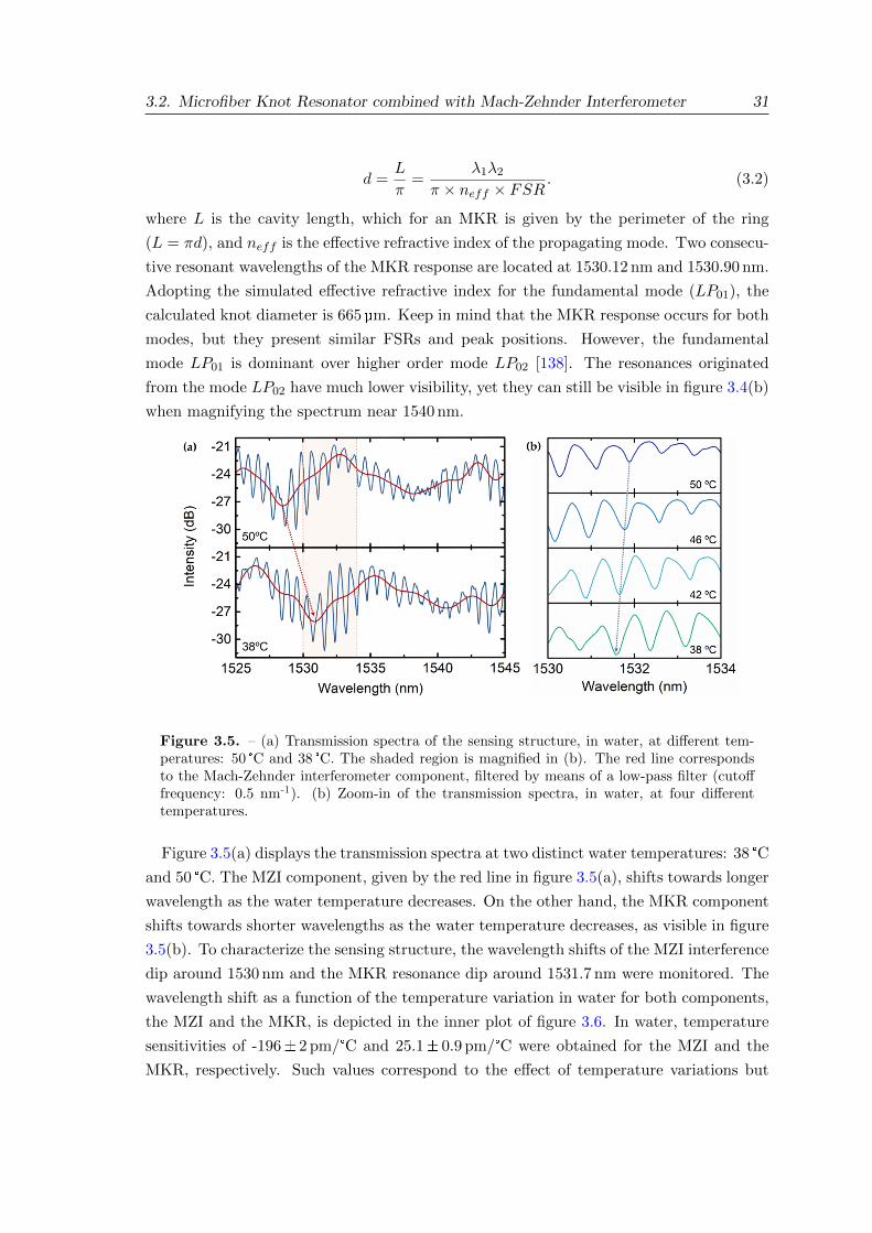
3.2. Microfiber Knot Resonator combined with Mach-Zehnder Interferometer 31
d =L
π=
λ1λ2π × neff × FSR
. (3.2)
where L is the cavity length, which for an MKR is given by the perimeter of the ring
(L = πd), and neff is the effective refractive index of the propagating mode. Two consecu-
tive resonant wavelengths of the MKR response are located at 1530.12 nm and 1530.90 nm.
Adopting the simulated effective refractive index for the fundamental mode (LP01), the
calculated knot diameter is 665 µm. Keep in mind that the MKR response occurs for both
modes, but they present similar FSRs and peak positions. However, the fundamental
mode LP01 is dominant over higher order mode LP02 [138]. The resonances originated
from the mode LP02 have much lower visibility, yet they can still be visible in figure 3.4(b)
when magnifying the spectrum near 1540 nm.
Figure 3.5. – (a) Transmission spectra of the sensing structure, in water, at different tem-peratures: 50 °C and 38 °C. The shaded region is magnified in (b). The red line correspondsto the Mach-Zehnder interferometer component, filtered by means of a low-pass filter (cutofffrequency: 0.5 nm-1). (b) Zoom-in of the transmission spectra, in water, at four differenttemperatures.
Figure 3.5(a) displays the transmission spectra at two distinct water temperatures: 38 °C
and 50 °C. The MZI component, given by the red line in figure 3.5(a), shifts towards longer
wavelength as the water temperature decreases. On the other hand, the MKR component
shifts towards shorter wavelengths as the water temperature decreases, as visible in figure
3.5(b). To characterize the sensing structure, the wavelength shifts of the MZI interference
dip around 1530 nm and the MKR resonance dip around 1531.7 nm were monitored. The
wavelength shift as a function of the temperature variation in water for both components,
the MZI and the MKR, is depicted in the inner plot of figure 3.6. In water, temperature
sensitivities of -196± 2 pm/°C and 25.1± 0.9 pm/°C were obtained for the MZI and the
MKR, respectively. Such values correspond to the effect of temperature variations but
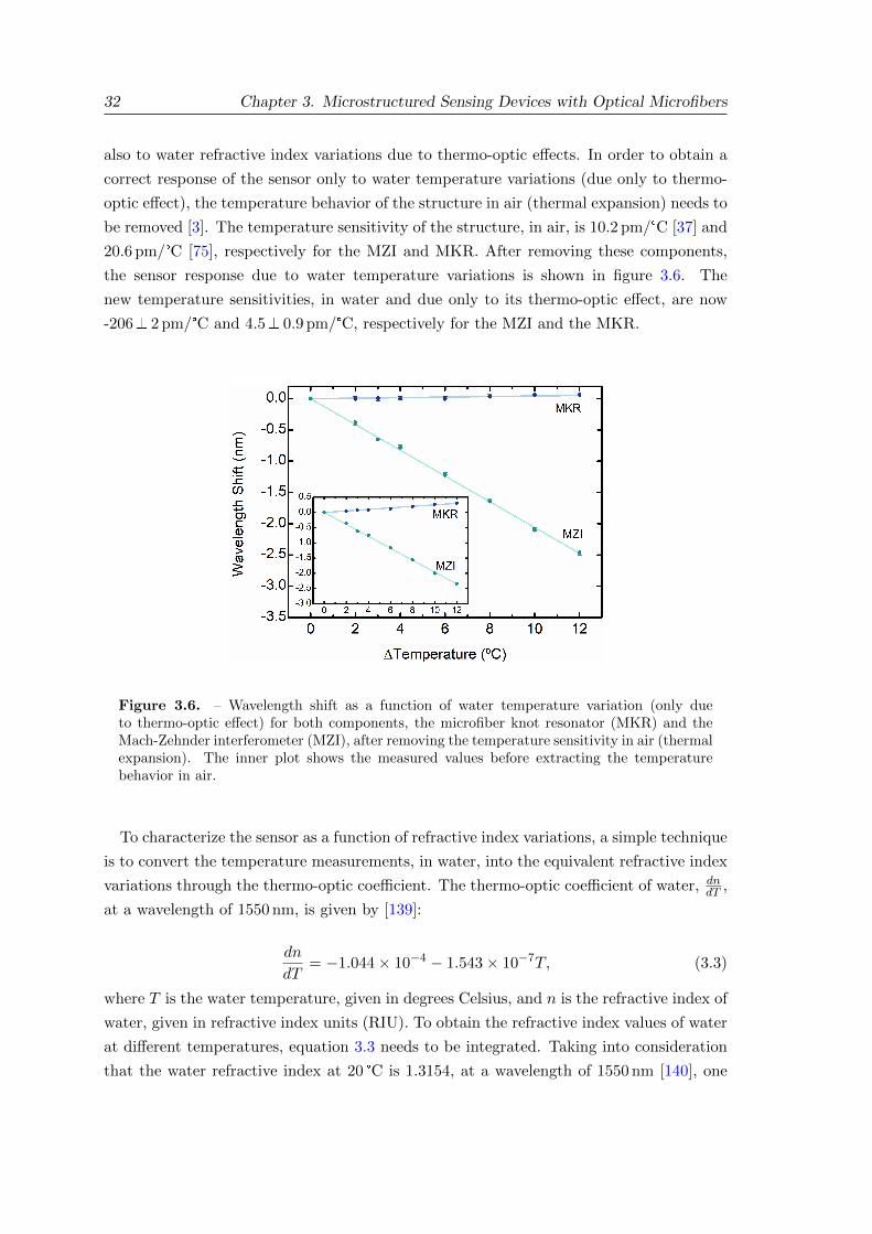
32 Chapter 3. Microstructured Sensing Devices with Optical Microfibers
also to water refractive index variations due to thermo-optic effects. In order to obtain a
correct response of the sensor only to water temperature variations (due only to thermo-
optic effect), the temperature behavior of the structure in air (thermal expansion) needs to
be removed [3]. The temperature sensitivity of the structure, in air, is 10.2 pm/°C [37] and
20.6 pm/°C [75], respectively for the MZI and MKR. After removing these components,
the sensor response due to water temperature variations is shown in figure 3.6. The
new temperature sensitivities, in water and due only to its thermo-optic effect, are now
-206± 2 pm/°C and 4.5± 0.9 pm/°C, respectively for the MZI and the MKR.
Figure 3.6. – Wavelength shift as a function of water temperature variation (only dueto thermo-optic effect) for both components, the microfiber knot resonator (MKR) and theMach-Zehnder interferometer (MZI), after removing the temperature sensitivity in air (thermalexpansion). The inner plot shows the measured values before extracting the temperaturebehavior in air.
To characterize the sensor as a function of refractive index variations, a simple technique
is to convert the temperature measurements, in water, into the equivalent refractive index
variations through the thermo-optic coefficient. The thermo-optic coefficient of water, dndT ,
at a wavelength of 1550 nm, is given by [139]:
dn
dT= −1.044× 10⁻⁴ − 1.543× 10⁻⁷T, (3.3)
where T is the water temperature, given in degrees Celsius, and n is the refractive index of
water, given in refractive index units (RIU). To obtain the refractive index values of water
at different temperatures, equation 3.3 needs to be integrated. Taking into consideration
that the water refractive index at 20 °C is 1.3154, at a wavelength of 1550 nm [140], one
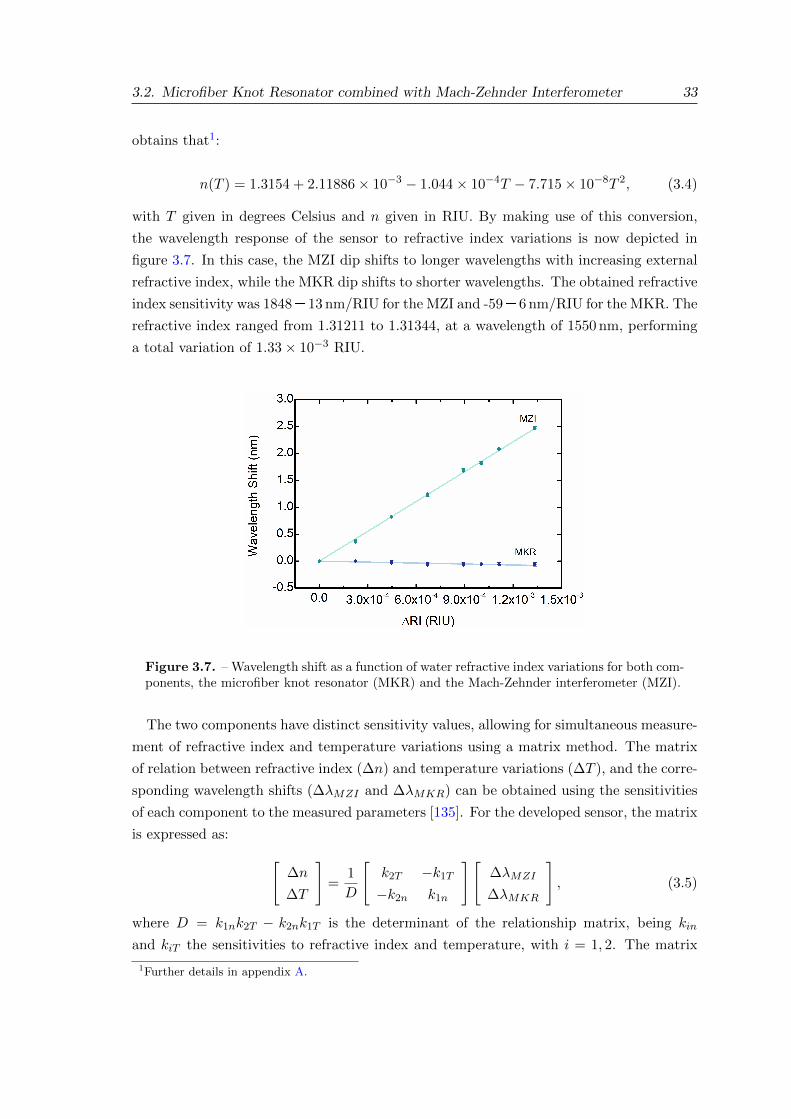
3.2. Microfiber Knot Resonator combined with Mach-Zehnder Interferometer 33
obtains that1:
n(T ) = 1.3154 + 2.11886× 10⁻³ − 1.044× 10⁻⁴T − 7.715× 10⁻⁸T 2, (3.4)
with T given in degrees Celsius and n given in RIU. By making use of this conversion,
the wavelength response of the sensor to refractive index variations is now depicted in
figure 3.7. In this case, the MZI dip shifts to longer wavelengths with increasing external
refractive index, while the MKR dip shifts to shorter wavelengths. The obtained refractive
index sensitivity was 1848± 13 nm/RIU for the MZI and -59± 6 nm/RIU for the MKR. The
refractive index ranged from 1.31211 to 1.31344, at a wavelength of 1550 nm, performing
a total variation of 1.33× 10⁻³ RIU.
Figure 3.7. – Wavelength shift as a function of water refractive index variations for both com-ponents, the microfiber knot resonator (MKR) and the Mach-Zehnder interferometer (MZI).
The two components have distinct sensitivity values, allowing for simultaneous measure-
ment of refractive index and temperature variations using a matrix method. The matrix
of relation between refractive index (∆n) and temperature variations (∆T ), and the corre-
sponding wavelength shifts (∆λMZI and ∆λMKR) can be obtained using the sensitivities
of each component to the measured parameters [135]. For the developed sensor, the matrix
is expressed as: [∆n
∆T
]=
1
D
[k2T −k1T−k2n k1n
][∆λMZI
∆λMKR
], (3.5)
where D = k1nk2T − k2nk1T is the determinant of the relationship matrix, being kin
and kiT the sensitivities to refractive index and temperature, with i = 1, 2. The matrix
1Further details in appendix A.
34 Chapter 3. Microstructured Sensing Devices with Optical Microfibers
method works well when the components have distinct sensitivity values, as long as the
matrix determinant, D, is large. A small value of D introduces significant errors and low
accuracy. Replacing the sensitivity values of the MZI and the MKR in equation 3.5, the
matrix can be expressed as:[∆n
∆T
]= 0.0267
[0.0206 −0.0102
59 1848
][∆λMZI
∆λMKR
], (3.6)
where ∆λMZI and ∆λMKR are given in nanometers. The obtained refractive index and
temperature variations are given in RIU and in degrees Celsius, respectively. The matrix
method presents a standard deviation (σ) of 3×10⁻⁵ RIU and 0.1 °C in the determination
of the resulting refractive index and temperature variations, respectively.
3.2.3. Discussion
In this section, a new compact sensing structure was presented, combining two distinct
optical interferometers into a single device: a microfiber knot resonator and a slightly
abrupt taper-based Mach-Zehnder interferometer. The structure was fabricated only via
post-processing with a CO2 laser. The sensor presents two distinct spectral components,
characteristic from the MZI and the MKR, that respond differently to temperature and
refractive index variations. Both components could be separated by applying FFT filters,
making it easier to monitor each response separately. The MZI component has higher
sensitivity to refractive index than the MKR component, mainly because it relies on the
difference between the effective refractive indices of the two main modes (the LP01 and
the LP02).
The device can be used to simultaneously measure temperature and refractive index
variations. Hence, the influence of temperature in the refractive index measurement can
be compensated, as initially targeted. Moreover, the proposed sensor is more compact and
stable than similar reported structures [84,85], since the MZI relies on a single taper struc-
ture and not on a second microfiber connected through Van-der-Waals forces. Structures
like [84,85], which use coupling between two microfibers, can be very fragile and unstable.
On the other hand, the proposed structure might have some issues while immersing in
water (or removing). During this process, the surface tension of water can change the
diameter of the MKR, or even break the microfiber. Hence in the future, it is important
to explore the possibility of coating the structure with a thin protective layer of a low
refractive index polymer. Such coatings increase the stability of the structure and avoid
modifications in its dimensions. Moreover, this type of coatings might have low impact on
the performance of the sensor, as its refractive index is lower than silica. Therefore, the
modes of the structure are preserved. However, one should not forget that the coating is a
small barrier between the propagating modes and the external environment, which might
3.3. FIB-Structured Multimode Fiber Probe 35
result in a slightly lower refractive index sensitivity.
3.3. FIB-Structured Multimode Fiber Probe
The use of a microfiber sensing device in a transmission configuration, as the one demon-
strated before, is less practical or inconvenient for applications that require local mea-
surements (point measurements). For instance, some biological and medical applications
require point measurements combined with minimally invasive sensors, especially for in-
vivo operation. Therefore, the current tendency is towards developing miniaturized sensors
capable of measuring physical, chemical, and biochemical parameters. A microfiber probe
(half of a microfiber) could be used for such applications instead of a complete microfiber.
Then, a sensing structure can be added to the microfiber probe via post-processing. A
useful sensing structure suitable to be adapted to a microfiber probe and interrogated in
a reflection configuration is the Fabry-Perot interferometer (FPI).
Microfabrication with a focused ion beam is an interesting approach to form FPIs in
microfiber probes. This technique has the advantage of creating small sensing structures
in thin microfiber probes, which can be smaller than a single cell. Examples of air and
silica FPIs in microfiber probes were demonstrated in 2016 [3]. One year later, ultra-short
FPI cavities milled in microfiber probes were also proved to be feasible and applicable
as miniaturized sensing devices [4]. For temperature sensing, conventional silica FPIs are
limited by the thermo-optic coefficient of silica, and to a lesser degree by the thermal
expansion coefficient. Typically, the temperature sensitivity values for those structures
range from 10 pm/°C to around 20 pm/°C [3, 90, 141, 142]. Polymers started to be imple-
mented to partially solve this issue of limited sensitivity. Polymer FPIs can attain one
order of magnitude higher temperature sensitivities due to their high thermal expansion
coefficient [143, 144]. Yet, their use is also limited to temperatures below the melting
point of the polymer. Apart from the use of polymeric structures, other possibilities to
surpass the sensitivity limitations were studied, including the application of other effects
beyond the normal FPI. Multimode interference [145] or non-linear responses [143, 145]
are examples of that.
In this section, the improvement of a focused ion beam-milled FPI in a microfiber probe
is explored for temperature sensing. For this purpose, the usual SMF used to fabricate the
microfiber was replaced by a multimode fiber (MMF). Thus, multiple propagating modes
are present in the structure, generating different FPI responses. The interference between
the FPI responses gives raise to a low-frequency envelope modulation, which mainly de-
pends on the refractive index differences between the propagating modes. Consequently,
one should expect such component to achieve higher sensitivity as it depends on an optical
path difference, similarly to the MZI demonstrated in the last section.
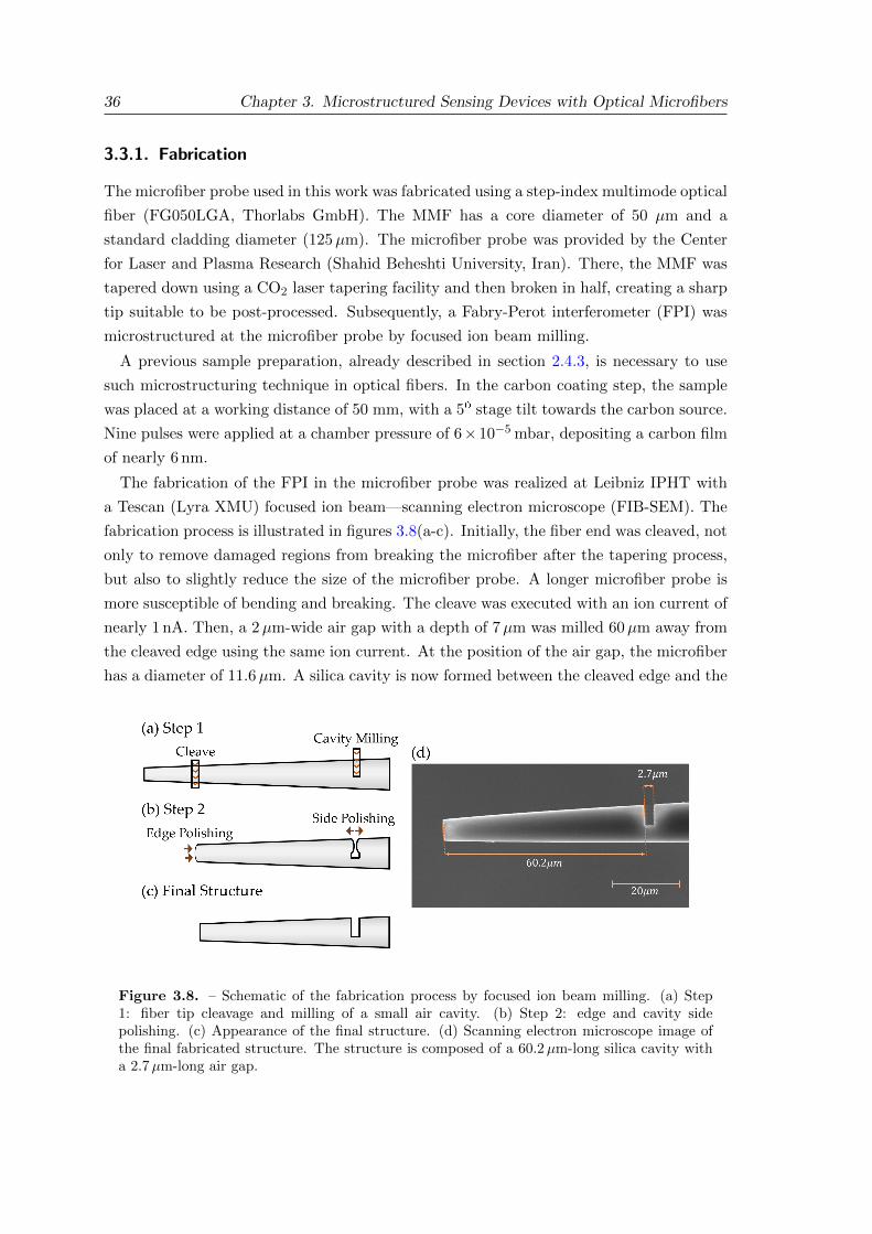
36 Chapter 3. Microstructured Sensing Devices with Optical Microfibers
3.3.1. Fabrication
The microfiber probe used in this work was fabricated using a step-index multimode optical
fiber (FG050LGA, Thorlabs GmbH). The MMF has a core diameter of 50 µm and a
standard cladding diameter (125µm). The microfiber probe was provided by the Center
for Laser and Plasma Research (Shahid Beheshti University, Iran). There, the MMF was
tapered down using a CO2 laser tapering facility and then broken in half, creating a sharp
tip suitable to be post-processed. Subsequently, a Fabry-Perot interferometer (FPI) was
microstructured at the microfiber probe by focused ion beam milling.
A previous sample preparation, already described in section 2.4.3, is necessary to use
such microstructuring technique in optical fibers. In the carbon coating step, the sample
was placed at a working distance of 50 mm, with a 5º stage tilt towards the carbon source.
Nine pulses were applied at a chamber pressure of 6×10⁻⁵ mbar, depositing a carbon film
of nearly 6 nm.
The fabrication of the FPI in the microfiber probe was realized at Leibniz IPHT with
a Tescan (Lyra XMU) focused ion beam—scanning electron microscope (FIB-SEM). The
fabrication process is illustrated in figures 3.8(a-c). Initially, the fiber end was cleaved, not
only to remove damaged regions from breaking the microfiber after the tapering process,
but also to slightly reduce the size of the microfiber probe. A longer microfiber probe is
more susceptible of bending and breaking. The cleave was executed with an ion current of
nearly 1 nA. Then, a 2µm-wide air gap with a depth of 7µm was milled 60µm away from
the cleaved edge using the same ion current. At the position of the air gap, the microfiber
has a diameter of 11.6µm. A silica cavity is now formed between the cleaved edge and the
Figure 3.8. – Schematic of the fabrication process by focused ion beam milling. (a) Step1: fiber tip cleavage and milling of a small air cavity. (b) Step 2: edge and cavity sidepolishing. (c) Appearance of the final structure. (d) Scanning electron microscope image ofthe final fabricated structure. The structure is composed of a 60.2µm-long silica cavity witha 2.7µm-long air gap.
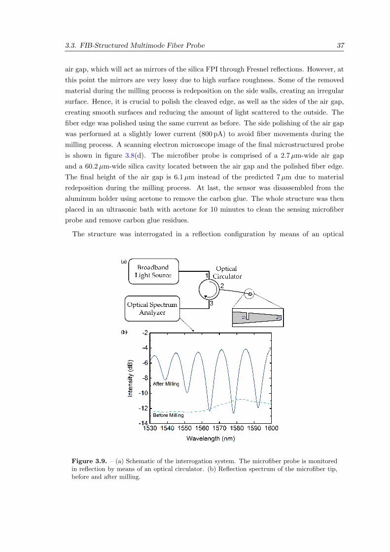
3.3. FIB-Structured Multimode Fiber Probe 37
air gap, which will act as mirrors of the silica FPI through Fresnel reflections. However, at
this point the mirrors are very lossy due to high surface roughness. Some of the removed
material during the milling process is redeposition on the side walls, creating an irregular
surface. Hence, it is crucial to polish the cleaved edge, as well as the sides of the air gap,
creating smooth surfaces and reducing the amount of light scattered to the outside. The
fiber edge was polished using the same current as before. The side polishing of the air gap
was performed at a slightly lower current (800 pA) to avoid fiber movements during the
milling process. A scanning electron microscope image of the final microstructured probe
is shown in figure 3.8(d). The microfiber probe is comprised of a 2.7µm-wide air gap
and a 60.2µm-wide silica cavity located between the air gap and the polished fiber edge.
The final height of the air gap is 6.1µm instead of the predicted 7µm due to material
redeposition during the milling process. At last, the sensor was disassembled from the
aluminum holder using acetone to remove the carbon glue. The whole structure was then
placed in an ultrasonic bath with acetone for 10 minutes to clean the sensing microfiber
probe and remove carbon glue residues.
The structure was interrogated in a reflection configuration by means of an optical
Figure 3.9. – (a) Schematic of the interrogation system. The microfiber probe is monitoredin reflection by means of an optical circulator. (b) Reflection spectrum of the microfiber tip,before and after milling.
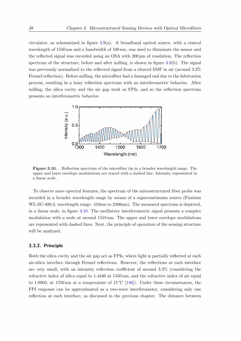
38 Chapter 3. Microstructured Sensing Devices with Optical Microfibers
circulator, as schematized in figure 3.9(a). A broadband optical source, with a central
wavelength of 1550 nm and a bandwidth of 100 nm, was used to illuminate the sensor and
the reflected signal was recorded using an OSA with 200 pm of resolution. The reflection
spectrum of the structure, before and after milling, is shown in figure 3.9(b). The signal
was previously normalized to the reflected signal from a cleaved SMF in air (around 3.3%
Fresnel reflection). Before milling, the microfiber had a damaged end due to the fabrication
process, resulting in a lossy reflection spectrum with no interferometric behavior. After
milling, the silica cavity and the air gap work as FPIs, and so the reflection spectrum
presents an interferometric behavior.
Figure 3.10. – Reflection spectrum of the microfiber tip in a broader wavelength range. Theupper and lower envelope modulations are traced with a dashed line. Intensity represented ina linear scale.
To observe more spectral features, the spectrum of the microstructured fiber probe was
recorded in a broader wavelength range by means of a supercontinuum source (Fianium
WL-SC-400-2, wavelength range: 410nm to 2400nm). The measured spectrum is depicted,
in a linear scale, in figure 3.10. The oscillatory interferometric signal presents a complex
modulation with a node at around 1518 nm. The upper and lower envelope modulations
are represented with dashed lines. Next, the principle of operation of the sensing structure
will be analyzed.
3.3.2. Principle
Both the silica cavity and the air gap act as FPIs, where light is partially reflected at each
air-silica interface through Fresnel reflections. However, the reflections at each interface
are very small, with an intensity reflection coefficient of around 3.3% (considering the
refractive index of silica equal to 1.4440 at 1550 nm, and the refractive index of air equal
to 1.0003, at 1550 nm at a temperature of 15 °C [146]). Under these circumstances, the
FPI response can be approximated as a two-wave interferometer, considering only one
reflection at each interface, as discussed in the previous chapter. The distance between
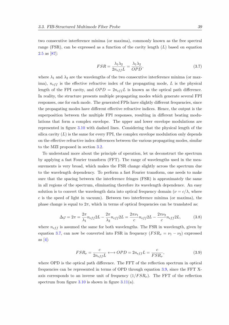
3.3. FIB-Structured Multimode Fiber Probe 39
two consecutive interference minima (or maxima), commonly known as the free spectral
range (FSR), can be expressed as a function of the cavity length (L) based on equation
2.5 as [87]:
FSR =λ1λ2
2neffL=
λ1λ2OPD
, (3.7)
where λ1 and λ2 are the wavelengths of the two consecutive interference minima (or max-
ima), neff is the effective refractive index of the propagating mode, L is the physical
length of the FPI cavity, and OPD = 2neffL is known as the optical path difference.
In reality, the structure presents multiple propagating modes which generate several FPI
responses, one for each mode. The generated FPIs have slightly different frequencies, since
the propagating modes have different effective refractive indices. Hence, the output is the
superposition between the multiple FPI responses, resulting in different beating modu-
lations that form a complex envelope. The upper and lower envelope modulations are
represented in figure 3.10 with dashed lines. Considering that the physical length of the
silica cavity (L) is the same for every FPI, the complex envelope modulation only depends
on the effective refractive index differences between the various propagating modes, similar
to the MZI proposed in section 3.2.
To understand more about the principle of operation, let us deconstruct the spectrum
by applying a fast Fourier transform (FFT). The range of wavelengths used in the mea-
surements is very broad, which makes the FSR change slightly across the spectrum due
to the wavelength dependency. To perform a fast Fourier transform, one needs to make
sure that the spacing between the interference fringes (FSR) is approximately the same
in all regions of the spectrum, eliminating therefore its wavelength dependence. An easy
solution is to convert the wavelength data into optical frequency domain (ν = c/λ, where
c is the speed of light in vacuum). Between two interference minima (or maxima), the
phase change is equal to 2π, which in terms of optical frequencies can be translated as:
∆ϕ = 2π =2π
λ1neff2L− 2π
λ2neff2L =
2πν1c
neff2L− 2πν2c
neff2L, (3.8)
where neff is assumed the same for both wavelengths. The FSR in wavelength, given by
equation 3.7, can now be converted into FSR in frequency (FSRν = ν1 − ν2) expressed
as [4]:
FSRν =c
2neffL←→ OPD = 2neffL =
c
FSRν, (3.9)
where OPD is the optical path difference. The FFT of the reflection spectrum in optical
frequencies can be represented in terms of OPD through equation 3.9, since the FFT X-
axis corresponds to an inverse unit of frequency (1/FSRν). The FFT of the reflection
spectrum from figure 3.10 is shown in figure 3.11(a).
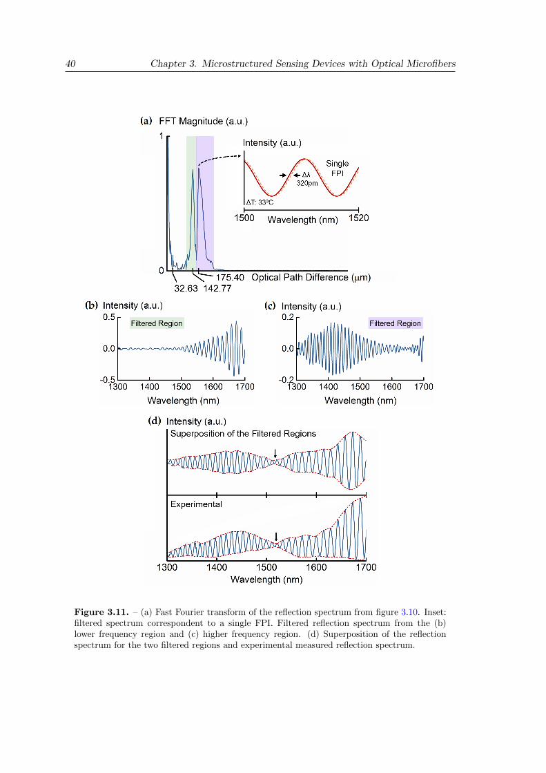
40 Chapter 3. Microstructured Sensing Devices with Optical Microfibers
Figure 3.11. – (a) Fast Fourier transform of the reflection spectrum from figure 3.10. Inset:filtered spectrum correspondent to a single FPI. Filtered reflection spectrum from the (b)lower frequency region and (c) higher frequency region. (d) Superposition of the reflectionspectrum for the two filtered regions and experimental measured reflection spectrum.
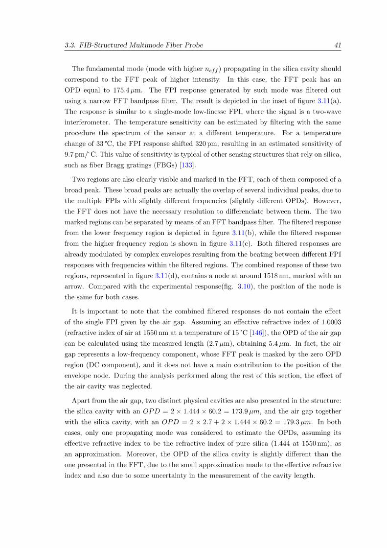
3.3. FIB-Structured Multimode Fiber Probe 41
The fundamental mode (mode with higher neff ) propagating in the silica cavity should
correspond to the FFT peak of higher intensity. In this case, the FFT peak has an
OPD equal to 175.4µm. The FPI response generated by such mode was filtered out
using a narrow FFT bandpass filter. The result is depicted in the inset of figure 3.11(a).
The response is similar to a single-mode low-finesse FPI, where the signal is a two-wave
interferometer. The temperature sensitivity can be estimated by filtering with the same
procedure the spectrum of the sensor at a different temperature. For a temperature
change of 33 °C, the FPI response shifted 320 pm, resulting in an estimated sensitivity of
9.7 pm/°C. This value of sensitivity is typical of other sensing structures that rely on silica,
such as fiber Bragg gratings (FBGs) [133].
Two regions are also clearly visible and marked in the FFT, each of them composed of a
broad peak. These broad peaks are actually the overlap of several individual peaks, due to
the multiple FPIs with slightly different frequencies (slightly different OPDs). However,
the FFT does not have the necessary resolution to differenciate between them. The two
marked regions can be separated by means of an FFT bandpass filter. The filtered response
from the lower frequency region is depicted in figure 3.11(b), while the filtered response
from the higher frequency region is shown in figure 3.11(c). Both filtered responses are
already modulated by complex envelopes resulting from the beating between different FPI
responses with frequencies within the filtered regions. The combined response of these two
regions, represented in figure 3.11(d), contains a node at around 1518 nm, marked with an
arrow. Compared with the experimental response(fig. 3.10), the position of the node is
the same for both cases.
It is important to note that the combined filtered responses do not contain the effect
of the single FPI given by the air gap. Assuming an effective refractive index of 1.0003
(refractive index of air at 1550 nm at a temperature of 15 °C [146]), the OPD of the air gap
can be calculated using the measured length (2.7µm), obtaining 5.4µm. In fact, the air
gap represents a low-frequency component, whose FFT peak is masked by the zero OPD
region (DC component), and it does not have a main contribution to the position of the
envelope node. During the analysis performed along the rest of this section, the effect of
the air cavity was neglected.
Apart from the air gap, two distinct physical cavities are also presented in the structure:
the silica cavity with an OPD = 2 × 1.444 × 60.2 = 173.9µm, and the air gap together
with the silica cavity, with an OPD = 2 × 2.7 + 2 × 1.444 × 60.2 = 179.3µm. In both
cases, only one propagating mode was considered to estimate the OPDs, assuming its
effective refractive index to be the refractive index of pure silica (1.444 at 1550 nm), as
an approximation. Moreover, the OPD of the silica cavity is slightly different than the
one presented in the FFT, due to the small approximation made to the effective refractive
index and also due to some uncertainty in the measurement of the cavity length.

42 Chapter 3. Microstructured Sensing Devices with Optical Microfibers
3.3.3. Temperature Characterization
To evaluate the improvement of sensitivity provided by the modulating envelope, the
sensing probe was characterized in terms of temperature. The probe was submitted to
different temperatures in air, ranging from 30 °C to 120 °C, using a tubular oven (Strohlein
Instruments). Then, the envelope shift was determined by tracking the position of the
node, located at 1518 nm, as a function of temperature. To obtain a more accurate value
for the position of the node, the average between the local minimum of the upper envelope
and the local maximum of the lower envelope was taken.
Figure 3.12. – (a) Reflection spectrum at two distinct temperatures. The position of theenvelope node, marked with an arrow, was monitored during the experiment. (b) Wavelengthshift of the envelope node as a function of temperature. The slope corresponds to a temperaturesensitivity of (=654± 19) pm/°C.
Figure 3.12(a) shows the reflection spectrum of the sensing probe at two distinct temper-
atures: 33 °C and 52 °C. The position of the node is marked with an arrow. The position
of the envelope node shifts towards shorter wavelengths with increasing temperature. The
full temperature characterization curve is depicted in figure 3.12(b). The temperature
sensitivity of the envelope is determined through a linear fit applied to the wavelength
shift of the node as a function of temperature. By means of this, a temperature sensitivity
of (=654± 19) pm/°C was achieved for the envelope modulation.
The stability of the sensing structure was also evaluated. Ten consecutive measurements
were performed at two different temperatures, 89.54 °C and 94.51 °C, in order to determine
the sensor resolution. To perform such kind of measurements, it is crucial to ensure a good
thermal stability, maintaining the same temperature along the measurements. Therefore,
the sensing probe was placed inside an aluminum box, and the whole set was installed inside
a Carbolite oven with high volumetric capacity. The aluminum box partially attenuates the
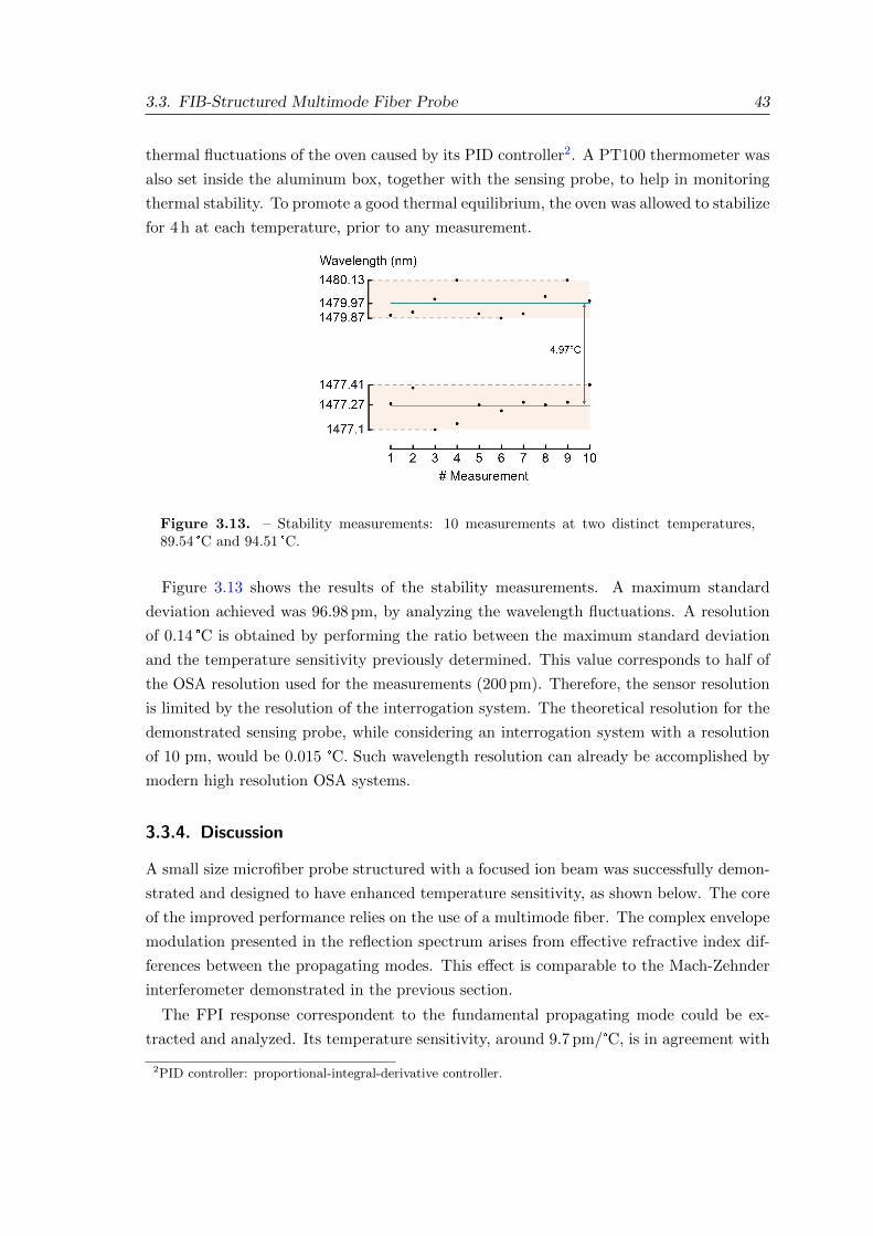
3.3. FIB-Structured Multimode Fiber Probe 43
thermal fluctuations of the oven caused by its PID controller2. A PT100 thermometer was
also set inside the aluminum box, together with the sensing probe, to help in monitoring
thermal stability. To promote a good thermal equilibrium, the oven was allowed to stabilize
for 4 h at each temperature, prior to any measurement.
Figure 3.13. – Stability measurements: 10 measurements at two distinct temperatures,89.54 °C and 94.51 °C.
Figure 3.13 shows the results of the stability measurements. A maximum standard
deviation achieved was 96.98 pm, by analyzing the wavelength fluctuations. A resolution
of 0.14 °C is obtained by performing the ratio between the maximum standard deviation
and the temperature sensitivity previously determined. This value corresponds to half of
the OSA resolution used for the measurements (200 pm). Therefore, the sensor resolution
is limited by the resolution of the interrogation system. The theoretical resolution for the
demonstrated sensing probe, while considering an interrogation system with a resolution
of 10 pm, would be 0.015 °C. Such wavelength resolution can already be accomplished by
modern high resolution OSA systems.
3.3.4. Discussion
A small size microfiber probe structured with a focused ion beam was successfully demon-
strated and designed to have enhanced temperature sensitivity, as shown below. The core
of the improved performance relies on the use of a multimode fiber. The complex envelope
modulation presented in the reflection spectrum arises from effective refractive index dif-
ferences between the propagating modes. This effect is comparable to the Mach-Zehnder
interferometer demonstrated in the previous section.
The FPI response correspondent to the fundamental propagating mode could be ex-
tracted and analyzed. Its temperature sensitivity, around 9.7 pm/°C, is in agreement with
2PID controller: proportional-integral-derivative controller.
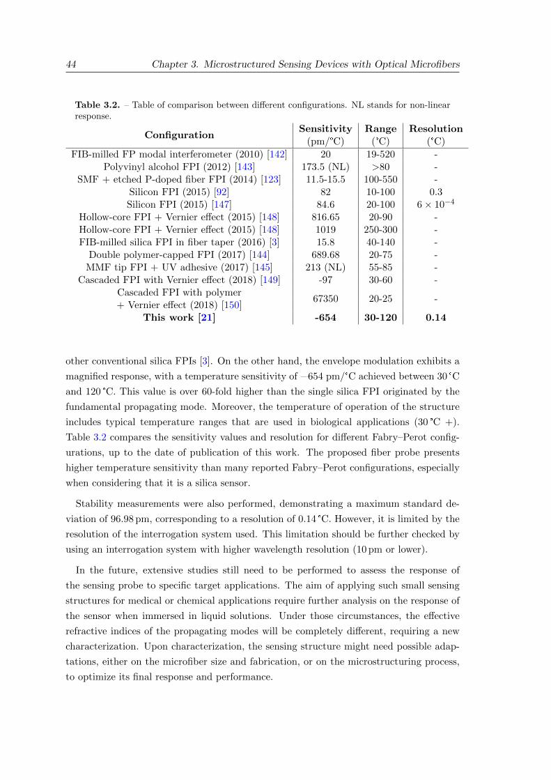
44 Chapter 3. Microstructured Sensing Devices with Optical Microfibers
Table 3.2. – Table of comparison between different configurations. NL stands for non-linearresponse.
ConfigurationSensitivity Range Resolution
(pm/°C) (°C) (°C)
FIB-milled FP modal interferometer (2010) [142] 20 19-520 -Polyvinyl alcohol FPI (2012) [143] 173.5 (NL) >80 -
SMF + etched P-doped fiber FPI (2014) [123] 11.5-15.5 100-550 -Silicon FPI (2015) [92] 82 10-100 0.3Silicon FPI (2015) [147] 84.6 20-100 6× 10⁻⁴
Hollow-core FPI + Vernier effect (2015) [148] 816.65 20-90 -Hollow-core FPI + Vernier effect (2015) [148] 1019 250-300 -FIB-milled silica FPI in fiber taper (2016) [3] 15.8 40-140 -
Double polymer-capped FPI (2017) [144] 689.68 20-75 -MMF tip FPI + UV adhesive (2017) [145] 213 (NL) 55-85 -
Cascaded FPI with Vernier effect (2018) [149] -97 30-60 -Cascaded FPI with polymer
67350 20-25 -+ Vernier effect (2018) [150]
This work [21] -654 30-120 0.14
other conventional silica FPIs [3]. On the other hand, the envelope modulation exhibits a
magnified response, with a temperature sensitivity of =654 pm/°C achieved between 30 °C
and 120 °C. This value is over 60-fold higher than the single silica FPI originated by the
fundamental propagating mode. Moreover, the temperature of operation of the structure
includes typical temperature ranges that are used in biological applications (30 °C +).
Table 3.2 compares the sensitivity values and resolution for different Fabry–Perot config-
urations, up to the date of publication of this work. The proposed fiber probe presents
higher temperature sensitivity than many reported Fabry–Perot configurations, especially
when considering that it is a silica sensor.
Stability measurements were also performed, demonstrating a maximum standard de-
viation of 96.98 pm, corresponding to a resolution of 0.14 °C. However, it is limited by the
resolution of the interrogation system used. This limitation should be further checked by
using an interrogation system with higher wavelength resolution (10 pm or lower).
In the future, extensive studies still need to be performed to assess the response of
the sensing probe to specific target applications. The aim of applying such small sensing
structures for medical or chemical applications require further analysis on the response of
the sensor when immersed in liquid solutions. Under those circumstances, the effective
refractive indices of the propagating modes will be completely different, requiring a new
characterization. Upon characterization, the sensing structure might need possible adap-
tations, either on the microfiber size and fabrication, or on the microstructuring process,
to optimize its final response and performance.
3.4. Conclusion 45
3.4. Conclusion
The aim of this chapter was to develop microstructured devices based on optical microfibers
with enhanced sensing capabilities. The first work tackled the problem of cross-sensitivity
in optical fiber sensing, especially targeting the influence of temperature variations. Here,
the microfiber was fabricated with abrupt transitions regions, generating a Mach-Zehnder
interferometer, and then tied up forming a microfiber knot resonator. Merging both sens-
ing configurations, the Mach-Zehnder interferometer and the microfiber knot resonator,
enabled simultaneous measurement of refractive index and temperature. Additionally, the
Mach-Zehnder interferometer achieved higher sensitivities than the microfiber knot res-
onator. This effect is mainly due to its dependence on the difference between the effective
refractive indices of the two main propagating modes in the microfiber.
The objective of the second work was to make use of focused ion beam milling to struc-
ture the microfiber into a small sensing probe. In this context, a Fabry-Perot interferom-
eter was milled with this technique in a microfiber probe, showing improved temperature
sensing. The enhancement, similarly to the Mach-Zehnder interferometer of the first work,
is based on differences between effective refractive indices of the propagating modes.
Until now, the presented sensing structures are high quality micro-interferometers in
fiber, providing mostly the expected typical sensitivity. However, the cases here explored
also indicate the possibility of using different modes to increase the sensitivity, through
an envelope modulation. From a different perspective, this enhancement of the envelope
wavelength shift can be interpreted as the Vernier effect. In the optical domain, the
Vernier effect consists of the superposition of two interferometric signals with slightly
shifted frequencies, originating a beating envelope with interesting properties. One of them
is the magnification of the spectral shift of the envelope, when compared with the normal
shift of the single interferometer. As seen before, the frequency of the different Fabry-Perot
interferometers in the microfiber probe is directly related with the effective refractive index
of each propagating mode, through equation 3.9. Note that the structure does not have
only two interferometers with slightly different interferometric frequencies, but as many
as the number of propagating modes. Hence, the generated Vernier beating envelope is
rather complex. Moreover, in this current form the Vernier effect is uncontrollable, since
one does not have control over the modes propagating in the structure. The next chapter
explores the optical Vernier effect from an optical fiber sensing perspective, and especially
how to apply it to maximize its enhancement effects in a controllable way.

Chapter 4.
Optical Vernier Effect in Fiber
Interferometers
4.1. Introduction
The use of a secondary scale in measuring equipment and instruments, such as calipers
and ancient astronomical quadrants, allows to increase the resolution and reduce the un-
certainty of measurements. The caliper was invented in 1631 by Pierre Vernier [151].
Some people name such instrument after his inventor as the “Vernier caliper”, where the
two scales overlapping each other are referred as the Vernier scale. Eventually, Pierre
Vernier may have been inspired by a portuguese measuring tool of the 16th century called
- the Nonius. The Nonius, created in 1542 by the mathematician and cosmographer Pedro
Nunes, was a tool used to perform finer measurements on circular instruments, improving
the angular measurements of devices like the astrolabe [152].
In the field of optical fibers, the Vernier effect (or the Vernier principle) also left his
mark. In 1988, Paul Urquhart was studying and designing compound resonators in opti-
cal fibers for application in fiber lasers and optical communications systems [153]. In his
work, Urquhart used the Vernier principle by combining optical fiber rings with unequal
lengths in parallel. In his configuration, the Vernier effect acted as a mechanism to sup-
press spectral modes (suppression of resonance peaks in the spectrum) and to narrow the
linewidth of fiber lasers. Moreover, adaptations of the Vernier effect in the fields of optics
also led to the development of the optical frequency comb technique, which gave the Nobel
Prize in Physics to John Hall and Theodor Hansch [154, 155]. Such technique is widely
used in Vernier spectroscopy [156].
The fast development in many research fields that make use of optical fibers, together
with the specific technical challenges in their use, places strong pressure and new challenges
in the fields of optical fiber sensing research. The demand for sensing structures able to
achieve higher sensitivities and resolutions than what conventional fiber sensors can offer
is increasing. With this, researchers are driven to find new options for improved optical
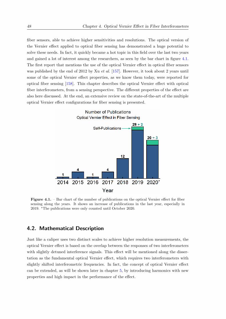
48 Chapter 4. Optical Vernier Effect in Fiber Interferometers
fiber sensors, able to achieve higher sensitivities and resolutions. The optical version of
the Vernier effect applied to optical fiber sensing has demonstrated a huge potential to
solve these needs. In fact, it quickly became a hot topic in this field over the last two years
and gained a lot of interest among the researchers, as seen by the bar chart in figure 4.1.
The first report that mentions the use of the optical Vernier effect in optical fiber sensors
was published by the end of 2012 by Xu et al. [157]. However, it took about 2 years until
some of the optical Vernier effect properties, as we know them today, were reported for
optical fiber sensing [158]. This chapter describes the optical Vernier effect with optical
fiber interferometers, from a sensing perspective. The different properties of the effect are
also here discussed. At the end, an extensive review on the state-of-the-art of the multiple
optical Vernier effect configurations for fiber sensing is presented.
Figure 4.1. – Bar chart of the number of publications on the optical Vernier effect for fibersensing along the years. It shows an increase of publications in the last year, especially in2019. ?The publications were only counted until October 2020.
4.2. Mathematical Description
Just like a caliper uses two distinct scales to achieve higher resolution measurements, the
optical Vernier effect is based on the overlap between the responses of two interferometers
with slightly detuned interference signals. This effect will be mentioned along the disser-
tation as the fundamental optical Vernier effect, which requires two interferometers with
slightly shifted interferometric frequencies. In fact, the concept of optical Vernier effect
can be extended, as will be shown later in chapter 5, by introducing harmonics with new
properties and high impact in the performance of the effect.
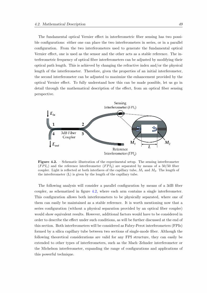
4.2. Mathematical Description 49
The fundamental optical Vernier effect in interferometric fiber sensing has two possi-
ble configurations: either one can place the two interferometers in series, or in a parallel
configuration. From the two interferometers used to generate the fundamental optical
Vernier effect, one is used as the sensor and the other acts as a stable reference. The in-
terferometric frequency of optical fiber interferometers can be adjusted by modifying their
optical path length. This is achieved by changing the refractive index and/or the physical
length of the interferometer. Therefore, given the properties of an initial interferometer,
the second interferometer can be adjusted to maximize the enhancement provided by the
optical Vernier effect. To fully understand how this can be made possible, let us go in
detail through the mathematical description of the effect, from an optical fiber sensing
perspective.
Figure 4.2. – Schematic illustration of the experimental setup. The sensing interferometer(FPI1) and the reference interferometer (FPI2) are separated by means of a 50/50 fibercoupler. Light is reflected at both interfaces of the capillary tube, M1 and M2. The length ofthe interferometer (L) is given by the length of the capillary tube.
The following analysis will consider a parallel configuration by means of a 3dB fiber
coupler, as schematized in figure 4.2, where each arm contains a single interferometer.
This configuration allows both interferometers to be physically separated, where one of
them can easily be maintained as a stable reference. It is worth mentioning now that a
series configuration (without a physical separation provided by an optical fiber coupler)
would show equivalent results. However, additional factors would have to be considered in
order to describe the effect under such conditions, as will be further discussed at the end of
this section. Both interferometers will be considered as Fabry-Perot interferometers (FPIs)
formed by a silica capillary tube between two sections of single-mode fiber. Although the
following theoretical considerations are valid for any FPI structure, they can easily be
extended to other types of interferometers, such as the Mach–Zehnder interferometer or
the Michelson interferometer, expanding the range of configurations and applications of
this powerful technique.
50 Chapter 4. Optical Vernier Effect in Fiber Interferometers
For simplification, the two FPIs are assumed to have identical interfaces, with an inten-
sity reflection coefficient R1 for the first mirror interface (M1) and R2 for the second mirror
interface (M2). In this case, all interfaces provide a silica/air Fresnel reflection. Note that
the reflection coefficient due to a silica/air Fresnel reflection is small (around 3.3% at 1550
nm), and hence, only one reflection at each interface was considered, corresponding to a
two-wave approximation. In this configuration, a coherent light source is injected at port 1
and split between the two arms (port 2 and 3) with equal intensity. The light reflected by
the system is collected and measured at port 4. The electric field of the input light, Ein,
propagating in the structure will be reflected at different points. In both interferometers,
the electric field of light reflected at the interface M1 is given by:
ER1 (λ) =√R1Ein (λ)√
2, (4.1)
while the electric field of light transmitted at the same interface is expressed as:
ET1 (λ) =√
(1−A1)√
(1−R1)Ein (λ)√
2, (4.2)
where A1 represents the transmission losses through interface M1, related to mode mis-
match and surface imperfections.
Light transmitted at interface M1, expressed by equation 4.2, will then travel through
the FPI, being partially reflected and transmitted at interface M2. The electric field of
light reflected at interface M2 of the sensing interferometer (FPI1) is expressed as:
E1R2 (λ) =
√(1−A1)
√(1−R1) exp (−αL1)
√R2Ein (λ)√
2exp
[−j(
2πn1L1
λ− π
)],
(4.3)
where exp (−αL1) represents the propagation losses up to interface M2 of the sensing
interferometer (FPI1), λ is the vacuum wavelength of the input light, n1 and L1 are
the effective refractive index and the length of the sensing interferometer (FPI1). The
factor 2πn1L1/λ − π corresponds to the phase accumulated in the propagation from the
interface M1 to the interface M2, with a reflection phase of π. This reflection phase arises
from the Fresnel reflection coefficient, which turns negative for incident light reflected at
the interface with a material of higher refractive index than the propagation medium.
Therefore, there is a phase difference of π between the incident and the reflected waves.
The reflected light, E1R2 (λ), will propagate back in the structure and get partially trans-
mitted at interface M1 towards the output, interfering with the light initially reflected at
that interface, described by equation 4.1. Hence, the electric field of the light coming from
the sensing interferometer, EFPI1 (λ), is given by:
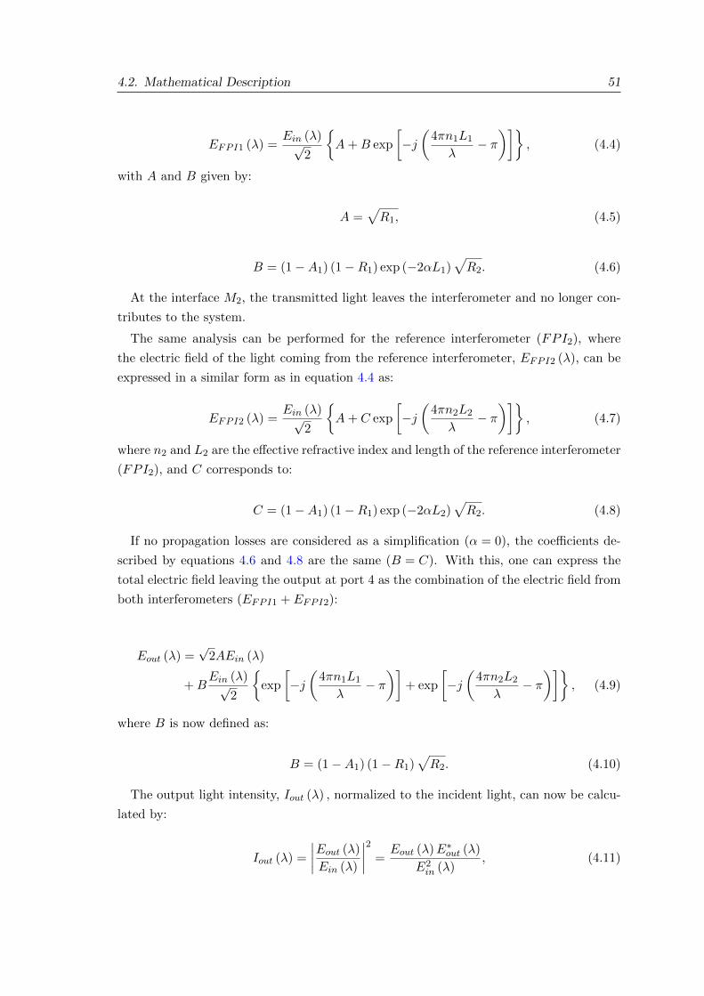
4.2. Mathematical Description 51
EFPI1 (λ) =Ein (λ)√
2
{A+B exp
[−j(
4πn1L1
λ− π
)]}, (4.4)
with A and B given by:
A =√R1, (4.5)
B = (1−A1) (1−R1) exp (−2αL1)√R2. (4.6)
At the interface M2, the transmitted light leaves the interferometer and no longer con-
tributes to the system.
The same analysis can be performed for the reference interferometer (FPI2), where
the electric field of the light coming from the reference interferometer, EFPI2 (λ), can be
expressed in a similar form as in equation 4.4 as:
EFPI2 (λ) =Ein (λ)√
2
{A+ C exp
[−j(
4πn2L2
λ− π
)]}, (4.7)
where n2 and L2 are the effective refractive index and length of the reference interferometer
(FPI2), and C corresponds to:
C = (1−A1) (1−R1) exp (−2αL2)√R2. (4.8)
If no propagation losses are considered as a simplification (α = 0), the coefficients de-
scribed by equations 4.6 and 4.8 are the same (B = C). With this, one can express the
total electric field leaving the output at port 4 as the combination of the electric field from
both interferometers (EFPI1 + EFPI2):
Eout (λ) =√
2AEin (λ)
+BEin (λ)√
2
{exp
[−j(
4πn1L1
λ− π
)]+ exp
[−j(
4πn2L2
λ− π
)]}, (4.9)
where B is now defined as:
B = (1−A1) (1−R1)√R2. (4.10)
The output light intensity, Iout (λ) , normalized to the incident light, can now be calcu-
lated by:
Iout (λ) =
∣∣∣∣Eout (λ)
Ein (λ)
∣∣∣∣2 =Eout (λ)E∗
out (λ)
E2in (λ)
, (4.11)
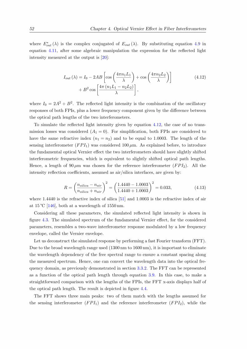
52 Chapter 4. Optical Vernier Effect in Fiber Interferometers
where E∗out (λ) is the complex conjugated of Eout (λ). By substituting equation 4.9 in
equation 4.11, after some algebraic manipulation the expression for the reflected light
intensity measured at the output is [20]:
Iout (λ) = I0 − 2AB
[cos
(4πn1L1
λ
)+ cos
(4πn2L2
λ
)](4.12)
+B2 cos
[4π (n1L1 − n2L2)
λ
],
where I0 = 2A2 + B2. The reflected light intensity is the combination of the oscillatory
responses of both FPIs, plus a lower frequency component given by the difference between
the optical path lengths of the two interferometers.
To simulate the reflected light intensity given by equation 4.12, the case of no trans-
mission losses was considered (A1 = 0). For simplification, both FPIs are considered to
have the same refractive index (n1 = n2) and to be equal to 1.0003. The length of the
sensing interferometer (FPI1) was considered 100µm. As explained before, to introduce
the fundamental optical Vernier effect the two interferometers should have slightly shifted
interferometric frequencies, which is equivalent to slightly shifted optical path lengths.
Hence, a length of 90µm was chosen for the reference interferometer (FPI2). All the
intensity reflection coefficients, assumed as air/silica interfaces, are given by:
R =
(nsilica − nairnsilica + nair
)2
=
(1.4440− 1.0003
1.4440 + 1.0003
)2
= 0.033, (4.13)
where 1.4440 is the refractive index of silica [51] and 1.0003 is the refractive index of air
at 15 °C [146], both at a wavelength of 1550 nm.
Considering all these parameters, the simulated reflected light intensity is shown in
figure 4.3. The simulated spectrum of the fundamental Vernier effect, for the considered
parameters, resembles a two-wave interferometer response modulated by a low frequency
envelope, called the Vernier envelope.
Let us deconstruct the simulated response by performing a fast Fourier transform (FFT).
Due to the broad wavelength range used (1300 nm to 1600 nm), it is important to eliminate
the wavelength dependency of the free spectral range to ensure a constant spacing along
the measured spectrum. Hence, one can convert the wavelength data into the optical fre-
quency domain, as previously demonstrated in section 3.3.2. The FFT can be represented
as a function of the optical path length through equation 3.9. In this case, to make a
straightforward comparison with the lengths of the FPIs, the FFT x-axis displays half of
the optical path length. The result is depicted in figure 4.4.
The FFT shows three main peaks: two of them match with the lengths assumed for
the sensing interferometer (FPI1) and the reference interferometer (FPI2), while the
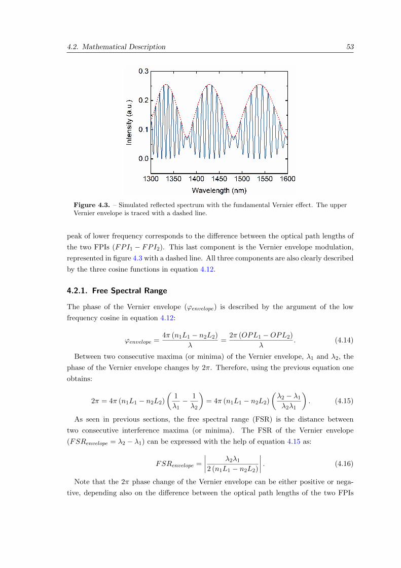
4.2. Mathematical Description 53
Figure 4.3. – Simulated reflected spectrum with the fundamental Vernier effect. The upperVernier envelope is traced with a dashed line.
peak of lower frequency corresponds to the difference between the optical path lengths of
the two FPIs (FPI1 − FPI2). This last component is the Vernier envelope modulation,
represented in figure 4.3 with a dashed line. All three components are also clearly described
by the three cosine functions in equation 4.12.
4.2.1. Free Spectral Range
The phase of the Vernier envelope (ϕenvelope) is described by the argument of the low
frequency cosine in equation 4.12:
ϕenvelope =4π (n1L1 − n2L2)
λ=
2π (OPL1 −OPL2)
λ. (4.14)
Between two consecutive maxima (or minima) of the Vernier envelope, λ1 and λ2, the
phase of the Vernier envelope changes by 2π. Therefore, using the previous equation one
obtains:
2π = 4π (n1L1 − n2L2)
(1
λ1− 1
λ2
)= 4π (n1L1 − n2L2)
(λ2 − λ1λ2λ1
). (4.15)
As seen in previous sections, the free spectral range (FSR) is the distance between
two consecutive interference maxima (or minima). The FSR of the Vernier envelope
(FSRenvelope = λ2 − λ1) can be expressed with the help of equation 4.15 as:
FSRenvelope =
∣∣∣∣ λ2λ12 (n1L1 − n2L2)
∣∣∣∣ . (4.16)
Note that the 2π phase change of the Vernier envelope can be either positive or nega-
tive, depending also on the difference between the optical path lengths of the two FPIs
54 Chapter 4. Optical Vernier Effect in Fiber Interferometers
Figure 4.4. – FFT of the simulated reflected spectrum from figure 4.3, expressed as a functionof half of the optical path length.
(n1L1 − n2L2). Regardless of the situation, the FSR should be always a positive value,
reason why the modulus was applied to equation 4.16.
The initial situation here presented, with two simple FPIs with similar characteristics,
led to a reflected light intensity (equation 4.12) where the phase of the envelope is clearly
visible in the equation. However, in more complex cases where both interferometers are
distinct, it is not always possible to deduce a simple equation for the measured intensity
that can be easily interpreted. Hence, the previous deduction of the Vernier envelope FSR
might not be trivial. Yet, there is a different way to obtain an expression for it.
The FSR of the Vernier envelope can also be described more generally by the relationship
between the FSRs of each individual interferometer. Let us consider the hypothetical
overlap between the responses of two FPIs with slightly shifted interferometric frequencies.
The individual spectral responses are shown in figure 4.5. The red curve corresponds to the
first interferometer, whose maxima are represented as λ1k, and the blue curve corresponds
to the second interferometer, with interference maxima described as λ2k, where k is the
number of the peak.
From observing figure 4.5, both interferometers are in phase at an initial wavelength
λm0 . The wavelength position of a maximum “k” can be expressed using the FSR of the
interferometer as:
λ1k = λ10 + kFSR1, (4.17)
for the first interferometer, and similarly as:
λ2k = λ20 + kFSR2, (4.18)
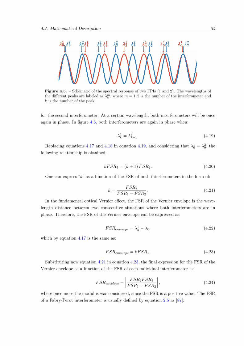
4.2. Mathematical Description 55
Figure 4.5. – Schematic of the spectral response of two FPIs (1 and 2). The wavelengths ofthe different peaks are labeled as λmk , where m = 1, 2 is the number of the interferometer andk is the number of the peak.
for the second interferometer. At a certain wavelength, both interferometers will be once
again in phase. In figure 4.5, both interferometers are again in phase when:
λ1k = λ2k+1. (4.19)
Replacing equations 4.17 and 4.18 in equation 4.19, and considering that λ10 = λ20, the
following relationship is obtained:
kFSR1 = (k + 1)FSR2. (4.20)
One can express “k” as a function of the FSR of both interferometers in the form of:
k =FSR2
FSR1 − FSR2. (4.21)
In the fundamental optical Vernier effect, the FSR of the Vernier envelope is the wave-
length distance between two consecutive situations where both interferometers are in
phase. Therefore, the FSR of the Vernier envelope can be expressed as:
FSRenvelope = λ1k − λ0, (4.22)
which by equation 4.17 is the same as:
FSRenvelope = kFSR1. (4.23)
Substituting now equation 4.21 in equation 4.23, the final expression for the FSR of the
Vernier envelope as a function of the FSR of each individual interferometer is:
FSRenvelope =
∣∣∣∣ FSR2FSR1
FSR1 − FSR2
∣∣∣∣ , (4.24)
where once more the modulus was considered, since the FSR is a positive value. The FSR
of a Fabry-Perot interferometer is usually defined by equation 2.5 as [87]:
56 Chapter 4. Optical Vernier Effect in Fiber Interferometers
FSR =λ1λ2
2neffL, (4.25)
where λ1 and λ2 are the wavelengths of two consecutive maxima (or minima) of the FPI
spectrum, neff is the effective refractive index of the FPI, and L is the length of the
interferometer. The expression deduced initially for the FSR of the Vernier envelope,
given by equation 4.16, can be retrieved by replacing equation 4.25 in equation 4.24, but
with a rough approximation of considering λ1 and λ2 the same for both interferometers,
and equal to the consecutive Vernier envelope maxima (or minima), λ10 and λ1k:
FSRenvelope ≈∣∣∣∣ λ10λ
1k
2 (n1L1 − n2L2)
∣∣∣∣ . (4.26)
Nevertheless, whenever possible, equation 4.24 should be used, as it provides a more
rigorous value.
4.2.2. Magnification Factor (M-Factor)
The magnification factor (M -factor) is an important characteristic of the optical Vernier
effect. Currently there are two definitions for this parameter [20]. In the first definition,
the M -factor expresses how large the FSR of the Vernier envelope is when compared with
the individual sensing FPI. In other words, the M -factor is defined as the ratio between the
FSR of the Vernier envelope and the FSR of the individual sensing interferometer. Since
the FPI1 was initially considered as the sensing interferometer, the M -factor is expressed
as:
M =FSRenvelopeFSR1
=FSR2
FSR1 − FSR2, (4.27)
which is the same as the index “k” defined in equation 4.21. In practical situations, it is
sometimes useful to have an estimate of the order of the M -factor value. Instead of having
to determine the FSR of the sensing and reference interferometers, one can substitute
equations 4.25 and 4.26 in equation 4.27, with the rough approximation of λ10λ1k ≈ λ1λ2.
This way, the M -factor can be roughtly estimated as a function of the refractive index
and physical length of the interferometers as:
M ≈ n1L1
n1L1 − n2L2=
OPL1
OPL1 −OPL2. (4.28)
It is important to notice that, similarly to the FSR of the Vernier envelope described by
equation 4.24, the M -factor also depends on the OPLs of the interferometers that form the
structure. This property is extremely helpful when dimensioning the sensing and reference
interferometers for real applications, as it will be demonstrated later in chapter 5.
The second definition for the M -factor is related to sensing applications and describes
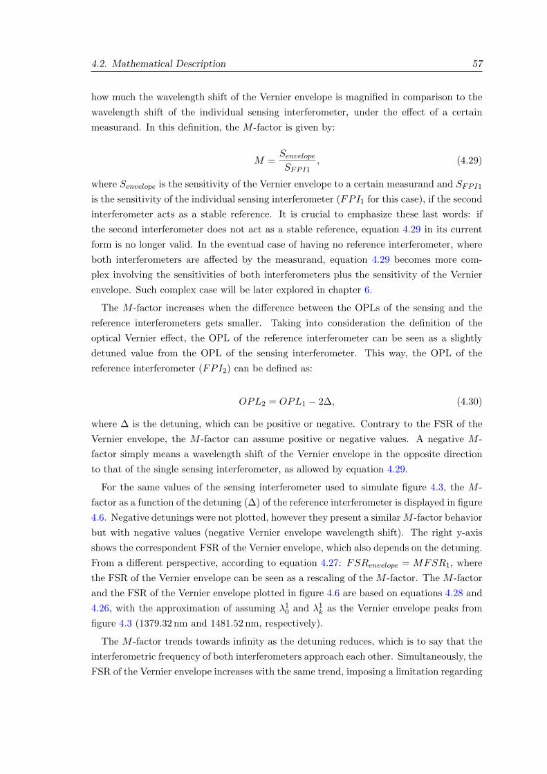
4.2. Mathematical Description 57
how much the wavelength shift of the Vernier envelope is magnified in comparison to the
wavelength shift of the individual sensing interferometer, under the effect of a certain
measurand. In this definition, the M -factor is given by:
M =SenvelopeSFPI1
, (4.29)
where Senvelope is the sensitivity of the Vernier envelope to a certain measurand and SFPI1
is the sensitivity of the individual sensing interferometer (FPI1 for this case), if the second
interferometer acts as a stable reference. It is crucial to emphasize these last words: if
the second interferometer does not act as a stable reference, equation 4.29 in its current
form is no longer valid. In the eventual case of having no reference interferometer, where
both interferometers are affected by the measurand, equation 4.29 becomes more com-
plex involving the sensitivities of both interferometers plus the sensitivity of the Vernier
envelope. Such complex case will be later explored in chapter 6.
The M -factor increases when the difference between the OPLs of the sensing and the
reference interferometers gets smaller. Taking into consideration the definition of the
optical Vernier effect, the OPL of the reference interferometer can be seen as a slightly
detuned value from the OPL of the sensing interferometer. This way, the OPL of the
reference interferometer (FPI2) can be defined as:
OPL2 = OPL1 − 2∆, (4.30)
where ∆ is the detuning, which can be positive or negative. Contrary to the FSR of the
Vernier envelope, the M -factor can assume positive or negative values. A negative M -
factor simply means a wavelength shift of the Vernier envelope in the opposite direction
to that of the single sensing interferometer, as allowed by equation 4.29.
For the same values of the sensing interferometer used to simulate figure 4.3, the M -
factor as a function of the detuning (∆) of the reference interferometer is displayed in figure
4.6. Negative detunings were not plotted, however they present a similarM -factor behavior
but with negative values (negative Vernier envelope wavelength shift). The right y-axis
shows the correspondent FSR of the Vernier envelope, which also depends on the detuning.
From a different perspective, according to equation 4.27: FSRenvelope = MFSR1, where
the FSR of the Vernier envelope can be seen as a rescaling of the M -factor. The M -factor
and the FSR of the Vernier envelope plotted in figure 4.6 are based on equations 4.28 and
4.26, with the approximation of assuming λ10 and λ1k as the Vernier envelope peaks from
figure 4.3 (1379.32 nm and 1481.52 nm, respectively).
The M -factor trends towards infinity as the detuning reduces, which is to say that the
interferometric frequency of both interferometers approach each other. Simultaneously, the
FSR of the Vernier envelope increases with the same trend, imposing a limitation regarding
58 Chapter 4. Optical Vernier Effect in Fiber Interferometers
Figure 4.6. – M -factor and FSR of the Vernier envelope as a function of the detuning (∆)of the reference interferometer (FPI2) from the sensing interferometer (FPI1). Based onequations 4.28 and 4.26, where λ10 and λ1k were assumed as the Vernier envelope peaks fromfigure 4.3 (1379.32 nm and 1481.52 nm, respectively).
the maximum magnification achievable. In practical applications, the maximum M -factor
is limited by the FSR of the Vernier envelope, where one period should stay within the
wavelength range available from the detection system. The M -factor is infinite when no
detuning is considered, translating in a Vernier envelope with an infinite FSR. Hence,
it corresponds to an impractical situation where the Vernier envelope cannot be tracked
and measured. Both interferometers would have the same interferometric frequency and
the spectral responses would add up. With this in mind, one has to deliberately apply,
in a controlled way, a detuning to the reference interferometer OPL. To maximize the
enhancement provided by the optical Vernier effect, one should target high M -factor values
which are below the maximum size of the Vernier envelope measurable.
The simulated reflected spectrum for the fundamental Vernier effect, presented previ-
ously in figure 4.3, corresponds to a detuning of 10µm, as marked in figure 4.6. For this
situation, the expected M -factor is 10. To estimate the wavelength shift of the Vernier
envelope, the OPL of the sensing interferometer (FPI1) was increased from 100µm to
100.2µm, simulating the effect of a measurand (ex. applied strain). Figure 4.7 shows the
simulated reflected spectra before and after the sensing interferometer hypothetically suf-
fers from the effect of a measurand. The minimum of the Vernier envelope, marked with
an arrow, was measured to estimate the envelope wavelength shift. The Vernier envelope
shifted by 27.62 nm. Considering the shift in the sensing interferometer OPL (0.2µm), the
simulated sensitivity of the Vernier envelope (Senvelope) is 138.1 nm/µm.
To verify the expected M -factor value through equation 4.29, the wavelength shift of the
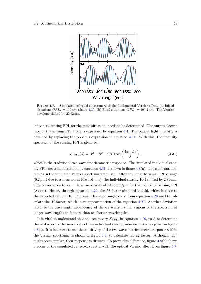
4.2. Mathematical Description 59
Figure 4.7. – Simulated reflected spectrum with the fundamental Vernier effect. (a) Initialsituation: OPL1 = 100µm (figure 4.3). (b) Final situation: OPL1 = 100.2µm. The Vernierenvelope shifted by 27.62 nm.
individual sensing FPI, for the same situation, needs to be determined. The output electric
field of the sensing FPI alone is expressed by equation 4.4. The output light intensity is
obtained by replacing the previous expression in equation 4.11. With this, the intensity
spectrum of the sensing FPI is given by:
IFPI1 (λ) = A2 +B2 − 2AB cos
(4πn1L1
λ
), (4.31)
which is the traditional two-wave interferometric response. The simulated individual sens-
ing FPI spectrum, described by equation 4.31, is shown in figure 4.8(a). The same parame-
ters as in the simulated Vernier spectrum were used. After applying the same OPL change
(0.2µm) due to a measurand (dashed line), the individual sensing FPI shifted by 2.89 nm.
This corresponds to a simulated sensitivity of 14.45 nm/µm for the individual sensing FPI
(SFPI1). Hence, through equation 4.29, the M -factor obtained is 9.56, which is close to
the expected value of 10. The small deviation might come from equation 4.28 used to cal-
culate the M -factor, which is an approximation of the equation 4.27. Another deviation
factor is the wavelength dependency of the wavelength shift: regions of the spectrum at
longer wavelengths shift more than at shorter wavelengths.
It is vital to understand that the sensitivity SFPI1 in equation 4.29, used to determine
the M -factor, is the sensitivity of the individual sensing interferometer, as given in figure
4.8(a). It is incorrect to use the sensitivity of the two-wave interferometric response within
the Vernier spectrum, as shown in figure 4.3, to calculate the M -factor. Although they
might seem similar, their response is distinct. To prove this difference, figure 4.8(b) shows
a zoom of the simulated reflected spectra with the optical Vernier effect from figure 4.7.
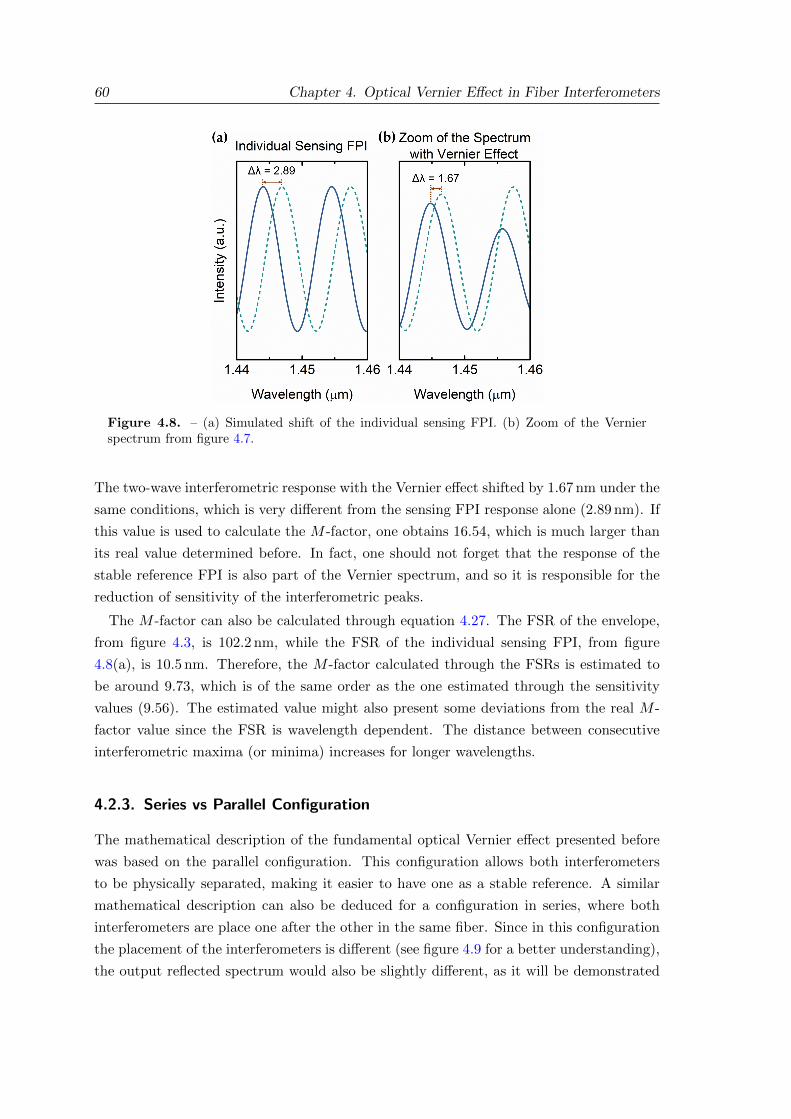
60 Chapter 4. Optical Vernier Effect in Fiber Interferometers
Figure 4.8. – (a) Simulated shift of the individual sensing FPI. (b) Zoom of the Vernierspectrum from figure 4.7.
The two-wave interferometric response with the Vernier effect shifted by 1.67 nm under the
same conditions, which is very different from the sensing FPI response alone (2.89 nm). If
this value is used to calculate the M -factor, one obtains 16.54, which is much larger than
its real value determined before. In fact, one should not forget that the response of the
stable reference FPI is also part of the Vernier spectrum, and so it is responsible for the
reduction of sensitivity of the interferometric peaks.
The M -factor can also be calculated through equation 4.27. The FSR of the envelope,
from figure 4.3, is 102.2 nm, while the FSR of the individual sensing FPI, from figure
4.8(a), is 10.5 nm. Therefore, the M -factor calculated through the FSRs is estimated to
be around 9.73, which is of the same order as the one estimated through the sensitivity
values (9.56). The estimated value might also present some deviations from the real M -
factor value since the FSR is wavelength dependent. The distance between consecutive
interferometric maxima (or minima) increases for longer wavelengths.
4.2.3. Series vs Parallel Configuration
The mathematical description of the fundamental optical Vernier effect presented before
was based on the parallel configuration. This configuration allows both interferometers
to be physically separated, making it easier to have one as a stable reference. A similar
mathematical description can also be deduced for a configuration in series, where both
interferometers are place one after the other in the same fiber. Since in this configuration
the placement of the interferometers is different (see figure 4.9 for a better understanding),
the output reflected spectrum would also be slightly different, as it will be demonstrated
4.3. State-of-the-Art Applications and Configurations 61
in chapter 5. However, the magnification properties of the fundamental optical Vernier
effect are the same.
The configuration in series implies, most of the times, that both interferometer are phys-
ically connected in the sense of having one interferometer placed after the other, sharing
the same interface. In exceptional situations it is possible to place both interferometers
away from each other along the same fiber. However, it compromises the visibility of the
interference, since the amount of light reaching the interferometer that is further away
from the light source is much smaller. If both interferometers are physically connected, it
is extremely difficult to keep one as a stable reference. In general, both interferometers
are affected by the measurands at the same time, and so they must be considered as a
combined sensing structure. In this combined structure, there is no specific interferom-
eter as a reference, unlike in a parallel configuration. Although equation 4.29 describes
correctly the M -factor for the situations described until now, it is no longer valid when
both interferometers act as sensors. One expects then that the sensitivity of the Vernier
envelope will depend on both interferometers. Such complex case of optical Vernier effect
will be analyzed later in chapter 6.
A way to avoid the inexistence of a reference interferometer in a series configuration is
to use distinct interferometric structures, where one of the interferometers is insensitive to
the measurand. For example, if one interferometer is sensitive to pressure but the second
interferometer is designed to be insensitive to the same parameter, it can act as a reference
interferometer.
Nevertheless, the fundamental optical Vernier effect in a series configuration was the
first to be employed in optical fiber sensing [157–159]. Only later, in 2019, the parallel
configuration by means of an optical fiber coupler was demonstrated [160,161].
4.3. State-of-the-Art Applications and Configurations
In the last 2 to 3 years, the fundamental optical Vernier effect became a hot topic in
the field of optical fiber sensing. Many distinct optical fiber interferometers were com-
bined with this technique to create sensing devices with enhanced sensitivity capabilities.
This section presents an overview on the state-of-the-art configurations and applications
using the fundamental optical Vernier effect. The configurations used to generate the
optical Vernier effect are divided in two main groups. The first group consists of config-
urations containing a single-type of interferometer. The second group is made of hybrid
configurations, where two different types of interferometers are combined together. The
configurations are presented here without a chronological order.
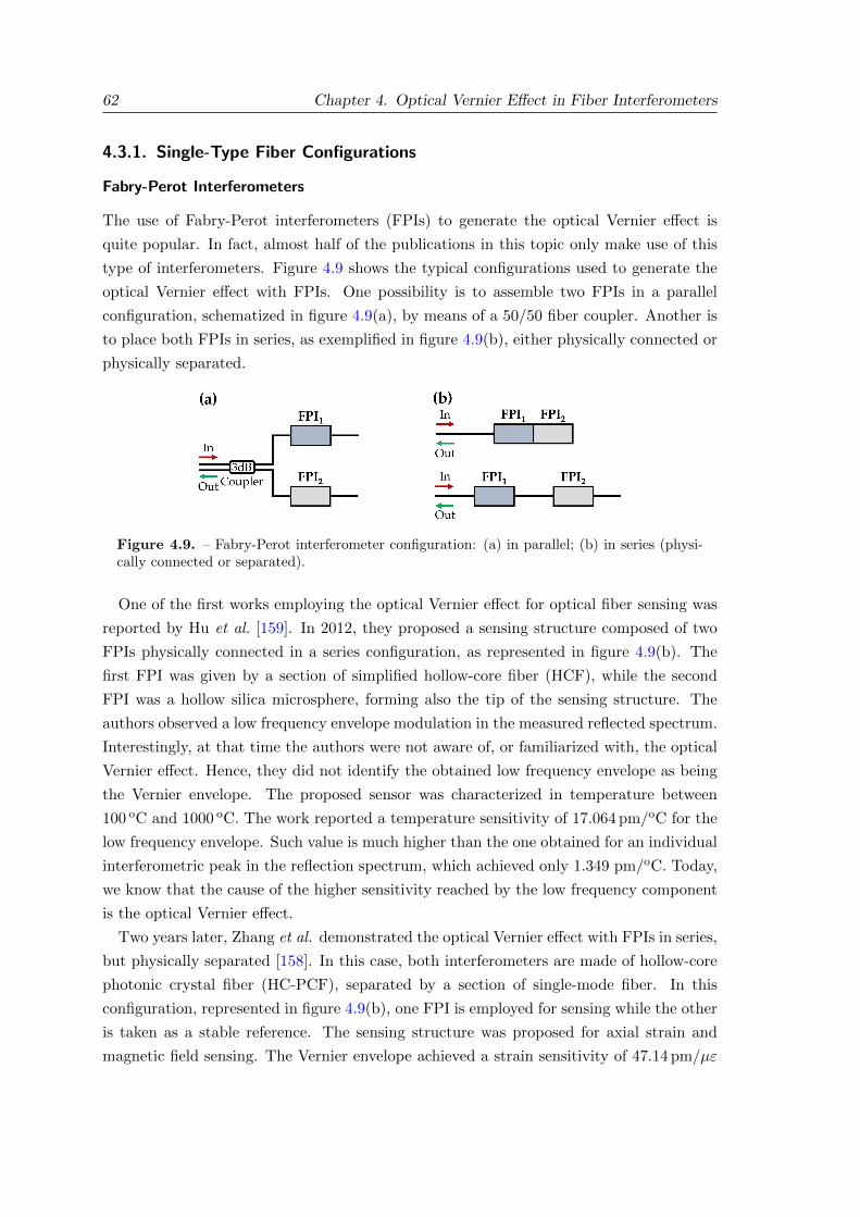
62 Chapter 4. Optical Vernier Effect in Fiber Interferometers
4.3.1. Single-Type Fiber Configurations
Fabry-Perot Interferometers
The use of Fabry-Perot interferometers (FPIs) to generate the optical Vernier effect is
quite popular. In fact, almost half of the publications in this topic only make use of this
type of interferometers. Figure 4.9 shows the typical configurations used to generate the
optical Vernier effect with FPIs. One possibility is to assemble two FPIs in a parallel
configuration, schematized in figure 4.9(a), by means of a 50/50 fiber coupler. Another is
to place both FPIs in series, as exemplified in figure 4.9(b), either physically connected or
physically separated.
Figure 4.9. – Fabry-Perot interferometer configuration: (a) in parallel; (b) in series (physi-cally connected or separated).
One of the first works employing the optical Vernier effect for optical fiber sensing was
reported by Hu et al. [159]. In 2012, they proposed a sensing structure composed of two
FPIs physically connected in a series configuration, as represented in figure 4.9(b). The
first FPI was given by a section of simplified hollow-core fiber (HCF), while the second
FPI was a hollow silica microsphere, forming also the tip of the sensing structure. The
authors observed a low frequency envelope modulation in the measured reflected spectrum.
Interestingly, at that time the authors were not aware of, or familiarized with, the optical
Vernier effect. Hence, they did not identify the obtained low frequency envelope as being
the Vernier envelope. The proposed sensor was characterized in temperature between
100 oC and 1000 oC. The work reported a temperature sensitivity of 17.064 pm/oC for the
low frequency envelope. Such value is much higher than the one obtained for an individual
interferometric peak in the reflection spectrum, which achieved only 1.349 pm/oC. Today,
we know that the cause of the higher sensitivity reached by the low frequency component
is the optical Vernier effect.
Two years later, Zhang et al. demonstrated the optical Vernier effect with FPIs in series,
but physically separated [158]. In this case, both interferometers are made of hollow-core
photonic crystal fiber (HC-PCF), separated by a section of single-mode fiber. In this
configuration, represented in figure 4.9(b), one FPI is employed for sensing while the other
is taken as a stable reference. The sensing structure was proposed for axial strain and
magnetic field sensing. The Vernier envelope achieved a strain sensitivity of 47.14 pm/µε
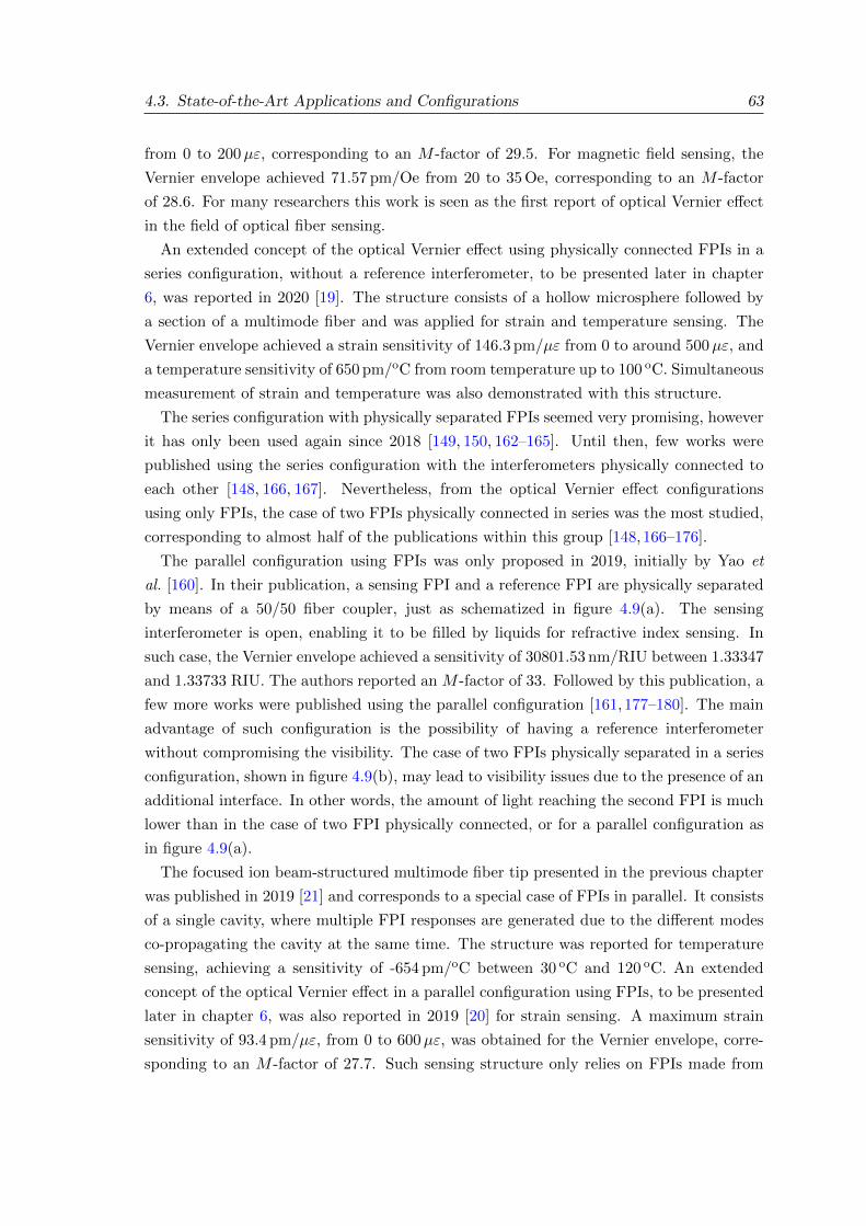
4.3. State-of-the-Art Applications and Configurations 63
from 0 to 200µε, corresponding to an M -factor of 29.5. For magnetic field sensing, the
Vernier envelope achieved 71.57 pm/Oe from 20 to 35 Oe, corresponding to an M -factor
of 28.6. For many researchers this work is seen as the first report of optical Vernier effect
in the field of optical fiber sensing.
An extended concept of the optical Vernier effect using physically connected FPIs in a
series configuration, without a reference interferometer, to be presented later in chapter
6, was reported in 2020 [19]. The structure consists of a hollow microsphere followed by
a section of a multimode fiber and was applied for strain and temperature sensing. The
Vernier envelope achieved a strain sensitivity of 146.3 pm/µε from 0 to around 500µε, and
a temperature sensitivity of 650 pm/oC from room temperature up to 100 oC. Simultaneous
measurement of strain and temperature was also demonstrated with this structure.
The series configuration with physically separated FPIs seemed very promising, however
it has only been used again since 2018 [149, 150, 162–165]. Until then, few works were
published using the series configuration with the interferometers physically connected to
each other [148, 166, 167]. Nevertheless, from the optical Vernier effect configurations
using only FPIs, the case of two FPIs physically connected in series was the most studied,
corresponding to almost half of the publications within this group [148,166–176].
The parallel configuration using FPIs was only proposed in 2019, initially by Yao et
al. [160]. In their publication, a sensing FPI and a reference FPI are physically separated
by means of a 50/50 fiber coupler, just as schematized in figure 4.9(a). The sensing
interferometer is open, enabling it to be filled by liquids for refractive index sensing. In
such case, the Vernier envelope achieved a sensitivity of 30801.53 nm/RIU between 1.33347
and 1.33733 RIU. The authors reported an M -factor of 33. Followed by this publication, a
few more works were published using the parallel configuration [161, 177–180]. The main
advantage of such configuration is the possibility of having a reference interferometer
without compromising the visibility. The case of two FPIs physically separated in a series
configuration, shown in figure 4.9(b), may lead to visibility issues due to the presence of an
additional interface. In other words, the amount of light reaching the second FPI is much
lower than in the case of two FPI physically connected, or for a parallel configuration as
in figure 4.9(a).
The focused ion beam-structured multimode fiber tip presented in the previous chapter
was published in 2019 [21] and corresponds to a special case of FPIs in parallel. It consists
of a single cavity, where multiple FPI responses are generated due to the different modes
co-propagating the cavity at the same time. The structure was reported for temperature
sensing, achieving a sensitivity of -654 pm/oC between 30 oC and 120 oC. An extended
concept of the optical Vernier effect in a parallel configuration using FPIs, to be presented
later in chapter 6, was also reported in 2019 [20] for strain sensing. A maximum strain
sensitivity of 93.4 pm/µε, from 0 to 600µε, was obtained for the Vernier envelope, corre-
sponding to an M -factor of 27.7. Such sensing structure only relies on FPIs made from
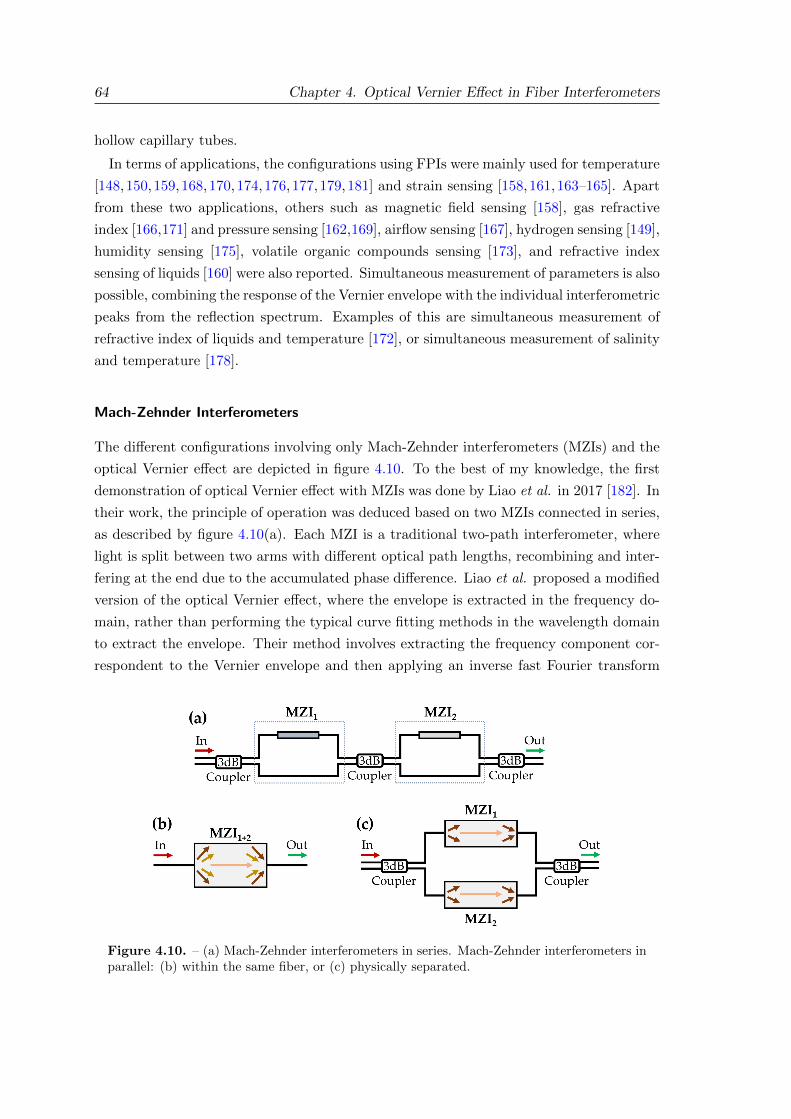
64 Chapter 4. Optical Vernier Effect in Fiber Interferometers
hollow capillary tubes.
In terms of applications, the configurations using FPIs were mainly used for temperature
[148,150,159,168,170,174,176,177,179,181] and strain sensing [158,161,163–165]. Apart
from these two applications, others such as magnetic field sensing [158], gas refractive
index [166,171] and pressure sensing [162,169], airflow sensing [167], hydrogen sensing [149],
humidity sensing [175], volatile organic compounds sensing [173], and refractive index
sensing of liquids [160] were also reported. Simultaneous measurement of parameters is also
possible, combining the response of the Vernier envelope with the individual interferometric
peaks from the reflection spectrum. Examples of this are simultaneous measurement of
refractive index of liquids and temperature [172], or simultaneous measurement of salinity
and temperature [178].
Mach-Zehnder Interferometers
The different configurations involving only Mach-Zehnder interferometers (MZIs) and the
optical Vernier effect are depicted in figure 4.10. To the best of my knowledge, the first
demonstration of optical Vernier effect with MZIs was done by Liao et al. in 2017 [182]. In
their work, the principle of operation was deduced based on two MZIs connected in series,
as described by figure 4.10(a). Each MZI is a traditional two-path interferometer, where
light is split between two arms with different optical path lengths, recombining and inter-
fering at the end due to the accumulated phase difference. Liao et al. proposed a modified
version of the optical Vernier effect, where the envelope is extracted in the frequency do-
main, rather than performing the typical curve fitting methods in the wavelength domain
to extract the envelope. Their method involves extracting the frequency component cor-
respondent to the Vernier envelope and then applying an inverse fast Fourier transform
Figure 4.10. – (a) Mach-Zehnder interferometers in series. Mach-Zehnder interferometers inparallel: (b) within the same fiber, or (c) physically separated.

4.3. State-of-the-Art Applications and Configurations 65
(IFFT). Experimentally, the authors used an offset spliced single-mode fiber to create each
MZI. Keeping one interferometer as a reference, the structure was demonstrated for tem-
perature and curvature sensing. For temperature sensing, the Vernier envelope achieved
a sensitivity of 397.36 pm/oC, with an M -factor of 8.8. With regard to curvature sensing,
the sensitivity of the Vernier envelope was -36.26 nm/m-1, with an M -factor of 8.0.
Instead of offset spliced fibers, the MZIs can also be fabricated by other means [183,184].
For example, Lin et al. used a multimode fiber (MMF), with a femtosecond laser machined
air cavity, between single-mode fibers [185], and Zhao et al. spliced hollow core fibers
between MMFs [186].
In 2018, a new type of configuration was introduced. Such configuration, represented in
figure 4.10(b), is composed of two integrated MZIs in a parallel configuration. Lin et al.
used a dual side-hole fiber (DSHF) spliced between two pieces of MMF to form the struc-
ture [187]. Light travels through the core of the dual side-hole fiber and simultaneously
through the two side holes. In their work, the authors opened an access to one of the air
holes, allowing to measure gas pressure with a sensitivity of -60 nm/MPa, between 0 and
0.8 MPa. The structure achieved an M -factor of 7. The same type of configuration was
demonstrated in a different way by Ni et al., by means of a single hole twin eccentric cores
fiber (SHTECF) spliced between two single-mode fibers [188]. In each splice position the
fiber was collapsed. In this case, the authors used the structure for temperature sensing,
obtaining a sensitivity of 2.057 nm/oC for the Vernier envelope, corresponding to an M -
factor of 48.8. In 2019, this configuration was also demonstrated by Hu et al., where the
integrated MZI structure consisted of an offset spliced side-hole fiber (SHF) between two
coreless fibers [189]. The authors applied the proposed sensor for refractive index sensing,
reporting a Vernier envelope sensitivity of 44084 nm/RIU from 1.33288 to 1.33311. In this
work, the M -factor achieved was only 3.1.
At last, the parallel configuration using separated MZIs, as represented in figure 4.10(c)
was proposed by Wang et al., in 2019 [190]. In their work, each MZI consists of a simple
hollow core fiber spliced between two MMFs. The parallel configuration is achieved by
connecting two MZIs using two 50/50 fiber couplers. The authors used the structure for
temperature sensing, achieving a sensitivity of 528.5 pm/oC, between 0 oC and 100 oC. An
M -factor of 17.5 was also reported.
Sagnac Interferometers
An optical fiber Sagnac interferometer (SI) consists of an optical fiber ring, assembled us-
ing a 50/50 fiber coupler, in which two beams are propagating in counter directions with
different polarization states [1]. In fiber sensing, a section of polarization maintaining
fiber (PMF) is typically placed inside the optical fiber ring, providing different propagat-
ing constants along the slow and fast axis. The output signal is given by the interference
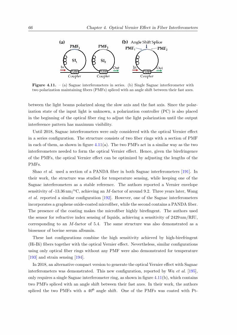
66 Chapter 4. Optical Vernier Effect in Fiber Interferometers
Figure 4.11. – (a) Sagnac interferometers in series. (b) Single Sagnac interferometer withtwo polarization maintaining fibers (PMFs) spliced with an angle shift between their fast axes.
between the light beams polarized along the slow axis and the fast axis. Since the polar-
ization state of the input light is unknown, a polarization controller (PC) is also placed
in the beginning of the optical fiber ring to adjust the light polarization until the output
interference pattern has maximum visibility.
Until 2018, Sagnac interferometers were only considered with the optical Vernier effect
in a series configuration. The structure consists of two fiber rings with a section of PMF
in each of them, as shown in figure 4.11(a). The two PMFs act in a similar way as the two
interferometers needed to form the optical Vernier effect. Hence, given the birefringence
of the PMFs, the optical Vernier effect can be optimized by adjusting the lengths of the
PMFs.
Shao et al. used a section of a PANDA fiber in both Sagnac interferometers [191]. In
their work, the structure was studied for temperature sensing, while keeping one of the
Sagnac interferometers as a stable reference. The authors reported a Vernier envelope
sensitivity of -13.36 nm/oC, achieving an M -factor of around 9.2. Three years later, Wang
et al. reported a similar configuration [192]. However, one of the Sagnac interferometers
incorporates a graphene oxide-coated microfiber, while the second contains a PANDA fiber.
The presence of the coating makes the microfiber highly birefingent. The authors used
the sensor for refractive index sensing of liquids, achieving a sensitivity of 2429 nm/RIU,
corresponding to an M -factor of 5.4. The same structure was also demonstrated as a
biosensor of bovine serum albumin.
These last configurations combine the high sensitivity achieved by high-birefringent
(Hi-Bi) fibers together with the optical Vernier effect. Nevertheless, similar configurations
using only optical fiber rings without any PMF were also demonstrated for temperature
[193] and strain sensing [194].
In 2018, an alternative compact version to generate the optical Vernier effect with Sagnac
interferometers was demonstrated. This new configuration, reported by Wu et al. [195],
only requires a single Sagnac interferometer ring, as shown in figure 4.11(b), which contains
two PMFs spliced with an angle shift between their fast axes. In their work, the authors
spliced the two PMFs with a 40º angle shift. One of the PMFs was coated with Pt-
4.3. State-of-the-Art Applications and Configurations 67
load WO3/SiO2 powder, which heats up under the presence of hydrogen. The authors
reported a temperature sensitivity of -2.44 nm/oC for the Vernier envelope. The structure
was also applied for hydrogen sensing, achieving a sensitivity of -14.61 nm/% between
0 and 0.8% of hydrogen. Liu et al. used the same configuration with two sections of
PANDA fiber, spliced with an angle of 45º between their fast axes [196]. The authors
used the structure for strain and temperature sensing. The Vernier envelope attained a
strain sensitivity of 58 pm/µε from 0 to 1440µε, achieving an M -factor of 9.8. As for
temperature sensing, the Vernier envelope had a sensitivity of -1.05 nm/oC between 20 oC
and 80 oC. The authors also reported simultaneous measurement of strain and temperature
using a matrix method. For a completely different application, Wu et al. employed the
same configuration for isopropanol measurement [197]. One of the PMFs was coated with
polypyrrole polymer, which swells in the presence of isopropanol, inducing strain in the
fiber. The authors reported a sensitivity of 239 pm/ppm of isopropanol for the Vernier
envelope, between 0 and 42 ppm, corresponding to an M -factor of 4.2.
Michelson Interferometers
Similarly to Mach-Zehnder interferometers, the Michelson interferometer consists of the
interference between light propagating in two arms. However, in the Michelson interfer-
ometer the propagating light is reflected at the end of each arm [1]. In 2019, Zhang et
al. demonstrated the generation of the optical Vernier effect using two juxtaposed fiber
Michelson interferometers [5]. In their configuration, the structure is made of a triple-core
fiber (TCF) spliced to a dual-side-hole fiber, as shown in the schematic of figure 4.12. The
triple-core fiber was tapered down, allowing the input light to split between the other cores.
The output signal is given by the interference between the light propagating in the cen-
tral core and the light propagating in the side cores, where both present slightly different
refractive indices. The authors proposed such structure for curvature sensing, achieving a
sensitivity of -57 nm/m-1 between 0 and 1.14 m-1 for the Vernier envelope. The same sensor
was also characterized in temperature, where the Vernier envelope obtained a sensitivity
of 143 pm/oC between 30 oC and 100 oC.
Figure 4.12. – Michelson interferometers in parallel. The structure consists of a taperedtriple-core fiber spliced to a dual-side-hole fiber. Adapted from [5].
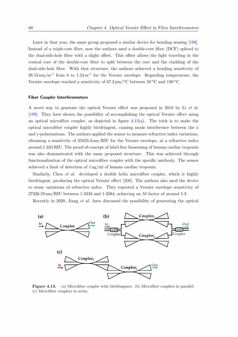
68 Chapter 4. Optical Vernier Effect in Fiber Interferometers
Later in that year, the same group proposed a similar device for bending sensing [198].
Instead of a triple-core fiber, now the authors used a double-core fiber (DCF) spliced to
the dual-side-hole fiber with a slight offset. This offset allows the light traveling in the
central core of the double-core fiber to split between the core and the cladding of the
dual-side-hole fiber. With that structure, the authors achieved a bending sensitivity of
38.53 nm/m-1 from 0 to 1.24 m-1 for the Vernier envelope. Regarding temperature, the
Vernier envelope reached a sensitivity of 67.2 pm/oC between 50 oC and 130 oC.
Fiber Coupler Interferometers
A novel way to generate the optical Vernier effect was proposed in 2018 by Li et al.
[199]. They have shown the possibility of accomplishing the optical Vernier effect using
an optical microfiber coupler, as depicted in figure 4.13(a). The trick is to make the
optical microfiber coupler highly birefringent, causing mode interference between the x
and y-polarizations. The authors applied the sensor to measure refractive index variations,
obtaining a sensitivity of 35823.3 nm/RIU for the Vernier envelope, at a refractive index
around 1.333 RIU. The proof-of-concept of label-free biosensing of human cardiac troponin
was also demonstrated with the same proposed structure. This was achieved through
functionalization of the optical microfiber coupler with the specific antibody. The sensor
achieved a limit of detection of 1 ng/ml of human cardiac troponin.
Similarly, Chen et al. developed a double helix microfiber coupler, which is highly
birefringent, producing the optical Vernier effect [200]. The authors also used the device
to sense variations of refractive index. They reported a Vernier envelope sensitivity of
27326.59 nm/RIU between 1.3333 and 1.3394, achieving an M -factor of around 5.3.
Recently in 2020, Jiang et al. have discussed the possibility of generating the optical
Figure 4.13. – (a) Microfiber coupler with birefringence. (b) Microfiber couplers in parallel.(c) Microfiber couplers in series.
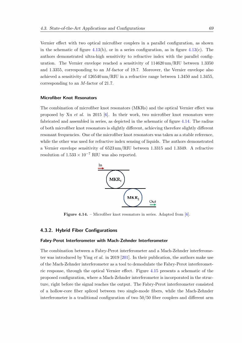
4.3. State-of-the-Art Applications and Configurations 69
Vernier effect with two optical microfiber couplers in a parallel configuration, as shown
in the schematic of figure 4.13(b), or in a series configuration, as in figure 4.13(c). The
authors demonstrated ultra-high sensitivity to refractive index with the parallel config-
uration. The Vernier envelope reached a sensitivity of 114620 nm/RIU between 1.3350
and 1.3355, corresponding to an M -factor of 19.7. Moreover, the Vernier envelope also
achieved a sensitivity of 126540 nm/RIU in a refractive range between 1.3450 and 1.3455,
corresponding to an M -factor of 21.7.
Microfiber Knot Resonators
The combination of microfiber knot resonators (MKRs) and the optical Vernier effect was
proposed by Xu et al. in 2015 [6]. In their work, two microfiber knot resonators were
fabricated and assembled in series, as depicted in the schematic of figure 4.14. The radius
of both microfiber knot resonators is slightly different, achieving therefore slightly different
resonant frequencies. One of the microfiber knot resonators was taken as a stable reference,
while the other was used for refractive index sensing of liquids. The authors demonstrated
a Vernier envelope sensitivity of 6523 nm/RIU between 1.3315 and 1.3349. A refractive
resolution of 1.533× 10⁻⁷ RIU was also reported.
Figure 4.14. – Microfiber knot resonators in series. Adapted from [6].
4.3.2. Hybrid Fiber Configurations
Fabry-Perot Interferometer with Mach-Zehnder Interferometer
The combination between a Fabry-Perot interferometer and a Mach-Zehnder interferome-
ter was introduced by Ying et al. in 2019 [201]. In their publication, the authors make use
of the Mach-Zehnder interferometer as a tool to demodulate the Fabry-Perot interferomet-
ric response, through the optical Vernier effect. Figure 4.15 presents a schematic of the
proposed configuration, where a Mach-Zehnder interferometer is incorporated in the struc-
ture, right before the signal reaches the output. The Fabry-Perot interferometer consisted
of a hollow-core fiber spliced between two single-mode fibers, while the Mach-Zehnder
interferometer is a traditional configuration of two 50/50 fiber couplers and different arm
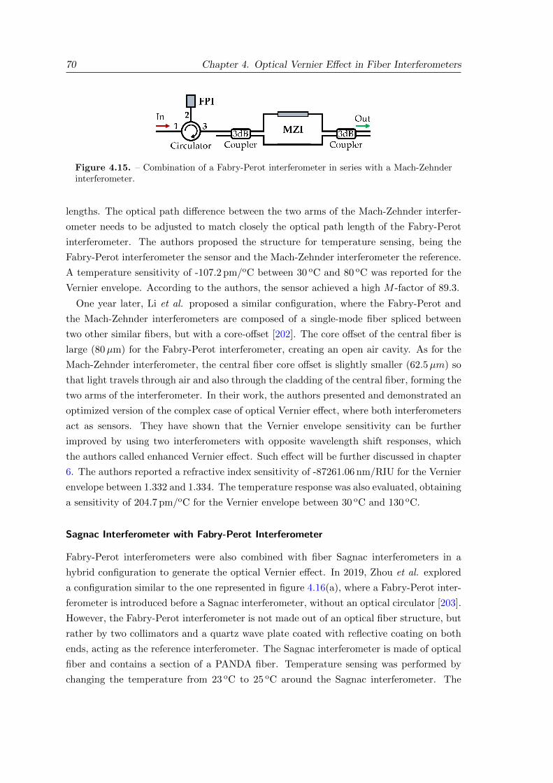
70 Chapter 4. Optical Vernier Effect in Fiber Interferometers
Figure 4.15. – Combination of a Fabry-Perot interferometer in series with a Mach-Zehnderinterferometer.
lengths. The optical path difference between the two arms of the Mach-Zehnder interfer-
ometer needs to be adjusted to match closely the optical path length of the Fabry-Perot
interferometer. The authors proposed the structure for temperature sensing, being the
Fabry-Perot interferometer the sensor and the Mach-Zehnder interferometer the reference.
A temperature sensitivity of -107.2 pm/oC between 30 oC and 80 oC was reported for the
Vernier envelope. According to the authors, the sensor achieved a high M -factor of 89.3.
One year later, Li et al. proposed a similar configuration, where the Fabry-Perot and
the Mach-Zehnder interferometers are composed of a single-mode fiber spliced between
two other similar fibers, but with a core-offset [202]. The core offset of the central fiber is
large (80µm) for the Fabry-Perot interferometer, creating an open air cavity. As for the
Mach-Zehnder interferometer, the central fiber core offset is slightly smaller (62.5µm) so
that light travels through air and also through the cladding of the central fiber, forming the
two arms of the interferometer. In their work, the authors presented and demonstrated an
optimized version of the complex case of optical Vernier effect, where both interferometers
act as sensors. They have shown that the Vernier envelope sensitivity can be further
improved by using two interferometers with opposite wavelength shift responses, which
the authors called enhanced Vernier effect. Such effect will be further discussed in chapter
6. The authors reported a refractive index sensitivity of -87261.06 nm/RIU for the Vernier
envelope between 1.332 and 1.334. The temperature response was also evaluated, obtaining
a sensitivity of 204.7 pm/oC for the Vernier envelope between 30 oC and 130 oC.
Sagnac Interferometer with Fabry-Perot Interferometer
Fabry-Perot interferometers were also combined with fiber Sagnac interferometers in a
hybrid configuration to generate the optical Vernier effect. In 2019, Zhou et al. explored
a configuration similar to the one represented in figure 4.16(a), where a Fabry-Perot inter-
ferometer is introduced before a Sagnac interferometer, without an optical circulator [203].
However, the Fabry-Perot interferometer is not made out of an optical fiber structure, but
rather by two collimators and a quartz wave plate coated with reflective coating on both
ends, acting as the reference interferometer. The Sagnac interferometer is made of optical
fiber and contains a section of a PANDA fiber. Temperature sensing was performed by
changing the temperature from 23 oC to 25 oC around the Sagnac interferometer. The
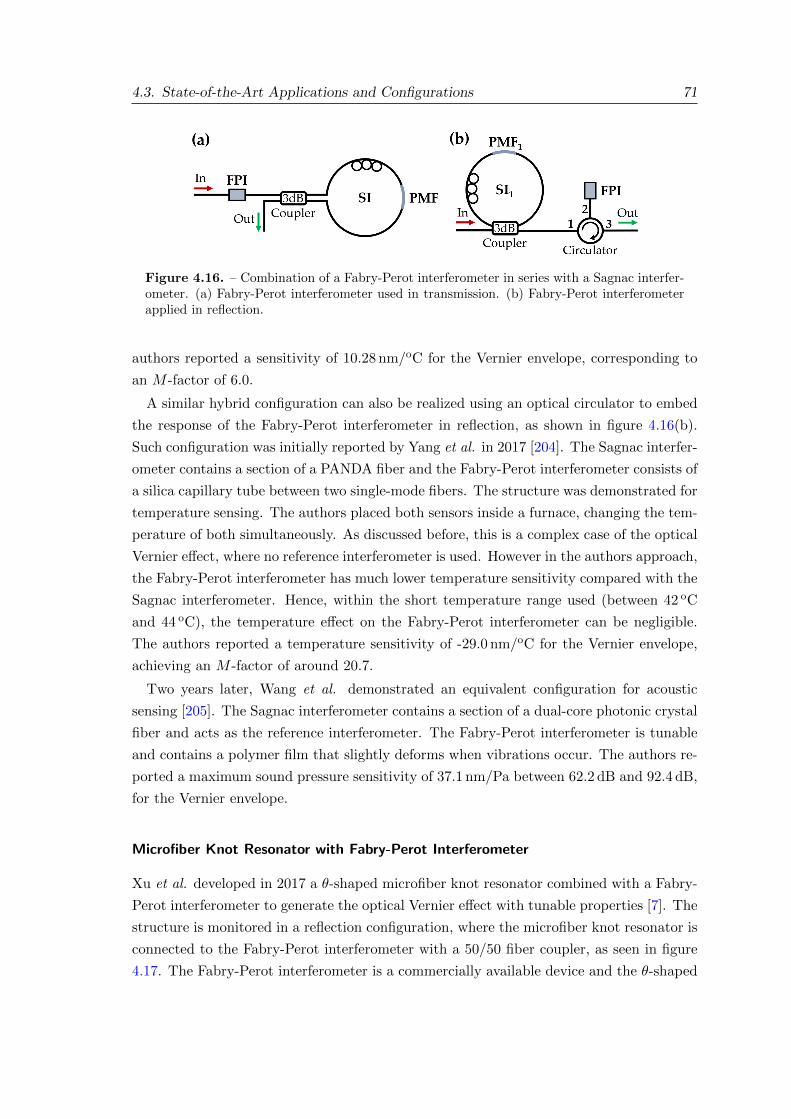
4.3. State-of-the-Art Applications and Configurations 71
Figure 4.16. – Combination of a Fabry-Perot interferometer in series with a Sagnac interfer-ometer. (a) Fabry-Perot interferometer used in transmission. (b) Fabry-Perot interferometerapplied in reflection.
authors reported a sensitivity of 10.28 nm/oC for the Vernier envelope, corresponding to
an M -factor of 6.0.
A similar hybrid configuration can also be realized using an optical circulator to embed
the response of the Fabry-Perot interferometer in reflection, as shown in figure 4.16(b).
Such configuration was initially reported by Yang et al. in 2017 [204]. The Sagnac interfer-
ometer contains a section of a PANDA fiber and the Fabry-Perot interferometer consists of
a silica capillary tube between two single-mode fibers. The structure was demonstrated for
temperature sensing. The authors placed both sensors inside a furnace, changing the tem-
perature of both simultaneously. As discussed before, this is a complex case of the optical
Vernier effect, where no reference interferometer is used. However in the authors approach,
the Fabry-Perot interferometer has much lower temperature sensitivity compared with the
Sagnac interferometer. Hence, within the short temperature range used (between 42 oC
and 44 oC), the temperature effect on the Fabry-Perot interferometer can be negligible.
The authors reported a temperature sensitivity of -29.0 nm/oC for the Vernier envelope,
achieving an M -factor of around 20.7.
Two years later, Wang et al. demonstrated an equivalent configuration for acoustic
sensing [205]. The Sagnac interferometer contains a section of a dual-core photonic crystal
fiber and acts as the reference interferometer. The Fabry-Perot interferometer is tunable
and contains a polymer film that slightly deforms when vibrations occur. The authors re-
ported a maximum sound pressure sensitivity of 37.1 nm/Pa between 62.2 dB and 92.4 dB,
for the Vernier envelope.
Microfiber Knot Resonator with Fabry-Perot Interferometer
Xu et al. developed in 2017 a θ-shaped microfiber knot resonator combined with a Fabry-
Perot interferometer to generate the optical Vernier effect with tunable properties [7]. The
structure is monitored in a reflection configuration, where the microfiber knot resonator is
connected to the Fabry-Perot interferometer with a 50/50 fiber coupler, as seen in figure
4.17. The Fabry-Perot interferometer is a commercially available device and the θ-shaped
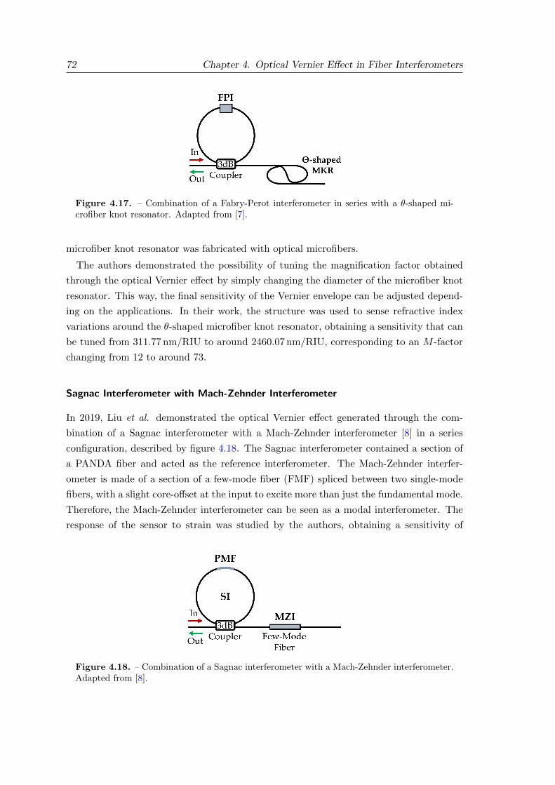
72 Chapter 4. Optical Vernier Effect in Fiber Interferometers
Figure 4.17. – Combination of a Fabry-Perot interferometer in series with a θ-shaped mi-crofiber knot resonator. Adapted from [7].
microfiber knot resonator was fabricated with optical microfibers.
The authors demonstrated the possibility of tuning the magnification factor obtained
through the optical Vernier effect by simply changing the diameter of the microfiber knot
resonator. This way, the final sensitivity of the Vernier envelope can be adjusted depend-
ing on the applications. In their work, the structure was used to sense refractive index
variations around the θ-shaped microfiber knot resonator, obtaining a sensitivity that can
be tuned from 311.77 nm/RIU to around 2460.07 nm/RIU, corresponding to an M -factor
changing from 12 to around 73.
Sagnac Interferometer with Mach-Zehnder Interferometer
In 2019, Liu et al. demonstrated the optical Vernier effect generated through the com-
bination of a Sagnac interferometer with a Mach-Zehnder interferometer [8] in a series
configuration, described by figure 4.18. The Sagnac interferometer contained a section of
a PANDA fiber and acted as the reference interferometer. The Mach-Zehnder interfer-
ometer is made of a section of a few-mode fiber (FMF) spliced between two single-mode
fibers, with a slight core-offset at the input to excite more than just the fundamental mode.
Therefore, the Mach-Zehnder interferometer can be seen as a modal interferometer. The
response of the sensor to strain was studied by the authors, obtaining a sensitivity of
Figure 4.18. – Combination of a Sagnac interferometer with a Mach-Zehnder interferometer.Adapted from [8].
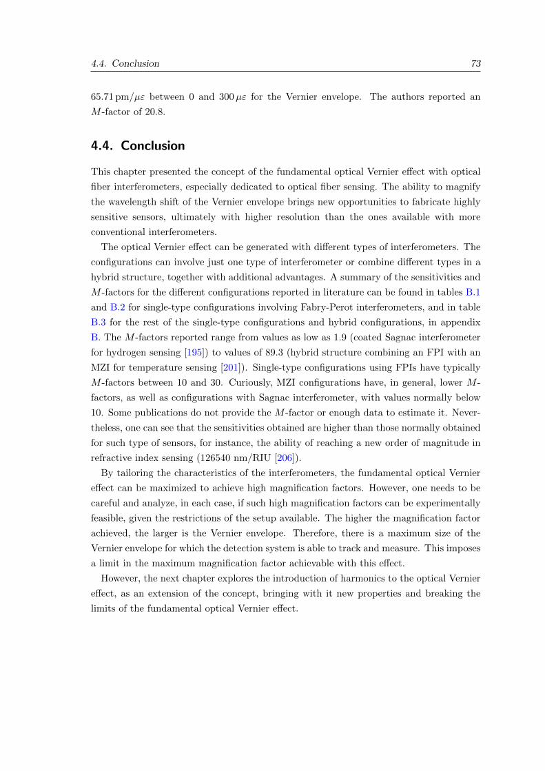
4.4. Conclusion 73
65.71 pm/µε between 0 and 300µε for the Vernier envelope. The authors reported an
M -factor of 20.8.
4.4. Conclusion
This chapter presented the concept of the fundamental optical Vernier effect with optical
fiber interferometers, especially dedicated to optical fiber sensing. The ability to magnify
the wavelength shift of the Vernier envelope brings new opportunities to fabricate highly
sensitive sensors, ultimately with higher resolution than the ones available with more
conventional interferometers.
The optical Vernier effect can be generated with different types of interferometers. The
configurations can involve just one type of interferometer or combine different types in a
hybrid structure, together with additional advantages. A summary of the sensitivities and
M -factors for the different configurations reported in literature can be found in tables B.1
and B.2 for single-type configurations involving Fabry-Perot interferometers, and in table
B.3 for the rest of the single-type configurations and hybrid configurations, in appendix
B. The M -factors reported range from values as low as 1.9 (coated Sagnac interferometer
for hydrogen sensing [195]) to values of 89.3 (hybrid structure combining an FPI with an
MZI for temperature sensing [201]). Single-type configurations using FPIs have typically
M -factors between 10 and 30. Curiously, MZI configurations have, in general, lower M -
factors, as well as configurations with Sagnac interferometer, with values normally below
10. Some publications do not provide the M -factor or enough data to estimate it. Never-
theless, one can see that the sensitivities obtained are higher than those normally obtained
for such type of sensors, for instance, the ability of reaching a new order of magnitude in
refractive index sensing (126540 nm/RIU [206]).
By tailoring the characteristics of the interferometers, the fundamental optical Vernier
effect can be maximized to achieve high magnification factors. However, one needs to be
careful and analyze, in each case, if such high magnification factors can be experimentally
feasible, given the restrictions of the setup available. The higher the magnification factor
achieved, the larger is the Vernier envelope. Therefore, there is a maximum size of the
Vernier envelope for which the detection system is able to track and measure. This imposes
a limit in the maximum magnification factor achievable with this effect.
However, the next chapter explores the introduction of harmonics to the optical Vernier
effect, as an extension of the concept, bringing with it new properties and breaking the
limits of the fundamental optical Vernier effect.

Chapter 5.
Optical Harmonic Vernier Effect
5.1. Introduction
The fundamental optical Vernier effect, as seen in the previous chapter, relies on the
fabrication of two interferometers with a small detuning between their optical path lengths
(OPLs) (i.e. slightly shifted interferometric frequencies). The interference signal produced
by these two interferometers is employed like the two Vernier scales in a caliper. In this
configuration, high magnification factors (M -factors) are only achieved if the OPLs of the
two interferometers are really close. From a practical point of view, considering the current
fabrication processes of fiber sensing structures, which is usually at sub-millimeter scale,
this requirement can be challenging, and in certain situations unfeasible. Additionally, the
Vernier envelope trends towards infinity, limiting the maximum M -factor achievable.
This chapter introduces the concept of optical harmonic Vernier effect, as an extension of
Figure 5.1. – Illustration of the optical harmonic Vernier effect. The novel concept ofharmonics of the Vernier effect shows that it is, in fact, possible to use two interferometerswith very different frequencies as the Vernier scale. The result is a complex harmonic responsewith enhanced magnification properties.
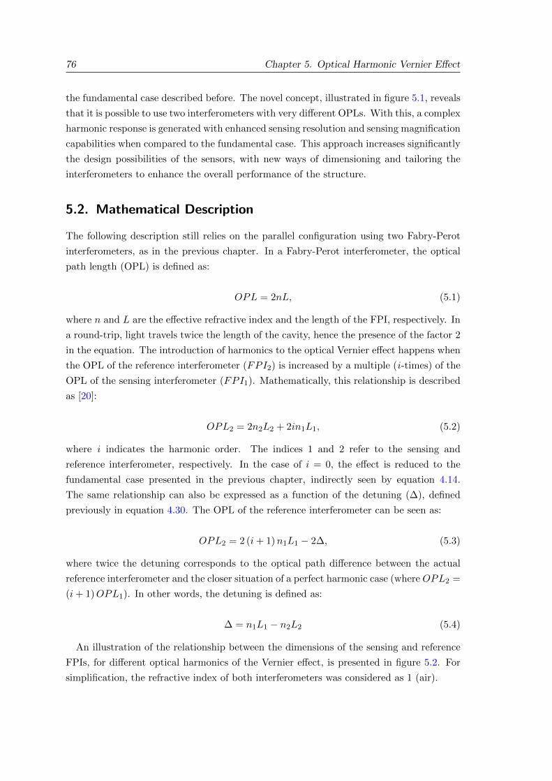
76 Chapter 5. Optical Harmonic Vernier Effect
the fundamental case described before. The novel concept, illustrated in figure 5.1, reveals
that it is possible to use two interferometers with very different OPLs. With this, a complex
harmonic response is generated with enhanced sensing resolution and sensing magnification
capabilities when compared to the fundamental case. This approach increases significantly
the design possibilities of the sensors, with new ways of dimensioning and tailoring the
interferometers to enhance the overall performance of the structure.
5.2. Mathematical Description
The following description still relies on the parallel configuration using two Fabry-Perot
interferometers, as in the previous chapter. In a Fabry-Perot interferometer, the optical
path length (OPL) is defined as:
OPL = 2nL, (5.1)
where n and L are the effective refractive index and the length of the FPI, respectively. In
a round-trip, light travels twice the length of the cavity, hence the presence of the factor 2
in the equation. The introduction of harmonics to the optical Vernier effect happens when
the OPL of the reference interferometer (FPI2) is increased by a multiple (i -times) of the
OPL of the sensing interferometer (FPI1). Mathematically, this relationship is described
as [20]:
OPL2 = 2n2L2 + 2in1L1, (5.2)
where i indicates the harmonic order. The indices 1 and 2 refer to the sensing and
reference interferometer, respectively. In the case of i = 0, the effect is reduced to the
fundamental case presented in the previous chapter, indirectly seen by equation 4.14.
The same relationship can also be expressed as a function of the detuning (∆), defined
previously in equation 4.30. The OPL of the reference interferometer can be seen as:
OPL2 = 2 (i+ 1)n1L1 − 2∆, (5.3)
where twice the detuning corresponds to the optical path difference between the actual
reference interferometer and the closer situation of a perfect harmonic case (where OPL2 =
(i+ 1)OPL1). In other words, the detuning is defined as:
∆ = n1L1 − n2L2 (5.4)
An illustration of the relationship between the dimensions of the sensing and reference
FPIs, for different optical harmonics of the Vernier effect, is presented in figure 5.2. For
simplification, the refractive index of both interferometers was considered as 1 (air).
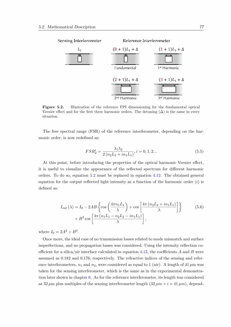
5.2. Mathematical Description 77
Figure 5.2. – Illustration of the reference FPI dimensioning for the fundamental opticalVernier effect and for the first three harmonic orders. The detuning (∆) is the same in everysituation.
The free spectral range (FSR) of the reference interferometer, depending on the har-
monic order, is now redefined as:
FSRi2 =λ1λ2
2 (n2L2 + in1L1), i = 0, 1, 2... (5.5)
At this point, before introducing the properties of the optical harmonic Vernier effect,
it is useful to visualize the appearance of the reflected spectrum for different harmonic
orders. To do so, equation 5.2 must be replaced in equation 4.12. The obtained general
equation for the output reflected light intensity as a function of the harmonic order (i) is
defined as:
Iout (λ) = I0 − 2AB
{cos
(4πn1L1
λ
)+ cos
[4π (n2L2 + in1L1)
λ
]}(5.6)
+B2 cos
[4π (n1L1 − n2L2 − in1L1)
λ
],
where I0 = 2A2 +B2.
Once more, the ideal case of no transmission losses related to mode mismatch and surface
imperfections, and no propagation losses was considered. Using the intensity reflection co-
efficient for a silica/air interface calculated in equation 4.13, the coefficients A and B were
assumed as 0.182 and 0.176, respectively. The refractive indices of the sensing and refer-
ence interferometers, n1 and n2, were considered as equal to 1 (air). A length of 41µm was
taken for the sensing interferometer, which is the same as in the experimental demonstra-
tion later shown in chapter 6. As for the reference interferometer, its length was considered
as 32µm plus multiples of the sensing interferometer length (32µm+ i× 41µm), depend-
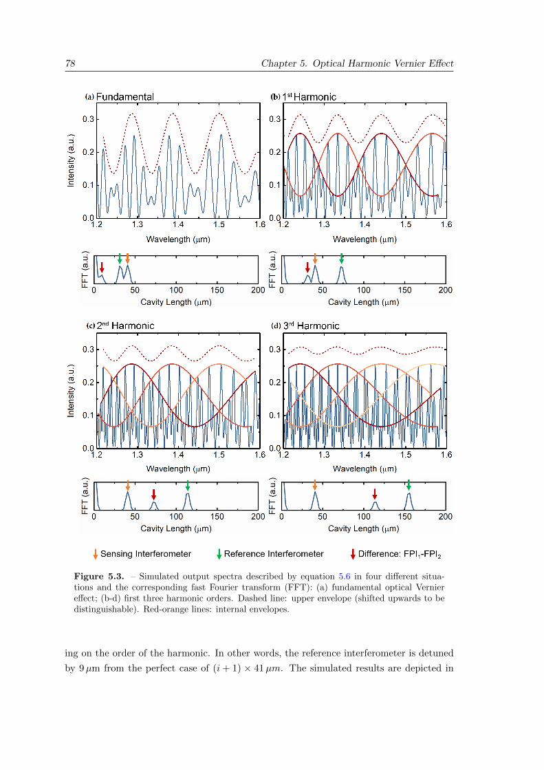
78 Chapter 5. Optical Harmonic Vernier Effect
Figure 5.3. – Simulated output spectra described by equation 5.6 in four different situa-tions and the corresponding fast Fourier transform (FFT): (a) fundamental optical Verniereffect; (b-d) first three harmonic orders. Dashed line: upper envelope (shifted upwards to bedistinguishable). Red-orange lines: internal envelopes.
ing on the order of the harmonic. In other words, the reference interferometer is detuned
by 9µm from the perfect case of (i+ 1) × 41µm. The simulated results are depicted in
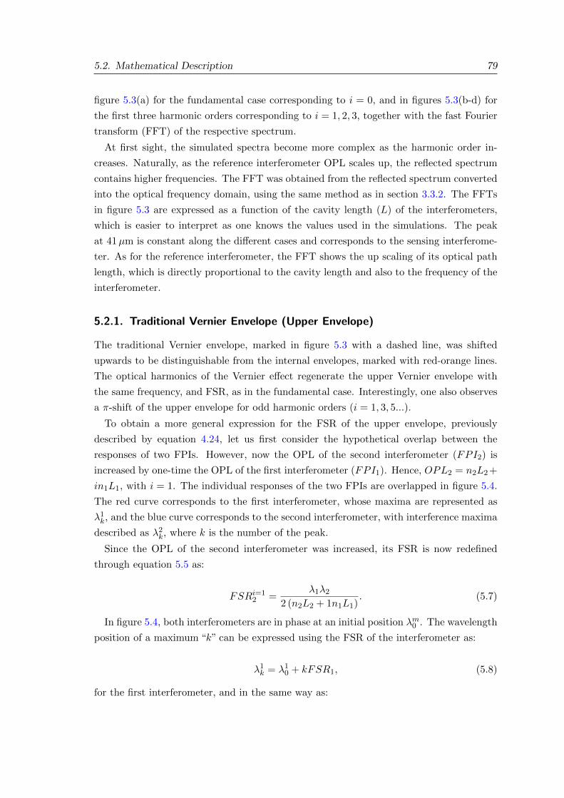
5.2. Mathematical Description 79
figure 5.3(a) for the fundamental case corresponding to i = 0, and in figures 5.3(b-d) for
the first three harmonic orders corresponding to i = 1, 2, 3, together with the fast Fourier
transform (FFT) of the respective spectrum.
At first sight, the simulated spectra become more complex as the harmonic order in-
creases. Naturally, as the reference interferometer OPL scales up, the reflected spectrum
contains higher frequencies. The FFT was obtained from the reflected spectrum converted
into the optical frequency domain, using the same method as in section 3.3.2. The FFTs
in figure 5.3 are expressed as a function of the cavity length (L) of the interferometers,
which is easier to interpret as one knows the values used in the simulations. The peak
at 41µm is constant along the different cases and corresponds to the sensing interferome-
ter. As for the reference interferometer, the FFT shows the up scaling of its optical path
length, which is directly proportional to the cavity length and also to the frequency of the
interferometer.
5.2.1. Traditional Vernier Envelope (Upper Envelope)
The traditional Vernier envelope, marked in figure 5.3 with a dashed line, was shifted
upwards to be distinguishable from the internal envelopes, marked with red-orange lines.
The optical harmonics of the Vernier effect regenerate the upper Vernier envelope with
the same frequency, and FSR, as in the fundamental case. Interestingly, one also observes
a π-shift of the upper envelope for odd harmonic orders (i = 1, 3, 5...).
To obtain a more general expression for the FSR of the upper envelope, previously
described by equation 4.24, let us first consider the hypothetical overlap between the
responses of two FPIs. However, now the OPL of the second interferometer (FPI2) is
increased by one-time the OPL of the first interferometer (FPI1). Hence, OPL2 = n2L2+
in1L1, with i = 1. The individual responses of the two FPIs are overlapped in figure 5.4.
The red curve corresponds to the first interferometer, whose maxima are represented as
λ1k, and the blue curve corresponds to the second interferometer, with interference maxima
described as λ2k, where k is the number of the peak.
Since the OPL of the second interferometer was increased, its FSR is now redefined
through equation 5.5 as:
FSRi=12 =
λ1λ22 (n2L2 + 1n1L1)
. (5.7)
In figure 5.4, both interferometers are in phase at an initial position λm0 . The wavelength
position of a maximum “k” can be expressed using the FSR of the interferometer as:
λ1k = λ10 + kFSR1, (5.8)
for the first interferometer, and in the same way as:

80 Chapter 5. Optical Harmonic Vernier Effect
Figure 5.4. – Schematic of the spectral response of two FPIs (1 and 2), where the OPL2
was increased by one-time the OPL1. The wavelengths of the different peaks are labeled asλmk , where m = 1, 2 is the number of the interferometer and k is the number of the peak.
λ2k = λ20 + kFSRi=12 , (5.9)
for the second interferometer. In figure 5.4, both interferometers will be once again in
phase when:
λ1k = λ22k+1. (5.10)
Combining equations 5.8 and 5.9 in equation 5.10, and considering that λ10 = λ20, the
following relationship is attained:
kFSR1 = (2k + 1)FSRi=12 . (5.11)
Expressing “k” as a function of the FSR of both interferometers, one obtains:
k =FSRi=1
2
FSR1 − 2FSRi=12
. (5.12)
The traditional Vernier envelope (upper envelope) in the optical Vernier effect is the
wavelength distance between two consecutive situations where both interferometers are in
phase. Hence the FSR of the Vernier upper envelope can be described as:
FSRenvelope = λ1k − λ0, (5.13)
which through equation 5.8 is the same as:
FSRenvelope = kFSR1. (5.14)
Replacing equation 5.12 in equation 5.14, the FSR of the the upper envelope for the
first harmonic of the Vernier effect as a function of the FSR of the two interferometers is:

5.2. Mathematical Description 81
FSRenvelope =
∣∣∣∣ FSRi=12 FSR1
FSR1 − 2FSRi=12
∣∣∣∣ , (5.15)
where the modulus was taken, since the FSR is a positive value.
This analysis can be generalized for any harmonic order (i) by considering that OPL2 =
n2L2 + in1L1. Therefore, equation 5.7 can be expressed more generally through equation
5.5. Starting from an initial in-phase situation, both interferometer will be once again in
phase when:
λ1k = λ2(i+1)k+1, (5.16)
being i the order of the harmonic. With this, equation 5.11 is generalized to:
kFSR1 = [(i+ 1) k + 1]FSRi2, (5.17)
where “k” is now defined as:
k =FSRi2
FSR1 − (i+ 1)FSRi2. (5.18)
At last, the general expression for the FSR of the upper envelope as a function of the
FSR of the two interferometers, for any harmonic order, is obtained when equation 5.18
is replaced in equation 5.14. The result is:
FSRienvelope =
∣∣∣∣ FSRi2FSR1
FSR1 − (i+ 1)FSRi2
∣∣∣∣ , (5.19)
where again the modulus was taken, since the FSR is always a positive quantity.
This general expression represents the regeneration property of the upper envelope, as
it turns out to be independent of the order of the harmonic. If one replaces the general
expression for the FSR of the reference FPI (equation 5.5) and the FSR of the sensing
FPI (equation 4.25) both in equation 5.19, assuming that the wavelengths λ1 and λ2 are
the same for both interferometers, the FSR of the upper envelope is independent of the
harmonic order i.
When using optical harmonics of the Vernier effect for sensing applications, tracing
the upper envelope and measuring the wavelength shift seems to have a drawback. The
visibility of the upper envelope decreases with the order of the harmonics, as seen in figure
5.3. In 2016, Zhao et al. had already discovered that increasing the ratio between the
OPLs by a multiple integer, keeping the same detuning, would reduce the visibility of
the upper envelope, while maintaining its FSR constant [167]. However, at that time
they did not figure out the concept of optical harmonic Vernier effect, together with its
benefits. Despite the reduction in visibility might seem to be a disadvantage, in practical
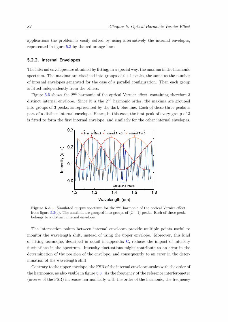
82 Chapter 5. Optical Harmonic Vernier Effect
applications the problem is easily solved by using alternatively the internal envelopes,
represented in figure 5.3 by the red-orange lines.
5.2.2. Internal Envelopes
The internal envelopes are obtained by fitting, in a special way, the maxima in the harmonic
spectrum. The maxima are classified into groups of i+ 1 peaks, the same as the number
of internal envelopes generated for the case of a parallel configuration. Then each group
is fitted independently from the others.
Figure 5.5 shows the 2nd harmonic of the optical Vernier effect, containing therefore 3
distinct internal envelope. Since it is the 2nd harmonic order, the maxima are grouped
into groups of 3 peaks, as represented by the dark blue line. Each of these three peaks is
part of a distinct internal envelope. Hence, in this case, the first peak of every group of 3
is fitted to form the first internal envelope, and similarly for the other internal envelopes.
Figure 5.5. – Simulated output spectrum for the 2nd harmonic of the optical Vernier effect,from figure 5.3(c). The maxima are grouped into groups of (2 + 1) peaks. Each of these peaksbelongs to a distinct internal envelope.
The intersection points between internal envelopes provide multiple points useful to
monitor the wavelength shift, instead of using the upper envelope. Moreover, this kind
of fitting technique, described in detail in appendix C, reduces the impact of intensity
fluctuations in the spectrum. Intensity fluctuations might contribute to an error in the
determination of the position of the envelope, and consequently to an error in the deter-
mination of the wavelength shift.
Contrary to the upper envelope, the FSR of the internal envelopes scales with the order of
the harmonics, as also visible in figure 5.3. As the frequency of the reference interferometer
(inverse of the FSR) increases harmonically with the order of the harmonic, the frequency
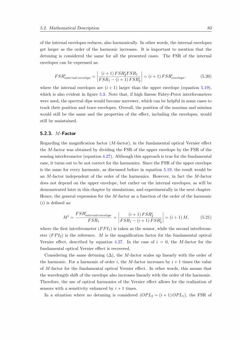
5.2. Mathematical Description 83
of the internal envelopes reduces, also harmonically. In other words, the internal envelopes
get larger as the order of the harmonic increases. It is important to mention that the
detuning is considered the same for all the presented cases. The FSR of the internal
envelopes can be expressed as:
FSRiinternal envelope =
∣∣∣∣ (i+ 1)FSRi2FSR1
FSR1 − (i+ 1)FSRi2
∣∣∣∣ = (i+ 1)FSRienvelope, (5.20)
where the internal envelopes are (i+ 1) larger than the upper envelope (equation 5.19),
which is also evident in figure 5.3. Note that, if high finesse Fabry-Perot interferometers
were used, the spectral dips would become narrower, which can be helpful in some cases to
track their position and trace envelopes. Overall, the position of the maxima and minima
would still be the same and the properties of the effect, including the envelopes, would
still be maintained.
5.2.3. M-Factor
Regarding the magnification factor (M -factor), in the fundamental optical Vernier effect
the M -factor was obtained by dividing the FSR of the upper envelope by the FSR of the
sensing interferometer (equation 4.27). Although this approach is true for the fundamental
case, it turns out to be not correct for the harmonics. Since the FSR of the upper envelope
is the same for every harmonic, as discussed before in equation 5.19, the result would be
an M -factor independent of the order of the harmonics. However, in fact the M -factor
does not depend on the upper envelope, but rather on the internal envelopes, as will be
demonstrated later in this chapter by simulations, and experimentally in the next chapter.
Hence, the general expression for the M -factor as a function of the order of the harmonic
(i) is defined as:
M i =FSRiinternal envelope
FSR1=
∣∣∣∣ (i+ 1)FSRi2FSR1 − (i+ 1)FSRi2
∣∣∣∣ = (i+ 1)M, (5.21)
where the first interferometer (FPI1) is taken as the sensor, while the second interferom-
eter (FPI2) is the reference. M is the magnification factor for the fundamental optical
Vernier effect, described by equation 4.27. In the case of i = 0, the M -factor for the
fundamental optical Vernier effect is recovered.
Considering the same detuning (∆), the M -factor scales up linearly with the order of
the harmonic. For a harmonic of order i, the M -factor increases by i+ 1 times the value
of M -factor for the fundamental optical Vernier effect. In other words, this means that
the wavelength shift of the envelope also increases linearly with the order of the harmonic.
Therefore, the use of optical harmonics of the Vernier effect allows for the realization of
sensors with a sensitivity enhanced by i+ 1 times.
In a situation where no detuning is considered (OPL2 = (i+ 1)OPL1), the FSR of
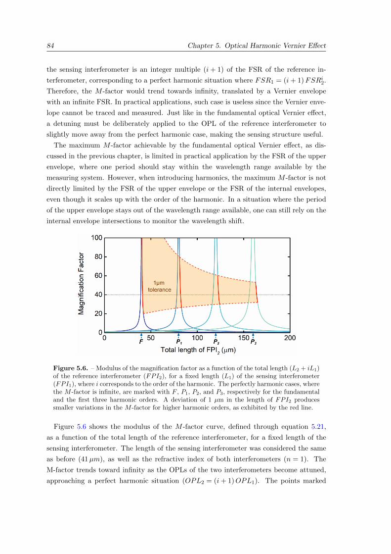
84 Chapter 5. Optical Harmonic Vernier Effect
the sensing interferometer is an integer multiple (i+ 1) of the FSR of the reference in-
terferometer, corresponding to a perfect harmonic situation where FSR1 = (i+ 1)FSRi2.
Therefore, the M -factor would trend towards infinity, translated by a Vernier envelope
with an infinite FSR. In practical applications, such case is useless since the Vernier enve-
lope cannot be traced and measured. Just like in the fundamental optical Vernier effect,
a detuning must be deliberately applied to the OPL of the reference interferometer to
slightly move away from the perfect harmonic case, making the sensing structure useful.
The maximum M -factor achievable by the fundamental optical Vernier effect, as dis-
cussed in the previous chapter, is limited in practical application by the FSR of the upper
envelope, where one period should stay within the wavelength range available by the
measuring system. However, when introducing harmonics, the maximum M -factor is not
directly limited by the FSR of the upper envelope or the FSR of the internal envelopes,
even though it scales up with the order of the harmonic. In a situation where the period
of the upper envelope stays out of the wavelength range available, one can still rely on the
internal envelope intersections to monitor the wavelength shift.
Figure 5.6. – Modulus of the magnification factor as a function of the total length (L2 + iL1)of the reference interferometer (FPI2), for a fixed length (L1) of the sensing interferometer(FPI1), where i corresponds to the order of the harmonic. The perfectly harmonic cases, wherethe M -factor is infinite, are marked with F , P1, P2, and P3, respectively for the fundamentaland the first three harmonic orders. A deviation of 1 µm in the length of FPI2 producessmaller variations in the M -factor for higher harmonic orders, as exhibited by the red line.
Figure 5.6 shows the modulus of the M -factor curve, defined through equation 5.21,
as a function of the total length of the reference interferometer, for a fixed length of the
sensing interferometer. The length of the sensing interferometer was considered the same
as before (41µm), as well as the refractive index of both interferometers (n = 1). The
M-factor trends toward infinity as the OPLs of the two interferometers become attuned,
approaching a perfect harmonic situation (OPL2 = (i+ 1)OPL1). The points marked
5.2. Mathematical Description 85
as F , P1, P2, and P3 correspond to these perfect harmonic cases, respectively for the
fundamental and the first three harmonic orders of the Vernier effect.
An interesting property is noticeable in the diagram of figure 5.6: the M -factor curve
broadens for higher harmonic orders. The M -factor curve broadening allows higher M -
factors to be achieved more easily. Moreover, it also reduces the impact of small detuning
errors. The red line in figure 5.6 targets a specific M -factor (M = 40). When changing the
length of the reference FPI by ±1 µm, simulating a detuning error, the variation caused
in the M -factor value is smaller for higher harmonic orders. Therefore, higher harmonic
orders allow larger tolerances in sensor fabrication without compromising its performance.
Figure 5.7. – Magnification factor as a function of the detuning (∆) from a perfectly har-monic situation applied to the reference interferometer (FPI2). For the same detuning, themagnification factor scales up linearly with the order of the harmonics as can be seen e.g. bythe values at the red circles. Small detuning errors from multiple sources, such as fabricationtolerances, can modify the obtained magnification factor.
There are different sources of detuning errors. Environmental effects, such as temper-
ature changes or deformation/strain, typically result in a percentage change in the in-
terferometer length and would become more relevant for longer reference interferometers.
Aside from these environmental effects, errors and tolerances in the fabrication process
also contribute as detuning errors. Strain or deformation effects are negligible in this case,
since the reference interferometer is considered stable, where no strain is applied to it.
The thermal expansion coefficient of silica is around 0.55 × 10⁻⁶K−1 [104], which for a
86 Chapter 5. Optical Harmonic Vernier Effect
5 °C temperature variation corresponds to a length variation of 2.75×10⁻⁴ %. In practical
terms, the length variation caused by such temperature change in a 100 µm-long FPI cavity
is of about 0.275 nm. For a 1 mm-long FPI cavity that corresponds to a length variation
of 0.275 µm. Note that these variable parameters produce a detuning error which is, in
general, below the error imposed by the accuracy of the fabrication procedures (normally
between 1 µm to a few micrometers). In sum, the limiting factor here is the detuning
error caused by the fabrication process, which is a fixed value dependent on the available
fabrication technology.
Figure 5.7 represents a different way to approach these concepts. Here, the M -factor
is shown as a function of the detuning (∆) from the perfectly harmonic case, for the
fundamental case and for the first three harmonic orders of the optical Vernier effect. One
can observe that, for the same detuning, the M -factor scales up linearly with the order
of the harmonics, as seen by the value at the red circles. It is worth mentioning that,
even though the red circles do not represent a perfect harmonic case, for a fixed detuning
the scaling properties of the effect (magnification factor, number of internal envelopes,
frequency of the internal envelope) can still be seen as harmonic. Recalling what has
been discussed previously, the detuning is introduced on purpose to make the envelope
measurable. Figure 5.7 also presents a detuning error of 1µm, showing how it can affect
the final M -factor.
The next section presents simulated results of the optical harmonic Vernier effect for
sensing applications. The improvement of sensitivity, due to the enhancement of the M -
factor, will especially be demonstrated.
5.3. Simulation
To simulate the enhanced response obtained through the optical harmonic Vernier effect,
let us first start from the initial situation described in figure 5.3. The sensing FPI has an
OPL of 41µm and the OPL of the reference FPI is adjusted to introduce the fundamental
optical Vernier effect (32µm), as well as the first three harmonic orders (32µm+i×41µm,
with i = 1, 2, 3, respectively), while keeping the same detuning of 9µm.
The effect of a measurand is perceived by the sensing interferometer as a variation of
its OPL (refractive index and/or physical length). Hence, in all cases, the sensing inter-
ferometer OPL was increased by steps of 0.02µm, to a maximum of 0.08µm, simulating
the effect of a measurand. Figure 5.8(a) shows the response of the sensing FPI for the
variations of OPL applied. The sensing FPI presents a wavelength shift towards longer
wavelengths, as indicated by the arrow. The resulting upper envelope for the fundamental
optical Vernier effect, as well as the internal envelopes for the first three harmonic orders,
are also depicted in figures 5.8(b-e). For the sake of clarity only the upper envelope and
internal envelopes were plotted, instead of the whole spectra. In all cases, a wavelength
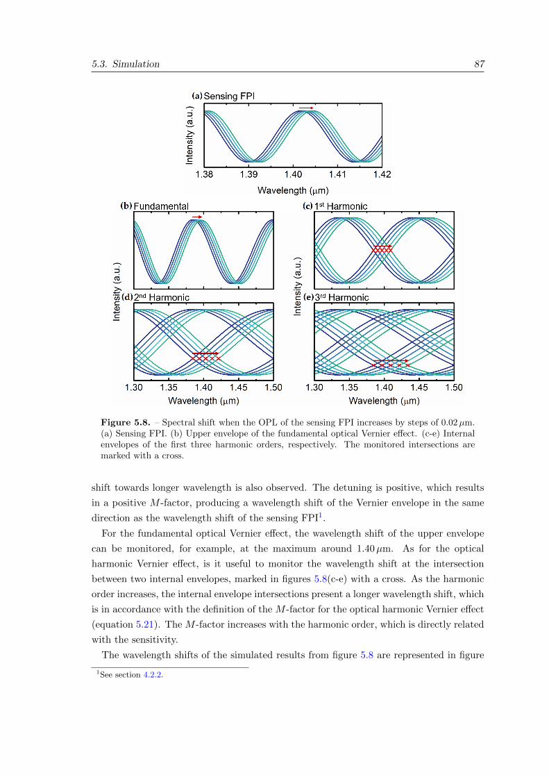
5.3. Simulation 87
Figure 5.8. – Spectral shift when the OPL of the sensing FPI increases by steps of 0.02µm.(a) Sensing FPI. (b) Upper envelope of the fundamental optical Vernier effect. (c-e) Internalenvelopes of the first three harmonic orders, respectively. The monitored intersections aremarked with a cross.
shift towards longer wavelength is also observed. The detuning is positive, which results
in a positive M -factor, producing a wavelength shift of the Vernier envelope in the same
direction as the wavelength shift of the sensing FPI1.
For the fundamental optical Vernier effect, the wavelength shift of the upper envelope
can be monitored, for example, at the maximum around 1.40µm. As for the optical
harmonic Vernier effect, is it useful to monitor the wavelength shift at the intersection
between two internal envelopes, marked in figures 5.8(c-e) with a cross. As the harmonic
order increases, the internal envelope intersections present a longer wavelength shift, which
is in accordance with the definition of the M -factor for the optical harmonic Vernier effect
(equation 5.21). The M -factor increases with the harmonic order, which is directly related
with the sensitivity.
The wavelength shifts of the simulated results from figure 5.8 are represented in figure
1See section 4.2.2.
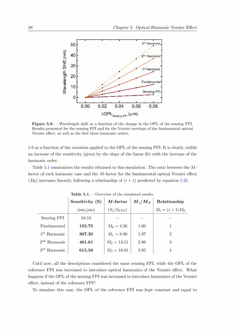
88 Chapter 5. Optical Harmonic Vernier Effect
Figure 5.9. – Wavelength shift as a function of the change in the OPL of the sensing FPI.Results presented for the sensing FPI and for the Vernier envelope of the fundamental opticalVernier effect, as well as the first three harmonic orders.
5.9 as a function of the variation applied to the OPL of the sensing FPI. It is clearly visible
an increase of the sensitivity (given by the slope of the linear fit) with the increase of the
harmonic order.
Table 5.1 summarizes the results obtained in this simulation. The ratio between the M -
factor of each harmonic case and the M -factor for the fundamental optical Vernier effect
(M0) increases linearly, following a relationship of (i+ 1) predicted by equation 5.21.
Table 5.1. – Overview of the simulated results.
Sensitivity (S) M -factor M i/M 0 Relationship
(nm/µm) (Si/SFPI) Mi = (i+ 1)M0
Sensing FPI 34.18 - - -
Fundamental 155.75 M0 = 4.56 1.00 1
1st Harmonic 307.20 M1 = 8.99 1.97 2
2nd Harmonic 461.61 M2 = 13.51 2.96 3
3rd Harmonic 615.50 M3 = 18.01 3.95 4
Until now, all the descriptions considered the same sensing FPI, while the OPL of the
reference FPI was increased to introduce optical harmonics of the Vernier effect. What
happens if the OPL of the sensing FPI was increased to introduce harmonics of the Vernier
effect, instead of the reference FPI?
To simulate this case, the OPL of the reference FPI was kept constant and equal to
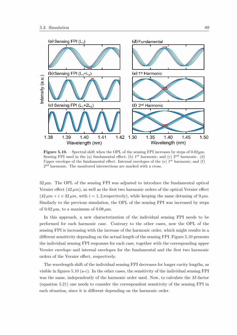
5.3. Simulation 89
Figure 5.10. – Spectral shift when the OPL of the sensing FPI increases by steps of 0.02 mm.Sensing FPI used in the (a) fundamental effect; (b) 1st harmonic; and (c) 2nd harmonic. (d)Upper envelope of the fundamental effect. Internal envelopes of the (e) 1st harmonic; and (f)2nd harmonic. The monitored intersections are marked with a cross.
32µm. The OPL of the sensing FPI was adjusted to introduce the fundamental optical
Vernier effect (42µm), as well as the first two harmonic orders of the optical Vernier effect
(42µm+ i× 32µm, with i = 1, 2,respectively), while keeping the same detuning of 9µm.
Similarly to the previous simulation, the OPL of the sensing FPI was increased by steps
of 0.02µm, to a maximum of 0.08µm.
In this approach, a new characterization of the individual sensing FPI needs to be
performed for each harmonic case. Contrary to the other cases, now the OPL of the
sensing FPI is increasing with the increase of the harmonic order, which might results in a
different sensitivity depending on the actual length of the sensing FPI. Figure 5.10 presents
the individual sensing FPI responses for each case, together with the corresponding upper
Vernier envelope and internal envelopes for the fundamental and the first two harmonic
orders of the Vernier effect, respectively.
The wavelength shift of the individual sensing FPI decreases for longer cavity lengths, as
visible in figures 5.10 (a-c). In the other cases, the sensitivity of the individual sensing FPI
was the same, independently of the harmonic order used. Now, to calculate the M -factor
(equation 5.21) one needs to consider the correspondent sensitivity of the sensing FPI in
each situation, since it is different depending on the harmonic order.
90 Chapter 5. Optical Harmonic Vernier Effect
The wavelength shifts of the upper envelope of the fundamental optical Vernier effect,
represented in figure 5.10 (d), and the internal envelopes for the first and second harmonic
orders, shown in figure 5.10(e) and (f), are approximately the same. The wavelength shift
of the Vernier envelope does not improve with the increase of the harmonic order. In fact,
it remains constant and independent of the harmonic order. Nevertheless, one should not
forget that the sensitivity of the individual sensing FPI is decreasing, which technically
results in an M -factor that is still increasing with the harmonic order. However, it does
not follow the relationship (i+ 1) presented before. To have a clear picture of these results,
a summary is shown in table 5.2.
Table 5.2. – Overview of the simulated results.
Sensitivity (S) M -factor M i/ FSR FSRInt. M-Factor
(nm/mm) (Si/SFPI) M 0 (nm) (nm) eq. 5.21
Sensing FPI 33.8 - - 23.96 -
Fundamental 155.24 M0 = 4.59 1.00 106.39 106.39 M0 = 4.44
Sensing FPI 19.05 13.37 -
1st Harmonic 154.26 M1 = 8.10 1.76 106.85 213.70 M1 = 15.98
Sensing FPI 13.33 9.40 -
2nd Harmonic 153.95 M2 = 11.55 2.52 106.66 319.97 M2 = 34.05
From the results depicted in the table, one observes that the M -factor increases with
the harmonic order, even though the sensitivity of the envelope is constant. As explained
before, this is caused by the reduction of the sensitivity of the individual sensing FPI.
Nevertheless, the ratio Mi/M0 does not follow the relationship (i+ 1) deduced previously.
Moreover, the M -factor calculated using the FSR of the internal envelopes, through equa-
tion 5.21, does not match with the one obtained by the sensitivities. In fact, the M -factor
calculated with the sensitivity values is approximately the same as if one calculates it
through the FSR of the upper envelope (instead of the internal envelope), which does not
change with the harmonic order.
The M -factors achieved in this case, shown in table 5.2, are slightly smaller than the
ones obtained in the results of table 5.1. However in practical applications, the sensitivity
of the Vernier envelope increases substantially in the first simulated situation, where the
OPL of the reference FPI is increasing. On the contrary, the second simulated case, where
the OPL of the sensing FPI is increasing, leads to a constant sensitivity, independent of
the harmonic order.
From a different point of view, increasing the OPL of the sensing FPI leads to a decrease
in its FSR, which is to say that the frequency of the interference signal increases. This
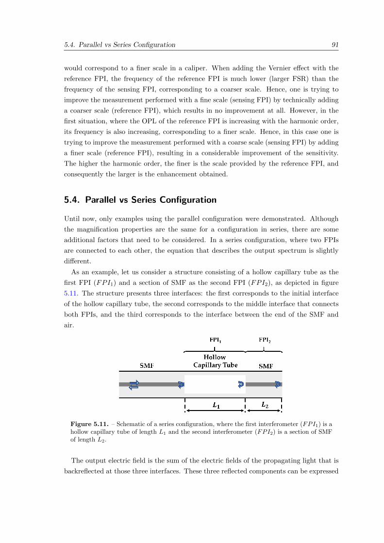
5.4. Parallel vs Series Configuration 91
would correspond to a finer scale in a caliper. When adding the Vernier effect with the
reference FPI, the frequency of the reference FPI is much lower (larger FSR) than the
frequency of the sensing FPI, corresponding to a coarser scale. Hence, one is trying to
improve the measurement performed with a fine scale (sensing FPI) by technically adding
a coarser scale (reference FPI), which results in no improvement at all. However, in the
first situation, where the OPL of the reference FPI is increasing with the harmonic order,
its frequency is also increasing, corresponding to a finer scale. Hence, in this case one is
trying to improve the measurement performed with a coarse scale (sensing FPI) by adding
a finer scale (reference FPI), resulting in a considerable improvement of the sensitivity.
The higher the harmonic order, the finer is the scale provided by the reference FPI, and
consequently the larger is the enhancement obtained.
5.4. Parallel vs Series Configuration
Until now, only examples using the parallel configuration were demonstrated. Although
the magnification properties are the same for a configuration in series, there are some
additional factors that need to be considered. In a series configuration, where two FPIs
are connected to each other, the equation that describes the output spectrum is slightly
different.
As an example, let us consider a structure consisting of a hollow capillary tube as the
first FPI (FPI1) and a section of SMF as the second FPI (FPI2), as depicted in figure
5.11. The structure presents three interfaces: the first corresponds to the initial interface
of the hollow capillary tube, the second corresponds to the middle interface that connects
both FPIs, and the third corresponds to the interface between the end of the SMF and
air.
Figure 5.11. – Schematic of a series configuration, where the first interferometer (FPI1) is ahollow capillary tube of length L1 and the second interferometer (FPI2) is a section of SMFof length L2.
The output electric field is the sum of the electric fields of the propagating light that is
backreflected at those three interfaces. These three reflected components can be expressed
92 Chapter 5. Optical Harmonic Vernier Effect
as:
ER1 (λ) = AEin (λ) , (5.22)
ER2 (λ) = BEin (λ) exp
[−j(
4πn1L1
λ− π
)], (5.23)
ER3 (λ) = CEin (λ) exp
[−j 4π (n1L1 + n2L2)
λ
]. (5.24)
The coefficients A, B, and C are given by:
A =√R1, (5.25)
B = (1−A1) (1−R1) exp (−2α1L1)√R2, (5.26)
C = (1−A1) (1−A2) exp (−2α1L1) exp (−2α2L2) (1−R1) (1−R2)√R3, (5.27)
where Ri is the intensity reflection coefficient at the interface i (with i = 1, 2, 3), A1 and
A2 represent the transmission losses through the first and second interfaces, respectively,
α1 and α2 are related with the propagation losses.
Through equation 4.11, the reflected light intensity measured at the output can then be
expressed as:
Iout (λ) = I0 − 2AB cos
(4πn1L1
λ
)− 2BC cos
(4πn2L2
λ
)(5.28)
+ 2AC cos
[4π (n1L1 + n2L2)
λ
],
where I0 = A2 +B2 + C2 .
Once again, if the OPL of the second interferometer (FPI2) is increased by a multiple
(i -times) of the OPL of the first interferometer (FPI1), then optical harmonics of the
Vernier effect are introduced. With this, the expression for the reflected light intensity
measured at the output can be rewritten as:
5.4. Parallel vs Series Configuration 93
Iiout (λ) = I0 − 2AB cos
(4πn1L1
λ
)− 2BC cos
[4π (n2L2 + in1L1)
λ
](5.29)
+ 2AC cos
{4π [(i+ 1)n1L1 + n2L2]
λ
}.
Comparing the output spectrum for a parallel configuration, given by equation 5.6, with
the output spectrum for a series configuration, expressed by equation 5.29, the main dif-
ference relies on the last cosine function, apart from the prefactors A, B, and C. In a
series configuration, the last cosine expresses the sum between the OPLs of both inter-
ferometers, while in a parallel configuration it is actually the difference. This leads to
the presence of an additional higher frequency component in the output spectrum for the
series configuration.
Interestingly, the output spectrum for a series configuration is visually one harmonic
order ahead of the output spectrum for a parallel configuration. For example, the output
spectrum for a series configuration corresponding to the first harmonic (i = 1), is given
by:
Ii=1out (λ) = I0 − 2AB cos
(4πn1L1
λ
)− 2BC cos
[4π (n2L2 + n1L1)
λ
](5.30)
+ 2AC cos
[4π (2n1L1 + n2L2)
λ
],
and the output spectrum for a parallel configuration corresponding to the second harmonic
(i = 2), is given by (equation 5.6, with i = 2):
II=2out (λ) = I0 − 2AB
{cos
(4πn1L1
λ
)+ cos
[4π (2n1L1 + n2L2)
λ
]}(5.31)
+B2 cos
[−4π (n2L2 + n1L1)
λ
].
Apart from the prefactors and the negative signs, the three frequencies presented in both
cases are the same. As a result, the output spectrum for a series configuration of harmonic
order i looks similar to the output spectrum for a parallel configuration of harmonic order
i+1. To verify this property, the output spectra for both configurations, given by equation
5.6 and equation 5.29, are represented in figure 5.12 for the fundamental and the first two
harmonic orders of the optical Vernier effect, respectively.
The output spectrum for a series configuration looks one harmonic order ahead of the
parallel configuration, which is also visible by the number of internal envelopes in figure
5.12. The number of internal envelopes for a series configuration increases with i+ 2, and
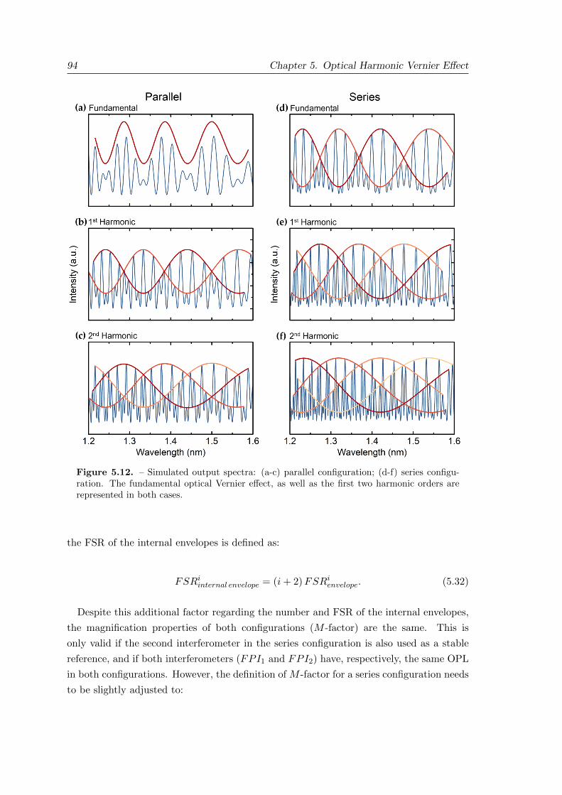
94 Chapter 5. Optical Harmonic Vernier Effect
Figure 5.12. – Simulated output spectra: (a-c) parallel configuration; (d-f) series configu-ration. The fundamental optical Vernier effect, as well as the first two harmonic orders arerepresented in both cases.
the FSR of the internal envelopes is defined as:
FSRiinternal envelope = (i+ 2)FSRienvelope. (5.32)
Despite this additional factor regarding the number and FSR of the internal envelopes,
the magnification properties of both configurations (M -factor) are the same. This is
only valid if the second interferometer in the series configuration is also used as a stable
reference, and if both interferometers (FPI1 and FPI2) have, respectively, the same OPL
in both configurations. However, the definition of M -factor for a series configuration needs
to be slightly adjusted to:
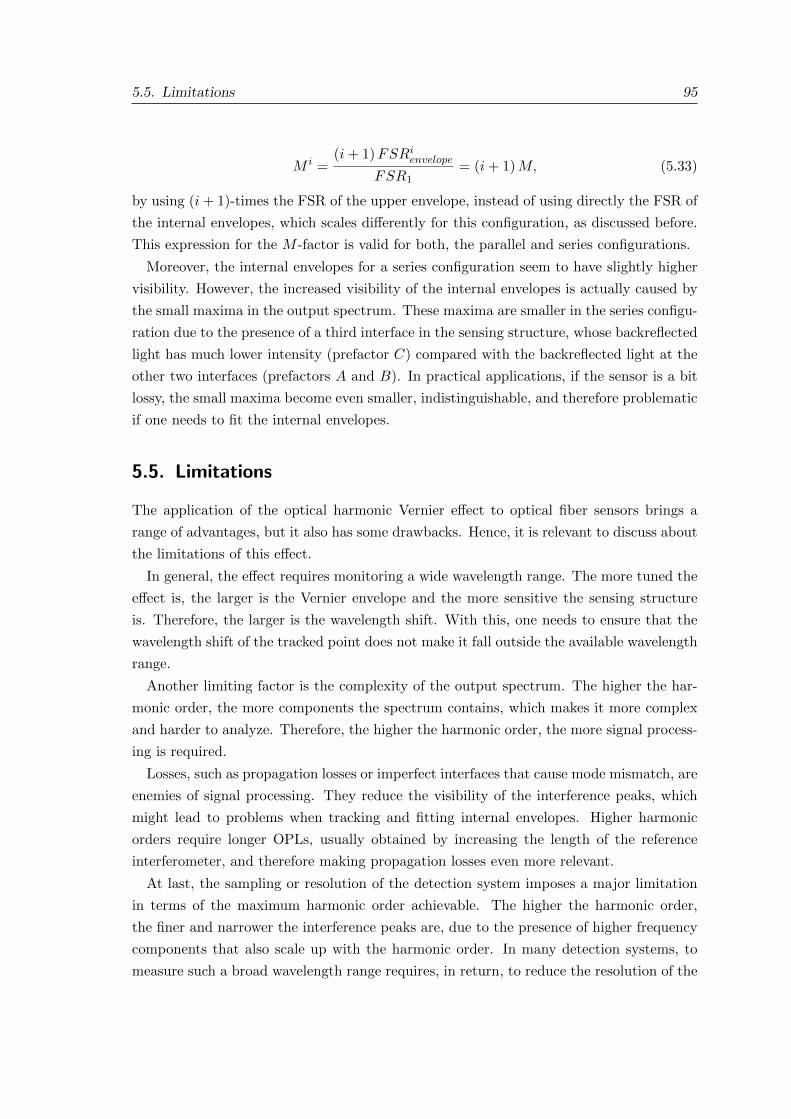
5.5. Limitations 95
M i =(i+ 1)FSRienvelope
FSR1= (i+ 1)M, (5.33)
by using (i+ 1)-times the FSR of the upper envelope, instead of using directly the FSR of
the internal envelopes, which scales differently for this configuration, as discussed before.
This expression for the M -factor is valid for both, the parallel and series configurations.
Moreover, the internal envelopes for a series configuration seem to have slightly higher
visibility. However, the increased visibility of the internal envelopes is actually caused by
the small maxima in the output spectrum. These maxima are smaller in the series configu-
ration due to the presence of a third interface in the sensing structure, whose backreflected
light has much lower intensity (prefactor C) compared with the backreflected light at the
other two interfaces (prefactors A and B). In practical applications, if the sensor is a bit
lossy, the small maxima become even smaller, indistinguishable, and therefore problematic
if one needs to fit the internal envelopes.
5.5. Limitations
The application of the optical harmonic Vernier effect to optical fiber sensors brings a
range of advantages, but it also has some drawbacks. Hence, it is relevant to discuss about
the limitations of this effect.
In general, the effect requires monitoring a wide wavelength range. The more tuned the
effect is, the larger is the Vernier envelope and the more sensitive the sensing structure
is. Therefore, the larger is the wavelength shift. With this, one needs to ensure that the
wavelength shift of the tracked point does not make it fall outside the available wavelength
range.
Another limiting factor is the complexity of the output spectrum. The higher the har-
monic order, the more components the spectrum contains, which makes it more complex
and harder to analyze. Therefore, the higher the harmonic order, the more signal process-
ing is required.
Losses, such as propagation losses or imperfect interfaces that cause mode mismatch, are
enemies of signal processing. They reduce the visibility of the interference peaks, which
might lead to problems when tracking and fitting internal envelopes. Higher harmonic
orders require longer OPLs, usually obtained by increasing the length of the reference
interferometer, and therefore making propagation losses even more relevant.
At last, the sampling or resolution of the detection system imposes a major limitation
in terms of the maximum harmonic order achievable. The higher the harmonic order,
the finer and narrower the interference peaks are, due to the presence of higher frequency
components that also scale up with the harmonic order. In many detection systems, to
measure such a broad wavelength range requires, in return, to reduce the resolution of the
96 Chapter 5. Optical Harmonic Vernier Effect
Figure 5.13. – Simulated output spectrum for the 4th harmonic of the optical Vernier effect.(a) Poor resolution spectrum: resolution of 500 pm. (b) Full resolution spectrum: resolutionof 1 pm. The position of the intersections between internal envelopes are marked with dashedlines.
measurement. If the detection system has poor resolution, the position of the interference
peaks are misleading and not well defined. Ultimately, tracing the upper envelope or
internal envelopes under these conditions can introduce large errors, producing an incorrect
result. Moreover, in worst scenarios where the resolution of the detection system (or
sampling rate) is not enough to detect the higher frequencies presented in higher harmonic
orders, then spectral aliasing is introduced. As a result, the output spectrum is malformed
and some interference peaks might be missing.
Figure 5.13 shows the simulated output spectrum for the 4th harmonic of the optical
Vernier effect for two different cases. The OPL of the sensing interferometer is 100µm and
the reference interferometer has a detuning of 9µm, with an OPL of (91µm+ 4× 100µm).
In figure 5.13(a), the resolution is poor (500 pm) and the position of the interference
peaks are not well defined. On contrary, figure 5.13(b) presents the same spectrum but
with a resolution of 1 pm, where all the interference peaks are well defined. In both
cases, the interference peaks were tracked and the internal envelopes were traced. It is
clearly visible that for a poor resolution spectrum the positions of the intersections between
internal envelopes are misplaced, when compared with the real positions showed in the
full resolution spectrum.
Note that the poor resolution spectrum is in the limit of the Nyquist criterion2. In
such case, performing a correct interpolation of the spectrum might still allow to achieve
2Nyquist criterion: the sampling rate should be higher than twice the highest frequency component ofthe spectrum
5.6. Conclusion 97
a corrected position of the interference peaks. Nevertheless, if one wants to use the next
harmonic order, the highest frequency of the spectrum would be even higher, falling out
of the Nyquist criterion. Moreover, the larger the initial sensing FPI, the smaller is its
FSR. Therefore, higher harmonic orders require an even longer reference FPIs, with even
smaller FSRs, and hence even higher frequencies.
5.6. Conclusion
As a way of closing this chapter, it is relevant to leave a few comments on the optical
harmonic Vernier effect as a summary of the different points discussed here.
In the previous chapter, the size of the upper Vernier envelope was a limiting factor
to the maximum M -factor achievable using the fundamental optical Vernier effect. With
the introduction of optical harmonics of the Vernier effect, the upper Vernier envelope
is regenerated with the same size as for the fundamental case. However, for the same
size of the upper Vernier envelope, the M -factors obtained are higher when using optical
harmonics of the Vernier effect. Hence, the proposed concept is a way to break the limits of
the fundamental effect, allowing for the realization of sensors with a sensitivity enhanced
by i+ 1 times. For example, achieving M -factors beyond 30 for single-type configurations
using FPIs becomes realistic. Moreover, the impact of detuning errors decreases with the
increase of the harmonic order.
Harmonics of the optical Vernier effect present internal envelopes that provide addi-
tional intersection points to better measure the wavelength shift. Measuring an intersec-
tion points is, in general, more accurate than measuring the position of a minimum (or
maximum) of the upper Vernier envelope.
When scaling up harmonically the sensing interferometer, instead of the reference inter-
ferometer, no improvement in sensitivity of the Vernier envelope is obtained when increas-
ing the harmonic order. In such case, the sensitivity for any harmonic order is the same
as the sensitivity of the fundamental case. Furthermore, the M -factor will not follow a
relationship of i+ 1.
In a series configuration, the magnification properties of the optical harmonic Vernier
effect are the same as for a parallel configuration. However, the output spectrum for a
series configuration looks visually one harmonic order ahead of the parallel configuration.
This means the series spectrum contains the higher frequencies of the next harmonic order
of the parallel spectrum, including also an extra internal envelope.
At last, some limitations of the effect were discussed, especially the impact of having a
detection system with a poor resolution or sampling rate.
The experimental demonstration of optical harmonics of the Vernier effect, in parallel
and in series, will be presented in the next chapter for real specific applications. Addition-
ally, the special case of having no reference interferometer will also be explored.

Chapter 6.
Demonstration and Applications of
Optical Harmonic Vernier Effect
6.1. Introduction
The optical harmonic Vernier effect was until now explored theoretically, together with
simulations that demonstrate the diverse properties of the effect. This chapter seeks to
demonstrate experimentally the introduction and application of optical harmonics of the
Vernier effect. Several experimental details are here discussed from a practical perspective,
especially regarding the fabrication of the structures.
The chapter is divided in two sections. The first one addresses the parallel configuration,
with a strong focus on validating the properties of the effect deduced theoretically, com-
paring experimental results with the theoretical ones. The second section is dedicated to
the series configuration, in particular to the special case of two interferometers physically
connected without a separation. This particular case can have three possible outputs, of
which one of them is the proposed structure and the other two are briefly discussed, but not
here demonstrated. The section also presents a way to use the structure for simultaneous
measurement of two parameters.
6.2. Parallel Configuration
6.2.1. Introduction
This section intends to demonstrate experimentally the optical harmonic Vernier effect in
a parallel configuration using Fabry-Perot interferometers (FPIs). Strain sensing is used
as possible application and as a mechanism to characterize and demonstrate the effect.
Important properties deduced in the previous chapter are here verified, as well as the
validation of the two definitions for the M -factor. At last, a compensated wavelength
shift method is presented as a way to compare the performance of the different structures
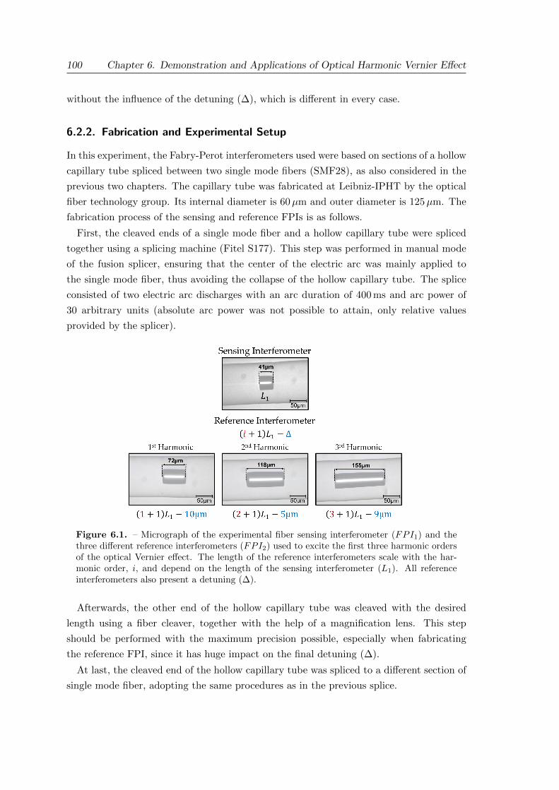
100 Chapter 6. Demonstration and Applications of Optical Harmonic Vernier Effect
without the influence of the detuning (∆), which is different in every case.
6.2.2. Fabrication and Experimental Setup
In this experiment, the Fabry-Perot interferometers used were based on sections of a hollow
capillary tube spliced between two single mode fibers (SMF28), as also considered in the
previous two chapters. The capillary tube was fabricated at Leibniz-IPHT by the optical
fiber technology group. Its internal diameter is 60µm and outer diameter is 125µm. The
fabrication process of the sensing and reference FPIs is as follows.
First, the cleaved ends of a single mode fiber and a hollow capillary tube were spliced
together using a splicing machine (Fitel S177). This step was performed in manual mode
of the fusion splicer, ensuring that the center of the electric arc was mainly applied to
the single mode fiber, thus avoiding the collapse of the hollow capillary tube. The splice
consisted of two electric arc discharges with an arc duration of 400 ms and arc power of
30 arbitrary units (absolute arc power was not possible to attain, only relative values
provided by the splicer).
Figure 6.1. – Micrograph of the experimental fiber sensing interferometer (FPI1) and thethree different reference interferometers (FPI2) used to excite the first three harmonic ordersof the optical Vernier effect. The length of the reference interferometers scale with the har-monic order, i, and depend on the length of the sensing interferometer (L1). All referenceinterferometers also present a detuning (∆).
Afterwards, the other end of the hollow capillary tube was cleaved with the desired
length using a fiber cleaver, together with the help of a magnification lens. This step
should be performed with the maximum precision possible, especially when fabricating
the reference FPI, since it has huge impact on the final detuning (∆).
At last, the cleaved end of the hollow capillary tube was spliced to a different section of
single mode fiber, adopting the same procedures as in the previous splice.
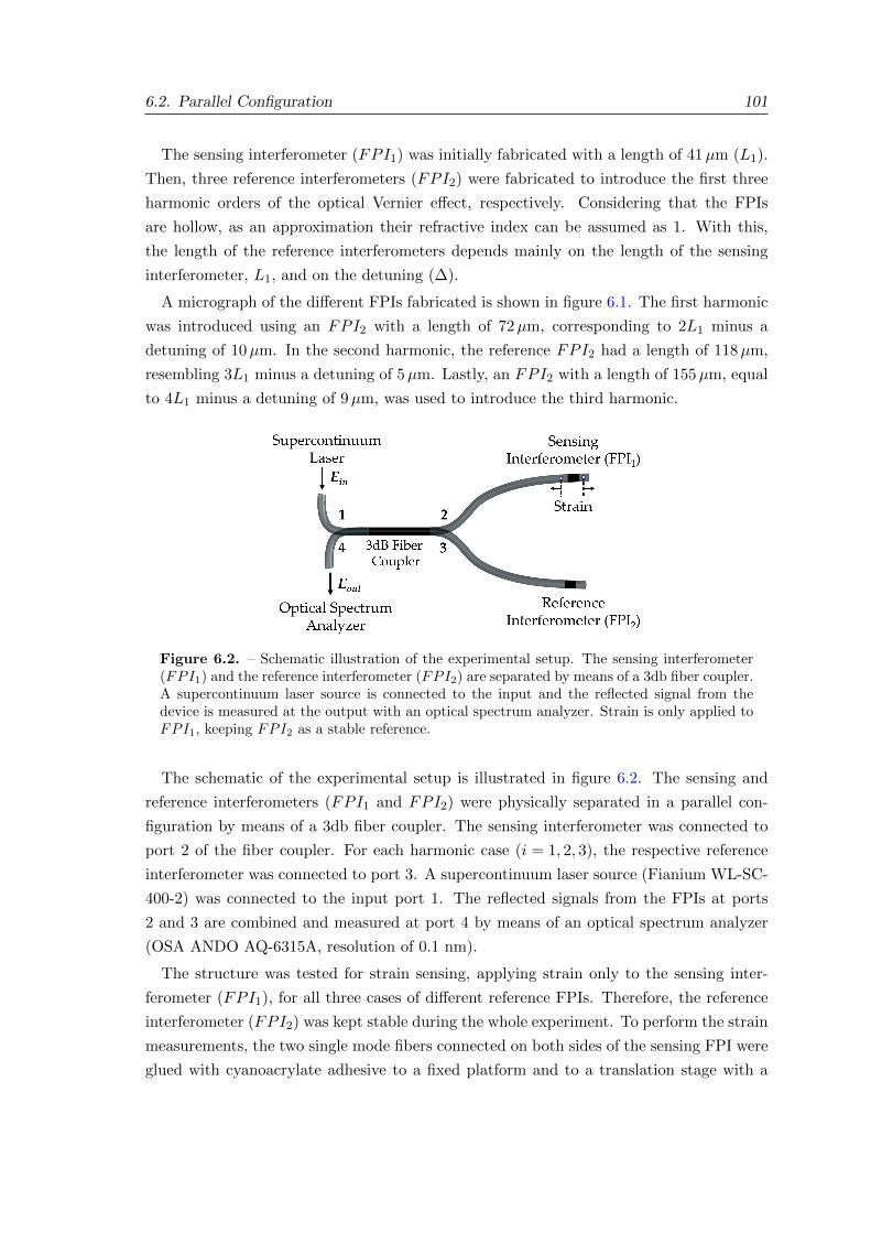
6.2. Parallel Configuration 101
The sensing interferometer (FPI1) was initially fabricated with a length of 41µm (L1).
Then, three reference interferometers (FPI2) were fabricated to introduce the first three
harmonic orders of the optical Vernier effect, respectively. Considering that the FPIs
are hollow, as an approximation their refractive index can be assumed as 1. With this,
the length of the reference interferometers depends mainly on the length of the sensing
interferometer, L1, and on the detuning (∆).
A micrograph of the different FPIs fabricated is shown in figure 6.1. The first harmonic
was introduced using an FPI2 with a length of 72µm, corresponding to 2L1 minus a
detuning of 10µm. In the second harmonic, the reference FPI2 had a length of 118µm,
resembling 3L1 minus a detuning of 5µm. Lastly, an FPI2 with a length of 155µm, equal
to 4L1 minus a detuning of 9µm, was used to introduce the third harmonic.
Figure 6.2. – Schematic illustration of the experimental setup. The sensing interferometer(FPI1) and the reference interferometer (FPI2) are separated by means of a 3db fiber coupler.A supercontinuum laser source is connected to the input and the reflected signal from thedevice is measured at the output with an optical spectrum analyzer. Strain is only applied toFPI1, keeping FPI2 as a stable reference.
The schematic of the experimental setup is illustrated in figure 6.2. The sensing and
reference interferometers (FPI1 and FPI2) were physically separated in a parallel con-
figuration by means of a 3db fiber coupler. The sensing interferometer was connected to
port 2 of the fiber coupler. For each harmonic case (i = 1, 2, 3), the respective reference
interferometer was connected to port 3. A supercontinuum laser source (Fianium WL-SC-
400-2) was connected to the input port 1. The reflected signals from the FPIs at ports
2 and 3 are combined and measured at port 4 by means of an optical spectrum analyzer
(OSA ANDO AQ-6315A, resolution of 0.1 nm).
The structure was tested for strain sensing, applying strain only to the sensing inter-
ferometer (FPI1), for all three cases of different reference FPIs. Therefore, the reference
interferometer (FPI2) was kept stable during the whole experiment. To perform the strain
measurements, the two single mode fibers connected on both sides of the sensing FPI were
glued with cyanoacrylate adhesive to a fixed platform and to a translation stage with a
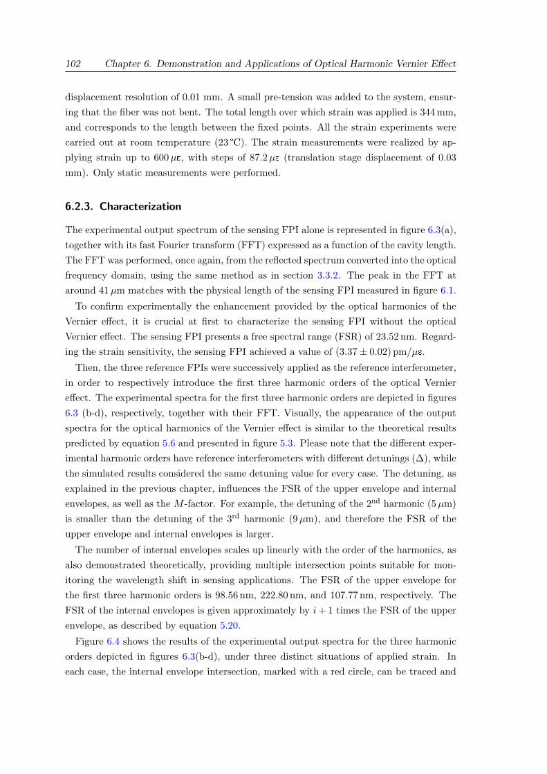
102 Chapter 6. Demonstration and Applications of Optical Harmonic Vernier Effect
displacement resolution of 0.01 mm. A small pre-tension was added to the system, ensur-
ing that the fiber was not bent. The total length over which strain was applied is 344 mm,
and corresponds to the length between the fixed points. All the strain experiments were
carried out at room temperature (23 °C). The strain measurements were realized by ap-
plying strain up to 600µe, with steps of 87.2µe (translation stage displacement of 0.03
mm). Only static measurements were performed.
6.2.3. Characterization
The experimental output spectrum of the sensing FPI alone is represented in figure 6.3(a),
together with its fast Fourier transform (FFT) expressed as a function of the cavity length.
The FFT was performed, once again, from the reflected spectrum converted into the optical
frequency domain, using the same method as in section 3.3.2. The peak in the FFT at
around 41µm matches with the physical length of the sensing FPI measured in figure 6.1.
To confirm experimentally the enhancement provided by the optical harmonics of the
Vernier effect, it is crucial at first to characterize the sensing FPI without the optical
Vernier effect. The sensing FPI presents a free spectral range (FSR) of 23.52 nm. Regard-
ing the strain sensitivity, the sensing FPI achieved a value of (3.37± 0.02) pm/µe.
Then, the three reference FPIs were successively applied as the reference interferometer,
in order to respectively introduce the first three harmonic orders of the optical Vernier
effect. The experimental spectra for the first three harmonic orders are depicted in figures
6.3 (b-d), respectively, together with their FFT. Visually, the appearance of the output
spectra for the optical harmonics of the Vernier effect is similar to the theoretical results
predicted by equation 5.6 and presented in figure 5.3. Please note that the different exper-
imental harmonic orders have reference interferometers with different detunings (∆), while
the simulated results considered the same detuning value for every case. The detuning, as
explained in the previous chapter, influences the FSR of the upper envelope and internal
envelopes, as well as the M -factor. For example, the detuning of the 2nd harmonic (5µm)
is smaller than the detuning of the 3rd harmonic (9µm), and therefore the FSR of the
upper envelope and internal envelopes is larger.
The number of internal envelopes scales up linearly with the order of the harmonics, as
also demonstrated theoretically, providing multiple intersection points suitable for mon-
itoring the wavelength shift in sensing applications. The FSR of the upper envelope for
the first three harmonic orders is 98.56 nm, 222.80 nm, and 107.77 nm, respectively. The
FSR of the internal envelopes is given approximately by i+ 1 times the FSR of the upper
envelope, as described by equation 5.20.
Figure 6.4 shows the results of the experimental output spectra for the three harmonic
orders depicted in figures 6.3(b-d), under three distinct situations of applied strain. In
each case, the internal envelope intersection, marked with a red circle, can be traced and
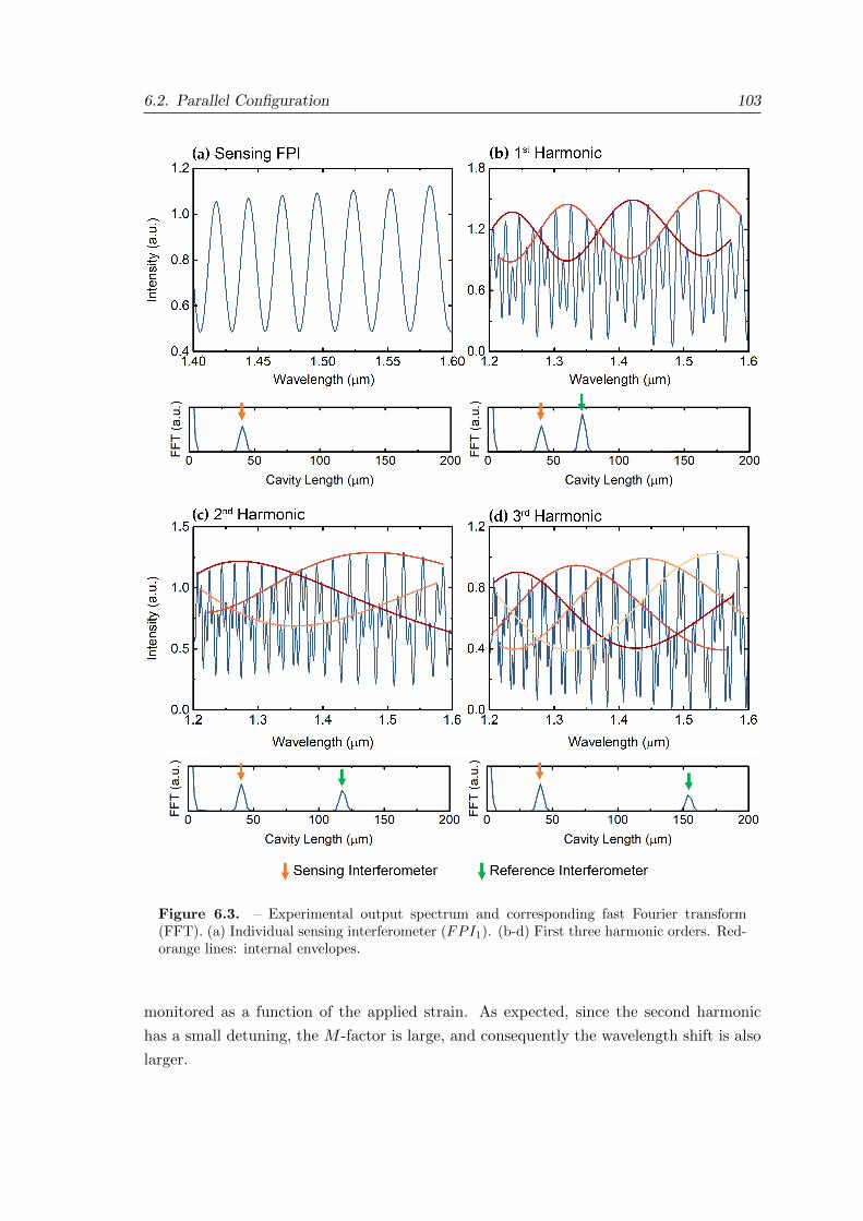
6.2. Parallel Configuration 103
Figure 6.3. – Experimental output spectrum and corresponding fast Fourier transform(FFT). (a) Individual sensing interferometer (FPI1). (b-d) First three harmonic orders. Red-orange lines: internal envelopes.
monitored as a function of the applied strain. As expected, since the second harmonic
has a small detuning, the M -factor is large, and consequently the wavelength shift is also
larger.
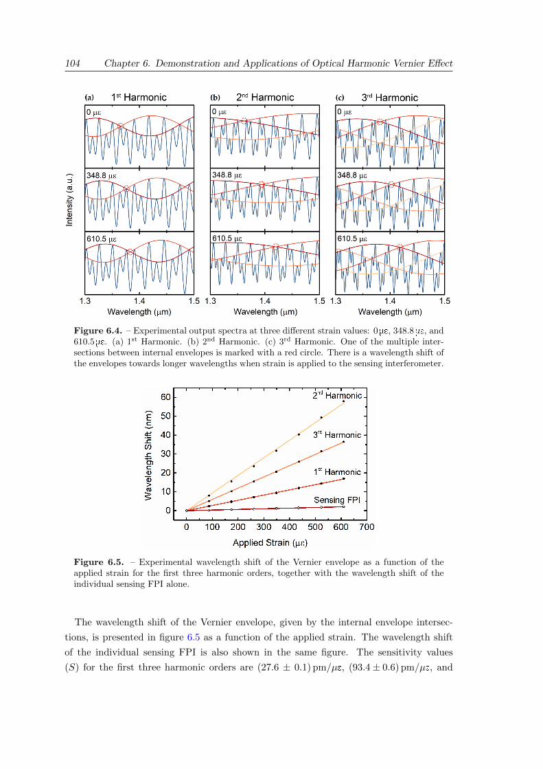
104 Chapter 6. Demonstration and Applications of Optical Harmonic Vernier Effect
Figure 6.4. – Experimental output spectra at three different strain values: 0 me, 348.8 me, and610.5 me. (a) 1st Harmonic. (b) 2nd Harmonic. (c) 3rd Harmonic. One of the multiple inter-sections between internal envelopes is marked with a red circle. There is a wavelength shift ofthe envelopes towards longer wavelengths when strain is applied to the sensing interferometer.
Figure 6.5. – Experimental wavelength shift of the Vernier envelope as a function of theapplied strain for the first three harmonic orders, together with the wavelength shift of theindividual sensing FPI alone.
The wavelength shift of the Vernier envelope, given by the internal envelope intersec-
tions, is presented in figure 6.5 as a function of the applied strain. The wavelength shift
of the individual sensing FPI is also shown in the same figure. The sensitivity values
(S) for the first three harmonic orders are (27.6 ± 0.1) pm/µe, (93.4± 0.6) pm/µe, and
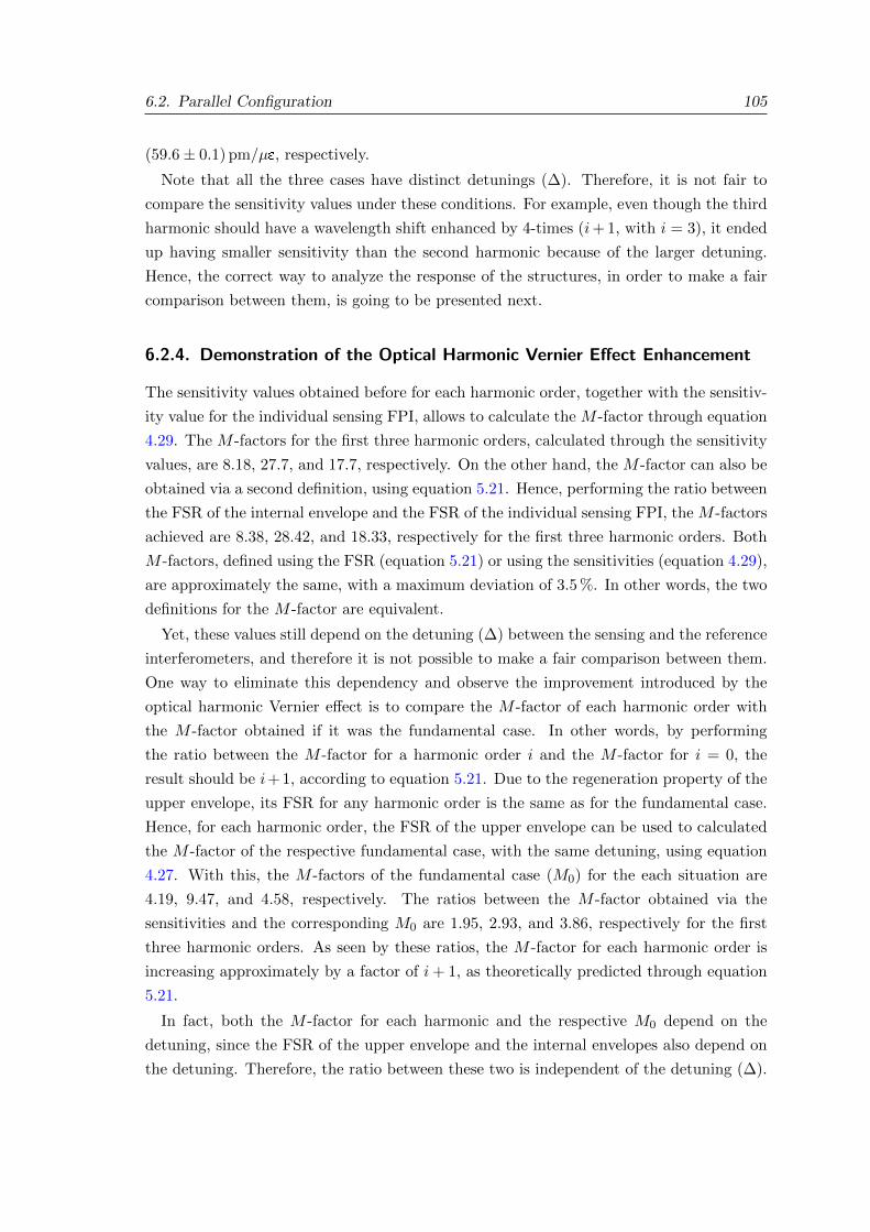
6.2. Parallel Configuration 105
(59.6± 0.1) pm/µe, respectively.
Note that all the three cases have distinct detunings (∆). Therefore, it is not fair to
compare the sensitivity values under these conditions. For example, even though the third
harmonic should have a wavelength shift enhanced by 4-times (i+ 1, with i = 3), it ended
up having smaller sensitivity than the second harmonic because of the larger detuning.
Hence, the correct way to analyze the response of the structures, in order to make a fair
comparison between them, is going to be presented next.
6.2.4. Demonstration of the Optical Harmonic Vernier Effect Enhancement
The sensitivity values obtained before for each harmonic order, together with the sensitiv-
ity value for the individual sensing FPI, allows to calculate the M -factor through equation
4.29. The M -factors for the first three harmonic orders, calculated through the sensitivity
values, are 8.18, 27.7, and 17.7, respectively. On the other hand, the M -factor can also be
obtained via a second definition, using equation 5.21. Hence, performing the ratio between
the FSR of the internal envelope and the FSR of the individual sensing FPI, the M -factors
achieved are 8.38, 28.42, and 18.33, respectively for the first three harmonic orders. Both
M -factors, defined using the FSR (equation 5.21) or using the sensitivities (equation 4.29),
are approximately the same, with a maximum deviation of 3.5 %. In other words, the two
definitions for the M -factor are equivalent.
Yet, these values still depend on the detuning (∆) between the sensing and the reference
interferometers, and therefore it is not possible to make a fair comparison between them.
One way to eliminate this dependency and observe the improvement introduced by the
optical harmonic Vernier effect is to compare the M -factor of each harmonic order with
the M -factor obtained if it was the fundamental case. In other words, by performing
the ratio between the M -factor for a harmonic order i and the M -factor for i = 0, the
result should be i+ 1, according to equation 5.21. Due to the regeneration property of the
upper envelope, its FSR for any harmonic order is the same as for the fundamental case.
Hence, for each harmonic order, the FSR of the upper envelope can be used to calculated
the M -factor of the respective fundamental case, with the same detuning, using equation
4.27. With this, the M -factors of the fundamental case (M0) for the each situation are
4.19, 9.47, and 4.58, respectively. The ratios between the M -factor obtained via the
sensitivities and the corresponding M0 are 1.95, 2.93, and 3.86, respectively for the first
three harmonic orders. As seen by these ratios, the M -factor for each harmonic order is
increasing approximately by a factor of i+ 1, as theoretically predicted through equation
5.21.
In fact, both the M -factor for each harmonic and the respective M0 depend on the
detuning, since the FSR of the upper envelope and the internal envelopes also depend on
the detuning. Therefore, the ratio between these two is independent of the detuning (∆).
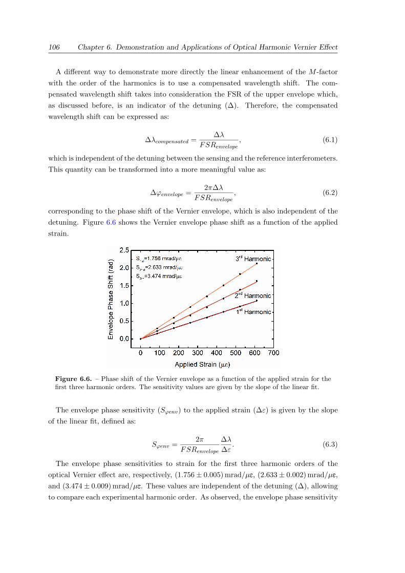
106 Chapter 6. Demonstration and Applications of Optical Harmonic Vernier Effect
A different way to demonstrate more directly the linear enhancement of the M -factor
with the order of the harmonics is to use a compensated wavelength shift. The com-
pensated wavelength shift takes into consideration the FSR of the upper envelope which,
as discussed before, is an indicator of the detuning (∆). Therefore, the compensated
wavelength shift can be expressed as:
∆λcompensated =∆λ
FSRenvelope, (6.1)
which is independent of the detuning between the sensing and the reference interferometers.
This quantity can be transformed into a more meaningful value as:
∆ϕenvelope =2π∆λ
FSRenvelope, (6.2)
corresponding to the phase shift of the Vernier envelope, which is also independent of the
detuning. Figure 6.6 shows the Vernier envelope phase shift as a function of the applied
strain.
Figure 6.6. – Phase shift of the Vernier envelope as a function of the applied strain for thefirst three harmonic orders. The sensitivity values are given by the slope of the linear fit.
The envelope phase sensitivity (Sϕenv) to the applied strain (∆ε) is given by the slope
of the linear fit, defined as:
Sϕenv =2π
FSRenvelope
∆λ
∆ε. (6.3)
The envelope phase sensitivities to strain for the first three harmonic orders of the
optical Vernier effect are, respectively, (1.756± 0.005) mrad/µe, (2.633± 0.002) mrad/µe,
and (3.474± 0.009) mrad/µe. These values are independent of the detuning (∆), allowing
to compare each experimental harmonic order. As observed, the envelope phase sensitivity
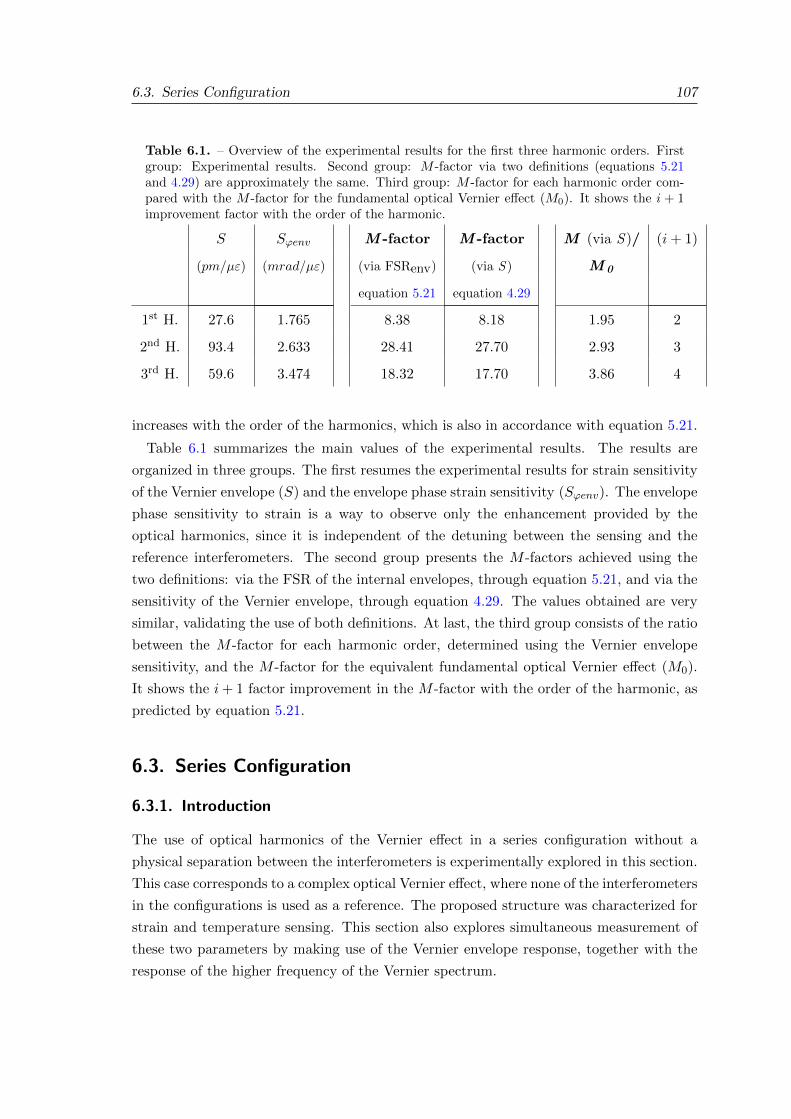
6.3. Series Configuration 107
Table 6.1. – Overview of the experimental results for the first three harmonic orders. Firstgroup: Experimental results. Second group: M -factor via two definitions (equations 5.21and 4.29) are approximately the same. Third group: M -factor for each harmonic order com-pared with the M -factor for the fundamental optical Vernier effect (M0). It shows the i + 1improvement factor with the order of the harmonic.
S Sϕenv M -factor M -factor M (via S )/ (i+ 1)
(pm/µε) (mrad/µε) (via FSRenv) (via S ) M 0
equation 5.21 equation 4.29
1st H. 27.6 1.765 8.38 8.18 1.95 2
2nd H. 93.4 2.633 28.41 27.70 2.93 3
3rd H. 59.6 3.474 18.32 17.70 3.86 4
increases with the order of the harmonics, which is also in accordance with equation 5.21.
Table 6.1 summarizes the main values of the experimental results. The results are
organized in three groups. The first resumes the experimental results for strain sensitivity
of the Vernier envelope (S) and the envelope phase strain sensitivity (Sϕenv). The envelope
phase sensitivity to strain is a way to observe only the enhancement provided by the
optical harmonics, since it is independent of the detuning between the sensing and the
reference interferometers. The second group presents the M -factors achieved using the
two definitions: via the FSR of the internal envelopes, through equation 5.21, and via the
sensitivity of the Vernier envelope, through equation 4.29. The values obtained are very
similar, validating the use of both definitions. At last, the third group consists of the ratio
between the M -factor for each harmonic order, determined using the Vernier envelope
sensitivity, and the M -factor for the equivalent fundamental optical Vernier effect (M0).
It shows the i+ 1 factor improvement in the M -factor with the order of the harmonic, as
predicted by equation 5.21.
6.3. Series Configuration
6.3.1. Introduction
The use of optical harmonics of the Vernier effect in a series configuration without a
physical separation between the interferometers is experimentally explored in this section.
This case corresponds to a complex optical Vernier effect, where none of the interferometers
in the configurations is used as a reference. The proposed structure was characterized for
strain and temperature sensing. This section also explores simultaneous measurement of
these two parameters by making use of the Vernier envelope response, together with the
response of the higher frequency of the Vernier spectrum.
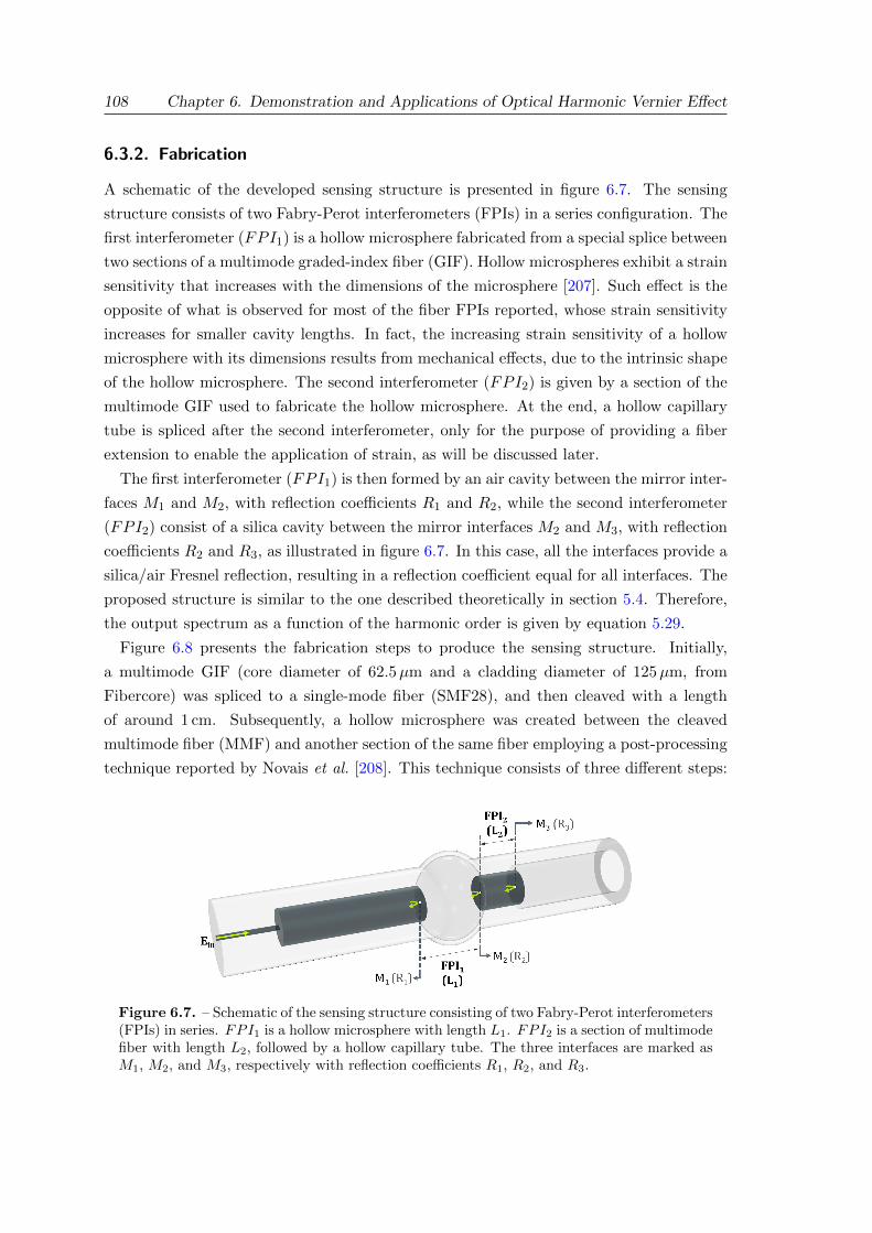
108 Chapter 6. Demonstration and Applications of Optical Harmonic Vernier Effect
6.3.2. Fabrication
A schematic of the developed sensing structure is presented in figure 6.7. The sensing
structure consists of two Fabry-Perot interferometers (FPIs) in a series configuration. The
first interferometer (FPI1) is a hollow microsphere fabricated from a special splice between
two sections of a multimode graded-index fiber (GIF). Hollow microspheres exhibit a strain
sensitivity that increases with the dimensions of the microsphere [207]. Such effect is the
opposite of what is observed for most of the fiber FPIs reported, whose strain sensitivity
increases for smaller cavity lengths. In fact, the increasing strain sensitivity of a hollow
microsphere with its dimensions results from mechanical effects, due to the intrinsic shape
of the hollow microsphere. The second interferometer (FPI2) is given by a section of the
multimode GIF used to fabricate the hollow microsphere. At the end, a hollow capillary
tube is spliced after the second interferometer, only for the purpose of providing a fiber
extension to enable the application of strain, as will be discussed later.
The first interferometer (FPI1) is then formed by an air cavity between the mirror inter-
faces M1 and M2, with reflection coefficients R1 and R2, while the second interferometer
(FPI2) consist of a silica cavity between the mirror interfaces M2 and M3, with reflection
coefficients R2 and R3, as illustrated in figure 6.7. In this case, all the interfaces provide a
silica/air Fresnel reflection, resulting in a reflection coefficient equal for all interfaces. The
proposed structure is similar to the one described theoretically in section 5.4. Therefore,
the output spectrum as a function of the harmonic order is given by equation 5.29.
Figure 6.8 presents the fabrication steps to produce the sensing structure. Initially,
a multimode GIF (core diameter of 62.5µm and a cladding diameter of 125µm, from
Fibercore) was spliced to a single-mode fiber (SMF28), and then cleaved with a length
of around 1 cm. Subsequently, a hollow microsphere was created between the cleaved
multimode fiber (MMF) and another section of the same fiber employing a post-processing
technique reported by Novais et al. [208]. This technique consists of three different steps:
Figure 6.7. – Schematic of the sensing structure consisting of two Fabry-Perot interferometers(FPIs) in series. FPI1 is a hollow microsphere with length L1. FPI2 is a section of multimodefiber with length L2, followed by a hollow capillary tube. The three interfaces are marked asM1, M2, and M3, respectively with reflection coefficients R1, R2, and R3.
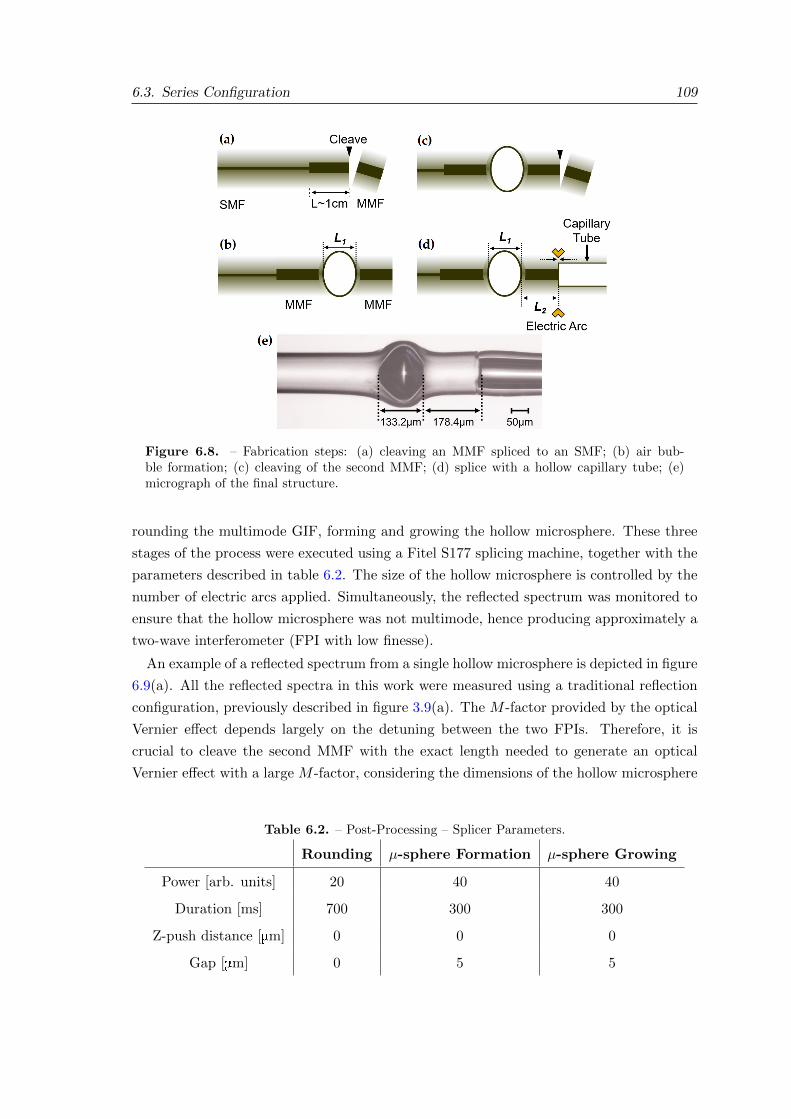
6.3. Series Configuration 109
Figure 6.8. – Fabrication steps: (a) cleaving an MMF spliced to an SMF; (b) air bub-ble formation; (c) cleaving of the second MMF; (d) splice with a hollow capillary tube; (e)micrograph of the final structure.
rounding the multimode GIF, forming and growing the hollow microsphere. These three
stages of the process were executed using a Fitel S177 splicing machine, together with the
parameters described in table 6.2. The size of the hollow microsphere is controlled by the
number of electric arcs applied. Simultaneously, the reflected spectrum was monitored to
ensure that the hollow microsphere was not multimode, hence producing approximately a
two-wave interferometer (FPI with low finesse).
An example of a reflected spectrum from a single hollow microsphere is depicted in figure
6.9(a). All the reflected spectra in this work were measured using a traditional reflection
configuration, previously described in figure 3.9(a). The M -factor provided by the optical
Vernier effect depends largely on the detuning between the two FPIs. Therefore, it is
crucial to cleave the second MMF with the exact length needed to generate an optical
Vernier effect with a large M -factor, considering the dimensions of the hollow microsphere
Table 6.2. – Post-Processing – Splicer Parameters.
Rounding µ-sphere Formation µ-sphere Growing
Power [arb. units] 20 40 40
Duration [ms] 700 300 300
Z-push distance [mm] 0 0 0
Gap [mm] 0 5 5
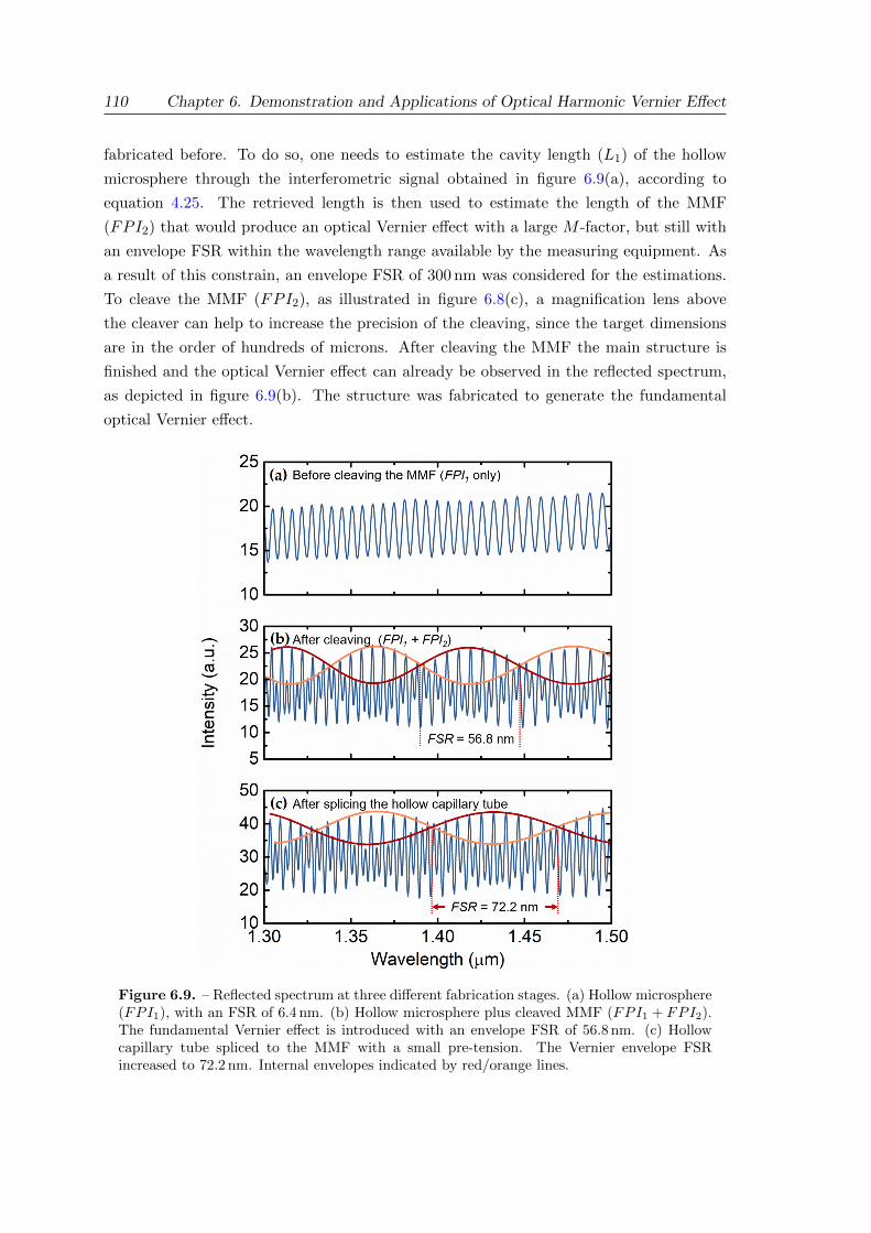
110 Chapter 6. Demonstration and Applications of Optical Harmonic Vernier Effect
fabricated before. To do so, one needs to estimate the cavity length (L1) of the hollow
microsphere through the interferometric signal obtained in figure 6.9(a), according to
equation 4.25. The retrieved length is then used to estimate the length of the MMF
(FPI2) that would produce an optical Vernier effect with a large M -factor, but still with
an envelope FSR within the wavelength range available by the measuring equipment. As
a result of this constrain, an envelope FSR of 300 nm was considered for the estimations.
To cleave the MMF (FPI2), as illustrated in figure 6.8(c), a magnification lens above
the cleaver can help to increase the precision of the cleaving, since the target dimensions
are in the order of hundreds of microns. After cleaving the MMF the main structure is
finished and the optical Vernier effect can already be observed in the reflected spectrum,
as depicted in figure 6.9(b). The structure was fabricated to generate the fundamental
optical Vernier effect.
Figure 6.9. – Reflected spectrum at three different fabrication stages. (a) Hollow microsphere(FPI1), with an FSR of 6.4 nm. (b) Hollow microsphere plus cleaved MMF (FPI1 + FPI2).The fundamental Vernier effect is introduced with an envelope FSR of 56.8 nm. (c) Hollowcapillary tube spliced to the MMF with a small pre-tension. The Vernier envelope FSRincreased to 72.2 nm. Internal envelopes indicated by red/orange lines.
6.3. Series Configuration 111
As stated before, a fiber extension is required so that the structure can work as a
strain sensor. However, the fiber extension must not affect the third interface (M3). The
best case is to add a fiber extension that preserves the silica/air interface. To solve this
problem, a hollow capillary tube with an inner diameter of 80µm (larger than the core of
the MMF) and an outer diameter of 125µm, fabricated at Leibniz IPHT, was used as a
fiber extension. The splice between the hollow capillary tube and the MMF was performed
with the electric arc centered in the capillary tube to avoid modifications of the MMF edge,
corresponding to the third interface (M3). Such modifications or deformations can cause
additional detuning between the two FPIs, reducing the M -factor of the optical Vernier
effect and, in extreme cases, leading to the annihilation of the effect. Nevertheless, if the
OPL of the second interferometer (FPI2) is slightly larger than desired, the splice between
the MMF and the hollow capillary tube can be used to tune the MMF length. The final
length of the MMF can be slightly reduced by compression if a small pre-tension between
the fibers is added before the splice. This effect is illustrated in figure 6.9(c), where the
reflection spectrum after splicing the hollow capillary tube with a small pre-tension allowed
to slightly reduce the OPL of the MMF, and consequently increase the FSR of the internal
envelopes compared with the previous case of figure 6.9(b). As a result, the final M -factor
of the structure is also increased.
The structure used as an example, whose spectra are presented in figure 6.9, corresponds
to the fundamental optical Vernier effect. To obtain a strain sensor with additional en-
hancement of sensitivity, it is valuable to make use of the optical harmonics of the Vernier
effect. In this case, a new hollow microsphere was fabricated using the same method and
the OPL of the second interferometer (FPI2), corresponding to the MMF, was increased
by 1-fold the OPL of the hollow microsphere. Such situation generates the first optical
harmonic of the Vernier effect. A micrograph of the final sensing structure is shown in
figure 6.8(e). The physical length (L1) of the hollow microsphere is 133.2 mm, while the
length of the MMF (L2) is 178.4 mm. Considering a refractive index (n2) of around 1.47
for the MMF, the OPL of the second interferometer (FPI2) is:
OPL2 = 2n2L2 = 2× 1.47× 178.4 = 524.5µm. (6.4)
As for the hollow microsphere, considering a refractive index of air (n1) equal to 1.0003
(at a temperature of 15 °C and wavelength of 1550 nm [146]), its OPL is given by:
OPL1 = 2n1L1 = 2× 1.0003× 133.2 = 266.5µm. (6.5)
The detuning between the two interferometers can be then estimated using equation
5.3, where the first harmonic corresponds to i = 1. Hence, the detuning of the fabricated
structure is approximately:

112 Chapter 6. Demonstration and Applications of Optical Harmonic Vernier Effect
Figure 6.10. – Reflected spectrum of the fabricated structure. The response corresponds tothe first harmonic of the Vernier effect in a series configuration.
OPL2 = (i+ 1)OPL1 − 2∆↔ ∆ = 4.25µm. (6.6)
Such small detuning value will generate a large Vernier envelope, with high M -factor.
The experimental reflected spectrum of this structure is presented in figure 6.10. The
presence of large internal envelopes is confirmed, as well as the number of internal envelopes
(3) matches expected number of i+2 for the first harmonic of the optical Vernier effect in a
series configuration, as discussed before in section 5.4. Note that peaks with low visibility
are visible in the experimental spectrum. Previously in the simulated reflected spectrum
of an equivalent structure, shown in figure 5.12(e), it was already possible to observe the
presence of peaks with lower visibility. This effect comes from the light reflected at the
third interface (M3) having much less intensity compared with the light reflected at the
other two interfaces. Adding to this, the presence losses and imperfections of the interfaces
reduces even more the visibility of the peaks.
6.3.3. Complex Optical Harmonic Vernier Effect
Up to now, all the cases of optical harmonic Vernier effect involved the use of one of the
interferometers as a stable reference. As explained in section 4.2.2, under the presence
of a stable reference interferometer the M -factor can be defined as the ratio between the
sensitivity of the Vernier envelope (Senvelope) and the sensitivity of the individual sensing
interferometer (SFPI1), expressed by equation 4.29.
Although for many sensing structures this description is correct, it is no longer valid for
this proposed configuration. Here, both interferometers are affected by the measurands at
the same time (strain and/or temperature). Hence, both interferometers are considered as
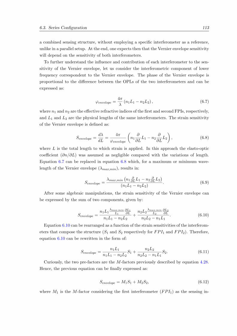
6.3. Series Configuration 113
a combined sensing structure, without employing a specific interferometer as a reference,
unlike in a parallel setup. At the end, one expects then that the Vernier envelope sensitivity
will depend on the sensitivity of both interferometers.
To further understand the influence and contribution of each interferometer to the sen-
sitivity of the Vernier envelope, let us consider the interferometric component of lower
frequency correspondent to the Vernier envelope. The phase of the Vernier envelope is
proportional to the difference between the OPLs of the two interferometers and can be
expressed as:
ϕenvelope =4π
λ(n1L1 − n2L2) , (6.7)
where n1 and n2 are the effective refractive indices of the first and second FPIs, respectively,
and L1 and L2 are the physical lengths of the same interferometers. The strain sensitivity
of the Vernier envelope is defined as:
Senvelope =dλ
dL=
4π
ϕenvelope
(n1
∂
∂LL1 − n2
∂
∂LL2
), (6.8)
where L is the total length to which strain is applied. In this approach the elasto-optic
coefficient (∂n/∂L) was assumed as negligible compared with the variations of length.
Equation 6.7 can be replaced in equation 6.8 which, for a maximum or minimum wave-
length of the Vernier envelope (λmax,min), results in:
Senvelope =λmax,min
(n1
∂∂LL1 − n2 ∂
∂LL2
)(n1L1 − n2L2)
. (6.9)
After some algebraic manipulations, the strain sensitivity of the Vernier envelope can
be expressed by the sum of two components, given by:
Senvelope =n1L1
λmax,min
L1
∂L1∂L
n1L1 − n2L2+n2L2
λmax,min
L2
∂L2∂L
n2L2 − n1L1. (6.10)
Equation 6.10 can be rearranged as a function of the strain sensitivities of the interferom-
eters that compose the structure (S1 and S2 respectively for FPI1 and FPI2). Therefore,
equation 6.10 can be rewritten in the form of:
Senvelope =n1L1
n1L1 − n2L2S1 +
n2L2
n2L2 − n1L1S2. (6.11)
Curiously, the two pre-factors are the M -factors previously described by equation 4.28.
Hence, the previous equation can be finally expressed as:
Senvelope = M1S1 +M2S2, (6.12)
where M1 is the M -factor considering the first interferometer (FPI1) as the sensing in-
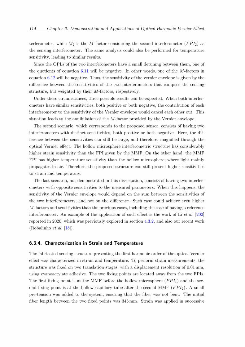
114 Chapter 6. Demonstration and Applications of Optical Harmonic Vernier Effect
terferometer, while M2 is the M -factor considering the second interferometer (FPI2) as
the sensing interferometer. The same analysis could also be performed for temperature
sensitivity, leading to similar results.
Since the OPLs of the two interferometers have a small detuning between them, one of
the quotients of equation 6.11 will be negative. In other words, one of the M -factors in
equation 6.12 will be negative. Thus, the sensitivity of the vernier envelope is given by the
difference between the sensitivities of the two interferometers that compose the sensing
structure, but weighted by their M -factors, respectively.
Under these circumstances, three possible results can be expected. When both interfer-
ometers have similar sensitivities, both positive or both negative, the contribution of each
interferometer to the sensitivity of the Vernier envelope would cancel each other out. This
situation leads to the annihilation of the M -factor provided by the Vernier envelope.
The second scenario, which corresponds to the proposed sensor, consists of having two
interferometers with distinct sensitivities, both positive or both negative. Here, the dif-
ference between the sensitivities can still be large, and therefore, magnified through the
optical Vernier effect. The hollow microsphere interferometric structure has considerably
higher strain sensitivity than the FPI given by the MMF. On the other hand, the MMF
FPI has higher temperature sensitivity than the hollow microsphere, where light mainly
propagates in air. Therefore, the proposed structure can still present higher sensitivities
to strain and temperature.
The last scenario, not demonstrated in this dissertation, consists of having two interfer-
ometers with opposite sensitivities to the measured parameters. When this happens, the
sensitivity of the Vernier envelope would depend on the sum between the sensitivities of
the two interferometers, and not on the difference. Such case could achieve even higher
M -factors and sensitivities than the previous cases, including the case of having a reference
interferometer. An example of the application of such effect is the work of Li et al. [202]
reported in 2020, which was previously explored in section 4.3.2, and also our recent work
(Robalinho et al. [18]).
6.3.4. Characterization in Strain and Temperature
The fabricated sensing structure presenting the first harmonic order of the optical Vernier
effect was characterized in strain and temperature. To perform strain measurements, the
structure was fixed on two translation stages, with a displacement resolution of 0.01 mm,
using cyanoacrylate adhesive. The two fixing points are located away from the two FPIs.
The first fixing point is at the MMF before the hollow microsphere (FPI1) and the sec-
ond fixing point is at the hollow capillary tube after the second MMF (FPI2) . A small
pre-tension was added to the system, ensuring that the fiber was not bent. The initial
fiber length between the two fixed points was 345 mm. Strain was applied in successive
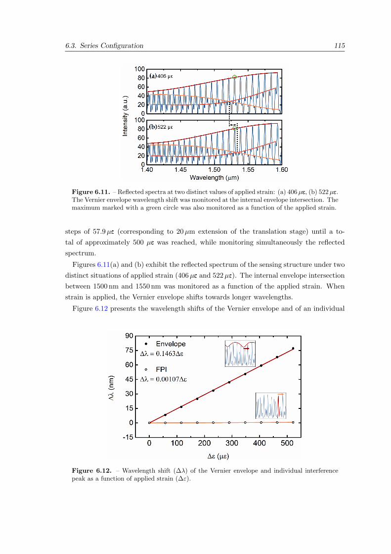
6.3. Series Configuration 115
Figure 6.11. – Reflected spectra at two distinct values of applied strain: (a) 406µe, (b) 522µe.The Vernier envelope wavelength shift was monitored at the internal envelope intersection. Themaximum marked with a green circle was also monitored as a function of the applied strain.
steps of 57.9µe (corresponding to 20µm extension of the translation stage) until a to-
tal of approximately 500 µe was reached, while monitoring simultaneously the reflected
spectrum.
Figures 6.11(a) and (b) exhibit the reflected spectrum of the sensing structure under two
distinct situations of applied strain (406µe and 522µe). The internal envelope intersection
between 1500 nm and 1550 nm was monitored as a function of the applied strain. When
strain is applied, the Vernier envelope shifts towards longer wavelengths.
Figure 6.12 presents the wavelength shifts of the Vernier envelope and of an individual
Figure 6.12. – Wavelength shift (∆λ) of the Vernier envelope and individual interferencepeak as a function of applied strain (∆ε).
116 Chapter 6. Demonstration and Applications of Optical Harmonic Vernier Effect
Figure 6.13. – Wavelength shift (∆λ) of the Vernier envelope and individual interferencepeak as a function of temperature (T ).
interference maximum, marked in figure 6.11 with a green circle, as a function of the
applied strain. The Vernier envelope achieved a strain sensitivity of (146.3± 0.4) pm/µe,
while the individual interference maximum showed a sensitivity of (1.070± 0.005) pm/µe.
The high sensitivity to strain achieved by the Vernier envelope is explained by two aspects:
first, by a large overall M -factor due to the first harmonic of the optical Vernier effect with
small detuning, and second, due the higher strain sensitivity of the hollow microsphere
when compared to the sensitivity of the second silica interferometer. The impact of using
higher harmonic orders of the optical Vernier effect in this configuration will be analyzed
later.
A similar analysis was performed to characterize the response of the sensing structure
to temperature. The sensor was placed inside a tubular oven, whose temperature was then
increased up to 100 °C. The sensor response was evaluated for a temperature decreasing
from 100 °C until room temperature. The wavelength shifts of the Vernier envelope and an
individual interference maximum, marked in figure 6.11 with a green circle, are depicted
in figure 6.13 as a function of temperature. The Vernier envelope showed a temperature
sensitivity of (−650± 9) pm/°C, while the individual interference maximum reached a
sensitivity value of (7.2± 0.2) pm/°C.
6.3.5. Simultaneous Measurement of Strain and Temperature
Even though the individual interference maximum does not correspond to the individual
response of the hollow microsphere (FPI1), neither to the individual response of the
MMF section (FPI2), as explored back in section 4.2.2, one can still make use of it.
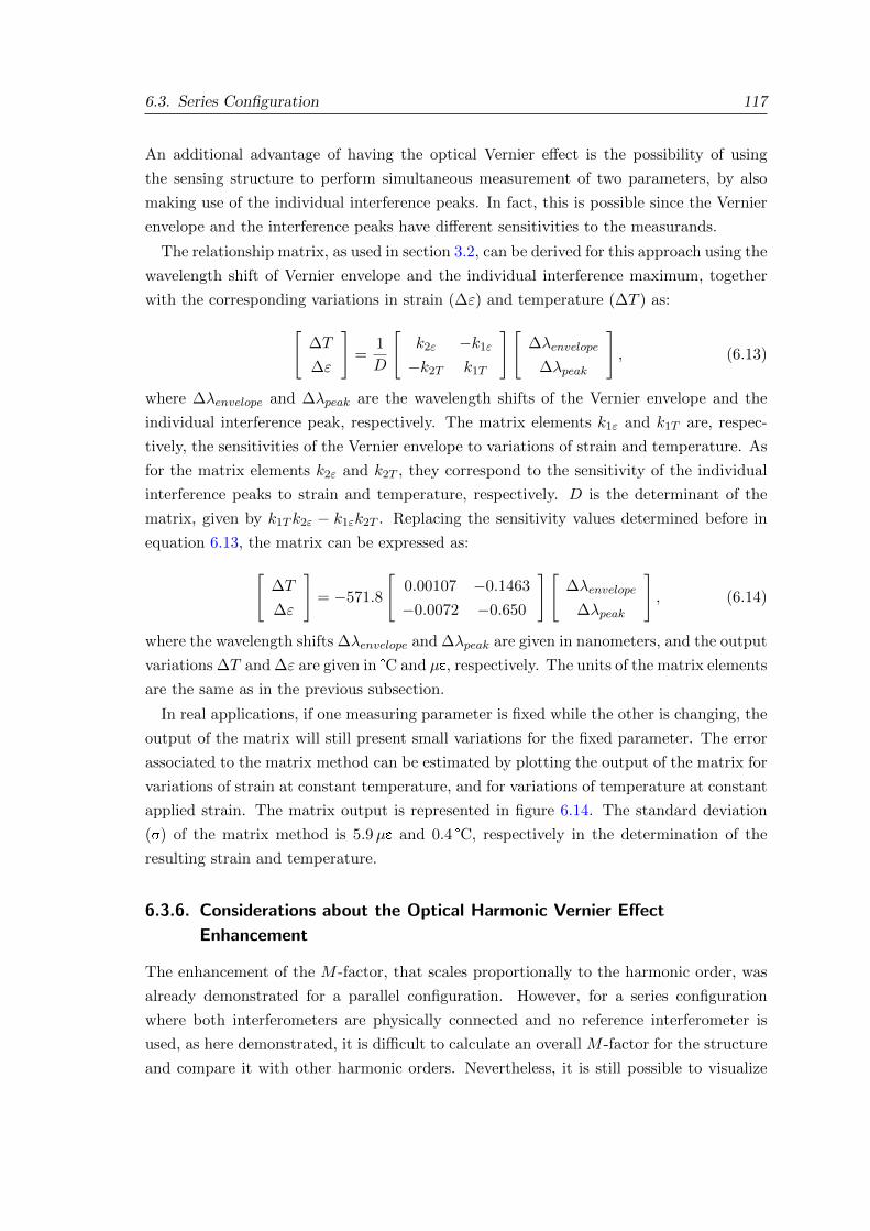
6.3. Series Configuration 117
An additional advantage of having the optical Vernier effect is the possibility of using
the sensing structure to perform simultaneous measurement of two parameters, by also
making use of the individual interference peaks. In fact, this is possible since the Vernier
envelope and the interference peaks have different sensitivities to the measurands.
The relationship matrix, as used in section 3.2, can be derived for this approach using the
wavelength shift of Vernier envelope and the individual interference maximum, together
with the corresponding variations in strain (∆ε) and temperature (∆T ) as:[∆T
∆ε
]=
1
D
[k2ε −k1ε−k2T k1T
][∆λenvelope
∆λpeak
], (6.13)
where ∆λenvelope and ∆λpeak are the wavelength shifts of the Vernier envelope and the
individual interference peak, respectively. The matrix elements k1ε and k1T are, respec-
tively, the sensitivities of the Vernier envelope to variations of strain and temperature. As
for the matrix elements k2ε and k2T , they correspond to the sensitivity of the individual
interference peaks to strain and temperature, respectively. D is the determinant of the
matrix, given by k1Tk2ε − k1εk2T . Replacing the sensitivity values determined before in
equation 6.13, the matrix can be expressed as:[∆T
∆ε
]= −571.8
[0.00107 −0.1463
−0.0072 −0.650
][∆λenvelope
∆λpeak
], (6.14)
where the wavelength shifts ∆λenvelope and ∆λpeak are given in nanometers, and the output
variations ∆T and ∆ε are given in °C and µe, respectively. The units of the matrix elements
are the same as in the previous subsection.
In real applications, if one measuring parameter is fixed while the other is changing, the
output of the matrix will still present small variations for the fixed parameter. The error
associated to the matrix method can be estimated by plotting the output of the matrix for
variations of strain at constant temperature, and for variations of temperature at constant
applied strain. The matrix output is represented in figure 6.14. The standard deviation
(sv) of the matrix method is 5.9µe and 0.4 °C, respectively in the determination of the
resulting strain and temperature.
6.3.6. Considerations about the Optical Harmonic Vernier Effect
Enhancement
The enhancement of the M -factor, that scales proportionally to the harmonic order, was
already demonstrated for a parallel configuration. However, for a series configuration
where both interferometers are physically connected and no reference interferometer is
used, as here demonstrated, it is difficult to calculate an overall M -factor for the structure
and compare it with other harmonic orders. Nevertheless, it is still possible to visualize
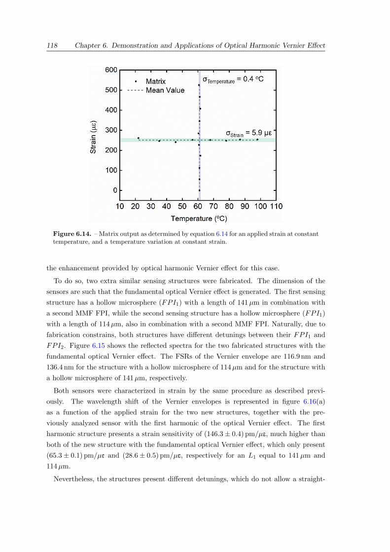
118 Chapter 6. Demonstration and Applications of Optical Harmonic Vernier Effect
Figure 6.14. – Matrix output as determined by equation 6.14 for an applied strain at constanttemperature, and a temperature variation at constant strain.
the enhancement provided by optical harmonic Vernier effect for this case.
To do so, two extra similar sensing structures were fabricated. The dimension of the
sensors are such that the fundamental optical Vernier effect is generated. The first sensing
structure has a hollow microsphere (FPI1) with a length of 141µm in combination with
a second MMF FPI, while the second sensing structure has a hollow microsphere (FPI1)
with a length of 114µm, also in combination with a second MMF FPI. Naturally, due to
fabrication constrains, both structures have different detunings between their FPI1 and
FPI2. Figure 6.15 shows the reflected spectra for the two fabricated structures with the
fundamental optical Vernier effect. The FSRs of the Vernier envelope are 116.9 nm and
136.4 nm for the structure with a hollow microsphere of 114µm and for the structure with
a hollow microsphere of 141µm, respectively.
Both sensors were characterized in strain by the same procedure as described previ-
ously. The wavelength shift of the Vernier envelopes is represented in figure 6.16(a)
as a function of the applied strain for the two new structures, together with the pre-
viously analyzed sensor with the first harmonic of the optical Vernier effect. The first
harmonic structure presents a strain sensitivity of (146.3± 0.4) pm/µe, much higher than
both of the new structure with the fundamental optical Vernier effect, which only present
(65.3± 0.1) pm/µe and (28.6± 0.5) pm/µe, respectively for an L1 equal to 141µm and
114µm.
Nevertheless, the structures present different detunings, which do not allow a straight-
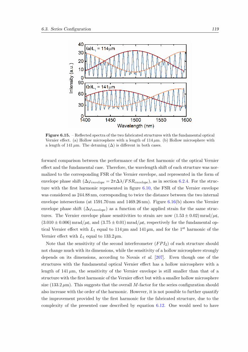
6.3. Series Configuration 119
Figure 6.15. – Reflected spectra of the two fabricated structures with the fundamental opticalVernier effect. (a) Hollow microsphere with a length of 114µm. (b) Hollow microsphere witha length of 141µm. The detuning (∆) is different in both cases.
forward comparison between the performance of the first harmonic of the optical Vernier
effect and the fundamental case. Therefore, the wavelength shift of each structure was nor-
malized to the corresponding FSR of the Vernier envelope, and represented in the form of
envelope phase shift (∆ϕenvelope = 2π∆λ/FSRenvelope), as in section 6.2.4. For the struc-
ture with the first harmonic represented in figure 6.10, the FSR of the Vernier envelope
was considered as 244.88 nm, corresponding to twice the distance between the two internal
envelope intersections (at 1591.70 nm and 1469.26 nm). Figure 6.16(b) shows the Vernier
envelope phase shift (∆ϕenvelope) as a function of the applied strain for the same struc-
tures. The Vernier envelope phase sensitivities to strain are now (1.53± 0.02) mrad/µe,
(3.010± 0.006) mrad/µe, and (3.75± 0.01) mrad/µe, respectively for the fundamental op-
tical Vernier effect with L1 equal to 114 mm and 141 mm, and for the 1st harmonic of the
Vernier effect with L1 equal to 133.2 mm.
Note that the sensitivity of the second interferometer (FPI2) of each structure should
not change much with its dimensions, while the sensitivity of a hollow microsphere strongly
depends on its dimensions, according to Novais et al. [207]. Even though one of the
structures with the fundamental optical Vernier effect has a hollow microsphere with a
length of 141µm, the sensitivity of the Vernier envelope is still smaller than that of a
structure with the first harmonic of the Vernier effect but with a smaller hollow microsphere
size (133.2µm). This suggests that the overall M -factor for the series configuration should
also increase with the order of the harmonic. However, it is not possible to further quantify
the improvement provided by the first harmonic for the fabricated structure, due to the
complexity of the presented case described by equation 6.12. One would need to have
120 Chapter 6. Demonstration and Applications of Optical Harmonic Vernier Effect
Figure 6.16. – (a) Wavelength shift of the Vernier envelope as a function of the appliedstrain for the two fabricated sensors with the fundamental optical Vernier effect and for the1st harmonic analyzed previously. (b) Phase shift of the Vernier envelope as a function of theapplied strain for the same structures as in (a).
access to the strain sensitivities of the hollow microspheres for the different dimensions,
as well as the strain sensitivity of the FPI2, which might change due to the OPL scaling
needed to introduce the first harmonic when compared to the fundamental case. Moreover,
the M2-factor, corresponding to a situation where the second interferometer (FPI2) is seen
as the sensing interferometer and the first interferometer (FPI1) is adopted as a reference,
might not scale with the harmonic order. As demonstrated in section 5.3, if the sensing
interferometer OPL is scaled up to introduce harmonics of the Vernier effect, instead of
the reference interferometer, the M -factor might not bring any improvement of sensitivity
with the harmonic order. Therefore, the number of variables to be considered is large.
Nevertheless, a further quantification of this enhancement would be very valuable to be
performed in the near future.
6.4. Conclusion
Optical harmonics of the Vernier effect bring considerable improvements in terms of the
sensitivity of interferometric fiber sensors. As experimentally demonstrated in the first
6.4. Conclusion 121
part of this chapter, the use of optical harmonics of the Vernier effect allows to enhance
the M -factor by (i+ 1)-times the value obtained for the fundamental optical Vernier effect,
considering the same detuning.
Experimentally, it is very difficult to fabricate interferometric structures with exactly
the same detuning, due to fabrication constrains. At the same time, one should have
control over the detuning, especially if aiming for high M -factors with large envelopes.
A small change in the detuning can be enough to reduce quite a lot the M -factor, or to
increase the FSR of the Vernier envelope beyond the measurable limits imposed by the
detection system. Therefore, it is crucial to explore and develop techniques to adjust the
detuning during the fabrication process. In this chapter, the detuning was adjusted by
means of adding small compressions, together with an electric arc, to slightly reduce the
OPL of a Fabry-Perot interferometer with a larger OPL than expected.
The structure produced to demonstrate the optical harmonic Vernier effect for a parallel
configuration simply relies on hollow capillary tubes. Nevertheless, together with a well-
tuned second harmonic of the optical Vernier effect, the sensing structure was capable of
achieving a strain sensitivity of about 90-fold than that of a fiber Bragg grating (sensitivity
of about 1 pm/µe [209]).
Regarding the optical harmonic Vernier effect in a series configuration, the approach
here adopted was towards the exploration of a complex case of the optical Vernier effect,
where no reference interferometer was used. For that, a hollow microsphere was combined
with a silica Fabry-Perot interferometer made of a section of multimode fiber, achieving
a strain sensitivity for the first harmonic of about 140-fold higher than that of an FBG.
Moreover, simultaneous measurement of two parameters (strain and temperature) was
achieved by taking advantage of the higher frequency component of the Vernier spectrum,
together with the Vernier envelope.
The complex case of optical Vernier effect, without the presence of a reference interfer-
ometer, should be further explored. If well designed and dimensioned, especially using two
interferometers with opposite sensitivities, this case has potential for the development of
sensing structures with even higher sensitivities than the ones reported in the literature
using the optical Vernier effect.
Now that the optical harmonic Vernier effect was explored and demonstrated, one can
make use of it to create advanced fiber sensing structures for more demanding applications.
The next chapter explores advanced optical fiber devices for liquid media sensing. All the
structures rely on simple hollow capillary tubes but combine different techniques, such
as focused ion beam milling, post-processing with electric arc, and/or optical harmonic
Vernier effect, enabling the development of novel and innovative fiber sensing structures.
Moreover, a special extreme case of optical harmonic Vernier effect is also presented,
allowing giant sensitivities to be achieved.

Chapter 7.
Advanced Fiber Sensors based on
Microstructures for Liquid Media
7.1. Introduction
The last two works of this dissertation, discussed in this chapter, are advanced optical
fiber sensing configurations for application in liquid media. Knowing the properties of a
liquid solution is essential in many important areas, from industry to chemistry, biology,
or even pharmacy. For this reason, there is a need for developing measurement techniques
adapted to the liquid properties that are relevant for characterization.
Both configurations are still based on microfabricated structures. One of them merges
simultaneously different concepts and techniques to obtain a high sensitivity and resolution
and the other was designed to measure a liquid property that only a few optical fiber sensors
are capable of measuring.
The first configuration combines an extreme case of optical Vernier effect with Fabry-
Perot interferometers (FPIs) based on hollow capillary tubes. The structure was developed
to create a sensing platform for liquid analytes with giant sensitivity to refractive index.
Refractive index measurements are present in medical research, clinical diagnosis, food
quality control, contamination of environments, industrial processes, or even to detect
chemical and biological analytes. Yet, there is a lack of highly sensitive sensors, capable of
providing higher resolution to sense tiny variations of the refractive index in small volumes,
important for some state-of-the-art applications, such as tracking molecular binding, ap-
plication in differential refractometers used for liquid chromatography, or possibly a new
way to track molecular photo-switching. Many of these applications require high precision
refractometers, in the order of 10−5 to 10−6 refractive index units (RIU) or lower. Optical
microfibers have a sensitivity that could range from around 600 nm/RIU in combination
with long period gratings [119], up to around 24000 nm/RIU in combination with a Mach-
Zehnder interferometer effect [210]. Alternatively, one can also force light to propagate
through the analyte by filling an interferometric cavity. Such approach consists of either
124 Chapter 7. Advanced Fiber Sensors based on Microstructures for Liquid Media
having an open cavity or creating access holes for the analyte. Femtosecond laser-milled
cavities have a sensitivity that can go from 1163 nm/RIU (with a resolution of 10−6 RIU)
for an FPI [211] to about 14297 nm/RIU for a Mach-Zehnder interferometric configuration
(with a resolution of 10−5 RIU) [212]. The combination of plasmonics and optical fibers
enabled the development of new sensing platforms, also for refractive index sensing. Their
sensitivity can go up to around 40000 nm/RIU (with a resolution of 10−6 [213]). Due to
the extreme optical Vernier effect, the configuration proposed in this chapter is able to
achieve refractive index sensitivities an order of magnitude higher, close to 500000 nm of
wavelength shift per RIU with an experimental resolution of 10−7 RIU.
The second configuration uses post-processing with an electric arc to create small hollow
probe based on a hollow capillary tube, with a small access hole for liquids. The fiber
probe was designed to use interferometric measurements to track the liquid displacement
inside the probe, allowing to retrieve the viscosity of the liquid. Viscosity is a challenging
property to measure in a fluid, especially if it involves small volumes. This property is
directly involved in fluid flow processes, which are relevant and a matter of interest for
different research areas. The optical fiber probe viscometer here presented is capable of
measuring the viscosity of liquids using only tiny volumes (in the order of picoliters).
7.2. Giant Refractometric Sensivity based on Extreme Optical
Vernier Effect
7.2.1. Introduction
All the different cases of optical Vernier effect explored and demonstrated before aimed to
achieve high sensitivity values. In all situations, the ultimate parameter that regulates the
particular enhancement outcome and the M -factor achieved by the effect is the detuning
(∆) between the two interferometers. However, dimensioning this parameter is quite a
tricky problem. To achieve high M -factors (typically in the order of tens, as discussed at
the end of chapter 4 and visible in the tables of appendix B), a small detuning value would
be desirable. On the other hand, detuning the reference interferometer by a very small
amount (as an extreme optical Vernier effect) may result in a beating modulation with a
very long period, which may become undetectable for a limited spectral range available,
and therefore immeasurable. These contradictory requirements present a considerable
challenge for the experimental implementation of such sensors with large M -factors for
sensitivity.
This section proposes and demonstrates a method to overcome this dilemma by using
few modes instead of a single mode in the sensing interferometer (ideally two modes),
preferably with a relatively large effective refractive index between them. The reference
interferometer is in tune with the fundamental mode (mode 1) of the sensing interferom-
7.2. Giant Refractometric Sensivity based on Extreme Optical Vernier Effect 125
eter, which would provide a giant M -factor but with an extremely large immeasurable
envelope. On the other hand, for a higher order mode (mode 2) it represents a lower
M -factor but with a smaller and measurable Vernier envelope, since the effective refrac-
tive index of the higher order mode is different, generating a Vernier effect slightly more
detuned. However, when both responses superimpose, the Vernier envelope is still mea-
surable, whilst maintaining a giant M -factor typical for large immeasurable envelopes. As
will be shown later, the method of combining the two modes in the sensing interferometer
provides M -factors an order of magnitude beyond the expected limits for the standard
Vernier effect technique.
Such a result with a giant M -factor is here demonstrated by implementing a few-mode
FPI refractometer in combination with a single-mode reference FPI. Through the use of
the first harmonic of the optical Vernier effect, FPIs made of hollow capillary tubes, FIB
milling to open access holes for liquid analytes, and mode interference, the fabricated
structure is born from combination of different techniques and knowledge gathered during
this PhD. First, the working principle is briefly introduced and the fabrication of the
sensing structure is described. Then, simulations are used to further understand the
behavior of the sensing structure and to have a first glimpse on the giant enhancement of
sensitivity. At last, the sensing FPI is filled with water and characterized for refractive
index variations, comparing the result with a single FPI, with the first harmonic of the
optical Vernier effect using a single mode sensing FPI, as explored in previous chapter,
and also with the simulated results.
7.2.2. Working Principle
The sensor is similar to the structure presented in section 6.2, where two FPIs made
from hollow capillary tubes are used to generate the optical Vernier effect in a parallel
configuration. In this case, the first harmonic of the optical Vernier effect will be used,
since it provides internal envelope intersections to easily monitor the wavelength shift, as
previously discussed in this dissertation. A schematic diagram of the working principle
is shown in figure 7.1. The sensing FPI is fabricated to present few modes (ideally two).
The sensing FPI cavity can be filled with an aqueous solution by opening access holes at
the edges of the cavity.
Let us consider the simpler case of two propagating modes in the sensing FPI, as repre-
sented in the inset of figure 7.1, while the reference FPI is single mode. The reference FPI
is produced to be in tune (detuning: ∆ ∼ 0) with the fundamental mode (mode 1) of the
sensing FPI, while introducing the first harmonic of the Vernier effect. One knows now
that this situation produces a Vernier envelope with an infinite period. As a consequence,
the sensitivity of the Vernier envelope is theoretically infinite, but there is no way one can
measure it.
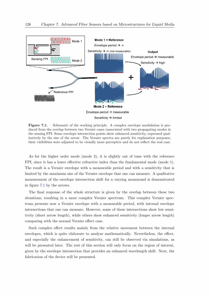
126 Chapter 7. Advanced Fiber Sensors based on Microstructures for Liquid Media
Figure 7.1. – Schematic of the working principle. A complex envelope modulation is pro-duced from the overlap between two Vernier cases (associated with two propagating modes inthe sensing FPI. Some envelope intersection points show enhanced sensitivity, expressed qual-itatively by the size of the arrow. The Vernier spectra are purely for explanation purposes,their visibilities were adjusted to be visually more perceptive and do not reflect the real case.
As for the higher order mode (mode 2), it is slightly out of tune with the reference
FPI, since it has a lower effective refractive index than the fundamental mode (mode 1).
The result is a Vernier envelope with a measurable period and with a sensitivity that is
limited by the maximum size of the Vernier envelope that one can measure. A qualitative
measurement of the envelope intersection shift for a varying measurand is demonstrated
in figure 7.1 by the arrows.
The final response of the whole structure is given by the overlap between these two
situations, resulting in a more complex Vernier spectrum. This complex Vernier spec-
trum presents now a Vernier envelope with a measurable period, with internal envelope
intersections that one can measure. However, some of these intersections show low sensi-
tivity (short arrow length), while others show enhanced sensitivity (longer arrow length)
comparing with the normal Vernier effect case.
Such complex effect results mainly from the relative movement between the internal
envelopes, which is quite elaborate to analyze mathematically. Nevertheless, the effect,
and especially the enhancement of sensitivity, can still be observed via simulations, as
will be presented later. The rest of this section will only focus on the region of interest,
given by the envelope intersection that provides an enhanced wavelength shift. Next, the
fabrication of the device will be presented.
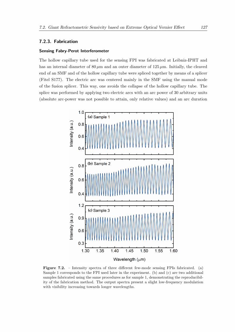
7.2. Giant Refractometric Sensivity based on Extreme Optical Vernier Effect 127
7.2.3. Fabrication
Sensing Fabry-Perot Interferometer
The hollow capillary tube used for the sensing FPI was fabricated at Leibniz-IPHT and
has an internal diameter of 80µm and an outer diameter of 125µm. Initially, the cleaved
end of an SMF and of the hollow capillary tube were spliced together by means of a splicer
(Fitel S177). The electric arc was centered mainly in the SMF using the manual mode
of the fusion splicer. This way, one avoids the collapse of the hollow capillary tube. The
splice was performed by applying two electric arcs with an arc power of 30 arbitrary units
(absolute arc-power was not possible to attain, only relative values) and an arc duration
Figure 7.2. – Intensity spectra of three different few-mode sensing FPIs fabricated. (a)Sample 1 corresponds to the FPI used later in the experiment. (b) and (c) are two additionalsamples fabricated using the same procedures as for sample 1, demonstrating the reproducibil-ity of the fabrication method. The output spectra present a slight low-frequency modulationwith visibility increasing towards longer wavelengths.
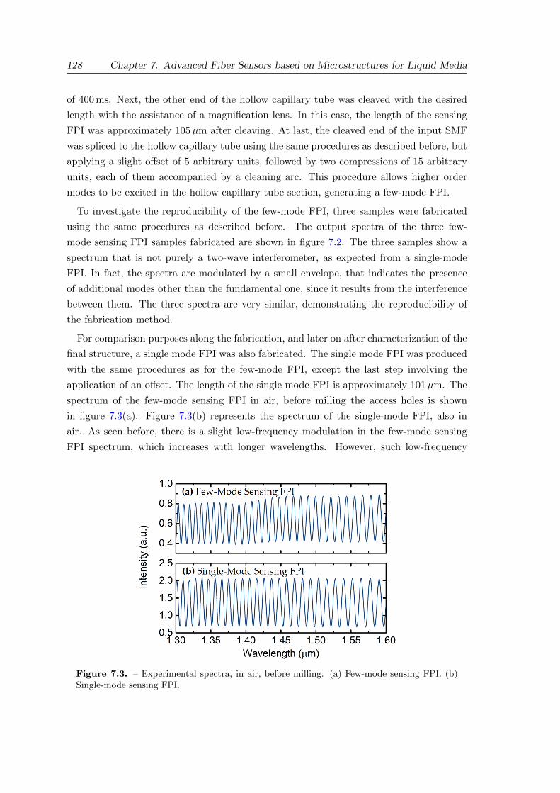
128 Chapter 7. Advanced Fiber Sensors based on Microstructures for Liquid Media
of 400 ms. Next, the other end of the hollow capillary tube was cleaved with the desired
length with the assistance of a magnification lens. In this case, the length of the sensing
FPI was approximately 105µm after cleaving. At last, the cleaved end of the input SMF
was spliced to the hollow capillary tube using the same procedures as described before, but
applying a slight offset of 5 arbitrary units, followed by two compressions of 15 arbitrary
units, each of them accompanied by a cleaning arc. This procedure allows higher order
modes to be excited in the hollow capillary tube section, generating a few-mode FPI.
To investigate the reproducibility of the few-mode FPI, three samples were fabricated
using the same procedures as described before. The output spectra of the three few-
mode sensing FPI samples fabricated are shown in figure 7.2. The three samples show a
spectrum that is not purely a two-wave interferometer, as expected from a single-mode
FPI. In fact, the spectra are modulated by a small envelope, that indicates the presence
of additional modes other than the fundamental one, since it results from the interference
between them. The three spectra are very similar, demonstrating the reproducibility of
the fabrication method.
For comparison purposes along the fabrication, and later on after characterization of the
final structure, a single mode FPI was also fabricated. The single mode FPI was produced
with the same procedures as for the few-mode FPI, except the last step involving the
application of an offset. The length of the single mode FPI is approximately 101µm. The
spectrum of the few-mode sensing FPI in air, before milling the access holes is shown
in figure 7.3(a). Figure 7.3(b) represents the spectrum of the single-mode FPI, also in
air. As seen before, there is a slight low-frequency modulation in the few-mode sensing
FPI spectrum, which increases with longer wavelengths. However, such low-frequency
Figure 7.3. – Experimental spectra, in air, before milling. (a) Few-mode sensing FPI. (b)Single-mode sensing FPI.
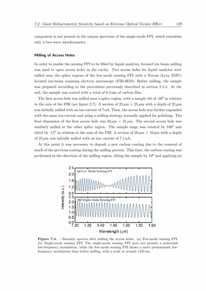
7.2. Giant Refractometric Sensivity based on Extreme Optical Vernier Effect 129
component is not present in the output spectrum of the single-mode FPI, which resembles
only a two-wave interferometer.
Milling of Access Holes
In order to enable the sensing FPI to be filled by liquid analytes, focused ion beam milling
was used to open access holes in the cavity. Two access holes for liquid analytes were
milled near the splice regions of the few-mode sensing FPI with a Tescan (Lyra XMU)
focused ion-beam scanning electron microscope (FIB-SEM). Before milling, the sample
was prepared according to the procedures previously described in section 2.4.3. At the
end, the sample was coated with a total of 6.4 nm of carbon film.
The first access hole was milled near a splice region, with a sample tilt of -20º in relation
to the axis of the FIB (see figure 2.7). A section of 25µm × 25µm with a depth of 25µm
was initially milled with an ion current of 7 nA. Then, the access hole was further expanded
with the same ion current and using a milling strategy normally applied for polishing. The
final dimension of the first access hole was 32µm × 31µm. The second access hole was
similarly milled at the other splice region. The sample stage was rotated by 180º and
tilted by -15º in relation to the axis of the FIB. A section of 20µm × 10µm with a depth
of 25µm was initially milled with an ion current of 7.1 nA.
At this point it was necessary to deposit a new carbon coating due to the removal of
much of the previous coating during the milling process. This time, the carbon coating was
performed in the direction of the milling region, tilting the sample by 10º and applying no
Figure 7.4. – Intensity spectra after milling the access holes. (a) Few-mode sensing FPI.(b) Single-mode sensing FPI. The single-mode sensing FPI does not present a noticeablelow-frequency modulation, while the few-mode sensing FPI shows a more predominant low-frequency modulation than before milling, with a node at around 1425 nm.
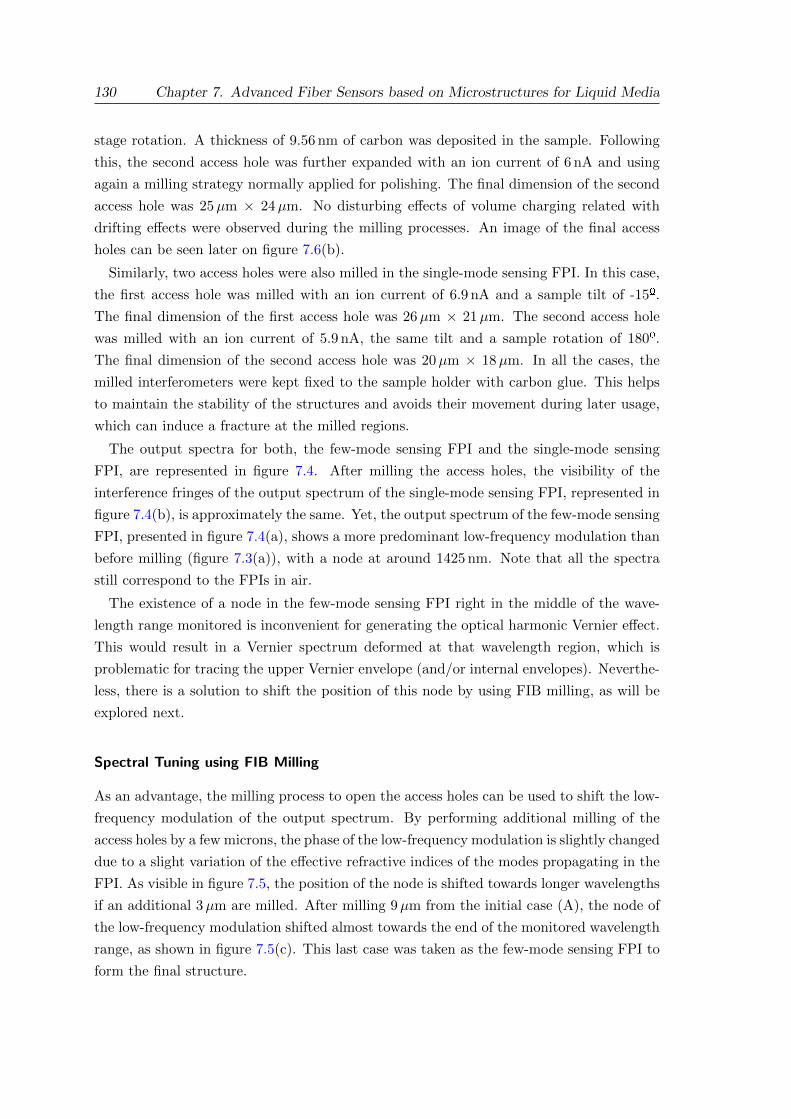
130 Chapter 7. Advanced Fiber Sensors based on Microstructures for Liquid Media
stage rotation. A thickness of 9.56 nm of carbon was deposited in the sample. Following
this, the second access hole was further expanded with an ion current of 6 nA and using
again a milling strategy normally applied for polishing. The final dimension of the second
access hole was 25µm × 24µm. No disturbing effects of volume charging related with
drifting effects were observed during the milling processes. An image of the final access
holes can be seen later on figure 7.6(b).
Similarly, two access holes were also milled in the single-mode sensing FPI. In this case,
the first access hole was milled with an ion current of 6.9 nA and a sample tilt of -15º.
The final dimension of the first access hole was 26µm × 21µm. The second access hole
was milled with an ion current of 5.9 nA, the same tilt and a sample rotation of 180º.
The final dimension of the second access hole was 20µm × 18µm. In all the cases, the
milled interferometers were kept fixed to the sample holder with carbon glue. This helps
to maintain the stability of the structures and avoids their movement during later usage,
which can induce a fracture at the milled regions.
The output spectra for both, the few-mode sensing FPI and the single-mode sensing
FPI, are represented in figure 7.4. After milling the access holes, the visibility of the
interference fringes of the output spectrum of the single-mode sensing FPI, represented in
figure 7.4(b), is approximately the same. Yet, the output spectrum of the few-mode sensing
FPI, presented in figure 7.4(a), shows a more predominant low-frequency modulation than
before milling (figure 7.3(a)), with a node at around 1425 nm. Note that all the spectra
still correspond to the FPIs in air.
The existence of a node in the few-mode sensing FPI right in the middle of the wave-
length range monitored is inconvenient for generating the optical harmonic Vernier effect.
This would result in a Vernier spectrum deformed at that wavelength region, which is
problematic for tracing the upper Vernier envelope (and/or internal envelopes). Neverthe-
less, there is a solution to shift the position of this node by using FIB milling, as will be
explored next.
Spectral Tuning using FIB Milling
As an advantage, the milling process to open the access holes can be used to shift the low-
frequency modulation of the output spectrum. By performing additional milling of the
access holes by a few microns, the phase of the low-frequency modulation is slightly changed
due to a slight variation of the effective refractive indices of the modes propagating in the
FPI. As visible in figure 7.5, the position of the node is shifted towards longer wavelengths
if an additional 3µm are milled. After milling 9µm from the initial case (A), the node of
the low-frequency modulation shifted almost towards the end of the monitored wavelength
range, as shown in figure 7.5(c). This last case was taken as the few-mode sensing FPI to
form the final structure.

7.2. Giant Refractometric Sensivity based on Extreme Optical Vernier Effect 131
Figure 7.5. – Intensity spectra of the few-mode sensing FPI after additional milling of theaccess holes. (a) Initial output spectrum [A] as in figure 7.4(a). (b) Output spectrum afteradditionally milling 3µm from the initial case [A]. (c) Output spectrum after additionallymilling 9µm from the initial case [A].
Final Structure
As explained before, the first harmonic of the Vernier effect is generated in a parallel
configuration, by means of a 3dB fiber coupler, as depicted in figure 7.6. A hollow capillary
tube with an internal diameter of 60µm and an outer diameter of 125µm, also fabricated
at Leibniz-IPHT, was used to form the reference FPI. The reference FPI should be in tune
with the fundamental mode of the sensing FPI when filled with water. Due to the necessity
of simulating the modes propagating in the water-filled few-mode sensing FPI in order to
calculate the length of the reference FPI, the dimensioning of the reference FPI will only be
presented in the next section. The structure is illuminated with a supercontinuum source,
and the output reflected spectrum is measured with an optical spectrum analyzer (OSA).
Figure 7.6(a) shows a micrograph of the two FPIs (sensing and reference). Scanning
electron microscope images of the milled sensing FPI and of one of the access holes are
also displayed in figure 7.6(b).
This structure will then be used to demonstrate the concept of extreme optical Vernier
effect applied to refractive index sensing of liquid analytes.
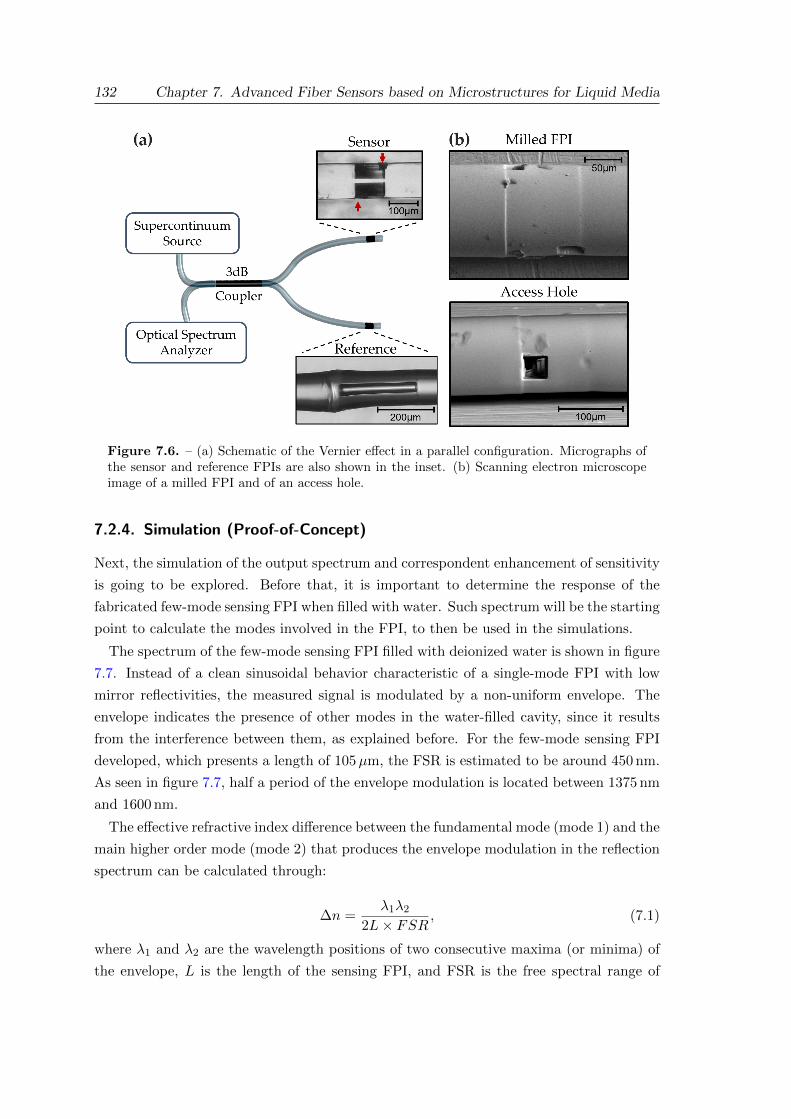
132 Chapter 7. Advanced Fiber Sensors based on Microstructures for Liquid Media
Figure 7.6. – (a) Schematic of the Vernier effect in a parallel configuration. Micrographs ofthe sensor and reference FPIs are also shown in the inset. (b) Scanning electron microscopeimage of a milled FPI and of an access hole.
7.2.4. Simulation (Proof-of-Concept)
Next, the simulation of the output spectrum and correspondent enhancement of sensitivity
is going to be explored. Before that, it is important to determine the response of the
fabricated few-mode sensing FPI when filled with water. Such spectrum will be the starting
point to calculate the modes involved in the FPI, to then be used in the simulations.
The spectrum of the few-mode sensing FPI filled with deionized water is shown in figure
7.7. Instead of a clean sinusoidal behavior characteristic of a single-mode FPI with low
mirror reflectivities, the measured signal is modulated by a non-uniform envelope. The
envelope indicates the presence of other modes in the water-filled cavity, since it results
from the interference between them, as explained before. For the few-mode sensing FPI
developed, which presents a length of 105µm, the FSR is estimated to be around 450 nm.
As seen in figure 7.7, half a period of the envelope modulation is located between 1375 nm
and 1600 nm.
The effective refractive index difference between the fundamental mode (mode 1) and the
main higher order mode (mode 2) that produces the envelope modulation in the reflection
spectrum can be calculated through:
∆n =λ1λ2
2L× FSR, (7.1)
where λ1 and λ2 are the wavelength positions of two consecutive maxima (or minima) of
the envelope, L is the length of the sensing FPI, and FSR is the free spectral range of

7.2. Giant Refractometric Sensivity based on Extreme Optical Vernier Effect 133
Figure 7.7. – Experimental spectrum of the water-filled few-mode sensing FPI.
the envelope modulation. The wavelength values in equation 7.1, corresponding to the
position of two consecutive envelope minima, are assumed as 1150 nm and 1600 nm. With
this, a refractive index difference of around 1.94× 10⁻² RIU is obtained.
Although this main higher order mode is expected to carry more energy than other
higher order modes, the structure still presents other higher order modes that contribute
to the FPI response, which is why the envelope is non-uniform. Such a structure is very
challenging to simulate, as it contains multiple variables and degrees of freedom. Therefore,
as a first approach, let us consider a sensing FPI with only two modes.
Mode Simulation
Mode analysis using COMSOL Multiphysics was performed to calculate the effective re-
fractive index of modes propagating in the water-filled sensing FPI. The simulated cross-
Figure 7.8. – Simulated mode profile of the fundamental mode and the three higher ordermodes with an effective refractive index difference close to the value calculated through theexperimental data (1.94× 10⁻² RIU).
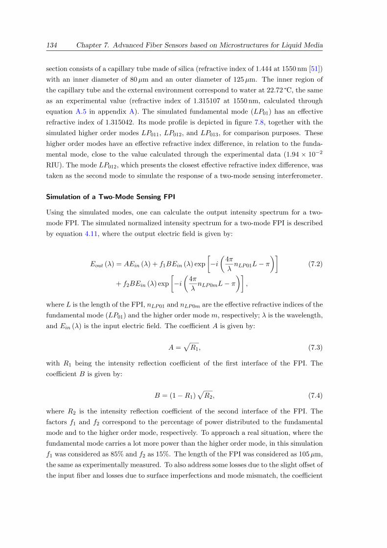
134 Chapter 7. Advanced Fiber Sensors based on Microstructures for Liquid Media
section consists of a capillary tube made of silica (refractive index of 1.444 at 1550 nm [51])
with an inner diameter of 80µm and an outer diameter of 125µm. The inner region of
the capillary tube and the external environment correspond to water at 22.72 °C, the same
as an experimental value (refractive index of 1.315107 at 1550 nm, calculated through
equation A.5 in appendix A). The simulated fundamental mode (LP01) has an effective
refractive index of 1.315042. Its mode profile is depicted in figure 7.8, together with the
simulated higher order modes LP011, LP012, and LP013, for comparison purposes. These
higher order modes have an effective refractive index difference, in relation to the funda-
mental mode, close to the value calculated through the experimental data (1.94 × 10⁻²
RIU). The mode LP012, which presents the closest effective refractive index difference, was
taken as the second mode to simulate the response of a two-mode sensing interferometer.
Simulation of a Two-Mode Sensing FPI
Using the simulated modes, one can calculate the output intensity spectrum for a two-
mode FPI. The simulated normalized intensity spectrum for a two-mode FPI is described
by equation 4.11, where the output electric field is given by:
Eout (λ) = AEin (λ) + f1BEin (λ) exp
[−i(
4π
λnLP01L− π
)](7.2)
+ f2BEin (λ) exp
[−i(
4π
λnLP0mL− π
)],
where L is the length of the FPI, nLP01 and nLP0m are the effective refractive indices of the
fundamental mode (LP01) and the higher order mode m, respectively; λ is the wavelength,
and Ein (λ) is the input electric field. The coefficient A is given by:
A =√R1, (7.3)
with R1 being the intensity reflection coefficient of the first interface of the FPI. The
coefficient B is given by:
B = (1−R1)√R2, (7.4)
where R2 is the intensity reflection coefficient of the second interface of the FPI. The
factors f1 and f2 correspond to the percentage of power distributed to the fundamental
mode and to the higher order mode, respectively. To approach a real situation, where the
fundamental mode carries a lot more power than the higher order mode, in this simulation
f1 was considered as 85% and f2 as 15%. The length of the FPI was considered as 105µm,
the same as experimentally measured. To also address some losses due to the slight offset of
the input fiber and losses due to surface imperfections and mode mismatch, the coefficient
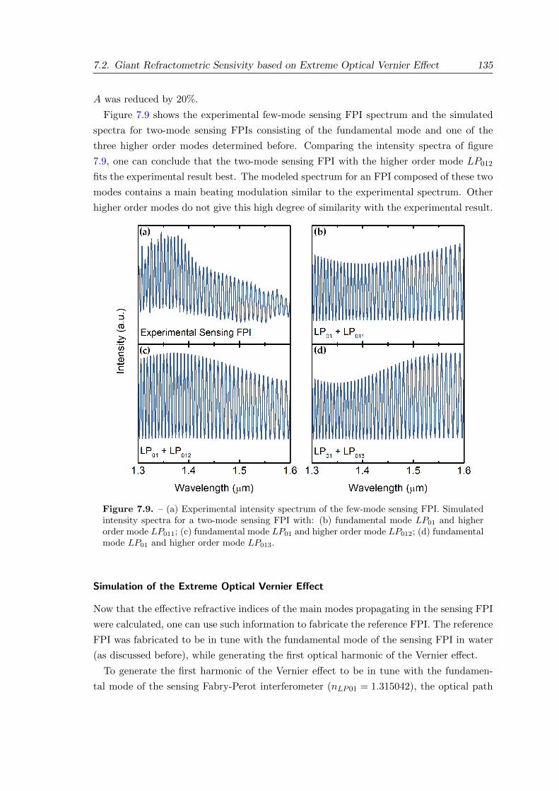
7.2. Giant Refractometric Sensivity based on Extreme Optical Vernier Effect 135
A was reduced by 20%.
Figure 7.9 shows the experimental few-mode sensing FPI spectrum and the simulated
spectra for two-mode sensing FPIs consisting of the fundamental mode and one of the
three higher order modes determined before. Comparing the intensity spectra of figure
7.9, one can conclude that the two-mode sensing FPI with the higher order mode LP012
fits the experimental result best. The modeled spectrum for an FPI composed of these two
modes contains a main beating modulation similar to the experimental spectrum. Other
higher order modes do not give this high degree of similarity with the experimental result.
Figure 7.9. – (a) Experimental intensity spectrum of the few-mode sensing FPI. Simulatedintensity spectra for a two-mode sensing FPI with: (b) fundamental mode LP01 and higherorder mode LP011; (c) fundamental mode LP01 and higher order mode LP012; (d) fundamentalmode LP01 and higher order mode LP013.
Simulation of the Extreme Optical Vernier Effect
Now that the effective refractive indices of the main modes propagating in the sensing FPI
were calculated, one can use such information to fabricate the reference FPI. The reference
FPI was fabricated to be in tune with the fundamental mode of the sensing FPI in water
(as discussed before), while generating the first optical harmonic of the Vernier effect.
To generate the first harmonic of the Vernier effect to be in tune with the fundamen-
tal mode of the sensing Fabry-Perot interferometer (nLP01 = 1.315042), the optical path
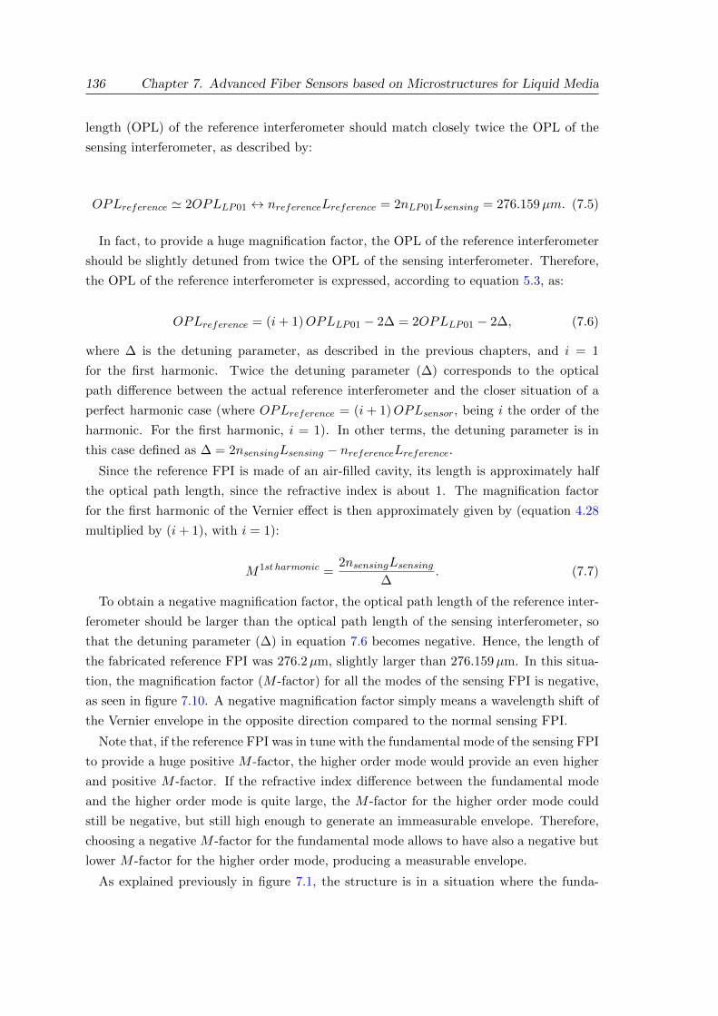
136 Chapter 7. Advanced Fiber Sensors based on Microstructures for Liquid Media
length (OPL) of the reference interferometer should match closely twice the OPL of the
sensing interferometer, as described by:
OPLreference ' 2OPLLP01 ↔ nreferenceLreference = 2nLP01Lsensing = 276.159µm. (7.5)
In fact, to provide a huge magnification factor, the OPL of the reference interferometer
should be slightly detuned from twice the OPL of the sensing interferometer. Therefore,
the OPL of the reference interferometer is expressed, according to equation 5.3, as:
OPLreference = (i+ 1)OPLLP01 − 2∆ = 2OPLLP01 − 2∆, (7.6)
where ∆ is the detuning parameter, as described in the previous chapters, and i = 1
for the first harmonic. Twice the detuning parameter (∆) corresponds to the optical
path difference between the actual reference interferometer and the closer situation of a
perfect harmonic case (where OPLreference = (i+ 1)OPLsensor, being i the order of the
harmonic. For the first harmonic, i = 1). In other terms, the detuning parameter is in
this case defined as ∆ = 2nsensingLsensing − nreferenceLreference.Since the reference FPI is made of an air-filled cavity, its length is approximately half
the optical path length, since the refractive index is about 1. The magnification factor
for the first harmonic of the Vernier effect is then approximately given by (equation 4.28
multiplied by (i+ 1), with i = 1):
M1st harmonic =2nsensingLsensing
∆. (7.7)
To obtain a negative magnification factor, the optical path length of the reference inter-
ferometer should be larger than the optical path length of the sensing interferometer, so
that the detuning parameter (∆) in equation 7.6 becomes negative. Hence, the length of
the fabricated reference FPI was 276.2µm, slightly larger than 276.159µm. In this situa-
tion, the magnification factor (M -factor) for all the modes of the sensing FPI is negative,
as seen in figure 7.10. A negative magnification factor simply means a wavelength shift of
the Vernier envelope in the opposite direction compared to the normal sensing FPI.
Note that, if the reference FPI was in tune with the fundamental mode of the sensing FPI
to provide a huge positive M -factor, the higher order mode would provide an even higher
and positive M -factor. If the refractive index difference between the fundamental mode
and the higher order mode is quite large, the M -factor for the higher order mode could
still be negative, but still high enough to generate an immeasurable envelope. Therefore,
choosing a negative M -factor for the fundamental mode allows to have also a negative but
lower M -factor for the higher order mode, producing a measurable envelope.
As explained previously in figure 7.1, the structure is in a situation where the funda-
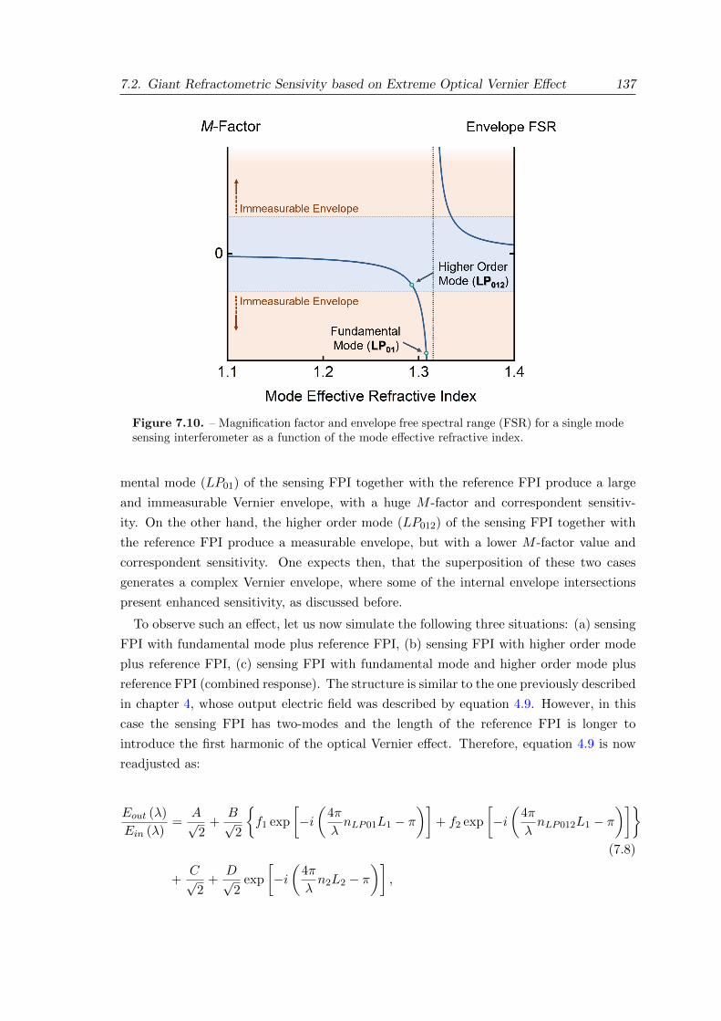
7.2. Giant Refractometric Sensivity based on Extreme Optical Vernier Effect 137
Figure 7.10. – Magnification factor and envelope free spectral range (FSR) for a single modesensing interferometer as a function of the mode effective refractive index.
mental mode (LP01) of the sensing FPI together with the reference FPI produce a large
and immeasurable Vernier envelope, with a huge M -factor and correspondent sensitiv-
ity. On the other hand, the higher order mode (LP012) of the sensing FPI together with
the reference FPI produce a measurable envelope, but with a lower M -factor value and
correspondent sensitivity. One expects then, that the superposition of these two cases
generates a complex Vernier envelope, where some of the internal envelope intersections
present enhanced sensitivity, as discussed before.
To observe such an effect, let us now simulate the following three situations: (a) sensing
FPI with fundamental mode plus reference FPI, (b) sensing FPI with higher order mode
plus reference FPI, (c) sensing FPI with fundamental mode and higher order mode plus
reference FPI (combined response). The structure is similar to the one previously described
in chapter 4, whose output electric field was described by equation 4.9. However, in this
case the sensing FPI has two-modes and the length of the reference FPI is longer to
introduce the first harmonic of the optical Vernier effect. Therefore, equation 4.9 is now
readjusted as:
Eout (λ)
Ein (λ)=
A√2
+B√
2
{f1 exp
[−i(
4π
λnLP01L1 − π
)]+ f2 exp
[−i(
4π
λnLP012L1 − π
)]}(7.8)
+C√
2+
D√2
exp
[−i(
4π
λn2L2 − π
)],
138 Chapter 7. Advanced Fiber Sensors based on Microstructures for Liquid Media
where L1 is the length of the two-mode sensing FPI, nLP01 and nLP012 are the effective
refractive indices of the considered fundamental mode (LP01) and the higher order mode
(LP012), respectively, in the two-mode sensing FPI, n2 and L2 are the effective refractive
index and the length of the reference FPI, λ is the wavelength, and Ein (λ) is the input
electric field. The coefficients A, B, f1, and f2, as well as the length of the sensing FPI
and the effective refractive indices of the modes LP01 and LP012 are the same as before.
The coefficient C is given by:
C =
√Rref1 , (7.9)
with Rref1 being the intensity reflection coefficient of the first interface of the reference FPI,
Figure 7.11. – Comparison between the Vernier effect with a single mode and a two-modesensing FPI. (a) Simulated Vernier spectrum for a sensing FPI with the fundamental mode(LP01). The Vernier spectrum has a high magnification factor, but an envelope too large tobe measured. (b) Simulated Vernier spectrum for a sensing FPI with the higher order mode(LP012), before and after applying a refractive index variation of 8× 10⁻⁵ RIU to the sensingFPI mode. The Vernier envelope is measurable but has a lower magnification factor (lowerwavelength shift). (c) Simulated Vernier spectrum for a two-mode sensing FPI, before andafter applying the same a refractive index variation to the sensing FPI modes. The Vernierenvelope is measurable, yet the magnification factor is still high (larger wavelength shift thanthe single mode case).
7.2. Giant Refractometric Sensivity based on Extreme Optical Vernier Effect 139
which has an air cavity (refractive index considered as 1). The coefficient D is expressed
as:
D =(
1−Rref1
)√Rref2 , (7.10)
where Rref2 is the intensity reflection coefficient of the second interface of the reference
FPI.
The coefficient D was reduced by 70% to adjust the intensity due to losses during
the fine-tuning of the reference interferometer by compression. The refractive index of
the reference FPI was considered as 1 (air). The length used for the reference FPI was
2×1.315042×105µm + 0.001µm, making sure that the OPL of the reference interferometer
is slightly longer than the perfect harmonic case, inducing a negative M -factor.
The simulated spectra for the three situations (a), (b), and (c) mentioned before are
depicted in figure 7.11. If the sensing FPI only presents the fundamental mode (LP01),
which is in tune with the reference FPI, the generated Vernier envelope would present an
extremely large FSR and a high magnification factor. In practice however, it would be
impossible to measure the Vernier envelope shift within the limited spectral range available,
as seen in figure 7.11(a). On the other hand, if the sensing FPI only presents the higher
order mode (LP012), the Vernier effect is less tuned, resulting in a smaller period Vernier
envelope. In this case, the Vernier envelope is now measurable, but it is accompanied by a
smaller magnification factor and, therefore, by a smaller wavelength shift, as demonstrated
in figure 7.11(b). Hence, in a standard single-mode situation, the maximum magnification
factor provided by the Vernier effect is limited by the largest Vernier envelope measurable.
However, if the sensing FPI presents both modes simultaneously, the superposition of both
responses results in a measurable Vernier envelope but with a higher magnification factor
(larger wavelength shift), as observed in figure 7.11(c). The wavelength shift was simulated
by changing the effective refractive indices of the sensing FPI modes by 8 × 10⁻⁵ RIU,
simulating a variation of the analyte. This result was simulated for a two-mode sensing
FPI, and it is expected to still be applicable to the fabricated sensing FPI, which may
present some additional modes (few mode case).
7.2.5. Characterization
Now that the enhanced wavelength shift provided by the extreme optical Vernier effect was
demonstrated via simulations, the fabricated structures were characterized for refractive
index variations in a very narrow range around the refractive index of water. This was
achieved by slightly changing, in steps, the water temperature, which, through the thermo-
optic effect, changes the refractive index of water1.
1Further details can be found in appendix A.
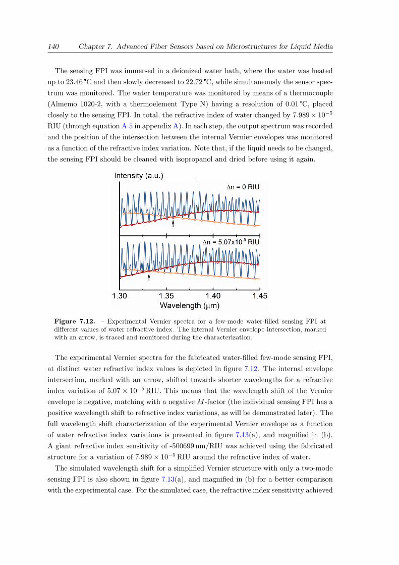
140 Chapter 7. Advanced Fiber Sensors based on Microstructures for Liquid Media
The sensing FPI was immersed in a deionized water bath, where the water was heated
up to 23.46 °C and then slowly decreased to 22.72 °C, while simultaneously the sensor spec-
trum was monitored. The water temperature was monitored by means of a thermocouple
(Almemo 1020-2, with a thermoelement Type N) having a resolution of 0.01 °C, placed
closely to the sensing FPI. In total, the refractive index of water changed by 7.989× 10⁻⁵
RIU (through equation A.5 in appendix A). In each step, the output spectrum was recorded
and the position of the intersection between the internal Vernier envelopes was monitored
as a function of the refractive index variation. Note that, if the liquid needs to be changed,
the sensing FPI should be cleaned with isopropanol and dried before using it again.
Figure 7.12. – Experimental Vernier spectra for a few-mode water-filled sensing FPI atdifferent values of water refractive index. The internal Vernier envelope intersection, markedwith an arrow, is traced and monitored during the characterization.
The experimental Vernier spectra for the fabricated water-filled few-mode sensing FPI,
at distinct water refractive index values is depicted in figure 7.12. The internal envelope
intersection, marked with an arrow, shifted towards shorter wavelengths for a refractive
index variation of 5.07 × 10⁻⁵ RIU. This means that the wavelength shift of the Vernier
envelope is negative, matching with a negative M -factor (the individual sensing FPI has a
positive wavelength shift to refractive index variations, as will be demonstrated later). The
full wavelength shift characterization of the experimental Vernier envelope as a function
of water refractive index variations is presented in figure 7.13(a), and magnified in (b).
A giant refractive index sensitivity of -500699 nm/RIU was achieved using the fabricated
structure for a variation of 7.989× 10⁻⁵ RIU around the refractive index of water.
The simulated wavelength shift for a simplified Vernier structure with only a two-mode
sensing FPI is also shown in figure 7.13(a), and magnified in (b) for a better comparison
with the experimental case. For the simulated case, the refractive index sensitivity achieved
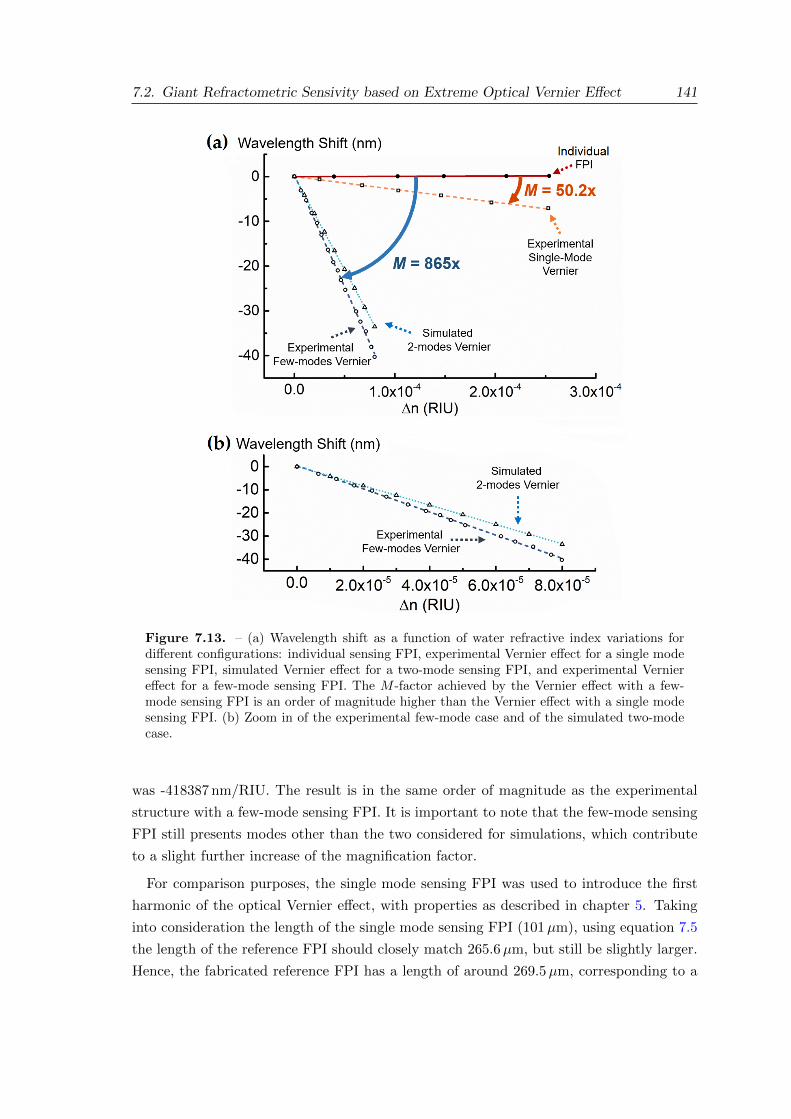
7.2. Giant Refractometric Sensivity based on Extreme Optical Vernier Effect 141
Figure 7.13. – (a) Wavelength shift as a function of water refractive index variations fordifferent configurations: individual sensing FPI, experimental Vernier effect for a single modesensing FPI, simulated Vernier effect for a two-mode sensing FPI, and experimental Verniereffect for a few-mode sensing FPI. The M -factor achieved by the Vernier effect with a few-mode sensing FPI is an order of magnitude higher than the Vernier effect with a single modesensing FPI. (b) Zoom in of the experimental few-mode case and of the simulated two-modecase.
was -418387 nm/RIU. The result is in the same order of magnitude as the experimental
structure with a few-mode sensing FPI. It is important to note that the few-mode sensing
FPI still presents modes other than the two considered for simulations, which contribute
to a slight further increase of the magnification factor.
For comparison purposes, the single mode sensing FPI was used to introduce the first
harmonic of the optical Vernier effect, with properties as described in chapter 5. Taking
into consideration the length of the single mode sensing FPI (101µm), using equation 7.5
the length of the reference FPI should closely match 265.6µm, but still be slightly larger.
Hence, the fabricated reference FPI has a length of around 269.5µm, corresponding to a
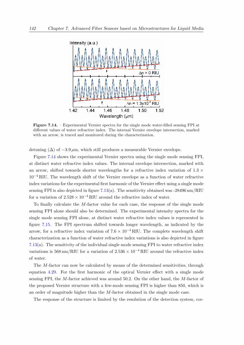
142 Chapter 7. Advanced Fiber Sensors based on Microstructures for Liquid Media
Figure 7.14. – Experimental Vernier spectra for the single mode water-filled sensing FPI atdifferent values of water refractive index. The internal Vernier envelope intersection, markedwith an arrow, is traced and monitored during the characterization.
detuning (∆) of −3.9µm, which still produces a measurable Vernier envelope.
Figure 7.14 shows the experimental Vernier spectra using the single mode sensing FPI,
at distinct water refractive index values. The internal envelope intersection, marked with
an arrow, shifted towards shorter wavelengths for a refractive index variation of 1.3 ×10⁻⁴ RIU. The wavelength shift of the Vernier envelope as a function of water refractive
index variations for the experimental first harmonic of the Vernier effect using a single mode
sensing FPI is also depicted in figure 7.13(a). The sensitivity obtained was -28496 nm/RIU
for a variation of 2.528× 10⁻⁴ RIU around the refractive index of water.
To finally calculate the M -factor value for each case, the response of the single mode
sensing FPI alone should also be determined. The experimental intensity spectra for the
single mode sensing FPI alone, at distinct water refractive index values is represented in
figure 7.15. The FPI spectrum shifted towards longer wavelength, as indicated by the
arrow, for a refractive index variation of 7.6 × 10⁻⁴ RIU. The complete wavelength shift
characterization as a function of water refractive index variations is also depicted in figure
7.13(a). The sensitivity of the individual single mode sensing FPI to water refractive index
variations is 568 nm/RIU for a variation of 2.536× 10⁻⁴ RIU around the refractive index
of water.
The M -factor can now be calculated by means of the determined sensitivities, through
equation 4.29. For the first harmonic of the optical Vernier effect with a single mode
sensing FPI, the M -factor achieved was around 50.2. On the other hand, the M -factor of
the proposed Vernier structure with a few-mode sensing FPI is higher than 850, which is
an order of magnitude higher than the M -factor obtained in the single mode case.
The response of the structure is limited by the resolution of the detection system, cor-
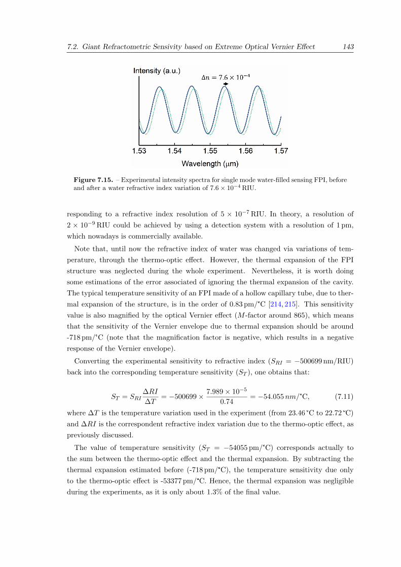
7.2. Giant Refractometric Sensivity based on Extreme Optical Vernier Effect 143
Figure 7.15. – Experimental intensity spectra for single mode water-filled sensing FPI, beforeand after a water refractive index variation of 7.6× 10⁻⁴ RIU.
responding to a refractive index resolution of 5 × 10⁻⁷ RIU. In theory, a resolution of
2 × 10⁻⁹ RIU could be achieved by using a detection system with a resolution of 1 pm,
which nowadays is commercially available.
Note that, until now the refractive index of water was changed via variations of tem-
perature, through the thermo-optic effect. However, the thermal expansion of the FPI
structure was neglected during the whole experiment. Nevertheless, it is worth doing
some estimations of the error associated of ignoring the thermal expansion of the cavity.
The typical temperature sensitivity of an FPI made of a hollow capillary tube, due to ther-
mal expansion of the structure, is in the order of 0.83 pm/°C [214, 215]. This sensitivity
value is also magnified by the optical Vernier effect (M -factor around 865), which means
that the sensitivity of the Vernier envelope due to thermal expansion should be around
-718 pm/°C (note that the magnification factor is negative, which results in a negative
response of the Vernier envelope).
Converting the experimental sensitivity to refractive index (SRI = −500699 nm/RIU)
back into the corresponding temperature sensitivity (ST ), one obtains that:
ST = SRI∆RI
∆T= −500699× 7.989× 10−5
0.74= −54.055nm/°C, (7.11)
where ∆T is the temperature variation used in the experiment (from 23.46 °C to 22.72 °C)
and ∆RI is the correspondent refractive index variation due to the thermo-optic effect, as
previously discussed.
The value of temperature sensitivity (ST = −54055 pm/°C) corresponds actually to
the sum between the thermo-optic effect and the thermal expansion. By subtracting the
thermal expansion estimated before (-718 pm/°C), the temperature sensitivity due only
to the thermo-optic effect is -53377 pm/°C. Hence, the thermal expansion was negligible
during the experiments, as it is only about 1.3% of the final value.
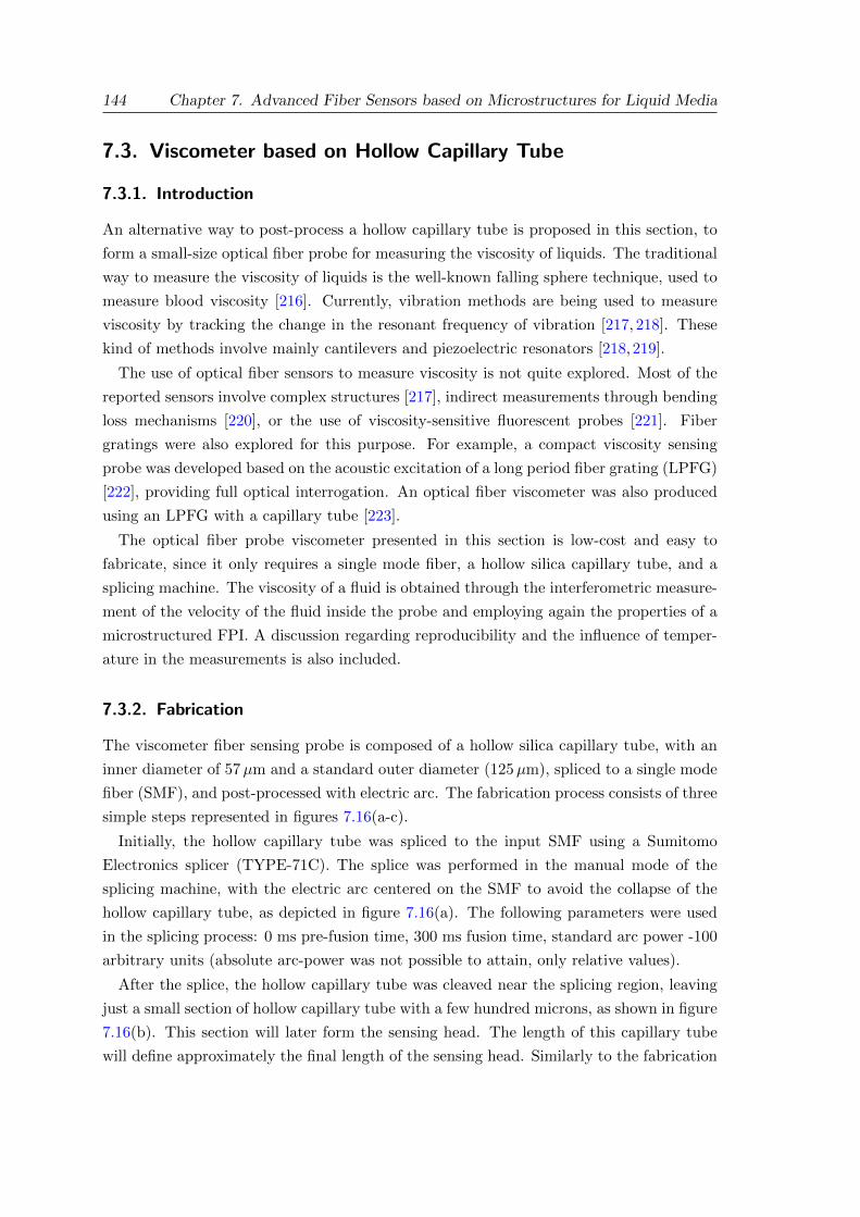
144 Chapter 7. Advanced Fiber Sensors based on Microstructures for Liquid Media
7.3. Viscometer based on Hollow Capillary Tube
7.3.1. Introduction
An alternative way to post-process a hollow capillary tube is proposed in this section, to
form a small-size optical fiber probe for measuring the viscosity of liquids. The traditional
way to measure the viscosity of liquids is the well-known falling sphere technique, used to
measure blood viscosity [216]. Currently, vibration methods are being used to measure
viscosity by tracking the change in the resonant frequency of vibration [217, 218]. These
kind of methods involve mainly cantilevers and piezoelectric resonators [218,219].
The use of optical fiber sensors to measure viscosity is not quite explored. Most of the
reported sensors involve complex structures [217], indirect measurements through bending
loss mechanisms [220], or the use of viscosity-sensitive fluorescent probes [221]. Fiber
gratings were also explored for this purpose. For example, a compact viscosity sensing
probe was developed based on the acoustic excitation of a long period fiber grating (LPFG)
[222], providing full optical interrogation. An optical fiber viscometer was also produced
using an LPFG with a capillary tube [223].
The optical fiber probe viscometer presented in this section is low-cost and easy to
fabricate, since it only requires a single mode fiber, a hollow silica capillary tube, and a
splicing machine. The viscosity of a fluid is obtained through the interferometric measure-
ment of the velocity of the fluid inside the probe and employing again the properties of a
microstructured FPI. A discussion regarding reproducibility and the influence of temper-
ature in the measurements is also included.
7.3.2. Fabrication
The viscometer fiber sensing probe is composed of a hollow silica capillary tube, with an
inner diameter of 57µm and a standard outer diameter (125µm), spliced to a single mode
fiber (SMF), and post-processed with electric arc. The fabrication process consists of three
simple steps represented in figures 7.16(a-c).
Initially, the hollow capillary tube was spliced to the input SMF using a Sumitomo
Electronics splicer (TYPE-71C). The splice was performed in the manual mode of the
splicing machine, with the electric arc centered on the SMF to avoid the collapse of the
hollow capillary tube, as depicted in figure 7.16(a). The following parameters were used
in the splicing process: 0 ms pre-fusion time, 300 ms fusion time, standard arc power -100
arbitrary units (absolute arc-power was not possible to attain, only relative values).
After the splice, the hollow capillary tube was cleaved near the splicing region, leaving
just a small section of hollow capillary tube with a few hundred microns, as shown in figure
7.16(b). This section will later form the sensing head. The length of this capillary tube
will define approximately the final length of the sensing head. Similarly to the fabrication
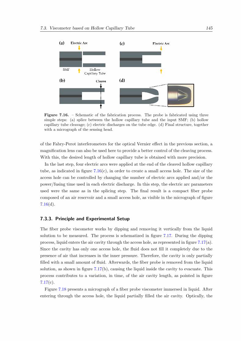
7.3. Viscometer based on Hollow Capillary Tube 145
Figure 7.16. – Schematic of the fabrication process. The probe is fabricated using threesimple steps: (a) splice between the hollow capillary tube and the input SMF; (b) hollowcapillary tube cleavage; (c) electric discharges on the tube edge. (d) Final structure, togetherwith a micrograph of the sensing head.
of the Fabry-Perot interferometers for the optical Vernier effect in the previous section, a
magnification lens can also be used here to provide a better control of the cleaving process.
With this, the desired length of hollow capillary tube is obtained with more precision.
In the last step, four electric arcs were applied at the end of the cleaved hollow capillary
tube, as indicated in figure 7.16(c), in order to create a small access hole. The size of the
access hole can be controlled by changing the number of electric arcs applied and/or the
power/fusing time used in each electric discharge. In this step, the electric arc parameters
used were the same as in the splicing step. The final result is a compact fiber probe
composed of an air reservoir and a small access hole, as visible in the micrograph of figure
7.16(d).
7.3.3. Principle and Experimental Setup
The fiber probe viscometer works by dipping and removing it vertically from the liquid
solution to be measured. The process is schematized in figure 7.17. During the dipping
process, liquid enters the air cavity through the access hole, as represented in figure 7.17(a).
Since the cavity has only one access hole, the fluid does not fill it completely due to the
presence of air that increases in the inner pressure. Therefore, the cavity is only partially
filled with a small amount of fluid. Afterwards, the fiber probe is removed from the liquid
solution, as shown in figure 7.17(b), causing the liquid inside the cavity to evacuate. This
process contributes to a variation, in time, of the air cavity length, as pointed in figure
7.17(c).
Figure 7.18 presents a micrograph of a fiber probe viscometer immersed in liquid. After
entering through the access hole, the liquid partially filled the air cavity. Optically, the
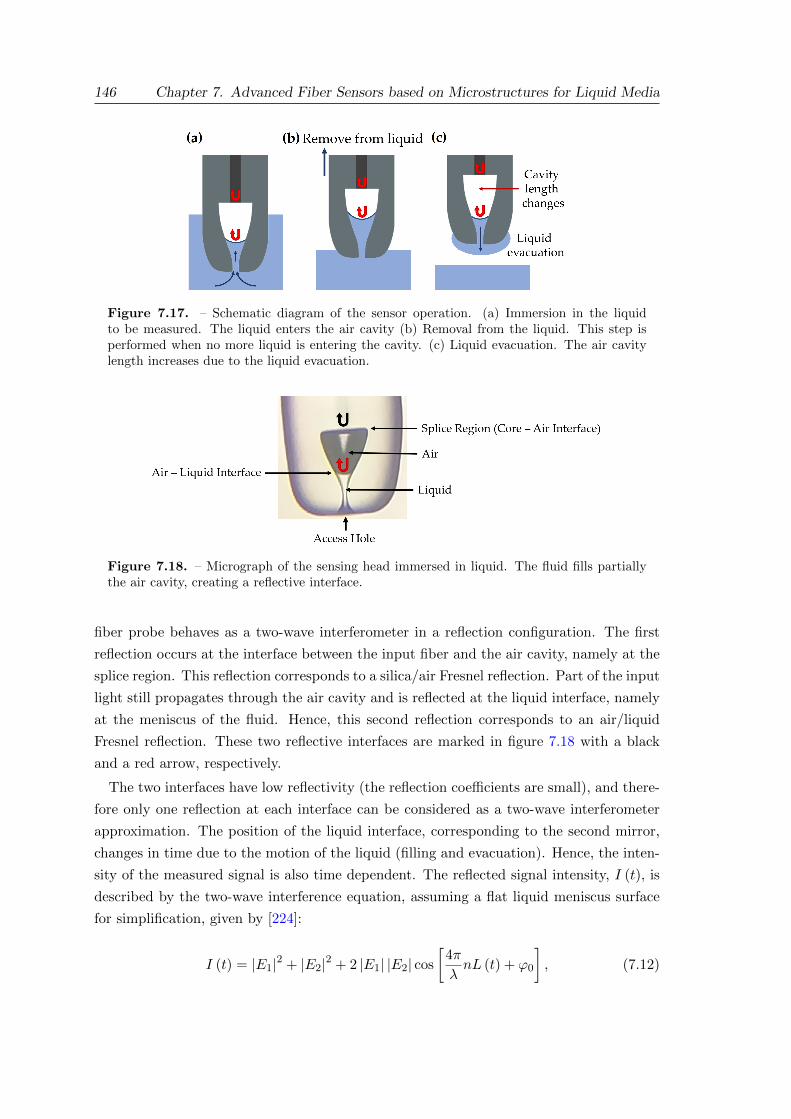
146 Chapter 7. Advanced Fiber Sensors based on Microstructures for Liquid Media
Figure 7.17. – Schematic diagram of the sensor operation. (a) Immersion in the liquidto be measured. The liquid enters the air cavity (b) Removal from the liquid. This step isperformed when no more liquid is entering the cavity. (c) Liquid evacuation. The air cavitylength increases due to the liquid evacuation.
Figure 7.18. – Micrograph of the sensing head immersed in liquid. The fluid fills partiallythe air cavity, creating a reflective interface.
fiber probe behaves as a two-wave interferometer in a reflection configuration. The first
reflection occurs at the interface between the input fiber and the air cavity, namely at the
splice region. This reflection corresponds to a silica/air Fresnel reflection. Part of the input
light still propagates through the air cavity and is reflected at the liquid interface, namely
at the meniscus of the fluid. Hence, this second reflection corresponds to an air/liquid
Fresnel reflection. These two reflective interfaces are marked in figure 7.18 with a black
and a red arrow, respectively.
The two interfaces have low reflectivity (the reflection coefficients are small), and there-
fore only one reflection at each interface can be considered as a two-wave interferometer
approximation. The position of the liquid interface, corresponding to the second mirror,
changes in time due to the motion of the liquid (filling and evacuation). Hence, the inten-
sity of the measured signal is also time dependent. The reflected signal intensity, I (t), is
described by the two-wave interference equation, assuming a flat liquid meniscus surface
for simplification, given by [224]:
I (t) = |E1|2 + |E2|2 + 2 |E1| |E2| cos
[4π
λnL (t) + ϕ0
], (7.12)
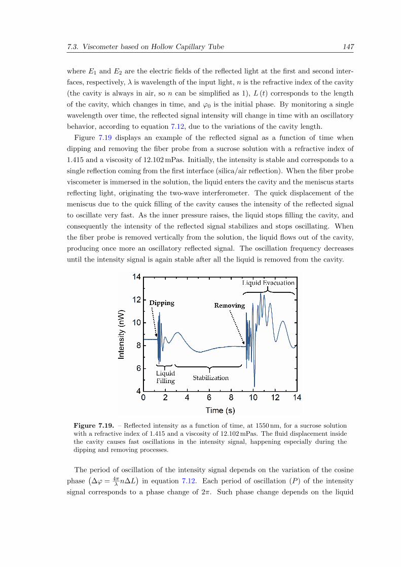
7.3. Viscometer based on Hollow Capillary Tube 147
where E1 and E2 are the electric fields of the reflected light at the first and second inter-
faces, respectively, λ is wavelength of the input light, n is the refractive index of the cavity
(the cavity is always in air, so n can be simplified as 1), L (t) corresponds to the length
of the cavity, which changes in time, and ϕ0 is the initial phase. By monitoring a single
wavelength over time, the reflected signal intensity will change in time with an oscillatory
behavior, according to equation 7.12, due to the variations of the cavity length.
Figure 7.19 displays an example of the reflected signal as a function of time when
dipping and removing the fiber probe from a sucrose solution with a refractive index of
1.415 and a viscosity of 12.102 mPas. Initially, the intensity is stable and corresponds to a
single reflection coming from the first interface (silica/air reflection). When the fiber probe
viscometer is immersed in the solution, the liquid enters the cavity and the meniscus starts
reflecting light, originating the two-wave interferometer. The quick displacement of the
meniscus due to the quick filling of the cavity causes the intensity of the reflected signal
to oscillate very fast. As the inner pressure raises, the liquid stops filling the cavity, and
consequently the intensity of the reflected signal stabilizes and stops oscillating. When
the fiber probe is removed vertically from the solution, the liquid flows out of the cavity,
producing once more an oscillatory reflected signal. The oscillation frequency decreases
until the intensity signal is again stable after all the liquid is removed from the cavity.
Figure 7.19. – Reflected intensity as a function of time, at 1550 nm, for a sucrose solutionwith a refractive index of 1.415 and a viscosity of 12.102 mPas. The fluid displacement insidethe cavity causes fast oscillations in the intensity signal, happening especially during thedipping and removing processes.
The period of oscillation of the intensity signal depends on the variation of the cosine
phase(∆ϕ = 4π
λ n∆L)
in equation 7.12. Each period of oscillation (P ) of the intensity
signal corresponds to a phase change of 2π. Such phase change depends on the liquid
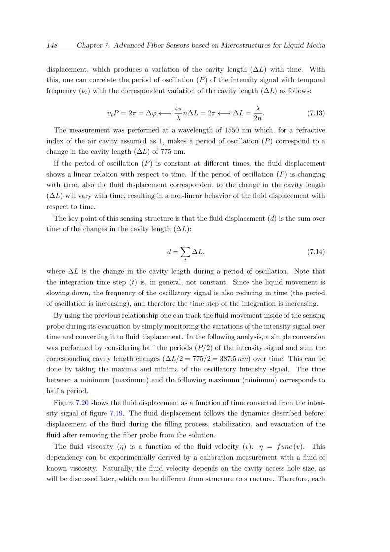
148 Chapter 7. Advanced Fiber Sensors based on Microstructures for Liquid Media
displacement, which produces a variation of the cavity length (∆L) with time. With
this, one can correlate the period of oscillation (P ) of the intensity signal with temporal
frequency (νt) with the correspondent variation of the cavity length (∆L) as follows:
υtP = 2π = ∆ϕ←→ 4π
λn∆L = 2π ←→ ∆L =
λ
2n. (7.13)
The measurement was performed at a wavelength of 1550 nm which, for a refractive
index of the air cavity assumed as 1, makes a period of oscillation (P ) correspond to a
change in the cavity length (∆L) of 775 nm.
If the period of oscillation (P ) is constant at different times, the fluid displacement
shows a linear relation with respect to time. If the period of oscillation (P ) is changing
with time, also the fluid displacement correspondent to the change in the cavity length
(∆L) will vary with time, resulting in a non-linear behavior of the fluid displacement with
respect to time.
The key point of this sensing structure is that the fluid displacement (d) is the sum over
time of the changes in the cavity length (∆L):
d =∑t
∆L, (7.14)
where ∆L is the change in the cavity length during a period of oscillation. Note that
the integration time step (t) is, in general, not constant. Since the liquid movement is
slowing down, the frequency of the oscillatory signal is also reducing in time (the period
of oscillation is increasing), and therefore the time step of the integration is increasing.
By using the previous relationship one can track the fluid movement inside of the sensing
probe during its evacuation by simply monitoring the variations of the intensity signal over
time and converting it to fluid displacement. In the following analysis, a simple conversion
was performed by considering half the periods (P/2) of the intensity signal and sum the
corresponding cavity length changes (∆L/2 = 775/2 = 387.5nm) over time. This can be
done by taking the maxima and minima of the oscillatory intensity signal. The time
between a minimum (maximum) and the following maximum (minimum) corresponds to
half a period.
Figure 7.20 shows the fluid displacement as a function of time converted from the inten-
sity signal of figure 7.19. The fluid displacement follows the dynamics described before:
displacement of the fluid during the filling process, stabilization, and evacuation of the
fluid after removing the fiber probe from the solution.
The fluid viscosity (η) is a function of the fluid velocity (v): η = func (v). This
dependency can be experimentally derived by a calibration measurement with a fluid of
known viscosity. Naturally, the fluid velocity depends on the cavity access hole size, as
will be discussed later, which can be different from structure to structure. Therefore, each
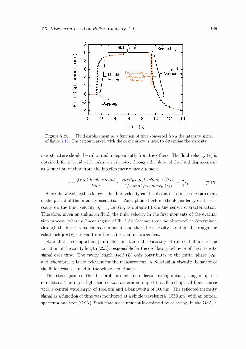
7.3. Viscometer based on Hollow Capillary Tube 149
Figure 7.20. – Fluid displacement as a function of time converted from the intensity signalof figure 7.19. The region marked with the orang arrow is used to determine the viscosity.
new structure should be calibrated independently from the others. The fluid velocity (v) is
obtained, for a liquid with unknown viscosity, through the slope of the fluid displacement
as a function of time from the interferometric measurement:
v =fluid displacement
time∼ cavity length change (∆L)
1/signal frequency (νt)=λ
2νt. (7.15)
Since the wavelength is known, the fluid velocity can be obtained from the measurement
of the period of the intensity oscillations. As explained before, the dependency of the vis-
cosity on the fluid velocity, η = func (v), is obtained from the sensor characterization.
Therefore, given an unknown fluid, the fluid velocity in the first moments of the evacua-
tion process (where a linear regime of fluid displacement can be observed) is determined
through the interferometric measurement, and then the viscosity is obtained through the
relationship η (v) derived from the calibration measurement.
Note that the important parameter to obtain the viscosity of different fluids is the
variation of the cavity length (∆L), responsible for the oscillatory behavior of the intensity
signal over time. The cavity length itself (L) only contributes to the initial phase (ϕ0)
and, therefore, it is not relevant for the measurement. A Newtonian viscosity behavior of
the fluids was assumed in the whole experiment.
The interrogation of the fiber probe is done in a reflection configuration, using an optical
circulator. The input light source was an erbium-doped broadband optical fiber source
with a central wavelength of 1550 nm and a bandwidth of 100 nm. The reflected intensity
signal as a function of time was monitored at a single wavelength (1550 nm) with an optical
spectrum analyzer (OSA). Such time measurement is achieved by selecting, in the OSA, a
150 Chapter 7. Advanced Fiber Sensors based on Microstructures for Liquid Media
central wavelength of 1550 nm and a measurement span of 0 nm. These settings allow the
OSA to measure the intensity at 1550 nm as a function of time, with a time step of 3 ms
(the time step might vary depending on the OSA model and settings).
Ideally, a fast photodetector should be used to monitor the intensity signal as a function
of time with high temporal resolution. The time resolution achieved by the OSA might
be problematic to resolve fast oscillations at the beginning of the dipping process. In this
situation, the liquid enters so fast in the cavity that the time resolution of the OSA cannot
measure correctly the oscillations produced in the intensity signal. Therefore in figure
7.20, the displacement obtained after the evacuation process appears to be lower than the
displacement obtained at the start of the dipping process (difference of around 4µm). In
fact, it does not mean that the amount of liquid entering the cavity is less than the amount
of liquid evacuating the cavity. The problem simply arises from the lack of time resolution
to observe correctly the initial condition. Apart from using a fast photodetector, another
solution to overcome such issue is to use longer wavelengths. From equation 7.13, increas-
ing the wavelength used in the experiment makes a period of oscillation correspond to a
larger cavity length change (∆L). Hence, this reduces the signal frequency, being easier
to measure fast displacements of liquid inside the cavity. Nevertheless, this problem is not
relevant for the final application of the fiber probe, since the initial region corresponding
to the dipping process is not used for viscosity measurements. To perform viscosity mea-
surements, only the variations of the intensity signal after removing the sensor from the
sucrose solution are considered, as indicated in figure 7.20.
Taking as a reference the reflected signal from a cleaved single mode fiber in air (3.3%
Fresnel reflection at 1550 nm), the splice losses have been measured to be about 0.5 dB,
assuring a good optical signal quality.
7.3.4. Characterization
Mixtures of sugar in water with different viscosities were used as calibrated solutions
to characterize the viscometer fiber probe. The relation between sugar concentration,
refractive index, viscosity, and temperature is well studied and can be found in different
books [9,10]. The viscosity (η) of the different sucrose solutions, at 20 °C, was determined
using the following relationship2:
η (n) = 0.59269 + 0.00758e[(n−1.35348)/0.01054] + 0.89366e[(n−1.35348)/0.02675], (7.16)
where η is the viscosity given in millipascal-second (mPa.s), and n is the refractive index
of the sucrose solution. It is important to mention that the coefficients in equation 7.16
2Further details can be found in appendix D.
7.3. Viscometer based on Hollow Capillary Tube 151
are material dependent. Therefore, this equation is only valid for sucrose solutions. These
solutions of known viscosity were then used to characterize and calibrate the viscometer
fiber probe. The objective is to obtain the relationship between the viscosity and the fluid
velocity during the evacuation: η = func (v).
The intensity signal as a function of time for two sucrose solutions with distinct vis-
cosities (1.887 mPa.s and 12.102 mPa.s), after removing the fiber probe from the solutions,
is shown in figure 7.21. As expected, the solution of lower viscosity moves faster and
produced a higher frequency signal, while the higher viscosity solution is slower and orig-
inates a low frequency signal. Another interesting property is also visible in figure 7.21.
The visibility of the interference signal is higher for the solution of higher viscosity, due
to its higher refractive index. The reflection coefficient at the interface of the higher vis-
cosity solution (second interface) is closer to the reflection coefficient of the first interface.
Therefore, the two interfering waves have closer intensities in the case of a higher viscosity
solution than in the case of a lower viscosity solution.
The viscometer fiber probe was then characterized using sucrose solutions with different
viscosities ranging from 1.887 mPa.s (19.5 %wt/wt of sucrose) to 19.170 mPa.s (51.8 %wt/wt
of sucrose). The liquid displacement at the evacuation process as a function of time was
obtained for each solution. The results can be found in figure 7.22.
As expected, lower viscosity solutions evacuate faster from the cavity than the ones of
higher viscosity, showing a larger fluid displacement in a smaller time frame. Between
every measurement, the probe was always cleaned by dipping it several times in deionized
Figure 7.21. – Reflected intensity as a function of time, at 1550 nm, for two sucrose solutionsof distinct viscosities: 1.887 mPa.s and 12.102 mPa.s. Higher viscosity solutions produce slowerintensity oscillations.
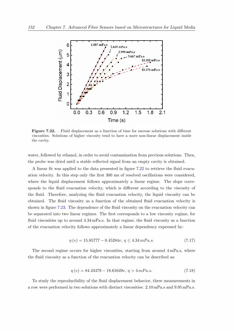
152 Chapter 7. Advanced Fiber Sensors based on Microstructures for Liquid Media
Figure 7.22. – Fluid displacement as a function of time for sucrose solutions with differentviscosities. Solutions of higher viscosity tend to have a more non-linear displacement insidethe cavity.
water, followed by ethanol, in order to avoid contamination from previous solutions. Then,
the probe was dried until a stable reflected signal from an empty cavity is obtained.
A linear fit was applied to the data presented in figure 7.22 to retrieve the fluid evacu-
ation velocity. In this step only the first 300 ms of resolved oscillations were considered,
where the liquid displacement follows approximately a linear regime. The slope corre-
sponds to the fluid evacuation velocity, which is different according to the viscosity of
the fluid. Therefore, analyzing the fluid evacuation velocity, the liquid viscosity can be
obtained. The fluid viscosity as a function of the obtained fluid evacuation velocity is
shown in figure 7.23. The dependence of the fluid viscosity on the evacuation velocity can
be separated into two linear regimes. The first corresponds to a low viscosity regime, for
fluid viscosities up to around 4.34 mPa.s. In that regime, the fluid viscosity as a function
of the evacuation velocity follows approximately a linear dependency expressed by:
η (v) = 15.85777− 0.45284v, η ≤ 4.34mPa.s. (7.17)
The second regime occurs for higher viscosities, starting from around 4 mPa.s, where
the fluid viscosity as a function of the evacuation velocity can be described as:
η (v) = 84.43479− 18.61649v, η > 4mPa.s. (7.18)
To study the reproducibility of the fluid displacement behavior, three measurements in
a row were performed in two solutions with distinct viscosities: 2.10 mPa.s and 9.95 mPa.s.
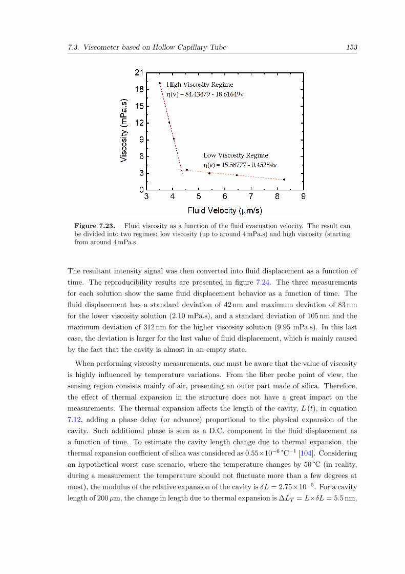
7.3. Viscometer based on Hollow Capillary Tube 153
Figure 7.23. – Fluid viscosity as a function of the fluid evacuation velocity. The result canbe divided into two regimes: low viscosity (up to around 4 mPa.s) and high viscosity (startingfrom around 4 mPa.s.
The resultant intensity signal was then converted into fluid displacement as a function of
time. The reproducibility results are presented in figure 7.24. The three measurements
for each solution show the same fluid displacement behavior as a function of time. The
fluid displacement has a standard deviation of 42 nm and maximum deviation of 83 nm
for the lower viscosity solution (2.10 mPa.s), and a standard deviation of 105 nm and the
maximum deviation of 312 nm for the higher viscosity solution (9.95 mPa.s). In this last
case, the deviation is larger for the last value of fluid displacement, which is mainly caused
by the fact that the cavity is almost in an empty state.
When performing viscosity measurements, one must be aware that the value of viscosity
is highly influenced by temperature variations. From the fiber probe point of view, the
sensing region consists mainly of air, presenting an outer part made of silica. Therefore,
the effect of thermal expansion in the structure does not have a great impact on the
measurements. The thermal expansion affects the length of the cavity, L (t), in equation
7.12, adding a phase delay (or advance) proportional to the physical expansion of the
cavity. Such additional phase is seen as a D.C. component in the fluid displacement as
a function of time. To estimate the cavity length change due to thermal expansion, the
thermal expansion coefficient of silica was considered as 0.55×10⁻⁶ °C−1 [104]. Considering
an hypothetical worst case scenario, where the temperature changes by 50 °C (in reality,
during a measurement the temperature should not fluctuate more than a few degrees at
most), the modulus of the relative expansion of the cavity is δL = 2.75×10⁻⁵. For a cavity
length of 200µm, the change in length due to thermal expansion is ∆LT = L×δL = 5.5 nm,
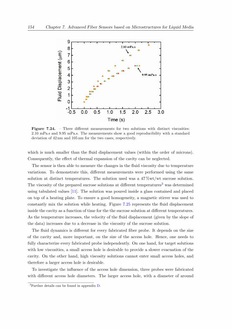
154 Chapter 7. Advanced Fiber Sensors based on Microstructures for Liquid Media
Figure 7.24. – Three different measurements for two solutions with distinct viscosities:2.10 mPa.s and 9.95 mPa.s. The measurements show a good reproducibility with a standarddeviation of 42 nm and 105 nm for the two cases, respectively.
which is much smaller than the fluid displacement values (within the order of microns).
Consequently, the effect of thermal expansion of the cavity can be neglected.
The sensor is then able to measure the changes in the fluid viscosity due to temperature
variations. To demonstrate this, different measurements were performed using the same
solution at distinct temperatures. The solution used was a 47 %wt/wt sucrose solution.
The viscosity of the prepared sucrose solutions at different temperatures3 was determined
using tabulated values [11]. The solution was poured inside a glass contained and placed
on top of a heating plate. To ensure a good homogeneity, a magnetic stirrer was used to
constantly mix the solution while heating. Figure 7.25 represents the fluid displacement
inside the cavity as a function of time for the the sucrose solution at different temperatures.
As the temperature increases, the velocity of the fluid displacement (given by the slope of
the data) increases due to a decrease in the viscosity of the sucrose solution.
The fluid dynamics is different for every fabricated fiber probe. It depends on the size
of the cavity and, more important, on the size of the access hole. Hence, one needs to
fully characterize every fabricated probe independently. On one hand, for target solutions
with low viscosities, a small access hole is desirable to provide a slower evacuation of the
cavity. On the other hand, high viscosity solutions cannot enter small access holes, and
therefore a larger access hole is desirable.
To investigate the influence of the access hole dimension, three probes were fabricated
with different access hole diameters. The larger access hole, with a diameter of around
3Further details can be found in appendix D.
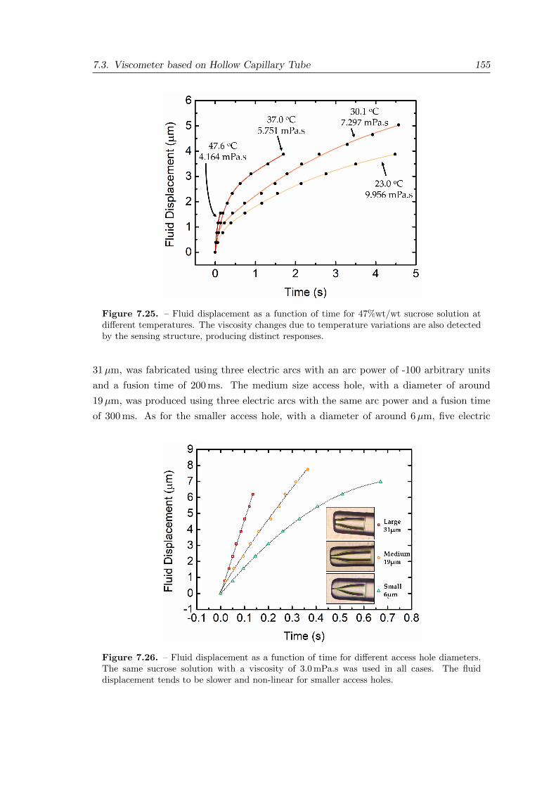
7.3. Viscometer based on Hollow Capillary Tube 155
Figure 7.25. – Fluid displacement as a function of time for 47%wt/wt sucrose solution atdifferent temperatures. The viscosity changes due to temperature variations are also detectedby the sensing structure, producing distinct responses.
31µm, was fabricated using three electric arcs with an arc power of -100 arbitrary units
and a fusion time of 200 ms. The medium size access hole, with a diameter of around
19µm, was produced using three electric arcs with the same arc power and a fusion time
of 300 ms. As for the smaller access hole, with a diameter of around 6µm, five electric
Figure 7.26. – Fluid displacement as a function of time for different access hole diameters.The same sucrose solution with a viscosity of 3.0 mPa.s was used in all cases. The fluiddisplacement tends to be slower and non-linear for smaller access holes.
156 Chapter 7. Advanced Fiber Sensors based on Microstructures for Liquid Media
arcs were applied with the same arc power and a fusion time of 300 ms. All three samples
were used to measure a sucrose solution with a viscosity of 3.0 mPa.s (at 20 °C). The fluid
displacement as a function of time for the three samples is depicted in figure 7.26, together
with microscope images of the samples. The probe with a small access hole presents a non-
linear behavior of the fluid displacement over time. For high viscosity solutions, the fluid
displacement is very slow or the fluid might not even be able to enter the cavity through
the access hole. Therefore, small access holes are more suitable to measure low viscosity
solutions. On the other hand, larger access holes result in faster fluid displacements, which
can be problematic for low viscosity fluids. The produced intensity signal oscillations are
very fast, making them hard to be resolved in time. In sum, the best option is to dimension
the access hole of the viscometer fiber probe depending on the range of viscosities to be
measured. Nevertheless, one should not forget that a measurement system with a fast
photodetector (instead of an OSA) is enough to track the fast oscillations originated by a
low viscosity fluid measured with a large access hole probe.
7.4. Conclusion
Two advanced sensing structures for application in liquid media were explored in this
chapter. The first structure was based on a new method that combines an extreme op-
tical Vernier effect with a few-mode sensing interferometer. The demonstrated method
proved to be capable of overcoming the limitations of the standard optical Vernier effect
techniques. The implementation of a few-mode fiber refractometer with such method reg-
istered a record M -factor of 865, also reaching a record value in terms of refractive index
sensitivity for this kind of interferometric fiber structure. In fact, for a single-mode Vernier
structure to achieve an extreme M -factor of 865, it would correspond to an immeasurable
Vernier envelope FSR longer than 6400 nm. Therefore, the proposed method allows us
to achieve such giant M -factors whilst maintaining a measurable envelope. From the ob-
tained results for refractive index sensing, it would be very attractive to apply a similar
structure for high resolution gas sensing and biosensing, namely in extreme environments,
where it is necessary to detect very small concentrations.
Although the concept was demonstrated experimentally and also via simulations, it is
still open the possibility of further exploration of the enhanced sensitivity observed at
some internal envelope intersections mathematically. The relative movement between the
internal envelopes was not fully explored, and it is the key for the behavior of this extreme
case of optical Vernier effect.
The proposed concept of extreme optical Vernier effect can also be adapted to other
sensing interferometers (Mach-Zehnder interferometers, Michelson interferometers, hybrid
interferometric structures, among others), to obtain giant sensitivities to other physical
and chemical parameters. Therefore, the proposed method opens new horizons for the
7.4. Conclusion 157
development of a new generation of sensors with extreme sensitivities and resolutions for
demanding state-of-the-art applications.
Regarding the second structure proposed in this chapter, the optical fiber probe viscome-
ter was capable of performing an all-optical interferometric measurement of the viscosity
of a liquid. Besides, the total volume of the cavity is approximately 50 pL, which makes
the volume of liquid required to perform the measurement negligible. In other words,
practically only a very small sample volume is required to realize the measurement.
For specific applications, a different configuration involving a temperature sensor in
parallel should be studied in the future, for instance incorporating a fiber Bragg grating
next to the cavity to read the temperature while the probe is immersed in the liquid.
The aim is to provide simultaneous temperature measurements and/or to compensate the
change of a fluid viscosity due to temperature. Another point worth of further investigation
is the influence of the size of the access hole in the maximum viscosity value measurable.
Moreover, the next step for future studies is also to determine the feasibility of applying
this sensing structure to the measurement of biological fluids.

Chapter 8.
Conclusions and Final Remarks
The works presented along this dissertation were focused on two main points of study. The
first was the study, design, and realization of advanced interferometric fiber sensors based
on microstructures. This included the combination of optical microfibers, which allow the
propagating light to interact better with the environment, together with microstructured
interferometers such as microfiber knot resonators, Mach-Zehnder interferometers, and
Fabry-Perot interferometers. Focused ion beam milling was also explored as a technology
to create not only microstructured interferometers in optical microfibers, but also to open
access holes in specialty fibers for liquid sensing. The second main point was the interest
of increasing the performance of the interferometric fiber sensors (i.e. enhance the sen-
sitivity). In this context, an in-depth study, further development, and application of the
optical Vernier effect to optical fiber interferometers as a tool to surpass the sensitivity
limits of conventional fiber interferometers were performed. Some of the enormous po-
tentials of this effect applied to optical fiber sensing were discussed and demonstrated in
this dissertation. However there are still other variants that have not been here explored
and that could still lead to very interesting results. This dissertation was meant to guide
the reader across the different topics and works, providing also the basic background and
the state-of-the-art of these topics for a better contextualization and understanding of the
concepts presented.
Chapter 2 introduced the reader to optical microfibers and their fabrication methods,
as well as to the different interferometric sensing structures that were later on being used.
The basic concepts and properties of the different interferometric sensing structures were
presented, together with a small state-of-the-art review on different applications, especially
when combined with optical microfibers. Since focused ion beam milling was used along the
dissertation, chapter 2 also included a brief overview on the focused ion beam technology,
with special focus on the application to optical fibers and respective sample preparation.
Chapter 3 explored microstructured sensing devices with optical microfibers, where
the different interferometric structures previously introduced (microfiber knot resonator,
Mach-Zehnder interferometer, and Fabry-Perot interferometer) were microfabricated in
160 Chapter 8. Conclusions and Final Remarks
optical microfibers and microfiber probes. The two devices proposed in this chapter tar-
geted two different issues related with optical fiber sensing. The first structure tackled
the problem of cross-sensitivity. By combining a microfiber knot resonator and a Mach-
Zehnder interferometer embedded in the same optical microfiber, the final response could
be used for simultaneous measurement of refractive index of liquids and temperature. The
use of a single optical microfiber and two co-propagating modes to form the Mach-Zehnder
interferometer is a novel alternative that makes the final structure more compact. The use
of microfiber knot resonators to sense liquids might lead to some problems: the microfiber
knot resonator can be very fragile and the surface tension of water is, in some cases, enough
to change the size of the knot or to break the microfiber. Therefore, it would be useful
to explored some protection techniques, like coating the structure with a low refractive
index polymer to ensure a good stability and protection of the microfiber knot resonator.
The second proposed device was meant to be a miniaturized sensing probe, with potential
to perform point measurements, but simultaneously with the possibility to achieve higher
sensitivities than what has been previously reported in the literature for these kind of
structures. A Fabry-Perot interferometer microfabricated with focused ion beam milling
in an optical microfiber probe (similar to what has already been published [3]) was taken
as the main structure. However, the Fabry-Perot interferometer was designed to be mul-
timode, which was different from the other works. The beating generated in the output
spectrum showed a higher wavelength shift in comparison to the normal sensing Fabry-
Perot interferometer signal. This phenomenon was actually the result of the optical Vernier
effect, however in an uncontrolled way, as one could not control the modes propagating in
the structure. This last work allowed to only have a small glimpse of the capabilities of
using the optical Vernier effect combined with fiber sensing. For this reason, the following
works headed in this new direction, trying to understand the essence of such an effect. To
fully understand and control the optical Vernier effect, it was first necessary to look deep
into its origins.
Chapter 4 presented the full mathematical description of the optical Vernier effect and
its properties. Important comments and small details were included along this chapter
for a deeper understanding and to avoid misuse and misinterpretation of the effect in the
future. Before starting to apply the effect, it was essential to have an overview of what was
published in this field until now. Therefore, the state-of-the-art, presented also in chapter
4, focused on the different configurations explored over the last few years to introduce the
optical Vernier effect, as well as the distinct applications that it can be used for.
Upon exploring the fundamentals of the optical Vernier effect, the following questions
were asked: “what is the limit? What is the maximum magnification that one can obtain
from such an effect?”. The answer led to a contradictory requirement: the smaller the
detuning between the two interferometers, the higher was the magnification factor ob-
tained, but also the larger was the Vernier envelope. The detection system imposes then
161
a limitation on how large the Vernier envelope could be to still be measurable, which in
return dictates the maximum magnification factor achievable.
Chapter 5 explored a new extended concept of the optical Vernier effect was found
during the investigations: the existence of optical harmonics of the Vernier effect, which
enable greater magnification factors to be achieved, beyond the limitations previously de-
scribed. This novel concept required the development of a new mathematical description,
presented in this chapter, that could describe correctly the effect and all its new properties.
By up-scaling the optical path length of the reference interferometer by multiples of the
optical path length of the sensing interferometer, different output spectra with harmonic
properties were generated. The important message here is that the magnification factor
can increase proportionally to the harmonic order (it increases by (i+ 1), being i the
order of the harmonic), for the same detuning, while maintaining the size of the Vernier
envelope.
Naturally, under certain conditions the effect does not work as desired and does not pro-
vide the enhancements discussed before. One of these situations, also discussed in chapter
5, is when the up-scaling of the optical path length is done in the sensing interferometer,
rather than in the reference interferometer. The result of such case was actually no im-
provement of the sensitivity with the harmonic order. Apart from this special situation,
there are also differences between the parallel and series configurations, reason why it was
important to present them in chapter 5, before experimentally applying the effect.
Once more, the same question as before can be asked: “what is now the limit? What
is the maximum harmonic order achievable?”. These questions were also examined at the
end of chapter 5. To my view, one of the most limiting factors here is the complexity of
the obtained spectrum. The higher the harmonic order, the more complex the spectrum
is. This requires a lot of signal processing and effort to be able to extract the wavelength
shift of the Vernier envelope. Hence, the limits depend on the processing capabilities and,
not less important, on the resolution of the interrogation system.
Now that the fundamentals of the optical harmonic Vernier effect were studied, the next
step was to experimentally demonstrate the effect and validate its properties. At the same
time, the sensing structures were applied to measure strain.
Chapter 6 presented the experimental demonstration of the optical harmonic Vernier
effect for two configurations, parallel and series, using Fabry-Perot interferometers. The
parallel configuration relied on Fabry-Perot interferometers made from hollow capillary
tubes. The structures were characterized in terms of applied strain for the first three
harmonic orders of the optical Vernier effect. It has been experimentally proven that the
enhancement of the magnification factor, and respective sensitivity, increased with the
order of the harmonic. An important message from this work is the importance of the
detuning between the optical path lengths of the two interferometers. The magnification
factor depends on this detuning, which is highly dependent on the fabrication methods. It
162 Chapter 8. Conclusions and Final Remarks
is very difficult to create multiple interferometric structures with exactly the same optical
path length, due to fabrication constrains. Hence, the envelope phase sensitivity was de-
termined in each case, in order to make a fair comparison between the different structures
used to introduce the three harmonic orders of the optical Vernier effect. The envelope
phase sensitivity takes into account the free spectral range of the Vernier envelope, and
therefore it is independent of the detuning. The series configuration, also demonstrated
in chapter 6, combined a hollow microsphere and a section of a multimode fiber to form
two Fabry-Perot interferometers physically connected. A special case of optical Vernier
effect was here explored, where none of the two interferometers was used as a reference. In
this specific case, the sensitivity of the Vernier envelope depends on the difference between
the sensitivities of the two interferometers, weighted by their magnification factors. One
saw that, if both interferometers have similar sensitivities, there would be no improve-
ment of sensitivity when using the optical Vernier effect. Yet, a high sensitivity to strain
was still observed for the proposed structure (about 140-fold larger than a fiber Bragg
grating), since the hollow microsphere alone had more strain sensitivity than the section
of multimode fiber used. Simultaneous measurement of strain and temperature was also
demonstrated with this structure, by using the Vernier envelope response together with
the high frequency response of the spectrum.
Chapter 7 demonstrates two last works dedicated to the measurement of liquid proper-
ties, in this case refractive index and viscosity. The first work results from the combination
of different concepts and techniques developed during the PhD: Fabry-Perot interferom-
eters using hollow capillary tubes, focused ion beam milling to open access holes in one
of the interferometers, and an extreme case of optical Vernier effect. The extreme optical
Vernier effect was discovered and proposed as a way to surpass once more the limitations
of the conventional optical Vernier effect. The use of a few-mode Fabry-Perot interferom-
eter, together with the optical Vernier effect in tune with the fundamental propagating
mode, allowed to achieve a magnification factor an order of magnitude higher than the
expected limit for the conventional optical Vernier effect, whilst maintaining a measurable
Vernier envelope. When applied to liquid sensing, the proposed arrangement is capable
of achieving a giant sensitivity to refractive index, allowing to measure fine variations of
this quantity. To the best of the author’s knowledge, the obtained sensitivity value (about
500000 nm/RIU) is a record value for a Fabry-Perot interferometer structure of this kind.
The second work explored in chapter 7 makes use of a similar hollow capillary tube, but
now post-processed with an electric arc to form a small-size optical fiber probe with an
access hole for viscosity sensing of liquids. The developed sensor works as a two-wave
interferometer once the liquid enters the probe, being the air-liquid interface inside the
microstructured hollow capillary tube one of the mirrors of the interferometer. Through
interferometric measurement of the liquid displacement inside the probe, the viscosity of
the liquid was retrieved. The fact that there are not many options for optical fiber sen-
163
sors to measure viscosity makes this novel approach very attractive. Additionally, the
probe volume is so small (about 50 pL) that practically no liquid is consumed during the
measurement.
The works developed during this PhD were very diverse, not just in terms of sensing
configurations, but also in the different possible options for the application of the optical
Vernier effect. Nevertheless, there is still space for improvement and for new ideas to be
explored in the future. The introduction of the optical Vernier effect, now in a controlled
way, to the focused ion beam-milled Fabry-Perot interferometer in a microfiber probe could
still be further explored. The concept of optical harmonic Vernier effect here proposed
can, from now on, be applied to other types of optical fiber interferometers, creating a
new generation of highly sensitive fiber sensors for different applications. By taking a
closer look into the state-of-the-art configurations for the optical Vernier effect, the future
trend will involve the use of hybrid configurations. The combination of different types of
interferometers in a hybrid configuration to introduce the optical Vernier effect is still very
attractive and can provide innovative results. One of these cases is the use of two inter-
ferometer with opposite responses to the measured parameter, in a configuration without
a reference interferometer, which could lead to even further improvements in the mag-
nification factors obtained. Moreover, the viability of such a structure for simultaneous
measurement of parameters is higher, since each of the two interferometer can be espe-
cially optimized to sense a specific different measurand. Regarding the sensing structure
with giant refractometric sensitivity, further studies should be performed to improve its
applicability, namely by exploring the possibility of functionalization of the Fabry-Perot
cavity to different substances. If viable, this approach could lead to a highly sensitive
platform for biological fluid analysis or chemical compound detection.
At last, a huge downside of the optical Vernier effect, that still requires a lot of investiga-
tion, is the interrogation system. There is a urgent need for the development of a simpler
interrogation system to analyze the response of the effect. The need of a broadband source
and an optical spectrum analyzer to measure a broad range of wavelengths, plus the ad-
ditional signal processing required to extract the Vernier envelope wavelength shift from
the spectrum, makes the use of this effect less attractive. If there was an interrogation
system relying only on photodetectors and two, or a few more, laser lines to measure and
characterize in a simpler, faster, and cheaper way the response of the optical Vernier effect,
it would represent a huge step towards the acceptance and quick adoption of the optical
Vernier effect as a viable sensing solution in different areas.

Bibliography
[1] Byeong Ha Lee, Young Ho Kim, Kwan Seob Park, Joo Beom Eom, Myoung Jin Kim,
Byung Sup Rho, and Hae Young Choi. Interferometric fiber optic sensors. Sensors,
12(3):2467–2486, 2012.
[2] Masaru Muranishi, Kazutaka Sato, Sumio Hosaka, Atsushi Kikukawa, Toshimichi
Shintani, and Kenchi Ito. Control of aperture size of optical probes for scanning
near-Field Optical microscopy using focused ion beam technology. Japanese Journal
of Applied Physics, 36(Part 2, No. 7B):L942–L944, jul 1997.
[3] Ricardo M Andre, Stephen C. Warren-Smith, Martin Becker, Jan Dellith, Man-
fred Rothhardt, M I Zibaii, H Latifi, Manuel B Marques, Hartmut Bartelt, and
Orlando Frazao. Simultaneous measurement of temperature and refractive index us-
ing focused ion beam milled Fabry-Perot cavities in optical fiber micro-tips. Optics
Express, 24(13):14053–14065, jun 2016.
[4] Stephen C. Warren-Smith, Ricardo M. Andre, Jan Dellith, Tina Eschrich, Martin
Becker, and Hartmut Bartelt. Sensing with ultra-short Fabry-Perot cavities written
into optical micro-fibers. Sensors and Actuators B: Chemical, 244:1016–1021, jun
2017.
[5] Shaoxian Zhang, Yin Liu, Huiyong Guo, Ai Zhou, and Libo Yuan. Highly sensitive
vector curvature sensor based on two juxtaposed fiber Michelson interferometers
with Vernier-like effect. IEEE Sensors Journal, 19(6):2148–2154, mar 2019.
[6] Zhilin Xu, Qizhen Sun, Borui Li, Yiyang Luo, Wengao Lu, Deming Liu, Perry Ping
Shum, and Lin Zhang. Highly sensitive refractive index sensor based on cascaded
microfiber knots with Vernier effect. Optics Express, 23(5):6662, mar 2015.
[7] Zhilin Xu, Yiyang Luo, Deming Liu, Perry Ping Shum, and Qizhen Sun. Sensitivity-
controllable refractive index sensor based on reflective θ-shaped microfiber resonator
cooperated with Vernier effect. Scientific Reports, 7(1):1–8, 2017.
[8] Ling Liu, Tigang Ning, Jingjing Zheng, Li Pei, Jing Li, Jihong Cao, Xuekai Gao, and
Chuanbiao Zhang. High-sensitivity strain sensor implemented by hybrid cascaded
166 Bibliography
interferometers and the Vernier-effect. Optics & Laser Technology, 119:105591, nov
2019.
[9] Mosen Asadi. Tables. In Beet-Sugar Handbook, pages 779–801. John Wiley & Sons,
Inc., 2005.
[10] United States Department of Agriculture. Technical Procedures Manual. In SCI
Division Inspection Series, pages 1–169. 2013.
[11] J.F. Swindells, C.F. Snyder, R.C. Hardy, and P.E. Golden. Viscosities of Sucrose
Solutions at Various Temperatures: Tables of Recalculated Values. U.S. Department
of commerce, National Bureau of standards, united sta edition, 1958.
[12] Alexey N Bashkatov and Elina A Genina. Water refractive index in dependence on
temperature and wavelength: a simple approximation. In Valery V Tuchin, editor,
Saratov Fall Meeting 2002: Optical Technologies in Biophysics and Medicine IV,
volume 5068, pages 393–395. International Society for Optics and Photonics, SPIE,
oct 2003.
[13] Bernard S. Finn. City of Light: The Story of Fiber Optics (review), volume 43. 2002.
[14] K.C. Kao and G.A. Hockham. Dielectric-fibre surface waveguides for optical fre-
quencies. Proceedings of the Institution of Electrical Engineers, 113(7):1151–1158,
jul 1966.
[15] Andre D. Gomes, Jiangbo Tim Zhao, Alessandro Tuniz, and Markus A. Schmidt.
Direct observation of modal hybridization in nanofluidic fiber [Invited]. Optical
Materials Express, 11(2):559, feb 2021.
[16] Andre D. Gomes, Jens Kobelke, Jorg Bierlich, Jan Dellith, Manfred Rothhardt,
Hartmut Bartelt, and Orlando Frazao. Giant refractometric sensitivity by com-
bining extreme optical Vernier effect and modal interference. Scientific Reports,
10(1):19313, dec 2020.
[17] Paulo Robalinho, Andre Gomes, and Orlando Frazao. Colossal Enhancement of
Strain Sensitivity Using the Push-Pull Deformation Method. IEEE Sensors Journal,
21(4):4623–4627, feb 2021.
[18] Paulo Manuel Ribeiro Robalinho, Andre D. Gomes, and Orlando Frazao. High
Enhancement Strain Sensor Based on Vernier Effect Using 2-Fiber Loop Mirrors.
IEEE Photonics Technology Letters, 32(18):1139–1142, sep 2020.
[19] Andre D Gomes, Marta S Ferreira, Jorg Bierlich, Jens Kobelke, Manfred Rothhardt,
Hartmut Bartelt, and Orlando Frazao. Hollow microsphere combined with optical
Bibliography 167
harmonic Vernier effect for strain and temperature discrimination. Optics and Laser
Technology, 127(February):106198, 2020.
[20] Andre D. Gomes, Marta S. Ferreira, Jorg Bierlich, Jens Kobelke, Manfred Roth-
hardt, Hartmut Bartelt, and Orlando Frazao. Optical harmonic Vernier effect: a
new tool for high performance interferometric fibre sensors. Sensors, 19(24):5431,
2019.
[21] Andre D. Gomes, Martin Becker, Jan Dellith, Mohammad I. Zibaii, Hamid Latifi,
Manfred Rothhardt, Hartmut Bartelt, and Orlando Frazao. Multimode Fabry-Perot
Interferometer Probe Based on Vernier Effect for Enhanced Temperature Sensing.
Sensors, 19(3):453, jan 2019.
[22] Andre D. Gomes, Jens Kobelke, Jorg Bierlich, Kay Schuster, Hartmut Bartelt, and
Orlando Frazao. Optical fiber probe viscometer based on hollow capillary tube.
Journal of Lightwave Technology, 37(18):4456–4461, sep 2019.
[23] Beatriz Silveira, Andre Gomes, Martin Becker, Henrik Schneidewind, and Orlando
Frazao. Bunimovich stadium-like resonator for randomized fiber laser operation.
Photonics, 5(3):17, jul 2018.
[24] Andre Gomes, Catarina Monteiro, Beatriz Silveira, and Orlando Frazao. A brief
review of new fiber microsphere geometries. Fibers, 6(3):48, jul 2018.
[25] Andre D Gomes, Fatemeh Karami, Mohammad I Zibaii, Hamid Latifi, Orlando
Frazao, Orlando Frazao, and O Frazo. Multipath interferometer polished micro-
sphere for enhanced temperature sensing. IEEE Sensors Letters, 2(2):1–4, jun 2018.
[26] A. D. Gomes, B. Silveira, J. Dellith, M. Becker, M. Rothhard, H. Bartelt, and
O. Frazao. Cleaved Silica Microsphere for Temperature Measurement. IEEE Pho-
tonics Technology Letters, 30(9):797–800, may 2018.
[27] Andre D. Gomes and Orlando Frazao. Microfiber knot with taper interferometer
for temperature and refractive index discrimination. IEEE Photonics Technology
Letters, 29(18):1517–1520, 2017.
[28] Andre D. Gomes, Martin Becker, Jan Dellith, Mohammad I. Zibaii, Hamid Latifi,
Manfred Rothhardt, Hartmut Bartelt, and Orlando Frazao. Enhanced temperature
sensing with Vernier effect on fiber probe based on multimode Fabry-Perot interfer-
ometer. In Manuel Filipe P. Martins Costa, editor, Fourth International Conference
on Applications of Optics and Photonics, page 117. SPIE, oct 2019.
168 Bibliography
[29] Andre D. Gomes, Jens Kobelke, Jorg Bierlich, Kay Schuster, Hartmut Bartelt, and
Orlando Frazao. Optical fiber probe for viscosity measurements. In 26th Interna-
tional Conference on Optical Fiber Sensors, volume 100, page TuE8, Washington,
D.C., 2018. OSA.
[30] Andre D Gomes, Beatriz Silveira, Fatemeh Karami, Mohammad I Zibaii, Hamid
Latifi, Jan Dellith, Martin Becker, Manfred Rothhardt, Hartmut Bartelt, and Or-
lando Frazao. Multi-path interferometer structures with cleaved silica microspheres
. In Katherine Creath, Jan Burke, Michael B North Morris, and Angela D Davies,
editors, Interferometry XIX, volume 10749, pages 195–200. International Society for
Optics and Photonics, SPIE, aug 2018.
[31] Orlando Frazao and Andre Delgado Gomes. Simultaneous measurement of tempera-
ture and refractive index based on microfiber knot resonator integrated in an abrupt
taper Mach-Zehnder interferometer. In Manuel Filipe P. Martins Costa, editor, Third
International Conference on Applications of Optics and Photonics, volume 10453,
page 141. SPIE, aug 2017.
[32] Andre Gomes and Orlando Frazao. Microfiber knot resonators as sensors - a re-
view. In Proceedings of the 5th International Conference on Photonics, Optics and
Laser Technology, number Photoptics, pages 356–364. SCITEPRESS - Science and
Technology Publications, mar 2017.
[33] A. D. Gomes and O. Frazao. Microfiber knot resonators for sensing applications. In
Springer Series in Optical Sciences, pages 145–163. 2019.
[34] Takeshi Ozeki and B. S. Kawasaki. Optical directional coupler using tapered sections
in multimode fibers. Applied Physics Letters, 28(9):528–529, 1976.
[35] B S Kawasaki and K O Hill. Low-loss access coupler for multimode optical fiber
distribution networks. Applied optics, 16(7):1794–1795, 1977.
[36] B S Kawasaki, K O Hill, and R G Lamont. Biconical-taper single-mode fiber coupler.
Optics letters, 6(7):327–328, 1981.
[37] Khanh Quoc Kieu and Masud Mansuripur. Biconical fiber taper sensors. IEEE
Photonics Technology Letters, 18(21):2239–2241, 2006.
[38] Xu Zeng, Yu Wu, Changlun Hou, Jian Bai, and Guoguang Yang. A tempera-
ture sensor based on optical microfiber knot resonator. Optics Communications,
282(18):3817–3819, 2009.
Bibliography 169
[39] J Yang, L Jiang, S Wang, B Li, M Wang, H Xiao, Y Lu, and H Tsai. High sensitivity
of taper-based Mach-Zehnder interferometer embedded in a thinned optical fiber for
refractive index sensing. Applied optics, 50(28):5503–5507, 2011.
[40] X Fang, C R Liao, and D N Wang. Femtosecond laser fabricated fiber Bragg grating
in microfiber for refractive index sensing. Optics letters, 35(7):1007–1009, 2010.
[41] Ping Zhao, Yuhua Li, Jihua Zhang, Lei Shi, and Xinliang Zhang. Nanohole induced
microfiber Bragg gratings. Optics Express, 20(27):28625–28630, dec 2012.
[42] Jing Feng, Ming Ding, Jun Long Kou, Fei Xu, and Yan Qing Lu. An optical fiber
tip micrograting thermometer. IEEE Photonics Journal, 3(5):810–814, 2011.
[43] Timothy a. Birks and Youwei W. Li. The shape of fiber tapers. Journal of Lightwave
Technology, 10(4):432–438, 1992.
[44] Limin Tong, Rafael R. Gattass, Jonathan B. Ashcom, Sailing He, Jingyi Lou,
Mengyan Shen, Iva Maxwell, and Eric Mazur. Subwavelength-diameter silica wires
for low-loss optical wave guiding. Nature, 426(6968):816–819, 2003.
[45] Fei Xu, Valerio Pruneri, Vittoria Finazzi, and Gilberto Brambilla. An embedded
optical nanowire loop resonator refractometric sensor. Optics express, 16(2):1062–
1067, 2008.
[46] Limin Xiao and T a Birks. High finesse microfiber knot resonators made from
double-ended tapered fibers. Optics letters, 36(7):1098–1100, 2011.
[47] Xiaoqin Wu and Limin Tong. Optical microfibers and nanofibers. Nanophotonics,
2(5-6):407–428, 2013.
[48] Limin Tong, Jingyi Lou, and Eric Mazur. Single-mode guiding properties
of subwavelength-diameter silica and silicon wire waveguides. Optics Express,
12(6):1025, 2004.
[49] Gilberto Brambilla, Fei Xu, Peter Horak, Yongmin Jung, Fumihito Koizumi, Neil P.
Sessions, Elena Koukharenko, Xian Feng, Ganapathy S. Murugan, James S. Wilkin-
son, and David J. Richardson. Optical fiber nanowires and microwires: fabrication
and applications. Advances in Optics and Photonics, 1(1):107–161, jan 2009.
[50] M. Sumetsky. Basic elements for microfiber photonics: micro/nanofibers and mi-
crofiber coil resonators. Journal of Lightwave Technology, 26(1):21–27, 2008.
[51] I. H. Malitson. Interspecimen comparison of the refractive index of fused silica.
Journal of the Optical Society of America, 55(10):1205–1209, oct 1965.
170 Bibliography
[52] S. W. Harun, K. S. Lim, C. K. Tio, K. Dimyati, and H. Ahmad. Theoretical analysis
and fabrication of tapered fiber. Optik, 124(6):538–543, 2013.
[53] J. M. Ward, A. Maimaiti, Vu H. Le, and S. Nic Chormaic. Contributed Review: Opti-
cal micro- and nanofiber pulling rig. Review of Scientific Instruments, 85(11):111501–
10, nov 2014.
[54] Zhaobing Tian, S. S H Yam, Jack Barnes, Wojtek Bock, Patricia Greig, James M.
Fraser, Hans Peter Loock, and Richard D. Oleschuk. Refractive index sensing with
Mach-Zehnder interferometer based on concatenating two single-mode fiber tapers.
IEEE Photonics Technology Letters, 20(8):626–628, 2008.
[55] Jie Shi, Shilin Xiao, Lilin Yi, and Meihua Bi. A sensitivity-enhanced refractive index
sensor using a single-mode thin-core fiber incorporating an abrupt taper. Sensors,
12:4697–4705, 2012.
[56] Robert Wiley and Brett Clark. High-power fused assemblies enabled by advances in
fiber-processing technologies. In Jay W. Dawson, editor, Fiber Lasers VIII: Tech-
nology, Systems, and Applications, volume 7914, page 79140F, feb 2011.
[57] Timothy E. Dimmick, George Kakarantzas, Timothy A. Birks, and Philip St. J.
Russell. Carbon dioxide laser fabrication of fused-fiber couplers and tapers. Applied
Optics, 38(33):6845–6848, nov 1999.
[58] Jonathan M. Ward, Danny G. O’Shea, Brian J. Shortt, Michael J. Morrissey, Kieran
Deasy, and Sıle G. Nic Chormaic. Heat-and-pull rig for fiber taper fabrication.
Review of Scientific Instruments, 77(8):083105, aug 2006.
[59] G. Brambilla, F. Koizumi, X. Feng, and D.J. Richardson. Compound-glass optical
nanowires. Electronics Letters, 41(7):400, 2005.
[60] Lu Ding, Cherif Belacel, Sara Ducci, Giuseppe Leo, and Ivan Favero. Ultralow
loss single-mode silica tapers manufactured by a microheater. Applied Optics,
49(13):2441–2445, 2010.
[61] B. Musa, A. A. Rozi, A. S. M. Noor, A. Ismail, and M. A. Mahdi. Effect of fiber
profile parameters on the transmission properties of the tapered optical fibers. In
2011 2nd International Conference on Photonics, pages 1–4. IEEE, oct 2011.
[62] R. Wonko, P. Marc, and L. R. Jaroszewicz. Fabrication of tapered long period fiber
gratings for sensors application by filament heating. In Jan Dorosz and Ryszard S.
Romaniuk, editors, Optical Fibers and Their Applications 2017, volume 10325, page
1032507, feb 2017.
Bibliography 171
[63] Gilberto Brambilla, Vittoria Finazzi, and David Richardson. Ultra-low-loss optical
fiber nanotapers. Optics express, 12(10):2258–2263, 2004.
[64] G Brambilla, F Xu, and X Feng. Fabrication of optical fibre nanowires and their
optical and mechanical characterisation. Electronics Letters, 42(9):517–519, 2006.
[65] Ryutaro Nagai and Takao Aoki. Ultra-low-loss tapered optical fibers with minimal
lengths. Optics Express, 22(23):28427–28436, 2014.
[66] Alexander Hartung, Sven Brueckner, and Hartmut Bartelt. Limits of light guidance
in optical nanofibers. Opt. Express, 18(4):3754–3761, 2010.
[67] A.J.C. J C Grellier, N.K. K Zayer, and C.N. N Pannell. Heat transfer modelling in
CO2 laser processing of optical fibres. Optics Communications, 152(4-6):324–328,
1998.
[68] M Sumetsky, Y Dulashko, and A Hale. Fabrication and study of bent and coiled
free silica nanowires: Self-coupling microloop optical interferometer. Optics express,
12(15):3521–31, 2004.
[69] Cheng-Ju Ju Ma, Li-Yong Yong Ren, Yi-Ping Ping Xu, Ying-Li Li Wang, Jian Liang,
and En-Shi Shi Qu. Design and fabrication of tapered microfiber waveguide with
good optical and mechanical performance. Journal of Modern Optics, 61(8):683–687,
2014.
[70] Bishnu P. Pal. Guided Wave Optical Components and Devices. 2006.
[71] John F Ready. Fiber Optics. In John F B T Industrial Applications of Lasers
(Second Edition) Ready, editor, Industrial Applications of Lasers, pages 530–545.
Elsevier, San Diego, 1997.
[72] Hongjuan Yang, Shanshan Wang, Xin Wang, Jing Wang, Yipeng Liao, Xin Liao, and
Jing Wang. Temperature sensing in seawater based on microfiber knot resonator.
Sensors, 14(10):18515–18525, oct 2014.
[73] Yu Wu, Yun-Jiang Rao, Yi-huai Chen, and Yuan Gong. Miniature fiber-optic tem-
perature sensors based on silica/polymer microfiber knot resonators. Optics Express,
17(20):18142–18147, sep 2009.
[74] Xianli Li and Hui Ding. A stable evanescent field-based microfiber knot resonator
refractive index sensor. IEEE Photonics Technology Letters, 26(16):1625–1628, 2014.
[75] Kok-Sing Sing Lim, Iman Aryanfar, Wu-Yi Yi Chong, Yew-Ken Ken Cheong, Su-
laiman W. Harun, and Harith Ahmad. Integrated microfibre device for refractive
index and temperature sensing. Sensors, 12(9):11782–11789, aug 2012.
172 Bibliography
[76] Lecheng Li, Li Xia, Zhenhai Xie, and Deming Liu. All-fiber Mach-Zehnder interfer-
ometers for sensing applications. Optics Express, 20(10):11109, 2012.
[77] Th Schubert, N Haase, and H Kuck. Refractive-index measurements using an in-
tegrated Mach-Zehnder interferometer. Sensors and Actuators A, 60(100):108–112,
1997.
[78] Shiuh-Chuan Her and Chih-Min Yang. Dynamic strain measured by Mach-Zehnder
interferometric optical fiber sensors. Sensors, 12(3):3314–3326, mar 2012.
[79] Jianmin Gong, J. M. K. MacAlpine, Wei Jin, and Yanbiao Liao. Locating acoustic
emission with an amplitude-multiplexed acoustic sensor array based on a modified
Mach-Zehnder interferometer. Applied Optics, 40(34):6199, dec 2001.
[80] Andre D Gomes and Orlando Frazao. Mach-Zehnder based on large knot fiber
resonator for refractive index measurement. IEEE Photonics Technology Letters,
28(12):1279–1281, jun 2016.
[81] Ping Lu, Liqiu Men, Kevin Sooley, and Qiying Chen. Tapered fiber Mach-Zehnder
interferometer for simultaneous measurement of refractive index and temperature.
Applied Physics Letters, 94(13):3–5, 2009.
[82] Haipeng Luo, Qizhen Sun, Zhilin Xu, Deming Liu, and Lin Zhang. Simultaneous
measurement of refractive index and temperature using multimode microfiber-based
dual Mach-Zehnder interferometer. Optics Letters, 39(13):4049, 2014.
[83] Haipeng Luo, Qizhen Sun, Zhilin Xu, Weihua Jia, Deming Liu, and Lin Zhang.
Microfiber-based inline Mach-Zehnder interferometer for dual-parameter measure-
ment. IEEE Photonics Journal, 7(2):1–8, apr 2015.
[84] Yipeng Liao, Jing Wang, Shanshan Wang, Hongjuan Yang, and Xin Wang. Simul-
taneous measurement of seawater temperature and salinity based on microfiber MZ
interferometer with a knot resonator. Journal of Lightwave Technology, 34(01):5378–
5384, 2016.
[85] Yipeng Liao, Jing Wang, Shanshan Wang, Hongjuan Yang, and Xin Wang. Spectral
characteristics of the microfiber MZ interferometer with a knot resonator. Optics
Communications, 389(October 2016):253–257, apr 2017.
[86] A. D. Kersey, D. A. Jackson, and M. Corke. A simple fibre Fabry-Perot sensor.
Optics and Lasers in Engineering, 5(3):141–154, 1984.
[87] M Born and E Wolf. Principles of Optics: Electromagnetic Theory of Propagation,
Interference and Diffraction of Light. Cambridge University Press, 1999.
Bibliography 173
[88] Yan Zhang, Helen Shibru, Kristie L. Cooper, and Anbo Wang. Miniature fiber-optic
multicavity Fabry-Perot interferometric biosensor. Optics Letters, 30(9):1021–1023,
may 2005.
[89] Yan Zhang, K.L. Cooper, and Anbo Wang. Multicavity Fabry-Perot interferometric
thin-film sensor with built-in temperature compensation. IEEE Photonics Technol-
ogy Letters, 17(12):2712–2714, dec 2005.
[90] Marta S Ferreira, Luıs Coelho, Kay Schuster, Jens Kobelke, Jose L Santos, and
Orlando Frazao. Fabry-Perot cavity based on a diaphragm-free hollow-core silica
tube. Optics Letters, 36(20):4029–4031, 2011.
[91] Ruohui Wang and Xueguang Qiao. Hybrid optical fiber Fabry-Perot interferometer
for simultaneous measurement of gas refractive index and temperature. Applied
Optics, 53(32):7724, 2014.
[92] Shaolin Zhang, Ziwen Zhao, Na Chen, Fufei Pang, Zhenyi Chen, Yunqi Liu, and
Tingyun Wang. Temperature characteristics of silicon core optical fiber Fabry-Perot
interferometer. Optics Letters, 40(7):1362–1365, apr 2015.
[93] Joel Villatoro, Vittoria Finazzi, Gianluca Coviello, and Valerio Pruneri. Photonic-
crystal-fiber-enabled micro-Fabry-Perot interferometer. Optics letters, 34(16):2441–
2443, 2009.
[94] Ming Deng, Chang-Ping Tang, Tao Zhu, Yun-Jiang Rao, Lai-Cai Xu, and Meng
Han. Refractive index measurement using photonic crystal fiber-based Fabry-Perot
interferometer. Applied optics, 49(9):1593–1598, 2010.
[95] Fernando. C. Favero, Geraud Bouwmans, Vittoria Finazzi, Joel Villatoro, and Vale-
rio Pruneri. Fabry-Perot interferometers built by photonic crystal fiber pressuriza-
tion during fusion splicing. Optics letters, 36(21):4191–4193, nov 2011.
[96] F. C. Favero, L. Araujo, G. Bouwmans, V. Finazzi, J. Villatoro, and V. Pruneri.
Spheroidal Fabry-Perot microcavities in optical fibers for high-sensitivity sensing.
Optics Express, 20(7):7112, 2012.
[97] Hao Sun, Xiaolei Zhang, Liutong Yuan, Libin Zhou, Xueguang Qiao, and Manli Hu.
An optical fiber Fabry-Perot interferometer sensor for simultaneous measurement of
relative humidity and temperature. IEEE Sensors Journal, 15(5):2891–2897, 2015.
[98] Jun Ma, Jian Ju, Long Jin, Wei Jin, and Dongning Wang. Fiber-tip micro-cavity
for temperature and transverse load sensing. Optics Express, 19(13):12418–12426,
2011.
174 Bibliography
[99] Lu Yan, Zhiguo Gui, Gao Guanjun Gao Guanjun Wang, Yongquan An, Jinyu Gu,
Meiqin Zhang, Xinglin Liu, Zhibin Wang, Gao Guanjun Gao Guanjun Wang, and
Pinggang Jia. A micro bubble structure based Fabry-Perot optical fiber strain sensor
with high sensitivity and low-cost characteristics. Sensors, 17(3):555, 2017.
[100] Catarina Monteiro, Susana Silva, and Orlando Frazao. Hollow microsphere
Fabry-Perot cavity for sensing applications. IEEE Photonics Technology Letters,
29(15):1229–1232, aug 2017.
[101] Yong Zhao, Feng Xia, Mao-qing Chen, Rui-jie Tong, and Yun Peng. Optical fiber
axial contact force sensor based on bubble-expanded Fabry-Perot interferometer.
Sensors and Actuators A: Physical, 272:318–324, 2018.
[102] Yun-Jiang Rao, Ming Deng, De-Wen Duan, Xiao-Chen Yang, Tao Zhu, and Guang-
Hua Cheng. Micro Fabry-Perot interferometers in silica fibers machined by fem-
tosecond laser. Optics Express, 15(21):14123–14128, 2007.
[103] Tao Wei, Yukun Han, Hai-Lung Tsai, and Hai Xiao. Miniaturized fiber inline Fabry-
Perot interferometer fabricated with a femtosecond laser. Optics letters, 33(6):536–
538, 2008.
[104] C. R. Liao, T Y Hu, and D. N. Wang. Optical fiber Fabry-Perot interferometer cavity
fabricated by femtosecond laser micromachining and fusion splicing for refractive
index sensing. Optics express, 20(20):22813–22818, sep 2012.
[105] C. A. Volkert and A. M. Minor. Focused ion beam microscopy and micromachining.
MRS Bulletin, 32(05):389–399, 2007.
[106] AA Ampere A Tseng. Recent developments in micromilling using focused ion beam
technology. Journal of Micromechanics and Microengineering, 14(4):R15–R34, 2004.
[107] Steve Reyntjens and Robert Puers. A review of focused ion beam applications in mi-
crosystem technology. Journal of Micromechanics and Microengineering, 11(4):287–
300, 2001.
[108] Nan Yao. Introduction to the focused ion beam system. Focused Ion Beam Systems:
Basics and Applications, pages 1–10, 2007.
[109] S.A. Boden, Z. Moktadir, D.M. Bagnall, H. Mizuta, and H.N. Rutt. Focused helium
ion beam milling and deposition. Microelectronic Engineering, 88(8):2452–2455, aug
2011.
[110] Cicero Martelli, Paolo Olivero, John Canning, Nathaniel Groothoff, Brant Gibson,
and Shane Huntington. Micromachining structured optical fibers using focused ion
beam milling. Optics letters, 32(11):1575–1577, 2007.
Bibliography 175
[111] Peter Sigmund. Theory of Sputtering. I. Sputtering Yield of Amorphous and Poly-
crystalline Targets. Physical Review, 184(2):383–416, aug 1969.
[112] Th Lacoste, Th Huser, R. Prioli, and H. Heinzelmann. Contrast enhancement using
polarization-modulation scanning near-field optical microscopy (PM-SNOM). Ultra-
microscopy, 71(1-4):333–340, mar 1998.
[113] Saeed Pilevar, Klaus Edinger, Walid Atia, Igor Smolyaninov, and Christopher Davis.
Focused ion-beam fabrication of fiber probes with well-defined apertures for use in
near-field scanning optical microscopy. Applied Physics Letters, 72(24):3133–3135,
jun 1998.
[114] A. Micco, A. Ricciardi, M. Pisco, V. La Ferrara, and A. Cusano. Optical fiber tip
templating using direct focused ion beam milling. Scientific Reports, 5:15935, 2015.
[115] S. Cabrini, C. Liberale, D. Cojoc, A. Carpentiero, M. Prasciolu, S. Mora, V. Degior-
gio, F. De Angelis, and E. Di Fabrizio. Axicon lens on optical fiber forming optical
tweezers, made by focused ion beam milling. Microelectronic Engineering, 83(4-9
SPEC. ISS.):804–807, 2006.
[116] Rita S. Rodrigues Ribeiro, Pabitra Dahal, Ariel Guerreiro, Pedro A. S. Jorge, and
Jaime Viegas. Fabrication of Fresnel plates on optical fibres by FIB milling for optical
trapping, manipulation and detection of single cells. Scientific Reports, 7(1):4485,
dec 2017.
[117] M L von Bibra, A Roberts, and J Canning. Fabrication of long-period fiber gratings
by use of focused ion-beam irradiation. Optics letters, 26(11):765–7, 2001.
[118] Jun-long Kou, Sun-jie Qiu, Fei Xu, and Yan-qing Lu. Demonstration of a compact
temperature sensor based on first-order Bragg grating in a tapered fiber probe.
Optics express, 19(19):18452–18457, 2011.
[119] Yanxin Liu, Chao Meng, a Ping Zhang, Yao Xiao, Huakang Yu, and Limin
Tong. Compact microfiber Bragg gratings with high-index contrast. Optics letters,
36(16):3115–3117, 2011.
[120] K. P. Nayak, Fam Le Kien, Y. Kawai, K. Hakuta, K. Nakajima, H. T. Miyazaki,
and Y. Sugimoto. Cavity formation on an optical nanofiber using focused ion beam
milling technique. Opt. Express Opt. Express, 19(15):14040–14050, 2011.
[121] Jun-long Kou, Jing Feng, Qian-jin Wang, Fei Xu, and Yan-qing Lu. Microfiber-
probe-based ultrasmall interferometric sensor. Optics letters, 35(13):2308–10, 2010.
176 Bibliography
[122] T. Wieduwilt, J. Dellith, F. Talkenberg, H. Bartelt, and M. a. Schmidt. Reflectivity
enhanced refractive index sensor based on a fiber-integrated Fabry-Perot microres-
onator. Optics Express, 22(21):25333–25346, 2014.
[123] Ricardo M Andre, Simon Pevec, Martin Becker, Jan Dellith, Manfred Rothhardt,
Manuel B Marques, Denis Donlagic, Hartmut Bartelt, and Orlando Frazao. Focused
ion beam post-processing of optical fiber Fabry-Perot cavities for sensing applica-
tions. Optics express, 22(11):13102–13108, jun 2014.
[124] Andre D. Gomes, Ricardo M. Andre, Stephen C. Warren-Smith, Jan Dellith, Mar-
tin Becker, Manfred Rothhardt, and Orlando Frazao. Combined microfiber knot
resonator and focused ion beam-milled Mach-Zehnder interferometer for refractive
index measurement. In Youngjoo Chung, Wei Jin, Byoungho Lee, John Canning,
Kentaro Nakamura, and Libo Yuan, editors, Proceedings of SPIE - The International
Society for Optical Engineering, volume 10323, page 1032340, apr 2017.
[125] Stephen C. Warren-Smith, Ricardo M. Andre, Christopher Perrella, Jan Dellith,
Manfred Rothhardt, and Hartmut Bartelt. Direct core structuring of microstructured
optical fibers using focused ion beam milling. Optics Express, 24(1):378–387, 2016.
[126] A.D. D. Gomes, M.F.S. F. S. Ferreira, J.P. P. Moura, R.M. M. Andre, J. Kobelke,
J. Bierlich, K. Wondraczek, K. Schuster, and O. Frazao. Acetone evaporation and
water vapor detection using a caterpillar-like microstructured fiber. Microwave and
Optical Technology Letters, 58(3):679–683, 2016.
[127] A. Ping Zhang, Li Yang Shao, Jin Fei Ding, and Sailing He. Sandwiched long-period
gratings for simultaneous measurement of refractive index and temperature. IEEE
Photonics Technology Letters, 17(11):2397–2399, 2005.
[128] Orlando Frazao, Diogo Egypto, Lucas Aragao-Bittencourt, Maria T M R Giraldi,
and Manuel B Marques. Strain and Temperature Discrimination Using High-
Birefringence Erbium-Doped Fiber Loop Mirror With High Pump Power Laser.
IEEE Photonics Technology Letters, 20(12):1033–1035, jun 2008.
[129] Orlando Frazao, S. H. Aref, Jose M. Baptista, Jose L. Santos, H. Latifi, F. Farahi,
Jens Kobelke, and Kay Schuster. Fabry-perot cavity based on a suspended-core
fiber for strain and temperature measurement. IEEE Photonics Technology Letters,
21(17):1229–1231, 2009.
[130] Yang Ran, Long Jin, Li-peng Sun, Jie Li, and Bai-ou Guan. Temperature-
Compensated Refractive-Index Sensing Using a Single Bragg Grating in an Abrupt
Fiber Taper. IEEE Photonics Journal, 5(2):7100208–7100208, 2013.
Bibliography 177
[131] Andre D. Gomes, Beatriz Silveira, Stephen C. Warren-Smith, Martin Becker, Man-
fred Rothhardt, and Orlando Frazao. Temperature independent refractive index
measurement using a fiber Bragg grating on abrupt tapered tip. Optics and Laser
Technology, 101:227–231, 2018.
[132] Qiqi Yao, Hongyun Meng, Wei Wang, Hongchao Xue, Rui Xiong, Ben Huang, Chun-
hua Tan, and Xuguang Huang. Simultaneous measurement of refractive index and
temperature based on a core-offset Mach-Zehnder interferometer combined with a
fiber Bragg grating. Sensors and Actuators, A: Physical, 209:73–77, 2014.
[133] Jinjie Chen, Bo Liu, and Hao Zhang. Review of fiber Bragg grating sensor technol-
ogy. Frontiers of Optoelectronics in China, 4(2):204–212, 2011.
[134] A. Ping Zhang, Shaorui Gao, Guofeng Yan, and Yinbing Bai. Advances in optical
fiber Bragg grating sensor technologies. Photonic Sensors, 2(1):1–13, mar 2012.
[135] F Farahi, D J Webb, J D C Jones, David A Jackson, F Farahi, D J Webb, J D C
Jones, and David A Jackson. Simultaneous measurement of temperature and strain:
cross-sensitivity considerations. Journal of Lightwave Technology, 8(2):138–142,
1990.
[136] A.W. Snyder. Coupling of modes on a tapered dielectric cylinder. IEEE Transactions
on Microwave Theory and Techniques, 18(7):383–392, jul 1970.
[137] Daniel T. Cassidy, Derwyn C. Johnson, and Kenneth O. Hill. Wavelength-dependent
transmission of monomode optical fiber tapers. Applied Optics, 25(3):328, feb 1986.
[138] Anh Duy Duong Le and Young-Geun Geun Han. Relative Humidity Sensor Based on
a Few-Mode Microfiber Knot Resonator by Mitigating the Group Index Difference of
a Few-Mode Microfiber. Journal of Lightwave Technology, 36(4):904–909, feb 2018.
[139] Susana Novais, Marta S. Ferreira, and Joao L. Pinto. Determination of thermo-
optic coefficient of ethanol-water mixtures with optical fiber tip sensor. Optical
Fiber Technology, 45(August):276–279, 2018.
[140] S Kedenburg, M Vieweg, T Gissibl, and H Giessen. Linear refractive index and
absorption measurements of nonlinear optical liquids in the visible and near-infrared
spectral region. Opt. Mater. Express, 2(11):1588–1611, nov 2012.
[141] Md. Islam, Muhammad Ali, Man-Hong Lai, Kok-Sing Lim, and Harith Ahmad.
Chronology of Fabry-Perot Interferometer Fiber-Optic Sensors and Their Applica-
tions: A Review. Sensors, 14(4):7451–7488, apr 2014.
178 Bibliography
[142] Jun-long Kou, Jing Feng, Liang Ye, Fei Xu, and Yan-qing Lu. Miniaturized fiber
taper reflective interferometer for high temperature measurement. Optics express,
18(13):14245–14250, jun 2010.
[143] Qiangzhou Rong, Hao Sun, Xueguang Qiao, Jing Zhang, Manli Hu, and Zhongyao
Feng. A miniature fiber-optic temperature sensor based on a Fabry-Perot interfer-
ometer. Journal of Optics, 14(4):045002, apr 2012.
[144] Meng Ge, Yan Li, Yanhua Han, Zehua Xia, Zhongyi Guo, Jianmin Gao, and Shiliang
Qu. High-sensitivity double-parameter sensor based on the fibre-tip Fabry-Perot
interferometer. Journal of Modern Optics, 64(6):596–600, mar 2017.
[145] W. P. Chen, D. N. Wang, Ben Xu, C. L. Zhao, and H. F. Chen. Multimode fiber
tip Fabry-Perot cavity for highly sensitive pressure measurement. Scientific Reports,
7(1):368, dec 2017.
[146] Philip E. Ciddor. Refractive index of air: new equations for the visible and near
infrared. Applied Optics, 35(9):1566, 1996.
[147] Guigen Liu, Ming Han, and Weilin Hou. High-resolution and fast-response fiber-optic
temperature sensor using silicon Fabry-Perot cavity. Optics express, 23(6):7237–
7247, mar 2015.
[148] Peng Zhang, Ming Tang, Feng Gao, Benpeng Zhu, Zhiyong Zhao, Li Duan, Songnian
Fu, Jun Ouyang, Huifeng Wei, Perry Ping Shum, and Deming Liu. Simplified hollow-
core fiber-based Fabry-Perot interferometer with modified Vernier effect for highly
sensitive high-temperature measurement. IEEE Photonics Journal, 7(1):1–10, 2015.
[149] Yina Li, Chunliu Zhao, Ben Xu, Dongning Wang, and Minghong Yang. Optical
cascaded Fabry-Perot interferometer hydrogen sensor based on Vernier effect. Optics
Communications, 414(2017):166–171, 2018.
[150] Jin Jiangshan Jin Zhang, Hao Liao, Ping Lu, Xinyue Jiang, Xin Fu, Wenjun Ni,
Deming Liu, Jin Jiangshan Jin Zhang, Hao Liao, Ping Lu, Xinyue Jiang, Xin Fu,
Wenjun Ni, Deming Liu, and Jin Jiangshan Jin Zhang. Ultrasensitive temperature
sensor with cascaded fiber optic Fabry-Perot interferometers based on Vernier effect.
IEEE Photonics Journal, 10(5):1–11, oct 2018.
[151] J Barrow. Navigatio britannica: or, A complete system of navigation in all its
branches, both with regard to theory and practice ... W. and J. Mount and T. Page,
1750.
[152] Maurice Daumas. Scientific instruments of the seventeenth and eighteenth centuries
and their makers. Portman Books, London, 1989.
Bibliography 179
[153] Paul Urquhart. Compound optical-fiber-based resonators. Journal of the Optical
Society of America A, 5(6):803, 1988.
[154] John L. Hall. Defining and measuring optical frequencies: The optical clock oppor-
tunity - and more (Nobel lecture), 2006.
[155] Theodor W. Hansch. Nobel lecture: Passion for precision. Reviews of Modern
Physics, 2006.
[156] Nathalie Picque and Theodor W. Hansch. Frequency comb spectroscopy. Nature
Photonics, 13(3):146–157, 2019.
[157] Rongrong Xu, Shuang Liu, Qizhen Sun, Ping Lu, and Deming Liu. Experimental
Characterization of a Vernier Strain Sensor Using Cascaded Fiber Rings. IEEE
Photonics Technology Letters, 24(23):2125–2128, dec 2012.
[158] Peng Zhang, Ming Tang, Feng Gao, Benpeng Zhu, Songnian Fu, Jun Ouyang,
Perry Ping Shum, and Deming Liu. Cascaded fiber-optic Fabry-Perot interferome-
ters with Vernier effect for highly sensitive measurement of axial strain and magnetic
field. Optics Express, 22(16):19581–19588, aug 2014.
[159] Dora Juan Juan Hu, Yixin Wang, Jun Long Lim, Taishi Zhang, Karolina Barbara
Milenko, Zhihao Chen, Meng Jiang, Guanghui Wang, Feng Luan, Ping P. Shum,
Qizhen Sun, Huifeng Wei, Weijun Tong, and Tomasz R. Wolinski. Novel miniaturized
Fabry-Perot refractometer based on a simplified hollow-core fiber with a hollow silica
sphere tip. IEEE Sensors Journal, 12(5):1239–1245, may 2012.
[160] Tianjun Yao, Shengli Pu, Yongliang Zhao, and Yuqi Li. Ultrasensitive refractive in-
dex sensor based on parallel-connected dual Fabry-Perot interferometers with Vernier
effect. Sensors and Actuators A: Physical, 290:14–19, 2019.
[161] Tong Nan, Bo Liu, Yongfeng Wu, Junfeng Wang, Yaya Mao, Lilong Zhao, Tingt-
ing Sun, and Jin Wang. Ultrasensitive strain sensor based on Vernier-effect im-
proved parallel structured fiber-optic Fabry-Perot interferometer. Optics Express,
27(12):17239, jun 2019.
[162] Zhe Li, Yan-Xin Zhang, Wei-Gang Zhang, Ling-Xin Kong, Tie-Yi Yan, Peng-
Cheng Geng, and Biao Wang. High-sensitivity gas pressure Fabry-Perot fiber
probe with micro-channel based on Vernier effect. Journal of Lightwave Technol-
ogy, 37(14):3444–3451, 2019.
[163] Jiajun Tian, Zhigang Li, Yunxu Sun, and Yong Yao. High-sensitivity fiber-optic
strain sensor based on the Vernier effect and separated Fabry-Perot interferometers.
Journal of Lightwave Technology, page 1, 2019.
180 Bibliography
[164] Jun Deng and D N Wang. Ultra-sensitive strain sensor based on femtosecond laser
inscribed in-fiber reflection mirrors and Vernier effect. Journal of Lightwave Tech-
nology, 37(19):4935–4939, oct 2019.
[165] Tiago Paixao, Francisco Araujo, and Paulo Antunes. Highly sensitive fiber optic
temperature and strain sensor based on an intrinsic Fabry-Perot interferometer fab-
ricated by a femtosecond laser. Optics Letters, 44(19):4833, oct 2019.
[166] Mingran Quan, Jiajun Tian, and Yong Yao. Ultra-high sensitivity Fabry-Perot
interferometer gas refractive index fiber sensor based on photonic crystal fiber and
Vernier effect. Optics Letters, 40(21):4891–4894, nov 2015.
[167] Yong Zhao, Peng Wang, Riqing Lv, and Xu Liu. Highly sensitive airflow sensor based
on Fabry-Perot interferometer and Vernier effect. Journal of Lightwave Technology,
34(23):5351–5356, 2016.
[168] Lingxin Kong, Yanxin Zhang, Weigang Zhang, Yunshan Zhang, Lin Yu, Tieyi
Yan, and Pengcheng Geng. Cylinder-type fiber-optic Vernier probe based on cas-
caded Fabry-Perot interferometers with a controlled FSR ratio. Applied Optics,
57(18):5043–5047, 2018.
[169] Peng Chen, Yutang Dai, Dongsheng Zhang, Xiaoyan Wen, and Minghong Yang.
Cascaded-cavity Fabry-Perot interferometric gas pressure sensor based on Vernier
effect. Sensors, 18(11):3677, oct 2018.
[170] Feiru Wang, Yongjun Liu, Yuelan Lu, Lingli Zhang, Ji Ma, Lei Wang, and Weimin
Sun. High-sensitivity Fabry-Perot interferometer temperature sensor probe based
on liquid crystal and the Vernier effect. Optics Letters, 43(21):5355, nov 2018.
[171] Yuqiang Yang, Yongguang Wang, Jiuxing Jiang, Yuxin Zhao, Xunjun He, and Linjun
Li. High-sensitive all-fiber Fabry-Perot interferometer gas refractive index sensor
based on lateral offset splicing and Vernier effect. Optik, 196(June):163181, nov
2019.
[172] Wei Zhang, Yinggang Liu, Ting Zhang, Danqing Yang, Yuxi Wang, and Dakuan Yu.
Integrated fiber-optic Fabry-Perot interferometer sensor for simultaneous measure-
ment of liquid refractive index and temperature. IEEE Sensors Journal, 19(13):5007–
5013, jul 2019.
[173] Chunliu Zhao, Fei Han, Yina Li, Bangning Mao, Juan Kang, Changyu Shen, and
Xinyong Dong. Volatile organic compound sensor based on PDMS coated Fabry-
Perot interferometer with Vernier effect. IEEE Sensors Journal, 19(12):4443–4450,
2019.
Bibliography 181
[174] Gang Zhang, Xuqiang Wu, Wujun Zhang, Shili Li, Jinhui Shi, Cheng Zuo, Shasha
Fang, and Benli Yu. High temperature Vernier probe utilizing photonic crystal
fiber-based Fabry-Perot interferometers. Optics Express, 27(26):37308, dec 2019.
[175] Yong Zhao, Rui-jie Tong, Mao-qing Chen, and Yun Peng. Relative humidity sensor
based on Vernier effect with GQDs-PVA un-fully filled in hollow core fiber. Sensors
and Actuators A: Physical, 285:329–337, 2019.
[176] Changpeng Lang, Yi Liu, Yingying Liao, Jinjian Li, and Shiliang Qu. Ultra-sensitive
fiber-optic temperature sensor consisting of cascaded liquid-air cavities based on
Vernier effect. IEEE Sensors Journal, pages 1–1, 2020.
[177] Huaiyin Su, Yundong Zhang, Yongpeng Zhao, Kai Ma, Kaiyue Qi, Ying Guo, and
Fuxing Zhu. Parallel double-FPIs temperature sensor based on suspended-core mi-
crostructured optical fiber. IEEE Photonics Technology Letters, 31(24):1905–1908,
dec 2019.
[178] Raquel Flores, Ricardo Janeiro, and Jaime Viegas. Optical fibre Fabry-Perot interfer-
ometer based on inline microcavities for salinity and temperature sensing. Scientific
Reports, 9(1):9556, 2019.
[179] Leyi Hou, Chunliu Zhao, Ben Xu, Bangning Mao, Changyu Shen, and D N Wang.
Highly sensitive PDMS-filled Fabry-Perot interferometer temperature sensor based
on the Vernier effect. Applied Optics, 58(18):4858–4865, 2019.
[180] Yongfeng Wu, Bo Liu, Jing Wu, Lilong Zhao, Tingting Sun, Yaya Mao, Tong Nan,
and Jin Wang. A transverse load sensor with ultra-sensitivity employing Vernier-
effect improved parallel-structured fiber-optic Fabry-Perot interferometer. IEEE Ac-
cess, 7:120297–120303, 2019.
[181] Tong Nan, Bo Liu, Yongfeng Wu, Junfeng Wang, Yaya Mao, Lilong Zhao, Tingt-
ing Sun, Jin Wang, and Delin Zhao. High-temperature fiber sensor based on two
paralleled fiber-optic Fabry-Perot interferometers with ultrahigh sensitivity. Optical
Engineering, 59(02):1, feb 2020.
[182] Hao Liao, Ping Lu, Xin Fu, Xinyue Jiang, Wenjun Ni, Deming Liu, and Jiangshan
Zhang. Sensitivity amplification of fiber-optic in-line Mach-Zehnder interferometer
sensors with modified Vernier-effect. Optics Express, 25(22):26898–26909, oct 2017.
[183] Mingyang Xie, Huaping Gong, Jun Zhang, Chun-Liu Zhao, and Xinyong Dong.
Vernier effect of two cascaded in-fiber Mach-Zehnder interferometers based on a
spherical-shaped structure. Appl. Opt., 58(23):6204–6210, 2019.
182 Bibliography
[184] Chenxu Lu, Xiaopeng Dong, Lihua Lu, Yunqing Guan, and Shiqi Ding. Label free all-
fiber static pressure sensor based on Vernier effect with temperature compensation.
IEEE Sensors Journal, 20(9):4726–4731, may 2020.
[185] Hongfeng Lin, Fufei Liu, Yutang Dai, and Ai Zhou. Cascaded fiber Mach-Zehnder
interferometers for sensitivity-enhanced gas pressure measurement. IEEE Sensors
Journal, 19(7):2581–2586, apr 2019.
[186] Yujia Zhao, Hongfeng Lin, Ciming Zhou, Hongchang Deng, Ai Zhou, and Libo Yuan.
Cascaded Mach-Zehnder interferometers with Vernier effect for gas pressure sensing.
IEEE Photonics Technology Letters, 31(8):591–594, apr 2019.
[187] Hongfeng Lin, Fufei Liu, Huiyong Guo, Ai Zhou, and Yutang Dai. Ultra-highly sen-
sitive gas pressure sensor based on dual side-hole fiber interferometers with Vernier
effect. Optics Express, 26(22):28763–28772, 2018.
[188] Wenjun Ni, Ping Lu, Xin Fu, Handong Sun, Perry Ping Shum, Hao Liao, Xinyue
Jiang, Deming Liu, Chunyong Yang, Jiangshan Zhang, and Zhengang Lian. Simul-
taneous implementation of enhanced resolution and large dynamic range for fiber
temperature sensing based on different optical transmission mechanisms. Optics
Express, 26(14):18341, 2018.
[189] Jie Hu, Mateusz Smietana, Taihong Wang, Tingting Lang, Liyang Shao, Guoqiang
Gu, Xuming Zhang, Yanjun Liu, Xuefeng Song, Zhangqi Song, Jiansong Feng, and
Ryszard Buczynski. Dual Mach-Zehnder interferometer based on side-hole fiber for
high-sensitivity refractive index sensing. IEEE Photonics Journal, 11(6):1–13, dec
2019.
[190] Zhenru Wang, Lin Huang, Chi Liu, Haiyong Wang, Shanshan Sun, and Dexing Yang.
Sensitivity-enhanced fiber temperature sensor based on Vernier effect and dual in-
line Mach-Zehnder interferometers. IEEE Sensors Journal, 19(18):7983–7987, sep
2019.
[191] Li-Yang Shao, Yuan Luo, Zhiyong Zhang, Xihua Zou, Bin Luo, Wei Pan, and Lian-
shan Yan. Sensitivity-enhanced temperature sensor with cascaded fiber optic Sagnac
interferometers based on Vernier-effect. Optics Communications, 336:73–76, feb
2015.
[192] Xue-Zhou Wang and Qi Wang. A high-birefringence microfiber sagnac-interferometer
biosensor based on the Vernier effect. Sensors, 18(12):4114, nov 2018.
[193] Zuowei Xu, Xuewen Shu, and Hongyan Fu. Sensitivity enhanced fiber sensor based
on a fiber ring microwave photonic filter with the Vernier effect. Optics Express,
25(18):21559, 2017.
Bibliography 183
[194] Yixin Zhang, Ben Xu, D. N. Wang, Huaping Gong, Yi Li, and Chun Liu Zhao.
Sensitivity-enhanced fiber strain sensing system based on microwave frequency scan-
ning with the Vernier effect. Optical Fiber Technology, 43(April):175–179, 2018.
[195] Binqing Wu, Chunliu Zhao, Ben Xu, and Yina Li. Optical fiber hydrogen sensor with
single Sagnac interferometer loop based on vernier effect. Sensors and Actuators B:
Chemical, 255:3011–3016, feb 2018.
[196] Shun Liu, Ping Lu, Enci Chen, Wenjun Ni, Deming Liu, Jiangshan Zhang, and
Zhenggang Lian. Vernier effect of fiber interferometer based on cascaded PANDA
polarization maintaining fiber. Chinese Optics Letters, 17(8):080601, 2019.
[197] Binqing Wu, Lihan Chen, Chunliu Zhao, and Chi Chiu Chan. Polypyrrole-coated po-
larization maintaining fiber-based Vernier effect for isopropanol measurement. Jour-
nal of Lightwave Technology, 37(11):2768–2772, jun 2019.
[198] Shaoxian Zhang, Liu Yin, Yujia Zhao, Ai Zhou, and Libo Yuan. Bending sensor
with parallel fiber Michelson interferometers based on Vernier-like effect. Optics &
Laser Technology, 120(May):105679, dec 2019.
[199] Kaiwei Li, Nan Zhang, Nancy Meng Ying Zhang, Wenchao Zhou, Ting Zhang,
Ming Chen, and Lei Wei. Birefringence induced Vernier effect in optical fiber
modal interferometers for enhanced sensing. Sensors and Actuators, B: Chemical,
275(August):16–24, 2018.
[200] Guan-Tao Chen, Yan-Xin Zhang, Wei-Gang Zhang, Ling-Xin Kong, Xinlei Zhao,
Yunshan Zhang, Zhe Li, and Tie-Yi Yan. Double helix microfiber coupler enhances
refractive index sensing based on Vernier effect. Optical Fiber Technology, 54:102112,
jan 2020.
[201] Yunbin Ying, Chunliu Zhao, Huaping Gong, Shiyan Shang, and Leyi Hou. De-
modulation method of Fabry-Perot sensor by cascading a traditional Mach-Zehnder
interferometer. Optics & Laser Technology, 118:126–131, oct 2019.
[202] Jiewen Li, Meng Zhang, Minggui Wan, Chunli Lin, Shihong Huang, Cuihong Liu,
Qingping He, Xiaozhong Qiu, and Xiaohui Fang. Ultrasensitive refractive index
sensor based on enhanced Vernier effect through cascaded fiber core-offset pairs.
Optics Express, 28(3):4145, feb 2020.
[203] Xuefang Zhou, Yu Zhou, Zengyang Li, Meihua Bi, and Guowei Yang. Research on
temperature sensing characteristics with cascaded fiber Sagnac interferometer and
fiber Fabry-Perot interferometer-based fiber laser. Optical Engineering, 58(05):1,
may 2019.
184 Bibliography
[204] Yuqiang Yang, Yongguang Wang, Yuxin Zhao, Jiuxing Jiang, Xunjun He, Wenlong
Yang, Zhihan Zhu, Wei Gao, and Linjun Li. Sensitivity-enhanced temperature sensor
by hybrid cascaded configuration of a Sagnac loop and a F-P cavity. Optics Express,
25(26):33290–33296, dec 2017.
[205] Shuai Wang, Shun Wang, Rui-bo Jin, Mingzhe Feng, Shun Wu, Liang Zhang, and
Peixiang Lu. All-optical demodulation fiber acoustic sensor with real-time control-
lable sensitivity based on optical Vernier effect. IEEE Photonics Journal, 11(4):1–11,
aug 2019.
[206] Pengfei Wang, Yuxuan Jiang, yating Yi, and Gilberto Brambilla. Ultra-high-
sensitivity refractive index sensor based on dual-microfiber coupler structure with
Vernier effect. Optics Letters, 45(5):1268–1271, 2020.
[207] Susana Novais, Marta S. Ferreira, and Joao L. Pinto. Fabry-Perot cavity based
on air bubble for high sensitivity lateral load and strain measurements. In Manuel
Filipe P. Martins Costa, editor, Third International Conference on Applications of
Optics and Photonics, number August 2017, page 204. SPIE, aug 2017.
[208] Susana Novais, Marta S Ferreira, and Joao L Pinto. Lateral load sensing with an
optical fiber inline microcavity. IEEE Photonics Technology Letters, 29(17):1502–
1505, 2017.
[209] Orlando Frazao, Susana F O Silva, Ariel Guerreiro, Jose L Santos, Luis A Ferreira,
and Francisco M Araujo. Strain sensitivity control of fiber Bragg grating structures
with fused tapers. Applied Optics, 46(36):8578–8582, 2007.
[210] Feng Xia, Yong Zhao, and Yun Peng. In-line microfiber MZI operating at two sides
of the dispersion turning point for ultrasensitive RI and temperature measurement.
Sensors and Actuators A: Physical, 301:111754, jan 2020.
[211] Tao Wei, Yukun Han, Yanjun Li, Hai-Lung Tsai, and Hai Xiao. Temperature-
insensitive miniaturized fiber inline Fabry-Perot interferometer for highly sensitive
refractive index measurement. Optics express, 16(8):5764–5769, 2008.
[212] Yi Liu, Min Li, Huihui Sun, Yan Li, and Shiliang Qu. Ultrasensitive liquid refrac-
tometer based on a Mach-Zehnder micro-cavity in optical fibre fabricated by fem-
tosecond laser-induced water breakdown. Journal of Modern Optics, 63(21):2285–
2290, nov 2016.
[213] Xinyu Wang, Shuguang Li, Junjun Wu, Shuhuan Zhang, Ying Guo, and Yundong
Liu. Ultrahigh-sensitivity refractive-index sensor based on gold-coated side-polished
photonic crystal fiber. Applied Physics Express, 11(10):102202, oct 2018.
Bibliography 185
[214] Catarina S. Monteiro, Marta S. Ferreira, Susana O. Silva, Jens Kobelke, Kay Schus-
ter, Jorg Bierlich, and Orlando Frazao. Fiber Fabry-Perot interferometer for curva-
ture sensing. Photonic Sensors, 6(4):339–344, 2016.
[215] Marta S. Ferreira, Paulo Roriz, Jorg Bierlich, Jens Kobelke, Katrin Wondraczek,
Claudia Aichele, Kay Schuster, Jose L. Santos, and Orlando Frazao. Fabry-Perot
cavity based on silica tube for strain sensing at high temperatures. Optics Express,
23(12):16063–16070, jun 2015.
[216] Yoko Eguchi and Takeshi Karino. Measurement of rheologic property of blood by
a falling-ball blood viscometer. Annals of Biomedical Engineering, 36(4):545–553,
2008.
[217] Jinyu Ma, Xinjing Huang, Hyungdae Bae, Yelong Zheng, Cong Liu, Meirong Zhao,
and Miao Yu. Liquid Viscosity Measurement Using a Vibrating Flexure Hinged
Structure and a Fiber-Optic Sensor. IEEE Sensors Journal, 16(13):5249–5258, 2016.
[218] H. Muramatsu, M. Suda, T. Ataka, A. Seki, E. Tamiya, and I. Karube. Piezoelectric
resonator as a chemical and biochemical sensing device. Sensors and Actuators: A.
Physical, 21(1-3):362–368, 1990.
[219] Frieder Lucklum, Erwin K. Reichel, and Bernhard Jakoby. Miniature density-
viscosity measurement cell utilizing electrodynamic- acoustic resonator sensors. Sen-
sors and Actuators, A: Physical, 172(1):75–81, 2011.
[220] Alexander I. Fedorchenko, Zdenek Travnicek, Cheng Ling Chang, and Wei Chih
Wang. Viscosity measurement using fiber bend loss sensor. 2012 International
Symposium on Optomechatronic Technologies, ISOT 2012, pages 0–4, 2012.
[221] Mark a Haidekker, Walter J Akers, Derek Fischer, and Emmanuel a Theodorakis.
Optical fiber-based fluorescent viscosity sensor. Optics letters, 31(17):2529–2531,
2006.
[222] R. A. Oliveira, J. Canning, K. Cook, M. Nashqbandi, and A. A.P. Pohl. Compact
dip-style viscometer based on the acousto-optic effect in a long period fiber grating.
Sensors and Actuators, B: Chemical, 157(2):621–626, 2011.
[223] Jian Neng Wang and Jaw Luen Tang. An optical fiber viscometer based on
long-period fiber grating technology and capillary tube mechanism. Sensors,
10(12):11174–11188, 2010.
[224] Min-Hwan Lee, Sung-Hyun Kim, Eun-Sun Kim, and In-Kag Hwang. Interference-
based optical measurement of fluidic flow in a hollow-core fiber. Photonic Sensors,
8(1):7–12, mar 2018.
186 Bibliography
[225] Xinlei Zhou, Qingxu Yu, and Wei Peng. Fiber-optic Fabry-Perot pressure sensor for
down-hole application. Optics and Lasers in Engineering, 121(May):289–299, 2019.
[226] Ying Wu, Li Xia, Wei Li, and Jianchun Xia. Highly sensitive Fabry-Perot demod-
ulation based on coarse wavelength sampling and Vernier effect. IEEE Photonics
Technology Letters, 31(6):487–490, 2019.
[227] Tom Claes, Wim Bogaerts, and Peter Bienstman. Experimental characterization of
a silicon photonic biosensor consisting of two cascaded ring resonators based on the
Vernier-effect and introduction of a curve fitting method for an improved detection
limit. Optics Express, 18(22):22747, 2010.

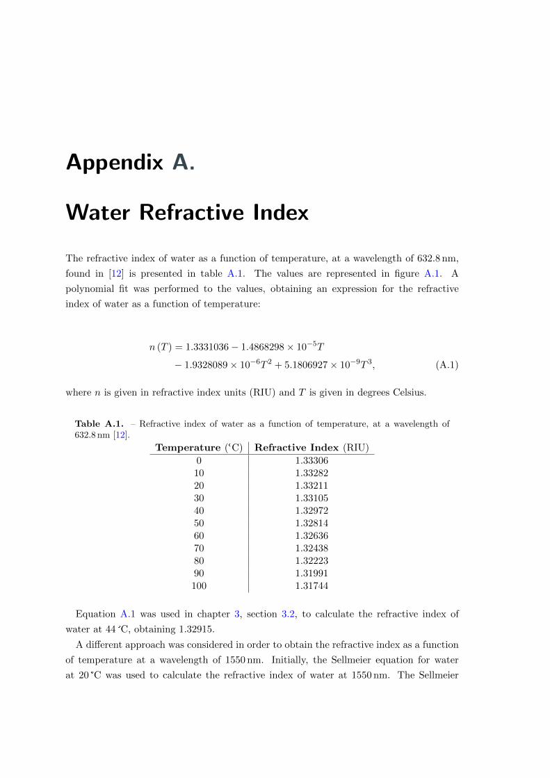
Appendix A.
Water Refractive Index
The refractive index of water as a function of temperature, at a wavelength of 632.8 nm,
found in [12] is presented in table A.1. The values are represented in figure A.1. A
polynomial fit was performed to the values, obtaining an expression for the refractive
index of water as a function of temperature:
n (T ) = 1.3331036− 1.4868298× 10⁻⁵T
− 1.9328089× 10⁻⁶T 2 + 5.1806927× 10⁻⁹T 3, (A.1)
where n is given in refractive index units (RIU) and T is given in degrees Celsius.
Table A.1. – Refractive index of water as a function of temperature, at a wavelength of632.8 nm [12].
Temperature (°C) Refractive Index (RIU)
0 1.3330610 1.3328220 1.3321130 1.3310540 1.3297250 1.3281460 1.3263670 1.3243880 1.3222390 1.31991100 1.31744
Equation A.1 was used in chapter 3, section 3.2, to calculate the refractive index of
water at 44 °C, obtaining 1.32915.
A different approach was considered in order to obtain the refractive index as a function
of temperature at a wavelength of 1550 nm. Initially, the Sellmeier equation for water
at 20 °C was used to calculate the refractive index of water at 1550 nm. The Sellmeier
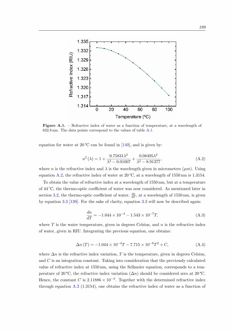
189
Figure A.1. – Refractive index of water as a function of temperature, at a wavelength of632.8 nm. The data points correspond to the values of table A.1.
equation for water at 20 °C can be found in [140], and is given by:
n2 (λ) = 1 +0.75831λ2
λ2 − 0.01007+
0.08495λ2
λ2 − 8.91377, (A.2)
where n is the refractive index and λ is the wavelength given in micrometers (µm). Using
equation A.2, the refractive index of water at 20 °C, at a wavelength of 1550 nm is 1.3154.
To obtain the value of refractive index at a wavelength of 1550 nm, but at a temperature
of 44 °C, the thermo-optic coefficient of water was now considered. As mentioned later in
section 3.2, the thermo-optic coefficient of water, dndT , at a wavelength of 1550 nm, is given
by equation 3.3 [139]. For the sake of clarity, equation 3.3 will now be described again:
dn
dT= −1.044× 10⁻⁴ − 1.543× 10⁻⁷T, (A.3)
where T is the water temperature, given in degrees Celsius, and n is the refractive index
of water, given in RIU. Integrating the previous equation, one obtains:
∆n (T ) = −1.044× 10⁻⁴T − 7.715× 10⁻⁸T 2 + C, (A.4)
where ∆n is the refractive index variation, T is the temperature, given in degrees Celsius,
and C is an integration constant. Taking into consideration that the previously calculated
value of refractive index at 1550 nm, using the Sellmeier equation, corresponds to a tem-
perature of 20 °C, the refractive index variation (∆n) should be considered zero at 20 °C.
Hence, the constant C is 2.11886 × 10⁻³. Together with the determined refractive index
through equation A.2 (1.3154), one obtains the refractive index of water as a function of
190 Appendix A. Water Refractive Index
temperature, at a wavelength of 1550 nm, given by equation 3.4. Once again, for the sake
of clarity, equation 3.4 will now be described again:
n(T ) = 1.3154 + 2.11886× 10⁻³ − 1.044× 10⁻⁴T − 7.715× 10⁻⁸T 2, (A.5)
with T given in degrees Celsius and n given in RIU.
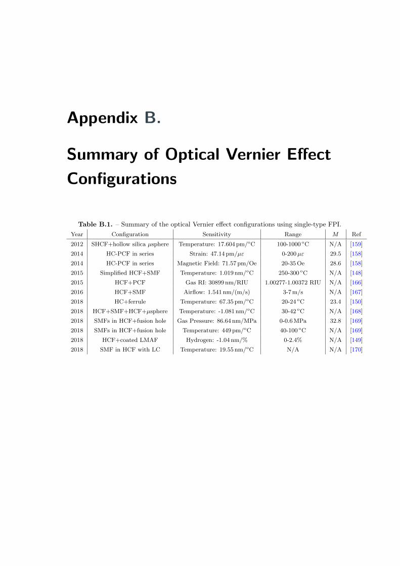
Appendix B.
Summary of Optical Vernier Effect
Configurations
Table B.1. – Summary of the optical Vernier effect configurations using single-type FPI.
Year Configuration Sensitivity Range M Ref
2012 SHCF+hollow silica µsphere Temperature: 17.604 pm/oC 100-1000 oC N/A [159]
2014 HC-PCF in series Strain: 47.14 pm/µε 0-200µε 29.5 [158]
2014 HC-PCF in series Magnetic Field: 71.57 pm/Oe 20-35 Oe 28.6 [158]
2015 Simplified HCF+SMF Temperature: 1.019 nm/oC 250-300 oC N/A [148]
2015 HCF+PCF Gas RI: 30899 nm/RIU 1.00277-1.00372 RIU N/A [166]
2016 HCF+SMF Airflow: 1.541 nm/(m/s) 3-7 m/s N/A [167]
2018 HC+ferrule Temperature: 67.35 pm/oC 20-24 oC 23.4 [150]
2018 HCF+SMF+HCF+µsphere Temperature: -1.081 nm/oC 30-42 oC N/A [168]
2018 SMFs in HCF+fusion hole Gas Pressure: 86.64 nm/MPa 0-0.6 MPa 32.8 [169]
2018 SMFs in HCF+fusion hole Temperature: 449 pm/oC 40-100 oC N/A [169]
2018 HCF+coated LMAF Hydrogen: -1.04 nm/% 0-2.4% N/A [149]
2018 SMF in HCF with LC Temperature: 19.55 nm/oC N/A N/A [170]
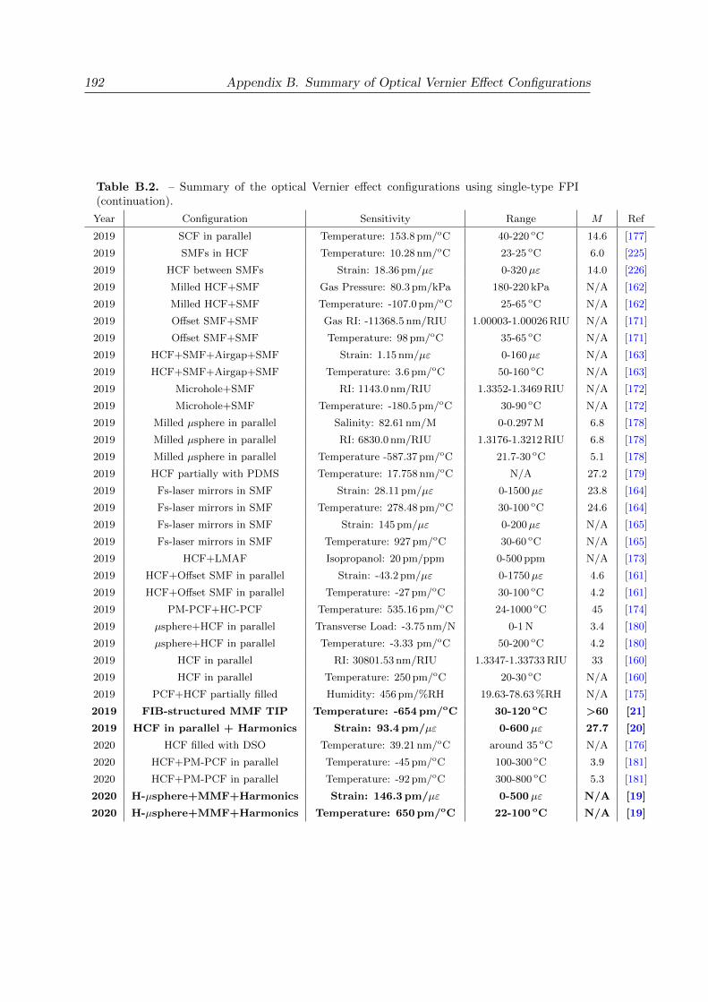
192 Appendix B. Summary of Optical Vernier Effect Configurations
Table B.2. – Summary of the optical Vernier effect configurations using single-type FPI(continuation).
Year Configuration Sensitivity Range M Ref
2019 SCF in parallel Temperature: 153.8 pm/oC 40-220 oC 14.6 [177]
2019 SMFs in HCF Temperature: 10.28 nm/oC 23-25 oC 6.0 [225]
2019 HCF between SMFs Strain: 18.36 pm/µε 0-320µε 14.0 [226]
2019 Milled HCF+SMF Gas Pressure: 80.3 pm/kPa 180-220 kPa N/A [162]
2019 Milled HCF+SMF Temperature: -107.0 pm/oC 25-65 oC N/A [162]
2019 Offset SMF+SMF Gas RI: -11368.5 nm/RIU 1.00003-1.00026 RIU N/A [171]
2019 Offset SMF+SMF Temperature: 98 pm/oC 35-65 oC N/A [171]
2019 HCF+SMF+Airgap+SMF Strain: 1.15 nm/µε 0-160µε N/A [163]
2019 HCF+SMF+Airgap+SMF Temperature: 3.6 pm/oC 50-160 oC N/A [163]
2019 Microhole+SMF RI: 1143.0 nm/RIU 1.3352-1.3469 RIU N/A [172]
2019 Microhole+SMF Temperature: -180.5 pm/oC 30-90 oC N/A [172]
2019 Milled µsphere in parallel Salinity: 82.61 nm/M 0-0.297 M 6.8 [178]
2019 Milled µsphere in parallel RI: 6830.0 nm/RIU 1.3176-1.3212 RIU 6.8 [178]
2019 Milled µsphere in parallel Temperature -587.37 pm/oC 21.7-30 oC 5.1 [178]
2019 HCF partially with PDMS Temperature: 17.758 nm/oC N/A 27.2 [179]
2019 Fs-laser mirrors in SMF Strain: 28.11 pm/µε 0-1500µε 23.8 [164]
2019 Fs-laser mirrors in SMF Temperature: 278.48 pm/oC 30-100 oC 24.6 [164]
2019 Fs-laser mirrors in SMF Strain: 145 pm/µε 0-200µε N/A [165]
2019 Fs-laser mirrors in SMF Temperature: 927 pm/oC 30-60 oC N/A [165]
2019 HCF+LMAF Isopropanol: 20 pm/ppm 0-500 ppm N/A [173]
2019 HCF+Offset SMF in parallel Strain: -43.2 pm/µε 0-1750µε 4.6 [161]
2019 HCF+Offset SMF in parallel Temperature: -27 pm/oC 30-100 oC 4.2 [161]
2019 PM-PCF+HC-PCF Temperature: 535.16 pm/oC 24-1000 oC 45 [174]
2019 µsphere+HCF in parallel Transverse Load: -3.75 nm/N 0-1 N 3.4 [180]
2019 µsphere+HCF in parallel Temperature: -3.33 pm/oC 50-200 oC 4.2 [180]
2019 HCF in parallel RI: 30801.53 nm/RIU 1.3347-1.33733 RIU 33 [160]
2019 HCF in parallel Temperature: 250 pm/oC 20-30 oC N/A [160]
2019 PCF+HCF partially filled Humidity: 456 pm/%RH 19.63-78.63 %RH N/A [175]
2019 FIB-structured MMF TIP Temperature: -654 pm/oC 30-120 oC >60 [21]
2019 HCF in parallel + Harmonics Strain: 93.4 pm/µε 0-600 µε 27.7 [20]
2020 HCF filled with DSO Temperature: 39.21 nm/oC around 35 oC N/A [176]
2020 HCF+PM-PCF in parallel Temperature: -45 pm/oC 100-300 oC 3.9 [181]
2020 HCF+PM-PCF in parallel Temperature: -92 pm/oC 300-800 oC 5.3 [181]
2020 H-µsphere+MMF+Harmonics Strain: 146.3 pm/µε 0-500 µε N/A [19]
2020 H-µsphere+MMF+Harmonics Temperature: 650 pm/oC 22-100 oC N/A [19]
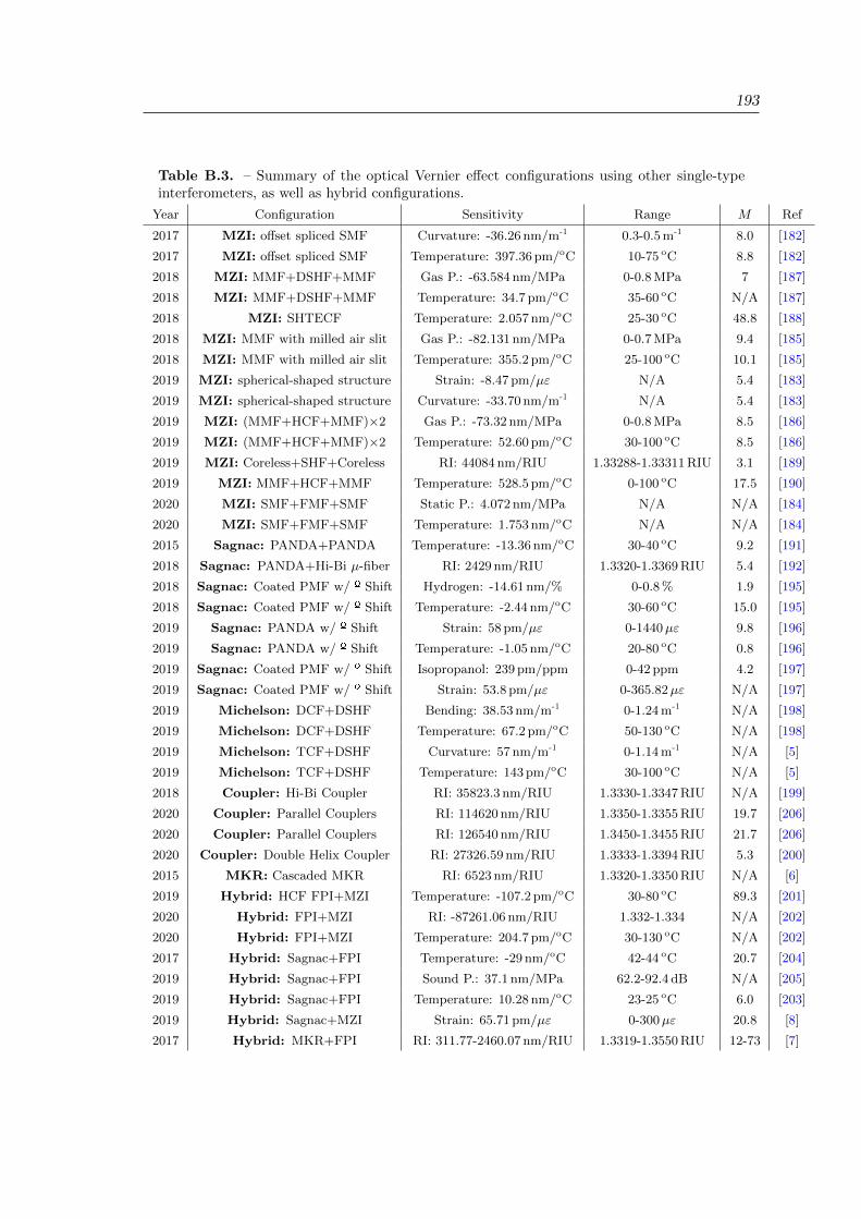
193
Table B.3. – Summary of the optical Vernier effect configurations using other single-typeinterferometers, as well as hybrid configurations.
Year Configuration Sensitivity Range M Ref
2017 MZI: offset spliced SMF Curvature: -36.26 nm/m-1 0.3-0.5 m-1 8.0 [182]
2017 MZI: offset spliced SMF Temperature: 397.36 pm/oC 10-75 oC 8.8 [182]
2018 MZI: MMF+DSHF+MMF Gas P.: -63.584 nm/MPa 0-0.8 MPa 7 [187]
2018 MZI: MMF+DSHF+MMF Temperature: 34.7 pm/oC 35-60 oC N/A [187]
2018 MZI: SHTECF Temperature: 2.057 nm/oC 25-30 oC 48.8 [188]
2018 MZI: MMF with milled air slit Gas P.: -82.131 nm/MPa 0-0.7 MPa 9.4 [185]
2018 MZI: MMF with milled air slit Temperature: 355.2 pm/oC 25-100 oC 10.1 [185]
2019 MZI: spherical-shaped structure Strain: -8.47 pm/µε N/A 5.4 [183]
2019 MZI: spherical-shaped structure Curvature: -33.70 nm/m-1 N/A 5.4 [183]
2019 MZI: (MMF+HCF+MMF)×2 Gas P.: -73.32 nm/MPa 0-0.8 MPa 8.5 [186]
2019 MZI: (MMF+HCF+MMF)×2 Temperature: 52.60 pm/oC 30-100 oC 8.5 [186]
2019 MZI: Coreless+SHF+Coreless RI: 44084 nm/RIU 1.33288-1.33311 RIU 3.1 [189]
2019 MZI: MMF+HCF+MMF Temperature: 528.5 pm/oC 0-100 oC 17.5 [190]
2020 MZI: SMF+FMF+SMF Static P.: 4.072 nm/MPa N/A N/A [184]
2020 MZI: SMF+FMF+SMF Temperature: 1.753 nm/oC N/A N/A [184]
2015 Sagnac: PANDA+PANDA Temperature: -13.36 nm/oC 30-40 oC 9.2 [191]
2018 Sagnac: PANDA+Hi-Bi µ-fiber RI: 2429 nm/RIU 1.3320-1.3369 RIU 5.4 [192]
2018 Sagnac: Coated PMF w/ º Shift Hydrogen: -14.61 nm/% 0-0.8 % 1.9 [195]
2018 Sagnac: Coated PMF w/ º Shift Temperature: -2.44 nm/oC 30-60 oC 15.0 [195]
2019 Sagnac: PANDA w/ º Shift Strain: 58 pm/µε 0-1440µε 9.8 [196]
2019 Sagnac: PANDA w/ º Shift Temperature: -1.05 nm/oC 20-80 oC 0.8 [196]
2019 Sagnac: Coated PMF w/ º Shift Isopropanol: 239 pm/ppm 0-42 ppm 4.2 [197]
2019 Sagnac: Coated PMF w/ º Shift Strain: 53.8 pm/µε 0-365.82µε N/A [197]
2019 Michelson: DCF+DSHF Bending: 38.53 nm/m-1 0-1.24 m-1 N/A [198]
2019 Michelson: DCF+DSHF Temperature: 67.2 pm/oC 50-130 oC N/A [198]
2019 Michelson: TCF+DSHF Curvature: 57 nm/m-1 0-1.14 m-1 N/A [5]
2019 Michelson: TCF+DSHF Temperature: 143 pm/oC 30-100 oC N/A [5]
2018 Coupler: Hi-Bi Coupler RI: 35823.3 nm/RIU 1.3330-1.3347 RIU N/A [199]
2020 Coupler: Parallel Couplers RI: 114620 nm/RIU 1.3350-1.3355 RIU 19.7 [206]
2020 Coupler: Parallel Couplers RI: 126540 nm/RIU 1.3450-1.3455 RIU 21.7 [206]
2020 Coupler: Double Helix Coupler RI: 27326.59 nm/RIU 1.3333-1.3394 RIU 5.3 [200]
2015 MKR: Cascaded MKR RI: 6523 nm/RIU 1.3320-1.3350 RIU N/A [6]
2019 Hybrid: HCF FPI+MZI Temperature: -107.2 pm/oC 30-80 oC 89.3 [201]
2020 Hybrid: FPI+MZI RI: -87261.06 nm/RIU 1.332-1.334 N/A [202]
2020 Hybrid: FPI+MZI Temperature: 204.7 pm/oC 30-130 oC N/A [202]
2017 Hybrid: Sagnac+FPI Temperature: -29 nm/oC 42-44 oC 20.7 [204]
2019 Hybrid: Sagnac+FPI Sound P.: 37.1 nm/MPa 62.2-92.4 dB N/A [205]
2019 Hybrid: Sagnac+FPI Temperature: 10.28 nm/oC 23-25 oC 6.0 [203]
2019 Hybrid: Sagnac+MZI Strain: 65.71 pm/µε 0-300µε 20.8 [8]
2017 Hybrid: MKR+FPI RI: 311.77-2460.07 nm/RIU 1.3319-1.3550 RIU 12-73 [7]

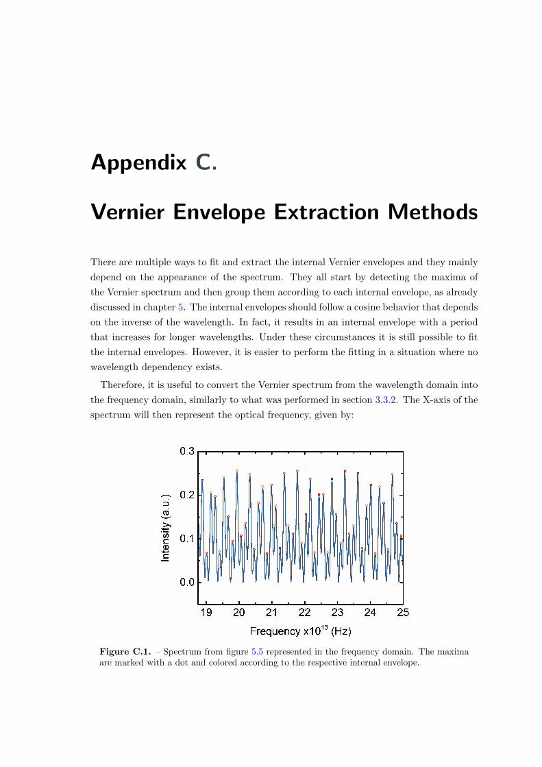
Appendix C.
Vernier Envelope Extraction Methods
There are multiple ways to fit and extract the internal Vernier envelopes and they mainly
depend on the appearance of the spectrum. They all start by detecting the maxima of
the Vernier spectrum and then group them according to each internal envelope, as already
discussed in chapter 5. The internal envelopes should follow a cosine behavior that depends
on the inverse of the wavelength. In fact, it results in an internal envelope with a period
that increases for longer wavelengths. Under these circumstances it is still possible to fit
the internal envelopes. However, it is easier to perform the fitting in a situation where no
wavelength dependency exists.
Therefore, it is useful to convert the Vernier spectrum from the wavelength domain into
the frequency domain, similarly to what was performed in section 3.3.2. The X-axis of the
spectrum will then represent the optical frequency, given by:
Figure C.1. – Spectrum from figure 5.5 represented in the frequency domain. The maximaare marked with a dot and colored according to the respective internal envelope.

196 Appendix C. Vernier Envelope Extraction Methods
ν =c
λ,
where c is the speed of light in vacuum and λ is the wavelength. Taking figure 5.5 as an
example, the corresponding spectrum in the frequency domain is depicted in figure C.1.
Now that the period of the internal envelopes do not depend on the wavelength, one
can fit the groups of maxima with a sinusoidal function such as:
I (ν) = I0 +A sin
(ν − ν0w
), (C.1)
where the fitting parameters are I0, A, ν0, and w. I0 corresponds to the offset component
(D.C. component), A is the amplitude of the envelope oscillation, ν0 is related with the ini-
tial phase, and w is related with the inverse frequency of oscillation. Due to the previously
mentioned conditions, and also to the fact that the spectrum is “perfect” (simulated), this
function fits very well the maxima, as shown in figure C.2.
Figure C.2. – Spectrum from figure 5.5 represented in the frequency domain after fitting theinternal envelopes according to equation C.1.
The problem of fitting internal Vernier envelopes starts when the experimental data
presents some imperfections due to experimental conditions and to the sensing structure
itself. One of the interferometers used to introduce the Vernier effect might have more
losses, or have more modes other than the fundamental mode, which might generate an
asymmetric spectrum. In such case the internal envelopes might no longer be fitted by
equation C.1. Figures 6.3(b) or (d) are interesting examples, where the D.C. component
and the amplitude of the internal envelopes increase for longer wavelengths. For this case,
a different fitting approach must be considered. Given the features of these spectra, the
197
following fit was used for those cases:
I (ν) = I0 exp
(bc
ν
)+A
c
νsin
(ν − ν0w
), (C.2)
where I0 exp (bc/ν) represents the D.C. component that increases with the wavelength
(decreases with the frequency), where b is a fitting parameter and c is the speed of light, A
is again a fitting parameter that corresponds to the amplitude of the envelope oscillation,
which is now multiplied by c/ν to include the increasing amplitude with the wavelength
(decrease with the frequency). Nevertheless, the previous fitting can be hard to converge.
In many cases, such as in figure 6.10 or 6.11, the internal envelopes are so large that
a period of oscillation does not fit within the wavelength range available. Yet, the main
interest still relies on the intersection between these internal envelopes. Adding to this,
the maxima suffer from intensity fluctuations. Given the circumstances, a sinusoidal fit
might be complex to achieve. An alternative way to fit these kind of internal envelopes is
to use a polynomial fitting as an approximation. In this case, it might not be necessary
to convert the spectrum into the frequency domain. For these two figures (6.10 and 6.11),
the polynomial fit used was of 5th order:
I (λ) = I0 +Aλ+Bλ2 + Cλ3 +D4 + Eλ5, (C.3)
where I0 is the offset components, and A, B, C, D, and E are the other fitting parameters.
Some fittings introduce more errors than other, however the important message here is
that, when performing measurements, the same fitting must be applied to all the measured
spectra. The errors associated with using the same fitting method will approximately be
systematic, which upon calibration can be slightly corrected. If different fitting methods
are used along the measurement, the errors between the different measurements start to
be random, which are more problematic for the experiment, since one cannot estimate
them.
Regarding the upper Vernier envelope, it can be traced using conventional envelope
extraction methods (signal processing) available in software like Origin or Matlab. Nev-
ertheless, the visual aspect of the upper envelope and the position of the maxima using
those methods highly depends on the number of points considered (smooth points). As
an alternative, some works use Lorentzian [6, 227] or Gaussian [82, 196] fitting curves to
find the position of the upper envelope maxima.

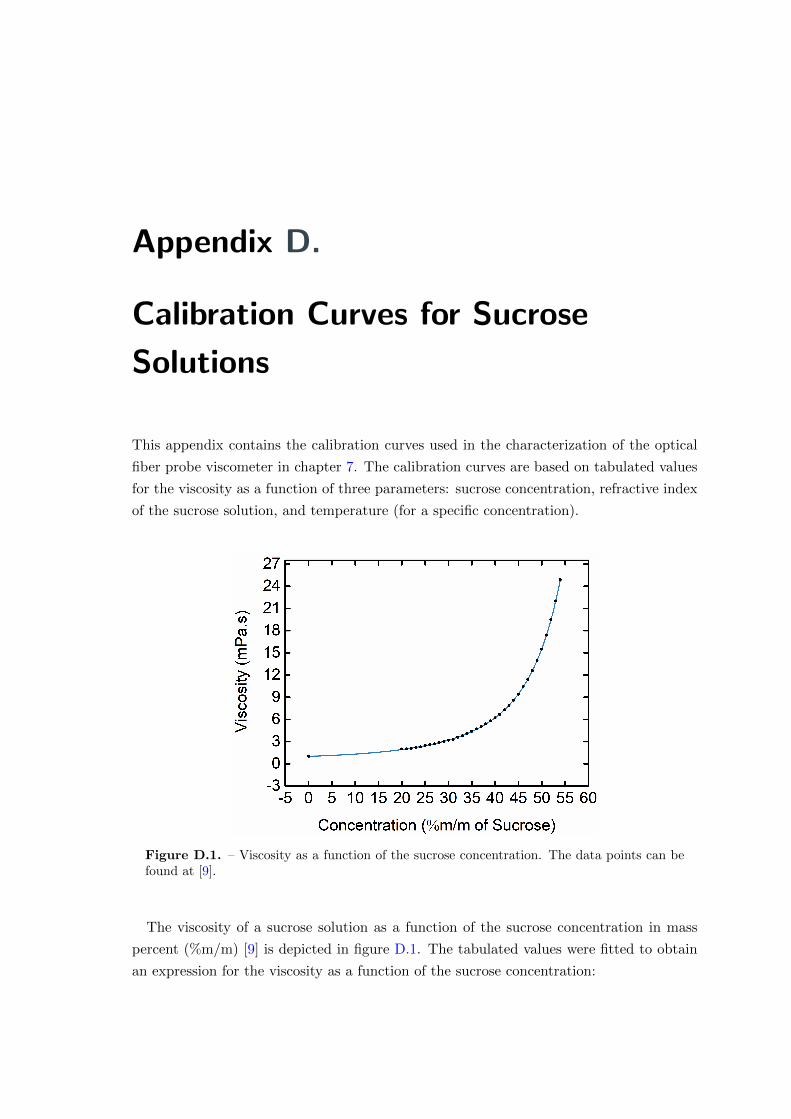
Appendix D.
Calibration Curves for Sucrose
Solutions
This appendix contains the calibration curves used in the characterization of the optical
fiber probe viscometer in chapter 7. The calibration curves are based on tabulated values
for the viscosity as a function of three parameters: sucrose concentration, refractive index
of the sucrose solution, and temperature (for a specific concentration).
Figure D.1. – Viscosity as a function of the sucrose concentration. The data points can befound at [9].
The viscosity of a sucrose solution as a function of the sucrose concentration in mass
percent (%m/m) [9] is depicted in figure D.1. The tabulated values were fitted to obtain
an expression for the viscosity as a function of the sucrose concentration:
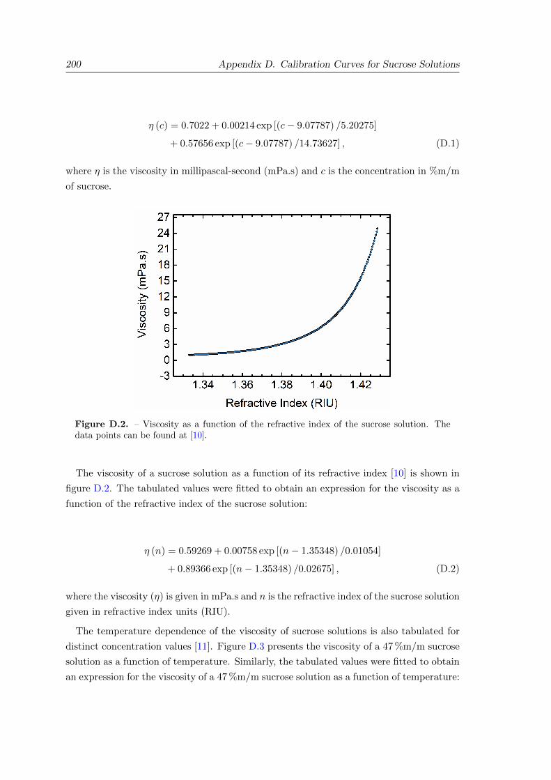
200 Appendix D. Calibration Curves for Sucrose Solutions
η (c) = 0.7022 + 0.00214 exp [(c− 9.07787) /5.20275]
+ 0.57656 exp [(c− 9.07787) /14.73627] , (D.1)
where η is the viscosity in millipascal-second (mPa.s) and c is the concentration in %m/m
of sucrose.
Figure D.2. – Viscosity as a function of the refractive index of the sucrose solution. Thedata points can be found at [10].
The viscosity of a sucrose solution as a function of its refractive index [10] is shown in
figure D.2. The tabulated values were fitted to obtain an expression for the viscosity as a
function of the refractive index of the sucrose solution:
η (n) = 0.59269 + 0.00758 exp [(n− 1.35348) /0.01054]
+ 0.89366 exp [(n− 1.35348) /0.02675] , (D.2)
where the viscosity (η) is given in mPa.s and n is the refractive index of the sucrose solution
given in refractive index units (RIU).
The temperature dependence of the viscosity of sucrose solutions is also tabulated for
distinct concentration values [11]. Figure D.3 presents the viscosity of a 47 %m/m sucrose
solution as a function of temperature. Similarly, the tabulated values were fitted to obtain
an expression for the viscosity of a 47 %m/m sucrose solution as a function of temperature:
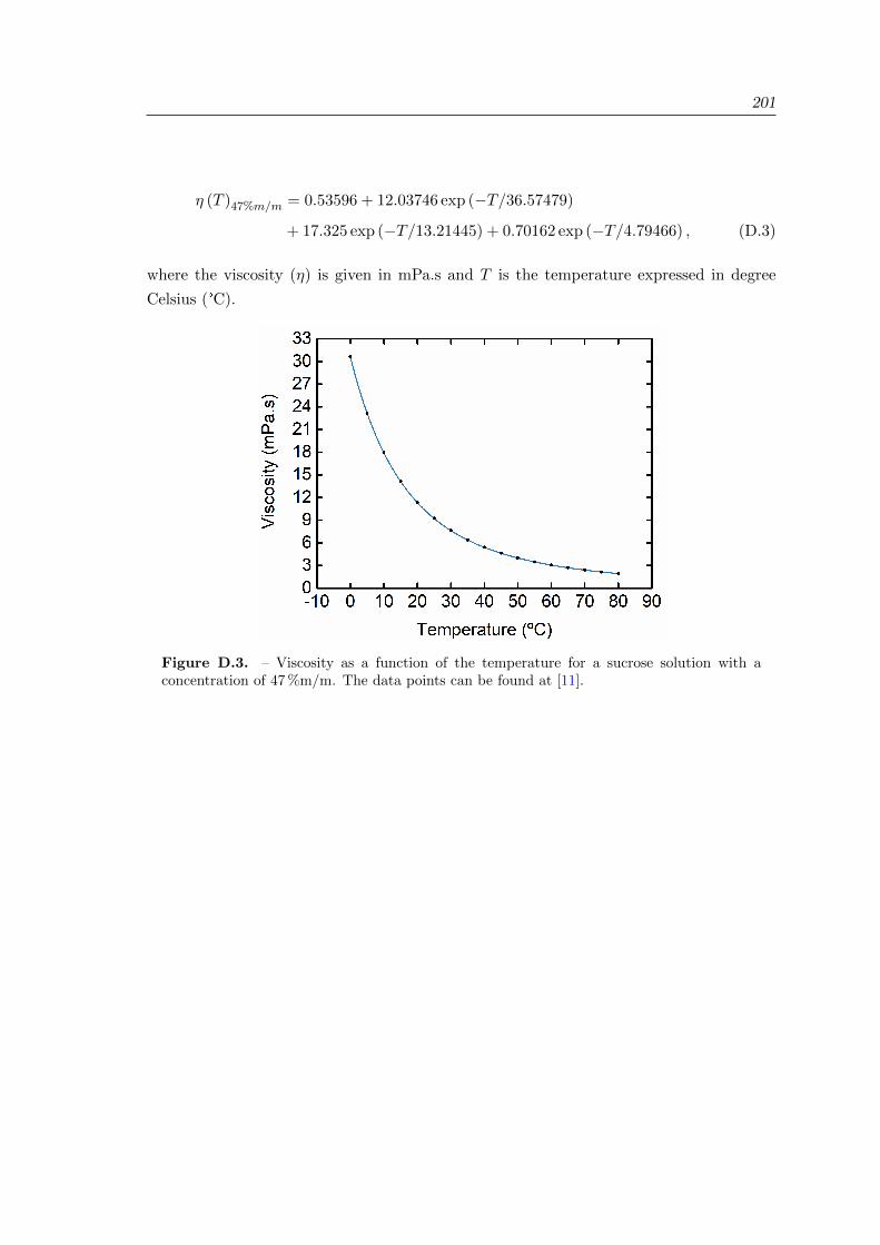
201
η (T )47%m/m = 0.53596 + 12.03746 exp (−T/36.57479)
+ 17.325 exp (−T/13.21445) + 0.70162 exp (−T/4.79466) , (D.3)
where the viscosity (η) is given in mPa.s and T is the temperature expressed in degree
Celsius (°C).
Figure D.3. – Viscosity as a function of the temperature for a sucrose solution with aconcentration of 47 %m/m. The data points can be found at [11].
Related Documents