Edited by Balraj Kumar DECAP770 Advanced Data Structures

Welcome message from author
This document is posted to help you gain knowledge. Please leave a comment to let me know what you think about it! Share it to your friends and learn new things together.
Transcript

Edited by Balraj Kumar
DECAP770Advanced Data Structures

Edited By: Balraj Kumar
user
Typewritten text
Advanced Data Structures

CONTENT
Unit 2: 15
Unit 10:
Introduction
Arrays vs Linked Lists
StacksUnit 3: 42
Heaps
Graphs
More on Graphs
Collision Resolution
More on Hashing
Unit 1: 1
Ashwani Kumar, Lovely Professional University
Ashwani Kumar, Lovely Professional University
Ashwani Kumar, Lovely Professional University
Ashwani Kumar, Lovely Professional University
Ashwani Kumar, Lovely Professional University
Ashwani Kumar, Lovely Professional University
Ashwani Kumar, Lovely Professional University
Ashwani Kumar, Lovely Professional University
Ashwani Kumar, Lovely Professional University
Ashwani Kumar, Lovely Professional University
Ashwani Kumar, Lovely Professional University
Ashwani Kumar, Lovely Professional University
Ashwani Kumar, Lovely Professional University
Ashwani Kumar, Lovely Professional University
Unit 4: Queues 56
Unit 5: Search Trees 69
Unit 6: Tree Data Structure 1 83
Unit 7: Tree Data Structure 2 98
Unit 8: 122
Unit 9: More on Heaps 136
161
Unit 11: 178
Unit 12: Hashing Techniques 200
Unit 13: 213
Unit 14: 226

Unit 01: Introduction
Notes
Unit 01: Introduction
CONTENTS
Objectives
Introduction
1.1 Data Structure
1.2 Data Structure Operations
1.3 Abstract Data Type
1.4 Algorithm
1.5 Characteristics of an Algorithm
1.6 Types of Algorithms
1.7 Algorithm Complexity
1.8 Asymptotic Notations
Summary
Keywords
Self Assessment
Answers for Self Assessment
Review Question
Further Readings
ObjectivesAfter studying this unit, you will be able to:
Describe basic concepts of data structure
Learn Algorithm and its complexity
Know Abstract data type
Data structure types
IntroductionThe static representation of a linear ordered list using an array wastes resources and, in somesituations, causes overflows. We no longer want to pre-allocate memory to any linear list; instead,we want to allocate memory to elements as they are added to the list. This necessitates memoryallocation that is dynamic.
Semantically data can exist in either of the two forms – atomic or structured. In most of theprogramming problems data to be read, processed and written are often related to each other. Dataitems are related in a variety of different ways. Whereas the basic data types such as integers,characters etc. can be directly created and manipulated in a programming language, theresponsibility of creating the structured type data items remains with the programmers themselves.Accordingly, programming languages provide mechanism to create and manipulate structureddata items.
A data structure is a type of storage that is used to organize and store data. It is a method oforganizing data on a computer so that it may be easily accessible and modified.
Ashwani Kumar, Lovely Professional University
Lovely Professional University 1

Advanced Data StructuresNotes
It's critical to choose the correct data format for your project based on your requirements andproject. If you wish to store data sequentially in memory, for example, you can use the Array datastructure.
1.1 Data StructureA data structure is a set of data values along with the relationship between the data values. Since,the operations that can be performed on the data values depend on what kind of relationshipsexists among them, we can specify the relationship amongst the data values by specifying theoperations permitted on the data values. Therefore, we can say that a data structure is a set ofvalues along with the set of operations permitted on them. It is also required to specify thesemantics of the operations permitted on the data values, and this is done by using a set of axioms,which describes how these operations work, and therefore a data structure is made of:
1. A set of data values.
2. A set of functions specifying the operations permitted on the data values.
3. A set of axioms describing how these operations work.
Hence, we conclude that a data structure is a triple (D,F,A), where
1. D is a set of data values
2. F is a set of functions
3. A is a set of axioms
A triple (D, F, A) is referred to as an abstract data structure because it does not tell anything aboutits actual implementation. It does not tell anything about how these values will be physicallyrepresented in the computer memory and these functions will be actually implemented.
Therefore, every abstract data structure is required to be implemented, and the implementation ofan abstract data structure requires mapping of the abstract data structure to be implemented intothe data structure supported by the computer. For example, if the abstract data structure to beimplemented is integer, then it can be implemented by mapping into bits which is a data structuresupported by hardware. This requires that every integer data value is to be represented usingsuitable bit patterns and expressing the operations on integer data values in terms of operations formanipulating bits.
Data Structure mainly two types:
1. Linear type data structure
2. Non-linear type data structure
Lovely Professional University2

Unit 01: Introduction
NotesNon-linear data structure: Each datum thing is joined to a few different information things in amanner that is explicit for reflecting connections. The information things are not organized in aconsecutive design. Ex: Trees, Graphs.
Trees: Trees are multilevel data structures with a hierarchical relationship among its elementsknown as nodes.
Graphs: Graphs can be defined as the pictorial representation of the set of elements (represented byvertices) connected by the links known as edges
Lovely Professional University 3

Advanced Data StructuresNotes
Multiple requests: If thousands of users are Searching the data simultaneously on a web server, thenthere are the chances that a very large server can be failed during that process To solve theseproblems data structures are used.
Basic Concept of DataThe memory (also called storage or core) of a computer is simply a group of bits (switches). At anyinstant of the computer’s operation any particular bit in memory is either 0 or 1 (off or on).
The setting or state of a bit is called its value and that is the smallest unit of information. A set of bitvalues form data.
Some logical properties can be imposed on the data. According to the logical properties data can besegregated into different categories. Each category having unique set of logical properties is knownas data type.
Data type are of two types:
1. Simple data type or elementary item like integer, character.
2. Composite data type or group item like array, structure, union.
Data structures are of two types:
1. Primitive Data Structures: Data can be structured at the most primitive level, where they aredirectly operated upon by machine-level instructions. At this level, data may be character ornumeric, and numeric data may consist of integers or real numbers.
2. Non-primitive Data Structures: Non-primitive data structures can be classified as arrays, lists, andfi les.
An array is an ordered set which contains a fixed number of objects. No deletions or insertions areperformed on arrays i.e. the size of the array cannot be changed. At best, elements may be changed.
A list, by contrast, is an ordered set consisting of a variable number of elements to which insertionsand deletions can be made, and on which other operations can be performed. When a list displaysthe relationship of adjacency between elements, it is said to be linear; otherwise, it is said to be non-linear.
A file is typically a large list that is stored in the external memory of a computer. Additionally, a filemay be used as a repository for list items (records) that are accessed infrequently.
From a real world perspective, very often we have to deal with structured data items which arerelated to each other. For instance, let us consider the address of an employee. We can take addressto be one variable of character type or structured into various fields, as shown below:
1.2 Data Structure OperationsThe data appearing in our data structure is processed by means of certain operations. Theparticular data structure that one chooses for a given situation depends largely on the frequencywith which specific operations are performed. The following four operations play a major role:
1. Traversing: Accessing each record exactly once so that certain items in the record may be
Lovely Professional University4

Unit 01: Introduction
Notesprocessed. (This accessing or processing is sometimes called ‘visiting” the records.)
2. Searching: Finding the location of the record with a given key value, or finding the locations
of all records, which satisfy one or more conditions.
3. Inserting: Adding new records to the structure.
4. Deleting: Removing a record from the structure.
Sometimes two or more data structure of operations may be used in a given situation; e.g., we maywant to delete the record with a given key, which may mean we first need to search for the locationof the record.
1.3 Abstract Data TypeBefore we move to abstract data type let us understand what data type is. Most of the languagessupport basic data types viz. integer, real, character etc. At machine level, the data is stored asstrings containing 1’s and 0’s. Every data type interprets the string of bits in different ways andgives different results. In short, data type is a method of interpreting bit patterns.
Every data type has a fixed type and range of values it can operate on. For example, an integervariable can hold values between the min and max values allowed and carry out operations likeaddition, subtraction etc. For character data type, the valid values are defined in the character setand the operations performed are like comparison, conversion from one case to another etc.
There are fixed operations, which can be carried out on them. We can formally defi ne data types asa formal description of the set of values and operations that a variable of a given type may take.That was about the inbuilt data types. One can also create user defined data types, decide the rangeof values as well as operations to be performed on them. The first step towards creating a userdefined data type or a data structure is to defi ne the logical properties. A tool to specify the logicalproperties of a data type is Abstract Data Type.
Data abstraction can be defined as separation of the logical properties of the organization ofprograms’ data from its implementation. This means that it states what the data should be like.
It does not consider the implementation details. ADT is the logical picture of a data type; inaddition, the specifications of the operations required to create and manipulate objects of this datatype.
While defining an ADT, we are not concerned with time and space efficiency or any otherimplementation details of the data structure. ADT is just a useful guideline to use and implementthe data type.
An ADT has two parts:
1. Value definition
2. Operation definition.
Value definition is again divided into two parts:
1. Definition clause
2. Condition clause
As the name suggests the definition clause states the contents of the data type and condition clausedefines any condition that applies to the data type. Definition clause is mandatory while conditionclause is optional.
In operation definition, there are three parts:
1. Function
2. Precondition
3. Postcondition
The function clause defines the role of the operation. If we consider the addition operation inintegers the function clause will state that two integers can be added using this function. In general,precondition specifies any restrictions that must be satisfied before the operation can be applied.
Lovely Professional University 5

Advanced Data StructuresNotes
This clause is optional. If we consider the division operation on integers then the precondition willstate that the divisor should not be zero. So any call for divide operation, which does not satisfy thiscondition, will not give the desired output.
Precondition specifies any condition that may apply as a pre-requisite for the operation definition.There are certain operations that can be carried out if certain conditions are satisfied. For example,in case of division operation the divisor should never be equal to zero. Only if this condition issatisfied the division operation is carried out. Hence, this becomes a precondition. In that case &(ampersand) should be mentioned in the operation definition.
Postcondition specifies what the operation does. One can say that it specifies the state after theoperation is performed. In the addition operation, the post condition will give the addition of thetwo integers.
Component of ADTAs an example, let us consider the representation of integer data type as an ADT. We will consider
only two operations addition and division.
Value Definition
1. Definition clause: The values must be in between the minimum and maximum values
specified for the particular computer.
2. Condition clause: Values should not include decimal point.
Operations
1. add (a, b)
Function: add the two integers a and b.
Precondition: no precondition.
Postcondition: output = a + b
2. Div (a, b)
Function: Divide a by b.
Precondition: b != 0
Postcondition: output = a/b.
There are two ways of implementing a data structure viz. static and dynamic. In staticimplementation, the memory is allocated at the compile time. If there are more elements than thespecified memory then the program crashes. In dynamic implementation, the memory is allocatedas and when required during run time.
Any type of data structure will have certain basic operations to be performed on its data like insert,delete, modify, sort, search etc. depending on the requirement. These are the entities that decide therepresentation of data and distinguish data structures from each other.
Let us see why user defined data structures are essential. Consider a problem where we need tocreate a list of elements. Any new element added to the list must be added at the end of the list andwhenever an element is retrieved, it should be the last element of the list. One can compare this to apile of plates kept on a table. Whenever one needs a plate, the last one on the pile is taken and if aplate is to be added on the pile, it will be kept on the top. The description wants us to implement astack. Let us try to solve this problem using arrays.
Lovely Professional University6

Unit 01: Introduction
NotesWe will have to keep track of the index of the last element entered in the list. Initially, it will be setto –1. Whenever we insert an element into the list, we will increment the index and insert the valueinto the new index position. To remove an element, the value of current index will be the outputand the index will be decremented by one. In the above representation, we have satisfied theinsertion and deletion conditions.
Using arrays we could handle our data properly, but arrays do allow access to other values inaddition to the top most one. We can insert an element at the end of the list but there is no way toensure that insertion will be done only at the end. This is because array as a data structure allowsaccess to any of its values. At this point we can think of another representation, a list of elementswhere one can add at the end, remove from the end and elements other than the top one are notaccessible. As already discussed, this data structure is called as STACK. The insertion operation isknown as push and removal as pop. You can try to write an ADT for stacks.
Another situation where we would like to create a data structure is while working with complexnumbers. The operations add, subtract division and multiplication will have to be created as per therules of complex numbers. The ADT for complex numbers is given below. Only addition andmultiplication operations are considered here, you can try to write the remaining operations.
Abstract Data Type (ADT)
1. A framework for an object interface
2. What kind of stuff it’d be made of (no details)?
3. What kind of messages it would receive and kind of action it’ll perform when properly
triggered?
From this we figure out
1. Object make-up (in terms of data)
2. Object interface (what sort of messages it would handle?)
3. How and when it should act when triggered from outside (public trigger) and by another
object friendly to it?
These concerns lead to an ADT – a definition for the object.
An Abstract Data Type (ADT) is a set of data items and the methods that work on them.
An implementation of an ADT is a translation into statements of a programming language, of thedeclaration that defines a variable to be of that ADT, plus a procedure in that language for eachoperation of the ADT. An implementation chooses a data structure to represent the ADT; each datastructure is built up from the basic data types of the underlying programming language.
Thus, if we wish to change the implementation of an ADT, only the procedures implementing theoperations would change. This change would not affect the users of the ADT.
Lovely Professional University 7

Advanced Data StructuresNotes
we must find some way of representing the ADTs in terms of the data types and operatorssupported by the programming language itself. To represent the mathematical model underlyingan ADT, we use data structures, which are a collection of variables, possibly of several data types,connected in various ways.The cell is the basic building block of data structures. We can picture a cell as a box that is capableof holding a value drawn from some basic or composite data type. Data structures are created bygiving names to aggregates of cells and (optionally) interpreting the values of some cells asrepresenting relationships or connections (e.g., pointers) among cells.
1.4 AlgorithmAlgorithm is set of rules/ instructions that step-by-step define how a work is to be executed uponin order to get the expected results.systematic procedure that produces in a finite number of steps the answer to a question or thesolution of a problem.Computer algorithms work via input and output. They take the input and apply each step of thealgorithm to that information to generate an output.E.g. a search engine is an algorithm that takes a search query as an input and searches its databasefor items relevant to the words in the query. It then outputs the results.Financial companies use algorithms in areas such as loan pricing, stock trading, asset-liabilitymanagement, and many automated functions. For example, algorithmic trading, known as algotrading, is used for deciding the timing, pricing, and quantity of stock orders. Also referred to asautomated trading or black-box trading, algo trading uses computer programs to buy or sellsecurities at a pace not possible for humans.Computer algorithms make life easier by trimming the time it takes to manually do things. In theworld of automation, algorithms allow workers to be more proficient and focused. Algorithmsmake slow processes more proficient. In many cases, especially in automation, algos can savecompanies money.
1.5 Characteristics of an Algorithm
Well defined Input and output Clear and Unambiguous Finite-ness Feasible Language Independent
Input and output should be defined precisely.
Each step in the algorithm should be clear and unambiguous.
Algorithms should be most effective among many different ways to solve a problem.
An algorithm shouldn't include computer code. Instead, the algorithm should be written in such away that it can be used in different programming languages.
The algorithm must be finite, i.e. it should not end up in an infinite loops or similar.
The algorithm must be simple, generic and practical, such that it can be executed upon will theavailable resources. It must not contain some future technology, or anything.
The Algorithm designed must be language-independent, i.e. it must be just plain instructions thatcan be implemented in any language, and yet the output will be same, as expected.
1.6 Types of AlgorithmsAlgorithms are categorized based on the concepts that they use to accomplish a task.
Divide and conquer algorithms Brute force algorithms
Lovely Professional University8

Unit 01: Introduction
Notes Greedy algorithms Backtracking algorithms Randomized algorithms
Example:
Step 1: Start
Step 2: Declare variables num1, num2 and sum.
Step 3: Read values num1 and num2.
Step 4: Add num1 and num2 and assign the result to sum.
Sum = num1+num2
Step 5: Display sum
Step 6: Stop
1.7 Algorithm ComplexitySpace Complexity
Time Complexity
Space Complexity: Space complexity of an algorithm refers to the amount of memory that thisalgorithm requires to execute and get the result. This can be for inputs, temporary operations, oroutputs.
Fixed Part: This refers to the space that is definitely required by the algorithm. For example, inputvariables, output variables, program size, etc.
Variable Part: This refers to the space that can be different based on the implementation of thealgorithm. For example, temporary variables, dynamic memory allocation, recursion stack space,etc.
Time Complexity: Time complexity of an algorithm refers to the amount of time that this algorithmrequires to execute and get the result. This can be for normal operations, conditional if-elsestatements, loop statements, etc.
Constant time part: Any instruction that is executed just once comes in this part. For example,input, output, if-else, switch, etc.
Variable Time Part: Any instruction that is executed more than once, say n times, comes in this part.For example, loops, recursion, etc.
1.8 Asymptotic NotationsTo measure the efficiency of an algorithm asymptotic analysis is used.
The efficiency of an algorithm depends on the amount of time, storage and other resources requiredto execute the algorithm.
Performance of algorithm is change with different type of inputs.
The study of change in performance of the algorithm with the change in the order of the input sizeis defined as asymptotic analysis.
Asymptotic notations are the mathematical notations used to describe the running time of analgorithm when the input tends towards a particular value or a limiting value.
Types of asymptotic notationsThere are three major asymptotic notations
Lovely Professional University 9

Advanced Data StructuresNotes
Big-O notation Omega notation Theta notation
Big-O notation represents the upper bound of the running time of an algorithm. It gives the worst-case complexity of an algorithm.
O(n) is useful when we only have an upper bound on the time complexity of an algorithm.
It is widely used to analyses an algorithm as we are always interested in the worst-case scenario.
O(g(n)) = f(n): there exist positive constants c and n0
such that 0 ≤ f(n) ≤ cg(n) for all n ≥ n0
Omega notation represents the lower bound of the running time of an algorithm. It provides thebest-case complexity of an algorithm.
Omega Notation can be useful when we have lower bound on time complexity of analgorithm.Omega notation is the least used notation among all three.
Ω (g(n)) = f(n): there exist positive constants c and
n0 such that 0 <= c*g(n) <= f(n) forall n >= n0.
Theta notation encloses the function from above and below. It represents the upper and the lowerbound of the running time of an algorithm, it is used for analysing the average-case complexity ofan algorithm.
Lovely Professional University10

Unit 01: Introduction
NotesΘ(g(n)) = f(n): there exist positive constants c1, c2 and n0 such
that 0 <= c1*g(n) <= f(n) <= c2*g(n) for all n >= n0
Properties of Asymptotic NotationsIf f(n) is O(g(n)) then a*f(n) is also O(g(n)) ; where a is a constant.
General Properties
If f(n) is O(g(n)) then a*f(n) is also O(g(n)) ; where a is a constant.
Transitive Properties
If f(n) is O(g(n)) and g(n) is O(h(n)) then f(n) = O(h(n))
Reflexive Properties
If f(n) is given then f(n) is O(f(n))
Symmetric Properties
If f(n) is Θ(g(n)) then g(n) is Θ(f(n))
Transpose Symmetric Properties
If f(n) is O(g(n)) then g(n) is Ω (f(n))
Summary
Data Structure is method or technique to data organization, management, and storageformatin the computer so we can perform operations on the stored data more efficiently.
Data structure is a combination of one or more basic data types to form a single addressabledata type.
An algorithm is a finite set of instructions which, when followed, accomplishes a particulartask, the termination of which is guaranteed under all cases, i.e. the termination isguaranteed for every input.
The instructions must be unambiguous and the algorithm must produce the output within afinite number of executions of its instructions.
Abstract data type (ADT) is a mathematical model with a collection of operations defined onthat model. Although the terms ‘data type’, ‘data structure’ and ‘abstract data type’ soundalike, they have different meanings.
Lovely Professional University 11

Advanced Data StructuresNotes
Self Assessment1. Which is type of data structure.
A. PrimitiveB. Non-primitiveC. Both primitive and non-primitiveD. None of above
2. Which of the following is linear data structure?
A. TreesB. ArraysC. GraphsD. None of these
3. Which of the following is non-linear data structure?
A. ArrayB. Linked listsC. StacksD. None of these
4. User defined data type is also called?
A. PrimitiveB. IdentifierC. Non-primitiveD. None of these
5. Stack is based on which principle
A. FIFOB. LIFOC. PushD. None of the Above
6. What are the characteristics of an Algorithm.
A. Clear and UnambiguousB. Finite-nessC. FeasibleD. All of above
7. A procedure for solving a problem in terms of action and their order is called as
A. Program instructionB. AlgorithmC. Process
Lovely Professional University12

Unit 01: Introduction
NotesD. Template
8. Algorithm can be represented as
A. PseudocodeB. FlowchartC. None of the aboveD. Both Pseudocode and Flowchart
9. What are the different types of Algorithms?
A. Brute force algorithmsB. Greedy algorithmsC. Backtracking algorithmsD. All of these
10. Which is algorithm complexity.
A. Space ComplexityB. Time ComplexityC. Both space and time complexityD. None of above one of these
11. Which one is asymptotic notations?
A. Big-O notationB. Omega notationC. Theta notationD. All of above
12. Big-O Notation represents…
A. Space complexityB. Upper bound of the running time of an algorithmC. Lower bound of the running time of an algorithmD. None of above
13. Omega Notation (Ω-notation) represents….
A. Upper bound of the running time of an algorithmB. Space complexityC. Lower bound of the running time of an algorithmD. None of above
14. Which is property of Asymptotic Notations?
A. ReflexiveB. SymmetricC. Transpose SymmetricD. All of these
Lovely Professional University 13

Advanced Data StructuresNotes
15. Abstract Data Type having.
A. Value definitionB. Operation definitionC. Both value and operation definitionD. None of above.
Answers for Self Assessment
1. C 2. B 3. D 4. C 5. B
6. D 7. B 8. D 9. D 10. C
11. D 12. B 13. C 14. D 15. C
Review Question
1. Define data structure and its application.2. What are the advantages of data structure?3. Discuss abstract data type.4. What is significance of space and time complexity in algorithm.5. Explain different types of algorithms.6. Discuss Asymptotic notations with example.7. Define record and file.
Further Readings
Data Structures and Algorithms; Shi-Kuo Chang; World Scientifi c. Data Structures and Efficient Algorithms, Burkhard Monien, Thomas Ottmann,
Springer. Mark Allen Weles: Data Structure & Algorithm Analysis in C Second Adition.
Addison-Wesley publishing Thomas H. Cormen, Charles E, Leiserson& Ronald L. Rivest: Introduction to
Algorithms. Prentice-Hall of India Pvt. Limited, New Delhi Timothy A. Budd, Classic Data Structures in C++, Addison Wesley.
Lovely Professional University14

Unit 02: Arrays vs Linked Lists
Notes
Unit 02: Arrays vs Linked Lists
CONTENTS
Objectives
Introduction
2.1 Arrays
2.2 Types of Arrays
2.3 Types of Array Operations
2.4 Linked list
2.5 Types of linked list
Summary
Keywords
Self-Assessment
Answers for Self Assessment
Review Questions
Further Readings
ObjectivesAfter studying this unit, you will be able to:
• Learn basic concepts of arrays
• Understand the basics of linked list
• Describe the types of array operations
• Discuss the operations of linked lists
IntroductionA data structure consists of a group of data elements bound by the same set of rules. The dataelements also known as members are of different types and lengths. We can manipulate data storedin the memory with the help of data structures. The study of data structures involves examining themerging of simple structures to form composite structures and accessing definite components fromcomposite structures. An array is an example of one such composite data structure that is derivedfrom a primitive data structure.
An array is a set of similar data elements grouped together. Arrays can be one-dimensional ormultidimensional. Arrays store the entries sequentially. Elements in an array are stored incontinuous locations and are identified using the location of the first element of the array.
2.1 ArraysAn array is a data type, much like a variable as both array and variable hold information. However,unlike a variable, an array can hold several pieces of data called elements. Arrays can hold any typeof data, which includes string, integers, Boolean, and so on. An array can also handle othervariables as well as other arrays. An integer index identifies the individual elements of an array.
Arrays are allocated the memory in a strictly contiguous fashion. The simplest array is one-dimensional array which is a list of variables of same data type. An array of one-dimensional arrays
Ashwani Kumar, Lovely Professional University
Lovely Professional University 15

Advanced Data StructuresNotes
is called a two-dimensional array; array of two-dimensional arrays is three-dimensional array andso on.
The members of the array can be accessed using positive integer values (indicating their order inthe array) called subscript or index.
a[0] a[1] a[2] a[3] a[4]
The description of this array is listed below:
Name of the array : a
Data type of the array : integer
Number of elements : 5
Valid index values : 0, 1, 2, 3, 4
Value stored at the location a[0] : 200
Value stored at the location a[1] : 120
Value stored at the location a[2] : -78
Value stored at the location a[3] : 100
Value stored at the location a[4] : 0
Initializing an ArrayWe can initialize an array by assigning values to the elements during declaration. We can access the
element by specifying its index. While initializing an array, the initial values are given sequentially
separated by commas and enclosed in braces.
Example:
Consider the elements 10, 20, 30, and 40. The array can be represented as:
a[4]=10, 20, 30, 40
The elements can be stored in an array as shown below:
a[0] = 10
a[1] = 20
a[2] = 30
a[3] = 40
The element 20 can be accessed by referencing a[1].
Now, consider n number of elements in an array. Hence, to access any element
within the array, we use a[i], where i is the value between 0 to n-1.
The corresponding code used in C language to read n number of integers in an
array is:
for(i= 0; i<n; i++)
scanf(“%d”,&a[i]);
Array Initialization in its DeclarationA variable is initialized in its declaration.
Lovely Professional University16

Unit 02: Arrays vs Linked Lists
Notes
Example:
int value = 10;
Here, the value 10 is called an initializer.
Similar to a variable, we can initialize an array at the time of its declaration. The following example
shows an array initialization.
Example:
int a[5] = 10, 11, 12, 13, 14;
In this declaration, a[0] is initialized to 10, a[1] is initialized to 11, and so on. There must be at leastone
initial value between braces. If the number of initialized array elements is lesser than the declaredsize,
then the remaining array elements are assigned the value 0.
If we provide all the array elements during initialization, it is not necessary to specify the array size.The compiler automatically counts the number of elements and reserves the space in the memoryfor the array.
Example:
int a[] = 10, 20, 30, 40;
Here the compiler reserves four spaces for array a.
2.2 Types of ArraysThe elements in an array are referred either by a single subscript or by two or more subscripts.Hence, the arrays are of two types namely, one-dimensional array and multidimensional array,based on the subscript referred. A two-dimensional array is also a type of multidimensional array.When the array is referred by a single subscript, then it is known as one-dimensional array or lineararray. When the array is referred by two subscripts, it is known as a two-dimensional array. Someprogramming languages allow more than two or three subscripts and these arrays are known asmultidimensional arrays.
According the number of subscripts required to access an array element, arrays can be of
following types:
1. One-dimensional array
2. Multi-dimensional array
Linear ArrayA linear or one-dimensional array is a structured collection of elements (often called arrayelements). It can be accessed individually by specifying the position of each element by an indexvalue.
Example: If we want to store a set of five numbers by an array variable number. Then it will beaccomplished in the following way:
int number [5];
This declaration will reserve five contiguous memory locations capable of storing an integer typevalue each, as shown below:
Lovely Professional University 17

Advanced Data StructuresNotes
Now let us see how individual elements of linear array are accessed. The syntax for accessing anarray component is:
ArrayName[IndexExpression]
The IndexExpression must be an integer value. The integer value can be of char, short int, long int,or
Boolean value because these are integral data types. The simplest form of index expression is aconstant.
Example:
If we consider an array number[25], then,
number[0] specifies the 1st component of the array
number[1] specifies the 2nd component of the array
number[2] specifies the 3rd component of the array
number[3] specifies the 4th component of the array
number[4] specifies the 5th component of the array
.
.
.
number[23] specifies the 2nd
To store and print values from the number array, we can perform the following:
for(int i=0; i< 25; i++)
number[i]=i; // Storing a number in each array element
printf("%d", number[i]); //Printing the value
Multidimensional ArrayMultidimensional arrays are also known as "arrays of arrays." Programming languages often needto store and manipulate two or more dimensional data structures such as, matrices, tables, and soon. When programming languages use two subscripts they are known as two-dimensional arrays.One subscript denotes a row and the other denotes a column.
The declaration of two-dimension array is as follows:
data_typearray_name[row_size][column_size];
Example:
int m[5][10]
Here, m is declared as a two dimensional array having 5 rows (numbered from 0 to 4) and 10columns (numbered from 0 to 9). The first element of the array is m[0][0] and the last row lastcolumn is m[4][9]
Now let us discuss a three-dimensional array. A three-dimensional array is considered as an arrayof two-dimensional arrays.
Example:
Lovely Professional University18

Unit 02: Arrays vs Linked Lists
NotesA three dimensional array is created as follows:
int bigArray[ ][ ][ ] = new int [10][10][4];
This will create an array named bigArray containing 400 integers. We can access any element of thisarray by using 3 indices.
Example:
Suppose we want to assign a value 312 to the element at position 3 down, 7 across, and 2 in, thenwe write it as:
bigArray [2][6][1] = 312;
Initialization of Multidimensional ArraysLike the one dimension arrays, two-dimensional arrays are also initialized by declaring a list ofinitial values enclosed in braces.
Example:
int table[2][3]=0,0,0,1,1,1;
The table array initializes the elements of first row to 0 and the second row to
1. The initialization is done row by row. The above statement can be equivalently written as:
int table[2][3]=0,0,0,1,1,1
Three or four-dimensional arrays are more complicated. They can also be initialized by declaring alist of initial values enclosed in braces.
Example:
int table[3][3][3]=1,2,3,4,5 6,7,8,…………….27 ;
This will create an array named table containing 27 integers. We can access any element of thisarray by using 3 indices.
The method to access table[1][1][1], is as shown below:
The values for array - table[3][3][3] are as follows:
1, 2, 3
4, 5, 6
7, 8, 9
10, 11, 12
13, 14, 15
16, 17, 18
19, 20, 21
22, 23, 24
25, 26, 27
The values in the array can be accessed using three for loops. The loop contains three variables i, j,and k respectively. This is as shown below:
for(i=0;i<3;i++)
for(j=0;j<3;j++)
for(k=0;k<3;k++)
Lovely Professional University 19

Advanced Data StructuresNotes
printf("%d\t",table[i][j][k]);
printf("\n");
printf(“%d”, table[1][1][1]);
For every iteration of the i, j and k loops, the values printed are:
[0][0][0] = 1
[0][0][1] =2
[0][0][2] =3
[1][1][1] =14
2.3 Types of Array OperationsThe operations performed on an array, are
1. Adding operation
2. Sorting operation
3. Searching operation
4. Traversing operation
Adding OperationAdding elements into an array is known as insertion. The insertion of data elements is done at theend of an array. This is possible only if there is enough space in the array to add the additionalelements. The elements can also be inserted in the middle of the array. Here, the average half of thearray elements is moved to the next location to empty the block of memory, and to accommodatethe new element.
Algorithm for Inserting an Element into an ArrayLet a be an array of size N and I be the array index. Algorithm to insert an element in theMthPosition of the array a is as follows
1. Start
2. read a[N], I<-0
3. repeat for I=N to M (Decrement I by one)
4. a[I+1]<- a[I]
5. a[M]<-ELEMENT
6. M<-M+1
7. Stop
The below program illustrates the concept of inserting an element into a one-dimensional array.
Example:
#include<stdio.h>
#include<conio.h>
void main()
Lovely Professional University20

Unit 02: Arrays vs Linked Lists
Notesint n, i, data, po_indx, a[50]; //Variable declaration
clrscr();
printf("Enter number of elements in the array\n");
/*Get the number of elements to be added to the array from the user*/
scanf("%d", &n);
printf("\nEnter %d elements\n\n", n); //Print the number of elements
for(i=0;i<n;i++) //Iterations using for loop
scanf("%d",&a[i]); //Accepting the values in the array
printf("\nEnter a data to be inserted\n");
scanf("%d",&data); //Reads the data added by user
printf("\nEnter the position of the item \n");
scanf("%d",&po_indx); //Reads the position where the data is inserted
/* Checking if the position is greater than the size of the array*/
if(po_indx-1>n)
printf("\nposition not valid\n"); //If the condition is true this will be printed
else //If the condition is false the ‘else’ part will get executed
for(i=n;i>=po_indx;i--) //Iterations using for loop
a[i]=a[i-1]; //Value of a[i-1] is assigned to a[i]
/*Value of data will be assigned to [po_indx-1] position*/
a[po_indx-1]=data;
n=n+1; //Incrementing the value of n
printf("\nArray after insertion\n"); //Print the array list after insertion
for(i=0;i<n;i++) //Use for loop and
printf("%d\t",a[i]); //Print the final array after insertion
getch(); //Display characters on screen
Output:
Enter number of elements in the array
5
Enter 5 elements
15 20 32 45 62
Enter a data to be inserted
77
Enter the position of the item
2
Array after insertion
15 77 20 32 45 62
In this example:
Lovely Professional University 21

Advanced Data StructuresNotes
1. First, the header files are included using #include directive.
2. Then, the index, array, and the variables are declared.
3. The program accepts the number of elements in the array.
4. Using a for loop, the values are accepted and stored in the array.
5. Then, the program accepts the data along with the position where it needs to beinserted.
6. If the position to be inserted is greater than the number of elements (po_indx-1>n) thenthe program displays “position is not valid”. Otherwise, the program by means of a forloop, checks whether i>=po_indx is true and assigns the a[i-1] value to a[i].
7. Then data is assigned to a[po_indx-1].
8. Then, the program increments the number of elements and prints the array afterinsertion.
9. getch() prompts the user to press a key and the program terminates.
Sorting OperationSorting operation arranges the elements of a list in a certain order. Efficient sorting is important foroptimizing the use of other algorithms that require sorted lists to work correctly.
Sorting an array efficiently is quite complicated. There are different sorting algorithms to performthe task of sorting, but here we will discuss only Bubble Sort.
Bubble SortBubble sort is a simple sorting technique when compared to other sorting techniques. The bubblesort algorithm starts from the very first element of the data set. In order to sort elements in theascending order, the algorithm compares the first two elements of the data set. If the first element isgreater than the second, then the numbers are swapped.
This process is carried out for each pair of adjacent elements to the end of the data set until noswaps occur on the last pass. This algorithm's average and worst case performance is O (2n) as it israrely used to sort large, unordered data sets.
Bubble sort can always be used to sort a small number of items where efficiency is not a highpriority. Bubble sort may also be effectively used to sort a partially sorted list.
Algorithm for Sorting an ArrayLet A be an array containing data with N elements. This algorithm sorts the elements in A asfollows:
1. Start
2. Repeat Steps 3 and 4 for K= 1 to N-1
3. Set PTR :=1 [Initializes pass pointer PTR]
4. Repeat while PTR ≤ N – K: [Executes pass]
If A[PTR] > A[PTR+1], then:
Interchange A[PTR] and A[PTR +1]
[End of If structure]
Set PTR := PTR+1
[End of inner loop]
[End of Step 2 outer loop]
5. Exit
In the algorithm, there is an inner loop, which is controlled by the variable PTR, and an index Kcontrols the outer loop. K is used as a counter and PTR is used as an index.
Lovely Professional University22

Unit 02: Arrays vs Linked Lists
NotesThe below program illustrates the concept of sorting an array using bubble sort.
Example:
#include <stdio.h>
#include <conio.h>
int A[8] = 55, 22, 2, 43, 12, 8, 32, 15; //Declaring the array with 8 elements
int N = 8; //Size of the array
void BUBBLE (void); //BUBBLE Function declaration
void main()
int i; //Variable declaration
clrscr();
/*Printing the values in the array*/
printf("\n\nValues present in array A =");
for (i=0; i<8; i++) //Iterations using for loop
printf(" %d, ", A[i]); //Printing the array
BUBBLE(); //BUBBLE function is called
/*Printing the values from the array after sorting*/
printf("\n\nValues present in the array after sorting =");
for (i=0; i<8; i++) //Iterations
printf(" %d, ", A[i]); // Printing the array after sorting
getch(); // waits for a key to be pressed
void BUBBLE(void) //BUBBLE Function definition
int K, PTR, TEMP; //Declaration variables
for(K=0; K <= (N-2); K++) //Iterations
PTR = 0; //Assign 0 to variable PTR
while(PTR <= (N-K-1-1)) //Checking if PTR <= (N-K-1-1)
/* Checking if the element at A[PTR] is greater than A[PTR+1]*/
if(A[PTR] > A[PTR+1])
TEMP = A[PTR];
A[PTR] = A[PTR+1];
A[ PTR +1] = TEMP;
/*Increment the array index*/
PTR = PTR+1;
Lovely Professional University 23

Advanced Data StructuresNotes
Output:
Values present in A[8] = 55, 22, 2, 43, 12, 8, 32, 15
Values present in A[8] after sorting = 2, 8, 12, 15, 22, 32, 43, 55
In this example:
1. First, the header files are included using #include directive.
2. Then, the array A is declared globally along with the array elements and the size.
3. Then, inside the main function the variable i is declared.
4. The values in the array are printed using a for loop.
5. Next, the Bubble function is called. The sorting operation is carried out and values present in thearray are printed.
6. getch() prompts the user to press a key. Then the program terminates.
7. In The BUBBLE function the variables K, PTR and TEMP are declared as integers.
8. PTR is set to 0.
9. Within the while loop the adjacent array elements are compared. If the element at a lowerposition is greater than the element at the next position, both the elements are interchanged.
10. The array index is then incremented.
Searching OperationSearching is an operation used for finding an item with specified properties among a collection ofitems. In a database, the items are stored individually as records, or as elements of a search spaceaddressed by a mathematical formula or procedure. The mathematical formula or procedure maybe the root of an equation containing integer variables.
Search operation is closely related to the concept of dictionaries. Dictionaries are a type of datastructure that support operations such as, search, insert, and delete.
Computer systems are used to store large amounts of data. From these large amount of data,individual records are retrieved based on some search criterion. The efficient storage of data is animportant issue to facilitate fast searching.
There are many different searching techniques or algorithms. The selection of algorithm dependson the way the information is organized in memory. Now, we will discuss linear searchingtechnique.
Algorithm for Linear searchLet A be a linear array with N elements and ITEM be the given item of information. The searchalgorithm will find the location LOC of ITEM in A or sets LOC :=0 if the search fails. The algorithmis as follows:
1. Start
2. [Insert ITEM at the end of A.] Set A[N+1] :=ITEM
3. [Initialize counter.] Set LOC :=1
4. [Search for ITEM.]
(a) Repeat while A[LOC] ≠ ITEM:
(b) Set LOC := LOC + 1
[End of loop]
5. [Successful?] If LOC = N + 1, then: Set LOC := 0
6. Exit
Lovely Professional University24

Unit 02: Arrays vs Linked Lists
NotesTraversing OperationTraversing an array refers to moving in inward and outward direction to access each element in anarray. To traverse an array, one can use for loop. The array elements are accessed using an arrayindex or a pointer of type similar to that of array elements. To access the elements using a pointer,the pointer must be initialized with the base address of the array. Traversing operation alsoinvolves printing the elements in an array.
Algorithm for Traversal OperationLet X be an array of size N. You need to traverse through the array and perform the requiredoperations on each element of the array. Let the required operation be OP. Here, i is the array indexand the lower bound starts with 0. The algorithm for traversing a given array is as follows:
1. Start
2. read X[N], i=0
3. repeat for I = 0, 1, 2…..N
OP on X[i]
4. Stop
Example:
#include<stdio.h>
#include<conio.h>
#define SIZE 20 //Define array size
void main()
float sum(float[], int); //Function declaration
float x[SIZE], Sum_total=0.0;
int i, n; //Variable declaration
clrscr();
printf("Enter the number of elements in array\n");
scanf(" %d", &n); //Reads the data added by user
printf("Enter %d elements:\n", n); //Printing the values in the array
for(i=0; i<n; i++) //Iterations using for loop
/* Input the elements of the array (Traverse operation)*/
scanf(" %f", &x[i]);
printf("The elements of array are:\n\n"); //Printing the elements of the array
for(i=0; i<n; i++) //Iterations using for loop
/*print the elements of array in floating point form(Traverse operation)*/
printf(" %.2f\t", x[i]);
/*Call the function sum and store the value returned in Sum_total*/
Sum_total = sum(x, n);
/*Printing the sum*/
printf("\n\nSum of the given array is: %.2f\n", Sum_total);
getch(); //wait until a key is pressed
float sum(float x[], int n) //Function declaration
Lovely Professional University 25

Advanced Data StructuresNotes
int i; //Variable declaration
float total=0.0; //the variable total is set to 0.0
for(i=0; i<n; i++) //Iterations
total+=x[i]; //each element x[i] is added to the value of total
return(total); //Returning the total value
Output:
Enter the number of elements in array
5
Enter 5 elements
14 15 16 17 18
The elements of array are:
14.00 15.00 16.00 17.00 18.00
Sum of the given array is: 80.00
In this example:
1. First, the header files are included using #include directive.
2. Using the #define directive, the array size, SIZE, is set to 20.
3. In the main() function, the function sum and the variables are declared.
4. A for loop is used accept the elements of the array.
5. The next for loop prints the elements of the array.
6. The program calls the sum() function to add all the elements of the array. The value returned bythe sum() function is stored in the variable Sum_total.
7. The program then prints the sum of the elements of the array.
8. getch() prompts the user to press a key to exit the program.
9. The function sum that accepts two arguments and returns a float value is defined. The functionsum does the following steps:
(a) Initializes an integer variable i.
(b) Initializes a float variable total and assigns 0.0 to it.
(c) Adds the elements of the array using a for loop and the result is stored in total.
(d) Finally, it returns the value of total.
2.4 Linked listLinked lists are the most common data structures. They are referred to as an array of connectedobjects where data is stored in the pointer fields. Linked lists are useful when the number ofelements to be stored in a list is indefinite.
Concept of Linked ListsAn array is represented in memory using sequential mapping, which has the property thatelements are fixed distance apart. But this has the following disadvantage. It makes insertion ordeletion at any arbitrary position in an array a costly operation, because this involves themovement of some of the existing elements.
Lovely Professional University26

Unit 02: Arrays vs Linked Lists
NotesWhen we want to represent several lists by using arrays of varying size, either we have to representeach list using a separate array of maximum size or we have to represent each of the lists using onesingle array. The first one will lead to wastage of storage, and the second will involve a lot of datamovement.
So we have to use an alternative representation to overcome these disadvantages. One alternative isa linked representation. In a linked representation, it is not necessary that the elements be at a fixeddistance apart. Instead, we can place elements anywhere in memory, but to make it a part of thesame list, an element is required to be linked with a previous element of the list. This can be doneby storing the address of the next element in the previous element itself. This requires that everyelement be capable of holding the data as well as the address of the next element. Thus everyelement must be a structure with a minimum of two fields, one for holding the data value, whichwe call a data field, and the other for holding the address of the next element, which we call linkfield.
Therefore, a linked list is a list of elements in which the elements of the list can be placed anywherein memory, and these elements are linked with each other using an explicit link field, that is, bystoring the address of the next element in the link field of the previous element.
This program uses a strategy of inserting a node in an existing list to get the list created. An insertfunction is used for this. The insert function takes a pointer to an existing list as the first parameter,and a data value with which the new node is to be created as a second parameter, creates a newnode by using the data value, appends it to the end of the list, and returns a pointer to the first nodeof the list. Initially the list is empty, so the pointer to the starting node is NULL.
Therefore, when insert is called first time, the new node created by the insert becomes the startnode. Subsequently, the insert traverses the list to get the pointer to the last node of the existing list,and puts the address of the newly created node in the link field of the last node, thereby appendingthe new node to the existing list. The main function reads the value of the number of nodes in thelist. Calls iterate that many times by going in a while loop to create the links with the specifiednumber of nodes.
2.5 Types of linked listSingle linked list
Double linked list
Circular linked list
A doubly-linked list is a linked data structure that consists of a set of sequentially linked recordscalled nodes. Each node contains two fields, called links, that are references to the previous and tothe next node in the sequence of nodes.
In the single linked list each node provides information about where the next node is in the list. Itfaces difficulty if we are pointing to a specific node, then we can move only in the direction of thelinks. It has no idea about where the previous node lies in memory. The only way to find the nodewhich precedes that specific node is to start back at the beginning of the list. The same problemarises when one wishes to delete an arbitrary node from a single linked list. Since in order to easilydelete an arbitrary node one must know the preceding node. This problem can be avoided by usingDoubly Linked List, we can store in each node not only the address of next node but also theaddress of the previous node in the linked list. A node in Doubly Linked List has three fields
1. Data
2. Previous Link
3. Next Link
Implementation of Doubly Linked List
Structure of a node of Doubly Linked List can be defi ned as:
Lovely Professional University 27

Advanced Data StructuresNotes
struct node
int data;
struct node *llink;
struct node *rlink;
Circular Linked ListCircular Linked List is another remedy for the drawbacks of the Single Linked List besides DoublyLinked List. A slight change to the structure of a linear list is made to convert it to circular linkedlist; link fi eld in the last node contains a pointer back to the fi rst node rather than a Null.
Representation of Linked ListBecause each node of an element contains two parts, we have to represent each node through astructure.
While defi ning linked list we must have recursive defi nitions:
struct node
int data;
struct node * link;
Here, link is a pointer of struct node type i.e. it can hold the address of variable of struct node type.Pointers permit the referencing of structures in a uniform way, regardless of the organization of thestructure being referenced. Pointers are capable of representing a much more complex relationshipbetween elements of a structure than a linear order.
Initialization:
main()
struct node *p, *list, *temp;
list = p = temp = NULL;
.
.
.
Example:
Program:
# include <stdio.h>
# include <stdlib.h>
struct node
int data;
struct node *link;
;
struct node *insert(struct node *p, int n)
Lovely Professional University28

Unit 02: Arrays vs Linked Lists
Notes
struct node *temp;
/* if the existing list is empty then insert a new node as the
starting node */
if(p==NULL)
p=(struct node *)malloc(sizeof(struct node)); /* creates new
node data value passes
as parameter */
if(p==NULL)
printf(“Error\n”);
exit(0);
p-> data = n;
p-> link = p; /* makes the pointer pointing to itself because
it is a circular list*/
else
temp = p;
/* traverses the existing list to get the pointer to the last node
of it */
while (temp->link != p)
temp = temp-> link;
temp-> link = (struct node *)malloc(sizeof(struct node)); /*
creates new node using
data value passes as
parameter and puts its
address in the link field
of last node of the
existing list*/
if(temp -> link == NULL)
printf(“Error\n”);
exit(0);
temp = temp-> link;
temp-> data = n;
temp-> link = p;
Lovely Professional University 29

Advanced Data StructuresNotes
return (p);
void printlist( struct node *p )
struct node *temp;
temp = p;
printf(“The data values in the list are\n”);
if(p!= NULL)
do
printf(“%d\t”,temp->data);
temp=temp->link;
while (temp!= p);
else
printf(“The list is empty\n”);
void main()
int n;
int x;
struct node *start = NULL ;
printf(“Enter the nodes to be created \n”);
scanf(“%d”,&n);
while ( n -- > 0 )
printf( “Enter the data values to be placed in a node\n”);
scanf(“%d”,&x);
start = insert ( start, x );
printf(“The created list is\n”);
printlist( start );
Deleting the Specified Node in Singly Linked ListTo delete a node, first we determine the node number to be deleted (this is based on the assumptionthat the nodes of the list are numbered serially from 1 to n). The list is then traversed to get apointer to the node whose number is given, as well as a pointer to a node that appears before thenode to be deleted. Then the link fi eld of the node that appears before the node to be deleted is
Lovely Professional University30

Unit 02: Arrays vs Linked Lists
Notesmade to point to the node that appears after the node to be deleted, and the node to be deleted isfreed.
Lovely Professional University 31

Advanced Data StructuresNotes
Lab Exercise:
# include <stdio.h>
# include <stdlib.h>
struct node *delet( struct node *, int );
int length ( struct node * );
struct node
int data;
struct node *link;
;
struct node *insert(struct node *p, int n)
struct node *temp;
if(p==NULL)
p=(struct node *)malloc(sizeof(struct node));
if(p==NULL)
printf(“Error\n”);
exit(0);
p-> data = n;
p-> link = NULL;
else
temp = p;
while (temp->link != NULL)
temp = temp-> link;
temp-> link = (struct node *)malloc(sizeof(struct node));
if(temp -> link == NULL)
printf(“Error\n”);
exit(0);
temp = temp-> link;
temp-> data = n;
temp-> link = NULL;
return (p);
Lovely Professional University32

Unit 02: Arrays vs Linked Lists
Notes
void printlist( struct node *p )
printf(“The data values in the list are\n”);
while (p!= NULL)
printf(“%d\t”,p-> data);
p = p-> link;
void main()
int n;
int x;
struct node *start = NULL;
printf(“Enter the nodes to be created \n”);
scanf(“%d”,&n);
while ( n- > 0 )
printf( “Enter the data values to be placed in a node\n”);
scanf(“%d”,&x);
start = insert ( start, x );
printf(“ The list before deletion id\n”);
printlist( start );
printf(“% \n Enter the node no \n”);
scanf( “ %d”,&n);
start = delet (start , n );
printf(“ The list after deletion is\n”);
printlist( start );
/* a function to delete the specified node*/
struct node *delet( struct node *p, int node_no )
struct node *prev, *curr ;
int i;
if (p == NULL )
printf(“There is no node to be deleted \n”);
Lovely Professional University 33

Advanced Data StructuresNotes
else
if ( node_no> length (p))
printf(“Error\n”);
else
prev = NULL;
curr = p;
i = 1 ;
while ( i<node_no )
prev = curr;
curr = curr-> link;
i = i+1;
if ( prev == NULL )
p = curr -> link;
free ( curr );
else
prev -> link = curr ->link ;
free ( curr );
return(p);
/* a function to compute the length of a linked list */
int length ( struct node *p )
int count = 0 ;
while ( p != NULL )
count++;
p = p->link;
Lovely Professional University34

Unit 02: Arrays vs Linked Lists
Notesreturn ( count ) ;
Inserting a Node after the Specified Node in a Singly Linked ListTo insert a new node after the specified node, first we get the number of the node in an existinglistafter which the new node is to be inserted. This is based on the assumption that the nodes ofthe listare numbered serially from 1 to n. The list is then traversed to get a pointer to the node,whosenumber is given. If this pointer is x, then the link field of the new node is made to point tothe nodepointed to by x, and the link field of the node pointed to by x is made to point to the newnode.Figures 2.3 and 2.4 show the list before and after the insertion of the node, respectively.
Insertion in Linked List can happen at following places:
At the beginning of the linked list.
At the end of the linked list.
At a given position in the linked list.
Algorithm: Insertion at beginningStep 1: IF PTR = NULL
Write OVERFLOW
Go to Step 7
[END OF IF]
Step 2: SET NEW_NODE = PTR
Step 3: SET PTR = PTR → NEXT
Step 4: SET NEW_NODE → DATA = VAL
Step 5: SET NEW_NODE → NEXT = HEAD
Step 6: SET HEAD = NEW_NODE
Step 7: EXIT
Deletion from a Linked ListDelete from beginning
Delete from end
Delete from middle/ given position
Find the previous node of the node to be deleted.
Change the next pointer of the previous node
Free the memory of the deleted node.
In case of first node deletion, we need to update the head of the linked list.
Algorithm: Deletion at beginningStep 1: IF HEAD = NULL
Write UNDERFLOW
Go to Step 5
[END OF IF]
Step 2: SET PTR = HEAD
Step 3: SET HEAD = HEAD -> NEXT
Step 4: FREE PTR
Step 5: EXIT
Lovely Professional University 35

Advanced Data StructuresNotes
Searching in linked listSearching is performed to find the location of a particular element in the list. Traversing isperformed in the list and make the comparison of every element of the list with the specifiedelement. If the element is matched with any of the list element then the location of the element isreturned from the function.
Algorithm: Searching in linked listStep 1: SET PTR = HEAD
Step 2: Set I = 0
STEP 3: IF PTR = NULL
WRITE "EMPTY LIST"
GOTO STEP 8
END OF IF
STEP 4: REPEAT STEP 5 TO 7 UNTIL PTR != NULL
STEP 5: if ptr → data = item
write i+1
End of IF
STEP 6: I = I + 1
STEP 7: PTR = PTR → NEXT
[END OF LOOP]
STEP 8: EXIT
Linked List Common ErrorsHere is summary of common errors of linked lists. Read these carefully, and read them againwhenyou have problem that you need to solve.
1. Allocating a new node to step through the linked list; only a pointer variable is needed.
2. Confusing the and the -> operators.
3. Not setting the pointer from the last node to 0 (null).
4. Not considering special cases of inserting/removing at the beginning or the end of thelinked list.
5. Applying the delete operator to a node (calling the operator on a pointer to the node)before it isremoved. Delete should be done after all pointer manipulations are completed.
6. Pointer manipulations that are out of order. These can ruin the structure of the linked list.
Sorting and Reversing a Linked ListTo sort a linked list, fi rst we traverse the list searching for the node with a minimum datavalue.Then we remove that node and append it to another list which is initially empty. We repeatthisprocess with the remaining list until the list becomes empty, and at the end, we return apointerto the beginning of the list to which all the nodes are moved.
Sorting of linked list
Lovely Professional University36

Unit 02: Arrays vs Linked Lists
NotesTo reverse a list, we maintain a pointer each to the previous and the next node, then we makethelink field of the current node point to the previous, make the previous equal to the current, andthe current equal to the next.
Arrays vs. Linked list
Array Linked list
Data elements are stored in contiguous locationsin memory.
New elements can be stored anywhere and areference is created for the new element usingpointers.
Insertion and Deletion operations are costliersince the memory locations are consecutive andfixed.
Insertion and Deletion operations are fast andeasy in a linked list.
Memory is allocated during the compile time(Static memory allocation).
Memory is allocated during the run-time(Dynamic memory allocation).
Size of the array must be specified at the time ofarray declaration/initialization.
Size of a Linked list grows/shrinks as and whennew elements are inserted/deleted.
Summary
An array is a set of same data elements grouped together. Arrays can be one-dimensionalormultidimensional.
A linear or one-dimensional array is a structured collection of elements (often called asarray elements) that are accessed individually by specifying the position of each elementwith a single index value.
Multidimensional arrays are nothing but "arrays of arrays". Two subscripts are used torefer to the elements.
The operations that are performed on an array are adding, sorting, searching, andtraversing.
Traversing an array refers to moving in inward and outward direction to access eachelement in an array.
Linked list is a technique of dynamically implementing a list using pointers. A linked listcontains two fields namely, data field and link field.
A singly-linked list consists of only one pointer to point to another node and the last nodealways points to NULL to indicate the end of the list.
A doubly-linked list consists of two pointers, one to point to the next node and the other topoint to the previous node.
In a circular singly-linked list, the last node always points to the first node to indicate thecircular nature of the list.
A circular doubly-linked list consists of two pointers for forward and backward traversaland the last node points to the first node.
Lovely Professional University 37

Advanced Data StructuresNotes
Searching operation involves searching for a specific element in the list using an associatedkey.
Insertion operation involves inserting a node at the beginning or end of a list. Deletion operation involves deleting a node at the beginning or following a given node or
at the end of a list.
Self-Assessment1. Which one is correct statement?
A. Search in array is delete an element from arrayB. Search in array is find an element from arrayC. Search in array is insert an element in arrayD. None of above
2. Which is not correct syntax?A. abcname[ ];B. abcname[10];C. abcname[3] = 20,25,35;D. abcname[5] = 15;20;28;
3. Searching is a process in which we find element in array
A. TrueB. False
4. Operations can be performed on array
A. SortingB. MergingC. TraversingD. All of above
5. To merge two arrays, how many variables are required (minimum)?
A. 1
Lovely Professional University38

Unit 02: Arrays vs Linked Lists
NotesB. 2C. 5D. 3
6. Elements of arrays are stored in ……….. memory locations
A. RandomB. SequentialC. Both random and sequentialD. None of above
7. Which is correct statement?
A. Insertion at the given index of an arrayB. Insertion after the given index of an arrayC. Insertion before the given index of an arrayD. All of above
8. Traversal is process of visit each element of an array
A. TrueB. False
9. Which statement is incorrect?
1. int arr[MAX]= 10,12,15,20,i,val;
2. printf("the array element are \n’);
3. for(i=0;i<4;i++)
4. none of above
A. 1B. 2C. 3D. 4
10. Array is___
A. A group of elements of same data typeB. Array elements are stored in memory in continuous or contiguous locationsC. An array contains more than one elementD. All of above
11. What are the advantages of arrays?
A. Objects of mixed data types can be storedB. Easier to store elements of same data typeC. Elements in an array cannot be sortedD. Index of first element of an array is 1
Lovely Professional University 39

Advanced Data StructuresNotes
12. The index of the first element in an array is______
A. 1B. 2C. -1D. 0
13. Linked list consist of…
A. Data fieldB. Link fieldC. Both data and link fieldD. None of above
14. What are the shortcomings of array?
A. Memory allocationB. Memory efficiencyC. Execution timeD. All of above
15. What are the types of linked list?
A. SingleB. DoubleC. CircularD. All of above
16. Operations performed on Linked list are…
A. InsertionB. DeletionC. SearchD. All of above
17. Insertion in Linked List can happen at following places
A. At the beginning of the linked list.B. At the end of the linked list.C. At a given position in the linked list.D. All of above
18. Linked list is considered as an example of ___________ type of memory allocation
A. StaticB. HeapC. DynamicD. Compile time
Lovely Professional University40

Unit 02: Arrays vs Linked Lists
NotesAnswers for Self Assessment
1. B 2. D 3. A 4. D 5. D
6. B 7. D 8. A 9. B 10. D
11. B 12. D 13. C 14. D 15. D
16. D 17. D 18. C
Review Questions
1. Define array and its types.2. Give an example of multidimensional array.3. Discuss any two types of array initialization methods with example.4. Discuss different sorting methods.5. Write a program to sort the elements of a linked list.6. Differentiate between array and linked list with suitable example.7. Discuss different operation performed with linked list.8. Discuss advantages of linked list as compared to arrays.
Further ReadingsData Structures and Effi cient Algorithms, Burkhard Monien, Thomas Ottmann,Springer.
Kruse Data Structure & Program Design, Prentice Hall of India, New Delhi
Mark Allen Weles: Data Structure & Algorithm Analysis in C Second Adition.Addison-Wesley publishing
Sorenson and Tremblay: An Introduction to Data Structure with Algorithms.
Thomas H. Cormen, Charles E, Leiserson& Ronald L. Rivest: Introduction to
Algorithms. Prentice-Hall of India Pvt. Limited, New Delhi
Timothy A. Budd, Classic Data Structures in C++, Addison Wesley.
Web Linkswww.en.wikipedia.org
www.web-source.net
www.webopedia.com
https://www.geeksforgeeks.org/data-structures/
https://www.programiz.com/dsa/data-structure-types
Lovely Professional University 41

Unit 03: Stacks
Notes
Unit 03: Stacks
CONTENTS
Objectives
Introduction
3.1 Stack Structure
3.2 Basic Operations of Stack
3.3 Implementation of Stacks
3.4 Applications of Stacks
Summary
Keywords
Self Assessment
Answers for Self Assessment
Review Questions
Further Readings
ObjectivesAfter studying this unit, you will be able to:
• Learn fundamentals of stacks
• Explain the basic operations of stack
• Explain the implementation and applications of stacks
IntroductionStacks are simple data structures and an important tool in programming language. Stacks are linearlists which have restrictions on the insertion and deletion operations. These are special cases ofordered list in which insertion and deletion is done only at the ends.
The basic operations performed on stack are push and pop. Stack implementation can be done intwo ways - static implementation or dynamic implementation. Stack can be represented in thememory using a one-dimensional array or a singly linked list.
Stack is another linear data structure having a very interesting property. Unlike arrays and linklists, an element can be inserted and deleted not at any arbitrary position but only at one end. Thus,one end of a stack is sealed for insertion and deletion while the other end allows both theoperations.
3.1 Stack StructureThe stack data structure is used to maintain records of a file in which the order among the recordsof file is not important. Figure 7.1 displays the structure of a stack where stack is like a hollowcylinder with a closed bottom end and an open top end. In the stack data structure, the records areadded and deleted at the top end. Last-In-First-Out (LIFO) principle is followed to retrieve recordsfrom the stack. The records added last are accessed first.
A stack is a linear data structure in as much as its member elements are ordered as 1st, 2nd,…. andlast. However, an element can be inserted in and deleted from only one end. The other end remainssealed. This open end to which elements can be inserted and deleted from is called stack top or topof the stack. Consequently, the elements are removed from a stack in the reverse order of insertion.
Ashwani Kumar, Lovely Professional University
Lovely Professional University42

Advanced Data StructuresNotes
A stack is said to possess LIFO (Last In First Out) property. A data structure has LIFO property ifthe element that can be retrieved first is the one that was inserted last.
3.2 Basic Operations of StackThe basic operations of stack are to:
1. Insert an element in the stack (Push operation)
2. Delete an element from the stack (Pop operation)
Push Operation
The procedure to insert a new element to the stack is called push operation. The push operationadds an element on the top of the stack. ‘Top’ refers to the element on the top of stack. Push makesthe ‘Top’ point to the recently added element on the stack. After every push operation, the ’Top’ isincremented by one. When the array is full, the status of stack is FULL and the condition is calledstack overflow. No element can be inserted when the stack is full
Algorithm to Implement Push Operation on Stack
PUSH (STACK, n, top, item) /* n = size of stack*/
if (top = n) then STACK_FULL; /* checks for stack overflow */
else
top = top+1; /* increases the top by 1 */
STACK [top] = item ; /* inserts item in the new top position */
end PUSH
Pop Operation
The procedure to delete an element from the top of the stack is called pop operation. After everypop operation, the ‘Top’ is decremented by one. When there is no element in the stack, the status ofthe stack is called empty stack or stack underflow. The pop operation cannot be performed when itis in stack underflow condition.
Algorithm to Implement Pop Operation in a Stack
POP (STACK, top, item)
if (top = 0) then STACK_EMPTY; /* check for stack underflow*/
else item = STACK [top]; /* remove top element*/
top = top – 1; /* decrement stack top*/
end POP
Lovely Professional University 43

Unit 03: Stacks
Notes3.3 Implementation of StacksThere are two basic methods for the implementation of stacks – one where the memory is usedstatically and the other where the memory is used dynamically.
Array-based Implementation
A stack is a sequence of data elements. To implement a stack structure, an array can be used as it isa storage structure. Each element of the stack occupies one array element. Static implementation ofstack can be achieved using arrays. The size of the array, once declared, cannot be changed duringthe program execution. Memory is allocated according to the array size. The memory requirementis determined before the compilation. The compiler provides the required memory. This is suitablewhen the exact number of elements is known. The static allocation is an inefficient memoryallocation technique because if fewer elements are stored than declared, the memory is wasted andif more elements need to be stored than declared, the array cannot expand. In both the cases, thereis inefficient use of memory.
The following pseudo-code shows the array-based implementation of a stack. In this, the elementsof the stack are of type T.
struct stk
T array[max_size];
/* max_size is the maximum size */
int top = -1;
/* stack top initially given value -1 */
stack;
void push(T e)
/*inserts an element e into the stack s*/
if (stack.top == max_size)
printf(“Stack is full-insertion not possible”);
else
stack.top = stack.top + 1;
stack.array[stack.top] = e;
T pop()
/*Returns the top element from the stack */
T x;
if(stack.top == -1)
printf(“Stack is empty”);
else
x = stack.array[stack.top];
stack.top = stack.top - l;
return(x);
Lovely Professional University44

Advanced Data StructuresNotes
booleanempty()
/* checks if the stack is empty * /
boolean empty = false;
if(stack.top == -1)
empty = true else empty = false;
return(empty);
void initialise()
/* This procedure initializes the stack s * /
stack.top = -1;
The above implementation strategy is easy and fast since it does not have run-time overheads. Atthe same time it is not flexible since it cannot handle a situation when the number of elementsexceeds max_size. Also, let us say, if max_size is derided statically to 100 and a stack actually hasonly 10 elements, then memory space for the rest of the 90 elements would be wasted.
Linked List Representation of Stacks
The array representation of stacks is easy and convenient. However, it allows the representation ofonly fixed sized stacks. The size of the stack varies during program application for differentapplications. Representing stack using linked list can solve this problem. A singly linked list can beused to represent any stack. In a singly linked list, the data field represents the ITEM and the LINKfield points to the next item.
In linked list implementation of the stack, we need to create nodes and the nodes are maintainednon-contiguously in the memory. Each node contains a pointer to its immediate successor node inthe stack. Stack is said to be overflown if the space left in the memory heap is not enough to create anode.
Here the memory is used dynamically. For every push operation, the memory space for oneelement is allocated at run-time and the element is inserted into the stack. For every pop operation,the memory space for the deleted element is de-allocated and returned to the free space pool.Hence the shortcomings of the array-based implementation are overcome. But since, this allocatesmemory dynamically, the execution is slowed down.
Lovely Professional University 45

Unit 03: Stacks
NotesThe following pseudo-code is for the pointer-based implementation of a stack. Each element of thestack is of type T.
struct stk
T element;
struct stk *next;
;
struct stk *stack;
void push(struct stk *p, T e)
struct stk *x;
x = new(stk);
x.element = e;
x.next = NULL;
p = x;
Here the stack full condition is checked by the call to new which would give an error if no memory
space could be allocated.
T pop(struct stk *p)
struct stk *x;
if (p == NULL)
printf(“Stack is empty”);
else
x = p;
x = x.next;
return(p.element);
booleanempty(sstructstk *p)
if (p == NULL)
return(true);
else
return(false);
void initialize(struct stk *p)
p = NULL;
Lovely Professional University46

Advanced Data StructuresNotes
3.4 Applications of StacksThere are numerous applications of the stack data structure in computer algorithms. It is used tostore return information in the case of function/procedure/subroutine calls. Hence, one would finda stack in architecture of any Central Processing Unit (CPU). In this section, we would just illustratea few of them.
Expression Evaluation and Conversion
Parenthesis Checking
Backtracking
Function Call
String Reversal
Memory Management
Syntax Parsing
Parenthesis checker
Parenthesis checker is used for balanced Brackets in an expression. The balanced parenthesis meansthat when the opening parenthesis is equal to the closing parenthesis, then it is a balancedparenthesis.
(a+b*(c/d))
[10+20*(6+7)]
(x+y)/(c-d)
Balanced parenthesisA = (50+25)
In the above expression there is one opening and one closing parenthesis means that both openingand closing brackets are equal; therefore, the above expression is a balanced parenthesis.
Unbalanced parenthesisA= [(15+25)
The above expression has two opening brackets and one closing bracket, which means that bothopening and closing brackets are not equal; therefore, the above expression is unbalanced.
Algorithm
Initialize a character stack. Now traverse the expression string exp. If the current character is a starting bracket (‘(‘ or ‘‘ or ‘[‘) then push it to stack. If the current character is a closing bracket (‘)’ or ‘’ or ‘]’) then pop from stack and if the
popped character is the matching starting bracket then balanced else brackets are notbalanced.
After complete traversal, if there is some starting bracket left in stack then not balanced
Expression conversion and evaluationArithmetic expressions can be represented in 3 forms:
Infix notation
Postfix notation (Reverse Polish Notation)
Prefix notation (Polish Notation)
Infix NotationInfix Notation can be represented as:
Lovely Professional University 47

Unit 03: Stacks
Notesoperand1 operator operand1
Example: 15 + 26
a + b
Postfix NotationPostfix Notation can be represented as
operand1 operand2 operator
Example: 15 29 +
a b +
Prefix notationPrefix notation can be represented as
operator operand1 operand2
Example: + 10 20
+ a b
Infix notation is used most frequently in our day to day tasks. Machines find infix notationstougher to process than prefix/postfix notations. Hence, compilers convert infix notations toprefix/postfix before the expression is evaluated.
The precedence of operators needs to be taken care as per hierarchy
(^) > (*) > (/) > (+) > (-)
Brackets have the highest priority.
To evaluate an infix expression, We need to perform 2 steps:
Convert infix to postfix Evaluate postfix
SortingA Sorting process is used to rearrange a given array or elements based upon selected algorithm/sort function.
Quick Sort is used for sorting a list of data elements.Quicksort is a sorting algorithm based on thedivide and conquer approach.An array is divided into subarrays by selecting a pivotelement.During array dividing, the pivot element should be positioned in such a way that elementsless than pivot are kept on the left side and elements greater than pivot are on the right side of thepivot.The left and right subarrays are also divided using the same approach. This process continuesuntil each subarray contains a single element
There are many different versions of quick Sort that pick pivot in different ways.
Always pick first element as pivot.
Always pick last element as pivot
Pick a random element as pivot.
Pick median as pivot.
Lovely Professional University48

Advanced Data StructuresNotes
AlgorithmquickSort(arr, beg, end)
if (beg < end)
pivotIndex = partition(arr,beg, end)
quickSort(arr, beg, pivotIndex)
quickSort(arr, pivotIndex + 1, end)
partition(arr, beg, end)
set end as pivotIndex
pIndex = beg - 1
for i = beg to end-1
if arr[i] < pivot
swap arr[i] and arr[pIndex]
pIndex++
swap pivot and arr[pIndex+1]
return pIndex + 1
Tower of HanoiThe Tower of Hanoi, is a mathematical problem which consists of three rods and multipledisks.Initially, all the disks are placed on one rod, one over the other in ascending order of sizesimilar to a cone-shaped tower.
The objective of this problem is to move the stack of disks from the source to destination, followingthese rules:
1. Only one disk can be moved at a time.
2. Only the top disk can be removed.
3. No large disk can sit over a small disk.
Lovely Professional University 49

Unit 03: Stacks
Notes
Unit 03: Stacks
Notes
Unit 03: Stacks
Notes
Lovely Professional University50

Advanced Data StructuresNotes
Iterative Algorithm1. At First Calculate the number of moves required i.e. "pow(2,n) - 1" where "n" is number of discs.
2. If the number of discs i.e n is even then swap Destination Rod and Auxiliary Rod.
3. for i = 1 upto number of moves:
Check if "i mod 3" == 1:
Perform Movement of top disc between Source Rod and Destination Rod.
Check if "i mod 3" == 2:
Perform Movement of top disc between Source Rod and Auxiliary Rod.
Check if "i mod 3" == 0:
Perform Movement of top disc between Auxiliary Rod and Destination Rod.
Simulating Recursive Function using StackA recursive solution to a problem is often more expensive than a non-recursive solution, both interms of time and space. Frequently, this expense is a small price to pay for the logical simplicityand self-documentation of the recursive solution. However, in a production program (such as acompiler, for example) that may be run thousands of times, the recurrent expense is a heavy burdenon the system’s limited resources.
Thus, a program may be designed to incorporate a recursive solution in order to reduce the expenseof design and certifi cation, and then carefully converted to a non-recursive version to be put intoactual day-to-day use. As we shall see, in performing such as conversion it is often possible toidentify parts of the implementation of recursion that are superfluous in a particular applicationand thereby significantly reduce the amount of work that the program must perform.
Suppose that we have the statement
rout (x); where route is defi ned as a function by the header
rout(a); x is referred to as an argument (of the calling function), and a is referred to as a parameter(of the called function).
What happens when a function is called? The action of calling a function may be divided into threeparts:
1. Passing Arguments
2. Allocating and initializing local variables
3. Transferring control to the function.
1. Passing arguments: For a parameter in C, a copy of the argument is made locally within thefunction, and any changes to the parameter are made to that local copy. The effect to this scheme isthat the original input argument cannot be altered. In this method, storage for the argument isallocated within the data area of the function.
2. Allocating and initializing local variables: After arguments have been passed, the localvariables of the function are allocated. These local variables include all those declared directly inthe function and any temporaries that must be created during the course of execution.
3. Transferring control to the function: At this point control may still not be passed to thefunction because provision has not yet been made for saving the return address. If a function is
Lovely Professional University 51

Unit 03: Stacks
Notesgiven control, it must eventually restore control to the calling routine by means of a branch.However, it cannot execute that branch unless it knows the location to which it must return. Sincethis location is within the calling routine and not within the function, the only way that the functioncan know this address is to have it passed as an argument. This is exactly what happens. Asidefrom the explicit arguments specified by the programmer, there is also a set of implicit argumentsthat contain information necessary for the function to execute and return correctly. Chief amongthese implicit arguments is the return address. The function stores this address within its own dataarea. When it is ready to return control to the calling program, the function retrieves the returnaddress and branches to that location. Once the arguments and the return address have beenpassed, control may be transferred to the function, since everything required has been done toensure that the function can operate on the appropriate data and then return to the calling routinesafely.
Summary
A stack is a linear data structure in which allocation and deallocation are made in a last-in-first-out (LIFO) method.
The basic operations of stack are inserting an element on the stack (push operation) anddeleting an element from the stack (pop operation).
Stacks are represented in main memory by using one-dimensional array or a singly linkedlist.
To implement a stack structure, an array can be used as its storage structure. Each elementof the stack occupies one array element. Static implementation of stack can be achievedusing arrays.
Stack is used to store return information in the case of function/procedure/subroutinecalls. Hence, one would fi nd a stack in architecture of any Central Processing Unit (CPU).
In infix notation operators come in between the operands. An expression can be evaluatedusing stack data structure.
KeywordsLIFO: (Last In First Out) the property of a list such as stack in which the element which can beretrieved is the last element to enter it.
Pop: Stack operation retrieves a value form the stack.
Infix: Notation of an arithmetic expression in which operators come in between their operands.
Postfix: Notation of an arithmetic expression in which operators come after their operands.
Prefix: Notation of an arithmetic expression in which operators come before their operands.
Push: Stack operation which puts a value on the stack.
Stack: A linear data structure where insertion and deletion of elements can take place only at oneend.
SelfAssessment1. Which method is followed by Stack?
A. FILOB. LIFOC. Both FILO and LIFOD. None of above
Lovely Professional University52

Advanced Data StructuresNotes
2. Which is not stack operation?
A. count()B. peek()C. getche()D. display()
3. Which is not part of stack?
A. OverflowB. EnqueueC. UnderflowD. None of above
4. To returns the element at the given position which function is used?
A. isEmpty()B. isFull()C. peek()D. display()
5. Stack implementation is done using……
A. ArrayB. Linked listC. Both using array and linked listD. None of above
6. Parenthesis checker is used for
A. Balanced BracketsB. Unbalanced BracketsC. Both balanced and unbalancedD. None of above
7. Which is incorrect statement?
A. (a+b*(c/d))B. [10+20*(6+7)]C. (x+y)/(c-d)D. None of above
8. Which is not Sorting type
A. BubbleB. MergeC. InsertionD. Linear
Lovely Professional University 53

Unit 03: Stacks
Notes
9. Tower of Hanoi is associated with….
A. QueueB. StackC. ArrayD. None of above
10. Arithmetic expressions can be represented as
A. Infix notationB. Postfix notationC. Prefix notationD. All of above
11. Prefix notation can be represented as
A. operator operand1 operand2B. operand1 operand2 operatorC. operand1 operator operand1D. None of above
12. Postfix notation can be represented as
A. operator operand1 operand2B. operand1 operator operand1C. operand1 operand2 operatorD. None of above
13. Stack implementation is done using______
A. StaticallyB. DynamicallyC. Both Statically and DynamicallyD. None of above
14. Which is not stack operation?
A. peek()B. pop()C. display()D. printf()
15. Underflow condition occur when stack is_____
A. FullB. EmptyC. HalfD. None of above
Lovely Professional University54

Advanced Data StructuresNotes
Answers for Self Assessment
1. C 2. C 3. B 4. C 5. C
6. C 7. B 8. D 9. B 10. D
11. A 12. C 13. C 14. D 15. B
Review Questions1 Explain how function calls may be implemented using stacks for return values.
2 What are the advantages of implementing a stack using dynamic memory allocation method?
3 Explain concept of tower of Hanoi.
4 what are the different methods for implementing stacks?
5 Give an example of push and pop operation using stack.
6 Write an algorithm to reverse an input string of characters using a stack.
Further ReadingsData Structures and Effi cient Algorithms, Burkhard Monien, Thomas Ottmann,Springer.
Kruse Data Structure & Program Design, Prentice Hall of India, New Delhi
Mark Allen Weles: Data Structure & Algorithm Analysis in C Second Adition. Addison-Wesley publishing
RG Dromey, How to Solve it by Computer, Cambridge University Press.
Shi-kuo Chang, Data Structures and Algorithms, World Scientifi c
Sorenson and Tremblay: An Introduction to Data Structure with Algorithms.
Thomas H. Cormen, Charles E, Leiserson& Ronald L. Rivest: Introduction toAlgorithms. Prentice-Hall of India Pvt. Limited, New Delhi
Timothy A. Budd, Classic Data Structures in C++, Addison Wesley.
Web Links
www.en.wikipedia.org
www.webopedia.com
https://www.programiz.com/
https://www.javatpoint.com/data-structure-stack
https://www.tutorialspoint.com/data_structures_algorithms/stack_algorithm.htm
Lovely Professional University 55

Unit 04: Queues
Notes
Unit 04: Queues
CONTENTS
Objectives
Introduction
4.1 Fundamentals of Queues
4.2 Basic Operations of Queue
4.3 Types of Queue
4.4 Implementation of Queues
4.5 Applications of Queues
Summary
Keywords
Self Assessment
Answers for Self Assessment
Review Questions
Further Readings
ObjectivesAfter studying this unit, you will be able to:
• Learn implementation of queues
• Explain priority queue
• Discuss applications of queues
IntroductionA queue is a linear list of elements that consists of two ends known as front and rear. We can deleteelements from the front end and insert elements at the rear end of a queue. A queue in anapplication is used to maintain a list of items that are ordered not by their values but by theirsequential value.
The queue abstract data type is also a widely used one with applications very common in real life.An example comes from the operating system software where the scheduler picks up the nextprocess to be executed on the system from a queue data structure. In this unit, we would study thevarious properties of queues, their operations and implementation strategies.
4.1 Fundamentals of QueuesA queue is an ordered collection of items in which deletion takes place at one end, which is calledthe front of the queue, and insertion at the other end, which is called the rear of the queue. Thequeue is a ‘First In First Out’ system (FIFO). In a time-sharing system, there can be many taskswaiting in the queue, for access to disk storage or for using the CPU. The queues in a bank, orrailway station counter are examples of queue. The first person in the queue is the first to beattended.
The two main operations in the queue are insertion and deletion of items. The queue has twopointers, the front pointer points to the first element of the queue and the rear pointer points to thelast element of the queue.
Ashwani Kumar, Lovely Professional University
Lovely Professional University56
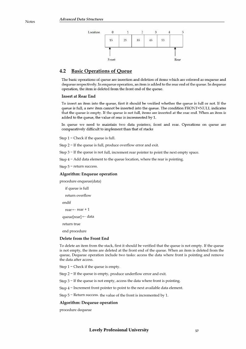
Advanced Data StructuresNotes
4.2 Basic Operations of Queue
Step 1 − Check if the queue is full.
Step 2 − If the queue is full, produce overflow error and exit.
Step 3 − If the queue is not full, increment rear pointer to point the next empty space.
Step 4 − Add data element to the queue location, where the rear is pointing.
Step 5 − return success.
Algorithm: Enqueue operation
procedure enqueue(data)
if queue is full
return overflow
endif
rear ← rear + 1
queue[rear] ← data
return true
end procedure
Delete from the Front End
To delete an item from the stack, first it should be verified that the queue is not empty. If the queueis not empty, the items are deleted at the front end of the queue. When an item is deleted from thequeue, Dequeue operation include two tasks: access the data where front is pointing and removethe data after access.
Step 1 − Check if the queue is empty.
Step 2 − If the queue is empty, produce underflow error and exit.
Step 3 − If the queue is not empty, access the data where front is pointing.
Step 4 − Increment front pointer to point to the next available data element.
Step 5 − Return success. the value of the front is incremented by 1.
Algorithm: Dequeue operation
procedure dequeue
Lovely Professional University 57

Unit 04: Queues
Notesif queue is empty
return underflow
end if
data = queue[front]
front ← front + 1
return true
end procedure
Example:
/*Program of queue using array*/
/*insertion and deletion in a queue*/
/*insertion and deletion in a queue*/
# include <stdio.h>
# define MAX 50
int queue_arr[MAX];
int rear = -1;
int front = -1;
void ins_delete();
void insert();
void display();
void main()
int choice;
while(1)
printf("1.Insert\n");
printf("2.Delete\n");
printf("3.Display\n");
printf("4.Quit\n");
printf("Enter your choice : \n");
scanf("%d",&choice);
switch(choice)
case 1 : insert();
break;
case 2 :ins_delete();
break;
case 3: ins_display();
break;
case 4: exit(1);
Lovely Professional University58

Advanced Data StructuresNotes
default:
printf("Wrong choice\n");
/*End of switch*/
/*End of while*/
/*End of main()*/
void insert()
int added_item;
if (rear==MAX-1)
printf("Queue overflow\n");
else
if (front==-1) /*If queue is initially empty */
front=0;
printf("Enter an element to add in the queue : ");
scanf("%d", &added_item);
rear=rear+1;
queue_arr[rear] = added_item ;
/*End of insert()*/
void ins_delete()
if (front == -1 || front > rear)
printf("Queue underflow\n");
return ;
else
printf("Element deleted from queue is : %d\n", queue_arr[front]);
front=front+1;
/*End of delete() */
void display()
int i;
if (front == -1)
printf("Queue is empty\n");
else
Lovely Professional University 59

Unit 04: Queues
Notesprintf("Elements in the queue:\n");
for(i=front;i<= rear;i++)
printf("%d ",queue_arr[i]);
printf("\n");
/*End of display() */
Output:
1. Insert
2. Delete
3. Display
4. Quit
Enter your choice: 1
Enter an element to add in the queue: 25
Enter your choice: 1
Enter an element to add in the queue: 36
Enter your choice: 3
Elements in the queue: 25, 36
Enter your choice: 2
Element deleted from the queue is: 25
In this example:
4.3 Types of QueueSimple Queue
In a simple queue, insertion takes place at the rear and removal occurs at the front. It follows theFIFO (First in First out) rule.
Circular Queue
In a circular queue, the last element points to the first element making a circular link. In a circularqueue, the rear end is connected to the front end forming a circular loop. An advantage of circularqueue is that, the insertion and deletion operations are independent of one another. This prevents
Lovely Professional University60

Advanced Data StructuresNotes
an interrupt handler from performing an insertion operation at the same time when the mainfunction is performing a deletion operation.
Double ended queue
Double ended queue is also known as deque. It is a type of queue where the insertions anddeletions happen at the front or the rear end of the queue. The various operations that can beperformed on the double ended queue are:
1. Insert an element at the front end
2. Insert an element at the rear end
3. Delete an element at the front end
4. Delete an element at the rear end
1. The header files are included and a constant value 5 is defined for variable SIZE using #definestatement. The SIZE defines the size of the queue.
2. A queue is created using an array named Q with an element capacity of 20. A variable namedCOUNT is declared to store the count of number elements present in the queue.
3. Four functions are created namely, Q_F(), Q_E(), rear_insert(), front_delete(),and display(). Theuser has to select an appropriate function to be performed.
4. The switch statement is used to call the rear_insert(), front_delete(), and display() functions.
5. When the user enters 1, rear_insert() function is called. In the rear_insert() function, the if loopchecks if the count is full. If the condition is true, then the program prints a message “Queue isempty”. Else, it checks for the value of R and assigns the element (num) entered by the user to R.Initially, when there are no elements in the queue, the value of R will be 0. After every insertion, thevariable COUNT is incremented.
6. When the user enters 2, the front_delete() function is called. In this function, the if loop checks ifthe variable COUNT is empty. If the condition is true, then the program prints a message “Queueunderflow”. Else, the element in the 0th
7. When the user enters 3, the display() function is called. In this function, the if loop checks if thevalue of COUNT is 0. If the condition is true, the program prints a message “Queue is empty”. Else,the value of F is assigned to the variable i. The for loop then displays the elements present in thequeue. position will be deleted. The size of F is computed and the COUNT is set to 1.
8. When the user enters 4, the program terminates.
Priority Queue
In priority queue, the elements are inserted and deleted based on their priority. Each element isassigned a priority and the element with the highest priority is given importance and processedfirst. If all the elements present in the queue have the same priority, then the first element is givenimportance.
A priority queue is an abstract data type in which each element is associated with a priorityvalue.Elements are served on the basis of their priority.An element with high priority is dequeuedbefore an element with low priority.If two elements have the same priority, they are servedaccording to their order in the queue.
The priority queue moves the highest priority elements at the beginning of the priority queue andthe lowest priority elements at the back of the priority queue.It supports only those elements thatare comparable. Priority queue in the data structure arranges the elements in either ascending ordescending order.
Types of Priority Queue
Ascending Order Priority Queue
An ascending order priority queue gives the highest priority to the lower number in that queue
Example:
Lovely Professional University 61

Unit 04: Queues
NotesList: 5 6 20 22 10
Arrange these numbers in ascending order.
List 5 6 10 20 22
Descending Order Priority Queue
A descending order priority queue gives the highest priority to the highest number in that queue.
Example:
List: 5 6 35 22 10
Arrange these numbers
List: 35 22 10 6 5
Priority Queue OperationsInserting an Element into the Priority Queue
Deleting an Element from the Priority Queue
Peeking from the Priority Queue (Find max/min)
Extract-Max/Min from the Priority Queue
Priority queue can be implemented using
Array
Linked list
Heap data structure
Binary search tree
Priority Queue Applications
Dijkstra’s algorithm: To find shortest path in graph.
Prim’s Algorithm: Prim’s algorithm uses the priority queue to the values or keys of nodes anddraws out the minimum of these values at every step.
Data Compression: Huffman codes use the priority queue to compress the data.
Operating Systems: load balancing and interrupt handling in an operating system
4.4 Implementation of QueuesThere are two possible implementation strategies – one where the memory is used statically and theother where memory is used dynamically.
Queue can be implemented using:
Array
Linked List
Queue implementation Using Array
To represent a queue we require a one-dimensional array of some maximum size say n to hold thedata items and two other variables front and rear to point to the beginning and the end of thequeue.
Queue implemented using array stores only fixed number of data values. Two variables frontandrear, that are implemented in queue. Front and rear variables point to the position from whereinsertions and deletions are performed in a queue.
Initially both front and rear are set to -1.For insert a new value into the queue, increment rear valueby one and then insert at that position. For delete a value from the queue, then delete the elementwhich is at front position and increment front value by one.
Lovely Professional University62

Advanced Data StructuresNotes
Enqueue operation
Enqueue() function is used to insert a new element into the queue. In a queue, the new element isalways inserted at rear position. The enQueue() function takes one integer value as a parameter andinserts that value into the queue.
Algorithm: Enqueue operation
Step 1: IF REAR = MAX - 1
Write OVERFLOW
Go to step
[END OF IF]
Step 2: IF FRONT = -1 and REAR = -1
SET FRONT = REAR = 0
ELSE
SET REAR = REAR + 1
[END OF IF]
Step 3: Set QUEUE[REAR] = NUM
Step 4: EXIT
Dequeue operation
Dequeue() is a function used to delete an element from the queue. In a queue, the element is alwaysdeleted from front position. The Dequeue() function does not take any value as parameter.
Algorithm: Dequeue operation
Step 1: IF FRONT = -1 or FRONT > REAR
Write UNDERFLOW
ELSE
SET VAL = QUEUE[FRONT]
SET FRONT = FRONT + 1
[END OF IF]
Step 2: EXIT
Queue implementation Using Linked list
Due to the drawbacks of array. The array implementation cannot be used for the large scaleapplications where the queues are implemented.The alternative of array implementation is linkedlist implementation of queue. In a linked queue, each node of the queue consists of two parts i.e.data part and the link part. Each element of the queue points to its immediate next element in thememory.
In the linked queue, there are two pointers maintained in the memory i.e. front pointer and rearpointer. The front pointer contains the address of the starting element of the queue while the rearpointer contains the address of the last element of the queue.
Insert operation
There can be the two scenario of inserting this new node ptr into the linked queue.In the firstscenario, we insert element into an empty queue. In this case, the condition front = NULL becomestrue.In the second case, the queue contains more than one element. The condition front = NULLbecomes false.
Algorithm
Step 1: Allocate the space for the new node PTR
Step 2: SET PTR -> DATA = VAL
Lovely Professional University 63

Unit 04: Queues
NotesStep 3: IF FRONT = NULL
SET FRONT = REAR = PTR
SET FRONT -> NEXT = REAR -> NEXT = NULL
ELSE
SET REAR -> NEXT = PTR
SET REAR = PTR
SET REAR -> NEXT = NULL
[END OF IF]
Step 4: END
Delete operation
Deletion operation removes the element that is first inserted among all the queue elements. Thecondition front == NULL becomes true if the list is empty. Otherwise, we will delete the elementthat is pointed by the pointer front.
Algorithm
Step 1: IF FRONT = NULL
Write " Underflow "
Go to Step 5
[END OF IF]
Step 2: SET PTR = FRONT
Step 3: SET FRONT = FRONT -> NEXT
Step 4: FREE PTR
Step 5: END
4.5 Applications of QueuesOne major application of the queue data structure is in the computer simulation of a real-worldsituation. Queues are also used in many ways by the operating system, the program that schedulesand allocates the resources of a computer system. One of these resources is the CPU (CentralProcessing Unit) itself. If you are working on a multi-user system and you tell the computer to runa particular program, the operating system adds your request to its “job queue”. When yourrequest gets to the front of the queue, the program you requested is executed. Similarly, the varioususers for the system must share the I/O devices (printers, disks etc.). Each device has its own queueof requests to print, read or write to these devices. The following subsection discusses oneapplication of the queues – the priority queue. It is used in time-sharing multi-user systems whereprograms of high priority are processed first arid programs with the same priority form a standardqueue.
In Operating systems:
a) Semaphores
b) FCFS ( first come first serve) scheduling,
c) Spooling in printers
d) Buffer for devices like keyboard
In Networks:
a) Queues in routers/ switches
b) Mail Queues
Queues are used in operating systems for handling interrupts.
Lovely Professional University64

Advanced Data StructuresNotes
Queues are used as buffers in most of the applications like MP3 media player, CD player, etc
When a resource is shared among multiple consumers.
CPU scheduling,
Disk Scheduling.
Summary
A queue is an ordered collection of items in which deletion takes place at the front andinsertion at the rear of the queue.
In a memory, a queue can be represented in two ways; by representing the way in which theelements are stored in the memory, and by naming the address to which the front and rearpointers point to.
The different types of queues are double ended queue, circular queue, and priority queue. The basic operations performed on a queue include inserting an element at the rear end and
deleting an element at the front end. A priority queue is a collection of elements such that each element has been assigned a
priority. An element of higher priority is processed before any element of lower priority. Two elements with the same priority are processed according to the order in which they
were inserted into the queue.
KeywordsFIFO: (First In First Out) The property of a linear data structure which ensures that the elementretrieved from it is the first element that went into it.
Front: The end of a queue from where elements are retrieved.
Queue: A linear data structure in which the element is inserted at one end while retrieved fromanother end.
Rear: The end of a queue where new elements are inserted.
Dequeue: Process of deleting elements from the queue.
Enqueue: Process of inserting elements into queue.
SelfAssessment1. Which technique is followed by queue?
A. FIFOB. LIFOC. Both LIFO and FIFOD. None of above
2. Enqueue () operation is used to perform
A. DeletionB. InsertionC. DisplayD. All of above
3. Which operation is part of queue
Lovely Professional University 65

Unit 04: Queues
NotesA. PeekB. isFullC. isEmptyD. All of above
4. Queue implementation is done using
A. ArrayB. StackC. Linked ListD. All of above
5. Which is not types of Queue
A. CircularB. SimpleC. ComplexD. Priority
6. Queue is a____________ data structure.
A. StaticB. LinearC. DynamicD. None of above
7. Front pointer and rear pointer are used in…
A. Implementation of Queue using Linked ListB. Implementation of Queue using arrayC. Implementation of Queue using stackD. All of above
8. Underflow condition represent.
A. It checks if the queue is full before enqueueing any element.B. It checks if there exists any item before popping from the queue.C. It checks whether all variables are declaredD. All of above
9. Overflow condition represent.
A. It checks if there exists any item before popping from the queue.B. It checks whether all variables are initialized.C. It checks if the queue is full before enqueueing any element.D. All of above
10. Front pointer contains
Lovely Professional University66

Advanced Data StructuresNotes
A. Address of the starting element of the queueB. Address of the last element of the queue.C. Link for next elementD. All of above
11. Priority queue is a____________ data structure.
A. StaticB. LinearC. AbstractD. All of above
12. Priority queue types are
A. Ascending orderB. Descending orderC. Both ascending and descending orderD. None of above
13. Priority Queue Operations are
A. Deleting an Element from the Priority QueueB. Peeking from the Priority Queue (Find max/min)C. Extract-Max/Min from the Priority QueueD. All of above
14. Priority Queue Implementation are performed using.
A. Linked listB. Heap data structureC. Binary search treeD. All of above
15. Binary Heap can be divided into
A. Max heapB. Min-heap.C. Both max and min heapD. None of above
Answers for Self Assessment
1. A 2. B 3. D 4. D 5. C
6. B 7. A 8. B 9. C 10. A
11. B 12. C 13. D 14. D 15. C
Lovely Professional University 67

Unit 04: Queues
Notes
Review Questions1 “Using double ended queues is more advantageous than using circular queues. “Discuss
2 “Stacks are different from queues.” Justify.
3 “Using priority queues is advantageous in job scheduling algorithms. “Analyze
4 Can a basic queue be implemented to function as a dynamic queue? Discuss
5 Describe the application of queue.
6 How will you insert and delete an element in queue?
7 Explain dynamic memory allocation advantages.
Further ReadingsData Structures and Algorithms; Shi-Kuo Chang; World Scientifi c.
Data Structures and Effi cient Algorithms, Burkhard Monien, Thomas Ottmann,
Springer.
Kruse Data Structure & Program Design, Prentice Hall of India, New Delhi
Mark Allen Weles: Data Structure & Algorithm Analysis in C Second Adition.
Addison-Wesley publishing
RG Dromey, How to Solve it by Computer, Cambridge University Press.
Shi-kuo Chang, Data Structures and Algorithms, World Scientifi c
Sorenson and Tremblay: An Introduction to Data Structure with Algorithms.
Thomas H. Cormen, Charles E, Leiserson& Ronald L. Rivest: Introduction to
Algorithms. Prentice-Hall of India Pvt. Limited, New Delhi
Timothy A. Budd, Classic Data Structures in C++, Addison Wesley.
Web Links
www.en.wikipedia.org
www.web-source.net
www.webopedia.com
https://www.geeksforgeeks.org/
https://www.javatpoint.com/data-structure-queue
https://www.tutorialspoint.com/data_structures_algorithms/dsa_queue.htm
Lovely Professional University68

Unit 05: Search Trees
Notes
Unit 05: Search Trees
CONTENTS
Objectives
Introduction
5.1 Concept of Tree
5.2 Binary Tree
5.3 Binary Search Tree
5.4 Binary Search Tree Operations
Summary
Keywords
Self Assessment
Review Questions
Answers for self Assessment
Further Readings
ObjectivesAfter studying this unit, you will be able to:
Discuss the basics of tree Learn concept of binary tree Know binary tree traversal Explain the representation of tree in memory
IntroductionWe know that data structure is a set of data elements grouped together under one name. A datastructure can be considered as a set of rules that hold the data together. Almost all computerprograms use data structures. Data structures are an essential part of algorithms. We can use it tomanage huge amount of data in large databases. Some modern programming languages emphasizemore on data structures than algorithms.
There are many data structures that help us to manipulate the data stored in the memory, which wehave discussed in the previous units. These include array, stack, queue, and linked-list.
Choosing the best data structure for a program is a challenging task. Similar tasks may requiredifferent data structures. We derive new data structures for complex tasks using the alreadyexisting ones. We need to compare the characteristics of the data structures before choosing theright data structure. A tree is a hierarchical data structure suitable for representing hierarchicalinformation. The tree data structure has the characteristics of quick search, quick inserts, and quickdeletes.
5.1 Concept of TreeA tree is a set of one or more nodes T such that:
1. There is a specially designated node called root, and
2. Remaining nodes are partitioned into n >= 0 disjoint set of nodes T1, T2,…,Tn each of which is atree.
Ashwani Kumar, Lovely Professional University
Lovely Professional University 69

Advanced Data StructuresNotes
This is a tree because it is a set of nodes A, B, C, D, E, F, G, H, I, with node A as a root node, andthe remaining nodes are partitioned into three disjoint sets: B, G, H, I, C, E, F AND Drespectively. Each of these sets is a tree individually because each of these sets satisfies the aboveproperties.
This is not a tree because it is a set of nodes A, B, C, D, E, F, G, H, I, with node A as a root node,but the remaining nodes cannot be partitioned into disjoint sets, because the node I is shared.
Given below are some of the important definitions, which are used in connection with trees.
Degree of Node of a Tree: The degree of a node of a tree is the number of sub-trees having thisnode as a root, or it is a number of decedents of a node. If degree is zero then it is called terminalnode or leaf node of a tree.
Degree of a Tree: It is defined as the maximum of degree of the nodes of the tree, i.e. degree of tree= max (degree (node i) for i = 1 to n).
Level of a Node: We defi ne the level of the node by taking the level of the root node to be 1, andincrementing it by 1 as we move from the root towards the sub-trees i.e. the level of all thedescendents of the root nodes will be 2. The level of their descendents will be 3 and so on. We thendefine depth of the tree to be the maximum value of level for node of a tree.
Root Node: The root of a tree is called a root node. A root node occurs only once in the whole tree.
Parent Node: The parent of a node is the immediate predecessor of that node.
Child Node: Child nodes are the immediate successors of a node.
Leaf Node: A node which does not have any child nodes is known as a leaf node.
Link: The pointer to a node in the tree is known as a link. A node can have more than one link.
Path: Every node in the tree is reachable from the root node through a unique sequence of links.This sequence of links is known as a path. The number of links in a path is considered to be thelength of the path.
Levels: The level of a node in the tree is considered to be its hierarchical rank in the tree.
Height: The height of a non-empty tree is the maximum level of a node in the tree. The height of anempty tree (no node in a tree) is 0. The height of a tree containing a single node is 1. The longestpath in the tree has to be considered to measure the height of the tree.
Height of a tree (h) = Imax+ 1, where Imax is the maximum level of a tree.
Siblings: The nodes which have the same parent node are known as siblings.
Lovely Professional University70

Unit 05: Search Trees
NotesGraphs consist of a set of nodes and edges, just like trees. But for graphs, there are no rules for theconnections between nodes. In graphs, there is no concept of a root node, nor a concept of parentsand children. Rather, a graph is just a collection of interconnected nodes. All trees are graphs. Atree is a special case of a graph, in which the nodes are all reachable from some starting node.
Representation of Tree in Graphs
A graph G consists of a set of objects V = v1, v2, v3 … called vertices (points or nodes) and a set ofobjects E = e1, e2, e3 …. called edges (lines or arcs).
The set V (G) is called the vertex set of G and E (G) is the edge set.
The graph is denoted as G = (V, E)
Let G be a graph and u, v an edge of G. Since u, v is 2-element set, we write v, u instead of u,v.
This edge can be represented as uv or vu.
If e = uv is an edge of a graph G, then u and v are adjacent in G and e joins u and v.
Consider given graph
This graph G is defined by the sets:
V (G) = u, v, w, x, y, z and E(G) = uv, uw, wx, xy, xz
Every graph has a diagram associated with it. The vertex u and an edge e are incident with eachother as are v and e. If two distinct edges e and f are incident with a common vertex, then they areadjacent edges.
5.2 Binary TreeA binary tree is a special tree where each non-leaf node can have atmost two child nodes. Mostimportant types of trees which are used to model yes/no, on/off, higher/lower, i.e., binarydecisions are binary trees.
A tree data structure in which every node has a maximum of two child nodes is known as a binarytree. It is the most commonly used non-linear data structure. A binary tree could either have only aroot node or two disjoint binary trees called the left sub-tree or the right sub-tree. An empty treecould also be a binary tree.
Recursive Definition: “A binary tree is either empty or a node that has left and right sub-trees thatare binary trees. Empty trees are represented as boxes (but we will almost always omit the boxes)”.
Binary Tree Structure
Lovely Professional University 71

Advanced Data StructuresNotes
In a formal way, we can define a binary tree as a finite set of nodes which is either empty orpartitioned in to sets of T0, Tl, Tr, where T0 is the root and Tl and Tr are left and right binary trees,respectively.
So, for a binary tree we find that:
1. The maximum number of nodes at level i will be 2i−1
2. If k is the depth of the tree then the maximum number of nodes that the tree can have is
2k − 1 = 2k−1 + 2k−2 + … + 20
Types of Binary Tree
There are two main binary tree and these are:
1. Full binary tree
2. Complete binary tree
Full Binary Tree
A full binary tree is a binary of depth k having 2k − 1 nodes. If it has < 2k − 1, it is not a full binarytree.
For k = 3, the number of nodes = 2k − 1 = 23 − 1 = 8 − 1 = 7. A full binary tree with depth k = 3 isshown in figure.
A Full Binary Tree
We use numbers from 1 to 2k − 1 as labels of the nodes of the tree.
If a binary tree is full, then we can number its nodes sequentially fom 1 to 2k−1, starting from theroot node, and at every level numbering the nodes from left to right.
Complete Binary Tree
A complete binary tree of depth k is a tree with n nodes in which these n nodes can be numberedsequentially from 1 to n, as if it would have been the fi rst n nodes in a full binary tree of depth k.
A complete binary tree with depth k = 3 is shown in Figure
A Complete Binary Tree
Properties of a Binary Tree
Main properties of binary tree are:
1. If a binary tree contains n nodes, then it contains exactly n – 1 edges;
2. A Binary tree of height h has 2h – 1 nodes or less.
Lovely Professional University72

Unit 05: Search Trees
Notes3. If we have a binary tree containing n nodes, then the height of the tree is at most n and at leastceiling log2 (n + 1).
4. If a binary tree has n nodes at a level l then, it has at most 2n nodes at a level l + 1
5. The total number of nodes in a binary tree with depth k (root has depth zero) is N = 20 + 21
+ 22 + …….+ 2k = 2k+1 – 1.
5.3 Binary Search TreeA binary search tree is a binary tree which may be empty, and every node contains an identifierand
1. Identifier of any node in the left sub-tree is less than the identifier of the root
2. Identifier of any node in the right sub-tree is greater than the identifier of the root and the leftsub-tree as well as right sub-tree both are binary search trees.
Binary Search Tree
A binary search tree is basically a binary tree, and therefore it can be traversed is in order, preorder,and post order. If we traverse a binary search tree in in order and print the identifiers contained inthe nodes of the tree, we get a sorted list of identifiers in the ascending order.
A binary search tree is an important search structure. For example, consider the problem ofsearching a list. If a list is an ordered then searching becomes faster, if we use a contiguous list andbinary search, but if we need to make changes in the list like inserting new entries and deleting oldentries. Then it is much slower to use a contiguous list because insertion and deletion in acontiguous list requires moving many of the entries every time. So we may think of using a linkedlist because it permits insertions and deletions to be carried out by adjusting only few pointers, butin a linked list there is no way to move through the list other than one node at a time hencepermitting only sequential access. Binary trees provide an excellent solution to this problem. Bymaking the entries of an ordered list into the nodes of a binary search tree, we find that we cansearch for a key in O(n log n) steps.
Creating a Binary Search Tree
We assume that every node a binary search tree is capable of holding an integer data item and thelinks which can be made pointing to the root of the left and the right sub-tree respectively.
Therefore the structure of the node can be defi ned using the following declaration:
struct tnode
int data;
tnode *lchid;
tnode *rchild;
Lovely Professional University 73

Advanced Data StructuresNotes
To create a binary search tree we use a procedure named insert which creates a new node with thedata value supplied as a parameter to it, and inserts into an already existing tree whose root pointeris also passed as a parameter. The procedure accomplishes this by checking whether the tree whoseroot pointer is passed as a parameter is empty. If it is empty then the newly created node is insertedas a root node. If it is not empty then it copies the root pointer into a variable temp1, it then storesvalue of temp1 in another variable temp2, compares the data value of the node pointed to by temp1with the data value supplied as a parameter, if the data value supplied as a parameter is smallerthan the data value of the node pointed to by temp1 then it copies the left link of the node pointedby temp1 into temp1 (goes to the left), otherwise it copies the right link of the node pointed bytemp1 into temp1(goes to the right). It repeats this process till temp1 becomes nil.
When temp1 becomes nil, the new node is inserted as a left child of the node pointed to by temp2 ifdata value of the node pointed to by temp2 is greater than data value supplied as parameter.Otherwise the new node is inserted as a right child of node pointed to by temp2. Therefore theinsert procedure is
void insert(tnode *p, int val)
tnode *temp1, *temp2;
if (p == NULL)
p = new(tnode);
p->data = val;
p->1child = NULL;
p->rchild = NULL;
else
temp1 = p;
while(temp1 != NULL)
temp2 = temp1;
if(temp1->data >val)
temp1 = temp1->1eft;
else
temp1 = temp1->right;
if(temp2->data >val)
temp2->left = new(tnode);
temp2 = temp2->left;
temp2->data = val;
temp2->left = NULL;
temp2->right= NULL;
else
Lovely Professional University74

Unit 05: Search Trees
Notestemp2->right = new(tnode);
temp2 = temp2->right;
temp2->data = val;
temp2->left = NULL;
temp2->right = NULL;
5.4 Binary Search Tree OperationsThe four main operations that we perform on binary trees are:
1. Searching
2. Insertion
3. Deletion
4. Traversal
Searching in Binary Search Trees
In searching, the node being searched is called as key node. We first match the key node with theroot node. If the value of the key node is greater than the current node, then we search for it in theright subtree, else we search in the left sub-tree. We continue this process until we find the node oruntil no nodes are left. The pseudo code for searching a binary search tree is as follows:
Pseudocode for a Binary Search Tree
find(X, node)
if(node = NULL)
return NULL
if(X = node:data)
return node
else if(X<node:data)
return find(Y,node:leftChild)
else if(X>node:data)
return find(X,node:rightChild)
Inserting in Binary Search Trees
To insert a new element in an existing binary search tree, first we compare the value of the newnode with the current node value. If the value of the new node is lesser than the current node value,we insert it as a left sub-node. If the value of the new node is greater than the current node value,then we insert it as a right sub-node. If the root node of the tree does not have any value, we caninsert the new node as the root node.
Algorithm for Inserting a Value in a Binary Search Tree
1. Read the value for the node that needs to be created and store it in a node called NEW.
2. At first, if (root! =NULL) then root = NEW.
3. If (NEW->value < root->value) then attach NEW node as a left child node of root, else attachNEW node as a right child node of root.
4. Repeat steps 3 and 4 for creating the desired binary search tree completely.
Lovely Professional University 75

Advanced Data StructuresNotes
When inserting any node in a binary search tree, it is necessary to look for its proper position in thebinary search tree. The new node is compared with every node of the tree. If the value of the nodewhich is to be inserted is more than the value of the current node, then the right sub-tree isconsidered, else the left sub-tree is considered. Once the proper position is identified, the new nodeis attached as the left or right child node. Let us now discuss the pseudo code for inserting a newelement in a binary search tree.
Pseudocode for Inserting a Value in a Binary Search Tree
//Purpose: Insert data object X into the Tree
//Inputs: Data object X (to be inserted), binary-search-tree node
//Effect: Do nothing if tree already contains X;
// otherwise, update binary search tree by adding a new node containing data object X
insert(X, node)
if(node = NULL)
node = new binaryNode(X,NULL,NULL)
return
if(X = node:data)
return
else if(X<node:data)
insert(X, node:leftChild)
else // X>node:data
insert(X, node:rightChild)
Deleting in Binary Search Trees
If the node to be deleted has no children, we can just delete it. If the node to be deleted has onechild,
then the node is deleted and the child is connected directly to the parent node.
There are mainly three cases possible for deletion of any node from a binary search tree. They are:
1. Deletion of the leaf node
2. Deletion of a node that has one child
3. Deletion of a node that has two children
We can delete an existing element from a binary search tree using the following pseudocode:
Pseudocode for Deleting a Value from a Binary Search Tree
//Purpose: Delete data object X from the Tree
//Inputs: Data object X (to be deleted), binary-search-tree node
//Effect: Do nothing if tree does not contain X;
// else, update binary search tree by deleting the node containing data object X
delete(X, node)
if(node = NULL) //nothing to do
return
if(X<node:data)
delete(X, node:leftChild)
Lovely Professional University76

Unit 05: Search Trees
Noteselse if(X>node:data)
delete(X, node:rightChild)
else // found the node to be deleted. Take action based on number of node children
if(node:leftChild = NULL and node:rightChild = NULL)
delete node
node = NULL
return
else if(node:leftChild = NULL)
tempNode = node
node = node:rightChild
delete tempNode
else if(node:rightChild = NULL)
tempNode = node
node = node:leftChild
delete tempNode
else //replace node:data with minimum data from right sub-tree
tempNode = findMin(node.rightChild)
node:data = tempNode:data
delete(node:data,node:rightChild)
Pseudocode for Finding Minimum Value from a Binary Search Tree//Purpose: return least data object X in the Tree
//Inputs: binary-search-tree node node
// Output: bst-node n containing least data object X, if it exists; NULL otherwise
findMin(node)
if(node = NULL) //empty tree
return NULL
if(node:leftChild = NULL)
return node
return findMin(node:leftChild)
Deleting a node with one child
Step 1 - Find the node to be deleted using search operation
Step 2 - If it has only one child then create a link between its parent node and child node.
Step 3 - Delete the node using free function and terminate the function.
Deleting a node with two children
Lovely Professional University 77

Advanced Data StructuresNotes
Step 1 - Find the node to be deleted using search operation
Step 2 - If it has two children, then find the largest node in its left subtree (OR) the smallest node inits right subtree.
Step 3 - Swap both deleting node and node which is found in the above step.
Step 4 - Then check whether deleting node came to case 1 or case 2 or else goto step 2
Step 5 - If it comes to case 1, then delete using case 1 logic.
Step 6- If it comes to case 2, then delete using case 2 logic.
Step 7 - Repeat the same process until the node is deleted from the tree.
Binary Search Tree time complexities
Search Operation - O(n)
Insertion Operation - O(1)
Deletion Operation - O(n)
Application of a Binary Search Tree
1. A prominent data structure used in many systems programming applications for representingand managing dynamic sets.
2. Average case complexity of Search, Insert, and Delete Operations is O(log n), where n is thenumber of nodes in the tree.
One of the applications of a binary search tree is the implementation of a dynamic dictionary.
A dictionary is an ordered list which is required to be searched frequently, and is also required tobe updated (insertions and deletions) frequently. Hence can be very well implemented using abinary search tree, by making the entries of dictionary into the nodes of binary search tree. A moreefficient implementation of a dynamic dictionary involves considering a key to be a sequence ofcharacters, and instead of searching by comparison of entire keys, we use these characters todetermine a multi-way branch at each step, this will allow us to make a 26-way branchingaccording the fi rst letter, followed by another branch according to the second letter and so on.
Summary
Search trees are data structures that support many dynamic-set operations such assearching, finding the minimum or maximum value, inserting, or deleting a value.
In a binary search tree, for a given node n, each node to the left has a value lesser than n andeach node to the right has a value greater than n.
The time taken to perform operations on a binary search tree is directly proportional to theheight of the tree.
Binary trees provide an excellent solution to this problem. By making the entries of anordered list into the nodes of a binary tree, we shall fi nd that we can search for a target keyin O(log n) steps, just as with binary search, and we shall obtain algorithms for inserting anddeleting entries also in time O(log n).
Keywords
Binary Search Tree: A binary search tree is a binary tree which may be empty, and everynode contains an identifier.
Searching: Searching for the key in the given binary search tree, start with the root nodeand compare the key with the data value of the root node.
Degree of a tree: The highest degree of a node appearing in the tree.
Lovely Professional University78

Unit 05: Search Trees
Notes Inorder: A tree traversing method in which the tree is traversed in the order of left-tree,
node and then right-tree. Level of a node: The number of nodes that must be traversed to reach the node from the
root. Root node: The node in a tree which does not have a parent node. Tree: A two-dimensional data structure comprising of nodes where one node is the root
and rest of the nodes form two disjoint sets each of which is a tree.
Self Assessment1. Tree is a _______ hierarchical data structure.
A. LinearB. NonlinearC. AbstractD. All of above
2. Data access is quick and easier in
A. Nonlinear data structureB. Linear data structureC. Both Linear and NonlinearD. None of above
3. Types of trees are
A. Binary TreeB. Binary Search TreeC. AVL TreeD. All of above
4. Binary search tree is also called.
A. OrderedB. SortedC. Both ordered and sorted binary treeD. None of above
5. value of the nodes in the left sub-tree is less than the value of the root is
A. General TreeB. Binary TreeC. Binary Search TreeD. None of above
6. Types of Binary Trees are
A. Full binary tree
Lovely Professional University 79

Advanced Data StructuresNotes
B. Complete binary treeC. Perfect binary treeD. All of above
7. Which is not Binary Tree operation?
A. SearchB. PeekC. InsertionD. Deletion
8. Binary Search Tree applications are
A. In multilevel indexing in the database.B. For dynamic sorting.C. It is used to implement various searching algorithms.D. All of above
9. Binary Search Tree time complexity for search operation is
A. O(n)B. O(1)C. O(2)D. None of above
10. Binary Search Tree time complexity for insert operation is
A. O(0)B. O(1)C. O(2)D. None of above
11. What is the worst case time complexity for Delete operation?
A. O(0)B. O(1)C. O(n)D. None of above
12. Which is incorrect statement about Binary search tree.
A. The left and right sub-trees should also be binary search treesB. In order sequence gives decreasing order of elementsC. The left child is always lesser than its parentD. The right child is always greater than its parent
13. To arrange binary tree in ascending order…
Lovely Professional University80

Unit 05: Search Trees
NotesA. Pre order traversal onlyB. Post order traversal onlyC. In order traversal onlyD. None of above
14. Which of the following is not component of binary tree
A. Data elementB. Pointer to right subtreeC. Super treeD. Pointer to left subtree
15. Which of the following is not a type of tree data structure
A. General TreeB. Primary TreeC. Binary TreeD. Binary Search TreeE.
Answers for self Assessment
1. B 2. A 3. D 4. C 5. C
6. D 7. B 8. D 9. A 10. B
11. C 12. B 13. C 14. C 15. B
Review Questions1. define tree with suitable example.
2. Draw a binary tree with six child node.
4. Discuss degree of tree.
5. Explain representation of tree.
6. what are the application of tree.
7. Discuss time complexity of Binary search tree.
Further ReadingsData Structures and Effi cient Algorithms, Burkhard Monien, Thomas Ottmann,Springer.
Kruse Data Structure & Program Design, Prentice Hall of India, New Delhi
Mark Allen Weles: Data Structure & Algorithm Analysis in C Second Adition. Addison-Wesley publishing
RG Dromey, How to Solve it by Computer, Cambridge University Press.
Shi-kuo Chang, Data Structures and Algorithms, World Scientifi c
Sorenson and Tremblay: An Introduction to Data Structure with Algorithms.
Thomas H. Cormen, Charles E, Leiserson& Ronald L. Rivest: Introduction toAlgorithms. Prentice-Hall of India Pvt. Limited, New Delhi
Lovely Professional University 81

Advanced Data StructuresNotes
Timothy A. Budd, Classic Data Structures in C++, Addison Wesley.
Web Linkswww.en.wikipedia.org
www.webopedia.com
https://www.programiz.com/
https://www.javatpoint.com/data-structure-stack
https://www.tutorialspoint.com/data_structures_algorithms/stack_algorithm.htm
Advanced Data StructuresNotes
Timothy A. Budd, Classic Data Structures in C++, Addison Wesley.
Web Linkswww.en.wikipedia.org
www.webopedia.com
https://www.programiz.com/
https://www.javatpoint.com/data-structure-stack
https://www.tutorialspoint.com/data_structures_algorithms/stack_algorithm.htm
Advanced Data StructuresNotes
Timothy A. Budd, Classic Data Structures in C++, Addison Wesley.
Web Linkswww.en.wikipedia.org
www.webopedia.com
https://www.programiz.com/
https://www.javatpoint.com/data-structure-stack
https://www.tutorialspoint.com/data_structures_algorithms/stack_algorithm.htm
Lovely Professional University82

Unit 06: Tree Data Structure 1
Notes
Unit 06: Tree Data Structure 1
CONTENTS
Objectives
Introduction
6.1 AVL Tree
6.2 AVL Operation
6.3 Applications of AVL Trees
6.4 B-tree
6.5 Operations on B-trees
Summary
Keywords
Self Assessment
Answers for Self Assessment
Review Questions
Further Readings
ObjectivesAfter studying this unit, you will be able to:
State about AVL tree Describe balancing operations Discuss B-tree Learn B-tree properties and operations
IntroductionOne of the most essential data structures is the tree, which is used to conduct operations likeinsertion, deletion, and searching of items efficiently. Construction of a well-balanced tree forsorting all data is not practicable when working with a huge number of data, though. As a result,only valuable data is saved as a tree, and the actual volume of data used changes over time as newdata is inserted and old data is deleted. It is possible to conduct traversals, insertions, and deletionswithout utilizing either stack or recursion in some circumstances where the NULL link to a binarytree to special links is referred to as threads.
6.1 AVL TreeAn AVL tree is another balanced binary search tree. AVL Tree is invented in 1962. It takes its namefrom the initials of its inventors – Adelson, Velskii and Landis. An AVL tree has the followingproperties:
1. The sub-trees of every node differ in height by at most one level.
2. Every sub-tree is an AVL tree.
Ashwani Kumar, Lovely Professional University
Lovely Professional University 83

Advanced Data StructuresNotes
Here, the height of the tree is h. Height of one subtree is h–1 while that of another subtree of thesame node is h–2, differing from each other by just 1. Therefore, it is an AVL tree.
AVL Tree is defined as height balanced binary search tree. In AVL tree each node is associated witha balance factor which is calculated by subtracting the height of its right sub-tree from that of its leftsub-tree.
Why AVL Tree
AVL tree controls the height of the binary search tree. The time taken for all operations in a binarysearch tree of height h is O(h). For skewed BST it can be extended to O(n) (worst case).By limitingthis height to log n, AVL tree imposes an upper bound on each operation to be O(log n) where n isthe number of nodes.
Balance FactorBalance factor of a node in an AVL tree is the difference between the height of the left sub tree andthat of the right sub tree of that node.
Balance Factor = (Height of Left Sub tree - Height of Right Sub tree) or (Height of Right Sub tree -Height of Left Sub tree). Balance factor value are: -1, 0 or 1.
If balance factor of any node is 1, it means that the left sub-tree is one level higher than the rightsub-tree.
If balance factor of any node is 0, it means that the left sub-tree and right sub-tree contain equalheight.
If balance factor of any node is -1, it means that the left sub-tree is one level lower than the rightsub-tree.
Lovely Professional University84

Unit 06: Tree Data Structure 1
Notes
Balanced Tree
AVL tree (Left Heavy Tree)
AVL Tree (Right Heavy Tree)
Unit 06: Tree Data Structure 1
Notes
Balanced Tree
AVL tree (Left Heavy Tree)
AVL Tree (Right Heavy Tree)
Unit 06: Tree Data Structure 1
Notes
Balanced Tree
AVL tree (Left Heavy Tree)
AVL Tree (Right Heavy Tree)
Lovely Professional University 85

Advanced Data StructuresNotes
AVL Tree Rotations for balancingRotations are performed in AVL tree only in case if Balance Factor is other than -1, 0, and 1.
Left rotation
Right rotation
Left-Right rotation
Right-Left rotation
The Left rotation and Right rotation are single rotations.
Left-Right rotation and Right-Left rotation are double rotations.
Left rotation
If a tree becomes unbalanced, when a node is inserted into the right subtree of the right subtree,then we perform a single left rotation.
Right rotation
AVL tree may become unbalanced, if a node is inserted in the left subtree of the left subtree. Thetree then needs a right rotation.
Left-Right rotation
Double rotations are slightly complex rotations. To understand them better, we should take note ofeach action performed while rotation. A left-right rotation is a combination of left rotation followedby right rotation.
Lovely Professional University86

Unit 06: Tree Data Structure 1
Notes
Step - 1
Step – 2
Right-Left rotation
It is a combination of right rotation followed by left rotation.
Step – 1
Unit 06: Tree Data Structure 1
Notes
Step - 1
Step – 2
Right-Left rotation
It is a combination of right rotation followed by left rotation.
Step – 1
Unit 06: Tree Data Structure 1
Notes
Step - 1
Step – 2
Right-Left rotation
It is a combination of right rotation followed by left rotation.
Step – 1
Lovely Professional University 87

Advanced Data StructuresNotes
Step – 2
6.2 AVL OperationInsertion into AVL Trees
To implement AVL trees, you need to maintain the height of each node. You insert into an AVL treeby performing a standard binary tree insertion. When you’re done, you check each node on thepath from the new node to the root. If that node’s height hasn’t changed because of the insertion,then you are done. If the node’s height has changed, but it does not violate the balance property,then you continue checking the next node in the path. If the node’s height has changed and it nowviolates the balance property, then you need to perform one or two rotations to fix the problem,and then you are done.
Insertion in AVL is same as binary search tree. Insertion may lead to violation in the tree propertyand therefore the tree may need balancing. The tree can be balanced by applying rotations.
Deletion
When you delete a node, there are three things that can happen to the parent:
1. Its height is decremented by one.
2. Its height doesn’t change and it stays balanced.
3. Its height doesn’t change, but it becomes imbalanced.
You handle these three cases in different ways:
1. The parent’s height is decremented by one. When this happens, you check the parent’s parent:you keep doing this until you return or you reach the root of the tree.
2. The parent’s height doesn’t change and it stays balanced. When this happens you may return –deletion is over.
3. The parent’s height doesn’t change, but it becomes imbalanced. When this happens, you have torebalance the subtree rooted at the parent. After rebalancing, the subtree’s height may be onesmaller than it was originally. If so, you must continue checking the parent’s parent.
To rebalance, you need to identify whether you are in a zig-zig situation or a zig-zag situation andrebalance accordingly.
Complexities of Different Operations on an AVL Tree
The rotation operations (left and right rotate) take constant time as only a few pointers are beingchanged there. Updating the height and getting the balance factor also takes constant time.
Insertion Deletion Search
O(log n) O(log n) O(log n)
Lovely Professional University88

Unit 06: Tree Data Structure 1
Notes6.3 Applications of AVL TreesAVL trees are applied in the following situations:
1. There are few insertion and deletion operations
2. Short search time is needed
3. Input data is sorted or nearly sorted
AVL tree structures can be used in situations which require fast searching. But, the large cost ofrebalancing may limit the usefulness.
Consider the following:
1. A classic problem in computer science is how to store information dynamically so as to allow forquick look up. This searching problem arises often in dictionaries, telephone directory, symboltables for compilers and while storing business records etc. The records are stored in a balancedbinary tree, based on the keys (alphabetical or numerical) order.
The balanced nature of the tree limits its height to O (log n), where n is the number of insertedrecords.
2. AVL trees are very fast on searches and replacements. But, have a moderately high cost foraddition and deletion. If application does a lot more searches and replacements than it doesaddition and deletions, the balanced (AVL) binary tree is a good choice for a data structure.
3. AVL tree also has applications in fi le systems.
Advantages of AVL tree
The height of the AVL tree is always balanced. The height never grows beyond log N, where N isthe total number of nodes in the tree.
Search time complexity is better as compared to Binary Search trees.
AVL trees have self-balancing capabilities.
6.4 B-treeA B-tree is a tree data structure that keeps data sorted and allows insertions and deletions that islogarithmically proportional to fi le size. It is commonly used in databases and fi le systems.
In B-trees, internal nodes can have a variable number of child nodes within some pre-definedrange. When data is inserted or removed from a node, its number of child nodes changes. In orderto maintain the pre-defi ned range, internal nodes may be joined or split. Because a range of childnodes is permitted, B-trees do not need re-balancing as frequently as other self balancing searchtrees, but may waste some space, since nodes are not entirely full. The lower and upper bounds onthe number of child nodes are typically fixed for a particular implementation.
A B-tree is kept balanced by requiring that all leaf nodes are at the same depth. This depth willincrease slowly as elements are added to the tree, but an increase in the overall depth is infrequent,and results in all leaf nodes being one more hop further removed from the root.
B-trees are balanced trees that are optimized for situations when part or the entire tree must bemaintained in secondary storage such as a magnetic disk. Since disk accesses are expensive (timeconsuming) operations, a b-tree tries to minimize the number of disk accesses.
Lovely Professional University 89

Advanced Data StructuresNotes
Structure of B-treesUnlike a binary-tree, each node of a b-tree may have a variable number of keys and children. Thekeys are stored in non-decreasing order. Each key has an associated child that is the root of asubtree containing all nodes with keys less than or equal to the key but greater than the precedingkey. A node also has an additional rightmost child that is the root for a subtree containing all keysgreater than any keys in the node.
A b-tree has a minimum number of allowable children for each node known as the minimizationfactor. If t is this minimization factor, every node must have at least t – 1 keys. Under certaincircumstances, the root node is allowed to violate this property by having fewer than t – 1 keys.
Every node may have at most 2t – 1 keys or, equivalently, 2t children. Since each node tends tohave a large branching factor (a large number of children), it is typically necessary to traverserelatively few nodes before locating the desired key. If access to each node requires a disk access,then a b-tree will minimize the number of disk accesses required.
The minimization factor is usually chosen so that the total size of each node corresponds to amultiple of the block size of the underlying storage device. This choice simplifies and optimizesdisk access. Consequently, a b-tree is an ideal data structure for situations where all data cannotreside in primary storage and accesses to secondary storage are comparatively expensive (or timeconsuming).
Why B TreeB-Trees is used to reduce the number of disk accesses.Most of the tree operations (search, insert,delete, max, min) require O(h) disk accesses where h is the height of the tree. B-tree is a fat tree. Theheight of B-Trees is kept low by putting maximum possible keys in a B-Tree node.
Data structures like binary search tree, avl tree, red-black tree, etc. can store only one key in onenode. If you have to store a large number of keys, then the height of such trees becomes very largeand the access time increases.
The height of the B-tree is low so total disk accesses for most of the operations are reducedsignificantly compared to balanced Binary Search Trees like AVL Tree, Red-Black Tree,etc.
B Tree propertiesB-Tree of Order m has the following properties:
1 - All leaf nodes must be at same level.
2 - All nodes except root must have at least [m/2]-1 keys and maximum of m-1 keys.
3 - All non leaf nodes except root (i.e. all internal nodes) must have at least m/2 children.
4 - If the root node is a non leaf node, then it must have at least 2 children.
5 - A non leaf node with n-1 keys must have n number of children.
6 - All the key values in a node must be in Ascending Order.
Lovely Professional University90

Unit 06: Tree Data Structure 1
Notes6.5 Operations on B-treesThe algorithms for the search, create, and insert operations are shown below. Note that thesealgorithms are single pass; in other words, they do not traverse back up the tree. Since b-trees striveto minimize disk accesses and the nodes are usually stored on disk, this single-pass approach willreduce the number of node visits and thus the number of disk accesses. Simpler double-passapproaches that move back up the tree to fi x violations are possible.
Since all nodes are assumed to be stored in secondary storage (disk) rather than primary storage(memory), all references to a given node be bepreceeded by a read operation denoted by Disk-Read. Similarly, once a node is modifi ed and it is no longer needed, it must be written out tosecondary storage with a write operation denoted by Disk-Write. The algorithms below assumethat all nodes referenced in parameters have already had a corresponding Disk-Read operation.New nodes are created and assigned storage with the Allocate-Node call. The implementationdetails of the Disk-Read, Disk-Write, and Allocate-Node functions are operating system andimplementation dependent.
Search Operation
The search operation on a b-tree is analogous to a search on a binary tree. Instead of choosingbetween a left and a right child as in a binary tree, a b-tree search must make an n-way choice. Thecorrect child is chosen by performing a linear search of the values in the node. After finding thevalue greater than or equal to the desired value, the child pointer to the immediate left of that valueis followed. If all values are less than the desired value, the rightmost child pointer is followed. Ofcourse, the search can be terminated as soon as the desired node is found. Since the running time ofthe search operation depends upon the height of the tree, B-Tree-Search is O(logt n).
B-Tree-Search(x, k)
i<- 1
while i<= n[x] and k >keyi[x]
do i<- i + 1
if i<= n[x] and k = keyi[x]
then return (x, i)
if leaf[x]
then return NIL
else Disk-Read(ci[x])
return B-Tree-Search(ci[x], k)
Search algorithm
Let the key (the value) to be searched by “X”.
Start searching from the root and recursively traverse down.
If X is lesser than the root value, search left sub tree, if X is greater than the root value, search theright sub tree.
If the node has the found X, simply return the node.
If the X is not found in the node, traverse down to the child with a greater Key.
If X is not found in the tree, we return NULL.
Insertion Operation
Insertions in B-Tree performed only at the leaf node level.Inserting operation performed with twosteps: searching the appropriate node to insert the element and splitting the node if required.
Insertion algorithm
Check whether tree is Empty.
If tree is Empty, then create a new node with new key value and insert it into the tree as a root node
Lovely Professional University 91

Advanced Data StructuresNotes
If tree is not empty, then, find the appropriate leaf node at which the node can be inserted.
If the leaf node contain less than m-1 keys then insert the element in the increasing order.
Else, if the leaf node contains m-1 keys, then follow the following steps.
-Insert the new element in the increasing order of elements.
-Split the node into the two nodes at the median.
-Push the median element upto its parent node.
-If the parent node also contain m-1 number of keys, then split it too by followingthesame steps.
Deletion operation
In case of deletion from B-Tree user need to follow more rule as compared to search and insertion.
Three case for deletion from B-Tree
If the key is in the leaf node
If the key is in an internal node
If the key is in a root node
Key is in the leaf node, case-1
Target is in the leaf node, more than min keys.
Deleting this will not violate the property of B Tree
Target is in leaf node, it has min key nodes
Deleting this will violate the property of B Tree
Target node can borrow key from immediate left node, orimmediate right node (sibling)
The sibling will say yes if it has more than minimum number of keys
The key will be borrowed from the parent node, the max value will betransferred to a parent, themax value of the parent node will betransferred to the target node, and remove the target value
Target is in the leaf node, but no siblings have more than min number of keys Search for key
Merge with siblings and the minimum of parent nodes
Total keys will be now more than min
The target key will be replaced with the minimum of a parent node
Key is in an internal node, case-2
Either choose, in- order predecessor or in-order successor
In case the of in-order predecessor, the maximum key from its left sub tree will be selected
In case of in-order successor, the minimum key from its right sub tree will be selected
If the target key’s in-order predecessor has more than the min keys, only then it can replace thetarget key with the max of the in-order predecessor
If the target key’s in-order predecessor does not have more than min keys, look for in-ordersuccessor’s minimum key.
If the target key’s in-order predecessor and successor both have less than min keys, then merge thepredecessor and successor.
Key is in a root node, Case- 3
Replace with the maximum element of the in-order predecessor sub tree
Lovely Professional University92

Unit 06: Tree Data Structure 1
NotesIf, after deletion, the target has less than min keys, then the target node will borrow max value fromits sibling via sibling’s parent.
The max value of the parent will be taken by a target, but with the nodes of the max value of thesibling.
Summary
AVL tree controls the height of the binary search tree. The time taken for all operations in abinary search tree of height h is O (h).
In AVL tree each node is associated with a balance factor which is calculated by subtractingthe height of its right sub-tree from that of its left sub-tree.
B-trees are balanced trees that are optimized for situations when part or the entire tree mustbe maintained in secondary storage such as a magnetic disk.
A B-tree is a specialized multiway tree designed especially for use on disk. In a B-tree eachnode may contain a large number of keys. The number of subtrees of each node, then, mayalso be large.
A B-tree is designed to branch out in this large number of directions and to contain a lot ofkeys in each node so that the height of the tree is relatively small.
This means that only a small number of nodes must be read from disk to retrieve an item. The goal is to get fast access to the data, and with disk drives this means reading a very
small number of records. Note that a large node size (with lots of keys in the node) also fitswith the fact that with a disk drive one can usually read a fair amount of data at once.
KeywordsB-Tree Algorithms: A B-tree is a data structure that maintains an ordered set of data and allowsefficient operations to fi nd, delete, insert, and browse the data.
B-trees: B-trees are balanced trees that are optimized for situations when part or the entire treemust be maintained in secondary storage such as a magnetic disk.
SelfAssessment1. AVL Tree is invented in
A. 1955B. 1966C. 1962D. None of above
2. Which statement is true about AVL tree?
A. AVL tree controls the height of the binary search tree.B. The time taken for all operations in a binary search tree of height h is O(h).C. For skewed BST it can be extended to O(n) (worst case).D. All of above
3. Balance Factor values in AVL tree is
A. -1B. 0
Lovely Professional University 93

Advanced Data StructuresNotes
C. 1D. All of above
4. The balance factor in diagram is
A. 1B. 0C. 2D. None of above
5. AVL Tree Rotations are
A. Right rotationB. Left-Right rotationC. Right-Left rotationD. All of above
6. Left rotation and Right rotation are
A. Double rotationsB. Single rotationC. Triple rotationD. None of above
7. Which statement is true about AVL tree?
A. AVL tree is a self-balancing Binary Search Tree.B. AVL Tree is defined as height balanced binary search tree.C. In AVL tree each node is associated with a balance factor.D. All of above
8. Left-Right rotation and Right-Left rotation are
A. Single rotationB. Triple rotationC. Double rotationsD. None of above
Lovely Professional University94

Unit 06: Tree Data Structure 1
Notes9. The balance factor in diagram is
A. 1B. 0C. 2D. None of above
10. B Tree properties are
A. All leaf nodes must be at same levelB. All non-leaf nodes except rootC. A non-leaf node with n-1 keys must have n number of childrenD. All of above
11. Which statement is true about B-tree?
A. Each node can contain more than one keyB. Each node can have more than two children.C. A B Tree of order m can have at most m-1 keys and m children.D. All of above
12. Diagram represents correct B-tree
A. TrueB. False
13. Which is not B-tree operation
A. SearchB. InsertC. Data manipulationD. Delete
Lovely Professional University 95

Advanced Data StructuresNotes
14. Insertion Operation can performed in B-tree at
A. Root nodeB. Leaf nodeC. Both root and leaf nodeD. None of above
15. What are the different cases for deletion from B-Tree?
A. If the key is in the leaf nodeB. If the key is in an internal nodeC. If the key is in a root nodeD. All of above
Answers for Self Assessment
1. C 2. D 3. D 4. B 5. D
6. B 7. D 8. C 9. A 10. B
11. D 12. B 13. C 14. B 15. D
Review Questions1. define AVL tree and its advantages.
2. How AVL tree is different from B-tree.
3. Describe the deletion of an item from b-trees.
4. Describe of structure of B-tree. Also explain the operation of B-tree.
5. Explain insertion of an item in b-trees.
6. Differentiate between Left Heavy Tree and right Heavy Tree with example.
7. Discuss different AVL tree rotations with suitable diagram.
Further ReadingsData Structures and Effi cient Algorithms, Burkhard Monien, Thomas Ottmann,Springer.
Kruse Data Structure & Program Design, Prentice Hall of India, New Delhi
Mark Allen Weles: Data Structure & Algorithm Analysis in C Second Adition. Addison-Wesley publishing
RG Dromey, How to Solve it by Computer, Cambridge University Press.
Shi-kuo Chang, Data Structures and Algorithms, World Scientifi c
Sorenson and Tremblay: An Introduction to Data Structure with Algorithms.
Thomas H. Cormen, Charles E, Leiserson& Ronald L. Rivest: Introduction toAlgorithms. Prentice-Hall of India Pvt. Limited, New Delhi
Timothy A. Budd, Classic Data Structures in C++, Addison Wesley.
Lovely Professional University96

Unit 06: Tree Data Structure 1
Notes
Web Linkswww.en.wikipedia.org
www.webopedia.com
https://www.programiz.com/
https://www.javatpoint.com/data-structure-stack
https://www.tutorialspoint.com/data_structures_algorithms/stack_algorithm.htm
Unit 06: Tree Data Structure 1
Notes
Web Linkswww.en.wikipedia.org
www.webopedia.com
https://www.programiz.com/
https://www.javatpoint.com/data-structure-stack
https://www.tutorialspoint.com/data_structures_algorithms/stack_algorithm.htm
Unit 06: Tree Data Structure 1
Notes
Web Linkswww.en.wikipedia.org
www.webopedia.com
https://www.programiz.com/
https://www.javatpoint.com/data-structure-stack
https://www.tutorialspoint.com/data_structures_algorithms/stack_algorithm.htm
Lovely Professional University 97

Unit 07: Tree Data Structure 2
Notes
Unit 07: Tree Data Structure 2
CONTENTS
Objectives
Introduction
7.1 Red-Black Tree
7.2 Red-Black Tree Properties
7.3 Red-Black Tree Operations
7.4 Splay Trees
7.5 Operations
7.6 Rotations in Splay Tree
7.7 2-3 Trees
7.8 Properties of 2-3 Trees
7.9 2-3 Tree Operations
Summary
Keywords
Self Assessment
Answers for Self Assessment
Review Questions
Further Readings
ObjectivesAfter studying this unit, you will be able to:
State about red-black trees Learn splay tree and its operations Discuss 2-3 trees and its properties Learn operations on 2-3 trees
IntroductionRecall that, for binary search trees, although the average-case times for the lookup, insert, anddelete methods are all O(log N), where N is the number of nodes in the tree, the worst-case time isO(N). We can guarantee O(log N) time for all three methods by using a balanced tree -- a tree thatalways has height O(log N)-- instead of a binary search tree.
A number of different balanced trees have been defined, including AVL trees, 2-4 trees, and B trees.Here we will look at yet another kind of balanced tree called a red-black tree. The important ideabehind all of these trees is that the insert and delete operations may restructure the tree to keep itbalanced. So lookup, insert, and delete will always be logarithmic in the number of nodes but insertand delete may be more complicated than for binary search trees.
Ashwani Kumar, Lovely Professional University
Lovely Professional University98

Advanced Data StructuresNotes
7.1 Red-Black TreeA Red Black Tree is a self-balancing binary search tree with one extra attribute for each node: thecolour, which is either red or black.It was invented in 1972 by Rudolf Bayer.Colours in tree are usedto ensure that the tree remains balanced during insertion and deletion.
A Red Black Tree is a self-balancing binary search tree in which each node has a red or black colour.The red black tree satisfies all of the features of the binary search tree, but it also has severaladditional properties. A Red-Black tree's height is O(Logn), where (n is the number of nodes in thetree).Red-black trees are one of many search-tree schemes that are "balance" in order to guaranteethat basic dynamic-set operations take O(lg n) time in the worst case.
BST operations take O(h) time where h is the height of the BST.Cost of these operations maybecome O(n) for a skewed Binary tree. If we make sure that the height of the tree remains O(log n)after every insertion and deletion, then an upper bound of O(log n) for all these operations. Theheight of a Red-Black tree is always O(log n) where n is the number of nodes in the tree.
Red-black tree
7.2 Red-Black Tree Properties
Red - Black Tree must be a Binary Search Tree. The root of the tree is always black. The children of Red colored node must be colored BLACK. (There should not be two
consecutive RED nodes) Every new node must be inserted with RED color. Every leaf (e.i. NULL node) must be colored BLACK. In all the paths of the tree, there should be same number of BLACK colored nodes.
Each node has the following attributes:
Color
Key
Left Child
Right Child
Parent (except root node)
Lovely Professional University 99

Unit 07: Tree Data Structure 2
Notes
Three InvariantsA red/black tree is a binary search tree in which each node is colored either red or black. At theinterface, we maintain three invariants:
Ordering Invariant This is the same as for binary search trees: all the keys to left of a node aresmaller, and all the keys to the right of a node are larger than the key at the node itself.
Height Invariant The number of black nodes on every path from the root to each leaf is the same.We call this the black height of the tree.
Color Invariant No two consecutive nodes are red. The balance and color invariants togetherimply that the longest path from the root to a leaf is at most twice as long as the shortest path. Sinceinsert and search in a binary search tree have time proportional to the length of the path from theroot to the leaf, this guarantees O (log(n)) times for these operations, even if the tree is not perfectlybalanced. We therefore refer to the height and color invariants collectively as the balance invariant.
7.3 Red-Black Tree OperationsInsertion
Deletion
Search
Recolor and Rotation performed on insertion and deletion operation as per Red-Black Treeproperties.
Insertion operation
The insertion operation in Red Black Tree is similar to the Binary Search Tree.Every new node mustbe inserted with the color RED.
After every insertion operation, we need to check all the properties of Red-Black Tree. If all theproperties are satisfied then we go to next operation otherwise we perform the following operationto make it Red Black Tree.
1. Recolor
2. Rotation
3. Rotation followed by Recolor
Steps for Red-black tree insertion operations
Check whether tree is Empty.
If tree is Empty then insert the newNode as Root node with color Black and exit from the operation.
If tree is not empty then insert the newNode as leaf node with color Red.
If the parent of newNode is Black then exit from the operation.
If the parent of newNode is Red then check the color of parentnode's sibling of newNode.
If it is colored Black or NULL then make suitable Rotation and Recolor it.
If it is colored Red then perform Recolor. Repeat the same until tree becomes Red Black Tree.
Red-black tree insertion operation
Lovely Professional University100

Advanced Data StructuresNotes
Algorithm to insert a nodeFollowing steps are followed for inserting a new element into a red-black tree:
Let y be the leaf (ie. NIL) and x be the root of the tree.
Advanced Data StructuresNotes
Algorithm to insert a nodeFollowing steps are followed for inserting a new element into a red-black tree:
Let y be the leaf (ie. NIL) and x be the root of the tree.
Advanced Data StructuresNotes
Algorithm to insert a nodeFollowing steps are followed for inserting a new element into a red-black tree:
Let y be the leaf (ie. NIL) and x be the root of the tree.
Lovely Professional University 101

Unit 07: Tree Data Structure 2
NotesCheck if the tree is empty (ie. whether x is NIL). If yes, insert newNode as a root node and color itblack.
Else, repeat steps following steps until leaf (NIL) is reached.
Compare newKey with rootKey.
If newKey is greater than rootKey, traverse through the right subtree.
Else traverse through the left subtree.
Assign the parent of the leaf as a parent of newNode.
If leafKey is greater than newKey, make newNode as rightChild.
Else, make newNode as leftChild.
Assign NULL to the left and rightChild of newNode.
Assign RED color to newNode.
Deletion operation
The deletion operation in Red-Black Tree is similar to the BST. In deletion operation, we need tocheck with the Red-Black Tree properties. If any of the properties are violated then make suitableoperations like Recolor, Rotation and Rotation followed by Recolor to make it Red-Black Tree.
Algorithm to delete a nodeSave the color of nodeToBeDeleted in origrinalColor.
If the left child of nodeToBeDeleted is NULL
Assign the right child of nodeToBeDeleted to x.
Transplant nodeToBeDeleted with x.
Else if the right child of nodeToBeDeleted is NULL
Assign the left child of nodeToBeDeleted into x.
Transplant nodeToBeDeleted with x.
Else
Assign the minimum of right subtree of noteToBeDeleted into y.
Save the color of y in originalColor.
Assign the rightChild of y into x.
If y is a child of nodeToBeDeleted, then set the parent of x as y.
Else, transplant y with rightChild of y.
Transplant nodeToBeDeleted with y.
Set the color of y with originalColor.
If the originalColor is BLACK, call DeleteFix(x).
Red-black tree applications
To implement Java packages. To implement Standard Template Libraries (STL) in C++. It is used in K-mean clustering algorithm for reducing time complexity. To implement finite maps It is used to implement CPU Scheduling in Linux. In MySQL Red-Black tree is used for indexes on tables.
Lovely Professional University102

Advanced Data StructuresNotes
Time complexity in big O notationSr. No. Algorithm Time Complexity
1. Search O(log n)
2. Insert O(log n)
3. Delete O(log n)
Lab Exercise:
Implementation of red-black tree
#include <iostream>
using namespace std;
struct Node
int data;
Node *parent;
Node *left;
Node *right;
int color;
;
typedef Node *NodePtr;
class RedBlackTree
private:
NodePtr root;
NodePtr TNULL;
void initializeNULLNode(NodePtr node, NodePtr parent)
node->data = 0;
node->parent = parent;
node->left = nullptr;
node->right = nullptr;
node->color = 0;
// Preorder
void preOrderHelper(NodePtr node)
if (node != TNULL)
cout<< node->data << " ";
preOrderHelper(node->left);
preOrderHelper(node->right);
// Inorder
void inOrderHelper(NodePtr node)
if (node != TNULL)
inOrderHelper(node->left);
Lovely Professional University 103

Unit 07: Tree Data Structure 2
Notescout<< node->data << " ";
inOrderHelper(node->right);
// Post order
void postOrderHelper(NodePtr node)
if (node != TNULL)
postOrderHelper(node->left);
postOrderHelper(node->right);
cout<< node->data << " ";
NodePtrsearchTreeHelper(NodePtr node, int key)
if (node == TNULL || key == node->data)
return node;
if (key < node->data)
return searchTreeHelper(node->left, key);
return searchTreeHelper(node->right, key);
// For balancing the tree after deletion
void deleteFix(NodePtr x)
NodePtr s;
while (x != root && x->color == 0)
if (x == x->parent->left)
s = x->parent->right;
if (s->color == 1)
s->color = 0;
x->parent->color = 1;
leftRotate(x->parent);
s = x->parent->right;
if (s->left->color == 0 && s->right->color == 0)
s->color = 1;
x = x->parent;
else
if (s->right->color == 0)
s->left->color = 0;
s->color = 1;
Lovely Professional University104

Advanced Data StructuresNotes
rightRotate(s);
s = x->parent->right;
s->color = x->parent->color;
x->parent->color = 0;
s->right->color = 0;
leftRotate(x->parent);
x = root;
else
s = x->parent->left;
if (s->color == 1)
s->color = 0;
x->parent->color = 1;
rightRotate(x->parent);
s = x->parent->left;
if (s->right->color == 0 && s->right->color == 0)
s->color = 1;
x = x->parent;
else
if (s->left->color == 0)
s->right->color = 0;
s->color = 1;
leftRotate(s);
s = x->parent->left;
s->color = x->parent->color;
x->parent->color = 0;
s->left->color = 0;
rightRotate(x->parent);
x = root;
x->color = 0;
void rbTransplant(NodePtr u, NodePtr v)
if (u->parent == nullptr)
root = v;
Lovely Professional University 105

Unit 07: Tree Data Structure 2
Notes else if (u == u->parent->left)
u->parent->left = v;
else
u->parent->right = v;
v->parent = u->parent;
void deleteNodeHelper(NodePtr node, int key)
NodePtr z = TNULL;
NodePtr x, y;
while (node != TNULL)
if (node->data == key)
z = node;
if (node->data <= key)
node = node->right;
else
node = node->left;
if (z == TNULL)
cout<< "Key not found in the tree" <<endl;
return;
y = z;
int y_original_color = y->color;
if (z->left == TNULL)
x = z->right;
rbTransplant(z, z->right);
else if (z->right == TNULL)
x = z->left;
rbTransplant(z, z->left);
else
y = minimum(z->right);
y_original_color = y->color;
x = y->right;
if (y->parent == z)
x->parent = y;
else
rbTransplant(y, y->right);
Lovely Professional University106

Advanced Data StructuresNotes
y->right = z->right;
y->right->parent = y;
rbTransplant(z, y);
y->left = z->left;
y->left->parent = y;
y->color = z->color;
delete z;
if (y_original_color == 0)
deleteFix(x);
// For balancing the tree after insertion
void insertFix(NodePtr k)
NodePtr u;
while (k->parent->color == 1)
if (k->parent == k->parent->parent->right)
u = k->parent->parent->left;
if (u->color == 1)
u->color = 0;
k->parent->color = 0;
k->parent->parent->color = 1;
k = k->parent->parent;
else
if (k == k->parent->left)
k = k->parent;
rightRotate(k);
k->parent->color = 0;
k->parent->parent->color = 1;
leftRotate(k->parent->parent);
else
u = k->parent->parent->right;
if (u->color == 1)
u->color = 0;
k->parent->color = 0;
k->parent->parent->color = 1;
Lovely Professional University 107

Unit 07: Tree Data Structure 2
Notesk = k->parent->parent;
else
if (k == k->parent->right)
k = k->parent;
leftRotate(k);
k->parent->color = 0;
k->parent->parent->color = 1;
rightRotate(k->parent->parent);
if (k == root)
break;
root->color = 0;
void printHelper(NodePtr root, string indent, bool last)
if (root != TNULL)
cout<< indent;
if (last)
cout<< "R----";
indent += " ";
else
cout<< "L----";
indent += "| ";
string sColor = root->color ? "RED" : "BLACK";
cout<< root->data << "(" <<sColor<< ")" <<endl;
printHelper(root->left, indent, false);
printHelper(root->right, indent, true);
public:
RedBlackTree()
TNULL = new Node;
TNULL->color = 0;
TNULL->left = nullptr;
TNULL->right = nullptr;
root = TNULL;
Lovely Professional University108

Advanced Data StructuresNotes
void preorder()
preOrderHelper(this->root);
void inorder()
inOrderHelper(this->root);
void postorder()
postOrderHelper(this->root);
NodePtrsearchTree(int k)
return searchTreeHelper(this->root, k);
NodePtrminimum(NodePtr node)
while (node->left != TNULL)
node = node->left;
return node;
NodePtrmaximum(NodePtr node)
while (node->right != TNULL)
node = node->right;
return node;
NodePtrsuccessor(NodePtr x)
if (x->right != TNULL)
return minimum(x->right);
NodePtr y = x->parent;
while (y != TNULL && x == y->right)
x = y;
y = y->parent;
return y;
NodePtrpredecessor(NodePtr x)
if (x->left != TNULL)
return maximum(x->left);
Lovely Professional University 109

Unit 07: Tree Data Structure 2
NotesNodePtr y = x->parent;
while (y != TNULL && x == y->left)
x = y;
y = y->parent;
return y;
void leftRotate(NodePtr x)
NodePtr y = x->right;
x->right = y->left;
if (y->left != TNULL)
y->left->parent = x;
y->parent = x->parent;
if (x->parent == nullptr)
this->root = y;
else if (x == x->parent->left)
x->parent->left = y;
else
x->parent->right = y;
y->left = x;
x->parent = y;
void rightRotate(NodePtr x)
NodePtr y = x->left;
x->left = y->right;
if (y->right != TNULL)
y->right->parent = x;
y->parent = x->parent;
if (x->parent == nullptr)
this->root = y;
else if (x == x->parent->right)
x->parent->right = y;
else
x->parent->left = y;
y->right = x;
x->parent = y;
Lovely Professional University110

Advanced Data StructuresNotes
// Inserting a node
void insert(int key)
NodePtr node = new Node;
node->parent = nullptr;
node->data = key;
node->left = TNULL;
node->right = TNULL;
node->color = 1;
NodePtr y = nullptr;
NodePtr x = this->root;
while (x != TNULL)
y = x;
if (node->data < x->data)
x = x->left;
else
x = x->right;
node->parent = y;
if (y == nullptr)
root = node;
else if (node->data < y->data)
y->left = node;
else
y->right = node;
if (node->parent == nullptr)
node->color = 0;
return;
if (node->parent->parent == nullptr)
return;
insertFix(node);
NodePtrgetRoot()
return this->root;
Lovely Professional University 111

Unit 07: Tree Data Structure 2
Notesvoid deleteNode(int data)
deleteNodeHelper(this->root, data);
void printTree()
if (root)
printHelper(this->root, "", true);
;
int main()
RedBlackTreebst;
bst.insert(55);
bst.insert(40);
bst.insert(65);
bst.insert(60);
bst.insert(75);
bst.insert(57);
bst.printTree();
cout<<endl
<< "After deleting" <<endl;
bst.deleteNode(40);
bst.printTree();
7.4 Splay TreesSplay trees are binary search trees that achieve our goals by being self-adjusting in a quiteremarkable way: Every time we access a node of the tree, whether for insertion or retrieval, weperform radical surgery on the tree, lifting the newly accessed node all the way up, so that itbecomes the root of the modified tree. Other nodes are pushed out of the way as necessary to makeroom for this new root. Nodes that are frequently accessed will frequently be lifted up to becomethe root, and they will never drift too far from the top position. Inactive nodes, on the other hand,will slowly be pushed farther and farther from the root.
It is possible that splay trees can become highly unbalanced, so that a single access to a node of thetree can be quite expensive. Later in this section, however, we shall prove that, over a longsequence of accesses, splay trees are not at all expensive and are guaranteed to require not manymore operations even than AVL trees. The analytical tool used is called amortized algorithmanalysis, since, like insurance calculations, the few expensive cases are averaged in with many lessexpensive cases to obtain excellent performance over a long sequence of operations.
Splay Trees were invented by Sleator and Tarjan. This data structure is essentially a binary treewith special update and access rules. It has the property to adapt optimally to a sequence of treeoperations. More precisely, a sequence of m operations on a tree with initially n nodes takes time O(n ln (n) + m ln (n)).
Splaying
Splaying is a process in which a node is transferred to the root by performing suitable rotations. Ina splay tree, whenever we access any node (searching, inserting or deleting a node), it is splayed tothe root.
Lovely Professional University112

Advanced Data StructuresNotes
7.5 OperationsSplay trees support the following operations. We write S for sets, x for elements and k for keyvalues.
splay(S, k) returns an access to an element x with key k in the set S. In case no such element exists,we return an access to the next smaller or larger element.
split(S, k) returns (S_1,S_2), where for each x in S_1 holds: key[x] <= k , and for each y in S_2 holds:k < key[y].
join(S_1,S_2) returns the union S = S_1 + S_2. Condition: for each x in S_1 and each y in S_2: x
<= y.
insert(S,x) augments S by x.
delete(S,x) removes x from S.
Each split, join, delete and insert operation can be reduced to splay operations and modifications ofthe tree at the root which take only constant time. Thus, the run time for each operation isessentially the same as for a splay operation.
The most important tree operation is splay(x), which moves an element x to the root of the tree. Incase x is not present in the tree, the last element on the search path for x is moved instead. The runtime for a splay(x) operation is proportional to the length of the search path for x. While searchingfor x we traverse the search path top-down. Let y be the last node on that path. In a second step, wemove y along that path by applying rotations as described later.
The time complexity of maintaining a splay tree is analyzed using an Amortized Analysis. Considera sequence of operations op_1, op_2, ..., op_m. Assume that our data structure has a potential. Onecan think of the potential as a bank account. Each tree operation op_i has actual costs proportionalto its running time. We’re paying for the costs c_i of op_i with its amortized costs a_i. Thedifference between concrete and amortized costs is charged against the potential of the datastructure. This means that we’re investing in the potential if the amortized costs are higher that theactual costs, otherwise we’re decreasing the potential.
Thus, we’re paying for the sequence op_1, op_2, ..., op_m no more than the initial potential plus thesum of the amortized costs a_1 + a_2 + ... + a_m.
The trick of the analysis is to defi ne a potential function and to show that each splay operation hasamortized costs O (ln (n)). It follows that the sequence has costs O (m ln (n) + n ln (n))
7.6 Rotations in Splay TreeZig rotation / Right rotation
Zag rotation / Left rotation
Zig zag / Zig followed by zag
Zag zig / Zag followed by zig
Zig zig / two right rotations
Zag zag / two left rotations
Factors for selecting a type of rotation
Does the node which we are trying to rotate have a grandparent?
Is the node left or right child of the parent?
Is the node left or right child of the grandparent?
Zig RotationThe Zig Rotation in splay tree is like single right rotation in AVL Tree rotations.In zig rotation,every node moves one position to the right from its current position.
Lovely Professional University 113

Unit 07: Tree Data Structure 2
Notes
Zag RotationIn zag rotation, every node moves one position to the left from its current position.
Zig-Zig RotationThe Zig-Zig Rotation in splay tree is a double zig rotation. In zig-zig rotation, every node movestwo positions to the right from its current position.
Zig-Zag Rotation
Lovely Professional University114

Advanced Data StructuresNotes
Advantages of Splay TreesSplaying ensures that frequently accessed elements stay near the root of the tree so that they areeasily accessible.
The average case performance of splay trees is comparable to other fully-balanced trees: O(logn).Splay trees do not need bookkeeping data; therefore, they have a small memory footprint.
DisadvantagesA splay tree can arrange itself linearly. Therefore, the worst-case performance of a splay tree isO(n).
Multithreaded operations can be complicated since, even in a read-only configuration, splay treescan reorganize themselves.
7.7 2-3 TreesA 2-3 tree is another type of tree which has 2 types of nodes, 2-node and 3-node.A 2-3 tree datastructure is a specific form of a B tree where every node with children has either two children andone data element or three children and two data elements.It is a self-balancing tree. It is balancedwith every leaf node at equal distance from the root node.
2-Node
2-Node: A node with a single data element that has two child nodes.
1. Every value appearing in the child (b) 38 must be ≤ (a) 40.
2. Every value appearing in the child (c) 55 must be ≥ (a) 40.
3. The length of the path from the root of a 2-node to every leaf in its child must be the same.
3-Node
3-Node: A node with two data elements that has three child nodes.
1. Every value appearing in child P must be ≤ X.
2. Every value appearing in child Q must be in between X and Y.
3. Every value appearing in child R must be ≥ Y.
Lovely Professional University 115

Unit 07: Tree Data Structure 2
Notes4. The length of the path from the root of a 3-node to every leaf in its child must be the same.
7.8 Properties of 2-3 Trees
Every internal node in the tree is a 2-node or a 3-node i.e it has either one value or twovalues.
A node with one value is either a leaf node or has exactly two children. Values in left subtree < value in node < values in right sub tree.
Data stored in sorted manner. Insertion operation performed in leaf node. A node with two values is either a leaf node or has exactly 3 children. It cannot have 2
children. Values in left sub tree < first value in node < values in middle sub tree < second value in
node < value in right sub tree. All leaf nodes are at the same level.
7.9 2-3 Tree OperationsInsertion
Deletion
Search
Insertion operation
If the tree is empty, create a node and put value into the node
Otherwise find the leaf node where the value belongs.
If the leaf node has only one value, put the new value into the node
If the leaf node has more than two values, split the node and promote the median of the threevalues to parent.
If the parent then has three values, continue to split and promote, forming a new root node ifnecessary
Search operation
If Tree is empty, return False (data item cannot be found in the tree).
If current node contains data value which is equal to data, return True.
If we reach the leaf-node and it doesn’t contain the required key value, return False.
Recursive CallsIf data <currentNode.leftVal, we explore the left sub tree of the current node.
Lovely Professional University116

Advanced Data StructuresNotes
Else if currentNode.leftVal< data <currentNode.rightVal, we explore the middle sub tree of thecurrent node.
Else if data data>currentNode.rightVal, we explore the right sub tree of the current node.
Deletion process
There are three cases in deletion process
1. When the record is to be removed from a leaf node containing two records.
In this case, the record is simply removed, and no other nodes are affected.
2. When the only record in a leaf node is to be removed.
3. When a record is to be removed from an internal node.
In both the second and the third cases, the deleted record is replaced with another that can take itsplace while maintaining the correct order of 2-3 tree.
Summary
A Red Black Tree is a self-balancing binary search tree in which each node has a red or blackcolour.
The red black tree satisfies all of the features of the binary search tree, but it also has severaladditional properties.
Splay trees are self-adjusting binary search trees in which every access for insertion or retrievalof a node, lifts that node all the way up to become the root, pushing the other nodes out of theway to make room for this new root of the modified tree. Hence, the frequently accessed nodeswill frequently be lifted up and remain around the root position; while the most infrequentlyaccessed nodes would move farther and farther away from the root.
A 2-3 tree data structure is a specific form of a B tree where every node with children has eithertwo children and one data element or three children and two data elements.
KeywordsAVL tree 2-3 tree
Zag rotation / Left rotation Zig zag / Zig followed by zag
Zag zig / Zag followed by zig Zigzig / two right rotations
Zag zag / two left rotations 2-Node, 3-Node
Self Assessment
1. Red Black Tree invented inA. 1960B. 1972C. 1976D. None of above
2. The height of a Red-Black tree is
A. O(1)B. O(log n)C. O(0)D. None of above
Lovely Professional University 117

Unit 07: Tree Data Structure 2
Notes3. The color of the root in red black tree is
A. RedB. BlackC. GreenD. All of above
4. Red-Black Tree must be
A. AVL treeB. BSTC. Binary treeD. All of above
5. What is color of newly inserted node in red-black tree
A. RedB. BlackC. BlueD. None of above
6. Recolor and Rotation performed in
A. InsertionB. DeletionC. Both insertion and deletionD. Search
7. 90-10 rule is part of
A. BSTB. Binary treeC. Splay treeD. All of above
8. Left rotation is also called
A. Zig rotationB. Zag rotationC. Zag-zag rotationD. None of above
9. Two right rotations is equal to
A. Zag zagB. Zag zigC. Zig zigD. All of above
10. What are factors for selecting a type of rotation
Lovely Professional University118

Advanced Data StructuresNotes
A. Does the node which we are trying to rotate have a grandparent?B. Is the node left or right child of the parent?C. Is the node left or right child of the grandparent?D. All of above
11. What are the operations performed on Splay Tree
A. InsertionB. DeletionC. SearchD. All of above
12. 2-node is
A. A node with a double data element that has two child nodes.B. A node with a single data element that has two child nodes.C. A node with a single data element that has one child nodes.D. All of above
13. 3-node is
A. A node with two data elements that has three child nodesB. A node with three data elements that has three child nodesC. A node with two data elements that has two child nodesD. None of above
14. Is diagram represent correct 3-node tree?
A. TrueB. False
15. Properties of 2-3 Trees are
A. Data stored in sorted mannerB. Every internal node in the tree is a 2-node or a 3-nodeC. Insertion operation performed in leaf nodeD. All of above
Answers for Self Assessment
1. B 2. B 3. B 4. C 5. A
Lovely Professional University 119

Unit 07: Tree Data Structure 2
Notes6. C 7. C 8. B 9. C 10. D
11. D 12. B 13. A 14. B 15. D
Review Questions
1. Discuss red black tree properties.2. Define recolor and rotation process.3. Differentiate between zig-zag rotation.4. Discuss concept of 2-node and 3-node with suitable diagram.5. Explain splay operation in splay trees.6. “The time complexity of maintaining a splay tree is analyzed using an Amortized
Analysis.” Explain7. “A splay tree does not keep track of heights and does not use any balance factors like an
AVL tree”. Explain
Further Readings
Burkhard Monien, Data Structures and Effi cient Algorithms, Thomas Ottmann,Springer.
Kruse, Data Structure & Program Design, Prentice Hall of India, New Delhi. Mark Allen Weles, Data Structure & Algorithm Analysis in C, Second Ed.,
Addison- Wesley Publishing. RG Dromey, How to Solve it by Computer, Cambridge University Press. Lipschutz. S. (2011). Data Structures with C. Delhi: Tata McGraw hill Reddy. P. (1999). Data Structures Using C. Bangalore: Sri Nandi Publications Samantha. D (2009). Classic Data Structures. New Delhi: PHI Learning Private
Limited
Web Linkswww.en.wikipedia.org
www.web-source.net
www.webopedia.com
https://www.cs.auckland.ac.nz/software/AlgAnim/red_black.html
https://www.javatpoint.com/daa-red-black-tree
http://www.btechsmhttp://www.cs.cornell.edu/courses/cs3110/2011sp/Recitations/rec25-splay/splay.htmartclass.com/data_structures/splay-trees.html
Lovely Professional University120

Advanced Data StructuresNotes
Lovely Professional University 121

Unit 08: Heaps
Notes
Unit 08: Heaps
CONTENTS
Objectives
Introduction
8.1 Heap
8.2 Heapify Method (Min Heap)
8.3 Deletion Operation on Heap Tree
8.4 Applications of Heaps
8.5 Priority Queue Operations
Summary
Keywords
Self Assessment
Answers for Self Assessment
Review Questions
Further Readings
ObjectivesAfter studying this unit, you will be able to:
Understand basics of heap Learn max and min heap Discuss operations on heap Learn priority queue
IntroductionThe heap data structure is a complete binary tree where each node of the tree has an orderlyrelationship with its successors. Binary search trees are totally ordered, but the heap data structureis only partially ordered. It is suitable for inserting and deleting minimum value operations.
Heap is an array object that is considered as a complete binary tree. Each node of the treecorresponds to an element of the array that stores the value in the node. The tree is completelyfilled at all levels except possibly the lowest, which is filled from the left upwards to a point. Heapdata structures are suitable for implementing priority queues. The heap serves as a foundation of atheoretically important sorting algorithm called heap sort, which we will discuss after defining theheap.
8.1 HeapThis implies that an element with the greatest key is always in the root node, and so such a
heap is sometimes called a max-heap. (Alternatively, if the comparison is reversed, the smallestelement is always in the root node, which results in a min-heap.) The heap is one maximally-efficient implementation of an abstract data type called a priority queue. Heaps are crucial inseveral efficient graph algorithms.
A heap is a storage pool in which regions of memory are dynamically allocated. For example, inC++ the space for a variable is allocated essentially in one of three possible places: Global variables
Ashwani Kumar, Lovely Professional University
Lovely Professional University122

Advanced Data StructuresNotes
are allocated in the space of initialized static variables; the local variables of a procedure areallocated in the procedure’s activation record, which is typically found in the processor stack; anddynamically allocated variables are allocated in the heap. In this unit, the term heap is taken tomean the storage pool for dynamically allocated variables.
I consider heaps and heap-ordered trees in the context of priority queue implementations. While itmay be possible to use a heap to manage a dynamic storage pool, typical implementations do not.In this context, the technical meaning of the term heap is closer to its dictionary defi nition–”a pileof many things.”
A binary tree has the heap property iff
1. It is empty or
2. The key in the root is larger than that in either child and both sub trees have the heap property.
A heap can be used as a priority queue: the highest priority item is at the root and is triviallyextracted. But if the root is deleted, you are left with two sub-trees and you must efficiently re-create a single tree with the heap property.
The value of the heap structure is that you can both extract the highest priority item and insert anew one in O (logn) time.
A heap can be defined as binary trees with keys assigned to its nodes (one key per node). The twotypes of heaps are:
1. Max heaps
2. Min heaps
Max heaps
The key present at the root node must be greatest or equal to the keys present at all of itschildren.The same property must be true for all sub-trees in that Binary Tree.
Max heap
Min heaps
The key present at the root node must be minimum or equal to the keys present at all of itschildren. The same property must be true for all sub-trees in that Binary Tree.
Lovely Professional University 123

Unit 08: Heaps
NotesHeap Tree construction
1. Create a new node at the end of heap.
2. Assign new value to the node.
3. Compare the value of this child node with its parent.
4. If value of parent is less than child, then swap them.
5. Repeat step 3 & 4 until Heap property holds.
Example: Max heap
Unit 08: Heaps
NotesHeap Tree construction
1. Create a new node at the end of heap.
2. Assign new value to the node.
3. Compare the value of this child node with its parent.
4. If value of parent is less than child, then swap them.
5. Repeat step 3 & 4 until Heap property holds.
Example: Max heap
Unit 08: Heaps
NotesHeap Tree construction
1. Create a new node at the end of heap.
2. Assign new value to the node.
3. Compare the value of this child node with its parent.
4. If value of parent is less than child, then swap them.
5. Repeat step 3 & 4 until Heap property holds.
Example: Max heap
Lovely Professional University124

Advanced Data StructuresNotes
8.2 Heapify Method (Min Heap)Complexity: O(n)
Advanced Data StructuresNotes
8.2 Heapify Method (Min Heap)Complexity: O(n)
Advanced Data StructuresNotes
8.2 Heapify Method (Min Heap)Complexity: O(n)
Lovely Professional University 125

Unit 08: Heaps
Notes
8.3 Deletion Operation on Heap TreeThere are two methods for deletion in heap tree.
Method 11. Remove root node.
2. Move the last element of last level to root.
3. Compare the value of this child node with its parent.
4. If value of parent is less than child, then swap them.
5. Repeat step 3 & 4 until Heap property holds.
Method 21. Select the element to be deleted.
2. Swap it with the last element.
3. Remove the last element.
4. Heapify the tree.
Example:
Deletion operation on heap
Lovely Professional University126

Advanced Data StructuresNotes
8.4 Applications of HeapsPriority queue implementation
Heap sort
Order statistics
Priority queue
In priority queue key is associated with every element.The element with highest priority will bemoved to the front of the queue and one with lowest priority will move to the back of thequeue.Queue returns the element according to priority.However, if elements with the same priorityoccur, they are served according to their order in the queue.
One of the most important applications of priority queues is in discrete event simulation.Simulation is a tool which is used to study the behavior of complex systems. The fi rst step insimulation is modeling. You construct a mathematical model of the system I wish to study. Thenyou write a computer program to evaluate the model.
The systems studied using discrete event simulation have the following characteristics: The systemhas a state which evolves or changes with time. Changes in state occur at distinct points insimulation time. A state change moves the system from one state to another instantaneously. Statechanges are called events.
A priority queue is a queue with items having an orderable characteristic called priority. Theobjects having the highest priority are always removed first from the priority queues. A priorityqueue can be obtained by creating a heap. First call a function that creates an ascending heap.
Lovely Professional University 127

Unit 08: Heaps
NotesAfter creating the heap, delete the root node and call a function to recreate the heap for theremaining elements. This method helps in implementing an ascending priority queue. In the sameway, we can implement a descending priority queue.
A max-priority queue returns the element with maximum key first. A max-heap is used for amax-priority queue.
A min-priority queue returns the element with the smallest key first. A min-heap is used for amin-priority queue.
Ascending order priority queue: In ascending order priority queue, a lower priority number isgiven as a higher priority in a priority.
Descending order priority queue: In descending order priority queue, a higher priority numberis given as a higher priority in a priority.
8.5 Priority Queue OperationsInsert
Delete
Peeking from the Priority Queue (Find max/min)
Extract-Max/Min from the Priority Queue
Insertion operationTo insert a new key into a heap, add a new node with key K after the last leaf of the existing heap.Then, shift K up to its suitable place in the new heap. Consider inserting value 8 into the heapshown in the figure
Compare 8 with its parent key. Stop if the parent key is greater than or equal to 8. Else, swap thesetwo keys and compare 8 with its new parent (Refer to figure 14.8). This swapping continues until 8is not greater than its last parent or it reaches the root. In this algorithm too, we can shift up anempty node until it reaches its proper position, where it acquires the value 8.
This insertion operation does not require more key comparisons than the heap’s height. Since theheight of a heap with n nodes is about log2n, the time efficiency of insertion is in O(log n).
Insertion operation: algorithm
If there is no node,
create a newNode.
else (a node is already present)
Lovely Professional University128

Advanced Data StructuresNotes
insert the newNode at the end (last node from left to right.)
Heapify the array
Delete operation
If nodeToBeDeleted is the leafNode
remove the node
Else swap nodeToBeDeleted with the lastLeafNode
remove noteToBeDeleted
heapify the array
Delete operation
Deleting the Root of a Heap/ Extract Maximum
Lovely Professional University 129

Unit 08: Heaps
NotesThe following steps show the method to delete the root key from a heap in the figure
Step 1: Exchange the root’s key with the last key K of the heaps as shown in the figure
Step 2: Decrease the heap’s size by 1
Step 3: “Heapify” the smaller tree by shifting K down the tree as we did in the bottom-up heapconstruction algorithm. That is, verify the parental dominance for K and if it holds, we complete theprocess. If not, swap K with the largest of its children and repeat this operation until the parentaldominance condition holds for K in its new position.
We can determine the efficiency of deletion by the number of key comparisons required to“heapify” the tree after the swap is done, and the size of the tree is decreased by 1. Since it does notneed more key comparisons than twice the heap’s height, the time efficiency of deletion is in O (logn).
Applications of Priority Queue
Dijkstra's algorithm for shortest path.
Load balancing and interrupt handling in an operating system.
Data compression in Huffman code.
Summary
A heap is a partially sorted binary tree. Although a heap is not completely in order, it conformsto a sorting principle: every node has a value less (for the sake of simplicity, I will assume thatall orderings are from least to greatest) than either of its children.
The heap data structure is a complete binary tree where each node of the tree relates to anelement of the array that stores the value in the node.
The two principal ways to construct a heap are by using the bottom-up heap constructionalgorithm and the top-down heap construction algorithm
Lovely Professional University130

Advanced Data StructuresNotes
A heap is used to implement heapsort. Heapsort is a comparison-based sorting algorithm whichhas a worst-case of O (n log n) runtime.
A priority queue is a queue with items having an orderable characteristic called priority. Theobjects having the highest priority are always removed first from the priority queues.
Priority queue can be attained by creating a heap.
Keywords
Ascending Heap: It is a complete binary tree in which the value of each node is greaterthan or equal to the value of its parent.
Heapify: Heapify is a procedure for manipulating heap data structures. N-ary Tree: An n-ary tree is either an empty tree, or a non-empty set of nodes which
consists of a root and exactly N sub-trees. The degree of each node of an N-ary tree iseither zero or N.
Heap: A heap is a specialized tree-based data structure that satisfi es the heap property: ifB is a child node of A, then key(A) ≥ key(B).
Binary Heap: A binary heap is a heap-ordered binary tree which has a very special shapecalled a complete tree.
Discrete Event Simulation: One of the most important applications of priority queues isin discrete event simulation.
Self Assessment1. Heap satisfy following properties
A. Structural propertyB. Ordering propertyC. Both Structural and Ordering propertyD. None of above
2. What are the types of Heap
A. Max-HeapB. Min-HeapC. Both Max-Heap and Min-HeapD. None of above
3. Which is correct option for Max-Heap?
Lovely Professional University 131

Unit 08: Heaps
Notes
4. Which is correct option for Min-Heap?
5. In which heap the root node must be greatest among the keys present at all of its children?
A. Max-heapB. Min-heapC. Both A and BD. None of the above
6. Heap can be used to perform___
A. A decreasing order arrayB. Normal ArrayC. Priority queueD. Stack
7. What is the complexity of adding an element to the heap?
A. O(log n)B. O(log h)C. Both O(log n) and O(log h)
Lovely Professional University132

Advanced Data StructuresNotes
D. None of above
8. In the worst case, the time complexity of inserting a node in a heap would be
A. O(logN)B. O(1)C. O(H)D. None of above
9. Applications of heap are___
A. Priority queue implementationB. Heap sortC. Order statisticsD. All of above
10. Priority queue types are__
A. MaxB. MinC. Descending orderD. All of above
11. Which is not Priority queue operation?
A. DeleteB. Peeking from the Priority QueueC. IsfullD. Extract-Max/Min from the Priority Queue
12. What are the methods used to implement Priority Queue?
A. Arrays,B. Linked list,C. Heap data structure and binary search treeD. All of above
13. Which is most efficient way to implementing the priority queue?
A. Arrays,B. Linked list,C. Heap data structureD. Binary search tree
14. What are the applications of Priority Queue
A. Dijkstra's algorithm for shortest pathB. It is used in prim's algorithmC. It is used in heap sort
Lovely Professional University 133

Unit 08: Heaps
NotesD. All of above
15. What is the time complexity to insert a node based on key in a priority queue?
A. O(nlogn)B. O(n)C. O(1)D. O(n2)
Answers for Self Assessment
1. C 2. C 3. D 4. B 5. A
6. C 7. C 8. A 9. D 10. D
11. C 12. D 13. D 14. D 15. B
Review Questions
1. Discuss heap properties.2. “A heap can be implemented as an array by recording its elements in top-down left-to-
right manner”. Describe in detail.3. “Binary search property is different from heap property”. Justify.4. Describe priority heap with example.5. What are the applications of Priority Queue?6. Represent the max heap and min heap for the data 3, 8, 20, 28, 42, 54.7. Differentiate between max heap and min heap with example.
Further Readings
Burkhard Monien, Data Structures and Effi cient Algorithms, ThomasOttmann,Springer.
Kruse, Data Structure & Program Design, Prentice Hall of India, New Delhi. Mark Allen Weles, Data Structure & Algorithm Analysis in C, Second Ed.,
Addison- Wesley Publishing. RG Dromey, How to Solve it by Computer, Cambridge University Press. Lipschutz. S. (2011). Data Structures with C. Delhi: Tata McGraw hill Reddy. P. (1999). Data Structures Using C. Bangalore: Sri Nandi Publications Samantha. D (2009). Classic Data Structures. New Delhi: PHI Learning Private
Limited
Web Links
Lovely Professional University134

Advanced Data StructuresNotes
www.en.wikipedia.org
www.web-source.net
www.webopedia.com
https://www.programiz.com/dsa/heap-data-structure
https://www.javatpoint.com/heap-data-structure
https://www.tutorialspoint.com/data_structures_algorithms/heap_data_structure.htm
Lovely Professional University 135

Unit 09: More on Heaps
Notes
Unit 09: More on Heaps
CONTENTS
Objectives
Introduction
9.1 Heap sort
9.2 Complexity of the Heap Sort
9.3 Heap Sort Applications
9.4 Advantages of Heap Sort
9.5 Binomial Heap
9.6 Operations of Binomial Heap
9.7 Fibonacci Heap
9.8 Operations on a Fibonacci Heap
Summary
Keywords
Self Assessment
Answers for Self Assessment
Review Questions
Further Readings
IntroductionA heap is a complete binary tree, and a binary tree is one in which each node can have no morethan two children. A complete binary tree is one in which all levels except the last, i.e., the leafnode, are completely filled and all nodes are justified to the left.
The elements of a heap sort are processed by generating a min-heap or max-heap with the items ofthe provided array. The ordering of an array in which the root element reflects the array's minimalor maximum element is known as min-heap or max-heap.Heapsort is a well-liked and efficientsorting method. The idea behind heap sort is to remove elements from the heap part of the list oneby one and then insert them into the sorted part.
9.1 Heap SortHeap sort is sorting technique based upon Binary Heap data structure.It is comparison-basedsorting technique.It processes the elements by creating the min heap or max heap using theelements of the array. Heap sort basically recursively performs two main operations -
Build a heap H, using the elements of array.
Ashwani Kumar, Lovely Professional University
Lovely Professional University136

Advanced Data StructuresNotes
Repeatedly delete the root element of the heap formed in 1st phase.
Steps for Heap Sort
Construct a Binary Tree from the list of Elements. Transform the Binary Tree into Max Heap / Min Heap. Delete the root element from Max Heap / Min Heap Reducing the size of heap by 1 Heapify the root of the tree. Put the deleted element into the Sorted list. Repeat the same until Min Heap becomes empty.
AlgorithmHeapSort(arr)
BuildMaxHeap(arr)
for i = length(arr) to 2
swap arr[1] with arr[i]
heap_size[arr] = heap_size[arr] ? 1
MaxHeapify(arr,1)
End
BuildMaxHeap(arr)
BuildMaxHeap(arr)
heap_size(arr) = length(arr)
for i = length(arr)/2 to 1
MaxHeapify(arr,i)
End
MaxHeapify(arr,i)
MaxHeapify(arr,i)
L = left(i)
R = right(i)
if L ?heap_size[arr] and arr[L] >arr[i]
largest = L
else
largest = i
if R ?heap_size[arr] and arr[R] >arr[largest]
Lovely Professional University 137

Unit 09: More on Heaps
Noteslargest = R
if largest != i
swap arr[i] with arr[largest]
MaxHeapify(arr,largest)
End
Heap sort first converts the initial array into a heap. The heapsort algorithm uses ‘heapify’ methodto complete the task. The heapify algorithm, as given in the above code, receives a binary tree asinput and converts it to a heap. Then, the root is compared with its two children, and the largerchild is swapped with it. This may result in one of the left or right sub-trees losing the heapproperty. As a result, the heapify algorithm is recursively applied to the suitable sub-tree rooted atthe node whose value was swapped with the root. This process continues until a leaf node isreached, or until the heap property is satisfied in the sub-tree.
Example: Heap sort
Step 1
Step 2
Lovely Professional University138

Advanced Data StructuresNotes
Step 3
Step 4
Step 5
Step 6
Lab Exercise: Heap sort implementation
#include <iostream>
Advanced Data StructuresNotes
Step 3
Step 4
Step 5
Step 6
Lab Exercise: Heap sort implementation
#include <iostream>
Advanced Data StructuresNotes
Step 3
Step 4
Step 5
Step 6
Lab Exercise: Heap sort implementation
#include <iostream>
Lovely Professional University 139

Unit 09: More on Heaps
Notesusing namespace std;
void heapify(int a[], int n, int i)
int largest = i; // Initialize largest as root
int left = 2 * i + 1; // left child
int right = 2 * i + 2; // right child
// If left child is larger than root
if (left < n && a[left] > a[largest])
largest = left;
// If right child is larger than root
if (right < n && a[right] > a[largest])
largest = right;
// If root is not largest
if (largest != i)
// swap a[i] with a[largest]
int temp = a[i];
a[i] = a[largest];
a[largest] = temp;
heapify(a, n, largest);
/*Function to implement the heap sort*/
void heapSort(int a[], int n)
for (int i = n / 2 - 1; i>= 0; i--)
heapify(a, n, i);
// One by one extract an element from heap
for (int i = n - 1; i>= 0; i--)
/* Move current root element to end*/
// swap a[0] with a[i]
int temp = a[0];
a[0] = a[i];
a[i] = temp;
heapify(a, i, 0);
/* function to print the array elements */
Lovely Professional University140

Advanced Data StructuresNotes
void printArr(int a[], int n)
for (int i = 0; i< n; ++i)
cout<<a[i]<<" ";
int main()
int a[] = 47, 9, 22, 42, 27, 25, 0;
int n = sizeof(a) / sizeof(a[0]);
cout<<"Before sorting array elements are - \n";
printArr(a, n);
heapSort(a, n);
cout<<"\nAfter sorting array elements are - \n";
printArr(a, n);
return 0;
9.2 Complexity of the Heap SortWorst Case: O(n log n)
Best Case: O(n log n)
Average Case: O(n log n)
9.3 Heap Sort Applications
9.4 Advantages of Heap SortEfficiency: As the number of objects to sort grows, the time required to conduct Heap sort growslogarithmically, whereas alternative methods may grow exponentially slower. This is a veryefficient sorting algorithm.
Memory usage: Memory usage is modest because it requires no additional memory space to workother than what is required to keep the initial list of objects to be sorted.
Lovely Professional University 141

Unit 09: More on Heaps
NotesSimplicity: Because it does not involve difficult computer science concepts like recursion, it iseasier to understand than other equally efficient sorting algorithms.
9.5 Binomial HeapA binomial Heap is a collection of Binomial Trees that satisfies the heap properties, i.e., min heap. Itsupports quicker merging of two heaps in O(log n).A min heap is a heap in which each node has avalue lesser than the value of its child nodes.
A Binomial tree is a tree in which Bk is an ordered tree defined recursively, where k is defined asthe order of the binomial tree.The binomial tree B0 consists of a single node. The binomial tree Bk
consists of two binomial trees Bk-1 that are linked together, the root of one is the leftmost child ofthe root of the other.
If the binomial tree is represented as B0 then the tree consists of a single node.In general terms, Bk
consists of two binomial trees, i.e., Bk-1 and Bk-1 are linked together in which one tree becomes theleft sub tree of another binomial tree.
Binomial Tree B0
If B0, k= 0, there would be only one node in the tree
Binomial Tree B1
If B1, k= 1, means k-1 equal to 0. Therefore, there would be two binomial trees of B0 in which oneB0 becomes the left sub tree of another B0.
Binomial Tree B2
If B2, k= 2, means k-1 equal to 1. Therefore, there would be two binomial trees of B1 in which oneB1 becomes the left sub tree of another B1.
Lovely Professional University142

Advanced Data StructuresNotes
Binomial Tree B3
If B3 , k= 3, means k-1 equal to 2. Therefore, there would be two binomial trees of B2 in which oneB2 becomes the left sub tree of another B2.
9.6 Operations of Binomial Heap
Union of two binomial heap Finding the minimum key Creating a new binomial heap Inserting a node Extracting minimum key Decreasing a key Deleting a node
Union of two binomial heap
Merging in a heap can be done by comparing the keys at the roots of two trees, and the root nodewith the larger key will become the child of the root with a smaller key than the other. The timecomplexity for finding a union is O (logn).
Case 1: If degree[x] is not equal to degree[next x] then move pointer ahead.
Case 2: if degree[x] = degree[next x] = degree[sibling(next x)] then
Move pointer ahead.
Lovely Professional University 143

Unit 09: More on Heaps
Notes
Comparison of root keys of H1 and H2
Find minimum
To find the minimum element of the heap, find the minimum among the roots of the binomialtrees.It requires O(Logn) time. It can be optimized to O(1) by maintaining a pointer to minimumkey root.
Decrease Key
We compare the decreases key with it parent and if parent’s key is more, we swap keys and recurfor the parent. Swap process stop when we either reach a node whose parent has a smaller key orwe hit the root node. Time complexity of decrease Key() is O(Logn).
Extract minimum key
Lovely Professional University144

Advanced Data StructuresNotes
First find this element, remove it from its binomial tree, and obtain a list of its sub trees. Transformthis list of sub trees into a separate binomial heap by reordering them from smallest to largestorder. Then merge this heap with the original heap.This operation requires O(Logn) time.
9.7 Fibonacci HeapA Fibonacci heap is a circular doubly linked list, with a pointer to the minimum key, but theelements of the list are not single keys. Instead, we collect keys together into structures calledbinomial heaps. Binomial heaps are trees that satisfy the heap property — every node has a smallerkey than its children.
Fibonacci heap data structure is collection of trees which follow min heap or max heap property. Ina Fibonacci heap, a node can have more than two children or no children at all.
Properties of a Fibonacci Heap
A pointer is maintained at the minimum element node. The trees within a Fibonacci heap are unordered but rooted. It is a set of min heap-ordered trees. It consists of a set of marked nodes.
The child nodes of a parent node are connected to each other through a circular doubly linkedlist.Deleting a node from the tree takes O(1) time.The concatenation of two such lists takes O(1)time.
Fibonacci heaps have a faster amortized running time than other heap types. Fibonacci heaps havea less rigid structure as compared to binomial heaps.Fibonacci heaps are used to implement thepriority queue element in Dijkstra’s algorithm.The reduced time complexity of Decrease-Key hasimportance in Dijkstra and Prim algorithms. With Binary Heap, time complexity of thesealgorithms is O(VLogV + ELogV). If Fibonacci Heap is used, then time complexity is improved toO(VLogV + E).
9.8 Operations on a Fibonacci Heap
Insertion Find Min Union Extract Min
Lovely Professional University 145

Unit 09: More on Heaps
Notes Decrease a key Delete a node
Insertion
Create a new node for the element. Check if the heap is empty. If the heap is empty, set the new node as a root node and mark it min. Else, insert the node into the root list and update min.
Algorithm: Insertion
insert(H, x)
degree[x] = 0
p[x] = NIL
child[x] = NIL
left[x] = x
right[x] = x
mark[x] = FALSE
concatenate the root list containing x with root list H
if min[H] == NIL or key[x] < key[min[H]]
then min[H] = x
n[H] = n[H] + 1
Union
Steps for Union of two Fibonacci heaps.
Concatenate the roots of both the heaps. Update min by selecting a minimum key from the new root lists.
Extract Min
In extract min minimum value is removed from the heap and the tree is re-adjusted.
Steps for Extract Min
Delete the min node. Set the min-pointer to the next root in the root list.
Lovely Professional University146

Advanced Data StructuresNotes
Create an array of size equal to the maximum degree of the trees in the heap beforedeletion.
Do the following (steps 5-7) until there are no multiple roots with the same degree. Map the degree of current root (min-pointer) to the degree in the array. Map the degree of next root to the degree in array. If there are more than two mappings for the same degree, then apply union operation to
those roots such that the min-heap property is maintained (i.e. the minimum is at the root).
Decrease Key
In decreasing a key operation, the value of a key is decreased to a lower value.
Decrease the value of the node ‘x’ to the new chosen value.
CASE 1 - If min heap order not violated,
Update min pointer if necessary.
CASE 2 - If min heap order violated and parent of ‘x’ is unmarked,
Cut off the link between ‘x’ and its parent.
Mark the parent of ‘x’.
Add tree rooted at ‘x’ to the root list and update min pointer if necessary.
CASE 3 - If min heap order is violated and parent of ‘x’ is marked,
Cut off the link between ‘x’ and its parent p[x].
Add ‘x’ to the root list, updating min pointer if necessary.
Cut off link between p[x] and p[p[x]].
Add p[x] to the root list, updating min pointer if necessary.
If p[p[x]] is unmarked, mark it.
Else, cut off p[p[x]] and repeat steps 4.2 to 4.5, taking p[p[x]] as ‘x’.
Deleting a Node
This process makes use of decrease-key and extract-min operations. The following steps arefollowed for deleting a node.
Let k be the node to be deleted.
Apply decrease-key operation to decrease the value of k to the lowest possible value (i.e. -∞).
Apply extract-min operation to remove this node.
Lab Exercise: Operations on a Fibonacci
#include <cmath>
#include <cstdlib>
#include <iostream>
using namespace std;
struct node
int n;
int degree;
node *parent;
node *child;
node *left;
Lovely Professional University 147

Unit 09: More on Heaps
Notesnode *right;
char mark;
char C;
;
class FibonacciHeap
private:
int nH;
node *H;
public:
node *InitializeHeap();
int Fibonnaci_link(node *, node *, node *);
node *Create_node(int);
node *Insert(node *, node *);
node *Union(node *, node *);
node *Extract_Min(node *);
int Consolidate(node *);
int Display(node *);
node *Find(node *, int);
int Decrease_key(node *, int, int);
int Delete_key(node *, int);
int Cut(node *, node *, node *);
int Cascase_cut(node *, node *);
FibonacciHeap() H = InitializeHeap();
;
// Initialize heap
node *FibonacciHeap::InitializeHeap()
node *np;
np = NULL;
return np;
// Create node
node *FibonacciHeap::Create_node(int value)
node *x = new node;
x->n = value;
return x;
// Insert node
node *FibonacciHeap::Insert(node *H, node *x)
x->degree = 0;
Lovely Professional University148

Advanced Data StructuresNotes
x->parent = NULL;
x->child = NULL;
x->left = x;
x->right = x;
x->mark = 'F';
x->C = 'N';
if (H != NULL)
(H->left)->right = x;
x->right = H;
x->left = H->left;
H->left = x;
if (x->n < H->n)
H = x;
else
H = x;
nH = nH + 1;
return H;
// Create linking
int FibonacciHeap::Fibonnaci_link(node *H1, node *y, node *z)
(y->left)->right = y->right;
(y->right)->left = y->left;
if (z->right == z)
H1 = z;
y->left = y;
y->right = y;
y->parent = z;
if (z->child == NULL)
z->child = y;
y->right = z->child;
y->left = (z->child)->left;
((z->child)->left)->right = y;
(z->child)->left = y;
if (y->n < (z->child)->n)
z->child = y;
z->degree++;
// Union Operation
node *FibonacciHeap::Union(node *H1, node *H2)
Lovely Professional University 149

Unit 09: More on Heaps
Notesnode *np;
node *H = InitializeHeap();
H = H1;
(H->left)->right = H2;
(H2->left)->right = H;
np = H->left;
H->left = H2->left;
H2->left = np;
return H;
// Display the heap
int FibonacciHeap::Display(node *H)
node *p = H;
if (p == NULL)
cout<< "Empty Heap" <<endl;
return 0;
cout<< "Root Nodes: " <<endl;
do
cout<< p->n;
p = p->right;
if (p != H)
cout<< "-->";
while (p != H && p->right != NULL);
cout<<endl;
// Extract min
node *FibonacciHeap::Extract_Min(node *H1)
node *p;
node *ptr;
node *z = H1;
p = z;
ptr = z;
if (z == NULL)
return z;
node *x;
node *np;
x = NULL;
if (z->child != NULL)
Lovely Professional University150

Advanced Data StructuresNotes
x = z->child;
if (x != NULL)
ptr = x;
do
np = x->right;
(H1->left)->right = x;
x->right = H1;
x->left = H1->left;
H1->left = x;
if (x->n < H1->n)
H1 = x;
x->parent = NULL;
x = np;
while (np != ptr);
(z->left)->right = z->right;
(z->right)->left = z->left;
H1 = z->right;
if (z == z->right && z->child == NULL)
H = NULL;
else
H1 = z->right;
Consolidate(H1);
nH = nH - 1;
return p;
// Consolidation Function
int FibonacciHeap::Consolidate(node *H1)
int d, i;
float f = (log(nH)) / (log(2));
int D = f;
node *A[D];
for (i = 0; i<= D; i++)
A[i] = NULL;
node *x = H1;
node *y;
node *np;
node *pt = x;
Lovely Professional University 151

Unit 09: More on Heaps
Notesdo
pt = pt->right;
d = x->degree;
while (A[d] != NULL)
y = A[d];
if (x->n > y->n)
np = x;
x = y;
y = np;
if (y == H1)
H1 = x;
Fibonnaci_link(H1, y, x);
if (x->right == x)
H1 = x;
A[d] = NULL;
d = d + 1;
A[d] = x;
x = x->right;
while (x != H1);
H = NULL;
for (int j = 0; j <= D; j++)
if (A[j] != NULL)
A[j]->left = A[j];
A[j]->right = A[j];
if (H != NULL)
(H->left)->right = A[j];
A[j]->right = H;
A[j]->left = H->left;
H->left = A[j];
if (A[j]->n < H->n)
H = A[j];
else
H = A[j];
Lovely Professional University152

Advanced Data StructuresNotes
if (H == NULL)
H = A[j];
else if (A[j]->n < H->n)
H = A[j];
// Decrease Key Operation
int FibonacciHeap::Decrease_key(node *H1, int x, int k)
node *y;
if (H1 == NULL)
cout<< "The Heap is Empty" <<endl;
return 0;
node *ptr = Find(H1, x);
if (ptr == NULL)
cout<< "Node not found in the Heap" <<endl;
return 1;
if (ptr->n < k)
cout<< "Entered key greater than current key" <<endl;
return 0;
ptr->n = k;
y = ptr->parent;
if (y != NULL &&ptr->n < y->n)
Cut(H1, ptr, y);
Cascase_cut(H1, y);
if (ptr->n < H->n)
H = ptr;
return 0;
// Cutting Function
int FibonacciHeap::Cut(node *H1, node *x, node *y)
if (x == x->right)
y->child = NULL;
(x->left)->right = x->right;
Lovely Professional University 153

Unit 09: More on Heaps
Notes(x->right)->left = x->left;
if (x == y->child)
y->child = x->right;
y->degree = y->degree - 1;
x->right = x;
x->left = x;
(H1->left)->right = x;
x->right = H1;
x->left = H1->left;
H1->left = x;
x->parent = NULL;
x->mark = 'F';
// Cascade cut
int FibonacciHeap::Cascase_cut(node *H1, node *y)
node *z = y->parent;
if (z != NULL)
if (y->mark == 'F')
y->mark = 'T';
else
Cut(H1, y, z);
Cascase_cut(H1, z);
// Search function
node *FibonacciHeap::Find(node *H, int k)
node *x = H;
x->C = 'Y';
node *p = NULL;
if (x->n == k)
p = x;
x->C = 'N';
return p;
if (p == NULL)
if (x->child != NULL)
p = Find(x->child, k);
if ((x->right)->C != 'Y')
Lovely Professional University154

Advanced Data StructuresNotes
p = Find(x->right, k);
x->C = 'N';
return p;
// Deleting key
int FibonacciHeap::Delete_key(node *H1, int k)
node *np = NULL;
int t;
t = Decrease_key(H1, k, -5000);
if (!t)
np = Extract_Min(H);
if (np != NULL)
cout<< "Key Deleted" <<endl;
else
cout<< "Key not Deleted" <<endl;
return 0;
int main()
int n, m, l;
FibonacciHeapfh;
node *p;
node *H;
H = fh.InitializeHeap();
p = fh.Create_node(7);
H = fh.Insert(H, p);
p = fh.Create_node(3);
H = fh.Insert(H, p);
p = fh.Create_node(17);
H = fh.Insert(H, p);
p = fh.Create_node(24);
H = fh.Insert(H, p);
fh.Display(H);
p = fh.Extract_Min(H);
if (p != NULL)
cout<< "The node with minimum key: " << p->n <<endl;
else
cout<< "Heap is empty" <<endl;
m = 26;
Lovely Professional University 155

Unit 09: More on Heaps
Notesl = 16;
fh.Decrease_key(H, m, l);
m = 16;
fh.Delete_key(H, m);
Complexities
Insertion O(1)
Find Min O(1)
Union O(1)
Extract Min O(log n)
Decrease Key O(1)
Delete Node O(log n)
Summary
Heap sort is sorting technique based upon Binary Heap data structure. It is comparison-basedsorting technique.
The elements of a heap sort are processed by generating a min-heap or max-heap with theitems of the provided array.
Advantages of heapsortare Efficiency, Memory usage and Simplicity A binomial Heap is a collection of Binomial Trees that satisfies the heap properties, i.e., min
heap. A Binomial tree is a tree in which Bk is an ordered tree defined recursively, where k is defined
as the order of the binomial tree. Fibonacci heap data structure is collection of trees which follow min heap or max heap
property. In a Fibonacci heap, a node can have more than two children or no children at all.
KeywordsMax heap Min heap
Binomial Heap Heap sort
Extract Min Decrease Key
Self-Assessment1. Heap sort is___
A. It is based upon Binary Heap data structure.B. It is comparison-based sorting technique.C. It processes the elements by creating the min heap or max heap using the elements of the
array.D. All of above
2. Elements arranged in descending order __
Lovely Professional University156

Advanced Data StructuresNotes
A. Max heapB. Min heapC. Both Max and Min heapD. None of above
3. Heapify is part of ___
A. Max heapB. Min heapC. Both Max and Min heapD. None of above
4. Elements arranged in ascending order_
A. Max heapB. Min heapC. Both Max and Min heapD. None of above
5. Complexity of the Heap Sort in worst case is___
A. (log 1)B. (log n)C. (n log n)D. None of above
6. Given graph is example of ____
A. Min heapB. Max heapC. Both max and min heapD. None of above
7. Binomial Heap is a collection of ___
A. Binary trees.B. AVL trees.C. Binomial trees.D. None of above
8. In binomial tree B1 what are the numbers of nodes.
A. 0
Lovely Professional University 157

Unit 09: More on Heaps
NotesB. 1C. 2D. 3
9. Operations of Binomial Heap __
A. Finding the minimum keyB. Creating a new binomial heapC. Inserting a nodeD. All of above
10. What is value of K in binomial tree B3?
A. 1B. 2C. 3D. None of above
11. Properties of a Fibonacci Heap are___
A. It is a set of min heap-ordered trees.B. It consists of a set of marked nodes.C. The trees within a Fibonacci heap are unordered but rooted.D. All of above
12. Which is not Fibonacci Heap operation.
A. UnionB. Extract MinC. PeekD. Decrease a key
13. A pointer is maintained in Fibonacci Heap at the __________ element node
A. MaximumB. MinimumC. Both minimum and maximumD. None of above
14. The child nodes of a parent node are connected to each other through______
A. Doubly linked listB. Singly linked listC. Circular doubly linked listD. None of above
15. Deleting a node from the tree in Fibonacci Heap takes_____time.
A. (1)
Lovely Professional University158

Advanced Data StructuresNotes
B. (0)C. (log n)D. None of above
Answers for Self Assessment
1. D 2. A 3. C 4. B 5. C
6. B 7. C 8. C 9. D 10. C
11. D 12. D 13. B 14. C 15. C
Review Questions
1. What are the steps for heap sort operation?2. Write algorithm for heap sort.3. Explain complexity of heap sort.4. Define binomial Heap with suitable example.5. Discuss different operations of binomial heap6. Describe insert and union operations in Fibonacci Heap.7. Explain different cases of Decrease Key.
Further Readings
Burkhard Monien, Data Structures and Effi cient Algorithms, Thomas Ottmann,Springer.
Kruse, Data Structure & Program Design, Prentice Hall of India, New Delhi. Mark Allen Weles, Data Structure & Algorithm Analysis in C, Second Ed.,
Addison- Wesley Publishing. RG Dromey, How to Solve it by Computer, Cambridge University Press. Lipschutz. S. (2011). Data Structures with C. Delhi: Tata McGraw hill Reddy. P. (1999). Data Structures Using C. Bangalore: Sri Nandi Publications Samantha. D (2009). Classic Data Structures. New Delhi: PHI Learning Private
Limited
Web Links
www.en.wikipedia.org
www.web-source.net
www.webopedia.com
https://www.tutorialspoint.com/fibonacci-heaps-in-data-structure
https://www.cl.cam.ac.uk/teaching/1415/Algorithms/fibonacci.pdf
http://staff.ustc.edu.cn/~csli/graduate/algorithms/book6/chap20.htm
Lovely Professional University 159

Unit 09: More on Heaps
Noteshttp://www.cs.toronto.edu/~anikolov/CSC265F18/binomial-heaps.pdf
Lovely Professional University160

Unit 10: Graphs
Notes
Unit 10: Graphs
CONTENTS
Objectives
Introduction
10.1 Graphs
10.2 Graph Terminology
10.3 Types of Graphs
10.4 Representations of Graphs
10.5 Connected Components
10.6 Spanning Tree
Summary
Keywords
Self Assessment
Answers for Self Assessment
Review Questions
Further Readings
ObjectivesAfter studying this unit, you will be able to:
Understand basics of graphs Learn basic graph terminology
Discuss adjacency matrix and linked adjacency chains learn spanning trees
IntroductionIn this unit, we introduce you to an important mathematical structure called Graph. Graphs havefound applications in subjects as diverse as Sociology, Chemistry, Geography and EngineeringSciences. They are also widely used in solving games and puzzles. In computer science, graphs areused in many areas one of which is computer design. In day-to-day applications, graphs find theirimportance as representations of many kinds of physical structure.
We use graphs as models of practical situations involving routes: the vertices represent the citiesand edges represent the roads or some other links, specially in transportation management,Assignment problems and many more optimization problems. Electric circuits are another obviousexample where interconnections between objects play a central role. Circuit’s elements liketransistors, resistors, and capacitors are intricately wired together. Such circuits can be representedand processed within a computer in order to answer simple questions like “Is everything connectedtogether?” as well as complicated questions like “If this circuit is built, will it work?”
10.1 GraphsA Graph G consists of a set V of vertice (nodes) and a set E of edges (arcs). We write G=(V,E). V
is a fi nite and non empty set of vertices. E is a set of pairs of vertices; these pairs are called edges.
Ashwani Kumar, Lovely Professional University
Lovely Professional University 161

Advanced Data StructuresNotes
Therefore
V(G), read as V of G, is set of vertices, and E(G), read as E of G, is set of edges.
An edge e = (v,w), is a pair of vertices v and w, and is said to be incident with v and w. It is apictorial representation of a set of objects where objects are connected by links.A graph may bepictorically represented as given in Figure
In an undirected graph, pair of vertices representing any edge is unordered. Thus (v,w) and (w,v)represent the same edge. In a directed graph each edge is an ordered pair of vertices, i.e. each edgeis represented by a directed pair. If e = (v,w), then v is tail or initial vertex and w is head or fi nalvertex. Subsequently (v,w) and (w,v) represent two different edges.
A directed graph may be pictorically represented as given in Figure
Directed graph
The direction is indicated by an arrow. The set of vertices for this graph remains the same as that
of the graph in the earlier example, i.e.
V(G) = (1,2,3,4,5
However the set of edges would be
E(G) = (1,2), (2,3), (3,4), (5,4), (5,1), (1,3), (5,3)
10.2 Graph TerminologyA good deal of nomenclature is associated with graphs. Most of the terms have straight forwarddefinitions, and it is convenient to put them in one place even though we would not be using someof them until later.
Vertices Edges Path Closed path Degree of the Node
Lovely Professional University162

Unit 10: Graphs
Notes Adjacent Nodes/ Adjacency
Vertices: Each node of the graph is represented as a vertex.
Edge: it is used to represent the relationships between various nodes in a graph. An edge betweentwo nodes expresses a one-way or two-way relationship between the nodes.
Path: Path represents a sequence of edges between the two vertices. E.g. ABC
Closed Path: A path will be called as closed path if the initial node is same as terminal node.
Degree of the Node: A degree of a node is the number of edges that are connected with that node.Degree of A=3.
Adjacent Nodes/ Adjacency: if two nodes are connected to each other through an edge are called asneighbors or adjacent nodes.
10.3 Types of Graphs
Undirected Graph Directed Graph Weighted Graph Un-weighted Graph Complete Graph Finite Graph Trivial Graph Multi Graph Pseudo Graph Connected Graph Labeled Graphs Disconnected Graph
Undirected graph
An undirected graph nodes are connected and all the edges are bi-directional i.e. the edges do notpoint in any specific direction.
Lovely Professional University 163

Advanced Data StructuresNotes
Directed graph
A directed graph is a graph in which all the edges are uni-directional i.e. the edges point in a singledirection. It is also called a digraph.
Weightedgraph
In weighted graph edges or path have values or cost. All the values seen associated with the edgesare called weights.
Un-weighted graph
In un-weighted graph there is no value or weight associated with the edge. By default, all thegraphs are un-weighted.
Complete graph
A complete graph is the one in which every node is connected with all other nodes. A completegraph contain n(n-1)/2 edges where n is the number of nodes in the graph.
Lovely Professional University164

Unit 10: Graphs
Notes
Finite graph
The graph G=(V, E) is called a finite graph if the number of vertices and edges in the graph islimited in number
Trivial Graph
A graph G= (V, E) is trivial if it contains only a single vertex and no edges.
Multi Graph
If there are numerous edges between a pair of vertices in a graph G= (V, E), the graph is referred toas a multi graph. There are no self-loops in a Multi graph.
Pseudo graph
If a graph G= (V, E) contains a self-loop besides other edges, it is a pseudo graph.
Lovely Professional University 165

Advanced Data StructuresNotes
Labeled graph
A graph G=(V, E) is called a labeled graph if its edges are labeled with some name or data.
10.4 Representations of GraphsGraph is a mathematical structure and fi nds its application in many areas of interest in whichproblems need to be solved using computers. Thus, this mathematical structure must berepresented as some kind of data structures. Two such representations are, commonly used.
There are various ways to represent a graph. A simple representation is given by an adjacency list,which specifies all vertices adjacent to each vertex of the graph. This list can be implemented as atable, in which case it is called a star representation, which can be forward or reverse.
Another representation is a matrix, which comes in two forms: an adjacency matrix and anincidence matrix. An adjacency matrix of graph G = (V,E) is a binary |V| × |V| matrix such thateach entry of this matrix.
These are:
1. Adjacent Matrix
2. Adjacency List representation.
The choice of representation depends on the application and function to be performed on thegraph.
Lovely Professional University166

Unit 10: Graphs
NotesAdjacent MatrixTwo vertices is called adjacent or neighbor if it support at least one common edge.A finite graphcan be represented in the form of a square matrix.Boolean value (0,1) of the matrix indicates if thereis a direct path between two vertices.
It is also called 2D matrix that is used to map the association between the graph nodes.If a graphhas n number of vertices, then the adjacency matrix of that graph is n x n, and each entry of thematrix represents the number of edges from one vertex to another.
Adjacency Matrix Representation
The adjacency matrix A for a graph G = (V,E) with n vertices, is an n × n matrix of bits, such that A
Aij = 1, iff there is an edge from vi to vj and
Aij = 0, if there is no such edge.
Undirected Graph Representation
Directed Graph Representation
Undirected Weighted Graph
Lovely Professional University 167

Advanced Data StructuresNotes
Applications: Adjacency Matrix
Navigation tasks It is used to represent finite graphs Creating routing table in networks
Adjacency List Representation
In this representation, we store a graph as a linked structure. We store all the vertices in a list andthen for each vertex, we have a linked list of its adjacent vertices.
The adjacency list representation needs a list of all of its nodes, i.e.
And for each node a linked list of its adjacent nodes.
Therefore we shall have
Lovely Professional University168

Unit 10: Graphs
NotesAdjacency List Structure for Graph
The adjacency list representation is better for sparse graphs because the space required is O(V + E),as contrasted with the O(V2) required by the adjacency matrix representation.
10.5 Connected ComponentsComponent of an undirected graph is a sub graph in which each pair of nodes is connected witheach other via a path.Every vertex of the graph lies in a connected component that consists of all thevertices that can be reached from that vertex, together with all the edges that join those vertices.
We can use traversal algorithm, depth-first or breadth-first, to find the connected components of anundirected graph.
Strongly Connected Component
For a directed graph, a strongly connected component has a directed path between any two nodes.
Lovely Professional University 169

Advanced Data StructuresNotes
10.6 Spanning TreeA spanning tree is a tree that connects all the vertices of a graph with the minimum possiblenumber of edges. Thus, a spanning tree is always connected. Also, a spanning tree never contains acycle. A spanning tree is always defined for a graph and it is always a subset of that graph. Thus, adisconnected graph can never have a spanning tree.
A spanning tree is a sub-graph of an undirected connected graph, which has all the vertices coveredwith minimum possible number of edges. If a vertex is missed, then it is not a spanning tree.Aspanning tree does not have cycles and it cannot be disconnected.
Every undirected and connected graph has a minimum of one spanning tree. Consider a graphhaving V vertices and E number of edges. Then, we will represent the graph as G(V, E). Itsspanning tree will be represented as G’(V, E’) where E’ ⊆ E and the number of vertices remain thesame. So, a spanning tree G’ is a subgraph of G whose vertex set is the same but edges may bedifferent.
Spanning Trees Terminologies
Undirected graph: An undirected graph is a graph in which all the edges do not point to anyparticular direction.
Connected graph: A connected graph is a graph in which a path always exists from a vertex to anyother vertex. A graph is connected if we can reach any vertex from any other vertex by followingedges in either direction.
Directed graph: A directed graph is defined as a graph in which set of V vertices and set of Edges,each connecting two different vertices, but it is not mandatory that node points in the oppositedirection also.
Properties of Spanning Tree
Lovely Professional University170

Unit 10: Graphs
Notes An undirected connected graph can have more than one spanning tree. All the possible spanning trees of a graph have the same number of edges and vertices. The spanning tree does not have any cycle / loops. Any connected and undirected graph will always have at least one spanning tree. Spanning tree is always minimally connected. Removing one edge from the spanning tree
will make the graph disconnected A spanning tree is maximally acyclic. Adding one edge to the spanning tree will create a
cycle or loop.
Mathematical Properties of Spanning Tree
Spanning tree has n-1 edges, where n is the number of nodes (vertices). A complete graph can have maximum nn-2 number of spanning trees. From a complete graph, by removing maximum e - n + 1 edges, we can construct a spanning
tree.
Example: If we have n = 4, the maximum number of possible spanning trees is equal to 44-2 =16. Thus, 16 spanning trees can be formed from a complete graph with 4 vertices.
Fig. a
Fig. b
Lovely Professional University 171

Advanced Data StructuresNotes
Fig. c
Fig. d
Fig. e
Application of Spanning Tree
It is used to find a minimum path to connect all nodes in a graph
Computer Network Routing Protocol
Cluster Analysis
Minimum Spanning TreeA minimum spanning tree is defined for a weighted graph. A spanning tree having minimumweight is defined as a minimum spanning tree. This weight depends on the weight of the edges. Inreal-world applications, the weight could be the distance between two points, cost associated withthe edges or simply an arbitrary value associated with the edges.
A minimum spanning tree is a spanning tree in which the sum of the weight of the edges is asminimum as possible.
Example: Minimum Spanning Tree
Lovely Professional University172

Unit 10: Graphs
Notes
A
B C
D
Minimum spanning tree = C, sum =9.
Summary
A Graph G consists of a set V of vertice (nodes) and a set E of edges (arcs) An undirected graph nodes are connected and all the edges are bi-directional i.e. the edges
do not point in any specific direction. If there are numerous edges between a pair of vertices in a graph G= (V, E), the graph is
referred to as a multi graph. There are no self-loops in a Multi graph. Two vertices is called adjacent or neighbor if it support at least one common edge. A finite
graph can be represented in the form of a square matrix. Every undirected and connected graph has a minimum of one spanning tree.
Lovely Professional University 173

Advanced Data StructuresNotes
KeywordsVertices Edges
Path Closed path
Degree of the Node Spanning tree
Self Assessment1. Graph is collection of ___
A. VerticesB. EdgesC. Both vertices and edgesD. None of above
2. Which is not part of graph.
A. PathB. Extract MinC. EdgeD. Closed path
3. Types of Graph are____
A. PseudoB. TrivialC. DisconnectedD. All of above
4. A complete graph is ______
A. Connected with all other nodesB. Connected with bidirectional nodesC. Connected with directional nodesD. None of above
5. Graphs are commonly represent using ___
A. Adjacency MatrixB. Adjacency ListC. Both Adjacency Matrix and Adjacency ListD. None of above
6. Two vertices is called adjacent.
A. If it there is no common edgeB. If it support at least two common edgeC. If it support at least one common edge
Lovely Professional University174

Unit 10: Graphs
NotesD. None of above
7. Applications of adjacency matrix are____
A. Navigation tasksB. It is used to represent finite graphsC. Creating routing table in networksD. All of above
8. Image represent a ______
A. Undirected Weighted GraphB. Directed Graph RepresentationC. Undirected Graph RepresentationD. None of above
9. To find the connected components of an undirected graph___
A. Depth-first search algorithmB. Dijkstra's AlgorithmC. Centrality AlgorithmsD. None of above
10. Strongly connected components are____
A. Undirected path between any two nodesB. Directed path between any two nodesC. It support at least two common edgeD. None of above
11. Graph represents ____
A. Undirected Connected Component
Lovely Professional University 175

Advanced Data StructuresNotes
B. Bidirectional Connected ComponentC. Strongly Connected ComponentD. All of above
12. Which is not type of graph ___
A. ConnectedB. DirectedC. CentralityD. Bidirectional
13. Spanning tree is ____
A. Have more than one spanning treeB. Have the same number of edges and verticesC. Does not have any cycle / loopsD. All of above
14. Mathematical properties of spanning tree____
A. Has n-1 edges, n = number of nodesB. Complete graph can have maximum nn-2 number of spanning treesC. All of above
15. Minimum Spanning Tree is ______
A. The sum of the weight of the edges is as minimum as possibleB. The sum of the weight of the edges is as maximum as possibleC. The sum of the weight of the edges is as average as possibleD. None of above
Answers for Self Assessment
1. C 2. B 3. D 4. A 5. C
6. C 7. D 8. A 9. A 10. B
11. C 12. C 13. D 14. D 15. A
Review Questions
1. Define graph and its different types.2. Discuss edge and vertices with example.3. How to find degree of node?4. Differentiate between directed and weighted graph with example.5. Give an example of Adjacency List representation.6. How spanning tree is different from minimum spanning tree?
Lovely Professional University176

Unit 10: Graphs
Notes7. What are the applications of spanning tree?
Further Readings
Burkhard Monien, Data Structures and Effi cient Algorithms, Thomas Ottmann,Springer.
Kruse, Data Structure & Program Design, Prentice Hall of India, New Delhi. Mark Allen Weles, Data Structure & Algorithm Analysis in C, Second Ed.,
Addison- Wesley Publishing. RG Dromey, How to Solve it by Computer, Cambridge University Press. Lipschutz. S. (2011). Data Structures with C. Delhi: Tata McGraw hill Reddy. P. (1999). Data Structures Using C. Bangalore: Sri Nandi Publications Samantha. D (2009). Classic Data Structures. New Delhi: PHI Learning Private
Limited
Web Linkswww.en.wikipedia.org
www.web-source.net
www.webopedia.com
https://www.javatpoint.com/spanning-tree
https://www.programiz.com/dsa/graph
Lovely Professional University 177

Unit 10: Graphs
Notes
Unit 11: More on Graphs
CONTENTS
Objectives
Introduction
11.1 Breadth First Search (BFS)
11.2 Depth First Search
11.3 Network Flow Problem
11.4 Ford-Fulkerson Algorithm
11.5 Floyd-Warshall Algorithm
11.6 Topological Sort
Summary
Keywords
Self Assessment
Answers for Self Assessment
Review Questions
Further Readings
ObjectivesAfter studying this unit, you will be able to:
Understand breadth first search Learn depth first search
Discuss network flow problems andwarshall's algorithm learn topological sort
IntroductionGraph traversal entails visiting each vertex and edge in a predetermined order. You must verifythat each vertex of the graph is visited exactly once when utilizing certain graph algorithms. Thesequence in which the vertices are visited is crucial, and it may be determined by the algorithm orquestion you're working on.It's critical to keep track of which vertices have been visited throughouta traversal. Marking vertices is the most popular method of tracking them.
In Graph traversal visiting every vertex and edge exactly once in a well-defined order.In graphalgorithms, you must ensure that each vertex of the graph is visited exactly once. The order inwhich the vertices are visited may depend upon the algorithm or type of problem going to solve.
Two common elementary algorithms for tree-searching are
– Breadth-first search (BFS)
– Depth-first search (DFS).
Both of these algorithms work on directed or undirected graphs. Many advanced graph algorithmsare based on the ideas of BFS or DFS. Each of these algorithms traverses edges in the graph,discovering new vertices as it proceeds. The difference is in the order in which each algorithmdiscovers the edges.
Ashwani Kumar, Lovely Professional University
Lovely Professional University178

Advanced Data StructuresNotes
11.1 Breadth First Search (BFS)Breadth first search is a graph traversal algorithm that starts traversing the graph from root nodeand explores all the neighbouring nodes. Then, it selects the nearest node and explore all theunexplored nodes. The algorithm follows the same process for each of the nearest node until itfinds the goal.
For using BFS algorithm user should know about data structure queue and its relevant operationslike en-queue and de-queue.
Algorithm: Breadth First Search
[
Example: Breadth First Search
Fig (a)
Lovely Professional University 179

Unit 10: Graphs
Notes
Fig (b)
Fig (c)
Fig (d)
Unit 10: Graphs
Notes
Fig (b)
Fig (c)
Fig (d)
Unit 10: Graphs
Notes
Fig (b)
Fig (c)
Fig (d)
Lovely Professional University180

Advanced Data StructuresNotes
Fig (e)
Fig (f)
Fig (g)
Advanced Data StructuresNotes
Fig (e)
Fig (f)
Fig (g)
Advanced Data StructuresNotes
Fig (e)
Fig (f)
Fig (g)
Lovely Professional University 181

Unit 10: Graphs
Notes
Fig (h)
Algorithm Complexity
The time complexity of the BFS algorithm is represented in the form of O(V + E), where V is thenumber of nodes and E is the number of edges.
The space complexity of the algorithm is O(V).
BFS Applications
Path finding algorithms To build index by search index Cycle detection in an undirected graph For GPS navigation In minimum spanning tree Social networking websites
11.2 Depth First SearchDepth first search is another way of traversing graphs, which is closely related to preorder traversalof a tree. Recall that preorder traversal simply visits each node before its children. It is most easy toprogram as a recursive routine.
DFS traversal is a recursive algorithm for searching all the vertices/ nodes of a graph or tree usingstack data structure.In Depth First Search (DFS) algorithm traverses a graph in a depth wardmotion.The DFS algorithm use the concept of backtracking.Depth-first search (DFS): Finds a pathbetween two vertices by exploring each possible path as far as possible before backtracking. Oftenimplemented recursively. Many graph algorithms involve visiting or marking vertices.Steps for DFS
Step 1 − Visit the adjacent unvisited vertex. Mark it as visited. Display it. Push it in a stack.
Step 2 − If no adjacent vertex is found, pop up a vertex from the stack. (It will pop up all thevertices from the stack, which do not have adjacent vertices.)
Step 3 − Repeat Rule 1 and Rule 2 until the stack is empty.
For using DFS algorithm user should know about data structure Stack (Last In First Out) and itsrelevant operations like Push and Pop.
Algorithm: Depth First Search
Step 1: SET STATUS = 1 (ready state) for each node in G
Step 2: Push the starting node A on the stack and set its STATUS = 2 (waiting state)
Step 3: Repeat Steps 4 and 5 until STACK is empty
Step 4: Pop the top node N. Process it and set its STATUS = 3 (processed state)
Lovely Professional University182

Advanced Data StructuresNotes
Step 5: Push on the stack all the neighbours of N that are in the ready state (whose STATUS = 1)and set their
STATUS = 2 (waiting state)
[END OF LOOP]
Step 6: EXIT
Example: Depth First Search
Fig (a)
Fig (b)
Fig (c)
Advanced Data StructuresNotes
Step 5: Push on the stack all the neighbours of N that are in the ready state (whose STATUS = 1)and set their
STATUS = 2 (waiting state)
[END OF LOOP]
Step 6: EXIT
Example: Depth First Search
Fig (a)
Fig (b)
Fig (c)
Advanced Data StructuresNotes
Step 5: Push on the stack all the neighbours of N that are in the ready state (whose STATUS = 1)and set their
STATUS = 2 (waiting state)
[END OF LOOP]
Step 6: EXIT
Example: Depth First Search
Fig (a)
Fig (b)
Fig (c)
Lovely Professional University 183

Unit 10: Graphs
Notes
Fig (d)
Fig (e)
Fig (f)
Unit 10: Graphs
Notes
Fig (d)
Fig (e)
Fig (f)
Unit 10: Graphs
Notes
Fig (d)
Fig (e)
Fig (f)
Lovely Professional University184

Advanced Data StructuresNotes
Fig (g)
Fig (h)
Fig (i)
Advanced Data StructuresNotes
Fig (g)
Fig (h)
Fig (i)
Advanced Data StructuresNotes
Fig (g)
Fig (h)
Fig (i)
Lovely Professional University 185

Unit 10: Graphs
Notes
Fig (j)
Fig (k)
Fig (l)
Unit 10: Graphs
Notes
Fig (j)
Fig (k)
Fig (l)
Unit 10: Graphs
Notes
Fig (j)
Fig (k)
Fig (l)
Lovely Professional University186

Advanced Data StructuresNotes
Fig (m)
Algorithm Complexity
Time complexity: O(V + E), where V is the number of vertices and E is the number of edges in thegraph.
Space Complexity: O(V).
DFS Applications
Mapping Routes and Network Analysis. Path Finding. Cycle detection in graphs. Topological Sorting. Solving puzzle.
11.3 Network Flow ProblemNetwork flow is an advanced branch of graph theory. The problem resolves around a special typeof weighted directed graph with two special vertices: the source vertex, which has no incomingedge, and the sink vertex, which has no outgoing edge. By convention, the source vertex is usuallylabelled s and the sink vertex labelled t.
In graph theory, a flow network is a directed graph involving a source(s) and a sink(t) and severalother nodes connected with edges. Each edge has an individual capacity which is the maximumlimit of flow that edge could allow.
Network Flow Problems
Problem1: Given a flow network G = (V, E), the maximum flow problem is to find a flow withmaximum value.
Problem 2: The multiple source and sink maximum flow problem is similar to the maximum flowproblem, except there is a set s1,s2,s3.......sn of sources and a set t1,t2,t3..........tn of sinks.
For any non-source and non-sink node, the input flow is equal to output flow.
For any edge(Ei) in the network, 0 ≤ flow (Ei) ≤capacity(Ei).
Total flow out of the source node is equal total to flow in to the sink node.
Net flow in the edges follows skew symmetry
Problem: Maximize the total amount of flow from s to t. subject to two constraints
– Flow on edge e doesn’t exceed c(e)
– For every node v ≠ s, t, incoming flow is equal to outgoing flow
Lovely Professional University 187

Unit 10: Graphs
Notes
Types of network flow problems
Minimum-cost flow problem: in which the edges have costs as well as capacities and the goal isto achieve a given amount of flow (or a maximum flow) that has the minimum possible cost.
Multi-commodity flow problem: in which one must construct multiple flows for differentcommodities whose total flow amounts together respect the capacities.
Nowhere-zero flow: a type of flow studied in combinatorics in which the flow amounts arerestricted to a finite set of nonzero values.
Maximum flow problem.
Algorithms for network flow problem
The Ford–Fulkerson algorithm, a greedy algorithm for maximum flow that is not in generalstrongly polynomial
Dinic's algorithm, a strongly polynomial algorithm for maximum flow
The Edmonds–Karp algorithm, a faster strongly polynomial algorithm for maximum flow
The network simplex algorithm, a method based on linear programming but specialized fornetwork flow
The out-of-kilter algorithm for minimum-cost flow
The push–relabel maximum flow algorithm, one of the most efficient known techniques formaximum flow
11.4 Ford-Fulkerson AlgorithmIt was developed by L. R. Ford, Jr. and D. R. Fulkerson in 1956. A simple and practical max-flowalgorithm. Objective: find valid flow paths until there is none left, and add them up.
Terminology: Ford-Fulkerson Algorithm
Source Sink
Bottleneck capacity Flow
Augmenting path Residual capacity
The source vertex has all outward edges, no inward edges.
Sink have all inward edges, no outward edges.
Bottleneck capacity of a path is the minimum capacity of any edge on the path.
Lovely Professional University188

Advanced Data StructuresNotes
An augmenting path is a simple path from source to sink which do not include any cycles andthat pass only through positive weighted edges.
Residual capacity: which is equal to original capacity of the edge minus current flow. Residualcapacity is basically the current capacity of the edge.
Example: Ford-Fulkerson Algorithm
Path: A-B-C-G
Flow = 4
Lovely Professional University 189

Unit 10: Graphs
NotesPath: A-D-E-G
Flow= 4+3
Path: A-B-F-C-G
Flow = 4+3+2
Path: A-D-F-C-G
Flow = 4+3+2+1 = 10
Unit 10: Graphs
NotesPath: A-D-E-G
Flow= 4+3
Path: A-B-F-C-G
Flow = 4+3+2
Path: A-D-F-C-G
Flow = 4+3+2+1 = 10
Unit 10: Graphs
NotesPath: A-D-E-G
Flow= 4+3
Path: A-B-F-C-G
Flow = 4+3+2
Path: A-D-F-C-G
Flow = 4+3+2+1 = 10
Lovely Professional University190

Advanced Data StructuresNotes
Ford-Fulkerson Applications
Circulation with demands Water distribution pipeline Bipartite matching problem
11.5 Floyd-Warshall AlgorithmThe Floyd Warshall Algorithm is used for solving the All Pairs Shortest Path problem. The problemis to finding the shortest path between all the pairs of vertices in a weighted directed Graph.
This algorithm works for both the directed and undirected weighted graphs.Floyd-Warhshallalgorithm follows the dynamic programming approach to find the shortest paths.Floyd-Warhshallalgorithm is also called as Floyd's algorithm, Roy-Floyd algorithm, Roy-Warshall algorithm, or WFIalgorithm.
Floyd-Warshall Algorithm
n = no of vertices
A = matrix of dimension n*n
for k = 1 to n
for i = 1 to n
for j = 1 to n
Ak[i, j] = min (Ak-1[i, j], Ak-1[i, k] + Ak-1[k, j])
return A
Example: Floyd Warshall Algorithm
D1
Lovely Professional University 191

Unit 10: Graphs
Notes
D2
D3
Unit 10: Graphs
Notes
D2
D3
Unit 10: Graphs
Notes
D2
D3
Lovely Professional University192

Advanced Data StructuresNotes
D4
All pair shortest path
Complexity
Time complexity = O(|V|3)
Space complexity = O(|V|2)
Applications: Floyd Warshall Algorithm
To find the transitive closure of directed graphs
To find the Inversion of real matrices
To find the shortest path is a directed graph
For testing whether an undirected graph is bipartite
11.6 Topological SortTopological Sort is a linear ordering of the vertices in such a way that if there is an edge in the DAG(directed acyclic graph) going from vertex ‘u’ to vertex ‘v’, then ‘u’ comes before ‘v’ in the ordering.
Topological Sorting is possible if and only if the graph is a Directed Acyclic Graph.There may existmultiple different topological orderings for a given directed acyclic graph.
Steps for topological sort
Lovely Professional University 193

Unit 10: Graphs
NotesStep 1: Find the indegree for every vertex.
Step 2: Place te vertices whose indegree is 0 on the empty queue.
Step 3: Dequeue the vertex V and decrement the indegree‟s of all its adjacent vertices.
Step 4: Enqueue the vertex on the queue, if its degree falls to zero.
Step 5: Repeat from step 3 until the queue becomes empty.
Step 6: The topological ordering is the order in which the vertices dequeued.
Example: Topological sort
In-degree of vertex Visited vertex: 1
Visited vertex: 1 2 Visited vertex: 1 3
Lovely Professional University194

Advanced Data StructuresNotes
Visited vertex: 1 2 3 Visited vertex: 1 3 2
Visited vertex: 1 2 3 5Visited vertex: 1 3 2 5
Visited vertex: 1 2 3 5 6 4Visited vertex: 1 3 2 5 4 6
Advanced Data StructuresNotes
Visited vertex: 1 2 3 Visited vertex: 1 3 2
Visited vertex: 1 2 3 5Visited vertex: 1 3 2 5
Visited vertex: 1 2 3 5 6 4Visited vertex: 1 3 2 5 4 6
Advanced Data StructuresNotes
Visited vertex: 1 2 3 Visited vertex: 1 3 2
Visited vertex: 1 2 3 5Visited vertex: 1 3 2 5
Visited vertex: 1 2 3 5 6 4Visited vertex: 1 3 2 5 4 6
Lovely Professional University 195

Unit 10: Graphs
Notes
Visited vertex: 1 2 3 5 6 4
Visited vertex: 1 3 2 5 4 6
Visited vertex: 1 2 3 5 4 6
Visited vertex: 1 3 2 5 6 4
Applications of Topological Sort
Instruction Scheduling
Determining the order of compilation tasks to perform in make files
Scheduling jobs from the given dependencies among jobs
Data Serialization
Summary
Graphs provide in excellent way to describe the essential features of many applications. Graphs are mathematical structures and are found to be useful in problem solving. They may
be implemented in many ways by the use of different kinds of data structures. Graph traversals, Depth first as well as Breadth First, are also required in many applications. Breadth first search is a graph traversal algorithm that starts traversing the graph from root
node and explores all the neighboring nodes. DFS traversal is a recursive algorithm for searching all the vertices/ nodes of a graph or tree
using stack data structure. The Floyd Warshall Algorithm is used for solving the All Pairs Shortest Path problem
KeywordsNetwork Flow BFS
DFS Floyd Warshall Algorithm
Topological sort network simplex algorithm
Self Assessment1. Which is not Graph traversal algorithm___
A. Breadth First SearchB. Depth First SearchC. Euclidean algorithmD. Dijkstra's Algorithm
Lovely Professional University196

Advanced Data StructuresNotes
2. Time complexity of the BFS algorithm is ____
A. Log nB. (V + E)C. (log 1)D. log n
3. Breadth First Search algorithm use ____ data structure.
A. StackB. QueueC. Linked listD. All of above
4. Depth First Search applications are___
A. Path Finding.B. Cycle detection in graphs.C. Topological Sorting.D. All of above
5. Space complexity of the BFS algorithm is ____
A. Log nB. (V + E)C. (V)D. log n
6. Breadth First Search algorithm use ____ data structure.
A. QueueB. Linked listC. StackD. All of above
7. Network flow Problems defines___
A. To find a flow with minimum value.B. To find a flow with maximum value.C. To find a flow with average value.D. All of above
8. Which is not network flow problem____
A. Multi-commodityB. Minimum-costC. Travelling salesman problemD. Nowhere-zero
Lovely Professional University 197

Unit 10: Graphs
Notes9. Algorithm used for network flow problem are ____
A. Dinic's algorithmB. Edmonds–Karp algorithmC. Out-of-kilterD. All of above
10. Floyd Warshall Algorithm is used for ___
A. To find a flow with average value.B. Travelling salesman problemC. All Pairs Shortest Path problem.D. All of above
11. Time complexity of Floyd-Warshall Algorithm ____
A. log nB. O(|V|3)C. O(|V|2)D. All of above
12. Space complexity of Floyd-Warshall Algorithm ____
A. (log 2)B. log 1C. O(|V|3)D. O(|V|2)
13. Topological Sorting is possible if ___
A. Graph is a Directed cyclic GraphB. Graph is a Directed Acyclic GraphC. Graph is an undirected Acyclic Graph.D. All of above
14. Applications of topological sort are ____
A. Data SerializationB. Instruction SchedulingC. Scheduling jobs from the given dependencies among jobsD. All of above
15. The In-degree of starting vertex in topological sort graph is ____
A. 1B. 0C. 2D. 4
Lovely Professional University198

Advanced Data StructuresNotes
Answers for Self Assessment
l. C 2. B 3. B 4. D 5. C
6. C 7. B 8. C 9. D 10. C
11. B 12. D 13. B 14. D 15. B
Review Questions
1. Discuss graph traversal with example.2. Why queue and stack data structure is used with BFS and DFS?3. Give an example of BFS with example.4. Describe different types of network flow problem.5. What are the applications of topological sort?6. Discuss all pair shortest path problem.7. Define Bottleneck capacity and Augmenting path.
Further ReadingsBurkhard Monien, Data Structures and Effi cient Algorithms, Thomas Ottmann,
Springer.
Kruse, Data Structure & Program Design, Prentice Hall of India, New Delhi.
Mark Allen Weles, Data Structure & Algorithm Analysis in C, Second Ed., Addison-
Wesley Publishing.
RG Dromey, How to Solve it by Computer, Cambridge University Press.
Lipschutz. S. (2011). Data Structures with C. Delhi: Tata McGraw hill
Reddy. P. (1999). Data Structures Using C. Bangalore: Sri Nandi Publications
Samantha. D (2009). Classic Data Structures. New Delhi: PHI Learning Private Limited
Web Linkswww.en.wikipedia.org
www.web-source.net
https://www.brainkart.com/article/Topological-Sort_10158
https://www.geeksforgeeks.org/topological-sorting
https://www.tutorialspoint.com/difference-between-bfs-and-dfs
Lovely Professional University 199

Unit 12: Hashing Techniques
Notes
Unit 12: Hashing Techniques
CONTENTS
Objectives
Introduction
12.1 Hashing
12.2 Steps to Implement Hashing
12.3 Hash Table
12.4 Hash Function
12.5 Division Method
12.6 Mid Square Method
12.7 Digit Folding Method
12.8 Multiplication Method
Summary
Keywords
Self Assessment
Answers for Self Assessment
Review Question
Further Readings
ObjectivesAfter studying this unit, you will be able to:
Learn basics of hashing Understand linear list representation Learn hash table representation
Discuss hash functions and its methods
IntroductionThe search time of each algorithm depend on the number n of elements of the collection S of thedata. A searching technique called Hashing or Hash addressing which is essentially independent ofthe number n.
Hashing is the transformation of a string of characters into a usually shorter fixed-length value orkey that represents the original string. Hashing is used to index and retrieve items in a databasebecause it is faster to find the item using the shorter hashed key than to find it using the originalvalue. It is also used in many encryption algorithms.
A Hash Function is a Unary Function that is used by Hashed Associative Containers: it maps itsargument to a result of type sized. A Hash Function must be deterministic and stateless. That is, thereturn value must depend only on the argument, and equal arguments must yield equal results.
12.1 HashingIn many applications we require to use a data object called symbol table. A symbol table is nothingbut a set of pairs (name, value). Where value represents collection of attributes associated with the
Ashwani Kumar, Lovely Professional University
Lovely Professional University200

Advanced Data StructuresNotes
name, and this collection of attributes depends upon the program element identified by the name.For example, if a name x is used to identify an array in a program, then the attributes associatedwith x are the number of dimensions, lower bound and upper bound of each dimension, and theelement type. Therefore a symbol table can be thought of as a linear list of pairs (name, value), andhence you can use a list of data object for realizing a symbol table. A symbol table is referred to oraccessed frequently either for adding the name, or for storing the attributes of the name, or forretrieving the attributes of the name. Therefore, accessing efficiency is a prime concern whiledesigning a symbol table. Hence the most common way of getting a symbol table implemented is touse a hash table. Hashing is a method of directly computing the index of the table by using somesuitable mathematical function called hash function. The hash function operates on the name to bestored in the symbol table, or whose attributes are to be retrieved from the symbol table. If h is ahash function and x is a name, then h(x) gives the index of the table where x along with itsattributes can be stored. If x is already stored in the table, then h(x) gives the index of the tablewhere it is stored to retrieve the attributes of x from the table. There are various methods ofdefining a hash function like a division method. In this method, you take the sum of the values ofthe characters, divide it by the size of the table, and take the remainder. This gives us an integervalue lying in the range of 0 to (n – 1) if the size of the table is n. The other method is a mid-squaremethod. In this method, the identifi er is first squared and then the appropriate number of bits fromthe middle of square is used as the hash value. Since the middle bits of the square usually dependon all the characters in the identifi er, it is expected that different identifiers will result into differentvalues. The number of middle bits that you select depends on the table size. Therefore if r is thenumber of middle bits that you use to form hash value, then the table size will be 2r. Hence whenyou use this method the table size is required to be power of 2. Another method is folding in whichthe identifi er is partitioned into several parts, all but the last part being of the same length. Theseparts are then added together to obtain the hash value.
To store the name or to add attributes of the name, you compute hash value of the name, and placethe name or attributes as the case may be, at that place in the table whose index is the hash value ofthe name. For retrieving the attribute values of the name kept in the symbol table, I apply the hashfunction to the name to obtain index of the table where you get the attributes of the name. Henceyou find that no comparisons are required to be done. Hence the time required for the retrieval isindependent of the table size. Therefore, retrieval is possible in a constant amount of time, whichwill be the time taken for computing the hash function. Therefore, hash table seems to be the bestfor realization, of the symbol table, but there is one problem associated with the hashing, and it is ofcollisions. Hash collision occurs when the two identifiers are mapped into the same hash value.This happens because a hash function defines a mapping from a set of valid identifiers to the set ofthose integers, which are used as indices of the table. Therefore, you see that the domain of themapping defined by the hash function is much larger than the range of the mapping, and hence themapping is of many to one nature. Therefore, when I implement a hash table a suitable collisionhandling mechanism is to be provided which will be activated when there is a collision.
Collision handling involve finding out an alternative location for one of the two colliding symbols.For example, if x and y are the different identifiers and if h(x) = h(y), x and y are the collidingsymbols. If x is encountered before y, then the ith entry of the table will be used for accommodatingsymbol x, but later on when y comes there is a hash collision, and therefore you have to fi nd out analternative location either for x or y. This means you find out a suitable alternative location andeither accommodate y in that location, or you can move x to that location. and place y in the ithlocation of the table. There are various methods available to obtain an alternative location to handlethe collision. They differ from each other in the way search is made for an alternative location. Thefollowing are the commonly used collision handling techniques.
Terminology: Hash table
Data bucket – Data buckets are memory locations where the records are stored. It is also known asunit of storage.
Hash index – It is an address of the data block. A hash function could be a simple mathematicalfunction to even a complex mathematical function.
Linear Probing – Linear probing is a fixed interval between probes. In this method, the nextavailable data block is used to enter the new record, instead of overwriting on the older record.
Lovely Professional University 201

Unit 12: Hashing Techniques
NotesDouble Hashing –Double hashing is a computer programming method used in hash tables toresolve the issues of has a collision.
Quadratic probing– It helps you to determine the new bucket address. It helps you to addInterval between probes by adding the consecutive output of quadratic polynomial to startingvalue given by the original computation.
Time complexity
Time complexity in linear search is O(n)
Time complexity in binary search is O(log n)
Time complexity in hashing is O(1)
12.2 Steps to Implement HashingAn element is converted into an integer by using a hash function. This element can be used as anindex to store the original element, which falls into the hash table.
The element is stored in the hash table where it can be quickly retrieved using hashed key.
hash = hash func(key)
index = hash % array size
The hash is independent of the array size and it is then reduced to an index (a number between 0and array size − 1) by using the modulo operator (%).
Operations of a hash table
Search − Searches an element in a hash table.
Insert − inserts an element in a hash table.
Delete − Deletes an element from a hash table.
12.3 Hash TableA Hash table is a data structure that stores information, and the information has basically twocomponents.
- key and value.
The hash table can be implemented with the help of an associative array
It uses a hash function to compute an index into an array of buckets or slots from which the desiredvalue can be found.It is an array of list where each list is known as bucket.It contains value basedon the key.Hash table is synchronized and contains only unique elements.
Lovely Professional University202

Advanced Data StructuresNotes
12.4 Hash FunctionA hash function is any function that can be used to map a data set of an arbitrary size to a data setof a fixed size, which falls into the hash table. The values returned by a hash function are calledhash values, hash codes, hash sums, or hashes. An efficient hash function should be built such thatthe index value of the added item is distributed equally across the table.
An effective collision resolution technique should be created to generate an alternate index for akey whose hash index corresponds to a previously inserted position in a hash table.
Characteristics of hash function
Uniform Distribution: For distribution throughout the constructed table.
Fast: The generation of hash should be very fast, and should not produce any considerableoverhead.
Less collisions: Collisions occur when pairs of elements are mapped to the same hash value.These should be avoided.
Some of the methods of defining hash function are discussed below:
1. Modular arithmetic: In this method, first the key is converted to integer, then it is divided bythe size of index range, and the remainder is taken to be the hash value. The spread achieveddepends very much on the modulus. If modulus is power of small integers like 2 or 10, then manykeys tend to map into the same index, while other indices remain unused. The best choice formodulus is often but not always is a prime number, which usually has the effect of spreading thekeys quite uniformly.
2. Truncation: This method ignores part of key, and use the remainder part directly as hash value.(considering non-numeric fi elds as their numerical code) If the keys for example are eight digitnumbers and the hash table has 1000 entries, then the first, second, and fifth digit from right mightmake hash value. So 62538194 maps to 394. It is a fast method, but often fails to distribute keysevenly.
3. Folding: In this method, the identifi er is partitioned into several parts all but the last part beingof the same length. These parts are then added together to obtain the hash value. For example aneight digit integer can be divided into groups of three, three, and two digits. The groups are theadded together, and truncated if necessary to be in the proper range of indices. Hence 62538149maps to, 625 + 381 + 94 = 1100, truncated to 100. Since all information in the key can affect the valueof the function, folding often achieves a better spread of indices than truncation.
4. Mid square method: In this method, the identifi er is squared (considering non-numeric fi eldsas their numerical code), and then the appropriate number of bits from the middle depend on allthe characters in the identifi er, it is expected that different identifiers will result in different values.The number of middle bits that we select depends on table size. Therefore if r is the number ofmiddle bits used to form hash value, then the table size will be 2r, hence when you use mid squaremethod the ta Division methodble size should be a power of 2.
12.5 Division MethodThe hash function can be described asthe hash function divides the value k by M and then uses theremainder obtained.The division method involves mapping a key k into one of m slots by takingthe remainder of k divided by m as expressed in the hash function.
h(K) = k mod M
Here,
k is the key value, and
M is the size of the hash table.
Lovely Professional University 203

Unit 12: Hashing Techniques
Notes
Example:
m=30; k=80
h(k) = k mod m = 20
Example:
Division method: pros
Any key will indeed map to one of mslots (as we want from a hash function, mapping a key to oneof m slots)
Fast and simple
Division method: cons
Need to avoid certain values of m to avoid bias (as in the even number example)
Lovely Professional University204

Advanced Data StructuresNotes
12.6 Mid Square MethodIn this technique, squares the key value. Then, some digits from the middle are extracted. Theseextracted digits form a number which is taken as the new number for address.
Limitation:
The size of key2 is too large.
E.g. 2025*2025= 4100625
Example:
12.7 Digit Folding MethodThe folding method for constructing hash functions begins by dividing the item into equal-sizepieces (the last piece may not be of equal size). These pieces are then added together to give theresulting hash value.
Fold shift
Fold boundary
Lovely Professional University 205

Unit 12: Hashing Techniques
Notes-The left and right numbers are folded on fixed boundary between them and the centre.
-The two outside values are then reversed.
Case 1: if hash table size is 100 (0-99) and sum in 3 digits, then we will ignore last carry, if any.
Or
Case 2: if hash table size is 100 (0-99) and sum in 3 digits, then we need to perform the extra step ofdividing by 100(size of table) and keeping the remainder.
Folding method: case 1
Folding method: case 2
Lovely Professional University206

Advanced Data StructuresNotes
Folding method: case 3
Fold boundary: case 1
Advanced Data StructuresNotes
Folding method: case 3
Fold boundary: case 1
Advanced Data StructuresNotes
Folding method: case 3
Fold boundary: case 1
Lovely Professional University 207

Unit 12: Hashing Techniques
NotesFold boundary: case 2
12.8 Multiplication Methodh(key) = floor(table size *(key *A)) % size
Or
h(k) = floor( n( kA mod 1 ) )
K= key
A is constant value between 0 and 1
Knuth recommends A = 0.6180339887... (Golden Ratio)
1) Choose constant
2) Multiply key k by A
3) Extract fractional part of k A (this gives us a number between 0 and 1)
4) Multiply fractional part by m and take floor of the multiplication (this transforms a numberbetween 0 and 1, to a discrete number between 0 and m-1 that we can map to slot in the hash table)
Example: Multiplication Method
k=34
Size of table = 100
A=0.618033
h(34) = floor (100(34 * 0.618033)) % 100
=floor (3461.80) %100
=3461 %100
=61
Pros: Indeed maps any key into 1 of m slots, as we expect from a hash function
Choice of m not as critical as in division method
There is also a bit implementation (not discussed)
Cons:
Slower than division method
Lovely Professional University208

Advanced Data StructuresNotes
Summary
• Hash functions are mostly used in hash tables, to quickly locate a data record (for example, adictionary defi nition) given its search key (the headword).
• Specifically, the hash function is used to map the search key to the index of a slot in the tablewhere the corresponding record is supposedly stored.
• A hash function is any function that can be used to map a data set of an arbitrary size to a dataset of a fixed size, which falls into the hash table.
• The folding method for constructing hash functions begins by dividing the item into equal-size pieces (the last piece may not be of equal size).
KeywordsHash function Division method
Mid square method Fold boundary
Hash table Hashes
Modular arithmetic
Self Assessment1. Time complexity in hashing is ___
A. (log o)B. (log n)C. (1)D. None of above
2. The values returned by a hash function are called ____
A. Hash valuesB. Hash codesC. Hash sumsD. All of above
3. Methods for calculating the hash function are____
a) Division methodb) Folding methodc) Mid square methodd) All of above
4. Hashing is process of__
A. Encrypt dataB. Converting an input of any length into a fixed size stringC. Calculate mean of numberD. None of above
Lovely Professional University 209

Unit 12: Hashing Techniques
Notes5. Hash table components are_
A. KeyB. ValueC. Both key and valueD. None of above
6. Which operator is used in hashing ___
A. +B. *C. %D. /
7. Which is not characteristics of hash function ____
A. Less collisionsB. Uniform DistributionC. StaticD. All of above
8. Which is not a methods for calculating the hash function ____
A. FoldingB. Mid squareC. SquareD. Division
9. (h(x)= x%10), 10 represent in statement __
A. Size of hash functionB. Size of hash keyC. Size of hash tableD. None of above
10. (h(x)= x%10), x represent in statement _
A. Key valueB. Hash table sizeC. Hash functionD. None of above
11. Fold shift and Fold boundary methods used in ___
A. Division methodB. Mid square methodC. Multiplication MethodD. None of above
Lovely Professional University210

Advanced Data StructuresNotes
12. h(k) = floor( n( kA mod 1 ) ), statement represent which method ____
A. Division methodB. Multiplication MethodC. Mid square methodD. Pairing method
13. Knuth recommends value for A is ____
A. 0.61803B. 0.62347C. 0.71803D. None of above
14. Golden ratio is recommended by __
A. Smith KB. KnuthC. George SD. None of above
15. In multiplication method the value of A is between _
A. 2 and 4B. 2 and 3C. 0 and 1D. None of above
Answers for Self Assessment
l. C 2. D 3. D 4. B 5. C
6. C 7. C 8. C 9. C 10. A
11. D 12. B 13. A 14. B 15. C
Review Question
1. Discuss hashing.2. What is the significance of hashing in data structure?3. Define hash function with suitable example.4. Give an example mid square method.5. Differentiate between division method and multiplication method.6. Define Linear Probing and data bucket.
Further ReadingsBurkhard Monien, Data Structures and Effi cient Algorithms, Thomas Ottmann,
Lovely Professional University 211

Unit 12: Hashing Techniques
NotesSpringer.
Kruse, Data Structure & Program Design, Prentice Hall of India, New Delhi.
Mark Allen Weles, Data Structure & Algorithm Analysis in C, Second Ed., Addison-
Wesley Publishing.
RG Dromey, How to Solve it by Computer, Cambridge University Press.
Lipschutz. S. (2011). Data Structures with C. Delhi: Tata McGraw hill
Reddy. P. (1999). Data Structures Using C. Bangalore: Sri Nandi Publications
Samantha. D (2009). Classic Data Structures. New Delhi: PHI Learning Private Limited
Web Linkswww.en.wikipedia.org
www.web-source.net
https://www.tutorialspoint.com/Hash-Functions-and-Hash-Tables
https://www.ee.ryerson.ca/~courses/coe428/structures/hash.html
https://www.techopedia.com/definition/19744/hash-function
https://www.cs.hmc.edu/~geoff/classes/hmc.cs070.200101/homework10/hashfuncs.html
Lovely Professional University212

Unit 13: Collision Resolution
Notes
Unit 13: Collision Resolution
CONTENTS
Objectives
Introduction
13.1 Collision Resolution
13.2 Separate Chaining
13.3 Open Addressing
13.4 Linear Probing
13.5 Quadratic Probing
Summary
Keywords
Self Assessment
Answers for Self Assessment
Review Questions
Further Readings
ObjectivesAfter studying this unit, you will be able to:
Discus separate chaining Understand open addressing-linear probing Learn quadratic probing
IntroductionThe implementation of hash tables is frequently called hashing. Hashing is a technique used forperforming insertions, deletions, and finds in constant average time. Tree operations that requireany ordering information among the elements are not supported efficiently. Thus, operations suchas findMin, findMax, and the printing of the entire table in sorted order in linear time are notsupported.
Note that straightforward hashing is not without its problems, because for almost all hashfunctions, more than one key can be assigned to the same position. For example, if the hashfunction h1 applied to names returns the ASCII value of the first letter of each name (i.e., h1(name)= name[0]), then all names starting with the same letter are hashed to the same position. Thisproblem can be solved by finding a function that distributes names more uniformly in the table. Forexample, the function h2 could add the first two letters (i.e., h2(name) = name[0] + name[1]), whichis better than h1. But even if all the letters are considered (i.e., h3(name) = name[0] + · · · +name[strlen(name) – 1]), the possibility of hashing different names to the same location still exists.The function h3 is the best of the three because it distributes the names most uniformly for the threedefined functions, but it also tacitly assumes that the size of the table has been increased. If the tablehas only 26 positions, which is the number of different values returned by h1, there is noimprovement using h3 instead of h1. Therefore, one more factor can contribute to avoiding conflictsbetween hashed keys, namely, the size of the table. Increasing this size may lead to better hashing,but not always! These two factors—hash function and table size—may minimize the number ofcollisions, but they cannot completely eliminate them. The problem of collision has to be dealt within a way that always guarantees a solution.
Ashwani Kumar, Lovely Professional University
Lovely Professional University 213

Advanced Data StructuresNotes
13.1 Collision ResolutionWhen two keys or hash values compete with a single hash table slot, then Collision occur.Toresolve collision we use collision resolution techniques.Collisions can be reduced with a selection ofa good hash function.
Collision Resolution TechniquesThere are two types of collision resolution techniques.
Separate chaining (open hashing)
Open addressing (closed hashing)
Open HashingThe simplest form of open hashing defines each slot in the hash table to be the head of a linked list.All records that hash to a particular slot are placed on that slot’s linked list. The figure belowillustrates a hash table where each slot stores one record and a link pointer to the rest of the list.
Records within a slot’s list can be ordered in several ways: by insertion order, by key value order,or by frequency-of-access order. Ordering the list by key value provides an advantage in the case ofan unsuccessful search, because I know to stop searching the list once you encounter a key that isgreater than the one being searched for. If records on the list are unordered or ordered byfrequency, then an unsuccessful search will need to visit every record on the list.
Given a table of size M storing N records, the hash function will (ideally) spread the records evenlyamong the M positions in the table, yielding on average N/M records for each list. Assuming thatthe table has more slots than there are records to be stored, you can hope that few slots will contain
Lovely Professional University214

Unit 13: Collision Resolution
Notesmore than one record. In the case where a list is empty or has only one record, a search requiresonly one access to the list. Thus, the average cost for hashing should be Θ(1). However, if clusteringcauses many records to hash to only a few of the slots, then the cost to access a record will be muchhigher because many elements on the linked list must be searched.
Open hashing is most appropriate when the hash table is kept in main memory, with the listsimplemented by a standard in-memory linked list. Storing an open hash table on disk in an efficientway is difficult, because members of a given linked list might be stored on different disk blocks.This would result in multiple disk accesses when searching for a particular key value, whichdefeats the purpose of using hashing.
Let:
1. U be the universe of keys:
(a) Integers
(b) Character strings
(c) Complex bit patterns
2. B the set of hash values (also called the buckets or bins). Let B = 0, 1,..., m - 1where m > 0 is apositive integer.
A hash function h: U → B associates buckets (hash values) to keys.
Two main issues:
Collisions
If x1 and x2 are two different keys, it is possible that h(x1) = h(x2). This is called a collision.Collision resolution is the most important issue in hash table implementations.
Hash Functions
Choosing a hash function that minimizes the number of collisions and also hashes uniformly isanother critical issue.
Closed Hashing1. All elements are stored in the hash table itself
2. Avoids pointers; only computes the sequence of slots to be examined.
3. Collisions are handled by generating a sequence of rehash values.
h: U × U → 0, 1, 2,..., m - 1
universe of primary keys probe number
4. Given a key x, it has a hash value h(x,0) and a set of rehash values
h(x, 1), h(x,2), . . . , h(x, m-1)
5. I require that for every key x, the probe sequence
< h(x,0), h(x, 1), h(x,2), . . . , h(x, m-1)>
be a permutation of <0, 1, ..., m-1>.
This ensures that every hash table position is eventually considered as a slot for storing a recordwith a key value x.
Search (x, T)
Search will continue until you fi nd the element x (successful search) or an empty slot (unsuccessfulsearch).
Delete (x, T)
1. No delete if the search is unsuccessful.
2. If the search is successful, then put the label DELETED (different from an empty slot).
Lovely Professional University 215

Advanced Data StructuresNotes
Insert (x, T)
1. No need to insert if the search is successful.
2. If the search is unsuccessful, insert at the fi rst position with a DELETED tag.
13.2 Separate ChainingIn this technique, a linked list is created from the slot in which collision has occurred, after whichthe new key is inserted into the linked list. This linked list of slots looks like a chain, so it is calledseparate chaining.
Separate chaining, is to keep a list of all elements that hash to the same value. We can use theStandard Library list implementation. If space is tight, it might be preferable to avoid their use(since these lists are doubly linked and waste space).
Performance of Chaining
Load factor α = n/m
m = Number of slots in hash table
n = Number of keys to be inserted in hash table
Expected time to search = O(1 + α)
Expected time to delete = O(1 + α)
Time to insert = O(1)
Time complexity
For SearchingIn worst case, all the keys might map to the same bucket of the hash table.
In such a case, all the keys will be present in a single linked list.
Sequential search will have to be performed on the linked list to perform the search.
Worst case complexity for searching is O(n).
For DeletionIn worst case, the key might have to be searched first and then deleted.
Lovely Professional University216

Unit 13: Collision Resolution
NotesIn worst case, time taken for searching is O(n).
Worst case complexity for deletion is O(n).
Example: Separate chaining
Advantages of separate chaining
It is easy to implement.
The hash table never fills full, so we can add more elements to the chain.
It is mostly used when it is unknown how many and how frequently keys may be inserted ordeleted.
It is less sensitive to the function of the hashing.
Disadvantages of separate chaining
The cache performance of chaining is not good.
The memory wastage is too much in this method.
It requires more space for element links.
If the chain becomes long, then search time can become O(n) in the worst case.
13.3 Open AddressingThe open addressing technique requires a hash table with fixed and known size. All elements arestored in the hash table itself. The size of the table must be greater than or equal to the total numberof keys.During insertion, if a collision is encountered, alternative cells are tried until an emptybucket is found.
In case of collision:
Probing is performed until an empty bucket is found.
Once an empty bucket is found, the key is inserted.
Probing is performed in accordance with the technique used for open addressing.
Lovely Professional University 217
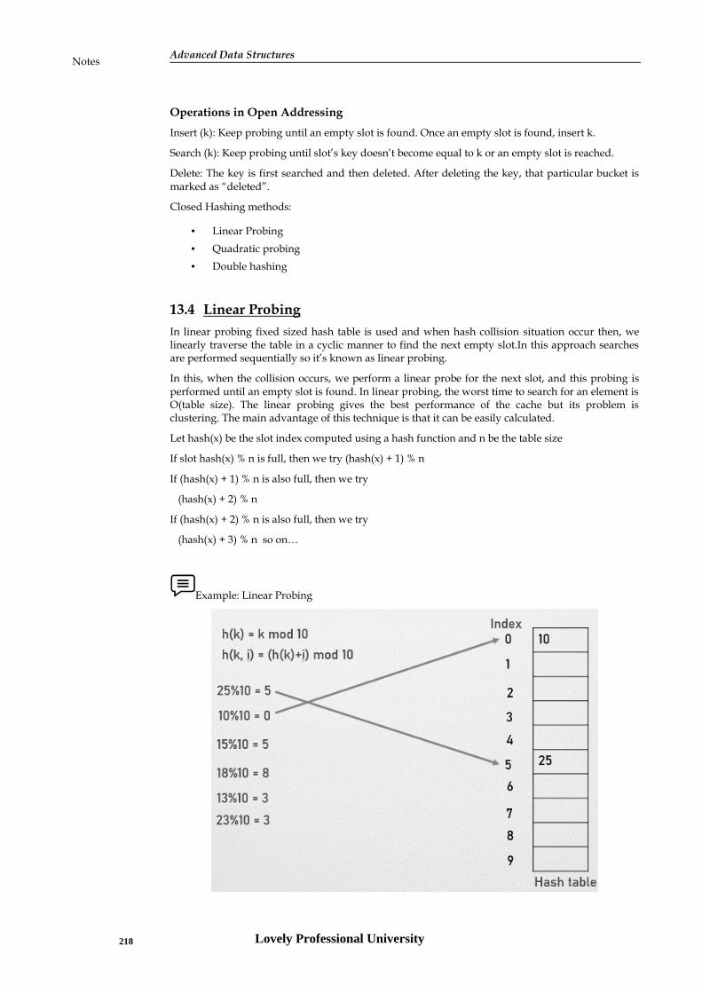
Advanced Data StructuresNotes
Operations in Open Addressing
Insert (k): Keep probing until an empty slot is found. Once an empty slot is found, insert k.
Search (k): Keep probing until slot’s key doesn’t become equal to k or an empty slot is reached.
Delete: The key is first searched and then deleted. After deleting the key, that particular bucket ismarked as “deleted”.
Closed Hashing methods:
Linear Probing Quadratic probing Double hashing
13.4 Linear ProbingIn linear probing fixed sized hash table is used and when hash collision situation occur then, welinearly traverse the table in a cyclic manner to find the next empty slot.In this approach searchesare performed sequentially so it’s known as linear probing.
In this, when the collision occurs, we perform a linear probe for the next slot, and this probing isperformed until an empty slot is found. In linear probing, the worst time to search for an element isO(table size). The linear probing gives the best performance of the cache but its problem isclustering. The main advantage of this technique is that it can be easily calculated.
Let hash(x) be the slot index computed using a hash function and n be the table size
If slot hash(x) % n is full, then we try (hash(x) + 1) % n
If (hash(x) + 1) % n is also full, then we try
(hash(x) + 2) % n
If (hash(x) + 2) % n is also full, then we try
(hash(x) + 3) % n so on…
Example: Linear Probing
Lovely Professional University218

Unit 13: Collision Resolution
Notesa
b
AdvantageIt is easy to compute.
DisadvantageThe clustering is major problem with linear probing
Many consecutive elements form groups.
It takes too much time to find an empty slot.
Time complexity
Worst time to search for an element is O(table size).
13.5 Quadratic ProbingQuadratic probing is a collision resolution method that eliminates the primary clustering problemof linear probing. Quadratic probing is what you would expect—the collision function is quadratic.
It is an open-addressing scheme.Here we look for i2 slot in ith iteration if the given hash value xcollides in the hash table.It is used to eliminate the primary clustering problem of linear probing.
In quadratic probing the sequence is that H+12, H+22, H+32,....H+K2
The hash function for quadratic probing is
hi(X) = ( Hash(X) + F(i)2) % Table Size for i = 0, 1, 2, 3,...etc.
If the slot hash(x) % S is full, then we try
(hash(x) + 1*1) % S.
If (hash(x) + 1*1) % S is also full, then we try (hash(x) + 2*2) % S.
If (hash(x) + 2*2) % S is also full, then we try (hash(x) + 3*3) % S.
This process continue until an empty slot is found.
In Quadratic Probing to get slot your table size must meet these requirements:
-Be a prime number
-never be more than half full (even by one element)
Lovely Professional University 219

Advanced Data StructuresNotes
Example :Quadratic probing
a
b
c
Advanced Data StructuresNotes
Example :Quadratic probing
a
b
c
Advanced Data StructuresNotes
Example :Quadratic probing
a
b
c
Lovely Professional University220

Unit 13: Collision Resolution
NotesAdvantage:Primary clustering problem resolved
Disadvantage:Secondary clustering
No guarantee for finding slots
Separate Chaining Vs. Open Addressing
Separate Chaining Open Addressing
Keys are stored inside the hash table as wellas outside the hash table.
All the keys are stored only inside the hashtable.
No key is present outside the hash table.
The number of keys to be stored in the hashtable can even exceed the size of the hashtable.
The number of keys to be stored in the hashtable can never exceed the size of the hashtable.
Deletion is easier. Deletion is difficult.
Extra space is required for the pointers tostore the keys outside the hash table. No extra space is required.
Cache performance is poor.
This is because of linked lists which store thekeys outside the hash table.
Cache performance is better.
This is because here no linked lists are used.
Some buckets of the hash table are neverused which leads to wastage of space.
Buckets may be used even if no key maps tothose particular buckets.
Summary
When two keys or hash values compete with a single hash table slot, then Collision occur. To resolve collision we use collision resolution techniques. Collisions can be reduced with a
selection of a good hash function. Hash functions are mostly used in hash tables, to quickly locate a data record (for example, a
dictionary definition) given its search key (the headword). Specifically, the hash function is used to map the search key to the index of a slot in the table
where the corresponding record is supposedly stored. In linear probing fixed sized hash table is used and when hash collision situation occur then,
we linearly traverse the table in a cyclic manner to find the next empty slot. Quadratic probing is a collision resolution method that eliminates the primary clustering
problem of linear probing.
Lovely Professional University 221

Advanced Data StructuresNotes
KeywordsSeparate chaining Quadratic probing
Linear Probing Open Addressing
Hash function Load factor
Self Assessment1. Which is part of collision resolution technique ___
A. Separate chainingB. Open addressingC. Double hashingD. All of above
2. Open addressing includes ____
A. Linear probingB. Quadratic probingC. Double hashingD. All of above
3. In Load factor α = n/m, m represent ____
A. Number of keysB. Number of slots in hash tableC. Hash functionD. None of above
4. In Load factor α = n/m, n represent __
A. Number of slots in hash tableB. Hash functionC. Number of keys to be inserted in hash tableD. None of above
5. Worst-case complexity for searching in Separate chaining is _
A. Log (1)B. (n)C. log (0)D. None of above
6. Worst-case complexity for deletion in Separate chaining is _
A. (n)B. log (1)C. log (2)D. None of above
Lovely Professional University222

Unit 13: Collision Resolution
Notes7. Advantages of separate chaining.
A. It is less sensitive to the function of the hashingB. The hash table never fills full, so we can add more elements to the chainC. It is easy to implementD. All of above
8. Quadratic probing is part of __
A. Open hashingB. Closed hashingC. Linear probingD. None of above
9. Double hashing is part of ___
A. Open hashingB. Closed hashingC. Linear probingD. All of above
10. Which is not part of open addressing.
A. Linear probingB. Quadratic probingC. Open hashingD. All of above
11. Operations in Open Addressing are ___
A. InsertB. DeleteC. SearchD. All of above
12. In open addressing __
A. All elements are stored in the hash table itselfB. The size of the table must be greater than or equal to the total number of keys.C. During insertion, if a collision is encountered, alternative cells are tried until an empty
bucket is found.D. All of above
13. Clustering is major problem in _
A. Linear probingB. Quadratic probingC. Double hashingD. None of above
Lovely Professional University 223

Advanced Data StructuresNotes
14. Which one is most relevant to Quadratic Probing?
A. h(k) = k mod 10B. h(k, i) = (h(k)+i2) mod 10C. h(k, i) = (h(k)+i) mod 10D. None of above
15. Which one is not relevant to Linear Probing?
A. h(k, i) = (h(k)+i) mod 10B. h(k) = k mod 10C. h(k, i) = (h(k)+i2) mod 10D. None of above
Answers for Self Assessment
l. D 2. D 3. B 4. C 5. B
6. A 7. D 8. B 9. B 10. C
11. D 12. D 13. A 14. B 15. C
Review Questions
1. Discuss significance of collision resolution.2. Differentiate between open hashing and closed hashing.3. Explain cluster problem and its solution in hashing.4. What are the advantages of quadratic probing?5. Give an example of linear probing.6. Discuss load factor in hashing.
Further ReadingsBurkhard Monien, Data Structures and Effi cient Algorithms, Thomas Ottmann,
Springer.
Kruse, Data Structure & Program Design, Prentice Hall of India, New Delhi.
Mark Allen Weles, Data Structure & Algorithm Analysis in C, Second Ed., Addison-
Wesley Publishing.
RG Dromey, How to Solve it by Computer, Cambridge University Press.
Lipschutz. S. (2011). Data Structures with C. Delhi: Tata McGraw hill
Reddy. P. (1999). Data Structures Using C. Bangalore: Sri Nandi Publications
Samantha. D (2009). Classic Data Structures. New Delhi: PHI Learning Private Limited
Web Links
Lovely Professional University224

Unit 13: Collision Resolution
Noteswww.en.wikipedia.org
https://www.gatevidyalay.com/collision-resolution-techniques-separate-chaining/
http://users.csc.calpoly.edu/~gfisher/classes/103/lectures/week5.2.html
https://www.tutorialandexample.com/collision-resolution-techniques-in-data-structure
Lovely Professional University 225

Unit 14: More on Hashing
Notes
Unit 14: More on Hashing
CONTENTS
Objectives
Introduction
14.1 Double Hashing
14.2 Rehashing
Summary
Keywords
Self Assessment
Answers for Assessment
Review Questions
Further Readings
ObjectivesAfter studying this unit, you will be able to:
Discus Double hashing techniques Understand load factor Learn rehashing
IntroductionWhen two keys or hash values compete with a single hash table slot, then Collision occur.Toresolve collision we use collision resolution techniques. Collisions can be reduced with a selectionof a good hash function.
The open addressing technique requires a hash table with fixed and known size. All elements arestored in the hash table itself. The size of the table must be greater than or equal to the total numberof keys.During insertion, if a collision is encountered, alternative cells are tried until an emptybucket is found.
In case of collision:Probing is performed until an empty bucket is found.Once an empty bucket isfound, the key is inserted.Probing is performed in accordance with the technique used for openaddressing.
14.1 Double HashingDouble Hashing is a hashing collision resolution technique in open addressed Hash tables.Indouble hashing, there are two hash functions.The second hash function is used to provide an offsetvalue in case the first function causes a collision.Second hash function used to remove the collisionwhen you encountered the collision.
Double hashing uses two hash functions, one to find the initial location to place the key and asecond to determine the size of the jumps in the probe sequence. The ith probe is
h(k, i) = (h1(k) + i * h2(k)) mod m.
Keys that hash to the same location, are likely to hash to a different jump size, and so will havedifferent probe sequences. Thus, double hashing avoids secondary clustering by providing as manyas m2 probe sequences. How do we ensure every location is checked? Since each successive probeis offset by h2(k), every cell is probed if h2(k) is relatively prime to m. Two possible ways to ensure
Ashwani Kumar, Lovely Professional University
Lovely Professional University226

Advanced Data StructuresNotes
h2(k) is relatively prime to m are, either make m = 2k and design h2(k) so it is always odd, or makem prime and ensure h2(k) < m. Of course, h2(k) cannot equal zero.
Double hashing can be performed using:
(hash1(key) + i * hash2(key)) mod TABLE_SIZE
Here hash1() and hash2() are hash functions
First hash function:
hash1(key) = key mod TABLE_SIZE
Second hash function is :
hash2(key) = PRIME – (key mod PRIME)
Where PRIME is a prime smaller than the TABLE_SIZE
A good second Hash function is:It must never evaluate to zero. Must make sure that all cells can beprobed.
Example: Double hashing
Elements: 20, 25, 36, 16, 55, 17 table size= 10 prime number = 7
Lovely Professional University 227

Unit 14: More on Hashing
Notes
Unit 14: More on Hashing
Notes
Unit 14: More on Hashing
Notes
Lovely Professional University228

Advanced Data StructuresNotes
Double hashing highlights
Computational cost is higher. No primary clustering. No secondary clustering. Double hashing can find the next free slot faster than the linear probing approach. Double hashing is used for uniform distribution of records throughout a hash table. Double hashing is useful if an application requires a smaller hash table.
14.2 RehashingThis is another method of collision handling. In this method you fi nd an alternative empty locationby modifying the hash function, and applying the modifi ed hash function to the colliding symbol.For example, if x is symbol and h(x) = i, and if the ith location is already occupied, then I modify thehash function h to h1, and fi nd out h1(x), if h1(x) =j, and jth location is empty, then I accommodatex in the jth location. Otherwise you once again modify h1 to some h2 and repeat the process till thecollision gets handled. Once the collision gets handled we revert back to the original hash functionbefore considering the next symbol.
Lovely Professional University 229
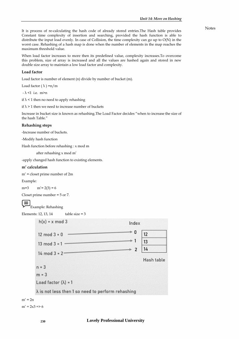
Unit 14: More on Hashing
NotesIt is process of re-calculating the hash code of already stored entries.The Hash table providesConstant time complexity of insertion and searching, provided the hash function is able todistribute the input load evenly. In case of Collision, the time complexity can go up to O(N) in theworst case. Rehashing of a hash map is done when the number of elements in the map reaches themaximum threshold value.
When load factor increases to more then its predefined value, complexity increases.To overcomethis problem, size of array is increased and all the values are hashed again and stored in newdouble size array to maintain a low load factor and complexity.
Load factor
Load factor is number of element (n) divide by number of bucket (m).
Load factor ( λ ) =n/m
- λ <1 i.e. m>n
if λ < 1 then no need to apply rehashing
if λ > 1 then we need to increase number of buckets
Increase in bucket size is known as rehashing.The Load Factor decides “when to increase the size ofthe hash Table.”
Rehashing steps
-Increase number of buckets.
-Modify hash function
Hash function before rehashing : x mod m
after rehashing x mod m’
-apply changed hash function to existing elements.
m’ calculation
m’ = closet prime number of 2m
Example:
m=3 m’= 2(3) = 6
Closet prime number = 5 or 7.
Example: Rehashing
Elements: 12, 13, 14 table size = 3
m’ = 2n
m’ = 2x3 => 6
Lovely Professional University230

Advanced Data StructuresNotes
Nearest prime numbers are 5 and 7
m’ = 7
x mod m’ => x mod 7
A Comparison of Rehashing Methods
Complexity of Rehashing
Time complexity – O (n)
Space complexity – O (n)
Summary
Rehashing schemes use a second hashing operation when there is a collision. The open addressing technique requires a hash table with fixed and known size. Double Hashing is a hashing collision resolution technique in open addressed Hash tables. Rehashing is process of re-calculating the hash code of already stored entries. The load factor in HashMap is basically a measure that decides when exactly to increase the
size of the HashMap to maintain the same time complexity of O(1). The Load Factor decides “when to increase the size of the hash Table.”
KeywordsRehashing Load factor
Hash map Open addressing
Double hashing Prime number
Clustering
Lovely Professional University 231

Unit 14: More on Hashing
NotesSelf Assessment
1. Which statement is correct about open addressing?
A. It requires a hash table with fixed and known size.B. All elements are stored in the hash table itselfC. The size of the table must be greater than or equal to the total number of keys.D. All of above
2. In double hashing prime value is __
A. Less than table sizeB. Greater than table sizeC. Equal to table sizeD. None of above
3. In double hashing how many hash functions used.
A. 4B. 2C. 1D. 3
4. Which statement is correct about double hashing?
A. The second hash function is used to provide an offset value in case the first function causes acollision.
B. In double hashing, there are two hash functions.C. Second hash function used to remove the collision when you encountered the collision.D. All of above
5. Which hash function used in double hashing?
A. (h1(key) + h2(key)) mod Table sizeB. (h1(key) + i * (key)) mod Table sizeC. (h1(key) + i * h2(key)) mod Table sizeD. None of above
6. In which situation second hash function is used in double hashing?
A. In case table size is smallerB. In case the first function causes a collisionC. In case first hash function provide zero valueD. None of above
7. In statement- h2(key) = 7 – (key mod 7), 7 represent _
A. Table sizeB. Key valueC. Prime number
Lovely Professional University232

Advanced Data StructuresNotes
D. None of above
8. Which statement is correct for double hashing technique?
A. No primary clusteringB. No secondary clusteringC. Double hashing can find the next free slot faster than the linear probing approachD. All of above
9. Which statement is correct about rehashing?
A. In which the table is resizedB. It is process of re-calculating the hash code of already stored entriesC. It is a collision resolution techniqueD. All of above
10. In Load factor =n/m, m represents _
A. Number of elementB. Number of key valuesC. Number of bucketD. None of above
11. In which situations rehashing is required.
A. When table is completely full.B. With quadratic probing when the table is filled half.C. When insertions fail due to overflow.D. All of above
12. The value of Load factor in rehashing should be__
a) Less than 1b) Greater then 1c) Equal to 0d) All of above
13. In Load factor =n/m, n represents _
A. Number of bucketB. Number of elementC. Number of key valuesD. None of above
14. Table size is 3 and elements are 12, 13, and 14. Load factor is_
A. 3B. 2C. 1
Lovely Professional University 233

Unit 14: More on Hashing
NotesD. 0
15. What is notation for load factor?
A. λB. ∞C. µD. Ω
Answers for Assessment
l. D 2. A 3. B 4. D 5. C
6. B 7. C 8. D 9. D 10. C
11. D 12. A 13. B 14. C 15. A
Review Questions
1. What are the conditions for double hashing?2. Discuss double hashing technique with example.3. What are the two hash functions used in double hashing?4. What is significance of load factor in hashing?5. What are the advantages of double hashing?6. Discuss steps for rehashing.7. What is time and space complexity of rehashing?
Further ReadingsBurkhard Monien, Data Structures and Effi cient Algorithms, Thomas Ottmann,
Springer.
Kruse, Data Structure & Program Design, Prentice Hall of India, New Delhi.
Mark Allen Weles, Data Structure & Algorithm Analysis in C, Second Ed., Addison-
Wesley Publishing.
RG Dromey, How to Solve it by Computer, Cambridge University Press.
Lipschutz. S. (2011). Data Structures with C. Delhi: Tata McGraw hill
Reddy. P. (1999). Data Structures Using C. Bangalore: Sri Nandi Publications
Samantha. D (2009). Classic Data Structures. New Delhi: PHI Learning Private Limited
Web Linkswww.en.wikipedia.org
https://learningsolo.com/what-is-rehashing-and-load-factor-in-hashmap/
Lovely Professional University234

Advanced Data StructuresNotes
https://www.scaler.com/topics/data-structures/load-factor-and-rehashing/
https://www.javatpoint.com/double-hashing-in-java
https://www.educative.io/edpresso/what-is-double-hashing
Lovely Professional University 235

Jalandhar-Delhi G.T. Road (NH-1)Phagwara, Punjab (India)-144411For Enquiry: +91-1824-521360Fax.: +91-1824-506111Email: [email protected]
LOVELY PROFESSIONAL UNIVERSITY
Related Documents


![CueCore and IoCore manual - [co]motion · LPU-1 vs LPU-2 The LPU is available in two versions, the LPU-1 and the LPU-2. The di@erence between the two units is that the LPU-2 has additional](https://static.cupdf.com/doc/110x72/5e6e492d8892da5af37f75f6/cuecore-and-iocore-manual-co-lpu-1-vs-lpu-2-the-lpu-is-available-in-two-versions.jpg)