Advanced Analysis Technique for the Evaluation of … Analysis Technique for the Evaluation of Linear Alternators and ... AOVANCED ANALYSIS TECHNIQUE FOR THE EVALUATION O_ ... the

NASA Contractor Report 198434l

Advanced Analysis Technique for the Evaluationof Linear Alternators and. Linear Motors

Jeffrey C. HollidayHOLLIDAYLABS

Guysville, Ohio

December 1995

Prepared forLewis Research Center

Under Contract NAS3-25827

National Aeronautics and

Space Administration

(NASA-CR-198434) AOVANCED ANALYSIS

TECHNIQUE FOR THE EVALUATION O_

LINEAR ALTERNATORS AND LINEAR

MOTORS Final Report (Hollidaylabs)49 p

G3/20

N96-17812

Unclas

0098289

https://ntrs.nasa.gov/search.jsp?R=19960011376 2018-06-26T06:01:35+00:00Z

Abstract

A method for the mathematical analysis of linear alternator

and linear motor devices and designs is described, and an example

of its use is included. The technique seeks to surpass other

methods of analysis by including more rigorous treatment of

phenomena normally omitted or coarsely approximated such as eddy

braking, non-linear material properties, and power losses

generated within structures surrounding the device. The

technique is broadly applicable to linear alternators and linear

motors involving iron yoke structures and moving permanent

magnets.

The technique involves the application of Amp_rian current

equivalents to the modeling of the moving permanent magnet

components within a finite element formulation. The resulting

steady state and transient mode field solutions can

simultaneously account for the moving and static field sources

within and around the device.

Technical Background and Motivation for the Advanced Technique

Linear alternators and linear motors have been identified by

NASA and others as critical component technologies for Stirling-

cycle devices applied to power conversion and thermal management

systems. Space and terrestrial uses for these systems include

refrigeration, cryocooling, and heat pumping, as well as remote

and grid connected power conversion systems fueled by various

heat sources (e.g. solar, nuclear, biomass).

These applications typically involve motors or alternators

which can be classified as iron yoke, moving permanent magnet

devices. Several distinct concepts'and design variations of such

1

devices have been proposed. Evaluation of the relative merits of

these designs has been hampered by a lack of broadly applicable

t_chniq_/es for the analysis of different devices within this

class. This report presents advanced analysis techniques by

which a broad range of differing linear alternator and motor

concepts may be thoroughly evaluated. This discussion is

presented for the analysis of a typical linear alternator; the

technique is used in the same manner to analyze a linear motor.

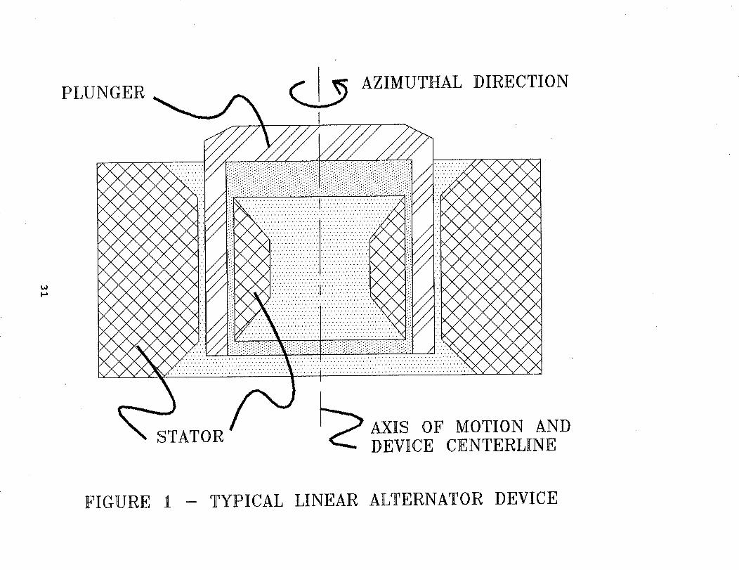
Figure i illustrates a representative linear alternator of

the subject class, with basic components identified. Not shown

is the surrounding system structure which includes the power

piston to which the plunger is typically attached, the power

piston cylinder and bearings, the converter pressure vessel, and

structural components supporting the stator. A specific linear

alternator design following this concept was provided by NASA and

is used as a subject for an example analysis in this report. The

example alternator has a stationary "stator" component, and a

moving "plunger" component, which undergoes a reciprocating

motion during operation. The stator consists of the iron yoke

and a copper coil for power take-off. The plunger is fitted with

permanent magnets.

The linear alternator converts the mechanical energy of the

moving plunger into electrical energy. The analysis is concerned

with estimating the efficiency of this energy conversion, as well

as the apportionment of the various power loss mechanisms. The

energy flows involved in a typical linear alternator can be very

complex as energy is transduced among the distributed electric

and magnetic fields of the system. The nature of these energy

flows is dependent on the particular linear alternator design

configuration and geometry, and on the design and geometry of the

external structures in the neighborhood of the alternator device.

The sensitivity to design type has complicated past efforts to

2

use analysis to compare different alternator designs falling

within the subject class.

In particular, large magnitude and rapidly varying magnetic

fields due to leakage from the intended magnetic circuits of the

linear alternator are very configurationally dependent. These

fields interact with the structure of the alternator and its

environment affecting alternator output power, efficiency, and

output voltage. Narrowly-focused design analyses that are

configuration specific have been used to estimate performance for

some designs, but it may not be accurate to apply these analyses

to other members of this class of alternators. This has made

even-handed comparison of competing proposed alternator designs

or design concepts difficult. A more broadly applicable analysis

technique was sought to provide a tool for thorough and accurate

comparisons.

Objectives of the AdvancedAnalysis Technique

The advanced analysis described here was motivated by the

need for accurate and detailed methods for alternator analysis in

assisting the evaluation of a variety of designs proposed for a

particular mission. The objectives for the formulation of the

technique were as follows:

I) The analysis should be equally valid in application to any

of the alternator design concepts falling in the iron yoke,

moving permanent magnet device class;

2) The analysis should not depend on configuration or concept-

dependent approximations or empirical formulation;

3) The analysis should treat more rigorously phenomena that are

often approximated or ignored in more narrowly-focussed

design analysis. These include:

a) effects due to moving permanent magnet components

3

b)

c)

d)

e)

simultaneous solution of induction effects due to

moving permanent magnet and conductor reaction fields

non-linear yoke material properties

fringing field intensity and distribution

non-uniformity of yoke induction fields.

Items a) and b) above are often completely omitted by other

analyses, and the accurate treatment of them in this analysis is

thought to be unique to this technique. Analysis results

involving items c), d), and e) are made more accurate by the

treatment of a) and b).

Description of the Advanced Analysis Technique

This advanced analysis technique combines aspects of finite

element mathematical formulation methods, which are rapidly

developing in the modern computer era, with some useful insight

into the nature of magnetization provided by Classical

Electromagnetic Physics. Analysts using this technique will need

to have access to a finite element analysis package and have some

general skill in its use. A general understanding of linear

alternators and electromagnetism will also be needed.

Many of the objectives toward thorough evaluation of linear

alternator designs can be addressed using finite element computer

modeling. Elaborate front ends have been written and marketed

for the finite element solvers developed over the past few

decades. Several commercially available finite element solver

packages have begun to provide capability to address basic

electromagnetic field problems. The utility of finite element

analysis (FEA) programs for the purpose of this linear alternator

4

analysis, however, is limited by practical (economic) and

fundamental capability concerns.

The commercial FEA package "ANSYS" by Swanson Analysis

Systems of Houston, Pennsylvania was chosen for use in the

example analysis of this project. ANSYS is one of the better

packages in term of capabilities for a variety of electromagnetic

field problems. Other FEA packages can also be used with this

analysis technique. However, the objectives of this project

cannot be met with the FEA tool alone. Rather, FEA provides a

framework for the linear alternator analysis technique developed

in this project.

Finite element formulation provides an attractive, but

limited, tool to remove gross geometrical constraints imposed by

narrowly-focused analysis methods. Very small geometrical

details of the static structure can be modeled with the finite

element formulations. The degree of accuracy of the results and

the fineness of detail included in the model can be increased, in

general, with increased level of human and computer effort. With

attention to balancing the levels of detail and of effort in the

formulation, analysts can generate static mathematical FEA models

for alternator designs with appropriate and fair consideration to

geometrical features and details that differentiate them.

Nonlinear material properties, such as yoke material

magnetic permeability, dB/dH, which is dependent on the magnitude

of the local magnetic field H, can be included is some FEA

formulations. Including nonlinear material properties typically

increases the computer time and capacity needed for the field

solution phase of the analysis.

5

One key limitation common to all of the FEA packages

examined is an inability to adequately model objects in motion

directly. This is due to the geometrical fixity required by

finite element formulations. Material properties assigned to a

particular element representing a fixed location in space cannot

be changed during an analysis. This precludes the direct FEA

model_nq of moving permanent magnet structures and the phen0mena

associated with the motion of these structures such as output

voltage generation and eddy braking power losses. "Gap-type

analysis", which allows a limited simulation of a variable gap

between components, is not a practical approach for the large

displacements of complex components typical in most linear

alternator problems.

In order to overcome the analysis barrierrepresentedby the

moving magnet material of the linear alternator, this advanced

technique involves the construction of a dynamic representation

of the moving permanent magnets which allows calculation of the

field solution by eliminating reliance on the volume

magnetization characterization. The volume magnetization, or

magnetic moment density, is a material property which would

require assignment to elements within a finite element

formulation and would not allow motion of thoseelements.

Instead of a direct representation of the permanent magnets

as a volume of material with distribution of magnetic moment

density, the permanent magnet structures are here represented as

a collection of current densities flowing in free space within or

on the surface of the magnet volume. These currents are imposed

on the finite element formulation as nodal or elemental current

loading and, as such, can be changed over time to simulate the

motion of the magnets. This is in contrast to direct material

property modeling of the magnets.

6

These current densities are chosen to provide a model

mathematically equivalent to the model using direct magnetized

material representation. Such a model is called an Amp_rian

current equivalent, Ampere having used the analogy during the

nineteenth century. The goal of the analysis model

representation of the physical alternator system is to provide

the framework of equations to calculate the magnetic field

distribution due to the physical system. This information is

contained in the solution to the magnetic vector potential

function A. Two representations that produce the same magnetic

vector potential are equivalent.

The equivalence of the Amp_rian current representation is

assured provided the current distribution at any point in space

is chosen to be the vector curl of the magnetization distribution

it is to represent.

Eq. 1 j = T xM

where: J is the equivalent current density distribution,

M is the volume magnetization of the magnet,

• x is the vector curl operator

and both J and M are vector functions of space.

The general equivalence of the Amp_rian representation can

be demonstrated bythe exercise of proving the mathematical

identity of the closed form vector potential solutions obtained

through the use of the following two representations for an

arbitrary magnetized volume (Lorrain and Corson, Electromaqnetic

Fields and Waves. page 386, chapter 9, copyright 1970, W. H.

Freeman and Company, San Francisco).

i)

2)

3)

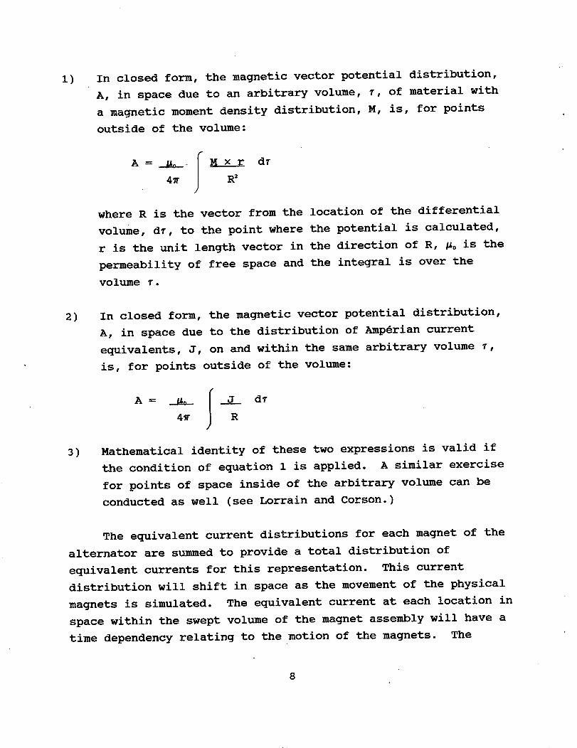
In closed form, the magnetic vector potential distribution,

A, in space due to an arbitrary volume, 7, of material with

a magnetic moment density distribution, M, is, for points

outside of the volume:

f

A = _p__ I M x r d7

4_ J R 2

where R is the vector from the location of the differential

volume, dT, to the point where the potential is calculated,

r is the unit length vector in the direction of R, _0 is the

permeability of free space and the integral is over the

volume 7.

In closed form, the magnetic vector potential distribution,

A, in space due to the distribution of Amp_rian current

equivalents, J, on and within the same arbitrary volume 7,

is, for points outside of the volume:

(

A= _ |__J d7

4_ ) R

Mathematical identity of these two expressions is valid if

the condition of equation I is applied. A similar exercise

for points of space inside of the arbitrary volume can be

conducted as well (see Lorrain and Corson.)

The equivalent current distributions for each magnet of the

alternator are summed to provide a total distribution of

equivalent currents for this representation. This current

distribution will shift in space as the movement of the physical

magnets is simulated. The equivalent current at each location in

space within the swept volume of the magnet assembly will have a

time dependency relating to the motion of the magnets. The

8

description of the current at a point over one period of the

plunger motion is called the equivalent current profile for that

point.

To accommodate the discrete nature of the finite element

formulation, both the spacial and the temporal descriptions of

the equivalent current distribution must be discretized andloaded into the finite element formulation for solution as a

time-transient field problem. This current loading must be

applied to elements or nodes in accordance with the capability of

the FEA package and the type of current density involved.Amp_rian current densities on a surface may best be modeled using

nodal loading. Volume current densities may be better applied as

elemental loading.

The solution for the magnetic vector potential over the time

of interest is now computed using the FEA code. For analysis

directed toward steady state operation of the alternator system,

the solution over the period via the time transient calculation

is repeated until a condition of periodicity is met.

Once this time history of the field solution over space is

obtained, the analysis problem becomes straightforward. Results

based on the time dependant field solution can be derived to

satisfy particular objectives of the analysis effort. For

example, gross power loss in structures, heat generation

distribution in these structures, and the spacial mapping of loss

sensitivity of the design can be calculated.

Step by Step Summary for the Application of the Technique

a) Decide what is important in the problem and what should be

included in the model. Create a solid model of the

9

alternator components. Force axisymmetry if computer system

is taxed. Remotely locate an infinite boundary to

accommodate leakage fields. This first step is critical as

the accuracy and economy of the remainder of the analysis

depend on these selections.

b) Model the volume swept by the plunger magnets with a mesh of

small uniform elements. An element width much less than the

plunger displacement amplitude should be used. In

developing this mesh, consideration should be given to the

plunger position waveform and the requirements of step e)

below. This mesh should include element nodes coincident

with the location of the permanent magnetization gradients,

particularly at the edges of the permanent magnet

structures, during each of the time instants chosen in step

e) below.

c) Develop a satisfactory element mesh distribution for all

areas outside of the swept volume. In each analysis case, a

balance must be struck between accuracy targets and the

economy of the analysis. The mesh should be finer in areas

experiencing large changes with time in the magnetic field

vector or large field gradients over space. Larger element

sizes are acceptable near the infinite boundary and in other

areas of low field activity. The air in narrow gap regions

such as that between the plunger and yoke should be modelled

using at least two element widths across the gap.

d) Make appropriate material property assignments such as

electric resistivity and magnetic permeability for the

elements comprising the components of the alternator.

Material properties should be defined to a level of detail

consistent with the analysis objectives and predicted

conditions experienced by the material. Nonlinearity,

i0

temperature dependance and anisotropy in thecharacterization of the material properties can be included.

Direct modeling of the permanent magnet requires that

material property tables to describe the permanent magnet

materials be developed. Permanent magnet material propertyinformation is also used in the formulation of the Amp_rian

current equivalent.

e) From the plunger position waveform, select particular

positions and tabulate the associated time instants in the

period. Calculate the time increments between successive

instants. The selected set of positions and instants need

not be spatially or temporally uniform. However, it is

useful to have generated the mesh of step c) with foresight

to this task. Nodes should be provided at locations with

large magnetization gradients, such as at the magnet edges,

at each of the chosen instants.

f) From the set of plunger positions, select points of interest

for the verification of the equivalent current model.

Conduct static field solutions at these particular plunger

positions with the permanent magnet material properties

assigned to the elements coincident with the magnet

locations at that instant. Other elements in the swept

volume are assigned the material properties of air or

another default material, such as that from which the

balance of the plunger is composed.

g) Conduct static field solutions for these particular

positions using the equivalent current representation. All

of the swept volume elements are assigned the properties of

air or other default material. Specific nodes representing

locations of the Amp_rian current equivalents are turned on

by assigning those currents to those nodes.

ii

h) Comparison of the results of the direct modeling of the

permanent magnet material of step f) to the results of the

equivalent current model (step g) can be used to guide

modification of the node locations and current assignments

to obtain the level of agreement required of the analysis.

These two methods should produce solutions for the static

field that are equivalent to the degree allowed by the level

of detail involved in the model. This comparison is

particularly useful if severe or non-uniform demagnetization

of the permanent magnets in the device confound the

discretization of the Amp_rian current equivalents.

Comparison at several points in the cycle and interpretation

of the results should identify this condition. In such

cases, the Amp_rian current equivalent will involve

significant volume current densities as well as surface

currents. A more complex set of node and/or element

ioadings will be needed to model this current distribution

adequately. Surface current densities are typically the

only loadings required in more straightforward problems such

as the example in the nextsection.

i) Create tables of the Amp_rian current equivalent profiles

for the nodes and elements having non-zero equivalent

currents at any of the time instants of the selected set.

The equivalent current profiles should include the value of

the current to be assigned during each of the time instants

that make up the period. Similarly, node and element

current loadings arising from real currents in the system,

such as that of the power takeoff, should be tabulated to

facilitate impressing them into the time transient analysis

to be performed in the next steps.

12

J) Set up a finite element time transient solution over the

full period including time steps of appropriate size to

match the time instants chosen. Node and element current

loadings should correspond to the Amp_rian current

equivalents and real current profiles for each instant.

Additional time steps for current load ramping or

intermediate time approximations can be used as needed for

numerical stability and accuracy concerns.

k) Execute the transient solution over the first period.

Initial conditions must be specified. If no estimate is

available for the periodic steady state values expected for

the beginning instant of the period, the static field

solution corresponding to the initial plunger position may

be used.

i) Execute successive transient solutions over the period using

the results of the previous period as initial conditions for

the new period. Compare results for a particular time

instant or instants to those of the previous period. Once a

satisfactory degree of repetition has been obtained, the

results of the final period may be used for postprocessing

in the next step. Until that condition is met, the

foregoing results are considered transient in that the

alternator system model has not settled into a periodic

steady state. Unless there is specific interest in this

transient response, this data maybe erased in the interest

of conserving computer storage capacity.

m) Solution results from each of the chosen time instants of

the final period are now taken to postprocessing to

calculate analysis results of interest to the particular

study. This data represents the periodic steady state

response of the alternator system. Calculable results that

13

will be useful in design evaluation include:

Eddy current losses, including eddy braking which

involves the transduction of mechanical power into heat

and a slowing of the plunger resulting from eddy

currents associated with the motion of the magnets as

distinguished from eddy currents arising from changes

in the power take-off current.

Mapping of the loss sensitivity of the system

structural design, derived from the time derivative of

local field intensity at locations surrounding the

alternator proper. This can be used to evaluate

various designs and may influence selection of the

device configuration, location and material of the

necessary surrounding structure, and possibly selection

of other Component configurations in the vicinity of

the device ( e.g. bearings).

Power loss breakdown for the components of the device

and its surrounding structure.

Operating performance aspects such as output voltage,

power, and impedance. Limitations and nominal ratings

can be explored.

Example Application of the Advanced AnalYS_S Technique

For the purpose of an example application of the advanced

analysis technique, a representative linear alternator design was

provided by NASA LeRC. This conceptual design was generated by

Mechanical Technology Inc. (MTI) in a DOE-funded project

targeting terrestrial solar dynamic energy conversion systems;

14

NASA LeRC provided technical management for this project. The

system concept investigated involved a linear alternator directly

coupled with a Stirling heat engine. This conceptual design is

described in NASA CR-180890, January 1988, "Conceptual Design of

an Advanced Stirling Conversion System for Terrestrial Power

Generation."

The example application follows the step-by-step summary

discussed in the previous section. The labeled steps in this

example refer to the steps of the step-by-step summary.

Step a):

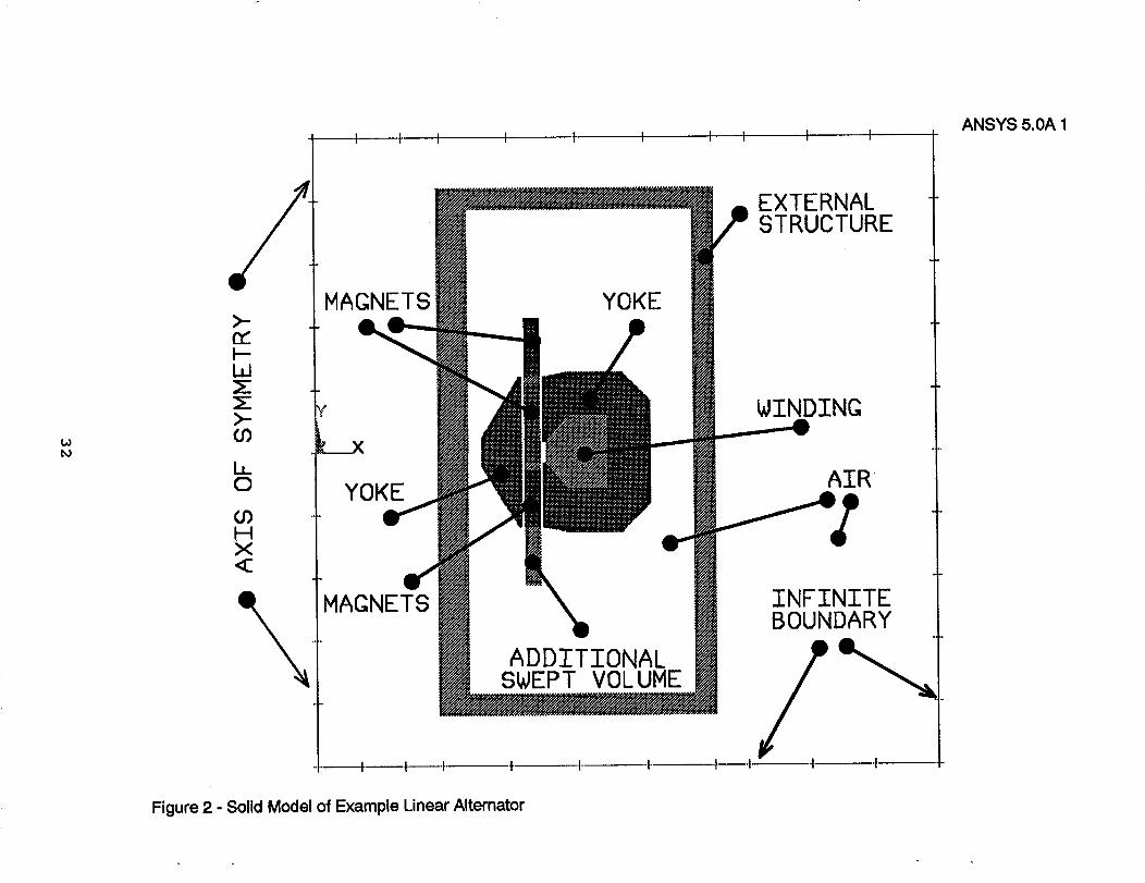
The FEA solid model approximating the linear alternator

design for this example analysis is shown in figure 2. The model

is cylindrically axisymmetric, which allows a two-dimensional

finite element formulation to be used for the analysis. Use of

this approximate model results in significant savings in the

amounts of computer capacity and computer time required to

complete the analysis. This restriction of symmetry precludes

the evaluation of azimuthal magnetic field effects, which were

felt to be relatively unimportant for this illustrative example.

This exclusion is due to this particular choice of symmetry

restriction and is not an inherent limitation of the advanced

analysis technique in general. Azimuthal magnetic field effects

can be analyzed using solid models that include important feature

details in all three dimensions.

In the example alternator, two components form a slotted

iron yoke which surrounds a single power takeoff winding. All of

these structures remain static during the alternator operation.

The "external structure" identified in figure 2 is included to

represent the converter pressure vessel, power piston cylinder,

and other structures in the immediate environment of the

alternator. The terms "external structure" and "surrounding

15

structure" are used interchangeably in this report.

Figure 2 indicates the nominal plunger end-of-stroke

position by the location of the three permanent magnets which are

all a part of the plunger in the physical alternator. The

additional volume swept by any magnet in the course of a machine

cycle is identified by shaded areas as labeled. The magnets form

three rings concentric with the machine axis and arranged in a

closely-separated stack. Each magnet ring has a radially

magnetized vector direction, and adjacent rings have opposite

sense. The poles of the magnets are on the inside and outside

cylindrical faces of the rings. The rest of the plunger

structure is treated as nonconductive nonmagnetic material and,

therefore, is modeled as air.

In anticipation of the requirement for reasonable field

solution results in the regions outside the alternator proper,

the solid model includes a specified volume of air surrounded by

an "infinite boundary". This model will include direct

elemental representation of the volume within the boundary and

the imposition of a zero magnetic potential condition at the

boundary. The boundary is located at a distance from the center

of the yoke cross section of at least 1.5 times the magnet ring

radius. This should provide for a good examination of the

fringing magnetic fields and their consequences. After the

analysis is completed, the magnetic field gradient near the

infinite boundary should be checked to see if the location of the

boundary appears satisfactory.

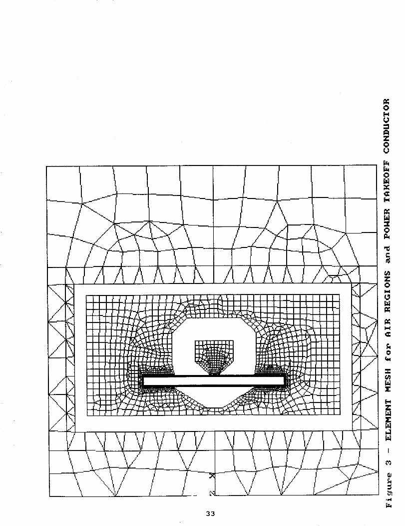
Steps b-c):

Features of the finite element mesh developed for use in

this example alternator analysis are illustrated in figures 3 and

4. Element shapes that are considered robust, i.e. not prone to

certain errorssuch as averaging or interpolation errors, are

16

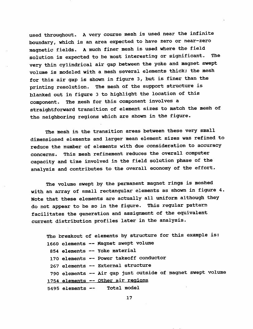
used throughout. A very course mesh is used near the infinite

boundary, which is an area expected to have zero or near-zero

magnetic fields. A much finer mesh is used where the fieldsolution is expected to be most interesting or significant. The

very thin cylindrical air gap between the yoke and magnet sweptvolume is modeled with a mesh several elements thick; the mesh

for this air gap is shown in figure 3, but is finer than the

printing resolution. The mesh of the support structure isblanked out in figure 3 to highlight the location of this

component. The mesh for this component involves astraightforward transition of element sizes to match the mesh of

the neighboring regionswhich are shown in the figure.

The mesh in the transition areas between these very small

dimensioned elements and larger mean element sizes was refined to

reduce the number of elements with due consideration to accuracy

concerns. This mesh refinement reduces the overall computer

capacity and time involved in the field solution phase of the

analysis and contributes to the overall economy of the effort.

The volume swept by the permanent magnet rings is meshed

with an array of small rectangular elements as shown in figure 4.

Note that these elements are actually all uniform although they

do not appear to be so in the figure. This regular pattern

facilitates the generation and assignment of the equivalent

current distribution profiles later in the analysis.

The breakout of elements by structure for this example is:

1660 elements -- Magnet swept volume

854 elements -- Yoke material

170 elements -- Power takeoff conductor

267 elements -- External structure

790 elements -- Air gap just outside of magnet swept volume

1754 elements -- Other air reqions

5495 elements -- Total model

17

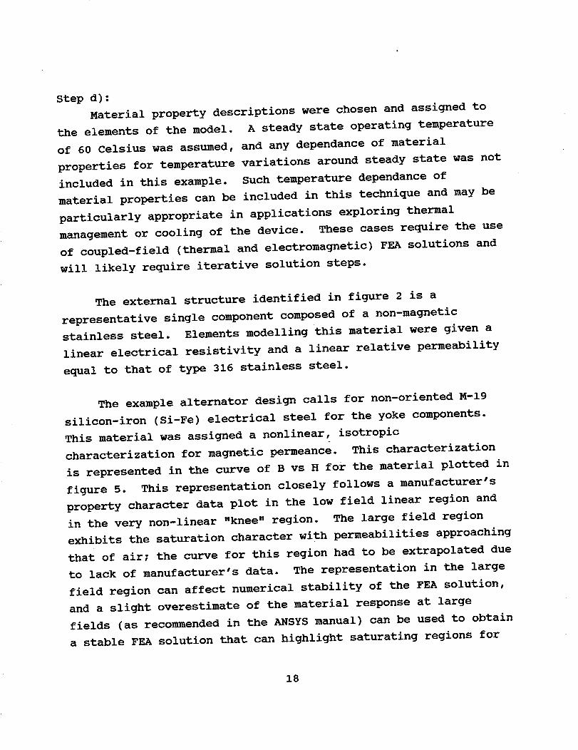
Step d):Material property descriptions were chosen and assigned to

the elements of the model. A steady state operating temperature

of 60 Celsius was assumed, and any dependance of material

properties for temperature variations around steady state was not

included in this example. Such temperature dependance of

material properties can be included in this technique and may be

particularly appropriate in applications exploring thermal

management or cooling of the device. These cases require the use

of coupled-field (thermal and electromagnetic) FEA solutions and

will likely require iterative solution steps.

The external structure identified in figure 2 is a

representative single component composed of a non-magnetic

stainless steel. Elements modelling this material were given a

linear electrical resistivity and a linear relative permeability

equal to that of type 316 stainless steel.

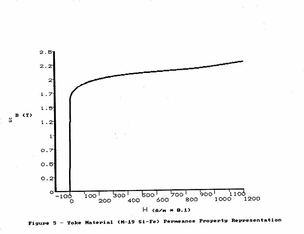
The example alternator design calls for non-oriented M-19

silicon-iron (Si-Fe) electrical steel for the yoke components.

This material was assigned a nonlinear, isotropic

characterization for magnetic permeance. This characterization

is represented in the curve of B vs H for the material plotted in

figure 5. This representation closely follows a manufacturer's

property character data plot in the low field linear region and

in the very non-linear "knee" region. The large field region

exhibits the saturation character with permeabilities approaching

that of air; the curve for this region had to be extrapolated due

to lack of manufacturer's data. The representation in the large

field region can affect numerical stability of the FEA solution,

and a slight overestimate of the material response at large

fields (as recommended in the ANSYS manual) can be used to obtain

a stable FEA solution that can highlight saturating regions for

18

further characterization or design refinement as needed. This

slight overestimate was included in the large field region of the

curve.

The power takeoff winding was modeled using the electrical

conductivity of copper at the specified temperature (60 C), and

unity relative magnetic permeability.

Material properties for the direct representation of the

permanent magnets were used for the static solutions of step f).

Neodymium-Iron-Boron magnet material grade NeIGT 30 H was

specified, and demagnetization data from the manufacturer, IG

Technologies, was used for the characterization. These magnet

properties were also used in the formulation of the Amp_rian

current equivalent.

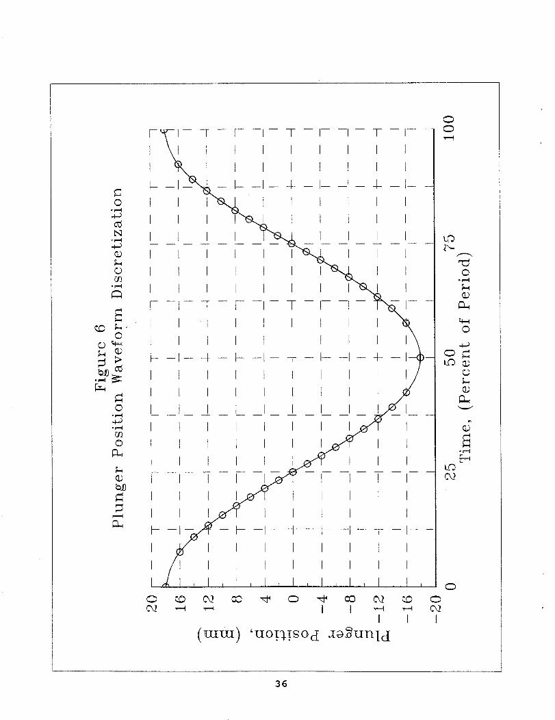
Step e):

The motion of the example alternator plunger in the

operating Stirling-cycle converter is a sixty hertz oscillation

with an 18 millimeter amplitude. A trace of this plunger

position for one period is shown in figure 6. A set of 36 points

representing specific instants were chosen for the discretized

representation for this motion. These points are marked on the

curve of figure 6. The period is thus divided into 36 time-

intervals or time-steps.

Further subdivision of each of these time-steps into two

substeps will be carried out automatically during the FEA

solution during steps k) and i). The ANSYS program will "ramp"

applied loads by interpolating any loads that change during the

time-step, and will calculate solutions for each of the 72

substeps. Only those solutions corresponding with the endpoints

of each time-step were saved. Gradually ramping loads over

several substeps within a time-step helps to satisfy time

19

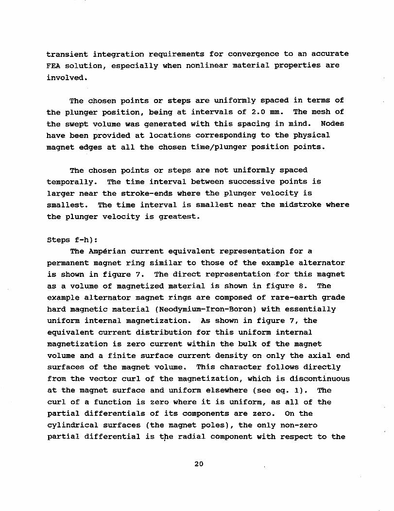
transient integration requirements for convergence to an accurateFEA solution, especially when nonlinear material properties areinvolved.

The chosen points or steps are uniformly spaced in terms of

the plunger position, being at intervals of 2.0 mm. The mesh of

the swept volume was generated with this spacing in mind. Nodeshave been provided at locations corresponding to the physical

magnet edges at all the chosen time/plunger position points.

The chosen points or steps are not uniformly spaced

temporally. The time interval between successive points is

larger near the stroke-ends where the plunger velocity issmallest. The time interval is smallest near the midstroke where

the plunger velocity is greatest.

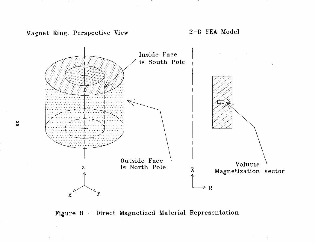
Steps f-h):

The Amp_rian current equivalent representation for apermanent magnet ring similar to those of the example alternator

is shown in figure 7. The direct representation for this magnet

as a volume of magnetized material is shown in figure 8. The

example alternator magnet rings are composed of rare-earth grade

hard magnetic material (Neodymium-Iron-Boron) with essentially

uniform internal magnetization. As shown in figure 7, the

equivalent current distribution for this uniform internal

magnetization is zero current within the bulk of the magnet

volume and a finite surface current density on only the axial end

surfaces of the magnet volume. This character follows directlyfrom the vector curl of the magnetization, which is discontinuous

at the magnet surface and uniform elsewhere (see eq. i). The

curl of a function is zero where it is uniform, as all of the

partial differentials of its components are zero. On the

cylindrical surfaces (the magnet poles), the only non-zero

partial differential is the radial component with respect to the

2O

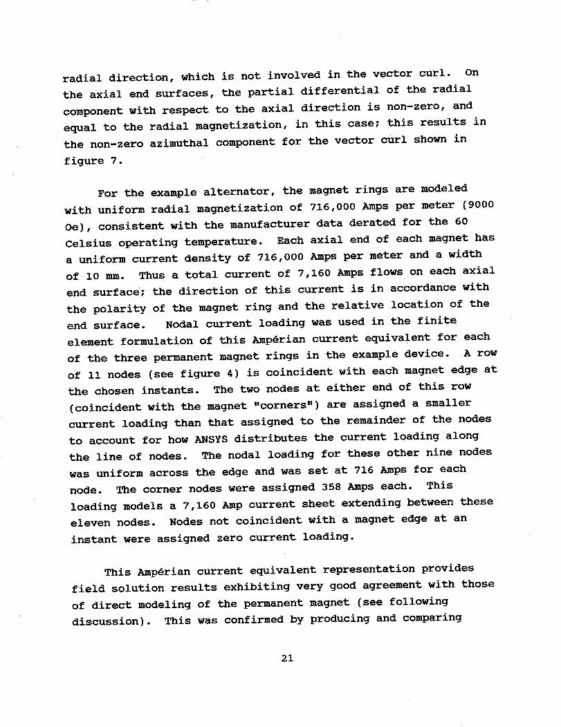
radial direction, which is not involved in the vector curl. On

the axial end surfaces, the partial differential of the radial

component with respect to the axial direction is non-zero, and

equal to the radial magnetization, in this case; this results in

the non-zero azimuthal component for the vector curl shown in

figure 7.

For the example alternator, the magnet rings are modeled

with uniform radial magnetization of 716,000 Amps per meter (9000

Oe), consistent with the manufacturer data derated for the 60

Celsius operating temperature. Each axial end of each magnet has

a uniform current density of 716,000 Amps per meter and a width

of I0 mm. Thus a total current of 7,160 Amps flows on each axial

end surface; the direction of this current is in accordance with

the polarity of the magnet ring and the relative location of the

end surface. Nodal current loading was used in the finite

element formulation of this Amp_rian current equivalent for each

of the three permanent magnet rings in the example device. A row

of ii nodes (see figure 4) is coincident with each magnet edge at

the chosen instants. The two nodes at either end of this row

(coincident with the magnet "corners") are assigned a smaller

current loading than that assigned to the remainder of the nodes

to account for how ANSYS distributes the current loading along

the line of nodes. The nodal loading for these other nine nodes

was uniform across the edge and was set at 716 Amps for each

node. The corner nodes were assigned 358 Amps each. This

loading models a 7,160 Amp current sheet extending between these

eleven nodes. Nodes not coincident with a magnet edge at an

instant were assigned zero current loading.

This Amp_rian current equivalent representation provides

field solution results exhibiting very good agreement with those

of direct modeling of the permanent magnet (see following

discussion). This was confirmed by producing and comparing

21

static field solutions for a severe-case plunger position using

the same FEA mesh for both the direct permanent magnet modeling

and the Amp_rian current equivalent model.

The degree of agreement between the solution results is

dependent on i) the quality of the finite element mesh common to

both analyses, and 2) the quality of the discretized

representation for the Amp_rian current equivalent. A greater

degree of agreement can be expected from a more refined Amp_rian

current representation. For instance, in this example, the nodal

current loading could be further refined by adjusting the

impressed load according to the radial position of the nodes

(node locations vary over plus or minus 5 mm around a median of

135.5mm)

Figure 9 is a mapping of the percent difference in the

magnetic field solution in the yoke determined by using the

Amp4rian current equivalent technique relative to the direct

modeling technique for the plunger end-of-stroke position.

Differences between the two techniques should be near their

largest values for this plunger position. A value of 0.01 in

this figure indicates that the induction field results differ by

less than 1%. Almost all of the yoke is seen to have results

that are in agreement within less than one-half of one percent.

Figure i0 is a plot of the magnetic field solution in the

yoke, represented by flux-lines, for the plunger end-of-stroke

position. This plot reveals a few small regions of high field

gradient where the field diverges and then leaks out of the yoke.

Greater solution variance and sensitivity to mesh character and

other factors can be expected in such regions. The solution

differences in these small high-gradient regions are seen (figure

9) to range from 1% to 5%. Other model areas that may be

particularly sensitive to solution variance include regions where

22

the discrete nature of the mesh or loading is large relative to

the geometry or field gradients (e.g. within one element width of

the magnet edge.) This is typical of all analyses that rely on

the FEA discretized characterization of physical systems.

In this example, the solution differences of greatest

concern were in the yoke; all other areas had differences of less

than one-half of one percent of the maximum yoke field, except

for very small regions near the magnet corners which had

differences approaching one to two percent. Overall, the

differences (including those in the yoke) are felt to be

reasonable and are not expected to have a significant impact on

the final solution.

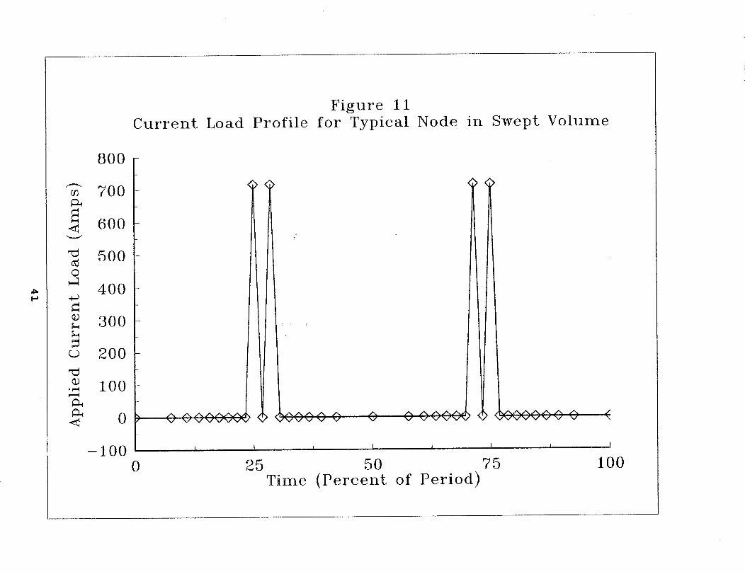
Step i):

As discussed in step e) and shown in figure 6, the period of

the plunger motion was divided into 36 steps. The timespans for

these steps were computed. The Amp_rian current distributions at

each of these instants were generated as previously described.

The equivalent current profiles were loaded for each node within

the magnet swept volume. Figure ii is a plot of the load profile

for one representative node in the magnet swept volume. This

node's load is seen to be "off" (zero) except at times when its

location is coincident with one of the magnet edges. The

direction (sign) of the applied current load depends on which one

of the magnet edges is involved.

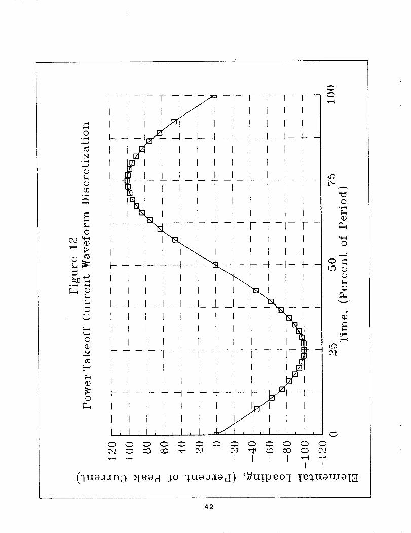
Elemental loading was used for the prescribed load current

in the winding (the real power takeoff). The power takeoff

current was assumed to be sinusoidal and have a power factor of

1.0 (i.e. no net reactance). This current waveform was

discretized to allow the loading at the chosen instants. The

phasing of this power takeoff current results in an element

current loading of zero when the plunger is at the stroke end,

23

and a maximum when the plunger is at the midstroke. Figure 12

illustrates the discretization used to load the real currents

into the elements modeling the winding. Currents up to 125 Arms,

corresponding to the design's nominal full power output rating of

30kWe, wereexplored.

Steps j-l):

An initial set of conditions for the magnetic vector

potential throughout the model was chosen. The position of the

plunger at the beginning of the representative period is at the

endstroke, and the power takeoff current is zero at that time.

The magnetic vector potential solution resulting from a static

analysis using the Amp_rian current equivalents for that position

and a zero power takeoff current was used. The magnetic vector

potential solution as a function of time was then sought using

the ANSYS time-transient mode and 36 time-steps (each with two

intermediate sub-steps for load ramping - in parlance of ANSYS,

this means one additional solution will be calculated during each

time-step) over the period for a total of five periods. This

solution phase was carried out using the node and element current

loading profiles generated in step i).

The set of results for the last full period of this solution

phase was saved for postprocessing as the "periodic steady-

state". In order to verify that a satisfactory level of periodic

repetition had been obtained, a variety of specific solution

results were examined and recorded as the solution progressed.

Both "instantaneous" and cycle integral results were charted.

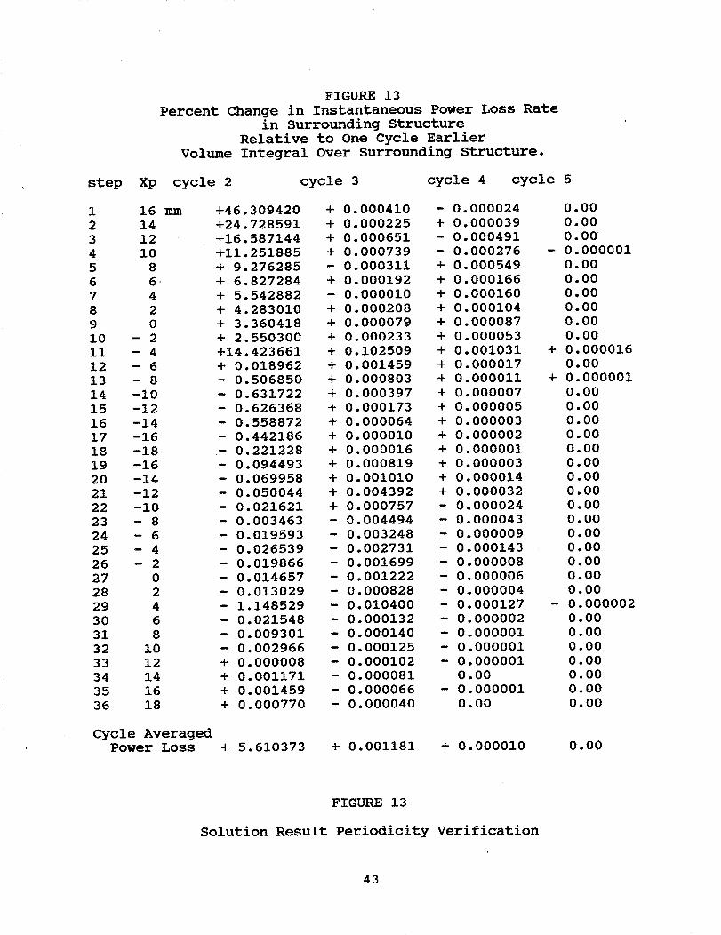
Figure 13 is a table of one of the solution results that was

so tracked, expressed in terms of percent change from the result

that was recorded one period earlier. A value of 0.00 indicates

complete agreement (8 significant figures) with the previous

period. The tracked solution result of figure 13 is the rate of

24

power loss (average for the time-step interval) within the

stainless steel structure that surrounds the linear alternator

for the 125 Arms takeoff case; this was calculated to at least

nine significant figures at each step. The variance of the

result is seen to settle down very quickly from the initial

perturbation. The waveform over the cycle of this power loss is

shown in figure 14 - see step m). For many systems, the solution

phase can be restricted to only three or so periods and will

still yield an accurate representation of the periodic steady

state. This example problem required about a 22 hour solution

time on a i00 Hz 80486 computer for five full cycles.

Step m):

The set of results computed for the last full period of the

solution phase was saved for postprocessing as the "periodic

steady-state". One such set was recorded for each power takeoff

case examined (open circuit and nominal full power output at 125

Arms). A variety of results of interest can be distilled from

these periodic steady-state field descriptions, providing device

performance predictions, support system requirements (e.g. heat

rejection needs) and insight useful for design revision or

improvements of the device.

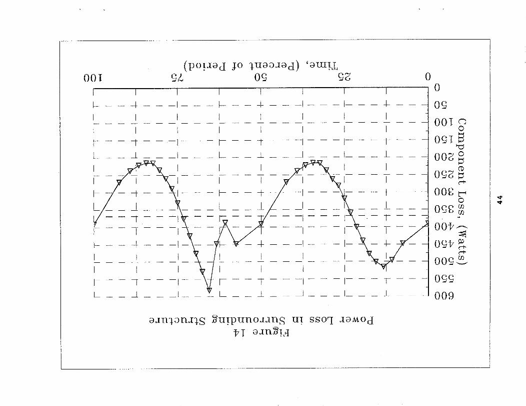
The rate of power loss in the surrounding structure of the

alternator (the result that was tracked during the solution phase

- see figure 13) for the 125 Arms output case is shown to vary

over the cycle in figure 14. The dashed line indicates the cycle

averaged power loss in this entire component. This power loss is

manifested by heat generation via eddy currents in the stainless

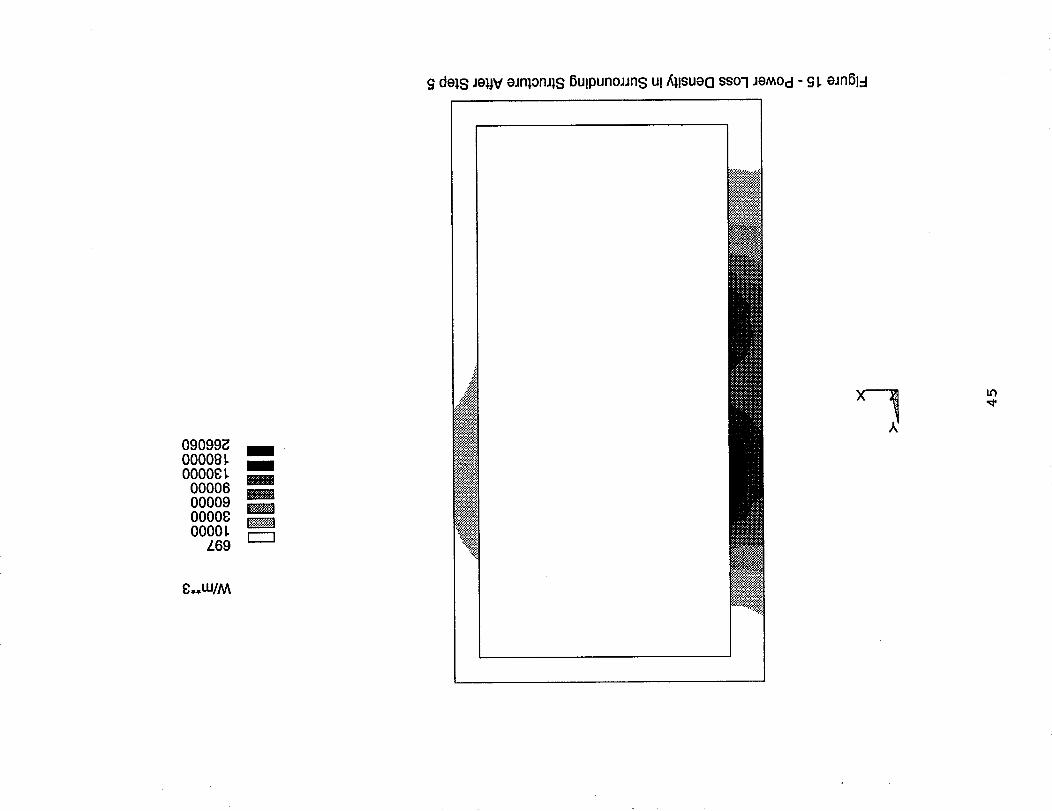
steel structure. The distribution of this heat generation (power

loss) throughout the surrounding structure is illustrated by

figure 15 which is a plot of the instantaneous power density for

a particular time in the cycle (again for the 125 Arms output

case). The particular instant shown is the end of the fifth step

25

from the period start. (For plunger position, see figure 6; this

is also the time instant involved in figures 16 and 17.) The

integral of this power density over the volume of the surrounding

structure is the total power loss in the surrounding structure at

that instant.

Results such as these are useful in efforts to identify

locations prone to structural power losses for design refinement

or evaluation. In this example, most of the power loss arises in

the area representing the inner piston cylinder. Such a

condition may impact bearing operation or require cooling.

The loss in the surrounding structure for the full output

power simulation is 367.6 W. Note that this loss represents more

than one percentage point in alternator efficiency for this

nominal 30-kW output alternator. During open circuit (i.e zero

power take-off current) operation, the power loss in the

surrounding structure components is strictly due to eddy braking.

The component loss at this open circuit operating condition was

calculated at 20.5 W.

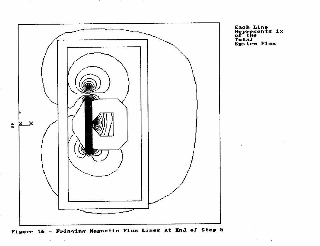
Fringing fields and the attendant space sensitivity to power

losses in external structures can be mapped as in figure 16. In

this figure, each flux line represents 2% of the total flux

present in the model at the instant at the end of the fifth step

for the 125 Arms output case. This kind of information is

particularly useful to guide the design of supporting or

peripheral structures in the neighborhood of the alternator

device. It can also be used to more broadly evaluate alternator

design concepts or designs when detailsregarding surrounding

objects are not well known or defined.

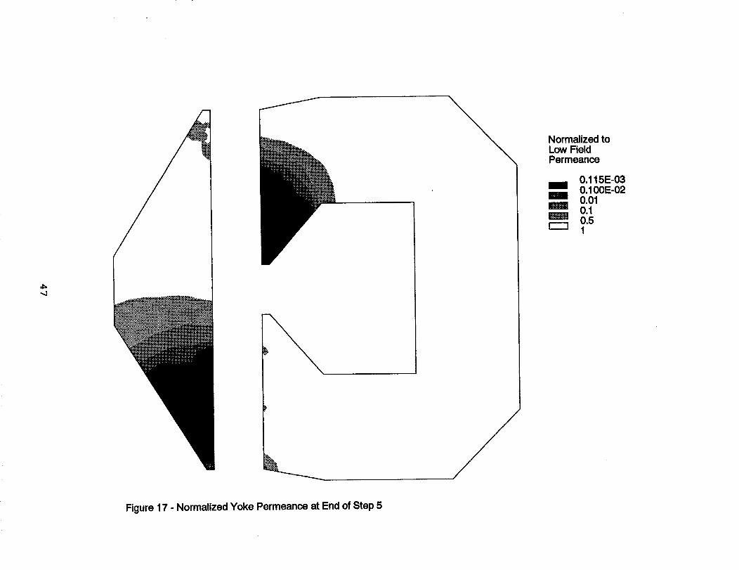
The magnitude of the power loss in the surrounding structure

at the full output power is due in part to the saturation

26

phenomenon in the yoke components, which can be better understood

by examining information like that of figure 17. Figure 17 is a

plot of the local instantaneous permeability of the yoke material

(normalized to the low-field linear permeability for this

material) at the end of the fifth step in the full output powercase (125 Arms). The low permeabilities indicated by shading in

much of the yoke are an indication of hard saturation of thismaterial. Greater leaked fields (figure 16) are one result of

this condition. Such leaked fields are ultimately responsible

for the power losses in the surrounding structure.

The information of figures 15-17 was plotted for every step

(2 mm intervals of the plunger motion, 36 steps total) of the 125

Arms full output power case. This type of information can be

integrated to determine total structural power loss as shown in

figure 14 and can also be examined to locate design problem areas

and evaluate their behavior over the course of the cycle.

The accurate and detailed magnetic field solution over space

and time is the crucial result of this analysis technique. The

information provided in this field solution is the basis for

further postprocessing for calculation of particular quantities

of interest to the analysis at hand. The details of such field

solution postprocessing will depend on the specific analysis

goals and can be carried out in the same manner as the analyst

normally would calculate such results from any magnetic field

solution and history. In the example alternator analysis,

emphasis was placed on using the field solutions to examine power

loss phenomena in the surrounding structure. Other aspects of

alternator performance can be calculated or derived from the

field solution and history. Output power and overall efficiency

of the device can be determined by calculating the generated

voltage from the flux linkage and properly accounting for power

losses in the winding, yoke, magnets and surrounding structure.

27

This advanced analysis technique can provide a more accurate

estimation of such operating characteristics because it

simultaneously involves both the moving permanent magnet and the

conductor reaction field sources in the calculation°

Phenomena Not Illustrated by the Example Analysis.

The example analysis here presented does not illustrate

rigorous treatment of the effects associated with:

- Azimuthal magnetic fields

- Non-isotropic material properties

- Movement of yoke or conductor material components.

These phenomena were excluded in consideration of the

practical limitations of available computer power and time and

due to the limitations of available finite element solvers. Of

the three areas noted, the first two can be included in a

straightforward way in this advanced analysis technique.

Accommodating the third area would require some significant

changes to the analysis approach and may not favor the use of

finite element formulation.

Azimuthal magnetic fields were excluded as a consequence of

the choice to restrict the mathematical model to cylindrically

symmetric geometry. This restriction to two dimensions

substantially reduces the required time and computer capacity,

but it precludes any non-zero components of the magnetic field

vector in the azimuthal direction. Typically, the most salient

features differentiating alternator designs, such as the number

or arrangement of permanent magnet rings, can be adequately

explored without regard to the azimuthal details. In such cases,

the economy offered by the two-dimensional model may

counterbalance the loss of some fine detail information.

28

Non-isotropic yoke materials used in some alternator and

motor designs have material properties that are directionally

dependent and can confound finite element formulation. Some FEA

packages allow the direct definition of nonisotropic material

properties, but this treatment is not available in most FEA

packages. Short of using the more powerful FEA packages for

direct formulation, the analyst can include a representation of

non-isotropic materials by assigning a range of material types to

the yoke elements according to the direction of the expected

field result for each element relative to the material "grain",

or preferred field orientation. Each region of the yoke can be

assigned a different isotropic permeability curve approximating

the natural response of the material to fields with the expected

magnetic field direction for that region relative to the

orientation of the grain of the anisotropy. The analysis is then

conducted using this piecewise description of the solid model.

The movement of yoke or conductor materials (in addition to

the moving magnets) during operation of the motor or alternator

device can not be analyzed directly in this technique. The

methods used to represent the motion of the permanent magnet

materials in the device via Amp_rian current equivalents are not

applicable to these other materials. Some estimate of the

external magnetic fields that these components might experience

during their travel, and the resultant power losses, can be made

with the aid of the existing technique.

Concluding Remarks

The analysis technique presented here can provide a basis

for thorough and accurate comparisons of competing linear

alternator or linear motor designs or design concepts proposed

29

for particular missions of interest. The technique can also be

used for indepth analysis of a particular design, to guide design

refinement. The technique is applicable to any linear

alternator or linear motor design concept of the iron yoke,

moving permanent magnet class.

The analysis provides special treatment of moving permanent

magnet components using Amp_rian current equivalents within a

finite element formulation. This allows the simultaneous

solution of the magnetic vector potential due to both the moving

permanent magnets and conductor reaction fields. Rigorous

treatment of eddy braking, yoke saturation, and structural power

loss calculations can be made using the technique.

A next step would be to compare test results from existing

linear alternators or linear motors with predictions from this

technique to allow validation and modification as required. This

would be particularly useful to do with existing hardware that

could be accurately modeled or possibly with hardware that could

be specifically built for verification purposes to be easy to

model.

3O

t.O

PLUNGER

1

//

...... 'i'

AZIMUTHAL

//////

.... . ........... //

..-.-........... ... ////

//•..:. .............. //

.... .................. //

/

DIRECTION

STATORMOTION AND

CENTERLINE

FIGURE 1 - TYPICAL LINEAR ALTERNATOR DEVICE

ANSYS 5.0A 1I I I I I I I

W

/nM

WZZ

¢0

b_0

GOHX<E

I I I

MAGNETS

YOKE

MAGNETS

YOKE

ADDITIONALSWEPT VOLUME

EXTERNALSTRUCTURE

WINDING

AIR

INFINITEBOUNDARY

Figure 2 - Solid Model of Example Linear Alternator

33

,0

w

ll ,_

II _ .i' l

_,_///

Fi_ttre 4 - ELEMEHT MESH £o_ YOKE _nd MAGNET SHEPT UOLUME

B £T)

•"_. 5"

2.,2

,

1- .7'

].,_'

0,7

0.,_'

0_2'

0

| I I

_1O01 _0012:00 400

_ool _oo i _oo i '1.....:o6600 800 1000 1200

Figure 3 - Yoke Mate_i_l (M-19 Si-Fe) PerMeance P_ope_t_ Representation

0ol,--I

c_N.p.-i

0

©

• ,_ N::

©• _,,,4

©

I

I

I

I

I

I

I I

I

00

0

I I

(_u) _uot._._sod _unIc_

C,2I

t_

©

@

©

36

Surface Current Density, Perspective View 2-D FEA Model

w

Current

z Z

X

R

Figure 7 - Amperian Current Equivalent Representation

Magnet Ring, Perspective View 2-D FEA Model

Inside Face I

is South Pole I

t_

,-.-.-......1..:.:.:.:.:.:.:.:.:.. .....

:::::::::..4....L.._._ 2._._.. _ .......... !........... ........ ... .......

..._ .................. 1........... I....... "-,,...7 ........ f :__- ___ "......... "

"'" "" " ".' ' • * "" "',

Outside

z is North PoleZ

Volume

Magnetization Vector

R

Figure 8 - Direct Magnetized Material Representation

(tutu 8 I. = dx ].B)SNOIlf'1708 0731::1 011V18 =1.o30N3_3::1.-IICI ::ihllV73t:l - 6 eJnl3!-I

t,gO'Ogt_O'Ogso'o .... ..........

. .........

g_o'o ...................:::::::::::::::::::

g_o'o_0"0

.900"0 r-'-7gO-::l 1,9I.'0

_:_

.J_:_; ..

• _._....

F

C_

T _8"c: S_SN_

8OO

700

600

"_ 5000

4OO

_ 300

o 200

•._ 1 O0

0

-100

Current

I

0

Load Profile

, t J I

25Time

Figure 1 1for Typical

5O(Percent

Node in

of Period)

Swept Volume

75. 100

00

U_L-

©

©

©

©

u_ON/

42

step

1

2

3

4

5

6

7

8

9

I0

ii

12

13

14

15

16

17

18

19

20

21

22

23

24

25

26

27

28

29

30

31

32

33

34

35

36

FIGURE 13

Percent Change in Instantaneous Power Loss Rate

in Surrounding Structure

Relative to One Cycle Earlier

Volume Integral Over Surrounding Structure.

Xp cycle 2 cycle 3 cycle 4 cycle 5

16 mm +46.309420 + 0.00.0410 - 0.000024

14 +24.728591 + 0.000225 + 0.000039

12 +16.587144 + 0.000651 - 0.000491

I0 +11.251885 + 0.000739 - 0.000276

8 + 9.276285 - 0.000311 + 0.00.0549

6 . + 6.827284 + 0.000192 + 0.000166

4 + 5.542882 - 0.000010 + 0.000160

2 + 4.28.3010 + 0.000208 + 0.000104

0 + 3.360418 + 0.000079 + 0.000087

- 2 + 2.550300 + 0.000233 + 0.000053

- 4 +14.423661 + 0.102509 + 0.001031

- 6 + 0.018962 + 0.001459 + 0.000017

- 8 - 0.506850 + 0.000803 + 0.000011

-i0 - 0.631722 + 0.000397 + 0.000007

-12 - 0.626368 + 0.000173 + 0.000005

-14 - 0.558872 + 0.000064 + 0.000003

-16 - 0.442186 + 0.000010 + 0.000002

-18 - 0.221228 + 0.000016 + 0.000001

-16 - 0.094493 + 0.000819 + 0.000003

-14 - 0.069958 + 0.001010 + 0.000014

-12 - 0.050044 + 0.004392 + 0.000032

-i0 - 0.021621 + 0.000757 - 0.000024

- 8 - 0.003463 - 0.004494 - 0.000043

- 6 - 0.019593 - 0.003248 - 0.000009

- 4 - 0.026539 - 0.002731 - 0.000143

- 2 - 0.019866 - 0.001699 - 0.000008

0 - 0.014657 - 0.001222 - 0.000006

2 - 0.013029 - 0.000828 - 0.000004

4 - 1.148529 - 0.010400 - 0.000127

6 - 0.021548 - 0.000132 - 0.000002

8 - 0.009301 - 0.000140 - 0.000001

I0 - 0.002966 - 0.000125 - 0.000001

12 + 0.000008 - 0.000102 - 0.000001

14 + 0.001171 - 0.000081 0.00

16 + 0.001459 - 0.000066 - 0.000001

18 + 0.000770 - 0.000040 0.00

0.00

0.00

0.00

- 0.000001

0.00

0.00

0.00

0.00

0.00

0.00

+ 0.000016

0.00

+ 0.000001

0.00

0.00

0.00

0.00

0.00

0.00

0.00

0.00

0.00

0.00

0.00

0.00

0.00

0.O0

0.00

- 0.000002

0.00

0.00

0.00

0.00

0.00

0.00

0.00

Cycle Averaged

Power Loss + 5.610373 + 0.001181 + 0.000010 0.00

FIGURE 13

Solution Result Periodicity Verification

43

00I

1

I

I

(pot._Od lo _uoa:_Od) 'omt.&0

I

[ L

t

F-

7 TI I

I 4-

I I

I I

r T

I i

oanlanals _u._punoaans m sso_l ao,_OdI oan_k4

0

O_

00I

00_

00£ _

o_

oo_.o_oo_

OOS

009

S deIs JeW eJn]onJIs6ulpunoJJnS Ul/qlsuec]sso-IJeh_od-S I. eJn61-1

09099_00009_00008_

0000600009000080000_

Z69

..;.....;.

.,.,.,..,......,

..,.,......,...

£_LU/M

m

:::;:::::::::::::.:o:.:.: :.:.:.:.:

r---I

%

Oh /

\

ii

Figure 16 - Fringing Hagneti© Flux Lines at End of Step 5

][aoh LineRepresents JL_of t]_eTotalS_steM Flux

¢=_J

k

Figure 17 - Normalized Yoke Permeance at End of Step 5

Normalized toLow FieldPermeance

0.115E-030.100E-02

m 0.01....,..........

. ........., .. 0.10.51

I Form ApprovedREPORT DOCUMENTATION PAGE OMBNo. 0704-0188

Public reporting burden for this collection of information is estimated to average 1 hour per response, including the time. for reviewing instru.ctions, .searching existing data. sour .ces..,

gathedng and maintaininQ the data needed, and cornple!ing .and.rev.iowing the .co,K_,on..or roTormat=on. ::;eno commpn= r .egaromg th_ buroen e_,mateoran_y ozner2_5 jl_effeO_Ionn=Scollection of information, including suggestions for reouclng this ouroen, io wasnmgton Heaoquaners :services, u.lrectorale lormlorrr_I_l_on.u_sr_lon.s ano .rtepon_ =,: _ _eDavis Highway, Suite 1204, Arlington.VA 22202-4302. and to the Office of Management and Budget, PapenNorK HeOUCtton Project (o/g4-UlU_), wasnmgton, L_ ZU:)U-J.

1. AGENCY USE ONLY (Leave blank) 2. REPORT DATE 3. REPORT TYPE AND DATES COVERED

December 1995

4. TITLE AND SUBTITLE

Advanced Analysis Technique for the Evaluation of Linear Alternators

and Linear Motors

6. AUTHOR(S)

Jeffrey C. Holliday

7. PERFORMING ORGANIZATION NAME(S) AND ADDRESS(ES)

HOLLIDAYLABS

GuysviUe, Ohio 45735

9. SPONSORING/MONITORING AGENCY NAME(S) AND ADDRESS(ES)

National Aeronautics and Space Administration

Lewis Research Center

Cleveland, Ohio 44135-3191

Final Contractor Report

5. FUNDING NUMBERS

WU-583-02-21

C-NAS3-25827

8. PERFORMING ORGANIZATION

REPORT NUMBER

E-10042

10. SPONSORING/MONITORING

AGENCY REPORT NUMBER

NASA CR-198434

11. SUPPLEMENTARY NOTES

Partial funding for this research was provided by the Department of Energy under Interagency Agreement

DE-AI04-85AL33408. Project Manager, Lanny G. Thieme, Power Technology Division, NASA Lewis Research Center,

organization code 5460, (216) 433--6119.

12a. DISTRIBUTION/AVAILABILITY STATEMENT 12b. DISTRIBUTION CODE

Unclassified - Unlimited

Subject Category 20

This publiealion is available from the NASA Center for Aerospace Information, (301) 621-0390.

13. ABSTRACT (Maximum 200 words)

A method for the mathematical analysis of linear alternator and linear motor devices and designs is described, and an

example of its use is included. The technique seeks to surpass other methods of analysis by including more rigorous

treatment of phenomena normally omitted or coarsely approximated such as eddy braking, non-linear material properties,

and power losses generated within structures surrounding the device. The technique is broadly applicable to linear

alternators and linear motors involving iron yoke structures and moving permanent magnets. The technique involves the

application of Amp6rian current equivalents to the modeling of the moving permanent magnet components within a f'mite

element formulation. The resulting steady state and Iransient mode field solutions can simultaneously account for the

moving and static field sources within and around the device.

14. SUBJECT TERMS

Linear alternators; Linear motors; Stifling machines; Elec_omagnetic analysis

17. SECURITY CLASSIFICATION

OF REPORT

Unclassified

NSN 7540-01-280-5500

18. SECURITY CLASSIFICATION

OF THIS PAGE

Unclassified

19. SECURITY CLASSIFICATION

OF ABSTRACT

Unclassified

15. NUMBER OFPAGES

4916. PRICE CODE

A03

20. LIMITATION OF AB:_I-IACT

Standard Form 298 (Rev. 2-89)

Prescribed by ANSI Std. Z39-18298-102