Advanced Analysis of Steel-Concrete Composite Frames A thesis in fulfilment of the requirement for the award of the degree Doctor of Philosophy in Infrastructure Engineering from Western Sydney University by Utsab Katwal BEng (Civil Engineering), MSc (Structural Engineering) Centre for Infrastructure Engineering School of Computing, Engineering and Mathematics April 2018

Welcome message from author
This document is posted to help you gain knowledge. Please leave a comment to let me know what you think about it! Share it to your friends and learn new things together.
Transcript

Advanced Analysis of Steel-Concrete Composite Frames
A thesis in fulfilment of the requirement
for the award of the degree
Doctor of Philosophy in Infrastructure Engineering
from
Western Sydney University
by
Utsab Katwal
BEng (Civil Engineering), MSc (Structural Engineering)
Centre for Infrastructure Engineering
School of Computing, Engineering and Mathematics
April 2018


ii
ABSTRACT
Modern specifications such as AS4100 and AISC360-10 permit the design of
steel frames by advanced analysis (second order nonlinear inelastic analysis). But the
research on advanced analysis for steel-concrete composite frames with concrete-
filled steel tubular (CFST) columns, composite beams, and composite connections is
still in its infancy despite widespread application of such frames in modern
construction. To conduct advanced analysis of composite frames, the best option is to
adopt simplified numerical models because of the computational efficiency.
However, it is very challenging to accurately capture the effects of composite action
between different components of a composite frame using simplified models. This
task initially requires the proper understanding of the fundamental behaviour of each
component of composite frames. Therefore, 3D FE modelling was utilised to
investigate the fundamental behaviour particularly for the CFST columns and
composite beams with headed shear studs welded through profiled steel sheeting.
Finally, a simplified tool to design composite frames by advanced analysis was
developed.
For CFST columns, simplified numerical models were developed using fibre
beam element (FBE) models. The main challenging part of FBE modelling is to
define accurate material properties because the FBE modelling cannot account for
the interaction between the steel tube and concrete, which have significant effects on
prediction accuracy. Therefore, the material models themselves should account for
the interaction. Although a few material models for either steel or concrete are
available in the literature for FBE modelling, such models cannot be used especially
when considering the rapid development and application of high strength materials
and/or thin-walled steel tubes. Therefore, versatile yet simple steel and concrete
material models were developed in this study based on extensive regression analysis
of data generated from 3D FE modelling. The FBE modelling results of circular
CFST columns indicate that the proposed material models can be utilised for
sufficiently wide practical ranges of such columns (concrete strength: 20 to 200 MPa,
steel yield strength: 185-960 MPa, diameter to thickness ratio: 10-220).
The full-scale experiments of composite beams are very expensive. Thus, FE
modelling can be a viable alternative to investigate the fundamental behaviour of
composite beams. But the FE models developed earlier have adopted various

iii
assumptions to simplify the modelling of some complex interactions such as the
interaction between the shear studs and concrete. Accordingly, those FE models have
limitations to capture certain types of failure modes. To address the above issues, a
FE model for composite beams with profiled steel sheeting was developed. The
realistic interaction between different components, including fracture of shear studs
and profiled steel sheeting, along with concrete damage, has been considered in the
FE modelling. The developed FE model successfully captured different types of
failure modes of composite beams, such as shear failure of the studs, concrete
crushing failure, steel beam failure and rib shear failure. Furthermore, the method to
determine shear force (𝑉s) −slip (𝛿s) behaviour of shear studs in composite beams
was introduced. Meanwhile, the contribution from profiled steel sheeting in carrying
axial loads in composite beams can be quantified.
The simplified numerical modelling for composite beams was developed
utilising shell, beam, and connector elements representing the composite slab, steel
beam, and shear studs, respectively. Similarly, the simplified models for composite
beam-to-CFST column connections (blind-bolted flush and extended as well as
through-plate connections) were developed where the connection behaviour was
defined in terms of moment-rotation curves using connector elements. The
simulation took just a few minutes for both composite beams and connections and
the predictions are in well agreement with the test data.
Finally, the proposed simplified numerical models of CFST columns, composite
beams and composite connections were assembled together to conduct advanced
analysis of steel-concrete composite frames. In particular, the proposed models were
verified for composite frames with joints, such as welded external diaphragms and
bolted endplate connections. The predictions obtained from simplified models of
composite frames show very good correlation with test results and are
computationally very efficient. Therefore, the proposed model can be efficiently used
to conduct advanced analysis of composite frames. Then, a comparative study was
conducted to investigate the differences between the traditional member-based
design and design by advanced analysis of composite frames. The results indicated
that the design based on advanced analysis was economical compared to traditional
design method.

iv
List of Publications
The thesis work presented herein has been supported by following papers that have
been published in internationally recognised journals and conferences.
Published Referred Journal and Conference Papers
1. Katwal, U., Tao, Z., & Hassan, M.K. 2018. Finite element modelling of steel-
concrete composite beams with profiled steel sheeting. Journal of
Constructional Steel Research, 146(7): 1-15.
2. Katwal, U., Tao, Z., Hassan, M.K., & Wang W.D. 2017. Simplified
numerical modelling of axially loaded circular concrete-filled steel stub
columns. Journal of Structural Engineering, ASCE, 143(12): 04017169 (1-
12).
3. Tao, Z., Katwal, U., & Hassan M.K. 2018. Simplified non-linear analysis of
steel-concrete composite frames. Proceedings of the 13th
International
Conference on Steel, Space and Composite Structures, 31 January-2
February 2018, Perth, Australia (Keynote Lecture).
4. Katwal, U., Tao, Z., & Hassan, M.K. 2018. Finite element modelling of steel-
concrete composite beams with profiled steel sheeting. Proceedings of the
13th
International Conference on Steel, Space and Composite Structures, 31
January-2 February 2018, Perth, Australia.
5. Katwal, U., Tao, Z., Hassan, M.K., & Wang, W.D. 2016. Simplified
numerical modelling of circular concrete-filled steel tubular stub columns.
Mechanics of Structures and Materials: Advancements and Challenges:
Proceedings of the 24th Australasian Conference on the Mechanics of
Structures and Materials (ACMSM24), December 2016, Perth, Australia,
223-229.
6. Katwal, U., Tao, Z., Song, T.Y., & Wang, W.D. 2015. Simplified numerical
modelling of steel-concrete composite beams with trapezoidal steel decking.
Proceedings of the 11th International Conference on Advances in Steel-
Concrete Composite Structures (ASCCS 2015), December 2015, Beijing,
China, 30-37.

v
DEDICATION
This dissertation is lovingly dedicated to my parents,
Min B. and Sita Katwal.

vi
ACKNOWLEDGEMENTS
First of all, I would like to express my sincere appreciation and gratitude to my
principal supervisor Professor Zhong Tao for his excellent guidance, endless support
and continuous encouragement throughout my doctoral journey. He has always been
a tremendous mentor for me. His enthusiasm towards advanced analysis of
composite structures, patience, knowledge and constructive advice has been the key
to successfully complete this thesis.
I am incredibly grateful to my co-supervisors Professor Wen-Da Wang, Dr Md
Kamrul Hassan and Associate Professor Tian-Yi Song for their kind help, excellent
advice, motivations and friendship.
My sincere thanks extend to all academic and administrative staff of Centre for
Infrastructure Engineering in Western Sydney University. Special thanks to Mr
Nathan Mckinlay for his technical support for supercomputing arrangements. Also,
my sincere thanks go to Dr Susan Mowbray and Ms Ann-Marie Blanchard for
assistance in proof-reading.
Part of the numerical analysis works were conducted using supercomputing facilities
available at National Computational Infrastructure, Australia. Computational
resources used in this work were provided by Intersect Australia Ltd. I would like to
sincerely acknowledge the efforts of Mr Peter Bugeia and Dr Joachim Mai at
Intersect.
I would also like to thank my colleagues and friends for their friendship and support.
Special thanks to Dr Xin Yu, Paritosh Giri, Santosh Gautam, Yifang Cao and Nima
Usefi for all the good moments in this arduous but exciting journey of PhD.
Finally, I would like to express my gratitude to all my family members for their
constant support and inspiration. Last but the not the least, I would like to thank my
beloved wife Rina and my son Aarohan for their understanding, love and moral
support throughout my PhD.

vii
TABLE OF CONTENTS
STATEMENT OF AUTHENTICATION………………………………………… i
ABSTRACT ………………………………………………………………………. ii
ACKNOWLEDGEMENTS…………………………………………….................. vi
TABLE OF CONTENTS………………………………………………………….. vii
LIST OF FIGURES……………………………………………………………….. xii
LIST OF TABLES……………………………………………………………….... xix
ABBREVIATIONS……………………………………………………………….. xx
PRINCIPAL NOTATIONS……………………………………………………….. xxi
CHAPTER 1
INTRODUCTION
1.1 General…………………………………………………………………. 1
1.2 Background……………………………………………………………. 1
1.2.1 Steel-concrete composite frames…………………………………. 1
1.2.2 Design philosophy of strucutures…………………………………. 4
1.3 Research motivations………….……………………………………….. 6
1.4 Research objectives……………………………………………………. 9
1.5 Research methodology…………………………………………………. 10
1.5.1 Experimental data collection………………….…………………... 10
1.5.2 Numerical studies based on FE analysis..…………………………. 12
1.5.3 Simplified numerical modelling….……………………………….. 12
1.6 Outline of thesis………………………………………………………… 12
CHAPTER 2
LITERATURE REVIEW
2.1 Introduction………………………………………………………………. 15
2.2 Concrete-filled steel tubular (CFST) columns………………………… 15
2.2.1 Experimental studies of CFST columns….………………………. 19
2.2.2 Three dimensional finite element modelling of CFST columns…… 20
2.2.3 Simplified numerical modelling of CFST columns………………. 20

viii
2.3 Composite beams with profiled steel sheeting………………………….. 22
2.3.1 Experimental studies of composite beams..………………………. 23
2.3.2 Finite element modelling of composite beams………………….... 28
2.3.3 Simplified numerical modelling of composite beams..…………..... 29
2.4 CFST column connections….……………………………………………. 34
2.4.1 Experimental studies of CFST column connections……………...... 36
2.4.2 Simplified numerical modelling of CFST column connections…… 38
2.5 Steel-concrete composite frames………………………………………… 40
2.5.1 Experimental studies of composite frames….……………………... 40
2.5.2 Literature review on advanced analysis of composite frames.……. 41
2.6 Summary of research gaps……………………………………….............. 42
CHAPTER 3
SIMPLIFIED NUMERICAL MODELLING OF CIRCULAR CONCRETE-
FILLED STEEL TUBULAR COLUMNS
3.1 Introduction………………………………………………………………. 45
3.2 Finite element (FE) modelling…………………………………………… 46
3.2.1 Steel material properties for FE modelling….……………………... 47
3.2.2 Concrete material properties for FE modelling……………………. 49
3.3 Fibre beam element (FBE) modelling……………………………………. 51
3.3.1 Assumptions used in FBE modelling….…………………………… 52
3.3.2 Procedure for FBE modelling……………………………………… 52
3.4 Development of material models for FBE modelling……………………. 53
3.4.1 Steel material model……………………………………………….. 54
3.4.2 Concrete material model…………………………………………… 66
3.5 Verification………………………………………………………………. 73
3.5.1 Columns with normal strength steel and concrete…………………. 75
3.5.2 Columns with high strength concrete……………………………… 76
3.5.3 Columns with ultra-high strength concrete………………………… 78
3.5.4 Columns with high strength steel and normal strength concrete…... 79

ix
3.5.5 Columns with high strength steel and concrete.…………………… 80
3.6 Summary….……………………………………………………………… 81
CHAPTER 4
FINITE ELEMENT MODELLING OF COMPOSITE BEAMS WITH PROFILED
STEEL SHEETING
4.1 Introduction………………………………………………………………. 82
4.2 Finite element modelling……………. ………………………………...... 82
4.2.1 Element types ….…………………………………………………... 84
4.2.2 Mesh discretisation…………… …………………………………... 86
4.2.3 Interaction properties………………………………………………. 89
4.2.4 Boundary and loading conditions………………………………….. 93
4.2.5 Material modelling…………………………………………………. 94
4.2.6 Residual stresses…………………………………………………… 104
4.2.7 Imperfections………………………………………………………. 105
4.2.8 Analysis method…………………………………………………… 106
4.3 Verification………………………………………………………………. 107
4.3.1 Fracture of shear studs……………………………………………... 110
4.3.2 Concrete crushing failure…….…………………………………….. 113
4.3.3 Steel beam failure………………………………………………….. 114
4.3.4 Rib shear failure……………………………………………………. 117
4.3.5 Interface slip……………………………………………………….. 121
4.4 Summary…………………………………………………………………. 124
CHAPTER 5
SIMPLIFIED NUMERICAL MODELLING OF COMPOSITE BEAMS WITH
PROFILED STEEL SHEETING
5.1 Introduction…………………………………………………………….... 126
5.2 Proposed simplified numerical modelling…………….……………….. 127
5.2.1 Simplified geometry………………………………………………. 127
5.2.2 Shear force-slip behaviour of shear studs in composite
beams……………………………………………………………………. 131

x
5.2.3 Boundary conditions……………………………………………… 141
5.2.4 Mesh discretisation………………………………………………… 142
5.2.5 Material non-linear constitutive relationships……………………... 143
5.2.6 Interactions………………………………………………………… 143
5.2.7 Analysis procedure……………………………………………….. 144
5.3 Verification………..……………………………………………………... 144
5.3.1 Specimens with stud fracture…………………………………….. 146
5.3.2 Specimens with concrete crushing failure…….………………….. 150
5.3.3 Specimens with steel beam failure…………………………………. 152
5.3.4 Specimens with rib shear failure…………………………………… 153
5.4 Summary…………………………………………………………………. 154
CHAPTER 6
SIMPLIFIED NUMERICAL MODELLING OF COMPOSITE BEAM-TO-CFST
COLUMN CONNECTIONS
6.1 Introduction…………………………………………………………….... 156
6.2 Proposed simplified numerical modelling……………………………… 157
6.2.1 Connection characteristics………..………………………………. 158
6.2.2 Interactions between steel beam and composite slab..……………. 167
6.3 Verification……………………………………………………………... 169
6.3.1 Blind-bolted flush endplate composite connections……....……….. 170
6.3.2 Blind-bolted extended endplate composite connections…..………. 173
6.3.3 Through-plate composite connections……………………...……… 173
6.4 Summary…………………………………………………………………. 175
CHAPTER 7
SIMPLIFIED NONLINEAR ANALYSIS OF STEEL-CONCRETE COMPOSITE
FRAMES
7.1 Introduction………………………………………………………………. 176
7.2 Proposed simplified numerical modelling for composite frames..……. 177
7.2.1 Composite frames with welded connections……………………… 178
xi
7.2.2 composite frames with bolted connections……………………….. 190
7.3 Comparative study between member-based design and design by
advanced analysis of composite frames……..…………………………… 193
7.4 Summary…………………………………………………………………. 198
CHAPTER 8
CONCLUSIONS AND FUTURE RESEARCH NEEDS
8.1 Conclusions………………………………………………………………. 199
8.2 Recommendations for future research……..…………………………….. 204
REFERENCES…………………………………………………………………….. 207
APPENDICES
APPENDIX A: CFST columns………………………………………………. 222
APPENDIX B: Composite beam-to-CFST column connections……………………. 227

xii
LIST OF FIGURES
Figure 1.1 World’s 100 tallest building by material
Figure 1.2 Structural analysis methods
Figure 1.3 Flowchart of research methodology
Figure 2.1 CFST composite frames under construction (Han et al., 2011)
Figure 2.2 Typical CFST column cross sections (Liew et al., 2016)
Figure 2.3 Techno station, Tokyo, Japan (Endo et al., 2011)
Figure 2.4 Abeno Harukas, Japan (Liew et al., 2014)
Figure 2.5 Typical 3D FE and simplified FBE model of CFST column
Figure 2.6 Schematic representation of composite beams with profiled steel sheeting
Figure 2.7 Location of favourable, central and unfavourable studs
Figure 2.8 Typical 3D FE and simplified models of composite beams
Figure 2.9 Plate model for composite slab analysis proposed by Wright (1990)
Figure 2.10 An orthotropic slab element model proposed by Yu et al. (2008)
Figure 2.11 Equivalent composite slab model proposed by Kwasniewski (2010)
Figure 2.12 Simplified modelling of composite floor slab proposed by Main (2014):
(a) actual profile; (b) alternating strong and weak strips
Figure 2.13 Simplified model for composite slab proposed by Jeyarajan et al. (2015)
Figure 2.14 Typical fin plate and through plate connections
Figure 2.15 Typical blind-bolted CFST column connection (Hassan, 2016)
Figure 2.16 Typical 3D FE and simplified model of CFST column connections
Figure 2.17 Typical joint model developed by Kang et al. (2014)
Figure 3.1 Typical sketch of solid FE and FBE models for circular CFST columns
Figure 3.2 Structural steel 𝜎 − 휀 model (Tao et al., 2013a)
Figure 3.3 Stress-strain curves of high strength steel
Figure 3.4 Confined concrete 𝜎 − 휀 curves
Figure 3.5 Influence of mesh size and number of fibre elements of steel tube
Figure 3.6 Effective σ- curves of steel and concrete for CFST Columns with normal
strength steel (𝑓y= 200, 300 and 400 MPa)
Figure 3.7 Effective σ- curves of steel and concrete for CFST Columns with high
strength steel (𝑓y=500, 800 and 960 MPa)
xiii
Figure 3.8 Proposed steel σ- curves for FBE modelling
Figure 3.9 Effects of 휀y/휀c0 and 𝐷/𝑡 on yy / ff
Figure 3.10 Verification of proposed equation of yy / ff
Figure 3.11 Effects of 𝜉c on 𝑓cr′ /𝑓y
Figure 3.12 Verification of proposed equation of 𝑓cr′ /𝑓y
Figure 3.13 Effects of 𝜉c ,𝐷/𝑡 and 𝑓c′on 휀cr
′ /휀y
Figure 3.14 Verification of proposed equation of 휀cr′
Figure 3.15 Effects of 𝜉c on 𝑓u′/𝑓y
Figure 3.16 Verification of proposed equation of 𝑓u′/𝑓y
Figure 3.17 Effects of 𝜉c on ψ
Figure 3.18 Validation of steel and concrete material models
Figure 3.19 Proposed curves of confined concrete
Figure 3.20 Effects of 𝜉c , D/t and 𝑓y/𝑓c′ on 𝑓cc
′ /𝑓c′
Figure 3.21 Verification of proposed equation of 𝑓cc′
Figure 3.22 Effects of 𝜉c and 𝐷/𝑡 on 𝑓r/𝑓cc′
Figure 3.23 Effects of 𝑓c′ and 𝐷(𝑓c
′)0.7/𝑡 on 𝑓r/𝑓cc′
Figure 3.24 Verification of proposed equation of 𝑓r
Figure 3.25 Effects of 𝜉c on 𝛼1and 𝐵
Figure 3.26 Verification of proposed equation of 𝛼1 and 𝐵
Figure 3.27 Comparison between Nue with Nuc and NuFE with respect to confinement
factor
Figure 3.28 Comparison between Nuc and Nue with respect to material strength
Figure 3.29 Comparison between Nuc and Nue with respect to D/t and L/D
Figure 3.30 Comparison between predicted and measured N-ε curves for columns with
normal materials
Figure 3.31 Comparison between predicted and measured N-ε curves for columns
with HSC
Figure 3.32 Comparison between predicted and measured N-ε curves for columns
with UHSC
Figure 3.32 Comparison between predicted and measured N-ε curves for columns
with UHSC (continued)
Figure 3.33 Comparison between predicted and measured N-ε curves for specimen
049C36_30 with high strength steel

xiv
Figure 3.34 Comparison between predicted and measured N-ε curves for columns
with high strength materials
Figure 4.1 Finite element model of a typical composite beam
Figure 4.2 Effect of different element types for steel beam on predicted 𝑀 − 𝛥
curves
Figure 4.3 Sensitivity analysis for concrete element size for specimen with concrete
crushing failure
Figure 4.4 Effect of concrete element size for specimen with stud fracture ( SB1, Nie
et al., 2005)
Figure 4.5 Effect of concrete element size for specimen with no major failure (CB2,
Ranzi et al., 2009)
Figure 4.6 Effects of μ between the concrete and sheeting for specimen with one stud
per rib
Figure 4.7 Effects of μ between the concrete and sheeting for specimen with two
studs per rib
Figure 4.8 Load distribution between the shear stud and profiled steel sheeting
(specimen SB1)
Figure 4.9 Effects of μ between the concrete and studs
Figure 4.10 Effects of μ between the steel beam and sheeting
Figure 4.11 Measured profiled steel sheeting 𝜎 − 휀 curves
Figure 4.12 Influence of fracture of profiled steel sheeting on prediction accuracy
Figure 4.13 Proposed 𝜎 − 휀 model for profiled steel sheeting
Figure 4.14 Effect of softening branch in 𝜎 − 휀 curves of profiled sheeting on
prediction accuracy
Figure 4.15 𝜎 − 휀 model for shear studs (Hassan, 2016)
Figure 4.16 Effect of dilation angle on prediction accuracy
Figure 4.17 Constitutive model of concrete under compression
Figure 4.18 Constitutive model of concrete under tension
Figure 4.19 Effect of concrete damage on prediction accuracy
Figure 4.20 Distribution of residual stresses (σR) in hot-rolled steel, ECCS (1984)
Figure 4.21 Effect of residual stress on prediction accuracy
Figure 4.22 Effects of initial imperfections on prediction accuracy
Figure 4.23 Comparison between kinetic energy and internal energy in simulation
xv
Figure 4.24 Comparison between predicted and measured ultimate loads
Figure 4.25 Prediction accuracy for specimens with fracture of studs
Figure 4.26 Comparison between measured and predicted 𝑃 − ∆ curves
Figure 4.27 Simulated concrete crushing; comparison between measured and
predicted 𝑀 − 𝛥 curves
Figure 4.28 Simulated and observed steel beam failure modes for specimen CB1
tested by Loh et al. (2004)
Figure 4.29 Prediction accuracy of 𝑃 − 𝛥 curves for specimens exhibiting steel beam
failure
Figure 4.30 Prediction accuracy of 𝑃 − 𝛥 curves (steel beam failure under negative
and positive moment)
Figure 4.31 Prediction accuracy of beam web yielding
Figure 4.32 Observed and predicted horizontal rib shear failure for specimen SB-5
(Nie et al., 2005)
Figure 4.33 Observed and predicted diagonal rib shear failure for specimen SB-5
(Nie et al., 2005)
Figure 4.34 Prediction accuracy of 𝑀 − 𝛥 curves for specimens exhibiting rib shear
failure.
Figure 4.35 Prediction accuracy of P − 𝛥 curves (rib shear failure)
Figure 4.36 Comparison between measured and predicted 𝑃 − 𝛥 curves
Figure 4.37 Predicted and observed separation between concrete and sheet
Figure 4.38 Comparison between measured and predicted 𝑃 − 𝛿s and 𝑉s − 𝛿s curves
Figure 4.39 Load distribution between the shear stud and profiled steel sheeting
Figure 5.1 Proposed simplified model for composite beams
Figure 5.2 Rendered view of a typical simplified FE model
Figure 5.3 Predicted 𝑉s − 𝛿s curve for specimen SB1 based on equations in Ollagard
et al. (1971) and Eurocode 4 (2004)
Figure 5.4 Comparison between measured and predicted 𝑀 − ∆ curves for specimen
SB1
Figure 5.5 Simulated push test specimens
Figure 5.6 Comparison of 𝑉s − 𝛿s curves obtained from push tests
Figure 5.7 Comparison of 𝑉s − 𝛿s curves obtained from FE modelling of composite
beam and push test specimens

xvi
Figure 5.8 Comparison between VusEC4 and Vus with respect to 𝜂s
Figure 5.10 Simulation results of specimen SB1
Figure 5.11 Predicted 𝑉s − 𝛿s curves of studs in tangential direction (specimen SB1)
Figure 5.12 Predicted 𝑉s − 𝛿s curves of studs in direction of X-axis (specimen SB1)
Figure 5.13 Comparison between measured and predicted 𝑀 − ∆ curves for
specimen SB1 with slip along X-axis and tangential axis
Figure 5.14 Averaged 𝑉s − 𝛿s curve used in simplfied model of specimen SB1
Figure 5.15 Comparison between measured and predicted 𝑀 − ∆ curves from 3D FE
and simplified FE modelling
Figure 5.16 Influence of mesh size
Figure 5.17 Comparison of internal and kinetic energy obtained from simulation
Figure 5.18 Comparison between Pue with Pus and PuFE with respect to degree of
shear connection
Figure 5.19 General arrangement of composite beam specimen Beam 2 (Hicks, 2007)
Figure 5.20 Predicted 𝑉s − 𝛿s curves of studs in tangential direction (specimen Beam 2)
Figure 5.21 Predicted 𝑉s − 𝛿s curves of studs in X-axis direction (specimen Beam 2)
Figure 5.22 Comparison of 𝑉s − 𝛿s curves between favourable, unfavourable and
central position shear studs
Figure 5.23 Averaged 𝑉s − 𝛿s curves used in simplfied model for specimen Beam 2
Figure 5.24 Comparison of M − ∆ curves between test, 3D FE and simplfied FE
models for specimen Beam 2
Figure 5.25 Predicted 𝑉s − 𝛿s curves of studs in X-axis direction (specimen SB10)
Figure 5.26 Comparison of M–Δ curves for specimens SB10
Figure 5.27 Effect of different 𝑉s − 𝛿s curves on M–Δ curves for specimen with stud
fracture (Specimen SB10)
Figure 5.28 Predicted 𝑉s − 𝛿s curves of studs close to hinge support for specimens
SB2 and SB3
Figure 5.29 Comparison of M–Δ curves for specimens with concrete crushing failure
Figure 5.30 Predicted 𝑉s − 𝛿s curves of studs for specimen SB7
Figure 5.31 Comparison of 𝑷– 𝜟 curves for specimen SB7
Figure 5.32 Effect of different 𝑉s − 𝛿s curves on M–Δ curves for specimen with steel
beam failure
Figure 5.33 Averaged 𝑉s − 𝛿s curves of studs for specimens SB4 and SB5

xvii
Figure 5.34 Comparison of M–Δ curves for specimens with rib shear failure
Figure 6.1 Schematic representation of blind-bolted flush and extended endplate
composite connections
Figure 6.2 Schematic representation of through-plate composite connection (Hassan,
2016)
Figure 6.3 Typical simplified models of CFST column connections
Figure 6.4 Schematic representation of composite connection specimens tested by
Tao et al. (2017a) [unit: mm]
Figure 6.5 Configuration details of specimen CB2-3 (Tao et al., 2017a)
Figure 6.6 Effect of idealisation of connections as rigid, semi-rigid and pinned
connections
Figure 6.7 Component model for the flush endplate composite joint (Thai and Uy,
2015)
Figure 6.8 Comparison of predicted 𝑀 − 𝜙 curves by Thai and Uy (2015) and
Hassan (2016) for specimens CJ1 and CJ2 tested by Loh et al. (2004)
Figure 6.9 𝑀 − 𝜙 curve of composite beam-to-CFST column connections with flush
endplates (Hassan, 2016)
Figure 6.10 Spring model to obtain initial rotational stiffness of composite beam-to-
CFST column connections with flush endplates (Hassan, 2016)
Figure 6.11 Stress blocks of components of flush endplate connection (Hassan, 2016)
Figure 6.12 Effects of full and partial shear interaction between steel beam and
composite slab in composite connections
Figure 6.13 Prediction accuracy for specimens with flush endplate connections tested
by Loh et al. (2006)
Figure 6.14 Prediction accuracy for specimens with flush endplate connections tested
by Thai et al. (2017)
Figure 6.15 Prediction accuracy for specimens with flush endplate connections tested
by Tao et al. (2017a)
Figure 6.16 Prediction accuracy for specimens with extended endplate connections
tested by Thai et al. (2017)
Figure 6.17 Prediction accuracy for specimens with through-plate connection tested
by Hassan (2016)
Figure 7.1 Typical simplified model of composite frame with CFST columns

xviii
Figure 7.2 Schematic view of frame model in a real structure (Han et al., 2011)
Figure 7.3 Typical failure mode of composite frame tested by Han et al. (2011)
Figure 7.4 Simplified numerical model and simulated composite frame deformation
Figure 7.5 Effect of beam stiffening at the beam edges
Figure 7.6 Arrangement of transverse braces in CFST frame (Han et al., 2008)
Figure 7.7 Influence of the number of elements on the prediction of ultimate capacity
(specimen CF-12, Han et al., 2011)
Figure 7.8 Influence of mesh size on prediction of horizontal load versus
displacement curves for composite frame specimen CF-12, tested by Han
et al. (2011)
Figure 7.9 Effect of idealisation of connections as perfectly rigid and with rotational
stiffness definition
Figure 7.10 𝑃 − ∆ and 𝑃 − 𝛿 effects (Composite column design manual, ETABS
2016)
Figure 7.11 Influence of imperfections for composite frame CF-12
Figure 7.12 Influence of residual stress of steel beam for composite frame specimen
CF-12
Figure 7.13 Prediction accuracy for lateral load (F) versus lateral displacement ()
curves
Figure 7.14 Frames tested by Wang and Li (2007) and general layout of frames A and B
Figure 7.15 Rendered view of simplified model of composite frame
Figure 7.16 Simulated frame deformation for frame A, tested by Wang and Li (2007)
Figure 7.17 Predicted and measured 𝑃 − 𝛥 curves for beams 1 and 2 in frame A
Figure 7.18 Predicted and measured 𝑃 − 𝛥 curves for beam 3 in frame B
Figure 7.19 Demand/capacity ratios for composite frames CF-11 and CF-21
calculated from ETABS evaluation version (2016) based on AISC 360-
10
Figure 7.20 Comparison of design horizontal force obtained from member-based
design and design by advanced analysis
Figure 7.21 Load factor versus horizontal displacement curves

xix
LIST OF TABLES
Table 2.1 Classification of rigid, semi-rigid and pinned connections (Eurocode 3,
2005)
Table 3.1. Parameter range of simulated CFST specimens
Table 4.1 Summary of test data for composite beams
Table 5.1 Comparison of predicted stud strength from FE model of composite beams
and Eurocode 4
Table 5.2 Comparison of ultimate capacity of composite beams between measured and
predicted from simplfied numerical modelling
Table 6.1 Summary of rotational parameters reported by Hassan (2016)
Table 6.2 Summary of test data for composite connections.
Table 7.1 Cross section dimensions of steel tube and beam section (Han et al., 2011)
Table 7.2 Comparison of ultimate horizontal load predicted by simplified FE with
test and 3D FE model reported by Han et al. (2011)
Table 7.3 Comparison of design forces obtained from member-based design and
design by advanced analysis
Table 7.4 Comparison of design CFST and steel beam sections obtained from
member-based design and design by advanced analysis for composite
frame A
Table 7.5 Comparison of design CFST and steel beam sections obtained from
member-based design and design by advanced analysis for composite
frame B
Table A.1 Summary of test data for circular CFST columns
Table B.1 Summary of equations required to calculate stiffness of various
components of composite beam-to-CFST column blind-bolted flush
endplate connections (Hassan, 2016)

xx
ABBREVIATIONS
CFST Concrete-filled steel tubular columns
CHS Circular hollow section
DL Dead load
EBM Scaling of Eigenbuckling modes
FBE Fibre beam element
FE Finite Element
FNM Shear studs placed favourably in the composite beams under
negative moment
FPM Shear studs placed favourably in the composite beams under
positive moment
HSC High strength concrete
HSS High strength steel
IE Internal energy
IGI Direct modelling of initial geometric imperfections
KE Kinetic energy
NHF Notional horizontal force
NSC Normal strength concrete
NSS Normal strength steel
SIGINI Subroutine program for residual stress in ABAQUS
UHSC Ultra-high strength concrete
UMAT Subroutine program for materials in ABAQUS
UNM Shear studs placed unfavourably in the composite beams under
negative moment
UPM Shear studs placed unfavourably in the composite beams under
positive moment
DAMAGEC Compressive damage variable of concrete in ABAQUS
DAMAGET Tensile damage variable of concrete in ABAQUS

xxi
PRINCIPAL NOTATIONS
𝐴s Cross-section area of steel beam
𝐴r Cross-section area of longitudinal reinforcement
B Width of the composite slab
𝑏f Width of the steel beam flange
D Outer diameter of CFST column
𝐷s Shank diameter of shear studs
𝑑c Compressive damage parameter
𝑑t Tensile damage parameter
𝐸c Young’s modulus of concrete
𝐸s Young’s modulus of steel
𝐹 Horizontal force applied at composite frames
𝐹uc Predicted horizontal ultimate load capacity of composite frames
form simplified model
𝐹ue Measured horizontal ultimate load capacity of composite frames
𝐹uFE Predicted horizontal ultimate load capacity of composite frames
from 3D FE model
𝑓r Residual stress of concrete
𝑓ry Yield stress of reinforcement
𝑓y Yield stress of steel
𝑓u Ultimate strength of steel
fus Ultimate tensile strength of the stud
𝑓c′ Unconfined concrete strength
𝑓cc′ Confined concrete strength
𝑓cr′ Critical longitudinal stress of steel in CFST column
𝑓t′ Tensile strength of concrete
𝑓u′ Effective stress of steel corresponding to the ultimate strain 휀u
𝑓y′ First peak stress of steel in the CFST column
H Height of composite frame
h Height of steel beam
hc Composite slab depth
hs Height of ribs of profiled sheeting

xxii
hsc Height of the shear studs
L Span length of the composite beams
𝐿c Height of CFST columns
M Moment
𝑀𝑒 Elastic moment capacity of composite connections
𝑀𝑝 Plastic moment capacity of composite connections
𝑀𝑢 Ultimate moment capacity of composite connections
𝑁 Column axial loads
Npss Axial force carried by profiled steel sheeting
𝑁uc Predicted ultimate strengths of CFST columns from the FBE
modelling
𝑁ue Measured ultimate strengths of CFST columns
𝑁uFE Ultimate strengths predicted from 3D FE modelling
n Number of columns in plane of frame
𝑃DA Design horizontal force (advanced analysis)
𝑃DM Design horizontal force (member based design)
Puc Predicted ultimate loads capacity of composite beams from 3D
FE modelling
𝑃ue Measured ultimate loads of composite beams
𝑃us Predicted ultimate load capacity composite beams from
simplified numerical modelling
𝑅2 Coefficient of determination
𝑆𝐷 Standard deviation
𝑆𝑗,𝑖𝑛𝑖 Initial rotational stiffness of composite connections
𝑡 Thickness of CFST column
tf Thickness of flange of steel I-section beam
tw Thickness of web of steel I-section beam
ttw Trough width of the rib
𝑉s Shear force resisted by studs
Vsu Ultimate shear force resisted by the shear stud
VsuEC4 Maximum resistance of a shear stud according to Eurocode 4
𝛿 Relative slips at the beam ends of composite beams
𝛿s Shear stud sip

xxiii
Vertical displacement
ΔH Horizontal displacement
ε Strain
휀cc Strain at peak stress of confined concrete
휀co Strain at peak stress of unconfined concrete
휀cr Strain corresponding to peak tensile strain of concrete
휀p Strain at the onset of strain hardening
휀u Strain corresponding to ultimate strength of steel
휀y Yield strain of steel
휀cr′ Strain corresponding to critical stress of steel in CFST column
휀y′ Strain corresponding to 𝑓𝑦
′
εcinel Compressive inelastic strain of concrete
휀tck Cracking strain of concrete
η Degree of shear connection of composite beams
𝜆 Load factor
μ Friction coefficient
𝜇m Mean
𝜉c Confinement factor
σ Stress
σR Residual stress in hot-rolled steel
𝜑s System resistance factor
𝜙 Rotation
𝜙𝑒 Rotation corresponding to the elastic moment
𝜙𝑝 Plastic rotation corresponding to the plastic moment
𝜙𝑢 Ultimate rotation corresponding to the ultimate moment
𝜓0 Initial angle of inclination of frame

CHAPTER 1 INTRODUCTION
- 1 -
CHAPTER 1
INTRODUCTION
1.1 General
This chapter provides an overview of this thesis on the advanced analysis of steel-
concrete composite frames using simplified numerical modelling of concrete-filled
steel tubular (CFST) columns, composite beams with profiled steel sheeting and
composite beam-CFST column connections. This includes the research background,
the motivations for this study, its objectives, and the layout of the following chapters.
1.2 Background
1.2.1 Steel-concrete composite frames
Steel-concrete composite frames are widely used in the modern construction indus-
try. This is due to the mechanical and economical advantages provided by the com-
posite technique. Concrete is the most used construction material worldwide because
of relatively high compressive strength, good fire resistance, long life, ease of casting
in any shape and size, and low cost. The properties of concrete such as its strength,
setting time, fire resistance and workability can be enhanced by using different types
of cement and additives. The disadvantages of concrete include its very low tensile
strength and general failure by cracking and crushing. On the other hand, steel is a
material with high tensile and compressive strength and high ductility. It is an ex-
pensive material however and has poor fire resistance. But the combination of con-
crete and steel utilises the compressive strength of concrete and tensile capacity of
steel and the resulting composite members such as CFST columns and composite
beams offer many structural as well as economic benefits.
The classification of the world’s 100 tallest buildings by construction material from
1930 to 2016 is presented in Figure 1.1. It shows that from 1930 to 1960 most of the
world’s 100 tallest buildings were built using steel. After 1960, there is a gradual de-

CHAPTER 1 INTRODUCTION
- 2 -
crease in steel‒based construction which drops to 9% in 2016. Meanwhile, from
1980 to 2016 the use of composite steel‒concrete construction in tall buildings in-
creased gradually from 12% to 53% respectively. This highlights the scope of utilisa-
tion of composite structures in the construction industry.
Source: http://skyscrapercenter.com/year‒in‒review/2016
Figure 1.1 World’s 100 tallest building by material
1.2.1.1 Concrete-filled steel tubular columns
Many experimental data on concrete-filled steel tubular (CFST) columns are availa-
ble in the literature from the late 1960s. As a result of this, the influence of various
parameters such as concrete strength, steel yield stress, diameter or breadth and
thickness of the tube can be investigated. Goode (2008) collected test data on 1819
CFST columns. In general, CFST columns offer many structural benefits such as
high strength, favourable ductility and large energy absorption capacities (Han et al.,
2014b). CFST columns incorporate the advantages of concrete and steel. The con-
crete strength is increased due to the confinement effect provided by the steel tube.
Moreover, the inward local buckling of the steel tube is prevented by the core con-
crete which helps to increase the load bearing capacity and enhances the ductility.
CFST columns also offer excellent static and seismic performances (Wang et al.
2009). Because of these advantages, CFST columns are extensively used in build-
ings, bridges, towers, substations etc.
0
25
50
75
100
1930 1940 1950 1960 1970 1980 1990 2000 2010 2016
Wo
rld
's 1
00
ta
lles
t b
uil
din
g
Unknown Mixed Composite Concrete Steel

CHAPTER 1 INTRODUCTION
- 3 -
Circular and rectangular cross sections are mostly used in CFST columns. The strong
confinement of concrete can be achieved in circular CFST columns. Although local
buckling is more likely to occur in CFST columns with rectangular or square cross
sections, such sections are used because of the easier installation of composite beam‒
CFST column connections (Han et al., 2014b). Meanwhile, the cross‒section can be
kept to a minimum using high strength materials in order to increase the carpet area
of buildings. Ongoing research and application around the globe is exploring the use
of high strength materials in CFST columns. For example, CFST columns with steel
yield stress (fy) of 590 MPa and concrete unconfined strength (fc′) of 150 MPa have
been used in CFST columns in Abeno Harukas, Japan (Liew et al. 2014). The tests of
CFST columns with concrete fc′ close to 200 MPa have been reported by Xiong et al.
(2017). Similarly, tests of CFST columns with fy of 854 MPa have been reported by
Sakino et al. (2004). The results of this ongoing research supports the wide use of
CFST columns with high strength materials will as a major compressive element in
infrastructure in the future.
1.2.1.2 Composite beams with profiled steel sheeting
Steel-concrete composite beams are widely used in steel framed building construc-
tion (Faella et al., 2003, Ranzi and Zona, 2007). In such beams comprising of com-
posite slabs, the concrete is often cast on thin high-strength profiled steel sheeting to
form the slab, which is connected to the steel I-section beam by welding headed
shear connectors through the profiled steel sheeting to the top flange of the beam.
Full-scale experimental investigations on steel-concrete composite beams with pro-
filed steel sheeting started nearly fifty years ago with the work reported by Robinson
(1969). The general details of 58 earlier experimental studies on composite beams
with profiled steel sheeting were summarised by Grant et al. (1977) who also con-
ducted 17 such composite beam tests. Other full-scale tests were conducted by Jayas
and Hosain (1989), Easterling et al. (1993), Rambo-Roddenberry (2002), Nie et al.
(2004), Loh et al. (2004), Nie et al. (2005), Nie et al. (2008), Ranzi et al. (2009) and
Ernst et al. (2010).
The use of profiled steel sheeting provides an immediate work platform and acts as a
form itself. Once the beam is in service, the steel deck acts as a tensile reinforcement

CHAPTER 1 INTRODUCTION
- 4 -
which partially reduces the time-consuming placing and handling of rebars. Further-
more, the cellular geometry of profiled steel sheeting permits the formation of duct-
ing cells within the floor so that services can be incorporated and distributed within
the floor depth (Abdullah 2004). Because of the structural, economic as well as con-
structional benefits, composite beams with profiled steel sheeting have been widely
used as flexural members in infrastructure.
1.2.1.3 Composite beam-to-CFST column connections
The behaviour of composite structures is highly influenced by the moment-rotation
characteristics of composite beam-to-CFST column connections. Such composite
connections can be welded or bolted. Generally, welded connections are used to con-
nect steel beams to CFST columns but such connections require expensive on-site
welding (Schneider and Alostaz, 1998, Mirza and Uy, 2011, Hassan, 2016). More
recently, blind-bolted endplate connections are utilised as structural bolts which can
be tightened from the outer side. The differences in the behaviour of connections
with or without slabs are explored in the experimental data on such connections with
composite slabs (Loh et al., 2006, Mirza and Uy, 2011, Tao et al., 2017a). Mean-
while, the influence of column type and flush and extended endplates are investigat-
ed by Thai et al. (2017). The results from these experimental works indicate that
blind-bolted connections are viable to be implemented in structures.
1.2.2 Design philosophy of structures
There are two types of design philosophies, namely member-based design and design
by advanced analysis in general. Member-based design is also known as an indirect
method of design or conventional design method and it has a history of more than
100 years. The research on design by advanced analysis, also considered to be direct
design, started around three decades earlier and is permitted for steel structures in
some specifications like AS4100 and AISC 360-10.
1.2.2.1 Member-based-design
In member-based design, the first step is to analyse the structure i.e. to find out the
internal forces such as shear force, bending moment, axial force, and torsion. The
second step is to design the structure and complete a capacity check of all compo-
CHAPTER 1 INTRODUCTION
- 5 -
nents such as columns, beams, and connections to verify that they are capable of re-
sisting the applied loads. The structural system is treated as a set of individual com-
ponents and interactions between the structural system and its members are only re-
flected indirectly by the use of effective length factors (Shabnam, 2013). This meth-
od cannot accurately address the effect of inelastic redistribution of internal forces
after yielding (Kim and Chen, 1999). Furthermore, in traditional design, the load car-
rying capacity of the system is assessed on a member-by-member basis, limiting the
load carrying capacity of the system to the strength of the weakest member (Surovek,
2011). It is therefore very important to note that the real global behaviour of struc-
tures cannot be predicted since the member behaviour and whole system behaviour
are different. There is, therefore a possibility of over estimation and the design may
be uneconomical for the same level of performance.
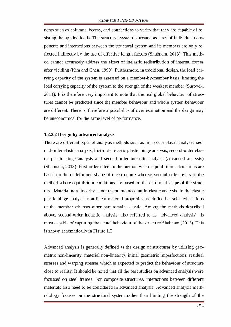
1.2.2.2 Design by advanced analysis
There are different types of analysis methods such as first-order elastic analysis, sec-
ond-order elastic analysis, first-order elastic plastic hinge analysis, second-order elas-
tic plastic hinge analysis and second-order inelastic analysis (advanced analysis)
(Shabnam, 2013). First-order refers to the method where equilibrium calculations are
based on the undeformed shape of the structure whereas second-order refers to the
method where equilibrium conditions are based on the deformed shape of the struc-
ture. Material non-linearity is not taken into account in elastic analysis. In the elastic
plastic hinge analysis, non-linear material properties are defined at selected sections
of the member whereas other part remains elastic. Among the methods described
above, second-order inelastic analysis, also referred to as “advanced analysis”, is
most capable of capturing the actual behaviour of the structure Shabnam (2013). This
is shown schematically in Figure 1.2.
Advanced analysis is generally defined as the design of structures by utilising geo-
metric non-linearity, material non-linearity, initial geometric imperfections, residual
stresses and warping stresses which is expected to predict the behaviour of structure
close to reality. It should be noted that all the past studies on advanced analysis were
focussed on steel frames. For composite structures, interactions between different
materials also need to be considered in advanced analysis. Advanced analysis meth-
odology focuses on the structural system rather than limiting the strength of the

CHAPTER 1 INTRODUCTION
- 6 -
structural system at design load levels by the first member failure. Advanced analysis
method can be considered as more beneficial in the case of complex framing system
since it eliminates the consideration of effective length factor and beam-column in-
teraction equations which is very difficult to use in the case of complex framing sys-
tem (Surovek, 2011). Till date, design by advanced analysis has not yet been general-
ly embraced in the structural engineering community because application of ad-
vanced analysis requires considerable modelling and design skills and the another
more significant reason is that current design standards do not specify prescriptive,
unambiguous requirements for design-by-advanced analysis (Zhang and Rasmussen,
2013).
Figure 1.2 Structural analysis methods
1.3 Research motivations
The rapid increase in the number of large structures using steel-concrete composite
frames indicates the need to develop a rational, practical approach of design method-
ology to using advanced analysis.
The main points that motivated this research work are:
1. The conventional member-based design method is considered to be tedious
and involve unreliable complicated formulas, such as the assumption of effec-
tive length factors used in sway and non-sway frames (Liu et al. 2012). The
effective length factor approach cannot accurately account for the interaction
Load
fac
tor,
λ
Displacement, ΔH
First-order elastic analysis
Second-order elastic analysis
First order elastic-plastic analysis
Second order inelastic analysis
(Advanced analysis) Actual
Second order elastic-plastic hinge analysis
N N
F ΔH

CHAPTER 1 INTRODUCTION
- 7 -
between the structural system and its members because the interaction in a
large redundant structural system is too complex to be represented by the
simple effective length factor and it cannot predict the failure modes of a
structural system (Kim and Chen, 1999). Therefore, there is a need to use ad-
vanced analysis in design where there is no need to use effective length fac-
tors as well as interaction equations and can predict the global failure modes
of the structural system.
2. Most previous studies on advanced analysis focussed on steel frames only
and there is no clear provision in current design codes to design composite
structures by using advanced analysis. So, there is a strong reason to carry out
research on the advanced analysis of steel-concrete composite frames.
3. To conduct advanced analysis, simplified numerical models are preferred to
detailed 3D FE modelling as the simplified models are computationally very
efficient. Although detailed 3D FE modelling can be utilised for fundamental
study, such models are tedious, extremely time consuming and numerical
convergence issues make such 3D FE modelling very difficult to be used for
routine design. However, the simplified models need to be rigorously verified
and should be based on solid theoretical backgrounds.
4. For CFST columns, simplified numerical modelling can be conducted using a
fibre beam element (FBE) model. Since the interaction between the steel tube
and core concrete cannot be defined in the FBE model, the material models
themselves have to account for the effects of interactions and any local buck-
ling effects. Few material models are available in the literature for FBE mod-
elling of CFST columns but those models that cannot be utilised, especially
when considering the rapid development and application of high strength ma-
terials and/or thin-walled steel tubes. Moreover, most of the previous steel
material models considered only the strain hardening behaviour in circular
CFST columns. However, because of the interactions between the steel tube
and concrete, there will be strain softening in the steel tubes depending on the
confinement factor. Only CFST columns with very high confinement factor
may have the strain hardening behaviour as proposed in previous models.

CHAPTER 1 INTRODUCTION
- 8 -
Therefore, there is a strong need to develop versatile, computationally simple
yet accurate steel and concrete material models for CFST columns to address
the current trend to use high strength materials in the construction industry.
5. The fundamental behaviour of composite beams, especially the behaviour of
shear studs in composite beams, is not fully understood yet. Full-scale tests of
composite beams are very expensive, sophisticated and require large testing
facilities. Therefore, it is very difficult to investigate the influence of various
parameters from the experimental study. Moreover, to date, the in-situ shear
studs’ strength cannot be measured directly from the tests and in many cases,
the strength of the shear studs is determined from push tests. The behaviour
of shear studs obtained from push tests may not represent the actual behav-
iour of shear studs in composite beams (Jayas and Hosain, 1989; Hicks,
2007). This is due to the absence of beam curvature and the normal force re-
sulting from the floor loading in push tests (Hicks, 2009).
6. The equations for shear force versus slip of shear studs developed by Ol-
lagard et al. (1971) has been used in the numerical simulation of composite
beams with profiled steel sheeting (Nie et al., 2004), however, originally the
equations were developed from the test results of push tests with solid rein-
forced concrete slabs. Therefore, the validity of using the model developed by
Ollagard et al. (1971) needs to be investigated. This can be done using the
shear force versus slip curves obtained from 3D FE modelling of composite
beams.
7. Few simplified models are available in the literature for the simulation of
composite beams (Kwasniewski, 2010, Main, 2014, and Jeyarajan et al.,
2015). Rigid bars were used by Main (2014) to connect the steel beam ex-
tending from the neutral axis of the steel I-section beam to the top surface of
the steel beam and beam elements were used to represent the behaviour of
shear studs through the definition of shear force‒slip curves based on Ol-
lagard et al. (1971). On the other hand, the model developed by Kwasniewski
(2010) and Jeyarajan et al. (2015) considers the full shear interaction between
steel beam and concrete which virtually ignores the slip between the steel and

CHAPTER 1 INTRODUCTION
- 9 -
concrete. Therefore, a new simplified model, based on the models proposed
by Kwasniewski (2010), Main (2014) and Jeyarajan et al. (2015), can be de-
veloped and utilised for partial, as well as full shear interactions. The steel
beam and composite slabs can be offset from the same reference plane in
ABAQUS. Therefore, there is no need to use rigid elements and the shear
force-slip curves obtained from 3D FE modelling can be utilised.
8. The simplified numerical models developed for CFST columns and compo-
site beams can be utilised for simplified numerical modelling of composite
connections. The connection behaviour can be obtained from analytical mod-
els such as that developed by Thai and Uy (2015), Hassan (2016), Thai et al.
(2017) and can be defined through connector elements. After that, the simpli-
fied numerical model can be used for advanced analysis of composite frames.
1.4 Research objectives
The main aim of this research is to develop suitable simplified models to carry out
advanced analysis of steel-concrete composite frames. The simplified models should
be easy to simulate, computationally efficient, accurate and should be capable of
modelling the complex geometrical shapes as well.
The overall objectives of this research are:
i. To propose accurate and versatile material models of steel and concrete in
circular CFST columns for simplified numerical modelling of such CFST
columns.
ii. To develop a general finite element (FE) model for composite beams with
profiled steel sheeting to capture different types of failure modes of compo-
site beams.
iii. To determine the full-range shear force versus slip curves of shear studs in
composite beams with profiled steel sheeting.
iv. To determine the contribution of profiled steel sheeting in carrying axial forc-
es in composite beams.

CHAPTER 1 INTRODUCTION
- 10 -
v. To develop a computationally efficient simplified numerical model for com-
posite beams with profiled steel sheeting.
vi. To develop a simplified numerical model for composite beam-to-CFST col-
umn connections.
vii. To develop a simplified numerical model for composite frames with CFST
columns in order to conduct advanced analysis of steel-concrete composite
frames.
viii. To conduct the comparative study between traditional member-based design
and design by advanced analysis of composite frames with CFST columns.
1.5 Research methodology
To accomplish the research objectives, this study was divided into three groups: exper-
imental data collection from the literature, numerical studies using detailed 3D FE
modelling, and developing simplified numerical modelling for composite columns,
beams, connections, and frames. The simplified numerical modelling of the composite
frame was then utilised to conduct advanced analysis of such frames. A summary of
the research methodology is presented below and is shown schematically in Figure 1.3.
1.5.1 Experimental data collection
Experimental data for CFST columns, composite beam‒CFST column connections,
composite beams with profiled steel sheeting and composite frames were collected
with a total of 150 CFST columns from 22 different sources being used to verify the
proposed simplified numerical modelling of such CFST columns. The test data co-
vers a wide range of column parameters from normal concrete strength to ultra-high
strength concrete with an unconfined concrete strength of close to 200 MPa, normal
to high strength steels up to 854 MPa, outer diameter to thickness ratio ranging be-
tween 10-220. Similarly, 22 test data for composite beams with profiled steel sheet-
ing were selected from the literature. The selected test data covers different types of
composite beam failure, different orientations of profiled steel sheeting, simply-

CHAPTER 1 INTRODUCTION
- 11 -
supported as well as continuous composite beams. The beam span length ranged be-
tween 2500 mm to 11400 mm and corresponding width was 515 mm and 2850 mm
respectively. Similarly, the test data for 15 composite beam-CFST column connec-
tions and 7 composite frames were collected from the literature.
Figure 1.3 Flowchart of research methodology
Experimental data collection Steel-concrete
composite frames
0
Determine shear
force-slip curves of
shear studs from 3D
FE modelling of com-
posite beams
Research Methodology
Composite beams with
profiled steel sheeting
Composite beam-to-
CFST column con-
nections
CFST columns
3D FE modelling
Development of
steel and concrete
material models
Fibre beam ele-
ment modelling
3D FE model
developement
Development of simpli-
fied model for compo-
site beams
Collect moment-
rotation relationship
for composite beam-to-
CFST column connec-
tions from literature
Develop simplified
models for composite
connections
Yes
Yes
Yes
No
No
No
Verify
Verify
Verify
Advanced analysis of steel-concrete composite frames

CHAPTER 1 INTRODUCTION
- 12 -
1.5.2 Numerical studies based on FE analysis
Detailed three dimensional (3D) finite element (FE) analysis was conducted to un-
derstand the fundamental behaviour of CFST columns and composite beams with
profiled steel sheeting. The FE model proposed by Tao et al. (2013b) was utilised in
the present study to investigate the behaviour of CFST columns. For composite
beams, 3D FE models were developed using solid elements available in ABAQUS
(2014). This model was utilised to obtain full range shear force-slip curves of shear
studs. Meanwhile, the contribution from profiled steel sheeting can be quantified.
1.5.3 Simplified numerical modelling
Simplified numerical models were developed for CFST columns, composite beams,
composite connections and composite frames. Fibre beam element (FBE) model was
utilised to conduct simplified numerical modelling of CFST columns whereas beam,
shell and connector elements were used for composite beams, connections and frames.
The material models required for FBE models were developed by extensive regression
analysis of the data generated by 3D FE analysis. For composite beams, a simplified
composite slab model was developed which can integrate the effects of concrete, rein-
forcement and profiled steel sheeting. The behaviour of shear studs were defined in
simplified models using connector elements by specifying shear force versus slip
curves obtained from 3D FE modelling. Similarly, connector elements were used to
define moment-rotation relationships obtained from analytical models collected from
the literature to reflect the behaviour of composite connections in simplified numerical
modelling. Finally, simplified models of CFST columns, composite beams and compo-
site connections are integrated together in order to conduct advanced analysis of com-
posite frames. The results obtained from simplified numerical modelling were verified
with test results and are reported in this thesis.
1.6 Outline of thesis
This thesis proposes a simplified numerical model for composite frames and its po-
tential application in the design of composite structures by advanced analysis meth-
od, and is organised in 8 chapters as follows.

CHAPTER 1 INTRODUCTION
- 13 -
Chapter 1 introduces the general background of steel-concrete composite structures;
design philosophies of structures and discusses the research motivation, objectives
and brief methodology.
Chapter 2 contains the literature review of experimental studies, finite element
modelling and simplified numerical modelling of CFST columns, composite beams
with profiled steel sheeting, composite beam-CFST column connections. Previously
developed analytical modelling of composite connections is briefly summarised. It
also summarises the experimental study and finite element modelling of composite
frames and design philosophy of structures. Finally, based on the literature review,
conclusions are drawn and the research gaps are pointed out.
Chapter 3 presents the numerical modelling techniques of CFST columns. The 3D
finite element modelling and fibre beam element (FBE) modelling are described in
detail. Based on the 3D FE modelling, accurate and versatile material models of steel
and concrete in CFST columns are developed which were then implemented in sim-
plified numerical modelling using fibre beam element models. Finally, predictions
from FBE modelling are verified with test data and FE modelling results.
Chapter 4 provides the details of proposed 3D FE modelling of composite beams
with profiled steel sheeting. The material models for various components of compo-
site beams, element types, contact modelling, loading and boundary conditions and
analysis procedure has been illustrated. The FE modelling was verified for different
types of failure modes such as shear studs failure, concrete crushing failure, steel
beam failure and rib shearing failure modes. Also, the FE modelling was validated
for orientation of profiled steel sheeting where the profiled sheets were placed along
or perpendicular to the beam longitudinal axis. In addition, it also presents the valida-
tion of FE modelling results against measured beam end slips, shear stud slips and
also a difference in axial force in the adjacent cross section of steel beam versus slip
curves. The method to determine the behaviour of shear studs in composite beams in
terms of full range shear force versus slip curves is introduced. Aslo, the method to
quantify contribution from profiled steel sheeting in carrying axial force is presented.

CHAPTER 1 INTRODUCTION
- 14 -
Chapter 5 presents the development of a simplified numerical modelling for compo-
site beams with profiled steel sheeting. The details of material models, loading and
boundary conditions, interactions and analysis procedure are presented. Finally, sim-
plified numerical models are validated against test as well as 3D FE modelling re-
sults.
Chapter 6 illustrates the simplified numerical modelling of composite beam-to-
CFST column connections. The moment-rotation curves for selected connection
types are collected from the literature and implemented using connector elements.
This chapter finally presents the validation of simplified numerical modelling with
the test results.
Chapter 7 presents the simplified numerical modelling of composite frames. The
simplified numerical models developed for CFST columns in Chapter 3, composite
beams in Chapter 5 and composite connections in Chapter 6 were assembled together
to conducts composite frame analysis. The results are validated against test data. Fi-
nally, this chapter reports a case study to find out the differences between member-
based design and design by advanced analysis and discusses the potential application
of advanced analysis method in designing composite structures.
Chapter 8 summaries the findings of this research work and provides some further
recommendations/suggestions for future works.

CHAPTER 2 LITERATURE REVIEW
- 15 -
CHAPTER 2
LITERATURE REVIEW
2.1 Introduction
Chapter 1 provided a brief description and background of this research project, along
with the motivations and objectives for the study. The main aim of this research is to
develop a framework to conduct advanced analysis of steel-concrete composite
frames by developing simplified models for CFST columns, composite beams and
composite connections. It should be noted that among different types of CFST
columns, composite beams and composite connections, this thesis focuses on the
following: circular CFST columns, composite beams with headed shear studs welded
through profiled steel sheeting, and CFST column connections with a composite
beam that utilises blind-bolted endplate connections. Accordingly, this chapter
presents a literature review of experimental and numerical studies (finite element as
well as simplified numerical models) of such members. Furthermore, this chapter
also presents a literature review of second-order inelastic analysis (advanced
analysis) of structures in past and recent years. Finally, based on the literature
review, potential research gaps are identified and the need to address those research
gaps is briefly discussed.
2.2 Concrete-filled steel tubular (CFST) columns
Steel-concrete composite structures consisting of concrete-filled steel tubular (CFST)
columns have been widely used in modern construction, because CFST columns
offer many structural as well as economic benefits (Han et al., 2014b; Tao et al.,
2013b; Liew et al., 2016). The main structural benefits offered by CFST columns are
their high strength-to-weight ratio (Chacon, 2015), fire resistance, favourable
ductility and large energy absorption capacities (Han et al., 2014b; Wang et al.,

CHAPTER 2 LITERATURE REVIEW
- 16 -
2017). Furthermore, there is no need to use shuttering during construction, thereby
saving construction cost and time (Han et al., 2014b). In addition, CFST columns
also offer excellent seismic performance (Wang et al., 2009).
In light of the aforementioned reasons, CFST columns have been widely used as
major compressive members in buildings, bridges, towers, electrical transmission
lines, and substations (Shanmugam and Lakshmi, 2001; Han et al., 2014b). Figure
2.1 shows a typical photo of a composite frame with circular CFST columns during
construction. Various types of cross-sections of CFST columns can be used, as
shown in Figure 2.2 (Liew et al., 2016); among them, CFST columns with circular,
square and rectangular cross-sections are frequently used in construction. However,
for aesthetic and architectural purposes, polygonal or elliptical cross-sections are also
employed. There is ongoing research on CFST columns with different cross-section
shapes, including octagonal CFST columns (Yu et al., 2013) and elliptical CFST
columns (Dai and Lam, 2010). Similarly, experimental research on double skin
tubular CFST columns were conducted by Tao et al. (2004) and Liew and Xiong
(2012).
Figure 2.1 CFST composite frames under construction (Han et al., 2011)
In recent years, there has been a rapid development and application of high strength
steel and concrete materials in structures. By using such high strength materials in
CFST columns, the column cross-section size can be reduced to maximise the
utilisation of valuable space. For example, ultra-high strength steel tubes (𝑓y=780
Steel beam
External diaphragm
CFST columns

CHAPTER 2 LITERATURE REVIEW
- 17 -
MPa, where 𝑓y is the yield stress of steel) and ultra-high strength concrete (UHSC) of
unconfined concrete strength (𝑓c′ = 160 MPa) were used for the main columns in
Techno Station, Tokyo, Japan (Figure 2.3), completed in 2010 (Endo et al., 2011).
Because of the utilisation of ultra-high strength materials, the diameter of the column
was successfully reduced from 800 mm (based on normal strength materials) to 500
mm. Similarly, 𝑓y of 590 MPa and 𝑓c′ of 150 MPa have been used in CFST columns
in 300 m tall Abeno Harukas building in Osaka, Japan (Figure 2.4) as reported by
Liew et al. (2014). Several other examples of structures can be found in literature
where CFST columns were utilised including the Latitude Tower (height 222 m) in
Sydney, Australia; Two-Union building (height 226 m), USA; SEG Plaza (height 356
m) in Shenzhen, China;Taipei 101 Tower (height 508m) in Taiwan; Goldin Finance
117 (height 597 m) in Tianjin, China (Liew, 2015). These examples highlight the
development and application of high strength steel and concrete in CFST columns, as
well as the increasing use of such columns in the construction industry.
Figure 2.2 Typical CFST column cross sections (Liew et al., 2016)
Concrete
le
Steel tube Concrete
le
Steel tube
(a)
(b)
(c)
Rebar Steel I-section

CHAPTER 2 LITERATURE REVIEW
- 18 -
Figure 2.3 Techno station, Tokyo, Japan (Endo et al., 2011)
(a) (b)
Figure 2.4 Abeno Harukas, Japan (Liew et al., 2014)
CFST column
Damper
column
Bottom
truss
column
Outrigger
Outrigger
Middle truss
Seismic resistance
brace
Guide damper
ATDM
Hat truss Observatory
Hotel
Office
Museum
Department
store
Piled raft
foundation
CFST columns

CHAPTER 2 LITERATURE REVIEW
- 19 -
2.2.1 Experimental studies of CFST columns
Experimental studies to understand the behaviour of CFST columns began in the
1960s and have since continued (Shanmugam and Laxmi, 2001; Han et al., 2014b;
Tao et al., 2016). Goode (2008) collected 1819 test data on CFST columns, including
circular and rectangular (mainly square) CFST columns. Recently, Liew et al. (2016)
expanded the work of Goode (2008) to include 2069 test results, and 36 of these tests
focused on UHSC and high strength steel. However, the majority of the tests were
conducted on normal strength concrete and steel. About 71.9% of CFST columns
were tested with 𝑓c′ below 50 MPa, while 18.8% of the tests utilised 𝑓c
′ between 50
and 90 MPa, and the remaining tests were conducted with 𝑓c′ between 90 MPa and
243 MPa. In regards to the steel, 91% of the tests on CFST columns were conducted
with 𝑓y below 460 MPa, while the 𝑓y between 460 and 550 MPa was used in 4.2% of
the tests, and the remaining tests were conducted with 𝑓y between 550 and 853 MPa
(Liew et al, 2016). In general, the circular CFST column provides the strongest
confinement to the concrete core, and hence the strength and ductility of concrete can
be significantly increased. However, in the square or rectangular CFST columns, the
local buckling is more susceptible, and yet these columns are increasingly used for
aesthetic reasons, and because of the ease in beam-to-column connection design and
high cross-sectional bending stiffness (Han et al., 2014b).
Tao et al. (2008) used a database of 2194 CFST columns to check the applicability of
different codes in calculating the strength of the columns, including 484 circular and
445 rectangular CFST stub columns. The majority of the test data only reported the
ultimate strength, and this is problematic because the definition of ultimate strength
might vary between different authors (Tao et al., 2013b). Therefore, the test data with
reported full-range curves is only utilised by Tao et a. (2013b) for consistent
comparisons, where a database of 142 circular, 154 square and 44 rectangular
specimens was developed. The database developed by Tao et al. (2013b) including
recently published test results such as those reported by de Oliveria et al. (2009),
Guler et al. (2013), Guler et al. (2014) and Xiong et al. (2017), with a special focus
on high strength materials can be further utilised for verification of FE models as
well as simplified numerical models.
CHAPTER 2 LITERATURE REVIEW
- 20 -
2.2.2 Three-dimensional finite element modelling of CFST columns
Three-dimensional (3D) finite element (FE) modelling, utilising shell and solid
elements, can be used to investigate the behaviour of CFST columns. The structural
properties such as initial stiffness, ultimate strength and deformation capacity can be
predicted precisely since the full range load versus deformation curves can be
obtained. Therefore, 3D FE models (Schneider, 1998; Shams and Saadeghvaziri,
1999; Varma et al., 2005; Han et al., 2007; Lam et al., 2012; Tao et al., 2013b) are
widely used to simulate the CFST columns. The detailed fundamental behaviour of
CFST columns can be investigated using such detailed FE models.
As described in Section 2.2.1, there is a rapid development and application of high
strength steel and concrete in CFST columns, and therefore thin-walled tubes are
more likely to be used in composite columns. To provide accurate predictions, the FE
model should be able to properly account for the properties of various grades of steel
and concrete strength. Moreover, the FE model should be able to simulate the passive
confinement provided by the steel tubes. For the above mentioned reasons, the FE
model proposed by Tao et al. (2013b) can be further utilised for fundamental study of
such columns, because the FE model has been extensively validated with a wide
range of material parameters (𝑓c′ between 18-185; fy between 186-853 MPa) as well
as other column parameters including D/t ratio (17-221) where D and t are the outer
diameter and thickness of the steel tube, respectively. More detailed information
about the solid FE modelling of CFST columns is presented in Chapter 3.
2.2.3 Simplified numerical modelling of CFST columns
Detailed three-dimensional (3D) finite element (FE) models (Figure 2.5 (a)) can be
developed to precisely predict the behaviour of composite structures, but such
models are tedious to build and impractical for the analysis of large structural
systems or for routine design. These challenges are mainly due to the complexity in
modelling, convergence issues and long computational time. In this context, to
achieve the balance between efficiency and accuracy in simulating CFST columns,
fibre beam element (FBE) models (Figure 2.5 (b)) can be utilised because of their
simplicity in simulation and high computational efficiency. The FBE models are
suitable for use in advanced analysis of composite frames. However, the main

CHAPTER 2 LITERATURE REVIEW
- 21 -
challenge is in developing proper material models which themselves have to account
for the interaction between the steel tube and core concrete.
Figure 2.5 Typical 3D FE and simplified FBE model of CFST column
There are a few steel and concrete stress (𝜎)strain (𝜀) models available in the
literature developed for FBE modeling of circular CFST columns. The material
models proposed by Sushanta et al. (2001), Sakino et al. (2004), Han et al. (2005),
Hatzigeorgiou (2008a,b), Liang (2008), Liang and Fragomeni (2009) and Denavit
and Hajjar (2012), are empirical and primarily based on experimental data. The
difficulty in utilising experimental data to develop uniaxial material models is that
the contributions from the steel or concrete are generally not directly measured and
assumptions are required to extract individual responses (Denavit and Hajjar 2012).
The normal practice is to assume an elastic-plastic response with or without strain-
hardening for steel. Following this, the 𝜎 − 𝜀 curve of the concrete is derived from
the experimental data by deducting the contribution from the steel. After that, an
empirical concrete model can be developed based on regression analysis. Although
empirical models may give reasonable predictions, they cannot reflect the actual
interaction between the steel tube and core concrete since the effects of local
buckling and concrete confinement have not been properly considered in the steel
model. Furthermore, the accuracy of the empirical models depends on the quality of
input information, and the validity is restricted to the test data range for optimising
the model parameters.
(b) FBE model
Column load
B31 element
(a) 3D FE model
Steel tube (S4R elements)
Concrete (C3D8R elements)

CHAPTER 2 LITERATURE REVIEW
- 22 -
A more scientific way to develop 𝜎 − 𝜀 models for FBE analysis is based on 3D FE
modelling, provided that the detailed model has been rigorously validated (Shams
and Saadeghvaziri 1999; Varma et al., 2005). Lai and Varma (2016) recently
conducted 3D FE analysis of circular CFST columns, and they found that the axial
stressstrain curve of steel has an initial ascending branch followed by a descending
branch. The post-peak response of the steel is mainly due to the tensile hoop stresses
developed in the steel tube to confine the concrete infill as it reaches its compressive
peak stress. The confined concrete, however, may demonstrate strain-softening or
strain-hardening behaviour depending on the confinement level. For simplicity, Lai
and Varma (2016) only proposed idealised elastic-perfectly plastic models for both
the steel and concrete. Ideally, steel and concrete models should be proposed to
represent the actual material responses.
2.3 Composite beams with profiled steel sheeting
Steel-concrete composite beams with profiled steel sheeting hereafter referred to as
“composite beams” are widely used in modern steel framed building construction
(Faella et al., 2003; Ranzi et al., 2009). In such beams comprising of composite
slabs, the concrete is often cast on thin high-strength profiled steel sheeting to form
the slab, which is connected to the steel I-section beam by welding headed stud shear
connectors through the profiled steel sheeting to the top flange of the beam, see
Figure 2.6. For such composite beams, the use of profiled steel sheeting immediately
provides a platform to work on, and acts as a permanent form itself, thereby saving
costly removal works of formwork in traditional rectangular reinforced concrete
slabs. Furthermore, the cellular geometry of profiled steel sheeting permits the form-
Figure 2.6 Schematic representation of composite beams with profiled steel sheeting
Profiled steel sheeting
A
A
Headed shear studs Reinforcement bars Concrete
Steel I-section
(a) Longitudinal section (b) Cross-section at A-A
Headed shear studs

CHAPTER 2 LITERATURE REVIEW
- 23 -
ation of ducting cells within the floor, so that services can be incorporated and
distributed within the floor depth (Abdullah 2004).
2.3.1 Experimental studies of composite beams
Full-scale tests of composite beams are highly sophisticated, time-consuming and
require large testing facilities (Ranzi et al., 2009), therefore, such experimental works
are very expensive. The experimental study of composite beams with profiled steel
sheeting started nearly fifty years ago, and includes the works of Robinson (1969)
and Grant et al. (1977). Grant et al. (1977) have also developed a database of 58
composite beams (ranging between 4572 mm to 11125 mm) tested between 1964 to
1977. Since the earlier test data had many uncontrolled and ill-defined variables,
Grant et al. (1977) pointed out a need to conduct additional research. Grant et al.
(1977) proceeded to conduct 17 tests of such composite beams, by varying yield
stress of steel, geometry of the deck, and the degree of partial shear connection.
A design formulation was proposed by Grant et al. (1977) for the composite beams,
where a reduction factor was introduced to determine the capacity of the stud shear
connectors in the rib of composite beams, with respect to the stud connector strength
in the solid slabs. This work formed the basis of the American code rules
(ANSI/AISC 360-05), but it has been widely acknowledged that these rules are
generally too all-encompassing (Ranzi et al., 2009). Therefore, further research was
conducted to address this issue, including the works of Easterling et al. (1993),
Johnson and Yuan (1998), Rambo-Roddenberry (2002), and Hicks, (2007). In many
cases, push tests were conducted to determine the behaviour of shear studs, but
premature failure modes occurred in the push tests. Therefore, using such push tests
to determine the behaviour of studs in composite beams must be questioned (Ranzi et
al., 2009). Hicks (2007) and Hicks and Smith (2014) observed that the behaviour of
shear studs obtained from push tests exhibited significantly lower ductility compared
to the shear stud behaviour obtained from composite beam tests. More detailed
discussion of shear studs behaviour in push test specimens and in composite beam
specimens is presented in Section 2.3.2. Clearly, data must be obtained from full-
scale experiment of composite beams to provide further understanding of the
individual component behaviour in composite beams. Therefore, the full-scale

CHAPTER 2 LITERATURE REVIEW
- 24 -
experimental data with through deck welded shear studs was collected from the
literature, and the brief descriptions of such tests are presented below.
2.3.1.1 Composite beams under positive moment
Jayas and Hosain (1989) conducted experiments of four simply-supported composite
beams under positive moment, primarily to study the shear failure mechanism. The
span length (L) and width of the composite slab (B) of the first specimen (JB-1) was
4100 mm and 1220 mm, respectively. However, this specimen failed due to rib shear
failure. On the other hand, stud fracture was observed in the second specimen JB-2
(L=2050 mm, B=1220 mm). For the third (JB-3) and fourth (JB-4) specimens, L
was the same as specimen JB-1, but B was increased to 2100 mm, and instead of rib
shear failure as observed in JB-1, stud fracture was observed in both specimens.
Easterling et al. (1993) presented results from a series of four composite beams. It
was found that the stud needs to be welded off-centre, due to the presence of the
stiffener in the middle of the bottom trough in many profiled steel sheeting
(Easterling et al., 1993; Ranzi et al., 2009). Therefore, the studs can be welded on
either side (close to the beam edge or close to the middle of the beam) of the central
stiffener, as shown in Figure 2.7. The push tests conducted by Easterling et al. (1993)
shows a significant difference in stud behaviour depending on the position of studs,
where 39% higher strength was reported when studs were welded on the beam edge
side. Therefore, the studs welded close to the beam edge were referred to as “studs at
strong or favourable position”, and the studs welded on the other side were referred
to as “studs at weak or unfavourable position”. The effect of the position of the stud
(strong or weak) on composite beams was also investigated by Easterling et al.
(1993). A clear difference in failure modes was observed on composite beams due to
the stud’s position. It was observed that the strong position studs exhibited failure by
developing concrete shear cones or by shearing off in the shank, whereas the weak
position studs exhibited failure by punching through the deck rib without developing
a significant shear cone in the concrete or shearing in the stud shank. It is also
noteworthy that the moment capacity of the composite beam with studs welded on
strong side (412 kN m) were 11.4% higher than the composite beam with studs
welded on the weak side (370 kN m). However, 𝑓c′ was also lower in the composite

CHAPTER 2 LITERATURE REVIEW
- 25 -
beam with studs placed at the weak side (22.1 MPa), compared to the composite
beam with studs located at the strong side (33.16 MPa). The differences in observed
strength is due to the amount of concrete between the stud and the web of the
profiled steel sheeting that is close to the mid-span of the beam (Easterling et al.,
1993).
Figure 2.7 Location of favourable, central and unfavourable studs
Rambo-Roddenberry (2002) conducted three composite beam experiments, in which
the beams were similar to those tested by Easterling et al. (1993). It should be noted
that the tests reported by Easterling et al. (1993) used profiled steel sheeting with
76.2 mm rib height, but the rib height of profiled steel sheeting was 50.8 mm in
Rambo-Roddenberry’s tests. In the first specimen, Beam 1, single studs were placed
in a strong position, whereas single studs were placed in weak position for the second
specimen, Beam 2. The third specimen had studs welded in pairs in the strong
position in alternate ribs, keeping the total number of shear studs equal to 28 for all
three specimens. All three specimens failed due to yielding of the steel beam.
Hicks (2007) tested two composite beams (Beam 1 and Beam 2) and six companion
push tests in order to investigate the shear stud’s behaviour obtained from push tests
and composite beams. The comparison indicates that the shear studs strength and
ductility obtained from push tests are significantly lower than that obtained from
beam tests. It should be noted that the specimen Beam 1 had two shear studs welded
alternately per rib in a favourable position on the left half of the beam, whereas one
stud per rib on a favourable location was welded on the right half side of the beam.
The failure for these specimens was due to stud fracture. The concrete uplift was also
Profiled steel sheeting Reinforcement bars
Concrete
Steel I-section
ℎsc ℎ𝑝
Beam edge Favourable
position of stud
Central
position of stud
Unfavourable
position of stud

CHAPTER 2 LITERATURE REVIEW
- 26 -
observed in un-studded rib regions. Since the concrete uplift may have adversely
affected the composite beam’s performance, Hicks and Smith (2014) tested another
composite beam with two and three studs per rib on each half of the beam, and
companion push tests were also conducted. The results further confirm the difference
in behaviour of shear studs in push tests and composite beam tests.
Ranzi et al. (2009) conducted experimental study of two composite beams (CB1 and
CB2). One stud per rib was welded in the specimen CB1, whereas specimen CB2
had two studs per rib. The composite beams behaved in a ductile manner. The tests
were terminated due to safety issues of large deflections (L/32 for CB1 and L/65 for
CB2, where L is the span length of the composite beams). Before the deflections
occurred, no specific major failure was observed in both specimens.
2.3.1.2 Composite beams under negative moment
There are obvious advantages of continuous steel-concrete composite beams, such as
higher span/depth ratio and less deflection, however an unfavourable and
complicated issue can occur when tensile cracks appear near the interior support (Nie
et al., 2004). Therefore, to investigate the behaviour of composite beams under
negative moment, Nie et al. (2004) conducted three tests (SB6, SB7 and SB8),
varying longitudinal reinforcement, which resulted in a different force ratio (R):
calculated as Eq. (2.1) in Nie et al. (2004). In general, ductile failure was observed
for all three specimens. The ductility of the beam decreased when the amount of
reinforcement increased. Steel web buckling, as well as the breaking of shear studs,
was observed for specimens with a high R ratio equal to 0.498 (SB8). However, no
web buckling and shear studs breaking was reported for specimens SB6 and SB7
with a low R ratio equal to 0.227 and 0.362, respectively.
𝑅 =𝐴r𝑓ry
𝐴s𝑓y (2.1)
where 𝐴r and 𝐴s are the cross sectional areas of longitudinal reinforcements and steel
beam, respectively; 𝑓ry and 𝑓y are the yield stresses of reinforcement and steel beam,
respectively.

CHAPTER 2 LITERATURE REVIEW
- 27 -
Loh et al. (2004) tested eight composite beams subjected to negative moment under
static and quasi-static loads. Investigations were undertaken on the influence of shear
stud spacing, reinforcement ratio and the effects of repeated loading. It was observed
that when the degree of shear connection was less than 50%, the composite beams
were less prone to local buckling, but the beams showed significant ductile
behaviour, although a connector fracture was observed for such specimens. However,
local buckling was observed for the beams with higher degrees of shear connection,
which restricted the ductility level. The influence of the reinforcement was similar to
that observed by Nie et al. (2004). When the reinforcement ratio was less, the ductile
behaviour of composite beams was observed. In contrast, for the beams with high
reinforcement ratio, the ductility was reduced but the observed strength and stiffness
were higher. The repeated loading has a negligible influence on the strength, stiffness
and ductility of the beams. It should be noted that the profiled steel sheeting was
placed parallel to the beam axis in Loh et al. (2004) whereas the profiled steel
sheeting was placed perpendicular to the beam axis in the tests of Nie et al. (2004).
2.3.1.2 Continuous composite beams
Nie et al. (2008) tested four two-span (SB9-SB12) and one three-span (SB3)
continuous composite beams. In the first stage, these beams show linear behaviour
before the formation of transverse cracks at the internal support regions. In the
second stage, the cracks continued up to the load where the steel beam started to
yield in the critical section. The formation of new cracks at the negative bending
regions was observed and the crack width and length continuously increased at this
stage. In the third stage, the steel beam started to yield and the specimen started to
behave nonlinearly up to the failure load, where the studs in the internal span were
fractured but all specimens exhibited some level of ductility.
As covered in the above literature review, four types of major failure modes of
composite beams are generally observed including shear studs fracture, concrete
crushing failure, steel beam failure due to yielding, and rib shear failures. However,
steel beam fracture and reinforcement fracture were not observed in the reviewed
literature.

CHAPTER 2 LITERATURE REVIEW
- 28 -
2.3.2 Finite element modelling of composite beams
Detailed finite element (FE) modelling (Figure 2.8 (a)) is a viable alternative
approach to understanding the fundamental behaviour of composite beams. As
described in section 2.3.1, experimental studies of such composite beams are very
expensive to conduct, thus FE models can be utilised to conduct detailed parametric
studies. However, modelling of composite beams, in particular beams with profiled
steel sheeting, can be very challenging due to the sophisticated configuration,
interactions between different components, material nonlinear behaviour, and
especially the inherent complex nonlinear behaviour of the shear studs (Bradford,
2012).
There have been extensive efforts in the past to develop FE models for composite
beams (Wang, 1998; Cas et al., 2004; Nie et al., 2004; Queiroz et al., 2007; Sadek et
al., 2008; Alashkar et al., 2010; Tahmasebinia et al., 2013; Ban et al., 2016) and for
shear studs in push tests (Lam and El-Lobody; 2005; Mirza and Uy, 2010; Qureshi et
al., 2011). However, due to the high computational cost and/or intention to avoid
numerical convergence issues, the shear studs in composite beams were normally
simulated either as “embedded constraints” (Sadek et al., 2008; Alashkar et al., 2010;
Tahmasebinia et al., 2012, 2013) or by using “connector elements” (Cas et al., 2004;
Nie et al., 2004; Queiroz et al., 2007; Ban et al., 2016). When a stud is embedded in
the concrete by using “embedded constraints”, the relative movement between the
stud and concrete is prevented and the actual slip behaviour of the stud will not be
revealed; possible fracture of the studs will also not be captured using this simplified
method. On the other hand, when connector elements are used, a simplified model is
required to represent the shear force‒slip relationship of the studs. For example, the
shear force‒slip model developed by Ollagard et al. (1971) has previously been the
most widely used model by researchers in simulating composite beams. This model
was directly derived from the results of push tests, where the shear studs were
embedded in solid slabs. One shortcoming of this model is that it does not have a
descending branch to represent the actual full-range shear force‒slip relationship of
shear studs; this can only be improved if the effects of concrete failure and shear stud
fracture are fully understood and properly incorporated into the model.

CHAPTER 2 LITERATURE REVIEW
- 29 -
Furthermore, the behaviour of shear studs observed from push tests may not
represent the actual behaviour of shear studs in composite beams (Jayas and Hosain,
1989; Hicks, 2007). In push tests there is an absence of beam curvature and normal
force resulting from the floor loading (Hicks, 2009), which has been confirmed by
comparing test results of full-scale composite beams with those of companion push
tests (Hicks, 2007; Hicks and Smith, 2014). In general, shear studs exhibit higher
ductility in composite beam tests than in push tests; however, this difference in
behaviour is not considered in Ollagard et al.’s model. Similar to Ollagard et al.’s
model, other shear force‒slip models of shear studs also have similar limitations
(Kwak and Hwang, 2010). Due to these limitations, FE models using “connector
elements” to represent shear studs also have limitations in predicting the behaviour
of composite beams.
2.3.3 Simplified numerical modelling of composite beams
Simplified numerical modelling of composite beams (Figure 2.8 (b)) is a preferred
option in routine design works and in conducting global analysis of structures.
However, the simplified numerical models should be thoroughly validated. For
composite beams with profiled steel sheeting, the orthotropic geometry of the
composite slab creates an additional difficulty in simulation using simplified
techniques; hence, this literature review is carried out on previously developed
simplified simulation techniques.
Figure 2.8 Typical 3D FE and simplified models of composite beams
(a) 3D FE model of composite beam (b) Simplified model of composite beam
Zero length connector elements
representing stud behaviour
Steel beam represented by
B31 element
Composite slab represented by S4R elements
Steel beam
Composite slab
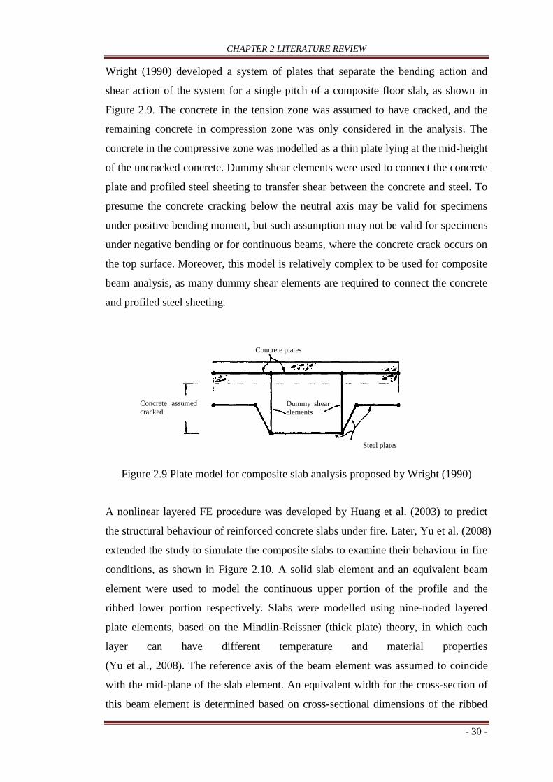
CHAPTER 2 LITERATURE REVIEW
- 30 -
Wright (1990) developed a system of plates that separate the bending action and
shear action of the system for a single pitch of a composite floor slab, as shown in
Figure 2.9. The concrete in the tension zone was assumed to have cracked, and the
remaining concrete in compression zone was only considered in the analysis. The
concrete in the compressive zone was modelled as a thin plate lying at the mid-height
of the uncracked concrete. Dummy shear elements were used to connect the concrete
plate and profiled steel sheeting to transfer shear between the concrete and steel. To
presume the concrete cracking below the neutral axis may be valid for specimens
under positive bending moment, but such assumption may not be valid for specimens
under negative bending or for continuous beams, where the concrete crack occurs on
the top surface. Moreover, this model is relatively complex to be used for composite
beam analysis, as many dummy shear elements are required to connect the concrete
and profiled steel sheeting.
Figure 2.9 Plate model for composite slab analysis proposed by Wright (1990)
A nonlinear layered FE procedure was developed by Huang et al. (2003) to predict
the structural behaviour of reinforced concrete slabs under fire. Later, Yu et al. (2008)
extended the study to simulate the composite slabs to examine their behaviour in fire
conditions, as shown in Figure 2.10. A solid slab element and an equivalent beam
element were used to model the continuous upper portion of the profile and the
ribbed lower portion respectively. Slabs were modelled using nine-noded layered
plate elements, based on the Mindlin-Reissner (thick plate) theory, in which each
layer can have different temperature and material properties
(Yu et al., 2008). The reference axis of the beam element was assumed to coincide
with the mid-plane of the slab element. An equivalent width for the cross-section of
this beam element is determined based on cross-sectional dimensions of the ribbed
Concrete plates
Concrete assumed cracked
Dummy shear
elements
Steel plates

CHAPTER 2 LITERATURE REVIEW
- 31 -
slab, and it shares the three middle nodes of the solid slab element on the reference
plane, as shown in Figure 2.10. The beam element is used to represent a group of ribs
of the composite slab, rather than defining several ribs, and the width of the beam
element is taken to be equivalent to the width calculated from the rib width ratio
(RWR). Although this model is relatively simple to build, the shear stud-beam
interaction cannot be defined at the exact shear stud locations because of the reduced
length of the single beam element which is used to represent the the group behaviour
of the profiled ribs.
Figure 2.10 An orthotropic slab element model proposed by Yu et al. (2008)
The trapezoidal concrete ribs were represented by equivalent rectangular ribs, which
were then implemented using shell elements, as shown in Figure 2.11 by
Kwasniewski (2010). The reference plane lies at the mid-plane of the composite slab
cross-section which is perpendicular to the composite slab height. The locations of
the concrete, rebar and profiled steel sheeting were adjusted with respect to the
reference plane for the profile without ribs, as shown in Figure 2.11. The weighting
factor has been introduced to account for the change in the location profile without
ribs. For the same profiled composite slab, Gillie (2000) chose the mid-plane, which
exactly coincides with geometric centroid of the cross-section. The inclined profiled
Reference plane Concrete layers
A real slab
element
An orthotropic
element
3D view of the
element
Reinforcement
Divide the
beam into
segments Reference plane
Steel layers
Divide the slab
into layers
ℎp
ℎs
Ribs
ℎs
ℎr
Concrete layers
W × Rib width ratio (R)
In plane temperature distribution
W (Width of slab element)
Type equation here.
Beam
Solid slab
𝑇1 𝑇2 𝑇1 𝑇2
𝑇1 𝑇2 𝑇1
𝑇2
𝑇2
𝑇1

CHAPTER 2 LITERATURE REVIEW
- 32 -
steel sheets were converted into equivalent vertical sheets and implemented in shell
element using corresponding layers of steel. The model proposed by Kwasniewski
(2010) utilises full shear interaction between the composite slab and steel beam.
Therefore, this model may not be suitable for analysis of composite beams with
partial shear interaction.
Figure 2.11 Equivalent composite slab model proposed by Kwasniewski (2010)
Recent efforts have been made by Main (2014) and Jeyarajan et al. (2015) to develop
simplified models for composite beams with trapezoidal steel decking. The model
developed by Main (2014) simplifies the trapezoidal shape of the ribs into alternating
strong and weak strips, where strong strips have a depth equal to the depth of the
composite slab and weak strips include only the concrete above the top of the steel
deck (Figure 2.12). The contribution from the steel deck is not included in the weak
strips. To incorporate the effect of shear studs, the analysis also considers the slip
characteristics based on Ollagard et al. (1971) model up to a certain slip of 5 mm.
After that, it is assumed that the shear force remains constant between 5 mm to 15
mm, after which it drops linearly to zero at a displacement of 25 mm. However, the
slip characteristics of shear studs can significantly vary depending on different
composite beam parameters, including the type of profiled steel sheeting, location of
0.9 mm Steel decking
Midplanes
Midplanes
Steel
Steel
Steel
Steel
slab
Concrete Anti-crack mesh T6@200mm

CHAPTER 2 LITERATURE REVIEW
- 33 -
shear studs and concrete strength. Further research is required on the descending
branch of the actual shear force-slip relationship of shear studs.
Figure 2.12 Simplified modelling of composite floor slab proposed by Main (2014):
(a) actual profile; (b) alternating strong and weak strips
The model proposed by Jeyarajan et al. (2015) simplifies the complicated trapezoidal
shape of composite slabs into an equivalent rectangular concrete slab with a uniform
thickness of hchs/2, where hc is the slab depth and hs is the height of the steel
decking. The steel decking is simplified as shown in Figure 2.13 and the
corresponding steel deck strip areas A1, A2, and A3 are calculated by multiplying the
deck thickness by its corresponding strip length. The deck strips are modelled as
rebars as shown in Figure 2.13(c). The equivalent area of a rebar (ai) is calculated
from the corresponding steel deck strip area (Ai) by equating their second moment of
area. The rebar areas are determined as: a1=A1, a2=A2 and a3=A3× hs2/[(hchs/2)
2].
The equivalent concrete slab is simulated using four-node homogeneous shell
element with reduced integration (S4R) and the equivalent rebars are defined using
*rebar option available in ABAQUS. Tie constraint is used to represent the bond
between the composite slab and steel beam. It should be noted that this model was
specifically developed for frame analysis, and can reasonably predict the behaviour
of beams with full shear interaction. However, for composite beams with partial
interaction, it may give unsafe predictions because this model virtually ignores the
slip between the slab and steel beam. Moreover, the depth of the equivalent
rectangular slab is reduced by ℎs/2 (Figure 2.13(c)). This reduction in depth might
not affect the membrane behaviour in beam axial direction because the equivalent
rectangular slab compensates the reduction of the concrete area by filling empty ribs,
but the lever arm (distance between the centroid of axial compression and tensile
Concrete
Welded wire reinforcement
Steel deck
Strong strip Weak strip
Concrete
Welded wire reinforcement
Steel deck

CHAPTER 2 LITERATURE REVIEW
- 34 -
forces in cross-section of the beam) will reduce, which can result in reduction of
moment capacity of the composite beam. The reduction can be higher for composite
beams with deep trapezoidal profiled steel sheeting.
Figure 2.13 Simplified model for composite slab proposed by Jeyarajan et al. (2015)
2.4 CFST column connections
A CFST column connection can be defined as a location where steel beams are
connected to the CFST column. Eurocode 3 (2005) classifies connections as rigid,
semi-rigid and pinned based on initial stiffness of connections as shown in Table 2.1.
Table 2.1 Classification of rigid, semi-rigid and pinned connections (Eurocode 3, 2005)
Type of connection Unbraced frames Braced frames
Rigid 𝑆j,ini ≥ 25 𝐾 𝑆j,ini ≥ 8 𝐾
Semi-rigid 25 𝐾 > 𝑆j,ini > 0.5 𝐾 8 𝐾 > 𝑆j,ini > 0.5 𝐾
Pinned 𝑆j,ini ≤ 0.5 𝐾 𝑆j,ini ≤ 0.5 𝐾
𝐾 = 𝐸𝐼
𝐿; E is the modulus of elasticity of steel, I is the moment of inertia and L is the
span length of the beam.
hc
A1
A2 A
2
A3
A3
hs
Concrete Simplified metal deck
Metal deck
Concrete
(a) Metal deck and concrete slab
(b) Equivalent metal deck and concrete slab
(c) Concrete slab with metal deck modelled as rebars with equivalent areas.
A2
A3 A
3
A2
A1
Metal deck strip area, Ai
hc −
hs ∕2
h
c − h
s ∕2 a
1
a2 a
2 a
3 a
3

CHAPTER 2 LITERATURE REVIEW
- 35 -
There are different techniques used to join steel beam to CFST columns including
welded connections, fin plate connections, through plate connections and endplate
connections. The welding can simply be done on the steel beam ends joining the
CFST column, however, in this method, tensile and shear forces are directly
transferred to the steel tube. Therefore, the steel tube can separate from the core
concrete and will be overstressed, especially in the case of thin-walled tubes (Hassan,
2016). Therefore, complex welded connections with an external and internal
diaphragm as well as stiffeners such as that reported by Qina et al. (2014) are used to
reduce the connection rotation thereby increasing connection stiffness (Hassan,
2016). For example, the CFST based frames utilising external diaphragms in CFST
columns (Han et al., 2011) is shown in Figure 2.1.
Fin plate connections consists of a fin plate which is welded to a steel tube and
connected to the steel beam by using structural bolts, as shown in Figure 2.14 (a).
This type of connection can be easily installed on site. The stiffness of fin plate
connections is relatively lower than that of welded connections, and tube wall tearing
is often observed (Kurobane et al., 2004). On the other hand, a steel plate is slotted
through the hollow section and welded to the two opposite faces, as shown in Figure
2.14 (b), which is generally termed as through plate connections. Through plate
connections have an advantage of engaging much more of the cross-section in load
resistance and, therefore, it has higher capacity than the counterpart fin plate
connections, and yet the fabrication process is difficult and expensive (Voth and
Packer, 2016).
(a) Typical fin plate connection
(Kurobane et al., 2004)
(b) Typical through plate connection
(Voth and Packer, 2016) Figure 2.14 Typical fin plate and through plate connections

CHAPTER 2 LITERATURE REVIEW
- 36 -
In endplate connections, a steel plate (end plate) is welded to the end of a steel beam
and connected to the CFST column by using structural bolts, such as blind bolts
(special type of structural bolts which can be installed from the outside of the steel
tube), as shown in Figure 2.15. Depending on the length of the end plate, end plate
connections can be classified into three categories: header end, extended, and flush.
If the length of the endplate is less than the height of the steel beam, it is called a
header endplate connection, whereas if the length of the endplate is more than the
depth of the steel beam, it is termed as an extended endplate connection. Finally, if
the length of the endplate is equal to the height of the steel beam, it is called a flush
endplate connection. The initial stiffness and ultimate capacity of the flush endplate
connection are relatively higher than those of header endplate connections, but they
are lower than those of the extended endplate connection (Hassan, 2016).
Figure 2.15 Typical blind-bolted CFST column connection (Hassan, 2016)
2.4.1 Experimental studies of CFST column connections
The composite beam-to-CFST columns with blind-bolted endplate connections can
be favourably used in multi-storey building construction, because of its simplicity
and economy both in fabrication and assembly (Thai et al., 2017). Moreover, the
experimental studies on CFST column connections conducted by Tao et al. (2017)
proved that the initial stiffness and flexural resistance were significantly increased in
the presence of composite slab. Therefore, this thesis is primarily focused on CFST
column connections with composite slab including blind-bolted endplate connections.
Several collections of test data are available in literature for the composite
(a) (b)
Reinforcing bar Shear connectors
Blind bolts
Steel beam
CFST column
Welded endplate

CHAPTER 2 LITERATURE REVIEW
- 37 -
connections with steel column sections, including the tests conducted by Anderson
and Najafi (1994), Xiao et al. (1994), Li et al. (1996b), Liew et al. (2000), and da
Silva et al. (2001). However, limited test data on CFST column connections with
composite slab utilising blind bolted endplate connections (hereafter referred to as
“composite connections”) are available in the literature, such as those reported by
Loh et al. (2006), Mirza and Uy (2011), Thai et al. (2017), and Tao et al. (2017a).
Loh et al. (2006) conducted five tests on CFST column connections with a novel
approach of blind bolting flush endplates to square hollow columns filled with
concrete. The effect of stud spacing (265, 480 and 800 mm) and the percentage of
reinforcement (0.65, 1.3 and 1.95) was investigated. It was found that for composite
connection specimens with partial shear connection, ductility was enhanced.
Meanwhile, the ultimate moment capacity can be increased by higher levels of
reinforcement up to a certain limit. Therefore, the favourable percentage of
reinforcement was suggested to be between 1.0% and 1.5%.
Mirza and Uy (2011) tested two composite connections: one specimen under static
loading and the other one under quasi-static cyclic loading. Although both specimens
have a similar configuration, the measured ultimate capacity was higher for the
specimen tested under static loading, which suggests that the composite connection
behaviour is also influenced by the loading type.
Thai et al. (2017) conducted an experimental study of four blind bolted endplate
connections representing the internal region of a composite frame. The effects of
different shapes (square and circular) of a CFST column were investigated, as well as
different endplate types (extended endplate with four bolt rows and flush endplate
with three bolt rows). In general, all four specimens failed in a ductile manner with
significant rotation capacity. The observed deformation of the endplate at the bolt
row close to the concrete slab was significant; however, the bolt rows furthest from
the concrete remained intact. The concrete cracks originated initially around the
perimeter of the column and propagated toward the slab edges, before finally
forming a transverse crack across the slab width. The composite connection with a
circular CFST column had 13.5% and 18.3% higher moment capacity and initial
stiffness, respectively, as compared to its counterpart with a square CFST column

CHAPTER 2 LITERATURE REVIEW
- 38 -
having equivalent section capacity. Meanwhile, the composite connections with
extended endplates resulted in an enhancement of moment resisting capacity and
initial stiffness by 15% and 22.6%, respectively, as compared to the composite
connections with flush endplates.
Tao et al. (2017a) performed seven experiments of composite connections. Various
parameters were investigated: the influence of the presence of slab, binding bars in
the connection region, types of steel used for the column (carbon or stainless steel),
loading type (monotonic or cyclic). The failure of the specimen without composite
slab, tested under monotonic loading, was dominated by the local outward
deformation of the square steel tube, which resulted from the pull-out force of the top
row of blind bolts. Significant differences were observed for the specimens with
composite slab, such as the initial damage which was observed in the form of
transverse concrete cracks near the column. Upon further loading, fracture of the
continuous longitudinal reinforcement was observed at its ultimate moment capacity.
Following this, the load-carrying capacity dropped sharply and on increasing further
deflection, profiled sheeting fracture was observed. The effects of binding bars had
some advantages in increasing the joint capacity, but the types of material of steel
tubes were found to have very minor influence. The cyclic loading had obvious
detrimental influences on the stiffness of composite connection.
2.4.2 Simplified numerical modelling of CFST column connections
To develop simplified numerical models for CFST column connections is very
important to analyse the behaviour of composite frames. Detailed FE models (Figure
2.16(a)) such as that developed by Mirza and Uy (2011), Atei and Bradford (2013),
Tizani et al. (2013), Hassan (2016) can be used to accurately predict the behaviour of
composite connections. Such models can also be used for behavioural study, but are
impractical for routine design and frame analysis. On the other hand, simplified
models (Figure 2.16 (b)) are computationally very efficient to conduct frame analysis.
It is easy to simulate pinned or rigid connections by using connector elements such
as CONN3D2 available in ABAQUS. However, for semi-rigid connections, either
the moment-rotation (𝑀 − 𝜙) relationship calculated using analytical models can be
defined through a single connector element (Figure 2.16 (b)) or various connector

CHAPTER 2 LITERATURE REVIEW
- 39 -
elements with calculated stiffness for each component need to be defined, such as
that developed by Kang et al. (2014) as shown in Figure 2.17. When various
connector elements are used, the convergence problem can arise, and it is relatively
difficult for large frame analysis. In contrast, the single connector element can be
easily used for frame analysis if the 𝑀 − 𝜙 relationship is known.
Figure 2.16 Typical 3D FE and simplified models of CFST column connections
Figure 2.17 Typical joint model developed by Kang et al. (2014)
(a) Detailed FE model
(b) Simplified model
Connector
elements
Connector
elements
CFST column
Composite slab

CHAPTER 2 LITERATURE REVIEW
- 40 -
There are a few analytical models available in the literature to ascertain the parameters
required to determine 𝑀 − 𝜙 relationships for flush endplate connections for steel
beam-to-steel column composite connections, including Aribert and Lachal (1992),
Anderson and Najafi (1994), Ahmed and Nethercot (1997), Liew et al. (2000) and Al-
Aasam (2013). Recently, 𝑀 − 𝜙 relationships for flush endplate connections for steel
beam-CFST column connections using blind bolts were developed by Thai and Uy
(2015) and Hassan (2016). Such 𝑀 − 𝜙 relationships can be implemented in the
simplified numerical modelling of isolated connections, as well as composite frames.
2.5 Steel-concrete composite frames
As described in sections 2.2, 2.3 and 2.4, CFST columns, composite beams and
composite connections have excellent mechanical performance and are easy to
construct. Therefore, steel-concrete composite frames utilising CFST columns,
composite beams and composite connections are widely used in construction
industry. The literature review on the experimental studies of composite frames is
presented below, along with the design approaches of frames.
2.5.1 Experimental studies of composite frames
In the literature, limited experimental studies of composite frames are available. A
summary of composite frames with steel columns tested by Leon et al. (1990), Jarett
and Grantham (1992), Grantham and Jarret (1993), Li et al. (1996a) and
Dhanalakshmi et al. (2002) was presented in Wang and Li (2007). Wang and Li
(2007) further conducted an experimental study of two-storey steel-concrete
composite frames with a steel column section. The beam-column connection consists
of a flush end-plate connection which is welded at the beam end and bolted to the
column flange. Similarly, Guo et al. (2013) tested a four bay composite frame with
steel column sections, where the middle column was not supported, in order to
simulate the loss of a column and investigate the progressive collapse resistance of
composite frames.
The composite frames with steel beams welded to square CFST columns were tested
by Han et al. (2008). In total, six one-bay one-storey frames were tested in order to

CHAPTER 2 LITERATURE REVIEW
- 41 -
investigate their behaviour. Similarly, Han et al. (2011) conducted six tests on a one-
bay one-storey composite frame with a steel beam welded to circular CFST columns.
A two-bay two-storey frame with square CFST columns and steel beams was tested
by Wang et al. (2010) under a cyclic horizontal load. Only the composite frame
specimens tested by Nie et al. (2012) have composite beams so far, so as to
investigate the effects of composite action on the behaviour of composite frames with
CFST columns and composite slab. The test results demonstrate the significant
increase in stiffness, strength and energy dissipation capacity of such frames when
composite slab was used.
2.5.2 Literature review on advanced analysis of composite frames
Traditionally, the design of structural frames is a member-based (indirect method)
design, which has a history of over one hundred years and is still in practice, as
described in Chapter 1. On the other hand, design by advanced analysis (direct
method) has been allowed in some codes, such as AISC360-10 (2010) and AS4100
(1998), but is limited to steel structures. It should be noted that the majority of the
past studies on advanced analysis were focussed on bare steel frames including Goto
and Chen (1987), Ziemian et al. (1992), Liew et al. (1993), Kim and Chen (1999),
Thai and Kim (2011), Zhang and Rasmussen (2013), and Thai et al. (2016). There
are a few studies on advanced analysis for steel-concrete composite frames with
reinforced concrete columns (Liu et al., 2012), steel columns (Salari and Spacone,
2001; ) and steel columns encased in concrete (Chiorean, 2013).
For the frames with CFST columns and composite beams, research on advanced
analysis is still in its infancy. One possible reason for this is that the experimental
data for such composite frames is very limited. Secondly, the fundamental behaviour
of composite frames is not yet fully understood (Nie et al., 2012). Although some
efforts can be found in the literature utilising the distributed plasticity approach for
2D frames with CFST columns (Hajjar et al., 1988; Hajjar and Molodan, 1988) or
utilising some techniques like incremental-iterative arc-length technique for the
ultimate strength analysis of composite steel-concrete cross-sections subjected to
axial force and biaxial bending (Chireon, 2010), there is a need to develop more
robust and versatile simplified numerical models which can properly account for the

CHAPTER 2 LITERATURE REVIEW
- 42 -
interaction between the CFST columns, composite beams, and various types of
composite connections.
2.6 Summary of research gaps
This thesis primarily focuses on developing a framework to conduct advanced
analysis of steel-concrete composite frames by developing simplified numerical
models for CFST columns, composite beams and composite connections. Prior to
developing simplified models, the detailed fundamental behaviour of each
component of composite frames needs to be fully understood. The scope of this
thesis is primarily limited to CFST columns with circular cross-section, composite
beams with headed studs welded through profiled deck, and composite beam-to-
CFST column connections with blind-bolted endplate connections as described in
section 2.1. Therefore, the literature review is conducted on this periphery and the
identified major research gaps are described below.
Behaviour of CFST columns can be predicted accurately using detailed finite
element (FE) models, but such models are impractical for routine design and frame
analysis. In contrast, fibre beam element (FBE) models can be used to achieve the
balance between accuracy and simplicity, but the material models themselves have to
account for the interaction between steel and concrete. The material models available
in the literature for steel and concrete in CFST columns are not suitable for some
cases, especially when considering the rapid development and application of high
strength materials and/or thin-walled steel tubes. Therefore, computationally simple
yet accurate and versatile steel and concrete material models need to be developed.
The fundamental behaviour of composite beams with profiled steel sheeting is not
yet fully understood. Detailed 3D FE models can be used to accurately simulate the
behaviour of composite beams and can be utilised to understand the behaviour of
composite beams, especially the complex interaction between shear studs and
concrete. However, previous FE models adopted various assumptions to simplify the
modelling of some complex interactions, such as the interaction between the shear
studs and concrete. Accordingly, those FE models have limitations in capturing
certain types of failure modes, and cannot reflect the actual bondslip behaviour of

CHAPTER 2 LITERATURE REVIEW
- 43 -
the shear studs. The shear studs’ strength in composite beams is obtained indirectly
by measuring the difference in axial forces on adjacent cross-sections of the steel
beam; however, the contribution of profiled steel sheeting in carrying axial force is
not yet known. In this regard, the direct method to obtain shear stud strength, as well
as axial force carried by the profiled steel sheeting, needs to be developed. Therefore,
there is an urgent need to develop a general 3D FE model for composite beams with
profiled steel sheeting, by considering the realistic interaction between different
components, possible fracture of the shear studs and profiled steel sheeting, along
with concrete damage.
In structural analysis and design, it is favourable to use simplified models
incorporating realistic shear force-slip behaviour of shear studs in composite beams.
However, available shear force-slip models are based on push tests, and the
behaviour of shear studs obtained from push tests cannot reflect the actual behaviour
of shear studs in composite beams. Therefore, based on detailed FE modelling, the
full-range shear force-slip curves, including failure, can be generated. Such generated
curves can be used to develop realistic shear force-slip models for shear studs in
composite beams. Furthermore, such models can be used to represent stud behaviour
in simplified numerical modelling of composite beams. Such simplified modelling of
composite beams is a computationally efficient technique for conducting analysis
and design, and can be further used in advanced analysis of composite frames, as the
3D FE models are impractical to use for frame analysis.
Similarly, 3D FE models can be used to accurately analyse the composite beam-to-
CFST column connections with endplates and blind bolts (semi-rigid joints), but such
approach is tedious and impractical for frame analysis. On the other hand, simplified
numerical models with connector elements representing momentrotation relationship
can be used for analysis of such composite connections. However, such models
detailed in the literature are generally only used for steel beam-to-steel columns.
Therefore, there is a need to develop relatively simple numerical models of composite
connections, which can be further used for advanced analysis of composite frames.

CHAPTER 2 LITERATURE REVIEW
- 44 -
A considerable number of research has been conducted in the past on advanced
analysis, and as a result, the design philosophy of structures can be shifted from
indirect member-based design to direct design by advanced analysis. Nevertheless,
those research works are mainly limited to steel frames, possibly because of the
limited number of composite frame test data, and the behaviour of individual
members of composite frames is not fully understood. Despite the developments in
computing technology, detailed FE models are still impractical to conduct advanced
analysis in a routine basis because such models are tedious to build. Moreover,
numerical convergence issues and the time-commitment limit the application of
detailed FE models to conduct advanced analysis. Therefore, there is persuasive
reason to develop computationally efficient simplified numerical models for
composite frames, which can be developed based on the simplified numerical models
of CFST columns, composite beams and composite connections.

CHAPTER 3 SIMPLIFIED NUMERICAL MODELLING OF CIRCULAR CONCRETE-FILLED
STEEL TUBULAR COLUMNS
- 45 -
CHAPTER 3
SIMPLIFIED NUMERICAL MODELLING OF
CIRCULAR CONCRETE-FILLED STEEL TUBULAR
COLUMNS
3.1 Introduction
Detailed three-dimensional (3D) finite element (FE) models can be developed to
precisely predict the behaviour of composite structures, but such models are tedious
to build and impractical for the analysis of large structural systems or for routine
design. On the other hand, fibre beam element (FBE) models can be utilised to
achieve the balance between efficiency and accuracy in simulating CFST columns.
This is due to the simplicity in simulation and high computational efficiency;
however, the material models need to be defined accurately as the material models
themselves have to account for the interaction between the steel and concrete
surfaces. Although a few steel and concrete stress (σ)strain (ε) models are available
for FBE modelling of circular CFST columns, they have certain limitations, as
described in Chapter 2, and may not accurately predict the behaviour of CFST
columns, especially when considering the rapid development and application of high
strength materials and/or thin-walled steel tubes. Moreover, the available models are
unable to accurately account for the softening of steel stress in a longitudinal
direction due to the developed hoop stress. Therefore, there is a need to develop
versatile and effective steel and concrete material properties for FBE modelling of
circular CFST columns that can be utilised to accurately predict full-range,
loaddeformation curves for sufficiently wide practical range of such columns.
In this chapter, the fundamental behaviour of circular CFST columns was thoroughly
investigated using 3D FE modelling and the data required to develop simplified
material models were extracted. Then, regression analysis was conducted to

CHAPTER 3 SIMPLIFIED NUMERICAL MODELLING OF CIRCULAR CONCRETE-FILLED
STEEL TUBULAR COLUMNS
- 46 -
determine the best-fit equations and finally, versatile simplified material models of
steel and concrete in the CFST columns required for FBE modelling were developed,
as described in Section 3.4. The FBE modelling was conducted using the finite
element package ABAQUS. Since ABAQUS does not have default options to input
such material models, they were implemented in ABAQUS through user subroutine
UMAT. The predictions from the proposed simplified numerical modelling
correlated well with the experimental, as well as the 3D FE modelling results, as
described in Section 3.5.
3.2 Finite element (FE) modelling
Concrete-filled steel tubular (CFST) columns were investigated using 3D FE analysis
to understand the fundamental behaviour of steel and core concrete. A versatile 3D FE
model was developed by Tao et al. (2013b) for circular, as well as rectangular CFST
columns, after extensive verification with experimental results; this model was used
in the present study to simulate circular CFST columns. A typical 3D FE model built
in ABAQUS is shown in Figure 3.1(a).
Figure 3.1 Typical sketch of solid FE and FBE models for circular CFST columns
Integration points
(b) FBE model (a) Solid FE model
Steel tube
Column load
Render view of FBE
model
Concrete
Steel as *rebar elements
Cross-section of FBE
Core concrete as B31 element
Fibre elements
Concrete Steel tube
(c) Discretisation of the steel tube and concrete core

CHAPTER 3 SIMPLIFIED NUMERICAL MODELLING OF CIRCULAR CONCRETE-FILLED
STEEL TUBULAR COLUMNS
- 47 -
The steel tube and concrete were simulated by four-node shell elements with reduced
integration (S4R) and 8-node brick elements with 3 translational degrees of freedom
at each node (C3D8R) respectively. The mesh size of each discretised element was
taken as D/15, where D is the overall diameter of the circular tube. In general, the
detailed model contained over 4000 elements for a typical stub column. The surface-
to-surface contact option available in ABAQUS was used to model the interaction
between the steel tube and concrete where the tangential friction coefficient between
the steel tube and core concrete was defined as 0.6 (Tao et al., 2013). The boundary
conditions were applied in such a way that all degrees of freedom were restrained at
the ends of CFST columns except at the loaded end which was allowed to move
along the axial direction.
3.2.1 Steel material properties for FE modelling
The collected test database of CFST columns contained normal carbon steel in CFST
columns. Therefore, structural steel 𝜎 − 𝜀 curves proposed by Tao et al. (2013a)
were utilised to simulate the material properties of the steel tubes in CFST columns
by Tao et al. (2013b) (Figure 3.2, Eq. 3.1).
Figure 3.2 Structural steel 𝜎 − 𝜀 model (Tao et al., 2013a)
𝜎 =
{
𝐸s𝜀 0 ≤ 𝜀 < 𝜀y𝑓y 𝜀y ≤ 𝜀 < 𝜀p
𝑓u − (𝑓𝑢 − 𝑓𝑦) ∙ (𝜀u − 𝜀
𝜀u − 𝜀p)
𝑝
𝜀p ≤ 𝜀 < 𝜀u
𝑓u 𝜀 ≥ 𝜀u
(3.1)
Str
ess
σ
Strain e
fu
fy
ey eu ep
arctan(Ep)
arctan(Es)

CHAPTER 3 SIMPLIFIED NUMERICAL MODELLING OF CIRCULAR CONCRETE-FILLED
STEEL TUBULAR COLUMNS
- 48 -
where fy and 𝜀y are the corresponding yield stress and strain of steel respectively;
𝜀p is the strain at the onset of strain hardening (Eq. 3.2); 𝑓u (Eq. 3.3) and 𝜀u (Eq. 3.4)
are the ultimate strength and corresponding strain respectively; 𝑝 is the strain
hardening exponent (Eq. 3.5); 𝐸p is the initial modulus of elasticity at the onset of
strain-hardening (Eq. 3.6).
𝜀p = {15𝜀y 𝑓y ≤ 300 MPa
[15 − 0.018(𝑓y − 300)]𝜀y 300 < 𝑓y ≤ 800 MPa (3.2)
𝑓u = {[1.6 − 2 × 10⁻³(𝑓y − 200)] 𝑓y 200 < 𝑓y ≤ 400 MPa
[1.2 − 3.75 × 10⁻⁴(𝑓y − 400)] 𝑓y 400 < 𝑓y ≤ 800 MPa (3.3)
𝜀u = {100𝜀y 𝑓y ≤ 300 MPa
[100 − 0.15(𝑓y − 300)]𝜀y 300 < 𝑓y ≤ 800 MPa (3.4)
𝑝 = 𝐸p (𝜀u−𝜀p
𝑓u−𝑓y) (3.5)
𝐸p = 0.02𝐸s (3.6)
It should be noted that the steel model used by Tao et al. (2013b) is only valid when
the yield stress (𝑓y) is 800 MPa or less. The work presented herein aims to extend the
validity range of 𝑓y to 960 MPa. Based on the coupon test results (Figure 3.3)
reported by Shi et al. (2012), Qiang et al. (2013) and Shi et al. (2015), a linear
equation (Eq. 3.7) is proposed to determine ep when fy is between 800 MPa and 960
MPa. Meanwhile, 𝑓u is taken as 1.05𝑓y for steel with a 𝑓y between 800 MPa and 960
MPa (Eq. 3.8). A linear equation, as presented in Eq. (3.9), is proposed to determine
eu when fy is between 800 MPa and 960 MPa based on ten coupon test results of
S960 steel reported by Shi et al. (2012), Qiang et al. (2013) and Shi et al. (2015).
𝜀p = {
15𝜀y 𝑓y ≤ 300 MPa
[15 − 0.018(𝑓y − 300)]𝜀y 300 < 𝑓y ≤ 800 MPa
[6 − 0.03125(𝑓y − 800)]𝜀y 800 < 𝑓y ≤ 960 MPa
(3.7)

CHAPTER 3 SIMPLIFIED NUMERICAL MODELLING OF CIRCULAR CONCRETE-FILLED
STEEL TUBULAR COLUMNS
- 49 -
𝑓u = {
[1.6 − 2 × 10⁻³(𝑓y − 200)] 𝑓y 200 < 𝑓y ≤ 400 MPa
[1.2 − 3.75 × 10⁻⁴(𝑓y − 400)] 𝑓y 400 < 𝑓y ≤ 800 MPa
1.05𝑓y 800 < 𝑓y ≤ 960 MPa
(3.8)
𝜀u = {
100𝜀y 𝑓y ≤ 300 MPa
[100 − 0.15(𝑓y − 300)]𝜀y 300 < 𝑓y ≤ 800 MPa
[25 − 0.1(𝑓y − 800)]𝜀y 800 < 𝑓y ≤ 960 MPa
(3.9)
Figure 3.3 Stress-strain curves of high strength steel
3.2.2 Concrete material properties for FE modelling
The material properties of confined concrete are different from the properties of
unconfined concrete because of the confinement effect provided by the steel tube to
the concrete. The behaviour of confined concrete also depends on the thickness of
the steel tube, its strength grade and the width-to-thickness ratio (D/t ratio for
circular columns). A three stage versatile confined concrete material model was
proposed by Tao et al. (2013b) in order to simulate core concrete material behaviour
in CFST columns, as shown in Figure 3.4, which is able to represent the strain
hardening/softening rule of concrete confined by steel tubes. As shown in Figure 3.4,
from point O to A, there is none to very little interaction between the steel tube and
the concrete. For that reason the ascending branch of the stress-strain relationship
(Eq. 3.10) of unconfined concrete was used until the peak strength 𝑓𝑐′ was reached.
The plateau from point A to point B represents the increased peak strain of the
concrete from confinement. It was assumed that any strength increase at this stage
would be captured in the detailed 3D FE simulation through the interaction between
0
200
400
600
800
1000
1200
0 0.1 0.2 0.3
Str
ess
σ (
MP
a)
Strain e
Shi et al. (2012)
Qiang et al. (2013)
Shi et al. (2015)

CHAPTER 3 SIMPLIFIED NUMERICAL MODELLING OF CIRCULAR CONCRETE-FILLED
STEEL TUBULAR COLUMNS
- 50 -
the steel tube and the concrete. This is possible because of the capabilities of detailed
3D FE analysis to capture composite action between the different components. Such
an increase in strength of concrete in CFST columns is further presented in Section
3.4. Beyond point B, a softening portion with increased ductility resulting from the
confinement was defined. The ascending curve OA was defined using the model
proposed by Samani and Attard (2012).
Figure 3.4 Confined concrete 𝜎 − 𝜀 curves (Tao et al., 2013)
𝜎
𝑓c′=
𝐴𝑋 + 𝐵 𝑋2
1 + (𝐴 − 2)𝑋 + (𝐵 + 1)𝑋2 0 < 𝜀𝑐 < 𝜀𝑐𝑜
(3.10)
where
𝑋 = 𝜀
𝜀𝑐0 (3.11)
𝐴 = 𝐸c𝜀c0𝑓c′
(3.12)
𝐵 = (𝐴 − 1)2
0.55− 1 (3.13)
The strain at peak stress under uniaxial compression 𝜀co was calculated by using the
equation proposed by De Nicolo et al. (1994).
𝜀c0= 0.00076 + √(0.626 𝑓c′ − 4.33) × 10−7 (3.14)
The strain at point B 𝜀ccwas calculated based on Samani and Attard (2012).
Str
ess
σ
Strain e
𝑓c′
ec0 ecc
Confined concrete
Unconfined concrete fr
C
B A
O

CHAPTER 3 SIMPLIFIED NUMERICAL MODELLING OF CIRCULAR CONCRETE-FILLED
STEEL TUBULAR COLUMNS
- 51 -
𝜀cc
𝜀c0 = 𝑒𝑘
(3.15)
where 𝑘 = (2.9224 − 0.00367 𝑓𝑐′) (
𝑓𝐵
𝑓𝑐′)0.3124+0.002𝑓𝑐
′
where 𝑓B is the confining stress provided to the concrete at point B.
𝑓B =(1 + 0.027𝑓y) ∙ 𝑒
−0.02𝐷𝑡
1 + 1.6𝑒−10 ∙ (𝑓c′)4.8
(3.16)
For the descending branch of the concrete model, an exponential function proposed
by Binici (2005) was used which is
𝜎 = 𝑓r + (𝑓c′ − 𝑓r)𝑒𝑥𝑝 [−(
𝜀−𝜀cc
𝛼)𝛽
] ε≥ 𝜀cc (3.17)
where 𝑓r is the residual stress as shown in Figure 3.4, α and β are parameters
determining the shape of the softening branch. The expression for 𝑓r is proposed as:
𝑓r = 0.7 (1 − 𝑒−1.38𝜉c)𝑓c′ ≤ 0.25𝑓c
′ (3.18)
α = 0.04 −0.036
1+𝑒6.08𝜉𝑐−3.49 (3.19)
where 𝜉𝑐 is the confinement factor which is obtained as
𝜉c =𝐴s𝑓y
𝐴c 𝑓c′ (3.20)
𝐴s and 𝐴c are the cross-sectional areas of the steel tube and concrete respectively.
The value of β was taken as 1.2 and 0.92 for circular and rectangular columns
respectively (Tao et al. 2013b).
3.3 Fibre beam element (FBE) modelling
The FBE model is an advanced tool in which the member is divided into a number of
longitudinal fibre elements, as shown in Figure 3.1 (b) and (c). The geometric
characteristics to be defined for a fibre are its area and location with respect to the
cross-section (Taucer et al. 1991). In FBE modelling of CFST columns, the
interaction between the steel tube and concrete core needs to be specifically

CHAPTER 3 SIMPLIFIED NUMERICAL MODELLING OF CIRCULAR CONCRETE-FILLED
STEEL TUBULAR COLUMNS
- 52 -
considered in the input material models to obtain accurate results. Due to the
computational efficiency, FBE models have been commonly used in advanced
analysis of frames, where the design process can be simplified as the system strength
can be directly assessed from the analysis without the need for calculating the
effective length factor or checking the specification of beam-column interaction
equations (Zhang and Rasmussen 2013). In particular, FBE models are suited to
analyse structures subjected to extreme events, such as fire, blast, seismic, and other
abnormal events.
3.3.1 Assumptions used in FBE modelling
In conducting FBE modelling of CFST stub columns, the following assumptions
were adopted:
(a) A plane section remains plane during deformation;
(b) A perfect bond exists between the steel tube and concrete infill;
(c) The longitudinal stress of any fibre is only decided by the strain at that point;
(d) The effects of concrete creep and shrinkage are not considered; and
(e) Steel fracture is not considered since it typically does not occur until very late
in loading histories (Denavit and Hajjar 2012).
Therefore, the results of the FBE modelling are only valid before the steel reaches its
tensile strain, which is sufficient for the needs of normal analysis.
3.3.2 Procedure for FBE modelling
To generate the FBE model in ABAQUS, the steel tube and concrete core were sub-
divided into a finite number of longitudinal fibres, as shown in Figure 3.1 (c). The
concrete was simulated using a 2-node linear beam element (B31), which is a first-
order, three-dimensional Timoshenko element. By changing the number of material
integration points, the number of concrete fibres could be changed accordingly. For
the steel tube, the steel fibres were directly defined as material integration points
using the *rebar option available in the keywords platform in ABAQUS (Wang et al.
2013). The steel and concrete material models were defined through a UMAT
subroutine which was written by the author using FORTRAN programming language
and implemented in ABAQUS through Microsoft Visual Studio.

CHAPTER 3 SIMPLIFIED NUMERICAL MODELLING OF CIRCULAR CONCRETE-FILLED
STEEL TUBULAR COLUMNS
- 53 -
Sensitivity analysis was conducted to determine the influence of section discretisation
on the simulation accuracy. For CFST stub columns under axial compression, it was
found that the effect of the mesh size and section discretisation had no obvious
influence on the predicted axial load (𝑁)strain (𝜀) curves. Identical specimens H-
58-1 and H-58-2 and specimen CU-070 tested by Sakino and Hayashi (1991) and
Huang et al. (2002) were taken as examples, as shown in Figure 3.5 (a) and (b),
respectively. Almost the same predictions were obtained using different mesh sizes
and different numbers of fibre elements. This is understandable since the whole stub
column was under axial compression. Similar behaviour was observed by Patel et al.
(2014) for axially loaded concrete-filled stainless steel short columns. However,
section discretisation is a prerequisite for fibre element modelling (Patel et al. 2014).
In this study, the steel tube was divided into 16 longitudinal fibre elements, and 17
longitudinal material integration points were specified for the core concrete.
Meanwhile, the CFST column was divided into 10 elements along its length. In
specifying the boundary conditions, only vertical displacement at the top end was
allowed whereas all other translational degrees of freedom were restrained for both
ends of the CFST column.
(a) Influence of mesh size (b) Number of fibre elements
Figure 3.5 Influence of mesh size and number of fibre elements of steel tube
3.4 Development of material models for FBE modelling
For a CFST column under axial compression, interaction can develop between the
steel tube and concrete. Thus, the concrete can have increased compressive strength
0
700
1400
2100
0 10000 20000 30000 40000
Axia
l lo
ad N
(kN
)
Axial strain e (me)
Test (Sakino and Hayashi, 1991)FE model
D=174 mm, t=3 mm, L=360 mm
fy=265.8 MPa, fc'=45.7 MPa, xc=0.42
Specimen,
H-58-1 and H-58-2
Mesh size 3.6 mm
Mesh size 18 mm
Mesh size 36 mm
0
1000
2000
3000
4000
0 10000 20000 30000 40000
Axia
l lo
ad N
(kN
)
Axial strain e (me)
Test (Huang et al., 2002)
FE model
D=280 mm, t=4 mm, L=840 mm
fy=272.6 MPa, fc'=31.15 MPa, xc=0.52
Specimen CU-070
8 fibre elements
16 fibre elements 64 fibre elements
CHAPTER 3 SIMPLIFIED NUMERICAL MODELLING OF CIRCULAR CONCRETE-FILLED
STEEL TUBULAR COLUMNS
- 54 -
and ductility due to the confinement of the steel tube. Meanwhile, tensile hoop
stresses will develop in the steel tube, which reduces its load-carrying capacity in the
axial direction (Lai and Varma 2016). During the loading process, the confining
stresses change with the increase in axial deformation. Furthermore, local buckling
of the steel tube might occur during the process, which affects the interaction
between the steel tube and concrete. The combined influence of all these factors is
complex and needs to be properly considered when proposing material models.
To develop simplified material models for the steel tube and concrete in CFST
columns, the detailed FE model developed by Tao et al. (2013b) was used to analyse
circular CFST stub columns with various parameter combinations. From the
simulation, axial stresses of all the elements were extracted from the middle section
of the CFST column. The stresses of all the steel elements were then “averaged” to
obtain the effective stress (𝜎) for the steel as a function of the axial strain (𝜀). A
similar procedure was adopted to obtain the effective uniaxial 𝜎 − 𝜀 relationship for
the concrete. Since the averaged 𝜎 − 𝜀 curves had already incorporated the influence
of the interaction between the steel tube and concrete, these 𝜎 − 𝜀 curves can be
directly used in FBE modelling. Based on a total of 212 FE simulations, regression
analysis was conducted in the following subsections to propose suitable steel and
concrete material models to represent the effective uniaxial 𝜎 − 𝜀 relationships. The
regression analysis is validated within the parameter range shown in Table 3.1.
3.4. 1 Steel material model
3.4.1.1 Characteristics of the stress-strain curves for steel
In 3D FE modelling, normally only a single 𝜎 − 𝜀 relationship is required as input
for steel; Tao et al. (2013b) used an elastic-plastic model with strain-hardening which
was also adopted in the present study. Typical CFST stub columns with different
confinement factors (𝜉c) were analysed using the 3D FE modelling; the obtained
effective 𝜎 − 𝜀 curves of steel are compared in Figures 3.6 and 3.7. These effective
𝜎 − 𝜀 curves are quite different from the input 𝜎 − 𝜀 curve. This is owing to the
development of hoop stresses in the steel tube and possible local buckling of the steel
tube. This observation highlights the need to develop a robust effective 𝜎 − 𝜀 model
for steel in FBE modelling.

CHAPTER 3 SIMPLIFIED NUMERICAL MODELLING OF CIRCULAR CONCRETE-FILLED
STEEL TUBULAR COLUMNS
- 55 -
Table 3.1. Parameter range of simulated CFST specimens
The parametric studies conducted for circular CFST columns where the steel and
concrete 𝜎 − 𝜀 curves were obtained from the simulation are presented in Figures 3.6
and 3.7. Different grades of steel (𝑓y = 200, 300, 400, 600, 800 and 960 MPa)
were utilised to conduct the parametric analysis and the CFST columns had different
thickness to simulate different confinement factors while keeping the outer diameter
of the columns constant to 220 mm. The concrete unconfined strength (𝑓c′) was 50
MPa for all CFST columns. L/D ratio was kept equal to 3, therefore the columns
were considered to be stub columns (Tao et al. 2013(b)). In general, the effective
𝜎 − 𝜀 curves of steel obtained from different columns coincided with each other very
well in the elastic stage. This can be explained by the weak interaction between the
steel tube and concrete in the beginning (Han et al., 2014a; Liew and Xiong, 2012,
Number of
specimens D (mm) 𝑡 (mm) 𝜉c 𝐷/𝑡 L/D 𝑓y(MPa) 𝑓c
′(MPa) Source
7 76-153 1.7-4.1 1.6-2.6 30-48 2.0 363-605 21-34 Gardener and Jacobson (1967)
1 169 2.6 0.563 65 1.8 317 37 Gardener (1968)
23 150 2.0-4.3 0.65-1.6 35-75 3.0 280-336 18-29 Tomii et al. (1977)
12 174-179 3.0-9.0 0.4-3.1 20-58 2.0 248-283 22-46 Sakino and Hayashi (1991)
2 190 1.15 0.05 165 3.5 202.8 110.3 O’Shea and Bridge (1994)
10 165-190 0.9-2.8 0.05-0.54 59-221 3.5 186-363 41-80 O’Shea and Bridge (1998)
2 141 3.0-6.5 0.92-2.8 22-47 4.3 285-313 24-28 Schneider (1998)
12 108-133 1.0-4.7 0.07-0.71 24-125 3.5 232-358 92-106 Tan et al. (1999)
6 102-319 3.2-10.3 0.92-2.5 31-32 3.0 334-452 23-52 Yamamoto et al. (2000)
3 200-300 2.0-5.0 0.34-1.1 40-150 3.0 266-342 27-31 Huang et al. (2002)
2 100-200 3.0 0.385 33-67 3.0 304 50 Han and Yao (2004)
7 114-115 3.8-5.0 0.58-2.0 23-30 2.6 343-365 26-95 Giakoumelis and Lam (2004)
5 108-450 3.0-6.5 0.64-3.22 17-52 3.0 308-853 41-85 Sakino et al. (2004)
22 60-250 1.9-2 0.12-0.52 30-134 3.0 282-404 75-80 Han et al. (2005)
8 89-113 2.7-2.9 1.3-1.7 33-39 3-3.8 360 28-33 Gupta et al. (2007)
2 165 2.7 0.36-0.50 61 3.1 350 48-67 Yu et al. (2007)
4 114.3 3.35 0.35-1.13 34 3.0 287 33-106 de Oliveira et al. (2009)
1 360 6 1.11 60 4.8 498 31.5 Lee et al. (2011)
16 114-219 3.6-10 0.19-1.5 18-44 2.2-2.7 300-428 54-193 Xiong D. X. (2012)
2 76.2 3-3.3 0.34-0.42 23-25 3.9 278-316 145 Guler et al. (2013)
2 114.3 4.0-5.9 0.42-0.67 19-28 3.5 306-314 115 Guler et al. (2014)
1 160 3.8 0.83 42 3.0 409 51 Han et al. (2014)
62 220 1-22 0.1-4.5 10-220 3 200-960 20-200 Additional FE models

CHAPTER 3 SIMPLIFIED NUMERICAL MODELLING OF CIRCULAR CONCRETE-FILLED
STEEL TUBULAR COLUMNS
- 56 -
Chacon, 2015). After reaching the peak stress however, the curves differed
significantly from each other, as shown in Figures 3.6(a c and e) and 3.7(a, c and e).
This is due to the concrete dilation, which strengthened the interaction between the
steel and concrete components. The increasing interaction leads to the rapid increase
in the hoop stress and the decrease of the axial stress in the steel tube. This
phenomenon has been well described and explained by Liew and Xiong (2012). As
can be seen in Figure 3.6(a, c and e) for normal strength steel (𝑓y= 200, 300 and 400
MPa) and Figure 3.7(a, c and e) for high strength steel (𝑓𝑦 = 800 MPa), the
descending speed of a column with a smaller 𝜉c was faster than that of a column with
a larger 𝜉c. The former also had lower residual strength. This is because the concrete
dilates faster when the confinement is less significant for the column with a smaller
𝜉c. After reaching a critical point [(𝜀cr′ , 𝑓cr
′ ), where 𝜀cr′ and 𝑓cr
′ are the critical strain
and stress respectively], the axial stress increased again because of the strain
hardening effect of steel considered in the input model.
There are some simplified steel 𝜎 − 𝜀 models available for the fibre modelling of
steel tubes in CFST columns. Elastic-perfectly plastic 𝜎 − 𝜀 models with yield stress
reduction factors of 0.89 and 0.9 were proposed by Sakino et al. (2004) and Lai and
Varma (2016) respectively. An idealised linear-rounded-linear 𝜎 − 𝜀 model with
strain hardening was proposed by Liang and Fragomeni (2009) for normal steel, and
the rounded part of the curve was replaced with a straight line for high strength steel.
Only Denavit and Hajjar (2012) presented a steel model with a softening branch after
yielding for circular CFST columns but a constant slope has been adopted for the
descending branch. No existing model can capture all the characteristics of the
effective stress-strain curves presented in Figures 3.6 and 3.7 for steel. Therefore, a
new model is proposed to fill this research gap, as detailed in the following
subsection.

CHAPTER 3 SIMPLIFIED NUMERICAL MODELLING OF CIRCULAR CONCRETE-FILLED
STEEL TUBULAR COLUMNS
- 57 -
(a) Steel σ-e curves (b) Concrete σ-e curves
(c) Steel σ-e curves (d) Concrete σ-e curves
(e) Steel σ-e curves (f) Concrete σ-e curves
Figure 3.6 Effective σ-e curves of steel and concrete for CFST Columns with normal
strength steel (𝑓y= 200, 300 and 400 MPa)
0
0.5
1
1.5
2
2.5
0 25000 50000 75000 100000
Str
ess
s /
fy
Strain e (µe)
FE input ξ=2.25
ξ=0.40 ξ=0.25
ξ=0.10
fy=200 MPa, fc'=50 MPa, D=220 mm
FE input
xc=0.40, D/t=40
xc=0.10, D/t=150
xc=2.25, D/t=10
xc=0.25, D/t=70
0
0.5
1
1.5
2
2.5
3
3.5
0 10000 20000 30000 40000
Str
ess
s /
fc'
Strain e (µe)
ξ=2.25 ξ=0.40
ξ=0.25 ξ=0.10
fy=200 MPa, fc'=50 MPa, D=220 mm
xc=2.25, D/t=10
xc=0.25, D/t=70
xc=0.40, D/t=40
xc=0.10, D/t=150
0
0.5
1
1.5
2
2.5
0 25000 50000 75000 100000
Str
ess
s /
fy
Strain e (µe)
FE input ξ=3.4
ξ=1.5 ξ=0.65
ξ=0.35 ξ=0.15
fy=300 MPa, fc'=50 MPa, D=220 mm
FE input
xc=1.50, D/t=18
xc=0.35, D/t=70
xc=3.40, D/t=10
xc=0.65, D/t=40
xc=0.15, D/t=150
0
0.5
1
1.5
2
2.5
3
3.5
0 10000 20000 30000 40000
Str
ess
s /
fc'
Strain e (µe)
ξ=4.5 ξ=2.0 ξ=0.85 ξ=0.45 ξ=0.20
fy=300 MPa, fc'=50 MPa, D=220 mm
xc=3.40, D/t=10
xc=0.65, D/t=40
xc=0.15, D/t=150
xc=1.50, D/t=18
xc=0.35, D/t=70
0
0.5
1
1.5
2
2.5
0 25000 50000 75000 100000
Str
ess
s /
fy
Strain e (µe)
FE input ξ=4.50
ξ=2.00 ξ=0.85
ξ=0.45 ξ=0.20
fy=400 MPa, fc'=50 MPa, D=220 mm
FE input
xc=2.00, D/t=18
xc=0.45, D/t=70
xc=4.50, D/t=10
xc=0.85, D/t=40
xc=0.20, D/t=150
0
0.5
1
1.5
2
2.5
3
3.5
0 10000 20000 30000 40000
Str
ess
s /
fc'
Strain e (µe)
ξ=4.5 ξ=2.0 ξ=0.85 ξ=0.45 ξ=0.20
fy=400 MPa, fc'=50 MPa, D=220 mm
xc=4.50, D/t=10
xc=0.85, D/t=40
xc=0.20, D/t=150
xc=2.00, D/t=18
xc=0.45, D/t=70
(𝜀cr′ , 𝑓cr
′ /𝑓y)
(𝜀cr′ , 𝑓cr
′ /𝑓y)
(𝜀cr′ , 𝑓cr
′ /𝑓y)

CHAPTER 3 SIMPLIFIED NUMERICAL MODELLING OF CIRCULAR CONCRETE-FILLED
STEEL TUBULAR COLUMNS
- 58 -
(a) Steel σ-e curves (b) Concrete σ-e curves
(c) Steel σ-e curves (d) Concrete σ-e curves
(e) Steel σ-e curves (f) Concrete σ-e curves
Figure 3.7 Effective σ-e curves of steel and concrete for CFST Columns with high
strength steel (𝑓y=500, 800 and 960 MPa)
0
0.5
1
1.5
2
2.5
0 25000 50000 75000 100000
Str
ess
s /
fy
Strain e (µe)
FE input ξ=8.8
ξ=4.25 ξ=2.36
ξ=1.08
fy=600 MPa, fc'=50 MPa, D=220 mm
FE input
xc=1.25, D/t=40
xc=0.20, D/t=220
xc=4.00, D/t=15
xc=0.55, D/t=87
0
1
2
3
4
0 10000 20000 30000 40000
Str
ess
s /
fc'
Strain e (µe)
ξ=8.8 ξ=4.25
ξ=2.36 ξ=1.08
fy=600 MPa, fc'=50 MPa, D=220 mm
xc=4.00, D/t=15
xc=0.55, D/t=87
xc=1.25, D/t=10
xc=0.20, D/t=220
0
0.5
1
1.5
2
2.5
0 25000 50000 75000 100000
Str
ess
s /
fy
Strain e (µe)
FE input ξ=22.6
ξ=4.25 ξ=2.36
Column1
fy=800 MPa, fc'=50 MPa, D=220 mm
FE input
xc=1.18, D/t=57
xc=0.30, D/t=220
xc=4.00, D/t=18
xc=0.55, D/t=117
0
1
2
3
4
0 10000 20000 30000 40000
Str
ess
s /
fc'
Strain e (µe)
ξ=22.62 ξ=4.25
ξ=2.36 Column1
fy=800 MPa, fc'=50 MPa, D=220 mm
xc=4.00, D/t=18
xc=0.55, D/t=117
xc=1.18, D/t=57
xc=0.30, D/t=220
0
0.5
1
1.5
2
2.5
0 12500 25000 37500 50000
Str
ess
s /
fy
Strain e (µe)
FE input ξ=22.6
ξ=4.25 ξ=2.36
Column1
fy=960 MPa, fc'=50 MPa, D=220 mm
FE input
xc=1.18, D/t=67
xc=0.35, D/t=220
xc=4.03, D/t=22
xc=0.53, D/t=146
0
1
2
3
4
0 10000 20000 30000 40000
Str
ess
s /
fc'
Strain e (µe)
ξ=22.62 ξ=4.25
ξ=2.36 ξ=1.08
fy=960 MPa, fc'=50 MPa, D=220 mm
xc=4.03, D/t=22
xc=0.53, D/t=146
xc=1.18, D/t=67
xc=0.35, D/t=220
(𝜀cr′ , 𝑓cr
′ /𝑓y)
(𝜀cr′ , 𝑓cr
′ /𝑓y)
(𝜀cr′ , 𝑓cr
′ /𝑓y)

CHAPTER 3 SIMPLIFIED NUMERICAL MODELLING OF CIRCULAR CONCRETE-FILLED
STEEL TUBULAR COLUMNS
- 59 -
3.4.1.2 Proposed steel stress-strain relationship
The steel 𝜎 − 𝜀 model used by Tao et al. (2013b) in 3D FE modelling was originally
proposed by Tao et al. (2013a) based on statistical analysis of a wide range of 𝜎 − 𝜀
curves of steel. Since that model cannot be directly used in FBE modelling, as
discussed in the last subsection, suitable modifications should be made to capture the
interaction between the steel tube and core concrete. In the present study, the model
proposed by Tao et al. (2013a) was revised and expressed as Eq. (3.21) for FBE
modelling.
𝜎 =
{
𝐸se 0 ≤ 𝜀 < 𝜀𝑦
′
𝑓cr′ − (𝑓cr
′ − 𝑓𝑦′) ∙ (
𝜀cr′ − 𝜀
𝜀cr′ − 𝜀𝑦′)
𝜓
𝜀𝑦′ ≤ 𝜀 < 𝜀𝑐𝑟
′
𝑓u′ − (𝑓u
′ − 𝑓cr′ ) ∙ (
𝜀u − 𝜀
𝜀u − 𝜀cr′)𝑝
𝜀𝑐𝑟′ ≤ 𝜀 < 𝜀u
𝑓u′ 𝜀 ≥ 𝜀u
(3.21)
where 𝑓y′ is the first peak stress of steel in the CFST column; 𝜀y
′ (= 𝑓y′/𝐸s) is the
strain corresponding to 𝑓𝑦′; 𝐸s is the Young’s modulus of steel, which can be taken as
200 GPa if the value was not reported in a test; 𝜓 and 𝑝 are the strain softening and
hardening exponents, respectively; 𝜀cr′ and 𝑓cr
′ are the critical strain and stress
respectively; and 𝑓u′ is the effective stress of steel corresponding to the ultimate strain
(𝜀u). The value of 𝜀u can be obtained from Eq. 3.9. A schematic view of the
simplified 𝜎 − 𝜀 curves with high, medium and low 𝜉c-values is shown in Figure 3.8.
As can be seen, six parameters (𝑓y′, 𝑓cr
′ , 𝜀cr′ , 𝑓u
′, 𝜓, and 𝑝) are required to define the
Figure 3.8 Proposed steel σ-e curves for FBE modelling
Typical σ-ε curve in 3D FE modelling
Proposed σ-ε curves for fiber models 𝑓u
𝑓y
Low ξc
High ξc
εy′
(𝜀cr′ ,𝑓cr
′ )
𝑓u′
𝑓u′
𝜀u
(𝜀cr′ ,𝑓cr
′ )
(𝜀cr′ ,𝑓cr
′ )
𝑓y′
Strain e
Str
ess
s

CHAPTER 3 SIMPLIFIED NUMERICAL MODELLING OF CIRCULAR CONCRETE-FILLED
STEEL TUBULAR COLUMNS
- 60 -
𝜎 − 𝜀 relationship of steel. Regression analysis was conducted to derive equations for
these parameters using the data generated from the 3D FE models.
(a) First peak stress 𝒇𝐲′
The ratio of 𝑓y′/𝑓y is an indication of the initial intensity of the interaction between the
steel tube and concrete. The stronger the interaction, the higher the hoop stresses
developed in the steel tube and the lower the 𝑓y′/𝑓y ratio. Based on parametric analysis,
it was found that the ratio of 𝑓y′/𝑓y was mainly affected by 𝜀y/𝜀c0 and 𝐷/𝑡 ratio
(Figure 3.9), where 𝜀c0 is the strain at peak stress of the corresponding unconfined
concrete. 𝜀c0 can be determined by Eq. (3.14) proposed by De Nicolo et al. (1994).
The ratio of 𝑓y′/𝑓y decreases with increasing 𝜀y/𝜀c0 ratio (Figure 3.9(a)). This is due
to the fact that a smaller 𝜀y/𝜀c0 ratio represents a relatively slower initiation of the
concrete dilation, leading to a weaker initial interaction. Meanwhile, 𝑓y′/𝑓y decreases
with an increase in 𝐷/𝑡 ratio (Figure 3.9(b)). When 𝐷/𝑡 decreases, the concrete is
under increased confinement. However, the ratio of the hoop tensile stress to the
yield stress of the steel tube decreases, leading to increased 𝑓y′/𝑓y ratio. Based on
regression analysis, Eq. (3.22) is proposed to determine 𝑓y′/𝑓y, and the prediction
accuracy is demonstrated in Figure 3.10. The coefficient of determination 𝑅2 is 0.81,
indicating a reasonably good fitting.
(a) (b)
Figure 3.9 Effects of 𝜀y/𝜀c0 and 𝐷/𝑡 on yy / ff
0.6
0.8
1
1.2
0 0.5 1 1.5 2
f y'/f
y
εy/εc0
0.6
0.8
1
1.2
0 100 200 300
f y'/f
y
D/t

CHAPTER 3 SIMPLIFIED NUMERICAL MODELLING OF CIRCULAR CONCRETE-FILLED
STEEL TUBULAR COLUMNS
- 61 -
𝑓y′
𝑓y= 1.02 − 0.01 ∙ (
𝜀y
𝜀c0)1.5
(𝐷
𝑡)0.5
≤ 1
(3.22)
Figure 3.10 Verification of proposed equation of yy / ff
(b) Critical stress 𝒇𝐜𝐫′ and critical strain 𝜺𝐜𝐫
′
By analysing the numerical data obtained from FE modelling, it was found that the
ratio of the critical stress 𝑓cr′ to the yield stress 𝑓y was mainly determined by 𝜉c
(Figure 3.11). When 𝜉c increases to about 0.6, 𝑓cr′ /𝑓y increases almost linearly to 0.6.
After that, 𝑓cr′ /𝑓y increases slowly with increasing 𝜉c. Eq. (3.23) was developed to
determine 𝑓cr′ , and the predictions from this equation are compared with the data
obtained from FE modelling in Figure 3.12. The value of 𝑅2 was found to be 0.99 for
the proposed equation, which indicates an excellent correlation between the
predictions and the numerical data.
𝑓cr′ = 𝑓y ∙ 𝑒
(−0.39+0.1𝜉c+0.06ln(𝜉c)
𝜉c2 )
> 0 and ≤ 𝑓𝑦′
(3.23)
The critical strain 𝜀cr′ is also mainly dependent on 𝜉c. As shown in Figure 3.13, 𝜀cr
′
increases with increasing 𝜉c (Figure 3.13(a)). When 𝜉c increases, the confinement to
concrete is stronger, leading to a slower concrete dilation. Thus, the strain-hardening
of the steel is delayed. When 𝜉c is smaller than 0.5, 𝜀cr′ increases almost linearly with
0.6
0.8
1
1.2
0 0.05 0.1 0.15
f y'/f
y
0.01(ey/ec0)1.5(D/t)0.5
R2=0.81
Eq. (3.22)

CHAPTER 3 SIMPLIFIED NUMERICAL MODELLING OF CIRCULAR CONCRETE-FILLED
STEEL TUBULAR COLUMNS
- 62 -
Figure 3.11 Effects of 𝜉c on 𝑓cr′ /𝑓y
Figure 3.12 Verification of proposed equation of 𝑓cr′ /𝑓y
the increase of 𝜉c . After that, the increase in 𝜀cr′ becomes slower. If the D/t ratio
increases, a decrease in 𝜀cr ′ can be observed because of the weaker interaction (Figure
3.13(b)). Similarly, when 𝑓c′ increases, there is a decrease in 𝜀cr
′ (Figure 3.13(c)). This
could be due to when the 𝑓c′ increases, the confinement factor reduces. When a factor
𝐷(𝑓c′)0.7/𝑡 is introduced, a strong correlation with respect to 𝜀cr
′ /𝜀y was observed
(Figure 3.13(d)). Regression analysis indicates that 𝜀cr′ may be expressed as a
function of 𝜉c only. However, if other terms such as 𝑓y, 𝑓c′ and 𝐷/𝑡 are introduced as
additional terms, a better model can be produced for 𝜀cr′ , as shown in Figure 3.14,
where the value of 𝑅2 is 0.96. Eq. (3.24) is proposed to predict 𝜀cr′ :
𝜀cr′ = 𝜀y [28 − 0.07𝜉c −
12
𝜉c0.2 − 0.13𝑓y
0.75 (𝑡
𝐷∙(𝑓c′)0.7)
0.07
] ≥ 𝜀yand ≤ 𝜀u (3.24)
0
0.2
0.4
0.6
0.8
1
0 1 2 3 4
0
0.2
0.4
0.6
0.8
1
0 0.2 0.4 0.6 0.8 1
3D FE output
Proposed equation
𝑅2=0.99
Eq. (3.23)
𝜉c
𝑓 cr′/𝑓y
𝑒(−0.39+0.1𝜉c+0.06𝑙𝑛(𝜉c)/𝜉c2)
𝑓 cr′/𝑓y

CHAPTER 3 SIMPLIFIED NUMERICAL MODELLING OF CIRCULAR CONCRETE-FILLED
STEEL TUBULAR COLUMNS
- 63 -
(a) (b)
(c) (d)
Figure 3.13 Effects of 𝜉c ,𝐷/𝑡 and 𝑓c′on 𝜀cr
′ /𝜀y
Figure 3.14 Verification of proposed equation of 𝜀cr
′
(c) Stress 𝒇𝐮′
Steel under uniaxial tension can reach its tensile strength 𝑓u corresponding to the
ultimate strain 𝜀u. However, for the steel tube of the CFST column, the obtained
0
4
8
12
16
0 1 2 3 4
0
4
8
12
16
0 50 100 150
D/t
fy=200 MPa
fy=300 MPa2
fy=400 Mpa
fy=800 Mpa
fc'=50 MPa; fy=200 MPa
fc'=50 MPa; fy=300 MPa
fc'=50 MPa; fy=400 MPa fc'=50 MPa; fy=800 MPa
0
4
8
12
16
0 50 100 150 200fc'
fy=400 MPa; D/t=40
fy=400 MPa; D/t=70
fy=400 MPa; D/t=150
fy=400 MPa; D/t=40
fy=400 MPa; D/t=70
fy=400 MPa; D/t=150
0
2
4
6
8
10
12
14
0 2000 4000 6000
0
0.005
0.01
0.015
0.02
0.025
0 0.005 0.01 0.015 0.02 0.025
𝑅2=0.96
Eq. (3.24)
e cr′/𝜀y
𝜉c
e cr′/𝜀y
e cr′/𝜀y
(𝐷(𝑓c′)0.7)/𝑡
e cr′/𝜀y
[28 − 0.07𝜉c − 12𝜉c−0.2 − 0.13𝑓y
0.75(𝑡/(𝐷(𝑓c′)0.7))
0.07] 𝜀y
e cr′

CHAPTER 3 SIMPLIFIED NUMERICAL MODELLING OF CIRCULAR CONCRETE-FILLED
STEEL TUBULAR COLUMNS
- 64 -
effective stress 𝑓u′ at 𝜀u is smaller than 𝑓u because the steel tube has to resist the
additional hoop stress in the lateral direction. It was found that factors affecting 𝜀cr′
also had similar influence on 𝑓u′ (Figure 3.15). Therefore, similar to Eq. (3.24), Eq.
(3.25) was proposed to determine 𝑓u′, which strongly agreed (𝑅2=0.92) with the data
obtained from FE modelling, as shown in Figure 3.16.
𝑓u′ = 𝑓y [6.8 − 0.013𝜉c −
3.5
𝜉c0.15 − 1.3𝑓y
0.25 (𝑡
𝐷 ∙ (𝑓c′)0.7)0.15
] > 𝑓cr′ 𝑎𝑛𝑑 ≤ 𝑓u (3.25)
Figure 3.15 Effects of 𝜉c on 𝑓u′/𝑓y
Figure 3.16 Verification of proposed equation of 𝑓u
′/𝑓y
(d) Strain softening exponent 𝝍 and strain hardening exponent 𝒑
Strain softening exponent 𝜓 was calibrated from the FE modelling results. It was
found that a constant value of 1.5 can be reasonably used to represent 𝜓, as shown in
Figure 3.17. Although some variation was found, this constant value of 1.5 suggested
for 𝜓 was acceptable since it only slightly affected the softening branch of the 𝜎 − 𝜀
0
0.3
0.6
0.9
1.2
1.5
0 1 2 3 4
f u'/f
y
0
0.2
0.4
0.6
0.8
1
1.2
1.4
1.6
0 0.5 1 1.5
𝑅2=0.92
Eq. (3.25)
𝜉c
6.8-[0.013𝜉c + 3.5𝜉c−0.15 + 1.3𝑓y
0.25(𝐷(𝑓c′)0.7/𝑡)−0.15]
𝑓 u′ /𝑓 y

CHAPTER 3 SIMPLIFIED NUMERICAL MODELLING OF CIRCULAR CONCRETE-FILLED
STEEL TUBULAR COLUMNS
- 65 -
curve.
Figure 3.17 Effects of 𝜉c on ψ
The strain hardening exponent 𝑝 is proposed, as shown in Eq. (3.26), which was
modified from an equation originally proposed by Tao et al. (2013a). The
modification was made by simply replacing the relevant parameters with 𝜀cr′ , 𝑓u
′ and
𝑓cr′ respectively where 𝐸p is the initial modulus of elasticity at the onset of strain-
hardening, and can be taken as 0.02𝐸s.
𝑝 = 𝐸p (𝜀u − 𝜀cr
′
𝑓u′ − 𝑓cr′)
(3.26)
The proposed steel model can accurately predict the effective 𝜎 − 𝜀 curve of steel
obtained from 3D FE modelling, as shown in Figure 3.18 (a), where the 𝜎 − 𝜀 model
input into ABAQUS is designated as “3D FE input” and the obtained effective 𝜎 −
𝜀 curve is shown as “3D FE output”. In this example, the specimen 4LN tested by
Tomii et al. (1977) was used.
0
0.5
1
1.5
2
2.5
3
0 1 2 3 4
ξc
3D FE output
Proposed value
ψ=1.5

CHAPTER 3 SIMPLIFIED NUMERICAL MODELLING OF CIRCULAR CONCRETE-FILLED
STEEL TUBULAR COLUMNS
- 66 -
(a) Comparison of steel models (b) Comparison of concrete models
(c) Comparison of predicted and measured 𝑁 − 𝜀 curves
Figure 3.18 Validation of steel and concrete material models
3.4.2 Concrete material model
3.4.2.1 Characteristics of the stress-strain curves for concrete
It is well-documented that the confinement provided by the steel tube can increase
the concrete strength and ductility (Han et al. 2014b; Liew and Xiong 2012).
However, the concrete confinement is of a passive nature and very difficult to
quantify. The confinement factor 𝜉c is a comprehensive parameter, which can
reasonably reflect the intensity of the concrete confinement (Han et al. 2014b). Based
on 3D FE modelling, Figure 3.6(b, d and f) and Figure 3.7(b, d and f) depict the
effective 𝜎 − 𝜀 curves of concrete for CFST columns with different 𝜉c values. When
the confinement was strong, there was a significant improvement in strength and
ductility, and no softening branch was available. On the other hand, the improvement
in concrete strength and ductility was relatively limited if the confinement was weak.
0
100
200
300
400
500
0 25000 50000 75000 100000
Str
ess
s (
MP
a)
Strain e (me)
3D FE input (Tao et al. 2013a)
3D FE output
Proposed equation
0
20
40
60
0 10000 20000 30000 40000
Str
ess
s (
MP
a)
Strain e (me)
3D FE input (Tao et al. 2013b)
3D FE output
Proposed equation
0
500
1000
1500
0 10000 20000 30000 40000
Axia
l lo
ad N
(k
N)
Axial strain e (me)
Test (Tomii et al., 1977)
3D FE model
Fibre beam model
D=150 mm, t=4.3 mm, L=450 mm fy=279.6 MPa, fc'=18.03 MPa, xc=1.94
Load carried by steel tube
Load carried by concrete

CHAPTER 3 SIMPLIFIED NUMERICAL MODELLING OF CIRCULAR CONCRETE-FILLED
STEEL TUBULAR COLUMNS
- 67 -
Lai and Varma (2016) proposed an elastic-perfectly plastic 𝜎 − 𝜀 model for concrete
in circular CFST columns. However, it cannot be used for weakly-confined concrete
with a strain-softening branch. In contrast, other empirical concrete models proposed
by Susantha et al. (2001), Sakino et al. (2004), and Liang and Fragomeni (2009)
normally have a strain-softening response after reaching peak stress. Since their steel
models did not properly consider the strength reduction resulting from the interaction
between the steel tube and concrete, the strength reduction of steel has to be
incorporated into the concrete models. Thus, these empirical concrete models cannot
reflect the actual concrete 𝜎 − 𝜀 response shown in Figure 3.6(b, d and f) and Figure
3.7(b, d and f). These existing empirical models are normally only validated by test
results of normal CFST columns. With the development of high-strength steel and
concrete, there is a need to develop a more versatile concrete model to cover a wider
range of parameters.
3.4.2.2 Proposed concrete stress-strain relationship
Samani and Attard (2012) proposed a 𝜎 − 𝜀 model for confined concrete which has
been verified by extensive test results. A single expression was used in that model to
represent both the ascending and descending branches. The model proposed by
Samani and Attard (2012) was revised in the present study to represent the effective
𝜎 − 𝜀 curve of concrete confined by the steel tube (Figure 3.19), which is expressed
by Eq. (3.27):
𝜎 = {
𝐴 ∙ 𝑋 + 𝐵 ∙ 𝑋2
1 + (𝐴 − 2) ∙ 𝑋 + (𝐵 + 1) ∙ 𝑋2∙ 𝑓cc
′ 𝑋 ≤ 1 or (𝑋 > 1 and σ > 𝑓r)
𝑓r 𝑋 > 1 and σ ≤ 𝑓r
(3.27)
𝑋 =𝜀
𝜀cc′ (3.28)
where 𝑓cc′ and 𝜀cc
′ are the confined concrete strength and the corresponding strain; 𝑓r
is the residual stress of concrete, as shown in Figure 3.19; and A and B are
coefficients to determine the shape of the 𝜎 − 𝜀 curve.
Figure 3.19 shows the effective 𝜎 − 𝜀 curves for weakly-confined concrete and

CHAPTER 3 SIMPLIFIED NUMERICAL MODELLING OF CIRCULAR CONCRETE-FILLED
STEEL TUBULAR COLUMNS
- 68 -
strongly-confined concrete. To define the full-range curves, five parameters
including 𝑓cc′ , 𝜀cc
′ , 𝑓r, 𝐴, and 𝐵, are required. Based on the numerical data generated
from the 3D FE modelling, regression analysis was conducted to derive suitable
equations for these parameters as follows.
Figure 3.19 Proposed curves of confined concrete
(a) Confined concrete strength 𝒇𝐜𝐜′ and corresponding ultimate strain 𝜺𝐜𝐜
′
The parameter 𝑓cc′ directly reflects the concrete strength increase due to the
confinement effect. Parametric analysis indicates that 𝑓cc′ depends mainly on 𝜉c. The
ratio of 𝑓cc′ /𝑓c
′ increases with increasing 𝜉c (Figure 3.20(a)). To further improve the
prediction accuracy, other terms including 𝑓y, 𝑓c′ and 𝐷/𝑡 ratio (Figure 3.20(b and
c)) are introduced into Eq. (3.29) to determine 𝑓cc′ . As shown in Figure 3.21,
excellent prediction accuracy (𝑅2=0.97) was obtained between 𝑓cc′ calculated from
the proposed equation and that obtained from FE modelling.
𝑓cc′
𝑓c′= 1 + 0.2 ∙ (
𝑓y
𝑓c′)
0.696
+ (0.9 − 0.25 ∙ (𝐷
𝑡)0.46
) ∙ √𝜉𝑐 ≥ 1 and ≤ 3 (3.29)
The strain 𝜀cc′ corresponding to 𝑓cc
′ partially reflects the deformation capacity and
ductility of a CFST column. Based on the same procedure of regression analysis,
Wang et al. (2017) proposed Eq. (3.30) to predict 𝜀cc′ , in which 𝑓y and 𝑓c
′ are in MPa;
and this equation is directly adopted in this paper. It should be noted that the
maximum value of 𝜀cc′ is limited to 0.01 by Wang et al. (2017) for design purposes.
This limitation is removed in this study.
Str
ess
σ
Strain e
Tao et al. (2013) for FE modelling
Proposed σ-ε curves for fiber models
fr
Low confined
Highly confined
(𝜀cc′ ,𝑓cc
′ )
𝑓c′

CHAPTER 3 SIMPLIFIED NUMERICAL MODELLING OF CIRCULAR CONCRETE-FILLED
STEEL TUBULAR COLUMNS
- 69 -
𝜀cc′ = 3000 − 10.4 ∙ 𝑓y
1.4(𝑓c′)−1.2 [0.73 − 3785.8 (
𝐷
𝑡)−1.5
] (με) (3.30)
(a) (b)
(c)
Figure 3.20 Effects of 𝜉c , D/t and 𝑓y/𝑓c′ on 𝑓cc′ /𝑓c
′
Figure 3.21 Verification of proposed equation of 𝑓cc
′
0
0.5
1
1.5
2
2.5
3
0 1 2 3 4 0.5
1
1.5
2
2.5
3
0 50 100 150
D/t
fc'=50 MPa; fy=200 MPa
fc'=50 MPa; fy=400 Mpa
fc'=50 MPa; fy=800 Mpa
fc'=50 MPa; fy=200 MPa
fc'=50 MPa; fy=400 MPa
fc'=50 MPa; fy=800 MPa
0.5
1
1.5
2
2.5
3
0 50 100 150 200
fc'
fy=400 MPa; D/t=40
fy=400 MPa; D/t=70
fy=400 MPa; D/t=150
fy=400 MPa; D/t=40
fy=400 MPa; D/t=70
fy=400 MPa; D/t=150
0
0.5
1
1.5
2
2.5
3
0 0.25 0.5 0.75 1 1.25
R2=0.97
Eq. (3.29)
𝑓 cc′/𝑓c′
𝜉c
𝑓 cc′/𝑓c′
𝑓 cc′/𝑓c′
0.2(𝑓y/𝑓c
′)0.696
+ (0.9 − 0.25(𝐷/𝑡)0.46)√𝜉c
𝑓 cc′/𝑓c′

CHAPTER 3 SIMPLIFIED NUMERICAL MODELLING OF CIRCULAR CONCRETE-FILLED
STEEL TUBULAR COLUMNS
- 70 -
(b) Residual concrete strength 𝒇𝐫
To analyse structures with large deformation, it is necessary to define the residual
strength 𝑓r for the confined concrete. Parametrical analysis indicates that the ratio of
𝑓𝑟/𝑓cc′ is mainly affected by 𝜉c, 𝐷/𝑡 and 𝑓c
′ (Figures 3.22 and 3.23). It was found that
𝑓𝑟/𝑓cc′ decreases with increasing 𝐷/𝑡 or 𝑓c
′ , and increases with an increase in 𝜉c .
Regression analysis was conducted and Eq. (3.31) is proposed to predict 𝑓𝑟, which is
a function of 𝐷/𝑡 , 𝑓c′ , and 𝜉c . The correlation (𝑅2=0.97) between the proposed
equation and the simulation results was very close, as shown in Figure 3.24.
𝑓𝑟 = 𝑓cc′ (3.5 ∙ (
𝑡
𝐷 ∙ (𝑓𝑐′)0.7
)0.2
−0.2
𝜉c0.3) ≤ 𝑓cc
′ (3.31)
in which 𝑓c′ is in MPa.
(a) (b)
Figure 3.22 Effects of 𝜉c and 𝐷/𝑡 on 𝑓r/𝑓cc′
(a) (b)
Figure 3.23 Effects of 𝑓c′ and 𝐷(𝑓c′)0.7/𝑡 on 𝑓r/𝑓cc
′
0
0.5
1
1.5
0 1 2 3 40
0.25
0.5
0.75
1
1.25
1.5
0 50 100 150
f r/f
cc'
D/t
fc'=50 MPa; fy=200 MPa
fc'=50 MPa; fy=400 Mpa
fc'=50 MPa; fy=800 Mpa
fc'=50 MPa; fy=200 MPa
fc'=50 MPa; fy=400 MPa
fc'=50 MPa; fy=800 MPa
0
0.25
0.5
0.75
1
1.25
1.5
0 50 100 150 200
f r,/
f cc'
fc'
fy=400 MPa; D/t=40
fy=400 MPa; D/t=70
fy=400 MPa; D/t=150
fy=400 MPa; D/t=40
fy=400 MPa; D/t=70
fy=400 MPa; D/t=150
0
0.5
1
1.5
0 2000 4000 6000
𝑓 r/𝑓cc′
𝐷(𝑓c′)0.7/𝑡
𝑓 r/𝑓cc′
𝜉c

CHAPTER 3 SIMPLIFIED NUMERICAL MODELLING OF CIRCULAR CONCRETE-FILLED
STEEL TUBULAR COLUMNS
- 71 -
Figure 3.24 Verification of proposed equation of 𝑓r
(c) Coefficients 𝑨 and 𝑩
The coefficient 𝐴 determines the shape of the ascending part, and Samani and Attard
(2012) suggested an equation of 𝐸c𝜀cc′ /𝑓cc
′ for it, where 𝐸c is the modulus of elasticity
of unconfined concrete. 𝐸c can be taken as 4700√𝑓c′ according to ACI 318 (2014),
where 𝑓c′ is in MPa. However, the proposed equation for 𝐴 by Samani and Attard
(2012) is for actively-confined concrete, which cannot be directly used for CFST
columns. The concrete inside a CFST column is passively-confined, and the direct
use of the coefficient 𝐴 leads to the underestimation of the initial stiffness of the
CFST column. Therefore, a correction factor 𝛼1 ranging from 1 to 1.3 is introduced
into Eq. (3.32) to determine the coefficient 𝐴:
𝐴 = 𝛼1𝐸c𝜀cc
′
𝑓cc′ (3.32)
Parametric analysis indicates that 𝛼1 has a strong correlation with 𝜉c (Figure
3.25(a)). Based on numerical tests, suitable values of 𝛼1 are determined for CFST
columns with different 𝜉c-values. A regression analysis was conducted and Eq. (3.33)
is proposed accordingly to determine 𝛼1. An excellent correlation (𝑅2=0.99) was
obtained between the proposed equation and the simulation results (Figure 3.26(a)).
𝛼1 = 1 + 0.25 ∙ 𝜉c(0.05+0.25/𝜉c) (3.33)
0
0.2
0.4
0.6
0.8
1
1.2
0 0.5 1 1.5
𝑅2=0.97
3.5[𝐷(𝑓c′)0.7/𝑡]−0.2 − 0.2𝜉c
−0.3
𝑓 r/𝑓cc′
Eq. (3.31)

CHAPTER 3 SIMPLIFIED NUMERICAL MODELLING OF CIRCULAR CONCRETE-FILLED
STEEL TUBULAR COLUMNS
- 72 -
The coefficient 𝐵 controls the shape of the descending part. The smaller the
coefficient 𝐵 , the steeper the descending curve. The coefficient B increases with
increasing 𝜉c or decreasing 𝑓c′ . The value of 𝐵 normally ranges from 0.75 to 2
(Figure 3.25(b)). For normal strength concrete with reasonably good confinement, 𝐵
will be positive. However, 𝐵 becomes negative for weakly-confined concrete or
high-strength concrete. Based on numerical tests, suitable values of 𝐵 are determined
for CFST columns with different combinations of 𝜉c and 𝑓c′ . Based on regression
analysis, Eq. (3.34) is proposed to determine the coefficient 𝐵 where 𝑅2=0.98 was
obtained between the proposed equation and the simulation results (Figure 3.26(b)).
𝐵 = 2.15 − 2.05𝑒−xc − 0.0076𝑓c′ ≥ −0.75 (3.34)
(a) (b)
Figure 3.25 Effects of 𝜉c on 𝛼1and 𝐵
(a) (b)
Figure 3.26 Verification of proposed equation of 𝛼1 and 𝐵
0.8
1
1.2
1.4
0 1 2 3 4
-1
-0.5
0
0.5
1
1.5
2
2.5
0 1 2 3 4
0.8
1
1.2
1.4
0.8 1 1.2 1.4 1.6
R2=0.99
Eq. (3.33)
-1
-0.5
0
0.5
1
1.5
2
2.5
-1 0 1 2 3
R2=0.98
Eq. (3.34)
𝜉c
𝐵
𝐵
2.15 − 2.05𝑒−xc − 0.0076𝑓c′
𝜉c
1 + 0.25 ∙ 𝜉c(0.05+0.25/𝜉c)
𝛼1
𝛼1

CHAPTER 3 SIMPLIFIED NUMERICAL MODELLING OF CIRCULAR CONCRETE-FILLED
STEEL TUBULAR COLUMNS
- 73 -
The proposed concrete model can accurately predict the effective 𝜎 − 𝜀 curve of
concrete obtained from 3D FE modelling, as shown in Figure 3.18(b). As
demonstrated by this example, all characteristics of the effective 𝜎 − 𝜀 curve of
concrete have been well captured by the proposed model.
3.5 Verification
The axial load (𝑁)axial strain (𝜀) curves of 150 circular CFST stub columns
collected from 22 sources are used to develop the proposed FBE model. The majority
of the test data was collected by Tao et al. (2013b) for developing the 3D FE model.
In addition, some newly reported test data was collected and assembled in the
database, as summarised in Table A.1 of Appendix A. It is worth noting that the
majority of the test data is from extensively cited references. The ranges of
parameters for the test specimens are: 𝑓y = 186-853 MPa; 𝑓c′ = 18-193 MPa; 𝐷 = 60-
450 mm; 𝐷/𝑡 =17-221 and 𝐿c/𝐷=1.8-4.8. As can be observed in Table A.1, these
parameters cover sufficiently wide practical ranges.
The predicted ultimate strengths (𝑁uc) from the FBE modelling are firstly compared
with the measured ultimate strengths (𝑁ue). Following the definition in Tao et al.
(2013b), the ultimate strength in this paper is defined as the peak load if the 𝑁 − 𝜀
curve has softening branch and the strain corresponding to the peak load is less than
0.01; otherwise it is defined as the load at a strain of 0.01. The comparison of
𝑁uc/𝑁ue with respect to 𝜉c for all 150 columns is presented in Figure 3.27(a), where
the mean value (𝜇m) and standard deviation (𝑆𝐷) are found to be 0.985 and 0.066
respectively. Meanwhile, the ultimate strengths (𝑁uFE) are also predicted using the
3D FE modelling. The comparison of 𝑁uFE/𝑁ue with respect to 𝜉c is presented in
Figure 3.27(b), where the obtained 𝜇m and 𝑆𝐷 are 0.992 and 0.064 respectively. As
can be seen, comparable results were obtained from the FBE modelling and the
detailed modelling in terms of ultimate strength. In general, the predictions from the
FBE modelling are slightly more conservative than the 3D FE predictions, but have
similar precision.
The effects of concrete strength and steel yield stress on the prediction accuracy of
ultimate strength are shown in Figures 3.28(a) and (b) respectively. In this thesis,

CHAPTER 3 SIMPLIFIED NUMERICAL MODELLING OF CIRCULAR CONCRETE-FILLED
STEEL TUBULAR COLUMNS
- 74 -
concrete with 𝑓c′ less than 60 MPa is considered as normal strength concrete (NSC).
If 𝑓c′ is between 60 MPa and 120 MPa, the concrete is referred to as high-strength
concrete (HSC). Concrete with 𝑓c′ higher than 120 MPa is considered as ultra-high
strength concrete (UHSC). Similarly, steel with 𝑓y less than 460 MPa is considered as
normal strength steel (NSS). Otherwise, it is grouped into high strength steel (HSS).
The comparison demonstrated in Figures 3.28(a) and (b) indicates that the prediction
accuracy of the ultimate strength using the FBE modelling was not obviously affected
by 𝑓c′ or 𝑓y . Similarly, the effects of D/t and L/D on prediction accuracy can be
observed in Figures 3.29(a) and (b) respectively. It seems that the prediction accuracy
is similar for different values of D/t and L/D. The verification with respect to different
material strengths of steel and concrete is presented in sub-sections below.
(a) Comparison between 𝑁uc and 𝑁ue (b) Comparison between 𝑁uFE and 𝑁ue
Figure 3.27 Comparison between Nue with Nuc and NuFE with respect to confinement
factor
(a) Concrete strength (𝑓c′) (b) Steel yield stress (𝑓y)
Figure 3.28 Comparison between Nuc and Nue with respect to material strength
0
0.2
0.4
0.6
0.8
1
1.2
1.4
0 0.5 1 1.5 2 2.5 3 3.5
10%
10%
Mean (𝜇m)=0.985
Standarad deviation (𝑆𝐷) =0.066
0
0.2
0.4
0.6
0.8
1
1.2
1.4
0 0.5 1 1.5 2 2.5 3 3.5
10%
10%
m=0.992, 𝑆𝐷=0.064ߤ
0
0.2
0.4
0.6
0.8
1
1.2
1.4
0 30 60 90 120 150 180 210
10%
10%
UHSC HSC NSC
0
0.2
0.4
0.6
0.8
1
1.2
1.4
180 460 740 1020
10%
10%
HSS NSS
𝑁uc/𝑁
ue
Concrete strength 𝑓c′ (MPa)
𝑁uc/𝑁
ue
Steel yield stress 𝑓y (MPa)
Confinement factor 𝜉c Confinement factor 𝜉c
𝑁uc/𝑁
ue
𝑁uFE/𝑁
ue

CHAPTER 3 SIMPLIFIED NUMERICAL MODELLING OF CIRCULAR CONCRETE-FILLED
STEEL TUBULAR COLUMNS
- 75 -
(a) (b)
Figure 3.29 Comparison between Nuc and Nue with respect to D/t and L/D
3.5.1 Columns with normal strength steel and concrete
The test results of 83 circular CFST columns were selected to verify the proposed
FBE modelling for normal strength materials which were collected from 17 different
sources. In predicting the 𝑁 − 𝜀 curves of normal CFST columns, the predictions
from the FBE modelling strongly agree with the test results and the 3D FE
modelling. This can be seen from the comparisons shown in Figure 3.30, where
specimens C-60-3D, 3HN, C-20A-4A, SPICIMEN14, C7 and C2 tested by de
Oliveira et al., (2009), Tomii et al. (1977), Yamamoto et al. (2000), Gardener and
Jacobson (1967), Giakoumelis and Lam (2004) and Schneider (1988) respectively
are taken as examples. It should be noted that the test data are presented in ascending
order of 𝜉c from 0.63 to 2.79. The loads carried by the steel tube or concrete can be
determined by simply multiplying the effective stress of the steel or concrete by the
cross-sectional area of the corresponding component. When the load is mainly
carried by the steel tube (SPICIMEN14, C7 and C2) or it is almost evenly shared by
the steel tube and concrete, the composite column usually does not have a post-peak
softening response. In contrast, it usually demonstrates a softening response after the
peak load if the concrete carries the majority of the load. Similarly, excellent
agreement can be seen on Figure 3.18 (c) for specimen 4LN tested by Tomi et al.
(1977).
0
0.2
0.4
0.6
0.8
1
1.2
1.4
0 50 100 150 200 250
10%
10%
0
0.2
0.4
0.6
0.8
1
1.2
1.4
0 1 2 3 4 5
10%
10% 𝑁uc/𝑁
ue
D/t
𝑁uc/𝑁
ue
L/D

CHAPTER 3 SIMPLIFIED NUMERICAL MODELLING OF CIRCULAR CONCRETE-FILLED
STEEL TUBULAR COLUMNS
- 76 -
(a) Specimen C-60-3D (b) Specimen 3HN
(c) Specimen C20A-4A (d) Specimen SPICIMEN14
(e) Specimen C7 (f) Specimen C2
Figure 3.30 Comparison between predicted and measured N-ε curves for columns with
normal materials
3.5.2 Columns with high strength concrete
The FBE model can also be successfully used to predict 𝑁 − 𝜀 curves of CFST
columns with HSC. In total, 47 test results from 9 different sources were selected to
0
450
900
1350
1800
0 10000 20000 30000
Axia
l lo
ad N
(k
N)
Axial strain e (me)
Test (de Oliveira et al., 2009)
3D FE model
Fibre beam model
D=114.3 mm, t=3.35 mm, L=342.9 mm fy=287.33 MPa, fc'=58.7 MPa, xc=0.63
Load carried by steel tube
Load carried by concrete
0
450
900
1350
1800
0 10000 20000 30000
Axia
l lo
ad N
(k
N)
Axial strain e (me)
Test (Tomii et al., 1977)
3D FE model
Fibre beam model
D=150 mm, t=3.2 mm, L=450 mm fy=287.43 MPa, fc'=28.71 MPa, xc=0.91
Load carried by steel tube
Load carried by concrete
0
1500
3000
4500
6000
7500
0 10000 20000 30000
Axia
l lo
ad N
(k
N)
Axial strain e (me)
Test (Yamamoto et al., 2000)
3D FE model
Fibre beam model
D=216.4 mm, t=6.61 mm, L=650 mm fy=452 MPa, fc'= 46.8MPa, xc= 1.29
Load carried by steel tube
Load carried by concrete
0
550
1100
1650
2200
0 5000 10000 15000
Axia
l lo
ad N
(k
N)
Axial strain e (me)
Test (Gardener and Jacobson,1967)
3D FE model
Fibre beam model
D=152.6 mm, t=3.15 mm, L=304.8 mm fy=415.13 MPa, fc'= 23.1MPa, xc= 1.58
Load carried by steel tube
Load carried by concrete
0
600
1200
1800
2400
0 50000 100000 150000
Axia
l lo
ad N
(k
N)
Axial strain e (me)
Test (Giakoumelis and Lam, 2004)
3D FE model
Fibre beam model
D=114.88 mm, t=4.91 mm, L=300.5 mm fy=365 MPa, fc'= 28.23MPa, xc= 2.53
Load carried by steel tube
Load carried by concrete 0
500
1000
1500
2000
0 10000 20000 30000 40000
Axia
l lo
ad N
(kN
)
Axial strain e (me)
Test (Schneider, 1998)
3D FE model
Fibre beam model
D=141.4 mm, t=6.5 mm, L=602 mm
fy=313 MPa, fc'=23.8 MPa, xc=2.79
Load carried
by concrete
Load carried
by steel tube

CHAPTER 3 SIMPLIFIED NUMERICAL MODELLING OF CIRCULAR CONCRETE-FILLED
STEEL TUBULAR COLUMNS
- 77 -
verify the proposed FBE modelling which were collected from 17 different sources.
This is demonstrated in Figure 3.31 for specimens S12CS80A, C-100-3D, CB2-1,
A4-1, B-3, and C8 tested by O’Shea and Bridge (1998), de Oliveira et al. (2009),
(a) Specimen S12CS80A (b) Specimen C-100-3D
(c) Specimen CB2-1 (d) Specimen A4-1
(e) Specimen B-3 (f) Specimen C8
Figure 3.31 Comparison between predicted and measured N-ε curves for columns
with HSC
0
800
1600
2400
0 10000 20000 30000 40000
Axia
l lo
ad N
(k
N)
Axial strain e (me)
Test (O'Shea and Bridge, 1998)3D FE modelFibre beam model
D=190 mm, t=1.13 mm,
L=662.5 mm, fy=185.7 MPa,
fc'=80.2 MPa, xc=0.06
Load carried by concrete
Load carried by steel tube
0
700
1400
2100
0 10000 20000 30000
Axia
l lo
ad N
(k
N)
Axial strain e (me)
Test (de Oliveira, 2009)3D FE modelFibre beam model
D=114.3 mm, t=3.35 mm, L=342.9 mm fy=287.3 MPa, fc'=105.5 MPa, xc=0.35
Load carried
by concrete Load carried
by steel tube
0
375
750
1125
1500
0 10000 20000 30000
Axia
l lo
ad N
(k
N)
Axial strain e (me)
Test (Han et al., 2005)
3D FE model
Fibre beam model
D=100 mm, t=2 mm, L=300 mm fy=404 MPa, fc'= 75.2MPa, xc= 0.45
Load carried by steel tube
Load carried by concrete
0
800
1600
2400
3200
0 25000 50000 75000 100000
Axia
l lo
ad N
(k
N)
Axial strain e (me)
Test (Tan et al., 1999)
3D FE model
Fibre beam model
D=133 mm, t=4.7 mm, L=465 mm fy=352 MPa, fc'= 106 MPa, xc= 0.52
Load carried by steel tube
Load carried by concrete
0
600
1200
1800
2400
0 25000 50000 75000 100000
Axia
l lo
ad N
(k
N)
Axial strain e (me)
Test (Tan et al., 1999)
3D FE model
Fibre beam model
D=108 mm, t=4.5 mm, L=378 mm fy=358 MPa, fc'= 96MPa, xc= 0.71
Load carried by steel tube
Load carried by concrete
0
800
1600
2400
3200
0 25000 50000 75000 100000
Axia
l lo
ad N
(k
N)
Axial strain e (me)
Test (Giakoumelis and Lam, 2004)
3D FE model
Fibre beam model
D=115 mm, t=4.92 mm, L=300 mm fy=365 MPa, fc'=94.9 MPa, xc=0.75
Load carried by steel tube
Load carried by concrete
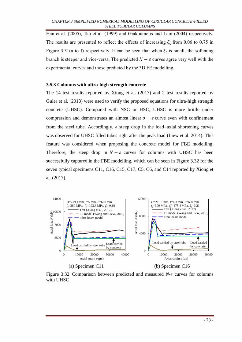
CHAPTER 3 SIMPLIFIED NUMERICAL MODELLING OF CIRCULAR CONCRETE-FILLED
STEEL TUBULAR COLUMNS
- 78 -
Han et al. (2005), Tan et al. (1999) and Giakoumelis and Lam (2004) respectively.
The results are presented to reflect the effects of increasing 𝜉c from 0.06 to 0.75 in
Figure 3.31(a to f) respectively. It can be seen that when 𝜉c is small, the softening
branch is steeper and vice-versa. The predicted 𝑁 − 𝜀 curves agree very well with the
experimental curves and those predicted by the 3D FE modelling.
3.5.3 Columns with ultra-high strength concrete
The 14 test results reported by Xiong et al. (2017) and 2 test results reported by
Guler et al. (2013) were used to verify the proposed equations for ultra-high strength
concrete (UHSC). Compared with NSC or HSC, UHSC is more brittle under
compression and demonstrates an almost linear 𝜎 − 𝜀 curve even with confinement
from the steel tube. Accordingly, a steep drop in the loadaxial shortening curves
was observed for UHSC filled tubes right after the peak load (Liew et al. 2014). This
feature was considered when proposing the concrete model for FBE modelling.
Therefore, the steep drop in 𝑁 − 𝜀 curves for columns with UHSC has been
successfully captured in the FBE modelling, which can be seen in Figure 3.32 for the
seven typical specimens C11, C16, C15, C17, C5, C6, and C14 reported by Xiong et
al. (2017).
(a) Specimen C11 (b) Specimen C16
Figure 3.32 Comparison between predicted and measured N-ε curves for columns
with UHSC
0
3500
7000
10500
14000
0 10000 20000 30000 40000
Axia
l lo
ad N
(k
N)
Axial strain e (me)
Test (Xiong et al., 2017)
FE model (Wang and Liew, 2016)
Fibre beam model
D=219.1 mm, t=5 mm, L=600 mm fy=380 MPa, fc'=193.3 MPa, xc=0.19
Load carried by steel tube Load carried
by concrete 0
4000
8000
12000
0 10000 20000 30000 40000
Axia
l lo
ad N
(k
N)
Axial strain e (me)
Test (Xiong et al., 2017)
FE model (Wang and Liew, 2016)
Fibre beam model
D=219.1 mm, t=6.3 mm, L=600 mm fy=300 MPa, fc'=175.4 MPa, xc=0.21
Load carried by steel tube Load carried
by concrete

CHAPTER 3 SIMPLIFIED NUMERICAL MODELLING OF CIRCULAR CONCRETE-FILLED
STEEL TUBULAR COLUMNS
- 79 -
(c) Specimen C15 (d) Specimen C17
(e) Specimen C5 and C6 (f) Specimen C14
Figure 3.32 Comparison between predicted and measured N-ε curves for columns
with UHSC (continued)
3.5.4 Columns with high strength steel and normal strength concrete
Because of the scarcity of test data on circular CFST columns with high strength
steel and normal strength concrete, only one specimen, 049C36_30, as tested by Lee
et al. (2011), was used to verify the proposed FBE model. It can be observed in
Figure 3.33 that the ultimate strength obtained from the FBE model was almost 6.5
% higher than that measured in experiments. However, the prediction form FBE
model was almost similar to the prediction obtained by 3D FE modelling. More tests
can be conducted for CFST columns under this category in the future to fill the
research gap.
0
3000
6000
9000
0 20000 40000 60000
Axia
l lo
ad N
(k
N)
Axial shortening (mm)
Test (Xiong et al., 2017)3D FE modelFibre beam model
D=219.1 mm, t=6.3 mm, L=600 mm
fy=300 MPa, fc'=163 MPa, xc=0.23
Load carried
by concrete
Load carried by
steel tube
0
2500
5000
7500
10000
0 20000 40000 60000
Axia
l lo
ad N
(k
N)
Axial strain e (me)
Test (Xiong et al., 2017)
3D FE model
Fibre beam model
D=219.1 mm, t=6.3 mm, L=600 mm fy=300 MPa, fc'=149 MPa, xc=0.25
Load carried by steel tube Load carried by concrete
0
900
1800
2700
3600
0 25000 50000 75000 100000
Axia
l lo
ad N
(k
N)
Axial strain e (me)
Test (Xiong et al., 2017)
3D FE model
Fibre beam model
D=114.3 mm, t=3.6 mm, L=250 mm fy=403 MPa, fc'=184.2 MPa, xc=0.31
Load carried
by steel tube Load carried
by concrete
0
4000
8000
12000
0 25000 50000 75000 100000
Axia
l lo
ad N
(kN
)
Axial shortening (mm)
Test (Xiong et al., 2017)3D FE modelFibre beam model
D=219.1 mm, t=10 mm, L=600 mm
fy=381 MPa, fc'=193.3 MPa, xc=0.41
Load carried
by concrete
Load carried by
steel tube

CHAPTER 3 SIMPLIFIED NUMERICAL MODELLING OF CIRCULAR CONCRETE-FILLED
STEEL TUBULAR COLUMNS
- 80 -
Figure 3.33 Comparison between predicted and measured N-ε curves for specimen
049C36_30 with high strength steel
3.5.5 Columns with high strength steel and concrete
For circular CFST columns with high strength steel and concrete, very limited test
data are available in the literature. To demonstrate the capability of the proposed
FBE model to simulate CFST columns under this category, three specimens reported
by Sakino et al. (2004) were utilised. Very good agreement between FBE modelling,
FE modelling and experiments were observed for specimens CC8-D-8 and CC8-A-8
(Figure 3.34). Since high strength materials are increasingly used in construction
industry, more tests can be done for CFST columns under this category to better
understand the behaviour of such columns.
(a) Specimen CC8-D-8 (b) Specimen CC8-A-8
Figure 3.34 Comparison between predicted and measured N-ε curves for columns
with high strength materials
0
2000
4000
6000
8000
10000
0 10000 20000 30000A
xia
l lo
ad N
(k
N)
Axial strain e (me)
Test (Lee et al., 2011)
3D FE model
Fibre beam model
D=360 mm, t=6 mm, L=1760 mm
fy=498 MPa, fc'=31.5 MPa, xc=1.11
Load carried
by concrete
Load carried
by steel tube
0
5000
10000
15000
20000
0 10000 20000 30000 40000
Axia
l lo
ad N
(k
N)
Axial strain e (me)
Test (Sakino et al., 2004)
3D FE model
Fibre beam model
D=337 mm, t=6.47 mm, L=1011 mm
fy=823 MPa, fc'=85.1 MPa, xc=0.78
Load carried
by concrete Load carried by steel tube
0
1000
2000
3000
4000
0 10000 20000 30000 40000
Axia
l lo
ad N
(k
N)
Axial strain e (me)
Test (Sakino et al., 2004)
3D FE model
Fibre beam model
D=108 mm, t=6.47 mm, L=324 mm
fy=854 MPa, fc'=77 MPa, xc=3.22
Load carried
by concrete
Load carried
by steel tube

CHAPTER 3 SIMPLIFIED NUMERICAL MODELLING OF CIRCULAR CONCRETE-FILLED
STEEL TUBULAR COLUMNS
- 81 -
It should be noted that the proposed FBE model can also be used for concrete-filled
thin-walled tubes, or stocky CFST columns with small 𝐷/𝑡 ratios. The prediction
accuracy can be observed for specimen S12CS80A with a tube thickness of 1.13 mm
and specimen S2-2-4 with a tube thickness of 10 mm, as shown in Figure 3.29(a) and
Figure 3.30(f) respectively.
It should also be noted that the proposed equations can be directly utilised to
calculate the loaddeformation curves of circular CFST stub columns using simple
spreadsheet software. This can help design engineers to conduct a preliminary design
of CFST columns.
3.6 Summary
In this chapter, effective stress-strain curves for the steel and core concrete were
developed for the simplified numerical modelling of axially loaded circular concrete-
filled steel stub columns using fibre beam elements. The effective steel and concrete
stressstrain models were proposed based on detailed finite element modelling. The
proposed stressstrain curves for steel have implicitly considered the interaction
between the steel tube and concrete, possible local buckling of the steel tube, and
strain-hardening of the steel material. Meanwhile, the concrete model has considered
the increase in strength and ductility resulting from the concrete confinement.
The proposed material models were implemented in the simplified fibre beam
element modelling, and the predictions were verified by 3D FE modelling and a large
amount of test data collected from the literature. The proposed simplified numerical
model covers a sufficiently wide range of CFST column parameters: diameter-to-
thickness ratio (𝐷/𝑡 = 10-220); yield stress (𝑓y = 186-960 MPa) and concrete
cylinder compressive strength ( 𝑓c′ = 20-200 MPa). The strength increase or
degradation of a CFST column after reaching its ultimate strength can be
automatically captured in the simulation.

CHAPTER 4 FINITE ELEMENT MODELLING OF COMPOSITE BEAMS WITH PROFILED STEEL
SHEETING
- 82 -
CHAPTER 4
FINITE ELEMENT MODELLING OF COMPOSITE
BEAMS WITH PROFILED STEEL SHEETING
4.1 Introduction
As described in Chapter 2, full scale experimental studies of composite beams with
profiled steel sheeting are very expensive and time consuming. Furthermore, there
are inherent difficulties in directly measuring the strength of shear studs in tests.
Therefore, finite element (FE) models can be considered as a viable approach to
overcome any experimental limitations and to study individual component
behaviour.
In this chapter, a detailed FE model has been developed for composite beams with
profiled steel sheeting. The steel fracture in shear studs and profiled steel sheeting,
damage in concrete, as well as realistic interactions are considered in the FE model.
Therefore, different types of failure modes are predicted, such as fracture of shear
studs, concrete crushing failure, steel beam failure and rib shear failures. The
proposed FE model is rigorously verified with 22 full-scale experimental data
(Section 4.3), which includes different types of failure modes, profiled steel sheeting
orientations, shear stud layout and boundary conditions. After extensive verification
with experimental studies, the proposed FE model is utilised to directly determine the
full-range shear force (𝑉s) versus slip (𝛿s) curves for shear studs in composite
beams, and the contribution from profiled steel sheeting is quantified.
4.2 Finite element modelling
Detailed 3D FE models were developed using ABAQUS version 6.14 to predict the
behaviour of steel-concrete composite beams with profiled steel sheeting.

CHAPTER 4 FINITE ELEMENT MODELLING OF COMPOSITE BEAMS WITH PROFILED STEEL
SHEETING
- 83 -
(a) Typical FE model
(b) Simulation of shear studs (c) Boundary conditions
Figure 4.1 Finite element model of a typical composite beam
As shown in Figure 4.1, a typical FE model consists of five types of components, i.e.,
the steel beam with or without stiffeners, shear studs, profiled steel sheeting, concrete
slab, and reinforcement bars. For a single-span beam under positive moment, a half-
symmetry model along the beam’s longitudinal axis was built to improve the
computational efficiency; it should be noted that a half symmetrical model along the
Symmetric boundary conditions:
Z=0, UR1=0, UR2=0
Boundary conditions: X=0,Y=0,Z=0
Boundary conditions: X=0,Y=0,Z=0
Loads
Surface-to-surface
interaction between the shear
stud and concrete
Stud
Bottom surface of the stud
and the corresponding
surface of the top flange of
the steel beam were merged
together to simulate weld
Steel beam
Node A
Node B
Frictionless contact
between the steel beam and end support
End support

CHAPTER 4 FINITE ELEMENT MODELLING OF COMPOSITE BEAMS WITH PROFILED STEEL
SHEETING
- 84 -
beam’s longitudinal axis restricts the web buckling of steel I-section beams.
Fortunately, the web buckling was not generally observed for simply-supported
composite beams in the collected test database (Section 4.3); this method can be
reasonably adopted for such composite beams. Moreover, this method allowed for
defining the hinge support or roller support at the ends, similar to the tests. However,
for single-span beams under negative moment or continuous beams, steel beam web
as well as flange buckling was observed in the tests. Therefore, if half symmetrical
models along the beam axis were utilised, the failure mode was not always predicted
properly. So, for composite beams under negative moment, full models were built to
capture the realistic deformation of the steel beams, including possible local
buckling. But for two-span continuous beam specimens where hinge support was
used at the middle and roller at the ends, and which were symmetrical in all aspects
(SB9, SB10 and SB11 tested by Nie et al., 2008), half symmetrical models
perpendicular to the beam axis were utilised to improve computational efficiency
thereby maintaining prediction accuracy. The Poisson’s ratios were taken as 0.3 and
0.2 for the steel and concrete, respectively.
4.2.1 Element types
The selection of proper element type plays a very important role in accuracy and
computational efficiency of composite beams. There are a variety of elements
available in the ABAQUS library to solve different types of problems, including
solid (continuum) elements, shell elements, beam elements, truss elements, and
connector elements. For the simulation of steel-concrete composite structures
including concrete-filled steel tubular columns, composite beams and composite
connections, the most widely adopted elements are 3D solid elements, shell elements
and rebar elements.
For the simulation of concrete, solid elements are normally used in FE models, as
discussed in literature including Nie et al. (2004), Sadek et al. (2008), Mirza (2008),
and Tahmasebinia et al. (2012). To represent the profiled steel sheeting in numerical
simulation, shell elements (S4R) are mostly used as it is the most appropriate type of
element to model thin walled steel structures (Mirza, 2008). For the simulation of
steel beams, both solid C3D8R elements (Mirza, 2008, Tahmasibinia et al., 2012) as

CHAPTER 4 FINITE ELEMENT MODELLING OF COMPOSITE BEAMS WITH PROFILED STEEL
SHEETING
- 85 -
well as shell S4R elements have been used (Nie et al., 2004, Sadek et al., 2008,
Alashkar et al., 2010). The rebars were normally modelled using truss elements
which were embedded in a host concrete element. Shear studs were modelled either
by connector elements (Cas et al., 2004, Nie et al., 2004, Queiroz et al., 2007) or by
solid C3D8R elements (Mirza, 2008, Tahmasebinia et al., 2012).
It should be noted that the shear force-slip relationships need to be defined when
connector elements are utilised to represent stud behaviour (which is basically used
to simplify the simulation). As described in Chapter 2, the available shear force-slip
curves are based on push tests data and there are some controversies in utilising such
curves obtained from push tests in composite beams. Such conflict can be easily
avoided by using solid elements to simulate shear studs, but as a result the
computation work will increase.
Sensitivity analysis was conducted to determine the effects of different types of
elements (C3D8, C3D8R, C3D8I and C3D20R) for the simulation of a steel I-section
beam using the specimen SB1 as tested by Nie et al. (2005). A similar prediction was
obtained in the initial stage from all four types of elements, but slight variations in
the ultimate load capacity was observed (Figure 4.2). Compared to C3D8R elements,
the ultimate prediction is 1.4% higher when C3D8 elements were used. However,
when C3D8I and C3D20R elements were used, the ultimate load capacity slightly
decreased by 0.4% and 1.5%, respectively, and yet the computational time
significantly increased.
Figure 4.2 Effect of different element types for steel beam on predicted 𝑀 − 𝛥
curves
0
40
80
120
160
0 20 40 60 80
Mid
-sp
an m
om
ent
M (
kN
m)
Mid-span deflection Δ (mm)
C3D8
C3D8R
C3D8I
C3D20R
Specimen SB1 (Nie et al., 2005)
P/2 P/2

CHAPTER 4 FINITE ELEMENT MODELLING OF COMPOSITE BEAMS WITH PROFILED STEEL
SHEETING
- 86 -
Therefore, C3D8R elements were further used for steel beams in the FE analysis to
balance the accuracy and efficiency. Similarly, for all other components, solid
elements (C3D8R) were used except for the profiled steel sheeting and reinforcement
bars. The profiled steel sheeting was simulated using shell elements (S4R), whereas
the reinforcement bars were simulated using two-node truss elements (T3D2).
4.2.2 Mesh discretisation
The accuracy of finite element analysis prediction largely depends on the mesh size
of the elements. Therefore, based on sensitivity analysis, the suitable element size
were determined. For the simply-supported composite beams under positive moment,
the web of a steel beam was partitioned into at least 8 elements along its height with
a maximum element size of 40 mm. For the simply-supported composite beams
under negative moment and for continuous beams, the steel beam web was
partitioned into 16 elements with a maximum element size of 40 mm. Similarly, the
flanges of a steel beam were partitioned into at least 10 elements along their width
with a maximum element size of 40 mm. Along the longitudinal direction, the
element size of the beam underneath the studs ranged from 8 to 20 mm depending
upon the number of shear studs per rib, whereas the steel beam in other regions was
meshed with a maximum element size of 40 mm. The element size of the studs was
selected to be 𝐷s/4 or 4 mm for the bottom half of the studs whichever is smaller,
where 𝐷s is the shank diameter of the studs. Since in most cases the stud head and
the upper half portion of the stud remained elastic, the mesh size can be increased up
to 12 mm along the height of the stud to reduce the number of elements.
Reinforcement bars were meshed using an element size of 100 mm.
The sensitivity analyses of concrete mesh size were conducted by using the
specimens with concrete crushing failure (SB3, Nie et al., 2005), stud fracture (SB1,
Nie et al., 2005) as well as the specimens which sustained the deformation up to L/65
with no major failure (CB2, Ranzi et al., 2009). The material properties adopted for
steel, concrete, sheeting and rebars are described in Section 4.2.5. Three levels of
mesh size A, B and C (Figure 4.3) were used for investigation. Mesh A refers to the
element size where rib height (hs) and trough width of the rib (ttw) is divided into two
and four elements, respectively (Figure 4.3(a)). Mesh B is discretised so that both hs

CHAPTER 4 FINITE ELEMENT MODELLING OF COMPOSITE BEAMS WITH PROFILED STEEL
SHEETING
- 87 -
and ttw were divided into four divisions (Figure 4.3(b)), whereas for Mesh C, the ttw
was divided into 8 divisions keeping the hs the same as Mesh B (Figure 4.3(c)).
For specimen SB3 (hs = 60 mm and ttw = 110 mm), it can be observed in Figure
4.3(d) that the predicted initial stiffness is similar in the cases of all three levels of
mesh size. However, the ultimate prediction obtained from Mesh A and C are 6.5%
higher and 2.5% lower than Mesh B. The computational time was around 15 hours
for Mesh A using 6 processors in i7 3.6GHz 32 GB RAM computer, whereas Mesh
B took around 30 hours. However, the computational time significantly increased for
(a) Mesh A (ℎs/2 × 𝑡tw/2)
(b) Mesh B (ℎs/4 × 𝑡tw/4)
(c) Mesh C (ℎs/4 × 𝑡tw/8)
(d) Specimen SB3
Figure 4.3 Sensitivity analysis for concrete element size for specimen with concrete
crushing failure
0
50
100
150
200
0 25 50 75 100 125 150 175
Mid
-sp
an m
om
ent
M (
kN
m)
Mid-span deflection Δ (mm)
Test (Nie et al. 2005)
FE (Mesh A)
FE (Mesh B)
FE (Mesh C)
Two studs per rib
P/2 P/2

CHAPTER 4 FINITE ELEMENT MODELLING OF COMPOSITE BEAMS WITH PROFILED STEEL
SHEETING
- 88 -
Mesh C, which took around 60 hours. It is interesting to note that the prediction
obtained from medium sized Mesh B is also reasonably close to test data. A similar
observation was reported by Mirza (2008) for push test specimens.
For specimen SB1 (hs = 60 mm and ttw = 110 mm) and CB2 (hs = 78 mm and ttw =
150 mm), the predictions were almost similar from all three mesh sizes (Figures 4.4
and 4.5). However, small difference was obtained for specimen SB1 in a later stage
(Figure 4.4) when Mesh A was used. Therefore, the medium mesh size was used to
simulate concrete slab for all specimens where the mesh size generally varied from
15 to 30 mm in the rib regions, and 40 to 150 mm in other regions. For the profiled
steel sheeting, the mesh size was kept equal to the concrete mesh size as it is in direct
contact with the concrete.
Figure 4.4 Effect of concrete element size for specimen with stud fracture ( SB1, Nie
et al., 2005)
Figure 4.5 Effect of concrete element size for specimen with no major failure (CB2,
Ranzi et al., 2009)
0
50
100
150
200
0 25 50 75 100 125
Mid
-sp
an m
om
ent
M (
kN
m)
Mid-span deflection Δ (mm)
Test (Nie et al. 2005)FE (Mesh A)FE (Mesh B)
One stud per rib
P/2 P/2
0
200
400
600
0 40 80 120 160
Load
P (
kN
)
Mid-span deflection Δ (mm)
Test (Ranzi et al. 2009)
FE (Mesh A)
FE (Mesh B)
FE (Mesh C)
Two studs per rib
P

CHAPTER 4 FINITE ELEMENT MODELLING OF COMPOSITE BEAMS WITH PROFILED STEEL
SHEETING
- 89 -
4.2.3 Interaction properties
Surface-to-surface interactions were considered for the contact surfaces between
concrete and profiled steel sheeting, concrete and shear studs, profiled steel sheeting
and top flange of the steel beam, as well as the steel beam and the end supports, as
shown in Figure 4.1. The studs and the steel beam were merged together in the
assembly, as shown in Figure 4.1(b). This option can be used to significantly
improve the robustness of the model compared to using the “Tie” constraint option.
Any vertical and/or horizontal stiffeners welded to a steel beam were simulated using
the “Tie” constraint to connect the stiffeners to the steel beam. All reinforcement
bars were embedded in the concrete of the composite slab.
For all contact surfaces, hard contact with no penetration was defined in the normal
direction. In a tangential direction, a friction coefficient (𝜇) between the contact
surfaces needs to be defined. Sensitivity analysis was conducted to investigate the
effect of 𝜇 on the prediction accuracy. In the sensitivity analysis, the composite beam
specimens SB1 and SB3, tested by Nie et al. (2005), were selected as examples. The
specimen SB1 has one stud per rib and specimen SB3 has two studs per rib and
accordingly the specimen SB1 failed due to fracturing of the shear studs, whereas
SB3 failed due to concrete crushing. It was found that the predictions are not
sensitive to the value of 𝜇 at the interface between the concrete and the profiled steel
sheeting during the initial stage, as shown in Figures 4.6(a) and 4.7(a) for specimens
SB1 and SB2, respectively. This is because in the elastic stage the interaction
between the steel beam and composite slab is ensured by the embedded shear studs,
and the influence of the friction force between the concrete and the profiled steel
sheeting is negligible. However, the ultimate capacity was slightly higher (2.3% for
SB1 and 5% for SB3) for both specimens when 𝜇 was defined as 0.25 compared to
0.01. For both specimens, the post-peak failure was better predicted when 𝜇 was
defined as 0.01. This could be due to the fact that once the beam exhibits nonlinear
behaviour, separation of the profiled steel sheeting from the concrete might occur,
significantly reducing the friction force between the two components.
It can be seen in Figures 4.6(b) that the slip between steel beam and slab is also
better predicted when 𝜇 is equal to 0.01 for specimen SB1 with one stud per rib. For

CHAPTER 4 FINITE ELEMENT MODELLING OF COMPOSITE BEAMS WITH PROFILED STEEL
SHEETING
- 90 -
specimen SB3 with two studs per rib, the initial stiffness is reasonably predicted
when 𝜇 was defined as 0.01. However, much higher slip was observed in test in
nonlinear regions.
More detailed investigation into the behaviour of profiled steel sheeting and shear
studs is presented in Figure 4.8 using specimen SB1, in which the second stud from
hinge support is considered. It can be seen in Figure 4.8(a) and (b) that the shear
force of the stud (measured at the bottom nodes of the stud) and the axial force of
profiled steel sheeting (measured from the nodes at the junction of the stud and top
flange of the steel beam) are slightly lower when 𝜇 was defined as 0.01, in contrast to
the values obtained when 𝜇 was defined as 0.25. Similarly, the difference in beam
axial force which is referred to as “indirect method” in Section 4.3.5 is determined in
Figure 4.8 (c) and (d). It is interesting to note that the force carried by steel sheeting
is higher in both cases than that carried by the shear studs. For comparison, the force
obtained from shear studs was added to the sheeting and the resulting total force
almost matches with the force obtained from employing the indirect method; this
phenomenon is described in detail in subsection 4.3.5. In both cases, conservative
prediction was obtained when 𝜇 = 0.01 was used. Therefore, for other specimens, 𝜇 =
0.01 has been used.
(a) (b) Figure 4.6 Effects of μ between the concrete and sheeting for specimen with one
stud per rib
0
20
40
60
80
100
120
140
160
0 20 40 60 80 100 120
Mid
-sp
an m
om
ent
M (
kN
m)
Mid-span deflection Δ (mm)
Test (Nie et al., 2005)
FE (μ=0.01)
FE (μ=0.25)
Specimen SB1
P/2 P/2
0
40
80
120
160
0 2 4 6 8 10 12
Mid
-sp
an m
om
ent
M (
kN
m)
Beam end slip δ (mm)
Test (Nie et al., 2005)
μ=0.01
μ=0.25
Specimen SB1
P/2 P/2

CHAPTER 4 FINITE ELEMENT MODELLING OF COMPOSITE BEAMS WITH PROFILED STEEL
SHEETING
- 91 -
(a) (b)
Figure 4.7 Effects of μ between the concrete and sheeting for specimen with two
studs per rib
(a) (b)
(c) (d)
Figure 4.8 Load distribution between the shear stud and profiled steel sheeting
(specimen SB1)
Similarly, the influence is negligible when 𝜇 is taken as 0.01 or 0.25 for the interface
between the concrete and the shear studs, as shown in Figure 4.9. This could be
0
50
100
150
200
0 50 100 150 200
Mid
-sp
an m
om
ent
M (
kN
m)
Mid-span deflection Δ (mm)
Test (Nie et al., 2005)μ=0.01 μ=0.25
Specimen SB3
P/2 P/2
0
50
100
150
200
0 2 4 6 8 10 12
Mid
-sp
an m
om
ent
M (
kN
m)
Beam end slip δ (mm)
Test (Nie et al., 2005)
μ=0.01
μ=0.25
Specimen SB3
P/2 P/2
0
10
20
30
40
50
0 3 6 9 12
Stu
d s
hea
r fo
rce
Vs
(kN
)
Shear stud slip δs (mm)
μ=0.01
μ=0.25
for shear studs-concrete
interaction,
0
10
20
30
40
50
0 3 6 9 12
Sh
eeti
ng a
xia
l fo
rce
Np
ss (
kN
)
Shear stud slip δs (mm)
μ=0.01
μ=0.25
for shear studs-concrete
interaction,
0
20
40
60
80
100
0 3 6 9 12
Vs,
Npss
(k
N)
Shear stud slip δs (mm)
Sheet
Stud
Sheet+stud
Indirect method
for shear studs-concrete
interaction, μ =0.25
0
20
40
60
80
100
0 3 6 9 12
Vs,
Npss
(k
N)
Shear stud slip δs (mm)
Sheet
Stud
Sheet+stud
Indirect method
for shear studs-concrete
interaction, μ =0.01

CHAPTER 4 FINITE ELEMENT MODELLING OF COMPOSITE BEAMS WITH PROFILED STEEL
SHEETING
- 92 -
explained by the presence of the heads of the shear studs, which prevent slip between
the concrete and shear studs. For the interface between the profiled steel sheeting and
steel beam, the value of 𝜇 has no obvious influence on the ascending branch of the
mid-span moment (M) versus mid-span deflection () curve, as shown in Figure
4.10. However, it has some influence on the descending branch of the M curve.
When 𝜇 was taken as 0.25, the post-peak strength was overestimated, whereas the
prediction correlates well with the test curve when 𝜇 was defined to be a very small
value of 0.01. This can be attributed to the fact that profiled steel sheeting is
normally coated with zinc/aluminium alloy, significantly reducing the friction
coefficient between the profiled steel sheeting and steel beam. Meanwhile, the
profiled steel sheeting might not be in perfect contact with the steel beam because of
its imperfections and residual deformation after welding the studs. The friction
coefficient of 0.01 was also used by Tahmasebinia et al. (2013) to simulate the
interaction between the profiled steel sheeting and the steel beam. Based on the
above sensitivity analyses, the friction coefficient of 0.01 was used in the following
FE modelling for the contact surfaces between the concrete and profiled steel
sheeting, concrete and shear studs, as well as the profiled steel sheeting and the top
flange of the steel beam. The suitability of this selection was further validated in
Section 4.3 by comparing the FE results with the test results. For the interaction
between the steel beam and end supports, a frictionless contact was defined to allow
smooth movement of the steel beam when in contact with the supports.
In the surface-to-surface interaction, the master and slave surfaces should be defined
properly to overcome the penetration problem. In this study, the surface with a stiffer
material was defined as the master surface. For example, the surfaces of the studs,
concrete and steel beam were defined as the master surfaces for the contact
interactions between the concrete and studs, concrete and profiled steel sheeting, and
the steel beam and profiled steel sheeting, respectively. For the interface between the
steel beam and end supports, the bottom surface of the bottom flange of the steel
beam was selected as the master surface and the top surface of the end support was
selected as the slave surface.

CHAPTER 4 FINITE ELEMENT MODELLING OF COMPOSITE BEAMS WITH PROFILED STEEL
SHEETING
- 93 -
(a) (b)
Figure 4.9 Effects of μ between the concrete and studs
(a) (b)
Figure 4.10 Effects of μ between the steel beam and sheeting
4.2.4 Boundary and loading conditions
In the literature, the support conditions of the test specimens of composite beams
were either hinged or roller-supported. For a hinged support, the corresponding
nodes at the bottom of the beam were restrained in all three translational directions.
In contrast, a roller support was modelled using an end support as shown in Fig. 4.1c.
The bottom of the roller support was restrained in all degrees of freedom, but the
definition of frictionless contact between the steel beam and the support ensure the
correct simulation of the roller support.
The self-weight of composite beams was also considered in the analysis. It was
found that the self-weight could range from 10 to 25% of the overall load-carrying
capacity of a composite beam, as reported by Rambo-Roddenberry (2002), Hicks
0
20
40
60
80
100
120
140
160
0 20 40 60 80 100 120
Mid
-sp
an m
om
ent
M (
kN
m)
Mid-span deflection Δ (mm)
Test (Nie et al., 2005)
FE (μ=0.01)
FE (μ=0.25)
Specimen SB1
P/2 P/2
0
40
80
120
160
0 2 4 6 8 10 12
Mid
-sp
an m
om
ent
M (
kN
m)
Beam end slip δ (mm)
Test (Nie et al., 2005)
μ=0.01
μ=0.25
Specimen SB1
P/2 P/2
0
20
40
60
80
100
120
140
160
0 20 40 60 80 100 120
Mid
-sp
an m
om
ent
M (
kN
m)
Mid-span deflection Δ (mm)
Test (Nie et al., 2005)
FE (μ=0.01)
FE (μ=0.25)
Specimen SB1
P/2 P/2
0
40
80
120
160
0 2 4 6 8 10 12
Mid
-sp
an m
om
ent
M (
kN
m)
Beam end slip δ (mm)
Test (Nie et al., 2005)
μ=0.01
μ=0.25
Specimen SB1
P/2 P/2

CHAPTER 4 FINITE ELEMENT MODELLING OF COMPOSITE BEAMS WITH PROFILED STEEL
SHEETING
- 94 -
(2007), Ranzi et al. (2009), Ernst et al. (2010) and Hicks and Smith (2014).
Therefore, the inclusion of the self-weight is necessary for realistic simulation of
such beams. The self-weight was applied in the first step and propagated as a
constant load in the remaining load steps together with the imposed loads.
4.2.5 Material modelling
4.2.5.1 Steel beams
Normal steel is very ductile to accommodate large deflection of the steel beam. Tao
et al. (2013a) developed an elastic-plastic strain hardening stress-strain model for
structural steels (Figure 3.2, Eq. 3.1) after extensive verifications with test data
which has been used in the present study. It should be noted that the fracture of the
steel is not considered in the material models of steel beams because no fracture of
the steel beam in composite beams has been reported in the literature.
4.2.5.2 Steel reinforcement
The 𝜎 − 휀 model proposed by Tao et al. (2013a) is also used to simulate material
properties of steel reinforcement. The model for steel reinforcement is very similar to
the 𝜎 − 휀 model of structural steel described in the last subsection. Therefore, Eq.
(3.1) can continue to be used to predict the 𝜎 − 휀 curve of steel reinforcement.
However, 𝐸p should be taken as 0.03𝐸s, while 𝑓u should be calculated by Eq. (4.1),
as suggested by Tao et al. (2013a). In the literature, no fracture of reinforcement has
been reported, therefore no post-peak branch was defined for the 𝜎 − 휀 curve of steel
reinforcement.
𝑓u = [1.6 − 9.17 × 10⁻⁴(𝑓y − 200)]𝑓y 200 ≤ 𝑓y ≤ 800 MPa (4.1)
4.2.5.3 Profiled steel sheeting
Profiled steel sheeting is generally produced from cold-worked steel, thus it has a
relatively high yield stress (Karren, 1965). However, it exhibits less pronounced
strain-hardening and elongation: 4.5% to 8.5% according to the tensile coupon tests
conducted by Loh (2004) and Ranzi et al. (2009) as presented in Figure 4.11.
Therefore, its yield stress and ultimate strength are generally very similar (Loh,

CHAPTER 4 FINITE ELEMENT MODELLING OF COMPOSITE BEAMS WITH PROFILED STEEL
SHEETING
- 95 -
2004); for this reason, the elastic-perfectly plastic model has been widely used in the
simulation of profiled steel sheeting. It should be noted that despite its low
elongation, the fracture of profiled steel sheeting has seldom been considered in the
previous modelling.
Figure 4.11 Measured profiled steel sheeting 𝜎 − 휀 curves
To investigate the influence of fracturing of profiled steel sheeting on the prediction
accuracy, the single-span specimen SB1 tested by Nie et al. (2005) was selected as
an example (Figure 4.12 (a)). In the case of the elastic-perfectly plastic model used in
the simulation, fracturing was not considered. No obvious strength deterioration was
found in the predicted M curve of the beam after reaching its ultimate strength, in
contrast to the experimental observation as shown in Figure 4.12 (a). In contrast,
when the 𝜎 − 휀 model with a failure criterion was used for the profiled steel sheeting,
fracture initiated in the profiled steel sheeting around the shear studs near the
locations of the applied concentrated loads, as shown in Figure 4.12. Following this,
the shear studs were sheared off accompanying by rib punching. The simulated
failure modes agree very well with the test results. Meanwhile, the prediction
accuracy of the post-peak response is greatly improved when the fracturing of
profiled steel sheeting is considered.
0
200
400
600
800
0 0.025 0.05 0.075 0.1
Str
ess σ
Strain ε
Loh et al. (2004)
Ranzi et al. (2009)

CHAPTER 4 FINITE ELEMENT MODELLING OF COMPOSITE BEAMS WITH PROFILED STEEL
SHEETING
- 96 -
(a) (b)
Figure 4.12 Influence of fracture of profiled steel sheeting on prediction accuracy
Therefore, the elastic-plastic 𝜎 − 휀 model with a failure criterion, defined in Figure
4.13, is used for profiled steel sheeting. Based on the test data reported by Ranzi et
al. (2009) and Loh (2004), the proposed 𝜎 − 휀 model has a linear response up to the
yield Point A, followed by a plateau response (AB) and a failure stage (BC). The
fracture strain at Point B is taken as 20휀𝑦, whereas the failure strain at Point C is
taken as 22휀𝑦. Sensitivity analysis was conducted to investigate the influence of the
slope of the failure branch. It can be observed in Figure 4.14 that there is no
significant influence on the overall prediction accuracy using failure strain as
22휀𝑦 and 50휀𝑦 . Therefore, failure strain of 22휀𝑦 was deemed sufficient for the
simulation of profiled steel sheeting.
Figure 4.13 Proposed 𝜎 − 휀 model for profiled steel sheeting
0
40
80
120
160
0 20 40 60 80 100 120
Mid
-sp
an m
om
ent
M (
kN
m)
Mid-span deflection Δ (mm)
Test (Nie et al., 2005)
FE (without fracture)
FE (with fracture)
Specimen SB1
P/2 P/2
0
40
80
120
160
0 2 4 6 8 10 12
Mid
-sp
an m
om
ent
M (
kN
m)
Beam end slip δ (mm)
Test (Nie et al., 2005)
FE (without fracture)
FE (with fracture)
Specimen SB1
P/2 P/2
Str
ess σ
Strain e
20εy 22εy εy
fy
O
B A
C

CHAPTER 4 FINITE ELEMENT MODELLING OF COMPOSITE BEAMS WITH PROFILED STEEL
SHEETING
- 97 -
Figure 4.14 Effect of softening branch in 𝜎 − 휀 curves of profiled sheeting on
prediction accuracy
4.2.5.4 Shear studs
The steel material used for shear studs generally has good ductility. According to the
Australian/New Zealand Standard (2003), the minimum required elongations are
0.14 and 0.16 for 15.9 mm and 19 mm shear studs, respectively. However, the
deformation demand for shear studs is also very high to accommodate the shear force
transfer from the concrete slab to the steel beam. It has been experimentally proven
that fracture of the shear studs could occur in composite beams either during
moments of positive (Nie et al., 2005) or negative (Nie et al., 2004, Loh et al., 2004)
bending, which greatly affect the performance of the composite beams. Therefore,
this effect should be considered in simulating shear studs. Based on regression
analysis of test data, Hassan (2016) developed a full-range 𝜎 − 휀 model for shear
studs, as shown in Figure 4.15, where a failure stage (CDE) was also defined to
reflect the fracture. The e model developed by Hassan (2016) is presented in Eq.
4.2.
𝜎 =
{
𝐸s휀 0 ≤ 휀 ≤ 휀y
𝑓u − (𝑓u − 𝑓y) ∙ (휀u − 휀
휀u − 휀y)
𝑝
휀y ≤ 휀 ≤ 휀u
𝑓u 휀u ≤ 휀 ≤ 휀u1
𝑓u − (𝑓u − 𝑓f) ∙ (휀 − 휀u1휀f − 휀u1
)𝑝′
휀u1 ≤ 휀 ≤ 휀f
𝑓f − 𝑓f ∙ (휀 − 휀f휀u2 − 휀f
) 휀f ≤ 휀 ≤ 휀u2
(4.2)
0
20
40
60
80
100
120
140
160
0 20 40 60 80 100 120
Mid
-sp
an m
om
ent
M (
kN
m)
Mid-span deflection Δ (mm)
Test (Nie et al., 2005)
FE (22ey)
FE (50ey)
Specimen SB1
P/2 P/2
(22εy)
(50εy)
0
40
80
120
160
0 2 4 6 8 10 12
Mid
-sp
an m
om
ent
M (
kN
m)
Beam end slip δ (mm)
Test (Nie et al., 2005)
FE (22ey)
FE (50ey)
Specimen SB1
P/2 P/2
(22εy)
(50εy)

CHAPTER 4 FINITE ELEMENT MODELLING OF COMPOSITE BEAMS WITH PROFILED STEEL
SHEETING
- 98 -
Figure 4.15 𝜎 − 휀 model for shear studs (Hassan, 2016)
where ey, eu, eu1, ef, and eu2 are strains corresponding to Points A, B, C, D and E,
respectively; 휀y = 𝑓y/𝐸s; Es=200,000 MPa, and 휀u = 22휀y. It should be noted that
the 𝜎 − 휀 model developed by Hassan (2016) is for shear studs with a fracture strain
(ef) of about 0.24 or greater. Accordingly, the strains 휀u1, 휀f, and 휀u2 were originally
taken as 휀u1 = 55휀y; 휀f = 120휀y; and 휀u2 = 130휀y by Hassan (2016), respectively.
However, the test data reported in Hicks (2007), Hicks and Smith (2014), Loh
(2004), Spremic et al. (2013) and Yan et al. (2016) indicates that the corresponding
shear studs had a smaller fracture strain (ef) of only about 0.16. Therefore, the strains
휀u1, 휀f, and 휀u2 are revised as 휀u1 = 25휀y; 휀f = 80휀y; and 휀u2 = 90휀y, respectively.
This is a more conservative representation of fracture of shear studs.
According to Hassan (2016); the exponents 𝑝 and 𝑝′ in Eq. (4.2) can be determined by
Eqs. (4.3) and (4.4), respectively. The fracture stress (𝑓f) can be obtained from Eq. (4.5).
𝑝 = 𝐸u1 (휀u − 휀𝑦
𝑓u − 𝑓y)
(4.3)
𝑝′ = 𝐸u1′ (
휀f − 휀u1𝑓u − 𝑓f
) (4.4)
𝑓f = 𝑓u − (휀f − 휀u1) ∙ 𝐸u1′ (4.5)
Str
ess σ
Strain e
fy
ft
fu
εu εu1 εf εu2 εy
Eq. (4.2)
O
A
B C
D
E

CHAPTER 4 FINITE ELEMENT MODELLING OF COMPOSITE BEAMS WITH PROFILED STEEL
SHEETING
- 99 -
In Eq. (4.3), 𝐸u1 is taken as 0.025𝐸s, whereas 𝐸u1′ in Eq. (4.4) is taken as 0.006𝐸s. It
was found that the ultimate strength 𝑓u for shear studs can be reasonably predicted by
Eq. (3.8) based on 𝑓y.
The fracture of shear studs can be successfully captured by using the above simple
material model with a post-peak response. This will be demonstrated in section 4.3.
Although the fracture may be more precisely predicted by using a continuum
mechanics based-material model (Yan et al., 2016), very fine mesh is required for the
shear studs (Pavlovic et al., 2013). Furthermore, material tests need to be conducted
to accurately calibrate the strain-hardening parameters and other parameters
controlling the damage initiation and evolution in the model. Due to the lack of test
data, the continuum mechanics based-material model is not used in this research.
4.2.5.5 Concrete material
The concrete damaged plasticity model available in ABAQUS was used for concrete
in the composite slab. Sensitivity analysis was conducted to find the influence of the
dilation angle (ψ) using the specimen SB3, as tested by Nie et al. (2005) (Figure
4.16). The specimen SB3 has two shear studs per rib this specimen failed by concrete
crushing during testing (Nie et al., 2005). Different values (25, 30, 36 and 55)
were used for the sensitivity analysis of ψ. When the value of 55 was used, the
initial stiffness as well as ultimate capacity was very high. The ψ value of 25, 30,
and 36 predicted similar initial stiffness, but the ultimate capacity and load dropping
behaviour was better predicted by the value of 30. Therefore, ψ value of 30 is used
further for all specimens.
For the other parameters in the concrete damaged plasticity approach such as flow
potential eccentricity (e), ratio of the compressive strength under biaxial loading to
uniaxial compressive strength (𝑓b0/𝑓c′), and ratio of the second stress invariant on
the tensile meridian to that on the compressive meridian (Kc), the values of 0.1, 1.16
and 0.667 can be reasonably used which is similar to that used by Han et al. (2007) in
simulating behaviour of core concrete in CFST columns. Meanwhile, the viscosity
parameter was assigned a small value of 0.0001 to improve the convergence of the

CHAPTER 4 FINITE ELEMENT MODELLING OF COMPOSITE BEAMS WITH PROFILED STEEL
SHEETING
- 100 -
FE computation. The suitability of these parameters is reflected in verification
section 4.3. The modulus of elasticity (𝐸c) was calculated from c4700 f according
to ACI 318 (2014), where 𝑓c′ is the concrete cylinder compressive strength in MPa.
The Poisson’s ratio was taken as 0.2. The compressive and tensile behaviours of the
concrete are described in the subsections below.
Figure 4.16 Effect of dilation angle on prediction accuracy
a. Compressive behaviour
The compressive 𝜎 − 휀 relationship of concrete is represented by the model shown in
Figure 4.17(a), where a linear response is assumed from Point O to Point A
(corresponding to 0.4𝑓c′). The following nonlinear behaviour is represented by the
ascending curve AB, where the peak concrete strength 𝑓c′ is reached at Point B. After
that, a post-peak response is represented by the curve BC, where the residual
compressive strength decreases to a very small value (close to zero) at Point C,
corresponding to the compressive failure strain (휀fc). Eq. (4.6) proposed by Carreira
and Chu (1985) is used in this research to represent both the ascending curve AB and
the descending curve BC.
𝜎 =𝑓c′𝛾(휀 휀c0⁄ )
𝛾 − 1 + (휀 휀c0⁄ )𝛾 (4.6)
where 𝛾 = [𝑓c′
32.4]3
+ 1.55 and 휀c0 is the peak strain corresponding to 𝑓c′ , which is
calculated using Eq. (3.14), as proposed by De Nicolo et al. (1994). The failure strain
0
50
100
150
200
0 40 80 120 160
Mid
-sp
an m
om
ent
M (
kN
m)
Mid-span deflection Δ (mm)
Test (Nie et al., 2005)
ψ=55
ψ=36
ψ=30
ψ=25
Two studs per rib Specimen SB3

CHAPTER 4 FINITE ELEMENT MODELLING OF COMPOSITE BEAMS WITH PROFILED STEEL
SHEETING
- 101 -
휀fc is taken as 50휀c0 in this research; this selected value has no influence on the
prediction accuracy but improves the numerical convergence.
As suggested by Pavlovic et al. (2013), the evolution law 𝑑c − 휀cinel was specified to
consider the concrete compression damage after the concrete reaches its peak stress,
where 𝑑c and εcinel are the compressive damage parameter and compressive inelastic
strain, respectively. The expression for 𝑑c is given by Eq. (4.7) and the 𝑑c − εcinel
relationship is shown in Figure 4.17(b).
𝑑c = 1 −𝜎
𝑓c′
(4.7)
(a) Compressive 𝜎 − 휀 model (Carreira
and Chu, 1985)
(b) Compression damage
Figure 4.17 Constitutive model of concrete under compression
b. Tensile behaviour
Figure 4.18(a) presents the 𝜎 − 휀 curve used to simulate tensile behaviour of
concrete. It is assumed that the tensile stress 𝜎 increases linearly until the tensile
strength of concrete (𝑓t′) is reached at Point A. The slope of OA is taken as the
Young’s modulus of concrete (𝐸c), therefore the crack strain (휀cr) at Point A can be
determined as 𝑓t′ /𝐸c . The tensile strength 𝑓t
′ is calculated using Eq. (4.8), as
suggested by CEB-FIP (2010). Beyond Point A, the post-peak response is
represented by the 𝜎 − 휀 curve of AB (Eq. 4.9) proposed by Hassan (2016), where
0
0.2
0.4
0.6
0.8
1
1.2
Norm
alis
ed c
om
pre
ssiv
e st
ress
σ/
f c'
Strain ε
0 εc0 εfc O
A
B
C
Linear response
𝜎 =𝑓c′γ 휀/휀c0
γ − 1 + 휀/휀c0𝛾
0
0.2
0.4
0.6
0.8
1
1.2
Dam
age
par
amet
er d
c
0 εfc
𝑑c = 1 −𝜎
𝑓c′
Inelastic strain 휀c𝑖𝑛𝑒𝑙

CHAPTER 4 FINITE ELEMENT MODELLING OF COMPOSITE BEAMS WITH PROFILED STEEL
SHEETING
- 102 -
the residual tensile strength drops to a very small value (close to zero) at Point B,
corresponding to the tensile failure strain (휀ft).
𝑓t′ = { 0.3(𝑓c
′ − 8)23 for concrete gradesC50
2.12ln(1 + 0.1𝑓c′) for concrete grades > 𝐶50
(4.8)
𝜎 = 𝑓t′𝑒−(
𝜀−𝜀cr0.00035
)0.85
(4.9)
It should be noted that 휀ft at Point B was originally defined as 25휀cr by Hassan
(2016). In this study, the value of 휀ft is increased to 30휀cr, although this modification
has no influence on the prediction accuracy. However, after the modification, the
tensile damage parameter 𝑑t at Point B will be close to one, and will represent
complete tensile damage. This modification improves the computational
convergence.
(a) Tensile 𝜎 − 휀 model (Hassan, 2016) (b) Tension damage
Figure 4.18 Constitutive model of concrete under tension
Similarly, the evolution law 𝑑t − 휀tck was specified to capture the concrete tensile
damage after the concrete reaches its tensile strength; where 𝑑t and 휀tck are the
tensile damage parameter and cracking strain of concrete, respectively, as used by
Pavlovic et al. (2013). 휀tck is calculated as the total strain minus the elastic strain
corresponding to the undamaged material. 𝑑t is determined by Eq. (4.10) and the
𝑑t − 휀tck relationship is shown in Figure 4.18(b).
0
0.2
0.4
0.6
0.8
1
1.2
Norm
alis
ed t
ensi
le s
tres
s σ
/ f t'
Strain ε
0 εcr εft O
A
B
Linear response
𝜎 = 𝑓t′𝑒−
𝜀−𝜀cr0.00035
0.85
0
0.2
0.4
0.6
0.8
1
1.2
Dam
age
par
amet
er d
t
𝑑t = 1 −𝜎
𝑓t′
0 휀ft Cracking strain 휀t
ck

CHAPTER 4 FINITE ELEMENT MODELLING OF COMPOSITE BEAMS WITH PROFILED STEEL
SHEETING
- 103 -
𝑑t = 1 −𝜎
𝑓t′ (4.10)
c. Sensitivity analysis on the definition of damage variables for
concrete
Tao et al. (2013b) developed a FE model to simulate concrete-filled steel tubular stub
columns under axial compression, and it was suggested that there is no need to define
damage variables of concrete for such stub columns. However, sensitivity analysis
indicates that it is not the case when simulating composite beams. Two specimens
are taken as examples, including a single-span specimen SB3 (Nie et al., 2005) and a
two-span continuous beam SB10 (Nie et al., 2008). When the damage parameters
were not specified in the FE analysis, the post-peak response was not accurately
simulated for either specimen, as shown in Figure 4.19. On the contrary, the concrete
crushing was captured in the FE analysis of specimen SB3 when the damage
parameters were specified. Similarly, concrete cracking was captured in the
simulation of specimen SB10 prior to the fracture of shear studs. Therefore, the
simulation accuracy of the post-peak response was significantly improved after
incorporating the damage parameters. An additional benefit of this practice is that
concrete damage can be visualised, which can help to identify critical regions. It
should be noted that the incorporation of concrete damage increases the
computational cost significantly. Despite this, concrete damage parameters were
specified in the current FE modelling to improve the simulation accuracy of
composite beams.
(a) (b)
Figure 4.19 Effect of concrete damage on prediction accuracy
0
50
100
150
200
0 40 80 120 160
Mid
-sp
an m
om
ent
M (
kN
m)
Mid-span deflection Δ (mm)
Test (Nie et al., 2005)
FE model without concrete damage
FE model with concrete damage
Specimen SB3
Simply-supported beam
P/2 P/2
0
75
150
225
300
0 25 50 75 100
Load
P (
kN
)
Deflection at loading point Δ (mm)
Test (Nie et al., 2008)
FE (with concrete damage)
FE (without concrete damage)
Specimen SB10
Two-span continuous beam
P P

CHAPTER 4 FINITE ELEMENT MODELLING OF COMPOSITE BEAMS WITH PROFILED STEEL
SHEETING
- 104 -
4.2.6 Residual stresses
Due to the unequal cooling rates in different parts of the cross-section, welding or hot
rolling can lead to significant residual stresses in steel beams, which can cause earlier
material nonlinearity and premature yielding (Shayan et al., 2012). Therefore, it is
normal practice to consider the influence of residual stresses in the FE simulation of
pure steel beams.
The influence of residual stresses on the prediction accuracy of composite beams is
investigated in this section. The literature review indicates that hot-rolled I-sections
were normally used in the fabrication of the composite beam specimens, therefore
this research will only focus on hot-rolled sections. Accordingly, the model proposed
by ECCS (1984) is used in this study to represent the distribution of longitudinal
residual stresses in the steel beam, as shown in Figure 4.20. It should be noted that
there are a number of residual stress models specifically developed for welded
sections, such as the one proposed by Ban et al. (2013).
Figure 4.20 Distribution of residual stresses (σR) in hot-rolled steel, ECCS (1984)
In the FE modelling, longitudinal residual stresses were introduced into the web and
flange elements of the steel beam as initial stresses, using the *predefined field
feature of ABAQUS. It appeared that the presence of the slab significantly reduces
the influence of residual stresses, since the steel beam is mainly in tension.
Sensitivity analysis has been conducted to investigate the effect of residual stresses
+
+
+
+ -
-
-
-
-
σR
σR
σR
σR
σR
σR
σR
h
b
If h/b≤1.2, σR=0.5 fy
If h/b>1.2, σR=0.3 fy
1 2 .. ... 9 10
1
2
7
8
.. ..

CHAPTER 4 FINITE ELEMENT MODELLING OF COMPOSITE BEAMS WITH PROFILED STEEL
SHEETING
- 105 -
using two-span continuous beam specimen SB10, tested by Nie et al. (2008) (Figure
4.21). Slightly lower (about 1%) predictions were obtained for specimen SB10, when
residual stresses were considered. Despite the insignificant influence of residual
stresses on the prediction accuracy, they were included in the FE modelling because
it is relatively easy to account for the initial stress conditions of the steel beam.
Figure 4.21 Effect of residual stress on prediction accuracy
4.2.7 Imperfections
It is widely accepted that initial imperfections can have significant influence on pure
steel beams, because the presence of the imperfections can promote lateral torsional
buckling. However, in composite beams, such lateral torsional buckling is restrained
by the composite slab. Despite this, the bottom flange of the steel beam will be in
compression near the intermediate support of a continuous beam. Buckling of the
bottom flange has been reported in the literature for such beams (Nie et al., 2008).
Therefore, the presence of the initial imperfections might have some influence on the
performance of continuous composite beams.
The effect of initial imperfections is investigated using the two-span continuous
beam specimen SB10 (Nie et al., 2008) as an example. The initial imperfections were
included in the FE analysis by scaling the lowest eigenmode obtained from a
buckling analysis (Shayan et al., 2012). The amplitude of the initial imperfections
was taken as 0.1% of the beam span or 3 mm, whichever was greater, as specified by
Australian Standard AS4100 (1998). For the analysed example, the specified
amplitude of the imperfections was 3.9 mm (Figure 4.22(a)). It should be noted that
convergence difficulties were encountered when the initial imperfections were
0
75
150
225
300
0 25 50 75 100
Load
P (
kN
)
Deflection at loading point Δ (mm)
FE model without residual stress
FE model with residual stress
Specimen SB10 (Nie et al., 2008)
Two-span continuous beam
P P

CHAPTER 4 FINITE ELEMENT MODELLING OF COMPOSITE BEAMS WITH PROFILED STEEL
SHEETING
- 106 -
specified together with the concrete damage variables. Therefore, the concrete
damage was not considered in the sensitivity analysis. As shown in Figure 4.22, the
presence of the initial imperfections has no obvious influence on the initial response
of the composite beam. After reaching a mid-span deflection of about 35 mm
(equivalent to L/115, where L is the span length), a slight reduction in the load-
carrying capacity is observed because of the influence of the initial imperfections.
However, the maximum strength reduction for this specimen is only 3.0% at a mid-
span deflection of 90 mm (equivalent to L/44). The sensitivity analysis demonstrates
that the influence of initial imperfections on the continuous beams is not significant.
Similarly, sensitivity analysis was conducted on simply-supported composite beams
under positive moment (Ban et al., 2016), and the results indicate that the influence
of initial imperfections is negligible for these beams. This is also consistent with the
finding reported by Ban et al. (2016). Since it is more important to consider the
concrete damage, initial imperfections are not considered in the following FE
modelling to simplify the simulation of composite beams.
(a) (b)
Figure 4.22 Effects of initial imperfections on prediction accuracy
4.2.8 Analysis method
Because of the complex interaction between different components in a composite
beam, convergence is always very difficult to achieve if using the General Static
approach in ABAQUS. Instead, the Dynamic Implicit approach was used to
accelerate convergence in this study. The automatic increment strategy was adopted
during analysis. Since the simulation is for static tests only, it is necessary to ensure
0
75
150
225
300
0 25 50 75 100
Load
P (
kN
)
Deflection at loading point Δ (mm)
FE model without imperfections
FE model with imperfections
Specimen SB10 (Nie et al., 2008)
Two-span continuous beam
P P
Middle support
Initial imperfections

CHAPTER 4 FINITE ELEMENT MODELLING OF COMPOSITE BEAMS WITH PROFILED STEEL
SHEETING
- 107 -
that the dynamic effects are negligible in the FE analysis, by comparing the kinetic
energy (KE) of the whole model with the internal energy (IE) of the whole model. It
was found that KE was less than 5% of IE in all cases, as shown in Figure 4.23.
Therefore, it can be concluded that any dynamic effects resulting from the analysis can
be ignored according to the ABAQUS User’s Manual (2014).
Figure 4.23 Comparison between kinetic energy and internal energy in simulation
4.3 Verification
A literature survey indicates that composite beam specimens mainly show four types
of failure modes, including shear stud fracture (Nie et al., 2004; Hicks, 2007; Hicks
and Smith, 2014; Nie et al., 2005; Nie et al., 2008), crushing failure of the concrete
slab (Nie et al., 2005; Nie et al., 2008), steel beam failure (Nie et al., 2004, Rambo-
Roddenberry, 2002; Loh et al., 2004), and rib shear failure (Jayas and Hosain, 1989;
Nie et al., 2005). Therefore, test results of a total of 22 composite beam specimens
from 9 references have been selected to verify the developed FE model. Key
information of these test specimens is presented in Table 4.1. As can be seen, there
are at least two specimens to represent a certain failure mode. It should be noted that
the ribs of the profiled steel sheeting were normally placed perpendicular to the beam
longitudinal axis, however, it is the opposite for the tests conducted by Loh et al.
(2004). Simulation results indicate that the prediction accuracy has not been
adversely affected by the direction of the profiled steel sheeting. It is also worth
noting that the majority of the test specimens presented in Table 4.1 are simply-
supported composite beams subjected to either a positive moment (Jayas and Hosain,
1989; Nie et al., 2005;, Rambo-Roddenberry, 2002) or a negative moment (Nie et al.,
0
2.5
5
7.5
0 15 30 45 60 75 90 105
KE
/IE
(%
)
Displacement (mm)
Specimen SB10 [30]
5%

CHAPTER 4 FINITE ELEMENT MODELLING OF COMPOSITE BEAMS WITH PROFILED STEEL
SHEETING
- 108 -
2004, Loh et al., 2004). However, SB9, SB10 and SB11, tested by Nie et al. (2008),
are two-span continuous beams. The simulation results indicate that the developed
model is also very good for the continuous composite beams. In general, the chosen
test specimens cover a wide range of initial conditions and geometries, as can be seen
in Table 4.1.
Table 4.1 Summary of test data for composite beams
Source Label Typea
L
(mm)
B
(mm)
Major
failure
modeb
Number
of studs
per rib
η 𝑃ue
(kN)
Puc
(kN)
𝑃ue𝑃uc
Jayas and
Hosain
(1989)
JB-1 SP 4100 1220 Type D 2 0.44 380 384 0.99
JB-2 SP 2050 1220 Type A 2 0.67 713 740 0.96
JB-3 SP 4100 2100 Type A 2 0.48 381 356 1.07
Rambo-
roddenberry
(2002)
Beam 1 SP 9144 2058 Type C 1 0.26 465 462 1.01
Nie et al.
(2004)
SB6 SN 3600 800 Type C 1 1.85 169 161 1.05
SB7 SN 3600 800 Type C 1 1.16 189 178 1.06
SB8 SN 3600 800 Type A 1 0.84 209 212 0.98
Loh et al.
(2004)
CB1 SN 2500 515 Type C 9 0.82 540 511 1.06
CB4 SN 2500 515 Type C 9 0.82 521 511 1.02
Nie et al.
(2005)
SB1 SP 3900 800 Type A 1 0.47 174 177 0.98
SB2 SP 3900 800 Type B 2 0.67 213 196 1.09
SB3 SP 3900 800 Type B 2 0.67 195 187 1.04
SB4 SP 3900 800 Type D 1 0.32 145 157 0.93
SB5 SP 3900 800 Type D 2 0.45 161 168 0.96
Hicks
(2007)
Beam 1 SP 10000 2500 Type A 1 or 2c 0.21 279
d 299
d 0.93
Beam 2 SP 5000 2500 Type A 1 0.11 438d 391
d 1.12
Nie et al.
(2008)
SB9 C 7800 800 Type A 2 0.52 207 200 1.04
SB10 C 7800 800 Type A 2 0.48 216 223 0.97
SB11 C 7800 800 Type A 2 0.51 203 216 0.94
Ranzi et al.
(2009) CB1 SP 8050 2000 1 0.30 362
d 342
d 1.06
CB2 SP 8050 2000 2 0.27 529d 530
d 0.99
Hicks and
Smith
(2014)
Beam 3 SP 11400 2850 Type A 2 or 3c 0.24 813 788 1.03
a SP Single-span beam under positive moment; SN Single-span beam under negative moment; C
two-span continuous beam. b Type A Stud fracture; Type B Concrete crushing failure; Type C Steel beam failure; Type D
Rib shear failure. c Shear studs were not uniformly distributed along the beam span.
d The ultimate load was taken as the force corresponding to a mid-span deflection of 1.5% of the span.

CHAPTER 4 FINITE ELEMENT MODELLING OF COMPOSITE BEAMS WITH PROFILED STEEL
SHEETING
- 109 -
For the purpose of comparison, there is a need to define the ultimate load of a
composite beam. The majority of the test specimens given in Table 4.1 have a
descending branch in the load‒deformation diagram. In these cases, the ultimate load
is simply defined as the peak load. But some specimens do not have a descending
branch, such as CB1 and CB2, as tested by Ranzi et al. (2009). Due to the
development of large deflection, the tests were terminated before major failure
occurred in any major components. For composite beam specimens 1 and 2 tested by
Hicks (2007), it was recorded that the tests stopped when the mid-span deflections
reached about 250 mm and 80 mm, respectively. The specimens were then modified
to conduct further tests.
Therefore, for these four specimens, the load corresponding to a mid-span deflection
of 1.5% of the span is taken as the ultimate load. The comparison between the
predicted ultimate loads (Puc) and the measured ultimate loads (Pue) is shown in
Figure 4.24. The mean and standard deviation of the Pue/Puc ratio are 1.012 and
0.052, respectively. This comparison shows very good agreement between the
predicted and measured ultimate loads; the prediction error is within 10% for all
specimens except Beam 2, tested by Hicks (2007). Further verification is made in the
following subsections to check the failure modes, load-deformation curves, as well as
the interface slip.
Figure 4.24 Comparison between predicted and measured ultimate loads
0
0.2
0.4
0.6
0.8
1
1.2
1.4
0 0.2 0.4 0.6 0.8 1 1.2 1.4 1.6 1.8 2
Pue/
Puc
Degree of shear connection (η)
10%
10%
Mean (m)=1.012
Standarad deviation (SD) =0.052

CHAPTER 4 FINITE ELEMENT MODELLING OF COMPOSITE BEAMS WITH PROFILED STEEL
SHEETING
- 110 -
4.3.1 Fracture of shear studs
The degree of shear connection () of composite beams refers to the ratio of the
actual number of shear studs (n) to the number of shear studs for full shear
connection (nf) (Eurocode 4, 2004). According to the test results reported by Nie et
al. (2005 and 2008), fracture of shear studs is likely to occur when is around 0.5 or
less, which leads to strength deterioration. In Table 4.1, a total of 10 specimens
exhibited fracture of the shear studs, which has been well captured by the FE
modelling. This is illustrated in Figure 4.25 using two single-span specimens of SB1
and SB8, where SB1 was subjected to positive moment (Nie et al., 2005) and SB8
was under negative moment (Nie et al., 2008). Fracture of the shear studs was
predicted to occur soon after reaching the peak load, which agrees very well with the
test observations of the two specimens. Furthermore, the predicted 𝑃 − 𝛥 curves are
also in very good agreement with the test results, as shown in Figure 4.25(a) and (b).
It should be noted that the predicted 𝑃 − 𝛥 curves are not very smooth when the
fracture of the shear studs occurs, because of the adoption of the dynamic implicit
method.
As mentioned earlier, previous studies commonly used “embedded constraints” or
“connector elements” to simulate shear studs. To evaluate the simulation accuracy of
using embedded constraints, a new FE model was built for SB1, where the shear
studs were simply embedded in the concrete. Prior to the peak load, there is no
significant difference in the prediction accuracy whether or not the slip between the
studs and concrete is considered in the numerical model, as shown in Figure 4.25(a).
However, the post-peak branch of the 𝑃 − 𝛥 curve is not properly predicted when
using the embedded constraints, because no separation between the studs and
concrete was allowed and fracture of the studs could not be predicted, as shown in
Figure 4.25(c). These issues are resolved in the current FE modelling, as
demonstrated in Figure 4.25(d). Furthermore, Nie et al. (2004) developed a FE model
for specimen SB8, where the shear studs were simulated using connector elements
and the shear forceslip model proposed by Ollagard et al. (1971) was adopted. The
corresponding predicted curve is shown in Figure 4.25(b) and compared with the test
curve and the predicted curve using the current FE model. Clearly, the ascending
branch of the 𝑃 − 𝛥 curve has been predicted very well by Nie et al. (2004), but no

CHAPTER 4 FINITE ELEMENT MODELLING OF COMPOSITE BEAMS WITH PROFILED STEEL
SHEETING
- 111 -
post-peak response has been obtained. The comparison further demonstrates the
improved accuracy of the current FE model.
(a) (b)
(c) Predicted failure mode (embedded
constraints)
(d) Predicted failure mode (hard
contact)
Figure 4.25 Prediction accuracy for specimens with fracture of studs
The predicted 𝑃 − 𝛥 curves for specimen JB-2 and JB-3 tested by Jayas and Hosain
(1989) are presented in Figures 4.26(a) and (b), respectively. It can be seen that the
overall prediction reasonably matches with the test data. The comparison between
predictions and test results for two-span continuous beam specimens SB9, SB10 and
SB11 tested by Nie et al. (2008) can be seen in Figures 4.26(c), 4.20 (b) and 4.27
(d), respectively. The predictions for SB9 and SB10 match excellently with the test
data, however, for specimen SB11, the ultimate prediction was 6% higher. For the
specimens Beam 1 and Beam 2 tested by Hicks (2007), a reasonable overall match
between prediction and test data can be seen in Figures 4.26(e) and (f), respectively.
The ultimate prediction was 7% higher than that obtained in the test for Beam 1,
0
75
150
225
0 40 80 120
Load
P (
kN
)
Mid-span deflection Δ (mm)
Test (Nie et al., 2005)FE (proposed model)FE (embedded constraint)
Specimen SB1
Embedded constraints between
studs and concrete
P/2 P/2
0
50
100
150
200
250
0 50 100 150 200
Mid-span deflection, Δ (mm)
Test (Nie et al., 2004)FE (proposed model)FE (Nie et al., 2004)
Load
P (
kN
)
Specimen SB8
Connector elements used to
simulate studs
P/2 P/2
Shear studs fracture No shear studs
fracture
Shear stud
No gap formed Gaps
formed
Shear stud

CHAPTER 4 FINITE ELEMENT MODELLING OF COMPOSITE BEAMS WITH PROFILED STEEL
SHEETING
- 112 -
(a) (b)
(c) (d)
(e) (f)
Figure 4.26 Comparison between measured and predicted 𝑃 − ∆ curves
whereas for Beam 2 the prediction was 12% lower. Since full range 𝑃 − 𝛥 curves are
not reported for specimen Beam 3, tested by Hicks and Smith (2014), the reported
ultimate moment at the loading location (1152.5 kNm) is compared to that obtained
0
250
500
750
1000
0 10 20 30 40
Load
P (
kN
)
Mid-span deflection Δ (mm)
Test (Jayas and Hosain, 1989)
FE
Specimen JB2
P
0
150
300
450
600
0 20 40 60 80
Load
P (
kN
)
Mid-span deflection Δ (mm)
Test (Jayas and Hosain, 1989)
FE
Specimen JB3
P
0
50
100
150
200
250
300
0 10 20 30 40
Load
P (
kN
)
Mid-span deflection Δ (mm)
Test (Nie et al., 2008)
FE
Specimen SB9
P P
0
50
100
150
200
250
300
0 40 80 120 160
Load
P (
kN
)
Mid-span deflection Δ (mm)
Test (Nie et al., 2008)
FE
Specimen SB11
P P
0
100
200
300
400
500
0 50 100 150 200
Mid
-sp
an m
om
ent
M (
kN
m)
Mid-span deflection Δ (mm)
Test (Hicks, 2007)
FE
Specimen Beam 1
P/4 P/4 P/4 P/4
0
100
200
300
400
500
0 40 80 120
Mid
-sp
an m
om
ent
M (
kN
m)
Mid-span deflection Δ (mm)
Test (Hicks, 2007)
FE
Specimen Beam 2
P/2 P/2

CHAPTER 4 FINITE ELEMENT MODELLING OF COMPOSITE BEAMS WITH PROFILED STEEL
SHEETING
- 113 -
from FE simulation (1115 kNm), which results in a deviation of only 3%. Besides
the Beam 2 specimen, the error lies within ±7% for all other specimens, which is
reasonable in FE simulation of such complex composite beams.
4.3.2 Concrete crushing failure
It is very common to observe tension cracks developed in the concrete of composite
slabs under bending; such concrete tensile failure has been predicted successfully by
the FE modelling. In contrast, it is relatively rare for a composite beam to be
governed by crushing failure of the concrete slab due to compression. This
phenomenon was observed by Nie at al. (2005) in two single-span specimens SB2
and SB3, where two studs were welded per rib. The beam was simply-supported and
loaded symmetrically at two points through a spreader beam. The corresponding
degree of shear connection () was 0.666, which was high enough to suppress the
fracture of the studs for these specimens. Furthermore, the adopted beam with a
compact section was also relatively rigid. Therefore, these two specimens failed,
mainly due to the concrete crushing rather than the failure of other components.
(a) (b)
Figure 4.27 Simulated concrete crushing; comparison between measured and
predicted 𝑀 − 𝛥 curves
The contour plot of the compressive damage variable (DAMAGEC) can be used to
represent the crushing failure of the concrete (ABAQUS User’s Manual, 2014).
Specimen SB2 is taken as an example. As illustrated in Figure 4.27(a), the concrete
crushing failure is successfully captured by the FE modelling of this specimen. As
0
50
100
150
200
0 40 80 120 160
Mid
-sp
an m
om
ent
M (
kN
m)
Mid-span deflection Δ (mm)
Test (Nie et al., 2005)
FE
Specimen SB2
Simply-supported beam
P/2 P/2
Specimen SB2 (Nie et al. 2005)
Steel beam Mid-span of the beam Studs
Concrete Concrete crushing

CHAPTER 4 FINITE ELEMENT MODELLING OF COMPOSITE BEAMS WITH PROFILED STEEL
SHEETING
- 114 -
shown in Figure 4.27(b), the overall agreement between the predicted and measured
M curves is also reasonable, although the ultimate strength of this specimen is
underestimated by 9%. For specimen SB3, excellent prediction accuracy was
achieved and can be observed in Figure 4.3.
4.3.3 Steel beam failure
Under positive moment, a composite beam might yield and develop excessive
deflection (greater than L/50) without significant damage to the individual
components (Rambo-Roddenberry, 2002). However, the bottom flange and/or web of
the steel beam could buckle under negative moment because the bottom flange and
lower portion of the web are under compression (Nie et al., 2004; Loh et al., 2004).
This is accompanied by steel yielding and excessive deflection of the steel beam.
For comparison purposes, specimen CB1 tested by Loh et al. (2004) is selected as an
example, which was simply-supported and subjected to negative moment. The
specimen had a span of 2500 mm and a -value of 0.83. As shown in Figure 4.28(a),
the steel beam developed a very large upward deflection in the simulation, which
agrees with the experimental observation. Meanwhile, the local buckling of the web
and bottom flange observed in the test was also captured by the FE modelling, as
shown in Figure 4.28(b). The von Mises stresses of the steel beam corresponding to a
mid-span deflection of 53 mm are shown in Figure 4.28(a) and (b). Obvious stress
concentration occurs in the buckled regions. It should be noted that the mesh of the
steel beam should be fine enough to facilitate the simulation of local buckling when
solid elements are used to model the beam. Figure 4.29(a) compares the predicted
and measured P −Δ curves for CB1. It seems that the prediction has excellent
agreement with the measurement before the critical local buckling occurs in the steel
beam. After reaching a mid-span deflection of 38.5 mm (span/65), the predicted
P −Δ curve demonstrates a post-peak response due to the severe local buckling of
the steel beam. But this adverse effect is not reflected in the measured P −Δ curve.

CHAPTER 4 FINITE ELEMENT MODELLING OF COMPOSITE BEAMS WITH PROFILED STEEL
SHEETING
- 115 -
Similarly, negative moment was applied to the single-span specimens SB6 and SB7
reported by Nie et al. (2004). These two specimens developed excessive deflection
with the yielding of the steel beams. But no local buckling of the web was reported.
In general, the behaviour of the two composite beams has also been predicted by the
FE model very well, although the ultimate strengths were slightly underestimated
(about 5% and 6% for specimens SB6 and SB7 as shown in Figures 4.29(b) and (c)
respectively).
Figure 4.28 Simulated and observed steel beam failure modes for specimen CB1
tested by Loh et al. (2004)
Cyclic loads were applied to specimen CB4 and Beam 1 tested by Loh et al. (2004)
and Rambo-Roddenberry (2002) under negative moments and positive moments. The
local buckling in steel beam web and flange was observed in specimen CB4, whereas
yielding of the bottom flange of the steel beam as well as diagonal yield lines were
observed in the web for specimen Beam 1. The comparison indicates that the initial
Load pad
Concrete
(a) Predicted global and local deformation of the beam.
(b) Predicted web and flange buckling (c) Test observation [19]
Steel beam
Horizontal web stiffener
Vertical web stiffener Flange stiffener
Profiled steel sheeting
Enlarged view is shown in Fig. 15b
Web out of plane buckling
Flange buckling Web out of plane buckling
Flange buckling
Von Mises Stress (S)

CHAPTER 4 FINITE ELEMENT MODELLING OF COMPOSITE BEAMS WITH PROFILED STEEL
SHEETING
- 116 -
stiffness and ultimate capacity are well predicted for specimen CB4, but the ductility
was higher in FE simulation (Figure 4.29(a)). This might be due to the fact that the
static loads were applied in FE simulation. For the specimen Beam 1, initial stiffness
as well as ultimate load capacity were well predicted, but the load dropping was
observed in FE simulation after reaching mid span deflection of 124 mm (equivalent
to a deflection of L/74 mm) (Figure 4.30). This could be due to the fact that failure
strain of the stud was defined as 0.24 for this specimen, since the full range stress-
strain curves are not explicitly reported by the author. In real experiment, the stud
could have a higher failure strain, such as 0.31 as reported by Ranzi et al. (2009).
Despite this, the web yielding was well predicted by the FE simulation (Figure 4.31).
(a)
(b) (c)
Figure 4.29 Prediction accuracy of 𝑃 − 𝛥 curves for steel beam failure under
negative moment
0
200
400
600
800
0 15 30 45 60 75
Load
P (
kN
)
Mid-span deflection Δ (mm)
Test [19]
FE
Specimen CB1
P
Specimen CB4
0
50
100
150
200
250
0 25 50 75 100 125 150
Load
P (
kN
)
Mid-span deflection Δ (mm)
Test [4]
FE
Specimen SB7
P/2 P/2
0
50
100
150
200
250
0 25 50 75 100 125 150
Load
P (
kN
)
Mid-span deflection Δ (mm)
Test [4]
FE
Specimen SB6
P/2 P/2

CHAPTER 4 FINITE ELEMENT MODELLING OF COMPOSITE BEAMS WITH PROFILED STEEL
SHEETING
- 117 -
Figure 4.30 Prediction accuracy of 𝑃 − 𝛥 curves for steel beam failure under positive
moment
(a) Simulated web yielding (a) Test observation (Rambo-
Roddenberry, 2002)
Figure 4.31 Prediction accuracy of beam web yielding
4.3.4 Rib shear failure
Rib shear failure was reported by Nie et al. (2005) for specimens SB4 and SB5, and
Jayas and Hosain (1989) for specimen JB-1. This failure occurred when either the
trough width or the slab width was too small. For example, the steel sheeting of SB4
and SB5 was placed in an inverted position, leading to a trough width of only 70
mm. However, when the steel sheeting was placed in the normal position for SB1
and SB2, the trough width became 110 mm and the rib shear failure was avoided. On
the other hand, specimen JB-1, tested by Jayas and Hosain (1989), had a slab width
of 1220 mm. Because of its rib shear failure, Jayas and Hosain (1989) deliberately
increased the slab width of specimens JB-3 and JB-4 to 2100 mm and the rib shear
failure was also successfully avoided.
0
150
300
450
600
0 50 100 150 200 250
Load
P (
kN
)
Mid-span deflection Δ (mm)
Test (Rambo-Roddenberry, 2002)
FE
Specimen Beam 1
P/4 P/4 P/4 P/4
Web yielding Web yielding

CHAPTER 4 FINITE ELEMENT MODELLING OF COMPOSITE BEAMS WITH PROFILED STEEL
SHEETING
- 118 -
Taking specimen SB5 tested by Nie et al. (2005) as an example, horizontal shear
failure of the ribs was observed in the pure bending zone (near the mid-span), as
shown in Figure 4.32(a). Meanwhile, diagonal shear failure of the ribs was observed
in the shear span of the beam, as shown in Figure 4.33(a). The contour plot of the
tensile damage variable (DAMAGET) can be used to represent the tensile cracks in
the concrete (ABAQUS User’s Manual, 2014). The FE predicted cracks in the ribs
are shown in Figures 4.32(b) and 4.33(b) for the pure bending zone and shear span,
respectively. The comparisons of the FE predicted cracks with the experimentally
observed cracks indicate that the shear failure of the ribs has been successfully
captured by the FE modelling. The predicted ultimate strengths for the three
specimens, i.e., JB-1, SB4 and SB5, also show good correlation with the
experimental results, as shown in Table 4.1.
(a) Observed failure mode (b) Predicted concrete shear failure
Figure 4.32 Observed and predicted horizontal rib shear failure for specimen SB-5
(Nie et al., 2005)
(a) Observed failure mode (b) Predicted concrete shear failure
Figure 4.33 Observed and predicted diagonal rib shear failure for specimen SB-5
(Nie et al., 2005)
For SB4 and SB5, the predicted M curves are compared with the measured curves
in Figures 4.34(a) and (b), respectively. Before reaching the ultimate strength, the
prediction accuracy is reasonably good, but the slight strength degradation observed
Horizontal rib shear failure
Horizontal rib shear failure
Diagonal rib shear failure
Diagonal rib shear failure

CHAPTER 4 FINITE ELEMENT MODELLING OF COMPOSITE BEAMS WITH PROFILED STEEL
SHEETING
- 119 -
in the tests is not accurately predicted by the FE modelling. This could be due to the
limitation of the concrete damage plasticity model in simulating concrete shear
failure. For specimen JB-1, the P curve reported by Jayas and Hosain (1989) does
not have the post peak behaviour. The initial stiffness and ultimate capacity for this
specimen is reasonably predicted (Figure 4.35). It is worth noting that the rib shear
failure is unlikely to occur in practice since the steel sheeting will be placed in the
normal position and the slab width should be wider than 2000 mm (Jayas and
Hosain, 1989). Therefore, no further efforts were made to improve the prediction
accuracy of the post-peak response of specimens SB4 and SB5.
(a) (b)
Figure 4.34 Prediction accuracy of 𝑀− 𝛥 curves for specimens exhibiting rib shear
failure.
Figure 4.35 Prediction accuracy of P − 𝛥 curves (rib shear failure)
0
50
100
150
200
0 25 50 75 100
Mid
-sp
an m
om
ent
M (
kN
m)
Mid-span deflection Δ (mm)
Test (Nie et al., 2005)
FE
Specimen SB4
P/2 P/2
0
50
100
150
200
0 50 100 150 200
Mid
-sp
an m
om
ent
M (
kN
m)
Mid-span deflection Δ (mm)
Test (Nie et al., 2005)
FE
Specimen SB5
P/2 P/2
0
100
200
300
400
500
600
0 20 40 60 80
Load
P (
kN
)
Mid-span deflection Δ (mm)
Test (Jayas and Hosain, 1989)
FE
Specimen JB1
P

CHAPTER 4 FINITE ELEMENT MODELLING OF COMPOSITE BEAMS WITH PROFILED STEEL
SHEETING
- 120 -
The specimens CB1 and CB2 tested by Ranzi et al. (2009) do not have a specific
failure mode and the tests were terminated after experiencing large deflection due to
safety concerns. Figure 4.36 compares the FE prediction with that measured in the
tests. Excellent agreement between tests and FE modelling can be observed for both
specimens. At the end of the beam, the sheet and concrete separation was observed in
the tests. The FE also simulated similar separation as shown in Figure 4.37. In
general, the FE model predicted different failure modes of a composite beam with
reasonable accuracy, as described earlier. The prediction accuracy remains
unaffected for simply-supported and continuous beams, as well as composite beams
with profiled steel sheeting oriented parallel or perpendicular to the beam’s
longitudinal axis.
(a) (b)
Figure 4.36 Comparison between measured and predicted 𝑃 − 𝛥 curves
(a) FE simulation results (b) Observed (Ranzi et al., 2009)
Figure 4.37 Predicted and observed separation between concrete and sheet
0
150
300
450
600
0 50 100 150 200 250
Load
P (
kN
)
Mid-span deflection Δ (mm)
Test (Ranzi et al., 2009)
FE
Specimen CB1
P
0
180
360
540
720
0 40 80 120 160
Load
P (
kN
)
Mid-span deflection Δ (mm)
Test (Ranzi et al., 2009)
FE
Specimen CB2
P
Separation between concrete and sheet Separation between concrete and sheet
Specimen CB2

CHAPTER 4 FINITE ELEMENT MODELLING OF COMPOSITE BEAMS WITH PROFILED STEEL
SHEETING
- 121 -
4.3.5 Verification for interface slip
The relative slip at the steel/concrete interface greatly affects the overall behaviour of
the composite beam (Cas et al., 2004; Nie et al., 2004), including the stiffness,
deflection and strength. Therefore, it is important to accurately capture the slip
behaviour in FE modelling of composite beams. Since the shear force (Vs) versus slip
(s) relationship of an individual stud cannot be directly measured in the test, most
researchers only reported the relative slips at the beam ends (𝛿) or relative slips at
the position of a certain stub (s). However, some efforts have also been made to
derive the 𝑉s − 𝛿s relationship based on the equilibrium of axial forces in the steel
beam, by Hicks (2007), Hicks and Smith (2014) and Ernst et al. (2010). The test data
will be compared with numerical simulation results obtained in this study.
Nie et al. (2005) measured the relative slip (𝛿) at the beam end, whereas Loh et al.
(2004) reported the relative slip of the stud (𝛿s). The predicted load versus slip
curves are compared with the measured curves in Figure 4.12(b) for specimen SB1
and Figure 4.38(a) for specimen CB1 (first stud from the hinge support),
respectively. It should be noted that 𝛿s in the simulation is taken as the displacement
difference in the axial direction of the beam between node A (located on the top
surface of the stud head) and node B (located on the top surface of the beam), as
shown in Figure 4.1(b). On the other hand, at the beam end is determined as the
relative slip between the top flange of the steel beam and the half-depth of the flat
portion of the concrete slab between ribs in accordance with the test procedure. As
can be seen in Figures 4.12(b) and 4.38(a), the predicted and measured curves are
found to be in good agreement.
The Vs − δs curve shown in Fig. 20b is for specimen Beam 3 tested by Hicks and
Smith (2014). The span of this specimen is 11400 mm and the width and thickness of
the slab are 2850 and 140 mm, respectively. The left half of this beam has two shear
studs per rib, whereas the right half has three studs per rib. The measured Vs − δs
curve is for the first pair of studs closest to the left support. To determine Vs for the
selected studs, the axial force in a certain cross-section of the steel beam near the
studs was firstly determined based on the measured strains at various locations along

CHAPTER 4 FINITE ELEMENT MODELLING OF COMPOSITE BEAMS WITH PROFILED STEEL
SHEETING
- 122 -
the cross-section (Hicks and Smith, 2014). Then Vs was obtained by calculating the
difference between axial forces in adjacent cross-sections of the steel beam, which is
hereafter referred to as “indirect method” to determine Vs as it is not directly
measured from the stud. The “indirect method” was adopted in previous studies
because of the intrinsic difficulties/limitation to directly measure Vs from the shear
studs in tests. However, the Vs obtained from the indirect method is actually the total
load resisted by studs and profiled steel sheeting, which is shown in Figure 4.38(b) as
“Beam test (stud+sheeting)”. Therefore, the exact load carried by studs cannot be
determined from the indirect method as the contribution of the profiled steel sheeting
in carrying loads remains unknown. Such limitation in indirect method can be
addressed by using the proposed FE model.
In the proposed FE modelling, the “free body cut” tool available in ABAQUS was
utilised to obtain axial forces in various sections of the steel beam, shear force
resisted by the studs and axial force resisted by the sheeting. Figure 4.38(b) compares
the measured and predicted Vs −δs curves for shear studs in combination with the
profiled steel sheeting. In general, the agreement between the curves is very good,
when considering the potential errors in determining stresses from strain
measurements, especially in the elastic-plastic stage. However, the predicted ultimate
Vs obtained directly from the shear studs is almost 25% lower than that obtained for
shear studs in combination with the profiled steel sheeting based on the indirect
method, as shown in Figure 4.38(b). This is explained by the fact that the profiled
steel sheeting carries a considerable amount of axial force, as shown in Figure 4.39.
At the ultimate state corresponding to a slip δs of 3.2 mm, the shear force in the
bottom section of the stud is 50.5 kN, whereas the load carried by the sheeting in the
beam axial direction is 15.2 kN. Obviously, the strength contribution from the
profiled steel sheeting should not be ignored when determining the Vs −δs
relationship using the indirect method. In fact, after adding the strength contribution
from the sheeting to the Vs actually carried by the shear stud, it matches that obtained
indirectly, as can be seen in Figure 4.39.

CHAPTER 4 FINITE ELEMENT MODELLING OF COMPOSITE BEAMS WITH PROFILED STEEL
SHEETING
- 123 -
Hicks and Smith (2014) also conducted companion push tests to directly measure the
Vs − δs relationship, and the result is shown in Figure 4.38(b). It is interesting to note
that the ultimate value of Vs (51.2 kN) obtained from the push tests is 21.8% lower
than the corresponding value of 65.5 kN measured in the beam test through the
indirect method. Meanwhile, the ultimate slips at Vs in the two tests do not
correspond to the same maximum slip either. As depicted in Figure 4.38(b), the shear
studs also exhibited higher ductility in the composite beam test than in the push tests.
Hicks and Smith (2014) attributed this mainly to the presence of the normal force at
the interface between the concrete and the top flange of the beam. The predicted
actual Vs −δs curve of the stud, as shown in Figure 4.38(b), is also compared with
the curve obtained from the push test. It confirms the improved ductility of the stud
embedded in the composite beam. Such Vs −δs curves obtained directly from the
studs in composite beams are required to represent the behaviour of studs when
conducting simplified numerical modelling of composite beams. Further parametric
studies are required to have a deep understanding of the behaviour of the shear studs
before a realistic shear forceslip relationship can be developed for the shear studs.
Further research is also required to compare the ultimate shear strengths of shear
studs in push tests and beam tests over a wide parameter range before a solid
conclusion can be drawn.
(a) (b)
Figure 4.38 Comparison between measured and predicted 𝑃 − 𝛿s and 𝑉s − 𝛿s curves
0
200
400
600
0 1 2 3 4
Load
P (
kN
)
Shear stud slip δs (mm)
Test [19]
FE
Specimen CB1
P
0
30
60
90
0 2 4 6 8 10
Sh
ear
forc
e V
s (k
N)
Shear stud slip δs (mm)
Beam test (stud+sheeting); Hicks and Smith,
2014) FE (stud+sheeting)
FE (stud only)
Push test (Hicks and Smith, 2014)

CHAPTER 4 FINITE ELEMENT MODELLING OF COMPOSITE BEAMS WITH PROFILED STEEL
SHEETING
- 124 -
Figure 4.39 Load distribution between the shear stud and profiled steel sheeting
(Specimen Beam 3)
4.4 Summary
A 3D finite element model has been developed in this chapter for steel-concrete
composite beams with headed shear studs and profiled steel sheeting. The following
conclusions can be drawn from the present study.
1) The developed FE model can successfully capture different types of failure modes
of composite beams, such as shear failure of the studs, concrete crushing failure,
steel beam failure and rib shear failure. To capture these failure modes, fracture
failure of shear studs and profiled steel sheeting is defined in the stress−strain
curves. Meanwhile, concrete damage parameters are defined to capture the strength
deterioration of composite beams due to concrete failure.
(2) Instead of using embedded interaction between the stud and concrete or using
connector elements to represent the stud behaviour, a realistic surface-to-surface
interaction has been defined for the contact interactions between the concrete and
studs. A friction coefficient of 0.01 can be used in the FE modelling for the contact
surfaces between concrete and the profiled steel sheeting, between concrete and the
shear studs, as well as between the profiled steel sheeting and the top flange of the
steel beam. This selection has been validated by comparing the FE results with the
test results.
0
30
60
90
0 2 4 6 8 10F
orc
e (k
N)
Shear stud slip δs (mm)
Difference in beam axial force
in adjacent cross sections
Stud +Sheeting
Stud
Sheeting
CHAPTER 4 FINITE ELEMENT MODELLING OF COMPOSITE BEAMS WITH PROFILED STEEL
SHEETING
- 125 -
(3) The proposed FE model can satisfactorily predict the full-range load−deformation
curves of composite beams. Meanwhile, the realistic shear force−slip curves of shear
studs can be obtained from the proposed FE model, and the contribution from the
profiled steel sheeting to composite action can be quantified.
It should be noted that the detailed FE modelling is not suitable for routine design
work. However, it is a powerful tool to understand the fundamental behaviour of
shear studs and profiled steel sheeting in composite beams. Based on future
parametric studies, it is possible to develop a realistic shear force versus slip model
for shear studs in composite beams. Such a model is highly desirable to obtain
robust, accurate and computationally efficient modelling of composite beams for
routine design. Furthermore, the governing criteria for each type of failure modes of
composite beams are needed to be developed.

CHAPTER 5 SIMPLIFIED NUMERICAL MODELLING OF COMPOSITE BEAMS WITH
PROFILED STEEL SHEETING
- 126 -
CHAPTER 5
SIMPLIFIED NUMERICAL MODELLING OF
COMPOSITE BEAMS WITH PROFILED STEEL
SHEETING
5.1 Introduction
In Chapter 4, it was rigorously proven that detailed three-dimensional (3D) finite
element (FE) models can be used to accurately predict the behaviour of composite
beams with profiled steel sheeting. Although such models are very important to
understand the fundamental behaviour of composite beams, such detailed models are
tedious to build, time-consuming and impractical for routine design. Therefore,
simplified models can be used to achieve a balance between accuracy and efficiency.
As described in Chapter 2, the simplified numerical modelling of composite beams
available in the literature generally considers full shear interaction between the
composite slab and steel beam. For composite beams with partial shear interaction,
such approach can unconservatively predict the load-carrying capacity of such
beams. Also, simplified shear force-slip models derived from push tests such as the
one developed by Ollagard et al. (1971) have been widely used in simplified
numerical modelling of composite beams. But the behaviour of shear studs obtained
from push tests differs from that obtained from beam tests which are described in
Chapter 2. Ideally, the shear force-slip curves of shear studs obtained from composite
beams are required to accurately represent behaviour of studs in simplified numerical
modelling of composite beams.
To address the above issues, a simplified model for composite beams is proposed in
this chapter. The load-slip curves of shear studs obtained from detailed FE modelling

CHAPTER 5 SIMPLIFIED NUMERICAL MODELLING OF COMPOSITE BEAMS WITH
PROFILED STEEL SHEETING
- 127 -
in Chapter 4 are incorporated in the proposed simplified model. The proposed
simplified model is verified with the test results and the 3D FE modelling results
(Section 5.3). Comparisons indicate that the accuracy of the simplified model is
reasonable, and the model can be efficiently used in global structural analysis;
however, further research is required to develop an accurate shear force-slip
relationship for shear studs.
5.2 Proposed simplified numerical modelling
In general, simplified FE models of composite beams can be developed to achieve a
balance between simplicity, accuracy, and computational efficiency. In the simplified
models, beam elements (B31) can be used to simulate the steel I-section beam,
connector elements (CONN3D2) can be used to represent the behaviour of shear
studs, and shell elements (S4R) can be used to simulate composite slab. The
reinforcement is included in the composite slab using the rebar option available in
ABAQUS. The subsections below present: detailed information about simplified
geometry of composite slabs, boundary conditions and loading, mesh discretisation,
material non-linear constitutive relationships, interactions and analysis procedure. To
maintain consistency with detailed FE modelling in Chapter 4, the residual stresses
of steel I section beams were defined according to ECCS (1984) model (Figure 4.21).
The residual stresses were considered in the analysis through user subroutine
SIGINI. However, initial imperfections are not considered in simplified FE
modelling because the influence of these parameters is found to be negligible for
composite beams, as presented in Chapter 4.
5.2.1 Simplified geometry
It is relatively easy to simulate a rectangular slab using shell elements, but in trying
to simulate a composite slab with profiled steel sheeting, difficulties arise due to the
shape of the sheeting. There have been several efforts in the past to simplify the
simulation of composite slabs, including the work of Kwasniewski (2010), Main
(2014) and Jeyarajan et al. (2015), as described in Chapter 2. Kwasniewski (2010)
and Main (2014) converted the trapezoidal shape of profiled ribs into equivalent
rectangular alternating ribs of strong and weak strips of slabs, as shown in Figures

CHAPTER 5 SIMPLIFIED NUMERICAL MODELLING OF COMPOSITE BEAMS WITH
PROFILED STEEL SHEETING
- 128 -
2.11 and 2.12, respectively. However, the model proposed by Jeyarajan et al. (2015)
utilises an equivalent rectangular slab, as shown in Figure 2.13. The model proposed
by Kwasniewski (2010) and Jeyarajan et al. (2015) utilises a full shear interaction
between a steel beam and composite slab, which virtually ignores the slip between
the elements. On the other hand, the model proposed by Main (2014) considers the
partial shear interaction by defining shear force versus slip behaviour, using a
discrete beam element available in the FE package LS-DYNA. The shear force
versus slip behaviour was obtained by using an empirical load-slip relationship
proposed by Ollagard et al. (1971), which is based on push tests of composite slab
without profiled steel sheeting. The Ollagard et al.’s model (Eq. 5.1) was used to
define the shear force-slip curve up to 5 mm. After that, a constant shear force was
assumed up to 15 mm and then the softening branch was defined by dropping the
shear force to zero at a slip of 25 mm. The ultimate shear strength was calculated
from AISC specification (AISC 360-10 (2010), Section I8.2a):
𝑉s
𝑉su= (1 − 𝑒−0.71𝛿su)
2/5 (5.1)
where 𝑉s is the shear force resisted by the shear stud; 𝑉su is the ultimate shear force
resisted by the shear stud; and 𝛿s represents the slip in mm. The discrete beam
element representing shear stud behaviour was connected to the top end of the rigid
links (extending vertically from the centre line of the beam to the level of top flange
of the steel beam) and the nodes of shell elements which represent the floor slab.
As described earlier, previous simplified models either utilised full shear interaction
between the steel beam and composite slab or partial shear interaction represented by
equations developed from push tests with rectangular slabs without profiled steel
sheeting based on certain assumptions. For composite beams with profiled steel
sheeting, the utilisation of full shear interaction may result in an overestimation of
composite beam capacity, as there is not enough space in the troughs to provide
sufficient stud connectors that are required for full shear interaction especially in the
negative moment regions (Nie et al., 2008). Therefore, design based on partial shear
interaction is essential. As mentioned earlier, design and analysis based on partial
shear interaction requires the definition of 𝑉s − 𝛿s curves. However, the 𝑉s − 𝛿s

CHAPTER 5 SIMPLIFIED NUMERICAL MODELLING OF COMPOSITE BEAMS WITH
PROFILED STEEL SHEETING
- 129 -
curves available in the literature, such as that developed by Ollagard et al. (1971), are
based on push tests, but the behaviour of shear studs obtained from push tests and
composite beam tests have significant variation (Hicks, 2009).
With this background in mind, a simplified FE model for composite beams with
profiled steel sheeting is developed in this Chapter, as shown in Figure 5.1. The
profiled ribs in a trapezoidal shape (Figure 5.1 (a)) are converted into equivalent
rectangular alternating ribs of strong and weak strips of slabs, as proposed by
Kwasniewski (2010) and shown in Figure 5.1 (b). The profiled steel sheeting below
the strong and weak strips is considered as a layer of shell elements. This is defined
using the *rebar option, available in ABAQUS, and used by Jeyarajan et al. (2015),
where the rebar diameter, spacing, position, and orientation need to be defined and
the steel sheeting is automatically converted into a smeared layer of shell elements
(ABAQUS Theory Manual 6.14). It is noteworthy that the orientation of the rebar
was defined along the longitudinal axis of the beam, as it has been found in detailed
FE modelling that the sheeting mainly carries the load in the longitudinal direction.
The effects of inclined sheeting are considered by the horizontal projection of the
sheeting, as shown in Figure 5.1 (b). However, the vertical component of profiled
steel sheeting is not considered in order to represent anisotropic behaviour of
composite beams in an orthogonal direction, as mentioned by Main (2014).
Kwasniewski (2010) and Jeyarajan et al. (2015) utilised the tie interaction between
the steel beam and composite slab to represent full shear interaction. On the other
hand, Main (2014) used rigid bars extending from the centre line of the beam to the
upper flange level, and the discrete beam element (representing stud behaviour) was
used to connect the top end of rigid bars to the nodes of the shell element. However,
the proposed model in this study uses a single reference plane (Figure 5.1(c)), as
used by Jeyarajan et al. (2015), for both the steel beam and concrete, so that there is
no need to use additional rigid bars to connect elements representing the steel beam
and composite slab. Since the steel beams and composite slabs can be offset with
respect to the reference plane, the exact cross-section properties can be defined. A
typical rendered view of the simplified model is shown in Figure 5.2. The hard
contact interaction was defined between the surfaces of the steel beam and concrete

CHAPTER 5 SIMPLIFIED NUMERICAL MODELLING OF COMPOSITE BEAMS WITH
PROFILED STEEL SHEETING
- 130 -
which is described in detail in Section 5.2.6. The behaviour of shear studs in terms of
𝑉s − 𝛿s curves was incorporated in the simplified model by utilising zero length
connector elements CONN3D2 available in ABAQUS, which connects beam flange
nodes with slab nodes in the interface where studs are located, as shown in Figure 5.1
(c). More detailed description about the 𝑉s − 𝛿s curves are presented in Section 5.2.2.
Figure 5.1 Proposed simplified model for composite beams (rebars not shown for
clarity)
Figure 5.2 Rendered view of a typical simplified FE model
Lever
arm, z
Concrete
(b) Trapezoidal profiled ribs converted into equivalent rectangular ribs
(a) Schematic representation of composite beams with profiled steel sheeting
(c) Simplified model of composite beams with profiled steel sheeting
Steel beam
Shear studs Profiled steel sheeting
Trapezoidal ribs Equivalent rectangular ribs
Reference plane
Equivalent profiled sheets Zero length connector elements representing stud behaviour
Horizontal projection of inclined sheet considered in the simplified model
Weak Strip Strong Strip Concrete slab offset up from
reference plane
Steel beam
offset down from reference
plane
Shell elements (S4R) representing composite slab
Beam elements (B31) representing steel beam Strong strips
Weak strips

CHAPTER 5 SIMPLIFIED NUMERICAL MODELLING OF COMPOSITE BEAMS WITH
PROFILED STEEL SHEETING
- 131 -
5.2.2 Shear force-slip behaviour of shear studs in composite beams
5.2.2.1 Evaluation of shear force-slip behaviour obtained from push tests
Push tests are now widely used to investigate the behaviour of shear studs, having
first been conducted by Viest (1956), as mentioned in the work of Ollagard et al.
(1971). Ollagard et al. (1971) also tested 48 specimens and developed a shear force
versus slip model (Eq. 5.1) for shear studs embedded in solid concrete slab. This
equation (Eq. 5.1) has widely been adopted by many researchers to represent stud
behaviour in composite beam analyses, including Nie et al. (2004), Ban and Bradford
(2013) and Ban et al. (2016). However, nowadays, composite beams with profiled
steel sheeting are the preferred choice in construction, as described in Chapter 4.
Accordingly, plenty of push tests for shear stud specimens embedded in composite
slab with profiled steel sheeting can be found in literature, including those conducted
by Jayas and Hosain (1989), Johnson and Yuan (1998), Rambo-Roddenberry (2002),
Hicks (2007), Ernst et al. (2010), Qureshi et al. (2011) and Hicks and Smith (2014).
In order to investigate the accuracy of the shear force-slip model proposed by
Ollagard et al. (1971) in simplified numerical modelling of composite beams with
profiled steel sheeting (hereafter referred to as “Model A”) a composite beam
specimen SB1 is selected, as tested by Nie et al. (2005). It is noteworthy that this
specimen failed due to stud fracture. In Ollagard et al.’s model (Eq. 5.1), the
maximum resistance of a shear stud and maximum slip capacity need to be defined.
The maximum resistance of shear studs can be calculated from Eurocode 4 (2004),
clause 6.6.3.1, where the maximum resistance of a shear stud (VsuEC4) can be
obtained using two formulae, as shown in Eqs. (5.2) and (5.3), whichever is smaller.
VsuEC4 = kt 0.2 fus πd2 (5.2)
or
VsuEC4= kt 0.29 α d2√𝑓𝑐𝐸𝑐 (5.3)
with: α = 0.2 (ℎ𝑠𝑐
𝑑 + 1) for 3 ≤ hsc / d ≤ 4
α = 1 for hsc / d ˃ 4

CHAPTER 5 SIMPLIFIED NUMERICAL MODELLING OF COMPOSITE BEAMS WITH
PROFILED STEEL SHEETING
- 132 -
where d is the diameter of the shank of the stud, fus is the specified ultimate tensile
strength of the stud but not greater than 500 N/mm2, hsc is the overall nominal height
of the stud, kt is the strength reduction factor, fc is the cylinder compressive strength
of the concrete and Ec is the secant modulus of elasticity of concrete. It should be
noted that the design partial safety factors are not considered for consistent
comparison. The slip capacity is defined as 6 mm, which is the characteristic slip
capacity for a connector to be ductile, based on Eurocode 4 (2004). Accordingly, the
predicted 𝑉s − 𝛿s curves for specimen SB1 is shown in Figure 5.3. It can be seen in
Figure 5.4 that slightly higher (11.2%) predictions are obtained using Model A.
Furthermore, Model A did not capture the load softening behaviour.
Figure 5.3 Predicted 𝑉s − 𝛿s curve for specimen SB1 based on equations in Ollagard
et al. (1971) and Eurocode 4 (2004)
Figure 5.4 Comparison between measured and predicted 𝑀 − ∆ curves for specimen
SB1
0
15
30
45
60
75
90
0 2 4 6 8
Sh
ear
forc
e V
s (
kN
)
Slip δs (mm)
Ollagard et al. (1971)
0
50
100
150
200
0 40 80 120
Mid
-sp
an m
om
ent
M (k
N·m
)
Mid-span deflection Δ (mm)
Test (Nie et al., 2005)
3D FE
Model A

CHAPTER 5 SIMPLIFIED NUMERICAL MODELLING OF COMPOSITE BEAMS WITH
PROFILED STEEL SHEETING
- 133 -
The reason for a higher prediction from Model A is due to the fact that no efforts
have been made by researchers in the past to investigate the contribution of sheeting
in carrying axial load in push tests. The total load resisted in a push test divided by
the number of studs is referred to as the stud strength. However, for the push tests
with profiled steel sheeting, the sheeting also carries a certain amount of axial force.
In such cases, the exact load carried by the stud will be lower. Since the profiled steel
sheeting is directly simulated in the simplified numerical modelling of composite
beams, the contribution from the profiled steel sheeting, if any, needs to be deducted
from the total applied load to determine the strength of studs.
To investigate this, three push test specimens with different configurations tested by
Loh et al. (2004), Hicks and Smith (2014), and Lam and El-Lobody (2005) were
simulated using the same approach detailed in 3D FE modelling of composite beams
in Chapter 4. Profiled steel sheeting was used in the tests of Loh et al. (2004) and
Hicks and Smith (2014) whereas solid slab without sheeting was used in the tests of
Lam and El-Lobody (2005). Meanwhile, the sheeting was placed parallel to the
beam’s longitudinal axis in the test of Loh et al. (2004), whereas the sheeting was
placed perpendicular to the beam longitudinal axis in Hicks and Smith (2014). The
FE models of the three push test specimens are shown in Figure 5.5.
The predicted 𝑉s − 𝛿s curves obtained from simulation are compared with the results
of push tests (Figure 5.6). It can be seen that the FE prediction has an excellent
match with the test data for all three specimens. The 𝑉s − 𝛿s curves of studs and the
corresponding axial load resisted by the profiled steel sheeting are presented in
Figure 5.6. The same technique as detailed in Chapter 4 was used to determine the
force carried by the profiled steel sheeting from FE analysis, and the load carried by
the studs is obtained by deducting the load carried by the profiled steel sheeting from
the total applied load.
It is interesting to note that the ultimate load resisted by the profiled steel sheeting is
almost 1.31 times that resisted by the studs when the profiled steel sheeting is placed
parallel to the beam’s longitudinal axis (Figure 5.6(a)). For the selected push test
specimen with profiled steel sheeting placed perpendicular to the beam longitudinal

CHAPTER 5 SIMPLIFIED NUMERICAL MODELLING OF COMPOSITE BEAMS WITH
PROFILED STEEL SHEETING
- 134 -
axis the ultimate load resisted by the profiled steel sheeting is almost 0.27 times that
resisted by a stud (Figure 5.6(b)). For a specimen without profiled steel sheeting, the
𝑉s − 𝛿s curve has an excellent match with the test data. These examples demonstrate
the effect of profiled steel sheeting in push tests. Clearly, the influence of profiled
steel sheeting should not be neglected while determining the shear stud strength from
the push tests.
Figure 5.5 Simulated push test specimens
Also, there remain questions regarding the applicability of 𝑉s − 𝛿s curves obtained
from push tests in composite beam analysis. To investigate this, the 𝑉s − 𝛿s curves of
shear studs obtained from the simulation of the composite beam specimen Beam 3 as
(a) Loh et al. (2004) (b) Hicks and Smith (2014)
Concrete
Steel beam
Steel beam
Shear studs bea
Profiled steel sheeting (ribs of the sheeting are
parallel to beam axis)
(c) Lam and El-Lobody (2005)
Steel beam
Shear studs
beam
Concrete
Profiled steel sheeting (ribs of the sheeting are
perpendicular to beam axis)
Concrete

CHAPTER 5 SIMPLIFIED NUMERICAL MODELLING OF COMPOSITE BEAMS WITH
PROFILED STEEL SHEETING
- 135 -
tested by Hicks and Smith (2014), and companion push tests are compared in Figure
5.7. Clearly, the 𝑉s − 𝛿s curves obtained from push tests possess lower strength and
ductility. Therefore, for composite beam analysis, the 𝑉s − 𝛿s curves obtained from
beam tests are required for accurate representation of shear stud behaviour in
simplified numerical modelling. Therefore, it is favourable to extract 𝑉s − 𝛿s curves
from the FE modelling results of composite beams.
(a) (b)
(c)
Figure 5.6 Comparison of 𝑉s − 𝛿s curves obtained from push tests
0
20
40
60
80
100
120
140
0 1 2 3 4 5
Sh
ear
forc
e V
s (k
N)
Shear stud slip δs (mm)
FE Test (Loh et al., 2004)
Stud
Sheeting
0
15
30
45
60
75
0 1 2 3 4
Sh
ear
forc
e V
s (k
N)
Shear stud slip δs (mm)
FE Test (Hicks and Smith, 2014)
Stud Sheeting
0
30
60
90
0 2 4 6 8 10
Sh
ear
forc
e V
s (k
N)
Shear stud slip δs (mm)
FE
Test (Lam and El-Lobody, 2005)
Specimen SP2
0
15
30
45
60
75
0 2 4 6 8 10
Sh
ear
forc
e V
s (k
N)
Shear stud slip δs (mm)
FE (Composite beam)
FE (Push test)

CHAPTER 5 SIMPLIFIED NUMERICAL MODELLING OF COMPOSITE BEAMS WITH
PROFILED STEEL SHEETING
- 136 -
Figure 5.7 Comparison of 𝑉s − 𝛿s curves obtained from FE modelling of composite
beam and push test specimens
The ultimate strength of studs, obtained from detailed FE modelling ( 𝑉su) of
composite beams, are compared with ultimate stud strength obtained from Eurocode
4 (𝑉suEC4) in Table 5.1. The mean and standard deviation of 𝑉suEC4/𝑉su are 1.40 and
0.39, respectively (Figure 5.8). The lower strength of shear studs predicted from
detailed FE modelling of composite beams compared to Eurocode 4 (2004), is due to
the fact that the stud strength in the simulation has deducted the contribution of the
profiled steel sheeting. It seems that the stud strength predictions from Eurocode 4
(2004) are unconservative to be used in simplified numerical modelling of composite
beams if the profiled steel sheeting is explicitly modelled in the analysis.
Table 5.1 Comparison of predicted stud strength from FE model of composite beams
and Eurocode 4
Reference Label Stud position
Typea Dia. of
stud
No of studs
per rib
𝑓c′
𝑓us 𝜂s 𝑉su 𝑉suEC4 𝑉suEC4
𝑉su
Rambo-
roddenberry (2002)
Beam 1 F SP 19 1 34.5 466 0.26 71.6 86.8 1.212
Nie et al.
(2004) SB6 C SN 16 1 36 480 1.85 26.0 54.0 1.800
SB7 C SN 16 1 34.1 480 1.16 32.5 54.0 1.662
Loh et al.
(2004) CB1 Cb SN 19 11 25 466 0.82 60.0 80.2 1.337
CB4 Cb SN 19 11 25 466 0.82 60.0 80.2 1.337
Nie et al.
(2005) SB1 C SP 16 1 31.6 480 0.47 30.5 53.4 1.751
SB2 F SP 16 2 34.2 480 0.67 25.0 38.2 1.528
SB2 U SP 16 2 31.5 480 0.67 17.2 38.2 2.212
SB3 C SP 16 1 31.5 480 0.67 22.5 37.6 2.364
SB4 C SP 16 1 31.4 480 0.32 30.0 35.4 1.180
SB5 C SP 16 2 31.1 480 0.45 15.0 24.9 1.556
Hicks (2007) Beam 1 F SP 19 1 20.4 513 0.21 46.0 58.6 1.274
Beam 1 F SP 19 2 20.4 513 0.21 46.0 47.0 1.022
Beam 2 F SP 19 1 20.4 513 0.11 47.0 58.6 1.247
Beam 2 U SP 19 1 20.4 513 0.11 42.0 58.6 1.395
Beam 2 C SP 19 1 20.4 513 0.11 43.0 58.6 1.363
Nie et al.
(2008) SB10 F CP 16 2 33.5 480 0.82 38.0 38.2 1.005
SB10 U CN 16 2 33.5 480 0.48 50.0 38.2 0.764
SB10 F CP 16 2 33.5 480 0.82 21.0 38.2 1.819
SB10 U CN 16 2 33.5 480 0.48 35.0 38.2 1.091
Ranzi et al.
(2009) CB1 C SP 19 1 26.4 533 0.3 60.0 62.3 1.038
CB2 C SP 19 2 25.6 533 0.27 45.0 43.0 0.956
Hicks and Smith (2014)
Beam 3 F SP 19 2 30.8 513 0.24 50.5 64.1 1.269
a SP: single-span beam under positive moment; SN: single-span beam under negative moment; CN:
negative moment regions in two-span continuous beam; CP: positive moment regions in two-span
continuous beam.

CHAPTER 5 SIMPLIFIED NUMERICAL MODELLING OF COMPOSITE BEAMS WITH
PROFILED STEEL SHEETING
- 137 -
b Profiled steel sheeting placed parallel to the beam longitudinal axis
Figure 5.8 Comparison between VusEC4 and Vus with respect to 𝜂s
5.2.2.2 Evaluation of shear force-slip behaviour obtained from composite beams
As described in Section 5.2.2.1, the shear force (𝑉s) versus slip (𝛿s) behaviour of
shear studs obtained from composite beams is required to represent the stud
behaviour in simplified numerical modelling. However, there are difficulties in
directly measuring the shear studs strength from composite beam tests, as described
in Chapter 4. Therefore, the 𝑉s − 𝛿s curves obtained from detailed FE analysis are
utilised instead. An example to determine 𝑉s − 𝛿s curves is presented below using
specimen SB1 (Figure 5.9), tested by Nie et al. (2005). The span of the specimen
SB1 was 3900 mm and the width of the composite slab was 800 mm. Two-point
loads were applied at the middle of the beam, as shown in Fig. 5.9. The diameter of
the shank of the shear stud was 16 mm, whereas the height of the stud was 90 mm.
One shear stud was welded per rib throughout the beam. The beam was simply-
supported with one end hinged and the other end roller supported.
From the detailed FE modelling conducted in Chapter 4, the shear force of a stud and
corresponding slip were initially obtained in the tangential direction (Xt-Yt axis as
shown in Figure 5.10). The shear force was obtained by using the free body cut
option available in ABAQUS, while the user defined coordinate transformation
option was used to obtain slip in the tangential direction. However, the slip can only
be defined in ABAQUS—along either X, Y or Z components—when connector
elements are used. For specimen SB1, the 𝑉s − 𝛿s curves obtained in the tangential
and axial directions are presented in Figures 5.11 and 5.12, respectively, for all 20
0.4
0.6
0.8
1
1.2
1.4
1.6
1.8
2
0 0.5 1 1.5 2
10%
10% Mean (𝜇m)=1.40
Standarad deviation (𝑆𝐷) =0.39
Degree of shear connection 𝜂s
𝑉 usE
C4
/𝑉u
s

CHAPTER 5 SIMPLIFIED NUMERICAL MODELLING OF COMPOSITE BEAMS WITH
PROFILED STEEL SHEETING
- 138 -
studs (1st stud being close to the support). It can be seen that the slip values obtained
along the tangential axis are significantly higher than that obtained along the
longitudinal axis of the initial beam.
Fig. 5.9: Layout of specimen SB1 (Nie et al. (2005)
Figure 5.10 Simulation results of specimen SB1
600 kN Jack
Load cell
Test beam
1650 mm 1650 mm 600 mm
Spreader
P
(a) Initial position of composite beam
position
(b) Deflected shape of composite beam
(c) Direction of slip along tangential and initial beam axes
Slip along tangential direction
Slip along X-axis
Origin O
𝑋t
Y
X
𝑌t

CHAPTER 5 SIMPLIFIED NUMERICAL MODELLING OF COMPOSITE BEAMS WITH
PROFILED STEEL SHEETING
- 139 -
(a) Studs close to hinge support (b) Studs close to roller support
Figure 5.11 Predicted 𝑉s − 𝛿s curves of studs in tangential direction (specimen SB1)
(a) Studs close to hinge support (b) Studs close to roller support
Figure 5.12 Predicted 𝑉s − 𝛿s curves of studs in direction of X-axis (specimen SB1)
The influence of using slips along the initial beam axis and tangential direction can
be seen in Figure 5.13. When the tangential slip was used, the initial stiffness was
slightly lower and the load dropping behaviour was not observed. However,
consideration of slip along the initial beam axis accurately predicted the behaviour of
composite beams, including the load softening behaviour. Therefore, for all other
beams, the slip along X-axis (initial beam longitudinal axis) was only extracted.
However, the tangential shear force was further used, because the rotation angle
between the tangential direction and the X-axis is very small and it has a negligible
influence.
0
15
30
45
60
75
90
0 4 8 12 16
Sh
ear
forc
e V
s (
kN
)
Slip δs (mm)
1st Stud 2nd Stud
3rd Stud 4th Stud
5th Stud 6th Stud
7th Stud 8th Stud
9th Stud 10th Stud
0
30
60
90
0 1 2 3 4 5
Sh
ear
forc
e V
s (
kN
)
Slip δs (mm)
1st Stud 2nd Stud3rd Stud 4th Stud5th Stud 6th Stud7th Stud 8th Stud9th Stud 10th Stud
0
15
30
45
60
75
90
0 4 8 12 16
Sh
ear
forc
e V
s (
kN
)
Slip δs (mm)
1st Stud 2nd Stud
3rd Stud 4th Stud
5th Stud 6th Stud
7th Stud 8th Stud
9th Stud 10th Stud
0
15
30
45
60
75
90
0 1 2 3 4 5
Sh
ear
forc
e V
s (
kN
)
Slip δs (mm)
1st Stud 2nd Stud3rd Stud 4th Stud5th Stud 6th Stud7th Stud 8th Stud9th Stud 10th Stud
Eurocode 4 (2004) Eurocode 4 (2004)
Eurocode 4 (2004) Eurocode 4 (2004)

CHAPTER 5 SIMPLIFIED NUMERICAL MODELLING OF COMPOSITE BEAMS WITH
PROFILED STEEL SHEETING
- 140 -
Figure 5.13 Comparison between measured and predicted 𝑀 − ∆ curves for
specimen SB1 with slip along X-axis and tangential axis
It can be seen in Figure 5.11 (a) and (b) that there are differences in shear stud
behaviour due to the influence of hinge or roller boundary conditions. In general, the
studs close to the hinge support have higher slip than the studs close to the roller
supports. This is because the steel beam near the roller support is easier to develop
axial deformation, which reduces the relative slip between the concrete and steel
beam. Accordingly, the studs close to the hinge support tend to fail, see Figure 5.11
(a), where the sudden dropping of shear force leads to strength deterioration.
However, the dropping of shear capacity can also occur for studs close to the roller
support, see Figure 5.11 (b), but this dropping does not result in the failure of studs;
the dropping is simply due to the overall reduction in load-carrying capacity of the
beam. This example further justifies the use of full model or half symmetrical model
along the beam’s longitudinal axis when developing a detailed FE model (see
Chapter 4), especially when there are different boundary conditions along the beam.
In general, there are variations in 𝑉s − 𝛿s curves for different shear studs, as shown in
Figure 5.11, but it is impractical to use all those different 𝑉s − 𝛿s curves in a
simulation. Therefore, realistic adjustments need to be made for simplicity without
affecting the prediction accuracy. Regarding the differences in studs in the hinged
side or roller side of SB1, the 𝑉s − 𝛿s curves obtained from the hinged side can be
effectively used to represent all studs because the shear studs failure was only
observed on the hinge side studs. Therefore, for simply-supported composite beams
with a hinge and roller support at the ends, the shear stud behaviour obtained from
0
50
100
150
200
0 40 80 120M
id-s
pan
mom
ent
M (k
N·m
) Mid-span deflection Δ (mm)
Test (Nie et al., 2005)
Simplfied FE (Tangential axis)
Simplified FE (X-axis)

CHAPTER 5 SIMPLIFIED NUMERICAL MODELLING OF COMPOSITE BEAMS WITH
PROFILED STEEL SHEETING
- 141 -
the hinged sides was considered. It should also be noted that the 1st stud (close to the
end support) and the 8th
stud (close to the loading point) were excluded for this
specimen while taking average (Figure 5.14) as these studs are slightly affected by
the boundary and loading positions. Sensitivity analysis indicates that the exclusion
of the 1st and 8
th stud have no obvious influence in prediction accuracy. It should be
noted that the averaged 𝑉s − 𝛿s curve was determined from the average of multiple
numerical curves. However, to avoid convergence problems, the averaged shear
force−slip curve was smoothed before inputting back into the simplified FE
modelling.
Figure 5.14 Averaged 𝑉s − 𝛿s curve used in simplfied model of specimen SB1
The averaged 𝑉s − 𝛿s curve was further implemented in the simplified FE model
using connector elements as described in 5.2.1. The prediction obtained from the
simplified model is compared with the test result (Figure 5.15). It can be observed
that the initial stiffness and ultimate capacity of the composite beam are accurately
predicted. Also, the load softening behaviour is captured in the simplified simulation.
Thus, the use of the averaged 𝑉s − 𝛿s curve is justified in the simplified numerical
modelling.
5.2.3 Boundary conditions
The tested composite beam specimens presented in the literature were supported by
hinge and roller supports. In the simulation, the slab lies in the X-Y plane and the
longitudinal axis of the beam is taken as the X-axis. For the hinged support, all
displacements in X, Y and Z axes are fully constrained (U1=U2=U3=0), whereas for
0
15
30
45
60
0 3 6 9 12
Sh
ear
forc
e V
s (
kN
)
Slip, δs (mm)
2nd Stud3rd Stud4th Stud5th Stud6th Stud7th StudAverage

CHAPTER 5 SIMPLIFIED NUMERICAL MODELLING OF COMPOSITE BEAMS WITH
PROFILED STEEL SHEETING
- 142 -
the roller support, the displacements in the Y and Z directions (U2=U3=0) and
rotation around the Z axis (UR3=0) are constrained.
Figure 5.15 Comparison between measured and predicted 𝑀 − ∆ curves from 3D FE
and simplified FE modelling
5.2.4 Mesh discretisation
A sensitivity analysis was conducted to determine the influence of element size on
prediction accuracy. Three levels of mesh sizes (A, B, C) were used to check the
influence of the element size of shell elements. Meshes A, B and C refer to the
element sizes of 𝑏f/2, 𝑏f/3, and 𝑏f/4, respectively, where 𝑏f is the width of the steel
beam flange. The size of the beam elements was similar to that of the element size of
shell elements. For a typical composite beam specimen SB3, tested by Nie et al.
(2005), Meshes A, B and C correspond to an element size of 50, 33.33 and 25 mm,
respectively. Similar predictions were obtained using three different mesh sizes
(Figure 5.16). However, the computational time for simulation with Mesh A was less
than that of the simulations with Meshes B and C. Since the centre-line of the shell
element, along the beam longitudinal axis, needs to be partitioned in order to define
connector elements, the element size of 𝑏f/2 was used at the regions of the shell
elements above the steel beam. However, for other regions, the shell element size up
to 200 mm can be used for computational efficiency, thereby maintaining prediction
accuracy. It is interesting to note that while using 50 mm mesh size at the central
regions and 200 mm mesh size at other regions, the computational time was just 2
minutes for specimen SB3, using a normal computer. But it took around 30 hours for
0
50
100
150
200
0 40 80 120
Mid
-sp
an m
om
ent
M (k
N·m
)
Mid-span deflection Δ (mm)
Test (Nie et al., 2005)
3D FE
Simplified FE

CHAPTER 5 SIMPLIFIED NUMERICAL MODELLING OF COMPOSITE BEAMS WITH
PROFILED STEEL SHEETING
- 143 -
a computer with 6 processors to conduct the analysis on the basis of detailed 3D
modelling, as reported in Chapter 4.
Figure 5.16 Influence of mesh size
5.2.5 Material non-linear constitutive relationships
The same material properties used in the 3D FE modelling in Chapter 4 are used in
developing simplified numerical models of composite beams in this chapter. The
stress-strain model proposed by Tao et al. (2013a) is used to represent the structural
steel beams and reinforcement, as mentioned in Sections 4.2.4.1 and 4.2.4.2. The
profiled steel sheeting stress-strain model proposed in Section 4.2.4.3 has been
utilised. The concrete damaged plasticity model available in ABAQUS is utilised to
define the concrete properties, as described in Section 4.2.4.5, which utilises the
model proposed by Carreira and Chu (1985) and Hassan (2016) for concrete in
compression and tension, respectively.
5.2.6 Interactions
In this study, concrete, reinforcement and profiled steel sheeting are integrated into a
slab component, and the zero length connector elements are used to define the stud
behaviour, as described in Section 5.2.1. Surface-to-surface interaction available in
ABAQUS is used to represent the interface between the slab and steel beam. A hard
contact property is defined in the direction normal to the interface plane, while the
tangential property is defined using the penalty approach. For the Coulomb friction
model, a very small friction coefficient of 0.01 is used. The same value was adopted
in the 3D FE modelling in Chapter 4, and has also been used by Tahmasebinia et al.
(2013).
0
50
100
150
200
0 25 50 75 100 125 150 175 200
Mid
-sp
an m
om
ent
M (k
N·m
)
Mid-span deflection Δ (mm)
Test (Nie et al., 2005)Mesh AMesh BMesh C

CHAPTER 5 SIMPLIFIED NUMERICAL MODELLING OF COMPOSITE BEAMS WITH
PROFILED STEEL SHEETING
- 144 -
5.2.7 Analysis procedure
Due to the convergence problem encountered in using the static general analysis
available in ABAQUS, the dynamic implicit method with automatic increment
strategy was used to analyse composite beams. Quasi-static loading was applied, and
the kinetic energy (KE) of the whole model during the entire time period was kept
below 5%, in contrast to the total internal energy (IE) of the structure as shown in
Figure 5.17. This style of loading was employed to ensure the solution did not lead
towards dynamic analysis (ABAQUS User’s Manual, 2014).
Figure 5.17 Comparison of internal and kinetic energy obtained from simulation
5.3 Verification of simplified FE model
The proposed simplified numerical modelling of composite beams were verified for
all types of failure modes identified in Chapter 4 (Table 5.2). The mean (𝜇m) and
standard deviation (SD) of 𝑃ue /𝑃us ratios (where 𝑃ue is the measured ultimate load
and 𝑃us is the predicted ultimate load from simplified numerical modelling) are
1.032 and 0.064, respectively (Figure 5.18 (a)). Similarly, the 𝜇m and SD for
𝑃ue /𝑃uFE (where 𝑃uFE is the predicted ultimate load from detailed FE modelling) are
1.020 and 0.056, respectively (Figure 5.18 (b)). This comparison indicates that
reasonably good agreement can be achieved using simplified numerical models to
predict the ultimate load capacity of the composite beams. The prediction accuracy
is further illustrated for each type of failure modes of composite beams in
subsections below.
0
4
8
12
16
0 0.25 0.5 0.75 1 1.25
En
ergy (
kN
m)
Time (s)
Internal Energy
Kinetic energy
Specimen SB1

CHAPTER 5 SIMPLIFIED NUMERICAL MODELLING OF COMPOSITE BEAMS WITH
PROFILED STEEL SHEETING
- 145 -
Table 5.2 Comparison of ultimate capacity of composite beams between measured and
predicted from simplfied numerical modelling
Source Label Type
a
Major
failure
modeb
Number
of studs
per rib
𝑃ue
(kN)
PuFE
(kN) 𝑃us
(kN)
𝑃ue
𝑃uFE
𝑃ue
𝑃us
Nie et al.
(2004)
SB6 SN Type C 1 169 161 160 1.05 1.06
SB7 SN Type C 1 189 178 183 1.06 1.03
SB8 SN Type A 1 209 212 205 0.98 1.02
Loh et al.
(2004) CB1 SN Type C
e - 540 511 498 1.06 1.08
CB4 SN Type Ce - 521 511 498 1.02 1.05
Nie et al.
(2005)
SB1 SP Type A 1 174 177 165 0.98 1.05
SB2 SP Type B 2 213 196 189 1.09 1.13
SB3 SP Type B 2 195 187 189 1.04 1.03
SB4 SP Type D 1 145 157 166 0.92 0.87
SB5 SP Type D 2 161 168 160 0.96 1.01
Hicks (2007) Beam 2 SP Type A 1 438d 391
d 390d 1.12 1.12
Nie et al.
(2008) SB10 C Type A 2 216 223 224 0.97 0.96
Ranzi et al.
(2009) CB2 SP 2 529
d 530
d 525
d 1.00 1.01
a SP: single-span beam under positive moment; SN: single-span beam under negative moment; C: two-
span continuous beam. b Type A: stud fracture; Type B: concrete crushing failure; Type C: steel beam failure; Type D: rib shear
failure. c Shear studs were not uniformly distributed along the beam span.
d The ultimate load was taken as the force corresponding to a mid-span deflection of 1.5% of the span.
e The ribs of th eprofiled sheeting were placed parallel to the beam axis.
Figure 5.18 Comparison between Pue with Pus and PuFE with respect to degree of
shear connection
0
0.2
0.4
0.6
0.8
1
1.2
1.4
0 0.2 0.4 0.6 0.8 1 1.2 1.4 1.6 1.8 2
Pue/
Pus
Degree of shear connection (η)
10%
10%
Mean (mm)=1.032
Standarad deviation (SD) =0.064
0
0.2
0.4
0.6
0.8
1
1.2
1.4
0 0.2 0.4 0.6 0.8 1 1.2 1.4 1.6 1.8 2
Pue/
PuF
E
Degree of shear connection (η)
10%
10%
Mean (mm)=1.020
Standarad deviation (SD) =0.056

CHAPTER 5 SIMPLIFIED NUMERICAL MODELLING OF COMPOSITE BEAMS WITH
PROFILED STEEL SHEETING
- 146 -
5.3.1 Specimens with stud failure
To verify the prediction accuracy for composite beams with stud failure as the major
failure mode, four specimens presented in Table 5.2 are used. In general, the
prediction accuracy is reasonable for all these specimens. The detail explanations for
specimen SB1 tested by Nie et al. (2005) can be seen in subsection 5.2.2.2. More
detail explanation for composite beams with studs placed at favourable and
unfavourable locations (specimen Beam 2 tested by Hicks (2007)) as well as two–
span continuous beam SB10 (tested by Nie et al. (2008)) are presented below.
The span length of Beam 2 tested by Hicks (2007) was 5000 mm and the width of the
composite slab was 2000 mm. The general arrangement of testing for this beam can
be seen in Figure 5.19. Roller supports were used at both ends. At the left side of the
beam, close to the support, one stud was placed in the central position of the rib;
whereas, one stud per rib was welded in an unfavourable position for the next seven
ribs. In contrast, on the right hand side, seven studs were welded favourably per rib.
It can be seen in Figure 5.20 that the 𝑉s − 𝛿s curves (tangential direction) obtained
for the favourable and unfavourable studs have obvious differences. Similarly, the
𝑉s − 𝛿s curves along the X-axis, as described in Section 5.2.2, are extracted in order
to use in the simplified models (Figure 5.21).
Figure 5.19 General arrangement of composite beam specimen Beam 2 (Hicks, 2007)
The 𝑉s − 𝛿s curves are also extracted for the studs located centrally in the rib (Figure
5.22(b)). The 𝑉s − 𝛿s curves used in the simplified model is also presented in Figure

CHAPTER 5 SIMPLIFIED NUMERICAL MODELLING OF COMPOSITE BEAMS WITH
PROFILED STEEL SHEETING
- 147 -
5.22(b) for centrally placed studs. Excluding the 𝑉s − 𝛿s curves for studs next to a
support or loading point, and studs at the centre, the 𝑉s − 𝛿s curves are averaged for
favourably and unfavourably placed shear studs, as presented in Figure 5.23. Those
averaged 𝑉s − 𝛿s curves for studs placed at favourable and unfavourable positions
were then implemented in simplified numerical modelling. The prediction obtained
from the simplified numerical modelling is presented in Figure 5.24. It can be seen
that the simplified numerical modelling prediction has good agreement with the test
as well as 3D FE modelling results.
(a) Studs placed unfavourably (b) Studs placed favourably
Figure 5.20 Predicted 𝑉s − 𝛿s curves of studs in tangential direction (specimen Beam
2)
(a) Studs placed unfavourably (b) Studs placed favourably
Figure 5.21 Predicted 𝑉s − 𝛿s curves of studs in X-axis direction (specimen Beam 2)
Another example is a two-span continuous specimen SB10, tested by Nie et al.
(2008), which has two studs welded per rib. The studs were welded parallel to the
beam’s longitudinal axis which resulted in favourable and unfavourable stud
0
30
60
90
0 6 12 18 24
Sh
ear
forc
e V
s (
kN
)
Slip δs (mm)
2nd Stud 3rd Stud
4th Stud 5th Stud
6th Stud 7th Stud
0
30
60
90
0 6 12 18 24
Sh
ear
forc
e V
s (
kN
)
Slip δs (mm)
1st Stud 2nd Stud
3rd Stud 4th Stud
5th Stud 6th Stud
7th Stud
0
30
60
90
0 3 6 9 12 15
Sh
ear
forc
e V
s (
kN
)
Slip δs (mm)
2nd stud 3rd stud
4th stud 5th stud
6th stud 7th stud
0
30
60
90
0 3 6 9 12 15
Sh
ear
forc
e V
s (
kN
)
Slip δs (mm)
1st stud 2nd stud
3rd stud 4th stud
5th stud 6th stud
7th stud

CHAPTER 5 SIMPLIFIED NUMERICAL MODELLING OF COMPOSITE BEAMS WITH
PROFILED STEEL SHEETING
- 148 -
(a) (b)
Figure 5.22 Comparison of 𝑉s − 𝛿s curves between favourable, unfavourable and
central position shear studs
(a) Studs placed favourably (b) Studs placed unfavourably
Figure 5.23 Averaged 𝑉s − 𝛿s curves used in simplfied model for specimen Beam 2
Figure 5.24 Comparison of 𝑀 − ∆ curves between test, 3D FE and simplfied FE
models for specimen Beam 2
0
30
60
90
0 6 12 18 24
Sh
ear
forc
e V
s (
kN
)
Slip δs (mm)
X-axis directionTangential dircetion
0
30
60
90
0 6 12 18 24
Sh
ear
forc
e V
s (
kN
)
Slip δs (mm)
X-axis direction
Tangential dircetion
Slip curve used in simplified model
0
30
60
90
0 2 4 6
Sh
ear
forc
e V
s (
kN
)
Slip δs (mm)
2nd Stud 3rd Stud
4th Stud Average
0
30
60
90
0 5 10 15 20
Sh
ear
forc
e V
s (
kN
)
Slip δs (mm)
2nd Stud 3rd Stud
4th Stud 5th Stud
6th Stud Average
0
100
200
300
400
500
0 40 80 120
Mid
-sp
an m
om
ent
M (k
N·m
)
Mid-span deflection Δ (mm)
Test (Hicks, 2007)3D FESimplified FE
Stud at unfavourable
position stud
Stud at
favourable position
stud
Studs at central
position
Specimen Beam-2

CHAPTER 5 SIMPLIFIED NUMERICAL MODELLING OF COMPOSITE BEAMS WITH
PROFILED STEEL SHEETING
- 149 -
position. The Vs −δs curves of studs in specimen SB10 are determined from
detailed FE modelling, as shown in Figure 5.25. It can be seen in Figure 5.25(a) that
the studs located in unfavourable position (1st, 3
rd, 5
th, 7
th, and 9
th studs from the
middle support) exhibited much lower stud strength (34%) than the studs placed at a
favourable position (2nd
, 4th
, 6th
, and 8th
studs from the middle support) under
negative moment. In a similar manner, the favourably placed studs (1st , 3rd
, 5th
, 7th
,
and 9th
studs from the end support) under positive moment possess much higher stud
strength than their counterparts, the unfavourably placed studs (2nd
, 4th
, 6th
, and 8th
studs from the end support), as shown in Figure 5.25. By using the average 𝑉s − 𝛿s
curves for this specimen in simplified numerical modelling, excellent agreement has
been obtained between test and detailed FE modelling results, as shown in Figure
5.26. Sensitivity analysis was conducted to investigate the influence on 𝑀 − ∆ curves
if the average curves obtained from different cases are used throughout the beam;
these cases are beams under positive moment, studs at favourable (FPM) and
unfavourable positions (UPM), beams under negative moment, and studs at
favourable (FNM) and unfavourable positions (UNM). It can be seen in Figure 5.27
that when the Vs −δs curves of FNM studs are used the overall prediction is much
higher (13%) than the test data. In contrast, when the Vs −δs curves of UPM studs
are used, the overall prediction is much lower (15%) compared to test data. However,
while using the Vs −δs curves of UNM or FPM studs, the predictions are close to
the test data. This example illustrates the need to define proper Vs −δs curves to
obtain accurate predictions.
(a) Under negative moment (b) Under positive moment
Figure 5.25 Predicted 𝑉s − 𝛿s curves of studs in X-axis direction (specimen SB10)
0
20
40
60
80
100
0 2 4 6 8 10
Sh
ear
forc
e V
s (
kN
)
Slip δs (mm)
1st Stud 2nd Stud
3rd Stud 4th Stud
5th Stud 6th Stud
7th Stud 8th Stud
9th Stud Average
0
20
40
60
80
100
0 2 4 6 8 10
Sh
ear
forc
e, V
s (
kN
)
Slip δs (mm)
1st Stud 2nd Stud
3rd Stud 4th Stud
5th Stud 6th Stud
7th Stud 8th Stud
9th Stud Average

CHAPTER 5 SIMPLIFIED NUMERICAL MODELLING OF COMPOSITE BEAMS WITH
PROFILED STEEL SHEETING
- 150 -
Figure 5.26 Comparison of M–Δ curves for specimens SB10
Figure 5.27 Effect of different 𝑉s − 𝛿s curves on M–Δ curves for specimen with stud
fracture (Specimen SB10)
5.3.2 Specimens with concrete crushing failure
Two specimens (SB2 and SB3 tested by Nie et al. (2005)) exhibited concrete
crushing failure in the collected database. These specimens have two studs welded
per rib. In specimen SB2 studs were placed longitudinally which resulted in
favourable and unfavourable locations of the shear studs. But in specimen SB3, two
studs were placed transversely to the beam’s longitudinal axis in a central position. It
can be seen in Figure 5.28(a) that the studs located at a favourable position have a
higher strength than the studs located at an unfavourable position. Similarly the
𝑉s − 𝛿s curves obtained from specimen SB3 are presented in Figure 5.28(b). It is
interesting to note that the slip is very small in the X-axis direction: less than 2 mm
for both specimens despite the large vertical deflections (L/25) for both specimens.
By using the averaged 𝑉s − 𝛿s curves in simplified numerical modelling as shown in
0
50
100
150
200
250
0 25 50 75 100
Mid-span deflection Δ (mm)
Test (Nie et al., 2004)3D FE modelSimplified model
Load
P (
kN
)
Specimen SB10
P P
0
50
100
150
200
250
0 25 50 75 100
Mid-span deflection Δ (mm)
Test (Nie et al., 2004)
FNM
UNM
FPM
UPM
Load
P (
kN
)
Specimen SB10

CHAPTER 5 SIMPLIFIED NUMERICAL MODELLING OF COMPOSITE BEAMS WITH
PROFILED STEEL SHEETING
- 151 -
Figure 5.28, excellent agreement has been obtained between the simplified numerical
simulation results, the tests, and the detailed FE modelling results (Figure 5.29).
It should be noted that while defining 𝑉s − 𝛿s curves in ABAQUS, there are two
options (constant or linear) to extrapolate 𝑉s − 𝛿s curves. For the concrete crushing
failure, since no sudden dropping of shear force was observed as what was obtained
in shear stud failure, described in Section 5.3.1, a linear extrapolation method was
defined in order to represent load softening due to concrete crushing. The softening
slope of 1.8 kN/mm was used based on predicted 𝑉s − 𝛿s curves which can
reasonably capture the concrete crushing behaviour indirectly, as the shell elements
used to represent concrete have limitations to capture such concrete crushing
behaviour.
(a) SB2 (b) SB3
Figure 5.28 Predicted 𝑉s − 𝛿s curves of studs close to hinge support for specimens
SB2 and SB3
(a) SB2 (b) SB3
Figure 5.29 Comparison of M–Δ curves for specimens with concrete crushing failure
0
10
20
30
40
50
60
0 1 2 3 4 5
Sh
ear
forc
e V
s (
kN
)
Slip δs (mm)
2nd Stud (F) 2nd stud (U)3rd Stud (F) 3rd Stud (U)6th Stud (F) 6th Stud (U)Average
0
10
20
30
40
50
60
0 1 2 3 4 5
Sh
ear
forc
e V
s (
kN
)
Slip δs (mm)
2nd Stud 3rd Stud
4th Stud 5th Stud
6th Stud 7th Stud
Average
0
25
50
75
100
125
150
175
200
225
0 40 80 120 160
Mid
-sp
an m
om
ent
M (k
N·m
)
Mid-span deflection Δ (mm)
Test (Nie et al., 2005)3D FE modelSimplified model
Specimen SB2
0
50
100
150
200
0 25 50 75 100 125 150 175 200
Mid
-sp
an m
om
ent
M (k
N·m
)
Mid-span deflection Δ (mm)
Test (Nie et al., 2005)3D FE modelSimplified model
Specimen SB3

CHAPTER 5 SIMPLIFIED NUMERICAL MODELLING OF COMPOSITE BEAMS WITH
PROFILED STEEL SHEETING
- 152 -
5.3.3 Specimens with steel beam failure
In general, steel beam buckling in the bottom flange and/or web was observed in
some tests when the composite beams were tested under a negative moment or in a
central region of continuous beams. Similar to the procedure described in Section
5.2.2.2, the 𝑉s − 𝛿s curves were obtained and implemented in simplified numerical
modelling. For example, 𝑉s − 𝛿s curves of specimen SB7 tested by Nie et al. (2004)
and the predicted 𝑃– 𝛥 curves are presented in Figures 5.30 and 5.31, respectively.
(a) Studs close to hinged support (b) Studs close to roller support
Figure 5.30 Predicted 𝑉s − 𝛿s curves of studs for specimen SB7
Figure 5.31 Comparison of 𝑷– 𝜟 curves for specimen SB7
Sensitivity analysis was conducted to investigate the influence of 𝑉s − 𝛿s curves
obtained from the hinge or roller side. However, the prediction accuracy is not
obviously affected, as shown in Figure 5.32, because the failure is due to the steel
beam buckling. Similar prediction accuracy was observed for other specimens such
0
15
30
45
60
75
90
0 2 4 6 8 10
Sh
ear
forc
e V
s (
kN
)
Slip δs (mm)
1st Stud 2nd Stud
3rd Stud 4th Stud
5th Stud 6th Stud
7th Stud 8th Stud
9th Stud Average
0
15
30
45
60
75
90
0 2 4 6 8 10
Sh
ear
forc
e V
s (
kN
)
Slip δs (mm)
1st Stud 2nd Stud
3rd Stud 4th Stud
5th Stud 6th Stud
7th Stud 8th Stud
9th Stud Average
0
50
100
150
200
250
0 40 80 120 160
Load
P (k
N)
Mid-span deflection Δ (mm)
Test (Nie et al., 2004)3D FE modelSimplified model

CHAPTER 5 SIMPLIFIED NUMERICAL MODELLING OF COMPOSITE BEAMS WITH
PROFILED STEEL SHEETING
- 153 -
as CB1 and CB4 (Loh et al., 2004) and SB6 (Nie et al., 2004). The predicted ultimate
strengths obtained from simplified numerical modelling are presented in Table 5.2.
Figure 5.32 Effect of different 𝑉s − 𝛿s curves on M–Δ curves for specimen with steel
beam failure
5.3.4 Specimens with rib shear failure
As described in Chapter 4, rib shear failure was observed when the trough width was
small or the slab width was relatively small. In total, three specimens exhibited such
rib shear failure in the collected test database (specimens SB4 and SB5 tested by Nie
et al. (2005) and specimen JB1 tested by Jayas and Hosain (1989)). Following a
similar procedure described in Section 5.3.1, the 𝑉s − 𝛿s curves are determined for
specimens SB4 and SB5, as shown in Figure 5.33. The predicted 𝑀– 𝛥 curves are
(a) SB4 (b) SB5
Figure 5.33 Averaged 𝑉s − 𝛿s curves of studs for specimens SB4 and SB5
0
50
100
150
200
250
0 40 80 120 160
Load
P (k
N)
Mid-span deflection Δ (mm)
Test (Nie et al., 2004)Studs at hinge sideStuds at roller side
0
15
30
45
60
75
0 2 4 6 8 10
Sh
ear
forc
e V
s (
kN
)
Slip δs (mm)
2nd Stud 3rd Stud
4th Stud 5th Stud
6th Stud Average
0
10
20
30
40
50
0 1 2 3 4 5
Sh
ear
forc
e V
s (
kN
)
Slip δs (mm)
1st Stud 2nd Stud
3rd Stud 4th Stud
5th Stud 6th Stud
7th stud Average

CHAPTER 5 SIMPLIFIED NUMERICAL MODELLING OF COMPOSITE BEAMS WITH
PROFILED STEEL SHEETING
- 154 -
presented in Figure 5.34 for both specimens. In regards to specimen JB1, the
predicted ultimate capacity is reported in Table 5.1. In general, the predictions are
reasonably accurate enough for the beams in this category.
(a) (b)
Figure 5.34 Comparison of M–Δ curves for specimens with rib shear failure
5.4 Summary
This chapter presented a simplified FE model for composite beams with profiled
steel sheeting utilising shear force−slip curves of studs obtained from detailed FE
analysis of composite beams presented in Chapter 4. In general, the predictions
obtained from simplified FE analysis have good correlation with the test results and
detailed 3D FE modelling results of composite beams. Compared with a detailed FE
model, the simplified FE model is much more efficient. Using a typical modern
computer, the computational time takes only a few minutes for both simply
supported and two-span continuous composite beams.
The FE model for push test specimens is capable of determining the load carried by
shear studs when profiled steel sheeting is introduced in the test specimens. Based on
the FE analysis of push test specimens, it is found that the profiled steel sheeting can
resist a considerable load. In the current practice, the total load applied to push test
specimens is considered to be the load resisted by shear studs embedded in concrete
slab. Accordingly, equations are developed to determine the stud strength in
Eurocode 4 (2004). However, this research found that the actual load resisted by the
0
40
80
120
160
200
0 25 50 75 100
Mid
-sp
an m
om
ent
M (k
N·m
)
Mid-span deflection Δ (mm)
Test (Nie et al., 2005)3D FE modelSimplified model
0
50
100
150
200
0 40 80 120 160
Mid
-sp
an m
om
ent
M (k
N·m
)
Mid-span deflection Δ (mm)
Test (Nie et al., 2005)3D FE modelSimplified model
Specimen SB5 Specimen SB4

CHAPTER 5 SIMPLIFIED NUMERICAL MODELLING OF COMPOSITE BEAMS WITH
PROFILED STEEL SHEETING
- 155 -
shear studs is lower than that reported in literature because a certain portion of the
load is carried by the profiled steel sheeting.
To represent the stud behaviour in the simplified FE modelling of composite beams,
only actual load versus slip curves of shear studs need to be defined as the profiled
steel sheeting has already been incorporated in the simulation. Therefore, the
equations to determine the load versus slip curves of shear studs in composite beams
with profiled steel sheeting can be further developed based on the 3D FE modelling,
but this is beyond the scope of this thesis.
CHAPTER 6 SIMPLIFIED NUMERICAL MODELLING OF COMPOSITE BEAM-TO-CFST
COLUMN CONNECTIONS
- 156 -
CHAPTER 6
SIMPLIFIED NUMERICAL MODELLING OF
COMPOSITE BEAM-TO-CFST COLUMN
CONNECTIONS
6.1 Introduction
In general, the behaviour of composite beam-to-CFST column connections is of a
semi-rigid type. Therefore, idealised pinned or rigid connections in simplified
numerical models are not suitable to capture the behaviour of such connections.
While detailed finite element (FE) modelling can accurately capture the behaviour of
composite connections, it is impractical to use detailed 3D FE models to analyse
large frames or even small frames in routine design works. Therefore, simplified
numerical models are essential for frame analysis and in routine design for
computational efficiency. Only a few simplified models are available in the literature
that simulate the composite beams to CFST column connections, and these models
are limited to welded connections, as described in Chapter 2. Nowadays, blind-bolted
connections are a favourable choice in multi-storey building construction, as
discussed in Chapter 2. Therefore, there is a need to develop simplified numerical
models for composite connections with blind bolts.
Set against this background, this chapter presents a simplified numerical model for
composite beam-to-CFST column connections. The simplified numerical models for
composite columns and composite beams developed in Chapter 3 and 5, respectively,
are utilised, and the connector elements, representing the moment-rotation (𝑀 −
∅) behaviour, are used to connect the composite columns and composite beams. The
proposed simplified numerical model for composite connections was verified with

CHAPTER 6 SIMPLIFIED NUMERICAL MODELLING OF COMPOSITE BEAM-TO-CFST
COLUMN CONNECTIONS
- 157 -
the test data, as shown in Section 6.3. The predictions are in good agreement with the
test data and the computational time is less than 10 minutes for the collected
specimens, which indicates that the proposed simplified model can be efficiently
used to conduct advanced analysis of composite frames and can also be used in
routine design works.
6.2 Proposed simplified numerical modelling
The simplified numerical model for composite connections is developed in this
chapter, taking into account the necessity for the model to be simple to build,
computationally efficient, and capable of predicting the behaviour of composite
connections with reasonable accuracy. As described in Section 6.1, the simplified
model is mainly developed for blind-bolted composite connections with flush
endplates, as shown schematically in Figure 6.1(a). However, the proposed
simplified model can be applicable for blind-bolted composite connections with
extended endplates (Figure 6.1(b)) and composite connections with through-plates
(Figure 6.2), which is demonstrated in Section 6.3.
(a) Flush endplate (Hassan, 2016) (b) Extended endplate
Figure 6.1 Schematic representation of blind-bolted flush and extended endplate
composite connections
The simplified model for composite connections requires simplified models for
CFST columns, composite beams and the incorporation of composite joint behaviour
in the simplified model. For the simulation of CFST columns, the simplified fibre
beam element model is utilised, as developed in Chapter 3. For circular CFST
columns, the steel and concrete material properties developed in Chapter 3 were
utilised, and for rectangular CFST columns, the steel and concrete material properties
Blind bolt
Endplate
7 Transverse rebar
Shear connector
Longitudinal rebar
Blind bolt
Endplate
7 Transverse bar
Shear connector
Longitudinal bar

CHAPTER 6 SIMPLIFIED NUMERICAL MODELLING OF COMPOSITE BEAM-TO-CFST
COLUMN CONNECTIONS
- 158 -
(a) Top view of connection (b) Elevation view of section A-A
Figure 6.2 Schematic representation of through-plate composite connection (Hassan,
2016)
are used, as proposed by Han (2007). It should be noted that concrete was filled in a
stainless steel tube for the specimens SB1-1, SB1-2 and CB2-1 (tested by Tao et al.
(2017a)). However, minor influence was observed on the behaviour of composite
connections when normal carbon steel and stainless steel tubes were used (Tao et al.,
2017a). Therefore, the material property developed for normal steel is used in the
present study for specimens with stainless steel tube in the CFST columns. The
simplified FE model developed in Chapter 5 is utilised for the simulation of
composite beams, and the material properties of said beams, as well as the mesh
discretisation, are the same as those used in Chapter 5. The connection characteristics
are incorporated in the simplified model by using connector element CONN3D2,
available in ABAQUS, which is described in detail in section 6.2.1. The typical
boundary conditions used in simplified models are shown in Figure 6.3. The analysis
was conducted using a dynamic implicit method, similar to that described in Chapter
5.
6.2.1 Connection characteristics
6.2.1.1 Evaluation of idealisation of connections as rigid, semi-rigid and pinned
In general, composite connections exhibit semi-rigid behaviour, however, in the
analysis of frames, the connections are often idealised as rigid connections or pinned
connections for the sake of simplicity. The composite connection specimen CB2-3
(tested by Tao et al. (2017a)) is selected to investigate the influence of idealisation of
connection behaviour as rigid, semi-rigid and pinned connections. M20 blind-bolts
Through plate
Half-through plate
A A
M20 Bolts
Through plate
Longitudinal rebar Shear
connector Transverse rebar
Steel beam CFST column

CHAPTER 6 SIMPLIFIED NUMERICAL MODELLING OF COMPOSITE BEAM-TO-CFST
COLUMN CONNECTIONS
- 159 -
Figure 6.3 Typical simplified models of CFST column connections
(Lindapter HB20-1 Hollo-Bolts grade 8.8) were used to connect 310UB40.4 steel
beams with 10 mm thick flush endplates, welded to the end of the steel beam, to
circular hollow section (CHS), where the diameter and thickness of the CHS are
equal to 360 mm and 6 mm, respectively. The schematic representation and the detail
cross-section geometry of this specimen CB2-3 can be seen in Figures 6.4 and 6.5,
respectively. Normal concrete (𝑓c′ = 43.8 MPa) was used in the composite slab
(3500 × 900 × 120 mm) and to fill the CHS. To provide composite action between
the steel beam and composite slab, sixteen ∅19 × 100 mm shear studs were welded
through 1 mm thick profiled steel sheeting.
The rigid connections were defined in the simplified numerical modelling by using
the *weld option available in ABAQUS which provides a fully bonded connection
between two nodes (ABAQUS Analysis User’s manual, v6.14). To represent the
semi-rigid behaviour, the 𝑀 − 𝜙 curve obtained from the test (Figure 6.6, Tao et al.
(2017a)) was defined using a *rotation type connector element. The nonlinear 𝑀 −𝜙
curve was defined about the axis which is perpendicular to the plane of frame. For
example, the 𝑀 − 𝜙 curves were defined about the Y axis where the plane of frame
lies along XZ plane (Figure 6.3). All other rotational and translational degrees of
freedom were restrained, which was deemed sufficient in the present study because
the composite connections in the collected database generally failed due to bending.
Rendered view
of composite connection
Connector
elements
Connector
elements
CFST column
Composite slab
U1=0, U2=0, U3=0
UR1=0, UR2=0, UR3=0
U1=0, U2=0
Load
Load
Steel beam
Simplified FE model of
composite connections

CHAPTER 6 SIMPLIFIED NUMERICAL MODELLING OF COMPOSITE BEAM-TO-CFST
COLUMN CONNECTIONS
- 160 -
(a) Elevation view of joint specimen
(b) Top view of slab
Figure 6.4 Schematic representation of composite connection specimens tested by
Tao et al. (2017a) [unit: mm]
However, further research is required to develop simplified equations which can
capture shear and tensile failure of composite joints; such as the model developed by
Huang (2011) which was designed to capture steel beam-to-steel column connection
failure due to bending, axial tension, and compression. In this study, pinned
connections were simulated using the *hinge option available in ABAQUS. As
expected, the initial stiffness was significantly lower when the connection was
idealised as pinned (Figure 6.6); this was clearly observable as the beam was allowed
to rotate freely and the analysis aborted because of the numerical convergence issues.
When the connection was idealised as a rigid connection, the prediction of initial
stiffness and ultimate load capacity was significantly higher compared to the test
Shear connectors
190 16 Ø19 @
75
1750 1750
Longitudinal bars
6 160 Ø12@
Distribution bars
200 18 Ø10@
900
70
140

CHAPTER 6 SIMPLIFIED NUMERICAL MODELLING OF COMPOSITE BEAM-TO-CFST
COLUMN CONNECTIONS
- 161 -
Figure 6.5 Configuration details of specimen CB2-3 (Tao et al., 2017a)
Figure 6.6 Effect of idealisation of connections as rigid, semi-rigid and pinned
connections
results where the ultimate load capacity prediction was 46% higher than that
observed in tests. Nevertheless, it is very interesting that the idealisation of
0
100
200
300
400
500
0 10 20 30 40
Mom
ent
M (
kNm
)
Rotation (mrad)
Test (Tao et al., 2017)Simplfied FE
Pinned connection
Semi-rigid
connection
Rigid connection
Specimen CB2-3 P P
(a) Top view of connection

CHAPTER 6 SIMPLIFIED NUMERICAL MODELLING OF COMPOSITE BEAM-TO-CFST
COLUMN CONNECTIONS
- 162 -
connection as a semi-rigid joint predicted 𝑀 − ∅ curves similar to that obtained in
the test. It should be noted that the moment M is obtained by multiplying the load
and the distance from loading to the face of the CFST column and rotation is
obtained from the nodal rotational at the steel beam end close to the CFST column in
the simplified numerical modelling. This example justifies the importance of
consideration of semi-rigid joints in analysis to accurately determine the behaviour of
composite connections.
6.2.1.2 Moment-rotation behaviour
In total, 15 composite connection specimens are collected from literature for the
verification of proposed simplified model (see, section 6.3). Out of the 15 collected
specimens, 11 specimens have flush endplate composite connections (Loh et al.,
2004; Tao et al., 2017a; and Thai et al., 2017), 2 specimens have extended endplates
(Thai et al., 2017) and the remaining 2 specimens have through-plates (Tao et al.,
2017a). For specimens with flush endplate composite connections, the analytical
𝑀 − 𝜙 relationship was developed by Thai and Uy (2015) and Hassan (2016). Both
models basically utilise a component based method.
In the Thai and Uy (2015) model (Figure 6.7), the force-deformation relationships of
the individual components such as reinforcement, shear connection, endplate in
bending and bolt row are calculated first and employing an iterative scheme
satisfying the compatibility conditions of joint as presented in Eq. 6.1 (Thai and Uy,
2015), the 𝑀 − 𝜙 curves are obtained.
∆r + 𝑠 − ∆p𝑧r
𝐻= ∆b
𝑧r
𝑧b (6.1)
where ∆r, s, ∆p, and ∆b are the deformations of the rebars, shear connection, endplate
in bending and bolt rows respectively. 𝑧r and 𝑧b are the distances from the level of
rebar and top bolt rows to the centre-line of the bottom flange of steel beam
respectively, as shown in Figure 6.7.
The plastic analysis approach was used by Hassan (2016) to determine the moment
capacity of the composite connection and the full-range of 𝑀 − 𝜙 curves can be

CHAPTER 6 SIMPLIFIED NUMERICAL MODELLING OF COMPOSITE BEAM-TO-CFST
COLUMN CONNECTIONS
- 163 -
directly obtained from the equations (Eq. 6.2) proposed by Hassan (2016). A
comparison is done between the predictions of two models using specimen CJ1 and
CJ2 tested by Loh et al. (2004). Almost similar prediction accuracy can be observed
between the two models, as presented in Figure 6.8. Therefore, in the present study,
the equations proposed by Hassan (2016) are utilised for specimens with flush
endplate composite connections. It should be noted that Eq. (6.2) proposed by
Hassan (2016) can predict the 𝑀 − 𝜙 curves only up to the ultimate moment capacity;
therefore, the proposed simplified model in this Chapter also has limitations to
capture post peak behaviour.
Figure 6.7 Component model for the flush endplate composite joint (Thai and Uy,
2015)
(a) (b)
Figure 6.8 Comparison of predicted 𝑀 − 𝜙 curves by Thai and Uy (2015) and
Hassan (2016) for specimens CJ1 and CJ2 tested by Loh et al. (2004)
0
50
100
150
200
250
300
0 20 40 60 80
Mom
ent
M (
kNm
)
Rotation (mrad)
Test (Loh et al., 2004)
Prediction (Hassan, 2016)
Prediction (Thai and Uy, 2015)
Specimen CJ1 P P
0
50
100
150
200
250
300
0 20 40 60 80
Mom
ent
M (
kNm
)
Rotation (mrad)
Test (Loh et al., 2004)
Prediction (Hassan, 2016)
Prediction (Thai and Uy, 2015)
Specimen CJ2 P P
𝑍r
𝑍b

CHAPTER 6 SIMPLIFIED NUMERICAL MODELLING OF COMPOSITE BEAM-TO-CFST
COLUMN CONNECTIONS
- 164 -
The 𝑀 − 𝜙 relationship proposed by Hassan (2016) is shown in Figure 6.9 and
expressed as
𝑀 =
{
𝑆j,ini𝜙 0 < 𝜙 ≤ 𝜙𝑒
𝑀𝑝 − (𝑀𝑝 −𝑀𝑒). (𝜙𝑝 − 𝜙
𝜙𝑝 − 𝜙𝑒)
𝑛
𝜙𝑒 < 𝜙 ≤ 𝜙𝑝
𝑀𝑢 − (𝑀𝑢 −𝑀𝑝). (𝜙𝑢 − 𝜙
𝜙𝑢 − 𝜙𝑝) 𝜙𝑝 < 𝜙 ≤ 𝜙𝑢
(6.2)
where 𝑆𝑗,𝑖𝑛𝑖 is the initial rotational stiffness of joint, 𝜙𝑒 is the rotation corresponding
to the elastic moment (𝑀𝑒) ; 𝜙𝑝 is the plastic rotation corresponding to the plastic
moment (𝑀𝑝 ); 𝜙𝑢 is the ultimate rotation corresponding to the ultimate moment
(𝑀𝑢); 𝑆𝑗,𝑠 is the secant stiffness of joint; 𝑆𝑗,𝑃 is the plastic stiffness of joint; 𝜂 is the
shape factor which depends on the value of 𝑆𝑗,𝑖𝑛𝑖 and 𝑀𝑝. The calculation procedure
for initial stiffness, rotation parameters and moment parameters are presented below.
Figure 6.9 𝑀 − 𝜙 curve of composite beam-to-CFST column connections with flush
endplates (Hassan, 2016)
The initial rotational stiffness of composite beam-to-CFST column connections with
flush endplates (Eq. 6.3) was derived by Hassan (2016) from the rotational spring
model as shown in Figure 6.10.
𝑆𝑗,𝑖𝑛𝑖 =
1𝑘𝑟𝐷𝑏2𝐻𝑏
′ +1𝑘𝑠𝐷𝑏2𝐷𝑟 +
1𝑘𝑏𝐷𝑟2𝐻𝑏
′ +1𝑘𝑐𝐻𝑏′ (𝐷𝑟 − 𝐷𝑏)
2
(1𝑘𝑟+1𝑘𝑐) (
1𝑘𝑏+1𝑘𝑐)𝐻𝑏
′ +1𝑘𝑠(1𝑘𝑏+1𝑘𝑐)𝐷𝑟 −
1𝑘𝑐2𝐻𝑏′ (6.3)
𝜙𝑃 𝜙𝑢 O
𝑀𝑃
𝑀𝑢
Sj,ini
𝑆𝑗,𝑠
𝑀𝑒 𝑆𝑗,𝑝
𝜙𝑒 Rotation 𝜙
Mo
men
t M

CHAPTER 6 SIMPLIFIED NUMERICAL MODELLING OF COMPOSITE BEAM-TO-CFST
COLUMN CONNECTIONS
- 165 -
where 𝑘𝑟 and 𝑘𝑠 are the stiffness of the slab reinforcement and shear connectors,
respectively. Meanwhile, 𝑘𝑏 and 𝑘c are the stiffness of the components at the level
of the top row of bolts (due to tension) and the components at the level of the bottom
flange of the beam (due to the compression), respectively. The equations required to
calculate the values of 𝑘𝑟, 𝑘𝑠, 𝑘𝑏, and 𝑘c (summarised in Table B.1 of Appendix B),
𝐷𝑟, 𝐷𝑏 and 𝐻b′ are the distance from centre-line of bottom flange of steel beam to
longitudinal rebars, level of top bolts row and top flange of the steel beam,
respectively. The equations to determine various parameters in Eq. 6.2 are presented
in Appendix B. The secant stiffness (𝑆𝑗,𝑠) and plastic stiffness (𝑆j,p) of the joint were
obtained from Eqs. (6.4) and (6.5) respectively as reported by Hassan (2016).
𝑆𝑗,𝑠 =𝑆𝑗,𝑖𝑛𝑖
𝜇 (6.4)
where 𝜇 = (𝑀𝑝
𝑀𝑒)1.5
𝑆𝑗,𝑝 = 0.04 𝑆𝑗,𝑖𝑛𝑖 (6.5)
Figure 6.10 Spring model to obtain initial rotational stiffness of composite beam-to-
CFST column connections with flush endplates (Hassan, 2016)
Fr Steel reinforcement spring, kr=𝐹𝑟
∆r
Spring of compression zone, kc =𝐹c
∆c
∆𝑐
Fb
Fc
∆𝑏
𝜙 Db
Dr
∆𝑠
Mj,c
Rotational spring, ks=𝐹s
∆s
(Shear connection)
∆𝑟
Fs
𝜙
Bolt row spring, kb=𝐹b
∆b
𝐻b′

CHAPTER 6 SIMPLIFIED NUMERICAL MODELLING OF COMPOSITE BEAM-TO-CFST
COLUMN CONNECTIONS
- 166 -
The moment capacity was determined based on the plastic analysis approach
(Hassan, 2016). The elastic moment was approximated as 𝑀𝑒 = 0.61𝑀𝑝. Similarly,
the 𝑀𝑝 was approximated as 0.85 𝑀u. To calculate 𝑀𝑢 it is necessary to determine
the location of plastic neutral axis (PNA), which generally depends on the total
tensile resistance forces (𝑅𝑡 = 𝑅𝑟 + 𝑅𝑠𝑠 + 𝑅𝑏 , ) and compression resistance force of
the beam flange (𝑅𝑐 = 𝑅𝑏𝑓), where 𝑅𝑟, 𝑅𝑠𝑠 and 𝑅𝑏 are the resistance capacity of the
reinforcement, profile sheet, and the resistance capacity at the level of top row bolts,
respectively. If 𝑅𝑐 ≥ 𝑅𝑡, the PNA is located at the centre of the bottom flange of the
beam (Figure 6.11), whereas the location of PNA needs to be calculated based on
the equilibrium of forces when 𝑅𝑐 < 𝑅𝑡 (Figure 6.11). The Mu can be calculated by
multiplying the resistant force of each component with their corresponding lever
arms measured from PNA.
When 𝑅𝑐 ≥ 𝑅𝑡, the 𝑀𝑢 was calculated as:
𝑀u = 𝑅𝑟𝐷𝑟 + 𝑅𝑠𝑠(𝐻𝑏′ + 𝑦𝑠𝑠) + 𝑅𝑏1. 𝑑𝑏1 + 𝑅𝑏2. 𝑑𝑏2 (6.6)
When 𝑅𝑐 < 𝑅𝑡, the 𝑀𝑢 was calculated as:
Mu = 𝑅𝑟𝐷𝑟 + 𝑅𝑠𝑠(𝐻𝑏′ + 𝑦𝑠𝑠) + 𝑅𝑏 . 𝑑𝑏 − 𝑅𝑏𝑤 (
𝑦𝑐 + 𝑡𝑏𝑓
2) (6.7)
Figure 6.11 Stress blocks of components of flush endplate connection (Hassan, 2016)
The summary of rotational parameters required in Eq. 6.2 is presented in Table 6.1.
Db
bbf
B
yss
Dc
dr dss db1 db2 Dr Hb
Mu
Rr
Rb1
Rss
(𝑖) 𝐹𝑐 ≥ 𝐹𝑡
NA
Rb2
Rr
Rb1
Rss
(𝑖𝑖)𝐹𝑐 < 𝐹𝑡
yc
NA
Rf Rf
Rw
Stress blocks

CHAPTER 6 SIMPLIFIED NUMERICAL MODELLING OF COMPOSITE BEAM-TO-CFST
COLUMN CONNECTIONS
- 167 -
Table 6.1 Summary of rotational parameters reported by Hassan (2016)
Parameters Equations
Elastic rotation (𝜙𝑒) 𝜙𝑒 =
𝑀𝑒
𝑆𝑗,𝑖𝑛𝑖
(6.8)
Plastic rotation (𝜙𝑝) 𝜙𝑝 =
𝑀𝑝
𝑆𝑗,𝑠
(6.9)
Ultimate rotation capacity
(𝜙𝑢) according to
Anderson et al. (2000)
If 𝐹𝑓 ≥ 𝐹𝑟, 𝜙𝑢 =Δ𝑟
𝐷𝑟+
Δ𝑠
𝐻𝑏−0.5 𝑡𝑓
If 𝐹𝑓 < 𝐹𝑟, 𝜙𝑢 =Δ𝑟
𝐷𝑟+
Δ𝑠+Δ𝑎
𝐻𝑏−0.5 𝑡𝑓
(6.10)
(6.11)
where 𝑡𝑓 is the thickness of the beam flange. 𝐹f is the compressive resistance of the
beam bottom flange and 𝐹r is the tensile resistance of the slab reinforcement.
For composite connections with extended endplates, Thai et al. (2017) extended the
analytical model developed for flush endplates to determine 𝑀 − 𝜙 curves. The
predicted curves by Thai et al. (2017) are implemented in simplified numerical
modelling of composite connections with extended endplates. Regarding composite
through-plate connections, the 𝑀− 𝜙 curves obtained from test data were used to
validate the simplified numerical modelling, as the analytical 𝑀− 𝜙 curves are not
available for such connections in literature. Further research is required to develop
𝑀 − 𝜙 curves for composite connection with through-plates, and to include the
softening response of 𝑀 − 𝜙 curves.
6.2.2 Interactions between steel beam and composite slab
The composite beams in the collected test database were designed based on the full
shear interaction between composite slab and steel beam, except for specimens CJ2
and CJ3 (tested by Loh et al. (2006)) that were designed as partial shear interaction
of 66% and 44%, respectively. Sensitivity analysis has been conducted using
specimen CJ1 and CJ3 (tested by Loh et al. (2006)) to investigate the influence of
using tie interaction (hereafter referred to as “Model A”) between steel beam and
concrete, and using surface–to–surface interaction with connector elements defining
the shear stud behaviour in terms of shear force versus slip (𝑉s − 𝛿s) curves
(hereafter referred to as “Model B”). It should be noted that the 𝑉s − 𝛿s curves

CHAPTER 6 SIMPLIFIED NUMERICAL MODELLING OF COMPOSITE BEAM-TO-CFST
COLUMN CONNECTIONS
- 168 -
obtained from detailed FE analysis in Chapter 4 for the composite beam specimen
CB1 tested by Loh et al. (2004) under negative moment were tentatively utilised. The
𝑀 − 𝜙 curves predicted from Eq. (6.2) proposed by Hassan (2016) is utilised and
shown in Figures 6.8(a) and (b) for specimens CJ1 and CJ3, respectively.
It can be seen in Figure 6.12(a) that the predictions obtained from Models A and B,
for specimen CJ1 (degree of shear connection ratio (𝜂s) = 1.11 (Loh et al., 2006)),
have an overall reasonable match with the test data, despite the ultimate prediction
obtained by Model A which was 7% higher than the test results and Model B.
However, for the specimen CJ3 (𝜂s = 0.44 (Loh et al., 2006)), the initial stiffness and
the predicted ultimate load obtained by Model A is relatively higher than that
predicted by Model B (Figure 6.4(b)). The predicted ultimate load from Model A is
16% and 12% higher than the predicted ultimate load of Model B and test data,
respectively. It can also be seen in Figures 6.12(a) and (b) that when the hard contact
interaction was defined between the steel beam and composite slab without
connector elements, the prediction is significantly lower. These examples illustrate
that Model B is better than Model A when used in simplified numerical modelling of
composite connections, which can be utilised for composite connections with
composite beam design, based on partial as well as full shear interaction.
(a) Specimen CJ1 (Loh et al., 2006) (b) Specimen CJ3 (Loh et al., 2006)
Figure 6.12 Effects of full and partial shear interaction between steel beam and
composite slab in composite connections
0
100
200
300
400
500
0 20 40 60 80
Load
P (
kN
)
Displacement at loading location Δ (mm)
Test (Loh et al., 2004)Simplified FE (Model A)Simplified FE (Model B)
Simplified FE
(without connector
elements, only hard contact interaction)
P P
0
100
200
300
400
500
0 20 40 60 80
Load
P (
kN
)
Displacement at loading location Δ (mm)
Test (Loh et al., 2004)
Simplified FE (Model A)
Simplified FE (Model B)
Simplified FE
(without connector
elements, only hard contact interaction)
P P

CHAPTER 6 SIMPLIFIED NUMERICAL MODELLING OF COMPOSITE BEAM-TO-CFST
COLUMN CONNECTIONS
- 169 -
In general, the predictions of Model A show slightly higher initial stiffness and
ultimate moment capacity, which is consistent with the observations of Loh et al.
(2006) and Thai and Uy (2015). The higher initial stiffness was obtained in tests
conducted by Loh et al. (2006) when the degree of shear connection was higher. In
the present study, observations were made of the slight increase in ultimate moment
capacity of composite connections when the degree of shear connection was
increased due to a reduction in slip between composite slab and steel beam (Thai and
Uy, 2015).
Although Model B is better than Model A, Model A is used in the present study for
the simulation of composite connections. Model A is deemed sufficient in the present
study because except for two specimens (CJ2 and CJ3 tested by Loh et al. (2004)),
the composite beams in all other specimens are designed based on full shear
interaction, and the predictions are reasonably accurate for specimens with full shear
interaction. It should be noted that the design of composite beams with full shear
interaction was possible because the ribs of the profiled steel sheeting were normally
placed parallel to the beam’s longitudinal axis. However, when the ribs of the
profiled steel sheeting are placed perpendicular to the beam’s longitudinal axis, there
is limited space in troughs to provide a sufficient number of shear connectors for full
shear interaction (Nie et al., 2008), and therefore design based on partial shear
connection is essential. Further research is required to consider the effects of partial
shear interaction by developing 𝑉s − 𝛿s curves for shear studs, as mentioned in
Chapter 5.
6.3 Verification
The proposed simplified numerical modelling for composite connections was
validated using 15 specimens, which were tested by Loh et al. (2006), Hassan (2016),
Thai et al. (2017) and Tao et al. (2017a). The summary of these specimens is
presented in Table 6.2. The predicted ultimate load capacity (𝑃uc) is compared with
ultimate load capacity obtained in tests (𝑃ue), see Table 6.2. It can be seen in Table
6.2 that the ratio of 𝑃ue/𝑃uc is within ±8%, except for the specimen SB1-1 tested by
Tao et al. (2017a). For specimen SB1-1, the prediction is 15% higher, but is

CHAPTER 6 SIMPLIFIED NUMERICAL MODELLING OF COMPOSITE BEAM-TO-CFST
COLUMN CONNECTIONS
- 170 -
consistent with the prediction of Hassan (2016) based on 3D FE modelling. In general,
the predictions are reasonably accurate. The verification for composite connections
with flush endplates, extended endplates and through-plate connections are described
in detail in the subsections below.
Table 6.2 Summary of test data for composite connections.
Source Label CFST column Composite slab Type of
endplate 𝑃ue
(kN)
Puc
(kN)
𝑃ue
𝑃uc
B or D
(mm)
t
(mm)
L
(mm)
B
(mm)
Loh et al.
(2006)
CJ1 200 9 3200 515 Flush 296.8 291.1 1.02
CJ2 200 9 3200 515 Flush 300.7 290.8 1.03
CJ3 200 9 3200 515 Flush 286.3 295.9 0.97
CJ4 200 9 3200 515 Flush 229.3 235.1 0.98
CJ5 200 9 3200 515 Flush 307.4 292.1 1.05
Thai et al.
(2017)
SE 250 9 3250 1000 Extended 868.6 896.1 0.97
SF 250 9 3250 1000 Flush 799.2 779.2 1.03
CE 273.1* 9.3 3250 1000 Extended 985.5 954.8 1.03
CF 273.1* 9.3 3250 1000 Flush 857.1 788.5 0.92
Tao et al.
(2017a)
SB1-1 360 6 3500 900 Flush 361.2 425.3 0.85
SB1-2 360 6 3500 900 Flush 400.0 425.7 0.94
CB2-1 360* 6 3500 900 Flush 385.5 413.6 0.93
CB2-3 360 * 6 3500 900 Flush 420.0 412.1 1.02
Hassan
(2016)
ST3-1 360 6 3500 900 Through-plate 187.4 188.2 1.00
ST3-3 360 6 3500 900 Through-plate 194.0 195.3 0.99
* Diameter of circular CFST column.
6.3.1 Flush endplate composite connections
The test results of 11 blind-bolted composite connections with flush endplates (see
Table 6.2) were selected to verify the proposed simplified numerical modelling that
was collected from four sources: Loh et al., 2006; Thai et al., 2017 and Tao et al.,
2017a. The input 𝑀 − 𝜙 curves are presented below; these were predicted using Eq.
(6.2) developed by Hassan (2016) to obtain 𝑃 − ∆ or 𝑀 − 𝜙 curves for connections.
It should be noted that ∆ refers to the vertical displacement at the loading locations.
In general, the predictions are in good agreement with the test data shown in Figures
6.13, 6.14, and 6.15 for specimens tested by Loh et al. (2006), Thai et al. (2017) and
Tao et al. (2017a), respectively.

CHAPTER 6 SIMPLIFIED NUMERICAL MODELLING OF COMPOSITE BEAM-TO-CFST
COLUMN CONNECTIONS
- 171 -
(a) Specimen CJ2 (b) Specimen CJ2
(c) Specimen CJ4 (d) Specimen CJ4
(e) Specimen CJ5 (f) Specimen CJ5
Figure 6.13 Prediction accuracy for specimens with flush endplate connections tested
by Loh et al. (2006)
0
50
100
150
200
250
300
0 20 40 60 80
Mom
ent
M (
kNm
)
Rotation 𝜙 (mrad)
Test (Loh et al., 2006)
Prediction (Hassan, 2016)
P P
0
100
200
300
400
500
0 20 40 60 80
Load
P (
kN
)
Displacement at the loading location Δ (mm)
Test (Loh et al., 2006)
Simplifed FE
P P
0
50
100
150
200
0 20 40 60 80
Mom
ent
M (
kNm
)
Rotation 𝜙 (mrad)
Test (Loh et al., 2006)
Prediction (Hassan, 2016)
P P
0
50
100
150
200
250
300
0 20 40 60 80
Load
P (
kN
)
Displacement at the loading location Δ (mm)
Test (Loh et al., 2006)
Simplified FE
P P
0
50
100
150
200
250
300
0 20 40 60 80
Mom
ent
M (
kNm
)
Rotation 𝜙 (mrad)
Test (Loh et al., 2006)
Prediction (Hassan, 2016)
P P
0
100
200
300
400
500
0 20 40 60 80
Load
P (
kN
)
Displacement at the loading location Δ (mm)
Test (Loh et al., 2006)
Simplified FE
P P

CHAPTER 6 SIMPLIFIED NUMERICAL MODELLING OF COMPOSITE BEAM-TO-CFST
COLUMN CONNECTIONS
- 172 -
(a) Specimen SF (b) Specimen SF
(c) Specimen CF (d) Specimen CF
Figure 6.14 Prediction accuracy for specimens with flush endplate connections tested
by Thai et al. (2017)
(a) Specimen SB1-1 (b) Specimen SB1-2
Figure 6.15 Prediction accuracy for specimens with flush endplate connections tested
by Tao et al. (2017a)
0
100
200
300
400
500
600
700
0 20 40 60 80
Mom
ent
M (
kNm
)
Rotation 𝜙 (mrad)
Test (Thai et al., 2017)
Prediction (Hassan, 2016)
P P
0
200
400
600
800
1000
0 20 40 60 80 100
Load
P (
kN
)
Displacement at the loading location Δ (mm)
Test (Thai et al., 2017)
Simplfied FE
P P
0
100
200
300
400
500
600
700
0 20 40 60 80
Mom
ent
M (
kNm
)
Rotation (mrad)
Test (Thai et al., 2017)
Prediction (Hassan, 2016)
P P
0
200
400
600
800
1000
0 20 40 60 80 100
Load
P (
kN
)
Displacement at the loading location Δ (mm)
Test (Thai et al., 2017)
Simplfied FE
P P
0
50
100
150
200
250
300
0 10 20 30 40
Mom
ent
M (
kNm
)
Rotation 𝜙 (mrad)
Test (Tao et al., 2017)
Prediction (Hassan, 2016)
Simplified FE
P P
0
50
100
150
200
250
300
0 10 20 30 40
Mom
ent
M (
kN
m)
Rotation 𝜙 (mrad)
Test (Tao et al., 2017)
Prediction (Hassan, 2016)
Simplified FE
P P

CHAPTER 6 SIMPLIFIED NUMERICAL MODELLING OF COMPOSITE BEAM-TO-CFST
COLUMN CONNECTIONS
- 173 -
(c) Specimen CB2-1
Figure 6.15 Prediction accuracy for specimens with flush endplate connections tested
by Tao et al. (2017a) (continued)
6.3.2 Extended endplate composite connections
Thai et al. (2017) tested two composite connections with extended endplates (SE and
CE) and two composite connections with flush endplates (SF and CF) to simulate the
internal region of a composite frame, in order to investigate the effects of column
section shapes and types of endplates. The two specimens with extended endplates
SE (square CFST column) and CE (circular CFST column) were simulated using the
simplified numerical model. The 𝑀 −𝜙 curves predicted from the analytical model
developed by Thai et al. (2017) are utilised to simulate semi-rigid behaviour of such
a connection (see Figures 6.16(a) and (c) for specimens SE and CE, respectively).
Figures 6.16(b) and (d) demonstrate that the predicted 𝑃 − ∆ curves match well with
the test data.
6.3.3 Through-plate composite connections
Hassan (2016) investigated the influence of full through-plate and half through-plate
connections in composite beam-to-CFST column connections. The ultimate moment
capacity and overall behaviour are similar for both full and half through plate
connections. Those two specimens ST3-1 (full through-plate) and ST3-3 (half
through-plate) were simulated using simplified numerical modelling. Since there are
no 𝑀 − 𝜙 models available in literature for such connections and development of
such 𝑀 − 𝜙 curves are beyond the scope of this thesis, the 𝑀 − 𝜙 curves obtained
0
50
100
150
200
250
300
0 10 20 30 40M
om
ent
M (
kNm
)
Rotation 𝜙 (mrad)
Test (Tao et al., 2017)
Prediction (Hassan, 2016)
Simplified FE
P P

CHAPTER 6 SIMPLIFIED NUMERICAL MODELLING OF COMPOSITE BEAM-TO-CFST
COLUMN CONNECTIONS
- 174 -
from test were directly used to verify simplified FE model. It should be noted that
some fluctuations in 𝑀 − 𝜙 curves were observed during test, and direct use of such
𝑀 − 𝜙 curves in analysis caused numerical convergence issues. Therefore the
fluctuations were averaged to smooth 𝑀− 𝜙 curves which are shown as “input curve
in simplified modelling” in Figs. 6.17 (a) and (b). The predicted 𝑀 −𝜙 curves are in
generally in good agreement with the
(a) Specimen SE (b) Specimen SE
(c) Specimen CE (d) Specimen CE
Figure 6.16 Prediction accuracy for specimens with extended endplate connections
tested by Thai et al. (2017)
test results (Figure 6.17) where M is calculated by multiplying the applied load and
the distance from the loading to the face of the column, and 𝝓 is obtained directly
from the node of the beam element close to the column face which indicates that the
0
100
200
300
400
500
600
700
0 20 40 60 80
Mom
ent
M (
kNm
)
Rotation 𝜙 (mrad)
Test (Thai et al., 2017)
Prediction (Thai et al., 2017)
P P
0
200
400
600
800
1000
0 50 100 150
Load
P (
kN
)
Displacement at loading location Δ (mm)
Test (Thai et al., 2017)
Simplified FE
P P
0
100
200
300
400
500
600
700
0 20 40 60 80
Mom
ent
M (
kNm
)
Rotation 𝜙 (mrad)
Test (Thai et al., 2017)Prediction (Thai et al., 2017)
P P
0
200
400
600
800
1000
0 50 100 150
Tota
l lo
ad P
(k
N)
Displacement at loading location Δ (mm)
Test (Thai et al., 2017)Simplified FE
P P

CHAPTER 6 SIMPLIFIED NUMERICAL MODELLING OF COMPOSITE BEAM-TO-CFST
COLUMN CONNECTIONS
- 175 -
proposed simplified model can be used for through-plate connections, provided that
the accurate 𝑀 − 𝜙 curves are known.
(a) Specimen ST3-1 (b) Specimen ST3-3
Figure 6.17 Prediction accuracy for specimens with through-plate connection tested
by Hassan (2016)
6.4 Summary
This chapter presented a simplified FE model for composite beam-to-CFST column
connections. It has been found from the analysis that if accurate 𝑀 − 𝜙 relationships
for composite connections are provided, the behaviour of composite connections can
be satisfactorily predicted from simplified FE model. Another finding is that the
accurate shear force-slip curves are required to accurately predict the behaviour of
composite connections especially when composite beams with partial shear
interaction are used. The main advantage is that the analysis can be conducted in a
few minutes; therefore it can be used efficiently to conduct advanced analysis of
steel-concrete composite frames. However, the moment-rotation (𝑀 − 𝜙)
relationship needs to be carefully defined because the prediction accuracy largely
depends upon the input 𝑀 − 𝜙 curves. The proposed model can only capture the
connection behaviour under bending failure up to the ultimate moment capacity.
Further research is required to develop simplified equations to determine the post
peak response of 𝑀 − 𝜙 curves. Furthermore, there is a need to develop equations to
include shear and tensile failure of composite joints so as to increase the robustness
of the proposed model.
0
50
100
150
200
0 20 40 60
Mom
ent
M (
kNm
)
Rotation 𝜙 (mrad)
Test (Hassan, 2016)
Input curve in simplified FE model
Prediction (simplified FE model)
P P
0
50
100
150
200
0 10 20 30 40
Mom
ent
M (
kNm
)
Rotation 𝜙 (mrad)
Test (Hassan, 2016)
Input curve in simplified FE model
Prediction (simplified FE model)
P P

CHAPTER 7 SIMPLIFIED NONLINEAR ANALYSIS OF STEEL-CONCRETE COMPOSITE FRAMES
- 176 -
CHAPTER 7
SIMPLIFIED NONLINEAR ANALYSIS OF STEEL-
CONCRETE COMPOSITE FRAMES
7.1 Introduction
Steel-concrete composite frames (hereafter referred to as “composite frames”)
comprising of CFST columns, composite beams and composite connections are
widely used in modern construction. As described in Chapter 2, the design
methodology of structures can be shifted from traditional member-based design to
advanced analysis (second-order inelastic analysis). In this context, some codes like
AS4100 and AISC-360-10 permit the use of advanced analysis in the design of steel
frames; but for composite frames, design by advanced analysis is still in its infancy.
Detailed 3D FE modelling is widely used by researchers for the behavioural study of
particular components such as columns, beams or connections. However, when it
comes to routine design work or analysis of large structural systems, building a
detailed 3D FE model is impractical because of the complexity in modelling, along
with the time commitment and numerical convergence issues. Therefore, simplified
models are preferred to conduct advanced analysis of composite frames, but the
model should be able to reflect the behaviour of composite sections by considering
the effects of various interactions.
In order to address the aforementioned issues, this chapter proposes a simplified FE
model that conducts second-order non-linear analysis (advanced analysis) of
composite frames. As will be detailed, the predictions from the proposed model have
good agreement with results of tests and 3D FE modelling. Following this, a
comparative study between traditional member-based design and design by advanced
analysis is conducted for a number of composite frames. The results indicate that the

CHAPTER 7 SIMPLIFIED NONLINEAR ANALYSIS OF STEEL-CONCRETE COMPOSITE FRAMES
- 177 -
composite frames, designed by advanced analysis, are more economical than those
designed by the traditional member-based design.
7.2 Proposed simplified numerical modelling for composite frames
The proposed simplified numerical model for composite frames combines the
simplified numerical models developed for CFST columns, composite beams and
composite connections in Chapters 3, 5 and 6, respectively. Fibre beam elements
were utilised to simulate CFST columns, where the steel and concrete material
models developed in Chapter 3 were utilised for circular CFST columns to simulate
the CFST columns under axial compression. To simulate the tensile behaviour of
steel tubes, Eq. (3.1) developed by Tao et al. (2013a) is utilised, whereas Eq. (4.8)
(Hasan, 2016) is used to simulate the tensile behaviour of core concrete in CFST
columns. The tensile and compressive 𝜎 − 휀 curves for the steel tube and core
concrete in CFST columns were implemented in the analysis through user subroutine
UMAT written in FORTRAN programming language. The composite beams were
simulated in the same way as those described in Chapter 5. Typical boundary
conditions of a composite frame are shown in Figure 7.1. The analysis was
conducted using dynamic implicit method similar to that used in Chapters 4, 5 and 6.
Figure 7.1 Typical simplified model of composite frame with CFST columns
It should be noted that the test results for composite frames are very scarce in the
literature, particularly in regards to frames with CFST columns. In this chapter, six
U1=0, U2=0, U3=0 UR1=0, UR2=0, UR3=0
U1=0, U2=0, U3=0 UR1=0, UR2=0, UR3=0
Connector
elements Connector
elements
CFST column
CFST column
Composite slab
Steel beam
Secondary beam
Primary beam

CHAPTER 7 SIMPLIFIED NONLINEAR ANALYSIS OF STEEL-CONCRETE COMPOSITE FRAMES
- 178 -
composite frames with circular CFST columns and steel beams with welded
connection tested by Han et al. (2011) were selected to verify the proposed model for
composite frames with welded connections. In order to verify the proposed model for
composite frames with bolted endplate connections and composite beams, two
composite frames tested by Wang and Li (2007) were selected. Although steel
columns were used in the tests conducted by Wang and Li (2007), these frames were
used herein to primarily verify the accuracy of the proposed model for steel-concrete
composite frames with bolted connections and composite beams, as the columns
were designed to remain elastic throughout testing. The detail descriptions for these
two types of composite frames are presented in subsections below.
7.2.1 Composite frames with welded connections
7.2.1.1 Experimental details
Han et al. (2011) tested six composite frames with circular CFST columns and steel
beam with welded connection; these test results are used to verify the proposed
simplified numerical modelling for composite frames with welded connections, such
as that presented in Figure 2.5. Primarily, these tests were conducted to investigate
the influence of the magnitude of axial load applied to a CFST column, the steel ratio
in a CFST column, and the beam to column linear stiffness ratio on the performance
of composite frames. The tested composite frames were one-storey one-bay frames
which represent a typical basic interior frame element in a building as shown in
Figure 7.2(a). The composite frames were tested under a constant axial load on the
CFST columns and a lateral cyclic load was applied at the level of beam as shown in
Figure 7.2(b).
The cross section dimensions of the steel tubes and beam sections for all six
specimens tested by Han et al. (2011) are presented in Table 7.1. The concrete
unconfined compressive strength (𝑓c′) was 43 MPa, whereas the yield stress (𝑓y) of
the steel beam was 303 MPa. Furthermore, values of 𝑓y were 327.7 MPa and 352
MPa for the steel tubes with thicknesses of 2 mm and 3.34 mm, respectively. The
constant axial loads (𝑁0) applied on the CFST columns were 50, 205, 410, 50, 273
and 545 kN for specimens CF-11, CF-12, CF-13, CF-21, CF-22 and CF-23,
respectively.

CHAPTER 7 SIMPLIFIED NONLINEAR ANALYSIS OF STEEL-CONCRETE COMPOSITE FRAMES
- 179 -
Table 7.1 Cross section dimensions of steel tubes and beam sections (Han et al.,
2011) Specimen Column section
D × t (mm)
Beam section
h × bf × tw × tf (mm)
CF-11 140 × 2 150 × 70 × 3.44 × 3.44
CF-12 140 × 2 150 × 70 × 3.44 × 3.44
CF-13 140 × 2 140 × 65 × 3.44 × 3.44
CF-21 140 × 3.34 160 × 80 × 3.44 × 3.44
CF-22 140 × 3.34 160 × 80 × 3.44 × 3.44
CF-23 140 × 3.34 140 × 65 × 3.44 × 3.44
(a) Frame
(b) Typical basic frame element (unit: mm)
Figure 7.2 Schematic view of frame model in a real structure (Han et al., 2011)
The composite frames tested by Han et al. (2011) were designed based on the strong
column-weak beam concept. Therefore, failure was expected to occur primarily on
the steel beam which was confirmed by the tests. A typical failure mode of a
composite frame was observed, where there was buckling of the steel beam and a
Steel beam
CFST
column
H=
1450
Cyclic load 𝐹
N
L=2500
150
N
CFST column
CFST
column
b×t1
External ring
b
b
b
100 70 70 100
Joint fabrication
b
100 70 70 b
b
b
b×t1
External ring CFST
column
Joint fabrication
tf
tf
tw
bf
h
bf
Beam section
Columns
Earthquake input
Joints
Beams
Typical basic frame element

CHAPTER 7 SIMPLIFIED NONLINEAR ANALYSIS OF STEEL-CONCRETE COMPOSITE FRAMES
- 180 -
formation of plastic hinges at the bottom of the column above the stiffener location,
see Figure 7.3 (a). Han et al. (2011) also developed the 3D FE modelling which
likewise captured the steel beam buckling and formation of plastic hinges in the
CFST columns, as shown in Figure 7.3 (b).
Figure 7.3 Typical failure mode of composite frame tested by Han et al. (2011)
7.2.1.2 Simplified numerical modelling of composite frames tested by Han et al.
(2011)
The simplified numerical model (rendered view) for a typical composite frame tested
by Han et al. (2011) is shown in Figure 7.4 (a). The CFST columns were simulated
using the simplified numerical model developed in Chapter 3. The steel beam was
simulated using B31 element available in ABAQUS. The bottom nodes of the CFST
columns were restrained against all degrees of freedom to simulate a fixed boundary
condition. The external diaphragms were welded to CFST columns in the tests of
Han et al. (2011), as shown in Figure 7.4 (c), which results in tapered beam profiles
at the edges of the steel beam with the larger beam profile being at the column side.
Sensitivity analysis was conducted to determine the influence of tapered beam profile
at the beam edges. An approximate tapered beam formulation is available in
ABAQUS which can be used to define the beam cross-section with different cross-
sectional profiles at each end of the beam, which is then scaled linearly between
starting and ending profiles (ABAQUS user’s manual, 2014). However, for
simplicity, the average width of top and bottom flanges of the steel beam was defined
to simulate a tapered beam profile at the edges (EF=(AB+CD)/2 as shown in Figures
7.4(a) and (b)). The sensitivity analysis shows that the consideration of tapered beam
profile at the edges of the beam in a simplified model gives better result than those
Buckling of beam
Plastic hinges of columns
Buckling of beam
Plastic hinge
of column
Plastic hinge
of column
(a) Test (b) 3D FE prediction

CHAPTER 7 SIMPLIFIED NONLINEAR ANALYSIS OF STEEL-CONCRETE COMPOSITE FRAMES
- 181 -
using the original beam size throughout the beam length (Figure 7.5); therefore, it
was considered further in numerical simulations. It should also be noted that cyclic
loads were applied by Han et al. (2011). However, in the present numerical
simulation, static loads were applied to frames to simplify the simulation.
Figure 7.4 Simplified numerical model and simulated composite frame deformation
It should be noted that stiffeners were welded at the bottom of the CFST columns in
the specimens tested by Han et al. (2011), as can be seen in Figure 7.3 (a), and the
movement of the column was restricted at the corresponding locations of the CFST
column. As a result, the plastic hinge was observed 25 mm above the stiffener
location. In the simplified model, the stiffeners were not directly modelled. To
represent the effects of stiffeners at the CFST column base on the simplified
numerical modelling, the elastic material properties having a modulus of elasticity
(a) Rendered view of simplified FE model (b) Simulated composite frame deformation
Rigid part to consider the
effect of stiffeners
Plastic hinges of columns
Beam failure
168 mm
70 mm
100 mm
119 mm
CFST column
(c) Joint with external diaphragm (d) Simplified representation of tapered beam
profile at edges of the beam (rendered view)
A
B
C
D
E
F

CHAPTER 7 SIMPLIFIED NONLINEAR ANALYSIS OF STEEL-CONCRETE COMPOSITE FRAMES
- 182 -
Figure 7.5 Effect of beam stiffening at the beam edges
1000 times greater than the modulus of elasticity of steel and Poisson’s ratio equal to
1/300 that of normal steel were assigned for the corresponding column sections to
represent the relatively rigid part as shown in Figure 7.4(a). The horizontal bracings
were also applied at two locations similar to that used in the test of Han et al. (2008)
in order to prevent lateral torsional buckling of the steel beam as shown in Figure 7.6
(Han et al., 2011). In order to simulate the effects of such bracing, the rotational
degree of freedom about the cross section and out of plane translation were restrained
for a distance of 200 mm at quarter points of the beam.
Figure 7.6 Arrangement of transverse braces in CFST frame (Han et al., 2008)
0
10
20
30
40
50
60
70
80
0 15 30 45 60 75H
ori
zon
tal
load
(k
N)
Displacement (mm)
Test (Han et al., 2011)
3D FE (Han et al., 2011)
Simplified FE (without beam stiffner)
Simplified FE (with beam stiffener)
Specimen CF12
Envelope curve

CHAPTER 7 SIMPLIFIED NONLINEAR ANALYSIS OF STEEL-CONCRETE COMPOSITE FRAMES
- 183 -
7.2.1.3 Mesh discretisation
The FE models are generally sensitive to mesh size. Therefore, it is necessary to
conduct mesh sensitivity analysis to obtain accurate and stable results thereby
optimising the computational time. Although the simulation time is not an issue for
simplified simulation of one-storey one-bay composite frames, it is necessary to
optimise the mesh size as the simulation of large structural frames can take
considerable amount of time to analyse. The mesh sensitivity analysis was conducted
herein using specimen CF-12 tested by Han et al. (2011). The converged solution was
obtained when the number of elements were greater than or equal to 77 (Fig. 7.7). This
corresponds to an element mesh size of 75 mm. Also, the predicted full range load-
displacement curves, utilising various mesh sizes, are presented in Figure 7.8. It can be
seen that similar predictions were obtained when the mesh size were equal to or
smaller than 75 mm. Therefore, the mesh size of 75 mm was used for all other frames.
Figure 7.7 Influence of the number of elements on the prediction of ultimate capacity
(specimen CF-12, Han et al., 2011)
Figure 7.8 Influence of mesh size on prediction of horizontal load versus
displacement curves for composite frame specimen CF-12, tested by Han et al. (2011)
20
40
60
80
100
0 50 100 150 200 250 300
Ult
imat
e lo
ad (
kN
)
Number of elements
0
10
20
30
40
50
60
70
80
90
0 15 30 45 60 75
Hori
zon
tal
load
(k
N)
Displacement (mm)
Test (Han et al., 2011)
Mesh size (400 mm)
(40 mm) (50 mm)
(125 mm)
(20 mm)
(75 mm)
Envelope curve

CHAPTER 7 SIMPLIFIED NONLINEAR ANALYSIS OF STEEL-CONCRETE COMPOSITE FRAMES
- 184 -
7.2.1.4 Properties of welded connections
In the tests of composite frames conducted by Han et al. (2011), the joint comprises
of welded external rings (external diaphragms). The initial rotational stiffness
(𝑆j,ini) for such connections with external diaphragms was found by Tao et al.
(2017b) to be almost equal to 25K (where K is the stiffness of the steel beam).
According to Eurocode 3 (2005), the connections are classified as rigid, semi-rigid
and pinned connection on the basis of 𝑆j,ini (Table 2.1). As can be seen in Table 2.1,
the connections can be considered rigid if the value of 𝑆j,ini is greater than 25K and
8K for unbraced and braced frames, respectively. Therefore, connections with
external diaphragms can be considered rigid connections for both sway and non-
sway composite frames (Tao et al., 2017b). Consequently, in the present study, 𝑆j,ini
for connections with external diaphragms were calculated as 25K, which is the
boundary limit for rigid connections in unbraced frames.
A sensitivity analysis was also conducted to compare the predictions obtained from
perfectly rigid connection idealisation. The perfectly rigid connection was defined
using the *weld option available in ABAQUS. It can be seen in Figure 7.9 that the
prediction is slightly un-conservative when the connection was idealised as perfectly
rigid compared to the connections with linear rotational stiffness definition. The
prediction obtained from the simplified model has a reasonable agreement with test
data and 3D FE predictions (Han et al., 2011) when 𝑆j,ini was defined to represent
connection behaviour. Therefore, 𝑆j,ini has been considered further for connections
with external diaphragm.
Figure 7.9 Effect of idealisation of connections as perfectly rigid and with rotational
stiffness definition
0
10
20
30
40
50
60
70
80
0 15 30 45 60 75
Hori
zon
tal
load
(k
N)
Displacement (mm)
Test (Han et al., 2011)
3D FE (Han et al., 2011)
Simplified FE (perfect rigid)
Simplified FE (rotational stiffness)
Specimen CF12
Envelope curve

CHAPTER 7 SIMPLIFIED NONLINEAR ANALYSIS OF STEEL-CONCRETE COMPOSITE FRAMES
- 185 -
7.2.1.5 Geometrical imperfections
The geometrical imperfections need to be considered while performing advanced
analysis because if the column inclines with the vertical gravity load it will generate
a secondary moment to the column (Toma and Chen, 1992).
Typically, two types of initial imperfections of the element need to be considered,
such as 𝑃 − ∆ effects (sway imperfection also known as initial out-of-plumb) and
𝑃 − 𝛿 effects (local deformation) as shown in Figure 7.10.
Figure 7.10 𝑃 − ∆ and 𝑃 − 𝛿 effects (Composite column design manual, ETABS
2016)
Various methods have been adopted in the past to simulate imperfections, including
scaling of the first eigenbuckling mode (EBM), application of notional horizontal
forces (NHF), the direct and explicit modelling of initial geometric imperfections
(IGI) and a further reduction of the member stiffness (𝐸t′) (Shayan et al., 2012).
While imperfections are included by scaling the eigenbuckling modes, the
eigenbuckling analysis is carried out first and the maximum imperfection amplitude
needs to be defined for the selected eigenbuckling mode. The NHF method was
developed by Liew et al. (1994) where artificial horizontal forces are added to the top
of each storey (Shayan, 2013). Further reduction of member stiffness ( 𝐸t′) was
introduced by Kim (1996), where a reduced modulus of elasticity (0.85𝐸s ) was
calibrated to consider imperfections of steel frames. Both NHF and 𝐸t′ methods are
simple in the sense that there is no need to change the shape of the frame initially to
consider imperfections. In the IGI method, the coordinates of each of the nodal
points should be explicitly and manually set in the finite element analysis by
Position of frame element as a
result of global lateral translation,
∆, shown by dashed line
Final deflected position of the
frame element that includes
the global lateral translation,
∆, and the local deformation
of the element, 𝛿
Original position of frame
element shown by vertical line
∆
𝛿
𝛿
𝑃

CHAPTER 7 SIMPLIFIED NONLINEAR ANALYSIS OF STEEL-CONCRETE COMPOSITE FRAMES
- 186 -
offsetting their original positions (Shanyan, 2013). However, this method is difficult
to implement especially for large frames with many nodes because many coordinates
need to be offset. In contrast, applying NHF and changing 𝐸t′ are simple to
implement, but rigorous calibration is required for composite frames with CFST
columns, for the previous studies were only focussed on steel frames, and such
calibration is beyond the scope of this thesis. Therefore, scaling of the first
eigenbuckling mode was utilised in the present study in order to consider the
imperfections in simplified simulation of composite frames; under consideration
were both columns and beam initial imperfections. Figure 7.11 presents the rendered
view of the first eigenvalue buckling mode for specimen CF-11, tested by Han et al.
(2011). The maximum geometrical imperfection amplitude was defined according to
ECCS (1984), which is obtained by the following equation (Toma and Chen, 1992):
𝜓0 =1
300𝑟1𝑟2 (Eq. 7.3)
where 𝜓0 is the initial angle of inclination,
𝑟1 = {√5/𝐻 𝐻 > 5000 𝑚𝑚
1 𝐻 ≤ 5000 mm , H is the height of frame in mm
𝑟2 =1
2(1 +
1
𝑛), n is the number of columns in the frame plane
It should be noted that the value of H is the storey height for a frame with more than
two bays (n≥3). When the frame has only one bay (n=2), the value of H is the
overall height of the frame. For composite frame specimen CF-12; H ≤ 5000 mm,
𝑟1 = 1; n=2, 𝑟2 = 0.75; 𝜓0 = 0.0025. Therefore, the imperfection amplitude was
taken as 1450 × 0.0025 =3.625 mm.
Figure 7.11 presents the comparison of predicted horizontal load versus displacement
curves with and without considering imperfections. It can be seen that considering
imperfections in simplified simulation reduces the load-carrying capacity of the
frame, in contrast to simulation that does not consider the imperfections. Therefore,
initial imperfections are considered further for all specimens.

CHAPTER 7 SIMPLIFIED NONLINEAR ANALYSIS OF STEEL-CONCRETE COMPOSITE FRAMES
- 187 -
Figure 7.11 Influence of imperfections for composite frame CF-12
7.2.1.6 Residual stresses
Residual stresses can have significant effects on the load-carrying capacity of beams
and columns with steel sections, and hence researchers such as Toma and Chen
(1992), Clarke et al. (1992) and Shayan (2013) have considered this factor in the
advanced analysis of steel frames; so too does this present study analyse residual
stresses for steel beams. The specification for a residual stress pattern for steel I
section beams in ECCS (1984) was used to define residual stresses in steel beams
(Figure 4.21), which were the specifications as those used to define residual stresses
in simulation of composite beams in Chapter 4. The residual stresses were directly
defined as initial stresses when the steel beams were simulated using 3D solid
elements in Chapter 4. However, for beam element B31 used in the simplified
numerical modelling, the initial residual stresses cannot be directly defined as in the
case of 3D solid elements. Therefore, the residual stresses were included in the
simplified analysis through user subroutine SIGINI. The subroutine SIGINI can be
used to assign user-defined initial stresses in beam elements in ABAQUS. In this
study, to introduce residual stresses in beam elements B31, a program written by
Shayan (2013) was used. However, in regards to the select example (specimen CF-
12), similar predictions were observed when residual stresses were considered and
when they were not (Figure 7.12). This result is consistent with the observations in
Shayan (2013) for two-bay six-storey steel frame tested by Vogel (1985) where
almost similar predictions are reported in the analysis when residual stresses are
considered and when they are not. However, for frames with slender members, the
effects of residual stresses were found to be significant (Shayan, 2013). Therefore,
0
10
20
30
40
50
60
70
0 15 30 45 60 75
Hori
zon
tal
load
(k
N)
Displacement (mm)
Simplified FE (without imperfection)
Simplified FE (with imperfection)
First eigenbuckling mode

CHAPTER 7 SIMPLIFIED NONLINEAR ANALYSIS OF STEEL-CONCRETE COMPOSITE FRAMES
- 188 -
the residual stresses for steel beams are considered in the composite frame analysis in
this study.
The effective steel and concrete 𝜎 − 휀 curves developed in Chapter 3 for circular
CFST columns were used to represent material responses of circular CFST columns
through fibre beam element modelling in the frame analysis. Those 𝜎 − 휀 curves
implicitly consider the interaction between the steel tube and concrete, possible local
buckling of the steel tube, and strain-hardening of the steel material. However, the
residual stresses were not considered while developing those stress-strain models,
because the effects of residual stresses are negligible due to concrete filling for stub
CFST columns under axial compression (Tao et al., 2013b). However, further
investigation is required to check the influence of residual stresses of steel tubes,
especially for the composite frames with slender columns.
Figure 7.12 Influence of residual stress of steel beam for composite frame specimen
CF-12
7.2.1.7 Verification
Figure 7.13 and Table 7.3 present the prediction accuracy for all specimens tested by
Han et al. (2011). The mean (𝜇m) and standard deviation (SD) of 𝐹uc/𝐹ue (where 𝐹uc
and 𝐹ue are the predicted horizontal ultimate load capacity from simplified numerical
model and that measured in the test, respectively) are 0.93 and 0.052, respectively,
which are almost similar to those predicted from 3D FE modelling developed by Han
et al. (2011), where 𝜇m and SD of 𝐹uFE/𝐹ue (where 𝐹uFE is the predicted ultimate
load capacity from 3D FE model) are 0.95 and 0.075, respectively. In general,
0
10
20
30
40
50
60
70
0 15 30 45 60 75
Hori
zon
tal
load
(k
N)
Displacement (mm)
Simplified FE (without residual stress)
Simplified FE (with residual stress)
Residual stress (ECCS, 1984)

CHAPTER 7 SIMPLIFIED NONLINEAR ANALYSIS OF STEEL-CONCRETE COMPOSITE FRAMES
- 189 -
(a) Specimen CF-11 (b) Specimen CF-12
(c) Specimen CF-13 (d) Specimen CF-21
(e) Specimen CF-22 (f) Specimen CF-23
Figure 7.13 Prediction accuracy for lateral load (F) versus lateral displacement ()
curves
predictions from simplified numerical modelling show reasonable agreement with
test data and 3D FE modelling. The simplified simulation is computationally very
efficient and takes less than 15 seconds for analysis using a typical modern
-140
-105
-70
-35
0
35
70
105
140
-100 -50 0 50 100 150
Hori
zon
tal
load
(k
N)
Displacement (mm)
Test (Han et al., 2011)
3D FE (Han et al., 2011)
Simplified FE
-140
-105
-70
-35
0
35
70
105
140
-100 -50 0 50 100 150
Hori
zon
tal
load
(k
N)
Displacement (mm)
Test (Han et al., 2011)
3D FE (Han et al., 2011)
Simplified FE
-140
-105
-70
-35
0
35
70
105
140
-100 -50 0 50 100 150
Hori
zon
tal
load
(k
N)
Displacement (mm)
Test (Han et al., 2011)
3D FE (Han et al., 2011)
Simplified FE-140
-105
-70
-35
0
35
70
105
140
-100 -50 0 50 100 150
Hori
zon
tal
load
(k
N)
Displacement (mm)
Test (Han et al., 2011)3D FE (Han et al., 2011)Simplified FE
-140
-105
-70
-35
0
35
70
105
140
-100 -50 0 50 100 150
Hori
zon
tal
load
(k
N)
Displacement (mm)
Test (Han et al., 2011)3D FE (Han et al., 2011)Simplified FE
-140
-105
-70
-35
0
35
70
105
140
-150 -100 -50 0 50 100 150
Hori
zon
tal
load
(k
N)
Displacement (mm)
Test (Han et al., 2011)3D FE (Han et al., 2011)Simplified FE
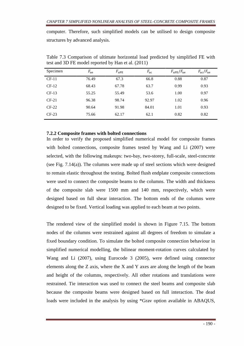
CHAPTER 7 SIMPLIFIED NONLINEAR ANALYSIS OF STEEL-CONCRETE COMPOSITE FRAMES
- 190 -
computer. Therefore, such simplified models can be utilised to design composite
structures by advanced analysis.
Table 7.3 Comparison of ultimate horizontal load predicted by simplified FE with
test and 3D FE model reported by Han et al. (2011)
Specimen 𝐹ue 𝐹uFE 𝐹uc 𝐹uFE/𝐹ue 𝐹uc/𝐹ue
CF-11 76.49 67.3 66.8 0.88 0.87
CF-12 68.43 67.78 63.7 0.99 0.93
CF-13 55.25 55.49 53.6 1.00 0.97
CF-21 96.38 98.74 92.97 1.02 0.96
CF-22 90.64 91.98 84.01 1.01 0.93
CF-23 75.66 62.17 62.1 0.82 0.82
7.2.2 Composite frames with bolted connections
In order to verify the proposed simplified numerical model for composite frames
with bolted connections, composite frames tested by Wang and Li (2007) were
selected, with the following makeups: two-bay, two-storey, full-scale, steel-concrete
(see Fig. 7.14(a)). The columns were made up of steel sections which were designed
to remain elastic throughout the testing. Bolted flush endplate composite connections
were used to connect the composite beams to the columns. The width and thickness
of the composite slab were 1500 mm and 140 mm, respectively, which were
designed based on full shear interaction. The bottom ends of the columns were
designed to be fixed. Vertical loading was applied to each beam at two points.
The rendered view of the simplified model is shown in Figure 7.15. The bottom
nodes of the columns were restrained against all degrees of freedom to simulate a
fixed boundary condition. To simulate the bolted composite connection behaviour in
simplified numerical modelling, the bilinear moment-rotation curves calculated by
Wang and Li (2007), using Eurocode 3 (2005), were defined using connector
elements along the Z axis, where the X and Y axes are along the length of the beam
and height of the columns, respectively. All other rotations and translations were
restrained. Tie interaction was used to connect the steel beams and composite slab
because the composite beams were designed based on full interaction. The dead
loads were included in the analysis by using *Grav option available in ABAQUS,

CHAPTER 7 SIMPLIFIED NONLINEAR ANALYSIS OF STEEL-CONCRETE COMPOSITE FRAMES
- 191 -
whereas the live loads were applied using a displacement control method. The
analysis was conducted using a dynamic implicit method.
(a) (b)
Figure 7.14 Frames tested by Wang and Li (2007) and general layout of frames A and
B
Figure 7.15 Rendered view of simplified model of composite frame
The simulated frame deformation for frame A is shown in Figure 7.16 where the
deformation of composite beams can be observed. But the columns remained elastic
which is consistent with the test observation. The predicted load versus mid-span
displacement curves are compared with test results for beams 1 and 2 in frame A
(Figure 7.17). In general, the agreement is good up to the ultimate load capacity.
Similar prediction accuracy was observed for beam 3 in frame B (Figure 7.18).
However, the load softening behaviour was not captured by the simplified model.
This could possibly be due to the definition of bilinear elastic-plastic moment–

CHAPTER 7 SIMPLIFIED NONLINEAR ANALYSIS OF STEEL-CONCRETE COMPOSITE FRAMES
- 192 -
rotation curves without softening branch. This can be further investigated in future
using 3D FE models such as that developed in Chapter 4. Figures 7.17 and 7.18
present the effects of idealisation of joint as rigid connection. It can be observed that
the initial stiffness and ultimate load capacity are over-predicted when the joint is
idealised as rigid. Obviously, the predicted initial stiffness of 𝑃 − ∆ curves are much
higher when the connections are assumed to be rigid. Similarly, the prediction of
ultimate load-carrying capacity is almost 20% higher when the joints are considered
as rigid compared to semi-rigid idealisation. This highlights the importance of
considering the actual performance of semi-rigid connections in the analysis.
Figure 7.16 Simulated frame deformation for frame A, tested by Wang and Li (2007)
(a) Beam 1 (b) Beam 2
Figure 7.17 Predicted and measured 𝑃 − 𝛥 curves for beams 1 and 2 in frame A
0
200
400
600
800
0 15 30 45 60 75 90
Load
P (
kN
)
Mid-span displacement Δ (mm)
Test (Wang and Li, 2007)
Simplified FE (rigid joint)
Simplified FE (semi-rigid joint)
0
200
400
600
800
0 15 30 45 60 75 90
Load
P (
kN
)
Mid-span displacement Δ (mm)
Test (Wang and Li, 2007)
Simplified FE (rigid joint)
Simplified FE (semi-rigid joint)
Frame A
Frame B
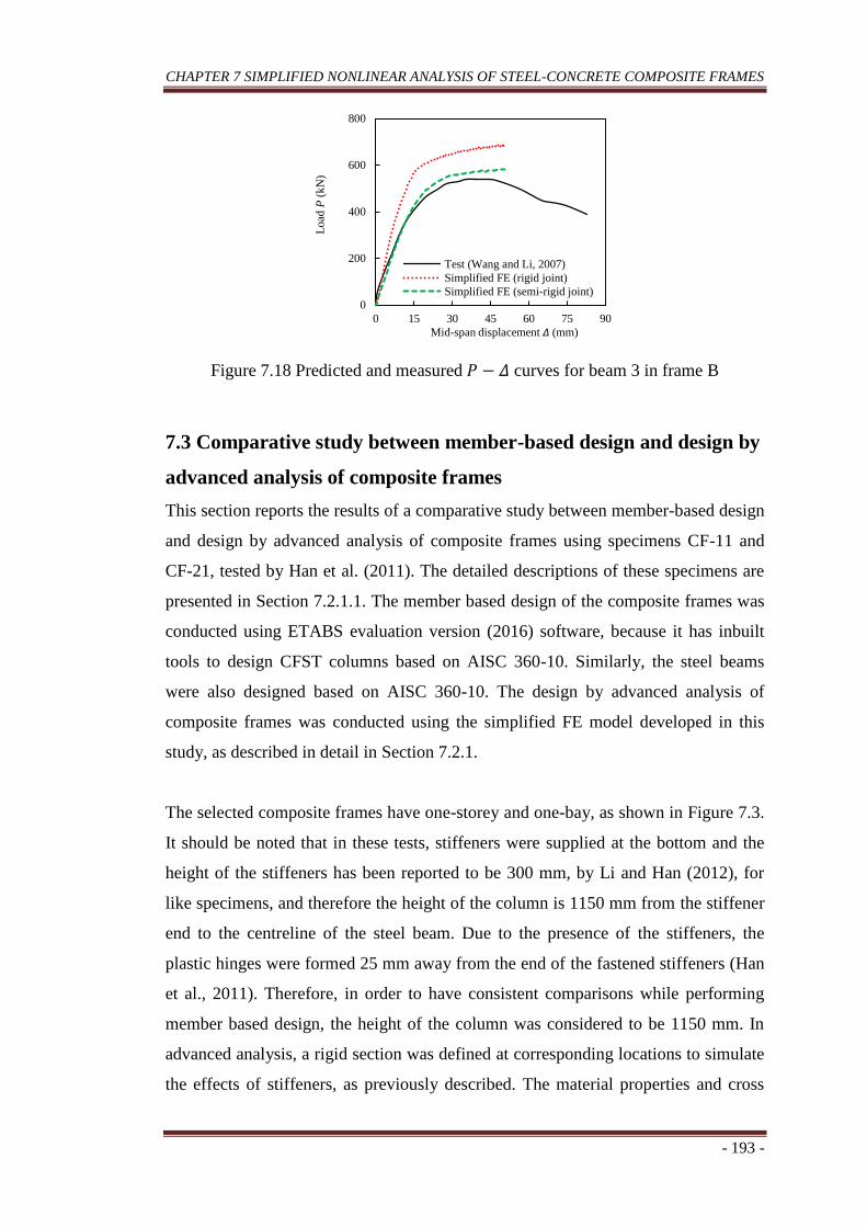
CHAPTER 7 SIMPLIFIED NONLINEAR ANALYSIS OF STEEL-CONCRETE COMPOSITE FRAMES
- 193 -
Figure 7.18 Predicted and measured 𝑃 − 𝛥 curves for beam 3 in frame B
7.3 Comparative study between member-based design and design by
advanced analysis of composite frames
This section reports the results of a comparative study between member-based design
and design by advanced analysis of composite frames using specimens CF-11 and
CF-21, tested by Han et al. (2011). The detailed descriptions of these specimens are
presented in Section 7.2.1.1. The member based design of the composite frames was
conducted using ETABS evaluation version (2016) software, because it has inbuilt
tools to design CFST columns based on AISC 360-10. Similarly, the steel beams
were also designed based on AISC 360-10. The design by advanced analysis of
composite frames was conducted using the simplified FE model developed in this
study, as described in detail in Section 7.2.1.
The selected composite frames have one-storey and one-bay, as shown in Figure 7.3.
It should be noted that in these tests, stiffeners were supplied at the bottom and the
height of the stiffeners has been reported to be 300 mm, by Li and Han (2012), for
like specimens, and therefore the height of the column is 1150 mm from the stiffener
end to the centreline of the steel beam. Due to the presence of the stiffeners, the
plastic hinges were formed 25 mm away from the end of the fastened stiffeners (Han
et al., 2011). Therefore, in order to have consistent comparisons while performing
member based design, the height of the column was considered to be 1150 mm. In
advanced analysis, a rigid section was defined at corresponding locations to simulate
the effects of stiffeners, as previously described. The material properties and cross
0
200
400
600
800
0 15 30 45 60 75 90 L
oad
P (
kN
)
Mid-span displacement Δ (mm)
Test (Wang and Li, 2007)
Simplified FE (rigid joint)
Simplified FE (semi-rigid joint)

CHAPTER 7 SIMPLIFIED NONLINEAR ANALYSIS OF STEEL-CONCRETE COMPOSITE FRAMES
- 194 -
sectional dimensions of CFST columns and steel beams were defined as reported by
Han et al. (2011) for both specimens. The fixed boundary condition was defined at
the bottom of the CFST column ends which restrains all degree of freedom. For both
specimens, a constant axial load of 50 kN was applied to each CFST column during
testing, and a cyclic horizontal load was applied by gradual increments at the level of
the steel beam, as shown in Figure 7.2.
In normal structural design, the design loads are calculated first and then the cross-
section sizes are designed to resist the prescribed amount of the load. However, in
the current research, the maximum permissible horizontal load was indirectly
determined from member-based design by keeping all other parameters identical to
the tests of Han et al. (2011). This approach was used in order to have consistency in
comparisons between the test, 3D FE modelling, advanced analysis and member-
based design. The demand/capacity ratio was checked for all members when the
frames were designed, based on member-based design, and the results were accepted
when the demand/capacity (D/C) ratio was close to but less than 1, as shown in
Figures 7.19 (a) and (b) for specimens CF-11 and CF-21, respectively. Accordingly,
the maximum permissible horizontal loads (design horizontal force from member
based design, 𝑃DM) were determined as 33.8 kN and 58.0 kN for specimens CF-11
and CF-21, respectively, from member-based design.
Figure 7.19 Demand/capacity ratios for composite frames CF-11 and CF-21
calculated from ETABS evaluation version (2016) based on AISC 360-10
It should be noted that these specimens were designed based on a Chinese code
following the strong-column weak-beam philosophy, and accordingly the steel beam
flange buckling was observed prior to formation of plastic hinges in columns during
testing (Han et al., 2011). However, the D/C ratios of CFST columns (0.994 and
0.9
61
0.9
95
0.9
94
0.9
64
0.654 0.876
(a) Specimen CF-11 (b) Specimen CF-21
Story 1 Story 1
Story 1
Base
Base
Horizontal load=33.8 kN
Axial load at columns=50.0 kN
Horizontal load=58.0 kN
Axial load at columns=50.0 kN

CHAPTER 7 SIMPLIFIED NONLINEAR ANALYSIS OF STEEL-CONCRETE COMPOSITE FRAMES
- 195 -
0.964 for specimen CF-11 and 0.995 and 0.961 for specimen CF-21) and steel beams
(0.654 and 0.876 for specimens CF-11 and CF-21, respectively), obtained from
member-based design, indicate that the CFST columns are critical members. This is
mainly due to the fact that AISC 360-10 is relatively conservative in designing CFST
columns compared with other design codes, highlighting the limitation of member-
based design.
It should also be noted that the member resistance factors stipulated in the AISC
specification have been applied to the member strengths while designing composite
frames based on member-based design. In contrast, the system resistance factor can
be used while designing structural frames by advanced analysis such as that reported
by Shayan (2013). Meanwhile, more consistent reliabilities are obtained using
system-based reliability analysis compared to member-based reliability analysis
(Zhang et al., 2018). Therefore, in the present study, the design horizontal forces
from advanced analysis (𝑃DA) were obtained by multiplying the system resistance
factor (𝜑s) to the ultimate load capacity obtained from the simulation. The value of
𝜑s equal to 0.8 was proposed by Shayan (2013) for 2D low- to mid-rise steel frames
based on a reliability analysis. The same value was tentatively used herein for
composite frames, and it is found that the design force obtained from advanced
analysis using the value of 𝜑s as 0.8 will ensure the composite frames to remain in
an elastic condition. However, there is a need to conduct further research to properly
quantify the value of 𝜑s for composite frames with CFST columns. The comparisons
of 𝑃DM and 𝑃DA are presented in Figures 7.20 (a) and (b) for specimens CF-11 and
CF-21, respectively. As expected, in both cases, the value of 𝑃DM is conservative
when compared to the value of 𝑃DA, where the ratios of 𝑃DM/𝑃DA are obtained as
0.68 and 0.78 for specimens CF-11 and CF-21, respectively (Table 7.4). This
indicates that a relatively lighter section can be designed based on advanced analysis
compared to member-based design.

CHAPTER 7 SIMPLIFIED NONLINEAR ANALYSIS OF STEEL-CONCRETE COMPOSITE FRAMES
- 196 -
(a) Specimen CF-11 (b) Specimen CF-21
Figure 7.20 Comparison of design horizontal force obtained from member-based
design and design by advanced analysis
In order to compare the reductions in steel and concrete quantities when composite
frames are designed based on advanced analysis, the composite frames are designed
to a design force level of 33.8 kN (Composite frame A) and 58 kN (Composite frame
B), which are the same as the 𝑃DM values for specimens CF-11 and CF-21,
respectively. Starting from the cross-section size used by Han et al. (2011), different
CFST columns and beam section sizes were tried while designing composite frames
by advanced analysis. This process was repeated until the maximum value of 𝜆
(where 𝜆 is the load factor which is the ratio of predicted load to the target design
force) is close to but greater than 1/ 𝜑s , which is equal to 1.25. The 𝜆 versus
horizontal displacement curves obtained from advanced analysis for both frames A
and B are presented in Figures 7.21(a) and (b), respectively. In both cases, the
maximum 𝜆 is equal to 1.26 which indicates an adequate design. It is noteworthy that
the out-of-plane degrees of freedom for the steel beams and CFST columns were
restrained, similar to the tests of Han et al. (2011), to avoid lateral-torsional buckling
of members and out-of-plane movement, which can have an adverse effect on the
load-carrying capacity of such frames. In reality, when composite beams are used in
structures, the composite slab provides restraint to the steel beam which can prevent
the lateral-torsional buckling likely to occur in pure steel beams. For CFST sections,
the use of compact section might prevent such out of plane buckling behaviour,
although future research in this area is recommended to ensure the safety levels.
0
20
40
60
80
0 25 50 75 100
Hori
zon
tal
load
(k
N)
Horizontal displacement (mm)
Test (Han et al., 2011)
3D FE (Han et al., 2011)
Simplified FE
Design force (advanced analysis)
Design force (member-based design)
0
30
60
90
120
0 25 50 75 100
Hori
zon
tal
load
(k
N)
Horizontal displacement (mm)
Test (Han et al., 2011)
3D FE (Han et al., 2011)
Simplified FE
Design force (member-based design)
Design force (advanced anaysis)

CHAPTER 7 SIMPLIFIED NONLINEAR ANALYSIS OF STEEL-CONCRETE COMPOSITE FRAMES
- 197 -
Table 7.4 Comparison of design forces obtained from member-based design and
design by advanced analysis
Specimen 𝑃DM 𝑃DA 𝑃DM/𝑃DA
CF-11 33.8 kN 49.8 kN 0.68
CF-21 58.0 kN 74.5 kN 0.78
(a) Composite frame A (b) Composite frame B
Figure 7.21 Load factor versus horizontal displacement curves
Advanced analysis was performed using exactly the same material parameters that
were used in member-based design. Tables 7.5 and 7.6 present the steel and concrete
quantity reductions when composite frames A and B were designed based on
advanced analysis compared to member-based designs. It was found that for
composite frame A, the quantity reductions for the steel tube and core concrete were
7.2% and 14.2%, respectively, while the reduction in the steel beam quantity was
39.7%. This huge reduction in the steel beam quantity can be attributed to the fact
that the demand/capacity ratio for the steel beam section was 0.654 (Figure 7.20).
However, when the demand/capacity ratio increased to 0.864 (i.e. closer to 1), the
reduction in quantity of the steel beam was only 9.8% (frame B). However, the
quantity reductions of the steel tube and concrete were 13.9% and 7.8%,
respectively, in composite frame B. It is interesting to note that the quantity
reductions are consistent with the observations of Shayan (2012), where on average
14.6% quantity reductions were reported for bare steel frames. However, for
composite frames with CFST columns, a more detailed study can be conducted in the
future to thoroughly investigate the quantity reductions when composite frames are
designed based on advanced analysis.
0
0.25
0.5
0.75
1
1.25
1.5
0 25 50 75 100
Load
fac
tor
(λ)
Horizontal displacement (mm)
Design horizontal load=33.8 kN
0
0.25
0.5
0.75
1
1.25
1.5
0 25 50 75 100L
oad
fac
tor
(λ)
Horizontal displacement (mm)
Design horizontal load=58.0 kN

CHAPTER 7 SIMPLIFIED NONLINEAR ANALYSIS OF STEEL-CONCRETE COMPOSITE FRAMES
- 198 -
Table 7.5 Comparison of CFST and steel beam section design, obtained from
member-based and advanced analysis design for composite frame A
Sections Member based design
Advanced analysis
Quantity reductions
Steel Concrete
CFST column
(D × 𝑡) mm 140 × 2 130 × 2 7.2 14.2
Steel beam
(h × bf × tf × tw) mm 150 × 70 × 3.44 × 3.44 120 × 60 × 2.5 × 2.5 39.7 -
Table 7.6 Comparison of CFST and steel beam section design, obtained from
member-based and advanced analysis design for composite frame B
Specimen Member based design
Advanced analysis
Quantity reductions (%)
Steel Concrete
CFST column
(D × 𝑡) mm 140 × 3.34 134 × 3 13.9 7.8
Steel beam
(h × bf × tf × tw) mm 160 × 80 × 3.44 × 3.44 150 × 80 × 3.2 × 3.2 9.8 -
7.4 Conclusions
This chapter combined the simplified models of CFST columns, composite beams
and composite connections presented in Chapter 3, 5 and 6 to conduct second order
inelastic analysis (advanced analysis) of steel-concrete composite frames. The
predictions obtained from the advanced analysis of composite frames were found to
be in good agreement with the test data. Then, a comparative study between the
traditional member-based design and design by advanced analysis was conducted
using one-bay, one-storey, composite frames with CFST columns. The comparison
indicates that the design by advanced analysis can lead towards lighter section, in
contrast to member-based design. However, more research needs to be done to
accurately quantify the system resistance factor for composite frames and to ensure
safety levels of all members in the steel-concrete composite framing system.

CHAPTER 8 CONCLUSIONS AND FUTURE RESEARCH NEEDS
- 199 -
CHAPTER 8
CONCLUSIONS AND FUTURE RESEARCH NEEDS
8.1 Conclusions
The design of steel structural frames by advanced analysis is permitted in modern
specifications and it is likely to become the next generation design tool for steel
frames (Shabnam, 2013). However, for steel-concrete composite structural frames,
design by advanced analysis is still in its infancy stage. To conduct advanced
analysis of composite frames, adopting simplified numerical models is the best
option because of the computational efficiency. However, it is very challenging to
accurately capture the effects of composite action between different components of
composite frame using simplified models. This task initially requires the proper
understanding of the fundamental behaviour of each component of composite frames.
This thesis presents a comprehensive study towards the development of a simplified
numerical model to conduct advanced analysis of steel-concrete composite frames. In
particular, this thesis work is mainly focussed on steel-concrete composite frames
with circular CFST columns, composite beams with through deck welded profiled
steel sheeting, composite beam-to-CFST column blind-bolted endplate connections.
Detailed investigations were conducted to understand the fundamental behaviour of
circular CFST columns and composite beams with through deck welded profiled
steel sheeting. Accordingly, simplified numerical models were developed for CFST
columns and composite beams. In order to simulate the composite connections in
simplified numerical model, the connector elements CONN3D2 available in
ABAQUS were used where the behaviour of connections in terms of moment-
rotation curves were defined. Based on the detailed finite element (FE) modelling
and simplified numerical modelling conducted in this thesis work, the major
conclusions drawn are summarised below:
CHAPTER 8 CONCLUSIONS AND FUTURE RESEARCH NEEDS
- 200 -
(a) From simplified numerical modelling of CFST columns
1. Effective stress-strain curves for the steel and core concrete were developed
to conduct fibre beam element (FBE) modelling of axially loaded circular
concrete-filled steel tubular (CFST) stub columns in Chapter 3. The FBE
modelling was conducted in ABAQUS using two noded linear beam element
B31 to simulate the core concrete and *rebar elements were used to simulate
the steel tube.
2. Since the FBE model cannot directly account for the interaction between steel
and concrete, the material models of steel and concrete themselves have to
account for such an interaction which has significant influence on the
behaviour of CFST columns. The proposed stressstrain model for steel has
implicitly considered the interaction between the steel tube and concrete,
possible local buckling of the steel tube, and strain-hardening of the steel
material. Meanwhile, the proposed concrete model has considered the
increase in strength and ductility resulting from the concrete confinement.
3. The proposed material models were implemented in the simplified FBE
modelling, and the predictions were verified by 3D FE modelling and 150 test
data collected from 23 different sources. The proposed simplified numerical
model covers a wide range of parameters: diameter-to-thickness ratio (𝐷/𝑡 =
10-220); yield stress (𝑓y = 186-960 MPa) and concrete cylinder compressive
strength (𝑓c′ = 20-200 MPa). The strength increase or degradation of a CFST
column after reaching its ultimate strength can be automatically captured in
the simulation.
4. The proposed FBE model can significantly improve the accuracy and
efficiency in simulating circular concrete-filled steel columns. Meanwhile the
proposed equations can be directly utilised to calculate the loaddeformation
curves of circular CFST stub columns using simple spreadsheet software.
This can help design engineers to conduct preliminary design of CFST
columns.

CHAPTER 8 CONCLUSIONS AND FUTURE RESEARCH NEEDS
- 201 -
(b) From detailed 3D FE modelling of composite beams
5. A 3D FE model has been developed in Chapter 4 for steel-concrete composite
beams with through deck welded profiled steel sheeting. The developed FE
model can successfully capture different types of failure modes of composite
beams, such as shear failure of the studs, concrete crushing failure, steel beam
failure and rib shear failure. To capture these failure modes, fracture failure
of shear studs and profiled steel sheeting is defined in the stress−strain curves.
Meanwhile, concrete damage parameters are defined to capture the strength
deterioration of composite beams due to concrete failure.
6. Instead of using embedded interaction between the stud and concrete or using
connector elements to represent the stud behaviour, a realistic surface-to-
surface interaction has been defined for the contact interactions between the
concrete and studs. A friction coefficient of 0.01 can be used in the FE
modelling for the contact surfaces between concrete and the profiled steel
sheeting, between concrete and the shear studs, as well as between the
profiled steel sheeting and the top flange of the steel beam. This selection has
been validated by comparing the FE results with the test results.
7. The proposed FE model can satisfactorily predict the full-range
load−deformation curves of composite beams. Meanwhile, the realistic shear
force−slip curves of shear studs can be obtained from the proposed FE model,
and the contribution from the profiled steel sheeting to composite action can
be quantified.
(c) From simplified numerical modelling of composite beams
8. A feasibility study of simplified FE model for composite beams with headed
shear studs and profiled steel sheeting has been conducted in Chapter 5, to
solve the modelling complexity of such composite beams. The proposed
simplified model utilises four-noded shell element (S4R) to simulate the
composite slab where the profiled steel sheeting and rebars are integrated
together. For the simulation of steel beams, two-noded linear beam elements

CHAPTER 8 CONCLUSIONS AND FUTURE RESEARCH NEEDS
- 202 -
B31 were used. The load versus slip behaviour of shear connectors obtained
through detailed FE modelling was defined through connector elements
CONN3D2.
9. The predictions obtained from simplified modelling have good correlation
with tests and detailed FE modelling results of composite beams.
10. From the simplified analysis, it was found that the predictions were
unconservative when tie constraints were utilised to represent the interaction
between steel beam and composite slabs especially for composite beams with
partial shear interaction. But the predictions have excellent match with test
data when the load-slip curves obtained from detailed FE modelling were
utilised with hard contact interaction between composite slab and steel beam.
11. The equations to determine the shear force of shear studs in composite beams
in Eurocode 4 (2004) were obtained from push test specimens. The detailed
FE modelling was conducted to examine the fundamental behaviour of
components of push test specimens. It was found that for push test specimens
with solid reinforced concrete slab, the predicted shear force matches with the
test data. But for push test specimens with profiled steel sheeting, the shear
forces of shear studs are found to be comparatively lower. This is because the
contribution from profiled steel sheeting is not deducted from the total load in
previous studies. It is interesting to note that when the ribs of the profiled
steel sheeting were placed parallel to the steel beam longitudinal axis, the
load resisted by sheeting is 1.31 times higher than that resisted by shear studs
for the selected specimen. When the ribs of profiled steel sheeting were
placed perpendicular to the beam longitudinal axis, the contribution from
profiled steel sheeting was only 0.27 times that resisted by shear studs. This
clearly indicates that contribution from profiled steel sheeting should not be
ignored when determining the shear capacity of shear studs.
12. Compared with detailed FE model, the simplified FE model was much more
efficient. Using a typical modern computer, the computational time was only
a few minutes for both simply supported and continuous composite beams.
For the same composite beams, the detailed FE modelling took a few days to

CHAPTER 8 CONCLUSIONS AND FUTURE RESEARCH NEEDS
- 203 -
weeks depending on the number of elements. Also, the detailed FE model
was much more tedious to develop. Therefore, the proposed simplified FE
model can be efficiently implemented in composite frame analysis.
(d) From simplified numerical modelling of composite connections
13. A simplified FE model for composite beams-to-CFST columns with blind-
bolted endplate connections has been developed in Chapter 6. The connection
behaviour was defined in terms of moment-rotation (𝑀 − ∅) relationship
utilising a single connector element CONN3D2 available in ABAQUS. For
the simulation of CFST columns and composite beams, the simplified FE
model developed in Chapter 3 and Chapter 5 were utilised respectively.
Meanwhile, the mathematical model developed by Hassan (2016) was used to
determine 𝑀 − ∅ curves for composite beams-to-CFST columns with blind-
bolted flush endplate connections. Meanwhile, the model developed by Thai
et al. (2017) was used to determine 𝑀 − ∅ curves for the composite beams-
to-CFST columns with blind-bolted extended endplate connections.
14. The initial stiffness as well as ultimate capacity predicted from simplified
numerical model are in good agreement with the test data. However, the
deterioration of moment capacity after reaching ultimate moment capacity
was not captured as the utilised 𝑀 − ∅ curves can only predict up to the
ultimate capacity.
15. The simplified FE model was also verified for through-plate composite
connections using the measured 𝑀 − ∅ data in tests and the predictions are
also found to be reasonably accurate for composite connections with through-
plate connections.
16. The influence of idealisation of composite connections as rigid and semi-rigid
connections was investigated. The initial stiffness as well ultimate capacity
were over predicted when connections were idealised as rigid. For a typical
case study reported in Chapter 6, the ultimate prediction is 46% higher than
the measured ultimate capacity. However, the prediction has excellent match
with test data when the connections were idealised as semi-rigid. This

CHAPTER 8 CONCLUSIONS AND FUTURE RESEARCH NEEDS
- 204 -
highlights the importance of considering the influence of joint rotation when
analysing composite frames with semi-rigid connections.
17. The simplified FE model is computationally very efficient. It took less than
10 minutes for the analysis of isolated composite connections.
(e) From simplified numerical modelling of composite frames
18. The simplified numerical models developed for CFST column, composite
beams and composite connections were implemented together in Chapter 7 to
conduct simplified nonlinear analysis of composite frames. The predictions
obtained from simplified model were found to be in good agreement with test
data. The simplified FE model was found to be computationally very efficient.
For a typical one-bay one-storey composite frame without composite slab, it
only took a few seconds for analysis while for two-bay two-storey frames
with composite slab and bolted connections, it took around 15 minutes using
a typical modern computer.
19. The simplified FE model can be used to design composite frames by
advanced analysis. As opposed to member-based design, the composite
frames can be directly designed using advanced analysis and there is no need
to use complicated effective length factors as well as interaction equations.
20. The comparative study between design of composite frames using traditional
member-based design and advanced analysis was conducted. The comparison
indicates that the design by advanced analysis can lead towards economical
design of composite frames than that designed by member-based design. For
the selected example (frame B), the quantity reductions for steel tubes and
concrete infill in CFST columns were 13.9 % and 7.8% respectively whereas
the quantity reductions for steel beam was found to be 9.8%.
8.2 Recommendations for future research
Extensive numerical investigations were conducted in this thesis work to explore the
fundamental behaviour of different components of composite frames and as a result,

CHAPTER 8 CONCLUSIONS AND FUTURE RESEARCH NEEDS
- 205 -
a framework model has been developed to conduct advanced analysis of composite
frames. However, further research is required for the implementation of advanced
analysis in design of composite frames. The recommendations for future research are
as follows:
1. In the present study, effective steel and concrete models for FBE modelling
are developed only for circular CFST columns. Further research is required to
propose a similar model for rectangular columns due to the difference in
section stability and concrete confinement between the two types of columns.
Further research is also required to consider the simulation of slender CFST
columns. Meanwhile, this research can be extended to CFST columns with
various cross-sections such as elliptical, polygonal, double-tube columns,
double-skin columns as well as CFST columns utilising different material
such as stainless steel and geopolymer concrete.
2. The proposed detailed FE modelling of composite beams can be extended for
composite beams with rectangular reinforced concrete slabs. Meanwhile, this
work can be further extended to composite beams with demountable features.
The influence of different types of connectors and other types of profiled
steel sheeting can be further investigated. Also, the proposed model can be
further utilised to conduct numerical analysis to check the effects of long
term loading on composite beams. Furthermore, the governing criteria for
each type of failure modes of composite beams are needed to be developed.
3. The developed detailed FE model of composite beams can be used further to
conduct parametric studies. The effects of various composite beam
parameters can be investigated thoroughly. This is particularly true for the
behaviour of the shear studs embedded in concrete. For example, previous
studies have demonstrated that the behaviour of shear studs observed from
push tests could not represent the actual behaviour of shear studs in
composite beams. A deep understanding of the shear studs behaviour can be
obtained by using the developed FE model. Such a deep understanding is
essential for proposing a versatile full-range shear force-slip relationship of
shear studs. Such a model is urgently needed to improve the accuracy of

CHAPTER 8 CONCLUSIONS AND FUTURE RESEARCH NEEDS
- 206 -
simplified numerical modelling of composite frames, especially when
conducting advanced analysis.
4. The 𝑀 − ∅ curves of composite blind-bolted connections are very important
in simplified nonlinear analysis as the majority of these connections exhibit
semi-rigid behaviour. However, the currently available 𝑀 − ∅ models can
predict only up to the ultimate capacity. This can be further extended to
consider softening part of the 𝑀 − ∅ curves to accurately capture the full-
range behaviour of composite connections including failure.
5. More experimental studies as well as 3D FE analysis can be done for CFST
column to composite beams with through-plate connections. A detailed study
is required to develop simplified moment-rotation model for such through-
plate composite connections.
6. The test data on steel-concrete composite frames is very limited. Therefore,
more tests can be conducted that can be used as benchmark models for
advanced analysis of composite frames including CFST columns and
composite slabs.
7. The system resistance factor plays a very important role to determine design
capacity of composite frames by advanced analysis. Therefore, reliability
assessment needs to be conducted to determine an accurate system resistance
factor for composite frames.
8. The developed advanced analysis method for composite frames can be
further extended to consider the influence of concrete creep and shrinkage.
Furthermore, the proposed method can be extended to consider seismic
loading, extreme events such as fire, impact and blast.

REFERENCES
- 207 -
REFERENCES
ABAQUS Theory Manual. 2014. Version 6.14. Providence, RI (USA): Dassault
Systèmes Corp.
ABAQUS. 2004. ABAQUS User’s Manual, Version 6.14. Providence, RI (USA):
Dassault Systèmes Corp.
Abdullah, R. 2004. Experimental evaluation and analytical modeling of shear bond
in composite slabs. PhD Thesis, Virginia Polytechnic Institute and State
University.
ACI (American Concrete Institute). 2014. Building Code Requirements for Structural
Concrete (ACI 318-11) and Commentary. Farmington Hills, MI, USA.
Ahmed, B. & Nethercot, D.A. 1997. Prediction of initial stiffness and available rotation
capacity of major-axis flush endplate connections. Journal of Constructional Steel
Research, 41(1): 31–60.
AISC360-10. 2010. Specification for structural steel buildings. American institute of
steel construction, Chicago, Illinois.
Al-aasam, H.S. 2013. Modern Engineering Design: Analytical and numerical
modelling of semi-rigid connections. PhD Thesis, The University of Manchester.
Alashker, Y.; El-Tawil, S. & Sadek, F. 2010. Progressive collapse resistance of steel-
concrete composite floors. Journal of Structural Engineering, ASCE, 136(10),
1187-1196.
Anderson, D. & Najafi, A.A. 1994. Performance of composite connections: major axis
endplate joints. Journal of Constructional Steel Research, 31:31- 57.
Anderson, D.A., Aribert, J.M., Bode, H. & Kronenburger, H.J. 2000. Design rotation
capacity of composite joints. The Structural Engineer, 78(6): 25-29.
Aribert, J.M. & Lachal, A. 1992. Experimental investigation of composite connections in
global interpretation. Proceedings of COST C1 Conference on Semi-rigid Joints,
Strasbourg, France, 1992: 158-169.
AS/NZS Standard. 2003. Structural steel welding, Part 2: Stud welding (steel studs to
steel). AS/NZS 1554.2:2003, Sydney, Australia.
AS4100. 1998. Australian standard AS4100-Steel structures, Sydney, NSW 2001,
Australia.
Ataei, A. & Bradford, M.A. 2013. FE modelling of semi-rigid flush endplate joints
with concrete-filled steel tubular columns. Proceedings of 5th International

REFERENCES
- 208 -
Conference on Structural Engineering and Mechanics, University of Cape Town,
Cape Town, South Africa.
Ban, H.Y. & Bradford, M.A. 2013. Flexural behaviour of composite beams with high
strength steel. Engineering Structures, 56: 1130-1140.
Ban, H.Y. ; Shi, G. ; Shi, Y. & Bradford, M.A. 2013. Experimental investigation of
the overall buckling behaviour of 960 MPa high strength steel columns. Journal
of Constructional Steel Research, 88: 256–266.
Ban, H.Y., Bradford. M.A., Uy, B. & Liu, X. 2016. Available rotation capacity of
composite beams with high-strength materials under sagging moment. Journal of
Constructional Steel Research, 118: 156‒168.
Binici, B. 2005. An analytical model for stress–strain behavior of confined concrete.
Engineering Structures, 27(7): 1040-1051.
Bradford, M.A. 2012. Numerical modelling of shear connection in steel-concrete
composite beams with trapezoidal slabs. Australian Journal of Structural
Engineering, 12(3): 185-195.
Carreira, D.J. & Chu, K.H. 1985. Stress-strain relationship for plain concrete in
compression. Journal of ACI Structural, 82: 797-804.
Cas, B.; Bratina, S.; Saje, M. & Planinc, I. 2004. Non-linear analysis of composite
steel-concrete beams with incomplete interaction. Steel and Composite
Structures, 4(6): 489-507.
CEB-FIB. 2010. International Federation for Structural Concrete (fib), Model Code
2010 – Final draft, Volume 1, Bulletin 65, Lausanne, Switzerland; 2012. pp. 118.
Chacon, R. 2015. Circular concrete-filled tubular columns: State of the art oriented to
the vulnerability assessment. The Open Civil Engineering Journal, 9: 249-259.
Chiorean, C. G. 2013. A computer method for nonlinear inelastic analysis of 3D
composite steel-concrete frame structures. Engineering Structures, 57: 125-152.
Chireon, C.G. 2010. Computerised interaction diagrams and moment capacity
contours for composite steel-concrete cross-sections. Engineering Structures,
32:3734-3757.
Clarke, M.J.; Bridge, R.Q.; Hancock, G.J. & Trahair, N.S. 1992. Advanced analysis
of steel building frames. Journal of Constructional Steel Research, 23: 1‐29.
Composite column Design Manual AISC 360-10 for ETABS. 2016.Computers &
Structures, INC.

REFERENCES
- 209 -
da Silva, L.S.; Costa-Neves, L.F. & Vellasco, P.C.G.D. 2004. Design procedure for I-
beam to concrete filled column and Minor axis joints; Characterization of the
component “Column web loaded in out-of-plane bending”. Brugge: ECCS Technical
Committee 10 "Connections".
da Silva, L.S.; Simoes, R. & Cruz, P.2001. Experimental behaviour of endplate beam-to-
column composite joints under monotonical loading. Engineering Structures, 23:
1383–409.
Dai, X., & Lam, D. 2010. Numerical modelling of the axial compressive behaviour
of short concrete-filled elliptical steel columns. Journal of Constructional Steel
Research, 66: 931-942.
De Nicolo B.; Pani, L. & Pozzo, E. 1994. Strain of concrete at peak compressive
stress for a wide range of compressive strengths. Materials and Structures, 27(4):
206-210.
de Oliveira, W.L.A.; de Nardin, S.; de Cresce El Debs, A.L.H. & El Debs, M.K.
2009. Influence of concrete strength and length/diameter on the axial capacity of
CFT columns. Journal of Constructional Steel Research, 65(12): 2103-2110.
Denavit, M.D. & Hajjar, J.F. 2012. Nonlinear seismic analysis of circular concrete-
filled steel tube members and frames. Journal of Structural Engineering, ASCE,
138(9): 1089-1098.
Dhanalakshmi, M.; Byfied, M.P. & Couchman, G.H. 2002. Composite connections at
perimeter locations in unpropped composite floors. Advances in Steel Structures,
1:261–8.
Easterling, W.S.; Gibbings, D.R. & Murray, T.M. 1993. Strength of Shear Studs in
Steel Deck on Composite Beams and Joists. Engineering Journal, AISC, 30(2):
44-55.
Elamin, A.M.E. A. 2013. The face bending behaviour of blind-bolted connections to
concrete-filled hollow sections. PhD Thesis, Faculty of Engineering, The University
of Nottingham.
Endo, F.; Watnabe, T.; Yoshida, O. & Takeshi, S. 2011. Advanced Technologies
Applied at the New “Techno Station” Building in Tokyo, Japan, Structutral
Engineering International, 4: 508-513
Ernst, S.; Bridge, R.Q. & Wheeler, A. 2010. Correlation of beam tests with pushout
tests in steel-concrete composite beams. Journal of Structural Engineering, ASCE,
136(2), 183-192.

REFERENCES
- 210 -
Eurocode 3. 2005. Design of steel structures, Part 1.8, Design of joints. prEN 1993-1-8:
2005.
Eurocode 4. 2004. Design of composite steel and concrete structures, Part 1.1, General
rules and rules for building. BS EN 1994-1-1: 2004. British Standards Institution,
London.
European Convention for Constructional Steelwork (ECCS). Ultimate limit state
calculation of sway frames with rigid joints. Technical Committee 8−Structural
Stability Technical Working Group. Publication No. 33. Brussels, Belgium; 1984.
Faella, C.; Martinelli, E. & Nigro, E. 2003. Shear connection nonlinearity and
deflections of steel-concrete composite beams: A simplified method. Journal of
Structural Engineering, 129(1): 12‒20.
Gardener, N. J. & Jacobson, R. 1967. Structural behavior of concrete filled steel
tubes. ACI Journal, 64(7): 404-413.
Gardener, N.J. 1968. Use of spiral welded steel tubes in pipe columns. Journal of
American Concrete Institute, 65(11): 937-942.
Giakoumelis, G. & Lam, D. 2004. Axial capacity of circular concrete-filled tube
columns. Journal of Constructional Steel Research, 60(7): 1049-1068.
Gillie M. 2000. Development of generalized stress strain relationships for the concrete
slab in shell models. PIT project research report SS2, Technical report. University of
Edinburgh.
Goode, C.D. (2008). Composite columns – 1819 tests on concrete-filled steel tube
columns compared with Eurocode 4. The Structural Engineer, 19: 33-38.
Goto, Y. & Chen, W.F. 1987. On the Computer-Based Design Analysis for the
Flexibility Jointed Frames. Journal of Constructional Steel research, 8:203-231.
Grant, J.A.; Fisher, J.W. & Slutter, R.G. 1977. Composite beams with formed steel
deck. Engineering Journal, AISC 14: 24-43.
Grantham, R. & Jarrett, N.D. 1993. Composite sub-frame tests. Report no.4: Results
from test NR3, N71/93. Building Research Establishment.
Guler, S.; Copur, A. & Aydogan, M. 2013. Axial capacity and ductility of circular
UHPC-filled steel tube columns. Magazine Concrete Research, 65(15): 898-905.
Guler, S.; Copur, A. & Aydogan, M. 2014. A comparative study on square and
circular high strength concrete-filled steel tube columns. Advanced Steel
Construction, 10(2): 234-247.

REFERENCES
- 211 -
Guo, L.; Gao, S.; Fu, F. & Wang, Y. 2013. Experimental study and numerical
analysis of progressive collapse resistance of composite frames. Journal of
Constructional Steel Research, 89, 236-251.
Gupta, P. K.; Sarda, S. M. & Kumar, M. S. 2007. Experimental and computational
study of concrete filled steel tubular columns under axial loads. Journal of
Constructional Steel Research, 63(2), 182-193.
Hajjar, J.F. & Molodan, A. 1998. A distributed plasticity model for cyclic analysis of
concrete-filled steel tube beam-columns and composite frames. Engineering
Structures, 20, 398-412.
Hajjar, J.F.; Schiller, P.H. & Molodan, A. 1998. A distributed plasticity model for
concrete-filled steel tube beam-columns with interlayer slip. Engineering
Structures, 20(8), 663-676.
Han, L.H. & Yao, G.H. 2004. Experimental behaviour of thin-walled hollow
structural steel (HSS) columns filled with self-consolidating concrete (SCC).
Thin-Walled Structures, 42(9): 1357-1377.
Han, L.H. 2007. Concrete filled steel tubular structures-theory and practice (2nd
edition). Beijing Science Press. (in Chinese).
Han, L.H., Yao, G.H. & Tao, Z. 2007. Performance of concrete-filled thin-walled
steel tubes under pure torsion. Thin-Walled Structures, 45(1): 24-36.
Han, L.H.; Hou, C.C. & Wang, Q.L. 2014a. Behavior of circular CFST stub columns
under sustained load and chloride corrosion. Journal of Constructional Steel
Research, 103: 23-36.
Han, L.-H.; Li, W. & Bjorhovde, R. 2014b. Developments and advanced applications
of concrete-filled steel tubular (CFST) structures: Members. Journal of
Constructional Steel Research, 100: 211-228.
Han, L.H.; Wang, W.D. & Tao, Z. 2011. Performance of circular CFST column to
steel beam frames under lateral cyclic loading. Journal of Constructional Steel
Research, 67(5), 876-890.
Han, L.H.; Wang, W.D. & Zhao, X.L. 2008. Behaviour of steel beam to concrete-
filled steel tubular column frames: finite element model and verifications.
Engineering Structures, 30(6):1647–58.
Han, L.H.; Yao, G.H. & Zhao, X.L. 2005. Tests and calculations for hollow
structural steel (HSS) stub columns filled with self-consolidating concrete (SCC).
Journal of Constructional Steel Research, 61(9), 1241-1269.

REFERENCES
- 212 -
Hassan, M.K. 2016. Behaviour of hybrid stainless-carbon steel composite beam-
column joints. PhD Thesis, Western Sydney University, Australia.
Hatzigeorgiou, G.D. (2008a). Numerical model for the behavior and capacity of
circular CFT columns, Part I: Theory. Enineering Structures, 30: 1573-1578.
Hatzigeorgiou, G.D. 2008b. Numerical model for the behaviour and capacity of
circular CFT columns, Part II Verification and extension. Engineering Structures,
30: 1579-1589.
Hicks, S.J. & Smith, A.L. 2014. Stud shear connectors in composite beams that
support slabs with profiled steel sheeting. Structural Engineering International
24(2): 246‒253.
Hicks, S.J. 2007. Strength and ductility of headed stud connectors welded in modern
profiled steel sheeting. The Structural Engineer, 32‒38.
Hicks, S.J. 2009. Strength and ductility of headed stud connectors welded in modern
profiled steel sheeting. Structural Engineering International, 4: 415‒419.
http://skyscrapercenter.com/year‒in‒review/2016
Huang, C.S.; Yeh, Y.K.; Liu, G.Y.; Hu, H.T.; Tsai, K.C.; Weng, Y.T.; Wang, S.H. &
Wu, M.H. 2002. Axial load behavior of stiffened concrete-filled steel columns.
Journal of Structural Engineering, ASCE, 128(9): 1222-1230.
Huang, Z. 2011. A connection element for modelling end-plate connections in fire.
Journal of Constructional Steel Research, 67(5): 841-853.
Huang, Z.; Burgess, I.W. & Plank, R.J. 2003, Modelling membrane action of
concrete slabs in composite buildings in Fire. I: Theoretical Development. Journal
of Structural Engineering, ASCE, 129(8): 1093-1102.
Jarrett, N.D. & Grantham, R. 1992. Composite sub-frame tests. Report no.3: Results
from test NR2, N141/92. Building Research Establishment.
Jayas, B.S. & Hosain, M.U. 1989. Behaviour of headed studs in composite beams:
full-size tests, Canadian Journal of Civil Engineering, 16(5): 712-724.
Jeyarajan, S.; Liew, J.Y.R. & Koh, C.G. 2015. Progressive collapse mitigation
approaches for steel-concrete composite buildings. International Journal of Steel
Structures, 15(1): 175-191.
Johnson, R.P. & Yuan, H. 1998. Existing rules and new tests for stud shear
connectors in troughs of profiled steel sheeting. Proceedings of the Institution of
Civil Engineers, Structures and Buildings, 128:244-51.

REFERENCES
- 213 -
Kang, L.; Leon, R.T. & Lu, X. 2014. A general analytical model for steel beam-to-
CFT column connections in OpenSEES. Journal of Constructional Steel
Research, 100: 82-96.
Karren, K.W. 1965. Effects of cold-forming on light-gage steel members. PhD
Thesis, Cornell University, New York, USA.
Kim, S.E. 1996. Practical advanced analysis for steel frame design. PhD Thesis,
Purdue University.
Kim, S.E.; & Chen, W.F. 1999. An Innovative Design for Steel Frame Using
Advanced Analysis. CRC Press, Boca Raton, FL.
Kurobane, Y.; Packer, J.; Wardenier, J. & Yeomans, N. 2004. Design guide for
structural hollow section column sections. ISBN 3-8249-0802-6.
Kwak, H.G. & Hwang, J.W. 2010. FE model to simulate bond-slip behavior in
composite concrete beam bridges. Computers & Structures, 88(17): 973‒984.
Kwasniewski, L. 2010. Nonlinear dynamic simulations of progressive collapse for a
multistory building. Engineering Structures, 32:1223-1235.
Lai, Z. & Varma, A.H. 2016. Effective stress-strain relationships for analysis of
noncompact and slender filled composite (CFT) members. Engineering
Structures, 124: 457-472.
Lam, D. & El-Lobody, E. 2005. Behavior of headed stud shear connectors in
composite beam. Journal of Structural Engineering, ASCE, 131(1): 96‒107.
Lam, D.; Dai, X.H.; Han, L.H.; Ren, Q.X. and Li, W. 2012. Behaviour of inclined,
tapered and STS square CFST stub columns subjected to axial load. Thin-Walled
structures, 54: 94-105.
Lee, S.H.; Uy, B.; Kim, S.H.; Choi, Y. H. & Choi, S.M. 2011. Behavior of high-
strength circular concrete-filled steel tubular (CFST) column under eccentric
loading. Journal of Constructional Steel Research, 67: 1-13.
Leon, R.T. 1990. Semi-rigid composite construction. Journal of Constructional Steel
Research, 25:99-120.
Li, T.Q.; Moore, D.B.; Nethercot, D.A. & Choo, B.S. 1996a. The experimental
behaviour of a full-scale, semi-rigidly connected composite frame: Detailed
appraisal. Journal of Constructional Steel Research, 39(3):193–220.
Li, T.Q.; Nethercot, D.A. & Choo, B.S. 1996b. Behaviour of flush end plate with
unbalanced moment and variable shear/moment ratios. I-Experimental behaviour.
Journal of Constructional Steel Research, 38(2): 125–164.

REFERENCES
- 214 -
Li, W. & Han, L.H. 2012. Seismic performance of CFST column to steel beam joint
with RC slab: Joint model. Journal of Constructional Steel Research, 73: 66-79.
Liang, Q.Q. & Fragomeni, S. 2009. Nonlinear analysis of circular concrete-filled
steel tubular short columns under axial loading. Journal of Constructional Steel
Research, 65(12): 2186-2196.
Liang, Q.Q. 2008. Nonlinear analysis of short concrete-filled steel tubular beam-
columns under axial load and biaxial bending. Journal of Constructional Steel
Research, 64: 295-304.
Liew, J.Y.R. & Xiong, D.X. 2012. Ultra-high strength concrete filled composite
columns for multi-storey building construction. Advances in Structural
Engineering, 15(9): 1487-1503.
Liew, J.Y.R.; Teo, T.H.; Shanmugam, N.E. & Yu, C.H. 2000. Testing of steel-concrete
composite connections and appraisal of results. Journal of Constructional Steel
Research, 56(2): 117-150.
Liew, J.Y.R.; White, D.W. & Chen, W.F. 1993. Second-order refined plastic-hinge
analysis for frame design. Part II. Journal of structural engineering, 119(11):
3217-3236.
Liew, J.Y.R.; White, D.W. & Chen, W.F. 1994. Notional‐load plastic‐hinge method
for frame design. Journal of Structural Engineering, ASCE, 120(5): 1434‐1454.
Liew, J.Y.R.; Xiong, M. and Xiong, D. 2016. Design of Concrete Filled Tubular
Beam-Columns with High Strength Steel and Concrete. Structures, 8(2):213-226.
Liew, J.Y.R.; Xiong, M.X., & Xiong, D.X. 2014. Design of high strength concrete
filled tubular columns for tall buildings. International Journal of High-Rise
Buildings, 3(3): 215-221.
Liew. J.Y.R. 2015. Design of concrete filled tubular members with high strength
materials: An extension of Eurocode 4 Method to C90/105 Concrete and S550 Steel.
International Symposium on Design and Construction of Steel and Composite
Structures, LT7A, Faculty of Engineering, National University of Singapore.
Liu, S.W.; Liu, Y.P. & Chan S.L. 2012, Advanced analysis of hybrid steel and
concrete frames Part 2: Refined plastic hinge and advanced analysis. Journal of
Constructional Steel Research, 70:337-349.
Loh, H.Y. 2004. The effects of partial shear connection in hogging moment regions
of composite steel-concrete structures, PhD Thesis, University of New South
Wales, Sydney, Australia.

REFERENCES
- 215 -
Loh, H.Y.; Uy, B. & Bradford, M.A. 2004. The effects of partial shear connection in
the hogging moment regions of composite beams Part I-Experimental study,
Journal of Constructional Steel Research, 60: 879‒919.
Loh, H.Y.; Uy, B. & Bradford, M.A. 2006. The effects of partial shear connection in
composite flush end plate joints. Journal of Constructional Steel Research, 62(6):
378-390.
LS-DYNA (Computer software). Livermore Software Technology Corporation,
Livermore, CA.
Main, J.A. 2014. Composite floor systems under column loss collapse: Collapse
resistance and tie force requirements. Journal of Structural Engineering, ASCE,
140: (A4014003), 1-15.
Mirza, O. & Uy, B. 2010. Effects of strain regimes on the behaviour of headed studs
shear connectors for composite steel-concrete beams. Advanced Steel
Construction, 6(1): 635‒661.
Mirza, O. & Uy, B. 2011. Behaviour of composite beam-column flush endplate
connections subjected to low-probability, high-consequence loading. Engineering
Structures, 33(2): 647-662.
Mirza, O. 2008. Behaviour and design of headed stud shear connectors in composite
steel-concrete beams. PhD Thesis, Western Sydney University.
Nie, J.; Cai C.S. & Wang T. 2004. Stiffness and deflection of steel-concrete
composite beams under negative bending, Journal of Structural Engineering,
130(11): 1842‒1851.
Nie, J.; Cai, C.S. & Wang, T. 2005. Stiffness and capacity of steel-concrete
composite beams with profiled sheeting. Engineering Structures, 27(7): 1074‒
1085.
Nie, J.; Fan J. & Cai, C.S. 2008. Experimental study of partially shear-connected
composite beams with profiled sheeting. Engineering Structures, 30(1): 1‒12.
Nie, J.; Yuan, H.; Weijian, Y. & Jiansheng F. 2012. Seismic behaviour of CFRSTC
composite frames considering slab effects. Journal of Constructional Steel
Research, 68, 165-175.
Ollgaard, J.G.; Slutter, R.G. & Fisher, J.W. 1971. Shear strength of stud connectors
in lightweight and normal weight concrete. AISC Engineering Journal, 8(2): 55–
64.

REFERENCES
- 216 -
O'Shea, M.D. & Bridge, R.Q. 1994. Tests on thin-walled concrete-filled steel tubes.
Proceedings of the 12th International Specialty Conference on Cold-Formed Steel
Strucures, St. Louis, Missouri, USA: 399419.
O'Shea, M.D. & Bridge, R.Q. 1998. Tests on circular thin-walled steel tubes filled
with medium and high strength concrete. Australian Civil Engineering
Transaction, 40: 15-27.
Patel, V.I.; Liang, Q.Q. & Hadi, M.N.S. 2014. Nonlinear analysis of axially loaded
circular concrete-filled stainless steel tubular short columns. Journal of
Constructional Steel Research, 101: 9-18.
Pavlović, M.; Marković, Z.; Veljković, M. & Buđevac, D. 2013. Bolted shear
connectors vs. headed studs behaviour in push-out tests. Journal of Constructional
Steeel Research, 88: 134-149.
Pitrakkos, T. 2012. The tensile stiffness of a novel anchored blind-bolt component for
moment-resisting connections to concrete-filled hollow sections. PhD Thesis, The
University of Nottingham.
Qiang, X.; Bijlaard, F.S.K. & Kolstein, H. 2013. Post-fire preformance of very high
strength steel S960. Journal of Constructional Steel Research, 80: 235-242.
Qina, Y.; Chena, Z.; Yangc, Q. & Shangd, K. 2014. Experimental seismic behavior of
through-diaphragm connections to concrete-filled rectangular steel tubular columns.
Journal of Constructional Steel Research, 93: 32-43.
Queiroz, F.D.; Vellasco, P.C.G.S. & Nethercot, D.A. 2007. Finite element modelling
of composite beams with full and partial shear connection. Journal of
Constructional Steel Research, 63(4): 505‒521.
Qureshi, J.; Lam, D. & Ye, J. 2011. Effect of shear connector spacing and layout on
the shear connector capacity in composite beams. Journal of Constructional Steel
Research, 67: 706‒719.
Rambo-Roddenberry, MD. 2002. Behavior and strength of welded stud shear
connectors. PhD Thesis, Virginia Polytechnic Institute and State University.
Ranzi, G. & Zona, A. 2007. A steel-concrete composite beam model with partial
interaction including the shear deformability of the steel component. Engineering
Structures, 29(11): 3026‒3041.
Ranzi, G.; Bradford, M.A.; Ansourian, P.; Filonov, A.; Rasmussen, K.J.R.; Hogan,
T.J. & Uy, B. 2009. Full-scale tests on composite steel-concrete beams with steel
trapezoidal decking. Journal of Constructional Steel Research, 65(7): 1490‒1506.
REFERENCES
- 217 -
Robinson, H. 1969. Composite beams incorporating cellular steel decking. Journal of
Structural Engineering, ASCE, 95(3):355-380.
Sadek, F.; El-Tawil, S. & Lew, H.S. 2008. Robustness of composite floor systems
with shear connections: Modeling, Simulation, and evaluation. Journal of
Structural Engineering, ASCE, 134(11): 1717-1725.
Sakino, K. & Hayashi, H. 1991. Behavior of concrete filled steel tubular stub
columns under concentric loading. Proceedings of the 3rd International
Conference on Steel-Concrete Composite Structures, Fukuoka, Japan: 25-30.
Sakino, K.; Nakahara, H.; Morino, S. & Nishiyama, I. 2004. Behavior of centrally
loaded concrete-filled steel-tube short columns. Journal of Structural
Engineering, ASCE, 130(2): 180-188.
Salari, M.R. & Spacone, E. 2001. Analysis of steel-concrete composite frames with
bond slip. Journal of Structural Engineering, ASCE, 127(11): 1243-1250.
Samani, A.K. & Attard, M.M. 2012. A stress–strain model for uniaxial and confined
concrete under compression. Engineering Structures, 41: 335-349.
Schneider, S. & Alostaz, Y. 1998. Experimental behaviour of connections to
concrete filled steel tubes. Journal of Constructional Steel Research, 453:321-52.
Schneider, S.P. 1998. Axially loaded concrete-filled steel tubes. Journal of Structural
Engineering, ASCE, 124(10): 1125-1138.
Shabnam, S. 2013. System reliability-based design of 2D steel frames by advanced
analysis. PhD Thesis, The University of Sydney.
Shams, M. & Saadeghvaziri, M.A. 1999. Nonlinear response of concrete-filled steel
tubular columns under axial loading. ACI Structural Journal, 96(6): 1009-1019.
Shanmugam, N.E. & Lakshmi, B. 2001. State of the art report on steel-concrete
composite columns. Journal of Constructional Steel Research. 57(10):1041–80.
Shayan, S.; Rasmussen, K.J.R. & Zhang, H. 2012. On the modelling of initial
geometric imperfections and residual stress of steel frames. A research report,
The University of Sydney, ISSN 1833-2781.
Shi, G.; Ban, H. & Bijlaard, F.S.K. 2012. Tests and numerical study of ultra-high
strength steel columns with end restraints. Journal of Constructional Steel
Research, 70: 236-247.
Shi, G.; Zhou, W. & Lin, C. 2015. Experimental investigation on the local buckling
behavior of 960 MPa high strength steel welded section stub columns. Advances
in Structural Engineering, 18(3): 423-437.

REFERENCES
- 218 -
Spremić, M.; Marković, Z.; Veljković, M. & Budjevac, D. 2013. Push-out
experiments of headed shear studs in group arrangements. Advanced Steel
Construction, 9(2):170–191.
Surovek, A.E. 2011. Advanced Analysis in Steel Frame Design - Guidelines for
Direct Second-Order Inelastic Analysis. ASCE.
Susantha, K.A.S.; Ge, H. & Usami, T. 2001. Uniaxial stress–strain relationship of
concrete confined by various shaped steel tubes. Engineering Structures, 23:
1331-1347.
Tahmasebinia, F, Ranzi, G. & Zona, A. 2013. Probabilistic three-dimensional finite
element study on composite beams with steel trapezoidal decking. Journal of
Constructional Steel Research, 80: 394-411.
Tahmasebinia, F.; Ranzi, G. & Zona, A. 2012. Beam tests of composite steel-
concrete members: A three-dimensional finite element model. International
Journal of Steel Structures, 12(1): 37-45.
Tan, K.F.; Pu, X.C. & Cai, S.H. 1999. Study on mechanical properties of extra-
strength concrete encased in steel tubes. Journal of Building Structures, P. R.
China (in Chinese), 20(1); 10-15.
Tao Z.; Uy, B.; Han L.H. & He, S.H. 2008. Design of concrete-filled steel tubular
members according to the Australian Standard AS 5100 model and calibration.
Australian Journal of Structural Engineering, 8(3):197-214.
Tao, Z.; Han, L.H. & Zhao, X.L. 2004, Behaviour of concrete-filled double skin
(CHS inner and CHS outer) steel tubular stub columns and beam-columns.
Journal of Constructional Steel Research, 60(8): 1129-1158.
Tao, Z.; Hassan, M.K.; Song, T.Y. & Han, L.H. 2017a. Experimental study on Blind
Bolted Connections to Concrete-filled Stainless Steel Columns, Journal of
Constructional Steel Research, 128, 825-838.
Tao, Z.; Li, W.; Shi, B.L. & Han, L.H. 2017b. Behaviour of bolted end-plate
connections to concrete-filled steel columns. Journal of Constructional Steel
Research, 134: 194-208.
Tao, Z.; Song, T.Y.; Uy, B. & Han, L.H. 2016. Bond behaviour in concrete-filled steel
tubes. Journal of Constructional Steel Research, 120: 81-93.
Tao, Z.; Wang, X.Q. & Uy, B. 2013a. Stress-Strain Curves of Structural and
Reinforcing Steels after Exposure to Elevated Temperatures. Journal of Materials
in Civil Engineering, 25(9), 1306-1316.

REFERENCES
- 219 -
Tao, Z.; Wang, Z.B. & Yu, Q. 2013b. Finite element modelling of concrete-filled
steel stub columns under axial compression. Journal of Constructional Steel
Research, 89, 121-131.s
Taucer, F.F.; Spacone, E. & Fillippou, F.C. 1991. A fiber beam column element for
seismic response analysis of reinforced concrete structures. Report No.
UCB/EERC-91/17, Earthquake Engineering Research Center, College of
Engineering, University of California, Berkely.
Thai, H.T. & Kim, S.E. 2011. Nonlinear inelastic analysis of space frames. Journal of
Constructional Steel Research, 67(4), 585-592.
Thai, H.T. and Uy, B. 2015. Finite Element Modelling of Blind Bolted Composite
Joints. Journal of Constructional Steel Research, 112:339-353.
Thai, H.T.; Uy, B.; Kang, W.H. & Hicks, S. 2016. System reliability evaluation of
steel frames with semi-rigid connections. Journal of Constructional Steel
Research, 121, 29-39.
Thai, H.T.; Uy, B.; Yamesri, & Aslani, F. 2017. Behaviour of bolted endplate
composite joints to square and circular CFST columns. Journal of Constructional
Steel Research, 131, 68-82.
Tizani, W.; Al-Mughairi, A.; Owen, J.S. & Pitrakkos, T. 2013. Rotational stiffness of a
blind-bolted connection to concrete-filled tubes using modified Hollo-bolt. Journal of
Constructional Steel Research, 80: 317–331.
Toma, S. & Chen, W.F. 1992. European Calibration frames for second order inelastic
analysis. Engineering Structures, 14(1): 7-14.
Tomii, M.; Yoshimura, K. & Morishita, Y. 1977. Experimental studies on concrete
filled steel tubular stub columns under concentric loading. Proceedings of the
international colloquium on stability of structures under static and dynamic loads,
Washington DC, USA: 718-741.
Varma, A.H.; Sause, R.; Ricles, J.M. & Li, Q. 2005. Development and validation of
fiber model for high-strength square concrete-filled steel tube beam-columns. ACI
Structural Journal, 102 (1): 73-84.
Viest, I. M. 1956. Investigation of stud shear connectors for composite concrete and
steel T-beams. Journal of the American Concrete Institute, 27(8): 875-891.
Vogel, U. 1985. Calibrating frames. Stahlbau, 54: 295-301.
Voth A. & Packer, J. 2016. Circular hollow through plate connections. Steel
construction, 9(1):16-23.

REFERENCES
- 220 -
Wang, J.F.; & Li, G.Q. 2007. Testing of semi-rigid steel–concrete composite frames
subjected to vertical loads. Engineering Structures, 29(8): 1903-1916.
Wang, W.D.; Han, L.H. & Zhao, X.L. 2009. Analytical behavior of frames with steel
beams to concrete-filled steel tubular column. Journal of Constructional Steel
Research, 65(3): 497-508.
Wang, X.T.; Hao, J.P.; Zhou, G.; Zhang, Y. & Ma, Y. 2010. Experimental research
on seismic behavior of two-story two-bay concrete filled square steel tube
columns frame. Journal of earthquake engineering and engineering vibration,
30(3): 70-76.
Wang, Y.B. & Liew, J.Y.R. 2016. Constitutive model for confined ultra-high
strength concrete in steel tube. Construction and Building Materials, 126:
812-822.
Wang, Y.C. 1998. Deflection of steel-concrete composite beams with partial shear
interaction. Journal of Structural Engineering, ASCE, 124(10): 1159‒1165.
Wang, Y.H.; Nie, J.G. & Cai, C.S. 2013. Numerical modeling on concrete structures
and steel–concrete composite frame structures. Composites Part B: Engineering,
51: 58-67.
Wang, Z.B.; Tao, Z.; Han, L.H.; Uy, B.; Lam, D. & Kang, W.H. 2017. Strength,
stiffness and ductility of concrete-filled steel columns under axial compression.
Engineering Structures, 135: 209-221.
Wright, H.D. 1990. A Plate Model for Composite Slab Analysis. Thin-Walled
Structures, 10, 299-328.
Wu, Q.; Yoshimura, M.; Takahashi, K.; Nakamura, S. & Nakamura, T. 2006.
Nonlinear seismic properties of the Second Saikai Bridge, A concrete filled
tubular (CFT) arch bridge. Engineering Structures, 28: 163-182.
Xiao, Y.; Choo, B.S. & Nethercot, D.A. 1994. Composite connections in steel and
concrete. 1-Experimental behaviour of composite beam-column connection. Journal
of Constructional Steel Research, 31(4): 3–30.
Xiong, M.X.; Xiong, D.X.; & Liew, J.Y.R. 2017. Axial performance of short concrete
filled steel tubes with high- and ultra-high- strength materials. Engineering
Structures, 136: 494-510.
Yamamoto, T.; Kawaguchi, J. & Morino, S. 2000. Experimental study of scale
effects on the compressive behavior of short concrete-filled steel tube columns.
Proceedings of the United Engineering Foundation Conference on Composite
Construction in Steel and Concrete IV (AICE), Banff, Canada: 879-891.

REFERENCES
- 221 -
Yan, J.B.; Qian, X.; Liew, J.Y.R. & Zong, L. 2016. Damage plasticity based
numerical analysis on steel-concrete-steel sandwich shells used in the Arctic
offshore structure. Engineering Structures, 117: 542-559.
Yao, H.; Goldsworthy, H. & Gad, E. 2006. Simplified component model for curved T-
stub connection to concrete-filled steel tube with blind bolts and extensions.
Earthquake Engineering in Australia. Canberra.
Yu, M.; Zha, X.; Ye, J. & Li, Y. 2013. A unified formulation for circle and polygon
concrete-filled steel tube columns under axial compression. Engineering
structures, 49, 1-10.
Yu, X.; Huang, Z.; Burgess, I. & Plank, R. 2008. Nonlinear analysis of orthotropic
composite slabs in fire. Engineering Structures, 30(1): 67-80.
Yu, Z.W.; Ding, F.X. & Cai, C.S. 2007. Experimental behavior of circular concrete-
filled steel tube stub columns. Journal of Constructional Steel Research, 63: 165-
174.
Zhang, H. & Rasmussen, K.J.R. 2013. System-based design for steel scaffold
structures using advanced analysis. Journal of Constructional Steel Research, 89,
1-8.
Zhang, H.; Liu, H.; Ellingwood, B.R. & Rasmussen, K.J.R. 2018. System reliabilities
of planar gravity steel frames designed by the inelastic method in AISC 360-10.
Journal of Structural Engineering, ASCE, 144(3): 04018011(1-8).
Ziemian, R.D.; McGuire, W.; Deierlein, G.G. 1992. Inelastic limit states design, Part
I: Planar frame studies. Journal of Structural Engineering, ASCE, 118(9): 2532-
2549.

APPENDIX A
-222-
Table A.1 Summary of test data for circular CFST columns
Source Specimen 𝐷
(mm)
𝑡
(mm)
𝑓c′
(MPa)
𝐸c (MPa)
𝑓y
(MPa)
𝐸s
(MPa)
𝐿
(mm) 𝜉
𝐷
𝑡
𝐿
𝐷
Ultimate load
𝑁uFE
𝑁ue
𝑁uc
𝑁ue
Test 3D FE FBE
𝑁ue
(kN)
𝑁uFE
(kN)
𝑁uc
(kN)
Gardener and
Jacobson (1967)
SPICIMEN8 120.8 4.06 34.4 27566 452 191536 241.3 1.962 30 2.0 1201 1187 1186 0.988 0.988
SPICIMEN9 120.8 4.09 29.58 25562 452 191536 241.4 2.3 30 2.0 1201 1168 1125 0.973 0.937
SPICIMEN10 120.8 4.09 25.92 23928 452 191536 241.4 2.625 30 2.0 1112 1099 1102 0.988 0.991
SPICIMEN13 152.6 3.18 20.89 21482 415 203395 304.8 1.766 48 2.0 1201 1150 1161 0.958 0.967
SPICIMEN14 152.6 3.15 23.1 22589 415 203395 304.8 1.581 48 2.0 1201 1206 1194 1.004 0.994
SPICIMEN4 101.7 3.07 31.16 26236 605 207050 203.3 2.575 33 2.0 1068 929 918 0.870 0.860
SPICIMEN3 101.7 3.07 34.13 27458 605 207050 203.3 2.351 33 2.0 1112 953 936 0.857 0.842
Gardener and
Jacobson (1968) SPICIMEN3a 169.3 2.62 36.54 28411 317 195811 305 0.563 65 1.8 1307 1335 1361 1.021 1.041
Tomii et al.
(1977)
4HN 150 4.3 28.71 25183 280 209720 450 1.222 35 3.0 1203 1185 1144 0.985 0.951
4HN 150 4.3 28.71 25183 280 209720 450 1.222 35 3.0 1225 1185 1144 0.967 0.934
4HN 150 4.3 28.71 25183 280 209720 450 1.222 35 3.0 1200 1185 1144 0.988 0.953
3HN 150 3.2 28.71 25183 287 190120 450 0.911 47 3.0 1040 1030 1029 0.990 0.990
3HN 150 3.2 28.71 25183 287 190120 450 0.911 47 3.0 998 1030 1029 1.032 1.032
3HN 150 3.2 28.71 25183 287 190120 450 0.911 47 3.0 980 1030 1029 1.051 1.050
2HN 150 2 28.71 25183 336 211680 450 0.65 75 3.0 882 903 914 1.024 1.036
2HN 150 2 28.71 25183 336 211680 450 0.65 75 3.0 882 903 914 1.024 1.036
4MN 150 4.3 21.95 22020 280 209720 450 1.599 35 3.0 1065 1058 1038 0.993 0.975
4MN 150 4.3 21.95 22020 280 209720 450 1.599 35 3.0 1087 1058 1038 0.973 0.955
4MN 150 4.3 21.95 22020 280 209720 450 1.599 35 3.0 1096 1058 1038 0.965 0.947
3MN 150 3.2 21.95 22020 287 190120 450 1.191 47 3.0 841 917 908 1.090 1.079
3MN 150 3.2 21.95 22020 287 190120 450 1.191 47 3.0 840 917 908 1.092 1.081
3MN 150 3.2 21.95 22020 287 190120 450 1.191 47 3.0 858 917 908 1.069 1.058
2MN 150 2 21.95 22020 336 211680 450 0.85 75 3.0 773 798 805 1.032 1.042
2MN 150 2 21.95 22020 336 211680 450 0.85 75 3.0 756 798 805 1.056 1.065
4LN 150 4.3 18.03 19957 280 209720 450 1.946 35 3.0 963 988 978 1.026 1.015
3LN 150 3.2 18.03 19957 287 190120 450 1.45 47 3.0 790 865 842 1.095 1.065
3LN 150 3.2 18.03 19957 287 190120 450 1.45 47 3.0 790 865 842 1.095 1.065
3LN 150 3.2 18.03 19957 287 190120 450 1.45 47 3.0 747 865 842 1.158 1.127
Appendix A: CFST columns

APPENDIX A
- 223 -
Table A.1 General details of circular CFST columns and comparison of predicted ultimate capacity (continued)
Source Specimen 𝐷
(mm)
𝑡
(mm)
𝑓c′
(MPa)
𝐸c (MPa)
𝑓y
(MPa)
𝐸s
(MPa)
𝐿
(mm) 𝜉
𝐷
𝑡
𝐿
𝐷
𝑁ue
(kN)
𝑁uFE
(kN)
𝑁uc
(kN)
𝑁uFE
𝑁ue
𝑁uc
𝑁ue
Tomii et al.
(1977)
2LN 150 2 18.03 19957 336 211680 450 1.035 75 3.0 656 735 730 1.120 1.112
2LN 150 2 18.03 19957 336 211680 450 1.035 75 3.0 638 735 730 1.152 1.144
2LN 150 2 18.03 19957 336 211680 450 1.035 75 3.0 672 735 730 1.094 1.086
Sakino and
Hayashi (1991)
L-20-1 178 9 22.15 22120 283 200000 360 3.036 20 2.0 2042 2082 2133 1.020 1.045
L-20-2 178 9 22.15 22120 283 200000 360 3.036 20 2.0 2102 2082 2133 0.990 1.015
H-20-1 178 9 45.37 31658 283 200000 360 1.482 20 2.0 2667 2630 2579 0.986 0.967
H-20-2 178 9 45.37 31658 283 200000 360 1.482 20 2.0 2677 2630 2579 0.982 0.963
L-32-1 179 5.5 22.15 22120 248 200000 360 1.514 33 2.0 1467 1480 1462 1.009 0.997
L-32-2 179 5.5 23.91 22982 248 200000 360 1.403 33 2.0 1530 1516 1462 0.991 0.956
H-32-1 179 5.5 43.61 31038 248 200000 360 0.769 33 2.0 2040 1958 1930 0.960 0.946
H-32-2 179 5.5 43.61 31038 248 200000 360 0.769 33 2.0 2030 1958 1930 0.965 0.951
L-58-1 174 3 23.91 22982 266 200000 360 0.809 58 2.1 1135 1128 1066 0.994 0.939
L-58-2 174 3 23.91 22982 266 200000 360 0.809 58 2.1 1135 1128 1066 0.994 0.939
H-58-1 174 3 45.67 31762 266 200000 360 0.423 58 2.1 1608 1581 1561 0.983 0.971
H-58-2 174 3 45.67 31762 266 200000 360 0.423 58 2.1 1677 1581 1561 0.943 0.931
O′Shea and
Bridge (1994)
R12CF1 190 1.15 110.3 32405 202 193200 662 0.045 165 3.5 2991 3153 3052 1.054 1.020
R12CF3 190 1.15 110.3 32405 202 193200 662 0.045 165 3.5 3137 3153 3052 1.005 0.973
O’Shea and
Bridge (1998)
S10CS50A 190 0.86 41 17810 211 177000 659 0.094 221 3.5 1350 1285 1186 0.952 0.879
S12CS50A 190 1.13 41 17810 186 178400 664.5 0.11 168 3.5 1377 1318 1186 0.957 0.861
S16CS50B 190 1.52 48.3 21210 306 207400 664.5 0.208 125 3.5 1695 1666 1608 0.983 0.949
S20CS50A 190 1.94 41 17810 256 204700 663.5 0.263 98 3.5 1678 1537 1441 0.916 0.859
S30CS50B 165 2.82 48.3 21210 363 200600 580.5 0.541 59 3.5 1662 1608 1663 0.968 1.000
S10CS80B 190 0.86 74.7 27576 211 177000 663.5 0.052 221 3.5 2451 2222 2080 0.907 0.849
S12CS80A 190 1.13 80.2 28445 186 178400 662.5 0.056 168 3.5 2295 2322 2220 1.012 0.967
S16CS80A 190 1.52 80.2 28445 306 207400 663.5 0.125 125 3.5 2602 2476 2363 0.952 0.908
S20CS80B 190 1.94 74.7 27576 256 204700 663.5 0.144 98 3.5 2592 2363 2237 0.912 0.863
S30CS80A 165 2.82 80.2 28445 363 200600 580.5 0.326 59 3.5 2295 2223 2246 0.969 0.979
Schneider
(1998)
C1 140.8 3 28.18 25599 285 189475 602 0.92 47 4.3 790 898 895 1.137 1.133
C2 141.4 6.5 23.81 23528 313 206011 602 2.797 22 4.3 1332 1367 1374 1.026 1.031
Tan et al. (1999)
A1-1 125 1 106 48389 232 200000 438 0.072 125 3.5 1275 1342 1272 1.053 0.997
A1-2 125 1 106 48389 232 200000 438 0.072 125 3.5 1239 1342 1272 1.083 1.026
A2-1 127 2 106 48389 258 200000 445 0.161 64 3.5 1491 1510 1433 1.013 0.961
A2-2 127 2 106 48389 258 200000 445 0.161 64 3.5 1339 1510 1433 1.128 1.070

APPENDIX A
- 224 -
Table A.1 General details of circular CFST columns and comparison of predicted ultimate capacity (continued)
Source Specimen 𝐷
(mm)
𝑡
(mm)
𝑓c′
(MPa)
𝐸c (MPa)
𝑓y
(MPa)
𝐸s
(MPa)
𝐿
(mm) 𝜉
𝐷
𝑡
𝐿
𝐷
𝑁ue
(kN)
𝑁uFE
(kN)
𝑁uc
(kN)
𝑁uFE
𝑁ue
𝑁uc
𝑁ue
Tan et al. (1999)
A3-1 133 3.5 106 48389 352 200000 465 0.379 38 3.5 1995 1916 1967 0.960 0.986
A3-2 133 3.5 106 48389 352 200000 465 0.379 38 3.5 1991 1916 1967 0.962 0.988
A4-1 133 4.7 106 48389 352 200000 465 0.524 28 3.5 2273 2032 2157 0.894 0.949
A4-2 133 4.7 106 48389 352 200000 465 0.524 28 3.5 2158 2032 2157 0.942 0.999
C-1 133 4.7 92 45081 352 200000 465 0.604 28 3.5 1854 1894 1987 1.022 1.072
C-2 133 4.7 92 45081 352 200000 465 0.604 28 3.5 1933 1894 1987 0.980 1.028
B-3 108 4.5 96 46050 358 200000 378 0.709 24 3.5 1518 1374 1430 0.905 0.942
Yamamoto et al.
(2000)
C10A-2A-3 101.8 3.03 23.2 22638 371 200000 305 2.088 34 3.0 628 610 608 0.971 0.968
C20A-2A 216.4 6.61 24.3 23169 452 200000 650 2.499 33 3.0 3278 3236 3260 0.987 0.994
C30A-2A 318.3 10.36 24.2 23121 335 200000 950 1.995 31 3.0 6319 5962 5901 0.944 0.934
C20A-4A 216.4 6.61 46.8 32153 452 200000 650 1.298 33 3.0 4214 4051 4041 0.961 0.959
C10A-4A-1 101.9 3.03 51.3 33663 371 200000 305 0.943 34 3.0 877 824 826 0.940 0.942
C30A-4A 318.5 10.36 52.2 33957 334 200000 950 0.921 31 3.0 8289 8006 7989 0.966 0.964
Huang et al.
(2002)
CU-040 200 5 27.15 24490 266 200000 600 1.058 40 3.0 1951 1849 1802 0.948 0.924
CU-070 280 4 31.15 26232 273 200000 840 0.523 70 3.0 3025 3060 3081 1.012 1.019
CU-150 300 2 27.23 24526 342 200000 900 0.342 150 3.0 2608 2732 2784 1.048 1.067
Han and Yao
(2004)
scv2-1 200 3 49.5 37420 304 206500 600 0.386 67 3.0 2383 2242 2181 0.941 0.915
scv2-2 200 3 49.5 37420 304 206500 600 0.386 67 3.0 2256 2242 2181 0.994 0.967
Giakoumelis
and Lam (2004)
C7 114.9 4.91 28.23 24972 365 200000 300.5 2.53 23 2.6 1020 997 1013 0.977 0.993
C9 115 5.02 48.6 32765 365 200000 300.5 1.506 23 2.6 1378 1207 1211 0.876 0.879
C11 114.3 3.75 48.6 32765 343 200000 300 1.026 30 2.6 1033 1033 1000 1.000 0.968
C12 114.3 3.85 25.71 23831 343 200000 300 1.997 30 2.6 761 810 804 1.064 1.056
C4 114.6 3.99 83.6 42974 343 200000 300 0.637 29 2.6 1308 1344 1374 1.028 1.051
C8 115 4.92 94.9 45786 365 200000 300 0.753 23 2.6 1787 1549 1604 0.867 0.897
C14 114.5 3.84 88.9 44315 343 200000 300 0.575 30 2.6 1359 1349 1403 0.993 1.032
Sakino et al.
(2004)
CC4-A-4-1 149 2.96 40.5 29911 308 200000 447 0.642 50 3.0 1064 1202 1210 1.130 1.137
CC8-A-8 108 6.47 77 41242 853 200000 324 3.221 17 3.0 2667 2579 2616 0.967 0.981
CC8-C-8 222 6.47 77 41242 843 200000 666 1.397 34 3.0 7304 7247 7238 0.992 0.991
CC8-D-8 337 6.47 85.1 43357 823 200000 1011 0.788 52 3.0 13776 13904 14234 1.009 1.033
CC4-D-4-1 450 2.96 41.1 30131 279 200000 1350 0.182 152 3.0 6870 7876 7493 1.146 1.091
CC4-D-4-2 450 3 41 30131 279 200000 1350 0.182 152 3.0 6985 7876 7493 1.128 1.073
Han et al.
(2005)
CA1-1 60 1.87 75.2 41540 282 201500 180 0.515 32 3.0 312 303 312 0.971 1.001
CA1-2 60 1.87 75.2 41540 282 201500 180 0.515 32 3.0 320 303 312 0.947 0.976

APPENDIX A
- 225 -
Table A.1 General details of circular CFST columns and comparison of predicted ultimate capacity (continued)
Source Specimen 𝐷
(mm)
𝑡
(mm)
𝑓c′
(MPa)
𝐸c (MPa)
𝑓y
(MPa)
𝐸s
(MPa)
𝐿
(mm) 𝜉
𝐷
𝑡
𝐿
𝐷
𝑁ue
(kN)
𝑁uFE
(kN)
𝑁uc
(kN)
𝑁uFE
𝑁ue
𝑁uc
𝑁ue
Han et al.
(2005)
CA2-1 100 1.87 75.2 41540 282 201500 300 0.297 53 3.0 822 768 738 0.934 0.898
CA2-2 100 1.87 75.2 41540 282 201500 300 0.297 53 3.0 845 771 738 0.912 0.874
CA3-1 150 1.87 75.2 41540 282 201500 450 0.194 80 3.0 1701 1604 1498 0.943 0.881
CA3-2 150 1.87 75.2 41540 282 201500 450 0.194 80 3.0 1670 1602 1498 0.959 0.897
CA4-1 200 1.87 75.2 41540 282 201500 600 0.144 107 3.0 2783 2722 2517 0.978 0.905
CA4-2 200 1.87 75.2 41540 282 201500 600 0.144 107 3.0 2824 2730 2517 0.967 0.891
CA5-1 250 1.87 75.2 41540 282 201500 750 0.115 134 3.0 3950 4135 3785 1.047 0.958
CA5-2 250 1.87 75.2 41540 282 201500 750 0.115 134 3.0 4102 4123 3785 1.005 0.923
CB2-1 100 2 75.2 41540 404 207000 300 0.457 50 3.0 930 858 872 0.923 0.937
CB2-2 100 2 75.2 41540 404 207000 300 0.457 50 3.0 920 858 872 0.933 0.948
CB3-1 150 2 75.2 41540 404 207000 450 0.298 75 3.0 1870 1764 1718 0.943 0.919
CB3-2 150 2 75.2 41540 404 207000 450 0.298 75 3.0 1743 1752 1718 1.005 0.986
CB4-1 200 2 75.2 41540 404 207000 600 0.222 100 3.0 3020 2948 2820 0.976 0.934
CB4-2 200 2 75.2 41540 404 207000 600 0.222 100 3.0 3011 2933 2820 0.974 0.936
CB5-1 250 2 75.2 41540 404 207000 750 0.176 125 3.0 4442 4415 4181 0.994 0.941
CB5-2 250 2 75.2 41540 404 207000 750 0.176 125 3.0 4550 4401 4181 0.967 0.919
CC2-1 150 2 80 41540 404 207000 450 0.281 75 3.0 1980 1840 1789 0.929 0.903
CC2-2 150 2 80 41540 404 207000 450 0.281 75 3.0 1910 1828 1789 0.957 0.936
CC3-1 250 2 80 41540 404 207000 750 0.166 125 3.0 4720 4630 4377 0.981 0.927
CC3-2 250 2 80 41540 404 207000 750 0.166 125 3.0 4800 4615 4377 0.961 0.912
Gupta et al.
(2007)
D3M4C2 89.32 2.74 33 26999 360 200000 340 1.473 33 3.8 494 528 523 1.069 1.059
D3M4F13 89.32 2.74 31.48 26370 360 200000 340 1.544 33 3.8 495 519 514 1.048 1.039
D3M4F22 89.32 2.74 31.48 26370 360 200000 340 1.544 33 3.8 478 519 514 1.086 1.076
D3M4F33 89.32 2.74 28.19 24954 360 200000 340 1.724 33 3.8 529 502 495 0.949 0.936
D4M4C1 112.6 2.89 30.84 26101 360 200000 340 1.297 39 3.0 702 749 738 1.067 1.052
D4M4F13 112.6 2.89 31.48 26370 360 200000 340 1.271 39 3.0 757 755 744 0.997 0.983
D4M4F21 112.6 2.89 25.28 23631 360 200000 340 1.583 39 3.0 659 696 687 1.056 1.043
D4M4F32 112.6 2.89 26.2 24057 360 200000 340 1.527 39 3.0 638 704 696 1.103 1.090
Yu et al. (2007) SZ3S4A1 165 2.72 48 32563 350 213000 510 0.506 61 3.1 1750 1589 1605 0.908 0.917
SZ3S6A1 165 2.73 67.2 38529 350 213000 510 0.363 60 3.1 2080 1991 1955 0.957 0.940
de Oliveira et al.
(2009)
C-30-3D 114.3 3.35 32.7 26876 287 206000 342.9 1.128 34 3.0 669 777 699 1.161 1.044
C-60-3D 114.3 3.35 58.7 36009 287 206000 342.9 0.629 34 3.0 946 961 973 1.016 1.028
C-80-3D 114.3 3.35 88.8 44290 287 206000 342.9 0.416 34 3.0 1133 1220 1210 1.077 1.068

APPENDIX A
- 226 -
Table A.1 General details of circular CFST columns and comparison of predicted ultimate capacity (continued)
Source Specimen 𝐷
(mm)
𝑡
(mm)
𝑓c′
(MPa)
𝐸c (MPa)
𝑓y
(MPa)
𝐸s
(MPa)
𝐿
(mm) 𝜉
𝐷
𝑡
𝐿
𝐷
𝑁ue
(kN)
𝑁uFE
(kN)
𝑁uc
(kN)
𝑁uFE
𝑁ue
𝑁uc
𝑁ue
de Oliveira et al.
(2009) C-100-3D 114.3 3.35 105.5 48275 287 206000 342.9 0.35 34 3.0 1455 1366 1376 0.939 0.946
Lee et al. 2011 049C36_30 360 6 31.5 26379 498 202000 1760 1.109 60 4.9 6888 7338 7493 1.065 1.088
Xiong et al.
(2017)
C3 114.3 3.6 173.5 63000 403 213000 250 0.323 32 2.2 2422 2090 2199 0.863 0.908
C4 114.3 3.6 173.5 63000 403 213000 250 0.323 32 2.2 2340 2090 2199 0.893 0.940
C5 114.3 3.6 184.2 63000 403 213000 250 0.304 32 2.2 2497 2170 2287 0.869 0.916
C6 114.3 3.6 184.2 63000 403 213000 250 0.304 32 2.2 2314 2170 2287 0.938 0.988
C7 114.3 6.3 173.5 63000 428 209000 250 0.649 18 2.2 2610 2413 2629 0.925 1.007
C8 114.3 6.3 173.5 63000 428 209000 250 0.649 18 2.2 2633 2413 2629 0.917 0.998
C9 219.1 5 51.6 28000 377 205000 600 0.684 44 2.7 3118 3437 3511 1.102 1.126
C10 219.1 5 185.1 66000 377 205000 600 0.199 44 2.7 7813 7736 7760 0.990 0.993
C11 219.1 5 193.3 66000 377 205000 600 0.191 44 2.7 8527 8898 8030 1.044 0.942
C12 219.1 10 51.6 28000 381 212000 600 1.489 22 2.7 4309 4652 4776 1.080 1.108
C13 219.1 10 185 66000 381 212000 600 0.435 22 2.7 9085 8406 9113 0.925 1.003
C14 219.1 10 193.3 66000 381 212000 600 0.416 22 2.7 9187 8809 9327 0.959 1.015
C15 219.1 6.3 163 66000 300 202000 600 0.231 35 2.7 6915 6882 6891 0.995 0.997
C16 219.1 6.3 175.4 59000 300 202000 600 0.215 35 2.7 7407 7171 7270 0.968 0.981
C17 219.1 6.3 148.8 52000 300 202000 600 0.254 35 2.7 6838 6298 6453 0.921 0.944
C18 219.1 6.3 174.5 52000 300 202000 600 0.216 35 2.7 7569 7354 7258 0.972 0.959
Guler et al.
(2013)
CF3-1 76.19 2.99 145 56595 278 200000 300 0.341 25 3.9 795 768 803 0.966 1.010
CF3.3-1 76.18 3.31 145 56595 305 200000 300 0.419 23 3.9 847 808 854 0.954 1.009
Guler et al.
(2014)
C4NG-1 114.2 4.02 115 50402 306 200000 400 0.418 28 3.5 1428 1521 1573 1.065 1.101
C6NG-1 114.3 5.98 115 50402 314 200000 400 0.675 19 3.5 1833 1710 1788 0.933 0.976
Han et al.
(2014a) c0 160 3.83 51 33900 409 200000 480 0.827 42 3.0 2023 2003 1951 0.990 0.965
Mean 0.994 0.985
Standard deviation 0.065 0.066

APPENDIX B
- 227 -
APPENDIX B
COMPOSITE BEAM-TO-CFST COLUMN CONNECTIONS
Table B.1 Summary of equations required to calculate stiffness of various components of
composite beam-to-CFST column blind-bolted flush endplate connections (Hassan, 2016)
Component Stiffness Formula References
Rebar in
concrete slab 𝑘𝑟 𝑘𝑟 =
𝐸𝑠𝐴𝑟
𝑙𝑟 ; where 𝑙𝑟 is the effective length of the reinforcement Hassan (2016)
Shear studs 𝑘𝑠
=
{
0.5𝜆𝑁𝑠𝑐𝐹𝑠𝑐,𝑚𝑎𝑥
ln[1−(0.5)1𝛼] for 𝜂 ≤ 1
−
0.5𝜆
𝜂𝑁𝑠𝑐𝐹𝑠𝑐,𝑚𝑎𝑥
ln[1−(0.5
𝜂)
1𝛼]
for 𝜂 > 1
α=0.8, λ=0.7 (Hassan, 2016); 𝑁𝑠𝑐 is the total number of shear studs; 𝐹𝑠𝑐,𝑚𝑎𝑥 is the maximum stud strength obtained from Eurocode 4 (2004); 𝜂
is the degree of shear connection
Al-Aasam (2013)
Stiffness at the
level of top bolt
row in tension
𝑘𝑏
=1
1𝑘𝑐𝑏
+1𝑘𝑝𝑏
+1𝑘𝑏𝑡
Eurocode 3
(2005)
Column face
in bending
𝑘𝑐𝑏
=16𝐸𝑡𝑡𝑏
3
(𝐵 − 𝑡𝑡𝑏)2
𝛼 + (1 − 𝛽)𝑡𝑎𝑛𝜃
(1 − 𝛽)3 +10.4(1.5 − 1.6𝛽)
𝜇2
𝛼 =𝑐
𝐵−𝑡𝑡𝑏; 𝛽 =
𝑔+𝑐
𝐵−𝑡𝑡𝑏; 𝜇 =
𝐵−𝑡𝑡𝑏
𝑡𝑏; 𝜃 = 35 − 10
𝑔+𝑐
𝐵−𝑡𝑡𝑏; 𝑐 = 𝑘𝑖𝑠 × 𝑑ℎ
𝑘𝑖𝑠 = 1.75656 + 0.0046268𝜇1 − 1.0416 𝛽1 − 0.000060718𝑓′𝑐2 + 0.0083156𝑓′𝑐
𝛽1 =𝑔
𝐵; 𝜇1 =
𝐵
𝑡𝑏
𝐵 and 𝑡𝑡𝑏 are the width and thickness of the steel tube of CFST column; 𝑔
is the bolt gauge (horizontal); 𝑑ℎ is the bolt hole diameter; and 𝑘𝑖𝑠 is the initial stiffness calibration factor.
da Silva et al.
(2004),
Elamin (2013),
Hassan (2016)
Endplate in
bending
𝑘𝑝𝑏
=6𝐸p𝐼𝑝
𝑚3 ; where 𝐸p is the elastic modulus of the endplate; 𝐼𝑝 is the moment
of the inertia of the endplate; and 𝑚 is the distance from one bolt line to the centre of the beam flange
Top row bolts in
tension 𝑘𝑏𝑡
=1
1
𝑘𝑏𝑠ℎ+
1
𝑘𝑐𝑠𝑙
; 𝑘𝑏𝑠ℎ =𝐸𝑠𝐴𝑠
𝐿𝑏; 𝑘𝑐𝑠𝑙 =
𝐸𝑐𝐴𝑠𝑙𝑏
𝐿𝑠𝑙𝑏;
𝐿𝑏 = 𝑡𝑝 + 𝑡𝑡𝑏 + 𝑡𝑤 +𝑡𝑏ℎ+𝑡𝑐
2; 𝐿𝑠𝑙𝑏 =
𝑡𝑐
𝑐𝑜𝑠𝛼
𝑘𝑏𝑠ℎ is the stiffness of the bolt shank, and 𝑘𝑐𝑠𝑙 is the stiffness of the sleeve
bearing on the concrete. 𝐸𝑠 is the elastic modulus of the bolt shank; 𝐸𝑐 is
the elastic modulus of the concrete 𝐴𝑠 is the tensile stress area of the bolt
shank; 𝐿𝑏 is the effective length of the Hollo-Bolt proposed by Pitrakkos
(2012); 𝑡𝑏ℎ is the thickness of the hexagonal bolt head; 𝑡𝑤 is the thickness
of the collar of the Hollo-Bolt; 𝑡𝑐 is the depth of the cone of the Hollo-
Bolt; and 𝑡𝑝 is the thickness of the endplate, 𝐿𝑠𝑙𝑏 is the effective length of
the sleeve bearing; 𝑡𝑐 is the depth of the cone of the Hollo-Bolt; and 𝛼 is the slope angle of the cone (15o).
Hassan (2016)
Stiffness at the
level of bottom
flange in
compression
𝑘𝑐 =
1
1𝑘𝑐𝑝
+1𝑘𝑐𝑐
Eurocode 3
(2005)

APPENDIX B
- 228 -
Endplate bearing
on steel tube in
compression
𝑘𝑐𝑝
= {
𝐸𝑝𝑏𝑒𝑓𝑓𝑙𝑒𝑓𝑓
(𝑡𝑝+𝑡𝑡𝑏) for flat endplate
𝜋𝐸𝑝𝛼 𝑏𝑒𝑓𝑓𝑟
180(𝑡𝑝+𝑡𝑡𝑏) for curved endplate
𝑏𝑒𝑓𝑓 = {𝑡𝑏𝑓 + 2𝑡𝑤 for short projection
𝑡𝑏𝑓 + 2𝑡𝑝 for large projection ; 𝑙𝑒𝑓𝑓 = {
𝑏𝑏𝑓 + 2𝑡𝑤 for short projection
𝑏𝑏𝑓 + 2𝑡𝑝 for large projection
𝑏𝑏𝑓 & 𝑡𝑏𝑓 are the width and thickness of the beam flange; 𝑟 is the radius of
the internal surface of the curved endplate; and 𝑡𝑤 is the throat thickness of the weld.
Flat endplate
(Hassan, 2016);
for curved
endplate (Yao et
al., 2006)
Concrete core in
compression 𝑘𝑐𝑐
= {𝐸𝑐(𝐵 − 2𝑡𝑡𝑏) for flat endplate
2𝑠𝑖𝑛𝛼(𝐷 − 2𝑡𝑡𝑏)𝐸𝑐 for curved endplate
𝐷 is the diameter of the circular steel tube; and α is the half of the angle made by lines joining the edges of the endplate to the centre of CFST column.
Hassan (2016)
Related Documents


![Characterisation of beam-to-column steel-concrete composite ......when considering (i) the behaviour of composite sway frames ([2] and [3]) in which sagging moments at the extremities](https://static.cupdf.com/doc/110x72/60a2b2c703736721cc288913/characterisation-of-beam-to-column-steel-concrete-composite-when-considering.jpg)


