Advance Eco No Metrics Techniques & Forecasting

8/8/2019 Advance Eco No Metrics Techniques & Forecasting

http://slidepdf.com/reader/full/advance-eco-no-metrics-techniques-forecasting 1/46

Topic:

Times Series Econometrics

By:

Zaheer KhanKamroon Taj

To:

Dr. M. Afzal



Time series is a sequence of data points, measured

typically at successive time spaced at uniform time

intervals.

Example of Time Series:

Daily stock prices, Exchange rate, CPI, GDP, etc.



Time series analysis is distinct from the other

data analysis problem in which there is no naturalobservation

A time series model will generally reflect the fact

that observation close together in time will be more

closely related then the observations further apart



Time Series analysis is divided into two main category.

Linear Analysis

Non Linear Analysis



Linear analysis three major model are mostly used.

1. AR (Auto-Regressive Integrated 1)2. MA (Moving Average Model)

3. ARMA (Auto-Regressive Moving Average)

4. ARIMA (Auto-Regressive Integrated Moving

Average)



In time series econometrics for Non-linear analysisfollowing model for used

1. ARCH2. GARCH

3. TARCH

4. EGARCH

5. FIGARCH

6. CGARCH



For the analysis of time sequence data in econometricsfollowing tests are used.

StationarityUnit Root

Correlogram

Co-integration

Causality



A time series is stationary if its mean and variance

do not vary systematically over time



Mean E(Yt) = µ

Variance var(Yt) = E(Yt- µ)² = ²

Covariance k = E[(Yt-µ)(Yt+k-µ)]



For econometrics analysis data must be stationary,

which should be check through graphical analysis.



A test of Stationarity which help to widely used for

the major purpose of time series econometrics

(stationarity of data)



Ho==1

Data is non-stationary

This hypothesis is going to be tested



Its known as the auto-correlation plot which is mostly

used to check the randomness of data



1. Shows that the data is random

2. Is the observed time series are auto-regressive

3. Is the time series are white-noise

4. Is an observation related to the adjacent observation



If two or more series are individually integrated

but some linear combination of them has a low

order of integration then the series are said to be

co-integrated



Is the relationship between an event (the cause)

and a second event (the effect) where the second

event is the consequences of the first event



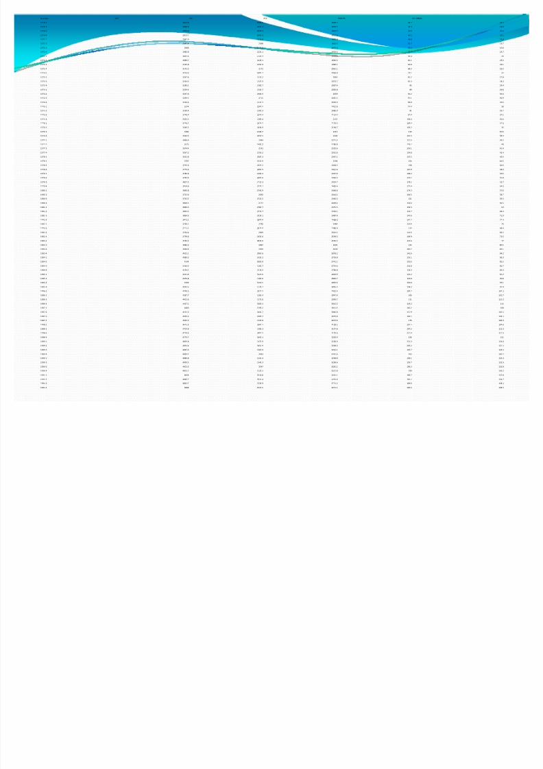
Quarters GDP PDI PCE PROFITS DIVIDENDS

1970-1 2872.8 1990.6 1800.5 44.7 24.5

1970-2 2860.3 2020.1 1807.5 44.4 23.9

1970-3 2896.6 2045.3 1824.7 44.9 23.3

1970-4 2873.7 2045.2 1821.2 42.1 23.1

1971-1 2942.9 2073.9 1849.9 48.8 23.8

1971-2 2947.4 2098 1863.5 50.7 23.7

1971-3 2966 2106.6 1876.9 54.2 23.8

1971-4 2980.8 2121.1 1904.6 55.7 23.7

1972-1 3037.3 2129.7 1929.3 59.4 25

1972-2 3089.7 2149.1 1963.3 60.1 25.5

1972-3 3125.8 2193.9 1989.1 62.8 26.1

1972-4 3175.5 2272 2032.1 68.3 26.5

1973-1 3253.3 2300.7 2063.9 79.1 27

1973-2 3267.6 2315.2 2062 81.2 27.8

1973-3 3264.3 2337.9 2073.7 81.3 28.3

1973-4 3289.1 2382.7 2067.4 85 29.4

1974-1 3259.4 2334.7 2050.8 89 29.8

1974-2 3267.6 2304.5 2059 91.2 30.4

1974-3 3239.1 2315 2065.5 97.1 30.9

1974-4 3226.4 2313.7 2039.9 86.8 30.5

1975-1 3154 2282.5 2051.8 75.8 30

1975-2 3190.4 2390.3 2086.9 81 29.7

1975-3 3249.9 2354.4 2114.4 97.8 30.1

1975-4 3292.5 2389.4 2137 103.4 30.6

1976-1 3356.7 2424.5 2179.3 108.4 32.6

1976-2 3369.2 2434.9 2194.7 109.2 35

1976-3 3381 2444.7 2213 110 36.6

1976-4 3416.3 2459.5 2242 110.3 38.3

1977-1 3466.4 2463 2271.3 121.5 39.2

1977-2 3525 2490.3 2280.8 129.7 40

1977-3 3574.4 2541 2302.6 135.1 41.4

1977-4 3567.2 2556.2 2331.6 134.8 42.4

1978-1 3591.8 2587.3 2347.1 137.5 43.5

1978-2 3707 2631.9 2394 154 44.5

1978-3 3735.6 2653.2 2404.5 158 46.6

1978-4 3779.6 2680.9 2421.6 167.8 48.9

1979-1 3780.8 2699.2 2437.9 168.2 50.5

1979-2 3784.3 2697.6 2435.4 174.1 51.8

1979-3 3807.5 2715.3 2454.7 178.1 52.7

1979-4 3814.6 2728.1 2465.4 173.4 54.5

1980-1 3830.8 2742.9 2464.6 174.3 57.6

1980-2 3732.6 2692 2414.2 144.5 58.7

1980-3 3733.5 2722.5 2440.3 151 59.3

1980-4 3808.5 2777 2469.2 154.6 60.5

1981-1 3860.5 2783.7 2475.5 159.5 64

1981-2 3844.4 2776.7 2476.1 143.7 68.4

1981-3 3864.5 2814.1 2487.4 147.6 71.9

1981-4 3803.1 2808.8 2468.6 140.3 72.4

1982-1 3756.1 2795 2484 114.4 70

1982-2 3771.1 2824.8 2488.9 114 68.4

1982-3 3754.4 2829 2502.5 114.6 69.2

1982-4 3759.6 2832.6 2539.3 109.9 72.5

1983-1 3783.5 2843.6 2556.5 113.6 77

1983-2 3886.5 2867 2604 133 80.5

1983-3 3944.4 2903 2639 145.7 83.1

1983-4 4012.1 2960.6 2678.2 141.6 84.2

1984-1 4089.5 3033.2 2703.8 155.1 83.3

1984-2 4144 3065.9 2741.1 152.6 82.2

1984-3 4166.4 3102.7 2754.6 141.8 81.7

1984-4 4194.2 3118.5 2784.8 136.3 83.4

1985-1 4221.8 3123.6 2824.9 125.2 87.2

1985-2 4254.8 3189.6 2849.7 124.8 90.8

1985-3 4309 3156.5 2893.6 129.8 94.1

1985-4 4333.5 3178.7 2895.3 134.2 97.4

1986-1 4390.5 3227.5 2922.4 109.2 105.1

1986-2 4387.7 3281.4 2947.9 106 110.7

1986-3 4412.6 3272.6 2993.7 111 112.3

1986-4 4427.1 3266.2 3012.5 119.2 111

1987-1 4460 3295.2 3011.5 140.2 108

1987-2 4515.3 3241.7 3046.8 157.9 105.5

1987-3 4559.3 3285.7 3075.8 169.1 105.1

1987-4 4625.5 3335.8 3074.6 176 106.3

1988-1 4655.3 3380.1 3128.2 195.5 109.6

1988-2 4704.8 3386.3 3147.8 207.2 113.3

1988-3 4734.5 3407.5 3170.6 213.4 117.5

1988-4 4779.7 3443.1 3202.9 226 121

1989-1 4809.8 3473.9 3200.9 221.3 124.6

1989-2 4832.4 3450.9 3208.6 206.2 127.1

1989-3 4845.6 3466.9 3241.1 195.7 129.1

1989-4 4859.7 3493 3241.6 203 130.7

1990-1 4880.8 3531.4 3258.8 199.1 132.3

1990-2 4900.3 3545.3 3258.6 193.7 132.5

1990-3 4903.3 3547 3281.2 196.3 133.8

1990-4 4855.1 3529.5 3251.8 199 136.2

1991-1 4824 3514.8 3241.1 189.7 137.8

1991-2 4840.7 3537.4 3252.4 182.7 136.7

1991-3 4862.7 3539.9 3271.2 189.6 138.1

1991-4 4868 3547.5 3271.1 190.3 138.5



This is the quarterly data of five major

macro-economic variable which is used for theapplication of time series econometrics



This have following steps to analysis the time series

econometrics1. Graphical analysis

2. Correlogram

3. Unit Root Test

4. Co-intergration Test

5. Causality Test

6. Chow Break Test



Dependent Variable: LNGDP

Method: Least Squares

Date: 12/03/10 Time: 03:12

Sample: 1970Q1 1991Q4

Included observations: 88

Variable Coefficient Std. Error t-Statistic Prob.

LNPCE 1.034618 0.115599 8.950079 0.0000

LNPDI 0.093431 0.097578 0.957501 0.3411

LNP

O ¡ 1.¢ 03905 0.167793 7.174936 0.0000

LNDVD 1.471¢ 57 0.6¢ 454 ¢ ¢ .355738 0.0¢ 08

C 719. ¢ 76¢ 99.79¢ ¢ 1 7.¢ 07739 0.0000

-squared 0.997318 Mean dependent var 3865.606

Adjusted

-squared 0.997189 S.D. dependent var 630.0349

S.E. of regression 33.40619 Akaike info criterion 9.910500

Sum squared resid 9 ¢ 6¢ 5.81 Schwarz criterion 10.051¢ 6

Log likelihood -431.06¢ 0 ¡ -statistic 7715.573

Dur £ in-Watson stat 0.478548 Pro£ ( ¡ -statistic) 0.000000



From the above result shows that only PDI is

insignificant while the other variables are significant.It also point out that the problem of hetroscedasticity

and auto-correlation occurred in the observed data



Dependent Variable: LNGDP

Method: Least Squares

Date: 12/06/10 Time: 03:0 ¤

Sample (adjusted): 1¥ ¤

0 ¦ 2 1¥ ¥

1¦ §

Included observations: 8 ¤ after adjustments

Convergence achieved after 10 iterations

Variable Coefficient Std. Error t-Statistic Prob.

LNPCE 0.817576 0.124656 6.558656 0.0000

LNPDI 0.301080 0.094193 3.196406 0.0020

LNPR ̈

F 1.387688 0.262312 5.290212 0.0000

LNDVD 1.406317 1.100136 1.278312 0.2048

C 666.7647 187.3353 3.559205 0.0006

AR(1) 0.789442 0.069469 11.36394 0.0000

R-squared 0.998912 Mean dependent var 3877.017

Adjusted R-squared 0.998845 S.D. dependent var 624.4732

S.E. of regression 21.22632 Akaike info criterion 9.014833

Sum squared resid 36495.09 Schwarz criterion 9.184895

Log likelihood -386.1452 F-statistic 14870.78

Durbin-©

atson stat 2.007510 Prob(F-statistic) 0.000000

.7



WhenWhite test apply along with AR1 this

will reduce the problem of cross productsbut still it shows the problem of

autocorrelation





To check the randomness of the data Q-statistics is apply which plot theautocorrelation







The graphicall analysis shows that the data is not stationary,

for this the Unit Root Test(ADF) is apply, on the integratedorder 1.

Stationarity of data is the necessary condition of the time

series analysis.















The unit root test shows that the data is stationary at the first

order integrationIn the observed data after applying the unit root test the data

become stationary



After the test apply there is the visual view of the stationarity

of data.

Which is obtained by plotting the residual of the observation



This is the graphical analysis of the residual which shows that

data is stationary



It shows that the variable have a long run relationship among

each other

n the observed data co-integration is apply for this purpose

we many test are used but Engle Granger test is apply to check

the relationship of the observed data.

ur Ho= No Co-integration in the data





Calculated values shows that at the level of 5% our Ho is

Rejected .



To check the casuality of the observed data a test of Granger

Casuality is used





For the structural stability of the observed data a test of chow

break is used in the above data

For this test there must be an a point of break which is

necessary for this 1982 is our break point for the above data



Our Ho is that there is no structural stability in the data is

going to be tested



While the result shows that the calculated F-statistics is grater

then the critical value of F which is 2.63.This should reject our Ho that there is no structural stability



The maximum log like hood ratio shows that distribution withDOF (m-1)*(k+1) is rejected the null hypothesis, because ourcritical value 9.49 is less then the calculated value.

Ho is rejected which mean the results are statistically significant

and there is a structural stability in the data

Advance Eco No Metrics Techniques & Forecasting

Documents