ADSP Lec 02

7/18/2019 ADSP Lec 02

http://slidepdf.com/reader/full/adsp-lec-02 1/46

Dr. Tahir Zaidi

Advanced Digital Signal Processing

Spring 2012

Lecture 2

Signal Representation and Time

Domain Analysis

7/18/2019 ADSP Lec 02


2

Multidimensional Digital Signals

Digital Photography

Digital Video

x1

x2

x1 x2 x (time)

Digital Speech

7/18/2019 ADSP Lec 02


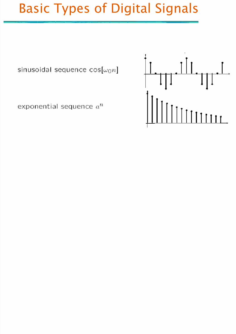
Basic Types of Digital SignalsBasic Types of Digital Signals

7/18/2019 ADSP Lec 02


2-D Signals

7/18/2019 ADSP Lec 02


2-D Unit Impulse Sequence

7/18/2019 ADSP Lec 02


2-D Line Impulse Sequence

7/18/2019 ADSP Lec 02


2-D Unit Step Sequence

7/18/2019 ADSP Lec 02


Basic Types of Digital Signals

7/18/2019 ADSP Lec 02


Sine and Exp Using Matlab

n = 0: 1: 50;

% amplitude

A = 0.87;

% phase

theta = 0.4;% frequency

omega = 2*pi / 20;

% sin generationxn1 = A*sin(omega*n+theta);

% exp generation

xn2 = A.^n;

7/18/2019 ADSP Lec 02


Basic Operations

7/18/2019 ADSP Lec 02


Operations in Matlab

xn1 = [1 0 3 2 -1 0 0 0 0 0];

xn2 = [1 3 -1 1 0 0 1 2 0 0];

yn = xn1 + xn2;

7/18/2019 ADSP Lec 02


7/18/2019 ADSP Lec 02


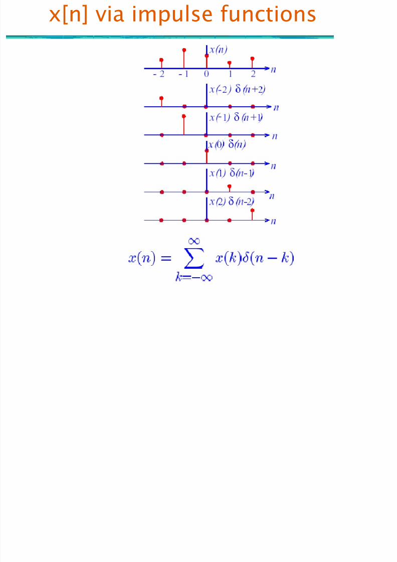
x[n] via impulse functions

7/18/2019 ADSP Lec 02


Input: sum of weighted shifted impulses

7/18/2019 ADSP Lec 02


x[n1,n2] via impulse functions

7/18/2019 ADSP Lec 02


Time Domain Analysis

7/18/2019 ADSP Lec 02


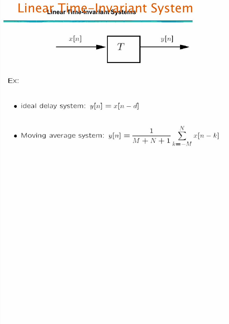
Linear Time-Invariant Systems

7/18/2019 ADSP Lec 02


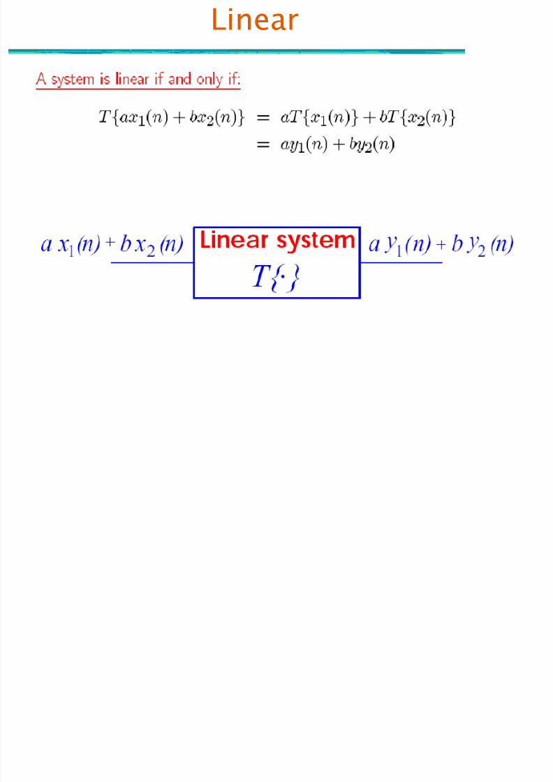
Linear

7/18/2019 ADSP Lec 02


Li Ti I i S

7/18/2019 ADSP Lec 02


Linear Time-Invariant SystemsLinear Time-Invariant System

Li Ti I i S

7/18/2019 ADSP Lec 02


Linear Time-Invariant System

7/18/2019 ADSP Lec 02


Input: sum of weighted shifted impulses

7/18/2019 ADSP Lec 02


Using Linearity and Time-Invariance for the impulses

7/18/2019 ADSP Lec 02


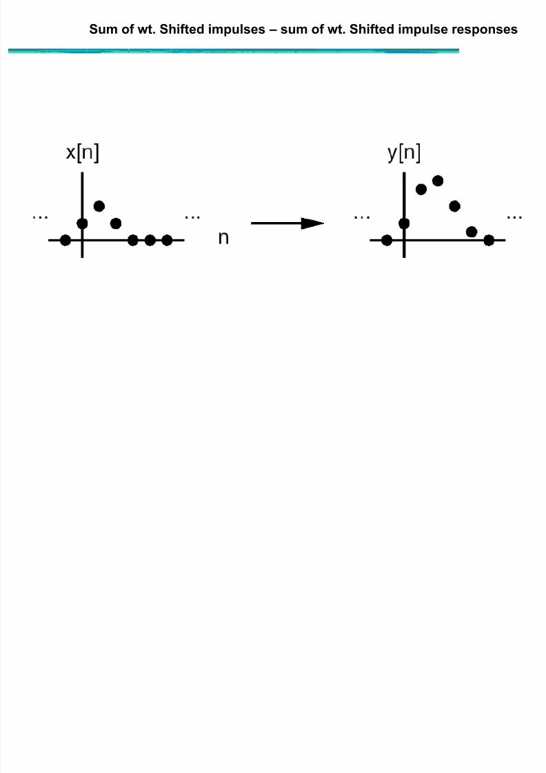
Sum of wt. Shifted impulses – sum of wt. Shifted impulse responses

LTI S t

7/18/2019 ADSP Lec 02


LTI System

T

7/18/2019 ADSP Lec 02


Two ways

As the representation of the output as asum of delayed and scaled impulseresponses.

As a computational formula forcomputing y[n] (“y at time n”) from theentire sequences x and h.

Form x[k]h[n-k] for -∞<k<+∞ for a fixed n

Sum over all k to produce y[n]

7/18/2019 ADSP Lec 02


2-D Linear Shift Invariant (LSI) System

7/18/2019 ADSP Lec 02


2-D Linear Shift Invariant (LSI) System

[ ] [ ] [ ]k h k

7/18/2019 ADSP Lec 02


Convolution in the time domain: [ ] [ ] [ ]k

y n x k h n k

y[n] = 2 –3 3 3 –6 0 1 0 0

E l C l ti f T R t l

7/18/2019 ADSP Lec 02


Example-Convolution of Two Rectangles

Example (Continued)

7/18/2019 ADSP Lec 02


Example..(Continued)

E l C l ti Of T S

7/18/2019 ADSP Lec 02


Example-Convolution Of Two Sequences

7/18/2019 ADSP Lec 02


Stability

7/18/2019 ADSP Lec 02


Stability

Causality

7/18/2019 ADSP Lec 02


Causality

Causality & Stability Example

7/18/2019 ADSP Lec 02


Causality & Stability- Example

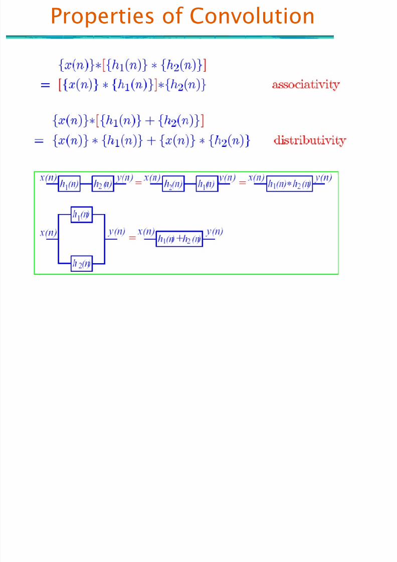
Properties of Convolution

7/18/2019 ADSP Lec 02


Properties of Convolution

Properties of Convolution 2 D

7/18/2019 ADSP Lec 02


Properties of Convolution 2-D

Difference Equation

7/18/2019 ADSP Lec 02


Difference Equation

For all computationally realizable LTI systems, the

input and output satisfy a difference equation of theform

This leads to the recurrence formula

which can be used to compute the “present” outputfrom the present and M past values of the input andN past values of the output

7/18/2019 ADSP Lec 02


Linear Constant-Coefficient Diff Equations LCCD)

First Order Example

7/18/2019 ADSP Lec 02


First-Order Example

Consider the difference equationy[n] =ay[n−1] +x[n]

We can represent this system by thefollowing block diagram:

7/18/2019 ADSP Lec 02


Linear Constant-Coefficient Diff Equations LCCD)

7/18/2019 ADSP Lec 02


Digital Filter

7/18/2019 ADSP Lec 02


Digital Filter

Y = FILTER(B,A,X)

filters the data in vector X with the filter described by

vectors A and B to create the filtered data Y. The filter

is a "Direct Form II Transposed" implementation of the

standard difference equation:

a(1)*y(n) = b(1)*x(n) + b(2)*x(n-1) + ... +

b(nb+1)*x(n-nb) - a(2)*y(n-1) - ... - a(na+1)*y(n-na)

[Y,Zf] = FILTER(B,A,X,Zi)

gives access to initial and final conditions, Zi and Zf, of

the delays.

LTI summary

7/18/2019 ADSP Lec 02


LTI summary

Complex Exp Input Signal

7/18/2019 ADSP Lec 02


Complex Exp Input Signal

ADSP Lec 02

Documents