adsorption of methylene blue and brilliant green dyes unto ...

1

ADSORPTION OF METHYLENE BLUE AND BRILLIANT

GREEN DYES UNTO MODIFIED ACTIVATED CARBON

PREPARED FROM AGRICULTURAL WASTES

This study intends to investigate the analysis of removal of Methylene Blue (MB) and

Brilliant Green (BG) dyes from aqueous solutions by adsorption on modified activated

carbon prepared by chemical activation of coconut shell, eucalyptus tree, corn cob and

flamboyant pod. The maximum percentage methylene blue removal was obtained as 95.0%

for coconut shell, 93.2% for eucalyptus tree, 99.9% for corn cob and 99.7% for flamboyant

pod with all adsorbent dosage at 5g per 0.003mL. Also, the maximum percentage brilliant

green removal was obtained as 97.0% for coconut shell, 98.2% for eucalyptus tree, 99.6%

for corn cob and 99.6% for flamboyant pod with all adsorbent dosage at 5g per 0.003mL.

The adsorption isotherms of the adsorption process were studied and Freundlich model

showed the best fit with equilibrium data. To optimize the operating conditions, the effects

of contact time, adsorbent dosage, and pH were investigated by two level factorial

experimental design method; adsorbent dosage was found as the most significant factor,

lower than 95% confidence level with P = 0.0008 for Methylene Blue and P = 0.0069 for

Brilliant Green. The obtained results are very promising since the utilization of these

agricultural wastes activated carbon used in this work played a critical role in the adsorption

of dyes.

2

CHAPTER ONE

1.0 INTRODUCTION

1.1 Background of the study

The release of dyes into wastewaters from textile, cosmetic, paper and coloring industries

poses serious environmental problems (El-Qada, Allen and Walker, 2008). Dye presence in

wastewater poses problems in a number of ways. Dye availability in water, even if it is just

small in quantity is unwanted and highly visible. Color prevents the proper entrance of

sunlight into water bodies; it also retards photosynthesis; hinder the growth of aquatic biota

and affect the solubility of gas within the water bodies in water bodies. Dyes role in

connection with several lung, skin and many other respiratory problems have been reported

globally (Jadhav, Phugare, Patil and Jadhav, 2011). Direct release of dyes containing

wastewater into municipal environment can cause the production of poisonous carcinogenic

products. The highest degrees of toxicity were discovered in diazo direct and raw dyes

(Gupta, Mittal, Malviya and Mittal, 2009). Therefore, before wastewater is released into

municipal environment, it is very important to reduce dye amount or concentration present

in it.

The commonly applied methods of treating wastewater are coagulation and flocculation,

electrochemical treatment, liquid–liquid extraction, chemical oxidation and adsorption.

Many methods have recently been used to remove both MB and BG from industrial effluents.

Among these methods, Adsorption is the most effective way for the removal of organic

compounds from solution in term of its low cost of operation, ease of design, sensitivity to

poisonous materials and simplicity of operation (El-Qada, et al., 2008). But its use is limited

because of high cost and associated problems of regeneration and this problem has initiated

3

a constant and continuous search for cheaper substitutes. Adsorption process make use of

carbons. Wide varieties of high carbon content materials such as wood, coal, peat; nutshells,

sawdust, bones, husk, petroleum coke and others have been utilized to produce activated

carbon of varying efficiencies (Ponnusami, Krithika, Madhuram and Srivastava, 2007).

These materials, usually in irregular and bulky shapes, are always adjusted to exhibit the

desired final shapes, roughness and hardness.

Generally, the production of activated carbon involves pyrolysis or carbonization and

activation as the two main production processes (Bonnamy, 1999). Numerous carbonaceous

materials, particularly, those of agricultural base, are being investigated to possess potential

as activated carbon. The suitable ones have minimum amount of organic material and a long

storage life. Similarly they consist of hard structure to maintain their properties under usage

conditions. They can be obtained at a low cost. Some of the materials that meet the above

conditions have been used, in past works, to produce activated carbons which were

subsequently used for the treatment of wastewater and adsorption of hazardous gases.

Agricultural by-products like rice straw, soybean hull, sugarcane bagasse, peanut shell, pecan

shell and walnut shells were used by Ponnusami et al. (2007) to produce Granulated

Activated Carbons (GACs). The choice of a particular material for the production of effective

adsorbent (activated carbon) is based on low cost, high carbon and low inorganic content.

Agricultural materials have attracted the interest of researchers for the production of

adsorbents because of their availability in large amount and at a low cost (Foo and Hameed,

2011). The selected materials employed in this study were coconut shell, corn cob,

flamboyant pod and eucalyptus tree. Use of agricultural by-product for the production of

activated carbon is primarily for economic and ecological advantages (Foo et al., 2011).

4

Commercial activated carbon used in surface and wastewater treatment is largely derived

from coal. The advantages of coal-based carbons can be seen in their ability to remove toxic

organic compounds from industrial and municipal wastewater and potable water as well.

Another significant application of coal-based carbons is decolorization. The feedstock for

these carbons, usually bituminous coal, is a non-renewable resource. The long-term

availability of coal and its long-term environmental impact coupled with its potentially

increasing cost has prompted researchers to consider renewable resources such as agricultural

by-products as an alternative. Many efforts have been made to use low cost agro waste

materials in substitute for commercial activated carbon (Crini, 2006). Some agro waste

materials studied for their capacity to remove dyes from aqueous solutions are coir pith, pine

sawdust, tamarind fruit shell, bagasse, rice husk, orange peel, palm kernel shell, cashew nut

shell and wall nut shell, (Mittal, Kaur and Mittal, 2008). The present investigation is an

attempt to remove Methylene blue and Brilliant green from synthetic wastewater by

adsorption process using a low cost activated carbon prepared from agricultural wastes as an

adsorbent. The coconut shell and corn cob are considered as an agricultural wastes, therefore

using them as raw materials for production of activated carbon is more economical than the

coal based activated carbon. In this study, the carbon adsorption method will be investigated

for its efficiency in colour removal from water bodies.

1.2 Statement of the problem

The presence of organic pollutants compounds such as dye in water causes serious problems

due to their toxicity, suspected carcinogenicity and adverse effects on the human nervous

system that cause many health disorders. Removing these contaminants from water is a

significant challenge because of ever-increasing pollution of drinking water, the shortage of

5

high quality fresh water and frequent release of wastewater by production companies into

water body.

1.3 Aim and objectives

The aim of this project is to remove methylene blue and brilliant green dyes from synthetic

wastewater using modified carbons made from agricultural wastes. This aim can be achieved

through the following objectives:

1. To carry out characterization of adsorbent by Raman Spectroscopy (RS) and

Brunauer-Emmet-Teller (BET).

2. To study the interaction of the mixture of methylene blue and brilliant green dyes on

the adsorption sites of the activated carbon.

3. To study the main and interaction effects of the parameters used for the experiments

on adsorption process

4. To study the percentage removal of the adsorbents and compare results by measuring

the percentage of color remove.

5. To determine the isotherm model where equilibrium data of the adsorption

mechanism will be best represented using modified activated carbon.

1.4 Scope of the study

This project investigates the adsorption capacity of four different activated carbons prepared

from low cost agricultural wastes on the removal of dyes from aqueous solution. The pH,

contact time and carbon dosage effects as well as the interaction nature of the mixture of

methylene blue and brilliant green on the adsorption sites of activated carbons will be

investigated. Adsorption equilibrium data will be determined. This data will be subjected to

6

Freundlich and Langmuir models to determine isotherm models that will be most appropriate

for equilibrium. This work will be experimental, Raman Spectroscopy (RS) will be used for

determination of functional groups present in the carbons and Brunauer-Emmet-Teller (BET)

will be used to determine the adsorption capacity of the carbons.

7

CHAPTER TWO

2.0 LITERATURE REVIEW

2.1 Origin of dye

A dye is a colored substance. It has an affinity to the substrate to which it is being applied.

Both stain and dye appear to be colored because they absorb some light wavelengths of more

than others. Dyed flax fibers were first found in the Republic of Georgia dated back in a

primitive cave to 36,000 BP (Zollinger, 2003). Archaeological proof reveals that, particularly

in Phoenicia and India, dyeing has been broadly carried out for over 5,100 years. Different

forms of dyes were obtained from vegetable, animal or mineral origin, with little to none

processing. The plant kingdom has been greatest source of dyes. Much dyes has been from,

notably barks, berries, leaves, and wood, but only few of the dyes obtained from the plant

kingdom have ever been used on a commercial scale (Gessner and Mayer, 2002).

2.2 Dyes types

2.2.1 Natural dye

Many of the biological or natural dyes are from plant kingdoms – barks, fungi, lichens,

berries, leaves, and wood. Fabric dyeing dates back to the Neolithic time. From the time

past, people have dyed their fabric by locally, common available materials. dyes that

produced permanent and brilliant colors such as brilliant green, the natural invertebrate dyes

and crimson kermes were highly treasured items in the ancient time and feudal world. Plant

source-based dyes such as indigo, madder and saffron were good for commercial and

economies development in Asia and Europe. Across Africa and Asia, patterned Textiles were

produced by dyeing techniques to control the absorption of stain in piece-dyed fabric. Before

the end of 19th century, man- made synthetic dyes were discovered. The discovery of man-

8

made synthetic dyes ended the large-scale market for natural dyes to countries around the

world. As at today, there are over 10,000 historical collection of dyes at Technical University,

Dresden, Germany (Zollinger, 2003).

2.2.2 Synthetic dye

The first man-made (organic) synthetic dye, mauveine, was discovered by William Henry

Perkin in 1856. After the discovery of mauveine, many thousands of organic dyes have since

been prepared. The natural dyes were quickly replaced by the organic dyes in many

applications. Synthetic dyes cost less, they imparted better properties to the dyed materials

and they offered a vast range of new colors. Presently, dyes are classified according to their

usefulness in the dyeing process, they include (Zollinger, 2003):

Acid dyes are water-soluble anionic dyes that can be applied to color fibers such as

nylon, wool, silk and modified acrylic fibers using neutral to acid dye baths. Most

synthetic food colors fall in this category.

Basic dyes are water-soluble cationic dyes that are applicable mainly to acrylic fibers,

but can also find application and use for wool and silk. Acetic acid is usually added

to the dye bath to help the absorption of the dye onto the fiber. Basic dyes are useful

in the paper making industries for coloration. MB with molecular formula C16

H18N3SCl and BG with molecular formula C27 H33N2.HO4S are both basic dyes

Direct dyeing is usually carried out in an alkaline dye bath with the addition of either

sodium carbonate (Na2CO3) or sodium chloride (NaCl) or sodium sulfate (Na2SO4).

Direct dyes are also used on silk, cotton, paper, leather, and nylon. They can be used

as biological stains or as pH indicators.

9

Vat dyes are insoluble in water and incapable of dyeing fibres directly. But, reduction

of vat dyes in alkaline liquor produces the water soluble alkali metal salt of the dye.

Reactive dyes utilize a chromophore that make it good at reacting with fibres

substrate. The covalent bonds that attach reactive dye to natural fibers make them

among the most permanent of dyes. Reactive dyes are very easy to use because the

dyes can be applied at room temperature. Reactive dyes are best for dyeing process

at home, industries or in the art studio.

Food dyes are classed as food additives, they are use is usually controlled by strictly

legislation and they are usually manufactured to a higher standard than some

industrial dyes. Food dyes can be vat, direct and mordant dyes. Many azo dyes, such

as triphenylmethane and anthraquinone compounds are used for colors such as green

and blue (Gessner and Mayer, 2002).

Other important dyes include: leather dyes for leather, oxidation bases, for mainly

hair and fur, solvent dyes, for wood staining and producing colored lacquers, solvent

inks, colouring oils, waxes.

2.3 Origin of activated carbon

Activated carbon existence can be traced back to 1500 B.C in Egypt (Pope, 1999). At that

time, AC application is limited to medicinal application only, but in the 21st century, AC

application is numerous. It can be used to do many things among which water treatment is

included. Across the world now, several water treatment plants make use of activated carbons

in their water purification to remove taste and odor associated with water. And the present

popularity and large number of AC application in water treatment is due to the fact that it

treats different problems effectively. Early applications of adsorption involved only

10

purification, for example, adsorption with charred wood to improve the taste of water has

been known for at least five centuries. Adsorption of gases by a solid charcoal was first

described by C.W. Chele in 1773. Commercial applications of bulk separation by gas

adsorption began in early 1920s, but did not escalate until the 1960s, following the invention

by Milton of synthetic molecular sieve zeolites, which provide high adsorptive selectivity.

Later the pressure swing cycle of Skarstrom, which made possible the efficient of operation

of a fixed bed cyclic gas adsorption process.

Activated carbon is probably the most common adsorbent. They are highly porous,

amorphous solids consisting of micro crystallites with a graphite lattice. They are non-polar

and cheap. Under an electron microscope, the structure of the activated carbon looks a little

like ribbons of paper which have been crumpled together, intermingled with wood chips.

There are a great number of nooks and crannies, and areas where flat surface of graphite-like

material run parallel to each other, separate by only a few nanometers or so. These micropores

provide superb conditions for adsorption to occur, since adsorbing material can interact with

many surfaces simultaneously. Activated carbon can be manufactured from carbonaceous

material, including coal, wood, nutshells and coconut shells. The manufacturing process

consists of two phases, carbonization and activation (Bonnamy, 1999). The immense

capacity for adsorption from gas and liquid phases make activated carbon a unique material.

It occupies a special place in terms of producing a clean environment involving water

purification as well as separations and purification in the chemical and associated industries.

In these roles, it exhibits a remarkable efficiency as the international production is a little

more than half a million tonnes per year, with perhaps 2 million tonnes being in continuous

use. This is equivalent to the allocation of 200 mg per person of the world population to be

11

compared with the world use of fossil fuels of 2 tonnes per person of the world population.

An effective use of activated carbon requires knowledge about the structure of its porosity,

obtained from equilibrium data, namely the pore-size distributions of the microporosity in

particular, of the pore-size distributions of the mesoporosity, of the composition of the carbon

surfaces onto which adsorption occurs, and knowledge of the dynamics of adsorption to

indicate its effectiveness in industrial use. Central to activated carbon is the activation process

which enhances the original porosity in a porous carbon.

Activation uses carbon dioxide, steam, zinc chloride, phosphoric acid and hydroxides of

alkali metals, each with its own activation chemistry. The story of what happens to a molecule

of carbon dioxide after entering the porosity of carbon at 800 °C leading to the eventual

emergence of less than two molecules of carbon monoxide is fascinating and talks about

"atomic ballet”. AC is an adsorbent that can be used to perform functions such as water

treatment, air treatment and mixture of gases separation. To activate a carbon, activation

process must be carried out, which could be thermal or chemical. Activation by selective

gasification (steam or CO2) in the absence of oxygen to remove carbon atoms is thermal

activation while activation that involves the use of some chemicals such as zinc chloride or

phosphoric acid is chemical activation. Activated carbon could be made from agricultural

waste and other carbonaceous materials such as coconut shell, wood, orange peels and

synthetic macromolecular. Not all natural carbonaceous materials are good material for

making commercial attractive activated carbon. Past researchers have shown that only few

of NOMs provide commercially acceptable activated carbon. Another fact we need to know

is that not all activated carbon look very similar to each other or one another even if they are

make from the same materials. The reason for this is because of different production

12

conditions. There are many commercially attractive AC available, even some are made from

the same materials but with different sizes of porosity due to activation process applied with

specific applications. The porosity plays a major role in determining the adsorption capacity

of an activated carbon (Gregg and Sing, 1982)

2.4 Activated carbon as an adsorbent

Some solids have capacity to attract some impurities on their surface, but only few of these

solids materials have industrial or commercial level adsorption capacity to adsorb adsorbate

molecules (Lopez-Gonzalez, Martinez-Vilchez and Rodriguez-Reinoso, 2008). The

adsorbate that can be adsorbed may be organic compounds such as odor, taste and color.

There are for major known adsorbents in the market today. Each one of them has different

characteristics that made them to be different from one another. They are

1. Silica gel : it is hydrophilic in nature, it can be used in drying of gas stream but it has

an disadvantage of not being able to remove trace substance effectively

2. Activated alumina: it is hydrophilic in nature, it can be used in drying of gas stream

but it has an disadvantage of not being able to remove trace substance effectively

3. Zeolites: it is hydrophilic in nature, it can be used in air separator

4. Activated Carbon: it is hydrophobic in nature, it favour organics over water. It can

be used in removal of organic pollutants. Its only disadvantage is that, it is always

difficult to regenerate for re-use.

2.5 Uses of activated carbon

There are several operations where AC is applicable today for impurities treatments, these

include

13

1. AC can be used in biological primary and secondary processes, physio-chemical

treatment to obtain purify effluent.

2. AC can be used for tertiary AC processes on wastewater that has already undergone

either primary or secondary biological treatment process. This will result in effluent

of about 99% purity. Tertiary treatment is adsorption which could be batch or fixed

bed treatment.

3. AC is also applicable for industrial waste treatment for either pre-treatment of

effluents before discharge into rivers, streams or municipal treatment plants or to

upgrade the wastewater for re-use.

4. AC can be used to purify water by removal of biodegradable, chemicals, oil and other

organic compounds that are not responsive to conventional biological treatment.

Biological treatment may include addition of lime, alum, chlorine, followed by

filtration.

5. AC can be used to treat wastewater that contain pesticide, polyols, detergents, phenols

and organic dyes.

6. AC can be used to treat wastewater and effluents from pulp and paper mills, fertilizer

plants, fabric dyeing, rubber tread factories, chemical and pharmaceutical factories

etc.

7. AC can be used to remove oil from wastewater or effluents.

2.6 Adsorbent and adsorbate peculiarity

Today, there is thousands of AC in the market that can be used to treat water related problems,

but before a particular AC is picked, there are some factors which will enable adsorption on

AC during water treatment. They include

14

1. Water pH, quality and ionic strength

2. The shape, size, charge, solubility, hydrophobicity of adsorbate

3. Surface chemistry and pore size of AC

The removal of target impurities can be achieved by the interaction of all the listed factors

above. The carbons most suitable for adsorption are the ones that has a large volume of pores

in size range slightly larger than the adsorbate. AC surface chemistry is very important in

adsorption process and all the other factors. Researches on adsorption have tried to proof that

the adsorption of a particular contaminants are related to the pore volume and surface

chemistry. This means that the adsorbate on a particular AC can be adsorbed depends on pore

volume and surface chemistry and these can be different from one laboratory to another.

(Gonzalez, Gonzalez, Molina-Sabio, Rodriguez-Reinoso and Sepulveda- Escribano, 1995).

2.7 Regeneration of activated carbon

By the time AC or adsorbent has become saturated then it can be either discarded or

regenerated. But for regeneration, saturated carbon will be removed from adsorption column

in the form of a slurry. The slurry (the semi-mixture of used up AC and water) will be

dewatered, and passed into the furnace for heating. Regeneration is always done by thermal

process and is a reversible process. Inside furnace AC is heated under controlled conditions

with no or little oxygen content to avoid carbon burning on combustion. The heating process

evaporates out organic compounds the adsorbent adsorbed during adsorption and also

removes residual water in the adsorbent. After the heat treatment is completed, the carbon is

cooled with water, wash and dry in the oven and recycled for adsorption process reverse. The

regeneration can be off-site or on-site activities. During regeneration, some carbon will be

burnt-up during the process. About 2 – 10wt% will be burnt-up. For re-use, some fresh carbon

15

will be added to the regenerated carbon to replace the lost carbon during regeneration. The

whole process can be done within 30 minutes to one hour. Physical regeneration require high

temperature due to this, it is a high energy process that is commercially and energetically

expensive process. Plants that use thermal regeneration of activated carbon must be very big

and must have adequate facilities on site before it can be economically viable to do so. Due

to this most of the activated carbon generation companies usually carry their waste for

treatment in specific AC regeneration facility center. Many generation process of AC can be

carried out in heating appliances such as toaster or baking ovens. Other regeneration

techniques are wet air oxidation, ultrasonic regeneration, microbial regeneration,

electrochemical regeneration and chemical and solvent regeneration. The expensive natures

of physical regeneration encourage researchers to come up with above listed means of AC

regeneration. All the techniques listed apart from physical regeneration can be used as

alternative regeneration which could be employed in medium-scale industries

2.8 Activated carbon production

Activated carbon is a carbon produced from carbonaceous source materials. The production

methods can either be by thermal activation or by chemical activation.

2.8.1 Thermal activation processes

Natural Organic Material (NOM) can be carbonized (convert into char by heating or burning

in the absence of oxygen) to microporous carbons (Gupta, Rastogi, Agarwal and Nayak,

2011). Carbonize materials do not maximize their porous potential, that is, carbon adsorption

capacity when measured is too low to be considered useful for commercial application. There

is need to widen the exiting porosity to wider micropores and some mesoporosity. Also,

16

because of narrow porosity within the carbon, it is closed to pick up some specific adsorbates

(contaminants) inside the water. To allow and increase the capacity of adsorbent to adsorb

the adsorbate, porosity and space within the carbon, which is closed must be opened in other

to allow access to larger adsorbates molecules. The process of opening the space within the

carbon to maximize it adsorption potentials is by activation. The activation process can either

be by chemical or physical activation. The first means of widening the porosity make use of

steam and carbon dioxide, either singly or both combine. The functions of this gasify agents

is to open the space or pores within the carbon by extracting carbon atoms from the structure

of the porous carbon. The method describe above is known as physical or thermal

modification or activation. The stoichiometric equation for thermal or physical activation is

given as

C + CO2 = 2CO (2.1)

C + H2O = CO + H2 (2.2)

The second suitable modification or activation process of widening the porosity make use of

chemicals such as potassium hydroxide, KOH, zinc chloride, ZnCl2, phosphoric acid H3PO4

and potassium carbonate K2CO3 (Foo et al., 2011). This activation method is known as

chemical activation, and the process of widening porosity follow the same as physical

activation. Some industrial adsorption processes of widening the space within the carbon

usually combine both thermal and chemical activation process together to obtain a desired

activated carbon. The mechanism of activation used does not produced identical result. The

use of gasifying agents to remove carbon atoms as carbon monoxide which then enhancing

space does not give the same result. The result one will get if steam is used for activation is

different from that of carbon dioxide.

17

2.8.2 Chemical activation processes

The chemical activation process consists of mixing a carbonaceous precursor with a chemical

activating agent, followed by a pyrolysis stage. The material after this stage is richer in carbon

content and presents a much ordered structure and, after the thermal treatment and the

removal of the activating agent, has a well-developed porous structure. Different compounds

can be used for the activation; among them, KOH, NaOH, H3P04, and ZnCl2 have been

reported in the literature to be the best for activation (Gonzalez et al., 1997). It has been

discovered that chemical activation has some advantages over physical activation. Some of

the advantages of chemical activation over the physical process include

I. The chemical activation uses lower temperatures and pyrolysis time,

II. It usually consists of one stage,

III. The yields obtained are higher,

IV. It produces highly microporous ACs

V. It is a suitable method for applying to materials with high ash content.

On the other hand, the chemical activation presents disadvantages such as the need of a

washing stage after the pyrolysis and the corrosiveness of the chemical agents used. For time

past, active carbon application as adsorbents have been used where impurities in the

concentration need to be removed. For active carbon to be effective as adsorbent, it must

have an appropriate pore-size distribution and large micropores volume to adsorb molecules

of different sizes. Also, to facilitate micropores access, there must be an adequate preparation

of mesopores (Gupta et al., 2011). So to meet the broad range of industrial requirement of

active carbon, intensive research to provide activation methods is undertaken by different

researchers in different laboratories. These researchers are developing methods of activation

to develop active carbon with optimum, pore-size distribution that industrial requirement

18

needs. As application become specific, the researchers’ are developing active carbon with

specific pore-size distribution to meet specific application. This means that not all activated

carbons can be used, for the nature of the impurities to be removed will determine active

carbon to be used in order to achieve desire result. For example, activated carbon with

homogenous microporosity is required to recover light hydrocarbons found in gasoline

vapour by adsorption process. So active carbon with homogenous microporosity and

controlled pore-size distribution are prepared by controlled activation of precursors

(Gonzalez et al., 1997).

To develop a specific microporosity in activated carbon, either thermal or chemical activation

process can be used. But in thermal activation, factors such as heating rate and time,

temperature, pressure etc, has little influence on micropore size distribution (Gonzalez et al.,

1997), it may be difficult to control the microporosity development of AC to specific desire

pore distribution size. In order to have a control pore – size distribution in AC, chemical

activation is an alternative that can be used. In chemical activation, precursors can be well-

controlled and modified to prepare activated carbon with specific microporosity. Chemicals

such as zinc chloride, H3PO4, CaCl2 are commonly used for carbon activation at a

temperature of about 723K-873K. At these temperatures, there is always incomplete

carbonization and hence the chemical composition of the carbon prepared is between that of

the char and precursor. During carbonization process, there is always a contraction in

dimensions of precursors. Studies carried out with agricultural waste (Almond shells) showed

that the loss in weight of about 75wt% is followed by 30wt% contraction (Gonzalez et al.,

1997). In chemical activations, change in dimension during carbonization is very necessary.

Change in dimension makes reagent to be able to be incorporated into carbon interior where

19

it prevents the expected contraction with increasing temperature. This means that the creation

of microporosity can be caused by reagent.

2.9 Factors on which activation depends

The following factors which may influence the properties of an activated carbon were

recommended by Gonzalez and co-workers (1997) to include:

1. The time of activation;

2. Activating gas flow rate

3. The equipment used for the experiment.

4. The activation temperature;

5. The activating gas;

6. The parent feedstock;

7. The rate of heating;

8. The flow rate of the containing gas, usually nitrogen

The above listed factors can influence the properties of AC and adsorption capacity. The way

the activating gas flow into the bed of carbon, the carbon bed construction and where the bed

is located in the furnace are all factors that influence the properties of AC. When comparing

results from laboratory to laboratory, some differences are to be expected, even when all the

conditions and the listed factors above are fixed (Gonzalez et al., 1997). Gonzalez and co-

workers used olive stone to prepared three different chars. The olive stones, 1 – 1.5mm

particle size, carbonized with the same conditions namely;

1. Slow carbonization inside horizontal furnace, heating rate 278K min3, N2 flow rate

of 80cm3/min, reaction temperature 1123K, 1 hour of soak time and 25.4wt % of char

yield was the result

20

2. Slow carbonization inside vertical furnace, heating rate 278K min3, N2 flow rate of

80cm3/min, reaction temperature 1123K, 1 hour of soak time and 26.8wt % of char

yield was the result

3. Flash carbonization inside vertical furnace, heating rate 278K min3, N2 flow rate of

80cm3/min, reaction temperature 1123K, 1 hour of soak time and 16.7wt % of char

yield was the result

The chars yield of the three precursors which were prepared under the same experimental

factors and conditions are not the same. And one will also expect that their reaction with

carbon oxide will also be different. In order to compare the activation carbon adsorption

capacity, the same activation process was used for the three chars yield. The activated carbon

produced were analyzed using carbon dioxide (273K) and N2 (77K) isotherms. The results

from the point of porosity development showed that there are differences between the two

activation methods used. The micropore volume of the chars activated in horizontal furnace

are larger compared to that of the vertical furnace. So the horizontal furnace is at the

advantage for AC activation. It was observed that the large micropore volume of horizontal

furnace is as a result of external mass – transport which is more limited and favour internal

gasification of the char particles and the creation of micropores. The conclusion of the study

showed that enhancement of micropore volume and adsorption capacity is favoured by

horizontal carbon bed than that of vertical carbon bed at the same activation temperature

(Gonzalez et al., 1997)

2.10 Comparison of activating agents

Factors such as temperature, activation time, soaking period, nature of the chemical used and

the concentration of chemical used are factors that determine the reaction between precursors

21

and chemicals during activation. The research shows that for activating agents such as KOH,

ZnCl2, and H3PO4 (Gonzalez et la., 1997), they always act on carbonized materials to

produced activated carbons with micropore volume of 0.4, 0.5 and 0.6 cm3/g respectively. In

chemical activation, chemical react with precursor, but at the end of impregnation, there is

always difference which can be observed. Impregnation with H3PO4 always make particle to

become elastic. Particle become elastic simply means that H3PO4 impregnation starts the

conversion to carbon process because at the surface of the particle a significant amount of tar

is observed. During impregnation with H3PO4, some visual changes are observed; there is

swelling of the particle, decrease in mechanical resistance and presence of tars on the surface

of particles. But with impregnation with KOH, there is no swelling up of the particles,

mechanical resistance, and no formation of tar but only a slight dehydrating occurs on particle

surface. Impregnation with ZnCl2 followed the nature of impregnation with H3PO4. In ZnCl2,

there are also visual changes such as swelling of the particle, presence of tars on the surface

and lower mechanical resistance. Another thing for comparison is dehydrating effect during

heat treatment. Chemical is a liquid at the temperature of the process, this made the

dehydration to be possible. Dehydration facilitates the bonding to the precursor being

thermally degraded and enable chemical to enter into the interior of the particles. The

dehydration produced by KOH is weak and does not seem to affect carbonization but

dehydration made by both H3PO4 and ZnCl2 is strong. The dehydration produced by

phosphoric acid and zinc chloride affects carbonization (Gonzalez et al., 1997). Both H3PO4

and ZnCl2 yield reaches values up to 45wt% with larger concentration of chemical for ZnCl2

and low concentration for H3 PO 4. The peak yield for KOH was 25wt%, which is the same

yield of the precursor un-impregnated with any chemical. The reduction in the dimension of

the particle is caused by precursor dehydration, and such reduction is partially prevented

22

because during physical treatment, reactant remains, thus acting as a template for

microporosity creation. Also both H3PO4 and ZnCl2 act as a dehydrating agent on the

precursor, thereby react during pyrolysis. KOH does not produce dehydrating effect on the

precursor. It does to prevent the contraction of the particles with heat treatment and does not

react during pyrolysis. KOH starts to react with pyrolysis at about 973K. At this temperature

precursor changes to char. In activation process with KOH, activation consists of a redox

reaction initially. A redox reaction is the reaction where carbon is oxidized to CO2 or CO,

thus creating some porosity and K2CO3 is produced as by – product. The conclusion of the

work is that H3PO4 and ZnCl2 are best activating agents and they always produced similar or

better yields of about 26-46wt% compared with physical activation with a yield of about

8wt% (Marsh, Heintz, and Rodriguez-Reinoso, 1997), and that activation by chemical

process has some advantages over thermal activation process. ZnCl2 always produce wide

pore surface area than base, but H3PO4 produces a better pore surface area and are relatively

safer than ZnCl2 (Gonzalez et al., 1997)

2.11 General considerations on activated carbon

The generation observation and common behavior discovered about most of the activated

carbons prepared by physical activation process from different raw materials is that, there is

initial increase in micropore volume up to about 20wt% burn off. This increase in micropore

volume occurs mainly by widening of existing microporosity and by creation of new

microporosity. After the initial increase of 20wt% micropore volume, thereafter, there is

increase in micropore volume which is smaller and after 40 – 45wt% burn – off, the

micropore volume then progressively decrease, this trend of burn- off shoes that pore

enlargement during activation shift from microporosity to mesoporosity and even to

23

macroporosity. The observation also shows that at a high level of burn-off, there is a fierce

burning of the exterior of the carbon particle in conjuction with interior of carbon porosity

widening. The industrial gasification of any char to open and widen porosity has three

mechanisms often carried out to explain how porosity develop during activation of a chair.

These mechanisms include

1. Existing pores widening

2. Creation of new pores

3. Opening up of pores that are not accessible previously.

The mechanisms written above make increase in micropore volume (15-20%) for the char

activated. There is about 10wt% burn-off which is a good indication of the opening of initial

inaccessible microporosity. The removal of reactive carbon atom which is in the form of

carbon monoxide for carbon takes place at the activation process initial stage (Rodriguez-

Reinoso et al., 1997)

2.12 The porosity of activated carbon

The voids, spaces, sites and pores in activated carbon make it to be a unique material that is

filled with holes, the size of the molecules. These pores in activation carbon have a strong

force known as Van der Waals which is responsible for the adsorption process. The pore size

determines how the adsorption process will take place in activated carbon. The pore sizes

range from macroporosity > 50nm, mesoporosity 20 – 50nm, and microporosity < 2nm. The

dominant characteristics of adsorption is imparts with porosity within activated carbon. There

is a wide range of materials of carbon family that are good for preparing activated carbon of

different structure and porosity. The porosity and structure of carbons are prerequisite to the

effectiveness of activated carbons. And the origins of parents materials of activated carbons

24

and preparation conditions and methods determines the porosity and structure within AC.

Porosity within a porous solid are sites, voids, holes, spaces and pores which is enhance to

molecules from liquid phase and gas phase. Carbon which is an adsorbent is a porous solid

material, while adsorbate is a solute from solution, gas or vapour which within the adsorbent

is adsorbed. The solute, gas or vapour which will be adsorbed as an adsorbate is adsorptive.

When an adsorbate enters into the porosity of the adsorbent, then adsorption process takes

place.

In adsorption, there are three kinds of entrance into porosity. The entrance dimension of

micropore is < 2nm, mesopores is 2 – 50nm and macropore is > 50nm. The entrance

dimension from 2 – 50nm and >50nm show that there is a continuous and progressive pattern

of adsorption within the AC from structural point of view. For carbon to have specific

dimension, there is a specific method of preparation which need to be applied before a carbon

with a specific dimension is created. The carbonization of precursor is responsible for the

creation of porosity to some degree in a carbon. Porosity of different sizes and the sizes make

carbon to be accessible or inaccessible to particles. For example, organic pollutants are

accessible to some porosities but inaccessible to organic pollutants. Some are accessible to

helium and closed to lithium. For porosity dimension, the nomenclature assigned has been in

used for past decades. In recent times, carbons with dimension < 1nm have been called

nanoporosity. Ultra micro porosity in literature is suggested to be dimensions of about <

0.7nm as well as dimension nearer to 2nm is called to be super – microporosity. All these

names in term of pore radius and diameter can be misleading. But this work concern is on

micro and meso- porosity dimension. There is a need to emphasize that adsorption processes

in porosity < 0.7 nm are distinct in the way that the intense dispersion forces, which operate

25

in such confined volumes, influence the physical state of the adsorbed phase. It has to be said

at the onset that the numerical values attached to these definitions of porosity do not have the

precision as is attached to a weight or a volume. Rather, a pore is defined according to the

way it adsorbs an adsorbate molecule and that is a function of the size and polarity of the

adsorbate molecule as well as the size of the porosity and surface polarity within the

adsorbent.

The above discussions have stressed that porosity in this family of carbons essentially is that

space where carbon material (atoms and heteroatoms) is absent. If the structure or relative

arrangements of carbon atoms is changed in some way then automatically a new set of porous

properties will be created. It therefore follows that a knowledge of structure assists with

knowledge of the nature of porosity in that carbon. Today, almost all the plants in the world

can be used to prepare active carbon on carbonization in an inert atmosphere. But causal

preparation of active carbon may not be able to meet requirements for commercial

application. Activated carbon for industrial application must be capable of performing

efficiently and effectively. The efficiency and effectiveness required in activated carbons

have led to extensive research for the development of active carbon for application

optimization. Active carbons in the market today are the product of intensive research and

development. And both the producers and the users of activated carbons in market must be

familiar with pores sizes. This is necessary because consumers need to be familiar with

abilities of activated carbons that he/she will buy. The pore dimension of AC determines its

functionalities during adsorption. Also the potential user should be acquainted with kind of

pore size within the carbon because this determines its application. As activated carbon has

so many applications, it is imperative that a detailed knowledge should be available of the

26

nature of the porosity within carbons, and those factors which adsorption process depends

on, are those that control the strengths and extent of adsorption. Activated carbon does

happen by either chemical of physical activation and carbonization. But porosities that

develop by initial carbonization are not sufficiently developed for most of commercially or

industrially applications. So, to make them fit sufficiently for commercially or industrially

applications, further process of activation must be applied. And this could be chemical or

physical activation that help to open up the porosity within the carbon in one of the following

ways

1. Opening up of closed pores

2. Creation of further spaces

3. Widening of existing porosities

4. Porosity surface modification

5. Improvement of carbonization process itself.

All these can be done in several ways. All thermal activation processes are heterogeneous

reactions which could be carried out by either carbon dioxide or steam or mixture of both

gases (Rodriguez-Reinoso et al., 1995). In thermal activation, steam or CO2 gives carbons

with different porosities. The process of selective removal of individual carbon atom by

steam and CO2 from carbonized carbon is thermal activation. The stoichiometric chemical

equation for gasification process is carbon plus CO2 gives CO. The temperature range for the

process is about 800 – 1000 0C. The reaction kinetic shows that carbon atoms are removed

from activated carbon by the effect of steam or CO2. Literature has revealed that only coals

possess the unique capacity as the parent precursor in which AC can be prepared without any

initial carbonization, but every other parent materials, will required the initial carbonization

for porosity to be developed which may later require activation to develop the porosity to the

27

desires pore volume size (Foo et al., 2011). In addition to the main processes of activation

by carbon dioxide or steam, three other techniques of chemical activation are used, involving

co-carbonization with (a) zinc chloride, (b) phosphoric acid and (c) with potassium

hydroxide. Mechanisms for these activations are all different, with zinc chloride promoting

the extraction of water molecules from the lignocellulosic structures of parent materials, and

phosphoric acid combining chemically within the lignocellulosic structures. There is no

selective removal of carbon atoms as during physical activation and carbonization yields are

improved. The mechanisms by which potassium hydroxide activates an existing carbon are

more complex and involve the disintegration (almost explosively) of structure following

intercalation as well as some gasification by the oxygen of the hydroxide. The presence of

oxygen is not essential (but may be helpful) to this form of activation.

2.13 Wastewater and water treatment

Water and wastewater can be considered as complex mixtures of suspended solids, colloids,

and dissolved organic or inorganic pollutants due to natural discharges or human activities.

The contaminant levels are quite low in drinking water sources compared to pollutant

concentrations found in industrial wastewater. However, to obtain clean water, several

physicochemical or biological processes are available and commonly carried out, such as

sedimentation, coagulation, flocculation, filtration, adsorption, oxidation, and free or fixed

microorganisms .To control and limit the impact of inorganic species on human health and

the environment, treatment processes have to be defined and proposed. The methods for the

removal of cations or anions from water are precipitation, membrane processes

(nanofiltration or reverse osmosis), oxidation, biotreatments, ion exchange, and adsorption

.Activated carbon in the form of powder, grains and, more recently, fibers (cloth or felt) is a

28

universal adsorbent and, in particular, some interactions occur with inorganic species present

in water. Literature revealed that the use of carbon in water purification has been in use as

back as 4000years. The purpose of using carbon is to remove odor, taste and color in water

(McGuire et al, 1983). But in this modern day, AC is mainly use for the removal of organic

pollutants. These organic pollutant compounds can be divided into three categories, namely

1. Synthetic compounds

2. Natural Organic Materials (NOMs)

3. Water treatment chemicals by-product

Synthetic organic compounds in water can be phenols, toluene, benzene, oil, chlorophenols,

Pesticides, dyes, tetrachloride, and so on. AC has the capacity to adsorb all these organic

compounds in water. Because of its capacity to remove synthetic organic compounds in water

, many water treatment industries are making use of AC to purify potable water. NOMs are

residues of living things metabolism. These NOMs are the source taste and odor in water.

Finally, trichloromethane is the chemical treatment by-products in water.

For removal of organic compounds and other water contaminants, AC has become a major

market in water treatment worldwide for liquid – phase application. AC can be used for

primary and tertiary treatment of effluent. The use of AC for water treatment has the highest

application .It has almost 50% , follow by waste water treatment which is about 40%

application, after the wastewater treatment, the next market for the application of AC is

groundwater. Both PAC and GAC are useful in water treatment processes. In batch process,

PAC is added to water as slurry, the electric agitator or stirrer is used to mix the slurry. After

a suitable contact period, PAC is removed by filtration or clarification. In taste and odor

control, dosage of AC depends on the level of impurities and contaminants in water. But the

29

ideal is that AC dosage should be low. PAC is useful in the removal of odor and tastes, toxins

cause by blue-green algae. It is also useful in the removal of high level of pesticides and other

man-made industrial impurities in water. PAC is always mixed with water to form slurry,

and the time that PAC stay in water determines its effectiveness. PAC has a lot of uses that

have been written down in the several literatures that are easily obtainable on-line. Generally,

PAC are active carbons made in a particulate form as powders or fine granules less than

1.0mm in size with an average diameter between 0.15mm to 0.25mm. Adsorption

effectiveness of PAC depends on the correct dosage pour into water to reduce target

compounds to the target level of acceptance by the operators. In this modern day, technology

such as computer modeling can be used to know specific dosage PAC that will be required

to reduce target compounds during water treatment. For adsorption to take place, these four

interaction process must take place between adsorbent and adsorbate. They include

1. External mass transfer of the adsorbate from the bulk fluid by convection from to the

outer surface of the adsorbent

2. Internal mass transfer of the adsorbate by pore ( hole or space) diffusion from the

outer surface of the adsorbent to the inner surface of adsorbent internal porous

structure

3. Diffusion inside internal pore structure to the most effective adsorption site

4. Adsorption of adsorbate onto AC surface

These four steps is the sequential order by which adsorption always take place during

purification processes. For effective prediction of adsorption, a series of experiments must

first be carried out using the active carbon that will be eventually use for overall treatment to

remove compounds of interest in water or wastewater. This will enable the operator to know

30

the best operation conditions under which treatment process must be carried out to achieve

the desire result during treatment.

GAC is also good for odor and taste treatment, but GAC is most useful in water treatment

when there are persistent odor and taste problems. GAC is also useful in water purification

using special filters and disposable cartridges in residential, industrial and commercial

installations. GAC is best useful in fixed bed continuous flow and gravity column in fixed

bed, the flow may be up-flow of down-flown system for a set contact time. The removal of

used AC in an up-flow system is done from column bottom while addition of new fresh AC

is done from the top of column. In down-flow system, suspended solids are accumulated at

the top AC bed. And because on the bed there is pressure drop caused the accumulated solids

periodic back-washing of the bed is required to relieve the pressure drop on the bed. Down-

flow is always operated as either parallel or series during purification process. In down flow

system, AC is used up first at the top of the bed and it is always important to remove entire

bed in order to replace the carbon. GAC is usually used in liquid-phase and vapour-phase

treatment. GAC is designated by sizes such as 20x40, 8x20 or 8x30 for liquid-phase

application and 4x6, 4x10 or 4x80 for liquid-phase application. A 20x40 carbon is made of

particles that will pass through U.S Standard mesh size No 20sieve (0.42mm). The most

common mesh size for GAC is 8x30 or 12x40 sizes. They are common because they have

surface area, head loss characteristics and a good balance size.

2.14 Removal of impurities of concern from potable water

AC found a major uses in the removal of chemicals present in water due to human activity.

These chemical impurities which includes personal care product, pesticides, pharmaceutical

and industrial chemicals that enter water sources through untreated wastewater or re-use of

31

treated wastewater. AC also has another major application in the removal of odor and taste.

Though odor and taste have no major health concern, but they become necessary to remove

because of frequent complaints by the water consumers and consumers complaints to

authorities on water. Another area where AC found every less important uses is removal of

blue-green algae toxic metabolites. Toxic metabolites is responsible for range of diseases and

illness such as nerve damage, liver damage etc. Toxic metabolites, even when they are

present in water in small amount, they are of very great concern to water industry because of

potential adverse health effects.

2.15 Industrial and pharmaceutical pollutants

A range of chemical pollutants can found their ways into the source of drinking water. Major

chemicals, pharmaceuticals, petroleum etc., industries are sited in cities and places where

their wastes or their production materials can easily found their ways into waterways or large

rivers. Many of these industries waste materials can also found their ways into water bodies

through storm carriage. Some of the chemicals can also found their ways into water bodies

or source through accidental spills of chemicals. All these and many other ways by which

chemical pollutants can found their ways into the drinking water sources are causing

environmental hazard. Though there are many environmental regulations by governments to

control chemical pollutants but many are still finding their ways into drinking water sources.

These contaminants are s major concern to water suppliers and potable water producers. To

remove these chemical from water, activated carbon becomes necessary in purification

process for adsorption of these chemicals out of the water. Both PAC and GAC has the ability

to remove industrial chemicals in water and today AC has become a widely used adsorbents

in the removal of industrial chemical such as methyl-tertiary, butyl-ether, trichloro-ethylene

32

and other chemical from water sources or bodies. Pharmaceutical and personal care products

such as antibiotics, shampoos, soaps, moisturizing notions, hormonal medicines and other

substances containing phenols, benzenes, phthalates are present in drinking water sources.

All these contaminants are the sources of problems in both humans and animals endocrine

system disruption. In water industries, aesthetic quality is of great concern. Odor, color and

taste are most complaints issue by the consumer of water worldwide. Apart from chlorine

which the purpose in water is to ensure microbiological safety, but chlorine at times, may be

the source of odor or taste in water, but majority of odor and taste in water are caused by

algae metabolites in the water sources. The most rampart and common algae metabolites is

2-Methyl-isoborneol (MIB) and geosmin. Other are cyanobacteria which can produce algae

toxins dangerous for health well-being and cause damage to liver, skin irritation, tumor

promotion and eventually death.

2.16 Natural organic material removal (NOM)

Activated carbon is not the most effective way for the removal of NOM in water, but when

both PAC and GAC are applied with intention to remove NOM, PAC when applied, remove

very small quantities when compare to solute concentration in solution. However, the

removal power of GAC filters is high when at first insertion. GAC initially can have the

capacity to remove between 10% - 20% of NOM at a steady state. The complex nature of

NOM has made GAC and PAC not to be able to remove it from water, but even little removal

of NOM in water is beneficial to water supplier because it will lower the disinfectant

consumption and formation of disinfection by-products. NOM which means natural organic

material are dissolved materials which consists of complex mixture of compounds, this make

it difficult to have a chemical structure by which NOMs could be identify. With the aid of

33

elemental analyses and spectroscope analyses, humic acid is one of the organic material in

NOM. Other include oxygen containing functional group such as hydroxyl, methoxyl,

aromatic, and aliphatic. NOM chemical characteristic depends on the source materials and

various compounds of the environment biogeochemical process is occurring. NOM is very

difficult or impossible to characterize because of its chemical structure is a complex mixture

of dissolved substances. Also the complex mixture of NOM has made it very difficult to its

effect during adsorption on AC. NOM always compete with micro-contaminants on the

adsorption sites of AC. Many test such as ideal adsorbed solution theory (IAST) and

equivalent background compound (EBC) model can be used to obtained the parameters that

will enable the water industries to know exact dosage of AC that will be effective and specific

time of operation that will be enough to remove both NOM and other compounds of target

in water to the desire level. Literature has also revealed that NOM is responsible for the GAC

fouling when AC adsorption sites are blocked by NOM particles. The surface properties of

AC can be charge by NOM particles when NOM adsorb onto the AC causing AC

ineffectiveness for adsorption process. NOM has a neutral pH has high negative charge.

Drinking water sources have NOM molecular weight ranging from 300 – 400 g/mol.

2.17 Adsorption

The process where van der Waal’s pull out impurities from water bodies and stick them onto

the surface of adsorbents is called adsorption. Due to intermolecular surface forces such as

the Van der Waals force, molecules attach to the surface of the adsorbent, and energy is

released. This is called physical adsorption. Additionally, there may be chemical forces such

as ion exchange, causing a chemical bond between adsorbate and adsorbent. This is called

chemical adsorption. Forces such as different electrical charges try to keep adsorbate and

34

adsorbent apart. Therefore, the adsorbate must have enough energy to overcome these forces.

Chemical adsorption appears more often when high temperatures are present. Compared to

physical adsorption, the bond between adsorbent and adsorbate is stronger when a molecule

is chemically adsorbed, and more energy is released. Due to the strong bond, film diffusion

is smaller when molecules are chemically adsorbed. Nevertheless, adsorption onto activated

carbon is usually physical rather than chemical (Safa and Bhatti, 2011). In adsorption

process, there are different types of adsorbents, but the most popular and commonly used is

activated carbon. AC is very good for both gas-phase and liquid-phase purification. AC for

gases purification through adsorption has played a major role in air pollution control.

Adsorption of organic and dissolved materials from solution is another area where activated

carbon has found major application. Adsorption is now major method used worldwide for

water, wastewater and gases treatment to remove hazardous compounds to human and living

organisms. Adsorption of contaminants from solution onto adsorbent may result from

adsorbate hydrophobicity or from a high affinity the solute has for adsorbent. The

contaminants removal from solution can either be by hydrophobicity or solute affinity for

carbon factors during treatment process. Hydrophobicity is repelling or failing of a substance

or material to mix with or dissolve in water. When a substance is soluble or dissolves in

water, there is solubility compatibility between that substance and water. Hydrophobicity is

the tendency of material to mix with or dissolve in water. The more hydrophilic a substance

is, the less likely it is to be adsorbed. And a hydrophobic substance will more readily

adsorbed. Also, when the solute has affinity for carbon, then that substance will be readily

adsorbed by the carbon too.

35

2.18 Adsorption system

The adsorption process can be carried out using at least three adsorption system listed below:

a. Batch contact system

b. Fixed bed

c. Pulsed bed

2.18.1 Batch contact

In batch process, wastewater is mixed with an amount of carbon and this mixture will be

subjected to stirrer or agitation until the adsorptive (contaminants) have been reduced to a

desired level. The filter paper is then used to separate carbon from filtrate. The carbon

removed can either be regenerated for re-use or completely discarded. Regenerated carbon

can be used for another volume of solution.

2.18.2 Pulsed bed

Adsorption can be carried out in a pulsed bed. Pulsed bed is an adsorption process where

saturated carbon is removed at a constant time intervals from the bottom of the column and

is replaced by fresh carbons. Any time carbon is removed, it is always kept for regeneration

and this make pulsed bed to be advantageous for better utilization of activated carbon.

2.18.3 Fixed bed

Fixed bed has advantage over batch contact because adsorption rate depends on solute

concentration in the mixture being treated. In fixed bed the adsorption is progressively and

continuously in contact with a fresh solution. The concentration of solute in a mixture is

progressively in contact with layer of carbons. And the carbon layers power to take up

contaminants in a column decrease and changes very slowly. The effectiveness of activated

36

carbons to remove solute decrease as the concentration of the solute in contact with specific

amount of carbon proceeds with time. For fixed bed the wastewater or water to be purified

and treated is passed through a stationary bed of activated carbon in a column. In fixed bed,

adsorbents continue to pick up impurities from water or wastewater over the entire operation

period. In this operation non-steady state condition set in. in fixed bed, the fresh few layers

of carbon during the initial stages of operation effectively adsorbed the impurities. During

the starting time of adsorption process, solution at its peak of solute concentration (Co) is in

contact with first layers of activated carbon. The adsorbents will pick up some solute layers

from the solution, but some solute will escape the first layer of carbon and move to the next

layer of carbon. The solutes that escape the first layer of activated carbon are then picked up

from the solution in the few second layers and those that escape the second layer is then

picked up in the subsequent strata or layers and at the end no solute escape from the adsorber.

But observation shows that in this operation solute concentration in a solution is decreasing

progressively through the layers of adsorbent beds in the column, and that the primary

adsorption zone is at the first few layers of adsorbents. But as the contaminated or wastewater

feed continue to enter and move down the column, the first layer of carbon become saturated

with no or less capacity to remove solute at this stage, the primary adsorption zone move

from the first few layer of the column to second few layers, and this zone becomes the zone

where much solute is removed from feed water and the second few layers become the zone

or region of fresher adsorbent. As the operation proceeds the wavelike movement will set in

within the column and the primary adsorption zone will proceed from these initial first few

layers of adsorbent and move through the column until the last or final few layers of

adsorbent becomes the primary adsorption zone. And as the primary adsorption zone

proceeds from the initial to the final layers of adsorbent, more and more solute will escape

37

from the effluents due to the fact that the saturated layers become ineffective in adsorbing

solute, and the solute moves down, the effective layer of carbon may not be too thick enough

to remove the solute, while some solutes are removed, some will find their way out of the

adsorbent bed and escape with effluent.

2.19 Adsorption equilibrium

Adsorption process operation requires varied mechanisms such as external mass transfer of

adsorbate onto adsorbent which is followed by intra-particle diffusion. Adsorption

equilibrium is activated when the rate at which molecule desorbs is equal to the rate at which

molecule adsorb onto the surfaces. The theory is being proposed to explain the physical

chemistry involved in adsorption, but this physical chemistry is of no or little importance to

engineers, engineer only require data at equilibrium conditions. Literature also revealed that

most of the theory developed for adsorption system is developed for gas-solid system (Jain

et al., 2009). Until now theory developed for liquid–solid systems is difficult to understand,

so gas solid system is commonly used for liquid-solid system. The most commonly used

equilibrium models for adsorption system calculation and understanding are Temkin,

Frumkin and Langmuir isotherm. Adsorption is a process where solutes are removed from

solution and their concentration at the surface, until equilibrium is reached between the

amount of adsorbate remaining in solution and that at the surface. When we express the

amount of solute adsorbed per unit weight of adsorbent qe as a function of concentration C

of adsorbate remaining in solution, this is the equilibrium of adsorption, which can be called

an adsorption isotherm. For wastewater and water applications, the two equations that fit for

adsorption description are Freundlich and Langmuir equations. The adsorption isotherms are

important for describing the functional dependence of capacity on pollutant concentration

38

and for representing the capacity of adsorbents for the removal of organics from wastewater.

The effectiveness of activated carbon can be determined by how steeper the isotherm for

determining the feasibility of adsorption for treatment, for carbon dosage requirement

estimation and for carbon per size selection, then experimental determination of the isotherm

is routine activities required in evaluating all these written above. Experimentally observed

dependence of capacity on concentration, equilibrium condition relates to the adsorption

isotherm. In most adsorption process, the practical time of detention for treatment application

is not always sufficient for true equilibrium to be obtained. For more rapid approach to

equilibrium, rate of adsorption are very significant for knowing the fraction of equilibrium

capacity used in a given system. The interaction of adsorbates with adsorbent can be

described by the adsorption isotherms. It is also important in adsorbent optimization. For

adsorption data prediction and interpretation, the correlation of equilibrium data using either

empirical or a theoretical equation is very necessary. The Freundlich and Langmuir equations

can be used as mathematical description experimentally; the four common isotherms are

Temkin, Sips, Langmuir and Freundlich isotherm. The significance of the adsorption is

gotten by correlation coefficient (R2).

2.19.1 Freundlich isotherm

The German physical chemist, Herbert Freundlich a model that can be used in adsorption

process called Freundlich model. Many models are available to describe the

adsorbate/adsorbent system. The Langmuir and the Freundlich model are the most often used.

The latter is particularly good if the concentration of the compound in the liquid is very low.

Therefore, it is usually preferred over the Langmuir isotherm. The Freundlich model is

described by the relationship

39

q = KF Ce 1/n (2.3)

Where KF and 1/n are Freundlich constants characteristics of the system, indicating the

adsorption capacity and the adsorption intensity, while qe is the colour adsorbed per unit

weight of adsorbent (carbon).The amount of solute adsorbed and concentration of solute in

solution can be represented by qe and Ce respectively. Equation (2.3) can be linearized to the

form shown in Equation (2.4), and the constants can thus be determined numerically.

Log qe = log Kf + 1

𝑛logCe (2.4)

A plot of log qe versus log Ce is a straight line with the interception at y-axis representing the

value of log KF with slope 1

𝑛. The linear plot showed the applicability of Freundlich isotherm

to both adsorbents. The value of 1

𝑛 which is closer to 0 means the adsorption is more

heterogeneous. A value for 1/n below one indicates a normal Freundlich isotherm while 1/n

above one is an indicative of cooperative adsorption or (1/n = 0), favorable (0 < 1/n < 1),

unfavorable (1/n > 1).

The capacity constant k and the intensity constant 1/n are parameters related to the system of

adsorbent and adsorbate (Jain, Garg and Kadirvelu, 2009). In order to determine the

parameters K and 1/n, isotherm experiments need to be conducted. An aqueous solution

containing a defined mass of the desired compound and a defined mass of activated carbon

is mixed in a flask for batch adsorption. Samples are taken after defined time periods.

Adsorption equilibrium occurs when the concentrations of the compound in the solution and

on the carbon are stable. The amount of adsorbate can be calculated from the concentration

difference in the solution at the beginning and the end of the experiment, multiplied by the

volume of liquid. Each experiment defines one point in the isotherm. The next point can be

determined by adding a defined mass of the same adsorbate to the system and repeating the

40

same procedure. Another way to determine several points of the isotherm is using individual

flasks for several compound concentrations or liquid volumes. The parameters K and 1/n can

be calculated using the Freundlich model.

2.19.2 Langmuir isotherm

The Langmuir isotherm was evaluated using the model

𝐶𝑒

𝑞𝑒=

1

𝑄𝐿 𝐾𝐿+

𝐶𝑒

𝑄𝐿 (2.5)

Where Ce is the equilibrium concentration (mg/ L), qe is the amount adsorbed at equilibrium

(mg/ g), while, QL (mg/ g), and KL (L/ mg) are Langmuir constants. QL is capacity of

adsorption and KL is adsorption energy. The linear plots of Ce/qe against Ce, reveals which

isotherm model is obeyed by the adsorbents. The values of QL and KL will be determined for

all adsorbents from intercept and slopes of the linear plots. The shape of the Langmuir

isotherm will be investigated by the dimensionless constant separation term (RL). RL is being

calculated as follows:

RL= 1

1+ 𝐾𝐿 𝐶0 (2.6)

RL indicates the type of isotherm to be irreversible (RL= 0), favorable (0 < RL < 1), linear (RL

= 1) and unfavorable (RL > 1) (Jain et al., 2009). To determine the adsorption feasibility for

a particular selected carbon for adsorption process, then experimental determination of the

isotherm is important. This will help in determine the carbon pore volume and carbon

requirement to carry out effective and efficient adsorption process. Freundlich and Langmuir

are useful for mathematical description of the experimentally observed dependence of

capacity on concentration. The equilibrium conditions is related to adsorption isotherm,

41

however, most treatment applications do not provide enough detention time and sufficient

time for equilibrium to be attained or obtained RL.

2.20 Experimental design

Designed experiments require some up front planning to be successful. Before the right

design can be chosen for a product or a process, a number of things will need to be decided.

This may include

Objectives of the design

Responses to be measured and how to measure them

Factors to be studied and at how many levels

Number of runs to be made that will provide enough power to estimate the effects

of the choosing factors on the process or the products.

The major objective of experimental design is to identify the significant factors and to screen

out insignificant factors. When the objective is set on the idea of how the factors are

interacting and how the interaction of the factors are affecting the process or the product, the

possible design to set to achieve this objective is factorial design (Lee et al., 2012). Response

surface design can be used to characterize how the significant factors affect the responses. It

can also be used for optimization purposes. So to study factors at 3-levels, Box – Behnken is

applicable. To study factors at 5-levels, central composite is applicable. D-optimal will create

a custom design based on the type of polynomial that must be fit in to design. Factorial design

is good so study factors at 2-levels.

42

2.20.1 Factorial design

Factorial designs are used primary for screening significant factors, but can also be used

sequentially to model and refine a process. In the design expert software, a number of

factorial design types can be chosen. Some of the factorial design types include 2-level

factorial design, Min Res V designs, Min Res IV designs, Irregular fraction designs, General

factorial designs, D-optimal designs, Plackett-Burman designs and Taguchi designs. All

these factorial designs – are tools that allow one to experiment on many factors

simultaneously (Safa and Bhatti, 2011)

2.20. 2 Two – level factorial designs

The 2-level factorial design builder dialog box offers two-level full factorial and fractional

factorial designs. It can be used to investigate 2 to 21 factors using 4 to 512 runs. This

collections of designs provides an effective means for screening through many factors to find

the critical few. 2-level factorial designs permit the estimation of all main effects and all

interaction effects. Design-Experts offer a wide variety of fractional factorial designs and

will also calculate detail information on the alias structure, which must be inspect or observe

to be sure that the selected design estimates the interactions of interests. Many different

effects tool exist that can be used to study the main and interaction effects of design factors.

Some of these tools include Half-Normal Plot, Normal Plot. Pareto Chart, Effects List,

ANOVA etc.

2.20.3 Factor coding in factorial design

Design descriptions and analyses for designed experiments are best done with coded factors.

Coding reduces the range of each factors to a common scale. Generally, - 1 to + 1, regardless

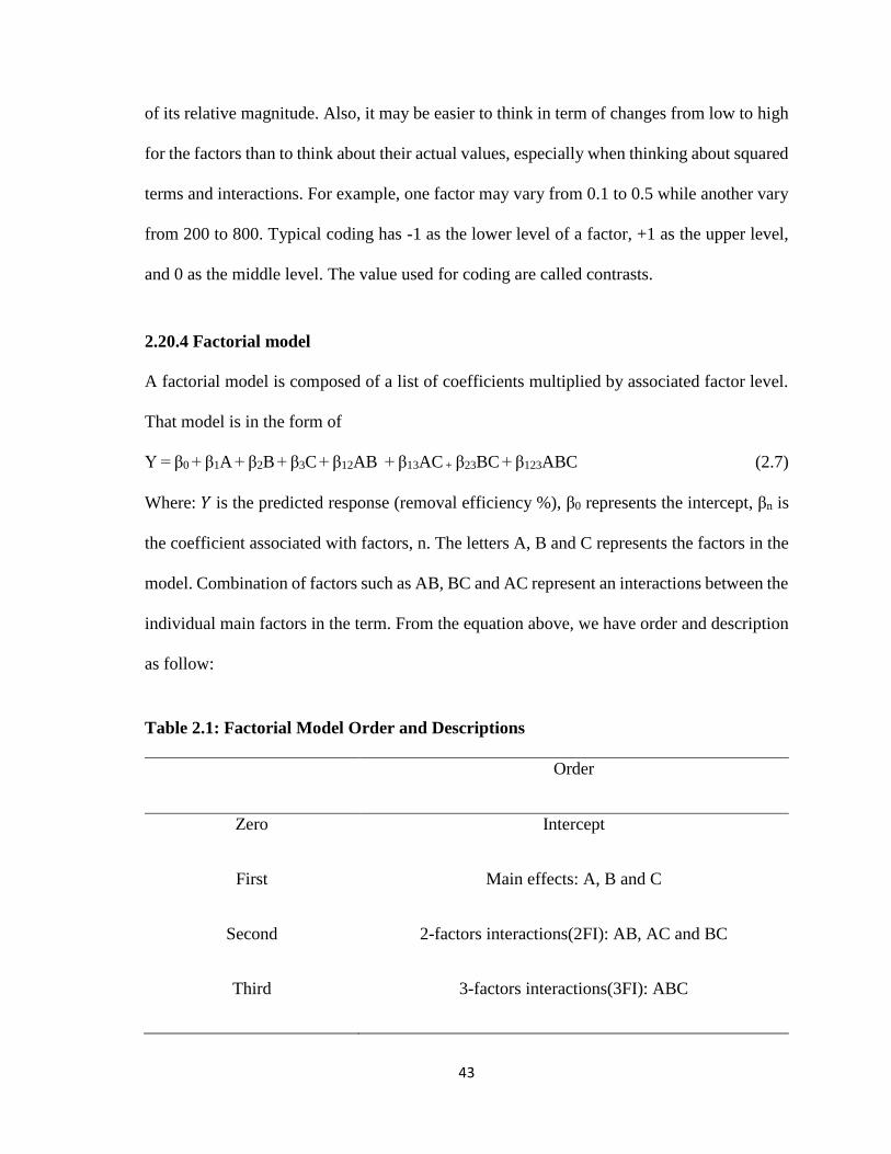
43

of its relative magnitude. Also, it may be easier to think in term of changes from low to high

for the factors than to think about their actual values, especially when thinking about squared

terms and interactions. For example, one factor may vary from 0.1 to 0.5 while another vary

from 200 to 800. Typical coding has -1 as the lower level of a factor, +1 as the upper level,

and 0 as the middle level. The value used for coding are called contrasts.

2.20.4 Factorial model

A factorial model is composed of a list of coefficients multiplied by associated factor level.

That model is in the form of

Y = β0 + β1A + β2B + β3C + β12AB + β13AC + β23BC + β123ABC (2.7)

Where: 𝑌 is the predicted response (removal efficiency %), β0 represents the intercept, βn is

the coefficient associated with factors, n. The letters A, B and C represents the factors in the

model. Combination of factors such as AB, BC and AC represent an interactions between the

individual main factors in the term. From the equation above, we have order and description

as follow:

Table 2.1: Factorial Model Order and Descriptions

Order

Zero Intercept

First Main effects: A, B and C

Second 2-factors interactions(2FI): AB, AC and BC

Third 3-factors interactions(3FI): ABC

44

2.20.5 Factorial design analysis process

After the response data are entered into design layout view, response is choosing by clicking

on the corresponding node under analysis on design expert software. The displaced

information must be followed in sequential order to analysis the response. The sequential

order include transformation, effects plot, model etc.

2.20.5.1 Response transformation

Transformation of the response is an important component of any data analysis.

Transformation is needed if the error (residual) is a function of the magnitude of the response

(predicted values). The available transformation on the design expert include, square roots.

Natural log, base 10 log, inverse square root, power, logit etc. The appropriate transformation

choice relies on subject matter or statistical consideration.

2.20.5.2 Factorial effects

Factorial effects tools include:

Half-Normal plot and Normal plot: probability plot can be used to choose

significant effects. From the plot, the Shapiro-Wilk test for normality should have a

high p-value (above 0.10) to indicate that there is no deviation from the assumption

of normality for the non-selected points.

Effects list: any factor selected from either half-normal or normal plot will also be

shown as selected on the effects list and vice-versa

45

Pareto chart: this is additional graphic tool used to display the t-value of the effects.

Though half-normal plot of effects is normally used to choose the statistically

significant effects, but Pareto chart is clearer and comfortable to view those effects

that are significant in a bar chart form. There are two different t-values plotted on the

graph – based on the Bonferroni corrected t and standard t. these t-limits are only

approximate to the 5% risk level. From the Pareto bar chart, effects that are above the

Bonferroni limit are almost certainly significant. Effects that are above t-value limit

are possibly significant and should be added to the model. Effects that are below the

t-values limit are not likely to be significant.

Analysis of variance (ANOVA): ANOVA helps to confirm that only statistically

significant effects are analyzed in the chosen model.

Diagnostics: This tool evaluates model fit and transformation choice with graph.

Model Graph: This is used to interpret and evaluate the model.

All these tools are useful in the identification of significant effects, insignificant effects and

effects interactions.

2.21 Raman spectroscopy

Raman spectroscopy is the formation and study of Raman scattering for the purpose of

identifying molecules. Raman scattering is formed by X-raying a sample with a light source

at one precise color and wavelength. The light source for irradiating a sample is usually in

the form of a laser. For Raman to work in identifying a sample molecules, the laser has to be

at a wavelength that molecule of the sample cannot absorbed. Raman spectroscopy has been

an important tool that is particular sensitive to the microstructure of the carbon. Raman

spectrum, thus providing useful diagnostics for carbon structure and properties. Many

46

research works were based on information about the physical basis of the observed Raman

spectra, with particular emphasis on relationships of Raman spectra with carbon

microstructure. Raman spectroscopy is one the method that can be used to characterize

carbon materials. Raman is a useful and valuable method that can be of great advantage to

carbon material characterization. Raman is very well suitable to detect small changes in

structural morphology of carbon materials, this is making it an essential instrument for many

material scientists working with carbon structures (Ferraro et al., 1994).

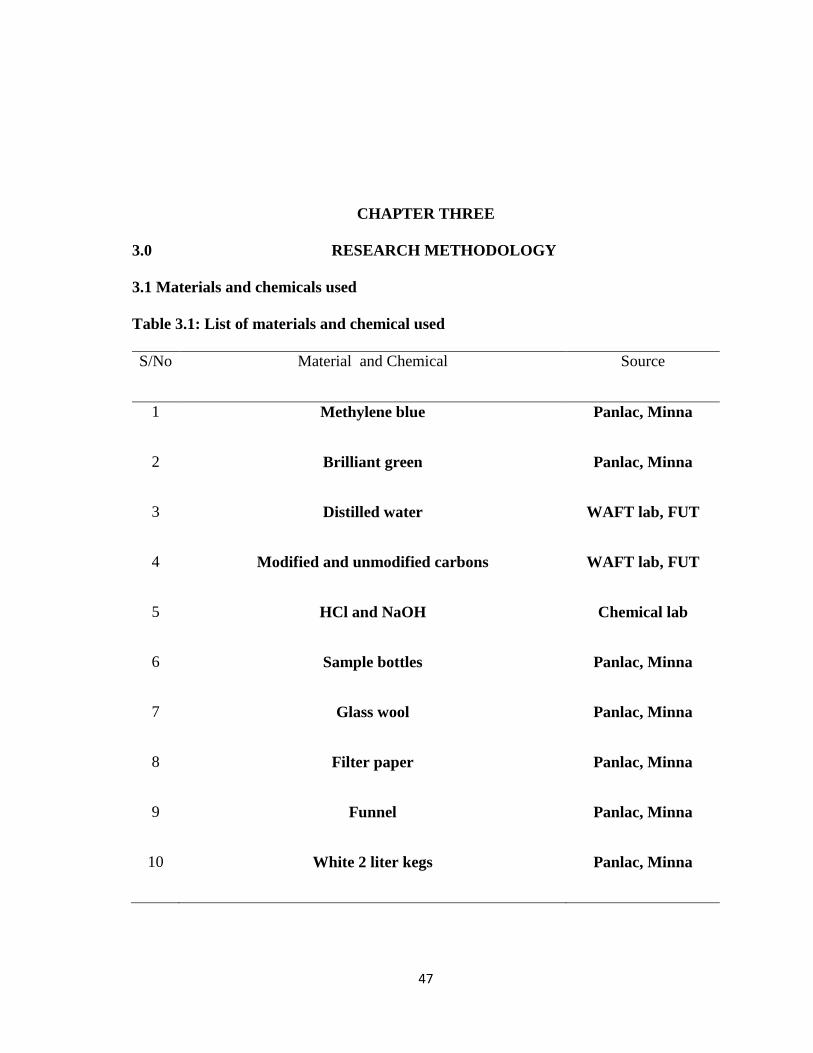
47

CHAPTER THREE

3.0 RESEARCH METHODOLOGY

3.1 Materials and chemicals used

Table 3.1: List of materials and chemical used

S/No Material and Chemical Source

1

2

3

4

5

6

7

8

9

10

Methylene blue

Brilliant green

Distilled water

Modified and unmodified carbons

HCl and NaOH

Sample bottles

Glass wool

Filter paper

Funnel

White 2 liter kegs

Panlac, Minna

Panlac, Minna

WAFT lab, FUT

WAFT lab, FUT

Chemical lab

Panlac, Minna

Panlac, Minna

Panlac, Minna

Panlac, Minna

Panlac, Minna

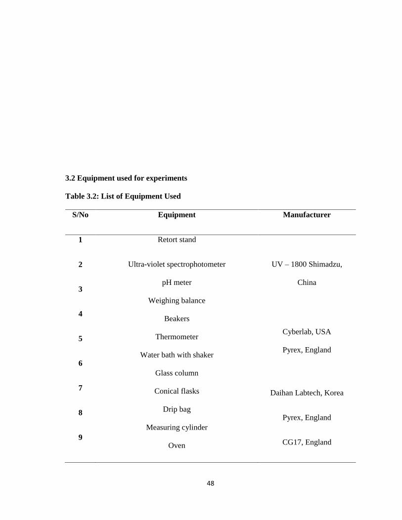
48

3.2 Equipment used for experiments

Table 3.2: List of Equipment Used

S/No Equipment Manufacturer

1

2

3

4

5

6

7

8

9

Retort stand

Ultra-violet spectrophotometer

pH meter

Weighing balance

Beakers

Thermometer

Water bath with shaker

Glass column

Conical flasks

Drip bag

Measuring cylinder

Oven

UV – 1800 Shimadzu,

China

Cyberlab, USA

Pyrex, England

Daihan Labtech, Korea

Pyrex, England

CG17, England

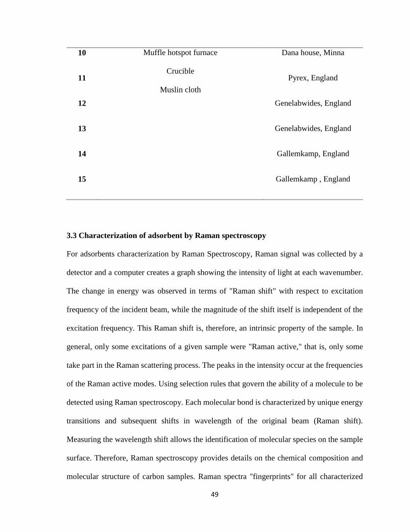
49

10

11

12

13

14

15

Muffle hotspot furnace

Crucible

Muslin cloth

Dana house, Minna

Pyrex, England

Genelabwides, England

Genelabwides, England

Gallemkamp, England

Gallemkamp , England

3.3 Characterization of adsorbent by Raman spectroscopy

For adsorbents characterization by Raman Spectroscopy, Raman signal was collected by a

detector and a computer creates a graph showing the intensity of light at each wavenumber.

The change in energy was observed in terms of "Raman shift" with respect to excitation

frequency of the incident beam, while the magnitude of the shift itself is independent of the

excitation frequency. This Raman shift is, therefore, an intrinsic property of the sample. In

general, only some excitations of a given sample were "Raman active," that is, only some

take part in the Raman scattering process. The peaks in the intensity occur at the frequencies

of the Raman active modes. Using selection rules that govern the ability of a molecule to be

detected using Raman spectroscopy. Each molecular bond is characterized by unique energy

transitions and subsequent shifts in wavelength of the original beam (Raman shift).

Measuring the wavelength shift allows the identification of molecular species on the sample

surface. Therefore, Raman spectroscopy provides details on the chemical composition and

molecular structure of carbon samples. Raman spectra "fingerprints" for all characterized

50

carbons provides information of the molecular structure of the carbon samples used for this

experiments.

3.4 Brunauer-Emmet-Teller (BET)

BET method is used for the determination of the surface area of most porous materials. Total

surface area is a crucial parameter since it helps to known the accessibility of the active site

of probing molecules. Surface area of modified and unmodified kaolin are carried out by

nitrogen adsorption which is generally known to refer to the enrichment of one or more of a

component between two bulk (gas and liquid) which is the adsorbate. Nitrogen is usually the

preferred adsorptive material because of quadra-pole moment that is permanent and it is

responsible for the formation of well-defined monolayer on most surfaces.

51

3.5 Sources of raw materials

The precursors used in the production of the adsorbents include coconut shells, flamboyant pod,

eucalyptus tree and corn cob. Coconut shells were obtained from local market in Minna (Niger

state). Flamboyant pod was sourced within Federal University of Technology main campus,

Gidan-kano, Minna. Corn cob was bought at Kasanguari village, Minna Territory. Eucalyptus tree

was sourced for on the farm land located in Minna Territory. The precursors were sorted to remove

stones, and debris, thereafter each agricultural waste was kept separately for further treatment.

Coconut shells, flamboyant pod, eucalyptus tree and corn cob obtained were then washed with tap

water, to remove surface impurities, and were air – dried in sunlight. They were then stored in dry

containers prior to carbonization

3.6 Carbonization

1 kg of each agricultural waste material was charged into the electric muffle furnace which was

then heated by in the absence of oxygen at a temperature of 600oC for one hours. The resulting

charred material was collected and cooled at room temperature.

3.7 Activation

Samples of the carbonized material were weighed on electric weigh machine, soaked in one mole

of phosphoric acid (H3PO4) 63 % concentrated solution for 24 hours (Jain et al., 2009). The

materials were then removed from the soaking after 24 hour lapsed and then washed with distilled

water until leachable impurities due to free acid and adherent powder were removed and the pH of

the water was 7. Finally, the samples were drained and dried in an oven at 110°C 12 hours.

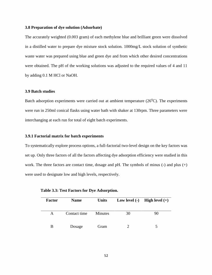
52

3.8 Preparation of dye solution (Adsorbate)

The accurately weighted (0.003 gram) of each methylene blue and brilliant green were dissolved

in a distilled water to prepare dye mixture stock solution. 1000mg/L stock solution of synthetic

waste water was prepared using blue and green dye and from which other desired concentrations

were obtained. The pH of the working solutions was adjusted to the required values of 4 and 11

by adding 0.1 M HCl or NaOH.

3.9 Batch studies

Batch adsorption experiments were carried out at ambient temperature (260C). The experiments

were run in 250ml conical flasks using water bath with shaker at 130rpm. Three parameters were

interchanging at each run for total of eight batch experiments.

3.9.1 Factorial matrix for batch experiments

To systematically explore process options, a full-factorial two-level design on the key factors was

set up. Only three factors of all the factors affecting dye adsorption efficiency were studied in this

work. The three factors are contact time, dosage and pH. The symbols of minus (-) and plus (+)

were used to designate low and high levels, respectively.

Table 3.3: Test Factors for Dye Adsorption.

Factor Name Units Low level (-) High level (+)

A Contact time Minutes 30 90

B Dosage Gram 2 5

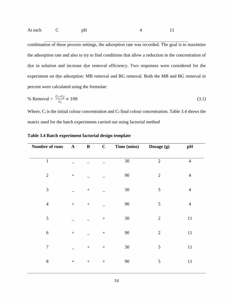
53

At each

combination of these process settings, the adsorption rate was recorded. The goal is to maximize

the adsorption rate and also to try to find conditions that allow a reduction in the concentration of

dye in solution and increase dye removal efficiency. Two responses were considered for the

experiment on dye adsorption: MB removal and BG removal. Both the MB and BG removal in

percent were calculated using the formulae:

% Removal = 𝐶𝑖−𝐶𝑓

𝐶𝑖× 100 (3.1)

Where, Ci is the initial colour concentration and Cf final colour concentration. Table 3.4 shows the

matrix used for the batch experiments carried out using factorial method

Table 3.4 Batch experiment factorial design template

Number of runs A B C Time (mins) Dosage (g) pH

1 _ _ _ 30 2 4

2 + _ _ 90 2 4

3 _ + _ 30 5 4

4 + + _ 90 5 4

5 _ _ + 30 2 11

6 + _ + 90 2 11

7 _ + + 30 5 11

8 + + + 90 5 11

C pH 4 11

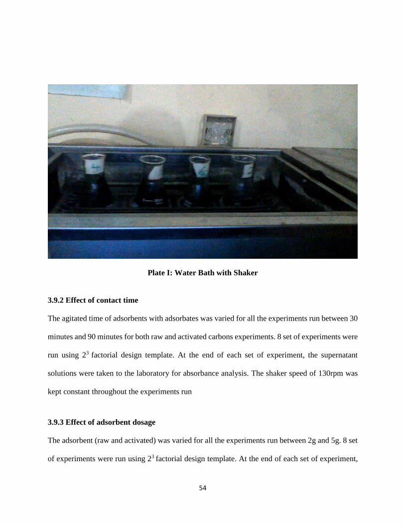
54

Plate I: Water Bath with Shaker

3.9.2 Effect of contact time

The agitated time of adsorbents with adsorbates was varied for all the experiments run between 30

minutes and 90 minutes for both raw and activated carbons experiments. 8 set of experiments were

run using 23 factorial design template. At the end of each set of experiment, the supernatant

solutions were taken to the laboratory for absorbance analysis. The shaker speed of 130rpm was

kept constant throughout the experiments run

3.9.3 Effect of adsorbent dosage

The adsorbent (raw and activated) was varied for all the experiments run between 2g and 5g. 8 set

of experiments were run using 23 factorial design template. At the end of each set of experiment,

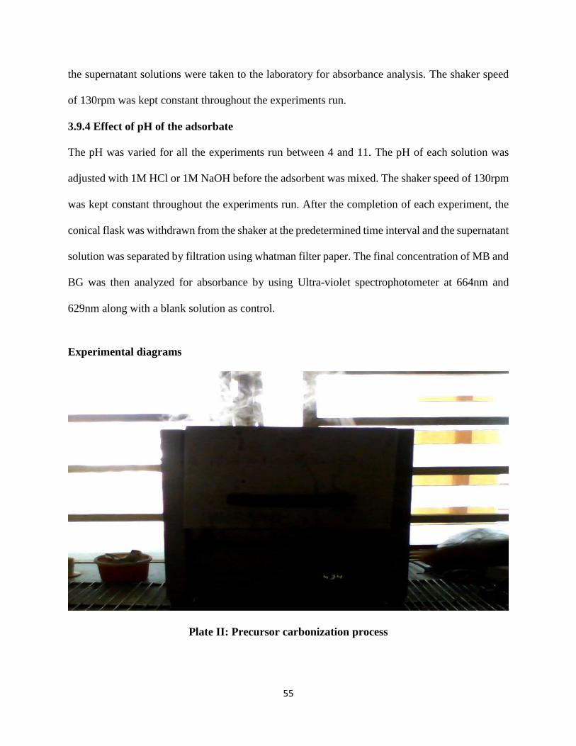
55

the supernatant solutions were taken to the laboratory for absorbance analysis. The shaker speed

of 130rpm was kept constant throughout the experiments run.

3.9.4 Effect of pH of the adsorbate

The pH was varied for all the experiments run between 4 and 11. The pH of each solution was

adjusted with 1M HCl or 1M NaOH before the adsorbent was mixed. The shaker speed of 130rpm

was kept constant throughout the experiments run. After the completion of each experiment, the

conical flask was withdrawn from the shaker at the predetermined time interval and the supernatant

solution was separated by filtration using whatman filter paper. The final concentration of MB and

BG was then analyzed for absorbance by using Ultra-violet spectrophotometer at 664nm and

629nm along with a blank solution as control.

Experimental diagrams

Plate II: Precursor carbonization process

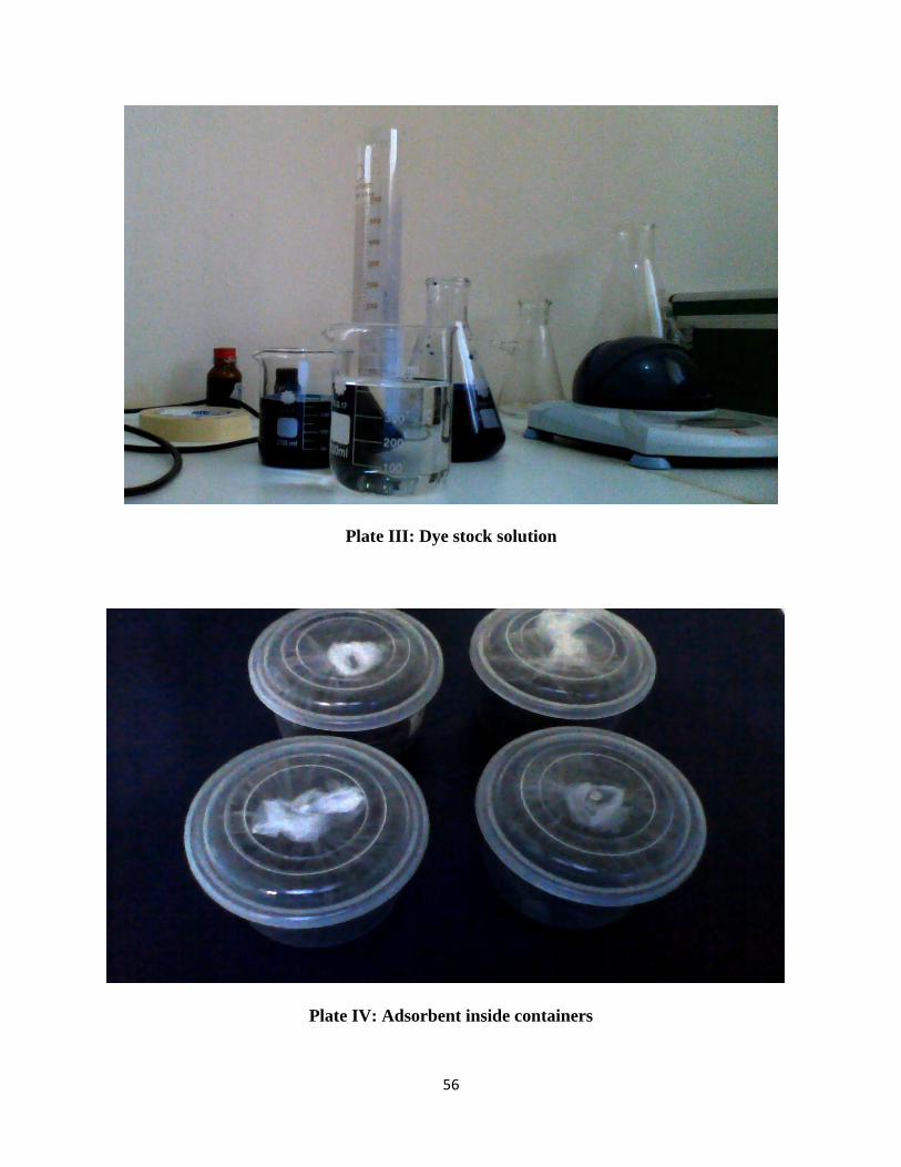
56

Plate III: Dye stock solution

Plate IV: Adsorbent inside containers

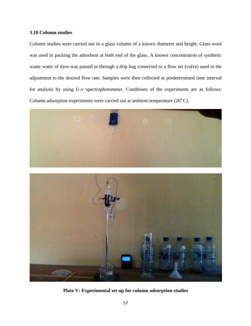
57

3.10 Column studies

Column studies were carried out in a glass column of a known diameter and height. Glass wool

was used in packing the adsorbent at both end of the glass. A known concentration of synthetic

waste water of dyes was passed in through a drip bag connected to a flow set (valve) used in the

adjustment to the desired flow rate. Samples were then collected at predetermined time interval

for analysis by using U-v spectrophotometer. Conditions of the experiments are as follows:

Column adsorption experiments were carried out at ambient temperature (260 C).

Plate V: Experimental set up for column adsorption studies

58

3.10.1 Effect of flow rate

The flow rate of dye solution through adsorbents mass was varied for all the experiments run

between 4.3 mL/min. and 8.6 mL/min. After the completion of each experiment and Prior to each

experiment, distilled water was passed through the column to rid the column impurities and air

bubbles. The final concentrations collected at interval were then analyzed for absorbance by using

Ultra-violet spectrophotometer at 659nm and 626nm along with a blank solution as control.

3.10.2 Effect of adsorbent mass

The adsorbents mass was varied for all the experiments run between 10.6g and 15.9g. After the

completion of each experiment and Prior to each experiment, distilled water was passed through

the column to rid the column impurities and air bubbles. The final concentrations collected at

interval were then analyzed for absorbance by using Ultra-violet spectrophotometer at 659nm and

626nm along with a blank solution as control.

3.10.3 Effect of pH of the adsorbate

The pH was varied for all the experiments run between 4 and 11. The pH of the solution was

adjusted with 1M HCl or 1M NaOH. After the completion of each experiment and Prior to each

experiment, distilled water was passed through the column to rid the column impurities and air

bubbles. The final concentration of MB and BG was then analyzed for absorbance by using Ultra-

violet spectrophotometer at 664nm and 629nm along with a blank solution as control. The

percentage colour removal was then calculated using equation (3.1). The uptake of dye at

equilibrium time was calculated from:

qe =(𝐶0−𝐶𝑒)𝑣

1000𝑤× 100 (3.2)

59

Where qe is the amount of adsorbed dye in mg/g. Co and Ce are the initial and equilibrium dye

concentration in mg/L, V is the volume of the aqueous solution in ml and W is the mass of the

adsorbent in g.

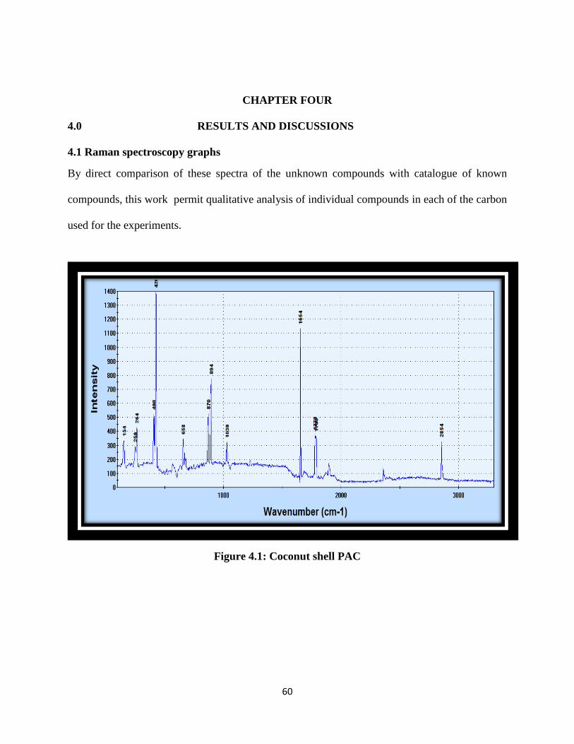
60

CHAPTER FOUR

4.0 RESULTS AND DISCUSSIONS

4.1 Raman spectroscopy graphs

By direct comparison of these spectra of the unknown compounds with catalogue of known

compounds, this work permit qualitative analysis of individual compounds in each of the carbon

used for the experiments.

Figure 4.1: Coconut shell PAC

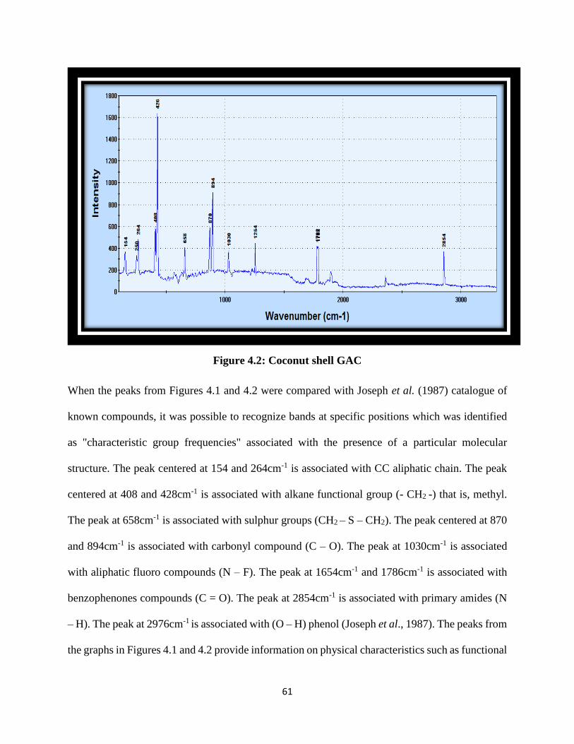
61

Figure 4.2: Coconut shell GAC

When the peaks from Figures 4.1 and 4.2 were compared with Joseph et al. (1987) catalogue of

known compounds, it was possible to recognize bands at specific positions which was identified

as "characteristic group frequencies" associated with the presence of a particular molecular

structure. The peak centered at 154 and 264cm-1 is associated with CC aliphatic chain. The peak

centered at 408 and 428cm-1 is associated with alkane functional group (- CH2 -) that is, methyl.

The peak at 658cm-1 is associated with sulphur groups (CH2 – S – CH2). The peak centered at 870

and 894cm-1 is associated with carbonyl compound (C – O). The peak at 1030cm-1 is associated

with aliphatic fluoro compounds (N – F). The peak at 1654cm-1 and 1786cm-1 is associated with

benzophenones compounds (C = O). The peak at 2854cm-1 is associated with primary amides (N

– H). The peak at 2976cm-1 is associated with (O – H) phenol (Joseph et al., 1987). The peaks from

the graphs in Figures 4.1 and 4.2 provide information on physical characteristics such as functional

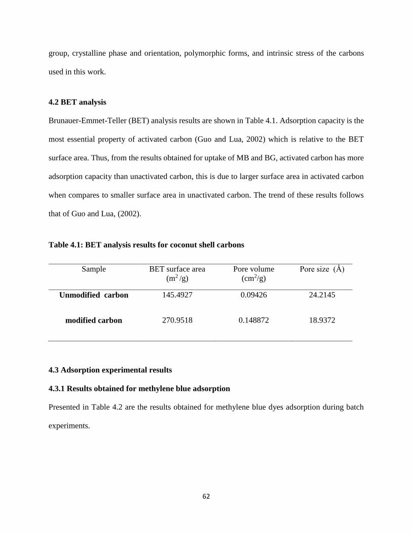
62

group, crystalline phase and orientation, polymorphic forms, and intrinsic stress of the carbons

used in this work.

4.2 BET analysis

Brunauer-Emmet-Teller (BET) analysis results are shown in Table 4.1. Adsorption capacity is the

most essential property of activated carbon (Guo and Lua, 2002) which is relative to the BET

surface area. Thus, from the results obtained for uptake of MB and BG, activated carbon has more

adsorption capacity than unactivated carbon, this is due to larger surface area in activated carbon

when compares to smaller surface area in unactivated carbon. The trend of these results follows

that of Guo and Lua, (2002).

Table 4.1: BET analysis results for coconut shell carbons

Sample BET surface area

(m2 /g)

Pore volume

(cm2/g)

Pore size (Ǻ)

Unmodified carbon 145.4927 0.09426 24.2145

modified carbon 270.9518 0.148872 18.9372

4.3 Adsorption experimental results

4.3.1 Results obtained for methylene blue adsorption

Presented in Table 4.2 are the results obtained for methylene blue dyes adsorption during batch

experiments.

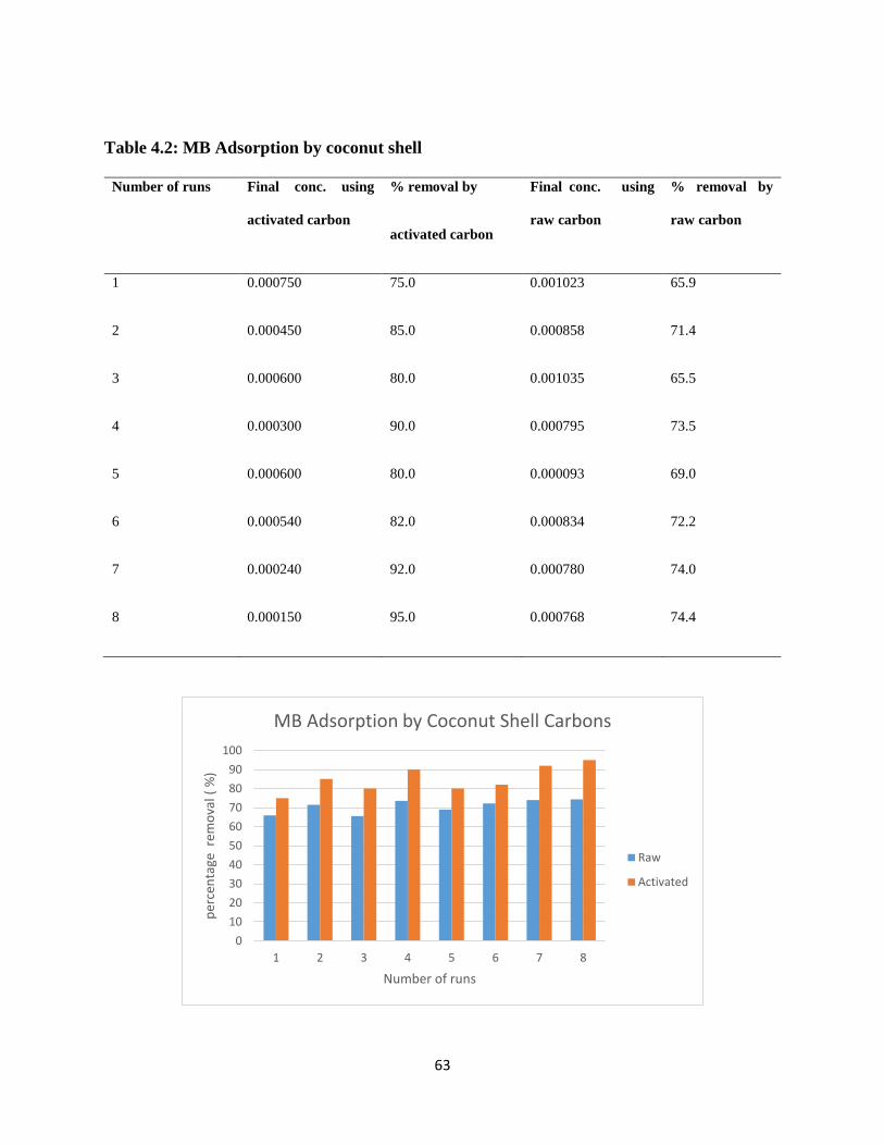
63

Table 4.2: MB Adsorption by coconut shell

Number of runs Final conc. using

activated carbon

% removal by

activated carbon

Final conc. using

raw carbon

% removal by

raw carbon

1 0.000750 75.0 0.001023 65.9

2 0.000450 85.0 0.000858 71.4

3 0.000600 80.0 0.001035 65.5

4 0.000300 90.0 0.000795 73.5

5 0.000600 80.0 0.000093 69.0

6 0.000540 82.0 0.000834 72.2

7 0.000240 92.0 0.000780 74.0

8 0.000150 95.0 0.000768 74.4

0

10

20

30

40

50

60

70

80

90

100

1 2 3 4 5 6 7 8

per

cen

tage

rem

ova

l ( %

)

Number of runs

MB Adsorption by Coconut Shell Carbons

Raw

Activated

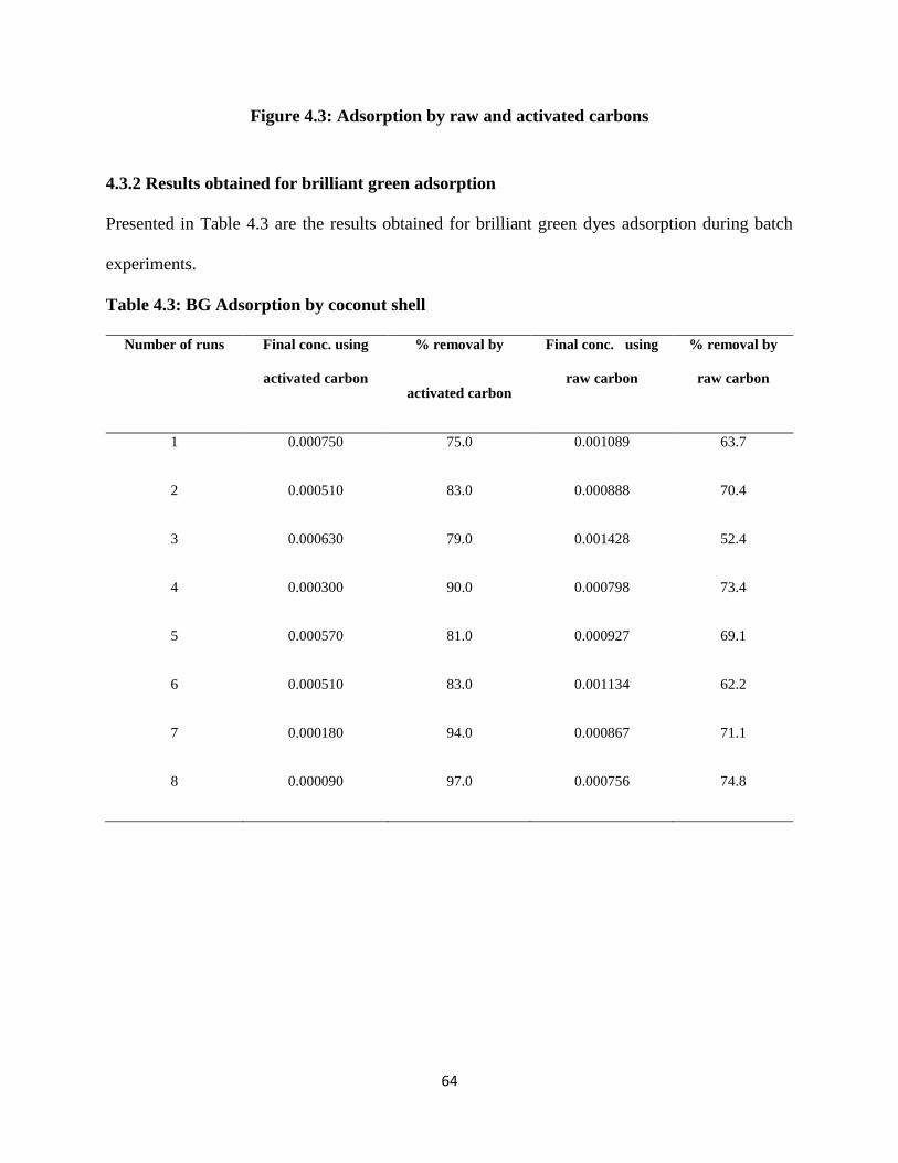
64

Figure 4.3: Adsorption by raw and activated carbons

4.3.2 Results obtained for brilliant green adsorption

Presented in Table 4.3 are the results obtained for brilliant green dyes adsorption during batch

experiments.

Table 4.3: BG Adsorption by coconut shell

Number of runs Final conc. using

activated carbon

% removal by

activated carbon

Final conc. using

raw carbon

% removal by

raw carbon

1 0.000750 75.0 0.001089 63.7

2 0.000510 83.0 0.000888 70.4

3 0.000630 79.0 0.001428 52.4

4 0.000300 90.0 0.000798 73.4

5 0.000570 81.0 0.000927 69.1

6 0.000510 83.0 0.001134 62.2

7 0.000180 94.0 0.000867 71.1

8 0.000090 97.0 0.000756 74.8

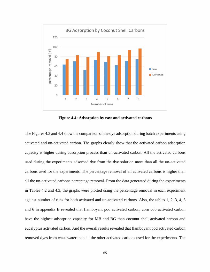
65

Figure 4.4: Adsorption by raw and activated carbons

The Figures 4.3 and 4.4 show the comparison of the dye adsorption during batch experiments using

activated and un-activated carbon. The graphs clearly show that the activated carbon adsorption

capacity is higher during adsorption process than un-activated carbon. All the activated carbons

used during the experiments adsorbed dye from the dye solution more than all the un-activated

carbons used for the experiments. The percentage removal of all activated carbons is higher than

all the un-activated carbons percentage removal. From the data generated during the experiments

in Tables 4.2 and 4.3, the graphs were plotted using the percentage removal in each experiment

against number of runs for both activated and un-activated carbons. Also, the tables 1, 2, 3, 4, 5

and 6 in appendix B revealed that flamboyant pod activated carbon, corn cob activated carbon

have the highest adsorption capacity for MB and BG than coconut shell activated carbon and

eucalyptus activated carbon. And the overall results revealed that flamboyant pod activated carbon

removed dyes from wastewater than all the other activated carbons used for the experiments. The

0

20

40

60

80

100

120

1 2 3 4 5 6 7 8

per

cen

tage

rem

ova

l ( %

)

Number of runs

BG Adsorption by Coconut Shell Carbons

Raw

Activated

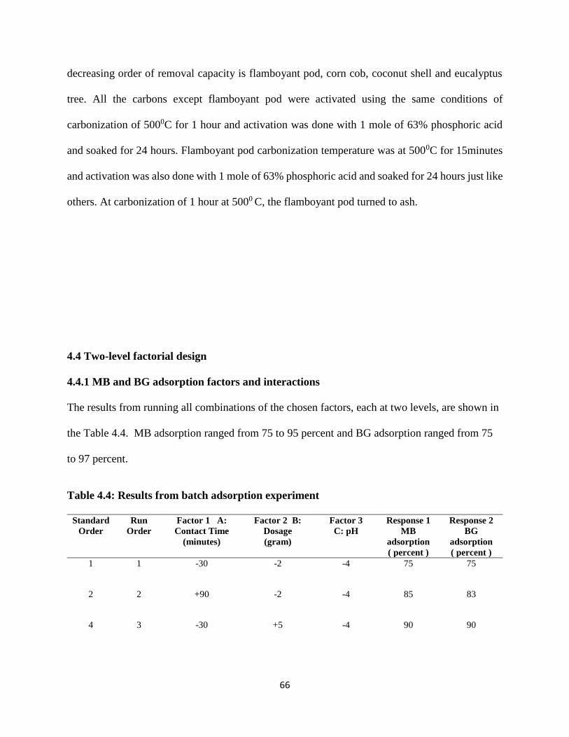
66

decreasing order of removal capacity is flamboyant pod, corn cob, coconut shell and eucalyptus

tree. All the carbons except flamboyant pod were activated using the same conditions of

carbonization of 5000C for 1 hour and activation was done with 1 mole of 63% phosphoric acid

and soaked for 24 hours. Flamboyant pod carbonization temperature was at 5000C for 15minutes

and activation was also done with 1 mole of 63% phosphoric acid and soaked for 24 hours just like

others. At carbonization of 1 hour at 5000 C, the flamboyant pod turned to ash.

4.4 Two-level factorial design

4.4.1 MB and BG adsorption factors and interactions

The results from running all combinations of the chosen factors, each at two levels, are shown in

the Table 4.4. MB adsorption ranged from 75 to 95 percent and BG adsorption ranged from 75

to 97 percent.

Table 4.4: Results from batch adsorption experiment

Standard

Order

Run

Order

Factor 1 A:

Contact Time

(minutes)

Factor 2 B:

Dosage

(gram)

Factor 3

C: pH

Response 1

MB

adsorption

( percent )

Response 2

BG

adsorption

( percent )

1 1 -30 -2 -4 75 75

2 2 +90 -2 -4 85 83

4 3 -30 +5 -4 90 90

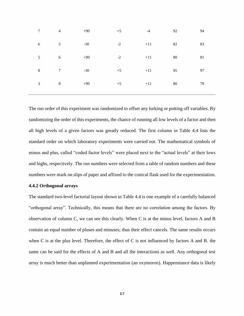
67

7 4 +90 +5 -4 92 94

6 5 -30 -2 +11 82 83

5 6 +90 -2 +11 80 81

8 7 -30 +5 +11 95 97

3 8 +90 +5 +11 80 79

The run order of this experiment was randomized to offset any lurking or putting off variables. By

randomizing the order of this experiments, the chance of running all low levels of a factor and then

all high levels of a given factors was greatly reduced. The first column in Table 4.4 lists the

standard order on which laboratory experiments were carried out. The mathematical symbols of

minus and plus, called “coded factor levels” were placed next to the “actual levels” at their lows

and highs, respectively. The run numbers were selected from a table of random numbers and these

numbers were mark on slips of paper and affixed to the conical flask used for the experimentation.

4.4.2 Orthogonal arrays

The standard two-level factorial layout shown in Table 4.4 is one example of a carefully balanced

“orthogonal array”. Technically, this means that there are no correlation among the factors. By

observation of column C, we can see this clearly. When C is at the minus level, factors A and B

contain an equal number of pluses and minuses; thus their effect cancels. The same results occurs

when C is at the plus level. Therefore, the effect of C is not influenced by factors A and B. the

same can be said for the effects of A and B and all the interactions as well. Any orthogonal test

array is much better than unplanned experimentation (an oxymoron). Happenstance data is likely

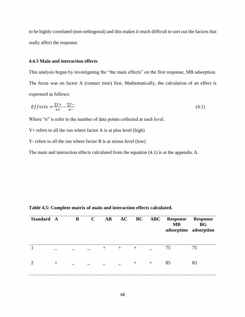
68

to be highly correlated (non-orthogonal) and this makes it much difficult to sort out the factors that

really affect the response.

4.4.3 Main and interaction effects

This analysis began by investigating the “the main effects” on the first response, MB adsorption.

The focus was on factor A (contact time) first. Mathematically, the calculation of an effect is

expressed as follows:

𝐸𝑓𝑓𝑒𝑐𝑡𝑠 =∑𝑌+

𝑛+−

∑𝑌−

𝑛− (4.1)

Where “n” is refer to the number of data points collected at each level.

Y+ refers to all the run where factor A is at plus level (high)

Y- refers to all the run where factor B is at minus level (low)

The main and interaction effects calculated from the equation (4.1) is at the appendix A.

Table 4.5: Complete matrix of main and interaction effects calculated.

Standard

A B C AB AC BC ABC Response

MB

adsorption

Response

BG

adsorption

1 _ _ _ + + + _ 75 75

2 + _ _ _ _ + + 85 83

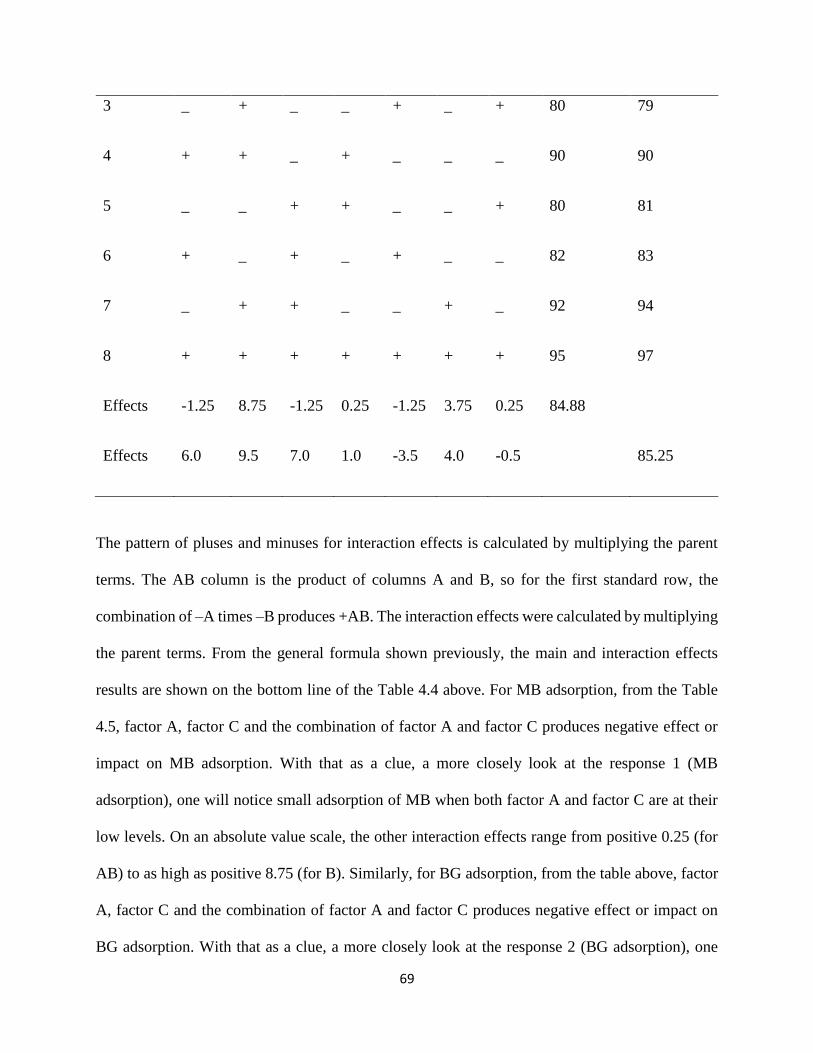
69

3 _ + _ _ + _ + 80 79

4 + + _ + _ _ _ 90 90

5 _ _ + + _ _ + 80 81

6 + _ + _ + _ _ 82 83

7 _ + + _ _ + _ 92 94

8 + + + + + + + 95 97

Effects -1.25 8.75 -1.25 0.25 -1.25 3.75 0.25 84.88

Effects 6.0 9.5 7.0 1.0 -3.5 4.0 -0.5 85.25

The pattern of pluses and minuses for interaction effects is calculated by multiplying the parent

terms. The AB column is the product of columns A and B, so for the first standard row, the

combination of –A times –B produces +AB. The interaction effects were calculated by multiplying

the parent terms. From the general formula shown previously, the main and interaction effects

results are shown on the bottom line of the Table 4.4 above. For MB adsorption, from the Table

4.5, factor A, factor C and the combination of factor A and factor C produces negative effect or

impact on MB adsorption. With that as a clue, a more closely look at the response 1 (MB

adsorption), one will notice small adsorption of MB when both factor A and factor C are at their

low levels. On an absolute value scale, the other interaction effects range from positive 0.25 (for

AB) to as high as positive 8.75 (for B). Similarly, for BG adsorption, from the table above, factor

A, factor C and the combination of factor A and factor C produces negative effect or impact on

BG adsorption. With that as a clue, a more closely look at the response 2 (BG adsorption), one

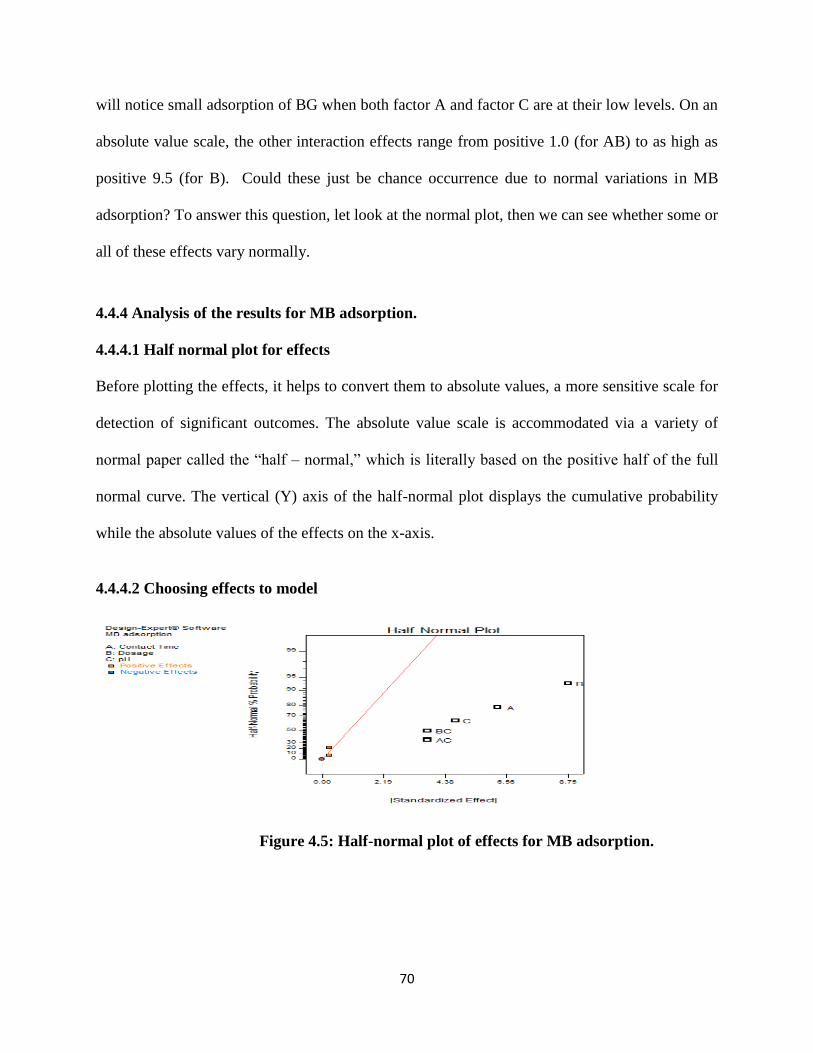
70

will notice small adsorption of BG when both factor A and factor C are at their low levels. On an

absolute value scale, the other interaction effects range from positive 1.0 (for AB) to as high as

positive 9.5 (for B). Could these just be chance occurrence due to normal variations in MB

adsorption? To answer this question, let look at the normal plot, then we can see whether some or

all of these effects vary normally.

4.4.4 Analysis of the results for MB adsorption.

4.4.4.1 Half normal plot for effects

Before plotting the effects, it helps to convert them to absolute values, a more sensitive scale for

detection of significant outcomes. The absolute value scale is accommodated via a variety of

normal paper called the “half – normal,” which is literally based on the positive half of the full

normal curve. The vertical (Y) axis of the half-normal plot displays the cumulative probability

while the absolute values of the effects on the x-axis.

4.4.4.2 Choosing effects to model

Figure 4.5: Half-normal plot of effects for MB adsorption.

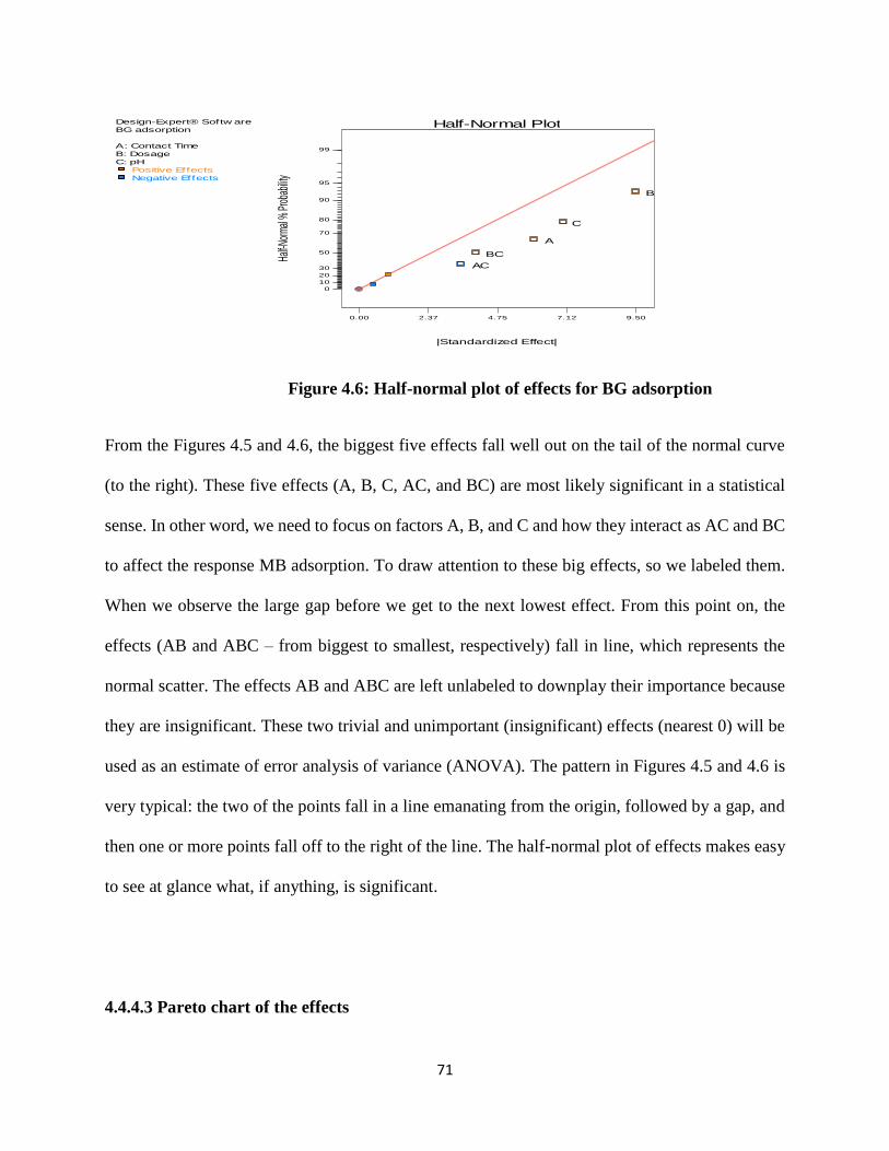
71

Figure 4.6: Half-normal plot of effects for BG adsorption

From the Figures 4.5 and 4.6, the biggest five effects fall well out on the tail of the normal curve

(to the right). These five effects (A, B, C, AC, and BC) are most likely significant in a statistical

sense. In other word, we need to focus on factors A, B, and C and how they interact as AC and BC

to affect the response MB adsorption. To draw attention to these big effects, so we labeled them.

When we observe the large gap before we get to the next lowest effect. From this point on, the

effects (AB and ABC – from biggest to smallest, respectively) fall in line, which represents the

normal scatter. The effects AB and ABC are left unlabeled to downplay their importance because

they are insignificant. These two trivial and unimportant (insignificant) effects (nearest 0) will be

used as an estimate of error analysis of variance (ANOVA). The pattern in Figures 4.5 and 4.6 is

very typical: the two of the points fall in a line emanating from the origin, followed by a gap, and

then one or more points fall off to the right of the line. The half-normal plot of effects makes easy

to see at glance what, if anything, is significant.

4.4.4.3 Pareto chart of the effects

Design-Expert® Softw are

BG adsorption

A: Contact Time

B: Dosage

C: pH

Positive Effects

Negative Effects

Half-Normal Plot

Half-N

orma

l % P

roba

bility

|Standardized Effect|

0.00 2.37 4.75 7.12 9.50

0

10

20

30

50

70

80

90

95

99

A

B

C

AC

BC

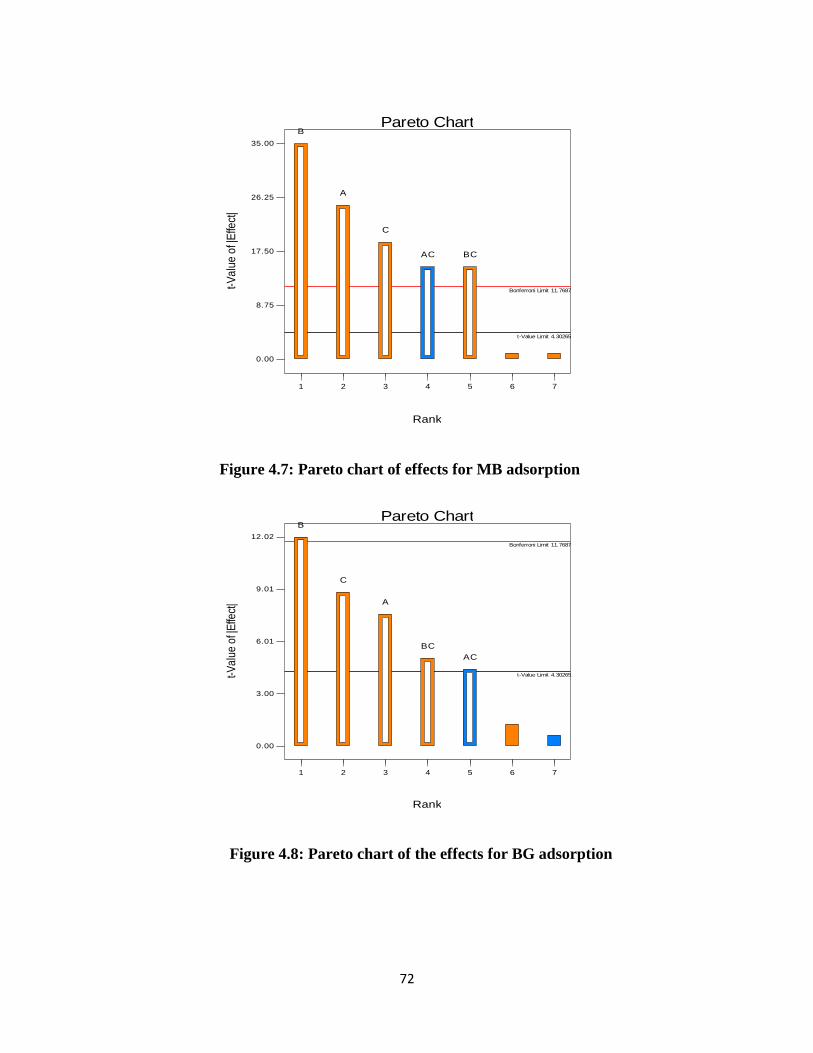
72

Figure 4.7: Pareto chart of effects for MB adsorption

Figure 4.8: Pareto chart of the effects for BG adsorption

Pareto Chart

t-V

alu

e o

f |E

ffect

|

Rank

0.00

8.75

17.50

26.25

35.00

Bonferroni Limit 11.7687

t-Value Limit 4.30265

1 2 3 4 5 6 7

B

A

C

AC BC

Pareto Chart

t-Val

ue o

f |E

ffect

|

Rank

0.00

3.00

6.01

9.01

12.02Bonferroni Limit 11.7687

t-Value Limit 4.30265

1 2 3 4 5 6 7

B

C

A

BC

AC

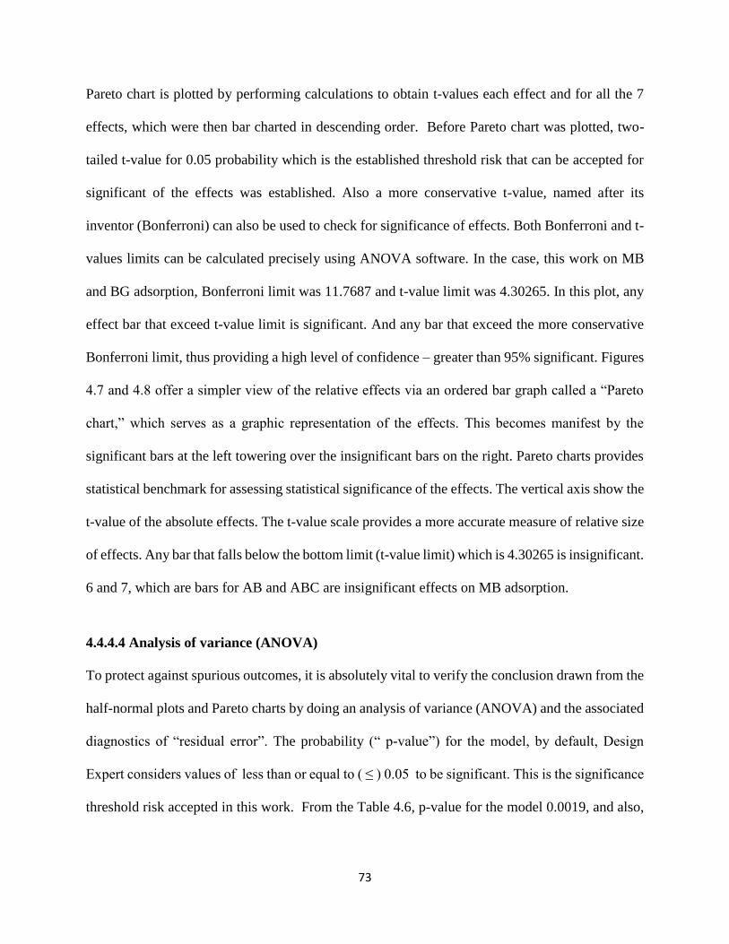
73

Pareto chart is plotted by performing calculations to obtain t-values each effect and for all the 7

effects, which were then bar charted in descending order. Before Pareto chart was plotted, two-

tailed t-value for 0.05 probability which is the established threshold risk that can be accepted for

significant of the effects was established. Also a more conservative t-value, named after its

inventor (Bonferroni) can also be used to check for significance of effects. Both Bonferroni and t-

values limits can be calculated precisely using ANOVA software. In the case, this work on MB

and BG adsorption, Bonferroni limit was 11.7687 and t-value limit was 4.30265. In this plot, any

effect bar that exceed t-value limit is significant. And any bar that exceed the more conservative

Bonferroni limit, thus providing a high level of confidence – greater than 95% significant. Figures

4.7 and 4.8 offer a simpler view of the relative effects via an ordered bar graph called a “Pareto

chart,” which serves as a graphic representation of the effects. This becomes manifest by the

significant bars at the left towering over the insignificant bars on the right. Pareto charts provides

statistical benchmark for assessing statistical significance of the effects. The vertical axis show the

t-value of the absolute effects. The t-value scale provides a more accurate measure of relative size

of effects. Any bar that falls below the bottom limit (t-value limit) which is 4.30265 is insignificant.

6 and 7, which are bars for AB and ABC are insignificant effects on MB adsorption.

4.4.4.4 Analysis of variance (ANOVA)

To protect against spurious outcomes, it is absolutely vital to verify the conclusion drawn from the

half-normal plots and Pareto charts by doing an analysis of variance (ANOVA) and the associated

diagnostics of “residual error”. The probability (“ p-value”) for the model, by default, Design

Expert considers values of less than or equal to ( ≤ ) 0.05 to be significant. This is the significance

threshold risk accepted in this work. From the Table 4.6, p-value for the model 0.0019, and also,

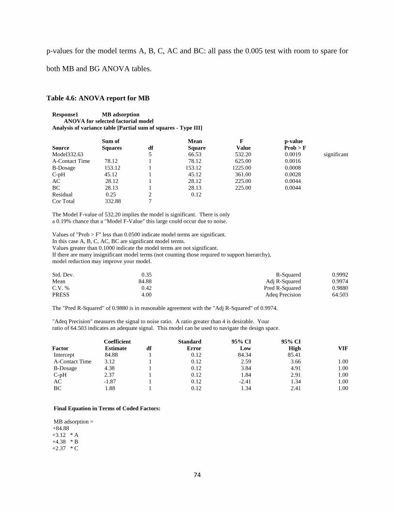
74

p-values for the model terms A, B, C, AC and BC: all pass the 0.005 test with room to spare for

both MB and BG ANOVA tables.

Table 4.6: ANOVA report for MB

Response1 MB adsorption

ANOVA for selected factorial model

Analysis of variance table [Partial sum of squares - Type III]

Sum of Mean F p-value

Source Squares df Square Value Prob > F Model332.63 5 66.53 532.20 0.0019 significant

A-Contact Time 78.12 1 78.12 625.00 0.0016

B-Dosage 153.12 1 153.12 1225.00 0.0008

C-pH 45.12 1 45.12 361.00 0.0028

AC 28.12 1 28.12 225.00 0.0044

BC 28.13 1 28.13 225.00 0.0044

Residual 0.25 2 0.12

Cor Total 332.88 7

The Model F-value of 532.20 implies the model is significant. There is only

a 0.19% chance that a "Model F-Value" this large could occur due to noise.

Values of "Prob > F" less than 0.0500 indicate model terms are significant.

In this case A, B, C, AC, BC are significant model terms.

Values greater than 0.1000 indicate the model terms are not significant.

If there are many insignificant model terms (not counting those required to support hierarchy),

model reduction may improve your model.

Std. Dev. 0.35 R-Squared 0.9992

Mean 84.88 Adj R-Squared 0.9974

C.V. % 0.42 Pred R-Squared 0.9880

PRESS 4.00 Adeq Precision 64.503

The "Pred R-Squared" of 0.9880 is in reasonable agreement with the "Adj R-Squared" of 0.9974.

"Adeq Precision" measures the signal to noise ratio. A ratio greater than 4 is desirable. Your

ratio of 64.503 indicates an adequate signal. This model can be used to navigate the design space.

Coefficient Standard 95% CI 95% CI

Factor Estimate df Error Low High VIF Intercept 84.88 1 0.12 84.34 85.41

A-Contact Time 3.12 1 0.12 2.59 3.66 1.00

B-Dosage 4.38 1 0.12 3.84 4.91 1.00

C-pH 2.37 1 0.12 1.84 2.91 1.00

AC -1.87 1 0.12 -2.41 1.34 1.00

BC 1.88 1 0.12 1.34 2.41 1.00

Final Equation in Terms of Coded Factors:

MB adsorption =

+84.88

+3.12 * A

+4.38 * B

+2.37 * C

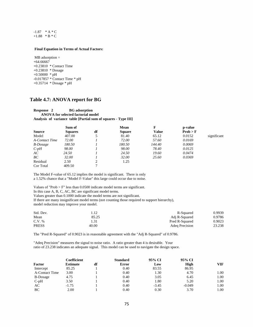
75

-1.87 * A * C

+1.88 * B * C

Final Equation in Terms of Actual Factors:

MB adsorption =

+64.66667

+0.23810 * Contact Time

+0.23810 * Dosage

+0.50000 * pH

-0.017857 * Contact Time * pH

+0.35714 * Dosage * pH

Table 4.7: ANOVA report for BG

Response 2 BG adsorption

ANOVA for selected factorial model

Analysis of variance table [Partial sum of squares - Type III]

Sum of Mean F p-value

Source Squares df Square Value Prob > F Model 407.00 5 81.40 65.12 0.0152 significant

A-Contact Time 72.00 1 72.00 57.60 0.0169

B-Dosage 180.50 1 180.50 144.40 0.0069

C-pH 98.00 1 98.00 78.40 0.0125

AC 24.50 1 24.50 19.60 0.0474

BC 32.00 1 32.00 25.60 0.0369

Residual 2.50 2 1.25

Cor Total 409.50 7

The Model F-value of 65.12 implies the model is significant. There is only

a 1.52% chance that a "Model F-Value" this large could occur due to noise.

Values of "Prob > F" less than 0.0500 indicate model terms are significant.

In this case A, B, C, AC, BC are significant model terms.

Values greater than 0.1000 indicate the model terms are not significant.

If there are many insignificant model terms (not counting those required to support hierarchy),

model reduction may improve your model.

Std. Dev. 1.12 R-Squared 0.9939

Mean 85.25 Adj R-Squared 0.9786

C.V. % 1.31 Pred R-Squared 0.9023

PRESS 40.00 Adeq Precision 23.238

The "Pred R-Squared" of 0.9023 is in reasonable agreement with the "Adj R-Squared" of 0.9786.

"Adeq Precision" measures the signal to noise ratio. A ratio greater than 4 is desirable. Your

ratio of 23.238 indicates an adequate signal. This model can be used to navigate the design space.

Coefficient Standard 95% CI 95% CI

Factor Estimate df Error Low High VIF Intercept 85.25 1 0.40 83.55 86.95

A-Contact Time 3.00 1 0.40 1.30 4.70 1.00

B-Dosage 4.75 1 0.40 3.05 6.45 1.00

C-pH 3.50 1 0.40 1.80 5.20 1.00

AC -1.75 1 0.40 -3.45 -0.049 1.00

BC 2.00 1 0.40 0.30 3.70 1.00

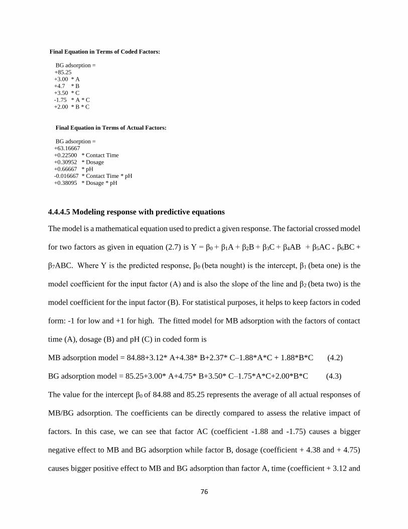
76

Final Equation in Terms of Coded Factors:

BG adsorption =

+85.25

+3.00 * A

+4.7 * B

+3.50 * C

-1.75 * A * C

+2.00 * B * C

Final Equation in Terms of Actual Factors:

BG adsorption =

+63.16667

+0.22500 * Contact Time

+0.30952 * Dosage

+0.66667 * pH

-0.016667 * Contact Time * pH

+0.38095 * Dosage * pH

4.4.4.5 Modeling response with predictive equations

The model is a mathematical equation used to predict a given response. The factorial crossed model

for two factors as given in equation (2.7) is Y = β0 + β1A + β2B + β3C + β4AB + β5AC + β6BC +

β7ABC. Where Y is the predicted response, β0 (beta nought) is the intercept, β1 (beta one) is the

model coefficient for the input factor (A) and is also the slope of the line and β2 (beta two) is the

model coefficient for the input factor (B). For statistical purposes, it helps to keep factors in coded

form: -1 for low and +1 for high. The fitted model for MB adsorption with the factors of contact

time (A), dosage (B) and pH (C) in coded form is

MB adsorption model = 84.88+3.12* A+4.38* B+2.37* C–1.88*A*C + 1.88*B*C (4.2)

BG adsorption model = 85.25+3.00* A+4.75* B+3.50* C–1.75*A*C+2.00*B*C (4.3)

The value for the intercept β0 of 84.88 and 85.25 represents the average of all actual responses of

MB/BG adsorption. The coefficients can be directly compared to assess the relative impact of

factors. In this case, we can see that factor AC (coefficient -1.88 and -1.75) causes a bigger

negative effect to MB and BG adsorption while factor B, dosage (coefficient + 4.38 and + 4.75)

causes bigger positive effect to MB and BG adsorption than factor A, time (coefficient + 3.12 and

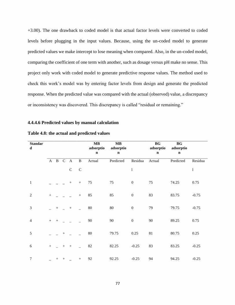
77

+3.00). The one drawback to coded model is that actual factor levels were converted to coded

levels before plugging in the input values. Because, using the un-coded model to generate

predicted values we make intercept to lose meaning when compared. Also, in the un-coded model,

comparing the coefficient of one term with another, such as dosage versus pH make no sense. This

project only work with coded model to generate predictive response values. The method used to

check this work’s model was by entering factor levels from design and generate the predicted

response. When the predicted value was compared with the actual (observed) value, a discrepancy

or inconsistency was discovered. This discrepancy is called “residual or remaining.”

4.4.4.6 Predicted values by manual calculation

Table 4.8: the actual and predicted values

Standar

d

MB

adsorptio

n

MB

adsorptio

n

BG

adsorptio

n

BG

adsorptio

n

A B C A

C

B

C

Actual Predicted Residua

l

Actual Predicted Residua

l

1 _ _ _ + + 75 75 0 75 74.25 0.75

2 + _ _ _ + 85 85 0 83 83.75 -0.75

3 _ + _ + _ 80 80 0 79 79.75 -0.75

4 + + _ _ _ 90 90 0 90 89.25 0.75

5 _ _ + _ _ 80 79.75 0.25 81 80.75 0.25

6 + _ + + _ 82 82.25 -0.25 83 83.25 -0.25

7 _ + + _ + 92 92.25 -0.25 94 94.25 -0.25

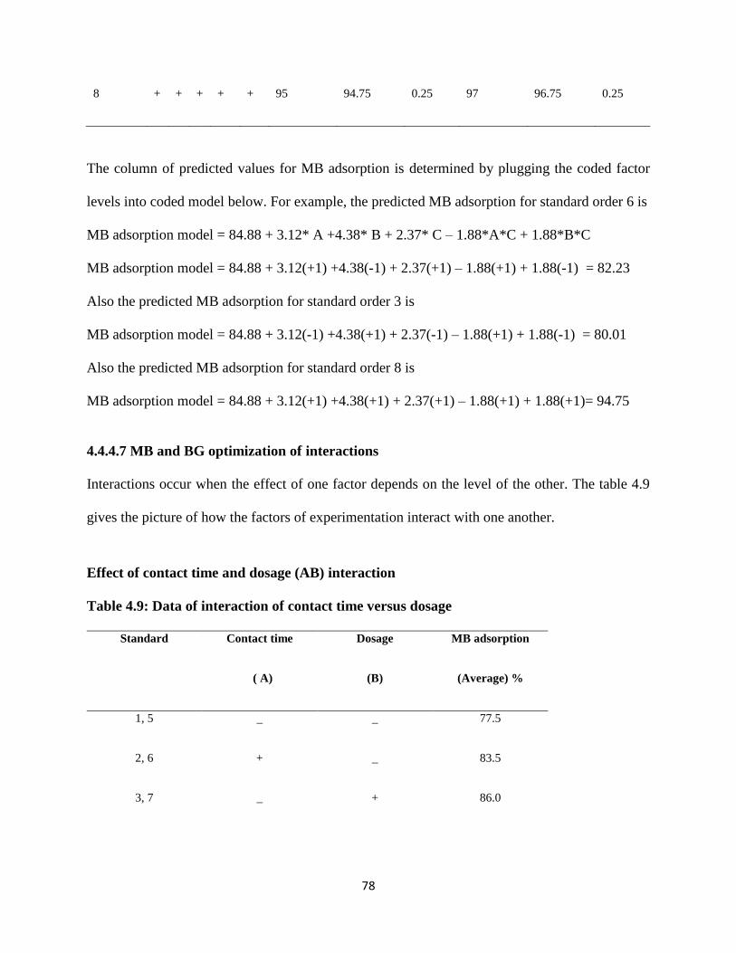
78

8 + + + + + 95 94.75 0.25 97 96.75 0.25

The column of predicted values for MB adsorption is determined by plugging the coded factor

levels into coded model below. For example, the predicted MB adsorption for standard order 6 is

MB adsorption model = 84.88 + 3.12* A +4.38* B + 2.37* C – 1.88*A*C + 1.88*B*C

MB adsorption model = 84.88 + 3.12(+1) +4.38(-1) + 2.37(+1) – 1.88(+1) + 1.88(-1) = 82.23

Also the predicted MB adsorption for standard order 3 is

MB adsorption model = 84.88 + 3.12(-1) +4.38(+1) + 2.37(-1) – 1.88(+1) + 1.88(-1) = 80.01

Also the predicted MB adsorption for standard order 8 is

MB adsorption model = 84.88 + 3.12(+1) +4.38(+1) + 2.37(+1) – 1.88(+1) + 1.88(+1)= 94.75

4.4.4.7 MB and BG optimization of interactions

Interactions occur when the effect of one factor depends on the level of the other. The table 4.9

gives the picture of how the factors of experimentation interact with one another.

Effect of contact time and dosage (AB) interaction

Table 4.9: Data of interaction of contact time versus dosage

Standard Contact time

( A)

Dosage

(B)

MB adsorption

(Average) %

1, 5 _ _ 77.5

2, 6 + _ 83.5

3, 7 _ + 86.0

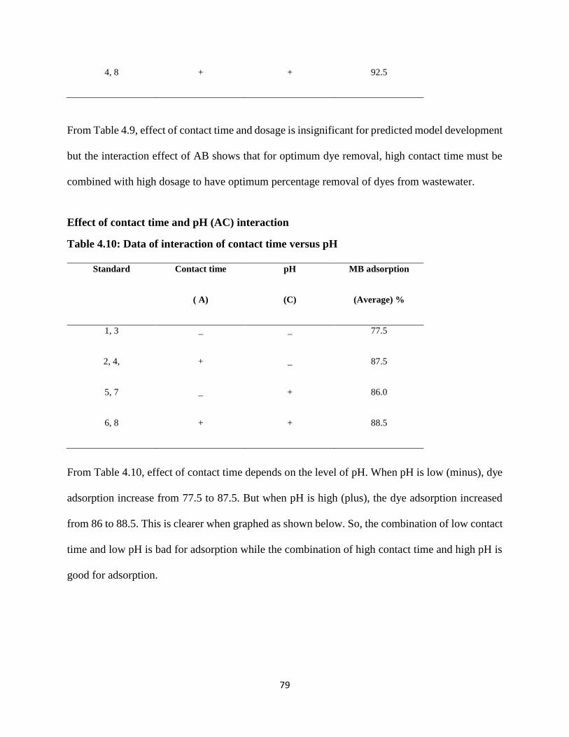
79

4, 8 + + 92.5

From Table 4.9, effect of contact time and dosage is insignificant for predicted model development

but the interaction effect of AB shows that for optimum dye removal, high contact time must be

combined with high dosage to have optimum percentage removal of dyes from wastewater.

Effect of contact time and pH (AC) interaction

Table 4.10: Data of interaction of contact time versus pH

Standard Contact time

( A)

pH

(C)

MB adsorption

(Average) %

1, 3 _ _ 77.5

2, 4, + _ 87.5

5, 7 _ + 86.0

6, 8 + + 88.5

From Table 4.10, effect of contact time depends on the level of pH. When pH is low (minus), dye

adsorption increase from 77.5 to 87.5. But when pH is high (plus), the dye adsorption increased

from 86 to 88.5. This is clearer when graphed as shown below. So, the combination of low contact

time and low pH is bad for adsorption while the combination of high contact time and high pH is

good for adsorption.

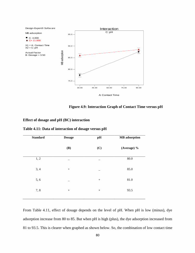
80

Figure 4.9: Interaction Graph of Contact Time versus pH

Effect of dosage and pH (BC) interaction

Table 4.11: Data of interaction of dosage versus pH

Standard Dosage

(B)

pH

(C)

MB adsorption

(Average) %

1, 2 _ _ 80.0

3, 4 + _ 85.0

5, 6 _ + 81.0

7, 8 + + 93.5

From Table 4.11, effect of dosage depends on the level of pH. When pH is low (minus), dye

adsorption increase from 80 to 85. But when pH is high (plus), the dye adsorption increased from

81 to 93.5. This is clearer when graphed as shown below. So, the combination of low contact time

Design-Expert® Softw are

MB adsorption

C- 4.000

C+ 11.000

X1 = A: Contact Time

X2 = C: pH

Actual Factor

B: Dosage = 3.50

C: pH

30.00 45.00 60.00 75.00 90.00

Interaction

A: Contact Time

MB

ads

orpt

ion

75.0

80.0

85.0

90.0

95.0

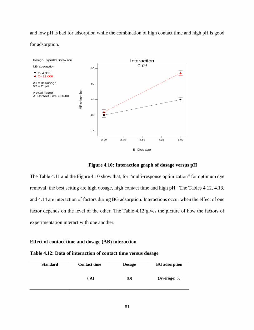
81

and low pH is bad for adsorption while the combination of high contact time and high pH is good

for adsorption.

Figure 4.10: Interaction graph of dosage versus pH

The Table 4.11 and the Figure 4.10 show that, for “multi-response optimization” for optimum dye

removal, the best setting are high dosage, high contact time and high pH. The Tables 4.12, 4.13,

and 4.14 are interaction of factors during BG adsorption. Interactions occur when the effect of one

factor depends on the level of the other. The Table 4.12 gives the picture of how the factors of

experimentation interact with one another.

Effect of contact time and dosage (AB) interaction

Table 4.12: Data of interaction of contact time versus dosage

Standard Contact time

( A)

Dosage

(B)

BG adsorption

(Average) %

Design-Expert® Softw are

MB adsorption

C- 4.000

C+ 11.000

X1 = B: Dosage

X2 = C: pH

Actual Factor

A: Contact Time = 60.00

C: pH

2.00 2.75 3.50 4.25 5.00

Interaction

B: Dosage

MB

ads

orpt

ion

75

80

85

90

95

82

1, 5 _ _ 78.0

2, 6 + _ 83.0

3, 7 _ + 86.5

4, 8 + + 93.5

From Table 4.12, the effect of contact time and dosage is insignificant for predicted model

development but the interaction effect of AB shows that for optimum dye removal, high contact

time must be combined with high dosage.

Effect of contact time and pH (AC) interaction

Table 4.13: Data of interaction of contact time versus pH

Standard Contact time

( A)

pH

(C)

BG adsorption

(Average) %

1, 3 _ _ 77.0

2, 4, + _ 86.5

5, 7 _ + 87.5

6, 8 + + 90.0

From Table 4.13, effect of contact time depends on the level of pH. When pH is low (minus), dye

adsorption increase from 77.0 to 86.5. But when pH is high (plus), the dye adsorption increased

from 87.5 to 90. This is clearer when graphed as shown below. So, the combination of low contact

83

time and low pH is bad for adsorption while the combination of high contact time and high pH is

good for adsorption.

Figure 4.12: Interaction graph of dosage versus pH

Effect of dosage and pH (BC) interaction

Table 4.14: Data of interaction of dosage versus pH

Standard Dosage

(B)

pH

(C)

BG adsorption

(Average) %

1, 2 _ _ 79.0

3, 4 + _ 84.5

5, 6 _ + 82.0

7, 8 + + 95.5

Design-Expert® Softw are

BG adsorption

C- 4.000

C+ 11.000

X1 = A: Contact Time

X2 = C: pH

Actual Factor

B: Dosage = 3.50

C: pH

30.00 45.00 60.00 75.00 90.00

Interaction

A: Contact Time

BG

ads

orpt

ion

74.0

79.8

85.5

91.3

97.0

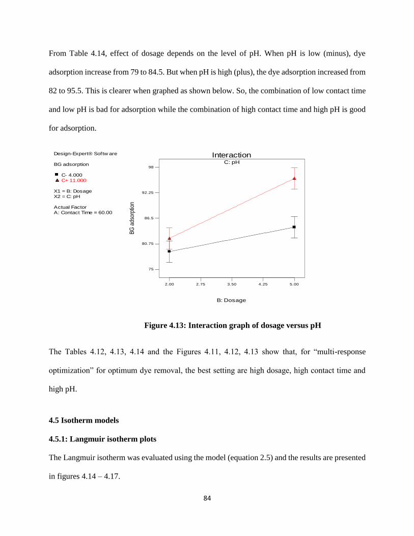
84

From Table 4.14, effect of dosage depends on the level of pH. When pH is low (minus), dye

adsorption increase from 79 to 84.5. But when pH is high (plus), the dye adsorption increased from

82 to 95.5. This is clearer when graphed as shown below. So, the combination of low contact time

and low pH is bad for adsorption while the combination of high contact time and high pH is good

for adsorption.

Figure 4.13: Interaction graph of dosage versus pH

The Tables 4.12, 4.13, 4.14 and the Figures 4.11, 4.12, 4.13 show that, for “multi-response

optimization” for optimum dye removal, the best setting are high dosage, high contact time and

high pH.

4.5 Isotherm models

4.5.1: Langmuir isotherm plots

The Langmuir isotherm was evaluated using the model (equation 2.5) and the results are presented

in figures 4.14 – 4.17.

Design-Expert® Softw are

BG adsorption

C- 4.000

C+ 11.000

X1 = B: Dosage

X2 = C: pH

Actual Factor

A: Contact Time = 60.00

C: pH

2.00 2.75 3.50 4.25 5.00

Interaction

B: Dosage

BG

ads

orpt

ion

75

80.75

86.5

92.25

98

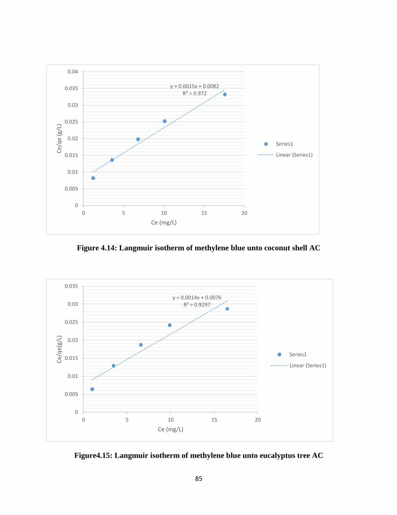
85

Figure 4.14: Langmuir isotherm of methylene blue unto coconut shell AC

Figure4.15: Langmuir isotherm of methylene blue unto eucalyptus tree AC

y = 0.0015x + 0.0082R² = 0.972

0

0.005

0.01

0.015

0.02

0.025

0.03

0.035

0.04

0 5 10 15 20

Ce/

qe

(g/L

)

Ce (mg/L)

Series1

Linear (Series1)

y = 0.0014x + 0.0076R² = 0.9297

0

0.005

0.01

0.015

0.02

0.025

0.03

0.035

0 5 10 15 20

Ce/

qe(

g/L)

Ce (mg/L)

Series1

Linear (Series1)

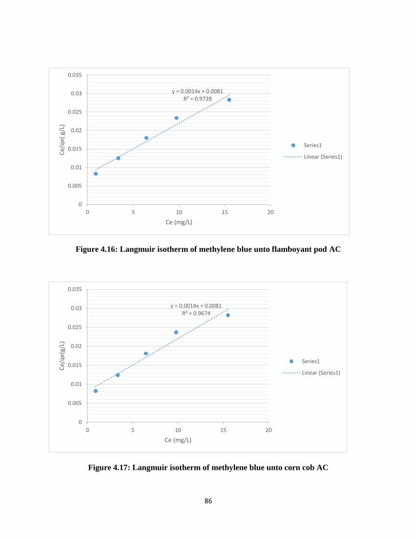
86

Figure 4.16: Langmuir isotherm of methylene blue unto flamboyant pod AC

Figure 4.17: Langmuir isotherm of methylene blue unto corn cob AC

y = 0.0014x + 0.0081R² = 0.9728

0

0.005

0.01

0.015

0.02

0.025

0.03

0.035

0 5 10 15 20

Ce/

qe(

g/L

)

Ce (mg/L)

Series1

Linear (Series1)

y = 0.0014x + 0.0081R² = 0.9674

0

0.005

0.01

0.015

0.02

0.025

0.03

0.035

0 5 10 15 20

Ce/

qe(

g/L)

Ce (mg/L)

Series1

Linear (Series1)

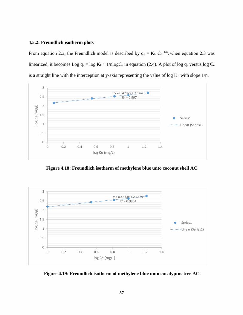
87

4.5.2: Freundlich isotherm plots

From equation 2.3, the Freundlich model is described by qe = KF Ce 1/n, when equation 2.3 was

linearized, it becomes Log qe = log Kf + 1/nlogCe in equation (2.4). A plot of log qe versus log Ce

is a straight line with the interception at y-axis representing the value of log KF with slope 1/n.

Figure 4.18: Freundlich isotherm of methylene blue unto coconut shell AC

Figure 4.19: Freundlich isotherm of methylene blue unto eucalyptus tree AC

y = 0.4702x + 2.1406R² = 0.997

0

0.5

1

1.5

2

2.5

3

0 0.2 0.4 0.6 0.8 1 1.2 1.4

log

qe(

mg/

g)

log Ce (mg/L)

Series1

Linear (Series1)

y = 0.4533x + 2.1829R² = 0.9934

0

0.5

1

1.5

2

2.5

3

0 0.2 0.4 0.6 0.8 1 1.2 1.4

log

qe

(mg/

g)

log Ce (mg/L)

Series1

Linear (Series1)

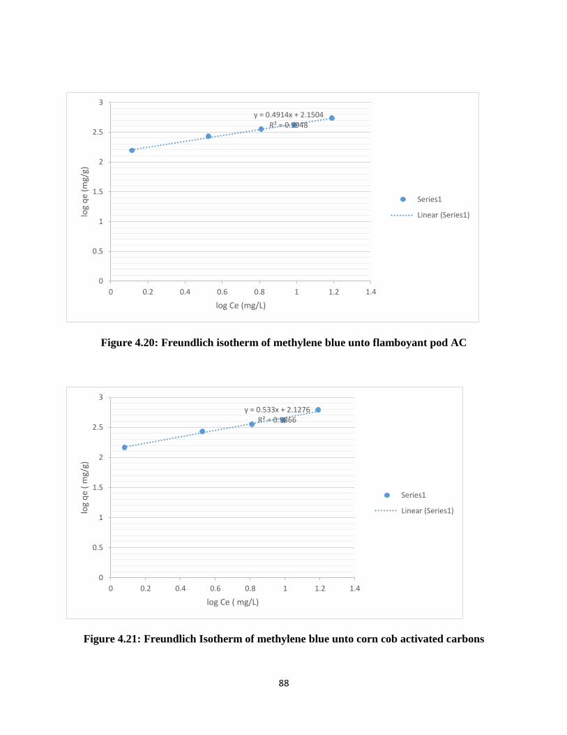
88

Figure 4.20: Freundlich isotherm of methylene blue unto flamboyant pod AC

Figure 4.21: Freundlich Isotherm of methylene blue unto corn cob activated carbons

y = 0.4914x + 2.1504R² = 0.9948

0

0.5

1

1.5

2

2.5

3

0 0.2 0.4 0.6 0.8 1 1.2 1.4

log

qe

(mg/

g)

log Ce (mg/L)

Series1

Linear (Series1)

y = 0.533x + 2.1276R² = 0.9866

0

0.5

1

1.5

2

2.5

3

0 0.2 0.4 0.6 0.8 1 1.2 1.4

log

qe

( m

g/g)

log Ce ( mg/L)

Series1

Linear (Series1)

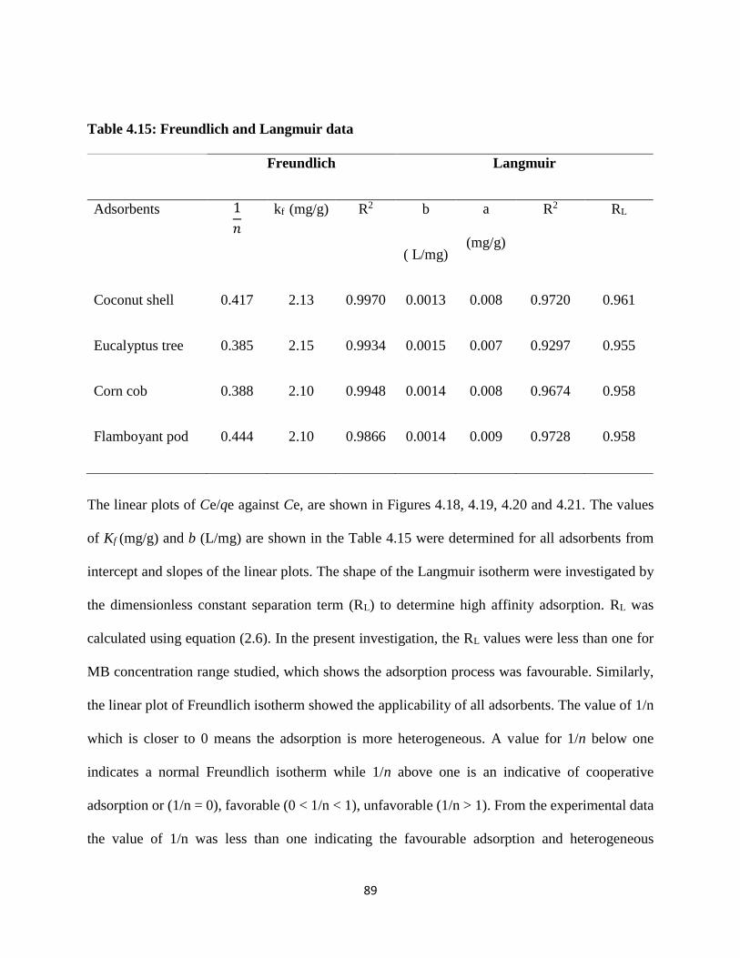
89

Table 4.15: Freundlich and Langmuir data

Freundlich Langmuir

Adsorbents 1

𝑛

kf (mg/g) R2 b

( L/mg)

a

(mg/g)

R2 RL

Coconut shell 0.417 2.13 0.9970 0.0013 0.008 0.9720 0.961

Eucalyptus tree 0.385 2.15 0.9934 0.0015 0.007 0.9297 0.955

Corn cob 0.388 2.10 0.9948 0.0014 0.008 0.9674 0.958

Flamboyant pod 0.444 2.10 0.9866 0.0014 0.009 0.9728 0.958

The linear plots of Ce/qe against Ce, are shown in Figures 4.18, 4.19, 4.20 and 4.21. The values

of Kf (mg/g) and b (L/mg) are shown in the Table 4.15 were determined for all adsorbents from

intercept and slopes of the linear plots. The shape of the Langmuir isotherm were investigated by

the dimensionless constant separation term (RL) to determine high affinity adsorption. RL was

calculated using equation (2.6). In the present investigation, the RL values were less than one for

MB concentration range studied, which shows the adsorption process was favourable. Similarly,

the linear plot of Freundlich isotherm showed the applicability of all adsorbents. The value of 1/n

which is closer to 0 means the adsorption is more heterogeneous. A value for 1/n below one

indicates a normal Freundlich isotherm while 1/n above one is an indicative of cooperative

adsorption or (1/n = 0), favorable (0 < 1/n < 1), unfavorable (1/n > 1). From the experimental data

the value of 1/n was less than one indicating the favourable adsorption and heterogeneous

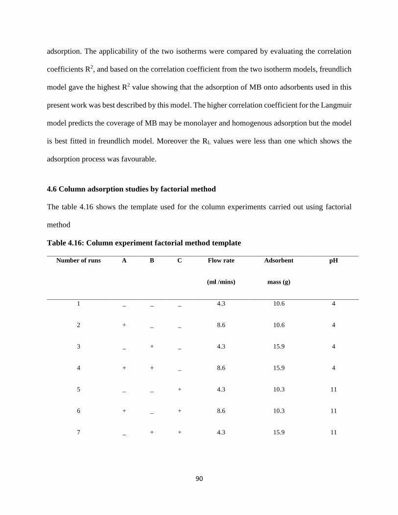
90

adsorption. The applicability of the two isotherms were compared by evaluating the correlation

coefficients R2, and based on the correlation coefficient from the two isotherm models, freundlich

model gave the highest R2 value showing that the adsorption of MB onto adsorbents used in this

present work was best described by this model. The higher correlation coefficient for the Langmuir

model predicts the coverage of MB may be monolayer and homogenous adsorption but the model

is best fitted in freundlich model. Moreover the RL values were less than one which shows the

adsorption process was favourable.

4.6 Column adsorption studies by factorial method

The table 4.16 shows the template used for the column experiments carried out using factorial

method

Table 4.16: Column experiment factorial method template

Number of runs A B C Flow rate

(ml /mins)

Adsorbent

mass (g)

pH

1 _ _ _ 4.3 10.6 4

2 + _ _ 8.6 10.6 4

3 _ + _ 4.3 15.9 4

4 + + _ 8.6 15.9 4

5 _ _ + 4.3 10.3 11

6 + _ + 8.6 10.3 11

7 _ + + 4.3 15.9 11

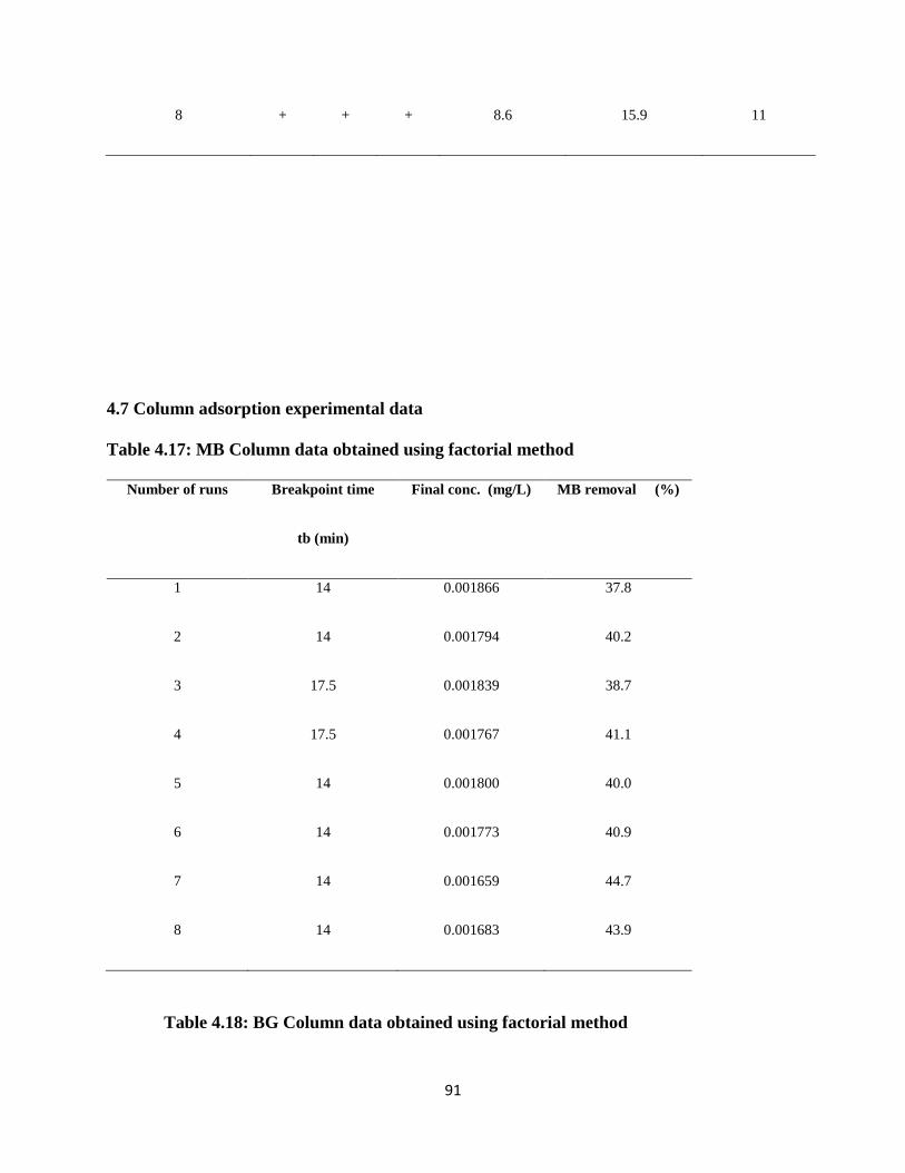
91

8 + + + 8.6 15.9 11

4.7 Column adsorption experimental data

Table 4.17: MB Column data obtained using factorial method

Number of runs Breakpoint time

tb (min)

Final conc. (mg/L) MB removal (%)

1 14 0.001866 37.8

2 14 0.001794 40.2

3 17.5 0.001839 38.7

4 17.5 0.001767 41.1

5 14 0.001800 40.0

6 14 0.001773 40.9

7 14 0.001659 44.7

8 14 0.001683 43.9

Table 4.18: BG Column data obtained using factorial method

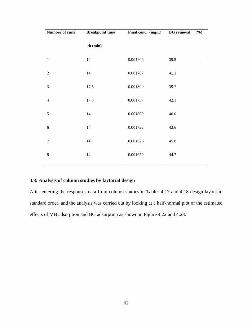
92

Number of runs Breakpoint time

tb (min)

Final conc. (mg/L) BG removal (%)

1 14 0.001806 39.8

2 14 0.001767 41.1

3 17.5 0.001809 39.7

4 17.5 0.001737 42.1

5 14 0.001800 40.0

6 14 0.001722 42.6

7 14 0.001626 45.8

8 14 0.001659 44.7

4.8: Analysis of column studies by factorial design

After entering the responses data from column studies in Tables 4.17 and 4.18 design layout in

standard order, and the analysis was carried out by looking at a half-normal plot of the estimated

effects of MB adsorption and BG adsorption as shown in Figure 4.22 and 4.23.

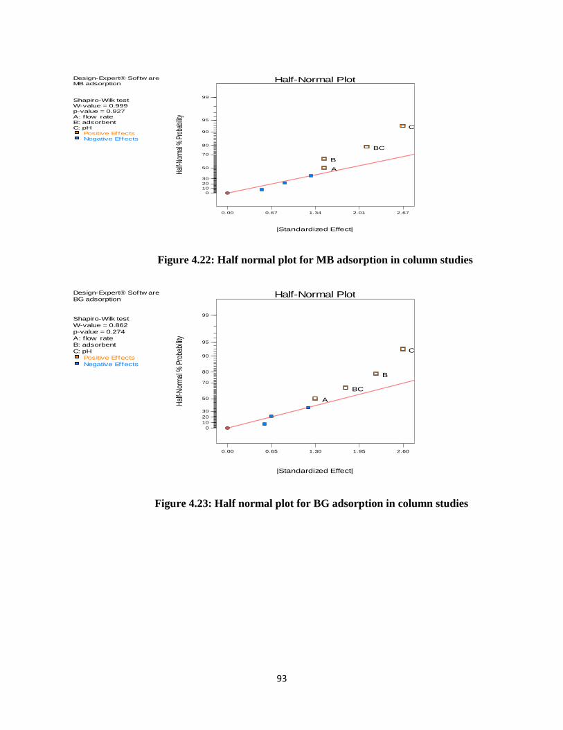
93

Figure 4.22: Half normal plot for MB adsorption in column studies

Figure 4.23: Half normal plot for BG adsorption in column studies

Design-Expert® Softw are

MB adsorption

Shapiro-Wilk test

W-value = 0.999

p-value = 0.927

A: f low rate

B: adsorbent

C: pH

Positive Effects

Negative Effects

Half-Normal Plot

Half-

Norm

al %

Pro

babi

lity

|Standardized Effect|

0.00 0.67 1.34 2.01 2.67

0

10

20

30

50

70

80

90

95

99

A

B

C

BC

Design-Expert® Softw are

BG adsorption

Shapiro-Wilk test

W-value = 0.862

p-value = 0.274

A: f low rate

B: adsorbent

C: pH

Positive Effects

Negative Effects

Half-Normal Plot

Hal

f-Nor

mal

% P

roba

bilit

y

|Standardized Effect|

0.00 0.65 1.30 1.95 2.60

0

10

20

30

50

70

80

90

95

99

A

B

C

BC

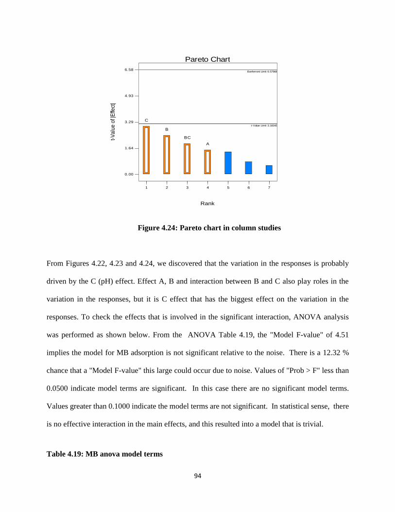
94

Figure 4.24: Pareto chart in column studies

From Figures 4.22, 4.23 and 4.24, we discovered that the variation in the responses is probably

driven by the C (pH) effect. Effect A, B and interaction between B and C also play roles in the

variation in the responses, but it is C effect that has the biggest effect on the variation in the

responses. To check the effects that is involved in the significant interaction, ANOVA analysis

was performed as shown below. From the ANOVA Table 4.19, the "Model F-value" of 4.51

implies the model for MB adsorption is not significant relative to the noise. There is a 12.32 %

chance that a "Model F-value" this large could occur due to noise. Values of "Prob > F" less than

0.0500 indicate model terms are significant. In this case there are no significant model terms.

Values greater than 0.1000 indicate the model terms are not significant. In statistical sense, there

is no effective interaction in the main effects, and this resulted into a model that is trivial.

Table 4.19: MB anova model terms

Pareto Chart

t-V

alu

e o

f |E

ffect

|

Rank

0.00

1.64

3.29

4.93

6.58Bonferroni Limit 6.57968

t-Value Limit 3.18245

1 2 3 4 5 6 7

C

B

BC

A

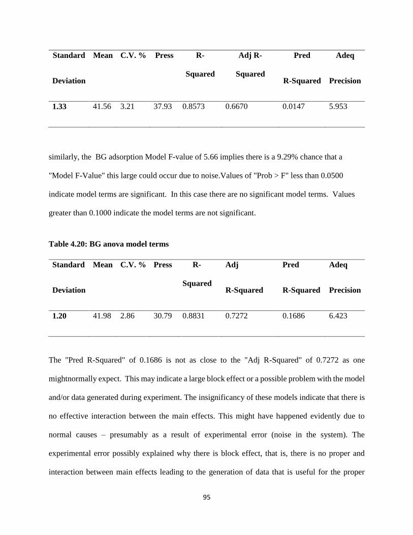
95

Standard

Deviation

Mean

C.V. % Press

R-

Squared

Adj R-

Squared

Pred

R-Squared

Adeq

Precision

1.33 41.56 3.21 37.93 0.8573 0.6670 0.0147 5.953

similarly, the BG adsorption Model F-value of 5.66 implies there is a 9.29% chance that a

"Model F-Value" this large could occur due to noise.Values of "Prob > F" less than 0.0500

indicate model terms are significant. In this case there are no significant model terms. Values

greater than 0.1000 indicate the model terms are not significant.

Table 4.20: BG anova model terms

Standard

Deviation

Mean

C.V. % Press

R-

Squared

Adj

R-Squared

Pred

R-Squared

Adeq

Precision

1.20 41.98 2.86 30.79 0.8831 0.7272 0.1686 6.423

The "Pred R-Squared" of 0.1686 is not as close to the "Adj R-Squared" of 0.7272 as one

mightnormally expect. This may indicate a large block effect or a possible problem with the model

and/or data generated during experiment. The insignificancy of these models indicate that there is

no effective interaction between the main effects. This might have happened evidently due to

normal causes – presumably as a result of experimental error (noise in the system). The

experimental error possibly explained why there is block effect, that is, there is no proper and

interaction between main effects leading to the generation of data that is useful for the proper

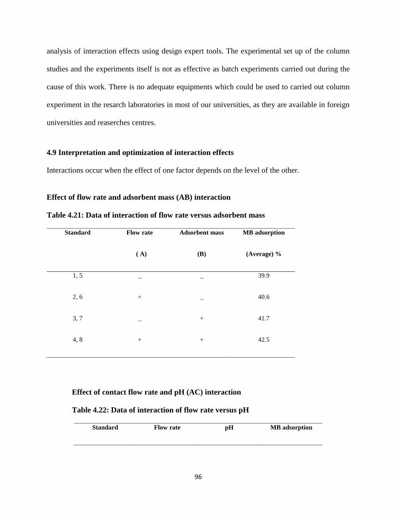
96

analysis of interaction effects using design expert tools. The experimental set up of the column

studies and the experiments itself is not as effective as batch experiments carried out during the

cause of this work. There is no adequate equipments which could be used to carried out column

experiment in the resarch laboratories in most of our universities, as they are available in foreign

universities and reaserches centres.

4.9 Interpretation and optimization of interaction effects

Interactions occur when the effect of one factor depends on the level of the other.

Effect of flow rate and adsorbent mass (AB) interaction

Table 4.21: Data of interaction of flow rate versus adsorbent mass

Standard Flow rate

( A)

Adsorbent mass

(B)

MB adsorption

(Average) %

1, 5 _ _ 39.9

2, 6 + _ 40.6

3, 7 _ + 41.7

4, 8 + + 42.5

Effect of contact flow rate and pH (AC) interaction

Table 4.22: Data of interaction of flow rate versus pH

Standard Flow rate pH MB adsorption

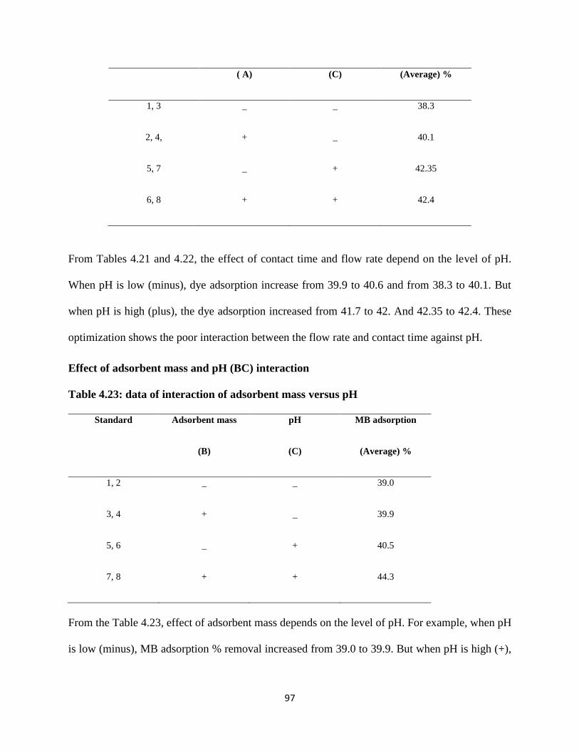
97

( A) (C) (Average) %

1, 3 _ _ 38.3

2, 4, + _ 40.1

5, 7 _ + 42.35

6, 8 + + 42.4

From Tables 4.21 and 4.22, the effect of contact time and flow rate depend on the level of pH.

When pH is low (minus), dye adsorption increase from 39.9 to 40.6 and from 38.3 to 40.1. But

when pH is high (plus), the dye adsorption increased from 41.7 to 42. And 42.35 to 42.4. These

optimization shows the poor interaction between the flow rate and contact time against pH.

Effect of adsorbent mass and pH (BC) interaction

Table 4.23: data of interaction of adsorbent mass versus pH

Standard Adsorbent mass

(B)

pH

(C)

MB adsorption

(Average) %

1, 2 _ _ 39.0

3, 4 + _ 39.9

5, 6 _ + 40.5

7, 8 + + 44.3

From the Table 4.23, effect of adsorbent mass depends on the level of pH. For example, when pH

is low (minus), MB adsorption % removal increased from 39.0 to 39.9. But when pH is high (+),

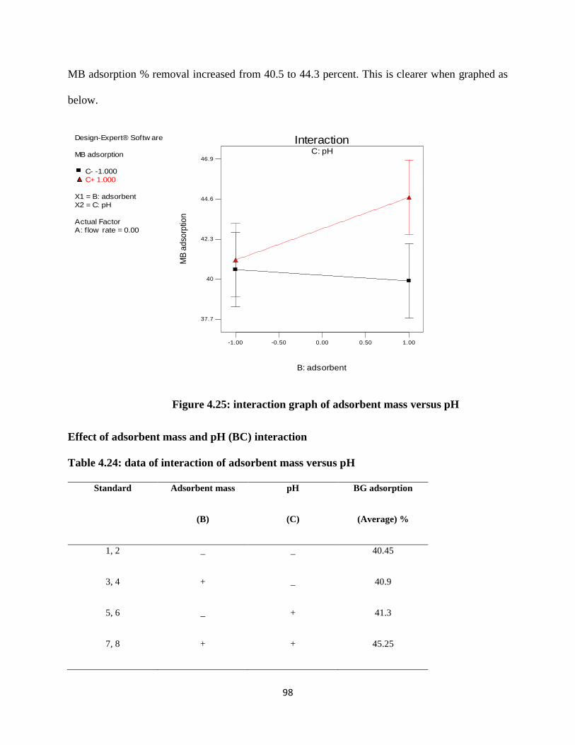
98

MB adsorption % removal increased from 40.5 to 44.3 percent. This is clearer when graphed as

below.

Figure 4.25: interaction graph of adsorbent mass versus pH

Effect of adsorbent mass and pH (BC) interaction

Table 4.24: data of interaction of adsorbent mass versus pH

Standard Adsorbent mass

(B)

pH

(C)

BG adsorption

(Average) %

1, 2 _ _ 40.45

3, 4 + _ 40.9

5, 6 _ + 41.3

7, 8 + + 45.25

Design-Expert® Softw are

MB adsorption

C- -1.000

C+ 1.000

X1 = B: adsorbent

X2 = C: pH

Actual Factor

A: f low rate = 0.00

C: pH

-1.00 -0.50 0.00 0.50 1.00

Interaction

B: adsorbent

MB

ad

sorp

tion

37.7

40

42.3

44.6

46.9

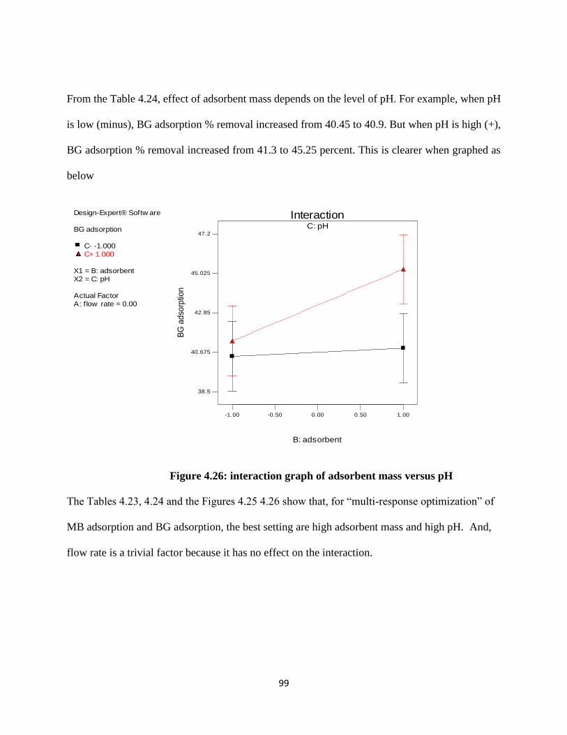
99

From the Table 4.24, effect of adsorbent mass depends on the level of pH. For example, when pH

is low (minus), BG adsorption % removal increased from 40.45 to 40.9. But when pH is high (+),

BG adsorption % removal increased from 41.3 to 45.25 percent. This is clearer when graphed as

below

Figure 4.26: interaction graph of adsorbent mass versus pH

The Tables 4.23, 4.24 and the Figures 4.25 4.26 show that, for “multi-response optimization” of

MB adsorption and BG adsorption, the best setting are high adsorbent mass and high pH. And,

flow rate is a trivial factor because it has no effect on the interaction.

Design-Expert® Softw are

BG adsorption

C- -1.000

C+ 1.000

X1 = B: adsorbent

X2 = C: pH

Actual Factor

A: f low rate = 0.00

C: pH

-1.00 -0.50 0.00 0.50 1.00

Interaction

B: adsorbent

BG

ad

sorp

tion

38.5

40.675

42.85

45.025

47.2

100

CHAPTER FIVE

5.0 CONCLUSION AND RECOMMENDATIONS

5.1 Conclusion

Based on the study, it can be concluded that:

The adsorption data for the batch process fitted into Langmuir and freundlich Isotherms,

and freundlich adsorption isotherm was found to have the highest coefficient of

determination, hence gave the best fit.

The pH of the adsorbate, contact time and adsorbent dosage are highly responsible for dyes

removal from wastewater

Experimental data were examined using analysis of variance (ANOVA), t-test, and

Bonferroni - test. According to Pareto Chart, ANOVA, main effects and interaction plots

in design expert, the most significant factors on removal efficiency (%) was found to be

adsorbent dosage.

Due to the obtained results, it can be concluded that modified carbons which were produced

by chemical activation of carbonized coconut shell, eucalyptus tree, corn cob and

flamboyant pod could be employed as an effective and low-cost adsorbent for the removal

of dyes from wastewater.

5.2 Recommendations

The following recommendations are necessary for future research

101

Factorial design for batch adsorption experiment should be encouraged because it helps to

optimize operation parameters to determine the best condition for optimum percentage

removal.

Peristaltic pump is a necessity for column studies and should be made available in the

laboratories.

102

REFERENCES

Asouhidou, D., Triantafyllidis, S., Lazaridis, K., and Matis, A. (2009). Adsorption

of remazol red3BS from aqueous solutions using APTES- and cyclodextrin-modified

HMS-typemesoporous silicas. Journal of Colloids materials, 346(1), 83–90.

Aksu, Z., and Isoglu, A. (2006). Use of agricultural waste sugar beet pulp for the removal

of gemazol turquoise blue-G reactive dye from aqueous solution. Journal of Hazardous

Materials, 137(1), 418–430.

Amin, K. (2008). Removal of reactive dye from aqueous solutions by adsorption onto

activated carbons prepared from sugarcane bagasse pith. Journal of Desalination, 223(3),

152–161.

Annadurai, G., Juang, S., and Lee, J. (2002). Factorial design analysis for adsorption

of dye on activated carbon beads incorporated with calciumalginate. Journal of Advances

in Environmental Research, 6(2), 191–198.

Bonnamy, S. (1999). Carbonization of various precursors. Effect of heating rate. Part II.

Transmission electron microscopy and physicochemical studies. Science Review, 37(11),

1707-1724.

Banat, M., Nigam, P., Singh, D., and Marchant, R. (1996). Microbial decolorization of

textile-dye-containing effluents. Journal of Bioresource Technology, 58, 217–227.

Cardoso, F., Pinto, R. B., and Lima, E. C. (2011). Removal of remazol black B textile dye

from aqueous solution by adsorption. Journal of Chemistry, 269(3), 92–103.

Cooper, N. (1993). Removing colour from dye house wastewaters—a critical review

of technology available. Journal of the Society of Dyers and Colourists,

9(3), 97–100.

103

Crini, G. (2006). Non-conventional low-cost adsorbents for dye removal: a review. Journal

of Bioresource Technology, 97(9), 1061–1085.

Cantamutto, M., and Poverene, M. (2007). Genetically modified sunflower release:

opportunities and risks. Field Crops Research Journal, 101(2), 133–144.

Dursun, Y., and Tepe, O. (2011). Removal of chemazol reactive red 195 from aqueous

solution by dehydrated beet pulp carbon. Journal of Hazardous Materials, 194,

303–311.

El-Qada, N., Allen, J., and Walker, M. (2008). Adsorption of basic dyes from

aqueous solution onto activated carbons. Chemical Engineering Journal,

135(3), 174–184.

Foo, Y., and Hameed, H. (2011). Preparation and characterization of activated carbon

from sunflower seed oil residue via microwave assisted K2CO3 activation. Journal of

Bioresource Technology, 102(20), 9794–9799.

Ferraro, R., and Kazuo, N. (1994). Introductory Raman Spectroscopy. San Diego: Guilford

Press

Gessner, T., and Mayer, U. (2002). Triarylmethane and Diarylmethane Dyes. Ullmann's

Encyclopedia of Industrial Chemistry (6th ed.). Weinheim: Wiley-VCH,

Gupta, K., Rastogi, A., Agarwal, S., and Nayak, A. (2011). A comparative investigation on

adsorption performances of mesoporous activated carbon prepared from waste rubber tire

and activated carbon for a hazardous azo dye—Acid Blue 113. Journal of Hazardous

Materials, 186(1), 891–901.

Gonzalez, T., Rodriguez-Reinoso, F., Garcia, N., and Marcilla, A. (1997). CO2

activation of olive stones carbonized under different experimental conditions. Materials

letters, 35(1), 159-162.

Gregg, J., and Sing, W. (1982). The physical adsorption of gases by mesoporous

solids: The Type IV isotherm (Chapter 3). Adsorption, Surface Area and Porosity. London,

Academic Press.

104

Griffith, M., and Hirst, W. (1943). The heat of wetting of coals in organic liquids. In:

Proceedings of a Conference on the Ultra-Fine Structure of Coals and Cokes. The British

Coal Utilization Research Association, London, 80-94.

Gonzalez, C., Gonzalez, T., Molina-Sabio, M., Rodriguez-Reinoso. F., and

Sepulveda-Escribano, A. (1995). Porosity of activated carbons prepared from different

lignocellulosic materials. Journal of Hazardous Materials,33(8), l175-1177.

Gurses, A., Dogar, S., Karaca, M., and Bayrak, B. (2006). Production of granular activated

carbon from waste Rosa canina sp. seeds and its adsorption characteristics for dye. Journal

of Hazardous Materials, 131 (1-3), 254–259.

Gupta, K., and Suhas, S. (2009). Application of low-cost adsorbents for dye removal - a

Review. Journal of Environmental Management, 90(8), 2313–2342.

Gupta, K., Mittal, A., Kurup, L., and Mittal, J. (2006). Adsorption of a hazardous dye,

erythrosine, over hen feathers. Journal of Colloid and Interface Science,

304(1), 52–57.

Gupta, K., Mittal, A., Malviya, A., and Mittal, J. (2009). Adsorption of carmoisine from

wastewater using waste materials - bottom ash and deoiled soya. Journal of Colloid and

Interface Science, 335(1), 24–33.

Gupta, V. K., Jain, R., and Varshney, S. (2007). Removal of reactofix golden yellow3 RFN

from aqueous solution using wheat husk—an agricultural waste. Journal of Hazardous

Materials, 142(1-2), 443–448.

Guelli Ulson de Souza, A., Peruzzo, C., and Ulson de Souza, A. (2008).

Numerical study of the adsorption of dyes from textile effluents. Applied Mathematical

Modelling Journal, 32(9), 1711–1718.

Guo, J. and Lua, G. (2002). Characterization of adsorbent prepared from oil-palm shell by CO2

activation for removal of gaseous pollutants. Materials letters, 55, 334-339.

Hameed, H. (2008). Equilibrium and kinetic studies of methyl violet sorption by

agricultural Waste. Journal of Hazardous Materials, 154(1-3), 204–212.

105

Joseph, N. (1931). Brilliant Green: A Clinical Study of its Value as a Local Antiseptic.

Annals of Surgery 1931 December, 94(6), 1007–1012.

Jadhav, B., Phugare, S., Patil, S., and Jadhav, P. (2011). Biochemical degradation

pathway of textile dye remazol red and subsequent toxicological evaluation by

cytotoxicity, genotoxicity and oxidative stress studies. International Biodeterioration and

Biodegradation Journal, 65(6), 733–743.

Jain, M., Garg, K., and Kadirvelu, K. (2009). Equilibrium and kinetic studies for

sequestration of Cr (VI) from simulated wastewater using sunflower waste biomass.

Journal of Hazardous Materials, 171(1–3), 328–334.

Joseph, B. (1987). Introduction to organic spectroscopy. New York, U.S.A: Macmillan

Publication.

Khan, R. (1987). Significance of char active surface area for appraising the reactivity of

low- and high temperature chars. Journal of Hazardous Materials, 66(12),

1626-1634.

Koresh, J., and Soffer, A. (1980). Study of molecular sieve carbons. Part I. Pore structure,

gradual pore opening and mechanism of molecular sieving. JCS Faraday 1, 76, 2457-2471.

Part 2. Estimation of cross-sectional diameters of non-spherical molecules. JCS Faraday 1

1980, 76, 2472-2485.

Konaganti, K., Kota, R., Patil, S., and Madras, G. (2010). Adsorption of anionic dyes

on chitosan grafted poly (alkyl methacrylate)s. Chemical Engineering Journal, 158 (3),

393–401.

Lopez-Gonzalez, D., Martinez-Vilchez, F., and Rodriguez-Reinoso, F. (2008). Preparation

and characterization of active carbons from olive stones. Journal of Hazardous Materials,

18(3), 413-18.

Lee, E., Morad, N., Teng, T., and Poh, T. (2012). Factorial experimental design

for reactive dye flocculation using inorganicorganic composite polymer. APCBEE

Procedia, 1, 59–65.

Mbolekwa, M., and Buckley, C. (2006). Dye removal with activated carbon for the reuse of

106

salt, water and energy, Industrial Wastewater Treatment, WISA.

Marsh, H., Heintz, A., and Rodriguez-Reinoso, F. (1997). Introduction to Carbon

Technologies. Universidad de Alicante, Spain: pp. 669. Secretariado de Publications.

Marsh, H. (2001). Carbon mesophase. Encyclopedia of Materials: Science and Technology.

Elsevier Science Ltd, Amsterdam, pp. 926-932.

McGuire, J., and Suffet, H. (1980). Activated Carbon Adsorption of Organics from

the Aqueous Phase, Vol. 1. Ann Arbor Science Publishers Inc., Michigan, pp. 508.

McGuire, J., and Suffet, H. (1983). Treatment of Water by Granular Activated

Carbon, Advances in Chemistry Series, 202. American Chemical Society, Washington, pp.

599.

Mittal, A., Kaur, D., and Mittal, J. (2008). Applicability of waste materials- bottom ash

and deoiled soya-as adsorbents for the removal and recovery of a hazardous dye, brilliant

green. Journal of Colloid and Interface Science, 326(1), 8–17.

Ponnusami, V., Krithika, V., Madhuram, R., and Srivastava, N. (2007). Biosorption of

reactive dye using acid-treated rice husk: factorial design analysis. Journal of Hazardous

Materials, 142(1-2), 397– 40.

Pope, J. (1999). Brief History of Activated Carbon and a Summary of its Uses. EPA, 2013.

Ramakrishna, R., and Viraraghavan, T. (1997). Dye removal using low cost adsorbents,

Water Science and Technology Journal, 36(2-3), 189–196.

Rodriguez-Reinoso. F., Garcial, N., and Marcial, A. (1997). CO2 activation

of olive stone carbonized under different experimental conditions. Journal of Hazardous

Materials, 35(1), 159-162.

Salah, M., Samy, N., and Fadel, M. (2009). Methylene blue mediated photodynamic therapy

for resistant plaque psoriasis. Journal of. Drugs Dermatol. 8(1), 42–9.

107

Selvapathy, P. (2006). Removal of reactive dyes from wastewater by adsorption on

coir pith activated carbon. Journal of Bioresource Technology, 97(11), 1329–1336.

Senthilkumaar, S., Kalaamani, P., Porkodi, K., Varadarajan, R., and Subburaam, V.

(2006). Adsorption of dissolved Reactive red dye from aqueous phase onto activated

carbon prepared from agricultural waste. Journal of Bioresource Technology, 97(14),

1618–1625.

Sathishkumar, P., Arulkumar, M., and Palvannan, T. (2012). Utilization of agro-industrial

waste jatropha curcas pods as an activated carbon for the adsorption of reactive dye

Remazol Brilliant Blue R (RBBR). Journal of Cleaner Production, 22(1), 67– 75.

Safa, Y., and Bhatti, N. (2011). Adsorptive removal of direct textile dyes by low cost

agricultural waste: application of factorial design analysis. Chemical Engineering Journal,

167(1), 35–41.

Zhong, Y., Yang, Q., Li, M., Luo, K., Liu, Y., and Zeng, M. (2012). Preparation

of peanut hull-based activated carbon by microwave-induced phosphoric acid activation

and its application in Remazol Brilliant Blue R adsorption. Journal of Industrial Crops and

Products, 37(1), 178–185.

Zollinger, H. (2003). Colour chemistry synthesis, properties, application of organic dyes and

Pigments (3rd ed.). Weinheim: Wiley-YCH.

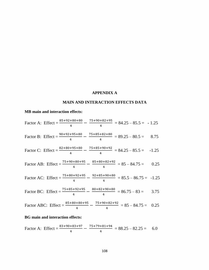
108

APPENDIX A

MAIN AND INTERACTION EFFECTS DATA

MB main and interaction effects:

Factor A: Effect = 85+92+80+80

4−

75+90+82+95

4 = 84.25 – 85.5 = - 1.25

Factor B: Effect = 90+92+95+80

4−

75+85+82+80

4 = 89.25 – 80.5 = 8.75

Factor C: Effect = 82+80+95+80

4−

75+85+90+92

4 = 84.25 – 85.5 = -1.25

Factor AB: Effect = 75+90+80+95

4−

85+80+82+92

4 = 85 – 84.75 = 0.25

Factor AC: Effect = 75+80+92+95

4−

92+85+90+80

4 = 85.5 – 86.75 = -1.25

Factor BC: Effect = 75+85+92+95

4−

80+82+90+80

4 = 86.75 – 83 = 3.75

Factor ABC: Effect = 85+80+80+95

4−

75+90+82+92

4 = 85 – 84.75 = 0.25

BG main and interaction effects:

Factor A: Effect = 83+90+83+97

4−

75+79+81+94

4 = 88.25 – 82.25 = 6.0

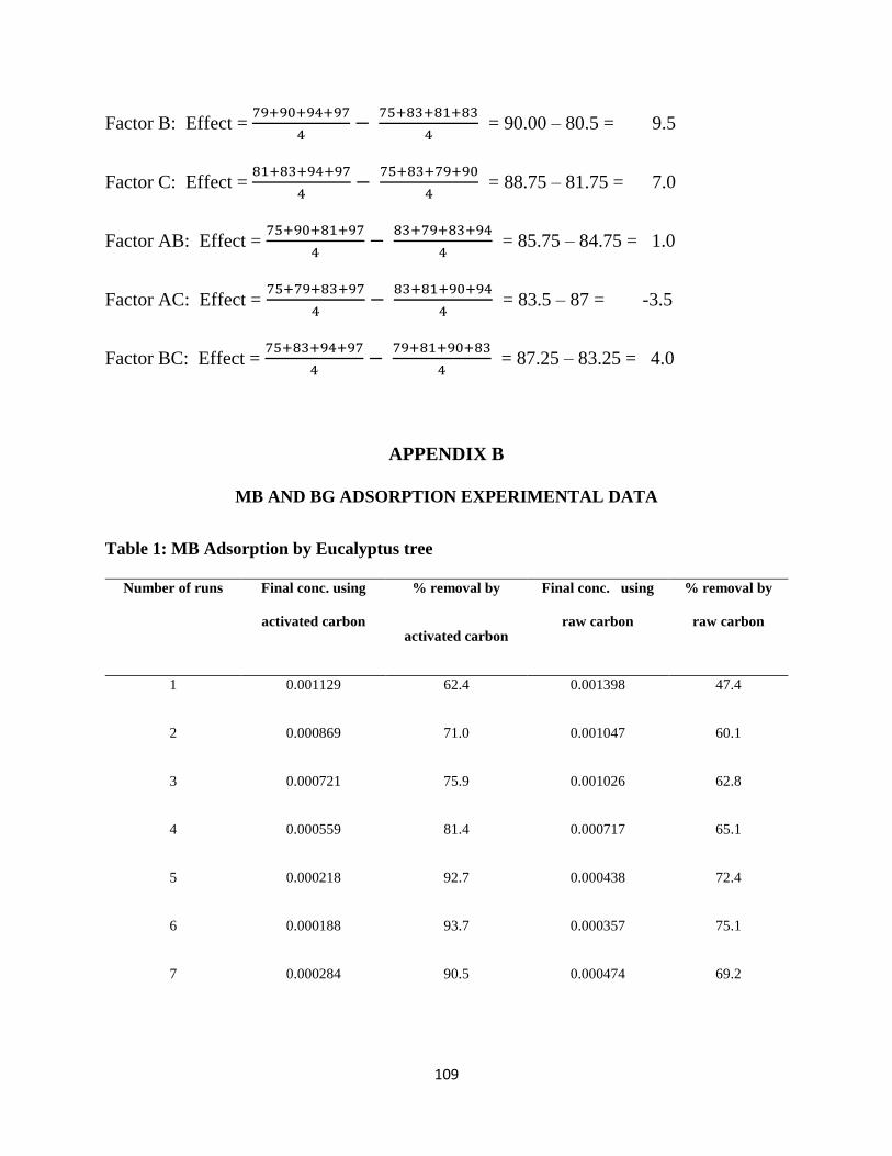
109

Factor B: Effect = 79+90+94+97

4−

75+83+81+83

4 = 90.00 – 80.5 = 9.5

Factor C: Effect = 81+83+94+97

4−

75+83+79+90

4 = 88.75 – 81.75 = 7.0

Factor AB: Effect = 75+90+81+97

4−

83+79+83+94

4 = 85.75 – 84.75 = 1.0

Factor AC: Effect = 75+79+83+97

4−

83+81+90+94

4 = 83.5 – 87 = -3.5

Factor BC: Effect = 75+83+94+97

4−

79+81+90+83

4 = 87.25 – 83.25 = 4.0

APPENDIX B

MB AND BG ADSORPTION EXPERIMENTAL DATA

Table 1: MB Adsorption by Eucalyptus tree

Number of runs Final conc. using

activated carbon

% removal by

activated carbon

Final conc. using

raw carbon

% removal by

raw carbon

1 0.001129 62.4 0.001398 47.4

2 0.000869 71.0 0.001047 60.1

3 0.000721 75.9 0.001026 62.8

4 0.000559 81.4 0.000717 65.1

5 0.000218 92.7 0.000438 72.4

6 0.000188 93.7 0.000357 75.1

7 0.000284 90.5 0.000474 69.2

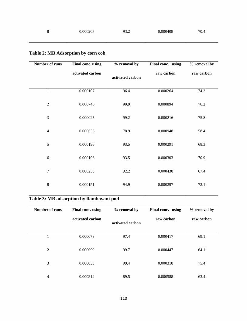
110

8 0.000203 93.2 0.000408 70.4

Table 2: MB Adsorption by corn cob

Number of runs Final conc. using

activated carbon

% removal by

activated carbon

Final conc. using

raw carbon

% removal by

raw carbon

1 0.000107 96.4 0.000264 74.2

2 0.000746 99.9 0.000894 76.2

3 0.000025 99.2 0.000216 75.8

4 0.000633 78.9 0.000948 58.4

5 0.000196 93.5 0.000291 68.3

6 0.000196 93.5 0.000303 70.9

7 0.000233 92.2 0.000438 67.4

8 0.000151 94.9 0.000297 72.1

Table 3: MB adsorption by flamboyant pod

Number of runs Final conc. using

activated carbon

% removal by

activated carbon

Final conc. using

raw carbon

% removal by

raw carbon

1 0.000078 97.4 0.000417 69.1

2 0.000099 99.7 0.000447 64.1

3 0.000033 99.4 0.000318 75.4

4 0.000314 89.5 0.000588 63.4

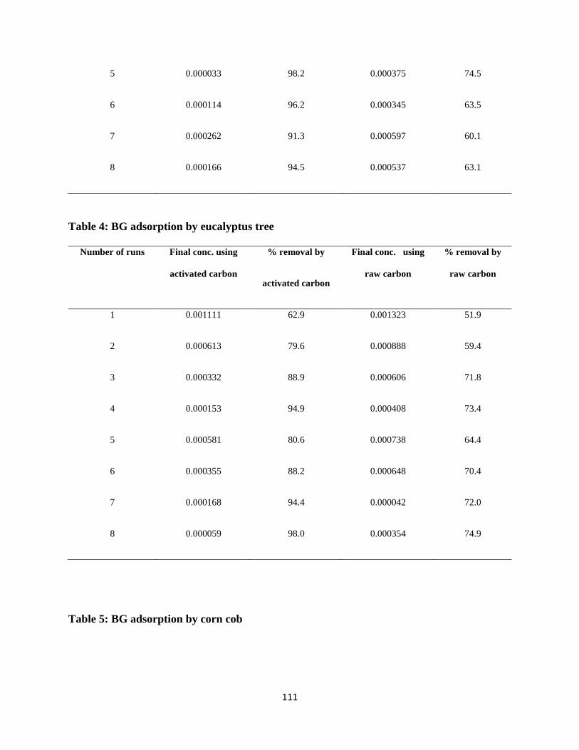
111

5 0.000033 98.2 0.000375 74.5

6 0.000114 96.2 0.000345 63.5

7 0.000262 91.3 0.000597 60.1

8 0.000166 94.5 0.000537 63.1

Table 4: BG adsorption by eucalyptus tree

Number of runs Final conc. using

activated carbon

% removal by

activated carbon

Final conc. using

raw carbon

% removal by

raw carbon

1 0.001111 62.9 0.001323 51.9

2 0.000613 79.6 0.000888 59.4

3 0.000332 88.9 0.000606 71.8

4 0.000153 94.9 0.000408 73.4

5 0.000581 80.6 0.000738 64.4

6 0.000355 88.2 0.000648 70.4

7 0.000168 94.4 0.000042 72.0

8 0.000059 98.0 0.000354 74.9

Table 5: BG adsorption by corn cob

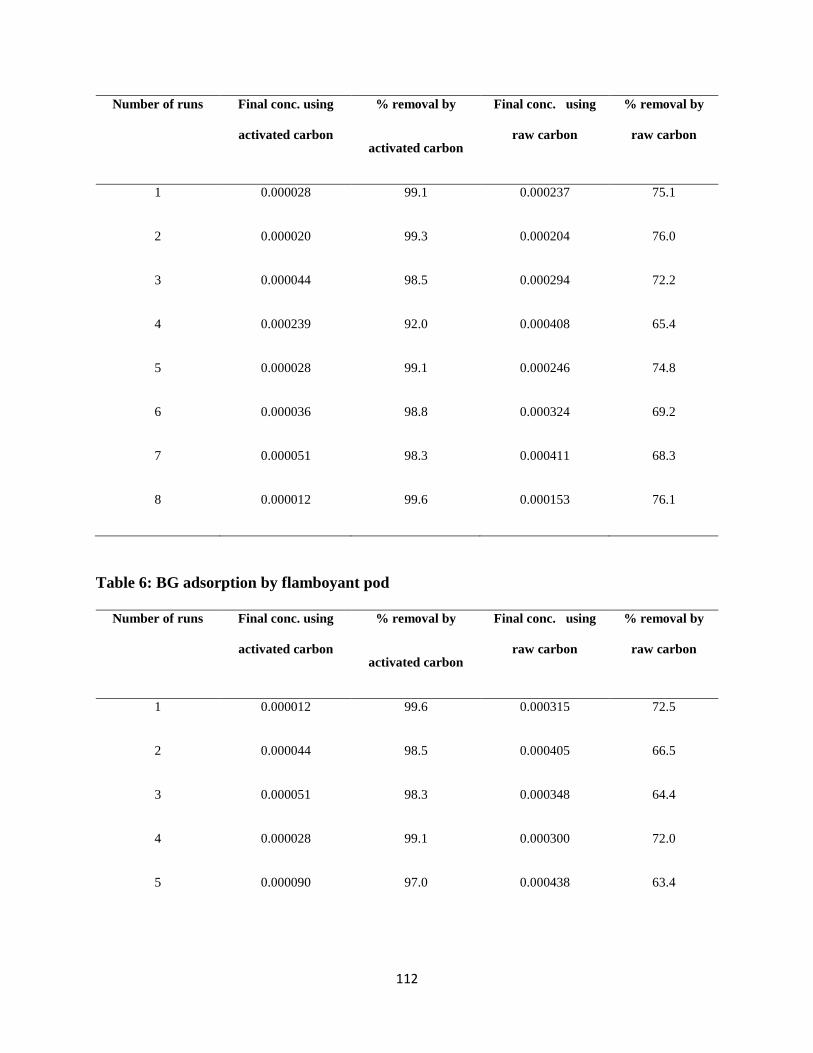
112

Number of runs Final conc. using

activated carbon

% removal by

activated carbon

Final conc. using

raw carbon

% removal by

raw carbon

1 0.000028 99.1 0.000237 75.1

2 0.000020 99.3 0.000204 76.0

3 0.000044 98.5 0.000294 72.2

4 0.000239 92.0 0.000408 65.4

5 0.000028 99.1 0.000246 74.8

6 0.000036 98.8 0.000324 69.2

7 0.000051 98.3 0.000411 68.3

8 0.000012 99.6 0.000153 76.1

Table 6: BG adsorption by flamboyant pod

Number of runs Final conc. using

activated carbon

% removal by

activated carbon

Final conc. using

raw carbon

% removal by

raw carbon

1 0.000012 99.6 0.000315 72.5

2 0.000044 98.5 0.000405 66.5

3 0.000051 98.3 0.000348 64.4

4 0.000028 99.1 0.000300 72.0

5 0.000090 97.0 0.000438 63.4

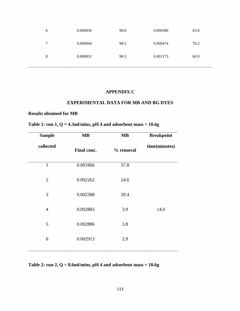
113

6 0.000036 98.8 0.000366 65.8

7 0.000044 98.5 0.000474 70.2

8 0.000831 98.5 0.001173 60.9

APPENDIX C

EXPERIMENTAL DATA FOR MB AND BG DYES

Results obtained for MB

Table 1: run 1, Q = 4.3ml/mins, pH 4 and adsorbent mass = 10.6g

Sample

collected

MB

Final conc.

MB

% removal

Breakpoint

time(minutes)

1 0.001866 37.8

2 0.002262 24.6

3 0.002388 20.4

4 0.002883 3.9 14.0

5 0.002886 3.8

6 0.002913 2.9

Table 2: run 2, Q = 8.6ml/mins, pH 4 and adsorbent mass = 10.6g

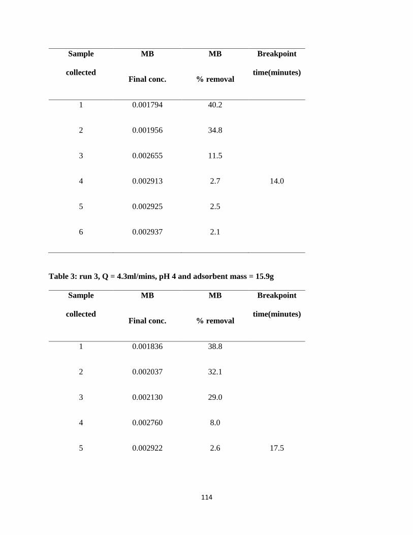
114

Sample

collected

MB

Final conc.

MB

% removal

Breakpoint

time(minutes)

1 0.001794 40.2

2 0.001956 34.8

3 0.002655 11.5

4 0.002913 2.7 14.0

5 0.002925 2.5

6 0.002937 2.1

Table 3: run 3, Q = 4.3ml/mins, pH 4 and adsorbent mass = 15.9g

Sample

collected

MB

Final conc.

MB

% removal

Breakpoint

time(minutes)

1 0.001836 38.8

2 0.002037 32.1

3 0.002130 29.0

4 0.002760 8.0

5 0.002922 2.6 17.5

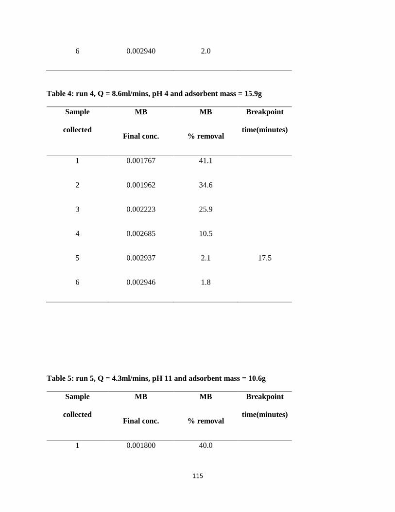
115

6 0.002940 2.0

Table 4: run 4, Q = 8.6ml/mins, pH 4 and adsorbent mass = 15.9g

Sample

collected

MB

Final conc.

MB

% removal

Breakpoint

time(minutes)

1 0.001767 41.1

2 0.001962 34.6

3 0.002223 25.9

4 0.002685 10.5

5 0.002937 2.1 17.5

6 0.002946 1.8

Table 5: run 5, Q = 4.3ml/mins, pH 11 and adsorbent mass = 10.6g

Sample

collected

MB

Final conc.

MB

% removal

Breakpoint

time(minutes)

1 0.001800 40.0

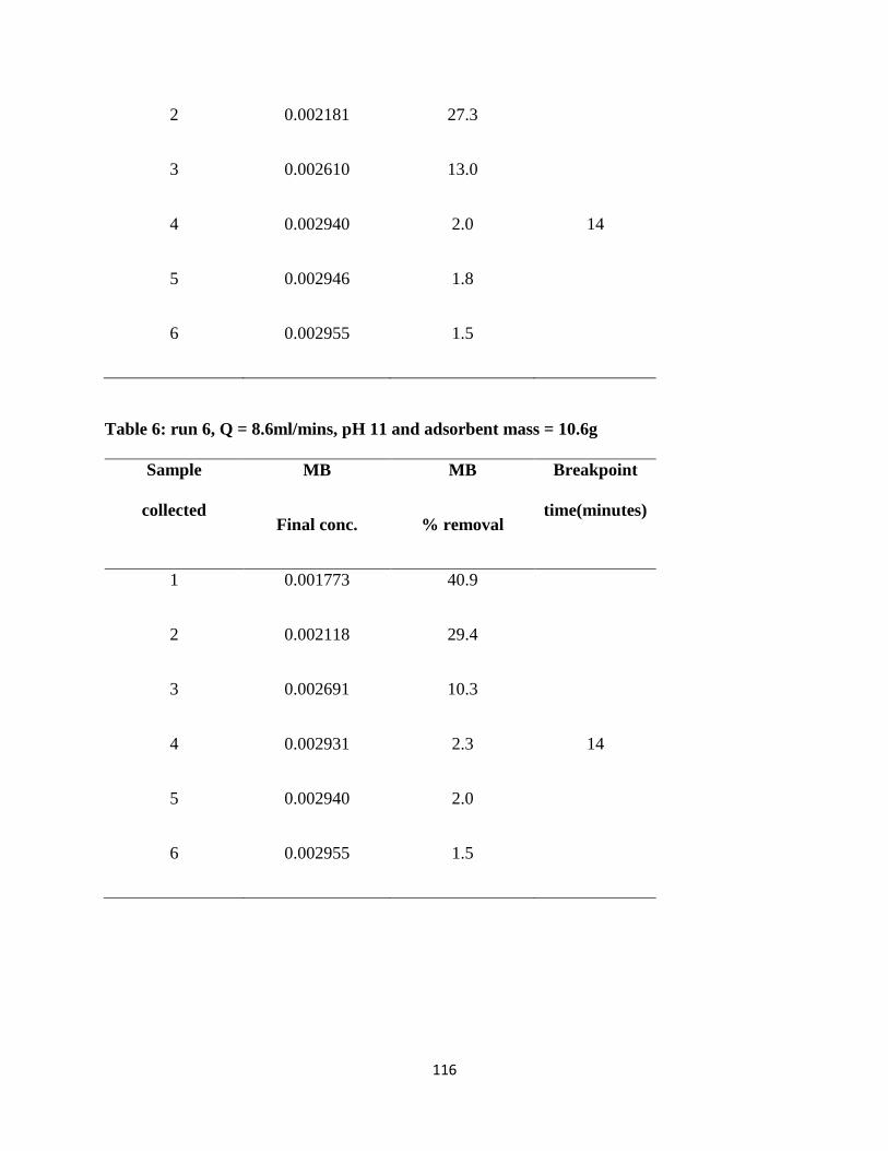
116

2 0.002181 27.3

3 0.002610 13.0

4 0.002940 2.0 14

5 0.002946 1.8

6 0.002955 1.5

Table 6: run 6, Q = 8.6ml/mins, pH 11 and adsorbent mass = 10.6g

Sample

collected

MB

Final conc.

MB

% removal

Breakpoint

time(minutes)

1 0.001773 40.9

2 0.002118 29.4

3 0.002691 10.3

4 0.002931 2.3 14

5 0.002940 2.0

6 0.002955 1.5

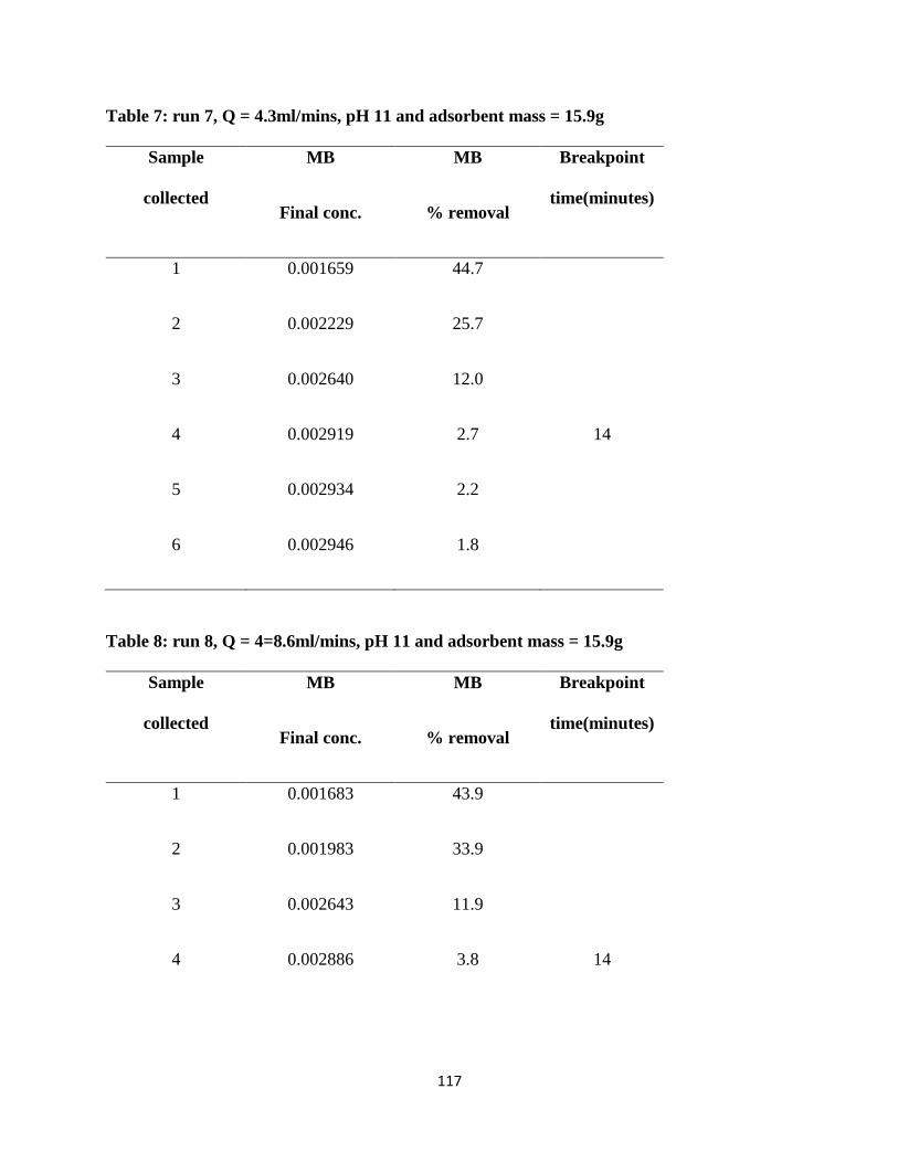
117

Table 7: run 7, Q = 4.3ml/mins, pH 11 and adsorbent mass = 15.9g

Sample

collected

MB

Final conc.

MB

% removal

Breakpoint

time(minutes)

1 0.001659 44.7

2 0.002229 25.7

3 0.002640 12.0

4 0.002919 2.7 14

5 0.002934 2.2

6 0.002946 1.8

Table 8: run 8, Q = 4=8.6ml/mins, pH 11 and adsorbent mass = 15.9g

Sample

collected

MB

Final conc.

MB

% removal

Breakpoint

time(minutes)

1 0.001683 43.9

2 0.001983 33.9

3 0.002643 11.9

4 0.002886 3.8 14

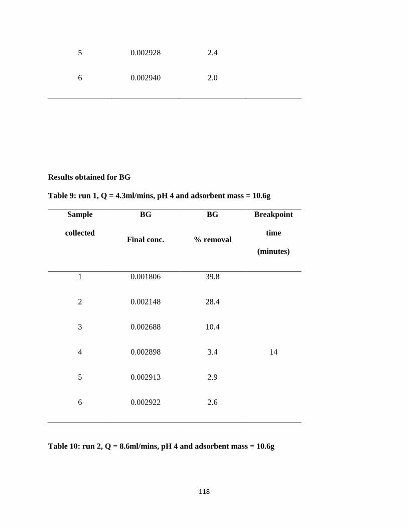
118

5 0.002928 2.4

6 0.002940 2.0

Results obtained for BG

Table 9: run 1, Q = 4.3ml/mins, pH 4 and adsorbent mass = 10.6g

Sample

collected

BG

Final conc.

BG

% removal

Breakpoint

time

(minutes)

1 0.001806 39.8

2 0.002148 28.4

3 0.002688 10.4

4 0.002898 3.4 14

5 0.002913 2.9

6 0.002922 2.6

Table 10: run 2, Q = 8.6ml/mins, pH 4 and adsorbent mass = 10.6g

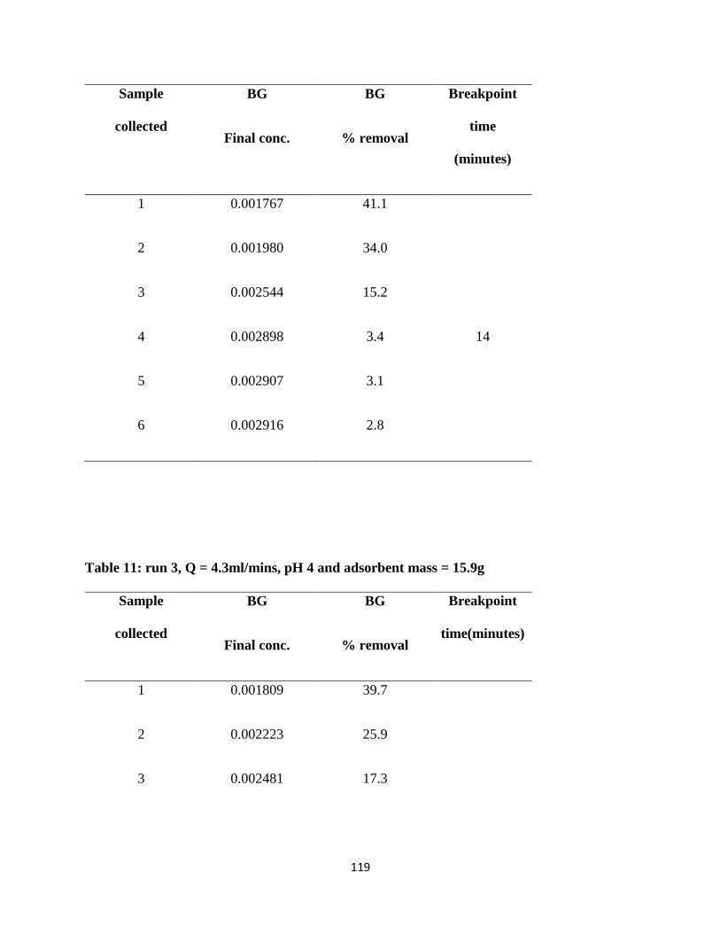
119

Sample

collected

BG

Final conc.

BG

% removal

Breakpoint

time

(minutes)

1 0.001767 41.1

2 0.001980 34.0

3 0.002544 15.2

4 0.002898 3.4 14

5 0.002907 3.1

6 0.002916 2.8

Table 11: run 3, Q = 4.3ml/mins, pH 4 and adsorbent mass = 15.9g

Sample

collected

BG

Final conc.

BG

% removal

Breakpoint

time(minutes)

1 0.001809 39.7

2 0.002223 25.9

3 0.002481 17.3

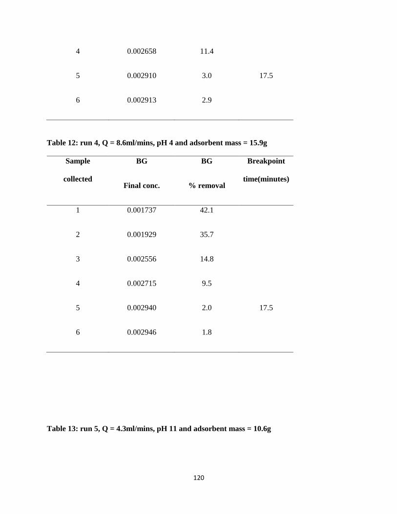
120

4 0.002658 11.4

5 0.002910 3.0 17.5

6 0.002913 2.9

Table 12: run 4, Q = 8.6ml/mins, pH 4 and adsorbent mass = 15.9g

Sample

collected

BG

Final conc.

BG

% removal

Breakpoint

time(minutes)

1 0.001737 42.1

2 0.001929 35.7

3 0.002556 14.8

4 0.002715 9.5

5 0.002940 2.0 17.5

6 0.002946 1.8

Table 13: run 5, Q = 4.3ml/mins, pH 11 and adsorbent mass = 10.6g

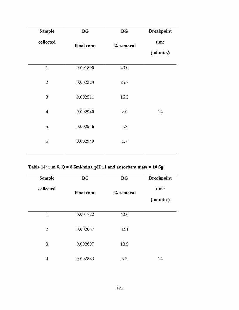
121

Sample

collected

BG

Final conc.

BG

% removal

Breakpoint

time

(minutes)

1 0.001800 40.0

2 0.002229 25.7

3 0.002511 16.3

4 0.002940 2.0 14

5 0.002946 1.8

6 0.002949 1.7

Table 14: run 6, Q = 8.6ml/mins, pH 11 and adsorbent mass = 10.6g

Sample

collected

BG

Final conc.

BG

% removal

Breakpoint

time

(minutes)

1 0.001722 42.6

2 0.002037 32.1

3 0.002607 13.9

4 0.002883 3.9 14

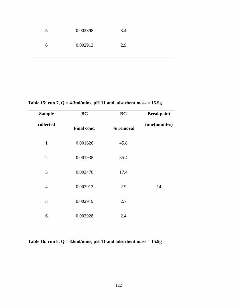
122

5 0.002898 3.4

6 0.002913 2.9

Table 15: run 7, Q = 4.3ml/mins, pH 11 and adsorbent mass = 15.9g

Sample

collected

BG

Final conc.

BG

% removal

Breakpoint

time(minutes)

1 0.001626 45.8

2 0.001938 35.4

3 0.002478 17.4

4 0.002913 2.9 14

5 0.002919 2.7

6 0.002928 2.4

Table 16: run 8, Q = 8.6ml/mins, pH 11 and adsorbent mass = 15.9g

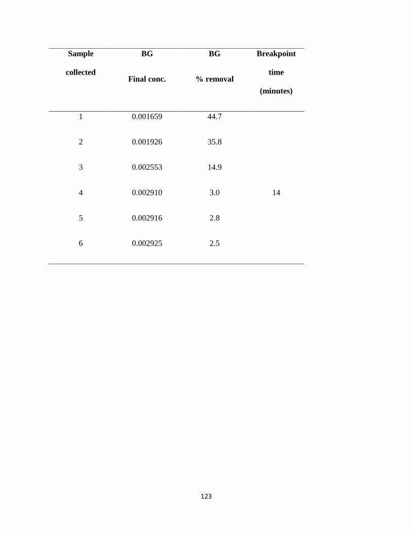
123

Sample

collected

BG

Final conc.

BG

% removal

Breakpoint

time

(minutes)

1 0.001659 44.7

2 0.001926 35.8

3 0.002553 14.9

4 0.002910 3.0 14

5 0.002916 2.8

6 0.002925 2.5