ERDC/CRREL TR-08-21 Addressing Uncertainty in Signal Propagation and Sensor Performance Predictions D. Keith Wilson, Chris L. Pettit, Sean Mackay, Matthew S. Lewis, and Peter M. Seman November 2008 Cold Regions Research and Engineering Laboratory Approved for public release; distribution is unlimited.

Welcome message from author
This document is posted to help you gain knowledge. Please leave a comment to let me know what you think about it! Share it to your friends and learn new things together.
Transcript
ERD
C/CR
REL
TR
-08
-21
Addressing Uncertainty in Signal Propagation and Sensor Performance Predictions
D. Keith Wilson, Chris L. Pettit, Sean Mackay, Matthew S. Lewis, and Peter M. Seman
November 2008
Col
d R
egio
ns
Res
earc
h
and
En
gin
eeri
ng
Lab
orat
ory
Approved for public release; distribution is unlimited.

COVER: Terrain and weather effects on the probability of detection for an aerial source. Shown are probability of detection
calculations for 16 equally likely, randomized combinations of source height, noise background, ground permeability, wind
speed, and wind direction.
ERDC/CRREL TR-08-21 November 2008
Addressing Uncertainty in Signal Propagation and Sensor Performance Predictions
D. Keith Wilson, Matthew S. Lewis, and Peter M. Seman
Cold Regions Research and Engineering Laboratory U.S. Army Engineer Research and Development Center 72 Lyme Road Hanover, NH 03755-1290
Chris L. Pettit
U.S. Naval Academy Aerospace Engineering Department Annapolis, MD 21402-5042
Sean Mackay
Atmospheric and Environmental Research, Inc. Lexington, MA 02421-3136
Final report
Approved for public release; distribution is unlimited.
Prepared for Headquarters, U.S. Army Corps of Engineers Washington, DC 20314-1000
Under ERDC Environmental Awareness for Sensor Employment (EASE)
ERDC/CRREL TR-08-21 ii
Abstract: As advanced sensors are increasingly relied upon for force protec-
tion, rapid strike, maneuver support, and other tasks, expert decision support
tools (DSTs) are needed to recommend appropriate mixes of sensors and place-
ments that will maximize their effectiveness. These tools should predict effects on
sensor performance of the many complexities of the environment, such as terrain
conditions, the atmospheric state, and background noise and clutter. However,
the information available for such inputs is often incomplete and imprecise. To
avoid drawing unwarranted conclusions from DSTs, the calculations should re-
flect a realistic degree of uncertainty in the inputs. In this report, a Bayesian
probabilistic framework is developed for this purpose. The initial step involves
incorporating uncertainty in the weather forecast, terrain state, and tactical situa-
tion by constructing an ensemble of scenarios. Next, a likelihood function for the
signal propagation model parameters specifies uncertainty at smaller spatial
scales, such as that caused by wind gusts, turbulence, clouds, vegetation, and
buildings. An object-oriented software implementation of the framework is
sketched. Examples illustrate the importance of uncertainty for optimal sensor
selection and determining sensor coverage.
DISCLAIMER: The contents of this report are not to be used for advertising, publication, or promotional purposes. Citation of trade names does not constitute an official endorsement or approval of the use of such commercial products. All product names and trademarks cited are the property of their respective owners. The findings of this report are not to be construed as an official Department of the Army position unless so designated by other authorized documents. DESTROY THIS REPORT WHEN NO LONGER NEEDED. DO NOT RETURN IT TO THE ORIGINATOR.

ERDC/CRREL TR-08-21 iii
Contents Figures and Tables.................................................................................................................................iv
Preface.....................................................................................................................................................v
Unit Conversion Factors........................................................................................................................vi
1 Introduction: Why Be Concerned about Uncertainty? ............................................................... 1
2 Practical Uncertainty Issues......................................................................................................... 3 Issue 1: Operational environment of the sensor differs from coarse-scale weather/terrain representation............................................................................................... 3 Issue 2: Wave propagation sensitivity to irresolvable and highly variable environmental details .............................................................................................................. 4 Issue 3: Varying resolutions and representations in environmental datasets ..................... 6 Issue 4: Inaccurate and missing environmental data............................................................ 6 Issue 5: Complex interrelationships among systems of environmental variables................ 7 Issue 6: Random (chaotic) behavior of atmospheric and dependent processes................. 8 Issue 7: Imperfect physics in wave propagation and signature models................................ 9 Issue 8: Correlated observations from suites of sensors ...................................................... 9 Issue 9: Lack of knowledge of sensor properties and algorithms.......................................10 Issue 10: Complex, dynamic, unknown scenarios in which the sensors are used.............11 Issue 11: Uncertainty of when and where predictions are required ...................................11
3 Describing Uncertainty................................................................................................................13
4 Probabilistic Framework for a DST.............................................................................................16 What does a DST do?.............................................................................................................16 An “object-oriented” discussion ............................................................................................19 Bayesian probabilistic formulation ........................................................................................21 Implementation architecture .................................................................................................25
5 Example Scenarios.......................................................................................................................28 Sensor selection from multiple modalities ...........................................................................28 Uncertain weather and terrain in acoustical predictions.....................................................32
6 Conclusion.....................................................................................................................................36
Appendix: Probability of Detection Calculations .............................................................................37
References............................................................................................................................................41
Report Documentation Page

ERDC/CRREL TR-08-21 iv
Figures and Tables
Figures
Figure 1. Propagation of sound upwind and downwind from a 100-Hz source at 5-m height........................................................................................................................................................... 5 Figure 2. Probabilistic model underlying a crisp (no uncertainty) DST calculation............................ 17 Figure 3. Probabilistic model underlying a DST calculation with uncertainty..................................... 24 Figure 4. Software architecture for a DST that may include uncertainty in the sensor performance assessments. ....................................................................................................................26 Figure 5. ROC curves for the daytime case............................................................................................30 Figure 6. ROC curves for the nighttime case.. .......................................................................................30 Figure 7. ROC curves for the nighttime case with uncertainty and , 0.5s nρ = − and
, 0.5s nρ = .................................................................................................................................................. 31 Figure 8. Synthesized terrain elevation model for the acoustic detection calculations, and baseline detection calculation, i.e., the calculation lacking parametric uncertainty.........................33 Figure 9. Sensitivity of predictions to parameter variations.................................................................33 Figure 10. Probability of detection calculations based on 16 random combinations of source height, noise background, ground permeability, wind speed, and wind direction.. ..............34 Figure 11. Mean probability of detection.. .............................................................................................35
Tables
Table 1. Signal and noise parameters for illustrative scenario involving multiple sensor modalities..................................................................................................................................................29

ERDC/CRREL TR-08-21 v
Preface
Funding was provided by the U.S. Army Engineer Research and Develop-ment Center (ERDC) AT42 work package Environmental Awareness for Sensor Employment (EASE).
M. S. Lewis is an Oak Ridge Institute for Science and Education (ORISE) fellow and works with ERDC/Cold Regions Research and Engineering Laboratory (CRREL) in Hanover, NH under an ORISE contract. ORISE is managed by the Oak Ridge Associated Universities (U.S. Department of Energy).
The authors thank George Koenig (ERDC/CRREL) for helpful comments provided during review of this report.
This report was prepared under the general supervision of Dr. Justin B. Berman, Chief, Research and Engineering Division, CRREL; Dr. Lance D. Hansen, Deputy Director, CRREL; and Dr. Robert E. Davis, Director, CRREL. The Commander and Executive Director of ERDC is COL Gary E. Johnston. The Director is Dr. James R. Houston.
ERDC/CRREL TR-08-21 vi
Unit Conversion Factors
Multiply By To Obtain
degrees Fahrenheit (F-32)/1.8 degrees Celsius
feet 0.3048 meters
inches 0.0254 meters
pounds (force) per square foot 47.88026 pascals
ERDC/CRREL TR-08-21 1
1 Introduction: Why Be Concerned about Uncertainty?
As the U.S. Army relies increasingly upon advanced sensors for force pro-tection, surveillance, rapid strike, maneuver support, and other tasks, ex-pert decision support tools (DSTs) are needed to recommend appropriate mixes of sensors and placements that will maximize their effectiveness. These tools should predict the effects on sensor performance of the many complexities of the environment, such as terrain conditions, the atmos-pheric state, and background noise and clutter. Some previous efforts to develop advanced DSTs for terrain-based analyses of seismic/acoustic and infrared (IR) sensor performance are described by Wilson and Szeto (2000), Wilson (2006), Hieb et al. (2007), and Wilson et al. (2007).
The reliability of the recommendations from a DST is a key to well-informed decision making. Mission success and lives may hinge on the question “Can I trust these predictions?” The answer depends not just on whether the software is functioning properly and has been tested in lim-ited, well-controlled circumstances; it also depends on whether the infor-mation being supplied to the software in particular, often unforeseen, cir-cumstances is sufficient for reliable recommendations. In practice, the quality and completeness of available environmental and tactical informa-tion may be more important than the fidelity of the actual physical models upon which a DST is built. The traditional verification, validation, and ac-creditation (VV&A) process only partially addresses this concern. Selection of an appropriate sensing strategy in harsh, complex, and urban environ-ments often requires system redundancy that is apparent only when im-perfect inputs and modeling capabilities in DSTs are recognized.
A familiar illustration of predictive uncertainty is weather forecasting. Most everyone has been frustrated at one time or another by a forecast that proved incorrect. While recognizing the occasional shortcomings of weather forecasts, however, we continue to place great value in them. Over time, we develop a fairly good understanding of the forecast reliability. Sensor performance predictions may be viewed similarly. Such predictions depend not only on the weather, but on many other uncertain environ-mental and tactical factors, such as the local terrain state and background noise activity at a particular site. Instead of dismissing predictions based
ERDC/CRREL TR-08-21 2
on imperfect and incomplete knowledge, we should systematically assess the skill, or uncertainty, associated with the predictions.
The essence of the problem is that most current DSTs for sensor perform-ance and signal propagation prediction treat the model inputs as exact, or “crisp,” information. If the wind speed at a particular location is forecast to be 6.789 m/s at 11:44 AM on next Tuesday, no probabilistic distribution, error bars, or “fuzziness” is associated with that information. The DST subsequently generates a single prediction based on the crisp input infor-mation, without providing any quantitative or qualitative information on the quality of the prediction.
The purpose of this report is to lay important groundwork for addressing uncertainty in predictions of signature propagation and sensor perform-ance. Section 2 describes some practical examples where uncertainty plays an important role in signature propagation and sensor performance pre-diction. These examples are presented first to help motivate and constrain the discussion in the remainder of the report. Section 3 discusses the lar-ger context of uncertainty classification and analysis, and how some of the examples mentioned in Section 2 fit into this broader context. Lastly, in Section 4, a probabilistic framework for dealing with uncertainty in signa-ture propagation and sensor performance is suggested, along with a soft-ware architecture through which it might be implemented.

ERDC/CRREL TR-08-21 3
2 Practical Uncertainty Issues
Issues involving uncertainty in signature propagation and sensor perform-ance predictions are discussed in this section. The list draws upon the au-thors’ practical experience; it is not claimed to be complete and some of the issues overlap with each other. The main purpose is not to create a formal taxonomy, but rather to elucidate particular issues that should be considered. The list is:
1. Operational environment of the sensor differs from coarse-scale weather/terrain representation;
2. Wave propagation sensitivity to irresolvable and highly variable environ-mental details;
3. Varying resolutions in environmental datasets and gridding methods; 4. Inaccurate and missing environmental data; 5. Complex interrelationships among systems of environmental variables; 6. Random (chaotic) behavior of atmospheric and dependent processes; 7. Imperfect physics in wave propagation and signature models; 8. Correlated observations from suites of sensors; 9. Lack of knowledge of sensor properties and algorithms; 10. Complex, dynamic, unknown scenarios in which the sensors are used; 11. Uncertainty of when and where predictions are required.
In the following, we explain these issues in more detail and illustrate them with examples. Possible solutions are mentioned for some of the issues; the reader may notice that similar solutions often apply to multiple issues. Whichever solutions are considered, a sensitivity analysis ought to be con-ducted to assess and document the relative importance of feeding inaccu-rate or imprecise information to the associated computational models.
Issue 1: Operational environment of the sensor differs from coarse-scale weather/terrain representation
Explanation
Weather and terrain representations often assume that the environment is homogeneous at a very coarse scale. In actuality, many distinct environ-ments may be present at scales below the resolution of the environmental data. This may be an issue in both the spatial and temporal sense.

ERDC/CRREL TR-08-21 4
Example
Weather forecasts from the U.S. Air Force Weather Agency now have a horizontal resolution of 15 km. A particular “grid cell” at this resolution may contain open plains, hilly areas, forests, cities, villages, parks, etc.
Possible solution
Attempt to supplement the coarse-scale environmental information with local information available to the analyst. For example, an analyst may know that sensor performance predictions for an urban area within the larger grid cell are desired. This provides an opportunity to tailor the pre-dictions to the urban conditions.
Issue 2: Wave propagation sensitivity to irresolvable and highly variable environmental details
Explanation
Propagation of acoustic, seismic, and electromagnetic (EM) waves is sensi-tive, in principle, to environmental objects as small as about one-tenth of the wavelength. Such objects can include small turbulent eddies, vegeta-tion, dust particles, and precipitation. Even with highly detailed atmos-pheric and terrain observations, it is generally not possible to characterize such small objects at a particular location and time. Therefore, the effect of these small variations in the environment cannot be calculated in a direct, deterministic sense.
Examples
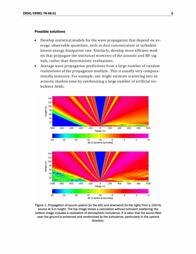
• Acoustic scattering by small turbulent eddies raises sound levels in shadow regions and reduces signal coherence across microphone ar-rays (see Figure 1).
• Optical signals are scattered and attenuated by dust and other small particles in the atmosphere.
• Radio frequency (RF) signals undergo random fading as a result of scattering from terrain objects (such as buildings, vegetation, and ran-dom surface variations) and atmospheric turbulence.
ERDC/CRREL TR-08-21 5
Possible solutions
• Develop statistical models for the wave propagation that depend on av-erage, observable quantities, such as dust concentration or turbulent kinetic energy dissipation rate. Similarly, develop more efficient mod-els that propagate the statistical moments of the acoustic and RF sig-nals, rather than deterministic realizations.
• Average wave propagation predictions from a large number of random realizations of the propagation medium. This is usually very computa-tionally intensive. For example, one might estimate scattering into an acoustic shadow zone by synthesizing a large number of artificial tur-bulence fields.
Figure 1. Propagation of sound upwind (to the left) and downwind (to the right) from a 100-Hz
source at 5-m height. The top image shows a calculation without turbulent scattering; the bottom image includes a realization of atmospheric turbulence. It is seen that the sound field
near the ground is enhanced and randomized by the turbulence, particularly in the upwind direction.

ERDC/CRREL TR-08-21 6
Issue 3: Varying resolutions and representations in environmental datasets
Explanation
The resolution of available environmental information varies widely. Weather predictions are available at a horizontal resolution of 1 km at best; 15 km is more typical. Terrain elevation data, on the other hand, are often available at a horizontal resolution of 3 to 30 m. Other datasets, such as those containing soil properties and cultural features, typically have resolutions of 100 to 500 m. The datasets may also rely on different repre-sentation techniques, such as regularly spaced points (a raster) or poly-gons.
Examples
In the U.S. Army Engineer Research and Development Center (ERDC) Battlefield Terrain Reasoning and Analysis software (Hieb et al. 2007), the meteorological forecast has very coarse resolution compared to terrain “complex,” which is a polygonal, variable resolution representation of the terrain facets including ground properties. This creates dramatic “step” changes in predictions across forecast grid-cell boundaries that do not ex-ist in actuality.
Possible solutions
Interpolation of coarse fields to make them smooth at finer scales of inter-est. Alternatively, one might interpolate the end product, namely the sig-nature propagation or sensor performance calculations. In many cases, software tools are available to convert between different data gridding techniques. However, these are mostly cosmetic solutions: the coarser datasets will usually be unrealistically smooth when interpolated to a higher resolution.
Issue 4: Inaccurate and missing environmental data
Explanation
Environmental observations, whether of the atmosphere or terrain, are rarely fully accurate and complete. This is particularly so in many areas where military conflicts may occur.

ERDC/CRREL TR-08-21 7
Examples
• Very little information is available on subsurface characteristics of the earth affecting seismic wave propagation. This makes accurate predic-tion of seismic detection ranges difficult.
• The acoustic background noise spectrum plays a key role in acoustic detection (just as important as the actual signal level), but is often not known accurately. Factors such as time of day, proximity to roadways, and intermittent activity, can all be dominant.
• Fog, snow, and rain, which greatly affect the performance of optical and infrared sensors, often occur in very localized and transient patches. Therefore, it is often uncertain in advance whether the sensors will be operating in such impaired conditions or not.
Possible solutions
Attempt to assess the predictive skill of lower fidelity models through comparisons to higher fidelity ones or empirical data. If this is infeasible, the experience of experts may provide a rough assessment of predictive skill.
Issue 5: Complex interrelationships among systems of environmental variables
Explanation
It is generally difficult to describe uncertainties in the behavior of systems of variables with complex, nonlinear, interrelationships. The atmospheric environment is such a system.
Examples
• Variations in the earth’s surface albedo (diffuse solar reflectivity) cause variations in ground heating, which are important to evaluating tem-perature contrasts for infrared sensing. These variations in ground heating help drive wind and turbulence. The turbulence transports heat, which again impacts temperatures of surfaces. Even if we could accurately describe the uncertainty in the surface albedo, modeling its subsequent effects and feedbacks on the other variables is extremely challenging.
• Ordinarily, the predictive skill of atmospheric models is assessed by calculating the standard deviation between the forecast and the ob-
ERDC/CRREL TR-08-21 8
served wind at a selected set of points. But sound propagation, among other processes, depends on multipoint correlations in the spatial structure of the wind field. These multipoint correlations are deter-mined by complex, nonlinear processes. The standard deviation at a particular point in the flow does not provide the information necessary for a meaningful skill assessment.
Possible solution
Use realistic physical models, such as numerical weather forecasts and acoustic/EM wave propagation models, to capture relationships between the variables of interest. Introduce randomness in the output through Monte Carlo or Latin hypercube sampling (LHS) of combinations of mul-tiple variables.
Issue 6: Random (chaotic) behavior of atmospheric and dependent processes
Explanation
The future state of the atmosphere cannot be predicted with certainty. As is now clearly recognized through chaos theory, small perturbations to the initial conditions, either through physical variations or through how these variations are represented in a computer model, can have a large impact on the true and forecasted future states.
Examples
When an acoustic propagation prediction is run for a single, crisp atmos-pheric forecast, the predictions may show very sharply delineated regions of low or high signal level. (An example is shown in Section 5, Figure 8.) The locations of these regions are very sensitive to details of the atmos-pheric data supplied to the model. When small perturbations are applied to the model inputs, the predictions are substantially smoothed.
Possible solution
Use ensemble forecast methods to predict a range of plausible environ-mental states (e.g., Kalnay 2003, Palmer 2006) and calculate propagation through these multiple states. In some cases, the distribution of forecasts and sensor performance predictions can be represented in an intuitive manner, such as the “fans” familiar in forecasts of hurricane tracks.

ERDC/CRREL TR-08-21 9
Issue 7: Imperfect physics in wave propagation and signature models
Explanation
Most practical models for wave propagation and signatures do not incor-porate all of the physics that may be significant. Compromises in fidelity must be made to keep the demands on computational resources reason-able.
Examples
• Many RF propagation models do not include diffraction over terrain features, such as buildings or hills, or refraction by the atmosphere.
• Acoustical propagation models often do not incorporate reflections and diffractions around buildings in urban environments.
• Wave propagation models may not properly handle terrain heterogene-ity, i.e., propagation paths that traverse multiple terrain types such as land and water.
Possible solutions
• Create more accurate, yet computationally efficient models. (This has usually been the subject of much previous research and is often very challenging.)
• Take advantage of increasing computational capabilities by employing more sophisticated propagation and signature models.
• Characterize the predictive skill associated with the computationally feasible, but less accurate, models by comparing them to experimental data or to computationally intensive, but more accurate, models. De-velop methods to express the predictive skill of the less accurate mod-els to their users.
Issue 8: Correlated observations from suites of sensors
Explanation
Most formulations for statistical hypothesis testing (as in signal detection problems) and sensor data fusion assume independent observations. This assumption greatly simplifies the mathematics. In real-world situations, however, there are often significant dependencies between sensor observa-tions.

ERDC/CRREL TR-08-21 10
Examples
• Fog and high humidity hinder transmission of infrared and high-frequency acoustical signals.
• Two similar sensors that are placed close to one another may provide very similar, highly correlated information.
Possible solution
Recent research is now beginning to address this problem, e.g., Ganana-pandithan and Natarajan (2007). However, the practicality and applicabil-ity of these approaches must be examined.
Issue 9: Lack of knowledge of sensor properties and algorithms
Explanation
The properties and processing algorithms of sensors are often proprietary, classified, or under development. Therefore the modeler often does not have access to them. The information about the sensor may never be fully captured by the manufacturer/testing agency; there will always be some uncertainty.
Example
The Army wishes to understand the efficacy of a proposed new unattended ground sensor (UGS) for urban operations. The normal practice, at this time, is to first study the value of the sensor information in force-on-force simulations. However, because the sensor types and algorithms are un-known at the outset, this is a “chicken-before-the-egg” problem.
Possible solution(s)
• Characterize the performance using idealized information theoretic measures, such as the Neyman-Pearson criterion or Fisher informa-tion. These measures often assume the performance of the actual sen-sor algorithms is close to ideal. On the other hand, they do not require proprietary or classified information, and typically are computationally efficient.
• Use “proxy” sensors and algorithms (sensors and algorithms thought to be close to the actual system of interest) until more information about
ERDC/CRREL TR-08-21 11
the actual sensor is known. A more sophisticated approach would be to use a variety of proxy sensors.
Issue 10: Complex, dynamic, unknown scenarios in which the sensors are used
Explanation
Uncertainty of when, where, and what kind of predictions are required is often a key consideration; scenarios in which the sensors are used are complex and vary dynamically as the warfighter responds to the battle-space. The geometry between target and sensor is not entirely known in advance.
Examples
• IR visibility of a target from the air typically depends strongly on the elevation angle and target orientation. These angles vary, however, over the course of an engagement and are often not known in advance.
• To avoid disruptions from hostile forces, a communications network must be laid out in an ad hoc manner, with the individual devices in different positions than initially planned.
Possible solutions
• “Play” different tactical and weather scenarios as part of pre-mission training exercises.
• Perform statistical analyses on a number of likely scenarios. • Attempt to provide useful, general information that will apply to a
number of situations when specific tactical details are unknown.
Issue 11: Uncertainty of when and where predictions are required
Explanation
Missions are often planned days, weeks, or months in advance. Thus, envi-ronmental conditions at the time of mission execution may be known only in a typical or climatological sense. Military engagements are also very dy-namic, with human factors and activity greatly altering the battle envi-ronment.

ERDC/CRREL TR-08-21 12
Examples
A brigade is to be deployed with advanced UGS systems and wants guid-ance on how to place the sensors. Time of deployment is weeks or months from present, so weather/terrain conditions are only known in a clima-tological sense. The locations of interest for sensor employment are not yet fully determined.
Possible solutions
Use climatologically based, or actual historical data, as representative at-mospheric and terrain conditions for the region of operations. Identify strategically significant spatial-temporal behavior based on the clima-tological/historical conditions.
ERDC/CRREL TR-08-21 13
3 Describing Uncertainty
“There are known knowns; there are things we know we know. We also know there are known unknowns; that is to say, we know there are some things we do not know. But there are also unknown unknowns — the ones we don't know we don't know.” Donald Rumsfeld
Identification, quantification, and reduction of uncertainty have long been sources of practical concern and vital areas of research. Our particular problems related to signal propagation and sensor performance modeling should be considered in this broader context. That is the purpose of this brief section.
The quote at the beginning of this section exemplifies a practical perspec-tive on uncertainty. The known knowns represent those aspects of a mis-sion that are understood with certainty. The phrases known unknowns and unknown unknowns establish two different degrees of uncertainty, based on whether the uncertainty is explicitly recognized. If it is recog-nized, it constitutes a known unknown, and can perhaps be dealt with sys-tematically. An unknown unknown, being unrecognized, could result in a surprise, possibly a dangerous one. Allen et al. (2006) mention the exis-tence of known and unknown uncertainties in the context of weather and climate forecasting; these correspond to Rumsfeld’s known unknowns and unknown unknowns.
The two degrees of uncertainty, known unknowns and unknown un-knowns, can be associated with many of the issues described in the preced-ing section. For example, “Issue 2: Wave propagation sensitivity to ir-resolvable and highly variable environmental details” and “Issue 4: Inaccurate and missing environmental data” are usually recognized limita-tions in a predictive capability and hence known unknowns. “Issue 7: Im-perfect physics in wave propagation and signature models” and “Issue 10: Complex, dynamic, unknown scenarios in which the sensors are used” ex-emplify unknown unknowns when the limitations of the modeling effort go unrecognized.
ERDC/CRREL TR-08-21 14
One might ask whether the fourth remaining combination of the words known and unknown not present in the Rumsfeld quote, namely unknown knowns, should be included among possible situations involving uncer-tainty. Because the overt purpose of a DST is to allow a warfighter to make expert decisions without him/her necessarily possessing extensive exper-tise, it is to be anticipated that the warfighter will not be aware of many uncertainties in the DST predictions. The modeler who created the DST has a much better appreciation for the limitations of the underlying mod-els than does the user. In effect, the DST creator’s known knowns or known unknowns are often the warfighter’s unknown knowns or unknown unknowns. When key information in a decision process may exist in the form of unknown knowns (unknown to the warfighter, known to the de-veloper), methods should be developed to quantify and communicate this information.
The discussion in the preceding paragraph anticipates the concept of risk. Although a warfighter would normally have higher priorities than becom-ing an expert in sensor phenomenology, he or she would normally have a strong interest in avoiding risk. Uncertainty and risk are related, but not equivalent. Risk implies a state of uncertainty that could lead to an unfa-vorable outcome. Uncertainty by itself is not a concern unless there is as-sociated, significant risk. Although uncertainty is emphasized in this re-port, we recognize that the end value of the uncertainty models lies in recognizing, evaluating, and dealing with risk.
In the academic study of statistics, uncertainty is often classified as either epistemological (pertaining to knowledge) or aleatory (pertaining to luck). Sometimes, these are more simply called uncertainty and random-ness, respectively. Issue 2 from the previous section, “Wave propagation sensitivity to irresolvable and highly variable environmental details,” would normally be considered aleatory uncertainty. Practically speaking, variations in sound levels caused by turbulent eddies and other small, dy-namic environmental features must be regarded as a random process. On the other hand, uncertainty in the weather for a particular time and loca-tion would normally be considered epistemological uncertainty because with more information the accuracy of the atmospheric state characteriza-tion could possibly be improved. Still, the distinctions between epistemo-logical and aleatory uncertainty are not always clear cut; they are often more a matter of viewpoint or purpose. Regarding weather forecasts, chaos theory teaches us that the state of the atmosphere at a distant time
ERDC/CRREL TR-08-21 15
in the future cannot be known deterministically, because it depends on small, random perturbations to the present atmospheric state. Hence, a long-range forecast may be considered essentially random. This is the es-sence of “Issue 6: Random (chaotic) behavior of atmospheric and depend-ent processes.”
Many authors and organizations have developed their own taxonomies for uncertainty. Some attempt to be comprehensive, whereas others are fo-cused on particular applications. In modeling, it is common to distinguish model and parameter uncertainty (e.g., Frey 1998). Model uncertainty re-sults when the real world is abstracted with a model; this process invaria-bly involves simplifying assumptions. Parameter uncertainty relates to the values, such as measurements, empirical constants, and decision variables that are used in the model. Similarly, regarding weather forecasting, Palmer (2006) singles out model and initial uncertainty. The latter is un-certainty in the initial conditions (atmospheric observations) of the weather forecast model. Among the uncertainty issues raised earlier, ini-tial uncertainty is most closely matched by “Issue 4: Inaccurate and miss-ing environmental data.” Model uncertainty is present in many issues, in-cluding 5, 7, and 9–11.
Lastly, we mention the taxonomy of Ayyub and Chao (1998) who consider uncertainty in the context of civil engineering. Their classification scheme, at its initial level, pertains to the origin of the uncertainty: ambiguity, vagueness, or information conflicts. Ambiguity refers to noncognitive (de-finable) issues such as physical randomness, limited sampling of a process, lack of knowledge, and modeling uncertainty. Issues 1–3 and 6–7 fall pri-marily into the category of ambiguity uncertainties. Vagueness relates to the inability to precisely define parameters and judgments (such as system failure or survival) and describe interrelationships between elements of a complex system. Issues 5 and 8–11 deal primarily with vagueness.
ERDC/CRREL TR-08-21 16
4 Probabilistic Framework for a DST
We now consider formulation of a probabilistic framework for sensor per-formance prediction including uncertainty. Ideally, the framework should be fairly simple, and yet accommodate the many sources for uncertainty mentioned in the preceding section. It should also be compatible with es-tablished approaches to dealing with uncertainty, such as ensemble weather forecasting, and leverage previous DST calculations based on a crisp specification of the environmental and tactical scenarios.
This section is structured as follows. We first analyze the important tasks performed by a DST, so we might better understand where uncertainty can occur. We then develop a probabilistic formulation for these tasks. Lastly, we consider a computational architecture for a DST with uncertainty.
What does a DST do?
Before attempting to formulate a probabilistic framework, it is helpful to take a step back and describe the general functions of a DST. We consider these to be the following:
• Step 1: information gathering and construction of the tactical and en-vironmental (atmosphere and terrain) scenario,
• Step 2: translation of the scenario information to parameters needed by the signal and noise prediction models,
• Step 3: signal and noise prediction models (source characteristics, propagation through the environment, and sensor processing),
• Step 4: calculation of sensor performance metrics (e.g., probability of detection or classification, or source localization accuracy), and
• Step 5: display of and interaction with the information (graphical in-terface).
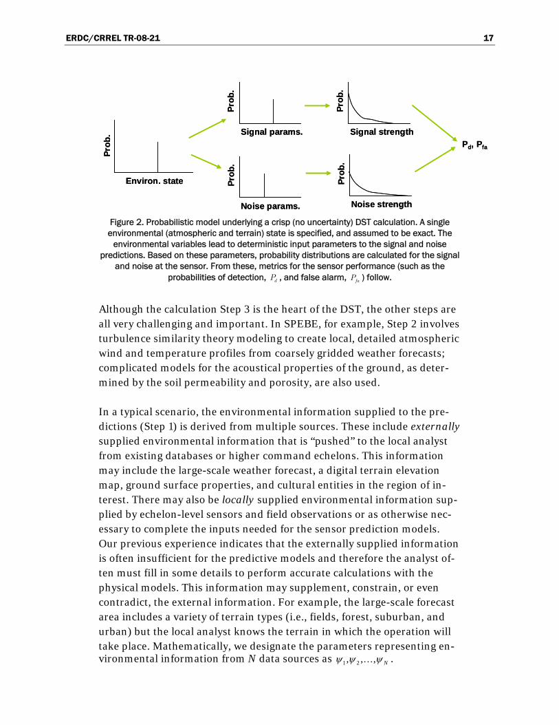
Figure 2 conceptually shows the first four steps of this process as imple-mented in a crisp DST (one in which the environmental information and tactical scenario are assumed to be exactly known), such as in the Sensor Performance Evaluator for Battlefield Environments (SPEBE) (Wilson and Szeto 2000; Wilson 2006).
ERDC/CRREL TR-08-21 17
Prob
.
Environ. state
Prob
.
Signal params.
Prob
.
Noise params.
Prob
.
Signal strength
Prob
.
Noise strength
Pd, Pfa
Prob
.
Environ. state
Prob
.
Signal params.
Prob
.
Noise params.
Prob
.
Signal strength
Prob
.
Noise strength
Pd, Pfa
Figure 2. Probabilistic model underlying a crisp (no uncertainty) DST calculation. A single environmental (atmospheric and terrain) state is specified, and assumed to be exact. The
environmental variables lead to deterministic input parameters to the signal and noise predictions. Based on these parameters, probability distributions are calculated for the signal
and noise at the sensor. From these, metrics for the sensor performance (such as the probabilities of detection, , and false alarm, ) follow. dP faP
Although the calculation Step 3 is the heart of the DST, the other steps are all very challenging and important. In SPEBE, for example, Step 2 involves turbulence similarity theory modeling to create local, detailed atmospheric wind and temperature profiles from coarsely gridded weather forecasts; complicated models for the acoustical properties of the ground, as deter-mined by the soil permeability and porosity, are also used.
In a typical scenario, the environmental information supplied to the pre-dictions (Step 1) is derived from multiple sources. These include externally supplied environmental information that is “pushed” to the local analyst from existing databases or higher command echelons. This information may include the large-scale weather forecast, a digital terrain elevation map, ground surface properties, and cultural entities in the region of in-terest. There may also be locally supplied environmental information sup-plied by echelon-level sensors and field observations or as otherwise nec-essary to complete the inputs needed for the sensor prediction models. Our previous experience indicates that the externally supplied information is often insufficient for the predictive models and therefore the analyst of-ten must fill in some details to perform accurate calculations with the physical models. This information may supplement, constrain, or even contradict, the external information. For example, the large-scale forecast area includes a variety of terrain types (i.e., fields, forest, suburban, and urban) but the local analyst knows the terrain in which the operation will take place. Mathematically, we designate the parameters representing en-vironmental information from N data sources as 1 2, , , Nψ ψ ψ… .
ERDC/CRREL TR-08-21 18
One might reasonably ask why we do not distinguish between atmospheric and terrain information, at least in a notational sense. Are not these data independent (e.g., a weather forecast and a digital elevation map)? There are actually many situations where the terrain and atmosphere have im-portant feedbacks. For example, precipitation alters the soil properties. By combining the atmospheric and terrain parameters, we have made a nota-tional decision consistent with an interacting atmosphere and terrain, al-though in practice the data may be obtained from different sources.
In addition to the environmental parameters, information must be gath-ered regarding the tactical scenario, by which we mean here the types of targets and sensors, their positions, orientations, etc. This information is indicated here with the symbol ξ. Conceivably, there could exist situations where the tactical parameters depend on the environmental state, al-though we will not consider that complication in the present model. One might now ask whether, analogously to the environmental parameters, we should consider multiple information sources for the tactical parameters. In our experience, information on the tactical parameters usually comes from a single data source, e.g., a command and control system or through manual entry by the user. Hence, we do not consider multiple sources, al-though it would be rather simple to add such a complication.
Taken together, the environmental information 1, , Nψ ψ… and tactical sce-
nario information ξ provide the parameters χ needed by the signal genera-tion (target signature), transmission (propagation), and reception (sensor) prediction models. (In the following, we will call these several models the signature propagation model for brevity.) This is Step 2 from the preced-ing description. The parameters χ are to be determined in a manner that is statistically consistent with 1, , Nψ ψ… and ξ; typically, only a subset of the
supplied information will be needed. For example, an acoustic prediction will need information on the atmospheric wind field, but fog is usually un-important; an IR prediction will depend on fog but not as strongly on wind.
Next, we feed the information χ into the signature propagation model to determine the signal and noise features at the sensor, s and n, respectively (Step 3). These features may represent different modalities (acoustic, seismic, visible, IR, and/or electromagnetic) as well as different frequency bands and statistics for these modalities. Due to unresolvable phenomena such as turbulence, vegetation, and small buildings, the signal and noise
ERDC/CRREL TR-08-21 19
are generally random variables. When modeled probabilistically, we de-scribe them with probability density functions (pdfs). The pdfs for s and n depend on sets of parameters and . For Gaussian pdfs, for example,
these parameters would consist of means and standard deviations of the signal and noise features.
sθ nθ
Step 4, the formation of metrics, involves processing the signal and noise information. For example, a probability of detection or classification may be calculated from and . Once this processing has been performed,
the information can be visualized (Step 5). sθ nθ
In summary, we have the following symbols, each of which actually repre-sents a (perhaps very large) set of parameters:
• 1, , Nψ ψ =… atmospheric and terrain parameters
• ξ = tactical scenario parameters
• χ = parameters for the signal/transmission/sensor prediction models
• =sθ pdf parameterization for the signal features
• =nθ pdf parameterization for the noise features
An “object-oriented” discussion
In this section, we outline how the functionality for a crisp DST, as laid out in the previous section, might be implemented in software. Later, we con-sider how this functionality could be generalized to include uncertainty. The discussion is based on a modern, “object-oriented” view to program-ming, as exemplified by languages such as Java and C#. Discussing the problem in this manner helps to organize one’s thoughts and describe them in a manner that can be more readily programmed. For the uniniti-ated, an object may represent a real-world entity or more abstract concept. Objects have characteristics, which may alternatively be called properties, data, or (in Java) fields. They also have functionality and perform tasks, which are usually called methods. Particular objects are instances of classes. For example, one might consider all helicopters to comprise a class. A particular helicopter would be an instance of this class. The object characteristics are the design of the helicopter and the instruments on it. The functionality consists of flying, firing weapons, etc.
Regarding the discussion in the previous section, we might consider the environmental and tactical state parameters ( 1, , Nψ ψ… and ξ) to be an in-
ERDC/CRREL TR-08-21 20
stance, of, say, an environmental/tactical data model class. For brevity, we will call such an instance a scenario. The class must define the particular properties that represent a scenario, such as the atmospheric wind and temperature, the ground permeability and albedo, the target and sensor types and positions, etc. In actual problems the environmental/tactical data model can be expected to be quite complicated and actually collect many different objects. Conceivably, different environmental/tactical data classes could be developed, depending on the level of sophistication and the information that is available or desired. In Java, we might thus develop a “parent class” environmental/tactical data model (a general, high-level description) and “subclasses” for more particular situations. Or, one might use a Java interface specification, and then develop subclasses that im-plement this interface.
The information gathering step (Step 1) can be viewed as constructing the scenarios. The construction could involve many different data resources, such as weather forecasts, digital terrain models, and inputs directly sup-plied by the user. Conceivably, many alternative methods could be devel-oped to construct scenarios, involving processes such as retrieving data over the Internet, reading data from media, and allowing users to enter data interactively. The processes of selecting data resources and entering data would likely involve a graphical user interface (GUI).
Next we must translate the scenario objects to parameters needed to run our signature propagation predictions (Step 2). These parameters can be considered a new type of object. We describe a method for converting sce-narios to prediction model parameters as a scenario translator. Different subclasses of prediction model parameters could be defined as needed for different prediction models. The prediction models could be implemented as methods for these subclasses. Indirectly, the prediction models thus op-erate on different environmental/tactical data model classes. The scenario translator serves as the intermediary.
Next we consider the signal and noise features, as parameterized by and . A signature propagation model can be regarded as a method that pro-
duces and . This is Step 3. It is expected that different methods would
be used to produce different kinds of features. For example, an acoustic prediction model would produce parameters related to acoustic features.
sθ
nθ
sθ nθ
ERDC/CRREL TR-08-21 21
Step 4 would consist of a set of methods that operate on signal and noise feature parameterizations to produce sensor metrics of interest, such as probability of detection or classification. Step 5 displays the results of these methods.
If good, modular coding practices are followed, most of the object-oriented code should be portable; that is, it should be able to run under different GUIs and geospatial information systems (GIS) with little or no change. The information gathering in Step 1 would initially involve some GUI-specific operations to gather the data, but then the construction of scenar-ios from this information should rely on portable code. Once Step 1 has been finished, Steps 2, 3, and 4 should proceed entirely with portable code. Step 5, of course, is GUI specific.
Bayesian probabilistic formulation
We now consider incorporation of uncertainty into the DST predictions. Many different approaches can be contemplated, including traditional probability-based statistics, or newer approaches such as fuzzy logic and belief functions. Here, we develop a formulation based on Bayesian prob-abilistic concepts, which means that probabilities are conditioned on prior knowledge. The scheme is loosely inspired by Maurer et al.’s (2006) Bayesian formulation for ballistic missile signatures.
The information gathering, Step 1, amounts to determining pdfs for
1, , Nψ ψ… and ξ. In the most general sense, these parameters will possess a
joint pdf . However, as mentioned previously, we assume that
the environmental and tactical parameters are independent, in which case (by definition) . Here
( 1, , ,Np ψ ψ… )ξ
p( ) ( ) ( )1 1, , , , ,N Np pψ ψ ξ ψ ψ ξ=… … ( )1, , Np ψ ψ… describes
the ubiquitous uncertainty in the environmental state. A distribution ( )p ξ
might be important, say, when there is uncertainty in the altitude of an air-craft.
The translation, Step 2, involves mapping the information in 1, , Nψ ψ… and
ξ to the signature propagation model parameters χ. Probabilistically, this mapping is indicated by the likelihood function ( )1 2| , , , ,Np χ ψ ψ ψ ξ… , where
the vertical bar indicates that the variable on the left is conditioned to the values on the right. According to the definition of conditional probability,
ERDC/CRREL TR-08-21 22
( ) ( )( )
11
1
, , , ,| , , , .
, , ,N
NN
pp
pχ ψ ψ ξ
χ ψ ψ ξψ ψ ξ
=…
……
(1)
The marginal pdf ( )p χ is determined by integrating ( )1, , , ,Np χ ψ ψ ξ… over
1, , Nψ ψ… and ξ. The result is
( ) ( ) ( )1 1| , , , , , ,N N ,p p p d dχ χ ψ ψ ξ ψ ψ ξ ξ= ∫ ∫ ψ… … (2)
where the boldface ψ indicates a vector containing 1, , Nψ ψ… . The predic-
tion, Step 3, can be considered a mapping of the model prediction parame-ters to the pdf parameters for the signal and noise features. When this mapping involves uncertainty, we represent it notationally as the likeli-hood function ( ), |s np θ θ χ . By definition,
( ) ( )( ), ,
, | .s ns n
pp
pθ θ χ
θ θ χχ
= (3)
An example situation where it is important to implement a distribution ( )p χ is when the ground surface may consist of grass or asphalt, in which
case the sound propagation characteristics will be very different. Another observation to make regarding Step 3 is that, since the propagation model parameters χ contain all the information from 1, , Nψ ψ… and ξ affecting the signal and noise distributions, ( ) ( )1, | , | , , , .s n s n Np pθ θ χ θ θ ψ ψ ξ= … From Equa-
tion 3 and then substituting with Equation 2 we have
( ) ( ) ( ) ( ) ( ) ( )1 1, , | , | | , , , , , ,s n s n s n N Np p p d p p p d d .dθ θ θ θ χ χ χ θ θ χ χ ψ ψ ξ ψ ψ ξ ξ⎡ ⎤= = ⎣ ⎦∫ ∫ ∫ ∫ ψ… … χ
(4)
This parameterization of the signal and noise pdf might be needed, for ex-ample, to perform a simulation. For a DST, in the end we would typically like to know the expected value of functions that depend on and ,
such as the probabilities of detection and false alarm. From Equation 4 we have
sθ nθ
( ) ( ) ( ) ( ) ( ){ }1 1, , , | | , , , , , , .s n s n s n N N s nf f p p p d d d d dθ θ θ θ θ θ χ χ ψ ψ ξ ψ ψ ξ ξ χ θ⎡ ⎤= ⎣ ⎦∫ ∫ ∫ ∫ ∫ ψ… … θ
(5)
ERDC/CRREL TR-08-21 23
Alternatively we might wish to determine the joint pdf of s and n them-selves, ( ),p s n . Assuming we have a model for ( ), | ,s np s n θ θ , as might be
known for example from a random scattering theory, Equation 4 and fur-ther application of Bayes’ theorem leads to
( ) ( ) ( ) ( ) ( ){ }1 1, , | , , | | , , , , , , .s n s n N N sp s n p s n p p p d d d d d nθ θ θ θ χ χ ψ ψ ξ ψ ψ ξ ξ χ θ⎡ ⎤= ⎣ ⎦∫ ∫ ∫ ∫ ∫ ψ… … θ
(6)
If the signal and noise are independent, then ( ) ( ) ( ),p s n p s p n= . Another
point to make regarding Equations 5 and 6 is that there is no causative in-teraction between the individual signal and noise features; for example, an IR feature does not alter an acoustic feature (although they may be af-fected by common environmental and tactical parameters). Hence, their pdfs may be calculated independently. If the probabilistic models for the environment and tactical scenario are discrete (but the signal and noise pdfs still continuous), we have, instead of Equation 6,
( ) ( ) ( ) ( ) ( )1
1 1, , | , , | | , , , , ,s n N
s n s n N Np s n p s n P P Pθ θ χ ψ ψ ξ
, .θ θ θ θ χ χ ψ ψ ξ ψ ψ= ∑∑ ∑ ∑ ∑∑ … … ξ
(7)
Here, the uppercase P indicates the probability of a particular value of its argument.
Equations 5–7 are various forms of our conceptual model for predictive uncertainty. Given that these results are six-dimensional integrals (or summations), solutions could be very computationally intensive. Instead of performing the integrations literally, it is probably necessary to develop a sampling strategy (such as Monte Carlo or Latin hypercube sampling). Also, only the most important sources of uncertainty should be included. This will become more apparent in the next section, which considers some illustrative applications. Five likelihood functions and pdfs are required, which to recapitulate are:
• ), | ,( s nnp s θ θ , the joint likelihood function for the signal and noise varia-
tions based on parameterizations of their pdfs. Alternatively, the prob-lem may require a deterministic function ( ),s nf θ θ . The capability to per-
form this calculation may often be extracted from an existing DST.
ERDC/CRREL TR-08-21 24
• ), |s n(p θ θ χ , the joint likelihood function for the signal and noise pdf pa-
rameters corresponding to a particular set of prediction models. The capability to perform this calculation may often be extracted from an existing DST.
• ), ,N( 1| ,p χ ψ ψ
p
ξ… , the likelihood function for the signature propagation
model parameters given the large-scale weather forecast and terrain in-formation, locally supplied weather and terrain information, and tacti-cal information. In practice, there is not much guidance for this likeli-hood function; it may be challenging to model it well.
• )1, , N(ψ ψ… , the pdf of a particular weather and terrain state. This
could be available from an ensemble forecast system or a model that generates sets of typical atmospheric conditions from climatology as well as terrain databases.
• ( )p ξ , the pdf of a particular tactical scenario. This information would
normally be supplied by the user.
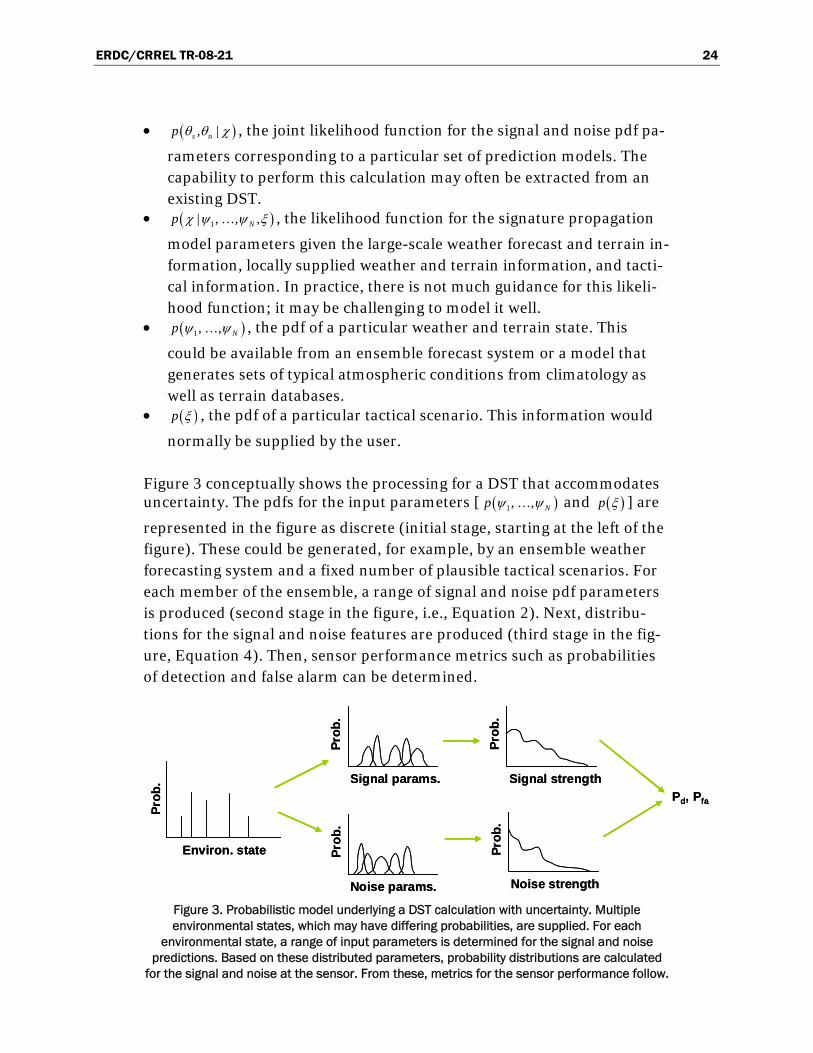
Figure 3 conceptually shows the processing for a DST that accommodates uncertainty. The pdfs for the input parameters [ ( )1, , Np ψ ψ… and ( )p ξ ] are
represented in the figure as discrete (initial stage, starting at the left of the figure). These could be generated, for example, by an ensemble weather forecasting system and a fixed number of plausible tactical scenarios. For each member of the ensemble, a range of signal and noise pdf parameters is produced (second stage in the figure, i.e., Equation 2). Next, distribu-tions for the signal and noise features are produced (third stage in the fig-ure, Equation 4). Then, sensor performance metrics such as probabilities of detection and false alarm can be determined.
Prob
.
Environ. state
Prob
.
Signal params.
Prob
.
Noise params.
Prob
.
Signal strength
Prob
.
Noise strength
Pd, Pfa
Prob
.
Environ. state
Prob
.
Signal params.
Prob
.
Noise params.
Prob
.
Signal strength
Prob
.
Noise strength
Pd, Pfa
Figure 3. Probabilistic model underlying a DST calculation with uncertainty. Multiple environmental states, which may have differing probabilities, are supplied. For each
environmental state, a range of input parameters is determined for the signal and noise predictions. Based on these distributed parameters, probability distributions are calculated
for the signal and noise at the sensor. From these, metrics for the sensor performance follow.
ERDC/CRREL TR-08-21 25
Implementation architecture
The probabilistic model in the previous section is general enough to ac-commodate a great variety of implementations. But it still does not pro-vide a practical prescription for including uncertainty in DSTs. The par-ticular approach one chooses should be guided by computational feasibility and compatibility with current approaches for dealing with en-vironmental uncertainty.
Since ensemble forecasting has become a widespread practice in weather forecasting, we anticipate leveraging this approach to dealing with uncer-tainty in the atmospheric state. In this manner, we directly address “Issue 5: Complex interrelationships among systems of environmental variables,” and “Issue 6: Random (chaotic) behavior of atmospheric and dependent processes.” The ensemble forecasts describe the atmosphere with a num-ber of discrete set of states, which may be equally likely or assigned differ-ing probabilities. In the notation of the preceding section, ( )1, , Np ψ ψ… be-
comes the discrete distribution ( )1, , NP ψ ψ… . It is then natural to extend
this approach to include tactical scenarios; that is, we consider joint, dis-crete pdfs ( )1, , ,NP ψ ψ ξ… . This allows Issues 10 and 11, which deal with un-
certainty in the tactical scenario, to be addressed.
The likelihood function ( 1| , , ,Np )χ ψ ψ ξ… is the appropriate point at which
to introduce uncertainties affecting the signature propagation model as due to incomplete knowledge of the environment and tactical scenario. This allows “Issue 2: Wave propagation sensitivity to irresolvable and highly variable environmental details” and “Issue 4: Inaccurate and miss-ing environmental data” to be addressed. Because, in general, the signa-ture propagation model is a crisp formulation (i.e., it maps a single set of values for χ to a single set of values for and ), we also perform this
stage of the calculation using a discrete probability model. Given a particu-lar parameter range for the elements of χ, we can use a Monte Carlo or Latin hypercube strategy to generate random samples. This is illustrated in Section 5.
sθ nθ
If there are uncertainties in the predictions of the propagation model (i.e., Issue 7), the appropriate place to introduce them would be ( ), |s np θ θ χ . Al-
though this may be appropriate in many situations, this work emphasizes uncertainty in signature propagation model parameters, rather than the
ERDC/CRREL TR-08-21 26
model itself. Hence, no uncertainty is introduced at this stage. In effect, ( , |s np )θ θ χ is assumed to be crisp, so that the summation over χ vanishes
from Equation 7 and we have
( ) ( ) ( ) ( ) ( )1
1 1, , | , | , , , , ,s n N
s n N Np s n p s n P Pθ θ ψ ψ ξ
, .θ χ θ χ χ ψ ψ ξ ψ ψ ξ= ⎡ ⎤⎣ ⎦∑∑ ∑ ∑∑ … … (8)
Correct application of this result will properly include correlated sensor observations (Issue 8).
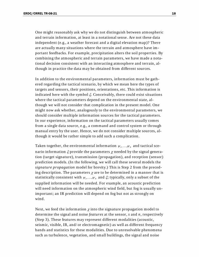
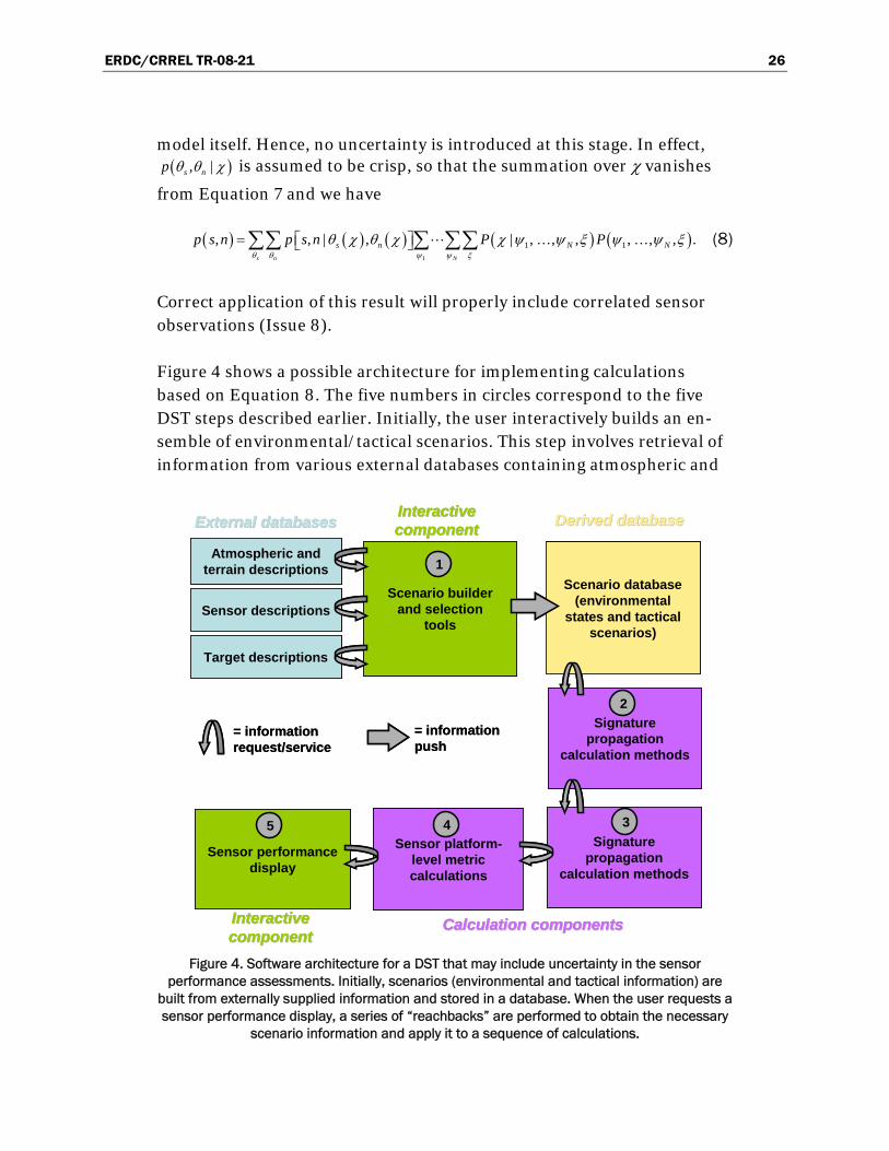
Figure 4 shows a possible architecture for implementing calculations based on Equation 8. The five numbers in circles correspond to the five DST steps described earlier. Initially, the user interactively builds an en-semble of environmental/tactical scenarios. This step involves retrieval of information from various external databases containing atmospheric and
Atmospheric and terrain descriptions
Sensor descriptions
Sensor platform-level metric calculations
Target descriptions
Calculation componentsCalculation components
Interactive Interactive componentcomponentExternal databasesExternal databases
Scenario builder and selection
tools
Sensor performance display
Scenario database (environmental
states and tactical scenarios)
Derived databaseDerived database
Signature propagation
calculation methods
1
5 34
Signature propagation
calculation methods
2
Interactive Interactive componentcomponent
= information request/service
= information push
Figure 4. Software architecture for a DST that may include uncertainty in the sensor
performance assessments. Initially, scenarios (environmental and tactical information) are built from externally supplied information and stored in a database. When the user requests a sensor performance display, a series of “reachbacks” are performed to obtain the necessary
scenario information and apply it to a sequence of calculations.

ERDC/CRREL TR-08-21 27
terrain data, and information on sensors and targets. The constructed sce-narios are pushed to a local database. Next, when the user requests a sen-sor-performance display, there is a sequence of “reachback” events. Even-tually, data are pulled from the scenario database to perform a signature propagation calculation. Each scenario is normally pulled, and multiple variations of the signature propagation model parameters are generated from each scenario to account for uncertainty. The signature propagation and performance metric calculations are then performed and finally dis-played.
ERDC/CRREL TR-08-21 28
5 Example Scenarios
Sensor selection from multiple modalities
Let us first consider an example involving multiple sensor modalities. The example, although highly idealized, illustrates how, even in rather simple scenarios, uncertainty in sensor performance can play an important role in determining which sensors or combination thereof are best suited to a par-ticular mission. Although we call the three sensor modalities passive IR, acoustic, and seismic, the postulated performance characteristics are not based on any actual sensor. The target is also a generic one; that is, its properties do not correspond to any actual target.
Initially, we consider daytime and nighttime cases without any uncertainty in sensors’ performance. Both cases involve mostly clear conditions, with sunshine during the day and a moderate, ground-based temperature in-version at night. The signal and noise are assumed to have Gaussian pdfs, with means and standard deviations for the various cases shown in Table 1. In the notation introduced earlier, the parameters in this table consti-tute sθ and nθ . All values are normalized by the mean of the noise at night.
The rationale behind the parameter values is the following. For the acous-tic sensor, we assume the signal is stronger at night than during the day-time, due to downward refraction of the sound at night by temperature gradients. Acoustic noise increases during the daytime due to wind. The standard deviation of the acoustic signal and noise is always high (half the mean). The seismic signal and noise are assumed to be the same, day or night. The passive IR sensor is assumed to have a strong signal, relative to the noise, at night. The signal at night is also assumed to be very steady. During the daytime, the IR signal and noise are both high, but also quite variable.
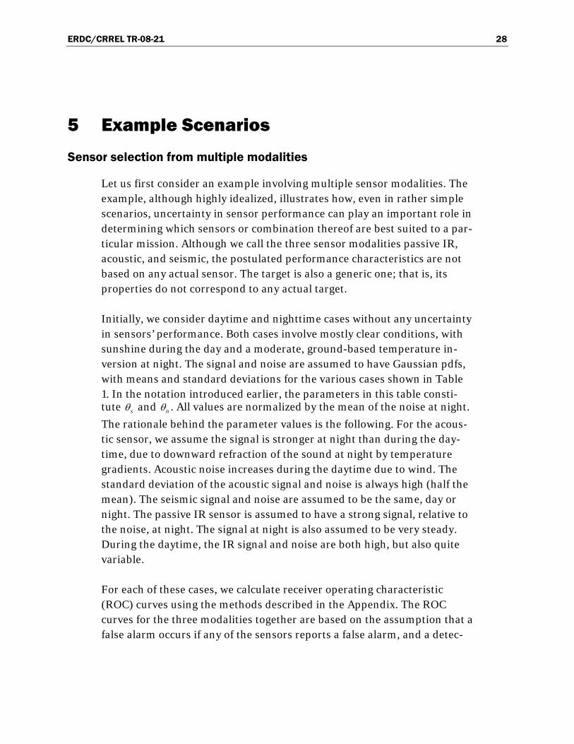
For each of these cases, we calculate receiver operating characteristic (ROC) curves using the methods described in the Appendix. The ROC curves for the three modalities together are based on the assumption that a false alarm occurs if any of the sensors reports a false alarm, and a detec-
ERDC/CRREL TR-08-21 29
Table 1. Signal and noise parameters for illustrative scenario involving multiple sensor modalities.
Modality, Condition
Mean, signal
( )sμ
Standard Deviation, signal
( )sσ
Mean, noise
( )nμ
Standard Deviation, noise
( )nσ
Passive IR, daytime 5 2.5 3 1.5
Passive IR, nighttime 3 0.1 1 0.5
Acoustic, daytime 2 1 2 1
Acoustic, nighttime 3 1.5 1 0.5
Seismic, daytime 2 0.5 1 0.5
Seismic, nighttime 2 0.5 1 0.5
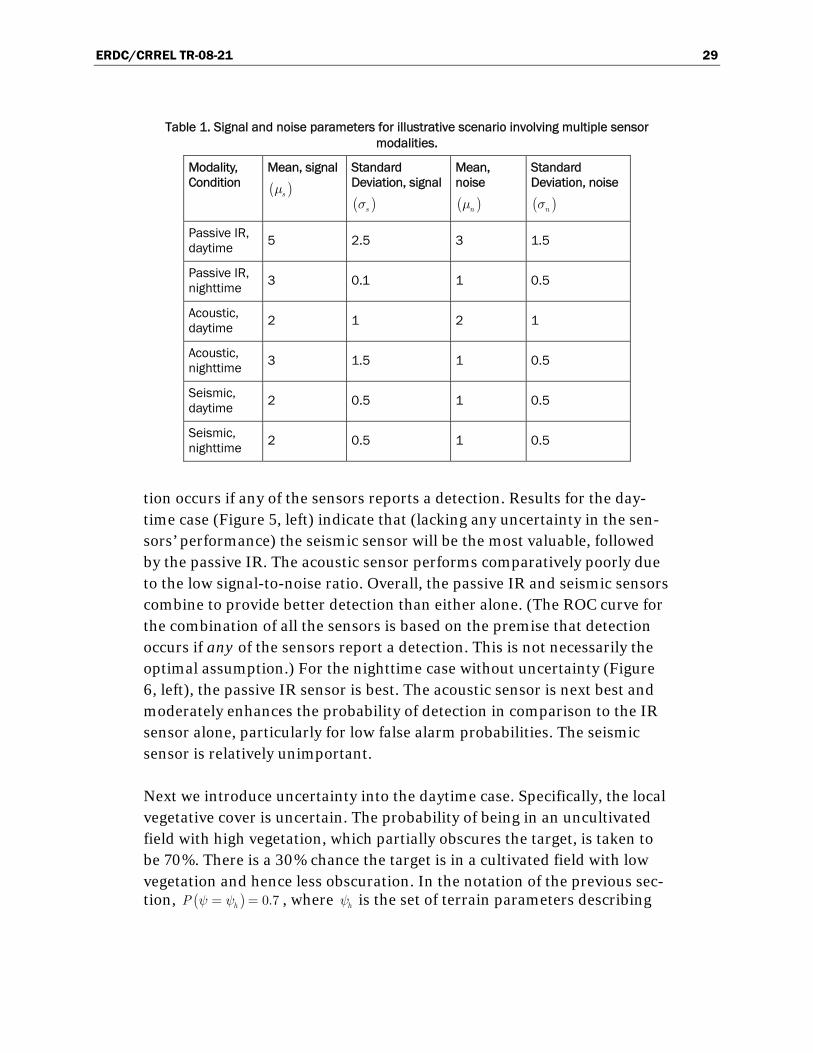
tion occurs if any of the sensors reports a detection. Results for the day-time case (Figure 5, left) indicate that (lacking any uncertainty in the sen-sors’ performance) the seismic sensor will be the most valuable, followed by the passive IR. The acoustic sensor performs comparatively poorly due to the low signal-to-noise ratio. Overall, the passive IR and seismic sensors combine to provide better detection than either alone. (The ROC curve for the combination of all the sensors is based on the premise that detection occurs if any of the sensors report a detection. This is not necessarily the optimal assumption.) For the nighttime case without uncertainty (Figure 6, left), the passive IR sensor is best. The acoustic sensor is next best and moderately enhances the probability of detection in comparison to the IR sensor alone, particularly for low false alarm probabilities. The seismic sensor is relatively unimportant.
Next we introduce uncertainty into the daytime case. Specifically, the local vegetative cover is uncertain. The probability of being in an uncultivated field with high vegetation, which partially obscures the target, is taken to be 70%. There is a 30% chance the target is in a cultivated field with low vegetation and hence less obscuration. In the notation of the previous sec-tion, P , where is the set of terrain parameters describing ( ) 0.7ψ ψ= = ψh h
ERDC/CRREL TR-08-21 30
Figure 5. ROC curves for the daytime case. Calculation on the left assumes with certainty that the sensors are in an open field. The calculation on the right is based on a 70% chance of the sensors being in a field with high vegetation, and 30% chance of the sensors being in a field
with low vegetation.
Figure 6. ROC curves for the nighttime case. Calculation on the left assumes with certainty that there is a moderate temperature inversion. The calculation on the right is based on a 60% chance of a moderate temperature inversion, a 20% chance of a weak temperature
inversion, and a 20% chance of a strong temperature inversion with fog.
the partially obscured case, and , where is the set of ter-
rain parameters for the less obscured case. The mapping
( ) 0.7lP ψ ψ= = lψ
( ), | ,s np θ θ ψ ξ is
assumed to remain crisp. For the less obscured case, the mean of the IR signal is increased from 5 to 8, to represent improved target contrast. The mean seismic noise is doubled in the cultivated field to represent increased vibrations from nearby cultural activity. Now (Figure 5, right), the passive IR sensor typically provides more useful data, although overall the ROC curve is not strongly affected.
ERDC/CRREL TR-08-21 31
Uncertainty is introduced into the nighttime case regarding the strength of the temperature inversion layer (the vertical temperature gradient). The probability of a moderate, ground-based temperature inversion is taken as 60%. The probability of a weak temperature inversion (as typically occurs at night after an intermittent episode of turbulent mixing) is taken to be 20%. For this situation, the acoustic signal mean is reduced from 3 to 2, to represent weaker downward refraction. The probability of a strong tem-perature inversion (as typically occurs at night before an intermittent epi-sode of turbulent mixing) coupled with fog is also taken to be 20%. For this situation, the acoustic signal mean is increased to 5, to represent stronger downward refraction. The IR signal mean is reduced to 0.5 due to obstruction by fog. With this combination of uncertainty, the IR and acoustic sensors are both necessary to maintain a high probability of de-tection (Figure 6, right).
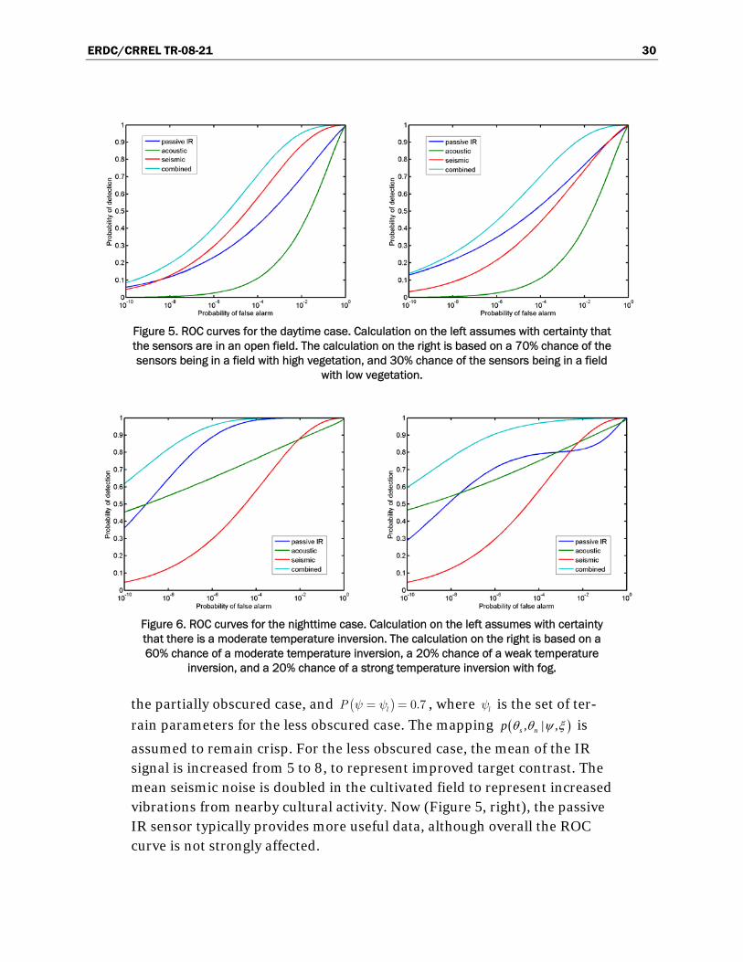
Finally we consider the case where the signal and noise are correlated. Such correlations can occur when the signal and noise are affected by the same phenomenon; for example, infrared detection in fog. In Figure 7, we show the nighttime case with uncertainty as described above, but with cor-relation coefficient , 0.5s nρ = − (left) and , 0.5s nρ = (right). As is most clearly
evident in the seismic ROC curves, negative signal-noise correlation cre-ates a sharper transition between regimes of low and high probability of detection, whereas positive correlation creates a smoother transition. Similar effects can be shown when a nonzero correlation is introduced into the other cases considered earlier.
Figure 7. ROC curves for the nighttime case with uncertainty and , 0.5s nρ = − (left) and
, 0.5s nρ = (right). The other parameters are the same as the ones for the plot on the right of
Figure 6.
ERDC/CRREL TR-08-21 32
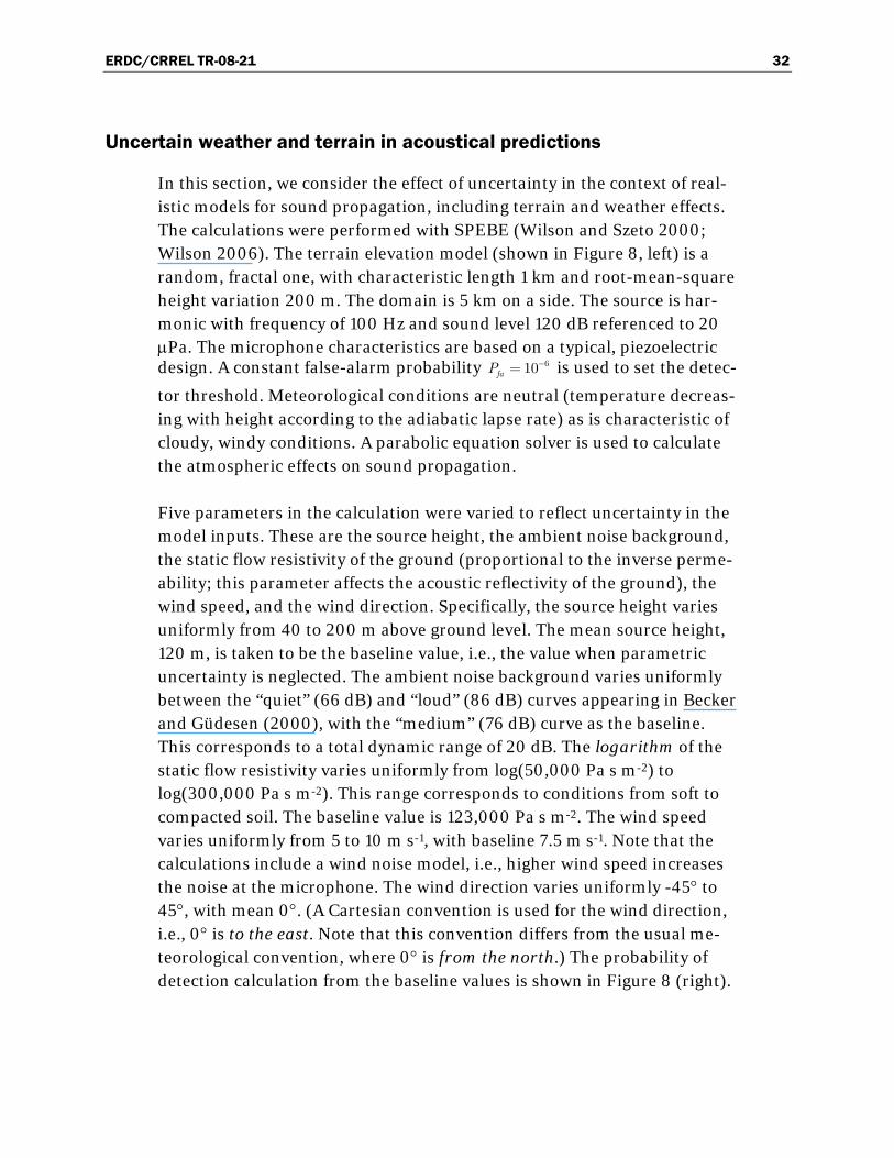
Uncertain weather and terrain in acoustical predictions
In this section, we consider the effect of uncertainty in the context of real-istic models for sound propagation, including terrain and weather effects. The calculations were performed with SPEBE (Wilson and Szeto 2000; Wilson 2006). The terrain elevation model (shown in Figure 8, left) is a random, fractal one, with characteristic length 1 km and root-mean-square height variation 200 m. The domain is 5 km on a side. The source is har-monic with frequency of 100 Hz and sound level 120 dB referenced to 20 μPa. The microphone characteristics are based on a typical, piezoelectric design. A constant false-alarm probability is used to set the detec-
tor threshold. Meteorological conditions are neutral (temperature decreas-ing with height according to the adiabatic lapse rate) as is characteristic of cloudy, windy conditions. A parabolic equation solver is used to calculate the atmospheric effects on sound propagation.
−= 610faP
Five parameters in the calculation were varied to reflect uncertainty in the model inputs. These are the source height, the ambient noise background, the static flow resistivity of the ground (proportional to the inverse perme-ability; this parameter affects the acoustic reflectivity of the ground), the wind speed, and the wind direction. Specifically, the source height varies uniformly from 40 to 200 m above ground level. The mean source height, 120 m, is taken to be the baseline value, i.e., the value when parametric uncertainty is neglected. The ambient noise background varies uniformly between the “quiet” (66 dB) and “loud” (86 dB) curves appearing in Becker and Güdesen (2000), with the “medium” (76 dB) curve as the baseline. This corresponds to a total dynamic range of 20 dB. The logarithm of the static flow resistivity varies uniformly from log(50,000 Pa s m-2) to log(300,000 Pa s m-2). This range corresponds to conditions from soft to compacted soil. The baseline value is 123,000 Pa s m-2. The wind speed varies uniformly from 5 to 10 m s-1, with baseline 7.5 m s-1. Note that the calculations include a wind noise model, i.e., higher wind speed increases the noise at the microphone. The wind direction varies uniformly -45° to 45°, with mean 0°. (A Cartesian convention is used for the wind direction, i.e., 0° is to the east. Note that this convention differs from the usual me-teorological convention, where 0° is from the north.) The probability of detection calculation from the baseline values is shown in Figure 8 (right).
ERDC/CRREL TR-08-21 33
Figure 8. Synthesized terrain elevation model for the acoustic detection calculations (left),
and baseline detection calculation, i.e., the calculation lacking parametric uncertainty (right). Green indicates high probability of detection; red indicates low probability. The source
position is indicated by an “x”. (The sensor position is varied across the terrain.)
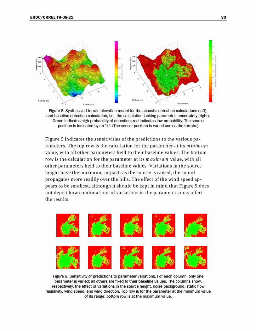
Figure 9 indicates the sensitivities of the predictions to the various pa-rameters. The top row is the calculation for the parameter at its minimum value, with all other parameters held to their baseline values. The bottom row is the calculation for the parameter at its maximum value, with all other parameters held to their baseline values. Variations in the source height have the maximum impact: as the source is raised, the sound propagates more readily over the hills. The effect of the wind speed ap-pears to be smallest, although it should be kept in mind that Figure 9 does not depict how combinations of variations in the parameters may affect the results.
Figure 9. Sensitivity of predictions to parameter variations. For each column, only one parameter is varied; all others are fixed to their baseline values. The columns show,
respectively, the effect of variations in the source height, noise background, static flow resistivity, wind speed, and wind direction. Top row is for the parameter at the minimum value
of its range; bottom row is at the maximum value.
ERDC/CRREL TR-08-21 34
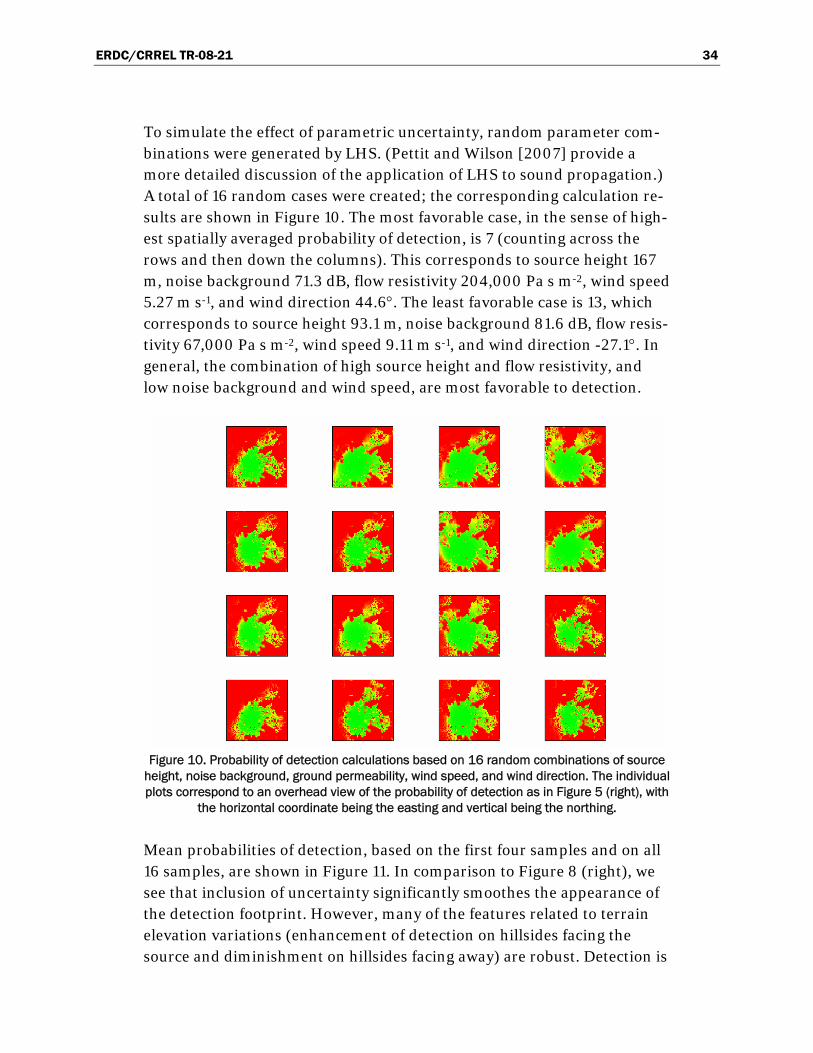
To simulate the effect of parametric uncertainty, random parameter com-binations were generated by LHS. (Pettit and Wilson [2007] provide a more detailed discussion of the application of LHS to sound propagation.) A total of 16 random cases were created; the corresponding calculation re-sults are shown in Figure 10. The most favorable case, in the sense of high-est spatially averaged probability of detection, is 7 (counting across the rows and then down the columns). This corresponds to source height 167 m, noise background 71.3 dB, flow resistivity 204,000 Pa s m-2, wind speed 5.27 m s-1, and wind direction 44.6°. The least favorable case is 13, which corresponds to source height 93.1 m, noise background 81.6 dB, flow resis-tivity 67,000 Pa s m-2, wind speed 9.11 m s-1, and wind direction -27.1°. In general, the combination of high source height and flow resistivity, and low noise background and wind speed, are most favorable to detection.
Figure 10. Probability of detection calculations based on 16 random combinations of source
height, noise background, ground permeability, wind speed, and wind direction. The individual plots correspond to an overhead view of the probability of detection as in Figure 5 (right), with
the horizontal coordinate being the easting and vertical being the northing.
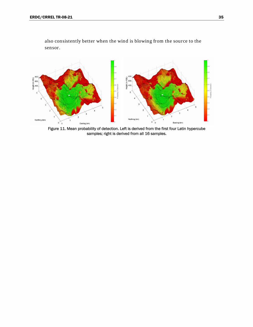
Mean probabilities of detection, based on the first four samples and on all 16 samples, are shown in Figure 11. In comparison to Figure 8 (right), we see that inclusion of uncertainty significantly smoothes the appearance of the detection footprint. However, many of the features related to terrain elevation variations (enhancement of detection on hillsides facing the source and diminishment on hillsides facing away) are robust. Detection is
ERDC/CRREL TR-08-21 35
also consistently better when the wind is blowing from the source to the sensor.
Figure 11. Mean probability of detection. Left is derived from the first four Latin hypercube
samples; right is derived from all 16 samples.
ERDC/CRREL TR-08-21 36
6 Conclusion
Predictions from complex models are much more valuable to decision makers when there is a good understanding of the predictive skill. How-ever, most current decision support tools for recommending sensor mixes and placements do not provide such an understanding. There are a variety of reasons for this state of affairs. First, the quality of the inputs to the DSTs is often in itself poorly understood. Second, the prediction models are often so complex that mapping of uncertainties in the model inputs to their impact on the model outputs is extremely challenging, if not impos-sible. Third, most developers of DSTs are more comfortable with pro-gramming and physical modeling than with statistical assessments of un-certainty and the subsequent decision-making process. With regard to this last point, it needs to be recognized that more complex, computationally intensive physical models may not significantly improve overall predictive skill when other sources of error, such as errors in model inputs, are sub-stantial.
In this report, we have started to address the need for a balanced examina-tion of uncertainties in DST predictions. Some key sources of uncertainty in sensor performance and signature propagation predictions have been described, and a probabilistic framework for assessing uncertainty in these predictions was formulated. Application of the framework is challenging, but provides a rational way forward for development of subsequent, prac-tical implementations. A software architecture was sketched by which un-certainty in weather, terrain, and tactical information can be incorporated into DST predictions. Uncertainty is injected at two stages: first, in the creation of an “ensemble” of environmental/tactical scenarios, and second by introducing variations into signature propagation model inputs.
We used two illustrative examples to show the importance of uncertainty in determining appropriate sensor selections, and in identifying the robust characteristics of sensor performance predictions when multiple sources of uncertainty are present. These examples involved a partial implementa-tion of the concepts described in this report. Future work will attempt to implement the full probabilistic framework and software architecture.
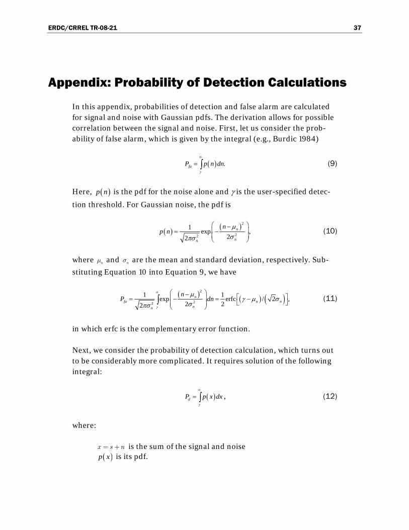
ERDC/CRREL TR-08-21 37
Appendix: Probability of Detection Calculations
In this appendix, probabilities of detection and false alarm are calculated for signal and noise with Gaussian pdfs. The derivation allows for possible correlation between the signal and noise. First, let us consider the prob-ability of false alarm, which is given by the integral (e.g., Burdic 1984)
(9) ( ) .faP p n dγ
∞
= ∫ n
Here, ( )p n is the pdf for the noise alone and γ is the user-specified detec-
tion threshold. For Gaussian noise, the pdf is
( ) ( )2
22
1 exp ,22
n
nn
np n
μσπσ
⎛ ⎞−⎜= −⎜⎝ ⎠
⎟⎟
(10)
where and are the mean and standard deviation, respectively. Sub-
stituting Equation 10 into Equation 9, we have nμ nσ
( ) ( ) ( )2
22
1 1exp erfc / 2 ,2 22
nfa n n
nn
nP dn
γ
μγ μ σ
σπσ
∞ ⎛ ⎞− ⎡ ⎤⎜ ⎟= − = −⎣ ⎦⎜ ⎟⎝ ⎠
∫ (11)
in which erfc is the complementary error function.
Next, we consider the probability of detection calculation, which turns out to be considerably more complicated. It requires solution of the following integral:
, (12) ( )dP p x dγ
∞
= ∫ x
where:
x s n= + is the sum of the signal and noise ( )p x is its pdf.
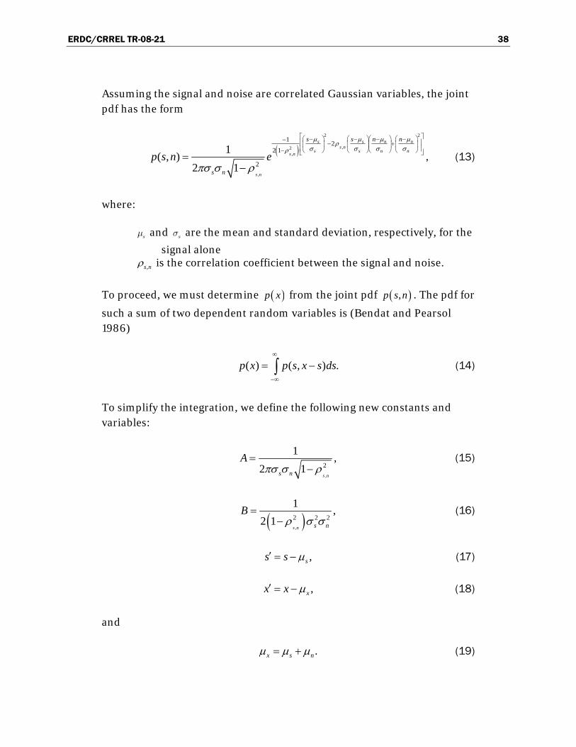
ERDC/CRREL TR-08-21 38
Assuming the signal and noise are correlated Gaussian variables, the joint pdf has the form
( )2 2
,2,
,
1 22 1
2
1( , )2 1
s s ns n
s s ns n
s n
s s n n
s n
p s n e
μ μ μρ
σ σ σ σρ
πσ σ ρ
n
n
μ⎡ ⎤⎛ ⎞ ⎛ ⎞⎛ ⎞ ⎛ ⎞− − − −− ⎢ ⎥− +⎜ ⎟ ⎜ ⎟⎜ ⎟ ⎜ ⎟⎢ ⎥− ⎝ ⎠ ⎝ ⎠⎝ ⎠ ⎝ ⎠⎣ ⎦=
−, (13)
where:
sμ and are the mean and standard deviation, respectively, for the
signal alone sσ
,s nρ is the correlation coefficient between the signal and noise.
To proceed, we must determine ( )p x from the joint pdf ( ),p s n . The pdf for
such a sum of two dependent random variables is (Bendat and Pearsol 1986)
( ) ( , ) .p x p s x s d∞
−∞
= −∫ s (14)
To simplify the integration, we define the following new constants and variables:
,
2
1 ,2 1
s ns n
Aπσ σ ρ
=−
(15)
( ),
2 2 2
1 ,2 1
s n s n
Bρ σ σ
=−
(16)
,ss s μ′ = − (17)
,xx x μ′ = − (18)
and
.x s nμ μ μ= + (19)
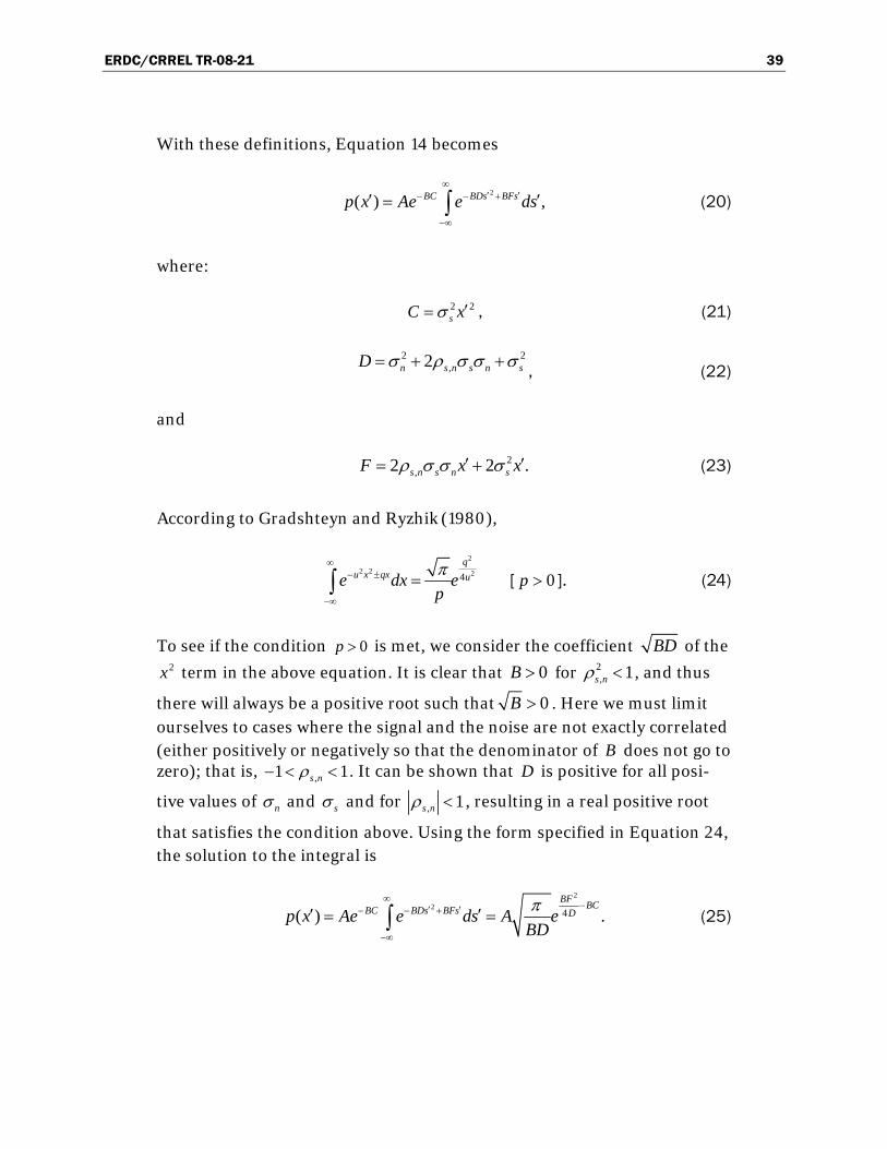
ERDC/CRREL TR-08-21 39
With these definitions, Equation 14 becomes
2
( ) ,BC BDs BFsp x Ae e ds∞
′ ′− − +
−∞
′ ′= ∫ (20)
where:
2 2sC xσ ′= , (21)
2 2
,2n s n s n sD σ ρ σ σ σ= + +, (22)
and
2,2 2s n s n sF xρ σ σ σ .x′ ′= + (23)
According to Gradshteyn and Ryzhik (1980),
2
2 2 24q
u x qx ue dx epπ∞
− ±
−∞
=∫ [ ]. (24) 0p >
To see if the condition is met, we consider the coefficient 0p > BD of the 2x term in the above equation. It is clear that for 0B > 2
, 1s nρ < , and thus
there will always be a positive root such that 0B > . Here we must limit ourselves to cases where the signal and the noise are not exactly correlated (either positively or negatively so that the denominator of B does not go to zero); that is, ,1 s n 1ρ− < < . It can be shown that is positive for all posi-
tive values of
D
nσ and sσ and for , 1s nρ < , resulting in a real positive root
that satisfies the condition above. Using the form specified in Equation 24, the solution to the integral is
2
24( ) .BF BCBC BDs BFs Dp x Ae e ds A e
BDπ∞
−′ ′− − +
−∞
′ ′= =∫ (25)

ERDC/CRREL TR-08-21 40
With some simplification, we find the following Gaussian pdf for x:
( )2
2
1( ) exp ,22
x
xx
xp x
μσσ π
⎛ ⎞−= −⎜ ⎟
⎜ ⎟⎝ ⎠
(26)
in which the mean is x s nμ μ μ= + and the variance is 2 2
,2 2x n s n s n sσ σ ρ σ σ σ= + + . Now, the calculation of the probability of detec-
tion proceeds exactly as it did for the probability of false alarm, and we have
( ) ( ) ( )2
22
1 1exp erfc / 2 .2 22
xd x x
xx
xP dx
γ
μγ μ σ
σπσ
∞ ⎛ ⎞− ⎡ ⎤⎜ ⎟= − = −⎣ ⎦⎜ ⎟⎝ ⎠
∫ (27)
To determine the ROC curve, the threshold γ is varied in Equations 11 and 27 and then is plotted versus for each value of γ. dP faP

ERDC/CRREL TR-08-21 41
References
Abramowitz, M., and I. A. Stegun. 1984. Pocketbook of mathematical functions. Frankfurt, Germany: Verlag Harri Deutsch.
Allen, M., D. Frame, J. Kettleborough, and D. Stainforth. 2006. Model error in weather and climate forecasting. In Predictability of weather and climate, ed. T. Palmer and R. Hagedorn, 392–427. Cambridge, UK: Cambridge University Press.
Ayyub, B. M., and R.-J. Chao. 1998. Uncertainty modeling in civil engineering with structural and reliability applications. In Uncertainty modeling and analysis in civil engineering, ed. B. M. Ayyub, 3–32. Baca Raton, FL: CRC Press.
Becker, G., and A. Güdesen. 2000. Passive sensing with acoustics on the battlefield. Appl. Acoust. 59:149–178.
Bendat, J. S., and A. G. Pearsol. 1986. Random data. New York: Wiley & Sons.
Burdic, W. S. 1984. Underwater acoustic system analysis. Englewood Cliffs, NJ: Prentice-Hall.
Frey, H. C. 1998. Quantitative analysis of variability and uncertainty in energy and environmental systems. In Uncertainty modeling and analysis in civil engineering, ed. B. M. Ayyub, 381–423. Boca Raton , FL: CRC Press.
Gananapandithan, N., and B. Natarajan. 2007. Decentralised sensor network performance with correlated observations. Int. J. Sensor Networks 2:179–187.
Gradshteyn, I. S., and I. M. Ryzhik. 1980. Table of integrals, series, and products. San Diego, CA: Academic Press.
Hieb, M. R., S. Mackay, M. W. Powers, H. Yu, M. Kleiner, and J. M. Pullen. 2007. Geospatial challenges in a net centric environment: actionable information technology, design, and implementation. In SPIE Defense and Security Symposium, Defense Transformation and Net-Centric Systems, ed. R. Suresh, 657816. Orlando, FL.
Kalnay, E. 2003. Atmospheric modeling, data assimilation, and predictability. Cambridge, UK: Cambridge University Press.
Maurer, D. E., R. W. Schirmer, M. K. Kalandros, and J. S. J. Peri. 2006. Sensor fusion architectures for ballistic missile defense. Johns Hopkins APL Technical Digest 27(1):19–31.
Palmer, T. 2006. Predictability of weather and climate: from theory to practice. In Predictability of weather and climate, ed. T. Palmer and R. Hagedorn, 1–30. Cambridge, UK: Cambridge University Press.
Pettit, C. L., and D. K. Wilson. 2007. Proper orthogonal decomposition and cluster weighted modeling for sensitivity analysis of sound propagation in the atmospheric surface layer. J. Acoust. Soc. Am. 122:1374–1390.

ERDC/CRREL TR-08-21 42
Wilson, D. K. 2006. Sensor performance evaluator for battlefield environments (SPEBE) tutorial. ERDC/CRREL Technical Report TR-06-12. Hanover, NH: Cold Regions Research and Engineering Laboratory, U.S. Army Engineer Research and Development Center.
Wilson, D. K., D. H. Marlin, and S. Mackay. 2007. Acoustic/seismic signal propagation and sensor performance modeling. In SPIE Defense and Security Symposium, Unattended Ground, Sea, and Air Sensor Technologies and Applications IX, ed. E. M. Carapezza, 65620R. Orlando, FL.
Wilson, D. K., J. M. Noble, B. H. VanAartsen, and G. L. Szeto. 2001. Battlefield decision aid for acoustical ground sensors with interface to meteorological data sources. In SPIE AeroSense Symposium, Battlespace Digitization and Network-Centric Warfare, ed. R. Suresh, 208–219. Orlando, FL.
Wilson, D. K., and G. L. Szeto. 2000. Reference guide for the acoustic battlefield aid (ABFA) version 2. Army Research Laboratory Technical Report ARL-TR-2159. Adelphi, ND: Army Research Laboratory.

REPORT DOCUMENTATION PAGE Form Approved
OMB No. 0704-0188 Public reporting burden for this collection of information is estimated to average 1 hour per response, including the time for reviewing instructions, searching existing data sources, gathering and maintaining the data needed, and completing and reviewing this collection of information. Send comments regarding this burden estimate or any other aspect of this collection of information, including suggestions for reducing this burden to Department of Defense, Washington Headquarters Services, Directorate for Information Operations and Reports (0704-0188), 1215 Jefferson Davis Highway, Suite 1204, Arlington, VA 22202-4302. Respondents should be aware that notwithstanding any other provision of law, no person shall be subject to any penalty for failing to comply with a collection of information if it does not display a currently valid OMB control number. PLEASE DO NOT RETURN YOUR FORM TO THE ABOVE ADDRESS.
1. REPORT DATE (DD-MM-YYYY) November 2008
2. REPORT TYPE Technical Report
3. DATES COVERED (From - To)
5a. CONTRACT NUMBER
5b. GRANT NUMBER
4. TITLE AND SUBTITLE
Addressing Uncertainty in Signal Propagation and Sensor Per-
formance Predictions 5c. PROGRAM ELEMENT NUMBER
5d. PROJECT NUMBER
5e. TASK NUMBER
6. AUTHOR(S)
D. Keith Wilson, Chris L. Pettit, Sean Mackay, Matthew S.
Lewis, and Peter M. Seman 5f. WORK UNIT NUMBER
7. PERFORMING ORGANIZATION NAME(S) AND ADDRESS(ES) 8. PERFORMING ORGANIZATION REPORT NUMBER
U.S. Army Engineer Research and Development Center Cold Regions Research and Engineering Laboratory 72 Lyme Road Hanover, NH 03755-1290
ERDC/CRREL TR-08-21
9. SPONSORING / MONITORING AGENCY NAME(S) AND ADDRESS(ES) 10. SPONSOR/MONITOR’S ACRONYM(S)
11. SPONSOR/MONITOR’S REPORT NUMBER(S)
12. DISTRIBUTION / AVAILABILITY STATEMENT Approved for public release; distribution is unlimited.13. SUPPLEMENTARY NOTES
14. ABSTRACT
As advanced sensors are increasingly relied upon for force protection, rapid strike, maneu-ver support, and other tasks, expert decision support tools (DSTs) are needed to recommend appropriate mixes of sensors and placements that will maximize their effectiveness. These tools should predict effects on sensor performance of the many complexities of the environ-ment, such as terrain conditions, the atmospheric state, and background noise and clutter. However, the information available for such inputs is often incomplete and imprecise. To avoid drawing unwarranted conclusions from DSTs, the calculations should reflect a realis-tic degree of uncertainty in the inputs. In this report, a Bayesian probabilistic framework is developed for this purpose. The initial step involves incorporating uncertainty in the weather forecast, terrain state, and tactical situation by constructing an ensemble of sce-narios. Next, a likelihood function for the signal propagation model parameters specifies uncertainty at smaller spatial scales, such as that caused by wind gusts, turbulence, clouds, vegetation, and buildings. An object-oriented software implementation of the frame-work is sketched. Examples illustrate the importance of uncertainty for optimal sensor se-lection and determining sensor coverage.
15. SUBJECT TERMS
battlespace sensor modeling, decision support tools, uncertainty, weather effects
16. SECURITY CLASSIFICATION OF: 17. LIMITATION OF ABSTRACT
18. NUMBER OF PAGES
19a. NAME OF RESPONSIBLE PERSON
a. REPORT
U b. ABSTRACT
U c. THIS PAGE
U U 51 19b. TELEPHONE NUMBER (include area code)
Standard Form 298 (Re . 8-98) vPrescribed by ANSI Std. 239.18
Related Documents