Additive compilation to achieve high-performance on GPUs Ulysse Beaugnon 1 , Basile Clément 2 , Albert Cohen 1 , Andi Drebes 2 , Nicolas Tollenaere 3 October 5, 2020 1 Google 2 Inria et École Normale Supérieure 3 Inria et Université Grenoble-Alpes 1

Welcome message from author
This document is posted to help you gain knowledge. Please leave a comment to let me know what you think about it! Share it to your friends and learn new things together.
Transcript

Additive compilation to achievehigh-performance on GPUs
Ulysse Beaugnon1, Basile Clément2, Albert Cohen1, Andi Drebes2, NicolasTollenaere3
October 5, 2020
1Google
2Inria et École Normale Supérieure
3Inria et Université Grenoble-Alpes
1

Achieving high performance onGPUs

GPU architecture 101
GPUs are designed for throughput of highly parallel computations
On my laptop:
8 SMs× 128 compute cores per SM= 1024 compute cores (1.16 TFLOP/s for $250)
(vs 4 cores x 2 units x 8 vector = 64 on my CPU – 0.25 TFLOP/s for$450)
2

GPU architecture 101
GPUs are designed for throughput of highly parallel computations
On my laptop:
8 SMs× 128 compute cores per SM= 1024 compute cores (1.16 TFLOP/s for $250)
(vs 4 cores x 2 units x 8 vector = 64 on my CPU – 0.25 TFLOP/s for$450)
2
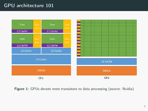
GPU architecture 101
Figure 1: GPUs devote more transistors to data processing (source: Nvidia)
3

GPU architecture 101
L2
RAM
L1 Shared
execution units
control control. . .SMX 0
L1 Shared
execution units
control control. . .SMX 1
Executes:
• threads (32x)
• blocks
Hierarchical parallelism
• SIMD model with 2 levels of parallelism
• Blocks are assigned to SMs
• Inside each SM, warps (group of 32 threads) are assigned toschedulers
4

Proto-language
// i: index variable// x: array variable// v: constant value// P: parameter
// Index expressionei ::= i | ei + ei | ei * P// Expressione ::= x[i, ..., i] | v
| e - e | e + e | e * e | fma(e, e, e)// Statements ::= x[i, ..., i] = e | i = ei
| s ; s | loop i in P do s
5

Case study: matrix multiplication
loop i in N doloop j in M do
C[i, j] = 0 ;loop k in P do
// C[i, j] += A[i, k] * B[k, j]C[i, j] = fma(C[i, j], A[i, k], B[k, j])
Compute-bound:
• NP + MP loads
• NM stores
• 2NMP FLOP
6

Case study: matrix multiplication
Strip-mine the loops to enable parallelism
loop i1 in N/Nt doloop i2 in Nt do
i = i1 * Nt + i2loop j1 in M/Mt do
loop j2 in Mt doj = j1 * Mt + j2C[i, j] = 0 ;loop k in P do
// C[i, j] += A[i, k] * B[k, j]C[i, j] = fma(C[i, j], A[i, k], B[k, j])
Something missing? Remainders!
7

Case study: matrix multiplication
Strip-mine the loops to enable parallelism
loop i1 in N/Nt doloop i2 in Nt do
i = i1 * Nt + i2loop j1 in M/Mt do
loop j2 in Mt doj = j1 * Mt + j2C[i, j] = 0 ;loop k in P do
// C[i, j] += A[i, k] * B[k, j]C[i, j] = fma(C[i, j], A[i, k], B[k, j])
Something missing?
Remainders!
7

Case study: matrix multiplication
Strip-mine the loops to enable parallelism
loop i1 in N/Nt doloop i2 in Nt do
i = i1 * Nt + i2loop j1 in M/Mt do
loop j2 in Mt doj = j1 * Mt + j2C[i, j] = 0 ;loop k in P do
// C[i, j] += A[i, k] * B[k, j]C[i, j] = fma(C[i, j], A[i, k], B[k, j])
Something missing? Remainders!
7

Case study: matrix multiplication
Reorder the loops and use parallelism
loop.block i1 in N/Nt doloop.block j1 in M/Mt do
loop.thread i2 in Nt doloop.thread j2 in Mt do
i = i1 * Nt + i2j = j1 * Mt + j2C[i, j] = 0 ;loop k in P do
// C[i, j] += A[i, k] * B[k, j]C[i, j] = fma(C[i, j], A[i, k], B[k, j])
8

Case study: matrix multiplication
Are we done?
No. 2NMP loads! 10x slower than CPU.
9

Case study: matrix multiplication
Are we done?
No. 2NMP loads! 10x slower than CPU.
9

Shared memory blocking
Figure 2: Matrix multiplication with shared memory (Nervana Systems)
10

Shared memory blocking
loop.block i1 in N/32, j1 in M/32 doloop.thread i2 in 32, j2 in 32 do
C[i1 * 32 + i2, j1 * 32 + j2] = 0
loop k1 in P/32 doloop.thread k2 in 32, ij2 in 32 do
As[k2, ij2] = A[i1 * 1024 + ij2 , k1 * 32 + k2]Bs[k2, ij2] = B[k1 * 32 + k2, j1 * 1024 + ij2]
loop.thread i2 in 32, j2 in 32 doi, j = ...loop k2 in 32 do
C[i, j] = fma(C[i, j],As[k2, i2],Bs[k2, j2])
11

Case study: matrix multiplication
What did we do?
• Loop splitting, interchange and fusion
• Parallelization
• Picking tile sizes (surprisingly hard)
• Temporary copies (including layout!)
• Bonus: register allocation, double buffering, . . .
All of this is "easy" to do; what is hard is figuring out what to do.
12

Additive compilation

Compilation as an Optimization Problem
Given:
• A source language S
• A program s in language S
• A target language T
• A concrete machine M to execute T
Solve:
argmaxt∈TperfM(t)
Under the constraint:t ∼ s
13

Separate schedule from algorithm (Halide)
Algorithm
Var i, j;RDom k;Func P("P"), C("C");P(i, j) = 0P(i, j) += A(i, k)
* B(k, j)C(i, j) = P(i, j)
Schedule
C.tile(x, y, xi, yi ,24, 32)
.fuse(x, y, xy)
.parallel(xy)
.vectorize(xi, 8)
.unroll(xi);
// ...
14

Code Transformation and Phase Ordering
Vectorizing scalar product (Lift)
λ (x, y) 7→ zip(x, y) » map(×) » reduce(+, 0)
λ (x, y) 7→ zip(asVector(n, x), asVector(n, y))» map(vectorize(n, ×))» asScalar» reduce(+, 0)
Rewrite rule
Code transformations suffer from the phase ordering problem.Can we do better?
15

Code Transformation and Phase Ordering
Vectorizing scalar product (Lift)
λ (x, y) 7→ zip(x, y) » map(×) » reduce(+, 0)
λ (x, y) 7→ zip(asVector(n, x), asVector(n, y))» map(vectorize(n, ×))» asScalar» reduce(+, 0)
Rewrite rule
Code transformations suffer from the phase ordering problem.
Can we do better?
15

Code Transformation and Phase Ordering
Vectorizing scalar product (Lift)
λ (x, y) 7→ zip(x, y) » map(×) » reduce(+, 0)
λ (x, y) 7→ zip(asVector(n, x), asVector(n, y))» map(vectorize(n, ×))» asScalar» reduce(+, 0)
Rewrite rule
Code transformations suffer from the phase ordering problem.Can we do better?
15
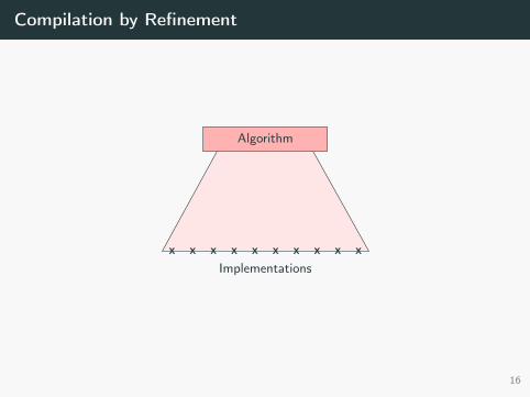
Compilation by Refinement
Algorithm
x x x x x x x x x xImplementations
16
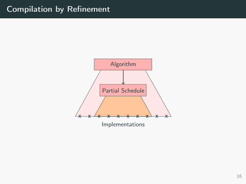
Compilation by Refinement
Algorithm
Partial Schedule
x x x x x x x x x xImplementations
16
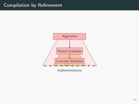
Compilation by Refinement
Algorithm
Partial Schedule
Concrete Schedulex x x x x x x x x x
Implementations
16

Choices for Linear Algebra on GPU
• Control flow structure (sequential ordering, nesting and fusion)order : Statements× Statements→ {before, after, in, out, merged}
• Dimensions implementationdim_kind : Dimensions→ {loop, unroll, vector, thread, block}
• Mapping to hardware thread dimensionsthread_mapping : StaticDims× StaticDims→ {none, same, in, out}
• Tile sizessize : StaticDims→ N
• Memory spacemem_space : Memory→ {global, shared}
• Cache levels to usecache : MemAccess→ {L1, L2, read_only, none}
17
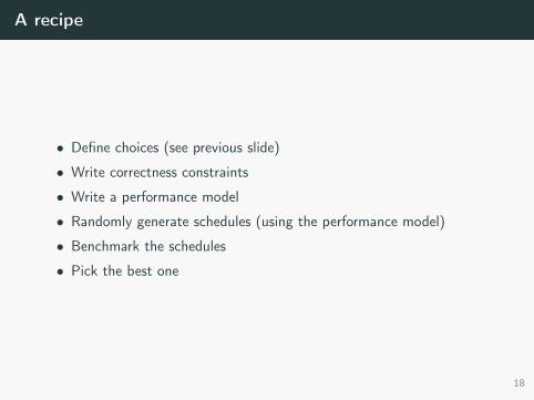
A recipe
• Define choices (see previous slide)
• Write correctness constraints
• Write a performance model
• Randomly generate schedules (using the performance model)
• Benchmark the schedules
• Pick the best one
18

Additivity
• The algorithm define objects (loops, arrays, instructions, . . . )
• Objects have properties (order, dim_kind, . . . )
• Schedules• Add information about property values• Add new objects without losing information on existing objects
19

Optimistic performance model
. . .
. . .
. . .
B(c) = 5ms
t = 4msExecution time ≥ 5ms
20

Branch and Bound
. . .
. . .
. . .
B(c) = 5ms
t = 4msExecution time ≥ 5ms
20

Branch and Bound
. . .
. . .
. . .
B(c) = 5ms
t = 4msExecution time ≥ 5ms
20

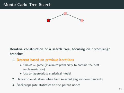
Monte Carlo Tree Search
t = 8ms
Iterative construction of a search tree, focusing on "promising"branches
1. Descent based on previous iterations• Choice = game (maximize probability to contain the best
implementation)• Use an appropriate statistical model
2. Heuristic evaluation when first selected (eg random descent)
3. Backpropagate statistics to the parent nodes21

Model of the Hardware
L2
RAM
L1 Shared
execution units
warp warp. . .SMX 0
L1 Shared
execution units
warp warp. . .SMX 1
Executes:
• threads
• blocks of threads
• the entire kernel
Hierarchical Parallelism• η1 threads in a block, η2 blocks in a kernel
• Limited resources at each level (bottlenecks)• e.g. execution units, memory bandwidth
22

Performance Model
Global ModelGlobal Bottlenecks
Block ModelBlock Bottlenecks
Thread ModelThread Bottlenecks
• Recursive model to account for bottlenecks at each parallelism level("hierarchical roofline")
• Separate model for dependencies within a thread
Bottleneck Model
23

Performance Model
Global ModelGlobal Bottlenecks
Block ModelBlock Bottlenecks
Thread ModelThread Bottlenecks
• Recursive model to account for bottlenecks at each parallelism level("hierarchical roofline")
• Separate model for dependencies within a thread
Bottleneck Model
23

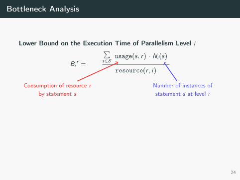
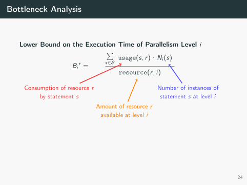
Bottleneck Analysis
Lower Bound on the Execution Time of Parallelism Level i
Bir =
maxr∈R
∑s∈S
usage(s, r) . Ni (s)
resource(r , i)
Consumption of resource r
by statement sNumber of instances ofstatement s at level i
Amount of resource r
available at level i
Optimize usage(s, r) and Ni (s) separately⇒ Local Optimistic Assumptions
24

Bottleneck Analysis
Lower Bound on the Execution Time of Parallelism Level i
Bi
r
= maxr∈R
∑s∈S
usage(s, r) . Ni (s)
resource(r , i)
Consumption of resource r
by statement sNumber of instances ofstatement s at level i
Amount of resource r
available at level i
Optimize usage(s, r) and Ni (s) separately⇒ Local Optimistic Assumptions
24
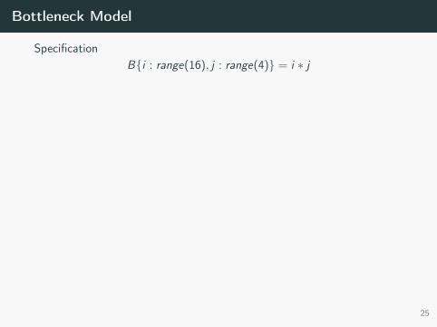
Bottleneck Model
SpecificationB{i : range(16), j : range(4)} = i ∗ j
Implementations
for i in range (16): # Loop Ifor j in range (4): # Loop J
B[i, j] = i * j # imul
for j in range (4): # Loop Jfor i in range (16): # Loop I
B[i, j] = i * j # imul
Minimal number of instances
• imul: N ≥ size(M)× size(N) = 64• I: N ≥ 1 (when outermost)• J: N ≥ 1 (when outermost)
25
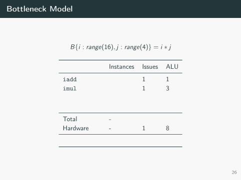
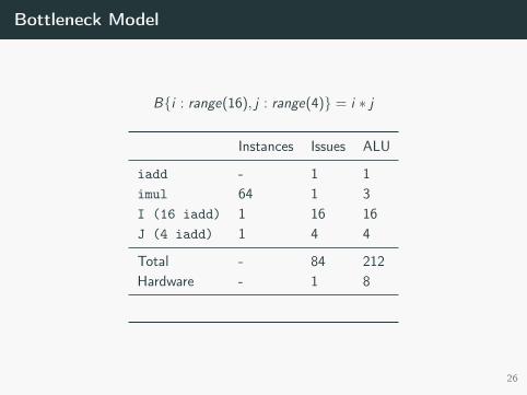
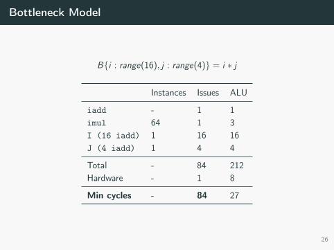
Bottleneck Model
B{i : range(16), j : range(4)} = i ∗ j
Instances Issues ALU
iadd
-
1 1imul
64
1 3
I (16 iadd)
1
J (4 iadd)
1
Total -
84 212
Hardware - 1 8
Min cycles - 84 27
26

Bottleneck Model
B{i : range(16), j : range(4)} = i ∗ j
Instances Issues ALU
iadd
-
1 1imul
64
1 3I (16 iadd)
1
16 16J (4 iadd)
1
4 4
Total -
84 212
Hardware - 1 8
Min cycles - 84 27
26

Bottleneck Model
B{i : range(16), j : range(4)} = i ∗ j
Instances Issues ALU
iadd - 1 1imul 64 1 3I (16 iadd) 1 16 16J (4 iadd) 1 4 4
Total -
84 212
Hardware - 1 8
Min cycles - 84 27
26
Bottleneck Model
B{i : range(16), j : range(4)} = i ∗ j
Instances Issues ALU
iadd - 1 1imul 64 1 3I (16 iadd) 1 16 16J (4 iadd) 1 4 4
Total - 84 212Hardware - 1 8
Min cycles - 84 27
26
Bottleneck Model
B{i : range(16), j : range(4)} = i ∗ j
Instances Issues ALU
iadd - 1 1imul 64 1 3I (16 iadd) 1 16 16J (4 iadd) 1 4 4
Total - 84 212Hardware - 1 8
Min cycles - 84 27
26

Optimistic Performance Model
Global ModelGlobal Bottlenecks
Block ModelBlock Bottlenecks
Thread ModelThread Bottlenecks
• Recursive model to account for bottlenecks at each parallelism level("hierarchical roofline")
• Separate model for dependencies within a thread
Parallelism Model
27

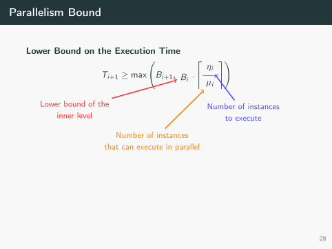
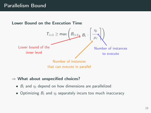
Parallelism Bound
Lower Bound on the Execution Time
Ti+1 ≥ max
(Bi+1, Bi
.
⌈ηi
µi
⌉)
Lower bound of theinner level
Number of instancesto execute
Number of instancesthat can execute in parallel
⇒ What about unspecified choices?
• Bi and ηi depend on how dimensions are parallelized
• Optimizing Bi and ηi separately incurs too much inaccuracy
28
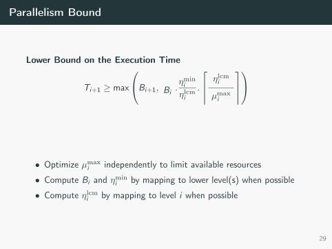
Parallelism Bound
Lower Bound on the Execution Time
Ti+1 ≥ max
Bi+1, Bi.ηmini
ηlcmi
.
ηlcmi
µmaxi
• Optimize µmaxi independently to limit available resources
• Compute Bi and ηmini by mapping to lower level(s) when possible
• Compute ηlcmi by mapping to level i when possible
29

Bottleneck Model
Instances Issues ALU
Threads
imul 64 1 3I (16 iadd) 1 16 16J (4 iadd) 1 4 4
Total - 84 212Hardware - 1 8
32
Min cycles - 84 27
Bthread = 84
Minimize overhead independently
ηminthread = 1 ηlcm
thread = 64
Bblock = 64× 164×⌈6432
⌉
30

Parallelism Model
Instances Issues ALU Threads
imul 64 1 3I
(16 iadd)
1 0 0J
(4 iadd)
1 0 0
Total - 64 192Hardware - 1 8 32
Min cycles - 64 24
Bthread = 64
Minimize overhead independently
ηminthread = 1 ηlcm
thread = 64
Bblock = 64× 164×⌈6432
⌉
30

Parallelism Model
Instances Issues ALU Threads
imul 64 1 3I
(16 iadd)
1 0 0J
(4 iadd)
1 0 0
Total - 64 192Hardware - 1 8 32
Min cycles - 64 24
Bthread = 64
Minimize overhead independently
ηminthread = 1 ηlcm
thread = 64
Bblock = 64× 164×⌈6432
⌉30

Parallelism Model
• Doesn’t need to be precise
• Used to prune catastrophic schedules
31
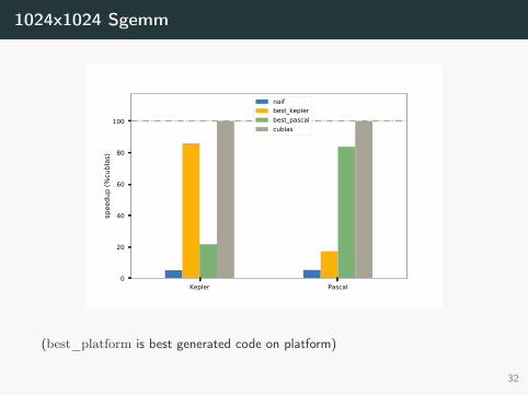
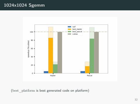
1024x1024 Sgemm
Kepler Pascal0
20
40
60
80
100
spee
dup
(%cu
blas
)naifbest_keplerbest_pascalcublas
(best_platform is best generated code on platform)
32
1024x1024 Sgemm
Kepler Pascal0
20
40
60
80
100
spee
dup
(%cu
blas
)naifbest_keplerbest_pascalcublas
(best_platform is best generated code on platform)
32

1024x1024 Sgemm
Kepler Pascal0
20
40
60
80
100
spee
dup
(%cu
blas
)
LiftTelamoncuBLAS 10.0TritonAutoTVMTensor Comprehensions
• Lift [2]: Rewrite rules + heuristics + exhaustive search• Triton [3]: Skeleton + exhaustive search• AutoTVM [1] (from [3]): Transformations + statistical cost model• Tensor Comprehensions [4] (from [3]): Polyhedral compilation
33

Is this correct?

Formalisation in Coq
Work in progress — Comments welcome!
34

Key ideas
• Only check the concrete generated schedule w.r.t. the algorithm (=do not verify the constraints or performance model)
• Use validation: keep enough information in the schedule to mapindices back to the original semantic indices
• A hierarchy of language: from generic and structured to concrete
35

Semantic indices and explicit reductions
i = ...j = ...D[i : M, j : N, k : {-1}] = 0D[i : M, j : N, k : P] = fma(
D[i, j, k - 1], A[i, k], B[k, j])C[i : M, j : N] = proj[k = P - 1](D[i, j, k])
• The union of domains matches the domains in the algorithm
• The domains are covered by the iterations
• Typing rules to ensure dependencies are respected
36

Typing rule: non-interference
`1, . . . , `n ⊆ dom(I) I|`1, . . . , `n; ∆ ` e : V x 6∈ ∆
I; ∆ ` x [`1, . . . , `n] = e : x [`1, . . . , `n]
During execution, a memory location x [i1, . . . , in] is either undefinedor has an unique value matching its definition.
37
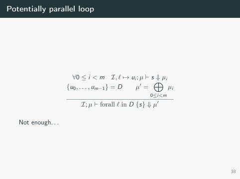
Potentially parallel loop
∀0 ≤ i < m I, ` 7→ ui ;µ ` s ⇓ µi
{u0, . . . , um−1} = D µ′ =⊕
0≤i<m
µi
I;µ ` forall ` in D {s} ⇓ µ′
Not enough. . .
38

And more. . .
• Traditional lowering compiler once the schedule is fixed
• GPU semantics? Hierarchical parallelism
39
References i
References
[1] Tianqi Chen, Thierry Moreau, Ziheng Jiang, Haichen Shen, Eddie Q.Yan, Leyuan Wang, Yuwei Hu, Luis Ceze, Carlos Guestrin, and ArvindKrishnamurthy. TVM: end-to-end optimization stack for deeplearning. CoRR, 2018.
[2] Michel Steuwer, Toomas Remmelg, and Christophe Dubach. Matrixmultiplication beyond auto-tuning: Rewrite-based gpu codegeneration. In Proceedings of the International Conference onCompilers, Architectures and Synthesis for Embedded Systems,CASES ’16, pages 15:1–15:10, New York, NY, USA, 2016. ACM.
40

References ii
[3] Philippe Tillet, H. T. Kung, and David Cox. Triton: An intermediatelanguage and compiler for tiled neural network computations. InProceedings of the 3rd ACM SIGPLAN International Workshop onMachine Learning and Programming Languages, MAPL 2019, pages10–19, New York, NY, USA, 2019. ACM.
[4] Nicolas Vasilache, Oleksandr Zinenko, Theodoros Theodoridis, PriyaGoyal, Zachary DeVito, William S. Moses, Sven Verdoolaege, AndrewAdams, and Albert Cohen. Tensor comprehensions:Framework-agnostic high-performance machine learning abstractions.CoRR, abs/1802.04730, 2018.
41

Thank you
• Optimization Space Pruning Wihout Regrets, CC 2017⇒ Idea of candidates and primitive lower bound performance model
• On the Representation of Partially Specified Implementationsand its Application to the Optimization of Linear AlgebraKernels on GPU, preprint arXiv⇒ Formalization of candidates as CSPs and statistical search
• https://github.com/ulysseB/telamon
42
Related Documents