Adding Value to Existing Models of International Agricultural ...

United States Department of Agriculture

Economic Research Service

Technical Bulletin Number 1833

C^

Adding Value to Existing Models of International Agricultural Trade Thomas W. Hertel Everett B. Peterson James V. Stout

i^

It's Easy To Order Another Copy!

Just dial 1-800-999-6779. Toll free in the United States and Canada. Other areas, please call 1-703-834-0125.

Ask for Adding Value to Existing Models of International Agricultural Trade (73-1833).

The cost is $12.00 per copy. For non-U.S. addresses (including Canada), add 25 per- cent. Charge your purchase to your Visa or MasterCard. Or send a checl< (made payable to ERS-NASS) to:

ERS-NASS 341 Victory Drive

Herndon, VA 22070

Well fill your order by first-class mail.

The United States Department of Agriculture (USDA) prohibits discrimina- tion in its programs on the basis of race, color, national origin, sex, religion, age, disability, political beliefs, and marital or familial status. (Not all prohib- ited bases apply to all programs.) Persons with disabilities who require al- ternative means for communication of program information (braille, large print, audiotape, etc.) should contact the USDA Office of Communications at (202) 720-5881 (voice) or (202) 720-7808 (TDD).

To file a complaint, write the Secretary of Agriculture, U.S. Department of Agriculture, Washington, DC 20250, or call (202) 720-7327 (voice) or (202) 720-1127 (TDD). USDA is an equal employment opportunity employer.

Adding Value to Existing Models of International Agricultural Trade. By Thomas W. Hertel, Everett B. Peterson, and James V. Stout Agriculture and Trade Analysis Division, Economic Research Service, U.S. Department of Agriculture. Technical Bulletin No. 1833.

Abstract

The computable general equilibrium (CGE) model described in this paper represents an effort to build a bridge between partial equilibrium models of agricultural trade and tiieir general equilibrium counterparts. Most of tiie information in the general equilibrium model is based on data in tiie U.S. Department of Agriculture's partial equilibrium SWOPSIM (Static Worid Policy Shnulation) models. The CGE model illustrates the process and problems associated with the construction of a general equilibrium model based largely on data from a partial equilibrium model. The process of building the general equilibrium model uncovers many areas in which the partial equilibrium model's specifications can be improved. The general equilibrium model highlights the importance of accounting for all agricultural activity, it offers a mechanism for incorporating nonfarm shocks to tiie model, and it provides simple and straightforward estimates of the welfare implications of agricultural policy liberalization.

Keywords: Trade, general equilibrium model, agriculture

Acknow^Iedgments

The autiiors wish to thank Steve Haley, Vem Roningen, Gerald Schlüter, and Jerry Sharpies for tiieir reviews; Judy Conner and Angela Lane for manuscript preparation; and Brenda Powell for editorial assistance. This research has been supported tiirough USDA cooperative agreement No. 43-3AEL-1-80088 entitied "Trade Policy Analysis wiüi a Computable General Equilibrium Model."

Thomas W. Hertel is a professor in the Deparünent of Agricultural Economics at Purdue University. Everett B. Peterson is an assistant professor in tiie Department of Agricultural and Applied Economics at Virginia Polytechnic Institute & State University. James V. Stout is an economist witii tiie U.S. Deparünent of Agriculture, Economic Research Service.

1301 New York Ave., NW. Washington, DC 20005-4788 August 1994

Contents

Page

Summíiry ^^

Introductíon 1 An Overview of SWOPSM 3

A Generic Model of the Fann and Food Economy 4 Consumer Demand 4 Agriculture as a Multiproduct Industry 4 Livestock Assembly Sectors 8 Food Processing Activities 8 Wholesale/Retail Margins 8

Specification of Preferences and Technology: Issues and Insights 8 Determining Prices in a Generic Region 8 Specification of Preferences 10

Specification of Agricultural Technology 13 Calibration of the Livestock Assembly Sectors 14 The Aggregate Revenue Function 15 Calibration of Oilseed Processing Sectors 16 Calibration of Dairy Processing Sectors 17

Completing the Model 18

Mode! Implementation and Solution 19

Application to Trade Liberalization 20 Base Case Results 20 Implications of Omitting Feedstuff Substitution 20

Implications of Factor Mobility 23 Implications of Partial Equilibrium 25

Conclusions 27

References 28

Appendix Tables 31

Appendix A-1989 Price Wedges 52

Appendix B-Derivation of Reduced Form Elasticities For the Livestock Assembly Sectors 53

Appendix C-Calibration of Oilseed Processing Industries 54

Appendix D--Model Description 56

Summary

The purpose of this paper is to "build a bridge" between existing partial equilibrium (PE) models of international agricultural trade and their general equilibrium (GE) counterparts. In particular, we describe a set of procedures which permit us to specify a general equilibrium model that is consistent with data and parameters from the U.S. Department of Agriculture's (USDA) partial equilibrium Static Worid Policy Simulation Demonstration (SWOPSM/DEMO) model.

The GE model illustrates the process and problems associated with the construction of a general equilibrium model based largely on data from a partial equilibrium model. The process of building the general equihbrium model uncovers many areas in which the partial equilibrium model's specifications can be improved. The general equilibrium model highlights the importance of accounting for all agricultural activity, it offers a mechanism for incorporating nonfarm shocks to the model, and it provides simple and straightforward estimates of the welfare hnplications of agricultural policy liberalization.

We find that the general equilibrium closure is not crucial to obtaining an accurate assessment of the agricultural price and quantity effects of agricultural trade liberalization. However, the complete general equilibrium closure does have the advantage of assuring a comprehensive accounting of the welfare effects of multilateral agricultural trade liberalization. It also offers a mechanism for incorporating nonfarm shocks to the model. Furthermore, in the process of closing the model, we highlight the importance of accounting for all agricultural activity, particularly when factor mobility is a consideration.

The issue of factor mobility is one which deserves greater attention in partial equilibrium models of international agricultural trade. In this paper we explore two extreme assumptions, one in which factors are fully iimnobile between the farm and nonfann sectors, and one in which they are highly mobile. Factor mobility is shown to raise the welfare gains from trade liberalization. It also has a dramatic impact on the pattern of global fann and food production and on the worid price effects of liberalization. This is clearly an hnportant area for future research.

in

Adding Value to Existing Models of International Agricultural Trade

Thomas W. Hertel Everett B. Peterson

James V. Stout

Introduction

Agricultural policy has played an important role in the Uruguay Round of General Agreement on Tariffs and Trade (GATT) negotiations and models of agricultural trade have increasingly been called upon to analyze the potential implications of liberalizing domestic and trade policies relating to farm and food products. These models have ranged from partial equilibrium (for example, Organization for Economic Cooperation and Development (OECD), 1989-90; Roningen and Dixit, 1989; Tyers and Anderson, 1986; Valdes and Zietz, 1980)* to multiple region, general equilibrium (Bumiaux and van der Mensbrugghei, 1990; Horridge and Pearce, 1988; McDonald, 1990; Parikh, and others, 1988; McDougall, and others, 1991; Burfisher and others, 1992). The structure of many of these models, and their predictions, are summarized in a conference volume cosponsored by the Worid Bank and the OECD (Goldin and Knudsen, 1990).

With some notable exceptions (to be discussed below), the partial equilibrium models have tended to be multicommodity generalizations of the familiar, one good, supply-demand model used in introductory economics courses. To make these partial equilibrium models operational, only information on traded conunodity prices, quantities, and the supply and demand elasticities for each commodity is needed. The simplicity of these models has facilitated considerable model disaggregation, by countries/regions and conunodities, and in some cases has also permitted researchers to directly estimate the model's parameters (Tyers and Anderson, 1986). An advantage of the partial equilibrium, supply-demand formulation is that it corresponds directly to a familiar diagrammatic representation of markets. Thus, numerical results may be readily explained as shifts in, and movements along, supply and demand schedules. This is an effective means of conmiunicating model results, and many of these models have generated results that have proven very useful to policymakers.

In contrast, most general equilibrium trade models have relatively heavy data requirements, since the nonagricultural economy must also be described. Furthermore, these models require the modeler to explicitly specify complete production and utility functions for all agents in all regions. In return for this extra effort, however, the modeler obtains an exhaustive accounting of economic activity and of the welfare implications of policy shocks. Also, a wide variety of food and nonfood policies may be embedded in the model. Other advantages of the general equilibrium approach are discussed in Hertel (1990, p. 4). They include:

'Names in parentheses refer to sources listed in the references at the end of this report.

(1) The partial equilibrium approach fails to acknowledge the finite resource base in an economy. The opportunity cost associated with factor movement between the agricultural and nonagricultural sectors is only superficially acknowledged by the introduction of upward sloping factor supply schedules into a partial equilibrium model of the farm sector.

(2) A general equilibrium model keeps track of the transfers implicit in a given (agricultural or nonagricultural) subsidy.

(3) A partial equilibrium model lacks any definitive check on the conceptual and computational consistency of the model. By contrast, Walras' Law offers a check on the consistency of a well-defined general equihbrium model; the equation specifying the market clearing condition for any one commodity may be omitted and the supply- demand balance in that market will be retained, provided the model and data are internally consistent.

(4) Gc^neral equilibrium specifications ensure that symmetry, homogeneity, and adding-up restrictions implied by economic theory are satisfied.

Any well defined general equilibrium model can be reduced to a partial equilibrium variant by rendering selected variables exogenous, and the opposite is also true-a well-defined partial equilibrium (PE) model may be expanded into its general equilibrium (GE) counterpart by endogenizing all prices and quantities. The problem of relating these two approaches is really a practical one, given the way existing PE and GE models are specified. The purpiose of this paper is to bridge the gap between these two approaches by illustrating the process of building a general equilibrium model based on the information available in one particular partial equilibrium model-the U.S. Department of Agriculture's (USDA) Static World Simulation/three-region demonstration model (SWOPSIM/DEMO) (Roningen, Sullivan, and Dixit, 1991). In so doing, we address two important questions that are frequently asked about the relationship between partial equilibrium and general equilibrium models:

(1) When GE models generate vastly different results from their PE counterparts, to what extent can this be attributed to dilffering assumptions about farm and food sector behavior?

For example, the supply elasticity for com in most GE models is not explicitly specified. Rather, it is a function of the modeler's assumptions about technology and factor mobility. Also, the GE fann level demand elasticity for com is a function of the price-responsiveness of demand of all agents in the model (Hertel, and others, 1989). Short of systematically perturbing the model, there is no set of GE supply and demand elasticities that one can compare with the PE model. This leaves great scope for discrepancies between PE and GE outcomes due to differences in assumed fann and food sector elasticities. These differences in model outcomes may be erroneously attributtîd to "general equilibrium feedback effects." Our general equilibrium model overcomes this difficulty through tlie use of the more flexible CDE (constant difference elasticity) functional form in place of the commonly used CES (constant elasticity of substitution) functional fonn. The CDE allows the general equilibrium model to duphcate elasticities used in the partial equihbrium model, as will be described below.

(2) To what degree can the two modeling approaches be built up from similar databases?

There is tremendous potential for economizing on data collection time as well as enhancing the comparability of results from different models by building them up from common data sources. Partial equilibrium models of agricultural trade tend to be built up from supply-utilization tables, whereas general equilibrium models begin with a country's input-output table. Merging the two may require a special type of model stmcture.

While there are many other examples of attempts to address these issues,^ this paper will provide a specific methodology for relating the parameters of a representative PE trade model back to explicit preference and technology parameters. This, in turn, establishes a mapping between partial and general equilibrium trade models that may be exploited, both for purposes of sharing databases, as well as for comparing model outcomes.

An Overview of S WOPSIM

There are several reasons for choosing to focus on USD A's S WOPSIM models. First of all, they are publicly available, and are among the most widely used and exhaustively documented of the partial equilibrium agricultural trade models. The SWOPSIM framework has replicated the results from a number of other widely cited partial equilibrium trade models (Magiera and Heriihy, 1988). And, numerous other government agencies and academics around the world have also adopted its use.

The basic information employed by SWOPSIM models includes the following parameters for each region:

• Matrices of aggregate supply (Ng) and demand (N^) elasticities.

• A vector of income elasticities of demand.

Quantity shares reflecting the relative share of total demand for a given commodity k, (q¿ ),

going to intermediate use;, that is, a^^. = (QDJ/QD )•

The following variables are also included:

Prices for producers (Pg), consumers (p^\ domestic market (p^^), traded commodities (p^),

and the world market (p^).

Quantities produced (Qg), consumed (q^\ and traded (q^ = % " %)-

^ere has been considerable work to date that has addressed subsets of these issues for selected models. For example, Horridge and Pearce (1988) completed the Tyers and Anderson (1986) model by adding a residual "other goods" conmiodity. They imposed symmetry and homogeneity on the supply and demand matrices, thus obtaining a trade computable general equilibrium (CGE) model in which economic activity in each region is represented by a production possibility frontier.

Krissoff and Ballenger (1989) introduced a residual good and imposed homogeneity of degree zero in final demand in a SWOPSIM model.

2^itsch (1989) introduced a nested constant elasticity of substitution (CES) technology for deriving a complete feed demand system for livestock industries in the OECD's PE trade model.

Zeitsch also developed a methodology for deriving a complete system of supply and demand elasticities for a multiproduct agricultural industry based on information on a selected subset of parameters. Liapis (1990) implemented this methodology for the U.S. component of USDA's SWOPSIM model (see also Liapis and Shane, 1992).

Surry (1993) proposed an alternative methodology for calibrating multiproduct technology in PE models of agricultural trade.

There have also been attempts to clarify individual relationships among products in parts of these models. For example, Haley (1988) derived restrictions on the multiproduct supply elasticities for several subsectors in SWOPSIM models.

General equilibrium modelers have also occasionally made an attempt to develop the partial equihbrium structure of their GE models in more detail. A good example of this is provided by research on the agricultural sector of the ORANI model (Dixon and others, 1982) where econometrically estimated multiproduct technologies were used to summarize supply behavior in each of the model's regions.

Hertel, and others, (1989) explored the farm level demand elasticities implicit in a U.S. CGE model for which both supply and preference relationships were econometrically estimated.

The level of commodity disaggregatíon in the SWOPSIM/DEMO model used in our analysis is given in appendix table 1, while the parameters for a representative region (the United States), are presented in appendix table 1}

The elasticities in appendix table 2 were assembled from a variety of sources (Gardiner, Roningen and Liu, 1989). They are intended to be consistent across regions in terms of the implied period of adjustment (3-5 years). However, to determine whether these elasticities are internally consistent given the assumptions of profit and/or utility maximization, one needs to determine whether they can be related to some underlying set of preferences or technology. If so, information about the underiying technology and preferences can be used to add further structure to the model and aid in its interpretation. This additional structure can also be used to help address questions one and two in the introduction.

A Generic Model of the Farm and Food Economy

Figures 1-3 depict a generic view of the structure of the fimn and food sector that can be related to information from SWOPSIM/DEMO reported in appendix table 2.

Consumer Demand

In figure 1, consumer preferences within a given region aie specified over all consumption items in the form of an aggregate expenditure function. Since SWOPSIM, like most PE agricultural trade models, does not exhaust total food consumption, we must add both a (non-SWOPSIM) "other food" (OF) category and a "nonfood" (NF) category to complete the demand system. The distinction between food and nonfood goods is important because food products are typically less income elastic than nonfood items. Furthermore, using a complete demand system places theoretical restrictions across food and nonfood elasticities. We provide for additional substitution possibilities among four separable groups of commodities: meats, dairy products, grains, and oilseeds and oilseed products, as will be described below.

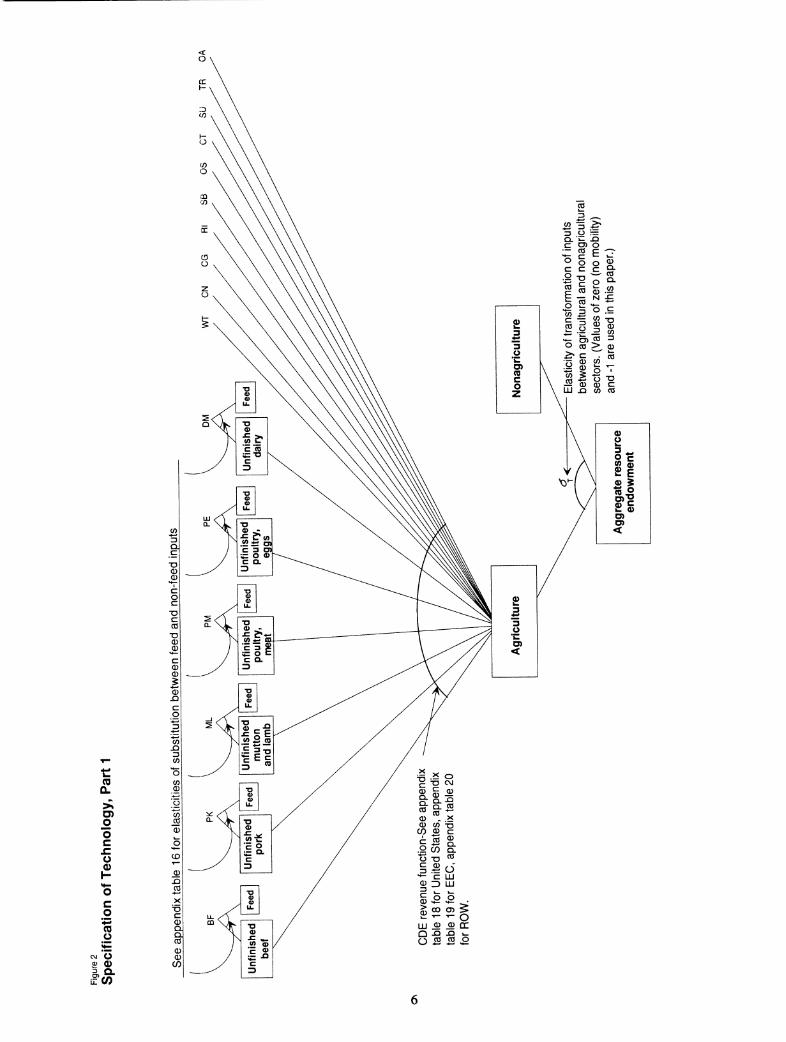
Agriculture as a Multiproduct Industry

Agricultural production, as depicted in figures 2 and 3, is divided into several parts. In figure 2, the core of agricultural technology is summarized by an aggregate revenue function. Application of Hotelling's lenwna generates product supplies, conditional on the available resource endowment. Partial differentiation of the revenue function with respect to the resource endowment in agriculture generates its shadow value. If this is less than the value of a unit of the resource in the nonagricultural sector, migration of resources from the farm to nonfarm sector will tend to occur. The degree of resourœ mobility is governed by an elasticity of transformation

(a^), which measures the ease with which the resource endowment is shifted between the agricultural and

nonagricultural sectors.

This specification of agricultural technology highlights the distinction between two components of supply

response, namely the substitution effect and the expansion effect. If a^, =0, then the agricultural resource base is fixed, as is likely true in the short run. In this case, agricultural supply response is entirely a function of farmers' willingness to divert resources from one product to another in response to relative price changes. In the

longer run, C^ is strictly negative, and commodity supply response will include an expansion effect. As a^ tends to minus infinity, we move to the very long run, where the rental rate on resources in agriculture is determined by the opportunity cost associated with their use in the nonfarm economy.

'We base our analysis on the 1989 SWOPSIM/DEMO model. A slightly revised version of this model is documented in Roningen, Sullivan, and Dixit (1991). Other SWOPSIM models include those described in Roningen (1986), Krissoff and Ballenger (1989), Roningen and Dixit (1989), Uapis (1990), Herlihy, Haley, and Johnson (1992), and Liapis and Shane (1992).

O) O) u c £ O) •^ O) 1^ Û.

to ü

H—

o O -1 0) O) Q.

Li- (/)

O ' o s JD ' o ^ ^ ■'"

0) CO O .^ O 5 2 O

■*-'

X T3 </) C

<D <D QC Q.

2 Q. CO o CO

co¿ m CO

CO in Ä O

CO ÛC

0) ^ o ^ "S '^

X

C => CD

© 'i^ CO

S Q. Q. ^ X CO "^ TD

<D c:

ü d m LU

1^ iS Q. X ^

âd 2 ü

o CO

''" CO LU O) OJÜJ

JO a> ir

' B X ir 0)

CO o

1

Q. ^^^ 9- CO CO LU C/)' ü B "cO C/)

CL CO ü 3

Q "O -o B o

QL ü

co^ "g ^ LU o ^ o ^ CQ Q

co ^i-° OlU-glU co -Qü OÜ (/) ■^ co "-C/) CD ■^ "co ^.E <i)

05 t -O o)0

9-c c c c co o o o o 05 E E E £ 05 co co co co

<^ c c c c ¿".2 o g o .9 3 "^ ■^ 3 ü ■•;= "^ -í: '-i^ c co co (O co 3-Q^^-Q CD CO CO CO CO

3 o 0*0 o

s -B ^2 ;o ü 9-^ 00 "co "co m — i5 i5 —

^j^jLULULULU

Û < OQ Ü Û

ti CO

CL

>i O) O O c x: o 0)

o c o

o CM ü

=5 Q. il (/)

3 QL

O c

T3 <D

S C

0)

C O

C/) JQ 13 CO

(/) O)

CO

JD ce

T3 c CD a a CO

0) CD

CO

ir

u ü 7= CL ■:=. JD C O) o

CO c r- »-

O O O CD c C c CL

.2 "co ? 2

CO d) NJ

CO CL CO x:

co

CO .. 3 O c

2 3

3 g? CO

4-« ««_ 0)3 13 3 o co > CD O .$*

03 C/> CO

O) \ •- ni ^ — 1—

s \ — St^ TD o CD <D C

z \ ^ JD CO CO

\ —

o V o

\ i? .A Y / \ £ E

Xi-

/ <

o 3 tt _"0 m c 0)0

.■= ^

*

(0 3

(0

(0 CL

>i O O O C

o o

lili ill 1

a> u.

H II /\ 1^

^í \ o (0

M (0

0) o o

JC kl ü o.

(Q

3

3 (0 O 3 k. Q. 0)C CB c o z

c o (O o o 0) Q.

CO

Before leaving this discussion of the aggregate agricultura] revenue function, it is important to point out that we have not drawn any distmction between fixed and variable inputs. Clearly, there are some factors of production that are responsive to relative prices, even m the very short run. While information on variable input use is readily obtamed for some countries, such is not the case for many regions covered by models of international trade. For this reason, we have chosen to aggregate all inputs into a single endowment This specification is adequate for analyzing broad questions of trade pohcy. Refinements might be introduced by replacing the revenue function with a restricted profit function, which would give rise to a set of variable input demand equations (as in Liapis and Shane, 1992).

Livestock Assembly Sectors

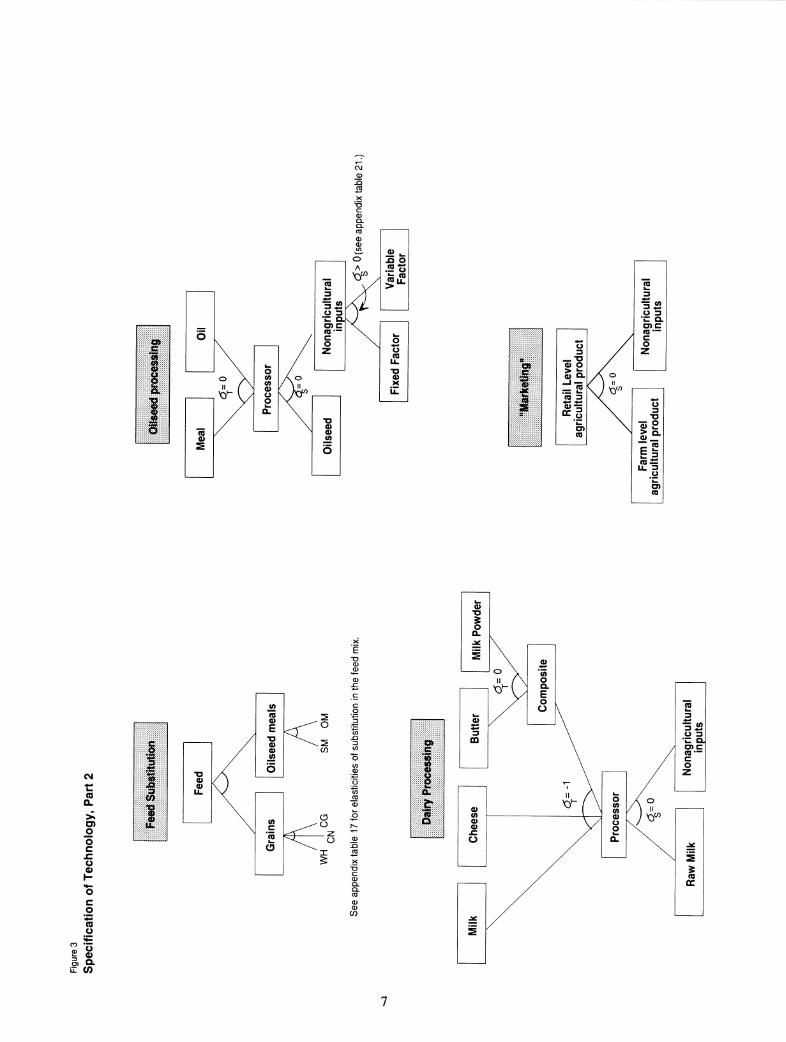
The role of the "livestock assembly sectors" in figure 2 is to combine feed and nonfeed inputs into a finished livestock product. The nonfeed input is derived from the aggregate revenue function and thus competes with other farm activities for the aggregate endowment. In a practical sense, one can think of a short- to medium-run increase in (for example) pork production bidding farm later and capital away from other livestock and crop activities. The degrœ to which this can be done will determine the supply response of pork, given exogenous feed prices. By having a distinct assembly sector for each livestock product, we can also incorporate information about relative feed intensities and cross-price elasticities among feeds as depicted in figure 3. This will be demonsti-ated below.

Food Processing Activities

Another aspect of the representative region's technology involves the further processing of certain raw products. The SWOPSIM/DEMO model outlined in appendix table 2 has relatively little food processing detail, but it is present in the case of dairy and oilseed products. In our framework, these activities are handled in a very simple manner, as depicted in figure 3. Each of these sectors combines the raw product with a "nonagricultural" input to produce a composite input. This, in turn, is used to produce multiple processed outputs. In the case of the oilseed processing sisctors, oil and meal are produced in fixed proportions. The same is true of butter and skinmied milk powder. However, there is a non-zero elasticity of transfonnation between fluid milk, cheese, and the butter/skimmed milk powder composite.

Wholesale/Retail Margins

At this point in the marketing chain, all products are evaluated at producer prices. In order to get to the (higher) consumer prices reported in appendix table 2, a marketing margin must be added. This would ideally be the outcome of the purchase and resale of the products by wholesale and retail sectors. (For an example of how this might be modeled, see Peterson and others, 1992.) Lacking detail on these other marketing activities, we adopt a very simple bridge between producer and consumer prices. In particular, we postulate a Leontief marketing technology, whereby the producer good is combined in fixed proportions with resources from the nonfarm sector to produce the consumer product. In this case, the nonfarm input requirement per unit of output (measured in dollars) may be shown to equal the difference between consumer and producer prices.

Specifîcation of Preferences and Technology: Issues and Insights

Having outlined the general structure of the farm and food sector, we now focus on how to represent consumer preferences and technology in a way that draws a link between our model in figures 1-3 and quantities and supply and demand elasticities from SWOPSIM/DEMO in appendix table 2. In the process of our analysis, we generate some insights concerning data consistency and thie parameters from the SWOPSIM/DEMO database in terms of the basic postulates of economic theory. We begin by examining the quantity and price infonnation contained in SWOPSIM/DEMO.

Determining Prices in a Generic Region

The first problem encountered in developing a balanced set of economic accounts, based on the infonnation contained in the SWOPSIM/DEMO database, is the detennination of price levels in each region. The DEMO

8

model assumes that all goods are homogeneous and provides only information on whether the region is a net importer or exporter of that good. The internal price level is determined by first applying a fixed perœntage adjustment to the world price, thereafter adjustmg for any policy wedges. This first step is difficult to justify, however, given that all goods are assumed to be homogeneous in SWOPSIM models. In the absence of transportation costs (not in the model), the internal price in each region should only vary from the world price by the level of policy interventions.

This type of exogenous price differential can have a confounding effect on global welfare analysis. For example, if soybeans are shipped from a region where the price is low to a region where it is high, worldwide welfare will increase. This makes sense if the hnporting region is a protected market. However, if the price difference is unrelated to policy interventions, this conclusion can easily be misleading. Furthermore, this problem will not be corrected by simply adjusting the price differential to reflect transportation costs. Unless transportation costs are explicitly modeled, this approach will still not provide unbiased welfare results, since the process of shipping goods and services uses resources and this must be accounted for in assessing global welfare changes. In sum, the only permissible price gaps in this homogenous products model are those attributable to either policy distortions, or to "margin" activities that consume real resources.

For these reasons, it is necessary to recompute the level of producer, consumer, and market prices in each region based on the world price. This can be accomplished as follows:

PM = Pw + ESW - MSW (1)

Ps = PM + DPSW (2)

PD = PM - CSW + MARGIN (3)

where: Pw = world price

PM = domestic market price

Ps = producer price

PD = consumer price

DPSW = producer subsidy price wedge,

CSW = consumer subsidy price wedge,

MSW = hnport subsidy price wedge,

ESW = export subsidy price wedge, and

MARGIN = marketing margin for commodity.

Appendix tables 3 and 4 report the 1989 price wedges for the United States and the European Economic Conmiunity (EEC) that were calculated for this modeling exercise. (See appendix A for a complete discussion of the sources and methodology used to calculate these price wedges.) Please note that we have taken a different approach to the modeling of distortions arising from the export enhancement program (EEP) than has been taken in SWOPSIM models (see ^pendix A). Because of the large degree of aggregation in Rest-of-Worid (ROW), we did not attempt to compute policy wedges for this region. Our policy simulations will be concerned only with changes in U.S. and EEC policies.

In computing consumer prices, we discovered that using the initial SWOPSIM margin percentages to recompute consumer prices resulted in the SWOPSIM commodities accounting for only about one-half of total food expenditures. This is somewhat surprising since about three-quarters of the value of all U.S. farm output is covered by SWOPSIM (fruits and vegetables are the major commodities not included). Upon closer inspection.

we discovered that most of the fann/retail margins for consumer products, particularly grains (see Dunham, 1991), and cotton (unpublished Economic Research Service (ERS) calculation), were far too small, as were the marketing margins for intermediate products such as oilseed meals (see Connor and Weimar, 1986). Appendix table 5 compares the initial SWOPSIM/DEMO model margins with revised margins for the United States, appendix table 6 shows the farm value share of each agricultural conunodity, and appendix table 7 details our margin data sources.

And finaUy, adjustments of world soyoü and soymeal prices of about 10 percent were required in order to allow positive profits in the soybean crushing industry, as will he detailed below.

Appendix tables 8, 9, and 10 give the recomputed price levels for the United States, EEC, and ROW based on the adjustments described above. The U.S. prices can be compared with prices in the SWOPSIM/DEMO model in ^pendix table 2.

Specifîcation of Preferences

Consider m more detail the demand elasticity matrix N^ in appendix table 2. It is essentially block-diagonal, with the blocks capturing cross-price relationships among closely related goods. In particular, meats, dairy products, grains, and oilseeds and oilseed products all show distinct groupings. Otherwise, almost all of the off- diagonal elements in this matrix are zero. This pattern of elasticity entries strongly suggests that consumer preferences can be modeled as a two-stage budgeting process as shown in figure 1. For example, consumers fu-st decide the level of expenditures to allocate for meat consumption, then determine the composition of meat consumption solely on the basis of relative prices within ttiis aggregate. Following the pattern of aggregation suggested by the elasticities in the N^ matrix, we arrive at seven separable groups of food items: meats (and eggs), dairy products, grains, oilseeds and associated products, cotton, sugar, and tobacco.

The assumption of a two-stage consumer budgeting process necessitates specification of a functional form representing consumer preferences at each stage. To do so, we will draw on the existing information in the N^ matrix."* Within the seven food groups, only a sprinkling of cross-price elasticities are available. Because of this limited information on the cross-price effects, we assume a single, constant elasticity of substitution between all commodities in each block of commodities. This implies the use of a Constant Elasticity of Substitution (CES) sub-utility function to represent preferences in the second stage of the budgeting process.

In order to implement the CES sub-utility function, we choose a value for the elasticity of substitution, for each composite good, based on the cross-price elasticities that are present in the SWOPSIM/DEMO database. These elasticities of substitution are reported in appendix table lie for the United States, appendix table 14b for the EEC, and appendix table 15b for ROW.

The choice of a functional form to represent preferences for the first stage of the consumer's budgeting process is more difficult due to the predominance of zero cross-price elasticities between conunodities in different blocks of the demand matrix. This undoubtedly reflects the absence of existing infonnation on these parameters. While zero is an acceptable choice, it is not a very plausible choice for these parameters. Consider the Slutsky equation for the uncompensated demand elasticity for good i with respect to changes in the price of good j:

B, =S.(a,-n,) (4)

^Before aggregating the individual elasticities in appendix table 1, it is first necessary to compensate for price responsiveness in demand attributed to intermediate uses treated elsewhere in our model. In particular, intermediate demands by the dairy and oilseed processing sectors, and those of the Hvestock sectors, must be netted out of Np. We do this by weigliting the elasticities in each row by the estimated ratio of own-price elastidty of final demand to the own-price elasticity of total demand. For example, in the case of wheat, the ratio is -0.10/-0.22.

10

where a.j is the partial elasticity of substitution between / and y, S. is the budget share of good y, and T]. is the income elasticity of demand for good i. Even if there is no direct substitutability between the two goods

(Gjj = 0), the income effect of a change in the price of; will affect the demand for good i. That is,

Bj. = -SjTij. The only utility function that will generate z.. = 0 is the Cobb-Douglas, whereby

Gjj = r|. = 1, Vi ity. But this restriction contradicts all of the income elasticities of demand in appendix table

2. In order to solve this inconsistency within the N^ matrix, one must specify an alternative representation of consumer preferences.

A less restrictive preference structure that is compatible with nonunitary income elasticities of demand is that implied by the Stone-Geary utility function. The resulting Linear Expenditure System (LES) includes one free substitution parameter (the so-called "Frisch parameter"), which may be used to replicate one of the own-price elasticities of demand. There is no guarantee, however, that the other own-price elasticities in the system will even be close to their desired value. This makes it difficult to compare results across a LES-based model and the type of PE trade model displayed in ^pendix table 2. Furthermore, since estimates of the own-price elasticity of demand by conmiodity and region are fairly widely available, it would be unfortunate to choose a representation of preferences that precludes incorporation of such information.

The LES restricts substitution relationships by virtue of its explicitly additive fonn; it is additive in prices. This is also the case with Houthakker*s indirect addilog utility function, as well as the CES utility function. At the other extreme are the demand systems that are fully flexible, in the sense that they have n(n -l)/2 free substitution parameters (where n is the number of commodities), so that the utility function may be calibrated to any arbitrary set of elasticities (provided they exhibit the basic properties of symmetry, homogeneity, and concavity). The translog indirect utility function is an example of these flexible functional forms. From the point of view of applied trade modeling (for example, models with many regions), a major problem with these flexible functional forms, however, is that they have too many free parameters and offer no particular guide to limiting these free parameters to a more manageable subset.

From a practical point of view, it would be attractive to have a representation of preferences that had n free parameters, since this is the number needed to replicate the group-wise own-price elasticities of demand in appendix table 2. Hanoch (1975) introduced a class of implicitly additive preference relationships with precisely n substitution parameters (Hanoch, 1975; see also Surry, 1993, for an agricultural application). One specification of this class is the Constant Difference Elasticity of substitution (CDE) expenditure function. Because it represents a dual approach, the CDE is easier to work with than Hanoch's primal-based Constant Ratio Elasticity of Substitution (CRES) functional form. The CDE is also somewhat more general in the degree of cross-price responsiveness that can be incorporated (Hanoch, 1975, pp. 411-412). Consequently, we have chosen to use a CDE expenditure function to represent preferences for the first stage.

One likely reason why the CDE representation has not been more widely applied in the last 15 years is that it is an implicit functional form. Specifically, the CDE may be written as follows:

G(z,u) =X;B^U^''Z.''^ 1. (5)

When the CDE is used as an expenditure function, all prices (Pj) are scaled by minhnum household expenditure, E(p,u), which is itself a function of prices (p) and utility (u): Zj = p¡ / E(p,u).

The CDE parameters and their restrictions are: B., e^ > 0, bj < 1, with either 0 < b. < 1 or b. < 0 for all i. In general, it is not possible to solve (5) for expenditures as an explicit function of p and u. Also, note that

p. enters both the numerator of z. and the denominator of z.. In economic terms, this implies that the effect of

a change in p^ on optimal demands enters both directly through z. and indirectly through a change in the

general price index affecting z/s.

11

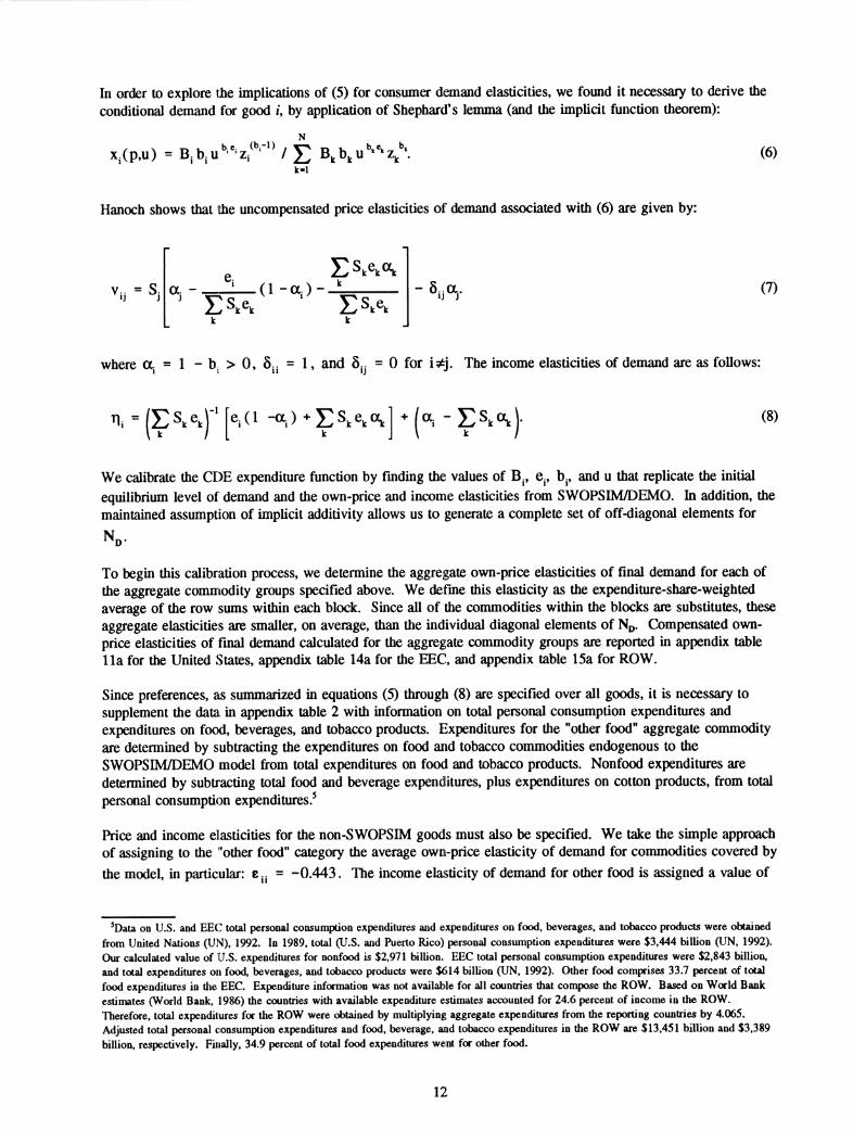
In order to explore iJie implications of (5) for consumer demand elasticities, we found it necessary to derive the conditional demand for good /, by application of Shephard's lenrnia (and the implicit function theorem):

x,(p.u) = B^b^u^'-'z/^'-'V E B^b^u'-^-'z;'. (6) k-l

Hanocb shows that the uncompensated price elasticities of demand associated with (6) are given by:

Vu = s. «j- ES.e, (1-a.)-. k

ES.e, - ô^a.. (7)

where a = l-b>0, 5. = 1, and 6,. = 0 for i?ij. The income elasticities of demand are as follows:

^i = (ÇS.^.)"' Ml -^i) *ÇS,e,(x,] . |a - ÇS,oc,j (8)

We calibrate the CDE expenditure function by finding the values of B., e., bj, and u that replicate the initial equilibrium level of demand and the own-price and income elasticities from SWOPSIM/DEMO. hi addition, the maintained assumption of implicit additivity allows us to generate a complete set of off-diagonal elements for N„.

To begin this calibration process, we determine the aggregate own-price elasticities of final demand for each of the aggregate conmriodity groups specified above. We deiiine this elasticity as the expenditure-share-weighted average of the row sums within each block. Since all of the conunodities within the blocks are substitutes, these aggregate elasticities are smaller, on average, than the individual diagonal elements of N^. Compensated own- price elasticities of final demand calculated for the aggregate conmiodity groups are reported in appendix table 11a for the United vStates, appendix table 14a for the EEC, and içpendix table 15a for ROW.

Since preferences, as summarized in equations (5) through (8) are specified over all goods, it is necessary to supplement the data in appendix table 2 with information on total personal consumption expenditures and expenditures on food, beverages, and tobacco products. Expenditures for the "other food" aggregate conmiodity are determined by subtracting the expenditures on food and tobacco conmiodities endogenous to the SWOPSBM/DEMO model from total expenditures on food and tobacco products. Nonfood expenditures are determined by subtiacting total food and beverage expenditures, plus expenditures on cotton products, from total personal consumption expenditures.^

Price and income elasticities for the non-SWOPSIM goods must also be specified. We take the simple approach of assigning to the "other food" category the average own-price elasticity of demand for commodities covered by the model, in particular: t.. = -0.443. The income elasticity of demand for other food is assigned a value of

'Data on U.S. and EEC total personal consumption expenditures and expenditures on food, beverages, and tobacco products were obtained from United Nations (UN), 1992. In 1989, total (U.S. and Puerto Rico) personal consumption expenditures were $3,444 billion (UN, 1992). Our calculated value of U.S. expenditures for nonfood is $2,971 billion. EEC total personal consumption expenditures were $2,843 billion, and total expenditures on food, beverages, and tobacco products were $<)14 billion (UN, 1992). Other food comprises 33.7 percent of total food expenditures in the EEC. Expenditure information was not available for all countries that compose the ROW. Based on World Bank estimates (World Bank, 1986) the countries with available expenditure estimates accounted for 24.6 percent of income in the ROW. Therefore, total expenditures for the ROW were obtained by multiplying aggregate expenditures from the reporting countries by 4.065. Adjusted total personal consumption expenditures and food, beverage, and tobacco expenditures in the ROW are $13,451 billion and $3,389 billion, respectively. Finally, 34.9 percent of total food expenditures went for other food.

12

0.4 because this category includes many highly processed products that are deemed more income responsive than the food conunodities in SWOPSIM. The income elasticity of demand for nonfood items is derived via Engel aggregation. Finally, the own-price elasticity of demand for nonfood items is rather closely circumscribed by the resüictions of the CDE, and may be left free for the moment.

Calibration of the parameters of the CDE implicit expenditure function proceeds in three steps (see Hertel and others (1991) for an exhaustive discussion of this process):^

Step one: derivation of the substitution parameters bj = (1 - a^) from the compensated own-price elasticities of demand and the shares.

Step two: derivation of the expansion parameters (c.) from the income elasticities of demand, the shares and the substitution parameters, and

Step three: derivation of the shift parameters (B.) from the demand quantities and all of the preceding information.

In the process of calibrating CDE preference parameters to any arbitrary set of elasticities, budget shares, and quantities, it is entirely possible that the sign restrictions on the CDE parameters might be violated. This might occur, for instance, if a commodity with a very large budget share were also assigned a relatively large compensated own-price elasticity of demand (v^j). In this case, the calibrated a. would be negative and it

would be necessary to reduce the absolute value of v... In fact, in the example at hand, this consistency

restriction restricts the value of v^j for the nonfood aggregate (the conmiodity with the largest budget share in this model), to lie between -0.057 and -0.067.

The extremely small, even negative, values for the income elasticities of demand for many of the food products in the SWOPSIM/DEMO database pose the most severe problem for the calibration process. These values result in numerous negative expansion parameters (e^ < 0) that violate the regularity resüictions for the CDE expenditure function. Consequently, we find it necessary to adjust the income elasticities of demand from SWOPSIM/DEMO upwards until all e/s are positive. This highlights the fact that one cannot choose a set of income elasticities independently of the price elasticities of demand and budget shares. The revised values of the income elasticities (TIJ) for the United States are listed in appendix table 11a, along with the price elasticities (v.j), and the calibrated CDE preference parameters (bj = (1 - a.)), (Cj), and (B.). The complete matrix of aggregated, compensated demand elasticities that is generated by the CDE specifications is given in appendix table lib. Appendix tables 12 and 13 give the full matrices of disaggregate demand elasticities (Nj^). CDE preference parameters for the EEC and the ROW are given in appendix tables 14a and 15a.

Specification of Agricultural Technology

With the exception of joint products such as wool and mutton, we expect a priori that agricultural products will be (net) substitutes in the short run. Indeed, the off-diagonal elements in the N^ matrix at the top of appendix table 2 exhibit this sign pattern. We therefore assume that these supply elasticities are short run and conditional on a fixed aggregate factor endowment. Our task is then to calibrate an aggregate agricultural revenue function which will replicate the supply behavior for raw farm products depicted in appendix table 2. At this stage, we abstract from the own- and cross-price elasticities involving processed products, as they will be handled below. We must specify the livestock "assembly" technology before calibrating the aggregate revenue function, however.

^While expressions (6) - (8) are nonlinear in parameters, a series of appropriate normalization rules permit steps one to three to be accomplished entirely via Unear operations.

13

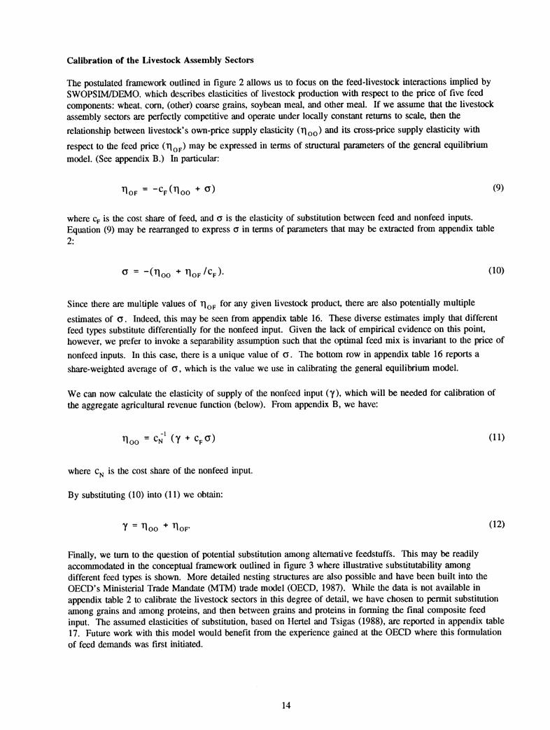
Calibration of the Livestock Assembly Sectors

The postulated framework outlined in figure 2 allows us to focus on the feed-livestock interactions hnplied by SWOPSM/DEMO, which describes elasticities of livestock production with respect to the price of five feed components: wheat, com, (other) coarse grains, soybean meal, and other meal. If we assume that the livestock assembly sectors are perfectly competitive and operate under locally constant returns to scale, then the relationship between livestock's own-price supply elasticity (TIQQ) and its cross-price supply elasticity with

respect to the feed price (TIQP) may be expressed in terms of structural parameters of the general equilibrium model. (See ^pendix B.) In particular:

TloF = -CpC^oo ■^^) i^)

where Cp is the cost share of feed, and a is the elasticity of substitution between feed and nonfeed inputs. Equation (9) may be rearranged to express a in terms of parameters that may be extracted from appendix table 2:

<^ = -(îloo -^^OF/CF). (10)

Since there are multiple values of ri^p for any given livestock product, there are also potentially multiple

estimates of a. Indeed, this may be seen from appendix table 16. These diverse estimates imply that different feed types substitute differentially for the nonfeed input. Given the lack of empirical evidence on this point, however, we prefer to invoke a separability assumption such that the optimal feed mix is invariant to the price of nonfeed inputs. In this case, there is a unique value of a. The bottom row in appendix table 16 reports a share-weighted average of a, which is the value we use in calibrating the general equilibrium model.

We can now calculate the elasticity of supply of the nonfeed input (Y), which will be needed for calibration of the aggregate agricultural revenue function (below). From appendix B, we have:

iloo =CN' (Y ^CpG) (11)

where Cj^ is the cost share of the nonfeed input.

By substituting (10) into (11) we obtain:

Y = îloo ^ ^oP (12)

Finally, we turn to the question of potential substitution iunong alternative feedstuffs. This may be readily acconunodated in the conceptual framework outlined in figure 3 where illustrative substitutability among different feed types is shown. More detailed nesting structures are also possible and have been built into the OECD's Ministerial Trade Mandate (MTM) trade model (OECD, 1987). While the data is not avaUable in appendix table 2 to calibrate the livestock sectors in this degree of detail, we have chosen to permit substitution among grains and iunong proteins, and then between grains and proteins in fonning the final composite feed input. The assumed elasticities of substitution, based on Hertel and Tsigas (1988), are reported in appendix table 17. Future work with this model would benefit from the experience gained at the OECD where this formulation of feed demands was first initiated.

14

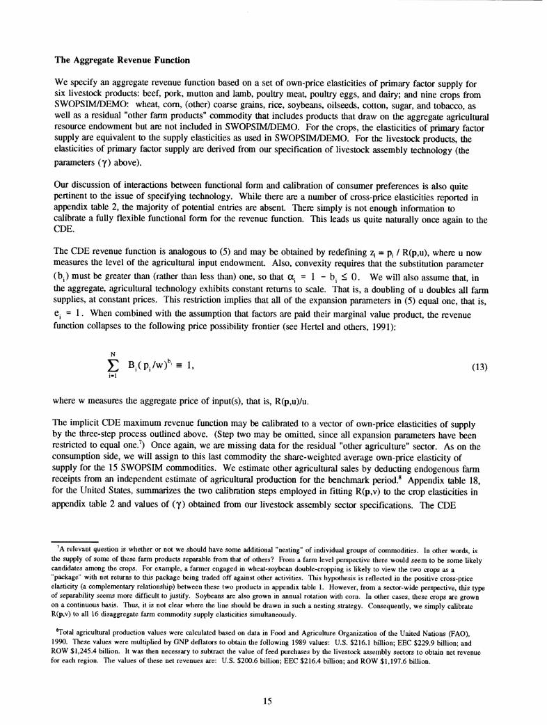
The Aggregate Revenue Function

We specify an aggregate revenue function based on a set of own-price elasticities of primary factor supply for six livestock products: beef, pork, mutton and lamb, poultry meat, poultry eggs, and dairy; and nine crops from SWOPSIM/DEMO: wheat, com, (other) coarse grains, rice, soybeans, oilseeds, cotton, sugar, and tobacco, as well as a residual "other farm products" commodity that includes products that draw on the aggregate agricultural resource endowment but are not included in SWOPSEM/DEMO. For Uie crops, the elasticities of primary factor supply are equivalent to tiie supply elasticities as used in SWOPSIM/DEMO. For tiie livestock products, üie elasticities of primary factor supply are derived from our specification of livestock assembly technology (the parameters (y) above).

Our discussion of interactions between functional form and calibration of consumer preferences is also quite pertinent to the issue of specifying technology. While there are a number of cross-price elasticities reported in appendix table 2, üie majority of potential entries are absent. There shnply is not enough information to calibrate a fully flexible functional form for the revenue function. This leads us quite naturally once again to the CDE.

The CDE revenue function is analogous to (5) and may be obtained by redefining z^ = Pi / R(p,u), where u now measures Üie level of the agricultural input endowment. Also, convexity requires Üiat the substitution parameter (h.) must be greater üian (radier tiian less üian) one, so üiat ttj = 1 - bj < 0. We will also assume tiiat, in Üie aggregate, agricultural technology exhibits constant returns to scale. That is, a doubling of u doubles all farm supplies, at constant prices. This restriction implies üiat all of Üie expansion parameters in (5) equal one, that is, Cj = 1. When combined wiüi Üie assumption üiat factors are paid üieir marginal value product, the revenue function collapses to the following price possibility frontier (see Hertel and oüiers, 1991):

J2 B^(p7w)^'= 1, (13)

where w measures the aggregate price of input(s), that is, R(p,u)/u.

The implicit CDE maximum revenue function may be calibrated to a vector of own-price elasticities of supply by Üie üiree-step process ouüined above. (Step two may be omitted, since all expansion parameters have been restricted to equal one.^) Once again, we are missing data for üie residual "oüier agriculture" sector. As on the consumption side, we wül assign to üiis last commodity tiie share-weighted average own-price elasticity of supply for üie 15 SWOPSIM commodities. We estimate oüier agricultural sales by deducting endogenous farm receipts from an independent estimate of agricultural production for üie benchmark period.^ Appendix table 18, for üie United States, summarizes the two calibration steps employed in fitting R(p,v) to üie crop elasticities in appendix table 2 and values of (y) obtained from our livestock assembly sector specifications. The CDE

^A relevant question is whether or not we should have some additional "nesting" of individual groups of commodities. In other words, is the supply of some of these farm products separable from that of others? From a farm level perspective there would seem to be some likely candidates among the crops. For example, a farmer engaged in wheat-soybean double-cropping is Ukely to view the two crops as a "package" with net returns to this package being traded off against other activities. This hypothesis is reflected in the positive cross-price elasticity (a complementary relationship) between these two products in appendix table 1. However, from a sector-wide perspective, this type of separability seems more difficult to justify. Soybeans are also grown in annual rotation with corn. In other cases, these crops are grown on a continuous basis. Thus, it is not clear where the line should be drawn in such a nesting strategy. Consequently, we simply cahbrate R(p,v) to all 16 disaggregate farm commodity supply elasticities simultaneously.

*Tota] agricultural production values were calculated based on data in Food and Agriculture Organization of the United Nations (FAO), 1990. These values were multiplied by GNP deflators to obtain the following 1989 values: U.S. $216.1 billion; EEC $229.9 billion; and ROW $1,245.4 billion. It was then necessary to subtract the value of feed purchases by the livestock assembly sectors to obtain net revenue for each region. The values of these net revenues are: U.S. $200.6 billion; EEC $216.4 bilhon; and ROW $1,197.6 billion.

15

revenue parameters for the EEC and ROW are listed in apipendix tables 19 and 20. Remember, we implicitly assume that the elasticities in SWOPSM/DEMO do not embody an expansion effect.

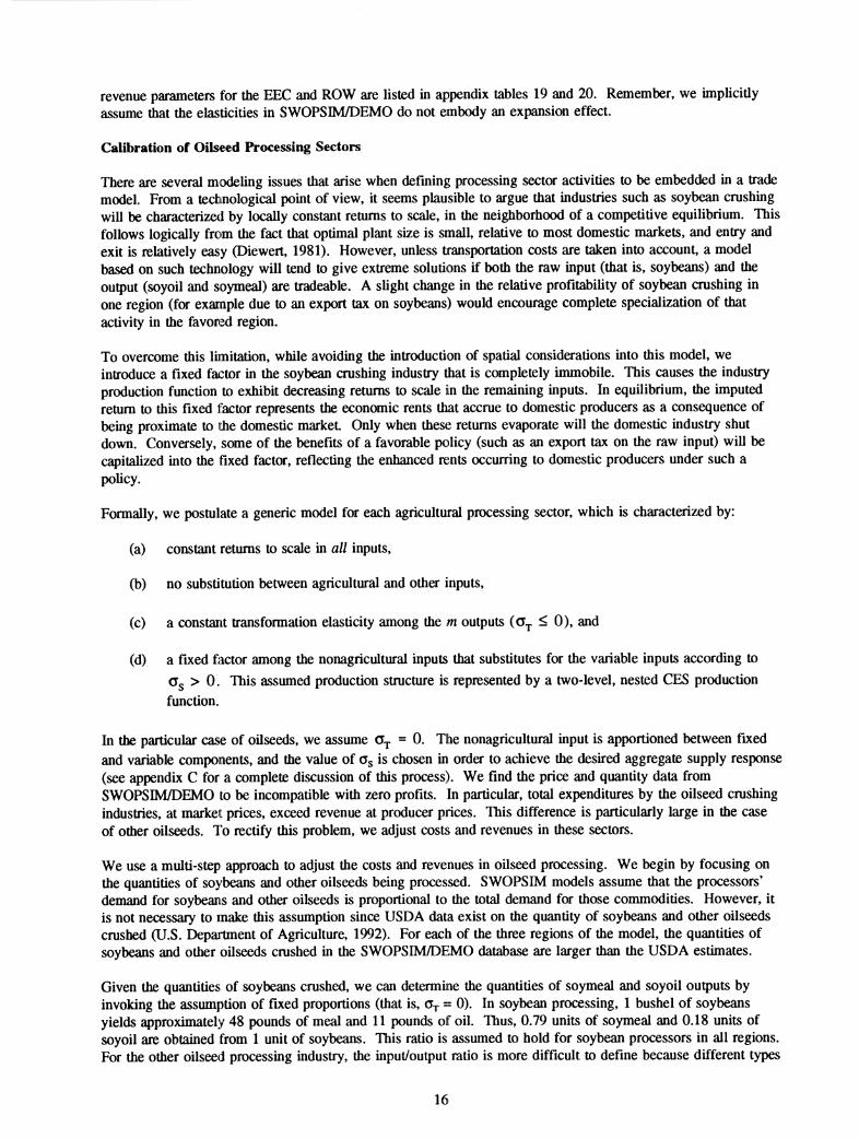
Calibration of Oilseed Processing Sectors

There are several modeling issues that arise when defining processing sector activities to be embedded in a trade model. From a technological point of view, it seems plausible to argue that industries such as soybean crushing will be characterized by locally constant returns to scale, in the neighborhood of a competitive equilibrium. This follows logically from the fact that optimal plant size is small, relative to most domestic markets, and entry and exit is relatively easy (Diewert, 1981). However, unless transportation costs are taken into account, a model based on such technology will tend to give extreme solutions if both the raw input (that is, soybeans) and the output (soyoil and soymeal) are tradeable. A slight change in the relative profitability of soybean crushing in one region (for example due to an export tax on soybeans) would encourage complete specialization of that activity in the favored region.

To overcome this limitation, while avoiding the introduction of spatial considerations into this model, we introduce a fixed factor in the soybean crushing industry that is completely inunobile. This causes the industry production function to exhibit decreasing returns to scale in the remaining inputs. In equilibrium, the imputed return to this fixed factor represents the economic rents that accrue to domestic producers as a consequence of being proximate to iLhe domestic market. Only when these returns evaporate will the domestic industry shut down. Conversely, some of the benefits of a favorable policy (such as an export tax on the raw input) will be capitalized into the fixed factor, reflecting the enhanced rents occurring to domestic producers under such a policy.

Formally, we postulate a generic model for each agricultural processing sector, which is characterized by:

(a) constant returns to scale m all inputs,

(b) no substitution between agricultural and other inputs,

(c) a constant transformation elasticity among the m outputs (a^ < 0), and

(d) a fixed factor among the nonagricultural inputs that substitutes for the variable inputs according to

Cg > 0. This assumed production structure is represented by a two-level, nested CES production function.

In the particular case of oilseeds, we assume a^ = 0. The nonagricultural input is apportioned between fixed and variable components, and the value of Og is chosen in order to achieve the desired aggregate supply response (see appendix C for a complete discussion of this process). We find the price and quantity data from SWOPSIM/DEMO to be incompatible with zero profits. In particular, total expenditures by the oilseed crushing industries, at market prices, exceed revenue at producer prices. This difference is particularly large in the case of other oilseeds. To rectify this problem, we adjust costij and revenues in these sectors.

We use a multi-step approach to adjust the costs and revenues in oilseed processing. We begin by focusing on the quantities of soybeans and other oilseeds being processed. SWOPSIM models assume that the processors' demand for soybeans and other oilseeds is proportional to the total demand for those commodities. However, it is not necessary to make this assumption since USDA data exist on the quantity of soybeans and other oilseeds crushed (U.S. Department of Agriculture, 1992). For each of the three regions of the model, the quantities of soybeans and other oilseeds crushed in the SWOPSIM/DEMO database are larger than the USDA estimates.

Given the quantities of soybeans crushed, we can determii[ie the quantities of soymeal and soyoil outputs by invoking the assumption of fixed proportions (that is, Cj == 0). In soybean processing, 1 bushel of soybeans yields approximately 48 pounds of meal and 11 pounds of oil. Thus, 0.79 units of soymeal and 0.18 units of soyoil are obtained from 1 unit of soybeans. This ratio is assumed to hold for soybean processors in all regions. For the other oilseed processing industry, the input/output ratio is more difficult to define because different types

16

of other oilseeds, with different meal and oil yields, are produced in each region. Thus, we use average meal and oil yields.

The next step is to determine crush margins for oilseed processing industries that reflect longrun returns. Based on 1960-89 prices of soybeans, soymeal, and soyoil (International Monetary Fund, 1990), we estimate that the average U.S. crush margin over that period was 2.6 percent. If this average margin for soybeans was used as the cost share for the entire nonagricultural input in the model, small changes in prices would lead to significant locational changes in processing activities. Since we do not typically observe large changes in plant locations between regions, we assume that the 2.6 percent margin only represents the cost share of the variable component of the soybean nonagricultural input, and that an additional margin, which will be specified below, is associated with a fixed nonagricultural input. For other oilseed processing, the cost share for the variable component of the nonagricultural input is assumed to be 0.075. This larger cost share is based on information from the 1987 Census of U.S. Manufacturers that shows the relative share of value added to value of shipments is approximately 2.75 times larger for cottonseed oil mills (SIC 2074) than for soybean oil mills (SIC 2075) during the period 1972 through 1987.

In order to determine the cost share of the fixed factor, we next need to determine the aggregate supply response of the processing industries. Because of our assumption of fixed output proportions, we can treat the oilseed processing industries as single product industries. The aggregate supply response can then be related to the own- price supply elasticities of meal and oil in the SWOPSIM/DEMO database. In particular, the aggregate supply response equals the own-price supply elasticity divided by the revenue share of that product.^ Appendix table 21 lists the aggregate supply responses for each industry and region.

Based on our assumed production structure, these aggregate supply elasticities can now be related to the cost shares of the fixed and variable nonagricultural inputs and the value of Os, which describes the elasticity of substitution between them. In particular, the aggregate supply response equals (see appendix C):

Tls = ^s Cf"' -(Cf "^C,)-^] (14)

where c^ is the cost share of the fixed factor and c^ is the cost share of the variable, nonagricultural input. Since both Gs and c^ are unknown, we simply assign a value of 0.05 for Og (for both the U.S. soybean and other oilseed processing industries) and then solve equation (14) for Cf. The resulting cost shares are reported in appendix table 21.

Given the input costs, we can now determine the market prices and receipts necessary to ensure zero profits. At this point, we focus entirely on one region, the United States, to determine market and world prices. This is an arbitrary choice because the market and world prices for processed oilseed products are the same in all regions. We use the initial SWOPSIM/DEMO model market prices for meal and oil as a starting point and adjust them proportionally until total revenue equals total expenditure. The new market (and world) prices of soymeal and soyoil are $271.45/metric ton (mt) and $473.66/mt, compared with the initial DEMO model world prices of $247/mt for soymeal and $431/mt for soyoil. The new market (and world) prices of other meal and other oil are $385.14/mt and $l,490.49/mt, compared with the initial DEMO model prices of $200/mt and $774/mt, respectively.

The fmal step is to choose parameters to calibrate equation (14) for the other regions of the model.

Calibration of Dairy Processing Sectors

There are several important differences between modeling dairy processing and modeling oilseed crushing. First of all, the agricultural input, fluid milk, is not generally traded. This obviates the need for a fixed input to

'The assumption of fixed output proportions implies that the own-price supply elasticities for meal and oil are not independent of each other. Thus, only one of these elasticities in the SWOPSIM/DEMO database can be used to determine the aggregate supply response in the processing industry.

17

prevent specialization in dairy proœssing. Thus, we can assume that dairy prcx:essing employs fixed coefficient technology without worrying about overspecialization. A second distinction arises fi^om the fact that the mix of dairy products can be altered in response to changes in the relative prices of (for example) cheese and butter.

Taking into account a non-zero elasticity of transformation among processed dairy products (G^ < 0) and the

inelastic domestic supply of raw milk (with elasticity Tl^^), we can solve the underlying system of equations to obtain the elasticity of transformation as a function of the own-price elasticity of supply for the processed product (r|..) and the raw product (Tl^^y^), as well as the cost share of the raw product in the processing sector

(c^) and the revenue share of the j"" processed product (v.):

^T = (^jj ""^AACA"')(rj - 1)"' ^0. (15)

Since r. and c^ are both less than 1, we must have r|^^ < c^ r| . < r|.. This makes intuitive sense. Processed products involve nonagricultural as well as raw milk inputs. Thus, the processing sector will be more price responsive than the primary product sector if the nonagricultural inputs (for example, labor and capital) are more supply responsive than agricultural inputs. In addition, it would seem plausible to assume that additional processing facilities can be brought "on-line" over the 3-5 year time period envisioned for the model's solution.

In light of these observations, it is rather striking that the own-price elasticity of supply for raw milk (r|^^) in

the SWOPSIM/DEMÍO model is larger than r\.. for each of the processed dairy products (see appendix table 2). Perhaps this is due to the fact that no distinction is made between raw and processed fluid milk in SWOPSM models. In the model developed here, all raw milk is required to pass through the processing sector. Since (15) is infeasible, given tl^e information in appendix table 2, we simply adopt the value of r|^^ in ^pendix table 2

(0.50), and arbitrarily choose a value of <Jj = -1.0.

Completing the Model

Thus far we have focused on procedures for calibrating technology and preferences for commodities that are endogenous to SWOPSIM/DEMO. However, in this calibration process we have also generated: (1) a supply of non-SWOPSM farmi products (other agriculture), (2) a demand for non-SWOPSIM food products (other food), and (3) a demand for nonfood products. With a few simple assumptions, it is now possible to complete this model.

First, consider the food system as a whole. If we assume a one-to-one mapping from "other agriculture" to "other food," then completion of the model's treatment of the food system requires us to impute a pattern of net trade and marketing margins such that world supplies of thiese residual products equal world demands, and consumer expenditures and farm receipts match tJieir initial equilibrium values. The pattern of net trade in "other agriculture" is a residual computed by subtracting tliie trade balance of the existing SWOPSIM conmiodities from the total agricultural ü-ade balance. To ensure that world supply equals world demand, this procedure is used for all but one of the regions, with the hist region's net trade position being a residual.

The price of "other agriculture" can be arbitrarily chosen v/ithout affecting the results of the model. Lacking policy information, we assume that there are no trade distortions in "other agriculture"; however, we do introduce producer subsidies for other agricultural products. The marketing margin for this residual commodity is determined by comp;aring retail expenditures for other food with the value of purchases of other agricultural products, from domestic and foreign suppliers, by the food marketing sector.

We obtain a balanced set of economic accounts by forcing each region to be in balance-of-payments equilibrium. Since we have abstracted from households' demand for savings, we allow no international capital flows. (By omitting these flows, we implicitly hold them constant in our simulations.) Consequently, we require a pattern

18

of net trade in nonagricultural products that exactly offsets the balance of trade in agriculture. We also abstract from distortions in the nonfood sector. This implies that the world price, producer price, and domestic market price are all equal. By arbitrarily setting the world price equal to $100/mt, we can derive the trade quantities. We assume that the marketing margin for nonfood equals 25 percent across regions (this implies a retail price of $125/mt). Given the retail price and the level of retail expenditures on nonfood, we can determine the quantity of nonfood going to final demand. From that, we can derive the quantity of domestic supply by subtracting the net trade flow from domestic demand (or availability).

After calibrating the nonfood sector, we find that domestic income (factor payments plus tax receipts [for example, tariffs on imports], less taxes paid [subsidies]) does not equal expenditures. The United States and EEC have an income surplus of $0.32 billion and $2.47 billion, respectively, while the ROW has an income deficit of $2.79 billion. To place each region on its budget constraint, we introduce transfers to ROW from the United States and the EEC, by means of a fictitious good called "goodwill" that the U.S. and EEC households purchase from ROW in the initial equilibrium. This balances the data set.

Model Implementation and Solution

The data and associated parameters developed in the previous section are used to construct a static, neoclassical trade model (see appendix D for a complete description of the model equations). As in the SWOPSIM/DEMO model, all goods are assumed to be homogeneous. Producers are assumed to maximize profits subject to a technology constraint and consumers are assumed to maximize utility subject to a budget constraint. All markets are assumed to be perfectly competitive. The aggregate factor is not mobile between regions, but may be mobile between sectors within a region, depending on the elasticity of transformation. Finally, we have chosen the nonfood good as the numeraire.

There are four blocks of equations in the model. The first set of equations describes producer behavior in individual sectors. Smce some of the sectors in this model are multiproduct in nature, the simplest approach is to permit every sector to produce multiple products. Constant Elasticity of Transformation (CET) production possibilities may be handled as a special case of the CDE in which all u*ansformatíon parameters are equal. Thus, the three types of equations in this block are the industry supply equations, industiy demand equations (input-output separability is assumed), and zero profit conditions.

The second block contains equations that describe consumer behavior in each region. This block contains two types of equations. First, because we assume tiiere is only one representative household per region, household income is the sum of factor payments and subsidies received by tiie household less taxes paid. The second set of equations represents the final demands of each household in tiie tiiree regions of tiie model.

The third block contains the market clearing conditions for traded producer goods and nontraded goods. In this model, the nontraded goods are all primary factors (including the nonfeed input to the livestock assembly sector), fluid milk, and all consumer goods. All other producer goods are traded. Finally, tiiere is a dummy equation that evaluates excess demand for the nonfood good that is omitted from the maricet-clearing conditions. According to Walras' Law, this must equal zero. Since any sort of logical or computational error will generally lead to a violation of Walras' Law, this offers a valuable consistency check on the entire model.

The final block of equations describes the price linkages and policy interventions in the model. They include market clearing conditions for all but one of the tradeable commodities, as well as price linkage equations translating world prices mto domestic prices, and domestic prices into producer and consumer prices. All taxes and subsidies are applied here.

The general equilibrium model is implemented using tiie General Equilibrium Modelling Package (GEMPACK), a suite of software developed at tiie IMPACT Project'^ and designed to support applied general equilibrium modeling (Codsi and Pearson, 1988). While GEMPACK has historically been oriented exclusively toward

'*^*The IMPACT Project is a cooperatíve venture between the Australian Federal Government and Monash University, LaTrobe University, and the Austrahan National University.

19

solving linear problems, the most recent version of this software now solves nonlinear general equilibrium problems. This is tlie version that we employ. The problem is still written down in its linearized form, but the addition of a set of update equations (for example, equations (7) and (8)), permits the nonlinear solution to be obtained after sucœssive iterations. (A complete description of the model's implementation is available from the authors upon request.)

Another advantage of using GEMPACK is that it is designed to handle large-dimensional problems. Thus, our model is capable of being expanded to more than three regions. Because USDA has published databases for more than 30 regions, there is considerable potential for further disaggregation.

Application to Trade Liberalization

In order to illustrate the framework developed in this paper, we have constructed a series of trade liberalization experiments involving the United States and the EEC. The residual ROW region does not change policies, as we do not have estimatifs of policy interventions for this composite region. The magnitude of producer, consumer, and trade interventions for the United States and the EEC are given in appendix tables 3 and 4. In the following experiments, we will remove all of these distortions and examine the consequences for production, consumption, prices, and welfare under a variety of modeling iissumptions. Results are presented in tables 1-7.

Base Case Results

Tables 1, 4, 5, and 7 include results from the base case simulation in which all distortions in the United States and the EEC are removed, but factors are not permitted to move between the agricultural and nonagricultural sectors (see figure 2). As may be seen from the last column of table 1, hberalization has very little impact on global agricultural supplies in this scenario. Indeed, the only cases in which global supplies change by at least 1 percent are com, mutton and lamb and other powdered milk, which decline, and pork and eggs, which increase. Thus, most of the changes in table 1 represent changes in the composition of global supply/demand among regions.

The first two columns in table 1 present percentage changes in supply and demand of tradeable products in the United States. Due to the no-mobiUty assumption, supply adjustinents only reflect movements around a fixed production possibilities frontier. Removal of all producer support causes producer prices of the heavily supported commodities to fall relative to conunodities reœiving relatively less support Consequently, production shifts from heavily supported to relatively less supported commodities. Production of grains, dairy, and sugar all fall substantially, while production of soybeans, other agriculture, beef, mutton and lamb, and poultry products increase. Of course, the extent to which grain production is likely to decline depends importantly on what happens to idled acreage. We assume that none of that idled acreage returns to production. Consequently, the placement of the production possibiHty frontier remains fixed. Other studies indicate that the effect of acreage returning to production, in particular, grain and oilseed acreage, could largely offset the decline in payments. As a result, U.S. grains output might not change very much (see for example, Herlihy, Haley, and Johnson, 1992).

The second set of columns in table 1 report percentage changes in regional supply and demand in the EEC in this scenario. Production of feed grains, rice, beef, oilsee<is, mutton and lamb, poultry meat, and dairy products decreases, while the production of wheat, cotton, tobacco, other agriculture, pork, and eggs increases.

Production changes in ROW are reported in the third group of columns in table 1. They show that this region steps in to fill gaps in production left after the United States and EEC have adjusted to liberalization.

The changes in regional demands in table 1 are driven by changes in market or household prices in each of the three regions once U.S. and EEC policies have been removed. Particularly striking is the reallocation of feed grain demand from the United States to the EEC.

Implications of Omitting Feedstuff Substitution

The importance of feedstuff substitution for model results is explored by rerunning the model with no feed substitution. Results of this simulation are reported in tables 2, 4, and 5. A comparison of tables 1 and 2

20

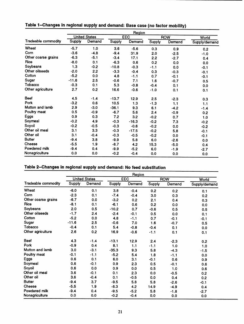
Table 1-Changes in regional supply and demand; Base case (no factor mobility)

Reqion United States EEC ROW World

Tradeable commodity Supply Demand Supply Demand Supply Demand Supply/demand

Wheat -5.7 1.0 3.6 -5.6 0.3 0.9 0.2 Com -3.6 -4.8 -9.4 31.9 2.0 -2.5 -1.0 Other coarse grains -6.3 -5.1 -3.4 17.1 2.2 -2.7 0.4 Rice -8.0 0.1 -6.3 0.6 0.2 0.0 0.0 Soybeans 1.3 -0.2 -10.8 -0.3 -1.1 0.0 -0.1 Other oilseeds -2.0 2.2 -3.3 -0.4 0.3 -0.3 -0.1 Cotton -5.2 0.0 4.8 -1.1 0.7 -0.1 -0.1 Sugar -11.6 2.5 -0.6 7.1 1.6 -0.7 0.5 Tobacco -0.3 0.1 5.3 -0.8 -0.4 0.1 0.0 Other agriculture 2.7 0.2 16.6 -0.6 -1.0 0.1 0.1

Beef 4.5 -1.4 -13.7 12.9 2.5 -2.3 0.3 Pork -3.2 0.6 10.5 1.3 -1.3 1.1 1.1 Mutton and lamb 2.9 -3.0 -36.1 9.3 6.1 -4.2 -1.4 Poultry meat 0.5 -0.9 -6.7 5.6 2.4 -0.9 0.2 Eggs 0.9 0.3 7.2 3.2 -0.2 0.7 1.0 Soymeal -0.2 4.9 -0.3 -16.3 -0.2 7.3 -0.2 Soyoil -0.2 -0.5 -0.3 -0.6 -0.2 0.0 -0.2 Other oil meal 3.1 3.3 -0.3 -17.5 -0.2 5.8 -0.1 Other oil 3.1 -0.4 -0.3 -0.5 -0.2 0.0 -0.1 Butter -9.4 3.8 -9.9 5.8 6.0 -2.6 0.0 Cheese -5.5 1.9 -8.7 4.2 15.3 -5.0 0.4 Powdered milk -9.4 0.4 -9.9 -5.2 6.0 -1.9 -2.7 Nonagricuhure 0.0 0.0 -0.2 -0.4 0.0 0.0 0.0

Table 2-Changes in regional supply and demand: No feed substitution

Reqion United States 1 EEC ROW World

Tradeable commodity Supply Demand Supply Demand Supply Demand Supply/demand

Wheat -6.0 0.1 3.8 -0.4 0.2 0.2 0.1 Corn -2.3 0.1 -7.4 -0.4 3.0 0.3 0.2 Other coarse grains -6.7 0.0 -3.2 0.2 2.1 0.4 0.3 Rice -8.1 0.1 -6.1 0.6 0.2 0.0 0.0 Soybeans 2.0 0.5 -10.2 0.7 -0.6 0.5 0.5 Other oilseeds -1.7 2.4 -2.4 -0.1 0.5 0.0 0.1 Cotton -5.2 0.0 4.8 -1.1 0.7 -0.1 -0.1 Sugar -11.6 2.5 -0.6 7.0 1.6 -0.7 0.5 Tobacco -0.4 0.1 5.4 -0.8 -0.4 0.1 0.0 Other agrk^ulture 2.6 0.2 16.9 -0.6 -1.1 0.1 0.1

Beef 4.3 -1.4 -13.1 12.9 2.4 -2.3 0.2 Pork -0.9 0.4 8.1 1.1 -1.1 1.0 1.0 Mutton and lamb 3.0 -3.1 -35.3 9.3 5.8 -4.3 -1.5 Poultry meat -0.1 -1.1 -5.2 5.4 1.8 -1.1 0.0 Eggs 0.6 0.1 6.0 3.1 -0.1 0.6 0.9 Soymeal 0.6 -0.1 0.9 2.3 0.5 -0.1 0.6 Soyoil 0.6 0.0 0.9 0.0 0.5 1.0 0.6 Other oil meal 3.6 -0.1 0.1 2.3 0.0 -0.5 0.2 Other oil 3.6 -0.4 0.1 -0.5 0.0 0.4 0.2 Butter -9.4 3.7 -9.5 5.8 5.8 -2.6 -0.1 Cheese -5.5 1.9 -8.3 4.2 14.9 -4.9 0.4 Powdered milk -9.4 0.4 -9.5 -5.2 5.8 -1.8 -2.7 Nonagriculture 0.0 0.0 -0.2 -0.4 0.0 0.0 0.0

21

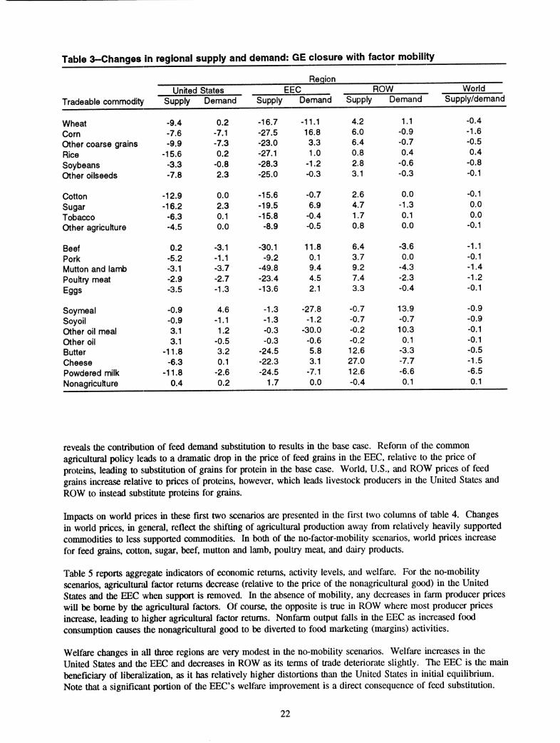
Table 3-Changes in regional supply and demand: GE closure with factor mobility

Reqion United States EEEC ROW World

Tradeable commodity Supply Demand Supply Demand Supply Demand Supply/demand

Wheat -9.4 0.2 -16.7 -11.1 4.2 1.1 -0.4

Corn -7.6 -7.1 -27.5 16.8 6.0 -0.9 -1.6

Other coarse grains -9.9 -7.3 -23.0 3.3 6.4 -0.7 -0.5

Rice -15.6 0.2 -27.1 1.0 0.8 0.4 0.4

Soybeans -3.3 -0.8 -28.3 -1.2 2.8 -0.6 -0.8

Other oilseeds -7.8 2.3 -25.0 -0.3 3.1 -0.3 -0.1

Cotton -12.9 0.0 -15.6 -0.7 2.6 0.0 -0.1

Sugar -16.2 2.3 -19.5 6.9 4.7 -1.3 0.0

Tobacco -6.3 0.1 -15.8 -0.4 1.7 0.1 0.0

Other agriculture -4.5 0.0 -8.9 -0.5 0.8 0.0 -0.1

Beef 0.2 -3.1 -30.1 11.8 6.4 -3.6 -1.1

Pork -5.2 -1.1 -9.2 0.1 3.7 0.0 -0.1

Mutton and lannb -3.1 -3.7 -49.8 9.4 9.2 -4.3 -1.4

Poultry meat -2.9 -2.7 -23.4 4.5 7.4 -2.3 -1.2

Eggs -3.5 -1.3 -13.6 2.1 3.3 -0.4 -0.1

Soymeal -0.9 4.6 -1.3 -27.8 -0.7 13.9 -0.9

Soyoil -0.9 -1.1 -1.3 -1.2 -0.7 -0.7 -0.9

Other oil meal 3.1 1.2 -0.3 -30.0 -0.2 10.3 -0.1

Other oil 3.1 -0.5 -0.3 -0.6 -0.2 0.1 -0.1 Butter -11.8 3.2 -24.5 5.8 12.6 -3.3 -0.5

Cheese -6.3 0.1 -22.3 3.1 27.0 -7.7 -1.5

Powdered milk -11.8 -2.6 -24.5 -7.1 12.6 -6.6 -6.5 Nonagriculture 0.4 0.2 1.7 0.0 -0.4 0.1 0.1

reveals the contribution of feed demand substitution to results in the base case. Refonn of the common agricultural policy leads to a dramatic drop in the price of feed grains in the EEC, relative to the price of proteins, leading to substitution of grains for protein in the base case. World, U.S., and ROW prices of feed grains increase relative to prices of proteins, however, which leads livestock producers in the United States and ROW to instead substitute proteins for grains.

Impacts on world prices in these first two scenarios are presented in the first two columns of table 4. Changes in worid prices, in general, reflect the shifting of agricultural production away from relatively heavily supported commodities to less supported commodities. In both of the no-factor-mobility scenarios, worid prices mercase for feed grains, cotton, sugar, beef, mutton and lamb, poultry meat, and dairy products.

Table 5 reports aggregate mdicators of economic returns, activity levels, and welfare. For the no-mobility scenarios, agriculturid factor returns deaease (relative to tiie price of tiie nonagricultural good) in tiie United States and the EEC when support is removed. In the absence of mobility, any decreases in farm producer prices will be borne by the agricultural factors. Of course, the opposite is true in ROW where most producer prices increase, leading to higher agricultural factor returns. Nonfarm output falls in tiie EEC as increased food consumption causes the nonagricultural good to be diverted to food marketing (margins) activities.

Welfare changes in iill three regions are very modest in the no-mobility scenarios. Welfare increases in üie United States and tiie EEC and decreases in ROW as its te^rms of trade deteriorate slightiy. The EEC is tiie main beneficiary of liberalization, as it has relatively higher distortions than tiie United States in initial equilibrium. Note that a significant portion of the EEC's welfjire improvement is a direct consequence of feed substitution.

22

Table 4--Changes ¡n world prices^ from U.S./EEC agricultural liberalization

No factor mobility Factor mobility No feed

Commodity Base case substitution GE^ PEÍ' PE2'

Percent change

Wheat -0.1 -0.2 6.3 6.2 6.1 Com 4.9 7.9 11.3 11.2 11.1 Other coarse grains 4.8 4.5 10.9 10.8 10.8 Rice -0.4 -0.3 -5.2 -5.3 -5.2 Soybeans -2.9 -1.6 2.2 2.1 2.1 Other oilseeds 0.1 0.8 2.6 2.6 2.6

Cotton 1.2 1.3 1.3 1.0 1.1 Sugar 3.8 3.9 7.5 7.4 7.3 Tobacco -4.0 -3.9 -5.1 -5.4 -5.5 Other agriculture -1.2 -1.1 0.4 0.3 0.0

Beef 6.1 6.3 12.3 12.2 12.2 Pork -2.5 -1.8 5.1 5.1 4.9 Mutton and lamb 13.6 14.2 17.6 17.6 17.6 Poultry meat 3.5 4.3 11.0 11.0 10.7 Poultry eggs -0.9 -0.3 4.6 4.5 4.4

Soymeal -4.4 2.4 -0.8 -0.8 -0.8 Soyoil -0.5 -1.1 1.4 1.3 1.3 Other oilmeal -4.0 4.8 0.1 0.0 0.0 Other oil -0.5 -0.5 0.6 0.5 0.5 Butter 12.1 12.3 16.3 16.2 16.2 Cheese 21.3 21.2 34.6 34.6 34.5 Powdered milk 9.5 9.2 29.8 29.8 29.6

^All price changes are expressed as changes relative to the price of the nonagricultural good. ^Results for the general equilibrium model assuming factor mobility. ^Partial equilibrium model with complete specification of the agricultural sector. ^Partial equilibrium model assumes production of "other agriculture" is constant.

Implications of Factor Mobility

We next turn to an examination of the effects of factor mobility on the results of the U.S./EEC liberalization experiment. We set the primary factor transformation elasticity equal to -1 in each region. This has two consequences: (1) any reduction in farm subsidies will cause a downsizing in agriculture, and (2) factor returns in the agricultural and nonagricultural sectors will be more closely linked. Individual agricultural commodity supply elasticities now embody both substitution possibilities within agriculture and expansion (contraction) effects associated with movements of resources between agriculture and nonagriculture.

The first two columns of table 6 report, for the United States, the conditional (no mobility) and unconditional

(<TT "^ "^ ) own-price supply elasticities in our model. Because the expansion effect associated with any single commodity price change is small, the unconditional responses are not much larger when the commodity in question is relatively minor. However, for those commodities with a large revenue share (see appendix table 18), the unconditional response can be enlarged considerably. For example, the unconditional elasticity of supply of com is 25 percent greater than the factor-constrained response. In the case of "other agriculture," which represents nearly a third of total output, the unconditional supply elasticity is more than 50 percent greater than the factor-constrained response.

23

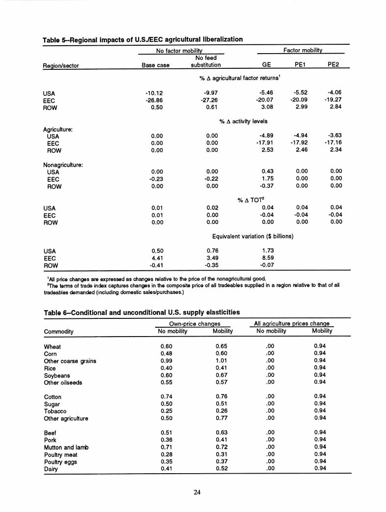
Table 5-Regional impacts of U.S7EEC agricultural liberalization

Region/sector

USA EEC ROW

Agriculture: USA EEC ROW

Nonagriculture: USA EEC ROW

USA EEC ROW

USA EEC ROW

No factor mobility Factor mobility

Base case No feed

substitution GE PEÍ

% A agricultural factor returns^

PE2

•10.12 -9.97 -5.46 -5.52 -4.06 •26.86 -27.26 -20.07 -20.09 -19.27

0.50 0.61

% A activity

3.08

levels

2.99 2.84

0.00 0.00 -4.89 -4.94 -3.63 0.00 0.00 -17.91 -17.92 -17.16 0.00 0.00 2.53 2.46 2.34

0.00 0.00 0.43 0.00 0.00 -0.23 -0.22 1.75 0.00 0.00 0.00 0.00

%A

-0.37

TOT^

0.00 0.00

0.01 0.02 0.04 0.04 0.04 0.01 0.00 -0.04 -0.04 -0.04 0.00 0.00 0.00 0.00 0.00

Equivalent variation ($ billions)

0.50 0.76 1.73 4.41 3.49 8.59

-0.41 -0.35 -0.07

^All price changes are expressed as changes relative to the price of the nonagricultural good. ^he terms of trade index captures changes in the composite price of all tradeables supplied in a region relative to that of all

tradeables demanded (including domestic sales/purchases.)

Table 6-Conditional and unconditional U.S. supply elasticities

Own-price changes All agriculture prices change Commodity No mobility Mobility No mobility Mobility

Wheat Corn Other coarse grains Rice Soybeans Other oilseeds

0.60 0.48 0.99 0.40 0.60 0.55

0.65 0.60 1.01 0.41 0.67 0.57

.00

.00

.00

.00

.00

.00

0.94 0.94 0.94 0.94 0.94 0.94

Cotton Sugar Tobacco Other agriculture

Beef Pork Mutton and \arrb Poultry meat Poultry eggs Dairy

0.74 0.50 0.25 0.50

0.51 0.36 0.71 0.28 0.35 0.41

0.76 0.51 0.26 0.77

0.63 0.41 0.72 0.31 0.37 0.52

.00

.00

.00

.00

.00

.00

.00

.00

.00

.00

0.94 0.94 0.94 0.94

0.94 0.94 0.94 0.94 0.94 0.94

24

Columns 3 and 4 in table 6 report supply response when all farm prices are changed simultaneously. Here the distinction between the mobility and no-mobility scenarios is sharpest. When factor mobility between the agricultural and nonagricultural sectors is zero, an equal across-the-board change in prices leaves agricultural supplies unchanged. (No expansion effect is permitted, and no substitution effect occurs when all agricultural prices change by the same percentage.) The elasticities in the final column of table 6 represent the aggregate expansion effect (no substitution effect) associated with an elasticity of transformation of -1 in our model.

Introduction of factor mobility into the model makes a big difference in the results. Consider, for example, the "GE" (general equilibrium) with factor mobility scenario in table 4 and compare it with the base case. In the no- mobility base case, many of the agricultural prices fall (relative to the price of nonfood, which is the numeraire), as resources are shifted from heavily supported to less heavily supported commodities. With factor mobility, there is a dramatic shift in both the pattern and the overall direction of world prices. Resources flow out of agriculture in the United States and the EEC and almost all world prices rise. However, there are several notable exceptions including: rice and tobacco. In these cases, ROW is the net supplier of the products, and as agriculture in ROW expands, the prices of these products are depressed. Thus, the pattern of regional expansion effects can have an important influence on world prices. Commodities for which the United States and the EEC are major suppliers show very strong price increases due to the contraction of production in these temperate regions.

Turning to table 5, we see that when factor mobility is permitted, declines in factor returns in the United States and EEC are dampened by downsizing of their agricultural sectors. Patterns of activity levels in nonagriculture mirror those of agriculture, with nonagricultural activity in the United States and the EEC increasing, and the ROW decreasing. The marked increase in nonagricultural output in the EEC suggests that the existing common agricultural policy (CAP) may act as a significant drag on the EEC's nonagricultural output

Note that the introduction of factor mobility reverses the sign of the terms of trade effect for the EEC. Nonetheless, EEC utility increases quite dramatically due to the substantial distortion imposed by the agricultural policies that are now reformed.

Finally, it is useful to consider what happens to an individual region's net trade position as the result of trade liberalization. Table 7 presents this information for the EEC. Column one shows that the EEC is currently a net exporter of many farm and food products. In the no-mobility base case scenario, U.S./EEC policy reform causes the EEC to switch from net exporter to net importer status in the case of four agricultural products, and net farm and food imports (and nonfood exports) increase by a total of $2,669 billion. However, the region as a whole remains a net exporter of wheat, sugar, pork, eggs, soyoil, butter, and milk powder.

When factor mobility is introduced, only wheat, soyoil, and milk powder remain net exports. Furthermore, total net farm and food imports now increase by more than $32 billion! The huge difference between the last two colunms of table 7 demonsü-ates the importance of understanding the distinction between substitution and expansion effects in the analysis of agricultural policy liberalization.

Implications of Partial Equilibrium

Maintaining the assumption of factor mobility between the agricultural and nonagricultural sectors, we next consider the implications of taking a partial versus general equilibrium ^proach when analyzing trade liberalization. We consider two alternative definitions of partial equilibrium. In the first case (PEl), output, primary factor returns, and conmiodity prices in the nonagricultural sector are fixed exogenously, and the associated market clearing and zero profit conditions are dropped from the model. Also, regional income is fixed and the associated equation is dropped. This is a partial equilibrium model of the entire farm and food economy. However, SWOPSIM models, like most other partial equilibrium models of agricultural trade, do not cover all farm and food commodities. Thus, we also consider a second partial equilibrium scenario (PE2) in which the model is further restricted by fixing the price of other agricultural products. In this case, "full liberalization" only applies to the SWOPSIM commodities.

25

Table 7-European Community's net trade position before and after U.S7EEC liberalization, 1989

Before liberalization After liberalization Connmodity No factor mobility Factor mobility

Million dollars

3,257 4,350 2,256 -272 -1,670 -1,826 645 -619 -1,181 -86 -116 -201

-3,587 -3,528 -3,773 -1,501 -1,672 -3,050

-1,615 -1.586 -1,705 735 471 -386

-1,122 -989 -1,257 13,758 -8,304 -16,356

1,473 -3,945 -7,852 1,721 4,404 -1,116 -462 -1,929 -2,422 368 -429 -1,620 116 462 -1,325

-2,387 -1,521 -1,043 305 304 305

-1,179 -735 -468 -1,265 -1,245 -1,256

983 162 -807 815 -1,213 -3,749

1,056 919 485 15,759 18,428 48,348

0 0 0

Wheat Corn Other coarse grains Rice Soybeans Other oilseeds

Cotton Sugar Tobacco Other agriculture

Beef Pork Mutton and lamb Poultry meat Poultry eggs

Soymeal Soyoil Other oilmeal Other oil Butter Cheese Powdered milk Nonfood^ Total

includes transfers or "goodwill."

The last two columns in tables 4 and 5 report simulation results for these two different partial equilibrium scenarios. The results in the column labeled PEl are extremely similar to those of the general equilibrium (GE) model with factor mobility. This is not surprising since agriculture, in this model, is such a small part of the economy of each region. In other words, one does not need a general equilibrium model to detennine the farm level effects of changes in agricultural policy. Of course, tlie partial equilibrium framework does not capture the effects on the nonagricultural sector, which may be quite important for policy analysis.

While the difference between the GE and PEl results is negligible, the difference between PEl and PE2 is sometimes significant When other agricultural production is ignored in PE2, there is less of a decline in the U.S. and EEC farm sectors and less expansion of agriculture in ROW. It seems that for purposes of assessing the farm level effects of U.S./EEC agricultural policy liberalization, complete coverage of agriculture is more important than extending the model to obtain full general equilibrium coverage.

26

Conclusions

The purpose of this paper has been to build a bridge between existing partial equilibrium models of international agricultural trade and their general equilibrium counterparts. In particular, a set of procedures has been outlined that permits us to specify a general equilibrium model that is consistent with data and parameters from USD A's SWOPSM/DEMO model. A number of insights were obtained that suggest methods of altering and improving the SWOPSIM database.

By invoking the assumption of implicitly additive consumer preferences, we are able to generate a complete matrix of uncompensated price elasticities from the parameters available in the DEMO model. In the process of doing so, we find evidence that the income elasticities of demand are inconsistent with the other model parameters. In particular, they require upward adjustment in order to satisfy regularity properties on the utility function (given the existing budget shares, price elasticities, and the maintained hypothesis of implicit additivity). Also, a detailed examination of the feed-livestock complex suggests a number of possibilities for "adding value" to this partial equilibrium model of agricultural trade.

The calibration exercise also points to the need to reexamine some of the price levels embodied in the database. A number of sectors exhibit remarkably small, or even negative value-added, given stated prices. In addition, the marketing margins for several food commodities are found to be very small. Finally, there are numerous instances where the domestic market price of a commodity is not equal to the world price, adjusted for price distortions. This can have confounding effects on welfare analyses conducted using this framework.

Our general equilibrium model may be simulated in a number of different "modes." By fixing exogenously the prices of all non-SWOPSIM commodities, as well as the aggregate agricultural resource endowment, and regional income, it is possible to imitate a solution of the SWOPSIM/DEMO model. The advantage of our particular partial equilibrium fonnulation is its specification in terms of fundamental preference and technology parameters.

We can easily examine the sensitivity of our model's solution to the degree of livestock-feed substitution. We find that feedstuff substitutability is important for assessing the effects of liberalization. It also has a significant effect on the welfare consequences of liberalization.

We find that the general equilibrium closure is not crucial to obtaining an accurate assessment of the agricultural price and quantity effects of agricultural trade liberalization. However, the complete general equilibrium closure does have the advantage of assuring a comprehensive accounting of the welfare effects of multilateral agricultural trade liberalization. It also offers a mechanism for incorporating nonfann shocks to the model. Furthennore, in the process of closing the model, we highlight the importance of accounting for all agricultural activity, particularly when factor mobility is a consideration.

The issue of factor mobility is one that deserves greater attention in partial equilibrium models of international agricultural trade. In this paper, we explore two extreme assumptions, one in which factors are fully inmiobile between the farm and nonfann sectors, and one in which they are highly mobile. Factor mobility is shown to raise the welfare gains from ü"ade liberalization. It also has a dramatic impact on the pattern of global farm and food production and on the world price effects of liberalization. This is clearly an important area for future research.

27

References

BaU, V.E. "Modeling Supply Response in a Multíproduct Framework," American Journal of Agricultural Economics, 70(4):813-825, 1988.

Burfisher, M., S. Robinson, and K. Thierfelder. "Agricultui^ and Food Poücies in a United States-Mexico Free Trade Area," North American Journal of Economics and Finance, 3(2):117-139, 1992.

Bumiaux, J., and D. van der Mensbrugghei. ne RUNS Model: A Rural-Urban North-South General Equilibrium Model for Agricultural Policy Analysis. OECD Development Centre Technical papers. Number 33, Paris, Dec. 1990.

Bumiaux, J., and J. Waelbroeck. "The Common Agricultural Policy of the European Conrndunity and the World Economy: A General Equüibrium Analysis," IIASA Conference Proceedings, 1989.

Bumiaux, J., F. Delorme, I. Lienert, J.P. Martin, and P. HoeUer. Quantifying the Economywide Effects of Agricultural Policies: A General Equilibrium Approach. Working P^)er No. 55, OECD Department of Economics and Statistics, Paris, 1988.

Codsi, G., and K.R. Pearson. Developing and Implementing Large Economic Models Using GEMPACK, a General Purpose Software Suite. Impact Prelhninary Working Paper No. IP-39, University of Melbourne, Melboume, 1988.

Connor, J.M., and S. Weimar. "The Intensity of Advertising and Other Selling Expenses in Food and Tobacco Manufacturing: Measurement, Determinants, and Impacts," Agribusiness, 2(3): 293-319, 1986.

Diewert, W.E. "The Comparative Statistics of Industry Long Run Equilibrium," Canadian Journal of Economics, 14(l):78-92, 1981.

Dixon, P.B., B.R. Paramenter, J. Sutton, and D.P. Vincent. ORAN I: A Multisectoral Model of the Australian Economy. North Holland Press, Amsterdam, 1982.

Dunham, D. Food Cost Review, 1990. AER-651, U.S. Dept. Agr., Econ. Res. Serv., 1991.

Food and Agriculture Organization of the United Nations. FAO Production Yearbook, 1989. Rome, 1990.

Gardiner, Walter H., Vemon O. Roningen, and Karen Liu. Elasticities in the Trade Liberalization Database. Staff Report AGES 89-20, U.S. Dept. Agr., Econ. Res. Seirv., May 1989.

Goldm, I., and O. Knudsen. "The Implications of Agricultural Trade Liberalization for Developing Countries," Agricultural Trade Liberalization: Implications for Developing Countries. I. Goldin and O. Knudsen (eds.). OECD, Paris, 1990.

Haley, Steven L. Joint Products in the Static World Policy Simulation Model (SWOPSIM) Modeling Framework. Staff Report AGES 881024, U.S. Dept. Agr., Econ. Res. Serv., Nov. 1988.

Hanoch, G. "Production and Demand Models with Direct or Indirect Implicit Additivity," Econometrica, 43(3):395^19, 1975.

Herlihy, M., S. Haley, and B. Johnson. Assessing Model Assumptions in Trade Liberalization Modeling: An Application to SWOPSIM. Intemational Agricultural Trade Consortium Working Paper #92-2, 1992.

Hertel, T.W. "Estimating Substitution and Expansion Effects: Comment," American Journal of Agricultural Economics, 69(1):188-192, 1987.

28

^ "Negotiating Reductions in Agricultural Support: Implications of Technology and Factory Mobility," American Journal of Agricultural Economics, 69(3):559-573, 1989a.

. "PSEs and the Mix of Measures to Support Fann Incomes," The World Economy, 12(l):17-27, 1989b.

. "General Equilibrium Analysis of Agriculture: What Does it Contribute?" Agricultural Economics Research, 42(3):3-9, 1990.

Hertel, T.W., E.B. Peterson, P.V. Preckel, Y. Surry, and M.E. Tsigas. "ImpHcit Additivity as a Strategy for Restricting tiie Parameter Space in CGE Models," Economic and Financial Computing, l(3):265-289, 1991.

Hertel, T.W., V.E. Ball, K.S. Huang, and M.E. Tsigas. Computing General Equilibrium Farm level Demand Elasticities for Agricultural Commodities. AES Research Bulletin No. 988, Purdue University, 1989.

Hertel, T.W., and M.E. Tsigas. "Tax Policy and U.S. Agriculture: A General Equilibrium Approach," American Journal of Agricultural Economics, 70(2):289-302, 1988.

Horridge, M. and D. Pearce. Modeling the Effects on Australia of Interventions in World Agricultural Trade. IMPACT Preliminary Woricing Paper No. OP-65, University of Melbourne, 1988.

International Monetary Fund. International Financial Statistics, 1990 Yearbook. Washington DC.

Krissoff, Barry and Nicole Ballenger. "Agricultural Trade Liberalization in a Multi-Sector Model: Implications for Argentina, Brazil, and Mexico," pp. 67-71 in Bruce Greenshields and Margot Dellamy (eds.) Government Intervention in Agriculture. lAAE Occasional Paper No. 5, 1989.

Liapis, Peter. Incorporating Inputs in the Static World Policy Simulation Model (SWOPSIM). TB-1780. U.S. Dept Agr., Econ. Res. Serv., June 1990.

Liapis, P. and M. Shane. Agricultural Trade Liberalization: Implications for Productive Factors in the US. Working Paper No. 92-5, International Agricultural Trade Research Consortium, 1992.

Magiera, S.L. and M.T. Herlihy. "A Technical Comparison of Trade Liberalization Model Results." Draft Manuscript, U.S. Dept., Agr., Econ., Res., Serv., 1988.

McDonald, B J. "Agricultural Negotiations in the Uruguay Round," The World Economy, 13(3):299-327, 1990.

McDougall, R.A., T.W. Hertel, J.F. Zeitsch, A. Welsh, S. Brown, P. Jomini, J. KeUy, and J. Hambley. "Gains from Global Trade Liberalization: An Illustrative Application of SALTER," Volume W, SALTER: A General Equilibrium Model of the World Economy. Industry Conmiission: Canberra, Australia, 1991.

Organization for Economic Cooperation and Development. National Policies and Agricultural Trade. Paris, 1987.

. Modeling the Effects of Agricultural Policies. Economic Studies Special Issue, Paris, Winter 1989-90.

. Tables of Producer Subsidy Equivalents and Consumer Subsidy Equivalents 1979-1990. Paris, 1991.

Parikh, K.S., G. Fischer, K. Frohberg, and O. Gulbrandsen. Towards Free Trade in Agriculture. Luxenburg, Austria: Martinus Nijhoff Publishers, 1988.

Pearson, K. UPDATE and multi-step version of TABLO, mimeo 21. Oct. 1990.

Peterson, E.B., P.V. Preckel, and T.W. Hertel. CGE Model Formulation Focused on Domestic Food System. Staff Paper No. 92-01, Department of Agricultural Economics, Virginia Polytechnic Institute and State University, Blacksburg, 1992.

29

Roningen, V.O. A Static World Policy Simulation (SWOPSIM) Modeling Framework. Staff Report AGES 860625, U.S. Dept. Agr., Econ. Res. Serv., July 1986.

Roningen, V.O., and P.M. Dixit. Economic Implications of Agricultural Policy Reform in Industrial Market Economies. Staff Report No. AGES 89-36, U.S. Dept. Agr., Econ. Res. Serv., 1989.

Roningen, V., J. Sulliviin, and P. Dixit. Documentation of the Static World Policy Simulation (SWOPSIM) Modeling Framework. Staff Report AGES 9151. U.S. Dept. Agr., Econ. Res. Serv., 1991.

Surry, Y. "The 'Constant Difference of Elasticities' Function With Application to the EC Animal Feed Sector," Journal of Agricultural Economics, 44(1):110-125, 1993.

Tangerman, S., T.E. Josling, and S. Pearson. "Multilateral Negotiations on Farm-support Level," The World Economy, 10(3):265-281, 1987.

Tyers, R., and K. Anderson. "Distortions in World Food Markets: A Quantitative Assessment," Background paper for the World Development Report. The World Bank, Washington DC, 1986.

United Nations. National Accounts Data (Tape). United Nations Statistical Office, New York, Jan. 1992.

U.S. Department of Agriculture, Economic Research Service. Foreign Agricultural Trade of the United States, various issues.

, Foreign Agriculture Service. Production, Supply, and Distribution (Tape). 1992.

Valdes, A., and J. Ziet2:. Agricultural Protection in OECD Countries: Its Costs to Less-Developed Countries. Research Report 21, International Food Policy Research Institute, Washington DC, 1980.

Worid Bank. 1986 World Development Report.

Zeitsch, J. "Adding Input Demands to Partial Equilibrium Agricultural Trade Models," paper presented at the 33rd conference of the Australian Agricultural Economics Society, Christchurch, New Zealand, Feb. 1989.

30

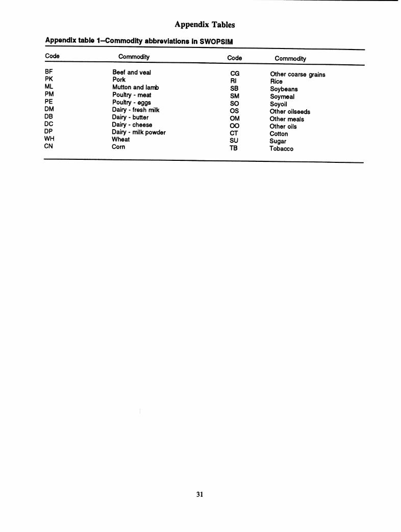
Appendix Tables

Appendix table 1-Commodity abbreviations in SWOPSIM

Code Commodity Code Commodity

BF Beef and veal CG Other coarse grains PK Pork RI Rice ML Mutton and lamb SB Soybeans PM Poultry - meat SM Soymeal PE Poultry - eggs SO Soyoil DM Dairy - fresh milk OS Other oilseeds DB Dairy - butter OM Other meals DC Dairy - cheese oo Other oils DP Dairy - milk powder CT Cotton WH Wheat SU Sugar CN Corn TB Tobacco

31

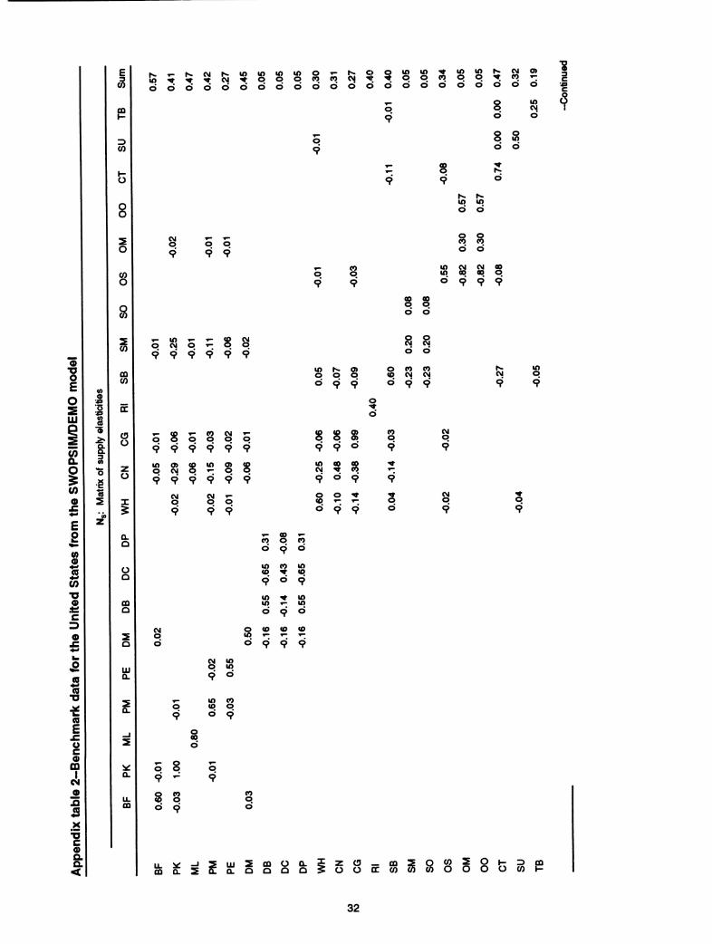
E

m

3 CO

ü

m -^ '^ ^ CM '^ q q q CO CO oi ^r ööööööööooooo

-^oocooq^cq^ ööööööööö

o 9

o 9

S 9

8 to CM

Ö Ö

O in Ö Ö

1^ Ö

C C

S

O

CO o

8

g o o 9 9

o 9

S 9

CO CO

lO CM CM 00 u) 00 a> o 0999

S

O -O o E (O

■5

i

E S (O

I (/) ■Ö o ±í c

CO

CD CO

0 ü

ü

X 5

o. o

ü Û

o

2 o

T- m ▼- ^ » w o CM o ^ o q 9 9 9 9 9 9

t- <p ▼- CO w »- 000000

9 9 9 9 9 9

§ a S !2 § 8 9 9 9 9 9 9

S

CM O o

o o 9 9

o Ö

to <0

10 to

s CO o

CO to ^ <0

to to o*

h- <J> o o 9 9

ö

s s s 996

o o CM CM Ö Ö

O CO CO (O CM CM

099

CO o

CM to O

to 00 CM ^ 909

8 2? 099

S ö

g

3 o

o (O (O (O

o $ 9 9

LU CL

(O £

JZ o c o m

I CM

J! iS X

'■5 c o a Q. <

CL

CD

O

9

O 8 9 ^ o CO <o o o c?

CM to o to

9 ^

to CO (O o o 9

o 00

o 9

CO o

ii^-lSUjSCDOa.SZO-.CQ míSÍSouuuSüüDCco 8 O O O ü CO

CD

32

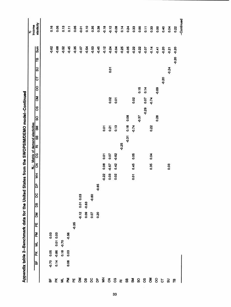
if o «o

C

C O

o E

UJ

O) Û. o O)

E S «»- (O

i5 O)

c

CO

E n o c o m

I CM

-2 i3

C 0) o. GL <

ü

8

8

CÛ

<oin(OT-u)^ou>oococMoo'^'^coo-«-coQO<^ oööööq>ööö<^c^ööööööööö o ^

€M00CMIAU)h.^C0lOCM'^'^tAl0CNICN|K^-<-O <0<0in^(0OU)U)^T-CMOCV|OC\lcvlo^<^cJ

9999 9 9999 9 9999999 9 99 9 9 o CM

O

Ö CM

8 9

CM ▼- O O Ö Ö

▼- »- eo o CM ^

CM o

00 o d

o cí

<0

o K o Q

0>

9 00 CM

Ö

Ö

CM

CO

9

o o Ö Ö

CM

00 o

a

h* CM

9 <=>

o o d d

o d

d

o d

o d

in CO d

CO o d

(O

s y CO O <0 d c?

o (O

£! 8 & a

lA

CO CO o o (O

T- o o r^ d d

U) <0 00 CO o 00 T- o Ö ó Ö Ö

o "*

UL ^

00 o

2 m s CÛ o o. a: a. o o o o Z o - 00

ü ü ce CO 2 O h- 3 O CO ^ U h- 3 CD

CO O O O ü CO I-

33

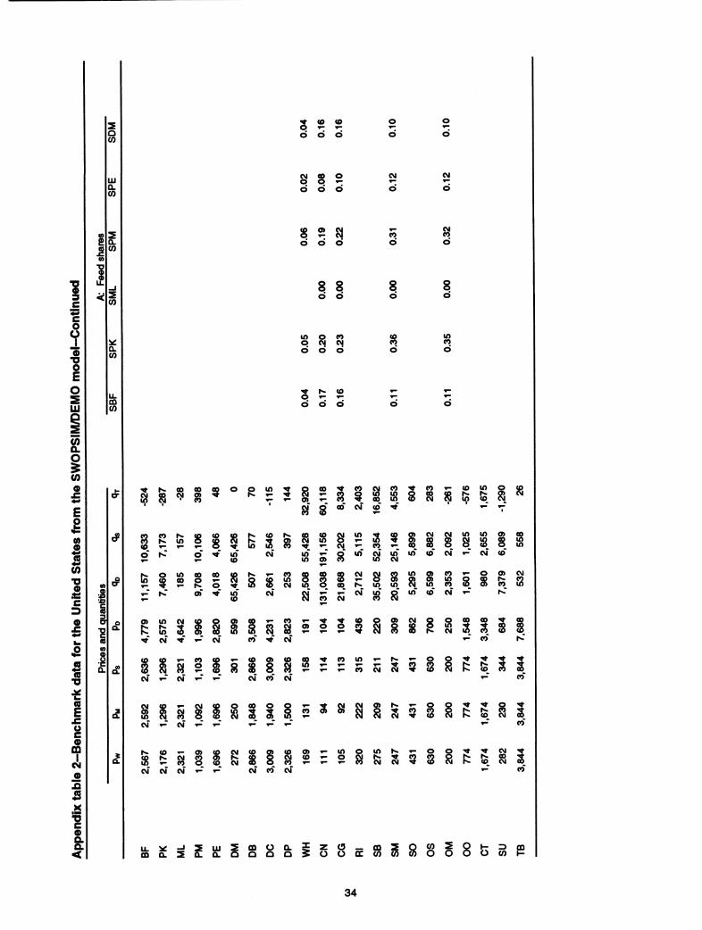
2 Û CO

s 2 Î5 Ö Ö Ö

o Ö

o ö

LU CL CO

8 8 2 ö ö ö

CM

Ö

CM

Ö

1 c 1 o

o E

iij

5

1 CO

CL CO

CD CO

8 2a Ö Ö Ö

8 8 Ö O

lA p CO O CM Oj Ö O O

S t 2 ö ö ö

CO ö

8 ö

ö

Si CO ö

8 Ö

in CO ö

Û.

i 0)

I 1^ S OOflOOOlO^OCO^WCMCO^CO^COlpO

ci g « CM- <g * - T ^

«

I </)

& c

CO E

o tn

I CM

n a >< c o Q, CL <

é

«0

a

«

o

CO h-

o

U)

CM"

^ § § ^ I s § ^ ^ ^ ^ ! i s s i i i § ö ^" 8 ~" " " " ' ' ■" " *■ " "■ '" 10 «- Q U> CM in

lO 0> CO tí) CM U) U) CO CM ▼- CM <0

CO ^ O CJ) CM

% l CM

1*^ (O » h-

CM CM

oí

* ^" 8 '^" a «" Î3 *^" 8 8 "*' * '^" '"" •"

i § § § g § i I M § i i I g II i I W CM CO* ^ CM ^ CO* r^"

8 i 8 i i § s î e 5 s ^ ? i i ^ M i T-* ^" oí eo" CM '- «

CM

3 '4 ^ CM

CNÍ

s CM (O (O (3>

CM" CO CM*

lO O lO N -r- 2 8 Î5 S 5

-^ -^ CM -^ fí <0 CM S

míSESoQUOSüüOCCOCOCOOOOüCOF

34

Appendix table 3-Price wedges for the United States

Commodity TracJe' DPSW CSW

Dollars per metric ton

BF -44 PK 0 ML' 0 PM 0 PE 0

DM -102 DB -1,120 DC -1,060 DP -276

WH 0 CN 0 CG 0 RI 0

SB 0 SM 0 SO 0 OS^ -59 OM 0 00 0

CT 0 SU -112 TB 0 Other agriculture 0

164.39 78.49

458.60 67.29 57.55

15.25 0 0 0

36.32 27.10 25.13

113.59

15.32 0 0

35.02 0 0

340.11 19.38

274.19 5.85

0 0 0 0 0

0 0 0 0

0 0 0 0

0 0 0 0 0 0

0 0 0 0

^A positive value is an export subsidy wedge and a negative value is an import subsidy wedge. ^Includes direct payments for the wool program. ^Includes trade support for peanuts.

35

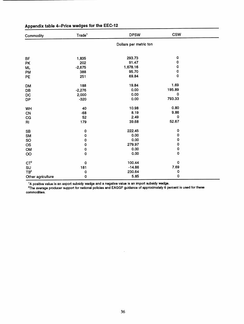
Appendix table 4-Price wedges for the EEC-12

Commodity Trade^

BF 1,835 PK 202 ML -2,675 PM 388 PE 251

DM 188 DB -2,276 DC 2,000 DP -320

WH 40 CN -68 CG 52 Ri 179

SB 0 SM 0 SO 0 OS 0 OM 0 OO 0

CT^ 0 SU 181 TB^ 0 Other agriculture 0

DPSW CSW

Doiiars per metric ton

293.73 0 91.47 0

.678.16 0 95.70 0 69.84 0

19.84 1.69 0.00 195.89 0.00 0 0.00 793.33

10.98 0.80 8.19 9.86 2.49 0

39.68 52.67

222.45 0 0.00 0 0.00 0

279.97 0 0.00 0 0.00 0

100.44 0 -14.86 7.69 230.64 0

5.85 0

^A positive value is an export subsidy wedge and a negative value is an import subsidy wedge, ^he average producer support for national policies and EAGGF guidance of approximately 6 percent is used for these

commodities.

36

Appendix table 5-lnitíal and revised marl(eting margins

United States EEC ROW Commodity Initial Revised Revised Revised

BF PK ML PM PE

DM DB DC DP

WH CN CG RI

SB SM SO OS OM 00

CT SU TB

Dollars per metric ton

2,110.01 2,157.72 3,666.26 1,711.33 1,366.95 3,269.63 3,586.90 2,884.47 2,393.90 3,721.61 9,513.05 2,514.42

904.87 1.275.41 1,758.57 1,081.41 766.63 1,413.13 1,628.95 1,228.14

294.99 417.17 516.97 231.70 704.96 1,708.29 2,399.61 1,228.29

1,311.37 1,743.86 2,146.71 1,289.57 581.46 1,115.14 1,927.33 996.86

58.71 1.884.17 1,991.63 825.12 10.44 1,270.04 1,702.72 541.94 9.22 1,196.31 1.437.86 512.65

164.99 1,962.04 2,388.84 865.19

10.84 1,107.47 2,093.80 641.67 42.50 116.34 116.34 116.34

451.98 203.00 203.00 203.00 13.22 2,758.71 3,703.21 1,470.00 46.25 165.06 165.06 165.06

440.98 638.78 638.78 638.78

1,411.94 18,467.13 16,070.40 9,486.00 301.99 652.53 679.22 344.67

3,582.86 65,962.99 60,967.59 57.660.00

37

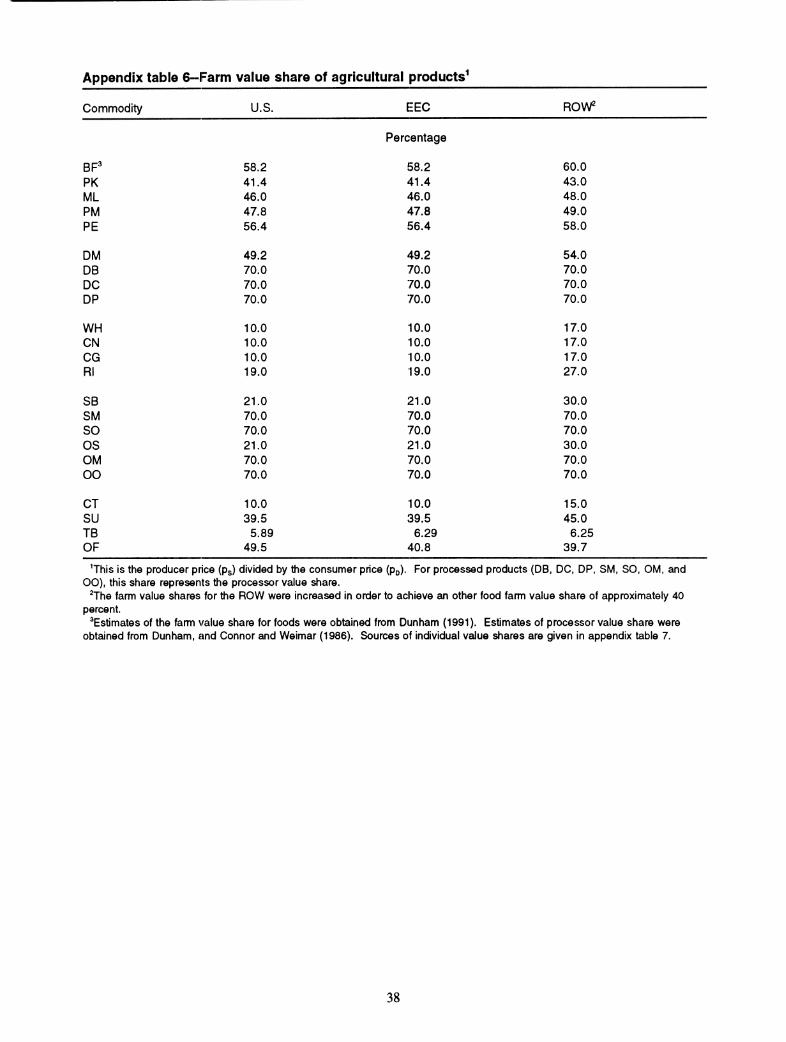
Appendix table 6-Farm value share of agricultural products^

Commodity U.S. EEEC ROW

Percentage

BF^ 58.2 58.2 60.0 PK 41.4 41.4 43.0 ML 46.0 46.0 48.0 PM 47.8 47.8 49.0 PE 56.4 56.4 58.0

DM 49.2 49.2 54.0 DB 70.0 70.0 70.0 DC 70.0 70.0 70.0 DP 70.0 70.0 70.0

WH 10.0 10.0 17.0 CN 10.0 10.0 17.0 CG 10.0 10.0 17.0 RI 19.0 19.0 27.0

SB 21.0 21.0 30.0 SM 70.0 70.0 70.0 SO 70.0 70.0 70.0 OS 21.0 21.0 30.0 OM 70.0 70.0 70.0 00 70.0 70.0 70.0

CT 10.0 10.0 15.0 SU 39.5 39.5 45.0 TB 5.89 6.29 6.25 OF 49.5 40.8 39.7

^This is the producer price (Ps) divided by the consumer price (Po). For processed products (DB, DC, DP, SM, SO, OM, and 00), this share represents the processor value share.

^The farm value shares for the ROW were increased in order to achieve an other food farm value share of approximately 40 percent.

^Estimates of the fami value share for foods were obtained from Dunham (1991). Estimates of processor value share were obtained from Dunham, and Connor and Weimar (1986). Sources of individual value shares are given in appendix table 7.

38

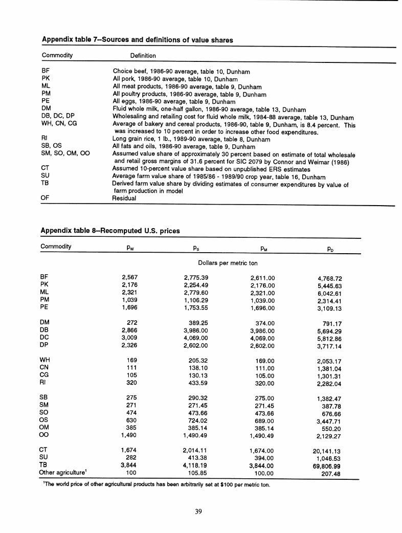
Appendix table 7-Sources and definitions of value shares

Commodity Definition

BF Choice beef, 1986-90 average, table 10, Dunham PK All pork, 1986-90 average, table 10, Dunham ML All meat products, 1986-90 average, table 9, Dunham PM All poultry products, 1986-90 average, table 9, Dunham PE All eggs, 1986-90 average, table 9, Dunham DM Fluid whole milk, one-half gallon, 1986-90 average, table 13, Dunham DB, DC, DP Wholesaling and retailing cost for fluid whole milk, 1984-88 average, table 13, Dunham WH, CN, CG Average of bakery and cereal products, 1986-90, table 9, Dunham, is 8.4 percent. This

was increased to 10 percent in order to increase other food expenditures. Rl Long grain rice, 1 Ib., 1989-90 average, table 8, Dunham SB, OS All fats and oils, 1986-90 average, table 9, Dunham SM, SO, OM, OO Assumed value share of approximately 30 percent based on estimate of total wholesale

and retail gross margins of 31.6 percent for SIC 2079 by Connor and Weimar (1986) CT Assumed 10-percent value share based on unpublished ERS estimates SU Average farm value share of 1985/86 - 1989/90 crop year, table 16, Dunham TB Derived farm value share by dividing estimates of consumer expenditures by value of

farm production in model OF Residual

Appendix table 8-Recomputed U.S. prices

Commodity Pw Ps PM PD

Dollars per metric ton

BF 2,567 2,775.39 2,611.00 4,768.72 PK 2,176 2,254.49 2,176.00 5,445.63 ML 2,321 2,779.60 2,321.00 6,042.61 PM 1,039 1,106.29 1,039.00 2,314.41 PE 1,696 1,753.55 1,696.00 3,109.13

DM 272 389.25 374.00 791.17 DB 2,866 3,986.00 3,986.00 5,694.29 DC 3,009 4,069.00 4,069.00 5,812.86 DP 2,326 2,602.00 2,602.00 3,717.14

WH 169 205.32 169.00 2,053.17 CN 111 138.10 111.00 1,381.04 CG 105 130.13 105.00 1.301.31 RI 320 433.59 320.00 2,282.04

SB 275 290.32 275.00 1,382.47 SM 271 271.45 271.45 387.78 SO 474 473.66 473.66 676.66 OS 630 724.02 689.00 3,447.71 OM 385 385.14 385.14 550.20 OO 1,490 1.490.49 1,490.49 2,129.27

CT 1,674 2,014.11 1,674.00 20,141.13 SU 282 413.38 394.00 1,046.53 TB 3,844 4,118.19 3,844.00 69,806.99 Other agriculture^ 100 105.85 100.00 207.48

'The worid price of other agricultural products has been arbitrarily set at $100 per metric ton

39

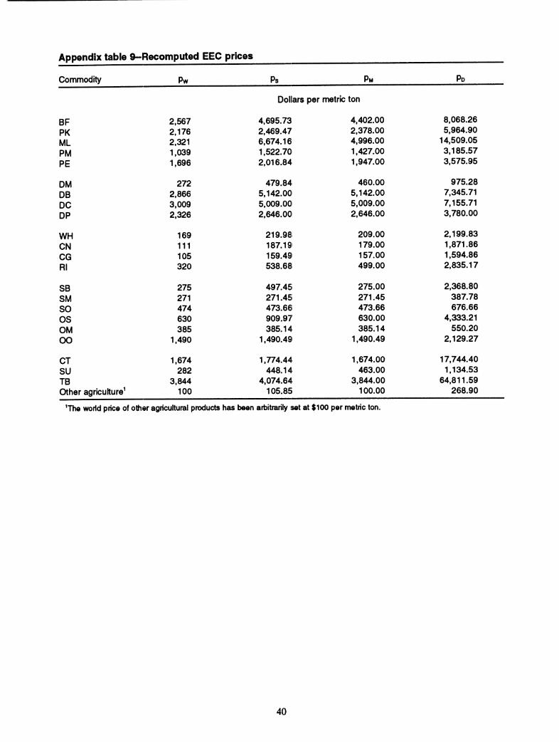
Appendix table 9-Recomputed EEC prices

Commodity Pw Ps PM PD_

Dollars per metric ton

BF 2,567 4.695.73 4.402.00 8,068.26 PK 2,176 2,469.47 2.378.00 5,964.90 ML 2,321 6,674.16 4.996.00 14,509.05 PM 1.039 1,522.70 1.427.00 3,185.57 PE 1,696 2,016.84 1.947.00 3,575.95

DM 272 479.84 460.00 975.28 DB 2,866 5.142.00 5.142.00 7,345.71 DC 3,009 5,009.00 5,009.00 7.155.71 DP 2,326 2,646.00 2,646.00 3.780.00

WH 169 219.98 209.00 2,199.83 CN 111 187.19 179.00 1,871.86 CG 105 159.49 157.00 1,594.86 RI 320 538.68 499.00 2,835.17

SB 275 497.45 275.00 2,368.80 SM 271 271.45 271.45 387.78 SO 474 473.66 473.66 676.66 OS 630 909.97 630.00 4,333.21 OM 385 385.14 385.14 550.20 OO 1,490 1,490.49 1,490.49 2,129.27

CT 1,674 1,774.44 1,674.00 17,744.40 SU 282 448.14 463.00 1,134.53 TB 3.844 4,074.64 3,844.00 64,811.59 Other agriculture' 100 105.85 100.00 268.90

'The world price of other agricultural products has been arbitrarily set at $100 per metric ton.

40

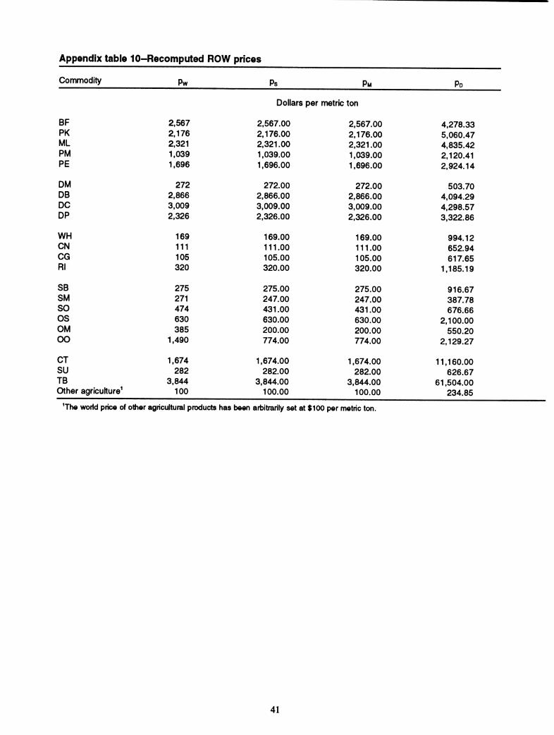
Appendix table 10-Recomputed ROW prices

Commodity Pw Ps PM PD

Dollars per metric ton

BF 2.567 2.567.00 2.567.00 4.278.33 PK 2.176 2.176.00 2,176.00 5.060.47 ML 2.321 2,321.00 2,321.00 4.835.42 PM 1.039 1.039.00 1,039.00 2,120.41 PE 1.696 1.696.00 1.696.00 2.924.14

DM 272 272.00 272.00 503.70 DB 2.866 2,866.00 2.866.00 4,094.29 DC 3.009 3.009.00 3.009.00 4,298.57 DP 2,326 2,326.00 2.326.00 3.322.86

WH 169 169.00 169.00 994.12 CN 111 111.00 111.00 652.94 CG 105 105.00 105.00 617.65 RI 320 320.00 320.00 1.185.19

SB 275 275.00 275.00 916.67 SM 271 247.00 247.00 387.78 SO 474 431.00 431.00 676.66 OS 630 630.00 630.00 2.100.00 OM 385 200.00 200.00 550.20 OO 1.490 774.00 774.00 2.129.27

CT 1.674 1.674.00 1.674.00 11,160.00 SU 282 282.00 282.00 626.67 TB 3.844 3.844.00 3.844.00 61.504.00 Other agricuKure' 100 100.00 100.00 234.85

'The worid price of other agricultural products has been arbitrarily set at $100 per metric ton.

41

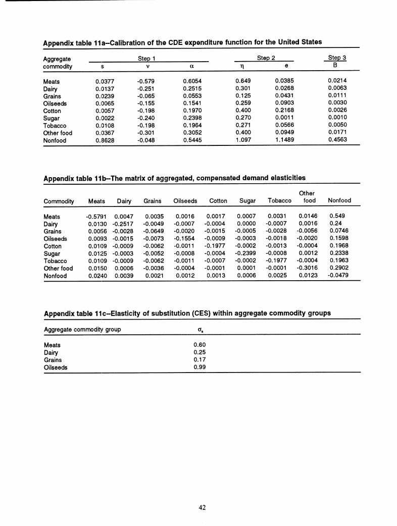
Appendix table 1 la-Calibration of the CDE expenditure function for the United States

Aggregate commodity

Step 1 Step 2

Meats 0.0377 -0.579 Dairy 0.0137 -0.251 Grains 0.0239 -0.065 Oilseeds 0.0065 -0.155 Cotton 0.0057 -0.198 Sugar 0.0022 -0.240 Tobacco 0.0108 -0.198 Other food 0.0367 -0.301 Nonfood 0.8628 -0.048

a

0.6054 0.2515 0.0553 0.1541 0.1970 0.2398 0.1964 0.3052 0.5445

Î1 e

0.649 0.0385 0.301 0.0268 0.125 0.0431 0.259 0.0903 0.400 0.2168 0.270 0.0011 0.271 0.0566 0.400 0.0949 1.097 1.1489

Step 3 B

0.0214 0.0063 0.0111 0.0030 0.0026 0.0010 0.0050 0.0171 0.4563

Appendix table llb-The matrix of aggregated, compensated demand elasticities

Other Commodity Meats Dairy Grains Oilseeds Cotton Sugar Tobacco food Nonfood

Meats -0.5791 0.0047 0.0035 0.0016 0.0017 0.0007 0.0031 0.0146 0.549 Dairy 0.0130 -0.2517 -0.0049 -0.0007 -0.0004 0.0000 -0.0007 0.0016 0.24 Grains 0.0056 -0.0028 -0.0649 -0.0020 -0.0015 -0.0005 -0.0028 -0.0056 0.0746 Oilseeds 0.0093 -0.0015 -0.0073 -0.1554 -0.0009 -0.0003 -0.0018 -0.0020 0.1598 Cotton 0.0109 -0.0009 -0.0062 -0.0011 -0.1977 -0.0002 -0.0013 -0.0004 0.1968 Sugar 0.0125 -0.0003 -0.0052 -0.0008 -0.0004 -0.2399 -0.0008 0.0012 0.2338 Tobacco 0.0109 -0.0009 -0.0062 -0.0011 -0.0007 -0.0002 -0.1977 -0.0004 0.1963 Other food 0.0150 0.0006 -0.0036 -0.0004 -0.0001 0.0001 -0.0001 -0.3016 0.2902 Nonfood 0.0240 0.0039 0.0021 0.0012 0.0013 0.0006 0.0025 0.0123 -0.0479

Appendix table He-Elasticity of substitution (CES) within aggregate commodity groups

Aggregate commodity group a^

Meats Dairy Grains Oilseeds

0.60 0.25 0.17 0.99

42

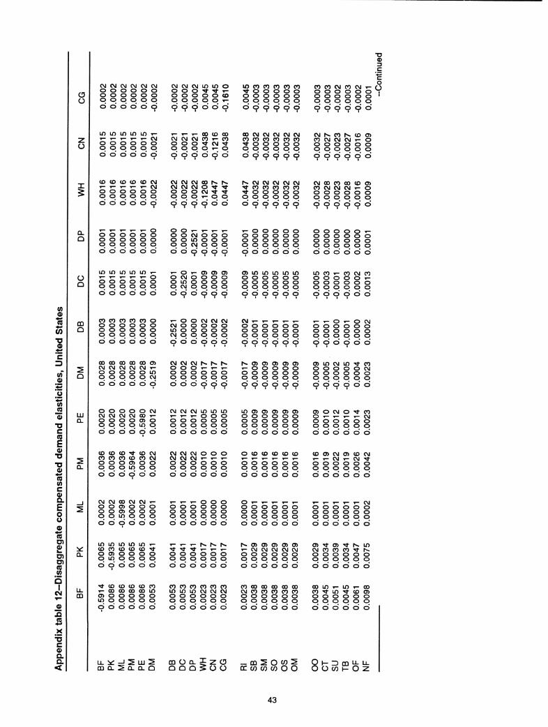
(D

O O

CM CM CVi CM CVJ CM O O O O O O O O O O O O O O O O O O d d CD CD Ö 9

CM CM CM in lí) o o o o '^ Tf ^ o o o o o CO o o o o o ^

lO CO CO CO CO CO ^ o o o o o o o o o o o o o o o o o

099000 099999

c o

CO CO CM CO CM T- o o o o o o o I 000000 ' 000000 o 9 o 9 9 d

ü

u) m LO u) m T- 1- T- r- 1- t- CM 000000 q q o o o o Ö Ö ó Ö Ö ö

1^ 1- T- 00 <0 CO CM CM CM CO ^ CO o o o -^ CM "^ o q q o T- o 9 9 9 d 9 d

CO CM CM CM CM CM CO CO CO CO CO CO '^00000 000000 d 9 9 9 9 9

CM h» CO h» (O C3> CO CM CM CM T- o 000000 q q q q q o Ö Ö Ö Ö ó Ö

X 5

(O CD (O (O (O CM

000000 000000 ó ö ö ö ó ö

CM CM CM CO h. 1^ CM CM CM o "^ "^ o o o CM '^ -^ o o o T- o o CD o 9 o d d

hr CM CM CM CM CM "^ CO CO CO CO CO 't o o o o o 000000

CM 00 CO CO <0 0> CO CM CM CM t- o 000000 000000

099999 99999^

CL 000000 000000 000000 ó ó ó ó ö ó

o o 1- ^ t- ^ o o CM o o o o o in o o o q q CM q q q ó ó Ö ó d d

i I I I

^00000 000000 000000 q q q q q q d d Ö Ö ó ó

o o o o o T- 000000 000000 q o o o o o ó ó Ö ó d d

ü Û

10 in iT) ID in r-

000000 000000

T- o T- 0> CJ> 0> o CM o o o o o lí) o o o o o CM o o o o

000000 000000 I III

O) in in in 10 in 000000 000000 000000 d d d d d d

in CO T- CO CM CO o o o o o 1- 000000 q q q o o o d d d d d d

0) o

(O

■g 'E D

0)

CO CO CO CO CO o 000000 000000 q o o o o o ó Ö Ö ó <D Ö

00 00 00 00 00 O) CM CM CM CM CM r- o o o o o in o o o o o CM Ö Ö ó ó Ö ó

^ o o CM CM CM CM o o o o o in o o o o o CM o o o o o d d d d d d

I III

CM CM CM h* h* h«. o o o T- 1- T- 000000 000000 ö ó ö ó ó ö

000000 000000 q q o q q o ö ó ö ó ó ó

h* O) O) O) O) o> t- o o o o o 000000 o q q q o o Ö Ö ó ó Ö Ö

T- T- o ^ o CM 000000 000000 q q q q q q Ö Ö ó ó ó ó

C3> in CM in '^ CO o o o o o CM 000000 q q o o o o ó ó ó ó ó ó

JS, o

■0 c (O E o

■o

"Ö o (ü (/) c Q> a E o o o % O)

2 a> 0) CO (ñ

O I

CM

-2 i2

c 0) o. a <

LU Û_

CL

CÛ

o o o O O CM CM CM CM CM 00 "I- 000000 O O O O m O ó Ö ó ó Ö ó

CO CO CO "* <o CM CO CO CO CO CO CM O O o C3> o o o o o in o o ó Ö ó ó ó ó

CM CM 00 CM CM ^ o o C5> o o o o o (3> o o o o O in O O O d d d d d d

in in in in in T- CO CO CO CO CO "^ O C3> O o o o O LO O o o o Ö ó Ö ó Ö Ö

"^ CO CO CO CO CO T— 00 00 00 00 in CJ) o o o o o in o o o o o d d d d d d

CM CM CM in in in T- T- T- o o o 000000 000000 ó ó Ö ó ó Ö

CM CM CM o o o CM CM CM T- T- T- 000000 O O q q O O ó ó Ö Ö d d

T- T- 1- o o o 000000 000000 000000 d d d d d d

^ i: s: ^ ^ '^ "^ ^ TT T- T- T— 000000 000000 Ó Ó Ö Ó Ó Ö

CO CO CO CO CO CO in in in CM CM CM 000000 000000 d d d d d d

in o> o> O) o> o> 000000 000000 q q q q q q Ö Ö ó ó ó ó

o CO CO CO CO CO

000000 000000 d d d d d d

0> o CM o "«it CO o ^ T- T- T- CM 000000 q q q o o o ó ó Ö ó Ö ó

CO O) CM CJ) CO CM 1- T- CM ^ CM '^ 000000 000000 d d d d d d

000000 000000 000000 d d d d d d

t^ 0> 0> O) 0> 0> 1- CM CM CM CM CM 000000 000000 Ö Ö Ó Ó Ö Ó

CO 00 œ 00 00 00 CM CO CO CO CO CO 000000 q o q q o o d d d d d d

1- T- T- T- 1- CM 000000 000000 q q q q q o d d d d d d

o> Tf C3> Ti" h* in CM CO CO CO ^t h- 000000 q q q q o o ó ó ó ó Ö ó

00 in T- in T- 00 CO '^ in '^ CO O) 000000 q q q o o o d d d d d d

LL ^ CÛ ÛL

12 LU 2 CL Û. Û

m ü CL 5 Q Q û § o o — CÛ 2 o CO 2

ûc CO CO CO O O Str =^ CÛ !ík Ü CO I- O

43

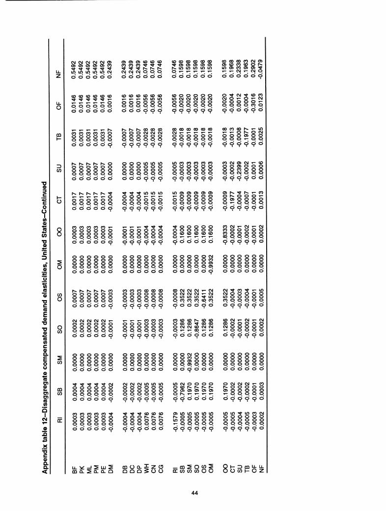
3

C O ü

I tñ o

O)

I c " D (O o

iS o

■Ö c (O E 0) •u ■Ö o (O 0) c a> a E o o

(O O) £ O) Ö) (O O) o

I T-

tn

O)

ü

8

O

O) O

O

CO

CÛ O)

CM CM CM CM CM 0> CJ> o> o> o> 0> CO -^ -«t "^ "^ ^ "^ in in ir> LO LO CM ó d Ö c> Ö ó

(O (O (O CO CO CO "^ '^ "^ "^ '^ ^ o o o o o o ó Ö ó ó ó ó

T- 1- r- ^ 1- h. CO CO CO CO CO o o o o o o o q q q q q q Ö Ö CD CD Ö Ö

fs. IS. r^ h^ h. o o o o o o o o o o o o o o q q q q q d CD Ö d CD d

h. fs. rs. is. h* "^ T- 1— t— 1— t^ o o o o o o o o q q q q q o d d d d d

CO CO CO CO CO '— o o o o o o o o o o o o o o o o o o

œ C3> en CO CO CO CO CO CO ^ ^ "^ Tf -^ "^ 1^ 1^ h* CM CM CM q q q ó ó ó ó ó ó

CO CO CO CO CO CO T- t- T- in lo in o o o o o o o o o o o o d d d o CD CD

^s. fs. ^ GO (X> 00 O O O CM CM CM O O O O O O O O O q q q d d d d d d

o o o lO lO lO o o o o o o o o o o o o o o o o o o

CO 00 GO (S œ 00 ^ 0> 0> 0> (3> 0> h. m u) LO i/> lo o 1^ ^ T- T- 1-; d d d d d d

CO o o o o o lO CM CM CM CM CM o o o o o o o o o o o o

9 9 9 9 9 9

00 00 00 00 iQO 00 CM T- T- ^ t- T- o o o o o o o o o o o o 999999

lO CO CO CO CO CO o o o o o o o o o o o o o o o o o o

00 (X> 00 CO CM 0> o> CO CO CO o h^ lO CJ) CO CJ> C3> '^ ^ T- CM i-¡ CM q ó Ö ó ó ó ó

o "^ CM "^ CO CO CM o T- o 1- CM o o o o o 1- q q q q co q d d d d d d

00 CO 00 1^ T- lO 1- T- o h* o CM o o o o> o o o o o T- o o

9 9 9 9 9 <=>

CO CM 0> CM 1- CO o o C3> o o o o o CO o o o o o CM o o o

doOOOCp CDCpOOCDO cDcpoooo

"^ ^ -^ lO lO lO o o o T- T- T- o o o o o o o o o o o q ó ó ó ó ó ó

T- 1- T- Tt Tf 'ít o o o o o o o o o o o o o o o o o o OOOOOC) CDCpCDOCpCD

o o o o o o o o o o o o o o o o o o o o q q q q ó ó ó Ö d d

r^ r^ is. r^ h. CO o o o o o o o o o o o o o o o o q q ó ó ó ó ó ó

CM CM CM CM CM T- o o o o o o o o o o o o o o q q q q ó ó ó ó ó Ö

o o o o o o o o o o o o o o o o o o o o o o o q ó Ö ó Ö ó ó

Tí- '*t "^ -^ "* CM o o o o o o o o o o o o o o q q q q d d d d d d

co co co co co "^ o o o o o o o o o o o o o o o o o o ó Ö ó ó ó ó

o o o o o o o o o o o o o o o o o o o o o o o q Ö ó ó ó Ö ó

CO CO CO 00 00 00 o o o o o o o o o o o o o o o o o q d d d d d d

1— T- T- co co co o o o o o o o o o o o o o o o q q q ó Ö ó Ö ó ó

o o o o o o o o o o o o o o o o o o o o o o o o ó ó ó Ö ó ó

CM CM CM ID in m o o o o o o o o o o o o o q q q q q ó ó ó Ö ó ó

^ Ti- "^ co co co o o o h* r^ 1^ o o o o o o o q q q q q d d d d d d

LO o> O) o> o> o> r- o o o o o o o o o o o o o o o o q ó Ö ó ó ó ó lililí

Tf o o o o o o o o o o o o CO CO CO CO CO o 1- ^ ^. r-; T-; d d d d d d

o o o o o CM o o o o o CO OOOOOC» o o o o o o> ó ó ó Ö ó ó

00 CM CM CM 1- CM o CM CM CM T- CM O in in in -^ LO o CO CO CO q CO Ö ó ó ó ó Ö

CO CO CO h*. CO CO o CO 00 ^ 00 CO o CM CM CO CM CM O ▼— T— (X) r- T-

d d d d d d

o o CM o o o o o CO o o o o o o> o o o o o q q q q ó ó ó ö ó ó

in CM o o o o o co h» f^ r^ h* o o> o> o> 0> O) o h- T- t- T- 1^ d d d d d d

cj) in in in in in r^ o o o o o in o o o o o t- o o o o o Ö ó Ö Ö Ö Ö

CJ) 1^ -^ is. ,- co o r^ o o o T- o C3> o o o o o r- o o o q d d d d d d

CO CM 1- CM r- CM CO o o o o o CO o o o o o 00 o o o o o

9 9 9 9 9 <=>

o o o o o o o o o o o o o o o o o o o o o o o q Ö Ö ó ó ó ó

CM "* CO -^ t- in CM o o o o o in o o o o o CO o o o o o ó ó Ö ó ó ó

CO CM t- CM T- CM CO o o o o o CM o o o o o T- o q q q q ó Ö Ö Ö ó Ö lili

o o o o o o o o o o o o o o o o o o o o o o o o d d d d d d

o CM CM CM ^ co r^ o o o o o cj> o o o o o T- o o q q q d c> CD o cp d

in in ^ in co CM o o o o o o o o o o o o o o o o o o ó ó ó Ö ó Ö

X '■5 c o a <

UL iï: =J 2 UJ 2 m Û. 2 Q- Û- Q

CD O CL 5 Z O — en 2 o c^ 2 oc co œ c/) O O

8H- Z) 00 LL li- O co iPO 2

44

CD ♦^ 0) ■Ö O

c

(0 0) IE o

'«s (O

c CO E ■ö

4^ CQ (fi c a E o o c 3 O 4-* CO D) S O) O) CO (O

o I

CO

X '•B c 0) Q. a <

o

ü

X

o

CÛ Û

LU

CL

LL CÛ

LO LO m LO lO LO o o o o o o o o o o o o o o o o o o d d d d d d

CM C\J C\J CM C\J CO LO LO LO LO LO LO o o o o o o o o o o o o d d d d d d

CO CO CO CO CO ^ LO LO LO LO in LO o o o o o o o o o o o o ó ó ó Ö Ö Ö

o o o o o o o o o o o o o q o o o o d d d d d d lililí

"^ "^ xf Tí- -^ CM O O O O O O q q q q q O ó ó ó ó Ö Ö

CO CO CO CO CO CM o o o o o o o o o o o o o o o o o o d d d d d d

LO in in iT) LO CO CM CM CM CM CM '^ o o o o o LO q q q o q CM d d d d d d

CO CO CO CO CO CM o o o o o o o o o o o o o o o o CD o d d d d d d

(O CO CO (£> CO CO o o o o o o o o o o o o o o o CO o o Ö ó Ö ó Ö ó

o o o o o o o o o o o o o o o o o o o o CO o o o ó ó ó ó ó ó

y- y- r- y- 1- m T— T— T— T- T- o o o o o o o o CO o o o o ó ó ó Ö ó Ö

LO LO LO LO LO h* o o o o o o CO o o o o o ó ó Ö ó ó ó

LO LO LO CO CO T- o o o -^ Ti- T- O o o o o CO o o o o o T- d d d d d d

CO CO CO LO C3> LO LO LO LO CM CM CM o o o "^ CM '^ q o o o t- o Ö Ö Ö ó Ö Ö

"^ "^ Tj- T- CO CO LO LO lO CM CO CO o o o CM "^ '^ o o o T- o o d d d d d d

CM

CO CO CO CO CO CO Tf o o o o o o o o o o o q q q q q q Ö ó ó ó Ö ó

LO 0> 0> O) o> o> CM LO LO LO LO lO Tt o o o o o q o o o o o ó Ö ó ó d d

CO o o o o o CO CO CO CO CO CO "^ o o o o o q q q q q q ó ó ó ó Ö ó

■o 0)

c o

CO h* LO CO CO 1- o o o o o o T- ^ o o o o o o q q q q o o d d d d d d

0> 0> 1- LO CO LO LO CO LO LO LO o o o o o o 1- o o o o o o Ö ó Ö Ö d d

o o CM CO o> r^ CO r^ LO LO LO o o o o o o 1- q q q o o o d d d d d d

o o CM o o o o o LO o o o q q CM q o o d d d d d d

CM CO CM LO LO LO o LO o o o o q CM q q o o d d d d d d

CO CM CM CO CO CO CM o o o o o LO o o o o o CM q o o o o d d d d d d

CM CM CM 1^ K r^ CM CM CM CM CM CM O O O O O O q q q q q q d d d d d d

CM CM CM 1- T- T- o o o o o o o o o o o o o o o o o o d d d d d d

CO CO CO "»— ^— "I- o o o o o o o o o o o o q q q q q o d d d d d d

o o o o o o o o o o o o o o o o o o o o o o o o Ö ó ó Ö Ö ó

LO LO LO CO CO CO o o o o o o o o o o o o o o o o o o Ö ó ó ó ó ó

h* h<. r^ CO CO CO o o o o o o o o o o o o q q q o o o Ö ó ó Ö Ö Ö

o o o o o o o o o o o o q q q o o o d d d d d d

LO CO CO CO CO CO o o o o o o q q q q o o d d d d d d

CO CO CO CO CO CO o o o o o o o o o o o o q q q o o o ó Ö ó ó ó ó

|s^ o o o o o CM CO CO CO CO CO o o o o o o q q q q q q d d d d d d

^ o o o o o o o o o o o o o o o o o q o o o o o ó ó ó ó ó Ö

o o o o o o o o o o o o q q q q q q d d d d d d

o o o o o o o o o o o o o o o o o o o o o o o o Ö Ö Ö ó Ö Ö

CO CM CM CM CM CM O O O O O O O O O O O O q q q q q o d d d d d d

CO CvJ CM CM CM CM o o o o o o o o o o o o q q q q q q d d d d d d

CSJ o o o o o o o o o o o o q q q q q q d d d d d d

CO T- CO LO CO r^ 1- CM 1- T- T- CO o o o o o o q q o o o o ó ó Ö ó ó ö

CO Ti- CM CO CO h». o o o o o o o o o o o o q q o o o o d d d d d d

o (30 "^ h* C3> CO CO CO CM CM CM CO o o o o o o q q q q q o d d d d d d

o Tj- CM 1- o N. o o o o o t- o o o o o o o o o o o o ó ó ó ó ó ó

T- r^ Tí- T- o o o o o o o CO o o o o o o o o o o o o

d d d d d d

o o o o o T- o o o o o o o o o o o o o o o o o o ó Ö ó ó ó Ö

CM CO h- CM o Tt o 1^ o o o LO o o o o o o q q q q q q ó ó ó ó ó Ö

CM r^ o CO o T- o T- 1- o o r^ o o o o o o o o o o o o Ö ó Ö Ö Ö Ö

LL >¿ m Û-

I :E LU :s : CL Q- Q

m O Q. 5 2 O — m :^ O c^ ^ QQQSüO ce CO C/) C/) O O

H 3 0Û LL O O) h- o

45

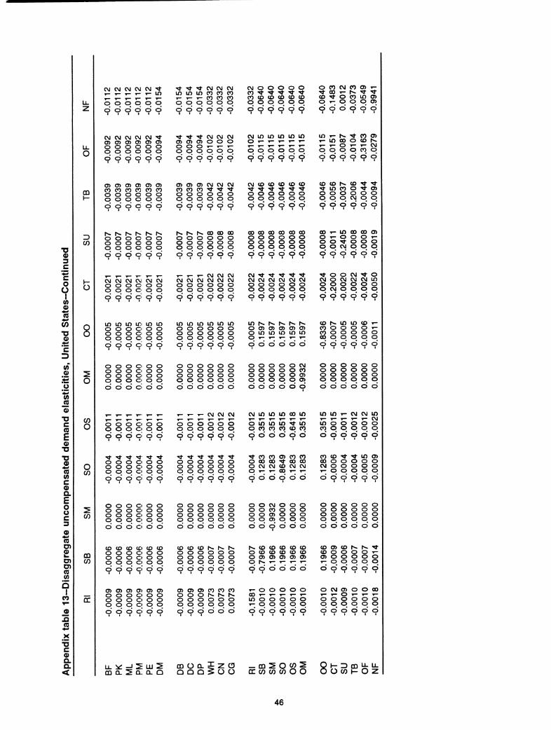
Ü.

^

c o ü

I

0) "ö Q

HM

c

oT 0) 5 u

JE Q

■ü C (0 E Q

■u 0) (0 0) c Q> a E o o c 3

O (O Ö) O) k. O) U)

(/) a

I CO

CD

3 C/3

O

CM CM CvJ CM C\J '«t T- ^ r- r- T- in

o o q q o o d Ö Ö d Ö Ö

CM CM CM CM CM "^ Oi 0> O) 0> Oi o> o o o o o o o o o o o o CD d d d d d lililí

0> 0> 0> 05 0> O) CO CO CO CO CO CO o o o o o o o q q q q q ó ó Ö ó ó ó

r^ h« N. r^ h- 1^ o o o o o o o o o o o o o o q o q q d d d d d d

CM CM CM CM CM CM o o o c o o o o o C' o q d d d C' d d

in in iT) iTi m lo o o o c» o o o o o C' o o o o o c o o Ö Ö ó ÓÓ Ö

o o o c» o o o o o c> o o o o o c o o o o q c¡ q q ó Ö ó ó ó ó

Tf Tf '^t CM CM CM ID in LO CO CO CO T- T- ^1— CO CO CO o o o o q q ó ó ó ó ó ó

-^ Tf 'st CM CM CM 0> O) O) O O O o o o T- T- ^ o o o q q q ó ó Ö Ö d d

0> 0> 0> CM CM CM CO CO CO 'it "^ ^ o o o o o o o o q q q q ó ó ó ó ó ó

fs» fsN. h-. 00 GO GO O O O O O O o o o o o o o o o o o q ó ó ó ó Ö ó

T- T- ^ CM CM CM CM CM CM CM CM CM O O O O O O O O O q q q ó ó Ö Ö ó Ö

LD LO LT) LO in Lf) o o o o o o o o o o o o o o q q q q d d d d d d

o o o o o o o o o o o o o o o o o o o o q q q q ó ó ó ó ó ó

CM o o o o o CO '^ "^ '«t '^ "^ CO (O (O CO (O (O o q q q q q d d d d d d

CM LO LO LO LO LO o ^ ▼- T- 1- ^

o o o o o o 9 9 9 9 9 9

CM (O (O (O (O CO "^ "^ '^ -^ '«t "^ O O O O O O o o o o o o

o CO CM CO 0> T- "^ CO T- h* '^ Ti- co ^ o CO LO C35 O T- O O q q ó ó ó Ö ó ó

LO T- h- -^ CO o> T- u> 00 o CO r^ r- T- o T- ^ CM o o o o CO o 9 9 9 9 9 9

CO CO h» CO "^ "^ "^ LO CO o Tf o> o o o o o o o o o CM o o

999999 99999

CO O

O CO

(/)

CÛ

00 00 00 00 00 00 o o o o o o o o o o o o o o o o q q d d d d d d

CM ^ "^ '^ "^ "^ CM CM CM CM CM CM O O O O O O o o o o q q d d d d d CD

lo h* h* h* h* r^ o O) O) o> O) o> o lO lO LO LO LO o 1^ T- ir- T-; r-;

d d d d d d

o o o o o CM o o o o o CO o o o o o o> o o o o o q ó ó ó Ö ó ó

CM IX) LO LO 00 LO

00 T- LO 00 00 0> o 1- o o o 1- O o 'íf o o o o o CM o q q d d d d d d lililí

Tf o o CM -^ o CM O CM CM CM LO O O O O O O O CM O O O q ó ó Ö ó Ö ó lililí

CO r^ LO LO CO 1^ CO o o o o ^ CO o o o o o 00 o o o o o Ö ó ó ó ó Ö lililí

o o o o o o o o o o o o o o o o o o o o q q q q ó ó ó ó Ö ó

o o o o o o o o o c> q q d d d c! d d

Tf "^ Tf ^- -^ "^ o o o o o o o o o o o o o o q c> q q Ö ó ó Ö ó ó

o o o o o o o o o o o o o o o o o o q q q c> q q d d d c> d d

CO (O CO (O CO CO o o o o o o o o o o o o o o o o q q d d d c> d d

O) CJ> C3) CT» (J> 0> o o o o o o o o o o o o q q q o q q d d d C) d d

o o o o o o o o o o o q d d d d d d

'•i Tt Tf "^ "^ Tí- o o o o o o o o o o o o o o o q q q Ö Ö ó ó d d

o o o o o o o o o o o o o o o o o o o q q q q q d d d d d d

CD CO CO r^ r^ 1^ o o o o o o o o o o o o o o o o o o ó Ö ó ó ó Ö

0> 0> 0> CO CO CO o o o h- r^ 1^ o o o o o o o o q q q q d d d d d d

o LO LO LO "^ LO o CO CO CO q cq ó ó ó Ö ó ó

Tt CO CO 0> CO co o 00 (O Tf (D 00 o CM CM CO CM CM O 1- ^ 00 1- r- Ö Ó Ö Ó Ö Ö

O O CM O O O O O CO O O O o o C3> o o o O O o> q q q ó ó ó ó ó ó

h- CO CO CO CO CO o CO CO CO CO CO o O) 0> 0> O) o> o h* T- t- T- ^ ó ó ó Ö <D ó

T- o o o o o LO o o o o o T- o o o o o d d d d d d

LO LO T- CM CM LO 1- T- T- 1- T- CM LO o o o o o CO o o o o o ó Ö ó ó Ö Ö

CO CO Tt Tí- LO C3> 00 o o o o o CM o o o o o r- o o o o o Ó Ö Ö Ó Ö Ó

o o o o o o o o o o o o o o o o o o o o o o o o ó ó ó Ö ó ó

CO cj) CO r>» r^ Tt CO o o o o 1- o> o o o o o 1- o o o o o

o o ?9 9 9 9

o CM CJ) o o 00 T— T- o T- T— T— o o o o o o o o o o o o d d d d d d

XI c

a o. < m CL 2 a. C]L Q

CÛ O Û. 5 z O Û Û o 5 ü ü

— CD 2 O CO 2 ce CO CO CO O O

81- Z) CD t O CO h- O

46

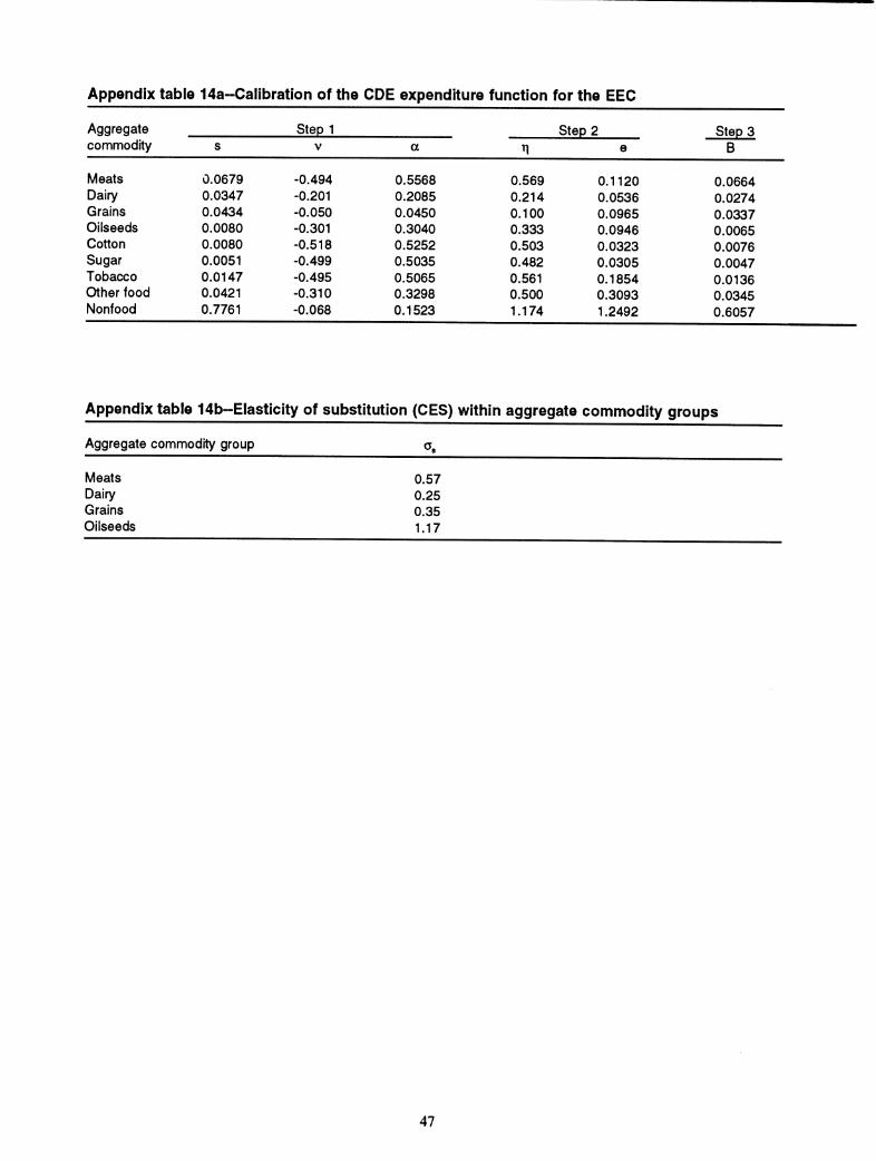
Appendix table 14a-Calibration of the CDE expenditure function for the EEC

Aggregate Step 1 Step 2 Step 3 commodity s V a Î1 e B

Meats 0.0679 -0.494 0.5568 0.569 0.1120 0.0664 Dairy 0.0347 -0.201 0.2085 0.214 0.0536 0.0274 Grains 0.0434 -0.050 0.0450 0.100 0.0965 0.0337 Oilseeds 0.0080 -0.301 0.3040 0.333 0.0946 0.0065 Cotton 0.0080 -0.518 0.5252 0.503 0.0323 0.0076 Sugar 0.0051 -0.499 0.5035 0.482 0.0305 0.0047 Tobacco 0.0147 -0.495 0.5065 0.561 0.1854 0.0136 Other food 0.0421 -0.310 0.3298 0.500 0.3093 0.0345 Nonfood 0.7761 -0.068 0.1523 1.174 1.2492 0.6057

Appendix table 14b-Elasticity of substitution (CES) within aggregate commodity groups

Aggregate commodity group a.

Meats Dairy Grains Oilseeds

0.57 0.25 0.35 1.17

47

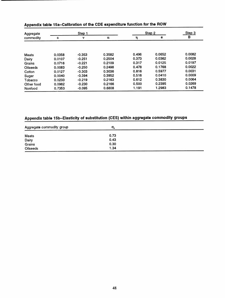
Appendix table 15a-Calibration of the CPE expenditure function for the ROW

Aggregate Step 1 Step 2 Step 3 commodity s v a ri e B

Meats 0.0358 -0.353 Dairy 0.0107 -0.251 Grains 0.0716 -0.221 Oilseeds 0.0083 -0.250 Cotton 0.0127 -0.303 Sugar 0.0040 -0.394 Tobacco 0.0233 -0.219 Other food 0.0982 -0.230 Nonfood 0.7353 -0.095

0.3582 0.496 0.0652 0.0082 0.2504 0.373 0.0362 0.0028 0.2109 0.317 0.0125 0.0197 0.2498 0.478 0.1768 0.0022 0.3036 0.816 0.5977 0.0031 0.3952 0.516 0.0410 0.0009 0.2163 0.612 0.3830 0.0064 0.2166 0.500 0.2395 0.0269 0.6808 1.191 1.2983 0.1478

Appendix table 15b-Elasticity of substitution (CES) within aggregate commodity groups

Aggregate commodity group a,

Meats 0.73 Dairy 0.43 Grains 0.30 Oilseeds 1.34

48

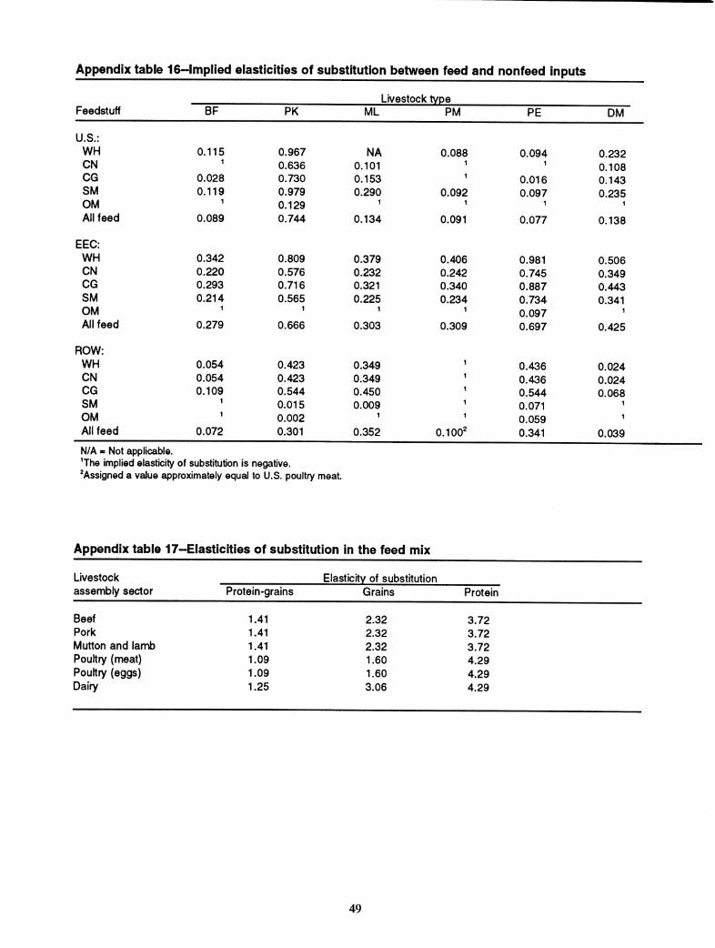
Appendix table 16-lmplied elasticities of substitution between feed and nonfeed inputs

Livestock tvpe Feedstuff BF PK ML PM PE DM

U.S.: WH 0.115 0.967 NA 0.088 0.094 0.232 CN 1 0.636 0.101 1 1 0.108 CG 0.028 0.730 0.153 1 0.016 0.143 SM 0.119 0.979 0.290 0.092 0.097 0.235 OM 1 0.129 1 1 1 1

All feed 0.089 0.744 0.134 0.091 0.077 0.138

EEC: WH 0.342 0.809 0.379 0.406 0.981 0.506 CN 0.220 0.576 0.232 0.242 0.745 0.349 CG 0.293 0.716 0.321 0.340 0.887 0.443 SM 0.214 0.565 0.225 0.234 0.734 0.341 OM 1 1 1 1 0.097 1

All feed 0.279 0.666 0.303 0.309 0.697 0.425

ROW: WH 0.054 0.423 0.349 0.436 0.024 CN 0.054 0.423 0.349 0.436 0.024 CG 0.109 0.544 0.450 0.544 0.068 SM 1 0.015 0.009 0.071 1

OM 1 0.002 1 0.059 1

Ail feed 0.072 0.301 0.352 0.100^ 0.341 0.039

N/A s Not applicable. ^The implied elasticity of substitution is negative. ^Assigned a value approximately equal to U.S. poultry meat.

Appendix table 17-Elasticities of substitution in the feed mix

Livestock Elasticitv of substitution assembly sector Protein-grains Grains Protein

Beef 1.41 2.32 3.72 Pork 1.41 2.32 3.72 Mutton and lannb 1.41 2.32 3.72 Poultry (meat) 1.09 1.60 4.29 Poultry (eggs) 1.09 1.60 4.29 Dairy 1.25 3.06 4.29

49

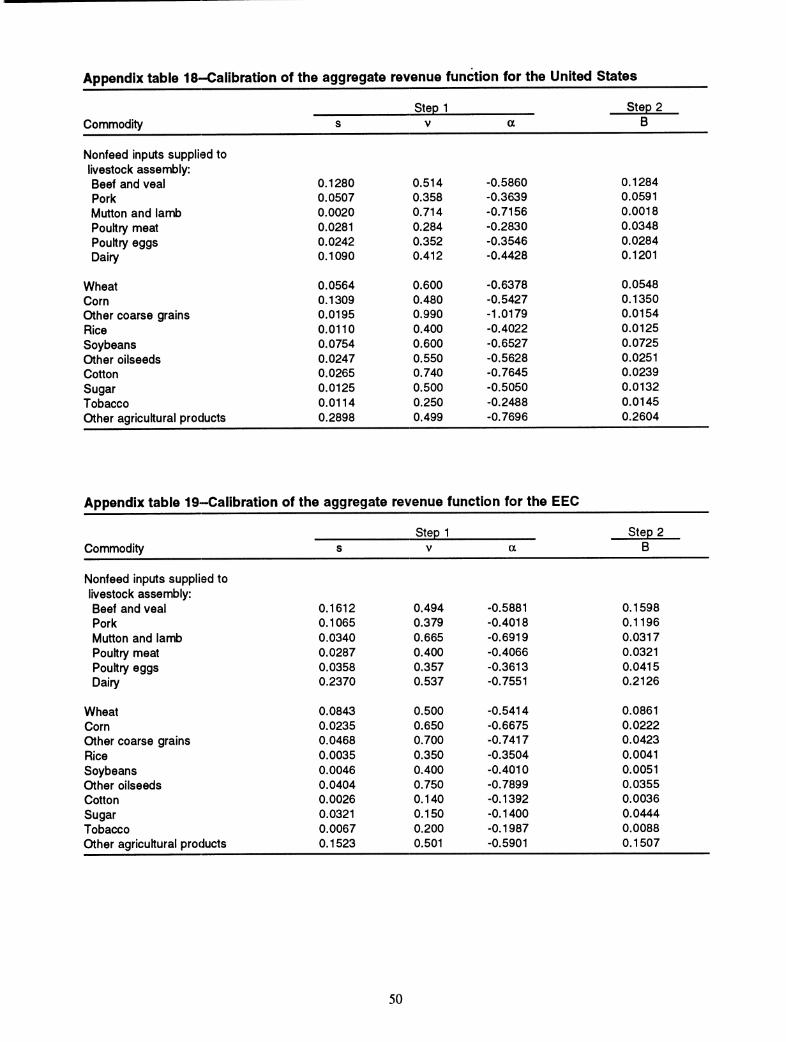
Appendix table 18-Calibration of the aggregate revenue function for the United States

Stepi Step 2 Commodity s V a B

Nonfeed inputs supplied to livestock assembly: Beef and veal 0.1280 0.514 -0.5860 0.1284 Pork 0.0507 0.358 -0.3639 0.0591 Mutton and lamb 0.0020 0.714 -0.7156 0.0018 Poultry meat 0.0281 0.284 -0.2830 0.0348 Poultry eggs 0.0242 0.352 -0.3546 0.0284 Dairy 0.1090 0.412 -0.4428 0.1201

Wheat 0.0564 0.600 -0.6378 0.0548 Corn 0.1309 0.480 -0.5427 0.1350 Other coarse grains 0.0195 0.990 -1.0179 0.0154 Rice 0.0110 0.400 -0.4022 0.0125 Soybeans 0.0754 0.600 -0.6527 0.0725 Other oilseeds 0.0247 0.550 -0.5628 0.0251 Cotton 0.0265 0.740 -0.7645 0.0239 Sugar 0.0125 0.500 -0.5050 0.0132 Tobacco 0.0114 0.250 -0.2488 0.0145 Other agricultural products 0.2898 0.499 -0.7696 0.2604

Appendix table 19-Calibration of the aggregate revenue function for the EEC

Step 1 Step 2 Commodity s V a B

Nonfeed inputs supplied to livestock assembly: Beef and veal 0.1612 0.494 -0.5881 0.1598 Pork 0.1065 0.379 -0.4018 0.1196 Mutton and lamb 0.0340 0.665 -0.6919 0.0317 Poultry meat 0.0287 0.400 -0.4066 0.0321 Poultry eggs 0.0358 0.357 -0.3613 0.0415 Dairy 0.2370 0.537 -0.7551 0.2126

Wheat 0.0843 0.500 -0.5414 0.0861 Corn 0.0235 0.650 -0.6675 0.0222 Other coarse grains 0.0468 0.700 -0.7417 0.0423 Rice 0.0035 0.350 -0.3504 0.0041 Soybeans 0.0046 0.400 -0.4010 0.0051 Other oilseeds 0.0404 0.750 -0.7899 0.0355 Cotton 0.0026 0.140 -0.1392 0.0036 Sugar 0.0321 0.150 -0.1400 0.0444 Tobacco 0.0067 0.200 -0.1987 0.0088 Other agricultural products 0.1523 0.501 -0.5901 0.1507

50

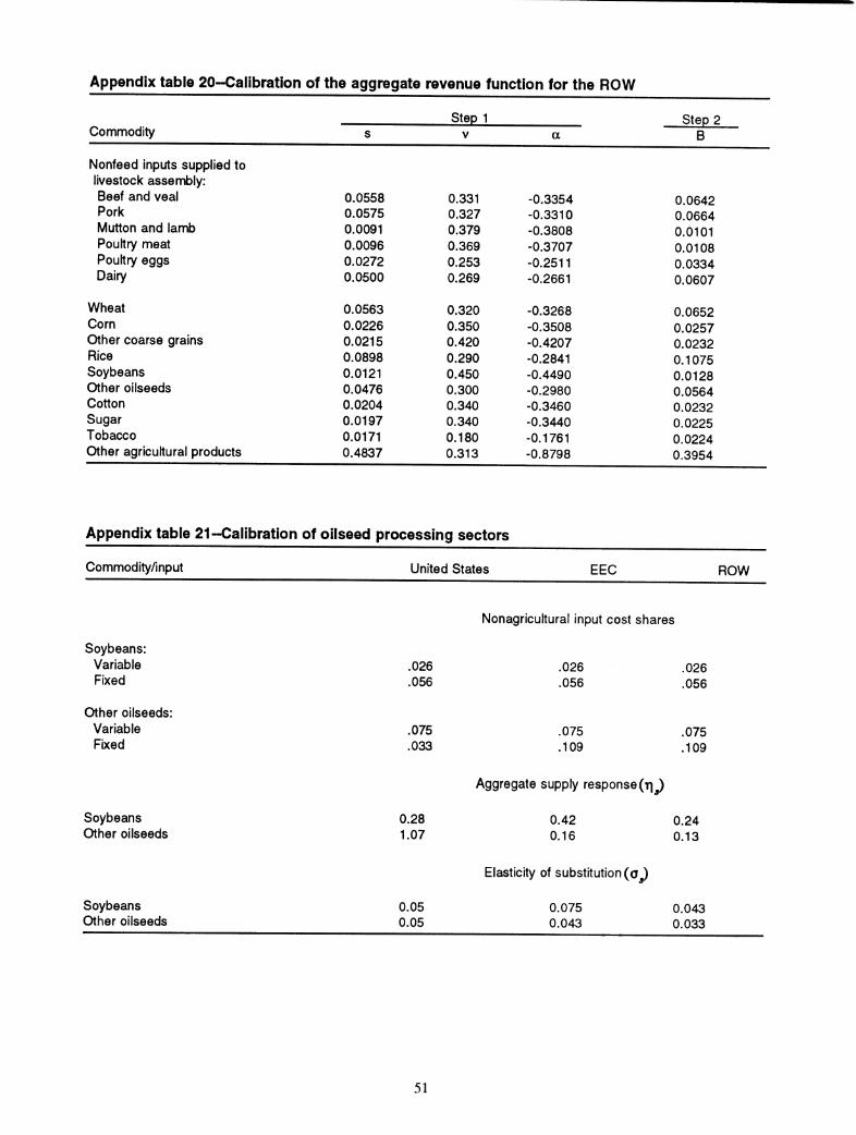
Appendix table 20-Calibratíon of the aggregate revenue function for the ROW

Step 1 Step 2 Commodity s V a B

Nonfeed inputs supplied to livestock assembly: Beef and veal 0.0558 0.331 -0.3354 0.0642 Pork 0.0575 0.327 -0.3310 0.0664 Mutton and lamb 0.0091 0.379 -0.3808 0.0101 Poultry meat 0.0096 0.369 -0.3707 0.0108 Poultry eggs 0.0272 0.253 -0.2511 0.0334 Dairy 0.0500 0.269 -0.2661 0.0607

Wheat 0.0563 0.320 -0.3268 0.0652 Corn 0.0226 0.350 -0.3508 0.0257 Other coarse grains 0.0215 0.420 -0.4207 0.0232 Rice 0.0898 0.290 -0.2841 0.1075 Soybeans 0.0121 0.450 -0.4490 0.0128 Other oilseeds 0.0476 0.300 -0.2980 0.0564 Cotton 0.0204 0.340 -0.3460 0.0232 Sugar 0.0197 0.340 -0.3440 0.0225 Tobacco 0.0171 0.180 -0.1761 0.0224 Other agricultural products 0.4837 0.313 -0.8798 0.3954

Appendix table 21-Calibration of oilseed processing sectors

Commodity/input United States EEC ROW

Nonagricultural input cost shares

Soybeans: Variable Fixed

Other oilseeds: Variable Fixed

.026

.056

.075

.033

.026 .026

.056 .056

.075 .075

.109 .109

Aggregate supply response (r|^

Soybeans Other oilseeds

0.28 1.07

0.42 0.16

0.24 0.13

Elasticity of substitution (a^

Soybeans Other oilseeds

0.05 0.05

0.075 0.043

0.043 0.033

51

Appendix A-.1989 Price Wedges

In the SWOPSIM fnunework, three different price wedges are identified: trade, producer, and consumer subsidies. A distinction is made between the trade wedges for goods for which a country/region is a net exporter-export supiK)rt wedges (ESW), and those goods for which the country/region is a net importer-import support wedges (MSW). If a good is exported and the domestic price exceeds the worid price, then ESW is positive, but if a good is hnported and the domestic price exceeds the worid price, then MSW is negative. The price wedges used for the United States and the EEC in the general equilibrium model are given in appendix tables 3 and 4.'^ A brief discussion of the sources and methodology used to construct these prices wedges is given below.

European Community

The primary source of data for the EEC is OECD (1991). In general, the trade price wedges (ESW and MSW) are calculated by div iding the value (European Currency Unit, ECU) of "market price support-trade measures" by the level of production. This per unit value is then converted from ECU's to U.S. dollars using the rate of 0.9082 ECU/$. The trade wedge for (other) coarse grains is a production weighted average of oats and barley. Trade wedges for processed dairy products are not available in the OECD data. For both skimmed milk powder and butter, the trade wedge is calculated by subtracting a weighted average price for the EEC from the New Zealand price (a proxy for the world price) plus transportation costs. The EEC "cheese price" is difficult to identify because of the variety of cheeses available. The cheese wedge is chosen based on observed EEC milk prices, "worid" milk and cheese prices, and transportation costs.

The value of the prcducer subsidy price wedge (DPSW) for each commodity includes: net of all producer levies imposed, all deficiency payments, area and hedge payments, disaster payments, diversion payments, and any "national" policies tliat support agriculture (that is, research, training, marketing programs, mfrastructure, etc.). However, national policies that are not specific to agriculture, such as rural development, social security, and any tax concessions, are not included in these calculations. Producer support data are not available for cotton, tobacco, and the aggregate "other agriculture," so an estimated DPSW for these commodities is calculated.

Finally, the value of the consumer subsidy price wedge (CSW) for each commodity equals all nontrade support in the OECD CSW tables. Consumer subsidies for com, wheat, rice, and sugar are included to enture the demand effects of compensatory payments received by industrial processors.

United States

Data on the agricultural conunodity support for the Unitedl States is obtained from USDA/ERS (unpublished) rather than from the OECD database. For most conunodities, ERS and the OECD use very similar methods and obtain similar PSE/CSE results. Some hnportant differences exist in the treatment of U.S. beef trade measures (tariffs), with the OECD estimating large distortions, but the ERS estimates assuming that these measures are ineffective. OECD calculations also include some CSE's estimated from "additionalities" associated with food stamp programs, while the ERS CSE's leave these out. We choose to use ERS estimates of U.S. PSE's and CSE's for this model largely because ERS was able to provide updated and revised estimates for our 1989 base year.

We take a different approach to the modeling of distortions arising from the export enhancement program (EEP) than has been taken in SWOPSIM. The EEP increases agricultural sector incomes by providing export subsidies on some U.S. exports of wheat, barley, rice, frozen poultry, and a few other products. This program distorts trade and is very damaging to EEC efforts to dispose of itó agricultural surpluses. It does not, however, cause aU of the effects which PSE's and CSE's (as calculated by the OECD and by ERS) seem to attribute to it.

"These values are updates of the 1989 three-region SWOPSIM demonstration model. All price wedges are assumed to equal zero for the

ROW due to a lack of information.

52

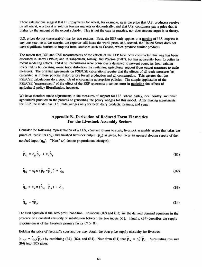
These calculations suggest that EEP payments for wheat, for example, raise the price that U.S. producers receive on all wheat, whether it is sold on foreign markets or domestically, and that U.S. consumers pay a price that is higher by the amount of the export subsidy. This is not the case in practice, nor does anyone argue it in theory.

U.S. prices do not (measurably) rise for two reasons. First, the EEP only applies to a portion of U.S. exports in any one year, so at the margin, the exporter still faces the world price, and, second, the United States does not have significant barriers to imports from countries such as Canada, which produce similar products.

The reason that FSE and CSE measurements of the effects of the EEP have been constructed this way has been discussed in Hertel (1989b) and in Tangerman, Josling, and Pearson (1987), but has apparently been forgotten in recent modeling efforts. PSE/CSE calculations were consciously designed to prevent countries from gaining lower PSE*s but creating worse trade distortions by switching agricultural support from output measures to trade measures. The original agreements on PSE/CSE calculations require that the effects of all trade measures be calculated as if these policies distort prices for ^ production and ^ consumption. This ensures that the PSE/CSE calculations do a good job of encouraging appropriate policies. The simple application of the PSE/CSE "measurement" of the effect of the EEP represents a serious error in modeling the effects of agricultural policy liberalization, however.

We have therefore made adjustments in the measures of support for U.S. wheat, barley, rice, poultry, and other agricultural products in the process of generating the policy wedges for this model. After makmg adjustments for EEP, the model has U.S. trade wedges only for beef, dairy products, peanuts, and sugar.

Appendix B-Derivation of Reduced Form Elasticities For flie Livestock Assembly Sectors

Consider the following representation of a CES, constant returns to scale, livestock assembly sector that takes the prices of feedstuffs (pp) and finished livestock output (p^) as given, but faces an upward sloping supply of the

nonfeed input (q^). ("Hats" (A) denote proportionate changes):

Po =C^PN -^^FPF (B1)

QN =Cpa(pp-p^) +qo (B2)

QF = CNCI(PN-PF) ^ho (B3)

QN = YPN (B4)

The first equation is the zero profit condition. Equations (B2) and (B3) are the derived demand equations in the presence of a constant elasticity of substitution between the two inputs (a). Finally, (B4) describes the supply responsiveness of the livestock primary factor (y > 0).

Holding the price of feedstuffs constant, we may obtain the own-price supply elasticity for livestock

(^00 "^ ^Q/PO) ^y combining (Bl), (B2), and (B4). Note from (Bl) that pj^ = cÑ Po- Substituting this and (B4) into (B2) gives:

53

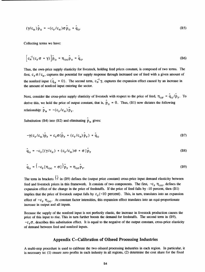
Collecting terms we have:

cÑ'íCpG + Y)]po = TlooPo = Qo. (B6)

Thus, the own-price supply elasticity for livestock, holding feed prices constant, is composed of two terms. The

first, Cp a / Cj^, captures the potential for supply response through inaeased use of feed with a given amount of

the nonfeed input (q^^ = 0). The second term, c^^ Y> ciiptures the expansion effect caused by an increase in the amount of nonfeed input entering the sector.

Next, consider the cross-price supply elasticity of livestock with respect to the price of feed, rj^p = Qo/pp- To

derive this, we hold the price of output constant, that is, p^ = 0. Thus, (Bl) now dictates the following A A

relationship: p^ = -(Cp/Cj^)pp.

A

Substitution (B4) into (B2) and eliminating p^ gives:

-Y(Cp/Cj,)Pp = CpGiPp + (Cp/Cj,)pp) + Qo (B7)

ho = -Cp[(Y/Cj,) + (Cp/cN)a + a]pp (B8)

q = ^ -Cp [Tloo -^ ^1 ^PF = ^OFPP (ß^)

The term in brackets i*/ in (B9) defines the (output price constant) cross-price input demand elasticity between

feed and livestock pdces in this framework. It consists of two components. The first, -Cp TJ^Q, defines the expansion effect of the change in the price of feedstuffs. If the price of feed falls by -10 percent, then (Bl)

implies that the price of livestock output falls by Cp(-10 percent). This, in turn, translates into an expansion

effect of -Cp TIQQ. At constant factor intensities, this expansion effect translates into an equi-proportionate increase in output aad all inputs.

Because the supply of the nonfeed input is not perfectly elastic, the increase in livestock production causes the price of this input to rise. This in turn further boosts the demand for feedstuffs. The second term in (B9),

-CpG, describes this substitution effect It is equal to the negative of the output constant, cross-price elasticity of demand between feed and nonfeed inputs.

Appendix C-Calibration of Oilseed Processing Industries

A multi-step procedure is used to calibrate the two oilseed processing industries in each region. In particular, it is necessary to: (1) ensure zero profits in each industry in all regions, (2) determine the cost share for the fixed

54

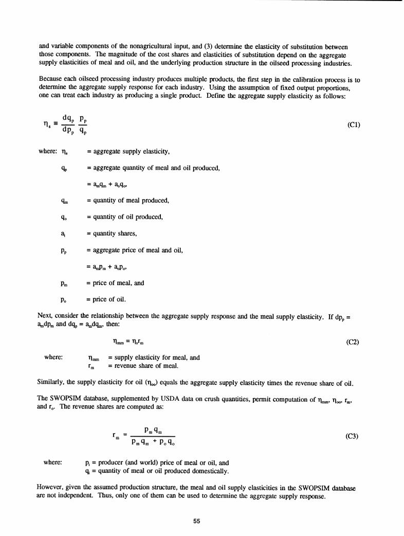
and variable components of the nonagricultural input, and (3) determine the elasticity of substitution between those components. The magnitude of the cost shares and elasticities of substitution depend on the aggregate supply elasticities of meal and oil, and the underiying production structure in the oilseed processing industries.

Because each oilseed processing industry produces multiple products, the first step in the calibration process is to determine the aggregate supply response for each industry. Using the assumption of fixed output proportions, one can treat each industry as producing a single product. Define the aggregate supply elasticity as follows:

(CD tip,

Pp

^p

'here: TI. = aggregate supply elasticity.

% = aggregate quantity of meal and oil produced.

= atnOm + aoQo»

qm = quantity of meal produced.

Qo = quantity of oil produced,

ai = quantity shares.

Pp = aggregate price of meal and oil.

= a^m + ^oPo,

Pm = price of meal, and

Po = price of oil.

Next, consider the relationship between the aggregate supply response and the meal supply elasticity. If dpp = a^dp^ and dqp = a^dq^, then:

îlmm = ^s^m (C2)

where: J\J^ = supply elasticity for meal, and r„ = revenue share of meal.

Similarly, the supply elasticity for oil (j\^) equals the aggregate supply elasticity times the revenue share of oil.

The SWOPSIM database, supplemented by USDA data on crush quantities, permit computation of r\^, r\^, T^, and r^. The revenue shares are computed as:

r, = ï:^ (C3) Hm ^m * o *o

where: R = producer (and world) price of meal or oil, and q^ = quantity of meal or oil produced domestically.

However, given the assumed production structure, the meal and oil supply elasticities in the SWOPSIM database are not independent. Thus, only one of them can be used to determine the aggregate supply response.

55

Given the assumed production structure, one can relate the aggregate supply elasticity to the fixed and variable nonagricultural input cost shares, and the elasticity of substitution between these inputs. Following Hertel (1989a), the relationship can be stated as:

n. = <Js cr' -(c, -cj-^] (C4)

where: o^ = elasticity of substitution between fixed and variable nonagricultural inputs,

Cf = cost share of fixed component, and

Cy = cost share of variable component.

The value of c^ is assumed to equal an average crush margin from 1960 through 1989. Both a and Cf are unknown in equation (C4), thus one can only determine one of these parameters during the calibration process. Given a choice of o, one can proceed to use equation (C4) to determine c^. Rearranging terms of equation (C4) gives:

(Cf^ -HCfC,)^ -c, =0. (C5) s

One can solve for c, in equation (C5) by using the quadraitic formula. Once Cf and c^ are known, the share of the agricultural input can be determined by subtracting Cf and c^ from one.

The next step in the calibration process is to check whether the oilseed processing industries have zero profits. Total expenditures can be determined by multiplying the CTush quantity times either the soybean or other oilseed price, then dividing by the agricultural cost share. Prices for meal and oil are then adjusted proportionally, if necessary, to ensure that revenues equal expenditures.

The procedure outlined above is first carried out for the United States. The worid prices for meal and oil are determined during tJiis process. Using this information, plus information on the quantities of meal and oil produced in the EEC and ROW, and the crush quantities in those regions, one can determine the cost share of the agricultural input for each oilseed processing industry in both regions. Because we assume that c^ is the same across all regions for each industry, Cf can now be determined by subtracting Cv and the agricultural input cost share from one. Thus, for the EEC and ROW, only ithe parameter a in equation (C4) is unknown and can be determined direcitly.

Appendix D-Model Description

Appendix table Dl presents the four blocks of equations in this model. Because the model is implemented using the GEMPACK software suite, it is written out in its linemzed form. When accompanied by a complete set of value flows for the initial equilibrium, and a set of update formulae for these values and the elasticities, GEMPACK is capable of obtaining the solution to the underiying, nonlinear problem. An example of the update formula for a value flow is:

dv/v = d(PQ)/PQ = P + q » ff^i)

where the lowercases p and q represent the percentage changes in price (P) and quantity (Q), respectively. (The complete algebraic representation of this model in GEMPACK is available upon request. We will also provide stand-alone executable files for those with an interest in replicating our results.)

56

rA In appendix table Dl, Vsij represents the value of sales of commodity i from industry j in region r at agents' prices. Logically, the sum of these values over all i conunodities supplied equals revenues, which must in turn equal costs, for zero profits to hold in the nonendowment industries. Subscripts D refer to derived demands and H to households. Lowercase variables refer to percentage changes in price (p), quantity (q), activity levels (z), income (j), and one plus the ad valorem tax rate (t). Income is computed as the sum of endowments supplied plus taxes on households, firms, and trade. The latter are obtained by looking at differences between values at

agents* prices (V ^), domestic market prices (V *^), and world prices ( V ^). The nonagricultural good in this model is the numeraire, and the associated market clearing condition must be satisfied by virtue of Walras' Law. This is our consistency check on the model structure and data set.

57

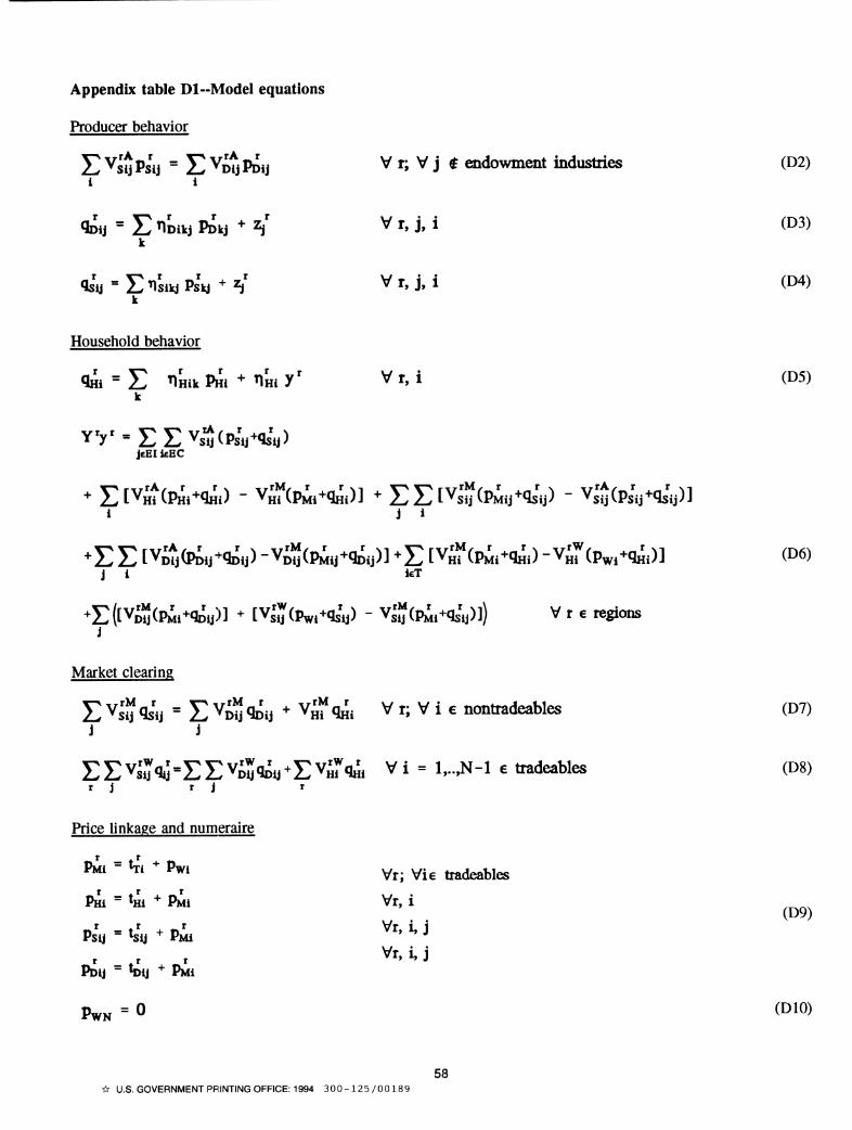
Appendix table Dl-Model equations

Producer behavior

E ^¡Jpsij = X) V¿íjp¿ij V r; V j $ endowment industries (D2) i i

q¿ij = E ^Dikj P¿kj ^ < V r, j, i (D3) k

fls'ij = E^siy Pskj ^^' V r, j, i (D4) k

Household behavior

q^i = E 'iHikP^i^nrny' vr,i (D5) k

JEEI íEEC

i J i

*E E [V¿Íj(P¿ij-^qi5ij) -V¿í;(p,^ij+q¿y)] ^E [Vm (P,^i+q¿i) "V¿7(Pw,-^<¿i)] (D6) j 1 kT

+E([V¿Í;(tói+q¿u)] + [VsJ(Pwt+qsy) - V^IJip^i+qs'y)]) V r e regions j

Market clearing

E Vsï q/ij = E V¿Í; qiSij + V¿^ q^i V r; V i e nontradeables (D7) J J

EEVW=EEV¿;q¿y-Ev¿rqiÍ, V i = 1....N-1 e tradeables (D8) t j I j r

Price linkage and numeraire

PMi = til * Pwi Vr; Vie tradeables

(D9) PHI = tffl + PMi Vr, i

T _ t r ^^'i'j PDIJ " ty ■•■ PMI

PwN = 0 i^lO)

58 ^ U.S. GOVERNMENT PRINTING OFFICE: 1994 300-125/00189

NATIONAL AGRICULTURAL LIBRARY

1022464456

1022464456

U.S. Department of Agriculture Economic Research Service

1301 New York Avenue, NW. Washington, DC 20005-4788