Added Value of Convection Permitting Climate Simulations Andreas Prein July 2013 Wegener Center for Climate and Global Change University of Graz Scientific Report No. 53-2013 kindly supported by:

Welcome message from author
This document is posted to help you gain knowledge. Please leave a comment to let me know what you think about it! Share it to your friends and learn new things together.
Transcript
Added Value of Convection Permitting Climate Simulations
Andreas Prein
July 2013
Wegener Center for Climate and Global Change
University of Graz
Scientific Report No. 53-2013
kindly supported by:
The Wegener Center for Climate and Global Change combines as an interdisciplinary, internationally oriented research institute the competences of the University of Graz in the research area „Climate, Environmental and Global Change“. It brings together, in a dedicated building close to the University central campus, research teams and scientists from fields such as geo- and climate physics, meteorology, economics, geography, and regional sciences. At the same time close links exist and are further developed with many cooperation partners, both nationally and internationally. The research interests extend from monitoring, analysis, modeling and prediction of climate and environmental change via climate impact research to the analysis of the human dimensions of these changes, i.e., the role of humans in causing and being effected by climate and environmental change as well as in adaptation and mitigation. (more information at www.wegcenter.at)
The present report is the result of a Doctoral thesis work completed in July 2013.
Alfred Wegener (1880-1930), after whom the Wegener Center is named, was founding holder of the University of Graz Geophysics Chair (1924-1930). In his work in the fields of geophysics, meteorology, and climatology he was a brilliant scientist and scholar, thinking and acting in an interdisciplinary way, far ahead of his time with this style. The way of his ground-breaking research on continental drift is a shining role model—his sketch on the relationship of the continents based on traces of an ice age about 300 million years ago (left) as basis for the Wegener Center Logo is thus a continuous encouragement to explore equally innovative scientific ways: paths emerge in that we walk them (Motto of the Wegener Center).
Wegener Center Verlag • Graz, Austria © 2013 All Rights Reserved. Selected use of individual figures, tables or parts of text is permitted for non-commercial purposes, provided this report is correctly and clearly cited as the source. Publisher contact for any interests beyond such use: [email protected].
ISBN 978-3-9503608-0-6
July 2013
Contact: Andreas F. Prein [email protected]
Wegener Center for Climate and Global Change University of Graz Brandhofgasse 5 A-8010 Graz, Austria www.wegcenter.at
Wegener Center for Climate and Global Change, University of Graz, Brandhofgasse 5,A-8010 Graz, Austria
Institute for Geophysics, Astrophysics, and Meteorology/Institute of Physics,University of Graz, Universitätsplatz 5/II, A-8010 Graz, Austria
Wegener Center for Climate and Global ChangeInstitute for Geophysics, Astrophysics,and Meteorology/Institute of Physics
University of Graz
Dissertationzur Erlangung des akademischen Grades eines Doktors der
Naturwissenschaften
Added Value of Convection PermittingClimate Simulations
Andreas Prein
Graz, June 2013
Betreuer:Univ.-Prof. Mag. Dr. Gottfried Kirchengast
Ass.-Prof. Mag. Dr. Andreas Gobiet

Abstract
Convection permitting climate simulations (CPCSs) are able to omit error pronedeep convection parameterizations by resolving deep convection explicitly. Fur-
thermore, they are resolving orography and surface fields more accurately which is anadvantage especially in mountainous or coastal regions compared to traditional climatesimulation with parameterized deep convection. In this thesis it is investigated if theseadvantages lead to added value in CPCSs compared to coarser gridded simulations.The main improvements of CPCSs are found in the representation of precipitation.
Especially sub-daily scales and spatial patterns smaller than approximately 100 km areimproved. At large (e.g., meso-α; 200 km to 2000 km) scales, precipitation patterns ofCPCSs tend to converge towards the patterns of coarser gridded simulations. However,two exceptions are found: (1) improved large-scale average heavy precipitation totalsin June, July, and August in the Colorado Headwaters, and (2) more accurate spatialpatterns of air temperature two meters above surface which is strongly related to theimproved orography in mountainous regions.The key added value which can be consistently found in an ensemble of CPCSs are: (1)
improved timing of the summer convective precipitation diurnal cycle in mountainousregions, (2) more accurate intensities of most extreme precipitation, (3) more realisticsize and shape of precipitation objects, and (4) better spatial distribution of precipitationpatterns. These improvements are not caused by the higher resolved orography but bythe explicit treatment of deep convection and the more realistic model dynamics. Incontrast, improvements in summer temperature fields can be fully attributed to thehigher resolved orography.Generally, added value of CPCSs is predominantly found in summer, in complex ter-
rain, on small spatial and temporal scales, and for high precipitation intensities.
i

Zusammenfassung
Konvektionsauflösende Klimasimulationen (CPCSs) ermöglichen eine expliziteSimulation der atmosphärischen Tiefenkonvektion wodurch fehleranfällige Parame-
trisierungen vermieden werden können. Desweiteren wird im Vergleich zu gewöhnlichenKlimasimulationen die Orographie und Landoberfläche detaillierter dargestellt was vorallem in Berg- und Küstenregionen vorteilhaft ist.In dieser Arbeit wird der Mehrwert von CPCSs im Vergleich zu gröber aufgelösten
Simulationen untersucht. Der größte Mehrwert findet sich in der Simulation des Nieder-schlages. Besonders Prozesse auf der Subtagesskala und räumliche Muster, die kleinerals ungefähr 100 km sind, werden verbessert. Auf größeren Skalen (z.B. der meso-α Skala) konvergieren Niederschlagsmuster von CPCSs mit jenen von grobskaligerenSimu-lationen. Allerdings werden zwei Ausnahmen gezeigt: (1) verbesserte sommerlicheStarkniederschlagsmengen im Quellgebiet des Colorado Flusses und (2) realitätsnähereräumliche Muster der bodennahen Lufttemperatur, die stark mit der verbesserten Oro-graphie zusammenhängen.Ein Mehrwert, der konsistent in einem Ensemble von CPCSs auftritt, wurde in folgen-
den Bereichen gefunden: (1) verbesserte zeitliche Abläufe des Tagesgangs von konvek-tiven Niederschlägen im Sommer, (2) verbesserte Intensitäten von Extremniederschlä-gen, (3) realistischere Größen und Formen von Niederschlagsobjekten und (4) verbesserteräumliche Niederschlagsmuster. Diese Verbesserungen sind nicht durch die höher aufge-löste Orographie bedingt, sondern durch die explizite Auflösung der Tiefenkonvektionund der realistischeren Modelldynamik. Im Gegensatz dazu können Verbesserungen derbodennahen Temperatur im Sommer der höher aufgelösten Orographie zugeschriebenwerden.Zusammengefasst kann ein Mehrwert von CPCSs überwiegend im Sommer, im kom-
plexen Gelände, auf kleinen räumlichen und zeitlichen Skalen und für hohe Nieder-schlagsintensitäten gefunden werden.
iii

Acknowledgement
Gratitude is the memory of theheart.
(Jean-Baptiste Massieu)
Personally, this is the most important part of this thesis because this chapter tellsabout the human dimension, the passion, the love, the understanding, the com-
passion, and the help of people who wanted nothing in return which made this thesispossible. It is so important to me because you will not be able to read much about itin the upcoming chapters. However, this support is the elemental source of every wordwritten here and cannot be appreciated enough.At first place I want to express my gratitude to my supervisors Dr.Gottfried Kirchen-
gast and Dr.Andreas Gobiet. First off all, because they gave me the opportunity to writemy thesis in the Regional and Local Climate Modeling and Analysis Research Group(ReLoClim) at the Wegener Center (WEGC), University of Graz, which is one of themost encouraging working environments that I can imagine. Secondly, they supportedme not only in a scientific way but also had an open ear and open heart for all kinds ofconcerns which arose during my journey leading to this thesis. Both of them are a greatsource of inspiration which taught me how passion and commitment can look like.The WEGC is a great place to work and to study. But this is not because of the nice
mansion in which it is located, the nice surrounding close to the University and city park,and also not because of the wide-screen LED monitor at my workplace. It is becauseof the people who are working there which have become much more than colleagues tome. During my five years at this institute I have got so much support, had so manyinspiring discussions, and was able to learn so many things that I am afraid that I amnot able give back only half as much as I have received. I especially want to thank thecolleagues from my former office: Barbara Scherllin-Pirscher, Georg Heinrich, MatthiasThemeßl, Renate Wilcke, and Andrea Damm with whom I shared all the ups and downsa Ph.D. study can provide. Furthermore, I am thankful to Martin Suklitsch who wasa great support not only for learning to use the Wegener Center Integrated ClimateModel Evaluation (WICE) toolkit but also for having so much patience with me asking
v
Acknowledgement
questions about dynamical downscaling in general and using the COSMO model inCLimate Mode (CCLM) in particular. Gratefulness belongs also to Heimo Truhetz fornumerous inspiring discussions and to the much too oft forgotten administration staff.Their support is rarely visible but still essential for all who work at the WEGC.Financial support was a key element which enabled me to study. Therefore, my
thankfulness goes at the first place to my mother who is the most selfless person Ihave ever met. My gratefulness belongs also to the Austrian government which greatlysupported me during my bachelor and master studies. Additional thanks should be givento the Austrian Science Fund (FWF) which funded the NHCM-1 and NHCM-2 projectsand the European Union FP7 framework for funding the ACQWA project. Parts of thisthesis were supported by the National Science Foundation (NSF) under the NationalCenter for Atmospheric Research (NCAR) Water System Program, through the NSFEASM contract on Assessing High-Impact Weather Response to Climate Variability andChange Utilizing Extreme Value Theory, and by the Austrian Marshall Plan Foundation.The studies presented relied heavily on computing resources. I am therefore grate-
ful to the Jülich Supercomputing Centre (JSC), the German Climate Computing Cen-ter (DKRZ) in Hamburg, the European Centre for Medium-Range Weather Forecasts(ECMWF), and NCAR’s Computational and Information Systems Laboratory (CISL),sponsored by the NSF for providing these resources.As a member of the CCLM community I want to thank my colleagues therein for the
open-hearted acceptance in their group, for providing guidance when help was needed,and the organization of great meetings. CCLM simulations are funded by the GermanFederal Ministry of Education and Research (BMBF).During my studies I have got the great opportunity to visit Dr. Greg Hollands Re-
gional Climate Group at NCAR in Boulder, Colorado, USA. Greg was a great host andsupported me in every possible way. Also the members of his group, especially Dr.James Done, made my visit to one of the best experiences in my life. I am also thankfulto Dr. Roy Rasmussen and his Colorado Headwaters group at NCAR who shared theirvaluable time, data, and knowledge with me.Finally, my greatest gratitude belongs to my girlfriend Marina and my family. Ma-
rina was always there for me, in good times and in bad. She was the one with whom Icelebrated my greatest successes and who helped me when I needed it the most. Fur-thermore I want to thank my mother for supporting me and believing in me ever since Ican imagine. Another central person of my studenthood (and also of the rest of my life)is my twin brother Michael. We moved to Graz, started studying, and went throughthick and thin together. Also my older brother Wolfgang was always there for me andwas often the cause of pleasant distraction when I started pushing too hard.
To my father.
vi
Preface
Parts of this Ph.D. thesis have already been published. The references are:
• Prein, A. F., A. Gobiet, M. Suklitsch, H. Truhetz, N. K. Awan, K. Keuler, and G.Georgievski (2013) Added Value of Convection Permitting Seasonal Simulations.Clim. Dyn., DOI:10.1007/s00382-013-1744-6
• Prein, A. F., G. J. Holland, R. M. Rasmussen, J. Done, K. Ikeda, M. P. Clark,and C. H. Liu (2013) Importance of Regional Climate Model Grid Spacing forthe Simulation of Precipitation Extremes. J. Climate, DOI:10.1175/JCLI-D-12-00727.1
• Prein, A. F. and A. Gobiet (2011) Defining and Detecting Added Value in CloudResolving Climate Simulations. Wegener Center Report Nr. 39, Wegener Cen-ter Verlag, Graz, Austria, http://www.uni-graz.at/en/igam7www-wcv-scirep-no39-apreinagobiet-nhcm1-i-feb2011.pdf
vii
Contents
Abstract i
Zusammenfassung iii
Acknowledgement v
Preface vii
1 Introduction 13
2 Climate Change and Climate Modeling 172.1 A Changing Climate . . . . . . . . . . . . . . . . . . . . . . . . . . . . . . 17
2.1.1 Panta Rhei . . . . . . . . . . . . . . . . . . . . . . . . . . . . . . . 172.1.2 The Human Factor . . . . . . . . . . . . . . . . . . . . . . . . . . . 19
2.2 From Zero Dimensional Energy Balance to Earth System Modeling . . . . 232.2.1 The Physics of Atmospheric Flow . . . . . . . . . . . . . . . . . . . 232.2.2 Computational Achievements . . . . . . . . . . . . . . . . . . . . . 252.2.3 Weather and Climate Modeling . . . . . . . . . . . . . . . . . . . . 262.2.4 Increasing Diversity, Resolution, and Complexity . . . . . . . . . . 292.2.5 Parameterizations and Limited Knowledge . . . . . . . . . . . . . . 322.2.6 A Scale Problem . . . . . . . . . . . . . . . . . . . . . . . . . . . . 33
2.3 Regional Climate Modeling . . . . . . . . . . . . . . . . . . . . . . . . . . 352.3.1 Current Issues With RCMs . . . . . . . . . . . . . . . . . . . . . . 36
2.4 Skill of RCM Simulations . . . . . . . . . . . . . . . . . . . . . . . . . . . 402.4.1 Downscaling Ability of RCMs . . . . . . . . . . . . . . . . . . . . . 40
2.5 Convection Permitting Simulations . . . . . . . . . . . . . . . . . . . . . . 432.5.1 Important Components of Convection Permitting Models . . . . . 462.5.2 Added Value in Convection Permitting Simulations . . . . . . . . . 49
3 Dynamical Downscaling and Detecting Added Value 533.1 Dynamical Downscaling with RCMs on the Example of CCLM . . . . . . 53
3.1.1 Dynamics . . . . . . . . . . . . . . . . . . . . . . . . . . . . . . . . 533.1.2 Numerics . . . . . . . . . . . . . . . . . . . . . . . . . . . . . . . . 56
viii
Contents
3.1.3 Physics . . . . . . . . . . . . . . . . . . . . . . . . . . . . . . . . . 603.2 Searching and Detecting Added Value . . . . . . . . . . . . . . . . . . . . 72
3.2.1 Mean Climate . . . . . . . . . . . . . . . . . . . . . . . . . . . . . . 723.2.2 Spatiotemporal High Resolution . . . . . . . . . . . . . . . . . . . 75
4 Added Value in Convection Permitting Simulations 904.1 Added Value of Convection Permitting Seasonal Simulations . . . . . . . . 90
4.1.1 Experimental Setup, Data, and Models . . . . . . . . . . . . . . . 914.1.2 Results . . . . . . . . . . . . . . . . . . . . . . . . . . . . . . . . . 964.1.3 Discussion . . . . . . . . . . . . . . . . . . . . . . . . . . . . . . . . 113
4.2 Importance of Grid-Spacing for Simulating Precipitation Extremes . . . . 1214.2.1 Experimental Setup, Data, and Models . . . . . . . . . . . . . . . 1214.2.2 Results and Discussion . . . . . . . . . . . . . . . . . . . . . . . . . 123
5 Summary and Conclusion 132
List of Figures 136
List of Tables 138
Acronyms 139
Bibliography 146
ix

1Introduction
Share your knowledge withothers. It’s a way to achieveimmortality.
(Dalai Lama)
Regional climate models (RCMs) (Dickenson et al. 1989; Giorgi and Bates 1989)are capable of providing additional regional details beyond the resolution of global
climate simulations and re-analysis products. With RCMs only limited areas of the globeare simulated. The required information at the lateral boundaries is usually providedby either global models, reanalyses, or from larger scale regional models. Over the lastdecade RCMs have proven themselves as important tools in climate sciences (e.g., Wanget al. 2004; Rummukainen 2010) and climate change impact research (e.g., Finger et al.2012; Heinrich and Gobiet 2011) and considerable efforts were made to further developand improve RCMs by increasing their complexity and resolution. The horizontal gridspacing of state-of-the-art RCMs typically ranges from 50 km to approximately 25 km(e.g., 50 km in PRUDENCE (Christensen and Christensen 2007), 25 km in ENSEMBLES(Linden and Mitchell 2009), 50 km in NARCCAP (Mearns et al. 2009)). More recently,due to advancements in the field of computer sciences, it is now possible to have higherresolved climate simulations with approximately 10 km horizontal grid spacing (e.g.,Loibl et al. 2011; Gobiet and Jacob 2012). Nevertheless, even with a mesh size of 10 kmthere are still numerous processes which cannot be resolved on the model grid and
13
1 Introduction
therefore have to be parameterized. These parameterizations are important sources ofmodel errors (Randall et al. 2007) and introduce large uncertainties in the projectionsof future climate (Déqué et al. 2007).One challenging task for modelers is the parameterization of deep convection. Al-
though much progress has been made in terms of improvement of old parameterizationschemes as well as formulation of new ones, they are still the source of major errors anduncertainties. The most important benefit of convection permitting climate simulations(CPCSs) is that error-prone deep convection parameterization schemes can be omittedas deep convection can be (at least partly) resolved explicitly (Weisman et al. 1997).Furthermore, increasing resolution leads to a more realistic representation of the orogra-phy and land surface. However, CPCSs are far from being established because of theirimmense demand of computational resources and their still widely unknown quality.In numerical weather prediction (NWP) convection resolving models are already widely
used for operational forecasts and research purposes (e.g., Mass et al. 2002; Kain et al.2006; Schwartz et al. 2009; Gebhardt et al. 2011). According to Weisman et al. (1997)the critical horizontal grid spacing for CPCSs is approximately 4 km. For grid spacingsbetween 8 km and 12 km certain aspects of deep convection are still reasonably repre-sented, but deep convection evolves too slowly and net heat transports, rainfall rates,and net strength of deep convection systems are overestimated. By using the fractionsskill score (FSS) method Roberts and Lean (2008) showed that convection resolvingforecasts are able to produce more realistic precipitation patterns due to a more accu-rate distribution of the rain and a better prediction of high accumulations. Weusthoffet al. (2010) investigated forecasts from three different NWP models over Switzerlandwith the FSS and the upscaling method from Zepeda-Arce et al. (2000) and found sig-nificantly improvements particularly for convective, more localized precipitation events.Langhans et al. (2012) found that in convection permitting simulations with differenthorizontal grid spacings (4.4 km, 2.2 km, 1.1 km, and 0.55 km) bulk flow properties, likeheating or moisture tendencies (but also precipitation), converge towards the 0.55 kmsolution. They concluded that convection permitting grid-spacings seem to be sufficientfor physical convergence of bulk properties in real case studies.On longer time scales (14 months) Grell et al. (2000) found similar results and showed
that spatial precipitation patterns are changing between CPCSs and coarser resolvedsimulations with parameterized convection in complex orography. Hohenegger et al.(2008) showed that in their CPCSs the precipitation maxima were better localized, acold bias was reduced, and the timing of the summertime precipitation diurnal cycle wasimproved compared to a larger scale reference simulation.Common limitations of the above mentioned studies are that they only investigate a
single model, a relatively small domain, a small set of parameters (mostly precipitationand temperature), or analyze a relatively short simulation period.
14
In this thesis this shortcomings are addressed in different ways. First, in Chapter 3,dynamical downscaling is explained on the example of COSMO model in CLimate Mode(CCLM) and multiple statistical methods are introduced which enable to investigatethe added value of CPCSs from climate average to sub-daily fields and with respectto spatial and temporal properties. A special focus lies on scale dependent analysesand novel statistical methods which enable to evaluate spatiotemporal highly resolvedprecipitation fields.The main part of this thesis is presented in Chapter 4 and consists of two studies. The
first one, presented in Section 4.1, follows a holistic approach by investigating whereadded value of CPCSs compared to coarser gridded simulations can be found in anensemble of simulations performed with three non-hydrostatic RCMs. Five simulationswith approximately 10 km and five CPCSs with approximately 3 km horizontal grid-spacing are compared. Additionally to the simulated temperature and precipitation alsorelative humidity and global radiation fields are evaluated within two seasons (June, July,and August (JJA) 2007 and December, January, and February (DJF) 2007 to 2008) inthe eastern part of the European Alps. Spatial variability, diurnal cycles, temporalcorrelations, and distributions with focus on extreme events are analyzed and specificmethods (FSS and Structure-Amplitude-Location (SAL) method) are used for in-depthanalysis of precipitation fields. The goal is to find added value of CPCSs which areconsistent in different RCMs. The text and figures of this study are based on a paperby Prein et al. (2013[a]).The results show that added value of CPCSs can especially be found for intense pre-
cipitation over complex orography in JJA where convective induced precipitation ispredominant.These results motivate to investigate the representation of heavy precipitation in
RCMs in more detail. Heavy precipitation events have high impacts on society, economy,and ecology by causing floods, landslides, and avalanches. However, heavy precipitationis often not only a hazardous weather event but also an important part of the hydro-logical water balance of regions like the European Alps (Cebon et al. 1998) or the U.S.Rocky Mountains (e.g., Petersen et al. 1999; Serreze et al. 2001; Weaver et al. 2000).One of the most important processes leading to heavy precipitation events is deep
convection. As mentioned above especially processes related to deep convective have ahigh potential to be improved in CPCSs while in traditional climate simulations deepconvection parameterizations can introduce large errors in the simulation of precipitation(e.g., Molinari and Dudek 1992; Dai et al. 1999; Brockhaus et al. 2008).In the second study (in Section 4.2) differences between simulated summer and winter
heavy precipitation events of coarse-scale simulations and one CPCS are analyzed indepth. Therefore, climate simulations with the Weather Research and Forecasting Model(WRF) with approximately 36 km, 12 km, and 4 km horizontal grid-spacing are evaluated
15

1 Introduction
against measurements in the headwaters of the Colorado River for an eight year period.Scale separation methods are used to understand differences across horizontal scales andto evaluate the effects of upscaling fine-scale processes to coarser-scale features associatedwith precipitating systems.Finally, Chapter 5 closes with summary and conclusions.
16
2Climate Change and Climate Modeling
In this chapter a brief introduction into the development of climate research is given.Therein, the difference between natural and anthropogenic climate change, the rise
and evolution of weather and climate models, the need for and skill of regional climatemodels (RCMs), and finally the potentials and added value of convection permittingclimate simulations (CPCSs) are discussed.
2.1 A Changing Climate
The knowledge that the earth’s climate is changing can be drawn back to ancient times.Also the theory that mankind has an influence on these changes is rather old but waslong disbelieved. Within this section the knowledge about climate change is summarizedfrom ancient Greek philosophers to climate research today. Thereby, important steppingstones are mentioned and discussed. The intention is to give a briefer introduction intothe knowledge on which modern climate science is built on. Readers who demand fora more detailed introduction are referred to textbooks like Weart (2003) or Edwards(2010).
2.1.1 Panta Rhei
Before the 18th century scientists did not suspect that prehistoric climate might havebeen different from the modern period. One of the first who had the idea that climate is
17
2 Climate Change and Climate Modeling
not stationary and can undergo dramatic changes was Jean-Pierre Perraudin (Bradley1999). He developed a theory how glaciers might have transported giant boulders intoalpine valleys which motivated Louis Agassiz to study that phenomenon in more detail.In 1837 he proposed a theory termed Ice Age which denotes times when large partsof Europe and North America were covered by glaciers (Evans 1887). After years ofdisbelieve and resistance the ice age theory was widely accepted by the 1870s.However, scientists still did not know why the earth’s climate in the past was partly
so different from the present conditions. James Croll was the first who was partly ableto answer this question. He published calculations in which he investigated the effect ofchanges of the earth’s orbit around the sun which last for ten thousands of years (Croll1875). He wrote that small changes in the orbit can lead to slightly less sunlight on thenorthern hemisphere which leads to more snow accumulations which, as a result, reflectmore sunlight. This is a positive feedback cooling down the earth’s surface may leadinto an ice age.In 1920 Milutin Milankovitch, a Serbian engineer, built on the theory of James Croll
and calculated tree cycles which are caused by the disturbance of the earth’s orbit by thesun and the moon (Weart 2003). The individual cycles have a 21 000-year (precession),41 000-year (axial tilt), and a 100 000-year period (eccentricity). However, each of thesecycles is too short to explain the sequence four ice ages which was recognized at thistime.Later on, in the mid 1960s, Milankovitch’s theory got supported based on analyses
from Emiliani (1955) and investigations of coral reef and deep-sea sediments by Broeckeret al. (1968). They found that in their records, instead of long ice ages, there were a largenumber of short ones fluctuating in a frequency suggested by Milankovitch. Actually,they have found the glacial-interglacial periods.Another important puzzle stone, why past climate did fluctuate that much, was added
by the German scientist Alfred Wegener who formulated the hypothesis of continentaldrift (Wegener 1929). His idea was that the earth’s continents are drifting on magmalike icebergs do on water. Thereby, the location of continents play an important role inthe development of ice ages (e.g., Muller and MacDonald 2000) because they can reducethe transport of energy by warm water from the equator to the poles. This can be donein three different ways. First, a continent is located on top of a pole (like Antarcticatoday). Second, there is an ocean located at a pole which is nearly entirely surroundedby land masses (like in the Arctic Ocean today) or third, most of the equator is coveredby land masses (like it was during the Cryogenian period).However, there are also other important factors which influenced the past climate
regimes like ocean current fluctuations, the uplift of large areas above the snow line,variations in the solar energy input, volcanism, and changes in the earth’s atmosphere.One additional factor is still missing which effects the earth’s climate increasingly
18
2.1 A Changing Climate
strong throughout the past millennia: humans. We are responsible for increasing green-house gases in the atmosphere, emission of aerosols, land use changes, and the destruc-tion of ecosystems. How mankind is affecting the climate system is discussed in the nextSubsection 2.1.2.
2.1.2 The Human Factor
The ancient Greeks were among the first to documented changing climate conditions andrelated them to human actions. For example, a pupil of Aristotle named Theophrastusnoted that local freezing conditions did change after the draining of wetlands (Neumann1985). This knowledge has been forgotten throughout the medieval times where thechurch tried to explain climate anomalies as response to human sin (Stehr et al. 1995).An important step toward the understanding how humans are influencing earth’s cli-
mate was made by Joseph Fourier in 1824. He discovered that the earth’s atmosphereis warming up the planet (Weart 2003). He described that the visible light from the suncan transmit through the earth’s atmosphere efficiently. It gets absorbed at the earth’ssurface and re-emitted as infrared radiation which is heavily absorbed by the atmo-sphere and therefore increases the temperature at the earth’s surface. In his visionarypublication Fourier (1827) wrote:
“The establishment and progress of human societies, the action of naturalforces, cannotably change, and in vast regions, the state of the surface, thedistribution of water and the great movements of the air. Such effects areable to make to vary, in the course of many centuries, the average degreeof heat; because the analytic expressions contain coefficients relating to thestate of the surface and which greatly influence the temperature.”
Some thirty years later John Tyndall found out which gases are responsible for theabsorption of infrared radiation in the earth’s atmosphere. In Tyndall (1872) he wrotethat water vapor, hydrocarbons like methane, and carbon dioxide (CO2) strongly blockthe radiation.Meanwhile, national weather agencies started to measure atmospheric parameters like
precipitation, temperature, and pressure. By the end of the 19th century large effortswere made to collect those observations globally. Analyzing these datasets scientists didsee many ups and downs in the time line but no continuous trend (e.g., Hann 1903).Observations like these led to the assumption that humans might influence local andregional climate but do not have influence on the climate of the planet (Weart 2003).Studying measurements of angle dependent variations in the infrared radiation from
the moon reaching the earth’s surface (at low angles the infrared rays have a largerpath length through the atmosphere and get stronger absorbed) the Swedish scientistSvante Arrhenius calculated the effect of changing CO2 concentrations on the global sur-
19
2 Climate Change and Climate Modeling
face temperature of the earth. Halving the CO2 concentrations, he concluded, would besufficient to produce an ice age while doubling the concentration would lead to a temper-ature increase of 5K to 6K (Arrhenius 1896) (a nowadays often used value called climatesensitivity). This estimation is surprisingly accurate compared to today’s best estimatesfor the climate sensitivity which is 3.2K with a spread of 2.1K to 4.4K (Randall et al.2007).Some 30 years later in 1938 Guy Stewart Callendar reviewed Arrhenius theory and
showed that temperature and CO2 levels were rising in the atmosphere during the last 50years (Callendar 1938). Furthermore, he argued that new spectroscopic measurementsshowed that CO2 is absorbing infrared radiation in the atmosphere. However, the ma-jority of scientists did not believe that humans can impact the climate globally (Fleming2007).Hans Suess performed a carbon-14 isotope analysis in 1955 which showed that CO2
from fossil fuel combustion is accumulating in the atmosphere (Revelle and Suess 1957).This was supported by findings of Roger Revelle in 1955 who found out that the surfacelayer of the ocean has only limited ability to absorb CO2 and Charles David Keelingwho showed that CO2 concentrations in the earth’s atmosphere were rising constantly.In the 50s and 60s digital computers enabled to simulate the earth’s atmosphere for
the very first time. Syukuro Manabe and Richard Wetherald used this new technologyto make a detailed calculation of the earth’s greenhouse effect and found out that adoubling of the CO2 concentration leads to approximately 2K warming (Manabe andWetherald 1967). This rather low value is a result of missing feedback mechanisms (e.g.,cloud feedbacks) which were unknown at this time. From thereon the number of climatemodels, their complexity, and their computational demands were constantly increasing.I will investigate the functionality and components of climate models in more detail inthe upcoming sections.Beside climate models also observations improved the understanding of human in-
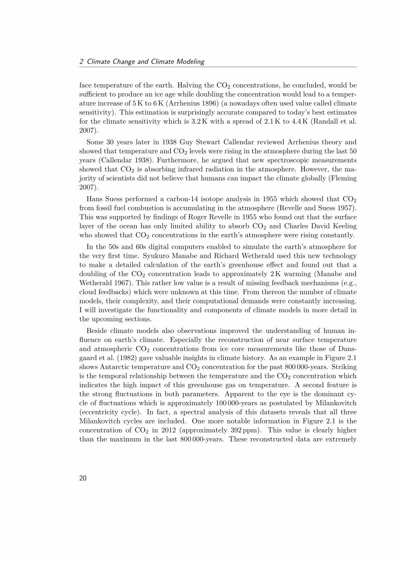
fluence on earth’s climate. Especially the reconstruction of near surface temperatureand atmospheric CO2 concentrations from ice core measurements like those of Dans-gaard et al. (1982) gave valuable insights in climate history. As an example in Figure 2.1shows Antarctic temperature and CO2 concentration for the past 800 000-years. Strikingis the temporal relationship between the temperature and the CO2 concentration whichindicates the high impact of this greenhouse gas on temperature. A second feature isthe strong fluctuations in both parameters. Apparent to the eye is the dominant cy-cle of fluctuations which is approximately 100 000-years as postulated by Milankovitch(eccentricity cycle). In fact, a spectral analysis of this datasets reveals that all threeMilankovitch cycles are included. One more notable information in Figure 2.1 is theconcentration of CO2 in 2012 (approximately 392 ppm). This value is clearly higherthan the maximum in the last 800 000-years. These reconstructed data are extremely
20
2.1 A Changing Climate
Fig. 2.1 Reconstructed CO2 concentration and near surface temperature in Antarctica fromAntarctic ice-cores over the past 800 000 years until 2012 (current) (Shakun 2013).
valuable to set the current atmospheric CO2 concentrations and temperatures in con-text to past conditions. However, they are no prove that the global temperature increaseduring the past approximately 150 years is of anthropogenic origin.Since in reality it is not possible to turn back time, remove all human traces from
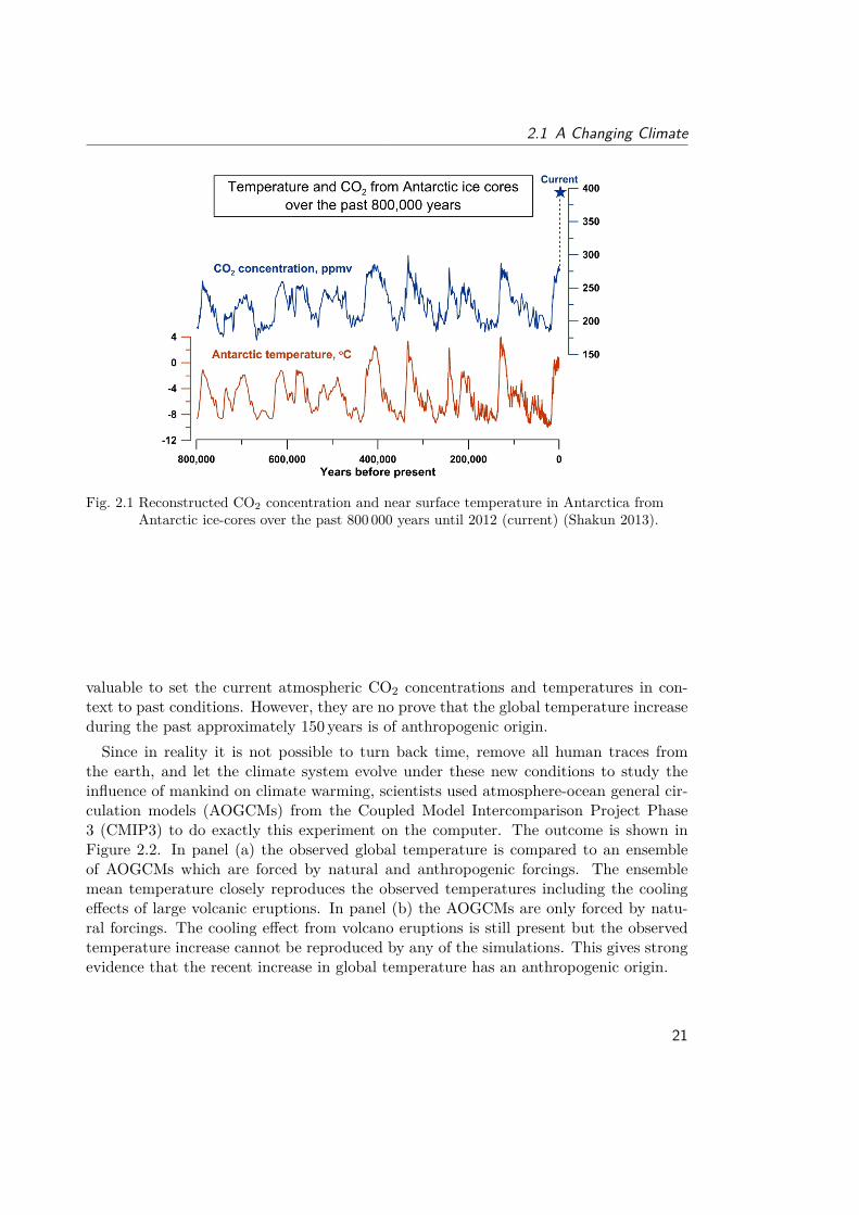
the earth, and let the climate system evolve under these new conditions to study theinfluence of mankind on climate warming, scientists used atmosphere-ocean general cir-culation models (AOGCMs) from the Coupled Model Intercomparison Project Phase3 (CMIP3) to do exactly this experiment on the computer. The outcome is shown inFigure 2.2. In panel (a) the observed global temperature is compared to an ensembleof AOGCMs which are forced by natural and anthropogenic forcings. The ensemblemean temperature closely reproduces the observed temperatures including the coolingeffects of large volcanic eruptions. In panel (b) the AOGCMs are only forced by natu-ral forcings. The cooling effect from volcano eruptions is still present but the observedtemperature increase cannot be reproduced by any of the simulations. This gives strongevidence that the recent increase in global temperature has an anthropogenic origin.
21
2 Climate Change and Climate Modeling
Fig. 2.2 Global mean temperature anomalies (relative to the period 1901 to 1950) for obser-vations (black) and AOGCMs simulations. Panel (a) shows simulations forced withanthropogenic and natural forcings while panel (b) displays simulations with naturalforcings only. Individual simulations are shown as thin lines and the model mean asthick red line in panel (a) and thick blue line in panel (b). Major volcanic eruptionsare shown as gray vertical lines (Randall et al. 2007).
22
2.2 From Zero Dimensional Energy Balance to Earth System Modeling
2.2 From Zero Dimensional Energy Balance to Earth SystemModeling
In Section 2.1 we already got insights in the importance of physical based models forclimate research. The modeling of the climate system has a long tradition. One of thefirst who used a so-called energy balance model to estimate climate sensitivity was Ar-rhenius (1896). No matter if energy balance model or modern AOGCMs are considered,all models follow the same three basic principals:
1. Models are simplifications of reality.2. In models processes are idealized. They emphasize processes considered as impor-
tant and neglect the others.3. Models are subjects of subjective design. The application of the model determines
which processes are important and which are negligible. A universal model for allranges of applications does not exist.
Even though, these principals are still valid this does not mean that there has notbeen large progress in climate modeling since the end of the 19th century. One importantstep was done soon after 1900 by Vilhelm Bjerknes, a Norwegian scientist, who showedthat the dynamics of large-scale flows can be described by a set of equations which arenowadays known as primitive equations (Bjerknes 1904).
2.2.1 The Physics of Atmospheric Flow
In his publication, Bjerknes (1904) combined thermodynamics and hydrodynamics todescribe the interaction of energy, mass, momentum, and moisture of every single par-cel of air with its surrounding parcels. This groundbreaking work was the first steptowards numerical weather prediction (NWP) and still serves as the basis for most cli-mate and NWP models. The primitive equations include the Newton’s law of motion,the hydrodynamic state equation, the thermodynamic energy equation, and the massconservation.Starting with the Newton’s second law of motion or momentum equation for a spher-
ical earth, Equations 2.1 to 2.3 describe that the change of the momentum of a body isproportional to the resulting force acting on the body, and that it acts in the same direc-tion of the force. The thermodynamic energy equation describes changes of temperature(T ) in time (t) caused by adiabatic and diabatic effects (Equation 2.4). Equation 2.5shows the continuity equation for mass and describes that mass is whether gained norlost. Equation 2.6 is similar and describes the mass continuity of specific humidity (qv).The last of the primitive equations is the equation of state or ideal gas law (Equation 2.7)which relates pressure (P ), T , and density (ρ).
23
2 Climate Change and Climate Modeling
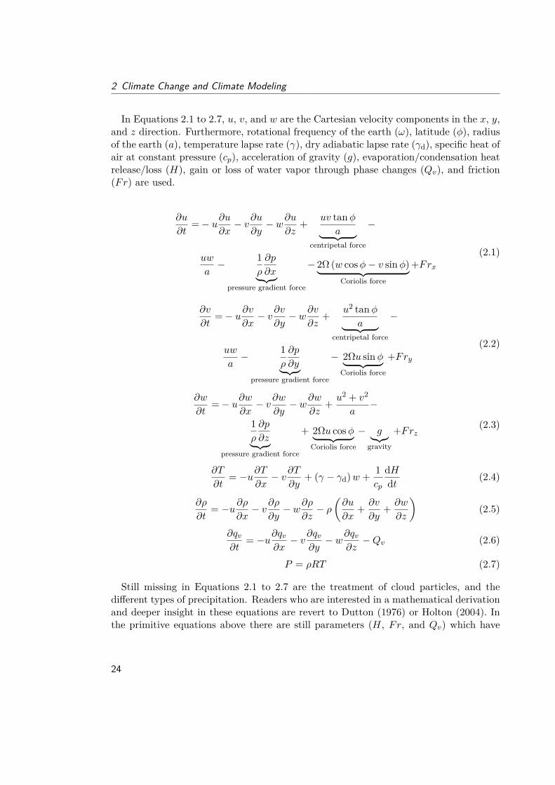
In Equations 2.1 to 2.7, u, v, and w are the Cartesian velocity components in the x, y,and z direction. Furthermore, rotational frequency of the earth (ω), latitude (φ), radiusof the earth (a), temperature lapse rate (γ), dry adiabatic lapse rate (γd), specific heat ofair at constant pressure (cp), acceleration of gravity (g), evaporation/condensation heatrelease/loss (H), gain or loss of water vapor through phase changes (Qv), and friction(Fr) are used.
∂u
∂t=− u∂u
∂x− v∂u
∂y− w∂u
∂z+ uv tanφ
a︸ ︷︷ ︸centripetal force
−
uw
a− 1
ρ
∂p
∂x︸ ︷︷ ︸pressure gradient force
− 2Ω (w cosφ− v sinφ)︸ ︷︷ ︸Coriolis force
+Frx(2.1)
∂v
∂t=− u∂v
∂x− v∂v
∂y− w∂v
∂z+ u2 tanφ
a︸ ︷︷ ︸centripetal force
−
uw
a− 1
ρ
∂p
∂y︸︷︷︸pressure gradient force
− 2Ωu sinφ︸ ︷︷ ︸Coriolis force
+Fry(2.2)
∂w
∂t=− u∂w
∂x− v∂w
∂y− w∂w
∂z+ u2 + v2
a−
1ρ
∂p
∂z︸︷︷︸pressure gradient force
+ 2Ωu cosφ︸ ︷︷ ︸Coriolis force
− g︸︷︷︸gravity
+Frz(2.3)
∂T
∂t= −u∂T
∂x− v∂T
∂y+ (γ − γd)w + 1
cp
dHdt (2.4)
∂ρ
∂t= −u∂ρ
∂x− v∂ρ
∂y− w∂ρ
∂z− ρ
(∂u
∂x+ ∂v
∂y+ ∂w
∂z
)(2.5)
∂qv∂t
= −u∂qv∂x− v∂qv
∂y− w∂qv
∂z−Qv (2.6)
P = ρRT (2.7)
Still missing in Equations 2.1 to 2.7 are the treatment of cloud particles, and thedifferent types of precipitation. Readers who are interested in a mathematical derivationand deeper insight in these equations are revert to Dutton (1976) or Holton (2004). Inthe primitive equations above there are still parameters (H, Fr, and Qv) which have
24
2.2 From Zero Dimensional Energy Balance to Earth System Modeling
to be formulated within the model. P is used as vertical coordinate which can beproblematic because pressure levels can intersect mountains. In Section 3.1 a solution tothis problem will be shown which is used in the COnsortium for Small scale MOdeling(COSMO) model in CLimate Mode (COSMO model in CLimate Mode (CCLM)) RCM.
2.2.2 Computational Achievements
The primitive equations (Equation 2.1 to Equation 2.7) paved the way for “weather bythe numbers” (Harper 2008). However, they are non-linear, non-homogeneous, prognos-tic1, coupled, partial differential equations which cannot be solved analytically. Solvingthese equations during Bjerknes lifetime was prohibitively difficult (Edwards 2010).In 1922 the English mathematician Lewis Fry Richardson attempted to perform the
first forecast with Bjerknes equations by developing new mathematical methods involvingfinite differential equations for the seven basic variables: P , ρ, T , qv, u, v, and w(Richardson 1922). With the help of finite difference equations the calculus to solve theprimitive equations is reduced to arithmetic by transforming operations on variables tooperations on numbers. Methods like this are generally called numerical approaches andare only approximations to the real solution because the time step and sizes of air parcelsare finite instead of infinitesimal like in the original differential equations.For his forecast Richardson (1922) divided Europe into 22 boxes with a square length
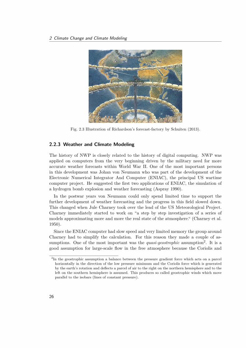
of approximately 200 km (2 latitude by 3 longitude). Vertically he had one layer atthe surface and four more above up to approximately 12 km which results in 110 three-dimensional grid-cells. Since computers were not invented at this time he calculatedsix weeks to finish a six-hour forecast. This huge effort brought him to the idea of aforecast-factory (see Figure 2.3) where groups of people, sitting in a large hall, solve theprimitive equations for different parts of the world. In the middle of the dome a directoris conducting the people like in an orchestra to ensure, for example, a uniform speed ofprogress in all parts of the world (Richardson 1922). However, even with this huge effortthis method would have only permitted a global weather forecast in real-time which wasone of the reasons why it was never implemented. Beside that, Richardsons test forecastwas a complete disaster because an error in his equations lead to a surface pressure ap-proximately 150 times larger than the observed value. These were the two major reasonswhy nobody used Richardson’s method for the next 25 years. Nevertheless, Richardsonwas a visionary and his forecast factory is still an accurate conceptual description of thepractical reality of parallel computing today.
1A prognostic equation means that the equation is predictive (has a time derivative), in contrast to adiagnostic equation which relates the state variables at the same time (e.g., like the ideal gas equationin Equation 2.7) (Warner 2011).
25
2 Climate Change and Climate Modeling
Fig. 2.3 Illustration of Richardson’s forecast-factory by Schuiten (2013).
2.2.3 Weather and Climate Modeling
The history of NWP is closely related to the history of digital computing. NWP wasapplied on computers from the very beginning driven by the military need for moreaccurate weather forecasts within World War II. One of the most important personsin this development was Johan von Neumann who was part of the development of theElectronic Numerical Integrator And Computer (ENIAC), the principal US wartimecomputer project. He suggested the first two applications of ENIAC, the simulation ofa hydrogen bomb explosion and weather forecasting (Aspray 1990).In the postwar years von Neumann could only spend limited time to support the
further development of weather forecasting and the progress in this field slowed down.This changed when Jule Charney took over the lead of the US Meteorological Project.Charney immediately started to work on “a step by step investigation of a series ofmodels approximating more and more the real state of the atmosphere.“ (Charney et al.1950).Since the ENIAC computer had slow speed and very limited memory the group around
Charney had to simplify the calculation. For this reason they made a couple of as-sumptions. One of the most important was the quasi-geostrophic assumption2. It is agood assumption for large-scale flow in the free atmosphere because the Coriolis and
2In the geostrophic assumption a balance between the pressure gradient force which acts on a parcelhorizontally in the direction of the low pressure minimum and the Coriolis force which is generatedby the earth’s rotation and deflects a parcel of air to the right on the northern hemisphere and to theleft on the southern hemisphere is assumed. This produces so called geostrophic winds which moveparallel to the isobars (lines of constant pressure).
26
2.2 From Zero Dimensional Energy Balance to Earth System Modeling
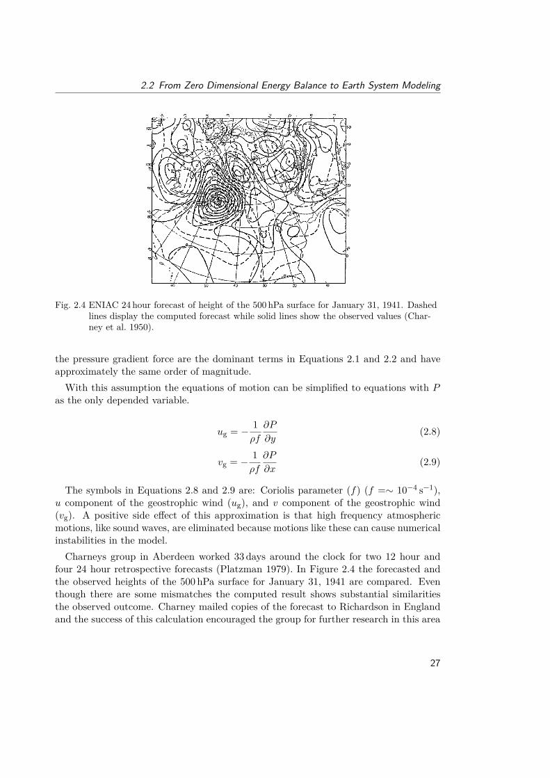
Fig. 2.4 ENIAC 24 hour forecast of height of the 500 hPa surface for January 31, 1941. Dashedlines display the computed forecast while solid lines show the observed values (Char-ney et al. 1950).
the pressure gradient force are the dominant terms in Equations 2.1 and 2.2 and haveapproximately the same order of magnitude.With this assumption the equations of motion can be simplified to equations with P
as the only depended variable.
ug = − 1ρf
∂P
∂y(2.8)
vg = − 1ρf
∂P
∂x(2.9)
The symbols in Equations 2.8 and 2.9 are: Coriolis parameter (f) (f =∼ 10−4 s−1),u component of the geostrophic wind (ug), and v component of the geostrophic wind(vg). A positive side effect of this approximation is that high frequency atmosphericmotions, like sound waves, are eliminated because motions like these can cause numericalinstabilities in the model.Charneys group in Aberdeen worked 33 days around the clock for two 12 hour and
four 24 hour retrospective forecasts (Platzman 1979). In Figure 2.4 the forecasted andthe observed heights of the 500 hPa surface for January 31, 1941 are compared. Eventhough there are some mismatches the computed result shows substantial similaritiesthe observed outcome. Charney mailed copies of the forecast to Richardson in Englandand the success of this calculation encouraged the group for further research in this area
27
2 Climate Change and Climate Modeling
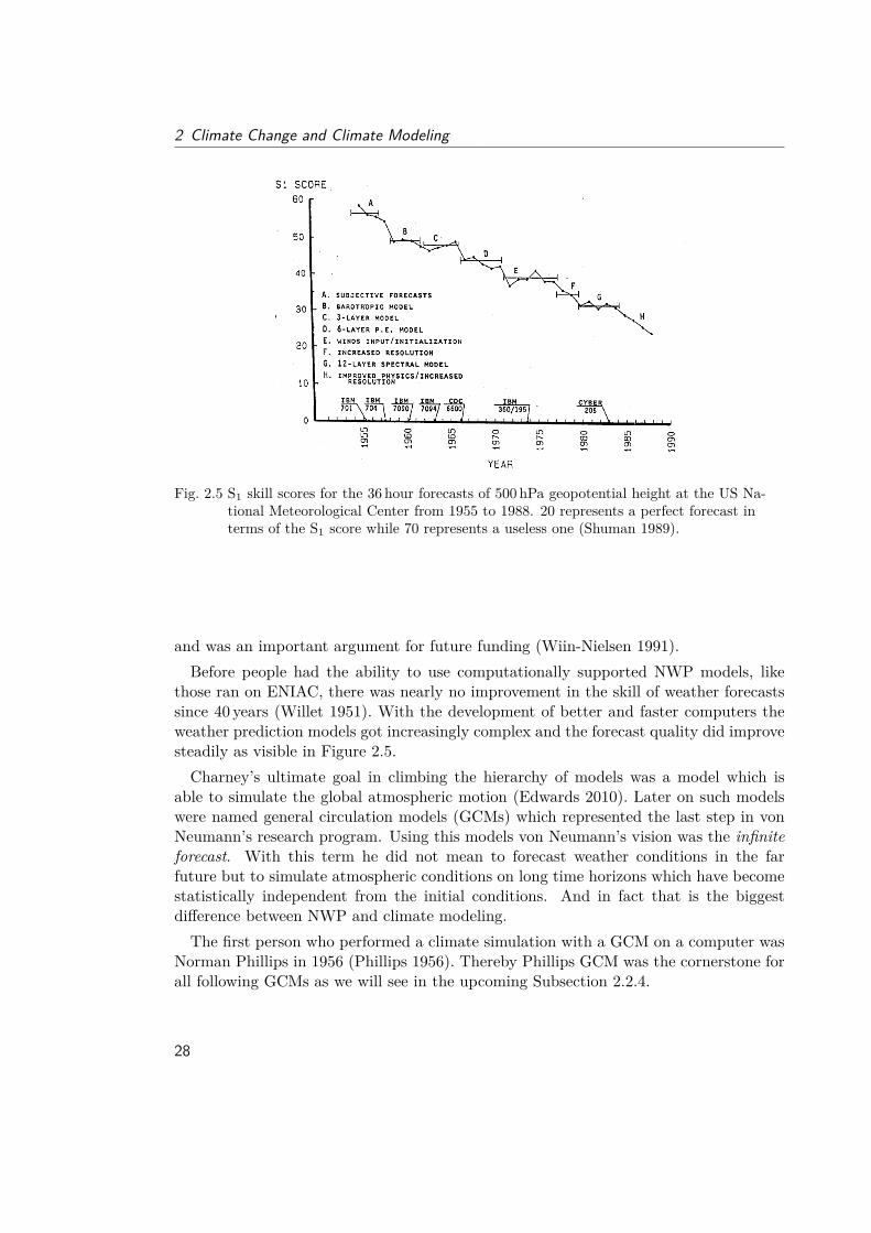
Fig. 2.5 S1 skill scores for the 36 hour forecasts of 500 hPa geopotential height at the US Na-tional Meteorological Center from 1955 to 1988. 20 represents a perfect forecast interms of the S1 score while 70 represents a useless one (Shuman 1989).
and was an important argument for future funding (Wiin-Nielsen 1991).Before people had the ability to use computationally supported NWP models, like
those ran on ENIAC, there was nearly no improvement in the skill of weather forecastssince 40 years (Willet 1951). With the development of better and faster computers theweather prediction models got increasingly complex and the forecast quality did improvesteadily as visible in Figure 2.5.Charney’s ultimate goal in climbing the hierarchy of models was a model which is
able to simulate the global atmospheric motion (Edwards 2010). Later on such modelswere named general circulation models (GCMs) which represented the last step in vonNeumann’s research program. Using this models von Neumann’s vision was the infiniteforecast. With this term he did not mean to forecast weather conditions in the farfuture but to simulate atmospheric conditions on long time horizons which have becomestatistically independent from the initial conditions. And in fact that is the biggestdifference between NWP and climate modeling.The first person who performed a climate simulation with a GCM on a computer was
Norman Phillips in 1956 (Phillips 1956). Thereby Phillips GCM was the cornerstone forall following GCMs as we will see in the upcoming Subsection 2.2.4.
28
2.2 From Zero Dimensional Energy Balance to Earth System Modeling
2.2.4 Increasing Diversity, Resolution, and Complexity
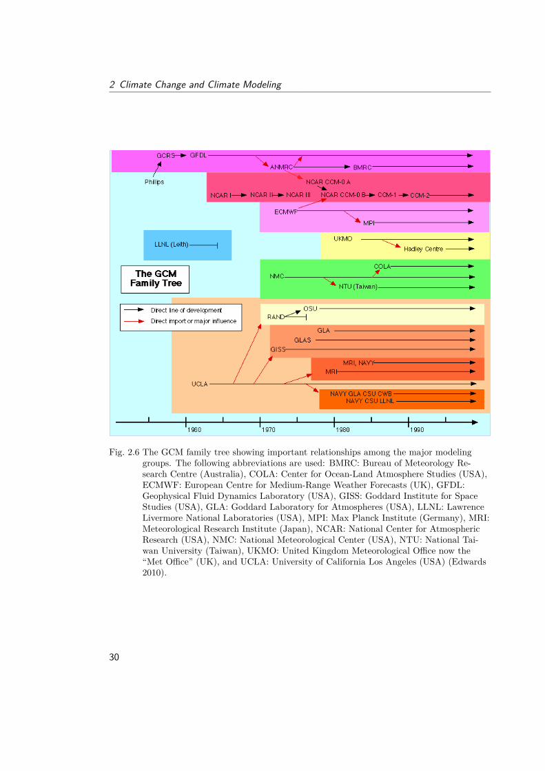
Phillips groundbreaking simulation of the earth’s general circulation caused a boomin GCM development from the 1960s onward. In Figure 2.6 the most important GCMmodeling groups and their relationships are shown schematically. Some institutes copiedthe computer code from an existing GCM with only minor modifications, others adaptedcode to another computing system or just used parts of the code and rewrote the rest,while others started to develop their models independently.Developing a GCM is a very costly and complex effort. This is the major reason
why there is still only a quite limited number of groups doing this. In the currentlyrunning Coupled Model Intercomparison Project Phase 5 (CMIP5) 20 modeling groupsmajorly from North America, Europe, Japan, and Australia are involved. There are nocontributions from Africa, Middle and South America, and the Middle East reflectingthe immense costs of model development, human infrastructure, and supercomputing.As already mentioned, the development of GCMs is closely related to the improve-
ments in computations. From the very beginning, GCMs used the most advanced,fastest, and most expensive computers available. An empirical “law” named after theIntel co-founder Gordon E. Moore says that the number of transistors on integratedcircuits doubles approximately every two years (Moore 1965). Moore’s law is also validfor the increase of processing speed and memory capacity. Moore predicted that thistrend will last for at least 10 years but until now, nearly 40 years later, it is still valid.These computational developments were a major source for the improvements in cli-
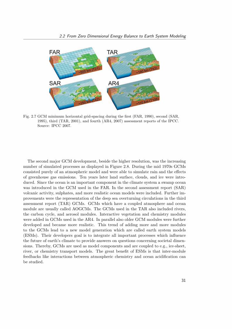
mate modeling during the last half century. Thereby, the model development simulta-neously went in two directions towards higher resolution and higher complexity.In Figure 2.7 the minimum horizontal grid-spacing of GCMs during the four assessment
reports of the Intergovernmental Panel on Climate Change (IPCC) is shown exemplaryfor the orography and surface fields of Europe. While in the first assessment report(FAR) in 1990 the highest resolved model had a grid-spacing of approximately 500 km,the highest resolution in the fourth assessment report (AR4) in 2007 was approximately110 km. This results in a highly improved representation of orography, coastlines, andsurface fields and furthermore allows the simulation of smaller processes in the atmo-sphere. For example, while Continental Europe consisted of approximately 40 grid-pointsin the 1990 GCMs, there were approximately 640 grid-points in 2007. It is importantto note that the quadrupling of the horizontal resolution needs 64 times more compu-tational steps for the same simulation because there are 16 times more grid-points andthe time step has to be quartered at the same time to keep the simulation stable. Inthe newest GCM simulations performed for the IPCC fifth assessment report (AR5) andcoordinated in the CMIP5 framework, the highest model resolution has again improvedto approximately 60 km.
29
2 Climate Change and Climate Modeling
Fig. 2.6 The GCM family tree showing important relationships among the major modelinggroups. The following abbreviations are used: BMRC: Bureau of Meteorology Re-search Centre (Australia), COLA: Center for Ocean-Land Atmosphere Studies (USA),ECMWF: European Centre for Medium-Range Weather Forecasts (UK), GFDL:Geophysical Fluid Dynamics Laboratory (USA), GISS: Goddard Institute for SpaceStudies (USA), GLA: Goddard Laboratory for Atmospheres (USA), LLNL: LawrenceLivermore National Laboratories (USA), MPI: Max Planck Institute (Germany), MRI:Meteorological Research Institute (Japan), NCAR: National Center for AtmosphericResearch (USA), NMC: National Meteorological Center (USA), NTU: National Tai-wan University (Taiwan), UKMO: United Kingdom Meteorological Office now the“Met Office” (UK), and UCLA: University of California Los Angeles (USA) (Edwards2010).
30
2.2 From Zero Dimensional Energy Balance to Earth System Modeling
Fig. 2.7 GCM minimum horizontal grid-spacing during the first (FAR, 1990), second (SAR,1995), third (TAR, 2001), and fourth (AR4, 2007) assessment reports of the IPCC.Source: IPCC 2007.
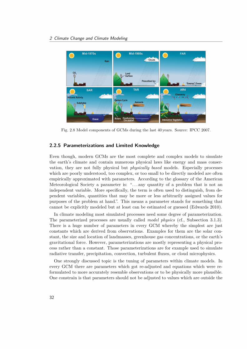
The second major GCM development, beside the higher resolution, was the increasingnumber of simulated processes as displayed in Figure 2.8. During the mid 1970s GCMsconsisted purely of an atmospheric model and were able to simulate rain and the effectsof greenhouse gas emissions. Ten years later land surface, clouds, and ice were intro-duced. Since the ocean is an important component in the climate system a swamp oceanwas introduced in the GCM used in the FAR. In the second assessment report (SAR)volcanic activity, sulphates, and more realistic ocean models were included. Further im-provements were the representation of the deep sea overturning circulations in the thirdassessment report (TAR) GCMs. GCMs which have a coupled atmosphere and oceanmodule are usually called AOGCMs. The GCMs used in the TAR also included rivers,the carbon cycle, and aerosol modules. Interactive vegetation and chemistry moduleswere added in GCMs used in the AR4. In parallel also older GCM modules were furtherdeveloped and became more realistic. This trend of adding more and more modulesto the GCMs lead to a new model generation which are called earth system models(ESMs). Their developers goal is to integrate all important processes which influencethe future of earth’s climate to provide answers on questions concerning societal dimen-sions. Thereby, GCMs are used as model components and are coupled to e.g., ice-sheet,river, or chemistry transport models. The great benefit of ESMs is that inter-modulefeedbacks like interactions between atmospheric chemistry and ocean acidification canbe studied.
31
2 Climate Change and Climate Modeling
Fig. 2.8 Model components of GCMs during the last 40 years. Source: IPCC 2007.
2.2.5 Parameterizations and Limited Knowledge
Even though, modern GCMs are the most complete and complex models to simulatethe earth’s climate and contain numerous physical laws like energy and mass conser-vation, they are not fully physical but physically based models. Especially processeswhich are poorly understood, too complex, or too small to be directly modeled are oftenempirically approximated with parameters. According to the glossary of the AmericanMeteorological Society a parameter is: “. . . any quantity of a problem that is not anindependent variable. More specifically, the term is often used to distinguish, from de-pendent variables, quantities that may be more or less arbitrarily assigned values forpurposes of the problem at hand.”. This means a parameter stands for something thatcannot be explicitly modeled but at least can be estimated or guessed (Edwards 2010).In climate modeling most simulated processes need some degree of parameterization.
The parameterized processes are usually called model physics (cf., Subsection 3.1.3).There is a huge number of parameters in every GCM whereby the simplest are justconstants which are derived from observations. Examples for them are the solar con-stant, the size and location of landmasses, greenhouse gas concentrations, or the earth’sgravitational force. However, parameterizations are mostly representing a physical pro-cess rather than a constant. Those parameterizations are for example used to simulateradiative transfer, precipitation, convection, turbulent fluxes, or cloud microphysics.One strongly discussed topic is the tuning of parameters within climate models. In
every GCM there are parameters which got re-adjusted and equations which were re-formulated to more accurately resemble observations or to be physically more plausible.One constrain is that parameters should not be adjusted to values which are outside the
32
2.2 From Zero Dimensional Energy Balance to Earth System Modeling
observed range. This means, some parameters are relatively fixed (the solar constantor earth’s gravity are two examples) whereas other parameters allow a large range ofpossible values. Examples for them can be especially found in the cloud and aerosolparameterizations which are said to be “highly tunable” (Randall et al. 2007).Less parameterizations and less tuning of the parameters therein (especially those
contained in cloud and aerosol effects) are likely to be those model parts which have thehighest potential to improve current climate model simulations in the near future (e.g.,Kiehl 2007; Schwartz et al. 2007). A general problem is that often the same data areused to develop a parameterization, tune the model, and at the end evaluate the outputof the model. This model-data symbiosis is a critical point and a further motivationto reduce the amount of parameterization schemes and tuning of parameters in climatemodels.
2.2.6 A Scale Problem
In Subsection 2.2.4 the trend towards higher horizontal resolution in GCM simulationswas discussed. As we have seen, the highest horizontal grid-spacing within the CMIP5dataset is approximately 60 km. This does not mean that there is meaningful informationon the grid-point scale. In fact it can be shown that the real resolution or effectiveresolution of grid-box models is approximately 6 to 8 times larger than their grid-spacing(e.g., Grotch and MacCracken 1991; Skamarock 2004; Prein et al. 2013[b]). This meansthat we can assume that the highest resolved GCM in the CMIP5 dataset has an effectiveresolution of approximately 360 km.Atmospheric processes and variations can be displayed in spectra of atmospheric space-
and timescales like shown in Figure 2.9. With state of the art GCMs scales larger thenseveral minutes (the model time step) and ∼ 105 m can be resolved. This scale iscalled synoptic- or macro-β scale and includes e.g., cyclones and anticyclones, planetarywaves, and oscillations like the El Niño–Southern Oscillation (ENSO) or Madden–Julianoscillation (MJO) (cf. Table 2.1). All processes which have smaller spatial scales thanthose resolved in the GCMs cannot be represented explicitly and therefore have to beneglected or parameterized (cf. Subsection 2.2.5).Impacts of climate change on society can typically be found on the micro- and meso-
scale. For example, water supply managements demand for reliable climate projectionson the scale of single river catchments which are in most cases much smaller than theresolution of modern GCMs. Another example is the insurance industry which is in-terested in the future development of extreme weather events. However, extremes oftenhave features which are smaller than the meso-α-scale and can be therefore not directlymodeled with GCMs.During the last centuries different methods have been developed to bridge the scale
33

2 Climate Change and Climate Modeling
Fig. 2.9 Temporal and spatial of atmospheric processes and variations (COMET 2013).
Tab. 2.1 Classification of atmospheric scales after Orlanski (1975)
Scale Macro- Meso- Micro-α β α β γ α β γ
from Earth’scircumf.
10 000 km 2000 km 200 km 20 km 2km 200m 20m
to 10 000 km 2000 km 200 km 20 km 2km 200m 20m ↓e.g., Long waves, cyclones, Fronts, tropical cyclones, Cumulus clouds,
anticyclones thunderstorms tornados
34
2.3 Regional Climate Modeling
difference between GCM output and the data demanded by impact researchers, stake-holders, and policy makers. These methods can be summarized to three basic categories:
1. dynamical downscaling using regional climate models (RCMs) (Dickinson et al.1989; Giorgi and Bates 1989),
2. statistical downscaling (e.g., Hewitson and Crane 1996), and3. stretched grid models (Schmidt 1977; Staniforth and Mitchell 1978).
Each of these approaches has its own advantages and disadvantages. A more detaileddescription and comparison is beyond the scope of this thesis. Interested readers aretherefore referred to the references given above. Here I only want to concentrate on thefirst downscaling technique: dynamical downscaling with RCMs.
2.3 Regional Climate Modeling
The primary difference between GCMs and RCMs is that with the first the entire globe issimulated while the second is used for simulations on limited areas. Thereby, the modelcode (numerics, physics, . . . ; see Section 3.1) is very similar in GCMs and RCMs. In fact,simulating only a limited area is not a new idea since the first numerical weather forecastperformed by the group of Jule Charney on ENIAC in 1950 (see Subsection 2.2.3) alsoonly covered the continental United States.The advantage of using RCMs compared to GCMs is that with RCM simulations
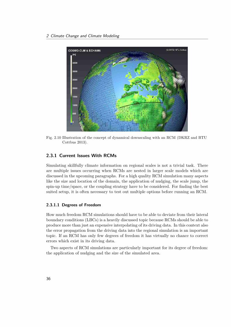
with higher resolutions can be performed if the same computational resources are used.The concept of RCM downscaling is displayed in Figure 2.10. The basic idea is thatthe larger-scale atmospheric conditions from a driving model are used to force/drive anRCM at the lateral and surface boundaries. These so called boundary conditions aretypically provided by GCMs, reanalyses3, or by another RCM with a coarser resolution.Usually, RCMs are one-way coupled with their driving model meaning that there is a flowof information from the lateral boundaries into the regional domain but no informationis feedback to the driving model. In contrast, two-way coupling enables a feedback ofinformation within the regional domain to the driving model. Therefore, the RCM andits driving model have to be simulated simultaneously on the same computer. Thebiggest advantage of this approach is the smoother transition between the driving modeland the RCM at the lateral boundaries.
3In reanalyses historical states of the atmosphere are re-modeled by using an unchanged model anddata assimilation scheme which includes all available observations over the period being analyzed.Therefore, reanalyse datasets are dynamically consistent estimate of atmospheric states of the past.
35
2 Climate Change and Climate Modeling
Fig. 2.10 Illustration of the concept of dynamical downscaling with an RCM (DKRZ and BTUCottbus 2013).
2.3.1 Current Issues With RCMs
Simulating skillfully climate information on regional scales is not a trivial task. Thereare multiple issues occurring when RCMs are nested in larger scale models which arediscussed in the upcoming paragraphs. For a high quality RCM simulation many aspectslike the size and location of the domain, the application of nudging, the scale jump, thespin-up time/space, or the coupling strategy have to be considered. For finding the bestsuited setup, it is often necessary to test out multiple options before running an RCM.
2.3.1.1 Degrees of Freedom
How much freedom RCM simulations should have to be able to deviate from their lateralboundary conditions (LBCs) is a heavily discussed topic because RCMs should be able toproduce more than just an expensive interpolating of its driving data. In this context alsothe error propagation from the driving data into the regional simulation is an importanttopic. If an RCM has only few degrees of freedom it has virtually no chance to correcterrors which exist in its driving data.Two aspects of RCM simulations are particularly important for its degree of freedom:
the application of nudging and the size of the simulated area.
36
2.3 Regional Climate Modeling
Nudging Nudging is a method to include large-scale information from the driving model(e.g., a GCMs) not only via the lateral boundaries of an RCM but also in the interior ofits domain. It prevents the solution of a RCM from deviating too much from the large-scale solution of the driving data. Spectral nudging is the most common used technique(e.g., Kida et al. 1991; Sasaki et al. 1995; Waldron et al. 1996; Von Storch et al. 2000)even though there are also other approaches.Von Storch et al. (2000) argues that with the application of spectral nudging RCM
simulations are more related to downscaling compared to the traditional approach ofdynamical downscaling which represents more or less a boundary value problem.There have been both, studies showing advantages and disadvantages of nudging. For
example, Winterfeldt and Weisse (2009) showed improvements in the wind speed distri-bution of nudged RCM simulations compared to the driving reanalysis data. However,studies by e.g., Radu et al. (2008) and Alexandru et al. (2009) showed disadvantages ofnudging in the simulation of precipitation extremes and small-scale dynamic phenomena.If nudging is applied in RCM simulations it is crucial to carefully consider which
atmospheric fields should be nudged and how strong the nudging of these fields shouldbe. Critics of nudging argue that it destroys the model’s consistency and prohibits theinfluence of small-scale processes, which get resolved in the RCM, on the large scales.Applying nudging in RCMs also implicates that the modeler trusts the correctness of
the large-scale atmospheric patters and dynamics in the driving data. This might be areasonable assumption if reanalysis or short term weather forecast datasets are used asLBCs but is questionable when the data come from GCMs. This is because GCMs canhave errors in the synoptic-scale dynamics which then are propagated even stronger intothe RCM simulation.
Domain Size Beside nudging also the size of the regional domain is important andinfluences the dependence of an RCM simulation on its driving data. Small domain sizesgenerally limit the possibility of RCMs to develop atmospheric situations that deviatefrom those in the driving model.A very powerful experiment to investigate the dependence of domain size on the so-
lution of an RCM simulation is the Big Brother/Little Brother experimentation (e.g.,Denis et al. 2002[b]; Denis et al. 2003; Antic et al. 2004; Dimitrijevic and Laprise 2005).Its setup is described in detail in Subsection 2.4.1.The outcomes of the Big Brother/Little Brother experiments suggest that RCM do-
mains have to have a delicate balance. They should be large enough to be able tosimulate regional phenomena which might be related to e.g., orography or coastlines butalso small enough so the solution cannot drift away from the large-scale forcing (Joneset al. 1995; Leduc and Laprise 2009). Drifting away from the forcing model solution
37
2 Climate Change and Climate Modeling
can result in problems at the boundaries where the large-scale field of the forcing dataand those of the RCM do not match anymore. Additionally, the RCM would no longerdownscale the solution of its driving data. However, this can also be intended if thelarge-scale patterns of the driving model are not fully trusted because regional effects(e.g., orography), which influence the large-scale flow, are missing.Vannitsem and Chomé (2005) performed one-way nested RCM simulations above west-
ern Europe on different domains to investigate the impact of domain size on the qualityof the simulation. They found a high sensitivity of the model quality on the domainsize due to the different dynamics which can be realized dependent on the regional do-main. In small domains the atmospheric flow showed only small deviations from theforcing data which was far from the real chaotic flow. The worst performance was foundfor intermediate domains while the best skill was found for their largest domain whichcovered almost a quarter of the Northern Hemisphere.As a general guideline, supported by the findings of Rojas and Seth (2003), the se-
lection of domain size should be motivated by the quality of the LBCs of the forcingmodel. If high quality forcing data are available smaller domains might be chosen tobe more economic. However, if the driving data have deficiencies, large domains can atleast partly compensate some of them.
2.3.1.2 Domain Location
Not only the domain size but also its location has impacts on the quality of RCM output(Rummukainen 2010). In general, the orientation of a regional domain should be chosenso that the impending large-scale flow from the driving model enters the domain asuniformly as possible. Furthermore, lateral boundaries should not cut through mountainranges which generate dynamic phenomena or strong precipitation gradients. If featuresgenerated e.g., by orography are of interest, the source region of those features shouldbe entirely captured within the domain or left outside if it is highly enough resolved inthe driving model (Marbaix et al. 2003).
2.3.1.3 Resolution Difference
Another setup parameter which has to be chosen is the resolution difference between thedriving model and the RCM. Rojas (2006) found that resolution difference up to 6 to 8times of the rsolution of the LBCs or somewhat larger can be chosen. For example, aGCM with 200 km horizontal grid-spacing allows for RCM gridspacings of approximately25 km. To large resolution jumps can lead to strong disturbances at the boundaries ofthe RCM domain. However, successful RCM simulations have already been performedwith larger resolution differences than 10 (Laprise 2008). The most important featureseems to be that the RCM domain spans several grid-meshes of the driving model.
38
2.3 Regional Climate Modeling
If it is necessary to simulate on grid-spacings which are approximately 10 timessmaller than those of the driving model, typically a multiple nesting approach is ap-plied. Thereby, the downscaling is made in several steps. First, an RCM simulation isperformed on a larger domain than the area of interest. Then a second simulation ismade by using the output of the first one as LBCs and so on.
2.3.1.4 Spin-up
The generation of fine-scale features in RCMs from coarse-scale driving data needs sometime and space which is usually called spin-up time/distance. Typically, most atmo-spheric fields have a rather short spin-up time of 1 to 2 days (Elía et al. 2002). However,some land-surface-fields have a much longer spin-up time of up to several years (e.g.,soil water content in deep soil layers; Seneviratne et al. (2006)). For climate studies itis important to exclude this spin-up time in any statistical calculation.In climate applications the spatial spin-up is as important as the temporal spin-up. It
is the distance from the lateral boundaries to the point where the fine-scale structuresreach their equilibrium amplitudes. It is not well defined how large the width of thisspin-up region is but it is definitively larger than the buffer zone (for an explanation ofthe buffer zone see Subsection 2.3.1.5) (Laprise 2008). The spin-up width tends to dependon the flow speed and is therefore larger in the upper troposphere and on the side wherethe flow impinges on the domain. It also depends on the resolution difference betweenthe LBCs and the RCM and increases for larger resolution jumps. Finally, the spin-upwidth is also a function of the strength of the acting free (hydrodynamic instabilitiesand non-linear processes) and forced (by surface processes) downscaling processes.It is hard to say how far away from the boundaries the fine-scale features have reached
their equilibrium. However, care has to be taken if small, computationally cheap, do-mains are used (approximately 50 by 50 grid-points) because they might be too smallto allow the RCM to spin-up. This should be taken into account in the decision of thedomain size (see Subsection 2.3.1.1).
2.3.1.5 Nesting and Lateral Boundary Conditions
The nesting of RCMs in coarser resolved forcing data is not an unproblematic task.Warner et al. (1997) discussed impacts of the lateral boundary problem on regionalnumerical weather simulations. As already discussed in Subsection 2.3.1.4 the influenceof the LBCs on the RCM fields in the interior of the regional domain is dependent onthe domain size. Déqué et al. (2007) noted that the influence of the LBCs on an RCMsimulation varies with season, and is strongest in winter and in mid-latitude domains.If very large regional domains are used (especially in summer) the solution of RCMs
39
2 Climate Change and Climate Modeling
is often only weakly controlled by the LBCs in the interior of their domains. Thisphenomenon is known as intermittent divergence in phase space (IDPS) (e.g., Von Storch2005). If IDPS does occur large gradients develop especially downstream (at the exitregion of the domain). In very severe cases un-meteorological features can develop withinthe domain so that the RCM can satisfy the LBCs. To prevent the occurrence of IDPSlarge-scale nudging can be applied with all the pros and cons discussed in Subsection2.3.1.1.
2.3.1.6 One-way vs. Two-way Coupling
Many problems discussed in the previous subsections (e.g., IDPS and spatial spin-up)are enhanced, or even caused by, the one-way coupling of RCMs with their drivingmodel. Two-way coupling allows for a feedback of the RCM to the driving model in theinterior or downstream the computational domain and therefore reduces disturbances inthe boundaries of the RCM. If two way coupling is applied both models have to be runsimultaneously on the same computer. There are only a few studies which investigatedthe effect of two-way coupling between a GCM and an RCM. Results suggest a benefit ofthis approach in the global simulation, partly far away from the regional domain (Lorenzand Jacob 2005; Inatsu and Kimoto 2009).
2.4 Skill of RCM Simulations
Whether RCMs do increase the quality of their forcing model is an often asked questionin climate science. Critics state that this is not the case and that RCMs even enlargeerrors which exist in their driving data (e.g., Oreskes et al. 2010; Pielke and Wilby 2012;Kerr 2011).Obviously the core potential of RCMs is their higher resolution which improves the
representation of orographic features, surface fields (e.g., land cover, soil types), andmakes the simulation of regional-scale dynamics possible. The finer grid-spacing also hasthe potential to improve synoptic-scale features like fronts and precipitation. Often thesesimulated fine-scale structures look very realistic like cloud filaments (similar to those onsatellite pictures) or precipitation patterns (Laprise 2008). However, to quantify if thesehigh resolution features are also meaningful and more correct is usually a challengingtask.
2.4.1 Downscaling Ability of RCMs
One intuitive way to analyze the downscaling ability of RCMs is to compare their outputwith observations. If the skill to resemble the observations is higher in the RCM than
40
2.4 Skill of RCM Simulations
in its driving model one can assume that this RCM is able to downscale coarse scaledatmospheric information. However, this approach includes two major problems. First,it is hard to find high quality regional datasets that cover a climatological period. Andsecond, errors which already exist in the driving model are propagating into the RCMvia the LBCs. This means, it is close to impossible to distinguish if differences betweena RCM simulation and observations are caused by errors in the LBCs, by the appliednesting technique, or by the RCM formulation.René Laprise and his group at the Université du Québecá Montréal proposed an elegant
solution to overcome these problems. Laprise (2008) stated that: “The key issue relatingto regional climate modelling is whether the climate of a high-resolution RCM simulationdriven by low-resolution GCM, is equivalent to the climate of a reference simulation witha GCM with equivalent high resolution.” But also this approach faces some problemsbecause running the same GCM in two resolutions will lead to two different atmosphericfields. Therefore, comparing the high-resolution GCM fields with those of the RCM willnot only show effects from the nesting approach but also contain differences arising fromthe different resolutions in the GCM. To overcome this issue and to isolate the effects ofthe nesting approach itself the Big-Brother Experiment was designed (e.g., Denis et al.2002[b]; Denis et al. 2002[a]; Denis et al. 2003; Antic et al. 2004; Dimitrijevic and Laprise2005). As already discussed in Subsection 2.3.1.1, the Big-Brother Experiment consistsof a high-resolution GCM simulation, which produces the reference against the RCMsimulation is compared to and furthermore provides the LBCs for the RCM simulation.The RCM simulation itself is called the Little-Brother. The only thing that is still missingare the coarse-scale LBCs for the RCM. They are derived from the fine-scale GCM runby low-pass filtering the atmospheric fields to emulate a coarse-scale GCM simulationwhich is consistent with the large-scales in the high-resolution GCM run. The differencesbetween the atmospheric fields of the Little-Brother run (the RCM simulation) to thoseof the Big-Brother (the high-resolution GCM simulation) can be now fully attributed tothe nesting method of the RCM.Unfortunately, due to the large computational costs of a high-resolution GCM sim-
ulation on climate time scale nobody has done this experiment so far. To make theexperiment computationally more efficient, the high-resolution GCM simulation was re-placed with a high-resolution RCM simulation with a large domain.With the above described setup several downscaling experiments were performed by
the Université du Québecá Montréal (e.g., Denis et al. 2002[b]; Denis et al. 2002[a];Denis et al. 2003; Antic et al. 2004; Dimitrijevic and Laprise 2005) which showed thatthe Little-Brother is able to “rather well” (Laprise 2008) reproduce the climate statisticsof the small- and large-scale features of the Big-Brother for all simulated fields. Theseresults indicate that RCMs are able to dynamically downscale low-resolution fields if thecorresponding large scales are perfect. This assumption of perfect large-scale LBCs isa crucial point because generally GCM simulations have errors and are not perfect. As
41
2 Climate Change and Climate Modeling
discussed in Subsection 2.3.1.1 it is imaginable that the RCM can correct some of thelarge-scale errors in the GCM but errors might also be amplified when the large-scaleflow interacts with small-scale forcing.To investigate the effect of non-perfect large-scale forcing on an RCM the Imperfect
Big-Brother Experiment has been supposed (Diaconescu et al. 2007). Beside the usageof perfect LBCs, additional LBCs are derived from simulations with a large-scale RCMwhich are performed with different resolutions and above different (large) domains. Thevariation of resolution and domain size produces controllable levels of errors and shouldmimic typical errors occurring in GCM simulations. Diaconescu et al. (2007) showedthat their RCM does not increase nor amplifies the errors in the LBCs for the summerseason over an Eastern North American domain. If large-scale errors are present in theLBCs the representation of small-scale features in the RCM is rather poor. Exceptionscan be found at locations where strong small-scale surface forcing is present.However, the above shown ability of RCMs to downscale large-scale LBCs correctly
seems not to be a universal feature. By downscaling European Centre for Medium-RangeWeather Forecasts 40 Year Re-analysis (ERA-40) with two different RCMs Castro et al.(2005) and Rockel et al. (2008a) showed that “. . . the utility of all regional climate modelsin downscaling global reanalysis primarily is not to add increased skill to the large-scalein the upper atmosphere, rather the value added is to resolve the smaller-scale featureswhich have a greater dependence on the surface boundary.” Furthermore, Castro et al.(2005) say that dynamical downscaling “. . . does not retain value of the large-scale overand above that which exists in the larger global reanalysis. If the variability of synopticfeatures is underestimated or there is a consistent bias in the larger model, no increasedskill would be gained by dynamical downscaling.”More user oriented studies showed no improvements of large-scale features in RCMs
but found added value compared to their forcing data at finer scales like in meso-scalestructures and extremes (Christensen and Christensen 2001). In fact there are manystudies which confirm this. For example, Feser (2006) showed improvements in precipi-tation patterns and Winterfeldt and Weisse (2009) found improvements in coastal windscompared to coarser models.Facing these very controversy results there is a clear need to further investigate the
downscaling ability of RCMs for different regions and different RCMs. Therefore theBig-Brother Experiment framework seems to be a well suited protocol.
2.4.1.1 Added Value in RCM Simulations
The ultimate goal of RCMs is to add information to larger-scale atmospheric fields whichis beyond the resolvable scale of their LBCs. This directly indicates where someoneshould start searching for added value in RCMs; at the scales which are not resolved in
42
2.5 Convection Permitting Simulations
the LBCs hereafter called fine-scales (Laprise 2003; Feser 2006; Feser and Von Storch2005).The two major advantages in RCMs are the improved representation of meso-scale
atmospheric dynamics and the better resolved small-scale surface forcings. In areaswhere surface forcing is strong, like in mountains or along coastlines, RCMs have thepotential that also time-averaged and larger-scale fields are improved (Laprise 2008).Especially near the surface the RCM outputs can get substantially different from featuresin the low-resolution driving data.The drawback, however, is that most of the time-stationary components of the variance
are captured in the very large spatial scales away from the surface in the free atmosphere(Laprise 2008). At small-scales the variance of transient-eddy component generally dom-inates over the stationary components (Bielli and Laprise 2006). This means, averagingover climatic time scales tend to remove added value except in areas with small-scalesurface forcing. Laprise (2008) stated therefore: “. . . the added value of RCMs is likelyto lie mostly in frequency distributions and high-order statistics, reflecting more intenseor localised weather events such as intense precipitation events.”
2.5 Convection Permitting Simulations
Like in the development of GCMs (see Subsection 2.2.4) also RCMs got more and morecomplex and the grid-spacing of their simulations constantly decreased since their risein the late 1980s.The horizontal grid-spacing of state-of-the-art RCMs typically ranges from 50 km to
approximately 25 km; PRUDENCE: 50 km (e.g., Christensen and Christensen 2007),ENSEMBLES: 25 km (Linden and Mitchell 2009), NARCCAP: 50 km (Mearns et al.2009).More recently, due to advancements in the field of computer sciences, it is possible
to have higher-resolved climate simulations with approximately 10 km horizontal gridspacing (e.g., Loibl et al. 2011; Gobiet and Jacob 2012). Nevertheless, even with a meshsize of 10 km there are still numerous processes which cannot be resolved on the modelgrid and therefore have to be parameterized. These parameterizations are importantsources of model errors (e.g., Randall et al. 2007) and introduce large uncertainties inthe projection of future climate (e.g., Déqué et al. 2007).Especially cloud processes (e.g., cloud albedo effects) belong to the least understood
processes in the atmosphere and contribute the largest amount of uncertainty to changesin the radiative forcing4 of past climate change (Solomon et al. 2007).
4Radiative forcing is defined as: “a systematic perturbation to the climatological value of the net radiantflux density at some point in the earth’s climate system.” Source: AMS glossary 2013.
43
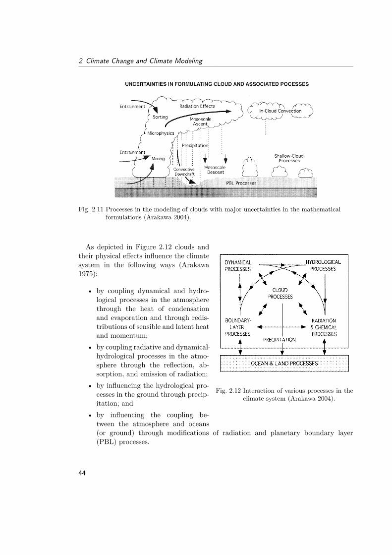
2 Climate Change and Climate Modeling
Fig. 2.11 Processes in the modeling of clouds with major uncertainties in the mathematicalformulations (Arakawa 2004).
Fig. 2.12 Interaction of various processes in theclimate system (Arakawa 2004).
As depicted in Figure 2.12 clouds andtheir physical effects influence the climatesystem in the following ways (Arakawa1975):
• by coupling dynamical and hydro-logical processes in the atmospherethrough the heat of condensationand evaporation and through redis-tributions of sensible and latent heatand momentum;
• by coupling radiative and dynamical-hydrological processes in the atmo-sphere through the reflection, ab-sorption, and emission of radiation;
• by influencing the hydrological pro-cesses in the ground through precip-itation; and
• by influencing the coupling be-tween the atmosphere and oceans(or ground) through modifications of radiation and planetary boundary layer(PBL) processes.
44
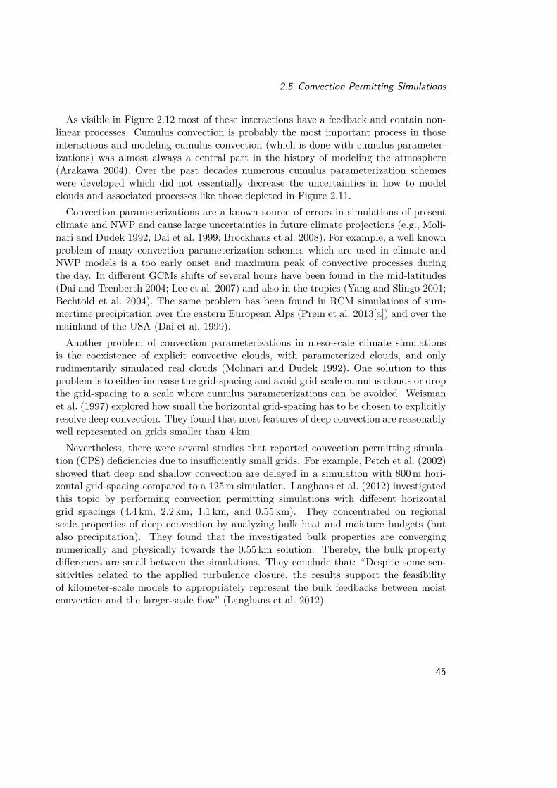
2.5 Convection Permitting Simulations
As visible in Figure 2.12 most of these interactions have a feedback and contain non-linear processes. Cumulus convection is probably the most important process in thoseinteractions and modeling cumulus convection (which is done with cumulus parameter-izations) was almost always a central part in the history of modeling the atmosphere(Arakawa 2004). Over the past decades numerous cumulus parameterization schemeswere developed which did not essentially decrease the uncertainties in how to modelclouds and associated processes like those depicted in Figure 2.11.Convection parameterizations are a known source of errors in simulations of present
climate and NWP and cause large uncertainties in future climate projections (e.g., Moli-nari and Dudek 1992; Dai et al. 1999; Brockhaus et al. 2008). For example, a well knownproblem of many convection parameterization schemes which are used in climate andNWP models is a too early onset and maximum peak of convective processes duringthe day. In different GCMs shifts of several hours have been found in the mid-latitudes(Dai and Trenberth 2004; Lee et al. 2007) and also in the tropics (Yang and Slingo 2001;Bechtold et al. 2004). The same problem has been found in RCM simulations of sum-mertime precipitation over the eastern European Alps (Prein et al. 2013[a]) and over themainland of the USA (Dai et al. 1999).Another problem of convection parameterizations in meso-scale climate simulations
is the coexistence of explicit convective clouds, with parameterized clouds, and onlyrudimentarily simulated real clouds (Molinari and Dudek 1992). One solution to thisproblem is to either increase the grid-spacing and avoid grid-scale cumulus clouds or dropthe grid-spacing to a scale where cumulus parameterizations can be avoided. Weismanet al. (1997) explored how small the horizontal grid-spacing has to be chosen to explicitlyresolve deep convection. They found that most features of deep convection are reasonablywell represented on grids smaller than 4 km.Nevertheless, there were several studies that reported convection permitting simula-
tion (CPS) deficiencies due to insufficiently small grids. For example, Petch et al. (2002)showed that deep and shallow convection are delayed in a simulation with 800m hori-zontal grid-spacing compared to a 125m simulation. Langhans et al. (2012) investigatedthis topic by performing convection permitting simulations with different horizontalgrid spacings (4.4 km, 2.2 km, 1.1 km, and 0.55 km). They concentrated on regionalscale properties of deep convection by analyzing bulk heat and moisture budgets (butalso precipitation). They found that the investigated bulk properties are convergingnumerically and physically towards the 0.55 km solution. Thereby, the bulk propertydifferences are small between the simulations. They conclude that: “Despite some sen-sitivities related to the applied turbulence closure, the results support the feasibilityof kilometer-scale models to appropriately represent the bulk feedbacks between moistconvection and the larger-scale flow” (Langhans et al. 2012).
45
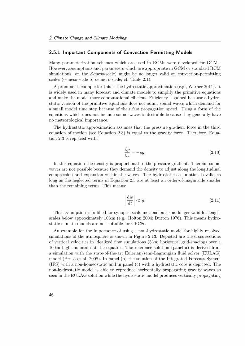
2 Climate Change and Climate Modeling
2.5.1 Important Components of Convection Permitting Models
Many parameterization schemes which are used in RCMs were developed for GCMs.However, assumptions and parameters which are appropriate in GCM or standard RCMsimulations (on the β-meso-scale) might be no longer valid on convection-permittingscales (γ-meso-scale to α-micro-scale; cf. Table 2.1).A prominent example for this is the hydrostatic approximation (e.g., Warner 2011). It
is widely used in many forecast and climate models to simplify the primitive equationsand make the model more computational efficient. Efficiency is gained because a hydro-static version of the primitive equations does not admit sound waves which demand fora small model time step because of their fast propagation speed. Using a form of theequations which does not include sound waves is desirable because they generally haveno meteorological importance.The hydrostatic approximation assumes that the pressure gradient force in the third
equation of motion (see Equation 2.3) is equal to the gravity force. Therefore, Equa-tion 2.3 is replaced with:
∂p
∂z= −ρg. (2.10)
In this equation the density is proportional to the pressure gradient. Therein, soundwaves are not possible because they demand the density to adjust along the longitudinalcompression and expansion within the waves. The hydrostatic assumption is valid aslong as the neglected terms in Equation 2.3 are at least an order-of-magnitude smallerthan the remaining terms. This means:∣∣∣∣dwdt
∣∣∣∣ g. (2.11)
This assumption is fulfilled for synoptic-scale motions but is no longer valid for lengthscales below approximately 10 km (e.g., Holton 2004; Dutton 1976). This means hydro-static climate models are not suitable for CPCSs.An example for the importance of using a non-hydrostatic model for highly resolved
simulations of the atmosphere is shown in Figure 2.13. Depicted are the cross sectionsof vertical velocities in idealized flow simulations (5 km horizontal grid-spacing) over a100m high mountain at the equator. The reference solution (panel a) is derived froma simulation with the state-of-the-art Eulerian/semi-Lagrangian fluid solver (EULAG)model (Prusa et al. 2008). In panel (b) the solution of the Integrated Forecast System(IFS) with a non-homeostatic and in panel (c) with a hydrostatic core is depicted. Thenon-hydrostatic model is able to reproduce horizontally propagating gravity waves asseen in the EULAG solution while the hydrostatic model produces vertically propagating
46
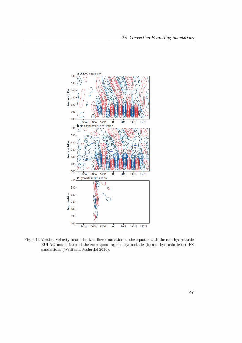
2.5 Convection Permitting Simulations
Fig. 2.13 Vertical velocity in an idealized flow simulation at the equator with the non-hydrostaticEULAG model (a) and the corresponding non-hydrostatic (b) and hydrostatic (c) IFSsimulations (Wedi and Malardel 2010).
47
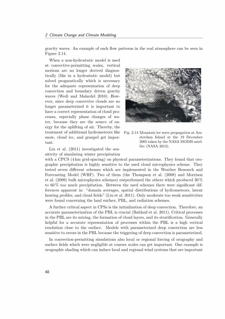
2 Climate Change and Climate Modeling
gravity waves. An example of such flow patterns in the real atmosphere can be seen inFigure 2.14.
Fig. 2.14 Mountain lee wave propagation at Am-sterdam Island at the 19 December2005 taken by the NASAMODIS satel-lite (NASA 2013).
When a non-hydrostatic model is usedat convective-permitting scales, verticalmotions are no longer derived diagnos-tically (like in a hydrostatic model) butsolved prognostically which is necessaryfor the adequate representation of deepconvection and boundary driven gravitywaves (Wedi and Malardel 2010). How-ever, since deep convective clouds are nolonger parameterized it is important tohave a correct representation of cloud pro-cesses, especially phase changes of wa-ter, because they are the source of en-ergy for the uplifting of air. Thereby, thetreatment of additional hydrometeors likesnow, cloud ice, and graupel get impor-tant.Liu et al. (2011) investigated the sen-
sitivity of simulating winter precipitationwith a CPCS (4 km grid-spacing) on physical parameterizations. They found that oro-graphic precipitation is highly sensitive to the used cloud microphysics scheme. Theytested seven different schemes which are implemented in the Weather Research andForecasting Model (WRF). Two of them (the Thompson et al. (2008) and Morrisonet al. (2009) bulk microphysics schemes) outperformed the others which produced 30%to 60% too much precipitation. Between the used schemes there were significant dif-ferences apparent in: “domain averages, spatial distributions of hydrometeors, latentheating profiles, and cloud fields” (Liu et al. 2011). Only moderate too weak sensitivitieswere found concerning the land surface, PBL, and radiation schemes.A further critical aspect in CPSs is the initialization of deep convection. Therefore, an
accurate parameterization of the PBL is crucial (Baldauf et al. 2011). Critical processesin the PBL are its mixing, the formation of cloud layers, and its stratification. Generallyhelpful for a accurate representation of processes within the PBL is a high verticalresolution close to the surface. Models with parameterized deep convection are lesssensitive to errors in the PBL because the triggering of deep convection is parameterized.In convection-permitting simulations also local or regional forcing of orography and
surface fields which were negligible at coarser scales can get important. One example isorographic shading which can induce local and regional wind systems that are important
48
2.5 Convection Permitting Simulations
for the climate of a region. Another example is the treatment of lakes or cities which arepoorly resolved in coarser gridded simulations. Related to this topic is the availability ofhighly resolved surface boundary conditions (e.g., land use, land type, soil type) whichis often a problem in CPCSs.
2.5.2 Added Value in Convection Permitting Simulations
Convection permitting climate modeling is a rather young scientific field and is farfrom being established because of the tremendously demand of computational resources.Therefore, it is still quite unknown how large the added value of CPCSs compared tostate-of-the-art RCM simulations is. However, there are some theoretical considerationswhich can help to answer this question.The most important advantage of CPCSs is the ability to avoid error-prone cumulus
parameterization schemes by resolving deep convection explicitly (as already discussedin Section 2.5). Beside that the high-resolution enables a more realistic representationof orography and surface fields which again can influence atmospheric dynamics.In this subsection I will investigate the added value of CPSs in NWP and in climate
applications.
2.5.2.1 Convection Permitting Simulations in Numerical Weather Forecasting
In NWP convection resolving models are already widely used for operational forecastsand research purposes (e.g., Mass et al. 2002; Kain et al. 2006; Schwartz et al. 2009; Geb-hardt et al. 2011). For example, the Deutscher Wetterdienst (DWD) uses the COSMOmodel for operational convection permitting forecasting with 2.8 km horizontal grid-spacing since April 2007. Baldauf et al. (2011) conclude that this high-resolution modelis able to improve the forecast quality of location, timing, and severity of deep convec-tion and has a better precipitation forecast in summer compared to coarser resolvedsimulations with parameterized deep convection.For convection resolving forecasts with the UK Met Office’s Unified Model (UM)
Roberts and Lean (2008) found a similar result. They showed with the help of the frac-tions skill score (FSS) method that their 1 km model is able to more accurately simulatethe distribution of precipitation and improves the predictability of high accumulationscompared to a 12 km model. However, the 1 km model overestimated the precipitationamounts. Forecasts with a 4 km model could not achieve the skill of the 1 km model.Weusthoff et al. (2010) investigated forecasts from three different NWP models over
Switzerland with the FSS (see Roberts and Lean (2008) or Subsection 3.2.2.1) andthe upscaling method (see Zepeda-Arce et al. (2000) or Subsection 3.2.2.1) and foundsignificant improvements particularly for convective, more localized precipitation events.
49
2 Climate Change and Climate Modeling
2.5.2.2 Convection Permitting Simulations in Climate Applications
One of the first studies which investigated the performance of CPCSs was done by Grell etal. (2000). They used the Fifth-Generation NCAR/Penn State Mesoscale Model (MM5)to simulate a 14month period with up to 1 km horizontal grid-spacing covering theLoisach Valley and parts of the Wetterstein and Karwendel massifs in the European Alps.They found that the domain average precipitation increases the higher the resolution ofthe model is. This is strongest in the winter season because of stronger upslope windsdue to the better resolved orography. In summer the effect of daytime thunderstormdevelopment and movement of convective cells could only be simulated with convectionpermitting resolutions.Hohenegger et al. (2008) analyzed the performance of a CPCS with 2.2 km grid-spacing
covering the entire Alpine Region. They used CCLM to simulate the weather in July2006 and compared the data to observations and a coarser CCLM run with 25 km gridspacing. They concluded that: “the cloud-resolving resolution yields a more accuratespatial localization of the precipitation maxima, reduces the cold bias, and especiallyreproduces a better timing of the convective diurnal cycle” (Hohenegger et al. 2008).In another study, Hohenegger et al. (2009) investigated the soil moisture-precipitation
feedback with the same model, region, and time period as described in the paragraphabove. They performed one control and two sensitivity studies with perturbed soil mois-ture. Previous studies have suggested a positive soil moisture feedback (e.g., Betts et al.1996; Eltahir 1998; Schär et al. 1999; Pal and Eltahir 2001; Findell and Eltahir 2003)meaning that wet soil leads to more precipitation. Hohenegger et al. (2009) found astrong positive soil moisture-precipitation feedback in their coarse resolution (25 km)simulation with parameterized deep convection while their CPCS (2.2 km) shows a pre-dominantly negative feedback. The reason for this is a stable layer which is on top ofthe PBL. The stronger sensible heating above the drier soil leads to stronger thermalsin the CPCS which can more easily break through the stable layer which then leads tomore deep convection and a negative soil moisture-precipitation feedback. The initial-ization of deep convection is much less sensitive to this stable layer in the 25 km modelbecause of the formulation of the applied deep convection parameterization. However,they also found that there are considerable differences in the feedback mechanism ifdifferent convection parameterizations are used.Rasmussen et al. (2011) concentrated on the effects of different grid spacings on the
simulation of snowfall in the headwaters of the Colorado River. Therefore, they simu-lated four cold seasons with the WRF RCM with four different horizontal grid-spacings(2 km, 6 km, 18 km, and 36 km). In the 2 km and 6 km simulations no deep convectionparameterization is used. The findings of this study suggest that global and regionalmodels with grid-spacing larger 18 km underestimate snow in high elevations by 20%to 40% and overestimate it in low elevations by a similar amount. With grid-spacings
50
2.5 Convection Permitting Simulations
lower than 6 km the WRF model was able to reproduce water-year accumulated snowfallwithin 20% for two thirds of the used observation sights. Ikeda et al. (2010) confirmthese results and conclude that: “Comparison of high-resolution WRF simulations ofseasonal snowfall to SNOTEL observations over the Colorado Headwaters regions showvery good agreement if a grid-spacing of <6 km is used” (Ikeda et al. 2010).One of the first studies which analyzed CPS on climate time scales was performed
by Kendon et al. (2012). They performed two simulations with the UM model: Onesimulation with 12 km and one CPCS with 1.5 km horizontal grid-spacing, covering thesouthern part of the United Kingdom between 1989 and 2008. Heavy rainfall in the1.5 km model has an more realistic duration and spatial extent compared to the 12 kmsimulation. The 12 km model simulates too weak heavy precipitation while the 1.5 kmrun tends to overestimate the intensity. The 1.5 km model furthermore removes thetendency for too much drizzling in the UM and corrects errors in the diurnal cycle ofprecipitation.Pryor et al. (2012) investigated the influence of horizontal grid-spacing in the Rossby
Centre version 3 (RCA3) RCM on the wind climate in a flat region centered over Den-mark. Therefore, the period 1987 to 2008 was simulated with 50 km, 25 km, 12.5 km, and6.25 km horizontal grid spacing. The mean wind speed 10m above ground increases by5% when the grid-spacing is reduced from 50 km to 6.25 km. Stronger signals are visiblein the 50 year return level wind speed and wind gusts which increase by 10% respec-tively 24%. At the lowest model level (approximately 70m) these increases are strongerand show approximately 10% in the mean and approximately 20% in the 50 year returnperiod. The found increases in wind speed are in the same order of magnitude as theclimate change signals in this region. However, comparisons with in situ observationsdid not show improvements at synoptic and meso-α time scales in the higher resolvedsimulations.Summing up the findings of the above discussed studies, the main added value of
CPCS compared to coarser gridded simulations are:
• better timing of the convection diurnal cycles (Hohenegger et al. 2008; Kendonet al. 2012),
• improved location and extend of heavy convective precipitation (Hohenegger et al.2008; Kendon et al. 2012),
• removed drizzling problem (Kendon et al. 2012),• more accurate distribution of snow (Rasmussen et al. 2011; Ikeda et al. 2010), and• improved simulation of the snowpack and runoff (Rasmussen et al. 2011; Ikeda
et al. 2010).
This thesis builds up on these results and extends them by investigating the commonadded value of an ensemble of CPCS (see Section 4.1). In addition to precipitation,
51

2 Climate Change and Climate Modeling
also two meter temperature, relative humidity, and global radiation are analyzed. Forthe evaluation of precipitation fields advanced statistical methods, which are commonlyused in NWP (see Subsection 2.5.2.1) are applied.Based on the findings of the CPCS ensemble evaluation and published literature a
second study focuses on the representation of summer- and wintertime extreme precip-itation events in complex terrain simulated with the WRF model in three horizontalgrid-spacings (see Section 4.2). The simulations are analyzed on different spatial scalesto investigate the effect of upscaling of small-scale features in CPCSs to coarser scales.
52
3Dynamical Downscaling and Detecting Added
Value
3.1 Dynamical Downscaling with RCMs on the Example ofCCLM
This section gives an overview on the formulation of regional climate models (RCMs)on the example of the COSMO model in CLimate Mode (CCLM). Thereby, the
model dynamics (Subsection 3.1.1), numerics (Subsection 3.1.2), and physics (Subsec-tion 3.1.3) are briefly described. The goal is to give an idea how state-of-the-art RCMsare built up, which processes are considered, and which assumptions are taken. Readerswho are interested in a more general and holistic description of weather and climate mod-els are referred to textbooks like Warner (2011) or Washington and Parkinson (2005).
3.1.1 Dynamics
The dynamical cores of three dimensional climate models are based on the primitiveequations (see Equations 2.1 to 2.7). As discussed in Subsection 2.2.1 these equa-tions combine the Newton’s law of motion, the hydrodynamic state equation, the ther-modynamic energy equation, and the mass conservation to a set of non-linear, non-homogeneous, prognostic coupled, partial differential equations.The dynamics of CCLM are based on the full set of primitive equations and describe
53
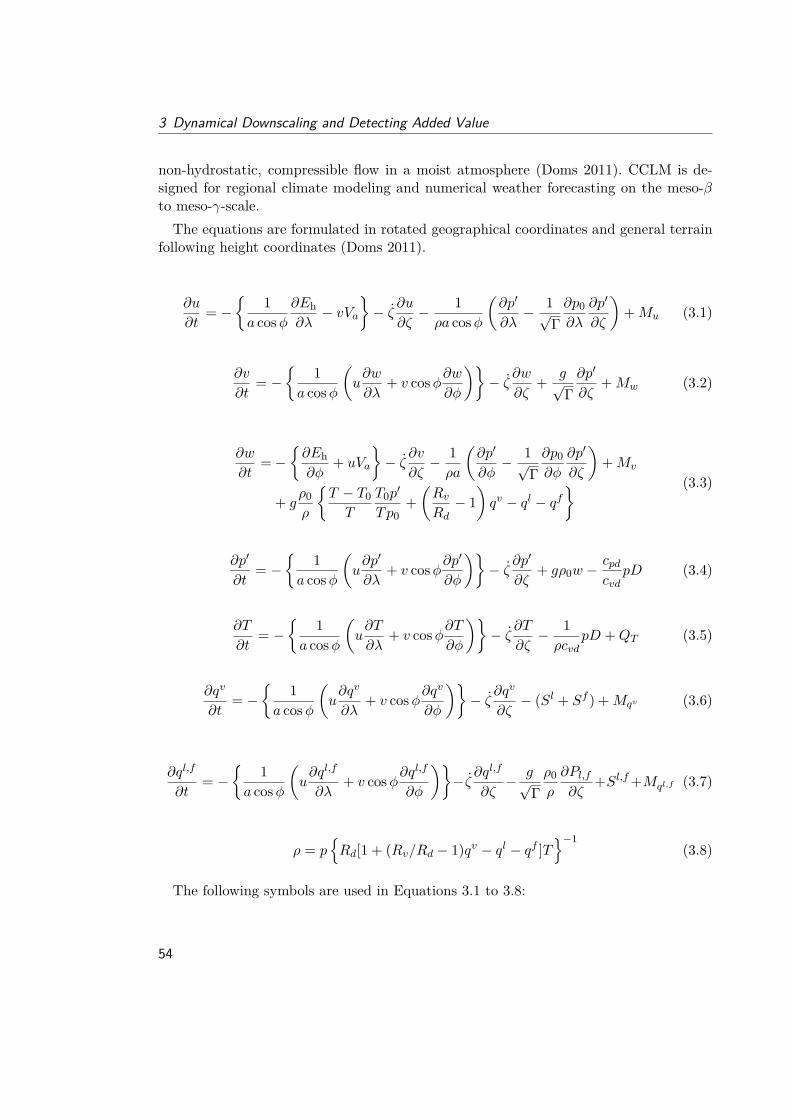
3 Dynamical Downscaling and Detecting Added Value
non-hydrostatic, compressible flow in a moist atmosphere (Doms 2011). CCLM is de-signed for regional climate modeling and numerical weather forecasting on the meso-βto meso-γ-scale.The equations are formulated in rotated geographical coordinates and general terrain
following height coordinates (Doms 2011).
∂u
∂t= −
1
a cosφ∂Eh∂λ− vVa
− ζ ∂u
∂ζ− 1ρa cosφ
(∂p′
∂λ− 1√
Γ∂p0∂λ
∂p′
∂ζ
)+Mu (3.1)
∂v
∂t= −
1
a cosφ
(u∂w
∂λ+ v cosφ∂w
∂φ
)− ζ ∂w
∂ζ+ g√
Γ∂p′
∂ζ+Mw (3.2)
∂w
∂t=−
∂Eh∂φ
+ uVa
− ζ ∂v
∂ζ− 1ρa
(∂p′
∂φ− 1√
Γ∂p0∂φ
∂p′
∂ζ
)+Mv
+ gρ0ρ
T − T0T
T0p′
Tp0+(RvRd− 1)qv − ql − qf
(3.3)
∂p′
∂t= −
1
a cosφ
(u∂p′
∂λ+ v cosφ∂p
′
∂φ
)− ζ ∂p
′
∂ζ+ gρ0w −
cpdcvd
pD (3.4)
∂T
∂t= −
1
a cosφ
(u∂T
∂λ+ v cosφ∂T
∂φ
)− ζ ∂T
∂ζ− 1ρcvd
pD +QT (3.5)
∂qv
∂t= −
1
a cosφ
(u∂qv
∂λ+ v cosφ∂q
v
∂φ
)− ζ ∂q
v
∂ζ− (Sl + Sf ) +Mqv (3.6)
∂ql,f
∂t= −
1
a cosφ
(u∂ql,f
∂λ+ v cosφ∂q
l,f
∂φ
)−ζ ∂q
l,f
∂ζ− g√
Γρ0ρ
∂Pl,f∂ζ
+Sl,f+Mql,f (3.7)
ρ = pRd[1 + (Rv/Rd − 1)qv − ql − qf ]T
−1(3.8)
The following symbols are used in Equations 3.1 to 3.8:
54

3.1 Dynamical Downscaling with RCMs on the Example of CCLM
Γ variation of reference pressureφ latitudeT0 constant reference temperatureT temperaturea radius of the earthcpd specific heat capacities of dry air at constannt pressurecvd specific heat capacities of dry air at constannt volumeD three-dimensional wind divergenceEh kinetic energy of horizontal motiong acceleration of gravityλ longitudeMu source terms due to turbulent mixing in uMv source terms due to turbulent mixing in vMw source terms due to turbulent mixing in wMqv source terms due to turbulent mixing in qvMql,f source terms due to turbulent mixing in ql,fp′ pressure perturbation from p0p0 constant reference pressurePl,f absolute values of the gravitational diffusion fluxes of water and iceqf mass fraction of iceql mass fraction of waterQT diabatic heating termqv mass fraction of water vaporRd gas constant for dry airρ0 constant reference densityρ densityRv gas constant for water vaporSl cloud microphysical sources/sinks per unit mass of moist airu zonal wind velocityVa vertical component of absolute vorticityv meridional wind velocityw vertical velocityζ nonnormalized contravariant vertical velocityζ terrain following vertical coordinate
Comparing Equations 3.1 to 3.8 with the primitive equations (2.1 to 2.7) reveals, thatthere are many terms that look different or pop up in the equations used in the CCLM.This is necessary because of assumptions in the model or adaptations which are madeto make the model more efficient for computing.For example, Equation 3.7 enables to calculate temporal changes of atmospheric water
55
3 Dynamical Downscaling and Detecting Added Value
and ice prognostically which is not included in the original primitive equations.Additional terms appear because of the transformation of curvilinear but orthogonal
spherical coordinate system with geometrical height z to a height following coordinatesystem with the new terrain following vertical coordinate (ζ). This transformation avoidsa costly formulation of the surface boundary conditions which would be necessary if zcoordinates would be used in the model (Doms 2011). In terrain following coordinates thisis omitted because the lowest level of constant vertical coordinates follows the orography.In CCLM a hybrid vertical coordinate system is used with terrain following levels betweenthe surface orography height and a defined height where the levels convert back to flathorizontal fields. In the current version of CCLM the height-based hybrid smooth levelvertical (SLEVE) coordinate system (Schär et al. 2002) is used.The thermodynamic variables (T , P , and ρ) in the CCLM are split into a sum of a
base state and deviations thereof (Doms 2011). Thereby, the base state is horizontallyhomogeneous (depends only on the height above the surface), time invariant, and inhydrostatic balance. This is beneficial because horizontal pressure gradients are removedfrom the base state pressure. If pressure does not deviate too strongly from the referencepressure, calculating with the difference can be beneficial for the computational accuracyof calculating the pressure gradient force when sloping coordinate surfaces occur (whichis the case because of the terrain following vertical coordinate system).With the Equations 3.1 to 3.8 the complete set of the thermodynamic state variables
is defined. The prognostic variables therein are zonal wind velocity (u), meridional windvelocity (v), vertical velocity (w), temperature (T ), pressure perturbation from p0 (p′),density (ρ), mass fraction of water vapor (qv), mass fraction of water (ql), and massfraction of ice (qf ). These variables are defined if the mixing terms M , the sources andsinks of cloud microphysical sources/sinks per unit mass of moist air (Sl) as well as theabsolute values of the gravitational diffusion fluxes of water and ice (Pl,f ), additionallyto the diabatic heating term (QT ) are known. These variables are calculated as functionsof the prognostic variables by various parameterization schemes.To solve the model equations finite differencing methods are necessary which are dis-
cussed in the next Subsection 3.1.2.
3.1.2 Numerics
To solve Equations 3.1 to 3.8 constant increments of the independent variables (∆λ, ∆φ,and ∆ζ) are used as setup for the computational grid (Doms 2011). With this method itis possible to derive a finite computational (λ, φ, ζ)-space with grid-points (i,j,k) withi in the λ-direction, j in the φ-direction, and k in the ζ-direction. The location of thegrid-points in the three dimensional grid is derived by:
56
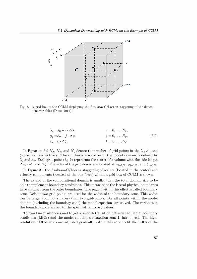
3.1 Dynamical Downscaling with RCMs on the Example of CCLM
Fig. 3.1 A grid-box in the CCLM displaying the Arakawa-C/Lorenz staggering of the depen-dent variables (Doms 2011).
λi =λ0 + i ·∆λ, i = 0, . . . , Nλ,
φj =φ0 + j ·∆φ, j = 0, . . . , Nφ, (3.9)ζk =k ·∆ζ, k = 0, . . . , Nζ .
In Equation 3.9 Nλ, Nφ, and Nζ denote the number of grid-points in the λ-, φ-, andζ-direction, respectively. The south-western corner of the model domain is defined byλ0 and φ0. Each grid-point (i,j,k) represents the center of a volume with the side length∆λ, ∆φ, and ∆ζ. The sides of the grid-boxes are located at λi+1/2, φj+1/2, and ζk+1/2.In Figure 3.1 the Arakawa-C/Lorenz staggering of scalars (located in the center) and
velocity components (located at the box faces) within a grid-box of CCLM is shown.The extend of the computational domain is smaller than the total domain size to be
able to implement boundary conditions. This means that the lateral physical boundarieshave an offset from the outer boundaries. The region within this offset is called boundaryzone. Default two grid points are used for the width of the boundary zone. This widthcan be larger (but not smaller) than two grid-points. For all points within the modeldomain (excluding the boundary zone) the model equations are solved. The variables inthe boundary zone are set to the specified boundary values.To avoid inconsistencies and to get a smooth transition between the lateral boundary
conditions (LBCs) and the model solution a relaxation zone is introduced. The high-resolution CCLM fields are adjusted gradually within this zone to fit the LBCs of the
57
3 Dynamical Downscaling and Detecting Added Value
driving model. Therefore, a relaxation boundary condition is defined which is similar tothat proposed by Davies (1976) and Davies (1983). In CCLM an attenuation function(αb) is calculated which controls the strength of the LBCs influence on the model solution(Kallberg 1977):
αb = 1− tanh(
d
2∆x
). (3.10)
In Equation 3.10 ∆x denotes the horizontal grid-spacing and d is the distance fromthe lateral boundary. If d = 0 then αb = 1 and if d ∆x then α → 0. Usually, 8grid-points are directly affected by the LBCs (Doms 2011).Vertically, grid stretching is applied for higher efficiency. Thereby, the distance of
vertical model levels is smaller near the surface and gets larger in higher altitudes.Since the CCLM is a non-hydrostatic model with a compressible model atmosphere
sound waves, which are not important for meteorological fields, are part of the modelsolutions (cf., Subsection 2.5.1). For a more efficient computation, the prognostic equa-tions are split into terms which are related to fast propagating acoustic waves and termswhich are related to slow moving waves according to the method described by Klempand Wilhelmson (1978). How this mode splitting is implemented in the CCLM can beseen in Doms (2011).Due to the time splitting there are two time steps used in the model. A shorter one
for sound waves and a longer one for slow moving waves (∆t). The discrete time levelsare therefore t = t0 + n∆t where n is the time step counter and t0 is the starting timeof the simulation.Two numerical time integration schemes are available in CCLM. The first one is the
Leapfrog-scheme which has second-order accuracy (Klemp and Wilhelmson 1978). Thesecond one is the Runge-Kutta-scheme and was implemented due to the need for de-creasing numerical noise at the grid-scale for convection permitting simulations. It isadapted from the time-slitting approach of Wicker and Skamarock (2002).The 3rd-order Runge-Kutta-scheme works with a 5th-order advection upwind scheme
which takes care of the horizontal advection of the dynamic variables (Doms 2011).Thereby, the tendencies of the two horizontal directions are added. Formally the usedRunge-Kutta-scheme is of 2nd-order accuracy but has 3rd-order accuracy for linear prob-lems. Combined with the 5th-order advection scheme it is one of the most effectiveschemes of this type (Baldauf 2008). More details about the implementation of thisscheme can be found in Doms (2011).Numerical smoothing is introduced to artificially damp small-scale computational
noise around two grid interval wavelengths (2∆x) and to prevent the initiation andgrowth of non-linear instabilities (Doms 2011). Numerical noise is introduced by nu-
58
3.1 Dynamical Downscaling with RCMs on the Example of CCLM
merical dispersion especially in the Leapfrog-scheme. Small-scale noise can also occurbecause of aliasing and may lead to weak non-linear numerical instabilities. Further-more, physical processes which generally act on a grid-point basis will generate 2∆xwaves.In CCLM time filtering is implemented which helps to avoid high-frequency oscilla-
tions. In addition, multiple options for spatial numerical smoothing are implementedwhich typically use horizontal diffusion and Rayleigh damping. They are applied to avoidreflections of gravity waves from the upper boundary of the model. For the descriptionsof those methods see Doms (2011) and the literature therein.In convection permitting simulations numerical smoothing with horizontal diffusion
can lead to systematic biases. This is because in a terrain following coordinate systemover complex orography horizontal diffusion leads to unwanted vertical mixing. Sinceorography is generally getting steeper when the horizontal grid-spacing is reduced thisproblem gets more severe in highly resolved simulations (Doms 2011). For example,horizontal diffusion of temperature will tend to cool the valleys and heat up the mountaintops. The same can happen to atmospheric moisture which is diffused from the valleysto the mountain tops.The usage of a reference atmosphere helps to reduce these errors in the CCLM. For
instance, the unwanted vertical mixing of temperature will be zero if the vertical tem-perature gradient is equal to the gradient used in the reference atmosphere. However,large errors can still occur if the stratification is very different from those in the referenceatmosphere (i.e., for very stable or unstable stratification).To furthermore reduce these errors a flux-limited scheme is used in the CCLM. This
scheme enables to reduce orographic induced biases and avoids mass-conservation er-rors by artificially reducing the fluxes according to the steepness of the model surface.The implemented scheme reduces the fluxes gradually with increasing steepness of theterrain-following coordinates. The fluxes become zero if a threshold height differencebetween two neighboring grid-points is exceeded. This threshold is 250m (namelist-switch hd_dhmax) by default (fitted to a grid-spacing of 7 km) and should be adjustedaccordingly if the horizontal grid-spacing is changed.High-resolution modeling in complex terrain leads to another long-standing problem
which is the simulation of unrealistic high precipitation values above mountain tops andtoo less precipitation in valleys (Doms 2011). One reason for this is the usage of averagealtitudes of grid-cells which leads to solitary (single grid-cell) mountain tops and valleyfloors. This introduces un-physical feedbacks to the simulated flow affecting the modelphysics in inaccurate ways. Investigations of this behavior (e.g., Gassmann 2002; Daviesand Brown 2001) have revealed that the orography has to be reasonably well resolvedin the applied resolution to achieve correct behavior of the flow.Therefore, Doms (2011) suggests a weak filtering of the orography to improve the
59
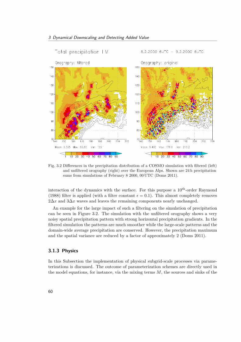
3 Dynamical Downscaling and Detecting Added Value
Fig. 3.2 Differences in the precipitation distribution of a COSMO simulation with filtered (left)and unfiltered orography (right) over the European Alps. Shown are 24 h precipitationsums from simulations of February 8 2000, 00UTC (Doms 2011).
interaction of the dynamics with the surface. For this purpose a 10th-order Raymond(1988) filter is applied (with a filter constant ε = 0.1). This almost completely removes2∆x and 3∆x waves and leaves the remaining components nearly unchanged.An example for the large impact of such a filtering on the simulation of precipitation
can be seen in Figure 3.2. The simulation with the unfiltered orography shows a verynoisy spatial precipitation pattern with strong horizontal precipitation gradients. In thefiltered simulation the patterns are much smoother while the large-scale patterns and thedomain-wide average precipitation are conserved. However, the precipitation maximumand the spatial variance are reduced by a factor of approximately 2 (Doms 2011).
3.1.3 Physics
In this Subsection the implementation of physical subgrid-scale processes via parame-terizations is discussed. The outcome of parameterization schemes are directly used inthe model equations, for instance, via the mixing terms M , the sources and sinks of the
60
3.1 Dynamical Downscaling with RCMs on the Example of CCLM
cloud microphysics Sl, the precipitation fluxes Pl,f , or to the radiative heating term QT(cf., Equations 3.1 to 3.8).
3.1.3.1 Subgrid-Scale Turbulence
Subgrid-scale turbulence parameterizations link the explicitly resolved atmospheric mo-tions with the unresolved fluctuating scales of motion. The representation of turbulentfluxes in an atmospheric model is important because they lead to an exchange of mo-mentum, humidity, and heat between the surface and the free atmosphere.The default subgrid-scale turbulence scheme of the CCLM uses a second-order closure
suggested by Mellor and Yamada (1974) and Mellor and Yamada (1982). The scheme isbased on prognostic turbulent kinetic energy (TKE) and is formulated in terms of liquidwater potential temperature and total water content. It includes effects from thermalcirculations and subgrid-scale condensation (Doms et al. 2011).Optional, a three-dimensional TKE-based scheme is implemented in the CCLM which
should be used in highly resolved simulations to avoid common approximations of bound-ary layer processes. The scheme was designed for large eddy simulations and is basedon a model described in Herzog et al. (2002a); Herzog et al. (2002b). However, at themoment this scheme does not consider cloud water.
3.1.3.2 Surface Layer Parameterization
Surface fluxes of moisture, heat, and momentum can have large impacts on the resultsof numerical models. Fluxes like these are coupling the atmosphere with the surfacemodel. In CCLM modified Businger relations (Businger et al. 1971) are used for thestability and roughness-length dependent surface flux formulation (Doms et al. 2011).For the flux calculation a computational efficient analytic procedure based on the workof Louse (1979) is applied.Optional in the CCLM is a TKE-based surface transfer scheme which is related to
the subgrid-scale turbulence TKE scheme mentioned above. Thereby, the surface layeris the layer between the lowest model level and the earths surface. This layer is dividedin three parts: a laminar-turbulent sublayer, a roughness layer, and a constant-flux orPrandtl layer (Doms et al. 2011).
3.1.3.3 Grid-Scale Clouds and Precipitation
The correct simulation of clouds and precipitation is essential for the water and energycycle of the earth (cf., Section 2.5). The various microphysical processes which lead to
61
3 Dynamical Downscaling and Detecting Added Value
the formation of clouds and precipitation are highly dependent on and interact with thethermodynamic conditions in the atmosphere.The standard parameterization scheme for grid-scale clouds and precipitation is based
on Kessler-type1 bulk formulation and clusters cloud and precipitation particles intospecified categories of water substances. Those categorized particles interact with themicrophysical processes which themselves have feedbacks to the thermodynamic of theatmosphere (Doms et al. 2011). The scheme was developed for meso-β- and meso-α-scalesimulations and accounts for stratiform mixed-phase clouds.Beside water vapor three different categories of water are used in the basic scheme:• cloud water qc are particles which have a radius smaller than 50µm and therefore
no relative fall speed compared to the airflow.• Rain water qr consist of spherical droplets which have a non-negligible fall velocity.
The distribution of the droplet size is derived from an exponential Marshall-Palmersize-distribution. The terminal velocity of the drops is purely dependent on thedrop diameter.
• Snow qs particles are treated as thin plates with a size proportional to the mass ofthe particles. The terminal velocity is only dependent on the particle size which isderived from a Gunn-Marshall size-distribution.
In the specific water content (qspec) budget equation (including mass fraction of watervapor (qv), cloud water (qc), cloud ice (qi), and graupel (qg), depending on the usedscheme) advective and turbulent processes are taken into account while rain water (qr)and snow (qs) is only advective transported.In Figure 3.3 the microphysical processes in the CCLM standard scheme are depicted.
The microphysical source/sink terms S enable the mass-transfers between the differentwater categories.Beside the above described basic scheme there are three more cloud precipitation
schemes implemented in CCLM (Doms et al. 2011) (namelist-switch itype_gscp):
1. The warm rain scheme is adapted from the Kessler (1969) scheme and has no iceface processes.
2. The one-category ice scheme is the above described basic scheme for applicationson the meso-β- and meso-α-scale.
3. The cloud ice scheme is an extension of the standard scheme and includes addi-tionally prognostic cloud ice and the corresponding source/sink terms. It is thedefault scheme in CCLM.
1Kessler (1969) suggested a simple parameterization which relates the autoconversion rate to the cloudliquid water content linearly. Because of its simplicity this parameterization is widely used in cloud-related modeling studies.
62
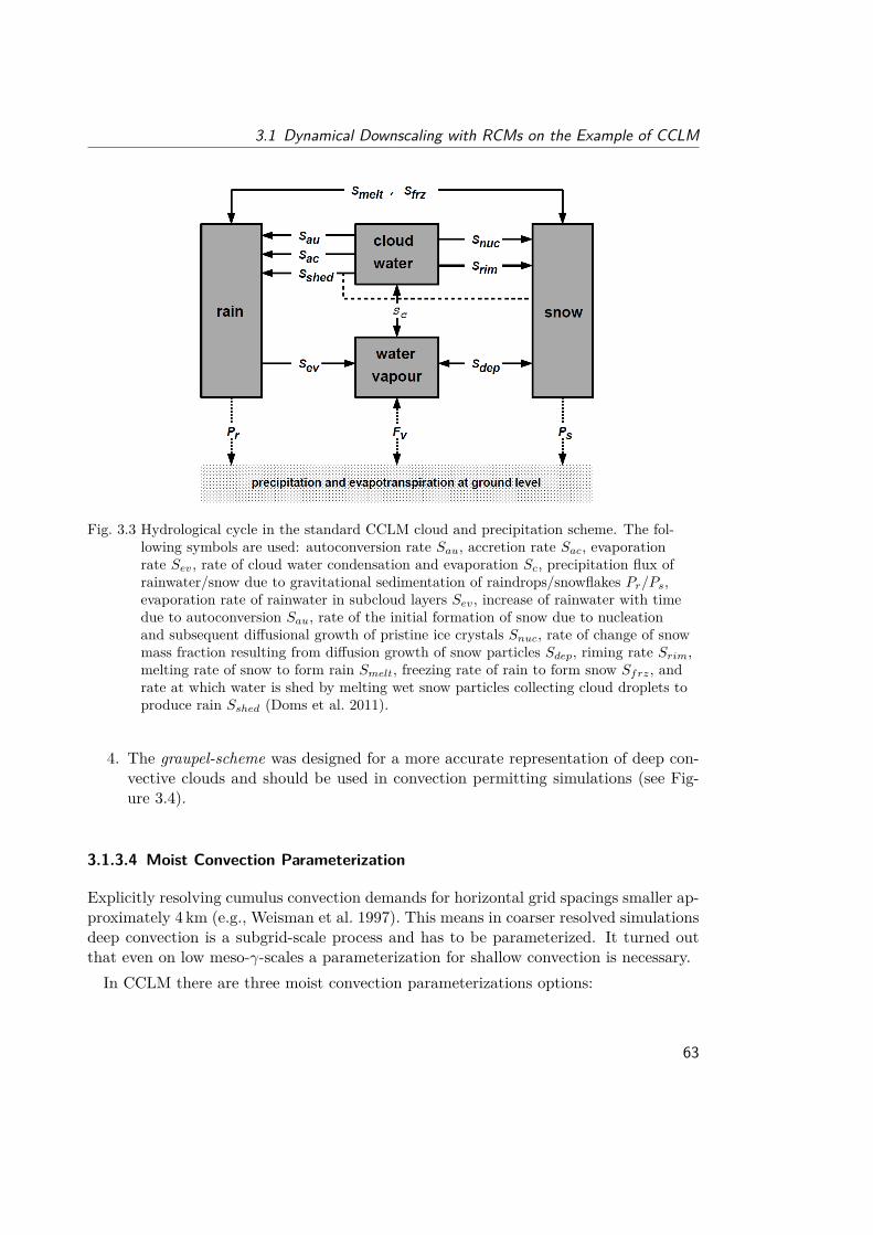
3.1 Dynamical Downscaling with RCMs on the Example of CCLM
Fig. 3.3 Hydrological cycle in the standard CCLM cloud and precipitation scheme. The fol-lowing symbols are used: autoconversion rate Sau, accretion rate Sac, evaporationrate Sev, rate of cloud water condensation and evaporation Sc, precipitation flux ofrainwater/snow due to gravitational sedimentation of raindrops/snowflakes Pr/Ps,evaporation rate of rainwater in subcloud layers Sev, increase of rainwater with timedue to autoconversion Sau, rate of the initial formation of snow due to nucleationand subsequent diffusional growth of pristine ice crystals Snuc, rate of change of snowmass fraction resulting from diffusion growth of snow particles Sdep, riming rate Srim,melting rate of snow to form rain Smelt, freezing rate of rain to form snow Sfrz, andrate at which water is shed by melting wet snow particles collecting cloud droplets toproduce rain Sshed (Doms et al. 2011).
4. The graupel-scheme was designed for a more accurate representation of deep con-vective clouds and should be used in convection permitting simulations (see Fig-ure 3.4).
3.1.3.4 Moist Convection Parameterization
Explicitly resolving cumulus convection demands for horizontal grid spacings smaller ap-proximately 4 km (e.g., Weisman et al. 1997). This means in coarser resolved simulationsdeep convection is a subgrid-scale process and has to be parameterized. It turned outthat even on low meso-γ-scales a parameterization for shallow convection is necessary.In CCLM there are three moist convection parameterizations options:
63
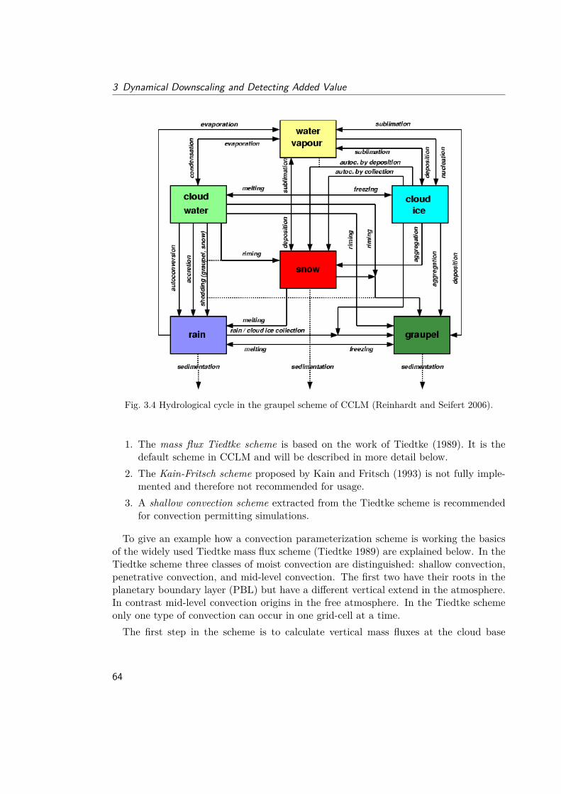
3 Dynamical Downscaling and Detecting Added Value
Fig. 3.4 Hydrological cycle in the graupel scheme of CCLM (Reinhardt and Seifert 2006).
1. The mass flux Tiedtke scheme is based on the work of Tiedtke (1989). It is thedefault scheme in CCLM and will be described in more detail below.
2. The Kain-Fritsch scheme proposed by Kain and Fritsch (1993) is not fully imple-mented and therefore not recommended for usage.
3. A shallow convection scheme extracted from the Tiedtke scheme is recommendedfor convection permitting simulations.
To give an example how a convection parameterization scheme is working the basicsof the widely used Tiedtke mass flux scheme (Tiedtke 1989) are explained below. In theTiedtke scheme three classes of moist convection are distinguished: shallow convection,penetrative convection, and mid-level convection. The first two have their roots in theplanetary boundary layer (PBL) but have a different vertical extend in the atmosphere.In contrast mid-level convection origins in the free atmosphere. In the Tiedtke schemeonly one type of convection can occur in one grid-cell at a time.The first step in the scheme is to calculate vertical mass fluxes at the cloud base
64
3.1 Dynamical Downscaling with RCMs on the Example of CCLM
which is derived from the grid-scale variables T , specific humidity (q), saturation vaporpressure (qsat), and dry static energy (s) (s = cpT + gz). For shallow and penetrativeconvection this mass flux is proportional to the integrated moisture convergence fromthe surface to the cloud base. For mid-level convection it is proportional to the verticalvelocity w in the grid-cell.A simple stationary cloud model is then used to calculate the vertical redistribution
of heat, moisture, and momentum for the up- and downdrafts from the previously calcu-lated mass flux at cloud base. This is then used to calculate the feedbacks of subgrid-scalevertical circulation on the resolved scales.The downdrafts originate at the level of free sinking2 and the mass-flux therein is
proportional to the updraft mass-flux at the cloud base. The disposable proportionalityfactor is controlling the intensity of the downdraft (currently set to a fixed value of 0.3in CCLM).For precipitation, evaporation at sub-saturated levels below the cloud base is imple-
mented. Precipitation reaches the ground as convective rain or snow dependent on thetemperature in the lowest model level.To be computationally more efficient the Tiedtke scheme does not have to be called
every time-step (by default it is called every 10th timestep). Convection tendencies stayconstant between two calls of the scheme.
3.1.3.5 Subgrid-Scale Clouds
In the grid-scale clouds and precipitation scheme (see Subsection 3.1.3.3) cloudiness isonly dependent on the presence of cloud water (qc) (Doms et al. 2011). Therefore, agrid-box is either totally filed with clouds if qc > 0 (relative humidity = 100%) or cloudfree if qc = 0 meaning that the cloud area fraction is either 0 or 1.However, even if the relative humidity in a grid-box is below 100% there can be
subgrid-scale clouds which influence the radiative transfer in the atmosphere. Therefore,in the CCLM a fractional cloud cover (σc) is defined in each grid-box which is empiricallydependent on the relative humidity, the height of the layer, and the convective activity.This scheme also cares for temperature inversions at the cloud tops to account for anvilswith an increase of σc.
2The level of free sinking is assumed to be the highest model level where negative buoyancy of a mixtureof equal parts of cloud air and saturated environmental air at wet-bulb temperature occurs comparedto the environment (Doms et al. 2011).
65
3 Dynamical Downscaling and Detecting Added Value
3.1.3.6 Radiation
With the radiation transfer scheme the heating rate due to radiation is parameter-ized within atmospheric models. For this purpose the Ritter and Geleyn (1992) ra-diative transfer scheme, referred to as RG92, is used in CCLM. It accounts for fivelongwave (thermal) and three shortwave (solar) spectral intervals. Radiation in theRG92 scheme interacts with cloud water droplets, cloud ice crystals, water vapor, ozone,and takes into account effects of Rayleigh scattering. The graupel produced by thegraupel-microphysics-scheme and the snow is not interacting with radiation in the RG92scheme.Within the scheme also partial cloudiness (produced by the sub-grid cloud scheme;
see Subsection 3.1.3.5) is considered by attributing two sets of optical properties andfluxes to each layer, one for the cloudy and one for the cloud free part (Geleyn andHollingsworth 1979). Thereby, clouds in adjacent model layers have maximum overlapwhile clouds which are separated by cloud free layers are independent from each other(random overlap assumption).The RG92 radiation-transfer scheme is computationally expensive. Therefore, it is
usually called hourly in meso-β-scale simulations (Doms et al. 2011). For the interme-diate time steps the short and longwave heating rates stay constant. In highly resolvedsimulations the calling frequency can be increased to get an improved interaction withthe cloud field. It is also possible to operate the scheme on a coarser grid to savecomputational resources.
3.1.3.7 Sub-Grid-Scale Orography
Small-scale orographic features cannot be resolved directly in state-of-the-art climatesimulations. However, they are important for atmospheric dynamics and not accountingfor those features can lead to an underestimation of surface drag. This can cause tooweak cross-isobaric flow in the PBL, biases in the surface pressure (in the order of 1 hPato 2 hPa), and an overestimation of wind speed by approximately 1m s−1 throughoutthe troposphere (Doms 2011).To reduce these impacts a sub-grid-scale orography scheme (SSO) was implemented
in CCLM which is based on the work of Lott and Miller (1997). Within that schemethe low-level flow is blocked when the subgrid-scale orography is sufficiently high. Theupper part of the low-level flow produces gravity waves when flowing over the orography.
66
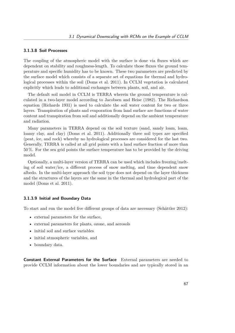
3.1 Dynamical Downscaling with RCMs on the Example of CCLM
3.1.3.8 Soil Processes
The coupling of the atmospheric model with the surface is done via fluxes which aredependent on stability and roughness-length. To calculate those fluxes the ground tem-perature and specific humidity has to be known. These two parameters are predicted bythe surface model which consists of a separate set of equations for thermal and hydro-logical processes within the soil (Doms et al. 2011). In CCLM vegetation is calculatedexplicitly which leads to additional exchanges between plants, soil, and air.The default soil model in CCLM is TERRA wherein the ground temperature is cal-
culated in a two-layer model according to Jacobsen and Heise (1982). The Richardsonequation (Richards 1931) is used to calculate the soil water content for two or threelayers. Transpiration of plants and evaporation from land surface are functions of watercontent and transpiration from soil and additionally depend on the ambient temperatureand radiation.Many parameters in TERRA depend on the soil texture (sand, sandy loam, loam,
loamy clay, and clay) (Doms et al. 2011). Additionally three soil types are specified(peat, ice, and rock) whereby no hydrological processes are considered for the last two.Generally, TERRA is called at all grid points with a land surface fraction of more than50%. For the sea grid points the surface temperature has to be provided by the drivingmodel.Optionally, a multi-layer version of TERRA can be used which includes freezing/melt-
ing of soil water/ice, a different process of snow melting, and time dependent snowalbedo. In the multi-layer approach the soil type does not depend on the layer thicknessand the structures of the layers are the same in the thermal and hydrological part of themodel (Doms et al. 2011).
3.1.3.9 Initial and Boundary Data
To start and run the model five different groups of data are necessary (Schättler 2012):
• external parameters for the surface,• external parameters for plants, ozone, and aerosols• initial soil and surface variables• initial atmospheric variables, and• boundary data.
Constant External Parameters for the Surface External parameters are needed toprovide CCLM information about the lower boundaries and are typically stored in an
67

3 Dynamical Downscaling and Detecting Added Value
external parameter file. The fields are two dimensional and have to cover the entirecomputational domain.In Table 3.1 those external parameters are listed which have to be provided to CCLM
in any case.
Tab. 3.1 Constant external parameters for the surface (Schättler 2012).
Name DescriptionHSURF Height of surface topographyFIS (alternatively) geopotential of surfaceFR_LAND Fraction of land in the grid-cellSOILTYP Soil type of the land (varies from 0 to 9)Z0 Roughness length
If the SSO scheme is used four additional two dimensional fields (listed in Table 3.2)have to be provided to the model.
Tab. 3.2 Constant external parameters for the SSO scheme (Schättler 2012).
Name DescriptionSSO_STDH standard deviation of sub-grid-scale orography [m]SSO_GAMMA anisotropy of the orography [-]SSO_THETA angle between the principal axis of orography and east
[rad]SSO_SIGMA mean slope of sub-grid-scale orography [-]
Since the lake model demands for the location and the depth of lakes (see Table 3.3)those two fields have to be provided if the lake model is applied.
Tab. 3.3 Constant external parameters for lakes (Schättler 2012).
Name DescriptionFR_LAKE lake fraction in a grid element [0,1]DEPTH_LK lake depth [m]
In Table 3.4 additional optional external parameter fields for the surface are listed.They include fields for the minimum stomata resistance of plants, surface emissivity, andground fraction covered by forests.
68
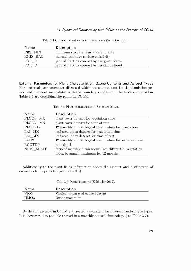
3.1 Dynamical Downscaling with RCMs on the Example of CCLM
Tab. 3.4 Other constant external parameters (Schättler 2012).
Name DescriptionPRS_MIN minimum stomata resistance of plantsEMIS_RAD thermal radiative surface emissivityFOR_E ground fraction covered by evergreen forestFOR_D ground fraction covered by deciduous forest
External Parameters for Plant Characteristics, Ozone Contents and Aerosol TypesHere external parameters are discussed which are not constant for the simulation pe-riod and therefore are updated with the boundary conditions. The fields mentioned inTable 3.5 are describing the plants in CCLM.
Tab. 3.5 Plant characteristics (Schättler 2012).
Name DescriptionPLCOV_MX plant cover dataset for vegetation timePLCOV_MN plant cover dataset for time of restPLCOV12 12 monthly climatological mean values for plant coverLAI_MX leaf area index dataset for vegetation timeLAI_MN leaf area index dataset for time of restLAI12 12 monthly climatological mean values for leaf area indexROOTDP root depthNDVI_MRAT ratio of monthly mean normalized differential vegetation
index to annual maximum for 12 months
Additionally to the plant fields information about the amount and distribution ofozone has to be provided (see Table 3.6).
Tab. 3.6 Ozone contents (Schättler 2012).
Name DescriptionVIO3 Vertical integrated ozone contentHMO3 Ozone maximum
By default aerosols in CCLM are treated as constant for different land-surface types.It is, however, also possible to read in a monthly aerosol climatology (see Table 3.7).
69
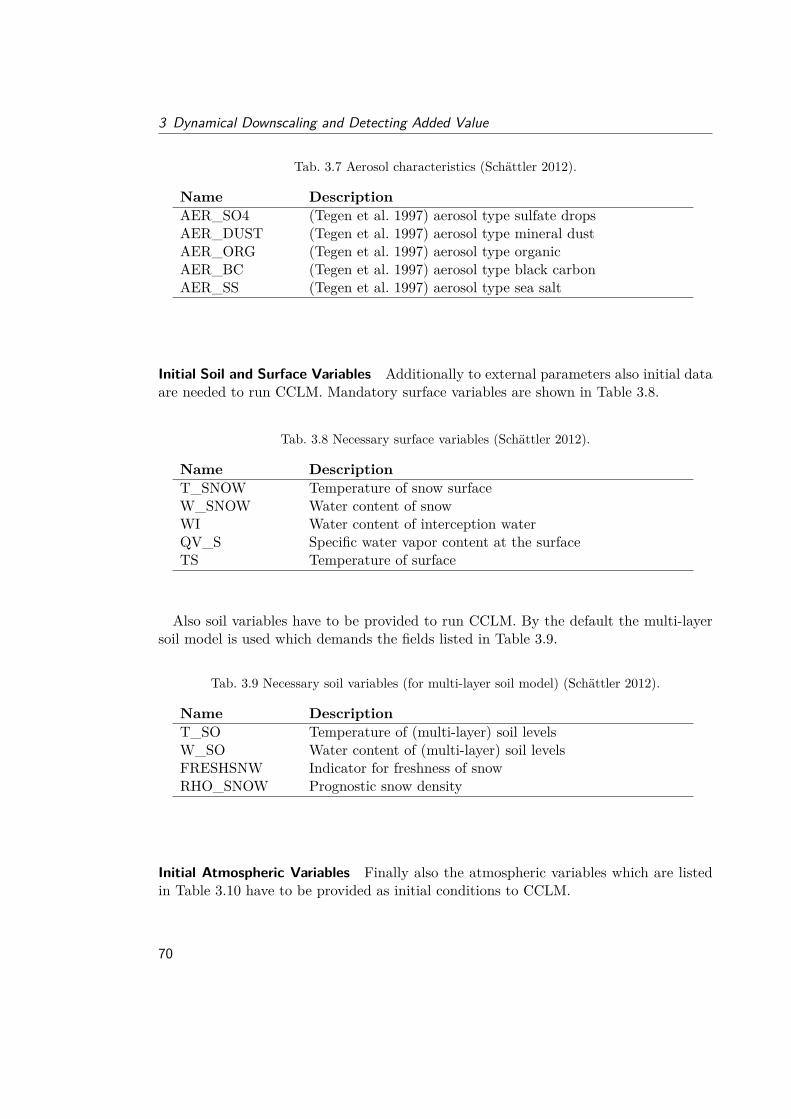
3 Dynamical Downscaling and Detecting Added Value
Tab. 3.7 Aerosol characteristics (Schättler 2012).
Name DescriptionAER_SO4 (Tegen et al. 1997) aerosol type sulfate dropsAER_DUST (Tegen et al. 1997) aerosol type mineral dustAER_ORG (Tegen et al. 1997) aerosol type organicAER_BC (Tegen et al. 1997) aerosol type black carbonAER_SS (Tegen et al. 1997) aerosol type sea salt
Initial Soil and Surface Variables Additionally to external parameters also initial dataare needed to run CCLM. Mandatory surface variables are shown in Table 3.8.
Tab. 3.8 Necessary surface variables (Schättler 2012).
Name DescriptionT_SNOW Temperature of snow surfaceW_SNOW Water content of snowWI Water content of interception waterQV_S Specific water vapor content at the surfaceTS Temperature of surface
Also soil variables have to be provided to run CCLM. By the default the multi-layersoil model is used which demands the fields listed in Table 3.9.
Tab. 3.9 Necessary soil variables (for multi-layer soil model) (Schättler 2012).
Name DescriptionT_SO Temperature of (multi-layer) soil levelsW_SO Water content of (multi-layer) soil levelsFRESHSNW Indicator for freshness of snowRHO_SNOW Prognostic snow density
Initial Atmospheric Variables Finally also the atmospheric variables which are listedin Table 3.10 have to be provided as initial conditions to CCLM.
70
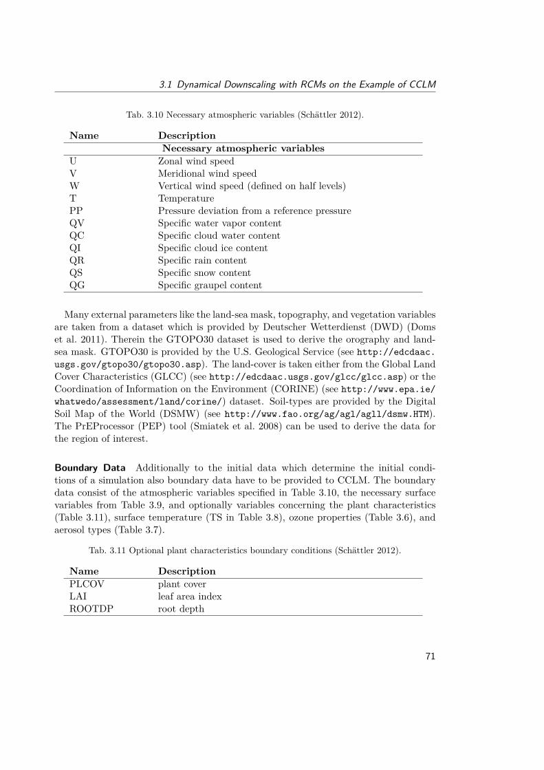
3.1 Dynamical Downscaling with RCMs on the Example of CCLM
Tab. 3.10 Necessary atmospheric variables (Schättler 2012).
Name DescriptionNecessary atmospheric variables
U Zonal wind speedV Meridional wind speedW Vertical wind speed (defined on half levels)T TemperaturePP Pressure deviation from a reference pressureQV Specific water vapor contentQC Specific cloud water contentQI Specific cloud ice contentQR Specific rain contentQS Specific snow contentQG Specific graupel content
Many external parameters like the land-sea mask, topography, and vegetation variablesare taken from a dataset which is provided by Deutscher Wetterdienst (DWD) (Domset al. 2011). Therein the GTOPO30 dataset is used to derive the orography and land-sea mask. GTOPO30 is provided by the U.S. Geological Service (see http://edcdaac.usgs.gov/gtopo30/gtopo30.asp). The land-cover is taken either from the Global LandCover Characteristics (GLCC) (see http://edcdaac.usgs.gov/glcc/glcc.asp) or theCoordination of Information on the Environment (CORINE) (see http://www.epa.ie/whatwedo/assessment/land/corine/) dataset. Soil-types are provided by the DigitalSoil Map of the World (DSMW) (see http://www.fao.org/ag/agl/agll/dsmw.HTM).The PrEProcessor (PEP) tool (Smiatek et al. 2008) can be used to derive the data forthe region of interest.
Boundary Data Additionally to the initial data which determine the initial condi-tions of a simulation also boundary data have to be provided to CCLM. The boundarydata consist of the atmospheric variables specified in Table 3.10, the necessary surfacevariables from Table 3.9, and optionally variables concerning the plant characteristics(Table 3.11), surface temperature (TS in Table 3.8), ozone properties (Table 3.6), andaerosol types (Table 3.7).
Tab. 3.11 Optional plant characteristics boundary conditions (Schättler 2012).
Name DescriptionPLCOV plant coverLAI leaf area indexROOTDP root depth
71
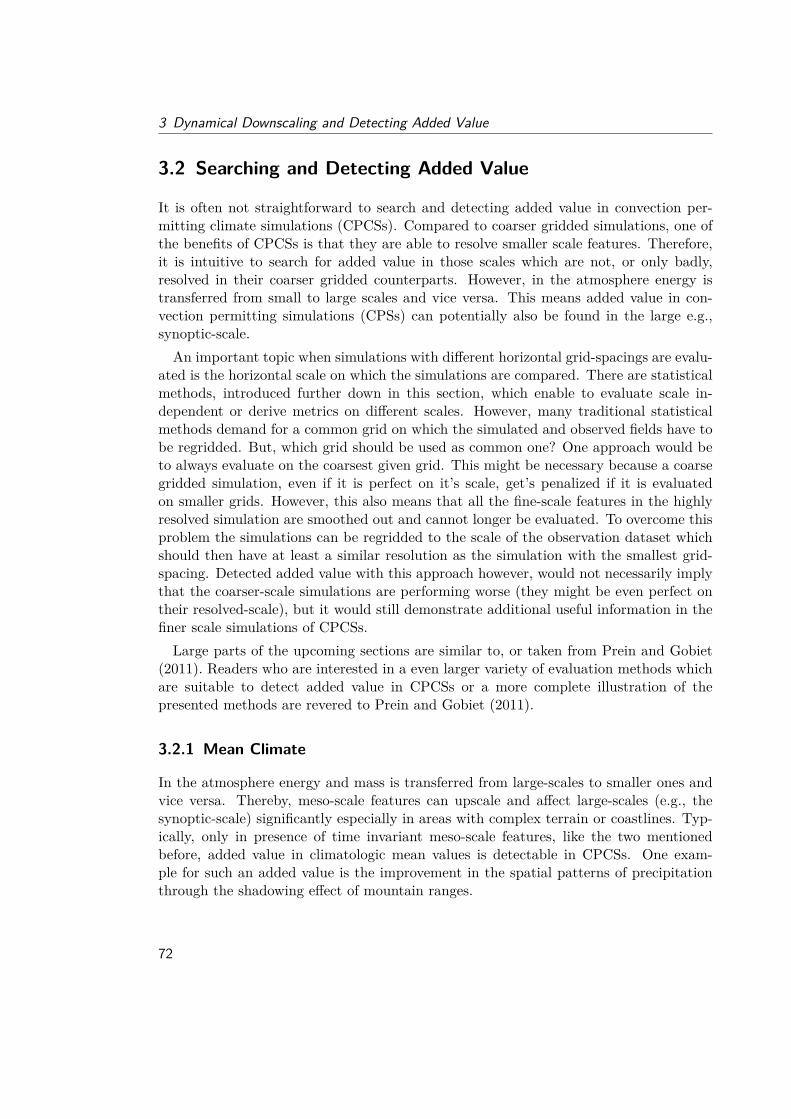
3 Dynamical Downscaling and Detecting Added Value
3.2 Searching and Detecting Added Value
It is often not straightforward to search and detecting added value in convection per-mitting climate simulations (CPCSs). Compared to coarser gridded simulations, one ofthe benefits of CPCSs is that they are able to resolve smaller scale features. Therefore,it is intuitive to search for added value in those scales which are not, or only badly,resolved in their coarser gridded counterparts. However, in the atmosphere energy istransferred from small to large scales and vice versa. This means added value in con-vection permitting simulations (CPSs) can potentially also be found in the large e.g.,synoptic-scale.An important topic when simulations with different horizontal grid-spacings are evalu-
ated is the horizontal scale on which the simulations are compared. There are statisticalmethods, introduced further down in this section, which enable to evaluate scale in-dependent or derive metrics on different scales. However, many traditional statisticalmethods demand for a common grid on which the simulated and observed fields have tobe regridded. But, which grid should be used as common one? One approach would beto always evaluate on the coarsest given grid. This might be necessary because a coarsegridded simulation, even if it is perfect on it’s scale, get’s penalized if it is evaluatedon smaller grids. However, this also means that all the fine-scale features in the highlyresolved simulation are smoothed out and cannot longer be evaluated. To overcome thisproblem the simulations can be regridded to the scale of the observation dataset whichshould then have at least a similar resolution as the simulation with the smallest grid-spacing. Detected added value with this approach however, would not necessarily implythat the coarser-scale simulations are performing worse (they might be even perfect ontheir resolved-scale), but it would still demonstrate additional useful information in thefiner scale simulations of CPCSs.Large parts of the upcoming sections are similar to, or taken from Prein and Gobiet
(2011). Readers who are interested in a even larger variety of evaluation methods whichare suitable to detect added value in CPCSs or a more complete illustration of thepresented methods are revered to Prein and Gobiet (2011).
3.2.1 Mean Climate
In the atmosphere energy and mass is transferred from large-scales to smaller ones andvice versa. Thereby, meso-scale features can upscale and affect large-scales (e.g., thesynoptic-scale) significantly especially in areas with complex terrain or coastlines. Typ-ically, only in presence of time invariant meso-scale features, like the two mentionedbefore, added value in climatologic mean values is detectable in CPCSs. One exam-ple for such an added value is the improvement in the spatial patterns of precipitationthrough the shadowing effect of mountain ranges.
72
3.2 Searching and Detecting Added Value
Typical methods to detect added values in climatological average fields are bias maps,spatial correlation coefficients, or annual cycles.
3.2.1.1 Bias Maps
Biases are systematic errors which can be calculated by subtracting observed values at agiven time or time span from simulated values. For deriving a map this has to be donepoint-wise on a common grid:
bmij = 1N
n∑t=1
(xijt − oijt) . (3.11)
Thereby, the simulated field (xijt) and the observed field (oijt) have to be given forcommon times t, common longitudes i, and latitudes j. Thereby t = 1, . . . , n and thetotal N , over which is averaged, has to be long enough to capture natural variability(30 years are often used) to derive a meaningful climatological bias of the simulation. Itis advisable to draw bias maps not only on annual basis but also on seasonal, becauseerror characteristics in climate models are often varying seasonally (see also Subsec-tion 3.2.1.3).
3.2.1.2 Spatial Correlation
The correlation coefficient (rxo) is a measure of linear connection between two variablesand is defined as the standardized covariance (covxo):
rxo = covxoσx · σo
covxo =∑N
i=1 (xi − x) · (oi − o)N
σx =
√∑Ni=1 (xi − x)2
N
σo =
√∑Ni=1 (oi − o)2
N
rxo =∑N
i=1 (xi − x) · (oi − o)N · σx · σo
.
(3.12)
Thereby σx and σo are the standard deviations of the simulated field xijt and observedfield oijt. In Equation 3.12, a bar above a variable means averaging. A useful tool to
73
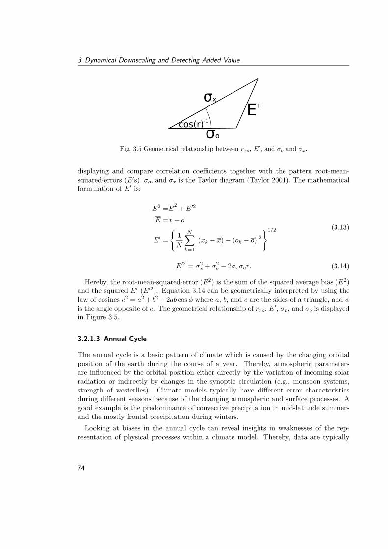
3 Dynamical Downscaling and Detecting Added Value
Fig. 3.5 Geometrical relationship between rxo, E′, and σo and σx.
displaying and compare correlation coefficients together with the pattern root-mean-squared-errors (E′s), σo, and σx is the Taylor diagram (Taylor 2001). The mathematicalformulation of E′ is:
E2 =E2 + E′2
E =x− o
E′ =
1N
N∑k=1
[(xk − x)− (ok − o)]21/2 (3.13)
E′2 = σ2x + σ2
o − 2σxσor. (3.14)
Hereby, the root-mean-squared-error (E2) is the sum of the squared average bias (E2)and the squared E′ (E′2). Equation 3.14 can be geometrically interpreted by using thelaw of cosines c2 = a2 + b2− 2ab cosφ where a, b, and c are the sides of a triangle, and φis the angle opposite of c. The geometrical relationship of rxo, E′, σx, and σo is displayedin Figure 3.5.
3.2.1.3 Annual Cycle
The annual cycle is a basic pattern of climate which is caused by the changing orbitalposition of the earth during the course of a year. Thereby, atmospheric parametersare influenced by the orbital position either directly by the variation of incoming solarradiation or indirectly by changes in the synoptic circulation (e.g., monsoon systems,strength of westerlies). Climate models typically have different error characteristicsduring different seasons because of the changing atmospheric and surface processes. Agood example is the predominance of convective precipitation in mid-latitude summersand the mostly frontal precipitation during winters.Looking at biases in the annual cycle can reveal insights in weaknesses of the rep-
resentation of physical processes within a climate model. Thereby, data are typically
74
3.2 Searching and Detecting Added Value
spatially and temporally averaged for each month of the year. The biases between thesimulated minus the reference values can then be displayed as a time line representingthe average monthly climatologically situation over a specific area.
3.2.2 Spatiotemporal High Resolution
Detecting added value of CPCSs in climate mean fields is often problematic becausetemporal and/or spatial averaging tends to cancel out improvements on small spatialscales (except those which are triggered by meso-scale time invariant features like orog-raphy; see Subsection 3.2.1). Therefore, statistical methods are needed which are capableto investigate spatiotemporal highly resolved fields. Beside those methods also reliablehigh-resolution gridded observation datasets are needed for evaluations on fine scales.However, reliable sub-daily observations on kilometer-scale grids are often not available.In most cases traditional statistical methods, like those discussed in Subsection 3.2.1,
can also be applied to spatiotemporally, highly resolved fields. However, there are someatmospheric parameters like precipitation, global radiation, or cloud cover which demandfor special evaluation methods because spatial and temporal highly resolved fields ofthose parameters are discontinues and highly variable.For example, a typical summertime mid-latitude precipitation field can have large ar-
eas with non-precipitation and small areas with precipitation. Thereby, the transitionbetween no precipitation to precipitation can be very sharp. Furthermore, the gener-ation of e.g., intermittent summertime convective precipitation is a highly non-linear,stochastic process. This means, even a perfect model would probably not be able to sim-ulate intermittent convective precipitation at the exactly same time and location whereit is observed. Even when the model is able to capture the larger scale precipitation pat-terns well, errors on the small-scale dominate the total error (e.g., Mass et al. 2002). Ingeneral, small misplacements cannot be avoided because upscale error propagation leadsto a decreasing predictability limit toward small scales (1 km – 100 km) (Wernli et al.2008). This means small spatial or temporal shifts between observed and simulated pre-cipitation should not be considered as model errors but are unavoidable in intermittentconvective precipitation producing systems.If traditional statistical metrics like correlation coefficients, or root-mean-square-errors
(RMSEs) are used to evaluate the skill of simulations in high spatiotemporal resolutionthe so called double penalty problem occurs. This means a small shift in the simu-lated precipitation field is penalized twice: first because there is precipitation observedwhere non is simulated and second because there is precipitation simulated where nonis observed. Considering the double penalty problem is especially important for CPSsbecause the higher the horizontal grid-spacing of a simulation the finer the locations ofprecipitation objects are defined. For example, detectable displacements in a simulation
75
3 Dynamical Downscaling and Detecting Added Value
with 50 km horizontal grid-spacing can only be larger than 50 km whereas in a CPSsdisplacements can be smaller than approximately 3 km.Multiple approaches have been developed (especially within the numerical weather
prediction (NWP) community) to overcome the double penalty problem. Those methodsdo not require a perfect fit of the simulation and the observation at the fine-scale. In thefollowing subsections an overview of commonly used methods is given. Methods whichare applied in Chapter 4 are explained in detail while others are briefly introduced.
3.2.2.1 Filtering Approaches
The common feature of filtering methods is that they separate the spatial structures indifferent scales and compare them with the observation. Thereby, filtering approachescan further be separated in neighborhood methods and scale separation methods.
Neighborhood Methods Neighborhood or fuzzy verification methods give credits tosimulated events which are close to the observation. Ebert (2008) provides a goodoverview of 10 fuzzy verification methods which are used in the verification of numericalweather predictions. A similar study was done by Ament et al. (2008) who found 3 fuzzyverification methods out of 12 which have an outstanding performance in detecting abroad range of forecast errors:
• fractions skill score (FSS) (Roberts and Lean 2008),• Upscaling (Zepeda-Arce et al. 2000), and• Intensity-Scale (Casati et al. 2004).
Those three methods are in detail discussed in the following paragraphs. For the sakeof completeness seven additional methods are mentioned with their references below:
• Minimum coverage (Damrath 2004),• Fuzzy logic, joint probability (Damrath 2004),• Multi-event contingency table (Atger 2001),• Pragmatic approach (Theis et al. 2005),• Practical perfect hindcast (Brooks et al. 1998),• Conditional square root for ranked probability score (Germann and Zawadzki
2004), and• Areal-related RMSE (Rezacova et al. 2007).
Fractional Skill Score Roberts and Lean (2008) developed a verification method whichinvestigates how the skill of a simulation varies with spatial scale. The basic idea behind
76
3.2 Searching and Detecting Added Value
the FSS is that a simulation is useful if the spatial frequency of events is similar inthe forecast and in the observation. The precondition for using this method is thatthe observation and the simulation are given on the same grid. In the first step, theoriginally observed and simulated fields are transferred to observed binary fields (Io)and simulated binary fields (Ix) by choosing a set of precipitation thresholds (qs) (e.g.,q = 0.5mmd−1, 1mmd−1, 2mmd−1, and 4mmd−1) and setting all gridcells exceedingthe threshold to 1 and all others to 0,
Io =
1 o ≥ q0 o < q
and Ix =
1 x ≥ q0 x < q.
Second, for all grid-points in the binary fields the spatial density of ones compared tozeros is calculated for a given squared neighborhood of length n:
O(n)(i, j) = 1n2
n∑k=1
n∑l=1
IO
[i+ k − 1− (n− 1)
2 , j + l − 1− (n− 1)2
],
X(n)(i, j) = 1n2
n∑k=1
n∑l=1
IX
[i+ k − 1− (n− 1)
2 , j + l − 1− (n− 1)2
].
(3.15)
In Equation 3.15 the field of observed fractions (On(i, j)) and field of simulated fractions(Xn(i, j)) contain the fractions of values exceeding the threshold for a square of lengthn. Thereby, i = 1, . . . , Nx and j = 1, . . . , Ny, where Nx corresponds to the numbersof columns in the domain and Ny to the number of rows. The fractional fields On(i, j)and Xn(i, j) are generated for different spatial scales by changing the value of n fromn = 1, . . . , 2N − 1, whereby N = max(Nx, Ny). If neighborhood points lie outside thedomain, their value is assumed as zero.After On(i, j) and Xn(i, j) are derived, the third step is to calculate fraction skill
scores. Therefore, the mean squared error (MSE) is calculated:
MSE(n) = 1NxNy
Nx∑i=1
Ny∑j=1
[O(n)i,j −X(n)i,j
]2,
MSE(n)ref = 1NxNy
Nx∑i=1
Ny∑j=1
O2(n)i,j +
Nx∑i=1
∑j=1
X2(n)i,j
.(3.16)
From Equation 3.16 the FSS can be calculated as an MSE skill score:
FSS(n) =MSE(n) −MSE(n)ref
MSE(n)perfect −MSE(n)ref= 1−
MSE(n)MSE(n)ref
. (3.17)
77
3 Dynamical Downscaling and Detecting Added Value
MSE(n)perfect is the MSE of a perfect simulation and therefore 0 for a given neighbor-hood length n. MSE(n)ref is the largest obtainable MSE from the given simulation andreference dataset. This means an FSS of 1 indicates the best possible simulation.
Upscaling The upscaling verification method was first published by Zepeda-Arce et al.(2000) and is conceptionally built on the assumption that a useful simulation resemblesthe observation when averaged to a coarser scale. In the upscaling method the threatscore (TS) is calculated as a measure of scale. The TS compares the area of precipitationabove a threshold between a simulation and an observation (e.g., see Wilks 2005) and isdefined as:
TS = AcAo +Ax −Ac
, (3.18)
thereby, Ac is the area where the simulation correctly produced precipitation above thethreshold, Ao is the total observed area, and Ax the total simulated area. The bestpossible TS is one whereas the worst is zero. The TS is scal-depended and gets typicallyhigher with increasing scale. Furthermore, the TS can be expressed as a function ofspatial scale and precipitation intensity by regridding the simulated and observed fieldson grids with different spacings and by using different precipitation thresholds.
Intensity-Scale Casati et al. (2004) used a method which gives credits to a simulationwhich has more accurate structures than a random arrangement of the observation. As afirst step, simulated and observed data have to be preprocessed. Therefore, all non-zeroprecipitation values are dithered by adding uniformly distributed noise with a magnitudeof ±1/64mmh−1. Thereafter, the precipitation values are normalized with a (base 2)logarithmic transformation and the pixels with zero precipitation are set to −6. Thenormalization is necessary to produce more normally distributed data and to removeskewness. These data are then recalibrated with the following transformation function:
X ′ = F−1O (FX(X)), (3.19)
where each value of the simulated field X is substituted with the value of the observedfield O having the same empirical cumulative probability FO and FX . With this proce-dure biases in the marginal distribution of the simulated precipitation are erased.After the preprocessing the simulated and observed fields are converted into a binary
fields using thresholds q = 0mmh−1, 1/32mmh−1, 1/16mmh−1, . . . , 128mmh−1:
78
3.2 Searching and Detecting Added Value
IO =
1 O > q0 O ≤ q
and
IX′ =
1 X ′ ≥ q0 X ′ < q.
Then the binary error Z is calculated:
Z = IX′ − IO. (3.20)
With a two-dimensional discrete Haar wavelet decomposition the binary error can beexpressed as the sum of components on different spatial scales:
Z =L∑l=1
Zl, (3.21)
where l is referring to the spatial scale of the error and not to the scales of the precipita-tion features or their displacements. A detailed description of the two dimensional Haarwavelet decomposition can, for example, be found in Mallat (1999) or Nievergelt (1999).With the mean squared Z-values the MSE of the binary image is calculated:
MSE = Z2. (3.22)
Since the components of a discrete wavelet transformation are orthogonal ZlZl′ =0 l 6= l′ the MSE can be written as:
MSE =L∑l=1
L∑l′=1
ZlZl′ =L∑l=1
Z2l
and
MSE =L∑l=1
MSEl,
(3.23)
where MSEl = Z2l . Thereby, MSEl depends on the spatial scale l and the threshold u
which enables the evaluation of precipitation on different scales and intensities. With thenow obtained data the MSE skill score can be calculated for every scale and threshold:
SS = MSE −MSErandomMSEbest −MSErandom
= 1− MSE2ε(1− ε) , (3.24)
79
3 Dynamical Downscaling and Detecting Added Value
where MSEbest = 0 is a perfect simulation, MSErandom = 2ε(1 − ε) is the MSE of arandomly created binary field and ε is the fraction of rain-pixels in the observation. Byassuming that the random observed and simulated binary fields are Bernoulli distributed(Be) variables IX ∼ Be(ε) and IO ∼ Be(ε) which have (unbiased) means E(IX′) =E(IO) = ε and variances σ2
IO= σI2
X′= ε(1 − ε) it can be shown that the binary error
(Equation 3.20) has a mean E(Z) = 0 and a variance σ2Z = σ2
IO+ σI2
X′= 2ε(1− ε). The
expected value of MSE is then MSErandom = E(Z2) = E(Z −E(Z))2 = σ2Z = 2ε(1− ε).
With the assumption that the MSE is uniformly distributed over all scales SS can bewritten as the sum of its means over all scales by using Equation 3.23 and Equation 3.24:
SSl = 1− MSEl2ε(1− ε)/L. (3.25)
3.2.2.2 Scale Separation Methods
The goal of the here presented methods is to investigate performance as a functionof spatial scale. Fourier or wavelet transformations are common tools to decomposeatmospheric fields and to look at different scales separately.
The Discrete Cosine Transformation (DCT) Using Fourier transformation enables todecompose a periodic function into its wavenumbers of partial frequencies (Peixoto andOort 1992). However, problems can occur if datasets with sharp boundaries (like RCMoutput) are standard Fourier transformed because of aliasing of large-scale variabilitiesinto shorter scales.A possible solution of this problem is the use of the discrete cosine transformation
(DCT) method. Denis et al. (2002[a]) were the first who used the 2D DCT for limitedareas. Therefore, the precipitation field has to be mirrored at the position i = j = −1/2to make it symmetric. Thereafter, the Fourier transformation can be applied, centeredon i = j = −1/2. This is a special case of a Fourier transformation which is calledDCT because the sine components of the Fourier series are zero for symmetric functions.Concerning a two dimensional matrix (zij) of Ni by Nj grid-points, the direct and inverseDCT are defined as:
Z(m,n) = β(m)β(n)i=Ni−1∑i=0
j=Nj−1∑j=0
z(i, j) cos[πm
(i+ 1/2)Ni
]cos[πn
(j + 1/2)Nj
](3.26)
z(i, j) =m=Ni−1∑m=0
n=Nj−1∑n=0
β(m)β(n)Z(m,n) cos[πm
(i+ 1/2)Ni
]cos[πn
(j + 1/2)Nj
](3.27)
80
3.2 Searching and Detecting Added Value
β(m) =
√
1Ni, for m = 0 (3.28)√
2Ni, for m = 1, 2, . . . , Ni − 1
β(n) =
√1Nj
, for n = 0 (3.29)√2Nj
, for n = 1, 2, . . . , Nj − 1
Thereby, zij is the value of the field at grid-point (i, j), and the real spectral coefficient(Zmn) corresponds to the 2D-wavenumber at (m,n). In the next step the Zmn is usedto calculate spectral variances (σ2(m,n)):
σ2(m,n) = Z2(n,m)NiNj
(3.30)
To generate variance spectra of a 2D-field, the σ2(m,n) have to be connected to aspecific wavelength. To do so, the method of binning was suggested by Denis et al.(2002[a]). It is based on dividing the wavenumber field into multiple quarters of ellipses.The space between two ellipses can be connected to a specific wavenumber for which thevariances are summed up. For a more detailed description see Denis et al. (2002[a]). Anapplication of this method to high resolved RCM output can be found in Kapper (2009)and Prein et al. (2013[b]).
Variogram and Correlograms The basic idea of evaluating fields with the variogrammethod is related to publications of Gebremichael and Krajewski (2004), Germann andJoss (2001), Harris et al. (2001), and Zepeda-Arce et al. (2000). Marzban and Sandgathe(2009) proposed this method to compare two fields in terms of their covariance structures.In this thesis correlograms and variograms are used to compare spatial similarities and
dissimilarities between observations and model output. Correlograms and variograms arefrequently used in geostatistics to explore the spatial organization of different phenomena(e.g., Isaaks and Srivastava 1989). They illustrate how the correlation and variancedepend on spatial scale. Therefore, spatial data z(u) at the locations u and sample datapairs at different distances are taken. The distance between a given data pair is usuallycalled the “lag” (plus/minus some lag tolerance (d); e.g., d = 10 000m). The lag vector(h) consists of I values where i = 0, 1, 2, . . . , I and hi = hi−1 + 2d . The lagged versions
81
3 Dynamical Downscaling and Detecting Added Value
of the data at locations z(u) is z(u+ h). Defining number of pairs (N) separated by lagh (plus or minus d) the statistics for lag h can be computed as covariance:
C(h) = 1N(h)
N(h)−1∑α=0
z(uα) · z(uα + h)−m0 ·m+h, (3.31)
correlation,:r(h) = C(h)
√σ0 · σ+h
, (3.32)
and variance:
σ2(h) =
12N(h)
N(h)−1∑α=0
[z(uα + h)− z(uα)]2 · 1
2 . (3.33)
In Equation 3.31 m0 and m+h denote the mean of the z(u) and z(u+ h) values:
m0 = 1N(h)
N(h)−1∑α=0
z(uα), (3.34)
m+h = 1N(h)
N(h)−1∑α=0
z(uα + h), (3.35)
and σ0 and σ+h in Equation 3.32 are the corresponding standard deviations:
σ0 = 1N(h)
N(h)−1∑α=0
[z(uα)−m0] , (3.36)
σ+h = 1N(h)
N(h)−1∑α=0
[z(uα + h)−m+h] . (3.37)
Once r(h) and σ2(h) are calculated they can be plotted against h. The plots arethen called correlograms and variograms. In correlograms similarities within a field aremeasured without accounting for magnitude differences while variograms give insight indissimilarities and are sensitive to differences in magnitude.
Scale Dependent Analysis by Regridding A method to do scale-dependent analysiswith observations from station data is proposed in Prein et al. (2013[b]). Thereby, theskill of simulated precipitation fields to accurately reproduce point measurements fordifferent horizontal scales of precipitation systems is evaluated by resampling the data
82
3.2 Searching and Detecting Added Value
to common grids with different grid-spacings. The grid spacings can range from thefinest simulated grid to a grid which contains at least a couple of grid-points within theevaluation domain to retain some spatial variability.With this method it is possible to investigate the upscaling effect of small-scale fea-
tures, which are resolved in fine gridded simulation, to larger scales. The proposedresampling technique, does not use any interpolation and is able to spatially conserveprecipitation amounts within a region (for details about the method see Suklitsch et al.(2008)). On each new grid, precipitation values are calculated at the locations of theobservation station by inverse-distance average the simulated precipitation values atthe four nearest grid-points around the station. Those values are then compared to theobserved values to calculate the spatial Pearson correlation coefficient (CC), spatial stan-dard deviations normalized by the standard deviation of the observations, and RMSE.The resampling approach enables the evaluation of the same spatial scales in simulationswith different grid-spacings and makes it possible to conduct a quantitative analysis ofthe upscaling effect of small-scale features on larger scales.
Intensity-scale The intensity-scale method, published by Casati et al. (2004) was al-ready introduced in Subsection 3.2.2.1. By using Haar wavelets, reference and simulatedprecipitation fields are separated in different scales which then are evaluated by an MSEskill score. Since the intensity-scale method uses spectral decomposition and skill scoreson different scales and intensities it can be assigned to both, fuzzy and scale separationmethods.
3.2.2.3 Displacement Approaches
Beside the above described filtering approaches, displacement approaches are the sec-ond category of methods which enable an evaluation of spatiotemporal highly resolvedprecipitation simulations. Displacement approach methods can be further categorizedin feature based approaches and field deformation methods.
Feature Based Approaches The basic idea behind object based or feature based spatialverification methods is to identify relevant features in the simulated and observed fieldsand compare characteristic attributes of both fields with each other. The Structure-Amplitude-Location (SAL) method (Wernli et al. 2008) will be discussed below in detailwhile other relevant methods are just listedbelow with their reference.
• Cluster Analysis (Marzban and Sandgathe 2006),• Method for Object-based Diagnostic Evaluation (MODE) (Davis et al. 2006),• Contiguous Rain Area (CRA) (Ebert and McBride 2000), and
83
3 Dynamical Downscaling and Detecting Added Value
• Procrustes (Micheas et al. 2007).
SAL Verification Method Wernli et al. (2008) introduced an object-based quality mea-sure which considers three components accounting for the Structure-Amplitude-Location(SAL) of a precipitation field. The SAL method aims to address the following issues:
• quantify the quality of a simulated precipitation field over a fixed area (e.g., a rivercatchment),
• considering the structure of the precipitation field (e.g., scattered convective cells,frontal rain, . . . ), and
• a one to one matching between the reference and the observed field is not required.
As a first step individual precipitation objects have to be identified for calculating thelocation and structure components. Therefore, a precipitation threshold is chosen:
R∗ = fRmax. (3.38)
In Equation 3.38 R is the precipitation field, R∗ is the precipitation threshold, and Rmax
is the maximum rainfall within the considered domain. For the constant f , Wernli et al.(2008) suggested a value of f = 1/15 because this factor leads to contours which arereasonable with contours identified by eye. Gridcells cluster to an object if one of theneighborhood cells is above the threshold f . A possible algorithm to identify objectscan be found in Wernli and Sprenger (2007).The amplitude component A is calculated by using the normalized differences of the
average precipitation values:
A = D(Rx)−D(Ro)0.5 [D(Rx) +D(Ro]
. (3.39)
D(R) denotes the domain average precipitation in the observed (o) or simulated (x)field.
D(R) = 1N
∑(i,j)∈D
Rij , (3.40)
where Rij are the grid-point values of the precipitation amount. A is a simple quantity,showing information of the domain wide amount of precipitation by ignoring the fieldssub-regional structure. It has values between [−2 . . .+2] whereby a perfect simulationin terms of amplitude leads to A = 0. An A-value of ±1 corresponds with an over- orunderestimation of precipitation by the factor of 3.The location component L consists of two additive parts: L = L1 + L2:
84
3.2 Searching and Detecting Added Value
L1 = | x(Rx − x(Ro) |d
, (3.41)
where d is the maximum distance between two boundary points of domain D and x(R)corresponds to the center of mass of the precipitation field R. L1 has values between 0and 1 and gives a first-order estimation of the precipitation distribution in the consideredregion whereby L1 = 0 if the centers of mass are at the same location. However, manydifferent fields can have equally centers of mass which makes the second quantity L2necessary. It accounts for the distances between the center of mass of the total precip-itation field and single precipitation objects. Therefore, the total precipitation amountis calculated for every object:
Rn =∑
(i,j)∈Rn
Rij . (3.42)
Then the averaged and weighted distances r between the centers of mass of the indi-vidual objects are calculated:
r =∑M
n=1Rn | x− xn |∑Mn=1Rn
, (3.43)
whereby, M is the total number of precipitation objects. r can have a maximum valueof d/2 (half of the maximum distance between two grid points in the domain). It is zeroif there is only one object in the domain. It should be noted that
∑Mn=1Rn is not equal
to∑
(i,j)∈D Rij (in Equation 3.40) because the former only considers grid-points abovethe threshold R∗. L2 is now calculated as follows:
L2 = 2[| r(Rx)− r(Ro) |
d
]. (3.44)
L2 is only greater than zero if either the observation or the simulation has more thanone object in the domain. L2 can range from zero to one which means that L can havevalues between zero and two. Zero indicates that the total center of mass as the averageddistances of the objects and the center of mass are the same in the observation and inthe simulation. However, this does not mean a perfect match between the two fields,because the L-value is for example invariant to rotations around the center of mass.The last missing component in the SAL method is the structure (S) component in
which the volumes of the precipitation objects are compared and which contains infor-mation about the mass and the shape of the objects. Therefore, first a scaled volumeVn is calculated for every object:
85
3 Dynamical Downscaling and Detecting Added Value
Vn =∑
(i,j)∈Rn
Rij/Rmaxn = Rn/R
maxn . (3.45)
In Equation 3.45 Rmaxn stands for the maximum precipitation within the object n and
has to be Rmaxn ≤ Rmax. Then V , the weighted mean of all objects scaled precipitation
volume is computed for the reference and the simulated field:
V (R) =∑M
n=1RnVn∑Mn=1Rn
. (3.46)
Similar to the A-component, the S-component is the normalized difference in V :
S = V (Rx)− V (Ro)0.5 [V (Rx) + V (Ro)]
. (3.47)
S becomes negative if too small or too peaked objects are simulated or positive ifwidespread precipitation is modeled but small convective cells are observed.
3.2.2.4 Field Deformation
Field deformation approaches have in general, that they evaluate how much a fieldhas to be transformed to match the observation. This is in particular interesting forprecipitation because models often produce phase errors and displace weather systemsin space or time.Often used methods and their references are:
• Displacement Amplitude Score (Keil and Craig 2007),• Forecast Quality Index (FQI) (Venugopal et al. 2005), and• Image Warping (e.g., Dickinson and Brown 1996; Alexander et al. 1999; Åberg
et al. 2005; Gilleland et al. 2010).
To give an idea how these methods are working the Displacement Amplitude Score(Keil and Craig 2007) is discussed as an example below.
Displacement Amplitude Score The displacement amplitude score was published byKeil and Craig (2007) and in a revised version by Keil and Craig (2009). An opticalflow technique is used to avoid problems in identifying features and problems occurringthrough linking specific objects in the simulation to objects in the observation.The optical flow method is based on a pyramid algorithm where the fields first are
re-gridded on a coarser grid where 2F pixels are averaged on one pixel element. F is
86
3.2 Searching and Detecting Added Value
thereby called the sub sampling factor. On the coarse grid for every grid-cell of thesimulation the distance of the minimum squared error (compared to the observation) issearched in a neighborhood of ±2 grid-cells. The obtained vector field of displacementsis then applied to the original simulated image which generates an intermediate imageaccounting for large-scale displacements. Afterwards, the intermediate image is coarsegrained by averaging 2F−1 pixels which is the next pyramid level and the displacementvector field is calculated and applied as mentioned above. This algorithm is repeateduntil the full resolution is obtained. After the total displacement vector field, whichmorphs the simulation to the observation, is defined, the displacement vector field, whichmorphs the observation to the simulation, is calculated with the same algorithm.The resulting displacement vector fields are the sum of the vector fields at each pyramid
level and are used to build the final morphed images. More details on the algorithm canbe found in Keil and Craig (2007) and Zinner et al. (2008).The displacement and amplitude score is then calculated by considering two quan-
tities. The first accounts for the displacement error which is the magnitude of thedisplacement vector giving the distance of a simulation to an observed object (if any).The second accounts for the amplitude error which is the difference between the observedand the morphed simulation field. Accordingly, the same quantities are calculated forthe morphed observation onto the simulation.If two objects in the simulation and the observations are separated by more than
the maximum search distance, they are treated as two independent objects and theamplitude error accounts for one missed event and one false alarm.Finally, the displacement and amplitude errors are combined to yield the displacement
amplitude score. Thereby, the two components are weighted so that the maximumpossible displacement error between two objects equals the amplitude error for the sametwo objects that would occur if the distance between the two objects would have beenlarger as the maximum search distance.To visualize the above described formalism, Figure 3.6 shows an idealized example
of an observation (panel a) and an identical forecast field (panel b) which is 50 pixelsshifted to the right. Also shown in panel b is the displacement vector field which min-imizes the differences between the observation and forecast. In panel c the morphedforecast is displayed. The magnitude of the displacement vector field which is within theboundaries of the observed object is quite uniform as visible in panel d. Finally, panel eshows the amplitude error between the observed and morphed forecast field. The smallremaining residual errors at the object boundaries are caused by the interpolation duringthe morphing.
87
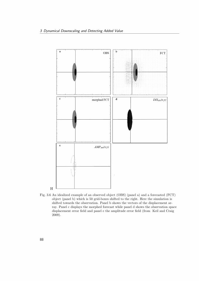
3 Dynamical Downscaling and Detecting Added Value
HFig. 3.6 An idealized example of an observed object (OBS) (panel a) and a forecasted (FCT)
object (panel b) which is 50 grid-boxes shifted to the right. Here the simulation isshifted towards the observation. Panel b shows the vectors of the displacement ar-ray. Panel c displays the morphed forecast while panel d shows the observation spacedisplacement error field and panel e the amplitude error field (from Keil and Craig2009).
88
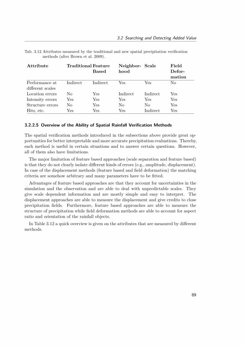
3.2 Searching and Detecting Added Value
Tab. 3.12 Attributes measured by the traditional and new spatial precipitation verificationmethods (after Brown et al. 2009).
Attribute Traditional FeatureBased
Neighbor-hood
Scale FieldDefor-mation
Performance atdifferent scales
Indirect Indirect Yes Yes No
Location errors No Yes Indirect Indirect YesIntensity errors Yes Yes Yes Yes YesStructure errors No Yes No No YesHits, etc. Yes Yes Yes Indirect Yes
3.2.2.5 Overview of the Ability of Spatial Rainfall Verification Methods
The spatial verification methods introduced in the subsections above provide great op-portunities for better interpretable and more accurate precipitation evaluations. Thereby,each method is useful in certain situations and to answer certain questions. However,all of them also have limitations.The major limitation of feature based approaches (scale separation and feature based)
is that they do not clearly isolate different kinds of errors (e.g., amplitude, displacement).In case of the displacement methods (feature based and field deformation) the matchingcriteria are somehow arbitrary and many parameters have to be fitted.Advantages of feature based approaches are that they account for uncertainties in the
simulation and the observation and are able to deal with unpredictable scales. Theygive scale dependent information and are mostly simple and easy to interpret. Thedisplacement approaches are able to measure the displacement and give credits to closeprecipitation fields. Furthermore, feature based approaches are able to measure thestructure of precipitation while field deformation methods are able to account for aspectratio and orientation of the rainfall objects.In Table 3.12 a quick overview is given on the attributes that are measured by different
methods.
89
4Added Value in Convection Permitting Sim-
ulations
This chapter consits of two seperate studies. In the first one, presented in Section 4.1,convection permitting climate simulations (CPCSs) of three different regional cli-
mate models (RCMs) are compared to coarser resolved simulations. Multiple statisticalmethods are applied to get a holistic view of added value which can be consistentlyfound in different RCMs. The second study in Section 4.2 builds up on the results of thefirst one. Here the representation of heavy precipitation events in one CPCS and twocoarser gridded runs are investigated by comparing the simulations with observations ondifferent spatial scales.
4.1 Added Value of Convection Permitting SeasonalSimulations
In this section an ensemble of non-hydrostatic RCMs is evaluated, which allows moregeneral conclusions than the analysis of single models. In addition to the often evaluatedparameters precipitation and two meter air temperature also relative humidity, andglobal radiation are analyzed. The study area contains the eastern part of the EuropeanAlps and a mountainous and a hilly sub-region therein.The major scientific question, which leads through this study is: which aspects can be
consistently improved by CPCSs compared to coarser gridded simulations? To answer
90
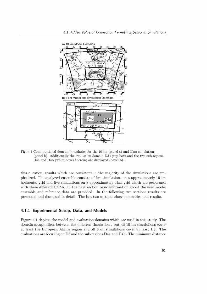
4.1 Added Value of Convection Permitting Seasonal Simulations
a) 10 km Model Domains
−10 −5 0 5 10 15 20 25 30
−10 −5 0 5 10 15 20 25 30
40
45
50
55
60
40
45
50
55
60
C10_4.8
C10_4.0, M10_OM10_T, W10
b) 3 km Model and Evaluation Domains
D3
D4aD4b10 15
45
M03_O, M03_T, W03
C03_4.8
C03_4.0
Fig. 4.1 Computational domain boundaries for the 10 km (panel a) and 3 km simulations(panel b). Additionally the evaluation domain D3 (gray box) and the two sub-regionsD4a and D4b (white boxes therein) are displayed (panel b).
this question, results which are consistent in the majority of the simulations are em-phasized. The analyzed ensemble consists of five simulations on a approximately 10 kmhorizontal grid and five simulations on a approximately 3 km grid which are performedwith three different RCMs. In the next section basic information about the used modelensemble and reference data are provided. In the following two sections results arepresented and discussed in detail. The last two sections show summaries and results.
4.1.1 Experimental Setup, Data, and Models
Figure 4.1 depicts the model and evaluation domains which are used in this study. Thedomain setup differs between the different simulations, but all 10 km simulations coverat least the European Alpine region and all 3 km simulations cover at least D3. Theevaluations are focusing on D3 and the sub-regions D4a and D4b. The minimum distance
91
4 Added Value in Convection Permitting Simulations
between the evaluation domain D3 and the lateral boundaries of the RCMs is eight grid-boxes and therefore larger than the relaxation zones. The first sub-region representsa hilly area in south-eastern Styria (D4a) which lies on the foothills of the Alps. Theclimate of this region is characterized by the predominant influence of Mediterraneancyclones and deep convection especially in summer. From the North and the West, theregion is shielded by the Alps. In summer, convective precipitation events on the onehand and partly long lasting dry spells on the other hand characterize this region. Thetypical weather conditions in winter are dry ones. The second sub-region is centeredon the highest peaks of the Austrian Alps which are in the Hohe Tauern National Park(D4b). The Großglockner, with an elevation of 3798m, is the highest summit in thisregion, and the valleys are roughly on a height of 550m. Precipitation patterns in thisarea reveal a great spatial variability from the scale of single slopes upwards. There is aprecipitation maximum in summer and a minimum in spring or fall (Barry 2008). Thestrong surface height variation and the diversity of weather and climate regimes withina relatively small region are challenging tasks for RCMs.In order to capture a significant part of the broad range of weather regimes the periods
June, July, and August (JJA) 2007 and December 2007, and January and February 2008DJF are chosen for the simulations. Compared to the climatological mean, JJA waswarmer than average and had at the same time an average amount of precipitation. InDJF warm and dry conditions were predominant. The main reason for the selection ofthese two seasons was the availability of homogeneous, highly resolved lateral boundaryconditions (LBCs) and reference data.Three RCMs have been used for the simulations.• The Wegener Center of the University of Graz (WEGC) used the COnsortium
for Small scale MOdeling COSMO Model in Climate Mode CCLM in the version4.0. The CCLM is the climate version of the former “Lokalmodell” of the Germanweather service with a non-hydrostatic core. A detailed description of the COSMOmodel is given by Steppeler et al. (2003) and Doms and Förstner (2004) and forthe CCLM model by Böhm et al. (2006), Rockel et al. (2008b), and in Section 3.1.
• CCLM was also used by the Brandenburg University of Technology Cottbus (BTU)but in the version 4.8. The major differences to CCLM4.0 are that, beside cor-rections and modifications of the source code, a new reference atmosphere and asubgrid-scale orography scheme were introduced in version 4.8. However, there arealso some differences in the model setup (see Table 4.1). These simulations aredescribed into some details by Georgievski et al. (2011).
• WEGC also applied the Pennsylvania State University (PSU)/National Center forAtmospheric Research (NCAR) Fifth-Generation NCAR/Penn State MesoscaleModel (MM5) version 3.7.4. Details about the model are given in Dudhia (1993).
• The Weather Research and Forecasting Model (WRF) version 2.2.1 was again used
92
4.1 Added Value of Convection Permitting Seasonal Simulations
by WEGC. Like the other RCMs it has a non-hydrostatic core and is developedby several research institutes in the USA. A detailed description can be found inSkamarock et al. (2005).
The major difference between the simulations with 10 km horizontal grid-spacing andthose with 3 km is that the deep convection parameterizations are switched off in thelatter. Simulations on the 3 km grid are permitting deep convection and hence they arereferred to as CPCSs. The 3 km simulations use the results of the coarser simulations aslateral boundary conditions (LBCs) in two different ways. The first one is called one-waycoupling, which means that there is no feedback of information from the 3 km simulationto the 10 km run and information from the 10 km to the 3 km simulation is only providedvia the lateral boundaries. This approach was used for the CCLM simulations and onepair of MM5 runs (M10_O and M03_O; see Table 4.1 for acronyms). In COSMO modelin CLimate Mode (CCLM), hourly data from the 10 km simulations were provided aslateral boundaries of the CPCSs, while the CPCS of MM5 was updated every time stepof its parent simulation (20 seconds). The second approach is called two-way coupling,meaning that there is a feedback from the 3 km to the 10 km simulation. Thereby,information from the interior of the 3 km domain is fed into the 10 km domain everytime step and the 10 km simulation is fed into the 3 km simulation via the LBCs, inturn. The feedback from the interior of the 3 km domain is realized by replacing thecoarse grid solution with the solution of the coincident points of the fine grid. Fornumerical stability, the fed back fields are additionally smoothed with a five point 1–2–1 smoother that removes two-grid-length noise, and damps other short wavelengthsstrongly. The models thereby do not conserve mean values. The advantage of a two-way nesting approach is a better behavior at outflow boundaries of the finer griddedsimulation. A similar two-way coupling approach was used in the WRF simulations andthe second pair of MM5 runs (M10_T and M03_T). Detailed information about themodel setups, the nesting strategies, and the hereafter used acronyms of the simulationscan be found in Table 4.1.For the 10 km simulations the LBCs were taken from the Integrated Forecast System
(IFS) of the European Centre for Medium-Range Weather Forecasts (ECMWF). Thosedata have a T799 L91 resolution (roughly 25 km horizontal grid-spacing at mid latitudes,and 91 vertical levels). A temporal resolution of three hours is achieved by combiningIFS analyses (00, 06, 12, and 18 UTC) and short-term forecast fields (3+h and +9h ofthe 00 UTC and 12 UTC forecasts; see also Suklitsch et al. (2011)). It is assumed thatthese boundary conditions represent the real weather conditions adequately, and hencethe RCMs performance can be judged apart from the quality of the LBCs.The surface boundary conditions (SBCs) were initialized with two different spin-up
periods. For the CCLM4.0 and MM5 simulations a long spin-up period was imitatedby initializing the SBCs from simulations which start at the beginning of January 2007.This has the advantage that the soil with its long term memory for initial conditions
93
4 Added Value in Convection Permitting Simulations
(e.g., Seneviratne et al. 2006) can be assumed to be in a more balanced state at thebeginning of the simulations. A shorter spin-up period of one month (May for JJA 2007and November for December, January, and February (DJF) 2007 to 2008) was used inthe WRF and CCLM4.8 simulations.The evaluations in this study are performed with the Integrated Nowcasting through
Comprehensive Analysis (INCA) dataset (Haiden et al. 2010), provided by the AustrianCentral Institute for Meteorology and Geodynamics (ZAMG). The INCA dataset has a1 km× 1 km resolution on an hourly basis and covers the Austria territory. It is derivedthrough a combination of numerical weather predictions (NWPs) (ALADIN, ECMWF)with current observation data from stations, radars, and satellites, and is further refinedwith highly resolved orographic information. The station density is especially high inmountainous regions. However, most of the stations are located in the valleys. Moretechnical details about the INCA system and its data processing can be found in Haidenet al. (2010).The usage of the INCA dataset as reference data has two major advantages. First, its
high spatial and temporal resolution and second, it allows for an assessment of the RCMsperformance by providing the following four atmospheric parameters: air temperaturetwo meters above surface (T2M), precipitation amount at surface (PR), relative humiditytwo meters above surface (RH), and global radiation at surface (GL).However, the advantage of the high spatial and temporal resolution of INCA has also
a disadvantage. Even though INCA is constrained by observations, the output containserrors especially in regions with low station density. For T2M, a mean absolute error of1.0K to 1.5K in lowland areas and 1.5K to 2.5K in Alpine valleys is estimated (Haidenet al. 2010). Precipitation mean absolute errors for point values and 15 minutes timescale can reach up to 50% in summer and more than 100% in winter. For larger scalesof the order of 100 km2 the errors get significantly smaller. Relative humidity was foundto be very accurate (5% to 7% ) in a hilly sub-region in southern Styria (Kann et al.2011). However, no information is available about the accuracy of relative humidity inmountainous areas and global radiation in general.
94
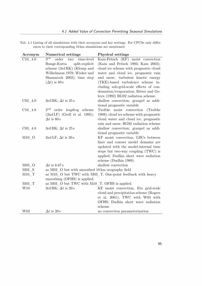
4.1 Added Value of Convection Permitting Seasonal Simulations
Tab. 4.1 Listing of all simulations with their acronyms and key settings. For CPCSs only differ-ences to their corresponding 10 km simulations are mentioned.
Acronym Numerical settings Physical settingsC10_4.0 3rd order two time-level
Runge-Kutta split-explicitscheme (3rdRK) (Klemp andWilhelmson 1978; Wicker andSkamarock 2002); time step(∆t) is 80 s
Kain-Fritsch (KF) moist convection(Kain and Fritsch 1993; Kain 2003);cloud ice scheme with prognostic cloudwater and cloud ice, prognostic rainand snow; turbulent kinetic energy(TKE)-based turbulence scheme in-cluding sub-grid-scale effects of con-densation/evaporation; Ritter and Ge-leyn (1992) RG92 radiation scheme.
C03_4.0 3rdRK; ∆t is 25 s shallow convection; graupel as addi-tional prognostic variable
C10_4.8 2nd order leapfrog scheme(2ndLF) (Grell et al. 1995);∆t is 60 s
Tiedtke moist convection (Tiedtke1989); cloud ice scheme with prognosticcloud water and cloud ice, prognosticrain and snow; RG92 radiation scheme
C03_4.8 3rdRK; ∆t is 25 s shallow convection; graupel as addi-tional prognostic variable
M10_O 2ndLF; ∆t is 20 s KF moist convection; LBCs betweenfiner and coarser model domains areupdated with the model-internal timesteps but two-way coupling (TWC) isapplied; Dudhia short wave radiationscheme (Dudhia 1989)
M03_O ∆t is 6.67 s shallow convectionM03_S as M03_O but with smoothed 10 km orography fieldM10_T as M10_O but TWC with M03_T. One-point feedback with heavy
smoothing (OFHS) is applied.M03_T as M03_O but TWC with M10_T. OFHS is applied.W10 3rdRK; ∆t is 20 s KF moist convection; Eta grid-scale
cloud and precipitation scheme (Rogerset al. 2001); TWC with W03 withOFHS; Dudhia short wave radiationscheme
W03 ∆t is 20 s no convection parameterization
95
4 Added Value in Convection Permitting Simulations
4.1.2 Results
This chapter is made up of four parts according to the different evaluation aspectsof the simulations. In Subsection 4.1.2.1 the error ranges of the seasonal mean fieldsare analyzed. In Subsection 4.1.2.2 the representation of sub-daily processes, temporalvariability, and correlation on grid-point-scale is focused. In Subsection 4.1.2.3 the rep-resentation of extremes in the models is analyzed and in Subsection 4.1.2.4 advancedevaluation methods are used to evaluate hourly precipitation fields.
4.1.2.1 Spatial Error Ranges and Variability
Figure 4.2 shows spatial error ranges of the seasonal bias fields. The term “error range”used here denotes the distance between the 25% to the 75% quantile of the error andis visible as box lengths in Figure 4.2.In JJA the error ranges of all CPCSs for T2M are smaller than those of the corre-
sponding 10 km simulations and those of IFS (Figure 4.2 a). The average error rangedecreases by 0.6K from 2.4K in the 10 km simulations to 1.8K in the CPCSs. Thiseffect is especially strong in the mountainous region D4b and it is smaller in the hillyregion D4a (both not shown).In DJF (Figure 4.2 b) the average error ranges of the CPCSs and the 10 km simulations
are both 1.9K. Only the C03_4.8 and M03_O simulations are able to reduce the errorranges of their parent simulations. In DJF the CCLM4.0 simulations have a remarkablystrong cold bias of −3K whereas the median biases of the other simulations are similarto those in JJA.The JJA relative PR and the relative error ranges in both 3 km CCLM simulations
are increased compared to the 10 km simulations (Figure 4.2 c). This is different in theone-way nested MM5 simulations because in M10_O PR is highly overestimated in largeareas of D3 which is not the case in the M03_O run leading to decreasing error ranges.In all three one-way coupled simulations, the median JJA precipitation sums are notimproved in the CPCS. For the two-way coupled MM5 and WRF simulations the errorranges stay nearly constant, because the 3 km fields are fed back to their driving 10 kmparent simulation.In DJF (Figure 4.2 d) the relative error ranges of PR are much larger than those
in JJA. However, the absolute error ranges (not shown) are smaller because there isgenerally less PR in winter and DJF 2007 to 2008 was remarkably dry in many partsof the Eastern Alps. In this season IFS has clearly a smaller error range than all RCMsimulations. There is a slight decrease in median PR of the CPCSs which improves thegeneral wet bias of the 10 km simulations (except for M03_O). Like in JJA the errorranges of the two-way coupled 3 km and 10 km simulations of MM5 and WRF are very
96
4.1 Added Value of Convection Permitting Seasonal Simulations
similar but in DJF also those of the one-way coupled simulations do not differ notably.The median errors of RH in JJA and DJF are roughly within ±10%. MM5 and WRF
are generally too dry and both versions of CCLM are too wet (Figures 4.2 e and 4.2 f). InDJF the error ranges are larger than in JJA, but an improvement of the median biasesof the CPCSs can be seen except for M03_O. The error ranges are not reduced in theCPCSs in general.All CPCSs have higher GL values compared to their parent simulations which is
stronger pronounced in JJA (Figure 4.2 g) but also visible in DJF (except for C03_4.0and M03_O) (Figure 4.2 h). Comparing the individual RCMs, the CCLM4.0 has astrong negative bias in JJA GL which is most probably related to an overestimationof cloud cover in this model. All other relative median RCM biases are within a rangeof ±20%. Remarkable is the different behavior of the one-way and two-way nestedsimulations of MM5. The M03_O and M03_T simulations look very similar but theM10_O has much higher GL values than the M10_T. In DJF (Figure 4.2 h) the relativeerror ranges are larger for CCLM and WRF than those in JJA. However, the absoluteerror ranges are smaller because of the lower GL values in DJF. In general, the CPCSsdo not reduce the error ranges.Summing up, the only systematic added value in terms of seasonal mean spatial pat-
terns of CPCSs is found in summertime temperature. Large differences between thetwo resolutions have been found in summer precipitation patterns in case of one-waycoupling. In addition, summertime global radiation is systematically increased in thehigh-resolution simulations. In winter, the differences between the two resolutions areless systematic and less pronounced.Concerning the overall performance, the CCLM4.0 simulations show often larger error
ranges (e.g., GL in DJF Figure 4.2 h) or larger differences (e.g., T2M in DJF Figure 4.2 bor GL in JJA 4.2 g) than the rest of the simulations. Because of this and because thedifferences between the C10_4.0 and C03_4.0 simulations are similar to the differencesbetween the C10 4.8 and C03_4.8 runs the results of the CCLM4.0 simulations are notshown in the evaluation results of the next section. This also reduces the informationdensity in the plots and helps to focus on the essential information.
97
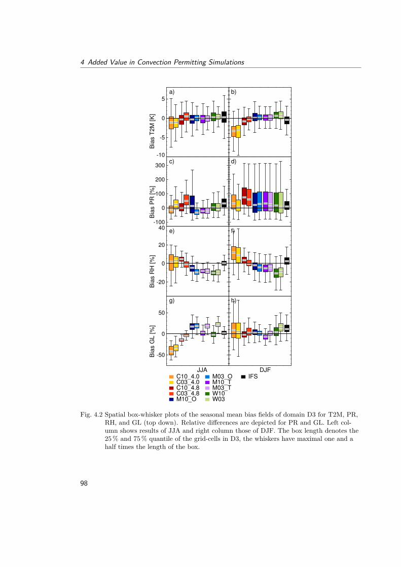
4 Added Value in Convection Permitting Simulations
-10
-5
0
5
-100
0
100
200
300
-20
0
20
40
-50
0
50
JJA
DJF
Bia
s T
2M
[K
]B
ias P
R [
%]
Bia
s R
H [
%]
Bia
s G
L [
%]
a)
c)
e)
g)
b)
d)
f)
h)
C10_4.0C03_4.0C10_4.8C03_4.8M10_O
M03_OM10_TM03_TW10W03
IFS
Fig. 4.2 Spatial box-whisker plots of the seasonal mean bias fields of domain D3 for T2M, PR,RH, and GL (top down). Relative differences are depicted for PR and GL. Left col-umn shows results of JJA and right column those of DJF. The box length denotes the25% and 75% quantile of the grid-cells in D3, the whiskers have maximal one and ahalf times the length of the box.
98
4.1 Added Value of Convection Permitting Seasonal Simulations
4.1.2.2 Diurnal Cycles, Temporal Correlation, and Variability
In this subsection the temporal performance of the RCMs is analyzed. For this purpose,two methods are used: diurnal cycles of the spatially averaged fields and Taylor plots(see Subsection 3.2.1.2) where hourly time series are evaluated on grid-point basis.
Diurnal Cycles In Figure 4.3 the mean diurnal cycles of the spatially averaged fieldsare displayed for the the eastern part of the European Alps and the two sub-regions D4aand D4b.The diurnal cycles of JJA T2M (Figure 4.3 a, b, c) are scattered around those of INCA
within a range of ±2K. In DJF (Figure 4.3A, B, C) the performance of the RCMs isroughly the same. In both seasons, the CPCSs have no deviations from their parentsimulations in common.In JJA PR has a distinct diurnal cycle with a maximum in the afternoon due to
convective rainfall in D3 (Figure 4.3 d) which is most pronounced in the mountainousregion (Figure 4.3 f). In the hilly sub-region D4a (Figure 4.3 e) no distinct diurnal cycleis visible. All RCMs are able to qualitatively reproduce this diurnal cycle and they aregenerally improving the timing of the afternoon peak compared to IFS. An added valuein the one-way nested CPCSs compared to their parent simulations becomes visible inthe better timing of the PR peak later in the afternoon and a more correct onset ofPR at noon. While the C03_4.8 simulation deteriorates the amplitude of the diurnalcycle the M03_O simulation improves the amplitude of the afternoon peak compared toM10_O. The two-way coupled 10 km and 3 km simulations have nearly identical diurnalcycles.In DJF (Figure 4.3D, E, F) PR shows no clear diurnal cycle. The RCMs perform well
in D4a (Figure 4.3E) and overestimate PR in D4b (Figure 4.3 F) which contributes toa general overestimation of PR in D3 (Figure 4.3D). There is no systematic differencebetween the 10 km simulations and the CPCSs in winter.The diurnal cycle of RH is inversely related to T2M, but reveals some additional
information and distinct model deficiencies. The shape is captured reasonably well byall simulations during JJA (Figure 4.3 g, h, i) but the minima occur too early and partlylarge offsets to INCA exist in the MM5 and WRF simulations. In DJF (Figure 4.3G,H, I) the RCMs have more problems to properly reproduce the diurnal cycle of RH.The performance becomes worse in the mountainous region D4b (Figure 4.3 I) where theCCLM and the WRF simulations have nearly constant RH values during the entire dayand all four MM5 simulations even show an inverse diurnal cycle. In both seasons nocommon differences between the CPCSs and their parent simulations are visible.Concerning the diurnal cycle of GL (not shown) the amplitude of the CPCSs is higher
than those of the 10 km simulations, especially during summer in the mountains. This
99
4 Added Value in Convection Permitting Simulations
is consistent with the results from Subsection 4.1.2.1 (Figure 4.2).In summary, the major added value of CPCSs in the diurnal cycle is found in the more
correct timing of the afternoon maximum and the noon onset of convective precipitationin summer and especially over mountainous terrain.
Temporal Correlation and Variability The ability of the RCMs to reproduce the tem-poral characteristics (Pearson’s correlation coefficients and standard deviations) of theconsidered atmospheric parameters on an hourly and grid-point basis in D3 is analyzedwith the help of Taylor plots (Figure 4.4; the Taylor plot method is described in Sub-section 3.2.1.2).In all simulations the temporal correlation of T2M lies between 0.88 to 0.93 in JJA
(Figure 4.4 a) and 0.83 to 0.90 in DJF (Figure 4.4 b). There are only small differences(below 0.02) in the median correlation coefficients between the CPCSs and their parentsimulations. Concerning the median normalized standard deviation in JJA the CPCSsshow a small (below 5%) but consistent increase compared to their parent simulationswhile in DJF there are positive and negative differences. IFS has the highest correlationcoefficients in both seasons. The generally high correlation coefficients are not surprisingas the main part of the correlation is caused by the diurnal cycle. Correlation is worse forvariables that have no regular diurnal variation. In JJA the temporal standard deviationis well captured in all simulations while in DJF the standard deviations are slightlyunderestimated. The horizontal and vertical lines, which represent the 25% to 75%quantile distance of individual grid-pint values are not visible, because those values areclustering very dense around the median correlation coefficients and normalized standarddeviations. This means, there is no big difference in temporal correlation coefficients andstandard deviations in different areas of D3.For PR in JJA (Figure 4.4 c) the correlation coefficients are between 0.12 and 0.25
and the standard deviations are spreading widely, which can be seen from the largevertical 25% to 75% quantile distance. Common in all CPCSs is their higher tempo-ral variability compared to their parent simulations. The poor performance of highlyresolved simulations of PR is a well known issue and is related to the “double penaltyproblem” which is discussed in Subsection 3.2.2. To avoid this problem special methodslike the fractions skill score (FSS) or the Structure-Amplitude-Location (SAL) analy-sis are applied in Subsection 4.1.2.4. In DJF (Figure 4.4 d) the correlation is generallyhigher than in JJA because of the predominance of large-scale precipitation which ismore deterministic than convective precipitation. Datapoints of individual gridcells arespreading widely according to the large 25% to 75% quantile distances. Compared totheir parent simulations all CPCSs show an increase in the median normalized spatialstandard deviation which is largest (10%) in the M03_O simulation. All RCMs havetoo high standard deviations and the differences in the correlation coefficients between
100
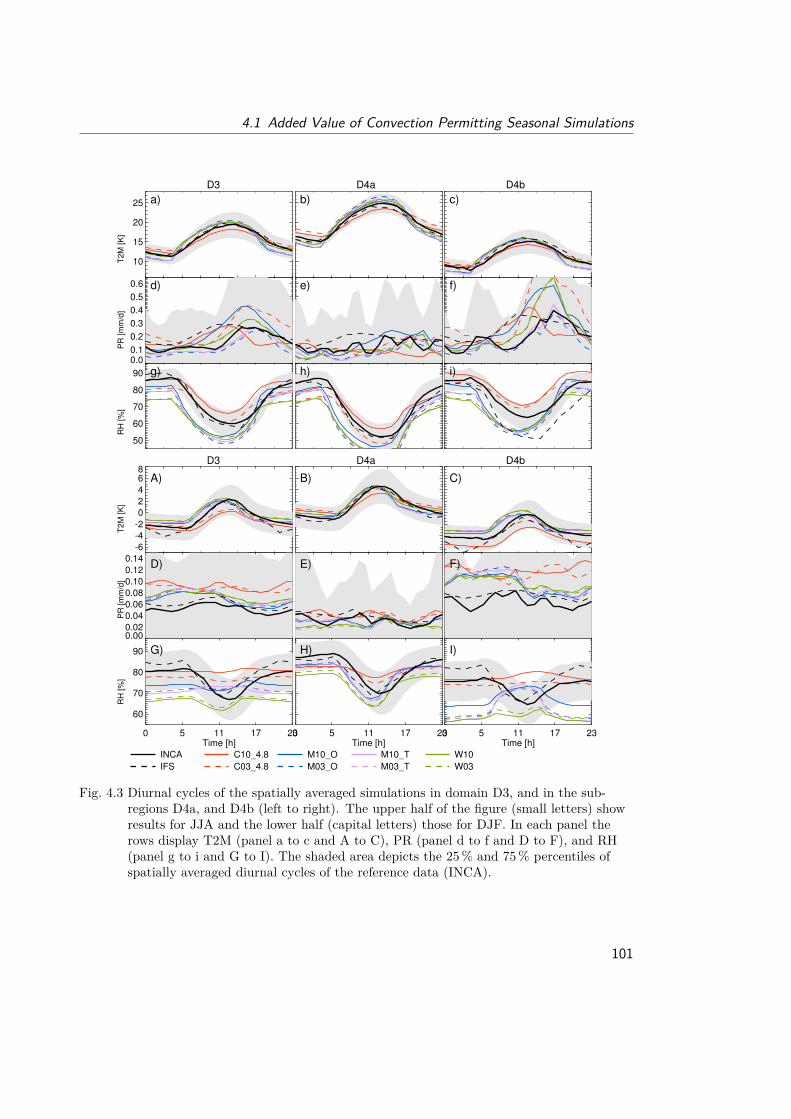
4.1 Added Value of Convection Permitting Seasonal Simulations
10
15
20
25 a)
-6
-4
-2
0
2
4
68
A)
0.00.1
0.2
0.3
0.4
0.5
0.6 d)
0.000.02
0.04
0.06
0.08
0.10
0.12
0.14D)
50
60
70
80
90 g)
0 5 11 17 23Time [h]
60
70
80
90 G)
b)
B)
e)
E)
h)
0 5 11 17 23Time [h]
H)
c)
C)
f)
F)
i)
0 5 11 17 23Time [h]
I)
T2M
[K
]P
R [m
m/d
]R
H [%
]T
2M
[K
]P
R [m
m/d
]R
H [%
]
D3 D4a D4b
D3 D4a D4b
INCA
IFS
C10_4.8
C03_4.8
M10_O
M03_O
M10_T
M03_T
W10
W03
Fig. 4.3 Diurnal cycles of the spatially averaged simulations in domain D3, and in the sub-regions D4a, and D4b (left to right). The upper half of the figure (small letters) showresults for JJA and the lower half (capital letters) those for DJF. In each panel therows display T2M (panel a to c and A to C), PR (panel d to f and D to F), and RH(panel g to i and G to I). The shaded area depicts the 25% and 75% percentiles ofspatially averaged diurnal cycles of the reference data (INCA).
101
4 Added Value in Convection Permitting Simulations
CPCSs and their parent simulations are inconsistent.For RH in JJA (Figure 4.4 e) the majority of the simulated correlation coefficients
are lower than those of IFS. The CPCSs feature slightly smaller correlation coefficientsthan their corresponding 10 km runs, except for C03_4.8. In common are increasedmedian normalized standard deviations in the CPCSs (4% to 6%). The CCLM (MM5)simulations have generally too low (high) temporal variability, while it is well representedin WRF. In DJF (Figure 4.4 f) the correlation coefficients of the CCLM simulations arelower than in JJA. Also the standard deviations are too low which is in agreement withthe nearly constant averaged diurnal cycles shown in Figure 4.3 I. The differences in themedian correlation coefficients are inconsistent however, the median normalized standarddeviations are commonly larger in the CPCSs (except for C03_4.8).The RCMs capture the temporal characteristics of GL with median correlation coef-
ficients between 0.85 and 0.93 in JJA (Figure 4.4 g). Note, a major part of these highvalues belong to the diurnal cycle of the sun. A shift towards higher temporal variabilityis visible in all CPCSs compared to their parent simulations, which is consistent withgenerally higher GL values of the CPCSs (see e.g., Figure 4.2 g). Similar results arefound in DJF (Figure 4.4 h), but the correlation coefficients are higher than in JJA withvalues ranging from 0.93 to 0.95.In summary, there are no systematic changes in the temporal correlation coefficient or
variability between the CPCSs and their parent simulations, except an increase of thevariability in summer precipitation and global radiation. High correlation coefficientsand accurate variability can be found for all simulated temperature and global radiationfields, while for relative humidity the simulations of MM5 and WRF are outperform-ing those of CCLM which shows too low temporal variability. Results for precipitationare especially poor in summer, partly due to the double penalty problem (see Subsec-tion 4.1.2.4).
102
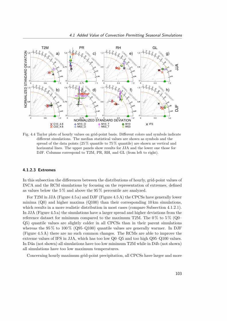
4.1 Added Value of Convection Permitting Seasonal Simulations
C10_4.8C03_4.8
M10_OM03_O
M10_TM03_T
W10W03
IFS
NO
RM
AL
IZE
D S
TA
ND
AR
D D
EV
IAT
ION
NORMALIZED STANDARD DEVIATION
JJA
DJF
T2M PR RH GL
a)
b)
c)
d)
e)
f)
g)
h)
Fig. 4.4 Taylor plots of hourly values on grid-point basis. Different colors and symbols indicatedifferent simulations. The median statistical values are shown as symbols and thespread of the data points (25% quantile to 75% quantile) are shown as vertical andhorizontal lines. The upper panels show results for JJA and the lower one those forDJF. Columns correspond to T2M, PR, RH, and GL (from left to right).
4.1.2.3 Extremes
In this subsection the differences between the distributions of hourly, grid-point values ofINCA and the RCM simulations by focusing on the representation of extremes, definedas values below the 5% and above the 95% percentile are analyzed.For T2M in JJA (Figure 4.5 a) and DJF (Figure 4.5A) the CPCSs have generally lower
minima (Q0) and higher maxima (Q100) than their corresponding 10 km simulations,which results in a more realistic distribution in most cases (compare Subsection 4.1.2.1).In JJA (Figure 4.5 a) the simulations have a larger spread and higher deviations from thereference dataset for minimum compared to the maximum T2M. The 0% to 5% (Q0–Q5) quantile values are slightly colder in all CPCSs than in their parent simulationswhereas the 95% to 100% (Q95–Q100) quantile values are generally warmer. In DJF(Figure 4.5A) there are no such common changes. The RCMs are able to improve theextreme values of IFS in JJA, which has too low Q0–Q5 and too high Q95–Q100 values.In D4a (not shown) all simulations have too low minimum T2M while in D4b (not shown)all simulations have too low maximum temperatures.Concerning hourly maximum grid-point precipitation, all CPCSs have larger and more
103
4 Added Value in Convection Permitting Simulations
realistic Q100 values than their parent simulations (Figure 4.5 b). An especially largeimprovement can be seen for the C03_4.8 run which reduces the Q100 difference ofits parent simulation from -44mmh−1 to +9mmh−1 (Figure 4.5 b). However, there isno systematic difference between the two resolutions in the Q95–Q100 deviations. Thelower quantile differences Q0 and Q0–Q5 are zero because of the many non-precipitatinghours in the distribution of INCA and the simulations. Compared to IFS the RCMs areable to improve the median Q95–Q100 and Q100 difference. In the sub-domains D4aand D4b (not shown) similar results are found.Similar to JJA there is also more intense PR in DJF (Figure 4.5B) in the CPCSs than
in their parent simulations which reduces the differences to INCA. Nevertheless, the mostextreme precipitation events are still underestimated by the CPCSs in all simulationsand all domains.Concerning RH in JJA (Figure 4.5 c) there is a consistent decrease in the Q0–Q5 val-
ues in all CPCSs compared to their parent runs while there are no common differencesin the Q95–Q100 values. The W03 simulation and especially the MM5 runs have un-realistically high maxima which are partly close to 300%. In DJF (Figure 4.5C) theWRF simulations have unphysical minimum values which are below 0% RH. There areno common changes in the Q0–Q5 and Q95–Q100 values between the CPCSs and thecorresponding 10 km simulations. All simulations are overestimating the median of theQ95–Q100 values by approximately 20%. As in JJA all MM5 simulations have too highmaximum values of RH. In D4a (not shown) extremes are better represented than in D3,while in D4b (not shown) the deviations from INCA distribution are especially large.
104
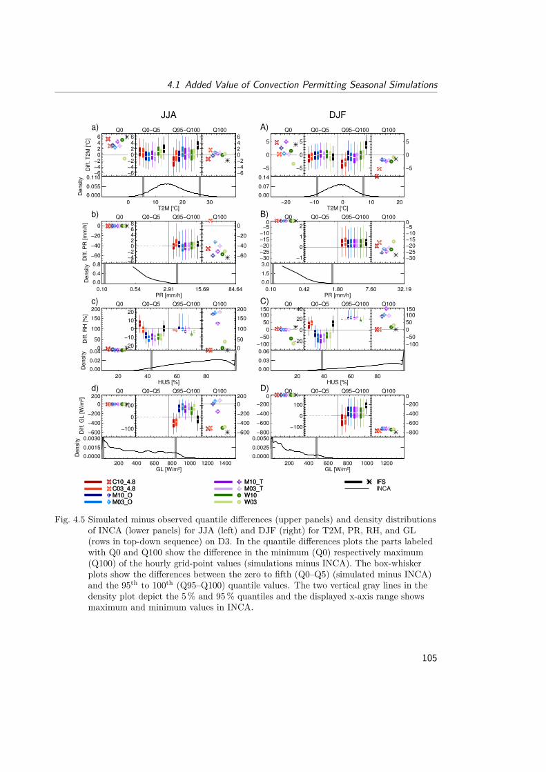
4.1 Added Value of Convection Permitting Seasonal Simulations
−6−4−2
0246
−6−4−2
0246
Diff. T
2M
[oC
]
−6−4−20246
0 10 20 30T2M [oC]
0.000
0.055
0.110
Density
a) Q0 Q0−Q5 Q95−Q100 Q100
−6−4−2
02468
−60
−40
−20
0
Diff. P
R [m
m/h
]
−60
−40
−20
0
0.10 0.54 2.91 15.69 84.64PR [mm/h]
0.0
0.4
0.8
Density
b) Q0 Q0−Q5 Q95−Q100 Q100
−20
−10
0
10
20
0
50
100
150
200
Diff. R
H [%
]
0
50
100
150
200
20 40 60 80HUS [%]
0.00
0.02
0.04
Density
c) Q0 Q0−Q5 Q95−Q100 Q100
−100
0
100
−600
−400
−200
0
200
Diff. G
L [W
/m²]
−600
−400
−200
0
200
200 400 600 800 1000 1200 1400GL [W/m²]
0.0000
0.0015
0.0030
Density
d) Q0 Q0−Q5 Q95−Q100 Q100
JJA
C10_4.8C03_4.8M10_OM03_O
M10_TM03_TW10W03
IFS
−5
0
5
−5
0
5
−5
0
5
−20 −10 0 10 20T2M [oC]
0.00
0.07
0.14
A) Q0 Q0−Q5 Q95−Q100 Q100
−1
0
1
2
−30−25−20−15−10−5
0
−30−25−20−15−10−50
0.10 0.42 1.80 7.60 32.19PR [mm/h]
0.0
1.5
3.0
B) Q0 Q0−Q5 Q95−Q100 Q100
−20
0
20
40
−100
−50
0
50
100150
−100
−50
0
50
100150
20 40 60 80HUS [%]
0.00
0.03
0.06
C) Q0 Q0−Q5 Q95−Q100 Q100
−100
0
100
−800
−600
−400
−200
0
−800
−600
−400
−200
0
200 400 600 800 1000 1200GL [W/m²]
0.0000
0.0025
0.0050
D) Q0 Q0−Q5 Q95−Q100 Q100
DJF
C10_4.8C03_4.8M10_OM03_O
M10_TM03_TW10W03
IFSINCA
Fig. 4.5 Simulated minus observed quantile differences (upper panels) and density distributionsof INCA (lower panels) for JJA (left) and DJF (right) for T2M, PR, RH, and GL(rows in top-down sequence) on D3. In the quantile differences plots the parts labeledwith Q0 and Q100 show the difference in the minimum (Q0) respectively maximum(Q100) of the hourly grid-point values (simulations minus INCA). The box-whiskerplots show the differences between the zero to fifth (Q0–Q5) (simulated minus INCA)and the 95th to 100th (Q95–Q100) quantile values. The two vertical gray lines in thedensity plot depict the 5% and 95% quantiles and the displayed x-axis range showsmaximum and minimum values in INCA.
105
4 Added Value in Convection Permitting Simulations
For GL (Figure 4.5 d and D), only the upper tail of the frequency distribution is ofrelevance in this study: the Q0 and Q0–Q5 values refer to nighttime conditions and hencedeviations from INCA become vanishingly small. In JJA (Figure 4.5 d) the Q95–Q100values of the CPCSs are higher than in their parent simulations, which is not the casefor the Q100 values. In DJF (Figure 4.5D), no common changes between the CPCSsand their parent runs are visible. The large negative deviations in the Q100 values canbe attributed to erroneous maximum values in the INCA dataset.Summing up, there is a consistent improvement in the representation of the most
extreme hourly precipitation values in CPCSs. In the case of T2M the CPCSs havelower minimum values and higher maximum values than their parent simulations, whichlead to more realistic cold temperature extremes in most cases.
4.1.2.4 Evaluation of PR at High Temporal and Spatial Resolution
The evaluation of simulated PR at high spatial and/or temporal resolution is difficult,because at small scales hourly PR partially gets unpredictable and double penalty prob-lems can occur (e.g., Figure 4.4 c and Figure 4.4 d).In this subsection two methods are applied, which are able to avoid the double penalty
problem and to evaluate the spatial properties of high-resolution precipitation fieldsmore appropriate than most traditional statistical methods, like correlations coefficientsor mean square errors.
Fractions skill score Figure 4.6 depicts the average fractions skill scores FSSs of allrecords with precipitation in JJA depending on the selected threshold values and hor-izontal extension of the moving window (horizontal scale). Compared to IFS the FSSsare widely improved by the simulations especially for threshold above 1mmh−1 (Fig-ure 4.6 c). However, this improvement is partly caused by the three hourly resolutionof IFS. The CPCSs have higher FSS than their corresponding 10 km simulations (ex-cept the M03_T and W03 simulations below 1mmh−1 threshold and the M03_O at allthresholds). Differences between the two resolutions are larger at higher precipitationthresholds (e.g., 2mmh−1 in Figure 4.6 d). The scales on which the simulations havemore than random skill are the same in both, the CPCSs and their parent simulationsin the two-way coupled simulations. C03_4.8 improves the scales at which C10 4.8 hasmore than random skill by a factor of 2 (for 0.5mmh−1) and a factor of 5 (for 2mmh−1).In the case of the one-way coupled MM5 simulations it is the other way around and theM03_O deteriorates the scale above random skill of the M10_O simulation. The mainreason for this might be the general underestimation of PR in the M03_O simulation (cf.Figure 4.2 ). Above 5mmh−1 threshold (Figure 4.6 e) only the CPCSs and the M10_Osimulation have FSSs greater than zero. The good performance of the M10_O simulation
106
4.1 Added Value of Convection Permitting Seasonal Simulations
compared to the M03_O run is partly related to the underestimation of precipitation inthe latter which is very similar to the M03_T simulation.In DJF (Figure 4.7) the differences between the FSSs of the CPCSs and their cor-
responding 10 km simulations are smaller than in JJA because winter precipitation isgenerally more dominated by large-scale and non-convective processes (e.g., frontal pre-cipitation). However, except for the WRF and the one-way nested MM5 simulations, theCPCSs have higher FSSs and a better representation of small scales than their 10 kmparent simulations. IFS has large FSSs at 0.1mmh−1 threshold and outperforms allRCMs except WRF. For higher thresholds most simulations exceed the FSSs of IFS.Only the C03_4.8 run is able to improve the scales on which the simulations have morethan random skill compared to its parent simulation (cf. Figure 4.7 b). For the othersimulations there is no difference in this value except for the W03 run which deterioratesthe performance of the W10 simulation.Comparing the FSSs of JJA with those of DJF it becomes visible that at small thresh-
old values (e.g., 0.1mmh−1) the FSSs are generally larger in DJF compared to JJA. Thisis because DJF precipitation is dominated by large-scale processes which are better rep-resented in RCMs than convective precipitation occurring frequently in JJA. For higherthresholds (e.g., 0.5mmh−1 or 1mmh−1) the FSS in JJA are larger than those in DJFbecause precipitation above e.g., 1mmh−1 occurs more often in JJA than in DJF (Fig-ure 4.5 b and 4.5B), and the probability that it is observed and simulated at the sametime is therefore much higher in JJA.
Structure-Amplitude-Location Evaluation The Structure-Amplitude-Location evalu-ation is an object based method which evaluates precipitation fields concerning the threecharacteristics after which it is named (see Subsection 3.2.2.3). Since we found that thereare no large changes in the location (L) component between different simulations, the fo-cus here lies on changes in the structure (S) and amplitude (A) component. It should benoted that the A-component is different from the PR bias, because in the SAL evaluationonly records with precipitation in the INCA dataset are considered.In Figure 4.8 the two dimensional distribution of the S- and A-components are shown
for JJA. On average the CPCSs have a median shift of −0.72 in the S-component whichmeans there are smaller and/or more peaked precipitation objects in the CPCSs than intheir parent simulations. For all models but MM5, this also means an improvement ofthe structure of precipitation objects in the CPCSs because the S-components are morecentered on zero. Furthermore, the median A-components of the CPCSs are 0.15 higherthan those of the 10 km simulations which leads to an average overestimation of precip-itation in all CPCSs, because the A-components of the 10 km simulations (except thoseof M10_O) are close to zero. The combination of smaller S values and larger A valuesin the CPCS means that there is more intense rainfall from smaller and/or more peaked
107
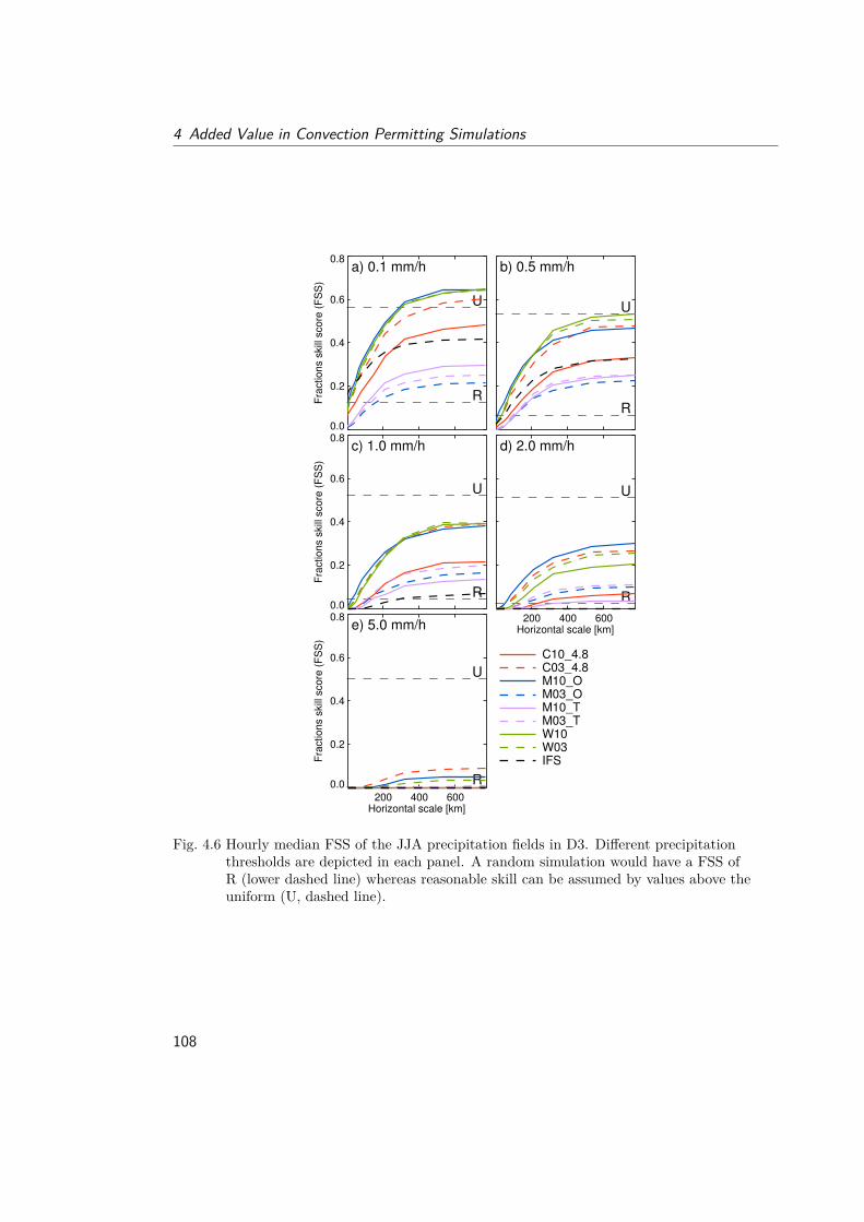
4 Added Value in Convection Permitting Simulations
0.0
0.2
0.4
0.6
0.8
Fra
ctions s
kill
score
(F
SS
)
U
R
a) 0.1 mm/h
U
R
b) 0.5 mm/h
0.0
0.2
0.4
0.6
0.8
Fra
ctions s
kill
score
(F
SS
)
U
R
c) 1.0 mm/h
200 400 600Horizontal scale [km]
U
R
d) 2.0 mm/h
200 400 600Horizontal scale [km]
0.0
0.2
0.4
0.6
0.8
Fra
ctions s
kill
score
(F
SS
)
U
R
e) 5.0 mm/h
C10_4.8C03_4.8M10_OM03_OM10_TM03_TW10W03IFS
Fig. 4.6 Hourly median FSS of the JJA precipitation fields in D3. Different precipitationthresholds are depicted in each panel. A random simulation would have a FSS ofR (lower dashed line) whereas reasonable skill can be assumed by values above theuniform (U, dashed line).
108
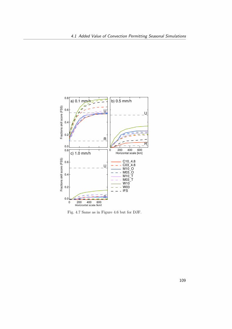
4.1 Added Value of Convection Permitting Seasonal Simulations
0.0
0.2
0.4
0.6
0.8
Fra
ctions s
kill
score
(F
SS
)
U
R
a) 0.1 mm/h
0 200 400 600Horizontal scale [km]
U
R
b) 0.5 mm/h
0 200 400 600Horizontal scale [km]
0.0
0.2
0.4
0.6
0.8
Fra
ctions s
kill
score
(F
SS
)
U
R
c) 1.0 mm/h
C10_4.8C03_4.8M10_OM03_OM10_TM03_TW10W03IFS
Fig. 4.7 Same as in Figure 4.6 but for DJF.
109
4 Added Value in Convection Permitting Simulations
precipitation objects. Compared to IFS (Figure 4.8 i) the RCMs are able to improvethe S- and A-component of precipitation objects to a large extent. The contingencytables in the lower right corner of each panel reveals insights into the representationof correctly simulated precipitation (OJ/MJ), non-precipitation records (ON/MN), theamount of missed events (OJ/MN), and the amount of false alarms (ON/MJ) of eachsimulation. All CPCS (except MM5) show on average 23% less missed events than theircorresponding 10 km simulations. However, only the C03_4.8 simulation is also able todecrease the amounts of false alarms.In DJF (Figure 4.9) the median S-components of the CPCSs are decreasing by−0.48which
leads to an improved structure of PR objects in all CPCSs (except for W03). The medianA-components slightly increase in the CPCSs on average by 0.1. The RCMs are able toimprove the S- and A-component of IFS (Figure 4.9 i) even though IFS performs betterthan in JJA. The contingency tables show that the missed events in the CPCSs of MM5and WRF are reduced by 13.6% on average while they stay constant for CCLM4.8.However, at the same time also the false alarms increase by 18% in M03_T, and 67% inW03. In case of M03_O they stay relatively constant and only the C03_4.8 simulationcan reduce the false alarms by 25%.
110
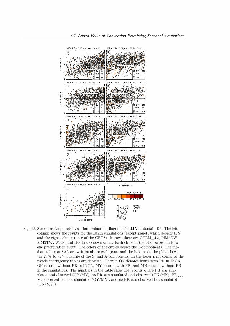
4.1 Added Value of Convection Permitting Seasonal Simulations
Fig. 4.8 Structure-Amplitude-Location evaluation diagrams for JJA in domain D3. The leftcolumn shows the results for the 10 km simulations (except panel i which depicts IFS)and the right column those of the CPCSs. In rows there are CCLM_4.8, MM5OW,MM5TW, WRF, and IFS in top-down order. Each circle in the plot corresponds toone precipitation event. The colors of the circles depict the L-components. The me-dian values of SAL are written above each panel and the box inside the plots showsthe 25% to 75% quantile of the S- and A-components. In the lower right corner of thepanels contingency tables are depicted. Therein OY denotes hours with PR in INCA,ON records without PR in INCA, MY records with PR, and MN records without PRin the simulations. The numbers in the table show the records where PR was sim-ulated and observed (OY/MY), no PR was simulated and observed (ON/MN), PRwas observed but not simulated (OY/MN), and no PR was observed but simulated(ON/MY)).
111
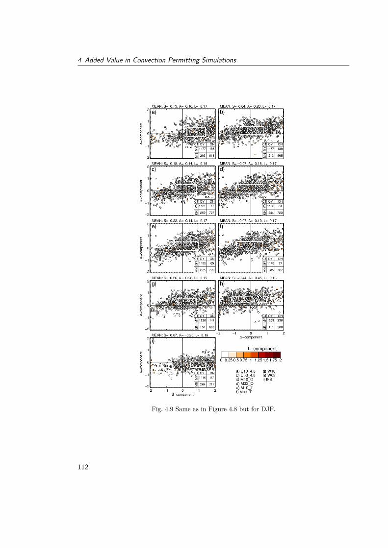
4 Added Value in Convection Permitting Simulations
Fig. 4.9 Same as in Figure 4.8 but for DJF.
112
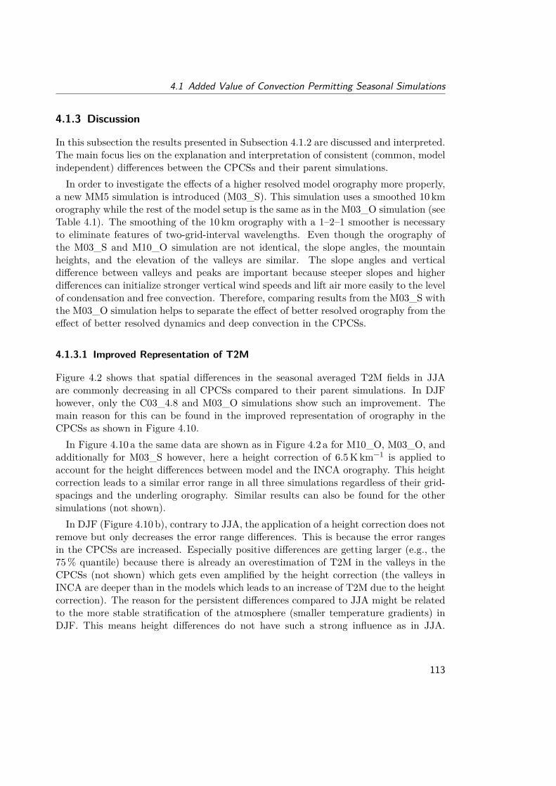
4.1 Added Value of Convection Permitting Seasonal Simulations
4.1.3 Discussion
In this subsection the results presented in Subsection 4.1.2 are discussed and interpreted.The main focus lies on the explanation and interpretation of consistent (common, modelindependent) differences between the CPCSs and their parent simulations.In order to investigate the effects of a higher resolved model orography more properly,
a new MM5 simulation is introduced (M03_S). This simulation uses a smoothed 10 kmorography while the rest of the model setup is the same as in the M03_O simulation (seeTable 4.1). The smoothing of the 10 km orography with a 1–2–1 smoother is necessaryto eliminate features of two-grid-interval wavelengths. Even though the orography ofthe M03_S and M10_O simulation are not identical, the slope angles, the mountainheights, and the elevation of the valleys are similar. The slope angles and verticaldifference between valleys and peaks are important because steeper slopes and higherdifferences can initialize stronger vertical wind speeds and lift air more easily to the levelof condensation and free convection. Therefore, comparing results from the M03_S withthe M03_O simulation helps to separate the effect of better resolved orography from theeffect of better resolved dynamics and deep convection in the CPCSs.
4.1.3.1 Improved Representation of T2M
Figure 4.2 shows that spatial differences in the seasonal averaged T2M fields in JJAare commonly decreasing in all CPCSs compared to their parent simulations. In DJFhowever, only the C03_4.8 and M03_O simulations show such an improvement. Themain reason for this can be found in the improved representation of orography in theCPCSs as shown in Figure 4.10.In Figure 4.10 a the same data are shown as in Figure 4.2 a for M10_O, M03_O, and
additionally for M03_S however, here a height correction of 6.5Kkm−1 is applied toaccount for the height differences between model and the INCA orography. This heightcorrection leads to a similar error range in all three simulations regardless of their grid-spacings and the underling orography. Similar results can also be found for the othersimulations (not shown).In DJF (Figure 4.10 b), contrary to JJA, the application of a height correction does not
remove but only decreases the error range differences. This is because the error rangesin the CPCSs are increased. Especially positive differences are getting larger (e.g., the75% quantile) because there is already an overestimation of T2M in the valleys in theCPCSs (not shown) which gets even amplified by the height correction (the valleys inINCA are deeper than in the models which leads to an increase of T2M due to the heightcorrection). The reason for the persistent differences compared to JJA might be relatedto the more stable stratification of the atmosphere (smaller temperature gradients) inDJF. This means height differences do not have such a strong influence as in JJA.
113
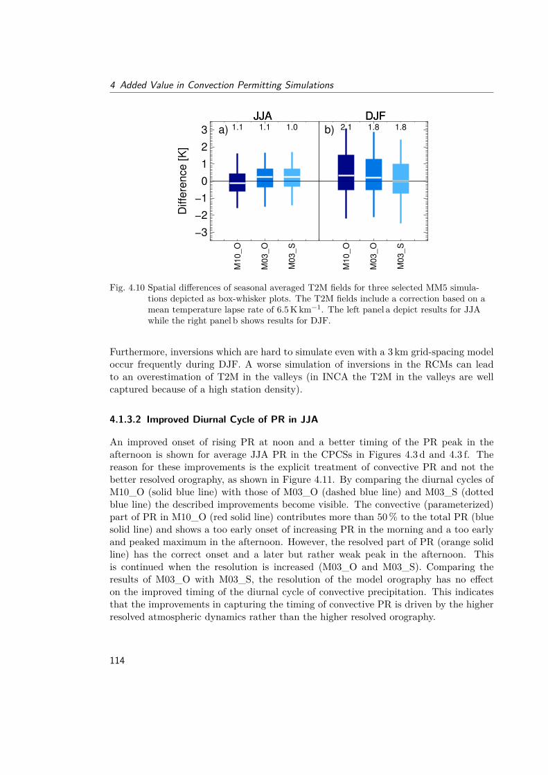
4 Added Value in Convection Permitting Simulations
−3
−2
−1
0
1
2
3
Diffe
rence [K
]
a) b)
M1
0_
O
1.1
M0
3_
O
1.1
M0
3_
S
1.0
JJA DJF
M1
0_
O
2.1
M0
3_
O
1.8
M0
3_
S
1.8
JJA DJF
Fig. 4.10 Spatial differences of seasonal averaged T2M fields for three selected MM5 simula-tions depicted as box-whisker plots. The T2M fields include a correction based on amean temperature lapse rate of 6.5Kkm−1. The left panel a depict results for JJAwhile the right panel b shows results for DJF.
Furthermore, inversions which are hard to simulate even with a 3 km grid-spacing modeloccur frequently during DJF. A worse simulation of inversions in the RCMs can leadto an overestimation of T2M in the valleys (in INCA the T2M in the valleys are wellcaptured because of a high station density).
4.1.3.2 Improved Diurnal Cycle of PR in JJA
An improved onset of rising PR at noon and a better timing of the PR peak in theafternoon is shown for average JJA PR in the CPCSs in Figures 4.3 d and 4.3 f. Thereason for these improvements is the explicit treatment of convective PR and not thebetter resolved orography, as shown in Figure 4.11. By comparing the diurnal cycles ofM10_O (solid blue line) with those of M03_O (dashed blue line) and M03_S (dottedblue line) the described improvements become visible. The convective (parameterized)part of PR in M10_O (red solid line) contributes more than 50% to the total PR (bluesolid line) and shows a too early onset of increasing PR in the morning and a too earlyand peaked maximum in the afternoon. However, the resolved part of PR (orange solidline) has the correct onset and a later but rather weak peak in the afternoon. Thisis continued when the resolution is increased (M03_O and M03_S). Comparing theresults of M03_O with M03_S, the resolution of the model orography has no effecton the improved timing of the diurnal cycle of convective precipitation. This indicatesthat the improvements in capturing the timing of convective PR is driven by the higherresolved atmospheric dynamics rather than the higher resolved orography.
114
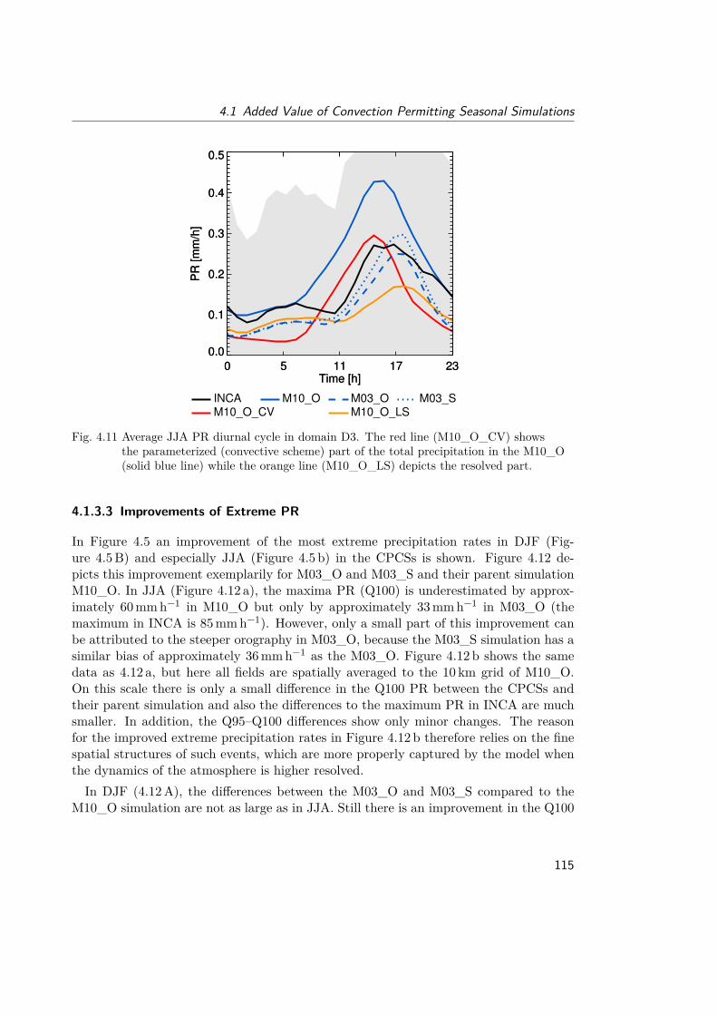
4.1 Added Value of Convection Permitting Seasonal Simulations
0 5 11 17 23Time [h]
0.0
0.1
0.2
0.3
0.4
0.5
PR
[m
m/h
]
0 5 11 17 23Time [h]
0.0
0.1
0.2
0.3
0.4
0.5
PR
[m
m/h
]
INCA M10_O M03_O M03_SM10_O_CV M10_O_LS
Fig. 4.11 Average JJA PR diurnal cycle in domain D3. The red line (M10_O_CV) showsthe parameterized (convective scheme) part of the total precipitation in the M10_O(solid blue line) while the orange line (M10_O_LS) depicts the resolved part.
4.1.3.3 Improvements of Extreme PR
In Figure 4.5 an improvement of the most extreme precipitation rates in DJF (Fig-ure 4.5B) and especially JJA (Figure 4.5 b) in the CPCSs is shown. Figure 4.12 de-picts this improvement exemplarily for M03_O and M03_S and their parent simulationM10_O. In JJA (Figure 4.12 a), the maxima PR (Q100) is underestimated by approx-imately 60mmh−1 in M10_O but only by approximately 33mmh−1 in M03_O (themaximum in INCA is 85mmh−1). However, only a small part of this improvement canbe attributed to the steeper orography in M03_O, because the M03_S simulation has asimilar bias of approximately 36mmh−1 as the M03_O. Figure 4.12 b shows the samedata as 4.12 a, but here all fields are spatially averaged to the 10 km grid of M10_O.On this scale there is only a small difference in the Q100 PR between the CPCSs andtheir parent simulation and also the differences to the maximum PR in INCA are muchsmaller. In addition, the Q95–Q100 differences show only minor changes. The reasonfor the improved extreme precipitation rates in Figure 4.12 b therefore relies on the finespatial structures of such events, which are more properly captured by the model whenthe dynamics of the atmosphere is higher resolved.In DJF (4.12A), the differences between the M03_O and M03_S compared to the
M10_O simulation are not as large as in JJA. Still there is an improvement in the Q100
115
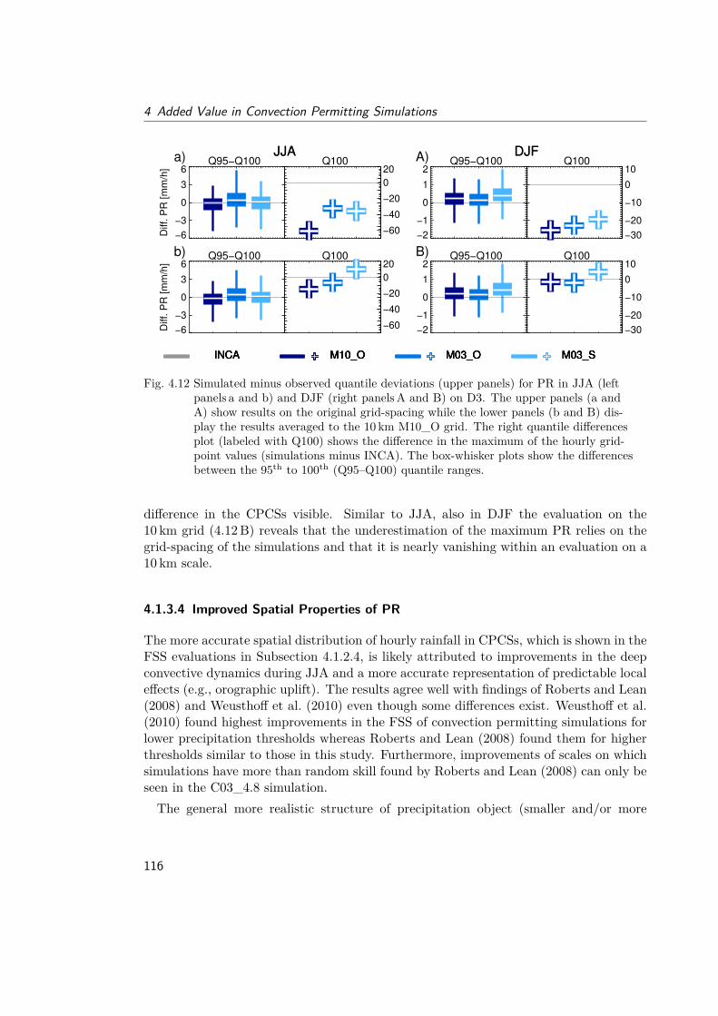
4 Added Value in Convection Permitting Simulations
−6
−3
0
3
6D
iff.
PR
[m
m/h
]
−60
−40
−20
0
20a) Q95−Q100 Q100
JJA
INCA M10_O M03_O M03_S
−2
−1
0
1
2
−30
−20
−10
0
10A) Q95−Q100 Q100
DJF
INCA M10_O M03_O M03_S
−6
−3
0
3
6
Diff. P
R [m
m/h
]
−60
−40
−20
0
20b) Q95−Q100 Q100
JJA
INCA M10_O M03_O M03_S
−2
−1
0
1
2
−30
−20
−10
0
10B) Q95−Q100 Q100
DJF
INCA M10_O M03_O M03_S
Fig. 4.12 Simulated minus observed quantile deviations (upper panels) for PR in JJA (leftpanels a and b) and DJF (right panelsA and B) on D3. The upper panels (a andA) show results on the original grid-spacing while the lower panels (b and B) dis-play the results averaged to the 10 km M10_O grid. The right quantile differencesplot (labeled with Q100) shows the difference in the maximum of the hourly grid-point values (simulations minus INCA). The box-whisker plots show the differencesbetween the 95th to 100th (Q95–Q100) quantile ranges.
difference in the CPCSs visible. Similar to JJA, also in DJF the evaluation on the10 km grid (4.12B) reveals that the underestimation of the maximum PR relies on thegrid-spacing of the simulations and that it is nearly vanishing within an evaluation on a10 km scale.
4.1.3.4 Improved Spatial Properties of PR
The more accurate spatial distribution of hourly rainfall in CPCSs, which is shown in theFSS evaluations in Subsection 4.1.2.4, is likely attributed to improvements in the deepconvective dynamics during JJA and a more accurate representation of predictable localeffects (e.g., orographic uplift). The results agree well with findings of Roberts and Lean(2008) and Weusthoff et al. (2010) even though some differences exist. Weusthoff et al.(2010) found highest improvements in the FSS of convection permitting simulations forlower precipitation thresholds whereas Roberts and Lean (2008) found them for higherthresholds similar to those in this study. Furthermore, improvements of scales on whichsimulations have more than random skill found by Roberts and Lean (2008) can only beseen in the C03_4.8 simulation.The general more realistic structure of precipitation object (smaller and/or more
116
4.1 Added Value of Convection Permitting Seasonal Simulations
peaked) which was shown in the SAL evaluations in Subsection 4.1.2.4 is in good agree-ment with findings by Wernli et al. (2008) who compared high-resolution precipitationforecasts with coarser scale global model forecasts.
4.1.3.5 Increase of GL
In Figure 4.2 g and 4.2 h a consistent increase of GL in most CPCSs is depicted. Thisincrease can be up to 20% in JJA, is especially large in the two-way coupled simulations,and leads to changes in the surface energy budged (not shown). For instance, theadditional energy increases the latent heat flux in W03 and M03_T simulation, whilein the M03_O run the sensible heat is increased. In C03_4.8 both reactions occur,depending on the region. In this subsection atmospheric fields which are important forGL are investigated in JJA between 06:00 am and 06:00 pm.To understand the reason for the increase in GL it is important to understand how the
shortwave radiation is interacting with the atmosphere in the models. In the MM5 andWRF simulations the Dudhia 1989 short wave radiation scheme (D89) (Dudhia 1989) isused. Within this scheme a simple downward integration of solar flux is applied whichknows three interaction mechanisms: (1) cloud albedo and absorption parameterizedwith the cloud liquid water (CLW), (2) water vapor absorption (Lacis and Hansen 1974),and (3) clear air scattering. In Figure 4.13 a the parameterized transmission coefficientof shortwave radiation and its dependency on CLW, as it is parameterized in the D89scheme, is depicted. At CLW values below 10 gm−2 more than 90% of the shortwaveradiation can transmit while above 1000 gm−2 the transmission part is only 10%. Inthe CCLM simulations the Ritter and Geleyn (1992) radiative transfer scheme (RG92) isused which is more complex than the D89 scheme. Solar radiation in the RG92 schemeinteracts with cloud water droplets, cloud ice crystals, water vapor, ozone, and takesinto account effects of Rayleigh scattering. In the RG92 scheme also partial cloudinessis treated by attributing two sets of optical properties and fluxes to each layer, one forthe cloudy and one for the cloud free part (Geleyn and Hollingsworth 1979). Thereby,clouds in adjacent model layers have maximum overlap while clouds which are separatedby cloud free layers are independent from each other (random overlap assumption).A general feature in all CPCSs are the higher values of CLW above approximately
500 gm−2 compared to their parent simulations (all lines are above the diagonal inFigure 4.13 a). This means that already dense clouds become even denser in the CPCSs.This should not have a very strong effect on the GL values in the CPCSs because thetransmission coefficients do not change a lot at these high values and the total amountof values higher than 500 gm−2 in the entire distribution is marginal (cf. Figure 4.13 c).In case of the M03_T simulation, the number of low CLW values (smaller approxi-
mately 300 gm−2) is higher than in the M10_T run (the violet line is below the diagonal
117
4 Added Value in Convection Permitting Simulations
for small CLW values in Figure 4.13 a). Also the GL is increased (Figure 4.13 b) while themean CLW stays constant (approximately 38 gm−2 Figure 4.13 c). However, the 75%quantile (upper box) of CLW is clearly decreased (from 34 gm−2 to 2 gm−2). This shiftsthe transmission coefficients towards higher values and supports the increase of GL. Ifone-way coupling is applied less CLW values below approximately 300 gm−2 occur in theM03_O simulation compared to the M10_O run (blue line is above the diagonal belowapproximately 300 gm−2) and GL values are only slightly increasing (Figure 4.13 b). Theboxes and whiskers of CLW are quite similar even though M03_O has a slightly highermean and upper whisker value (Figure 4.13 c). The water vapor absorption is a func-tion of the atmospheric water vapor (AWV) which stays the same in both, the CPCSsand their parent simulations in MM5 (Figure 4.13 d). In the D89 scheme the clear airscattering is proportional to the atmosphere’s mass path length and can therefore onlybe responsible for small changes in GL.Considering those results the primary effect which causes changes of GL between
the CPCSs and the 10 km simulations of MM5 are changes in the low values (lowerthan approximately 200 gm−2) of the CLW distribution because the gradient of thetransmission curve is much larger and the large majority of CLW values are smallerthan approximately 200 gm−2 (see Figure 4.13 c). This means that in M03_T there arelarger fractions with “cloud free areas” compared to M10_T which directly leads to anincrease of GL. Since the W03 and W10 are also two-way coupled and the D89 schemewas used in WRF as well, the reason for the increasing GL values might be similar. InM03_O an increase of the “cloud free areas” fraction is not visible compared to M10_O(because M10_O already has low CLW values) and therefore GL changes are small.To investigate the reasons of the GL increases in CCLM the simulations of both
versions (4.8 and 4.0) are considered because in the CCLM4.8 runs no AWV and cloudarea fraction (CAF) fields have been stored. The low CLW values (below approximately500 gm−2) are very similar in the C03_4.8 and C10_4.8 runs whereas C03_4.0 hasclearly lower values than C10_4.0 (Figure 4.13 a). However, both show a similar medianincrease in GL (24Wm−2 in C03_4.0 and 28Wm−2 in C03_4.8) (Figure 4.13 b). InC03_4.0 the mean and the 75% quantile (upper box limit) of the CLW is decreasingcompared to C10_4.0 (Figure 4.13 c) while the mean is slightly increasing and the 75%quantile is constant in the C03_4.8 run (compared to C10 4.8). There is more AWV inthe C03_4.0 simulation than in the C10_4.0 run (Figure 4.13 d) and the median CAFdecreases by 14% (Figure 4.13 e).Summing up, for C03_4.0 the increase of GL compared to C10_4.0 can be related to
a higher “cloud free area” fraction indicated by increased low CLW values and decreasedCAF (similar as in MM5). Changes in the cloud ice content cannot be investigatedbecause cloud ice was not stored. The reason for the GL increase in C03_4.8 cannot befully analyzed because of missing data.
118
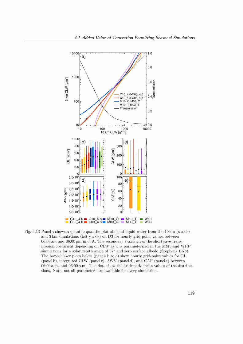
4.1 Added Value of Convection Permitting Seasonal Simulations
10 100 1000 1000010 km CLW [g/m2]
10
100
1000
10000
3 k
m C
LW
[g/m
2]
0.0
0.2
0.4
0.6
0.8
1.0
Tra
nsm
issio
n
a)
C10_4.0-C03_4.0C10_4.8-C03_4.8M10_O-M03_OM10_T-M03_TTransmission
0
100
200
300
CLW
[g/m
2]
c)
5.0•103
1.0•104
1.5•104
2.0•104
2.5•104
3.0•104
3.5•104
AW
V [g/m
2]
d)
0
20
40
60
80
100
CA
F [%
]
e)
0
200
400
600
800
1000
GL [W
/m2]
b)
C10_4.0C03_4.0
C10_4.8C03_4.8
M10_OM03_O
M10_TM03_T
W10W03
Fig. 4.13 Panel a shows a quantile-quantile plot of cloud liquid water from the 10 km (x-axis)and 3 km simulations (left y-axis) on D3 for hourly grid-point values between06:00 am and 06:00 pm in JJA. The secondary y-axis gives the shortwave trans-mission coefficient depending on CLW as it is parameterized in the MM5 and WRFsimulations for a solar zenith angle of 37° and zero surface albedo (Stephens 1978).The box-whisker plots below (panels b to e) show hourly grid-point values for GL(panel b), integrated CLW (panel c), AWV (panel d), and CAF (panel e) between06:00 a.m. and 06:00 p.m.. The dots show the arithmetic mean values of the distribu-tions. Note, not all parameters are available for every simulation.
119
4 Added Value in Convection Permitting Simulations
4.1.3.6 Two-way vs. One-way Coupling
If two-way coupling is applied the atmospheric fields in the 10 km simulation are over-written by the values of the CPCS within the area of the 3 km nest. This means that the3 km run is compared to a coarser (smoothed) version of itself. On the other hand, alsoone-way coupled CPCSs are often more similar to their corresponding 10 km simulationsthan to the observations (except for precipitation) or to CPCS of other RCMs. Thisindicates that a large part of the errors in CPCS comes from the RCM formulation, theRCM setup, or from the LBCs of the CPCSs. The small domains in the CPCSs arecontributing to this behavior (see Subsection 4.1.3.8). Comparing the one-way coupledM03_O simulations with the two-way coupled M03_T run shows that in this study thebenefit of two-way coupling is rather small because the results of both simulations arevery similar.
4.1.3.7 Added Value in the Sub-regions and Seasons
Detecting added value is generally easier in the mountainous region D4b than in the hillyarea of D4a because of the high impact of better resolved orography in complex terrain.For instance, this can be seen in the improvements of the JJA precipitation diurnal cyclewhere no diurnal cycle is visible in D4a (Figure 4.3 e) whereas a strongly amplified cycleis visible in D4b (Figure 4.3 f). Furthermore, improvements in the seasonal mean T2Mfields are much stronger in D4b than in D4a because of the large improvements of thecomplex orography in D4b.Added value is additionally easier to find in JJA than in DJF mainly because of the
more accurate representation of convective processes during the hot season and the wellmixed conditions in the troposphere. Furthermore, in DJF the large-scale flow is moredominant than in JJA which reduces the influence of small-scale processes.
4.1.3.8 Domain Size
A notable limitation of this study are the relatively small sizes of the 3 km simula-tion domains (see Figure 4.1) which have an East-West/North-South extension be-tween approximately 580 km/approximately 510 km (in C03_4.0) and approximately440 km/approximately 370 km (in M03_O, M03_T, and W03). This implicates thatthe boundary conditions from the 10 km simulations have a strong influence on theCPCSs, especially in situations with strong synoptic scale weather patterns (e.g., pas-sages of cold fronts) which occur more frequently in DJF. In such situations the CPCSshave only a limited degree of freedom and are strongly determined by the solution oftheir parent simulations. In larger domains the differences between the CPCSs and theirparent simulations might be more amplified.
120
4.2 Importance of Grid-Spacing for Simulating Precipitation Extremes
4.2 Importance of Grid-Spacing for Simulating PrecipitationExtremes
Because the results from the above study in Section 4.1 show high potential for animproved representation of heavy precipitation in CPCSs compared to coarser griddedsimulations the simulation of precipitation extremes is investigated in more detail. Sinceheavy precipitation events are typically rare events longer time periods than in Sec-tion 4.1 have to be investigated to be able to get statistically robust results. Therefore,the eight year period 2001 to 2008 is simulated with three different grid-spacings of4 km, 12 km, and 36 km over the headwaters of the Colorado River (hereafter: ColoradoHeadwaters). These simulations enable to investigate a sample of heavy precipitationevents which makes a statistical evaluation of such events possible. The focus lies onevents in DJF and JJA because heavy precipitation events in these seasons have typ-ically different synoptic-scale forcing and meso-scale processes. In March, April, andMay (MAM) and September, October, and November (SON) a mixture of DJF and JJAtypes of heavy precipitation events can occur. Analyses from these transitional seasonsare briefly described in Subsection 4.2.2.6.An important difference to the first study is the applied nesting strategy. While in
the first study a two step nesting strategy was used (the outcome of first step 10 kmgrid-spacing simulations were used as LBCs for the 3 km CPCSs) here all three simula-tions were forced with exactly the same LBCs over a common domain (the headwaters ofthe Colorado River). This has the advantage that errors in the coarse resolution 36 kmsimulation are not propagating into the finer resolved runs via the LBCs. This meansthe simulations are independent from each other which is beneficial for the detectionand attribution of differences between them. Furthermore, in this study the computa-tional domain is much larger and the evaluation domain is further apart from the lateralboundaries which also is advantageous.The main research questions are:
1. What is the effect of grid-spacing on the representation of heavy precipitationevents in the Colorado Headwaters?
2. On which spatial scales do differences occur?3. Which grid-spacing should be used to simulate heavy precipitation events?
4.2.1 Experimental Setup, Data, and Models
The simulations were performed with the WRF model version 3.1.1 (Skamarock et al.2008) for an eight-year period from January 1st 2001 to December 31st 2008 (plus threemonths of spin-up) by the Colorado Headwaters research group at the National Cen-
121
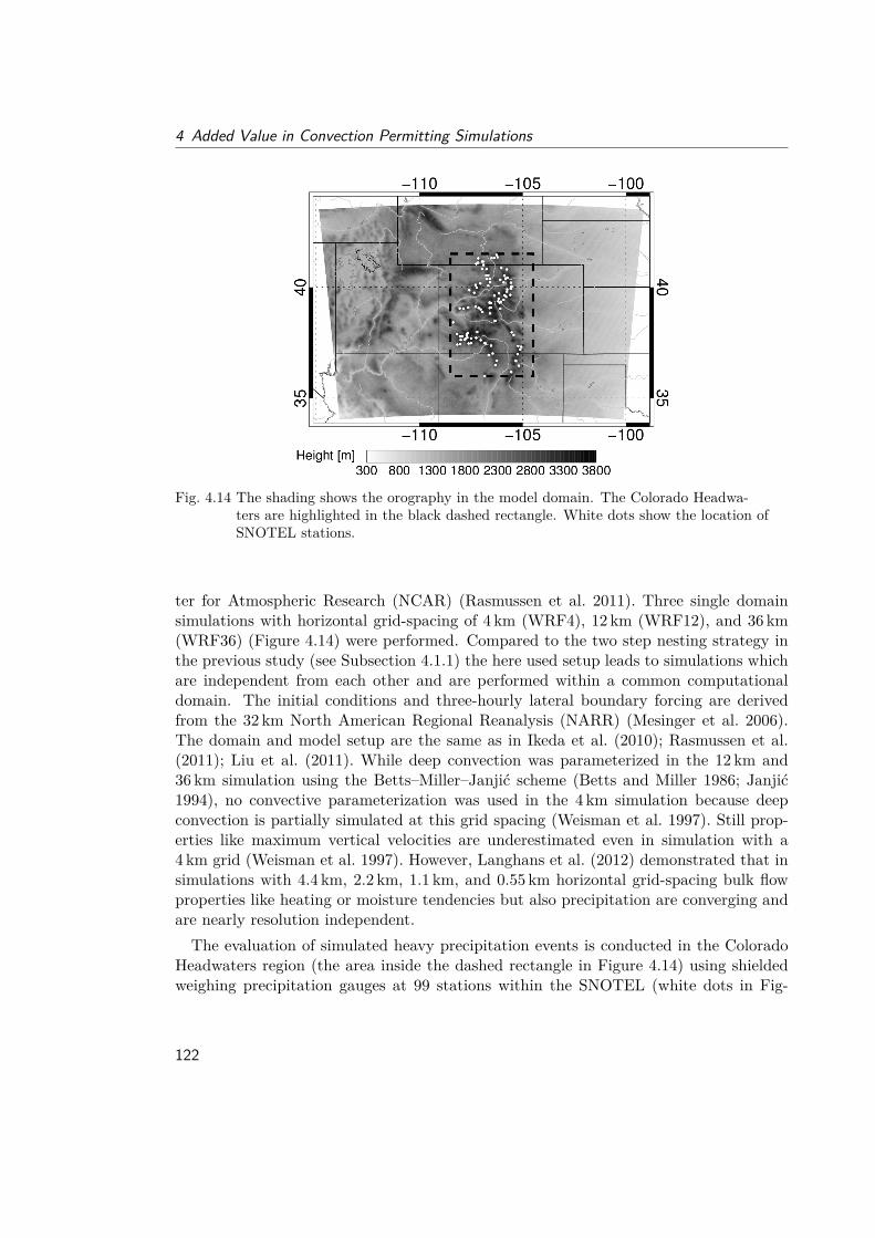
4 Added Value in Convection Permitting Simulations
Fig. 4.14 The shading shows the orography in the model domain. The Colorado Headwa-ters are highlighted in the black dashed rectangle. White dots show the location ofSNOTEL stations.
ter for Atmospheric Research (NCAR) (Rasmussen et al. 2011). Three single domainsimulations with horizontal grid-spacing of 4 km (WRF4), 12 km (WRF12), and 36 km(WRF36) (Figure 4.14) were performed. Compared to the two step nesting strategy inthe previous study (see Subsection 4.1.1) the here used setup leads to simulations whichare independent from each other and are performed within a common computationaldomain. The initial conditions and three-hourly lateral boundary forcing are derivedfrom the 32 km North American Regional Reanalysis (NARR) (Mesinger et al. 2006).The domain and model setup are the same as in Ikeda et al. (2010); Rasmussen et al.(2011); Liu et al. (2011). While deep convection was parameterized in the 12 km and36 km simulation using the Betts–Miller–Janjić scheme (Betts and Miller 1986; Janjić1994), no convective parameterization was used in the 4 km simulation because deepconvection is partially simulated at this grid spacing (Weisman et al. 1997). Still prop-erties like maximum vertical velocities are underestimated even in simulation with a4 km grid (Weisman et al. 1997). However, Langhans et al. (2012) demonstrated that insimulations with 4.4 km, 2.2 km, 1.1 km, and 0.55 km horizontal grid-spacing bulk flowproperties like heating or moisture tendencies but also precipitation are converging andare nearly resolution independent.The evaluation of simulated heavy precipitation events is conducted in the Colorado
Headwaters region (the area inside the dashed rectangle in Figure 4.14) using shieldedweighing precipitation gauges at 99 stations within the SNOTEL (white dots in Fig-
122
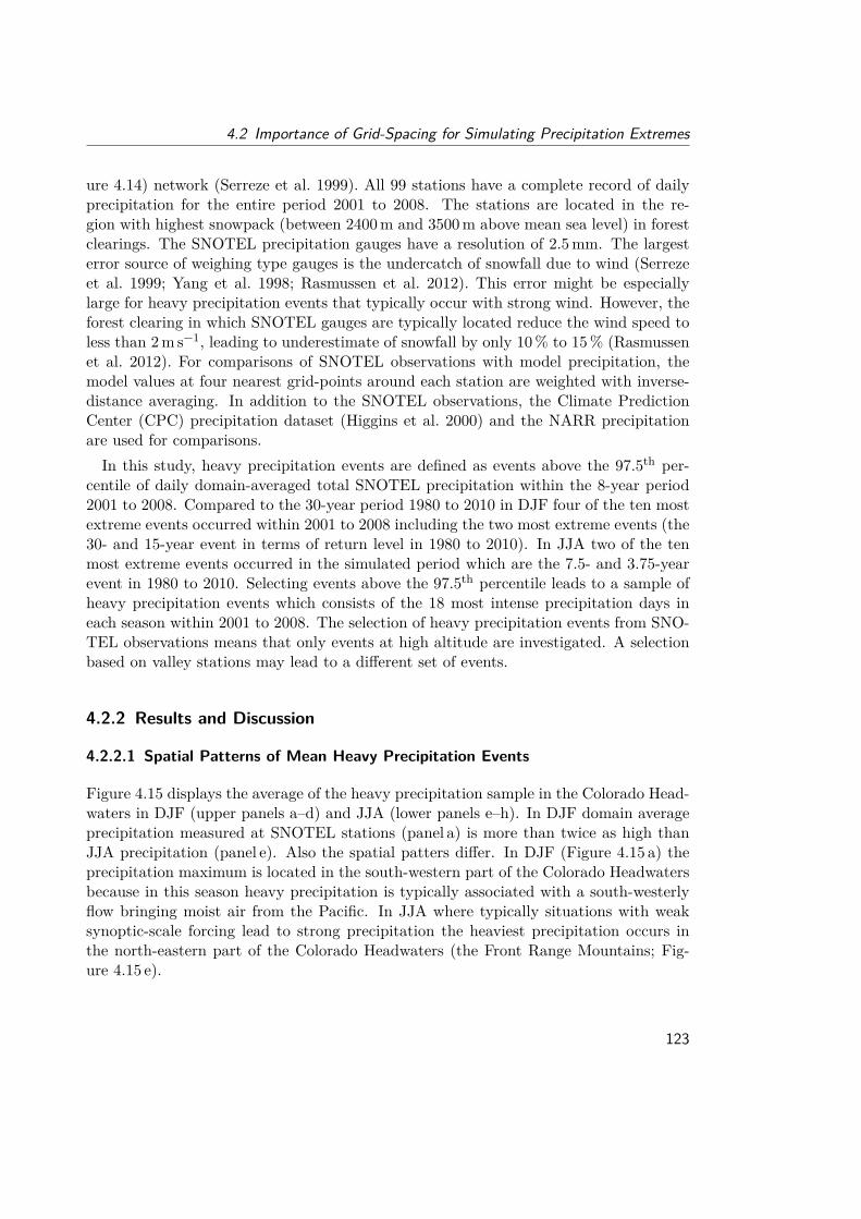
4.2 Importance of Grid-Spacing for Simulating Precipitation Extremes
ure 4.14) network (Serreze et al. 1999). All 99 stations have a complete record of dailyprecipitation for the entire period 2001 to 2008. The stations are located in the re-gion with highest snowpack (between 2400m and 3500m above mean sea level) in forestclearings. The SNOTEL precipitation gauges have a resolution of 2.5mm. The largesterror source of weighing type gauges is the undercatch of snowfall due to wind (Serrezeet al. 1999; Yang et al. 1998; Rasmussen et al. 2012). This error might be especiallylarge for heavy precipitation events that typically occur with strong wind. However, theforest clearing in which SNOTEL gauges are typically located reduce the wind speed toless than 2m s−1, leading to underestimate of snowfall by only 10% to 15% (Rasmussenet al. 2012). For comparisons of SNOTEL observations with model precipitation, themodel values at four nearest grid-points around each station are weighted with inverse-distance averaging. In addition to the SNOTEL observations, the Climate PredictionCenter (CPC) precipitation dataset (Higgins et al. 2000) and the NARR precipitationare used for comparisons.In this study, heavy precipitation events are defined as events above the 97.5th per-
centile of daily domain-averaged total SNOTEL precipitation within the 8-year period2001 to 2008. Compared to the 30-year period 1980 to 2010 in DJF four of the ten mostextreme events occurred within 2001 to 2008 including the two most extreme events (the30- and 15-year event in terms of return level in 1980 to 2010). In JJA two of the tenmost extreme events occurred in the simulated period which are the 7.5- and 3.75-yearevent in 1980 to 2010. Selecting events above the 97.5th percentile leads to a sample ofheavy precipitation events which consists of the 18 most intense precipitation days ineach season within 2001 to 2008. The selection of heavy precipitation events from SNO-TEL observations means that only events at high altitude are investigated. A selectionbased on valley stations may lead to a different set of events.
4.2.2 Results and Discussion
4.2.2.1 Spatial Patterns of Mean Heavy Precipitation Events
Figure 4.15 displays the average of the heavy precipitation sample in the Colorado Head-waters in DJF (upper panels a–d) and JJA (lower panels e–h). In DJF domain averageprecipitation measured at SNOTEL stations (panel a) is more than twice as high thanJJA precipitation (panel e). Also the spatial patters differ. In DJF (Figure 4.15 a) theprecipitation maximum is located in the south-western part of the Colorado Headwatersbecause in this season heavy precipitation is typically associated with a south-westerlyflow bringing moist air from the Pacific. In JJA where typically situations with weaksynoptic-scale forcing lead to strong precipitation the heaviest precipitation occurs inthe north-eastern part of the Colorado Headwaters (the Front Range Mountains; Fig-ure 4.15 e).
123
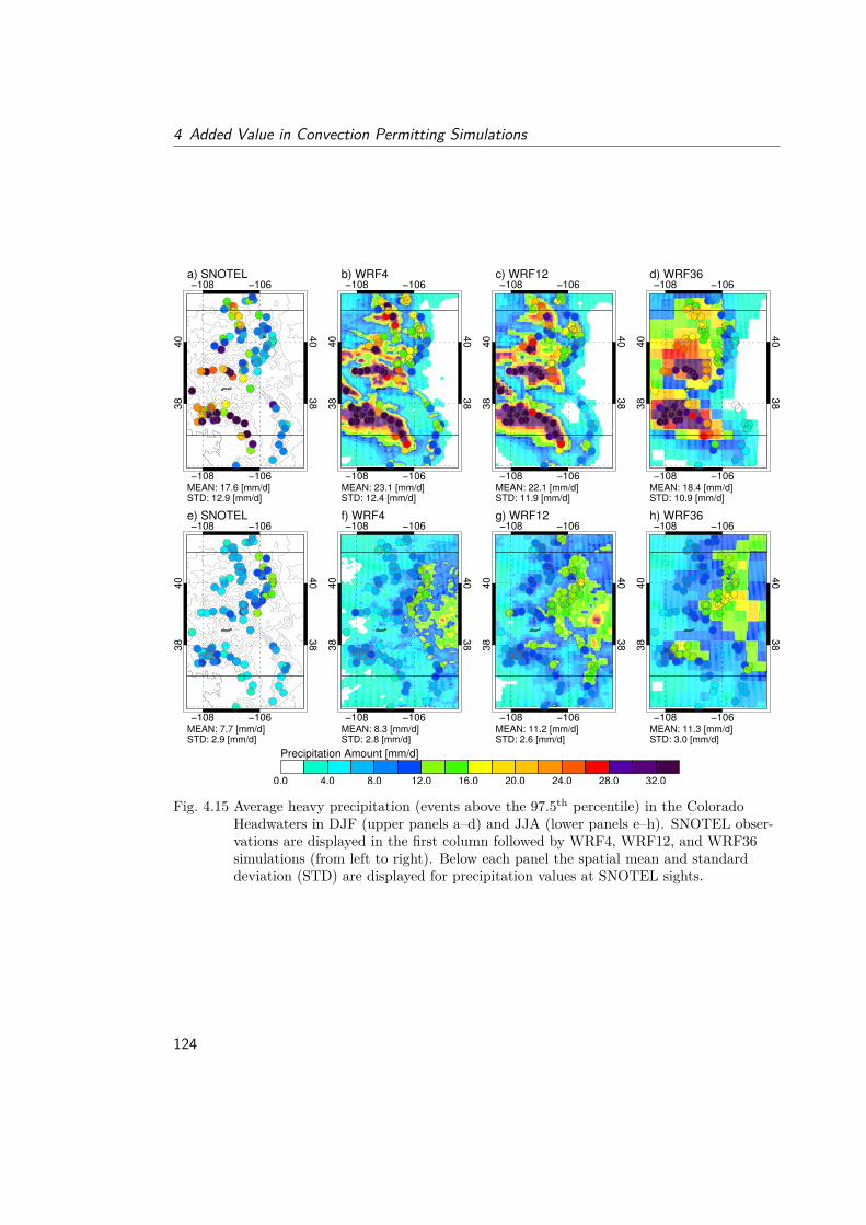
4 Added Value in Convection Permitting Simulations
−108 −106
−108 −106
38
40
38
40
MEAN: 17.6 [mm/d]STD: 12.9 [mm/d]
a) SNOTEL
−108 −106
−108 −106
38
40
38
40
MEAN: 23.1 [mm/d]STD: 12.4 [mm/d]
b) WRF4
−108 −106
−108 −106
38
40
38
40
MEAN: 22.1 [mm/d]STD: 11.9 [mm/d]
c) WRF12
−108 −106
−108 −106
38
40
38
40
MEAN: 18.4 [mm/d]STD: 10.9 [mm/d]
d) WRF36
−108 −106
−108 −106
38
40
38
40
MEAN: 7.7 [mm/d]STD: 2.9 [mm/d]
e) SNOTEL
−108 −106
−108 −106
38
40
38
40
MEAN: 8.3 [mm/d]STD: 2.8 [mm/d]
f) WRF4
−108 −106
−108 −106
38
40
38
40
MEAN: 11.2 [mm/d]STD: 2.6 [mm/d]
g) WRF12
−108 −106
−108 −106
38
40
38
40
MEAN: 11.3 [mm/d]STD: 3.0 [mm/d]
h) WRF36
0.0 4.0 8.0 12.0 16.0 20.0 24.0 28.0 32.0
Precipitation Amount [mm/d]
Fig. 4.15 Average heavy precipitation (events above the 97.5th percentile) in the ColoradoHeadwaters in DJF (upper panels a–d) and JJA (lower panels e–h). SNOTEL obser-vations are displayed in the first column followed by WRF4, WRF12, and WRF36simulations (from left to right). Below each panel the spatial mean and standarddeviation (STD) are displayed for precipitation values at SNOTEL sights.
124
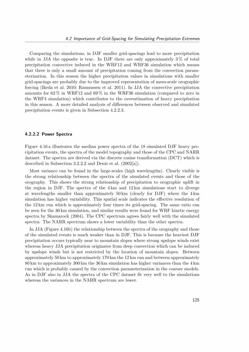
4.2 Importance of Grid-Spacing for Simulating Precipitation Extremes
Comparing the simulations, in DJF smaller grid-spacings lead to more precipitationwhile in JJA the opposite is true. In DJF there are only approximately 3% of totalprecipitation convective induced in the WRF12 and WRF36 simulation which meansthat there is only a small amount of precipitation coming from the convection param-eterization. In this season the higher precipitation values in simulations with smallergrid-spacings are probably due to the improved representation of meso-scale orographicforcing (Ikeda et al. 2010; Rasmussen et al. 2011). In JJA the convective precipitationamounts for 62% in WRF12 and 69% in the WRF36 simulation (compared to zero inthe WRF4 simulation) which contributes to the overestimation of heavy precipitationin this season. A more detailed analysis of differences between observed and simulatedprecipitation events is given in Subsection 4.2.2.3.
4.2.2.2 Power Spectra
Figure 4.16 a illustrates the median power spectra of the 18 simulated DJF heavy pre-cipitation events, the spectra of the model topography and those of the CPC and NARRdataset. The spectra are derived via the discrete cosine transformation (DCT) which isdescribed in Subsection 3.2.2.2 and Denis et al. (2002[a]).Most variance can be found in the large-scales (high wavelengths). Clearly visible is
the strong relationship between the spectra of the simulated events and those of theorography. This shows the strong relationship of precipitation to orographic uplift inthe region in DJF. The spectra of the 4 km and 12 km simulations start to divergeat wavelengths smaller than approximately 50 km (clearly for DJF) where the 4 kmsimulation has higher variability. This spatial scale indicates the effective resolution ofthe 12 km run which is approximately four times its grid-spacing. The same ratio canbe seen for the 36 km simulation, and similar results were found for WRF kinetic energyspectra by Skamarock (2004). The CPC spectrum agrees fairly well with the simulatedspectra. The NARR spectrum shows a lower variability than the other spectra.In JJA (Figure 4.16b) the relationship between the spectra of the orography and those
of the simulated events is much weaker than in DJF. This is because the heaviest DJFprecipitation occurs typically near to mountain slopes where strong upslope winds existwhereas heavy JJA precipitation originates from deep convection which can be inducedby upslope winds but is not restricted by the location of mountain slopes. Betweenapproximately 50 km to approximately 170 km the 12 km run and between approximately80 km to approximately 300 km the 36 km simulation has higher variances than the 4 kmrun which is probably caused by the convection parameterization in the coarser models.As in DJF also in JJA the spectra of the CPC dataset fit very well to the simulationswhereas the variances in the NARR spectrum are lower.
125
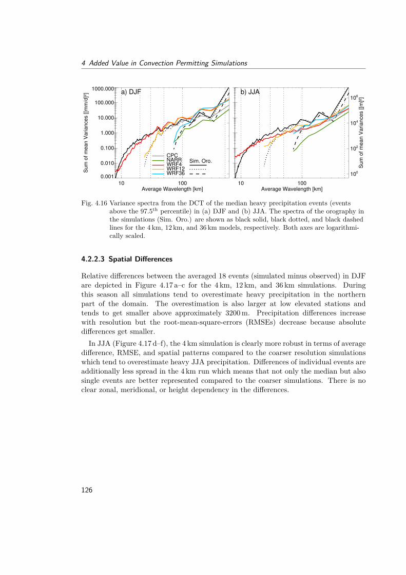
4 Added Value in Convection Permitting Simulations
10 100Average Wavelength [km]
0.001
0.010
0.100
1.000
10.000
100.000
1000.000S
um
of
me
an
Va
ria
nce
s [
[mm
/d]²
]
a) DJF
10 100Average Wavelength [km]
100
102
104
106
Su
m o
f m
ea
n V
aria
nce
s [
[m]²
]
b) JJA
WRF4WRF12WRF36
CPCNARR Sim. Oro.
Fig. 4.16 Variance spectra from the DCT of the median heavy precipitation events (eventsabove the 97.5th percentile) in (a) DJF and (b) JJA. The spectra of the orography inthe simulations (Sim. Oro.) are shown as black solid, black dotted, and black dashedlines for the 4 km, 12 km, and 36 km models, respectively. Both axes are logarithmi-cally scaled.
4.2.2.3 Spatial Differences
Relative differences between the averaged 18 events (simulated minus observed) in DJFare depicted in Figure 4.17 a–c for the 4 km, 12 km, and 36 km simulations. Duringthis season all simulations tend to overestimate heavy precipitation in the northernpart of the domain. The overestimation is also larger at low elevated stations andtends to get smaller above approximately 3200m. Precipitation differences increasewith resolution but the root-mean-square-errors (RMSEs) decrease because absolutedifferences get smaller.In JJA (Figure 4.17 d–f), the 4 km simulation is clearly more robust in terms of average
difference, RMSE, and spatial patterns compared to the coarser resolution simulationswhich tend to overestimate heavy JJA precipitation. Differences of individual events areadditionally less spread in the 4 km run which means that not only the median but alsosingle events are better represented compared to the coarser simulations. There is noclear zonal, meridional, or height dependency in the differences.
126
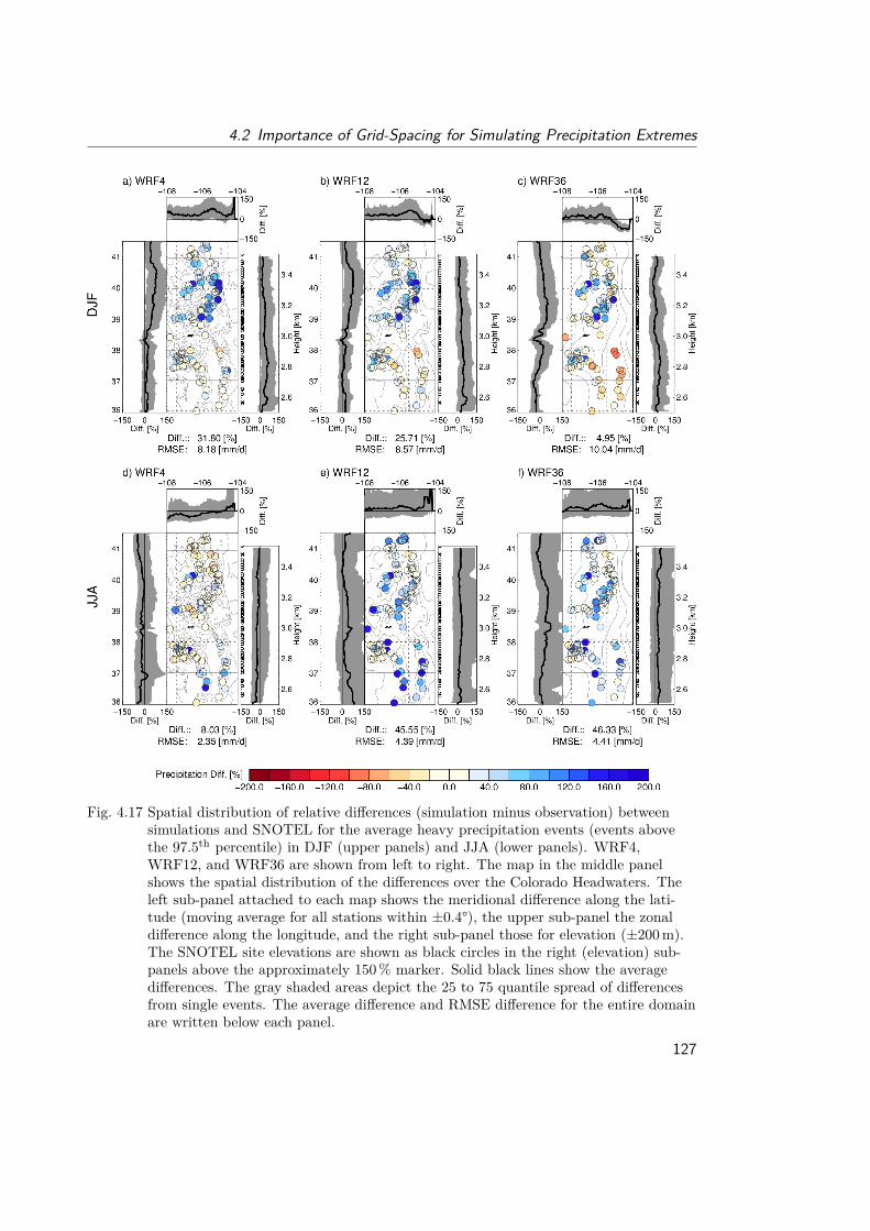
4.2 Importance of Grid-Spacing for Simulating Precipitation Extremes
Fig. 4.17 Spatial distribution of relative differences (simulation minus observation) betweensimulations and SNOTEL for the average heavy precipitation events (events abovethe 97.5th percentile) in DJF (upper panels) and JJA (lower panels). WRF4,WRF12, and WRF36 are shown from left to right. The map in the middle panelshows the spatial distribution of the differences over the Colorado Headwaters. Theleft sub-panel attached to each map shows the meridional difference along the lati-tude (moving average for all stations within ±0.4°), the upper sub-panel the zonaldifference along the longitude, and the right sub-panel those for elevation (±200m).The SNOTEL site elevations are shown as black circles in the right (elevation) sub-panels above the approximately 150% marker. Solid black lines show the averagedifferences. The gray shaded areas depict the 25 to 75 quantile spread of differencesfrom single events. The average difference and RMSE difference for the entire domainare written below each panel.
127
4 Added Value in Convection Permitting Simulations
4.2.2.4 Scale Dependent Analysis
In this subsection the spatial Pearson correlation coefficients (CCs), normalized standarddeviations (NSDs), and RMSEs of the simulated, CPC, and NARR data are evaluatedfor a range of horizontal scales as described in Subsection 3.2.2.2.In DJF the highest median CCs can be found for the 4 km simulation on its original grid
(Figure 4.18 a). At their resolved scales the 12 km and 4 km simulations have very similarCCs whereas, the 36 km run has slightly lower CCs and larger sample variabilities. TheCPC data have higher CCs than the simulations below approximately 90 km while theNARR dataset has lower values on all scales. Similar results can be found for the NSDs(Fig 5b). The 4 km simulation has closest values to one at scales below 12 km and verysimilar values to the 12 km run afterwards. The 36 km run has generally higher medianNSDs, while the CPC and NARR data show lower values. The smallest RMSEs in the4 km simulation show robustness especially at scales larger than 50 km (Figure 4.18 c).All simulations are improving the RMSEs of the NARR driving data.The median CCs in JJA are generally smaller and the sample spread larger compared
to DJF (Figure 4.18 d). This is probably due to the stochastic nature (non-linear in-teractions between land-atmosphere, cloud-cloud and/or cloud-radiation that can growupscale, particularly under generally weak synoptic forcing in JJA) of convective pre-cipitation. At scales from 12 km to 60 km, the 12 km run has higher CCs than the 4 kmsimulation. CPC and NARR have higher CCs below approximately 120 km. The 4 kmsimulation has high NSD below 12 km and similar to the 12 km simulation and CPC af-terwards (Figure 4.18 e). Below 100 km, the 36 km run clearly has higher variability thanthe finer grid datasets. The sample spread of NSDs is smallest for the 12 km simulationabove 20 km. The best RMSEs and smallest sample variability below approximately100 km are achieved with the 4 km model (Figure 4.18 f). Smallest RMSEs can be foundin the CPC dataset whereas the NARR RMSEs are similar to the simulations.
4.2.2.5 Spatial Similarities and Dissimilarities
Figure 4.19 shows median correlograms and variograms from the WRF simulations,CPC, NARR, and SNOTEL observations. For details about the method see Subsection3.2.2.2.All simulations show median CCs that are larger than SNOTEL at scales below ap-
proximately 70 km in DJF (Figure 4.19 a). Some of these differences may be due tomeasurement errors at the SNOTEL sites. Below 70 km the 4 km run is most similar tothe SNOTEL sites. At scales larger than approximately 70 km the correlations of the4 km and 12 km simulations start to match the SNOTEL observations; whereas the 36 kmrun has too high correlations until approximately 120 km. The correlation between pairsof stations becomes anticorrelated at approximately 190 km which is the typical scale of a
128
4.2 Importance of Grid-Spacing for Simulating Precipitation Extremes
mountain range in the Colorado Headwaters (see also the peak in Figure 4.16). The CCsof NARR and CPC are similar to those of the WRF12 simulation. The DJF variogram(Figure 4.19 b) shows weaker variability in all simulations at scales below approximately70 km than SNOTEL. The 4 km simulation shows the most realistic spatial variabilityat all scales while the NARR and CPC data have the lowest variability.In JJA (Figure 4.19 c), CCs at small scales are generally lower than in DJF because of
the higher spatial variability and smaller size of convective precipitation cells (anticorre-lation starts at approximately 110 km). All simulations have higher CCs than SNOTELat scales below approximately 100 km. The 4 km simulation performs best at these scaleswhile above approximately 100 km all simulations begin to match the SNOTEL observedCCs. For scales above approximately 260 km all simulations except the 4 km model gen-erate stronger anti-correlations than SNOTEL. The CPC CCs are similar to those of theWRF12 simulation while the NARR fit more to those of the WRF36 run. Variabilityin all simulations is lower than those of SNOTEL in JJA (Figure 4.19 d). At scalesbelow approximately 110 km the 4 km simulation has the closest correspondence withobservations, and at larger spatial scales the 36 km run matches the 4 km simulations.As in JJA variances are lowest in the CPC and NARR dataset.
4.2.2.6 Analyses of MAM and SON Heavy Precipitation
In the transition seasons MAM and SON heavy precipitation can arise from a mixtureof DJF (large-scale frontal system) and JJA (air-mass thunderstorm) types of storms.The mean precipitation of the SON and MAM heavy precipitation sample (12.3mmd−1
in MAM and 14.8mmd−1 in SON) is higher than the mean in JJA but lower than thosein DJF. Also the convective part of the total precipitation in the WRF12 and WRF36runs is with approximately 12% in MAM and approximately 33% in SON between thepercentage in DJF and JJA (see Subsection 4.2.2.1). The highest observed precipitationvalues in MAM are in the north-eastern part of the domain (similar to JJA) and in SONin the south-western part (similar to DJF). In both seasons the domain total heavyprecipitation is increasing with decreasing grid-spacing (similar to DJF). The lowestRMSEs are found in the WRF4 simulation followed by the WRF12 and WRF36 runs.In MAM and on small scales in SON the WRF4 simulation has higher CCs than thecoarser simulations. The correlogram and variogram analyses lead to similar conclusionsas those in JJA and DJF. The WRF4 simulation resembles correlations from SNOTELobservations best at scales below approximately 100 km and has most realistic varianceson larger scales.
129
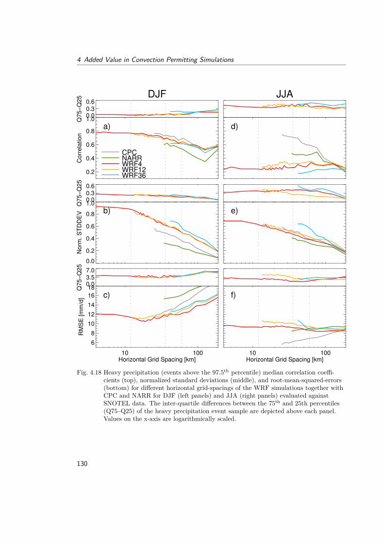
4 Added Value in Convection Permitting Simulations
0.2
0.4
0.6
0.8
1.0
Co
rre
latio
n
0.00.30.6
Q7
5−
Q2
5
a)
0.0
0.2
0.4
0.6
0.8
1.0
No
rm.
ST
DD
EV
0.00.30.6
Q7
5−
Q2
5
b)
10 100Horizontal Grid Spacing [km]
6
8
10
12
14
16
18
RM
SE
[m
m/d
]
0.03.57.0
Q7
5−
Q2
5
c)
d)
e)
10 100Horizontal Grid Spacing [km]
f)
CPCNARRWRF4WRF12WRF36
DJF JJA
Fig. 4.18 Heavy precipitation (events above the 97.5th percentile) median correlation coeffi-cients (top), normalized standard deviations (middle), and root-mean-squared-errors(bottom) for different horizontal grid-spacings of the WRF simulations together withCPC and NARR for DJF (left panels) and JJA (right panels) evaluated againstSNOTEL data. The inter-quartile differences between the 75th and 25th percentiles(Q75–Q25) of the heavy precipitation event sample are depicted above each panel.Values on the x-axis are logarithmically scaled.
130
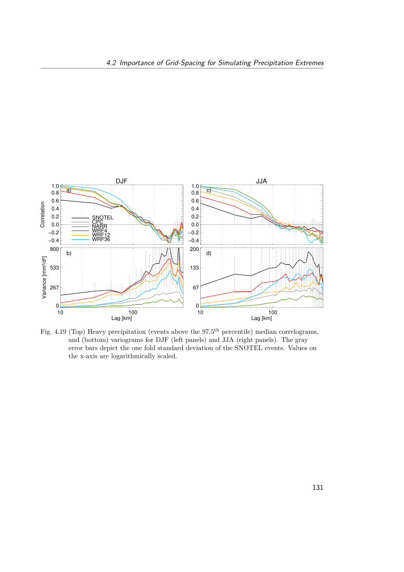
4.2 Importance of Grid-Spacing for Simulating Precipitation Extremes
−0.4
−0.2
0.0
0.2
0.4
0.6
0.8
1.0
Co
rre
latio
n
10 100Lag [km]
0
267
533
800
Va
ria
nce
[m
m²/
d²]
DJF
a)
b)
−0.4
−0.2
0.0
0.2
0.4
0.6
0.8
1.0
10 100Lag [km]
0
67
133
200
JJA
c)
d)
SNOTELCPCNARRWRF4WRF12WRF36
Fig. 4.19 (Top) Heavy precipitation (events above the 97.5th percentile) median correlograms,and (bottom) variograms for DJF (left panels) and JJA (right panels). The grayerror bars depict the one fold standard deviation of the SNOTEL events. Values onthe x-axis are logarithmically scaled.
131
5Summary and Conclusion
The basic research question of this thesis is if and where added value in convectionpermitting climate simulations (CPCSs) compared to coarser gridded simulations
can be found.Answering this question demands for the definition of statistical metrics which enable a
comparison of simulations with different grid-spacings and which account for the specialproblems of evaluating highly resolved datasets. Finding such metrics was a central partof this thesis which is reflected in the numerous introduced (Section 3.2) and applied(Chapter 4) methods which can be regarded as a best practice example for searchingand detecting added value in CPCSs.Two main studies have been performed in this thesis. The first one focuses on the ro-
bustness of added value in an ensemble of three non-hydrostatic regional climate models(RCMs). The second one builds up on the findings of the first study and investigatesscale dependent differences in the simulation of heavy precipitation events.In the first study (Section 4.1) two seasons (June, July, and August (JJA) 2007 and
December, January, and February (DJF) 2007 to 2008) are simulated with three differentRCMs. Five simulations are conducted with a horizontal grid-spacing of approximately10 km and five with approximately 3 km (CPCSs without deep convection parameter-ization) over the Eastern European Alpine region. Four atmospheric parameters (airtemperature two meters above surface, precipitation amount at surface, relative humid-ity two meters above surface, and global radiation at surface) are evaluated which enablesa holistic view on the RCM performance.
132
The second study (Section 4.2) focuses on the representation of heavy precipitationevents in a CPCS and two coarser gridded simulations. It extends the first study by thelength of the simulation period which is January 2001 to December 2008. This enables astatistically robust evaluation of heavy precipitation events. The Weather Research andForecasting Model (WRF) was used to perform simulations with grid-spacings of 36 km,12 km, and 4 km. In the last one deep convection is assumed to be explicitly resolved.The focus region of this study is the headwaters of the Colorado River.The largest changes between simulations with and without convection parameteriza-
tions can be found in the representation of precipitation. Typically, the average amountof precipitation (but also averages of temperature, relative humidity, and global radia-tion) in a region is not improved in CPCS (cf., Figure 4.2) eventhough in some casesimprovements can been found (e.g., JJA heavy precipitation events in the ColoradoHeadwaters; Figure 4.17 d–f). This is because most variance and spatial information inprecipitation fields can be found in the large-scale patterns (cf., Figure 4.16). Thereby,precipitation patterns of CPCSs tend to converge towards patterns of coarser griddedsimulations on scales larger than approximately 100 km (cf., Figures 4.16 and 4.19 aand c) meaning that typically most of the improvements in CPCSs get averaged out onlarge-scales.Added value is therefore easier to find on small scales. In particular, CPCSs outper-
form coarser resolution simulations by producing spatially more independent and vari-able heavy precipitation fields at scales below approximately 100 km which agree wellwith observations. Similar to spatial averaging also temporal averaging tends to reducethe visibility of added value of CPCSs. According to the findings above, added valuein CPCSs can typically be found at small scales (smaller than approximately 100 km)and on sub-daily (e.g., hourly) basis. One exception for this are the error ranges of airtemperature two meters above surface which are strongly related to the better resolvedorography in mountainous regions (Figure 4.2 a).A very robust added value of CPCSs is the improved timing in the onset and peak
of convective induced afternoon precipitation in mountainous regions during JJA (seeFigure 4.3). This is in line with findings of Hohenegger et al. (2008) and Kendon et al.(2012). In addition to those temporal aspects the intensity of the most intense precip-itation extreme events is improved (see Figure 4.12). The fractions skill score (FSS)analysis shows that added value is more apparent at medium to higher, than in lowintensities (cf., Figure 4.6) and Structure-Amplitude-Location (SAL) evaluations revealthat most CPCSs represent spatial patterns of precipitation objects more realistically(smaller and more peaked; see Figures 4.8 and 4.9). It could be demonstrated that theseimprovements are caused by explicitly resolved deep convection and the better repre-sented atmospheric dynamics, rather than by the better resolved orography (see Figures4.11 and 4.12). In general, orography has a weaker influence on convective precipitationpatterns than on large-scale patterns (cf., Figure 4.16). For DJF grid-spacings of at least
133
5 Summary and Conclusion
12 km are needed to simulate spatial patterns of heavy precipitation which are compa-rable to those in the CPCS and observations in the Colorado Headwaters (see Figures4.17 and 4.19 b). In the European Alps this might be different because of the typicallysteeper slopes and narrower valleys compared to the U.S. Rocky Mountains.Larger differences between CPCSs compared to their forcing simulations (which are
not necessarily improvements), are found in the surface energy balance. This is causedby a general increase of global radiation at surface in all CPCSs (on average 11.5% inJJA and 3.5% in DJF; see Figure 4.2 g and h) which can be mainly attributed to anincrease of areas with low integrated cloud liquid water content and/or a decrease of thecloud area fractions (in the case of COSMO model in CLimate Mode). The RCMs reactvery differently to this additional energy input and partly large changes in the sensibleor latent heat fluxes occur.Concluding, CPCSs show promising results to improve state-of-the-art climate simula-
tions especially by explicitly resolving deep convection in the atmosphere. Nevertheless,they are computationally very demanding and therefore the choice of horizontal grid-spacing for RCMs depends on the underlying question.If the main interest is the accurate representation of climate average, large-scale fields
(e.g., on the scale of the European Alps or the Colorado Headwaters), even 36 km grid-spacing can be sufficient in SON, DJF, and MAM. This is not true for JJA when deepconvective processes are predominant in northern hemisphere mid-latitudes. Improve-ments like the more realistic diurnal cycle of precipitation or the more accurate repre-sentation of heavy precipitation events cannot be achieved with convection parameter-izations. Furthermore, in JJA also feedback processes can be sensitive to the accuraterepresentation of deep convection like shown for the soil moisture-precipitation feedbackby Hohenegger et al. (2009).If the model output is used for impact studies which focus, for example, on meso-
scale river catchments, ecology in mountain lakes and rivers, or economic losses fromextreme events CPCSs can have large benefits by improving especially meso-scale struc-tures which can be essential for these applications. Additionally, the more realistic lateseason runoff in CPCSs due to their accurate simulation of high snowpack values at highelevations, which typically melt two months earlier in coarser resolved simulations, isimportant for water supply and flood protection management (Rasmussen et al. 2011).Further work is in progress to study the representation of atmospheric processes in
models with parameterized and explicitly resolved convection, potentially including theuse of large eddy simulations. Furthermore, there is great potential in applying convec-tion permitting simulations in climate studies to analyze possible changes in extremeevents. This would have the advantage that errors from convective parameterizationschemes can be avoided and uncertainties are reduced. One interesting topic which wasnot addressed in this thesis is the influence of better resolved meso-scale features (like
134

mountains) in CPCSs on the synoptic-scale flow in the model. One example for suchan influence is the generation of lee cyclones which tend to occur at the lee side of mid-latitude mountains like the European Alps, the Rocky Mountains, and the Andes, orshielding effects.However, CPCSs are still far from being established tools for climate projections,
partly due to the lack of comprehensive reference data with resolutions appropriate forthe evaluation of CPCSs. Therefore, the detection of errors and the further developmentof CPCSs will remain challenging.
135
List of Figures
2.1 CO2 concentration and near surface temperature in Antarctica recon-structed from ice core measurements. . . . . . . . . . . . . . . . . . . . . . 21
2.2 Comparisons of observation with atmosphere-ocean general circulationmodels (AOGCMs) simulations with and without anthropogenic forcings. 22
2.3 Richardson’s forecast-factory. . . . . . . . . . . . . . . . . . . . . . . . . . 262.4 ENIAC 24 hour forecast of height of the 500 hPa surface. . . . . . . . . . . 272.5 Development of forecast quality from 1955 to 1988. . . . . . . . . . . . . . 282.6 The GCM family tree. . . . . . . . . . . . . . . . . . . . . . . . . . . . . . 302.7 Development of GCM resolution. . . . . . . . . . . . . . . . . . . . . . . . 312.8 Development of GCM components. . . . . . . . . . . . . . . . . . . . . . . 322.9 Temporal and spatial scales of atmospheric processes and variations. . . . 342.10 Illustration of the concept of dynamical downscaling with an RCM. . . . . 362.11 Processes in the modeling of clouds with major uncertainties in the math-
ematical formulations. . . . . . . . . . . . . . . . . . . . . . . . . . . . . . 442.12 Interaction of various processes in the climate system. . . . . . . . . . . . 442.13 Differences between a highly resolved IFS model forecast with and without
a non-hydrostatic core. . . . . . . . . . . . . . . . . . . . . . . . . . . . . . 472.14 Mountain lee waves at Amsterdam Island. . . . . . . . . . . . . . . . . . . 48
3.1 A grid-box in the CCLM displaying the staggering of the dependent vari-ables. . . . . . . . . . . . . . . . . . . . . . . . . . . . . . . . . . . . . . . 57
3.2 Impact of orographic smoothing on the spatial precipitation distributionover the European Alps in the COSMO model. . . . . . . . . . . . . . . . 60
3.3 Hydrological cycle in the standard CCLM cloud and precipitation scheme. 633.4 Hydrological cycle in the graupel scheme of CCLM. . . . . . . . . . . . . . 643.5 Geometrical relationship in the Taylor diagram. . . . . . . . . . . . . . . . 743.6 An idealized example to illustrate the algorithm used in the displacement
and amplitude score. . . . . . . . . . . . . . . . . . . . . . . . . . . . . . . 88
4.1 Computational domains of the 10 km and 3 km simulations including theevaluation domains. . . . . . . . . . . . . . . . . . . . . . . . . . . . . . . 91
136
List of Figures
4.2 Spatial box-whisker plots of the seasonal mean bias fields of domain theeastern part of the European Alps (D3) for T2M, PR, RH, and GL. . . . 98
4.3 Diurnal cycles of the spatially averaged simulations in domain D3, and inthe sub-regions D4a, and D4b. . . . . . . . . . . . . . . . . . . . . . . . . 101
4.4 Taylor plots of hourly values on grid-point basis. . . . . . . . . . . . . . . 1034.5 Simulated minus observed quantile differences and density distributions
of INCA for JJA and DJF for T2M, PR, RH, and GL on D3. . . . . . . . 1054.6 Hourly median FSS of the JJA precipitation fields in D3. . . . . . . . . . 1084.7 Same as in Figure 4.6 but for DJF. . . . . . . . . . . . . . . . . . . . . . . 1094.8 Structure-Amplitude-Location evaluation diagrams for JJA in domain D3. 1114.9 Same as in Figure 4.8 but for DJF. . . . . . . . . . . . . . . . . . . . . . . 1124.10 Spatial differences of seasonally averaged T2M fields for three selected
MM5 simulations depicted as box-whisker plots. . . . . . . . . . . . . . . . 1144.11 Average JJA PR diurnal cycle in domain D3 . . . . . . . . . . . . . . . . . 1154.12 Simulated minus observed quantile deviations for PR in JJA and DJF on
D3. . . . . . . . . . . . . . . . . . . . . . . . . . . . . . . . . . . . . . . . . 1164.13 Quantile-quantile plot of cloud liquid water from the 10 km (x-axis) and
3 km simulations on D3 for hourly grid point values between 06:00 am and06:00 pm in JJA. . . . . . . . . . . . . . . . . . . . . . . . . . . . . . . . . 119
4.14 The shading shows the orography in the model domain. The ColoradoHeadwaters are highlighted in the black dashed rectangle. White dotsshow the location of Snowpack Telemetry (SNOTEL) stations. . . . . . . 122
4.15 Average heavy precipitation (events above the 97.5th percentile) in theColorado Headwaters in DJF and JJA. . . . . . . . . . . . . . . . . . . . . 124
4.16 Variance spectra from the discrete cosine transformation (DCT) of themedian heavy precipitation events (events above the 97.5th percentile) inDJF and JJA. . . . . . . . . . . . . . . . . . . . . . . . . . . . . . . . . . . 126
4.17 Spatial distribution of relative differences (simulation minus observation)between simulations and SNOTEL for the average heavy precipitationevents (events above the 97.5th percentile) in DJF and JJA. . . . . . . . . 127
4.18 Heavy precipitation (events above the 97.5th percentile) median correla-tion coefficients, normalized standard deviations, and root-mean-squared-errors for different horizontal grid-spacings of the WRF simulations to-gether with CPC and NARR for DJF and JJA evaluated against SNOTELdata. . . . . . . . . . . . . . . . . . . . . . . . . . . . . . . . . . . . . . . . 130
4.19 Heavy precipitation (events above the 97.5th percentile) median correlo-grams, and variograms for DJF and JJA. . . . . . . . . . . . . . . . . . . 131
137
List of Tables
2.1 Classification of atmospheric scales after Orlanski (1975) . . . . . . . . . . 34
3.1 Constant external parameters for the surface (Schättler 2012). . . . . . . . 683.2 Constant external parameters for the sub-grid-scale orography scheme
(SSO) scheme (Schättler 2012). . . . . . . . . . . . . . . . . . . . . . . . . 683.3 Constant external parameters for lakes (Schättler 2012). . . . . . . . . . . 683.4 Other constant external parameters (Schättler 2012). . . . . . . . . . . . . 693.5 Plant characteristics (Schättler 2012). . . . . . . . . . . . . . . . . . . . . 693.6 Ozone contents (Schättler 2012). . . . . . . . . . . . . . . . . . . . . . . . 693.7 Aerosol characteristics (Schättler 2012). . . . . . . . . . . . . . . . . . . . 703.8 Necessary surface variables (Schättler 2012). . . . . . . . . . . . . . . . . . 703.9 Necessary soil variables (for multi-layer soil model) (Schättler 2012). . . . 703.10 Necessary atmospheric variables (Schättler 2012). . . . . . . . . . . . . . . 713.11 Optional plant characteristics boundary conditions (Schättler 2012). . . . 713.12 Attributes measured by the traditional and new spatial precipitation ver-
ification methods (after Brown et al. 2009). . . . . . . . . . . . . . . . . . 89
4.1 Listing of all simulations with their acronyms and key settings. For CPCSsonly differences to their corresponding 10 km simulations are mentioned. . 95
138
Acronyms
SymbolsD three-dimensional wind divergence. 54E′ pattern root-mean-squared-error. 73, 74E2 root-mean-squared-error. 74Eh kinetic energy of horizontal motion. 54Fr friction. 23, 24H evaporation/condensation heat release/loss. 23, 24Io observed binary fields. 76Ix simulated binary fields. 76Mu source terms due to turbulent mixing in u. 54Mv source terms due to turbulent mixing in v. 54Mw source terms due to turbulent mixing in w. 54Mqv source terms due to turbulent mixing in qv. 54Mql,f source terms due to turbulent mixing in ql,f . 54N number of pairs. 81On(i, j) field of observed fractions. 77P pressure. 23–25, 27, 56Pl,f absolute values of the gravitational diffusion fluxes of water and ice. 54, 56, 60QT diabatic heating term. 54, 56, 60Qv gain or loss of water vapor through phase changes. 23, 24Rv gas constant for water vapor. 54Rd gas constant for dry air. 54Sl cloud microphysical sources/sinks per unit mass of moist air. 54, 56, 60T temperature. 23, 25, 54, 56, 64T0 constant reference temperature. 54
139
Acronyms
Va vertical component of absolute vorticity. 54Xn(i, j) field of simulated fractions. 77Zmn real spectral coefficient. 81∆t time step. 94Γ variation of reference pressure. 54αb attenuation function. 57E2 squared average bias. 74ζ nonnormalized contravariant vertical velocity. 54γ temperature lapse rate. 23γd dry adiabatic lapse rate. 23λ longitude. 54, 57ω rotational frequency of the earth. 23φ latitude. 23, 54, 57ρ density. 23, 25, 54, 56ρ0 constant reference density. 54σ standard deviation. 73σ2(m,n) spectral variances. 81σc fractional cloud cover. 65covxo covariance. 73ζ terrain following vertical coordinate. 54, 56, 57a radius of the earth. 23, 54cp specific heat of air at constant pressure. 23cpd specific heat capacities of dry air at constannt pressure. 54cvd specific heat capacities of dry air at constannt volume. 54d lag tolerance. 81f Coriolis parameter. 27g acceleration of gravity. 23, 54h lag vector. 81, 82i longitude index. 56, 57, 73j latitude index. 56, 57, 73k altitude index. 56, 57
140
Acronyms
n time step counter. 58p′ pressure perturbation from p0. 54, 56p0 constant reference pressure. 54q specific humidity. 64q precipitation threshold. 76qc cloud water. 62, 65qf mass fraction of ice. 54, 56qg graupel. 62qi cloud ice. 62ql mass fraction of water. 54, 56qr rain water. 62qs snow. 62qv mass fraction of water vapor. 54, 56, 62qv specific humidity. 23, 25qsat saturation vapor pressure. 64qspec specific water content. 62rxo correlation coefficient. 73, 74s dry static energy. 64t time. 23, 58, 73u zonal wind velocity. 54, 56ug u component of the geostrophic wind. 27v meridional wind velocity. 54, 56vg v component of the geostrophic wind. 27w vertical velocity. 54, 56, 64zij two dimensional matrix. 80, 812nd LF 2nd order leapfrog scheme. 943rd RK 3rd order two time-level Runge-Kutta split-explicit scheme. 94
AAMS American Meteorological Society. 43AOGCM atmosphere-ocean general circulation model. 21, 29, 136AR4 fourth assessment report. 29
141
Acronyms
AR5 fifth assessment report. 29AWV atmospheric water vapor. 117, 118
BBTU Brandenburg University of Technology Cottbus. 92
CCAF cloud area fraction. 118CC Pearson correlation coefficient. 83, 128, 129CCLM COSMO model in CLimate Mode. v, vi, 14, 24, 50, 53, 55–59, 61–63, 65–71, 92,
93, 96, 97, 99, 102, 110, 117, 118, 134, 136CLW cloud liquid water. 117, 118, 137CMIP3 Coupled Model Intercomparison Project Phase 3. 21CMIP5 Coupled Model Intercomparison Project Phase 5. 29, 33CO2 carbon dioxide. 19, 20, 136CORINE Coordination of Information on the Environment. 71COSMO COnsortium for Small scale MOdeling. 24, 49, 60, 92, 136CPC Climate Prediction Center. 122, 125, 128, 129, 137CPCS convection permitting climate simulation. i, 14, 15, 17, 46, 48–52, 71, 72, 75, 90,
93, 94, 96, 97, 99, 100, 102–107, 110, 113–118, 120, 121, 132–135, 138CPS convection permitting simulation. 45, 48, 49, 51, 71, 75
DD3 the eastern part of the European Alps. 91, 96, 98–100, 104, 105, 107, 110, 114, 116,
118, 136, 137D4a south-eastern Styria. 91, 96, 99, 100, 103, 104, 120, 137D4b the Hohe Tauern National Park. 91, 96, 99, 100, 103, 104, 120, 137D89 Dudhia 1989 short wave radiation scheme. 117, 118DCT discrete cosine transformation. 80, 125, 137DJF December, January, and February. 15, 92, 93, 96–100, 102–105, 107, 110, 113–116,
120, 123, 125, 126, 128, 129, 132–134, 137DSMW Digital Soil Map of the World. 71DWD Deutscher Wetterdienst. 49, 71
E
142
Acronyms
ECMWF European Centre for Medium-Range Weather Forecasts. vi, 93, 94ENIAC Electronic Numerical Integrator And Computer. 25–28, 35, 136ENSO El Niño–Southern Oscillation. 33ERA-40 European Centre for Medium-Range Weather Forecasts 40 Year Re-analysis.
42ESM earth system model. 29EULAG Eulerian/semi-Lagrangian fluid solver. 46
FFAR first assessment report. 29FSS fractions skill score. 14, 15, 49, 76, 77, 100, 106, 107, 116, 133, 137FWF Austrian Science Fund. vi
GGCM general circulation model. 28, 29, 31–33, 35–38, 40–43, 45, 136GL global radiation at surface. 94, 97–99, 102, 105, 117, 118, 132, 134, 136, 137GLCC Global Land Cover Characteristics. 71
IIDPS intermittent divergence in phase space. 39, 40IFS Integrated Forecast System. 46, 93, 96, 99, 100, 102, 103, 106, 107, 110INCA Integrated Nowcasting through Comprehensive Analysis. 94, 99, 100, 103–105,
107, 110, 113, 115, 116, 137IPCC Intergovernmental Panel on Climate Change. 29, 31
JJJA June, July, and August. i, 15, 92, 93, 96–100, 102–107, 110, 113–118, 120, 123, 125,
126, 128, 129, 132–134, 137
KKF Kain-Fritsch. 94
LLBC lateral boundary condition. 36–42, 57, 58, 93, 94, 120, 121
M
143
Acronyms
MAM March, April, and May. 120, 129, 134MJO Madden–Julian oscillation. 33MM5 Fifth-Generation NCAR/Penn State Mesoscale Model. 49, 92, 93, 96, 97, 99, 102,
104, 106, 107, 110, 113, 114, 117, 118, 137MSE mean squared error. 77, 79, 83
NNARR North American Regional Reanalysis. 121, 122, 125, 128, 129, 137NCAR National Center for Atmospheric Research. vi, 121NSD normalized standard deviation. 128NWP numerical weather prediction. 14, 23, 25, 28, 45, 49, 51, 76, 94
OOFHS One-point feedback with heavy smoothing. 94
PPBL planetary boundary layer. 44, 48, 50, 64, 66PEP PrEProcessor. 71PR precipitation amount at surface. 94, 96, 98–100, 102, 104–107, 110, 114–116, 132,
136, 137
RRCA3 Rossby Centre version 3. 51RCM regional climate model. 13, 15, 17, 24, 35–43, 45, 49–51, 53, 80, 81, 90–94, 96–100,
102, 103, 107, 110, 113, 120, 132, 134, 136ReLoClim Regional and Local Climate Modeling and Analysis Research Group. vRG92 Ritter and Geleyn (1992) radiative transfer scheme. 65, 66, 94, 117RH relative humidity two meters above surface. 94, 97–100, 102, 104, 105, 132, 136, 137RMSE root-mean-square-error. 75, 83, 125, 126, 128, 129
SSAL Structure-Amplitude-Location. 15, 83–85, 100, 107, 110, 116, 133, 137SAR second assessment report. 29SBC surface boundary condition. 93SLEVE smooth level vertical. 56
144
Acronyms
SNOTEL Snowpack Telemetry. 122, 123, 126, 128, 129, 137SON September, October, and November. 120, 129, 134SSO sub-grid-scale orography scheme. 66, 68, 138
TT2M air temperature two meters above surface. i, 94, 96–100, 102, 103, 105, 106, 113,
114, 120, 132, 133, 136, 137TAR third assessment report. 29TKE turbulent kinetic energy. 61, 94TS threat score. 78TWC two-way coupling. 94
UUM Unified Model. 49, 51
WWEGC Wegener Center of the University of Graz. 92WICE Wegener Center Integrated Climate Model Evaluation. vWRF Weather Research and Forecasting Model. 15, 48, 50, 52, 92, 93, 96, 97, 99, 102,
104, 107, 110, 117, 118, 121, 125, 128, 132, 137
ZZAMG Austrian Central Institute for Meteorology and Geodynamics. 94
145
Bibliography
Åberg, S., F. Lindgren, A. Malmberg, J. Holst, and U. Holst (2005). “An image warp-ing approach to spatio-temporal modelling.” In: Environmetrics 16.8, 833–848 (cit.on p. 86).
Alexander, G. D., J. A. Weinman, V. M. Karyampudi, W. S. Olson, and A. C. L. Lee(1999). “The effect of assimilating rain rates derived from satellites and lightning onforecasts of the 1993 superstorm.” In: Mon. Weather Rev. 127.7, 1433–1457 (cit. onp. 86).
Alexandru, A., R. de Elia, R. Laprise, L. Separovic, and S. Biner (2009). “Sensitivitystudy of regional climate model simulations to large-scale nudging parameters.” In:Mon. Wea. Rev. 137, 1666–1686 (cit. on p. 37).
Ament, F., T. Böhler, T. Weusthoff, M. Buzzi, Damrath, F. Schubiger, and M. Arpa-gaus (2008). Results of fuzzy verification methods with COSMO over Swizerlandand Germany. URL: http://www.aemet.es/documentos/es/divulgacion/conferencias/prediccion/Ewglam/VER_MArpagaus.pdf (cit. on p. 76).
Antic, S., R. Laprise, B. Denis, and R. de Elía (2004). “Testing the downscaling abilityof a one-way nested regional climate model in regions of complex topography.” In:Clim. Dyn. 23, 473–493 (cit. on pp. 37, 41).
Arakawa, A. (1975). “Modelling clouds and cloud processes for use in climate model.”In: The Physical Basis of Climate and Climate Modelling. GARP Publication Series16. GARP Publication Series, WMO, pp. 183–197 (cit. on p. 44).
– (2004). “The Cumulus Parameterization Problem: Past, Present, and Future.” In: J.Climate 17, pp. 2493–2525 (cit. on pp. 44, 45).
Arrhenius, S. (1896). “On the Influence of Carbonic Acid in the Air upon the Temper-ature of the Ground.” In: London, Edinburgh, and Dublin Philosophical Magazineand Journal of Science 41, 237–275 (cit. on pp. 20, 23).
Aspray, W. (1990). John Von Neumann and the Origins of Modern Computing. MITPress (cit. on p. 26).
146
Bibliography
Atger, F. (2001). “Verification of intense precipitation forecasts from single models andensemble prediction systems.” In: Nonlinear Proc. in Geoph. 8.6, pp. 401–417 (cit.on p. 76).
Baldauf, M. (2008). “Stability analysis for linear discretisations of the advection equa-tion with Runge-Kutta time integration.” In: J. Comput. Phys. 227, pp. 6638–6659(cit. on p. 58).
Baldauf, M., A. Seifert, J. Förstner, D. Majewski, M. Raschendorfer, and T. Rein-hardt (2011). “Operational Convective-Scale Numerical Weather Prediction with theCOSMO Model: Description and Sensitivities.” In: Mon. Wea. Rev. 139, pp. 3887–3095 (cit. on pp. 48, 49).
Barry, R. G. (2008). Mountain Weather and Climate. 3rd ed. Cambridge UniversityPress (cit. on p. 92).
Bechtold, P., J. P. Chaboureau, A. Beljaars, A. K. Betts, M. Köhler, M. Miller, andJ. L. Redelsperger (2004). “The simulation of the diurnal cycle of convective precip-itation over land in a global model.” In: Quart. J. Roy. Meteor. Soc. 130, pp. 3119–3137 (cit. on p. 45).
Betts, A. K. and M. J. Miller (1986). “A new convective adjustment scheme. Part II:Single column tests using GATE wave, BOMEX, ATEX and arctic air-mass datasets.” In: Quart. J. Roy. Meteor. Soc. 112, pp. 693–709 (cit. on p. 122).
Betts, A. K., J. H. Ball, A. C. M. Beljaars, M. J. Miller, and P. A. Viterbo (1996).“The land surface–atmosphere interaction: A review based on observational andglobal modeling perspectives.” In: J. Geophys. Res. 101, pp. 7209–7225 (cit. on p. 50).
Bielli, S. and R. Laprise (2006). “A methodology for regional-scale-decomposed atmo-spheric water budget: application to a simulation of the Canadian RCM nested byNCEP-NCAR reanalyses over North America.” In: Mon. Weather Rev. 134, pp. 854–873 (cit. on p. 43).
Bjerknes, V. (1904). “Das Problem der Wettervorhersage, betrachtet vom Standpunkteder Mechanik und der Physik.” In: Met. Zeit. 21, 1–7 (cit. on p. 23).
Böhm, U., M. Kücken, W. Ahrens, A. Block, D. Hauffe, K. Keuler, B. Rockel, andA. Will (2006). CLM—The climate version of LM: Brief description and long-termapplications. Tech. rep. COSMO Newsletter, pp. 225–235 (cit. on p. 92).
Bradley, R. (1999). Paleoclimatology. Academic Press, Harcourt Brace and Company(cit. on p. 18).
Brockhaus, P., D. Lüthi, and C. Schär (2008). “Aspects of the diurnal cycle in a re-gional climate model.” In: Meteorol. Z. 17, 433–443 (cit. on pp. 15, 45).
147
Bibliography
Broecker, W., D. L. Thurber, J. Goddard, T. L. Ku, R. K. Matthews, and K. J. Mesolella(1968). “Milankovitch Hypothesis Supported by Precise Dating of Coral Reef andDeep-Sea Sediments.” In: Science 159, 297–300 (cit. on p. 18).
Brooks, H. E., M. Kay, and J. A. Hart (1998). Objective limits on forecasting skill ofrare events (cit. on p. 76).
Brown, B., R. Bullock, J. H. Gotway, D. Ahijevych, E. Gilleland, B. Ebert, and B.Casati (2009). Spatial Verification Methods (cit. on p. 89).
Businger, J. A., J. C. Wyngaard, Y. Izumi, and E. F. Bradley (1971). “Flux profilerelationships in the atmospheric surface layer.” In: J. Atmos. Sci. 28, pp. 181–189(cit. on p. 61).
COMET (May 2013). The COMET Program. URL: http://www.meted.ucar.edu/tropical/textbook_2nd_edition/navmenu.php?tab=2&page=8.1.0 (cit. on p. 34).
Callendar, G. S. (1938). “The artificial production of carbon dioxide and its influenceon temperature.” In: Quart. J. Roy. Meteor. Soc. 64 (275), 223–240 (cit. on p. 20).
Casati, B., G. Ross, and D. B. Stephenson (2004). “A new intensity-scale approach forthe verification of spatial precipitation forecasts.” In: Meteorol. Appl. 11.2, 141–154(cit. on pp. 76, 78, 83).
Castro, C. L., S. R. A. Pielke, and G. Leoncini (2005). “Dynamical downscaling: as-sessment of value retained and added using the Regional Atmospheric Modeling Sys-tem (RAMS).” In: J. Geophys. Res. 110 (cit. on p. 42).
Cebon, P., U. Dahinden, H. Davies, D. Imboden, and C. C. Jaeger, eds. (1998). Viewsfrom the Alps: Regional Perspectives on Climate Change (Politics, Science, and theEnvironment). The MIT Press, p. 531 (cit. on p. 15).
Charney, J. G., R. Fjörtoft, and J. von Neumann (1950). “Numerical Integration ofthe Barotropic Vorticity Equation.” In: Tellus 2 (4), 237–245 (cit. on pp. 26, 27).
Christensen, J. H. and O. B. Christensen (2001). “Regional climate scenarios—A studyon precipitation.” In: Climate Change Research, Danish Contributions. ISBN 8712-03775-3. Gads Forlag Danish Meteorological Institute, pp. 151–166 (cit. on p. 42).
– (2007). “A summary of the PRUDENCE model projection of changes in Europeanclimate by the end of this century.” In: Mon. Weather Rev. 81, pp. 7–30 (cit. onpp. 13, 43).
Croll, J. (1875). Climate and time in their geological relations. A theory of secularchanges of the Earth’s climate. New York: Appleton (cit. on p. 18).
DKRZ and BTU Cottbus (May 2013). URL: www.clm-community.eu (cit. on p. 36).Dai, A. G., F. Giorgi, and K. E. Trenberth (1999). “Observed and model-simulateddiurnal cycles of precipitation over the contiguous United States.” In: J. Geophys.Res. 104, 6377–6402 (cit. on pp. 15, 45).
148
Bibliography
Dai, A. and K. E. Trenberth (2004). “The diurnal cycle and its depiction in the com-munity climate system model.” In: J. Climate 5, pp. 930–951 (cit. on p. 45).
Damrath, U. (2004). Verification against precipitation observations of a high densitynetwork, what did we learn? (Cit. on p. 76).
Dansgaard, W., H. B. Clausen, N. Gundestrup, C. U. Hammer, S. F. Johnsen, P. M.Kristinsdottir, and N. Reeh (1982). “A new greenland deep ice core.” In: Science218 (4579), 1273–1277 (cit. on p. 20).
Davies, H. C. (1976). “A lateral boundary formulation for multi-level prediction mod-els.” In: Quart. J. R. Met. Soc. 102, pp. 405–418 (cit. on p. 58).
– (1983). “Limitations of some common lateral boundary schemes used in regionalNWP models.” In: Mon. Wea. Rev. 111, pp. 1002–1012 (cit. on p. 58).
Davies, L. A. and A. R. Brown (2001). “Assessment of which scales of orography canbe credibly resolved in a numerical model.” In: Quart. J. Roy. Meteor. Soc. 127,pp. 1225–1237 (cit. on p. 59).
Davis, C., B. Brown, and R. Bullock (2006). “Object-based verification of precipitationforecasts. Part I: Methodology and application to mesoscale rain areas.” In: Mon.Weather Rev. 134.7, 1772–1784 (cit. on p. 83).
Denis, B., R. Laprise, D. Caya, and J. Cot (2002[a]). “Downscaling ability of one-waynested regional climate models: The Big-Brother experiment.” In: Clim. Dyn. 18,627–646 (cit. on pp. 41, 80, 81, 125).
Denis, B., J. Cote, and R. Laprise (2002[b]). “Spectral decomposition of two-dimensionalatmospheric fields on limited-area domains using the discrete cosine transform (DCT).”In: Mon. Weather Rev. 130.7, 1812–1829 (cit. on pp. 37, 41).
Denis, B., R. Laprise, and D. Caya (2003). “Sensitivity of a regional climate modelto the spatial resolution and temporal updating frequency of the lateral boundaryconditions.” In: Clim. Dyn. 20, 107–126 (cit. on pp. 37, 41).
Déqué, M., D. Rowell, D. Lüthi, F. Giorgi, J. Christensen, B. Rockel, D. Jacob, E.Kjellström, M. de Castro, and B. van den Hurk (2007). “An intercomparison of re-gional climate simulations for Europe: assessing uncertainties in model projections.”In: Clim. Change 81, pp. 53–70 (cit. on pp. 14, 39, 43).
Diaconescu, E. P., R. Laprise, and L. Sushama (2007). “The impact of lateral bound-ary data errors on the simulated climate of a nested regional climate model.” In: J.Climate 4, pp. 333–350 (cit. on p. 42).
Dickenson, R. E., R. M. Errico, F. Giorgi, and G. T. Bates (1989). “A regional climatemodel for western United States.” In: Climatic Change 15, pp. 383–422 (cit. onp. 13).
149
Bibliography
Dickinson, R. E., R. M. Errico, F. Giorgi, and G. T. Bates (1989). “A regional climatemodel for western United States.” In: Clim. Change 15.3, 383–422 (cit. on p. 35).
Dickinson, S. and R. A. Brown (1996). “A study of near-surface winds in marine cy-clones using multiple satellite sensors.” In: J. Appl. Meteorol. 35.6, 769–781 (cit. onp. 86).
Dimitrijevic, M. and R. Laprise (2005). “Validation of the nesting technique in a RCMand sensitivity tests to the resolution of the lateral boundary conditions during sum-mer.” In: Clim. Dyn. 25, 555–580 (cit. on pp. 37, 41).
Doms, G. (2011). A Description of the Nonhydrostatic Regional COSMO-Model; PartI: Dynamics and Numerics. Tech. rep. Deutscher Wetterdienst. URL: http://www.cosmo- model.org/content/model/documentation/core/#p1 (cit. on pp. 54,56–60, 66).
Doms, G. and J. Förstner (2004). Development of a kilometer-scale NWP-system:LMK. Tech. rep. COSMO Newsletter, pp. 159–167 (cit. on p. 92).
Doms, G., J. Förstner, E. Heise, H.-J. Herzog, D. Mironov, M. Raschendorfer, T. Rein-hardt, B. Ritter, R. Schrodin, J.-P. Schulz, and G. Vogel (2011). A Description ofthe Nonhydrostatic Regional COSMO-Model; Part II: Physical Parameterization.Tech. rep. Deutscher Wetterdienst. URL: http://www.cosmo-model.org/content/model/documentation/core/#p2 (cit. on pp. 61–63, 65–67, 71).
Dudhia, J. (1989). “Numerical study of convection observed during the Winter Mon-soon Experiment using a mesoscale two-dimensional model.” In: J. Atmos. Sci. 46,pp. 3077–3107 (cit. on pp. 95, 117).
– (1993). “A nonhydrostatic version of the Penn State/NCAR Mesoscale Model: Val-idation tests and simulation of an Atlantic cyclone and cold front.” In: Mon. Wea.Rev. 121, pp. 1493–1513 (cit. on p. 92).
Dutton, J. A. (1976). The Ceaseless Wind. McGraw-Hill, New York, USA (cit. onpp. 24, 46).
Ebert, E. E. (2008). “Fuzzy verification of high-resolution gridded forecasts: a reviewand proposed framework.” In: Meteorol. Appl. 15.1, 51–64 (cit. on p. 76).
Ebert, E. E. and J. L. McBride (2000). “Verification of precipitation in weather sys-tems: determination of systematic errors.” In: J. Hydrol. 239.1–4, 179–202 (cit. onp. 83).
Edwards, P. N. (2010). A vast machine: computer models, climate data, and the poli-tics of global warming. The MIT Press (cit. on pp. 17, 25, 28, 30, 32).
Elía, R. de, R. Laprise, and B. Denis (2002). “Forecasting skill limits of nested limited-area models: a perfect-model approach.” In: Mon. Weather 130, 2206–2023 (cit. onp. 39).
150
Bibliography
Eltahir, E. A. B. (1998). “A soil moisture–rainfall feedback mechanism 1. Theory andobservations.” In: Water Resour. Res. 34, pp. 765–776 (cit. on p. 50).
Emiliani, C. (1955). “Pleistocene Temperatures.” In: J. Geology 63, 538–578 (cit. onp. 18).
Evans, E. P. (1887). “The Authorship of the Glacial Theory.” In: North American re-view 145 (368), 94–104 (cit. on p. 18).
Feser, F. (2006). “Enhanced detectability of added value in limited-area model resultsseparated into different spatial scales.” In: Mon. Wea. Rev. 134, pp. 2180–2190 (cit.on pp. 42, 43).
Feser, F. and H. Von Storch (2005). “A spatial two-dimensional discrete filter for lim-ited area model evaluation purposes.” In: Mon. Wea. Rev. 133, pp. 1774–1786 (cit.on p. 43).
Findell, K. L. and E. A. B. Eltahir (2003). “Atmospheric controls on soil moisture-boundary layer interactions. Part I: Framework development.” In: J. Hydrometeor.4, pp. 552–569 (cit. on p. 50).
Finger, D., G. Heinrich, A. Gobiet, and A. Bauder (2012). “Projections of future waterresources and their uncertainty in a glaciarized catchment in the Swiss Alps and thesubsequent effects on hydropower production during the 21st century.” In: Water.Resour. Res. (Cit. on p. 13).
Fleming, J. R. (2007). The Callendar Effect. The Life and Work of Guy Stewart Cal-lendar (1898-1964). American Meteorological Society (cit. on p. 20).
Fourier, J. J. (1827). “Mémoire sur les Températures du Globe Terrestre et des Es-paces Planétaires.” In: Mémoires d l’Académie Royale des Sciences de l´Institute deFrance 7, 570–604 (cit. on p. 19).
Gassmann, A. (2002). 3D-transport of precipitation. Tech. rep. COSMO Newsletter,pp. 113–117 (cit. on p. 59).
Gebhardt, C., S. E. Theisa, M. Paulata, and Z. B. Bouallèguea (2011). “Uncertaintiesin COSMO-DE precipitation forecasts introduced by model perturbations and vari-ation of lateral boundaries.” In: Atmos Res. 100 (2–3), pp. 168–177 (cit. on pp. 14,49).
Gebremichael, M. and W. F. Krajewski (Aug. 2004). “Assessment of the statisticalcharacterization of small-scale rainfall variability from radar: Analysis of TRMMground validation datasets.” In: J. Appl. Meteorol. 43.8, 1180–1199 (cit. on p. 81).
Geleyn, J. F. and A. Hollingsworth (1979). “An Economical Analytic Method for theComputing of the Interaction Between Scattering and Line Absorption of Radia-tion.” In: Beitr. Phys. Atm. 52, pp. 1–16 (cit. on pp. 66, 117).
151
Bibliography
Georgievski, G., K. Keuler, A. Will, and K. Radtke (2011). Evaluation of Central Eu-ropean and Eastern Alpine seasonal climate simulated with CCLM: double nestingvs. direct forcing techniques. Tech. rep. COSMO Newsletter, pp. 133–143 (cit. onp. 92).
Germann, U. and J. Joss (2001). “Variograms of radar reflectivity to describe the spa-tial continuity of Alpine precipitation.” In: J. Appl. Meteorol. 40.6, 1042–1059 (cit.on p. 81).
Germann, U. and I. Zawadzki (2004). “Scale dependence of the predictability of pre-cipitation from continental radar images. Part II: Probability forecasts.” In: J. Appl.Meteorol. 43.1, 74–89 (cit. on p. 76).
Gilleland, E., J. Lindstrom, and F. Lindgren (2010). “Analyzing the Image Warp Fore-cast Verification Method on Precipitation Fields from the ICP.” In: Weather Fore-cast. 25.4, 1249–1262 (cit. on p. 86).
Giorgi, F. and G. T. Bates (1989). “The climatological skill of a regional model overcomplex terrain.” In: Mon. Weather Rev. 117.11, 2325–2347 (cit. on pp. 13, 35).
Gobiet, A. and D. Jacob (2012). EURO-CORDEX Community (2012) A new gener-ation of regional climate simulations for Europe: The EURO-CORDEX Initiative.Geophysical Research Abstracts Vol. 14, EGU2012-8211, 2012, EGU General Assem-bly 2012 (cit. on pp. 13, 43).
Grell, G. A., J. Dudhia, and D. R. Stauffer (1995). A Description of the Fifth-GenerationPenn State/NCAR Mesoscale Model (MM5). Tech. rep. NCAR/TN-398+STR. URL:http://www.mmm.ucar.edu/mm5/mm5-home.html (cit. on p. 95).
Grell, G. A., L. Schade, R. Knoche, A. Pfeiffer, and J. Egger (2000). “Nonhydrostaticclimate simulations of precipitation over complex terrain.” In: J. Geophys. Res. 105,pp. 595–608 (cit. on pp. 14, 50).
Grotch, S. L. and M. C. MacCracken (1991). “The use of general circulation models topredict regional climatic change.” In: J. Climate 4, 286–303 (cit. on p. 33).
Haiden, T., A. Kann, G. Pistotnik, K. Stadlbacher, and C. Wittmann (2010). Inte-grated Nowcasting through Comprehensive Analysis (INCA) System description.Tech. rep. Central Institute for Meteorology and Geodynamics, Vienna, Austria.URL: http://www.zamg.ac.at/fix/INCA_system.doc (cit. on p. 94).
Hann, J. von (1903). Handbook of Climatology. Macmillan (cit. on p. 19).Harper, K. (2008). Weather by the Numbers: The Genesis of Modern Meteorology. MITPress (cit. on p. 25).
Harris, D., E. Foufoula-Georgiou, K. K. Droegemeier, and J. J. Levit (2001). “Mul-tiscale statistical properties of a high-resolution precipitation forecast.” In: J. Hy-drometeorol. 2.4, 406–418 (cit. on p. 81).
152
Bibliography
Heinrich, G. and A. Gobiet (2011). “The future of dry and wet spells in Europe: Acomprehensive study based on the ENSEMBLES regional climate models.” In: Int.J. Climatol. 32 (13) (cit. on p. 13).
Herzog, H.-J., G. Vogel, and U. Schubert (2002a). “LLM - a nonhydrostatic model ap-plied to high-resolving simulations of turbulent fluxes over heteogeneous terrain.” In:Theor. Appl. Climatol. 73, pp. 67–86 (cit. on p. 61).
Herzog, H.-J., U. Schubert, G. Vogel, A. Fiedler, and R. Kirchner (2002b). LLM -the high-resolving nonhydrostatic simulation model in the DWD-project LITFASS.Part I: Modelling technique and simulation method. COSMO Technical Report 4.Deutscher Wetterdienst (cit. on p. 61).
Hewitson, B. C. and R. G. Crane (1996). “Climate downscaling: techniques and appli-cation.” In: Climate Research 7, 85–95 (cit. on p. 35).
Higgins, R. W., W. Shi, E. Yarosh, and J. R. (2000). Improved United States Precip-itation Quality Control System and Analysis. Tech. rep. NCEP/Climate PredictionCenter Atlas 7. URL: http://www.esrl.noaa.gov/psd/data/gridded/data.unified.html (cit. on p. 123).
Hohenegger, C., P. Brockhaus, and C. Schär (2008). “Towards climate simulations atcloud-resolving scales.” In: Meteorol. Z. 17 (4), 383–394 (cit. on pp. 14, 50, 51, 133).
Hohenegger, C., P. Brockhaus, C. S. Bretherton, and C. Schär (2009). “The Soil Mois-ture–Precipitation Feedback in Simulations with Explicit and Parameterized Con-vection.” In: J. Climate 22, 5003–5020 (cit. on pp. 50, 134).
Holton, J. R. (2004). An Introduction to Dynamic Meteorology. Elsevier (cit. on pp. 24,46).
Ikeda, K., R. M. Rasmussen, C. Liu, D. Gochis, D. Yates, F. Chen, M. Tewari, M.Barlage, J. Dudhia, K. Miller, K. Arsenault, V. Grubišis, G. Thompson, and E.Guttman (2010). “Simulation of seasonal snowfall over Colorado.” In: Atmos. Res.97 (4), 462–477 (cit. on pp. 51, 122, 125).
Inatsu, M. and M. Kimoto (2009). “A scale interaction study on East Asian cyclogen-esis using a General Circulation Model coupled with an interactively nested regionalmodel.” In: Mon. Wea. Rev. 9, p. 137 (cit. on p. 40).
Isaaks, E. H. and S. M. Srivastava (1989). An Introduction to Applied Geostatistics.Vol. 1. Oxford University Press, p. 592 (cit. on p. 81).
Jacobsen, I. and E. Heise (1982). “A new economic method for the computation of thesurface temperature in numerical models.” In: Contr. Atmos. Phys. 55, pp. 128–141(cit. on p. 67).
153
Bibliography
Janjić, Z. I. (1994). “The step-mountain Eta coordinate model: Further developmentsof the convection, viscous sublayer, and turbulence closure schemes.” In: Mon. Wea.Rev. 122, pp. 927–945 (cit. on p. 122).
Jones, R. G., J. M. Murphy, and M. Noguer (1995). “Simulation of climate changeover Europe using a nested regional climate model. I: assessment of control climate,including sensitivity to location of lateral boundaries.” In: Quart. J. R. Met. Soc.121, 1413–1449 (cit. on p. 37).
Kain, J. S. (2003). “The Kain-Fritsch convection parameterization: an update.” In: J.Appl. Meteor. 43, pp. 170–181 (cit. on p. 95).
Kain, J. S. and J. Fritsch (1993). “Convective parameterization for mesoscale models:The Kain Fritsch scheme. In The Representation of Cumulus Convection in Numeri-cal Models.” In: Meteor. Monogr. 24, pp. 165–170 (cit. on pp. 64, 95).
Kain, J. S., S. J. Weiss, J. J. Levit, M. E. Baldwin, and D. R. Bright (2006). “Exam-ination of Convection-Allowing Configurations of the WRF Model for the Predic-tion of Severe Convective Weather: The SPC/NSSL Spring Program 2004.” In: Wea.Forecasting. 21 (2), pp. 167–181 (cit. on pp. 14, 49).
Kallberg, P. (1977). A lateral boundary formulation for multi-level prediction models.Tech. rep. 3. ECMWF Research Department. URL: http://www.cosmo-model.org/content/model/documentation/core/#p1 (cit. on p. 58).
Kann, A., T. Haiden, K. von der Emde, C. Gruber, T. Kabas, A. Leuprecht, and G.Kirchengast (2011). “Verification of Operational Analyses Using an Extremely High-Density Surface Station Network.” In: Wea. Forecasting 26 (4), pp. 572–578 (cit. onp. 94).
Kapper, K. L. (2009). Scale Sensitive Analysis of Regional Climate Models. WegenerCenter Verlag Graz, p. 114 (cit. on p. 81).
Keil, C. and G. C. Craig (2007). “A displacement-based error measure applied in aregional ensemble forecasting system.” In: Mon. Weather Rev. 135.9, 3248–3259 (cit.on pp. 86, 87).
– (2009). “A Displacement and Amplitude Score Employing an Optical Flow Tech-nique.” In: Weather Forecast. 24.5, 1297–1308 (cit. on pp. 86, 88).
Kendon, E. J., N. M. Roberts, C. A. Senior, and M. J. Roberts (2012). “Realism ofRainfall in a Very High-Resolution Regional Climate Model.” In: J. Climate 25,pp. 5791–5806 (cit. on pp. 51, 133).
Kerr, R. A. (2011). “Predicting Climate Change Vital Details of Global Warming AreEluding Forecasters.” In: Science 334 (6053), 173–174 (cit. on p. 40).
Kessler, E. (1969). On the Distribution and Continuity of Water Substance in Atmo-spheric Circulation. Vol. 32. Meteor. Monogr., AMS, USA, p. 84 (cit. on p. 62).
154
Bibliography
Kida, H., T. Koide, H. Sasaki, and M. Chiba (1991). “A new approach for coupling alimited area model to a GCM for regional climate simulations.” In: J. Meteorol. Soc.Japan 69, 723–728 (cit. on p. 37).
Kiehl, J. T. (2007). “Twentieth Century Climate Model Response and Climate Sensi-tivity.” In: Geophys. Res. Lett. 34, L22710 (cit. on p. 33).
Klemp, J. and R. Wilhelmson (1978). “The simulation of three-dimensional convectivestorm dynamics.” In: J. Atmos. Sci. 35, pp. 1070–1096 (cit. on pp. 58, 95).
Lacis, A. A. and J. E. Hansen (1974). “A parameterization for the absorption of so-lar radiation in the earth’s atmosphere.” In: J. Atmos. Sci. 31, pp. 118–133 (cit. onp. 117).
Langhans, W., J. Schmidli, and C. Schär (2012). “Bulk convergence of cloud-resolvingsimulations of moist convection over complex terrain.” In: J. Atmos. Sci. 69, pp. 2207–2228 (cit. on pp. 14, 45, 122).
Laprise, R. (2003). “Resolved scales and nonlinear interactions in limited-area mod-els.” In: J. Atmos. Sci. 60 (5), pp. 768–779 (cit. on p. 43).
– (2008). “Regional climate modelling.” In: J. Comput. Phys. 227 (7), pp. 3641–3666(cit. on pp. 38–41, 43).
Leduc, M. and R. Laprise (2009). “Regional climate model sensitivity to domain size.”In: Clim. Dyn. 32, 833–854 (cit. on p. 37).
Lee, M.-I., S. D. Schubert, M. J. Suarez, I. M. Held, A. Kumar, T. L. Bell, J. K. E.SChemm, N. C. LAU, J. J. PLoshay, H. K. Kim, and S. H. Yoo (2007). “Sensitiv-ity to horizontal resolution in the AGCM simulations of warm season diurnal cycleof precipitation over the United States and northern Mexico.” In: J. Climate 20,pp. 1862–181 (cit. on p. 45).
Linden, P. van der and J. F. B. Mitchell (2009). ENSEMBLES: Climate Change andits Impacts: Summary of research and results from the ENSEMBLES project. Tech.rep. Met Office Hadley Centre, p. 160 (cit. on pp. 13, 43).
Liu, C. H., K. Ikeda, G. Thompson, R. M. Rasmussen, and J. Dudhia (2011). “High-Resolution Simulations of Wintertime Precipitation in the Colorado HeadwatersRegion: Sensitivity to Physics Parameterizations.” In: Mon. Wea. Rev. 139 (11),pp. 3533–3553 (cit. on pp. 48, 122).
Loibl, W., H. Formayer, W. Schöner, H. Truhetz, I. Anders, A. Gobiet, G. Heinrich,M. Köstl, I. Nadeem, J. Peters-Anders, I. Schicker, M. Suklitsch, and H üger (2011).reclip:century 1, Research for Climate Protection: Century Climate Simulations:Models, Data and GHG-Scenarios, Simulations. Tech. rep. ACRP final report re-clip:century part A, Vienna, AUT (cit. on pp. 13, 43).
155
Bibliography
Lorenz, P. and D. Jacob (2005). “Influence of regional scale information on the globalcirculation: A two-way nesting climate simulation.” In: Geophys. Res. Lett. 32, p. L18706(cit. on p. 40).
Lott, F. and M. Miller (1997). “A new subgrid-scale orographic drag parametrization:Its formulation and testing.” In: Q. J. R. Meteor. Soc. 123, pp. 101–127 (cit. onp. 66).
Louse, J.-F. (1979). “A parametric model of vertical eddy fluxes in the atmosphere.”In: Bound. Layer Meteor. 17, pp. 187–202 (cit. on p. 61).
Mallat, S. (1999). A Wavelet Tour of Signal Processing, Second Edition (Wavelet Anal-ysis & Its Applications). 2nd ed. Academic Press. ISBN: 012466606X (cit. on p. 79).
Manabe, S. and R. T. Wetherald (1967). “Thermal Equilibrium of the Atmospherewith a Given Distribution of Relative Humidity.” In: J. Atmos. Sci. 24 (3), 241–259(cit. on p. 20).
Marbaix, P., H. Gallé, O. Brasseur, and J.-P. van Ypersele (2003). “Lateral boundaryconditions in regional climate models: a detailed study of the relaxation procedure.”In: Mon. Wea. Rev. 131, 461–479 (cit. on p. 38).
Marzban, C. and S. Sandgathe (2006). “Cluster analysis for verification of precipita-tion fields.” In: Weather Forecast. 21.5, 824–838 (cit. on p. 83).
– (2009). “Verification with Variograms.” In: Weather Forecast. 24.4, 1102–1120 (cit.on p. 81).
Mass, C. F., D. Ovens, K. Westrick, and B. A. Colle (2002). “Does Increasing Horizon-tal Resolution Produce More Skillful Forecasts?” In: Bull. Amer. Meteor. Soc. 83.3,407–430 (cit. on pp. 14, 49, 75).
Mearns, L. O., W. J. Gutowski, R. Jones, L.-Y. Leung, S. McGinnis, A. M. B. Nunes,and Y. Qian (2009). “A regional climate change assessment program for North Amer-ica.” In: EOS. 90, pp. 311–312 (cit. on pp. 13, 43).
Mellor, G. and T. Yamada (1974). “A hierarchy of turbulence closure models for plan-etary boundary layers.” In: J. Atm. Sc. 31, pp. 1791–1806 (cit. on p. 61).
– (1982). “Development of a turbulence closure model for geophysical fluid problems.”In: Rev. Geophys. and Space Phys. 20, pp. 851–875 (cit. on p. 61).
Mesinger, F., G. Dimego, E. K. Alnay, K. Mitchell, P. C. Shafran, W. Ebisuzaki, D. A.Jović, J. Woollen, E. Rogers, E. H. Berbery, M. B. Ek, Y. Fan, R. Grumbine, W.Higgins, H. Li, Y. Lin, G. Manikin, D. Parrish, and W. Shi (2006). “North Amer-ican Regional Reanalysis.” In: Bull. Amer. Meteor. Soc. 87, pp. 343–360 (cit. onp. 122).
156
Bibliography
Micheas, A. C., N. I. Fox, S. A. Lack, and C. K. Wikle (2007). “Cell identificationand verification of QPF ensembles using shape analysis techniques.” In: J. Hydrol.343.3–4, 105–116 (cit. on p. 84).
Molinari, J. and M. Dudek (1992). “Parameterization of convective precipitation inmesoscale numerical models - a critical review.” In: Mon. Wea. Rev. 120, 326–344(cit. on pp. 15, 45).
Moore, G. E. (1965). “Cramming more components onto integrated circuits.” In: Elec-tronics Magazine 38 (8), 114–117 (cit. on p. 29).
Morrison, H., G. Thompson, and V. Tatarskii (2009). “Impact of cloud microphysicson the development of trailing stratiform precipitation in a simulated squall line:Comparison of one- and two-moment schemes.” In: Mon. Wea. Rev. 137, pp. 991–1007 (cit. on p. 48).
Muller, R. A. and J. MacDonald (2000). Ice Ages and Astronomical Causes: Data,spectral analysis and mechanisms. Springer Praxis Books (cit. on p. 18).
NASA (May 2013). URL: http://upload.wikimedia.org/wikipedia/commons/thumb/b/b1/Wave_cloud.jpg/180px-Wave_cloud.jpg (cit. on p. 48).
Neumann, J. (1985). “Climatic Change as a Topic in the Classical Greek and RomanLiterature.” In: Climatic Change 7, 441–454 (cit. on p. 19).
Nievergelt, Y. (1999). Wavelets Made Easy. 2nd ed. Birkhauser. ISBN: 0817640614(cit. on p. 79).
Oreskes, N., D. A. Stainforth, and L. A. Smith (2010). “Adaptation to Global Warm-ing: Do Climate Models Tell Us What We Need to Know?” In: Philosophy of Sci-ence 77, (cit. on p. 40).
Orlanski, I. (1975). “A rational subdivision of scales for atmospheric processes.” In:Bull. Amer. Meteor. Soc. 50 (5), pp. 527–530 (cit. on p. 34).
Pal, J. S. and E. A. B. Eltahir (2001). “Pathways relating soil moisture conditions tofuture summer rainfall within a model of the land–atmosphere system.” In: J. Cli-mate 14, pp. 1227–1242 (cit. on p. 50).
Peixoto, J. P. and A. H. Oort (1992). Physics of climate. American Institute of Physics,p. 520 (cit. on p. 80).
Petch, J. C., A. R. Brown, and M. E. B. Gray (2002). “The impact of horizontal res-olution on the simulations of convective development over land.” In: Quart. J. Roy.Meteor. Soc. 128, pp. 2031–2044 (cit. on p. 45).
Petersen, W. A., L. D. Carey, S. A. Rutledge, J. C. Knievel, R. H. Johnson, N. J.Doesken, T. B. McKee, T. V. Haar, and J. F. Weaver (1999). “Mesoscale and RadarObservations of the Fort Collins Flash Flood of 28 July 1997.” In: Bull. Amer. Me-teor. Soc. 80, pp. 191–216 (cit. on p. 15).
157
Bibliography
Phillips, N. A. (1956). “The General Circulation of the Atmosphere: A Numerical Ex-periment.” In: Quart. J. Roy. Meteor. Soc. 82, 123–164 (cit. on p. 28).
Pielke, R. A. S. and R. L. Wilby (2012). “Regional climate downscaling: What’s thepoint?” In: Eos, Transactions American Geophysical Union 93 (5), 52–53 (cit. onp. 40).
Platzman, G. W. (1979). “The ENIAC Computations of 1950 – Gateway to NumericalWeather Prediction.” In: Bull. Amer. Met. Soc. 60, 302–312 (cit. on p. 27).
Prein, A. F. and A. Gobiet (2011). Defining and Detecting Added Value in Cloud Re-solving Climate Simulations. Tech. rep. Wegener Center Report, 39, Wegener CenterVerlag, Graz, Austria (cit. on p. 72).
Prein, A. F., A. Gobiet, M. Suklitsch, H. Truhetz, N. K. Awan, K. Keuler, and G.Georgievski (2013[a]). “Added Value of Convection Permitting Seasonal Simula-tions.” In: Clim. Dyn. DOI:10.1007/s00382-013-1744-6 (cit. on pp. 15, 45).
Prein, A. F., G. J. Holland, R. M. Rasmussen, J. Done, K. Ikeda, M. P. Clark, andC. H. Liu (2013[b]). “Importance of Regional Climate Model Grid Spacing for theSimulation of Precipitation Extremes.” In: J. Climate DOI:10.1175/JCLI-D-12-00727.1 (cit. on pp. 33, 81, 82).
Prusa, J. M., P. K. Smolarkiewicz, and A. A. Wyszogrodzki (2008). “EULAG, a com-putational model for multiscale flows.” In: Comput. Fluids 37, pp. 1193–1207 (cit.on p. 46).
Pryor, S. C., G. Nikulin, and C. Jones (2012). “Influence of spatial resolution on re-gional climate model derived wind climates.” In: J. Geophys. Res. 117 (D3), pp. 2156–2202 (cit. on p. 51).
Radu, R., M. Déqué, and S. Somot (2008). “Spectral nudging in a spectral regionalclimate model.” In: Tellus A 60, 898–910 (cit. on p. 37).
Randall, D. A., R. A. Wood, S. Bony, R. Colman, T. Fichefet, J. Fyfe, V. Kattsov, A.Pitman, J. Shukla, J. Srinivasan, R. J. Stouffer, A. Sumi, and K. E. Taylor (2007).Climate Models and Their Evaluation. In: Climate Change 2007: The Physical Sci-ence Basis. Contribution of Working Group I to the Fourth Assessment Report ofthe Intergovernmental Panel on Climate Change. Ed. by S. Solomon, D. Qin, M.Manning, Z. Chen, M. Marquis, K. Averyt, M.Tignor, and H. L. Miller. CambridgeUniversity Press, Cambridge, United Kingdom and New York, NY, USA (cit. onpp. 14, 20, 22, 33, 43).
Rasmussen, R. M., K. Ikeda, C. Liu, D. J. Gochis, J. Dudhia, G. Thompson, F. Chen,M. Tewari, E. D. Gutmann, V. Grubisic, and K. R. Arsenault (2011). “Accelerationof the Water Cycle over the Colorado Headwaters Region from Eight Year CloudResolving Simulations of the WRF Climate Model.” In: Abstract A31K-07 presentedat 2011 Fall Meeting, AGU, San Francisco, Calif., 5-9 Dec. (cit. on p. 122).
158
Bibliography
Rasmussen, R. M., C. Liu, K. Ikeda, D. Gochis, D. Yates, F. Chen, M. Tewari, M.Barlage, J. Dudhia, W. Yu, K. Miller, K. Arsenault, V. Grubišić, G. Thompson, andE. Gutmann (2011). “High-Resolution Coupled Climate Runoff Simulations of Sea-sonal Snowfall over Colorado: A Process Study of Current and Warmer Climate.”In: J. Climate 24, 3015–3048 (cit. on pp. 50, 51, 122, 125, 134).
Rasmussen, R. M., B. Baker, J. Kochendorfer, T. Meyers, S. Landolt, A. P. Fischer, J.Black, J. M. Thèriault, P. Kucera, D. Gochis, C. Smith, R. Nitu, M. Hall, K. Ikeda,and E. Gutmann (2012). “How Well Are We Measuring Snow: The NOAA/FAA/N-CAR Winter Precipitation Test Bed.” In: Bull. Amer. Meteor. Soc. 93, pp. 811–829(cit. on p. 123).
Raymond, W. H. (1988). “High-order low-pass implicit tangent filters for use in finitearea calculations.” In: Mon. Wea. Rev. 116, pp. 2132–2141 (cit. on p. 60).
Reinhardt, T. and A. Seifert (2006). A Three-Category Ice Scheme For LMK. Tech.rep. COSMO Newsletter, pp. 115–121 (cit. on p. 64).
Revelle, R. and H. E. Suess (1957). “Carbon Dioxide Exchange between Atmosphereand Ocean and the Question of an Increase of Atmospheric CO2 During the PastDecades.” In: Tellus 9, 18–27 (cit. on p. 20).
Rezacova, D., Z. Sokol, and P. Pesice (2007). “A radar-based verification of precipita-tion forecast for local convective storms.” In: Atmos. Res. 83.2-4, 211–224 (cit. onp. 76).
Richards, L. A. (1931). “Capillary conduction of liquids through porous mediums.” In:Physics 1 (5), pp. 318–333 (cit. on p. 67).
Richardson, L. F. (1922). Weather Prediction by Numerical Process. Cambridge Uni-versity Press, Cambridge, UK (cit. on p. 25).
Ritter, B. and J. F. Geleyn (1992). “A comprehensive radiation scheme for numericalweather prediction models with potential applications in climate simulations.” In:Mon. Wea. Rev. 120, pp. 303–325 (cit. on pp. 66, 95).
Roberts, N. M. and H. W. Lean (2008). “Scale-selective verification of rainfall accumu-lations from high-resolution forecasts of convective events.” In: Mon. Weather Rev.136.1, 78–97 (cit. on pp. 14, 49, 76, 116).
Rockel, B., C. L. Castro, R. A. P. Sr., H. Von Storch, and G. Leoncini (2008a). “Dy-namical Downscaling: Assessment of Model System Dependent Retained and AddedVariability for Two Different Regional Climate Models.” In: J. Geophys. Res. 113(cit. on p. 42).
Rockel, B., A. Will, and A. Hense (2008b). “Special Issue on Regional Climate Mod-elling With COSMO-CLM (CCLM).” In: Meteorol. Z. 17 (4), pp. 477–485 (cit. onp. 92).
159
Bibliography
Rogers, E., T. Black, B. Ferrier, Y. Lin, D. Parrish, and G. D. Mego (2001). Changesto NCEP meso ETA analysis and forecast system: increase in resolution, new cloudmicrophysics, modified precipitation assimilation, modified 3DVAR analysis. Tech.rep. NWS technical procedures bulletin. NOAA, USA (cit. on p. 95).
Rojas, M. (2006). “Multiply nested regional climate simulation for Southern America:Sensitivity to model resolution.” In: Mon. Wea. Rev. 134, 2208–2223 (cit. on p. 38).
Rojas, M. and A. Seth (2003). “Simulation and sensitivity in a nested modeling systemfor South America. Part II: GCM boundary forcing.” In: J. Climate 16, 2454–2471(cit. on p. 38).
Rummukainen, M. (2010). “State-of-the-art with regional climate models.” In: WIREsClimate Change 1, 82–96 (cit. on pp. 13, 38).
Sasaki, H., H. Kida, V. Koide, and M. Chiba (1995). “The performance of long-termintegrations of a limited area model with the spectral boundary coupling method.”In: J. Meteorol. Soc. Japan 73, 165–181 (cit. on p. 37).
Schär, C., D. Lüthi, U. Beyerle, and E. Heise (1999). “The soil-precipitation feedback:A process study with a regional climate model.” In: J. Climate 12, pp. 722–741 (cit.on p. 50).
Schär, C., D. Leuenberger, O. Fuhrer, D. Lüthi, and C. Girard (2002). “A new terrain-following vertical coordinate formulation for atmospheric prediction models.” In:Mon. Wea. Rev. 130, pp. 2459–2480 (cit. on p. 56).
Schättler, U. (2012). A Description of the Nonhydrostatic Regional COSMO-Model;Part V: Preprocessing: Initial and Boundary Data for the COSMO-Model. Tech. rep.Deutscher Wetterdienst. URL: http://www.cosmo-model.org/content/model/documentation/core/#p5 (cit. on pp. 67–71).
Schmidt, F. (1977). “Variable fine mesh in spectral global model.” In: Beitr. Phys. At-mos. 50, 211–217 (cit. on p. 35).
Schuiten, F. (May 2013). URL: http://www.maths.tcd.ie/~plynch/Publications/Woolly_art_figs/View_Figs.html (cit. on p. 26).
Schwartz, C. S., J. S. Kain, J. S Weiss, M. Xue, D. R. Bright, F. Kong, K. W. Thomas,J. J. Levit, and M. C. Coniglio (2009). “Next-Day Convection-Allowing WRF ModelGuidance: A Second Look at 2-km versus 4-km Grid Spacing.” In: Mon. Wea. Rev.137, pp. 3351–3372 (cit. on pp. 14, 49).
Schwartz, S. E., R. J. Charlson, and H. Rodhe (2007). “Quantifying climate change –too rosy a picture?” In: Nature Reports Climate Change, (cit. on p. 33).
Seneviratne, S. I., D. Luethi, M. Litschi, and C. Schär (2006). “Land-atmosphere cou-pling and climate change in Europe.” In: Nature 443, pp. 205–209 (cit. on pp. 39,94).
160
Bibliography
Serreze, M. C., M. P. Clark, R. L. Armstrong, D. A.McGinnis, and R. S. Pulwarty(1999). “Characteristics of the western United States snowpack from snowpack teleme-try (SNOTEL) data.” In: Water Resources Research, 35.7, pp. 2145–2160 (cit. onp. 123).
Serreze, M. C., M. P. Clark, R. L.Armstrong, D. A. McGinnis, and R. S. Pulwarty(2001). “Characteristics of large snowfall events in the mountain western UnitedStates as examined using snowpack telemetry (SNOTEL) data.” In: Water ResourcesResearch, 37, pp. 675–688 (cit. on p. 15).
Shakun, J. (May 2013). Harvard University. URL: http://simpleclimate.wordpress.com/category/glaciers/ (cit. on p. 21).
Shuman, F. G. (1989). “History of Numerical Weather Prediction at the National Me-teorological Center.” In: Wea. Forecasting 4, 286–296 (cit. on p. 28).
Skamarock, W. C. (2004). “Evaluating Mesoscale NWP Models Using Kinetic EnergySpectra.” In: Mon. Wea. Rev. 132 (12), pp. 3019–3032 (cit. on pp. 33, 125).
Skamarock, W. C., J. B. Klemp, J. Dudhia, D. O. Gill, D. M. Barker, W. Wang, andJ. G. Powers. (2005). A Description of the Advanced Research WRF Version 2.Tech. rep., 88 pp. (Cit. on p. 93).
Skamarock, W. C., J. Klemp, J. Dudhia, D. Gill, D. Barker, W. Wang, and J. Powers(2008). A Description of the Advanced Research WRF Version 3. NCAR TechnicalNote 475. Tech. rep. NCAR Technical Note 475. 113 pp. (cit. on p. 121).
Smiatek, G., B. Rockel, and U. Schättler (2008). “Time invariant data preprocessorfor the climate version of the COSMO model (COSMO-CLM).” In: Meteorol. Z. 17,pp. 395–405 (cit. on p. 71).
Solomon, S., D. Qin, M. Manning, Z. Chen, M. Marquis, K. B. Averyt, M. Tignor, andH. L. Millerq (2007). “Climate Change 2007: The Physical Science Basis. Contri-bution of Working Group I to the Fourth Assessment Report of the Intergovern-mental Panel on Climate Change.” In: Cambridge University Press, Cambridge,United Kingdom and New York, NY, USA. Chap. Summary for Policymakers (cit.on p. 43).
Staniforth, A. and H. Mitchell (1978). “A variable resolution finite element techniquefor regional forecasting with primitive equations.” In: Mon. Weather Rev. 106, 439–447 (cit. on p. 35).
Stehr, N., H. V. Storch, and M. Flügel (1995). Ice Ages and Astronomical Causes:Data, spectral analysis and mechanisms: Analogies for Present Debate? Max-Planck-Institut für Meteorologie, 22 (cit. on p. 19).
Stephens, G. L. (1978). “Radiation profiles in extended water clouds Part II: Parame-terization schemes.” In: J. Atmos. Sci. 35, pp. 2123–2131 (cit. on p. 119).
161
Bibliography
Steppeler, J., G. Doms, U. Schättler, H. W. Bitzer, A. Gassmann, U. Damrath, andG. Gregoric (2003). “Meso-gamma scale forecasts using the nonhydrostatic modelLM.” In: Meteor. Atmos. Phys. 82, pp. 75–96 (cit. on p. 92).
Suklitsch, M., A. Gobiet, A. Leuprecht, and C. Frei (2008). “High Resolution Sensi-tivity Studies with the Regional Climate Model CCLM in the Alpine Region.” In:Meteorol Z. 17 (4), pp. 467–476 (cit. on p. 83).
Suklitsch, M., H. Truhetz, A. F. Prein, and A. Gobiet (2011). NHCM-1: Non-hydrostaticclimate modelling. Part II: Current state of selected cloud-resolving regional climatemodels and their error characteristics. Tech. rep. Wegener Center Report 40 We-gener Center Verlag (cit. on p. 93).
Taylor, K. E. (2001). “Summarizing multiple aspects of model performance in a singlediagram.” In: J. Geophys. Res.-Atmos. 106.D7, 7183–7192 (cit. on p. 74).
Tegen, I., P. Hollrig, M. Chin, I. Fung, D. Jacob, and J. Penner (1997). “Contribu-tion of different aerosol species to the global aerosol extinction optical thickness:Estimates from model results.” In: J. Geophys. Res. 102, pp. 23895–23915 (cit. onp. 70).
Theis, S. E., A. Hense, and U. Damrath (2005). “Probabilistic precipitation forecastsfrom a deterministic model: a pragmatic approach.” In: Meteorol. Appl. 12.3, 257–268 (cit. on p. 76).
Thompson, G., P. R. Field, R. M. Rasmussen, and W. D. Hall (2008). “Explicit fore-casts of winter precipitation using an improved bulk microphysics scheme. Part II:Implementation of a new snow parameterization.” In: Mon.Wea. Rev. 136, pp. 5095–5115 (cit. on p. 48).
Tiedtke, M. (1989). “A comprehensive mass flux scheme for cumulus parameterizationin large-scale models.” In: Mon. Wea. Rev. 117, pp. 1779–1799 (cit. on pp. 64, 95).
Tyndall, J. (1872). Contributions to Molecular Physics in the Domain of Radiant Heat.Longmans, Green, and co. (cit. on p. 19).
Vannitsem, S. and F. Chomé (2005). “One-way nested regional climate simulationsand domain size.” In: J. Climate 18, 229–233 (cit. on p. 38).
Venugopal, V., S. Basu, and E. Foufoula-Georgiou (2005). “A new metric for compar-ing precipitation patterns with an application to ensemble forecasts.” In: J. Geo-phys. Res.-Atmos. 110.D8 (cit. on p. 86).
Von Storch, H. (2005). Conceptual basis and applications of Regional Climate Model-ing. Barring L, Laprise R, eds. Extended Abstracts of a WMO/WCRP-sponsoredRegional-Scale Climate Modelling Workshop High-resolution Climate Modelling: As-sessment, Added Value and Applications. Lund, Sweden, 29 March—2 April 2004.Lund eRep Phys Geogr No. 5. (cit. on p. 40).
162
Bibliography
Von Storch, H., H. Langenberg, and F. Feser (2000). “A spectral nudging techniquefor dynamical downscaling purposes.” In: Mon. Wea. Rev. 128, 3664–3673 (cit. onp. 37).
Waldron, K. M., J. Paegle, and J. D. Horel (1996). “Sensitivity of a spectrally filteredand nudged limited-area model to outer model options.” In: Mon. Wea. Rev. 124,529–547 (cit. on p. 37).
Wang, Y. Q., L. R. Leung, J. L. McGregor, D. K. Lee, W. C. Wang, Y. H. Ding, andF. Kimura (2004). “Regional climate modeling: Progress, challenges, and prospects.”In: J. Meteor. Soc. Japan 82 (6), pp. 1599–1628 (cit. on p. 13).
Warner, T. T. (2011). Numerical Weather and Climate Prediction. Cambridge Univer-sity Press, New York, USA (cit. on pp. 25, 46, 53).
Warner, T. T., R. A. Peterson, and R. E. Treadon (1997). “A tutorial on lateral con-ditions as a basic and potentially serious limitation to regional numerical weatherprediction.” In: Bull. Am. Meteor. Soc. 78 (11), pp. 2599–2617 (cit. on p. 39).
Washington, W. M. and C. C. L. Parkinson (2005). An Intro to 3-Dimensional Cli-mate Modeling. Vol. 2. University Science Books, USA, p. 355 (cit. on p. 53).
Weart, S. (2003). The Discovery of Global Warming. San Diego, California, USA: Cen-ter for History of Physics, American Institute of Physics (cit. on pp. 17–19).
Weaver, J. F., E. Gruntfest, and G. M. Levy (2000). “Two Floods in Fort Collins, Col-orado: Learning from a Natural Disaster.” In: Bull. Amer. Meteor. Soc. 81, pp. 2359–2366 (cit. on p. 15).
Wedi, N. P. and S. Malardel (2010). Non-hydrostatic modelling at ECMWF. Tech. rep.ECMWF Newsletter, pp. 17–21 (cit. on pp. 47, 48).
Wegener, A. (1929). Die Entstehung der Kontinente und Ozeane. Ed. by W. West-phal. Braunschweig Druck und Verlag von Friedr. Vieweg & Sohn Akt.-Ges. (cit. onp. 18).
Weisman, M. L., W. C. Skamarock, and J. B. Klemp (1997). “The Resolution De-pendence of Explicitly Modeled Convective Systems.” In: Mon. Wea. Rev. 125.4,pp. 527–548 (cit. on pp. 14, 45, 63, 122).
Wernli, H. and M. Sprenger (2007). “Identification and ERA-15 climatology of poten-tial vorticity streamers and cutoffs near the extratropical tropopause.” In: J. Atmos.Sci. 64.5, 1569–1586 (cit. on p. 84).
Wernli, H., M. Paulat, M. Hagen, and C. Frei (2008). “SAL-A Novel Quality Measurefor the Verification of Quantitative Precipitation Forecasts.” In: Mon. Weather Rev.136.11, 4470–4487 (cit. on pp. 75, 83, 84, 117).
163
Bibliography
Weusthoff, T., F. Ament, M. Arpagaus, and M. W. Rotach (2010). “Assessing theBenefits of Convection-Permitting Models by Neighborhood Verification: Examplesfrom MAP D-PHASE.” In: Mon. Wea. Rev. 138, pp. 3418–3433 (cit. on pp. 14, 49,116).
Wicker, L. and W. C. Skamarock (2002). “Time-splitting methods for elastic mod-els using forward time schemes.” In: Mon. Wea. Rev. 130, pp. 2088–2097 (cit. onpp. 58, 95).
Wiin-Nielsen, A. (1991). “The Birth of Numerical Weather Prediction.” In: Tellus43AB (4), 36–52 (cit. on p. 28).
Wilks, D. S. (Dec. 2005). Statistical Methods in the Atmospheric Sciences. 2nd ed.Academic Press. ISBN: 0127519661 (cit. on p. 78).
Willet, H. C. (1951). The Forecast Problem. Ed. by T. F. Malone. American Meteoro-logical Society (cit. on p. 28).
Winterfeldt, J. and R. Weisse (2009). “Assessment of value added for surface marinewind speed obtained from two Regional Climate Models (RCM).” In: Mon. Wea.Rev. 137 (9), 2955–2965 (cit. on pp. 37, 42).
Yang, D., B. E. Goodison, J. R. Metcalfe, V. S. Golubev, R. Bates, T. Pangburn, andC. L. Hanson (1998). “Accuracy of NWS 8" Standard Nonrecording PrecipitationGauge: Results and Application of WMO Intercomparison.” In: J Atmos Sol-TerrPhy 15, 54–68 (cit. on p. 123).
Yang, G.-Y. and J. Slingo (2001). “The diurnal cycle in the tropics.” In: Month. Wea.Rev. 129, pp. 784–801 (cit. on p. 45).
Zepeda-Arce, J., E. Foufoula-Georgiou, and K. K. Droegemeier (Apr. 2000). “Space-time rainfall organization and its role in validating quantitative precipitation fore-casts.” In: J. Geophys. Res.-Atmos. 105.D8, 10129–10146 (cit. on pp. 14, 49, 76, 78,81).
Zinner, T., H. Mannstein, and A. Tafferner (2008). “Cb-TRAM: Tracking and moni-toring severe convection from onset over rapid development to mature phase usingmulti-channel Meteosat-8 SEVIRI data.” In: Meteorol. Atmos. Phys. 101.3–4, 191–210 (cit. on p. 87).
164


Abstract: Convection permitting climate simulations (CPCSs) are able to omit error prone deep convection parameterizations by resolving deep convection explicitly. Furthermore, they are resolving orography and surface fields more accurately which is an advantage especially in mountainous or coastal regions compared to traditional climate simulation with parameterized deep convection. In this thesis it is investigated if these advantages lead to added value in CPCSs compared to coarser gridded simulations. The main improvements of CPCSs are found in the representation of precipitation. Especially sub-daily scales and spatial patterns smaller than approximately 100 km are improved. At large (e.g., meso-α; 200 km to 2000 km) scales, precipitation patterns of CPCSs tend to converge towards the patterns of coarser gridded simulations. However, two exceptions are found: (1) improved large-scale average heavy precipitation totals in summer in the Colorado Headwaters, and (2) more accurate spatial patterns of two meter temperature which is strongly related to the improved orography in mountainous regions. The key added value which can be consistently found in an ensemble of CPCSs are: (1) improved timing of the summer convective precipitation diurnal cycle in mountainous regions, (2) more accurate intensities of most extreme precipitation, (3) more realistic size and shape of precipitation objects, and (4) better spatial distribution of precipitation patterns. These improvements are not caused by the higher resolved orography but by the explicit treatment of deep convection and the more realistic model dynamics. In contrast, improvements in summer temperature fields can be fully attributed to the higher resolved orography. Zum Inhalt: Konvektionsauflösende Klimasimulationen (CPCSs) ermöglichen eine explizite Simulation der atmosphärischen Tiefenkonvektion wodurch fehleranfällige Parametrisierungen vermieden werden können. Desweiteren wird im Vergleich zu gewöhnlichen Klimasimulationen die Orographie und Landoberfläche detaillierter dargestellt was vor allem in Berg- und Küstenregionen vorteilhaft ist. In dieser Arbeit wird der Mehrwert von CPCSs im Vergleich zu gröber aufgelösten Simulationen untersucht. Der größte Mehrwert findet sich in der Simulation des Niederschlages. Besonders Prozesse auf der Subtagesskala und räumliche Muster, die kleiner als ungefähr 100 km sind, werden verbessert. Auf größeren Skalen (z.B. der meso-α Skala) konvergieren Niederschlagsmuster von CPCSs mit jenen von grobskaligeren Simulationen. Allerdings werden zwei Ausnahmen gezeigt: (1) verbesserte sommerliche Starkniederschlagsmengen im Quellgebiet des Colorado Flusses und (2) realitätsnähere räumliche Muster der bodennahen Lufttemperatur, die stark mit der verbesserten Orographie zusammenhängen. Ein Mehrwert, der konsistent in einem Ensemble von CPCSs auftritt, wurde in folgenden Bereichen gefunden: (1) verbesserte zeitliche Abläufe des Tagesgangs von konvektiven Niederschlägen im Sommer, (2) verbesserte Intensitäten von Extremniederschlägen, (3) realistischere Größen und Formen von Niederschlagsobjekten und (4) verbesserte räumliche Niederschlagsmuster. Diese Verbesserungen sind nicht durch die höher aufgelöste Orographie bedingt, sondern durch die explizite Auflösung der Tiefenkonvektion und der realistischeren Modelldynamik. Im Gegensatz dazu können Verbesserungen der bodennahen Temperatur im Sommer der höher aufgelösten Orographie zugeschrieben werden.
Wegener Center for Climate and Global Change University of Graz Brandhofgasse 5
A-8010 Graz, Austria www.wegcenter.at
ISBN 978-3-9503608-0-6
Related Documents