Adaptive ultrafast nano-optics in a tight focus

DOI: 10.1007/s00340-006-2202-5

Appl. Phys. B 84, 89–95 (2006)

Lasers and OpticsApplied Physics B

t. brixner1,�

f.j. garcıa de abajo2

c. spindler1

w. pfeiffer1

Adaptive ultrafast nano-optics in a tight focus1 Physikalisches Institut, Universität Würzburg, Am Hubland, 97074 Würzburg, Germany2 Centro Mixto CSIC-UPV/EHU, Apartado 1072, 20080 San Sebastian, Spain

Received: 31 January 2006/Revised version: 14 March 2006Published online: 14 April 2006 • © Springer-Verlag 2006

ABSTRACT We theoretically demonstrate the control of elec-tromagnetic field properties on a sub-diffraction length scale,by polarization shaping of tightly focused femtosecond laserpulses. The field distribution in a tight focus is represented asa superposition of plane waves. The near-field of a model nanos-tructure is then obtained as a sum of the near-field distributionsinduced by the planar waves components. A self-consistent so-lution of Maxwell’s equations in the frequency domain yieldsthe near-field distributions for planar wave illumination. Adap-tive optimization of the incident polarization pulse shape usingan evolutionary algorithm allows controlling of a number of ob-servables, such as local nonlinear flux, simultaneous spatial andtemporal control of the intensity evolution, and control of thelocal spectrum. The tight focusing reduces the controllability ofthe flux distribution in comparison to plane wave illumination.However, it is still possible to control the spatial and tempo-ral field evolution for particular locations in the vicinity of thenanostructure.

PACS 42.65.Re; 78.47.+p; 78.67.-n; 82.53.-k

1 Introduction

A growing number of optical near-field experi-ments are performed using broad-band femtosecond laserpulses as radiation sources. For example, near-field fluores-cence microscopy exploiting the field enhancement at metaltips offers spatial resolution on the order of 20 nm [1]. Near-field distributions of metal nanostructures also play a vi-tal role in surface-enhanced Raman scattering from singlemolecules [2, 3], enhanced transmission through subwave-length holes [4], or subwavelength-sized waveguides [5].Femtosecond two-photon photoemission spectroscopy andmicroscopy were applied to investigate the local field en-hancement with spatial [6] and temporal [7] resolution, andshowed that the temporal evolution of the local field deter-mines the photoemission process [8]. Hence the possibilityof control of the optical near-field as demonstrated theor-etically [9], opens new possibilities in the investigation of

� Fax: +49-931-888-4906, E-mail: [email protected]

structures on a nanometer scale with femtosecond time reso-lution. Stockman et. al. showed that the field distribution ofa V-shaped and an arbitrarily shaped nanostructure could bemodified by varying the quadratic spectral phase of the illumi-nating laser pulses [9, 10].

More recently, we have proposed a new spatially and tem-porally resolved spectroscopy scheme based on ultrafast op-tical near-field control via polarization pulse shaping [11].The polarization shaping technique [12–14] itself is an exten-sion of linear phase-only shaping of femtosecond laser pulsesand has already found a number of applications in the fieldof quantum control [15–18]. With this method, the spectralphases of two orthogonal electric-field components can becontrolled independently leading to a time-dependent mod-ulation of the polarization state within a single light pulse.In the context of nano-optics, we have discussed in detailthe controllability of the optical near-field in the vicinity ofa nanostructure under plane-wave illumination [19].

However, in many situations it is necessary to work withtightly focused light. For instance the detection of nonlinearsignals benefits from high light intensities that are presentonly in a tight focus. In near-field enhancement experiments,tight focusing also reduces undesired background signals.However, the control of optical near-field distributions by po-larization shaped laser pulses relies on the local interferenceof near-fields generated by the two orthogonal incident polar-ization components [19]. Under tight focusing conditions thenanostructure is illuminated from different directions and thusthe interference scheme is more complex. In particular, it isnot obvious how the controllability of the optical near-field isinfluenced. Therefore, we investigate theoretically if controlof the optical near-field is possible even under tight focusingconditions.

2 Methods

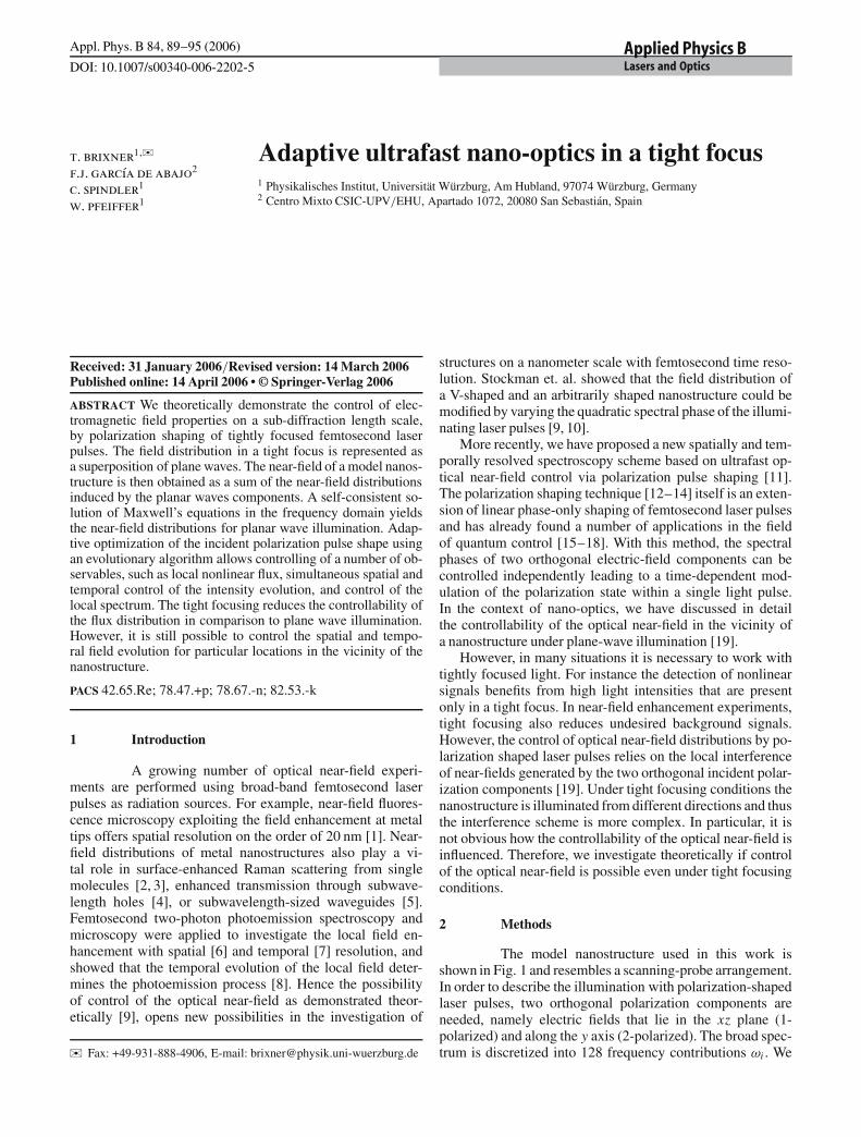
The model nanostructure used in this work isshown in Fig. 1 and resembles a scanning-probe arrangement.In order to describe the illumination with polarization-shapedlaser pulses, two orthogonal polarization components areneeded, namely electric fields that lie in the xz plane (1-polarized) and along the y axis (2-polarized). The broad spec-trum is discretized into 128 frequency contributions ωi . We

90 Applied Physics B – Lasers and Optics

FIGURE 1 Model nanostructure. A gold sphere of 25 nm radius resides inthe origin of the coordinate system. The apex of a truncated conical gold tipof 1500 nm length, a tip radius of 10 nm, and an opening angle of 5◦ is lo-cated 5 nm above the sphere. The focused illumination and the representationof the focused beam as a superposition of planar waves with wave vectorsk(θ ′, φ′) is indicated. The polarization directions 1 and 2 in front of the lensare shown as arrow and ⊗, respectively

then consider an ideal thin lens of focal length f and apertureradius R that focuses these incident polarization-shaped laserpulses. The field distribution in the focus is represented asplane waves with appropriate amplitudes, phases, and polar-ization directions (see below). In order to obtain the completefield in the presence of the nanostructure, we first calculatethe near-field response for each planar wave component foreach frequency ωi , and for the two external input polariza-tion components 1 and 2. Then the vectorial and coherentsuperposition gives the total field.

The optical near-field distribution for a particular pla-nar wave is obtained by solving the frequency-dependentMaxwell equations by means of the boundary-element method.This Green’s function approach is extensively discussed else-where [20, 21], and offers a rigorous solution. The materialproperties are taken into account by a frequency-dependentdielectric function. In our case, an experimentally determinedε(ω) is used for gold [22], setting µ(ω) = 1. As a result, weobtain complex-valued field enhancement vectors A(1)

near(r, ω)

and A(2)near(r, ω) for any point r in the near-field at frequency

ω, induced by linearly 1-polarized and 2-polarized complex-valued incident fields, respectively. The local field Enear(r, ω)

for plane-wave illumination is obtained as a superposition ofthe near-fields induced by the two incident polarization com-ponents:

Enear(r, ω) =2∑

j=1

√I ( j)(ω)eiΦ( j)(ω) A( j)

near(r, ω) , (1)

with the spectrum I ( j)(ω) and the spectral phase Φ( j)(ω) ofthe laser pulse polarization components after the pulse shaper.

We omit the proportionality factors connecting the intensityand electric field. The amplitude |A( j)

near(r, ω)| gives the en-hancement of the field strength, and the phase arg A( j)

near(r, ω)

is required for the correct vectorial superposition of the fieldcomponents.

In addition to the near-field calculation, the illuminationby a tightly focused laser beam is considered using a repre-sentation first derived by Richards and Wolf [23]. The field ina focus Efocal(r, ω) is represented as a superposition of planarwaves with wave vectors k(θ ′, φ′) pointing towards the focalpoint at the origin:

E( j)focal(r, ω) = iω f

2πc

√I ( j)(ω)eiΦ( j)(ω)

×θ′

c∫

0

2π∫

0

u(θ ′)√

cos θ ′ sin θ ′ p′( j)(θ ′, φ′)eik·r dφ′dθ ′,

(2)

with angular frequency ω = kc, focal length f , and the projec-tion k · r of the propagation vector k onto the position vectorr of the observation point. The vector p′( j)

(θ ′, φ′)eik·r = Avac

describes the field distribution of a planar wave with polar-ization vector p′( j). In the case of near-field calculations, Avac

will be replaced by the local response Anear(

p′( j)(θ0, θ

′, φ′),r, ω

)in the presence of a nanostructure (see below). The

superscript ( j) again indicates the two different field distri-butions for externally 1-polarized and 2-polarized light. Theintegration over the azimuth angle φ′ covers the entire range[0, 2π], while the polar angle θ ′ runs from 0 to a limiting angleθ ′

c. This limit is given by the radius R = f tan θ ′c of the lens

aperture used for focusing.As mentioned above, in this work we are mainly interested

in the question of how the superposition of many plane-wavecomponents in a tight focus influences the degree of attain-able near-field control. Hence we concentrate on the idealizedplane-wave components and do not consider the implicationsthat arise from real (thick) lenses such as microscope objec-tives. However, the spatial variation of material dispersion forlight transmitted through different parts of the lens (and there-fore through different amounts of material) could in principlebe taken into account in (6) below by adding an appropriatedispersion term for each partial component, or one could con-sider using a reflective mirror.

The vectorial electric-field amplitude of a plane-wavecomponent in (2) is given by u(θ ′)

√cos θ ′ sin θ ′ p′( j)

(θ ′, φ′)where u(θ ′) = exp(− f 2 tan2 θ ′/σ2) represents the transverseGaussian amplitude profile of the laser beam before focusingthat has unit amplitude on the optical axis. The beam waist isσ , and p′( j)

(θ ′, φ′) is a unit vector describing the polarizationdirection that is discussed below. The factors

√cos θ ′ sin θ ′

ensure the conservation of energy.The polarization of a plane wave depends on the input po-

larization j = 1 or j = 2 of the laser pulse. For a 1-polarizedwave in front of the lens, the polarization direction in the focalregion is given by [23]

p′(1)(θ ′, φ′) =

⎛

⎝(cos θ ′ −1) sin2 φ′ − cos θ ′(cos θ ′ −1) cosφ′ sin φ′

sin θ ′ cos φ′

⎞

⎠ , (3)

BRIXNER et al. Adaptive ultrafast nano-optics in a tight focus 91

in the primed coordinate system of the mean propagation di-rection (optical axis) for a partial wave propagating in thedirection defined by the angles θ ′ and φ′. For 2-polarized light,it can be shown that

p′(2)(θ ′, φ′) =

⎛

⎝(cos θ ′ −1) cosφ′ sin φ′

(cos θ ′ −1) cos2 φ′ − cos θ ′sin θ ′ sin φ′

⎞

⎠ . (4)

However, for the illumination of a nanostructure as inFig. 1 this is not yet the most general description. Here theorientation of the optical axis with respect to the coordinatesystem of the nanostructure must also be considered. This isdone via a coordinate transformation (x ′, y′, z′) → (x, y, z)into the unprimed coordinate system of the nanostructure, andit requires a rotation of the polarization vectors p′(1)

(θ ′, φ′)and p′(2)

(θ ′, φ′) around the y axis by the angle θ0 (Fig. 1). Forthat purpose the two vectors p′(1)

(θ ′, φ′) and p′(2)(θ ′, φ′) are

multiplied with the rotation matrix

Dy(θ0) =⎛

⎝cos θ0 0 sin θ0

0 1 0− sin θ0 0 cos θ0

⎞

⎠ . (5)

The resulting vectors p(1)(θ0, θ′, φ′) and p(2)(θ0, θ

′, φ′) de-scribe the polarization of the partial waves after the lens in thecoordinate system of the nanostructure that is used to calculatethe optical near-field response.

So far in this section, the electric field in a (tight) focus infree space has been calculated as a coherent superposition ofplane wave components. In order to get the total field in thevicinity of the nanostructure, we have to sum over the opticalnear-field response A( j)

near(r, ω) for each planar wave compon-ent. For this purpose, A( j)

near(

p( j)(θ0, θ′l , φ

′l), r, ω

)is calculated

separately for each planar wave component, and the total fieldis then obtained as

E(r, ω) = ∆θ ′∆Φ′2∑

j=1

√I ( j)(ω)eiΦ( j)(ω)

×N∑

l=1

u(θ ′l )

√cos θ ′

l sin θ ′l A( j)

near

(p( j)(θ0, θ

′l , φ

′l), r, ω

). (6)

The continuous integration over θ ′ and φ′ has been replaced bya discretization over a grid (θ ′

l , φ′l) of N input directions and

homogeneous step sizes ∆θ ′, ∆Φ′. Here 10 equidistant dis-cretization steps were used for both angles. The convergenceof the resulting field distribution was checked by increasingthe number of steps. Assuming an identical beam profile forall incident frequency components, the second sum in (6) canbe carried out irrespective of the particular incidence pulseshape, thus defining an effective Anear,focal. Hence the simplestructure of (1) is recovered with an Anear,focal that contains theeffects of tight focusing. Once Anear,focal has been determinedit is thus computationally cheap to calculate any desired near-field properties for different polarization-shaped input laserpulses.

In the calculation, the laser pulses have Gaussian spec-tra (central frequency ω0 = 2.456 fs−1, FWHM = 0.23 fs−1)

that are sampled at 128 equidistant frequency points. This dis-cretization is chosen to describe pulse shaping with a commer-cially available two-layer liquid-crystal display (LCD) spatiallight modulator that contains 128 pixels. Polarization shap-ing is achieved in a zero-dispersion compressor that spatiallydisperses the frequency components onto the LCD pixelsvia a grating/lens combination, followed by recollimation ina second lens/grating pair [12–14]. Each LCD pixel containstwo successive layers with mutually orthogonal preferentialorientation axes of the liquid-crystal molecules. By adjust-ing the LCD pixel voltages, the refractive index can thus bemodified independently for the two polarization componentsj = 1 and j = 2 and for each of the 128 frequency compo-nents. In the time domain this corresponds to complex tran-sient polarization states. According to the time–bandwidthproduct the width of the spectrum determines the fastest pos-sible change of local illumination conditions, i.e. variationsin the field strength and/or the field vector orientation [14].The number of LCD pixels, on the other hand, is proportionalto the maximum time window that is available for shapedpulses.

3 Objectives

In the previous section, we have shown how to cal-culate the total electric field in the vicinity of a nanostructureunder tight focusing conditions for any frequency ω and loca-tion r. The input polarization state is taken into account via theamplitudes

√I ( j)(ω) and the phases Φ( j)(ω), of the polariza-

tion components j = 1 and j = 2.Using the polarization-shaped incident fields in (6), we

obtain the local near-field of a polarization-shaped femtosec-ond laser pulse, and an additional Fourier transformation de-livers the time-dependent local field E(r, t). The quality ofhow well a given pulse shape produces the desired near-fieldproperties is measured by means of a fitness value. In the fol-lowing, some near-field observables and the correspondingfitness functions are defined.

The local nonlinear flux is defined as the integratedsquared intensity,

F(r) =∞∫

−∞I2(r, t)dt =

∞∫

−∞

[∑

α=x,y,z

a2α E2

α(r, t)

]2

dt. (7)

Here Eα(r, t) are the local amplitude components in the co-ordinate system of the nanostructure after frequency–timeFourier transformation of (6), and the factors aα determinewhich components are considered. A possible control objec-tive is now to localize F at a desired point ri in the near-field.This can be achieved with the fitness function

fF =

+∞∫−∞

[∑

α=x,y,za2

α E2α(ri, t)

]2

dt

∑n �=i

[1 − g(rn − ri)]+∞∫−∞

[∑

α=x,y,za2

α E2α(rn, t)

]2

dt

. (8)

Maximizing fF leads to high nonlinear flux at ri (numerator)and low nonlinear flux at all other points rn (denominator).

92 Applied Physics B – Lasers and Optics

In the following a regular mesh of 21 ×21 points rj coveringa 200×200 nm2 square in the z = 27.5 nm plane is used. Thisplane is located in the middle between tip and nanosphere andtherefore controllability of the field distribution in this plane isof particular interest. Since near-field distributions are contin-uous and do not vary abruptly [19], localizing high flux at thetarget ri will necessarily also increase flux at positions nearby.For that reason, the Gaussian weighting factor

1 − g(rn − ri) = 1 − e−4 ln 2

|rn−ri |2w2

g , (9)

is introduced. The penalty weight for high flux at undesiredpoints hence increases with distance from the target point ri

until for points much further away than wg all penalty weightsare equal to 1. The Gaussian width wg is chosen on the orderof the near-field variation length scale, here wg = 25 nm.

Another near-field property that we will attempt to controlis the local time-dependent intensity, defined as the squaredamplitude of the electric field,

I(r, t) =∑

α=x,y,z

a2α E2

α(r, t) . (10)

Again, certain components of the electric field can be selectedby adjusting the parameters aα. In order to enable a spatial lo-calization of time-dependent intensity, the following fitnessfunction is introduced:

f I =∑

i

+∞∫

−∞

⎡

⎢⎣

∑α=x,y,z

a2α E2

α(ri, t)

∑α=x,y,z

a2α E2

α(ri, ti)− pi(t)

⎤

⎥⎦

2

dt . (11)

The individual target functions at points ri ,

pi(t) = e−4 ln 2

(t−tiτi

)2

, (12)

are Gaussian pulses of FWHM τi and centered at ti , that canbe chosen separately for each target point i = 1, 2, 3, . . . .Equation (11) describes the deviation of the actual field in-tensity from the target profile, summed over all target pointsand times. For a given electric near-field Eα(r, t), the fractionin (11) denotes the normalized temporal intensity for point ri

at time t. The normalization occurs with respect to the timeti of the target maximum that can be chosen differently forevery point. Minimization of fI leads to the smallest deviationfrom the target profiles and hence to the best realization of theobjective.

As a third and final objective, we consider control of thelocal spectrum, defined as

S(r, ω) =∑

α=x,y,z

a2α E2

α(r, ω) . (13)

In corresponding optimizations, the fitness function

fS =∫

b1S(r1, ω)dω

∫b1

S(r1, ω)dω·∫

b2S(r2, ω)dω

∫b2

S(r2, ω)dω(14)

is employed. Here, the regions b1, b2 are subsets of the laserbandwidth, and bi contains all those frequencies in the spec-trum that are not contained in bi . The two ratios can be read

as follows: the fitness increases if there are predominant fre-quencies of band b1 at position r1 and of band b2 at r2,whereas the fitness fS decreases if there are undesired fre-quencies outside of b1 at r1 and outside of b2 at r2. If anoptimization with such a fitness function succeeds, this re-sults in spatial regions where one of the two frequency bandsdominates.

The optimization procedure in all cases works in the fol-lowing way: first, the near-field enhancement factors are cal-culated as described in Sect. 2. Then, for every particular opti-mization objective the fitness function is minimized/maximi-zed employing an evolutionary algorithm [24] that varies thespectral phases of the two incident polarization components.All spectral values Φ( j)(ω) are varied independently, and con-vergence is typically reached after 200 generations with 60individuals each. One full optimization thus takes about 1 h onan Athlon XP 2600+ machine. Results will be discussed forthe best individual of the last generation.

The illumination direction is always as indicated in Fig. 1,using focal length f = 2.9 mm, lens aperture radius R =6 mm and beam waist σ = 2 mm. This corresponds to a nu-merical aperture of NA = 0.9, and the mean angle of inci-dence is θ0 = 45◦. Each coordinate axis θ ′, φ′ is discretizedin 10 steps with step sizes of ∆θ ′ = 6.42◦ and ∆φ′ = 36.00◦,respectively.

4 Results

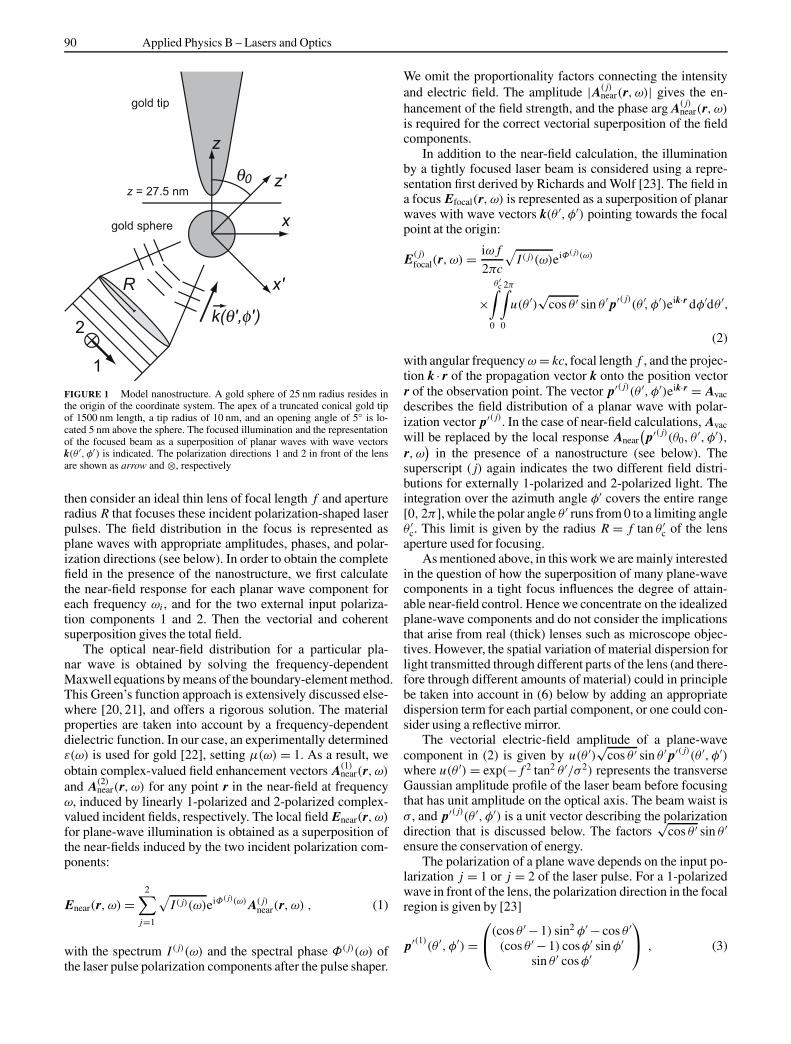
The fitness function defined in (8) for the nonlin-ear flux allows localization at a defined point ri in the near-field. In Fig. 2 the optimized nonlinear flux distributions (withax = ay = 1, az = 0) for some representative target points areshown. For targets in the left half-plane, nonlinear flux canbe localized over a wide range, i.e. the actual flux distribu-tions (contour lines) are peaked at the desired target locations(crosses). In the case of positive x values for ri (Fig. 2, lowerright), the algorithm still succeeds in shifting nonlinear flux to

FIGURE 2 Control of nonlinear flux. The distributions of nonlinear flux areshown as contour lines for four different target points (crosses). In contrastto plane-wave illumination [19], here the high-contrast controllable area isrestricted to points with negative x coordinates

BRIXNER et al. Adaptive ultrafast nano-optics in a tight focus 93

the desired point. However, the simultaneous increase of thesignal at the opposed position (−20, 20, 27.5) nm cannot beavoided.

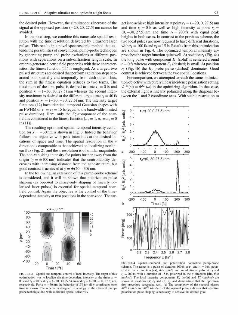
In the next step, we combine this nanoscale spatial reso-lution with the time resolution delivered by ultrashort laserpulses. This results in a novel spectroscopic method that ex-tends the possibilities of conventional pump-probe techniquesby generating pump and probe excitations at different pos-itions with separations on a sub-diffraction length scale. Inorder to generate electric field properties with these character-istics, the fitness function (11) is employed. As a target, twopulsed structures are desired that perform excitation steps sep-arated both spatially and temporally from each other. Thus,the sum in the fitness equation reduces to two terms. Themaximum of the first pulse is desired at time t1 = 0 fs andposition r1 = (−30, 30, 27.5) nm whereas the second inten-sity maximum is desired at the different target time t2 = 40 fsand position r2 = (−30,−30, 27.5) nm. The intensity targetfunctions (12) have identical temporal Gaussian shapes withan FWHM of τ1 = τ2 = 15 fs (equal to the bandwidth-limitedpulse duration). Here, only the E2

y-component of the near-field is considered in the fitness function [ay = 1, ax = az = 0in (11)].

The resulting optimized spatial–temporal intensity evolu-tion for x = −30 nm is shown in Fig. 3. Indeed the behaviorfollows the objective with peak intensities at the desired lo-cations of space and time. The spatial resolution in the ydirection is comparable to that achieved on localizing nonlin-ear flux (Fig. 2), and the x resolution is of similar magnitude.The non-vanishing intensity for points further away from theorigin (y = ±100 nm) indicates that the controllability de-creases with increasing distance from the nanostructure, butgood contrast is achieved at y = ±(20 −30) nm.

In the following, an extension of this pump-probe schemeis considered, and it will be shown that polarization pulseshaping (as opposed to phase-only shaping of linearly po-larized laser pulses) is essential for spatial–temporal near-field control. Again the objective is the control of the time-dependent intensity at two positions in the near-zone. The tar-

FIGURE 3 Spatial and temporal control of local intensity. The target of thisoptimization was to localize the time-dependent intensity at the times t1 =0 fs and t2 = 40 fs at r1 = (−30, 30, 27.5) nm and r2 = (−30,−30, 27.5) nm,respectively. For x = −30 nm the behavior of E2

y for all y-coordinates overtime is shown. The scheme is designed in analogy to the classical pump-probe technique, but with additional spatial selectivity

get is to achieve high intensity at point r1 = (−20, 0, 27.5) nmand time t1 = 0 fs as well as high intensity at point r2 =(0,−30, 27.5) nm and time t2 = 200 fs with equal peakheights in both cases. In contrast to the previous scheme, thetwo local pulses are now required to have different durations,with τ1 = 100 fs and τ2 = 15 fs. Results from this optimizationare shown in Fig. 4. The optimized temporal intensity ap-proaches the target function quite well. At position r1 (Fig. 4a)the long pulse with component Ex (solid) is centered aroundt = 0 fs whereas component Ey (dashed) is small. At positionr2 (Fig. 4b) the Ey probe pulse (dashed) dominates. Goodcontrast is achieved between the two spatial locations.

For comparison, we attempted to reach the same optimiza-tion objective with purely linear incidence polarization settingΦ(1)(ω) = Φ(2)(ω) in the optimizing algorithm. In that case,the external light is linearly polarized along the diagonal be-tween the 1 and 2 coordinate axes. With such a restriction to

FIGURE 4 Spatial–temporal and polarization controlled pump-probescheme. The target is a pulse of duration 100 fs at r1 and t1 = 0 fs, polar-ized in the x direction [(a), thin solid], and an additional pulse at r2 andt2 = 200 fs, with a duration of 15 fs, polarized in the y direction [(b), thindashed]. The local intensity components E2

x (solid) and E2y (dashed) are

shown at locations (a) r1 and (b) r2, and demonstrate that the optimiza-tion procedure succeeded well. (c) The complexity of the spectral phasesΦ(1) (solid) and Φ(2) (dashed) of the optimal pulse indicates that adaptivepolarization pulse shaping is necessary to achieve the desired goal

94 Applied Physics B – Lasers and Optics

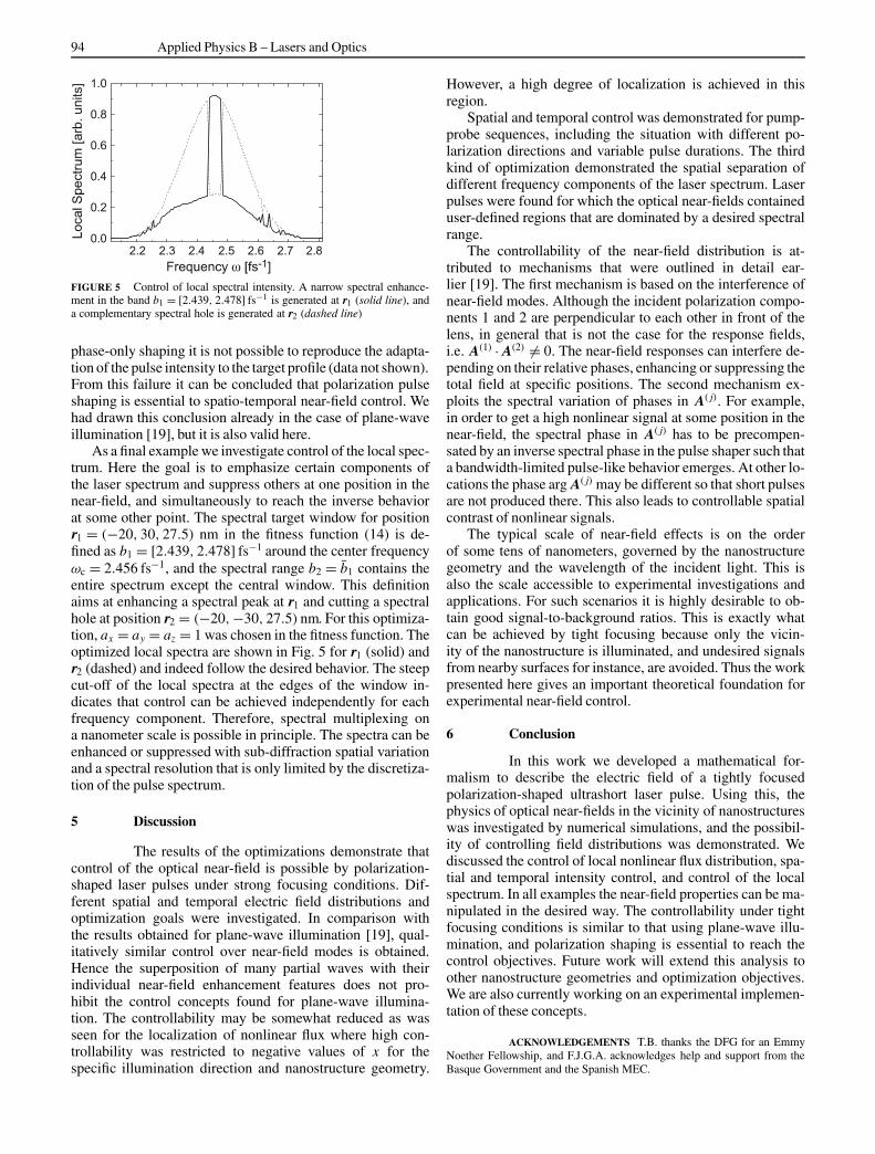
FIGURE 5 Control of local spectral intensity. A narrow spectral enhance-ment in the band b1 = [2.439, 2.478] fs−1 is generated at r1 (solid line), anda complementary spectral hole is generated at r2 (dashed line)

phase-only shaping it is not possible to reproduce the adapta-tion of the pulse intensity to the target profile (data not shown).From this failure it can be concluded that polarization pulseshaping is essential to spatio-temporal near-field control. Wehad drawn this conclusion already in the case of plane-waveillumination [19], but it is also valid here.

As a final example we investigate control of the local spec-trum. Here the goal is to emphasize certain components ofthe laser spectrum and suppress others at one position in thenear-field, and simultaneously to reach the inverse behaviorat some other point. The spectral target window for positionr1 = (−20, 30, 27.5) nm in the fitness function (14) is de-fined as b1 = [2.439, 2.478] fs−1 around the center frequencyωc = 2.456 fs−1, and the spectral range b2 = b1 contains theentire spectrum except the central window. This definitionaims at enhancing a spectral peak at r1 and cutting a spectralhole at position r2 = (−20,−30, 27.5) nm. For this optimiza-tion, ax = ay = az = 1 was chosen in the fitness function. Theoptimized local spectra are shown in Fig. 5 for r1 (solid) andr2 (dashed) and indeed follow the desired behavior. The steepcut-off of the local spectra at the edges of the window in-dicates that control can be achieved independently for eachfrequency component. Therefore, spectral multiplexing ona nanometer scale is possible in principle. The spectra can beenhanced or suppressed with sub-diffraction spatial variationand a spectral resolution that is only limited by the discretiza-tion of the pulse spectrum.

5 Discussion

The results of the optimizations demonstrate thatcontrol of the optical near-field is possible by polarization-shaped laser pulses under strong focusing conditions. Dif-ferent spatial and temporal electric field distributions andoptimization goals were investigated. In comparison withthe results obtained for plane-wave illumination [19], qual-itatively similar control over near-field modes is obtained.Hence the superposition of many partial waves with theirindividual near-field enhancement features does not pro-hibit the control concepts found for plane-wave illumina-tion. The controllability may be somewhat reduced as wasseen for the localization of nonlinear flux where high con-trollability was restricted to negative values of x for thespecific illumination direction and nanostructure geometry.

However, a high degree of localization is achieved in thisregion.

Spatial and temporal control was demonstrated for pump-probe sequences, including the situation with different po-larization directions and variable pulse durations. The thirdkind of optimization demonstrated the spatial separation ofdifferent frequency components of the laser spectrum. Laserpulses were found for which the optical near-fields containeduser-defined regions that are dominated by a desired spectralrange.

The controllability of the near-field distribution is at-tributed to mechanisms that were outlined in detail ear-lier [19]. The first mechanism is based on the interference ofnear-field modes. Although the incident polarization compo-nents 1 and 2 are perpendicular to each other in front of thelens, in general that is not the case for the response fields,i.e. A(1) · A(2) �= 0. The near-field responses can interfere de-pending on their relative phases, enhancing or suppressing thetotal field at specific positions. The second mechanism ex-ploits the spectral variation of phases in A( j). For example,in order to get a high nonlinear signal at some position in thenear-field, the spectral phase in A( j) has to be precompen-sated by an inverse spectral phase in the pulse shaper such thata bandwidth-limited pulse-like behavior emerges. At other lo-cations the phase arg A( j) may be different so that short pulsesare not produced there. This also leads to controllable spatialcontrast of nonlinear signals.

The typical scale of near-field effects is on the orderof some tens of nanometers, governed by the nanostructuregeometry and the wavelength of the incident light. This isalso the scale accessible to experimental investigations andapplications. For such scenarios it is highly desirable to ob-tain good signal-to-background ratios. This is exactly whatcan be achieved by tight focusing because only the vicin-ity of the nanostructure is illuminated, and undesired signalsfrom nearby surfaces for instance, are avoided. Thus the workpresented here gives an important theoretical foundation forexperimental near-field control.

6 Conclusion

In this work we developed a mathematical for-malism to describe the electric field of a tightly focusedpolarization-shaped ultrashort laser pulse. Using this, thephysics of optical near-fields in the vicinity of nanostructureswas investigated by numerical simulations, and the possibil-ity of controlling field distributions was demonstrated. Wediscussed the control of local nonlinear flux distribution, spa-tial and temporal intensity control, and control of the localspectrum. In all examples the near-field properties can be ma-nipulated in the desired way. The controllability under tightfocusing conditions is similar to that using plane-wave illu-mination, and polarization shaping is essential to reach thecontrol objectives. Future work will extend this analysis toother nanostructure geometries and optimization objectives.We are also currently working on an experimental implemen-tation of these concepts.

ACKNOWLEDGEMENTS T.B. thanks the DFG for an EmmyNoether Fellowship, and F.J.G.A. acknowledges help and support from theBasque Government and the Spanish MEC.

BRIXNER et al. Adaptive ultrafast nano-optics in a tight focus 95

REFERENCES

1 E.J. Sanchez, L. Novotny, X.S. Xie, Phys. Rev. Lett. 82, 4014 (1999)2 K. Kneipp, Y. Wang, H. Kneipp, L.T. Perelman, I. Itzkan, R.R. Dasari,

M.S. Feld, Phys. Rev. Lett. 78, 1667 (1997)3 S.R. Emroy, S. Nie, Anal. Chem. 69, 2631 (1997)4 T.W. Ebbesen, H.J. Lezec, H.F. Ghaemi, T. Thio, P.A. Wolff, Nature 391,

667 (1998)5 M. Quinten, A. Leitner, J.R. Krenn, F.R. Aussenegg, Opt. Lett. 23, 1331

(1998)6 M. Munzinger, C. Wiemann, M. Rohmer, L. Guo, M. Aeschlimann,

M. Bauer, New J. Phys. 7, 68 (2005)7 A. Kubo, K. Onda, H. Petek, Z. Sun, Y.S. Jung, H.K. Kim, Nano Lett. 5,

1123 (2005)8 M. Merschdorf, C. Kennerknecht, W. Pfeiffer, Phys. Rev. B 70, 193 401

(2004)9 M.I. Stockman, S.V. Faleev, D.J. Bergman, Phys. Rev. Lett. 88, 067 402

(2002)10 M.I. Stockman, D.J. Bergman, T. Kobayashi, Phys. Rev. B 69, 054 202

(2004)11 T. Brixner, F.J. Garcıa de Abajo, J. Schneider, W. Pfeiffer, Phys. Rev.

Lett. 95, 093 901 (2005)

12 T. Brixner, G. Gerber, Opt. Lett. 26, 557 (2001)13 T. Brixner, G. Krampert, P. Niklaus, G. Gerber, Appl. Phys. B 74, S133

(2002)14 T. Brixner, Appl. Phys. B 76, 531 (2003)15 D. Oron, N. Dudovich, Y. Silberberg, Phys. Rev. Lett. 90, 213 902

(2003)16 N. Dudovich, D. Oron, Y. Silberberg, Phys. Rev. Lett. 92, 103 003

(2004)17 T. Suzuki, S. Minemoto, T. Kanai, H. Sakai, Phys. Rev. Lett. 92, 133 005

(2004)18 T. Brixner, G. Krampert, T. Pfeifer, R. Selle, G. Gerber, M. Wollenhaupt,

O. Graefe, C. Horn, D. Liese, T. Baumert, Phys. Rev. Lett. 92, 208 301(2004)

19 T. Brixner, F.J. Garcıa de Abajo, J. Schneider, C. Spindler, W. Pfeiffer,Phys. Rev. B 73, 125 437 (2006)

20 F.J. Garcıa de Abajo, A. Howie, Phys. Rev. Lett. 80, 5180 (1999)21 F.J. Garcıa de Abajo, A. Howie, Phys. Rev. B 65, 115 418 (2002)22 E.D. Palik, Handbook of Optical Constants of Solids (Academic, New

York, 1997)23 B. Richards, E. Wolf, Proc. R. Soc. London A 253, 358 (1959)24 T. Baumert, T. Brixner, V. Seyfried, M. Strehle, G. Gerber, Appl. Phys.

B 65, 779 (1997)