Adaptive Slope Filtering of Airborne LiDAR Data … hilly areas such as forests, and from flat area such as riverbanks. Validation using reference data showed that, compared with commercial

Remote Sens. 2012, 4, 1804-1819; doi:10.3390/rs4061804

Remote Sensing ISSN 2072-4292

www.mdpi.com/journal/remotesensing

Article

Adaptive Slope Filtering of Airborne LiDAR Data in Urban

Areas for Digital Terrain Model (DTM) Generation

Junichi Susaki

Graduate School of Engineering, Kyoto University, Kyotodaigaku Katsura, Nishikyo-ku,

Kyoto 615-8540, Japan; E-Mail: [email protected]; Tel.: +81-75-383-3300;

Fax: +81-75-383-3300

Received: 30 April 2012; in revised form: 14 June 2012 / Accepted: 14 June 2012 /

Published: 18 June 2012

Abstract: A filtering algorithm is proposed that accurately extracts ground data from

airborne light detection and ranging (LiDAR) measurements and generates an estimated

digital terrain model (DTM). The proposed algorithm utilizes planar surface features and

connectivity with locally lowest points to improve the extraction of ground points (GPs). A

slope parameter used in the proposed algorithm is updated after an initial estimation of the

DTM, and thus local terrain information can be included. As a result, the proposed

algorithm can extract GPs from areas where different degrees of slope variation are

interspersed. Specifically, along roads and streets, GPs were extracted from urban areas,

from hilly areas such as forests, and from flat area such as riverbanks. Validation using

reference data showed that, compared with commercial filtering software, the proposed

algorithm extracts GPs with higher accuracy. Therefore, the proposed filtering algorithm

effectively generates DTMs, even for dense urban areas, from airborne LiDAR data.

Keywords: airborne LiDAR; filtering; slope variation

1. Introduction

Three-dimensional (3D) urban building models are used in various applications, and the data

necessary for modeling, such as building height estimates, can be generated by using airborne light

detection and ranging (LiDAR). Airborne LiDAR measures laser light reflected from the surface of

objects, and a digital surface model (DSM) is generated by interpolating the discrete LiDAR data.

During preprocessing of the 3D models, ground points (GPs) in the LiDAR data are separated from

non-GPs. This process is called filtering, and a digital terrain model (DTM) can be generated by

OPEN ACCESS

Remote Sens. 2012, 4

1805

interpolating the extracted GPs. The heights of objects, such as trees and buildings, are then estimated

by examining the differences between the DSM and the DTM. The accuracy of DTM estimation,

therefore, affects the accuracy of the building models.

Sithole and Vosselman [1] classified approaches to airborne LiDAR data filtering as slope-based

[2,3], block-minimum [4,5], surface-based, and clustering/segmentation [6]. Slope-based and

block-minimum filters are straightforward to implement. In clustering/segmentation approaches,

mathematical morphology—which is widely used in image processing—has been applied in the

filtering process [7,8]. Meng et al. [9] pointed out that LiDAR ground filtering algorithms make

different assumptions about ground characteristics to differentiate between ground and nonground

features, and listed eight features that confound ground filtering algorithms: (1) shrubs, (2) short walls

along walkways, (3) bridges, (4) buildings with different size and shape, (5) hill cut-off edges,

(6) complex mixed covering, (7) areas combining low and high-relief terrains, and (8) lack of reliable

accuracy assessment [9]. Sithole and Vosselman [1] presented experimental results that assessed the

different types of filters. The performance was analyzed qualitatively and quantitatively by using

datasets that included terrain with steep slopes, vegetation, buildings, ramps, underpasses, tunnel

entrances, bridges, a quarry, and data gaps. Their performance assessment showed that the greatest

challenges for filters appear to be complex cityscapes and discontinuities in the bare earth, and

therefore tailoring the algorithms for these areas may improve categorization results [1].

My interest is in efficient, automatic generation of 3D models in dense urban areas from airborne

LiDAR for civil engineering applications, for example, earthquake damage assessment. In such

applications, 3D models should have geolocational accuracy of approximately 30–50 cm. Prior to 3D

modeling, however, a filtering algorithm applicable to dense urban areas is necessary. Among the

features mentioned above, filtering for dense urban areas requires dealing with steep slopes,

vegetation, buildings, bridges, and rivers. Narrow streets and numerous buildings are found in dense

urban areas, and therefore filtering of airborne LiDAR data is more challenging because data sampling

has not been tuned to the level of information to be extracted. In addition, when areas are hilly, GP

detection may fail because of height variations. Another problem encountered in filtering of dense

urban areas is that a river running through the area may lower DTM accuracy. This may be partly

because GPs on or near bridges over the river are not extracted accurately, and partly because

erroneous GPs are selected near the river and bridges when generating the DTM by interpolation.

DTMs in urban areas have been estimated by using the morphological approach [8] and a hybrid

conditional random field [10]. Yuan et al. [11] proposed a filtering algorithm that combines slope-

based and region-growing methods, and applied their algorithm to urban areas. However, their results

suggest that this combined approach is not guaranteed to function well in dense urban areas. In

addition, the slope angle in slope-based morphological filtering [2,3] is defined as the relative angle

with the ground inclination subtracted. This slope setting may extract more points on objects,

especially in dense urban areas.

Tuning the parameters used in filters is among the most important issues for efficient filtering.

Sithole and Vosselman [1] addressed an ideal case of automatic filter selection and tuning because the

optimal filter algorithm may vary according to the landscape. Zhang et al. [7] pointed out that filtering

parameter selection has a considerable impact on the removal of non-GPs. They suggested tuning

parameters by analyzing terrain and nonterrain measurement data. In another example, Yuan et al. [11]


1806

stated that the slope threshold used in their algorithm was empirically selected and instead should be

self-adaptively selected.

To tune the parameters, iterative filtering approaches has been reported [12–14]. For instance,

Axelsson [13] proposed a filtering algorithm to generate sparse triangular irregular networks (TINs)

from seed points and to densify them through an iterative process. This example is pertinent here

because Axelsson’s algorithm is embedded in the widely used commercial filtering software,

TerraScan [15], which is used for performance validation in this paper. Threshold parameters for

distances to TIN facet planes and angles to TIN nodes are computed from data at each iteration.

However, these thresholds are common to the entire study area. In a preliminary examination using a

similar method, GPs were poorly extracted in a study area where relatively flat and hilly areas were

mixed. This poor extraction may occur because the slope parameter was set to a common value for

both flat and hilly areas. Although algorithms that use adaptive slope thresholds [16,17] and a

parameter-free algorithm [18] have been proposed, it is not assured that such algorithms perform

satisfactorily in dense urban areas where narrow streets and numerous buildings are found.

Therefore, I propose a filtering algorithm using an adaptive slope threshold that accurately

distinguishes GPs from non-GPs even in dense urban areas. The performance of the proposed

algorithm is compared with existing algorithms using data obtained from a study area and publicly

available datasets. The rest of this paper is structured as follows. Section 2 describes the new filtering

algorithm. Features of the employed data and the study area are described in Section 3, and

experimental and validation results are reported in Section 4. Conclusions are given in Section 5.

2. Algorithm

This paper focuses on a filtering algorithm for estimating a final DTM. The proposed algorithm

assumes that grid data are used, since using grid-based data is better than irregularly distributed point

clouds in terms of algorithm efficiency and calculation time. When more than one data point is

available within a pixel, the lowest data point is selected. However, the original xy coordinates are

recorded in the pixels.

The proposed algorithm utilizes information on whether a point is contained in a plane for filtering,

and the algorithm can be classified as a slope-based morphological filtering approach. Sithole and

Vosselman [6] and Tovari and Pfeifer [19] proposed segmentation based on planar surface information

prior to filtering. Segmentation is also implemented on planar surface information in the proposed

algorithm, but planar surface information in flat and almost flat areas is used to generate initial GPs only.

Another challenge is the automatic updating of parameters. For example, the slope-based approach

requires setting a maximum slope parameter to extract GPs from inclined streets. However, a fixed

slope parameter is not suitable for areas where flat and hilly areas are interspersed. The proposed

approach extracts wide rather than narrow streets first. Narrow streets are then extracted by

considering their connectivity with the wide streets. Through this approach, focus is placed on the

planar nature of wide streets in dense urban areas. In addition, the slope parameter in the proposed

algorithm is automatically updated. After an initial DTM is generated with an initial slope parameter, a

local maximum slope is calculated. The slope parameter given to each cell of the grid data is updated

by considering local terrain. Then, the DTM generation process is repeated using the updated


1807

parameter. During the interpolation procedure when generating the DTM, bodies of water are masked

to prevent incorrect GP selection near rivers and bridges.

Figure 1 shows the flowchart of the algorithm. Step (1) selects a large area without data, including

the null pixels connected to this area, as an initial body of water. In Step (2), locally lowest points

(LLPs) are selected by searching elevation data within a window. Step (3) extracts planar areas by

estimating the planes that minimize the root mean square error (RMSE). The planar equation is

expressed as:

,0 dczbyax (1)

where a, b, c, and d are coefficients. The minimum eigenvalue, and thus the minimum eigenvector, of

the matrix:

n

i

i

n

i

ii

n

i

ii

n

i

ii

n

i

i

n

i

ii

n

i

ii

n

i

ii

n

i

i

zzzzyyzzxx

zzyyyyyyxx

zzxxyyxxxx

1

2

11

11

2

1

111

2

)())(())((

))(()())((

))(())(()(

(2)

is then calculated, where x , y , and z are the means of x, y, and z, respectively. The minimum

eigenvector is equivalent to the optimal vector )ˆ,ˆ,ˆ( cba in Equation (1). Step (3) checks whether the

RMSE of each optimal plane is less than a given threshold.

Figure 1. Flowchart of proposed algorithm to generate a DTM.

The calculation is conducted using all the points in a window, and is repeated for regions within

windows that include a target pixel. The plane with the lowest RMSE is selected. If the RMSE is

(2) Find locally

lowest points (LLP)

(4) Determine ground point (GP)

(3) Estimate plane

Start

Initial slope

parameter

(5) Determine new GPs

using GP planes

(6) Estimate DTM

End

(8) Update

slope

parameter1st loop?

No

Yes

(7) Determinate new GPs

by using DTM

New GPs?Yes

No

Iteration

To Step (6)

From Step (5)(1) Extract bodies of water


1808

smaller and the distance between the pixel and the plane is shorter than the designated thresholds, the

pixel is regarded as having a planar surface. At this stage, ground data in addition to roof data for

buildings are selected. “Minimum vertical component of the planar normal” is used to extract streets.

The estimated planes include streets and building roofs. To exclude the roofs, especially pitched roofs,

and to retain hilly streets, normals to the plane whose vertical component is within a small tilt range in

any direction are accepted.

In Step (4), if data selected above are connected with a LLP within designated vertical distance and

slope angle thresholds, they are labeled as GP. The slope angle i is defined as

,)()(

tan22

1

tgtitgti

tgti

i

yyxx

zz (3)

where xi, yi, and zi are the x, y, and z coordinates of point i, respectively, and xtgt, ytgt, and ztgt are the x, y,

and z coordinates of the target ground point, respectively (Figure 2). When calculating the slope, the

original xy coordinates of the LLP are used. Others data are temporarily labeled as non-GP candidates.

Step (5) adds more GPs. If non-GP candidates within the same window size as Step (3) are closer to

the GP plane than a designated threshold (as indicated in Figure 2), they are labeled as GPs. Although

some of the actual GPs are not extracted in Step (4), more are extracted at this stage.

Figure 2. Searching for new GPs by using planes. A new GP is added when the distance

between the point and plane calculated at the target ground point is within a threshold, and

the horizontal distance between the point and target ground point is within another threshold,

“Window size”.

Step (6) estimates the DTM by using neighboring GPs. In the present research, inverse distance

weighted (IDW) interpolation is employed because of its simple implementation. The weights of the

data available for the interpolation are assigned such that they are inversely proportional to the distance

from the target point. When at least three GPs are available within a threshold distance along four

directions, the elevation of a non-GP is interpolated by using the elevations of GPs. The search along

any direction is terminated when a water body pixel is found to prevent the result from being affected

by the elevation at the river. Two patterns of four directions are examined. This interpolation is

repeated for the entire area. If a pixel does not have at least three available GPs, its elevation is set as

the average elevation of its eight neighboring pixels.

Step (7) filters non-GPs a second time by calculating their distances from the DTM. If the distance

is within a designated threshold, the non-GPs are added to the set of GPs. When a new GP is added,

Step (6) is repeated after completion of Step (7). If no new GPs are added during the first loop, the

dist_max

dh

Target ground

pointPlane

dist

slope

angle


1809

slope parameter is updated by referring to the maximum slope derived from the DTM. Then, the

second loop is conducted (Step (8)).

3. Data Characteristics

Kyoto is famous for being the former capital of Japan, and still has many traditional houses and

landscapes. Higashiyama Ward and Nakagyo Ward of Kyoto were selected as study areas.

Higashiyama is hilly and contains traditional temples and shrines. Nakagyo has a commercial district

and a large number of multistoried buildings. Both areas have narrow streets, which are approximately

5–6 m in width. Details of the airborne LiDAR data for these areas are listed in Table 1.

In total, two LiDAR datasets were available for this research: one for Higashiyama Ward and one

for Nakagyo Ward. These datasets were classified into two categories: “hilly” (Higashiyama dataset)

and “flat with rivers” (Nakagyo dataset).

Table 1. Details of airborne LiDAR.

Measurement date June 2002 to February 2003

Measurer Aero Asahi Corporation

Density

(calculated as valid pixels divided by all

pixels of the area)

Approx. 0.68 points/m2

0.70 for Higashiyama, and

0.66 for Nakagyo

Altitude 900 to 1,000 m

Horizontal accuracy ±50 cm

Vertical accuracy ±15 cm

4. Experiments

4.1. Results

From the original point clouds, 1 m grid data were generated. In this experiment, the parameters

were set to the values listed in Table 2. Results had greater sensitivity to “Window size” in Step (2),

“Maximum slope” in Steps (4), (5), and (8), and “Window size for mean of DTM” in Step (8) than the

other parameters. Those parameters were empirically set through several preliminary experiments.

Among the parameters, the slope parameter, which is the most important, is addressed here. Its value

was fixed at 3.0° in the first loop. In Step (8), a 21 m × 21 m window was selected for the mean DTM

calculations. Then, local maximum slopes were obtained by examining the eight neighboring pixels of

target pixels. If the local maximum slope was ≥4.5°, “Maximum slope” in Steps (4) and (5) was

updated to 4.5°; otherwise, it was kept at 3.0°. The DTM was then regenerated with this updated slope

parameter.

To save computation time, the criterion to repeat Step (6) after Step (7) was that ≥30 points were

added and the number of iterations in Steps (6) and (7) was ≤30. Figure 3 shows the results in hilly

areas (Higashiyama), and Figure 4 shows the results in flat areas with rivers (Nakagyo). Note that the

aerial photographs were acquired in 2007, and LiDAR data were acquired from 2002 to 2003.


1810

Table 2. Parameters in the proposed algorithm and values used for experiments.

Process Parameter Value Used

Step (1): River extraction Window size for initial area detection 7 m × 7 m

Minimum area to accept water body 100 m2

Step (2): Finding locally

lowest points (LLPs) Window size 60 m × 60 m

Step (3): Planar surface

calculation

Window size (used also in Steps (4) and (5)) 5 m × 5 m

Minimum data number to calculate 6 points

Maximum root mean square of errors (RMSE) to

accept plane 0.1 m

Maximum distance to plane (used also in Step (5)) 0.1 m

Minimum vertical component of planar normal 0.9

Step (4): GP determination

Maximum slope

(used also in Steps (5) and (8))

1st loop: 3°

2nd loop: 3° or 4.5°s

Maximum height difference to determine as GP (used

also in Step (7)) 0.5 m

Step (6): DTM estimation

Maximum distance of the closest point (same as

“Window size” in Step (2)) 50 m

Maximum distance of other points 100 m

Window size for mean of DTM 21 m × 21 m

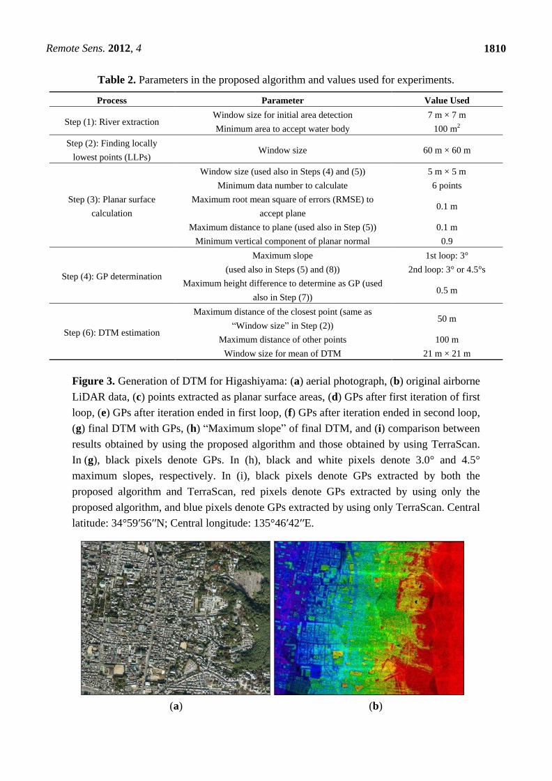
Figure 3. Generation of DTM for Higashiyama: (a) aerial photograph, (b) original airborne

LiDAR data, (c) points extracted as planar surface areas, (d) GPs after first iteration of first

loop, (e) GPs after iteration ended in first loop, (f) GPs after iteration ended in second loop,

(g) final DTM with GPs, (h) “Maximum slope” of final DTM, and (i) comparison between

results obtained by using the proposed algorithm and those obtained by using TerraScan.

In (g), black pixels denote GPs. In (h), black and white pixels denote 3.0° and 4.5°

maximum slopes, respectively. In (i), black pixels denote GPs extracted by both the

proposed algorithm and TerraScan, red pixels denote GPs extracted by using only the

proposed algorithm, and blue pixels denote GPs extracted by using only TerraScan. Central

latitude: 34°59′56′′N; Central longitude: 135°46′42′′E.

(a) (b)


1811

Figure 3. Cont.

(c) (d)

(e) (f)

(g) (h)


1812

Figure 3. Cont.

500 m

(i)

Figure 4. Generation of DTM for Nakagyo: (a) aerial photograph, (b) original airborne

LiDAR data, (c) final DTM with GPs, (d) “Maximum slope” of the final DTM, and

(e) comparison between results obtained by using the proposed algorithm and those

obtained by using TerraScan. Explanations for (d) and (e) are the same as those for Figure

3(h,i), respectively. In DTM images, bodies of water are shown in white. Central latitude:

34°59′56′′N; Central longitude: 135°45′′57′′E.

(a) (b)

(c) (d)

82 m 31 m


1813

Figure 4. Cont.

500 m

(e)

Table 3. Comparison of filtering errors of TerraScan, Mongus and Žalik’s algorithm

(Mongus) [18], and the proposed algorithm for ISPRS benchmark datasets.

Sample Algorithm Total (%) Type I (%) Type II (%)

11

TerraScan 16.14 26.66 2.00

Mongus 11.01 7.32 15.98

Proposed 18.62 21.87 14.24

12

TerraScan 11.55 21.49 1.12

Mongus 5.17 4.23 6.15

Proposed 7.08 8.45 5.64

21

TerraScan 11.56 14.30 1.95

Mongus 1.98 0.01 8.87

Proposed 8.50 0.60 36.17

22

TerraScan 10.78 14.51 2.56

Mongus 6.56 4.97 10.09

Proposed 7.29 2.82 17.13

23

TerraScan 8.01 12.92 2.54

Mongus 5.83 4.38 7.45

Proposed 8.42 11.14 5.39

24

TerraScan 12.97 16.38 3.98

Mongus 7.98 5.69 14.04

Proposed 6.71 5.24 10.59

31

TerraScan 4.85 8.36 8.97

Mongus 3.34 0.21 7.00

Proposed 2.74 0.38 5.51

41

TerraScan 13.15 25.10 0.74

Mongus 3.71 3.39 4.03

Proposed 3.93 2.84 5.01

42

TerraScan 2.55 8.00 1.39

Mongus 5.72 0.06 8.06

Proposed 3.26 6.97 1.72

43 m 26 m B1

B2


1814

4.2. Validation

4.2.1. Validation Using ISPRS Benchmark Data

The proposed algorithm was validated by using benchmark datasets provided by the International

Society for Photogrammetry and Remote Sensing (ISPRS) Commission III/WG3. Sithole and

Vosselman [1] have compared several filtering algorithms using these datasets. Because the focus here

is on urban areas in particular, the urban datasets (samples 11, 12, 21, 22, 23, 24, 31, 41, and 42) were

used. The accuracy of the algorithm was evaluated in terms of type I error (rejection of bare-earth

points), type II error (acceptance of object points as bare earth), and total error. Table 3 shows a

comparison of the filtering errors of the commercial filtering software TerraScan [15], Mongus and

Žalik’s algorithm [18], and the proposed algorithm for the ISPRS benchmark datasets. The errors of

the proposed algorithm were determined in this work, whereas the errors in the other cases were taken

from [18]. A 0.5 m grid was used in the calculations in order to minimize the number of pixels with

multiple data. Almost all the parameter values used for the benchmark data were the same as those

used for the study areas, whereas the grid resolution was set to 0.5 m and “Window size” in Step (3)

was set to 3.5 m × 3.5 m instead of 5 m × 5 m.

4.2.2. Comparison with TerraScan Using Study Area Data

Next, GPs extracted by the proposed algorithms were qualitatively validated through a comparison

with GPs extracted by TerraScan. The parameters of the “Classify ground” function are listed in the

central column of Table 4, and were set to the values in the right-hand column of the table. Note that

the parameter “Iteration angle” is defined as the angle to the plane, which is different from “Maximum

slope” in the proposed algorithm. When “Iteration angle” was set to 4.5°, many points were incorrectly

extracted as GPs around two-story parking structures where a slope links the roof (second story) with

the ground. As a result, “Iteration angle” was set to 3.0°. For Higashiyama and Nakagyo, respectively,

Figure 3(i,e) shows the GPs extracted by both the proposed algorithm and TerraScan, GPs extracted by

only the proposed algorithm, and GPs extracted by only TerraScan.

Table 4. TerraScan parameters and values used in experiments.

Process Parameter Value Used

Classify ground

Max building size 60 m

Iteration angle 3.0° to plane

Iteration distance 0.5 m

[Option] Reduce iteration angle Off

[Option] Stop triangulation Off

5. Discussion

5.1. Qualitative and Quantitative Assessment

First, Table 3 shows that the accuracy of the proposed algorithm is higher than that of TerraScan for

most of samples, and almost equal to that of Mongus and Žalik’s algorithm. The accuracy of the


1815

proposed algorithm was lowest for sample 11 because it extracted many vegetation points as GPs. In

other samples, the proposed algorithm functioned effectively to extract GPs. Almost all the parameter

values used for the benchmark data were same as those used for the study areas except the grid

resolution and “Window size” in Step (3). GP extraction results were found to be sensitive to “Window

size.” Mongus and Žalik proposed a parameter-free filtering algorithm [18]. In contrast, “Window size”

must be tuned for the proposed algorithm because the optimal size may depend on the density of the

points. However, tuning of the other parameter values may not be necessary, and thus this issue is not

considered critical.

Second, Figure 3(i,e) shows that the proposed algorithm extracted a greater number of GPs on

narrow streets than TerraScan did. In addition, TerraScan extracted considerably fewer GPs in

graveyards. This shortcoming of TerraScan was found for the majority of the graveyards in

Higashiyama. In the case of dense urban areas, the overall classification accuracy of the proposed

algorithm was approximately equal to or higher than that of TerraScan. This difference in accuracy

was independent of terrain, but a larger accuracy difference was found for narrow streets.

The proposed algorithm was also successful in extracting GPs on bridges and riverbanks, as shown

in Figure 4(e). Note that the proposed algorithm extracts GPs from bridges, whereas TerraScan does

not because it treats them as nonground features. The proposed algorithm utilizes information on the

connectivity with LLPs and considers planar surface information. In addition, the algorithm updates

the local slope parameter (which is discussed in Section 4.2). These factors lead to successful GP

extraction on bridges and riverbanks.

5.2. Effect of Updating Slope Parameter

The proposed algorithm starts with planar surface estimation. In actuality, points extracted from

planar surface areas (Figure 3(c)) are too sparse to estimate a DTM. However, utilization of the planar

surface features and connectivity with LLPs improved GP extraction. This is a type of region-growing

technique. The LLP image had low accuracy because outliers with elevations less than 0.5 m were not

excluded and such outliers were selected as LLPs. However, because the parameters for determining

connections with LLPs (Step (3)) were set to 0.5 m, the effect of the outliers was lessened. LLPs are

part of the initial data used to extract GPs. Therefore, the quality of LLP images is not of high

importance in the proposed algorithm.

“Maximum slope” in Steps (4), (5), and (8) has an effect on the final DTMs of the study area. In a

preliminary examination, the slope parameter was fixed. A low value, for example, 3.0°, was used for

flat areas and a higher value, for example, 4.5° or 5.0°, was used for hilly areas. This approach worked

in general, but not for riverbanks in flat areas (Nakagyo). When a higher slope value was applied in

such flat areas, GP extraction and DTM estimation around the riverbanks were improved, but some

points on the roofs of buildings were incorrectly extracted. Therefore, the approach was taken to begin

with a common low value for the slope parameter, and then repeat processing after updating the value

by calculating the local maximum slope from the tentatively estimated DTM. In Figure 3(d), few GPs

were extracted after the first iteration in the first loop, and GPs on hilly areas were poorly extracted.

However, by the end of the process, GPs were extracted even from the hilly areas. Figure 4(c,e) shows

that the proposed algorithm also extracted GPs along riverbanks.


1816

“Maximum slope” for the final DTMs of Higashiyama and Nakagyo is shown in Figures 3(h) and

4(d), respectively. Black and white pixels in the right-hand images denote 3.0° and 4.5° maximum

slopes, respectively. Hilly and flat areas are mixed in Higashiyama, and it was found that hilly areas

were given maximum slope values of 4.5°. An experiment was also conducted using data on Fushimi

Ward, Kyoto, which has flat terrain, as well as rivers and canals. Although the results are not included

in this paper, they showed that the areas around rivers, including river banks and inclined roads, were

given maximum slope values of 4.5°. It was verified that the updated “Maximum slope” represents

local terrain and contributes to improving GP extraction in the second loop. In contrast, TerraScan,

which uses a constant slope parameter, extracted fewer GPs.

Note that “Maximum slope” has a considerably weaker effect on the final DTMs of the ISPRS

benchmark datasets than those of the study area. This may be because different degrees of slope

variation are interspersed in the study area.

5.3. Definition of Slope Angle

The slope angle in the proposed algorithm given by Equation (3), is different from that in slope-

based morphological filtering [2,3], which is defined as the relative angle with the ground inclination

subtracted. Because this relative slope angle was judged to extract more points on objects, absolute

slope angles were used in the proposed algorithm.

In Figure 4(e), B1 denotes a commercial building, and B2 denotes a two-story parking structure

where a slope links the roof (second story) with the ground. The blue pixels in B1 and B2 show that

TerraScan incorrectly extracted points on the high building and the parking structure as GPs, while the

proposed algorithm avoided such incorrect extraction. Similar results were found for the Fushimi Ward

data (not shown). Therefore, the slope angle as defined in the proposed algorithm provides higher

accuracy than that in existing algorithms.

5.4. Effect of Water Body Mask

Figure 5 shows four images of bridges over the Kamo River, Nakagyo Ward. Figure 5(a,c) was

generated by the proposed algorithm with its water body mask, and Figure 5(b,d) wasgenerated by the

proposed algorithm without the mask. GPs were successfully extracted by the proposed algorithm with

and without a water mask. However, Figure 5(b,d) shows that the elevations of water body pixels with

null LiDAR data were overestimated with respect to the elevation of the bridge. In Figure 5(a,c), such

overestimation was prevented by masking the river.

In the present algorithm, when at least three GPs were available within a threshold distance along

four directions, the elevation of a non-GP was estimated using inverse distance weighted interpolation.

In a preliminary examination to find flat areas with rivers, DTMs for buildings along rivers were found

to be underestimated because points were selected from the riverbed or on the other side of riverbank.

Therefore, a decision was made to mask bodies of water. Converting LiDAR data into grid-based data

is quite useful for this purpose because the labeling of null pixels as bodies of water can be achieved

by using a conventional image-processing algorithm. This approach prevented underestimation of

DTMs along rivers. In this regard, a promising avenue of research would be to merge raster image

processing and point data processing techniques for LiDAR data handling.


1817

Figure 5. Effect of water body mask for Nakagyo dataset: (a), (c) final DTMs with GPs

generated by proposed algorithm with water body mask, and (b), (d) final DTMs with GPs

generated by proposed algorithm without water body mask.

(a) (b)

Central latitude: 34°59′45′′N, Central longitude: 135°46′05′′E

(c) (d)

Central latitude: 35°00′07′′N; Central longitude: 135°46′16′′E

5.5. Computation Time and Limitations

Overall, the proposed filtering algorithm can effectively generate a DTM from airborne LiDAR

data, even for dense urban areas. The algorithm utilizes connectivity with streets for GP extraction.

This calculation is efficiently implemented by converting original LiDAR data into grid-based data.

However, the computation time is relatively long. While TerraScan processed a dataset (approximately

930 m × 1140 m) within several seconds, the proposed algorithm took approximately 80–90 s using a

personal computer with an Intel Core i7 (3.20 GHz) processor and 6 GB memory. The majority of this

computation time was to execute the iterations in Steps (6) and (7). In the experiment, the criterion to

continue the iteration was that ≥30 points were added and the number of iterations for Steps (6) and (7)

was ≤30. When the number of iteration was set to 5 in order to save computation time, the proposed

algorithm failed to extract GPs from several narrow streets on hilly areas and from a flat schoolyard in

Higashiyama. The missed schoolyard was greater than 30 m away from a road, the GPs of which were

43 m 26 m 100 m


1818

mostly extracted in the first iteration of the first loop (Figure 3(d)). Extraction of such isolated GPs

requires a certain number of iterations. Therefore, a future task is to reduce the computation time,

while retaining the accuracy of GP extraction.

Although the algorithm can work effectively when streets are available, whether the algorithm is

applicable to forests where planar surfaces are limited is uncertain. However, if only part of the study

area is forest, as in the eastern part of Higashiyama in Figure 3, the algorithm is effective. As Figure

3(c–e) indicate, GPs can be extracted from urban and forest areas along streets. In addition, existing

algorithms applicable to forests are available, for example, Kobler et al. [14] and Bretar and

Chehata [20].

6. Conclusions

A filtering algorithm was proposed that is applicable to areas where flat and hilly areas are

interspersed. The proposed algorithm is based on a slope-based morphological filtering approach. A

slope parameter used in the proposed algorithm is updated after an initial estimation of the DTM, and

thus local terrain information can be included. Because of this update, extraction of GPs and the final

DTM are improved. During the interpolation procedure when generating the DTM, bodies of water are

masked to prevent incorrect GP selection near rivers and bridges. Validation of the results against the

ISPRS benchmark datasets indicated that the accuracy of the proposed algorithm is greater than that of

TerraScan for most samples, and is almost equal to that of Mongus and Žalik’s algorithm. Qualitative

comparison using the study area data show that the proposed algorithm extracted a greater number of

GPs on narrow streets than TerraScan did. In the case of dense urban areas, the overall classification

accuracy of the proposed algorithm was approximately equal to, or higher than, that of TerraScan.

Therefore, it is concluded that the proposed filtering algorithm performs GP extraction and DTM

generation effectively for urban areas. In future work, the 3D modeling of buildings in dense urban

areas will be reported, based on the proposed filtering algorithm.

Acknowledgments

This research was supported by a Grant-in-Aid for Scientific Research (KAKENHI) for Young

Scientists (B) (22760393), and by a grant from the Japan Construction Information Center. The author

expresses gratitude to Wesco Co. Ltd., Okayama, Japan, for providing aerial photographs used for

experiments.

References and Notes

1. Sithole, G.; Vosselman, G. Experimental comparison of filter algorithms for bare-earth extraction

from airborne laser scanning point clouds. ISPRS J. Photogramm. 2004, 59, 85–101.

2. Vosselman, G. Slope based filtering of laser altimetry data. Int. Arch. Photogram. Remote Sens.

Spat. Inform. Sci. 2000, 33 (B4), 935–942.

3. Sithole, G. Filtering of laser altimetry data using a slope adaptive filter. Int. Arch. Photogram.

Remote Sens. Spat. Inform. Sci. 2001, 34 (Pt. 3/W4), 203–210.


1819

4. Petzold, B.; Reiss P.; Stossel, W. Laser scanning-surveying and mapping agencies are using a new

technique for the derivation of digital terrain models. ISPRS J. Photogramm. 1999, 54, 95–104.

5. Wack, R.; Wimmer, A. Digital terrain models from airborne laser scanner data—A grid based

approach. Int. Arch. Photogram. Remote Sens. Spat. Inform. Sci. 2002, 34 (Pt. 3B), 293–296.

6. Sithole, G.; Vosselman, G. Filtering of airborne laser scanner data based on segmented point

clouds. Int. Arch. Photogram. Remote Sens. Spat. Inform. Sci. 2005, 36 (Part 3/W19), 66–71.

7. Zhang, K.; Chen, S.; Whitman, D.; Shyu, M.; Yan, J.; Zhang, C. A progressive morphological

filter for removing non-ground measurements from airborne lidar data. IEEE Trans. Geosci.

Remote Sens. 2003, 41, 872–882.

8. Chen, Q.; Gong, P.; Baldocchi, D.; Xie, G. Filtering airborne laser scanning data with

morphological methods. Photogramm. Eng. Remote Sensing 2007, 73, 175–185.

9. Meng, X.; Currit, N.; Zhao, K. Ground filtering algorithms for airborne LiDAR data: A review of

critical issues. Remote Sens. 2010, 2, 833–860.

10. Lu, W.; Murphy, K.P.; Little, J.J.; Sheffer, A.; Fu H. A hybrid conditional random field for

estimating the underlying ground surface from airborne LiDAR data. IEEE Trans. Geosci. Remote

Sens. 2009, 47, 2913–2922.

11. Yuan, F.; Zhang J.; Zhang L.; Gao J. Urban DEM Generation from Airborne Lidar Data. In

Proceedings of Joint Urban Remote Sensing Event, Shanghai, China, 20–22 May 2009.

12. Axelsson, P. Processing of laser scanner data—Algorithms and applications, ISPRS J.

Photogramm. 1999, 54, 138–147.

13. Axelsson, P. DEM generation from laser scanner data using adaptive TIN models. Int. Arch.

Photogram. Remote Sens. Spat. Inform. Sci. 2000, 33 (Part B4/1), 110–117.

14. Kobler, A.; Pfeifer, N.; Ogrinc, P.; Todorovski, L.; Oštir, K.; Džeroski, S. Repetitive

interpolation: A robust algorithm for DTM generation from aerial laser scanner data in forested

terrain. Remote Sens. Environ. 2007, 108, 9–23.

15. Terra Scan User’s Guide; Available online: http://www.terrasolid.fi/system/files/tscan_2.pdf

(accessed on 31 August 2011).

16. Wang, M.; Tseng, Y.H.; Chou, F.C. DEM Generation Using Adaptive Point Cloud Filtering

Algorithm. In Proceedings of the 25th Asia Conference on Remote Sensing, Chiang Mai,

Thailand, 22–26 November 2004; pp. 55–60.

17. Wang, C.K.; Tseng, Y.H. DEM generation from airborne LiDAR data by adaptive dual-directional

slope filter. Int. Arch. Photogram. Remote Sens. Spat. Inform. Sci. 2010, 38 (Part 7B), 628–632.

18. Mongus, D.; Žalik, B. Parameter-free ground filtering of LiDAR data for automatic DTM

generation. ISPRS J. Photogramm. 2012, 67, 1–12.

19. Tóvári, D.; Pfeifer, N. Segmentation based robust interpolation—A new approach to laser data

filtering. Int. Arch. Photogram. Remote Sens. Spat. Inform. Sci. 2005, 36 (Part 3/W19), 79–84.

20. Bretar, F.; Chehata, N. Terrain modeling from LiDAR range data in natural landscapes: A

predictive and Bayesian framework. IEEE Trans. Geosci. Remote Sens. 2010, 48, 1568–1578.

© 2012 by the authors; licensee MDPI, Basel, Switzerland. This article is an open access article

distributed under the terms and conditions of the Creative Commons Attribution license

(http://creativecommons.org/licenses/by/3.0/).

Adaptive Slope Filtering of Airborne LiDAR Data … hilly areas such as forests, and from flat area such as riverbanks. Validation using reference data showed that, compared with commercial

Documents