ADAPTIVE SEAMLESS DESIGNS: SELECTION AND …people.bath.ac.uk/mascj/papers/JBS07.pdf · in elapsed time and economy in organizational e ort if both phases ... adaptive, seamless designs

ADAPTIVE SEAMLESS DESIGNS: SELECTION AND

PROSPECTIVE TESTING OF HYPOTHESES

Christopher Jennison

Department of Mathematical Sciences,

University of Bath, Bath BA2 7AY, U. K.

email: [email protected]

and

Bruce W. Turnbull

Department of Statistical Science,

227 Rhodes Hall, Cornell University, Ithaca, New York 14853-3801, U. S. A.

email:[email protected]

July 21, 2007

1

SUMMARY

There is a current trend towards clinical protocols which involve an initial “selection” phase

followed by a hypothesis testing phase. The selection phase may involve a choice between competing

treatments or different dose levels of a drug, between different target populations, between different

endpoints, or between a superiority and a non-inferiority hypothesis. Clearly there can be benefits

in elapsed time and economy in organizational effort if both phases can be designed up front as one

experiment, with little downtime between phases. Adaptive designs have been proposed as a way to

handle these selection/testing problems. They offer flexibility and allow final inferences to depend

on data from both phases, while maintaining control of overall false positive rates. We review and

critique the methods, give worked examples and discuss the efficiency of adaptive designs relative

to more conventional procedures. Where gains are possible using the adaptive approach, a variety

of logistical, operational, data handling and other practical difficulties remain to be overcome if

adaptive, seamless designs are to be effectively implemented.

Key words: Adaptive designs; Clinical trials; Closure principle; Combination tests; Early data

review; Enrichment designs; Flexible design; Group sequential tests; Interim analysis; Meta-

analysis; Multiple testing; Non-inferiority testing; Nuisance parameters; Phase II/III designs;

Sample size re-estimation; Seamless designs; Targeted designs; Two-stage procedure; Variance

spending.

2

1 Introduction

In this paper we provide a review, examples and commentary on adaptive designs for clinical trials.

This article is based on parts of a tutorial and short course that were given at the 62nd Deming

Conference on Applied Statistics, held in Atlantic City NJ, December 4–8, 2006.

The topic of adaptive design for clinical trials is very broad and can include many aspects —

Chow and Chang (2007). Here we concentrate on how interim (unblinded) estimates of primary

outcome variables may be used to suggest modifications in the design of successive phases of a

confirmatory trial. These may be changes in the sample size, design effect size, power curve,

or treatments to be studied; they may be restrictions on the eligible patient population, or

modifications of the hypotheses to be tested. Of course the drug development process has always

consisted of a series of studies where the results of one trial influence the design of the succeeding

study until the final confirmatory study (or studies) have been concluded. The difference now is

(i) the studies are considered as phases of a single trial with little or no delay between them and

(ii) all the data collected are combined to test the hypothesis (or hypotheses) ultimately decided

upon. This latter is in contrast to the current conventional process in which primary inferences are

based solely upon the data from the final confirmatory trial(s) and the design is strictly specified in

the protocol. At first, this possibility would seem like “voodoo magic” to a frequentist statistician

and open to all kinds of selection bias. However, statistical procedures have been developed in the

past ten to fifteen years that allow data driven design modifications while preserving the overall

type I error. As has been pointed out, the flexibility afforded by these procedures comes at a

cost: there is a loss of efficiency (Jennison and Turnbull, 2003, 2006a, b) and some procedures can

lead to anomalous results in certain extreme situations (Burman and Sonesson, 2006). There is

still opportunity for abuse (Fleming, 2006) and regulatory authorities have been justifiably wary

(EMEA, 2006, Koch, 2006, Hung, O’Neill, et al, 2006, Hung, Wang et al, 2006). Some of the

perceived potential for abuse can be moderated by the presence of a “firewall”, such as a DSMB

or CRO, so that the sponsor remains blinded to outcome data to the extent that this is possible;

see the discussion in Gallo (2006) and Jennison and Turnbull (2006c, p. 295).

3

2 Combination tests

2.1 The combination hypothesis

The key ingredient in most (although not all) adaptive procedures is the combination test. This

is an idea borrowed from the methodology of meta-analysis. Suppose our experiment consists of

K stages. In stage k (1 ≤ k ≤ K), we denote by θk the treatment effect for the endpoint, patient

population, etc., used in this stage and we test

H0k: θk ≤ 0 versus H1k: θk > 0.

The combination test is a test of the combined null hypothesis

H0 =K⋂

k=1

H0k

against the alternative:

HA: At least one H0k is false.

2.2 Interpreting rejection of the combination hypothesis

In some cases, all hypotheses H0k are identical and the interpretation of rejection of H0 is clear.

However in an adaptively designed study, any changes in treatment definition, primary endpoint

and/or patient eligibility criteria, etc., imply that the H0k are not identical. When the H0k differ,

rejection of H0 does not imply rejection of any one particular H0k. Typically, interest lies in the

final version of the treatment, patient population and primary endpoint and its specific associated

null hypothesis, H0K . Then, special methods are needed to be able to test this H0K in order to

account for other hypotheses having been tested “along the way” and the dependence of the chosen

H0K on previously observed responses.

We will use P -values (or Z-values) to assess evidence for or against H0. Let Pk be the P -value

from stage k and Zk = Φ−1(1 − Pk) the associated Z-value.

2.3 Combining P -values

Becker (1994) and Goutis et al. (1996) review the many different methods that have been proposed

for combining P -values. The two most popular methods are

1. Inverse χ2 (R. A. Fisher 1932)

4

Reject H0 if −2 log(P1 . . . PK) > χ22K(α),

where χ22K(α) is the upper α tail point of the χ2

2K distribution.

This method has been preferred in adaptive designs by Bauer and Kohne (1994) and

colleagues.

2. Weighted inverse normal (Mosteller and Bush, 1954)

Reject H0 if w1Z1 + . . . + wKZK > z(α),

where z(α) is the upper α tail point of the standard normal distribution, w1, . . . , wK are

pre-specified and∑

w2i = 1.

For adaptive designs this method has been used, explicitly or implicitly, by L. Fisher (1998),

Cui, Hung and Wang (1999), Lehmacher and Wassmer (1999) and Denne (2001).

Another test is the “maximum rule” where H0 is rejected if max P1, . . . , PK < α1/K . An

example with K = 2 is the “two pivotal trial rule”. If we require both P1 < 0.025 and P2 < 0.025,

then we are operating with an overall α = 0.000625. Other combination rules are possible, for

example, the test proposed by Proschan and Hunsberger (1995) in the case K = 2 can be cast as

a combination test — Proschan (2003). For a review of combination tests and their relation to

methods of meta-analysis, see Jennison and Turnbull (2005).

The key point is that even if the studies are designed dependently, conditional on previously

observed P -values, Pk is still U(0, 1) if θk = 0. As this distribution does not depend on the previous

Pis, this is also true unconditionally so P1, . . . , PK are statistically independent if θ1 = . . . = θK = 0.

Similarly, Z1, . . . , ZK are independent standard normal variates in this case. Of course, the Pks

(or Zks) are not independent if H0 is not true. Since we have defined composite null hypotheses,

H0k: θk ≤ 0, we should also comment on the general case where the set of θks lies in H0 = ∩H0k

but some are strictly less than zero. Here, it can be shown that the sequence of Pks is jointly

stochastically larger than a set of independent U(0, 1) variates and, hence, tests which attain a

type I error rate α when θ1 = . . . = θK = 0 will have lower type I error probability elsewhere in H0.

For Pk to be U(0, 1), we have assumed the test statistic to be continuous (or approximately so) but

actually a weaker condition than stochastic independence is all that is required. The combination

test will be a conservative level α test if the distribution of each Pk is conditionally sub-uniform,

which will typically be the case for discrete outcome variables — Bauer and Kieser (1999, p. 1835).

We are also making some measurability assumptions about the nature of the dependence — Liu,

Proschan and Pledger (2002).

5

3 Application 1: Sample size modification.

Many papers in the literature on adaptive designs focus on this application. This is the most

straightforward problem as there is just one parameter of interest, θ1 = . . . = θK = θ, say, and the

null hypothesis is unchanged throughout the trial so all the H0k are identical. At an interim stage,

the outcome data are inspected with a view to modifying the sample size.

3.1 Sample size modification based on interim estimates of nuisance parameters

The sample size needed to satisfy a power requirement often depends on an unknown nuisance

parameter. Examples include: unknown variance (σ2) for a normal response; unknown control

response rate for binary outcomes; unknown baseline event rate and censoring rate for survival

data.

Internal pilots. Wittes and Brittain (1990) and Birkett and Day (1994) suggest use of an “internal

pilot study”. Let φ denote a nuisance parameter and suppose the fixed sample size required to

meet type I error and power requirements under a given value of this parameter is n(φ). From a

pre-study estimate, φ0, we calculate an initial planned sample size of n(φ0). At an interim stage,

we compute a new estimate φ1 from the data obtained so far. The planned sample size n(φ0) is

then modified to a new target sample size of n(φ1). Variations on this are possible, such as only

permitting an increase over the original target sample size. Upon conclusion of the trial, the usual

fixed sample size test procedure is employed. The problem is that the random variation in φ1

implies that the standard test statistic does not have its usual distribution. For example, in the

case of normal responses, the final t-statistic does not have the usual Student’s t-distribution based

on the sample size of n(φ1). This causes the final test to be somewhat liberal, with type I error

rate slightly exceeding the specified value of α. The intuitive reasoning for this is as follows. If σ 2

is underestimated at the interim stage, n(φ1) will be low and the final estimate of σ2 will have less

chance to “recover” to be closer to the true value. On the other hand, if σ2 is overestimated at

the interim stage, n(φ1) will be large and the additional data will give a more accurate estimate

of σ2. Thus, the final estimate of σ2 is biased downwards and results appear more significant

than they should. A similar inflation of type I error occurs in studies involving binary endpoints.

However, numerical investigations have shown this inflation to be modest in most cases. Typically

the increase is of the order of 10%, e.g., from α = 0.05 to 0.055. Kieser and Friede (2000) were able

to quantify the maximum excess of the type I error rate over the nominal α and this knowledge can

6

be applied to calibrate the final test when using a sample size re-estimation rule, so as to guarantee

that the type I error probability does not exceed α.

For normal responses, Denne and Jennison (1999) proposed a more accurate internal pilot

procedure based on Stein’s (1945) two-stage test. Stein’s procedure guarantees exact control of

error rates, but the final t-statistic uses the estimate σ2 from the pilot stage only. Since the

analysis is not based on a sufficient statistic, it may suffer from inefficiency or lack of credibility.

The approximation of Denne and Jennison (1999) follows Stein’s approach but uses the usual

fixed sample t-statistic and adjusts the degrees of freedom in applying the significance test. The

adjustment is somewhat ad hoc, but their numerical examples show type I and II error rates are

more accurately controlled.

In a comparative study with normal responses, estimating the variance would typically require

knowledge of the two treatment arm means at the interim stage. This unblinding of the interim

estimate of the mean treatment difference is often considered undesirable. Methods have been

proposed to obtain an interim estimate of σ2 without unblinding — Gould and Shih (1992), Zucker

et al. (1999), Friede and Kieser (2001, 2002).

Information monitoring. Information monitoring is a natural extension of the internal pilot

approach to incorporate group sequential testing. Because estimated treatment effects are used

to decide when early stopping is appropriate, blinding of monitors to the estimated effect is not an

issue.

Lan and DeMets (1983) presented group sequential tests which “spend” type I error as a function

of observed information. In a K-stage design, at the end of the kth stage (1 ≤ k ≤ K) a standardized

test statistic based on the current estimate θk is compared with critical values derived from an error

spending boundary. The critical values depend on the current information in the accumulated data,

typically given by Ik = Var(θk)−1 which of course depends on the accumulated sample size. A

maximum information level is set to guarantee a specified type II error requirement. When the

quantity Ik = Ik(φ) depends also on an unknown nuisance parameter φ, Mehta and Tsiatis (2001)

and Tsiatis (2006) suggest using the same procedure but replacing Ik(φ) by Ik(φ) at each stage,

where φk is the current estimate of φ. The overall target sample size is updated based on the

current estimate φk so that the maximum information will be achieved. When the sample sizes

are large, type I and II error rates are controlled approximately. However this control may not

be achieved so accurately in small or moderate sample sizes. There are typically several types of

7

approximation going on here. In the case of normal response with unknown variance, t-statistics

are being monitored but the error spending boundary is computed using the joint distribution of

Z-statistics. Furthermore, only estimates of the observed information are available. The correlation

between Z-statistics at analyses k1 and k2 (k1 < k2) is√

(Ik1/Ik2

) and it is natural to approximate

this by√

(Ik1/Ik2

); however, it is preferable to write the correlation as√

(nk1/nk2

), where nk1and

nk2are the sample sizes at the two analyses, since this removes the ratio of two different estimates

of σ2. Surprisingly perhaps, simulation studies show that even with moderate to large sample

sizes the estimated information may actually decrease from one stage to the next, due to a high

increase in the estimate of σ2. A pragmatic solution is simply to omit any analysis at which such

a decrease occurs and to make a special adjustment to spend all remaining type I error probability

if this happens at the final analysis. Finally, we note that re-estimating the target sample size

based on σ2k produces a downwards bias in the final estimate of σ2 and inflation of the type I

error rate for the same reasons as explained above for the Wittes and Brittain (1990) internal pilot

procedure. In fact, repeated re-estimation of sample size exacerbates the problem since it enhances

the effect of stopping when the current estimate of σ2 is unusually low. In our simulations we

have seen the type I error probability increase from α = 0.05 to 0.06 or more for a K = 5 stage

study with a target degrees of freedom equal to 50. For more accurate approximations, Denne and

Jennison (2000, Sec. 3) suggest a K-stage generalization of their two-stage procedure (Denne and

Jennison, 1999).

Bauer and Kohne’s (1994) adaptive procedure. The combination test principle of Section 2 can be

used to construct a two-stage test of H0 with exact level α, yet permit an arbitrary modification of

the planned sample size in the second stage. Consider the case of comparing two treatments with

normal responses. From the first stage, estimates θ1 and σ21 are obtained from n1 observations per

treatment. The t-statistic t1 for testing H0 vs θ > 0 is converted to a P -value

P1 = Prθ=0T2n1−2 > t1

or Z-value Z1 = Φ−1(1−P1). The sample size for stage 2 may be calculated using σ21 as an estimate

of variance — for example, following the method of Wittes and Brittain (1990). Posch and Bauer

(2000) propose modifying sample size to attain conditional power at the original alternative, again

assuming variance is equal to the estimate σ21 .

In stage 2, estimates θ2 and σ22 are obtained from n2 observations per treatment. The t-statistic

8

t2 for testing H0 vs θ > 0 based on stage 2 data is converted to a P -value

P2 = Prθ=0T2n2−2 > t2

or Z-value Z2 = Φ−1(1 − P2). In the final analysis the null hypothesis θ ≤ 0 is tested using one of

the combination methods described in Section 2, such as the inverse χ2 test or an inverse normal

test with pre-assigned weights. We note that the test statistic in these cases is not a function

of a sufficient statistic. Friede and Kieser (2001) compare this design with that of Wittes and

Brittain (1990) with respect to power and sample size. Timmesfeld et al. (2007) consider adaptive

re-designs which may increase (but not decrease) sample size and show how a test based on the final

standard t-statistic can be constructed to meet a type I error condition exactly. Their method is also

applicable in multi-stage procedures. Although the construction of an exact t-test is an impressive

feat, the power advantage of the test proposed by Timmesfeld et al. (2007) over combination tests

using non-sufficient statistics appears to be slight.

Lehmacher and Wassmer (1999) propose a generalization of the adaptive, weighted inverse

normal test which facilitates exact K-stage tests when an exact P -value can be obtained from each

group of data. Pre-assigned weights w1, . . . , wK are defined, then for k = 1, . . . ,K, test statistics

are

Z(k) = (w1Z1 + . . . + wkZk) / (w21 + . . . + w2

k)1/2,

where the Zk are Z-statistics based on data in each group. The joint distribution of the sequence

Z(1), . . . , Z(K) has the standard form seen in group sequential tests and a boundary with type I

error rate α can be created in the usual way. For normal responses with unknown variance,

the process for obtaining Zk from group k data of nk observations per treatment is as follows:

first calculate the t-statistic tk for testing H0 vs θ > 0, then convert this to the P -value

Pk = Prθ=0T2nk−2 > tk, and finally, obtain the Z-value Zk = Φ−1(1 − Pk).

3.2 Sample size modification based on interim estimates of efficacy parameters

When sample size is modified in response to an interim estimate of the treatment effect, it is

typically increased because results are less promising than anticipated and conditional power is low.

In this case a combination test using P -values from the different stages can be used to protect the

type I error rate despite the adaptations employed. This flexibility will inevitably lead to a testing

procedure which does not obey the sufficiency principle. Our investigations of rules for modifying

sample size based on conditional power under the estimated effect size, an idea that appears to

9

have intuitive appeal, show that the resulting procedures are less efficient than conventional group

sequential tests with the same type I and II error probabilities — Jennison and Turnbull (2003,

2006a, b). See also Fleming (2006) for a critical commentary on an adaptive trial design and the

inefficiency arising from unequal weighting of observations. Burman and Sonesson (2006) point out

how lack of sufficiency and lack of invariance in the treatment of exchangeable observations can

lead to anomalous results. Admittedly, their examples concern extreme situations but they show

just how far credibility could be undermined.

Adaptation ought to be unnecessary if the trial objectives and operating characteristics of the

statistical design have been discussed and understood in advance. Thought experiments can be

conducted to try to predict any eventualities that may occur during the course of the trial, and

how they might be addressed. For example, discussion of the changes investigators might wish to

make to sample size on seeing a particular interim estimate of the effect size could indicate the

power they would really wish to achieve if this were the true effect size. It may seem an attractive

option to circumvent this process and start the trial knowing that necessary design changes, such

as extending the trial, can be implemented later using, say, the variance spending methodology of

Fisher (1998). However, postponing key decisions can be costly in terms of efficiency (Jennison and

Turnbull, 2006b).

We recommend that in a variety of situations, conventional non-adaptive group sequential tests

should still be the first methodology of choice. These tests have been well studied and designs have

been optimized for a variety of criteria. For example, Jennison and Turnbull (2006d) show how to

design conventional group sequential boundaries when the sponsor team have differing views about

the likely effect size and wish to attain good power across a range of values without excessive sample

sizes under the highest effect sizes. With error spending (Lan and DeMets, 1983) and information

monitoring (Mehta and Tsiatis, 2001), conventional group sequential tests already possess a great

degree of flexibility. Incorporating adaptive choice of group sizes in pre-planned group sequential

designs based on sufficient statistics, as proposed by Schmitz (1993), can lead to additional gains

in efficiency but these gains are small and unlikely to be worth the administrative complications

— see Jennison and Turnbull (2006a, d).

Of course, it is always possible that truly unexpected events may occur. In that case,

modifications to the trial design can be implemented within a group sequential design following the

approach of Cui et al. (1999) or the more general method based on preserving conditional type I

error described by Muller and Schafer (2001). Perhaps a statement that such adaptations might be

10

considered in exceptional circumstances would be a worthwhile “escape clause” to include in the

protocol document.

4 Testing multiple hypotheses

In the following applications we will be testing multiple hypotheses. These may arise when

considering multiple treatments, multiple endpoints, multiple patient population subsets, or both

a superiority and a non-inferiority hypothesis. Even if there is only a single hypothesis, H0K , to

be tested at the final analysis, if the hypotheses H0k have been changing along the way we need

to account for the selection bias caused by presence of other hypotheses which might have been

selected as the final H0K .

Suppose there are ` null hypotheses, Hi: θi ≤ 0 for i = 1, . . . , `. A multiple testing procedure

must decide which of these are to be rejected and which not. A procedure’s familywise error

rate under a set of values (θ1, . . . , θ`) is

PrReject Hi for some i with θi ≤ 0 = PrReject any true Hi.

The familywise error rate is controlled strongly at level α if this error rate is at most α for all

possible combinations of θi values. Then

PrReject any true Hi ≤ α for all (θ1, . . . , θ`).

Using such a procedure, the probability of choosing to focus on any particular parameter, θi∗ say,

and then falsely claiming significance for the null hypothesis Hi∗ is at most α.

There are a number of procedures that provide strong control; see, for example, Hochberg

and Tamhane (1987) and Westfall and Young (1993). Here we concentrate on the closed testing

procedures of Marcus et al. (1976) which provide strong control by combining level α tests of each

Hi and of intersections of these hypotheses.

We proceed as follows. For each subset I of 1, . . . , `, define the intersection hypothesis

HI = ∩i∈I Hi.

Suppose we are able to construct a level α test of each intersection hypothesis HI , i.e., a test which

rejects HI with probability at most α whenever all hypotheses specified in HI are true. Special

methods are required to test an intersection hypothesis HI = ∩i∈I Hi. For instance, tests of the

individual His could be combined using a Bonferroni adjustment for the multiplicity of hypotheses.

11

Often a less conservative method is available — for example, Dunnett (1955), Hochberg (1988) and

Hommel (1988). If test statistics are positively associated, as is often the case, then the method

of Simes (1986) gives a level α test of HI — Sarkar and Chang (1997), Sarkar (1998). In specific

applications, there may be relationships between hypotheses. For example, the null hypotheses of

no treatment effect in several small patient sub-groups imply there is no treatment effect in a larger

combined sub-group.

The closed testing procedure of Marcus et al. (1976) can be stated succinctly:

The hypothesis Hj: θj ≤ 0 is rejected overall if, and only if, HI is rejected

for every set I containing index j.

The proof that this procedure provides strong control of familywise error rate is immediate:

Let I be the set of all true hypotheses Hi. For a familywise error to be committed, HI

must be rejected. Since HI is true, PrReject HI = α and, thus, the probability of a

familywise error is no greater than α.

We shall need to deal with combination tests of a hypothesis or an intersection hypothesis using

data from the different stages between re-design points. At the final analysis, applying the closed

testing procedure will require computation of various intersection hypothesis test statistics, each

one being the combination of the corresponding test statistics from each stage. We review these

methods by means of some examples. We will see that the closed testing approach is essential to

avoid inflation of type I error probability by data-dependent hypothesis generation brought about

by possible re-design rules. Principal references for this material include Bauer and Kohne (1994),

Bauer and Kieser (1999), Bretz et al. (2006) and Schmidli et al. (2006). In some of the examples, we

will also examine how the same problems might be handled using alternative, more “conventional”

methods. In these examples, for pedagogical reasons (and for notational ease) we will look only at

two-stage procedures, so there is just a single re-design point. This is the most common case. Note,

however, that either or both stages could themselves have a sequential or group sequential design.

In any case, one way to construct multi-stage adaptive designs is by recursive use of a two-stage

design — Brannath, Posch and Bauer (2002). We start by considering the problem of treatment

selection and testing.

12

5 Application 2: Treatment selection and seamless Phase IIb/III

transition

5.1 Adaptive designs

There is an extensive literature on selection and ranking procedures dating back more than 50

years — see Bechhofer, Santner and Goldsman (1995). Group sequential methods for multi-armed

trials have been surveyed in Jennison and Turnbull (2000, Chap. 16). However, here we desire a

very specific structure: a treatment selection phase followed by a testing phase. We start in stage 1

(Phase IIb) with ` competing treatments (or dose levels) and a control. At the end of this stage, one

or possibly several treatments are selected and carried forward into stage 2 (Phase III) along with

a control arm. Usually Phase III is planned after the results of Phase IIb are received and there

is a hiatus between the two phases. In a seamless design, the two stages are jointly planned “up

front” in a single protocol, with no hiatus. A committee, preferably independent of the sponsor,

makes the selection decision at the end of Phase IIb based on accumulated safety and efficacy

outcomes, according to pre-specified guidelines. Some flexibility may be permitted, but if there is

too much flexibility or if there is major deviation from selection guidelines, this may necessitate

new approvals from institutional review boards (IRBs) and changes in patient consent forms, and

the ensuing delay could negate the benefits of the seamless design. In an adaptive seamless design,

data from both phases are combined, using methods described in Section 2, in such a way that

the selection bias is avoided and the familywise type I error is controlled at the specified level α.

This is the flexible approach espoused by Bauer and Kohne (1994), Posch et al. (2005), Schmidli

et al. (2006) and others. There are, however, other more traditional methods available, which we

will also discuss.

Let θi, i = 1, . . . , `, denote the true effect size of treatment (or dose level) i versus the control

treatment. The two-stage design proceeds as follows:

Stage 1 (Phase IIb)

Observe estimated treatment effects θ1,i, i = 1, . . . , `.

Select a treatment i∗ to go forward to Phase III. Treatment i∗ will have a high estimate θ1,i∗

(not necessarily the highest) and a good safety profile.

Stage 2 (Phase III)

Test treatment i∗ against control.

13

Formally, in order to reject Hi∗ : θi∗ ≤ 0, we need to reject each intersection hypothesis HI with

i∗ ∈ I at level α, based on combined Phase IIb and Phase III data. Here, HI = ∩i∈I Hi states that

θi ≤ 0 for all i ∈ I. Intuitively, treatment i∗ is chosen for the good results observed at this dose

in Phase IIb and we must adjust for this selection effect when adding the Phase IIb data on dose

level i∗ to the final analysis after Phase III. Under a global null hypothesis of no treatment effect

for any treatment, the Phase IIb data on treatment i∗ should be viewed as possibly the best results

out of ` ineffective treatments, rather than typical results for a single, pre-specified treatment.

Thus, there are two ingredients needed to apply the closure principle to combination tests:

(a) Testing an intersection hypothesis.

(b) Combining data from the two stages, Phase IIb and Phase III.

We tackle problem (b) first using a combination test as described in Section 2. We denote the

P -value for testing HI in Phase IIb by P1,I and the P -value for testing HI in Phase III by P2,I .

Correspondingly, we define Z1,I = Φ−1(1 − P1,I) and Z2,I = Φ−1(1 − P2,I).

Using the inverse χ2 method, we reject HI if

− log(P1,I P2,I) >1

2χ2

4(α). (1)

Alternatively, using the weighted inverse normal method, we reject HI if

w1Z1,I + w2Z2,I > z(α). (2)

Here w1 and w2 are pre-specified weights with w21 + w2

2 = 1. If there is a common sample size,

m1 say, per treatment arm in Phase IIb and an anticipated sample size m2 in Phase III, then an

obvious choice is wi =√

(mi/m), i = 1, 2, where m = m1 + m2.

Turning to problem (a), consider first testing HI in Phase IIb. Suppose we calculate a P -value,

P1,i, for each Hi: θi ≤ 0. Using the Bonferroni inequality, the overall P -value for testing HI is

m×mini∈I P1,i, where m is the number of indices in I. Schmidli et al. (2006) propose using Simes’

(1986) modification of the Bonferroni inequality which can be described as follows. Let P1,(j),

j = 1, . . . ,m, denote the m P -values in increasing order. Then the P -value for testing HI is

P1,I = minj=1,...,m

(mP1,(j)/j).

If treatment i∗ has the highest θ1,i and smallest P -value of all k treatments, then P1,(1) = P1,i∗ in

any set I containing i∗. The term mP1,(j)/j with j = 1 becomes mP1,i∗ , the usual “Bonferroni

14

adjusted” version of P1,i∗ . Simes’ method allows other low P -values to reduce the overall result: if

a second treatment performs well, P1,(2)/2 may be smaller than P1,i∗ , reducing P1,I . We shall give

an example of Simes’ calculation shortly.

Testing HI in Phase III is simpler. In order to reject Hi∗: θi∗ ≤ 0, we need to reject each HI

with i∗ ∈ I. Only treatment i∗ is studied in Phase IIb (along with the control), so a test of such

an HI using Phase IIb data is based on θ2,i∗ — and there is just one such test. Hence, all HI of

interest have a common P -value in Phase III, namely P2,I = P2,i∗ . Using either combination test,

inspection of (1) or (2) shows that the key statistic from Phase IIb is:

maxI P1,I over sets I containing i∗.

Finally, we note that it is possible to construct unbiased point and interval estimates of

treatment effect upon conclusion of the procedure; see Posch et al. (2005).

5.2 Alternative two-stage selection/testing designs

There have been several more classical proposals for addressing this problem. These include Thall,

Simon and Ellenberg (1988), Schaid, Wieand and Therneau (1990) and Sampson and Sill (2005).

Also, Stallard and Todd (2003) present a K-stage group sequential procedure where at stage 1 the

treatment i∗ with the highest value of θ1,i is selected to be carried forward to stages 2 to K. For

two stages, their procedure turns out to be equivalent to that of Thall, Simon and Ellenberg (1988).

None of these tests are presented in terms of the closure principle, but they can be interpreted in

that framework. We shall focus first on the approach of Thall, Simon and Ellenberg (TSE), which

can be described as follows.

Stage 1 (Phase IIb)

Take m1 observations per treatment and control.

Denote the estimated effect of treatment i against control by θ1,i and let the

maximum of these be θ1,i∗ .

If θ1,i∗ < C1, stop and accept H0: θ1 = . . . = θ` = 0, abandoning the trial as futile.

If θ1,i∗ ≥ C1, select treatment i∗ and proceed to Phase III.

Stage 2 (Phase III)

Take m2 observations on treatment i∗ and the control.

Combine data in Ti∗ = (m1 θ1,i∗ + m2 θ2,i∗)/(m1 + m2).

15

If Ti∗ < C2, accept H0.

If Ti∗ ≥ C2, reject H0 and conclude θi∗ > 0.

Type I error and power requirements impose conditions on the values of m1, m2, C1 and C2.

In defining the type I error rate, treatment i∗ is said to be “chosen” if it is selected at the end of

stage 1 and H0 is rejected in favor of θi∗ > 0 in the final analysis. TSE define the type I error rate

as

PrAny experimental treatment is “chosen”

under H0: θ1 = . . . = θ` = 0.

The power of the procedure is defined as Prθ An acceptable choice is made where θ =

(θ1, . . . , θ`). Any treatment with θi ≥ δ2 is said to be “acceptable” for a specified δ2 > 0, termed

the clinically significant improvement. Clearly power depends on the full vector θ = (θ1, . . . , θ`).

Specifying also a marginal improvement δ1 where 0 < δ1 < δ2, TSE set their power condition at

θ = θ∗, defined by θ1 = . . . = θ`−1 = δ1 and θ` = δ2. They show this is the least favorable

configuration (i.e., has the smallest power) for cases where at least one treatment is “acceptable”

and no θi lies in the interval (δ1, δ2) — see the figure below.

-

0 δ1 δ2

Marginalimprovement

Clinically significantimprovement

×× ×× ×

Numerical integration under H0 and θ∗ enables parameters m1, m2, C1 and C2 to be found

satisfying type I error and power conditions. Tests minimizing expected sample size averaged over

these two cases can then be found by searching feasible parameter combinations. It is notable that

in carrying out this minimization, TSE make an overall assessment of costs and benefits in dividing

sample size between Phases IIb and III.

Although the TSE method was proposed for testing the simple null hypothesis θ1 = . . . = θ` = 0,

Jennison and Turnbull (2006e) show that it protects the familywise error rate at level α when testing

the ` hypotheses Hi: θi ≤ 0, i = 1, . . . , `. The TSE method can also be written as a closed testing

procedure and this allows a less conservative approach when a treatment i∗ is selected with θ1,i∗

below the highest θ1,i.

Jennison and Turnbull (2006e) note that studies of efficiency gains from combining Phase IIb

and Phase III have been somewhat limited up to now. Some comparisons have been made of the

16

total sample size in (a) separate Phase IIb and Phase III trials versus (b) a combined design with

Phase IIb data used at the end of Phase III. Bretz et al. (2006) consider examples where the sample

size per treatment in Phase IIb is equal to the sample size per treatment in Phase III. In this case,

the combined study saves 30% of the total sample size for selecting one of K = 2 treatments and

testing this against the control. However, such a large overall sample size in Phase IIb is unusual

and in such a situation the case could be made for counting the Phase IIb trial as a supporting

study (filling the role of one of the two confirmatory trials normally required). Todd and Stallard

(2005) present an example where sample size per treatment is 25 in Phase IIb and 1400 in Phase III,

so savings can be at most 2% of the total sample size!

5.3 A pedagogic example

To help clarify the ideas in this section, let us consider an example. Suppose four treatments for

asthmatic patients are to be compared against a control treatment of current best practice. The

endpoint is an asthma quality of life score (AQLS) at six weeks. We assume that responses are

approximately normal with standard deviation σ/√

2, where σ = 5 units.

Suppose that in Phase IIb, 100 observations are taken for each of the four treatments and a

control group. Treatment i∗ = 4 is selected for testing in Phase III, where a further 500 observations

are taken on that treatment and the control treatment. The results are summarized in Table 1.

The question we examine is whether treatment 4 should be recommended at significance level

α = 0.025. According to the frequentist paradigm, the answer will depend on the design that was

specified. We consider three possible types of design that could have led to the results in Table 1.

1. Conventional. Here we suppose separate Phase IIb and Phase III trials were conducted

with the final decision to be made on the Phase III data alone.

2. Bauer and Kohne. Here, we assume the protocol specified that Phase IIb and Phase III

results would be combined using the procedure of Bauer and Kohne (BK) with (a) inverse

χ2 or (b) weighted inverse normal methods, the particular form of combination test being

specified in advance. In either case, a closed testing procedure is to be applied using Simes’

method to test intersection hypotheses.

3. Thall, Simon and Ellenberg. In this case, we assume the design described in Section 5.2

was used with C1 = 0, so the trial would have been abandoned if the highest experimental

mean in Phase IIb was lower than the control mean. The final critical value is set as C2 = 0.449

17

Table 1: Observed P -values and Z-values in the pedagogic example. On the strength of its Phase IIb

performance, treatment i∗ = 4 was selected to go forward to Phase III.

Phase IIb results

Control Trt 1 Trt 2 Trt 3 Trt 4

n 100 100 100 100 100

P (1-sided) 0.20 0.04 0.05 0.03

Z 0.84 1.75 1.64 1.88

Phase III results

Control Trt 4

n 500 500

P (1-sided) 0.04

Z 1.75

which maintains the overall type I error probability of 0.025 with allowance for the selection

of treatment i∗ in Phase IIb. (Note: This is equivalent to a two-stage version of the Stallard

and Todd (2003) procedure with a particular futility boundary.)

Design 1. The analysis under the Conventional protocol, is straightforward. Since the Phase III

P -value of 0.04 is greater than 0.025, the null hypothesis is not rejected and the result of the trial

is negative.

Design 2. In a Bauer and Kohne design, we must obtain (adjusted) P -values from each stage and

combine them.

Stage 1

Using the closure principle and Simes’ method to test each intersection hypothesis, we

find P1 = maxI:4∈IP1,I = 0.075.

(For sets I containing i∗ = 4, namely 1, 2, 3, 4, 1, 2, 4, 1, 3, 4, 2, 3, 4, 1, 4, 2, 4,

18

3, 4 and 4, the maximum P1,I comes from I = 1, 3, 4 and equals 3P1,3/2 = 0.075.)

Stage 2

P2 = 0.04.

(a) Combining P1 and P2 by the inverse χ2 method

The combination statistic is −2 log(0.075 × 0.04) = 11.6. Since P = Prχ24 > 11.6

= 0.0204, treatment 4 is found effective against control at overall level α = 0.025.

(b) Combining P1 and P2 by the inverse normal method

The combination statistic is

√

100/600 · Φ−1(1 − 0.075) +√

500/600 · Φ−1(1 − 0.04) = 2.19.

Since P = PrZ > 2.19 = 0.0144, treatment 4 is found effective against control

at overall level α = 0.025.

So, both methods of combining P1 and P2 produce a positive outcome for the trial.

Design 3. In the TSE design, we have

Stage 1

Z1,i∗ = 1.88, θ1,i∗ = σ · Z1,i∗/√

n1 = 0.940.

Stage 2

Z2 = 1.75, θ2,i∗ = σ · Z2/√

n2 = 0.391.

Combining these,

Ti∗ =100 θ1,i∗ + 500 θ2,i∗

600= 0.483.

Since Ti∗ > C2 = 0.449, treatment 4 is found to be effective against the control at an overall

significance level less than 0.025. Thus, the trial has a positive outcome and a recommendation

can be made in support of treatment 4.

Here, Ti∗ is a sufficient statistic for comparing treatment i∗ = 4 against the control based on

data from both stages and the critical value C2 satisfies the requirement

Prθ1,i∗ > C1 = 0 and θ2,i∗ > C2|H0 = 0.025.

19

The associated Z-statistic is

Z =

√

100

600· Z1,i∗ +

√

500

600· Z2 =

√600

σ· Ti∗ = 2.365

and this exceeds the equivalent critical value of√

600/σ × 0.449 = 2.20.

Now we have seen how the data would be analyzed in each case, we can compare properties of

the three designs. Note that each design has at most two stages. In the first stage, Phase IIb, there

are to be 100 subjects on each of the four competing treatments and in the control group, making

500 in all. The program may be ended as futile if no treatments look promising. Otherwise, the

best treatment will be chosen for comparison with the control in the second stage, Phase III, where

there will be 500 subjects on the selected treatment and 500 controls. At the end, a decision will

be made either to accept the selected treatment or to reject it for insufficient improvement over the

control. The overall probability of accepting an experimental treatment when all four treatments

are equal to the control is to be no greater than α = 0.025.

We consider the designs described above:

(1) Conventional

(2a) BK with inverse χ2 combination test

(2b) BK with inverse normal combination test

(3) TSE design.

Since the expected sample sizes are the same for all three strategies, the key comparison is between

their power functions. Power depends on the full vector of treatment effects (θ1, . . . , θ4) in a

complex way. We have made a simple start to exploring the power functions of the above designs by

calculating power when three treatment effects are zero and the fourth is positive, so θ = (0, 0, 0, δ)

with δ > 0. For (1), the Conventional design, power is given by

PrTreatment 4 is selected in Phase IIb × PrH0,4: θ4 ≤ 0 is rejected after Phase III.

The first factor is the probability the observed mean of treatment 4 exceeds that of treatments 1

to 3 and the control at the end of Phase IIb. The second factor is simply the power of a two-sample

Z-test based on n2 = 500 observations per sample. Both terms can be computed directly. Power for

(2a) and (2b), the two BK designs, was obtained by simulation using 500,000 replications. For (3),

the TSE design, power was computed using Equation (3) of Thall, Simon and Ellenberg (1988)

or, equivalently, from the formulae given by Stallard and Todd (2003, Sec. 2) with K = 2. These

power calculations were checked by simulations.

20

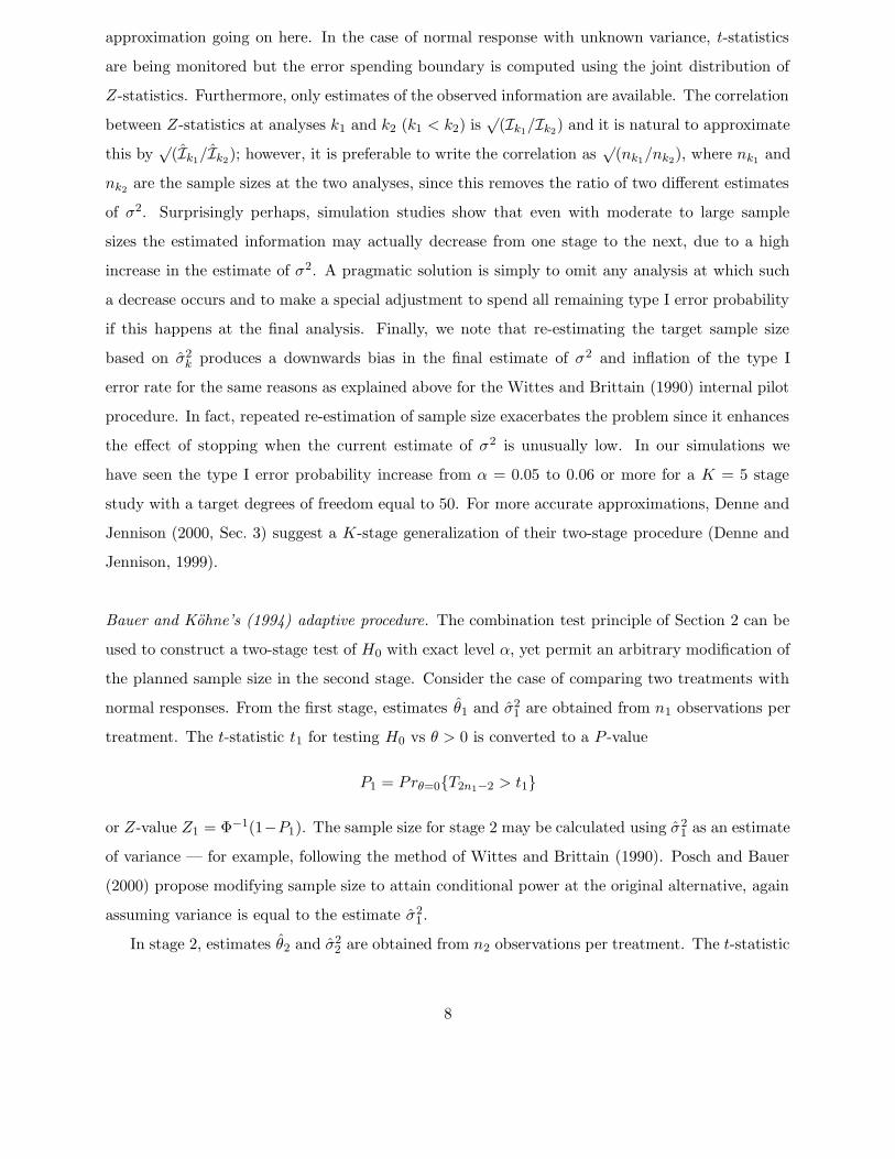
Figure 1: Power functions of four 2-stage selection/testing procedures. The top curve is for the

TSE procedure; the middle curves, which are hardly distinguishable, are for the Conventional and

BK (inverse normal) procedures; the bottom curve is for the BK (inverse χ2) procedure.

0 0.2 0.4 0.6 0.8 1 1.2 1.4 1.6 1.8 20

0.1

0.2

0.3

0.4

0.5

0.6

0.7

0.8

0.9

1

δ

Pro

b C

orre

ct S

elec

tion

Power curves for the four designs are shown in Figure 1. It can be seen from these results that,

in this example, the TSE procedure is uniformly more powerful than the other designs, but not by

much. The BK procedures have added flexibility and this might be regarded as compensation for

the slight reductions in power. Note, though, that modifying Phase III sample size in the light of

Phase IIb data could raise inefficiency concerns similar to those described in Section 3. Combining

the two phases can have other significant benefits if this removes the delay in passing from Phase IIb

to Phase III. Of course, the Conventional and TSE designs can also be applied “seamlessly” and

gain this advantage too.

It should be noted that in this comparison, the TSE design has a subtle, small advantage as it is

constructed to have type I error rate exactly equal to 0.025. In contrast, because of the the futility

boundary in Phase IIb, the Conventional design and the two BK designs are conservative, with

type I error probabilities 0.0200, 0.0212 and 0.0206, respectively, when θ1 = . . . = θ4 = 0. These

three procedures can be adjusted to have type I error rate equal to 0.025: for the Conventional

design, the critical value for Z2 is reduced from 1.96 to 1.86, corresponding to a significance level of

P = 0.031; in the BK (inverse χ2) procedure, we change the significance level for P1P2 from 0.025

to 0.030, and in the BK (inverse normal) test we decrease the critical value for the combination

Z-statistic from 1.96 to 1.86. This adjustment for a futility boundary has been termed “buying

21

back alpha”. When the conservative procedures are adjusted as just described, their power curves

become closer to that of the TSE procedure, but remain in the same order.

6 Application 3: Target population selection in “enrichment”

designs

Suppose we are interested in testing a particular experimental treatment versus a control. In

stage 1, subjects are drawn from a general population, Ω1 say, and assigned at random to treatment

and control groups. We define θ1 to be the treatment effect in Ω1. However, the population Ω1

is heterogeneous and we can think of θ1 as a weighted average of effects taken over the whole

population. We also specify `−1 sub-populations of Ω1. These sub-populations, denoted Ω2, . . . ,Ω`,

are not necessarily disjoint or nested, although they could be. The case of sub-populations based

on genomic markers is considered by Freidlin and Simon (2005) and Temple (2005). We denote

the treatment effects in these populations by θ2, . . . , θ`, respectively. At the end of stage 1, based

on the observed outcomes, one population, Ωi∗ , is chosen and all subjects randomized between the

treatment and control in stage 2 are taken from Ωi∗ . The selected population could be Ω1 or any

of the sub-populations. The choice of i∗ will reflect a trade-off. A highly targeted sub-population

where the treatment is most effective could lead to a positive result with a smaller sample size;

otherwise, a highly effective treatment in a small sub-population could be masked by dilution with

responses from the remainder of the population where there is little or no effect. On the other

hand, if a positive effect is present across the broad population, there are benefits for public health

in demonstrating this and associated commercial advantages from more general labelling. It follows

that Ωi∗ will not necessarily be the population with the highest observed treatment effect at the

end of stage 1. The choice will be based both on the magnitudes of the observed treatment effects

and on various medical and economic considerations. Thus, a “flexible” procedure is needed. As

in the previous application, we must account for a selection bias if we are to combine stage 1 and

stage 2 results to test the data generated hypothesis Hi∗ : θi∗ ≤ 0.

The procedure is analogous to that of Section 5. For each population i, the null hypothesis of no

treatment effect, Hi : θi ≤ 0, is to be tested against the alternative θi > 0. We shall follow a closed

testing procedure in order to control familywise type I error. This involves testing intersection

hypotheses of the form HI = ∩i∈IHi, implying that θi ≤ 0 for all i ∈ I. For a given HI , we perform

a test in each stage of the trial and then combine the test statistics (P -values) across stages. At

the end of stage 2 we can test Hi∗ and, additionally, any Hj such that Ωj is a subset of Ωi∗ . In

22

particular if i∗ = 1 and the full general population is selected, then it will be possible to test all of

H1, . . . ,H`. It is easiest to describe the procedure by means of a simple example, from which the

general method should be clear.

Example.

In our illustrative example, sub-populations are:

1. The entire population

2. Men only

3. Men over 50

4. Men who are smokers

Within a stage, each intersection hypothesis will be tested by combining P -values from individual

hypotheses using Simes’ (1986) method. We then combine P -values from the two stages by a

weighted inverse normal rule, giving

Z(p1, p2) = w1 Φ−1(1 − p1) + w2 Φ−1(1 − p2),

where w1 = w2 =√

0.5.

The elementary null hypotheses are Hi: θi ≤ 0 for i = 1, . . . , 4. In stage 1, the individual test

of Hi is performed using the estimate θ1,i from subjects within the relevant sub-population, giving

P -value P1,i.

In stage 2, it may only be possible to test some of the Hi using stage 2 data, for example,

if recruitment is restricted to “Men only”, we can test H2, H3 and H4 but not H1, since θ1 is a

weighted average of effects on both men and women. Thus, we obtain stage 2 P -values P2,i for

some hypotheses Hi but not for others.

Using the closure principle. In order to reject Hi∗: θi∗ ≤ 0 in the overall procedure with

familywise error probability α, we need to reject each intersection hypothesis HI for which i∗ ∈ I

at level α, based on combined stage 1 and stage 2 data. The need for adjustment when testing

multiple hypotheses is clear. Even when some of these hypotheses are taken out of consideration

by focusing on a sub-population Ωi∗ in stage 2, the choice of this sub-population is data driven

and subject to selection bias. The familywise test will automatically take care of these effects of

multiplicity and sub-population selection.

Testing an intersection hypothesis HI : θi ≤ 0 for all i ∈ I. As in Section 5, we will need (a)

to test an intersection hypothesis and (b) to combine data from the two stages. We first tackle

23

problem (b) using the weighted inverse normal combination test described above. Letting P1,I and

P2,I denote P -values for testing HI from stages 1 and 2, we calculate

Z(P1,I , P2,I) = w1 Φ−1(1 − P1,I) + w2 Φ−1(1 − P2,I),

using the specified weights w1 = w2 =√

0.5. Then, we reject HI if

Z(P1,I , P2,I) > Φ−1(1 − α).

Now consider the problem (a) of testing the intersection hypothesis HI within each stage. In stage 1,

we can calculate a P -value, P1,i, for each Hi: θi ≤ 0. Using the Bonferroni inequality, the overall

P -value for testing HI would be m times the minimum P1,i over i ∈ I, where m is the number of

indices in I. However, as in Section 5, we follow the recommendation of Schmidli et al. (2006) and

use Simes’ (1986) modification of the Bonferroni inequality. Recall that in Simes’ method, if I has

m elements, the P -value for testing HI is

P1,I = minj=1,...,m

(mP1,(j)/j),

where P1,(j), j = 1, . . . ,m, denote the m P -values in increasing order.

For testing an intersection hypothesis in stage 2, we have P -values, P2,i, for some of the

Hi: θi ≤ 0, depending on the section of the population from which recruitment took place in

this stage. Let I ′ denote the set of indices i ∈ I for which we have a P -value P2,i and suppose there

are m′ such indices.

We can apply Simes’ method on the reduced set I ′, as long as it is non-empty, yielding the

P -value for testing HI

P2,I = minj=1,...,m′

(m′ P2,(j)/j),

where P2,(j), j = 1, . . . ,m′, are the m′ available P -values arranged in increasing order.

Suppose, in our example, that recruitment in stage 2 is restricted to “Men only” and we observe

the results shown in Table 2. Had the study continued to recruit from the full population in

stage 2, a P -value could have been calculated for each sub-population and all combination tests

would be feasible. Because recruitment is restricted, elementary tests are only possible for sub-

populations which are contained completely in the new recruitment pool. Since the sub-populations

“Men over 50” and “Men who are smokers” are still sampled fully, we can test H3 and H4 as well

as H2. We cannot test H1 since θ1 is a weighted average of effects on both men and women and

stage 2 provides no information about women. Consequently, we can test H2, H3 and H4 at the

24

Table 2: Observed P -values in the example of sub-population selection. After stage 1, it is decided

to restrict recruitment in stage 2 to “Men only”.

Stage 1 results

Full population: P1,1 = 0.20

All men: P1,2 = 0.10

Men over 50 years: P1,3 = 0.03

Men who smoke: P1,4 = 0.03

Stage 2 results

All men: P2,2 = 0.11

Men over 50 years: P2,3 = 0.08

Men who smoke: P2,4 = 0.03

global level. As an example, in testing H2, the relevant sets I all contain i = 2, so there is at least

one element in the reduced set I ′.

Adjusted combined P -values. The P -values for testing hypotheses after combining data from the

two stages are displayed in Table 3. In order to reject Hi at global level α = 0.025, each intersection

hypothesis HI with i ∈ I must be rejected at this level. The adjusted P -value, Pi, for testing Hi

with protection of familywise error rate is the maximum P -value (combined over stages 1 and 2)

for all HI with i ∈ I. Thus, for testing H2 concerning the sub-population of “All men”, we have

P2 = maxP2, P12, P23, P24, P123, P124, P234, P1234 = 0.072;

in testing H3 for “Men over 50 years”, we obtain

P3 = maxP3, . . . , P1234 = 0.035;

and the test of H4 for “Men who smoke” has

P4 = maxP4, . . . , P1234 = 0.020.

We can therefore reject H4, but not H2 or H3, at global significance level α = 0.025 and quote an

adjusted P -value of P4 = 0.020.

25

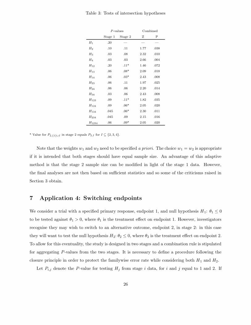
Table 3: Tests of intersection hypotheses

P -values Combined

Stage 1 Stage 2 Z P

H1 .20 — — —

H2 .10 .11 1.77 .038

H3 .03 .08 2.32 .010

H4 .03 .03 2.66 .004

H12 .20 .11* 1.46 .072

H13 .06 .08* 2.09 .018

H14 .06 .03* 2.43 .008

H23 .06 .11 1.97 .025

H24 .06 .06 2.20 .014

H34 .03 .06 2.43 .008

H123 .09 .11* 1.82 .035

H124 .09 .06* 2.05 .020

H134 .045 .06* 2.30 .011

H234 .045 .09 2.15 .016

H1234 .06 .09* 2.05 .020

* Value for P2,1∪I in stage 2 equals P2,I for I ⊆ 2, 3, 4.

Note that the weights w1 and w2 need to be specified a priori. The choice w1 = w2 is appropriate

if it is intended that both stages should have equal sample size. An advantage of this adaptive

method is that the stage 2 sample size can be modified in light of the stage 1 data. However,

the final analyses are not then based on sufficient statistics and so some of the criticisms raised in

Section 3 obtain.

7 Application 4: Switching endpoints

We consider a trial with a specified primary response, endpoint 1, and null hypothesis H1: θ1 ≤ 0

to be tested against θ1 > 0, where θ1 is the treatment effect on endpoint 1. However, investigators

recognise they may wish to switch to an alternative outcome, endpoint 2, in stage 2: in this case

they will want to test the null hypothesis H2: θ2 ≤ 0, where θ2 is the treatment effect on endpoint 2.

To allow for this eventuality, the study is designed in two stages and a combination rule is stipulated

for aggregating P -values from the two stages. It is necessary to define a procedure following the

closure principle in order to protect the familywise error rate while considering both H1 and H2.

Let Pi,j denote the P -value for testing Hj from stage i data, for i and j equal to 1 and 2. If

26

data on an endpoint are only recorded when it is the “designated” endpoint for a stage, some of

the Pi,j will not be available. We define the following tests of individual null hypotheses for use in

the overall procedure.

To test H1:

Apply the specified combination test to P1,1 and P2,1.

To test H12 = H1 ∩ H2:

If endpoint 1 is retained in stage 2, apply the combination test to P1,1 and P2,1.

If a switch is made to endpoint 2, apply the combination test to P1,1 and P2,2.

To test H2:

Use P2,2 only, rejecting H2 at level α if P2,2 ≤ α.

If the original endpoint is retained throughout the study, rejection of H1 overall requires both

individual hypotheses H1 and H12 to be rejected. However, in this case the test of H12 is the same

as that of H1 so the result is just as it would have been had the option of switching to endpoint 2

not been considered. We have deliberately chosen to define the test of H12 this way, using P1,1

from stage 1 even if data on endpoint 2 are available in this stage, in order for the overall test of

H1 to have this property.

If the switch is made to endpoint 2, overall rejection of H2 needs both H2 and H12 to be

rejected. The individual test of H2 is the test that would arise if the second stage were a self-

contained study conducted to test H2. The closure principle imposes the additional requirement

that the combination test applied to P1,1 and P2,2 should lead to rejection of H12. One might

question whether it might not be preferable to start a new trial after stage 1, defining endpoint 2

as the primary response variable, so that only the test of H2 need be considered. However, staying

with the original trial could save time by avoiding the waiting period while a new study is organized

and approved. Moreover, credibility might suffer if a sponsor were to stop a number of trials early,

discarding unfavorable results to start new trials with slightly different endpoints.

The above procedure can be extended to allow a switch to a different new endpoint. Suppose, for

example, other events in stage 1 could have led to use of endpoint 3 with associated null hypothesis

H3. A closed testing procedure should include H3 in the set of null hypotheses. If endpoint 1 is

retained, rejection of H1 overall requires all the individual hypotheses H1, H12, H13 and H123 to

27

be rejected. Applying the combination test to P1,1 and P2,1 gives a valid test for each of these

hypotheses and, with this definition, there is no change to the overall requirement for rejecting H1.

Under a switch to endpoint 2 after stage 1, global rejection of H2 requires each of H2, H12, H23

and H123 to be rejected. In this case, we retain the previous definitions for tests of H2 and H12,

we use P2,2 to test H23, and we define the test of H123 to be the combination test applied to P1,1

and P2,2. Since the tests of H23 and H123 replicate those of H2 and H12, the addition of endpoint

3 does not change the requirements that must be met in order to reject H2. If the switch is made

to endpoint 3, we test both H13 and H123 by the combination test applied to P1,1 and P2,3, and we

test both H3 and H23 through the single P -value P2,3.

It is not difficult to check that this approach can accommodate other potential endpoints too,

treating these in the same way as the above extension to endpoint 3. The criteria for overall

rejection of endpoints 1, 2 or 3 will not be affected by these additional endpoints. It follows that

the precise definition of a new endpoint can actually be left until the end of stage 1 and information

emerging from this first stage can be used in making this definition.

This flexibility to consider a variety of possible new endpoints contrasts with the requirements

for changing to a sub-population seen in Section 6. There, it was crucial to define the set of potential

sub-populations at the outset and the degree of “adjustment” to P -values for having this option

increased with the number of potential sub-populations. The reason for this qualitative difference

is that in the “switching” procedure there is a precedence of hypotheses, with H1 taking priority:

in particular, the P -value P1,1 is defined as the data summary from stage 1 to be used in all tests

of intersection hypotheses involving H1.

If there is a clear restriction to just two endpoints and data are available on both in the first

stage, it may be reasonable to use an alternative definition for the test of H2, making this a

combination test of P1,2 and P2,2. This must, of course, be specified in the study protocol as the

method that will be used. Consider, for example, a study where the primary endpoint is the change

in a clinical measurement over a 6 month period following the start of treatment. Investigators may

declare a second endpoint to be the change in this measurement after 4 months. It is necessary

to keep the test of H12 as we have defined above in order to (a) leave the overall test of H1 the

same and (b) maintain validity in the test H12. One cannot, for example, use P1,2 in place of P1,1

in the test of H12 only when a switch is made to endpoint 2, as the decision to make this switch

will have been motivated by stage 1 data on endpoint 2. If three or more endpoints are considered,

it is technically possible to define an overall procedure that makes use of stage 1 data on an all

28

endpoints, but we would not necessarily recommend this: with endpoints 2 and 3 available, a test

of H23 using stage 1 data will have to combine P1,2 and P1,3 by, for example, Simes’ test and the

procedure becomes more complex as further endpoints are added.

8 Application 5: Selecting between superiority and non-inferiority

hypotheses

Let θ denote the treatment effect when testing a single experimental treatment versus an active

control with respect to a single primary endpoint of interest. We consider the situation where,

although it would be preferable to demonstrate superiority of the experimental treatment, it is also

of value to demonstrate non-inferiority. Let 0 = δ1 < δ2 < . . . < δ` be a sequence of pre-specified

non-inferiority margins, as discussed by Hung and Wang (2004). We are interested in the collection

of hypothesis tests T1, . . . , T`, where in Ti, we test:

Hi : θ ≤ −δi versus θ > −δi.

Rejection of H1 implies a positive result for superiority, whereas rejection of Hi for a value of i

between 2 and ` implies non-inferiority with margin δi. Often ` = 2 and there is only one non-

inferiority margin of interest.

Consider testing Hi using the closed testing procedure that controls the familywise error α. In

order to reject Hi we must reject intersection hypotheses HI for every subset I with i ∈ I. Because

of the nesting of the hypotheses implied by 0 = δ1 < δ2 < . . . < δ`, we have HI = Hmax(I) where

max(I) = maxj : j ∈ I. Also, because of the nested hypotheses, we have P1 ≥ P2 ≥ . . . ≥ P`.

Thus PI = Pmax(I) and maxPI : i ∈ I = Pi, which is achieved when I = i. This means that

for each i = 1, . . . , `, we may reject Hi if Pi ≤ α and no adjustment is needed for multiplicity. Nor

does it matter in which order the hypotheses are tested. Of course, this is a well-known result —

see, for example, Morikawa and Yoshida (1995) and Dunnett and Gent (1996).

Consider now a two-stage or multi-stage adaptive design. The P -values for each of the

elementary hypothesis can be combined across stages using the methods described in Section 2.

Each hypothesis can be tested separately using combination P -values and there is no need to adjust

for the multiplicity of hypotheses. This problem has been considered by a number of authors

including Wang et al. (2001), Brannath et al. (2003), Shih et al. (2004) and Koyama et al. (2005).

The possible advantages of an adaptive multistage design are described by Wang et al. (2001).

They consider the case ` = 2 where there is only one non-inferiority margin. They point out that

29

often the non-inferiority margin is smaller than the effect size at which power for the superiority

test is specified, and so the target sample size for demonstrating non-inferiority with power when

θ = 0 can be much larger than that needed to demonstrate superiority. As data accrue, it can

become apparent which goal is the most relevant and the sample size may be adjusted accordingly.

Wang et al. (2001) give an example where there are impressive savings in expected sample size.

However, the procedures are not based on sufficient statistics and so some of the criticisms raised

in Section 3 obtain. It should be possible to design a conventional group sequential test that is

planned for the larger non-inferiority trial, but with an aggressive boundary so that the trial can

be terminated early if the results justify a superiority declaration. This would follow the spirit of

the approach recommended by Jennison and Turnbull (2006d) and bear similarities to the designs

proposed by Koyama et al. (2005).

9 Discussion

There has been lively debate about the potential advantages and disadvantages of adaptive designs.

Methodological criticisms have concentrated on issues of inefficiency and failure to satisfy the

sufficiency principle — Tsiatis and Mehta (2003), Jennison and Turnbull (2003, 2006a, b), Fleming

(2006), Burman and Sonesson (2006). Some of the practical problems of implementation are

considered in Gallo et al. (2006) and the accompanying discussion, Gallo (2006), Gould (2006)

and Fleming (2006).

In practice, adaptive designs have been utilized with some success and continue to be applied

in new trials. If the logistics can be put in place to implement “seamless” designs, the elimination

of delays between different stages of a trial will be a major advance. Adaptive methods promise

the additional flexibility to refine the target population or primary endpoint during the course of

a trial. It is clear that the current interest in adaptive designs will continue and there is a keen

audience for further developments in the methodology and reports of its application.

REFERENCES

Bauer P. and Kieser M. (1999). Combining different phases in the development of medical

treatments within a single trial. Statistics in Medicine 18, 1833–1848.

Bauer, P. and Kohne, K. (1994). Evaluation of experiments with adaptive interim analyses.

Biometrics 50, 1029–1041. Correction Biometrics 52, (1996), 380.

30

Bechhofer, R.E., Santner, T.J. and Goldsman, D.M. (1995). Design and Analysis of Experiments

for Statistical Selection, Screening, and Multiple Comparisons. Wiley, New York.

Becker, B.J. (1994). Combining significance levels. In The Handbook of Research Synthesis, Eds.

Cooper, H. and Hedges, L.V. Russell Sage Foundation, New York, Chap. 15, pages 215–230.

Birkett, M.A. and Day, S.J. (1994). Internal pilot studies for estimating sample size. Statistics in

Medicine 13, 2455–2463.

Brannath, W., Posch, M. and Bauer, P. (2002). Recursive combination tests. J. American

Statistical Association 97, 236–244.

Brannath, W., Bauer, P., Maurer, W. and Posch, M. (2003). Sequential tests for noninferiority

and superiority. Biometrics 59, 106–114.

Bretz, F., Schmidli, H., Konig, F., Racine, A. and Maurer, W. (2006). Confirmatory seamless

phase II/III clinical trials with hypotheses selection at interim: General concepts (with

discussion). Biometrical Journal 48, 623–634.

Burman, C-F. and Sonesson, C. (2006). Are flexible designs sound? Biometrics 62, 664–669.

Chow, S-C. and Chang, M. (2007). Adaptive Design Methods in Clinical Trials. Chapman &

Hall/CRC, Boca Raton, Florida.

Cui, L., Hung, H.M.J. and Wang, S-J. (1999). Modification of sample size in group sequential

clinical trials. Biometrics 55, 853–857.

Denne, J.S. (2001). Sample size recalculation using conditional power. Statistics in Medicine 20,

2645–2660.

Denne, J.S. and Jennison, C. (1999). Estimating the sample size for a t-test using an internal

pilot. Statistics in Medicine 18, 1575–1585.

Denne, J.S. and Jennison, C. (2000). A group sequential t-test with updating of sample size.

Biometrika 87, 125–134.

Dunnett, C.W. (1955). A multiple comparison procedure for comparing several treatments with

a control. J. American Statistical Association 50, 1096–1121.

31

Dunnett, C.W. and Gent, M. (1996). An alternative to the use of two-sided tests in clinical trials.

Statistics in Medicine 15, 1729–1738.

EMEA (2006). Reflection paper on methodological issues in confirmatory clinical trials

with flexible design and analysis plan. (Draft 23 March 2006). EMEA (European

Medicines Agency) Committee for Medicinal Products for Human Use (CHMP).

http://www.emea.eu.int/pdfs/human/ewp/245902en.pdf

Fisher, L.D. (1998). Self-designing clinical trials. Statistics in Medicine 17, 1551–1562.

Fisher, R.A. (1932). Statistical Methods for Research Workers, 4th Ed. Oliver and Boyd, London.

Fleming, T.R. (2006). Standard versus adaptive monitoring procedures: a commentary. Statistics

in Medicine 25, 3305–3312.

Freidlin, B. and Simon, R. (2005). Adaptive signature design: An adaptive clinical trial design

for generating and prospectively testing a gene expression signature for sensitive patients.

Clinical Cancer Research 11, 7872–7878.

Friede, T. and Kieser, M. (2001). A comparison of methods for adaptive sample size adjustment.

Statistics in Medicine 20, 3861–3873.

Friede, T. and Kieser, M. (2002). On the inappropriateness of an EM based procedure for blinded

sample size re-estimation. Statistics in Medicine 21, 165–176.

Gallo, P. (2006). Operational challenges in adaptive design implementation. Pharmaceutical

Statistics 5, 119–124.

Gallo, P., Chuang-Stein, C., Dragalin, V., Gaydos, B., Krams, M. and Pinheiro, J. (2006).

Adaptive designs in clinical drug development — an executive summary of the PhRMA

Working Group (with discussion). J. Biopharmaceutical Statistics 16, 275–312.

Gould, A.L. (2006). How practical are adaptive designs likely to be for confirmatory trials?

Biometrical Journal 48, 644–649.

Gould, A.L. and Shih, W.J. (1992). Sample size re-estimation without unblinding for normally

distributed outcomes with unknown variance. Communications in Statistics: Theory and

Methods 21, 2833–2853.

32

Goutis, C., Casella, G., and Wells, M.T. (1996). Assessing evidence in multiple hypotheses. J.

American Statistical Association 91, 1268–1277.

Hochberg, Y. (1988). A sharper Bonferroni procedure for multiple tests of significance. Biometrika

75, 800–802.

Hochberg, Y. and Tamhane, A.C. (1987). Multiple Comparison Procedures. Wiley, New York.

Hommel, G. (1988). A stagewise rejective multiple test procedure based on a modified Bonferroni

test. Biometrika 75, 383–386.

Hung, H.M.J., O’Neill, R.T., Wang S.J. and Lawrence J. (2006). A regulatory view on

adaptive/flexible clinical trial design. Biometrical Journal 48, 565–573.

Hung, H.M.J. and Wang, S.J. (2004). Multiple testing of noninferiority hypotheses in active

controlled trials. J. Biopharmaceutical Statistics 14, 327–335.

Hung, H.M.J., Wang, S.J. and O’Neill R.T. (2006). Methodological issues with adaptation of

clinical trial design. Pharmaceutical Statistics 5, 99–107.

Jennison, C. and Turnbull, B.W. (2000). Group Sequential Methods with Applications to Clinical

Trials. Chapman & Hall/CRC, Boca Raton.

Jennison, C. and Turnbull, B.W. (2003). Mid-course sample size modification in clinical trials

based on the observed treatment effect. Statistics in Medicine 23, 971–993.

Jennison, C. and Turnbull, B.W. (2005). Meta-analyses and adaptive group sequential designs in

the clinical development process. J. Biopharmaceutical Statistics 15, 537–558.

Jennison, C. and Turnbull, B.W. (2006a). Adaptive and nonadaptive group sequential tests.

Biometrika 93, 1–21.

Jennison, C. and Turnbull, B.W. (2006b). Discussion of “Are flexible designs sound?” Biometrics

62, 670–673

Jennison, C. and Turnbull, B.W. (2006c). Discussion of “Executive summary of the PhRMA

Working Group on adaptive designs in clinical drug development.” J. Biopharmaceutical

Statistics 16, 293–298.

33

Jennison, C. and Turnbull, B.W. (2006d). Efficient group sequential designs when there are several

effect sizes under consideration. Statistics in Medicine 35, 917–932.

Jennison, C. and Turnbull, B.W. (2006e). Confirmatory seamless Phase II/III clinical trials with

hypotheses selection at interim: Opportunities and limitations. Biometrical Journal 48, 650–

655.

Kieser, M. and Friede, T. (2000). Recalculating the sample size in internal pilot study designs

with control of the type I error rate. Statistics in Medicine 19, 901–911.

Koch, A. (2006). Confirmatory clinical trials with an adaptive design. Biometrical Journal 48,

574–585.

Koyama, T., Sampson, A.R. and Gleser, L.J. (2005). A framework for two-stage adaptive

procedures to simultaneously test non-inferiority and superiority. Statistics in Medicine 24,

2439–2456.

Lan, K.K.G. and DeMets, D.L. (1983). Discrete sequential boundaries for clinical trials.

Biometrika 70, 659–663.

Lehmacher, W. and Wassmer, G. (1999). Adaptive sample size calculation in group sequential

trials. Biometrics 55, 1286–1290.

Liu, Q., Proschan, M.A. and Pledger, G.W. (2002). A unified theory of two-stage adaptive designs.

J. American Statistical Association 97, 1034–1041.

Marcus, R., Peritz, E. and Gabriel, K.R. (1976). On closed testing procedures with special

reference to ordered analysis of variance. Biometrika 63, 655–660.

Mehta, C. and Tsiatis, A.A. (2001). Flexible sample size considerations using information-based

interim monitoring. Drug Information Journal 35, 1095–1112.

Mosteller, F. and Bush, R.R. (1954). Selected quantitative techniques. In Handbook of Social

Psychology, Vol.1 Ed. G. Lindzey, Addison-Wesley, Cambridge, MA, pages 289–334.

Morikawa, T., Yoshida, M. (1995). A useful testing strategy in phase III trials: Combined test of

superiority and test of equivalence. J. Biopharmaceutical Statistics 5, 297–306.

34

Muller, H-H. and Schafer, H. (2001). Adaptive group sequential designs for clinical trials:

Combining the advantages of adaptive and of classical group sequential procedures.

Biometrics 57, 886–891.

Posch, M. and Bauer, P. (2000). Interim analysis and sample size reassessment. Biometrics 56,

1170–1176.

Posch, M., Koenig, F., Branson, M., Brannath, W., Dunger-Baldauf, C. and Bauer, P. (2005).

Testing and estimation in flexible group sequential designs with adaptive treatment selection.

Statistics in Medicine 24, 3697–3714.

Proschan, M.A. (2003). The geometry of two-stage tests. Statistica Sinica 13, 163–177.

Proschan, M.A. and Hunsberger, S.A. (1995). Designed extension of studies based on conditional

power. Biometrics 51, 1315–1324.

Sampson, A.R. and Sill, M.W. (2005). Drop-the-losers design: Normal case (with discussion).

Biometrical Journal 47, 257–281.

Sarkar, S. K. (1998). Some probability inequalities for ordered MTP2 random variables: A proof

of the Simes conjecture. The Annals of Statistics 26, 494–504.

Sarkar, S. K. and Chang, C-K. (1997). The Simes method for multiple hypothesis testing with

positively dependent test statistics. J. American Statistical Association 92, 1601–1608.

Schaid, D.J., Wieand, S. and Therneau, T.M. (1990). Optimal two-stage screening designs for

survival comparisons. Biometrika 77, 507–513.

Schmidli, H., Bretz, F., Racine, A. and Maurer, W. (2006). Confirmatory seamless phase II/III

clinical trials with hypotheses selection at interim: Applications and practical considerations.

Biometrical Journal 48, 635–643.

Schmitz, N. (1993). Optimal Sequentially Planned Decision Procedures. Lecture Notes in

Statistics, 79, Springer-Verlag: New York.

Shih, W.J., Quan, H. and Li, G. (2004). Two-stage adaptive strategy for superiority and non-

inferiority hypotheses in active controlled clinical trials. Statistics in Medicine 23, 2781–2798.

Simes, R.J. (1986). An improved Bonferroni procedure for multiple tests of significance.

Biometrika 73, 751–754.

35

Stallard, N. and Todd, S. (2003). Sequential designs for phase III clinical trials incorporating

treatment selection. Statistics in Medicine 22, 689–703.

Stein, C. (1945). A two-sample test for a linear hypothesis whose power is independent of the

variance. Annals of Mathematical Statistics 16, 243–258.

Temple, R.J. (2005). Enrichment designs: Efficiency in development of cancer treatments. J.

Clinical Oncology 23, 4838–4839.

Thall, P.F., Simon, R. and Ellenberg, S.S. (1988). Two-stage selection and testing designs for

comparative clinical trials. Biometrika 75, 303–310.

Timmesfeld, N., Schafer, H. and Muller, H-H. (2007). Increasing the sample size during clinical

trials with t-distributed test statistics without inflating the type I error rate. Statistics in

Medicine 26, 2449–2464.

Todd, S. and Stallard, N. (2005). A New Clinical Trial Design Combining Phases 2 and 3:

Sequential designs with treatment selection and a change of endpoint. Drug Information

Journal 39, 109–118.

Tsiatis, A.A. (2006). Information-based monitoring of clinical trials. Statistics in Medicine 25,

3236–3244.

Tsiatis, A.A. and Mehta, C. (2003). On the inefficiency of the adaptive design for monitoring

clinical trials. Biometrika 90, 367–78.

Wang, S-J, Hung, H.M.J., Tsong, Y. and Cui, L. (2001). Group sequential test strategies for

superiority and non-inferiority hypotheses in active controlled clinical trials. Statistics in

Medicine 20, 1903–1912.

Westfall, P.H. and Young, S.S, (1993). Resampling-based Multiple Testing: Examples and Methods

for p-Value Adjustment. Wiley, New York.

Wittes J. and Brittain, E. (1990). The role of internal pilot studies in increasing the efficiency of

clinical trials. Statistics in Medicine 9, 65–72.

Zucker, D.M., Wittes, J.T., Schabenberger, O. and Brittain, E. (1999) Internal pilot studies II:

Comparison of various procedures. Statistics in Medicine 18, 3493–3509.

36