Adaptive Routing in Ad Hoc Wireless Multi-hop Networks

Universita della Svizzera italiana

Faculty of Informatics

Adaptive Routing in Ad Hoc WirelessMulti-hop Networks

Frederick Ducatelle

Dissertation submitted in partial fulfillment of therequirements for the Degree of Doctor of Philosophy

Lugano, Switzerland, May 2007

Doctoral Committee:

Professor Luca M. Gambardella, research advisor (IDSIA)

Professor Antonio Carzaniga, academic advisor (USI)

Professor Amy L. Murphy, internal member (USI)

Professor Patrick Thiran, external member (EPFL)

Academic year 2006-2007

The research for this thesis was carried out at the Istituto DalleMolle di Studi sull’Intelligenza Artificiale (IDSIA), under the su-pervision of Luca Maria Gambardella. This work was partially sup-ported by the Future & Emerging Technologies unit of the EuropeanCommission through project “BISON: Biology-Inspired techniquesfor Self Organization in dynamic Networks” (IST-2001-38923) andby the Swiss Hasler Foundation through grant DICS-1830.

To Lili and Delphine

Abstract

Ad hoc wireless multi-hop networks (AHWMNs) are communication net-works that consist entirely of wireless nodes, placed together in an ad hoc man-ner, i.e. with minimal prior planning. All nodes have routing capabilities, andforward data packets for other nodes in multi-hop fashion. Nodes can enter orleave the network at any time, and may be mobile, so that the network topol-ogy continuously experiences alterations during deployment. AHWMNs posesubstantially different challenges to networking protocols than more traditionalwired networks. These challenges arise from the dynamic and unplanned natureof these networks, from the inherent unreliability of wireless communication,from the limited resources available in terms of bandwidth, processing capacity,etc., and from the possibly large scale of these networks. Due to these differ-ent challenges, new algorithms are needed at all layers of the network protocolstack.

We investigate the issue of adaptive routing in AHWMNs, using ideas fromartificial intelligence (AI). Our main source of inspiration is the field of AntColony Optimization (ACO). This is a branch of AI that takes its inspirationfrom the behavior of ants in nature. ACO has been applied to a wide range ofdifferent problems, often giving state-of-the-art results. The application of ACOto the problem of routing in AHWMNs is interesting because ACO algorithmstend to provide properties such as adaptivity and robustness, which are neededto deal with the challenges present in AHWMNs. On the other hand, the fieldof AHWMNs forms an interesting new application domain in which the ideas ofACO can be tested and improved. In particular, we investigate the combinationof ACO mechanisms with other techniques from AI to get a powerful algorithmfor the problem at hand.

We present the AntHocNet routing algorithm, which combines ideas fromACO routing with techniques from dynamic programming and other mecha-nisms taken from more traditional routing algorithms. The algorithm has a hy-brid architecture, combining both reactive and proactive mechanisms. Througha series of simulation tests, we show that for a wide range of different environ-ments and performance metrics, AntHocNet can outperform important referencealgorithms in the research area. We provide an extensive investigation of theinternal working of the algorithm, and we also carry out a detailed simulationstudy in a realistic urban environment. Finally, we discuss the implementationof ACO routing algorithms in a real world testbed.

Acknowledgements

I would like to thank in the first place my supervisor, Luca Maria Gambardella,who has given me the opportunity to work on this project and has assisted mein any way possible. Then, I want to thank my colleague, Gianni A. Di Caro,who has been like a second supervisor to me, and has been an invaluable helpthroughout this project. Other people who have been of scientific importancefor my work on this thesis include (in order of appearance) John Levine, whohas first introduced me to the field of ant colony optimization, Marco Dorigo,who initiated this interesting research field and also brought me in contact withIDSIA, Patrick Thiran, who brought us in contact with the field of ad hocnetworks, and Martin Roth, who gave me the opportunity to work with him atDeutsche Telekom Laboratories in Berlin. Furthermore, I would like to thankall the people at IDSIA for all scientific input, in the form of presentations,discussions, etc..

Apart from the scientific input, of equal importance to me has been the per-sonal support I have received throughout the years that I have spent on thisthesis. I want to thank a number of people without whom this work would neverhave been completed. In the first place, I thank my wife, Liliana Carrillo, andmy daughter, Delphine, who arrived just in time to give me the final supportI needed to finish the work. Then I want to thank my family, my mother, myfather and my sisters, Caroline and Barbara, who have been, from distance, agreat support. Next, I thank Alex Graves and Matteo Gagliolo, partners incrime during all those years in Lugano. Friends back home, Pieter Vanden-bossche and family, Kobe Lootens, Dieter Herregodts, Pieter Orbie, FrederikDemilde, Katelijne Carbonez, Tom Ghyselinck, and many others. And all otherfriends, wherever they are, Matthew Davies, Elaine Boyd, Jesper Salomon, OlgaChrysanthopoulou, Ola Svenson, Nikos Mutsanas, Shane Legg, Maciej Kurant,etc..

1

Contents

1 Introduction 151.1 General introduction . . . . . . . . . . . . . . . . . . . . . . . . . 151.2 Contributions of this thesis . . . . . . . . . . . . . . . . . . . . . 181.3 Outline of the thesis . . . . . . . . . . . . . . . . . . . . . . . . . 19

2 Ad hoc wireless multi-hop networks 212.1 A definition of ad hoc wireless multi-hop networks . . . . . . . . 212.2 Types of ad hoc wireless multi-hop networks . . . . . . . . . . . . 22

2.2.1 Mobile ad hoc networks . . . . . . . . . . . . . . . . . . . 222.2.2 Wireless mesh networks . . . . . . . . . . . . . . . . . . . 232.2.3 Sensor networks . . . . . . . . . . . . . . . . . . . . . . . 252.2.4 Algorithms for different types of AHWMNs . . . . . . . . 26

2.3 Issues in ad hoc wireless multi-hop networking . . . . . . . . . . 262.3.1 Network topology and node mobility . . . . . . . . . . . . 262.3.2 The physical layer . . . . . . . . . . . . . . . . . . . . . . 282.3.3 The data link layer . . . . . . . . . . . . . . . . . . . . . . 292.3.4 The transport layer . . . . . . . . . . . . . . . . . . . . . 32

2.4 Routing in ad hoc wireless multi-hop networks . . . . . . . . . . 332.4.1 Proactive versus reactive routing algorithms . . . . . . . . 342.4.2 Important routing algorithms for AHWMNs . . . . . . . . 352.4.3 Other techniques for AHWMN routing . . . . . . . . . . . 40

2.5 Conclusion . . . . . . . . . . . . . . . . . . . . . . . . . . . . . . 47

3 Adaptive routing and learning 493.1 Adaptive routing in the internet . . . . . . . . . . . . . . . . . . 49

3.1.1 Distance vector routing . . . . . . . . . . . . . . . . . . . 503.1.2 Link state routing . . . . . . . . . . . . . . . . . . . . . . 55

3.2 Ant Colony Optimization routing algorithms . . . . . . . . . . . 573.2.1 Ants in nature . . . . . . . . . . . . . . . . . . . . . . . . 583.2.2 The Ant Colony Optimization metaheuristic . . . . . . . 593.2.3 AntNet: an ACO algorithm for routing in telecommuni-

cation networks . . . . . . . . . . . . . . . . . . . . . . . . 623.2.4 ACO routing principles . . . . . . . . . . . . . . . . . . . 653.2.5 Existing ACO routing algorithms for wired networks . . . 66

2

3.2.6 Existing ACO routing algorithms for AHWMNs . . . . . 703.3 Routing and machine learning . . . . . . . . . . . . . . . . . . . . 73

3.3.1 The reinforcement learning framework . . . . . . . . . . . 733.3.2 Elementary solution methods for reinforcement learning:

dynamic programming and Monte Carlo sampling . . . . 763.3.3 Temporal-difference learning and Q-routing . . . . . . . . 78

3.4 Conclusion . . . . . . . . . . . . . . . . . . . . . . . . . . . . . . 80

4 AntHocNet: an adaptive routing algorithm for ad hoc wirelessmulti-hop networks 814.1 General overview of the AntHocNet routing algorithm . . . . . . 82

4.1.1 Algorithm description . . . . . . . . . . . . . . . . . . . . 824.1.2 Schematic representation . . . . . . . . . . . . . . . . . . 85

4.2 Detailed descriptions . . . . . . . . . . . . . . . . . . . . . . . . . 874.2.1 Data structures in AntHocNet . . . . . . . . . . . . . . . 874.2.2 Reactive route setup . . . . . . . . . . . . . . . . . . . . . 884.2.3 Proactive route maintenance . . . . . . . . . . . . . . . . 904.2.4 Data packet forwarding . . . . . . . . . . . . . . . . . . . 964.2.5 Link failures . . . . . . . . . . . . . . . . . . . . . . . . . 964.2.6 Routing metrics . . . . . . . . . . . . . . . . . . . . . . . 100

4.3 Further Discussions . . . . . . . . . . . . . . . . . . . . . . . . . . 1024.3.1 AntHocNet and reinforcement learning . . . . . . . . . . . 1024.3.2 Challenges for routing in AHWMNs . . . . . . . . . . . . 1044.3.3 AntHocNet related to other routing algorithms . . . . . . 1054.3.4 Older versions of AntHocNet . . . . . . . . . . . . . . . . 106

4.4 Conclusion . . . . . . . . . . . . . . . . . . . . . . . . . . . . . . 108

5 An evaluation study of AntHocNet 1105.1 Setup of the evaluation study . . . . . . . . . . . . . . . . . . . . 110

5.1.1 On the use of simulation . . . . . . . . . . . . . . . . . . . 1115.1.2 The QualNet network simulator . . . . . . . . . . . . . . . 1125.1.3 Simulation scenarios . . . . . . . . . . . . . . . . . . . . . 1135.1.4 Algorithms used for comparison . . . . . . . . . . . . . . . 1145.1.5 Evaluation measures . . . . . . . . . . . . . . . . . . . . . 115

5.2 Comparisons to other routing algorithms . . . . . . . . . . . . . . 1165.2.1 Varying the maximum node speed for RWP mobility . . . 1165.2.2 Varying the pause time for RWP mobility . . . . . . . . . 1185.2.3 Varying the speed for GM mobility . . . . . . . . . . . . . 1215.2.4 Varying the data send rate . . . . . . . . . . . . . . . . . 1245.2.5 Varying the number of data sessions . . . . . . . . . . . . 1275.2.6 Varying the network area size . . . . . . . . . . . . . . . . 1295.2.7 Varying the number of nodes . . . . . . . . . . . . . . . . 1315.2.8 Summary . . . . . . . . . . . . . . . . . . . . . . . . . . . 133

5.3 Analysis of AntHocNet’s internal working . . . . . . . . . . . . . 1345.3.1 Switching off proactive actions and local repair . . . . . . 1355.3.2 Using different routing metrics . . . . . . . . . . . . . . . 137

3

5.3.3 Varying the proactive ant send interval . . . . . . . . . . 1385.3.4 Varying the number of entries in the pheromone diffusion

messages . . . . . . . . . . . . . . . . . . . . . . . . . . . 1415.3.5 Varying the routing coefficient for ants . . . . . . . . . . . 1425.3.6 Varying the routing coefficient for data . . . . . . . . . . 1435.3.7 Summary . . . . . . . . . . . . . . . . . . . . . . . . . . . 145

5.4 Conclusion . . . . . . . . . . . . . . . . . . . . . . . . . . . . . . 146

6 Simulation of an urban scenario 1476.1 Design of the simulation study . . . . . . . . . . . . . . . . . . . 148

6.1.1 General description of the simulation study . . . . . . . . 1486.1.2 The urban environment and node mobility . . . . . . . . 1496.1.3 Radio propagation . . . . . . . . . . . . . . . . . . . . . . 1516.1.4 Data traffic . . . . . . . . . . . . . . . . . . . . . . . . . . 1536.1.5 Related work on the simulation of AHWMNs in urban

environments . . . . . . . . . . . . . . . . . . . . . . . . . 1546.2 Test results . . . . . . . . . . . . . . . . . . . . . . . . . . . . . . 155

6.2.1 General network properties . . . . . . . . . . . . . . . . . 1566.2.2 Data send rate . . . . . . . . . . . . . . . . . . . . . . . . 1576.2.3 Number of data sessions . . . . . . . . . . . . . . . . . . . 1606.2.4 Node density . . . . . . . . . . . . . . . . . . . . . . . . . 1616.2.5 Node speed . . . . . . . . . . . . . . . . . . . . . . . . . . 1646.2.6 Supporting VoIP traffic data loads . . . . . . . . . . . . . 166

6.3 Conclusion . . . . . . . . . . . . . . . . . . . . . . . . . . . . . . 168

7 Towards the implementation of adaptive routing in AHWMNs1707.1 On the deployment of AHWMNs . . . . . . . . . . . . . . . . . . 171

7.1.1 AHWMN testbeds . . . . . . . . . . . . . . . . . . . . . . 1717.1.2 Implementations of AHWMN routing algorithms . . . . . 173

7.2 The MagAntA routing system . . . . . . . . . . . . . . . . . . . . 1767.2.1 The program structure . . . . . . . . . . . . . . . . . . . . 1767.2.2 The control module . . . . . . . . . . . . . . . . . . . . . 1777.2.3 The routing interface . . . . . . . . . . . . . . . . . . . . . 1787.2.4 The routing module . . . . . . . . . . . . . . . . . . . . . 1787.2.5 The MagAntA adaptive routing algorithm . . . . . . . . . 179

7.3 Integration with the Linux kernel . . . . . . . . . . . . . . . . . . 1827.3.1 Ana4 . . . . . . . . . . . . . . . . . . . . . . . . . . . . . . 1827.3.2 Current state of the system . . . . . . . . . . . . . . . . . 1847.3.3 Other approaches . . . . . . . . . . . . . . . . . . . . . . . 185

7.4 Conclusion . . . . . . . . . . . . . . . . . . . . . . . . . . . . . . 187

8 Conclusions 1888.1 Contributions and findings of this thesis . . . . . . . . . . . . . . 1888.2 Future research directions . . . . . . . . . . . . . . . . . . . . . . 190

4

List of Figures

2.1 An example of a MANET built up of mobile phones. The dashedlines symbolize the wireless links. . . . . . . . . . . . . . . . . . . 23

2.2 An example of a WMN, in which five static wireless nodes (inthis example, these are WiFi access points) act as mesh routersand a number of heterogeneous mobile devices play the role ofmesh clients. . . . . . . . . . . . . . . . . . . . . . . . . . . . . . 24

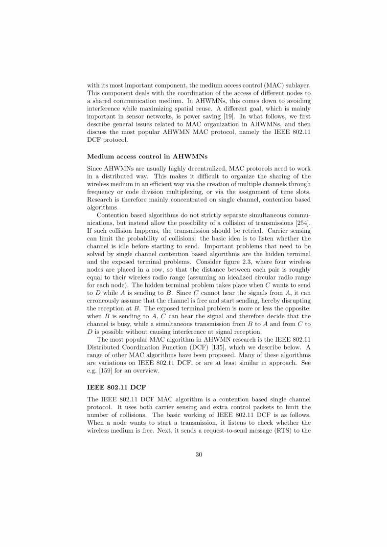
2.3 The hidden and exposed terminal problems (figure adapted from[254]) . . . . . . . . . . . . . . . . . . . . . . . . . . . . . . . . . 31

2.4 The working of OLSR. The dashed lines symbolize wireless links(not all links are drawn in order not to overload the picture).Node j chooses i, k, l and m as MPR nodes, since they are suffi-cient to reach all its two-hop neighbors. Figure adapted from [61]. 37

3.1 An example of the working of RIP. The figure shows the routingtable maintained in node 2, and one of the update messages thatare periodically sent out by this node. The trajectories of theupdate messages are given in dashed lines. The cost of each linkis given in milliseconds. . . . . . . . . . . . . . . . . . . . . . . . 51

3.2 The counting to infinity problem. After the failure of the linkbetween node 2 and node 3, node 1 and node 2 adapt their es-timate of the cost of the route to node 4 based on the updatesthey receive from each other. Figure adapted from [254]. . . . . . 53

3.3 An example of the working of OSPF. The figure shows the topo-logical database maintained in node 2 (this should be the samefor each node in the network), and a link state advertisementssent out by node 2. The link state advertisements are floodedover the network, as is indicated by the dashed lines. . . . . . . . 56

3.4 The shortest path mechanism used by ants. The different col-ors indicate increasing levels of pheromone intensity. From leftto right and then from top to bottom, we see the situation insuccessive time steps. Figure taken from [70]. . . . . . . . . . . . 59

5

3.5 Data structures for the AntNet routing algorithm. We show fornode 2 the pheromone routing table, with one row for each nexthop and one column for each destination, and the local trafficstatistics table, with the average, variance and best value forthe trip time to each destination. The values given along eachlink are the expected delay of a data packet on this link. Theline thickness for the outgoing links of node 2 indicate differentpreferences for ants going towards destination 7. . . . . . . . . . 63

3.6 An example of a reinforcement learning problem. A learningagent A enters the gridworld at position S. It can move to differentpositions by taking one of four possible actions: north, south, eastor west. The reward is 0 in each position, except for position G,where the reward is 10. After reaching position G, the agent isautomatically moved back to S. The agent should learn by trialand error to find which movements maximize its total reward. . 74

3.7 A formal model for the RL problem. The agent interacts withits environment. At time step t, the agent is in state st in theenvironment, and receives the corresponding reward rt. In re-sponse, it takes action at. The environment, in turn, respondsto the action in time step t + 1, providing the agent with a newstate st+1 and reward rt+1. Figure taken from [252]. . . . . . . . 75

4.1 A finite state machine representation of the AntHocNet routingalgorithm. . . . . . . . . . . . . . . . . . . . . . . . . . . . . . . . 85

4.2 An example of available pheromone in an AHWMN. Node 1 isrunning a communication session with node 8 as destination.Regular pheromone is indicated by solid arrows. The route overthe nodes 3, 6 and 7 is the result of a reactive route setup. Theone-hop route from node 5 to node 8 is there independent ofthe running session: node 5 is aware that node 8 is its neighborand therefore knows it has a one hop path to node 8. Virtualpheromone is indicated by dashed arrows. It forms a field point-ing towards the destination node 8. Virtual pheromone is theresult of the pheromone diffusion process. . . . . . . . . . . . . . 92

5.1 Results for AntHocNet, AODV, OLSR and ANSI using differentvalues for the maximum speed in the RWP mobility model: (a)delivery ratio, (b) average end-to-end delay, (c) average delayjitter, (d) overhead in number of packets, and (e) overhead innumber of bytes. . . . . . . . . . . . . . . . . . . . . . . . . . . . 117

5.2 Results for AntHocNet, AODV, OLSR and ANSI using differentvalues for the pause time in the RWP mobility model: (a) deliveryratio, (b) average end-to-end delay, (c) average delay jitter, (d)overhead in number of packets, and (e) overhead in number ofbytes. . . . . . . . . . . . . . . . . . . . . . . . . . . . . . . . . . 119

6

5.3 A node moving according to the RWP mobility model. The nodestarts in a randomly chosen initial point (A). It chooses a randomdestination point (B) and moves to it in a straight line. Then,it pauses for a fixed amount of time. After that, it repeats thissequence of actions till the end of the simulation (leading to thepoints C, D, E, and F). . . . . . . . . . . . . . . . . . . . . . . . 120

5.4 Results for AntHocNet, AODV, OLSR and ANSI using differentvalues for the maximum speed using the GM mobility model:(a) delivery ratio, (b) average end-to-end delay, (c) average delayjitter, (d) overhead in number of packets, and (e) overhead innumber of bytes. . . . . . . . . . . . . . . . . . . . . . . . . . . . 122

5.5 Results for AntHocNet, AODV, OLSR and ANSI using differentvalues for the data send rate: (a) delivery ratio, (b) average end-to-end delay, (c) average delay jitter, (d) overhead in number ofpackets, and (e) overhead in number of bytes. . . . . . . . . . . . 125

5.6 Results for AntHocNet, AODV, OLSR and ANSI using differentvalues for the number of data sessions: (a) delivery ratio, (b)average end-to-end delay, (c) average delay jitter, (d) overheadin number of packets, and (e) overhead in number of bytes. . . . 127

5.7 Results for AntHocNet, AODV, OLSR and ANSI using differentsizes for the network area surface. The length of the long edge inmeters is given on the x-axis, while the length of the short edge isalways one third of this. We report (a) delivery ratio, (b) averageend-to-end delay, (c) average delay jitter, (d) overhead in numberof packets, and (e) overhead in number of bytes. . . . . . . . . . 130

5.8 Results for AntHocNet, AODV, OLSR and ANSI using differentnetwork sizes. The number of nodes in the network is indicated onthe x-axis. The network area size is incremented proportionally sothat the node density remains the same as in the base scenario.We report (a) delivery ratio, (b) average end-to-end delay, (c)average delay jitter, (d) overhead in number of packets, and (e)overhead in number of bytes. . . . . . . . . . . . . . . . . . . . . 132

5.9 Results for AntHocNet, AntHocNet without proactive route main-tenance process (“AntHocNetnp”), AntHocNet without local routerepair (“AntHocNetnr”) and AntHocNet with neither proactiveroute maintenance nor route repair (“AntHocNetnpnr”). Thetests are carried out in scenarios with increasing number of nodes,as in subsection 5.2.7. We report (a) delivery ratio, (b) averageend-to-end delay, (c) average delay jitter, and (d) overhead innumber of packets. . . . . . . . . . . . . . . . . . . . . . . . . . . 135

5.10 The average number of hops for different versions of AntHocNetin scenarios with increasing number of nodes. . . . . . . . . . . . 136

7

5.11 Results for AntHocNet using different routing metrics: signal-to-interference-and-noise ratio (“SINR”), number of hops (“Hops”),delay (“Delay”), and the combination of hops and delay (“De-lay+Hops”). The tests are carried out in scenarios with increasingnumber of nodes, as in subsection 5.2.7. We report (a) deliveryratio, (b) average end-to-end delay, (c) average delay jitter, and(d) overhead in number of packets. . . . . . . . . . . . . . . . . . 137

5.12 The average number of hops for AntHocNet using different rout-ing metrics in scenarios with increasing number of nodes. . . . . 138

5.13 Results for AntHocNet using different send intervals for the proac-tive ants. We send 1 ant every 0.5, 1, 2, 5, 10, 20, and 50s. Thisis indicated on the x-axis. We use scenarios with varying mobil-ity: we apply RWP with maximum speeds of 2, 5, 10 and 20m/s.The results for different speed values are represented with differ-ent curves. We report (a) delivery ratio, (b) average end-to-enddelay, (c) average delay jitter, and (d) overhead in number ofpackets. . . . . . . . . . . . . . . . . . . . . . . . . . . . . . . . . 139

5.14 Results for AntHocNet using different send intervals for the proac-tive ants. We send 1 ant every 0.5, 1, 2, 5, 10, 20, and 50s. This isindicated on the x-axis. We use scenarios with varying data load:we use data sessions sending 1, 4 and 8 packets per second. Theresults for different data send rates are represented with differ-ent curves. We report (a) delivery ratio, (b) average end-to-enddelay, (c) average delay jitter, and (d) overhead in number ofpackets. . . . . . . . . . . . . . . . . . . . . . . . . . . . . . . . . 140

5.15 Results for AntHocNet using different number of entries in thepheromone diffusion messages. The number of entries used are 0,2, 5, 10 and 20, and are indicated on the x-axis. We do experi-ments with varying node mobility: we apply RWP with maximumspeeds of 2, 5, 10 and 20m/s. The results for different speed val-ues are represented with different curves. We report (a) deliveryratio, (b) average end-to-end delay, (c) average delay jitter, and(d) overhead in number of packets. . . . . . . . . . . . . . . . . . 141

5.16 Results for AntHocNet using different values for the proactiveant routing exponent. The exponent values that we use are 2, 5,10, 20 and ∞ (the latter represents deterministic forwarding ofproactive forward ants along the best path). The tests are carriedout in scenarios with varying data load: we use data sessionssending 1, 4 and 8 packets per second. The results for differentdata send rates are represented with different curves. We report(a) delivery ratio, (b) average end-to-end delay, (c) average delayjitter, and (d) overhead in number of packets. . . . . . . . . . . . 142

8

5.17 Results for AntHocNet using different values for the data routingexponent. The exponent values that we use are 2, 5, 10, 20 and∞(the latter represents deterministic forwarding of data along thebest path). The tests are carried out in scenarios with varyingdata load: we use data sessions sending 1, 4 and 8 packets persecond. The results for different data send rates are representedwith different curves. We report (a) delivery ratio, (b) averageend-to-end delay, (c) average delay jitter, and (d) overhead innumber of packets. . . . . . . . . . . . . . . . . . . . . . . . . . . 144

6.1 The setting of our simulation study: an area of 1561× 997m2 inthe center of the Swiss town of Lugano. . . . . . . . . . . . . . . 149

6.2 A graph representing street patterns in our urban environment.The graph is indicated by the red lines in the figure. This graphwas used to calculate locations and movements for the networknodes. . . . . . . . . . . . . . . . . . . . . . . . . . . . . . . . . 150

6.3 For the modeling of radio wave propagation, we make use of pre-calculated signal strength data. In order to calculate this data,we choose discrete sample points at regular intervals in the areaswhere the nodes move, and make ray propagation calculationsfor each pair of points. In the map, the locations of the samplepoints are indicated with red circles. . . . . . . . . . . . . . . . . 153

6.4 Graph properties of AHWMNs with increasing number of nodesin the urban setting versus in an open space environment. Wereport here (a) the average number of neighbors per node, (b) theaverage fraction of node pairs between which a path exists, (c)the average length of the shortest path between nodes (measuredin number of hops), and (d) the average link duration. . . . . . . 157

6.5 Results for AntHocNet and AODV with increasing data sendrates in the urban scenario. We report (a) delivery ratio, (b)average end-to-end delay, (c) average delay jitter, (d) overheadin number of packets, and (e) overhead in number of bytes. . . . 158

6.6 Results for AntHocNet and AODV with increasing number ofdata sessions in the urban scenario. We use data rates of 5 and 10packets/s, indicated by different curves in the figure. We report(a) delivery ratio, (b) average end-to-end delay, (c) average delayjitter, (d) overhead in number of packets, and (e) overhead innumber of bytes. . . . . . . . . . . . . . . . . . . . . . . . . . . . 161

6.7 Results for AntHocNet and AODV with increasing number ofnodes in the urban scenario. We use data rates of 0.033, 2 and25packets/s, indicated by different curves in the figure. We re-port (a) delivery ratio, (b) average end-to-end delay, (c) averagedelay jitter, (d) overhead in number of packets, and (e) overheadin number of bytes. . . . . . . . . . . . . . . . . . . . . . . . . . . 162

9

6.8 Results for AntHocNet and AODV with increasing maximumnode speed in the urban scenario. We use data rates of 0.033,2 and 25packets/s, indicated by different curves in the figure.We report (a) delivery ratio, (b) average end-to-end delay, (c)average delay jitter, (d) overhead in number of packets, and (e)overhead in number of bytes. . . . . . . . . . . . . . . . . . . . . 165

6.9 Results for AntHocNet and AODV with VoIP level data rates(25packets/s) and varying numbers of data sessions in the urbanscenario. We report (a) delivery ratio, (b) average end-to-enddelay, (c) average delay jitter, (d) overhead in number of packets,and (e) overhead in number of bytes. . . . . . . . . . . . . . . . . 167

6.10 Sessions reaching VoIP quality requirements in terms of deliveryratio, delay and jitter: (a) as a fraction of the total number ofstarted sessions and (b) in absolute numbers. . . . . . . . . . . . 168

7.1 The layout of the Magnets backbone network in the center ofBerlin. The figure shows the name and the location of the build-ings on which the backbone nodes are placed, and indicates thewireless links that exist between them, with their lengths. Figuretaken from [148]. . . . . . . . . . . . . . . . . . . . . . . . . . . . 172

7.2 The structure of the MagAntA routing system. . . . . . . . . . . 1767.3 Declaration of the routing interface structure. Some details were

left out to improve readability; e.g., the parameters taken by eachof the functions are left out here. . . . . . . . . . . . . . . . . . . 179

7.4 The integration of MagAntA with the Linux kernel using Ana4. . 1837.5 The Ana4 ad hoc layer, (a) as seen from layer 3, and (b) as seen

from layer 2. . . . . . . . . . . . . . . . . . . . . . . . . . . . . . 1837.6 The different tables used for routing in Ana4: (a) the ARP ta-

ble maps IP addresses to ad hoc addresses, (b) the COM tablemaps destination ad hoc addresses to next hop ad hoc addresses,and (c) the ATP table maps next hop ad hoc addresses to MACaddresses and outgoing device names. Example adapted from [38].185

10

List of Tables

5.1 Different control packets used by AntHocNet and AODV in theexperiments with increasing RWP pause times. We report thenumber of route setups, route retries and route repairs per session.121

5.2 The average link duration for RWP and GM mobility over a 900second scenario using increasing maximum speeds. . . . . . . . . 123

11

Glossary

ABC Ant-Based Control, 62ABR Associativity-Based Routing, 43ACK ACKnowledgement, 30ACO Ant Colony Optimization, 49ACS Ant Colony System, 61ADRA Ant-based Distributed Routing Algorithm, 72AHWMN Ad Hoc Wireless Multi-hop Network, 15AI Artificial Intelligence, 59AMQR Ant colony based Multi-path QoS-aware Rout-

ing, 72ANSI Ad hoc Networking with Swarm Intelligence, 71AODV Ad-hoc On-demand Distance Vector routing, 33ARA Ant-colony-based Routing Algorithm, 71ARP Address Resolution Protocol, 172AS Ant System, 60AS Autonomous System, 49ASR Adaptive Swarm-based Routing, 68ATM Asynchronous Transfer Mode, 68

BGP Border Gateway Protocol, 35, 49

CAF Co-operative Asymmetric Forward, 68CBR Constant Bit Rate, 113CE Cross-Entropy, 69CGSR Clusterhead Gateway Switched Routing, 41CTS Clear To Send, 30

DCF Distributed Coordination Function, 30DSDV Destination-Sequenced Distance-Vector rout-

ing, 33DSR Dynamic Source Routing, 33DTL Deutsche Telekom Laboratories, 24DTN Delay Tolerant Network, 28

12

ETT Expected Transmission Time, 44ETX Expected Transmission Count, 44

FSR Fisheye State Routing, 42

GA Genetic Algorithm, 69GM Gauss-Markov mobility model, 115GPS Global Positioning System, 42GSM Global System for Mobile Communications, 15

IETF Internet Engineering Task Force, 23

LAN Local Area Network, 44LEACH Low Energy Adaptive Clustering Hierarchy, 42LoS Line of Sight, 151LQSR Link Quality Source Routing, 38LSA Link State Advertisement, 55

MABR Mobile Ants Based Routing, 44MAC Medium Access Control, 29MANET Mobile Ad hoc NETwork, 22MCL Mesh Connectivity Layer, 38MIT Massachusetts Institute of Technology, 24MMAS MAX-MIN Ant System, 61MPLS Multiprotocol Label Switching, 174MPR Multi-Point Relays, 36

NoC Networks-on-Chip, 69

OLSR Optimized Link State Routing, 33OSPF Open Shortest Path First, 36, 49

PERA Probabilistic Emergent Routing Algorithm, 70

QoS Quality of Service, 55

RBA Routing By Ants, 68RERR Route ERRor message, 38RIP Routing Information Protocol, 35, 49RL Reinforcement Learning, 73RREP Route REPly message, 38RREQ Route REQuest message, 38RTS Request To Send, 30RTT Round Trip Time, 32RWP Random WayPoint, 27

13

SELA Stochastic Estimator Learning Automata, 68SINR signal-to-interference-and-noise ratio, 101SMS Short Messaging Service, 148

TCP Transmission Control Protocol, 32TORA Temporally-Ordered Routing Algorithm, 40TSP Traveling Salesman Problem, 60

UDP User Datagram Protocol, 32UWB Ultra Wide Band, 15

VoIP Voice-over-IP, 148

WAN Wide Area Network, 44WDM Wavelength-Division Multiplexing, 69WiFi Wireless-Fidelity, 15WiMax Worldwide Interoperability for Microwave Ac-

cess, 15WLAN Wireless Local Area Network, 15WMN Wireless Mesh Network, 23

ZRP Zone Routing Protocol, 34

14

Chapter 1

Introduction

In this thesis, we investigate the development of adaptive routing algorithms forad hoc wireless multi-hop networks using techniques from artificial intelligence,and in particular from swarm intelligence. The aim of the thesis is two-fold.From the point of view of networking, we want to take advantage of promisingtechniques from the area of artificial intelligence to develop a strong algorithmto solve the challenging task of routing in ad hoc wireless multi-hop networks.From the point of view of artificial intelligence, we want to show how the basicideas from swarm intelligence can be adapted to work well for a realistic, verychallenging dynamic problem.

In what follows, we first give a general introduction to the problem thatis investigated in the thesis. Then we list the contributions of the thesis, andfinally, we provide an outline of its content.

1.1 General introduction

One of the most important developments in recent years in the field of telecom-munication networks is the increased use of wireless communication. A widerange of different wireless technologies and standards have been developed, in-cluding Wireless-Fidelity [3] (WiFi, IEEE 802.11), Bluetooth [33] (IEEE 802.15.1),Zigbee [13] (IEEE 802.15.4), Ultra Wide Band [4, 282] (UWB, IEEE 802.15.3),Worldwide Interoperability for Microwave Access [5] (WiMax, IEEE 802.16),etc.. These technologies are being made available on an ever increasing num-ber of devices such as laptops, mobile phones, palmtops, etc., allowing themto connect to a variety of different networks. This explosive growth has madewireless communication networks one of the most important areas of researchin computer science.

Within the field of wireless networks, one can make a distinction between in-frastructured networks and infrastructureless networks [227]. In infrastructurednetworks, a fixed, wired backbone infrastructure is available, and all communi-cation is directed over this backbone. This approach is followed in traditional

15

wireless network systems such as the Global System for Mobile Communications(GSM) [222] and Wireless Local Area Networks (WLANs) [110]. In infrastruc-tureless networks, such a backbone does not exist, and wireless devices commu-nicate directly with one another through point-to-point connections. An impor-tant aspect in infrastructureless wireless networks is the use of multi-hop dataforwarding: since direct point-to-point connections are only possible betweenwireless nodes that are in immediate radio range of each other, communicationbetween nodes that are remote from each other needs to be supported by othernodes in the network, which function as relay points, effectively substitutingthe missing wired backbone infrastructure. Infrastructureless wireless networksare also referred to as ad hoc networks, since they can be deployed on-the-fly,without the need for prior planning (as opposed to infrastructured networks,where considerable efforts and investments are needed before communicationcan take place). In this thesis, we will use the term ad hoc wireless multi-hopnetworks (AHWMNs).

Different types of AHWMNs exist. Examples are mobile ad hoc networks,wireless mesh networks and sensor networks. Mobile ad hoc networks (MANETs)[227] are networks that are made up of a set of homogeneous mobile devices.These devices communicate exclusively through wireless connections, normallyusing a single, omnidirectional antenna. All nodes in the network are equal,and there are no designated routers, meaning that all nodes can serve both asend points of data communication and as intermediate relay points or routers.Wireless mesh networks (WMNs) [16] differ from MANETs mainly because theyare more heterogeneous. They consist of mesh client nodes, which are similarto MANET nodes, and mesh router nodes, which are usually less mobile, havemore resources (e.g. more powerful processors, more battery power, etc..), andsupport a variety of different wireless technologies. The availability of meshrouters allows the creation of a structured organization and can greatly improvethe applicability and the capacities of the network. Finally, sensor networks [17]are AHWMNs that consist of wireless sensor nodes. Each sensor node is a smallunit containing one or more sensors, a small processing unit and a wireless radio.Problems specific to sensor networks stem from the fact that sensor nodes aresmall and have very limited capacities, that usually vast numbers of nodes aredeployed, and that data traffic patterns show certain characteristic regularities.

In this thesis, we focus on the problem of routing in AHWMNs. Routing isthe task of constructing and maintaining the paths that connect remote sourceand destination nodes of data. This task is particulary hard in AHWMNs dueto issues that result from the particular characteristics of these networks. Afirst important issue is the fact that AHWMNs are dynamic networks. Thisis due to their ad hoc nature: connections between nodes in the network areset up in an unplanned manner, and are often changed while the network isin use. Especially when mobile nodes are used, such changes can take placecontinuously. An AHWMN routing algorithm should be adaptive in order tokeep up with such dynamics. A second issue is the unreliability of wireless com-munication. Data and control packets can easily get lost during transmission,especially when mobile nodes are involved, and when multiple transmissions

16

take place simultaneously and interfere with each other. A routing algorithmshould be robust with respect to such losses. A third issue is caused by the oftenlimited capabilities of the AHWMN nodes. There are limitations in terms ofnetwork bandwidth, node processing power, memory, battery power, etc.. It istherefore important for a routing algorithm to work in an efficient way. Finally,a last important issue is the network size. With the ever growing numbers ofportable wireless devices, many AHWMNs are expected to grow to very largesizes. Routing algorithms should be scalable to keep up with such evolutions.

To solve the challenging problem of routing in AHWMNs, we apply methodsfrom the field of artificial intelligence. Specifically, we are interested in the useof techniques from swarm intelligence (SI) [34,151] and ant colony optimization(ACO) [83, 87]. SI is the branch of artificial intelligence that is focused on thedesign of algorithms inspired by the collective behavior of social insects andother animal societies. ACO is a subset of SI that takes its inspiration fromthe foraging behavior of ants living in colonies. It has been observed from ex-periments that ants in a colony are able to find the shortest path between theirnest and a food source, even though this task is well outside the capabilitiesof each individual ant. The key to this colony level shortest path behavior isthe use of a volatile chemical substance called pheromone. Ants going betweentheir nest and a food source leave a trail of pheromone behind, and also pref-erentially move in the direction of higher pheromone intensities. Shorter pathscan be completed quicker and more frequently by the ants, and therefore getmarked with a higher pheromone intensity. These paths then attract more ants,which in turn increases their pheromone level, until there is a convergence ofthe majority of the ants onto the shortest paths. The ants completing pathscan be seen as repetitive samples of possible paths, while the laying and fol-lowing of pheromone results in a collective learning process guided by implicitreinforcement of good solutions. ACO algorithms inspired by this shortest pathbehavior have been developed in recent years for many different problems. Themain areas of application have been on the one hand the field of static combi-natorial optimization problems (see e.g. [84, 107, 169]), and on the other handthe field of routing in telecommunication networks (see e.g. [70, 71,235]).

ACO algorithms for routing in telecommunication networks differ substan-tially from more traditional routing algorithms. They gather routing informa-tion through the repetitive sampling of possible paths between source and des-tination nodes using artificial ant packets. Probabilistic distance vector tables,called pheromone tables, fulfill the role of pheromone in nature, with artificialants being forwarded along them in a hop-by-hop way using stochastic for-warding decisions. Also data packets are forwarded stochastically using similartables, resulting in automatic data load balancing. ACO routing algorithmsboast some of the properties that we have outlined earlier as being importantfor AHWMN routing, such as adaptivity and robustness. This is mainly dueto the continuous exploration of the network by stochastically forwarded antprobing packets. However, existing ACO routing algorithms have mainly beendesigned for wired networks. They are not able to deal with the high levels ofchange that are present in AHWMNs, nor do they offer the efficiency needed to

17

work in AHWMNs. For example, the same repetitive sampling of paths usingant agents that ensures continued adaptivity and robustness, can easily generatehigh levels of overhead that can clutter the network.

In this thesis, we investigate how ideas from ACO routing can be used effi-ciently to build an adaptive routing algorithm for AHWMNs. Our aim with thiswork is twofold. On the one hand, we want to develop a routing algorithm forAHWMNs that contains the advantages of adaptivity and robustness that arepresent in ACO routing. In this way, we want to obtain an algorithm that candeliver a better service than currently existing algorithms for these networks.On the other hand, we want to use AHWMNs as a testbed for the use of SIand ACO: it forms an interesting problem domain to see how principles fromSI and ACO can be applied to a realistic and challenging dynamic optimizationproblem. This will lead to the development of new practices in the use of ACOand ACO routing.

One important aspect in the work presented here is the hybridization be-tween different technologies. Since ACO routing as it exists now is not fit to workwell in AHWMNs, we combine it with techniques from other fields. On the onehand, we include techniques that are present in existing AHWMN routing algo-rithms, such as e.g. flooding and local repair mechanisms. On the other hand,we also consider the integration with other methods from artificial intelligence.In particular, we use ideas from information bootstrapping [252] and dynamicprogramming [26], which in artificial intelligence are important for the field ofreinforcement learning [252], and in networking have been used as the basis forthe development of distance vector routing algorithms [27] such as RIP [123].This novel combination of the techniques from ACO, which are primarily basedon repeated sampling and are therefore related to Monte Carlo methods, withtechniques from dynamic programming gives a fruitful interaction and allows tobuild a powerful algorithm.

1.2 Contributions of this thesis

The contributions of the work presented in this thesis can be considered fromtwo different points of view. On the one hand, the thesis contains contributionsfor the field of computer networking, and on the other hand for the field ofartificial intelligence.

From a networking point of view, we propose a new algorithm for routingin AHWMNs, based on ideas from artificial intelligence. The algorithm showsa novel way of combining reactive and proactive routing. It incorporates ideasfrom ACO routing, from dynamic programming, and from traditional AHWMNrouting algorithms. In simulation tests over a wide range of different scenarios,we show that it can outperform existing state-of-the-art algorithms. We alsocarry out an analysis of the internal working of the algorithm, investigating theindividual contribution of each of the mechanisms applied by the algorithm.Finally, we carry out tests using a detailed simulation of an urban scenario.We show how such a simulation can be carried out in an efficient way, and

18

investigate what the effect is of the urban environment on the performance ofour routing algorithm compared to the current state-of-the-art.

From an artificial intelligence point of view, we show how mechanisms fromACO and SI can be adapted to work well for a realistic dynamic optimiza-tion problem. We apply ACO routing in a reactive way, and combine it withtechniques from traditional AHWMN routing algorithms and techniques frominformation bootstrapping and dynamic programming. Especially the latter isrelevant in the field of machine learning and more specifically reinforcementlearning. In this research area, algorithms already exist that combine samplingtechniques such as the ones used in ACO with elements from information boot-strapping. However, these combinations are done in a way that is completelydifferent from what we present here. Our novel way of integrating elementsfrom these important approaches to learning is dictated by the needs of theextremely challenging, dynamic environment formed by AHWMNs, and showsa way to form a powerful learning algorithm that can operate in such envi-ronments. Finally, we also describe a system for the implementation of ACOrouting algorithms on a hardware implementation of an AHWMN.

1.3 Outline of the thesis

The work presented in this thesis is organized in the following chapters:

Chapter 2 - Ad hoc wireless multi-hop networks. This chapter gives anoverview of the field of AHWMNs. The aim is to provide the technicalbackground needed to understand the problem area we address in thisthesis. While the focus of the chapter is mainly on routing, as this is thetopic of this thesis, we also cover issues related to other aspects of thenetwork protocol stack, in as far as they are relevant for our work.

Chapter 3 - Adaptive routing and learning. In this chapter, we give anintroduction to adaptive routing. Here, the aim is to provide backgroundknowledge about the techniques we use in the thesis. We first discuss adap-tive techniques that are used in traditional routing algorithms. Then, wegive a detailed description of ACO and ACO routing, which form the mainsource of inspiration for the work in this thesis. Finally, we also discussthe field of reinforcement learning, in order to provide a unifying frame-work, based on machine learning, in which we place different approachesto adaptive routing.

Chapter 4 - AntHocNet: an adaptive routing algorithm for ad hocwireless multi-hop networks. This chapter is dedicated to the de-scription of AntHocNet, the algorithm for adaptive routing in AHWMNsthat was developed for this thesis. The algorithm is based on ideas fromACO routing, but also contains elements from more traditional routingalgorithms and from other techniques from the field of machine learning.

19

Chapter 5 - An evaluation study of AntHocNet. In this chapter, wepresent results of an extensive set of simulation studies in which we eval-uate the AntHocNet routing algorithm. The chapter is divided in twoparts, with the first part dedicated to a comparison with current state-of-the-art AHWMN routing algorithms, and the second part focused oninvestigating the internal working of AntHocNet itself.

Chapter 6 - Simulation of an urban scenario. Here, we describe a dif-ferent set of simulation tests, carried out in an urban environment. Wefirst describe how we got a detailed simulation of such an environmentin an efficient way, and then evaluate the behavior of AntHocNet in thisenvironment.

Chapter 7 - Towards the implementation of adaptive routing in AHWMNs.In this final chapter, we discuss a system for the implementation of ACOrouting algorithms in real AHWMN testbeds. The system is based on aset of kernel modules and a routing daemon running in user space.

20

Chapter 2

Ad hoc wireless multi-hopnetworks

The work presented in this thesis is focused on ad hoc wireless multi-hop net-works (AHWMN). This chapter gives an overview of existing research on thiskind of networks. Section 2.1 provides a definition for AHWMNs. Section 2.2describes which different types exist. Section 2.3 lists a number of networkingissues in AHWMNs, related to different levels of the network protocol stack.Finally, we dedicate the whole of section 2.4 to routing in AHWMNs, since thatis the main focus of this thesis.

2.1 A definition of ad hoc wireless multi-hopnetworks

In recent years, a growing number of devices are getting equipped with net-working capabilities. Many of these devices are mobile and communicate usinga variety of wireless technologies, such as Bluetooth, WiFi, etc., which allowthem to connect to existing telecommunication networks and to each other. Ifthese devices also support routing, they can forward data for each other. Onecan then combine a number of such devices with minimal planning to form a net-work. Such a network would be an ad hoc wireless multi-hop network. Formally,we can say that an AHWMN is a network consisting of nodes that communi-cate solely through wireless connections, in which data can be forwarded overmultiple hops, and which is at least partly deployed in ad hoc manner. Ad hocdeployment entails that little or no planning is needed, and that changes in thenetwork (such as adding, moving or removing nodes) can be done with minimalextra work.

From the above definition, it is clear that there are some substantial differ-ences between AHWMNs and traditional telecommunication networks. Prob-ably the most important difference is that the topology of an AHWMN is not

21

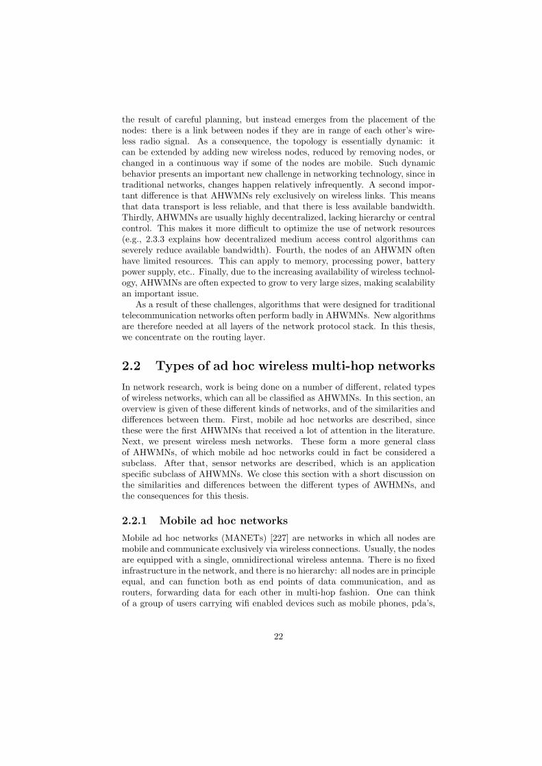
the result of careful planning, but instead emerges from the placement of thenodes: there is a link between nodes if they are in range of each other’s wire-less radio signal. As a consequence, the topology is essentially dynamic: itcan be extended by adding new wireless nodes, reduced by removing nodes, orchanged in a continuous way if some of the nodes are mobile. Such dynamicbehavior presents an important new challenge in networking technology, since intraditional networks, changes happen relatively infrequently. A second impor-tant difference is that AHWMNs rely exclusively on wireless links. This meansthat data transport is less reliable, and that there is less available bandwidth.Thirdly, AHWMNs are usually highly decentralized, lacking hierarchy or centralcontrol. This makes it more difficult to optimize the use of network resources(e.g., 2.3.3 explains how decentralized medium access control algorithms canseverely reduce available bandwidth). Fourth, the nodes of an AHWMN oftenhave limited resources. This can apply to memory, processing power, batterypower supply, etc.. Finally, due to the increasing availability of wireless technol-ogy, AHWMNs are often expected to grow to very large sizes, making scalabilityan important issue.

As a result of these challenges, algorithms that were designed for traditionaltelecommunication networks often perform badly in AHWMNs. New algorithmsare therefore needed at all layers of the network protocol stack. In this thesis,we concentrate on the routing layer.

2.2 Types of ad hoc wireless multi-hop networks

In network research, work is being done on a number of different, related typesof wireless networks, which can all be classified as AHWMNs. In this section, anoverview is given of these different kinds of networks, and of the similarities anddifferences between them. First, mobile ad hoc networks are described, sincethese were the first AHWMNs that received a lot of attention in the literature.Next, we present wireless mesh networks. These form a more general classof AHWMNs, of which mobile ad hoc networks could in fact be considered asubclass. After that, sensor networks are described, which is an applicationspecific subclass of AHWMNs. We close this section with a short discussion onthe similarities and differences between the different types of AWHMNs, andthe consequences for this thesis.

2.2.1 Mobile ad hoc networks

Mobile ad hoc networks (MANETs) [227] are networks in which all nodes aremobile and communicate exclusively via wireless connections. Usually, the nodesare equipped with a single, omnidirectional wireless antenna. There is no fixedinfrastructure in the network, and there is no hierarchy: all nodes are in principleequal, and can function both as end points of data communication, and asrouters, forwarding data for each other in multi-hop fashion. One can thinkof a group of users carrying wifi enabled devices such as mobile phones, pda’s,

22

Figure 2.1: An example of a MANET built up of mobile phones. The dashedlines symbolize the wireless links.

laptops, etc., moving in a specific area and forming a dynamic wireless networkamong them. See for example the MANET made up of mobile phones depictedin figure 2.1, where the dashed lines symbolize the wireless links.

As a consequence of the above mentioned properties, MANETs are dynamic,flat, fully decentralized networks without central control or overview. Thisgives rise to a number of tough challenges for networking algorithms. MANETalgorithms should be highly adaptive to the ever changing environment. Theyshould be robust in order to deal with unreliable wireless transmissions. Theyshould work in a fully distributed way. Finally, they should be efficient in theiruse of the limited network resources, such as bandwidth, battery power in themobile nodes, etc..

The idea for MANETs stems from research into DARPA packet radio net-works [142, 145]. Starting from the publication of the Destination-SequencedDistance-Vector routing algorithm [211] in 1994, MANETs were the first typeof AHWMNs to be investigated. The specific challenges that are encountered inthese networks have called the attention of many researchers and have made thisa very active research area. Also, the Internet Engineering Task Force (IETF)has set up a MANET working group to guideline standardizations. However,when it comes to implementation, the MANET challenges have proven to bevery hard to deal with, so that there is now also a growing interest in AH-WMNs with less mobility and more hierarchy and organization, such as thewireless mesh networks described in 2.2.2.

2.2.2 Wireless mesh networks

Wireless mesh networks (WMNs) [16] consist of two types of nodes: mesh clientsand mesh routers. Mesh clients are equivalent to MANET nodes: they are mo-bile, and usually communicate through one wireless interface, which is normally

23

Figure 2.2: An example of a WMN, in which five static wireless nodes (in thisexample, these are WiFi access points) act as mesh routers and a number ofheterogeneous mobile devices play the role of mesh clients.

an omnidirectional antenna. Like MANET nodes, they can serve both as endpoints of data traffic and as routers. Mesh routers, on the other hand, areless mobile or even static, and are usually equipped with various wireless de-vices, supporting different technologies. They are usually more powerful devicesthan the mesh clients, and often run on external power supply rather than onbattery power. The aim of the mesh routers is to form a wireless backbone in-frastructure for the WMN. An example of a WMN is given in figure 2.2: a smallgroup of static wireless nodes function as mesh routers, while a larger numberof heterogeneous mobile devices play the role of mesh clients.

The use of a more or less static backbone of mesh routers gives importantadvantages compared to MANETs. First, it gives some stability and organiza-tion to the network, which allows better exploitation of network resources. Forexample, data traffic can be routed primarily over the backbone nodes, whichare normally more powerful and have higher bandwidth, alleviating the taskof the mesh clients. Second, the fact that the mesh routers usually support avariety of different wireless communication technologies allows easy integrationof heterogeneous devices and networks. Finally, the mesh routers partly solvethe problem of battery power usage.

The mentioned advantages make WMNs easier to implement than MANETs.Consequently, an increasing number of mesh network implementation projectsare being started. These include projects from academic research, such as the

24

Roofnet [30] experiment of the Massachusetts Institute of Technology (MIT),projects by businesses, such as the Magnets [148] project of Deutsche TelekomLaboratories (DTL), and even spontaneous efforts by independent enthusiasts,such as the olsr.freifunk.net experiment in Berlin [9]. These networks have largedifferences in the way they were set up, their structure, the devices that are used,etc.. For example, Roofnet and olsr.freifunk.net are both totally unplannednetworks that only consist of randomly placed WiFi access points. Magnetson the other hand has a planned backbone of five high power routers thatare connected via directed wireless antenna’s, providing connectivity for a highnumber of randomly placed, less powerful devices around them. A detaileddescription of the Magnets project will be given in subsection 7.1.1.

2.2.3 Sensor networks

Sensor networks [17] are AHWMNs that consist of wireless sensor nodes. Thoseare small devices equipped with one or more sensors, some small processingcapacity, and a radio transmitter. The aim of sensor networks is to deploy alarge number of such sensor devices to measure a certain phenomenon. This canbe geological activity, human body functioning, etc.. By forming a multi-hopnetwork among them, the sensor nodes have a means to send the data theyhave measured to a ”sink” node, where they can be processed. The fact thatthe network is ad-hoc allows to set it up with minimal planning. One can forexample throw sensors from a boat into the sea so that they can form a networkat the bottom, or drop them from a plane.

Sensor networks come with their own specific challenges. First of all, theyare usually very large networks, possibly consisting of thousands of nodes ormore, so that algorithms need to scale well. Next, the sensor nodes are nor-mally designed to be very cheap, light devices. This means that they have verylimited resources for storage, processing and transmission, so that highly effi-cient algorithms are needed. This problem is acerbated by the fact that sensorbatteries can often not be replaced (e.g., when the sensors are thrown at thebottom of the ocean). Moreover, the use of cheap, low power radio technologyalso means that communication is highly unreliable and irregular. For example,changing radio ranges can give rise to unidirectional connections [290]. So algo-rithms have to be robust and should be able to deal with unidirectional links.Another issue in sensor networks is that their topology is usually very dynamic.Different from MANETs, this is not so much due to mobility of the sensor nodes(they are in fact often static), but rather to the easy failure of lightweight de-vices with limited power, and the fact that often new sensor devices are added.Finally, the communication patterns in sensor networks are quite specific: eachsensor node acquires data at regular intervals, and needs to send this data tothe sink node. It is important to take these patterns into account when design-ing network protocols, in order to obtain better usage of the limited availableresources.

25

2.2.4 Algorithms for different types of AHWMNs

All three types of networks described above possess the typical properties ofAHWMNs: they have an ad hoc, dynamic topology, they use unreliable connec-tions, they are highly decentralized, and they have limited network resources.Also, they might all grow to large sizes, although this aspect is more pronouncedin sensor networks than in MANETs and WMNs. Due to these similarities, net-working algorithms for different types of AHWMNs should have similar prop-erties, such as adaptivity to a changing environment, robustness with respectto packet corruption or loss, a highly distributed organization, efficiency andscalability. As a result, there is often a large overlap between algorithms usedfor the different types of AHWMNs. Especially for MANETs and WMNs thisis the case. MANETs were the first AHWMNs that received a lot of researchattention, and WMNs can in a way be seen as the follow up of MANETs. There-fore, WMNs use to a large extent the algorithms that have been proposed forMANETs. Sensor networks have been developed more or less in parallel withMANETs, and have more specific algorithms. The work in this thesis is in thefirst place focused on MANETs and WMNs.

2.3 Issues in ad hoc wireless multi-hop network-ing

This section builds on the general description provided in section 2.2 to inves-tigate important issues for networking in AHWMNs. We start with aspects ofnetwork connectivity and node mobility, and then move up the network proto-col stack discussing issues related to the physical layer, the data link layer, andthe transport layer. Specific attention is given to how these issues have conse-quences for the task of routing. Routing itself is not discussed in this section:since it is the main focus of attention of this dissertation, it is treated in moredetail in section 2.4.

2.3.1 Network topology and node mobility

As stated in 2.2, the topology of an AHWMN is normally not the result ofcareful planning, but arises from the placement of the nodes. In what follows,we first comment on how this affects network connectivity, and then on how itrelates to node mobility.

Network connectivity

There is a link between two nodes of an AHWMN if they can receive eachother’s radio signals. Therefore, the topology of the network is directly definedby the relative placement of the nodes and the range of their radio transmitters.Since the placement of the nodes in an AHWMN is done in ad hoc manner, withminimal planning, it can be considered as a random process, from which the net-work topology emerges. An important factor in this process is the node density,

26

since it directly influences the connectivity in the resulting network topology.In [88, 89], the theory of percolation is used to investigate this relationship be-tween node density and network connectivity analytically. The authors showthat there is a quite clear cut off point in node density, called the critical density,under which the network falls apart into small, internally connected islands, andabove which there is connectivity between the majority of the nodes in the net-work. For densities that are just above the critical density, this network wideconnectivity is quite sparse, so that paths between most pairs of nodes dependon the availability of a few critical links. The failure of any of these criticallinks has a large impact on the routing possibilities in the network. This is incontrast with densely connected networks, where often many alternatives areavailable to route around a failed link. This means that in sparse networks, itis more difficult for a routing algorithm to provide adaptivity to changes in thenetwork topology. So, we can conclude that the node density of an AHWMNdirectly affects the difficulty of the routing task.

Node density only has meaning when treated relative to the transmissionrange of the nodes’ radio equipment: if this range is reduced while the number ofnodes per unit of area stays the same, the connectivity of the network decreases.This means that variations of the radio range influence network connectivityas much as node density. Radio range variations can happen accidently, forexample because of random variations in the environment or because of changesin the available power in each node (see also explanations in 2.3.2), or can beinduced intentionally, for example in order to save battery power or to reduceradio interference between different transmitters [150, 195]. Some work treatsthe problem of defining a minimal power usage for each node under the explicitconstraint that there needs to be at least one path between each pair of nodes inthe network [114, 196]. This is particularly relevant in sensor networks, where,as mentioned in 2.2.3, batteries can sometimes not be replaced. Clearly, theapplication of such schemes can give rise to difficult topologies to maintainrouting in.

Node mobility

Since the network topology is defined by the placement of the nodes, it changeswhen the nodes move. As a consequence, the difficulty of the routing taskis also strongly influenced by the characteristics of the node mobility. Thesecharacteristics include the speed of the movements, and the specific patternsfollowed by the nodes. The latter defines for example how the nodes moverelative to each other, and can give rise to temporary differences in node density.The impact of node mobility is especially important in MANETs, where allnodes are mobile.

Node mobility depends on the usage of the network. Unfortunately, most re-search on AHWMNs is done in academic context, without a clear understandingof their purpose. Mobility is therefore usually simulated with artificial models,of which the Random Waypoint model (RWP) [140] is by far the most popular.Under this model, each node picks a random destination, and a random speed,

27

and moves in a straight line to this destination with the chosen speed. Thenthe node pauses for a certain time, after which it picks a new destination andspeed. Other models use different approaches, or model specific behaviors suchas e.g. group movements. An overview of mobility models used in the litera-ture is given in [46]. In recent years, there is a growing suspicion towards theseartificial mobility models, because they do not reflect real movements very well,and because they may artificially give rise to certain node distributions. Forexample, under RWP, nodes tend to cluster more in the center of the AHWMNarea, so that there is higher density there, giving better connectivity [29]. Thereis now a lot of interest in collecting traces of real movements of people (e.g.,see [55]), but so far very few such information is available.

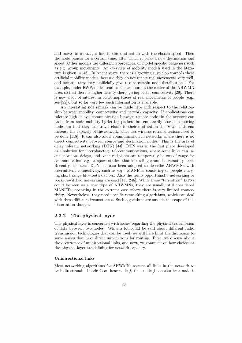
An interesting side remark can be made here with respect to the relation-ship between mobility, connectivity and network capacity. If applications cantolerate high delays, communication between remote nodes in the network canprofit from node mobility by letting packets be temporarily stored in movingnodes, so that they can travel closer to their destination this way. This canincrease the capacity of the network, since less wireless retransmissions need tobe done [118]. It can also allow communication in networks where there is nodirect connectivity between source and destination nodes. This is the area ofdelay tolerant networking (DTN) [44]. DTN was in the first place developedas a solution for interplanetary telecommunications, where some links can in-cur enormous delays, and some recipients can temporarily be out of range forcommunication, e.g. a space station that is circling around a remote planet.Recently, the term DTN has also been adopted to describe AHWMNs withintermittent connectivity, such as e.g. MANETs consisting of people carry-ing short-range bluetooth devices. Also the terms opportunistic networking orpocket switched networking are used [133,246]. While these “terrestrial” DTNscould be seen as a new type of AHWMNs, they are usually still consideredMANETs, operating in the extreme case where there is very limited connec-tivity. Nevertheless, they need specific networking algorithms, which can dealwith these difficult circumstances. Such algorithms are outside the scope of thisdissertation though.

2.3.2 The physical layer

The physical layer is concerned with issues regarding the physical transmissionof data between two nodes. While a lot could be said about different radiotransmission technologies that can be used, we will here limit the discussion tosome issues that have direct implications for routing. First, we discuss aboutthe occurrence of unidirectional links, and next, we comment on how choices atthe physical layer are defining for network capacity.

Unidirectional links

Most networking algorithms for AHWMNs assume all links in the network tobe bidirectional: if node i can hear node j, then node j can also hear node i.

28

In reality however, an AHWMN can also contain unidirectional links. Thesecan occur for various reasons. One reason can be a difference in radio rangebetween the nodes: if i has a higher range than j, it is possible that j canhear i while i cannot hear j. Such a difference in radio range can be chosendeliberately, or can be the result of a difference in available battery power inthe nodes (see subsection 2.3.1). Another, related reason for the occurrence ofunidirectional links is radio irregularity. It has been observed that the radiorange of wireless nodes does not form a perfect circle around the node, butinstead shows quite irregular patterns [290]. This is mainly due to differences inradio wave propagation in different directions. A third reason for unidirectionallinks can be interference by other transmitters. It is possible that the levelof interference is different at i and j, so that one of the two can temporarilynot receive data from the other. The negative impact on network performancedue to the presence of unidirectional links has been documented in variousworks [187,219].

Network capacity

Choices at the physical layer are defining for the network capacity. Most workon AHWMNs relies on WiFi technology (IEEE 802.11) [3], which can in theoryprovide a relatively high throughput of up to 54 Mbps. Other, newer tech-nologies, such as UWB (IEEE 802.15.3) [4,282] and WiMax (IEEE 802.16) [5],promise even much higher throughput. Despite these high bandwidth values,however, the actual available capacity in an AHWMN is much lower. This is dueto interference between different transmitters. Different pairs of nodes in thenetwork can only communicate simultaneously if they are situated far enoughfrom each other, so that they do not disrupt each other’s signal. This is alsoreferred to with the term “spatial reuse”: the wireless channel can be used formultiple simultaneous communications if there is spatial separation. In [120],the authors investigate how much capacity is actually available in an AHWMNif spatial reuse is optimally used. They conclude that the available capacityper node in bit-meters per second is inversely correlated with the square rootof the total number of nodes in the network, which means that for large AH-WMNs, the available capacity per node tends to zero. This result is not veryencouraging for AHWMN research, but needs to be read with some caution.The investigation was done for networks using single-channel, omnidirectionalantennas. If more than one channel is used, or other antenna systems, suchas directional antennas [284] or multi-antenna systems [179], better capacitycan be obtained. Nevertheless, when developing algorithms for AHWMNs, oneneeds to be aware that the total available bandwidth is much lower than whatwireless technologies can in theory provide, so that efficiency is important.

2.3.3 The data link layer

The data link layer is concerned with the organization of transmission andretransmission of data between two nodes. Often, the data link layer is identified

29

with its most important component, the medium access control (MAC) sublayer.This component deals with the coordination of the access of different nodes toa shared communication medium. In AHWMNs, this comes down to avoidinginterference while maximizing spatial reuse. A different goal, which is mainlyimportant in sensor networks, is power saving [19]. In what follows, we firstdescribe general issues related to MAC organization in AHWMNs, and thendiscuss the most popular AHWMN MAC protocol, namely the IEEE 802.11DCF protocol.

Medium access control in AHWMNs

Since AHWMNs are usually highly decentralized, MAC protocols need to workin a distributed way. This makes it difficult to organize the sharing of thewireless medium in an efficient way via the creation of multiple channels throughfrequency or code division multiplexing, or via the assignment of time slots.Research is therefore mainly concentrated on single channel, contention basedalgorithms.

Contention based algorithms do not strictly separate simultaneous commu-nications, but instead allow the possibility of a collision of transmissions [254].If such collision happens, the transmission should be retried. Carrier sensingcan limit the probability of collisions: the basic idea is to listen whether thechannel is idle before starting to send. Important problems that need to besolved by single channel contention based algorithms are the hidden terminaland the exposed terminal problems. Consider figure 2.3, where four wirelessnodes are placed in a row, so that the distance between each pair is roughlyequal to their wireless radio range (assuming an idealized circular radio rangefor each node). The hidden terminal problem takes place when C wants to sendto D while A is sending to B. Since C cannot hear the signals from A, it canerroneously assume that the channel is free and start sending, hereby disruptingthe reception at B. The exposed terminal problem is more or less the opposite:when B is sending to A, C can hear the signal and therefore decide that thechannel is busy, while a simultaneous transmission from B to A and from C toD is possible without causing interference at signal reception.

The most popular MAC algorithm in AHWMN research is the IEEE 802.11Distributed Coordination Function (DCF) [135], which we describe below. Arange of other MAC algorithms have been proposed. Many of these algorithmsare variations on IEEE 802.11 DCF, or are at least similar in approach. Seee.g. [159] for an overview.

IEEE 802.11 DCF

The IEEE 802.11 DCF MAC algorithm is a contention based single channelprotocol. It uses both carrier sensing and extra control packets to limit thenumber of collisions. The basic working of IEEE 802.11 DCF is as follows.When a node wants to start a transmission, it listens to check whether thewireless medium is free. Next, it sends a request-to-send message (RTS) to the

30

A B C D

Figure 2.3: The hidden and exposed terminal problems (figure adapted from[254])

node it wants to transmit to, in order to request the start of a conversation.If this node is free to receive, it sends a clear-to-send message (CTS) back.The requesting node can then start the transmission of data, and if this issuccessful, the receiving node concludes the communication by sending out anacknowledgement message (ACK). Between each of the steps of this process,there are small waiting times to avoid collisions. If the process goes wrong atany time, it needs to be restarted completely, after a randomly chosen backoffinterval. With each failed transmission attempt, the window from which thisbackoff interval is chosen, is doubled. The hidden terminal problem is solvedby the RTS/CTS mechanism. The exposed terminal problem is not solved bythe IEEE 802.11 DCF algorithm. A special remark needs to be made regardingbroadcasting. In principle, all communication with omnidirectional wirelessantennas is done in broadcast mode (i.e., all nodes on the medium receive themessage). However, the RTS/CTS and ACK mechanisms are done with just onenode and assure the implementation of unicasting. Therefore, if a node wantsto broadcast a message to all its neighbors, it cannot use these mechanisms.As a consequence, broadcast transmissions are less protected and therefore lessreliable than unicast transmissions.

A lot of research has been done to assess the efficiency of the IEEE 802.11DCF algorithm. First of all, due to the sending of extra control packets aroundeach data packet, and the small delays between each of these sendings, the the-oretical maximum throughput using IEEE 802.11 DCF is a lot lower than theactual capacity of the radio transmitters [143] (down to 50% or less dependingon the size of the transmitted data packets). More problematic is the use of theexponentially growing random backoff interval: if there are a lot of collisions, e.g.when there is a lot of data traffic in the network, it is possible that some commu-nications are suspended for a longer time, or even get completely starved [28].This problem can be acerbated in multi-hop communications, where subsequenthops in a path can actually interfere with each other [170,280].

As a consequence of all this, the use of IEEE 802.11 DCF puts further severe

31

limitations on the already compromised capacity of AHWMNs (the capacitylimitations based on spatial reuse calculations described in 2.3.2 assumed aperfect MAC layer protocol). Some improvements have been proposed in otherMAC protocols (see [159]), but the basic problems stay the same. The maincause of inefficiency in MAC layer organization is the decentralized nature ofAHWMNs, which commands a distributed approach. Improvements are possibleif there is some structure in the network, such as between backbone nodes in aWMN (see 2.2.2), or if node mobility is low enough so that there is time to set upa different MAC organization, as is sometimes done in sensor networks [19,161].In other cases, however, we need to be aware that the MAC layer limits thecapacity of the network, and increases the need for efficiency at the routinglayer.

2.3.4 The transport layer

The transport layer is situated above the routing layer. It is concerned with theorganization of the transport of data between the source and destination nodes ofa communication session over the path provided by the routing algorithm [254].The two main transport protocols in the internet are the User Datagram Pro-tocol (UDP) [217] and the Transmission Control Protocol (TCP) [218]. TCPoffers a secure transport service: a triple handshake mechanism is used to estab-lish a connection at the start of the transport session, the arrival of each datapacket is acknowledged by the receiver, warnings are sent from the destinationto the source if packets arrive out of order, lost packets are retransmitted, anda congestion control mechanism is used to adapt the speed of the data flowin case there is packet loss. UDP, on the other hand, offers a service withoutany guarantees: it just sends packets on their way from source to destination,without using any of the mentioned mechanisms. UDP can be preferred overTCP for short data transports when the underlying network is very reliable. Inwhat follows, we comment on the use of TCP and UDP in AHWMNs.

TCP versus UDP in AHWMNs

AHWMNs are inherently unreliable networks, due to their use of wireless linksand their dynamic nature. So it makes sense to use a secure service like TCP,rather than UDP. However, there are problems with the use of TCP in AH-WMNs, stemming from various causes.

A first problem for TCP in AHWMNs is that its various mechanisms cause alot of extra overhead [111]. For example, for each data packet going from sourceto destination, an acknowledgement is sent back from destination to source.This goes in conflict with the typically low capacity of AHWMNs, as describedin 2.3.2 and 2.3.3. This problem can be acerbated due to interactions withthe MAC layer algorithm, as TCP uses exponentially growing random backofftimers for retransmission, just like IEEE 802.11 DCF (see 2.3.3). A secondproblem is caused by TCP’s congestion management mechanism [22,250]. TCPwas designed with wired networks in mind, where data transmissions are quite

32

reliable. Therefore, when TCP detects a problem with data delivery (out oforder delivery or packet loss), it assumes that the cause is congestion of thenetwork, and consequently reduces the data flow. In AHWMNs, however, packetloss is often caused by the use of unreliable wireless links or mobility inducedpath loss. TCP will therefore lower its throughput unnecessarily and reducethe throughput of the network. A third problem has to do with TCP timers.To define whether a packet was lost, TCP uses timers, which are based on anestimate of the time it takes for a packet to go to a destination and for anacknowledgement to come back to the source. This is the so-called round triptime (RTT). In an AHWMN, which is an inherently dynamic environment, theRTT can vary greatly, making its estimation difficult. This causes TCP todetect false packet losses, which are again interpreted as caused by congestion,with a reduction of the data throughput as a consequence. A final problem hasto do with the frequent path failures that occur in AHWMNs [130]. In thesesituations, there is again packet loss, but the destination will not be able towarn the source about it. Therefore, the source only detects the loss when itstimer for the acknowledgement runs out, causing extra delay.

The above problems make the use of TCP in AHWMNs problematic. There-fore, many variations of TCP have been proposed, in an attempt to deal withthese difficulties. See [268] for an overview. Nevertheless, many AHWMN re-search studies avoid these problems altogether by using the UDP transportprotocol. For the routing layer, the important message is that correct data de-livery is an important evaluation criterium, as the transport layer above it hasdifficulties providing reliability.

2.4 Routing in ad hoc wireless multi-hop net-works

Routing is the task of directing data flows from source nodes to destinationnodes while maximizing network performance. This is particularly hard in AH-WMNs. Due to the ad hoc and dynamic nature of the network, the topology canchange constantly, and paths between sources and destinations that were ini-tially efficient can quickly become inefficient or even infeasible. This means thatrouting information should be updated more regularly than in traditional wiredtelecommunication networks. However, this can be a problem in AHWMNs,with their limited bandwidth and node resources, and their possibly unreliablecommunication channels. New routing algorithms are therefore needed, whichcan give adaptivity in an efficient and robust way.

A lot of research has been done on routing in AHWMNs in the past few years.In this section, we give an overview of the research in this area. The aim is notto present an exhaustive list of existing protocols (for this, we refer to existingsurveys, such as [14, 227]), but rather to describe the most important ones andto give insight into interesting ideas and techniques that have been developed inthis area. We start the section with an explanation of the distinction between

33

proactive and reactive routing protocols, which is the most used criterium toclassify AHWMN routing algorithms. Next, we describe in detail a number ofrepresentative routing algorithms. Finally, we give an overview of importanttechniques used in other AHWMN routing algorithms.

2.4.1 Proactive versus reactive routing algorithms

Traditionally, AHWMN routing protocols are classified as proactive or reac-tive protocols. Under proactive routing protocols, all nodes of the network tryto maintain consistent routing information about all other nodes at all times.This means that routing information needs to be updated after each changein the network. Data are routed by a simple lookup in the tables which storethe routing information, and proactive routing algorithms are therefore alsocalled table-driven [227]. Examples of proactive algorithms are Destination-Sequenced Distance-Vector Routing (DSDV) [211] and Optimized Link StateRouting (OLSR) [61] (see subsection 2.4.2 for descriptions of both algorithms).Under reactive routing protocols, nodes only gather the routing informationthat is strictly needed. This is the case when a new data session is started,or when a currently used path fails. Gathering routing information usuallyinvolves a route discovery or a route repair phase. Reactive algorithms arealso called on-demand algorithms [227]. Examples are Dynamic Source Routing(DSR) [140] and Ad-Hoc On-Demand Distance Vector Routing (AODV) [213](see subsection 2.4.2).

Proactive algorithms have the advantage that routing information is alwaysreadily available when data needs to be sent. Also, all changes in the networkare taken into account, so that new routing opportunities can be exploited, andbackup paths can be provided when primary paths fail. On the downside, thesealgorithms can become quite inefficient or even break down completely whena lot of changes need to be tracked. This is the case when the topology ishighly dynamic, or when the network is large. Reactive algorithms only focuson the routing information that is strictly necessary. This way, they can greatlyreduce the overhead they create, so that they are in general more efficient. Thedisadvantage is that they are never prepared for disruptive events, and thatsome data packets can therefore incur large delays, e.g. during the route setupphase at the start of a communication session. In MANETs, where all nodesare mobile, so that there are a lot of topology changes, the general preference isfor reactive algorithms [42]. However, in WMNs, which are less dynamic, andin sensor networks, where nodes are often not mobile, proactive algorithms canalso be a good choice.

So far we have used the terms proactive and reactive routing in a rather strictsense. We can define reactive behavior in a more general way as the gatheringof routing information in reaction to an event, and proactive behavior as thegathering of routing information at all other times. Algorithms which combineboth reactive and proactive elements are called hybrid algorithms. They tryto combine the advantages of both approaches. The classic example is theZone Routing Protocol (ZRP) [121] (see subsection 2.4.2). In practice, a lot

34

of AHWMN routing algorithms can be labeled hybrid, since they contain somecombination of reactive and proactive behavior.

2.4.2 Important routing algorithms for AHWMNs

In what follows we describe in detail some of the most representative routingalgorithms for AHWMNs. For routing in MANETs and WMNs, which largelyuse the same protocols, we describe two proactive algorithms, DSDV and OLSR,two reactive algorithms, DSR and AODV, and one hybrid algorithm, ZRP. Forsensor networks, we describe directed diffusion, which is a reactive protocol.

Destination-Sequenced Distance-Vector Routing

DSDV, published in 1994 [211], was the first routing algorithm for AHWMNs. Itis a direct adaptation of distance vector routing, which is at the basis of internetrouting protocols such as Routing Information Protocol (RIP) [123] and BorderGateway Protocol (BGP) [178] (see also subsection 3.1.1).

In distance vector routing algorithms, every node i keeps for every destina-tion x a set of distances {dx

ij}, indicating the distance to reach x from i whenneighbor j is used as the next hop in the path. The distance metric can be thenumber of hops or the end-to-end delay. Data that need to be routed for desti-nation x are sent to the neighbor with the lowest value for the distance. In orderto keep the distance vector tables up to date, each node periodically broadcastsan update of its shortest routes to its neighbors. A neighbor k receiving fromi the update dx

i , which is the shortest distance from i to x, can calculate itsown distance to x over i, dx

ki, by combining dxi with the cost of the link from

k to i (which it monitors locally). Even if nodes initially start with completelyrandom estimates for each of the path costs {dx

ij}, the system of continuouslyupdating the cost estimates eventually converges, so that all nodes have correctestimates for the costs of all paths. Distance vector routing is also known as dis-tributed Bellman-Ford routing [27], and stems from the adaptation of dynamicprogramming [26] to the problem of routing. More on distance vector routingwill follow in subsection 3.1.1.

One of the main problems with distance-vector methods is that loops can beformed. This is mainly due to the fact that nodes make routing decisions in adistributed way, and possibly do so using stale distance information. Moreover,since nodes base their routing information on estimates provided by other nodes,wrong information can quickly propagate through the network, and even thougheventually all routing information should converge to correct values, this mighttake quite long (see e.g. the problem of counting to infinity [254]). As routinginformation gets out of date really fast in AHWMNs, this problem can getquite severe. DSDV solves the problem using sequence numbers assigned bythe destination node. When faced with multiple route updates, nodes alwaysprefer the fresher information (the newest sequence number). Only when tworoutes are equally fresh the shorter route is chosen. Another feature in DSDV isthe use of incremental updates. In order to avoid that nodes have to broadcast

35

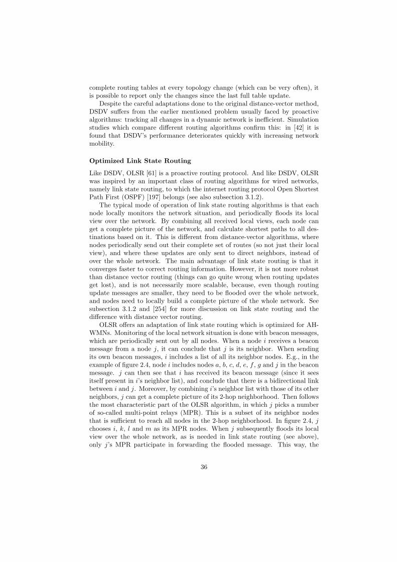
complete routing tables at every topology change (which can be very often), itis possible to report only the changes since the last full table update.

Despite the careful adaptations done to the original distance-vector method,DSDV suffers from the earlier mentioned problem usually faced by proactivealgorithms: tracking all changes in a dynamic network is inefficient. Simulationstudies which compare different routing algorithms confirm this: in [42] it isfound that DSDV’s performance deteriorates quickly with increasing networkmobility.

Optimized Link State Routing

Like DSDV, OLSR [61] is a proactive routing protocol. And like DSDV, OLSRwas inspired by an important class of routing algorithms for wired networks,namely link state routing, to which the internet routing protocol Open ShortestPath First (OSPF) [197] belongs (see also subsection 3.1.2).

The typical mode of operation of link state routing algorithms is that eachnode locally monitors the network situation, and periodically floods its localview over the network. By combining all received local views, each node canget a complete picture of the network, and calculate shortest paths to all des-tinations based on it. This is different from distance-vector algorithms, wherenodes periodically send out their complete set of routes (so not just their localview), and where these updates are only sent to direct neighbors, instead ofover the whole network. The main advantage of link state routing is that itconverges faster to correct routing information. However, it is not more robustthan distance vector routing (things can go quite wrong when routing updatesget lost), and is not necessarily more scalable, because, even though routingupdate messages are smaller, they need to be flooded over the whole network,and nodes need to locally build a complete picture of the whole network. Seesubsection 3.1.2 and [254] for more discussion on link state routing and thedifference with distance vector routing.

OLSR offers an adaptation of link state routing which is optimized for AH-WMNs. Monitoring of the local network situation is done with beacon messages,which are periodically sent out by all nodes. When a node i receives a beaconmessage from a node j, it can conclude that j is its neighbor. When sendingits own beacon messages, i includes a list of all its neighbor nodes. E.g., in theexample of figure 2.4, node i includes nodes a, b, c, d, e, f , g and j in the beaconmessage. j can then see that i has received its beacon message (since it seesitself present in i’s neighbor list), and conclude that there is a bidirectional linkbetween i and j. Moreover, by combining i’s neighbor list with those of its otherneighbors, j can get a complete picture of its 2-hop neighborhood. Then followsthe most characteristic part of the OLSR algorithm, in which j picks a numberof so-called multi-point relays (MPR). This is a subset of its neighbor nodesthat is sufficient to reach all nodes in the 2-hop neighborhood. In figure 2.4, jchooses i, k, l and m as its MPR nodes. When j subsequently floods its localview over the whole network, as is needed in link state routing (see above),only j’s MPR participate in forwarding the flooded message. This way, the

36

i d

eg

a

l

k b

c

f

j

m

Figure 2.4: The working of OLSR. The dashed lines symbolize wireless links(not all links are drawn in order not to overload the picture). Node j choosesi, k, l and m as MPR nodes, since they are sufficient to reach all its two-hopneighbors. Figure adapted from [61].

flood needs less packet transmissions. Moreover, the local view sent out by j isnothing more than a list of all nodes that have selected j as MPR, j’s so-calledMPR selector nodes. This means that the flooded messages can be quite small.It also means that the global network views constructed based on these localviews contain only connections between nodes and their MPR selector nodes,so that the network is smaller but still fully connected. Finally, if MPR nodesare chosen from among neighbors with which there is a bidirectional connection,the global network view will contain only bidirectional connections. This canbe important in case there is irregular radio wave propagation which can causelinks to be unidirectional (see also 2.3.2).

Being a proactive routing protocol, OLSR inherits the earlier mentioned ef-ficiency problems in highly dynamic AHWMNs. Also, being a link state routingprotocol, OLSR is not very robust with respect to loss of control packets, andnot very scalable. Nevertheless, the mechanisms adopted for improving effi-ciency are interesting, and the fact that bidirectional links can be identified canbe an important asset. Consequently, OLSR has received considerable attentionsince its publication in 2001, especially when it comes to making implementa-tions for real deployment: it was the routing algorithm of choice for the alreadymentioned olsr.freifunk.net experiment in Berlin [9], and has been implementedfor use under Windows and Linux by the Navy Research Labs [8]. In one studywith a real MANET testbed [36], OLSR has been shown to give comparable per-formance to the AODV reactive routing algorithm when the network is small

37

and has limited mobility. OLSR has been published as a standard by the IETFMANET working group [60].

Dynamic Source Routing

DSR [140] was in 1996 the first reactive routing algorithm to be published. Asin other reactive algorithms, nodes only actively look for routing informationwhen it is strictly needed, i.e. when data needs to be sent to a destination forwhich no valid route exists. Important features of the algorithm are that ituses source routing, and that it makes extensive use of caching to increase theavailable routing information.

Under DSR, nodes that need to send data first check whether they haveany routing information available for the requested destination. If this is notthe case, a route discovery process is started, in which a route request message(RREQ) is flooded over the network. Once the RREQ reaches the destination, aroute reply message (RREP) is sent back to the source, either following the samepath of the RREQ back, or following a different path from the destination tothe source. At the return of the RREP, the route discovery process is complete,and the source can start sending data. If later, during the communication, oneof the links on the path fails, a route error message (RERR) is sent from thenode where the error was detected back to the source, which can then start anew route discovery process.

An important aspect of DSR is that it uses source routing. This meansthat data are not routed hop by hop, as is common practice in most routingalgorithms, but that instead the source node decides about the complete pathto the destination, and adds it to each data packet. While this means extraoverhead per data packet, source routing has as an advantage that the sourcehas complete control over the path, so that e.g. loops can be avoided. Anotheradvantage is that all nodes that receive a data packet on its way to its destinationcan extract information about the topology of the network. This last propertyis exploited extensively in DSR, which allows nodes to cache all routes theycan extract from passing data packets (if promiscuous mode is possible, thisincludes also data packets that were not destined for the current node, butcould somehow be overheard). This allows to build a database of existing routes,which can be used to avoid the need for a route discovery process, to providebackup paths in case of failure, etc.. However, caching can also be dangerous.Overheard routes often stay in cache unused for a while before they are actuallyneeded, at which point they might have expired already. As a consequence, datapackets can be sent onto erroneous routes, leading to extra delay and overhead.Moreover, these erroneous routes can be overheard by other nodes, so that wronginformation can actually spread over the network. This phenomenon is called“cache pollution” [183,186].

DSR is an important reference algorithm in the field. A number of studiescompare it to AODV, the other important reactive algorithm, which is describedbelow, however with few conclusive results [42, 65]. Recently, DSR formed theinspiration for Link Quality Source Routing (LQSR) [92], which is the routing

38

algorithm used in the Mesh Connectivity Layer (MCL) architecture developedby Microsoft Research labs, and for the Srcr routing algorithm, which was de-veloped for use in MIT’s Roofnet WMN testbed [30].

Ad-Hoc On-Demand Distance Vector Routing

AODV [213] was published as the on-demand version of DSDV. Like DSDV,it uses hop by hop data routing based on distance vector tables. Also, it usesthe destination based sequence numbers of DSDV to distinguish old from newrouting information. Being a reactive algorithm however, AODV is in its generalworking more similar to DSR.

Under AODV, nodes that have data to send to a destination that theyhave no information about, start a route discovery process. This process issimilar to the one of DSR: a RREQ is flooded over the network, and when itreaches the destination, a RREP is sent back to the source, which can thenstart sending data over the newly established path. The difference with DSRlies in the way routes are identified: the RREQ does not store the full paththat it has traveled, but instead leaves in the routing table of each intermediatenode a pointer towards the source. The RREP follows these pointers backto the source, and changes them into pointers towards the destination. Datapackets are routed from source to destination following these pointers, and donot have to carry full paths. When there is a failure anywhere along the path,a RERR is used to warn the source, which can start a new route discoveryprocess. A possible improvement, which was studied together with some otheroptimizations of AODV in [165], allows for intermediate nodes to try to locallyrebuild failed routes, i.e. to find a route around a failed link. This is called localrepair.

The use of hop by hop rather than source routing has as most importantadvantage that there is no extra overhead for each data packet. A disadvantageis that nodes cannot extract routes from passing data packets, so that cachinglike in DSR is impossible. However, as was explained before, caching can alsohave a negative impact.

AODV is by far the most cited and studied AHWMN routing protocol.It forms the most important benchmark algorithm for the evaluation of otherrouting protocols, and has been standardized by the IETF [212].

Zone Routing Protocol

ZRP [121] was the first hybrid routing algorithm. It is less used than other rout-ing algorithms presented in this section, but is described here because it providesa simple example of how reactive and proactive routing can be combined.

Under ZRP, proactive routing is used within a certain zone around eachnode (so each node keeps up-to-date routes to nodes in a k hop radius, where kcan be equal to 2 or 3 e.g.), and reactive routing is used for destinations furtheraway. Data for destinations within the zone can therefore be delivered straightaway. For destinations further away, a route discovery process is needed. The

39

use of the zones allows to design a route discovery process that is more efficientthan those of AODV and DSR: the source node sends the RREQ to the nodesat the outer edges of its zone, and those nodes forward it to their zone’s outeredges and so on, so that the RREQ travels in jumps. The discovered pathsconsist of a list of zone edge nodes, and do not contain information about thenodes between them. This means that the paths can be smaller to store, andthat they can in principle be more robust (since they are not affected by themovement of nodes between the zone edge nodes).

Directed diffusion

Directed diffusion [137] is a reactive routing protocol for sensor networks. It ad-dresses issues of scalability, robustness and efficiency, and was designed specifi-cally to support the typical communication patterns of sensor networks, wherethe sensor nodes periodically need to forward their sensed data to one or moresink nodes. Directed diffusion has similarities to Temporally-Ordered Rout-ing Algorithm (TORA) [209], which is a reactive routing algorithm that wasdeveloped for MANETs.

In directed diffusion, the setup of data paths is initiated from the sink nodewhen data are needed. To this end, an interest message is formulated, whichdescribes which data are needed, for which period they are needed, and withwhich frequency. This interest is subsequently propagated through the networkto all sensor nodes. Each node that receives it sets up a gradient, which isa pointer to the node it received the interest from, and starts looking for therequested data with the requested frequency. When a node obtains data that fitthe interest message, it forwards them along the corresponding gradient. Datacoming from different parts of the sensor network can be aggregated when theymeet in an intermediate node while traveling to the sink. This way, forwardingcan be done more efficiently, which is very important given the strict powerlimitations in sensor networks. Once the sink node starts receiving data, itstarts to regularly resend its interest, in order to reinforce and repair the existingpaths. This way, higher robustness is provided.

2.4.3 Other techniques for AHWMN routing

The algorithms described in 2.4.2 represent the most cited ones in the area ofAHWMN routing. In what follows, we give a broader overview of this researcharea. In particular, we describe a number of interesting techniques that havebeen developed, explain how they are used in different algorithms, and commenton advantages and disadvantages of each of them. In particular, we talk aboutthe use of multipath routing, about creating a hierarchical structure in thenetwork, about the use of geographical location information, about differentrouting metrics, about techniques for large scale AHWMNs, about multicasting,geocasting and broadcasting, and about data-centric routing, which is importantin sensor networks.

40

Single path versus multipath routing

Most routing algorithms use single path routing: at all times, only one pathis maintained between source and destination. The alternative is to maintainmultiple paths simultaneously. Advantages of multipath routing include higherthroughput, because data can be spread over the different paths, and higherrobustness, because backup paths are available in case of a failure and becausemultiple copies of the data can be sent in parallel over different paths. Bothof these are important features in the face of the low capacity and reliabilitythat are typical for AHWMNs. Disadvantages of multipath routing are mainlydue to the fact that more than one path needs to be set up and maintained.This leads to more complex algorithms, and more overhead. A confirmationof the advantages and disadvantages of multipath routing in AHWMNs, bothvia analysis and simulation, is given in [214]. On the other hand, a similaranalytical study in [109] shows how a bad spreading of the multiple paths cannegatively affect the throughput advantage.

A large number of multipath routing algorithms have been proposed in AH-WMN research. See [198] for an overview. These algorithms differ in the waymultiple paths are set up, maintained and used. During path setup, a num-ber of different paths are selected. Some algorithms allow braided multiplepaths [108], whereas others look for link [186] or node [283] disjoint paths, oreven paths which are outside each other’s interference range [278]. This is im-portant in AHWMNs, where the augmented throughput offered by the use ofmultiple paths can only be realized if these paths do not interfere with eachother. Once the paths are set up, they need to be maintained. Most algorithmsmanage the paths in a reactive way: they remove paths when a link break oc-curs, and only take action when no valid path to the destination is left. A fewalgorithms use probing to obtain up-to-date information about the paths andto detect failures [108,269]. Finally, the way the multiple paths are used differsstrongly among algorithms. In many of them, only one of the paths is used fordata transport, while the others are only used in case of a failure in the primarypath [163, 201]. Some algorithms also explore the idea of spreading data overthe multiple paths to increase the throughput [108,164,269]. An interesting wayof spreading data to increase robustness is presented in [261]: diversity codingallows to encode N blocks of data into M + N blocks in such a way that anysubset of size N of these M + N blocks allows to reconstruct the original data.By using this encoding and spreading data over multiple paths, robustness ofdata delivery can be greatly improved.

Network structure

Many AHWMN routing algorithms, including the algorithms DSDV, OLSR,AODV and DSR described in 2.4.2, consider all nodes in the network as equaland perform routing in an essentially flat space. These are called uniform pro-tocols. A different approach is to try to make the routing task easier by givingsome structure to the routing space. This is the strategy used by partition-

41

ing protocols. A classic example is Clusterhead Gateway Switched Routing(CGSR) [59]. This algorithm organizes the AHWMN in clusters, each with aclusterhead and a number of gateways, and organizes all communication be-tween nodes of different clusters via the clusterheads and the gateways.

The advantage of partitioning algorithms is that they simplify routing, sothat in principle better efficiency and scalability can be achieved. In practice,however, there are also some important disadvantages. First, if mobility ishigh, the maintenance of the network partitioning can cause a lot of overhead.Second, attributing roles such as clusterhead or gateway to certain nodes meansthat the network is more dependent on them, and that they have to performmore work than other nodes (this can be a problem if there is limited batterypower e.g.). Finally, although partitioning leads to faster route discovery inlarge networks, the discovered routes are not always the shortest: nodes couldbe close to each other in the network, but still have to communicate throughtheir respective clusterheads. In sensor networks, where nodes are often staticand scalability is a very important factor, partitioning algorithms are relativelymore popular than in MANETs and WMNs. An example is the Low EnergyAdaptive Clustering Hierarchy protocol (LEACH) [125].

A middle way between uniform and partitioning protocols is given by neigh-bor selection protocols [102]. In these protocols, each node gives some structureto the network from its own point of view. An example is the previously men-tioned ZRP (see 2.4.2), in which each node uses a proactive protocol to maintainrouting information about nodes within a certain number of hops, and a reac-tive protocol for nodes further away. Another example is Fisheye State Routing(FSR) [210], in which updating of routing information is done frequently fornearby nodes, and less frequently for nodes further away. This results in ablurred vision of the network: for faraway nodes only a vague routing direc-tion is known, but as the data packet approaches its destination, more preciserouting information is available. The advantage of neighbor selection protocolsis that there is some structure in the network, which improves scalability andefficiency, without there being an overall structure that needs to be maintained.

Using location information

Some AHWMN routing algorithms use geographic location information for rout-ing (e.g. [146]). In such location based algorithms, source nodes add the ge-ographic coordinates of the destination to each data packet, and forwardingdecisions are based on which next hop brings the data packet closest to its des-tination. This approach exploits the fact that the network topology is definedby the placement of the nodes (see 2.3.1), so that geographical proximity isclosely related to proximity on the network topology graph. A good overviewof existing location based algorithms can be found in [113].

Advantages of location based routing are that no explicit path setup is nec-essary, that paths are flexible (here, a path is not a list of nodes to be visited,but instead results from the location based decisions at each intermediate node),and that very little routing information needs to be maintained. This makes the

42

system more efficient, scalable and robust. There are, however, also a numberof problems that need to be solved in this approach to AHWMN routing. Firstof all, each node has be able to obtain its own location coordinates. This isnormally done through the use of the Global Positioning System (GPS) [129].However, use of GPS can be expensive, and is not always possible (e.g. indoors).In [47], the authors present a rather complicated method for GPS free locationdetection. A second problem is that source nodes need a way to figure out thelocation coordinates of the destination node, and maintain them in the face ofmobility. This is usually done using some form of location server. However,the use of a single location server is in conflict with the distributed and ad hocnature of AHWMNs, and creates a single point of failure. Some solutions tothis problem are described in [31, 171]. Finally, location based algorithms canexperience difficulties when there is a big gap in the graph that stops greedyforwarding from finding the destination. Approaches to get around wholes inthe network graph are presented in [31,157].

Routing metrics

Routing algorithms need a metric to evaluate different routes and choose one(or several) among them. The most straightforward choices are the end-to-enddelay and the hop count. The end-to-end delay can however be quite unstable inAHWMNs. One reason is that there is often only one wireless device, with onequeue that is shared for all wireless links, so that the traffic for one neighbor alsosuffers from high delays for the traffic for other neighbors. Another reason isthat differences in wireless connection quality can lead to high delay variations,e.g. due to the exponential backoff interval used for retransmissions at the MAClayer as explained in 2.3.3. Compared to delay, the hop count is a very simpleand stable metric. It has therefore been used by a lot of AHWMN routingalgorithms. Nevertheless, there is a growing awareness that hop count is notnecessarily a good metric [67]. This is because paths with a low number of hopsusually consist of long hops, which can be of low quality and break easily as aconsequence of node movement, and because short paths tend to go through thecenter of the AHWMN area, where congestion and wireless channel contentionis higher.

A number of other metrics have been proposed to evaluate paths. In Associativity-Based Routing (ABR) [257], nodes periodically broadcast beacon messages, andthey count how many of these messages they have received from each of theirneighbors. These are called “associativity ticks”. Links with a high number ofassociativity ticks are considered more stable, and are therefore preferred.

Power aware routing algorithms (e.g. [247]) evaluate paths based on theirpower usage. Apart from saving on limited power resources, lowering powerusage also reduces interference and increases the possibility for spatial reuse.Different power based metrics are possible. One can e.g. choose the path whichuses minimal power, or the path going over nodes with most power left (sothat the remaining lifetime of the path is maximized). A number of powerbased routing metrics are discussed in [240]. A general survey on power aware

43

networking (not just routing) is given in [141]. Power aware networking isespecially important in sensor networks, where power resources are usually morelimited and can often not be replaced (see also 2.2.3).

An interesting newly proposed metric is the Expected Transmission Count(ETX) [66]. This metric estimates the expected number of transmissions thatwill be needed to successfully conclude the transfer of a data packet over a link.This includes possible retransmissions of the data packet due to failures, andthe transmission of the acknowledgment packet in backward direction. The esti-mate is obtained by measuring the transmission success of regularly sent probemessages. An important reason for the development of ETX was the observa-tion that MAC layer mechanisms such as the RTS/CTS and ACK messages ofIEEE 802.11 DCF allow to send data packets over lossy links, making it difficultto assess the real link quality. The ETX measure was developed based on expe-riences from real AHWMN deployment, and formed the basis for the ExpectedTransmission Time (ETT) metric used in the Roofnet testbed [30]. In [93], theETX metric was compared to hop count and end-to-end delay. It was foundto give significantly better performance in static networks (although producinglonger paths), but was outperformed by hop count in dynamic networks becausethe probe based transmission estimation was too slow to adapt.

Large AHWMNs

In the field of MANET and WMN routing, most of the work is done on the scaleof a local area network (LAN), with simulation and implementation tests carriedout with networks of up to maximally 100 nodes. An exception is the scalabilitystudy of AODV described in [162], which evaluates the performance of AODVin a network of up to 10000 nodes. This paper proposes a number of extensionsto AODV to improve its performance in such large networks: expanding ringsearch, query localization and local repair. With expanding ring search, theflooding of the RREQ message for initial path setup is limited in size in orderto improve the efficiency of the process: the flooded message is forwarded for amaximum number of hops, and only if this limited flood does not result in a pathto the destination, it is gradually increased in size. Also query localization andlocal repair are meant to make the path setup more efficient, but only in the caseof the failure of an existing path. With query localization (originally proposedin [53]), the RREQ flood is only allowed to propagate in the neighborhood ofa previously known path to the destination. With local repair, path failuresare resolved with a limited flooding of a repair message around the area wherethe failure was detected. Despite these adaptations, AODV’s performance wasfound to degrade quickly for large networks, due to the long path lengths. Forexample, throughput was down to 50% at 1000 nodes.

A few algorithms were proposed specifically for MANETs and WMNs ofwide area network (WAN) scale. An example is the Terminodes routing al-gorithm [31]. It uses geographic location information for scalable routing, andmaintains a small world overlay network to support efficient route detection [32].The algorithm performed well in large scale simulation tests that went up to

44

600 nodes. Also the Mobile Ants Based Routing (MABR) algorithm [126, 127]aims at supporting routing in large AHWMNs. Like Terminodes, MABR usesgeographical information to increase scalability. Also, it divides the whole areaof the AHWMN into zones to make the system more manageable. In a largesimulation study with 10000 nodes, it compared favorably to Terminodes rout-ing [127]. The MABR algorithm is partly based on the Ant Colony Optimizationmeta-heuristic described in chapter 3.

In the field of sensor network routing, scalability is very important, since theexpected size of such networks is typically very large. To provide such scala-bility, sensor network routing protocols often use location based routing [281],and/or network partitioning techniques [125]. Sometimes, sensor networks areconsidered so large that it is impossible to assign a unique identifier to eachnode. In that case, a possible solution is to apply data centric routing, wheredata is routed based on their content, rather than based on a destination nodeidentifier [18]. Data-centric routing is described in more detail later in thissection.

Unicasting versus multicasting, geocasting and broadcasting

So far, we have only discussed unicast routing protocols, in which a sendersends to one particular receiver. Some protocols also support communicationbetween a sender and a group of receivers. Based on characteristics of thegroup of receivers, one can distinguish between multicasting, geocasting andbroadcasting.

In multicast protocols, the group of receivers is a subset of the nodes of thenetwork, where each member needs to be explicitly identified. Many of the oftencited applications of AHWMNs, like disaster recovery and battlefield commu-nication, typically need support for this form of communication. Multicastingcould be provided via the use of parallel unicast sessions between the sourceand each of the destinations. Such an approach would however be quite inef-ficient. A commonly used alternative is to built a routing structure betweenthe members of the multicast receiver group, so that messages from the sourcecan efficiently be forwarded between them. This routing structure can in prin-ciple have any shape. E.g., the approach described in [279] proposes to use atree structure. In [166], several multicast routing protocols for AHWMNs aredescribed, and their performances are compared in a simulation study. One con-clusion of the paper is that multicast protocols using a mesh routing structureare to be preferred over those using a tree structure, since they provide multiplepaths between each pair of receivers.

Geocasting can be seen as a special case of multicasting, whereby the groupof receivers is defined as all the nodes that are currently in a certain geographicalarea. The term was first proposed in [203]. Typical applications of geocastingcould be local advertising or service provisioning, finding out who is in yourneighborhood, or geographic message delivery (e.g., sending an emergency mes-sage to all nodes in a certain area). In sensor networks, where the relationbetween the sensed data and their location is often important, geocasting is of-

45

ten needed. In [154], three different geocast routing protocols, all adapted fromexisting multicast routing protocols, are described and compared.

In broadcasting, the group of receivers contains all the nodes in the network.It is important to understand the difference between broadcasting at the MAClevel and broadcasting at the network level. At the MAC level, a broadcastreaches all nodes that are in radio range of the sender. Some details aboutMAC level broadcasting in AHWMNs are given in 2.3.3. At the network level, abroadcast reaches all nodes in the AHWMN, some of which possibly after multi-hop relaying. Network level broadcasting is also often referred to as flooding.Many existing AHWMN unicast routing algorithms rely on flooding to spreador gather routing information. Examples are AODV’s and DSR’s flooding ofRREQ messages to set up paths, and OLSR’s flooding of local network viewsvia MPR nodes (see 2.4.2). Due to the need for multi-hop forwarding of floodedmessages, flooding can get quite inefficient. In fact, in reactive algorithms suchas AODV and DSR, flooding is the most important source of control overhead.Some mechanisms have been proposed to make flooding more efficient, such asOLSR’s use of MPR nodes. An overview and comparison of efficient floodingprotocols is given in [285].

Address-centric versus data-centric routing

Address-centric routing is the normal way of operation in computer networks:data are routed through the network based on the address of their destinationnode. Data-centric routing provides a radically different approach: destinationaddresses are not used, and data are instead forwarded based on their con-tents. Under data-centric routing, routing information does not indicate thenext hop corresponding to a specific destination address, but corresponding tocertain data properties. An important example is the directed diffusion algo-rithm described in 2.4.2. In terms of operation, data-centric protocols can beclassified as query based or negotiation based. In query based algorithms, suchas directed diffusion [137] and rumor routing [41], the destination node definesthe properties of the data it is interested in, and the sensor nodes forward therequested data. In negotiation based algorithms, such as sensor protocols for in-formation via negotiation (SPIN) [158], sensor nodes advertise which data theyhave available, and destination nodes can register to receive this data. Closelyrelated to data-centric routing is the more general framework of content-basednetworking [52].

Data-centric routing was in the first place developed for sensor networks,to support the typical communication patterns of such networks, where datameasured by sensors spread over a wide area need to be drawn to one or moresink nodes. In this context, data-centric routing has some important advantages.These are in the first place related to the fact that data forwarding is made moreefficient: sensor nodes only send the data that are requested by the sink node,and similar data coming from different sensors can be aggregated at intermediatenodes to travel more efficiently till the sink. The efficiency advantages dueto aggregation have been confirmed via analytical modeling in [156]. Other

46

advantages of data-centric routing come from the fact that no destination nodeaddress is used in the routing. This can help reduce the need for network widetopology information, as in directed diffusion [137], and eliminates the need fora global space of unique addresses. These are important elements to improvescalability and efficiency in very large sensor networks.

2.5 Conclusion

In this chapter, we have described the context in which the work for this thesisis situated. We have explained what AHWMNs are, which different types exist,what issues need to be dealt with in AHWMN networking, and what the currentstate-of-the-art is in the area of AHWMN routing. Throughout this chapter, wehave explained how the properties of AHWMNs define in a direct or indirect waythe characteristics of the routing task in such networks. Specifically, we haveformulated a number of different challenges that will need to be addressed by thealgorithms developed in this thesis. The first of these is adaptivity. An AHWMNrouting algorithm needs to provide adaptivity to deal with the dynamic natureof these networks. We have shown how the placement of the nodes and theirmovements affect the topology and its changes, and how the node density andradio transmission range influence this. The second challenge is robustness.Wireless transmissions are often unreliable, and mobility induced path failurescan cause extra packet loss. AHWMN routing algorithms should be able towork correctly and provide a reliable service in such a challenging environment.This is especially important since, as we described, the traditional approach ofproviding service level guarantees at the transport layer encounters difficultiesin AHWMNs. The third challenge is efficiency: the needed adaptivity androbustness have to be obtained in an efficient way, wasting as little as possibleof the limited network resources. These resources refer in the first place tonetwork capacity. Network capacity is mainly limited due to the need to sharethe wireless channel among the nodes of the network, and the difficulties that areencountered at the MAC layer when trying to organize this sharing effectively.Other limited resources are the battery power of the nodes, their processingpower, etc.. Finally, the last challenge is scalability. In the flat AHWMNenvironment with limited capacity, AHWMN routing algorithms should providea service that can scale to large numbers of nodes.

We have in this chapter also described a number of techniques that havebeen developed by different researchers in the field of AHWMN routing to dealwith the above challenges. We have first described multipath routing, and haveexplained how it can improve throughput, adaptivity and reliability. Then, wehave explained how the use of structure and organization can help scalability.Next, we have described how location information can be used in routing, andhow it can increase scalability and efficiency. We have also given an overviewof different path evaluation metrics that can be used, and have discussed theirrespective advantages and disadvantages. Then, we have discussed some routingalgorithms for large scale AHWMNs, and have explained the techniques that

47

they use. Next, we have discussed techniques used for multicasting, geocastingand broadcasting. Finally, we have described the possibility to use data-centricrouting to improve scalability and efficiency in sensor networks. Many of thetechniques described in this chapter are used in the algorithms developed in thisthesis, or in the algorithms we compare with.

The focus in the rest of this thesis will be on routing in MANETs andWMNs. Sensor networks have slightly different properties, as has been ex-plained throughout this chapter, and command therefore a different approach.Nevertheless, since they are also types of AHWMNs, there are a lot of similari-ties with MANETs and WMNs, so that the techniques developed in this thesiscan to some extent also serve in them. On a related note, we expect that alsoresearch in other types of networks could benefit from the ideas developed in thisthesis. We think hereby of more traditional, wired networks, and of applicationlayer overlay networks, such as peer-to-peer networks [243] or resilient overlaynetworks [20]. Also in these kinds of networks, properties such as adaptivity,robustness, efficiency, etc. can be very useful. In wired networks, for example,algorithms need to be adaptive to deal with link failures, or to change theirbehavior depending on the network load. In overlay networks, where nodesare connected through virtual links, the topology is at least as dynamic as inAHWMNs, so that also there adaptivity is important. On the other hand, ro-bustness and efficiency could be less important, both in wired and in overlaynetworks.

48

Chapter 3

Adaptive routing andlearning

In this chapter, we discuss existing approaches to adaptive routing. The aimis to make the reader acquainted with some important core techniques behindthese algorithms, and their advantages and disadvantages, so that the choicesmade for the work presented in this thesis can be better understood. Wherepossible, we will comment on how the adaptive techniques discussed here scorewith respect to the important challenges in AHWMN routing that were outlinedin the previous chapter, namely adaptivity, robustness, efficiency and scalability.We will also point out how and where these techniques are used in the AHWMNrouting algorithms described before.

In what follows, we first discuss adaptivity in internet routing algorithms.Due to the large size of the internet, it is impossible for human operators tokeep track of all changes in its network topology. Therefore, internet routing al-gorithms contain built-in mechanisms for adaptivity. Some of these mechanismswill be used further on in this thesis. Next, we discuss Ant Colony Optimization(ACO) routing algorithms. This is a relatively new class of routing algorithms,which was inspired by the mechanisms used by ant colonies to find the short-est path between their nest and a food source, and by the ACO metaheuristicwhich was derived from this. ACO routing algorithms form the main source ofinspiration for the work in this thesis. In the final section, we provide a deeperdiscussion on those of the described techniques that are most relevant for thisthesis, and on their relationship with the field of machine learning.

3.1 Adaptive routing in the internet

The internet today can be considered as a collection of subnetworks, commonlyreferred to as autonomous systems (ASs) [254]. For routing inside an AS, intra-domain routing protocols such as the Routing Information Protocol (RIP) [123]and Open Shortest Path First (OSPF) [197] are used. For routing between ASs,

49

which is called inter-domain routing, the standard is the Border Gateway Proto-col (BGP) [178]. Underlying these different algorithms are two basic approachesto routing: distance vector routing and link state routing. While RIP is a directimplementation of the basic ideas behind distance vector routing, OSPF is themost important instantiation of link state routing. BGP is based on distancevector routing, but it follows a significantly different approach from RIP, inorder to allow the implementation of internet policies and to overcome someof the shortcomings of RIP. Recently, a new approach to routing, ant colonyoptimization (ACO) routing, has been proposed as an alternative to both dis-tance vector and link state routing. ACO routing is a class of highly adaptivealgorithms, which was developed based on artificial intelligence techniques, andin particular on the ACO metaheuristic for optimization.

In what follows, we describe the working of distance vector routing and linkstate routing, using the mentioned internet routing algorithms as examples,and discuss advantages and disadvantages of both approaches. ACO routingis described separately later in section 3.2; since it forms the most importantsource of inspiration for the work in this thesis, a full separate section is devotedto it.

3.1.1 Distance vector routing

Distance vector routing is also known as Bellman-Ford routing [27] or Ford-Fulkerson routing [103], after the authors of the earliest work on this approach.Below, we first describe RIP as an example of the basic working of distance vec-tor routing. Then, we discuss advantages and disadvantages of this approach.Next, we describe BGP, which implements distance vector routing differentlyfrom RIP. Finally, we comment on the use of distance vector routing in AH-WMNs. A short description of distance vector routing has also been providedin the description of DSDV in subsection 2.4.2.

RIP: basic distance vector routing

Distance vector routing was originally derived from the principles of dynamicprogramming, which is a general solution method for optimization problemsproposed by Bellman in 1957 [26]. The basic idea behind dynamic programmingis to split an optimization problem into subproblems, and use the solutions tothese subproblems to construct an optimal solution for the main problem. Thesubproblems themselves are recursively split into smaller subproblems, until anelementary case is reached that is easy to solve. In routing, the optimizationproblem is to find the shortest path from a source node s to a destination noded. This problem is split into the subproblems of finding the shortest path fromeach of the neighbors of s to the destination d. Each of these subproblems isrecursively split up further, until they are reduced to the simple case of findingthe one hop path between one of d’s neighbors and d. As an example, considerthe network of figure 3.1. The shortest path from node 1 to node 7 is found bycalculating the shortest path from node 2 to node 7 and that from node 3 to

50

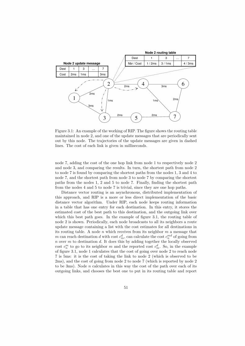
Nbr / Cost

Dest

4 / 3ms3 / 1ms1 / 2ms

7…31

1

2

3 5

4 6

7

Cost

Dest

3ms1ms2ms

7…31

2ms

Node 2 routing table

Node 2 update message

3ms

1ms

2ms

2ms

2ms

1ms

3ms

2ms

Figure 3.1: An example of the working of RIP. The figure shows the routing tablemaintained in node 2, and one of the update messages that are periodically sentout by this node. The trajectories of the update messages are given in dashedlines. The cost of each link is given in milliseconds.

node 7, adding the cost of the one hop link from node 1 to respectively node 2and node 3, and comparing the results. In turn, the shortest path from node 2to node 7 is found by comparing the shortest paths from the nodes 1, 3 and 4 tonode 7, and the shortest path from node 3 to node 7 by comparing the shortestpaths from the nodes 1, 2 and 5 to node 7. Finally, finding the shortest pathfrom the nodes 4 and 5 to node 7 is trivial, since they are one hop paths.

Distance vector routing is an asynchronous, distributed implementation ofthis approach, and RIP is a more or less direct implementation of the basicdistance vector algorithm. Under RIP, each node keeps routing informationin a table that has one entry for each destination. In this entry, it stores theestimated cost of the best path to this destination, and the outgoing link overwhich this best path goes. In the example of figure 3.1, the routing table ofnode 2 is shown. Periodically, each node broadcasts to all its neighbors a routeupdate message containing a list with the cost estimates for all destinations inits routing table. A node n which receives from its neighbor m a message thatm can reach destination d with cost cd

m, can calculate the cost cmdn of going from

n over m to destination d. It does this by adding together the locally observedcost cm

n to go to its neighbor m and the reported cost cdm. So, in the example

of figure 3.1, node 1 calculates that the cost of going over node 2 to reach node7 is 5ms: it is the cost of taking the link to node 2 (which is observed to be2ms), and the cost of going from node 2 to node 7 (which is reported by node 2to be 3ms). Node n calculates in this way the cost of the path over each of itsoutgoing links, and chooses the best one to put in its routing table and report

51

in its own periodic update messages.Starting from any initial values in the routing tables of all nodes (initializa-

tion can for example be random), this distributed and asynchronous process willeventually converge to a situation where correct routing information is availablein all nodes. This means that when there are changes in the network that makethe current routing information incorrect, the RIP updating algorithm will as-sure that the routing information is adapted and eventually reflects the newsituation.

Advantages and disadvantages of distance vector routing

We investigate the behavior of basic distance vector routing as implemented inRIP in terms of adaptivity, robustness, efficiency and scalability.

As pointed out above, RIP is in principle adaptive, in the sense that itsupdating process is guaranteed to converge and produce routing informationthat reflects the network situation correctly. However, there is no bound onhow long this convergence takes. In general, it is known that RIP reacts fastto good news, such as e.g. the appearance of a new link or node, but slowlyto bad news, such as the failure of a link or node [254]. An extreme exampleis the counting-to-infinity problem. Consider the simple network of figure 3.2,where the link between the nodes 2 and 3 fails. Node 2 realizes that its 2mspath to node 4 over node 3 is no longer feasible. However, it receives fromnode 1 an update stating that node 1 can reach node 4 in 3ms. Node 2 isunaware that this path includes itself, and uses the information to adapt itsown routing table: it registers a path to node 4, going over node 1, with acost of 4ms. When it subsequently sends this new information out to node 1,node 1 adapts its own path to node 4 to have a cost of 5ms, and includes thisnew information in the next message it sends to node 2. This updating processgoes on indefinitely, with both nodes slowly adapting their cost estimate of thepath to node 4 to the correct value of infinity. A number of adaptations forRIP have been proposed in order to provide better adaptivity and deal with thecounting-to-infinity problem. See [182] for an overview.

The robustness of RIP is related to its adaptivity. In principle, the algo-rithm’s capacity to converge to correct routing information allows it to recoverfrom disruptive events, loss of control packets, or the presence of erroneous infor-mation (e.g. out-of-date routing information). However, as pointed out before,this recovery process can be quite slow. This means that stale routing informa-tion can remain in the network for extended periods of time. The presence ofsuch wrong information can lead to problems such as the formation of loops [58].This is because nodes base their routing information on estimates provided byother nodes, and because routing decisions are taken independently in each node.An example is provided in the earlier mentioned counting-to-infinity problem:in the situation of figure 3.2, node 2 and node 3 form a routing loop betweenthem for packets going to destination node 4 as long as they have not reachedthe correct cost value of infinity.

In terms of efficiency, RIP scores very well. The ability to reuse routing

52

Nbr / Cost

Dest

3 / 2ms3 / 1ms1 / 1ms

431

1 2 3 4

Node 2 routing table

1ms 1ms 1ms

Nbr / Cost

Dest

2 / 3ms2 / 2ms2 / 1ms

432

Node 1 routing table

…

1 / 6ms

1 / 4ms

1 / 4ms

3 / 2ms

…

2 / 5ms

2 / 5ms

2 / 3ms

2 / 3ms

…

Update step 3:

Update step 2:

Update step 1:

Next hop and Route cost to node 4:

Figure 3.2: The counting to infinity problem. After the failure of the linkbetween node 2 and node 3, node 1 and node 2 adapt their estimate of the costof the route to node 4 based on the updates they receive from each other. Figureadapted from [254].

estimates provided by neighboring nodes allows to extract maximal informationfrom minimal communication. Scalability, on the other hand, is often considereda big problem for distance vector algorithms. This is because nodes shouldinclude their full routing table in each periodic update message they send out.

BGP: Advanced distance vector routing

BGP is the routing algorithm used for routing between ASs in the internet. Itimplements distance vector routing, but in a different way than RIP. The mainreason for the differences between both algorithms is the need to apply policies.At the level of inter-domain routing, politics and economics play an importantrole in forwarding decision. E.g., it is possible that an AS only wants to forwardpackets if it gets paid for it, and therefore refuses packets originating from ASswhich it does not have a contract with. Or an AS of one country might wantto avoid routes over ASs situated in a hostile neighbor country. BGP has beendesigned specifically to implement such policies.

The main difference between BGP and RIP is that under BGP, routing tableentries do not just contain the cost and the outgoing link of the best path to acertain destination, but also the sequence of nodes that make up the entire pathto that destination. Similarly, when a node sends an update message about itsrouting information to a neighbor, it includes full paths. By combining the pathsfor different destinations reported by all neighbors, each node can construct aview of the network, on which it bases its own routing decisions. Thanks tothe availability of full path information, it is easy to implement policies such asthe ones mentioned above. BGP is sometimes also called a path vector routingalgorithm, since its routing table is a vector of paths, rather than distances.

53

In terms of adaptivity, BGP scores better than RIP. The availability of fullpath information allows to solve the counting to infinity problem, and to avoidloop formation [254]. Nevertheless, observations of internet behavior have shownthat BGP can still be slow to converge to correct routing information after afailure, in the order of tens of minutes [160]. Also robustness remains a problem,since the loss of control packets or the presence of erroneous information stillleads to instabilities (see e.g. [270] for a study of the behavior of BGP in a stress-ful situation). Finally, in terms of efficiency and scalability, BGP scores worsethan RIP, since the algorithm is more complex, and more routing informationneeds to be exchanged between nodes. The growing size of routing tables in theinternet has become an important problem, and different strategies have beendeveloped to deal with it [43,134].

Distance vector routing in AHWMNs

The first routing algorithm that was developed for AHWMNs, DSDV, is a dis-tance vector algorithm. It follows quite closely the basic approach described forRIP. The main reasons for adopting the distance vector approach for AHWMNrouting are its relative simplicity and efficiency, which are important proper-ties in resource constrained environments such as an AHWMNs. To deal withproblems that stem from slow adaptivity and low robustness, such as loop for-mation, DSDV contains an elegant solution based on sequence numbers. Allrouting table entries are labeled with a sequence number that is assigned by thedestination. A node i only accepts new routing information for a destinationd if the new information has a higher sequence number than what is alreadyavailable in i, or when it has the same sequence number but a better routingmetric. For an example of how this solves the problem of loop formation, con-sider again the counting-to-infinity problem depicted in figure 3.2. After thefailure of the link between node 2 and node 3, updates about the route to des-tination node 4 sent out by node 1 or node 2 always have the same sequencenumber. This is because assigning new sequence numbers is the responsibilityof the destination, node 4, and all connectivity to this node is lost. Moreover,the updates sent back and forth between the two nodes have increasing routingmetrics, and are therefore not accepted. Details about the DSDV algorithm aregiven in subsection 2.4.2 and in [211].

Despite the use of the destination based sequence number mechanism, DSDVwas found to be insufficiently adaptive and robust to work in AHWMNs, espe-cially as network size or dynamism increased (see e.g. [42, 180]). Therefore, afew years later, AODV was proposed as a follow up to DSDV. AODV is labeleda distance vector algorithm, since its routing tables hold the cost and next hopof the best route for each destination, and are therefore distance vectors justlike the tables used in DSDV and RIP. However, AODV’s approach to gatheringand updating routing information has nothing in common with the distributedalgorithm described in this subsection. One could therefore say that AODVis a distance vector algorithm but not a Bellman-Ford algorithm. However,since these two terms have always been associated with each other, this can

54

create some confusion. For details about AODV we refer to subsection 2.4.2and to [213].

3.1.2 Link state routing

Link state routing was in the first place developed to overcome problems ofslow convergence and scalability that are present in distance vector protocols.Its basic approach to spreading and calculating routing information is funda-mentally different. In what follows, we first describe OSPF, which is the mainrepresentant of link state routing, then discuss advantages and disadvantagesof this approach, and finally comment on the use of link state routing in AH-WMNs. A short description of link state routing was also provided earlier, inthe discussion of the OLSR protocol in 2.4.2.

OSPF

The basic working of link state routing algorithms is depicted in figure 3.3. Eachnode locally monitors the cost to go to each of its neighbors. This forms thenode’s local state. Whenever a node detects a change in its local state, it floodsit to all other nodes in the network in a link state advertisement (LSA) message.LSA messages contain sequence numbers in order to distinguish old from newrouting information. By combining the LSAs received from all nodes in thenetwork, each node can get a complete view of the current network situation.This is stored in the node’s topological database. Using this database, each noderuns the Dijkstra shortest path algorithm [208] to construct a shortest path treewith itself as root, and uses the result to fill its routing table. In terms ofthe mechanism used to spread routing information, the difference with distancevector routing could be summarized as follows: while in distance vector routing,nodes send their global network information out locally to their neighbors, inlink state routing, they send their local network view out globally to all othernodes.

The OSPF algorithm implements the above scheme. However, it has a lot ofadded features to make it better suited to the specific properties of the internet.Some of these are aimed at improving scalability. OSPF allows to split the net-work into so-called areas, so that inside each area, nodes only maintain routinginformation about that area. For routing between areas, a backbone is set up.Note that these areas are subnetworks inside the earlier mentioned ASs (whichare themselves subnetworks of the internet). Another scalability related featureof OSPF is the possibility to represent a group of directly connected routersby one node in the OSPF network. To this end, one of the routers, called thedesignated router, acts on behalf of the whole group. This is for example rele-vant in LANs where all nodes are connected through an Ethernet bus; it wouldbe inefficient to let each of these nodes run OSPF separately. Other featuresof OSPF, which are not related to scalability, include the fact that all messageexchanges are authenticated, in order to improve security, and the possibility

55

2ms

6 - 7

2ms

2 - 1

Cost

Link

2ms3ms2ms …

7 - 6…1 - 31 - 2

1

2

3 5

4 6

7

Cost

Nbr

2ms1ms2ms

431

2ms

Node 2 topological database

Node 2 link state advertisement

3ms

1ms

2ms

2ms

2ms

1ms

3ms

2ms

Figure 3.3: An example of the working of OSPF. The figure shows the topo-logical database maintained in node 2 (this should be the same for each nodein the network), and a link state advertisements sent out by node 2. The linkstate advertisements are flooded over the network, as is indicated by the dashedlines.

to route packets distinctly based on their IP Type of Service field, so that inprinciple differentiated Quality-of-Service (QoS) routing [153] can be supported.

Advantages and disadvantages of link state routing

Link state routing offers good adaptivity: any detected change is flooded throughthe network in LSAs, and as soon as the nodes in the network have received allupdates, they can recalculate the shortest paths to all destinations so that theirrouting tables reflect the new network situation. This is faster than the slowlyconverging distributed updating process used in distance vector routing.

Robustness, on the other hand, can be a problem for link state routingalgorithms. If LSAs get lost, or stale LSAs are used for updates, nodes end upwith erroneous topological databases, and calculate wrong paths. In OSPF, anumber of measures have been taken to alleviate these problems. In order toavoid the loss of LSAs, each LSA transmission needs to be acknowledged, andduplicate transmissions are done in case of failure. Also, each node periodicallysends out refresh LSAs, which repeat previously transmitted information. Inorder to avoid the use of stale routing information, each LSA is given a sequencenumber, so that receiving nodes can figure out the relative age of different LSAscoming from the same source node. Furthermore, LSAs are given a timestamp,so that they can be discarded when they get too old.

In terms of efficiency, link state routing should in principle score quite well.However, the previously mentioned measures to improve robustness compromisethis: extra overhead is created by LSA acknowledgements, duplicate LSAs and

56

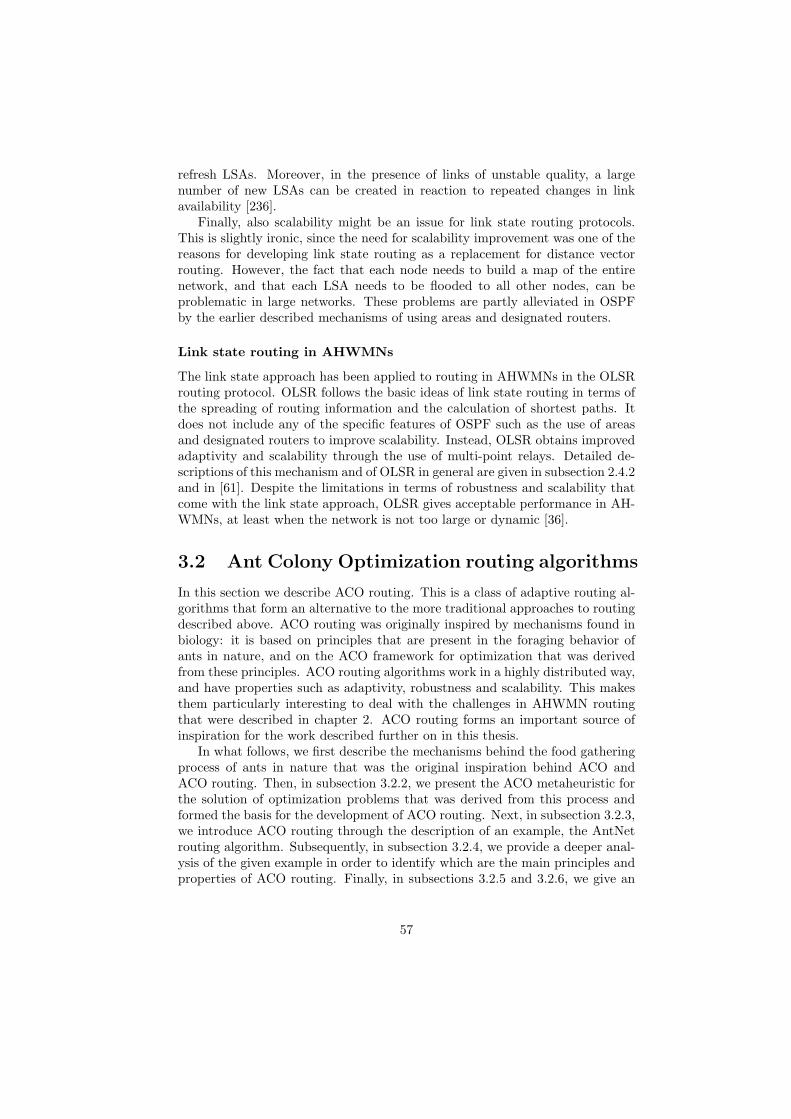
refresh LSAs. Moreover, in the presence of links of unstable quality, a largenumber of new LSAs can be created in reaction to repeated changes in linkavailability [236].

Finally, also scalability might be an issue for link state routing protocols.This is slightly ironic, since the need for scalability improvement was one of thereasons for developing link state routing as a replacement for distance vectorrouting. However, the fact that each node needs to build a map of the entirenetwork, and that each LSA needs to be flooded to all other nodes, can beproblematic in large networks. These problems are partly alleviated in OSPFby the earlier described mechanisms of using areas and designated routers.

Link state routing in AHWMNs

The link state approach has been applied to routing in AHWMNs in the OLSRrouting protocol. OLSR follows the basic ideas of link state routing in terms ofthe spreading of routing information and the calculation of shortest paths. Itdoes not include any of the specific features of OSPF such as the use of areasand designated routers to improve scalability. Instead, OLSR obtains improvedadaptivity and scalability through the use of multi-point relays. Detailed de-scriptions of this mechanism and of OLSR in general are given in subsection 2.4.2and in [61]. Despite the limitations in terms of robustness and scalability thatcome with the link state approach, OLSR gives acceptable performance in AH-WMNs, at least when the network is not too large or dynamic [36].

3.2 Ant Colony Optimization routing algorithms

In this section we describe ACO routing. This is a class of adaptive routing al-gorithms that form an alternative to the more traditional approaches to routingdescribed above. ACO routing was originally inspired by mechanisms found inbiology: it is based on principles that are present in the foraging behavior ofants in nature, and on the ACO framework for optimization that was derivedfrom these principles. ACO routing algorithms work in a highly distributed way,and have properties such as adaptivity, robustness and scalability. This makesthem particularly interesting to deal with the challenges in AHWMN routingthat were described in chapter 2. ACO routing forms an important source ofinspiration for the work described further on in this thesis.

In what follows, we first describe the mechanisms behind the food gatheringprocess of ants in nature that was the original inspiration behind ACO andACO routing. Then, in subsection 3.2.2, we present the ACO metaheuristic forthe solution of optimization problems that was derived from this process andformed the basis for the development of ACO routing. Next, in subsection 3.2.3,we introduce ACO routing through the description of an example, the AntNetrouting algorithm. Subsequently, in subsection 3.2.4, we provide a deeper anal-ysis of the given example in order to identify which are the main principles andproperties of ACO routing. Finally, in subsections 3.2.5 and 3.2.6, we give an

57

overview of existing ACO routing algorithms, respectively for wired networksand for AHWMNs.

3.2.1 Ants in nature

The main source of inspiration behind ACO and ACO routing is a behavior thatis displayed by certain species of ants in nature during foraging. It has beenobserved that ants from e.g. the family of Argentine ants Linepithema Humileare able to find the shortest path between their nest and a food source [115]. Thisis remarkable because each individual ant is a rather simple creature, with verylimited vision and computing power, and finding the shortest among severalavailable paths is certainly beyond its capabilities. The only way that thisdifficult task can be realized is through the cooperation between the individualsin the colony.

The key behind the colony level shortest path behavior is the use of pheromone.This is a volatile chemical substance that is secreted by the ants in order to in-fluence the behavior of other ants and of itself. Pheromone is not only used byants to find shortest paths, but is in general an important tool that is used bymany different species of ants (and also by a lot of other social animals) for awide variety of tasks that involve coordinated behavior [131].

In the case of the path finding task we describe here, the ants use pheromoneto recruit subsequent ants to the paths they have followed. Ants moving betweentheir nest and a food source leave a trail of pheromone behind, and they alsopreferably go in the direction of high intensities of pheromone. We use theexample situation depicted in figure 3.4 to explain how this simple behaviorleads to the discovery of shortest paths. In our example, there are two possiblepaths between the ant nest and the food source, one of which is considerablyshorter than the other. The first ants leaving the nest have no informationavailable. They therefore choose their movements randomly. This leads toapproximately 50% of the ants choosing the short path and 50% choosing thelong path. All moving ants leave a trail of pheromone behind. The ants goingover the short path reach the destination earlier than those going over the longpath. Moreover, they can return faster. This leads temporarily to a higherpheromone concentration on the shortest path. Subsequent ants leaving thenest are attracted by this higher intensity, and go therefore preferably also overthe shortest path. As this process continues, the majority of the ants eventuallyconcentrate on the shortest path. It needs to be pointed out however, that thebehavior of the ants is never deterministic, so that there will always remain aminority of ants that explore the longer path.

The use of pheromone is an example of a form of indirect communicationthat is often referred to as stigmergy [116, 256]. We speak of stigmergy whenconcurrent agents communicate through local adaptations of the environment:agents make local changes to the environment, and in turn locally sense theenvironment for this kind of changes. The environment’s properties that arechanged and sensed by the agents are called stigmergic variables. In the caseof the above described shortest path mechanism, the stigmergic variable is the

58

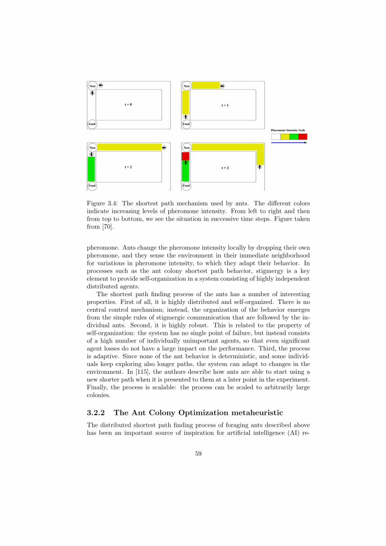
Nest

Food

Pheromone Intensity Scale

t = 2 t = 3

t = 1

Nest

Food

Nest

FoodFood

Nest

t = 0

Figure 3.4: The shortest path mechanism used by ants. The different colorsindicate increasing levels of pheromone intensity. From left to right and thenfrom top to bottom, we see the situation in successive time steps. Figure takenfrom [70].

pheromone. Ants change the pheromone intensity locally by dropping their ownpheromone, and they sense the environment in their immediate neighborhoodfor variations in pheromone intensity, to which they adapt their behavior. Inprocesses such as the ant colony shortest path behavior, stigmergy is a keyelement to provide self-organization in a system consisting of highly independentdistributed agents.

The shortest path finding process of the ants has a number of interestingproperties. First of all, it is highly distributed and self-organized. There is nocentral control mechanism; instead, the organization of the behavior emergesfrom the simple rules of stigmergic communication that are followed by the in-dividual ants. Second, it is highly robust. This is related to the property ofself-organization: the system has no single point of failure, but instead consistsof a high number of individually unimportant agents, so that even significantagent losses do not have a large impact on the performance. Third, the processis adaptive. Since none of the ant behavior is deterministic, and some individ-uals keep exploring also longer paths, the system can adapt to changes in theenvironment. In [115], the authors describe how ants are able to start using anew shorter path when it is presented to them at a later point in the experiment.Finally, the process is scalable: the process can be scaled to arbitrarily largecolonies.

3.2.2 The Ant Colony Optimization metaheuristic

The distributed shortest path finding process of foraging ants described abovehas been an important source of inspiration for artificial intelligence (AI) re-

59

searchers. In particular, it was the basis for the development of the ACO meta-heuristic [83,87]. This is a general framework for the development of algorithmsto solve optimization problems. The main idea behind ACO is the use of acolony of artificial ants and a matrix of artificial pheromone. ACO algorithmswork in an iterative way. In each iteration, all artificial ants build a solution tothe problem at hand in parallel, using the artificial pheromone matrix. Then,the pheromone matrix is updated based on the solutions that were found. Thisway, the pheromone matrix reflects information about good solutions that havebeen found so far, and allows ants in subsequent generations to use this infor-mation when building new solutions.

The first applications of ACO were for the traveling salesman problem (TSP).An instance of the TSP is defined by a fully connected weighted graph G =(V,E), where the set of vertices V corresponds to a number of cities, and theset of edges E represents the connections between the cities. With each of theedges (i, j), a distance d(i, j) is associated. The distances can be symmetric (inwhich case d(i, j) = d(j, i) for all pairs of cities i and j), or asymmetric. The aimis to find a closed tour that visits all cities exactly once while minimizing thetotal traveled distance. This combinatorial optimization problem is NP-hard.The TSP can very easily be seen as a shortest path finding problem, whichmakes it an obvious first choice for the implementation of ACO.

The first ACO algorithm that was developed for the TSP is Ant System(AS), which was originally proposed by Dorigo in his PhD thesis in 1992 [82]and first published in English in 1996 [85]. In AS, an artificial pheromonevalue τ(i, j) is associated with each edge (i, j). The algorithm maintains acolony of artificial ants, which build solutions using this artificial pheromone,and afterwards update the pheromone based on the quality of the solution theyobtain. The algorithm works in an iterative way. At the start of each iteration,each ant is placed in a randomly chosen initial city. Starting from there, itmoves from city to city, building a solution to the TSP. When choosing the nextcity to move to, an ant considers all cities that it has not visited yet. It picksone of these using the random-proportional rule given in equation 3.1. This rulecalculates the probability pk(i, j) that ant k in city i chooses city j to move tonext.

pk(i, j) =

{[τ(i,j)]α[η(i,j)]β∑

l∈Nki

[τ(i,l)]α[η(i,l)]βif j ∈ Nk

i

0 otherwise(3.1)

In this equation, Nki represents the set of cities that ant k has not yet

visited before reaching city i. η(i, j) is equal to 1/d(i, j), the inverse of thedistance between i and j. It serves as a heuristic value that helps guiding theconstruction of solutions. Using the rule of equation 3.1, the probability ofchoosing city j after city i increases when the pheromone between i and j ishigher and when the distance between i and j is lower. The parameters α and βdefine the relative weight given to respectively the pheromone and the distanceheuristic in the decision process: with β = 0, the decision is purely based on thepheromone, meaning the experience gathered in previous iterations, while with

60

α = 0, the decision is purely based on the heuristic, so that AS comes down toa randomized local search.

At the end of each iteration, the solutions constructed by the ants are eval-uated, and the pheromone values are updated. Pheromone updating includespheromone evaporation and pheromone deposition. Pheromone evaporationrefers to the decrease of all pheromone values. It is done using equation 3.2.In this equation, 0 ≤ ρ ≤ 1 is the pheromone evaporation rate. Pheromoneevaporation allows to forget old solutions. Pheromone deposition refers to theincrease of pheromone on edges that have been used in the solutions constructedby the ants. It is done using equation 3.3. In this equation, m is the total num-ber of ants, and ∆τ(i, j)k is the inverse of the cost of the solution constructedby ant k if edge (i, j) is part of this solution, and is 0 otherwise. Pheromonedeposition serves to reinforce good solutions.

τ(i, j) = (1− ρ)τ(i, j), ∀(i, j) ∈ E (3.2)

τ(i, j) = τ(i, j) +m∑

k=1

∆τ(i, j)k, ∀(i, j) ∈ E (3.3)

The algorithm is run until a given number of iterations is reached, or untilno solution improvement has been obtained for a number of iterations.

AS was found to work well for small instances of the TSP, but failed tocompete with state-of-the-art methods on large instances. However, its publi-cation raised a general interest in the approach, and inspired the developmentof a number of similar algorithms for the TSP that were more powerful anddid manage to provide state-of-the-art performance. These algorithms includeElitist AS [85], Ant-Q [105], Ant Colony System (ACS) [84] and MAX-MIN AS(MMAS) [245]. All of these algorithms are based on the same basic principles asAS: a number of artificial ants each build their own solution to the TSP. Theydo this in a constructive way, starting from a random initial city and adding newcities until a full solution is reached. Each decision to add a new city is madestochastically, using probabilities that depend partly on a pheromone value andpartly on a heuristic value. Pheromone is updated according to the qualityof the solutions provided by the ants. The main difference between these newalgorithms and the original AS lies in the balance between the exploitation ofinformation that has been learnt so far and the exploration of new possibili-ties. In general, AS’s successors are more aggressive to exploit. For example, inElitist AS, pheromone updating is only done for the ants that found the bestsolutions in the current iteration, and for the best solution found so far over allpast iterations. In ACS, exploitation is also increased by using the selection rulefor cities (equation 3.1) deterministically in a certain percentage of cases. Also,AS’s successors provide mechanisms to balance exploration and exploitation, sothat the algorithms can be better tweaked for the problem at hand. Apart fromthese differences, some of AS’s successors, namely ACS and MMAS, have beencombined with local search: to each of the solutions found by the ants, a localsearch procedure is applied to bring it to a local optimum. Then, pheromone

61

is updated based on the improved solution. This hybrid approach was found tobe very powerful.

After the applications to the TSP, ACO has in recent years also been adaptedfor the solution of a wide range of other problems. These include the quadraticassignment problem [107, 184], the vehicle routing problem [106], the graphcoloring problem [63], the shortest common super-sequence problem [193], themultiple knapsack problem [168], the bin packing problem [99,169], the 2D HPprotein folding problem [239], etc.. Most of these problems are very differentfrom the TSP and have a structure that is much less easy to reduce to a shortestpath finding problem. ACO algorithms for these problems use therefore oftenquite different approaches, which is mainly reflected in the way pheromone isstored, updated and used. The core ideas always remain the same however:to produce multiple parallel solutions in each iteration, using a high degree ofstochasticity, and to store information about previously found good solutionsin an artificial pheromone matrix, which is used to produce new solutions insubsequent iterations. Overviews of applications of ACO can be found in [34,86,87].

ACO has also been applied to networking problems. Some of these areoff-line combinatorial problems, such as the problem of routing and wavelength-allocation in an optical fibre network [202] or the problem of finding disjointpaths in a telecommunication network [267]. ACO algorithms for these prob-lems follow a similar pattern as the other ACO algorithms for combinatorialproblems described earlier. A very different problem is that of adaptive routingin telecommunication networks. This is an online dynamic problem: the prop-erties of the problem change continuously and the optimization algorithm has toadapt its solution online. Applications of ACO for routing, such as Ant-BasedControl (ABC) [235] and AntNet [71], are therefore very different from those forstatic off-line problems. The rest of this section is dedicated to the descriptionof these algorithms.

3.2.3 AntNet: an ACO algorithm for routing in telecom-munication networks

A number of different ACO algorithms for adaptive routing in networks havebeen proposed. The first of these were ABC [235] for connection orientedtelecommunication networks, and AntNet [70,71] for packet switched data net-works. Both of these algorithms were developed for wired networks. Here, wedescribe AntNet as a prototype example of ACO routing.

In AntNet, every node in the network keeps two data structures: a routingtable and a local traffic statistics table. This is illustrated in figure 3.5. Therouting tables contain the artificial pheromone, and are therefore also calledpheromone tables. Pheromone tables contain for every destination a vectorwith one entry per outgoing link. The entry T d

ij of node i’s pheromone table Ti

contains the pheromone value τdij , which is a floating point number indicating

the relative goodness of taking outgoing link j on the way to destination d.

62

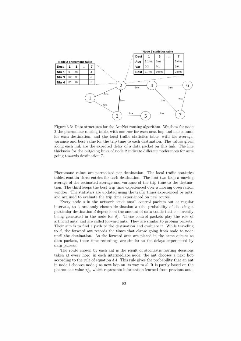
1

2

3 5

4 6

7

2ms

3ms

1ms

2ms

2ms

2ms

1ms

3ms

2ms

Node 2 pheromone table

.6.02.01Nbr 4

.3.9.09Nbr 3

.1.08.9Nbr 1

7…31Dest

2.8ms0.8ms1.7msBest

0.60.10.2Var

3.4ms1ms2.1msAvg

7…31Dest

Node 2 statistics table

Figure 3.5: Data structures for the AntNet routing algorithm. We show for node2 the pheromone routing table, with one row for each next hop and one columnfor each destination, and the local traffic statistics table, with the average,variance and best value for the trip time to each destination. The values givenalong each link are the expected delay of a data packet on this link. The linethickness for the outgoing links of node 2 indicate different preferences for antsgoing towards destination 7.

Pheromone values are normalized per destination. The local traffic statisticstables contain three entries for each destination. The first two keep a movingaverage of the estimated average and variance of the trip time to the destina-tion. The third keeps the best trip time experienced over a moving observationwindow. The statistics are updated using the traffic times experienced by ants,and are used to evaluate the trip time experienced on new routes.

Every node s in the network sends small control packets out at regularintervals, to a randomly chosen destination d (the probability of choosing aparticular destination d depends on the amount of data traffic that is currentlybeing generated in the node for d). These control packets play the role ofartificial ants, and are called forward ants. They are similar to probing packets.Their aim is to find a path to the destination and evaluate it. While travelingto d, the forward ant records the times that elapse going from node to nodeuntil the destination. As the forward ants are placed in the same queues asdata packets, these time recordings are similar to the delays experienced bydata packets.

The route chosen by each ant is the result of stochastic routing decisionstaken at every hop: in each intermediate node, the ant chooses a next hopaccording to the rule of equation 3.4. This rule gives the probability that an antin node i chooses node j as next hop on its way to d. It is partly based on thepheromone value τd

ij , which represents information learned from previous ants,

63

and the heuristic value ηij , which is based on the length of the queue for the linkto j in node i. The role of ηij is to provide an estimate of local traffic, in order tohelp guide the ant routing process. The value α in equation 3.4 is a parameterused to balance the relative importance of the pheromone and the heuristicvalue in the routing decision, and |Ni| is the number of neighbors, used inthe denominator for normalization purposes. Using this approach, forward antsbuild paths like the artificial ants in AS build solutions to the TSP: constructingthe path hop by hop in a stochastic way using both pheromone and heuristicinformation. Through the use of probabilistic decision making, different pathsare explored and made available for data routing.

P dij =

τdij + αηij

1 + α(|Ni| − 1)(3.4)

Once an ant reaches its destination, it turns around and becomes a backwardant which returns to the source node s. Backward ants do not use the samequeues as data packets, but high priority ones (in order to distribute the newinformation quicker), and do not take probabilistic routing decisions, but followthe exact reverse path of their associated forward ant. When a backward antarrives in an intermediate node i on its way back to s, it updates the entries ini’s tables for destination d. First, the traffic statistics table is updated using thetrip time t experienced by the ant: the average and variance are updated usingmoving averages, while the best value is updated using a moving window. Thenthe pheromone entry τd

ij is updated, with j being the neighbor over which thebackward ant arrived in i. One important problem is how to define how goodthe trip time t of the newly received ant is. To this end, the traffic statisticsare used: using equation 3.5, a reinforcement value r is derived, which reflectsthe relative goodness of the new route from i to d over j compared to what hasbeen observed so far.

r = c1

(Wbest

t

)+ c2

(Isup − Iinf

(Isup − Iinf ) + (t− Iinf )

)(3.5)

In this equation, Wbest is the best trip time over the moving window, asrecorded in the statistics table, so that the first term of equation 3.5 reflects howwell the new time t scores with respect to the best known time. Iinf and Isup areestimates of the lower and upper limits of an approximate confidence intervalfor the mean of the trip time to d. They are based on the average, varianceand best trip time recorded in the statistics table. The second term of theequation reflects how well the new trip time scores with respect to these limits,so that equation 3.5 takes into account the variability in past measurements oftrip time. It is meant as a correction for the first term. The parameters c1 andc2 allow to balance both parts of the equation. The result of the equation isthe reinforcement value r, which, after the application of a further modificationfunction (for which we refer to [71]), is used to update the pheromone value τd

ij

through a moving average. This way, the new pheromone value incorporatesthe latest reported trip time. If enough ants are used, all pheromone values can

64

be kept up-to-date so that they give an accurate image of the current networksituation.

Data packets are routed in a similar way as forward ants, choosing a nexthop stochastically at every hop. Stochastic forwarding of data packets allowsper packet data load balancing. The probability Rd

ij for a data packet in node iwith destination d to take node j as a next hop is given in equation 3.6. Like theprobability for forward ants, it is based on pheromone values. However, thereare two important differences. First of all, the local heuristic ηij based on thequeue lengths is not used here. Second, the pheromone is raised to a power ε,which is normally larger than 1. This increases the probability of taking pathswith higher pheromone values, so that data packets are only routed over thebest paths, and are not used for exploration like the forward ants.

Rdij =

(τdij)

ε

∑l∈Ni

(τdil)ε

(3.6)

In simulation studies using the Omnet++ simulator [265], AntNet was com-pared to traditional routing algorithms such as OSPF and distance vector rout-ing, and to other adaptive routing algorithms, such as Q-routing (see subsec-tion 3.3.3 and [39]). In a wide range of test scenarios, using different networkssuch as NSFNET and the Japanese NTTnet, and using different patterns interms of data load, AntNet was shown to be superior to all other algorithms interms of packet throughput and end-to-end delay. It did produce more overheadthan traditional static routing algorithms, but not more than other adaptiverouting algorithms.

3.2.4 ACO routing principles

In the previous subsection, we took a detailed look at AntNet, an example of anACO routing algorithm. Now, we take a more general point of view, and extractthe main principles behind ACO routing with their properties. The materialpresented here has also been described in [76], in a slightly different form.

A first important characteristic of ACO routing algorithms is that theygather routing information through the repeated sampling of full paths. Thisis in line with the behavior of ants in nature, where a large number of antscontinuously move between their nest and the food source, and with the work-ing of ACO algorithms for combinatorial optimization, where multiple artificialants repeatedly and in parallel construct sample solutions for the problem athand. The ACO approach to routing is quite different from the distance vectorapproach, where routing information is derived from information provided byneighboring nodes, and from the link state approach, where routing informa-tion is calculated based on the update messages received from all other nodes inthe network. Due to the use of redundant probing packets such as the forwardants in AntNet, the ACO approach to the gathering of routing information isquite robust: each ant is individually unimportant and loss of control packetscan be tolerated. An important aspect of the whole process is the fact that

65

ants always sample full paths between source and destination. At no point isrouting information derived from information provided by other nodes. Thisis in stark contrast to the distance vector approach, where all routing infor-mation is derived from estimates provided by neighbor nodes. Relying onlyon direct experiences from full path samples adds further to the robustness ofthe algorithm, as updates are not dependent on the correctness of the routinginformation available in other nodes. More about this will follow also in subsec-tion 3.3.2. On the downside, the constant use of probing also leads to increasedoverhead, which can negatively influence the efficiency of ACO routing.

A second characteristic is the way ants choose a path to sample: they con-struct the path hop by hop in a stochastic way using pheromone information.The relation with the foraging behavior of ants in nature and with ACO forcombinatorial optimization is again evident, as also there ants follow their pathor construct their solution step by step using pheromone in a non-deterministicway. The use of the pheromone information allows to build on experiences gath-ered by previous ants. It is the key to the stigmergic process that guides thecoordinated working of a highly distributed process. The fact that ants buildtheir paths in a probabilistic way allows the exploration of multiple paths. Thismakes the algorithm adaptive to changes in the network environment. More-over, it leads to the availability of multiple paths for data routing, each with anassociated goodness value. This increases robustness, through the availabilityof backup paths, and allows to spread data over the multiple paths, increasingnetwork throughput (see also subsection 2.4.3).

A third characteristic is the stochastic forwarding of data packets based onthe pheromone information. This relates to the issue of using multiple pathsdiscussed above. By forwarding data probabilistically, the data load is spreadover the multiple available paths on a per packet basis. This allows to makebetter use of available network resources and obtain better throughput. Theuse of pheromone in this process ensures that data is focused on the best paths.If pheromone is always kept up-to-date, by using sufficient ants, data load bal-ancing automatically follows the changes in the network. An important aspectin the stochastic forwarding of data is that it uses a different formula than theants, focusing more on the best pheromone. This way, ants are more explorative,while data packets concentrate on exploiting the routing information providedby the ants. Here, the relation with ant foraging behavior in nature and ACO forcombinatorial problems is less obvious: in those processes, the same ants needto take care of exploration of the solution space and exploitation of previouslyfound information in order to find the best solution. Using separate mechanismsfor exploration and exploitation allows to build a more flexible system.

3.2.5 Existing ACO routing algorithms for wired networks

Apart from the AntNet algorithm described in subsection 3.2.3, a wide rangeof different ACO routing algorithms have been proposed. Here, we give anoverview of existing ACO routing algorithms for wired networks, while in thenext subsection, we discuss ACO routing algorithms for AHWMNs.

66

ABC [235] was developed before AntNet, in 1996, and takes a significantlydifferent approach, mainly because it was developed for a different type ofnetworks: it assumes a network with symmetric path travel costs, in whichdata communication is organized through virtual circuits (rather than using thepacket switched approach supported by AntNet). Like in AntNet, each nodes periodically sends out ants to randomly chosen destinations. Each ant hasan associated age, which is increased proportionally to the load of each visitednode (the age is increased more when heavily loaded nodes are passed, so thatit reflects the free space on the followed route). While traveling from its sources to its destination d, the ant updates the pheromone for the path backward tos, based on its age. This is an important difference with AntNet: ants updatepheromone about the path to their source while going forward, and no backwardants are used. This is possible because of the assumption of symmetric pathcosts. Other major differences compared to AntNet are that no path statis-tics are used to evaluate path quality measurements reported by the ants, andthat no local heuristic is used to help guide the ants (in AntNet, the local queuelengths are used). Finally, in ABC, it is not data packets that are routed accord-ing to the pheromone, but call setup messages. Moreover, these messages do notfollow pheromone probabilistically, but greedily choose the directions with thehighest pheromone level. Once a call has been set up successfully, data packetsfollow its circuit deterministically. ABC was tested in simulation on a modelof the British Telecom network and was shown to give superior performancecompared to other approaches.

The algorithm proposed in [248], called Ants Routing, builds on ABC. It ismeant for networks with frequent node and link failures. The main differencecompared to ABC is the use of so-called uniform ants. These are different fromthe regular ABC ants in the sense that they do not have a specific destinationand do not follow pheromone information. Instead, they wander through thenetwork choosing each next hop according to a uniform distribution, until theyhave reached a maximum time-to-live, after which they are discarded. Theuse of uniform ants improves exploration. This is particulary important whendealing with frequent topology changes; the algorithms AntNet and ABC weredesigned to be adaptive with respect to data traffic changes, rather than withrespect to topology changes. Another advantage of the uniform ants is thatthey do not have a specific destination, so that they can be used in case a nodedoes not know all possible destinations in the network. A disadvantage is thatuniform ants can lead to inefficiencies, due to the overhead they cause and thesuboptimal paths they follow.

A number of papers propose further adaptations to ABC. The algorithm pro-posed in [35] allows ants in ABC to update pheromone not only for their sourcenode s, but also for all intermediate nodes on their path. The authors of [226]describe ABC-backward, which combines ABC with elements from AntNet, suchas the use of forward and backward ants and the use of the ants’ trip time forpheromone updating. In [230], the authors extend ABC with probabilistic rout-ing of call setups and the use of anti-pheromone, which allows ants to decreasepheromone in some cases, instead of increasing it.

67

AntNet-FA [72] is an adaptation of AntNet, proposed by the same authorsof the original algorithm. It is very similar to the original AntNet, but containsan improvement in the behavior of the forward ants: AntNet-FA’s forward antsdo not use the same queues as data packets, but instead take high priorityqueues like backward ants. The trip times experienced by the forward ants aretherefore no longer representative for what can be expected for data packets;the trip time for data packets are instead calculated by the backward ants asthe sum of local estimates maintained in each of the intermediate nodes. Themain advantage of this approach is that ants can travel faster so that updatesare done more in real-time.

Other papers propose further improvements to AntNet. In [80] and [205]some mechanisms to enhance the exploratory behavior of AntNet are presented.In [23], the authors propose other improvements to AntNet such as the possi-bility to explicitly take link and node failures into account, and a better ini-tialization of the pheromone tables. In [149], adaptive-SDR is proposed. Themain difference with AntNet is that in adaptive-SDR, the network is dividedinto clusters, and a distinction is made between inter-cluster and intra-clusterrouting. This improves scalability, since routing tables do not have to maintainentries for all possible destinations. Scalability issues of AntNet were also in-vestigated in [51]. Finally, in [286], the authors present Adaptive Swarm-basedRouting (ASR). Differences with AntNet include the use of a momentum termin pheromone updating, and the fact that pheromone is updated for all inter-mediate nodes as destinations. In simulation, ASR was shown to outperformAntNet in terms of packet delay and throughput.

In [274] and other papers from the same authors, Routing By Ants (RBA)is proposed. It uses virtual circuits and supports both unicast and multicastrouting. RBA has similarities both with ABC and AntNet. An interestingdifference with these two algorithms is the fact that the parameters which definehow routing decisions are derived from pheromone values are carried inside theants, so that they can be different for each ant. These parameters are assignedto ants in their source node and are calculated using a genetic algorithm (GA).Some small improvements to this algorithm were proposed by different authorsin [249].

The authors of [128] propose the Co-operative Asymmetric Forward (CAF)mechanism. It shows how forward ants can update routing information aboutthe path to their source without sending a backward ant and without assumingsymmetric path costs. In CAF, each data packet hopping from a node i toa node j leaves at j an estimate cij of the queuing and transmission time ithas experienced while traveling from i. Later, ants traveling in the oppositedirection read this estimate and store it. By adding all estimates over theirforward path from their source node s till intermediate node i, the ants obtaina good estimate of the delay on the backward path from i to s, so that they cancorrectly update pheromone information about their full backward path.

ACO has also been applied to QoS routing. A first example is AntNet+SELA[78], an adaptation of AntNet for QoS routing in asynchronous transfer mode(ATM) networks. It integrates AntNet with stochastic estimator learning au-

68

tomata (SELA) [266], a framework for QoS provisioning in ATM networks thatuses static reinforcement learning agents to derive routing and application ad-mission strategies. The original SELA uses a link state approach to gather rout-ing information. AntNet+SELA, on the other hand, uses ant based probing forthe collection of routing information. An interesting feature of AntNet+SELAis that nodes have the possibility to reactively send out extra ants in order tosearch specific information that they need. For details about the AntNet+SELAsystem, we refer to [70,78]. A number of other adaptations of ACO routing forQoS have also been proposed. Most of these aim to provide hard QoS guaran-tees, following the IntServ approach to QoS [40]. This is the case for Agent-basedRouting System, proposed in [206], and for Q-Colony, proposed in [253]. Otherapproaches, such as the algorithm proposed in [192] and AntNet-QoS, presentedin [50], combine ACO with a soft approach to QoS routing. The latter proposesan integration of AntNet with the DiffServ framework for QoS [153].

Recently, ACO routing has also been used for routing problems in new kindsof networks (other that the applications to the equally new field of AHWMNs,which are described separately in subsection 3.2.6). One interesting exampleis its use for the problem of dynamic routing and wavelength assignment inwavelength-division multiplexing (WDM) networks, where the aim is to setup a primary path between source and destination and one or more disjointbackup paths, in on-demand fashion. This work is described in [204] and otherpapers by the same authors. Another very interesting new application is theuse of ACO routing in the domain of Networks-on-Chip (NoC). These are sub-micron scale networks that connect the elements on an integrated circuit. NoChave many characteristics in common with traditional wired networks, but poseadditional challenges that mainly arise from the extremely limited availableresources. In [64], the authors propose an AntNet based approach to routing inNoC.

Finally, we want to mention some algorithms that use biological metaphorsthat are different from the ant foraging behavior, but reference ACO routingand have elements in common with this approach. In [273], the BeeHive algo-rithm is proposed. This algorithm is inspired by the behavior of honey bees.Like AntNet, however, it gathers routing information using path probing packets(called bee agents here), and it builds stochastic routing tables for data forward-ing. Different from ants in AntNet, bees are flooded (with a maximum numberof hops) instead of unicast along a stochastically chosen path to a specific des-tination. Also different from AntNet, the network is divided into regions, sothat not all destinations need to be put in the routing table of each node andbetter scalability can be provided. The authors of [173] also address this issueof scalability in AntNet. They propose GA-agents, which is based on the useof a distributed GA. In GA-agents, each node maintains a GA population, inwhich each individual represents a path in the network. Paths are encoded asa sequence of turns (rather than a sequence of nodes). Individuals are evalu-ated by letting them probe the path they represent. This way, they are similarto the ants in AntNet. Typical GA operations such as mutation and selectionare executed to find the best paths. Finally, in [276] and other papers by the

69

same authors, the CE-ants approach is presented. This algorithm is inspiredby the cross-entropy (CE) metaheuristic for combinatorial optimization pro-posed by Rubinstein [228]. The CE method is in principle quite different fromACO, since it was originally derived from techniques for rare event simulation.However, due to their use of repeated sampling, many CE algorithms have inpractice strong similarities with ACO algorithms. The same is true for CE-ants:in overall architecture it is quite similar to ACO routing algorithms like AntNet.The main difference lies in the formulas used for pheromone updating, whichbear the signature of the CE method. CE-ants has been applied to a variety ofrouting related problems, such as the problem of finding protection cycles [277],and the problem of finding primary and backup paths [275].

3.2.6 Existing ACO routing algorithms for AHWMNs

Due to its properties of adaptivity and robustness, ACO has also attractedattention as a paradigm for routing in AHWMNs. Here, we give an overview ofalgorithms that have been proposed in recent years.

A number of the ACO routing algorithms for AHWMNs that have beenproposed have a structure that is quite similar to that of the ACO algorithmsfor wired networks described in subsection 3.2.5. The Accelerated Ants Routingalgorithm described in [104, 191], is derived from the Ants Routing algorithmfor wired networks. It contains small adaptations to this algorithm, such as theno-return rule (which simply states that ants cannot pick their previous hopas next hop, so that simple loops are avoided), and is shown in simulation toperform better than AntNet in MANETs. The ABC-AdHoc algorithm [255] onthe other hand is based both on ABC and AntNet. While it uses forward antsthat update pheromone for the path to their source, as in done in ABC, it usesformulas of AntNet to calculate pheromone updates and to make probabilisticrouting decisions. In a simulation with rather limited mobility, the ABC-AdHocalgorithm was shown to perform better than AntNet. In [288], the authorspropose adaptations of AntNet for use in sensor networks. These include aninformed initialization of pheromone values at node activation, the possibilityto flood forward ants, rather than unicast them to their destination, and topiggyback these flooded forward ants on top of data packets. The adaptationsof AntNet are shown to perform better than the original algorithm in sensornetworks.

The problem with following the design of ACO routing algorithms for wirednetworks too closely is that it results in proactive routing algorithms, which, ashas been explained in subsection 2.4.1, is not always the best approach to routingin AHWMNs. This problem and a solution to it are well illustrated in [24]. Inthis work, the authors first propose an algorithm that is very similar to AntNet.The main differences are that some uniform ants are used to improve explo-ration (see also the Ants Routing algorithm described in subsection 3.2.5), andthat data are routed deterministically over the path with the best pheromone.In simulation tests, this algorithm was found to perform worse than AODV,mainly due to inefficient route discovery and large amounts of overhead. Then,

70

the authors propose a new algorithm, called Probabilistic Emergent RoutingAlgorithm (PERA). This is a purely reactive algorithm: forward ants are onlysent out at the start of a communication session, or when all existing routinginformation is out of date. They are flooded towards the destination. For everycopy of the forward ant that reaches the destination, a backward ant is sent tothe source, so that multiple paths are created at route setup. It is not clearwhether data are routed stochastically or not. In simulation studies, PERA isfound to have a performance that is comparable to AODV. Unfortunately, it isalso clear from the description of the algorithm that this is mainly due to thefact that PERA is quite similar to AODV, with forward ants and backward antsreplacing respectively RREQ and RREP messages. Of the original ACO ideas,not much is left.

The approach of building a reactive kind of ACO routing algorithm hasbeen followed by several other researchers in the field. Ant-Colony-Based Rout-ing Algorithm (ARA) [119] is quite similar to PERA (and hence to AODV). Onedifference is that both forward and backward ants leave pheromone behind: for-ward ants update pheromone about the path to the source, while backward antsupdate pheromone about the path to the destination. Another difference is thatalso data packets update pheromone, so that paths which are in use are alsoreinforced while the data session is going on. This comes down to repeated pathsampling, so that ARA keeps more of the original ACO characteristics thanPERA. In simulation, ARA was found to perform better than AODV but worsethan DSR in highly dynamic environments. Also the Termite algorithm [224]follows a reactive approach. Important differences with ARA and PERA arethat forward ants are not flooded, but follow a random walk. And backwardants do not necessarily follow the exact same path of the RREQ back to thesource, but are themselves routed stochastically (this can be an advantage if uni-directional links are present; see subsection 2.3.2). Pheromone updating is doneby all packets (also by data), and is always done with respect to the source thata packet is coming from. This means that cost symmetric paths are assumed.In a small set of simulation tests, Termite was shown to perform better thanAODV for varying values of node speed [225]. Ad hoc Networking with SwarmIntelligence (ANSI) [220] is again a variation on the same approach. It onlyuses ants at route setup time. A mechanism using forward and backward antsis applied, and like in Termite and ARA, data packets also deposit pheromone,in order to reinforce the paths they use. Data are routed deterministically overthe best paths. ANSI evaluates paths based on the congestion rates (definedby the free versus occupied space in the node IP queues) of nodes along thepath. ANSI was shown to perform better than AODV in simulation. Finally,also Emergent Ad Hoc Routing Algorithm (EARA) [177] follows a similar ap-proach. Different in EARA is that during the course of a data session, pathsare reinforced by ants that are sent out from the destination. New paths aredetected using ants that do random walks through the network.

A number of other algorithms use ants in a different way. The authors of [194]propose to use a set of mobile agents that are quite independent from networknodes or data sessions: these agents are generated at network setup time, and

71

they stay around indefinitely. They perform a continuous random walk throughthe network, keeping a history of the last N nodes they have visited. At eachnew node they arrive, paths are extracted from this history list in order toupdate routing information. The algorithm proposed in [190] is a combinationbetween this approach and AODV. Also here, a number of ant agents keepgoing through the network indefinitely, performing a random walk and keepinga history list of the last N visited nodes. However, here the network nodesalso run AODV. They are therefore not solely dependent on the informationgiven to them by the randomly moving ants. Instead, the ants only providepossibilities to improve on routing information gathered by AODV, or to avoidAODV route setups. The authors show that their Ant-AODV method performsbetter than Ants Routing or AODV separately. In [45], the authors propose analgorithm that combines geographic routing (see subsection 2.4.3) with ants. Intheir approach, each node keeps a database of the positions of all other nodes.To keep these databases up-to-date, information is exchanged locally amongneighbors, and globally by sending ants to nodes further away. The destinationnodes for the ants are chosen according to a probabilistic mechanism, and nodescan copy the routing information from ants that pass by. So, in this approach,ants replace flooding as a way to spread routing information over the network.The Mobile Ants-Based Routing Protocol (MABR),proposed in [126, 127] wasdesigned for WAN scale AHWMNs. The algorithm divides the AHWMN areain rectangular zones, corresponding to geographical areas. All nodes of a zonetogether make up a logical router. Long distance routing is done between logicalrouters, with the aid of location information. Ants are used at this level, toproactively update routing tables between logical routers. In simulation, MABRcompared favorably to Terminodes routing, a different algorithm for WAN scaleAHWMNs.

Finally, a number of ACO routing algorithms for QoS routing in AHWMNshave also been proposed. Ant-based Distributed Routing Algorithm (ADRA)[289] follows a reactive approach, similar to the PERA algorithm describedabove. A difference is that, in order to support QoS, nodes check resourceavailability before they forward a forward ant, so that paths are only set upwhen their QoS requirements can be met. In case available resources changeand an existing path can no longer rely on the necessary resources, nodes send so-called anti-ants to erase the path and inform downstream nodes that they needto find a new path. In simulations, ADRA was found to outperform the DSRrouting algorithm, especially in highly dynamic scenarios. Ant colony basedMulti-path QoS-aware Routing (AMQR) [176] uses ants to set up multiple, linkdisjoint paths. The source node stores information about the paths followed bydifferent ants, and combines it to construct a topology database for the network.Based on this database, it calculates n different link disjoint paths, and it senddata packets over these different paths. These data packets update pheromone.The use of a topological database is different from most other ACO routingalgorithms, but can also be found in the AntNet+SELA algorithm for QoSrouting in wired networks (see subsection 3.2.5). It allows the source node tohave better control over the paths that are set up. In simulation tests, AMQR

72

was shown to outperform ADRA and DSR, especially in low mobility scenarios.

3.3 Routing and machine learning

In this section, we investigate the relationship between routing and the field ofmachine learning. We show that the problem solved by a distributed routingalgorithm fits well into the description of reinforcement learning problems. Thisallows to investigate the learning algorithms behind several existing routingalgorithms in a unified framework. The aim is to view these algorithms froma machine learning point of view, and to provide the reader with the necessaryfoundation to follow some of the discussion further on in this thesis. The focuswill be on the distance vector and the ACO routing algorithms described before,as these have the most relevance for the work presented later in this thesis.

In what follows, we first describe the reinforcement learning framework.Then, we discuss two elementary solution methods in this area, namely dynamicprogramming and Monte Carlo sampling, and we show how these methods re-late to the distance vector and ACO routing algorithms respectively. We endwith a description of temporal difference learning and Q-routing. Temporal dif-ference learning is a more advanced solution method for reinforcement learningproblems that combines elements from dynamic programming and Monte Carlosampling, while Q-routing is an adaptive routing algorithm for wired networksthat was directly inspired by one of the most popular a temporal differencealgorithms, namely Q-learning.

3.3.1 The reinforcement learning framework

Reinforcement learning (RL) [252] is the name of a class of problems in machinelearning. Generally speaking, one can say that it refers to the task of learningactions by trail-and-error in order to maximize a reward. RL is a relativelynew topic of research. Its characteristic trait of learning from experience sets itapart from the traditional distinction in machine learning between the classes ofsupervised learning and unsupervised learning problems. In supervised learning,the aim is to learn from examples of correct behavior, while in unsupervisedlearning, one searches for any kind of pattern that seems interesting withoutany clear guidance (what is learned depends on the inductive bias present inthe learning algorithm). An example of a RL problem is given by the gridworldof figure 3.6. A learning agent A enters the gridworld at position S. It can movearound to different positions by taking one of four possible actions: north, south,east or west. The agent receives a reward of 0 in all of the positions, exceptfor position G, where it receives a reward of 10. After reaching position G, theagent is automatically moved back to S. The agent should learn the optimalaction to take in each of the different positions, so that it maximizes its totalreward.

Let us now provide a more formal description of the RL problem framework.A graphical presentation is given in figure 3.7. Central to each RL problem is

73

GA

S

Figure 3.6: An example of a reinforcement learning problem. A learning agentA enters the gridworld at position S. It can move to different positions by takingone of four possible actions: north, south, east or west. The reward is 0 in eachposition, except for position G, where the reward is 10. After reaching positionG, the agent is automatically moved back to S. The agent should learn by trialand error to find which movements maximize its total reward.

the interaction between an agent and its environment. The agent is a learnerand decision maker. The environment is defined as the system that the agentinteracts with; this includes everything outside the agent. At each moment intime, the agent finds himself in a certain situation in its environment. Such asituation is called a state. In the example of figure 3.6, each position of thegridworld forms a state. The environment provides the agent with informationabout its state. In each state, the agent selects an action. Based on this action,the environment provides the agent with a new state and with a correspondingreward. The aim for the agent is to learn which actions should be taken in whichstates in order to maximize the total reward. This includes current and futurerewards, since actions often do not give immediate rewards, but do bring theagent to states which allow it to receive a better reward later. Future rewardsare usually discounted so that actions that lead to these rewards faster arepreferred.

In order to solve the learning task, the agent maintains a policy π, whichindicates for each state s the probability π(s, a) of taking each possible actiona. By trying out different actions in the different states, and observing the(possibly delayed) rewards that follow the action, the agent learns the policy π∗

that maximizes its total amount of reward in the long run in the environment.This learning is always an iterative process, in which the policy is improved ineach iteration. Most solution methods make use of a state value function V or

74

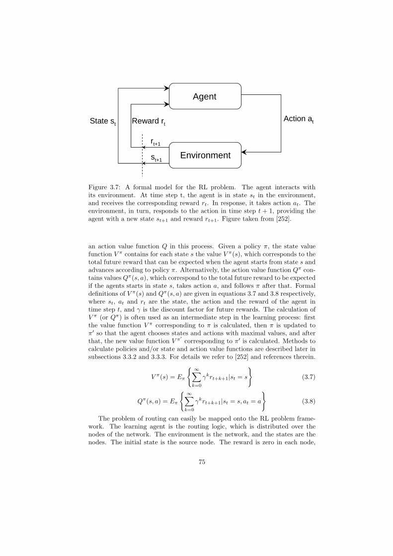
Agent

Environment

Action atReward rtState st

st+1

rt+1

Figure 3.7: A formal model for the RL problem. The agent interacts withits environment. At time step t, the agent is in state st in the environment,and receives the corresponding reward rt. In response, it takes action at. Theenvironment, in turn, responds to the action in time step t + 1, providing theagent with a new state st+1 and reward rt+1. Figure taken from [252].

an action value function Q in this process. Given a policy π, the state valuefunction V π contains for each state s the value V π(s), which corresponds to thetotal future reward that can be expected when the agent starts from state s andadvances according to policy π. Alternatively, the action value function Qπ con-tains values Qπ(s, a), which correspond to the total future reward to be expectedif the agents starts in state s, takes action a, and follows π after that. Formaldefinitions of V π(s) and Qπ(s, a) are given in equations 3.7 and 3.8 respectively,where st, at and rt are the state, the action and the reward of the agent intime step t, and γ is the discount factor for future rewards. The calculation ofV π (or Qπ) is often used as an intermediate step in the learning process: firstthe value function V π corresponding to π is calculated, then π is updated toπ′ so that the agent chooses states and actions with maximal values, and afterthat, the new value function V π′ corresponding to π′ is calculated. Methods tocalculate policies and/or state and action value functions are described later insubsections 3.3.2 and 3.3.3. For details we refer to [252] and references therein.

V π(s) = Eπ

{ ∞∑

k=0

γkrt+k+1|st = s

}(3.7)

Qπ(s, a) = Eπ

{ ∞∑

k=0

γkrt+k+1|st = s, at = a

}(3.8)

The problem of routing can easily be mapped onto the RL problem frame-work. The learning agent is the routing logic, which is distributed over thenodes of the network. The environment is the network, and the states are thenodes. The initial state is the source node. The reward is zero in each node,

75

apart from the destination node, where it is a number larger than zero. Shorterpaths are preferred because they lead faster to a non-zero reward. The agent’spossible actions are the next hops it can take in each of the nodes. The agent’spolicy, which indicates which action (next hop) to take in each of the states(nodes) in order to maximize reward (to find the destination fastest), is kept ina distributed way: it is spread over the routing tables maintained in the differentnodes. The relationship between the task of routing and the RL framework wasfirst pointed out in [39].

3.3.2 Elementary solution methods for reinforcement learn-ing: dynamic programming and Monte Carlo sam-pling

A wide range of different solution methods have been developed for RL prob-lems. The two most elementary ones are dynamic programming and MonteCarlo sampling. Here, we describe these approaches, and discuss how theyrelate to strategies used in routing. Later, in subsection 3.3.3, we describe an-other solution method, temporal-difference learning, and discuss how one of itsinstances, namely Q-learning, formed the basis for a different adaptive routingalgorithm, called Q-routing.

A first solution method for RL problems is dynamic programming. This isa general technique for solving optimization problems proposed in [26], and hasbeen in use for a long time before it was applied to RL. Dynamic programminghas been discussed before in 3.1.1, as it was at the basis of the developmentof distance vector routing algorithms. The basic idea behind this method isto split an optimization problem into subproblems, and use the solutions tothese subproblems to construct an optimal solution for the main problem. Astraightforward way of using dynamic programming in RL is policy iteration.The agent starts with a random initial policy π0, and uses dynamic programmingto calculate the state value function V π0 corresponding to it. Then π0 is updatedto π1 by choosing in each state the actions that optimize the values of the statesvisited by the agent with respect to V π0 . Then, dynamic programming is usedagain to calculate V π1 . The formula for calculating each state value V π(s) usingdynamic programming is given in equation 3.9, where Pa

ss′ is the probability ofreaching state s′ after taking action a in state s, and Ra

ss′ is the expectedreward when reaching state s′ after taking action a from state s. Compared tothe formula of equation 3.7, the infinite sum of future rewards is replaced by thesum of the expected immediate reward and the estimated values of the neighborstates s′. This is the trademark approach of dynamic programming: the taskof calculating the value of a state is solved based on the solution of a numberof subtasks, namely the values of the neighboring states. This characteristicapproach of calculating estimates based on other estimates is in the context ofRL also called information bootstrapping.

V π(s) ←∑

a

π(s, a)∑

s′Pa

ss′ [Rass′ + γV π(s′)] (3.9)

76

Dynamic programming formed the inspiration for distance vector routingalgorithms such as RIP. Details about this have been given before in subsec-tion 3.1.1. Here, we only want to point out how this approach to routing isaffected by the use of the characteristic technique of information bootstrapping.This provides high efficiency, due to the reuse of solutions that were calculatedfor different subproblems (routing estimates calculated for neighboring nodes).However, it is not very robust or adaptive: if estimates are wrong in one node(e.g. due to changes in the environment), they are propagated over the networksince other estimates are based on them, and it can take a long time until theerror is fixed and all the routing information converges again to correct values.This limits the usability of a pure dynamic programming approach for adaptiverouting in AHWMNs.

A second elementary solution method for RL is Monte Carlo sampling. Alsothis method has been around long before RL itself was a topic. In fact, the termMonte Carlo refers to any problem solving method in which solutions are learnedfrom experiences obtained by repeated sampling. In the field of RL, Monte Carlosampling can be used to calculate value functions in a policy iteration approach,like the one described for dynamic programming above. One difference is thatin Monte Carlo learning usually the action values Qπ(s, a) are used rather thanthe state values V π(s). To calculate the value Qπ(s, a) of action a in state s,the agent tries it out: it runs a full episode of the task (i.e. until it reachesthe goal state), starting from state s with action a and then following policy πafter that. By executing repeated samples and taking the average of the totalrewards experienced in each of these samples, a good estimate of the expectedvalue of the total future reward can be obtained. In practice, a moving averagecan be used, applying the formula of equation 3.10 after each newly collectedsample experience. In this formula, Rπ(s, a) is the total reward experiencedwhen taking action a in state s and following π after that, and α is a constantfactor used for the moving average. A special case of Monte Carlo sampling isthe off-policy version, in which the agent collects sample experiences followinga different policy than the one it is actually learning about. This allows morefreedom (e.g. to do exploration), but is computationally more complicated, asone has to make an adjustment to the average experienced rewards in order tofind the correct value for the other policy.

Qπ(s, a) ← Qπ(s, a) + α[Rπ(s, a)−Qπ(s, a)] (3.10)

It is easy to see how the ACO approach to routing relies in its process forgathering routing information on the same ideas as the Monte Carlo approachto learning in RL. Ants learn action values (the value of taking a next hopin a certain node) by executing complete samples of solutions to the task (bysampling a path to the destination). The final pheromone values are the resultof taking a sufficiently high number of samples. ACO routing algorithms inwhich different forwarding policies are used for ants and data forwarding aresimilar to off-policy Monte Carlo learning. The fact that the pheromone valuesdo not always correspond to the average of the values experienced by the ants,

77

but are instead the result of more complicated evaluations of these values (e.g.in AntNet, described in subsection 3.2.3, the experienced delay is manipulatedusing the local traffic statistics), is reminiscent of actor-critic methods, whichare more advanced RL learning methods [25]. The most important advantageof Monte Carlo sampling compared to information bootstrapping is that all es-timates are based on direct experiences. This makes the estimates more reliablethan when they are based on other estimates, giving increased robustness to thealgorithm. This is particularly important in a changing and unreliable environ-ment like AHWMNs. Adaptivity can in principle be a problem in Monte Carlolearning, namely when on-policy learning is applied and the policy has con-verged. In ACO routing, this problem is solved by using an off-policy approachin which ants follow a slightly different policy from data packets.

It is interesting to note that more traditional routing algorithms for AH-WMNs, such as AODV, DSR and other reactive algorithms (see subsection 2.4.2),also rely on sampling. They construct a path based on a single sample. Thisis of course quite different from taking the average value obtained from re-peated sampling such as in ACO routing. Nevertheless, it is a confirmation ofthe usefulness in AHWMNs of the increased robustness obtained through pathsampling. This is especially clear in the development of AODV. This algorithmis presented as a distance vector algorithm as it was conceived as a successorto DSDV, a routing algorithm that relies purely on information bootstrapping.However, the only elements it still contains of distance vector routing is theshape of the routing tables. The information bootstrapping approach used inDSDV is deemed unworkable in the highly dynamic and unreliable AHWMNenvironment, and is replaced by a strategy that relies on sampling. However, itneeds to be noted that the sampling in AODV and other reactive routing algo-rithms is not always done in a consequent way. E.g., AODV RREQ messagesdo not always go all the way until the destination, but return to the source assoon as they find a node that has routing information about the destination. Atthat point, the source node’s routing information is again based on an estimateprovided by another node.

3.3.3 Temporal-difference learning and Q-routing

Here we describe a more advanced class of solution methods for RL problems,namely temporal-difference learning. This approach combines elements of dy-namic programming and Monte Carlo sampling, in order to get advantages fromboth methods. It is at this point important to point out that the AntHocNetalgorithm for routing in AHWMNs presented in chapter 4 of this thesis also com-bines elements of both dynamic programming and Monte Carlo sampling. Itdoes so in a completely different way than temporal-difference learning though,as will become clear later.

The simplest version of temporal-difference learning is the one step temporal-difference method, referred to as TD(0). The main idea behind this method isfor the agent to take a sample of just one step, and then bootstrap information.Concretely, in TD(0), the agents calculates Q(s, a) by taking action a in state s,

78

observing the immediately received reward r, and bootstrapping on the value ofthe new state it arrives in. An example update formula is given in equation 3.11,where α is a constant factor for calculating the moving average, and γ is aconstant factor to discount rewards that are received in a future time step. Thedifference with the update formula for Monte Carlo learning (equation 3.10)is that only one step of experienced reward is used. The difference with theupdate formula for dynamic programming (equation 3.9) is that an experienceis used for the one-step reward, rather than the expected value. Variations arepossible in the choice of the action a′ in the new state s′ on the basis of which thebootstrapped value Q(s′, a′) is chosen. E.g., the most popular TD(0) method, Q-learning, uses the action a′ that gives the maximal value for Q(s′, a′) [272]. Thiscorresponds to an off-policy form of temporal-difference learning, and allows fastconvergence to the optimal policy π∗. The one-step form of temporal differencelearning found in TD(0) can be extended to an n-step algorithm, in which theagent takes a sample of n steps before bootstrapping the local state value. If nis equal to infinity or to the number of steps needed to reach the goal, this comesdown to Monte Carlo sampling. Finally, when the results from several n-stepsamples are combined, with different values for n, we get the TD(λ) methods,which are also referred to as eligibility traces [271].

Qπ(s, a) ← Qπ(s, a) + α[r + γQ(s′, a′)−Qπ(s, a)] (3.11)

Just like dynamic programming and Monte Carlo sampling, temporal-differencelearning has been applied to routing. In particular, the Q-learning algorithmmentioned above has lead to the development of Q-routing [39]. In Q-routing,nodes keep routing tables that are similar to those in AntNet, with one entry percombination of next hop and destination. The routing table entry cd

ij indicatesthe cost of going from i over neighbor j to destination d. Each time node i sendsa data packet to a neighbor j for a destination d, j sends a control packet backto i. This packet contains the values ttot, the total queueing and transmissiondelay experienced by the data packet to reach j from i, and cd

j , the cost of thebest path to destination d present in j’s routing table. In node i, ttot and cd

j

are summed to get an estimate of the cost from i to d over j, and the value cdij

in i’s routing table is updated accordingly. When compared to Q-learning, ttot

corresponds to the immediate reward experienced in the one step sample, andcdj corresponds to the value of the next state. Like in dynamic programming

approaches to routing, such as the basic distance vector routing algorithm, rout-ing updates are based on the best paths reported by neighboring nodes. Themain difference is that in Q-routing the cost of the single hop to the neighboris taken from a sample, while in distance vector routing, it is an estimate of theexpected value, obtained via local monitoring. In direct comparisons with theAntNet adaptive routing algorithm, Q-routing scored less well [70].

Another RL inspired approach to routing is SAMPLE [90]. This is an adap-tive algorithm for MANETs. Similarly to Q-routing, it does an update of routinginformation with the transmission of each data packet. Also like Q-routing anddynamic programming, the best path available in neighboring nodes is used for

79

information bootstrapping in the update process. For the calculation of the costof the one hop to the neighbor, SAMPLE relies on a model of the environment.Model-based RL [91] is not presented here, as it would lead us to far. However,the end result is an algorithm that is similar to both Q-routing and distancevector routing. Important for MANETs, SAMPLE uses an estimate of linkqualities with similarities to the ETX measure (see subsection 2.4.3) to definepath costs.

3.4 Conclusion

In this chapter we have described existing adaptive routing algorithms. Theaim of the chapter was on the one hand to provide information about otheralgorithms in the field, and on the other hand to get the reader acquainted withthe techniques and terminology that will be used further in this thesis.

In a first section, we have described adaptive routing algorithms in the in-ternet. Two main approaches were discussed, namely distance vector routingand link state routing. For either of these approaches, we have investigated howthey perform in terms of the major challenges for AHWMN routing: adaptivity,robustness, efficiency and scalability. We have also indicated to what extentboth approaches to routing have been adapted to work in AHWMNs.

Then, in a second section, we have described ACO and ACO routing. ACOis a metaheuristic for the solution of optimization problems that was inspiredby the shortest path finding behavior of ant colonies in nature. ACO routingis an approach to routing that is based on the ACO framework. It forms animportant source of inspiration for the work presented in this thesis. Here, wehave described the major characteristics of ACO routing in detail, and havegiven an extensive overview of existing ACO routing algorithms, both for wirednetworks and for AHWMNs.

In a last section, we have treated adaptive routing from a machine learningpoint of view. To that end, we have described RL, an important class of learningproblems. We have shown that the problem of routing in telecommunicationnetworks fits well into this problem framework. Then, we have investigated howthe strategies for the gathering of routing information used by distance vectorand ACO routing algorithms correspond to two important learning methods forRL problems, namely dynamic programming and Monte Carlo learning. Fi-nally, we have described temporal difference learning, a more advanced solutionmethod for RL problems that combines elements of both dynamic programmingand Monte Carlo learning, and we have explained the Q-routing algorithm thatwas derived from it. The AntHocNet routing algorithm for AHWMNs describedin the next chapter also combines elements from both of these learning methods,but in quite a different way.

80

Chapter 4

AntHocNet: an adaptiverouting algorithm for adhoc wireless multi-hopnetworks

In this chapter, we describe AntHocNet, an adaptive routing algorithm for AH-WMNs. AntHocNet is a hybrid routing algorithm, in the sense that it containselements from both reactive and proactive routing. Specifically, it combines areactive route setup process with a proactive route maintenance and improve-ment process. AntHocNet was in the first place inspired by the ACO approachto routing. This is evident in the way that it gathers, stores and uses routing in-formation. Consequently, the terminology used in this chapter is mostly relatedto the ACO routing literature. Nevertheless, AntHocNet also contains elementsfrom distance vector routing. In particular, the information gathering processused in its proactive route maintenance and improvement process combines theroute sampling strategy from ACO routing with an information bootstrappingprocess that is similar to the one used in distance vector routing algorithms.The way both approaches are combined is novel and allows the algorithm toget the best of both worlds. AntHocNet was in the first place developed forMANETs and WMNs. Descriptions of the AntHocNet algorithm have beenpublished in [73–75,94,95,98].

The rest of this chapter is organized as follows. First, we give a generaloverview of the AntHocNet routing algorithm. This includes a high level de-scription of the algorithm in words, and a schematic representation. Then, wegive a detailed description of each of the algorithm’s components. Finally, weprovide further discussions on the presented material, such as an investigationof the relations between AntHocNet and other AHWMN routing algorithms,a discussion of how AntHocNet relates to the RL solution methods presented

81

in chapter 3, and a description of elements that were present in older versionsof AntHocNet. Evaluations of AntHocNet and experimental comparisons withother routing algorithms will be provided in the following chapters.

4.1 General overview of the AntHocNet routingalgorithm

In this section, we give an overview of the algorithm. We start with a generaldescription in words. Then, we also provide a schematic representation in theform of a finite state machine.

4.1.1 Algorithm description

AntHocNet is a hybrid algorithm, containing both reactive and proactive el-ements. The algorithm is reactive in the sense that it only gathers routinginformation about destinations that are involved in communication sessions. Itis proactive in the sense that it tries to maintain and improve information aboutexisting paths while the communication session is going on (unlike purely reac-tive algorithms, which do not search for routing information until the currentlyknown routes are no longer valid). Routing information is stored in pheromonetables that are similar to the ones used in other ACO routing algorithms. For-warding of control and data packets is done in a stochastic way, using thesetables. Link failures are dealt with using specific reactive mechanisms, suchas local route repair and the use of warning messages. Below, we describe thegeneral working of the AntHocNet routing algorithm. Details will follow laterin section 4.2.

In AntHocNet, routing information is organized in pheromone tables, similarto the ones used in other ACO routing algorithms such as the earlier describedAntNet (see subsection 3.2.3). Each node i maintains one pheromone table Ti,which is a two-dimensional matrix. An entry T d

ij of this pheromone table con-tains information about the route from node i to destination d over neighbor j.This information includes the pheromone value τd

ij , which is a value indicatingthe relative goodness of going over node j when traveling from node i to desti-nation d, as well as statistics information about the path, and possibly virtualpheromone (see later). Apart from a pheromone table, each node also maintainsa neighbor table, in which it keeps track of which nodes it has a wireless link to.Details about the data structures maintained under AntHocNet are describedin subsection 4.2.1.

At the start of a communication session, the source node of the session con-trols its pheromone table, to see whether it has any routing information availablefor the requested destination. If it does not, it starts a reactive route setup pro-cess, in which it sends an ant packet out over the network to find a route tothe destination. Such an ant packet is called a reactive forward ant. Each in-termediate node receiving a copy of the reactive forward ant forwards it. Thisis done via unicasting in case the node has routing information about the ant’s

82

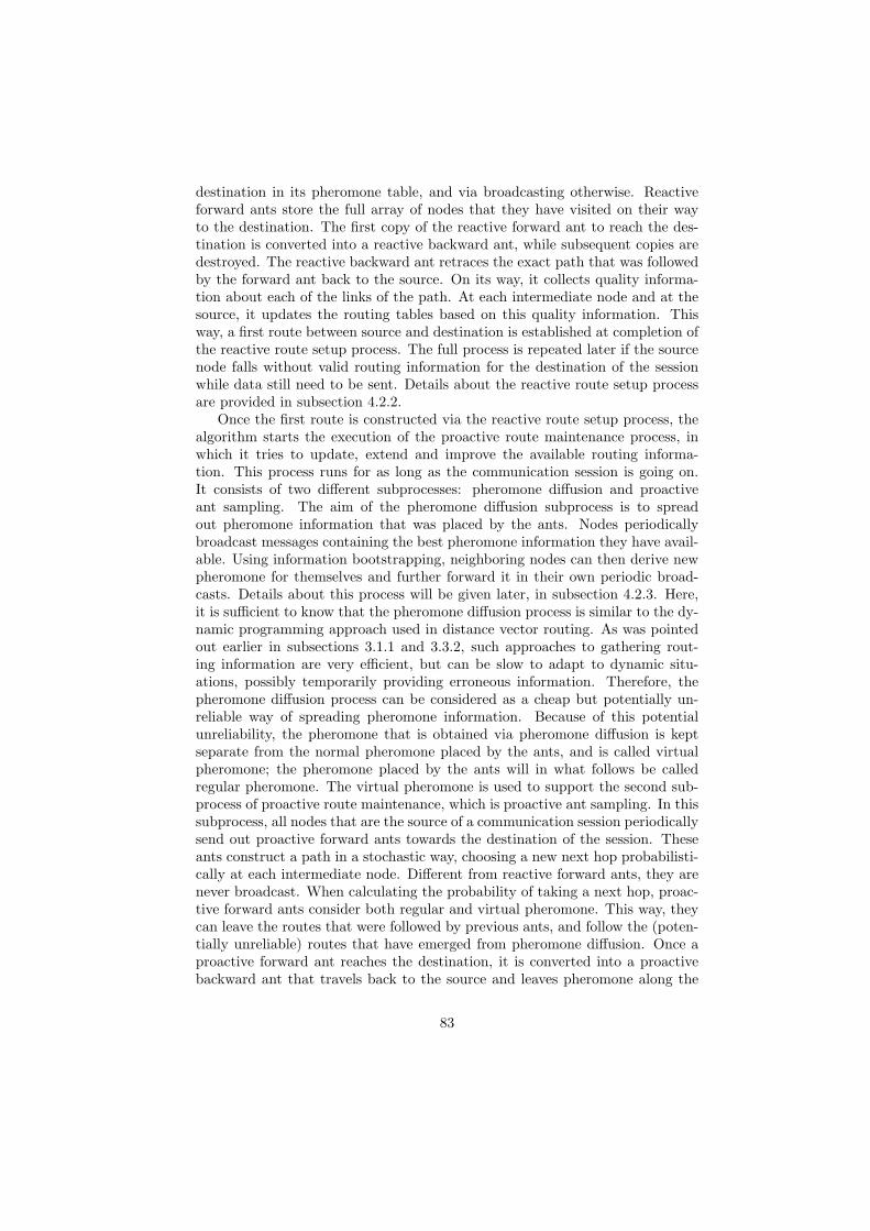
destination in its pheromone table, and via broadcasting otherwise. Reactiveforward ants store the full array of nodes that they have visited on their wayto the destination. The first copy of the reactive forward ant to reach the des-tination is converted into a reactive backward ant, while subsequent copies aredestroyed. The reactive backward ant retraces the exact path that was followedby the forward ant back to the source. On its way, it collects quality informa-tion about each of the links of the path. At each intermediate node and at thesource, it updates the routing tables based on this quality information. Thisway, a first route between source and destination is established at completion ofthe reactive route setup process. The full process is repeated later if the sourcenode falls without valid routing information for the destination of the sessionwhile data still need to be sent. Details about the reactive route setup processare provided in subsection 4.2.2.

Once the first route is constructed via the reactive route setup process, thealgorithm starts the execution of the proactive route maintenance process, inwhich it tries to update, extend and improve the available routing informa-tion. This process runs for as long as the communication session is going on.It consists of two different subprocesses: pheromone diffusion and proactiveant sampling. The aim of the pheromone diffusion subprocess is to spreadout pheromone information that was placed by the ants. Nodes periodicallybroadcast messages containing the best pheromone information they have avail-able. Using information bootstrapping, neighboring nodes can then derive newpheromone for themselves and further forward it in their own periodic broad-casts. Details about this process will be given later, in subsection 4.2.3. Here,it is sufficient to know that the pheromone diffusion process is similar to the dy-namic programming approach used in distance vector routing. As was pointedout earlier in subsections 3.1.1 and 3.3.2, such approaches to gathering rout-ing information are very efficient, but can be slow to adapt to dynamic situ-ations, possibly temporarily providing erroneous information. Therefore, thepheromone diffusion process can be considered as a cheap but potentially un-reliable way of spreading pheromone information. Because of this potentialunreliability, the pheromone that is obtained via pheromone diffusion is keptseparate from the normal pheromone placed by the ants, and is called virtualpheromone; the pheromone placed by the ants will in what follows be calledregular pheromone. The virtual pheromone is used to support the second sub-process of proactive route maintenance, which is proactive ant sampling. In thissubprocess, all nodes that are the source of a communication session periodicallysend out proactive forward ants towards the destination of the session. Theseants construct a path in a stochastic way, choosing a new next hop probabilisti-cally at each intermediate node. Different from reactive forward ants, they arenever broadcast. When calculating the probability of taking a next hop, proac-tive forward ants consider both regular and virtual pheromone. This way, theycan leave the routes that were followed by previous ants, and follow the (poten-tially unreliable) routes that have emerged from pheromone diffusion. Once aproactive forward ant reaches the destination, it is converted into a proactivebackward ant that travels back to the source and leaves pheromone along the

83

way (regular, not virtual pheromone), just like reactive backward ants. Thisway, proactive ants can follow virtual pheromone and then, once they have ex-perienced that it leads to the destination, convert it into regular pheromone.One could say that pheromone diffusion suggests new paths and that proactiveants check them out. The ant based full path sampling provides the reliabilitythat is lacking in the efficient information bootstrapping process. Details aboutthe proactive route maintenance process are given in subsection 4.2.3.

Data packet forwarding in AntHocNet is done similarly to other ACO routingalgorithms: routing decisions are taken hop-by-hop, based on the locally avail-able pheromone. Only regular pheromone is considered, as virtual pheromoneis not considered reliable enough. Each forwarding decision is taken using astochastic formula that gives preference to next hops that are associated withhigher pheromone values. The formula is different from that used by the forwardants, so that data packets can follow a less exploratory strategy. Via param-eter tuning, it is possible to vary between spreading the data packets over allpossible available paths and deterministically sending them over the best path.While the former can in principle provide higher throughput through the useof multiple paths (see subsection 2.4.3), the latter allows greedy exploitationof the learned information. Later, in chapter 5, we compare both strategiesempirically. Details about data packet forwarding in AntHocNet are providedin subsection 4.2.4.

Link failures can be detected in AntHocNet via failed transmissions of dataor control packets, or through the use of hello messages. Hello messages areshort messages that are periodically sent out by all nodes in the network. Thereception of a hello message is indicative of the presence of a wireless link,while the failure to receive such messages point to the absence of a link. Inpractice in AntHocNet, the function of hello messages is fulfilled by the sameperiodic messages that are used for pheromone diffusion. When a node detectsa link failure, it controls its pheromone table, to see which routes become invaliddue to the failure, and whether alternative routes are available for the affecteddestinations. Then, it broadcasts a link failure notification message to warnneighboring nodes about all relevant changes in its pheromone table. In casethe link failure was associated with a failed data packet transmission, the nodecan also start a local route repair to restore the route to the destination of thisdata packet. To this end, it sends out a repair forward ant. Repair forwardants are similar to reactive forward ants, in the sense that they follow availablepheromone information where possible, and are broadcast otherwise, but theyhave a limited maximum number of broadcasts, so that they cannot travel farfrom the old failed route. Upon arrival at the destination, the repair forwardant is converted into a repair backward ant that travels back to the node thatstarted the repair process and sets up the pheromone for the repaired route.A last tool in dealing with link failures is the use of unicast warning messages.These are needed when data packets for a lost destination still arrive at thenode after a link failure notification has already been broadcast. This can bedue to bad reception of the broadcast notification message. In this case, thenode unicasts a warning to the node it received the data from, in order to inform

84

Send reactive forward ant

Route data packets

Send repair forward ant

Repair timeout

Initial state

Process reactive forward ant

Process link failure notification

Process Hello

Process proactive forward ant

Process unicast warning

Process received control packet

Process repair forward ant

Process backward ant

Link failure notification

Backward ant

Repair forward ant

Proactive forward ant

Reactive forward ant

Hello message

Unicast warning

Final state

Send Hello

Receive control packetIdle state

Send unicast warning

No route at source Link failure

Send link failure notification

Receive data

No route at intermediate, data

No route at intermediate, no data

Hello timer

Reactive ant timeout

No route at source

No route at intermediateReactive ant timer

Repair ant timer

Adapt pheromone table

Send proactive ant

Proactive ant timer

Figure 4.1: A finite state machine representation of the AntHocNet routingalgorithm.

it that it can no longer forward data for this destination. Details about howAntHocNet deals with link failures are described in subsection 4.2.5.

4.1.2 Schematic representation

Figure 4.1 gives a schematic representation of the AntHocNet routing algorithm.It contains a finite state machine showing the most important components ofthe algorithm. Below we explain the structure of the finite state machine. Fordetails about each of the components, we refer to section 4.2.

The algorithm is started up in its initial state, in which internal variables areinitialized. Then, it moves to its idle state, where it waits for events to happen.The events that can take place are the arrival of a data packet, the arrival of acontrol packet, the detection of a link failure, and a number of timer events.

In case of a data reception event, the algorithm tries to route the data.Details about data forwarding are given in subsection 4.2.4. This might beimpossible, due to the lack of routing information about the destination. If thecurrent node is the source node of the data packet, the unavailability of routing

85

information can be because the data packet is the first of a new communicationsession, or because it belongs to a session for which all routing information hasbecome invalid. In both cases, the node starts a reactive route setup process.Details about this process are given in subsection 4.2.2. If the current node isnot the source of the data packet, it concludes that the upstream node of thedata has wrong routing information, and sends it a unicast warning message.This is further explained in subsection 4.2.5, which talks about link failures.

In case of a control packet reception event, the algorithm checks which typeof control packet it is dealing with. In case it is a hello message, the node needsto take note in its neighbor table that it has a wireless link with the packet’ssender, and it needs to extract the routing information inside to update its ownvirtual pheromone information. This is part of the proactive route maintenanceprocess described in subsection 4.2.3. In case it is a reactive, proactive or re-pair forward ant, the node needs to execute the correct forwarding action, or,if it is the final destination of the ant, create a backward ant and send it backtowards the source. In case the control packet is a backward ant (reactive,proactive and repair backward ants have essentially the same behavior, and aretherefore collapsed here), the node needs to adapt its pheromone table, andforward the ant if it is not its final destination. Details about the treatmentof reactive, proactive and repair forward and backward ants are given respec-tively in subsections 4.2.2, 4.2.3 and 4.2.5. In case the control packet is a linkfailure notification, the node needs to update its pheromone table, and possiblyforward the notification. Finally, if it is a unicast warning, it needs to updateits pheromone table, removing the erroneous route. Details about link failurenotifications and unicast warnings are given in subsection 4.2.5.

In case of a link failure event, the node first of all adapts the informationin its pheromone table to reflect the changed situation. Then, if destinationshave become unreachable due to the link failure, it needs to take action. If thecurrent node is the source of a session to one of the lost destinations, it starts areactive route setup process. If, on the other hand, it is an intermediate node onthe lost route, it controls whether the link failure event involved the unsuccessfultransmission of a data packet. If this is the case, it starts a local route repairprocess. Otherwise, it broadcasts a link failure notification message. Details onhow link failures are dealt with are given in subsection 4.2.5.

The different timers are events that are scheduled by the node itself, in orderto plan delayed actions. Hello timer events are scheduled at regular intervals,from the moment the node is switched on and for as long as it is up and running.Reception of a hello timer event provokes the node to send a hello message, inwhich it includes its best pheromone information. This is part of the proactiveroute maintenance process described in subsection 4.2.3. Proactive ant timerevents are also scheduled at regular intervals, but only from the moment a sessionis started, and until the end of it. Reception of a proactive ant timer eventleads the node to send out a proactive forward ant. Details about this are givenin subsection 4.2.3. Repair timer events are scheduled after a repair forwardant has been sent out. At reception of a repair timer event, the node checkswhether a repair backward ant was received, and in case not, it broadcasts a

86

link failure notification. This is part of the process of dealing with link failures,described in 4.2.5. Finally, reactive ant timer events are similarly sent outafter the transmission of a reactive forward ant. At reception of a reactiveant timer event, the node controls whether it has already received a reactivebackward ant. In case not, it can send out a new reactive forward ant (in casethe maximum number of retransmissions has not yet been reached), or concludethat the destination is currently unreachable, and drop queued data packets forit. This is described in detail in subsection 4.2.2, which explains the reactiveroute setup phase.

4.2 Detailed descriptions

In this section, we give a detailed description of the different components ofthe AntHocNet routing algorithm. We follow the same structure as in subsec-tion 4.1.1. First we describe the data structures that are maintained in eachnode. Then, we give details about the reactive route setup process. Subse-quently, we discuss the proactive route maintenance process. Next, we talkabout data packet forwarding. After that, we discuss the algorithm’s behaviorwith respect to link failures. Finally, we talk about the routing metrics used inAntHocNet.

4.2.1 Data structures in AntHocNet

Here, we describe the different data structures that are maintained by each ofthe network nodes under AntHocNet. In particular, we talk about pheromonetables and neighbor tables.

Pheromone tables

Under AntHocNet, each node i maintains a pheromone table Ti, which is a two-dimensional matrix. An entry T d

ij of this matrix contains information aboutthe route from node i to destination d over neighbor j. This includes a regularpheromone value τd

ij , a virtual pheromone value ωdij , and an average number of

hops hdij . The regular pheromone value τd

ij is an estimate of the goodness ofthe route from i to d over j. Goodness is expressed as the inverse of a cost.Exact values depend on the metric that is used to evaluate the cost of routes.More about the use of different metrics will follow in subsection 4.2.6. Regularpheromone is updated by backward ants. These can be reactive, proactive orrepair backward ants. Details about the updating process for regular pheromoneare given in subsection 4.2.2. The virtual pheromone value ωd

ij forms an alter-native estimate of the goodness of the route from i to d over j. Differently fromτdij , it is obtained through information bootstrapping using goodness values re-

ported by neighbor nodes during the proactive route maintenance process. Theupdating of virtual pheromone is discussed in subsection 4.2.3. The averagenumber of hops hd

ij is, like the regular pheromone, updated by backward ants.

87

This updating process is described in subsection 4.2.2. hdij is used when deciding

how long to wait for repair backward ants (see subsection 4.2.5).Nodes do not necessarily always have values available for τd

ij , ωdij , and hd

ij

for each possible combination of destination and next hop. This is in the firstplace because nodes do not maintain routing information about all possible des-tinations in the network (they only gather routing information for destinationswhich communication sessions are going on with), and because for a specificdestination, nodes do not necessarily have a route available over each of theirpossible neighbors (for instance, during a reactive route setup phase only oneroute is set up, so that the source node has exactly one outgoing next hop for theinvolved destination). Also, since regular and virtual pheromone are obtainedthrough different processes, it is possible that a node has a value for τd

ij , but notfor ωd

ij , or vice versa. On the other hand, since τdij and hd

ij are both obtainedfrom backward ants, nodes that have a value for one of the two will also have avalue for the other.

Neighbor tables

Apart from the pheromone table, each node also maintains a neighbor table.The neighbor table Ni kept by node i is a one-dimensional vector with oneentry for each of i’s neighbors. The entry Nij corresponding to i’s neighbor jcontains a time value thij indicating when i last heard from j. Node i uses thistime value to derive whether there is a wireless link with node j, and to detectlink failures. More on the detection and handling of link failures will follow laterin subsection 4.2.5.

4.2.2 Reactive route setup

The reactive route setup process is triggered whenever a node receives a datapacket that was locally generated (i.e., the current node is the packet’s source)for a destination for which no routing information is available. This lack of rout-ing information can happen either because the data packet in question is thefirst of a new communication session, and no routing information for its destina-tion is available from a different or previous session, or because the data packetbelongs to an ongoing session for which all routes have become invalid (e.g., dueto node movements). The reactive route setup process involves the sending ofa reactive forward ant from source to destination, and a reactive backward antfrom destination to source. Below, we discuss each of these separately.

Reactive forward ants

At the start of the reactive route setup process, the source node s creates areactive forward ant. This is a control packet that has as a goal to find a pathfrom s to an assigned destination d. At the start, the ant contains just theaddresses of s and d. Later, as it proceeds through the network, it collects a listP = [1, 2, . . . , d− 1] of all the nodes that it has visited on its way from s to d.

88

After its creation at s, the reactive forward ant is broadcast, so that all of s’sneighbors receive a copy of it. At each subsequent node, the ant is either unicastor broadcast, depending on whether the current node has routing informationfor d. If routing information is available, the node chooses a next hop for the antprobabilistically, based on the different pheromone values associated with nexthops for d. Concretely, a node i chooses node n as next hop for the ant withprobability P d

in, as calculated by equation 4.1. In this equation, Ndi is the set

of neighbors of i over which a path to d is known, and β1 is a parameter valuewhich can control the exploratory behavior of the ants. In our experiments, wekeep β1 relatively high, on 20. This is because we want to obtain the initialroute as fast as possible, and limit the time we spend on exploration at thisstage.

P din =

(τdin)β1

∑j∈Nd

i(τd

ij)β1, β1 ≥ 1, (4.1)

In case the intermediate node i does not have routing information for d, itbroadcasts the reactive forward ant. Due to this broadcasting (and also theinitial broadcasting at s), a reactive forward ant can proliferate quickly overthe network, with different copies of the ant following different paths to thedestination. In order to limit the amount of overhead that is created this way,nodes only forward the first copy of the ant that they receive. Subsequent copiesare simply discarded. In previous versions of AntHocNet, nodes were to someextent allowed to forward multiple copies of the same ant, in order to improvethe creation of multiple paths (see also subsection 4.3.4). However, this lead toa lot of overhead.

At the destination, the reactive forward ant is converted into a reactivebackward ant, which follows the list of nodes P visited by the forward antback to s. If more than one copy of the forward ant is received, only the firstis accepted and converted into a backward ant, while subsequent copies arediscarded. This way, only one route is set up during the reactive route setupprocess. The reason is again to reduce overhead created during this procedure.For the creation of multiple routes, AntHocNet relies on the proactive routemaintenance process, which extends the initially created route into a full meshof routes during the course of the communication session (see subsection 4.2.3).

Reactive backward ants

The reactive backward ant created by the destination node in response to areactive forward ant contains the addresses of the forward ant’s source node sand destination node d, as well as the full list of nodes P that the forward anthas visited. The reactive backward ant is unicast from d and between the nodesof P back to s.

The aim of the reactive backward ant is to update routing information ineach of the nodes of P and in s. At each node i that it visits, it updates thenumber of hops hd

in and the regular pheromone value τdin in the pheromone table

89

entry T din, where n is the node that it visited before i on its way from d. The

updating of hdin is done using a moving average, as shown in equation 4.2. In this

equation, h is the number of hops that the backward ant has traveled betweend and i, and α is a parameter regulating how quickly the formula adapts to newinformation. In our experiments, α is always kept on 0.7.

hdin ← αhd

in + (1− α)h, α ∈ [0, 1] (4.2)

Updating of the regular pheromone τdin is done based on the cost of the

route from i to d. This cost can be calculated using different metrics, such asthe number of hops, the end-to-end delay, etc.. Later on, in subsection 4.2.6,we comment on different metrics used in AntHocNet. Here, we talk in terms ofa generic cost c, where cd

i is the cost of the route from i to d, and cji is the cost

of the link from i to its neighbor j (it is the cost of a one-hop route). UnderAntHocNet, each node maintains a local estimate of the cost cj

i to go to each ofits neighbors j. Details about how these local estimates are calculated dependon the metric and are discussed in subsection 4.2.6. The reactive backward antreads at each node i the local estimate cn

i of the cost to go from i to the nexthop n that the ant is coming from. It adds this cost to the total cost cd

n ofthe route from n to d (which it has been calculating on its way back from d),which is stored inside the ant. The new cost cd

i is used to update the pheromonevalue τd

in in node i, using the moving average formula of equation 4.3. In thisequation, γ is a parameter regulating the speed of adaptation of the pheromoneto new cost values. In our experiments, γ was kept on 0.7. The cost value cd

i

is inverted to calculate the pheromone value τdij , as pheromone indicates the

goodness of a route, rather than its cost.

τdij ← γτd

ij + (1− γ)(cdi )−1, γ ∈ [0, 1] (4.3)

It is interesting to note that in terms of gathering route cost information,there is an important difference here with the AntNet algorithm described insubsection 3.2.3 and other ACO routing algorithms. Rather than relying onthe cost values experienced by the forward ants, AntHocNet uses the estimatescji calculated locally by the nodes. This is in order to improve reliability of

the measured values. Depending on the cost metric used, the high variabilityof the wireless medium can cause large differences between values measuredby subsequent samples. For example, the delay incurred on a link can varystrongly in case of congestion if IEEE 802.11 is used as a MAC layer protocol(see subsection 2.3.3). Using local estimates that are based on more than onesample can take away some of this variability.

4.2.3 Proactive route maintenance

The proactive route maintenance process serves to update and extend availablerouting information. In particular, it allows to build a mesh of multiple routesaround the initial route created during the reactive route setup process. Theproactive route maintenance process consists of two subprocesses: pheromone

90

diffusion and proactive ant sampling. Pheromone diffusion is aimed at spreadingavailable pheromone information over the network through the use of periodicupdate messages and information bootstrapping. Proactive ant sampling isaimed at controlling and updating pheromone information through path sam-pling using proactive forward ants. While proactive ant sampling is started bythe source node of a communication session at the start of the session and con-tinues for as long as the session is going on, pheromone diffusion is executed byall nodes throughout their whole lifetime, and is not particulary bound to theoccurrence of a single session. Below, we describe each of the two subprocessesof proactive route maintenance separately.

Pheromone diffusion

The reactive route setup process described in subsection 4.2.2 leads to the avail-ability of a single route from the source of a communication session to its des-tination, indicated by regular pheromone values in the pheromone tables of thenodes. Moreover, each neighbor node of the destination also has a one-hop routeto the destination. This is independent of the running session, and is simply dueto the fact that neighboring nodes are aware of each other’s presence, as is ex-plained further in subsection 4.2.5. The aim of the pheromone diffusion processis to spread all this pheromone information out, so that a field of pheromonepointing towards the destination becomes available in the network. This fieldof pheromone is indicated in the virtual pheromone values in the pheromonetables of the nodes. The fact that pheromone is spread out is similar to thenormal diffusion of real pheromone in nature [185], which allows ants furtheraway to sense it. In the example of figure 4.2, a communication session is go-ing on between node 1 and node 8. Regular pheromone is indicated by solidarrows. It consists of a single route from 1 to 8 over the nodes 3, 6 and 7 thatis the result of reactive route setup, and a one-hop route from 5 to 8 that isthere independently of the running session, because 5 is aware of the presenceof its neighbor 8. The field of virtual pheromone that is the result of pheromonediffusion is indicated with dashed arrows.

A crucial role in the pheromone diffusion process is played by hello messages.These are short messages broadcast every thello seconds asynchronously by allthe nodes of the network throughout their whole lifetime. In AntHocNet, thello

is set to 1 second. Hello messages are used in many existing protocols, suchas ABR [257] and OLSR [61] (see subsection 2.4.2), to allow nodes to find outwhich are their immediate neighbors, and to detect link failures. While also inAntHocNet hello messages are used for this purpose (as is explained in subsec-tion 4.2.5), they also serve a different goal, namely to carry information in thepheromone diffusion process. They serve as the periodic update messages thatare needed in the information bootstrapping process of pheromone diffusion.The idea to convey extra routing information inside hello messages has beenused in some other routing algorithms, such as the earlier mentioned OLSR.

Nodes include in each hello message that they send out routing informationthey have available. In particular, a node i constructing a hello message consults

91

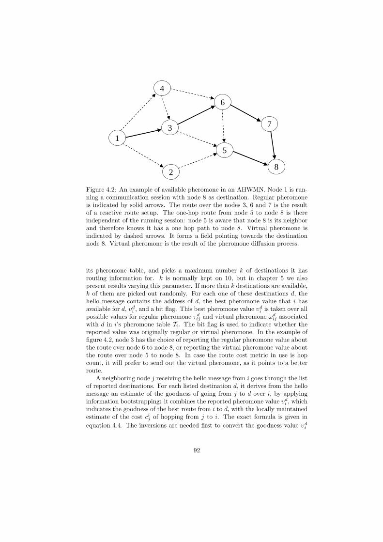
3

2

4

6

7

8

5

1

Figure 4.2: An example of available pheromone in an AHWMN. Node 1 is run-ning a communication session with node 8 as destination. Regular pheromoneis indicated by solid arrows. The route over the nodes 3, 6 and 7 is the resultof a reactive route setup. The one-hop route from node 5 to node 8 is thereindependent of the running session: node 5 is aware that node 8 is its neighborand therefore knows it has a one hop path to node 8. Virtual pheromone isindicated by dashed arrows. It forms a field pointing towards the destinationnode 8. Virtual pheromone is the result of the pheromone diffusion process.

its pheromone table, and picks a maximum number k of destinations it hasrouting information for. k is normally kept on 10, but in chapter 5 we alsopresent results varying this parameter. If more than k destinations are available,k of them are picked out randomly. For each one of these destinations d, thehello message contains the address of d, the best pheromone value that i hasavailable for d, υd

i , and a bit flag. This best pheromone value υdi is taken over all

possible values for regular pheromone τdij and virtual pheromone ωd

ij associatedwith d in i’s pheromone table Ti. The bit flag is used to indicate whether thereported value was originally regular or virtual pheromone. In the example offigure 4.2, node 3 has the choice of reporting the regular pheromone value aboutthe route over node 6 to node 8, or reporting the virtual pheromone value aboutthe route over node 5 to node 8. In case the route cost metric in use is hopcount, it will prefer to send out the virtual pheromone, as it points to a betterroute.

A neighboring node j receiving the hello message from i goes through the listof reported destinations. For each listed destination d, it derives from the hellomessage an estimate of the goodness of going from j to d over i, by applyinginformation bootstrapping: it combines the reported pheromone value υd

i , whichindicates the goodness of the best route from i to d, with the locally maintainedestimate of the cost ci

j of hopping from j to i. The exact formula is given inequation 4.4. The inversions are needed first to convert the goodness value υd

i

92

into a cost value so that it can be added to the cost value cij , and then to convert

the total sum again into a goodness value. The result of the calculation is whatwe call the bootstrapped pheromone value κd

ji. In the example of figure 4.2, node3 receives a hello message from node 5 reporting the one hop route from 5 to8. Node 3 extracts this reported pheromone and uses it to derive bootstrappedpheromone for the route over node 5 to node 8.

κdji =

((υd

i )−1 + cij

)−1(4.4)

With κdji, node j has obtained a new estimate for the goodness of the path

to d over i in a relatively cheap way. Thanks to the use of information boot-strapping, all that was needed in terms of communication overhead was thesending of the value υd

i from i to j. Moreover, since υdi was piggybacked on top

of a hello message, which i needed to send out anyway in order to support linkfailure detection, the overhead is limited to a few extra bytes in transmission.In AHWMNs, this is an important detail, since a major part of the cost of datatransmission is formed by channel access control activities (see subsection 2.3.3),which only need to be executed once for each packet, making the transmission ofone large packet favorable compared to the transmission of several small pack-ets. On the downside, the cheap procedure to obtain κd

ji comes at a price, inthe form of reliability: since κd

ji is derived from the estimate υdi reported by i,

it is only correct as long as υdi is correct. This can be problematic in a highly

dynamic environment like AHWMNs, where routing information can get outof date quickly, and especially if the value υd

i reported by i was in itself theproduct of pheromone diffusion (i.e., if the value reported by i was originallyvirtual pheromone). We have provided discussions on the reliability of informa-tion bootstrapping and dynamic programming approaches in subsections 3.1.1and 3.3.2. Since we do not adopt any additional mechanisms to ensure the relia-bility of the bootstrapped pheromone (in order to keep the system simple), andsince the bootstrapping process is relatively slow using the periodic hello mes-sages (in order to keep it efficient), we have to be aware that the bootstrappedpheromone value κd

ji is potentially unreliable. This influences the way node j

can use κdji to update its pheromone table.

As described earlier in subsection 4.2.1, node j maintains in its pheromonetable entry T d

ji two distinct pheromone values for the route over its neighbor i todestination d: the regular pheromone value τd

ji and the virtual pheromone ωdji.

Of these, only the virtual pheromone value ωdji is normally updated with the

new bootstrapped pheromone value κdji. This way, the pheromone obtained via

the pheromone diffusion process is kept separate from the regular pheromone,which is the product of ant based route sampling and is therefore consideredmore reliable. The updating is done by replacing ωd

ji by κdji. In the exam-

ple of figure 4.2, node 3 would use the earlier derived bootstrapped pheromoneabout the route over node 5 to node 8 to update its virtual pheromone. Theapproach of keeping virtual and regular pheromone separate means that boot-strapped pheromone is not used directly for the forwarding of data packets,

93

since data packets only consider regular pheromone when choosing a next hop(see subsection 4.2.4). Virtual pheromone is used when forwarding proactiveforward ants towards their destination (more on this follows below, when wetalk about proactive ant sampling). When reaching the destination, proactiveforward ants are converted into proactive backward ants, which do deposit reg-ular pheromone, which in turn is used for routing data packets. So, in this way,bootstrapped pheromone influences data forwarding indirectly. One could saythat the potentially unreliable bootstrapped pheromone provides hints aboutpossible routes, which are then explored and verified by the proactive forwardants.

There is one situation that forms an exception to this normal mode of oper-ation, in which we do allow the bootstrapped pheromone value κd

ji to be usedfor updating the regular pheromone value τd

ji and influencing data forwardingdirectly. This is the case when the following two conditions are fulfilled: a) jalready has a non-zero value for the regular pheromone τd

ji, and b) the boot-strapped pheromone κd

ji was derived from a reported pheromone value υdi that

was based on regular pheromone in i, rather than virtual pheromone (rememberthat i indicates this in a bit flag in its hello message). In the example of thenetwork of figure 4.2, the described situation arises for instance when node 3receives a hello message from node 6 reporting the regular pheromone value ofthe path from node 6 to node 8 going over node 7: node 3 already has non-zeroregular pheromone for the route over node 6 to node 8, and the hello messagereceived from node 6 reports regular pheromone. Under these conditions, weknow that there is a reliable route from j to d over i, since the presence ofregular pheromone indicates that this route has been sampled by ants in thepast. Also, we know that κd

ji reflects information about this reliable route thatis available in the next hop i, since it was based on a value υd

i that reflectsregular pheromone about d available in i. This means that the bootstrappedpheromone is in fact a one step update of the routing information about thisspecific route. So, under these strict conditions, we consider it reliable enough toupdate regular pheromone: we replace τd

ji directly by κdji. This way, pheromone

on current paths is kept up-to-date.

Proactive ant sampling

The proactive ant sampling process is started by the source node of a session atthe moment the first data packet of a new session is received, and continues foras long as the session is going on. The aim of the process is to use ant based sam-pling to gather routing information for ongoing sessions. To this end, proactiveforward ants are generated. These ants can follow regular pheromone, which isrouting information placed by previous ants, or virtual pheromone, which is theresult of the pheromone diffusion process described above. While the formerleads the ants to update goodness estimates of existing routes, the latter allowsthem to find new routes based on the hints provided by the pheromone diffu-sion process. This way, the single route that was initially constructed in thereactive route setup process is extended to a full mesh of multiple paths. In the

94

example of figure 4.2, a proactive forward ant arriving in node 3 can follow theregular pheromone over node 6 to node 8, or the virtual pheromone indicatingthe shorter route over node 5 to node 8.

Each node which is the source of a communication session periodically (nor-mally, we use a period of thello seconds, but we have also done tests with othervalues; see subsection 5.3.3) schedules the transmission of a proactive forwardant towards the session’s destination. In order to improve efficiency, the actualsending of a proactive forward ant is conditional to the availability of good newvirtual pheromone: only if the best virtual pheromone is significantly better(in our experiments: at least 10% better) than the best regular pheromone, aproactive forward ant is sent out. The aim of the proactive forward ant is to finda route towards the destination, and to store the list of nodes P that it visits onthe way. The proactive forward ant takes a new routing decision at each inter-mediate node i, using the formula of equation 4.5 to calculate the probabilityof choosing each possible next hop n. In this formula, the function max(a, b)takes the maximum of the two values a and b, and β2 is a parameter that definesthe exploratory character of the ants. Like for reactive forward ants, β2 is nor-mally kept on 20, but in chapter 5 we also compare results using different valuesfor β2. As can be seen from the equation, unlike reactive forward ants, proac-tive forward ants rely both on regular and virtual pheromone for their routingdecisions: they use the maximum between regular and virtual pheromone tocalculate the probability of each next hop. Also different from reactive forwardants is that proactive forward ants are never broadcast: when they arrive at anode that does not have any routing information for their destination, they arediscarded.

P din =

[max(τdin, ωd

in)]β2

∑j∈Nd

i[max(τd

ij , ωdij)]β2

, β2 ≥ 1, (4.5)

When a proactive forward ant arrives at its destination, it is converted intoa proactive backward ant, which is sent back to the source. Proactive backwardants have the same behavior as reactive backward ants: they follow the exactpath P recorded by their corresponding forward ant back to the source, andupdate regular pheromone entries at intermediate nodes and at the source. Fordetails about this behavior, we refer to the description of reactive backward antsin subsection 4.2.2.

An important aspect to note here is that while the proactive forward antscan follow both regular and virtual pheromone, proactive backward ants alwaysdeposit regular pheromone. This way, the proactive ant sampling process caninvestigate promising virtual pheromone, and if the investigation is successfulturn it into a regular route that can be used for data. In the example of fig-ure 4.2, a proactive forward ant following the virtual pheromone from node 3over node 5 to node 8 is at its arrival in 8 converted into a backward ant, whichdeposits regular pheromone on the link from node 3 to node 5. The processof proactive ant sampling increases in this way the number of routes availablefor data routing, which can grow to a full mesh, and allows the algorithm to

95

exploit new routing opportunities in the ever changing AHWMN topology. Asstated earlier, the proactive ants provide through their full path sampling thenecessary control to verify the reliability of new routes obtained through theinformation bootstrapping process of pheromone diffusion.

4.2.4 Data packet forwarding

Data packets are forwarded from their source to their destination in hop-by-hop fashion, taking a new routing decision at each intermediate node. Routingdecisions for data packets are based only on regular pheromone. This means thatthey only follow the reliable routes that are the result of ant based sampling,and leave the virtual pheromone information that is the result of informationbootstrapping out of consideration. The combination of the reactive route setupand the proactive route maintenance processes leads to the availability of a fullmesh of such reliable routes between the source and destination of each session.

Nodes in AntHocNet forward data packets stochastically, based on the rel-ative values of the different regular pheromone entries they have available forthe packet’s destination. The probability P d

in for a node i to pick next hop nwhen forwarding a packet with destination d is given in the formula of equa-tion 4.6. This formula is very similar to the one used for reactive forward ants(see equation 4.1), but uses a different parameter, β3, for the power functionof the pheromone values. This way, the relative preference for the best routescan be adapted separately for data and for ants (as is common practice in ACOrouting algorithms, see section 3.2).

Pnd =(τd

in)β3

∑j∈Nd

i(τd

ij)β3, β3 ≥ 1 (4.6)

By adapting the β3 parameter, one can make data forwarding less or moregreedy with respect to the best available routes. By setting β3 low, data isspread over multiple routes, considering also low quality ones. Using multipleroutes for data forwarding can improve throughput, as the data load is spreadmore evenly over the available network resources (see also subsection 2.4.3). Bysetting β3 high, on the other hand, data is concentrated on the best routes.This can also be a good choice, since the routes that according to the antsampling give the best performance, are exploited as much as possible. In ourexperiments, we normally keep β3 on 20, which is relatively high and only allowsdata load spreading when there are several good routes of more or less equalquality. In chapter 5, we also compare results when using different values forβ3.

4.2.5 Link failures

In AHWMNs, link failures can occur due to physical changes such as the move-ment or disappearance of a node, or due to changes that influence the connec-tivity of the wireless communication, such as an increase of radio interference or

96

a decrease in the used transmission power. Since AHWMNs are usually highlydynamic, such events are expected to occur frequently, and AHWMN routingalgorithms should be prepared to deal with them effectively. The componentsof AntHocNet described so far already offer some basic protection against linkfailures. The reactive route setup process allows source nodes to rebuild entireroutes if needed, and the proactive route maintenance process offers protec-tion in a proactive way through the creation of new paths, which can serve asbackup routing possibilities. In this subsection, we outline further mechanismsin AntHocNet that are specifically aimed at dealing with link failures.

The first step in dealing with link failures is their detection. In AntHocNet,link failures are detected if lower layer protocols report the failure of the unicasttransmission of a control or data packet, or if a node fails to receive periodichello messages from its neighbors. Once a failure is detected, the next step isto take action to neutralize its effect. In AntHocNet, the action to be takendepends on the way the failure was detected. If the detection was throughthe failed transmission of a control packet or through the missed reception ofhello messages, the node that detected the link failure broadcasts a link failurenotification message, in which it warns downstream nodes about changed routes.If the detection was through the failed transmission of a data packet, the nodestarts a local route repair process in order to repair the route to the destinationof the failed data packet. A final action that can be taken is the sending ofa unicast warning message. These are messages that are used when an earlierbroadcast link failure notification message got lost. Below, we first discuss thedetection of link failures, then the use of link failure notification messages, nextthe process of local route repair, and finally the use of unicast warning messages.

Detecting link failures

Link failures can be detected through the failed unicast transmission of controlor data packets, or via the use of hello messages. Detection through a failedunicast transmission is straightforward. MAC layer protocols usually have mech-anisms that inform it about the success or failure of a unicast transmission. Forinstance, the IEEE 802.11 DCF protocol, which is often used in AHWMNs (seesubsection 2.3.3), requires receiving nodes to send an acknowledgement uponsuccessful reception of a unicast transmission. AntHocNet gives MAC layerprotocols the possibility to report the failure of a transmission, and assumes inthat case that the corresponding link has failed.

Relying solely on this mechanism to detect link failure is not satisfactoryhowever. First of all, it does not allow to detect a link failure in advance, butonly at the moment that it causes damage. Second, on a more technical note,many implementations of MAC layer protocols do not include the possibilityto warn higher layers about a failed transmission. Therefore, AntHocNet alsouses hello messages to detect link failures. These are messages that are sentout by all the nodes of the network asynchronously at a fixed interval of thello

seconds. When a node i receives a hello message from a new node j, it canassume that j is its neighbor, and create an entry Nij for j in its neighbor

97

table, indicating in it the last time that it has heard from j. It also makes anentry T j

ij in its pheromone table, indicating that there is a one-hop route fromi to j over next hop j. After this, i expects to receive a message from j at leastevery thello seconds. If i does not hear from j for a certain number of thello

second intervals (set to 2 intervals here), i assumes that the wireless connectionto j has disappeared.

In AntHocNet, hello messages are not only used to detect link failures, butalso to carry pheromone information in the pheromone diffusion process (seesubsection 4.2.3). This means that hello messages in AntHocNet are larger thanthose used in many other routing algorithms (such as e.g. in AODV [213], seesubsection 2.4.2). For link failure detection, this can actually be an advantage.It has been pointed out in [56] that since hello messages are usually smallerthan data packets, they can more easily be received correctly over shaky wirelessconnections, and therefore give a false image of link availability for data packets.The authors propose exactly the use of larger hello messages to get a betterimage of the real network topology.

Link failure notifications

When a node i detects that the link with a neighboring node j is lost, it removesj from its neighbor table. Then, it updates its pheromone table Ti, building alink failure notification message in the process. It scans its pheromone table tocontrol which destinations d have a non-zero regular pheromone value τd

ij (i.e.,for which destinations d neighbor node j is used as a next hop from i). Foreach such destination, i sets τd

ij to 0. Furthermore, it checks whether the lostpheromone τd

ij was the best or only regular pheromone value available for d. Ifthis is the case, it adds the address of the destination d to the link failure noti-fication message, together with the new best regular pheromone it has availablefor d. If τd

ij was the only non-zero regular pheromone entry for d, this is alsoindicated in the link failure notification message.

Once the link failure notification message is fully constructed, it is broadcast.All of i’s neighbors receive the message, and update their routing tables forthe routes going over i to the involved destinations, using the new estimatesreported in the message. To this end, they use the same formula that is appliedfor information bootstrapping in the pheromone diffusion process, as given inequation 4.4. In case they in turn loose their best or only route to one of theinvolved destinations due to the reported failure, they in turn construct theirown link failure notification message, in the same way as i did, and broadcastit further. This way, all involved nodes eventually get warned and can updatetheir pheromone tables.

Local route repair

When a node i detects a link failure through the failed transmission of a datapacket, and i does not have any alternative routing information available forthe destination d of this data packet, i does not include d in the link failure

98

notification it sends out. Instead, it starts a local route repair process to try torepair the route to d, so that the data packet can still be delivered.

At the start of the local route repair process, i creates a repair forward ant.Repair forward ants are identical to reactive forward ants, and are forwarded inthe same way: they are broadcast when no routing information is available, andare otherwise unicast to a stochastically chosen next hop using the formula ofequation 4.1. The only real difference with reactive forward ants is that repairforward ants can only be broadcast a limited maximum number of times (weset this number to 2). Therefore, they can only travel far if they are unicastover existing pheromone. Concretely, this means that repair forward ants needto stay close to existing routes in order to reach the destination, so that theyreally focus on the repair of the lost route. Upon arrival at the destination d,the repair forward ant is converted into a repair backward ant, which travelsback to the node i that launched the local route repair process. It does so inexactly the same way as a reactive backward ant traveling back to its source(see subsection 4.2.2), updating regular pheromone entries on the way. Oncethe repair backward ant is back at the original node i, this node can send itsstored data packet to d.

Node i uses a timer to decide how long to wait for a repair backward ant.The value of this timer is an estimate of the time it takes to go from i to d andcome back, and is calculated as shown in equation 4.7. In this equation, thop is afixed delay value per hop (set to 50 milliseconds), and hd

ij is the number of hopsto the destination as reported by the backward ants and stored in i’s pheromonetable (see subsections 4.2.1 and 4.2.2). The multiplication with 2 is to accountfor the way to go to the destination and come back. If no backward ant hasbeen received before the timer runs out, i discards the stored data packet, andbroadcasts a link failure notification about destination d.

timer = 2 ∗ thop ∗ hdij (4.7)

Unicast warning messages

A final aspect of dealing with link failures in AntHocNet is the use of unicastwarning messages. These are emergency messages that are needed when linkfailure notification messages are not delivered correctly. This can happen be-cause link failure notifications are broadcast. The IEEE 802.11 DCF MAC layerprotocol, which is very often used in AHWMNs, does not provide any guaran-tees for the delivery of broadcast messages. This makes broadcast transmissiona lot less reliable than unicast transmissions, which are supported with extramechanisms to improve reliability (see subsection 2.3.3). Suppose now that anode i has lost its only route to a destination d due to a link failure, and warnsother nodes about this in a link failure notification message as described above.If a neighboring node n, which has a route to d using i as next hop, does notreceive this message correctly, it will continue sending data packets for d to i.At this point, i cannot forward the data packets. It therefore answers to thedata packet by unicasting a short warning message to n, indicating that it has

99

no routing information for d. Upon reception of this message, n removes theerroneous routing information from its pheromone table.

4.2.6 Routing metrics

So far, we have not given any details about how paths are evaluated in Ant-HocNet, and have instead talked in terms of a generic cost value. In principle,this generic cost value can be replaced by any possible route cost metric. Con-cretely, we have explored the use of the following ones: the number of hops,the end-to-end delay, a combination of hops and end-to-end delay, and a met-ric based on the signal-to-interference-and-noise ratio of links along the route.While the calculation of the number of hops is trivial, the other three are abit more complicated. Therefore, we explain in what follows for each of thesemetrics how a node i locally estimates the cost cj

i of the link to its neighborj. How local estimates of link costs are then combined into full route costs hasbeen explained earlier in the description of the working of reactive backwardants (see subsection 4.2.2). In the experimental results reported in chapters 5and 6, we normally use the signal-to-interference-and-noise ratio metric, as thisgave the best results. Comparisons with versions of AntHocNet using the othermetrics will also be reported in chapter 5.

End-to-end delay

When using the end-to-end delay cost metric, the cost estimate cji maintained

locally by node i reflects the expected delay incurred by a data packet whenfollowing the wireless link from i to its neighbor j. Concretely, cj

i is calculated bythe formula given in equation 4.8. In this formula, qi

mac is the number of packetsthat are currently in queue at the node to be sent, and timac is an estimate of thetime it takes to send one packet via unicasting. timac is calculated as a movingaverage of the time elapsed between the arrival of a packet at the MAC layer andthe end of a successful transmission, which is indicated by an acknowledgementreceived from the next hop. This is shown in equation 4.9, where timac is thelatest observed send time, and η is a parameter defining how quickly the movingaverage adapts to new observations (η is kept on 0.7).

cji = (qi

mac + 1)timac (4.8)

timac ← ηtimac + (1− η)timac, η ∈ [0, 1] (4.9)

As can be seen from equations 4.8 and 4.9, the calculation of cji here is in

fact independent of j. This is because we assumed network nodes that haveonly one wireless interface which is an omnidirectional antenna. In this case,the data traffic for all next hops needs to go over the same outgoing queue, andneeds to access the same wireless channel, so that a packet queuing to be sentto a node j might need to wait behind packets for any other neighboring node,experiencing also their delays.

100

End-to-end delay combined with number of hops

We also considered the possibility to combine the end-to-end delay with thenumber of hops. While the end-to-end delay is adaptive to the local trafficsituation, it can be quite unstable, showing large oscillations due to variationsin the quality of the wireless channel and local interference. The number ofhops, on the other hand, is not adaptive, but is a stable metric. The goal ofcombining both is to have a metric that is both adaptive and stable.

The formula for the calculation of cji using the combined metric is given in

equation 4.10. The first part of this formula corresponds to the calculation ofthe delay, and is identical to the formula of equation 4.8. The second part ofthe formula reflects the number of hops. While the number of hops to reachneighbor j from node i is obviously always 1, here we use a different constantvalue, namely thop. This is a fixed estimate of the time needed to take one hop inunloaded conditions (we kept thop on 0.003 sec). Using the constant thop, ratherthan 1, allows to scale the number of hops to the same order of magnitude asthe time estimation.

cji = (qi

mac + 1)timac + thop (4.10)

Signal-to-interference-and-noise ratio

The signal-to-interference-and-noise ratio (SINR) between a node i and a nodej is the ratio between the strength of the signal received by node i from node jand the general noise and interference from other radio signals present around i.This value can be calculated at the physical layer of the node. SINR is a crucialfactor defining the success of a wireless reception. When SINR is high, receptionhas a high probability of being successful, whereas when it is low, reception isimpossible. In between there is a range for which reception is possible with someprobability. Note that also factors other than SINR can influence reception, sothat it is sometimes also possible to have bad reception when SINR is high (seee.g. [15]). Nevertheless, SINR is an important indicator of link quality.

When using SINR to define cji in AntHocNet, we are not interested in fine

variations in the SINR level, but rather in a coarse grained distinction between“good” and “bad” wireless links: we want to capture the difference betweenlinks on which reception has a high probability of being successful, and links onwhich reception is possible but with a lower probability of success. Therefore,we apply a simple approach using a critical SINR value SINRc as threshold, inwhich links with an SINR value lower than SINRc are penalized. Concretely,we use the formula of equation 4.11, where cj

i is set to 1 for links with SINRhigher than SINRc (this corresponds to using normal hop count as a metric),and to a constant value cconst > 1 for links with SINR lower than SINRc. Insimulation tests using IEEE 802.11b radios sending at 2Mbps, we empiricallyset SINRc to 17dB and cconst to 3. The value of 17dB for SINRc is in linewith critical values of SINR found in empirical research on wireless LANs usingthe same radio technology [200].

101

cji =

{1, if SINR > SINRc

cconst, if SINR ≤ SINRc(4.11)

4.3 Further Discussions

In this section, we provide further discussions related to the AntHocNet rout-ing algorithm. First, we consider AntHocNet in the light of the RL frameworkpresented in chapter 3, and discuss its particular strategies for information gath-ering from this point of view. Then, we take a look at the different challengesfor AHWMN routing that were pointed out in chapter 2, and investigate qual-itatively how AntHocNet deals with these. Next, we discuss how AntHocNetrelates to other existing routing algorithms. In particular, we search in howfar components of AntHocNet are also used elsewhere. Finally, we write a fewwords about mechanisms that were present in older versions of AntHocNet, andabout why they were discarded.

4.3.1 AntHocNet and reinforcement learning

In chapter 3 we have described RL, an important class of problems in machinelearning, and we have explained how the problem of routing fits into this frame-work. Then, we have discussed two basic solution methods for RL problems,namely dynamic programming and Monte Carlo sampling, each with their ownadvantages and disadvantages, and we have shown how existing routing algo-rithms relate to them, with distance vector routing being a direct implemen-tation of dynamic programming, and ACO routing relying mainly on MonteCarlo sampling. Subsequently, we have also described a more advanced learn-ing method, temporal difference learning, which combines elements of both basicmethods, and we have shown the Q-routing algorithm that was based on it. Inwhat follows, we investigate how the AntHocNet routing algorithm proposed inthis chapter relates to all of this. In particular, we describe how AntHocNet usesboth the Monte Carlo sampling and dynamic programming learning methods,but combines them in a way that is different from temporal difference learning.

Monte Carlo sampling is used extensively in AntHocNet, since it is the learn-ing method applied in ACO routing, which was the main source of inspirationof our algorithm. This is most evident in the proactive ant sampling subprocessof the proactive route maintenance process (see subsection 4.2.3). In this sub-process, ants are regularly sent out by the source node of each session in orderto sample a path towards the destination of the session. This is very much inline with the continuous path sampling done in other ACO routing algorithms.Apart from this, also the reactive route setup process (see subsection 4.2.2)and the local route repair process (see subsection 4.2.5) use a form of MonteCarlo sampling: the reactive and repair forward ants used in these processeseach take a single sample of a path through the network, and use it to set up anew route. As was explained earlier in subsection 3.3.2, this approach of usingMonte Carlo sampling by taking a single sample of a path through the network

102

is also applied in many existing reactive routing algorithms. An important pointto note here is that AntHocNet is more consistent in its use of sampling, sinceboth reactive and repair forward ants always go all the way till the destination.In most existing reactive routing algorithms, including the AODV and DSRprotocols described in subsection 2.4.2, this is not the case: RREQ messagesthat are searching for a path to the destination can be returned by intermediatenodes that have routing information about the destination available. At thatpoint, the obtained routing information relies on the estimate provided by theintermediate node, so that a form of information bootstrapping is applied.

The most important advantage of using Monte Carlo sampling here is thatit provides a high level of reliability. This is because all routing information isthe result of direct experiences, giving a certain guarantee about its correctness.A disadvantage is that it can be inefficient. The need to send sampling packetsfrom source to destination can lead to high levels of overhead. The use of IEEE802.11 DCF as MAC layer mechanism can deteriorate this problem, becausethis protocol creates a lot of overhead for each sent packet, making the trans-mission of multiple small packets particulary problematic. Traditional reactiverouting algorithms deal with the efficiency issue by using just a single sample.AntHocNet, on the other hand, improves efficiency by combining Monte Carlosampling with a supporting dynamic programming process.

AntHocNet uses dynamic programming in the pheromone diffusion subpro-cess of its proactive route maintenance process (see subsection 4.2.3). Thissubprocess works more or less in the same way as distance vector routing al-gorithms do, using information bootstrapping in each node to derive routinginformation from estimates calculated by neighboring nodes. Such an approachhas as an advantage that it is highly efficient, as the information obtained byeach node is optimally reused in the calculation of the information needed byother nodes. In AntHocNet, this efficiency is further increased by piggyback-ing routing updates on top of hello messages, which avoids the transmission ofmultiple small control packets. An important disadvantage of using dynamicprogramming and information bootstrapping is that it can lead to processesthat are slow to converge, so that routing information can be temporarily unre-liable. This is especially a problem in dynamic situations. In existing distancevector routing algorithms for AHWMNs, such as DSDV (see subsection 2.4.2),extra techniques are applied to ensure reliability in the face of the highly dy-namic network environment. Unfortunately, these techniques introduce extraoverhead, and can severely reduce the efficiency of the process. Therefore, inAntHocNet, we have chosen a different strategy: the dynamic programmingpart of AntHocNet is kept very simple and lightweight, and is not expected toprovide information that is 100% reliable. This way, we focus maximally onits efficiency, and do not worry about its unreliability. Instead, we are awarethat the information produced by the process can contain errors and thereforewe do not use it directly for routing. We use it as a guideline for the MonteCarlo sampling of the proactive ant sampling subprocess. Using this guideline,the ants do not have to explore the whole network, but can concentrate onroutes that are suggested by pheromone diffusion. This reduction in the need

103

for exploration makes the sampling process more effective, so that less ants areneeded, leading to better efficiency. This way, we obtain an adaptive algorithmthat combines the efficiency of dynamic programming with the reliability androbustness of Monte Carlo sampling.

Note that the way Monte Carlo sampling and dynamic programming arecombined here is very different from temporal difference learning methods. Inn-step temporal difference learning (see subsection 3.3.3), the learning agenttakes a sample of a few steps, after which it arrives in an intermediate statei, where it reads the local value estimate, which it uses to bootstrap on. Thisapproach can be highly efficient, but does not avoid the potential unreliabilityof dynamic programming, since it still uses information bootstrapping. It isinteresting to see that the temporal difference learning approach to informationgathering is similar to the returning of RREQ messages by intermediate nodes inreactive routing algorithms as described above: the RREQ samples a path till anintermediate node that has routing information available about the destination,at which point it bootstraps on this information and returns to the source. InAntHocNet, we aimed to be more consistent, and keep sampling and informationbootstrapping strictly separate.

4.3.2 Challenges for routing in AHWMNs

In chapter 2, we have defined a number of challenges for routing in AHWMNs.These included adaptivity, robustness, efficiency and scalability. Here, we in-vestigate qualitatively how AntHocNet is equipped to deal with each of these.

Adaptivity is very important in AHWMNs, as the dynamic network environ-ment constantly presents the routing algorithms with new changes. Adaptivityis in AntHocNet provided in two different ways. On the one hand, the algo-rithm has a wide range of reactive mechanisms at its disposal. These includethe reactive route setup process and the different mechanisms to deal with linkfailures, such as link failure notifications, local route repair, and unicast warn-ing messages. These provide the algorithm with tools to react immediately incase a disruptive event takes place. On the other hand, AntHocNet applies alsoproactive mechanisms, in its proactive route maintenance process. These allowthe algorithm to take adaptive actions without the need for being prompted byan event. Proactive actions can avoid problems with disruptive events in thefuture, by providing backup routes, or exploit new possibilities that arise fromthe changes in the environment.

Robustness is in general obtained from the extensive use of ant based fullpath sampling, a practice that is taken over from ACO routing. As was explainedin chapter 3, using full path sampling as a method to gather routing informationleads to increased robustness in two ways. First of all, each individual sample isunimportant, so that the loss of control packets only has a marginal effect, notimmediately leading to erroneous routing information. Second, since ants alwayssample full paths, they provide a certain guarantee that the path actually existsand the reported information is correct. This is in contrast with distance vectorrouting and link state routing, which are both in principle more vulnerable in

104

a highly dynamic environment.Efficiency is taken care of in AntHocNet in two ways. First of all, the algo-

rithm’s hybrid architecture combining reactive and proactive components allowsto concentrate on the routing information that is most needed. Second, the useof a highly efficient dynamic programming approach, which uses piggybackingon top of hello messages, as a way to guide ant based sampling in the proactiveroute maintenance process allows to improve efficiency during the gathering ofrouting information.

Good scalability is expected to arise from the provided efficiency, adaptivityand robustness. We refer here to the empirical results in chapter 5 that showthe scalability of the algorithm compared to other, state-of-the-art routing al-gorithms for AHWMNs.

4.3.3 AntHocNet related to other routing algorithms

In this subsection we take a look at routing algorithms that are related to Ant-HocNet. We isolate mechanisms that are used in AntHocNet, and investigateto what extent they are also applied in other AHWMN routing algorithms. Inparticular we will talk about multipath routing, the use of path sampling, andthe approach to combine reactive route setup with proactive route improvement.

Multipath routing is used in many AHWMN routing algorithms. An overviewhas been given earlier in subsection 2.4.3. The main objectives when using mul-tipath routing is to improve failure resilience by providing backup paths, and toimprove throughput. The former is inherent to all algorithms that set up multi-ple paths. The latter can only be obtained when data traffic is spread over themultiple paths. In AntHocNet, this is possible by choosing a low value for theparameter β3 in equation 4.6, which leads to a stochastic spreading of the dataload according to the relative quality of the different available paths. Such anapproach is typical for ACO routing algorithms, and can therefore also be foundin some of the other algorithms that apply ACO routing for AHWMNs, suchas ARA [119] and Termite [225] (nevertheless, many ACO routing algorithmsalso forward data deterministically over the best path; see subsection 3.2.6 foran overview). Outside the area of ACO routing, adaptive data load spreading isfar less common. Most algorithms that do spread data over multiple paths doso in a simple, even way (see e.g. [164]). A few algorithms explore the idea ofadaptive data load spreading depending on the estimated quality of the paths(e.g. [108,269]). Stochastic data load spreading is to the best of our knowledgeunexplored outside the area of ACO routing.

The use of path sampling as a strategy for obtaining routing information hasbeen discussed amply in chapter 3 and in subsection 4.3.1. AntHocNet appliessampling both reactively, using a single sample to set up a route between sourceand destination, and proactively, using repeated samples to update existingrouting information and explore new possibilities. As was mentioned before,reactive use of single path samples is quite common in AHWMNs. It is at thebasis of the working of some important algorithms, such as AODV [213] andDSR [140] (see subsection 2.4.2). Proactive use of repeated path sampling is

105

far less common. Some algorithms apply it in a limited way, using sampling toget up-to-date information about existing routes, but not to explore new ones.This is the case in [108, 269], and in many of the ACO routing algorithms forAHWMNs (see subsection 3.2.6). The use of sampling to proactively find newrouting information is quite rare in AHWMNs, even for ACO routing algorithms.Exceptions are the Termite [225] and EARA [177] algorithms, in which ants (orin the case of Termite any kind of packets) can take random routing decisions,so that they leave existing routes, and start exploring new ones. Such randomexploration is quite blind. A system where the exploration is guided such asin AntHocNet’s proactive route maintenance process has to our knowledge notbeen explored outside the work presented in this thesis.

A hybrid strategy of combining reactive route setup with proactive routeimprovement like the one used in AntHocNet is not very common in AHWMNrouting. It is applied in some ACO routing algorithms such as Termite andEARA through the use of random exploration decisions during the path sam-pling process, as is explained above. Outside the area of ACO routing, theapproach can to some extent be found in the reactive routing protocol DSR. Aswas explained in subsection 2.4.2, DSR uses source routing, which means thateach data packet carries the full route from its source to its destination, as alist of addresses. Nodes that are not on this route can overhear the data packet,and extract the routing information it is carrying. This allows these nodes todiscover new routes. Unlike AntHocNet, however, DSR does not include anymechanism to verify the reliability of these new routes, and in experiments thismechanism has often been found ineffective, as it allows erroneous routing in-formation to be copied by other nodes, leading to a quick “pollution” of routingtables throughout the network. Nevertheless, DSR’s approach to route improve-ment has recently been taken over in two new routing algorithms: LQSR [92,93]and Srcr [30]. Quite interestingly, both algorithms have been developed specif-ically for use in real WMN deployment projects: LQSR for Microsoft’s MCLarchitecture, and Srcr for MIT’s Roofnet project. A very different approach toproactive route improvement is found in the LUNAR algorithm [259], which isin essence a reactive algorithm in which improvements are obtained by repeat-ing the route setup phase every 3 seconds. For efficiency reasons, the algorithmis limited to networks of maximally 3 hops. Like LQSR and Srcr, also LUNARwas developed based on experiences with a real WMN deployment project. Thefact that proactive route improvement was chosen as the approach in severalWMN deployment studies is an indication of its usefulness in realistic settings.

4.3.4 Older versions of AntHocNet

In the first papers about AntHocNet [73, 74], an older version of the algorithmwas described. This version contains some important differences compared tothe version described in this chapter. Specifically, it uses different mechanisms inthe reactive route setup process and in the proactive route maintenance process.Here, we describe these different mechanisms, and explain why we droppedthem.

106

The main difference in the reactive route setup process of the older versionof AntHocNet is that not one but multiple routes are set up. To this end, nodesthat receive multiple reactive forward ants belonging to the same route setupprocess do not immediately discard these duplicate ants. Instead, they comparethe path traveled by each ant to that of the previously received ants of thisroute setup. If the number of hops and travel time of a newly received ant areboth within an acceptance factor a1 of those of the best previously receivedant of the same route setup, the new ant is accepted and forwarded; otherwise,it is discarded. a1 is set quite low (to 0.9), in order to only allow the bestants through and avoid too much proliferation of forward ants in the network.The multiple reactive forward ants arriving in the destination are convertedinto backward ants, which return to the source, so that a number of multiple,good paths are set up simultaneously. A problem with the approach is that dueto the use of strict acceptance criteria when comparing to the best previouslyreceived ant (using the low acceptance factor a1), the process can lead to asituation where the different resulting paths are all just small variations of thebest one. In general, it is better to have more disjoint paths, as this gives betterprotection in case of link failures. To boost the creation of disjoint paths, adifferent mechanism is applied, which takes into account the first hop taken byeach ant. If this first hop is different from those taken by previously acceptedants, we apply a higher (less restrictive) acceptance factor a2 than in the casethe first hop was already seen before (a2 was set to 2). A similar strategy canbe found in [186].

The strategy of setting up multiple routes during the reactive route setupprocess has as an obvious advantage that multiple routes are available from thestart of the communication session, so that the session is better protected againstlink failures and can start data load spreading immediately. However, throughexperiments we experienced that it is hard to get a good balance between thenumber of routes that are obtained and the overhead that is created. High levelsof overhead were often experienced. Therefore, we decided to restrict reactiveroute setup to the creation of just one single route, and to rely on proactiveroute maintenance to obtain multiple routes.

The proactive route maintenance process of the older version of AntHocNetis considerably different from the new one. It consists of only the proactive antsampling subprocess, and does not apply pheromone diffusion. Proactive for-ward ants can be forwarded through unicasting or through broadcasting. Theunicasting is done in the same way as in the current version of AntHocNet:a next hop is chosen probabilistically according to available pheromone infor-mation. However, since no pheromone diffusion is done, no virtual pheromoneis spread out, and the only available pheromone information for the proactiveforward ants is regular pheromone. This means that through pheromone guidedunicasting, ants can check out existing routes, but not explore new ones. This iswhere the broadcasting comes into play. At each node, proactive forward antshave a small probability (set to 10%) of being broadcast. After such a broadcastthe ant arrives in all the neighbors of the broadcasting node. This way, it canleave the currently existing paths and start the exploration of new ones. It is

107

possible that in these neighbors it does not find pheromone pointing towardsthe destination, in which case it is broadcast again. The ant will then quicklyproliferate and flood the network, like reactive forward ants do. In order toavoid this, the number of broadcasts is limited to nb (nb was set to 2). If theant does not find routing information within nb hops, it is deleted.

Compared to the route exploration done in the current version of AntHoc-Net, this older mechanism has some important shortcomings. First of all, itsexploration is completely blind: the broadcasts are done randomly, withoutusing any information about whether it would be possible to find new goodroutes there. Second, it creates a lot of overhead. Due to the nb possiblebroadcasts, each proactive forward ant can multiply quickly, leading to a lotof extra control packets in the network. Therefore, nb needs to be kept quitelow. As a consequence, however, exploration is more limited, and the number ofexploratory moves cannot be more than nb. The proactive route maintenanceprocess adopted in the current version of AntHocNet is both more effective andmore efficient.

4.4 Conclusion

In this section we have presented the AntHocNet routing algorithm for AH-WMNs. AntHocNet is a hybrid algorithm that combines a reactive route setupprocess with a proactive route maintenance process. The reactive route setup iscarried out at the start of a communication session or whenever the source of acurrent session has no more routing information available for the destination. Itcreates a single route for the session. The proactive route maintenance is run forthe entire duration of the session. Its aim is to keep information about existingroutes up to date and to explore new routes. Under impulse of this process,the initial single route created during reactive route setup is extended to a fullmesh, and improved to exploit new possibilities in the changing AHWMN en-vironment. Other features of AntHocNet are the possibility to do probabilisticdata load spreading, and the use of a number of reactive components to dealwith link failure, such as the transmission of failure notification messages andthe possibility to execute local route repair.

Considered from a machine learning point of view, AntHocNet relies on twodistinct strategies for information gathering, namely Monte Carlo sampling anddynamic programming. The Monte Carlo sampling approach is inherited fromACO routing, which was the main source of inspiration for AntHocNet. It isapplied extensively throughout the different components of the algorithm. Col-lecting routing information through the sampling of full paths leads in general toreliable routing information. Dynamic programming is only used during proac-tive route maintenance. It is the basis of the pheromone diffusion subprocess,which uses information bootstrapping to spread earlier obtained routing infor-mation over the network. Using a dynamic programming approach allows togather routing information in an efficient way. However, it can sometimes tem-porarily lead to erroneous information. Therefore, it is in AntHocNet combined

108

with full path sampling in order to improve reliability. The way ideas fromdynamic programming and Monte Carlo sampling are combined in AntHocNetis novel in the area of machine learning.

The different mechanisms used in AntHocNet help the algorithm to deal withsome of the important challenges of AHWMN routing that were pointed out inchapter 2, such as adaptivity, robustness and efficiency. Adaptivity is on theone hand provided by the availability of reactive algorithms such as the reactiveroute setup and the different mechanisms to deal with link failures, which makesure that disruptive events can always be dealt with. On the other hand, the useof proactive route maintenance allows to adapt to change in the environmentbefore they cause disruptions. Robustness is in general provided through the useof full path sampling to establish routes for data traffic. Efficiency is obtainedby combining the path sampling with a dynamic programming approach whichallows to spread routing information in an efficient way.

109

Chapter 5

An evaluation study ofAntHocNet

In this chapter, we present an evaluation study of the AntHocNet routing al-gorithm. We show results of an extensive set of simulation tests, in which wecompare AntHocNet to a number of state-of-the-art AHWMN routing algo-rithms under a wide variety of different scenarios. We also present results oftests in which we introduce variations to the parameters and components ofAntHocNet, in order to get a better understanding of the internal working ofthe algorithm. Since AntHocNet was in the first place developed for workingin MANETs, we organized our simulation experiments according to commonpractice in the area of MANET routing research. In particular, we use openspace scenarios in which nodes move according to typical MANET mobility pat-terns. This allows us to compare to existing algorithms on a fair basis. Later,in chapter 6, we present results of a different study, in which we use a WMN inan urban scenario.

The rest of this chapter is organized as follows. First, in section 5.1, wedescribe the setup of the evaluation study. Next, in section 5.2, we present thetests in which we compare AntHocNet to existing AHWMN routing algorithms.Finally, in section 5.3, we present results of the experimental investigation ofthe internal working of AntHocNet. The work presented in this chapter hasbeen published in part in the earlier mentioned papers [73–75,94,95], as well asin [96] and in project deliverable [77].

5.1 Setup of the evaluation study

In this section, we describe the organization of the evaluation study presentedin this chapter. First, we provide a general discussion regarding the use ofsimulation for the evaluation of AHWMN routing algorithms. Then, we talkabout the simulator software we use. Next, we give specific details about thesetup of the simulation studies we carry out. Then, we give a brief overview of

110

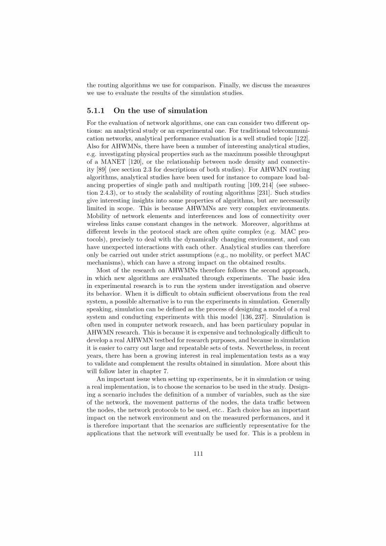
the routing algorithms we use for comparison. Finally, we discuss the measureswe use to evaluate the results of the simulation studies.

5.1.1 On the use of simulation

For the evaluation of network algorithms, one can can consider two different op-tions: an analytical study or an experimental one. For traditional telecommuni-cation networks, analytical performance evaluation is a well studied topic [122].Also for AHWMNs, there have been a number of interesting analytical studies,e.g. investigating physical properties such as the maximum possible throughputof a MANET [120], or the relationship between node density and connectiv-ity [89] (see section 2.3 for descriptions of both studies). For AHWMN routingalgorithms, analytical studies have been used for instance to compare load bal-ancing properties of single path and multipath routing [109, 214] (see subsec-tion 2.4.3), or to study the scalability of routing algorithms [231]. Such studiesgive interesting insights into some properties of algorithms, but are necessarilylimited in scope. This is because AHWMNs are very complex environments.Mobility of network elements and interferences and loss of connectivity overwireless links cause constant changes in the network. Moreover, algorithms atdifferent levels in the protocol stack are often quite complex (e.g. MAC pro-tocols), precisely to deal with the dynamically changing environment, and canhave unexpected interactions with each other. Analytical studies can thereforeonly be carried out under strict assumptions (e.g., no mobility, or perfect MACmechanisms), which can have a strong impact on the obtained results.

Most of the research on AHWMNs therefore follows the second approach,in which new algorithms are evaluated through experiments. The basic ideain experimental research is to run the system under investigation and observeits behavior. When it is difficult to obtain sufficient observations from the realsystem, a possible alternative is to run the experiments in simulation. Generallyspeaking, simulation can be defined as the process of designing a model of a realsystem and conducting experiments with this model [136, 237]. Simulation isoften used in computer network research, and has been particulary popular inAHWMN research. This is because it is expensive and technologically difficult todevelop a real AHWMN testbed for research purposes, and because in simulationit is easier to carry out large and repeatable sets of tests. Nevertheless, in recentyears, there has been a growing interest in real implementation tests as a wayto validate and complement the results obtained in simulation. More about thiswill follow later in chapter 7.

An important issue when setting up experiments, be it in simulation or usinga real implementation, is to choose the scenarios to be used in the study. Design-ing a scenario includes the definition of a number of variables, such as the sizeof the network, the movement patterns of the nodes, the data traffic betweenthe nodes, the network protocols to be used, etc.. Each choice has an importantimpact on the network environment and on the measured performances, and itis therefore important that the scenarios are sufficiently representative for theapplications that the network will eventually be used for. This is a problem in

111

AHWMN research, and especially in the field of MANETs. Until recently, thecommunity remained rather vague about possible applications for this kind ofnetworks, so that it was difficult to figure out what would be a realistic sce-nario. Hence, MANET algorithms have mainly been evaluated in experimentalsetups that make minimal assumptions about the environment and the use ofthe network: they use very simple scenarios, in which nodes move accordingto random patterns in a rectangular, open area and send data packets to eachother at fixed rates. Only in the last few years there has been an increasinginterest in experiments that use scenarios that are more complex and possiblymore realistic. Especially urban scenarios are popular, as recently a number ofreal WMNs have been set up in urban environments, such as e.g. the publicWMNs in San Francisco and Philadelphia. However, there are still considerablyless studies available that use these different scenarios compared to those usingsimpler scenarios.

In the current chapter, our aim is to carry out a detailed evaluation studyof AntHocNet, comparing it to existing state-of-the-art routing algorithms forMANETs and WMNs, and investigating its internal working. In order to obtaina better and more fair comparison with existing work in the research area, wedecided to stick here with the common practice in the research community, anduse simulation studies with simple scenarios that are similar to those used byother researchers. Later, in chapter 6, we will take a different approach andinvestigate the behavior of AntHocNet in a realistic urban scenario. Finally,in chapter 7, we go again a step further, and discuss the implementation ofAntHocNet and other ACO routing algorithms in a real testbed.

5.1.2 The QualNet network simulator

When simulating a computer network, one needs to create models of the pro-tocols and technologies that are used. Furthermore, in the case of AHWMNs,it is also necessary to develop models of the movement of the network nodesand of relevant physical phenomena, such as radio wave propagation and in-terference. Comparative tests have shown that differences in the used modelscan lead to significant differences in observed results (see [54]). It is thereforeimportant that all the models are detailed and accurate. Such accurate modelsare provided in an integrated way in a number of different network simulatorsoftware packages that are available to the research community. These includens-2 [262], OPNET [207], GloMoSim [263], SWAN [175] and QualNet [232].

For the work presented in this thesis, we used the QualNet simulator. Thisis a commercial simulation tool developed by Scalable Network Technologiesas the follow up of the older GloMoSim simulator. QualNet offers a numberof important advantages when compared to other simulators. First of all, itincludes a wide range of models to support the simulation of both wired andwireless networks, and comes with an extensive library that is specifically re-lated to MANETs and WMNs. Second, it uses a clear, modular organization,following the layered TCP/IP architecture. This makes it easy to understandand to plug in new protocols. Third, being a commercial product, it comes with

112

good documentation and support. Fourth, it is equipped with several graphicaluser interfaces, to support the design of new algorithms, the setup of simulationstudies, etc.. Finally, QualNet has been specifically designed to simulate largeAHWMNs, something that has traditionally been a problem in other networksimulators such as ns-2.

5.1.3 Simulation scenarios

The aim of this chapter is to investigate the performance of AntHocNet in arange of different scenarios. In order to do tests in a controlled way, we definea common base scenario, from which all other scenarios are derived by varyingrelevant parameters such as the node speed, the data send rate, the networksize, etc.. This base scenario was designed in line with the most commonly usedscenarios in the research area, in order to allow a fair comparison with otheralgorithms. Here, we describe the properties of the base scenario. Later, in eachof the experiments, we specify how the different applied scenarios were derivedfrom it.

We consider a network of 100 nodes that move in a rectangular area of2400× 800m2. It is an open area, in the sense that there are no obstacles thatcould limit node mobility or signal propagation. Node movements are definedaccording to the RWP mobility model (see subsection 2.3.1 and [140]). Underthis model, each node starts from a randomly chosen initial position in thearea, and independently chooses a random speed between a given minimum andmaximum speed, and a random destination. Then, it moves at the chosen speedtowards the chosen destination in a straight line. Upon arrival, it remains staticfor a fixed pause time, after which it chooses a new speed and destination. Weuse a minimum and maximum speed of respectively 0 and 10m/s, and a pausetime of 30s. Each experiment has a duration of 900s, and is repeated 20 times,using different random instances of the same scenario. Data traffic is generatedby constant bit rate (CBR) sessions: 20 data sessions are run between randomlychosen source and destination nodes. Sessions start between 0 and 180s afterthe beginning of the simulation, and run till the end. Each session generates 4packets of 64 bytes per second.

For the simulation of radio propagation, we use the two-ray signal propaga-tion model, which is a common approach to model the propagation of wirelesssignals in open space [167]. The two-ray model assumes that a signal reaches areceiver over two different paths: one direct and one reflected over the ground.Compared to the signal that travels along the direct path, the one that trav-els along the reflected path arrives with a certain delay, which depends on thedistance between the source of the signal and the receiver. Depending on thisdelay and the relative phase, the reflected signal can reinforce or disturb thedirect signal. As a consequence, the two-ray model considers a different decayof the signal strength depending on the distance: it applies a decay of order R2

(where R is the transmission distance) for short distance transmission and oforder R4 for long distance transmissions.

At the physical layer, we use the IEEE 802.11 protocol, with data transmis-

113

sion rate of 2Mbit/s. The estimated radio range is 250m. At the MAC layer,we use the IEEE 802.11 DCF protocol, which was described in subsection 2.3.3.Finally, at the transport layer, we use the UDP protocol, rather than TCP, asis common in AHWMN research. There are several reasons not to use TCP.First of all, TCP is known to behave badly in AHWMNs (see subsection 2.3.4).Second, TCP’s various mechanisms to control the flow and to resend packetscan influence the results in unforeseen ways so that it becomes difficult to eval-uate the performance of the routing algorithms. Finally, UDP is the normaltransport protocol to be used in combination with CBR applications.

5.1.4 Algorithms used for comparison

In the tests of section 5.2, we investigate how well AntHocNet performs incomparison to existing AHWMN routing algorithms. To this end, we havechosen a selection of algorithms that are representative for the wide class ofavailable routing algorithms in the research area. The selection includes AODV,OLSR and ANSI. Here, we briefly discuss the choice for each one of them.

AODV [213] is a reactive routing algorithm. It is under investigation for stan-dardization by the IETF MANET group [6], and has gained considerable statusas the de facto standard routing algorithm for MANETs and WMNs. Mostexisting work in this research area uses AODV as a benchmark for comparisons,and we have followed this common practice. A short description of AODV canbe found in subsection 2.4.2. Originally, we also included the DSR [140] rout-ing algorithm in our comparative study. This is a different reactive algorithmthat has also received a lot of attention in the community. However, the resultsobtained with DSR were quite bad and were therefore not included here.

OLSR [61] is a proactive routing algorithm. While proactive routing hasoften been considered a less good approach in AHWMNs [42], OLSR has receivedconsiderable attention since its publication in 2001. It is one of the most studiedproactive algorithm, and it is together with AODV one of the prime candidatesfor standardization by the IETF MANET group. While it is less used thanAODV as a benchmark in comparative studies, we consider it important touse also a proactive algorithm in our evaluation of AntHocNet, and thereforedecided to include OLSR. A description of the OLSR algorithm has been givenearlier in subsection 2.4.2.

ANSI [220] is, like AntHocNet, an ACO routing algorithm for AHWMNs.Due to this common source of inspiration, it has more similarities with Ant-HocNet than the previously mentioned algorithms. It uses full path samplingto gather routing information, sets up multiple routes, and applies to some ex-tent a hybrid approach, where initial routes are set up reactively, and proactivesampling is used to keep this initial routing information up-to-date. The full al-gorithm, however, is quite different from AntHocNet. ANSI was chosen to makecomparisons because we consider it important to also include an ACO routingalgorithm. A brief description of ANSI has been given in subsection 3.2.6.

114

5.1.5 Evaluation measures

Here, we describe the measures that we use to evaluate the performance ofthe different routing algorithms in the experiments. We distinguish betweenmeasures of effectiveness and measures of efficiency. The measures we apply areall derived from recommendations made by the IETF MANET standardizationgroup [62].

Measures of effectiveness are external measures of performance: they mea-sure to what extent the algorithm manages to execute the task it was designedfor. We use three different measures of effectiveness. The first one is the datadelivery ratio. This is the fraction of correctly delivered data packets versus sentpackets. This is an important measure in AHWMNs, as due to the constantchanges in the topology it is difficult to deliver all data packets. As a secondmeasure of effectiveness, we consider the end-to-end packet delay. This is thecumulative statistical measure of the delays experienced by packets travelingbetween their source and destination. Finally, as a third measure, we use theaverage delay jitter. This is the variation in the time interval between the ar-rivals of subsequent packets. It is calculated as shown in equation 5.1, whereti is the time of arrival of the ith packet, and n is the total number of packetsreceived by a destination during a communication session. Delay jitter is animportant measure for QoS applications, and also gives an indication of thealgorithm’s ability to respond smoothly to disruptive events in the network. Inthis sense, it is a measure of robustness and adaptivity.

jitter =n∑

i=2

|(ti − ti−1)− (ti−1 − ti−2)| (5.1)

Measures of efficiency are internal evaluation measures. They are concernedwith the generated overhead. We consider two different measures of efficiency.The first is the overhead in number of packets. It is the total number of controlpackets transmitted by the nodes of the network versus data packets deliveredat their destination. The second is the overhead in number of bytes. This is thetotal number of control bytes transmitted versus data bytes delivered. Whileboth of these are closely related, the difference between the two measures isimportant in AHWMNs. As has been pointed out earlier in subsection 2.3.3,the limitations in available bandwidth in AHWMNs are for a large part dueto MAC layer issues, rather than to intrinsic limitations in the possible datatransmission rate. MAC layer overhead is incurred with the transmission of eachpacket, and the number of transmitted packets is therefore important when itcomes to measuring efficiency. On the other hand, sending more bytes leads tolonger channel occupancy, and also requires nodes to spend more energy. Soalso the overhead in number of bytes has its importance.

115

5.2 Comparisons to other routing algorithms

In this section, we present the results of a range of tests in which we compareAntHocNet to representative routing algorithms for MANETs and WMNs. Foreach of the tests, we derive scenarios from the above described common basescenario. We vary a different environmental property each time, in order toinvestigate its effect on the performance of the algorithms independently. Wedo tests changing the node mobility, the data traffic, the node density, and thenetwork size. To change the node mobility, we run separate tests varying themaximum speed in the RWP mobility model, varying the pause time of theRWP model and using a different mobility model, namely the Gauss-Markovmodel (GM). To change the data traffic, we run tests varying the data send rateand the number of sessions. To change the node density, we vary the size of thearea in which the nodes of the network move. Finally, to change the networksize, we vary the number of nodes and the network area simultaneously.

5.2.1 Varying the maximum node speed for RWP mobility

In this first set of experiments, we vary the maximum node speed in the RWPmobility model, from 1m/s (3.6km/h, or the speed of a leisurely walk) up to30m/s (108km/h, or the speed of a car on a highway), using as intermediatevalues 2, 5, 10 and 20m/s. Varying the maximum speed in the RWP mobilitymodel affects the node mobility directly in an obvious way: the higher the speed,the higher the mobility. Higher mobility leads to more frequent changes in thenetwork environment, and therefore to more difficult scenarios. The results ofthe experiments are shown in figure 5.1, where we report (a) the delivery ratio,(b) the average end-to-end delay, (c) the average delay jitter, (d) the overheadratio in number of packets, and (e) the overhead ratio in number of bytes.

The results for delivery ratio reflect the increasing level of difficulty of thescenarios: for all algorithms the delivery ratio decreases with increasing nodespeeds. The best results are obtained by AntHocNet, that even at the highestspeeds is able to deliver almost 90% of all packets. This shows that AntHocNetis able to adapt well to the fast changes in the highly dynamic environmentcaused by high node mobility. AODV and ANSI give less good results, and withANSI, the performance gap grows as the speed increases. The worst results areobtained by OLSR, that gives a delivery ratio of less than 40% for the highestspeed scenario. This confirms the earlier mentioned observation that proactiverouting algorithms have a hard time keeping up in highly dynamic environments(see subsection 2.4.1).

The results for average delay show similar trends. Like for delivery ratio,AntHocNet gives better results than AODV and ANSI. However, the gap inperformance between AntHocNet and AODV decreases slightly for the highestdelays. For ANSI, on the other hand, the performance gap increases, evenstronger than when considering delivery ratio. One striking difference with thedelivery ratio results is that for delay, OLSR gives good performances for thehighest speed scenarios. For 20 and 30m/s, OLSR even outperforms AODV

116

0.3

0.4

0.5

0.6

0.7

0.8

0.9

1

0 5 10 15 20 25 30

Fra

ctio

n of

del

iver

ed d

ata

pack

ets

RWP maximum speed (m/sec)

AntHocNetAODVOLSRANSI

0

0.05

0.1

0.15

0.2

0.25

0.3

0 5 10 15 20 25 30

Ave

rage

end

-to-

end

pack

et d

elay

(se

c)

RWP maximum speed (m/sec)

AntHocNetAODVOLSRANSI

(a) (b)

0

0.1

0.2

0.3

0.4

0.5

0.6

0.7

0 5 10 15 20 25 30

Ave

rage

del

ay ji

tter

(sec

)

RWP maximum speed (m/sec)

AntHocNetAODVOLSRANSI

2

4

6

8

10

12

14

16

18

20

0 5 10 15 20 25 30

Ove

rhea

d in

num

ber

of p

acke

ts

RWP maximum speed (m/sec)

AntHocNetAODVOLSRANSI

(c) (d)

0

5

10

15

20

25

30

35

0 5 10 15 20 25 30

Ove

rhea

d in

num

ber

of b

ytes

RWP maximum speed (m/sec)

AntHocNetAODVOLSRANSI

(e)

Figure 5.1: Results for AntHocNet, AODV, OLSR and ANSI using differentvalues for the maximum speed in the RWP mobility model: (a) delivery ratio,(b) average end-to-end delay, (c) average delay jitter, (d) overhead in numberof packets, and (e) overhead in number of bytes.

and AntHocNet. These results need to be read with some caution though. Thegood delay results are obtained in a situation where OLSR delivers only a verylow percentage of the packets, and have therefore little value.

The results for average delay jitter follow the same trend as those for delivery

117

ratio, with AntHocNet performing better than AODV, ANSI, and OLSR, in thatorder. The delay jitter measures the variation in the time between arrivals ofsubsequent data packets. It is an indicator of robustness and adaptivity, as lowjitter shows that the algorithm is able to limit the effect of disruptive events.

Finally, also in the results for the overhead measures, that reflect the effi-ciency of the algorithms, we can observe similar trends. There is a difference,however, between the overhead in number of packets and the overhead in num-ber of bytes. When considering the number of packets, we obtain the sameorder as before, with AntHocNet giving the best performance in terms of effi-ciency, followed by AODV, ANSI and OLSR. When considering the number ofbytes, the ACO algorithms AntHocNet and ANSI suffer a bit more, with Ant-HocNet becoming slightly worse than AODV, and ANSI becoming a lot worsethan OLSR. This indicates that ANSI and AntHocNet use considerably largercontrol packets than AODV and OLSR. One reason for this is that ants gatherinformation about the full path that they have followed. In the case of Ant-HocNet, an obvious other cause of large control packets is the piggybacking ofrouting information on top of hello messages. As mentioned before in subsec-tion 5.1.5, both the overhead in terms of number of packets and in terms ofnumber of bytes have their importance in AHWMNs. When we compare to themeasures of effectiveness, however, the slightly worse results in terms of over-head in number of bytes does not seem to affect the performance of AntHocNetdirectly.

5.2.2 Varying the pause time for RWP mobility

Here, we vary the pause time of the RWP mobility model, from 0s up to 480s,with as intermediate values 15, 30, 60, 120 and 240s. The results of the ex-periments are shown in figure 5.2. Increasing the pause time has two differenteffects on the general properties of the scenario that are relevant for routing.The first of these is a decrease in node mobility: since nodes stay still for longerperiods, they are less mobile, and the network becomes less dynamic. As aconsequence, the scenario becomes less difficult. The second effect is a bit lessstraightforward, and has to do with the distribution of nodes over the networkarea when the RWP mobility model is used. It has been shown that underRWP, there tends to be a higher node density in the center of the network areathan on the edges, especially when pause times are low [29]. To understandthis, consider the square network area of figure 5.3, where we follow a singlenode moving according to RWP. The node starts from a randomly chosen startpoint (A). It chooses a random destination point (B), moves to it in a straightline according to a random speed, and then pauses for a while. After that, itrepeats this same sequence of actions till the end of the simulation (in the figure,the node moves subsequently to C, D, E and F). The initial start point and allsubsequent destination points are chosen according to a uniform distribution,and can therefore be anywhere in the network area. However, the straight linebetween any two random points has a higher probability of going through thecenter than of visiting edge or corner areas. As a consequence, nodes that are

118

0.55

0.6

0.65

0.7

0.75

0.8

0.85

0.9

0.95

1

0 50 100 150 200 250 300 350 400 450 500

Fra

ctio

n of

del

iver

ed d

ata

pack

ets

RWP pause time (sec)

AntHocNetAODVOLSRANSI

0

0.05

0.1

0.15

0.2

0.25

0.3

0.35

0.4

0.45

0 50 100 150 200 250 300 350 400 450 500

Ave

rage

end

-to-

end

pack

et d

elay

(se

c)

RWP pause time (sec)

AntHocNetAODVOLSRANSI

(a) (b)

0.05

0.1

0.15

0.2

0.25

0.3

0.35

0 50 100 150 200 250 300 350 400 450 500

Ave

rage

del

ay ji

tter

(sec

)

RWP pause time (sec)

AntHocNetAODVOLSRANSI

3

4

5

6

7

8

9

10

11

12

0 50 100 150 200 250 300 350 400 450 500

Ove

rhea

d in

num

ber

of p

acke

ts

RWP pause time (sec)

AntHocNetAODVOLSRANSI

(c) (d)

4

6

8

10

12

14

16

18

20

22

0 50 100 150 200 250 300 350 400 450 500

Ove

rhea

d in

num

ber

of b

ytes

RWP pause time (sec)

AntHocNetAODVOLSRANSI

(e)

Figure 5.2: Results for AntHocNet, AODV, OLSR and ANSI using differentvalues for the pause time in the RWP mobility model: (a) delivery ratio, (b)average end-to-end delay, (c) average delay jitter, (d) overhead in number ofpackets, and (e) overhead in number of bytes.

pausing in their destination points are uniformly spread over the network, whilenodes that are on the move are more clustered in the center, giving a highernode density there. Concretely, this means that when pause times are increased,nodes are more spread out, giving a lower effective node density to the network.

119

Earlier, in subsection 2.3.1, we have discussed how a lower node density makesa scenario more difficult to deal with, as the lower connectivity provides lessrouting alternatives. Hence, increasing the pause time can both decrease andincrease the difficulty of the scenario for routing, depending on whether the usedrouting algorithm is more sensitive to high mobility or to low node density.

A

B

C

D

E

F

Figure 5.3: A node moving according to the RWP mobility model. The nodestarts in a randomly chosen initial point (A). It chooses a random destinationpoint (B) and moves to it in a straight line. Then, it pauses for a fixed amount oftime. After that, it repeats this sequence of actions till the end of the simulation(leading to the points C, D, E, and F).

When we consider the results for the delivery ratio, the ambiguity in theeffect of increasing the pause time can be noted in the difference in performancebetween the algorithms. AntHocNet shows the best performance, and is ratherinsensitive to the increase in pause time. ANSI is also quite insensitive, but itslevel of performance is lower than that of AntHocNet. AODV shows a decreasein delivery ratio for higher pause times: from 88% for the lowest pause timedown to 80% for the highest pause time. This is an indication that it is moresensitive to the decrease in connectivity than to the decrease in mobility. Finally,OLSR shows an opposite trend: its delivery ratio increases from 60% for thelowest pause time to almost 65% for the highest pause time.

For delay, the results are similar but slightly different. AntHocNet continuesto show good results that are rather insensitive to the variance in pause time,AODV and OLSR show a slight drop in performance, and ANSI a strong one.For the other measures, jitter, overhead in terms of control packets and overheadin terms of bytes, we see the same trends as for delivery ratio: AntHocNetand ANSI show stable results, AODV displays a rather strongly deterioratingperformance, and OLSR shows a slight improvement in performance.

We investigate in a bit more detail the difference between AntHocNet and

120

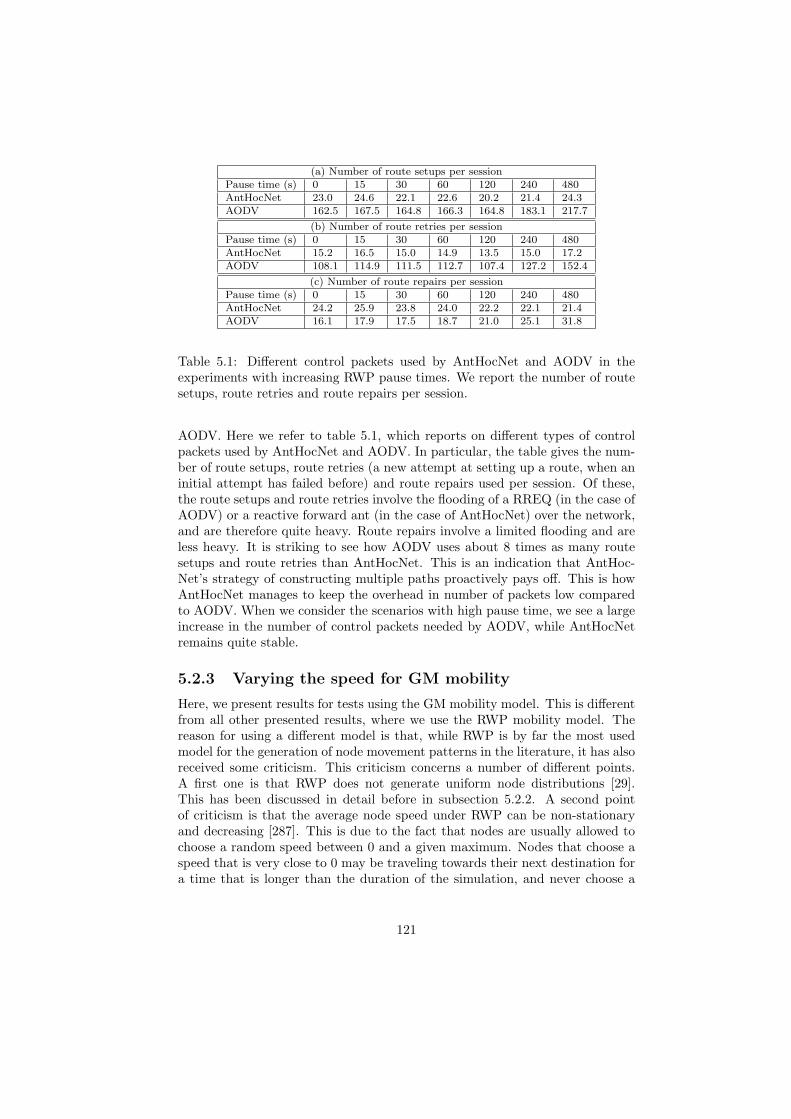
(a) Number of route setups per sessionPause time (s) 0 15 30 60 120 240 480AntHocNet 23.0 24.6 22.1 22.6 20.2 21.4 24.3AODV 162.5 167.5 164.8 166.3 164.8 183.1 217.7

(b) Number of route retries per sessionPause time (s) 0 15 30 60 120 240 480AntHocNet 15.2 16.5 15.0 14.9 13.5 15.0 17.2AODV 108.1 114.9 111.5 112.7 107.4 127.2 152.4

(c) Number of route repairs per sessionPause time (s) 0 15 30 60 120 240 480AntHocNet 24.2 25.9 23.8 24.0 22.2 22.1 21.4AODV 16.1 17.9 17.5 18.7 21.0 25.1 31.8

Table 5.1: Different control packets used by AntHocNet and AODV in theexperiments with increasing RWP pause times. We report the number of routesetups, route retries and route repairs per session.

AODV. Here we refer to table 5.1, which reports on different types of controlpackets used by AntHocNet and AODV. In particular, the table gives the num-ber of route setups, route retries (a new attempt at setting up a route, when aninitial attempt has failed before) and route repairs used per session. Of these,the route setups and route retries involve the flooding of a RREQ (in the case ofAODV) or a reactive forward ant (in the case of AntHocNet) over the network,and are therefore quite heavy. Route repairs involve a limited flooding and areless heavy. It is striking to see how AODV uses about 8 times as many routesetups and route retries than AntHocNet. This is an indication that AntHoc-Net’s strategy of constructing multiple paths proactively pays off. This is howAntHocNet manages to keep the overhead in number of packets low comparedto AODV. When we consider the scenarios with high pause time, we see a largeincrease in the number of control packets needed by AODV, while AntHocNetremains quite stable.

5.2.3 Varying the speed for GM mobility

Here, we present results for tests using the GM mobility model. This is differentfrom all other presented results, where we use the RWP mobility model. Thereason for using a different model is that, while RWP is by far the most usedmodel for the generation of node movement patterns in the literature, it has alsoreceived some criticism. This criticism concerns a number of different points.A first one is that RWP does not generate uniform node distributions [29].This has been discussed in detail before in subsection 5.2.2. A second pointof criticism is that the average node speed under RWP can be non-stationaryand decreasing [287]. This is due to the fact that nodes are usually allowed tochoose a random speed between 0 and a given maximum. Nodes that choose aspeed that is very close to 0 may be traveling towards their next destination fora time that is longer than the duration of the simulation, and never choose a

121

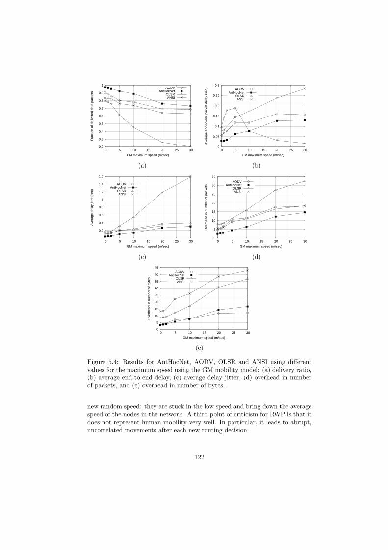
0.2

0.3

0.4

0.5

0.6

0.7

0.8

0.9

1

0 5 10 15 20 25 30

Fra

ctio

n of

del

iver

ed d

ata

pack

ets

GM maximum speed (m/sec)

AODVAntHocNet

OLSRANSI

0

0.05

0.1

0.15

0.2

0.25

0.3

0 5 10 15 20 25 30

Ave

rage

end

-to-

end

pack

et d

elay

(se

c)

GM maximum speed (m/sec)

AODVAntHocNet

OLSRANSI

(a) (b)

0

0.2

0.4

0.6

0.8

1

1.2

1.4

1.6

0 5 10 15 20 25 30

Ave

rage

del

ay ji

tter

(sec

)

GM maximum speed (m/sec)

AODVAntHocNet

OLSRANSI

0

5

10

15

20

25

30

35

0 5 10 15 20 25 30

Ove

rhea

d in

num

ber

of p

acke

ts

GM maximum speed (m/sec)

AODVAntHocNet

OLSRANSI

(c) (d)

0

5

10

15

20

25

30

35

40

45

0 5 10 15 20 25 30

Ove

rhea

d in

num

ber

of b

ytes

GM maximum speed (m/sec)

AODVAntHocNet

OLSRANSI

(e)

Figure 5.4: Results for AntHocNet, AODV, OLSR and ANSI using differentvalues for the maximum speed using the GM mobility model: (a) delivery ratio,(b) average end-to-end delay, (c) average delay jitter, (d) overhead in numberof packets, and (e) overhead in number of bytes.

new random speed: they are stuck in the low speed and bring down the averagespeed of the nodes in the network. A third point of criticism for RWP is that itdoes not represent human mobility very well. In particular, it leads to abrupt,uncorrelated movements after each new routing decision.

122

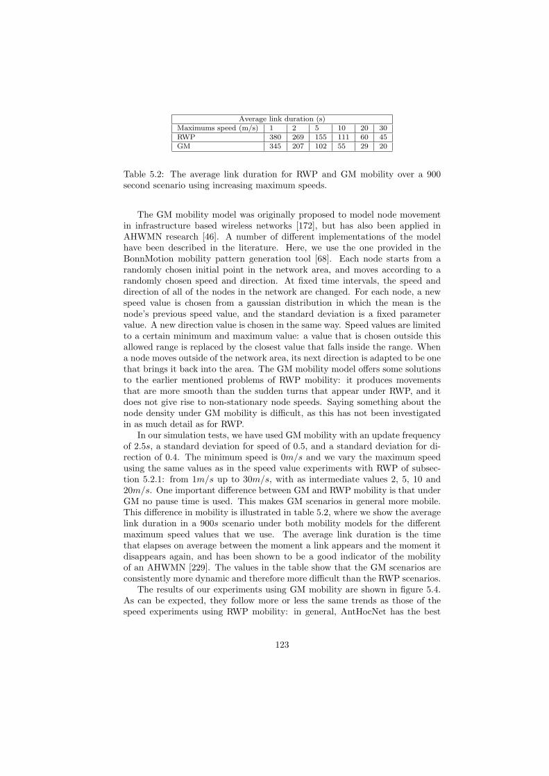
Average link duration (s)Maximums speed (m/s) 1 2 5 10 20 30RWP 380 269 155 111 60 45GM 345 207 102 55 29 20

Table 5.2: The average link duration for RWP and GM mobility over a 900second scenario using increasing maximum speeds.

The GM mobility model was originally proposed to model node movementin infrastructure based wireless networks [172], but has also been applied inAHWMN research [46]. A number of different implementations of the modelhave been described in the literature. Here, we use the one provided in theBonnMotion mobility pattern generation tool [68]. Each node starts from arandomly chosen initial point in the network area, and moves according to arandomly chosen speed and direction. At fixed time intervals, the speed anddirection of all of the nodes in the network are changed. For each node, a newspeed value is chosen from a gaussian distribution in which the mean is thenode’s previous speed value, and the standard deviation is a fixed parametervalue. A new direction value is chosen in the same way. Speed values are limitedto a certain minimum and maximum value: a value that is chosen outside thisallowed range is replaced by the closest value that falls inside the range. Whena node moves outside of the network area, its next direction is adapted to be onethat brings it back into the area. The GM mobility model offers some solutionsto the earlier mentioned problems of RWP mobility: it produces movementsthat are more smooth than the sudden turns that appear under RWP, and itdoes not give rise to non-stationary node speeds. Saying something about thenode density under GM mobility is difficult, as this has not been investigatedin as much detail as for RWP.

In our simulation tests, we have used GM mobility with an update frequencyof 2.5s, a standard deviation for speed of 0.5, and a standard deviation for di-rection of 0.4. The minimum speed is 0m/s and we vary the maximum speedusing the same values as in the speed value experiments with RWP of subsec-tion 5.2.1: from 1m/s up to 30m/s, with as intermediate values 2, 5, 10 and20m/s. One important difference between GM and RWP mobility is that underGM no pause time is used. This makes GM scenarios in general more mobile.This difference in mobility is illustrated in table 5.2, where we show the averagelink duration in a 900s scenario under both mobility models for the differentmaximum speed values that we use. The average link duration is the timethat elapses on average between the moment a link appears and the moment itdisappears again, and has been shown to be a good indicator of the mobilityof an AHWMN [229]. The values in the table show that the GM scenarios areconsistently more dynamic and therefore more difficult than the RWP scenarios.

The results of our experiments using GM mobility are shown in figure 5.4.As can be expected, they follow more or less the same trends as those of thespeed experiments using RWP mobility: in general, AntHocNet has the best

123

performance, followed by AODV, ANSI and OLSR, and all algorithms show adecreasing performance as the maximum speed increases. The fact that nodemobility is higher under GM compared to RWP is clearly visible: for all mea-sures and all algorithms, the results are worse under GM than under RWP. Thisis especially true for the highest speed values, where, according to table 5.2, therelative difference in link duration between RWP and GM is largest. We canalso see that in terms of delivery ratio, the difference in performance betweenAntHocNet and AODV first increases with increasing node speed, and thendecreases again. The initial increase confirms what we observed earlier in thetests with RWP, namely that AntHocNet is better able to deal with the grow-ing number of changes in the network. The eventual decrease in the differencebetween AntHocNet and AODV shows that there is a limit to the adaptivityof AntHocNet. At the highest levels of mobility, the proactive mechanisms ofAntHocNet get more difficulties keeping up with the changes in the network,and are less able to make a difference. As a consequence, we can also see a de-creasing advantage of AntHocNet in terms of jitter and an increasing advantageof AODV in terms of overhead in number of bytes. So, for very high levels ofmobility, AntHocNet keeps performing well, but looses a bit of its advantageover competing algorithms. Finally, we note that the advantage of OLSR interms of delay for the highest speed values is even stronger here than in theRWP experiments. Again, however, this good delay is only obtained when lessthan 50% of all packets are delivered and has therefore little relevance.

5.2.4 Varying the data send rate

With the experiments described here and in the next subsection, we investigatethe effect of the data load on the performance of the different routing algorithms.In the base scenario, 20 data sessions each sending 4 packets per second are runbetween randomly chosen start and destination nodes. Here, we investigate theeffect of varying the data send rate, while in the next subsection, we investigateswhat happens when the number of sessions is changed. We do tests sending 1,4, 8, 10 and 12.5 packets per second, or 1 packet every 1, 0.25, 0.125, 0.1 and0.08 seconds. Increasing the data rate has as an effect that the network loadgets higher, so that congestion and interference become more likely. The resultsfor the tests with varying data rates are presented in figure 5.5.

In terms of delivery ratio, the effect of the increasing congestion is obvious:all algorithms have a monotonously decreasing performance. AntHocNet per-forms better than the competing algorithms, but also suffers starting from 8packets per second, where the delivery ratio is down to 66%. It is remarkableto see how AODV’s performance drops very suddenly: from 88% at 4 packetsper second down to just 40% at 8 packets per second. To understand this be-havior, it is important to realize that an AHWMN is a highly non-linear systemwhere the interaction between different mechanisms can have dramatic conse-quences. In the current experiments, the increase of the data load augmentsthe congestion, which leads to packet loss. AODV interprets this packet lossas an indication of a link failure, and reacts to it with a route repair or a new

124

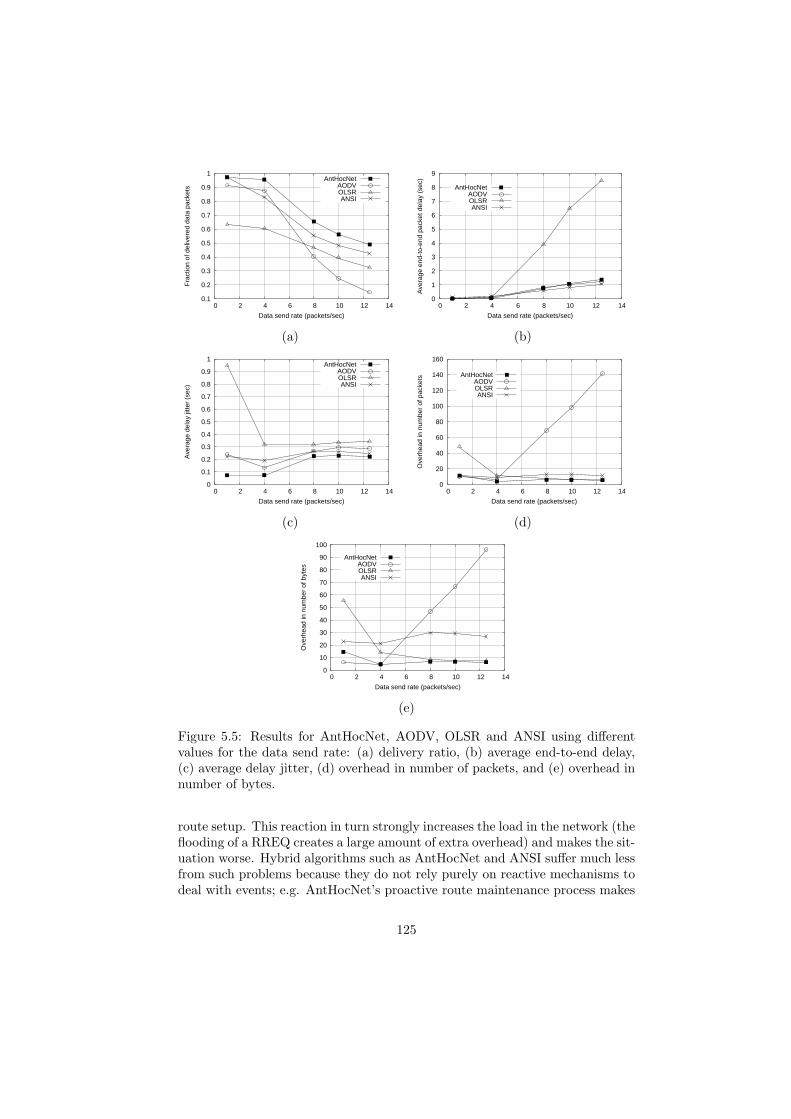
0.1

0.2

0.3

0.4

0.5

0.6

0.7

0.8

0.9

1

0 2 4 6 8 10 12 14

Fra

ctio

n of

del

iver

ed d

ata

pack

ets

Data send rate (packets/sec)

AntHocNetAODVOLSRANSI

0

1

2

3

4

5

6

7

8

9

0 2 4 6 8 10 12 14

Ave

rage

end

-to-

end

pack

et d

elay

(se

c)

Data send rate (packets/sec)

AntHocNetAODVOLSRANSI

(a) (b)

0

0.1

0.2

0.3

0.4

0.5

0.6

0.7

0.8

0.9

1

0 2 4 6 8 10 12 14

Ave

rage

del

ay ji

tter

(sec

)

Data send rate (packets/sec)

AntHocNetAODVOLSRANSI

0

20

40

60

80

100

120

140

160

0 2 4 6 8 10 12 14

Ove

rhea

d in

num

ber

of p

acke

ts

Data send rate (packets/sec)

AntHocNetAODVOLSRANSI

(c) (d)

0

10

20

30

40

50

60

70

80

90

100

0 2 4 6 8 10 12 14

Ove

rhea

d in

num

ber

of b

ytes

Data send rate (packets/sec)

AntHocNetAODVOLSRANSI

(e)

Figure 5.5: Results for AntHocNet, AODV, OLSR and ANSI using differentvalues for the data send rate: (a) delivery ratio, (b) average end-to-end delay,(c) average delay jitter, (d) overhead in number of packets, and (e) overhead innumber of bytes.

route setup. This reaction in turn strongly increases the load in the network (theflooding of a RREQ creates a large amount of extra overhead) and makes the sit-uation worse. Hybrid algorithms such as AntHocNet and ANSI suffer much lessfrom such problems because they do not rely purely on reactive mechanisms todeal with events; e.g. AntHocNet’s proactive route maintenance process makes

125

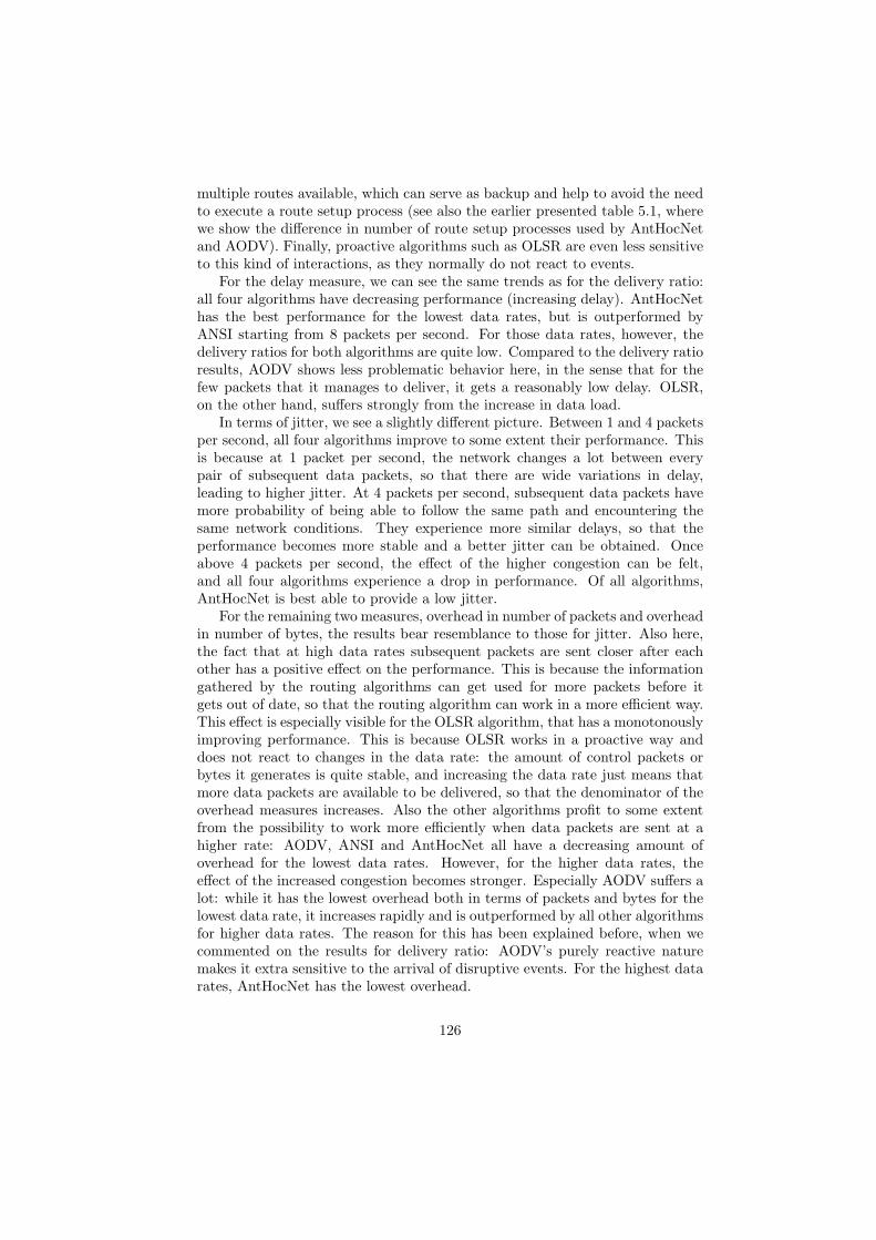
multiple routes available, which can serve as backup and help to avoid the needto execute a route setup process (see also the earlier presented table 5.1, wherewe show the difference in number of route setup processes used by AntHocNetand AODV). Finally, proactive algorithms such as OLSR are even less sensitiveto this kind of interactions, as they normally do not react to events.

For the delay measure, we can see the same trends as for the delivery ratio:all four algorithms have decreasing performance (increasing delay). AntHocNethas the best performance for the lowest data rates, but is outperformed byANSI starting from 8 packets per second. For those data rates, however, thedelivery ratios for both algorithms are quite low. Compared to the delivery ratioresults, AODV shows less problematic behavior here, in the sense that for thefew packets that it manages to deliver, it gets a reasonably low delay. OLSR,on the other hand, suffers strongly from the increase in data load.

In terms of jitter, we see a slightly different picture. Between 1 and 4 packetsper second, all four algorithms improve to some extent their performance. Thisis because at 1 packet per second, the network changes a lot between everypair of subsequent data packets, so that there are wide variations in delay,leading to higher jitter. At 4 packets per second, subsequent data packets havemore probability of being able to follow the same path and encountering thesame network conditions. They experience more similar delays, so that theperformance becomes more stable and a better jitter can be obtained. Onceabove 4 packets per second, the effect of the higher congestion can be felt,and all four algorithms experience a drop in performance. Of all algorithms,AntHocNet is best able to provide a low jitter.

For the remaining two measures, overhead in number of packets and overheadin number of bytes, the results bear resemblance to those for jitter. Also here,the fact that at high data rates subsequent packets are sent closer after eachother has a positive effect on the performance. This is because the informationgathered by the routing algorithms can get used for more packets before itgets out of date, so that the routing algorithm can work in a more efficient way.This effect is especially visible for the OLSR algorithm, that has a monotonouslyimproving performance. This is because OLSR works in a proactive way anddoes not react to changes in the data rate: the amount of control packets orbytes it generates is quite stable, and increasing the data rate just means thatmore data packets are available to be delivered, so that the denominator of theoverhead measures increases. Also the other algorithms profit to some extentfrom the possibility to work more efficiently when data packets are sent at ahigher rate: AODV, ANSI and AntHocNet all have a decreasing amount ofoverhead for the lowest data rates. However, for the higher data rates, theeffect of the increased congestion becomes stronger. Especially AODV suffers alot: while it has the lowest overhead both in terms of packets and bytes for thelowest data rate, it increases rapidly and is outperformed by all other algorithmsfor higher data rates. The reason for this has been explained before, when wecommented on the results for delivery ratio: AODV’s purely reactive naturemakes it extra sensitive to the arrival of disruptive events. For the highest datarates, AntHocNet has the lowest overhead.

126

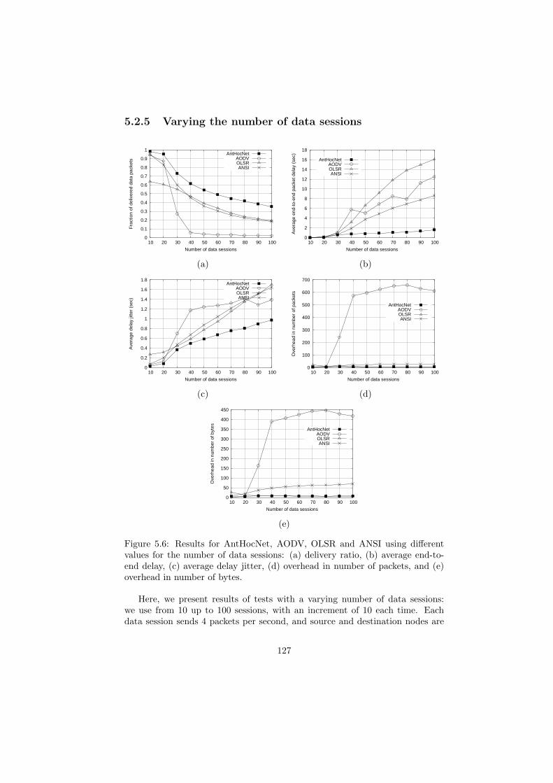
5.2.5 Varying the number of data sessions

0

0.1

0.2

0.3

0.4

0.5

0.6

0.7

0.8

0.9

1

10 20 30 40 50 60 70 80 90 100

Fra

ctio

n of

del

iver

ed d

ata

pack

ets

Number of data sessions

AntHocNetAODVOLSRANSI

0

2

4

6

8

10

12

14

16

18

10 20 30 40 50 60 70 80 90 100

Ave

rage

end

-to-

end

pack

et d

elay

(se

c)

Number of data sessions

AntHocNetAODVOLSRANSI

(a) (b)

0

0.2

0.4

0.6

0.8

1

1.2

1.4

1.6

1.8

10 20 30 40 50 60 70 80 90 100

Ave

rage

del

ay ji

tter

(sec

)

Number of data sessions

AntHocNetAODVOLSRANSI

0

100

200

300

400

500

600

700

10 20 30 40 50 60 70 80 90 100

Ove

rhea

d in

num

ber

of p

acke

ts

Number of data sessions

AntHocNetAODVOLSRANSI

(c) (d)

0

50

100

150

200

250

300

350

400

450

10 20 30 40 50 60 70 80 90 100

Ove

rhea

d in

num

ber

of b

ytes

Number of data sessions

AntHocNetAODVOLSRANSI

(e)

Figure 5.6: Results for AntHocNet, AODV, OLSR and ANSI using differentvalues for the number of data sessions: (a) delivery ratio, (b) average end-to-end delay, (c) average delay jitter, (d) overhead in number of packets, and (e)overhead in number of bytes.

Here, we present results of tests with a varying number of data sessions:we use from 10 up to 100 sessions, with an increment of 10 each time. Eachdata session sends 4 packets per second, and source and destination nodes are

127

chosen randomly. When increasing the number of sessions, we increment thetotal data load in the network, just like we did when increasing the data sendrate in the experiments of subsection 5.2.4. In particular, in terms of number ofgenerated data packets, the scenarios with 40 sessions presented here are equiv-alent to those with 8 packets per second in the experiments of subsection 5.2.4,and the scenarios with 50 sessions to those with 10 packets per second (otherapproximate points of comparison between both sets of experiments are at 10sessions, which corresponds to sending 2 packets per second, and at 60 sessions,which corresponds to sending 12 packets per second). Nevertheless, increasingthe data load by augmenting the number of sessions can have a different effectthan increasing it by sending at a higher rate. This is because the increased dataload is spread over multiple sessions. When extra actions need to be performedon a per-session basis, as is the case for reactive routing algorithms, increasingthe number of sessions can be more challenging. The results of the experimentswith the number of sessions are shown in figure 5.8.

When considering the delivery ratio, we see a picture that is very similarto that for the data rate experiments: all four algorithms have a decreasingperformance for increasing data load, AntHocNet shows the best results, andAODV has a more sudden drop in performance than the other algorithms. Whencomparing results directly, we can see that for AODV they are even lower herethan in the data rate experiments (at 40 sessions, AODV delivers only 5% ofall packets, compared to 25% when sending 8 packets per second in the datarate experiments). Apparently the higher number of route setups needed dueto the presence of more sessions makes the algorithm even more sensitive to theincrease in data load and congestion. Also ANSI suffers a bit more than in thedata rate experiments: its delivery ratio even drops below that of OLSR when40 or more data sessions are used. For AntHocNet, the difference with the datarate experiments is much smaller. Apparently its lower need for route setups(see table 5.1) protects its performances sufficiently. Finally, for OLSR there ispractically no difference with the data rate experiments. This is because thealgorithm works in a purely proactive way, so that increasing the number ofsessions does not provoke higher overhead than increasing the data rate.

In terms of delay, we can notice the same trends as for the delivery ratio.Also here, all four algorithms show decreasing performance, and AntHocNet hasthe best results. Moreover, like for the delivery ratio, the results for OLSR andAntHocNet are very similar to those obtained in the experiments with increasingdata rates. For AODV and ANSI on the other hand, the performance is worsethan in the data rate experiments, with a larger difference for the purely reactiveAODV algorithm and a smaller difference for the hybrid ANSI algorithm.

In terms of jitter, all four algorithms have decreasing performance, with Ant-HocNet showing the best results. The overall trends are considerably differentfrom those obtained in the tests with increasing data rates, where all algorithmsfirst showed an improvement in performance, and then a slow deterioration. Insection 5.2.4, we explained that the performance improvement was due to thefact that at higher data rates, subsequent packets come closer after each otherand therefore experience more similar conditions, leading to lower variations in

128

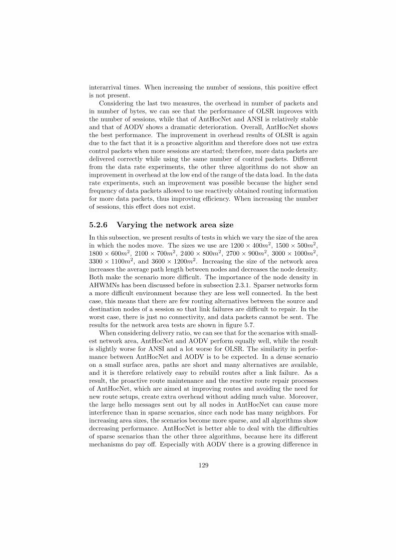
interarrival times. When increasing the number of sessions, this positive effectis not present.

Considering the last two measures, the overhead in number of packets andin number of bytes, we can see that the performance of OLSR improves withthe number of sessions, while that of AntHocNet and ANSI is relatively stableand that of AODV shows a dramatic deterioration. Overall, AntHocNet showsthe best performance. The improvement in overhead results of OLSR is againdue to the fact that it is a proactive algorithm and therefore does not use extracontrol packets when more sessions are started; therefore, more data packets aredelivered correctly while using the same number of control packets. Differentfrom the data rate experiments, the other three algorithms do not show animprovement in overhead at the low end of the range of the data load. In the datarate experiments, such an improvement was possible because the higher sendfrequency of data packets allowed to use reactively obtained routing informationfor more data packets, thus improving efficiency. When increasing the numberof sessions, this effect does not exist.

5.2.6 Varying the network area size

In this subsection, we present results of tests in which we vary the size of the areain which the nodes move. The sizes we use are 1200 × 400m2, 1500 × 500m2,1800 × 600m2, 2100 × 700m2, 2400 × 800m2, 2700 × 900m2, 3000 × 1000m2,3300 × 1100m2, and 3600 × 1200m2. Increasing the size of the network areaincreases the average path length between nodes and decreases the node density.Both make the scenario more difficult. The importance of the node density inAHWMNs has been discussed before in subsection 2.3.1. Sparser networks forma more difficult environment because they are less well connected. In the bestcase, this means that there are few routing alternatives between the source anddestination nodes of a session so that link failures are difficult to repair. In theworst case, there is just no connectivity, and data packets cannot be sent. Theresults for the network area tests are shown in figure 5.7.

When considering delivery ratio, we can see that for the scenarios with small-est network area, AntHocNet and AODV perform equally well, while the resultis slightly worse for ANSI and a lot worse for OLSR. The similarity in perfor-mance between AntHocNet and AODV is to be expected. In a dense scenarioon a small surface area, paths are short and many alternatives are available,and it is therefore relatively easy to rebuild routes after a link failure. As aresult, the proactive route maintenance and the reactive route repair processesof AntHocNet, which are aimed at improving routes and avoiding the need fornew route setups, create extra overhead without adding much value. Moreover,the large hello messages sent out by all nodes in AntHocNet can cause moreinterference than in sparse scenarios, since each node has many neighbors. Forincreasing area sizes, the scenarios become more sparse, and all algorithms showdecreasing performance. AntHocNet is better able to deal with the difficultiesof sparse scenarios than the other three algorithms, because here its differentmechanisms do pay off. Especially with AODV there is a growing difference in

129

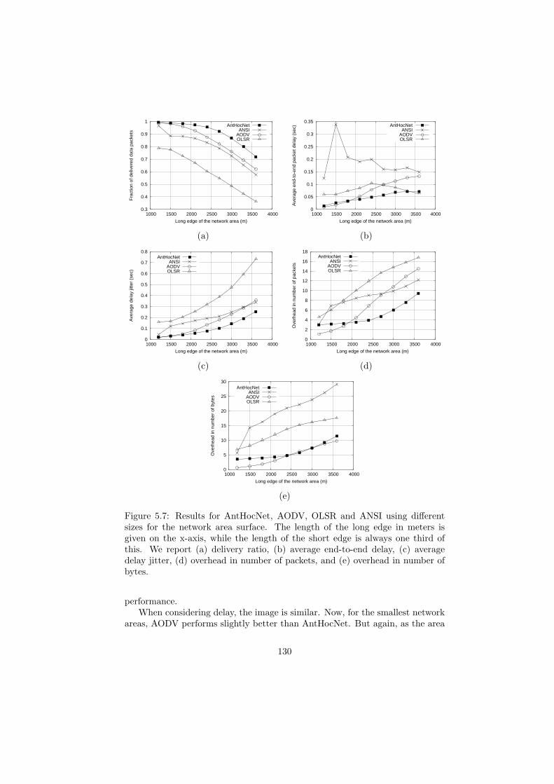
0.3

0.4

0.5

0.6

0.7

0.8

0.9

1

1000 1500 2000 2500 3000 3500 4000

Fra

ctio

n of

del

iver

ed d

ata

pack

ets

Long edge of the network area (m)

AntHocNetANSI

AODVOLSR

0

0.05

0.1

0.15

0.2

0.25

0.3

0.35

1000 1500 2000 2500 3000 3500 4000

Ave

rage

end

-to-

end

pack

et d

elay

(se

c)

Long edge of the network area (m)

AntHocNetANSI

AODVOLSR

(a) (b)

0

0.1

0.2

0.3

0.4

0.5

0.6

0.7

0.8

1000 1500 2000 2500 3000 3500 4000

Ave

rage

del

ay ji

tter

(sec

)

Long edge of the network area (m)

AntHocNetANSI

AODVOLSR

0

2

4

6

8

10

12

14

16

18

1000 1500 2000 2500 3000 3500 4000

Ove

rhea

d in

num

ber

of p

acke

ts

Long edge of the network area (m)

AntHocNetANSI

AODVOLSR

(c) (d)

0

5

10

15

20

25

30

1000 1500 2000 2500 3000 3500 4000

Ove

rhea

d in

num

ber

of b

ytes

Long edge of the network area (m)

AntHocNetANSI

AODVOLSR

(e)

Figure 5.7: Results for AntHocNet, AODV, OLSR and ANSI using differentsizes for the network area surface. The length of the long edge in meters isgiven on the x-axis, while the length of the short edge is always one third ofthis. We report (a) delivery ratio, (b) average end-to-end delay, (c) averagedelay jitter, (d) overhead in number of packets, and (e) overhead in number ofbytes.

performance.When considering delay, the image is similar. Now, for the smallest network

areas, AODV performs slightly better than AntHocNet. But again, as the area

130

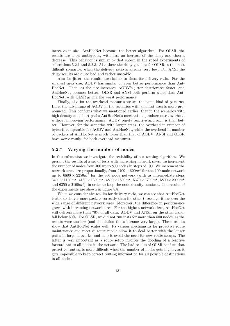
increases in size, AntHocNet becomes the better algorithm. For OLSR, theresults are a bit ambiguous, with first an increase of the delay and then adecrease. This behavior is similar to that shown in the speed experiments ofsubsections 5.2.1 and 5.2.3. Also there the delay gets low for OLSR in the mostdifficult scenarios, when the delivery ratio is already very low. For ANSI thedelay results are quite bad and rather unstable.

Also for jitter, the results are similar to those for delivery ratio. For thesmallest area size, AODV has similar or even better performance than Ant-HocNet. Then, as the size increases, AODV’s jitter deteriorates faster, andAntHocNet becomes better. OLSR and ANSI both perform worse than Ant-HocNet, with OLSR giving the worst performance.

Finally, also for the overhead measures we see the same kind of patterns.Here, the advantage of AODV in the scenarios with smallest area is more pro-nounced. This confirms what we mentioned earlier, that in the scenarios withhigh density and short paths AntHocNet’s mechanisms produce extra overheadwithout improving performance. AODV purely reactive approach is then bet-ter. However, for the scenarios with larger areas, the overhead in number ofbytes is comparable for AODV and AntHocNet, while the overhead in numberof packets of AntHocNet is much lower than that of AODV. ANSI and OLSRhave worse results for both overhead measures.

5.2.7 Varying the number of nodes

In this subsection we investigate the scalability of our routing algorithm. Wepresent the results of a set of tests with increasing network sizes: we incrementthe number of nodes from 100 up to 800 nodes in steps of 100. We increment thenetwork area size proportionally, from 2400× 800m2 for the 100 node networkup to 6800 × 2250m2 for the 800 node network (with as intermediate steps3400× 1130m2, 4150× 1390m2, 4800× 1600m2, 5370× 1790m2, 5800× 2000m2

and 6350× 2100m2), in order to keep the node density constant. The results ofthe experiments are shown in figure 5.8.

When we consider the results for delivery ratio, we can see that AntHocNetis able to deliver more packets correctly than the other three algorithms over thewide range of different network sizes. Moreover, the difference in performancegrows with increasing network sizes. For the highest network sizes, AntHocNetstill delivers more than 70% of all data. AODV and ANSI, on the other hand,fall below 50%. For OLSR, we did not run tests for more than 500 nodes, as theresults were too low (and simulation times became very large). These resultsshow that AntHocNet scales well. Its various mechanisms for proactive routemaintenance and reactive route repair allow it to deal better with the longerpaths in large networks, and help it avoid the need for new route setups. Thelatter is very important as a route setup involves the flooding of a reactiveforward ant to all nodes in the network. The bad results of OLSR confirm thatproactive routing is more difficult when the number of nodes gets higher, as itgets impossible to keep correct routing information for all possible destinationsin all nodes.

131

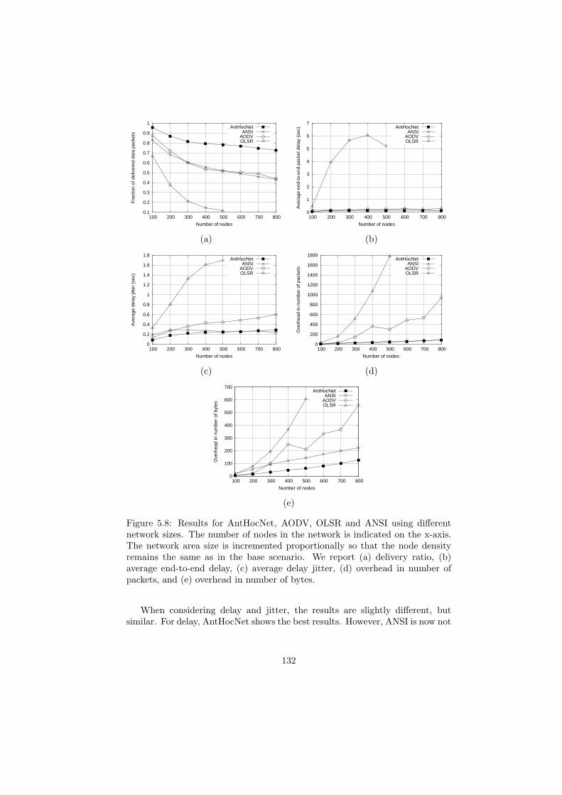
0.1

0.2

0.3

0.4

0.5

0.6

0.7

0.8

0.9

1

100 200 300 400 500 600 700 800

Fra

ctio

n of

del

iver

ed d

ata

pack

ets

Number of nodes

AntHocNetANSI

AODVOLSR

0

1

2

3

4

5

6

7

100 200 300 400 500 600 700 800

Ave

rage

end

-to-

end

pack

et d

elay

(se

c)

Number of nodes

AntHocNetANSI

AODVOLSR

(a) (b)

0

0.2

0.4

0.6

0.8

1

1.2

1.4

1.6

1.8

100 200 300 400 500 600 700 800

Ave

rage

del

ay ji

tter

(sec

)

Number of nodes

AntHocNetANSI

AODVOLSR

0

200

400

600

800

1000

1200

1400

1600

1800

100 200 300 400 500 600 700 800

Ove

rhea

d in

num

ber

of p

acke

ts

Number of nodes

AntHocNetANSI

AODVOLSR

(c) (d)

0

100

200

300

400

500

600

700

100 200 300 400 500 600 700 800

Ove

rhea

d in

num

ber

of b

ytes

Number of nodes

AntHocNetANSI

AODVOLSR

(e)

Figure 5.8: Results for AntHocNet, AODV, OLSR and ANSI using differentnetwork sizes. The number of nodes in the network is indicated on the x-axis.The network area size is incremented proportionally so that the node densityremains the same as in the base scenario. We report (a) delivery ratio, (b)average end-to-end delay, (c) average delay jitter, (d) overhead in number ofpackets, and (e) overhead in number of bytes.

When considering delay and jitter, the results are slightly different, butsimilar. For delay, AntHocNet shows the best results. However, ANSI is now not

132

much worse. For jitter, ANSI is slightly better than AntHocNet for the largestnetworks. For both measures, AODV lags more behind, and the differencegrows with increasing networks sizes. OLSR, finally, performs really badly. Itsdelay goes down slightly for the largest networks, where it is only delivering theeasiest data packets (a similar effect was also visible in the speed experimentsof subsections 5.2.1 and 5.2.3 and the density experiments of subsection 5.2.6).

In terms of both overhead measures, finally, we again see similar results.AntHocNet and ANSI have the best performance, with a small difference whenconsidering number of packets, and a larger one in the advantage of AntHocNetwhen considering number of bytes. AODV has worse performance, and thedifference grows with increasing network sizes, indicating that it is less scalablethan the two ACO routing algorithms. Finally, the proactive OLSR algorithmturns out to be highly inefficient for large network sizes.

5.2.8 Summary

In the results presented in this section, we have compared AntHocNet to anumber of representative routing algorithms. We have varied many differentenvironmental parameters, in order to investigate how each of these affects theperformance of the algorithms in absolute and relative terms. In general, wecould observe that AntHocNet shows very good behavior over the wide rangeof scenarios, and often outperforms the other three algorithms.

When considering the mobility experiments, we can see that AntHocNetcan deal better than the other algorithms with increasing mobility. It is betterable to deal with the network changes induced by mobility. In the RWP testswith increasing maximum node speed, we can see that as the network gets moredynamic, AntHocNet’s advantage over the other routing algorithms grows. Inthe pause time tests, results are rather ambiguous, due to the various conflictingtrends that are caused by changes in the pause time. In the test with increasingspeed under GM mobility, we can see similar trends as under RWP mobility,but we can also see that there is a limit to AntHocNet’s adaptivity: for thehighest speed values AntHocNet’s advantage over AODV becomes smaller. Thisis because mobility under GM gets higher than under RWP, and under theextreme mobility of these scenarios, it becomes hard for AntHocNet’s proactivemechanisms to keep up and make a difference.

When considering the data load experiments, we can see that none of theconsidered algorithms are really able to deal with high data send rates or highnumbers of sessions. The AHWMN capacity is just too limited. Nevertheless,we can see that AntHocNet keeps better up with the increasingly challengingenvironment. Only for the delay results in the data rate experiments, it isslightly worse than ANSI. So we can say that the performance of AntHocNetscales well with increasing data load. On the other hand, the purely reactiveapproach of AODV turns out to be quite sensitive to changes in the data load,since it creates too much overhead in reaction to disruptive events.

When considering the experiments with varying node density, we can observethat all algorithms suffer from the longer path lengths and lower connectivity as

133

scenarios get sparser. However, AntHocNet deals better with these challenges,and especially compared to AODV there is a growing gap in performance as nodedensity decreases. On the downside, we can observe that AntHocNet has moredifficulties in the densest scenarios. Its proactive route maintenance and reactiveroute repair mechanisms are rather useless there, as in those scenarios reactivelyrebuilding a route like AODV does can be more efficient than continuously tryingto extend, improve and repair routes. This is most visible in the overhead results,where AODV clearly outperforms AntHocNet when the network is small anddense.

Finally, when we consider the experiments with increasing network sizes, wesee similar patterns. Again, all algorithms suffer from the increasing scale, andespecially OLSR turns out to be unable to cope with large AHWMNs. In termsof delivery ratio, we see again the same trend as before, with an increasing per-formance gap between AntHocNet on the one hand and AODV and ANSI on theother hand, showing that AntHocNet is better able to deal with the difficultiesthat arise in larger networks. In terms of the other performance measures, thesame growing performance gap between AntHocNet and AODV remains visible,but ANSI’s performance is more similar to that of AntHocNet. In general, theresults of the tests with increasing network sizes show that AntHocNet is ableto maintain its good performance as the network size increases, thereby showingits good scalability.

5.3 Analysis of AntHocNet’s internal working

In this section, we present a number of tests in which we try to get a betterunderstanding of the working of AntHocNet. To this aim, we make variationsin the parameters and components used by the algorithm and observe the effectof these changes. In particular, we do tests switching off the proactive compo-nents and the local repair mechanism, using different routing metrics, varyingthe send frequency of proactive forward ants, varying the number of entries inthe pheromone diffusion messages, varying the routing exponent of proactiveforward ants, and varying the routing exponent of data packets. All tests areagain carried out in the earlier described base scenario and adaptations of it.We use adaptations that are relevant for the analysis at hand. We use as eval-uation measures the delivery ratio, end-to-end-delay, delay jitter and overheadin number of packets. For some of the experiments, we also include the num-ber of hops taken by successfully delivered data packets. This is a measure ofefficiency, as it indicates how many transmissions were needed to bring each ofthe data packets to its destination. The overhead in number of bytes was notincluded here, due to general similarity with the results for the other overheadmeasure.

134

0.4

0.5

0.6

0.7

0.8

0.9

1

100 200 300 400 500

Pac

ket d

eliv

ery

ratio

Number of nodes

AntHocNetAntHocNetnpAntHocNetnr

AntHocNetnpnr

0

0.05

0.1

0.15

0.2

0.25

0.3

0.35

100 200 300 400 500

Ave

rage

end

-to-

end

pack

et d

elay

(se

c)

Number of nodes

AntHocNetAntHocNetnpAntHocNetnr

AntHocNetnpnr

(a) (b)

0

0.1

0.2

0.3

0.4

0.5

0.6

0.7

0.8

100 200 300 400 500

Ave

rage

del

ay ji

tter

(sec

)

Number of nodes

AntHocNetAntHocNetnpAntHocNetnr

AntHocNetnpnr 0

20

40

60

80

100

120

140

160

180

200

100 200 300 400 500

Ove

rhea

d in

num

ber

of p

acke

ts

Number of nodes

AntHocNetAntHocNetnpAntHocNetnr

AntHocNetnpnr

(c) (d)

Figure 5.9: Results for AntHocNet, AntHocNet without proactive routemaintenance process (“AntHocNetnp”), AntHocNet without local route repair(“AntHocNetnr”) and AntHocNet with neither proactive route maintenance norroute repair (“AntHocNetnpnr”). The tests are carried out in scenarios with in-creasing number of nodes, as in subsection 5.2.7. We report (a) delivery ratio,(b) average end-to-end delay, (c) average delay jitter, and (d) overhead in num-ber of packets.

5.3.1 Switching off proactive actions and local repair

In the experiments presented in this subsection, we try to figure out what theindividual effect is of different components of AntHocNet. In particular, weinvestigate the relevance of the proactive route maintenance process and theroute repair process, as these are two components that we found to be definingfor the algorithm’s behavior. We compare the performance of the full Ant-HocNet algorithm with the performance of the algorithm without proactiveroute maintenance (which we refer to as AntHocNetnp), the algorithm with-out local route repair (which we refer to as AntHocNetnr), and the algorithmwith neither proactive route maintenance nor local route repair (which we referto as AntHocNetnpnr). The tests scenarios that we use are the ones of sub-section 5.2.7, where we increase the number of nodes and the network areasimultaneously. The maximum number of nodes here is 500. The results are

135

presented in figure 5.9.When we first consider the smallest network size (100 nodes), we can see that

AntHocNetnr performs equally well as, or even better than, the full AntHocNetalgorithm. This shows that the local repair component adds little or no valueat this scale. On the other hand, the proactive route maintenance process doesadd a lot of value: AntHocNetnp performs considerably worse than the fullAntHocNet algorithm for all evaluation measures. It is also interesting to seethat proactive route maintenance and local repair can substitute each other upto a certain extent. This can be concluded from the fact that AntHocNetnpnr

performs considerably worse than AntHocNetnp, while AntHocNetnr does notperform worse than the full AntHocNet algorithm: it seems that the local repairmechanism has more value in AntHocNetnp, where there is no proactive routemaintenance, than in the full AntHocNet algorithm.

When we consider larger network sizes, we can see that the performance gapbetween the full AntHocNet algorithm and AntHocNetnp grows steadily for allevaluation measures, indicating the continued importance of the proactive routemaintenance component. On the other hand, the gap between AntHocNet andAntHocNetnr grows fast, indicating that in large network sizes, the local repairmechanism does become an important mechanism in order to maintain goodperformance.

4

5

6

7

8

9

10

11

100 200 300 400 500

Ave

rage

num

ber

of h

ops

Number of nodes

AntHocNetAntHocNetnpAntHocNetnr

AntHocNetnpnr

Figure 5.10: The average number of hops for different versions of AntHocNetin scenarios with increasing number of nodes.

Finally, we also present results for the average number of hops taken bysuccessfully delivered data packets. The number of hops is an indication ofhow efficiently algorithms manage to bring data packets to their destination.The results are shown in figure 5.10. It is striking to see that the relativeperformances for this measure of efficiency go directly against the performancesfor all other measures. The full AntHocNet algorithm, which has the best resultsfor delivery ratio, delay, jitter and overhead, uses the longest paths to deliver itsdata. On the other hand, AntHocNetnpnr, which has the worst results for theother measures, uses the shortest paths. An explanation for the shorter pathlengths used by AntHocNetnpnr is that due to the lack of proactive maintenanceor repair, routes have to be rebuild from scratch after each link failure. When

136

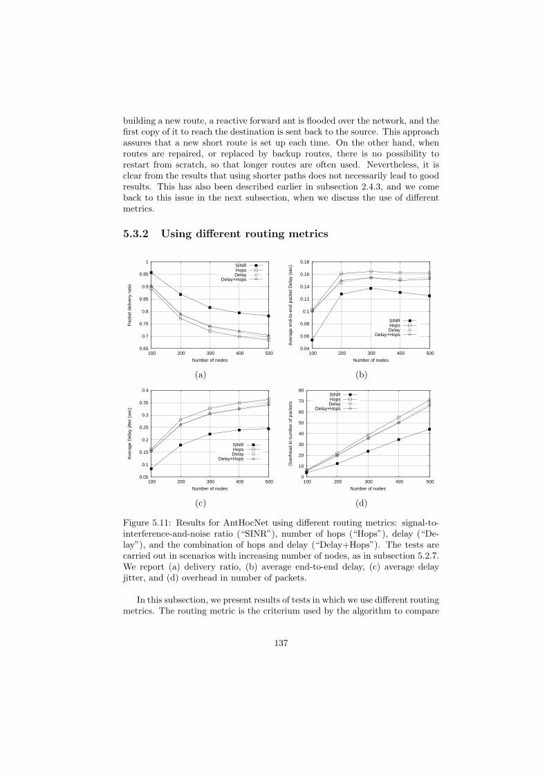
building a new route, a reactive forward ant is flooded over the network, and thefirst copy of it to reach the destination is sent back to the source. This approachassures that a new short route is set up each time. On the other hand, whenroutes are repaired, or replaced by backup routes, there is no possibility torestart from scratch, so that longer routes are often used. Nevertheless, it isclear from the results that using shorter paths does not necessarily lead to goodresults. This has also been described earlier in subsection 2.4.3, and we comeback to this issue in the next subsection, when we discuss the use of differentmetrics.

5.3.2 Using different routing metrics

0.65

0.7

0.75

0.8

0.85

0.9

0.95

1

100 200 300 400 500

Pac

ket d

eliv

ery

ratio

Number of nodes

SINRHopsDelay

Delay+Hops

0.04

0.06

0.08

0.1

0.12

0.14

0.16

0.18

100 200 300 400 500

Ave

rage

end

-to-

end

pack

et D

elay

(se

c)

Number of nodes

SINRHopsDelay

Delay+Hops

(a) (b)

0.05

0.1

0.15

0.2

0.25

0.3

0.35

0.4

100 200 300 400 500

Ave

rage

Del

ay ji

tter

(sec

)

Number of nodes

SINRHopsDelay

Delay+Hops

0

10

20

30

40

50

60

70

80

100 200 300 400 500

Ove

rhea

d in

num

ber

of p

acke

ts

Number of nodes

SINRHopsDelay

Delay+Hops

(c) (d)

Figure 5.11: Results for AntHocNet using different routing metrics: signal-to-interference-and-noise ratio (“SINR”), number of hops (“Hops”), delay (“De-lay”), and the combination of hops and delay (“Delay+Hops”). The tests arecarried out in scenarios with increasing number of nodes, as in subsection 5.2.7.We report (a) delivery ratio, (b) average end-to-end delay, (c) average delayjitter, and (d) overhead in number of packets.

In this subsection, we present results of tests in which we use different routingmetrics. The routing metric is the criterium used by the algorithm to compare

137

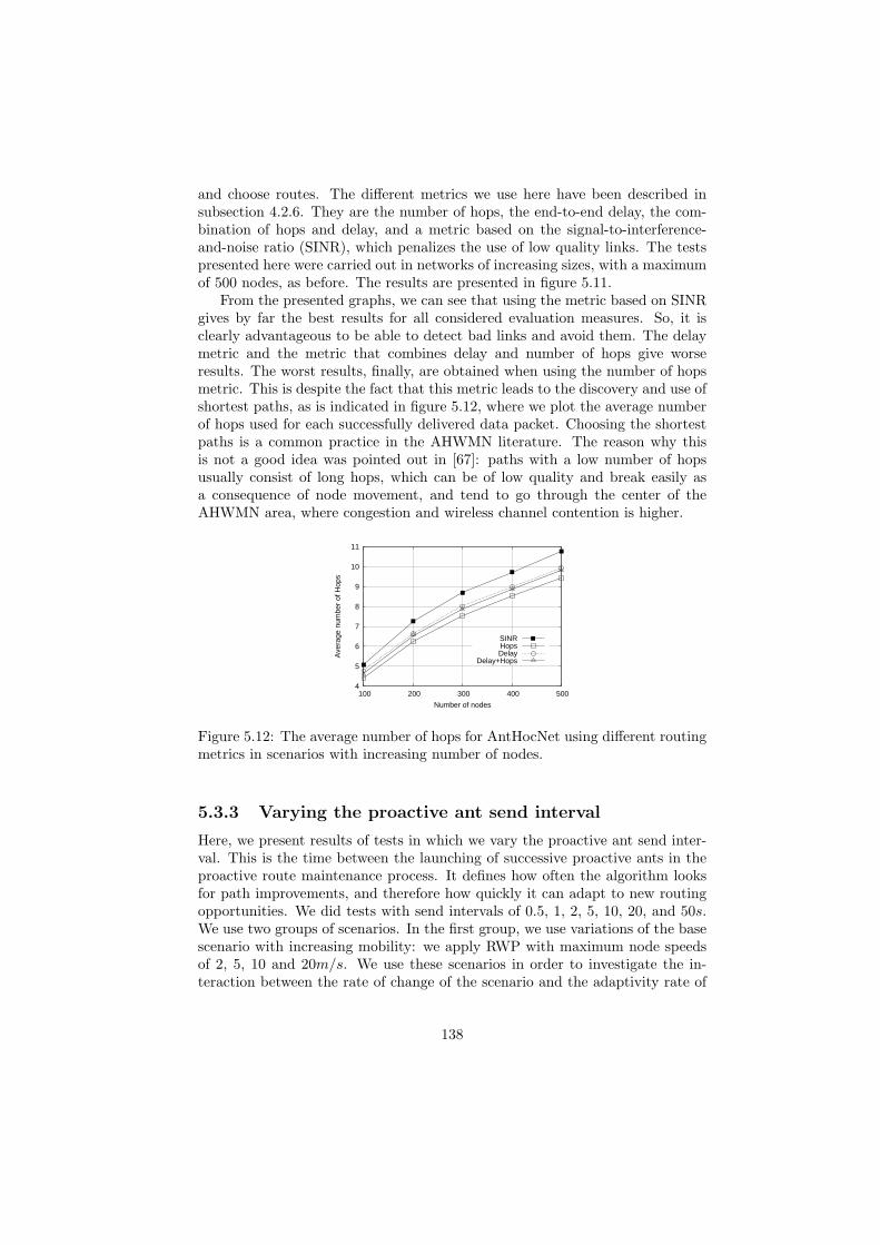
and choose routes. The different metrics we use here have been described insubsection 4.2.6. They are the number of hops, the end-to-end delay, the com-bination of hops and delay, and a metric based on the signal-to-interference-and-noise ratio (SINR), which penalizes the use of low quality links. The testspresented here were carried out in networks of increasing sizes, with a maximumof 500 nodes, as before. The results are presented in figure 5.11.

From the presented graphs, we can see that using the metric based on SINRgives by far the best results for all considered evaluation measures. So, it isclearly advantageous to be able to detect bad links and avoid them. The delaymetric and the metric that combines delay and number of hops give worseresults. The worst results, finally, are obtained when using the number of hopsmetric. This is despite the fact that this metric leads to the discovery and use ofshortest paths, as is indicated in figure 5.12, where we plot the average numberof hops used for each successfully delivered data packet. Choosing the shortestpaths is a common practice in the AHWMN literature. The reason why thisis not a good idea was pointed out in [67]: paths with a low number of hopsusually consist of long hops, which can be of low quality and break easily asa consequence of node movement, and tend to go through the center of theAHWMN area, where congestion and wireless channel contention is higher.

4

5

6

7

8

9

10

11

100 200 300 400 500

Ave

rage

num

ber

of H

ops

Number of nodes

SINRHopsDelay

Delay+Hops

Figure 5.12: The average number of hops for AntHocNet using different routingmetrics in scenarios with increasing number of nodes.

5.3.3 Varying the proactive ant send interval

Here, we present results of tests in which we vary the proactive ant send inter-val. This is the time between the launching of successive proactive ants in theproactive route maintenance process. It defines how often the algorithm looksfor path improvements, and therefore how quickly it can adapt to new routingopportunities. We did tests with send intervals of 0.5, 1, 2, 5, 10, 20, and 50s.We use two groups of scenarios. In the first group, we use variations of the basescenario with increasing mobility: we apply RWP with maximum node speedsof 2, 5, 10 and 20m/s. We use these scenarios in order to investigate the in-teraction between the rate of change of the scenario and the adaptivity rate of

138

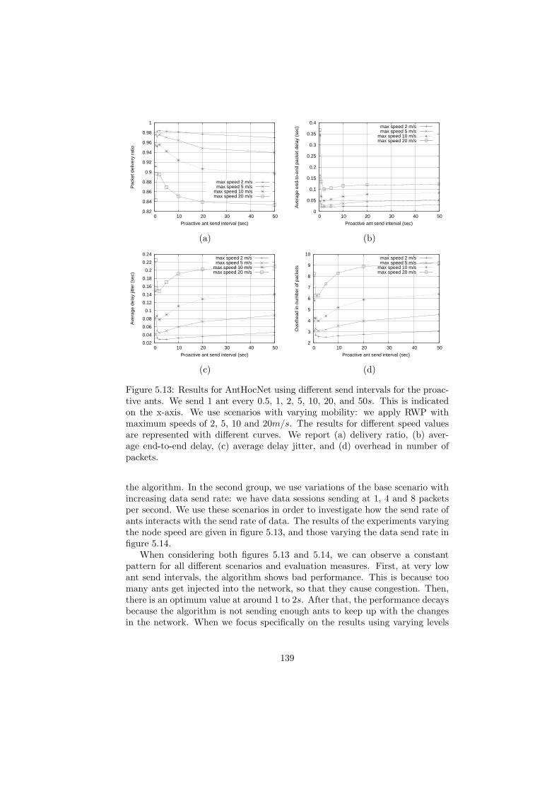
0.82

0.84

0.86

0.88

0.9

0.92

0.94

0.96

0.98

1

0 10 20 30 40 50

Pac

ket d

eliv

ery

ratio

Proactive ant send interval (sec)

max speed 2 m/smax speed 5 m/s

max speed 10 m/smax speed 20 m/s

0

0.05

0.1

0.15

0.2

0.25

0.3

0.35

0.4

0 10 20 30 40 50

Ave

rage

end

-to-

end

pack

et d

elay

(se

c)

Proactive ant send interval (sec)

max speed 2 m/smax speed 5 m/s

max speed 10 m/smax speed 20 m/s

(a) (b)

0.02

0.04

0.06

0.08

0.1

0.12

0.14

0.16

0.18

0.2

0.22

0.24

0 10 20 30 40 50

Ave

rage

del

ay ji

tter

(sec

)

Proactive ant send interval (sec)

max speed 2 m/smax speed 5 m/s

max speed 10 m/smax speed 20 m/s

2

3

4

5

6

7

8

9

10

0 10 20 30 40 50

Ove

rhea

d in

num

ber

of p

acke

ts

Proactive ant send interval (sec)

max speed 2 m/smax speed 5 m/s

max speed 10 m/smax speed 20 m/s

(c) (d)

Figure 5.13: Results for AntHocNet using different send intervals for the proac-tive ants. We send 1 ant every 0.5, 1, 2, 5, 10, 20, and 50s. This is indicatedon the x-axis. We use scenarios with varying mobility: we apply RWP withmaximum speeds of 2, 5, 10 and 20m/s. The results for different speed valuesare represented with different curves. We report (a) delivery ratio, (b) aver-age end-to-end delay, (c) average delay jitter, and (d) overhead in number ofpackets.

the algorithm. In the second group, we use variations of the base scenario withincreasing data send rate: we have data sessions sending at 1, 4 and 8 packetsper second. We use these scenarios in order to investigate how the send rate ofants interacts with the send rate of data. The results of the experiments varyingthe node speed are given in figure 5.13, and those varying the data send rate infigure 5.14.

When considering both figures 5.13 and 5.14, we can observe a constantpattern for all different scenarios and evaluation measures. First, at very lowant send intervals, the algorithm shows bad performance. This is because toomany ants get injected into the network, so that they cause congestion. Then,there is an optimum value at around 1 to 2s. After that, the performance decaysbecause the algorithm is not sending enough ants to keep up with the changesin the network. When we focus specifically on the results using varying levels

139

0.55

0.6

0.65

0.7

0.75

0.8

0.85

0.9

0.95

1

0 10 20 30 40 50

Pac

ket d

eliv

ery

ratio

Proactive ant send interval (sec)

data rate 1 packet/sdata rate 4 packets/sdata rate 8 packets/s

0

0.5

1

1.5

2

2.5

0 10 20 30 40 50

Ave

rage

end

-to-

end

pack

et d

elay

(se

c)

Proactive ant send interval (sec)

data rate 1 packet/sdata rate 4 packets/sdata rate 8 packets/s

(a) (b)

0.06

0.08

0.1

0.12

0.14

0.16

0.18

0.2

0.22

0.24

0.26

0.28

0 10 20 30 40 50

Ave

rage

del

ay ji

tter

(sec

)

Proactive ant send interval (sec)

data rate 1 packet/sdata rate 4 packets/sdata rate 8 packets/s

3

4

5

6

7

8

9

10

11

12

13

14

0 10 20 30 40 50

Ove

rhea

d in

num

ber

of p

acke

ts

Proactive ant send interval (sec)

data rate 1 packet/sdata rate 4 packets/sdata rate 8 packets/s

(c) (d)

Figure 5.14: Results for AntHocNet using different send intervals for the proac-tive ants. We send 1 ant every 0.5, 1, 2, 5, 10, 20, and 50s. This is indicatedon the x-axis. We use scenarios with varying data load: we use data sessionssending 1, 4 and 8 packets per second. The results for different data send ratesare represented with different curves. We report (a) delivery ratio, (b) aver-age end-to-end delay, (c) average delay jitter, and (d) overhead in number ofpackets.

of mobility, we can see that the above pattern is less clearly visible for the lowspeed scenarios than for the high speed ones. This is because when the networkchanges slowly, it is less crucial to adapt quickly. When we zoom in on theresults with varying data load, we can see that the pattern is best visible at theintermediate send rate of 4 data packets per second. When sending less data,paths often need to be rebuilt for each data packet (see also subsection 5.2.4),so that adaptivity is less able to make a difference. For high data rates, theperformance generally deteriorates strongly due to high levels of congestion, andagain it is more difficult to make a difference using proactive adaptivity. Oneinteresting observation when comparing the results over all different scenariosis that the optimal ant send rate is relatively stable and independent from thenode mobility or data send rate. Sending one ant every 2s almost always givesthe best performance.

140

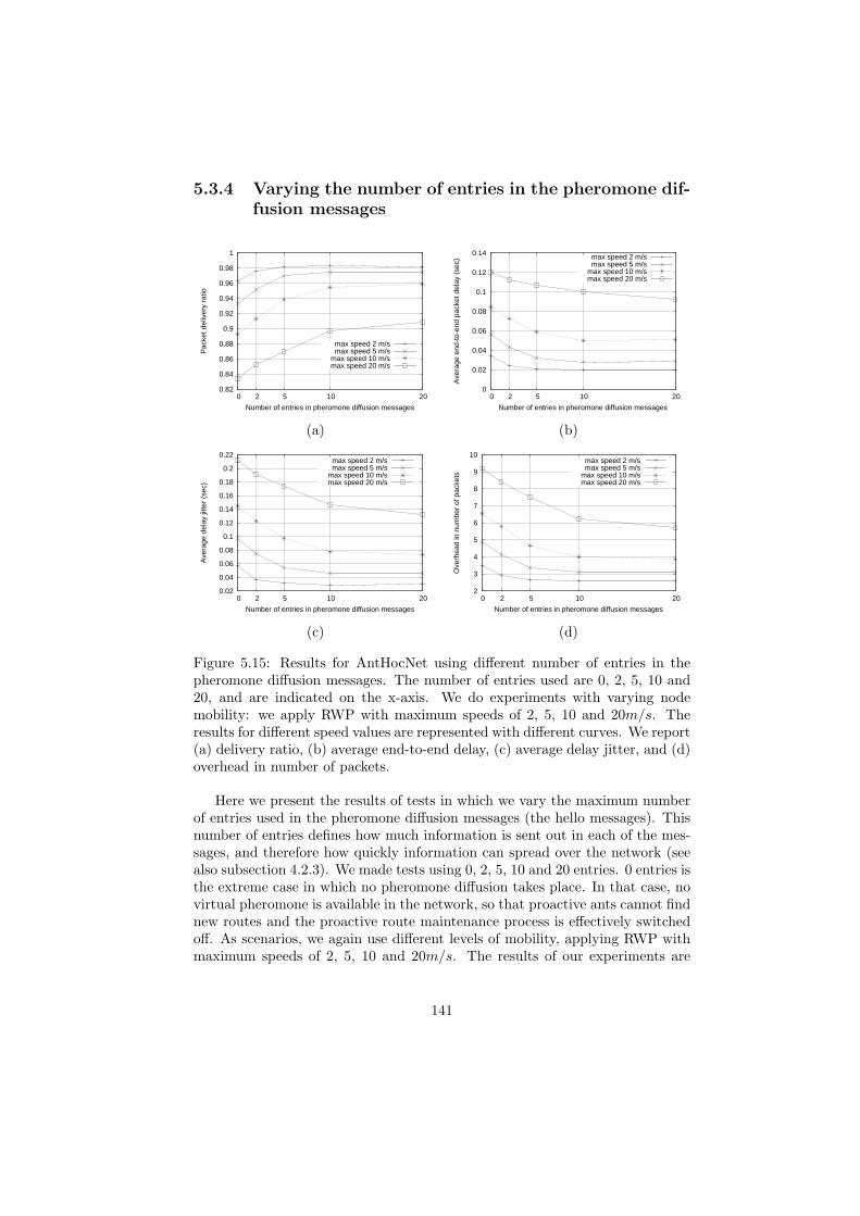
5.3.4 Varying the number of entries in the pheromone dif-fusion messages

0.82

0.84

0.86

0.88

0.9

0.92

0.94

0.96

0.98

1

20 10 5 2 0

Pac

ket d

eliv

ery

ratio

Number of entries in pheromone diffusion messages

max speed 2 m/smax speed 5 m/s

max speed 10 m/smax speed 20 m/s

0

0.02

0.04

0.06

0.08

0.1

0.12

0.14

20 10 5 2 0

Ave

rage

end

-to-

end

pack

et d

elay

(se

c)

Number of entries in pheromone diffusion messages

max speed 2 m/smax speed 5 m/s

max speed 10 m/smax speed 20 m/s

(a) (b)

0.02

0.04

0.06

0.08

0.1

0.12

0.14

0.16

0.18

0.2

0.22

20 10 5 2 0

Ave

rage

del

ay ji

tter

(sec

)

Number of entries in pheromone diffusion messages

max speed 2 m/smax speed 5 m/s

max speed 10 m/smax speed 20 m/s

2

3

4

5

6

7

8

9

10

20 10 5 2 0

Ove

rhea

d in

num

ber

of p

acke

ts

Number of entries in pheromone diffusion messages

max speed 2 m/smax speed 5 m/s

max speed 10 m/smax speed 20 m/s

(c) (d)

Figure 5.15: Results for AntHocNet using different number of entries in thepheromone diffusion messages. The number of entries used are 0, 2, 5, 10 and20, and are indicated on the x-axis. We do experiments with varying nodemobility: we apply RWP with maximum speeds of 2, 5, 10 and 20m/s. Theresults for different speed values are represented with different curves. We report(a) delivery ratio, (b) average end-to-end delay, (c) average delay jitter, and (d)overhead in number of packets.

Here we present the results of tests in which we vary the maximum numberof entries used in the pheromone diffusion messages (the hello messages). Thisnumber of entries defines how much information is sent out in each of the mes-sages, and therefore how quickly information can spread over the network (seealso subsection 4.2.3). We made tests using 0, 2, 5, 10 and 20 entries. 0 entries isthe extreme case in which no pheromone diffusion takes place. In that case, novirtual pheromone is available in the network, so that proactive ants cannot findnew routes and the proactive route maintenance process is effectively switchedoff. As scenarios, we again use different levels of mobility, applying RWP withmaximum speeds of 2, 5, 10 and 20m/s. The results of our experiments are

141

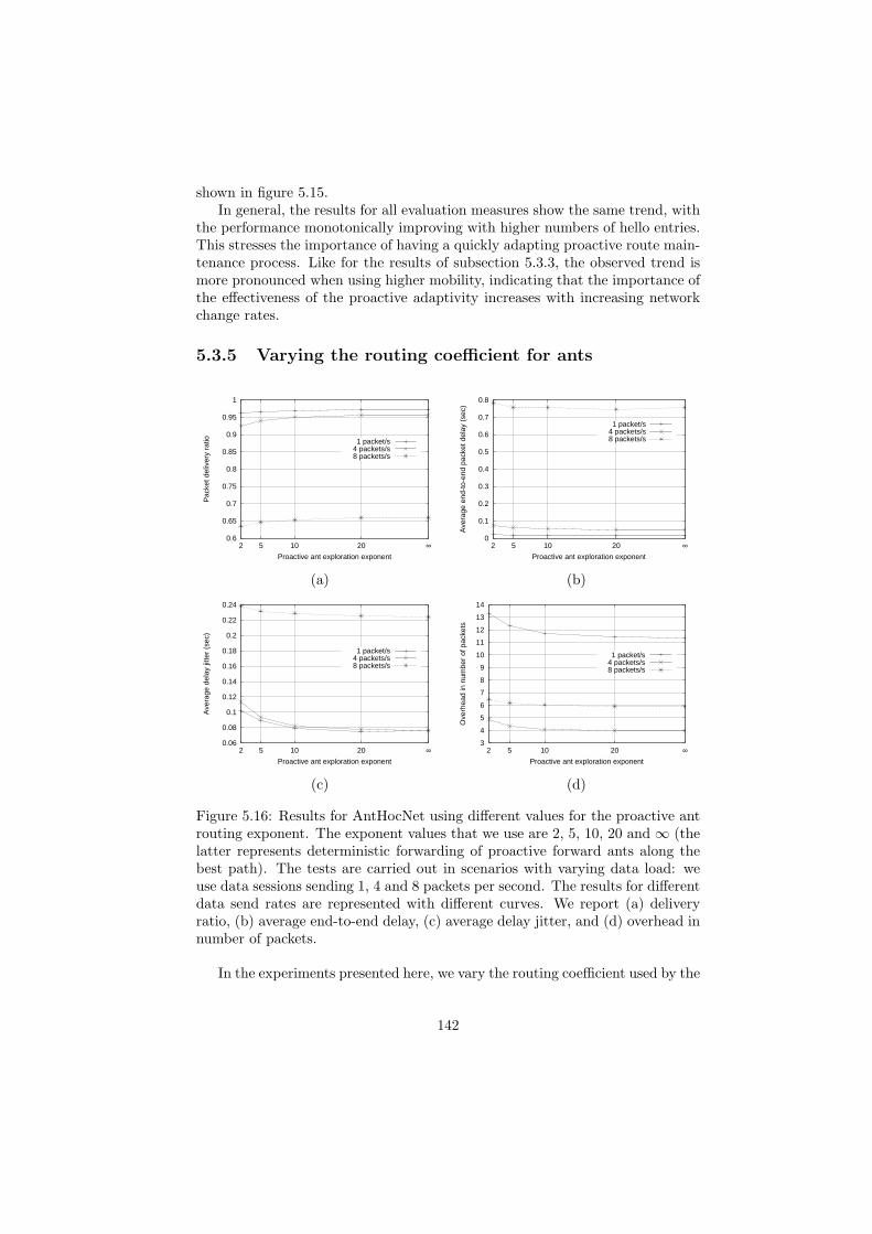
shown in figure 5.15.In general, the results for all evaluation measures show the same trend, with

the performance monotonically improving with higher numbers of hello entries.This stresses the importance of having a quickly adapting proactive route main-tenance process. Like for the results of subsection 5.3.3, the observed trend ismore pronounced when using higher mobility, indicating that the importance ofthe effectiveness of the proactive adaptivity increases with increasing networkchange rates.

5.3.5 Varying the routing coefficient for ants

0.6

0.65

0.7

0.75

0.8

0.85

0.9

0.95

1

∞201052

Pac

ket d

eliv

ery

ratio

Proactive ant exploration exponent

1 packet/s4 packets/s8 packets/s

0

0.1

0.2

0.3

0.4

0.5

0.6

0.7

0.8

∞201052

Ave

rage

end

-to-

end

pack

et d

elay

(se

c)

Proactive ant exploration exponent

1 packet/s4 packets/s8 packets/s

(a) (b)

0.06

0.08

0.1

0.12

0.14

0.16

0.18

0.2

0.22

0.24

∞201052

Ave

rage

del

ay ji

tter

(sec

)

Proactive ant exploration exponent

1 packet/s4 packets/s8 packets/s

3

4

5

6

7

8

9

10

11

12

13

14

∞201052

Ove

rhea

d in

num

ber

of p

acke

ts

Proactive ant exploration exponent

1 packet/s4 packets/s8 packets/s

(c) (d)

Figure 5.16: Results for AntHocNet using different values for the proactive antrouting exponent. The exponent values that we use are 2, 5, 10, 20 and ∞ (thelatter represents deterministic forwarding of proactive forward ants along thebest path). The tests are carried out in scenarios with varying data load: weuse data sessions sending 1, 4 and 8 packets per second. The results for differentdata send rates are represented with different curves. We report (a) deliveryratio, (b) average end-to-end delay, (c) average delay jitter, and (d) overhead innumber of packets.

In the experiments presented here, we vary the routing coefficient used by the

142

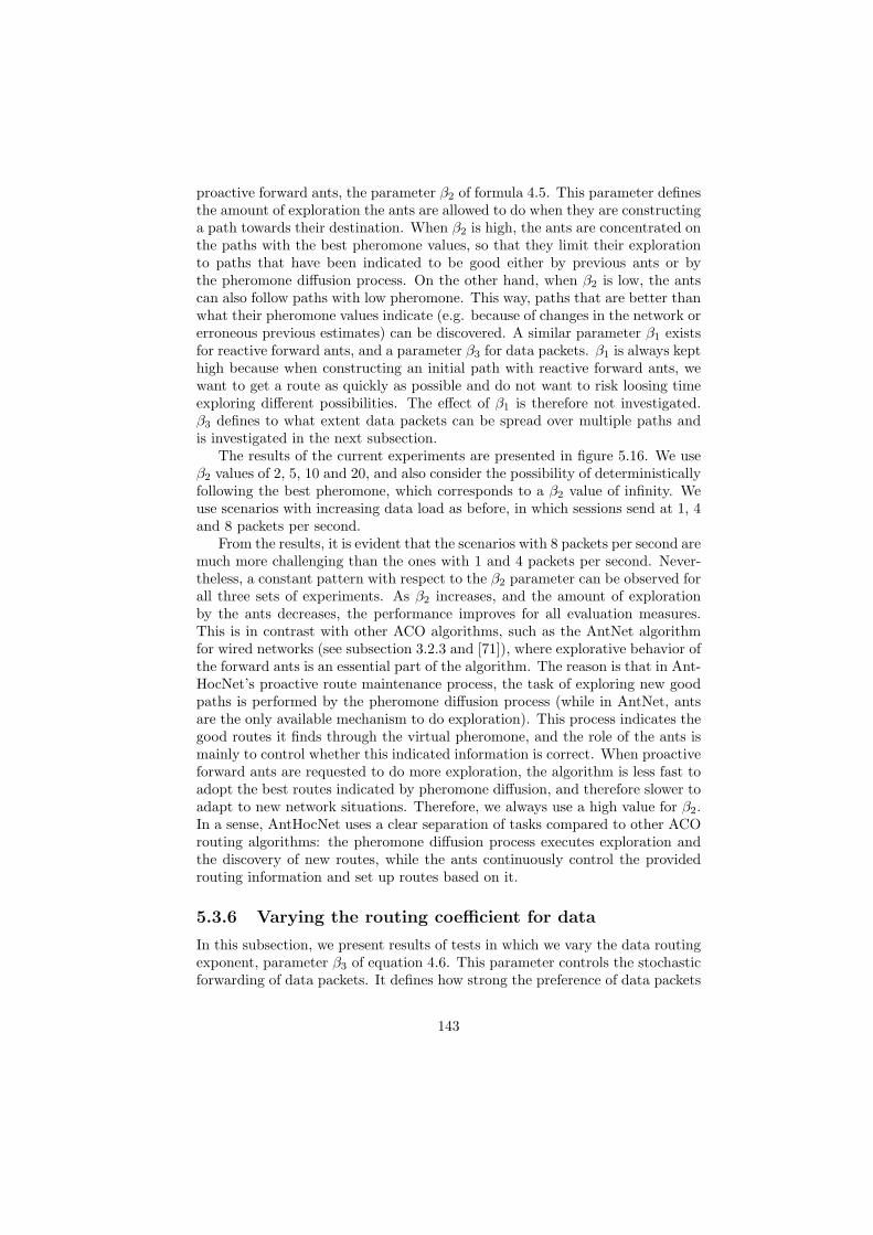
proactive forward ants, the parameter β2 of formula 4.5. This parameter definesthe amount of exploration the ants are allowed to do when they are constructinga path towards their destination. When β2 is high, the ants are concentrated onthe paths with the best pheromone values, so that they limit their explorationto paths that have been indicated to be good either by previous ants or bythe pheromone diffusion process. On the other hand, when β2 is low, the antscan also follow paths with low pheromone. This way, paths that are better thanwhat their pheromone values indicate (e.g. because of changes in the network orerroneous previous estimates) can be discovered. A similar parameter β1 existsfor reactive forward ants, and a parameter β3 for data packets. β1 is always kepthigh because when constructing an initial path with reactive forward ants, wewant to get a route as quickly as possible and do not want to risk loosing timeexploring different possibilities. The effect of β1 is therefore not investigated.β3 defines to what extent data packets can be spread over multiple paths andis investigated in the next subsection.

The results of the current experiments are presented in figure 5.16. We useβ2 values of 2, 5, 10 and 20, and also consider the possibility of deterministicallyfollowing the best pheromone, which corresponds to a β2 value of infinity. Weuse scenarios with increasing data load as before, in which sessions send at 1, 4and 8 packets per second.

From the results, it is evident that the scenarios with 8 packets per second aremuch more challenging than the ones with 1 and 4 packets per second. Never-theless, a constant pattern with respect to the β2 parameter can be observed forall three sets of experiments. As β2 increases, and the amount of explorationby the ants decreases, the performance improves for all evaluation measures.This is in contrast with other ACO algorithms, such as the AntNet algorithmfor wired networks (see subsection 3.2.3 and [71]), where explorative behavior ofthe forward ants is an essential part of the algorithm. The reason is that in Ant-HocNet’s proactive route maintenance process, the task of exploring new goodpaths is performed by the pheromone diffusion process (while in AntNet, antsare the only available mechanism to do exploration). This process indicates thegood routes it finds through the virtual pheromone, and the role of the ants ismainly to control whether this indicated information is correct. When proactiveforward ants are requested to do more exploration, the algorithm is less fast toadopt the best routes indicated by pheromone diffusion, and therefore slower toadapt to new network situations. Therefore, we always use a high value for β2.In a sense, AntHocNet uses a clear separation of tasks compared to other ACOrouting algorithms: the pheromone diffusion process executes exploration andthe discovery of new routes, while the ants continuously control the providedrouting information and set up routes based on it.

5.3.6 Varying the routing coefficient for data

In this subsection, we present results of tests in which we vary the data routingexponent, parameter β3 of equation 4.6. This parameter controls the stochasticforwarding of data packets. It defines how strong the preference of data packets

143

0.6

0.65

0.7

0.75

0.8

0.85

0.9

0.95

1

∞201052

Pac

ket d

eliv

ery

ratio

Data packet routing exponent

data rate 1 packet/sdata rate 4 packets/sdata rate 8 packets/s

0

0.1

0.2

0.3

0.4

0.5

0.6

0.7

0.8

0.9

∞201052

Ave

rage

end

-to-

end

pack

et d

elay

(se

c)

Data packet routing exponent

data rate 1 packet/sdata rate 4 packets/sdata rate 8 packets/s

(a) (b)

0.06

0.08

0.1

0.12

0.14

0.16

0.18

0.2

0.22

0.24

∞201052

Ave

rage

del

ay ji

tter

(sec

)

Data packet routing exponent

data rate 1 packet/sdata rate 4 packets/sdata rate 8 packets/s

3

4

5

6

7

8

9

10

11

12

∞201052

Ove

rhea

d in

num

ber

of p

acke

ts

Data packet routing exponent

data rate 1 packet/sdata rate 4 packets/sdata rate 8 packets/s

(c) (d)

Figure 5.17: Results for AntHocNet using different values for the data routingexponent. The exponent values that we use are 2, 5, 10, 20 and ∞ (the latterrepresents deterministic forwarding of data along the best path). The tests arecarried out in scenarios with varying data load: we use data sessions sending1, 4 and 8 packets per second. The results for different data send rates arerepresented with different curves. We report (a) delivery ratio, (b) average end-to-end delay, (c) average delay jitter, and (d) overhead in number of packets.

for paths with high pheromone is. When β3 is low, this preference is weak, anddata can therefore be spread out over a range of multiple paths. On the otherhand, when β3 is high, data packets are only sent over the best paths. In thelimit, where β3 reaches infinity, data is forwarded deterministically over the bestpath. In our experiments, we use β3 values of 2, 5, 10, 20, and infinity. Weagain use scenarios with increasing data load, in which sessions send at 1, 4 and8 packets per second. The results are presented in figure 5.17.

The graphs show a similar trend as those for the tests with β2. Also here,performance improves with increasing values for the routing coefficient underall scenarios and for all evaluation measures. So, it turns out that the featureof stochastically spreading data packets over multiple paths is not beneficial,but, on the contrary, deteriorates results. This is again in contrast with otherACO routing algorithms, where stochastic data forwarding allows to improve

144

performance by spreading the data load over multiple paths and making betteruse of the full network resources. An explanation of why this is not working inthe case of AntHocNet can be found in the fact that in AHWMNs different pathsbetween source and destination nodes are not very well separated: due to radiointerference, data packets traveling over parallel paths can hinder each other, sothat it is difficult to obtain any advantages. This issue can possibly be dealt withif specific mechanisms are used during the construction of the different paths,e.g. choosing paths that go over nodes that are outside each other’s transmissionrange (see also subsection 2.4.3). However, such mechanisms would be quitecomplex, especially if we take into account the fact that nodes move, and pathsthat were originally sufficiently apart could move into each other’s transmissionrange. In AntHocNet, we did not use such an approach. Instead, we keep thedata routing coefficient high, and only use the very best paths. This way, wemaximally exploit the best routes available.

5.3.7 Summary

In this section we have presented results of tests in which we switched on and offdifferent components of the AntHocNet routing algorithm and varied its internalparameters. The aim was to investigate AntHocNet’s internal working.

First, we have looked at the individual contribution to the algorithm’s perfor-mance of the proactive route maintenance process and the reactive route repairmechanism. We have shown that the proactive route maintenance process has astrong positive influence on the performance over a range of different scenarios.On the other hand, the reactive route repair mechanism turned out to have alarge positive contribution in large networks but very little or no contributionin small networks.

Next, we have investigated the use of different routing metrics. From theresults, it was clear that the metric using the SINR was superior. The metricusing delay and the one using a combination of delay and hops gave worseresults. The worst results were for the number of hops metric, despite the factthat this metric lead to the use of the shortest paths and is very often used forrouting in AHWMNs.

Then, we have investigated two parameters that are related to the speed ofworking of the proactive route maintenance process: we have done tests varyingthe send rate of proactive forward ants and varying the number of entries inthe pheromone diffusion messages. Both tests indicated that a faster workingproactive route maintenance process is better: sending ants more regularly andspreading out more information in each message during pheromone diffusiongave better results. Limits are present only when too much overhead is created.For example, sending more ants than one per second lead to rather bad results.

Finally, we have done tests varying the routing coefficient of proactive for-ward ants and data packets. In both cases, it turned out that increasing thecoefficient lead to monotonically improving results. In the case of proactiveforward ants, this shows that it is better to leave the task of exploring newpaths to the pheromone diffusion process, and let the ants focus on the task of

145

controlling the obtained information and turn it into routes that can be used fordata. In the case of data packets, it shows that it is difficult to get throughputadvantage from spreading data over multiple paths, and that instead it is betterto fully exploit the best routes found by the ants.

5.4 Conclusion

In this chapter we have provided an evaluation study of the AntHocNet rout-ing algorithm. Tests were carried out in scenarios that are similar to thosecommonly used in the literature on MANET routing.

In a first set of tests, we compared AntHocNet to existing state-of-the-artrouting algorithms. These included AODV, a reference reactive routing algo-rithm, OLSR, an important proactive routing algorithm, and ANSI, which isa representative of the class of ACO routing algorithms. Results showed thatAntHocNet could outperform the other three algorithms over a wide range ofdifferent scenarios. Specifically, AntHocNet turned out to perform well in testswith increasing levels of mobility, to deal better than the other algorithms withdifferent levels of data load, to cope well with sparse network situations, andto scale well to networks of increasing sizes. On the downside, AntHocNet’sadvantage was decreased when mobility got very high, and the algorithm wasoutperformed by AODV when very dense scenarios were used.

In a second set of tests, we investigated the internal working of AntHocNet.We switched on and off the use of different components of the algorithm, andvaried various internal parameters. We found that the proactive maintenanceprocess has a high contribution to the algorithm’s performance over a rangeof scenarios, while the local repair mechanism did not have a positive effect insmall networks, but was increasingly valuable in large ones. We also found thatit is important that the proactive maintenance process works as fast as possible,as long as it does not produce excessive overhead. Among the possible routingmetrics, we discovered that the SINR based metric lead to the best results.Finally, we saw that exploration in the proactive route maintenance processshould be left to the pheromone diffusion process rather than to the ants, andthat data packets should be forwarded over the best paths, with minimal dataload spreading.

146

Chapter 6

Simulation of an urbanscenario

In the previous chapter we have presented the results of a number of tests inwhich we evaluate the performance of the AntHocNet routing algorithm. Allof those tests used scenarios that were derived from a common base scenario,in which a number of nodes move in an open, rectangular area along straightline segments, and data are sent at fixed rates. The reason to use this type ofscenarios was to stay in line with the common practice in the literature, so thatcomparisons with other algorithms are easier and more fair. However, as waspointed out already in subsection 5.1.1, these scenarios are rather simple, andmight not give a correct image of situations that occur in reality. Therefore,observed results are not necessarily representative for what can be expectedwhen the network is deployed for a practical application. The aim of the currentchapter is to complement the previous tests with new ones that use more realisticscenarios. For these new scenarios, we have chosen an urban environment, asthe development of recent projects with public WMNs in some cities such asPhiladelphia [12] and Taipei [10] indicate that this will be an important areaof application for AHWMN technology. We take special care to simulate thisenvironment and the use of an AHWMN in it in an accurate way. We use thisdetailed simulation to make new evaluations of AntHocNet’s performance.

The rest of this chapter is organized as follows. First, we describe the simu-lation setup, giving special attention to the way we obtained a model of wirelesscommunication in the urban environment and how we were able to simulate itin an efficient way. Then, we present results of a simulation study, in which wefirst investigate network properties of the AHWMN in the urban environment,and then perform a comparative test of the AntHocNet and AODV routing al-gorithms. The work presented here has been described in [97] and in projectdeliverable [49].

147

6.1 Design of the simulation study

In this section we describe the design of the simulation study. In what followswe first provide a general overview of the study. Then, we give detailed descrip-tions of the urban environment and the implementation of node mobility, of theused radio propagation models and their implementation, and of the simulateddata traffic. Finally, we review related literature on the topic of simulations ofAHWMNs in urban settings.

6.1.1 General description of the simulation study

The aim of the study presented in this chapter is to evaluate the behavior ofthe AntHocNet routing protocol in an urban environment through simulation.We have chosen the center of the Swiss town of Lugano as the setting of ourstudy. Compared to the open space scenarios of the previous chapter, there arethree important differences. The first concerns node mobility. We model urbanmobility by limiting the movements of nodes to the streets and open areas inthe town, and adjusting their speed to the typical speed of people in a urbanenvironment, be it pedestrians, cyclists or slowly moving cars. We also use acertain percentage of static nodes, to model immobile network users. This makesthat the network is not just a MANET, but also has some characteristics of aWMN. Details about the urban environment and the movement of nodes in itwill be given in subsection 6.1.2. The second difference concerns the propagationof radio waves in the urban setting. We model the physical propagation ofradio waves through the streets of the town using a ray-tracing approach, whichaccounts for interactions between radio waves and buildings, such as reflectionand diffraction [221]. Details about this will be given in subsection 6.1.3. Finally,the third difference concerns the way the network is used at the application layer.Rather than using CBR sessions, we modeled different kinds of data traffic, inorder to account for different possible uses of the network. The applications weconsidered range from an interactive short messaging service (SMS) to voice-over-IP (VoIP) traffic. Details about the modeling of data traffic will be givenin subsection 6.1.4.

We run simulations of 500s each, and do 20 individual runs per scenario. Wenormally use AHWMNs of 300 nodes, but also carry out experiments varyingthe number of nodes from 100 up to 400. Like in the previous chapter we use theQualNet discrete event network simulator (see subsection 5.1.2 and [232]). Wemade some adaptations to the simulator code in order to be able to simulatethe propagation of radio waves in an urban environment in an efficient way,as will be explained in subsection 6.1.3. Also for the selection of networkingprotocols, we stick with the choices of the previous chapter. At the physicallayer we use the IEEE 802.11 protocol sending at a frequency of 2.4GHz andwith a bit rate of 2Mbps. At the MAC layer, we use the IEEE 802.11 DCFprotocol (see subsection 2.3.3). At the transport layer, we use UDP, due to thebefore mentioned problems of TCP in AHWMNs (see subsection 2.3.4). Finally,as benchmark routing algorithm to compare and evaluate the performance of

148

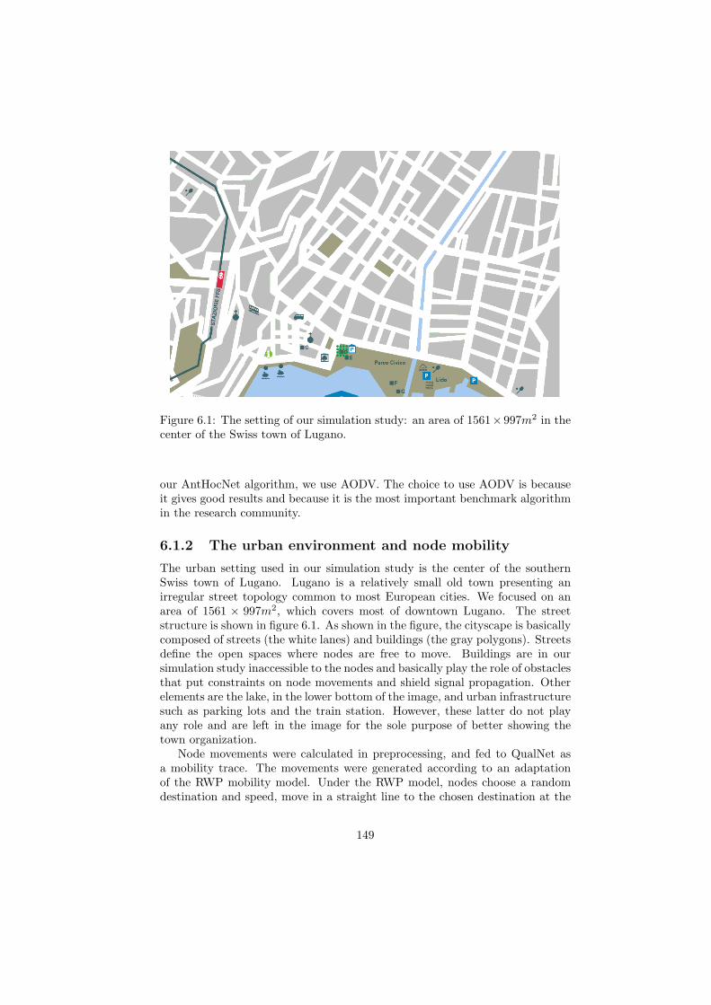
Figure 6.1: The setting of our simulation study: an area of 1561× 997m2 in thecenter of the Swiss town of Lugano.

our AntHocNet algorithm, we use AODV. The choice to use AODV is becauseit gives good results and because it is the most important benchmark algorithmin the research community.

6.1.2 The urban environment and node mobility

The urban setting used in our simulation study is the center of the southernSwiss town of Lugano. Lugano is a relatively small old town presenting anirregular street topology common to most European cities. We focused on anarea of 1561 × 997m2, which covers most of downtown Lugano. The streetstructure is shown in figure 6.1. As shown in the figure, the cityscape is basicallycomposed of streets (the white lanes) and buildings (the gray polygons). Streetsdefine the open spaces where nodes are free to move. Buildings are in oursimulation study inaccessible to the nodes and basically play the role of obstaclesthat put constraints on node movements and shield signal propagation. Otherelements are the lake, in the lower bottom of the image, and urban infrastructuresuch as parking lots and the train station. However, these latter do not playany role and are left in the image for the sole purpose of better showing thetown organization.

Node movements were calculated in preprocessing, and fed to QualNet asa mobility trace. The movements were generated according to an adaptationof the RWP mobility model. Under the RWP model, nodes choose a randomdestination and speed, move in a straight line to the chosen destination at the

149

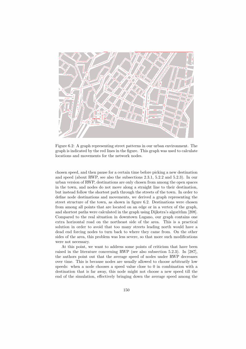
Figure 6.2: A graph representing street patterns in our urban environment. Thegraph is indicated by the red lines in the figure. This graph was used to calculatelocations and movements for the network nodes.

chosen speed, and then pause for a certain time before picking a new destinationand speed (about RWP, see also the subsections 2.3.1, 5.2.2 and 5.2.3). In oururban version of RWP, destinations are only chosen from among the open spacesin the town, and nodes do not move along a straight line to their destination,but instead follow the shortest path through the streets of the town. In order todefine node destinations and movements, we derived a graph representing thestreet structure of the town, as shown in figure 6.2. Destinations were chosenfrom among all points that are located on an edge or in a vertex of the graph,and shortest paths were calculated in the graph using Dijkstra’s algorithm [208].Compared to the real situation in downtown Lugano, our graph contains oneextra horizontal road on the northeast side of the area. This is a practicalsolution in order to avoid that too many streets leading north would have adead end forcing nodes to turn back to where they came from. On the othersides of the area, this problem was less severe, so that more such modificationswere not necessary.

At this point, we want to address some points of criticism that have beenraised in the literature concerning RWP (see also subsection 5.2.3). In [287],the authors point out that the average speed of nodes under RWP decreasesover time. This is because nodes are usually allowed to choose arbitrarily lowspeeds: when a node chooses a speed value close to 0 in combination with adestination that is far away, this node might not choose a new speed till theend of the simulation, effectively bringing down the average speed among the

150

nodes of the network. Following a suggestion by the authors of that paper, weavoid this situation here by keeping the minimum speed for moving nodes at1m/s. Another criticism on RWP is that it gives rise to artificial variations innode density, with more nodes being situated in the middle of the simulationarea than at the sides (see subsection 5.2.2 and [29]). However, in the scenarioconsidered here, the middle of the area corresponds to the center of the town.Therefore, we do not think that such density differences are unrealistic in thegiven setup.

In all our experiments, we have chosen maximum node speeds that corre-spond to realistic inner city movements. In most experiments, we chose thenetwork nodes to be pedestrians or cyclists, with a maximum speed of 3m/s(10.8km/h). Only for the set of experiments with increased mobility, we allownodes to go up to 15m/s (54km/h), which is a reasonable maximum speed forcars in an urban environment. The pause time of our RWP model is always30s. Finally, in all experiments, we keep 20% of the nodes static, to representimmobile network users in the town. These can for example be wireless accesspoints placed by shop or restaurant owners, or mesh infrastructure nodes pro-vided by the town authorities. Due to the presence of these static nodes, thenetworks considered here have more similarities with WMNs than those studiedin the experiments of chapter 5, which could be considered pure MANETs.

6.1.3 Radio propagation

Wireless communication in an urban environment is strongly conditioned by theway radio waves interact with the objects they encounter. The most basic effectis that waves produced at street level are blocked by buildings, so that connec-tivity in urban wireless networks is restricted compared to open space scenarios.Some urban simulation studies for AHWMNs in the literature only account forthis effect, using open space propagation models along the line of sight (LoS)and blocking any non-LoS communication (see e.g. [188]). In our study, we usea more detailed approach, which incorporates also other propagation effects.The most important of these effects is reflection off buildings: as radio raysbounce off building walls, they can travel around corners into side streets. Also,reflection allows a signal to travel further along the LoS through a street thanit would in open space, since multiple reflected rays are tunneled in the samedirection. This means that crude approximation models that do not accountfor reflection are too restrictive. Another important effect is diffraction, whichallows rays to bend around corners to a certain extent. This further improvesconnectivity into side streets. Other effects include scattering, which is the re-flection off small objects and uneven surfaces, and signal variations over timedue to changes in the environment, such as the passing of vehicles or people.Both of these last effects are hard to model correctly and greatly increase thecomputational complexity (see [241]), and are therefore not taken into accountin this study.

Making detailed calculations of radio wave propagation in an environmentwith many obstacles is a computationally intensive task, especially when many

151

simultaneous transmitters and receivers are involved, as is the case in AHWMNexperiments. Therefore, we decided to do all propagation calculations off-line ina preprocessing step. We started from the two-dimensional map of the center ofLugano, and assumed each building on the map to be of a height that is sufficientto block radio communication going over it (a height of 5 meters already makesdiffraction over a building impossible [241]). Then, we defined a discretization ofthe space in which the nodes move, in order to allow an efficient preprocessing:we chose sample points at regular intervals of 5 meters along the streets ofthe town, resulting in 6070 different positions. The locations of the differentsample points are shown in figure 6.3. In each of these points, we placed atransmitter sending at 2.4Ghz and with a power of 10mW , and we calculatedwith which strength its signal was received in each of the other points. Allradio propagation calculations were done using the WinProp tool [21]. This is acommercial software package to model ray propagation in urban environments.WinProp makes use of raytracing, a technique derived from the field of computergraphics in which the trajectories of all the waves going between a transmitterand a receiver are first calculated individually, and then combined in order toderive the resulting signal [238]. The results of the preprocessing calculationswere stored in a matrix of 6070 × 6070 entries. Subsequently, we adapted theradio propagation module of QualNet. The precalculated signal strength valueswere read into memory. During the simulation, the signal strength between atransmitter a and a receiver b was approximated by the precalculated signalstrength between a transmitter in the sample point closest to a and a receiverin the point closest to b. This allows very fast calculations, while only causingan inaccuracy of maximally 2.5 meters on each side.

Our proposed approach allows for an efficient and reasonably accurate sim-ulation of the use of an AHWMN in an urban environment. Nevertheless, wewould like to give a word of caution. It is clear that we have made a numberof simplifications with respect to reality when we made the calculations of theradio propagation. These influence the correctness of the obtained results. Afirst simplification is the fact that we used discrete sample points which ap-proximate the location of transmission and reception of radio signals. A secondis that we did not model small objects in town such as trees, cars, etc.., andthat we assumed all buildings to have smooth, flat walls. Finally, we did notaccount for altitude differences: while most of the area we considered is flat,the railway station and the streets near it on the west side of the town center(see the map in figure 6.1) are situated on a hill. Due to all of these simpli-fications, the results obtained in our simulations can be expected to differ tosome extent from what could be experienced during a real deployment test inthe center of Lugano. However, we want to stress the fact that the greaterdegree of detail used in these simulations does provide a better approximationof the behavior of an AHWMN in a realistic urban scenario, and that withoutgiving us exact performance results for the Lugano scenario, they do allow us tolearn more about the performance of our algorithm in such a setting. Moreover,realistically speaking, no AHWMN simulation can ever be expected to be 100%accurate and efforts to improve accuracy can therefore only be justified up to a

152

Figure 6.3: For the modeling of radio wave propagation, we make use of precal-culated signal strength data. In order to calculate this data, we choose discretesample points at regular intervals in the areas where the nodes move, and makeray propagation calculations for each pair of points. In the map, the locationsof the sample points are indicated with red circles.

certain extent.

6.1.4 Data traffic

When modeling data traffic we use patterns that can reflect realistic applica-tions of the network. We assume that the AHWMN will in the first place beused to support interactive communication between users. We model this typeof applications using bidirectional point-to-point data communication sessions.The data packet size is 160 bytes in all tests. The data rate is varied, from 1packet every 30 seconds, representing an interactive SMS conversation, up to25 packets per second, which is sufficient to support good quality VoIP appli-cations. In order to represent silent periods in the interactive communication,only 40% of all scheduled packets are sent. This corresponds to the typicalproportion of send time in VoIP traffic [139]. Note that here we do not applydetailed models of VoIP traffic, but rather a rough approximation that reflectsthe data load that can be expected. Developing accurate models of VoIP is atopic of ongoing research in the networking community (see e.g. [79]), and isoutside the scope of this thesis.

153

6.1.5 Related work on the simulation of AHWMNs in ur-ban environments

While there exists a lot of work on the evaluation and comparison of differentrouting algorithms for AHWMNs (e.g., see [42, 65]), almost all of it is carriedout using open space scenarios with random mobility and idealized signal prop-agation models such as the ones applied in chapter 5. Only recently a numberof studies have appeared that investigate the use of AHWMNs in urban envi-ronments. Here we provide a short overview of this work.

One could make a distinction between simulation studies that make ratherrough approximations of how an urban setting influences node mobility andradio wave propagations, and studies that specifically aim at high accuracy,thereby sacrificing efficiency. The work presented in [138] belongs to the firstcategory. The authors propose a scenario with randomly placed building blocks.Node mobility is modeled in a way that is similar to what we propose in sub-section 6.1.2, in the sense that they use an adaptation of RWP whereby nodemovements are limited to certain paths between the buildings. Radio wavepropagation is implemented using a simple LoS approach: nodes can only com-municate with each other when no building is situated between them. As men-tioned in subsection 6.1.3, such a simple model is too restrictive compared toreality. The authors investigate how the considered setup influences the behav-ior of AODV in comparison to open space scenarios and notice a severe dropin performance. The authors of [188] follow a similar approach. In their urbanenvironment, buildings are not placed randomly, but aligned according to a reg-ular grid pattern. Nodes move through this grid according to a sort of randomwalk that is limited to the spaces between the buildings. Radio propagation issimulated with an LoS approach. The authors evaluate how the performance ofDSR is influenced by the urban setting and find a drop in performance that ishowever not as strong as the one observed by the authors of [138] (however, thisis partly due to the fact that they specifically set scenario parameters so thatthe performance of the routing algorithm is not affected too much). Finally, theauthors of [132] use a similar grid town pattern, but with a different heuristicradio propagation model. Here, radio signals are weakened with a fixed amountfor every corner they take. The aim of the paper is to investigate the feasibil-ity of a commercial MANET application; in particular, the authors investigatewhether a MANET could be used to support communication between a fleetof taxis. Node movement patterns in the grid world are based on data aboutthe behavior of real taxis and can therefore be considered more realistic thanthe random patterns used in the previously described studies. The conclusionsfrom the study are not entirely positive. Especially, the authors point out thata high density of users in the system is a critical factor for good performance.

Among the studies that apply a higher level of accuracy in their simulations,we find in the first place the work presented in [242] and other papers by thesame authors. In this work, real and very detailed town maps are used, andradio propagation is modeled using a raytracing approach. The authors applysome discretization of the space, which allows to perform a preprocessing step,

154

and use a number of optimization techniques to speed up raytracing calcula-tions. Nevertheless, the final simulations take very long (in the order of tens ofprocessor days). Also in terms of the modeling of node mobility, the authors tryto develop very accurate models. The movement patterns they use are based onthe combination of a number of different models that are derived from differentresearch areas: they use results from the fields of urban planning (which allowsto derive how people typically navigate from one location to another), meetinganalysis (which allows to define how people move around and cluster together),and time use (which allows to figure out when people typically start and endcertain activities). The proposed simulation environment is used to simulate theuse of a WMN running AODV in an area of central London. The conclusion isalso here that high node density is a critical factor in the system’s performance.Another study that uses a very detailed simulation model is the one describedin [234]. The authors also use raytracing, and apply a preprocessing step that isbased on using a discrete set of transmitter locations but an unlimited numberof receiver locations. Their simulations are reasonably efficient: they are onlyabout a factor 1.5 slower than comparable open space simulations when usingthe ns-2 simulator. The authors perform experiments both with an indoor andan outdoor scenario, using variations of RWP to derive node movement patterns.In both cases, they compare the performance of AODV in the urban scenarioto that in an open space scenario, and observe a large drop in performance.

The work presented in the current chapter of this thesis is in approach andlevel of detail similar to the last described work. It allows to get a reasonablefeel for what the effects can be of an urban environment, while making enoughabstraction to get an efficient simulation. This allows us to run a number ofdifferent tests in order to see how the approach followed by AntHocNet dealswith the challenges of the urban setting, and compare this to the differentstrategy adopted by AODV. None of the urban scenario simulations we foundin the literature provides a performance comparison between different routingalgorithms.

6.2 Test results

In this section we describe the results of a range of tests that we ran with thesimulation setup described above. The aim is to investigate how AntHocNetperforms in an urban environment, and to compare it to AODV. In what follows,we first describe in subsection 6.2.1 results of tests in which we investigategeneral properties of the AHWMN network in the urban scenario, as comparedto an open space scenario. These tests are meant to aid in the understandingof the results observed further on. Then, we present results of comparativetests, in which we vary similar parameters as in the tests of subsection 5.2: wepresent results with varying data send rates in subsection 6.2.2, with varyingnumbers of data sessions in subsection 6.2.3, with varying node densities insubsection 6.2.4 and with varying maximum node speeds in subsection 6.2.5.Finally, in subsection 6.2.6, we also investigate whether it is possible to support

155

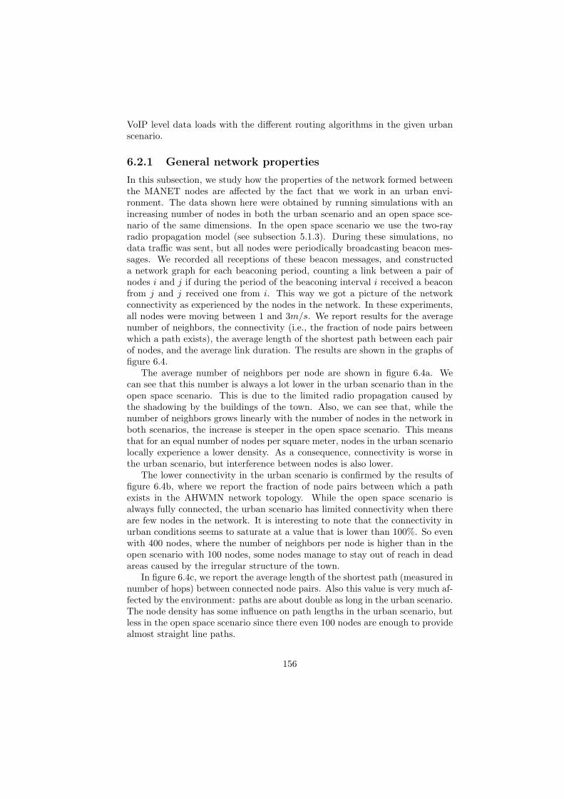
VoIP level data loads with the different routing algorithms in the given urbanscenario.

6.2.1 General network properties

In this subsection, we study how the properties of the network formed betweenthe MANET nodes are affected by the fact that we work in an urban envi-ronment. The data shown here were obtained by running simulations with anincreasing number of nodes in both the urban scenario and an open space sce-nario of the same dimensions. In the open space scenario we use the two-rayradio propagation model (see subsection 5.1.3). During these simulations, nodata traffic was sent, but all nodes were periodically broadcasting beacon mes-sages. We recorded all receptions of these beacon messages, and constructeda network graph for each beaconing period, counting a link between a pair ofnodes i and j if during the period of the beaconing interval i received a beaconfrom j and j received one from i. This way we got a picture of the networkconnectivity as experienced by the nodes in the network. In these experiments,all nodes were moving between 1 and 3m/s. We report results for the averagenumber of neighbors, the connectivity (i.e., the fraction of node pairs betweenwhich a path exists), the average length of the shortest path between each pairof nodes, and the average link duration. The results are shown in the graphs offigure 6.4.

The average number of neighbors per node are shown in figure 6.4a. Wecan see that this number is always a lot lower in the urban scenario than in theopen space scenario. This is due to the limited radio propagation caused bythe shadowing by the buildings of the town. Also, we can see that, while thenumber of neighbors grows linearly with the number of nodes in the network inboth scenarios, the increase is steeper in the open space scenario. This meansthat for an equal number of nodes per square meter, nodes in the urban scenariolocally experience a lower density. As a consequence, connectivity is worse inthe urban scenario, but interference between nodes is also lower.

The lower connectivity in the urban scenario is confirmed by the results offigure 6.4b, where we report the fraction of node pairs between which a pathexists in the AHWMN network topology. While the open space scenario isalways fully connected, the urban scenario has limited connectivity when thereare few nodes in the network. It is interesting to note that the connectivity inurban conditions seems to saturate at a value that is lower than 100%. So evenwith 400 nodes, where the number of neighbors per node is higher than in theopen scenario with 100 nodes, some nodes manage to stay out of reach in deadareas caused by the irregular structure of the town.

In figure 6.4c, we report the average length of the shortest path (measured innumber of hops) between connected node pairs. Also this value is very much af-fected by the environment: paths are about double as long in the urban scenario.The node density has some influence on path lengths in the urban scenario, butless in the open space scenario since there even 100 nodes are enough to providealmost straight line paths.

156

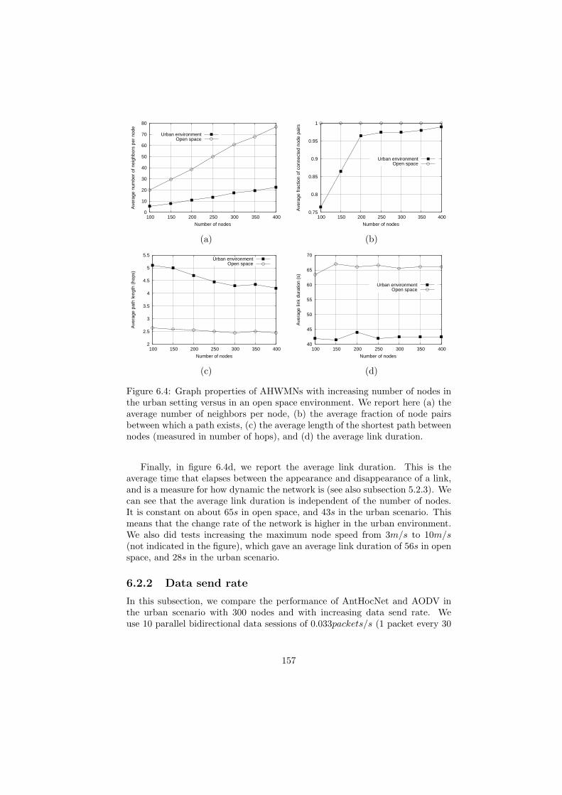
0

10

20

30

40

50

60

70

80

100 150 200 250 300 350 400

Ave

rage

num

ber

of n

eigh

bors

per

nod

e

Number of nodes

Urban environmentOpen space

0.75

0.8

0.85

0.9

0.95

1

100 150 200 250 300 350 400

Ave

rage

frac

tion

of c

onne

cted

nod

e pa

irs

Number of nodes

Urban environmentOpen space

(a) (b)

2

2.5

3

3.5

4

4.5

5

5.5

100 150 200 250 300 350 400

Ave

rage

pat

h le

ngth

(ho

ps)

Number of nodes

Urban environmentOpen space

40

45

50

55

60

65

70

100 150 200 250 300 350 400

Ave

rage

link

dur

atio

n (s

)

Number of nodes

Urban environmentOpen space

(c) (d)

Figure 6.4: Graph properties of AHWMNs with increasing number of nodes inthe urban setting versus in an open space environment. We report here (a) theaverage number of neighbors per node, (b) the average fraction of node pairsbetween which a path exists, (c) the average length of the shortest path betweennodes (measured in number of hops), and (d) the average link duration.

Finally, in figure 6.4d, we report the average link duration. This is theaverage time that elapses between the appearance and disappearance of a link,and is a measure for how dynamic the network is (see also subsection 5.2.3). Wecan see that the average link duration is independent of the number of nodes.It is constant on about 65s in open space, and 43s in the urban scenario. Thismeans that the change rate of the network is higher in the urban environment.We also did tests increasing the maximum node speed from 3m/s to 10m/s(not indicated in the figure), which gave an average link duration of 56s in openspace, and 28s in the urban scenario.

6.2.2 Data send rate

In this subsection, we compare the performance of AntHocNet and AODV inthe urban scenario with 300 nodes and with increasing data send rate. Weuse 10 parallel bidirectional data sessions of 0.033packets/s (1 packet every 30

157

0.6

0.65

0.7

0.75

0.8

0.85

0.9

0.95

0.033 2 5 10 25

Pac

ket d

eliv

ery

ratio

Packet generation frequency (packets/s)

AntHocNetAODV

0

0.1

0.2

0.3

0.4

0.5

0.6

0.033 2 5 10 25

Ave

rage

end

-to-

end

pack

et d

elay

(se

c)

Packet generation frequency (packets/s)

AntHocNetAODV

(a) (b)

0.1

0.2

0.3

0.4

0.5

0.6

0.7

0.8

0.9

1

1.1

0.033 2 5 10 25

Ave

rage

del

ay ji

tter

(sec

)

Packet generation frequency (packets/s)

AntHocNetAODV

0

200

400

600

800

1000

0.033 2 5 10 25

Ove

rhea

d in

num

ber

of p

acke

ts

Packet generation frequency (packets/s)

AntHocNetAODV

(c) (d)

0

200

400

600

800

1000

0.033 2 5 10 25

Ove

rhea

d in

num

ber

of b

ytes

Packet generation frequency (packets/s)

AntHocNetAODV

(e)

Figure 6.5: Results for AntHocNet and AODV with increasing data send ratesin the urban scenario. We report (a) delivery ratio, (b) average end-to-end delay,(c) average delay jitter, (d) overhead in number of packets, and (e) overhead innumber of bytes.

seconds, corresponding to slow interactive SMS data load) up to 25packets/s(corresponding to the data load needed to support good quality VoIP communi-cation data load), using as intermediate values 0.2, 0.5, 1, 2, 5 and 10packets/s.Like in the comparative tests of section 5.2, we report the delivery ratio, theaverage end-to-end delay, the average delay jitter, the overhead ratio in number

158

of packets, and the overhead ratio in number of bytes. All results are shown infigure 6.5.

When considering delivery ratio and delay (figure 6.5a and 6.5b), we cansee that both algorithms have bad performance for the lowest data rates, betterperformance at intermediate rates, and worse performance again for the highestrates. The bad performance at the lowest rates is due to the fact that both Ant-HocNet and AODV need to set up a route between source and destination priorto communication. When data packets are sent sporadically, previously con-structed routes can rarely be reused, and new route setups are often necessary.As data rates increase, subsequent packets can profit from previous route setups.In AntHocNet, where routes are proactively maintained and therefore remainvalid for longer, this effect is visible at lower rates than for AODV. For thehighest rates, both algorithms have a decrease in performance, because the highload of data packets starts to interfere with the control packets. In general, wecan see that AntHocNet outperforms AODV for most data rates (except for thedelay at the highest data rate). Considering that the urban scenario has longerpaths and less good connectivity than a comparable open space scenario, thisresult was to be expected, as it was shown in subsections 5.2.6 and 5.2.7 thatAntHocNet performs well under such conditions. When we compare directlywith the results for varying data send rates in open space scenarios presentedin subsection 5.2.4, we can see that both algorithms are better able to deliverthe highest data rates in the urban scenario (especially for AODV the differenceis large). This is on the one hand because we use only 10 sessions here (seealso further in subsection 6.2.3), and on the other hand because there is lessinterference due to the shadowing by the buildings. Nevertheless, it must benoted that neither of the algorithms is able to provide a delivery ratio that issufficient to support a VoIP application (see also further in subsection 6.2.6).

When considering average delay jitter, we can see more or less monotonicallydecreasing values for both algorithms, with a slight advantage for AntHocNet.The fact that jitter improves with increasing data rates is due to the fact that asdata packets are sent more frequently, subsequent packets travel closer after eachother, and therefore encounter more similar conditions. Hence, the differencesin their delays are smaller. A similar effect was visible in the comparative testsin the open space scenarios of subsection 5.2.4. However, in those tests, jittervalues only decreased for the lowest values for the data rate, and then startedto increase. It must be pointed out that in absolute terms, the jitter values inthe city scenario are much higher for the lowest data rates (due to the worseconnectivity and the longer path lengths), and that therefore more improvementis possible.

In terms of both overhead measures, we can observe monotonically improvingperformances for both algorithms. This is because of the earlier mentioned effectthat at low data rates, routes practically need to be rebuilt for each data packet,whereas at higher rates, subsequent packets can profit from earlier route setups.Especially AntHocNet produces high overhead for the lowest data rates. This isbecause its mechanisms to proactively maintain routes create a lot of overheadcompared to the number of packets that are delivered. For the higher data rates,

159

both algorithms have similar overhead ratios. AntHocNet slightly outperformsAODV in overhead in number of packets, but not in overhead in number ofbytes.

6.2.3 Number of data sessions

Here, we report the results of test in which we vary the number of data sessions,from 5 up to 25 sessions, with as intermediate values 10, 15 and 20 sessions.All data sessions are bidirectional. We did tests with two different values forthe data send rate: 5 and 10packets/s. In figure 6.6, we report delivery ratio,delay, jitter, overhead ratio in number of packets and overhead ratio in numberof bytes.

When considering delivery ratio (figure 6.6a) we can see that AntHocNetoutperforms AODV for all scenarios. Apart from that, we observe a com-mon trend for both algorithms under both data rates: performance monotoni-cally deteriorates when we increase the number of sessions. At the higher datarate of 10packets/s, this deterioration is more clear than at the lower rate of5packets/s: at 10packets/s, AntHocNet’s delivery ratio goes down from 93%for 5 sessions to 57% for 25 sessions, and AODV’s delivery ratio from 77% for5 sessions to 43% for 25 sessions. The larger difficulties experienced by bothalgorithms when more data sessions and high data rates are used are in linewith the open space results of subsections 5.2.4 and 5.2.5. They confirm thatthe ability of both algorithms to deal better with high data rates in the urbanscenario, as was observed in subsection 6.2.2, was at least in part due to thefact that we used less sessions.

When considering average end-to-end delay (figure 6.6b) and average delayjitter (figure 6.6c), we observe similar trends as for the delivery ratio: AntHoc-Net consistently outperforms AODV, performance for both algorithms deterio-rates monotonically with increasing numbers of sessions, and the deterioration ismore pronounced at the higher data rate of 10packets/s. The end-to-end delayof AODV shows a particulary bad increase for the highest numbers of sessions.This pattern is similar to the bad results we observed for AODV in the openspace scenarios of subsections 5.2.4 and 5.2.5. Also in those tests, AODV hadmuch more difficulties than AntHocNet when dealing with increasing numbersof sessions.

Finally, when looking at both overhead measures (figures 6.6d and 6.6e), wecan see that the performance at the low data rate of 5packets/s stays stable forincreasing numbers of sessions, while for 10packets/s, it deteriorates. EspeciallyAODV shows a huge increase for both overhead measures for the highest numberof sessions. This extra overhead is responsible for AODV’s increase in averageend-to-end delay. It confirms that AODV’s purely reactive approach, wherebynew route setups are frequently needed, does not scale well with increasingnumbers of sessions.

160

0.4

0.5

0.6

0.7

0.8

0.9

1

5 10 15 20 25

Pac

ket d

eliv

ery

ratio

Number of bidirectional data sessions

AntHocNet 10AODV 10

AntHocNet 5AODV 5

0

0.1

0.2

0.3

0.4

0.5

0.6

0.7

0.8

0.9

5 10 15 20 25

Ave

rage

end

-to-

end

pack

et d

elay

(se

c)

Number of bidirectional data sessions

AntHocNet 10AODV 10

AntHocNet 5AODV 5

(a) (b)

0.25

0.3

0.35

0.4

0.45

0.5

0.55

0.6

5 10 15 20 25

Ave

rage

del

ay ji

tter

(sec

)

Number of bidirectional data sessions

AntHocNet 10AODV 10

AntHocNet 5AODV 5

0

50

100

150

200

250

300

350

400

5 10 15 20 25

Ove

rhea

d in

num

ber

of p

acke

ts

Number of bidirectional data sessions

AntHocNet 10AODV 10

AntHocNet 5AODV 5

(c) (d)

0

20

40

60

80

100

120

5 10 15 20 25

Ove

rhea

d in

num

ber

of b

ytes

Number of bidirectional data sessions

AntHocNet 10AODV 10

AntHocNet 5AODV 5

(e)

Figure 6.6: Results for AntHocNet and AODV with increasing number of datasessions in the urban scenario. We use data rates of 5 and 10 packets/s, indi-cated by different curves in the figure. We report (a) delivery ratio, (b) averageend-to-end delay, (c) average delay jitter, (d) overhead in number of packets,and (e) overhead in number of bytes.

6.2.4 Node density

In the tests reported on here, we increase the number of nodes from 100 to 400with increments of 50. This is similar to the tests of subsection 6.2.1. Since

161

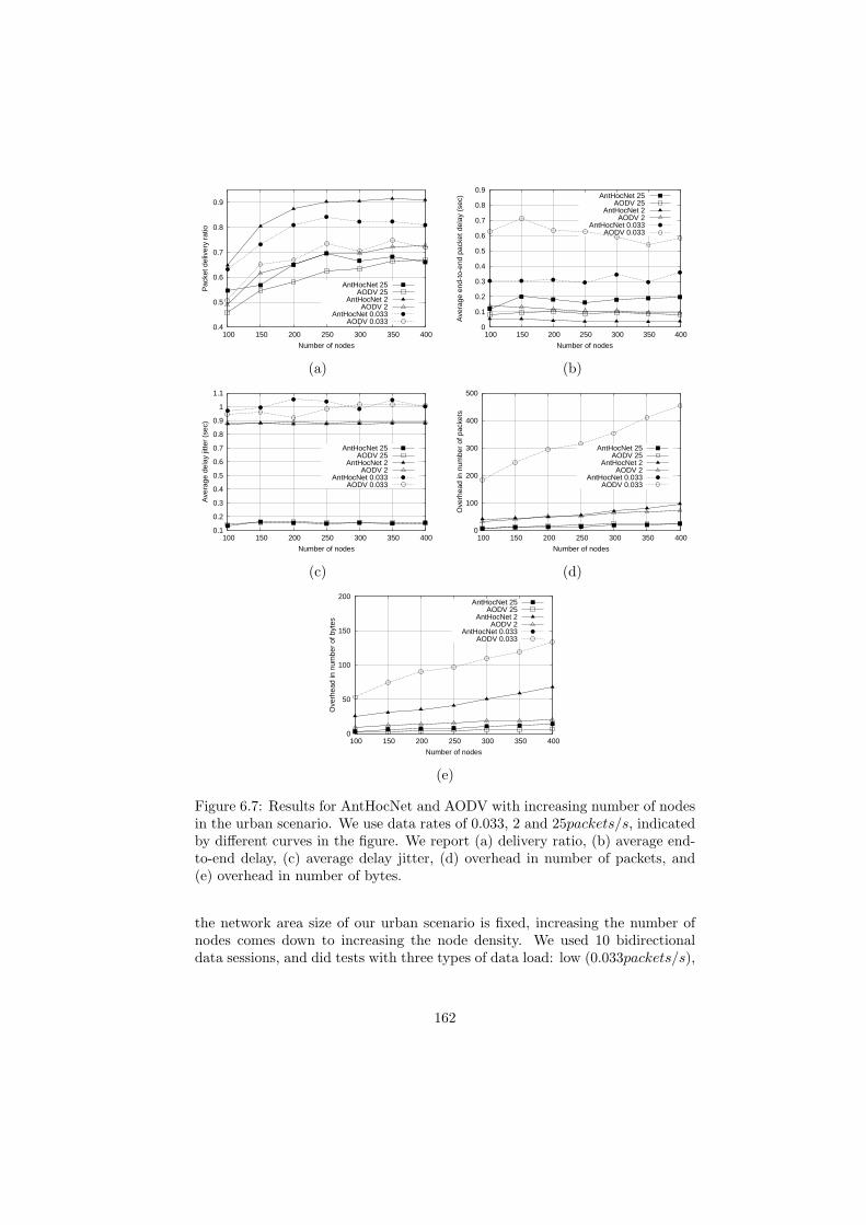
0.4

0.5

0.6

0.7

0.8

0.9

100 150 200 250 300 350 400

Pac

ket d

eliv

ery

ratio

Number of nodes

AntHocNet 25AODV 25

AntHocNet 2AODV 2

AntHocNet 0.033AODV 0.033

0

0.1

0.2

0.3

0.4

0.5

0.6

0.7

0.8

0.9

100 150 200 250 300 350 400

Ave

rage

end

-to-

end

pack

et d

elay

(se

c)

Number of nodes

AntHocNet 25AODV 25

AntHocNet 2AODV 2

AntHocNet 0.033AODV 0.033

(a) (b)

0.1

0.2

0.3

0.4

0.5

0.6

0.7

0.8

0.9

1

1.1

100 150 200 250 300 350 400

Ave

rage

del

ay ji

tter

(sec

)

Number of nodes

AntHocNet 25AODV 25

AntHocNet 2AODV 2

AntHocNet 0.033AODV 0.033

0

100

200

300

400

500

100 150 200 250 300 350 400

Ove

rhea

d in

num

ber

of p

acke

ts

Number of nodes

AntHocNet 25AODV 25

AntHocNet 2AODV 2

AntHocNet 0.033AODV 0.033

(c) (d)

0

50

100

150

200

100 150 200 250 300 350 400

Ove

rhea

d in

num

ber

of b

ytes

Number of nodes

AntHocNet 25AODV 25

AntHocNet 2AODV 2

AntHocNet 0.033AODV 0.033

(e)

Figure 6.7: Results for AntHocNet and AODV with increasing number of nodesin the urban scenario. We use data rates of 0.033, 2 and 25packets/s, indicatedby different curves in the figure. We report (a) delivery ratio, (b) average end-to-end delay, (c) average delay jitter, (d) overhead in number of packets, and(e) overhead in number of bytes.

the network area size of our urban scenario is fixed, increasing the number ofnodes comes down to increasing the node density. We used 10 bidirectionaldata sessions, and did tests with three types of data load: low (0.033packets/s),

162

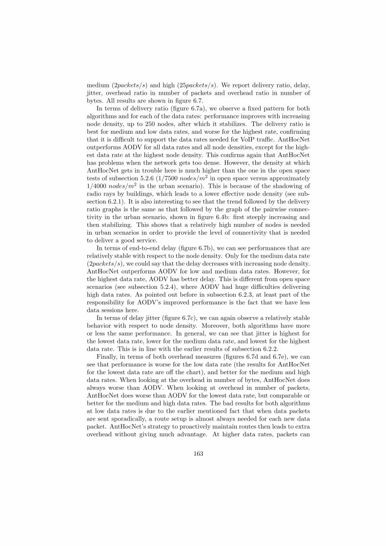
medium (2packets/s) and high (25packets/s). We report delivery ratio, delay,jitter, overhead ratio in number of packets and overhead ratio in number ofbytes. All results are shown in figure 6.7.

In terms of delivery ratio (figure 6.7a), we observe a fixed pattern for bothalgorithms and for each of the data rates: performance improves with increasingnode density, up to 250 nodes, after which it stabilizes. The delivery ratio isbest for medium and low data rates, and worse for the highest rate, confirmingthat it is difficult to support the data rates needed for VoIP traffic. AntHocNetoutperforms AODV for all data rates and all node densities, except for the high-est data rate at the highest node density. This confirms again that AntHocNethas problems when the network gets too dense. However, the density at whichAntHocNet gets in trouble here is much higher than the one in the open spacetests of subsection 5.2.6 (1/7500 nodes/m2 in open space versus approximately1/4000 nodes/m2 in the urban scenario). This is because of the shadowing ofradio rays by buildings, which leads to a lower effective node density (see sub-section 6.2.1). It is also interesting to see that the trend followed by the deliveryratio graphs is the same as that followed by the graph of the pairwise connec-tivity in the urban scenario, shown in figure 6.4b: first steeply increasing andthen stabilizing. This shows that a relatively high number of nodes is neededin urban scenarios in order to provide the level of connectivity that is neededto deliver a good service.

In terms of end-to-end delay (figure 6.7b), we can see performances that arerelatively stable with respect to the node density. Only for the medium data rate(2packets/s), we could say that the delay decreases with increasing node density.AntHocNet outperforms AODV for low and medium data rates. However, forthe highest data rate, AODV has better delay. This is different from open spacescenarios (see subsection 5.2.4), where AODV had huge difficulties deliveringhigh data rates. As pointed out before in subsection 6.2.3, at least part of theresponsibility for AODV’s improved performance is the fact that we have lessdata sessions here.

In terms of delay jitter (figure 6.7c), we can again observe a relatively stablebehavior with respect to node density. Moreover, both algorithms have moreor less the same performance. In general, we can see that jitter is highest forthe lowest data rate, lower for the medium data rate, and lowest for the highestdata rate. This is in line with the earlier results of subsection 6.2.2.

Finally, in terms of both overhead measures (figures 6.7d and 6.7e), we cansee that performance is worse for the low data rate (the results for AntHocNetfor the lowest data rate are off the chart), and better for the medium and highdata rates. When looking at the overhead in number of bytes, AntHocNet doesalways worse than AODV. When looking at overhead in number of packets,AntHocNet does worse than AODV for the lowest data rate, but comparable orbetter for the medium and high data rates. The bad results for both algorithmsat low data rates is due to the earlier mentioned fact that when data packetsare sent sporadically, a route setup is almost always needed for each new datapacket. AntHocNet’s strategy to proactively maintain routes then leads to extraoverhead without giving much advantage. At higher data rates, packets can

163

profit from earlier route setups, so that the overhead ratio can be reduced.AntHocNet’s mechanisms to proactively maintain paths augments this effect,so that the algorithm can get a lower overhead ratio when measured in numberof packets. However, the fact that AntHocNet uses larger hello messages aswell as larger control messages (forward and backward ants carry full paths,whereas AODV’s RREQ and RREP messages do not) causes a higher overheadwhen measured in number of bytes. Finally, we would like to point out that bothalgorithms experience increasing overhead for increasing numbers of nodes. Thisis because in networks with more nodes flooded control packets are forwardedmore times, and more hello messages are produced.

6.2.5 Node speed

In the experiments presented here, we vary the maximum node speed. Weincrease it from the 3m/s used in the previous tests up to 15m/s, which is areasonable maximum speed for cars in an urban environment. As intermediatevalues we use 6, 10 and 12.5m/s. We keep using 10 bidirectional data sessionsand again do tests with different data rates: a low rate of 0.033 packets persecond, a medium rate of 2 packets per second, and a high rate of 25 packetsper second. In figure 6.8, we report delivery ratio, end-to-end delay, delay jitter,overhead in number of packets and overhead in number of bytes.

As can be expected, delivery ratios (figure 6.8a) go down with increasingnode speeds under all data send rates for both algorithms. Apart from that, weget a confirmation of earlier results. Delivery ratios are highest for medium andlow data rates, and lowest for the highest data rate. AntHocNet delivers morepackets than AODV, except for the highest data rate, where delivery ratios arecomparable.

In terms of delay (figure 6.8b), we get a similar picture. Delay goes upwith increasing nodes speeds, although the effect is minimal. The best delaysare obtained for the low and medium data rates, and the worst for the highestrates. AntHocNet outperforms AODV at low and medium data rates, whileAODV is the best at the highest data rate.

In terms of jitter (figure 6.8c), the effect of the node speed is again minimal:both algorithms give more or less stable jitter for increasing node speeds at alldata rates. As in previous tests, jitter is highest for the lowest data rates andlower for the medium and high data rates. The performances of both algorithmsin terms of jitter are very comparable.

Finally, also for both overhead measures, we get familiar patterns. For bothmeasures, performances get slightly worse with increasing node speeds. Foroverhead in number of bytes, AODV outperforms AntHocNet at all data rates(the curve for the lowest data rate for AntHocNet is outside the range of thegraph). For overhead in number of packets, AODV outperforms AntHocNet forthe low and medium data rates, but not for the highest data rate.

In general, it is surprising to see that the effect of increasing the node speedis rather limited. This is of course partly because we considered only limitedranges of speed. However, using higher speeds would be unrealistic in the given

164

0.5

0.6

0.7

0.8

0.9

1

15 12 9 6 3

Pac

ket d

eliv

ery

ratio

Max node velocity (m/s)

AntHocNet 25AODV 25

AntHocNet 2AODV 2

AntHocNet 0.033AODV 0.033

0

0.1

0.2

0.3

0.4

0.5

0.6

0.7

0.8

0.9

15 12 9 6 3

Ave

rage

end

-to-

end

pack

et d

elay

(se

c)

Max node velocity (m/s)

AntHocNet 25AODV 25

AntHocNet 2AODV 2

AntHocNet 0.033AODV 0.033

(a) (b)

0.1

0.2

0.3

0.4

0.5

0.6

0.7

0.8

0.9

1

1.1

15 12 9 6 3

Ave

rage

del

ay ji

tter

(sec

)

Max node velocity (m/s)

AntHocNet 25AODV 25

AntHocNet 2AODV 2

AntHocNet 0.033AODV 0.033

0

100

200

300

400

500

15 12 9 6 3

Ove

rhea

d in

num

ber

of p

acke

ts

Max node velocity (m/s)

AntHocNet 25AODV 25

AntHocNet 2AODV 2

AntHocNet 0.033AODV 0.033

(c) (d)

0

50

100

150

200

15 12 9 6 3

Ove

rhea

d in

num

ber

of b

ytes

Max node velocity (m/s)

AntHocNet 25AODV 25

AntHocNet 2AODV 2

AntHocNet 0.033AODV 0.033

(e)

Figure 6.8: Results for AntHocNet and AODV with increasing maximum nodespeed in the urban scenario. We use data rates of 0.033, 2 and 25packets/s,indicated by different curves in the figure. We report (a) delivery ratio, (b)average end-to-end delay, (c) average delay jitter, (d) overhead in number ofpackets, and (e) overhead in number of bytes.

urban setting. It appears therefore that in this kind of urban scenarios, theeffect of the data send rate, the number of data sessions and the number ofnodes in the network is much more important than the effect of the node speed.

165

6.2.6 Supporting VoIP traffic data loads

In a final set of experiments, we investigate the issue of delivering sessions withVoIP level data rates. In 6.2.2, we saw that both algorithms have trouble whendata rates go up to VoIP levels: AntHocNet drops to a delivery ratio of 67% anda delay of 0.19s, while AODV has a delivery of 63% and a delay of 0.1s. Jitteris for both algorithms around 0.15s. To support good quality VoIP, a deliveryratio of 90% is needed, and end-to-end delay should not exceed 0.15s (see [189]).Jitter is normally considered in conjunction with delay, as applications deal withjitter by keeping packets in buffer for a short time before delivering them; jittercan therefore be added to delay to count towards the delay limit [189]. Usingthis approach, we can see that both in terms of delivery ratio and delay, thestandards needed to deliver good quality VoIP conversations are not met byeither of the algorithms. Here, we investigate this in more detail.

We do tests varying the number of data sessions from 1 to 10. All sessionsare bi-directional and send 25packets/s. The results are show in figure 6.9.When few sessions are started, we can see that AntHocNet manages to reachthe formulated VoIP requirements both in terms of delivery ratio and delay(when delay and jitter are added together). AODV on the other hand fallsshort on both requirements. Then, when the number of sessions is increased,also AntHocNet fails to reach the VoIP requirements.

These reported results are averages over all the started communication ses-sions though. In order to get a more precise view, we investigate for each scenariohow many of the individual sessions reach the cited requirements. In figure 6.10,we show this number (a) as a fraction of the total number of started sessions,and (b) in absolute terms. We can see that using AntHocNet, at least a few ofthe sessions can obtain VoIP quality. When only one session is started, it almostalways gets the required quality (in 90% of the cases, as shown in figure 6.10a).Then, as more sessions are started, the fraction of them that receive VoIP qual-ity decreases. However, in absolute terms, the total number of sessions thatreceive the required quality grows up to almost 2.5 when 4 sessions are started,and then remains more or less stable. Finally, when more than 7 sessions arestarted, the absolute number also decreases. When 10 sessions are started, onaverage about only 1 receives VoIP quality. This is because too many sessionsare interfering with each other. For AODV, the number of sessions receivingthe required service quality always remains low.

The results show that using AntHocNet it is in principle possible to supportVoIP in the given urban scenario. However, not all sessions can get the requiredlevels of service, and when too many sessions are started, all of them suffer.This indicates that it might be useful to refuse some sessions to start (e.g.,sessions that would likely not receive the required quality anyway, because theyneed paths that go through highly congested or poorly connected parts of thenetwork) in order to be able to deliver a good service to other sessions. Thispoints to the importance of the use of admission control or some other system forQuality-of-Service support in resource limited urban MANETs: if only sessionsthat are likely to get the levels of service they need are allowed to start, less

166

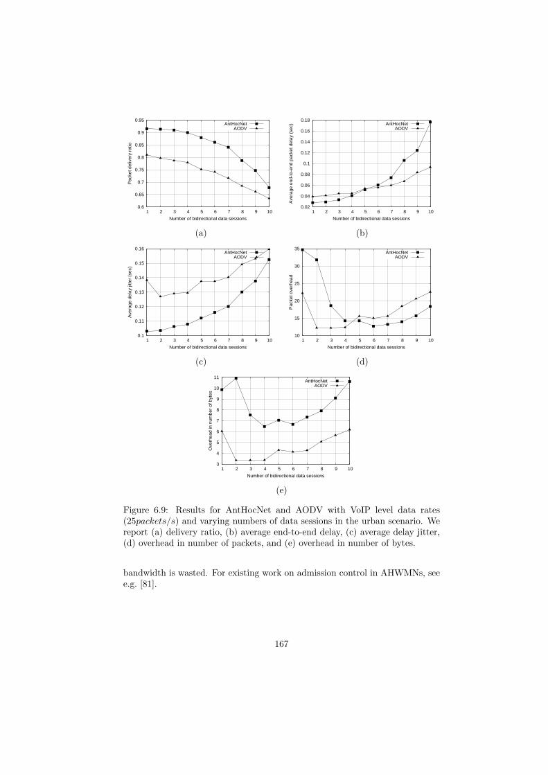
0.6

0.65

0.7

0.75

0.8

0.85

0.9

0.95

1 2 3 4 5 6 7 8 9 10

Pac

ket d

eliv

ery

ratio

Number of bidirectional data sessions

AntHocNetAODV

0.02

0.04

0.06

0.08

0.1

0.12

0.14

0.16

0.18

1 2 3 4 5 6 7 8 9 10

Ave

rage

end

-to-

end

pack

et d

elay

(se

c)

Number of bidirectional data sessions

AntHocNetAODV

(a) (b)

0.1

0.11

0.12

0.13

0.14

0.15

0.16

1 2 3 4 5 6 7 8 9 10

Ave

rage

del

ay ji

tter

(sec

)

Number of bidirectional data sessions

AntHocNetAODV

10

15

20

25

30

35

1 2 3 4 5 6 7 8 9 10

Pac

ket o

verh

ead

Number of bidirectional data sessions

AntHocNetAODV

(c) (d)

3

4

5

6

7

8

9

10

11

1 2 3 4 5 6 7 8 9 10

Ove

rhea

d in

num

ber

of b

ytes

Number of bidirectional data sessions

AntHocNetAODV

(e)

Figure 6.9: Results for AntHocNet and AODV with VoIP level data rates(25packets/s) and varying numbers of data sessions in the urban scenario. Wereport (a) delivery ratio, (b) average end-to-end delay, (c) average delay jitter,(d) overhead in number of packets, and (e) overhead in number of bytes.

bandwidth is wasted. For existing work on admission control in AHWMNs, seee.g. [81].

167

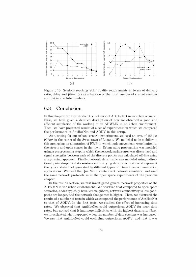
0

0.1

0.2

0.3

0.4

0.5

0.6

0.7

0.8

0.9

1 2 3 4 5 6 7 8 9 10Fra

ctio

n of

ses

sion

s re

achi

ng V

oIP

req

uire

men

ts

Number of data sessions

AntHocNetAODV

0

0.5

1

1.5

2

2.5

1 2 3 4 5 6 7 8 9 10Num

ber

of s

essi

ons

reac

hing

VoI

P r

equi

rem

ents

Number of data sessions

AntHocNetAODV

(a) (b)

Figure 6.10: Sessions reaching VoIP quality requirements in terms of deliveryratio, delay and jitter: (a) as a fraction of the total number of started sessionsand (b) in absolute numbers.

6.3 Conclusion

In this chapter, we have studied the behavior of AntHocNet in an urban scenario.First, we have given a detailed description of how we obtained a good andefficient simulation of the working of an AHWMN in an urban environment.Then, we have presented results of a set of experiments in which we comparedthe performance of AntHocNet and AODV in this setup.

As a setting for our urban scenario experiments, we used an area of 1561×997m2 in the center of the Swiss town of Lugano. We modeled node mobility inthis area using an adaptation of RWP in which node movements were limited tothe streets and open spaces in the town. Urban radio propagation was modeledusing a preprocessing step, in which the network surface area was discretized andsignal strengths between each of the discrete points was calculated off-line usinga raytracing approach. Finally, network data traffic was modeled using bidirec-tional point-to-point data sessions with varying data rates that could representthe typical data load generated by different types of interactive communicationapplications. We used the QualNet discrete event network simulator, and usedthe same network protocols as in the open space experiments of the previouschapter.

In the results section, we first investigated general network properties of theAHWMN in the urban environment. We observed that compared to open spacescenarios, nodes typically have less neighbors, network connectivity is less good,paths are longer, and the network change rate is higher. Then, we discussed theresults of a number of tests in which we compared the performance of AntHocNetto that of AODV. In the first tests, we studied the effect of increasing datarates. We observed that AntHocNet could outperform AODV for most datarates, but noticed that it had more difficulties with the highest data rate. Next,we investigated what happened when the number of data sessions was increased.We saw that AntHocNet could each time outperform AODV, and that it was

168

AODV that had large difficulties when the number of sessions became high.Then, we did tests with increasing number of nodes. Both algorithms had moredifficulties in networks with more nodes. AntHocNet outperformed AODV whenlow and medium data rates were used, but had more difficulties at the highestdata rate. After that, we also investigated what happened with increasing nodespeeds. We found that increasing the node speed had a relatively small negativeeffect on the performance of both algorithms. Finally, we considered whether itwould at all be possible to deliver the level of service needed to support VoIPconversations in the given scenario. Our conclusion is that using AntHocNet,it is in principle possible, if at least a mechanism is applied to control whichsessions are allowed to start.

169

Chapter 7

Towards theimplementation of adaptiverouting in AHWMNs

Most existing work on the development of routing algorithms for AHWMNs iscarried out in simulation, rather than in real deployment studies. This is alsothe case for the work that has been presented in this thesis. An important fac-tor that influences the choice for simulation as a research tool is that buildingan AHWMN testbed is expensive and requires a substantial effort, in whichmany technological issues need to be resolved. Simulation is often the only realoption for researchers who want to investigate a specific aspect of AHWMNssuch as routing. Moreover, simulation also gives other advantages, such as theease with which different and large test scenarios can be investigated, and thepossibility to easily repeat previous tests. Nevertheless, since a few years thereis a growing awareness in the AHWMN research community that simulation ex-periments have their limitations [54,117,124,260]. The main concern is that theabstractions and simplifications used in simulation studies can have a significantimpact on the network behavior, so that observed results can diverge from whatcan be expected in reality. Consequently, researchers are increasingly interestedin the use of real world testbeds to support research in AHWMNs. Several suchtestbeds have been set up, such as the Roofnet experiment of MIT [30] and theMagnets project of DTL [148].

In the current chapter, we describe work that we have done regarding theimplementation of adaptive routing in AHWMNs. We have developed a system,called MagAntA1, that is aimed at supporting adaptive routing in Linux basedAHWMNs. MagAntA runs as a daemon in user space. It is written in C, andpossesses a modular structure, which makes it easy to adapt and extend with

1The name MagAntA is derived from the Magnets testbed set up at DTL, the color magentaof the DTL logo, and the ants that formed the initial inspiration for the adaptive routingalgorithms we study.

170

new algorithms.In what follows, we first describe related work on AHWMN testbeds and

the implementation of AHWMN routing algorithms. Then, we describe ourMagAntA routing system. Finally, we discuss how MagAntA integrates withthe network protocol stack in the Linux kernel. The material described in thischapter was based on work carried out during an internship at DTL. It has beenpresented in [101].

7.1 On the deployment of AHWMNs

Here, we provide a general discussion on the deployment of AHWMNs. Wefirst discuss existing AHWMN testbeds. In particular, we give details aboutthe Magnets testbed of DTL, in order to give a concrete example of the kindof networks that MagAntA was developed for. Then, we discuss the implemen-tation of AHWMN routing algorithms. We first describe in general the kindof issues that need to be addressed when implementing a routing algorithm forAHWMNs. Then, we discuss existing implementations that have appeared inthe literature.

7.1.1 AHWMN testbeds

A number of AHWMN testbeds have been developed for research purposes anddescribed in the literature. These include the Roofnet project of MIT [30],the Magnets project of DTL [148], the BerlinRoofNet project run by studentsof Humboldt University in Berlin [1], the APE testbed of Uppsala Universityin Sweden [181], etc.. Most of these testbeds are WMNs, although the APEtestbed is meant for the deployment of MANETs. Apart from these researchtestbeds, a number of WMNs have also been deployed by local authorities inorder to provide services to the general public. These include WMN projects inTaipei [10] and Philadelphia [12]. Finally, some WMNs are arising in truly adhoc fashion from the voluntary efforts of computer enthusiasts. Examples of suchnetworks are the olsr.freifunk.net experiment in Berlin [9], and the FeuerFunkexperiment in Vienna and other Austrian cities [2]. Here, we discuss details ofthe Magnets research testbed of DTL. Magnets was the network that MagAntAwas in the first place developed for. Its description will help the reader to get aconcrete idea of the kind of environment we are working in.

The Magnets network is a WMN that is deployed in the center of Berlin.It contains a wireless backbone network of 5 nodes and a wireless mesh of 50nodes. The structure of the backbone network is shown in figure 7.1. It consistsof 5 mesh routers, with point-to-point links between them. The mesh routersare placed on top of tall buildings, so that they are in line of sight of eachother. The links between them are realized using directional antennas and arebased on 802.11 technology. Two of the links (the one between the T-Systemsand ETF buildings, and the one between the T-Labs and TC buildings) workat a frequency of 5Ghz, while the others work at a frequency of 2.4GHz. Be-

171

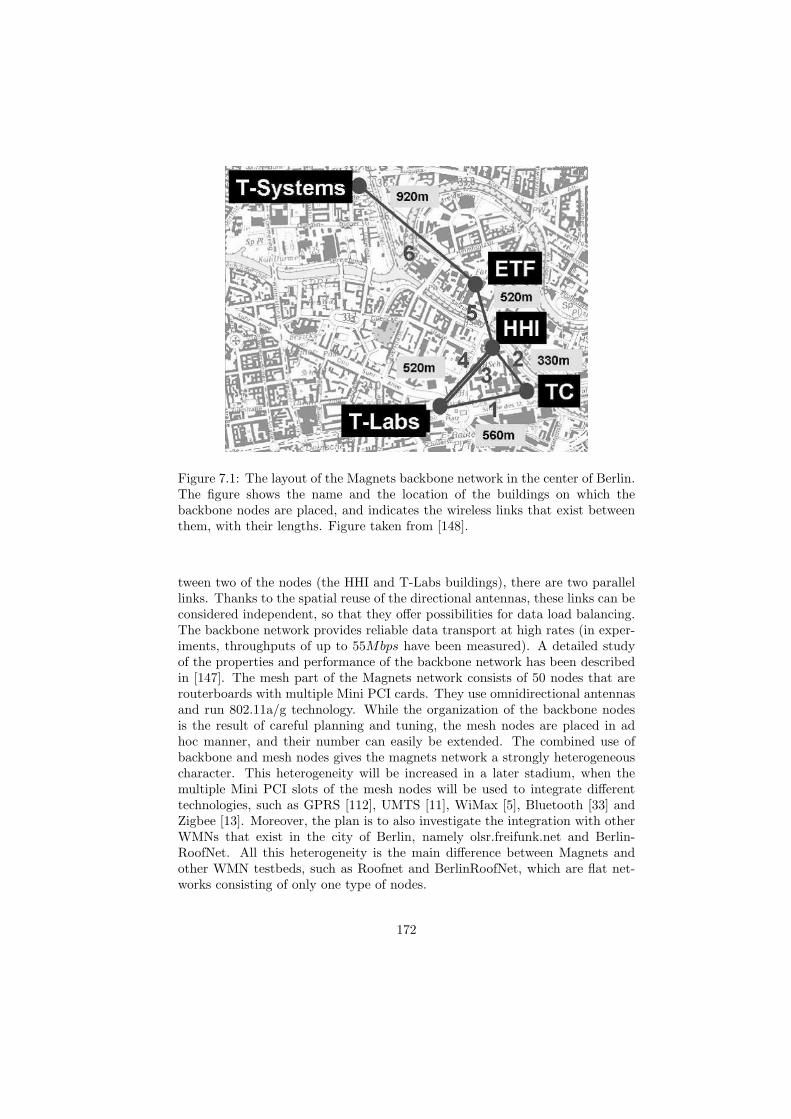
Figure 7.1: The layout of the Magnets backbone network in the center of Berlin.The figure shows the name and the location of the buildings on which thebackbone nodes are placed, and indicates the wireless links that exist betweenthem, with their lengths. Figure taken from [148].

tween two of the nodes (the HHI and T-Labs buildings), there are two parallellinks. Thanks to the spatial reuse of the directional antennas, these links can beconsidered independent, so that they offer possibilities for data load balancing.The backbone network provides reliable data transport at high rates (in exper-iments, throughputs of up to 55Mbps have been measured). A detailed studyof the properties and performance of the backbone network has been describedin [147]. The mesh part of the Magnets network consists of 50 nodes that arerouterboards with multiple Mini PCI cards. They use omnidirectional antennasand run 802.11a/g technology. While the organization of the backbone nodesis the result of careful planning and tuning, the mesh nodes are placed in adhoc manner, and their number can easily be extended. The combined use ofbackbone and mesh nodes gives the magnets network a strongly heterogeneouscharacter. This heterogeneity will be increased in a later stadium, when themultiple Mini PCI slots of the mesh nodes will be used to integrate differenttechnologies, such as GPRS [112], UMTS [11], WiMax [5], Bluetooth [33] andZigbee [13]. Moreover, the plan is to also investigate the integration with otherWMNs that exist in the city of Berlin, namely olsr.freifunk.net and Berlin-RoofNet. All this heterogeneity is the main difference between Magnets andother WMN testbeds, such as Roofnet and BerlinRoofNet, which are flat net-works consisting of only one type of nodes.

172

7.1.2 Implementations of AHWMN routing algorithms

When implementing a routing algorithm for AHWMN deployment, one has todeal with a number of important issues [38]. A first of these is addressing.WMN nodes should be able to identify themselves even before IP addresses areassigned. This is not so much a problem for mesh routers such as the nodesin the Magnets backbone network, but it is for mesh nodes that are connectedto the network in ad hoc fashion. For these nodes, connectivity to a serverproviding IP addresses cannot always be guaranteed. Moreover, some form ofrouting will need to be performed to reach such a server. Therefore, addressauto-configuration is important. A second issue is the integrated use of the dif-ferent wireless interfaces available on each node. A node that has for example abluetooth interface and an 802.11 interface will have different neighbors on eachof these two interfaces, so that it in fact takes part in two different networks.These different networks should be integrated to form one AHWMN. A thirdissue is the integration with the existing TCP/IP network protocol stack andthe routing protocols therein. AHWMNs often need to connect to other net-works (e.g., the Internet), running traditional routing protocols such as OSPFor RIP (see section 3.1). It is important that these protocols integrate smoothlywith the AHWMN routing protocol. Finally, an important aspect for any sys-tem addressing these issues is that it should require minimal or no changes toexisting operating systems and firmware, in order to provide easy installationand portability.

A number of approaches to implement AHWMN routing functionality haveappeared in the literature. Here, we give a short description of the most inter-esting ones. We give special attention to how they deal with the different issueslisted above.

The first implementation of an AHWMN routing protocol that was madepublicly available is Mad-hoc AODV [174], an implementation of AODV for useunder Linux. In this implementation, all code runs in user space, and no mod-ifications whatsoever are made to the Linux kernel. This means that Mad-hocAODV can get only limited feedback about what is going on inside the kerneland in particular inside the routing layer in the network protocol stack. It dealswith this problem by making use of snooping: it monitors what kind of packetsare being sent out by the kernel and derives from that which routing informationis needed and which actions should be taken. For example, to find out that anew route setup is needed, Mad-hoc AODV checks for request packets sent outby the Address Resolution Protocol (ARP) [215]. ARP is a protocol used inbroadcast type networks such as Ethernet in order to map IP addresses to MACaddresses: when a node does not know the MAC address that corresponds to agive IP address, it uses ARP to find this out. Therefore, when Mad-hoc AODVobserves that the local node is sending out an ARP request message, it infersthat the node does not know how to reach a certain destination, and reacts tothis with the transmission of an AODV RREQ. Once it has obtained a route, itupdates the routing tables in IP. In a similar way, all other AODV events are de-rived from packet snooping. The functions needed to perform snooping, as well

173

as the functions to update IP routing tables, exist in the kernel and are availableto user space programs. The approach of making absolutely no modificationsto the kernel gives Mad-hoc AODV the advantages that code development andinstallation are easy, and that it is portable across different systems. There arehowever several disadvantages. In the first place, the approach is quite ineffi-cient. In the example of the snooping of ARP requests to define the need for aroute setup, it is clear that the sending of the ARP request is not needed andleads to extra overhead. A second disadvantage is that the system is dependenton the working of ARP and IP and the synchronization between them. Apartfrom these disadvantages, we point out that also other issues, including addressauto-configuration, the integration of different network views, and the integra-tion with other networks, are not dealt with in this system. Moreover, Mad-hocAODV was found to contain several severe bugs (see e.g. [199]). Now, it is nolonger supported or distributed.

In [57], the authors present an different implementation of the AODV rout-ing algorithm, called AODV-UCSB. This implementation makes use of Netfil-ter [144], a packet filtering framework that is available inside Linux. Netfilterconsists of a number of hooks that are present at various points in the Linuxnetwork protocol stack. Data packets traversing any of these hooks are divertedto functions in user defined kernel modules, where they can be examined, modi-fied, queued or dropped. In the case of AODV-UCSB, a kernel module is definedthat stores incoming and outgoing data packets until a routing decision is takenfor them. The actual routing is done by a daemon running in user space, whichacts upon the stored data packets. This way, the use of other routing algo-rithms is circumvented. An advantage of this approach is that the routing coderunning in user space can easily be adapted and modified, while the necessarykernel code is limited to the definition of a kernel module, which is easier toinstall and port than a kernel modification [216]. A disadvantage of the ap-proach is that it does not include solutions for integration with other networks,for address auto-configuration, and for the integrated use of different networkinterfaces. A different implementation of AODV that follows a similar approachto AODV-UCSB is AODV-UU [181]. In its newest versions, this system doesinclude solutions for addressing and integration with other networks.

In [69], yet another implementation of AODV is described. Here, AODV isimplemented as an extension inside ARP. As explained before, the ARP pro-tocol allows nodes in broadcast networks to find out the MAC address that isassociated with a certain IP address. In the normal mode of operation, a re-questing node A broadcasts an ARP request message with the IP address of anode B. If B receives the message (i.e., a node with the requested IP addressexists on the same broadcast network), it sends back an ARP reply messagecontaining its MAC address, and A can start sending to B. A special case iswhen B exists in a different network that is connected to A’s network via agateway node G. G can then answer to A’s ARP request, and A maps B’s IPaddress to G’s MAC address, indicating that all packets for B need to be sentto G. This technique is called Proxy ARP [48]. It allows communication withremote nodes in a way that is transparent to the routing algorithm at the IP

174

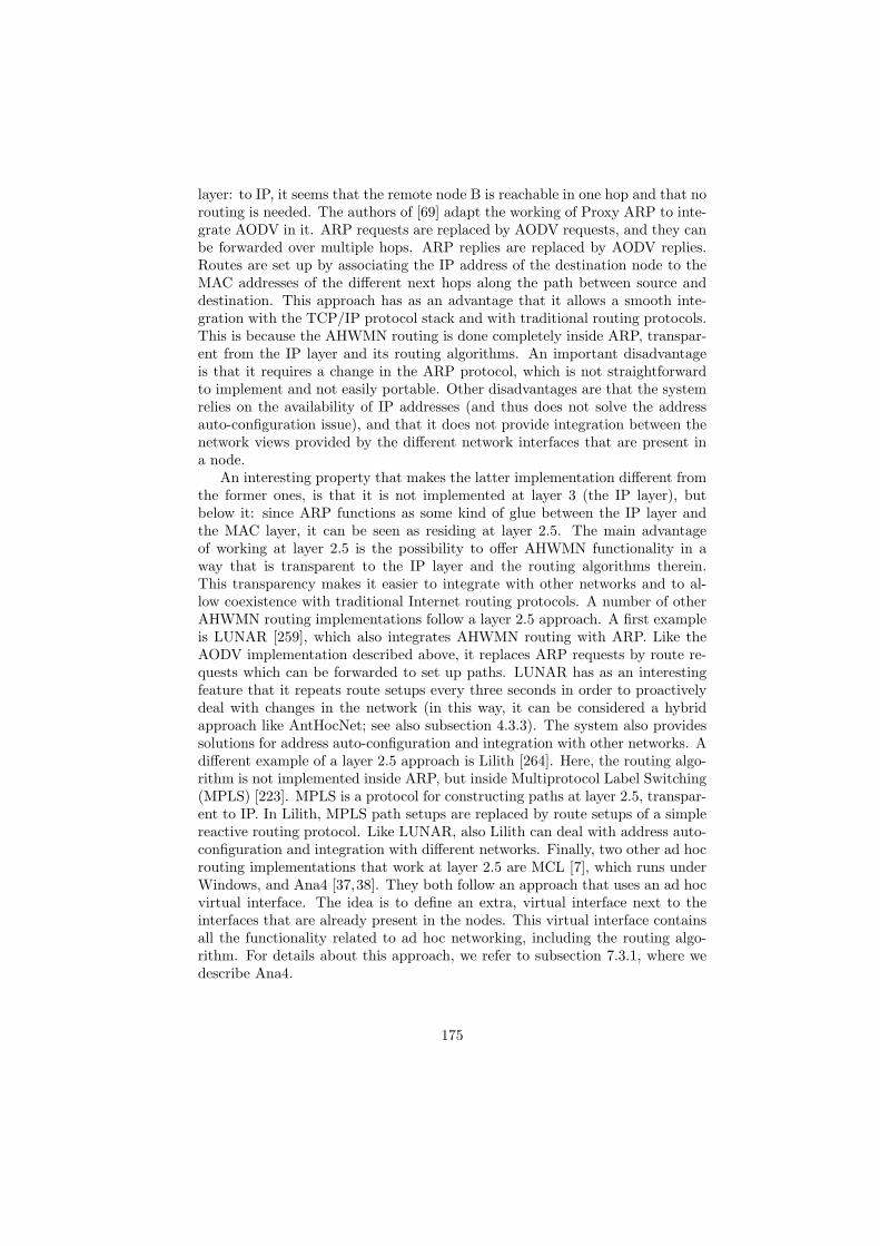
layer: to IP, it seems that the remote node B is reachable in one hop and that norouting is needed. The authors of [69] adapt the working of Proxy ARP to inte-grate AODV in it. ARP requests are replaced by AODV requests, and they canbe forwarded over multiple hops. ARP replies are replaced by AODV replies.Routes are set up by associating the IP address of the destination node to theMAC addresses of the different next hops along the path between source anddestination. This approach has as an advantage that it allows a smooth inte-gration with the TCP/IP protocol stack and with traditional routing protocols.This is because the AHWMN routing is done completely inside ARP, transpar-ent from the IP layer and its routing algorithms. An important disadvantageis that it requires a change in the ARP protocol, which is not straightforwardto implement and not easily portable. Other disadvantages are that the systemrelies on the availability of IP addresses (and thus does not solve the addressauto-configuration issue), and that it does not provide integration between thenetwork views provided by the different network interfaces that are present ina node.

An interesting property that makes the latter implementation different fromthe former ones, is that it is not implemented at layer 3 (the IP layer), butbelow it: since ARP functions as some kind of glue between the IP layer andthe MAC layer, it can be seen as residing at layer 2.5. The main advantageof working at layer 2.5 is the possibility to offer AHWMN functionality in away that is transparent to the IP layer and the routing algorithms therein.This transparency makes it easier to integrate with other networks and to al-low coexistence with traditional Internet routing protocols. A number of otherAHWMN routing implementations follow a layer 2.5 approach. A first exampleis LUNAR [259], which also integrates AHWMN routing with ARP. Like theAODV implementation described above, it replaces ARP requests by route re-quests which can be forwarded to set up paths. LUNAR has as an interestingfeature that it repeats route setups every three seconds in order to proactivelydeal with changes in the network (in this way, it can be considered a hybridapproach like AntHocNet; see also subsection 4.3.3). The system also providessolutions for address auto-configuration and integration with other networks. Adifferent example of a layer 2.5 approach is Lilith [264]. Here, the routing algo-rithm is not implemented inside ARP, but inside Multiprotocol Label Switching(MPLS) [223]. MPLS is a protocol for constructing paths at layer 2.5, transpar-ent to IP. In Lilith, MPLS path setups are replaced by route setups of a simplereactive routing protocol. Like LUNAR, also Lilith can deal with address auto-configuration and integration with different networks. Finally, two other ad hocrouting implementations that work at layer 2.5 are MCL [7], which runs underWindows, and Ana4 [37,38]. They both follow an approach that uses an ad hocvirtual interface. The idea is to define an extra, virtual interface next to theinterfaces that are already present in the nodes. This virtual interface containsall the functionality related to ad hoc networking, including the routing algo-rithm. For details about this approach, we refer to subsection 7.3.1, where wedescribe Ana4.

175

7.2 The MagAntA routing system

In this section, we describe the MagAntA routing system. First, we presentthe general structure of the system. Then, we discuss each of its differentcomponents separately. These are the control module, the routing interface andthe routing module. We conclude the section with a description of the adaptiverouting algorithm that is currently implemented in MagAntA.

7.2.1 The program structure

A schematic representation of the MagAntA routing system is shown in fig-ure 7.2. It consists of a daemon that runs in user space. The advantage ofworking in user space as opposed to kernel space is that coding and debuggingis easier, while a disadvantage is that the system’s working is less efficient. Weopted for this approach because we see MagAntA mainly as a research tool,rather than a finished product for routing.

User space

Kernel space

MagAntA routing daemon

Routing module

Control module

Routing interface

Data packets Control packets

Figure 7.2: The structure of the MagAntA routing system.

The MagAntA routing daemon performs routing on a per packet basis, mean-ing that it provides a new routing decision for each data packet. This givesmaximum flexibility to the system, and allows to implement adaptive routingstrategies such as probabilistic data forwarding. In order to implement perpacket routing, MagAntA relies on kernel modules that send all data packetsup to user space. These kernel modules are developed independently by fellow

176

researchers at DTL and are therefore described separately in section 7.3; herewe focus our attention on the user space routing daemon.

Internally, the program structure of MagAntA consists of two main modules:the control module, which provides basic functionality that is needed for anyrouting algorithm, and the routing module, which contains the actual routinglogic. The two modules communicate through a simple interface, which wecall the routing interface. The advantage of this modular structure is that therouting algorithm code can be developed independently from technical issues.Below, we describe each of the two modules and the interface. For a moredetailed account of the system, we refer to the related technical report [100].

7.2.2 The control module

The function of the control module is to sustain the working of the daemonand to provide basic functionality to the routing module. The daemon is im-plemented using an infinite for-loop, in which the program waits for differentevents to take place. In particular, it waits for data packets coming from thekernel, for incoming control packets, for routing events timing out, and for userinterrupts (which can be used to pause the daemon). When either of thesehappen, it takes the appropriate actions.

The functionality provided by the control module to the routing module in-cludes four basic services. The first is to gather information about the localhost, such as the available network interfaces and their MAC addresses, the lo-cal IP address (if it is available), etc.. It presents this information to the routingmodule, so that it can be used by the routing algorithm. The second service isthe transfer of data packets to and from the kernel. For this part, it commu-nicates with kernel modules that send packets up to user space. Details aboutthese kernel modules are given in section 7.3. The control module deals with thetechnical issues involved in interacting with the kernel modules and hides thesefrom the routing module. Upon reception of a data packet, it stores the packetin a static buffer, and provides the routing module with pointers to fields in thepacket headers that are relevant for routing, such as the destination address,the next hop address, the outgoing interface, etc.. The routing algorithm canthen work directly with these pointers without being aware of the structure ofthe data packets or their headers. The third service is the sending and receivingof control packets. For this service, the control module communicates directlywith the device drivers of the different network interfaces in the kernel. Thisis done through the use of raw packet sockets that are standard available inthe kernel [244]; no kernel modules or modifications are needed. To the routingmodule, several different possibilities to transmit control packets are provided.These include unicast and broadcast transmission, as well as delayed broadcasttransmission, in which the control packet is broadcast after a short randomjitter (this is useful for the implementation of flooding). The fourth service isevent scheduling. The control module keeps an event list, to which the routingmodule can add any event that it needs. Whenever an event times out, thecontrol module calls the event handling function of the routing module.

177

7.2.3 The routing interface

The function of the routing interface is to form a bridge between the controlmodule, which provides basic functionality, and the routing module, which con-tains the routing protocol logic. Its most important component is the rout-ing interface structure, which defines all communication possibilities betweenthe two modules. Apart from this structure, the routing interface code containsalso a number of other structures and functions that provide useful function-alities for the routing module. These include functions to copy and compareaddresses and time structures.

The contents of the routing interface structure are shown in figure 7.3 (somedetails, such as the parameters taken by each of the functions, are left out hereto improve readability). It contains a pointer to a local data structure anda number of function pointers. The local data structure contains informationabout the local host, and is filled in by the control module. It contains the nameof the local host, its IP address, the IP, ad hoc and MAC broadcast addresses,and the list of devices available for ad hoc routing, with their names and MACaddresses. This is basic information that is needed by the routing module. Thefunction pointers of routing interface are used for the communication betweenthe control module and the routing module. The first half of these pointers arefilled in by the control module, in order to allow the routing module to make useof the functionality it provides. They include a function to send data packets tothe kernel (either to be delivered locally or to be forwarded), different functionsto send control packets over the network (see subsection 7.2.2), a function toschedule events, and one to remove previously scheduled events. The other halfof the function pointers are filled in by the routing module. They allow thecontrol module to call the routing module whenever needed. They include afunction to initialize the routing algorithm and one to start it, a function todeliver received data packets to the routing algorithm, one to deliver receivedcontrol packets to it, and one to pass it events that have timed out.

7.2.4 The routing module

The routing module contains the actual routing code. Since lower level technicalissues are taken care of by the control module, this code can concentrate on thealgorithm logic. The routing interface provides a clear definition for the inter-actions between the routing module and the control module, which simplifiesthe design and integration of new routing algorithms. On the one hand, theinterface describes the functions that are provided by the control module andcan be used by the routing module (the top half of the function pointers shownin figure 7.3). On the other hand, it describes the functions that the routingmodule needs to implement so that the control module can call it (the lower halfof the function pointers shown in figure 7.3). To integrate a new algorithm intothe system, it is sufficient to provide implementations for these latter functionsand initialize the function pointers with them. Currently, we have implementedone adaptive routing algorithm in the routing module of MagAntA, which we

178

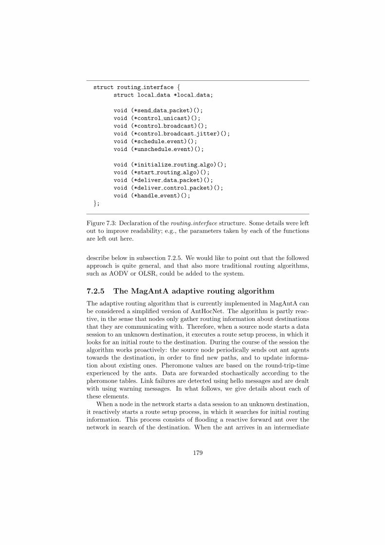
struct routing interface {struct local data *local data;

void (*send data packet)();void (*control unicast)();void (*control broadcast)();void (*control broadcast jitter)();void (*schedule event)();void (*unschedule event)();

void (*initialize routing algo)();void (*start routing algo)();void (*deliver data packet)();void (*deliver control packet)();void (*handle event)();

};

Figure 7.3: Declaration of the routing interface structure. Some details were leftout to improve readability; e.g., the parameters taken by each of the functionsare left out here.

describe below in subsection 7.2.5. We would like to point out that the followedapproach is quite general, and that also more traditional routing algorithms,such as AODV or OLSR, could be added to the system.

7.2.5 The MagAntA adaptive routing algorithm

The adaptive routing algorithm that is currently implemented in MagAntA canbe considered a simplified version of AntHocNet. The algorithm is partly reac-tive, in the sense that nodes only gather routing information about destinationsthat they are communicating with. Therefore, when a source node starts a datasession to an unknown destination, it executes a route setup process, in which itlooks for an initial route to the destination. During the course of the session thealgorithm works proactively: the source node periodically sends out ant agentstowards the destination, in order to find new paths, and to update informa-tion about existing ones. Pheromone values are based on the round-trip-timeexperienced by the ants. Data are forwarded stochastically according to thepheromone tables. Link failures are detected using hello messages and are dealtwith using warning messages. In what follows, we give details about each ofthese elements.

When a node in the network starts a data session to an unknown destination,it reactively starts a route setup process, in which it searches for initial routinginformation. This process consists of flooding a reactive forward ant over thenetwork in search of the destination. When the ant arrives in an intermediate

179

node, this node’s address is added to the ant, and the ant is forwarded. Theforwarding at intermediate nodes is normally done by broadcasting, unless theant is in a node where routing information to its destination is available. In thatcase, the ant is unicast to a stochastically chosen next hop. The probability ofchoosing a next hop n is given in formula 7.1.

Pnd =(τnd)β1

∑j∈N (τjd)β1

(7.1)

In this formula, τnd is the pheromone associated with neighbor n and desti-nation d. By raising it to a power β1, exploration can be encouraged (β1 < 1)or limited (β1 > 1). When a copy of the forward ant reaches the destination,a backward ant retraces the forward path and updates the routing tables of in-termediate nodes. In this way an initial route is established between the sourceand destination of the session.

During the course of the session, the source node proactively tries to improveand extend existing routing information. To this end, it periodically sends outproactive forward ants to sample existing and new paths towards the destina-tion. Proactive ants are not broadcast, but are unicast based on the pheromonevalues. Like during the unicasting of reactive forward ants, a next hop is chosenprobabilistically at each node. The probability for a proactive forward ant withdestination d to take next hop n is given in formula 7.2.

Pnd = (1− q) · (τnd)β2

∑j∈N (τjd)β2

+ q · 1|N | (7.2)

In this formula, (1 − q) is the probability that the ant will be forwardedusing the pheromone values. Again, we raise the pheromone value τnd to apower β2, in order to increase exploration (β2 < 1) or decrease it (β2 > 1). qis the probability that uniform forwarding is applied. This is another way ofenhancing exploration: each of the |N | neighbors can be picked with probability(1/|N |). While a low value for power β2 can allow the exploration of paths withlow pheromone, uniform forwarding allows to choose neighbors for which norouting information at all is available. Different from AntHocNet, we do notimplement pheromone diffusion (see subsection 4.2.3) here, in order to keepthe first algorithm implementation in MagAntA simple. Therefore, there is novirtual pheromone available to guide the exploration of unknown paths. Thesource nodes stop sending proactive ants to a destination if for a certain periodno data have been sent to this destination.

Pheromone variables are calculated based on the round trip times (RTT)experienced by the ants. When a forward ant passes through a node, this nodeadds its address to the ant, and a timestamp. When the backward ant arrivesback at the same node, the timestamp in the ant is compared to the currenttime in the node to get the RTT. This allows to get a good estimate withoutthe need for synchronized clocks in the different nodes. Pheromone values areupdated as indicated in equation 7.3. As pheromone represents a goodnessvalue rather than a cost, we update with δid, which is the inverse of the RTT

180

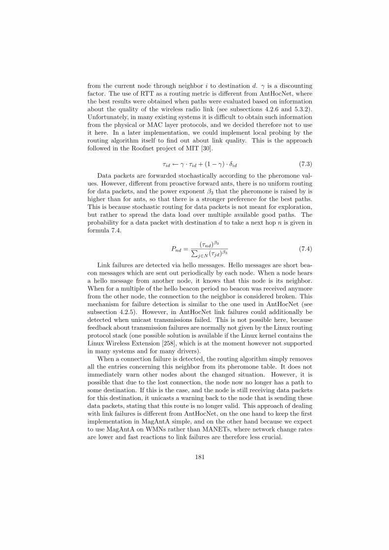
from the current node through neighbor i to destination d. γ is a discountingfactor. The use of RTT as a routing metric is different from AntHocNet, wherethe best results were obtained when paths were evaluated based on informationabout the quality of the wireless radio link (see subsections 4.2.6 and 5.3.2).Unfortunately, in many existing systems it is difficult to obtain such informationfrom the physical or MAC layer protocols, and we decided therefore not to useit here. In a later implementation, we could implement local probing by therouting algorithm itself to find out about link quality. This is the approachfollowed in the Roofnet project of MIT [30].

τid ← γ · τid + (1− γ) · δid (7.3)

Data packets are forwarded stochastically according to the pheromone val-ues. However, different from proactive forward ants, there is no uniform routingfor data packets, and the power exponent β3 that the pheromone is raised by ishigher than for ants, so that there is a stronger preference for the best paths.This is because stochastic routing for data packets is not meant for exploration,but rather to spread the data load over multiple available good paths. Theprobability for a data packet with destination d to take a next hop n is given informula 7.4.

Pnd =(τnd)β3

∑j∈N (τjd)β3

(7.4)

Link failures are detected via hello messages. Hello messages are short bea-con messages which are sent out periodically by each node. When a node hearsa hello message from another node, it knows that this node is its neighbor.When for a multiple of the hello beacon period no beacon was received anymorefrom the other node, the connection to the neighbor is considered broken. Thismechanism for failure detection is similar to the one used in AntHocNet (seesubsection 4.2.5). However, in AntHocNet link failures could additionally bedetected when unicast transmissions failed. This is not possible here, becausefeedback about transmission failures are normally not given by the Linux routingprotocol stack (one possible solution is available if the Linux kernel contains theLinux Wireless Extension [258], which is at the moment however not supportedin many systems and for many drivers).

When a connection failure is detected, the routing algorithm simply removesall the entries concerning this neighbor from its pheromone table. It does notimmediately warn other nodes about the changed situation. However, it ispossible that due to the lost connection, the node now no longer has a path tosome destination. If this is the case, and the node is still receiving data packetsfor this destination, it unicasts a warning back to the node that is sending thesedata packets, stating that this route is no longer valid. This approach of dealingwith link failures is different from AntHocNet, on the one hand to keep the firstimplementation in MagAntA simple, and on the other hand because we expectto use MagAntA on WMNs rather than MANETs, where network change ratesare lower and fast reactions to link failures are therefore less crucial.

181

7.3 Integration with the Linux kernel

In this section we discuss how the MagAntA routing daemon running in userspace integrates with the TCP/IP network protocol stack inside the Linux ker-nel. First, in subsection 7.3.1, we explain the approach using Ana4, a layer 2.5architecture for the deployment of WMNs. A prototype of this system has beendeveloped by fellow researchers at DTL [233]. However, a number of problemswere also encountered. We discuss these problems and the current state of thesystem in subsection 7.3.2. Then, in subsection 7.3.3, we discuss a number ofpossible alternative approaches.

7.3.1 Ana4

The current implementation of MagAntA relies on Ana4 [37,38], an architecturefor the deployment of AHWMNs using Linux. Ana4 provides solutions forAHWMN related issues such as address auto-configuration, combining the viewsprovided by different network interfaces, and providing a smooth integrationwith the existing protocols in the TCP/IP network protocol stack (see alsosubsection 7.1.2). Its functionality is placed in an ad hoc protocol layer, whichis located at layer 2.5, between the link layer (layer 2) and the IP layer (layer3). By working at layer 2.5, Ana4 can hide AHWMN related complexity fromprotocols both at lower and higher layers, so that no changes are needed forthose. For the interaction between the Ana4 system in the Linux kernel andthe MagAntA routing daemon in user space, we make use of a new version ofAna4 [233], developed at DTL, in which each individual data packet is sent upto user space to be routed. An overview of the full system is given in figure 7.4.In what follows, we explain details of this setup. We discuss how Ana4 isimplemented inside the TCP/IP network protocol stack in the Linux kernel,how it deals with issues of AHWMN deployment, and how it interacts with theMagAntA routing daemon.

The integration of Ana4 at layer 2.5 is based on the definition of a virtualinterface: Ana4 presents itself as a new, virtual network interface, which existsin parallel to the real interfaces that are present in the node. We refer tothis interface as the Ana4 ad hoc interface. For the IP protocol at layer 3,the Ana4 system appears to be an extra layer 2 interface. This situation isillustrated in figure 7.5a. IP considers this new interface as the single interfaceover which it sends and receives all data packets to and from the WMN. Insidethe virtual interface, packets are in the layer 2.5 architecture, where they aretreated by Ana4. If they are outgoing packets coming from IP or if they arepackets in transit, they are assigned a next hop and outgoing (real) interface,and are passed on to this interface. If they are incoming packets arriving attheir destination, they are passed on to IP. For the other (real) interfaces atlayer 2, the Ana4 ad hoc layer appears as another layer 3 protocol that theyexchange data packets with, more or less in parallel to IP. This is illustrated infigure 7.5b. The interfaces distinguish between packets from IP and those fromthe ad hoc layer based on the MAC type field in the packet headers.

182

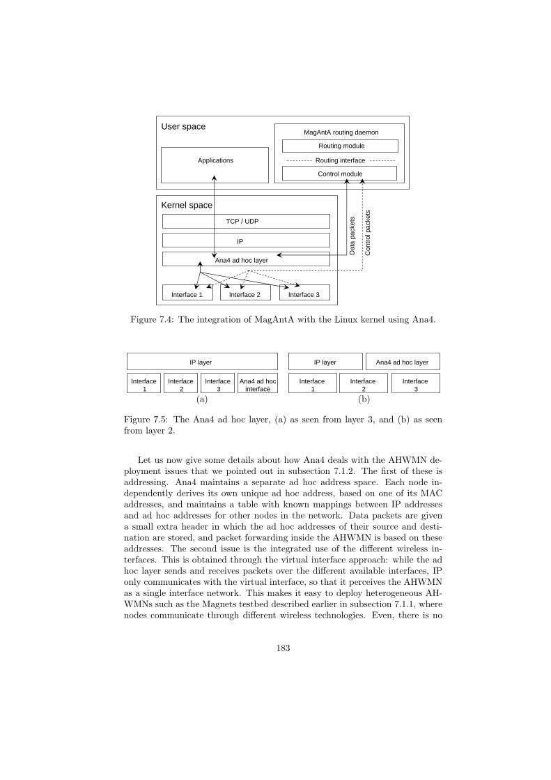
User space

Kernel space

MagAntA routing daemon

Routing module

Control module

Routing interface

Dat

a pa

cket

s

Con

trol

pac

kets

Applications

TCP / UDP

IP

Ana4 ad hoc layer

Interface 1 Interface 2 Interface 3

Figure 7.4: The integration of MagAntA with the Linux kernel using Ana4.

Interface1

Interface2

Interface3

Ana4 ad hoc interface

IP layer IP layer Ana4 ad hoc layer

Interface1

Interface2

Interface3

(a) (b)

Figure 7.5: The Ana4 ad hoc layer, (a) as seen from layer 3, and (b) as seenfrom layer 2.

Let us now give some details about how Ana4 deals with the AHWMN de-ployment issues that we pointed out in subsection 7.1.2. The first of these isaddressing. Ana4 maintains a separate ad hoc address space. Each node in-dependently derives its own unique ad hoc address, based on one of its MACaddresses, and maintains a table with known mappings between IP addressesand ad hoc addresses for other nodes in the network. Data packets are givena small extra header in which the ad hoc addresses of their source and desti-nation are stored, and packet forwarding inside the AHWMN is based on theseaddresses. The second issue is the integrated use of the different wireless in-terfaces. This is obtained through the virtual interface approach: while the adhoc layer sends and receives packets over the different available interfaces, IPonly communicates with the virtual interface, so that it perceives the AHWMNas a single interface network. This makes it easy to deploy heterogeneous AH-WMNs such as the Magnets testbed described earlier in subsection 7.1.1, wherenodes communicate through different wireless technologies. Even, there is no

183

need for the used interfaces to be wireless, and one could also include wiredlinks in the network. The third issue is integration with other networks andexisting IP routing protocols. Ana4 performs routing inside the ad hoc layer.It assigns next hops to data packets that are sent over the AHWMN based onan internally maintained routing table. By placing AHWMN routing inside thead hoc layer, it is transparent to IP. This means that from IP’s perspective, theAHWMN seems to need no routing, so that it appears like a flat, single-hopnetwork, similar to an Ethernet bus. This way, compatibility with IP routingalgorithms running in the Internet is straightforward. Finally, we point out thatall the code for Ana4 is defined in kernel modules. This means that no kernelmodifications are needed, allowing easy installation and good portability.

In the original Ana4 system, data forwarding is based on the use of threetables: the ARP table, which contains the mapping between IP addresses andad hoc addresses for known destinations, the COM table, which is the actualrouting table holding a next hop ad hoc address for each destination, and theATP table, which is the table with lower layer information storing an outgoinginterface name and MAC address for each neighbor (next hop). A simplifiedrepresentation of the different tables is shown in figure 7.6. The tables arekept in the ad hoc layer in kernel space, and are updated by a routing daemonrunning in user space, through the use of IOCTL commands. This way, theuser space routing algorithm defines the forwarding of data packets indirectlythrough the tables. In the current version of Ana4, the proactive OLSR pro-tocol is implemented for this purpose. For the working with MagAntA, thistable based approach is not satisfactory. Since we want to support per packetstochastic data load spreading, we need to be able to take a new routing decisionfor each individual packet. This is not possible if the routing daemon influencesdata routing indirectly through the routing tables that are present in Ana4.Therefore, we use a different version of the Ana4 system [233], in which the adhoc layer sends the address part of each packet up to user space (sending thedata part is avoided to improve efficiency), through a character device file. TheMagAntA routing daemon then fills in the necessary address fields in the adhoc and MAC headers, and sends the packet back down. After that, the ad hoclayer resumes its normal operation. This approach is illustrated in figure 7.4,where the solid arrows show the flow of data packets.

7.3.2 Current state of the system

The MagAntA system has been implemented to work with the Ana4 architec-ture described above. The adaptation of Ana4 that sends data packets up touser space was developed by colleagues at DTL [233]. Currently, their system isworking sufficiently well so that preliminary testing and debugging of the Ma-gAntA code could be performed. However, there are some problems with theadapted Ana4 system that make the performance unsatisfactory and limit thepossibility for extensive testing of MagAntA.

The most important problem with the adapted Ana4 system is that it isunstable and fails after a number of packets have been sent. This has to do

184

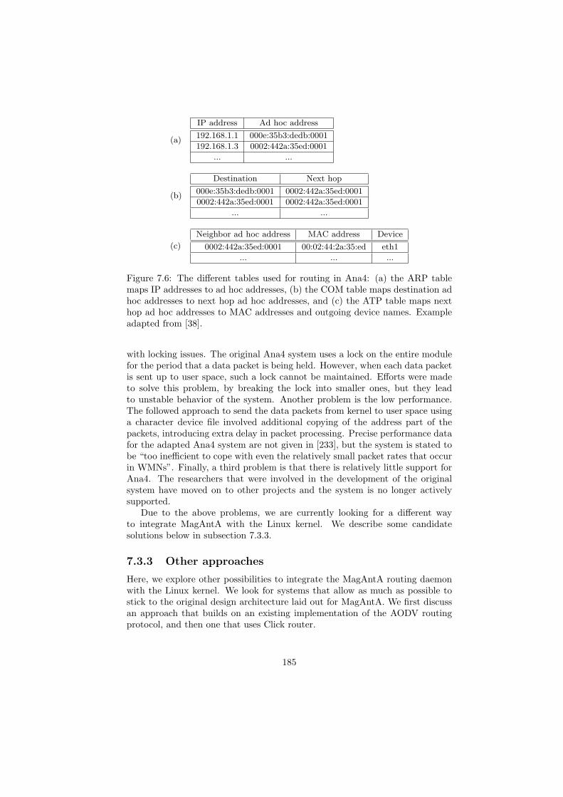
(a)

IP address Ad hoc address

192.168.1.1 000e:35b3:dedb:0001

192.168.1.3 0002:442a:35ed:0001

... ...

(b)

Destination Next hop

000e:35b3:dedb:0001 0002:442a:35ed:0001

0002:442a:35ed:0001 0002:442a:35ed:0001

... ...

(c)

Neighbor ad hoc address MAC address Device

0002:442a:35ed:0001 00:02:44:2a:35:ed eth1

... ... ...

Figure 7.6: The different tables used for routing in Ana4: (a) the ARP tablemaps IP addresses to ad hoc addresses, (b) the COM table maps destination adhoc addresses to next hop ad hoc addresses, and (c) the ATP table maps nexthop ad hoc addresses to MAC addresses and outgoing device names. Exampleadapted from [38].

with locking issues. The original Ana4 system uses a lock on the entire modulefor the period that a data packet is being held. However, when each data packetis sent up to user space, such a lock cannot be maintained. Efforts were madeto solve this problem, by breaking the lock into smaller ones, but they leadto unstable behavior of the system. Another problem is the low performance.The followed approach to send the data packets from kernel to user space usinga character device file involved additional copying of the address part of thepackets, introducing extra delay in packet processing. Precise performance datafor the adapted Ana4 system are not given in [233], but the system is stated tobe “too inefficient to cope with even the relatively small packet rates that occurin WMNs”. Finally, a third problem is that there is relatively little support forAna4. The researchers that were involved in the development of the originalsystem have moved on to other projects and the system is no longer activelysupported.

Due to the above problems, we are currently looking for a different wayto integrate MagAntA with the Linux kernel. We describe some candidatesolutions below in subsection 7.3.3.

7.3.3 Other approaches

Here, we explore other possibilities to integrate the MagAntA routing daemonwith the Linux kernel. We look for systems that allow as much as possible tostick to the original design architecture laid out for MagAntA. We first discussan approach that builds on an existing implementation of the AODV routingprotocol, and then one that uses Click router.

185

In subsection 7.1.2, we have described several existing implementations of theAODV routing protocol. Of these, the AODV-UCSB [57] implementation has adesign that is similar to the one that we are following with MagAntA. It uses arouting daemon that runs in user space and that makes routing decisions on aper packet basis. The integration with the kernel is obtained through Netfilterand a kernel module. Each packet entering or leaving the node passes throughthe Netfilter hooks, from where it is redirected to a kernel module. This kernelmodule temporarily queues the packet. The user space daemon then takes arouting decision for each queued data packet. The main difference with the ap-proach we have been following is that data packets do not go up to user space.Instead, the routing module manipulates the packets in the kernel space. Nev-ertheless, per packet routing is still possible, and all routing code remains inuser space. This means that limited changes would be needed to MagAntA inorder to work with this system; it would suffice to adapt the functions in thecontrol module that deal with receiving and sending data packets. The changescould be made transparent from the routing module. Disadvantages of usingthe AODV-UCSB approach is that, different from Ana4, this system does notprovide ready solutions for some important AHWMN related issues such as ad-dress auto-configuration, integration of heterogeneous interfaces, and a smoothintegration with other networks running traditional IP routing algorithms.

A different approach, which is also proposed in [233] in response to theproblems with Ana4, is to use a Click router. Click [155] is a flexible, modularsoftware architecture for building configurable routers under Linux. The Clicksystem defines a number of modules, called elements, which carry out basic func-tionality that is needed in a router. Examples of existing elements are Queue,which queues data packets, LookupIPRoute, which looks for the destination ofa packet in a static routing table, ToDevice, which hands packets to a Linuxdevice driver for transmission, etc.. To build a Click router, one needs to select acombination of these elements that together perform the required functionality,and define connections between them. If the functionality of existing elementsis not sufficient, one can also program new elements: all elements are writtenin C++ and are subclasses of the class Element. Once a Click router has beenput together, it can be placed in the Click system to function as a Linux router.One has the choice between running the router using a Linux in-kernel driver, orusing a user-level driver. While the former gives better performance, the latterallows easier debugging and fast prototyping. For MagAntA, the advantage ofworking with Click would be that we can continue working in user space, andmaintain a modular and flexible structure for the program. Another advantageis that Click is widely used and well documented and supported, which makes itan easy to use developing environment. A disadvantage is that we would needto make considerable changes to the structure of MagAntA, in order to make itadhere to the typical structure of a Click router in which the code is organizedaccording to the flow of packets through a connected system of elements. More-over, we would need to program a number of new Click elements to supportfunctions that are needed in adaptive routing. Another disadvantage is that,unlike Ana4, Click does not support ready solutions for AHWMN related issues

186

such as address auto-configurations and the like. Since, however, Click allowsflexible routing design, such solutions could be implemented.

When comparing the two possibilities described above, it seems that theapproach using the AODV-UCSB implementation would be the easiest solutionto continue with the work implemented so far. However, the approach usingClick gives more flexibility and is better documented and supported, so that inthe long run, it might be more interesting to invest the extra effort needed tomigrate to Click.

7.4 Conclusion

In this chapter, we have described efforts that we have made towards the imple-mentation of adaptive routing in AHWMNs. We have presented the MagAntAsystem, a user space routing daemon for adaptive routing. MagAntA has a mod-ular structure, consisting of a control module, a routing module, and a routinginterface between these two. This structure, together with the fact that thesystem runs entirely in user space, makes it easily extendible and adaptable, sothat it is an easy to use research tool. For integration with the Linux kernel, theMagAntA system relies on Ana4, a layer 2.5 architecture for the deployment ofAHWMNs. The interaction between MagAntA and Ana4 is established throughpacket forwarding: we use an adapted version of Ana4, developed by colleaguesat DTL, in which each data packet is sent up to user space to be routed. Thefact that each data packet can be routed individually by the MagAntA routingdaemon provides the flexibility that is needed to perform adaptive routing.

The work presented in this chapter is still in progress. While MagAntA hasbeen subjected to preliminary tests, these were only sufficient to do debuggingand verify basic functionality. Thorough tests of the system to get performancedata have not been carried out yet. This is due to programming problemsthat were encountered by the developers of the adapted Ana4 system. Thissystem is currently still unstable and gives poor performance. We have describedsome possible alternatives for the integration of Ana4 with the kernel, using theexisting AODV-UCSB system and using Click. Further developments will beneeded to find out which approach is best suited for our work.

187

Chapter 8

Conclusions

In this thesis, we have addressed the problem of adaptive routing in AHWMNsusing techniques from AI and ACO. We have first given an introduction to thefields of AHWMNs and adaptive routing. Then, we have described the Ant-HocNet routing algorithm, and next, we have presented a range of experimentaltests in which we investigated the behavior and performance of this algorithm.The tests were carried out both in traditional open space scenarios and in anurban setting. Finally, we have also described a system for the implementationof ACO algorithms in real world testbeds.

In what follows, we first give an overview of the contributions and findingsof this thesis, and then discuss possible future research directions.

8.1 Contributions and findings of this thesis

The main contribution of this thesis is the development of the AntHocNet rout-ing algorithm. AntHocNet has a hybrid architecture, whereby a reactive routesetup process is used at the start of each new communication session in orderto obtain an initial path for data forwarding, and a proactive route mainte-nance process is run throughout the duration of the session with the objectiveto keep information about existing paths up-to-date and to explore new andpossibly better paths, continuously adapting to the changing network environ-ment. AntHocNet also possesses a number of reactive mechanisms to deal withlink failures, such as the transmission of failure notification messages and thepossibility to execute local route repairs.

A distinct feature of AntHocNet is that it is based on methods from AI. Inparticular, it uses elements from ACO and from dynamic programming. FromACO it inherits the use of continuous Monte Carlo sampling of full paths, andthe use of stochastic decision making. From dynamic programming, it adoptsthe use of information bootstrapping. Both Monte Carlo sampling and infor-mation bootstrapping are important paradigms in the field of reinforcementlearning. In AntHocNet, Monte Carlo sampling is applied extensively through-

188

out the different components of the algorithm, while information bootstrappingis the basis of the pheromone diffusion process that is part of the proactiveroute maintenance process. While the continuous sampling of full paths pro-vides adaptivity and reliability, information bootstrapping gives a highly effi-cient but potentially unreliable way of spreading routing information. In thecombination of both techniques, the sampling practices can be considered a wayto confirm the information suggested earlier by the information bootstrappingprocess. This approach to combining Monte Carlo sampling and informationbootstrapping is inherently different from other ways of integrating these twoimportant learning paradigms in the field of reinforcement learning.

We have evaluated the AntHocNet routing algorithm in a wide range of dif-ferent tests. A first set of tests was based on standard, open space scenarios.This is a common approach in the field AHWMN research, and was adopted herein order to allow fair comparisons. In these tests, we first compared AntHocNetto existing state-of-the-art AHWMN routing algorithms, including AODV, animportant reactive routing algorithm, OLSR, a representative proactive routingalgorithm, and ANSI, which is like AntHocNet based on ACO. Results showedthat AntHocNet could outperform the other three algorithms over a wide rangeof different scenarios. Specifically, AntHocNet turned out to perform well intests with increasing levels of mobility, to deal better than the other algorithmswith different levels of data load, to cope well with sparse network situations,and to scale well to networks of increasing sizes. On the downside, AntHocNet’sadvantage was decreased when mobility got very high, and the algorithm wasoutperformed by AODV when node density got high. In the same test scenar-ios, we also investigated the internal working of AntHocNet. We alternativelyenabled and disabled various components of the algorithm, and investigatedtheir influence. We found that the proactive maintenance process always has ahigh contribution to the algorithm’s performance, and that this process shouldwork as fast as possible (i.e., producing large and frequent update messages),as long as no excessive levels of overhead are reached. The local route repairmechanism was found to give important advantages in large networks, but tohave a negative impact in small networks. Among the different routing metrics,the SINR based measure gave best results. Finally, we found that, contrary toresults in wired networks, stochastic forwarding of forward ants and data didnot give advantages; it is better to exploit the best available information.

A second set of tests was based on an urban scenario. We proposed a simu-lation setup providing a detailed and at the same time computationally efficientmodeling of outdoor radio propagation, node mobility, and user traffic. Weapplied this model using the street map of Lugano as a reference. We first in-vestigated properties of the urban network graph and compared them to those ofequivalent open space environments. We found that nodes have less neighbors,that network connectivity is worse, that paths are longer, and link durationsshorter. Next, we compared the behavior of AntHocNet with that of AODV inthis setup, applying tests in which we varied data send rate, number of datasessions, node density, and node speed. We found that AntHocNet profits fromthe lower local density in urban settings to let its proactive mechanism work

189

efficiently. However, at high rates, it suffers from interference. At very lowrates, both algorithms have difficulties due to their approach to construct ini-tial routing information reactively. We found that node density has a strongimpact on the delivery ratio, while the node speed has relatively little impact.Finally, we also found that using AntHocNet, it is possible to deliver VoIP levelsof service, but only for a limited number of sessions. This points to the needfor call admission control mechanisms in urban MANETs.

Finally, we investigated the implementation of ACO routing in a Linux basedtestbed. We presented the MagAntA system, which is a user space routingdaemon that implements ACO routing. MagAntA has a modular structure,consisting of a control module, a routing module, and a routing interface betweenthese two. Thanks to this modular approach and the system’s location in userspace, MagAntA is easily extendible and adaptable. For the communicationwith the Linux kernel, the system relies on Ana4, a layer 2.5 architecture forthe deployment of AHWMNs that is defined in a number of kernel modules.We use a version of Ana4 developed by colleagues at DTL, in which all packetsgoing to and from the AHWMN are sent up to user space to be treated forrouting by MagAntA. This version of Ana4 is in its current state unfortunatelystill unstable, and MagAntA can therefore not fully be used. We investigatedsome possible alternative deployment plans for our system.

8.2 Future research directions

Here we point out some future research directions that are relevant for thework presented in this thesis. These concern the deployment and testing ofAntHocNet in hardware testbeds, the support of QoS issues in AntHocNet, theuse of the ideas behind AntHocNet in other types of networks, the applicationof other ideas from artificial intelligence in the field of computer networking,and finally the support of autonomic networking.

In chapter 7, we have described a system for the implementation of Ant-HocNet in a Linux testbed. However, further work is needed in this direction.Implementation and testing in real testbeds is important in the field of network-ing and especially in the area of AHWMNs. Real deployment tests can bringup issues that did not come up in simulation. To work well in real implemen-tations, changes might be needed to the AntHocNet algorithm. However, it isencouraging to see that the few other algorithms that take into account linkquality and use it to proactively improve paths during the course of communi-cation sessions, namely LQSR, Srcr and LUNAR, have come out of research onreal testbeds.

In chapter 6, we have investigated the use of AntHocNet in a detailed sim-ulation of an urban environment. One of the tests was concerned with thesupport of VoIP traffic. Our finding was that VoIP data traffic can in principlebe supported by AntHocNet, if the number of data sessions with such demandsis limited. This brings up the issue of admission control and QoS support. Suchmechanisms should be integrated with AntHocNet. An interesting aspect is the

190

fact that AntHocNet uses extensive probing, which could provide the informa-tion needed to support QoS. Admission control could be carried out during thereactive route setup process.

Interesting future work would also be to apply the ideas behind AntHocNetin different kinds of networks. One could in the first place target packet switchedwired networks. Existing ACO routing algorithms developed for such networksprovide adaptivity with respect to variations in data load, and often ignorethe effect of topology changes. While such changes are less frequent in wirednetworks compared to AHWMNs, they can still occur, e.g. due to link or nodefailures, and the mechanisms developed in AntHocNet could be used to dealwith this. Other types of networks in which AntHocNet’s mechanisms couldbe useful are application layer overlay networks. In such networks, nodes areconnected at the application layer through virtual links, that are implementedas paths in the underlying physical network. Overlay networks can have verydynamic topologies. Examples of application layer overlay networks are peer-to-peer networks [243] and resilient overlay networks [20].

Another interesting direction for future research is to elaborate further onthe relationship between the problem of routing and the field of reinforcementlearning. In the reinforcement learning literature, one can find more approachesto learning that can be useful for network routing. One aspect that seemsinteresting is the possibility to perform off-policy Monte Carlo learning [252].In off-policy learning the policy used to sample paths is different from the onethat information is gathered for. A routing algorithm could then use a ratherexplorative policy for sampling, but gather information for a data packet routingpolicy that is more exploitative or even radically different (e.g. in the case ofdifferentiated QoS routing [153]). Another interesting approach would be to useintermediate bootstrapping, as is done in temporal difference learning [251].

Finally, our work on AntHocNet could be extended in the direction of au-tonomic computing [152]. The main idea behind autonomic computing is thatcomputer systems are getting too complex for human operators to manage, andthat they should become more “self-organized”. For the area of networking,this means that the network should be self-configuring, self-optimizing, self-protecting and self-healing. While these properties are to some extent alreadypresent in the adaptivity, robustness and scalability of AntHocNet, further de-velopments would be needed to get to a fully autonomic routing algorithm. E.g.,the algorithm should be able to tune its parameters, and to adapt its workingautomatically to different types of networks and different types of data trafficto be served. Nevertheless, AntHocNet’s approach to constantly gather infor-mation about the network through sampling and pheromone diffusion gives agood basis to build such a system.

191

Bibliography

[1] Berlinroofnet. Available from: http://sarwiki.informatik.hu-berlin.de/BerlinRoofNet.

[2] Funkfeuer. Available from: http://www.funkfeuer.at/.

[3] IEEE 802.11 standard group website. Available from: http://www.ieee802.org/11/.

[4] IEEE 802.15 standard group website. Available from: http://www.ieee802.org/15/.

[5] IEEE 802.16 standard group website. Available from: http://www.ieee802.org/16/.

[6] The internet engineering task force mobile ad-hoc networking page(MANET). Available from: http://www.ietf.org/html.charters/manet-charter.html.

[7] Microsoft Mesh Networks. Available from: http://research.microsoft.com/mesh/.

[8] The NRL OLSR routing protocol implementation. Available from: http://pf.itd.nrl.navy.mil/olsr/.

[9] olsr.freifunk.net. Available at: http://olsrexperiment.de.

[10] Taipei-wlan. Available from: http://wlan.taipei-elife.net/english/main.html.

[11] Technical specifications and technical reports for a utran-based 3gpp sys-tem. Available from: http://www.3gpp.org/ftp/Specs/html-info/21101.htm.

[12] Wireless philadelphia. Available from: http://www.wirelessphiladelphia.org.

[13] The zigbee alliance. Available from: http://www.zigbee.org/en/index.asp.

192

[14] M. Abolhasan, T. Wysocki, and E. Dutkiewicz. A review of routing pro-tocols for mobile ad hoc networks. Ad Hoc Networks, 2:1–22, 2004.

[15] D. Aguayo, J. Bicket, S. Biswas, G. Judd, and R. Morris. Link-level mea-surements from an 802.11b mesh network. SIGCOMM Computer Com-mununication Review, 34(4):121–132, 2004.

[16] I. F. Akyildiz, X. Wang, and W. Wang. Wireless mesh networks: a survey.Computer Networks Journal, 47:445–487, March 2005.

[17] I. F. Akyildiz, S. Weilian, Y. Sankarasubramaniam, and E. Cayirci. Asurvey on sensor networks. IEEE Communications Magazine, 40(8):102–116, August 2002.

[18] J. N. Al-Karaki and A. E. Kamal. Routing techniques in wireless sensornetworks: a survey. IEEE Wireless Communications, 11(6):6–28, Decem-ber 2004.

[19] M. Ali, U. Saif, A. Dunkels, T. Voigt, K. Romer, K. Langendoen, J. Po-lastre, and Z. A. Uzmi. Medium access control issues in sensor networks.ACM SIGCOMM Computer Communication Review, 36(2), April 2006.

[20] D. G. Andersen, H. Balakrishnan, M. F. Kaashoek, and R. Morris. Re-silient overlay networks. In Proceedings of the 18th ACM Symposium onOperating Systems Principles, Banff, Canada, October 2001.

[21] AWE Communications. WinProp software suite.

[22] H. Balakrishnan, V. N. Padmanabhan, S. Seshan, and R. H. Katz. Acomparison of mechanisms for improving TCP performance over wirelesslinks. In Proceedings of ACM SIGCOMM ’96, August 1996.

[23] B. Baran and R. Sosa. A new approach for AntNet routing. In Proceed-ings of the 9th International Conference on Computer CommunicationsNetworks, Las Vegas, USA, 2000.

[24] J. S. Baras and H. Mehta. A probabilistic emergent routing algorithmfor mobile ad hoc networks. In WiOpt03: Modeling and Optimization inMobile, Ad Hoc and Wireless Networks, 2003.

[25] A. G. Barto, R. S. Sutton, and C. W. Anderson. Neuronlike adaptive ele-ments that can solve difficult learning control problems. IEEE Transactionon Systems, Man and Cybernetics, SMC-13:834–846, 1983.

[26] R. Bellman. Dynamic Programming. Princeton University Press, 1957.

[27] R. Bellman. On a routing problem. Quarterly of Applied Mathematics,16(1):87–90, 1958.

193

[28] B. Bensaou, Y. Wang, and C. C. Ko. Fair medium access in 802.11 basedwireless ad hoc networks. In Proceedings of Mobile Ad Hoc Networkingand Computing (MobiHoc 2000), pages 99–106, 2000.

[29] C. Bettstetter, G. Resta, and P. Santi. The node distribution of therandom waypoint mobility model for wireless ad hoc networks. IEEETransactions on Mobile Computing, 2(3):257–269, 2003.

[30] J. Bicket, D. Aguayo, S. Biswas, and R. Morris. Architecture and evalua-tion of an unplanned 802.11b mesh network. In Proceedings of Mobicom,August 2005.

[31] L. Blazevic, L. Buttyan, S. Capkun, S. Giordano, J.-P. Hubaux, and J.-Y.Le Boudec. Self-organization in mobile ad-hoc networks: the approach ofterminodes. IEEE Communications Magazine, 39(6), June 2001.

[32] L. Blazevic, S. Giordano, and J.-Y. Le Boudec. Anchored path discoveryin terminode routing. In Proceedings of The Second IFIP-TC6 NetworkingConference (Networking 2002), May 2002.

[33] Bluetooth Special Interest Group. Specification of bluetooth system,February 2002. Version 1.1.

[34] E. Bonabeau, M. Dorigo, and G. Theraulaz. Swarm Intelligence: FromNatural to Artificial Systems. Oxford University Press, 1999.

[35] E. Bonabeau, F. Henaux, S. Guerin, D. Snyers, P. Kuntz, and G. Ther-aulaz. Routing in telecommunication networks with ”Smart” ant-likeagents. In Proceedings of IATA’98, Second Int. Workshop on IntelligentAgents for Telecommunication Applications, volume 1437 of Lecture Notesin Artificial Intelligence. Springer Verlag, 1998.

[36] E. Borgia, M. Conti, F. Delmastro, and E. Gregori. Experimental com-parison of routing and middleware solutions for mobile ad hoc networks:legacy vs cross-layer approach. In Proceedings of the ACM SIGCOMMWorkshop on Experimental Approaches to Wireless Network Design andAnalysis (E-WIND), August 2005.

[37] N. Boulicault, G. Chelius, and E. Fleury. Experiments of ana4: An im-plementation of a 2.5 framework for deploying real multi-hop ad hoc andmesh networks. In Proceedings of the IEEE ICPS Workshop on Multi-hopAd hoc Networks: from theory to reality, Santorini, Greece, July 2005.

[38] N. Boulicault, G. Chelius, and E. Fleury. Ana4: a 2.5 framework fordeploying real multi-hop ad hoc and mesh networks. Ad Hoc & SensorWireless Networks: an International Journal (AHSWN), 2006. To appear.

[39] J. A. Boyan and M. L. Littman. Packet routing in dynamically changingnetworks: A reinforcement learning approach. In J. D. Cowan, G. Tesauro,

194

and J. Alspector, editors, Advances in Neural Information Processing Sys-tems 6 (NIPS6), pages 671–678. Morgan Kaufmann, San Francisco, CA,USA, 1994.

[40] R. Braden, D. Clark, and S. Shenker. Integrated services in the Internetarchitecture: an overview. Request For Comments (RFC) 1633, NetworkWorking Group, 1994.

[41] D. Braginsky and D. Estrin. Rumor routing algorithm for sensor net-works. In Proceedings of the First Workshop on Sensor Networks andApplications (WSNA), Atlanta, GA, USA, October 2002.

[42] J. Broch, D. A. Maltz, D. B. Johnson, Y.-C. Hu, and J. Jetcheva. Aperformance comparison of multi-hop wireless ad hoc network routingprotocols. In Proceedings of the Fourth Annual ACM/IEEE InternationalConference on Mobile Computing and Networking (MobiCom), 1998.

[43] T. Bu, L. Gao, and D. Towsley. On characterizing bgp routing tablegrowth. In Proceedings of the IEEE Global Internet Symposium, Taipei,Taiwan, November 2002.

[44] S. Burleigh, A. Hooke, L. Torgerson, K. Fall, V. Cerf, B. Durst, K. Scott,and H. Weiss. Delay-tolerant networking: An approach to interplanetaryinternet. IEEE Communications Magazine, June 2003.

[45] D. Camara and A.A.F. Loureiro. Gps/ant-like routing in ad hoc networks.Telecommunication Systems, 18(1–3):85–100, 2001.

[46] T. Camp, J. Boleng, and V. Davies. A survey of mobility models for ad hocnetwork research. Wireless Communications & Mobile Computing: Specialissue on Mobile Ad Hoc Networking: Research, Trends and Applications,2002.

[47] S. Capkun, M. Hamdi, and J.-P. Hubaux. Gps-free positioning in mobilead-hoc networks. In Proceedings of the 34th Hawaii International Confer-ence on System Sciences (HICSS), January 2001.

[48] S. Carl-Mitchell and J. S. Quarterman. Using ARP to Implement Trans-parent Subnet Gateways. Network Working Group, October 1987. RFC1027.

[49] G. Di Caro, F. Ducatelle, and L. M. Gambardella. Demonstrator formobile ad hoc networks. Internal Deliverable D12-D13 of FET ProjectBISON (IST-2001-38923), 2004.

[50] L. Carrillo, C. Guadall, J. L. Marzo, G. Di Caro, F. Ducatelle, and L. M.Gambardella. Differentiated quality of service scheme based on the use ofmulti-classes of ant-like mobile agents. In CoNEXT’05: Proceedings of the2005 ACM conference on Emerging network experiment and technology,Toulouse, France, 2005.

195

[51] L. Carrillo, J.L. Marzo, D. Harle, and P. Vila. A review of scalability andits application in the evaluation of the scalability measure of antnet rout-ing. In C.E. Palau Salvador, editor, Proceedings of the IASTED Confer-ence on Communication Systems and Networks (CSN’03), pages 317–323.ACTA Press, 2003.

[52] A. Carzaniga, M. J. Rutherford, and A. L. Wolf. A routing scheme forcontent-based networking. In Proceedings of IEEE Infocom, Hong Kong,China, March 2004.

[53] R. Castaneda and S. R. Das. Query localization techniques for on-demandrouting protocols in ad hoc networks. In Proceedings of the ACM/IEEEMobiCom, pages 186–194, Seattle, WA, USA, August 1999.

[54] D. Cavin, Y. Sasson, and A. Schiper. On the accuracy of manet simula-tors. In Proceedings of the Workshop on Principles of Mobile Computing(POMC), 2002.

[55] A. Chaintreau, P. Hui, J. Crowcroft, C. Diot, R. Gass, and J. Scott. Impactof human mobility on the design of opportunistic forwarding algorithms.In Proceedings of 25th IEEE Conference on Computer Communications(INFOCOM), April 2006.

[56] I. D. Chakeres and E. M. Belding-Royer. The utility of hello messagesfor determining link connectivity. In Proceedings of the 5th InternationalSymposium on Wireless Personal Multimedia Communications (WPMC),Honolulu, HI, USA, October 2002.

[57] I. D. Chakeres and E. M. Belding-Royer. Aodv implementation designand performance evaluation. 2/3, 2005.

[58] C. Cheng, R. Riley, S. P. R. Kumar, and J. J. Garcia-Luna-Aceves. Aloop-free extended bellman-ford routing protocol without bouncing effect.In Proceedings of the Symposium on Communications architectures & pro-tocols (SIGCOMM), pages 224–236, 1989.

[59] C.-C. Chiang, H. Wu, W. Liu, and M. Gerla. Routing in clustered mul-tihop, mobile wireless networks with fading channel. In Proceedings ofIEEE SICON’97, pages 197–211, April 1997.

[60] T. Clausen and P. Jacquet. Optimized Link State Routing Protocol(OLSR). IETF, October 2003. RFC 3626.

[61] T. Clausen, P. Jacquet, A. Laouiti, P. Muhlethaler, A. Qayyum, andL. Viennot. Optimized link state routing protocol. In Proceedings ofIEEE INMIC, 2001.

[62] S. Corson and J. Macker. Mobile ad hoc networking (MANET): Rout-ing protocol performance issues and evaluation considerations. NetworkWorking Group, Request for Comments 2501, January 1999. Availablefrom: http://www.ietf.org/rfc/rfc2501.txt.

196

[63] D. Costa and A. Hertz. Ants can colour graphs. Journal of the OperationalResearch Society, 48:295–305, 1997.

[64] M. Daneshtalab, A. A. Kusha, A. Sobhani, Z. Navabi, M. D. Mottaghi,and O. Fatemi. Ant colony based routing architecture for minimizinghot spots in NoCs. In Proceedings of the 19th annual symposium on In-tegrated circuits and systems design (SBCCI), pages 56–61, Ouro Preto,MG, Brazil, 2006.

[65] S. R. Das, C. E. Perkins, and E. M. Royer. Performance comparison oftwo on-demand routing protocols for ad hoc networks. In Proceedings ofthe IEEE Conference on Computer Communications (INFOCOM), March2000.

[66] D. S. J. De Couto, D. Aguayo, J. Bicket, and R. Morris. A high-throughputpath metric for multi-hop wireless routing. In Proceedings of the 9th ACMInternational Conference on Mobile Computing and Networking (Mobi-Com), September 2003.

[67] D. S. J. De Couto, D. Aguayo, B. A. Chambers, and R. Morris. Perfor-mance of multihop wireless networks: Shortest path is not enough. InProceedings of the First Workshop on Hot Topics in Networks (HotNets-I). ACM SIGCOMM, 2002.

[68] Christian de Waal. Bonnmotion: A mobility scenario generation andanalysis tool, 2002. Available from: http://web.informatik.uni-bonn.de/IV/Mitarbeiter/dewaal/BonnMotion/.

[69] S. Desilva and S. R. Das. Experimental evaluation of a wireless ad hocnetwork. In Proceedings of the 9th International Conference on ComputerCommunications and Networks (IC3N), 2000.

[70] G. Di Caro. Ant Colony Optimization and its application to adaptiverouting in telecommunication networks. PhD thesis, Faculte des SciencesAppliquees, Universite Libre de Bruxelles, Brussels, Belgium, 2004.

[71] G. Di Caro and M. Dorigo. AntNet: Distributed stigmergetic controlfor communications networks. Journal of Artificial Intelligence Research(JAIR), 9:317–365, 1998.

[72] G. Di Caro and M. Dorigo. Two ant colony algorithms for best-effortrouting in datagram networks. In Proceedings of the Tenth IASTED Inter-national Conference on Parallel and Distributed Computing and Systems(PDCS’98), pages 541–546. IASTED/ACTA Press, 1998.

[73] G. Di Caro, F. Ducatelle, and L. M. Gambardella. AntHocNet: an ant-based hybrid routing algorithm for mobile ad hoc networks. In Proceedingsof Parallel Problem Solving from Nature (PPSN) VIII, volume 3242 ofLecture Notes in Computer Science, pages 461–470. Springer-Verlag, 2004.

197

[74] G. Di Caro, F. Ducatelle, and L. M. Gambardella. AntHocNet: an adap-tive nature-inspired algorithm for routing in mobile ad hoc networks. Eu-ropean Transactions on Telecommunications (ETT), 16(5), 2005.

[75] G. Di Caro, F. Ducatelle, and L. M. Gambardella. Swarm intelligencefor routing in mobile ad hoc networks. In Proceedings of the 2005 IEEESwarm Intelligence Symposium (SIS), June 2005.

[76] G. Di Caro, F. Ducatelle, and L. M. Gambardella. Reflecting Interfaces:The Complex Coevolution of Information Technology Ecosystems, chapterTheory and practice of Ant Colony Optimization for routing in dynamictelecommunications networks. Idea Group Inc., 2008. To appear.

[77] G. Di Caro, F. Ducatelle, P. Heegarden, M. Jelasity, R. Montemanni,and A. Montresor. Evaluation of basic services in ad-hoc, peer-to-peerand grid networks. Internal Deliverable D7 of FET Project BISON (IST-2001-38923), 2004.

[78] G. Di Caro and T. Vasilakos. Ant-SELA: Ant-agents and stochastic au-tomata learn adaptive routing tables for QoS routing in ATM networks.ANTS’2000 - From Ant Colonies to Artificial Ants: Second InternationalWorkshop on Ant Colony Optimization, Brussels (Belgium), September8-9, 2000.

[79] T. Dinh Dang, B. Sonkoly, and S. Molnar. Fractal analysis and modeling ofvoip traffic. In Proceedings of the 11th International TelecommunicationsNetwork Strategy and Planning Symposium (NETWORKS 2004), June2004.

[80] S. Doi and M. Yamamura. Bntnetl and its evaluation on a situation ofcongestion. Electronics and Communications in Japan (Part I: Commu-nications), 85(9):31–41, April 2002.

[81] Y. Dong, D. Makrakis, and T. Sullivan. Effective admission control inmultihop mobile ad hoc networks. In Proc. of the International Conferenceon Communication Technology (ICCT), 2003.

[82] M. Dorigo. Optimization, Learning and Natural Algorithms (in Italian).PhD thesis, Dipartimento di Elettronica e Informazione, Politecnico diMilano, IT, 1992.

[83] M. Dorigo, G. Di Caro, and L. M. Gambardella. Ant algorithms fordistributed discrete optimization. Artificial Life, 5(2):137–172, 1999.

[84] M. Dorigo and L. M. Gambardella. Ant colony system: A cooperativelearning approach to the traveling salesman problem. IEEE Transactionson Evolutionary Computation, 1(1):53–66, 1997.

198

[85] M. Dorigo, V. Maniezzo, and A. Colorni. The ant system: Optimizationby a colony of cooperating agents. IEEE Transactions on Systems, Man,and Cybernetics–Part B, 26(1):29–41, 1996.

[86] M. Dorigo and T. Stutzle. The ant colony optimization metaheuristic: Al-gorithms, applications, and advances. In F. Glover and G. Kochenberger,editors, Handbook of Metaheuristics, volume 57 of International Series inOperations Research and Management Science. Kluwer Academic Pub-lishers, 2003.

[87] M. Dorigo and T. Stutzle. Ant Colony Optimization. MIT Press, Cam-bridge, MA, 2004.

[88] O. Dousse, F. Baccelli, and P. Thiran. Impact of interferences on connec-tivity in ad hoc networks. In Proceedings of IEEE INFOCOM 2003, SanFrancisco, April 2003.

[89] O. Dousse, P. Thiran, and M. Hasler. Connectivity in ad-hoc and hybridnetworks. In Proceedings of IEEE INFOCOM 2002, pages 1079–1088,New York, June 2002.

[90] J. Dowling, E. Curran, R. Cunningham, and V. Cahill. Using feedback incollaborative reinforcement learning to adaptively optimize manet routing.IEEE Transactions on Systems, Man, and Cybernetics - Part A: Systemsand Humans, 35(3), May 2005.

[91] K. Doya, K. Samejima, K. Katagiri, and K. Kawato. Multiple model-basedreinforcement learning. Neural Computing, 14(6):1347–1369, 2002.

[92] R. Draves, J. Padhye, and B. Zill. The architecture of the link qualitysource routing protocol. Technical report MSR-TR-2004-57, MicrosoftResearch, 2004.

[93] R. Draves, J. Padhye, and B. Zill. Comparison of routing metrics for staticmulti-hop wireless networks. In Proceedings of ACM SIGCOMM, pages133–144, Portland, Oregon, USA, 2004.

[94] F. Ducatelle, G. Di Caro, and L. M. Gambardella. Ant agents for hybridmultipath routing in mobile ad hoc networks. In Proceedings of the SecondAnnual Conference on Wireless On demand Network Systems and Services(WONS), St. Moritz, Switzerland, January 18–19 2005.

[95] F. Ducatelle, G. Di Caro, and L. M. Gambardella. Using ant agents tocombine reactive and proactive strategies for routing in mobile ad hocnetworks. International Journal of Computational Intelligence and Appli-cations (IJCIA), 5(2), 2005.

[96] F. Ducatelle, G. Di Caro, and L. M. Gambardella. An analysis of thedifferent components of the anthocnet routing algorithm. In Proceedings ofthe Fifth International Workshop on Ant Colony Optimization and SwarmIntelligence (ANTS), September 2006.

199

[97] F. Ducatelle, G. Di Caro, and L. M. Gambardella. A study on the use ofMANETs in urban environments. Technical Report IDSIA-01-07, IstitutoDalle Molle di Studi Sull’Intelligenza Artificiale (IDSIA), 2007.

[98] F. Ducatelle, L. M. Gambardella, M. Kurant, H. X. Nguyen, and P. Thi-ran. Dependable Systems: Software, Computing, Networks, volume 4028of Lecture Notes in Computer Science, chapter Algorithms for failure de-tection in large IP-over-Fiber and Wireless Ad Hoc Networks. Springer,2006.

[99] F. Ducatelle and J. Levine. Ant colony optimisation for bin packing andcutting stock problems. In Proceedings of the UK Workshop on Compu-tational Intelligence, Edinburgh, UK, September 2001.

[100] F. Ducatelle and M. Roth. Documentation for the maganta routing pack-age. Technical report, Deutsche Telekom Laboratories, July 2006.

[101] F. Ducatelle, M. Roth, and L. M. Gambardella. Design of a user spacesoftware suite for probabilistic routing in ad-hoc networks. In Proceedingsof the Fourth European Workshop on the application of Nature-inspiredtechniques to Telecommunication Networks and other Connected Systems(EvoCOMNET2007), Valencia, Spain, April 2007. Poster presentation.

[102] L. M. Feeney. A taxonomy for routing protocols in mobile ad hoc networks.Technical Report T99-07, Swedish Institute of Computer Science, 1 1999.

[103] L. Ford and D. Fulkerson. Flows in Networks. Prentice-Hall, 1962.

[104] K. Fujita, A. Saito, T. Matsui, and H. Matsuo. An adaptive ant-basedrouting algorithm used routing history in dynamic networks. In Proc. ofthe 4th Asia-Pacific Conf. on Simulated Evolution and Learning, 2002.

[105] L. M. Gambardella and M. Dorigo. Ant-Q: A reinforcement learningapproach to the traveling salesman problem. In Proceedings of the TwelfthInternational Conference on Machine Learning, ML-95, pages 252–260.Palo Alto, CA: Morgan Kaufmann, 1995.

[106] L. M. Gambardella, E. Taillard, and G. Agazzi. Ant colonies for vehiclerouting problems. In D. Corne, M. Dorigo, and F. Glover, editors, NewIdeas in Optimization, pages 63–76. London,UK: McGraw-Hill, 1999.

[107] L. M. Gambardella, E. D. Taillard, and M. Dorigo. Ant colonies forthe quadratic assignment problem. Journal of the Operational ResearchSociety (JORS), 50(2):167–176, 1999. Also TR-IDSIA-4-97.

[108] D. Ganesan, R. Govindan, S. Shenker, and D. Estrin. Highly-resilient,energy-efficient multipath routing in wireless sensor networks. MobileComputing and Communications Review, 1(2), 2002.

200

[109] Y. Ganjali and A. Keshavarzian. Load balancing in ad hoc networks:Single-path routing vs. multi-path routing. In Proceedings of IEEE IN-FOCOM, March 2004.

[110] M. Gast. 802.11 Wireless Networks: The Definitive Guide. O’Reilly Me-dia, Inc., 2 edition, April 2005.

[111] M. Gerla, K. Tang, and R. Bagrodia. TCP performance in wireless multi-hop networks. In 2nd IEEE Workshop on Mobile Computing Systems andApplications, pages 41–50, 1999.

[112] B. Ghribi and L. Logrippo. Understanding gprs: The gsm packet radioservice. Computer Networks, 34:763–779, 2000.

[113] S. Giordano, I. Stojmenovic, and L. Blazevic. Ad Hoc Wireless Network-ing, chapter Position based routing algorithms for ad hoc networks: Ataxonomy. Kluwer, 2003.

[114] I. Glauche, W. Krause, R. Sollacher, and M. Greiner. Continuum percola-tion of wireless ad hoc communication networks. Physica A, 325:577–600,2003.

[115] S. Goss, S. Aron, J. L. Deneubourg, and J. M. Pasteels. Self-organizedshortcuts in the Argentine ant. Naturwissenschaften, 76:579–581, 1989.

[116] P. P. Grasse. La reconstruction du nid et les coordinations interindi-viduelles chez bellicositermes natalensis et cubitermes sp. La theorie dela stigmergie: essai d’interpretation du comportement des termites con-structeurs. Insectes Sociaux, 6:41–81, 1959.

[117] R. S. Gray, D. Kotz, C. Newport, N. Dubrovsky, A. Fiske, J. Liu, C. Ma-sone, S. McGrath, and Y. Yuan. Outdoor experimental comparison offour ad hoc routing algorithms. In Proceedings of the ACM/IEEE Inter-national Symposium on Modeling, Analysis and Simulation of Wirelessand Mobile Systems (MSWiM), pages 220–229, October 2004.

[118] M. Grossglauser and D. N. C. Tse. Mobility increases the capacity ofad-hoc wireless networks. In Proceedings of INFOCOM, 2001.

[119] M. Gunes, U. Sorges, and I. Bouazizi. ARA - The ant-colony based rout-ing algorithm for MANETs. In Proceedings of the ICPP InternationalWorkshop on Ad Hoc Networks (IWAHN), 2002.

[120] P. Gupta and P. R. Kumar. The capacity of wireless networks. IEEETransactions on Information Theory, March 2000.

[121] Z. J. Haas. A new routing protocol for the reconfigurable wireless net-works. In Proceedings of the IEEE International Conference on UniversalPersonal Communications, 1997.

201

[122] J. F. Hayes and T. V. J. Ganesh Babu. Modeling and Analysis of Telecom-munications Networks. John Wiley & Sons, Inc., 2004.

[123] C. Hedrick. Routing Information Protocol. IETF, 1988. RFC 1058.

[124] J. Heidemann, N. Bulusu, J. Elson, C. Intanagowiwat, K. Lan, Y. Xu,W. Ye, D. Estrin, and R. Govindan. Effects of detail in wireless networksimulation. In Proceedings of the SCS Multiconference on Distributed Sim-ulation, pages 3–11, January 2001.

[125] W. Heinzelman, A. Chandrakassan, and H. Balakrishnan. Energy-efficientcommunication protocol for wireless microsensor networks. In Proceedingsof the 33rd Hawaii International Conference on System Sciences (HICSS),January 2000.

[126] M. Heissenbuttel and T. Braun. Ants-based routing in large scale mobilead-hoc networks. In Kommunikation in verteilten Systemen (KiVS03),March 2003.

[127] M. Heissenbuttel, T. Braun, D. Jorg, and T. Huber. A framework for rout-ing in large ad-hoc networks with irregular topologies. International Jour-nal of Ad Hoc & Sensor Wireless Networks, Special Issue on the FourthAnnual Mediterranean Ad Hoc Networking Workshop, 2(2), June 2006.

[128] M. Heusse, D. Snyers, S. Guerin, and P. Kuntz. Adaptive agent-drivenrouting and load balancing in communication networks. Advances in Com-plex Systems, 1(2):237–254, 1998.

[129] B. Hoffmann-Wellenhof, H. Lichtenegger, and J. Collins. GPS: Theoryand Practice. Springer-Verlag, 2001.

[130] G. Holland and N. H. Vaidya. Analysis of TCP performance over mobilead hoc networks. In Proceedings of IEEE/ACM MOBICOM ’99, pages219–230, August 1999.

[131] B. Holldobler and E.O. Wilson. The Ants. Springer-Verlag, Berlin, Ger-many, 1990.

[132] E. Huang, W. Hu, J. Crowcroft, and I. Wassell. Towards commercialmobile ad hoc network applications: A radio dispatch system. In Pro-ceedings of the sixth ACM Symposium on Mobile Ad Hoc Networking andComputing (MobiHoc), May 2005.

[133] P. Hui, A. Chaintreau, R. Gass, J. Scott, J. Crowcroft, and C. Diot.Pocket switched networking: Challenges, feasibility and implementationissues. In Proceedings of the Second IFIP Workshop on Autonomic Com-munications, October 2005.

[134] G. Huston. Analyzing the internet’s BGP routing table. Internet ProtocolJournal, 4(1), March 2001.

202

[135] IEEE 802.11 working group. ANSI/IEEE std. 802.11, 1999 edition: Wire-less LAN medium access control (MAC) and physical layer (PHY) speci-fications. Technical report, ANSI/IEEE, 1999.

[136] R. G. Ingalls. Introduction to simulation. In Proceedings of the 2002Winter Simulation Conference, 2002.

[137] C. Intanagonwiwat, R. Govindan, and D. Estrin. Directed diffusion: Ascalable and robust communication paradigm for sensor networks. In Pro-ceedings of the ACM/IEEE International Conference on Mobile Comput-ing and Networks (Mobicom), pages 56–67, Boston, MA, USA, 2000.

[138] A. Jardosh, E. M. Belding-Royer, K. C. Almeroth, and S. Suri. Towardsrealistic mobility models for mobile ad hoc networks. In Proceedings ofMobiCom, 2003.

[139] W. Jiang and H. Schulzrinne. Analysis of on-off patterns in voip and theireffect on voicetraffic aggregation. In Proceedings of the Ninth InternationalConference on Computer Communications and Networks, 2000.

[140] D. B. Johnson and D. A. Maltz. Mobile Computing, chapter DynamicSource Routing in Ad Hoc Wireless Networks. Kluwer, 1996.

[141] C. E. Jones, K. M. Sivalingam, P. Agrawal, and J. C. Chen. A surveyof energy efficient network protocols for wireless networks. Wireless Net-works, 7:343–358, 2001.

[142] J. Jubin and J. D. Tornow. The darpa packet radio network protocols.Proceedings of the IEEE, 1987.

[143] J. Jun, P. Peddabachagari, and M.L. Sichitiu. Theoretical maximumthroughput of IEEE 802.11 and its applications. In Proceedings of the2nd IEEE International Symposium on Network Computing and Applica-tions (NCA), April 2003.

[144] J. Kadlecsik, H. Welte, J. Morris, M. Boucher, and R. Russel. The netfil-ter/iptables project. http://www.netfilter.org.

[145] R. E. Kahn, S. A. Gronemeyer, J. Burchfiel, and R. C. Kunzelman. Ad-vances in packet radio technology. Proceedings of the IEEE, 1978.

[146] B. Karp and H. T. Kung. Gpsr: Greedy perimeter stateless routing forwireless networks. In Proceedings of the 6th Annual ACM/IEEE Interna-tional Conference on Mobile Computing and Networking (MobiCom ’00),2000.

[147] R. Karrer, I. Matyasovszki, A. Botta, and A. Pescape. Experimental eval-uation and characterization of the magnets wireless backbone. In Pro-ceedings of the 1st ACM International Workshop on Wireless NetworkTestbeds, Experimental evaluation and CHaracterization (WiNTECH),Los Angeles, CA, USA, September 2006.

203

[148] R. Karrer, P. Zerfos, and N. Piratla. Magnets - a next generation accessnetwork. In Proceedings of IEEE INFOCOM, April 2006.

[149] I. Kassabalidis, M. A. El-Sharkawi, R. J. Marks II, P. Arabshahi, andA. A. Gray. Swarm intelligence for routing in communication networks. InProceedings of the IEEE World Congress on Computational Intelligence,Hawaii, May 12–17 2002, 2002.

[150] V. Kawadia and P. R. Kumar. Power control and clustering in ad hocnetworks. 2003.

[151] J. Kennedy, R. C. Eberhart, and Y. Shi. Swarm Intelligence. MorganoKaufmann, 2001.

[152] J. Kephart and D. Chess. The vision of autonomic computing. IEEEComputer magazine, pages 41–50, January 2003.

[153] K. Kilkki. Differentiated Services for the Internet. Macmillan TechnologySeries. Sams, 1999.

[154] Y. B. Ko and N. H. Vaidya. Flooding-based geocasting protocols formobile ad hoc networks. Mobile Networks and Applications, 7(6):471–480,2002.

[155] E. Kohler, R. Morris, B. Chen, J. Jannotti, and M. F. Kaashoek. Theclick modular router. ACM Transactions on Computer Systems, 18(3),2000.

[156] B. Krishnamachari, D. Estrin, and S. Wicker. Modelling data-centricrouting in wireless sensor networks. In Proceedings of IEEE Infocom,2002.

[157] F. Kuhn, R. Wattenhofer, and A. Zollinger. Worst-case optimal andaverage-case efficient geometric ad-hoc routing. Technical report, Dis-tributed Computing Group, ETH Zurich, December 2002.

[158] J. Kulik, W. Heinzelman, and H. Balakrishnan. Adaptive Protocols forInformation Dissemination in Wireless Sensor Networks. In Proceedings ofthe Fifth Annual ACM/IEEE International Conference on Mobile Com-puting and Networking (MobiCom), Seattle, WA, USA, August 1999.

[159] S. Kumar, V. S. Raghavan, and J. Deng. Medium access control proto-cols for ad-hoc wireless networks: A survey. Elsevier Ad-Hoc NetworksJournal, 4(3):326–358, May 2006.

[160] C. Labovitz, A. Ahuja, A. Bose, and F. Jahanian. Delayed internet routingconvergence. In Proceedings of ACM SIGCOMM, pages 175–187, Stock-holm, Sweden, 2000.

[161] K. Langendoen and G. Halkes. Embedded Systems Handbook, chapterEnergy-Efficient Medium Access Control. CRC Press, August 2005.

204

[162] S.-J. Lee, E. M. Belding-Royer, and C. E. Perkins. Ad hoc on-demanddistance-vector routing scalability. ACM SIGMOBILE Mobile Computingand Communications Review, July 2002.

[163] S.-J. Lee and M. Gerla. AODV-BR: Backup routing in ad hoc networks.In Proceedings of the IEEE Wireless Communications and NetworkingConference (WCNC), 2000.

[164] S.-J. Lee and M. Gerla. Split multipath routing with maximally disjointpaths in ad hoc networks. In Proceedings of IEEE ICC, 2001.

[165] S.-J. Lee, E. M. Royer, and C. E. Perkins. Scalability study of the ad hocon-demand distance vector routing protocol. ACM/Wiley InternationalJournal of Network Management, 13(2):97–114, 2003.

[166] S.-J. Lee, W. Su, J. Hsu, M. Gerla, and R. Bagrodia. A performancecomparison study of ad hoc wireless multicast protocols. In Proceedingsof IEEE INFOCOM 2000, March 2000.

[167] W. C. Y. Lee. Mobile Communications Engineering: Theory and Appli-cations. McGraw Hill Professional, 1997.

[168] G. Leguizamon and Z. Michalewicz. A new version of Ant System forsubset problems. In Proceedings of the 1999 Congress on EvolutionaryComputation, pages 1459–1464. IEEE Press, Piscataway, NJ, USA, 1999.

[169] J. Levine and F. Ducatelle. Ant colony optimisation and local searchfor bin packing and cutting stock problems. Journal of the OperationalResearch Society, Special Issue on Local Search, 55(7), July 2004.

[170] J. Li, C. Blake, D. S. J. De Couto, H. I. Lee, and R. Morris. Capacityof ad hoc wireless networks. In Proceedings of the 7th ACM InternationalConference on Mobile Computing and Networking (Mobicom), pages 61–69, July 2001.

[171] J. Li, J. Jannotti, D. De Couto, D. R. Karger, and R. Morris. A scalablelocation service for geographic ad-hoc routing. In Proceedings of the 6thAnnual ACM/IEEE International Conference on Mobile Computing andNetworking (MobiCom), pages 120–130, August 2000.

[172] B. Liang and Z. J. Haas. Predictive distance-based mobility managementfor PCS networks. In Proceedings of Annual IEEE Conference on Com-puter Communications (INFOCOM), 1999.

[173] S. Liang, A. N. Zincir-Heywood, and M. I. Heywood. Adding more intel-ligence to the network routing problem: Antnet and ga-agents. AppliedSoft Computing, 2006.

[174] F. Lilieblad, O. Mattsson, P. Nylund, D. Ouchterlony, and A. Roxenhag.Mad-Hoc AODV Implementation and Documentation. http://mad-hoc.flyinglinux.net.

205

[175] J. Liu, L. F. Perrone, Y. Yuan, and D. Nicol. The simulator for wirelessad hoc networks (SWAN). Bucknell University, 2005. Available from:http://www.eg.bucknell.edu/swan.

[176] L. Liu and G. Feng. A novel ant colony based QoS-aware routing algorithmfor MANETs. In Proceedings of the First International Conference onadvances in Natural Computation (ICNC), pages 457–466, August 2005.

[177] Z. Liu, M. Kwiatkowska, and C. Constantinou. A self-organised emergentrouting mechanism for mobile ad hoc networks. European Transactionson Telecommunications (ETT), 16(5):457–470, 2005.

[178] K. Lougheed and Y. Rekhter. A border gateway protocol. IETF, June1990. RFC 1163.

[179] A. Lozano, F. R. Farrokhi, and R. A. Valenzuela. Lifting the limits onhigh-speed wireless data access using antenna arrays. IEEE Communica-tions Magazine, 39:156–162, 2001.

[180] Y. Lu, W. Wang, Y. Zhong, and B. Bhargava. Study of distance vectorrouting protocols for mobile ad hoc networks. In Proceedings of the FirstIEEE International Conference on Pervasive Computing and Communi-cations (PERCOM), 2003.

[181] H. Lundgren, D. Lundberg, J. Nielsen, E. Nordstrom, and C. Tschudin.A large-scale testbed for reproducible ad hoc protocol evaluations. In3rd annual IEEE Wireless Communications and Networking Conference(WCNC 2002), pages 412–418. IEEE, March 2002.

[182] G. S. Malkin and M. E. Steenstrup. Distance-vector routing. In M. E.Steenstrup, editor, Routing in Communications Networks, chapter 3,pages 83–98. Prentice-Hall, 1995.

[183] D. A. Maltz, J. Broch, J. Jetcheva, and D. B. Johnson. The effects ofon-demand behavior in routing protocols for multi-hop wireless ad hocnetworks. IEEE Journal on Selected Areas in Communications, specialissue on mobile and wireless networks, August 1999.

[184] V. Maniezzo, A. Colorni, and M. Dorigo. The ant system applied to thequadratic assignment problem. Technical Report IRIDIA/94-28, Univer-site Libre de Bruxelles, Belgium, 1994.

[185] R.W. Mankin, R.T. Arbogast, P.E. Kendra, and D.K. Weaver. Activespaces of pheromone traps for Plodia interpunctella in enclosed environ-ments. Environmental Entomology, 28(4):557–565, 1999.

[186] M. Marina and S. Das. On-demand multipath distance vector routing inad hoc networks. In Proceedings of IEEE International Conference onNetwork Protocols (ICNP), pages 14–23, 2001.

206

[187] M. Marina and S. Das. Routing performance in the presence of unidi-rectional links in multihop wireless networks. In Proceedings of ACMMobiHoc, pages 12–23, 2002.

[188] S. Marinoni and H. H. Kari. Ad hoc routing protocol performance in arealistic environment. In Proceedings of IEEE ICN, April 2006.

[189] Ian Marsh, Fengyi Li, and Gunnar Karlsson. Wide area measurements ofvoip quality. In Proceedings of the 4th International Workshop on Qualityof Future Internet Services, 2003.

[190] S. Marwaha, C. K. Tham, and D. Srinivasan. Mobile agents based routingprotocol for mobile ad hoc networks. In Proc. of IEEE Globecom, 2002.

[191] H. Matsuo and K. Mori. Accelerated ants routing in dynamic networks.In 2nd Int. Conf. on Software Engineering, Artificial Intelligence, Net-working and Parallel/Distributed Computing, 2001.

[192] T. Michalareas and L. Sacks. Stigmergic techniques for solving multi-constraint routing for packet networks. In P. Lorenz, editor, Networking- ICN 2001, Proceedings of the First International Conference on Net-working, Part II, Colmar, France July 9-13, 2001, volume 2094 of LectureNotes in Computer Science, pages 687–697. Springer-Verlag, 2001.

[193] R. Michel and M. Middendorf. An ACO algorithm for the shortest super-sequence problem. In D. Corne, M. Dorigo, and F. Glover, editors, NewIdeas in Optimization, pages 51–61. London,UK: McGraw-Hill, 1999.

[194] N. Minar, K. H. Kramer, and P. Maes. Cooperating mobile agents fordynamic network routing. In Alex Hayzelden and John Bigham, editors,Software Agents for Future Communication Systems, chapter 12. Springer-Verlag, 1999.

[195] J. P. Monks, V. Bhargavan, and W.-M. Hwu. A power controlled multipleaccess protocol for wireless packet networks. pages 219–228, 2001.

[196] R. Montemanni and L. M. Gambardella. Exact algorithms for the mini-mum power symmetric connectivity problem in wireless networks. Com-puters and Operations Research, 32(11):2891–2904, November 2005.

[197] J. Moy. OSPF version 2. Request For Comments (RFC) 1583, NetworkWorking Group, 1994.

[198] S. Mueller, R. Tsang, and D. Ghosal. Multipath routing in mobile ad hocnetworks: Issues and challenges. In Performance Tools and Applicationsto Networked Systems, volume 2965 of LNCS. Springer-Verlag, 2004.

[199] M. Musuvathi, D. Y. W. Park, A. Chou, D. R. Engler, and D. L. Dill.CMC: A pragmatic approach to model checking real code. In Proceedingsof the Fifth Symposium on Operating Systems Design and Implementation(OSDI), 2002.

207

[200] C. Na, J. K. Chen, and T. S. Rappaport. Measured traffic statistics andthroughput of IEEE 802.11b public WLAN hotspots with three differ-ent applications. IEEE Transactions on Wireless Communications, 5(11),November 2006.

[201] A. Nasipuri, R. Castaneda, and S. R. Das. Performance of multipath rout-ing for on-demand protocols in mobile ad hoc networks. Mobile Networksand Applications, August 2001.

[202] G. Navarro Varela and M. C. Sinclair. Ant colony optimisation for virtual-wavelength-path routing and wavelength allocation. In Proceedings ofthe 1999 Congress on Evolutionary Computation, pages 1809–1816. IEEEPress, Piscataway, NJ, USA, 1999.

[203] J. C. Navas and T. Imielinski. Geocast geographic addressing and routing.In Proceedings of the 3rd annual ACM/IEEE international conference onMobile computing and networking (MobiCom), pages 66–76, Budapest,Hungary, 1997.

[204] S. Ngo, X. Jiang, V. Le, and S. Horiguchi. Ant-based survivable rout-ing in dynamic WDM networks with shared backup paths. Journal ofSupercomputing, 36(3):297–307, June 2006.

[205] K. Oida and A. Kataoka. Lock-free AntNet and its evaluation for adap-tiveness. Journal of IEICE B (in Japanese), J82-B(7):1309–1319, 1999.

[206] K. Oida and M. Sekido. ARS: an efficient agent-based routing system forQoS guarantees. Computer communications, 23:1437–1447, 2000.

[207] OPNET Technologies, Inc. OPNET Users’ Manual. Avilable from: http://www.opnet.com.

[208] C. H. Papadimitriou and K. Steiglitz. Combinatorial Optimization.Prentice-Hall, New Jersey, 1982.

[209] V. D. Park and M. S. Corson. A highly adaptive distributed routingalgorithm for mobile wireless networks. In Proceedings of INFOCOM’97,April 1997.

[210] G. Pei, M. Gerla, and T.-W. Chen. Fisheye state routing: A routingscheme for ad hoc wireless networks. In Proceedings of the IEEE Interna-tional Conference on Communications, pages 70–74, June 2000.

[211] C. Perkins and P. Bhagwat. Highly dynamic destination-sequenceddistance-vector routing (DSDV) for mobile computers. In ACM SIG-COMM’94 Conference on Communications Architectures, Protocols andApplications, pages 234–244, 1994.

[212] C. E. Perkins. Ad hoc On-Demand Distance Vector (AODV) Routing.IETF, July 2003.

208

[213] C. E. Perkins and E. M. Royer. Ad-hoc on-demand distance vector rout-ing. In Proc. of the 2nd IEEE Workshop on Mobile Computing Systemsand Applications, 1999.

[214] P. Pham and S. Perreau. Performance analysis of reactive shortest pathand multi-path routing mechanism with load balance. In Proceedings ofIEEE INFOCOM, March 2003.

[215] D. C. Plummer. An Ethernet Address Resolution Protocol, or: ConvertingNetwork Protocol Addresses to 48.bit Ethernet Address for Transmissionon Ethernet Hardware. Network Working Group, November 1982. RFC826.

[216] O. Pomerantz. The Linux Kernel Module Programming Guide. iUniverseInc, 2000.

[217] J. Postel. User Datagram Protocol. IETF, August 1980. RFC 768.

[218] J. Postel. Transmission Control Protocol. IETF, September 1981. RFC793.

[219] R. Prakash. Unidirectional links prove costly in wireless ad hoc networks.In Proceedings of the 3rd International Workshop on Discrete Algorithmsand Methods for Mobile Computing and Communications, 1999.

[220] S. Rajagopalan and C.-C. Shen. ANSI: A unicast routing protocol formobile ad hoc networks using swarm intelligence. In Proceedings of theInternational Conference on Artificial Intelligence (ICAI), June 2005.

[221] T.S. Rappaport. Wireless communications, principles and practice. Pren-tice Hall, 1999.

[222] S. M. Redl, M. K. Weber, and M. W. Oliphant. An Introduction to GSM.Artech House, March 1995.

[223] E. Rosen, A. Viswanathan, and R. Callon. Multiprotocol Label SwitchingArchitecture. Network Working Group, January 2001. RFC 3031.

[224] M. Roth and S. Wicker. Termite: Ad-hoc networking with stigmergy. InProceedings of Globecom, 2003.

[225] M. Roth and S. Wicker. Swarm Intelligence and Data Mining, chapterTermite: A Swarm Intelligence Routing Algorithm for Mobile WirelessAd-Hoc Networks. Springer, 2005.

[226] L. Rothkrantz and R. van der Put. Routing in packet switched networksusing agents. In First International Workshop on Ant Colony Optimiza-tion (ANTS), 1998.

[227] E. M. Royer and C.-K. Toh. A review of current routing protocols for adhoc mobile wireless networks. IEEE Personal Communications, 1999.

209

[228] R. Y. Rubinstein. Combinatorial optimization, cross-entropy, ants andrare events. In S. Uryasev and P.M. Pardalos, editors, Stochastic Opti-mization: Algorithms and Applications. Kluwer Academic Publisher, 2000.

[229] N. Sadagopan, F. Bai, B. Krishnamachari, and A. Helmy. PATHS: analysisof PATH duration statistics and their impact on reactive MANET routingprotocols. In Proceedings of MobiHoc’03, pages 245–256, 2003.

[230] H. Sandalidis, K. Mavromoustakis, and P. Stavroulakis. Ant-based prob-abilistic routing with pheromone and antipheromone mechanisms. Inter-national Journal of Communication Systems (IJCS), 17:55–62, January2004.

[231] C.A. Santivanez, B. McDonald, I. Stavrakakis, and R. Ramanathan. Onthe scalability of ad hoc routing protocols. In Proceedings of the 21st

Annual Joint Conference of the IEEE Computer and CommunicationsSocieties (Infocom), 2002.

[232] Scalable Network Technologies, Inc. QualNet Simulator, Version 3.8,2005. Available from: http://www.scalable-networks.com.

[233] H. Schioberg. A performance evaluation framework for wireless mesh rout-ing protocols. Master’s thesis, Technische Universitat Munchen, Fakultatfur Informatik, December 2006.

[234] A. Schmitz and M. Wenig. The effect of the radio wave propagation modelin mobile ad hoc networks. In Proceedings of ACM MSWiM, October 2006.

[235] R. Schoonderwoerd, O. Holland, J. Bruten, and L. Rothkrantz. Ant-based load balancing in telecommunications networks. Adaptive Behavior,5(2):169–207, 1996.

[236] A. Shaikh, C. Isett, A. Greenberg, M. Roughan, and J. Gottlieb. A casestudy of OSPF behavior in a large enterprise network. In Proceedings ofthe 2nd ACM SIGCOMM Internet Measurement Workshop (IMW), pages217–230, Marseille, France, 2002.

[237] R. E. Shannon. Systems Simulation - The Art and Science. Prentice-Hall,1975.

[238] P. Shirley and R. Morley Keith. Realistic Ray Tracing. A.K. Peters, 2001.

[239] A. Shmygelska and H. H. Hoos. An ant colony optimisation algorithm forthe 2d and 3d hydrophobic polar protein folding problem. BMC Bioin-formatics, 6(30), February 2005.

[240] S. Singh, M. Woo, and C. S. Raghavendra. Power-aware routing in mobilead hoc networks. In Proceedings of Mobicom, Dallas, TX, USA, October1998.

210

[241] V. Sridhana and S. Bohacek. Realistic propagation simulation of urbanmesh networks. Technical report, University of Delaware, Department ofElectrical and Computer Engineering, 2006.

[242] V. Sridhara, J. Kim, and S. Bohacek. Performance of urban mesh net-works. In Proceedings of ACM MSWiM, October 2005.

[243] R. Steinmetz and K. Wehrle. Peer-to-Peer Systems and Applications,volume 3485 of Lecture Notes in Computer Scienc. Springer Publishing,September 2005.

[244] W. R. Stevens, B. Fenner, and A. M. Rudoff. Unix Network Programming,Vol. 1: The Sockets Networking API. Addison-Wesley Professional, 3edition, October 2003.

[245] T. Stutzle and H. Hoos. MAX–MIN Ant System. Future GenerationComputer Systems, 16(8), 2000.

[246] J. Su, A. Chin, A. Popivanova, A. Goel, and E. de Lara. User mobilityfor opportunistic ad-hoc networking. In Proceedings of the Sixth IEEEWorkshop on Mobile Computing Systems and Applications, pages 41–50,2004.

[247] M. W. Subbarao. Dynamic power-conscious routing for MANET’s: aninitial approach. Journal of Research of the National Institute of Standardsand Technology, 1999.

[248] D. Subramanian, P. Druschel, and J. Chen. Ants and reinforcement learn-ing: A case study in routing in dynamic networks. In Proceedings ofIJCAI-97, International Joint Conference on Artificial Intelligence, pages832–838. Morgan Kaufmann, 1997.

[249] J. Sum, H. Shen, G. Young, and J. Wu. Analysis on extended ant routingalgorithms for network routing and management. Journal of Supercom-puting, 24(3), March 2003.

[250] D. Sun and H. Man. Performance comparison of transport control proto-cols over mobile ad hoc networks. In The 12th IEEE International Sym-posium on Personal, Indoor and Mobile Radio Communication (PIMRC),September 2001.

[251] R. Sutton. Learning to predict by the methods of temporal differences.Machine Learning, 3:9–44, 1988.

[252] R. S. Sutton and A. G. Barto. Reinforcement Learning: An Introduction.MIT Press, 1998.

[253] S. Tadrus and L. Bai. A QoS network routing algorithm using multiplepheromone tables. In Proceedings of the IEEE/WIC International Con-ference on Web Intelligence, Halifax, Canada, October.

211

[254] A. Tanenbaum. Computer Networks. Prentice-Hall, 4th edition, 2002.

[255] B. Tatomir and L. Rothkrantz. Dynamic routing in mobile wireless net-works using ABC-AdHoc. In Proceedings of the fourth InternationalWorkshop on Ant Colony Optimization and Swarm Intelligence (ANTS),September 2004.

[256] G. Theraulaz and E. Bonabeau. A brief history of stigmergy. ArtificialLife, Special Issue on Stigmergy, 5:97–116, 1999.

[257] C.-K. Toh. Associativity-based routing for ad-hoc mobile networks. Wire-less Personal Communications, pages 1–36, March 1997.

[258] J. Tourrilhes. Wireless tools for linux. http://www.hpl.hp.com/personal/Jean_Tourrilhes/Linux/Tools.html, 1996.

[259] C. Tschudin, R. Gold, O. Rensfelt, and O. Wibling. LUNAR: a lightweightunderlay network ad-hoc routing protocol and implementation. In Pro-ceedings of Next Generation Teletraffic and Wired/Wireless Advanced Net-working (NEW2AN), February 2004.

[260] C. Tschudin, P. Gunningberg, H. Lundgren, and E. Nordstrom. Lessonsfrom experimental MANET research. Elsevier Ad Hoc Networks Journal,3(2), 2005.

[261] A. Tsirigos and Z. J. Haas. Multipath routing in the presence of fre-quent topological changes. IEEE Communications Magazine, 39, Novem-ber 2001.

[262] UC Berkeley, LBL, USC/ISI, and Xerox PARC. The ns Manual. Availablefrom: http://www.isi.edu/nsnam/ns/ns-documentation.html.

[263] UCLA Parallel Computing Laboratory. GloMoSim Manual, 1999. Avail-able from: http://pcl.cs.ucla.edu/projects/glomosim/.

[264] V. Untz, M. Heusse, F. Rousseau, and A. Duda. Lilith: an interconnectionarchitecture based on label switching for spontaneous edge networks. InProceedings of the First Annual International Conference on Mobile andUbiquitous Systems: Networking and Services (MOBIQUITOUS), pages146–151, August 2004.

[265] A. Varga. OMNeT++, Discrete event simulation system, Version 2.2.Technical University of Budapest, Department of Telecommunications,2002. Available from: http://www.hit.bme.hu/phd/vargaa/omnetpp.htm.

[266] A. V. Vasilakos and G. A. Papadimitriou. A new approach to the de-sign of reinforcement scheme for learning automata: Stochastic EstimatorLearning Algorithms. Neurocomputing, 7(275), 1995.

212

[267] P. Vrancx and A. Nowe. Using pheromone repulsion to find disjoint paths.In Fifth international workshop on ant colony optimization and swarmintelligence (ANTS), 2006.

[268] F. Wang and Y. Zhang. Ad Hoc and Sensor Networks, chapter A Surveyon TCP over Mobile Ad-Hoc Networks, pages 267–281. Nova SciencePublishers, 2005.

[269] L. Wang, Y. T. Shu, O. W. W. Yang, M. Dong, and L. F. Zhang. Adaptivemultipath source routing in wireless ad hoc networks. In Proc. of the IEEEInt. Conf. on Communications, 2001.

[270] L. Wang, Z. Zhao, D. Pei, R. Bush, D. Massey, A. Mankin, S.F. Wu,and L. Zhang. Observation and analysis of bgp behavior under stress. InProceedings of the 2nd ACM Workshop on Internet Measurement, 2002.

[271] C. J. Watkins. Learning with Delayed Rewards. PhD thesis, PsychologyDepartment, University of Cambridge, UK, 1989.

[272] C. J. Watkins and P. Dayan. Q-learning. Machine Learning, 8:279–292,1992.

[273] H. F. Wedde, M. Farooq, and Y. Zhang. BeeHive: An efficient fault tol-erant routing algorithm under high loads inspired by honey bee behavior.In M. Dorigo, M. Birattari, L. Gambardella, F. Mondada, and T. Stutzle,editors, Ants Algorithms - Proceedings of ANTS 2004, Fourth Interna-tional Workshop on Ant Algorithms, Lecture Notes in Computer Science.Springer-Verlag, 2004. To appear.

[274] T. White, B. Pagurek, and F. Oppacher. Connection management usingadaptive mobile agents. In H.R. Arabnia, editor, Proceedings of the In-ternational Conference on Parallel and Distributed Processing Techniquesand Applications (PDPTA’98), pages 802–809. CSREA Press, 1998.

[275] O. Wittner and B. E. Helvik. Cross entropy guided ant-like agents findingdependable primary/backup path patterns in networks. In Proceedings ofthe Congress on Evolutionary Computation (CEC), Honolulu, HI, USA,May 2002.

[276] O. Wittner and B. E. Helvik. Ce-ants: Ant-like agents for path manage-ment in the next-generation internet. Ercim News, (64):31–32, January2006.

[277] O. Wittner, B. E. Helvik, and V. Nicola. Internet failure protection usinghamiltonian p-cycles found by ant-like agents. In Proceedings of The 5thInternational Workshop on Design of Reliable Communication Networks(DRCN), Island of Ischia (Naples), Italy, October 2005.

[278] K. Wu and J. Harms. On-demand multipath routing for mobile ad hocnetworks. In Proceedings of EPMCC, 2001.

213

[279] J. Xie, R. R. Talpade, A. McAuley, and M. Liu. Amroute: Ad hoc mul-ticast routing protocol. Mobile Networks and Applications, 7:429–439,2002.

[280] S. Xu and T. Saadawi. Does the IEEE 802.11 mac protocol work well inmultihop wireless ad hoc networks? IEEE Communications Magazine,111:130–137, June 2001.

[281] Y. Xu, J. Heidemann, and D. Estrin. Geography-informed energy con-servation for ad-hoc routing. In Proceedings of the Seventh AnnualACM/IEEE International Conference on Mobile Computing and Network-ing (MobiCom), pages 74–80, 2001.

[282] L. Yang and G. B. Giannakis. Ultra-wideband communications: An ideawhose time has come. IEEE Signal Processing Magazine, 21(6):26–54,November 2004.

[283] Z. Ye, S. V. Krishnamurthy, and S. K. Tripathi. A framework for reliablerouting in mobile ad hoc networks. In Proceedings of IEEE INFOCOM,2003.

[284] S. Yi, Y. Pei, and S. Kalyanaraman. On the capacity improvement of adhoc wireless networks using directional antennas. In Proceedings of thefourth ACM Symposium on Mobile Ad Hoc Networking and Computing(MobiHoc), Annapolis, MD, USA, June 2003.

[285] Y. Yi, M. Gerla, and T.-J. Kwon. Efficient flooding in ad hoc networks:a comparative performance study. In Proceedings of IEEE ICC, 2003.

[286] L. Yong, Z. Guang-zhou, S. Fan-jun, and L. Xiao-run. Adaptive swarm-based routing in communication networks. Journal of Zhejiang UniversitySCIENCE, 5(7):867–872, 2004.

[287] J. Yoon, M. Liu, and B. Noble. Random waypoint considered harmful. InProceedings of IEEE INFOCOM, 2003.

[288] Y. Zhang, L. D. Kuhn, and M. P. J. Fromherz. Improvements on antrouting for sensor networks. In Proceedings of the fourth InternationalWorkshop on Ant Colony Optimization and Swarm Intelligence (ANTS),September 2004.

[289] X. Zheng, W. Guo, and R. Liu. An ant-based distributed routing algo-rithm for ad-hoc networks. In Proceedings of the International Confer-ence on Communications, Circuits and Systems (ICCCAS), pages 412–417, June 2004.

[290] G. Zhou, T. He, and J. A. Stankovic. Impact of radio irregularity on wire-less sensor networks. In Proceedings of The Second International Con-ference on Mobile Systems, Applications, and Services (MobiSys), June2004.

214