Adaptive input shaping for manoeuvring flexible structures using an algebraic identification technique

Automatica 45 (2009) 1046–1051

Contents lists available at ScienceDirect

Automatica

journal homepage: www.elsevier.com/locate/automatica

Brief paper

Adaptive input shaping for manoeuvring flexible structures using an algebraicidentification techniqueI

E. Pereira ∗, J.R. Trapero, I.M. Díaz, V. FeliuE.T.S. Ingenieros Industriales, Universidad de Castilla-La Mancha, Av. Camilo José Cela s/n, 13071, Ciudad Real, Spain

a r t i c l e i n f o

Article history:Received 14 September 2007Received in revised form31 May 2008Accepted 10 November 2008Available online 21 January 2009

Keywords:Identification algorithmAdaptive controlFeedforward controlFlexible structureInput shaping

a b s t r a c t

Input shaping is an efficient feedforward control technique which has motivated a great number ofcontributions in recent years. Such a technique generates command signals with which manoeuvreflexible structures without exciting their vibration modes. This paper presents a novel adaptive inputshaper based on an algebraic non-asymptotic identification. The main characteristic of the algebraicidentification in comparison with other identification methods is the short time needed to obtain thesystem parameters without defining initial conditions. Thus, the proposed adaptive control can updatethe input shaper during each manoeuvre when large uncertainties are present. Simulations illustrate theperformance of the proposed method.

© 2008 Elsevier Ltd. All rights reserved.

1. Introduction

Applications, such as those of the aerospace industry, havemotivated the use of very lightweight structures. Their advantagesmay be an increase in the speed of the system without the need touse large actuators, or a reduction in transport costs, among others.However, when flexible structures are manoeuvred, undesirablevibrations appear at the end of the trajectory. Thus, control systemsare included and designed to suppress such vibrations.Input shaping (IS) is an efficient technique through which to

generate command signals that do not excite the flexible vibrationmodes, whilst the final position is attained without steady-stateerrors (Singer & Seering, 1990; Smith, 1958). In order to overcomesystem uncertainties, robust, learning or adaptive input shaping(AIS) approaches have been proposed in recent years. When largevariations in the system parameters are present, the use of aRobust IS which is not combined with an adaptive or learningtechnique might not be appropriate since the duration of the

I This paper was not presented at any IFAC meeting. This paper wasrecommended for publication in revised form by Associate Editor Masayuki Fujitaunder the direction of Editor Ian R. Petersen. This work has been supported by theSpanish Government Research Programme with the project DPI2006-13593, andthe Consejería de Educación y Ciencia de la Junta de Comunidades de Castilla-LaMancha and the European Social Fund with the project PCI-08-0135.∗ Corresponding author. Tel.: +34 926 295 300x6205; fax: +34 926 29 53 61.E-mail addresses: [email protected] (E. Pereira),

[email protected] (J.R. Trapero), [email protected] (I.M. Díaz),[email protected] (V. Feliu).

0005-1098/$ – see front matter© 2008 Elsevier Ltd. All rights reserved.doi:10.1016/j.automatica.2008.11.014

command signal could be excessive (Singhose, Derezinski, andSinger (1996), Singhose, Porter, Tuttle,and Singer (1997), amongothers). Furthermore, learning IS is not suitable for non-repetitivemanoeuvres (Park & Chang, 2001; Park, Chan, Park, & Lee, 2006).AIS should therefore be used in these cases. The performance of AISdepends on the identification procedure used. AIS may, therefore,be developed in the frequency domain (Tzes & Yurkovich, 1993),or in the time domain (Bodson, 1998; Cutforth & Pao, 2004; Rhim& Book, 2001).Tzes and Yurkovich (1993) use the time-varying transfer

function estimation (TTFE) approach to adjust the time intervalsof the input shaping impulses on-line. However, TTFE has ahigh computational load and needs a high number of periodsto obtain the system parameters with sufficient precision. Thishas motivated a great number of more recent approaches in AISbased on time domain identification. Methods developed in thetime domain have several limitations such as: the estimationmust be carried out after each manoeuvre (Rhim & Book, 2001)or the steady-state position is not guaranteed unless the shaperis updated between manoeuvres (Bodson, 1998). The solutionproposed in Cutforth and Pao (2004) presents an AIS techniquebased on the learning rule expounded in Park and Chang (2001).This AIS can update the shaper during and after the manoeuvres.However, initial conditionsmust be defined and the adaptation canonly take place during one part of the reference signal. Therefore,the utilization of this method for the adaptation of the IS duringthe manoeuvre when large system uncertainties occur is notappropriate.In this work, we propose a novel AIS that is able to update

the IS during the manoeuvre and is robust to large system

E. Pereira et al. / Automatica 45 (2009) 1046–1051 1047

uncertainties before eachmanoeuvre. In order to update the IS, thenew controller parameters are calculated from the identificationof the natural frequency and the damping ratio of the system.Such an identification is carried out by a non-asymptotic algebraicestimator developed in continuous time. This method is used forfast constant parameter identification, state estimation in feedbackcontrol systems and signal processing problems (see Fliess, Join,and Sira-Ramírez (2008) and Fliess and Sira-Ramírez (2008)).The main advantages of the algebraic estimator for the proposedapplication are (see Chapter 3 of Fliess and Sira-Ramírez (2008)):(a) it works on-line and it is able to achieve an estimation in a timewhich is less than half the period of that of the vibrationmode; and(b) it does not require any assumption concerning the statisticaldistribution of the unstructured noise.This paper presents an AIS for a damped flexible system with a

single dominant vibration mode. In Section 2, the dynamic modelassumed in this work is presented. In Section 3, the AIS controlscheme is explained. In Section 4, the deduction of an algebraicestimator for a system with a single dominant vibration mode isexpounded. Section 5 includes two examples of applications withwhich to illustrate the performance of this AIS approach. Finally,some conclusions and suggestions for future works are given inSection 6.

2. Systemmodel

The system model considered in this paper is a second ordersystem with the following transfer function

Y (s)Uc(s)

=Kfω2f

s2 + 2ξfωf s+ ω2f, (1)

where Y (s) is the output, Uc(s) is the input, ξf is the dampingratio, ωf is the natural frequency, and Kf is the gain of the system.The assumed model can be used in the following situations: (1)when the system response is essentially governed by one vibrationmode; (2) when the rigid-body motion and the other significantvibration modes can be suppressed by a filter; and (3) when theinput and output of the model are chosen in order to isolate therigid-body motion and suppress the other significant vibrationmodes.

3. Control strategy

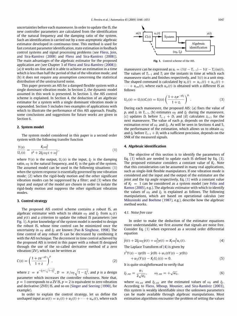
The proposed AIS control scheme contains a robust IS, analgebraic estimator with which to obtain ωf and ξf from uc(t)and y(t) and a criterion to update the robust IS parameters (seeFig. 1). A prior knowledge of the systemmodel is needed to designthe robust IS, whose time control can be minimized once theuncertainty in ωf and ξf are known (Pao & Singhose, 1998). Thetime control of any robust IS can be decreased by combining itwith the AIS technique. The decrement in time control achieved bythe proposed AIS is tested in this paper with a robust IS designedthrough the use of the so-called derivative method of a zerovibration (ZV), which can be written as

C(s) =(1+ ze−sD

1+ z

)p, (2)

where z = e−ξf π/√1−ξ2f , D = π/ωf

√1− ξ 2f , and p is a design

parameter which increases the controller robustness. Note that,p = 1 corresponds to a ZV IS, p = 2 is equivalent to zero vibrationand derivative (ZVD) IS, and so on (Singer and Seering (1990), forexample).In order to explain the control strategy, let us define the

unshaped input as u(t) = u1(t)+ u2(t)+ · · · + um(t), where each

Fig. 1. Control scheme of the AIS.

manoeuvre can be expressed as ui = (1(t − Ti−1)− 1(t − Ti))u(t).The values of Ti−1 and Ti are the instants in time at which eachmanoeuvre starts and finishes respectively, and 1(t) is a unit step.The shaped command is calculated by uc(t) = uc1(t) + uc2(t) +· · · + ucm(t), where each uci(t) is obtained with a different IS asfollows

Uci(s) = Ui(s)Ci(s) = Ui(s)(1+ zie−sDi

1+ zi

)pi. (3)

During each manoeuvre, the proposed AIS: (a) fixes the value ofpi and zi in Ti−1, (b) estimates ωf and ξf during the manoeuvre,(c) updates Di before Ti−1 + Di and (d) calculates zi+1 for thenext manoeuvre. The value of each pi depends on the expectedestimation error of ωf and ξf . As will be seen in Sections 4 and 5,the performance of the estimation, which allows us to obtain ωfand ξf before Ti−1 + Di with a sufficient precision, depends on theSNR of the measured signals.

4. Algebraic identification

The objective of this section is to identify the parameters ofEq. (1) which are needed to update each IS defined by Eq. (3).The proposed estimator considers a constant value of Kf . Notethat this consideration can be assumed in many real applications,such as single-link flexible manipulators. If one vibration mode isconsidered and the input and the output of the estimator are thejoint and the tip angle respectively, Eq. (1) with a constant valueof Kf = 1 can be considered as a system model (see Feliu andRamos (2005), e.g.). The algebraic estimator with which to identifythe values of ωf and ξf is explained as follows. The followingmanipulations, which are based on operational calculus (seeMikusinski and Boehme (1987), e.g.), describe how the algebraicmethod works.

4.1. Noise free case

In order to make the deduction of the estimator equationsmore understandable, we first assume that signals are noise free.Consider Eq. (1) when expressed as a second order differentialequation

y(t)+ 2ξfωf y(t)+ ω2f y(t) = Kfω2f uc(t). (4)

The Laplace Transform of (4) is given by

s2Y (s)− sy(0)− y(0)+ α1(sY (s)− y(0))+α2(Y (s)− KfUc(s)) = 0. (5)

It is quite straightforward to verify that

ξf ,est =α1

2√α2, ωf ,est = +

√α2, (6)

where ωf ,est and ξf ,est are the estimated values of ωf and ξf .According to Fliess, Mboup, Mounier, and Sira-Ramírez (2003),this system is weakly identifiable since the unknown parameterscan be made available through algebraic manipulations. Mostestimation algorithms encounter the problem of setting the values

1048 E. Pereira et al. / Automatica 45 (2009) 1046–1051

which correspond to initial conditions. However, this method canavoid this problem by taking two derivatives with regard to thecomplex variable s as follows

d2(s2Y )ds2

+ α1d2(sY )ds2

+ α2

[d2(Y )ds2− Kf

d2(Uc)ds2

]= 0. (7)

By developing these expressions via the chain rule, we obtain

s2d2Yds2+ 4s

dYds+ 2Y + α1

(sd2Yds2+ 2dYds

)+α2

(d2Yds2− Kf

d2Ucds2

)= 0. (8)

The time derivatives are noise amplifiers, (see Moussaoui, Brie,and Richard (2005)). To suppress these time derivatives, Eq. (8)is therefore multiplied by s−2, and the following expression isobtained

d2Yds2+ 4s−1

dYds+ 2s−2Y + α1

(s−1d2Yds2+ 2s−2

dYds

)+α2

(s−2d2Yds2− Kf s−2

d2Ucds2

)= 0. (9)

In order to translate Eq. (9) into the time domain, it shouldbe noted that L−1s(·) = d

dt (·), L−1 dνdsν (·) = (−1)ν tν(·) and

L−1 1s (·) =∫ t0 (·)(σ )dσ , where L denotes the usual operational

calculus transform operator and ν is the derivation order. Bytaking this into account, the equivalent time domain expressionof Eq. (9) is

η1(t)+ α1η2(t)+ α2η3(t) = 0, (10)

in which

η1(t) = t2y(t)− 4∫ t

0σy(σ )dσ + 2

∫ t

0

∫ σ

0y(λ)dλdσ ,

η2(t) =∫ t

0σ 2y(σ )dσ − 2

∫ t

0

∫ σ

0λy(λ)dλdσ ,

η3(t) =∫ t

0

∫ σ

0λ2y(λ)dλdσ − Kf

∫ t

0

∫ σ

0λ2uc(λ)dλdσ . (11)

The above set of equations can be readily implementable bymeansof time-varying linear (unstable) filters, such as

η1 = t2y+ x1 η2 = x3 η3 = x5x1 = −4ty+ x2 x3 = t2y+ x4 x5 = x6x2 = 2y x4 = −2ty x6 = t2

(y− Kf uc

).

(12)

If Eq. (10) is integrated in the following way∫ t

0η1(σ )dσ + α1

∫ t

0η2(σ )dσ + α2

∫ t

0η3(σ )dσ = 0, (13)

we obtain Eqs. (10) and (13), and are thus able to find the values α1and α2 as follows

α1 =n1(t)d(t)

=η3(t)

∫ t0 η1(σ )dσ − η1(t)

∫ t0 η3(σ )dσ

η2(t)∫ t0 η3(σ )dσ − η3(t)

∫ t0 η2(σ )dσ

α2 =n2(t)d(t)

=η1(t)

∫ t0 η2(σ )dσ − η2(t)

∫ t0 η1(σ )dσ

η2(t)∫ t0 η3(σ )dσ − η3(t)

∫ t0 η2(σ )dσ

. (14)

As a result, the unknownparameters can be computed by using (6).

4.2. Noisy signals case

The performance of the algebraic estimator is improved byadding low-pass filters to both the numerator and denominator of(14) when noise is presented in the measured signals as follows

α1 =(f ∗ n1)(t)(f ∗ d)(t)

, α2 =(f ∗ n2)(t)(f ∗ d)(t)

, (15)

where f is the impulse response of a low-pass filter. This ismotivated by the assumption of high frequency noise (see Fliess(2006) for more details). A robustness analysis of this kind of low-pass filters with regard to the algebraic estimators was carried outby Trapero, Sira-Ramírez, and Feliu (2007) for the case of a biasedsinusoidal signal. In this work, a double integrator is used as F(s).

4.3. Computational complexity

In order to discover the feasibility of this approach in a realcontrol system, the number of operations required to compute theparameters a step ahead was measured. Since it is only necessaryto know the state values a step before, there is not a considerablememory effort. A proper on-line performance of this algorithmis thus assured if the time required to compute the estimatesa step ahead is less than the sampling time. The majority ofcomputations regard the numerical integration in (12) and (13).For instance, if a Euler solver is chosen, the calculations needed toobtain the estimates one step ahead are 23 real additions, 29 realmultiplications, 1 power calculation and 3 divisions. Nonetheless,a Runge–Kutta solver is also a feasible option which achieves acompromise between accuracy and numeric burden.

4.4. Updating of IS parameters

The algorithm used to update the parameters of each Ci(s) isexplained as follows. Firstly, itmust be noted that: (a) the quotientsα1 and α2, which are used to obtain ωf ,est and ξf ,est , are ill-posedat t = 0 (see Eq. (14)); and (b) due to the unstable nature of thelinear systems in the perturbed Brunovsky’s form, the differentialequation presented in (12) is not bounded, although the inputis bounded. However, the quotients α1 and α2 are certainly welldefined at the end of a certain interval of the form (0, ε), whereε > 0 is a small real number. The proposed solution to overcomethese problems therefore consists of: (a) taking the values of α1and α2 after ε to calculate ωf ,est and ξf ,est and (b) resetting theestimation once this has been accomplished.Secondly, it is necessary to decide when the required precision

in the estimation of ωf ,est and ξf ,est is achieved. To this end, analgorithmwhich takes into account the standard deviation ofωf ,estand ξf ,est is proposed. Aswas commented on Section 4.3, the valuesof ωf ,est and ξf ,est are obtained by sampling the signals uc(t) andy(t). Let us denote this sampling time as Ts, and the results of eachcalculation, which are discrete signals, as ωf ,est(n) and ξf ,est(n).Thus, the moving average and the standard deviation of a samplesignal (ϕf ,est(n)) are defined as follows

E[ϕf ,est(n)] =M−1∑k=0

1Mϕf ,est(n− k), (16)

σ(n) =√E[ϕ2f ,est(n)] −

(E[ϕf ,est(n)]

)2, (17)

where MTs is the minimum time interval needed to calculateϕf ,est(n), whichmay beωf ,est(n) or ξf ,est(n). The proposed criterionconsiders that the variable ϕf ,est(n) achieves sufficient precisionwhenσ(n)

E[ϕf ,est(n)]≤ ∆, (18)

E. Pereira et al. / Automatica 45 (2009) 1046–1051 1049

in which the parameter ∆ expresses the required precision in theestimation of ϕf ,est(n).Thirdly, the IS parameters must be calculated. The estimation

of ωf and ξf are used to update Di and zi+1 (since zi is fixed beforeeach manoeuvre). The value of ε is considered as being equal toTs and the first sample (n = 1) corresponds with Ti−1 + Ts. Letus denote the first sample in which Eq. (18) is achieved as ni.After this sample, we have observed that the white noise in uc(t)and y(t) makes ωf ,est(n) and ξf ,est(n) oscillate around ωf and ξfrespectively. Thus, the estimation can be improved by using thefollowing equation

ϕf ,up(nf ) =nf−ni∑k=0

1nf − ni + 1

ϕf ,est(nf − k), (19)

where nf is the last sample before the value of ϕf is updated withϕf ,up. Note that the values of ωf and ξf are recalculated in eachsample, thus updating the value of Di. The value of Di thereforeremains constant when nTs ≥ Di. In addition, the value of zi+1has to be fixed in the previous sample before the next manoeuvrestarts.

5. Examples of applications

Two examples of applications are presented: (a) the first showsthe performance of the proposed method when white noise ispresent; and (b) the second illustrates the advantages of using anAIS in combination with a robust IS.

5.1. Influence of the SNR level on the estimation performance

Since the estimation of ωf or ξf is based on an algebraicframework which includes algebraic tools such as (i) the module-theoretic approach to linear systems; (ii) elementary non-commutative ring theory; and (iii) operational calculus (see Fliessand Sira-Ramírez (2008)), some notions such as persistentlyexciting signalsmay not be useful in this new setting. Nevertheless,the algebraic estimation performance is influenced by the SNRlevel of the signals. Robustness analysis of the algebraic estimationof the SNR by using low-pass filters (see Eq. (15)) was carriedout in Trapero et al. (2007). The SNR of the output thus worsensas the level of the input is reduced and its shape becomessmoother (i.e. the output vibration is smaller). Therefore, in areal application, the SNR level and the type of input affect theestimation performance.Preliminary simulations using different input signals (step,

slope and parabolic) have shown that the performance of thealgebraic estimation is independent of the input (shape and finalvalue) when the free noise case is considered. In order to simplifythe example and to show the influence of the SNR step inputs,which produce the biggest residual vibration level in the output,are therefore used. The noise free case and three different valuesof SNR (90 dB, 50 dB and 30 dB) are simulated in this example. TheSNR of y(t) is obtained as follows

SNR = 10 log10E(y2)σ 2N

, (20)

where σ 2N is the variance of the white noise added to y(t) andE(y2) represents the power of a sinusoidal signalwith an amplitudewhich is equal to the product of Kf multiplied by the final valueof the step. The considered system has a gain (Kf ) equal to 1. Theparameters needed to implement the updating algorithm are Ts =5 ms, M = 10 and ∆ = 0.02. The value of nf is considered asbeing the same forDi and zi+1 and it is the last sample that achievesnTs < Di.

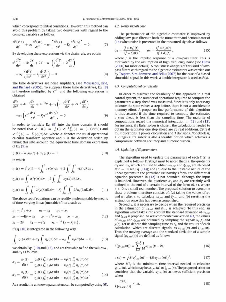
Table 1Results of the Monte Carlo simulations.

SNR (dB) Numb. of conv %Di (%) Max error of Di Max error of zi+1

∞ 1000 10.4 ∼= 0 ∼= 070 998 26.7 0.4% 0.9%50 985 49.3 1.9% 3.4%30 801 74.2 8.4% 11.4%

Fig. 2. Vibration percentage for ZV, ZVD and ZVDDD.

Monte Carlo simulations consisting of 1000 simulations foreach SNR level are carried out to show the relationship betweenthe performance of the AIS and the SNR. The values of ωf andξf are considered to be random numbers between [π, 3π ] and[0, 0.4] respectively. The results are summarized in Table 1.The second column shows the number of occasions on whichEq. (18) is achieved for ωf ,est(n) and ξf ,est(n) before Di, the thirdcolumn shows the average time needed to achieve condition (18),which is defined as a percentage of Di, and the fourth and fifthcolumns indicate the maximum error in the estimation of Di andzi with regard to their theoretical values. Note that the velocityand precision of the estimation depends on the SNR level. Thus,the proposed AIS is useful for large model uncertainties if SNR issufficiently high.

5.2. AIS combined with a robust IS

This example shows the improvements in the robust IS of Eq. (2)when it is combined with the proposed AIS control scheme. Let usconsider that: (i) the input of the system is u(t) = 1(t)+1(t−4)+1(t − 8); (ii) the SNR of y(t) is∼= 30 dB; (iii) the initial conditionsare ωf = 2π and ξf = 0.05; and (iv) the value of ωf changes int = 4 s and t = 8 s to ωf = π and ωf = 3π respectively. Notethat these abrupt changes inωf occur, for example, when a flexiblemanipulator takes or leaves an unknown payload at a particularinstant in time.Firstly, we design the robust IS. The range of values of ωf

([π, 3π ]) are normalized, and are equal to [0.5, 1.5], and thedamping ratio is considered as being equal to 0. Then, from Fig. 2,if a value of p = 4 is chosen, the maximum residual vibrationis approximately equal to 25%. The value of ωf for designing thecontroller is equal to 2π . The delay introduced by the controller(pD) is thus equal to 2 s.Secondly, the AIS design is presented. The performance of the

AIS combinedwith a robust IS depends on the SNR. Thus, if the SNRis equal to 30 dB, themaximumdeviationwith regard to the designfrequency is around 8.4%. The normalized range of values for ωfis therefore approximately equal to [0.916, 1.084]. From Fig. 2, amaximum residual vibration of less than 13% can be achieved withonly one ZV.

1050 E. Pereira et al. / Automatica 45 (2009) 1046–1051

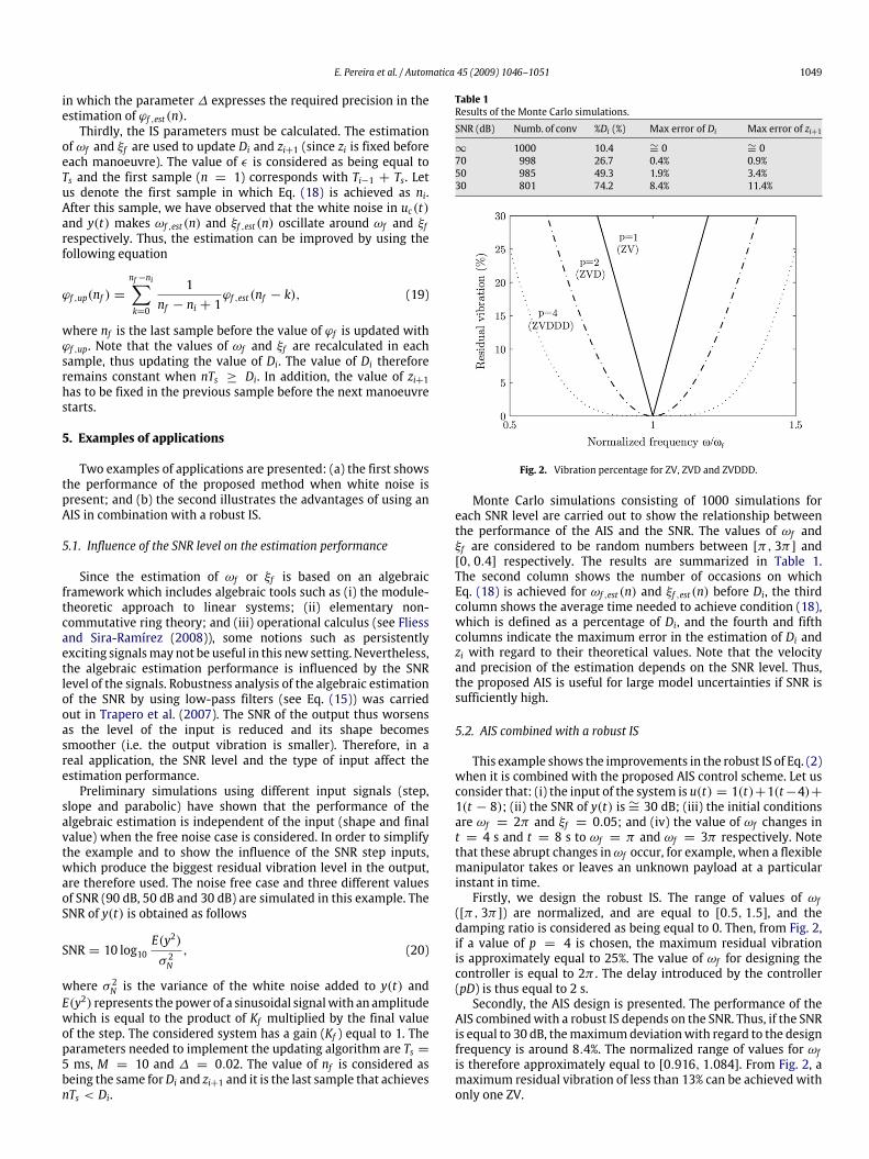
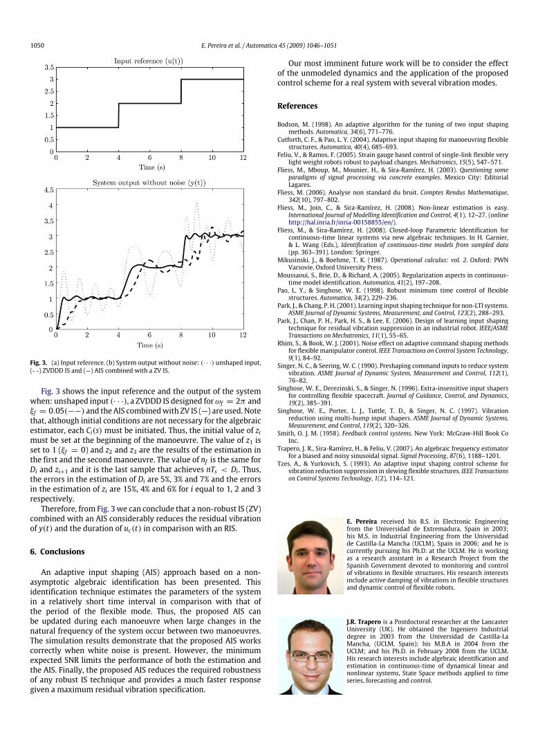
Fig. 3. (a) Input reference. (b) System output without noise: (· · ·) unshaped input,(- -) ZVDDD IS and (—) AIS combined with a ZV IS.

Fig. 3 shows the input reference and the output of the systemwhen: unshaped input (· · ·), a ZVDDD IS designed forωf = 2π andξf = 0.05(−−) and the AIS combinedwith ZV IS (—) are used. Notethat, although initial conditions are not necessary for the algebraicestimator, each Ci(s) must be initiated. Thus, the initial value of zimust be set at the beginning of the manoeuvre. The value of z1 isset to 1 (ξf = 0) and z2 and z3 are the results of the estimation inthe first and the second manoeuvre. The value of nf is the same forDi and zi+1 and it is the last sample that achieves nTs < Di. Thus,the errors in the estimation of Di are 5%, 3% and 7% and the errorsin the estimation of zi are 15%, 4% and 6% for i equal to 1, 2 and 3respectively.Therefore, from Fig. 3 we can conclude that a non-robust IS (ZV)

combined with an AIS considerably reduces the residual vibrationof y(t) and the duration of uc(t) in comparison with an RIS.

6. Conclusions

An adaptive input shaping (AIS) approach based on a non-asymptotic algebraic identification has been presented. Thisidentification technique estimates the parameters of the systemin a relatively short time interval in comparison with that ofthe period of the flexible mode. Thus, the proposed AIS canbe updated during each manoeuvre when large changes in thenatural frequency of the system occur between two manoeuvres.The simulation results demonstrate that the proposed AIS workscorrectly when white noise is present. However, the minimumexpected SNR limits the performance of both the estimation andthe AIS. Finally, the proposed AIS reduces the required robustnessof any robust IS technique and provides a much faster responsegiven a maximum residual vibration specification.

Our most imminent future work will be to consider the effectof the unmodeled dynamics and the application of the proposedcontrol scheme for a real system with several vibration modes.

References

Bodson, M. (1998). An adaptive algorithm for the tuning of two input shapingmethods. Automatica, 34(6), 771–776.

Cutforth, C. F., & Pao, L. Y. (2004). Adaptive input shaping for manoeuvring flexiblestructures. Automatica, 40(4), 685–693.

Feliu, V., & Ramos, F. (2005). Strain gauge based control of single-link flexible verylight weight robots robust to payload changes.Mechatronics, 15(5), 547–571.

Fliess, M., Mboup, M., Mounier, H., & Sira-Ramírez, H. (2003). Questioning someparadigms of signal processing via concrete examples. Mexico City: EditorialLagares.

Fliess, M. (2006). Analyse non standard du bruit. Comptes Rendus Mathematique,342(10), 797–802.

Fliess, M., Join, C., & Sira-Ramírez, H. (2008). Non-linear estimation is easy.International Journal of Modelling Identification and Control, 4(1), 12–27. (onlinehttp://hal.inria.fr/inria-00158855/en/).

Fliess, M., & Sira-Ramírez, H. (2008). Closed-loop Parametric Identification forcontinuous-time linear systems via new algebraic techniques. In H. Garnier,& L. Wang (Eds.), Identification of continuous-time models from sampled data(pp. 363–391). London: Springer.

Mikusinski, J., & Boehme, T. K. (1987). Operational calculus: vol. 2. Oxford: PWNVarsovie, Oxford University Press.

Moussaoui, S., Brie, D., & Richard, A. (2005). Regularization aspects in continuous-time model identification. Automatica, 41(2), 197–208.

Pao, L. Y., & Singhose, W. E. (1998). Robust minimum time control of flexiblestructures. Automatica, 34(2), 229–236.

Park, J., & Chang, P. H. (2001). Learning input shaping technique for non-LTI systems.ASME Journal of Dynamic Systems, Measurement, and Control, 123(2), 288–293.

Park, J., Chan, P. H., Park, H. S., & Lee, E. (2006). Design of learning input shapingtechnique for residual vibration suppression in an industrial robot. IEEE/ASMETransactions on Mechatronics, 11(1), 55–65.

Rhim, S., & Book, W. J. (2001). Noise effect on adaptive command shaping methodsfor flexible manipulator control. IEEE Transactions on Control System Technology,9(1), 84–92.

Singer, N. C., & Seering, W. C. (1990). Preshaping command inputs to reduce systemvibration. ASME Journal of Dynamic System, Measurement and Control, 112(1),76–82.

Singhose, W. E., Derezinski, S., & Singer, N. (1996). Extra-insensitive input shapersfor controlling flexible spacecraft. Journal of Guidance, Control, and Dynamics,19(2), 385–391.

Singhose, W. E., Porter, L. J., Tuttle, T. D., & Singer, N. C. (1997). Vibrationreduction using multi-hump input shapers. ASME Journal of Dynamic Systems,Measurement, and Control, 119(2), 320–326.

Smith, O. J. M. (1958). Feedback control systems. New York: McGraw-Hill Book CoInc.

Trapero, J. R., Sira-Ramírez, H., & Feliu, V. (2007). An algebraic frequency estimatorfor a biased and noisy sinusoidal signal. Signal Processing , 87(6), 1188–1201.

Tzes, A., & Yurkovich, S. (1993). An adaptive input shaping control scheme forvibration reduction suppression in slewing flexible structures. IEEE Transactionson Control Systems Technology, 1(2), 114–121.

E. Pereira received his B.S. in Electronic Engineeringfrom the Universidad de Extremadura, Spain in 2003;his M.S. in Industrial Engineering from the Universidadde Castilla-La Mancha (UCLM), Spain in 2006; and he iscurrently pursuing his Ph.D. at the UCLM. He is workingas a research assistant in a Research Project from theSpanish Government devoted to monitoring and controlof vibrations in flexible structures. His research interestsinclude active damping of vibrations in flexible structuresand dynamic control of flexible robots.

J.R. Trapero is a Postdoctoral researcher at the LancasterUniversity (UK). He obtained the Ingeniero Industrialdegree in 2003 from the Universidad de Castilla-LaMancha, (UCLM, Spain); his M.B.A in 2004 from theUCLM; and his Ph.D. in February 2008 from the UCLM.His research interests include algebraic identification andestimation in continuous-time of dynamical linear andnonlinear systems, State Space methods applied to timeseries, forecasting and control.

E. Pereira et al. / Automatica 45 (2009) 1046–1051 1051

I.M. Díaz was born in Spain in 1980. He received theB.S., M.S. and Ph.D. (with honors) degrees in Mechani-cal Engineering from the Universidad de Castilla-La Man-cha, Spain in 2003, 2005 and 2007, respectively. He iscurrently an Assistant Professor in the Continuum Me-chanics Department at the same university. His researchinvolves modeling of flexible structures for vibrationscontrol, mechatronics, continuum mechanics and consti-tutive laws of materials and simulations by the finiteelement method. Dr. I.M. Díaz is a member of IIAV andIEEE.

V. Feliu (M’88) received the M.S. degree (with honors) inindustrial engineering and the Ph.D. degree from the Uni-versidad Politécnica of Madrid, Spain in 1979 and 1982,respectively. He was with the Electrical Engineering De-partment, Universidad Nacional de Educación a Distancia,Spain, from 1980 to 1994. He reached the position of FullProfessor in 1990 and was Head of the Department from1991 to 1994. He was Dean of the School of Industrial En-gineering, Universidad de Castilla-La Mancha, Spain, from1994 to 2008. He was a Fulbright Scholar, from 1987 to1989, at the Robotics Institute, Carnegie Mellon Univer-

sity, Pittsburgh, PA. His research interests include automatic and control systems,and kinematics and dynamic control of rigid and flexible robots. Dr. Feliu is a seniormember of IFAC and IEEE.