Adaptive fuzzy modeling versus artificial neural networks

Adaptive fuzzy modeling versus artificial

neural networks

Ralf Wieland 1 , Wilfried Mirschel

Leibniz-Center for Agricultural Landscape Resaerch, Institute of Landscape

Systems Analysis, Eberswalder Str. 84, 15374 Muencheberg, Germany

Abstract

In this paper two areas of soft computing (fuzzy modeling and artificial neural net-works) are discussed. Based on the fundamental mathematical similarity of fuzzytechnique and radial basis function networks a new training algorithm for fuzzymodels was introduced. A feed forward neural network (NN), a radial basis func-tion network (RBF) and a trained fuzzy algorithm are compared for regional yieldestimation of agricultural crops (winter rye, winter barley). As training pattern adata set from a training region (Maerkisch-Oderland district, Germany) and as testpattern a data set from a three times larger region were used. Specific advantagesand disadvantages of these methods for the estimation of yield were discussed.

Key words: Fuzzy modeling; artificial neural network; feed forward network; radialbasis function network; training algorithm; yield estimation; agricultural crops

1 Introduction

The modeling of natural process has to cope with uncertainty in the parameters andthe modeling methods. The crux of ecological modeling lies in our understanding:“depending upon the nature of the study, complexity can confound the analysis ofan ecosystem model; the more interacting components a model has, the less straight-forward it is to extract and separate causes and consequences; this is compoundedwhen uncertainty about components obscures the accuracy of a simulation” (Ecolog-ical Model, 2006). This leads to the wish of the modelers to use expert knowledgeas model basis or to extract models from the data in a straightforward way (Ghielmi

1 Corresponding author: Tel.: +49 33432 82337; fax: +49 33432 82334. E-mail address:[email protected]

Preprint submitted to Elsevier 25 July 2007

et al., 2006). The focus of this paper is on these soft-computing methods and theirapplication to a simplified but realistic problem.

In this paper models will be discussed as function approximators. On the one handthere are some inputs (for example soil quality, nitrogen fertilizer, cropping year) andon the other hand a single output (crop yield). There are a lot of possible methods fordeveloping models from data sets, such as multiple regression, artificial neural networks,fuzzy methods etc. Because of the lack in understanding in ecological modeling theintroduction of expert knowledge in form of fuzzy modeling or artificial neural networksas universal function approximators can be one step towards creating models withoutan explicit mathematical equation. It can be shown that fuzzy modeling and neuralnetworks are similar from a mathematical point of view. This offers the opportunityto introduce a training algorithm in fuzzy models and to compare these with artificialneural networks.

The complete investigation was based on the software “Spatial Analysis and ModelingTool” (SAMT). This tool is available as free open source software (SAMT, 2007).Additionally were used free open source libraries like the gnu scientific library (GSL,2007), the hierarchical data format (HDF, 2007) and for the graphical user interfacethe QT-library (QT, 2007).

To be useful for practical simulations, models should satisfy the following requirements:

• accuracy: the error resulting between the simulated and measured values should beminimal

• generalization: the model should reduce the complexity of the real world using anapproximation of the data based on fundamental knowledge

• portability: the model should be usable in different sites with slightly changed inputs(compared to the training data)

These requirements are contradictory (for example a high accuray can lead to lowgeneralization) to some degree so a practical compromise between them must be found.

2 Description of the data sets

The handling of different artificial neural networks and fuzzy methods to develop simplemodels, their specifics (advantages and disadvantages) and their suitability for appli-cation in the field of ecology is shown using data sets for spatial grain yield (yield)estimation for winter rye and winter barley under practical field cropping conditions.An example from the literature using artifical neural networks in a similar applicationis given in (Grzesiak et al., 2006); an introduction to the use of neural networks inagriculture is given in (Schultz et al., 1999). For the further methodical investigationit was assumed that only the three most important values which influence the process

2

of crop yield formation are taken into account.

The first value represents the cropping site as a whole and characterizes the complexsize-connected growing conditions among them the soil type and the water supply. Thiscomplex site value is described by the so called soil quality index (SQI) which rangesfrom 1 to 100. The SQI is defined on the basis of the parent material of the soil, its pe-dogenetic development stage and the hydrological boundary conditions. Lowest valuesare attributed to the poor diluvial sandy soils and highest values to the chernozomsfrom loess. The SQI was developed, starting in the 1930’s, for the evaluation of agri-cultural used land in Germany. To take into account the influence of agro-managementon the yield, the nitrogen supply is chosen as the second value, i.e. the nitrogen fertil-ization (NF) given in 1 up to 4 separate applications.This is one of the most influentialmanagement practices undertaken by the farmer to increase yield. The sum of all nitro-gen fertilizer amounts applied during the winter rye and winter barley growing periodis taken into account. The third very important value influencing yearly yields is theplant breeding and cropping technology level. For winter rye and winter barley a yieldanalysis for the Federal State of Brandenburg, Germany, in the period from 1975 to2000 respectively shows a linear yearly increase in the yields of 0.812 t/(ha ∗ a) and0.810 t/(ha∗a) for winter barley and winter rye, respectively. Instead of the not so easynumerical quantification of plant breeding and cropping technology level, the croppingyear, i.e. the year of grain harvest (year) is used.

For effective development of a model for estimation of the spatial winter rye and winterbarley yields, the necessary data were taken from the Maerkisch-Oderland district (asmodel training area) with an area under arable use of about 115,000 ha, located in theeastern part of Germany, between Berlin and the river Oder. This mainly agriculturallyused (64%) region is characterized by sandy soils and continental influenced climateconditions (low annual precipitation, hot and dry early summer and summer conditionsand cold winter conditions). The data sets used here are from the period between1974 and 1988 and are distributed uniformly within the whole district. A data setoverview, including abbreviations, is given in the upper part of table 1 to enable abetter recognition of these data sets within the following description and discussion ofmethods for model development and model comparison.

3

Maerkisch-Oderland district (2, 128 km2)

crop data set year SQI NF (kgN/ha) yield (t/ha)

w. barley (N=119) A1 1974 ... 1988 22 ... 40 80 ... 170 2.0 ... 5.9

w. rye (N=449) A2 1974 ... 1988 14 ... 36 60 ... 173 1.5 ... 5.6

Expanded area (7, 186 km2)

crop data set year SQI NF (kgN/ha) yield (t/ha)

w. barley (N=406) B1 1976 ... 1989 21 ... 59 30 ... 221 1.1 ... 7.4

w. rye (N=401) B2 1976 ... 1989 23 ... 59 42 ... 210 0.8 ... 5.7

Table 1: Overview of used data sets

For the verification of the model and its application to other areas, i.e. with data setsindependent from the training district, data sets were taken from an expanded areain the eastern part of the Federal State of Brandenburg, Germany, which is 3.5 timesgreater than the Maerkisch-Oderland district, but includes the Maerkisch-Oderlanddistrict completely. About 320,000 ha of this extended area is under arable use i.e. thisarea also is mainly (50 %) agriculturally used. The expanded area is characterized bysandy soils in the middle and southern parts and has sandy-loamy soils in the northernpart. The climate conditions are similar to the Maerkisch-Oderland district. The datasets used for the expanded area were collected from farmers in connection with thecomputer-aided plant protection service during the period between 1976 and 1989 andare distributed uniformly over the whole expanded area. They do not contain the datasets from the Maerkisch-Oderland district. The original data sets do not contain theSQI values, but only information on site type. The SQI values were calculated on thebasis of these site type data using the transformation algorithm proposed by Kindler(Kindler, 1992). An overview of the data sets is given in the lower part of table 1.

3 Feed forward networks

An artificial neural network as function approximator is useful because it can approxi-mate a desired behavior without the need to specify a particular function. This is a bigadvantage of artificial neural networks compared to multivariate statistics. The pricefor this is the difficult nonlinear optimization technique, that can lead to local optimaor to the so called over training. Feed forward networks are the most established typeof artificial neural networks. A good introduction is given in (Principe et al., 2000). Ifsomebody speaks about artificial neural networks he often means this type of network.This can lead to the assumption that these neural networks must not be discussed. Thisis not so. It has become evident that this type is often used without the carefulnesswhich is necessary. This impression is increased by much software that implements feed

4

forward networks which the user can apply merely by clicking some buttons.

3.1 Training of feed forward networks

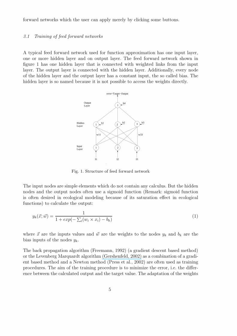
A typical feed forward network used for function approximation has one input layer,one or more hidden layer and on output layer. The feed forward network shown infigure 1 has one hidden layer that is connected with weighted links from the inputlayer. The output layer is connected with the hidden layer. Additionally, every nodeof the hidden layer and the output layer has a constant input, the so called bias. Thehidden layer is so named because it is not possible to access the weights directly.

I2I1 I3

b1 b3

w11

1 3

1 2 3

HiddenLayer

InputLayer

OutputLayer

w33

2b2

error=Target−Output

b41

Fig. 1. Structure of feed forward network

The input nodes are simple elements which do not contain any calculus. But the hiddennodes and the output nodes often use a sigmoid function (Remark: sigmoid functionis often desired in ecological modeling because of its saturation effect in ecologicalfunctions) to calculate the output:

yk(~x; ~w) =1

1 + exp(−∑

i(wi × xi) − bk)(1)

where ~x are the inputs values and ~w are the weights to the nodes yk and bk are thebias inputs of the nodes yk.

The back propagation algorithm (Freemann, 1992) (a gradient descent based method)or the Levenberg Marquardt algorithm (Gershenfeld, 2002) as a combination of a gradi-ent based method and a Newton method (Press et al., 2002) are often used as trainingprocedures. The aim of the training procedure is to minimize the error, i.e. the differ-ence between the calculated output and the target value. The adaptation of the weights

5

during the training process can lead to a so called over training. This means that theneural network can reproduce the training data quite well but has lost its ability togeneralize. The phenomenon is especially important when only a few training patternsare available. To avoid this a rule of thumb was given by Schultz (Schultz et al., 1997):

parameter = inputs ∗ hidden + hidden + hidden + 1 (2)

parameter < 5 ∗ training pattern (3)

One strategy for use of neural networks therefore should be: start with a “simple”network structure and go over stepwise to more complicated structures. For such tasklike described below start with 2, 3, 4 hidden nodes for example. However this canonly be a first approach to use feed forward networks. It has been shown that the overtraining arises from some dominant values of the weights of the trained network. Thismeans that not only the number of weights are important, but also their values. Byregularization (MacKay, 2003) a method is available to avoid the over training:

M(~w) = error(~w) + αn∑

i=1

w2

i (4)

The error is the mean square error: error(~w) = 1

n

∑ni=1

(Targeti − Outputi)2.

With regularization not only the error is reduced during the training process, but alsothe sum of the square of the weights (multiplied by an empirical factor α). In the neuralnetwork toolbox of SAMT, called SAMT NN (Wieland et al., 2006), a similar methodwas employed. The training procedure was left unchanged but optional use was madeof a stop criterion the value of M(~w). This leads to an abort of the training procedurebefore over training could occur. Many examples have shown that this criterion is morepowerful than the frequently used split sample technique. A critical view of the crossvalidation technique is given by Nadeau (Nadeau et al., 2003).

3.2 Application of feed forward networks

The feed forward network toolbox as part of SAMT was used to train a model on thebasis of data sets of the training region. The soil quality index (SQI), the nitrogenfertilizer amount (NF) and the cropping year for winter barley and winter rye wereselected as inputs. The network has three hidden nodes and one output node for bothtraining data sets. The back propagation algorithm (BP) and the Levenberg Marquardtalgorithm (LM) were used as training algorithms.

6

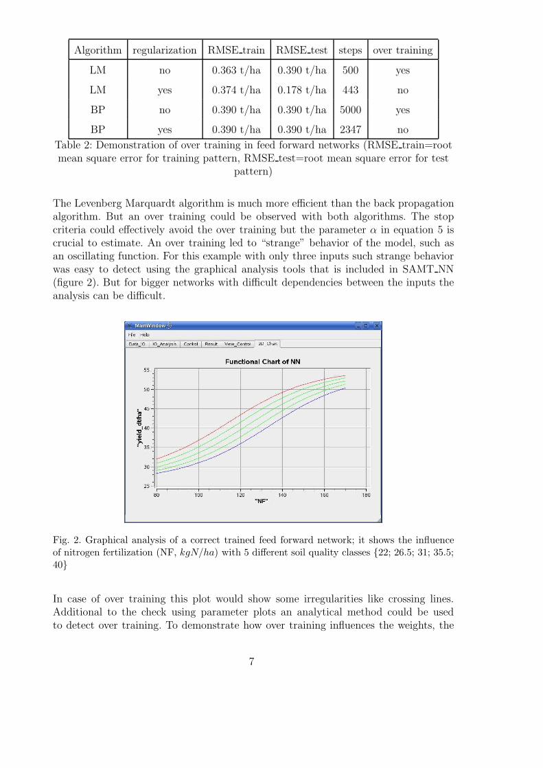
Algorithm regularization RMSE train RMSE test steps over training

LM no 0.363 t/ha 0.390 t/ha 500 yes

LM yes 0.374 t/ha 0.178 t/ha 443 no

BP no 0.390 t/ha 0.390 t/ha 5000 yes

BP yes 0.390 t/ha 0.390 t/ha 2347 no

Table 2: Demonstration of over training in feed forward networks (RMSE train=rootmean square error for training pattern, RMSE test=root mean square error for test

pattern)

The Levenberg Marquardt algorithm is much more efficient than the back propagationalgorithm. But an over training could be observed with both algorithms. The stopcriteria could effectively avoid the over training but the parameter α in equation 5 iscrucial to estimate. An over training led to “strange” behavior of the model, such asan oscillating function. For this example with only three inputs such strange behaviorwas easy to detect using the graphical analysis tools that is included in SAMT NN(figure 2). But for bigger networks with difficult dependencies between the inputs theanalysis can be difficult.

Fig. 2. Graphical analysis of a correct trained feed forward network; it shows the influenceof nitrogen fertilization (NF, kgN/ha) with 5 different soil quality classes {22; 26.5; 31; 35.5;40}

In case of over training this plot would show some irregularities like crossing lines.Additional to the check using parameter plots an analytical method could be usedto detect over training. To demonstrate how over training influences the weights, the

7

biggest and the lowest weight were selected in the over trained and in the stoppednetwork with [-4.04; 2.26] and [-0.75; 1.71], respectively. These differences show howuseful the introduction of the stop criterion can be. On the other hand the root meansquare error (RMSE) of the test pattern approc. (20 % of all patterns were used as atest pattern and excluded from the training) gave no hint of over training. The use ofan increase in the RMSE of the test pattern as stop criterion, as often used in neuralnetworks (Nadeau et al., 2003), was not successful in our case. Our own numeroussimulations have shown that it is often a better alternative to use the whole set astraining set and apply the new introduced stop criterion.

4 Radial basis function network (RBF)

A feed forward network used as a function approximator is a black box fed with inputs,which it is hoped will produced meaningful outputs. However there are no methods forchecking if the inputs are in the region were the network was trained. An further typeof artificial neural network is the so called radial basis function network (Bishop, 1995),which uses a cluster algorithm in the first step (unsupervised training) and calculatesthe approximation in the second step (supervised training).

4.1 Unsupervised training part of RBF

As cluster algorithm a Kohonen feature map was used (Kohonen, 2001). The Kohonennodes are organized as a map with n rows and m columns. Every node s contains aweight vector ws whose components match the components of an input vector x ∈ V ,where V is the input space. The training algorithm adjusts iteratively the weight vectorof the winning neuron (the neuron with the best match to a randomly selected inputvector) and the weights of the nodes in the neighborhood of the winning node (seefigure 3).

8

S

V

∆

v

Kohonen map A

wsws

Fig. 3. Training of a Kohonen feature map

The training algorithm is well described in existing literature (Kohonen, 2006) so itis not further discussed in this paper. A Kohonen feature network tends to learn astatistic of the input space V , which means that the nodes are located in such a waythat their density is higher where the input density is high. This has the advantagethat the trained network is more sensitive where more data on a location are available.To show this in three dimensional space a splatter technique (Schroeder et al., 1998)was applied in figure 4.

Fig. 4. Splatter plot of trained Kohonen feature map

In figure 4 the gray elements represent the input data and the dark elements stand forthe trained nodes.

9

4.2 Supervised training part of RBF

The fundamental idea in RBF is to use a trained (Kohonen) network to develop aradial basis function:

f(~x, ~ws) = exp(−scale × ‖~x − ~ws‖) (5)

A radial basis function is often realized as a Gaussian bell shape function (Bishop,1995), with the empirical factor scale. This function is used with a simple linear esti-mator to calculate the desired function:

y(~x) =m∑

s=1

as × f(~x, ~ws) (6)

To determine the parameters as the following system of equations must be solved:

a1 ∗ f(~x1, ~w1) + a2 ∗ f(~x1, ~w2) + . . . + am ∗ f(~x1, ~wm) = y1

a1 ∗ f(~x2, ~w1) + a2 ∗ f(~x2, ~w2) + . . . + am ∗ f(~x2, ~wm) = y2

. . .

a1 ∗ f(~xn, ~w1) + a2 ∗ f(~xn, ~w2) + . . . + am ∗ f(~xn, ~wm) = yn

(7)

This system (m is the number of nodes and is usually much smaller than the numberof training patterns n) can be solved in sense of least square approximation using thesingular value decomposition (SVD) (Bing et al., 2006) in one step or using iteratively(Korn, 2004). The simulation system SAMT contains a special toolbox which permitstraining with both methods. The results will be discussed below.

An other interesting question is the estimation of the optimal number of Kohonennodes for a training process. When too few Kohonen nodes are used, approximationof the desired function with low error is not possible. Too many nodes lead to an overtraining, which means in extreme that all inputs have their own node. In such a casethe system can be used in a much simpler way: “the winner takes all” that means onlyone kohohnen node is active, so that only one as is responsible for the output. This typeof artificial neural network is called as “counter propagation” network (HechtNielsen,1988) and can be useful (fast because of its simplicity and robust because no numeric isused) for some applications. In this paper the focus is on a real RBF where the numberof radial basis functions is much smaller than the number of inputs. To find an optimalnumber of nodes at this point, only such methods as three dimensional visualizationusing splatter technique are suited. If the nodes are able to fill out all interesting regionsof the training data, then the number of nodes falls within a reasonable range.

10

4.3 The use of RBF for training data

The data sets A1 and A2 were used to show how a RBF can cope with these datasets. Three different RBFs for each data set were created and the resulting root meansquare error determined (see Table 3).

Data set Neurons RMSE iter RMSE SVD

A1 10 0.433 t/ha 0.433 t/ha

A1 30 0.354 t/ha 0.346 t/ha

A1 60 0.269 t/ha 0.241 t/ha

A2 10 0.504 t/ha 0.504 t/ha

A2 30 0.459 t/ha 0.457 t/ha

A2 60 0.426 t/ha 0.416 t/ha

Table 3: Training results of different RBFs (RMSE iter=root mean square error foriterative training procedure, RMSE SVD= root mean square error for the SVD

procedure)

Compared to the feed forward networks the results are in a similar region. Table 3shows that for a small set of neurons the iterative procedure achieves the same resultsas the SVD. Interesting in this context is that the differences between the iterativetraining procedure and the one step solution using SVD is increased with increasingnumber of nodes. The stored values ai show that the difference between the lowest andthe highest is in the range [-1.8; 2.5] for A1 and iter; [-26.0; 26.4] for A1 and SVD;[-3.5; 4.4] for A2 and iter; [-20.2; 13.5] for A2 and SVD. This is the same situation asoccurs with over training in feed forward networks. The consequences of this will bediscussed below.

5 Fuzzy modeling

Fuzzy modeling is designed to use knowledge of an experienced expert directly as basisof modeling. This means that:

• fuzzy sets for the inputs of the model have to be created,• the outputs have to be created and• a set of rules that combines the inputs with the outputs has to be created.

The rules are easy to understand and provide a basis for understanding of a fuzzymodel and the discussion with other experts. We have learned that it is important tofind the real expert and not a group of people with different experiences. The mean

11

of knowledge is often not useful: if you want to control a car to draw aside one expertmay say “go left” an other “go right” - the mean does not realy solve the problem. Itshould be stressed that for a fuzzy model the most important step is the estimation offuzzy sets for the inputs. In this step the knowledge provided by the expert is especiallynecessary. Finding the fuzzy rules is often not so difficult. The big advantage of a fuzzysystem in comparison with an artificial neural network is that the expert can build amodel that covers all cases known to the expert. This means that a fuzzy model can beused in a robust way for data sets which are not contained in the training set as in thecase of neural networks. Whilst an artificial neural network used in a region withouttraining can lead to a disaster, a fuzzy model can often cope with this situation. Adisadvantage of a fuzzy system is that the model can not be better than the expert,because it can not be trained like a neural network.

5.1 Fuzzy algorithm

The fuzzy algorithm that was used in the fuzzy development toolbox of SAMT (SAMT -FUZZY) is described in detail by Wieland (Wieland et al., 2004). Only a short summaryof the features of the fuzzy description is given here:

• the membership function µijm(xi) of the intputs xi can be triangular or trapezoid

(this function types can approximate Gaussian bell shapes quite well),• the outputs ok are crisp values (k = 1...n),• the rules combine every membership combination of the input with the desired output

and• the defuzzification method is simply a weighted sum.

The use of crisp outputs is rather uncommon, but it is very fast and can approximatelinear and nonlinear behavior (Lutz et al., 1998). A further advantage is the easy imple-mentation of a training algorithm based on adaptation of the outputs, explained below.An other restriction is the use up to three inputs in a fuzzy model in SAMT FUZZY.If more inputs are needed a hierarchy of fuzzy models can be used. In such a hierarchyan output of a fuzzy model can be an input of a fuzzy model higher in this hierarchy.This avoids a combinatorial explosion of the number of rules of the fuzzy models. Thenumber of rules is the multiplication of the number of membership functions of eachinput. In the example below 5 membership functions for SQI, 5 membership functionsfor NF and 2 membership functions for years where used. This leads to 5*5*2= 50rules. The algorithm is divided into the following steps:

• assign a membership to all rules (using min or prod method)

amk = min{µ1jm

(x1), µ2jm(x2), µ3jm

(x3)} (8)

12

• select the best rule for each different output

ak = max{a1

k, a2

k, · · ·} (9)

• defuzzification

o =

∑nk=1

ak × ok∑nk=1

ak

(10)

with m as index to rule; k as index to output; ok as the crips output value; n as thenumber of outputs.

This algorithm is almost a basic algorithm in fuzzy modeling (Zadeh, 1968). It is veryfast and can be used also in a spatial application where the inputs are coded usingmaps with a huge number of inputs (Wieland et al., 2002).

5.2 Fuzzy training

The fuzzy algorithm is simple and has three different possibilities for training:

• adaptation of the membership function for the inputs• adaptation of the outputs• adaptation of the rules

The possible adaptation of the inputs was investigated by Korn (Korn, 2007) for a fuzzymembership using bell shaped functions. An algorithm to train triangular and trapezoidmembership functions is given in (Nauck et al. , 2003). The algorithm is critical becauseof its high number of training data sets needed to adjust all the parameters and timeconsuming.

The adaptation of the outputs is a simple iteration over the number of training patternn and using the following steps:

• calculate the error of an output of active rule:

error = yi − fuzzy(x1i, x2i, x3i)

• determine the step δk:

δk = ak ∗ ok ∗ error ∗ gain

• adapt the outputs:

ok = ok + δk

with gain as empirical training factor.

13

This algorithm is nothing other than an application of the delta rule (McClelland et al.,1988) for the training of simple neural networks. The outputs will be iteratively changedto minimize the error. During this procedure it may be that one output, “small” forexample, tries to step over the following output, “medium”. This should be avoidedbecause of the integrity of the fuzzy model. In the utilized algorithm the adaptationstep will be suppressed in such a case. But this can be used to generate a signal tochange a special rule. This will be a subject of future investigation.

The adaptation of the rules is simple to realize (only a pointer must be changed), butit is a global change in a fuzzy system and must be done with care. It is not includedin the actual version 2.4 of SAMT up to now.

5.3 Application of a fuzzy system to model the training data

The fuzzy model has the same three inputs: soil quality index (SQI), nitrogen fertilizeramount (NF), and the cropping year as the two artificial neural networks investigatedabove. The results are therefore comparable. The inputs SQI and NF were split intofive membership functions each: very small, small, medium, large, very large (vs, s, m,l, vl). The cropping year was split into two membership functions: early and late. Forwinter rye the membership functions for SQI and NF are shown in the figures 5 and 6

s m vl

0.5

1.0vs l

10 20 30 40 50

µ

SQI

Fig. 5. Membership function for SQI for the winter rye model

14

Vs lm vls

50 100 150 200 250

0.5

1.0

µ

NF

Fig. 6. Membership function for NF for the winter rye model

The cropping year is a very simple fuzzy set consisting only of two membership functionused to “interpolate” between the yield in “early” years (1950) and “late” years (2000)to model the influence of the altered quality of the seed. The outputs are given intabular form below. The rules combine all possible inputs (5*5*2=50 Rules). A sampleof the rules is given in figure 7

Fig. 7. Sample of the rules for winter rye model

The outputs for the training data sets A1 and A2 are developed using expert knowledge.The training algorithm of the fuzzy system changed these outputs to obtain a smallererror. For winter rye the root mean square error (RMSE) was 1.21 t/ha before trainingand 0.565 t/ha after training, for winter barley the RMSE was 0.862 t/ha before and0.60 t/ha after training. Table 4 shows the adaptation of the outputs:

15

A2 winter rye A1 winter barley

training training

before after before after

1.0 t/ha 1.00 t/ha 2.0 t/ha 1.86 t/ha

2.0 t/ha 1.01 t/ha 3.0 t/ha 1.87 t/ha

3.0 t/ha 3.09 t/ha 3.7 t/ha 3.65 t/ha

4.0 t/ha 3.11 t/ha 4.5 t/ha 4.41 t/ha

5.0 t/ha 3.14 t/ha 5.5 t/ha 4.42 t/ha

6.0 t/ha 4.67 t/ha 6.5 t/ha 5.77 t/ha

7.5 t/ha 4.68 t/ha 8.0 t/ha 6.01 t/ha

9.0 t/ha 9.00 t/ha 9.5 t/ha 9.50 t/ha

Table 4: Training of fuzzy outputs

The extreme outputs vs and vl were unchanged but the intermediate outputs werechanged dramatically. This shows how the algorithm has been influenced by the rulesto change the output. For the output vl no training data was available so it was leftunchanged.

The results are acceptable, but they could not reach the quality of results obtainedwith the trained neural networks. This was expected. The fuzzy model is much morerobust compared to trained neural networks at the expense of accuracy. Figure 8 showsthe three dimensional splatter plot of the fuzzy model.

Fig. 8. Splatter plot of fuzzy classes versus data set

16

The centers of the fuzzy membership functions (dark elements in figure 8) are locatedoutside the training data set (gray elements in figure 8). This could be changed by adifferent model of the cropping year, but it would not change the principal deterministiclocations of the fuzzy membership functions. The fuzzy membership functions camefrom the expert and were not changed during the training process. If the trainingwould also change the membership function of the fuzzy model, a model similar to theradial basis function network would emerge. The differences between a fuzzy modeland a RBF are based on the different form of the membership functions, in case offuzzy it mustn’t be symmetric. This analogy between a fuzzy model and a RBF givesan introduction of number of nodes required in RBF. The number of nodes should beapproximately equal to the number of fuzzy membership functions, with addition ofsome nodes to implement the asymmetry in the membership function. In the exampleabout 50-60 nodes are a good starting point for the RBF.

As mentioned above, the training of the outputs is restricted in the tool SAMT FUZZY,so that one output can not jump over an immediate neighbor. This means that thenew outputs for the winter rye from 4.0 to 3.11 t/ha and 5.0 to 3.14 t/ha could notcross. The output for 4.0 t/ha must be remain smaller than the output for 5.0 t/haotherwise the set of rules will be inconsistent. In a future enhancement of the trainingalgorithm this could be used to adapt the rules and expand the training region.

6 Comparison of feed forward network, radial basis function network, anda fuzzy system using an independent data set

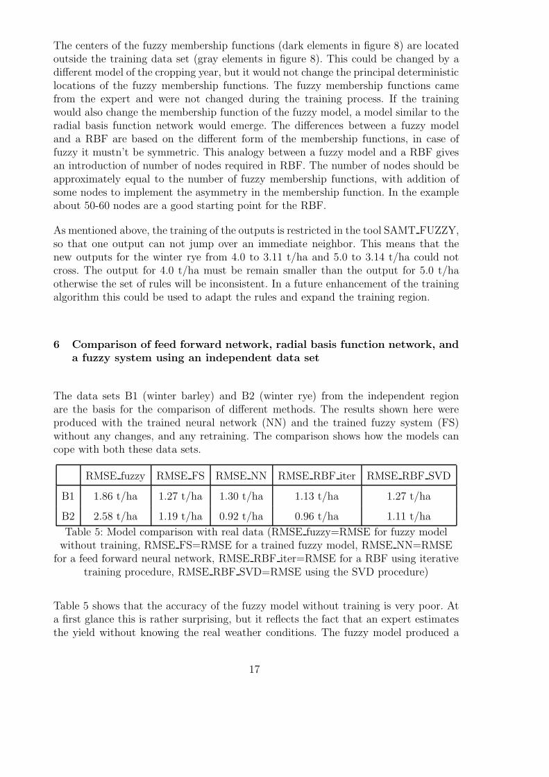
The data sets B1 (winter barley) and B2 (winter rye) from the independent regionare the basis for the comparison of different methods. The results shown here wereproduced with the trained neural network (NN) and the trained fuzzy system (FS)without any changes, and any retraining. The comparison shows how the models cancope with both these data sets.

RMSE fuzzy RMSE FS RMSE NN RMSE RBF iter RMSE RBF SVD

B1 1.86 t/ha 1.27 t/ha 1.30 t/ha 1.13 t/ha 1.27 t/ha

B2 2.58 t/ha 1.19 t/ha 0.92 t/ha 0.96 t/ha 1.11 t/ha

Table 5: Model comparison with real data (RMSE fuzzy=RMSE for fuzzy modelwithout training, RMSE FS=RMSE for a trained fuzzy model, RMSE NN=RMSE

for a feed forward neural network, RMSE RBF iter=RMSE for a RBF using iterativetraining procedure, RMSE RBF SVD=RMSE using the SVD procedure)

Table 5 shows that the accuracy of the fuzzy model without training is very poor. Ata first glance this is rather surprising, but it reflects the fact that an expert estimatesthe yield without knowing the real weather conditions. The fuzzy model produced a

17

more theoretical estimation. Much better is the trained fuzzy model, emphasizing theeffectivity of the proposed training algorithm. The different types of neural networksproduced comparable results. The SVD algorithm led to a slight over training for theRBF. This was expected, but it could also be shown that this over training usingSVD could only be observed when the number of Kohonen nodes was sufficiently large(about 60). However, it is interesting to interprete the results in more detail. If theresults obtained are high ( about 6.0 t/ha for winter barley (B1) or about 5.5 t/hafor winter rye (B2)) then the fuzzy model gave a small error. This emphasizes theusefulness of fuzzy models in calculating the potential yield. For a realistic use of thismodel in predicting the real yields, for instance, it must be combined with an additionalmodel to take into account the concrete weather conditions and additional managementinfluences like plant protection or sowing date. On the other hand the trained modelsare quite usable for producing a yield estimation for a larger independent region. Fora better regionalization of fuzzy models it is necessary to find reliable expert in theregion of interest. A model controlling software can switch between models for differentregions. This can improve the results but the modeler has to take care of the accuracyof the underlying knowledge.

The big disadvantage of a feed forward network (in some respects also of a RBF) is itsblack box character. There are no events in a feed forward network that can indicateto the user that the inputs are outside of the tolerable range given by the trained data.In the case of the RBF there is such a possibility: the highest value of a RBF-functioncould be used. If the difference between an input vector and the best matching weightvector of a Kohonen network is large then the resulting radial basis function will be verysmall. This information can be used to estimate the reliability of a result produced bya neural network. In this way a feed forward network can be combined with a Kohonennetwork to estimate the reliability of the output. This value can be used to produce anevent which serves as a warning.

In our case this approach did not lead to better results. This may however be because ofa large error in the datasets and the unknown influences caused by weather or manage-ment. For the general use of a feed forward network the additional computation effortis not to great compared with the additional information obtained about reliability. Itis worth trying.

7 Conclusions and perspectives

It has been shown that the fuzzy system and neural networks have similar mathematicalfundamentals, so that a training method used with neural networks could be appliedto fuzzy models, and RBFs could be used as fuzzy models. An interesting approach tointerprete Kohonen maps as linguistic variables is given in (Pedrycz and Card , 1992).The combination of a fuzzy model with a training of the outputs has the advantagethat the model can be understood by the expert and adapt to the measured values.

18

This leads to a better fit of the model, but it could perhaps restrict its portability.The focusing on the outputs in the fuzzy approach leads to a restricted training andconsequently to a bigger error. This can be improved by expanding the training to theinputs and the rules. An automatic adaptation of the rules is possible but an interactionwith the modeler makes more sense because the modeler should be in a position tocontrol the rules. To learn the complete set of rules using the C4.5 (Quillian , 1993)could be an alternative way. The generated rules can be imported in SAMT FUZZYand presented to the developer as a initial rule set. A precondition for the use ofsuch an algorithm are the defined membership functions for the inputs. This algorithmwill be included in a future version of SAMT. To build a complete fuzzy rule set theNEFCLASS algorithm (Nauck et al. , 2003) could be used. The adaptation of theinputs can be done using the algorithm “ComputeAntecedentUpdates” in (Nauck etal. , 2003) or by approximating of the triangular or trapezoid membership functionswith Gaussian bell shaped functions and using an iterative training procedure, or by angenetic algorithm (Goldberg, 1989) to adapt the original membership functions. Thisso called “Neuro Fuzzy Systems” will be part of a future investigation for an aimedenhancement of the software SAMT.

The artificial neural networks are often used as a black box. This is dangerous, becausethe network will in any case produce a result, but the reliability is not ensured. In aRBF the difference to the trained basis classes can be used to control the network. Thisshould also be used in feed forward networks as an additional component.

The application of artificial neural networks and fuzzy systems to real problems shouldbe done with care. A good software basis with an integrated graphical analysis canrelax the situation significantly. There still remain, however, many traps for the mod-eler. For example, the commonly used technique of cross validation is sometimes notpotent enough. A better way could be the regularization of artificial neural networks,as discussed in the paper. However, different training algorithms can also produce dif-ferent results. Additionally, the input data for a realistic yield estimation model hasto include more input variables, such as the weather conditions or other agriculturalmanagement activities. This leads to a bigger system with more complicated models(cascaded fuzzy models for instance). One way to cope with this might to empty ahierarchy of models, as was used in the modeling of habitat quality in (Wieland et al.,2004).

A precondition for an efficient application of neural networks or fuzzy models is asoftware framework with additional components such as fuzzy analysis or graphicalanalysis of the neural networks. SAMT (http://www.samt-lsa.de) includes such a tool-box, which will be continously expanded for future requirements. This open sourcesoftware gives the user the opportunity to understand the algorithms and to enhancethem if necessary.

19

8 Acknowledgment

This contribution was supported by the German Federal Ministry of Consumer Protec-tion, Food and Agriculture, and the Ministry of Agriculture, Environmental Protectionand Regional Planning of the Federal State of Brandenburg (Germany). Thank you toDr. W. Haberstock (Institute of Land Use Systems and Landscape Ecology) and toDr. sc. G. Lutze (Institute of Landscape Systems Analysis) of the Leibniz-Center forAgricultural Landscape Research in Muencheberg (Germany) for the friendly commu-nication of data sets collected from Farmers within the Maerkisch-Oderland districtand from the expanded area in the eastern part of the Federal State of Brandenburg,Germany.

References

Bing Yu , Xingshi He, 2006. Training Radial Basis Function Networks with Differen-tial Evolution. TRANSACTIONS ON ENGINEERING COMPUTING AND TECH-NOLOGY 11.

Bishop, Ch., M., 1995. Neural Networks for Pattern Recognition. Oxford UniversityPress.

Ecological Model. Wikipedia homepage, http://en.wikipedia.org/wiki/Ecological modelFreemann, J.A., 1992. Simulating neural networks with Mathematica. Addison-Wesley.Gershenfeld, N., 2002. The nature of mathematical modeling. Cambride university

press.Ghielmi, L.; Eccel, E., 2006. Descriptive models and artificial neural networks for spring

frost prediction in an agricultural mountain area. Computers and electronic in agri-culture 54, 101-114

Goldberg, D., E., 1989. Genetic Algorithms in Search, Optimization, and MachineLearning. Addison Wesley.

Grzesiak, W.; Blaszczyk, P.; Lacroix, R., 2006. Methods of prediction milk yield indiary cows - Predictive cababilities of Wood’s lactietion curve and artificial neuralnetworks. Computers and electronics in agriculture 54, 101-114.

GSL, gsl homepage, http://www.gnu.org/software/gsl/HechtNielsen, R., 1988. Application of Counterporpagation networks. Neural Networks

1, 131-139.HDF, hdf homepage, http://www.hdfgroup.org/Kindler, R., 1992. Ertragsschtzung in den neuen Bundeslaendern. Verlag Pflug und

Feder GmbH, St. AugustinKohonen, T., 2001. Self-Organizing Maps. SpringerKohonen, T., 2006. Kohonen homepage, http://www.cis.hut.fi

/projects/somtoolbox/theory/somalgorithm.shtmlKorn, G.A., 2007. Advanced Dynamic-system Simulation. Wiley, N.Y.Korn, G.A., 2004. Model replication Techniques for Parameter-influence Studies and

20

Monte Carlo Simulation with Random Parameters. Math. and Computers in Simu-lation 67 (6) 501-513.

Lutz, H.; Wendt, W., 1998. Taschenbuch der Regelungstechnik. Harry DeutschMacKay, D., 2003. Information Theory, Inference, and Learning Algorithms. Cambridge

University Press.McClelland, J., Rumelhart, D., 1988. Explorations in parallel distributed processing.

MIT Press.Nadeau, C., Bengio, Y., 2003. Inference for the Generalization Error. Machine Learning

52.Nauck, D.; Borgelt, Ch.; Klawonn, F.; Kruse, R., 2003. Neuro-Fuzzy-Systeme Vieweg

WiesbadenPress, W.,H.; Teukolsky, S.,A.,;Vetterling, W.,T.; Flannery, B., P., 2002. Numerical

Recipies in C++. Cambridge University Press 387-393.Predrycz, W., Card, H.,C., 1992. Linguistic Interpretation of Self-Organizing Maos.

Proc. IEEE Int Conf. on Fuzzy Systems (FUZZ-IEEE’92, San Diego,CA), IEEEPress, Piscataway, NJ, USA

Principe, J.; Euliano, N.; Letebvre, C., 2000. Innovating Adaptive and Neural SystemsInstructions with Interactive Electronic Books. Proceedings of the IEEE, specialissue on engineering.

Quillian, J.,R., 1993. C4.5: Programs for Machine Learning, Morgan Kaufman, SanMateo CA

QT. qt homepage, http://www.trolltech.com/SAMT. samt homepage, http://www.samt-lsa.orgSchroeder, W.; Martin, K.; Lorenzen, B., 1998. The Visualization Toolkit. Prentice

Hall PTR.Schultz, A.; Wieland, R., 1997. The use of neural networks in agroecological modelling.

Computers and Electronics in Agriculture 18, 73-90.Schultz, A., R. Wieland, G. Lutze, 1999. Neural networks in agroecological modelling

- stylish application or helpful tool?. Computers and Electronics in Agriculture 29,73-97.

Wieland, R.; Voss, M.; Holtmann, X.; Mirschel W.; Ajibefun, I., 2006. Spatial Analyisand Modeling Tool (SAMT), structure and possibilities. Ecological Informatics 1,67-76.

Wieland R., Voss, M., 2004. Spatial Analysis and Modeling Tool - Structure, Possibil-ities and Applications. Environmental Modelling and Simulation EMS 2004.

Wieland, R., Voss M., 2002. Land use change and habitat quality in Northeast Ger-man agro-landscapes. In: Tenhunen, J. D., R. Lenz, R. Hantschel (Eds), Ecosystemapproaches to landscape management in Central Europe, Springer: Berlin 341-346.

Wieland, R.; Voss, M., 2004. Spatial Analysis and Modeling Tool - structure possibilitiesand applications. IASTED: Environmental Modeling and Simulation.

Zadeh L.A., 1968. Fuzzy algorithms. Information and Control 5, 94-102.

21