Adaptive FIT-SMC Approach for an Anthropomorphic ...

This work is licensed under a Creative Commons Attribution 4.0 License. For more information, see https://creativecommons.org/licenses/by/4.0/

This article has been accepted for publication in a future issue of this journal, but has not been fully edited. Content may change prior to final publication. Citation information: DOI10.1109/ACCESS.2021.3139041, IEEE Access

Date of publication xxxx 00, 0000, date of current version xxxx 00, 0000.

Digital Object Identifier 10.1109/ACCESS.2017.DOI

Adaptive FIT-SMC Approach for anAnthropomorphic Manipulator withRobust Exact Differentiator and NeuralNetwork-Based Friction CompensationKHURRAM ALI1, SAFEER ULLAH1, ADEEL MEHMOOD1, HALA MOSTAFA2, MOHAMEDMAREY3, (Senior Member, IEEE), and JAMSHED IQBAL4, (Senior Member, IEEE)1Department of Electrical and Computer Engineering, COMSATS University, Islamabad 45550, Pakistan2Department of Information Technology, College of Computer and Information Sciences, Princess Nourah bint Abdulrahman University, Riyadh 84428, SaudiArabia3Smart Systems Engineering Laboratory, College of Engineering, Prince Sultan University, Riyadh 11586, Saudi Arabia4Department of Computer Science and Technology, Faculty of Science and Engineering, University of Hull, HU6 7RX, UK

Corresponding author: Jamshed Iqbal ([email protected]).

ABSTRACT In robotic manipulators, feedback control of nonlinear systems with fast finite-time con-vergence is desirable. However, because of the parametric and model uncertainties, the robust controland tuning of the robotic manipulators pose many challenges related to the trajectory tracking of therobotic system. This research proposes a state-of-the-art control algorithm, which is the combination offast integral terminal sliding mode control (FIT-SMC), robust exact differentiator (RED) observer, andfeedforward neural network (FFNN) based estimator. Firstly, the dynamic model of the robotic manipulatoris established for the n degrees of freedom (DoFs) system by taking into account the dynamic LuGrefriction model. Then, a FIT-SMC with friction compensation-based nonlinear control has been proposedfor the robotic manipulator. In addition, a RED observer is developed to get the estimates of roboticmanipulator joints’ velocities. Since the dynamic friction state of the LuGre friction model is unmeasurable,FFNN is established for training and estimating the friction torque. The Lyapunov method is presented todemonstrate the finite-time sliding mode enforcement and state convergence for a robotic manipulator. Theproposed control approach has been simulated in the MATLAB/Simulink environment and compared withthe system with no observer to characterize the control performance. Simulation results obtained with theproposed control strategy affirm its effectiveness for a multi-DoF robotic system with model-based frictioncompensation having an overshoot and a settling time less than 1.5% and 0.2950 seconds, respectively, forall the joints of the robotic manipulator.

INDEX TERMS robotic manipulator, robust exact differentiator, feedforward neural network, fast integralsliding mode control, LuGre friction model, autonomous articulated robotic educational platform.

I. INTRODUCTION

R esearchers in academia and industry have shown a sig-nificant deal of interest in robotic manipulators in recent

years due to scientific advancements and industrial needs[1]. In reality, robotic manipulators play a significant rolein the industry by lowering manufacturing costs, improvingaccuracy, quality, and efficiency, and offering more flexibilitythan specialized equipment. They ought to be controlled andoperated smoothly, securely, and reliably to accomplish taskswith higher throughput or productive exploration [2]. The

control of robotic manipulators is a complex task becausetheir dynamic behavior is exceptionally nonlinear, highlycoupled, and time-varying. Apart from that, uncertainties inthe system model, such as external disturbances, parame-ter uncertainty, and nonlinear frictions, constantly exist andcause the unstable performance of the robotic system [3].In the literature, several approaches have been proposed forcontrolling the robotic systems, such as sliding mode control(SMC) [4] , H-infinity (H∞) control [5], optimal control[6], PID control [7], adaptive control [8], model predictive

VOLUME 4, 2016 1



control (MPC) [9], and other nonlinear controls reported in[10]–[12].One of the main issues impeding the fast-tracking behaviorof robotic manipulators is friction, resulting in steady-statetracking inaccuracy [13]. On the other hand, nonlinear fric-tion often causes disturbances in a control system and mayeven make it to unstable [14]. As a consequence, friction isan intrinsically nonlinear occurrence that is hard to predict[15]. Therefore, friction should be modeled for better con-trol performance and efficiency. Various friction modelingtechniques are available in the literature, each describingand predicting improved and more accurate friction behavior[16]. Friction models are, generally, categorized into static[17] and dynamic [18] friction models. Static models merelyillustrate the direct relationship between actual velocity andfriction. They ignore the friction memory effect and hys-teresis resulting in inaccuracy near zero velocity. In [19],an overview of static model methods based on the Coulomband Stribeck effects is provided. Furthermore, the dynamicmodels capture physical characteristics and reactions byadding up the extra state variables. To put it simply, the staticand dynamic friction models vary primarily in the predictedfrictional effects, computing efficiency, and implementationcomplexity [20]. A suitable friction model is a fundamentalneed for effective compensation outcomes. A dynamic modelknown as the LuGre model has been widely utilized becauseit provides a fair balance of complexity and accuracy [21][22]. A reasonably compact formula captures the significantfriction phenomena, such as Coulomb friction, viscous fric-tion, stiction, and dynamic brittle behavior at the contactsurface.Friction is a significant element influencing the accuracywith which an actuator system places or positions itself. Thefeedback linearization technique may be used to compensatefor known nonlinearities. In terms of friction compensation,there are two types of schemes [23]: friction model-based andfriction non-model-based schemes. The concluding method-ology is employed when precise friction modeling is compli-cated or unnecessary, such as for variable structure control[24], PD control [25], and neural network control [26]. Themodel-based methodology [27] may be used if the frictionparameter can be accurately identified to a certain degree. Fordynamic friction compensation with backstepping control in[28], a robust observer for friction and a recurrent fuzzyneural network (RFNN) were designed. The generalizedMaxwell-slip (GMS) friction compensation in a two-DoFrobotic manipulator utilized an online least-squares estimatorto estimate the friction force in each joint [29]. A propor-tional derivative (PD) controller was illustrated in [30] withfriction compensation. The adaptive sliding control (A-SC)algorithm with friction compensation for robotic manipulatorestablished on fuzzy random vector function is described in[31]. The tracking control of robotic manipulator is presentedin [32], the proportional derivative adaptive control approachis employed for the estimation of system dynamics, and SMCis implemented for the unknown dynamics of the robotic

manipulator. A robust adaptive control technique based onfuzzy wavelet neural networks (FWNNs) dynamic structureis presented in [33]. Furthermore, using a radial basis func-tion (RBF) neural networks technique, [34] proposed anamplitude saturation controller (ASC) that can ensure thedevelopment of exclusively saturated unidirectional attractiveforce for maglev vehicles on an elastic track. This paper’sprimary objectives and contributions are summarized as fol-lows:

• The robot’s dynamic model for the five-DoF AUTAREProbotic manipulator is built using the dynamic LuGrefriction model. Under the uncertainties limited by cer-tain positive functions, the velocity of each link isobtained using the RED observer.

• The FFNN approximates the friction torque, using theestimated velocities of joints obtained from the REDobserver. Furthermore, a FIT-SMC scheme is proposedto achieve the desired trajectory tracking in finite timein the presence of uncertainties.

• Henceforth, the Lyapunov method is utilized tostrengthen the robotic manipulator’s stability. Resultsobtained from the proposed approach are illustratedin the MATLAB/Simulink environment to validate theFIT-SMC performance.

The contents in the remaining article are organized as fol-lows: Section II presents a robotic manipulator state-spacemodel, including the LuGre friction model. In Section III, theFIT-SMC approach is designed; RED observer, FFNN, andLyapunov stability analysis is provided. Simulated results areprovided in Section IV. Section V provides some concludingobservations and remarks. Finally, Section VI presents theacknowledgment.

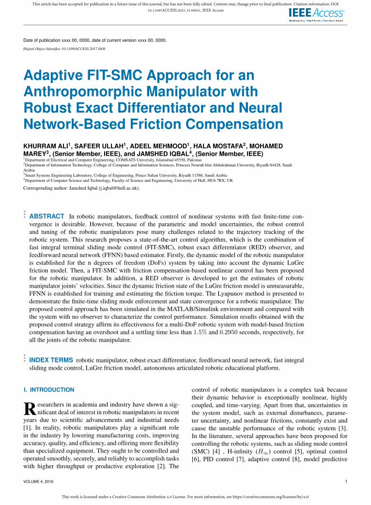
II. MATHEMATICAL MODELINGThe effectiveness of robotic manipulators can be improvedby combining high motion accuracy with high speed. Feed-back robot controllers have a challenging task to accom-plish this objective because they rely on the operating statewithout taking into account the dynamic features of therobot manipulator. In the last several years, certain model-based controllers have been created, and the performanceof robot manipulators has been improved. The research inthis paper has been accomplished using the AutonomousArticulated Robotic Educational Platform (AUTAREP) ED-7220C robotic manipulator as shown in Fig. 1.A manipulator is typically comprised of a kinematic chain,and its dynamic model is influenced by various drawbacks,such as coupling among the links, low rigidity, and unknownparameters. Furthermore, nonlinear effects often induced bythe actuation mechanism include dead zone and friction.Thus, a robotic manipulator’s motion is greatly influencedby its dynamic modeling, which is an extremely importantconsideration [35]. In order to implement control algorithms,the mathematical system model is an essential requirement.It is a five-DoF articulated robotic manipulator. Each jointmovement is operated by a single DC servo motor except for

2 VOLUME 4, 2016



FIGURE 1. AUTAREP robotic manipulator ED-7220C.

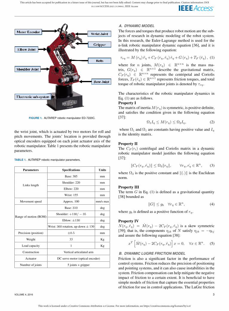
the wrist joint, which is actuated by two motors for roll andpitch movements. The joints’ location is provided throughoptical encoders equipped on each joint actuator axis of therobotic manipulator. Table 1 presents the robotic manipulatorparameters.

TABLE 1. AUTAREP robotic manipulator parameters.

Parameters Specifcations Units

Links length

Base: 385 mm

Shoulder: 220 mm

Elbow: 220 mm

Wrist: 155 mm

Movement speed Approx. 100 mm/s max

Range of motion (ROM)

Base: 310 deg

Shoulder: +130/− 35 deg

Eblow: ±130 deg

Wrist: 360 rotation, up-down ± 130 deg

Precision (position) ±0.5 mm

Weight 33 Kg

Load capacity 1 Kg

Construction Vertical articulated arm

Actuator DC servo motor (optical encoder)

Number of joints 5 joints + gripper

A. DYNAMIC MODELThe forces and torques that produce robot motion are the sub-jects of research in dynamic modeling of the robot system.In this research, the Euler-Lagrange method is used for then-link robotic manipulator dynamic equation [36], and it isillustrated by the following equation:

τrη =M (rη) rη +CF (rη, rη) rη +G (rη) + TF (rη) , (1)

where for n joints, M(rη) ∈ Rn×n is the mass ma-trix, G(rη) ∈ Rn×1 describe the gravitational matrix,CF (rη) ∈ Rn×n represents the centripetal and Coriolisforces, TF (rη) ∈ Rn×1 represents friction torques, and totaltorque of robotic manipulator joints is denoted by τrη.

The characteristics of the robotic manipulator dynamics inEq. (1) are as follows.Property IThe matrix of inertiaM(rη) is symmetric, is positive definite,and satisfies the condition given in the following equation[37]:

Ω1Iη ≤M(rη) ≤ Ω2Iη, (2)

where Ω1 and Ω1 are constants having positive value and Iηis the identity matrix.

Property IIThe CF (ri) centrifugal and Coriolis matrix in a dynamicrobotic manipulator model justifies the following equation[37]:

∥CF (rη, rη)∥ ≤ Ω3∥rη∥, ∀rη, rη ∈ Rn, (3)

where Ω3 is the positive constant and ∥(.)∥ is the Euclideannorm.

Property IIIThe term G in Eq. (1) is defined as a gravitational quantity[38] bounded as

∥G∥ ≤ gb ∀rη ∈ Rn, (4)

where gb is defined as a positive function of rη .

Property IVN(rη, rη) = M(rη) − 2CF (rη, rη) is a skew symmetric[39]; that is, the components ηjk of N satisfy ηjk = −ηkjand assure the following equation [38]:

xT[M(rη)− 2CF (rη, rη)

]x = 0, ∀x ∈ Rn. (5)

B. DYANMIC LUGRE FRICTION MODELFriction is also a significant factor in the performance ofcontrol systems. Friction reduces the precision of positioningand pointing systems, and it can also cause instabilities in thesystem. Friction compensation can help mitigate the negativeimpact of friction to a certain extent. It is beneficial to havesimple models of friction that capture the essential propertiesof friction for use in control applications. The LuGre friction

VOLUME 4, 2016 3



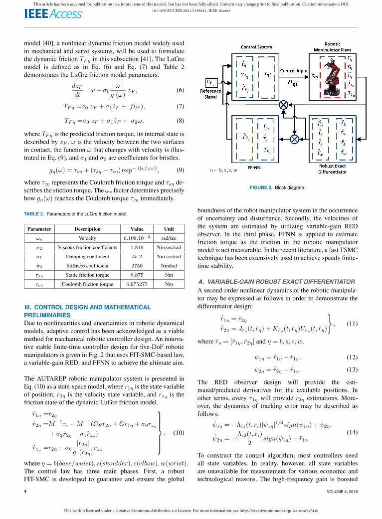
model [40], a nonlinear dynamic friction model widely usedin mechanical and servo systems, will be used to formulatethe dynamic friction TFη in this subsection [41]. The LuGremodel is defined as in Eq. (6) and Eq. (7) and Table 2demonstrates the LuGre friction model parameters.

dzFdt

=ω − σ0| ω |g (ω)

zF , (6)

TFη =σ0 zF + σ1zF + f(ω), (7)

TFη =σ0 zF + σ1zF + σ2ω, (8)

where TFη is the predicted friction torque, its internal state isdescribed by zF , ω is the velocity between the two surfacesin contact, the function ω that changes with velocity is illus-trated in Eq. (9), and σ1 and σ0 are coefficients for bristles.

gη(ω) = τcη + (τsη − τcη) exp− (|ω/ωs|), (9)

where τcη represents the Coulomb friction torque and τsη de-scribes the stiction torque. The ωs factor determines preciselyhow gη(ω) reaches the Coulomb torque τcη immediately.

TABLE 2. Parameters of the LuGre friction model.

Parameter Description Value Unit

ωs Velocity 6.109.10−2 rad/sec

σ2 Viscous friction coefficients 1.819 Nm.sec/rad

σ1 Damping coefficient 45.2 Nm.sec/rad

σ0 Stiffness coefficient 2750 Nm/rad

τsη Static friction torque 8.875 Nm

τcη Coulomb friction torque 6.975275 Nm

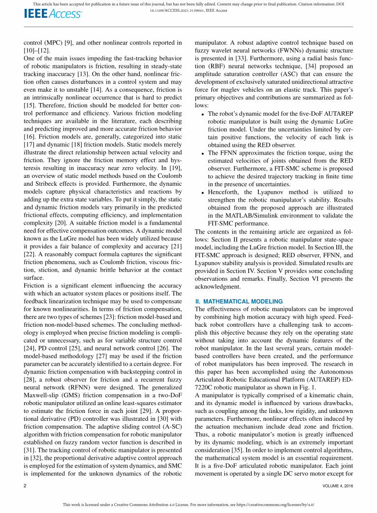
III. CONTROL DESIGN AND MATHEMATICALPRELIMINARIESDue to nonlinearities and uncertainties in robotic dynamicalmodels, adaptive control has been acknowledged as a viablemethod for mechanical robotic controller design. An innova-tive stable finite-time controller design for five-DoF roboticmanipulators is given in Fig. 2 that uses FIT-SMC-based law,a variable-gain RED, and FFNN to achieve the ultimate aim.

The AUTAREP robotic manipulator system is presented inEq. (10) as a state-space model, where r1η is the state variableof position, r2η is the velocity state variable, and rzη is thefriction state of the dynamic LuGre friction model.

r1η =r2η

r2η =M−1τr −M−1(CF r2η +Gr1η + σ0rzη+ σ2r2η + σ1rzη )

rzη =r2η − σ0|r2η|g (r2η)

rzη

, (10)

where η = b(base/waist), s(shoulder), e(elbow), w(wrist).The control law has three main phases. First, a robustFIT-SMC is developed to guarantee and ensure the global

FIGURE 2. Block diagram.

boundness of the robot manipulator system in the occurrenceof uncertainty and disturbance. Secondly, the velocities ofthe system are estimated by utilizing variable-gain REDobserver. In the third phase, FFNN is applied to estimatefriction torque as the friction in the robotic manipulatormodel is not measurable. In the recent literature, a fast TSMCtechnique has been extensively used to achieve speedy finite-time stability.

A. VARIABLE-GAIN ROBUST EXACT DIFFERENTIATORA second-order nonlinear dynamics of the robotic manipula-tor may be expressed as follows in order to demonstrate thedifferentiator design:

˙r1η = r2η˙r2η = Jrη (t, rη) +Krη (t, rη)Urη (t, rη)

, (11)

where rη = [r1η, r2η] and η = b, s, e, w.

ψ1η = ˆr1η − r1η, (12)

ψ2η = ˆr2η − ˙r1η. (13)

The RED observer design will provide the esti-mated/predicted derivatives for the available positions. Inother terms, every r1η will provide r2η estimations. More-over, the dynamics of tracking error may be described asfollows:

ψ1η = −Λi1(t, ri)|ψ1η|1/2sign(ψ1η) + ψ2η,

ψ2η = −Λi2(t, ri)

2sign(ψ1η)− r1η.

(14)

To construct the control algorithm, most controllers needall state variables. In reality, however, all state variablesare unavailable for measurement for various economic andtechnological reasons. The high-frequency gain is boosted

4 VOLUME 4, 2016



by a differentiator (classical). The controller design requiresthe whole state to be accessible; however, in this study, onlythe measurements of position states are considered to beavailable. As a result, to estimate its velocities, a smoothdifferentiator is used as an observer. The proposed differ-entiator has a unique feature that reduces high-frequencychattering compared to the conventional sliding mode-baseddifferentiators. The globally converging RED is taken intoaccount.

˙r1η = −γ1η(t, rη)|ψ1η|1/2signψ1η + ˆri2, (15)

˙r2η = −γ2η(t, rη)2

signψ1η, (16)

where γ1η and γ2η are the variable gains of RED observerexpressed in Eq. (15) and Eq. (16), respectively:

γ1η(t, rη) =χi +1

βi

[V 2η (t, rη)

2ϵi+ 2ϵi(βi + 4ϵ2i )

+ 4ϵiVη(t, rη)

],

(17)

γ2η(t, rη) = 2ϵiγ1η(t, rη) + βi + 4ϵ2i , (18)

where i = 1, 2, 3, 4, η = b, s, e, w and the arbitrary positiveconstants are χi, ϵi, βi. It is worth noting that the errordynamics are globally converged to zero in limited timewith the aid of this velocity observer. Now, the previouslymentioned robust global convergence differentiator can beused to estimate the derivatives of the AUTAREP roboticmanipulator system.For the waist (base) joint,

˙r1b = −γ1b|r1b − r1b|1/2sign(r1b − r1b) + r1b,

˙r2b = −γ2b2sign(r1b − r1b)

γ1b = δ1 +1

β1

(V 21

2ϵ1+ 2ϵ1(β1 + 4ϵ21) + 4ϵ1V1

),

γ2b = 2ϵ1γ1b + β1 + 4ϵ21

. (19)

For the shoulder joint,

˙r1s = −γ1s|r1s − r1s|1/2sign(r1s − r1s) + r2s,

˙r2s = −γ2s2sign(r1s − r1s)

γ1s = δ2 +1

β2

(V 22

2ϵ2+ 2ϵ2(β2 + 4ϵ22) + 4ϵ2V2

),

γ2s = 2ϵ2γ1s + β2 + 4ϵ22

. (20)

For the elbow joint,

˙r1e = −γ1e|r1e − r1e|1/2sign(re1 − r1e) + r2e,

˙r2e = −γ2e2sign(r1e − r1e)

γ1e = δ3 +1

β3

(V 23

2ϵ3+ 2ϵ3(β3 + 4ϵ23) + 4ϵ3V3

),

γ2e = 2ϵ3γ1e + β3 + 4ϵ23

. (21)

For the wrist joint,

˙r1w = −γ1w|r1w − r1w|1/2sign(r1w − r1w) + r2w,

˙r2w = −γ2w2sign(r1w − r1w)

γ1w = δ4 +1

β4

(V 24

2ϵ4+ 2ϵ4(β4 + 4ϵ24) + 4ϵ4V4

),

γ2w = 2ϵ4γ1w + β4 + 4ϵ24

.

(22)

B. NEURAL NETWORK-BASED APPROXIMATION

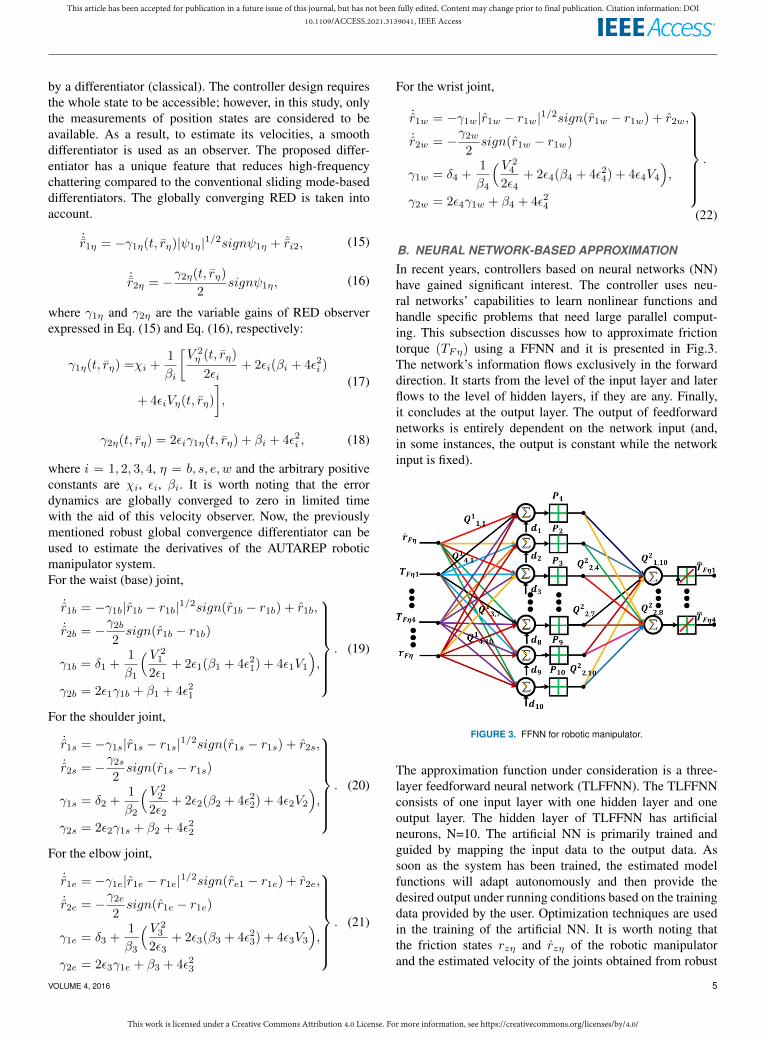
In recent years, controllers based on neural networks (NN)have gained significant interest. The controller uses neu-ral networks’ capabilities to learn nonlinear functions andhandle specific problems that need large parallel comput-ing. This subsection discusses how to approximate frictiontorque (TFη) using a FFNN and it is presented in Fig.3.The network’s information flows exclusively in the forwarddirection. It starts from the level of the input layer and laterflows to the level of hidden layers, if they are any. Finally,it concludes at the output layer. The output of feedforwardnetworks is entirely dependent on the network input (and,in some instances, the output is constant while the networkinput is fixed).

FIGURE 3. FFNN for robotic manipulator.

The approximation function under consideration is a three-layer feedforward neural network (TLFFNN). The TLFFNNconsists of one input layer with one hidden layer and oneoutput layer. The hidden layer of TLFFNN has artificialneurons, N=10. The artificial NN is primarily trained andguided by mapping the input data to the output data. Assoon as the system has been trained, the estimated modelfunctions will adapt autonomously and then provide thedesired output under running conditions based on the trainingdata provided by the user. Optimization techniques are usedin the training of the artificial NN. It is worth noting thatthe friction states rzη and rzη of the robotic manipulatorand the estimated velocity of the joints obtained from robust

VOLUME 4, 2016 5



exact differentiator functioned as inputs of TLFFNN. TFη isconsidered a network output. Consider TFη = Jr:

PN = N 1N

( N∑n=1

Q1N,nX + d1N

)= N 1

N

(Q1T

N Xn + d1N

),

Jr = N 2m

( m∑N=1

Q2Jr,NPN

)= Q2T

JrPN

, (23)

where n = 3 and m = 1 denote the number of networkinputs and outputs for a single joint of robotic manipulator,respectively (for all joints, n = 12 and m = 4). The hiddenlayer of neurons is N = 10 and M = 4 is the number ofoutput layer neurons.The tan-sigmoid N 1

N ∈ Rn → RN and pure linear activationN 2

M ∈ RM → Rm are functions of the hidden layerneuron and output layer neuron, respectively. b1N ∈ Rn

demonstrate the network bias that are utilized to improvelearning speed during network training. The input vector isdescribed as X = [rzη rzη r1η] ∈ Rn. TFη is thedesired target output.Q1

N ∈ Rn andQ2Jr

are the hidden layerand output layers weights vector, respectively. The suggestedNN’s output algorithm is as follows:

Jr = Q2T

JrP+ eJ , (24)

where eJ describes the network approximation error.

Jr = Jr − Jr = TFη

= Q2T

JrP− eJ

(25)

Q2Jr

= Q2Jr

−Q2Jr,

˙Q2Jr

=˙Q2

Jr

. (26)

C. FIT-SMC SCHEMEThe difference between the expected and reference trajec-tories in the controller that generates the control inputs isutilized as a performance benchmark. The speed of thedifferent motors fluctuates and varies as the control inputsare supplied to the actuator. As an outcome, the underlyingsystem’s anticipated motion is accomplished. The referencetracking errors expressed for the said purpose are given in thefollowing equation:

eη =r1η − rdη,

eη =r1η − rdη,

eη =r1η − rdη.

(27)

In contrast to the conventional SMC-based designs, TSMChas superior speedy and finite-time convergence characteris-tics, which improves high-precision control performance byincreasing the convergence rate towards an equilibrium point.Consider the sliding surface manifold design as described

in the following equation to accomplish the primary controlobjectives:

δη = eη + αηeη + βη

∫ t

0

|eη|γηsign(eη)dt, (28)

where δη ∈ Rn, αη , βη > 0, and 0 < γη < 1 is the positivenumber. Henceforth, the time derivative of δη(t) is used toretain the system on the integral terminal sliding surfaceδη(t) = 0. The time derivative of Eq. (28) is determined asfollows:

δη = eη + αη eη + βη|eη|γηsign(eη). (29)

The objective is accomplished in SMC by setting δη = 0.Using this value as a substitute in Eq. (29),

0 = eη + αη eη + βη|eη|γηsign(eη). (30)

Substituting the values of error dynamics from Eq. (27) intoEq. (30),

0 =r2η − rdη + αη(r1η − rdη) + βη|r1η − rdη|γη

sign(r1η − rdη),(31)

r2η =rdη − αη(r1η − rdη)− βη|r1η − rdη|γη

sign(r1η − rdη).(32)

Replace the value of r2η in Eq. (32) from Eq. (10). Therefore,Eq. (31) after considering TLFFNN can be written as follows:

0 =M−1

[τη − (CF r2η +Gr1η + TFη

)

]− rdη + αη(r1η − rdη) + βη|r1η − rdη|γη

sign(r1η − rdη).

(33)

Solving Eq. (33) for τη , we get

τη =M

[rdη − αη(r1η − rdη)− βη|r1η − rdη|γη+

sign(r1η − rdη)

]+ CF r2η +Gr1η + TFη

(34)

The SMC law’s control input is divided into two components.The equivalent control legislation (τηeq) is the first compo-nent, and it is a continuous term. The signum function is usedin the second half of the discontinuous control legislation(τηdis). The sliding phase drive system guarantees slide toequilibrium, while the reaching phase drive system maintainsa steady manifold. Consider the robotic manipulator system’soverall control law (τηt) as follows:

τηt = τηdis + τηeq. (35)

The discontinuous function τηdis is defined in the followingequation to compensate for the dynamic model uncertainties.

τηdis =−Υ1ηδη −Υ2ηsign(δη). (36)

6 VOLUME 4, 2016



The equivalent control input τηeq can be described as in thefollowing equation:

τηeq =M

[rdη − αη(r1η − rdη)− βη|r1η − rdη|γη

sign(r1η − rdη)


.

(37)

By invoking the values from Eq. (36) and Eq. (37) into Eq.(35), the total control effort τηt of robotic manipulator systemis given by the following:

τηt =M


sign(r1η − rdη)


−Υ1ηδη −Υ2ηsign(δη),

(38)

where Υ1η and Υ2η are constants with positive value. Thecontrol input τηt will be used to execute the tracking task forrobotic manipulator joints.The following theorem is presented to demonstrate slidingmode enforcement and tracking errors convergence in finitetime.

Theorem 1. Consider the robotic manipulator dynamics de-scribed by Eq. (10). In the presence of matched uncertainties,the proposed Eq. (28), the reaching law Eq. (36), and therobust control law Eq. (38) provide finite-time enforcement ofthe sliding mode. Furthermore, the tracking errors convergeto the origin in a finite amount of time.

Proof. In order to prove the above statement theorem, theLyapunov function time derivative is given by function Lr,along the dynamics Eq. (10), one gets

Lr =1

2δ2η, (39)

Lr = δη δη, (40)

Lr =δη

[M−1(τηt − (CF r2η +Gr1η + TFη))

− rdη + αη(r1η − rdη) + βη|r1η − rdη|γη

sign(r1η − rdη)

].

(41)

Substituting Eq. (38) in Eq. (41) and then re-arranging it, onehas

Lr =δη (−Υ1ηδη −Υ2ηsign(δη)

≤ −Υ1ηδ2η −Υ2η|δη|

, (42)

Lr + 2Υ1ηLr +√

2LrΥ2η ≤ 0, (43)

where Υ1η = 2Υ1η , Υ2η =√2Υ2η ,

Lr + Υ1ηLr + Υ2η

√Lr ≤ 0. (44)

The numerical expression of the settling time is derived fromEq. (44) in the following form:

TS ≤ 1

2Υ1ηln

(Υ1η

√Lr (sz (0)) + Υ2η

Υ2η

). (45)

The finite-time FIT-SMC function defined in Eq. (28) isensured by the differential inequality in Eq. (44) with slidingmode convergence time in Eq. (45). Now, it is abundantly ob-vious that δη = 0 is obtained by ensuring sliding modes alongEq. (28). To put that into perspective, when δη approacheszero, one must deal with

eη + αη eη + βη|eη|γηsign(eη) = 0. (46)

The second-order differential equation is finite-time stablein δη; i.e., δη −→ 0 in finite time. It is worth noting thatthe estimation of frictional torque is done using FFNNs. Itis appropriate to address neural networks in the followingsubsection at this stage.

D. STABILITY ANALYSIS WITH LYAPUNOV FUNCTIONFor stability analysis, the enhanced Lyapunov function isdescribed as follows:

V =1

2δ2η +

1

2ζ1Q2T

JrQ2

Jr. (47)

The Lyapunov candidate function derivative is computedas follows:

V =δη δη +1

ζ1Q2T

Jr

˙Q2

Jr. (48)

By substituting the values of δη from Eq. (33),

V =δη

[r2η − rdη + αη(r1η − rdη) + βη|r1η − rdη|γη

sign(r1η − rdη)

]+

1

ζ1Q2T

Jr

˙Q2

Jr.

(49)

By replacing the value of r2η with estimated friction torqueTzη , Eq. (49) after TLFFNN is

V =δη

[M−1(τηt − (CF r2η +Gr1η + TFη))

− rdη + αη(r1η − rdη) + βη|r1η − rdη|γη

sign(r1η − rdη)

]+

1

ζ1Q2T

Jr

˙Q2

Jr.

(50)

The control input is built accordingly after evaluation ofTLFFNN is demonstrated as follows:

τηt =M


sign(r1η − rdη)

]+ CF r2η +Gr1η + TFη−

−Υ1ηδη −Υ2ηsign(δη).

(51)

By inserting the value of control input from Eq. (51), we get

V =δη

[−Υ1ηδη −Υ2ηsign(δη)− CF r2η −Gr1η − TFη

−M(rdη − αη(r1η − rdη)−

βη|r1η + rdη|γηsign(r1η − rdη))

]+

1

ζ1Q2T

Jr

˙Q2

Jr.

(52)

VOLUME 4, 2016 7



By solving Eq. (52) and taking Eq. (23) and Eq. (24) intoconsideration, we get

V = δη

(−Υ1δη −Υ2sign(δη)− Q2T

JrP+ eJ

)+

1

ζ1Q2T

Jr

˙Q2

Jr,

(53)

V =−Υ1δη2 −Υ2δηsign(δη) + δηeJ − δηQ

2T

JrP

+1

ζ1Q2T

Jr

˙Q2

Jr,

(54)

V =−Υ1δη2 −Υ2δηsign(δη) + δη(eJ)− Q2T

Jr(δηP− 1

ζ1

˙Q2

Jr

).

(55)

The predicted weight selected from the above Eq. (55) is asfollows:

˙Q2

Jr= ζ1Pδη

.(56)

The eJ elements are assumed to be norm bounded by aconstant Γα ∈ Rn having positive value. Therefore, Eq. (56)can be written as follows:

V =−Υ1δ2η −Υ2δηsign(δη) + δηΓα, (57)

V ≤ −Υ1δ2η −

[Υ2 − |Γα|

]|δη|, (58)

where Υ1 is a constant with a positive value and if the gainof controller Υ2 is selected in such a manner that Υ2 > |Γα|,then Eq. (58) can be written as Eq. (59). Therefore, Eq. (59)would be negatively semidefinite:

V ≤−Υ1δ2η −∆|δη|, (59)

where ∆ in Eq. (59) is defined as ∆ = min(Υ2 −∆, Υ2 +∆).As approximation error eJ based on NN has a minimumvalue, the state of the system achieves an equilibrium pointin finite duration.

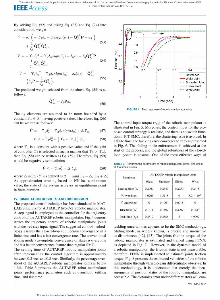
IV. SIMULATION RESULTS AND DISCUSSIONThe proposed control technique has been simulated in MAT-LAB/Simulink for AUTAREP five-DoF robotic manipulator.A step signal is employed to the controller for the trajectorycontrol of the AUTAREP robotic manipulator. Fig. 4 demon-strates the trajectory control of robotic manipulator jointswith desired step input signal. The suggested control method-ology assures the closed-loop equilibrium convergence in afinite time and has a fast convergence rate. The conventionalsliding mode’s asymptotic convergence of states is overcomeand it a better convergence feature than regular SMC.The settling time of AUTAREP robotic manipulator jointsafter implementing the control algorithm is approximatelybetween 0.2 secs and 0.3 secs. Similarly, the percentage over-shoot of the AUTAREP robotic manipulator joints is below1.5%. Table 3 presents the AUTAREP robot manipulatorjoints’ performance parameters such as overshoot, settlingtime, and rise time

FIGURE 4. Step response of robotic manipulator joints.

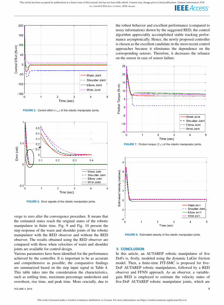
The control input torque (τηt) of the robotic manipulator isillustrated in Fig. 5. Moreover, the control input for the pro-posed control strategy is realistic, and there is no switch func-tion in FIT-SMC; therefore, the chattering issue is avoided. Ina finite time, the tracking error converges to zero as presentedin Fig. 6. The sliding mode enforcement is achieved at thestart of the process, and the global robustness of the closed-loop system is ensured. One of the most effective ways of

TABLE 3. Performance parameters of robotic manipulator joints. The unit ofall the times is secs.

ParameterAUTAREP robotic manipulator joints

Waist Shoulder Elbow Wrist

Settling time (ts) 0.2060 0.2340 0.2950 0.2418

% overshoot 1.0766 1.5118 0 8.2 × 10-8

% undershoot 0 0.1064 0.0015 0

Rise time (ts) 0.1411 0.1567 0.2002 0.1624

Peak time (tp) 0.2512 0.2886 5 4.9992

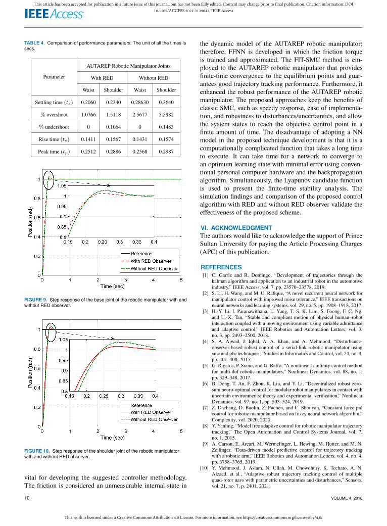
tackling uncertainties appears to be the SMC methodology.Sliding mode, as widely known, is precise and insensitiveto disturbances [42], [43]. The joints friction torque of therobotic manipulator is estimated and trained using FFNN,as depicted in Fig. 7. However, in the dynamic model ofa robotic manipulator, the friction state is not measurable;therefore, FFNN is implemented to estimate joints frictiontorque. Fig. 8 presents the estimated velocities of the roboticmanipulator through variable-gain differentiator observer. Inthis methodology, it is understood that merely the mea-surements of position states of the robotic manipulator areaccessible. The dynamics error under differentiators will con-

8 VOLUME 4, 2016



FIGURE 5. Control effort (τηt) of the robotic manipulator joints.

FIGURE 6. Error signals of the robotic manipulator joints.

verge to zero after the convergence procedure. It means thatthe estimated states reach the original states of the roboticmanipulator in finite time. Fig. 9 and Fig. 10 present thestep response of the waist and shoulder joints of the roboticmanipulator with the RED observer and without the REDobserver. The results obtained using the RED observer arecompared with those when velocities of waist and shoulderjoints are available for control design.Various parameters have been identified for the performanceachieved by the controller. It is important to be as accurateand comprehensive as possible; the comparative findingsare summarized based on the step input signal in Table 4.This table takes into the consideration the characteristics,such as settling time, maximum percentage undershoot andovershoot, rise time, and peak time. More crucially, due to

the robust behavior and excellent performance (compared tonoisy information) shown by the suggested RED, the controlalgorithm appreciably accomplished stable tracking perfor-mance asymptotically. Hence, the newly proposed controlleris chosen as the excellent candidate in the most recent controlapproaches because it eliminates the dependence on thecorresponding sensors. Therefore, it decreases the relianceon the sensor in case of sensor failure.

FIGURE 7. Friction torque (TF ) of the robotic manipulator joints.

FIGURE 8. Estimated velocity of the robotic manipulator joints.

V. CONCLUSIONIn this article, an AUTAREP robotic manipulator of fiveDoFs is, firstly, modeled using the dynamic LuGre frictionmodel. Then, a finite-time FIT-SMC is proposed for five-DoF AUTAREP robotic manipulators, followed by a REDobserver and FFNN approach. As an observer, a variable-gain RED is employed to estimate the velocity states offive-DoF AUTAREP robotic manipulator joints, which are

VOLUME 4, 2016 9



TABLE 4. Comparison of performance parameters. The unit of all the times issecs.

Parameter

AUTAREP Robotic Manipulator Joints

With RED Without RED

Waist Shoulder Waist Shoulder

Settling time (ts) 0.2060 0.2340 0.28630 0.3640

% overshoot 1.0766 1.5118 2.5677 3.5982

% undershoot 0 0.1064 0 0.1483

Rise time (ts) 0.1411 0.1567 0.1431 0.1574

Peak time (tp) 0.2512 0.2886 0.2568 0.2987

FIGURE 9. Step response of the base joint of the robotic manipulator with andwithout RED observer.

FIGURE 10. Step response of the shoulder joint of the robotic manipulatorwith and without RED observer.

vital for developing the suggested controller methodology.The friction is considered an unmeasurable internal state in

the dynamic model of the AUTAREP robotic manipulator;therefore, FFNN is developed in which the friction torqueis trained and approximated. The FIT-SMC method is em-ployed to the AUTAREP robotic manipulator that providesfinite-time convergence to the equilibrium points and guar-antees good trajectory tracking performance. Furthermore, itenhanced the robust performance of the AUTAREP roboticmanipulator. The proposed approaches keep the benefits ofclassic SMC, such as speedy response, ease of implementa-tion, and robustness to disturbances/uncertainties, and allowthe system states to reach the objective control point in afinite amount of time. The disadvantage of adopting a NNmodel in the proposed technique development is that it is acomputationally complicated function that takes a long timeto execute. It can take time for a network to converge toan optimum learning state with minimal error using conven-tional personal computer hardware and the backpropagationalgorithm. Simultaneously, the Lyapunov candidate functionis used to present the finite-time stability analysis. Thesimulation findings and comparison of the proposed controlalgorithm with RED and without RED observer validate theeffectiveness of the proposed scheme.

VI. ACKNOWLEDGMENTThe authors would like to acknowledge the support of PrinceSultan University for paying the Article Processing Charges(APC) of this publication.

REFERENCES[1] C. Garriz and R. Domingo, “Development of trajectories through the

kalman algorithm and application to an industrial robot in the automotiveindustry,” IEEE Access, vol. 7, pp. 23570–23578, 2019.

[2] S. Li, H. Wang, and M. U. Rafique, “A novel recurrent neural network formanipulator control with improved noise tolerance,” IEEE transactions onneural networks and learning systems, vol. 29, no. 5, pp. 1908–1918, 2017.

[3] H.-Y. Li, I. Paranawithana, L. Yang, T. S. K. Lim, S. Foong, F. C. Ng,and U.-X. Tan, “Stable and compliant motion of physical human–robotinteraction coupled with a moving environment using variable admittanceand adaptive control,” IEEE Robotics and Automation Letters, vol. 3,no. 3, pp. 2493–2500, 2018.

[4] S. A. Ajwad, J. Iqbal, A. A. Khan, and A. Mehmood, “Disturbance-observer-based robust control of a serial-link robotic manipulator usingsmc and pbc techniques,” Studies in Informatics and Control, vol. 24, no. 4,pp. 401–408, 2015.

[5] G. Rigatos, P. Siano, and G. Raffo, “A nonlinear h-infinity control methodfor multi-dof robotic manipulators,” Nonlinear Dynamics, vol. 88, no. 1,pp. 329–348, 2017.

[6] B. Dong, T. An, F. Zhou, K. Liu, and Y. Li, “Decentralized robust zero-sum neuro-optimal control for modular robot manipulators in contact withuncertain environments: theory and experimental verification,” NonlinearDynamics, vol. 97, no. 1, pp. 503–524, 2019.

[7] Z. Dachang, D. Baolin, Z. Puchen, and C. Shouyan, “Constant force pidcontrol for robotic manipulator based on fuzzy neural network algorithm,”Complexity, vol. 2020, 2020.

[8] Y. Yanling, “Model free adaptive control for robotic manipulator trajectorytracking,” The Open Automation and Control Systems Journal, vol. 7,no. 1, 2015.

[9] A. Carron, E. Arcari, M. Wermelinger, L. Hewing, M. Hutter, and M. N.Zeilinger, “Data-driven model predictive control for trajectory trackingwith a robotic arm,” IEEE Robotics and Automation Letters, vol. 4, no. 4,pp. 3758–3765, 2019.

[10] Y. Mehmood, J. Aslam, N. Ullah, M. Chowdhury, K. Techato, A. N.Alzaed, et al., “Adaptive robust trajectory tracking control of multiplequad-rotor uavs with parametric uncertainties and disturbances,” Sensors,vol. 21, no. 7, p. 2401, 2021.

10 VOLUME 4, 2016



[11] N. Ullah, I. Sami, W. Shaoping, H. Mukhtar, X. Wang, M. Sha-hariar Chowdhury, and K. Techato, “A computationally efficient adaptiverobust control scheme for a quad-rotor transporting cable-suspended pay-loads,” Proceedings of the Institution of Mechanical Engineers, Part G:Journal of Aerospace Engineering, p. 09544100211013617, 2016.

[12] Y. Sun, J. Xu, H. Wu, G. Lin, and S. Mumtaz, “Deep learning basedsemi-supervised control for vertical security of maglev vehicle with guar-anteed bounded airgap,” IEEE Transactions on Intelligent TransportationSystems, 2021.

[13] S. Ullah, A. Mehmood, Q. Khan, S. Rehman, and J. Iqbal, “Robust integralsliding mode control design for stability enhancement of under-actuatedquadcopter,” International Journal of Control, Automation and Systems,vol. 18, p. 1671–1678, 2020.

[14] S.-H. Han, M. S. Tran, and D.-T. Tran, “Adaptive sliding mode controlfor a robotic manipulator with unknown friction and unknown controldirection,” Applied Sciences, vol. 11, no. 9, p. 3919, 2021.

[15] L. Zhang, J. Wang, J. Chen, K. Chen, B. Lin, and F. Xu, “Dynamicmodeling for a 6-dof robot manipulator based on a centrosymmetric staticfriction model and whale genetic optimization algorithm,” Advances inEngineering Software, vol. 135, p. 102684, 2019.

[16] F. Marques, P. Flores, J. P. Claro, and H. M. Lankarani, “Modeling andanalysis of friction including rolling effects in multibody dynamics: areview,” Multibody System Dynamics, vol. 45, no. 2, pp. 223–244, 2019.

[17] Y.-H. Sun, T. Chen, C. Qiong Wu, and C. Shafai, “Comparison of four fric-tion models: feature prediction,” Journal of Computational and NonlinearDynamics, vol. 11, no. 3, 2016.

[18] Z. A. Khan, V. Chacko, and H. Nazir, “A review of friction models ininteracting joints for durability design,” Friction, vol. 5, no. 1, pp. 1–22,2017.

[19] J. Wojewoda, A. Stefanski, M. Wiercigroch, and T. Kapitaniak, “Hystereticeffects of dry friction: modelling and experimental studies,” PhilosophicalTransactions of the Royal Society A: Mathematical, Physical and Engi-neering Sciences, vol. 366, no. 1866, pp. 747–765, 2008.

[20] S. Wu, F. Mou, Q. Liu, and J. Cheng, “Contact dynamics and control ofa space robot capturing a tumbling object,” Acta Astronautica, vol. 151,pp. 532–542, 2018.

[21] J. Moreno, R. Kelly, and R. Campa, “Manipulator velocity control usingfriction compensation,” IEE Proceedings-Control Theory and Applica-tions, vol. 150, no. 2, pp. 119–126, 2003.

[22] F. Yue and X. Li, “Robust adaptive integral backstepping control for opto-electronic tracking system based on modified lugre friction model,” ISAtransactions, vol. 80, pp. 312–321, 2018.

[23] H. Saied, A. Chemori, M. El Rafei, C. Francis, and F. Pierrot, “From non-model-based to model-based control of pkms: a comparative study,” inMechanism, Machine, Robotics and Mechatronics Sciences, pp. 153–169,Springer, 2019.

[24] S. A. Al-Samarraie, “Variable structure control design for a magneticlevitation system,” Journal of Engineering, vol. 24, no. 12, pp. 84–103,2018.

[25] X. Shan and G. Cheng, “Structural error and friction compensation controlof a 2 (3pus+ s) parallel manipulator,” Mechanism and Machine Theory,vol. 124, pp. 92–103, 2018.

[26] J. Hu, Y. Wang, L. Liu, and Z. Xie, “High-accuracy robust adaptivemotion control of a torque-controlled motor servo system with frictioncompensation based on neural network,” Proceedings of the Institutionof Mechanical Engineers, Part C: Journal of Mechanical EngineeringScience, vol. 233, no. 7, pp. 2318–2328, 2019.

[27] B. Denkena, B. Bergmann, and D. Stoppel, “Reconstruction of processforces in a five-axis milling center with a lstm neural network in compar-ison to a model-based approach,” Journal of Manufacturing and MaterialsProcessing, vol. 4, no. 3, p. 62, 2020.

[28] B. Kim and S. Han, “Non-linear friction compensation using backsteppingcontrol and robust friction state observer with recurrent fuzzy neuralnetworks,” Proceedings of the Institution of Mechanical Engineers, Part I:Journal of Systems and Control Engineering, vol. 223, no. 7, pp. 973–988,2009.

[29] S. Han and J. M. Lee, “Friction and uncertainty compensation of robot ma-nipulator using optimal recurrent cerebellar model articulation controllerand elasto-plastic friction observer,” IET control theory & applications,vol. 5, no. 18, pp. 2120–2141, 2011.

[30] S. Grami and Y. Gharbia, “Gms friction compensation in robot manip-ulator,” in IECON 2013-39th Annual Conference of the IEEE IndustrialElectronics Society, pp. 3555–3560, IEEE, 2013.

[31] Z. Zhou and B. Wu, “Adaptive sliding mode control of manipulators basedon fuzzy random vector function links for friction compensation,” Optik,vol. 227, p. 166055, 2021.

[32] P. R. Ouyang, J. Tang, W. Yue, and S. Jayasinghe, “Adaptive pd plussliding mode control for robotic manipulator,” in 2016 IEEE InternationalConference on Advanced Intelligent Mechatronics (AIM), pp. 930–934,IEEE, 2016.

[33] V. T. Yen, W. Y. Nan, P. Van Cuong, N. X. Quynh, and V. H. Thich, “Robustadaptive sliding mode control for industrial robot manipulator using fuzzywavelet neural networks,” International Journal of Control, Automationand Systems, vol. 15, no. 6, pp. 2930–2941, 2017.

[34] Y. Sun, J. Xu, G. Lin, W. Ji, and L. Wang, “Rbf neural network-basedsupervisor control for maglev vehicles on an elastic track with networktime-delay,” IEEE Transactions on Industrial Informatics, 2020.

[35] X. Yang, S. S. Ge, and W. He, “Dynamic modelling and adaptive robusttracking control of a space robot with two-link flexible manipulators underunknown disturbances,” International Journal of Control, vol. 91, no. 4,pp. 969–988, 2018.

[36] N. Shi, F. Luo, Z. Kang, L. Wang, Z. Zhao, Q. Meng, and W. Hou, “Fault-tolerant control for n-link robot manipulator via adaptive nonsingularterminal sliding mode control technology,” Mathematical Problems inEngineering, vol. 2021, 2021.

[37] M. A. Arteaga, “On the properties of a dynamic model of flexible robotmanipulators,” 1998.

[38] N. Kapoor and J. Ohri, “Sliding mode control (smc) of robot manipulatorvia intelligent controllers,” Journal of The Institution of Engineers (India):Series B, vol. 98, no. 1, pp. 83–98, 2017.

[39] M. W. Spong, “Seth. hutchinson, and m. vidyasagar,” Robot modeling andcontrol, 2005.

[40] L. Simoni, M. Beschi, A. Visioli, and K. J. Åström, “Inclusion of the dwelltime effect in the lugre friction model,” Mechatronics, vol. 66, p. 102345,2020.

[41] C. Canudas-de Wit and R. Kelly, “Passivity analysis of a motion controlfor robot manipulators with dynamic friction,” Asian Journal of Control,vol. 9, no. 1, pp. 30–36, 2007.

[42] S. Ullah, Q. Khan, A. Mehmood, and R. Akmeliawati, “Integral backstep-ping based robust integral sliding mode control of underactuated nonlinearelectromechanical systems,” Journal of Control Engineering and AppliedInformatics, vol. 21, no. 3, pp. 42–50, 2019.

[43] S. Ullah, Q. Khan, A. Mehmood, and A. I. Bhatti, “Robust backstep-ping sliding mode control design for a class of underactuated electro-mechanical nonlinear systems,” Journal of Electrical Engineering & Tech-nology, vol. 15, pp. 1821–1828, 2020.

KHURRAM ALI is a PhD student in Electricaland Computer Engineering Department (ECE) atCOMSATS University Islamabad, Pakistan. Hereceived the BE degree in Electrical Engineeringfrom the Air University, Pakistan, and Master ofScience in Electrical Engineering from the Na-tional University of Science and Technology, Pak-istan, in 2013. He has also worked as a hardwaredesign engineer at AKSA Solution DevelopmentServices for three years. He is currently serving as

a Lecturer at COMSATS University Islamabad, Pakistan. His research focusis control, automation, and robotics.

VOLUME 4, 2016 11



SAFEER ULLAH holds PhD (2021) and MS(2016) degrees in control and automation fromCOMSATS University Islamabad, Pakistan. Hereceived his BS degree in Electronics Engineeringfrom International Islamic University, Islamabad,in 2012. He is currently working as an AssistantMonitoring Officer in Khyber Pakhtunkhwa Ed-ucational Monitoring Authority. His research in-terests are in analysis, observation, and control ofunder-actuated nonlinear systems using advanced

sliding mode based control approaches.

ADEEL MEHMOOD holds a PhD degree in Non-linear Control from the Technical University ofBelfort-Montbeliard, France. He earned the MSdegree in robotics and embedded systems fromthe University of Versailles Saint-Quentin en Yve-lines, France, in 2008, and BS degree in Mecha-tronics Engineering from the National Universityof Science and Technology, Pakistan, in 2006. Healso worked as a Postdoctoral Researcher with theUniversity of Haute-Alsace, France. He is cur-

rently working as an Assistant Professor at COMSATS University Islam-abad, Pakistan. His research interests include robotics, renewable energy,and robust and nonlinear control of servo systems.

HALA MOSTAFA received the PhD degree inElectrical Engineering from the Faculty of Engi-neering and Applied Science, Memorial Univer-sity, Canada, in 2014. From 2014 to 2015, shewas a Research Scientist at Memorial University.She is currently an Assistant Professor at the Infor-mation Technology Department, College of Com-puter and Information Sciences, Princess Nourahbint Abdulrahman University, Riyadh, Saudi Ara-bia. Her main research interests are wireless com-

munications, with a particular focus on smart antennas and wireless sensornetworks.

MOHAMED MAREY (SM ′14) received theMSc degree in Electrical Engineering fromMenoufia University, Egypt, in 1999, and the PhDdegree in Electrical Engineering from Ghent Uni-versity, Belgium, in 2008. From 2009 to 2014, hewas a Research Associate and a Visiting Profes-sor with the Faculty of Engineering and AppliedScience, Memorial University, Canada. He is cur-rently a Full Professor with the Faculty of Elec-tronic Engineering, Menoufia University, Egypt.

He is on a sabbatical leave in order to join Prince Sultan University, SaudiArabia, as a research laboratory leader of the smart systems engineeringlaboratory. He authored the book Multi-Carrier Receivers in the Presenceof Interference: Overlay Systems (VDM Publishing House Ltd., 2009) andaround 100 scientific papers published in international journals and confer-ences. His main research interests are wireless communications and digitalsignal processing, with a particular focus on smart antennas, cooperativecommunications, signal classification for cognitive radio systems, synchro-nization and channel estimation, multiple-input multiple-output antennasystems, multicarrier systems, and error correcting codes. He was a recipientof the Young Scientist Award from the International Union of Radio Sciencein 1999.

JAMSHED IQBAL (SM ′16) holds a PhD inRobotics from Italian Institute of Technology (IIT)and three Master degrees in various fields of En-gineering from Finland, Sweden, and Pakistan.He is currently working as a Lecturer (AssistantProfessor)of Robotics in the University of Hull,UK, with more than 20 years of multi-disciplinaryexperience in industry and academia. He has morethan 80 reputed journal papers on his credit withan H-index of 32. He is on the editorial board of

several reputed journals and program committee member of various IEEEinternals conferences.

12 VOLUME 4, 2016

Adaptive FIT-SMC Approach for an Anthropomorphic ...

Documents