Adaptive filtering in adaptive feedback cancellation for PA ...

Adaptive filteringin adaptive feed-back cancellationfor PA systems

AuthorsCees KosMathijs Bekkering

Adaptive filteringin adaptivefeedback

cancellation forPA systems

by Cees Kos and Mathijs Bekkering

to obtain the degree of Bachelor of Scienceat the Delft University of Technology

Student numbers: 4697030 (C.H. Kos)4443683 (M.C. Bekkering)

Project duration: 20 April 2020 – 3 July 2020Thesis committee: Prof.dr. J. Schmitz, TU Delft, proposer

Dr.ir. R. C. Hendriks TU Delft, supervisorDr. J. Martinez Castaneda, TU Delft, supervisorDr.ir. S. Izadkhast, TU Delft

AbstractThis report is written as part of the Bachelor Graduation Project in the third year of the Electrical Engi-neering Bachelor programme at the Delft University of Technology. This report is made by a subgroupthat is part of a larger project dedicated to finding a solution to frequency feedback in electroacousticsystems, also known as the Larsen effect.

This problem has a long history of literature and many solutions to this problem have been pre-sented. For this project, the focus lies on the application of Adaptive Feedback Cancellation (AFC).This technique uses estimations of the Room Impulse Response (RIR) to minimise the feedback com-ponent. This report focuses on estimating such a RIR in the case of a PA system. Several methodswill be discussed and compared by implementing and testing them in a simulation environment built inMatlab. The different methods are subjected to a set of performance measurements that provide thenecessary information to see for each method and situation if and how the results measure up against aset of predetermined system requirements. From the researched algorithms, one is chosen as the oneto be implemented in the final design of the group. At last, some considerations and recommendationsare given for implementing one of the algorithms into software and hardware components.

i

PrefaceThis thesis was made as part of a bachelor graduation project, which is the final course of the BachelorElectrical Engineering Programme at the TU Delft University of Technology. The goal was to realise animplementation to stop the howling effect known in public address systems.

Firstly, we want to thank dr. John Schmitz for providing the idea for the project. Secondly, we thankdr.ir. Richard Hendriks and dr. Jorge Martinez for being our supervisors for this project and being ableto guide us through the course of the project, as well as Metin Çaliş, who acted as our daily supervisorand helped us with some of the problems and questions that came up during the project.

The members of our group were all interested in working with electroacoustic systems, which madethis project perfect for us. When reading the document we hope to give insight to the problem, theaspects of a solution and how we as a team confronted the task resulting in our implementation of theadaptive filter design that fits into the complete system.

Cees Kos and Mathijs BekkeringDelft, 19-06-2020

ii

Contents

1 Introduction 11.1 Frequency Feedback . . . . . . . . . . . . . . . . . . . . . . . . . . . . . . . . . . . . . . 11.2 State of the Art in Acoustic Frequency Feedback. . . . . . . . . . . . . . . . . . . . . . . 21.3 Synopsis . . . . . . . . . . . . . . . . . . . . . . . . . . . . . . . . . . . . . . . . . . . . 2

2 Problem Description 32.1 Least Squares Estimate . . . . . . . . . . . . . . . . . . . . . . . . . . . . . . . . . . . . 4

2.1.1 Bias . . . . . . . . . . . . . . . . . . . . . . . . . . . . . . . . . . . . . . . . . . . 42.2 Maximum stable gain. . . . . . . . . . . . . . . . . . . . . . . . . . . . . . . . . . . . . . 52.3 Filter size . . . . . . . . . . . . . . . . . . . . . . . . . . . . . . . . . . . . . . . . . . . . 5

3 System Requirements 63.1 Group System Requirements . . . . . . . . . . . . . . . . . . . . . . . . . . . . . . . . . 63.2 Adaptive Filter Estimation System Requirements. . . . . . . . . . . . . . . . . . . . . . . 6

4 State of the Art 74.1 RLS and Fast RLS . . . . . . . . . . . . . . . . . . . . . . . . . . . . . . . . . . . . . . . 74.2 Stochastic gradient descent methods . . . . . . . . . . . . . . . . . . . . . . . . . . . . . 84.3 APA and Fast APA . . . . . . . . . . . . . . . . . . . . . . . . . . . . . . . . . . . . . . . 84.4 Frequency-domain Kalman Filter . . . . . . . . . . . . . . . . . . . . . . . . . . . . . . . 84.5 Comparison . . . . . . . . . . . . . . . . . . . . . . . . . . . . . . . . . . . . . . . . . . . 9

5 Testing & Results 105.1 Test Setup . . . . . . . . . . . . . . . . . . . . . . . . . . . . . . . . . . . . . . . . . . . 10

5.1.1 Assumptions . . . . . . . . . . . . . . . . . . . . . . . . . . . . . . . . . . . . . . 115.1.2 Room impulse response . . . . . . . . . . . . . . . . . . . . . . . . . . . . . . . . 115.1.3 Input Signals . . . . . . . . . . . . . . . . . . . . . . . . . . . . . . . . . . . . . . 115.1.4 Procedure. . . . . . . . . . . . . . . . . . . . . . . . . . . . . . . . . . . . . . . . 11

5.2 Analysis criteria . . . . . . . . . . . . . . . . . . . . . . . . . . . . . . . . . . . . . . . . . 125.2.1 Misalignment . . . . . . . . . . . . . . . . . . . . . . . . . . . . . . . . . . . . . . 125.2.2 Maximum stable gain. . . . . . . . . . . . . . . . . . . . . . . . . . . . . . . . . . 125.2.3 Estimation Error . . . . . . . . . . . . . . . . . . . . . . . . . . . . . . . . . . . . 12

5.3 Test Results. . . . . . . . . . . . . . . . . . . . . . . . . . . . . . . . . . . . . . . . . . . 125.3.1 Computation time. . . . . . . . . . . . . . . . . . . . . . . . . . . . . . . . . . . . 125.3.2 Open Loop Simulations . . . . . . . . . . . . . . . . . . . . . . . . . . . . . . . . 125.3.3 Closed Loop Simulations. . . . . . . . . . . . . . . . . . . . . . . . . . . . . . . . 13

6 Discussion 176.1 Open Loop Simulations . . . . . . . . . . . . . . . . . . . . . . . . . . . . . . . . . . . . 176.2 Closed Loop Simulations. . . . . . . . . . . . . . . . . . . . . . . . . . . . . . . . . . . . 17

7 Implementation Advice & Considerations 19

8 Conclusion 20

A Algorithms 21A.1 RLS . . . . . . . . . . . . . . . . . . . . . . . . . . . . . . . . . . . . . . . . . . . . . . . 21A.2 LMS . . . . . . . . . . . . . . . . . . . . . . . . . . . . . . . . . . . . . . . . . . . . . . . 21A.3 NLMS . . . . . . . . . . . . . . . . . . . . . . . . . . . . . . . . . . . . . . . . . . . . . . 22A.4 Circular FDAF . . . . . . . . . . . . . . . . . . . . . . . . . . . . . . . . . . . . . . . . . 22A.5 LMS derivation . . . . . . . . . . . . . . . . . . . . . . . . . . . . . . . . . . . . . . . . . 22A.6 MDF . . . . . . . . . . . . . . . . . . . . . . . . . . . . . . . . . . . . . . . . . . . . . . . 23

iii

Contents iv

B Figures 24B.1 Test Results. . . . . . . . . . . . . . . . . . . . . . . . . . . . . . . . . . . . . . . . . . . 25

C Matlab Code 27C.1 Matlab Simulation Environment Without Feedback . . . . . . . . . . . . . . . . . . . . . . 27C.2 Matlab Simulation Environment With Feedback . . . . . . . . . . . . . . . . . . . . . . . 31

Bibliography 37

1Introduction

Acoustic systems are used on a large scale. Such systems make use of both recording devices andplayback devices. Systems like that can be found in different forms, from mobile phones to publicaddress (PA) systems used at festivals and concerts. These systems are of a different scale, but rep-resent the same. That makes that they also have a problem in common, one that holds for any systemthat uses interconnected microphones and loudspeakers. A problem called frequency feedback. Thisproblem describes the situation in which sound from the loudspeaker is fed back to the microphoneand played again. When certain components of the signal are amplified with a gain larger than unity,a loud and irritating sound occurs, referred to as ’howling’ or ’ringing’. This effect is also known as theLarsen effect, after Danish scientist Søren Absalon Larsen, who first discovered the idea behind theproblem of frequency feedback.

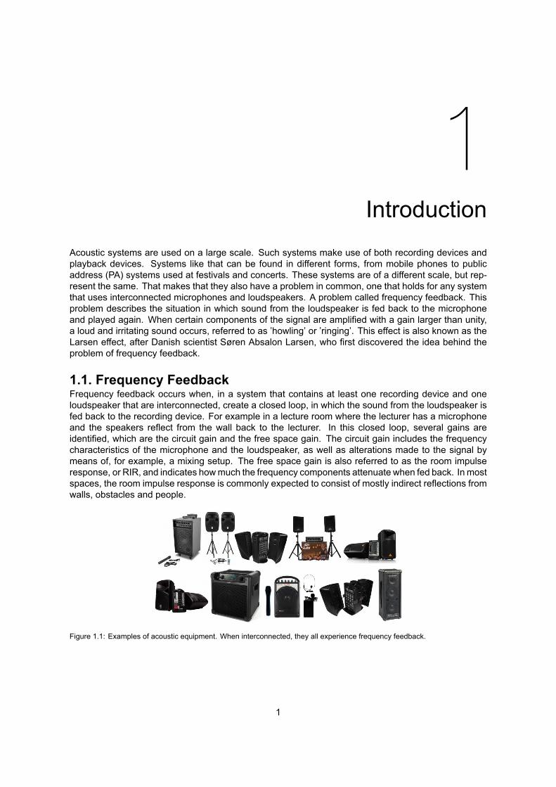
1.1. Frequency FeedbackFrequency feedback occurs when, in a system that contains at least one recording device and oneloudspeaker that are interconnected, create a closed loop, in which the sound from the loudspeaker isfed back to the recording device. For example in a lecture room where the lecturer has a microphoneand the speakers reflect from the wall back to the lecturer. In this closed loop, several gains areidentified, which are the circuit gain and the free space gain. The circuit gain includes the frequencycharacteristics of the microphone and the loudspeaker, as well as alterations made to the signal bymeans of, for example, a mixing setup. The free space gain is also referred to as the room impulseresponse, or RIR, and indicates howmuch the frequency components attenuate when fed back. In mostspaces, the room impulse response is commonly expected to consist of mostly indirect reflections fromwalls, obstacles and people.

Figure 1.1: Examples of acoustic equipment. When interconnected, they all experience frequency feedback.

1

1.2. State of the Art in Acoustic Frequency Feedback 2

1.2. State of the Art in Acoustic Frequency FeedbackThe problem of frequency feedback is a longstanding problem, with publications dating back as far asthe 1960’s.

Frequency and Phase Shifting (FS and PS) [1] [2] were one of the first solutions to the acous-tic feedback problem, with articles dating back to the 1960’s. This concept uses phase modulationtechniques that shifts the phase and/or frequency of the signal slightly, to shift the rise in amplitudeto another frequency, which prevents the components from building up. Doing so smooths the loopgain and makes the maximum stable gain (MSG) depend on the average gain magnitude instead ofthe peak gain magnitude [2]. An increase of the MSG margin of 14 dB was reported, but for audibleafter-effects of the FS operation, this is limited to 6 dB [2]. Because FS shifts the frequency compo-nents of signals, relative relations between frequency components can change, which is not desired inthe case of speech and music signals [2]. A second group of methods makes use of adaptive notchfilters [3], called notch-based howling suppression (NHS) [2]. The goal of these methods is to detecthowling and use adaptive filters to reduce the gain around the critical frequencies. These filters are bynature reactive, but efforts have been made make proactive versions [4]. Another set of solutions isgrouped under the term of Adaptive Feedback Cancellation (AFC). These methods try to estimate thefeedback component and subtract it from the received signal. These are generally effective methodsand many algorithms exist using this principle [5]. The estimation, however, has a certain bias towardsthe source signal, which is to be kept. Such a bias is counteracted by accompanying the adaptive filterwith a decorrelation block.

1.3. SynopsisFor this project, the AFC method was chosen for reasons that are explained in Ch. 2 , since it is saidthat FS, PS and NHS do not have much space to work with in terms of increasing the maximum stablegain (MSG), whereas AFC does [2]. There is a lot of freedom in how one can make such an adaptivefilter. That is why the group decided on AFC. For this project, the group was split into three subgroups,each of them working on a different part of an AFC filter, which are the Adaptive Filtering, Decorrelation[6] and Postfiltering [7].

Adaptive Filtering includes estimating the RIR and building a cancellation filter based on the RIR,Decorrelation handles decorrelation of the signals coming from the loudspeaker with the signals re-ceived by the microphone and Postfiltering is about smoothing of residual peaks that the adaptive filtercouldn’t fix.

This report will discuss, as mentioned before, the Adaptive Filtering part. In Ch. 2 of the report,the problem at hand is explained in more detail, to give you a good sense of the situation. Systemrequirements that are aimed at to meet are listed in Ch. 3. In chapter 4 a state of the art of existingmethods and algorithms to estimate the room impulse response (RIR) will be provided, to analyse andcompare the methods proposes in literature. Promising methods will be researched and eventuallycompared with each other to determine which method will be chosen to be implemented in accordanceto our specifications, which is done in. Underlying theory about the different methods will be givento support the choices that are made. In Chapter 5 A simulation setup will be discussed and usedto analyse the performance of the methods in multiple scenarios, which will be further discussed inchapter 6 the discussion. At last, a number of considerations and advice will be given on creatingimplementations based on our work. The report is closed with a final conclusion in Ch. 8.

2Problem Description

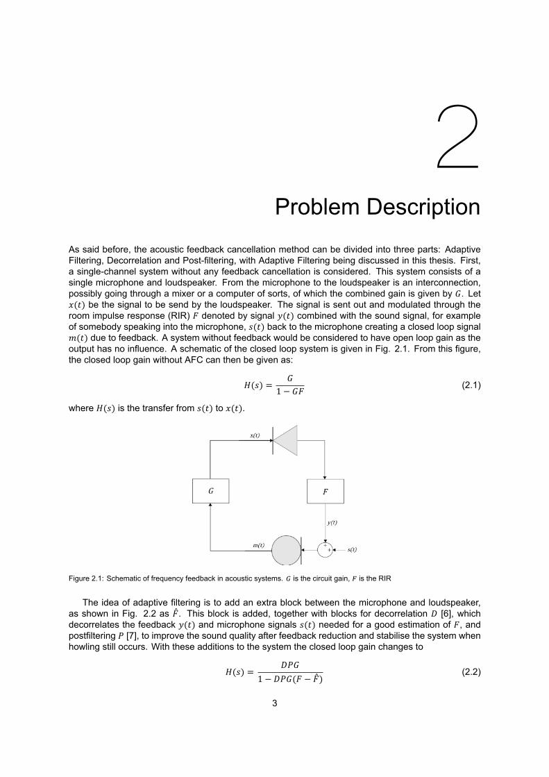
As said before, the acoustic feedback cancellation method can be divided into three parts: AdaptiveFiltering, Decorrelation and Post-filtering, with Adaptive Filtering being discussed in this thesis. First,a single-channel system without any feedback cancellation is considered. This system consists of asingle microphone and loudspeaker. From the microphone to the loudspeaker is an interconnection,possibly going through a mixer or a computer of sorts, of which the combined gain is given by 𝐺. Let𝑥(𝑡) be the signal to be send by the loudspeaker. The signal is sent out and modulated through theroom impulse response (RIR) 𝐹 denoted by signal 𝑦(𝑡) combined with the sound signal, for exampleof somebody speaking into the microphone, 𝑠(𝑡) back to the microphone creating a closed loop signal𝑚(𝑡) due to feedback. A system without feedback would be considered to have open loop gain as theoutput has no influence. A schematic of the closed loop system is given in Fig. 2.1. From this figure,the closed loop gain without AFC can then be given as:

𝐻(𝑠) = 𝐺1 − 𝐺𝐹 (2.1)

where 𝐻(𝑠) is the transfer from 𝑠(𝑡) to 𝑥(𝑡).

Figure 2.1: Schematic of frequency feedback in acoustic systems. is the circuit gain, is the RIR

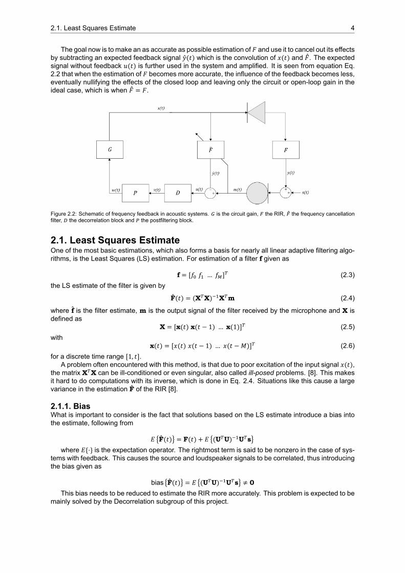
The idea of adaptive filtering is to add an extra block between the microphone and loudspeaker,as shown in Fig. 2.2 as ��. This block is added, together with blocks for decorrelation 𝐷 [6], whichdecorrelates the feedback 𝑦(𝑡) and microphone signals 𝑠(𝑡) needed for a good estimation of 𝐹, andpostfiltering 𝑃 [7], to improve the sound quality after feedback reduction and stabilise the system whenhowling still occurs. With these additions to the system the closed loop gain changes to

𝐻(𝑠) = 𝐷𝑃𝐺1 − 𝐷𝑃𝐺(𝐹 − ��) (2.2)

3

2.1. Least Squares Estimate 4

The goal now is to make an as accurate as possible estimation of 𝐹 and use it to cancel out its effectsby subtracting an expected feedback signal ��(𝑡) which is the convolution of 𝑥(𝑡) and ��. The expectedsignal without feedback 𝑢(𝑡) is further used in the system and amplified. It is seen from equation Eq.2.2 that when the estimation of 𝐹 becomes more accurate, the influence of the feedback becomes less,eventually nullifying the effects of the closed loop and leaving only the circuit or open-loop gain in theideal case, which is when �� = 𝐹.

Figure 2.2: Schematic of frequency feedback in acoustic systems. is the circuit gain, the RIR, the frequency cancellationfilter, the decorrelation block and the postfiltering block.

2.1. Least Squares EstimateOne of the most basic estimations, which also forms a basis for nearly all linear adaptive filtering algo-rithms, is the Least Squares (LS) estimation. For estimation of a filter f given as

f = [𝑓 𝑓 … 𝑓 ] (2.3)the LS estimate of the filter is given by

F(𝑡) = (X X) X m (2.4)

where f is the filter estimate, m is the output signal of the filter received by the microphone and X isdefined as

X = [x(𝑡) x(𝑡 − 1) … x(1)] (2.5)with

x(𝑡) = [𝑥(𝑡) 𝑥(𝑡 − 1) … 𝑥(𝑡 − 𝑀)] (2.6)for a discrete time range [1, 𝑡].

A problem often encountered with this method, is that due to poor excitation of the input signal 𝑥(𝑡),the matrix X X can be ill-conditioned or even singular, also called ill-posed problems. [8]. This makesit hard to do computations with its inverse, which is done in Eq. 2.4. Situations like this cause a largevariance in the estimation F of the RIR [8].

2.1.1. BiasWhat is important to consider is the fact that solutions based on the LS estimate introduce a bias intothe estimate, following from

𝐸 {F(𝑡)} = F(𝑡) + 𝐸 {(U U) U s}where 𝐸{⋅} is the expectation operator. The rightmost term is said to be nonzero in the case of sys-

tems with feedback. This causes the source and loudspeaker signals to be correlated, thus introducingthe bias given as

bias {F(𝑡)} = 𝐸 {(U U) U s} ≠ 0This bias needs to be reduced to estimate the RIR more accurately. This problem is expected to be

mainly solved by the Decorrelation subgroup of this project.

2.2. Maximum stable gain 5

2.2. Maximum stable gainThe howling effect occurs when the loop gain is too large, which can be traced back to the Nyquiststability criterion [2] [9] for closed loops, where we include the effects of �� and exclude those of 𝐷 and𝑃, which is given as

|𝐺(𝜔, 𝑡) [𝐹(𝜔, 𝑡) − ��(𝜔, 𝑡)]| ≥ 1 (2.7)∠𝐺(𝜔, 𝑡) [𝐹(𝜔, 𝑡) − ��(𝜔, 𝑡)] = 𝑛2𝜋, 𝑛 ∈ ℤ (2.8)

The maximum stable gain (MSG) follows as

MSG(𝑡)[dB] = −20 log [max∈𝒫 |𝐽(𝜔, 𝑡) [𝐹(𝜔, 𝑡) − ��(𝜔, 𝑡)]|] (2.9)

with𝒫 = {𝜔|∠𝐺(𝜔, 𝑡) [𝐹(𝜔, 𝑡) − ��(𝜔, 𝑡)] = 𝑛2𝜋} (2.10)

and 𝐽(𝜔, 𝑡) relates to 𝐺 as

𝐺(𝜔, 𝑡) = 𝐾𝐽(𝜔, 𝑡) (2.11)

This shows that if 𝐹 = ��, the MSG should be infinite. For this project, it is assumed that the gain 𝐺is the same for all frequencies, which means that 𝐽(𝜔, 𝑡) = 1.

2.3. Filter sizeThe size of the estimated filter depends the time required to properly catch the effect of the room impulseresponse. A longer filter length is required when the main components of feedback have to travel longdistances. A filter time 𝑡 = 100 ms will be assumed to capture enough information about the RIR. Asampling frequency 𝐹 = 40 kHz is needed to include the required frequency range. In literature, this isoften increased to 𝐹 = 44.1 kHz, which will be used in this project as well. Fact is that the same samplefrequency is used for CD’s. The needed filter size is then given by 𝑀 = 𝐹 ⋅ 𝑡 resulting in a filter order of𝑀 = 4410 weights. Large filter orders do come with disadvantages of more computational complexityand possible lower convergence speed.

3System Requirements

The goal of the project is to create a software implementation of an acoustic feedback cancellationmethod.

3.1. Group System Requirements• The system should consist of a program that can be added into a sound system loop and shouldoperate independently of the type of hardware used.

• The system is meant for speech and audio, which means the operating frequency range shouldbe 20Hz - 20 kHz

• It should increase the Maximum Stable Gain (MSG) by at least 10 dB. The MSG is the maxi-mum gain the circuit can deliver over the input signal before the system becomes unstable. Theincrease of MSG (Δ𝑀𝑆𝐺) is the increase in gain due to the implemented improvements.

• It should operate automatically without human interaction, besides setting up and starting thesystem.

• The system should be able to sustain the throughput of incoming and outgoing audio data, notcreating gaps between frames. With a frame delay within 50 ms to avoid noticeable or distractingdelays in the sound. [10]

• The sound after being altered by the system should still be intelligible.

• It should work with a single channel setup.

• It should work for both music and speech signals.

3.2. Adaptive Filter Estimation System Requirements• The program should be quick enough in computation to not block other needed operations thatare in the loop and interfere with the delay requirement of the complete system

• The estimated filter should converge to stability.

• While converging the filter should not introduce noticeable signal changes due to it not being atthe right estimation, for example increasing the feedback temporarily.

• The estimated filter should, when stable, have a misalignment equal to or smaller than -5 dB

• The filter subsystem itself should give an increase of the maximum stable gain Δ𝑀𝑆𝐺 of at least10 dB.

• The system should be stable with multiple speech and music samples for 30 seconds.

• With inputs 𝑥(𝑡) and 𝑚(𝑡) the program has to pass a signal 𝑢(𝑡) which is the microphone inputwith the estimated feedback subtracted.

6

4State of the Art

As mentioned before, the problem of estimating an unknown system is a longstanding problem. Overtime, different kinds of solutions have been presented, most of these also having different ways toimplement them. There are several groups of methods. The first group is based on minimising theleast squares error. The second group is based on minimising the gradient of the error. The thirdgroup is the use of Cepstral analysis to estimate the filter, which has recently been proposed, but dueto it being very distinct from the other solutions and being rather complex with limited information, thismethod will not be considered. This leaves a set of more similar algorithms, which are discussed below.

In the following algorithms 𝑚(𝑡) denotes the desired signal the filter output should converge to and𝑥(𝑡) the input signal.

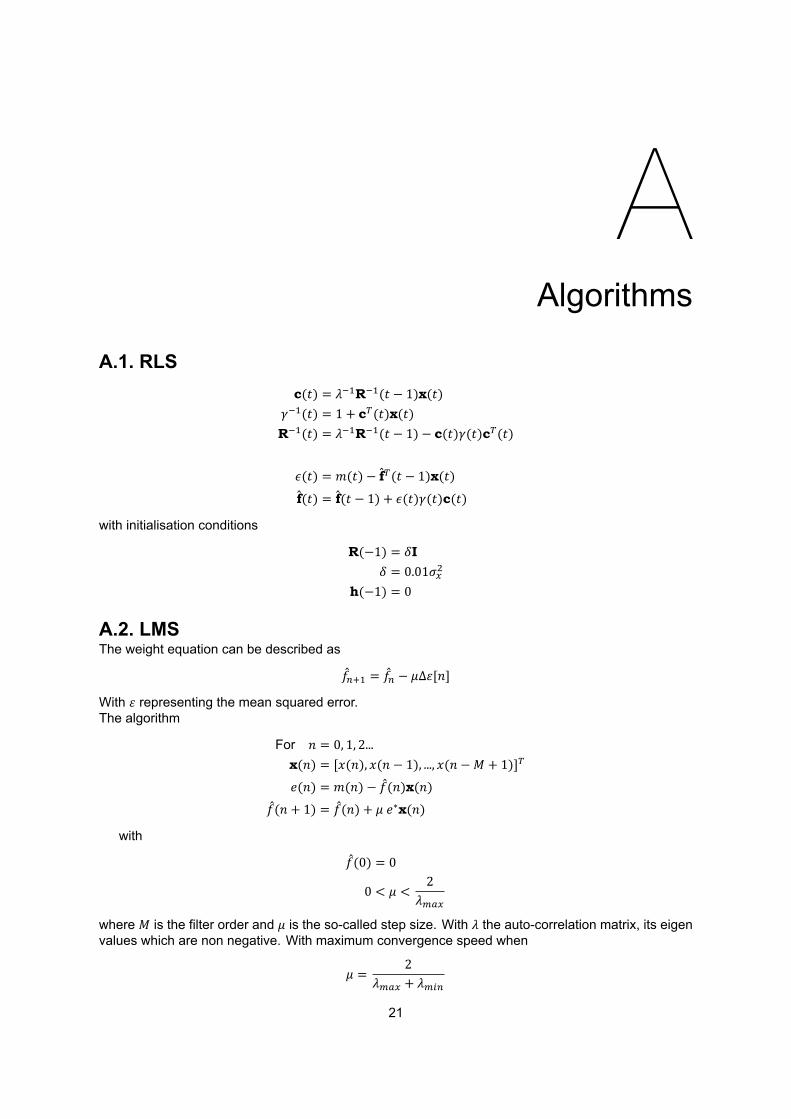
4.1. RLS and Fast RLSTo solve the so-called ill-posed problems, mentioned in section 2.1, in which singular matrices areused, regularisation is applied. Regularisation techniques make ill-posed problems into more well-posed ones. Most often seen is the method derived by Tikhonov et al. [11], which adds a scaledidentity matrix to the matrix X X. Using this method, an algorithm can be derived called the RecursiveLeast Squares (RLS) algorithm [8]. Just as the normal LS algorithm, the RLS tries to estimate thecoefficients of the RIR f.

RLS is a high-performance algorithm, often at the cost of higher complexity. There exist, however,fast versions of the algorithm. A benefit of RLS is being able to converge very fast [5].

In Horita et al. [12], a method is proposed that uses the normal RLS algorithm, but with the additionof a so-called forgetting factor. This gives relatively more weight to more recent samples.

The RLS algorithm [5] is given by A.1, where R(𝑡) is the time-average correlation matrix of the inputsignal, x(𝑡), f(𝑡) is a vector with the estimated filter weights, 𝑦(𝑡) is the desired output signal and c(𝑡)is the Kalman gain vector. In an ideal, noise-free case, the RLS algorithm would converge exactly, butsince there is the initialisation of the matrix R(−1) = 𝛿I and the vector f(−1) = f = 0 gives a certainbias to the estimate [5]. The complexity of RLS algorithms is of order 𝑂(𝑀 ).

It is shown in literature, that the previously mentioned Kalman gain vector can be updated in so-called ’fast’ schemes [13]. To do so, the FRLS algorithm uses amechanism using forward and backwardpredictions. This gives the order of the complexity as 𝑂(7𝑀). This means that while having the sameproperties of the RLS algorithms, its complexity is made comparable to that of the LMS algorithm, whichis discussed later.

A drawback of FRLS is the fact that it has poor error performance, caused by the innate instabilityof the algorithm [13]. There has been quite some research into the instability of the algorithm and somesuccessful solutions have already been presented. These solutions use specific variables and try toestimate these variables as part of a feedback system. These variables lead to another set of variablesthat include parameters that are chosen through careful selection [13]. Another drawback is the factthat there exists a constraint on the factor 𝜆, which negatively affects the convergence rate and trackingability of the algorithm [13].

7

4.2. Stochastic gradient descent methods 8

4.2. Stochastic gradient descent methodsA large portion of the available algorithms are based on the stochastic gradient descent method. Con-vergence is dependent on a step size 𝜇 in the direction of the steepest descent of the mean squarederror. These methods commonly only use the current error and can categorised as posteriori erroralgorithms.

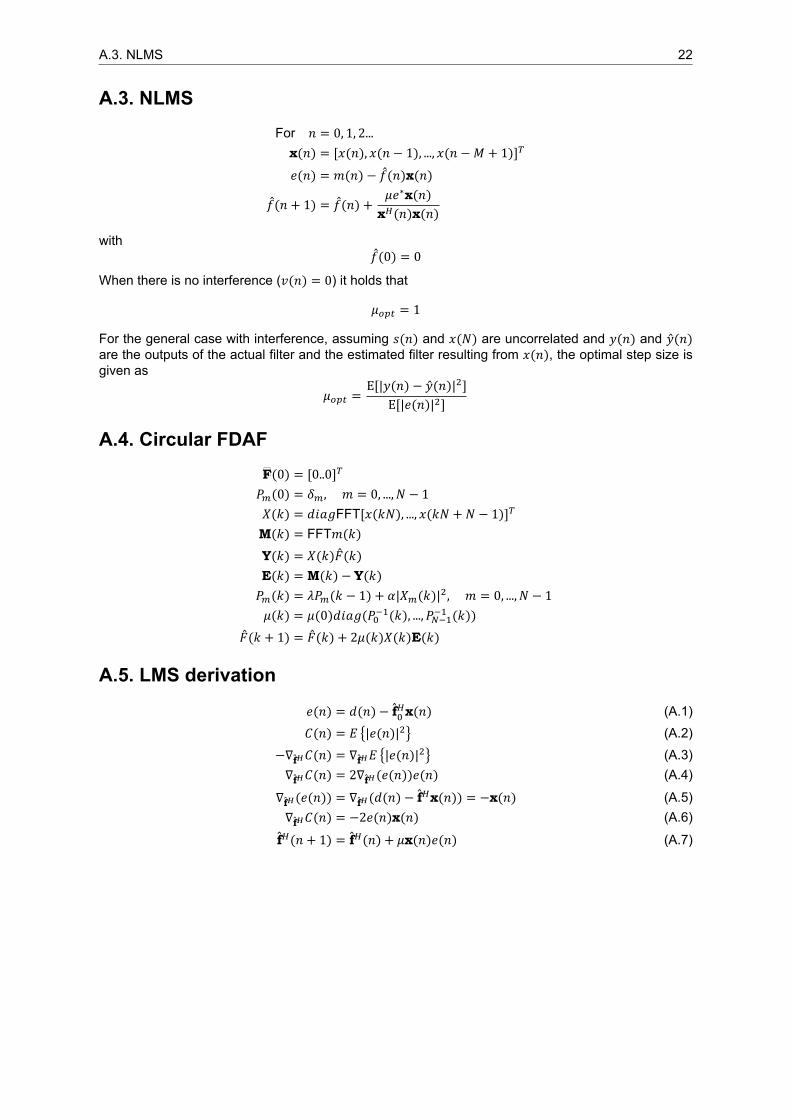
The least mean squares (LMS) algorithm, given in A.2, uses a constant step size independent of thesignal power. The Normalised LMS (NLMS) algorithm, given in A.3, is a variant that solves the problemof LMS for choosing a step size that is stable by normalising with the input to cancel the effects of signalpower deviation [14].

Block processing for adaptive filter design was studied by Clark et al. where the convergence wasfound to be the same as for continuous LMS [15]. Further reductions in computational complexitycan be achieved by realising the LMS algorithm in the frequency-domain (FLMS) and were shown toachieve the optimum filter weights[16]. The advantage of block implementations is that the new weightsare only calculated once per block thus reducing complexity.

There are many variants of the Frequency Domain Adaptive Filter (FDAFs). J.J.Shynk [17] givesan overview of several FDAFs. FDAFs generally have lower computational complexity and a higherconvergence rate than the time domain alternatives. Circular convolution FDAF, given in A.4, wasfound to be the most computationally efficient of the single window approaches. Dividing the frame infrequency sub-bands can also improve decorrelation and computational complexity.

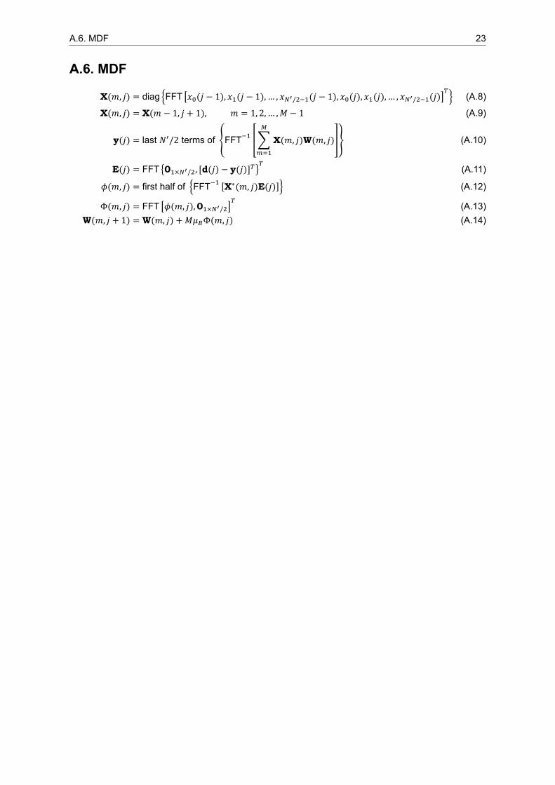
MDF (Multi Delay block FDAF), as given in A.6, reduces the size of the FFT blocks by bufferingmultiple delayed frames. Using multiple smaller FFT blocks reduces the block delay and computationalcomplexity by calculating smaller FFT’s for a longer filter estimation order. The convergence speed is,up to a certain extend, increased with the number of blocks. Its complexity is

𝑂((4𝐷 + 6)𝑙𝑜𝑔 (𝑁) + 8𝐷 − (4𝐵 + 6)𝑙𝑜𝑔 (𝐷)

where 𝐷 is the number of blocks and 𝑁 the frame length which is half the length of the FFT [18].

4.3. APA and Fast APAA generalised form of NLMS and RLS exists, called the Affine Projection algorithm (APA). As mentionedin [13], APA can be seen as an algorithm that estimates the filter by minimising the error norm

𝑐 (𝑛) = argmin ‖𝑐 − 𝑐 (𝑛 − 1)‖

with use of the constraint given as𝑌 (𝑛) = 𝑋 , 𝑐

This algorithm was introduced in [19] as an improvement of NLMS. In there most common form, APAhas poor performance when there is noise present in the output signal or if the input signal is non-stationary, as is for most cases of acoustic feedback cancellation. Countermeasures for this are reg-ularisation and using the time-average correlation matrix of the input signal in the algorithm, whichmakes the APA resemble the RLS algorithm [5].

Fast implementations of APA are of an order comparable to LMS and are not very sensitive tocomputational noise due to the use of predictions [5].

Fast APA uses the shift-invariant property of the input signal vector and the error vector in com-bination with derivations done for the Fast RLS algorithm in [13]. From the sliding-window Fast RLSalgorithm, back and forward prediction vectors can be computed and used to estimate the variablevector. In Fast APA, this is the error with the unknown filter, rather than the estimated coefficients ofthe filter [13]. A derivation of the Fast APA is found in [20].

4.4. Frequency-domain Kalman FilterAn adaptation to the Kalman filter for implementation in echo cancellation was successfully developedin the frequency domain (FDKF) [21]. It is based on the use of a first-order Markov process that modelsthe behaviour of the acoustic path which is assumed to change slowly. Further research on the use,performance and improvements for the Kalman filter in acoustic feedback cancellation are very recent

4.5. Comparison 9

but show promising results [22] [23] without increase of complexity due to the simplicity of the underlyingstatistical model [21]. Obtaining said underlying models would require additional research that fallsoutside of the scope of this thesis.

4.5. ComparisonRLS and APA have a much higher complexity than the other options if the filter order is increased andare not viable as high filter orders are required. Most of the used methods are based on the LMSalgorithm which is well known and researched. Frequency domain analysis has advantages over timedomain due to the options it gives like sub-band analysis and partitioned blocks resulting in FDAF andMDF with reduced complexity due to efficient use of the frequency domain. Cepstral Analysis and theFrequency domain Kalman Filter approaches are not feasible due to their high complexity, asmentionedbefore.

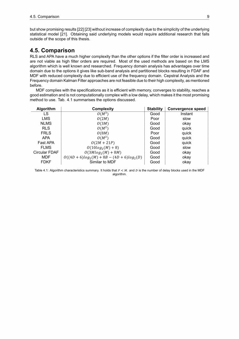
MDF complies with the specifications as it is efficient with memory, converges to stability, reaches agood estimation and is not computationally complex with a low delay, which makes it the most promisingmethod to use. Tab. 4.1 summarises the options discussed.

Algorithm Complexity Stability Convergence speedLS 𝑂(𝑀 ) Good InstantLMS 𝑂(2𝑀) Poor slowNLMS 𝑂(3𝑀) Good okayRLS 𝑂(𝑀 ) Good quickFRLS 𝑂(8𝑀) Poor quickAPA 𝑂(𝑀 ) Good quick

Fast APA 𝑂(2𝑀 + 21𝑃) Good quickFLMS 𝑂(10𝑙𝑜𝑔 (𝑀) + 8) Good slow

Circular FDAF 𝑂(3𝑀𝑙𝑜𝑔 (𝑀) + 8𝑀) Good okayMDF 𝑂((4𝐷 + 6)𝑙𝑜𝑔 (𝑀) + 8𝐵 − (4𝐷 + 6)𝑙𝑜𝑔 (𝐷) Good okayFDKF Similar to MDF Good okay

Table 4.1: Algorithm characteristics summary. It holds that . and is the number of delay blocks used in the MDFalgorithm.

5Testing & Results

To check the insights and knowledge gained from literature, all methods that are deemed feasible wereimplemented. Methods that were considered feasible were LMS, NLMS, Circular FDAF and MDF. Itwas decided not to implement the Fast APA, Fast RLS and Frequency-domain Kalman Filter methods,because of the extent of the theory behind it. APA and RLS were considered unfeasible options, sincetheir high complexity wouldmake them very slow and not satisfy our requirements by blocking continuesaudio throughput. It was decided that, to match the scope of this project, it would be better to implementmultiple smaller algorithms, giving this project a wider approach.

To test and simulate the different methods and algorithms, a simulation environment was built inMatlab, for this subgroup in specific for the easier tracking and control of computations. For the projectgroup Simulink is used for the time based simulation approach.

In the following chapter, powers of 10 are denoted by E, i.e. 2𝐸 means 2 ⋅ 10 .

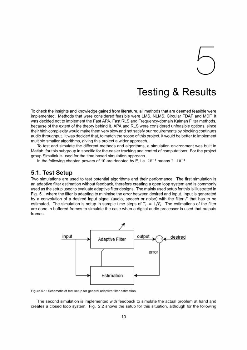
5.1. Test SetupTwo simulations are used to test potential algorithms and their performance. The first simulation isan adaptive filter estimation without feedback, therefore creating a open loop system and is commonlyused as the setup used to evaluate adaptive filter designs. Themainly used setup for this is illustrated inFig. 5.1 where the filter is adapting to minimise the error between desired and input. Input is generatedby a convolution of a desired input signal (audio, speech or noise) with the filter 𝐹 that has to beestimated. The simulation is setup in sample time steps of 𝑇 = 1/𝐹 . The estimations of the filterare done in buffered frames to simulate the case when a digital audio processor is used that outputsframes.

Figure 5.1: Schematic of test setup for general adaptive filter estimation

The second simulation is implemented with feedback to simulate the actual problem at hand andcreates a closed loop system. Fig. 2.2 shows the setup for this situation, although for the following

10

5.1. Test Setup 11

tests, 𝐷 and 𝑃 are excluded. The adaptive filter estimation and output function is implemented with theinput signal 𝑥(𝑡) and the desired signal 𝑚(𝑡). The output is the estimated feedback from 𝑥(𝑡) in 𝑚(𝑡),denoted by ��.

5.1.1. AssumptionsIn the feedback simulation maximum signal strengths are implemented. Typical conversion rates formicrophones are used to create a base voltage reference. Using the specifications of a typical podiummicrophone [24] with a sensitivity of 20 mV/Pa. Normal conversation voice sound level is 70 dB [25]which is converted to 𝑠(𝑡) = ±1.25 mV, and maximum microphone range is set to 102 dB or ±50 mVfor 𝑚(𝑡) and ��(𝑡) and a maximum of 130 dB or ±1.25V which is the pain threshold for sound for theloudspeaker signal x(t) is used as a maximum. The conversion from pascal to decibel is done by

𝑃 = 20 ⋅ 𝑙𝑜𝑔10(𝑃 /0.00002)

where 𝑃 is the sound pressure in decibel and 𝑃 the sound pressure in pascal. Then, the voltagescan be calculated as

𝑈 = 20 ⋅ 10 (𝑉)It is expect that no unknown delay exist between 𝑢(𝑡) and 𝑥(𝑡), any delay that is added will be known.

From the decorrelation group a delay of 2000 samples at 𝐹 = 44.1 kHz has been implemented. A delayis implemented between 𝑢(𝑡) and 𝑥(𝑡) to simulate the delay effect of the decorrelation sub-group.

The system is only aware of the inputs 𝑚(𝑡) and 𝑥(𝑡) and no other setting will be supplied to theestimator.

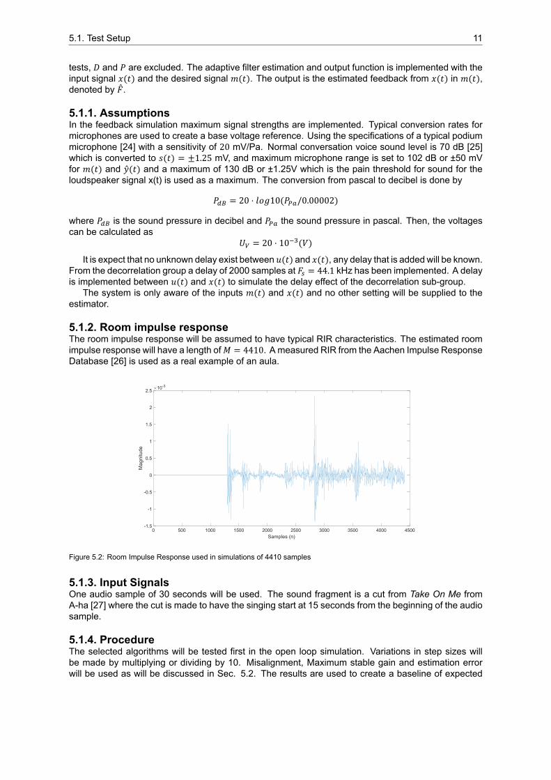
5.1.2. Room impulse responseThe room impulse response will be assumed to have typical RIR characteristics. The estimated roomimpulse response will have a length of𝑀 = 4410. A measured RIR from the Aachen Impulse ResponseDatabase [26] is used as a real example of an aula.

Figure 5.2: Room Impulse Response used in simulations of 4410 samples

5.1.3. Input SignalsOne audio sample of 30 seconds will be used. The sound fragment is a cut from Take On Me fromA-ha [27] where the cut is made to have the singing start at 15 seconds from the beginning of the audiosample.

5.1.4. ProcedureThe selected algorithms will be tested first in the open loop simulation. Variations in step sizes willbe made by multiplying or dividing by 10. Misalignment, Maximum stable gain and estimation errorwill be used as will be discussed in Sec. 5.2. The results are used to create a baseline of expected

5.2. Analysis criteria 12

performance, viable parameters and exclude methods that under perform or of which the calculationtime will be to high.

The second simulation is used to test the performance in a feedback environment. Under performingalgorithms from the first test will be excluded. Gains of 1, 10, 25 and 100 will be used to analyse theperformance of the methods.

5.2. Analysis criteriaThree criteria will be considered to analyse the achieved performance of the algorithms in the suggestedsimulation setups. These are the misalignment,maximum stable gain (MSG) and the estimation error.

5.2.1. MisalignmentThe performance of the system is highly related to the estimation of the adaptive filter. Themisalignmentmis(𝑘) with 𝑘 the frame number is calculated as [28]

mis(𝑘) = ‖𝑓 − 𝑓‖‖𝑓‖ (5.1)

5.2.2. Maximum stable gainTo get an indication of the MSG a different approach was used from Sec. 2.2 due to the lack of criticalfrequencies the simulation setup. The simplified approach from B. Bispo [28] is used instead.

𝜀(𝜔, 𝑛) = |𝐹(𝜔, 𝑛) − ��(𝜔, 𝑛)|𝜀(𝑛)[𝑑𝐵] = 20 log [max𝜀(𝜔, 𝑛)]MSG(𝑛) = −20 log [max𝜀(𝜔, 𝑛)]

5.2.3. Estimation ErrorA simple method that was implemented was taking the relative error between the feedback signal 𝑦(𝑡)and the estimated feedback signal ��(𝑡) or the desired signal and estimated signal in the no feedbacksimulation.

𝐸(𝑡) = 10 log (|𝑦(𝑡) − ��(𝑡)| − 10 log (|𝑦(𝑡)|) (5.2)

where 𝐸(𝑡) is the estimation error.Local differences come up pretty fast with this method, which is why there was mostly looked at the

mean of this error. An average of the errors can be used to quantify the performance.

5.3. Test ResultsIn the following section, the results of the simulations done are presented in the form of tables, with themethods, simulation parameters and results displayed. Essentially, the only parameter that is adjustedis the step size. Step sizes larger or smaller than the listed values were found to be unstable, show noimprovements or even decreased the performance.

5.3.1. Computation timeThe simulations are performed in Matlab on a personal computer. The computation times in Tab. 5.1and 5.2 are factors relative to the lowest method computation time of 1.5ms to indicate the differencesin computational complexity. The actual computation time will dependant on the hardware.

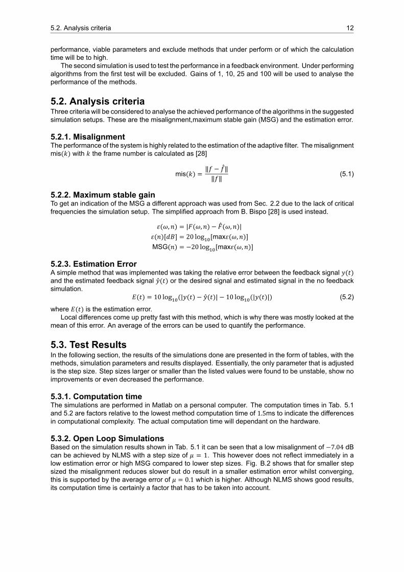
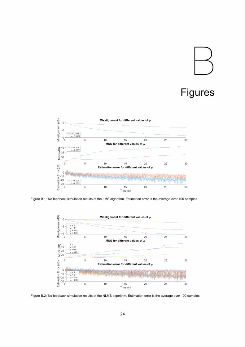
5.3.2. Open Loop SimulationsBased on the simulation results shown in Tab. 5.1 it can be seen that a low misalignment of −7.04 dBcan be achieved by NLMS with a step size of 𝜇 = 1. This however does not reflect immediately in alow estimation error or high MSG compared to lower step sizes. Fig. B.2 shows that for smaller stepsized the misalignment reduces slower but do result in a smaller estimation error whilst converging,this is supported by the average error of 𝜇 = 0.1 which is higher. Although NLMS shows good results,its computation time is certainly a factor that has to be taken into account.

5.3. Test Results 13

The lowest error and largest MSG are both achieved by LMS at a step size of 𝜇 = 1E . Notable isthat increasing the step size breaks the trend of increasing performance, resulting in a unstable systemof which the results are excluded from the table.

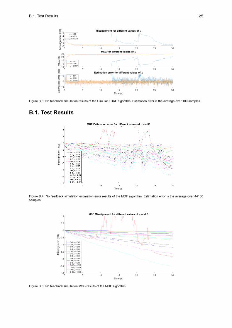
Circular FDAF shows a lower misalignment than MDF but has a higher average error. In Fig. B.3 itcan be seen that for longer simulation the algorithm does not seem to converge further and for higherstep size is unstable even. Circular FDAF will not be tested in a feedback loop due to the long compu-tation time and does not meet the requirements.

MDF shows the best results in the case 𝐷 = 32, 𝜇 = 1E and continues improving in time as seenin Fig. B.5, B.6 and B.4. As expected the performance improves for more delay blocks except for𝐷 = 1. The computation time increases in the test setup for more delay blocks, this might be causedby the program not having a noticeable difference for shorter FFT lenghts.

Without feedback LMS has the highest MSG, NLMS the lowest MIS and MDF the lowest computa-tion time.

Method Step size 𝜇 Avg. MIS [dB] Avg. MSG [dB] Avg. error [dB] comp. time factorLMS 0.001 -5.86 36.58 -13.77 100

1E -1.93 29.41 -6.93NLMS 1 -7.04 34.15 -9.80 200

0.1 -4.91 34.81 -12.420.01 -1.39 28.47 -5.940.001 -0.33 26.68 -3.17

Circular FDAF 0.01 27.00 -44.92 27.48 6660.001 -1.49 27.77 -1.501E -1.24 27.95 -1.19

MDF(𝐷 = 1) 1E -0.70 27.25 -4.46 11E -0.16 26.29 -2.101E -0.03 26.00 -0.39

MDF(𝐷 = 2) 1E -0.19 18.18 0.67 21E -0.25 26.52 -2.811E -0.05 26.00 -0.71

MDF(𝐷 = 4) 1E -0.39 26.23 -3.50 41E -0.08 25.87 -1.20

MDF(𝐷 = 8) 1E -0.60 26.00 -4.24 81E -0.14 25.48 -1.87

MDF(𝐷 = 16) 1E -0.93 26.60 -5.11 161E -0.22 25.55 -2.60

MDF(𝐷 = 32) 1E -1.44 27.66 -6.21 321E -0.34 25.69 -3.29

Table 5.1: Simulation results without feedback. With MDF, indicates the amount of delay blocks. The computation time isgiven as a factor w.r.t. 0.0015s, which is the lowest achieved loop time.

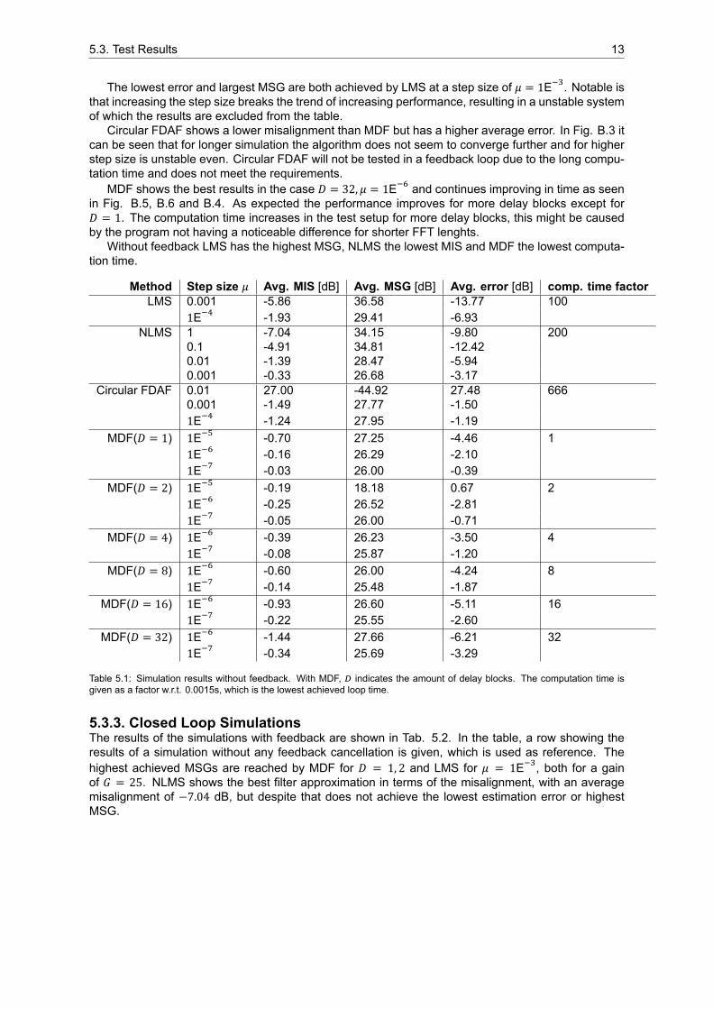
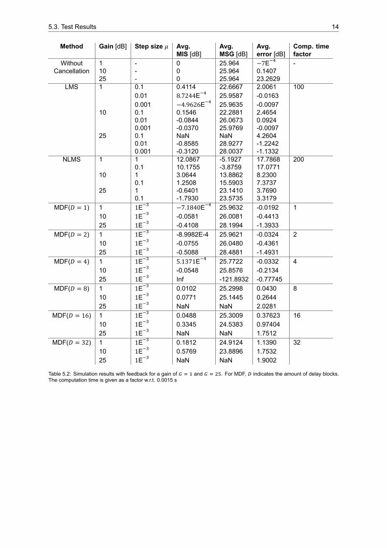
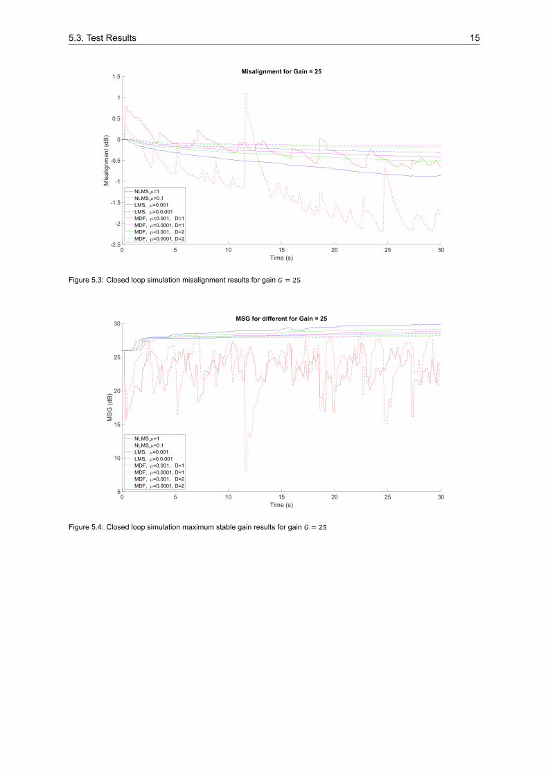
5.3.3. Closed Loop SimulationsThe results of the simulations with feedback are shown in Tab. 5.2. In the table, a row showing theresults of a simulation without any feedback cancellation is given, which is used as reference. Thehighest achieved MSGs are reached by MDF for 𝐷 = 1, 2 and LMS for 𝜇 = 1E , both for a gainof 𝐺 = 25. NLMS shows the best filter approximation in terms of the misalignment, with an averagemisalignment of −7.04 dB, but despite that does not achieve the lowest estimation error or highestMSG.

5.3. Test Results 14

Method Gain [dB] Step size 𝜇 Avg. Avg. Avg. Comp. timeMIS [dB] MSG [dB] error [dB] factor

Without 1 - 0 25.964 −7E -Cancellation 10 - 0 25.964 0.1407

25 - 0 25.964 23.2629LMS 1 0.1 0.4114 22.6667 2.0061 100

0.01 8.7244E 25.9587 -0.01630.001 −4.9626E 25.9635 -0.0097

10 0.1 0.1546 22.2881 2.46540.01 -0.0844 26.0673 0.09240.001 -0.0370 25.9769 -0.0097

25 0.1 NaN NaN 4.26040.01 -0.8585 28.9277 -1.22420.001 -0.3120 28.0037 -1.1332

NLMS 1 1 12.0867 -5.1927 17.7868 2000.1 10.1755 -3.8759 17.0771

10 1 3.0644 13.8862 8.23000.1 1.2508 15.5903 7.3737

25 1 -0.6401 23.1410 3.76900.1 -1.7930 23.5735 3.3179

MDF(𝐷 = 1) 1 1E −7.1840E 25.9632 -0.0192 110 1E -0.0581 26.0081 -0.441325 1E -0.4108 28.1994 -1.3933

MDF(𝐷 = 2) 1 1E -8.9982E-4 25.9621 -0.0324 210 1E -0.0755 26.0480 -0.436125 1E -0.5088 28.4881 -1.4931

MDF(𝐷 = 4) 1 1E 5.1371E 25.7722 -0.0332 410 1E -0.0548 25.8576 -0.213425 1E Inf -121.8932 -0.77745

MDF(𝐷 = 8) 1 1E 0.0102 25.2998 0.0430 810 1E 0.0771 25.1445 0.264425 1E NaN NaN 2.0281

MDF(𝐷 = 16) 1 1E 0.0488 25.3009 0.37623 1610 1E 0.3345 24.5383 0.9740425 1E NaN NaN 1.7512

MDF(𝐷 = 32) 1 1E 0.1812 24.9124 1.1390 3210 1E 0.5769 23.8896 1.753225 1E NaN NaN 1.9002

Table 5.2: Simulation results with feedback for a gain of and . For MDF, indicates the amount of delay blocks.The computation time is given as a factor w.r.t. 0.0015 s

5.3. Test Results 15

Figure 5.3: Closed loop simulation misalignment results for gain

Figure 5.4: Closed loop simulation maximum stable gain results for gain

5.3. Test Results 16

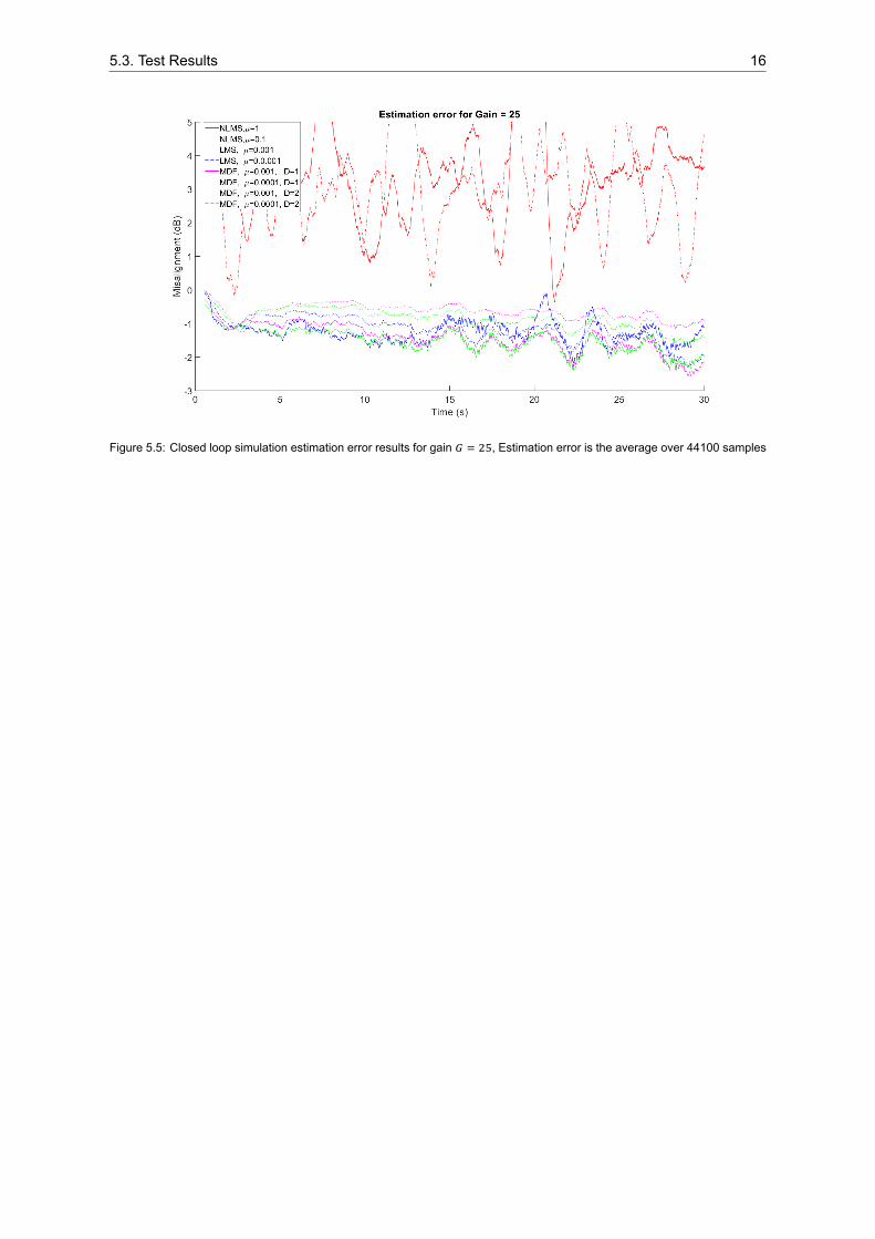
Figure 5.5: Closed loop simulation estimation error results for gain , Estimation error is the average over 44100 samples

6Discussion

In the following sections, the results of the simulations, both without and with feedback, are discussed.The results will be mentioned again, which will be discussed in further detail, with as goal to find logicalexplanations behind the achieved results.

6.1. Open Loop SimulationsA difference with the initial expectations is seen from the results, where it is shown the best filter esti-mation does not result in the lowest estimation error and highest MSG, as is the case with NLMS.

In the case of the open loop estimation with no feedback, The lack of correlation of the misalignmentwith the MSG with respect to the estimation error could be explained by stating that the misalignmentsays more about the differences with the RIR in a global way and the estimation error more locally,making the latter also more susceptible for local variations, making it possibly less consistent. In thecase of NLMS, bigger steps are taken due to it being normalised from a small signal input, which resultsin a quick approximation with the addition of errors as a consequence. It could be seen that for MDF ahigher step size resulted in a higher MSG, but that after a certain threshold the estimation completelyderails. A bigger step size results more quickly in a better estimation of the RIR, and in literature it wasalready shown that for a higher value of 𝐷, the error would decrease as well.

6.2. Closed Loop SimulationsIn the simulations with feedback, the misalignment seems to be more in line with the estimation errorfor all methods. It still holds that the best results in terms of average MSG come from LMS with a gainof 𝐺 = 25 and MDF with 𝐷 = 1, 2. For all methods a higher gain, within the stable range, is beneficial forthe three specifications. For low gains and attenuation through the room the magnitude of the feedbackis relatively small compared to the voice signal. For LMS and MDF the error and MIS do not changemuch from the initial state, due to the fixed step size and low signal strength, NLMS however showsmore variation. Higher gains see improvements to the estimation and compared to without cancellationthe system becomes stable for a gain of 𝐺 = 25.

In the test setup no decorrelation techniques or noise has been added. The length of the RIR usedfor the simulation could be changed to simulate the effect on the estimation and error when using ashorter filter estimation. Typical and atypical RIR’s could be used for the filter estimation testing, ashaving multiple scenarios would benefit the research.

From the closed loop simulations it can be concluded that LMS or MDF is the most suitable solution,MDF with 𝜇 = 1𝐸 and 𝐷 = 2 showed the lowest average error and MSG. The misalignment is lowerthan for LMS 𝜇 = 0.01, however a lower error is a more direct link to the feedback cancellation and isconsidered more valuable. While LMS shows the top results, MDF shows results of about the sameorder, but more consistently for different values of the gain, while LMS is merely situationally effective.Due to this, the most viable method to be implemented is MDF with 𝐷 = 2 delay blocks. This complieswith the comparison made in the Ch. 4.

The specifications set in the requirements 3 are not met by the proposed solution, in terms of theamount of misalignment and increase in MSG. This could be because of several reasons. The first is

17

6.2. Closed Loop Simulations 18

that the requirements were unreasonable in the first place, due to misinterpretation of literature, fromwhere most of the expected performance is derived. Secondly, the fault could lie in the simulationenvironment being imperfect in the sense that not the right parameters were used and conditions weremet to achieve the results derived from literature. However, when listening to the output compared towhen no feedback cancellation is present, howling was successfully removed by the solution and onlya small echo was still audible.

7Implementation Advice & ConsiderationsDue to situational restrictions, no physical implementation of the system could be realised. However,in the following sections, some advice and considerations are given for future reference.

One option is to implement the algorithm into software. Common languages that one can use arePython, C and C++. It is even possible to implement the algorithm into Matlab and convert it into C.In addition to this, one would also have to make a graphical interface of sorts, as well as provide theprogram with the ability to adapt itself to the hardware used, letting the user of the program choosehow and where to use the program. Advantages of making a software implementation are that it savesphysical space, but the way the program is executed will be greatly dependent on the hardware used.A program also requires a computer with operating system to run.

To implement the solution into real hardware two audio inputs, one audio output and a processorwith memory will be required. The audio input and outputs could either work on frame or sample base,although sample base would be preferred to remove block delay from the MDF algorithm when theestimated RIR is used on a single sample base. The delay would be lower if more delay blocks areused resulting in smaller buffers. MDF with 𝐷 = 2 and 𝑀 = 4410 requires a FFT length of 2𝑁 = 4410and buffer frame length of 𝑁 = 2205 which would result in a delay of 𝑇 = 𝑁/𝐹 = 50 ms which isoutside of the specifications, when combined with the decorrelation. Increasing the amount of delayblocks would reduce the delay and the FFT size. In the algorithm, a total of 𝑀 + 3 FFT’s and 𝑀 + 2IFFT’s are computed, all with the same previously mentioned FFT length. A latency time for calculatingthe FFT’s is realistically between 4.9 and 57 ms for FFT and between 4.9 and 38.9 ms for IFFT astested on a FPGA for lengths of a 4096[29]. The computation time will be between 44 and 423 ms.The selection of proper hardware that can compute the FFT’s within a frame of 50 ms is possible forthis solution. Performance can be increased by considering the availability of more efficient DigitalSignal Processors with dedicated FFT hardware which are more effective than FPGA’s and makes theimplementation of the algorithm easily possible within the frame.

19

8Conclusion

The goal of this thesis was to implement an adaptive filter design to remove acoustic feedback froma closed loop system. The literature study showed many years of work on the subject in fields suchas hearing aids, noise cancelling and echo cancellation. The state of the art listed potential solutions,of which MDF was deemed the most promising. A test setup and simulation were designed to testa selection of the algorithms. Without the possibility to have a real system, research was done tomake a realistic simulation by implementing signal hysteresis and relate it to voltage levels. Althoughit was concluded in the end that the MDF algorithms would be the best to implement of the selectedalgorithms, the open loop and closed loop simulations showed unexpected results. The performanceswere lower than expected from literature, which could be a result from the simulation setup, which mightnot have been designed in a way that fully used the algorithms correctly, variations of systems and roomimpulse responses, i.e. in length, amplitude, signal levels and parameter settings that have not beenfully explored. In the end, we could not meet the set requirements derived from the performance ofcertain algorithms in literature, although there were clear improvements to the system signals withrespect to the case without any feedback cancellation and when listening the audible feedback wasclearly reduced.

Quite some research was done on the state of the art and trying to compare the algorithms byliterature alone. Since the initial thought was to compare the different algorithms based on literature andpast results alone, less time was spent preparing a simulation setup on our own. More time time couldhave been better spent working on the Matlab implementations rather than theorising. In hindsight,the goals of the project would be better reached if one algorithm from the state of the art was selectedbased on literature, thoroughly understood and implemented with improvements to robustness andperformance. The initial results of the simulations showed a lot of instability for some of the algorithms,against all expectations. This caused for more effort being put into making sure of the trustworthinessof the results and the way the algorithms were implemented, rather than making real improvements tothe system with the chosen method.

20

AAlgorithms

A.1. RLSc(𝑡) = 𝜆 R (𝑡 − 1)x(𝑡)

𝛾 (𝑡) = 1 + c (𝑡)x(𝑡)R (𝑡) = 𝜆 R (𝑡 − 1) − c(𝑡)𝛾(𝑡)c (𝑡)

𝜖(𝑡) = 𝑚(𝑡) − f (𝑡 − 1)x(𝑡)f(𝑡) = f(𝑡 − 1) + 𝜖(𝑡)𝛾(𝑡)c(𝑡)

with initialisation conditions

R(−1) = 𝛿I𝛿 = 0.01𝜎

h(−1) = 0

A.2. LMSThe weight equation can be described as

𝑓 = 𝑓 − 𝜇Δ𝜀[𝑛]

With 𝜀 representing the mean squared error.The algorithm

For 𝑛 = 0, 1, 2...x(𝑛) = [𝑥(𝑛), 𝑥(𝑛 − 1), ..., 𝑥(𝑛 − 𝑀 + 1)]𝑒(𝑛) = 𝑚(𝑛) − 𝑓(𝑛)x(𝑛)

𝑓(𝑛 + 1) = 𝑓(𝑛) + 𝜇 𝑒∗x(𝑛)

with

𝑓(0) = 0

0 < 𝜇 < 2𝜆

where 𝑀 is the filter order and 𝜇 is the so-called step size. With 𝜆 the auto-correlation matrix, its eigenvalues which are non negative. With maximum convergence speed when

𝜇 = 2𝜆 + 𝜆

21

A.3. NLMS 22

A.3. NLMSFor 𝑛 = 0, 1, 2...x(𝑛) = [𝑥(𝑛), 𝑥(𝑛 − 1), ..., 𝑥(𝑛 − 𝑀 + 1)]𝑒(𝑛) = 𝑚(𝑛) − 𝑓(𝑛)x(𝑛)

𝑓(𝑛 + 1) = 𝑓(𝑛) + 𝜇𝑒∗x(𝑛)x (𝑛)x(𝑛)

with𝑓(0) = 0

When there is no interference (𝑣(𝑛) = 0) it holds that

𝜇 = 1

For the general case with interference, assuming 𝑠(𝑛) and 𝑥(𝑁) are uncorrelated and 𝑦(𝑛) and ��(𝑛)are the outputs of the actual filter and the estimated filter resulting from 𝑥(𝑛), the optimal step size isgiven as

𝜇 = Ε[|𝑦(𝑛) − ��(𝑛)| ]Ε[|𝑒(𝑛)| ]

A.4. Circular FDAF�F(0) = [0..0]𝑃 (0) = 𝛿 , 𝑚 = 0, ..., 𝑁 − 1𝑋(𝑘) = 𝑑𝑖𝑎𝑔FFT[𝑥(𝑘𝑁), ..., 𝑥(𝑘𝑁 + 𝑁 − 1)]M(𝑘) = FFT𝑚(𝑘)Y(𝑘) = 𝑋(𝑘)��(𝑘)E(𝑘) =M(𝑘) − Y(𝑘)𝑃 (𝑘) = 𝜆𝑃 (𝑘 − 1) + 𝛼|𝑋 (𝑘)| , 𝑚 = 0, ..., 𝑁 − 1𝜇(𝑘) = 𝜇(0)𝑑𝑖𝑎𝑔(𝑃 (𝑘), ..., 𝑃 (𝑘))

��(𝑘 + 1) = ��(𝑘) + 2𝜇(𝑘)𝑋(𝑘)E(𝑘)

A.5. LMS derivation

𝑒(𝑛) = 𝑑(𝑛) − f x(𝑛) (A.1)𝐶(𝑛) = 𝐸 {|𝑒(𝑛)| } (A.2)

−∇f 𝐶(𝑛) = ∇f 𝐸 {|𝑒(𝑛)| } (A.3)∇f 𝐶(𝑛) = 2∇f (𝑒(𝑛))𝑒(𝑛) (A.4)

∇f (𝑒(𝑛)) = ∇f (𝑑(𝑛) − f x(𝑛)) = −x(𝑛) (A.5)∇f 𝐶(𝑛) = −2𝑒(𝑛)x(𝑛) (A.6)

f (𝑛 + 1) = f (𝑛) + 𝜇x(𝑛)𝑒(𝑛) (A.7)

A.6. MDF 23

A.6. MDF

X(𝑚, 𝑗) = diag {FFT [𝑥 (𝑗 − 1), 𝑥 (𝑗 − 1), … , 𝑥 / (𝑗 − 1), 𝑥 (𝑗), 𝑥 (𝑗), … , 𝑥 / (𝑗)] } (A.8)

X(𝑚, 𝑗) = X(𝑚 − 1, 𝑗 + 1), 𝑚 = 1, 2, … ,𝑀 − 1 (A.9)

y(𝑗) = last 𝑁 /2 terms of {FFT [∑ X(𝑚, 𝑗)W(𝑚, 𝑗)]} (A.10)

E(𝑗) = FFT {0 × / , [d(𝑗) − y(𝑗)] } (A.11)

𝜙(𝑚, 𝑗) = first half of {FFT [X∗(𝑚, 𝑗)E(𝑗)]} (A.12)

Φ(𝑚, 𝑗) = FFT [𝜙(𝑚, 𝑗),0 × / ] (A.13)W(𝑚, 𝑗 + 1) =W(𝑚, 𝑗) + 𝑀𝜇 Φ(𝑚, 𝑗) (A.14)

BFigures

Figure B.1: No feedback simulation results of the LMS algorithm, Estimation error is the average over 100 samples

Figure B.2: No feedback simulation results of the NLMS algorithm, Estimation error is the average over 100 samples

24

B.1. Test Results 25

Figure B.3: No feedback simulation results of the Circular FDAF algorithm, Estimation error is the average over 100 samples

B.1. Test Results

Figure B.4: No feedback simulation estimation error results of the MDF algorithm, Estimation error is the average over 44100samples

Figure B.5: No feedback simulation MSG results of the MDF algorithm

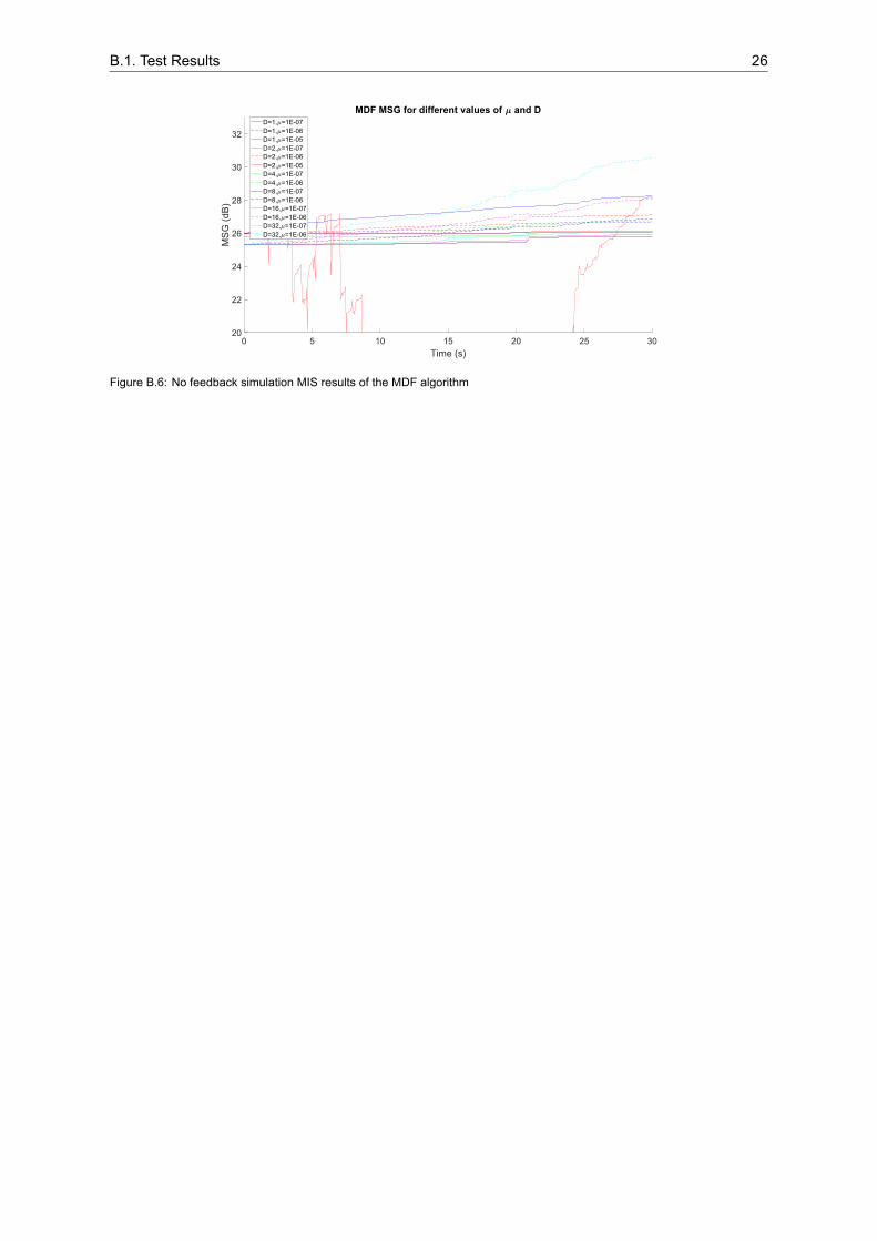
B.1. Test Results 26

Figure B.6: No feedback simulation MIS results of the MDF algorithm

CMatlab Code

C.1. Matlab Simulation Environment Without Feedback1 %{2 Testing enviorment for adaptive filter estimation algorithms3 Authors; Cees Kos, Mathijs Bekkering4 %}5 clear all6 close all78 M = 4410; %Estimated filter length9 Nf = 4410; %Room Impulse Response (RIR) filter length used for filter

output1011 load RIR44100.mat %Load RIR12 f = f(1:Nf); %Section to wanted length1314 %load test audio sample (input) and sampling frequency (Fs)15 [input,Fs] = audioread(’a-ha - Take On Me.mp3’);1617 input = input(23*Fs:24*Fs,1); %Section 30 seconds18 samples = length(input); %Samples in test signal1920 desired = conv(f,input); %Generate desired signal for testing with RIR21 desired = desired(1:samples); %Resize2223 Methods = [”No” ”Perfect” ”LS” ”LMS” ”NLMS” ”FNLMS” ”APA” ”MDF” ”

CircularFDAF” ”Overlap_safe_FLMS” ”FNLMS” ”BLMS” ”BNLMS” ”RLS”];24 selected = [”LMS”];25 for method = selected26 disp(method)27 %Initialization of algorithm28 %mu is the stepsize29 switch method30 case ”No”31 w = zeros(M,1);32 N = M; %Size of frame33 case ”Perfect”34 N = M;35 w = f(1:M);36 case ”LS”

27

C.1. Matlab Simulation Environment Without Feedback 28

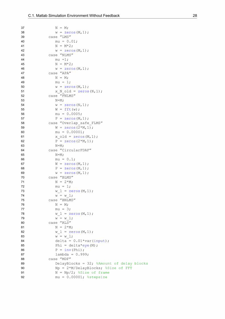
37 N = M;38 w = zeros(M,1);39 case ”LMS”40 mu = 0.01;41 N = M*2;42 w = zeros(M,1);43 case ”NLMS”44 mu =1;45 N = M*2;46 w = zeros(M,1);47 case ”APA”48 N = M;49 mu = 1;50 w = zeros(M,1);51 x_N_old = zeros(N,1);52 case ”FNLMS”53 N=M;54 w = zeros(N,1);55 W = fft(w);56 mu = 0.0005;57 P = zeros(M,1);58 case ”Overlap_safe_FLMS”59 W = zeros(2*M,1);60 mu = 0.00001;61 x_old = zeros(M,1);62 P = zeros(2*M,1);63 N=M;64 case ”CircularFDAF”65 N=M;66 mu = 0.1;67 W = zeros(M,1);68 P = zeros(M,1);69 w = zeros(M,1);70 case ”BLMS”71 N = 2*M;72 mu = 1;73 w_l = zeros(M,1);74 w = w_l;75 case ”BNLMS”76 N = M;77 mu = 3;78 w_l = zeros(M,1);79 w = w_l;80 case ”RLS”81 N = 2*M;82 w_l = zeros(M,1);83 w = w_l;84 delta = 0.01*var(input);85 Phi = delta*eye(M);86 P = inv(Phi);87 lambda = 0.999;88 case ”MDF”89 DelayBlocks = 32; %Amount of delay blocks90 Np = 2*M/DelayBlocks; %Size of FFT91 N = Np/2; %Size of frame92 mu = 0.00001; %stepsize

C.1. Matlab Simulation Environment Without Feedback 29

93 x_previous = zeros(Np/2,1);94 W = zeros(Np,DelayBlocks);95 X = zeros(Np,DelayBlocks);96 w = zeros(M,1);97 otherwise98 disp(”NO case”)99 end

100101 %Reset simulation enviorment102 xx = []; %Input103 yy = []; %Output104 dd = []; %Desired105 ww = []; %Estimated Filter106 buffer_fh = zeros(M,1); %M buffer length for estimated filter length107 bufferx = zeros(N,1); %N buffer length for frames108 bufferd = zeros(N,1);109 buffery = zeros(N,1);110111 loopcountN = 0;112 loopcountW = 0; %Loop count for storing estimated weights113 simulation_time = tic;114115 for n = 1:samples116 calculationstime = tic;117 x = input(n);118 d = desired(n);119 [y,buffer_fh] = ContinuesFIR(w,x,M,buffer_fh); %Estimated filter

output120121 %Buffers for estimators122 bufferx = circshift(bufferx,1);123 bufferx(1) = x;124125 bufferd = circshift(bufferd,1);126 bufferd(1) = d;127128 buffery = circshift(buffery,1);129 buffery(1) = y;130131 if loopcountN == N %If buffer is full132 method_time = tic; %Method time estimation133 switch method134 case ”No”135 case ”Perfect”136 case ”LS”137 [w] = LS_Func(M,N,flip(bufferx),flip(bufferd));138 case ”LMS”139 [w,e] = LMS_Func(bufferd,bufferx,N,M,mu,w);140 case ”NLMS”141 [w,e] = NLMS_Func(bufferd,bufferx,N,M,mu,w);142 case ”APA”143 [e,w,x_N_old,X_LN] = AlgorithmAPAloop_rec(N,M,mu,w,x_N_old,

flip(bufferx),flip(bufferd));144 case ”FNLMS”145 [W,~,e] = FNLMS_Basic(flip(bufferx),flip(bufferd),W,mu,N,P)

;

C.1. Matlab Simulation Environment Without Feedback 30

146 w = ifft(W);147 case ”Overlap_safe_FLMS”148 [x_old,W,e,~] = Overlap_Save_Func(N,x_old,x,W,mu,d,P);149 w = ifft(W);150 w = w(1:M);151 case ”CircularFDAF”152 [W,E,Y,P] = Circular_Conv_Func(flip(bufferx),W,mu,flip(

bufferd),P);153 w = ifft(W);154 case ”BLMS”155 [w_l] = BLMS_Func((bufferd),flip(bufferx),M,N,mu,w_l,(

buffery));156 w = flip(w_l);157 case ”BNLMS”158 [w_l] = BNLMS_Func(flip(bufferd),bufferx,N,M,mu,w_l,flip(

buffery));159 w = flip(w_l);160 case ”RLS”161 [e,w] = AlgorithmRLSloop((bufferx),(bufferd),M,P,lambda,w);162 case ”MDF”163 [~,X,W,x_previous,PHI,phi,E] = MDF_1Func(Np,DelayBlocks,mu,

flip(bufferx),flip(bufferd),X,W,x_previous);164 w = ifft(W);165 w = (reshape(fliplr(w(1:Np/2,:)), [DelayBlocks*Np/2,1])); %

Reshape to single filter estimation166 otherwise167 end168 loopcountN = 0;169 method_time = toc(method_time);170 end171172 loopcountN = loopcountN + 1;173 loopcountW = loopcountW + 1;174175 if loopcountW > M %Store filter estimation176 ww= [ww w];177 loopcountW = 0;178 end179180 %% save information181 dd(n) =d;182 xx(n) =x;183 yy(n) =y;184 end185 end186187 %Calculate performance188 for k = 1:size(ww,2)189 mis = sqrt(sum((abs((f(1:M)-ww(1:M,k)).^2))/sum(f(1:M).^2)));190 MIS(k) = mis; %Misalignment191 msg = calcMSG(1,f,[ww(1:M,k); zeros(length(f)-M,1)]);192 MSG(k) = msg.M; %Maximum Stable Gain193194 end195196 Estimation_error = movmean(10*log10(abs(dd-yy)),100)-movmean(10*log10(abs(

C.2. Matlab Simulation Environment With Feedback 31

dd)),100);197198 %Plots199 timeaxis =(0:samples-1)/Fs;200 frametimeaxis = linspace(0,(samples-1)/Fs,length(MIS));201202 figure;203 subplot(3,1,1)204 plot(frametimeaxis,10*log10(MIS));205 title(’MIS’)206207 subplot(3,1,2)208 plot(timeaxis,Estimation_error)209 title(’estimationerror’)210211 subplot(3,1,3)212 plot(frametimeaxis,MSG)213 title(’MSG’)214215 sgtitle(strcat((method), ” M:”, num2str(M), ” Nf:”, num2str(Nf), ” u:”,

num2str(mu) ))

C.2. Matlab Simulation Environment With Feedback1 %{2 Testing enviorment for adaptive filter estimation algorithms3 Authors; Cees Kos, Mathijs Bekkering4 %}5 clear all6 close all78 M = 4410; %Estimated filter length9 Nf = 4410; %Room Impulse Response (RIR) filter length used for filter

output10 G = 50; %Loop gain1112 load RIR44100.mat %Load RIR13 f = f(1:Nf); %Section to wanted length1415 %load test audio sample (input) and sampling frequency (Fs)16 [input,Fs] = audioread(’a-ha - Take On Me.mp3’);1718 input = input(23*Fs:24*Fs,1); %Section 30 seconds19 samples = length(input); %Samples in test signal2021 buffermst =[];22 bufferxst =[];2324 Methods = [”No” ”Perfect” ”LS” ”LMS” ”NLMS” ”FNLMS” ”APA” ”MDF” ”

CircularFDAF” ”Overlap_safe_FLMS” ”FNLMS” ”BLMS” ”BNLMS” ”RLS”];25 selected = [”APA”];26 for method = selected27 disp(method)28 %s is signal going into microphone from person or music29 %y is feedback from speaker30 %y_hat is estimated feedback31 %x is signal going to speaker

C.2. Matlab Simulation Environment With Feedback 32

32 %u is signal after subtraction of extimation33 %m is signal from microphone34 %mu is the stepsize3536 %Initialization of algorithm37 switch method38 case ”Perfect”39 w = f;40 N = M; %N is frame size41 case ”NO”42 w = zeros(M,1);43 N = M;44 case ”LS”45 M = N/2;46 f_l = f(1:M);47 w = f;48 case ”LMS”49 mu = 0.001;50 N=M*2;51 w = zeros(M,1);52 case ”NLMS”53 mu = 0.1;54 N = M*2;55 w = zeros(M,1);56 case ”APA”57 N = M;58 mu = 1;59 w = zeros(M,1);60 x_N_old = zeros(N,1);61 case ”FNLMS”62 mu = 0.02;63 w = zeros(M,1);64 W = fft(w);65 N=M;66 case ”Overlap_safe_FLMS”67 W = zeros(2*N,1);68 mu = 0.00001;69 x_old = zeros(N,1);70 P = zeros(2*N,1);71 M = N;72 f_l = f(1:N);73 case ”CircularFDAF”74 N = M;75 W = zeros(N,1);76 mu = 0.001;77 P = zeros(N,1);78 w = zeros(N,1);79 case ”BLMS”80 M = N/2;81 f_l = f(1:M);82 mu = 50;83 w_l = zeros(M,1);84 case ”BNLMS”85 M = N/2;86 f_l = f(1:M);87 mu = 30;

C.2. Matlab Simulation Environment With Feedback 33

88 w_l = zeros(M,1);89 case ”RLS”90 f_l = f(1:M);91 M_RLS = length(f);92 w_l = zeros(M_RLS,1);93 w = zeros(M_RLS,1);94 delta = 0.01*var(input);95 Phi = delta*eye(M_RLS);96 P = inv(Phi);97 lambda = 0.999;98 case ”MDF”99 DelayBlocks = 1; %Amount of delay blocks

100 Np = 2*M/DelayBlocks;101 N = Np/2;102 mu = 0.0001; %stepsize103 x_previous = zeros(Np/2,1);104 W = zeros(Np,DelayBlocks);105 X = zeros(Np,DelayBlocks);106 w = zeros(M,1);107 otherwise108 disp(”NO case”)109 end110 %Reset simulation enviorment111 xx = [];112 yy = [];113 uu = [];114 mm = [];115 yy_hat = [];116 ww = [];117 ss = [];118 Delaybuffer = zeros(2000,1); %Delay in loop119 buffer_f = zeros(Nf,1);120 buffer_fh = zeros(M,1);121 bufferx = zeros(N,1);122 bufferm = zeros(N,1);123 bufferu = zeros(N,1);124 loopcountN = 0;125 loopcountW = 0;126127 for n = 1:samples128 % insert estimation function129 s = input(n);130131 [y,buffer_f] = ContinuesFIR(f,x,Nf,buffer_f);132 [y_hat,buffer_fh] = ContinuesFIR(w,x_est,M,buffer_fh);133134 m = s+y; %Feedback + Input signal135136 %Saturation of input signal137 if m > 0.05138 m = 0.05 ;139 elseif m < -0.05140 m = -0.05 ;141 end142143 %Saturation of estimation signal

C.2. Matlab Simulation Environment With Feedback 34

144 if y_hat > 0.05145 y_hat = 0.05 ;146 elseif y_hat < -0.05147 y_hat = -0.05 ;148 end149150 u = m-y_hat; %Feedback cancellation151152 %buffers153 bufferx = circshift(bufferx,1);154 bufferx(1) = x;155156 bufferm = circshift(bufferm,1);157 bufferm(1) = m;158159 bufferu = circshift(bufferu,1);160 bufferu(1) = u;161162 if n > 2*N %Delay to fill buffers with usable data163 if loopcountN > N %If buffer is full164 method_time= tic; %Method time estimation165 switch method166 case ”Perfect”167 case ”NO”168 case ”LS”169 [w] = LS_Func(M,N,estimation_bufferx,estimation_bufferm);170 case ”LMS”171 [w,e] = LMS_Func((estimation_bufferm),(estimation_bufferx),N,M

,mu,w);172 case ”NLMS”173 [w,e] = NLMS_Func(estimation_bufferm,estimation_bufferx,N,M,mu

,w);174 case ”APA”175 [e,w,x_N_old,X_LN] = AlgorithmAPAloop_rec(N,M,mu,w,x_N_old,

flip(estimation_bufferx),flip(estimation_bufferm));176 case ”FNLMS”177 [W,~,e] = FNLMS_Basic(estimation_bufferx,estimation_bufferm,W,

mu,N);178 w = ifft(W);179 case ”Overlap_safe_FLMS”180 [x_old,W,e,~] = Overlap_Save_Func(N,x_old,x,W,mu,m,P);181 w = ifft(W);182 w = w(1:N);183 case ”CircularFDAF”184 [W,E,Y,P] = Circular_Conv_Func(flip(estimation_bufferx),W,mu,

flip(estimation_bufferm),P);185 w = ifft(W);186 case ”BLMS”187 [~,w,e] = BNLMS_Func(m,x,N,M,mu,w);188 case ”BNLMS”189 [~,w,e] = BNLMS_Func(m,x,N,M,mu,w);190 case ”RLS”191 [e,w_l] = AlgorithmRLSloop(x,m,M_RLS,P,lambda,w_l);192 w = flip(w_l);193 case ”MDF”194 [~,X,W,x_previous,PHI,phi,E] = MDF_1Func(Np,DelayBlocks,mu,

C.2. Matlab Simulation Environment With Feedback 35

flip(estimation_bufferx),flip(estimation_bufferm),X,W,x_previous);

195 w = ifft(W);196 w = (reshape(fliplr(w(1:Np/2,:)), [DelayBlocks*Np/2,1]));197 otherwise198 disp(”NO case”)199 end200 method_time = toc(method_time);201 loopcountN = 0;202 end203 end204 loopcountN = loopcountN + 1;205206 x = Delaybuffer(end)*G; %Delay buffer and loop gain G207 Delaybuffer = circshift(Delaybuffer,1);208 Delaybuffer(1) = u;209210 %Loudspeaker saturation211 if x > 1.25212 x = 1.25;213 elseif x < -1.25214 x = -1.25;215 end216217 %% save information218 ss(n) = s;219 xx(n) = x;220 yy(n) = y;221 uu(n) = u;222 mm(n) = m;223 yy_hat(n) = y_hat;224 xx_est(n) = x_est225226 loopcountW = loopcountW + 1;227 if loopcountW > M228 ww= [ww w];229 loopcountW = 0;230 end231 end232 end233234 %Calculate performance235 for k = 1:size(ww,2)236 mis = sqrt(sum((abs((f(1:M)-ww(1:M,k)).^2))/sum(f(1:M).^2)));237 MIS(k) = mis; %Misalignment238 msg = calcMSG(1,f,[ww(1:M,k); zeros(length(f)-M,1)]);239 MSG(k) = msg.M; %Maximum Stable Gain240 end241242 Estimation_error = movmean(10*log10(abs(yy-yy_hat)),100)-movmean(10*log10(

abs(yy)),100);243 Signal_error = movmean(10*log10(abs(ss-uu)),100)-movmean(10*log10(abs(ss))

,100);244245 timeaxis =(0:length(yy)-1)/Fs;246 frameaxis = linspace(0,(length(yy)-1)/Fs,length(MIS));

C.2. Matlab Simulation Environment With Feedback 36

247248 %% Plot249 figure()250 subplot(241)251 plot(timeaxis,yy);252 title(’yy’);253 subplot(243)254 plot(timeaxis,ss);255 title(’ss’);256 subplot(242)257 plot(timeaxis,yy_hat);258 title(’yy_hat’);259 subplot(244)260 plot(timeaxis,uu);261 title(’uu’);262263 subplot(245)264 plot(frameaxis,10*log10(MIS));265 title(’mis’);266 subplot(246)267 plot(frameaxis,MSG)268 title(’MSG’);269 subplot(247)270 plot(timeaxis,Estimation_error);271 title(’Estimation_error y_hat-y’);272 subplot(248)273 plot(timeaxis,Signal_error);274 title(’Signal_error u-s’);275276 sgtitle(strcat(method,” u ”, num2str(mu),”G ”, num2str(G)))

Bibliography[1] M. R. Schroeder, “Improvement of acoustic-feedback stability by frequency shifting,” The Journal

of the Acoustical Society of America, vol. 36, September 1964.

[2] T. van Waterschoot and M. Moonen, “Fifty years of acoustic feedback control: State of the art andfuture challenges,” Proc. IEEE, vol. 99, pp. 288–327, February 2011.

[3] W. Leotwassana, R. Punchalard, and W. Silaphan, “Adaptive howling canceller using adaptive iirnotch filter: simulation and implementation,” in International Conference on Neural Networks andSignal Processing, 2003. Proceedings of the 2003, vol. 1, pp. 848–851 Vol.1, 2003.

[4] G. Rombouts, T.van Waterschoot, and M.Moonen, “Proactive notch filtering for acoustic feedbackcancellation,” Proc. 2nd Annual IEEE Benelux/DSP Valley Signal Process, 2006.

[5] A. Gilloire, E. Moulines, D. Slock, and P.Duhamel, “State of the art in acoustic echo cancellation,”in Digital Signal Processing in Telecommunications, pp. 45–91, Springer, 1996.

[6] L. C. A. Huijbregts and M. A. Jongepier, “Decorrelation in adaptive feedback cancellation for pasystems.” B.S. Thesis, Delft Univ. Technol., Delft, 2020.

[7] J. W. de Vries and C. A. Weustink, “Postfiltering in adaptive feedback cancellation for pa systems.”B.S. Thesis, Delft Univ. Technol., Delft, 2020.

[8] T. van Waterschoot, G. Rombouts, and M. Moonen, “Optimally regularized adaptive filtering al-gorithms for room acoustic signal enhancement,” Signal Processing, vol. 88, pp. 594–611, March2008.

[9] H. Nyquist, “Regeneration theory,” The Bell System Technical Journal, vol. 11, no. 1, pp. 126–147,1932.

[10] A. Mcpherson, R. Jack, and G. Moro, “Action-sound latency: Are our tools fast enough?,” in Pro-ceedings of the International Conference on New Interfaces for Musical Expression, 07 2016.

[11] A. N. Tikhonov and V. Y. Arsenin, “Solutions of ill-posed problems,” Siam Rev., vol. 21, no. 2,pp. 266–267, 1979.

[12] E. Horita, K. Sumiya, H. Urakami, and S. Mitsuishi, “A leaky rls algorithm: its optimality and im-plementation,” IEEE Transactions on Signal Processing, vol. 52, no. 10, pp. 2924–2936, 2004.

[13] G. Glentis, K. Berberidis, and S. Theodoridis, “Efficient least squares adaptive algorithms for FIRtransversal filtering,” IEEE Signal Processing Magazine, vol. 16, no. 4, pp. 13–41, 1999.

[14] J. Dhiman, S. Ahmad, K. Gulia, et al., “Comparison between adaptive filter algorithms (lms, nlmsand rls),” International journal of science, engineering and technology research (IJSETR), vol. 2,no. 5, pp. 1100–1103, 2013.

[15] G. Clark, S. Mitra, and S. Parker, “Block implementation of adaptive digital filters,” IEEE Transac-tions on Acoustics, Speech, and Signal Processing, vol. 29, no. 3, pp. 744–752, 1981.

[16] J. C. Lee and C. K. Un, “Performance analysis of frequency-domain block lms adaptive digitalfilters,” IEEE Transactions on Circuits and Systems, vol. 36, no. 2, pp. 173–189, 1989.

[17] J. J. Shynk, “Frequency-domain and multirate adaptive filtering,” IEEE Signal Processing Maga-zine, vol. 9, no. 1, pp. 14–37, 1992.

[18] J. Soo and K. K. Pang, “Multidelay block frequency domain adaptive filter,” IEEE Transactions onAcoustics, Speech, and Signal Processing, vol. 38, no. 2, pp. 373–376, 1990.

37

Bibliography 38

[19] K.Ozeki and T. Umeda,, “An adaptive filtering algorithm using an orthogonal projection to an affinesubspace and its properties,” Electronics and Communications in Japan (Part I: Communications),vol. 67, no. 5, pp. 19–27, 1984.

[20] S. L.Gay, “A fast converging, low complexity adaptive filtering algorithm,” in Proceedings of IEEEWorkshop on Applications of Signal Processing to Audio and Acoustics, pp. 4–7, IEEE, 1993.

[21] G. Enzner and P. Vary, “Frequency-domain adaptive kalman filter for acoustic echo control inhands-free telephones,” Signal Processing, vol. 86, Issue 6, pp. 1140–1156.

[22] G. Bernardi, T. van Waterschoot, J. Wouters, and M. Moonen, “Adaptive feedback cancella-tion using a partitioned-block frequency-domain kalman filter approach with pem-based signalprewhitening,” IEEE/ACM Transactions on Audio, Speech, and Language Processing, vol. 25,no. 9, pp. 1784–1798, 2017.

[23] F. Yang, G. Enzner, and J. Yang, “Frequency-domain adaptive kalman filter with fast recoveryof abrupt echo-path changes,” IEEE Signal Processing Letters, vol. 24, no. 12, pp. 1778–1782,2017.

[24] E. Audio, “Fm360, fm500, fmr500, fmr600 fmr720.” https://earthworksaudio.com/products/microphones/flexmic-series/20khz-fm/. Accessed on 19-06-2020.

[25] E. ToolBox, “Voice level at distance.” https://www.engineeringtoolbox.com/voice-level-d_938.html, 2005. Accessed on 19-06-2020.

[26] M. Jeub, M. Schäfer, and P.Vary, “A binaural room impulse response database for the evalua-tion of dereverberation algorithms,” in Proceedings of International Conference on Digital SignalProcessing (DSP), (Santorini, Greece), pp. 1–4, IEEE, IET, EURASIP, IEEE, July 2009.

[27] A-ha, “Take on me.” https://www.youtube.com/watch?v=djV11Xbc914, 1985. Accessedon 19-06-2020.

[28] B. C. Bispo, “Acoustic feedback and echo cancellation in speech communication systems,” 2015.

[29] M. A. Jaber, D. Massicotte, and Y. Achouri, “A higher radix fft fpga implementation suitable forofdm systems,” in 2011 18th IEEE International Conference on Electronics, Circuits, and Systems,pp. 744–747, 2011.