ADAPTIVE EDGE-ENHANCED CORRELATION BASED ROBUST AND REAL-TIME VISUAL TRACKING FRAMEWORK AND ITS DEPLOYMENT IN MACHINE VISION SYSTEMS by Javed Ahmed Submitted to the Department of Electrical Engineering, Military College of Signals, in partial fulfillment of the requirements for the degree of Doctor of Philosophy National University of Sciences and Technology Rawalpindi, Pakistan February 2008

Welcome message from author
This document is posted to help you gain knowledge. Please leave a comment to let me know what you think about it! Share it to your friends and learn new things together.
Transcript
ADAPTIVE EDGE-ENHANCED CORRELATION BASED
ROBUST AND REAL-TIME VISUAL TRACKING FRAMEWORK
AND ITS DEPLOYMENT IN MACHINE VISION SYSTEMS
by
Javed Ahmed
Submitted to the Department of Electrical Engineering, Military College of Signals, in partial fulfillment of the requirements for
the degree of Doctor of Philosophy
National University of Sciences and Technology Rawalpindi, Pakistan
February 2008

Approved for the Department of Electrical Engineering
Supervisor
Chairman of the Guidance & Examination Committee
Head of the Department
iii
Abstract
An adaptive edge-enhanced correlation based robust and real-time visual tracking
framework, and two machine vision systems based on the framework are proposed.
The visual tracking algorithm can track any object of interest in a video acquired from
a stationary or moving camera. It can handle the real-world problems, such as noise,
clutter, occlusion, uneven illumination, varying appearance, orientation, scale, and
velocity of the maneuvering object, and object fading and obscuration in low contrast
video at various zoom levels. The proposed machine vision systems are an active
camera tracking system and a vision based system for a UGV (unmanned ground
vehicle) to handle a road intersection.
The core of the proposed visual tracking framework is an Edge Enhanced
Back-propagation neural-network Controlled Fast Normalized Correlation (EE-
BCFNC), which makes the object localization stage efficient and robust to noise,
object fading, obscuration, and uneven illumination. The incorrect template
initialization and template-drift problems of the traditional correlation tracker are
handled by a best-match rectangle adjustment algorithm. The varying appearance of
the object and the short-term neighboring clutter are addressed by a robust template-
updating scheme. The background clutter and varying velocity of the object are
handled by looking for the object only in a dynamically resizable search window, in
which the likelihood of the presence of the object is high. The search window is
created using the prediction and the prediction error of a Kalman filter. The effect of
the long-term neighboring clutter is reduced by weighting the template pixels using a
2D Gaussian weighting window with adaptive standard deviation parameters. The
occlusion is addressed by a data association technique. The varying scale of the object

iv
is handled by correlating the search window with three scales of the template, and
accepting the best-match region that produces the highest peak in the three correlation
surfaces. The proposed visual tracking algorithm is compared with the traditional
correlation tracker and, in some cases, with the mean-shift and the condensation
trackers on real-world imagery. The proposed algorithm outperforms them in
robustness and executes at the speed of 25 to 75 frames/second depending on the
current sizes of the adaptive template and the dynamic search window.
The proposed active camera tracking system can be used to get the target
always in focus (i.e. in the center of the video frame) regardless of the motion of the
target in the scene. It feeds the target coordinates estimated by the visual tracking
framework into a predictive open-loop car-following control (POL-CFC) algorithm
which in turn generates the precise control signals for the pan-tilt motion of the
camera. The performance analysis of the system shows that its percent overshoot, rise
time, and maximum steady state error are 0%, 1.7 second, and ±1 pixel, respectively.
The hardware of the proposed vision based system, that enables a UGV to
handle a road intersection, consists of three on-board computers and three cameras
(mounted on top of the UGV) looking towards the other three roads merging at the
intersection. The software in each computer consists of a vehicle detector, the
proposed tracker, and a finite state machine model (FSM) of the traffic. The
information from the three FSMs is combined to make an autonomous decision
whether it is safe for the UGV to cross the intersection or not. The results of the actual
UGV experiments are provided to validate the robustness of the proposed system.
Index terms – visual tracking, adaptive edge-enhanced correlation, active camera,
unmanned ground vehicle.

© 2008 Javed Ahmed

vi
To the Prophet Muhammad (Sallallahu Alaih Wa Aalihee Wasallam)

vii
Acknowledgements
It would be an injustice if I do not thank, first of all, Allah, the creator and controller
of the whole universe. He blessed me with the will to get into the world of research
and guided me through ups and downs in the course of achieving my goal. I thank
Him without any limit...
I am grateful to my parents (who always pray for me to have a good place in
this world and hereafter), my wife and children (for being with me even when I was
not completely with them), and my brothers and sisters (who are my perpetual well-
wishers).
I would like to thank my supervisor Dr. M. Noman Jafri (Professor, MCS) for
his technical as well as managerial support during my PhD studies. I am also grateful
to my co-supervisor Dr. Mubarak Shah (Agere Chair Profesor, University of Central
Florida, USA), who graciously invited me to conduct the collaborative research with
his research group at the world famous Computer Vision Lab under his guidance. The
8-month visit provided me with the opportunity to learn many new ideas and current
trends in the field of computer vision.
I am grateful to Dr. Zhigang Zhu (City University of New York, USA), Dr.
Alper Yilmaz (Ohio State University, USA), and Dr. Sohaib Ahmad Khan (Lahore
University of Management Sciences, Pakistan) for accepting the manuscript of this
dissertation for PhD and providing me with their positive comments and valuable
suggestions for the further improvement.
I would also like to thank Brig.® Dr. Muhammad Akbar (Professor, MCS), Dr.
Saleem Akbar (Professor, MCS), and Dr. Jamil Ahmad (Professor and Dean, Iqra

viii
University, Islamabad Campus) for being members of my Guidance and Examination
Committee (GEC).
I think I am going to remember Dr. Muhammad Ali Chaudhry, Robina Ashraf,
Lt. Col. Fahim Arif, Lt. Col. Alamdar Raza, and Lt. Cmdr. Junaid Ahmed for a long
time for accompanying me in the same vulnerable boat.
ix
Table of Contents
LIST OF FIGURES………………………………………………………………...XII
LIST OF TABLES……………………………………………………………….XVIII
1 INTRODUCTION..................................................................................... 1
1.1 Chapter Overview.................................................................................................................... 1
1.2 Visual Tracking........................................................................................................................ 1 1.2.1 Introduction......................................................................................................................... 1 1.2.2 Previous Work .................................................................................................................... 2 1.2.3 Contribution of the Present Research.................................................................................. 4
1.3 Active Camera Tracking System ............................................................................................ 7 1.3.1 Introduction......................................................................................................................... 7 1.3.2 Previous Work .................................................................................................................... 8 1.3.3 Contribution of the Present Research.................................................................................. 9
1.4 A Vision Based System for a UGV to Handle a Road Intersection.................................... 10 1.4.1 Introduction....................................................................................................................... 10 1.4.2 Previous Work .................................................................................................................. 11 1.4.3 Contribution of the Present Research................................................................................ 12
1.5 Thesis Organization ............................................................................................................... 12
1.6 Chapter Summary.................................................................................................................. 13
2 CORRELATION BASED OBJECT LOCALIZATION............................ 14
2.1 Chapter Overview.................................................................................................................. 14
2.2 Object and Its Representation .............................................................................................. 14
2.3 Correlation Metrics................................................................................................................ 15 2.3.1 Standard Correlation (SC)................................................................................................. 16 2.3.2 Phase Correlation (PC) ..................................................................................................... 17 2.3.3 Normalized Correlation (NC) ........................................................................................... 18 2.3.4 Normalized Correlation Coefficient (NCC)...................................................................... 19 2.3.5 Edge Enhanced BPNN-Controlled Fast Normalized Correlation (EE-BCFNC) .............. 20
2.4 Generic Correlation Based Object Localization Algorithm............................................... 33
2.5 Comparison among Different Correlation Techniques ...................................................... 34
2.6 Chapter Summary.................................................................................................................. 38
3 VISUAL TRACKING FRAMEWORK .................................................... 39
3.1 Chapter Overview.................................................................................................................. 39
x
3.2 Challenges for a Visual Tracking Algorithm....................................................................... 39
3.3 Proposed Visual Tracking Framework ................................................................................ 40 3.3.1 Video Frame Acquisition.................................................................................................. 40 3.3.2 Initialization of Template, Kalman Filter, and Search Window ....................................... 42 3.3.3 Edge-enhancement of Template and Search Window ...................................................... 43 3.3.4 Template Scaling .............................................................................................................. 43 3.3.5 Gaussian Weighting of Template Pixels ........................................................................... 46 3.3.6 Object Localization........................................................................................................... 47 3.3.7 Template Updating ........................................................................................................... 48 3.3.8 Best-Match Rectangle (BMR) Adjustment ....................................................................... 50 3.3.9 Occlusion Handling .......................................................................................................... 58 3.3.10 Kalman Filter .................................................................................................................... 60 3.3.11 Search Window Updating ................................................................................................. 64
3.4 Experimental Results............................................................................................................. 68
3.5 Comparison with Traditional Correlation Tracker............................................................ 72
3.6 Chapter Summary.................................................................................................................. 78
4 ACTIVE CAMERA TRACKING SYSTEM ............................................. 80
4.1 Chapter Overview.................................................................................................................. 80
4.2 Problem Description .............................................................................................................. 80
4.3 Pan-Tilt Control Algorithm .................................................................................................. 81 4.3.1 Car-Following Control (CFC) Law................................................................................... 82 4.3.2 Predictive Open-Loop CFC (POL-CFC) .......................................................................... 85 4.3.3 Determining Cdpp Factor.................................................................................................... 88 4.3.4 Performance Analysis of POL-CFC ................................................................................. 89
4.4 Experimental Results............................................................................................................. 92 4.4.1 Tracking a Distant and Faded Airplane ............................................................................ 93 4.4.2 Tracking a Helicopter ....................................................................................................... 95 4.4.3 Tracking a Crow Flying with Variable Velocity............................................................... 96 4.4.4 Tracking a Maneuvering Kite and Handling Occlusion.................................................... 96 4.4.5 Tracking a Person in the Shrubbery.................................................................................. 98 4.4.6 Tracking a Car in Clutter and Occlusion........................................................................... 99 4.4.7 Face Tracking in Uneven Illumination and Occlusion.................................................... 100 4.4.8 Tracking a Goat amidst Multiple Goats in Clutter and Noise......................................... 102
4.5 Chapter Summary................................................................................................................ 103
5 A VISION BASED SYSTEM FOR A UGV TO HANDLE A ROAD INTERSECTION.................................................................................. 104
5.1 Chapter Overview................................................................................................................ 104
5.2 Problem Description ............................................................................................................ 104
5.3 Overview of the Proposed Solution..................................................................................... 106
5.4 Vehicle Detector ................................................................................................................... 108
5.5 Tracker ................................................................................................................................. 109
xi
5.6 Finite State Machine (FSM) Model .................................................................................... 110
5.7 Final Decision ....................................................................................................................... 112
5.8 Experimental Results........................................................................................................... 112
5.9 Chapter Summary................................................................................................................ 115
6 CONCLUSION AND FUTURE DIRECTIONS ..................................... 119
6.1 Visual Tracking Framework............................................................................................... 119
6.2 Active Camera Tracking System ........................................................................................ 122
6.3 A Vision Based System for a UGV to Handle a Road Intersection.................................. 123
REFERENCES……………………………………………………………………124
AUTHOR BIOGRAPHY.………………………………………………………...132
xii
List of Figures
Figure 2.1 Effect of the proposed edge-enhancement operations. (a) A 240×320 gray level
image containing a very low-contrast (faded) object, (b) Edges of the image
without using the proposed edge-enhancement operations, (c) Result of the
proposed edge-enhancement operations
23
Figure 2.2 Surface plot of G as a function of Rts and Ss , where G is the speed-gain of FFT-
SAT method of NC implementation relative to the direct method, Rts is the ratio
of template-size to search-window-size, and Ss is the search-window-size.
28
Figure 2.3 The proposed architecture of the BPNN classifier, where tansig is the activation
function used for the neurons in the hidden and the output layers [see Eqs.
(2.16) and (2.17)].
29
Figure 2.4 Tangent sigmoid activation function 31
Figure 2.5 Surface plot showing the decisions made by the BPNN classifier when it was
provided with various combinations of the search-window-size and the size-
ratio as 2-element input patterns.
32
Figure 2.6 The 21×23 templates (shown enlarged for easy view). (a) Original, (b) Edge-
enhanced.
35
Figure 2.7 Results of various correlation-based object localization methods. (a) SC surface,
(b) PC surface, (c) NC surface, (d) NCC surface, (e) Proposed EE-BCFNC
surface, and (f) Overlay of the + signs on the target coordinates (correctly found
by NC, NCC and EE-BCFNC methods) on the search-window, where the black
sign represents the top-left coordinates (mtl, ntl) of the best-match and the white
sign represents its center-coordinates (mc, nc).
36
Figure 3.1 Flow chart of the proposed visual tracking algorithm 41
Figure 3.2 Tracking a car going away from the camera without using template scaling
stage. The yellow rectangle represents the best-match rectangle, and the blue
rectangle represents the dynamic search window (discussed in Section 3.3.11).
Since the template size is fixed and the size of the car is reducing with time, the
background becomes more dominant than the car being tracked. As a result, the
tracker starts tracking the background instead of the car from 75th frame.
44
xiii
Figure 3.3 Illustration of the scale-handling capability of the proposed visual tracking
algorithm. A car is being tracked successfully, even when the scale of the car is
being reduced due to its ever-increasing distance from the camera. It can be seen
that if the template is reduced in size with time, the dynamic search window is
also reduced. Thus, three benefits are obtained: scale handling, more
background clutter rejection and less processing burden on the system.
45
Figure 3.4 Template split into nine non-overlapping equal regions 52
Figure 3.5 Flow chart of the voting function for obtaining the vote from a non-central
region for expansion, shrinking, or no change of the best-match rectangle from
the corresponding side. The μuc, μc, and μopp are the input parameters of the
function and they are basically the mean values of the region under
consideration, the central region, and the opposite region, respectively.
53
Figure 3.6 Tracking a maneuvering kite (the bird) in a test video, without using BMR
adjustment algorithm. Yellow rectangle is the BMR and the blue rectangle is the
dynamic search window. The current template is overlaid at the upper-right
corner on each frame. The template is incorrectly initialized in such a way, that
it is significantly larger than the object and the object is deviated from its center.
It can be seen that the object is slowly going away from the center of the
template with time. At 347th frame, the tracker has left the object of interest and
started tracking another similar object, which was also inside the current search
window.
56
Figure 3.7 Tracking a maneuvering kite (the bird) in a test video clip, when the BMR
adjustment algorithm is performed. The current template is overlaid at the
upper-right corner on each frame. The template is initialized incorrectly in such
a way, that it is significantly larger than the object and the object is deviated
from its center. The BMR adjustment algorithm reduces the size of the template
appropriately to tightly enclose the object in every frame. As a result, the object
does not drift away from the center of the template with time. That is, the
template drift problem is eliminated. The size of the dynamic search window is
smaller as compared to the one in Figure 3.6, because the template size is now
smaller than the initial template. At 347th frame, the tracker is not misled by the
other similar objects, because the template is now a good representative of the
object of interest and the appropriately sized search window does not contain
the other kites inside it. The tracking is continued robustly and persistently till
the last (i.e. 2600th) frame of the long video clip.
57
Figure 3.8 Frames from seq_fast.avi [55] showing the benefit of the dynamic search 67
xiv
window as compared to the fixed-size search window, when the object is
moving to and fro very fast. Upper row: When a fixed-size search window is
used, the fast to and fro motion causes the object to get out of the search
window; Lower row: The object is always inside the search window, when the
proposed dynamic search window is used. Note: Search window is represented
by a blue rectangle and the template by a yellow rectangle.
Figure 3.9 Some frames from ShopAssistant2cor.mpg video clip from CAVIAR dataset
[40], illustrating the robustness of the proposed visual tracking algorithm even
in the presence of multiple similar objects, uneven illumination, clutter, object
scaling, and occlusion.
68
Figure 3.10 Some frames from a shaky video sequence recorded from an unmanned aerial
vehicle (UAV) showing a small car being tracked perfectly by the proposed
algorithm in the presence of blur, glare, noise, and UAV motion in 6 degree-of-
freedom. The current template is shown at the top left corner of every frame.
69
Figure 3.11 Some frames from seq_fast.avi sequence [55], in which the proposed algorithm
tracks the face even during its fast left and right motion. However, the mean-
shift and condensation trackers could not track the fast-moving face (see Figure
6 in [51]).
70
Figure 3.12 Some frames from seq_mb.avi sequence [55]. The proposed algorithm tracks the
face of the girl even during occlusion. However, the mean-shift and
condensation trackers could not robustly survive the occlusion in this sequence
(see Figure 7 in [51]).
70
Figure 3.13 Some frames from PetsD2CeT2.avi in the PETS dataset [83] showing a car
being tracked by the proposed visual tracking algorithm in the presence of
background clutter and variation in the scale as well as shape of the car.
71
Figure 3.14 The proposed visual tracking algorithm is handling occlusion and clutter while
tracking a person’s face in a long video sequence seq45-3p-1111_cam2.avi in
AV 16.3 v6 dataset [84]. The red rectangle indicates there is no occlusion and
the algorithm is working in its normal tracking mode. When the algorithm
detects and handles the occlusion, the rectangle color is changed to pink for
demonstration.
72
Figure 3.15 Result of TCT (Traditional Correlation Tracker) for S1 image sequence,
showing the template drift problem starting from Frame 150 and its failure
starting from Frame 273 during object fading
74
xv
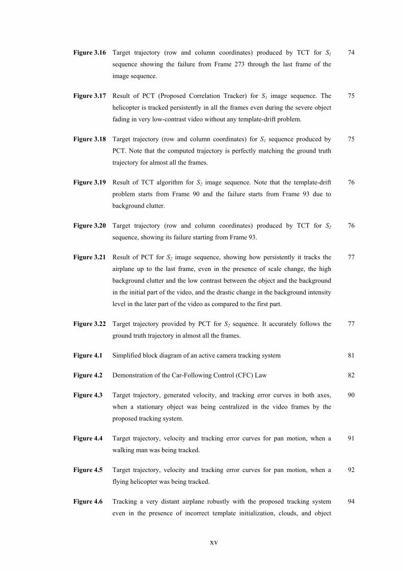
Figure 3.16 Target trajectory (row and column coordinates) produced by TCT for S1
sequence showing the failure from Frame 273 through the last frame of the
image sequence.
74
Figure 3.17 Result of PCT (Proposed Correlation Tracker) for S1 image sequence. The
helicopter is tracked persistently in all the frames even during the severe object
fading in very low-contrast video without any template-drift problem.
75
Figure 3.18 Target trajectory (row and column coordinates) for S1 sequence produced by
PCT. Note that the computed trajectory is perfectly matching the ground truth
trajectory for almost all the frames.
75
Figure 3.19 Result of TCT algorithm for S2 image sequence. Note that the template-drift
problem starts from Frame 90 and the failure starts from Frame 93 due to
background clutter.
76
Figure 3.20 Target trajectory (row and column coordinates) produced by TCT for S2
sequence, showing its failure starting from Frame 93.
76
Figure 3.21 Result of PCT for S2 image sequence, showing how persistently it tracks the
airplane up to the last frame, even in the presence of scale change, the high
background clutter and the low contrast between the object and the background
in the initial part of the video, and the drastic change in the background intensity
level in the later part of the video as compared to the first part.
77
Figure 3.22 Target trajectory provided by PCT for S2 sequence. It accurately follows the
ground truth trajectory in almost all the frames.
77
Figure 4.1 Simplified block diagram of an active camera tracking system 81
Figure 4.2 Demonstration of the Car-Following Control (CFC) Law 82
Figure 4.3 Target trajectory, generated velocity, and tracking error curves in both axes,
when a stationary object was being centralized in the video frames by the
proposed tracking system.
90
Figure 4.4 Target trajectory, velocity and tracking error curves for pan motion, when a
walking man was being tracked.
91
Figure 4.5 Target trajectory, velocity and tracking error curves for pan motion, when a
flying helicopter was being tracked.
92
Figure 4.6 Tracking a very distant airplane robustly with the proposed tracking system
even in the presence of incorrect template initialization, clouds, and object
94
xvi
fading (obscuration) in very low contrast imagery.
Figure 4.7 A helicopter is being tracked persistently and smoothly with the proposed
tracking system even when the template was incorrectly initialized by the user
and the size of the object is being reduced to about 3×3 pixels.
95
Figure 4.8 Tracking a crow persistently even in the presence of sudden variation in
appearance, speed, background, and camera zoom (from 3x to 7x).
97
Figure 4.9 Tracking a distant kite with the proposed tracking system for long duration,
even in the presence of its ever-changing direction and appearance, varying
zoom level, multiple similar objects, and occlusion (Frames 1565 to 1585).
Yellow overlaid content in Frame 1574 indicates that the tracker is working in
its occlusion handling mode.
98
Figure 4.10 Tracking a man walking in the cluttered shrubbery at the highest zoom level
(25x) of the camera used in this research, until he disappears beyond a bush.
99
Figure 4.11 Tracking a car in a highly cluttered scene and multiple occlusions. The yellow
color of the overlaid content indicates the normal tracking mode and the dark
yellow color (in Frame 250 and 341) indicates the occlusion handling mode of
the tracking system.
100
Figure 4.12 Tracking the face of a person during severe illumination variation, noise, low
detail, and occlusion. All the lights in the room were turned off in this
experiment to create a challenging scenario. The dark yellow rectangle in Frame
495 indicates that the tracker is currently working in its occlusion handling
mode.
101
Figure 4.13 Tracking a goat amidst many other goats in a highly cluttered and noisy scene at
about 7:26 p.m. in the evening. Initially, the front part of the goat is selected by
the user from top of the video. The goat is then centralized and tracked until it
disappears beyond a home.
102
Figure 5.1 The four way intersection scenario. All vehicles must come to a stop before
entering the intersection. The UGV must be aware of incoming vehicles in the
right-hand lane of each of the three roads (left, front, and right), in the regions
indicated by the shaded boxes.
105
Figure 5.2 The experimental UGV is a Subaru Outback with an autopilot system and three
cameras mounted to the roof.
106
xvii
Figure 5.3 Block diagram of our proposed system. The Vehicle Detector, Tracker, and
Finite State Machine (FSM) are run on the three on-board computers
simultaneously for each camera view. The actual OT-MACH filters used for
each view are also shown at the top.
107
Figure 5.4 Finite state machine (FSM) model for the state of traffic on a road. 110
Figure 5.5 The UGV is arriving at the intersection, but another car is already waiting on the
left road.
116
Figure 5.6 The UGV stops and turns on the computer vision system. The system detects
that the car is at the intersection and commands the UGV to wait.
116
Figure 5.7 The car at the other road begins to pass the intersection. 117
Figure 5.8 The car has exited the view of the left camera, although it is still visible in the
video from the camcorder. The computer vision system is turned off because it
will now be the UGV’s turn to cross the intersection.
117
Figure 5.9 Two seconds later, the UGV begins to pass the intersection automatically. 118

xviii
List of Tables
Table 2.1 BPNN decision, d, and its validation, G, for some sizes of the images 33
Table 3.1 Post-regression analysis for comparing accuracy of TCT and PCT 78
Table 4.1 The values of K for different zoom levels of the camera to have 0% overshoot 87
Table 4.2 Maximum steady state error of the proposed tracker at different camera zoom
levels
93
Table 5.1 Detection results in uncontrolled traffic 113
Table 5.2 Results of the actual UGV experiments under autonomous control 113
1
1 Introduction
1
Introduction
1.1 Chapter Overview
This chapter provides the introduction to visual tracking and its deployment in an
active camera tracking system and a vision system for a UGV to handle a road
intersection. It also discusses the limitations of the previous techniques, and presents
the summary of the proposed solutions.
1.2 Visual Tracking
This section provides a brief introduction to visual tracking, previous work, and the
contribution of the present research.
1.2.1 Introduction
Visual tracking, in general, can be defined as localizing the object of interest in
consecutive frames of a video. Efficient tracking of the object in complex
environments is a challenging task for the computer vision community. The complex
environments or real-world problems include noise, object fading obscuration, clutter
(including other similar objects in the scene), occlusion, uneven illumination, high
computational complexity, and varying shape, orientation, scale, and velocity of the
maneuvering object at different zoom levels of the camera. The computational
complexity of the tracker is critical for most applications. Only a small percentage of
2
the system resources can be allocated for tracking and the rest is assigned to
preprocessing stages or high-level tasks such as recognition, trajectory interpretation,
and reasoning [6].
Some widely known applications of real-time visual tracking are surveillance
and monitoring [1], perceptual user interfaces [2], smart rooms [3, 4], video
compression [5], active camera tracking system [58], and vision-based system for a
UGV (unmanned ground vehicle) to handle a road intersection [57]. The last two
systems are also part of this research work.
1.2.2 Previous Work
Several techniques have been proposed by the researchers for target tracking in the
consecutive video frames. Most of these are either limited to tracking specific class of
objects [7, 8, 9, 10], or assume that the camera is stationary (and exploit back-ground
subtraction) [41, 42]. The trackers based on the particle filter or condensation [51, 52,
53, 54] and active contours [45, 46] do not assume constant background and they are
reported to track the whole object instead of only the centroid or a portion of the
object [46]. However, keeping in mind the present power of a high-end computer,
they are computationally too expensive to be exploited for a practical real-time
tracking application. The mean shift tracker [43, 48] has gained a significant influence
in the computer vision community in recent years, because it is fast, general-purpose
and does not assume static background. Mean-shift is a nonparametric density
gradient estimator to find the image window that is most similar to the color
histogram of the object in the current frame. It iteratively carries out a kernel-based
search starting at the previous location of the object [50]. There are variants, e.g. [49],
to improve its localization by using additional modalities, but the original method
requires the object kernels in the consecutive frames to have a certain overlap. The
3
success of the mean-shift highly depends on the discriminating power of the
histograms that are considered as the probability density function of the object [50].
Another issue in the mean shift tracker is inherent in its use of histogram, which does
not carry the spatial information of the pixels [44]. The integral histogram based
tracker [47] matches the color histogram of the target with every possible region in
the whole frame; therefore, it can track even a very fast moving object. It works
slower than the mean shift tracker, because the mean shift tracker searches for the
target in only a small neighborhood of the previous target-position. On a P4 3.2 GHz
machine, the integral histogram tracker works with the speed of about 18 fps (frames
per second), and the mean shift tracker works with the speed of about 66 fps [47].
Since the histogram does not contain the spatial information, and there is a risk of
picking up a wrong candidate having similar histogram as that of the target (especially
when the search is carried out in the whole image), this tracker is not adequately
robust. More recently, in the covariance tracking [50], the object is modeled as the
covariance matrix of its features, and the region (in the search image) which has
minimum covariance distance with the model is considered to be the next target
position. The covariance matching process in [50] is carried out on a half-resolution
grid in the search image, so the accuracy of the target coordinates found by the
algorithm is reduced. The reported results are quite robust, but the computational
efficiency of the algorithm is not adequate for a real-time tracking application,
because its maximum throughput (as reported in [50]) is only 7 fps on a P4 (3.2 GHz)
PC.
There are also some widely used classic trackers, such as edge tracker,
centroid tracker, and the correlation tracker. A good introduction to these trackers can
be found in [11], where it is reported that the correlation tracker has proved to be the

4
most robust of the three, especially in a noisy and cluttered scene. However, the
standard correlation tracker has some inherent problems. Firstly, it is prone to the
template-drift problem; secondly, its performance tremendously deteriorates in the
presence of varying illumination conditions; thirdly, if the template is kept constant
throughout the tracking session, the detection performance declines especially when
the object changes its shape, size, and orientation; lastly, if the user has initialized the
template incorrectly due to the motion of the object in the streaming video, the
tracking accuracy is not adequate. Therefore, the standard correlation tracker is not
robust enough, if some preprocessing is not performed, the template is not adaptive,
and above all the modification in the basic correlation formulation is not done [11, 12,
58]. Furthermore, the correlation tracker alone does not handle the other real-world
problems mentioned in Section 1.2.1. As far as the implementation of the correlation
operation is concerned, it can be computationally expensive in the spatial domain,
especially when the sizes of the search window and the template are large. In order to
speed up the computation, the standard correlation can be implemented in the
frequency domain using the convolution theorem of the discrete Fourier transform
[11, 12, 13]. However, the modified correlation metrics, which are more robust than
the standard correlation, have no direct counterparts in the frequency domain.
Moreover, it is not necessary that the correlation in the frequency domain is always
faster than its spatial domain implementation, as discussed in Chapter 2.
1.2.3 Contribution of the Present Research
The present research proposes to enhance the efficiency and robustness of the classic
correlation tracker by addressing all of its inherent problems mentioned in the
previous subsection and the other real-world problems mentioned in Section 1.2.1.
5
The core of the visual tracking module in the proposed system is the edge
enhanced BPNN-controlled fast normalized correlation (EE-BCFNC) algorithm. The
edge-enhancement stage in the EE-BCFNC algorithm resolves the problems of noise,
object fading, obscuration, and varying illumination in the scene. The edge-
enhancement consists of Gaussian smoothing, gradient magnitude, normalization, and
thresholding operations applied on the images to be correlated. The normalized
correlation (NC) [58] makes the proposed tracker robust to the varying illumination in
the scene and produces a normalized response in the range [0.0, 1.0]. The normalized
response is exploited in the post processing stages, such as template updating and
occlusion handling. The role of the BPNN (Back-Propagation Neural Network) in the
EE-BCFNC algorithm is to predict whether the NC will be performed more efficiently
using the direct method in the spatial domain or the FFT-SAT (fast Fourier transform
and summed-area-table) method. The NC is then computed efficiently using the
implementation technique suggested by the BPNN controller. The FFT-SAT method
exploits the power of the FFT to efficiently compute the standard correlation in the
frequency domain and the SAT [18] to normalize the resulting correlation surface
very fast. The SAT is also known as the running-sum [16] or integral image [47, 58,
64, 65] in the computer vision literature. It is a very efficient technique to calculate
the sum of the elements in any rectangular section in a matrix (or image) using only
four algebraic addition operations.
Furthermore, an effective template updating scheme is proposed in order to
make the tracker adaptive to the varying appearance of the object being tracked. It
changes the template gradually with time using the history of the template and the
current best-match. This template updating scheme also limits the template drift
problem to some extent, and handles the short-lived neighboring background clutter.

6
The varying scale of the object is addressed by correlating three scales of the template
with the search window, and selecting the scale that produces the maximum
correlation value. The long-lived neighboring background clutter is handled by
applying a weight on every pixel in the template using a 2D Gaussian weighting
window with adaptive standard deviation parameters. The template drift problem is
formally dealt with by adjusting the size of the best-match rectangle and relocating its
position in the frame. The technique is accordingly named as the best-match rectangle
adjustment algorithm, which also handles the incorrect template initialization by the
user. Besides, a novel algorithm is introduced to dynamically determine the position
and size of the search window using the prediction and the prediction-error of a
Kalman filter. The search window is a small region (in the frame), where the
probability of the presence of the target is high. The benefit of searching for the target
in the small search window is that it reduces the processing burden on the system and
it eliminates the false alarms due to the background clutter in the scene. Though the
Kalman filter assumes a unimodal Gaussian noise distribution, the motivation behind
its use in the present research is that it is simple and fast and offers adequate
prediction accuracy for most of the real-world maneuvering targets (because of their
inherent inertia). However, in order to further increase the prediction accuracy, the
“constant acceleration with random walk model” instead of the most commonly used
“constant velocity with random walk model” for the target dynamics is used in this
research. It is demonstrated that the proposed visual tracking framework outperforms
the traditional correlation tracker and, in some cases, the CONDENSATION [51, 52,
53, 54] and the mean-shift [43, 48] trackers.
7
1.3 Active Camera Tracking System
This section provides a brief introduction to the active camera tracking system,
previous work, and the contribution of the present research.
1.3.1 Introduction
The active camera tracking system contains an active camera which moves
automatically to the target using the target coordinates provided by a visual tracking
algorithm. The motion of the camera is controlled by a pan-tilt unit (PTU) driven by a
control algorithm. The control algorithm is responsible for generating the control
signals for the PTU in such a way, that the target should remain precisely at the center
of the video frame. If the PTU motion is not smooth and precise, the object in the
video will oscillate to and fro around the center of the frame, and in the worst case the
object may get out of the entire field of view (FOV) of the camera.
There are many prospective applications of an active camera tracking system.
For instance, it can be deployed for precisely tracking and viewing a celestial body
(e.g. satellite, star, etc.) with an automatically moving telescope, remotely monitoring
an unattended child at home, performing surveillance of the enemy region by
mounting the tracking system on an unmanned aerial vehicle (UAV), monitoring the
movement of the objects in the strategic buildings and industries, automatically firing
at the target with precision when the target is locked at the predefined track-point in
the video frame, and so on.
Since the visual tracking algorithm has been introduced in the previous
section, the focus of the next two subsections will be on the pan-tilt control algorithm.
8
1.3.2 Previous Work
Most of the time, the algorithm used to control a plant or system is the classic
proportional-integral-derivative (PID) controller [56]. However, its design requires a
mathematical model of the plant or system. Besides, it necessitates a sensitive and
rigorous tuning of its proportional, differential and integral gain parameters. The
tuning of the three parameters is very time consuming, if they are to be optimized for
use with all the zoom levels of the camera in a tracking application. An alternative
approach is to use a fuzzy controller [10, 59, 60, 61] that does not require the system
model, but choosing a set of right membership functions and fuzzy rules calibrated for
every zoom-level of the camera is practically very cumbersome. Another alternative is
to implement a neural network controller [25, 62], but it is heavily dependent on the
quality and the variety of the examples in the training dataset, which can accurately
represent the complete behavior of the controller in all possible scenarios, including
the varying zoom-levels of the camera. Furthermore, the traditional control
algorithms, e.g. the one used in [14], are generally implemented based on the
difference between the center (i.e. reference) position and the current target position
in the image. They do not account for the target velocity. As a result, there will be
oscillations (if the object is moving slow), a lag (if it is moving with a mediocre
speed), and loss of the object from the frame (if it is moving faster than the maximum
pan-tilt velocity generated by the control algorithm). The most relevant work to the
proposed approach is the car-following control (CFC) law [15], which is very easy to
implement and offers adequate robustness and accuracy. However, the main problem
with the CFC is that it assumes that the current pan-tilt velocities of the PTU are
available. Unfortunately, the PTU used in the current research is an open-loop system,

9
i.e. it does not feedback its current pan-tilt velocities. Therefore, the CFC law can not
be used in its existing form.
1.3.3 Contribution of the Present Research
Keeping in view the limitations of the various control algorithms mentioned in the
previous subsection, a predictive open-loop car-following control (POL-CFC)
algorithm is proposed. Although its basic idea is borrowed from the car-following
control (CFC) strategy [15], it does not assume the availability of the current pan-tilt
velocities of the PTU. It simply: (1) considers that the current PTU velocity is the
previous velocity generated by itself, (2) receives the predicted target coordinates
from the visual tracking module, (3) estimates the predicted target velocity relative to
the currently estimated PTU velocity, (4) estimates the velocity to be added into the
current velocity of the PTU to generate the new velocity command, and (5) sends the
new velocity to the PTU to move the camera to follow the target accurately in real-
time.
A software application has been developed using multi-threading technique in
LabVIEW (a graphical programming language by National Instruments [86]). The
visual tracking algorithm is executed in one thread, while the pan-tilt control
algorithm and the serial communication (between the PC and the PTU, and between
the PC and the camera) are executed in another thread. This approach exploits the
parallel processing power available in an off-the-shelf PC (e.g. P4 Centrino 1.7 GHz,
512 MB RAM). The visual tracking module has been actually implemented as a DLL
(Dynamic Linked Library) using C/C++, which is invoked in one of the threads in the
main LabVIEW application program. The camera, used in this research, is Sony FCB-
EX780BP, which offers 1x to 25x optical zoom and serial interface for PC control.
Since the output of the camera is an analog video signal, Dazzle DVC-90 Digital

10
Video Creator is used to digitize the video signal into a sequence of frames. The
maximum frame rate, that the module can output, is 30 fps. The module can send
640×480 size frames, but it is configured to send 320×240 size frames in order to
reduce the computational complexity without significantly sacrificing the robustness
of the tracker. The PTU, used in this research, is Directed Perception PTU-D46
17.5W. It is a stepper motor PTU with configurable step size. The smallest step size,
that it offers, is 0.01285 degree/step. Its maximum speed at this step size is 77.1
degree/second, which is enough for tracking most of the fast moving objects.
When the object is stationary or moving with no abrupt change in its direction,
the proposed pan-tilt control algorithm centralizes the object in the video frame with
0% overshoot, 1.7 second rise time, and ±1 pixel maximum steady state error (at least
for up to 6x zoom levels of the camera). These performance parameters of a control
system are discussed in [56] and briefly defined in Section 4.3.4 for completeness.
1.4 A Vision Based System for a UGV to Handle a Road Intersection
This section provides an introduction to a machine vision system that enables a UGV
(unmanned ground vehicle) to automatically handle a road intersection [57]. The
previous work and the contribution of the present research are also discussed.
1.4.1 Introduction
Unmanned vehicles, e.g. UAVs (unmanned aerial vehicles) and UGVs (unmanned
ground vehicles), are steadily growing in demand since they save humans from
having to perform hazardous or tedious tasks and the equipment is often cheaper than
the personnel. It further reduces cost to have unmanned vehicles remotely controlled
by fewer remote operators by implementing autonomous robotics to partially assume
the burden of control. UGVs in particular have been successfully used for
11
reconnaissance, inspection and fault detection, and active tasks like removal of
dangerous explosives. These deployments have usually required the UGV to operate
in relative isolation. However, future uses of UGVs will require them to be more
aware of their surroundings. Deployment in an urban environment, for example, will
require a UGV to behave within challenging constraints in order to avoid endangering
or interfering with humans.
In order to foster the growth of research in practical autonomous UGVs, the
United States defense research agency DARPA recently organized the Urban
Challenge 2007 event, in which the participating organizations developed roadworthy
vehicles that can navigate a mock urban obstacle course under complete autonomy.
The original DARPA Grand Challenge event in 2005 required the UGVs to
autonomously cross the Mojave Desert. The Urban Challenge 2007 event was more
challenging since the UGV had to deal with a number of more difficult obstacles and
constraints, such as parking in a confined space, following traffic laws, and avoiding
interference with other vehicles on the same course.
1.4.2 Previous Work
Computer vision approaches have been successfully used in several previous UGV
applications. For example, vision has been used to make the vehicle stay in its lane
while driving on a road [88, 89], to detect unexpected obstacles in the road [90, 91,
92, 93, 94], to recognize road signs [93], and to avoid collisions with pedestrians [95].
Some research that enables multiple agents (UGVs and UAVs) to coordinate with
each other to accomplish a task has also been reported [96].
12
1.4.3 Contribution of the Present Research
In this research, a new problem is highlighted and solved. That is, a UGV must be
able to pass a street intersection regulated by a stop sign where vehicles from up to
four directions are expected to voluntarily take turns crossing the intersection
according to the order of their arrivals. In the DARPA Grand Challenge, the UGV
prepared by Team UCF (University of Central Florida) was equipped with sweeping
laser range finders to detect and avoid obstacles. However, these sensors can only
detect objects along a single line in space, so they are ill-suited to the recovery of
higher level information about the scene. Additionally, if the UGV travels on uneven
roads, the laser range finders often point off-target. Cameras are preferable in this
situation because they have a conical field-of-view (FOV). Thus, a computer vision
system is proposed to solve the problem. The system hardware consists of three on-
board computers and three cameras (mounted on top of the UGV) looking towards the
other three roads merging at the intersection. The software in each computer consists
of: (1) a vehicle detector (which detects any vehicle of any color and type on the other
road), (2) the proposed tracker (which tracks the detected vehicle), and (3) a finite
state machine model (FSM) of the traffic (which informs the status of the traffic at the
corresponding road). The information from the three FSMs is combined to make an
autonomous decision whether it is safe for the UGV to cross the intersection or not.
The results of the actual UGV experiments are provided to validate the robustness of
the proposed system.
1.5 Thesis Organization
The rest of the thesis is organized as follows. Chapter 2 reviews various correlation
techniques for object localization in an image, and proposes the edge-enhanced
BPNN-controlled fast normalized correlation (EE-BCFNC) method. The comparison

13
among all the correlation techniques with EE-BCFNC is also performed in this
chapter. The proposed robust and real-time visual tracking framework to track an
object in a video and its results are presented in Chapter 3. The proposed active
camera tracking system (specifically the pan-tilt control algorithm to move the video
camera) and its experimental results are presented in Chapter 4. The proposed
machine vision system for a UGV to handle a road intersection and its experimental
results are discussed in detail in Chapter 5. Finally, Chapter 6 concludes the thesis and
presents the future directions.
1.6 Chapter Summary
Visual tracking is an important and challenging area of computer vision. There are
many visual tracking algorithms, but they are either not robust to various real-world
problems or they require too much computation time to be used in the practical real-
time machine vision systems. In this thesis, a robust as well as real-time visual
tracking algorithm is proposed which has been practically deployed in two important
machine vision systems: an active camera tracking system and a system for a UGV to
handle a road intersection. The correlation based object localization techniques, the
visual tracking framework, and the two machine vision systems that use the visual
tracking framework are individually discussed in detail in the following chapters.
14
2 Correlation Based Object Localization
2
Correlation Based Object Localization
2.1 Chapter Overview
This chapter answers the following questions. What is an object? How is it
represented in a visual tracking paradigm? What is the correlation and what are its
types? What are the pros and cons of the traditional correlation metrics? Then, an
edge-enhanced BPNN-controlled fast normalized correlation (EE-BCFNC) algorithm
is proposed. After that, a generic algorithm for localizing an object in a single frame is
described. Finally, the EE-BCFNC technique is compared with all the other
correlation techniques.
2.2 Object and Its Representation
In a visual tracking scenario, an object can be defined as anything that is of interest
for further analysis [66]. The object that may be important to track in a specific
domain can be a boat on the sea, a fish inside an aquarium, a vehicle on a road, a
plane in the air, a person walking on a road, a bubble in the water, etc. Objects can be
represented by their shapes and/or appearances [66].
The shape based representation of the object can be a point [67], a primitive
geometric shape (e.g. rectangle, ellipse, etc.) [43], an object silhouette and contour
[46], an articulated shape model [66], or a skeletal model [68, 69].
15
The appearance based representation of the object can be a probability density
[43, 70, 71], a template [58, 72], or a multi-view model [73, 74, 75]. The probability
densities of the object appearance features (e.g. color) can be computed from the
image regions specified by the shape models (e.g. interior region of an ellipse or a
contour). A template encodes object appearance generated from one view. Thus, it is
suitable for tracking only the object, whose pose does not vary considerably during
the course of tracking [66]. One limitation of multi-view appearance model is that the
appearances of the object from all view angles are required ahead of time [66].
As far as the proposed correlation tracker is concerned, a rectangular template
is used for the object representation. A template is basically a gray-level image of the
whole (or part of the) object to be localized in the search image. An obvious
advantage of a template is that it carries both the spatial and the appearance
information [66]. The template is initialized by the user of the visual tracking system
by extracting a rectangular patch from the initial frame. In order to overcome the
limitation of the template mentioned above, it is updated according to the varying
appearance of the object with time for robust and persistent tracking as discussed in
Section 3.3.7.
2.3 Correlation Metrics
A correlation metric is used to determine the similarity of a small template of an
object of interest with a candidate region in a search window. The search window is
basically a small section (inside the video frame), where the likelihood of finding the
object is high. If the expected location of the object is not already known, the whole
frame can become the search window. Throughout the thesis, it is assumed that:
• The template and the search window are gray-level images,
16
• The template is represented by a matrix t of size K×L and the search
window by a matrix s of size M×N,
• K and L are odd integers to have a proper center of the template, and
• The template is smaller than or equal to the search window in size (i.e. K ≤
M and L ≤ N).
There are four metrics usually used in the correlation-based tracking systems:
standard correlation (SC), phase correlation (PC), normalized correlation (NC), and
normalized correlation coefficient (NCC). In the following subsections, all these
metrics are overviewed one by one with their pros and cons, and then the proposed
edge-enhanced BPNN-controlled fast normalized correlation (EE-BCFNC) is
introduced.
2.3.1 Standard Correlation (SC)
The 2D standard correlation (SC) metric in the spatial domain is given as [11, 13]:
1 1
0 0( , ) ( , ) ( , )
K L
i jc m n s m i n j t i j
− −
= == + +∑∑ (2.1)
where c(m, n) is the element of the correlation surface (i.e. matrix) at row m and
column n, where m = 0, 1, 2, …, M – K, and n = 0, 1, 2, …, N – L.
The SC metric can also be computed efficiently in the frequency domain as:
( . )c real idft S T∗⎡ ⎤= ⎣ ⎦ (2.2)
where S and T are the 2-D discrete Fourier transforms (DFTs) of s and t, respectively.
The superscript (*) over T indicates its conjugate, the dot operator (.) indicates the
element-by-element multiplication, idft(.) is the 2-D inverse discrete Fourier
transform function, and the real(.) function extracts the real part of a complex matrix.

17
The real part is extracted, because the imaginary part of the resulting complex matrix
is almost zero, since s and t are real 2-D signals. Note that s and t must be
appropriately zero padded before getting their transforms to obtain true (linear)
correlation instead of circular correlation [87], because of the repeated-signal
assumption by the discrete Fourier transform [13]. The minimum size of the zero-
padded images must be P × Q, where P = M + K - 1 and Q = N + L - 1. Once the
correlation surface, c, is obtained, the highest peak, cmax, in the surface is found. The
position of the peak in the surface is denoted by (mtl, ntl), which indicates the location
of the top-left corner of the best-match rectangle (BMR) in the search window.
The main problem with the standard correlation is that it is highly sensitive to
the illumination conditions, because it always produces cmax at the brightest spot in the
search image. Furthermore, the correlation value is dependent on the size and content
of the images, and is not normalized in the range [-1.0, 1.0]. Thus, an absolute
measure of confidence is not obtained to be exploited in the later stages of the
tracking algorithm (e.g. template updating, occlusion handling, etc).
2.3.2 Phase Correlation (PC)
Phase correlation (PC), also called symmetric phase-only matched filter (SPOMF),
has also been used for registration and tracking [12, 19, 20, 21]. It is defined as:
.S Tc real idftS T
∗⎡ ⎤⎛ ⎞⎢ ⎥= ⎜ ⎟⎜ ⎟⎢ ⎥⎝ ⎠⎣ ⎦
(2.3)
where |.| operator computes the magnitude of every complex number in its input
matrix, and all the division and multiplication operations are computed element-by-
element. In the phase correlation technique, the transform coefficients are normalized
to unit magnitude prior to computing correlation in the frequency domain. Thus, the
18
correlation is based only on the phase information and is insensitive to changes in
image intensity. It has an interesting property that it yields a sharp peak at the best-
match position and attenuates all the other elements in the correlation surface to
almost zero, but at the cost of being more sensitive to noise than SC [87]. Although
this approach has proved to be successful, it has a drawback that all transform
components are weighted equally, whereas one might expect that insignificant
components should be given less weight [16]. It is shown in [22, 23, 58] and this
thesis, that PC may produce false alarms and a very small peak (usually much less
than 0.5) even at the correct position in the correlation surface. Furthermore, the value
of the peak is highly dependent on the scene content. Therefore, it is very difficult to
set a single threshold, which is needed to compare the peak value for template
updating and other later stages of the tracking algorithm. The false-alarm rate can be
reduced to some extent by phase-correlating the edge images of the search window
and the template, rather than their gray-level images [12]. An alternative approach to
minimize the false alarms is to modulate the gray-level images by an Extended Flat-
top Gaussian (EFG) weighting function before phase-correlating them [63]. Some
other methods to improve the performance of the phase correlation can be found in
[80, 81, 82]. Nevertheless, these techniques do not eliminate the problem of
unpredictable peak value and they do not make the PC as robust to the distortion in
the appearance, shape, brightness, contrast, etc. of the object as the normalized
correlation metrics discussed in the next subsections.
2.3.3 Normalized Correlation (NC)
In order to handle the limitations of SC and PC, some researchers, e.g. [12, 58], use
the normalized correlation (NC):
19
∑∑∑∑
∑∑−
=
−
=
−
=
−
=
−
=
−
=
++
++=
1
0
1
0
21
0
1
0
2
1
0
1
0
),(),(
),(),(),(
K
i
L
j
K
i
L
j
K
i
L
j
jitjnims
jitjnimsnmc (2.4)
It may be noted that the numerator of NC is basically SC. The two
normalizing factors are the square-roots of the energies of the candidate region [with
its top-left position at (m, n) in the search image] and the template, respectively. This
correlation metric has two salient features: (1) it is less sensitive to varying
illumination conditions than SC, and (2) its values are normalized within the range
[0.0, 1.0]. Therefore, further decision making is possible for template-updating, etc.
However, its counterpart in the frequency domain does not exist, so it is
computationally more intensive than SC or PC.
2.3.4 Normalized Correlation Coefficient (NCC)
This is the most commonly used correlation metric for object localization [11, 13, 16,
17, 79]. It is more robust to varying illumination conditions than NC, and its values
are normalized within the range [-1.0, 1.0]. It is defined as:
∑∑∑∑
∑∑−
=
−
=
−
=
−
=
−
=
−
=
−−++
−−++=
1
0
1
0
21
0
1
0
2
1
0
1
0
]),([]),([
]),(][),([),(
K
i
L
jt
K
i
L
js
K
i
L
jts
jitjnims
jitjnimsnmc
μμ
μμ (2.5)
where μs and μt are the mean intensity values of the candidate region [with its top-left
coordinates at (m, n) in the search image] and the template, respectively. However,
this metric has two disadvantages. Firstly, it requires that the intensity values of s or t
must not be constant; otherwise, the correlation value will be infinity or
indeterminate. However, this problem is not so serious in real-world imagery because
of the inherent sensor noise. Secondly, its implementation in the spatial-domain is
20
computationally more intensive than even NC. However, there is an efficient method
[16] to compute it using FFT and the concept of summed-area table (SAT) [18] or
integral image [64, 65].
2.3.5 Edge Enhanced BPNN-Controlled Fast Normalized Correlation (EE-BCFNC)
It has been found out in this research that when the images to be correlated are first
edge-enhanced, the NC metric outperforms even the NCC. The proposed EE-BCFNC
is not a new correlation metric, but it is the combination of edge-enhancement (EE)
and a fast implementation of NC (i.e. BCFNC). They are explained as follows.
2.3.5.1 Edge Enhancement (EE)
The edge enhancement operation is performed on the search window and the template
before they are correlated. This technique makes the object localization algorithm
robust to noise, varying lighting conditions, obscuration and object fading even in the
low-contrast imagery. The proposed edge-enhancement process consists of four
operations: Gaussian smoothing, gradient magnitude, normalization, and thresholding.
2.3.5.1.1 Gaussian Smoothing
It is a well-known fact that the video frames captured from any camera have noise in
them – at least to some extent, especially when the ambient light around the sensor is
low. If the frames are extracted from a compressed video clip instead of camera, they
usually contain undesired artifacts (e.g. dim lines) in addition to noise. The smoothing
process attenuates the sensor noise and reduces the effects of artifacts, resulting in less
number of false edges in the subsequent operation (i.e. gradient magnitude).
The average filter could be used to attenuate the noise and artifacts in the
images, but it introduces unwanted blur resulting in the loss of the fine detail of the
object [13]. On the contrary, the Gaussian smoothing filter does the same job without
21
sacrificing the fine detail of the object [13]. Thus, a w× w Gaussian smoothing filter
with standard deviation, σw, is applied on the search window and the template. It has
been experimentally found out that w = 7 works fine in almost all scenarios. However,
setting a value for σw is critical. If the value of σw is too low, the image pixels
corresponding to the boundary coefficients of the Gaussian smoothing mask get too
small weight, and the smoothing is not satisfactory. On the other hand, if the value of
σw is too large, the image pixels corresponding to the boundary coefficients of the
filter get too much weight, and the resulting image is too much smoothed (or blurred)
to be acceptable. An effective formula [29] given below is exploited in this research
for automatically calculating an optimum value of σw:
8.012
3.0 +⎟⎠⎞
⎜⎝⎛ −= w
wσ (2.6)
As a result, the effective coefficients for the Gaussian smoothing filter according to
the size of the filter are obtained. Another desirable property of the resulting filter is
that the sum of all the filter coefficients, which basically act as the weights of the
image pixels under consideration, equals 1.
2.3.5.1.2 Gradient Magnitude
The edge-enhanced gray-level images instead of the actual gray-level images are used
in this research in the correlation process, because edge-enhanced images are less
sensitive to lighting conditions and they produce a cleaner correlation surface with
less number of false peaks. In this regard, the standard horizontal and vertical Sobel
masks [13, 30] are applied on the Gaussian smoothed image, and the two resulting
images, Eh and Ev, are obtained Then, the gradient magnitude image, E, can be
obtained as follows:
22
2 2( , ) ( , ) ( , )h vE i j E i j E i j= + (2.7)
where i = 0, 1, 2, …, U - 1, j = 0, 1, 2, …, V - 1, where (U, V) = (K, L) for the
template, and (U, V) = (M, N) for the search-window. Since Eq. (2.7) is computation
intensive, its efficient approximation (given below) is actually used in this research,
which produces almost identical result [13, 30].
( , ) ( , ) ( , )h vE i j E i j E i j= + (2.8)
2.3.5.1.3 Normalization
It has been found out in this research that the dynamic range of the edge image, E, is
often too narrow towards darker side as compared to the available pixel-value range
[0, 255], especially in low-contrast imagery. Conventionally, the edge image is
converted into a binary image using a predefined threshold; however, this approach
does not work well in a template matching application, because the rich content of the
gray-level edge-features of the object is lost in the process of binarization. In order to
make the object localization algorithm robust to object fading and obscuration, which
occur when the object is very far and the zoom level of the camera is set to a high
value, the edges are enhanced using a normalization procedure given by:
[ ]minmax min
255( , ) ( , )nE i j E i j EE E
⎡ ⎤= −⎢ ⎥−⎣ ⎦
(2.9)
where En is the normalized edge image, 255 is the maximum value a pixel can have,
and Emin and Emax are the minimum and maximum values in the un-normalized edge
image, E, respectively. The normalization stage effectively tries to stretch the
histogram of the image in the whole range [0, 255], so the contrast between the object
and the background is enhanced.
23
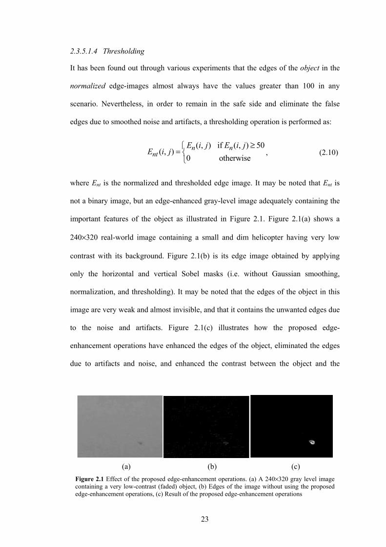
2.3.5.1.4 Thresholding
It has been found out through various experiments that the edges of the object in the
normalized edge-images almost always have the values greater than 100 in any
scenario. Nevertheless, in order to remain in the safe side and eliminate the false
edges due to smoothed noise and artifacts, a thresholding operation is performed as:
( , ) if ( , ) 50
( , )0 otherwise
n nnt
E i j E i jE i j
≥⎧= ⎨⎩
, (2.10)
where Ent is the normalized and thresholded edge image. It may be noted that Ent is
not a binary image, but an edge-enhanced gray-level image adequately containing the
important features of the object as illustrated in Figure 2.1. Figure 2.1(a) shows a
240×320 real-world image containing a small and dim helicopter having very low
contrast with its background. Figure 2.1(b) is its edge image obtained by applying
only the horizontal and vertical Sobel masks (i.e. without Gaussian smoothing,
normalization, and thresholding). It may be noted that the edges of the object in this
image are very weak and almost invisible, and that it contains the unwanted edges due
to the noise and artifacts. Figure 2.1(c) illustrates how the proposed edge-
enhancement operations have enhanced the edges of the object, eliminated the edges
due to artifacts and noise, and enhanced the contrast between the object and the
(a) (b) (c) Figure 2.1 Effect of the proposed edge-enhancement operations. (a) A 240×320 gray level image containing a very low-contrast (faded) object, (b) Edges of the image without using the proposed edge-enhancement operations, (c) Result of the proposed edge-enhancement operations
24
background.
2.3.5.2 BPNN-Controlled Fast Normalized Correlation (BCFNC)
Though NCC is the best correlation metric for the actual gray-level images, NC
outperforms it for the edge-enhanced images according to the experiments performed
during this research. Furthermore, computing the mean value for every candidate
region of the search image is time-consuming in the NCC. Therefore, NC as defined
in Eq. (2.4) is used in this research as the correlation metric for the edge-enhanced
images, but with an efficient implementation. The technique is appropriately named
as BPNN-Controlled Fast Normalized Correlation (BCFNC). It may be noted that the
correlation surface yielded by BCFNC is the same as that by NC. The role of the
BPNN is to predict whether the NC will be performed efficiently by the direct method
described by Eq. (2.4) or by the FFT-SAT (fast Fourier transform – summed area
table) method described in the next sub-section.
2.3.5.2.1 Efficient Implementation of NC Using FFT-SAT Method
This implementation of normalized correlation exploits the combined efficiency of
FFT (Fast Fourier Transform) and SAT (Summed-Area-Table) [18]. Summed-area-
table is also known as the running sum or the integral image in the computer vision
literature [47, 58, 64, 65]. The same method has been exploited in [16], but for
implementing the normalized correlation coefficient described by Eq. (2.5). The idea
is that the numerator of Eq. (2.4) is computed in the frequency domain using Eq.
(2.2), and the second normalizing factor (i.e. the square-root of the energy of the
template) in the denominator of Eq. (2.4) is pre-calculated only once for each video
frame. Since the first normalizing factor in the denominator of Eq. (2.4) varies with
(m, n), it has to be calculated for every candidate region in the search image. For
25
efficient computation of all the local energies of the search window, the concept of
summed area table (SAT) [18] is exploited.
The SAT of the M×N search window, s, is a matrix, I, of the size (M + 1) × (N
+ 1). The elements in its 0th row and 0th column are set to 0. All the other elements are
efficiently calculated in a recursive manner as:
( , ) ( 1, 1) ( , 1) ( 1, ) ( 1, 1)I i j s i j I i j I i j I i j= − − + − + − − − − , (2.11)
where i = 1, 2, …, M, and j = 1, 2, …, N. Once the SAT is computed, the sum of all
the elements in any rectangular section in the search-window can be easily calculated
by algebraically adding only the four corner elements of the corresponding
rectangular section in its SAT. Specifically, in order to calculate the sum of elements
contained in a K × L rectangular section (in the search window) with top-left element
s(i, j), top-right element s(i, j+L-1), bottom-right element s(i+K-1, j+L-1), and bottom-
left element s(i+K-1, j), then sum of all the pixels in the rectangular section is
computed using the SAT of the search window very efficiently as:
( , ) ( , ) ( , ) ( , )sum I i K j L I i j I i K j I i j K= + + + − + − + (2.12)
Thus, the local energies of the search window can be determined by first
obtaining the SAT of the square of the search window, and then computing the local
sums of the squared search image using its SAT. The size of the resulting matrix
containing the local energies is exactly same as that of the normalized correlation
surface, c, in Eq. (2.4). If the square-roots of the elements in this matrix are multiplied
with the pre-calculated “second factor in the denominator of Eq. (2.4)”, a normalizing
matrix is obtained. Finally, if the numerator of Eq. (2.4), which was computed using
FFT, is divided by this normalizing matrix element-by-element, the normalized
correlation surface, c, is determined.
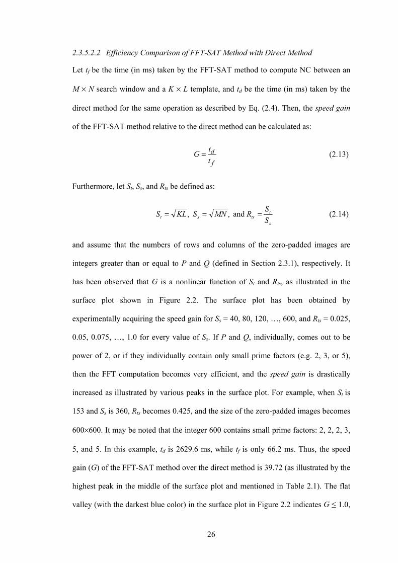
26
2.3.5.2.2 Efficiency Comparison of FFT-SAT Method with Direct Method
Let tf be the time (in ms) taken by the FFT-SAT method to compute NC between an
M × N search window and a K × L template, and td be the time (in ms) taken by the
direct method for the same operation as described by Eq. (2.4). Then, the speed gain
of the FFT-SAT method relative to the direct method can be calculated as:
d
f
tGt
= (2.13)
Furthermore, let St, Ss, and Rts be defined as:
s
ttsst S
SRMNSKLS === and , , (2.14)
and assume that the numbers of rows and columns of the zero-padded images are
integers greater than or equal to P and Q (defined in Section 2.3.1), respectively. It
has been observed that G is a nonlinear function of St and Rts, as illustrated in the
surface plot shown in Figure 2.2. The surface plot has been obtained by
experimentally acquiring the speed gain for Ss = 40, 80, 120, …, 600, and Rts = 0.025,
0.05, 0.075, …, 1.0 for every value of Ss. If P and Q, individually, comes out to be
power of 2, or if they individually contain only small prime factors (e.g. 2, 3, or 5),
then the FFT computation becomes very efficient, and the speed gain is drastically
increased as illustrated by various peaks in the surface plot. For example, when St is
153 and Ss is 360, Rts becomes 0.425, and the size of the zero-padded images becomes
600×600. It may be noted that the integer 600 contains small prime factors: 2, 2, 2, 3,
5, and 5. In this example, td is 2629.6 ms, while tf is only 66.2 ms. Thus, the speed
gain (G) of the FFT-SAT method over the direct method is 39.72 (as illustrated by the
highest peak in the middle of the surface plot and mentioned in Table 2.1). The flat
valley (with the darkest blue color) in the surface plot in Figure 2.2 indicates G ≤ 1.0,
27
while all the higher regions in the surface plot indicate G > 1. It shows that the FFT-
SAT method can be sometimes slower than the direct method for computing NC.
(This finding is contrary to the common notion that the FFT based correlation is
always faster than the spatial domain correlation as the sizes of the images are
increased). The reason behind this phenomenon is explained as follows.
In this research, the valid correlation of size ( 1) ( 1)M K N L− + × − + is
performed as mentioned in Eq. (2.1), instead of the full correlation of size
( 1) ( 1)M K N L+ − × + − , because the object is expected to be inside the search image
(and not outside it). If the correlation is performed in the frequency domain, the
search image and the template has to be zero-padded to the size at least
( 1) ( 1)M K N L+ − × + − before computing their FFTs, regardless of full or valid
correlation. If the zero-padding of the images is not performed, the undesired wrap-
around effect will be obtained in the correlation result. Therefore, when template size
is too large, the FFT computation of the two large zero-padded matrices becomes time
consuming. On the contrary, the correlation performed in the spatial domain works
directly on the original (i.e. M N× and K L× ) images and it has to find the matching
score only at ( 1) ( 1)M K N L− + × − + positions. Thus, the spatial domain NC
becomes faster than the FFT-SAT based NC, when the ratio of the template size to the
search window size is large (near 1.0).
In order to get the best from the two approaches, the proposed method does
not use a single approach for all cases, but switches between the two implementations
according to the decision of a Back-propagation Neural Network (BPNN) controller.
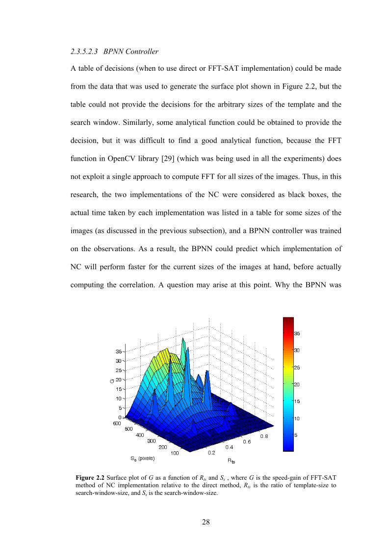
28
2.3.5.2.3 BPNN Controller
A table of decisions (when to use direct or FFT-SAT implementation) could be made
from the data that was used to generate the surface plot shown in Figure 2.2, but the
table could not provide the decisions for the arbitrary sizes of the template and the
search window. Similarly, some analytical function could be obtained to provide the
decision, but it was difficult to find a good analytical function, because the FFT
function in OpenCV library [29] (which was being used in all the experiments) does
not exploit a single approach to compute FFT for all sizes of the images. Thus, in this
research, the two implementations of the NC were considered as black boxes, the
actual time taken by each implementation was listed in a table for some sizes of the
images (as discussed in the previous subsection), and a BPNN controller was trained
on the observations. As a result, the BPNN could predict which implementation of
NC will perform faster for the current sizes of the images at hand, before actually
computing the correlation. A question may arise at this point. Why the BPNN was
Figure 2.2 Surface plot of G as a function of Rts and Ss , where G is the speed-gain of FFT-SAT method of NC implementation relative to the direct method, Rts is the ratio of template-size to search-window-size, and Ss is the search-window-size.
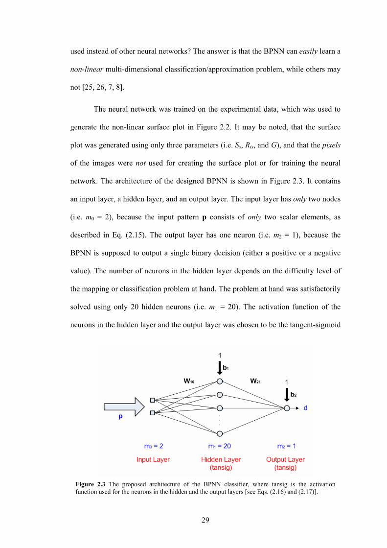
29
used instead of other neural networks? The answer is that the BPNN can easily learn a
non-linear multi-dimensional classification/approximation problem, while others may
not [25, 26, 7, 8].
The neural network was trained on the experimental data, which was used to
generate the non-linear surface plot in Figure 2.2. It may be noted, that the surface
plot was generated using only three parameters (i.e. Ss, Rts, and G), and that the pixels
of the images were not used for creating the surface plot or for training the neural
network. The architecture of the designed BPNN is shown in Figure 2.3. It contains
an input layer, a hidden layer, and an output layer. The input layer has only two nodes
(i.e. m0 = 2), because the input pattern p consists of only two scalar elements, as
described in Eq. (2.15). The output layer has one neuron (i.e. m2 = 1), because the
BPNN is supposed to output a single binary decision (either a positive or a negative
value). The number of neurons in the hidden layer depends on the difficulty level of
the mapping or classification problem at hand. The problem at hand was satisfactorily
solved using only 20 hidden neurons (i.e. m1 = 20). The activation function of the
neurons in the hidden layer and the output layer was chosen to be the tangent-sigmoid
Figure 2.3 The proposed architecture of the BPNN classifier, where tansig is the activation function used for the neurons in the hidden and the output layers [see Eqs. (2.16) and (2.17)].
30
function. This activation function was used, because it is non-linear and it supports
negative as well as positive values [24, 25, 26]. The non-linearilty requirement is
necessary to solve a non-linear classification problem. The support of positive and
negative values in the activation function speeds up the learning process of the neural
network [26]. The training of the BPNN was carried out using the efficient scaled-
conjugate gradient learning algorithm [27]. This algorithm is far more efficient for
training a BPNN than any of the conventional learning algorithms, e.g. gradient
descent method [24]. The proposed neural network architecture accepts a pattern (p)
as its input, defined as:
,600
Ts
tsS R⎡ ⎤= ⎢ ⎥⎣ ⎦
p (2.15)
where the Ss is normalized by 600, which is the maximum value of Ss in the
experimental data. The normalization is necessary, since the input layer of the neural
network assumes that the values in the input pattern are in the range [0.0, 1.0]. Thus,
the maximum size of the search window, that the designed BPNN can support is
600×600 pixels. This constraint is not of much significance, because the video frame
is of size 320×240 pixels only, and the search window is normally much smaller than
even the frame. Since the training was performed in a supervised manner, the ideal
output for each example was provided in the training dataset. The ideal output was a
scalar value: either +0.8 or -0.8. The scalar values ±1 could be used instead of ±0.8,
respectively, but that approach would have caused slow learning [26], because the
tansig(.) activation function is saturated at ±1, as shown in Figure 2.4.
Once the training is completed, the neural network is ready to be a fast
decision maker. The decision output, d, of the trained BPNN is easily determined as:

31
( )21 10 1 2tansig .tansig .d ⎡ ⎤= + +⎣ ⎦W W p b b (2.16)
where W10, b1, W21, and b2 are the m1×m0, m1×1, m2× m1, and m2×1 matrices,
respectively. Each row of W10 contains the learnt synaptic weights of its
corresponding neuron in the hidden layer. The elements of the row vector W21 are the
synaptic weights of the output neuron. The column vector b1 contains the bias weights
of the neurons in the hidden layer, and b2 is the bias weight of the output neuron. All
these synaptic weights are adapted and optimized according to the training dataset
during the learning phase of the neural network. The tansig(.) function, as defined in
Eq. (2.17) and illustrated in Figure 2.4, is basically a fast approximation of the well-
known tanh(.) function [28].
1-1
2)(tansig 2n-en
+= (2.17)
The output of the BPNN (i.e. d) will be either a positive or a negative value. If
d > 0, the FFT-SAT method of computing NC will be faster than its direct method;
and vice versa, if d < 0. The response of the BPNN has been tested with all the
patterns from its training dataset, and the resulting surface plot is shown in Figure 2.5.
tansig(n)
n
Figure 2.4 Tangent sigmoid activation function
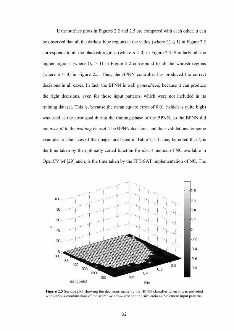
32
If the surface plots in Figures 2.2 and 2.5 are compared with each other, it can
be observed that all the darkest blue regions at the valley (where Gp ≤ 1) in Figure 2.2
corresponds to all the blackish regions (where d < 0) in Figure 2.5. Similarly, all the
higher regions (where Gp > 1) in Figure 2.2 correspond to all the whitish regions
(where d > 0) in Figure 2.5. Thus, the BPNN controller has produced the correct
decisions in all cases. In fact, the BPNN is well generalized, because it can produce
the right decisions, even for those input patterns, which were not included in its
training dataset. This is, because the mean square error of 0.01 (which is quite high)
was used as the error goal during the training phase of the BPNN, so the BPNN did
not over-fit to the training dataset. The BPNN decisions and their validations for some
examples of the sizes of the images are listed in Table 2.1. It may be noted that td is
the time taken by the optimally coded function for direct method of NC available in
OpenCV b4 [29] and tf is the time taken by the FFT-SAT implementation of NC. The
Figure 2.5 Surface plot showing the decisions made by the BPNN classifier when it was provided with various combinations of the search-window-size and the size-ratio as 2-element input patterns.
33
value of Gp is machine independent, because it is a ratio of the two elapsed times and
both of the implementations are executed on the same machine. The downward arrow
(↓) and the upward arrow (↑) indicate d < 0 and d > 0, respectively. The testing was
carried out on a PC having P4 Centrino 1.7 GHz processor and 512 MB RAM. The
value of Gp, for every case listed in Table 2.1, validates the corresponding decision
(d) of the BPNN. At first sight, it may seem that the direct spatial-domain
implementation is applied rarely. However, it is the one, which is applied frequently,
especially when the template size is small in case of distant object tracking, or when
the template size is very large in case of nearby smoothly moving object.
2.4 Generic Correlation Based Object Localization Algorithm
No matter which correlation technique is used, the basic algorithm for localizing an
object (or target) in a frame is the same in every case. It is described in the following
simple steps.
Step 1 Prepare the search window (i.e. s) and the template of the target (i.e. t).
Step 2 Compute the correlation surface, c, using SC, PC, NC, NCC, or the proposed
Table 2.1 BPNN decision, d, and its validation, G, for some sizes of the images
M×N K×L Rts d td (ms) Tf (ms) G 50×50 30×30 0.6000 ↓ 0.8 3.2 0.25 75×75 25×25 0.33 ↓ 4 8.81 0.45
320×240 10×10 0.036 ↓ 28.68 82.28 0.35 320×240 51×51 0.18 ↑ 260 80 3.25 320×240 75×75 0.27 ↑ 450 90 5 320×240 100×100 0.3610 ↑ 601.8 100.4 5.99 320×240 125×125 0.44 ↑ 681 100 6.81 320×240 300×200 0.884 ↓ 135.2 282.4 0.48 360×360 153×153 0.4250 ↑ 2629.6 66.2 39.72 512×512 60×30 0.0820 ↑ 776.34 317 2.45 512×512 205×205 0.4 ↑ 7631 390 19.56 640×480 400×300 0.6245 ↑ 10111 701 14.42
34
EE-BCFNC.
Step 3 Locate the peak value cmax in the correlation surface, and denote its position by
(mtl, ntl), where mtl and ntl are the row and the column coordinates of the top-
left position of the best-match rectangle (BMR) in the search-window,
respectively.
Step 4 Locate the center of the BMR using:
1 1( , ) ,
2 2c c tl tlK Lm n m n− −⎛ ⎞= + +⎜ ⎟
⎝ ⎠ (2.18)
Step 5 Let the position of the top-left pixel of the search window in the frame be (xs,
ys), where xs and ys are the column (i.e. horizontal) and row (i.e vertical)
coordinates relative to the frame origin (0, 0), respectively. Then, locate the
center of the BMR with respect to the frame origin, as:
( )( , ) , s c s cx y x n y m= + + , (2.19)
where (x, y) is the center of the target in the current frame, assuming that the
target is at the center of the BMR. If the object is to be searched for in the
whole frame instead of a small search window, then (xs, ys) = (0, 0) and (x, y)
= (nc, mc).
2.5 Comparison among Different Correlation Techniques
In this section, the performance of different correlation-based template matching
techniques (discussed in this chapter) is compared. A challenging search image as
shown in Figure 2.1(a) is selected as test image, because it contains a very distant and
dim object (a helicopter) in a hazy scene. The objective is to determine the location of
the object in the search image. A 21×23 template of the object is shown in Figure
35
2.6(a). The correct top-left position of the object in the search image is at (mtl, ntl) =
(169, 224). The correlation technique, which produces a clean peak exactly at this
location in the resulting correlation surface, will be considered the best one.
Figure 2.7(a) illustrates the correlation surface obtained, when the original
template was correlated with the original search image using SC given by Eq. (2.1) or
Eq. (2.2). This method failed to locate the correct position of the object, because it
produced the highest peak of 8,871,601 value at (10, 11) instead of (169, 224).
Additionally, it has produced many other (false) peaks at all those spots, which were
brighter than the object in the search window. In fact, the correlation value is lower
(i.e. 8,226,021) at (169, 224) position, where the object actually lies, since the object
is darker than the background. Moreover, the correlation values are not normalized in
the range [0.0, 1.0] or [-1.0, 1.0].
Figure 2.7(b) shows the correlation surface obtained, when the original
template was correlated with the original search image, using PC described in Eq.
(2.3). The method failed to locate the correct location of the object, because it
produced the highest peak at (10, 11) instead of (169, 224). It may be noted, that the
highest peak value is only 0.14, and there are also some other lower peaks (including
the true peak illustrating the location of the target).
(a) (b)
Figure 2.6 The 21×23 templates (shown enlarged for easy view). (a) Original, (b) Edge-enhanced.
36
Figure 2.7(c) illustrates the correlation surface, which is the result of matching
the original template with the original search image using NC given by (2.4). The
object is located correctly at (169, 224), and the highest peak has value of 1.0.
However, if the surface is observed closely, it can be found that the minimum
correlation value in the whole surface is also too high, i.e. 0.9945. This behavior of
(a) (b)
(c) (d)
(e) (f)
Figure 2.7 Results of various correlation-based object localization methods. (a) SC surface, (b) PC surface, (c) NC surface, (d) NCC surface, (e) Proposed EE-BCFNC surface, and (f) Overlay of the + signs on the target coordinates (correctly found by NC, NCC and EE-BCFNC methods) on the search-window, where the black sign represents the top-left coordinates (mtl, ntl) of the best-match and the white sign represents its center-coordinates (mc, nc).
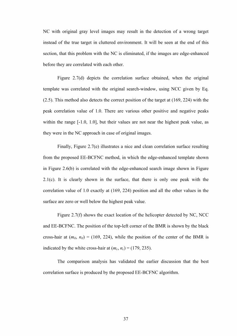
37
NC with original gray level images may result in the detection of a wrong target
instead of the true target in cluttered environment. It will be seen at the end of this
section, that this problem with the NC is eliminated, if the images are edge-enhanced
before they are correlated with each other.
Figure 2.7(d) depicts the correlation surface obtained, when the original
template was correlated with the original search-window, using NCC given by Eq.
(2.5). This method also detects the correct position of the target at (169, 224) with the
peak correlation value of 1.0. There are various other positive and negative peaks
within the range [-1.0, 1.0], but their values are not near the highest peak value, as
they were in the NC approach in case of original images.
Finally, Figure 2.7(e) illustrates a nice and clean correlation surface resulting
from the proposed EE-BCFNC method, in which the edge-enhanced template shown
in Figure 2.6(b) is correlated with the edge-enhanced search image shown in Figure
2.1(c). It is clearly shown in the surface, that there is only one peak with the
correlation value of 1.0 exactly at (169, 224) position and all the other values in the
surface are zero or well below the highest peak value.
Figure 2.7(f) shows the exact location of the helicopter detected by NC, NCC
and EE-BCFNC. The position of the top-left corner of the BMR is shown by the black
cross-hair at (mtl, ntl) = (169, 224), while the position of the center of the BMR is
indicated by the white cross-hair at (mc, nc) = (179, 235).
The comparison analysis has validated the earlier discussion that the best
correlation surface is produced by the proposed EE-BCFNC algorithm.
38
2.6 Chapter Summary
An object can be represented by its shape (e.g. ellipse) or appearance (e.g. template).
Correlation based object localization technique looks for a region in the search image,
which matches best with the template of the object. The template matching process
can be performed using any of various correlation metrics, such as standard
correlation (SC), phase correlation (PC), normalized correlation (NC), and normalized
correlation coefficient (NCC). Every metric has its own pros and cons. In order to
address the limitations of these metrics, an edge-enhanced BPNN-controlled fast
normalized correlation (EE-BCFNC) technique is proposed. The algorithm for
localizing an object in a single frame is quite generic, regardless of the choice of the
correlation technique used for the matching process. The results of the comparison
among these correlation techniques validate that the proposed EE-BCFNC technique
outperforms all the other methods by efficiently producing a clean normalized
correlation surface with a dominant peak at the object location. The next chapter
discusses the proposed visual tracking framework, which can track an object of
interest in the consecutive frames of a video, and handles the real-world problems,
such as incorrect template initialization, template-drift, occlusion, varying shape of
the object, etc.

39
3 Visual Tracking Framework
3
Visual Tracking Framework
3.1 Chapter Overview
This chapter discusses the proposed visual tracking framework and tests it on various
videos obtained from the public datasets, such as CAVIAR, PETS, and AV16.3.
Additionally, for some other public test videos, the results of the proposed tracker are
compared with those of the CONDENSATION [52, 53, 54] and the mean-shift [43,
48] trackers reported in [51]. The proposed correlation tracker is also compared with
the traditional correlation tracker at the end of the chapter.
3.2 Challenges for a Visual Tracking Algorithm
Visual tracking can be simply defined as the problem of estimating the trajectory of
an object of interest as it moves around the scene in a video [66]. It is a very complex
problem for the computer vision community, because of the:
• Loss of information due to the projection of the 3D world on a 2D image,
• Noise in images due to sensor noise and low illumination conditions,
• Background clutter due to other similar or different objects in the scene,
• Complex object motion (slow, fast, linear, and nonlinear),
• Object fading due to high-zoom operation of the moving camera in cloudy
environment,
40
• Obscuration of the object due to smoke, dust, or fog,
• Intermittent occlusions due to other objects hiding the target,
• Complex object shape variations during its maneuvering,
• Change in the object scale due to its varying distance from the camera or
varying zoom level of the camera,
• Uneven scene illumination, and
• Real time processing requirements.
Additionally, there is a severe problem of template-drift, if the tracking is
performed using a basic correlation method. Due to this problem, the object tends to
drift away from the template with time. Ultimately, it gets out of the template and the
tracking becomes a complete failure.
The basic object localization algorithm, given in Section 2.4, is for localizing
an object in only a single frame when a good template of the object is already present.
It can not solve the practical problems listed above. Therefore, an efficient visual
tracking algorithm is proposed to explicitly address all of these problems.
3.3 Proposed Visual Tracking Framework
A simplified flowchart of the proposed visual tracking algorithm is shown in Figure
3.1. The individual blocks of the flowchart are discussed in the following sub-
sections.
3.3.1 Video Frame Acquisition
If the tracking is performed off-line on an image sequence or the video frames coming
from a digital video camera, the individual frames can be acquired easily in the
software. However, if the tracking is performed on the video coming from a live
analog camera, the digital frames can be acquired using a digitizer module, such as
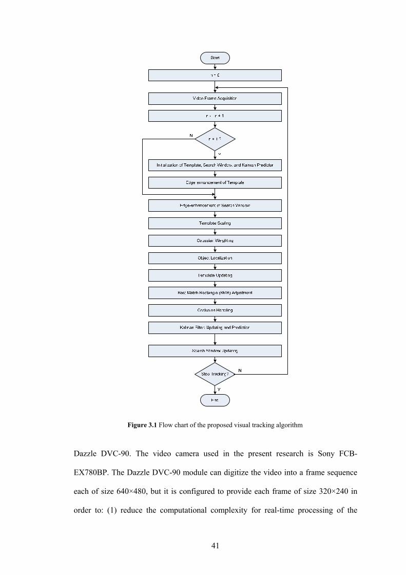
41
Dazzle DVC-90. The video camera used in the present research is Sony FCB-
EX780BP. The Dazzle DVC-90 module can digitize the video into a frame sequence
each of size 640×480, but it is configured to provide each frame of size 320×240 in
order to: (1) reduce the computational complexity for real-time processing of the
Figure 3.1 Flow chart of the proposed visual tracking algorithm
42
frame without significantly sacrificing the robustness of the tracker, and (2) efficiently
encode the processed frame for video recording purpose. The DVC-90 module can
digitize the analog video with a maximum frame rate of 30 fps, which is quite
adequate for tracking a physical object moving with significant velocity and
maneuvering. Each frame is an RGB color image, but it is converted into gray-level
image in order to further reduce the computational burden on the system.
3.3.2 Initialization of Template, Kalman Filter, and Search Window
At the start of the tracking session, the template, the Kalman filter, and the search
window are initialized as described in the following sub-subsections.
3.3.2.1 Template Initialization
The template is initialized by the user of the tracking system by selecting any object
of interest (or its salient part) appearing in the video. In order to have a long and good
tracking session, the traditional trackers require that:
• The object should be well centered in the extracted template, if full object
is selected, or
• The template should be extracted from the middle region of the object, if a
part of the object is to be tracked.
However, it is usually difficult for the user to extract a good template during the
motion of the maneuvering object in the streaming video coming directly from a
camera. In order to eliminate the above-mentioned requirements, a best match
rectangle (BMR) adjustment algorithm is proposed in Section 3.3.8.
43
3.3.2.2 Kalman Filter Initialization
The center of the region, from where the template is extracted, is used to initialize the
target coordinates in the frame, (x, y), where x represents the column index and y the
row index of the matrix representing the frame. The measurement vector (defined in
Section 3.3.10) of the Kalman filter is initialized with these target coordinates instead
of (0, 0). This strategy is exploited to reduce the initial error of the Kalman filter and
expedite the convergence of the filter to the trajectory of the target. Further detail of
the filter, including its benefits in the proposed tracker, is given in Section 3.2.10.
3.3.2.3 Search Window Initialization
The center of the initial search window is considered to be at the initial target
coordinates, and the size of the window is initialized to be three times that of the
initial template to accommodate the unknown velocity of the target at the start of the
tracking session. After the convergence of the Kalman filter, the search window will
be appropriately updated using Kalman prediction and its error, as discussed in
Section 3.3.11.
3.3.3 Edge-enhancement of Template and Search Window
The edge enhancement operation is proposed to be performed on the search window
and the template before correlating them. This technique makes the object localization
algorithm robust to noise, varying lighting conditions and object fading even in the
low-contrast imagery. The detail of this operation is given in Section 2.3.5.1.
3.3.4 Template Scaling
The moving object can get larger (or smaller) with time in the video frames, when the
object comes nearer to (or goes farther from) the camera, or when the zoom level of
the camera is increased (or decreased). If the template size is kept constant throughout
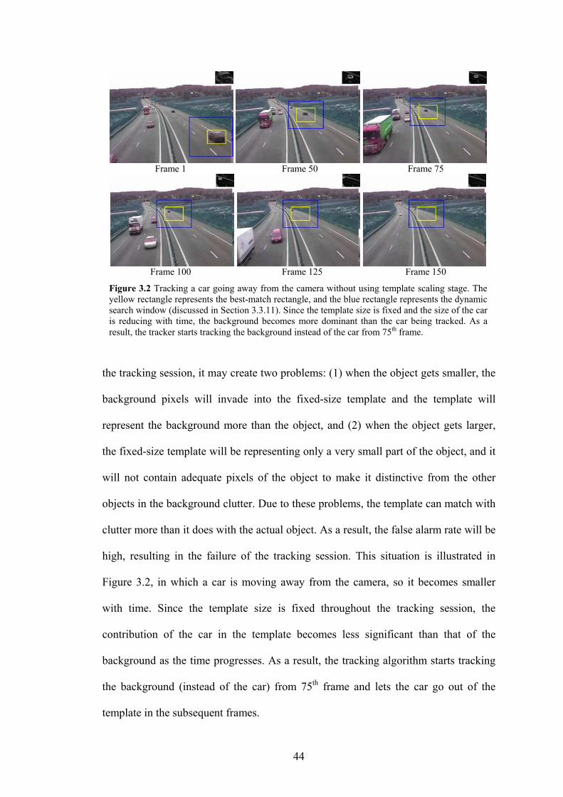
44
the tracking session, it may create two problems: (1) when the object gets smaller, the
background pixels will invade into the fixed-size template and the template will
represent the background more than the object, and (2) when the object gets larger,
the fixed-size template will be representing only a very small part of the object, and it
will not contain adequate pixels of the object to make it distinctive from the other
objects in the background clutter. Due to these problems, the template can match with
clutter more than it does with the actual object. As a result, the false alarm rate will be
high, resulting in the failure of the tracking session. This situation is illustrated in
Figure 3.2, in which a car is moving away from the camera, so it becomes smaller
with time. Since the template size is fixed throughout the tracking session, the
contribution of the car in the template becomes less significant than that of the
background as the time progresses. As a result, the tracking algorithm starts tracking
the background (instead of the car) from 75th frame and lets the car go out of the
template in the subsequent frames.
Frame 1 Frame 50 Frame 75
Frame 100 Frame 125 Frame 150
Figure 3.2 Tracking a car going away from the camera without using template scaling stage. The yellow rectangle represents the best-match rectangle, and the blue rectangle represents the dynamic search window (discussed in Section 3.3.11). Since the template size is fixed and the size of the car is reducing with time, the background becomes more dominant than the car being tracked. As a result, the tracker starts tracking the background instead of the car from 75th frame.

45
In order to handle the varying scale of the object, a fact about the highest peak
in the correlation response is exploited. That is, the correlation peak is high if the
scale of the object in the template is same as that of the object in the search window;
otherwise, the peak is low. Thus, the search window is correlated with three scales of
the template: 110%, 100%, and 90%. The 100% scale of the template is the original
one, which comes from the previous iteration. As a result, three correlation surfaces
with the corresponding three peaks are obtained. The best-match rectangle (BMR)
corresponding to only that template scale, which produces the highest of the three
peaks, is accepted. Thus, the template scale for the next iteration is updated according
to the current scale of the object and the tracking becomes persistent. It may be noted
that the minimum and the maximum size limits on the template are applied in order to
have robust tracking and decrease the computational complexity, respectively, as
discussed in Section 3.3.8. Figure 3.3 shows how the varying scale of the car in the
same video shown in Figure 3.2 is handled appropriately to have a persistent tracking
Frame 1 Frame 50 Frame 75
Frame 100 Frame 200 Frame 300
Figure 3.3 Illustration of the scale-handling capability of the proposed visual tracking algorithm. A car is being tracked successfully, even when the scale of the car is being reduced due to its ever-increasing distance from the camera. It can be seen that if the template is reduced in size with time, the dynamic search window is also reduced. Thus, three benefits are obtained: scale handling, more background clutter rejection and less processing burden on the system.
46
session. It may be noted that this scale handling technique can work with any
correlation metric or/and actual gray-level images.
3.3.5 Gaussian Weighting of Template Pixels
The background clutter, which is far from the object in the scene, is handled by
looking for the object only inside a small search window (see Section 3.3.11) instead
of the whole frame. However, the search window does not handle the neighboring
clutter, which may be present immediately around the object inside the template.
There are two kinds of neighboring clutter: short-term and long-term. In order
to clarify the difference between them, suppose there is a big picture hanging on a
wall in the video and there is a person (whose head is the target of interest) appearing
from the right side of the video and walking towards left. If the person passes the
picture without standing in front of it, the content of the picture appearing around the
head of the person will behave as a short-term neighboring clutter, because the
content can be part of the template only for a very short duration. However, if the
person stands in front of the picture for a long duration, the content of the picture
appearing around the head of the person will behave as a long-term neighboring
clutter, because the content will be part of the template for a long duration.
The effect of the short-term neighboring clutter is efficiently diminished by
temporally smoothing the template (discussed in Section 3.3.7), but the long-term
clutter is not handled by the filter. Therefore, the effect of the long-term neighboring
clutter is decreased by assuming that the object is at the center of the template (due to
the best-match rectangle adjustment algorithm discussed in Section 3.3.8) and
applying a weight on every pixel in the template. The farther the pixel from the center
of the template, the lower the weight it gets. Specifically, a 2D Gaussian weighting
function with standard deviation parameter as a function of the size of the template is
47
used. This way, the object pixels, which are assumed to be at or near the center of the
template, will take part in the correlation process more actively as compared to the
long-term neighboring clutter pixels, which are assumed to be far from the center of
the template. The appropriate values for the two standard deviation parameters of the
2D Gaussian function are calculated using Eq. (2.6).
3.3.6 Object Localization
Once the three scales of the edge-enhanced template are obtained, the corresponding
2D Gauussian weighting window is applied individually on every scaled template,
and the search window is edge-enhanced, the object is localized in the frame very
efficiently using the BPNN-controlled fast normalized correlation (BCFNC) proposed
in Section 2.3.5.2. It may be noted, that the search window is correlated individually
with every scale of the template. As a result, three correlation surfaces and the three
corresponding highest peaks in those surfaces are obtained. The values of the three
correlation peaks are then compared with one another, and the surface which provides
the highest peak is selected. The location of the peak in the selected surface
determines the location of the top-left vertex of the best-match rectangle (BMR) in the
search window. The BMR has the width and height equal to those of the template,
which the selected correlation surface belongs to. Finally, the target coordinates, (x,
y), with respect to the origin of the frame are determined using Eqs. (2.18) and (2.19).
These coordinates will be further adjusted by the best-match rectangle adjustment
algorithm proposed in Section 3.3.8, in order to deal with the possible incorrect
template initialization and the template drift. Furthermore, the highest peak value in
the selected correlation surface, i.e. cmax, will work as the normalized confidence level
of the object localization process in the later stages of the tracker.
48
3.3.7 Template Updating
The shape and orientation of the object being tracked may change during its motion in
the video. Therefore, a constant template can not work for a long and good tracking
session. It must be adapted with time according to the change in the appearance and
orientation of the object in the video. This section describes some conventional
template updating schemes as well as the proposed one. In all cases, let bn be the best-
match section in the current search window, and let tn and tn+1 be the current and the
updated templates, respectively. The cmax is the peak value in correlation surface, as
previously defined. Finally, let τt be some threshold, such that 0 < τt < 1. Satisfactory
results have been obtained by permanently setting τt = 0.84 for every scenario.
3.3.7.1 Simple Template Updating Method
In this scheme, the template can be updated by just replacing the current template
with the best-match region, if the correlation peak is greater than the threshold;
otherwise the template is not updated. This approach is mathematically described as:
max1
if otherwise
n tn
n
b c τt
t+>⎧
= ⎨⎩
. (3.1)
This approach assumes that the best-match provided by the correlation is always the
true target. On the contrary, sometimes the nearby clutter can produce a higher
correlation value than the actual object does. Thus, the template is corrupted by the
clutter in the simple template updating method and the object quickly walks off it.
3.3.7.2 α-Tracker Template Updating Method
In order to resolve the limitation of the simple template updating method, some
researchers use α-tracker template updating method [11, 31, 32, 85]. It is given as:
49
( ) max
1 if
otherwisen n n t
nn
t b t c τt
tα
+⎧ + − >⎪= ⎨⎪⎩
. (3.2)
A larger value of α (close to 1.0), will cause a greater change in the template than a
smaller value. If α = 0, the template will not be updated at all. In [31, 32], a small
constant value for α (e.g. 0.02) is used, which reduces the effect of short-lived noise
or neighboring object by smoothing the update of the template over time. However, if
the tracked object is rapidly changing its shape, α should be large so as to avoid
stagnation on the previous appearance of the object.
3.3.7.3 The Proposed Template Updating Method
In order to eliminate the problems of the conventional template updating schemes
mentioned in the previous sections, a robust template updating scheme is proposed. It
uses a low-pass IIR (Infinite Impulse Response) filter [33, 34] with adaptive
coefficients, λcmax and (1-λcmax):
( )max max max
11 if
otherwisen n t
nn
c b c t c τt
tλ λ
+⎧ + − >⎪= ⎨⎪⎩
, (3.3)
The value of λ should be low in the range (0.0, 0.3], so that the bn can have less
weight as compared to that of tn, and the short-term clutter and the noise can be
eliminated from the template. Typically, if the frame rate is adequately high (e.g. 25
fps), a reasonable value of λ is 0.16. In fact, the updated template is a weighted-sum
of the current best-match and the current template (and the weights are adaptively
changing). The current template itself is not the previous best-match, but weighted-
sum of the previous best-match and the previous template. Thus, the proposed
approach uses the history of the template, and it does not quickly assign the best-
match as the new template. The amount of change to be introduced in the updated
50
template is determined by the quality of the correlated object. A stronger match is a
good candidate for being the next template, so it introduces a larger weight to the
best-match, when the peak correlation value is large. When the camera is moving and
tracking an object, the neighboring background pixels are continuously changing
randomly. Therefore, these pixels will not become the dominant part of the template
due to the low value of λcmax. On the contrary, the pixels belonging to the object do
not change as rapidly, so their effect will become more and more dominant in the
template with time. As a result, the template will contain only the object and not the
neighboring clutter. Thus, the proposed template updating method also handles the
short-lived neighboring clutter. This method also decreases, to some extent, the
tendency of the object to drift away from the template. Nevertheless, the template-
drift problem is also handled formally by the best-match rectangle adjustment
algorithm presented in the next section.
3.3.8 Best-Match Rectangle (BMR) Adjustment
Regardless of the correlation metric used in the template matching process, there are
two main concerns that should be addressed properly for precise and persistent
correlation tracking. Firstly, the human operator is usually unable to initialize (or
extract) a good template of the object of interest, while the object is moving and
maneuvering in the video. As a result, the extracted template is usually larger or
smaller than the object, or the object is significantly deviated from the center of the
template. Secondly, the object tends to drift away from the center of the template
slowly with time in a typical correlation tracking session, especially when the object
being tracked is rotating in the video. The proposed template updating method
discussed in Section 3.3.7 reduces the template-drift to some extent, but the technique
does not completely eliminate the problem. The incorrect template initialization and
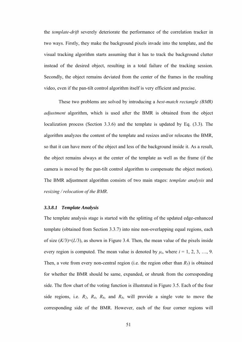
51
the template-drift severely deteriorate the performance of the correlation tracker in
two ways. Firstly, they make the background pixels invade into the template, and the
visual tracking algorithm starts assuming that it has to track the background clutter
instead of the desired object, resulting in a total failure of the tracking session.
Secondly, the object remains deviated from the center of the frames in the resulting
video, even if the pan-tilt control algorithm itself is very efficient and precise.
These two problems are solved by introducing a best-match rectangle (BMR)
adjustment algorithm, which is used after the BMR is obtained from the object
localization process (Section 3.3.6) and the template is updated by Eq. (3.3). The
algorithm analyzes the content of the template and resizes and/or relocates the BMR,
so that it can have more of the object and less of the background inside it. As a result,
the object remains always at the center of the template as well as the frame (if the
camera is moved by the pan-tilt control algorithm to compensate the object motion).
The BMR adjustment algorithm consists of two main stages: template analysis and
resizing / relocation of the BMR.
3.3.8.1 Template Analysis
The template analysis stage is started with the splitting of the updated edge-enhanced
template (obtained from Section 3.3.7) into nine non-overlapping equal regions, each
of size (K/3)×(L/3), as shown in Figure 3.4. Then, the mean value of the pixels inside
every region is computed. The mean value is denoted by μi, where i = 1, 2, 3, …, 9.
Then, a vote from every non-central region (i.e. the region other than R5) is obtained
for whether the BMR should be same, expanded, or shrunk from the corresponding
side. The flow chart of the voting function is illustrated in Figure 3.5. Each of the four
side regions, i.e. R2, R4, R6, and R8, will provide a single vote to move the
corresponding side of the BMR. However, each of the four corner regions will
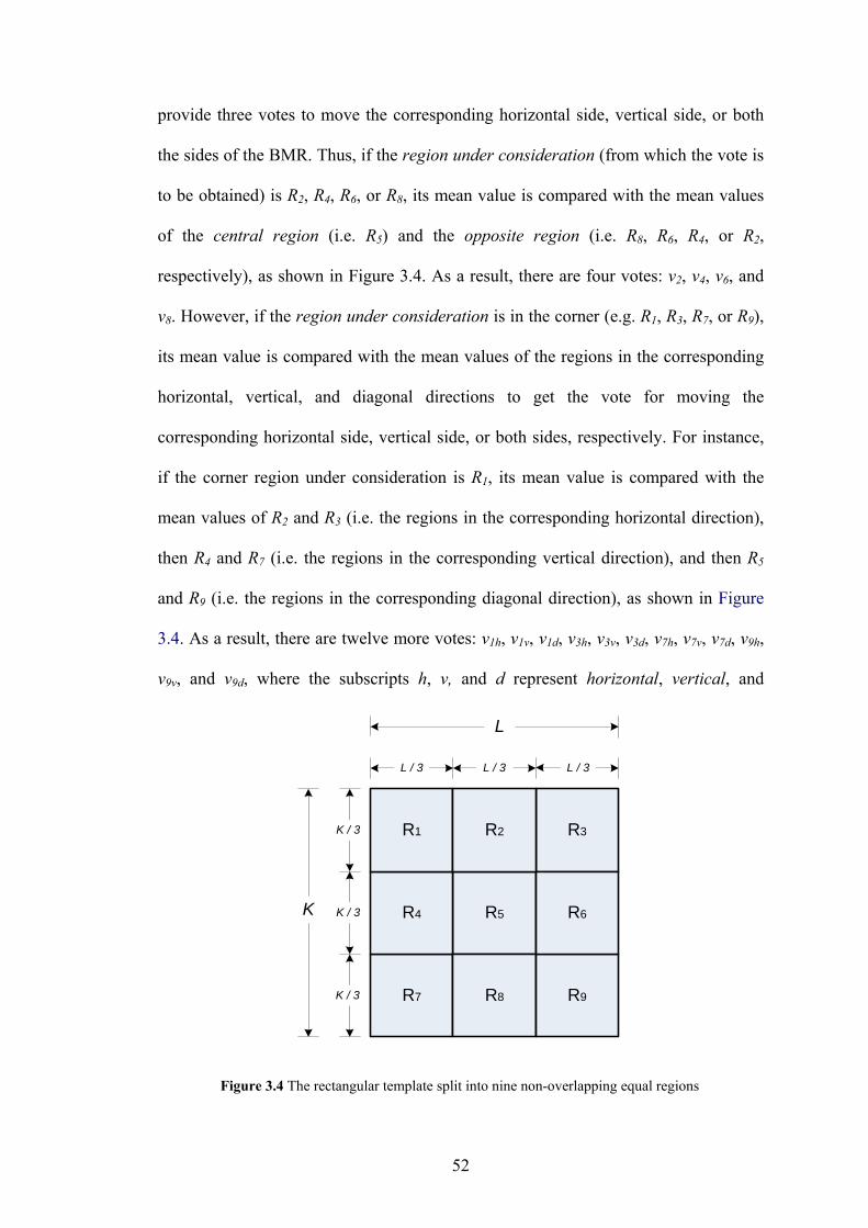
52
provide three votes to move the corresponding horizontal side, vertical side, or both
the sides of the BMR. Thus, if the region under consideration (from which the vote is
to be obtained) is R2, R4, R6, or R8, its mean value is compared with the mean values
of the central region (i.e. R5) and the opposite region (i.e. R8, R6, R4, or R2,
respectively), as shown in Figure 3.4. As a result, there are four votes: v2, v4, v6, and
v8. However, if the region under consideration is in the corner (e.g. R1, R3, R7, or R9),
its mean value is compared with the mean values of the regions in the corresponding
horizontal, vertical, and diagonal directions to get the vote for moving the
corresponding horizontal side, vertical side, or both sides, respectively. For instance,
if the corner region under consideration is R1, its mean value is compared with the
mean values of R2 and R3 (i.e. the regions in the corresponding horizontal direction),
then R4 and R7 (i.e. the regions in the corresponding vertical direction), and then R5
and R9 (i.e. the regions in the corresponding diagonal direction), as shown in Figure
3.4. As a result, there are twelve more votes: v1h, v1v, v1d, v3h, v3v, v3d, v7h, v7v, v7d, v9h,
v9v, and v9d, where the subscripts h, v, and d represent horizontal, vertical, and
R3
R5
R7 R8 R9
R6R4
R1 R2
L
K
L / 3 L / 3L / 3
K / 3
K / 3
K / 3
Figure 3.4 The rectangular template split into nine non-overlapping equal regions
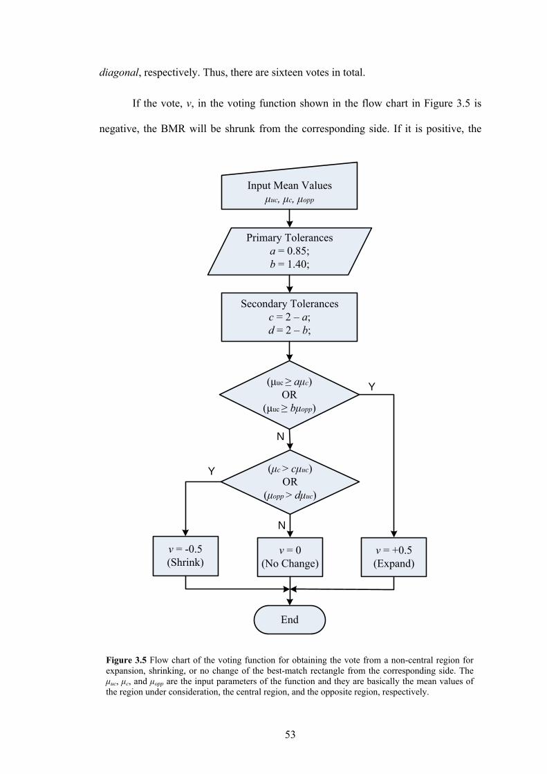
53
diagonal, respectively. Thus, there are sixteen votes in total.
If the vote, v, in the voting function shown in the flow chart in Figure 3.5 is
negative, the BMR will be shrunk from the corresponding side. If it is positive, the
Primary Tolerancesa = 0.85;b = 1.40;
Input Mean Valuesμuc, μc, μopp
Secondary Tolerancesc = 2 – a;d = 2 – b;
(μuc ≥ aμc)OR
(μuc ≥ bμopp)
v = -0.5(Shrink)
Y (μc > cμuc)OR
(μopp > dμuc)
N
v = +0.5(Expand)
Y
N
v = 0(No Change)
End
Figure 3.5 Flow chart of the voting function for obtaining the vote from a non-central region for expansion, shrinking, or no change of the best-match rectangle from the corresponding side. The μuc, μc, and μopp are the input parameters of the function and they are basically the mean values of the region under consideration, the central region, and the opposite region, respectively.
54
BMR will be expanded from the corresponding side. If it is zero, the BMR will
remain same at the corresponding side. The magnitude of the vote defines the step
size of the movement of the corresponding side of the BMR. It is set to 0.5 in order to
have smooth resizing and relocation of the BMR. If the values of the primary
tolerances (i.e. a and b) are increased, the BMR will be reluctant to resize/relocate.
However, if their values are decreased, the BMR will expand and shrink freely.
Satisfactory results have been obtained by setting their values as mentioned in the
flow chart shown in Figure 3.5.
3.3.8.2 Resizing / Relocation of the BMR
Once all the sixteen votes are obtained in the template analysis stage, the changes to
be introduced in the coordinates of the BMR are calculated. Since every vote from a
corner region has its own importance in moving the corresponding sides of the BMR,
the changes are computed by taking weighted sums of the votes, as:
1 4 7 1 7
1 2 3 1 3
3 6 9 3 9
7 8 9 7 9
( )( )( )( )
,,,,
TL d d d d s h s h
TL d d d d s v s v
BR d d d d s h s h
BR d d d d s v s v
x round w v v w v w v w vy round w v v w v w v w vx round w v v w v w v w vy round w v v w v w v w v
Δ = + + + +Δ = + + + +Δ = + + + +Δ = + + + +
(3.4)
where the function round(.) simply rounds a number to its nearest integer, wd is the
weight applied on the votes obtained from the diagonal regions and ws is the weight
applied on the votes obtained from the horizontal or vertical regions. The values for
these weights are set experimentally as: wd = 0.250 and ws = 0.375. It may be noted
that wd < ws, because the distance between the centers of two diagonally connected
regions is larger than that between the centers of two horizontally or vertically
connected regions. Thus, the nearer the regions, the more weighted their votes. The
ΔxTL and ΔyTL are the changes to be introduced in the x and y coordinates of the top-
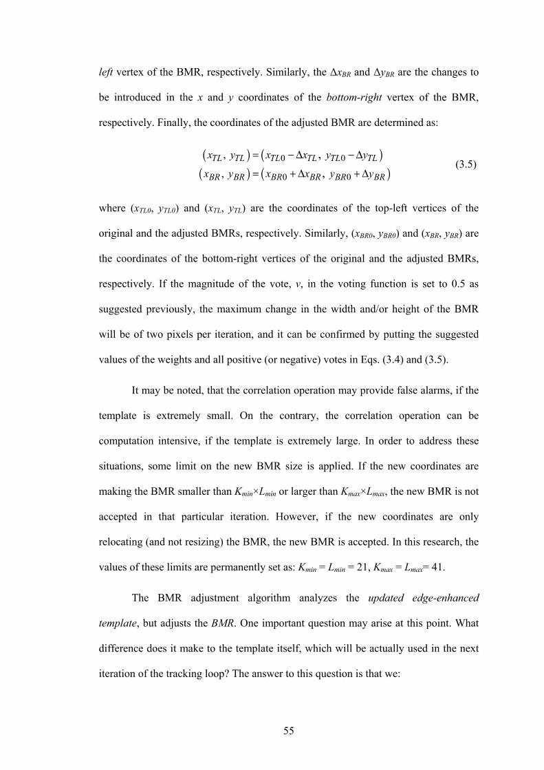
55
left vertex of the BMR, respectively. Similarly, the ΔxBR and ΔyBR are the changes to
be introduced in the x and y coordinates of the bottom-right vertex of the BMR,
respectively. Finally, the coordinates of the adjusted BMR are determined as:
( ) ( )( ) ( )
0 0
0 0
,
,
, ,
TL TL TL TL TL TL
BR BR BR BR BR BR
x y x x y y
x y x x y y
= −Δ −Δ
= + Δ + Δ (3.5)
where (xTL0, yTL0) and (xTL, yTL) are the coordinates of the top-left vertices of the
original and the adjusted BMRs, respectively. Similarly, (xBR0, yBR0) and (xBR, yBR) are
the coordinates of the bottom-right vertices of the original and the adjusted BMRs,
respectively. If the magnitude of the vote, v, in the voting function is set to 0.5 as
suggested previously, the maximum change in the width and/or height of the BMR
will be of two pixels per iteration, and it can be confirmed by putting the suggested
values of the weights and all positive (or negative) votes in Eqs. (3.4) and (3.5).
It may be noted, that the correlation operation may provide false alarms, if the
template is extremely small. On the contrary, the correlation operation can be
computation intensive, if the template is extremely large. In order to address these
situations, some limit on the new BMR size is applied. If the new coordinates are
making the BMR smaller than Kmin×Lmin or larger than Kmax×Lmax, the new BMR is not
accepted in that particular iteration. However, if the new coordinates are only
relocating (and not resizing) the BMR, the new BMR is accepted. In this research, the
values of these limits are permanently set as: Kmin = Lmin = 21, Kmax = Lmax= 41.
The BMR adjustment algorithm analyzes the updated edge-enhanced
template, but adjusts the BMR. One important question may arise at this point. What
difference does it make to the template itself, which will be actually used in the next
iteration of the tracking loop? The answer to this question is that we:
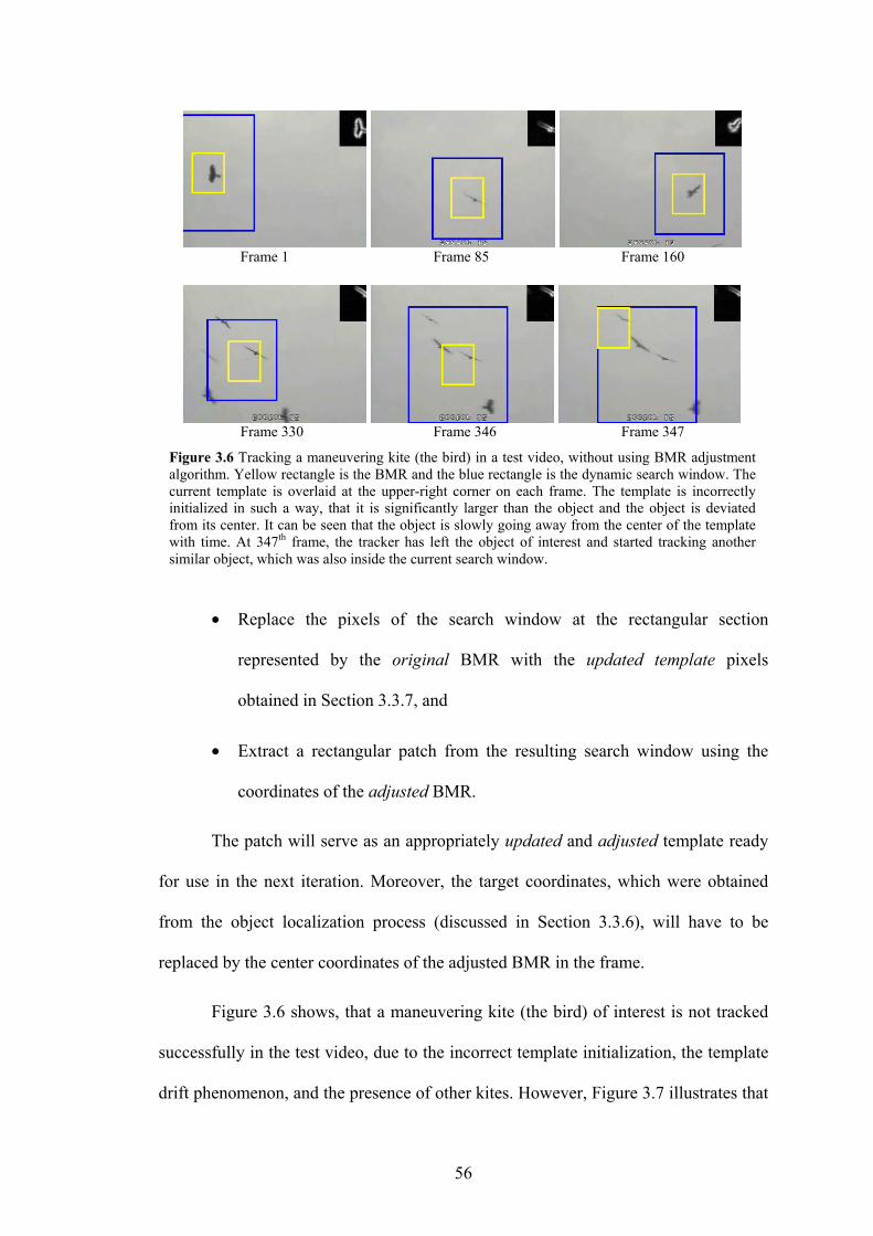
56
• Replace the pixels of the search window at the rectangular section
represented by the original BMR with the updated template pixels
obtained in Section 3.3.7, and
• Extract a rectangular patch from the resulting search window using the
coordinates of the adjusted BMR.
The patch will serve as an appropriately updated and adjusted template ready
for use in the next iteration. Moreover, the target coordinates, which were obtained
from the object localization process (discussed in Section 3.3.6), will have to be
replaced by the center coordinates of the adjusted BMR in the frame.
Figure 3.6 shows, that a maneuvering kite (the bird) of interest is not tracked
successfully in the test video, due to the incorrect template initialization, the template
drift phenomenon, and the presence of other kites. However, Figure 3.7 illustrates that
Frame 1 Frame 85 Frame 160
Frame 330 Frame 346 Frame 347
Figure 3.6 Tracking a maneuvering kite (the bird) in a test video, without using BMR adjustment algorithm. Yellow rectangle is the BMR and the blue rectangle is the dynamic search window. The current template is overlaid at the upper-right corner on each frame. The template is incorrectly initialized in such a way, that it is significantly larger than the object and the object is deviated from its center. It can be seen that the object is slowly going away from the center of the template with time. At 347th frame, the tracker has left the object of interest and started tracking another similar object, which was also inside the current search window.
57
the same object in the same test video is tracked successfully up to the last frame,
even if the template is initialized incorrectly. This is because the BMR adjustment
algorithm continuously adjusts the BMR, so that it can enclose the object of interest
tightly. Due to the adjusted BMR, the template is reduced in size and contains more of
the object and less of the background. Therefore, the dynamic search window is also
appropriately small, which does not let the other objects invade inside it. As a result,
the computational complexity is reduced, the tracking accuracy is increased, and the
Frame 1 Frame 85 Frame 160
Frame 330 Frame 346 Frame 347
Frame 415 Frame 460 Frame 2600
Figure 3.7 Tracking a maneuvering kite (the bird) in a test video, when the BMR adjustment is performed. The current template is overlaid at the upper-right corner on each frame. The template is initialized incorrectly in such a way, that it is significantly larger than the object and the object is deviated from its center. The BMR adjustment algorithm reduces the size of the template appropriately to tightly enclose the object in every frame. As a result, the object does not drift away from the center of the template with time. That is, the template drift problem is eliminated. The size of the dynamic search window is smaller as compared to the one in Figure 3.6, because the template size is now smaller than the initial template. At 347th frame, the tracker is not distracted by the other kites, because the template is now a good representative of the kite of interest and the appropriately sized search window does not contain the other kites inside it. The tracking is continued robustly and persistently till the last (i.e. 2600th) frame of the long test video.
58
tracker is not distracted by the other objects in the scene even if they are very similar
to the object being tracked. Due to the visual tracking accuracy, the object will be
exactly at the center of the frame and the moving camera will point precisely at the
object if the pan-tilt control algorithm is controlling its motion, as discussed in
Chapter 4.
The BMR adjustment algorithm can work with any correlation metric or/and
gray-level images, as far as the template is first edge-enhanced before it is analyzed.
For example, in [100], the technique has been used with NCC and gray-level images
to have persistent and precise tracking results.
3.3.9 Occlusion Handling
A target is said to be (partially or completely) occluded when it is (partially or
completely) hidden due to the appearance of another object between the camera and
the target. Before handling the occlusion, the tracker has to sense when an occlusion
has occurred. In order to sense the occurrence of an occlusion, a fact about the
correlation process is exploited. That is, when the object being tracked is suddenly
occluded by another object, the peak correlation value is dropped below the threshold
(τt). This threshold is the same which is also used for updating the template in Eq.
(3.3). When the correlation peak value is dropped, the proposed tracker goes to its
occlusion handling mode, as described by the following steps:
1. Assume that the target coordinates provided by the correlation process are not
correct and that the target is at the coordinates predicted by the Kalman filter
in the previous iteration.
2. Update the Kalman filter in the current iteration with its own prediction made
in the previous iteration.
59
3. Stop updating the template in order to prevent it from being distorted by the
appearance of the occluding object.
4. Slightly reduce the threshold to be used in the next frame, iteratively, as:
, 1 , 0.0005t n t nτ τ+ = − (3.6)
if τt,n ≥ τt_min, where τt_min is the minimum threshold that can be used safely
without increasing the risk of having false alarms (it is set to 0.65 in this
research). Furthermore, n is the current frame index. The threshold is
iteratively decreased in order to allow the object to slightly change its
appearance with time during its occlusion.
5. Gradually expand the dynamic search window for the next frame by iteratively
increasing the value of the border parameter κ in Eq. (3.24), as:
1 2n nκ κ+ = + (3.7)
This is done in order to compensate for the uncertainty in the speed and
direction of the object during occlusion. This approach, effectively, enlarge
the search window by 4 rows and 4 columns per iteration during the occlusion,
because of the addition of 2 (i.e. the half of 4). If this value is increased, the
search window will be expanded accordingly in larger steps.
6. If the correlation peak in the next iteration reaches above the current threshold
value, assume that the object has come out of the occlusion, and that the
coordinates provided by the correlation process are now correct. At this point,
the values of τt and κ should be reset to their initial default values (i.e. 0.84 and
19 respectively) for normal correlation tracking.
60
3.3.10 Kalman Filter
The Kalman filter [7, 77] in the proposed tracker estimates (or predicts) the position
of the target in the next frame. The predicted position is exploited to:
• Search for the object of interest in the next frame only around the
predicted position (see Section 3.3.11), so that the probability of picking-
up a similar object moving in a different direction can be minimized,
• Create a dynamic search window of optimal size (see Section 3.3.11.2), so
that the tracker can track the object even in the presence of complex object
motion and there can be less amount of background in the search window
without losing the track of the object,
• Make the motors of PTU ready, one step ahead of time, to start moving the
camera to follow the target without any delay (see Chapter 4).
3.3.10.1 Dynamic Model for the Motion of the Target
The dynamic model for the target motion normally used for Kalman filter in the
literature of trackers is “constant velocity with random walk” [43], but in this research
a 2-D “constant-acceleration with random walk [36]” model with six states [see Eqs.
(3.8) - (3.15)] is used, because it provides better accuracy in case of slow as well as
accelerating target. The target state equation and the observation equation,
respectively, are given as [7, 77]:
nnn UΦXX +=+1 , (3.8)
nnn VMXY += , (3.9)
where Xn is the proposed state vector containing six states (position, velocity, and
acceleration in x and y direction), defined as:
61
. .. . .. T
n n n n n n nx x x y y y⎡ ⎤
= ⎢ ⎥⎣ ⎦
X , (3.10)
where the single dot and the double dot over a variable represent single derivative and
double derivative with respect to time, respectively. The state transition matrix, Φ, is
defined as in Eq. (3.11), where T is the sampling time (which is simply the inverse of
the frame rate). It may be noted, that the xn and yn are expressed in terms of 2nd order
approximation of their Taylor expansions, respectively [36].
2
2
1 0 0 02
0 1 0 0 00 0 1 0 0 0
0 0 0 12
0 0 0 0 10 0 0 0 0 1
TT
T
TT
T
⎡ ⎤⎢ ⎥⎢ ⎥⎢ ⎥⎢ ⎥⎢ ⎥= ⎢ ⎥⎢ ⎥⎢ ⎥⎢ ⎥⎢ ⎥⎢ ⎥⎣ ⎦
Φ . (3.11)
Un in Eq. (3.8) is the system noise vector, given by:
0 0 0 0T
n xn ynu u⎡ ⎤= ⎣ ⎦U , (3.12)
where uxn and uyn are the assumed uncorrelated zero-mean Gaussian noise elements
with variances 2uxσ and 2
uyσ , respectively. They account for the small uncertainty in
the acceleration of the object. For simplicity, the values of these variances can be set
to unity. Yn in Eq. (3.9) is the measurement vector given by:
[ ]Tn n nx y=Y , (3.13)
where xn and yn are the noisy target-coordinates. They are obtained from the
correlation based object localization algorithm at time step n. M in Eq. (3.9) is the
observation matrix given by:
62
⎥⎦
⎤⎢⎣
⎡=
001000000001
M , (3.14)
and Vn in Eq. (3.9) is the observation noise vector given by:
T
n xn ynv v⎡ ⎤= ⎣ ⎦V , (3.15)
where vxn and vyn are the assumed uncorrelated zero-mean Gaussian noise elements
with variances 2vxσ and 2
vyσ , respectively. If the variances are set to high values, the
Kalman filter will give the predicted coordinates high importance as compared to the
measurement coordinates, during its updating (or correcting) phase after the arrival of
the new measurement [37]. For simplicity, the values of these variances can be set to
unity.
3.3.10.2 Kalman Filter Updating
Once the Kalman filter receives the new measurement (i.e. the pixel coordinates of
the target), it is updated to correct its last prediction error if any. The filter is updated
as [36, 37, 38]:
( )| | 1 | 1n n n n n n n n∗ ∗ ∗
− −= + −X X K Y MX , (3.16)
where the subscript “n|n-1” means the prediction made in the previous iteration, and
“n|n” means the updated (or corrected) versions of the previous prediction. Kn in Eq.
(3.16) is the Kalman gain matrix defined as [36, 37, 38]:
1
| 1 | 1T T
n n n n n n−∗ ∗
− −⎡ ⎤= +⎣ ⎦K S M R MS M , (3.17)
where | 1n n∗
−S is the predictor error covariance computed in the previous iteration as:
63
| 1 | 1 1| 1( ) Tn n n n n n nCOV∗ ∗ ∗
− − − −= = +S X ΦS Φ Q , (3.18)
where 1| 1n n∗− −S is the covariance of the updated estimate computed in the previous
iteration as:
[ ]1| 1 1| 1 1 1| 2( )n n n n n n nCOV∗ ∗ ∗− − − − − − −= = −S X I K M S . (3.19)
The Qn in Eq. (3.18) is the noise covariance matrix of the dynamic model. It is given
as:
( ) [ ]Tn n n nCOV E= =Q U U U , (3.20)
and Rn in Eq. (3.17) is the observation noise covariance defined as:
( ) [ ]Tn n n nCOV E= =R V V V , (3.21)
where E[.] is the “expected value of” operator [36].
3.3.10.3 Prediction by Kalman Filter
The predicted estimate of the state vector is given by the state transition or prediction
equation given as under [36, 37, 38]:
1| |n n n n∗ ∗+ =X ΦX , (3.22)
where the superscript (*) indicates, that the state vector has been estimated by the
Kalman filter, and is not the actual measurement obtained from the object localization
algorithm. |n n∗X is the updated (or corrected) estimate of the state vector coming from
Eq. (3.16). Finally, the position of the target in the next frame is predicted as:
64
*
1| *1|*
1|
n nn n
n n
x
y
++
+
⎡ ⎤⎢ ⎥ =⎢ ⎥⎣ ⎦
MX . (3.23)
The predicted target position will be used for generating the dynamic search window
for the next iteration (Section 3.3.11), occlusion handling (Section 3.3.9) in the next
iteration, and generating the pan-tilt control signals in the current iteration (Chapter 4)
for efficient and accurate target tracking with moving camera.
3.3.11 Search Window Updating
The target is usually looked for in a small search window instead of the whole frame.
This is done in order to save CPU time and get rid of the false alarms due to the
clutter possibly present in the background. However, the search window should not be
too small, because there will be a risk of losing the target if it is moving fast [11].
3.3.11.1 Traditional Fixed-Size Search Window
Conventionally, the size of the search window is set to be constant throughout the
tracking session and its center is updated with the center of the last best-match
rectangle (BMR) [39] or the predicted position [11]. These approaches have some
drawbacks: (1) If the search window size is fixed and small, and the target is moving
and maneuvering very fast, it may go out of the search window. (2) If the search
window size is fixed and large, and the target is moving and maneuvering very slow,
the redundant background in the search window may contain some clutter. As a result,
the clutter may create false alarms and the large size of the search window will make
the correlation process slow.
3.3.11.2 Proposed Dynamic Search Window
In order to eliminate the problems of the fixed-size search window highlighted above,
the location and the size of the search window are proposed to be dynamically
65
updated using the prediction and the prediction-error of the Kalman filter explained as
follows.
Assuming that K (template-height) and L (template-width) are odd integers,
the top-left and the bottom-right co-ordinates, i.e. (xtl, ytl) and (xbr, ybr) respectively, of
the search window in the frame are determined by Eq. (3.24), where * *1| 1|( , )n n n nx y+ +
are the future target-coordinates estimated by Kalman filter.
*1|
*1|
*1|
*1|
1 ,2
1 ,2
1 ,2
1 ,2
tl n n tx x
tl n n ty y
br n n bx x
br n n by y
Lx x a
Ky y a
Lx x a
Ky y a
κ ε
κ ε
κ ε
κ ε
+
+
+
+
−⎛ ⎞= − + +⎜ ⎟⎝ ⎠
−⎛ ⎞= − + +⎜ ⎟⎝ ⎠
−⎛ ⎞= + + +⎜ ⎟⎝ ⎠
−⎛ ⎞= + + +⎜ ⎟⎝ ⎠
(3.24)
The first three terms in case of every coordinate in Eq. (3.24) make a
minimum-size search window of size (K+2κ) × (L+2κ), where κ is the minimum width
of the border around K×L area centered at the predicted position. The value of κ is
experimentally set to 19. Furthermore, εx and εy in Eq. (3.24) are the prediction
errors, defined as:
*| 1
*| 1
,
,
x n n n
y n n n
x x
y y
ε
ε
−
−
= −
= − (3.25)
where * *| 1 | 1( , )n n n nx y− − is the target position predicted by Kalman filter in the
previous iteration. Furthermore, (xn, yn) is the target position provided by the
correlation process in the current iteration. It may be noted, that in the first iteration
these coordinates are initialized with the actual target coordinates, from where the
template was extracted by the user.
66
The atx, aty, abx, and aby parameters in Eq. (3.24) are the scaling factors, which
compensate for the possible prediction errors in case of a sudden maneuvering of the
object. If any of the scaling factors is positive, the minimum-size search-window will
be expanded further in the direction of the object motion proportional to the
corresponding prediction error. If it is negative, the minimum-size search-window will
be contracted from opposite direction of the object motion proportional to the
corresponding prediction error. The scaling factors are given as:
( ) otherwise ) ,(
0 if ) ,(,
12
x21
⎩⎨⎧ ≥
=aaaa
aa bxtx
ε (3.26)
( ) otherwise ) ,(
0 if ) ,(,
12
y21
⎩⎨⎧ ≥
=aa
aaaa byty
ε (3.27)
where a1 = -0.25 and a2 = +1.25 in this research to contract/expand the search window
from the the corresponding opposite sides by 25% of the error. If their magnitude is
increased, the contraction/expansion will occur in larger steps.
For example, if the prediction error in x-axis is εx = +8, the actual target
position (determined by the correlation process) is to the right of the predicted
position, thus the minimum-size search window will be contracted by 2 pixels from
left (using atx = -0.25), and expanded towards right side by 10 pixels (using abx =
1.25). Thus, the search window is dynamically created in every frame according to the
nature of the motion of the maneuvering object. If the object is moving smoothly,
there will be no prediction error, so the search window will be of minimum size. If the
object is moving with abrupt maneuvering, the search window will be expanded
towards the object motion and contracted from the opposite side. The resulting search
window is large enough to get the target always inside the window, and small enough
to reduce the background clutter and the computational complexity.
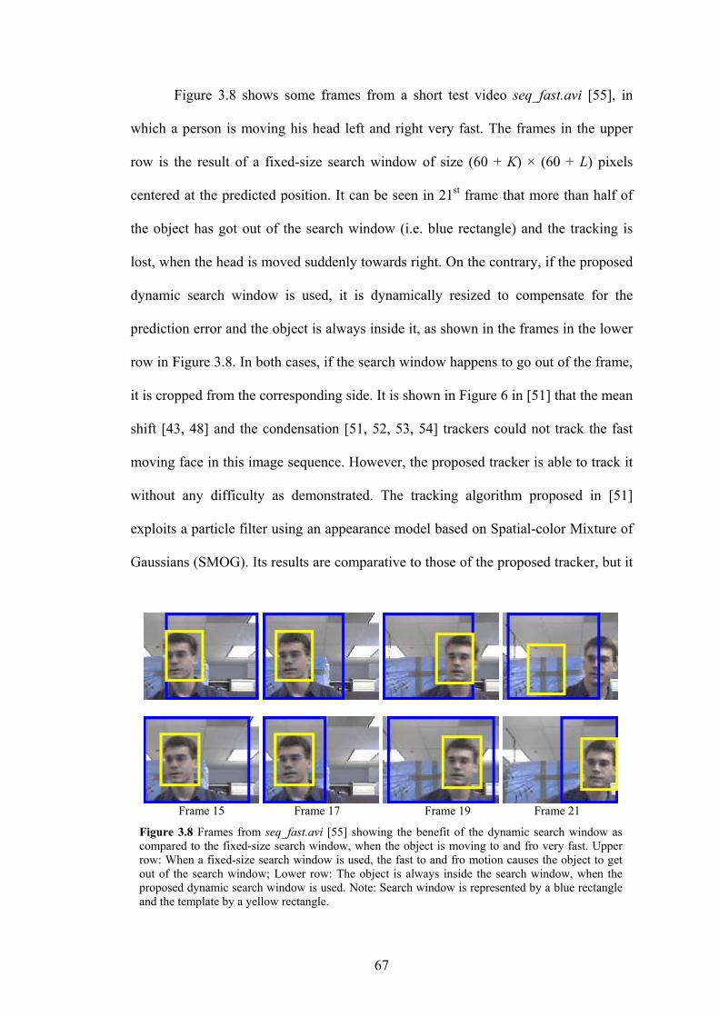
67
Figure 3.8 shows some frames from a short test video seq_fast.avi [55], in
which a person is moving his head left and right very fast. The frames in the upper
row is the result of a fixed-size search window of size (60 + K) × (60 + L) pixels
centered at the predicted position. It can be seen in 21st frame that more than half of
the object has got out of the search window (i.e. blue rectangle) and the tracking is
lost, when the head is moved suddenly towards right. On the contrary, if the proposed
dynamic search window is used, it is dynamically resized to compensate for the
prediction error and the object is always inside it, as shown in the frames in the lower
row in Figure 3.8. In both cases, if the search window happens to go out of the frame,
it is cropped from the corresponding side. It is shown in Figure 6 in [51] that the mean
shift [43, 48] and the condensation [51, 52, 53, 54] trackers could not track the fast
moving face in this image sequence. However, the proposed tracker is able to track it
without any difficulty as demonstrated. The tracking algorithm proposed in [51]
exploits a particle filter using an appearance model based on Spatial-color Mixture of
Gaussians (SMOG). Its results are comparative to those of the proposed tracker, but it
Frame 15 Frame 17 Frame 19 Frame 21
Figure 3.8 Frames from seq_fast.avi [55] showing the benefit of the dynamic search window as compared to the fixed-size search window, when the object is moving to and fro very fast. Upper row: When a fixed-size search window is used, the fast to and fro motion causes the object to get out of the search window; Lower row: The object is always inside the search window, when the proposed dynamic search window is used. Note: Search window is represented by a blue rectangle and the template by a yellow rectangle.
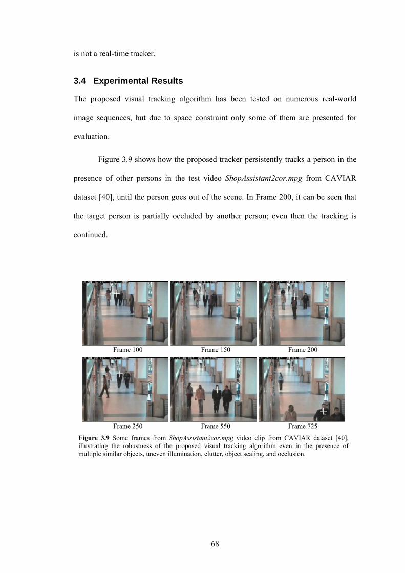
68
is not a real-time tracker.
3.4 Experimental Results
The proposed visual tracking algorithm has been tested on numerous real-world
image sequences, but due to space constraint only some of them are presented for
evaluation.
Figure 3.9 shows how the proposed tracker persistently tracks a person in the
presence of other persons in the test video ShopAssistant2cor.mpg from CAVIAR
dataset [40], until the person goes out of the scene. In Frame 200, it can be seen that
the target person is partially occluded by another person; even then the tracking is
continued.
Frame 100 Frame 150 Frame 200
Frame 250 Frame 550 Frame 725
Figure 3.9 Some frames from ShopAssistant2cor.mpg video clip from CAVIAR dataset [40], illustrating the robustness of the proposed visual tracking algorithm even in the presence of multiple similar objects, uneven illumination, clutter, object scaling, and occlusion.
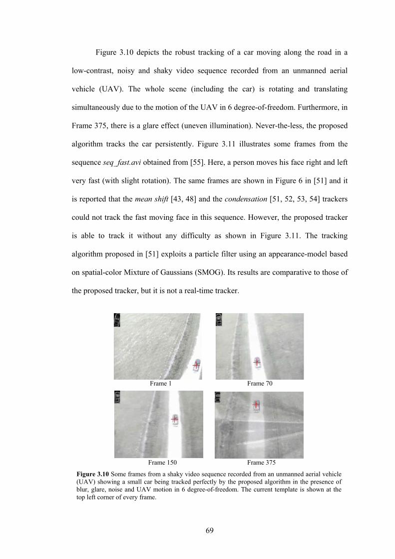
69
Figure 3.10 depicts the robust tracking of a car moving along the road in a
low-contrast, noisy and shaky video sequence recorded from an unmanned aerial
vehicle (UAV). The whole scene (including the car) is rotating and translating
simultaneously due to the motion of the UAV in 6 degree-of-freedom. Furthermore, in
Frame 375, there is a glare effect (uneven illumination). Never-the-less, the proposed
algorithm tracks the car persistently. Figure 3.11 illustrates some frames from the
sequence seq_fast.avi obtained from [55]. Here, a person moves his face right and left
very fast (with slight rotation). The same frames are shown in Figure 6 in [51] and it
is reported that the mean shift [43, 48] and the condensation [51, 52, 53, 54] trackers
could not track the fast moving face in this sequence. However, the proposed tracker
is able to track it without any difficulty as shown in Figure 3.11. The tracking
algorithm proposed in [51] exploits a particle filter using an appearance-model based
on spatial-color Mixture of Gaussians (SMOG). Its results are comparative to those of
the proposed tracker, but it is not a real-time tracker.
Frame 1 Frame 70
Frame 150 Frame 375
Figure 3.10 Some frames from a shaky video sequence recorded from an unmanned aerial vehicle (UAV) showing a small car being tracked perfectly by the proposed algorithm in the presence of blur, glare, noise and UAV motion in 6 degree-of-freedom. The current template is shown at the top left corner of every frame.
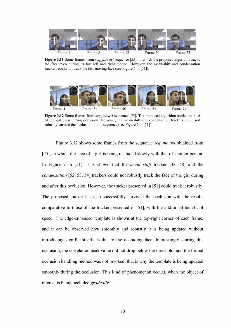
70
Figure 3.12 shows some frames from the sequence seq_mb.avi obtained from
[55], in which the face of a girl is being occluded slowly with that of another person.
In Figure 7 in [51], it is shown that the mean shift tracker [43, 48] and the
condensation [52, 53, 54] trackers could not robustly track the face of the girl during
and after this occlusion. However, the tracker presented in [51] could track it robustly.
The proposed tracker has also successfully survived the occlusion with the results
comparative to those of the tracker presented in [51], with the additional benefit of
speed. The edge-enhanced template is shown at the top-right corner of each frame,
and it can be observed how smoothly and robustly it is being updated without
introducing significant effects due to the occluding face. Interestingly, during this
occlusion, the correlation peak value did not drop below the threshold, and the formal
occlusion handling method was not invoked, that is why the template is being updated
smoothly during the occlusion. This kind of phenomenon occurs, when the object of
interest is being occluded gradually.
Frame 1 Frame 8 Frame 12 Frame 20 Frame 25
Figure 3.11 Some frames from seq_fast.avi sequence [55], in which the proposed algorithm tracks the face even during its fast left and right motion. However, the mean-shift and condensation trackers could not track the fast-moving face (see Figure 6 in [51]).
Frame 1 Frame 31 Frame 40 Frame 53 Frame 74
Figure 3.12 Some frames from seq_mb.avi sequence [55]. The proposed algorithm tracks the face of the girl even during occlusion. However, the mean-shift and condensation trackers could not robustly survive the occlusion in this sequence (see Figure 7 in [51]).
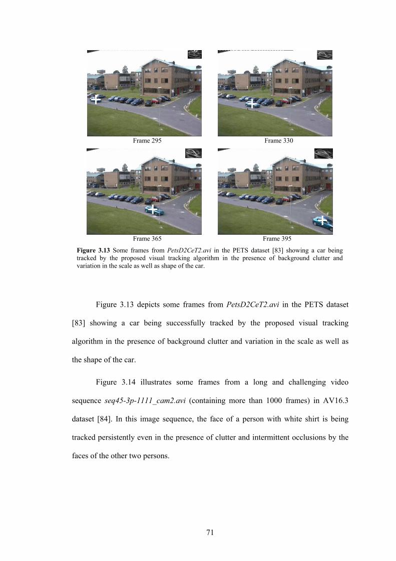
71
Figure 3.13 depicts some frames from PetsD2CeT2.avi in the PETS dataset
[83] showing a car being successfully tracked by the proposed visual tracking
algorithm in the presence of background clutter and variation in the scale as well as
the shape of the car.
Figure 3.14 illustrates some frames from a long and challenging video
sequence seq45-3p-1111_cam2.avi (containing more than 1000 frames) in AV16.3
dataset [84]. In this image sequence, the face of a person with white shirt is being
tracked persistently even in the presence of clutter and intermittent occlusions by the
faces of the other two persons.
Frame 295 Frame 330
Frame 365 Frame 395
Figure 3.13 Some frames from PetsD2CeT2.avi in the PETS dataset [83] showing a car being tracked by the proposed visual tracking algorithm in the presence of background clutter and variation in the scale as well as shape of the car.
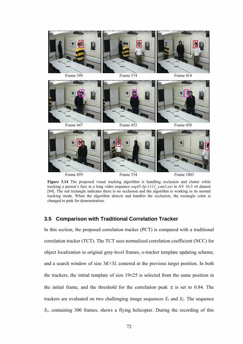
72
3.5 Comparison with Traditional Correlation Tracker
In this section, the proposed correlation tracker (PCT) is compared with a traditional
correlation tracker (TCT). The TCT uses normalized correlation coefficient (NCC) for
object localization in original gray-level frames, α-tracker template updating scheme,
and a search window of size 3K×3L centered at the previous target position. In both
the trackers, the initial template of size 19×25 is selected from the same position in
the initial frame, and the threshold for the correlation peak τt is set to 0.84. The
trackers are evaluated on two challenging image sequences S1 and S2. The sequence
S1, containing 300 frames, shows a flying helicopter. During the recording of this
Frame 349 Frame 374 Frame 414
Frame 447 Frame 452 Frame 458
Frame 459 Frame 534 Frame 1003
Figure 3.14 The proposed visual tracking algorithm is handling occlusion and clutter while tracking a person’s face in a long video sequence seq45-3p-1111_cam2.avi in AV 16.3 v6 dataset [84]. The red rectangle indicates there is no occlusion and the algorithm is working in its normal tracking mode. When the algorithm detects and handles the occlusion, the rectangle color is changed to pink for demonstration.
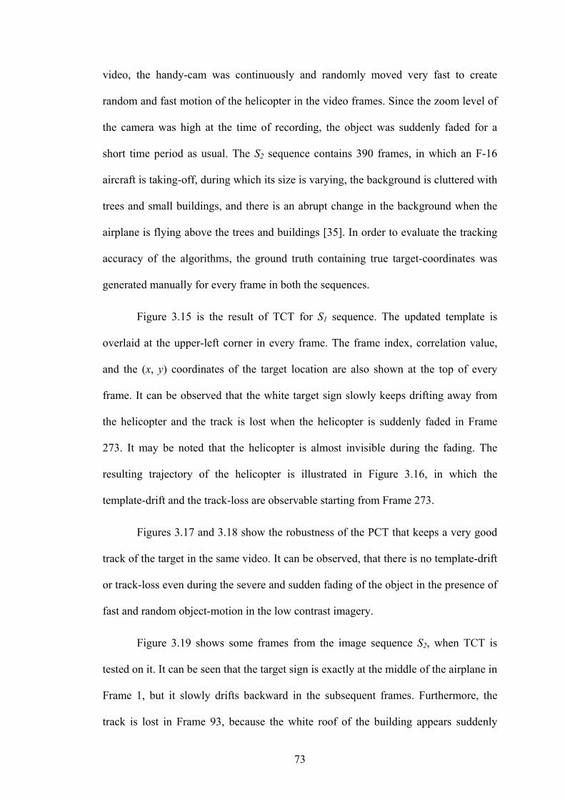
73
video, the handy-cam was continuously and randomly moved very fast to create
random and fast motion of the helicopter in the video frames. Since the zoom level of
the camera was high at the time of recording, the object was suddenly faded for a
short time period as usual. The S2 sequence contains 390 frames, in which an F-16
aircraft is taking-off, during which its size is varying, the background is cluttered with
trees and small buildings, and there is an abrupt change in the background when the
airplane is flying above the trees and buildings [35]. In order to evaluate the tracking
accuracy of the algorithms, the ground truth containing true target-coordinates was
generated manually for every frame in both the sequences.
Figure 3.15 is the result of TCT for S1 sequence. The updated template is
overlaid at the upper-left corner in every frame. The frame index, correlation value,
and the (x, y) coordinates of the target location are also shown at the top of every
frame. It can be observed that the white target sign slowly keeps drifting away from
the helicopter and the track is lost when the helicopter is suddenly faded in Frame
273. It may be noted that the helicopter is almost invisible during the fading. The
resulting trajectory of the helicopter is illustrated in Figure 3.16, in which the
template-drift and the track-loss are observable starting from Frame 273.
Figures 3.17 and 3.18 show the robustness of the PCT that keeps a very good
track of the target in the same video. It can be observed, that there is no template-drift
or track-loss even during the severe and sudden fading of the object in the presence of
fast and random object-motion in the low contrast imagery.
Figure 3.19 shows some frames from the image sequence S2, when TCT is
tested on it. It can be seen that the target sign is exactly at the middle of the airplane in
Frame 1, but it slowly drifts backward in the subsequent frames. Furthermore, the
track is lost in Frame 93, because the white roof of the building appears suddenly
74
above the airplane in the image and this white portion is not included in the current
template. The complete trajectory of the airplane provided by TCT is compared with
Frame 50 Frame 150 Frame 250
Frame 270 Frame 273 Frame 274
Frame 280 Frame 285 Frame 290
Figure 3.15 Result of TCT (Traditional Correlation Tracker) for S1 image sequence, showing the template drift problem starting from Frame 150 and its failure starting from Frame 273 during object fading.
Figure 3.16 Target trajectory (row and column coordinates) produced by TCT for S1 sequence showing the failure from Frame 273 through the last frame of the image sequence.
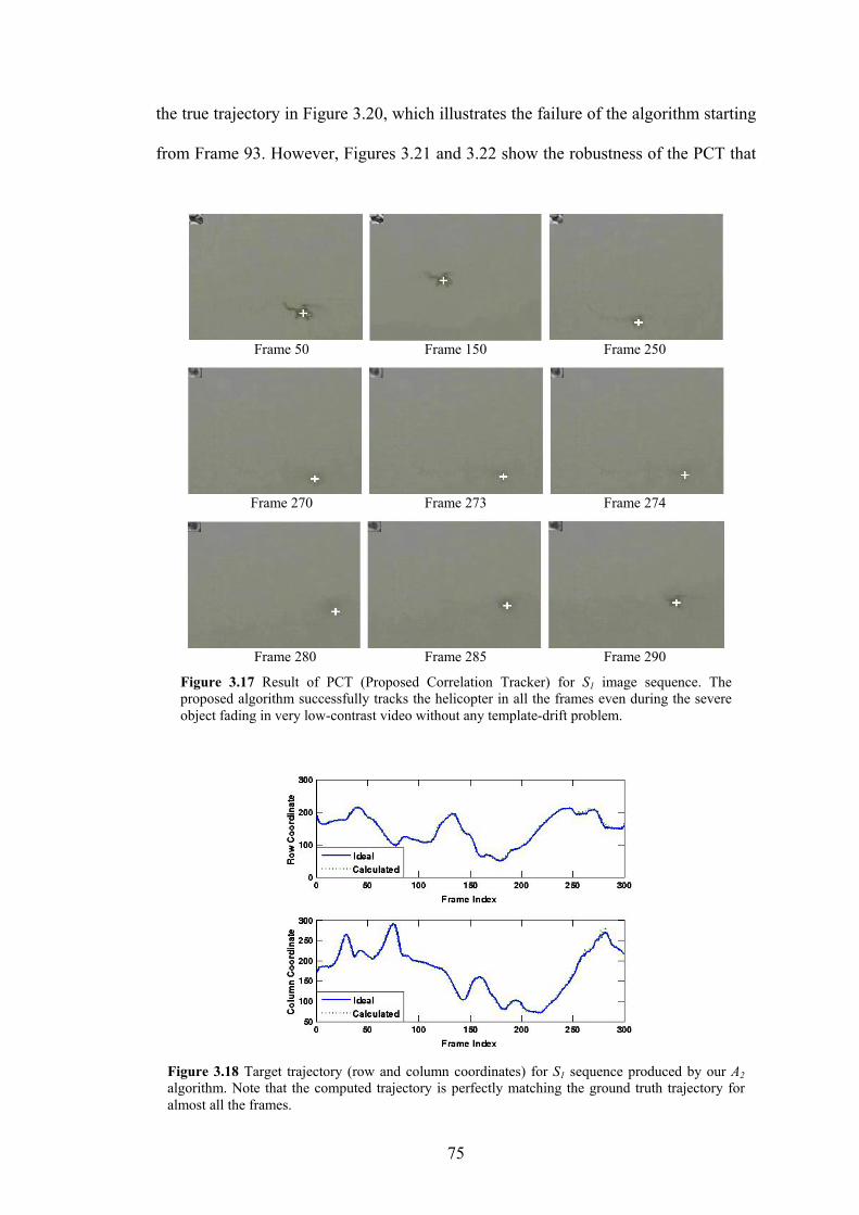
75
the true trajectory in Figure 3.20, which illustrates the failure of the algorithm starting
from Frame 93. However, Figures 3.21 and 3.22 show the robustness of the PCT that
Frame 50 Frame 150 Frame 250
Frame 270 Frame 273 Frame 274
Frame 280 Frame 285 Frame 290
Figure 3.17 Result of PCT (Proposed Correlation Tracker) for S1 image sequence. The proposed algorithm successfully tracks the helicopter in all the frames even during the severe object fading in very low-contrast video without any template-drift problem.
Figure 3.18 Target trajectory (row and column coordinates) for S1 sequence produced by our A2 algorithm. Note that the computed trajectory is perfectly matching the ground truth trajectory for almost all the frames.
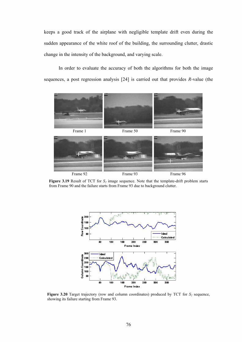
76
keeps a good track of the airplane with negligible template drift even during the
sudden appearance of the white roof of the building, the surrounding clutter, drastic
change in the intensity of the background, and varying scale.
In order to evaluate the accuracy of both the algorithms for both the image
sequences, a post regression analysis [24] is carried out that provides R-value (the
Frame 1 Frame 50 Frame 90
Frame 92 Frame 93 Frame 96
Figure 3.19 Result of TCT for S2 image sequence. Note that the template-drift problem starts from Frame 90 and the failure starts from Frame 93 due to background clutter.
Figure 3.20 Target trajectory (row and column coordinates) produced by TCT for S2 sequence, showing its failure starting from Frame 93.
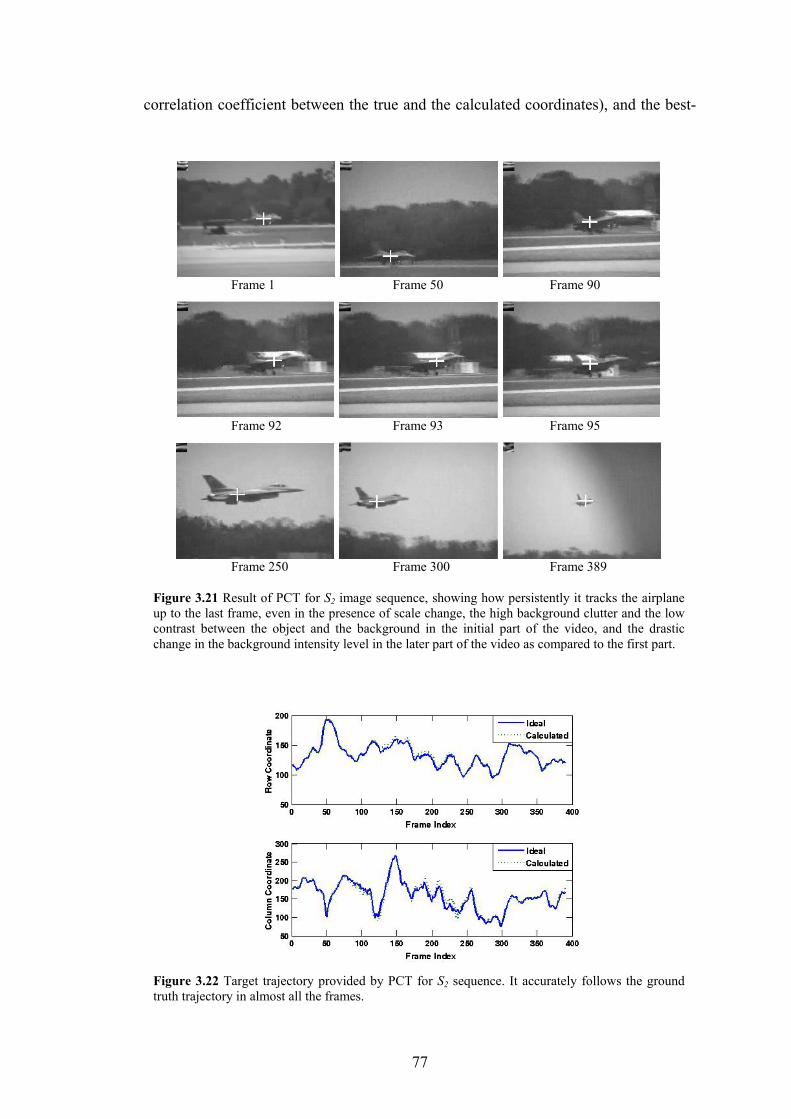
77
correlation coefficient between the true and the calculated coordinates), and the best-
Frame 1 Frame 50 Frame 90
Frame 92 Frame 93 Frame 95
Frame 250 Frame 300 Frame 389
Figure 3.21 Result of PCT for S2 image sequence, showing how persistently it tracks the airplane up to the last frame, even in the presence of scale change, the high background clutter and the low contrast between the object and the background in the initial part of the video, and the drastic change in the background intensity level in the later part of the video as compared to the first part.
Figure 3.22 Target trajectory provided by PCT for S2 sequence. It accurately follows the ground truth trajectory in almost all the frames.
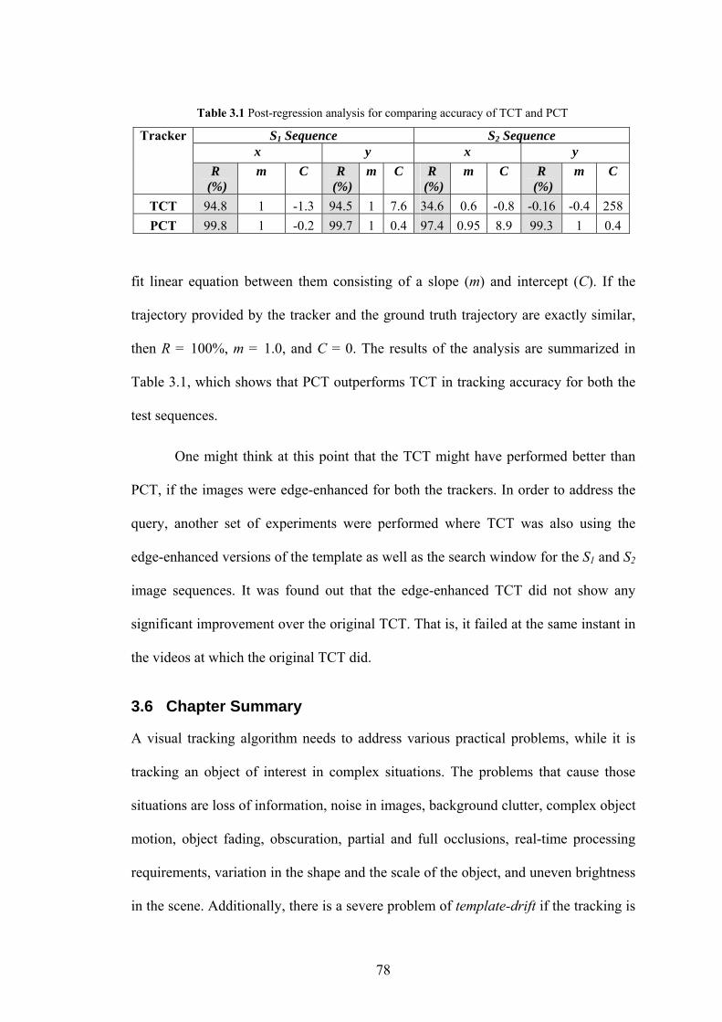
78
fit linear equation between them consisting of a slope (m) and intercept (C). If the
trajectory provided by the tracker and the ground truth trajectory are exactly similar,
then R = 100%, m = 1.0, and C = 0. The results of the analysis are summarized in
Table 3.1, which shows that PCT outperforms TCT in tracking accuracy for both the
test sequences.
One might think at this point that the TCT might have performed better than
PCT, if the images were edge-enhanced for both the trackers. In order to address the
query, another set of experiments were performed where TCT was also using the
edge-enhanced versions of the template as well as the search window for the S1 and S2
image sequences. It was found out that the edge-enhanced TCT did not show any
significant improvement over the original TCT. That is, it failed at the same instant in
the videos at which the original TCT did.
3.6 Chapter Summary
A visual tracking algorithm needs to address various practical problems, while it is
tracking an object of interest in complex situations. The problems that cause those
situations are loss of information, noise in images, background clutter, complex object
motion, object fading, obscuration, partial and full occlusions, real-time processing
requirements, variation in the shape and the scale of the object, and uneven brightness
in the scene. Additionally, there is a severe problem of template-drift if the tracking is
Table 3.1 Post-regression analysis for comparing accuracy of TCT and PCT
Tracker S1 Sequence S2 Sequence x y x y R
(%) m C R
(%)m C R
(%)m C R
(%) m C
TCT 94.8 1 -1.3 94.5 1 7.6 34.6 0.6 -0.8 -0.16 -0.4 258PCT 99.8 1 -0.2 99.7 1 0.4 97.4 0.95 8.9 99.3 1 0.4

79
performed using a simple correlation tracker. A correlation tracking framework has
been proposed that addresses almost all of these problems very efficiently. Various
experimental results have been presented to demonstrate the robustness and
performance of the proposed tracker. The proposed tracker has also been compared
with the mean-shift and the condensation trackers for some real-world publicly
available test sequences and it has been shown that the proposed tracker outperforms
them in robustness to the occlusion and the fast to-and-fro motion of the object. A
comparison of the proposed correlation tracker (PCT) has also been performed with a
traditional correlation tracker (TCT). The results of the post-regression analysis show
that the proposed tracker is more robust and accurate than TCT. The next two
chapters discuss the design, implementation, and analysis of the machine vision
systems in which the proposed tracker is deployed.
80
4 Active Camera Tracking System
4
Active Camera Tracking System
4.1 Chapter Overview
This chapter discusses the design, implementation, and analysis of an active camera
tracking system that exploits the proposed visual tracking framework as an integrated
module. Various experimental results, that validate the robust and accurate
performance of the system, are also shown at the end of the chapter.
4.2 Problem Description
An active camera tracking system tracks an object of interest automatically with a
pan-tilt-zoom (PTZ) video camera. The system, in its simplest form, is illustrated
using a block diagram shown in Figure 4.1. It consists of a video camera, a visual
tracking algorithm, a pan-tilt control algorithm, and a pan-tilt unit (PTU). Every frame
acquired from the video camera is analyzed by the visual tracking algorithm, which
localizes the object of interest inside the image in pixel-coordinates. The coordinates
are then sent to a pan-tilt control algorithm, which generates the pan-tilt motion
control signals to rotate the PTU according to the motion of the object in the scene.
Since the camera is securely attached to the PTU, it also rotates in synchronization
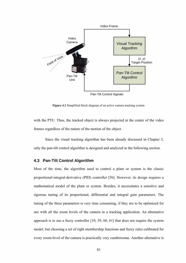
81
with the PTU. Thus, the tracked object is always projected at the center of the video
frames regardless of the nature of the motion of the object.
Since the visual tracking algorithm has been already discussed in Chapter 3,
only the pan-tilt control algorithm is designed and analyzed in the following section.
4.3 Pan-Tilt Control Algorithm
Most of the time, the algorithm used to control a plant or system is the classic
proportional-integral-derivative (PID) controller [56]. However, its design requires a
mathematical model of the plant or system. Besides, it necessitates a sensitive and
rigorous tuning of its proportional, differential and integral gain parameters. The
tuning of the three parameters is very time consuming, if they are to be optimized for
use with all the zoom levels of the camera in a tracking application. An alternative
approach is to use a fuzzy controller [10, 59, 60, 61] that does not require the system
model, but choosing a set of right membership functions and fuzzy rules calibrated for
every zoom-level of the camera is practically very cumbersome. Another alternative is
Visual TrackingAlgorithm
Pan-Tilt Control Algorithm
Video Frame
(x, y)Target Position
Pan-TiltUnit
Video Camera
Pan-Tilt Control Signals
Field of View
Figure 4.1 Simplified block diagram of an active camera tracking system

82
to implement a neural network controller [25, 62], but it is heavily dependent on the
quality and the variety of the examples in the training dataset, which can accurately
represent the complete behavior of the controller in all possible scenarios, including
the varying zoom-levels of the camera. Furthermore, the traditional control
algorithms, e.g. the one used in [14], are generally implemented based on the
difference between the center (i.e. reference) position and the current target position
in the image. They do not account for the target velocity. As a result, there will be
oscillations (if the object is moving slow), a lag (if it is moving with a mediocre
speed), and loss of the object from the frame (if it is moving faster than the maximum
pan-tilt velocity generated by the control algorithm). In order to address the
limitations of the traditional control algorithms, a “Predictive Open-Loop Car
Following Control (POL-CFC)” is proposed. Its basic idea has been obtained from
“Car-Following Control (CFC)” law [15].
4.3.1 Car-Following Control (CFC) Law
Suppose a car, F, is moving with a velocity VF and is following another car, L,
moving with a velocity VL, as shown in Figure 4.2. The letters ‘F’ and ‘L’ in the
subscript stands for “follow” and “lead”, respectively. Let the positional error
between the cars be denoted by e. Then, the basic Car-Following Control (CFC) law
is simply defined as [15]:
Figure 4.2 Demonstration of the Car-Following Control (CFC) law
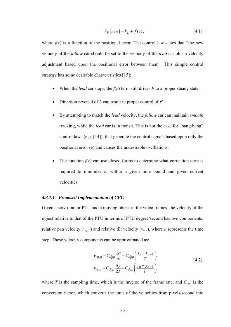
83
[ ] ( )F LV new V f e= + , (4.1)
where f(e) is a function of the positional error. The control law states that “the new
velocity of the follow car should be set to the velocity of the lead car plus a velocity
adjustment based upon the positional error between them”. This simple control
strategy has some desirable characteristics [15]:
• When the lead car stops, the f(e) term still drives F to a proper steady state.
• Direction reversal of L can result in proper control of F.
• By attempting to match the lead velocity, the follow car can maintain smooth
tracking, while the lead car is in transit. This is not the case for “bang-bang”
control laws (e.g. [14]), that generate the control signals based upon only the
positional error (e) and causes the undesirable oscillations.
• The function f(e) can use closed forms to determine what correction term is
required to minimize e, within a given time bound and given current
velocities.
4.3.1.1 Proposed Implementation of CFC
Given a servo-motor PTU and a moving object in the video frames, the velocity of the
object relative to that of the PTU in terms of PTU degree/second has two components:
relative pan velocity (vrp,n) and relative tilt velocity (vrt,n), where n represents the time
step. These velocity components can be approximated as:
1
,
1,
,
,
n nrp n dpp dpp
n nrt n dpp dpp
x xxv C Ct T
y yyv C Ct T
−
−
⎛ ⎞⎜ ⎟⎝ ⎠⎛ ⎞⎜ ⎟⎝ ⎠
−Δ= =Δ
−Δ= =Δ
(4.2)
where T is the sampling time, which is the inverse of the frame rate, and Cdpp is the
conversion factor, which converts the units of the velocities from pixels/second into
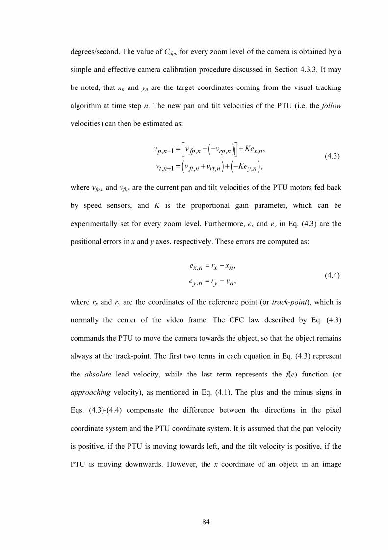
84
degrees/second. The value of Cdpp for every zoom level of the camera is obtained by a
simple and effective camera calibration procedure discussed in Section 4.3.3. It may
be noted, that xn and yn are the target coordinates coming from the visual tracking
algorithm at time step n. The new pan and tilt velocities of the PTU (i.e. the follow
velocities) can then be estimated as:
( )
( ) ( ), 1 , ,,
, 1 , ,,
,
,
p n rp n x nfp n
t n rt n y nft n
v v v Ke
v v v Ke
+
+
⎡ ⎤⎢ ⎥⎣ ⎦
= + − +
= + + − (4.3)
where vfp,n and vft,n are the current pan and tilt velocities of the PTU motors fed back
by speed sensors, and K is the proportional gain parameter, which can be
experimentally set for every zoom level. Furthermore, ex and ey in Eq. (4.3) are the
positional errors in x and y axes, respectively. These errors are computed as:
,,
,,
e r xx n x n
e r yy n y n
= −
= − (4.4)
where rx and ry are the coordinates of the reference point (or track-point), which is
normally the center of the video frame. The CFC law described by Eq. (4.3)
commands the PTU to move the camera towards the object, so that the object remains
always at the track-point. The first two terms in each equation in Eq. (4.3) represent
the absolute lead velocity, while the last term represents the f(e) function (or
approaching velocity), as mentioned in Eq. (4.1). The plus and the minus signs in
Eqs. (4.3)-(4.4) compensate the difference between the directions in the pixel
coordinate system and the PTU coordinate system. It is assumed that the pan velocity
is positive, if the PTU is moving towards left, and the tilt velocity is positive, if the
PTU is moving downwards. However, the x coordinate of an object in an image
85
increases when the object moves towards right, and its y coordinate increases when
the object moves downwards.
4.3.2 Predictive Open-Loop CFC (POL-CFC)
The basic CFC law implemented by Eq. (4.3) assumes that the current pan-tilt
velocities (i.e. vfp,n and vft,n) of the PTU are fed back to the control algorithm through
some velocity sensors. But, unfortunately, the PTU used in the current research is a
stepper-motor mechanism instead of a servo-mechanism. Therefore, its does not feed
back its current pan-tilt velocities. In control theory, such a system is referred to as
“open-loop” system. The proposed POL-CFC algorithm eliminates the requirement of
the current velocities. It simply replaces these velocities with the previously generated
pan-tilt velocities, and uses an η factor to smooth the amount added to the previously
generated velocities to compute the new velocities. Furthermore, it uses the predicted
position of the target in the image rather than its current position. The predicted
position is estimated by the Kalman filter, discussed in Section 3.3.10. The predicted
position is exploited so that the PTU can be ready one step ahead of time to accurately
reach the angular position corresponding to the 3-D position of the target at the same
time when the target is supposed to reach there. The proposed POL-CFC algorithm
generates the new pan-tilt velocities as:
( )
( )* *
, 1 , , 1| , 1|
* *, 1 , , 1| , 1|
,
,
p n p n rp n n x n n
t n t n rt n n y n n
v v v Ke
v v v Ke
η
η
+ + +
+ + +
⎡ ⎤= + − +⎢ ⎥⎣ ⎦⎡ ⎤= + + −⎢ ⎥⎣ ⎦
(4.5)
where the positive and the negative signs compensate for the difference between the
image pixel coordinate system and the PTU coordinate system, as mentioned
previously. Furthermore, η is a positive constant such that 0.0 < η < 1.0, which
controls the amount of velocity added to the previously generated velocity command.
86
The value of η is set to 0.145 to have smooth change in the PTU velocity. K is the
proportional gain parameter, which is tuned for every zoom level as given in Table
4.1 to have 0% overshoot [defined in Eq. (4.9)] to track the target without any
oscillation effect. Moreover, *, 1|x n ne + and *
, 1|y n ne + are the predicted errors in both
the axes, which are defined as:
* *, 1| 1|
* *, 1| 1|
,
,
x n n x n n
y n n y n n
e r x
e r y
+ +
+ +
= −
= − (4.6)
where *1|n nx + and *
1|n ny + are the predicted coordinates of the target in the image
estimated by Kalman filter in Eq. (3.23). The *, 1|rp n nv + and *
, 1|rt n nv + in Eq. (4.5) are
the predicted velocities of the target relative to those of the PTU in degree/second.
They are approximated as:
* *1| | 1*
, 1|
* *1| | 1*
, 1|
,
.
n n n nrp n n dpp
n n n nrt n n dpp
x xv C
T
y yv C
T
+ −+
+ −+
⎛ ⎞⎜ ⎟⎜ ⎟⎝ ⎠⎛ ⎞⎜ ⎟⎜ ⎟⎝ ⎠
−=
−=
(4.7)
It may be noted that vp,n and vt,n in Eq. (4.5) are the pan and tilt velocities
generated by the POL-CFC controller in its previous iteration, and they are only the
approximations of the actual current velocities of the PTU. The reason for saying that
they are approximation is that it is not necessary that the PTU has attained the
previously generated velocity within a small sampling time, T, due to the practical
limitations (e.g. the motor response, the inertia of the PTU and the camera, etc). For
example, if an object is captured from a region, which is far from the center of the
frame, the control algorithm will go on increasing the velocity very quickly, since the

87
motors take some time to start from stand-still. Before the motors start moving, the
algorithm-generated velocity will be increased up to the saturation point, and there
can be an unacceptable overshoot. In order to control this phenomenon, the following
limit conditions are applied on vp,n+1 and vt,n+1 after they are computed by Eq. (4.5):
max
11
max 1 max
if 1212
if 12 and n
n
vKn
Kvv n v v
+
+
≤=
> >
⎧ ⎛ ⎞⎪ ⎜ ⎟
⎝ ⎠⎨⎪⎩
(4.8)
where the time step n is initialized to 1 at the start of the tracking session, K1 and K
are the proportional gain parameters for the 1× zoom level and the current zoom level
of the camera, respectively, vmax is the maximum velocity of the pan-tilt unit (which is
Table 4.1 The values of K for different zoom levels of the camera to have 0% overshoot
Zoom Level K 1 12 2 6 3 5 4 4.4 5 3.4 6 2.8 7 1.8 8 1.4 9 1.2 10 1 11 0.9 12 0.9 13 0.9 14 0.9 15 0.9 16 0.8 17 0.7 18 0.7 19 0.6 20 0.6 21 0.6 22 0.5 23 0.4 24 0.3 25 0.3
88
77.1 degrees/second for the PTU used in this research as specified in its specification
sheet), and the constant number is set to the smallest value (i.e. 12 in this research)
which can result in zero overshoot and efficient target following behavior of the
tracking system.
4.3.3 Determining Cdpp Factor
This section briefly describes the calibration method for obtaining the conversion
factor Cdpp used in the proposed pan-tilt control algorithm. The subscript “dpp” stands
for “degrees per pixel”, which indicates that the conversion factor is basically a ratio
of the degrees, that the PTU must traverse to cause an object to move by one pixel in
the video frame. The Cdpp is determined as described in the following steps.
Step 1: Find a stationary object having a sharp vertical edge in the video.
Step 2: Move the PTU towards right, so that the sharp edge of the object
reaches the left edge of the video frame.
Step 3: Note the step index of the current pan position of the PTU, i.e. sl.
Step 4: Note the index of the left-most column of the video frame, i.e. xl.
Step 5: Move the PTU towards left, so that the same sharp edge of the object
reaches the right edge of the frame.
Step 6: Note the step index of the current pan position of the PTU, i.e. sr.
Step 4: Note the index of the right-most column of the frame, i.e. xr.
Step 5: Let rptu, having unit of degree/step, be the resolution of the PTU.
Then, calculate the value of the Cdpp as:
89
l rdpp ptu
l r
s sC rx x−
=−
(4.9)
The resolution of the stepper-motor PTU and the frame size used in the
present research are 0.01285 degree/step and 320×240 pixels,
respectively. Therefore, rptu = 0.01285, xl = 0 and xr = 319. Thus, Eq.
(4.9) can be simplified as:
0.01285319r l
dpps sC −= (4.10)
For example, when the camera was operating in its first zoom level, the pan step-
indices were: sl = 3353 and sr = 128. Thus, for this zoom level, Cdpp = 0.1299
degree/pixel. Similarly, the conversion factors for the higher zoom levels of the
camera were determined very easily using Eq. (4.10).
4.3.4 Performance Analysis of POL-CFC
In order to evaluate the performance of the POL-CFC algorithm, a stationary object
was selected from the top-left section of the live video from the camera and the
algorithm was let to generate the appropriate pan-tilt velocities to move the camera to
centralize the object in the video frames. Figure 4.3 shows the instantaneous position
of the object in the video frame, the instantaneous control action (velocity) generated
by the proposed controller and the instantaneous positional error in both the axes,
while the object was being centralized. It is again reminded, that the PTU moves to
the left, if vp > 0, and upwards, if vt < 0. The curves illustrate that initially the
controller generates a constant velocity using Eq. (4.8) to start the motors from rest.
When the controller senses that the positional error is not reduced adequately, it starts
increasing the speed after about 0.4 second. As a result, the object starts coming
closer and closer to the center of the frame, i.e. (160, 120), efficiently, within the time
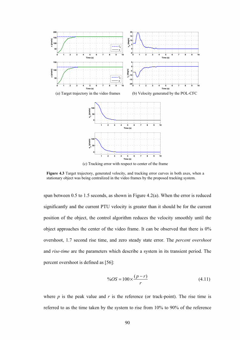
90
span between 0.5 to 1.5 seconds, as shown in Figure 4.2(a). When the error is reduced
significantly and the current PTU velocity is greater than it should be for the current
position of the object, the control algorithm reduces the velocity smoothly until the
object approaches the center of the video frame. It can be observed that there is 0%
overshoot, 1.7 second rise time, and zero steady state error. The percent overshoot
and rise-time are the parameters which describe a system in its transient period. The
percent overshoot is defined as [56]:
r
rpOS )(100% −×= (4.11)
where p is the peak value and r is the reference (or track-point). The rise time is
referred to as the time taken by the system to rise from 10% to 90% of the reference
0 1 2 3 4 5 6 7 8 9 10
50
100
150
200
Time (s)
x (p
ixel
s)
rx
x
0 1 2 3 4 5 6 7 8 9 10
50
100
150
Time (s)
y (p
ixel
s)
ry
y
0 1 2 3 4 5 6 7 8 9 10-5
0
5
10
15
20
Time (s)
v p (deg
/s)
0 1 2 3 4 5 6 7 8 9 10-20
-15
-10
-5
0
5
Time (s)
v t (deg
/s)
(a) Target trajectory in the video frames (b) Velocity generated by the POL-CFC
1 2 3 4 5 6 7 8 9 10
0
50
100
Time (s)
e x (pix
els)
1 2 3 4 5 6 7 8 9 10
0
50
100
Time (s)
e y (pix
els)
(c) Tracking error with respect to center of the frame
Figure 4.3 Target trajectory, generated velocity, and tracking error curves in both axes, when a stationary object was being centralized in the video frames by the proposed tracking system.

91
(or track-point) [56]. The steady state error is the deviation of the target coordinates
from the track-point, after the transient period of the system has passed. Thus, the
stationary target selected from a position farthest from the center of the frame is
perfectly centralized within 3 seconds.
The performance of the system was also tested for various moving objects
such as helicopters, airplanes, vehicles, walking and running persons, etc. in real-
world scenarios. In Figure 4.4, the results for a person with varying walking speed are
presented. Since there was no significant motion in the tilt axis in this example, the
results are shown only for the pan axis. It can be observed that the object is perfectly
centralized within 2 seconds and then it remains centralized accurately regardless of
the increasing velocity of the object. The small vibration in the curves is due to the
jerky motion of the walking person. This kind of vibration does not occur, when the
object being tracked is moving smoothly, e.g. airplane, helicopter, etc. In order to
validate the statement, the target trajectory in x-axis, the pan velocity, and the tracking
error in x-axis for the case of a flying helicopter are shown in Figure 4.5. In this
scenario, the helicopter was captured from the position (x, y) = (192, 118) in the frame
as shown by the initial point in the trajectory curve. Since the helicopter was moving
fast towards right and the camera was initially stationary, the helicopter in the video
0 2 4 6 8 10 12 14 16 18 20120
140
160
180
Time (s)
x (p
ixel
s)rx
x
0 2 4 6 8 10 12 14 16 18 20
2
3
4
5
6
Time (s)
v p (deg
/s)
0 2 4 6 8 10 12 14 16 18 20-20
0
20
40
60
Time (s)
e x (pix
els)
Figure 4.4 Target trajectory, velocity and tracking error curves for pan motion, when a walking person was being tracked.
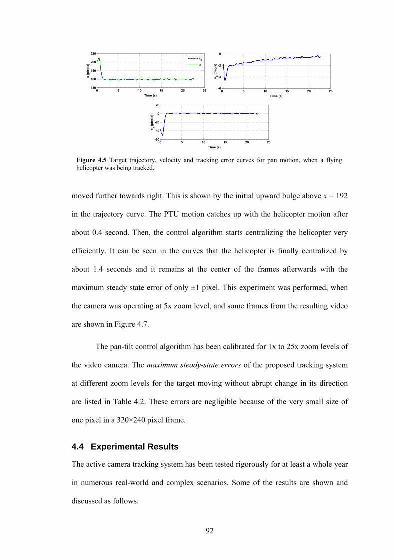
92
moved further towards right. This is shown by the initial upward bulge above x = 192
in the trajectory curve. The PTU motion catches up with the helicopter motion after
about 0.4 second. Then, the control algorithm starts centralizing the helicopter very
efficiently. It can be seen in the curves that the helicopter is finally centralized by
about 1.4 seconds and it remains at the center of the frames afterwards with the
maximum steady state error of only ±1 pixel. This experiment was performed, when
the camera was operating at 5x zoom level, and some frames from the resulting video
are shown in Figure 4.7.
The pan-tilt control algorithm has been calibrated for 1x to 25x zoom levels of
the video camera. The maximum steady-state errors of the proposed tracking system
at different zoom levels for the target moving without abrupt change in its direction
are listed in Table 4.2. These errors are negligible because of the very small size of
one pixel in a 320×240 pixel frame.
4.4 Experimental Results
The active camera tracking system has been tested rigorously for at least a whole year
in numerous real-world and complex scenarios. Some of the results are shown and
discussed as follows.
0 5 10 15 20 25140
160
180
200
220
Time (s)
x (p
ixel
s)
rx
x
0 5 10 15 20 25
-6
-4
-2
0
Time (s)
v p (deg
/s)
0 5 10 15 20 25-60
-40
-20
0
20
Time (s)e x (p
ixel
s)
Figure 4.5 Target trajectory, velocity and tracking error curves for pan motion, when a flying helicopter was being tracked.
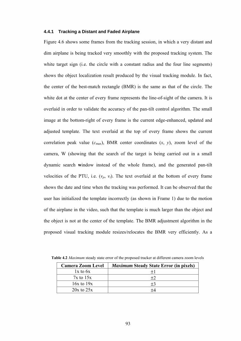
93
4.4.1 Tracking a Distant and Faded Airplane
Figure 4.6 shows some frames from the tracking session, in which a very distant and
dim airplane is being tracked very smoothly with the proposed tracking system. The
white target sign (i.e. the circle with a constant radius and the four line segments)
shows the object localization result produced by the visual tracking module. In fact,
the center of the best-match rectangle (BMR) is the same as that of the circle. The
white dot at the center of every frame represents the line-of-sight of the camera. It is
overlaid in order to validate the accuracy of the pan-tilt control algorithm. The small
image at the bottom-right of every frame is the current edge-enhanced, updated and
adjusted template. The text overlaid at the top of every frame shows the current
correlation peak value (cmax), BMR center coordinates (x, y), zoom level of the
camera, W (showing that the search of the target is being carried out in a small
dynamic search window instead of the whole frame), and the generated pan-tilt
velocities of the PTU, i.e. (vp, vt). The text overlaid at the bottom of every frame
shows the date and time when the tracking was performed. It can be observed that the
user has initialized the template incorrectly (as shown in Frame 1) due to the motion
of the airplane in the video, such that the template is much larger than the object and
the object is not at the center of the template. The BMR adjustment algorithm in the
proposed visual tracking module resizes/relocates the BMR very efficiently. As a
Table 4.2 Maximum steady state error of the proposed tracker at different camera zoom levels
Camera Zoom Level Maximum Steady State Error (in pixels) 1x to 6x ±1 7x to 15x ±2 16x to 19x ±3 20x to 25x ±4
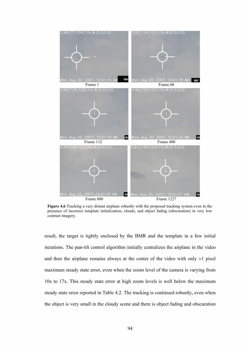
94
result, the target is tightly enclosed by the BMR and the template in a few initial
iterations. The pan-tilt control algorithm initially centralizes the airplane in the video
and then the airplane remains always at the center of the video with only ±1 pixel
maximum steady state error, even when the zoom level of the camera is varying from
10x to 17x. This steady state error at high zoom levels is well below the maximum
steady state error reported in Table 4.2. The tracking is continued robustly, even when
the object is very small in the cloudy scene and there is object fading and obscuration
Frame 1 Frame 60
Frame 112 Frame 400
Frame 800 Frame 1227
Figure 4.6 Tracking a very distant airplane robustly with the proposed tracking system even in the presence of incorrect template initialization, clouds, and object fading (obscuration) in very low contrast imagery.
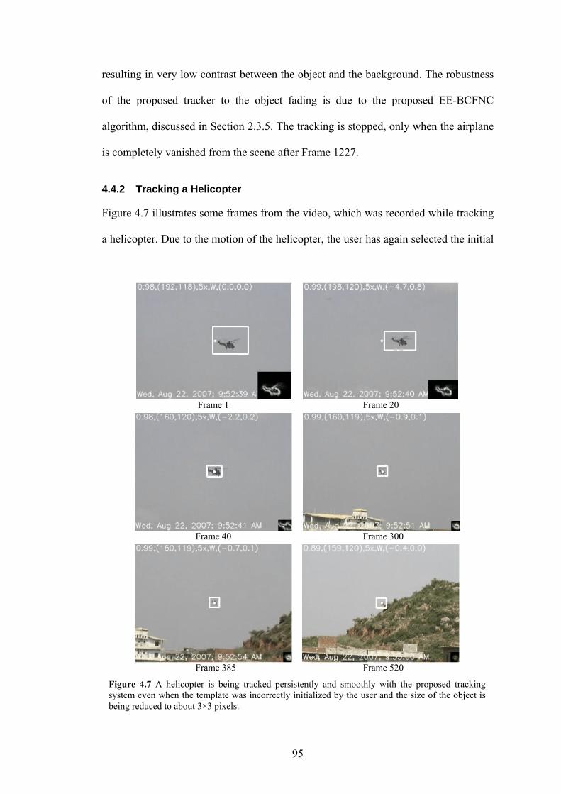
95
resulting in very low contrast between the object and the background. The robustness
of the proposed tracker to the object fading is due to the proposed EE-BCFNC
algorithm, discussed in Section 2.3.5. The tracking is stopped, only when the airplane
is completely vanished from the scene after Frame 1227.
4.4.2 Tracking a Helicopter
Figure 4.7 illustrates some frames from the video, which was recorded while tracking
a helicopter. Due to the motion of the helicopter, the user has again selected the initial
Frame 1 Frame 20
Frame 40 Frame 300
Frame 385 Frame 520
Figure 4.7 A helicopter is being tracked persistently and smoothly with the proposed tracking system even when the template was incorrectly initialized by the user and the size of the object is being reduced to about 3×3 pixels.
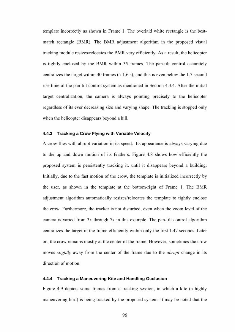
96
template incorrectly as shown in Frame 1. The overlaid white rectangle is the best-
match rectangle (BMR). The BMR adjustment algorithm in the proposed visual
tracking module resizes/relocates the BMR very efficiently. As a result, the helicopter
is tightly enclosed by the BMR within 35 frames. The pan-tilt control accurately
centralizes the target within 40 frames (≈ 1.6 s), and this is even below the 1.7 second
rise time of the pan-tilt control system as mentioned in Section 4.3.4. After the initial
target centralization, the camera is always pointing precisely to the helicopter
regardless of its ever decreasing size and varying shape. The tracking is stopped only
when the helicopter disappears beyond a hill.
4.4.3 Tracking a Crow Flying with Variable Velocity
A crow flies with abrupt variation in its speed. Its appearance is always varying due
to the up and down motion of its feathers. Figure 4.8 shows how efficiently the
proposed system is persistently tracking it, until it disappears beyond a building.
Initially, due to the fast motion of the crow, the template is initialized incorrectly by
the user, as shown in the template at the bottom-right of Frame 1. The BMR
adjustment algorithm automatically resizes/relocates the template to tightly enclose
the crow. Furthermore, the tracker is not disturbed, even when the zoom level of the
camera is varied from 3x through 7x in this example. The pan-tilt control algorithm
centralizes the target in the frame efficiently within only the first 1.47 seconds. Later
on, the crow remains mostly at the center of the frame. However, sometimes the crow
moves slightly away from the center of the frame due to the abrupt change in its
direction of motion.
4.4.4 Tracking a Maneuvering Kite and Handling Occlusion
Figure 4.9 depicts some frames from a tracking session, in which a kite (a highly
maneuvering bird) is being tracked by the proposed system. It may be noted that the
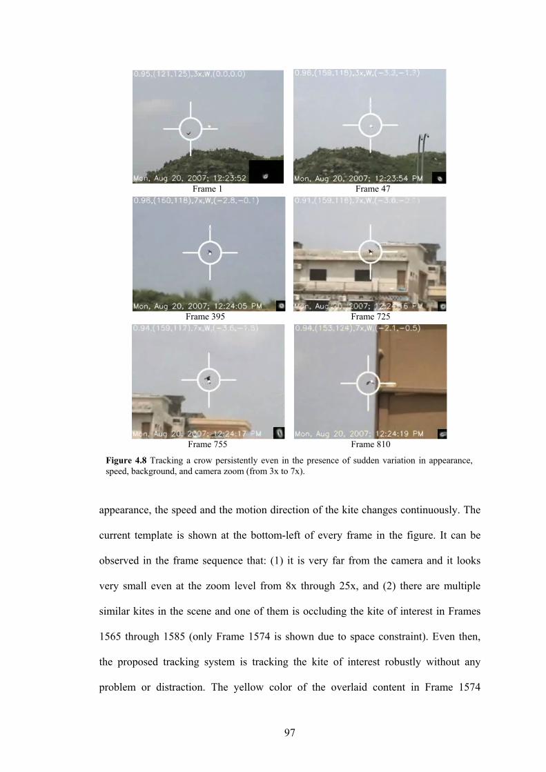
97
appearance, the speed and the motion direction of the kite changes continuously. The
current template is shown at the bottom-left of every frame in the figure. It can be
observed in the frame sequence that: (1) it is very far from the camera and it looks
very small even at the zoom level from 8x through 25x, and (2) there are multiple
similar kites in the scene and one of them is occluding the kite of interest in Frames
1565 through 1585 (only Frame 1574 is shown due to space constraint). Even then,
the proposed tracking system is tracking the kite of interest robustly without any
problem or distraction. The yellow color of the overlaid content in Frame 1574
Frame 1 Frame 47
Frame 395 Frame 725
Frame 755 Frame 810
Figure 4.8 Tracking a crow persistently even in the presence of sudden variation in appearance, speed, background, and camera zoom (from 3x to 7x).
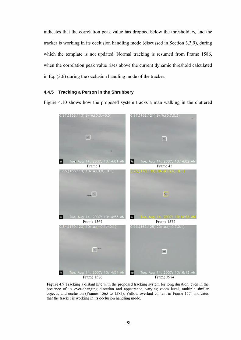
98
indicates that the correlation peak value has dropped below the threshold, τt, and the
tracker is working in its occlusion handling mode (discussed in Section 3.3.9), during
which the template is not updated. Normal tracking is resumed from Frame 1586,
when the correlation peak value rises above the current dynamic threshold calculated
in Eq. (3.6) during the occlusion handling mode of the tracker.
4.4.5 Tracking a Person in the Shrubbery
Figure 4.10 shows how the proposed system tracks a man walking in the cluttered
Frame 1 Frame 45
Frame 1564 Frame 1574
Frame 1586 Frame 3974
Figure 4.9 Tracking a distant kite with the proposed tracking system for long duration, even in the presence of its ever-changing direction and appearance, varying zoom level, multiple similar objects, and occlusion (Frames 1565 to 1585). Yellow overlaid content in Frame 1574 indicates that the tracker is working in its occlusion handling mode.
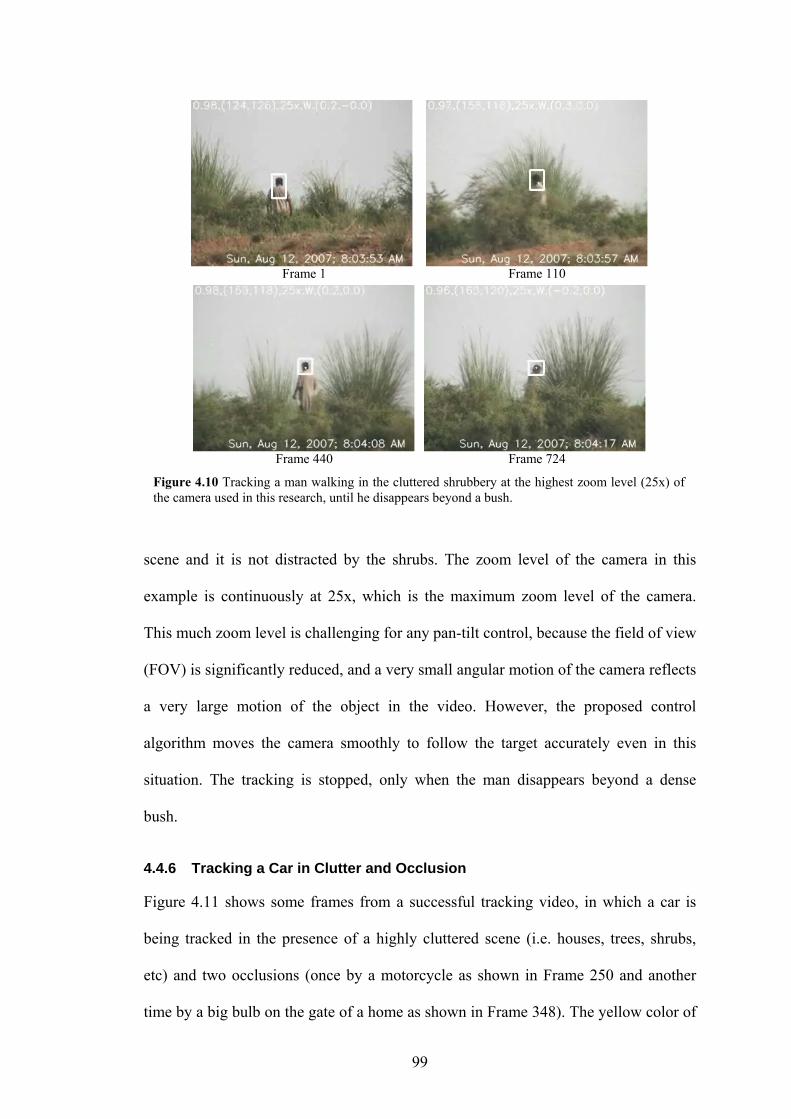
99
scene and it is not distracted by the shrubs. The zoom level of the camera in this
example is continuously at 25x, which is the maximum zoom level of the camera.
This much zoom level is challenging for any pan-tilt control, because the field of view
(FOV) is significantly reduced, and a very small angular motion of the camera reflects
a very large motion of the object in the video. However, the proposed control
algorithm moves the camera smoothly to follow the target accurately even in this
situation. The tracking is stopped, only when the man disappears beyond a dense
bush.
4.4.6 Tracking a Car in Clutter and Occlusion
Figure 4.11 shows some frames from a successful tracking video, in which a car is
being tracked in the presence of a highly cluttered scene (i.e. houses, trees, shrubs,
etc) and two occlusions (once by a motorcycle as shown in Frame 250 and another
time by a big bulb on the gate of a home as shown in Frame 348). The yellow color of
Frame 1 Frame 110
Frame 440 Frame 724
Figure 4.10 Tracking a man walking in the cluttered shrubbery at the highest zoom level (25x) of the camera used in this research, until he disappears beyond a bush.
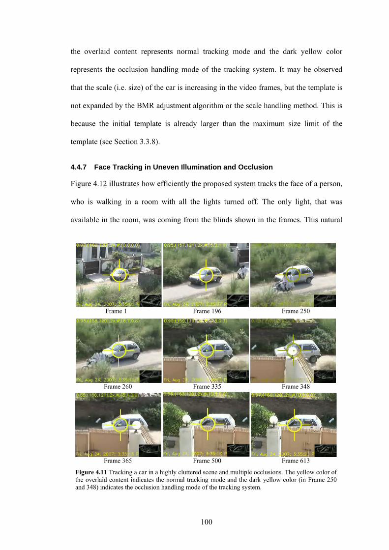
100
the overlaid content represents normal tracking mode and the dark yellow color
represents the occlusion handling mode of the tracking system. It may be observed
that the scale (i.e. size) of the car is increasing in the video frames, but the template is
not expanded by the BMR adjustment algorithm or the scale handling method. This is
because the initial template is already larger than the maximum size limit of the
template (see Section 3.3.8).
4.4.7 Face Tracking in Uneven Illumination and Occlusion
Figure 4.12 illustrates how efficiently the proposed system tracks the face of a person,
who is walking in a room with all the lights turned off. The only light, that was
available in the room, was coming from the blinds shown in the frames. This natural
Frame 1 Frame 196 Frame 250
Frame 260 Frame 335 Frame 348
Frame 365 Frame 500 Frame 613
Figure 4.11 Tracking a car in a highly cluttered scene and multiple occlusions. The yellow color of the overlaid content indicates the normal tracking mode and the dark yellow color (in Frame 250 and 348) indicates the occlusion handling mode of the tracking system.
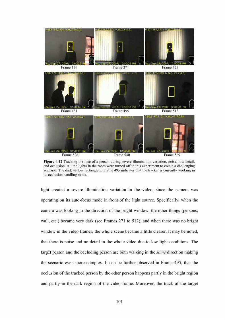
101
light created a severe illumination variation in the video, since the camera was
operating on its auto-focus mode in front of the light source. Specifically, when the
camera was looking in the direction of the bright window, the other things (persons,
wall, etc.) became very dark (see Frames 271 to 512), and when there was no bright
window in the video frames, the whole scene became a little clearer. It may be noted,
that there is noise and no detail in the whole video due to low light conditions. The
target person and the occluding person are both walking in the same direction making
the scenario even more complex. It can be further observed in Frame 495, that the
occlusion of the tracked person by the other person happens partly in the bright region
and partly in the dark region of the video frame. Moreover, the track of the target
Frame 176 Frame 271 Frame 325
Frame 481 Frame 495 Frame 512
Frame 528 Frame 540 Frame 569
Figure 4.12 Tracking the face of a person during severe illumination variation, noise, low detail, and occlusion. All the lights in the room were turned off in this experiment to create a challenging scenario. The dark yellow rectangle in Frame 495 indicates that the tracker is currently working in its occlusion handling mode.
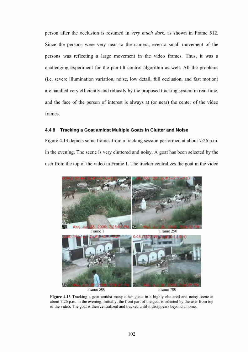
102
person after the occlusion is resumed in very much dark, as shown in Frame 512.
Since the persons were very near to the camera, even a small movement of the
persons was reflecting a large movement in the video frames. Thus, it was a
challenging experiment for the pan-tilt control algorithm as well. All the problems
(i.e. severe illumination variation, noise, low detail, full occlusion, and fast motion)
are handled very efficiently and robustly by the proposed tracking system in real-time,
and the face of the person of interest is always at (or near) the center of the video
frames.
4.4.8 Tracking a Goat amidst Multiple Goats in Clutter and Noise
Figure 4.13 depicts some frames from a tracking session performed at about 7:26 p.m.
in the evening. The scene is very cluttered and noisy. A goat has been selected by the
user from the top of the video in Frame 1. The tracker centralizes the goat in the video
Frame 1 Frame 250
Frame 500 Frame 700
Figure 4.13 Tracking a goat amidst many other goats in a highly cluttered and noisy scene at about 7:26 p.m. in the evening. Initially, the front part of the goat is selected by the user from top of the video. The goat is then centralized and tracked until it disappears beyond a home.
103
and tracks it robustly and persistently in the middle of many other goats, until it
disappears beyond the wall of a home. This tracking session shows the robustness of
the visual tracking algorithm to the noise, other similar objects, and background
clutter (i.e. grass, homes, people, logs, stones, debris, etc).
4.5 Chapter Summary
This chapter presented the design, implementation, analysis, and experimental results
of the proposed active camera tracking system (ACTS), that exploited the visual
tracking framework discussed in Chapter 3. The system offers 0% overshoot, 1.7
second rise time, and ±1 pixel maximum steady state error, if the object being tracked
does not change its direction of motion abruptly. The experimental results validate
that, due to the proposed visual tracking framework, the ACTS is quite able to track
any object of interest with a pan-tilt-zoom camera in real-world complex scenarios,
such as object fading, clutter, occlusion, uneven illumination, distraction by multiple
similar objects, noise, and change in scale, orientation, appearance, and velocity of the
object.
104
5 A Vision Based System for a UGV to Handle a Road Intersection
5
A Vision Based System for a UGV to Handle a Road Intersection
5.1 Chapter Overview
This chapter presents the design and implementation of a machine vision system that
exploits the proposed visual tracking framework discussed in Chapter 3. The system
enables an unmanned ground vehicle (UGV) to automatically handle a road
intersection [57]. The experimental results of the actual system deployed on a UGV
are also shown to validate its performance.
5.2 Problem Description
Consider the scenario of a UGV approaching a four way intersection regulated by a
stop sign. Traffic laws require that each vehicle must come to a stop before entering
the intersection and allow any other vehicles that arrive earlier to pass first. The UGV
must effectively wait for its turn and look for the leading vehicles at the other roads
that want to pass the intersection. It is not sufficient to simply detect the presence of
other vehicles at the intersection, since the UGV should have the right-of-way if other
vehicles approach the intersection after it has already stopped. Thus, it will be
necessary to determine the behavior of each other vehicle, i.e. whether it is just
arriving at the intersection, waiting for its turn to go, or already passing through. It is
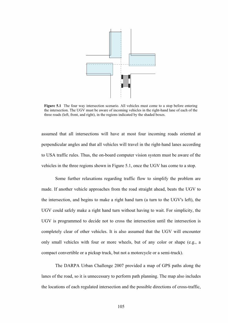
105
assumed that all intersections will have at most four incoming roads oriented at
perpendicular angles and that all vehicles will travel in the right-hand lanes according
to USA traffic rules. Thus, the on-board computer vision system must be aware of the
vehicles in the three regions shown in Figure 5.1, once the UGV has come to a stop.
Some further relaxations regarding traffic flow to simplify the problem are
made. If another vehicle approaches from the road straight ahead, beats the UGV to
the intersection, and begins to make a right hand turn (a turn to the UGV's left), the
UGV could safely make a right hand turn without having to wait. For simplicity, the
UGV is programmed to decide not to cross the intersection until the intersection is
completely clear of other vehicles. It is also assumed that the UGV will encounter
only small vehicles with four or more wheels, but of any color or shape (e.g., a
compact convertible or a pickup truck, but not a motorcycle or a semi-truck).
The DARPA Urban Challenge 2007 provided a map of GPS paths along the
lanes of the road, so it is unnecessary to perform path planning. The map also includes
the locations of each regulated intersection and the possible directions of cross-traffic,
Figure 5.1 The four way intersection scenario. All vehicles must come to a stop before entering the intersection. The UGV must be aware of incoming vehicles in the right-hand lane of each of the three roads (left, front, and right), in the regions indicated by the shaded boxes.
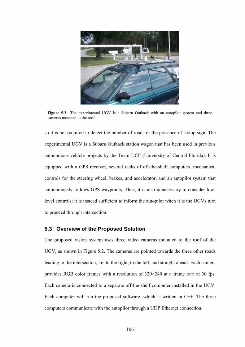
106
so it is not required to detect the number of roads or the presence of a stop sign. The
experimental UGV is a Subaru Outback station wagon that has been used in previous
autonomous vehicle projects by the Team UCF (University of Central Florida). It is
equipped with a GPS receiver, several racks of off-the-shelf computers, mechanical
controls for the steering wheel, brakes, and accelerator, and an autopilot system that
autonomously follows GPS waypoints. Thus, it is also unnecessary to consider low-
level controls; it is instead sufficient to inform the autopilot when it is the UGVs turn
to proceed through intersection.
5.3 Overview of the Proposed Solution
The proposed vision system uses three video cameras mounted to the roof of the
UGV, as shown in Figure 5.2. The cameras are pointed towards the three other roads
leading to the intersection, i.e. to the right, to the left, and straight ahead. Each camera
provides RGB color frames with a resolution of 320×240 at a frame rate of 30 fps.
Each camera is connected to a separate off-the-shelf computer installed in the UGV.
Each computer will run the proposed software, which is written in C++. The three
computers communicate with the autopilot through a UDP Ethernet connection.
Figure 5.2 The experimental UGV is a Subaru Outback with an autopilot system and three cameras mounted to the roof.
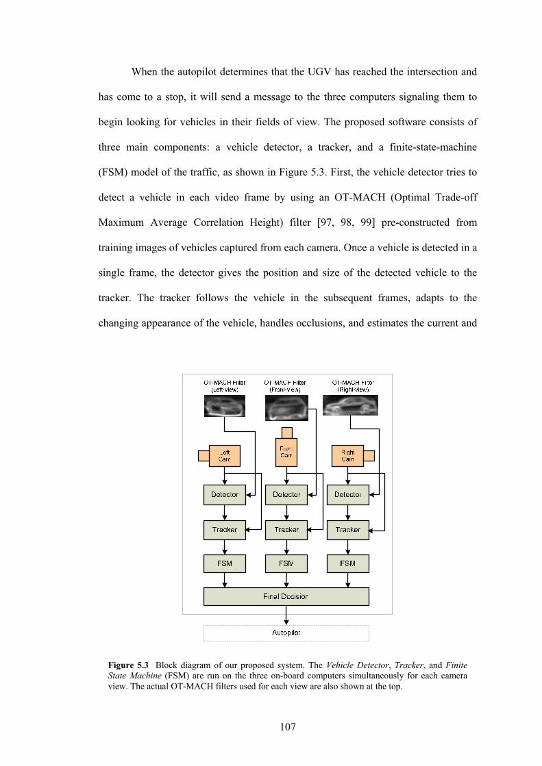
107
When the autopilot determines that the UGV has reached the intersection and
has come to a stop, it will send a message to the three computers signaling them to
begin looking for vehicles in their fields of view. The proposed software consists of
three main components: a vehicle detector, a tracker, and a finite-state-machine
(FSM) model of the traffic, as shown in Figure 5.3. First, the vehicle detector tries to
detect a vehicle in each video frame by using an OT-MACH (Optimal Trade-off
Maximum Average Correlation Height) filter [97, 98, 99] pre-constructed from
training images of vehicles captured from each camera. Once a vehicle is detected in a
single frame, the detector gives the position and size of the detected vehicle to the
tracker. The tracker follows the vehicle in the subsequent frames, adapts to the
changing appearance of the vehicle, handles occlusions, and estimates the current and
Figure 5.3 Block diagram of our proposed system. The Vehicle Detector, Tracker, and Finite State Machine (FSM) are run on the three on-board computers simultaneously for each camera view. The actual OT-MACH filters used for each view are also shown at the top.
108
next position of the vehicle in the imagery. A finite state machine (FSM) model is
used to determine the state of the leading vehicle in each view. The states of the
leading vehicle in each view are then used to make a final decision about when it is
safe for the autopilot to drive the UGV through the intersection. All the components
of the proposed solution are discussed separately in the next sections.
5.4 Vehicle Detector
The first step of the proposed solution is to detect a vehicle in a video frame by
matching an appearance template that has been prepared for each of the three views.
The template is basically an OT-MACH (Optimal Trade-off Maximum Average
Correlation Height) filter, which combines the training images into a single composite
template by optimizing four performance metrics: the Average Correlation Height
(ACH), the Average Correlation Energy (ACE), the Average Similarity Measure
(ASM), and the Output Noise Variance (ONV), as explained in [97, 98, 99]. Since
each incoming vehicle from a given road is oriented in approximately the same pose,
and since the UGV always sees each road in the intersection from roughly the same
point of view, this method produces a template that expresses the general shape of a
vehicle in each view. The color invariance is achieved by using edge-enhanced
images instead of the original color frames as described in [58]. The edge-enhanced
OT-MACH filter generated for each of the three views is shown in Figure 5.3.
Once the edge-enhanced OT-MACH filter is prepared, it is applied to edge-
enhanced search window inside the incoming video frames by performing normalized
cross-correlation very efficiently as discussed in Chapter 2. The highest peak in the
correlation response is compared with a threshold. The threshold was determined just
after the synthesis of the filter as 1 2 30.95min( , , ,..., )Np p p pτ = , where pi is the
correlation peak value obtained when the filter was applied on ith training image, and
109
N is the total number of the training images. The 95% of the minimum peak value is
used in order to tolerate small amount of perturbation of the actual vehicles from the
vehicles used in the training phase. If the peak is greater than the threshold, it
indicates the position of a vehicle; otherwise it is assumed that there is no vehicle in
the scene.
The most significant change in the appearance of vehicles between different
intersections comes from varying number and width of lanes. A specific solution is
proposed to this uncertainty in distance between the camera and the vehicle. The filter
is obtained from the training images each resized to an average size, but the detection
is performed with several rescaled versions of the average size filter. The scales are
80%, 100%, and 120% of the size of the original OT-MACH filter. After computing
the correlation at each scale, the scale that produces the maximum correlation peak
decides the size of the vehicle in the image.
5.5 Tracker
While the vehicle detector locates a vehicle in a single frame, the tracker is intended
to follow the vehicle in the subsequent frames to determine its current and next
position, velocity, and acceleration. The tracker is initialized using the image
rectangle identified by the vehicle detector. While the detector uses only the prior
knowledge of the appearance of a vehicle, the tracking stage ignores the prior
knowledge and instead exploits the temporal and spatial consistency of appearance
from frame to frame. This tracker is basically the same as the one discussed in
Chapter 3. The current and predicted position of the vehicle coming from every road
under observation is used by the finite-state-machine (discussed in the next section) to
determine the state of the traffic on the intersection.
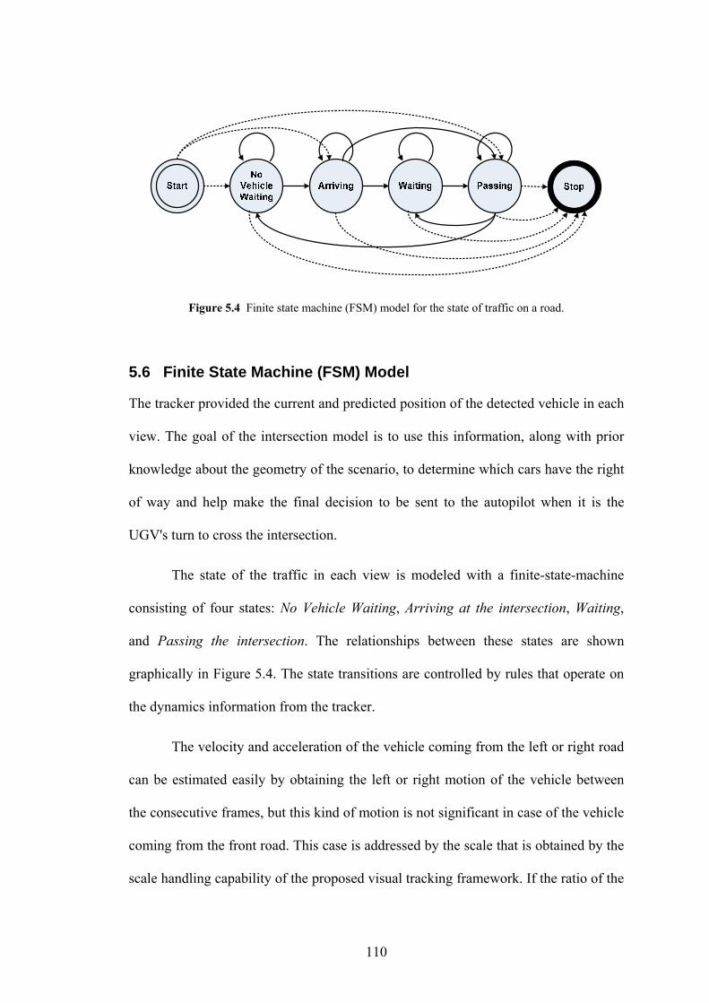
110
5.6 Finite State Machine (FSM) Model
The tracker provided the current and predicted position of the detected vehicle in each
view. The goal of the intersection model is to use this information, along with prior
knowledge about the geometry of the scenario, to determine which cars have the right
of way and help make the final decision to be sent to the autopilot when it is the
UGV's turn to cross the intersection.
The state of the traffic in each view is modeled with a finite-state-machine
consisting of four states: No Vehicle Waiting, Arriving at the intersection, Waiting,
and Passing the intersection. The relationships between these states are shown
graphically in Figure 5.4. The state transitions are controlled by rules that operate on
the dynamics information from the tracker.
The velocity and acceleration of the vehicle coming from the left or right road
can be estimated easily by obtaining the left or right motion of the vehicle between
the consecutive frames, but this kind of motion is not significant in case of the vehicle
coming from the front road. This case is addressed by the scale that is obtained by the
scale handling capability of the proposed visual tracking framework. If the ratio of the
Figure 5.4 Finite state machine (FSM) model for the state of traffic on a road.
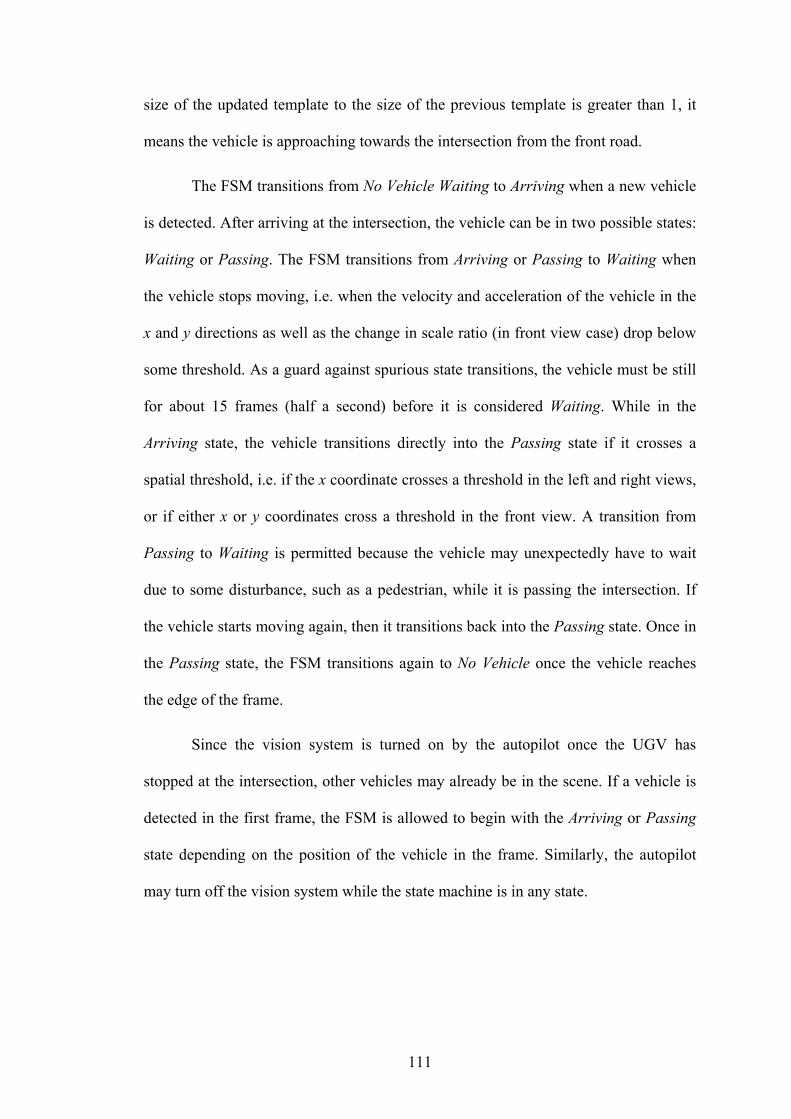
111
size of the updated template to the size of the previous template is greater than 1, it
means the vehicle is approaching towards the intersection from the front road.
The FSM transitions from No Vehicle Waiting to Arriving when a new vehicle
is detected. After arriving at the intersection, the vehicle can be in two possible states:
Waiting or Passing. The FSM transitions from Arriving or Passing to Waiting when
the vehicle stops moving, i.e. when the velocity and acceleration of the vehicle in the
x and y directions as well as the change in scale ratio (in front view case) drop below
some threshold. As a guard against spurious state transitions, the vehicle must be still
for about 15 frames (half a second) before it is considered Waiting. While in the
Arriving state, the vehicle transitions directly into the Passing state if it crosses a
spatial threshold, i.e. if the x coordinate crosses a threshold in the left and right views,
or if either x or y coordinates cross a threshold in the front view. A transition from
Passing to Waiting is permitted because the vehicle may unexpectedly have to wait
due to some disturbance, such as a pedestrian, while it is passing the intersection. If
the vehicle starts moving again, then it transitions back into the Passing state. Once in
the Passing state, the FSM transitions again to No Vehicle once the vehicle reaches
the edge of the frame.
Since the vision system is turned on by the autopilot once the UGV has
stopped at the intersection, other vehicles may already be in the scene. If a vehicle is
detected in the first frame, the FSM is allowed to begin with the Arriving or Passing
state depending on the position of the vehicle in the frame. Similarly, the autopilot
may turn off the vision system while the state machine is in any state.
112
5.7 Final Decision
In order to decide when to cross the intersection, the system combines the traffic
information from all the three FSMs. If the vehicle on the other road is already
Waiting when the UGV arrives at the intersection, then it has the right-of-way, and the
UGV is commanded to wait for it to leave the scene before proceeding. If at any time
a vehicle is Passing the intersection, the UGV is commanded not to cross. Since a
vehicle will reach the edge of the frame before it has crossed the intersection, the
UGV waits for two seconds after the corresponding FSM stops indicating that the
vehicle is passing. Any vehicle that is Arriving or Waiting after the UGV arrives does
not have the right-of-way, so it is assumed they will let the UGV pass the intersection.
5.8 Experimental Results
The low-level components of the system were tested by parking the UGV at several
real four-way intersections at which one of the roads was a dead end, so the traffic
was not interfered. It is easy to objectively evaluate the vehicle detector since the total
number of visible vehicles is a discrete and unambiguous value. Table 5.1 shows the
number of successfully detected vehicles, as well as the false alarms and
misdetections for each camera view. The tradeoff between false alarms and
misdetections is controlled by the parameters and thresholds. The misdetections were
favored over false alarms, since if the tracker got stuck on a patch of stationary
background clutter, the UGV would wait indefinitely. Since these results were
gathered from several intersections with uncontrolled traffic, they demonstrate the
robustness and generalization of the detection system.
For testing the entire system as a whole, each experiment was staged as a
coordinated event where the UGV and another vehicle (operated by a human driver)
would approach the intersection in an agreed-upon order. The results for these
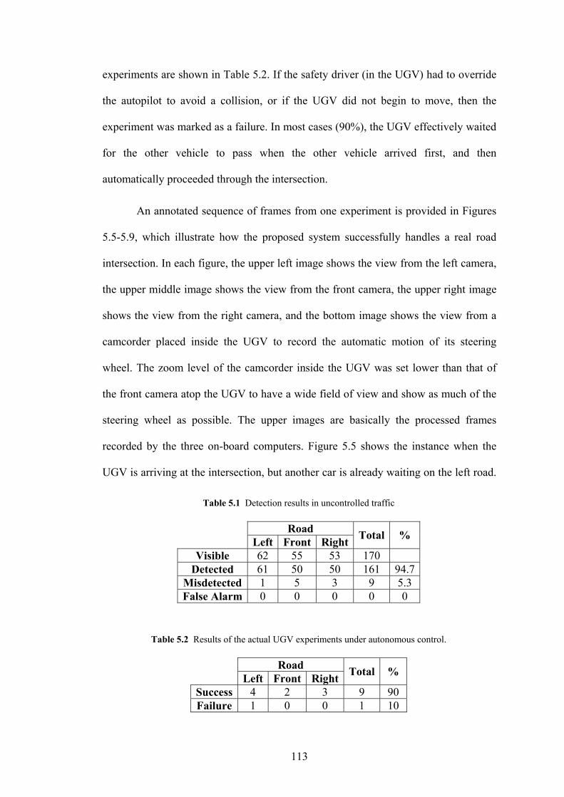
113
experiments are shown in Table 5.2. If the safety driver (in the UGV) had to override
the autopilot to avoid a collision, or if the UGV did not begin to move, then the
experiment was marked as a failure. In most cases (90%), the UGV effectively waited
for the other vehicle to pass when the other vehicle arrived first, and then
automatically proceeded through the intersection.
An annotated sequence of frames from one experiment is provided in Figures
5.5-5.9, which illustrate how the proposed system successfully handles a real road
intersection. In each figure, the upper left image shows the view from the left camera,
the upper middle image shows the view from the front camera, the upper right image
shows the view from the right camera, and the bottom image shows the view from a
camcorder placed inside the UGV to record the automatic motion of its steering
wheel. The zoom level of the camcorder inside the UGV was set lower than that of
the front camera atop the UGV to have a wide field of view and show as much of the
steering wheel as possible. The upper images are basically the processed frames
recorded by the three on-board computers. Figure 5.5 shows the instance when the
UGV is arriving at the intersection, but another car is already waiting on the left road.
Table 5.2 Results of the actual UGV experiments under autonomous control.
Road Left Front Right Total %
Success 4 2 3 9 90 Failure 1 0 0 1 10
Table 5.1 Detection results in uncontrolled traffic
Road Left Front Right Total %
Visible 62 55 53 170 Detected 61 50 50 161 94.7
Misdetected 1 5 3 9 5.3 False Alarm 0 0 0 0 0
114
The computer vision system is not turned on, because the UGV has not reached the
stop sign yet. Figure 5.6 shows the instance when the UGV stops and turns on the
proposed computer vision system. The system detects that a car is already waiting at
the left road and commands the UGV to wait. The detected vehicle is surrounded by
the best-match rectangle (BMR) overlaid in the left view. The large rectangles on the
front and right views indicate the corresponding areas where the vehicles are being
searched for by the vehicle detector using the corresponding OT-MACH filters. The
vehicles were being searched for in these small areas of interest instead of the whole
frames, in order to reduce the computation time in the correlation process and
eliminate the possible false detections due to the background clutter. The small
images overlaid at the bottom-left of every frame shows either the OT-MACH filters
(if there is no vehicle on the road) or the current adaptive template (if there is a
vehicle being tracked by the proposed tracker). The first line of the text indicates the
maximum correlation value and the coordinates of the center of the best match
rectangle (BMR). The BMR is shown only when the correlation value is above some
threshold (as can be seen in the left view). The second line of the text indicates the
scale of the OT-MACH filter that provides the maximum correlation value in the
detection mode. The third line of the text indicates the road state provided by the
corresponding FSM. Figure 5.7 shows the instance when the car at the other road
begins to pass the intersection. The FSM for the left road correctly senses that the car
is passing the intersection, as can be seen in the overlaid text. Figure 5.8 shows the
instance when the car has exited the view of the left camera, although it is still visible
in the video frames from the front camera and the camcorder. Since there were no
vehicles on the right and the front roads, and the car has exited the view of the left
road. The decision is made that it is now the UGV’s turn to pass the intersection, so
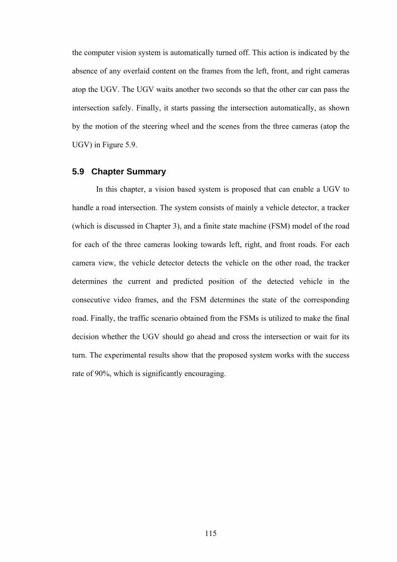
115
the computer vision system is automatically turned off. This action is indicated by the
absence of any overlaid content on the frames from the left, front, and right cameras
atop the UGV. The UGV waits another two seconds so that the other car can pass the
intersection safely. Finally, it starts passing the intersection automatically, as shown
by the motion of the steering wheel and the scenes from the three cameras (atop the
UGV) in Figure 5.9.
5.9 Chapter Summary
In this chapter, a vision based system is proposed that can enable a UGV to
handle a road intersection. The system consists of mainly a vehicle detector, a tracker
(which is discussed in Chapter 3), and a finite state machine (FSM) model of the road
for each of the three cameras looking towards left, right, and front roads. For each
camera view, the vehicle detector detects the vehicle on the other road, the tracker
determines the current and predicted position of the detected vehicle in the
consecutive video frames, and the FSM determines the state of the corresponding
road. Finally, the traffic scenario obtained from the FSMs is utilized to make the final
decision whether the UGV should go ahead and cross the intersection or wait for its
turn. The experimental results show that the proposed system works with the success
rate of 90%, which is significantly encouraging.
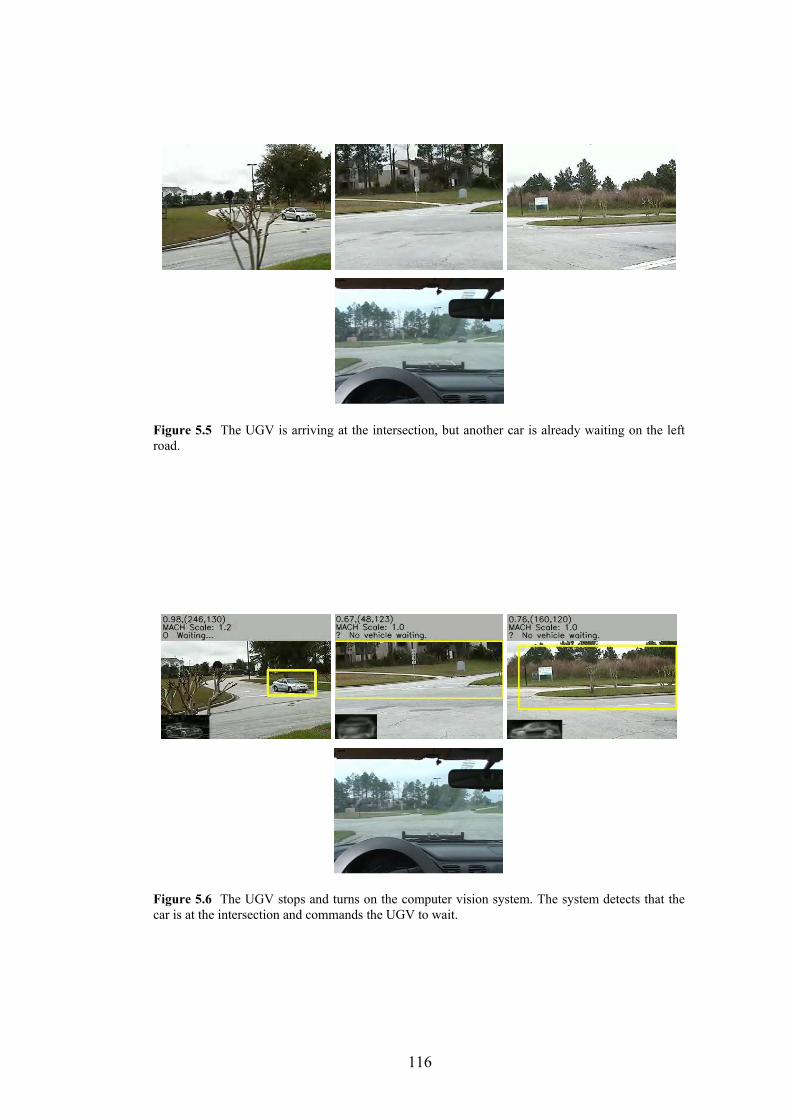
116
Figure 5.6 The UGV stops and turns on the computer vision system. The system detects that the car is at the intersection and commands the UGV to wait.
Figure 5.5 The UGV is arriving at the intersection, but another car is already waiting on the left road.
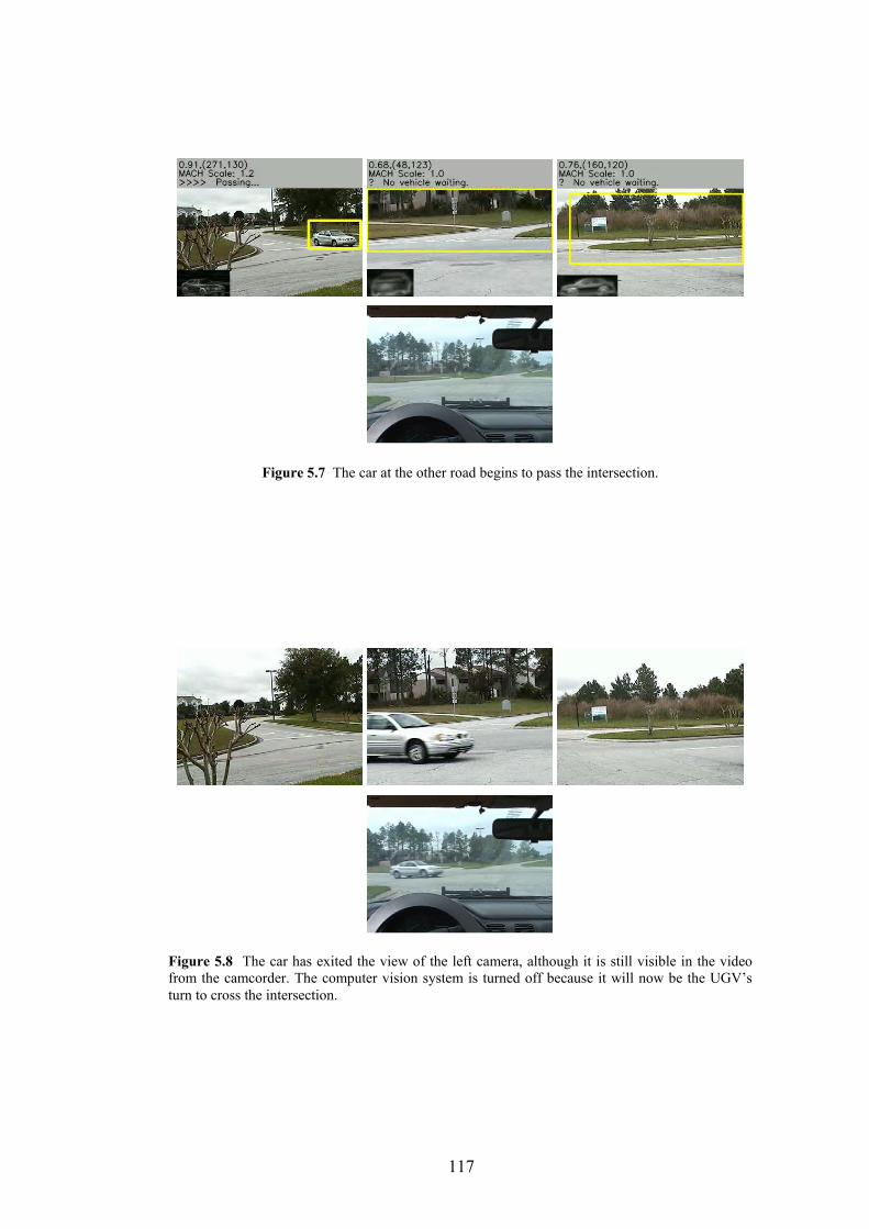
117
Figure 5.8 The car has exited the view of the left camera, although it is still visible in the video from the camcorder. The computer vision system is turned off because it will now be the UGV’s turn to cross the intersection.
Figure 5.7 The car at the other road begins to pass the intersection.
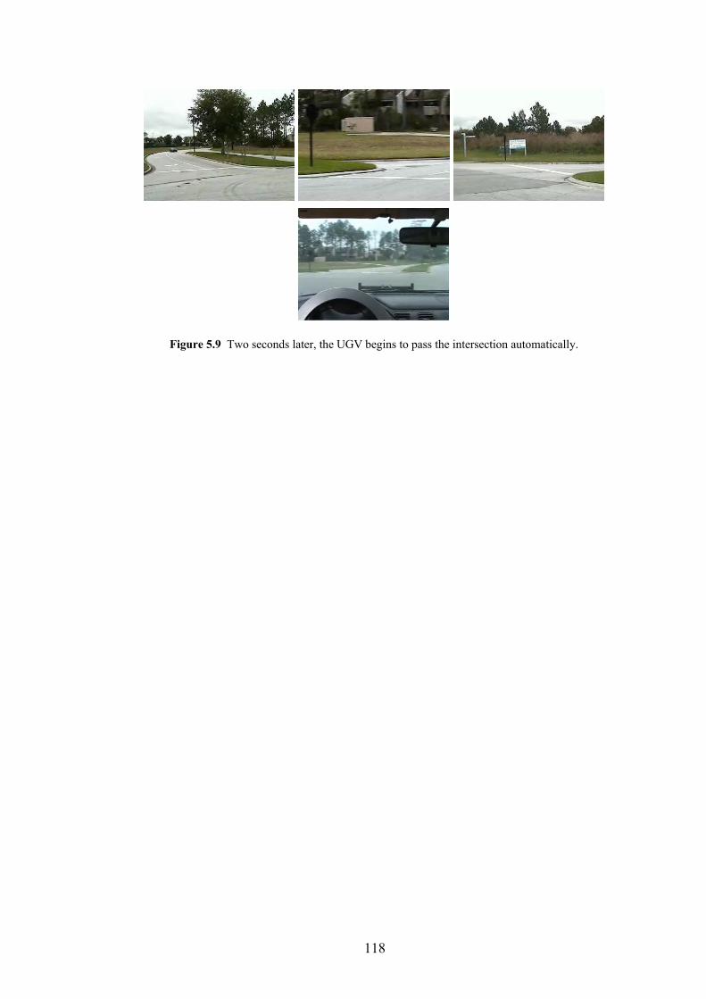
118
Figure 5.9 Two seconds later, the UGV begins to pass the intersection automatically.
119
6 Conclusion and Future Directions
6
Conclusion and Future Directions
The thesis presented an adaptive edge-enhanced correlation based robust and real-
time visual tracking framework, and its deployment in two machine vision systems:
(1) an active camera tracking system, and (2) a system for a UGV to handle road
intersections. In this chapter, the conclusion and the future work for the visual
tracking framework and the machine vision systems based on it are drawn and
presented, respectively.
6.1 Visual Tracking Framework
The proposed visual tracking algorithm is based on edge-enhanced BPNN-controlled
fast normalized correlation (EE-BCFNC). The edge-enhancement (EE) operation in
the EE-BCFNC is performed using Gaussian smoothing filter with an automatic
standard deviation parameter, gradient magnitude, normalization, and thresholding.
This kind of enhancement helps the correlation process handle object fading, low-
contrast imagery and variation in the scene illumination in a better way and provides
cleaner peak at the object location in the correlation surface than the most commonly
used normalized correlation coefficient (NCC). The next operation in the EE-BCFNC
is the BCFNC (BPNN-controlled fast normalized correlation), which exploits a back-
propagation neural network (BPNN) to work as a switch between two

120
implementations of the normalized correlation (NC): direct method and FFT-SAT
(fast Fourier transform – summed area table) method. The BPNN predicts which
implementation will be faster for computing NC, given the search-window-size and
the ratio of the template-size to the search-window-size. The varying scale of the
object is handled by preparing scaled versions of the template, correlating them
individually with the search window, and accepting the best scale, which produces the
highest correlation peak in all the three correlation surfaces. The long-term
neighboring clutter is dealt with by applying a 2D Gaussian weighting on the template
pixels, using automatically computed optimal standard deviation parameters
depending on the size of the current template. An effective and smooth method for
updating the template is also introduced to handle the varying object appearance, the
short-term neighboring clutter, and to some extent the template-drift. In order to
formally handle the template drift and the inaccurate object initialization problems, a
best match rectangle adjustment algorithm has been proposed. The visual tracking
algorithm has been further improved using a Kalman predictor, in which a “constant
acceleration with random walk” model of the target motion is used for good
prediction accuracy. A novel method is presented to dynamically determine the
location and size of the search-window depending on the prediction and the
prediction-error of the Kalman filter. The occlusion of the target by other object(s) has
been handled using a simple data association technique. The proposed algorithm has
been compared with the most commonly used correlation tracker, and (for some
sequences) the mean-shift and the condensation trackers. The results prove that the
proposed tracker outperforms them in the presence of temporary object fading,
significant background clutter, variations in the size of the object, variations in the
illumination conditions, significant object maneuvering, multiple objects, obscuration,
121
and intermittent occlusion of the object, and variation in velocity, shape and
orientation of the object.
The computational efficiency of the spatial domain implementation of NC for
template matching can be further improved using the early termination algorithms, for
example [101]. Then, its efficiency can be compared with the FFT-SAT method for
different sizes of the templates and search images. If there is a significant difference
between their computational efficiencies for different sizes of the images, the BPNN
can be trained accordingly to switch between the two implementations.
Furthermore, a significant improvement in the proposed visual tracking
framework would be to address the following complex real-world situations in which
it may fail:
• A moving object is completely occluded by other object(s) for a very long
duration, when the object changes its shape, speed, or direction
significantly during the occlusion.
• The object is being occluded very slowly, in which case the correlation
peak never falls below the threshold (τt) to sense the occurrence of the
occlusion, because in this scenario the template is continuously being
updated and the occluding object slowly invades into the template.
• There is a lot of clutter including exactly similar objects having similar
orientation and scale in the search window as that of the object of interest.
• The object is changing its appearance fast, while its scale is increasing, e.g.
a turning vehicle coming nearer the camera.
122
6.2 Active Camera Tracking System
As far as the active camera tracking system is concerned, a predictive open-loop car-
following control (POL-CFC) has been presented to maneuver the pan-tilt unit (PTU),
which moves the camera towards the object. The control algorithm calculates the
predictive velocity of the object to be tracked using Kalman predicted position
estimated by the visual tracking algorithm, and then smoothly adjusts the velocity of
the PTU accordingly (without using any velocity feedback from the motors). As a
result, the object remains always locked to the line-of-sight of the camera with good
accuracy, regardless of the change in the velocity of the object. The POL-CFC
algorithm offers 0% overshoot, 1.7 second rise-time, and ±1 pixel maximum steady
state error for an object, which does not change its direction of motion abruptly. The
steady state error is slightly increased, if the zoom level is more than 6x. The
maximum error, while the camera is working at its highest zoom level of 25x, is only
±4 pixels from the center of the frame. However, if the object is changing its direction
fast, the error may be increased further depending on the rate of change of the
direction of the object motion. Nevertheless, the object remains always near the center
of the frame. The precision of the motion controller depends mainly on the resolution
of the PTU. Presently, a stepper-motor based PTU having resolution of 0.01285
degree/step is used. If a servo-motor based PTU having better resolution is used, the
tracking can be smoother and more precise, especially when the camera is operating at
very high zoom level.
The visual tracking algorithm and the pan-tilt control algorithm are
implemented in separate threads exploiting the parallel processing capability of the
presently available microprocessor in a standard PC. The throughput of the integrated

123
system is 25 to 75 fps (on a Centrino P4 1.7 GHz machine with 512 MB RAM)
depending on the sizes of the adaptive template and the dynamic search window.
The system has been tested for more than a year in real-world indoor as well
as outdoor scenarios. Some of the frames from the resulting videos recorded during
various tracking sessions have been presented in this thesis. They prove that the
system works very efficiently and robustly in the real-world complex scenarios.
6.3 A Vision Based System for a UGV to Handle a Road Intersection
UGVs will have to develop the capability to safely cross intersections with stop signs
if they are going to be deployed in urban environments. In this research, some
analysis of this specific problem is provided and a complete computer vision solution
that combines a vehicle detection-and-tracking algorithm with a finite-state-machine
model of the traffic near the intersection to automatically navigate the UGV through
the intersection is proposed. The initial experiments of the system suggest that a
computer vision approach can be the basis of an effective solution, but a truly robust
system will need to better deal with subtle uncertainties in such a scenario. For
example, it is currently assumed that the vehicle will take no more than two seconds
to pass the intersection, but it is possible that the vehicle will unexpectedly stop while
it is outside the view of the camera. The next work can be to address this problem by
combining the output from the computer vision system with other systems, like a laser
range finder, which can detect obstacles in the immediate path of the UGV.
124
References
[1] Y. Cui, S. Samarasekera, Q. Huang, M Greienhagen, “Indoor Monitoring Via the Collaboration
Between a Peripheral Sensor and a Foveal Sensor,” IEEE Workshop on Visual Surveillance,
Bombay, India, 2-9, 1998.
[2] G. R. Bradski, “Computer Vision Face Tracking as a Component of a Perceptual User
Interface,” IEEE Workshop on Applications of Computer Vision, Princeton, 214-219, 1998.
[3] S. S. Intille, J.W. Davis, A.F. Bobick, “Real-Time Closed-World Tracking,” IEEE Conference
on Computer Vision and Pattern Recognition, Puerto Rico, 697-703, 1997.
[4] C. Wren, A. Azarbayejani, T. Darrell, A. Pentland, “PFinder: Real-Time Tracking of the Human
Body,” IEEE Transactions on Pattern Analysis Machine Intelligence, 19:780-785, 1997.
[5] A. Eleftheriadis, A. Jacquin, “Automatic Face Location Detection and Tracking for Model-
Assisted Coding of Video Teleconference Sequences at Low Bit Rates,” Signal
Processing−Image Communication, 7(3): 231-248, 1995.
[6] R. Rosales, S. Sclaro, “3D Trajectory Recovery for Tracking Multiple Objects and Trajectory
Guided Recognition of Actions,” IEEE Conference on Computer Vision and Pattern
Recognition, Fort Collins, vol. 2, 117-123, 1999.
[7] J. Ahmed, M. N. Jafri, J. Ahmad, and M. I. Khan, “Design and Implementation of a Neural
Network for Real-Time Object Tracking,” International Conference on Machine Vision and
Pattern Recognition in Conjunction with 4th World Enformatika Conference, Istanbul, 2005.
[8] J. Ahmed, M. N. Jafri, J. Ahmad, “Target Tracking in an Image Sequence Using Wavelet
Features and a Neural Network,” IEEE Region 10: Tencon’05 Conference, Melbourne,
Australia, 2005
[9] A. Doulamis, N. Doulamis, K. Ntalianis, and S. Kollias, “An Efficient Fully Unsupervised
Video Object Segmentation Scheme Using an Adaptive Neural-Network Classifier
Architecture,” IEEE Transaction on Neural Networks, May 2003.
[10] E. V. Cuevas, D. Zaldivar, and R. Rojas, “Intelligent Tracking,” Technical Report B-03-15,
Freie Universitat Berlin, Germany, November 10, 2003.
[11] S. Blackman and R. Popoli, Design and Analysis of Modern Tracking Systems, pp. 309-313,
Artech House, Boston, 1999.
125
[12] S. Wong, “Advanced Correlation Tracking of Objects in Cluttered Imagery,” Proceedings of
SPIE, Vol. 5810, 2005.
[13] R. C. Gonzalez, R. E. Woods, Digital Image Processing, 2nd Ed., Prentice-Hall, Inc., 2002
[14] N. Mir-Nasiri, “Camera-based 3D Tracking,” IEEE Region 10: Tencon’05 Conference,
Melbourne, Australia, 2005.
[15] “Basic Control Law for PTU to Follow a Moving Target,” Application Note 01, Directed
Perception Inc., 1996.
[16] J. P. Lewis, “Fast Normalized Cross-Correlation”, Industrial Light & Magic, 1995.
[17] R. C. Gonzalez, R. E. Woods, and S. L. Eddins, Digtal Image Processing Using MATLAB,
Pearson Education Pte. Ltd., 2004.
[18] F. Crow, “Summed-Area Tables for Texture Mapping”, Computer Graphics, vol 18, No. 3, pp.
207-212, 1984.
[19] G. X. Ritter and J. N. Wilson, Handbook of Computer Vision Algorithms in Image Algebra.
CRC Press, Boca Raton, Fl., 1996.
[20] C. Kuglin and D. Hines, “The Phase Correlation Image Alignment Method,” International
Conference on Cybernetics and Society, 1975, pp. 163-165.
[21] Q. Chen, M. Defrise, and F. Deconinck, “Symmetric Phase-Only Matched Filtering of Fourier-
Mellin Transforms for Image Registration and Recognition,” IEEE Transactions on Pattern
Analysis and Machine Intelligence, Vol.16, December, 1994.
[22] H. S. Stone and B. Tao and M. McGuire, “Analysis of Image Registration Noise Due to
Rotationally Dependent Aliasing,” Journal of Visual Communication and Image Representation,
Vol. 14, pp. 114-135, 2003.
[23] H. S. Stone, “Fourier-Based Image Registration Techniques”, NEC Research, 2002.
[24] H. Demuth, and M. Beale, Neural Network Toolbox for Use with MATLAB: User’s Guide (v. 4),
The Mathworks, Inc., 2001.
[25] S. Haykin, Neural Networks: A Comprehensive Foundation, 2nd Ed., Pearson Education, Delhi,
1999.
[26] L. Fausett, Fundamentals of Neural Networks: Architectures, Algorithms, and Applications,
Prentice Hall, Englewood Cliffs, 1994.

126
[27] M. F. Moller, “A Scaled Conjugate Gradient Algorithm for Fast Supervised Learning,” Neural
Networks, vol. 6, pp. 525-533, 1993.
[28] MATLAB 7.0 On-line Help Documentation
[29] G. Bradski, A. Kaehler, and V. Pisarevsky, “Learning-Based Computer Vision with Open
Source Computer Vision Library,” Intel Technology Journal, Vol. 9, Issue 2, May 2005.
[30] S. E. Umbaugh, Computer Imaging: Digital Image Analysis and Processing, CRC Press, 2005.
[31] J. M. Fitts, “Precision Correlation Tracking via Optimal Weighting Functions,” 18th IEEE
Conference on Decision and Control Including the Symposium on Adaptive Processes, 1979.
[32] R. L. Brunson, D. L. Boesen, G. A. Crockett, and J. F. Riker, “Precision Trackpoint Control via
Correlation Track Referenced to Simulated Imagery,” Bellingham, WA: Society of Photo-
Optical Instrumentation Engineers, 1992.
[33] A. V. Oppenheim, R. W. Schafer, J. R. Buck, Discrete-Time Signal Processing, 2nd Ed., Prentice
Hall, 1999.
[34] M. H. Hayes, Digital Signal Processing, McGraw-Hill, New York, 1999.
[35] Available at http://www.fastpasses.com
[36] E. Brookner, Tracking and Kalman Filtering Made Easy, John Wiley & Sons, 1998.
[37] G. Welch, and G. Bishop , “An Introduction to the Kalman Filter,” TR 95-041, Department of
Computer Science, University of North Carolina at Chapel Hill, Chapel Hill, NC 27599-3175,
2004
[38] M. S. Grewal, and A. P. Andrews, Kalman Filtering: Theory and Practice Using MATLAB, 2nd
Ed., John Wiley & Sons Inc., New York, 2001.
[39] C. Fagiani and J. Gips, An Evaluation of Tracking Methods for Human-Computer Interaction,
Senior Thesis, Computer Science Department, Boston College, Fulton Hall, Chestnut Hill, MA
02467, 2002
[40] CAVIAR (Context Aware Vision using Image-based Active Recognition) test video clips 2003-
2004, available at http://homepages.inf.ed.ac.uk/rbf/CAVIAR/
[41] C. R. Wren, A. Azarbayejani, T. Darrell, and A.P. Pentland, “Pfinder: Real-Time Tracking of
the Human Body,” IEEE Transactions on Pattern Analysis and Machine Intelligence, vol. 19,
no. 7, July 1997.
127
[42] C. Stauffer and W. Grimson, “Learning Patterns of Activity Using Real Time Tracking,” IEEE
Transactions on Pattern Analysis and Machine Intelligence, vol. 22, no. 8, pp. 747-767, Aug.
2000.
[43] D. Comaniciu, R. Visvanathan, and P. Meer, “Kernel based object tracking,” IEEE Transactions
on Pattern Analysis and Machine Intelligence, 25(5):564–575, 2003.
[44] A. Adam, E. Rivlin, and I. Shimshoni, “Robust Fragments-based Tracking using the Integral
Histogram,” IEEE Conference on Computer Vision and Pattern Recognition, 2006.
[45] M. Kass, A. Witkin, and D. Terzopoulos, “Snakes: Active Contour Models,” International
Journal of. Computer Vision, vol. 1, 1988.
[46] A. Yilmaz, X. Li, and M. Shah, “Contour-Based Object Tracking with Occlusion Handling in
Video Acquired Using Mobile Cameras,” IEEE Transactions on Pattern Analysis and Machine
Intelligence, Vol. 26, No. 11, November 2004.
[47] F. Porikli, “Integral Histogram: A Fast Way to Extract Histograms in Cartesian Spaces,” IEEE
Conference on Computer Vision and Pattern Recognition, 2005
[48] D. Comaniciu, V. Ramesh, and P. Meer, “Real-time Tracking of Non-rigid Objects Using Mean
Shift,” IEEE Conference on Computer Vision and Pattern Recognition, Hilton Head, SC,
volume 1, pages 142–149, 2000.
[49] F. Porikli and O. Tuzel, “Multi-kernel Object Tracking,” IEEE International Conference on
Multimedia and Expo, Amsterdam, Netherlands, 2005.
[50] F. Porikli, O. Tuzel, and P. Meer, “Covariance Tracking Using Model Update Based on Lie
Algebra,” IEEE Conference on Computer Vision and Pattern Recognition, 2006
[51] H. Wang, D. Suter and K. Schindler, “Effective Appearance Model and Similarity Measure for
Particle Filtering and Visual Tracking,” European Conference on Computer Vision, 2006.
[52] K. Nummiaroa, E. Koller-Meierb, and L. V. Gool, “An Adaptive Color-Based Particle Filter,”
Image and Vision Computing, 21: p. 99-110, 2003.
[53] M. Isard, and A. Blake, “CONDENSATION-Conditional Density Propagation for Visual
Tracking,” International Journal of Computer Vision, 29(1): p. 5-28, 1998.
[54] P. Perez, et al., “Color-Based Probabilistic Tracking,” European Conference on Computer
Vision, p. 661-675, 2002.
[55] Available at http://vision.stanford.edu/~birch/headtracker/seq/
[56] B. C. Kuo, Automatic Control Systems, 7th Ed., John Wiley & Sons, 1995.
128
[57] J. Ahmed, M. Shah, A. Miller, D. Harper, and M. N. Jafri, “A Vision Based System for a UGV
to Handle a Road Intersection,” AAAI-07: 22nd Conference on Artificial Intelligence, Vancouver,
Canada, July 22-26, 2007.
[58] J. Ahmed, M. N. Jafri, M. Shah, and M. Akbar, “Real-Time Edge-Enhanced Dynamic
Correlation and Predictive Open-Loop Car Following Control for Robust Tracking,” Machine
Vision and Applications Journal, Vol. 19, No. 1, pp. 1–25, January 2008.
[59] G. Chen and T. Tat Pham, Introduction to Fuzzy Sets, Fuzzy Logic, and Fuzzy Control Systems,
CRC Press, Boca Raton, 2001.
[60] T. J. Ross, Fuzzy Logic with Engineering Applications, 2nd Edition, John Wiley & Sons Ltd.,
England, 2004.
[61] H. T. Nguyen and E. A. Walker, A First Course in Fuzzy Logic, 2nd Edition, Chapman &
Hall/CRC, Boca Raton, 2000.
[62] H. T. Nguyen, N. R. Prasad, C. L. Walker, and E. A. Walker, A First Course in Fuzzy and
Neural Control, Chapman & Hall/CRC, Boca Raton, 2003.
[63] J. Ahmed, and M. N. Jafri, “Improved Phase Correlation Matching,” Accepted in ICISP-08:
International Conference on Image and Signal Processing, France, July 1-3, 2008.
[64] O. Veksler, “Fast Variable Window for Stereo Correspondence using Integral Images,” IEEE
Conference on Computer Vision and Pattern Recognition, 2003.
[65] B. Han, C. Yang, R. Duraiswami, and Larry Davis, “Bayesian Filtering and Integral Image for
Visual Tracking,” Workshop on Image Analysis for Multimedia Interactive Services
(WIAMIS’05), 2005.
[66] A. Yilmaz, O. Javed, and M. Shah, “Object Tracking: A Survey,” ACM Computing Surveys,
2006.
[67] C. Veenman, M. Reinders, and E. Backer, “Resolving Motion Correspondence for Densely
Moving Points,” IEEE Transactions on Pattern Analysis and Machine Intelligence, 23, 1, 54–
72, 2001.
[68] D. Ballard and C. Brown, Computer Vision, Prentice-Hall, 1982.
[69] A. Ali and J. Aggarwal, “Segmentation and Recognition of Continuous Human Activity,” IEEE
Workshop on Detection and Recognition of Events in Video, 2001.
129
[70] S. Zhu, and A. Yuille, “Region Competition: Unifying Snakes, Region Growing, and
Bayes/MDL for Multiband Image Segmentation,” IEEE Transactions on Pattern Analysis and
Machine Intelligence, 18, 9, 884–900, 1996.
[71] N. Paragios, and R. Deriche, “Geodesic Active Regions and Level Set Methods for Supervised
Texture Segmentation,” International Journal of Computer Vision, 46, 3, 223–247, 2002.
[72] P. Fieguth, and D. Terzopoulos, “Color-based Tracking of Heads and Other Mobile Objects at
Video Frame Rates,” IEEE Conference on Computer Vision and Pattern Recognition, 21–27,
1997.
[73] M. Black, and A. Jepson, “Eigentracking: Robust Matching and Tracking of Articulated Objects
Using a View-based Representation,” International Journal of Computer Vision, 26, 1, 63–84,
1998.
[74] S. Avidan, “Support Vector Tracking,” IEEE Conference on Computer Vision and Pattern
Recognition, 2001.
[75] S. Park, and J. K. Aggarwal, “A Hierarchical Bayesian Network for Event Recognition of
Human Actions and Interactions,” Multimedia Systems, 10, 2, 164–179, 2004.
[76] R. E. Kalman, “A New Approach to Linear Filtering and Prediction Problems,” Transactions of
the ASME - Journal of Basic Engineering Vol. 82: pp. 35-45, 1960.
[77] R. E. Kalman, and R. S. Bucy, “New Results in Linear Filtering and Prediction Theory,”
Transactions of the ASME - Journal of Basic Engineering Vol. 83: pp. 95-107, 1961.
[78] M. Blank, L. Gorelick, E. Shechtman, M. Irani, and R. Basri, “Actions as Space-time Shapes,”
10th IEEE International Conference on Computer Vision, pages 1395–1402, 2005. Available at:
http://www.wisdom.weizmann.ac.il/~vision/SpaceTimeActions.html
[79] M. Nixon and A. Aguado, Feature Extraction and Image Processing, Newnes, Oxford, 2002.
[80] J. Jingying, H. Xiaodong, X. Kexin, and Y. Qilian, “Phase Correlation-based Matching Method
with Sub-pixel Accuracy for Translated and Rotated Images,” IEEE International Conference on
Signal Processing (ICSP’02), 2002.
[81] H. Foroosh (Shekarforoush) and J. B. Zerubia, “Extension of Phase Correlation to Subpixel
Registration,” IEEE Transactions on Image Processing, Vol. 11, NO. 3, March 2002.
[82] Y. Keller, A. Averbuch, and O. Miller, “Robust Phase Correlation,” 17th International
Conference on Pattern Recognition (ICPR’04), 2004.
[83] PETS-2001 Dataset: http://www.research.ibm.com/peoplevision/performanceevaluation.html
130
[84] G. Lathoud, J. Odobez, and D. Gatica-Perez, “AV16.3: An Audio-Visual Corpus for Speaker
Localization and Tracking,” IDIAP, Martigny, Switzerland, IDIAP-RR 28, 2004; MLMI 2004;
LNCS 3361, pp. 182–195, Springer-Verlag Berlin Heidelberg, 2005.
[85] P. S. Maybeck, T. D. Herrera, and R. J. Evans, “Target Tracking Using Infrared Measurements
and Laser Illumination,” IEEE Transactions on Aerospace and Electronic Systems, vol. 30, pp.
758-68, 1994.
[86] http://www.ni.com/labview
[87] R. Manduchi and G. A. Mian, “Accuracy Analysis for Correlation-Based Image Registration
Algorithms,” IEEE, 2001.
[88] C. Rasmussen, “Combining Laser Range, Color, and Texture Cues for Autonomous Road
Following,” ICRA, 2002.
[89] W. Chun, J. Faukoner, and S. Munkeby, “UGV Demo II: Reuse Technology for AHS,” IEEE
Intelligent Vehicles Symposium, 1995.
[90] L. Matthies, A. Kelly, T. Litwin, and G. Tharp, “Obstacle Detection for Unmanned Ground
Vehicles: A Progress Report,” Robotics Research 7 Springer-Verlag, 1995.
[91] Z. Zhang, R. Weiss, and A.R. Hanson, “Qualitative Obstacle Detection,” In Proc. IEEE CVPR,
1994.
[92] L. Matthies, “Stereo Vision for Planetary Rovers: Stochastic Modeling to Near Real-Time
Implementation,” International Journal of Computer Vision, Vol. 8, No. 1, 1992.
[93] L. Matthies, L., and E. Brown, “Machine Vision for Obstacle Detection and Ordnance
Recognition,” AUVSI, 1996.
[94] A. Talukder, R. Manduchi, L. Matthies, and A. Rankin, “Fast and Reliable Obstacle Detection
and Segmentation for Cross Country Navigation,” IEEE Intelligent Vehicle Symposium, 2002.
[95] A. Shashua, Y. Gdalyahu, and G. Hayun, “Pedestrian Detection for Driving Assistance Systems:
Single frame Classification and System Level Performance,” IEEE Intelligent Vehicle
Symposium, 2004.
[96] R. Vidal, O. Shakernia, J. Kim, H. Shim, and S. Sastry, “Multiple Agent Probabilistic Pursuit-
Evasion Games with Unmanned Ground and Aerial Vehicles,” IEEE Trans. on Robotics and
Automation, 2001.
[97] P. Refregier, “Optimal Trade-off Filters for Noise Robustness, Sharpness of the Correlation
Peak, and Horner Efficiency,” Optics Letters, Vol. 16, No. 11, 1991.
131
[98] A. Mahalanobis, B.V.K.V. Kumar, S. Song, S. Sims, and J. Epperson, “Unconstrained
Correlation Filters,” Applied Optics, Vol. 33, No. 17, 1994.
[99] H. Zhou, and T.-H Chao, “MACH Filter Synthesizing for Detecting Targets in Cluttered
Environments for Gray-scale Optical Correlator,” Proc. SPIE, vol. 3715, 1999.
[100] J. Ahmed and M. N. Jafri, “Best-Match Rectangle Adjustment Algorithm for Persistent and
Precise Correlation Tracking,” Proc. IEEE International Conference on Machine Vision,
Islamabad, Pakistan, on 28-29 December, 2007.
[101] A. Mahmood, and S. Khan, “Early Termination Algorithms for Correlation Coefficient Based
Block Matching,” Proc. ICIP-07: IEEE International Conference on Image Processing, 2007.
132
Author Biography
Javed Ahmed received BE (Electronics Engineering) from Dawood College of
Engineering & Technology (NED University of Engineering & Technology), Karachi
(Pakistan), at the end of 1994. He obtained his MSc (Systems Engineering) with
distinction (2nd position), under the fellowship program from Pakistan Institute of
Engineering & Applied Sciences, Islamabad (Pakistan), in 1997. Then, he joined
National Engineering & Scientific Commission (NESCOM) in 1997 and worked in
the fields of real-time embedded systems, signal processing, and control systems. He
got enrolled in Military College of Signals as a PhD candidate under the NUST
Endowment Fund Scholarship program on 28 May 2003. During his PhD studies, he
focused his research work on the real-time object detection and tracking in the real-
world imagery. He proceeded to Computer Vision Lab, University of Central Florida
(UCF), Orlando (USA) on 3 July 2006 to conduct a funded collaborative research
until 28 February 2007. His publications include one journal paper and six conference
papers given below:
1. Javed Ahmed, and M. Noman Jafri, “Improved Phase Correlation Matching,”
Accepted in ICISP-08: 3rd International Conference on Image and Signal
Processing, to be held in Normandy, France, July 1-3, 2008.
2. Mikel Rodriguiz, Javed Ahmed, and Mubarak Shah “Action MACH: A
Spatiotemporal Maximum Average Correlation Height Filter for Action
Recognition,” Accepted in CVPR-08: IEEE International Conference on
Computer Vision and Pattern Recognition, to be held in Alaska, USA, in June
23-28, 2008.
3. Javed Ahmed, M. N. Jafri, Mubarak Shah, and Muhammad Akbar, “Real-Time
Edge-Enhanced Dynamic Correlation and Predictive Open-Loop Car Following
133
Control for Robust Tracking,” Machine Vision and Applications Journal, Vol.
19, No. 1, pp. 1–25, January 2008.
4. Javed Ahmed and M. N. Jafri, “Best-Match Rectangle Adjustment Algorithm
for Persistent and Precise Correlation Tracking,” Proc. IEEE International
Conference on Machine Vision, Islamabad, Pakistan, on 28-29 December, 2007.
5. Javed Ahmed, Mubarak Shah, Andrew Miller, Don Harper, and M. N. Jafri, “A
Vision Based System for a UGV to Handle a Road Intersection,” Proc. AAAI-
07: 22nd Conference on Artificial Intelligence, Vancouver, Canada, July 22-26,
2007.
6. Javed Ahmed, M. N. Jafri, and Jamil Ahmad, “Target Tracking in an Image
Sequence Using Wavelet Features and a Neural Network,” Proc. IEEE Region
10: Tencon’05 conference, Melbourne, Australia, 21-24 November 2005.
7. Javed Ahmed, M. N. Jafri, Jamil Ahmad, and Muhammed I. Khan, “Design and
Implementation of a Neural Network for Real-Time Object Tracking,” Proc.
International Conference on Machine Vision and Pattern Recognition, Fourth
World Enformatika Conference (WEC’05), Istanbul, Turkey, 24-26 June 2005.
Besides, his following paper is under review process:
J. Ahmed, and M. N. Jafri, “Decaying Extension Based Phase Correlation for Robust
Object Localization in Full Search Space,” Submitted in EUSIPCO-08: 16th European
Signal Processing Conference, to be held in Switzerland on August 25-29, 2008.
He served as a Technical Program Co-chair, papers reviewer and a member
Organizing Committee of the ICMV-07: IEEE International Conference on Machine
Vision organized by MCS (NUST) and University of Central Florida in Islamabad
(Pakistan) on 28-29 December 2007. Besides, he has reviewed research papers of
various international conferences and journals (including Machine Vision and
Applications journal).
He is a graduate member of IEEE and a student member of SPIE. His current areas of
research are computer vision, signal processing, control systems, and soft computing
(i.e. artificial neural networks, fuzzy logic, and genetic algorithms).
Related Documents