Adaptive decoding for dense and sparse evaluation/interpolation codes Cl´ ement PERNET INRIA/LIG-MOAIS, Grenoble Universit´ e joint work with M. Comer, E. Kaltofen, J-L. Roch, T. Roche S´ eminaire Calcul formel et Codes, IRMAR, Rennes 23 Novembre, 2012

Welcome message from author
This document is posted to help you gain knowledge. Please leave a comment to let me know what you think about it! Share it to your friends and learn new things together.
Transcript

Adaptive decoding for dense and sparseevaluation/interpolation codes
Clement PERNET
INRIA/LIG-MOAIS, Grenoble Universitejoint work with
M. Comer, E. Kaltofen, J-L. Roch, T. Roche
Seminaire Calcul formel et Codes, IRMAR, Rennes23 Novembre, 2012
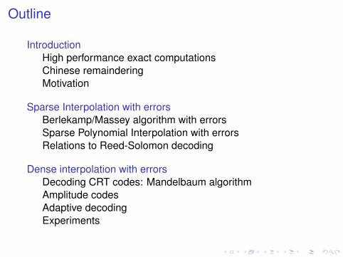
Outline
IntroductionHigh performance exact computationsChinese remainderingMotivation
Sparse Interpolation with errorsBerlekamp/Massey algorithm with errorsSparse Polynomial Interpolation with errorsRelations to Reed-Solomon decoding
Dense interpolation with errorsDecoding CRT codes: Mandelbaum algorithmAmplitude codesAdaptive decodingExperiments

High Performance Algebraic Computations (HPAC)Domain of Computation
I Z,Q ⇒variable sizeI Zp,GF(pk) ⇒specific arithmeticI K[X] for K = Zp, ....
Application domains:Computational number theory:
I computing tables of elliptic curves, modular forms,I testing conjectures
Crypto: Algebraic attacks (Quadratic sieves, Groebnerbases, index calculus,...)
Graph theory: testing conjectures (graph isomorphism,...)Representation theory
...

HPAC: rules of thumbDeal with size of arithmeticEvaluation/interpolation schemes:
over Z: Chinese Remainder Algorithm:Z→ Z/mZ→ Z/m1Z× · · · × Z/mkZ
over K[X]: Evaluation/interpolation: K[X]→ K
I Embarassingly parallel
Lifting schemes Z→ Z/pkZ→ Z/pZI Best sequential complexities
Deal with complexity/efficiency: reduce to Linear algebra
I Matrix product over Zp,KI Eliminations: Gauss, Gram-Schmidt (LLL), ...I Krylov iteration

Chinese remainder algorithmIf m1, . . . ,mk pariwise relatively prime:
Z/(m1 . . .mk)Z ≡ Z/m1Z× · · · × Z/mkZ
Computation of y = f (x) for f ∈ Z[X], x ∈ Zm
beginCompute an upper bound β on |f (x)|;Pick m1, . . .mk, pairwise prime, s.t. m1 . . .mk > β;for i = 1 . . . k do
Compute yi = f (x mod mi) mod mi
; /* Evaluation */
Compute y = CRT(y1, . . . , yk)
; /* Interpolation */
CRT : Z/m1Z× · · · × Z/mkZ → Z/(m1 . . .mk)Z(x1, . . . , xk) 7→
∑ki=1 xiΠiYi mod Π
where
Π =
∏ki=1 mi
Πi = Π/mi
Yi = Π−1i mod mi

Chinese remainder algorithmIf m1, . . . ,mk pariwise relatively prime:
Z/(m1 . . .mk)Z ≡ Z/m1Z× · · · × Z/mkZ
Computation of y = f (x) for f ∈ Z[X], x ∈ Zm
beginCompute an upper bound β on |f (x)|;Pick m1, . . .mk, pairwise prime, s.t. m1 . . .mk > β;for i = 1 . . . k do
Compute yi = f (x mod mi) mod mi ; /* Evaluation */
Compute y = CRT(y1, . . . , yk); /* Interpolation */
CRT : Z/m1Z× · · · × Z/mkZ → Z/(m1 . . .mk)Z(x1, . . . , xk) 7→
∑ki=1 xiΠiYi mod Π
where
Π =
∏ki=1 mi
Πi = Π/mi
Yi = Π−1i mod mi

Chinese remaindering and evaluation/interpolation
Evaluate P in a ↔ Reduce P modulo X − a
Polynomials
Integers
Evaluation:P mod X − a
N mod m
Evaluate P in a
“Evaluate” N in m
Interpolation:
P =∑k
i=1 yi
∏j 6=i(X−aj)∏j6=i(ai−aj)
N =∑k
i=1 yi∏
j6=i mj(∏
j 6=i mj)−1[mi]

Chinese remaindering and evaluation/interpolation
Evaluate P in a ↔ Reduce P modulo X − a
Polynomials
Integers
Evaluation:P mod X − a
N mod m
Evaluate P in a
“Evaluate” N in m
Interpolation:
P =∑k
i=1 yi
∏j 6=i(X−aj)∏j6=i(ai−aj)
N =∑k
i=1 yi∏
j6=i mj(∏
j 6=i mj)−1[mi]

Chinese remaindering and evaluation/interpolation
Evaluate P in a ↔ Reduce P modulo X − a
Polynomials Integers
Evaluation:P mod X − a N mod m
Evaluate P in a “Evaluate” N in m
Interpolation:
P =∑k
i=1 yi
∏j 6=i(X−aj)∏j6=i(ai−aj)
N =∑k
i=1 yi∏
j6=i mj(∏
j 6=i mj)−1[mi]

Early terminationClassic Chinese remaindering Deterministic
I bound β on the resultI Choice of the mi: such that m1 . . .mk > β
Early termination Probabilistic Monte Carlo
I For each new modulo mi:I reconstruct yi = f (x) mod m1 × · · · × miI If yi == yi−1 ⇒terminated
Advantage:
I Adaptive number of moduli depending on the output valueI Interesting when
I pessimistic bound: sparse/structured matrices, ...I no bound available

Motivation
ABFT: Algorithm Based Fault Tolerance
HPC: clusters, grid, P2P, cloud computing
I Parallelization based on Evaluation/Interpolation scheme
Need to tolerate:I soft errors (cosmic rays,...)I malicious corruption
Signal processing
I Sparse polynomial interpolation
Distinction between noise and outliersI Symbolic-numeric methods

Dense/Sparse interpolation with errors
Problem 1: Dense interpolation with errors over Z
Given (yi,mi) for i = 1 . . . n,Find Y ∈ Z such that Y = yi mod mi except on ≤ e values.
Problem 2: Sparse interpolation with errors over K[X]
Given (yi, xi) for i = 1 . . . n,Find a t-sparse poly. f such that f (xi) = yi except on ≤ e values.

State of the art
Dense interpolationInterpolation Interpolation with errors
over K[X] Lagrange Generalized Reed-Solomon codesover Z CRT CRT codes
Sparse InterpolationInterpolation Interpolation with errors
over K[X] Ben-Or & Tiwari ?over Z ? ?

State of the art
Dense interpolationInterpolation Interpolation with errors
over K[X] Lagrange Generalized Reed-Solomon codesover Z CRT CRT codes
Sparse InterpolationInterpolation Interpolation with errors
over K[X] Ben-Or & Tiwari ?over Z ? ?

Contribution
Sparse interpolation code over K[X]
I lower bound on the necessary number of evaluationsI optimal unique decoding algorihtmI list decoding variant
Dense interpolation code over Z
I finer bounds on the correction capacityI adaptive decoding using the best effective redundancy

Outline
IntroductionHigh performance exact computationsChinese remainderingMotivation
Sparse Interpolation with errorsBerlekamp/Massey algorithm with errorsSparse Polynomial Interpolation with errorsRelations to Reed-Solomon decoding
Dense interpolation with errorsDecoding CRT codes: Mandelbaum algorithmAmplitude codesAdaptive decodingExperiments

Preliminaries
Linear recurring sequences
Sequence (a0, a1, . . . , an, . . . ) such that
∀j ≥ 0 aj+t =
t−1∑i=0
λiai+j
generating polynomial: Λ(z) = zt −∑t−1
i=0 λizi
minimal generating polynomial: Λ(z) of minimal degreelinear complexity of (ai)i: the minimal degree of Λ
Hamming weight: weight(x) = #{i|xi 6= 0}Hamming distance: dH(x, y) = weight(x− y)

Berlekamp/Massey algorithm
Input: (a0, . . . , an−1) a sequence of field elements.Output: Λ(z) =
∑Lni=0 λizi a monic polynomial of minimal degree
Ln ≤ n such that∑Ln
i=0 λiai+j = 0 forj = 0, . . . , n− Ln − 1.
I Guarantee : BMA finds Λ of degree t from ≤ 2t entries.

Problem Statement
Berlkamp/Massey with errors
Suppose (a0, a1, . . . ) is linearly generated by Λ(z) of degree twhere Λ(0) 6= 0.Given (b0, b1, . . . ) = (a0, a1, . . . ) + ε, where weight(ε) ≤ E:
1. How to recover Λ(z) and (a0, a1, . . . ) ?2. How many entries required for
I a unique solution ?I a list of solutionse including (a0, a1, . . . ) ?
Coding Theory formulation
Let C be the set of all sequences of linear complexity t.1. How to decode C ?2. What are the best correction capacities ?
I for unique decodingI list decoding

How many entries to guarantee uniqueness?
Case E = 1, t = 2
(ai) Λ(z)(0, 1, 0, 1, 0, 1, 0, −1, 0, 1, 0) 2− 2z2 + z4 + z6
(0, 1, 0, 1, 0, 1, 0, 1, 0, 1, 0) −1 + z2
(0, 1, 0, −1, 0, 1, 0, −1, 0, 1, 0) 1 + z2
Where is the error?
A unique solution is not guaranteed with t = 2,E = 1 and n = 11

How many entries to guarantee uniqueness?
Case E = 1, t = 2
(ai) Λ(z)(0, 1, 0, 1, 0, 1, 0, −1, 0, 1, 0) 2− 2z2 + z4 + z6
(0, 1, 0, 1, 0, 1, 0, 1, 0, 1, 0) −1 + z2
(0, 1, 0, −1, 0, 1, 0, −1, 0, 1, 0) 1 + z2
Where is the error?
A unique solution is not guaranteed with t = 2,E = 1 and n = 11

How many entries to guarantee uniqueness?
Case E = 1, t = 2
(ai) Λ(z)(0, 1, 0, 1, 0, 1, 0, −1, 0, 1, 0) 2− 2z2 + z4 + z6
(0, 1, 0, 1, 0, 1, 0, 1, 0, 1, 0) −1 + z2
(0, 1, 0, −1, 0, 1, 0, −1, 0, 1, 0) 1 + z2
Where is the error?
A unique solution is not guaranteed with t = 2,E = 1 and n = 11

How many entries to guarantee uniqueness?
Case E = 1, t = 2
(ai) Λ(z)(0, 1, 0, 1, 0, 1, 0, −1, 0, 1, 0) 2− 2z2 + z4 + z6
(0, 1, 0, 1, 0, 1, 0, 1, 0, 1, 0) −1 + z2
(0, 1, 0, −1, 0, 1, 0, −1, 0, 1, 0) 1 + z2
Where is the error?A unique solution is not guaranteed with t = 2,E = 1 and n = 11

Generalization to any E ≥ 1
Let 0 = (
t−1 times︷ ︸︸ ︷0, . . . , 0). Then
s = (0, 1, 0, 1, 0, 1, 0,−1)
is generated by zt − 1 or zt + 1 up to E = 1 error.Then
(
E times︷ ︸︸ ︷s, s, . . . , s, 0, 1, 0)
is generated by zt − 1 or zt + 1 up to E errors.⇒ambiguity with n = 2t(2E + 1)− 1 values.
TheoremNecessary condition for unique decoding:
n ≥ 2t(2E + 1)

The Majority Rule Berlekamp/Massey algorithm
2t
Λ Λ Λ Λ Λ1 2 3 4 5
E=2 n=2t(2E+1)
Input: (a0, . . . , an−1) + ε, where n = 2t(2E + 1), weight(ε) ≤ E,and (a0, . . . , an−1) minimally generated by Λ of degree t,where Λ(0) 6= 0.
Output: Λ(z) and (a0, . . . , an−1).
beginRun BMA on 2E + 1 segments of 2t entries and record Λi(z)on each segment;Perform majority vote to find Λ(z);
Use a clean segment to clean-up the sequence ;return Λ(z) and (a0, a1, . . . );

The Majority Rule Berlekamp/Massey algorithm
2t
Λ Λ Λ Λ Λ1 2 3 4 5
E=2 n=2t(2E+1)
Input: (a0, . . . , an−1) + ε, where n = 2t(2E + 1), weight(ε) ≤ E,and (a0, . . . , an−1) minimally generated by Λ of degree t,where Λ(0) 6= 0.
Output: Λ(z) and (a0, . . . , an−1).begin
Run BMA on 2E + 1 segments of 2t entries and record Λi(z)on each segment;Perform majority vote to find Λ(z);
Use a clean segment to clean-up the sequence ;return Λ(z) and (a0, a1, . . . );

The Majority Rule Berlekamp/Massey algorithm
2t
Λ Λ Λ Λ Λ1 2 3 4 5
E=2 n=2t(2E+1)
Input: (a0, . . . , an−1) + ε, where n = 2t(2E + 1), weight(ε) ≤ E,and (a0, . . . , an−1) minimally generated by Λ of degree t,where Λ(0) 6= 0.
Output: Λ(z) and (a0, . . . , an−1).begin
Run BMA on 2E + 1 segments of 2t entries and record Λi(z)on each segment;Perform majority vote to find Λ(z);Use a clean segment to clean-up the sequence ;return Λ(z) and (a0, a1, . . . );

Algorithm SequenceCleanUp
Input: Λ(z) = zt +∑t−1
i=0 λixi where Λ(0) 6= 0Input: (a0, . . . , an−1), where n ≥ t + 1Input: E, the maximum number of corrections to makeInput: k, such that (ak, ak+2t−1) is cleanOutput: (b0, . . . , bn−1) generated by Λ at distance ≤ E to
(a0, . . . , an−1)
begin(b0, . . . , bn−1)← (a0, . . . , an−1); e, j← 0;i← k + 2t;while i ≤ n− 1 and e ≤ E do
if Λ does not satisfy (bi−t+1, . . . , bi) thenFix bi using Λ(z) as a LFSR; e← e + 1;
i← k − 1;while i ≥ 0 and e ≤ E do
if Λ does not satisfy (bi, . . . , bi+t−1) thenFix bi using ztΛ(1/z) as a LFSR; e← e + 1;
return (b0, . . . , bn−1), e

Algorithm SequenceCleanUp
Input: Λ(z) = zt +∑t−1
i=0 λixi where Λ(0) 6= 0Input: (a0, . . . , an−1), where n ≥ t + 1Input: E, the maximum number of corrections to makeInput: k, such that (ak, ak+2t−1) is cleanOutput: (b0, . . . , bn−1) generated by Λ at distance ≤ E to
(a0, . . . , an−1)begin
(b0, . . . , bn−1)← (a0, . . . , an−1); e, j← 0;i← k + 2t;while i ≤ n− 1 and e ≤ E do
if Λ does not satisfy (bi−t+1, . . . , bi) thenFix bi using Λ(z) as a LFSR; e← e + 1;
i← k − 1;while i ≥ 0 and e ≤ E do
if Λ does not satisfy (bi, . . . , bi+t−1) thenFix bi using ztΛ(1/z) as a LFSR; e← e + 1;
return (b0, . . . , bn−1), e
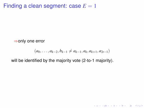
Finding a clean segment: case E = 1
⇒only one error
(a0, . . . , ak−2, bk−1 6= ak−1, ak, ak+1, a2t−1)
will be identified by the majority vote (2-to-1 majority).
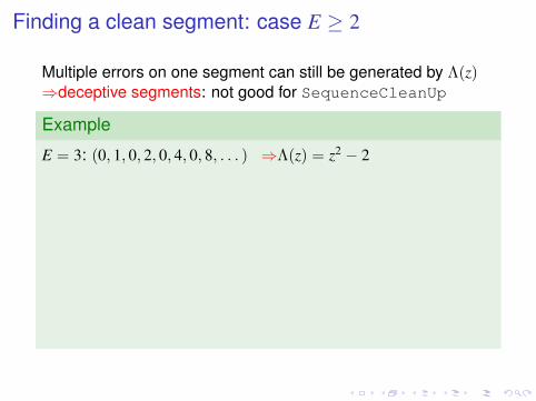
Finding a clean segment: case E ≥ 2
Multiple errors on one segment can still be generated by Λ(z)⇒deceptive segments: not good for SequenceCleanUp
Example
E = 3: (0, 1, 0, 2, 0, 4, 0, 8, . . . ) ⇒Λ(z) = z2 − 2
(1, 1, 2, 2) is deceptive. Applying SequenceCleanUp with thisclean segment produces
(1, 1, 2, 2, 4, 4, 8, 8, 16, 16, 32, 32, 64, . . . )
E > 3 ? contradiction. Try (0, 16, 0, 32) as a clean segmentinstead.

Finding a clean segment: case E ≥ 2
Multiple errors on one segment can still be generated by Λ(z)⇒deceptive segments: not good for SequenceCleanUp
Example
E = 3: (0, 1, 0, 2, 0, 4, 0, 8, . . . ) ⇒Λ(z) = z2 − 2
(1, 1, 2, 2, 4, 4, 0, 8, 0, 16, 0, 32, . . . )
(1, 1, 2, 2) is deceptive. Applying SequenceCleanUp with thisclean segment produces
(1, 1, 2, 2, 4, 4, 8, 8, 16, 16, 32, 32, 64, . . . )
E > 3 ? contradiction. Try (0, 16, 0, 32) as a clean segmentinstead.

Finding a clean segment: case E ≥ 2
Multiple errors on one segment can still be generated by Λ(z)⇒deceptive segments: not good for SequenceCleanUp
Example
E = 3: (0, 1, 0, 2, 0, 4, 0, 8, . . . ) ⇒Λ(z) = z2 − 2
( 1, 1, 2, 2︸ ︷︷ ︸z2−2
, 4, 4, 0, 8︸ ︷︷ ︸z2+2z−2
, 0, 16, 0, 32︸ ︷︷ ︸z2−2
, . . . )
(1, 1, 2, 2) is deceptive. Applying SequenceCleanUp with thisclean segment produces
(1, 1, 2, 2, 4, 4, 8, 8, 16, 16, 32, 32, 64, . . . )
E > 3 ? contradiction. Try (0, 16, 0, 32) as a clean segmentinstead.

Success of the sequence clean-up
TheoremIf n ≥ t(2E + 1), then a deceptive segment will necessarily beexposed by a failure of the condition e ≤ E in algorithmSequenceCleanUp.
Corollary
n ≥ 2t(2E + 1) is a necessary and sufficient condition for uniquedecoding of Λ and the corresponding sequence.
RemarkAlso works with an upper bound t ≤ T on deg Λ.

List decoding for n ≥ 2t(E + 1)
2t
Λ Λ Λ1 2 3
E=2 n=2t(E+1)
Input: (a0, . . . , an−1) + ε, where n = 2t(E + 1), weight(ε) ≤ E,and (a0, . . . , an−1) minimally generated by Λ of degree t,where Λ(0) 6= 0.
Output: (Λi(z), si = (a(i)0 , . . . , a
(i)n−1))i a list of ≤ E candidates
beginRun BMA on E + 1 segments of 2t entries and record Λi(z)on each segment;
foreach Λi(z) doUse a clean segment to clean-up the sequence;Withdraw Λi if no clean segment can be found.
return the list (Λi(z), (a(i)0 , . . . , a
(i)n−1))i;

List decoding for n ≥ 2t(E + 1)
2t
Λ Λ Λ1 2 3
E=2 n=2t(E+1)
Input: (a0, . . . , an−1) + ε, where n = 2t(E + 1), weight(ε) ≤ E,and (a0, . . . , an−1) minimally generated by Λ of degree t,where Λ(0) 6= 0.
Output: (Λi(z), si = (a(i)0 , . . . , a
(i)n−1))i a list of ≤ E candidates
beginRun BMA on E + 1 segments of 2t entries and record Λi(z)on each segment;foreach Λi(z) do
Use a clean segment to clean-up the sequence;Withdraw Λi if no clean segment can be found.
return the list (Λi(z), (a(i)0 , . . . , a
(i)n−1))i;

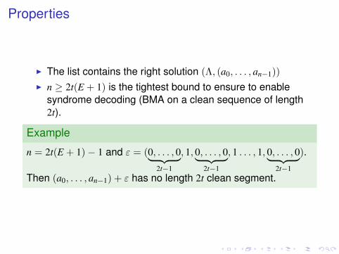
Properties
I The list contains the right solution (Λ, (a0, . . . , an−1))
I n ≥ 2t(E + 1) is the tightest bound to ensure to enablesyndrome decoding (BMA on a clean sequence of length2t).
Example
n = 2t(E + 1)− 1 and ε = (0, . . . , 0︸ ︷︷ ︸2t−1
, 1, 0, . . . , 0︸ ︷︷ ︸2t−1
, 1 . . . , 1, 0, . . . , 0︸ ︷︷ ︸2t−1
).
Then (a0, . . . , an−1) + ε has no length 2t clean segment.

Sparse Polynomial Interpolation
x ∈ F
f =∑t
i=1 cixei
f (x)
ProblemRecover a t-sparse polynomial f given a black-box computingevaluations of it.
Ben-Or/Tiwari 1988:
I Let ai = f (pi) for p a primitive element,I and let Λ(z) =
∏ti=1(z− pei).
I Then Λ(z) is the minimal generator of (a0, a1, . . . ).
⇒only need 2t entries to find Λ(z) (using BMA)⇒only need 2T(2E + 1) with e ≤ E errors and t ≤ T.

Sparse Polynomial Interpolation
x ∈ F
f =∑t
i=1 cixei
f (x)
ProblemRecover a t-sparse polynomial f given a black-box computingevaluations of it.
Ben-Or/Tiwari 1988:
I Let ai = f (pi) for p a primitive element,I and let Λ(z) =
∏ti=1(z− pei).
I Then Λ(z) is the minimal generator of (a0, a1, . . . ).
⇒only need 2t entries to find Λ(z) (using BMA)
⇒only need 2T(2E + 1) with e ≤ E errors and t ≤ T.

Sparse Polynomial Interpolation
x ∈ F
f =∑t
i=1 cixei
f (x)+ε
ProblemRecover a t-sparse polynomial f given a black-box computingevaluations of it.
Ben-Or/Tiwari 1988:
I Let ai = f (pi) for p a primitive element,I and let Λ(z) =
∏ti=1(z− pei).
I Then Λ(z) is the minimal generator of (a0, a1, . . . ).
⇒only need 2t entries to find Λ(z) (using BMA)⇒only need 2T(2E + 1) with e ≤ E errors and t ≤ T.

Ben-Or & Tiwari’s Algorithm
Input: (a0, . . . , a2t−1) where ai = f (pi)Input: t, the numvber of (non-zero) terms of f (x) =
∑tj=1 cjxej
Output: f (x)begin
Run BMA on (a0, . . . , a2t−1) to find Λ(z)Find roots of Λ(z) (polynomial factorization)Recover ej by repeated division (by p)Recover cj by solving the transposed Vandermonde system
(p0)e1 (p0)e2 . . . (p0)et
(p1)e1 (p1)e2 . . . (p1)et
......
...(pt)e1 (pt)e2 . . . (pt)et
c1c2...ct
=
a0a1...
at−1

Blahut’s theorem
Theorem (Blahut)
The D.F.T of a vector of weight t has linear complexity at most t
DFTω(v) = Vandemonde(ω0, ω1, ω2, . . . )v = Evalω0,ω1,ω2,...(v)
I Univariate Ben-Or & Tiwari as a corollaryI Reed-Solomon codes: evaluation of a sparse error⇒BMA

Blahut’s theorem
Theorem (Blahut)
The D.F.T of a vector of weight t has linear complexity at most t
DFTω(v) = Vandemonde(ω0, ω1, ω2, . . . )v = Evalω0,ω1,ω2,...(v)
I Univariate Ben-Or & Tiwari as a corollary
I Reed-Solomon codes: evaluation of a sparse error⇒BMA

Blahut’s theorem
Theorem (Blahut)
The D.F.T of a vector of weight t has linear complexity at most t
DFTω(v) = Vandemonde(ω0, ω1, ω2, . . . )v = Evalω0,ω1,ω2,...(v)
I Univariate Ben-Or & Tiwari as a corollaryI Reed-Solomon codes: evaluation of a sparse error⇒BMA

Reed-Solomon codes as Evaluation codes
C = {(f (ω1), . . . , f (ωn))| deg f < k}
m=f(x), deg f < k
f
error
y = c + ε
ε
g
0
Interpolation
Evaluation
g = f + Interp ( )ε
ic = Eval(f), c = f(w )i
g

Reed-Solomon codes as Evaluation codes
C = {(f (ω1), . . . , f (ωn))| deg f < k}
������������������������������
������������������������������
m=f(x), deg f < k
f
error
y = c + ε
ε
g
0
Interpolation
Evaluation
ic = Eval(f), c = f(w )i
g = f + Interp ( )ε
BMA
f
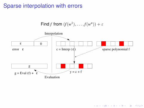
Sparse interpolation with errors
Find f from (f (w1), . . . , f (wn)) + ε
error
g
0
g = Eval (f) + ε
sparse polynomial f
Interpolation
Evaluation
y = c + f
ε εc = Interp ( )
ε
f

Sparse interpolation with errors
Find f from (f (w1), . . . , f (wn)) + ε
������������������������������
������������������������������
error
g
0
g = Eval (f) + ε
sparse polynomial f
Interpolation
Evaluation
y = c + f
ε εc = Interp ( )
ε
f
BMA
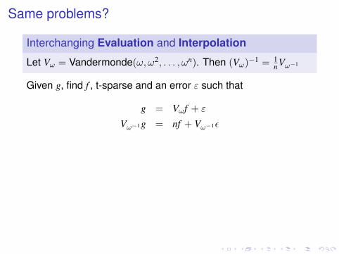
Same problems?
Interchanging Evaluation and Interpolation
Let Vω = Vandermonde(ω, ω2, . . . , ωn). Then (Vω)−1 = 1n Vω−1
Given g, find f , t-sparse and an error ε such that
g = Vωf + ε
Vω−1g = nf + Vω−1ε
Reed-Solomon decoding: unique solution provided ε has 2tconsecutive trailing 0’s⇔ clean segment of length 2t⇔ n ≥ 2t(E + 1)
BUT: location of the syndrome, is a priori unknown⇒no uniqueness

Same problems?
Interchanging Evaluation and Interpolation
Let Vω = Vandermonde(ω, ω2, . . . , ωn). Then (Vω)−1 = 1n Vω−1
Given g, find f , t-sparse and an error ε such that
g = Vωf + ε
Vω−1g = nf︸︷︷︸weight t error
+ Vω−1ε︸ ︷︷ ︸RS code word
Reed-Solomon decoding: unique solution provided ε has 2tconsecutive trailing 0’s⇔ clean segment of length 2t⇔ n ≥ 2t(E + 1)
BUT: location of the syndrome, is a priori unknown⇒no uniqueness

Numeric Sparse Interpolation
I numerical evaluations (with noise) of a sparse polynomialI and outliers
Symbolic numeric approach [Giesbrecht, Labahn&Lee’06] [Kaltofen, Lee, Yang’11]:
I Interpolation/correction using Berlekamp-MasseyI Termination (zero-discrepancy) is ill-conditioned
I But the conditioning is the termination criteriaI Better: track two perturbed executions⇒divergence = termination

Numeric Sparse Interpolation
I numerical evaluations (with noise) of a sparse polynomialI and outliers
Symbolic numeric approach [Giesbrecht, Labahn&Lee’06] [Kaltofen, Lee, Yang’11]:
I Interpolation/correction using Berlekamp-MasseyI Termination (zero-discrepancy) is ill-conditionedI But the conditioning is the termination criteria
I Better: track two perturbed executions⇒divergence = termination

Numeric Sparse Interpolation
I numerical evaluations (with noise) of a sparse polynomialI and outliers
Symbolic numeric approach [Giesbrecht, Labahn&Lee’06] [Kaltofen, Lee, Yang’11]:
I Interpolation/correction using Berlekamp-MasseyI Termination (zero-discrepancy) is ill-conditionedI But the conditioning is the termination criteriaI Better: track two perturbed executions⇒divergence = termination

Outline
IntroductionHigh performance exact computationsChinese remainderingMotivation
Sparse Interpolation with errorsBerlekamp/Massey algorithm with errorsSparse Polynomial Interpolation with errorsRelations to Reed-Solomon decoding
Dense interpolation with errorsDecoding CRT codes: Mandelbaum algorithmAmplitude codesAdaptive decodingExperiments

CRT codes : Mandelbaum algorithm over Z
Chinese Remainder Theorem
x1 x2 . . . xkx ∈ Z
where m1 × · · · × mk > x and xi = x mod mi ∀i
Definition(n, k)-code: C ={
(x1, . . . , xn) ∈ Zm1 × · · · × Zmn s.t. ∃x,{
x < m1 . . .mkxi = x mod mi ∀i
}

CRT codes : Mandelbaum algorithm over Z
Chinese Remainder Theorem
x1 x2 . . . xkx ∈ Z xk+1 xn. . .
where m1 × · · · × mn > x and xi = x mod mi ∀i
Definition(n, k)-code: C ={
(x1, . . . , xn) ∈ Zm1 × · · · × Zmn s.t. ∃x,{
x < m1 . . .mkxi = x mod mi ∀i
}

CRT codes : Mandelbaum algorithm over Z
Chinese Remainder Theorem
x1 x2 . . . xkx ∈ Z xk+1 xn. . .
where m1 × · · · × mn > x and xi = x mod mi ∀i
Definition(n, k)-code: C ={
(x1, . . . , xn) ∈ Zm1 × · · · × Zmn s.t. ∃x,{
x < m1 . . .mkxi = x mod mi ∀i
}

Principle
Property
X ∈ C iff X < Πk.
p1 p2 . . . pk pk+1 pn. . .
Πk = p1 × · · · × pk
Πn = p1 × · · · × pn
Redundancy : r = n− k

ABFT with Chinese remainder algorithm
Correction
Computation
Encoding
Decoding
Input
Solutionx = (x1, . . . , xn)
x′ = (r1, . . . , rn)
A = (A1, . . . An)
x′ < Πn
x < Πk
A

Properties of the code
Error model:I Error: E = X′ − XI Error support: I = {i ∈ 1 . . . n,E 6= 0 mod mi}I Impact of the error: ΠF =
∏i∈I mi
Detects up to r errors:
If X′ = X + E with X ∈ C,#I ≤ r,
then X′ > Πk.
I Redundancy r = n− k, distance: r + 1I ⇒can correct up to
⌊ r2
⌋errors in theory
I More complicated in practice...

Correction
I ∀i /∈ I : E mod mi = 0I E is a multiple of ΠV : E = ZΠV = Z
∏i/∈I mi
I gcd(E,Π) = ΠV
Property
The Extended Euclidean Algorithm, applied to (Π,E) and to(X′ = X + E,Π), performs the same first iterations until ri < ΠV .
=
+X
X′Π
E
u0Π + v0E = Π u0Π + v0X′ = X′...
...ui−1Π + vi−1E = Πv ui−1Π + vi−1X′ = ri−1
uiΠ + viE = 0 uiΠ + viX′ = ri
⇒viX = ri

Correction capacity
Mandelbaum 78:
I 1 symbol = 1 residueI Polynomial time algorithm if e ≤ (n− k) log mmin−log 2
log mmax+log mmin
I worst case: exponential (random perturbation)
Goldreich Ron Sudan 99 weighted residues ⇒equivalentGuruswami Sahai Sudan 00 invariably polynomial time
Interpretation:
Errors have variable weights depending on their impact∏
i∈I mi
Example: m1 = 3,m2 = 5,m3 = 3001I Mandelbaum: only corrects 1 error provided X < 3I Adaptive: also corrects
I 1 error mod 3 if X < 333I 1 error mod 5 if X < 120I 2 errors mod 2 and 3 if X < 13

Generalized point of view: amplitude code
Over a Euclidean ring A with a Euclidean function ν,multiplicative and sub-additive, ie such that
ν(ab) = ν(a)ν(b)
ν(a + b) ≤ ν(a) + ν(b)
eg.I over Z: ν(x) = |x|I over K[X]: ν(P) = 2deg(P)
Definition
Error impact between x and y: ΠF =∏
i|x 6=y[mi]mi
Error amplitude: ν(ΠF)

Amplitude codes
Distance
∆ : A×A → R+
(x, y) 7→∑
i|x 6=y[mi]
log2 ν (mi)
∆(x, y) = log2 ν(ΠF)

Definition ((n, k)-amplitude code)
Given {mi}i≤m pairwise rel. prime, and κ ∈ R+ The set
C = {x ∈ A : ν(x) < κ},
n = log2∏
i≤m mi, k = log2 κ. is a (n, k)-amplitude code.
Property (Quasi MDS)
∀(x, y) ∈ C
∆(x, y)n− k1
∼ Singleton bound
⇒correction capacity = maximal amplitude of an error that canbe corrected

Definition ((n, k)-amplitude code)
Given {mi}i≤m pairwise rel. prime, and κ ∈ R+ The set
C = {x ∈ A : ν(x) < κ},
n = log2∏
i≤m mi, k = log2 κ. is a (n, k)-amplitude code.
Property (Quasi MDS)
∀(x, y) ∈ C
∆(x, y) > n− k − 1
∼ Singleton bound
⇒correction capacity = maximal amplitude of an error that canbe corrected

Definition ((n, k)-amplitude code)
Given {mi}i≤m pairwise rel. prime, and κ ∈ R+ The set
C = {x ∈ A : ν(x) < κ},
n = log2∏
i≤m mi, k = log2 κ. is a (n, k)-amplitude code.
Property (Quasi MDS)
∀(x, y) ∈ C, A = K[X]
∆(x, y) ≥ n− k + 1
∼ Singleton bound
⇒correction capacity = maximal amplitude of an error that canbe corrected

Advantages
I Generalization over any Euclidean ringI Natural representation of the amount of informationI No need to sort moduliI Finer correction capacities
I Adaptive decoding: taking advantage of all the availableredundancy
I Early termination: with no a priori knowledge of a boundon the result

Advantages
I Generalization over any Euclidean ringI Natural representation of the amount of informationI No need to sort moduliI Finer correction capacitiesI Adaptive decoding: taking advantage of all the available
redundancyI Early termination: with no a priori knowledge of a bound
on the result

Amplitude decoding, with static correction capacityAmplitude based decoder over R
Input: Π,X′
Input: τ ∈ R+ | τ < ν(Π)2 : bound on the maximal error amplitude
Output: X ∈ R: corrected message s.t. ν(X)4τ 2 ≤ ν(Π)begin
u0 = 1, v0 = 0, r0 = Π;u1 = 0, v1 = 1, r1 = X′;i = 1;while (ν(ri) > ν(Π)/2τ ) do
Let ri−1 = qiri + ri+1 be the Euclidean division of ri−1 by ri;ui+1 = ui−1 − qiui;vi+1 = vi−1 − qivi;i = i + 1;
return X = rivi
I reaches the quasi-maximal correction capacity
I requires an a priori knowledge of τ⇒How to make the correction capacity adaptive?

Amplitude decoding, with static correction capacityAmplitude based decoder over R
Input: Π,X′
Input: τ ∈ R+ | τ < ν(Π)2 : bound on the maximal error amplitude
Output: X ∈ R: corrected message s.t. ν(X)4τ 2 ≤ ν(Π)begin
u0 = 1, v0 = 0, r0 = Π;u1 = 0, v1 = 1, r1 = X′;i = 1;while (ν(ri) > ν(Π)/2τ ) do
Let ri−1 = qiri + ri+1 be the Euclidean division of ri−1 by ri;ui+1 = ui−1 − qiui;vi+1 = vi−1 − qivi;i = i + 1;
return X = rivi
I reaches the quasi-maximal correction capacityI requires an a priori knowledge of τ⇒How to make the correction capacity adaptive?

Adaptive approach
Multiple goals:
I With a fixed n, the correction capacity depends on a boundon ν(X)⇒pessimistic estimate⇒how to take advantage of all the available redundancy?
X
bound on v(X)
redundancy effectively available
redundancy being used

A first adaptive approach: divisibility checkTermination criterion in the Extended Euclidean alg.:
I ui+1Π + vi+1E = 0⇒E = −ui+1Π/vi+1⇒test if vj divides Π
I check if X satisfies: ν(X) ≤ ν(Π)4ν(vj)2
I But several candidates are possible⇒discrimination by a post-condition on the result
Example
mi 3 5 7xi 2 3 2
I x = 23 with 0 errorI x = 2 with 1 error

Detecting a gap
uiΠ + vi(X + E) = ri ⇒ uiΠ + viE = ri − viX
ri
viX
X = −ri/vi
I At the final iteration: ν(ri) = ν(viX)I If necessary, a gap appears between ri−1 and ri.
I ⇒Introduce a blank 2g in order to detect a gap > 2g
Property
I Loss of correction capacity: very small in practiceI Test of the divisibility for the remaining candidatesI Strongly reduces the number of divisibility tests

Detecting a gap
uiΠ + vi(X + E) = ri ⇒ uiΠ + viE = ri − viX
ri
viX 2g
X = −ri/vi
I At the final iteration: ν(ri) = ν(viX)I If necessary, a gap appears between ri−1 and ri.I ⇒Introduce a blank 2g in order to detect a gap > 2g
Property
I Loss of correction capacity: very small in practiceI Test of the divisibility for the remaining candidatesI Strongly reduces the number of divisibility tests

Experiments
Size of the error 10 50 100 200 500 1000
g = 2 1/446 1/765 1/1118 2/1183 2/4165 1/7907
g = 3 1/244 1/414 1/576 2/1002 2/2164 1/4117
g = 5 1/53 1/97 1/153 2/262 1/575 1/1106
g = 10 1/1 1/3 1/9 1/14 1/26 1/35
g = 20 1/1 1/1 1/1 1/1 1/1 1/1
Table: Number of remaining candidates after the gap detection: c/d
means d candidates with a gap > 2g, and c of them passed thedivisibility test. n ≈ 6001 (3000 moduli), κ ≈ 201 (100 moduli).

Experiments
0
0.05
0.1
0.15
0.2
0.25
0.3
0.35
0.4
0 50 100 150 200 250 300 350 400
Tim
e (s
)
Size of the errors
DivisibilityGap g=2Gap g=5
Gap g=10Threshold T=500
Figure: Comparison for n ≈ 26 016 (m = 1300 moduli of 20 bits),κ ≈ 6001 (300 moduli) and τ ≈ 10007 (about 500 moduli).

ConclusionAdaptive decoding of CRT codes
I finer bounds on the correction capacityI adaptive decoding using the best effective redundancyI efficient termination heuristics
Sparse interpolation code over K[X]
I lower bound on the necessary number of evaluationsI optimal unique decoding algorihtmI list decoding variant
Perspectives
I Generalization to adaptive list decoding of CRT codesI Tight bound on the size of the list when n ≥ 2t(E + 1),I Sparse Cauchy interpolation with errors.
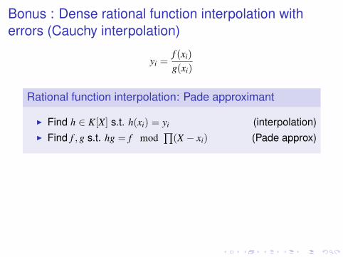
Bonus : Dense rational function interpolation witherrors (Cauchy interpolation)
yi =f (xi)
g(xi)
Rational function interpolation: Pade approximant
I Find h ∈ K[X] s.t. h(xi) = yi (interpolation)I Find f , g s.t. hg = f mod
∏(X − xi) (Pade approx)
Introducing an error of impact ΠF =∏
i∈I(X − xi):
hgΠF = f ΠF mod∏
(X − xi)
Property
If n ≥ deg f + deg g + 2e, one can interpolate with at most e errors
Related Documents