Adaptive communication: Languages with more non-native speakers tend to have fewer word forms

Adaptive Communication: Languages with more Non-NativeSpeakers tend to have fewer Word Forms

Christian Bentz1, Annemarie Verkerk2, Douwe Kiela3, Felix Hill3, Paula Buttery1,3

1 Department of Theoretical and Applied Linguistics, University ofCambridge, Cambridge, United Kingdom2 Reading Evolutionary Biology Group, School of Biological Sciences,University of Reading, Reading, United Kingdom3 Computer Laboratory, University of Cambridge, Cambridge, UnitedKingdom* E-mail: [email protected]

Abstract

Explaining the diversity of languages across the world is one of the central aims oftypological, historical and evolutionary linguistics. We consider the effect of languagecontact - the number of non-native speakers a language has - on the way languageschange and evolve. By analysing hundreds of languages within and across languagefamilies, regions and text types, we show that languages with greater levels of contacttypically employ fewer word forms to encode the same information content (a propertywe refer to as lexical diversity). Based on three types of statistical analyses, wedemonstrate that this variance can in part be explained by the impact of non-nativespeakers on information encoding strategies. Finally, we argue that languages areinformation encoding systems shaped by the varying needs of their speakers. Languageevolution and change should be modeled as the co-evolution of multiple intertwinedadaptive systems: On one hand, the structure of human societies and human learningcapabilities, and on the other, the structure of language.

Introduction 1

All languages are carriers of information. However, they differ greatly in terms of the 2

encoding strategies they adopt. For example, while in German a single compound can 3

transmit complex concepts (e.g. Schifffahrtskapitankabinenschlussel), English uses 4

whole phrases to transmit the same information (key to the cabin of the captain of a 5

ship). In the Eskimo-Aleut language Inuktitut the word qimmiq ‘dog’ can be modified 6

to encode different case relations, e,g. qimmi-mik ’with the dog’, qimmi-mut ’onto the 7

dog’, qimmi-mi ’in the dog’, qimmi-mit ’away from the dog’, etc [1]. Likewise, many 8

languages encode information about number, gender and case in a multitude of different 9

articles, e.g. German der, die, das, dem, den, des or Italian il, la, lo, i, le, li, gli, 10

whereas in English there is only one definite article the and in Mandarin Chinese there 11

is none. 12

We refer to this property of languages - the number of word forms or word types 13

they use to encode essentially the same information - as their lexical diversity (LDT). 14

This difference is a central part of the variation in encoding strategies we find across 15

languages of the world. 16

This paper centers on the question of where variation in lexical diversity stems from. 17

Why do some languages employ a wide range of opaque lexical items while others are 18

1/22

more economical? Variation between languages has often be seen as driven by language 19

acquisition of native speakers (L1) [2–8]. However, some sociolinguistic and historical 20

studies have raised the question of whether large numbers of non-native (L2) language 21

speakers in a society can also lead to systematic changes in the use of the language in 22

generall [9–16]. 23

In this work we investigate with quantitative analyses the association between 24

non-native language speaker proportions - here referred to as language contact - and 25

variation in lexical diversity. Adults learning a second language encounter difficulties 26

with the panoply of word forms that native speakers seem to master with ease, so that 27

non-native language is typically characterised by lower lexical diversity [17,18]. We 28

consider whether higher proportions of non-native speakers in a population should over 29

time reduce the lexical diversity of a language. A clear prediction of this hypothesis is 30

that, at any point in time, languages with higher L2 speaker proportions are those 31

languages that have lower lexical diversities. 32

To systematically compare lexical diversities cross-linguistically we use parallel 33

translations of the same texts into hundreds of languages. Parallel translations provide 34

a natural means of controlling for constant information content. The LDT of these texts 35

can be quantified by applying three measures: the parameters of the Zipf-Mandelbrot 36

law [19,20], Shannon entropy [21,22] and type-token ratios [23–26]. Using this 37

measures, we observe a great variety of lexical diversities across language families and 38

regions of the world despite constant content of the texts. 39

To test whether some of this variation can be attributed to language contact, we 40

employ three types of statistical model: a) simple linear regression, regressing lexical 41

diversities on L2 speaker proportions; b) linear mixed-effects regression controlling for 42

family relationships, regional clustering and text type; and c) phylogenetic generalized 43

least squares regression (PGLS) that models the potential co-evolution of L2 speaker 44

proportions with lexical diversities. The results of these models converge to show that 45

the ratio of non-native speakers predicts lexical diversity beyond language families, 46

regional clustering and text types. 47

These results can be interpreted as an example of a co-evolution between 48

sociolinguistic niches (more or less non-native influence) and language structure (lower 49

or higher lexical diversity) [12,27]. From this perspective languages are complex 50

adaptive systems shaped by the communicative needs and learning constraints of 51

speaker populations [28–33]. We conclude that lexical diversity is a quantitative 52

linguistic measure which is highly relevant to the enquiry of language evolution, 53

language typology and language change, and that it can be modeled taking into account 54

sociolinguistic and genealogical information. This supports the claim that the evolution 55

of language structure can only be understood as a co-evolution of population structure, 56

human cognitive constraints and communicative encoding strategies. 57

Materials and Methods 58

Parallel texts 59

The parallel texts used in this study are the Universal Declaration of Human Rights 60

(UDHR) in unicode (http://www.unicode.org/udhr/), the Parallel Bible Corpus (PBC) 61

[34] and the Europarl Parallel Corpus (EPC) [35]. 62

The UDHR currently comprises a collection of more than 400 parallel translations. 63

However, only 376 of these are fully converted into unicode. The UDHR is a short legal 64

text of 30 articles and ca. 1700 words in English. 65

The PBC is a collection of parallel translations of the Bible. It currently comprises 66

918 texts that have been assigned 810 unique ISO 639-3 codes (i.e. unique languages). 67

2/22

Texts are aligned by verses, which allows us to fully parallelize them by including only 68

the verses that occur in all the texts of the respective language sample we are looking at. 69

Note that there is a trade-off between number of texts and number of verses. Not a 70

single verse is represented in all texts. We chose a sample of 800 texts which yields 71

overlapping verses that amount to ca. 20000 words in the English translation. This 72

sample represents 632 languages (unique ISO 639-3 codes). 73

The EPC is a collection of transcripts of discussions in the European Parliament in 74

21 European languages. The English transcripts amount to ca. 7 million words. 75

Combining the UDHR, PBC and EPC yields a sample of 867 texts with 647 unique 76

ISO 639-3 codes representing languages (see Appendix 1). These languages stem from 77

83 families and 182 genera according to the World Atlas of Language Structures 78

(WALS) classification [36]. 79

Defining word types 80

Any measure of lexical diversity relates to the frequency of occurrence of word types in 81

a given text. A word type is here defined as a recurring sequence of letters delimited by 82

white spaces, punctuation marks, and other non-word characters. 83

Note, that this definition of a word type rules out pictographic and logographic 84

writing systems (see Appendix 2 for a discussion). Also, this simplified definition of 85

”word” is contested by linguistically more informed approaches [37,38]. However, to 86

our knowledge it is currently the only computationally feasible approach for 87

automatically generating lists of word types across hundreds of languages. 88

Lexical diversity measures 89

To scrutinize the distribution of word types in a given text they are ordered according 90

to their frequency of occurrence. For example, Figure 1 displays the first 7 ranks of 91

word types with their frequencies for the UDHR in German and English. Despite the 92

constant information content of these parallel translations, English’s repetitive usage of 93

the same word types results in high frequencies in the upper ranks. For example, the 94

letter sequence representing the definite article in English (the) occurs roughly 120 95

times in the English UDHR, whereas German distributes occurrences of articles over 96

different word types, i.e. der (ca. 60), die (ca. 50) and das (ca. 30). 97

Figure 1. Word frequency distributions for English and German UDHR.Bars indicate frequencies of occurrence in German (blue) and English (red) for thehighest ranking words in the UDHR text.

3/22

To facilitate an investigation of varying lexical diversities across languages we 98

introduce three quantitative measures of LDT: The parameters of Zipf-Mandelbrot’s 99

law, Shannon entropy, and type-token ratios. 100

Zipf-Mandelbrot’s law. The shape of word frequency distributions can be 101

approximated by the Zipf-Mandelbrot curve (adopted from Mandelbrot, 1953: 491): 102

f(r) =C

(β + r)αC > 0, α > 0, β > −1, r ∈ R+, (1)

where f(r) is the frequency of a word in rank r, α and β are parameters and C is a 103

normalizing constant. The parameters specify the shape of the approximated 104

distribution. They can be estimated for individual languages by using a maximum 105

likelihood estimation procedure (see Appendix 3). The lines in Figures 1a-1c represent 106

such approximations for Fijian, English, German and Hungarian. Notably, the Fijian 107

approximation has the highest values (C = 0.39, β = 2.07, α = 1.2) and Hungarian the 108

lowest values (C = 0.06, β = -0.33, α = 0.76), with German and English in between 109

(see Figure 2). 110

Figure 2. Word frequency distributions with ZM parameterapproximations for selected languages. (a) Dots represent frequencies and ranksfor the 50 highest frequency words in English (red), Fijian (green), German (blue) andHungarian (purple). Lines reflect Zipf-Mandelbrot approximations. (b) Lowerfrequencies towards the first ranks are associated with more word types in the tails ofdistributions. More diverse languages have more hapax legomena (i.e. words withfrequency = 1), i.e. Hungarian has more hapax legomena than German, English, andFijian, in this order. Constant values were added to Fijian, English and German toavoid over-plotting and to make the tails visible.

There is an inverse relationship between lexical diversity and the ZM-parameters: 111

lower diversity is associated with higher values for C, α and β. 112

Shannon entropy. Another measure for LDT is the entropy Hw over a distribution 113

of words calculated as [21][p. 19]: 114

Hw = −Kk∑i=1

pi × log2(pi), (2)

4/22

where K is a positive constant determining the unit of measurement (which is bits 115

for K=1 and log to the base 2), k is the number of ranks (or different word types) in a 116

word frequency distribution, and pi is the probability of occurrence of a word of ith rank 117

(wi). 118

The Shannon entropy in Equation 2 is a measure of the overall uncertainty when we 119

draw words randomly from a text. A lexically diverse language such as Hungarian has 120

more word types with lower frequencies. To put it differently, if we select a word at 121

random from a Hungarian text and have to guess which word this is, the overall 122

uncertainty is higher compared to a language with fewer word types and higher 123

frequencies, such as English. Shannon entropy can therefore be used as an index for 124

LDT, in parallel to the entropy index for biodiversity [39]. In particular, higher 125

entropies of word frequency distributions are associated with higher LDT. 126

Type-token ratios. Finally, the most basic measure of lexical diversity is the 127

so-called type-token ratio (TTR). TTR simply represents the number of different word 128

types divided by the overall number of word tokens. Higher TTRs reflect higher lexical 129

diversity. Note, that TTRs have been criticized as a measure of lexical diversity, since 130

they are strongly dependent on text size [23,25,40]. However, in the case of parallel 131

texts, information content is constant. Therefore, in the present analyses variation in 132

text size is not a confound, but rather a crucial part of the differences in lexical 133

encoding strategies that we aim to measure. 134

Differences between the measures. While Zipf-Mandelbrot parameters, Shannon 135

entropy and type-token ratios are all measures that reflect LDT, there are important 136

differences. ZM-parameters are negatively correlated with LDT (higher parameter 137

values mean lower lexical diversity), whereas both entropy and TTRs exhibit a positive 138

relationship with LDT. Less evidently, the “responsiveness” of these measures to 139

changes in word frequency distributions varies somewhat. As we show in Appendix 4, 140

TTR is the most responsive and hence fast changing measure, whereas 141

Zipf-Mandelbrot’s α and Shannon entropy Hw are more conservative, in this order. 142

However, to our knowledge there is no a priori reason to prefer one measure over the 143

others. Hence, we calculate values for each of them and include them in our analyses. 144

Scaling of LDT measures. Since ZM’s α is negatively correlated with LDT, 145

whereas Hw and TTR are positively correlated with LDT, we inverse ZM’s α by 146

substracting the values from 1. Additionally, we scale the LDT values using the scale() 147

function in R [41]. By default, this centeres and scales a vector of LDT values dividing 148

it by the standard deviations per measure m and text t: 149

LDTscaled =LDT

σmt=

LDT√∑(LDT−µmt)2

(nmt−1)

. (3)

This way, we combine the values for α, Hw and TTR into a single, scaled LDT 150

measure. Note that different parallel corpora vary in text sizes, which in turn influences 151

LDT values. Scaling these values makes them commensurable across text sizes. The 152

scaled LDT is then used as dependent variable for statistical modeling. 153

Non-native speaker data 154

Our dataset of speaker information contains languages for which we could obtain the 155

numbers of native (L1) and non-native (L2) speakers in the linguistic community. We 156

were able to collect this speaker information for 226 languages using the SIL Ethnologue 157

5/22

[42], the Rosetta project website (www.rosettaproject.org), the UCLA Language 158

Materials Project (www.lmp.ucla.edu), and the Encarta 159

(http://en.wikipedia.org/wiki/Encarta). 160

We define L2 speakers as adult non-native speakers as opposed to early bilinguals. 161

Generally, the sources follow our L2 definition, although in some cases the exact 162

“degree” of bilingualism might vary (see, e.g., “bilingualism remarks” in Ethnologue). 163

Whenever native and non-native speaker numbers differed in the sources, we 164

calculated the average. Note, that this averages out some of the incommensurable 165

values that are certainly to be found in sources like Ethnologue. For example, English 166

has 505 million L2 users world wide according to Ethnologue, whereas for German only 167

L2 users within Germany are counted, which amounts to 8 million. Though English 168

arguably has more L2 speakers than German, the difference is probably too big here. 169

However, averaging across different sources in our data sample we arrive at 365 million 170

L2 speakers for English and 50 million L2 users for German, which seems much more 171

realistic (see Appendix 5). 172

Note that we excluded Sanskrit and Esperanto from the sample. Sanskrit is an 173

extreme outlier in the Indo-European family. In our database it is listed with a very 174

high ratio of L2 to L1 speakers. This is due to the fact that it is learned and used almost 175

exclusively as liturgical language in Hinduism. In this sense, there are very few native 176

speakers of Sanskrit but many that learn it in schools as L2 for liturgical purposes. 177

Clearly, this is not the kind of L2 learning and usage scenario that is supposed to reduce 178

lexical diversity. Esperanto, on the other hand, is an artificial language with a high ratio 179

of L2 speakers. However, since it is a constructed language there is no point to be made 180

about potential shaping of its linguistic structure due to natural processes of language 181

change (though there might be such processes at play in its very recent history). 182

Based on the remaining averaged speaker numbers we then calculated the ratio of 183

L2/L1 speakers for each of the 226 languages. This serves as our main predictor 184

variable in the statistical models. 185

Statistical models 186

Linear regression. To explore a potential association between lexical diversity and 187

L2 speaker proportions we first merge the data on scaled LDTs (647 languages) with 188

the data on L2 ratios (226) languages. This yields a sample of 91 languages (26 different 189

families) (see Appendix 5 for the full data set). We then construct a simple linear model 190

with the scaled LDT measure as response variable and the ratio of non-native (L2) to 191

native (L1) speakers as predictor variable. L2 speaker ratios are logarithmically 192

transformed to reduce extreme outliers. The model is outlined in Equation 4: 193

LDT = β0 + β1 × log(L2) + ε,

ε ∼ N(0, σ2).(4)

The lexical diversity LDT is predicted by the intercept β0 plus the slope β1 194

multiplied by the logarithm of the ratio of L2 to L1 speakers (here represented by L2), 195

and the error ε. One of the underlying assumptions of a linear regression model is that 196

the errors are normally distributed between 0 and the variance σ2. Likewise, the 197

assumption of linearity and homoscedasticity have to be met for the model to be valid. 198

Post hoc checking of these assumptions can be found in Appendix 6. 199

We use the function lm() in R [41] for building this linear model. 200

Linear mixed-effects regression. Language typologists have suggested that simple 201

linear models are undermined by the non-independence of data points. Namely, 202

6/22

languages naturally group into families and regions [43,44]. Moreover, we draw texts 203

from three different sources, use three different measures of LDT and hence have 204

multiple LDT values per ISO 639-3 code. These groupings can introduce systematic 205

variation. Such grouped data require modeling by means of mixed-effects models 206

[45, 46]. 207

Hence, we expand the simple linear model by introducing (non-correlated) intercepts 208

and slopes by family, region, LDT measure, text type and ISO 639-3 code. Information 209

on language families and language regions is taken from Bickel and Nichol’s AUTOTYP 210

database (www.spw.uzh.ch/autotyp/). 211

The mixed-effects model specification can be found in Equation 5: 212

LDTfrmti = β0 + F0f +R0r +M0m + Tt0 + Ii0+

(β1 + F1f +R1r +M1m + T1t + I1i)× log(L2frmti) + εfrmti,

εfrmti ∼ N(0, σ2).

(5)

Here, LDTfrmti is the predicted lexical diversity for languages of the f th family, rth 213

region, mth measure and tth text type and ith ISO 639-3 code. The coefficients β0 and 214

β1 represent the fixed effects intercept and slope respectively. F0f , R0r, M0m, T0t, Ii0 215

are the random intercepts by family, region, measure, text type and ISO code. F1f , R1r, 216

M1m, T1t, I1i denote random slopes by family, region, measure, text type and ISO code. 217

The linear predictor is the log-transformed L2 ratio (L2frmti). Model residuals are 218

represented by εfrmti. Again, residuals are supposed to be normally distributed between 219

0 and their variance σ2. 220

Again, the models are run in R [41] using the package lme4 [47]. As for the simple 221

linear model, we check for linearity, normality and homoscedasticity in Appendix 6. 222

Phylogenetic analyses. The Mixed-effects model tests whether the statistical 223

association between L2 ratio and lexical diversity holds even if systematic differences 224

between language families are accounted for. However, we could also ask if the patterns 225

we find hold within language families, namely at the level of genera and sub-genera (e.g. 226

Romance and Germanic languages within the Indo-European family). The dataset of L2 227

speakers and lexical diversities is currently too small to run a mixed-effects model with 228

genera as random effects, since there are very few genera with more than 5 229

representatives. Instead, phylogenetic regressions [48–50] can be used to assess whether 230

lexical diversities of extant languages are driven by differences in the ratios of L2 231

speakers while taking into account their genealogical relationships. 232

We first use published linguistic family trees [51–53] based on cognate lists as a 233

measure of genealogical relationships. The tips of these phylogenetic trees represent 234

extant languages. The nodes within the trees reflect ancestral languages, and their 235

branches reflect the evolutionary pathways that individual languages have taken. 236

We can assess the likelihood of whether the lexical diversities of extant languages 237

followed closely the evolutionary pathways given in the tree (high “phylogenetic signal”) 238

or whether this tree has to be strongly reduced to fit the lexical diversity data (low 239

“phylogenetic signal”) [48]. On the basis of the phylogenetic signal analysis, we can then 240

use phylogenetic generalized least squares (PGLS) regression to test whether L2 ratio is 241

still a significant predictor of LDT if we correct for the co-variance within the family. 242

Phylogenetic signal. To establish whether lexical diversities evolve along the 243

phylogenetic branches of family trees, a test for phylogenetic signal called λ (lambda) is 244

employed. The estimation of λ is a phylogenetic comparative method that transforms a 245

phylogenetic tree to best fit the comparative data [48,49]. Namely, λ is a factor that 246

7/22

modifies the branch lengths of phylogenetic trees so that they fit the comparative data 247

of interest. The λ-values can range from 0 to 1, with 1 meaning that the similarities in 248

LDT can be explained by their relationship on the phylogeny; while 0 means that there 249

is no evidence for similar behaviour due to shared decent. 250

Note, that for the phylogenetic analyses we need to link a single ISO code to both the 251

phylogenetic tree information, and to the respective LDT information. A dataset with 252

doubled ISO codes is not workable. Hence, analyses have to be run by LDT measures 253

and text types separately. Moreover, since we do within family analyses, there need to 254

be LDT data available for at least 20 languages in the family tree [48]. Given these 255

restrictions, the phylogenetic signal λ is estimated for data from three different language 256

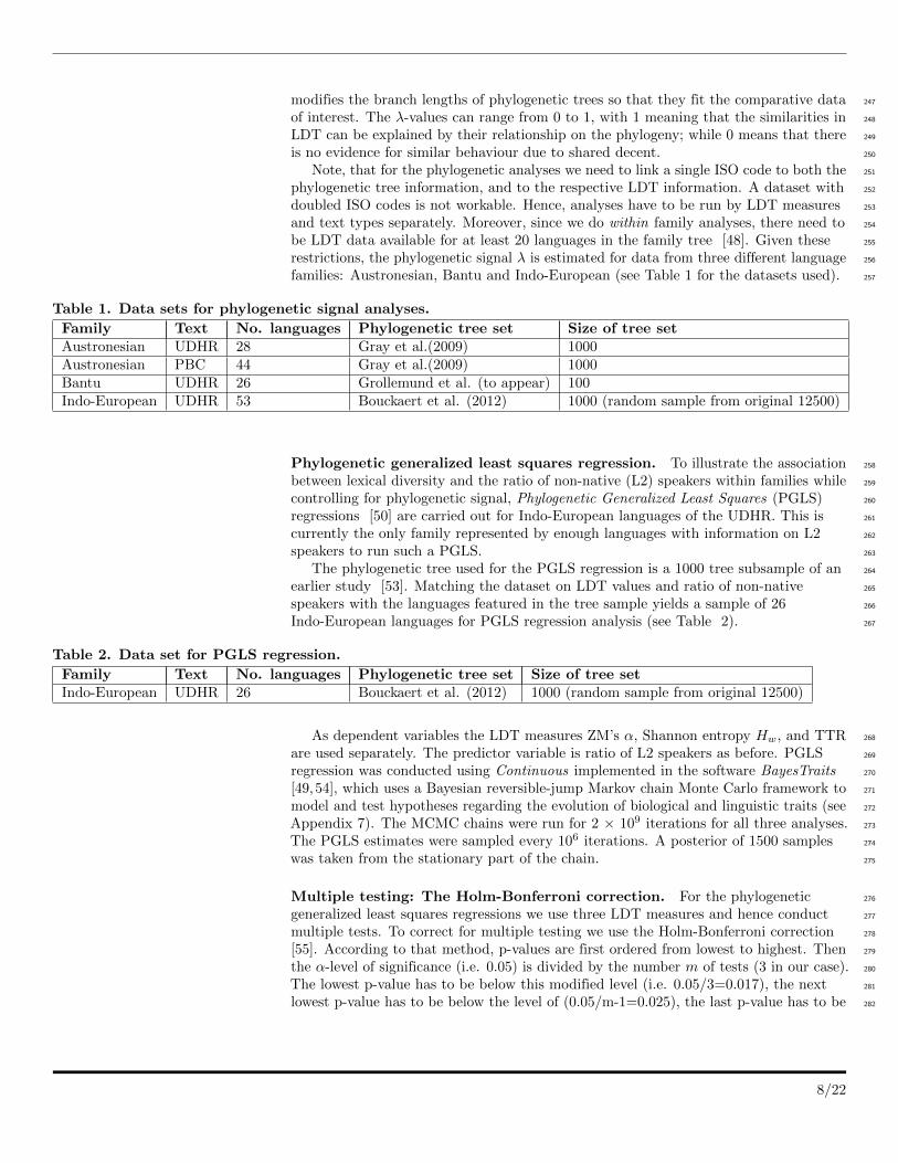
families: Austronesian, Bantu and Indo-European (see Table 1 for the datasets used). 257

Table 1. Data sets for phylogenetic signal analyses.

Family Text No. languages Phylogenetic tree set Size of tree setAustronesian UDHR 28 Gray et al.(2009) 1000Austronesian PBC 44 Gray et al.(2009) 1000Bantu UDHR 26 Grollemund et al. (to appear) 100Indo-European UDHR 53 Bouckaert et al. (2012) 1000 (random sample from original 12500)

Phylogenetic generalized least squares regression. To illustrate the association 258

between lexical diversity and the ratio of non-native (L2) speakers within families while 259

controlling for phylogenetic signal, Phylogenetic Generalized Least Squares (PGLS) 260

regressions [50] are carried out for Indo-European languages of the UDHR. This is 261

currently the only family represented by enough languages with information on L2 262

speakers to run such a PGLS. 263

The phylogenetic tree used for the PGLS regression is a 1000 tree subsample of an 264

earlier study [53]. Matching the dataset on LDT values and ratio of non-native 265

speakers with the languages featured in the tree sample yields a sample of 26 266

Indo-European languages for PGLS regression analysis (see Table 2). 267

Table 2. Data set for PGLS regression.

Family Text No. languages Phylogenetic tree set Size of tree setIndo-European UDHR 26 Bouckaert et al. (2012) 1000 (random sample from original 12500)

As dependent variables the LDT measures ZM’s α, Shannon entropy Hw, and TTR 268

are used separately. The predictor variable is ratio of L2 speakers as before. PGLS 269

regression was conducted using Continuous implemented in the software BayesTraits 270

[49, 54], which uses a Bayesian reversible-jump Markov chain Monte Carlo framework to 271

model and test hypotheses regarding the evolution of biological and linguistic traits (see 272

Appendix 7). The MCMC chains were run for 2 × 109 iterations for all three analyses. 273

The PGLS estimates were sampled every 106 iterations. A posterior of 1500 samples 274

was taken from the stationary part of the chain. 275

Multiple testing: The Holm-Bonferroni correction. For the phylogenetic 276

generalized least squares regressions we use three LDT measures and hence conduct 277

multiple tests. To correct for multiple testing we use the Holm-Bonferroni correction 278

[55]. According to that method, p-values are first ordered from lowest to highest. Then 279

the α-level of significance (i.e. 0.05) is divided by the number m of tests (3 in our case). 280

The lowest p-value has to be below this modified level (i.e. 0.05/3=0.017), the next 281

lowest p-value has to be below the level of (0.05/m-1=0.025), the last p-value has to be 282

8/22

below the original α-level of 0.05. All p-values that are significant according to the 283

Holm-Bonferroni method will be marked by a star. 284

Results 285

Lexical diversities across 647 languages 286

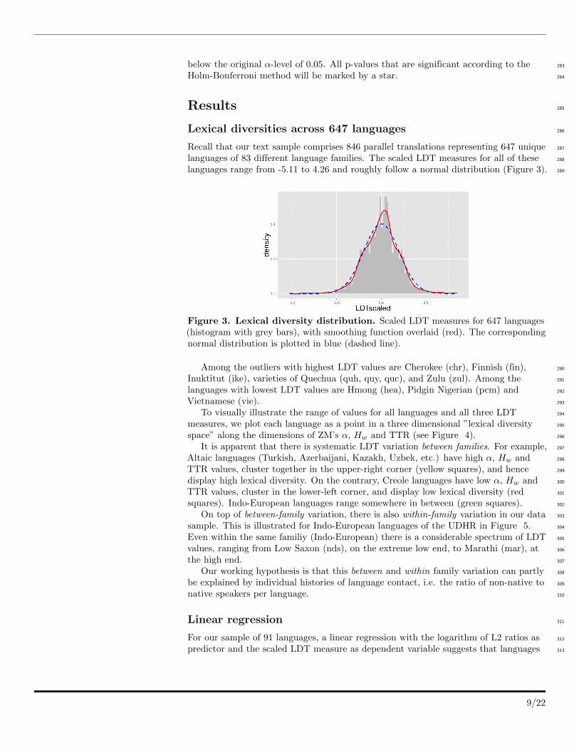
Recall that our text sample comprises 846 parallel translations representing 647 unique 287

languages of 83 different language families. The scaled LDT measures for all of these 288

languages range from -5.11 to 4.26 and roughly follow a normal distribution (Figure 3). 289

Figure 3. Lexical diversity distribution. Scaled LDT measures for 647 languages(histogram with grey bars), with smoothing function overlaid (red). The correspondingnormal distribution is plotted in blue (dashed line).

Among the outliers with highest LDT values are Cherokee (chr), Finnish (fin), 290

Inuktitut (ike), varieties of Quechua (quh, quy, quc), and Zulu (zul). Among the 291

languages with lowest LDT values are Hmong (hea), Pidgin Nigerian (pcm) and 292

Vietnamese (vie). 293

To visually illustrate the range of values for all languages and all three LDT 294

measures, we plot each language as a point in a three dimensional ”lexical diversity 295

space” along the dimensions of ZM’s α, Hw and TTR (see Figure 4). 296

It is apparent that there is systematic LDT variation between families. For example, 297

Altaic languages (Turkish, Azerbaijani, Kazakh, Uzbek, etc.) have high α, Hw and 298

TTR values, cluster together in the upper-right corner (yellow squares), and hence 299

display high lexical diversity. On the contrary, Creole languages have low α, Hw and 300

TTR values, cluster in the lower-left corner, and display low lexical diversity (red 301

squares). Indo-European languages range somewhere in between (green squares). 302

On top of between-family variation, there is also within-family variation in our data 303

sample. This is illustrated for Indo-European languages of the UDHR in Figure 5. 304

Even within the same familiy (Indo-European) there is a considerable spectrum of LDT 305

values, ranging from Low Saxon (nds), on the extreme low end, to Marathi (mar), at 306

the high end. 307

Our working hypothesis is that this between and within family variation can partly 308

be explained by individual histories of language contact, i.e. the ratio of non-native to 309

native speakers per language. 310

Linear regression 311

For our sample of 91 languages, a linear regression with the logarithm of L2 ratios as 312

predictor and the scaled LDT measure as dependent variable suggests that languages 313

9/22

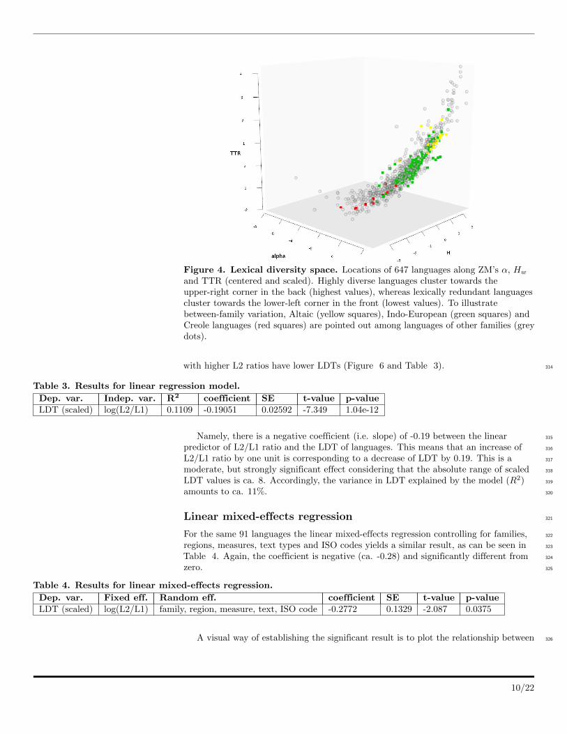
Figure 4. Lexical diversity space. Locations of 647 languages along ZM’s α, Hw

and TTR (centered and scaled). Highly diverse languages cluster towards theupper-right corner in the back (highest values), whereas lexically redundant languagescluster towards the lower-left corner in the front (lowest values). To illustratebetween-family variation, Altaic (yellow squares), Indo-European (green squares) andCreole languages (red squares) are pointed out among languages of other families (greydots).

with higher L2 ratios have lower LDTs (Figure 6 and Table 3). 314

Table 3. Results for linear regression model.

Dep. var. Indep. var. R2 coefficient SE t-value p-valueLDT (scaled) log(L2/L1) 0.1109 -0.19051 0.02592 -7.349 1.04e-12

Namely, there is a negative coefficient (i.e. slope) of -0.19 between the linear 315

predictor of L2/L1 ratio and the LDT of languages. This means that an increase of 316

L2/L1 ratio by one unit is corresponding to a decrease of LDT by 0.19. This is a 317

moderate, but strongly significant effect considering that the absolute range of scaled 318

LDT values is ca. 8. Accordingly, the variance in LDT explained by the model (R2) 319

amounts to ca. 11%. 320

Linear mixed-effects regression 321

For the same 91 languages the linear mixed-effects regression controlling for families, 322

regions, measures, text types and ISO codes yields a similar result, as can be seen in 323

Table 4. Again, the coefficient is negative (ca. -0.28) and significantly different from 324

zero. 325

Table 4. Results for linear mixed-effects regression.

Dep. var. Fixed eff. Random eff. coefficient SE t-value p-valueLDT (scaled) log(L2/L1) family, region, measure, text, ISO code -0.2772 0.1329 -2.087 0.0375

A visual way of establishing the significant result is to plot the relationship between 326

10/22

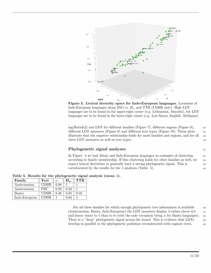
Figure 5. Lexical diversity space for Indo-European languages. Locations ofIndo-European languages along ZM’s α, Hw and TTR (UDHR only). High LDTlanguages are to be found in the upper-right corner (e.g. Lithuanian, Marathi), low LDTlanguages are to be found in the lower-right corner (e.g. Low Saxon, English, Afrikaans).

log(RatioL2) and LDT for different families (Figure 7), different regions (Figure 8), 327

different LDT measures (Figure 9) and different text types (Figure 10). These plots 328

illustrate that the negative relationship holds for most families and regions, and for all 329

three LDT measures as well as text types. 330

Phylogenetic signal analyses 331

In Figure 4 we had Altaic and Indo-European languages as examples of clustering 332

according to family membership. If this clustering holds for other families as well, we 333

expect lexical diversities to generally have a strong phylogenetic signal. This is 334

corroborated by the results for the λ analyses (Table 5). 335

Table 5. Results for the phylogenetic signal analysis (mean λ).

Family Text α Hw TTRAustronesian UDHR 0.98 1 1Austronesian PBC 0.94 0.82 1Bantu UDHR 0.46 0.85 0.58Indo-European UDHR 1 0.64 1

For all three families for which enough phylogenetic tree information is available 336

(Austronesian, Bantu, Indo-European) the LDT measures display λ-values above 0.5 337

and hence closer to 1 than to 0 (with the only exception being α for Bantu languages). 338

There is a ”deep” phylogenetic signal across the board. This is evidence that LDTs 339

develop in parallel to the phylogenetic pathways reconstructed with cognate trees. 340

11/22

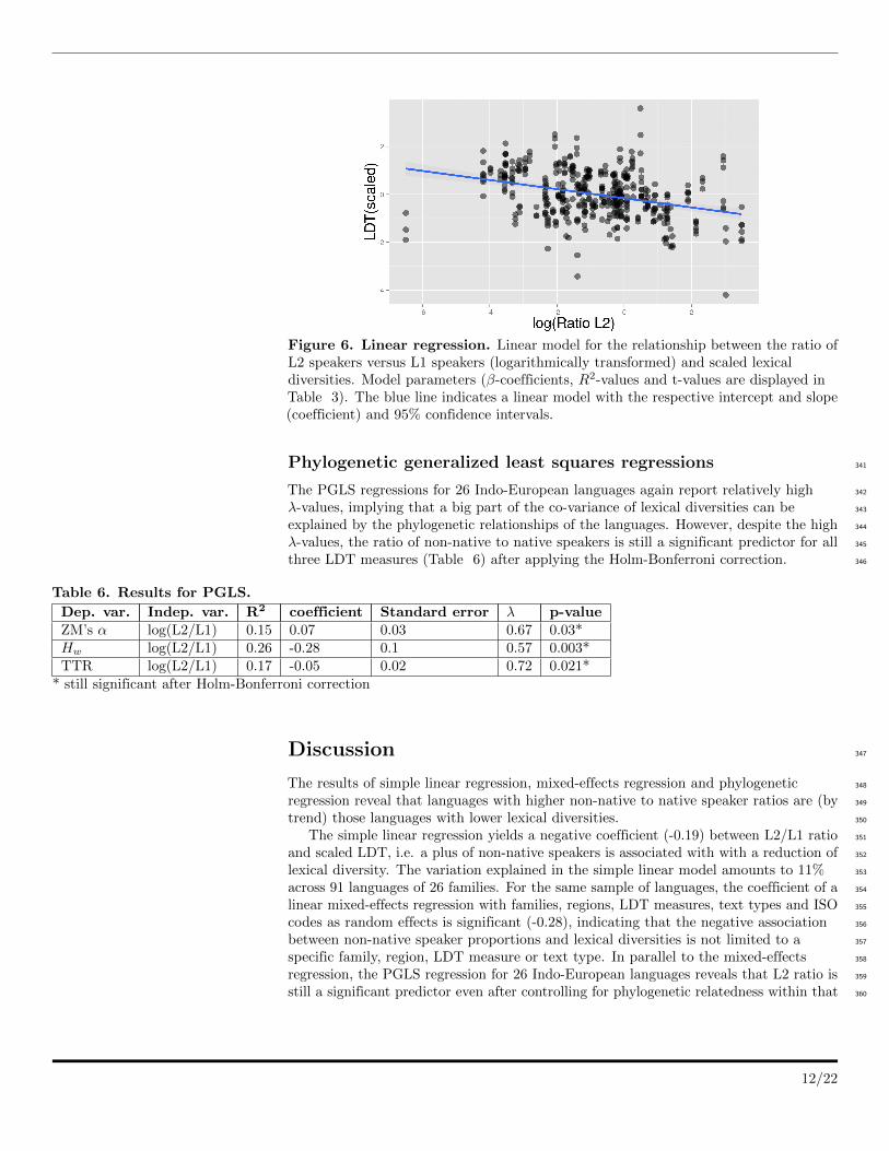
Figure 6. Linear regression. Linear model for the relationship between the ratio ofL2 speakers versus L1 speakers (logarithmically transformed) and scaled lexicaldiversities. Model parameters (β-coefficients, R2-values and t-values are displayed inTable 3). The blue line indicates a linear model with the respective intercept and slope(coefficient) and 95% confidence intervals.

Phylogenetic generalized least squares regressions 341

The PGLS regressions for 26 Indo-European languages again report relatively high 342

λ-values, implying that a big part of the co-variance of lexical diversities can be 343

explained by the phylogenetic relationships of the languages. However, despite the high 344

λ-values, the ratio of non-native to native speakers is still a significant predictor for all 345

three LDT measures (Table 6) after applying the Holm-Bonferroni correction. 346

Table 6. Results for PGLS.

Dep. var. Indep. var. R2 coefficient Standard error λ p-valueZM’s α log(L2/L1) 0.15 0.07 0.03 0.67 0.03*Hw log(L2/L1) 0.26 -0.28 0.1 0.57 0.003*TTR log(L2/L1) 0.17 -0.05 0.02 0.72 0.021*

* still significant after Holm-Bonferroni correction

Discussion 347

The results of simple linear regression, mixed-effects regression and phylogenetic 348

regression reveal that languages with higher non-native to native speaker ratios are (by 349

trend) those languages with lower lexical diversities. 350

The simple linear regression yields a negative coefficient (-0.19) between L2/L1 ratio 351

and scaled LDT, i.e. a plus of non-native speakers is associated with with a reduction of 352

lexical diversity. The variation explained in the simple linear model amounts to 11% 353

across 91 languages of 26 families. For the same sample of languages, the coefficient of a 354

linear mixed-effects regression with families, regions, LDT measures, text types and ISO 355

codes as random effects is significant (-0.28), indicating that the negative association 356

between non-native speaker proportions and lexical diversities is not limited to a 357

specific family, region, LDT measure or text type. In parallel to the mixed-effects 358

regression, the PGLS regression for 26 Indo-European languages reveals that L2 ratio is 359

still a significant predictor even after controlling for phylogenetic relatedness within that 360

12/22

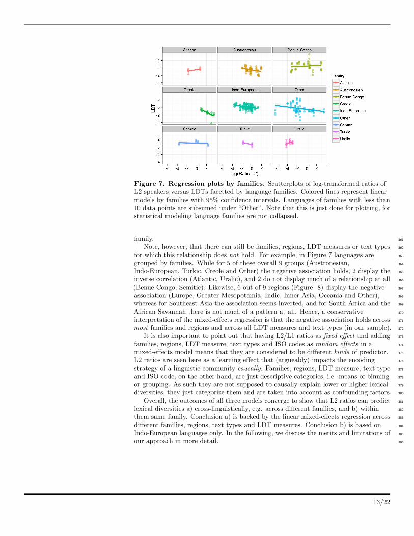
Figure 7. Regression plots by families. Scatterplots of log-transformed ratios ofL2 speakers versus LDTs facetted by language families. Colored lines represent linearmodels by families with 95% confidence intervals. Languages of families with less than10 data points are subsumed under “Other”. Note that this is just done for plotting, forstatistical modeling language families are not collapsed.

family. 361

Note, however, that there can still be families, regions, LDT measures or text types 362

for which this relationship does not hold. For example, in Figure 7 languages are 363

grouped by families. While for 5 of these overall 9 groups (Austronesian, 364

Indo-European, Turkic, Creole and Other) the negative association holds, 2 display the 365

inverse correlation (Atlantic, Uralic), and 2 do not display much of a relationship at all 366

(Benue-Congo, Semitic). Likewise, 6 out of 9 regions (Figure 8) display the negative 367

association (Europe, Greater Mesopotamia, Indic, Inner Asia, Oceania and Other), 368

whereas for Southeast Asia the association seems inverted, and for South Africa and the 369

African Savannah there is not much of a pattern at all. Hence, a conservative 370

interpretation of the mixed-effects regression is that the negative association holds across 371

most families and regions and across all LDT measures and text types (in our sample). 372

It is also important to point out that having L2/L1 ratios as fixed effect and adding 373

families, regions, LDT measure, text types and ISO codes as random effects in a 374

mixed-effects model means that they are considered to be different kinds of predictor. 375

L2 ratios are seen here as a learning effect that (argueably) impacts the encoding 376

strategy of a linguistic community causally. Families, regions, LDT measure, text type 377

and ISO code, on the other hand, are just descriptive categories, i.e. means of binning 378

or grouping. As such they are not supposed to causally explain lower or higher lexical 379

diversities, they just categorize them and are taken into account as confounding factors. 380

Overall, the outcomes of all three models converge to show that L2 ratios can predict 381

lexical diversities a) cross-linguistically, e.g. across different families, and b) within 382

them same family. Conclusion a) is backed by the linear mixed-effects regression across 383

different families, regions, text types and LDT measures. Conclusion b) is based on 384

Indo-European languages only. In the following, we discuss the merits and limitations of 385

our approach in more detail. 386

13/22

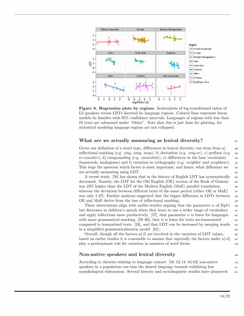
Figure 8. Regression plots by regions. Scatterplots of log-transformed ratios ofL2 speakers versus LDTs facetted by language regions. Colored lines represent linearmodels by families with 95% confidence intervals. Languages of regions with less than10 texts are subsumed under “Other”. Note that this is just done for plotting, forstatistical modeling language regions are not collapsed.

What are we actually measuring as lexical diversity? 387

Given our definition of a word type, differences in lexical diversity can stem from a) 388

inflectional marking (e.g. sing, sang, sung), b) derivation (e.g. sing-er), c) prefixes (e.g. 389

re-consider), d) compounding (e.g. snowwhite), e) differences in the base vocabulary 390

(loanwords, neologisms) and f) variation in orthography (e.g. neighbor and neighbour). 391

This begs the question which factor is most important, and hence, what difference we 392

are actually measuring using LDT. 393

A recent study [56] has shown that in the history of English LDT has systematically 394

decreased. Namely, the LDT for the Old English (OE) version of the Book of Genesis 395

was 23% higher than the LDT of the Modern English (MnE) parallel translation, 396

whereas the deviation between different texts of the same period (either OE or MnE) 397

was only 1-2%. Further analyses suggested that the bigger difference in LDTs between 398

OE and MnE derive from the loss of inflectional marking. 399

These observations align with earlier studies arguing that the parameter α of Zipf’s 400

law decreases in children’s speech when they learn to use a wider range of vocabulary 401

and apply inflections more productively [57], that parameter α is lower for languages 402

with more grammatical marking [58–60], that it is lower for texts un-lemmatized 403

compared to lemmatized texts [24], and that LDT can be increased by merging words 404

in a simplified grammaticalization model [61]. 405

Overall, though all the factors a)-f) are involved in the variation of LDT values, 406

based on earlier studies it is reasonable to assume that especially the factors under a)-d) 407

play a predominant role for variation in numbers of word forms. 408

Non-native speakers and lexical diversity 409

According to theories relating to language contact [10–12,14–16,62] non-native 410

speakers in a population can bias the shared language towards exhibiting less 411

morphological elaboration. Several historic and sociolinguistic studies have pioneered 412

14/22

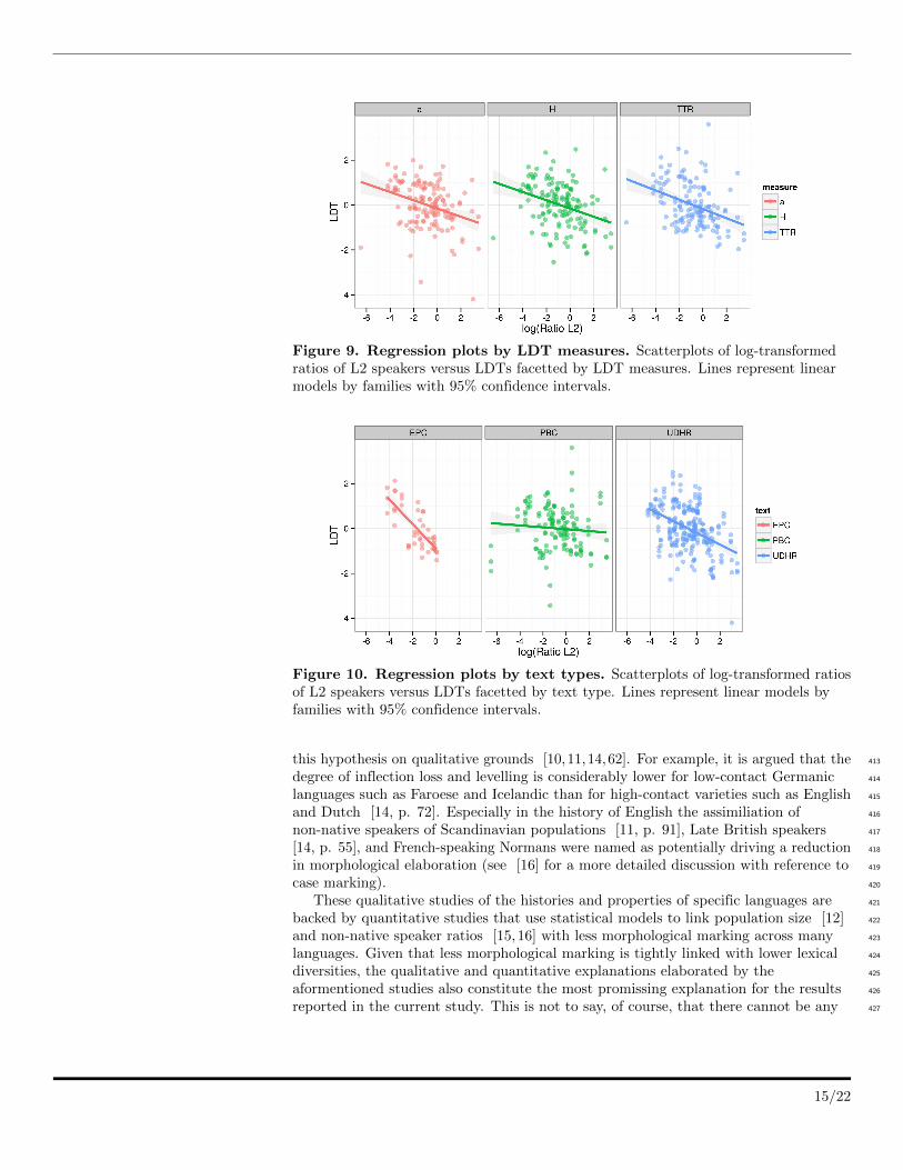
Figure 9. Regression plots by LDT measures. Scatterplots of log-transformedratios of L2 speakers versus LDTs facetted by LDT measures. Lines represent linearmodels by families with 95% confidence intervals.

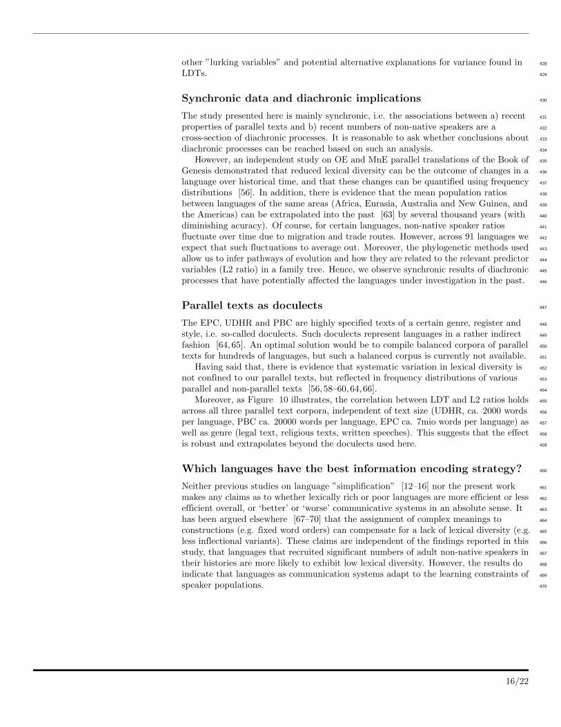
Figure 10. Regression plots by text types. Scatterplots of log-transformed ratiosof L2 speakers versus LDTs facetted by text type. Lines represent linear models byfamilies with 95% confidence intervals.

this hypothesis on qualitative grounds [10,11,14,62]. For example, it is argued that the 413

degree of inflection loss and levelling is considerably lower for low-contact Germanic 414

languages such as Faroese and Icelandic than for high-contact varieties such as English 415

and Dutch [14, p. 72]. Especially in the history of English the assimiliation of 416

non-native speakers of Scandinavian populations [11, p. 91], Late British speakers 417

[14, p. 55], and French-speaking Normans were named as potentially driving a reduction 418

in morphological elaboration (see [16] for a more detailed discussion with reference to 419

case marking). 420

These qualitative studies of the histories and properties of specific languages are 421

backed by quantitative studies that use statistical models to link population size [12] 422

and non-native speaker ratios [15,16] with less morphological marking across many 423

languages. Given that less morphological marking is tightly linked with lower lexical 424

diversities, the qualitative and quantitative explanations elaborated by the 425

aformentioned studies also constitute the most promissing explanation for the results 426

reported in the current study. This is not to say, of course, that there cannot be any 427

15/22

other ”lurking variables” and potential alternative explanations for variance found in 428

LDTs. 429

Synchronic data and diachronic implications 430

The study presented here is mainly synchronic, i.e. the associations between a) recent 431

properties of parallel texts and b) recent numbers of non-native speakers are a 432

cross-section of diachronic processes. It is reasonable to ask whether conclusions about 433

diachronic processes can be reached based on such an analysis. 434

However, an independent study on OE and MnE parallel translations of the Book of 435

Genesis demonstrated that reduced lexical diversity can be the outcome of changes in a 436

language over historical time, and that these changes can be quantified using frequency 437

distributions [56]. In addition, there is evidence that the mean population ratios 438

between languages of the same areas (Africa, Eurasia, Australia and New Guinea, and 439

the Americas) can be extrapolated into the past [63] by several thousand years (with 440

diminishing acuracy). Of course, for certain languages, non-native speaker ratios 441

fluctuate over time due to migration and trade routes. However, across 91 languages we 442

expect that such fluctuations to average out. Moreover, the phylogenetic methods used 443

allow us to infer pathways of evolution and how they are related to the relevant predictor 444

variables (L2 ratio) in a family tree. Hence, we observe synchronic results of diachronic 445

processes that have potentially affected the languages under investigation in the past. 446

Parallel texts as doculects 447

The EPC, UDHR and PBC are highly specified texts of a certain genre, register and 448

style, i.e. so-called doculects. Such doculects represent languages in a rather indirect 449

fashion [64,65]. An optimal solution would be to compile balanced corpora of parallel 450

texts for hundreds of languages, but such a balanced corpus is currently not available. 451

Having said that, there is evidence that systematic variation in lexical diversity is 452

not confined to our parallel texts, but reflected in frequency distributions of various 453

parallel and non-parallel texts [56,58–60,64,66]. 454

Moreover, as Figure 10 illustrates, the correlation between LDT and L2 ratios holds 455

across all three parallel text corpora, independent of text size (UDHR, ca. 2000 words 456

per language, PBC ca. 20000 words per language, EPC ca. 7mio words per language) as 457

well as genre (legal text, religious texts, written speeches). This suggests that the effect 458

is robust and extrapolates beyond the doculects used here. 459

Which languages have the best information encoding strategy? 460

Neither previous studies on language ”simplification” [12–16] nor the present work 461

makes any claims as to whether lexically rich or poor languages are more efficient or less 462

efficient overall, or ‘better’ or ‘worse’ communicative systems in an absolute sense. It 463

has been argued elsewhere [67–70] that the assignment of complex meanings to 464

constructions (e.g. fixed word orders) can compensate for a lack of lexical diversity (e.g. 465

less inflectional variants). These claims are independent of the findings reported in this 466

study, that languages that recruited significant numbers of adult non-native speakers in 467

their histories are more likely to exhibit low lexical diversity. However, the results do 468

indicate that languages as communication systems adapt to the learning constraints of 469

speaker populations. 470

16/22

Are all languages directly comparable? 471

Our analyses include Creole languages. Because of their abrupt creation by L2 speakers, 472

it might be argued that Creole languages are not a coherent group comparable to a 473

language family like Indo-European. However, it is equally plausible that the same L2 474

learning pressures that most strongly shape Creole languages are at play in historical 475

language change of other languages as well, albeit to a lesser extent (see also [11,14]). 476

From this perspective, the difference between Creole languages and other language 477

groupings is a matter of degree, rather than categorical. Including them as a sub-group 478

instead of excluding them categorically can therefore only help to better understand the 479

pressures that shape languages over time. 480

Correlation is not causation 481

Spurious correlations are a recurring problem in studies of sociolinguistic variation 482

[71, 72], where independent evidence can help to support claims of a causal relationship. 483

In the present case, a causal link between non-native learning and reduction of lexical 484

diversity is supported by two areas of research: 485

1) Qualitative sociolinguistic studies are replete with examples of non-native 486

speakers reducing morphological marking and hence lexical diversity over time 487

[11, 13,14,62] and these are backed by quantitative evidence [12,15,16]. 488

2) In the context of measuring lexical diversity for teaching purposes it has been 489

shown that L2 learners of French [18] and English with various L1 backgrounds [17] 490

produce output of lower lexical diversity compared to native speakers. 491

We therefore emphasise the converging evidence from qualitative and quantitative, 492

diachronic and synchronic studies showing that the presence of significant numbers of 493

non-native speakers systematically lowers the likelihood of preserving lexically rich 494

encoding systems. 495

Conclusion 496

Languages with more non-native speakers tend to have lower lexical diversities, i.e. 497

fewer word forms and higher word form frequencies. This trend holds across different 498

language families, regions, measures, and text types. In other words, non-native 499

language learning and usage emerges as important factor driving language change and 500

evolution besides native language transmission. 501

Since non-native language learners are prone to reduce manifold word forms to a 502

smaller set of base forms, it is natural that they shape the lexical encoding strategies of 503

the next generation of learners. It is not clear, and not particularly relevant for our 504

approach, whether the resulting lower lexical diversity results in a ‘better’ or ‘worse’ 505

encoding strategy. The picture that emerges, however, suggests that in the long run, 506

languages as encoding systems can adapt to sociolinguistic pressures, including those 507

determined by learning abilities and constraints of their speakers. This finding can help 508

to disentangle the complex relationship between language learning, language typology 509

and language change. As a result, theories of language evolution should take into 510

account the co-evolution of population structure, human learning abilities and language 511

structure. 512

Acknowledgements 513

We would like to thank (in alphabetical order) Dimitris Alikanoitis, Damian Blasi, Ted 514

Briscoe, Sean Roberts, Martijn Wieling, Bodo Winter as well as the audiences at the 515

17/22

NLIP Seminar Series (Computer Laboratory, Cambridge 2014), Workshop for 516

Computational Linguistics (Department of Theoretical and Applied Linguistics, 517

Cambridge 2014), Evolang 2010 (Vienna) and EACL 2014 (Gothenburg) for valuable 518

input. 519

CB is funded by an Arts and Humanities Research Council (UK) doctoral grant(reference number: 04325), a grant from the Cambridge Home and EuropeanScholarship Scheme, and by Cambridge English, University of Cambridge. AV issupported by ERC grant ’The evolution of human languages’ (reference number:268744). DK is supported by EPSRC grant EP/I037512/1. FH is funded by aBenefactor’s Scholarship of St. John’s College, Cambridge. PB is supported byCambridge English, University of Cambridge.

References

1. Fortescue M (1984) West Greenlandic (Croom Helm Descriptive Grammars).London: Croom Helm.

2. Lightfoot DW (1979) Principles of diachronic syntax. Cambridge: CambridgeUniversity Press.

3. Clark R, Roberts I (1993) A computational model of language learnability andlanguage change. Linguistic Inquiry 24: 299–345.

4. Niyogi P, Berwick RC (1997) Evolutionary consequences of language learning.Linguistics and Philosophy 20: 697–719.

5. Briscoe T (2000) Grammatical acquisition: Inductive bias and coevolution oflanguage and the language acquisition device. Language 76: 245–296.

6. Yang CD (2000) Internal and external forces in language change. LanguageVariation and Change 12: 231–250.

7. Roberts I, Roussou A (2003) Syntactic change: A minimalist approach togrammaticalization. Cambridge: Cambridge University Press.

8. Roberts I (2007) Diachronic syntax. Oxford: Oxford University Press.

9. Thomason SG, Kaufman T (1988) Language contact, creolization, and geneticlinguistics. Berkeley, Los Angeles, Oxford: University of California Press.

10. Wray A, Grace GW (2007) The consequences of talking to strangers :Evolutionary corollaries of socio-cultural influences on linguistic form. Lingua117: 543–578.

11. McWhorter JH (2007) Language interrupted: Signs of non-native acquisition instandard language grammars. New York: Oxford University Press.

12. Lupyan G, Dale R (2010) Language Structure Is Partly Determined by SocialStructure. PloS ONE 5: e8559.

13. McWhorter JH (2011) Linguistic simplicity and complexitiy: Why do languagesundress? Boston: Mouton de Gruyter.

14. Trudgill P (2011) Sociolinguistic typology: Social determinants of linguisticcomplexity. Oxford: Oxford University Press.

18/22

15. Bentz C, Winter B (2012) The impact of L2 speakers on the evolution of casemarking. In: Scott-Phillips TC, Tamariz M, Cartmill EA, Hurford JR, editors,The evolution of language. Proceedings of the 9th international conference(EVOLANG9). Singapore: World Scientific, pp. 58–64.

16. Bentz C, Winter B (2013) Languages with more second language speakers tend tolose nominal case. Language Dynamics and Change 3: 1–27.

17. Jarvis S (2002) Short texts, best-fitting curves and new measures of lexicaldiversity. Language Testing 19: 57–84.

18. Treffers-Daller J (2013) Measuring lexical diversity among L2 learners of French:An exploration of the validity of D , MTLD and HD-D as measures of languageability. In: Jarvis S, M D, editors, Vocabulary knowledge: Human ratings andautomated measures, Amsterdam: Benjamins, volume 28. pp. 79–104.

19. Mandelbrot B (1953) An informational theory of the statistical structure oflanguage. In: Jackson W, editor, Communication Theory, London: ButterworthsScientific Publications. pp. 468–502.

20. Zipf GK (1949) Human behavior and the principle of least effort. Cambridge(Massachusetts): Addison-Wesley.

21. Shannon CE, Weaver W (1949) The mathematical theory of communication.Urbana: The University of Illinois Press.

22. Shannon CE (1951) Prediction and entropy of printed English. The Bell SystemTechnical Journal : 50–65.

23. Tweedie FJ, Baayen RH (1998) How Variable May a Constant be? Measures ofLexical Richness in Perspective. Computers and the Humanities 32: 323–352.

24. Baroni M (2009) Distributions in text. In: Ludeling A, Kyto M, editors, CorpusLinguistics. An international handbook, Berlin, New York: Mouton de Gruyter,Sampson 2002, chapter 39. pp. 803–821.

25. Baayen HR (2001) Word frequency distributions. Dordrecht, Boston & London:Kluwer.

26. Baayen HR (2008). Analyzing linguistic data: A practical introduction using R.URL http://cran.r-project.org/package=languageR.

27. Dale R, Lupyan G (2012) Understanding the origins of morphological diversity:The linguistic niche hypothesis. Advances in Complex Systems 15:1150017–1–1150017–16.

28. Croft W (2000) Explaining language change: An evolutionary approach.Edinburgh: Pearson Education Limited.

29. Ritt N (2004) Selfish Sounds and Linguistic Evolution: A Darwinian Approach toLanguage Change. Cambridge University Press, 342 pp. URLhttp://books.google.com/books?hl=en&lr=&id=jGGAaOZxA_gC&pgis=1.

30. Christiansen MH, Kirby S (2003) Language evolution: consensus andcontroversies. TRENDS in Cognitive Science 7: 300–305.

31. Christiansen MH, Chater N (2008) Language as shaped by the brain. Behavioraland Brain Sciences 31: 489–509.

19/22

32. Kirby S, Dowman M, Griffiths TL (2007) Innateness and culture in the evolutionof language. Proceedings of the National Academy of Sciences of the UnitedStates of America 104: 5241–5245.

33. Beckner C, Ellis NC, Blythe R, Holland J, Bybee J, et al. (2009) Language is acomplex adaptive system. Language Learning 59: 1–26.

34. Mayer T, Cysouw M (2014) Creating a massively parallel bible corpus. In:Calzolari N, Choukri K, Declerck T, Loftsson H, Maegaard B, et al., editors,Proceedings of the Ninth International Conference on Language Resources andEvaluation (LREC-2014), Reykjavik, Iceland, May 26-31, 2014. EuropeanLanguage Resources Association (ELRA), pp. 3158–3163. URLhttp://www.lrec-conf.org/proceedings/lrec2014/summaries/220.html.

35. Koehn P (2005) Europarl: A parallel corpus for statistical machine translation.In: MT summit. volume 5, pp. 79–86.

36. Dryer MS, Haspelmath M, editors (2013) World atlas of language structuresonline. Munich: Max Planck Digital Library. URL http://wals.info/.

37. Haspelmath M (2011) The indeterminacy of word segmentation and the nature ofmorphology and syntax. Folia Linguistica 45: 31–80.

38. Wray A (2014) Whay are we so sure we k now what a word is?, OxfordUniversity Press, chapter 42.

39. Jost L (2006) Entropy and diversity. OIKOS 113.

40. Duran P, Malvern D, Richards B, Chipere N (2004) Developmental trends inlexical diversity. Applied Linguistics 25: 220–242.

41. R Core Team (2013). R: A language and environment for statistical computing.doi:ISBN3-900051-07-0. URL http://www.r-project.org/.

42. Lewis MP, Simons GF, Fenning CD, editors (2013) Ethnologue: Languages of theworld. Dallas, Texas: SIL International, 17th edition. URLhttp://www.ethnologue.com.

43. Jaeger TF, Graff P, Croft W, Pontillo D (2011) Mixed effect models for geneticand areal dependencies in linguistic typology. Linguistic Typology 15: 281–320.

44. Cysouw M (2010) Dealing with diversity : Towards an explanation of NP-internalword order frequencies. Linguistic Typology 14: 253–286.

45. Baayen HR, Davidson DJ, Bates DM (2008) Mixed-effects modeling with crossedrandom effects for subjects and items. Journal of Memory and Language 59:390–412.

46. Barr DJ, Levy R, Scheepers C, Tily HJ (2013) Random effects structure forconfirmatory hypothesis testing: Keep it maximal. Journal of Memory andLanguage 68: 255–278.

47. Bates D, Maechler M, Bolker B (2012). lme4: Linear mixed-effects models usingS4 classes. URL http://cran.r-project.org/package=lme4.

48. Freckleton RP, Harvey PH, Pagel M (2002) Phylogenetic analysis andcomparative data: A test and review of evidence. The American Naturalist 160:712–726.

20/22

49. Pagel M (1999) Inferring the historical patterns of biological evolution. Nature401: 877–884.

50. Pagel M (1997) Inferring evolutionary processes from phylogenies. ZoologicaScripta 26: 331–348.

51. Grollemund SBKMAVCPM Rebecca; Branford (to appear) Bantu populationdispersal shows preference for routes following similar habitats. .

52. Gray RD, Drummond AJ, Greenhill SJ (2009) Language phylogenies revealexpansion pulses and pauses in Pacific settlement. Science 323: 479–483.

53. Bouckaert R, Lemey P, Dunn M, Greenhill SJ, Alekseyenko AV, et al. (2012)Mapping the origins and expansion of the Indo-European language family.Science 337: 957–960.

54. Pagel M, Meade A. Bayes Traits V2. URLwww.evolution.rdg.ac.uk/Files/BayesTraitsV2Manual(Beta).pdf.

55. Holm S (1979) A simple sequentially rejective multiple test procedure.Scandinavian journal of statistics : 65–70.

56. Bentz C, Kiela D, Hill F, Buttery P (2014) Zipf’s law and the grammar oflanguages: A quantitative study of Old and Modern English parallel texts.Corpus Linguistics and Linguistic Theory .

57. Baixeries J, Elveva g B, Ferrer-i Cancho R (2013) The evolution of the exponentof Zipf ’s law in language ontogeny. PloS ONE 8: e53227.

58. Ha LQ, Stewart DW, Hanna P, Smith FJ (2006) Zipf and type-token rules for theEnglish, Spanish, Irish and Latin languages. Web Journal of Formal,Computational and Cognitive Linguistics 8.

59. Popescu II, Altmann G (2008) Hapax legomena and language typology. Journalof Quantitative Linguistics 15: 370–378.

60. Popescu II, Altmann G, Grzybek P, Jayaram BD, Kohler R, et al. (2009) Wordfrequency studies. Berlin & New York: Mouton de Gruyter.

61. Bentz C, Buttery P (2014) Towards a computational model of grammaticalizationand lexical diversity. In: Proc. of 5th Workshop on Cognitive Aspects ofComputational Language Learning (CogACLL)@ EACL. pp. 38–42.

62. McWhorter JH (2002) What happened to English ? Diachronica 19: 217–272.

63. Wichmann Sr, Holman EW (2009) Population size and rates of language change.Human Biology 81: 259–274.

64. Walchli B (2012) Indirect measurement in morphological typology. In: Ender A,Leemann A, Walchli B, editors, Methods in contemporary linguistics, Berlin: DeGruyter Mouton. pp. 69–92.

65. Cysouw M, Walchli B (2007) Parallel texts. Using translational equivalents inlinguistic typology. Sprachtypologie & Universalienforschung STUF 60.2.

66. Popescu II, Altmann G, Kohler R (2010) Zipf’s law—another view. Quality &Quantity 44: 713–731.

21/22

67. Hawkins JA (2004) Efficiency and complexity in grammars. Oxford: OxfordUniversity Press.

68. Hawkins JA (2009) An efficiency theory of complexity and related phenomena.In: Sampson G, Gil D, Trudgill P, editors, Language complexity as an evolvingvariable, Oxford: Oxford University Press. pp. 252–269.

69. Hawkins JA (2012) The drift of English toward invariable word order from atypological and Germanic perspective. In: Nevalainen T, Traugott EC, editors,The Oxford handbook of the history of English, Oxford: Oxford University Press.pp. 622–633.

70. Ehret K, Szmrecsanyi B (to appear) An information-theoretic approach to assesslinguistic complexity. In: Baechler R, Seiler G, editors, Complexity and Isolation,Berlin: de Gruyter.

71. Roberts S, Winters J (2012) Social structure and language structure: The newnomothetic approach. Psychology of Language and Communication 16: 89–112.

72. Roberts S, Winters J (2013) Linguistic diversity and traffic accidents : Lessonsfrom statistical studies of cultural traits. PloS ONE 8: e70902.

22/22