Adaptive Classification on Brain-Computer Interfaces Using Reinforcement Signals

Adaptive classification on BCI using reinforce-

ment signals 1

A. Llera, V. Gomez, H. J. Kappen

Donders Institute for Brain, Cognition and Behaviour, Radboud University,Nijmegen,

the Netherlands

Keywords: Adaptive classification, Brain computer interfaces.

Abstract

We introduce a probabilistic model that combines a classifier with an extra Reinforce-

ment Signal (RS) encoding the probability of an erroneous feedback being delivered by

the classifier. This representation computes the class probabilities given the task re-

lated features and the reinforcement signal. Using Expectation Maximization (EM) to

estimate the parameter values under such a model shows that some existing adaptive

classifiers are particular cases of such an EM algorithm. Further, we present a new

algorithm for adaptive classification, we call it Constrained means adaptive classifier

(CMAC), and show using EEG data and simulated RS that this classifier is able to sig-

nificantly outperform state-of-the-art adaptive classifiers.

1Authors preprint.

1 Introduction

The final goal of a Brain Computer Interface (BCI) is to provide human subjects with

control over some device or computer application only through their measured brain

activity by e.g. electroencephalogram (EEG) (Wolpaw et al, 2002). To gain control over

the device, the user usually participates in an off-line train/calibration session, where

he/she is instructed to perform some mental task according to visual stimuli while the

generated brain activity is being recorded (Ramoser et al, 1998; van Gerven et al, 2009).

From the recorded data, discriminative features associated with the different intentions

of the user are extracted and used to train a classifier which will predict the intention of

the user during the test/feedback session.

However, due to the poor signal to noise ratio and the non stationary character of

the EEG data (Krauledat, 2008), the patterns extracted during the training of the BCI

may differ for the feedback session leading to a poor performance (Shenoy et al, 2006).

It has been shown that to keep an acceptable performance, EEG based BCIs require a

robustified feature space (Tomioka et al, 2006; Blankertz et al, 2008; von Bunau et al,

2010; Reuderink et al, 2011; Samek et al, 2012) and/or online adaptation of the classifier

parameters (Millan, 2004; Shenoy et al, 2006). Since in practical BCI scenarios the

user intention is unknown, online supervised adaptation is not possible, so the design

of unsupervised adaptive classifiers that are robust to changes due to the non stationary

character of the data has become focus of intense research within the BCI community

(Sykacek et al, 2004; Gan, 2006; Kawanabe et al, 2006; Vidaurre et al, 2006; Hasan

et al, 2009).

A common approach considers the class conditional features as normally distributed

2

variables, and performs unsupervised adaptation of a Linear Discriminant Analysis

(LDA) classifier. Adaptive LDA Pooled-mean (Pmean), and adaptive LDA Pooled-

mean + Global Covariance (PmeanGcov) are two representative examples of this kind

of methods (Vidaurre et al, 2010). Recently, interesting online experiments have shown

the practical application of these techniques, not only for improving the performance

with respect to static classifiers, but also for reducing the training time or increasing

the amount of possible BCI users (Vidaurre et al, 2010b,c). Other methods model the

user intention as a latent variable for which its posterior probabilities (responsibilities)

are computed and subsequently used to update a classifier. This idea has been intro-

duced using Expectation Maximization (EM) in Gaussian Mixture Models (GMM) in

Blumberg et al (2007), and extended to sequential EM in Hasan et al (2009) and Liu

et al (2010). Other extension for joint adaptive feature extraction and classification was

considered in Li et al (2006).

A possible way to improve unsupervised adaptive methods consists of the use of

a reinforcement signal (RS) which acts as a feedback provided by the user to the ma-

chine. Examples of RS can range from button presses delivered by the user (supervised),

to measured muscular activity in an hybrid BCI (Leeb et al, 2010). Another relevant

example of RS is the Error Related Potential (ErrP), a stereotyped pattern elicited fol-

lowing an unexpected response from the BCI (Ferrez, 2007; Ferrez et al, 2008). There

is evidence that this signal can be detected with high accuracy (Chavarriaga et al, 2007,

2010; Blankertz et al, 2004; Llera et al, 2011). The inclusion of such a RS into the

adaptive BCI cycle was introduced in Blumberg et al (2007). In that work, the authors

extend the latent variable approach with an additional binary ErrP classifier. Similarly,

3

in Llera et al (2011) we proposed a discriminant-based approach that also uses a binary

ErrP classifier, and provided a detailed analysis of the negative effect due to false posi-

tives/negatives on the ErrP misclassification.

In this work we introduce a unifying framework which accommodates existing ap-

proaches in two families according to whether a latent variable is explicitly modeled or

not. Our framework is derived from a graphical model which includes a probabilistic

RS instead of a binary RS. This is a way to include the reliability over the measured RS

which implements soft updates when the uncertainty is high, and recovers unsupervised

and supervised learning as particular cases. Further, we develop a novel algorithm for

adaptive classification and present an overview of the relations between existing meth-

ods.

In section 2.1 we introduce a probabilistic graphical model, describe the EM al-

gorithm for estimating the parameters in this model, and derive its sequential version

(CSEM). In section 2.2 we develop a new sequential algorithm (CMAC) for classifi-

cation and parameter estimation. In 3.1 we provide a description of the simulated RS

which will be considered to evaluate the proposed methods. In sections 3.2 and 3.3 we

present the results obtained using synthetic data. In section 4 we compare the proposed

methods with other state of the art classifiers using EEG data and simulated RS. Then,

in section 5 we give a brief description of the methods which are related to our work and

describe the relationships and/or differences between the proposed and the previously

existing methods. Finally, in section 6 we discuss the presented results and consider

future work directions.

4

2 Methods

In section 2.1, we introduce a probabilistic graphical model which includes the task re-

lated features as well as a Reinforcement Signal (RS) encoding the discrepancy between

the user intention and the output given by the device. This formulation estimates the

posterior probabilities of each class (responsibilities) after observing not only the task

related features but also the RS. We describe the EM algorithm for this model and derive

a sequential version of it (CSEM). In 2.2 we derive a new algorithm for online parame-

ter estimation and classification (CMAC), which can use the responsibilities computed

including the RS.

2.1 The model

We consider a binary random variable I ∈ {1, 2} representing the hidden intention of

the user. Given the intention, a vector x ∈ Rn represents the features extracted from the

recorded brain activity of the user while having intention I . Based on these features,

a probabilistic task classifier is used to compute the output of the BCI, Z ∈ {1, 2},

which is used for control. The output Z can be interpreted as a feedback from the BCI

to the user. Further, once Z is observed by the user, we consider a probabilistic RS

which provides the probability of an erroneous feedback, E ∈ [0, 1]. Given Z and E

as evidence, we can use the fact that I is a binary variable and write its conditional

probability as:

p(I|Z,E) =

1− E if I = Z

E if I 6= Z

. (1)

5

For simplicity, we will not explicitly consider the dependence of Z on x through the

task classifier, nor the dependence of E on Z through the brain activity measured after

observing Z and the RS. Instead, although the intention of the user is not actually caused

by Z and E, we summarize the influence of Z through E as given by (1). Figure 1 shows

a Bayesian network that captures the probabilities described above.

x

Z

E

I .

Figure 1: Probabilistic graphical model: x ∈ Rn represents the task related features

extracted from the EEG data, Z ∈ {1, 2} the BCI output computed using the task

classifier, E ∈ [0, 1] the RS encoding the probability that Z was an erroneous output

and I ∈ {1, 2} denotes the intention of the user.

The joint probability distribution of the proposed model is

p(I,x, Z, E) = p(x|I)p(I|Z,E)p(Z)p(E). (2)

We consider p(I|Z,E) as given by (1), and assume normally distributed features

given the intention, that is

p(x|I) =1

(2π)n/2|ΣI |1/2exp

(

−1

2(x− µI)

⊺Σ−1

I (x− µI)

)

≡ N (x|µI ,ΣI),

with the intention I replaced with a mean vector µI ∈ Rn and covariance matrix ΣI ∈

Mn×n as sufficient statistics. Further, we will assume a flat prior over E and Z, so

p(E) = 1, ∀E ∈ [0, 1], and p(Z) = 1

2, ∀Z ∈ {1, 2}. We compactly represent the set of

parameters of the model using the vector θ := (µ1,Σ1,µ2,Σ2).

6

Suppose that we have a data set of observations S from which we can estimate

the unknown model parameters θ. In our case, the observations correspond to T trials

that are composed of an observed component S = {〈xt, Zt, Et〉}t∈{1,...,T}, and a latent

variable I t, the intention at trial t. The log-likelihood of the data given the model

parameters can be written as

log p(S|θ) =T∑

t=1

log2

∑

It=1

p(I t,xt, Zt, Et|θ) =T∑

t=1

log2

∑

It=1

p(xt|I t)p(I t|Zt, Et)p(Zt)p(Et).

(3)

Maximizing (3) is not straightforward, since the summation over the latent variables

I t occurs inside of the logarithm. Typically, the Expectation Maximization (EM) algo-

rithm is used to solve this problem (Bishop, 2007). The EM algorithm is a procedure

which iterates two steps until convergence.

In the E-Step, one assumes current parameter values θold and computes the posterior

distribution of each of the intentions I t ∈ {1, 2}, the so-called responsibilities:

p(I t|xt, Zt, Et,θold) =p(xt|I t,θold)p(I t|Zt, Et)

∑

2

It=1p(xt|I t,θold)p(I t|Zt, Et)

≡ γtI . (4)

In the M-step, we replace the old parameter values with the ones that result of max-

imizing the expected log-likelihood:

θnew = argmaxθ

T∑

t=1

2∑

It=1

p(I t|xt, Zt, Et,θold) log p(I t,xt, Zt, Et|θ). (5)

Taking derivatives of (5) with respect to the elements of θ and setting them to zero

results in the updates

µI =1

NI

T∑

t=1

γtIx

t, (6)

7

ΣI =1

NI

T∑

t=1

γtI(x

t − µI)(xt − µI)

⊺. (7)

where NI =∑T

t=1γtI .

Note that this representation (Figure 1) computes the posterior probability of each

of the intentions given the task related features and the RS. As a consequence, the

difference between the proposed methodology and the standard EM for GMM relies on

the use of p(I t|xt, Zt, Et,θold) (4), a RS dependent quantity, instead of simply

p(I t|xt,θold) =p(xt|I t,θold)

∑

2

It=1p(xt|I t,θold)

. (8)

It is interesting to see that the model recovers the two following well-known cases:

Unsupervised case : If the RS is non-informative, Et = 1/2, the updates become the

ones of the EM for GMM.

Supervised case : If the RS is always correct and returns only a binary answer Et ∈

{0, 1}, the responsibility of the incorrect intention is zero, whereas the responsi-

bility of the correct intention is one.

Using the responsibilities as defined in (4), we can interpolate between unsuper-

vised and supervised learning using the RS. This suggests an improvement over the

unsupervised method given that the RS is informative. We show evidence for this later

in section 3.2.

In the case that we have an incoming stream of data, as it is the case for online

BCI, the previous optimization might not be efficient since it uses a batch of data and

an iterative procedure in order to optimize the model parameters. For online BCI an

incremental approach is necessary (Hasan et al, 2009b). A sequential version of the

8

previously described EM algorithm is defined by the updates

µ′I = (1− βµγI)µI + βµγIx, (9)

Σ′I = (1− βΣγI)ΣI + βΣγI(x− µI)(x− µI)

′, (10)

where x is the observed task related feature vector, γI are the responsibilities computed

using (4) and, βµ and βΣ learning rates. We will denote this algorithm as corrected

sequential EM (CSEM).

2.2 Constrained Means Adaptive Classifier (CMAC).

In this section we develop the Constrained Means Adaptive Classifier (CMAC) algo-

rithm for online classification and parameter estimation, a novel sequential update for

the model parameters θ which will allow for different rates of adaptation for shifts and

rotations.

When no labels are available (unsupervised case) one can update a global mean of

the data (µ1 + µ2)/2 by means of the learning rule

µ′1 + µ′

2

2= (1− β)

µ1 + µ2

2+ βx, (11)

where µ′I represents the updated µI , β ∈ [0, 1] is the learning rate controlling the

adaptation and x is the observed task related feature vector. This update rule can be seen

as a constraint over the sum of the means and it was introduced in (Vidaurre et al, 2010).

In terms of a discriminant function, this learning rule updates of the bias term. Despite

its simplicity, this learning rule has been shown to be able to reliably keep track of

the bias, significantly improving the classification accuracy wrt an static classifier. We

9

generalize this rule and obtain an update for each of the means independently, which in

terms of a LDA discriminant function will allow to update both the bias and the weights

of the discriminant function. Consider an update rule for the means of the form

µ′I = (1− β)µI + 2βγIx, (12)

where µ′I represents the updated µI , β ∈ [0, 1] is the learning rate controlling the

adaptation, x is the observed task related feature vector and γI are the responsibilities

computed using equation (4). A well known fact from online learning in changing

environments (Heskes et al, 1991, 1992), is that the optimal learning rate depends on

the noise as well as on the rate of change on the data. Under the assumption (12),

the difference of the means depends on the responsibilities, while the sum does not.

Therefore, the sum can be adapted more reliably than the difference, i.e. using larger

learning rates. Extending equation (12) for the case of different learning rates (β+ >

β−) for the sum and the difference of the means respectively, results in

µ′1 + µ′

2 = (1− β+)(µ1 + µ2) + 2β+x, (13)

µ′2 − µ′

1 = (1− β−)(µ2 − µ1) + 2β−(γ2 − γ1)x. (14)

Solving for µ′1 and µ′

2 gives the final updates for the means, which are shown in

equations (15) and (16) in algorithm 1. To update the covariances, we use the up-

dated means and the learning rule (10), where the learning rate βΣ ∈ [0, 1] controls

the adaptation of the covariances. The full CMAC algorithm is described in algorithm

1. The initial parameters required by this algorithm can be obtained from a previous

train/calibration session.

10

Algorithm 1 Constrained Means Adaptive Classifier (CMAC)

Require: Current model parameters {µI , ΣI}I∈{1,2}.

Currently observed feature vector at present trial t, xt.

Reinforcement Signal Et (after observing the output of the task classifier Zt).

Parameters controlling the adaptation β+, β−, βΣ.

1: Σ := Σ1+Σ2

2.

2: Compute the output of the task classifier at trial t as:

Zt = argmaxI

p(I|xt,µI ,Σ) := argmaxI

p(xt|µI ,Σ).

3: Observe Et and evaluate the responsibilities using (4) and (1) :

γtZt =

N (xt|µZt ,Σ)(1− Et)

N (xt|µZt ,Σ)(1− Et) +N (xt|µ¬Zt ,Σ)Et.

γt¬Zt = 1− γt

Zt .

4: Update the model parameters:

µ′1 = (1−

β+ + β−

2)µ1 +

β− − β+

2µ2 +

(

β+ − β−(γt2 − γt

1))

xt. (15)

µ′2 = (1−

β+ + β−

2)µ2 +

β− − β+

2µ1 +

(

β+ + β−(γt2 − γt

1))

xt. (16)

Σ′I =

(

1− βΣγtI

)

ΣI + βΣγtI(x

t − µI)(xt − µI)

⊺, ∀I ∈ {1, 2}. (17)

5: return Updated parameters: {µ′I ,Σ

′I}I∈{1,2}.

11

3 Results: Synthetic data

In this section we first explain the way in which the RS will be simulated in the rest of

this work. In the rest of the section we show that using the responsibilities obtained by

including the RS can improve the quality of the parameter estimation wrt an unsuper-

vised GMM estimation, and then we perform a simulated online scenario to identify the

kind of non stationarities CMAC is able to deal with while considering different RS’s.

3.1 The simulated Reinforcement Signal (RS)

By definition, the RS encodes the probability of presence of an error, so E ∈ [0, 1].

Thus, an informative RS should provide at each trial a value E, such that E ≈ 0 for

correctly classified trials and E ≈ 1 for erroneously classified trials. Obviously no RS

is totally reliable, and violations of this conditions are due to false positives/negatives

of the RS. In order to illustrate such an scenario, we model p(E) as a symmetric mixture

of beta distributions:

p(E) =1

2(β(E|w1, w2) + β(E|w2, w1)) , (18)

where

β(E|w1, w2) =Ew1−1(1− E)w2−1

∫

1

0zw1−1(1− z)w2−1dz

for some (w1, w2) ∈ R+ × R

+.

Making use of the output delivered by the task classifier Z and the real intention of

the user I , we define p(E|I = Z) := β(E|w1, w2) and p(E|I 6= Z) := β(E|w2, w1)

with w1 < w2. In this way, at each trial, E is generated by drawing a sample from

p(E|I = Z) if the trial was correctly classified, and from p(E|I 6= Z) otherwise.

12

As an illustration, in the second row of figure 2, we show three different examples

of the resulting density functions for (w1, w2) ∈ {(1, 5), (2.5, 5), (4, 5)} respectively.

This parameterization results in a Bayes classification error of the RS of approximately

5%, 20% and 40% respectively.

Summarizing, the presented parametrization allows for the simulation of a proba-

bilistic RS whose accuracy can be controlled by means of the values of (w1, w2). Note

that the supervised case is an extreme scenario in which the beta distributions became

delta peaks at zero or one.

3.2 Batch learning

We start by generating a data set S = {〈xt, Zt, Et〉}t∈{1,...,T}. We consider for simplic-

ity a two dimensional feature space and generate consequently the task related features

{xt}t∈{1,...,T} by sampling with the same probability from two Gaussian distributions

with parameters µI ∈ R2 and ΣI ∈ M2×2, I ∈ {1, 2}. Each sample x

t is classified

as Zt = argmaxI p(I|xt, µI , ΣI), where the values for µI are chosen randomly and

ΣI = I2×2. Then we generate the RS outputs by drawing for each trial one sample Et

from p(E|I = Z) if the trial was correctly classified and from p(E|I 6= Z) otherwise

as explained in 3.1. Once the data set S is defined, we iterate equations (4), (6) and (7)

until convergence of the log-likelihood (5).

To evaluate the quality of the solutions obtained, we can compare their log-likelihood

with the one obtained applying an unsupervised EM algorithm for GMM (analytically

equivalent to Et = 1

2∀t in our model), and with the supervised case (analytically

equivalent to the proposed model using a RS which at each trial produces an output

13

Et = 1− δIt,Zt , with I t the real intention at trial t).

100

101

102

−1600

−1400

−1200

Lo

glike

lih

oo

d

0 0.5 10

2

4

6

p(E

|I,Z

)

100

101

102

−1600

−1400

−1200

Iteration number − log. scale

0 0.5 10

1

2

3

E = RS encoding probability of error

100

101

102

−1600

−1400

−1200

0 0.5 10

1

2

3

supervised

unsupervised

RS model

std RS model

I = ZI 6= Z

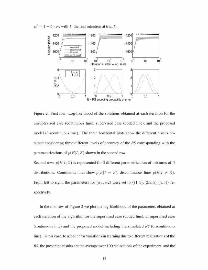
Figure 2: First row: Log-likelihood of the solutions obtained at each iteration for the

unsupervised case (continuous line), supervised case (dotted line), and the proposed

model (discontinuous line). The three horizontal plots show the different results ob-

tained considering three different levels of accuracy of the RS corresponding with the

parameterizations of p(E|I, Z) shown in the second row.

Second row: p(E|I, Z) is represented for 3 different parametrization of mixtures of β

distributions. Continuous lines show p(E|I = Z), discontinuous lines p(E|I 6= Z).

From left to right, the parameters for (w1, w2) were set to {(1, 5), (2.5, 5), (4, 5)} re-

spectively.

In the first row of Figure 2 we plot the log-likelihood of the parameters obtained at

each iteration of the algorithm for the supervised case (dotted line), unsupervised case

(continuous line) and the proposed model including the simulated RS (discontinuous

line). In this case, to account for variations in learning due to different realizations of the

RS, the presented results are the average over 100 realizations of the experiment, and the

14

shadowed area describes the standard deviation around the plotted mean solution. The

three plots reflect the different behavior of the model while considering three different

RS corresponding with the three parameterizations of p(E|I, Z) plotted in the second

row.

For this illustration we considered T = 100,

µ1 = (1, 1), µ2 = (2,−1), Σ1 =

2 1

1 2

, Σ2 =

3 2

2 3

,

and the parameters were initialized as µ1 = µ1, µ2 = µ2 and ΣI = I2×2. However,

the results obtained are not critically dependent on the choice of the parameters.

Note that the log-likelihood in the supervised scenario is the highest, and the so-

lutions obtained using the proposed RS model improve the ones obtained in the un-

supervised case for all considered RS. Further, as the RS becomes more reliable, the

log-likelihood of the solutions is higher. This occurs because the RS is able to cor-

rect the responsibilities for the wrongly classified trials, either because they lie close

to the decision boundary, or because they would have been wrongly assigned a large

responsibility in the standard unsupervised sense.

These results confirm that this model allows to interpolate between the unsupervised

and the supervised parameter estimation with the help of the RS, and additionally that

the responsibilities computed using (4) provide a more accurate class measure than the

responsibilities computed using (8).

15

3.3 CMAC - online learning behavior

We consider now two simulated online scenarios in which the underlying feature dis-

tributions are modified from the train session to the test session by means of a rotation

and a translation of the optimal decision boundaries. These simulations provide insight

on which kind of non stationarities can be captured by the proposed algorithm CMAC.

In figure 3, black and grey curves represent the distributions of two different classes.

Each row represents a different situation; the left most column shows the situation at the

beginning of the test session, with the continuous curves representing the distributions

of the test features while the discontinuous curves represent the distributions of the train

features. In the first row there is a rotation between train and test distributions, while

the second row there is a shift of the distributions.

Columns 2 to 5 show the test distributions (continuous lines) and the learned dis-

tributions using CMAC (discontinuous curves) under the assumption of different RS

after generating 100 samples by sampling with the same probability from both test dis-

tributions. For the cases of 60 % and 80 % of accuracy of the RS, the results are the

average over 100 realizations of the experiment. The standard deviation of these results

was considered not significant for visualization. In this example, the parameter values

were fixed to the values β+ = 0.05, β− = 0.005 and βΣ = 0.01; The choice of this

parameters do not change drastically the results in terms of the obtained solution.

Note that in the case of a translation of the distributions (second row), the new

distributions can be estimated without the use of any RS. On the other hand, if a rotation

of the distributions occurred (first row), a RS is necessary, and the estimation improves

with the quality of the RS. This result is due to the fact that in order to correct for a

16

−4 −2 0 2 4−3

−2

−1

0

1

2

3Initial situation

−4 −2 0 2 4−3

−2

−1

0

1

2

3CMAC−unsup.

−4 −2 0 2 4−3

−2

−1

0

1

2

3CMAC−60%

−4 −2 0 2 4−3

−2

−1

0

1

2

3CMAC−80%

−4 −2 0 2 4−3

−2

−1

0

1

2

3CMAC−sup.

−4 −2 0 2 4−3

−2

−1

0

1

2

3Initial situation

−4 −2 0 2 4−3

−2

−1

0

1

2

3CMAC−unsup.

−4 −2 0 2 4−3

−2

−1

0

1

2

3CMAC−60%

−4 −2 0 2 4−3

−2

−1

0

1

2

3CMAC−80%

−4 −2 0 2 4−3

−2

−1

0

1

2

3CMAC−sup.

.

Figure 3: Black and grey curves represent the distributions of two different classes.

Each row represents a different change in the feature distributions, a rotation in the first

row and a shift in the second. The left column represents the situation at the begin-

ning of the test session, with discontinuous lines representing the train features distri-

butions and continuous lines the test features distributions. Columns 2 to 5 show the

test features distributions (continuous lines) and the learned distributions using CMAC

(discontinuous lines) under the assumption of different RS after 50 samples were drawn

from each of the test feature distributions.

17

rotation in the optimal decision boundary, the weights of the discriminant function need

to be updated, and that requires the class label information.

4 Results: EEG data

In this section we use EEG data to perform a comparison between CMAC and other

classifiers.

The EEG data was recorded from 6 subjects who participated in an experiment

performing a binary motor imagery task (left-right hand) according to visual stimuli.

Each subject participated in a calibration measurement consisting of 35 trials per class

where no feedback was delivered, and two test sessions of 70 trials each where the

feedback was delivered to the user in the form of a binary response. See Figure 4 for

more detailed information about the experiment design. Between each two sessions

there was a pause of 5 minutes.

The brain activity was recorded using a multi-channel EEG with 64 electrodes at

2048 Hz. The data was down sampled at 250 Hz and made into trials using at each

trial the data from the imaginary movement period (1200 − 4900 ms). An automatic

variance based routine was applied to remove noisy trials and channels. The data was

then linearly detrended and bandpass filtered in the frequency band 8 − 30 Hz since

these have been previously reported as the frequencies of main interest (Muller-Gerking

et al, 1998). Common Spatial Patterns (CSP) (Fukunaga, K. , 1990; Lemm et al, 2005)

were computed using the data from the calibration session, and the number of selected

filters was three from each side of the spectrum. After projecting each trial to the space

18

LEFT

1200 ms 4900 ms 7300 ms6300 ms

time course

0 ms

.

Figure 4: Experimental protocol during each trial of the test sessions: From time 0 −

1200 ms an arrow indicates the side to which the task must be performed. After this

period, a fixation cross is presented (1200− 4900 ms) indicating the period to perform

the task. At the end of this period, the device returns feedback to the user (4900− 6300

ms), and it is followed by 1000 ms of no activity previous to the beginning of a new

trial. During the calibration measurement the protocol was identical with the exception

that no feedback was returned.

generated by the six filters, the logarithm of the normalized variance of these projections

were used as features, resulting in a feature space of dimension 6.

1 2 3 4 5 6 mean0.5

0.55

0.6

0.65

0.7

0.75

0.8

0.85

0.9

0.95

1

Subject number

Max

imum

exp

ecte

d cla

sifica

tion

accu

racy

CMACCSEMPmeanPmeanGcovLDA

.

Figure 5: Maximum performance achievable using CMAC, CSEM, Pmean, PmeanG-

cov, as well as the performance obtained using LDA.

19

In the remaining of this section we use the previously described data set to perform a

comparison between different classifiers, including a static classifier, LDA (Fukunaga,

K. , 1990), and the adaptive classifiers Pmean, PmeanGcov, CSEM and CMAC. We

first study the best possible performance obtained while using each of the considered

methods. Figure 5 shows the maximum classification accuracy (number of correctly

classified trials divided by the total number of trials) obtained by each method while

considering optimized learning rates and an optimal RS. For each algorithm and each

subject, the learning rates were optimized using grid search in parameter space.

First note that all adaptive classifiers are able to outperform LDA. From the adaptive

classifiers, CMAC is clearly the algorithm able to reach the highest accuracy, followed

by CSEM and PmeanGcov which reflect a similar performance. In the case of Pmean,

we see that the model with less parameters (only one learning rate), is the one achieving

the lowest accuracy but it is still able to clearly outperform LDA. This result clearly

shows that CMAC has the potential power to outperform all other considered methods.

As a reference for the reader, in table 1 we show the mean (across subjects) and stan-

dard deviation of the optimal parameter values set for each of the considered adaptive

classifiers.

In practice, we do not have prior access to the optimal learning rates and further-

more, no RS is optimal. Clearly, different choices for the learning rates will affect the

performance of all methods and moreover, suboptimal RS will affect the performance of

CMAC and CSEM. In Figure 6 we present the performance of each of the methods as a

function of different RS simulated as explained in 3.1, while using for each subject a set

20

CMAC CSEM PmeanGcov Pmean

β+, β−, βΣ βµ, βΣ βµ, βΣ βµ

Mean 0.068, 0.019, 0.035 0.019, 0.069 0.019, 0.063 0.084

Standard Deviation 0.079, 0.011, 0.062 0.014, 0.049 0.014, 0.041 0.073

Table 1: Mean across subjects and standard deviation of the optimal learning rates for

each of the considered adaptive classifiers

of learning rates computed using leave-one (subject) out cross-validation. For CMAC

and CSEM, the reported results are averages over 100 realizations of the experiment to

account for fluctuations due to different realizations of the RS. For CMAC, the standard

deviation of the results is shown as error bars. In the case of CSEM, the standard devi-

ation of the solutions was very similar to that of CMAC and we decided to ignore them

for visualization reasons.

We observe that in general all adaptive classifiers are able to outperform the static

LDA. Considering the supervised scenarios, note that CMAC (100%) outperforms CSEM

(100%). Only for subject number 1 CSEM (100%) is the best algorithm. Ignoring the

supervised methods, we see also that CMAC is less sensible to non-optimal RS than

CSEM. For subjects 3, 4 and 6 CMAC is the best algorithm for all considered RS, while

for subjects number 2 and 5, it requires an accurate RS in order to improve wrt the

unsupervised classifiers.

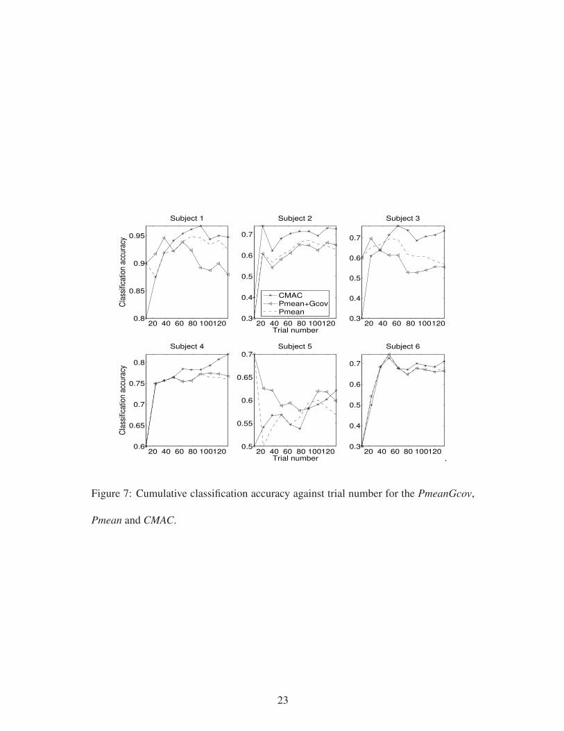
In Figure 7 we consider the cumulative classification accuracy against the trial num-

ber for PmeanGcov, Pmean and CMAC with optimal RS. CMAC is able to outperform

the other methods not only at the end of the experiment (trial 140) but in general also

21

50 100

0.88

0.9

0.92

0.94

0.96

Subject 1

Cla

ssifi

catio

n ac

cura

cy

CMAC

CSEM

FLD

Pmean

PmeanGcov

50 100

0.5

0.55

0.6

0.65

0.7

0.75

Percentage of RS accuracy

Subject 2

50 100

0.5

0.55

0.6

0.65

0.7

0.75Subject 3

50 100

0.76

0.78

0.8

0.82

Subject 4

Cla

ssifi

catio

n ac

cura

cy

50 100

0.5

0.55

0.6

0.65

0.7

0.75Subject 5

Percentage of RS accuracy50 100

0.5

0.55

0.6

0.65

0.7

0.75Subject 6

.

Figure 6: Classification accuracy (y-axis) as a function of the accuracy of the RS (x-

axis) for all subjects. For CMAC the standard deviation of the solutions obtained is

presented as an error bar.

at the end of the first test session (trial number 70). While for subject number 6 all

methods show a similar trend, note that for subjects number 1 to 4, the difference in

performance between CMAC and the other methods is bigger at trial 140 than at trial

70, showing that CMAC was able to adapt better after the pause between sessions. It

is interesting to see that CMAC finishes the experiment with a general increasing trend,

suggesting that the model continues a proper adaptation. Note in particular that for sub-

ject number 5 the performance of CMAC was worse at trial number 70 than the one of

the other methods, but due to the ability to keep adapting after the pause, CMAC is the

best algorithm at the end of the experiment.

An interesting observation is that for some subjects, for example subject number 6,

all methods perform similarly, while for other subjects, for example number 3, the in-

22

20 40 60 80 1001200.8

0.85

0.9

0.95

Subject 1

Cla

ssifi

catio

n ac

cura

cy

20 40 60 80 1001200.3

0.4

0.5

0.6

0.7

Subject 2

Trial number

CMAC

Pmean+Gcov

Pmean

20 40 60 80 1001200.3

0.4

0.5

0.6

0.7

Subject 3

20 40 60 80 1001200.6

0.65

0.7

0.75

0.8

Subject 4

Cla

ssifi

catio

n ac

cura

cy

20 40 60 80 1001200.5

0.55

0.6

0.65

0.7Subject 5

Trial number20 40 60 80 100120

0.3

0.4

0.5

0.6

0.7

Subject 6

.

Figure 7: Cumulative classification accuracy against trial number for the PmeanGcov,

Pmean and CMAC.

23

crease in performance obtained using CMAC is significant. To understand this behavior,

in figure 8 we show the distributions of the projected train data (discontinuous curves)

and test data (continuous curves) onto the first and second CSP filters for subjects 6

and 3. Black and grey curves represent the two different classes. The boundary learned

using the train data as well as the optimal boundary for the test data are also shown.

For subject number 6 we observe that the change in the distributions is very small,

allowing every method to adapt to the changes. In constrast, the features of subject

number 3 change notably between train and test. In particular, there is a clear rota-

tion of the optimal boundary, which prevents Pmean to adapt properly. In this subject,

although PmeanGcov should theoretically be able to correct for the rotation since it

updates the global covariance matrix, we observe that it is not the case. The reason

why PmeanGcov performs worse than CMAC could then be explained by the fact that,

in addition to the rotation, the classes are swapped in the second filter (y-axis). Class

information is therefore required to adapt to this type of changes, making it impossible

for unsupervised methods such as PmeanGcov.

5 Related work and relations between methods.

In this section we provide a short description of the existing adaptive classification

methods commonly used for BCI purposes, and we show the relationships between

them. We also give a brief description of the binary Linear Discriminant Analysis (LDA)

classifier.

1. Binary Linear Discriminant Analysis (LDA).

24

−1.5 −1 −0.5 0

−1.2

−1

−0.8

−0.6

−0.4

−0.2Subject 6

Feature dimension 1

Fe

atu

re d

ime

nsi

on

2

Train dist. class 1

Train dist. class 2

Optimal boundary for train dist.

Test dist. class 1

Test dist. class 2

Optimal boundary for test dist.

−1.5 −1 −0.5 0

−1.2

−1

−0.8

−0.6

−0.4

−0.2Subject 3

Feature dimension 1

Fe

atu

re d

ime

nsi

on

2

.

Figure 8: Projection of the data onto the first two CSP filters for subjects 6 and 3.

Black and grey ellipses represent two different classes and discontinuous and contin-

uous curves represent the train data and the test data respectively. Discontinuous and

continuous straight lines show the optimal boundary for the train distributions and the

test distributions respectively. For subject 6 (left) feature distributions do not change

significantly. In contrast, for subject 3 (right) the optimal boundary rotates and the class

labels are swapped in the vertical axis.

25

The binary LDA (Fukunaga, K. , 1990) is a classifier which is identified by a

discriminant function D(x) ∈ R of the input feature vector x ∈ Rn. Denoting

by µk and Σk the means and covariance matrices of the train features of class

k ∈ {1, 2} respectively, and by Σ = Σ1+Σ2

2the mean of the covariance matrices,

the discriminant function is defined by the equations

D(x) = [b,w⊺]

1

x

, (19)

w = Σ−1 (µ2 − µ1) , (20)

b = −w⊺µ, (21)

µ =1

2(µ1 + µ2) . (22)

Using this notation, x is classified as class 2 if D(x) > 0, and as class 1 otherwise.

Note that w ∈ Rn describes the vector of weights and b ∈ R describes the bias

term of the discriminant function. Consequently, w determines the direction of

the separating hyperplane while b the shift of the hyperplane wrt the origin.

2. Linear Discriminant Analysis with pooled mean adaptation (Pmean).

Pmean (Vidaurre et al, 2010) is a discriminant-based unsupervised adaptive LDA

algorithm which under the assumption of balanced classes, identifies (22) with

the global mean of the data. In this way, (22) can be updated without any label

information using the learning rule

µ′ = (1− β)µ+ βx (23)

26

where µ′ is the updated µ, x is the new observed feature vector and β ∈ [0, 1] is

the learning rate controlling the adaptation. In this way the bias from the discrim-

inant function gets updated through (21).

This kind of adaptation tracks changes in the bias of the discriminant function,

consequently Pmean is able to adapt to shifts in feature space. Since the weights

are not modified, this model can not account with changes in the direction of the

separating hyperplane, as for example, rotations on feature space.

Note that Pmean can be considered a particular case of CMAC where β− = 0 and

βΣ = 0.

3. Pmean with global covariance adaptation (PmeanGcov).

PmeanGcov (Vidaurre et al, 2010) is a discriminant-based unsupervised adaptive

LDA algorithm which in addition to the Pmean adaptation performs a sequen-

tial adaptation of the inverse of the global covariance. Under the assumption of

balanced classes, we have that

w = Σ−1 (µ2 − µ1) ∝ Σ−1 (µ2 − µ1) := w,

where Σ is the global covariance matrix. Then, defining

b = −w⊺µ,

we have that D(x) ∝ D(x) :=[

b, w⊺

]

1

x

. This means that if the classes are

balanced we obtain the same separating hyperplane using Σ than using Σ. Using

Σ has the advantage that it can be updated online without using class informa-

tion. Furthermore, making use of the Woodbury matrix identity (matrix inversion

27

lemma) we can directly update its inverse as

I = Σ−vv

⊺

1−βΣ

βΣ

+ x⊺v, (24)

Σ′−1

=I

1− βΣ

, (25)

where Σ is the global covariance, Σ′−1

the updated inverse global covariance

matrix, v = Σ−1x, and βΣ ∈ [0, 1] is a learning rate controlling the adaptation

of the covariance. This direct update of the inverse is recommended for online

applications due to its efficiency.

The update of the inverse of the covariance allows for an update of (20), so

PmeanGcov allows for the update of the weights and also the bias of the clas-

sifier. Consequently, this model has the potential power to adapt for shifts as well

as for changes in the direction of the separating hyperplane.

Note that the update of the covariance in PmeanGcov is different from the class

dependent covariance updates in CMAC. However, as previously explained, if the

classes are balanced, using the pooled covariance in place of the mean of the

class-wise covariance matrices results in the same separating hyperplane, so in

that case PmeanGcov is equivalent with CMAC with β− = 0.

4. Adaptive Linear Discriminant Analysis (ALDA).

ALDA (Blumberg et al, 2007) is a latent-variable-based unsupervised adaptive

LDA algorithm in the sens that considers the user intention as a hidden variable,

models the feature space as a GMM, and constructs a LDA classifier with the

parameters estimated using EM. The batch optimization is performed using a

28

sliding window of the last M ∈ N trials. In this way, only the most recent trials

take part in the optimization, allowing to model non stationary environments.

Since ALDA updates means and covariances, it performs an adaptation of all pa-

rameters included in the discriminant function, allowing like this to adapt for

shifts as well as for rotation on feature space.

Note that since CSEM in the unsupervised scenario (Et = 1

2∀t) is a sequential

EM algorithm for GMM, we can identify ALDEC as the batch version of CSEM,

and we can consider them as equivalent.

5. Adaptive Linear Discriminant Analysis with Error Correction (ALDEC).

Similarly to our algorithm CSEM, in (Blumberg et al, 2007) the authors introduce

a probabilistic model of a binary error signal, which corresponds to our RS term

p(Ik|Z,E). ALDEC performs implicit modeling of the decoding power DP (ac-

curacy of the task classifier) and the reliability R of the RS. In contrast, in CSEM

we explicitly include this information in the model and provide update rules for

the means and covariances (6, 7) where the RS is included through the novel re-

sponsibilities (4). This allows us to recover both supervised and unsupervised

cases. Further, this allows to include more realistic, single trial realizations of the

RS. Notice that in (Blumberg et al, 2007) the RS is modeled as two delta peaks at

R and 1−R (see section 3.1).

6. Sequential EM (SEM).

SEM (Hasan et al, 2009) is a sequential version of EM for GMM. In this algo-

rithm, the means and covariance matrices of the task related feature distributions

29

are sequentially updated using

µ′I = (1− βµγI)µI + βµγIx, (26)

Σ′I = (1− βΣγI)ΣI + βΣγI(x− µI)(x− µI)

′, (27)

where µ′I and Σ

′I represent the updated means and covariance matrices respec-

tively, x is the observed task related feature vector, γI the responsibilities com-

puted using (8), and βµ and βΣ are learning rates which values decrease on size

with the iteration number in order to reach convergence to the optimal static set

of parameters. If our goal is to dynamically model a non stationary environment,

we can relax the dependence of the learning rates value on the trial number, so

βµ ∈ [0, 1] and βΣ ∈ [0, 1].

Note that SEM is analytically equal to CSEM in the unsupervised scenario (Et =

1

2∀t). Consequently, SEM is equivalent to the unsupervised CSEM and conse-

quently to ALDA.

7. CMAC and CSEM.

CMAC and CSEM can not be reduced to the same class. If we compare the CMAC

equations for the mean updates (15) and (16) with the CSEM equations (9), we

see that CMAC contains additional terms involving the mean of the opposite class

that are not in the CSEM update rule. These terms appear because CMAC con-

straints the sum and the differences of the class means.

30

6 Discussion

Our contribution in this article is two-fold. On the one hand, we introduced the proba-

bilistic methodology to include a Reinforcement Signal (RS) in the adaptive BCI cycle,

and we show that under the assumption of an informative RS, this model allows for a

better estimation of the class probabilities (responsibilities) than the one obtained using

only the task related features. On the other hand, we develop a novel update scheme

for adaptive classification in BCI (CMAC), which can make use of the responsibilities

computed using the proposed model, and is able to outperform state of the art adaptive

classifiers.

It is interesting to note that in the supervised scenario, CMAC is able to improve

a standard supervised adaptation (supervised CSEM), and also that even in the unsu-

pervised scenario, CMAC has the potential to outperform other methods. However, the

ability to get a big improvement wrt to other methods, clearly depends on the quality of

the RS. As previously mentioned, such a RS can range from button presses delivered by

the user (supervised), to measured muscular activity in an hybrid BCI (Leeb et al, 2010)

or an ErrP classifier if we consider a pure BCI setting. Clearly, using muscular activity

to detect erroneous performance can provide an accurate RS. It is important to note that

in previous work (Llera et al, 2011) we have reported the possibility of relatively high

ErrP classification rates (80 % of mean accuracy across 8 subjects), which agrees with

the results presented previously by other researchers (Blankertz et al, 2004; Ferrez et al,

2008). Furthermore, in (Ferrez et al, 2008), it was also shown the high stability in ErrP

detection across sessions. This facts make of this kind of RS a optimal candidate to

include in online BCI experiments.

31

The improvement reported using the CMAC algorithm is due not only to the accu-

racy of the RS, but also to the introduction of an extra parameter β− controlling the

change in the difference between the means of the feature distributions. The optimal

value for this parameter is clearly dependent on the accuracy of the estimated responsi-

bilities. However, the simulations performed showed that the choice of this parameter

value is not critical. In fact, we observed that setting βΣ = 0, β+ = βµ ∈ [00.1],

β− ∈ [0, 0.005], CMAC showed no significant difference wrt Pmean independently of

the accuracy of the estimated responsibilities. For values β− ∈ [0.005, 0.03], the im-

provement wrt Pmean was proportional to the accuracy of the estimated responsibilities,

and values β− > 0.03 produced a decrease on performance wrt Pmean. The improve-

ment wrt Pmean was obtained independently of β+, which confirms the robustness of

the method.

It is clear that the optimal choice of the learning rates is important to obtain good re-

sults for all subjects and all methods. There exist methods that can automatically adapt

the learning rate to an optimal value that make a trade-off between accuracy for station-

ary data (low learning rate) and adaptivity to change (large learning rates) (Heskes et al,

1991b, 1992). We believe that such methods should be integrated in the adaptive BCI

methodology.

An open question of considerable importance is how to generalize the proposed

adaptive BCI methodology to non-binary tasks. Such learning tasks are more complex,

since the error signal will indicate that an error has occurred, but will not provide infor-

mation on what the correct output should have been. This type of learning paradigm is

called reinforcement learning (Rescorla, 1967; Sutton et al, 1998; Dayan et al, 2001).

32

An important future research direction is to integrate these reinforcement learning meth-

ods in on-line adaptive BCI.

Finally, we would like to remark that due to its generality, the proposed methodol-

ogy has a broader application not restricted to BCI, for instance, in the construction of

adaptive Spam filters (Zhou et al, 2005). In this environment the RS could be repre-

sented by the user getting a file out of or in the Spam folder.

Acknowledgments

The authors gratefully acknowledge the support of the Brain-Gain Smart Mix Pro-

gramme of the Netherlands Ministry of Economic Affairs and the Netherlands Ministry

of Education, Culture and Science.

References

Bishop, C. M.(2007). Pattern Recognition and Machine Learning. Springer.

Blankertz, B., Dornhege, G., Schafer, C., Krepki, R., Kohlmorgen, J., Muller, K. R.,

Kunzmann, V., Losch, F & Curio, G. (2004). Boosting Bit Rates and Error Detection

for the Classification of Fast-paced Motor Commands Based on Single-trial EEG

Analysis. IEEE Transactions on Biomedical Engineering, vol. 51, no.6, 993 - 1002 .

Blankertz, B., Kawanabe, M., Tomioka, R., Hohlefeld, F., Nikulin, V. & Muller, K. R.

(2008) Invariant Common Spatial Patterns: Alleviating Nonstationarities in Brain-

Computer Interfacing. Advances in Neural Information Processing Systems 20, MIT

Press,113–120.

33

Blumberg, J., Rickert, J., Waldert, S., Schulze-Bonhage, A., Aertsen, A., Mehring, C.

(2007) Adaptive classification for brain computer interfaces. 29th Annual Interna-

tional Conference of the IEEE, Engineering in Medicine and Biology Society EMBS

2007, pp. 2536–2539.

Chavarriaga, R., Ferrez, P.W. & Millan, J. del R. (2007). To Err Is Human: Learning

from Error Potentials in Brain-Computer Interfaces International Conference on

Cognitive Neurodynamics, Shanghai, China, 777–782.

Chavarriaga, R. & Millan, J. del R. (2010). Learning from EEG Error-related Potentials

in Noninvasive Brain-Computer Interfaces. IEEE Transactions on Neural Systems

and Rehabilitation Engineering, vol. 18, 381–388.

Dayan, P. & Abbott, L. F.(2001). Theoretical Neuroscience: Computational and Math-

ematical Modeling of Neural Systems MIT Press.

Ferrez, P.W. & Millan, J. del R. (2005). You Are Wrong!—Automatic Detection of

Interaction Errors from Brain Waves. Proceedings of the 19th International Joint

Conference on Artificial Intelligence, 1413 - 1418 .

Ferrez, P.W. (2007) Error-related EEG potentials in brain-computer interfaces. These

Ecole polytechnique federale de Lausanne EPFL, no 3928.

Ferrez, P. W. & Millan, J. del R. (2008). Error-Related EEG Potentials Generated

during Simulated Brain-Computer Interaction. IEEE Transactions on Biomedical

Engineerings, vol. 55, 3, 923 – 929.

Fukunaga, K. (1990) Introduction to Statistical Pattern Recognition. Academic Press.

34

Gan, J. G. (2006). Self-adapting BCI based on unsupervised learning. 3rd International

Workshop on Brain-Computer Interfaces,Graz, Austria,Verslag, 50–51.

Hasan, B. A. S. & Gan, J. Q. (2009). Unsupervised adaptive GMM for BCI. Interna-

tional IEEE EMBS Conf. on Neural Engineering, Antalya, Turkey, 295–298 .

Hasan, B.A.S. & Gan, J.Q. (2009b). Sequential EM for unsupervised adaptive Gaus-

sian mixture model based classifier. Machine Learning and Data Mining in Pattern

Recognition, Lecture Notes in Computer Science, Springer Berlin / Heidelberg, vol.

5632, 96–106.

Heskes, T., Gielen, S. & Kappen, H.J. (1991). Neural networks learning in a changing

environment. Artificial Neural Networks, North-Holland, vol.1, 15–20.

Heskes, T. & Kappen, H.J. (1991b). Learning processes in neural networks Physical

Review A, vol.44, 4, 2718–2726.

Heskes, T. & Kappen, H.J. (1992). Learning-parameter adjustment in neural networks.

Physical Review A, vol.45, 8885–8893.

Kawanabe, M., Krauledat, M. & Blankertz, B. (2006). A bayesian approach for adaptive

BCI classification In Proceedings of the 3rd International Brain-Computer Interface

Workshop and Training Course 2006, Verslag, 54–55.

Krauledat M. (2008). Ph.d thesis. Technische Universitat Berlin, Fakultat IV – Elek-

trotechnik und Informatik.

Lemm, S., Blankertz, B., Curio, G. & Muller, K. R. (2005). Spatio-Spectral Filters

35

for Improved Classification of Single Trial EEG IEEE Trans. Biomed. Eng, vol. 52,

1541–1548.

Leeb, R. and Sagha, H. and Chavarriaga, R. and del R Millan, J. (2010). Multimodal

Fusion of Muscle and Brain Signals for a Hybrid-BCI. Engineering in Medicine and

Biology Society (EMBC), 2010 Annual International Conference of the IEEE, 4343

-4346.

Li, Y., & Guan, C. (2006) An Extended EM Algorithm for Joint Feature Extraction

and Classification in Brain-Computer Interfaces. Neural Computation, vol.18, 11,

2730–2761.

Liu, G., Huang, G., Meng, J., Zhang, D. & Zhu, X. (2010) Improved GMM with pa-

rameter initialization for unsupervised adaptation of Brain-Computer interface. In-

ternational Journal for Numerical Methods in Biomedical Engineering, vol.26, 6,

681–691.

Llera, A., van Gerven, M.A.J., Gomez, V., Jensen, O. & Kappen, H. J. (2011). On

the use of interaction error potentials for adaptive brain computer interfaces. Neural

Networks, vol. 24, 10, 1120 - 1127.

Millan, J. del R. (2004). On the Need for On-Line Learning in Brain-Computer Inter-

faces. IEEE Proc. of the Int. Joint Conf. on Neural Networks, vol.4, 2877 - 2882.

Muller-Gerking, J., Pfurtscheller, G. & Flyvbjerg, H.(1998) Designing optimal spatial

filters for single-trial EEG classification in a movement task Clinical Neurophysiol-

ogy, vol.110, 787–798.

36

Ramoser, H., Muller-Gerking, J. & Pfurtscheller, G. (1998). Optimal spatial filtering of

single trial EEG during imagined hand movement. IEEE Transactions on Rehabili-

tation and Engineering, 8, 441–446.

Reuderink, B., Farquhar, J., Poel, M. & Nijholt, A. (2011). A Subject-Independent

Brain-Computer Interface based on Smoothed, Second-Order Baselining. Pro-

ceedings of the 33st Annual International Conference of the IEEE Engineering in

Medicine and Biology Society, EMBC 2011, 4600–4604.

Samek, W., Vidaurre, C., Muller, K. R. & Kawanabe, M. (2012). Stationary Common

Spatial Patterns for Brain-Computer Interfacing. Journal of Neural Engineering, 9

(2), 0260134.

Schmidt, N., Blankertz, B., Treder, M. S. (2012). Online detection of error-related

potentials boosts the performance of mental typewriters. BMC neuroscience, 13:19.

Shenoy, P., Krauledat, M., Blankertz, B., Rao, R. P. & Muller, K. R. (2006). Towards

adaptive classification for BCI. Journal of neural engineering, 3, R13-R23.

Sutton, R. S. & Barto, A. G.(1967). Pavlovian conditioning and its proper control

procedures. Psychological Review, 74(1), 71–80.

Sutton, R. S. & Barto, A. G.(1998). Reinforcement Learning: An Introduction MIT

Press.

Sykacek, P., Roberts, S. J. & Stokes M. (2004). Adaptive BCI Based on variational

Kalman filtering: An empirical evaluation IEEE Transactions on biomedical engi-

neering, vol.51, no.5, 719–727.

37

Tomioka, R., Hill, J.N., Blankertz, B. & Aihara, K. (2006) Adapting Spatial Filter

Methods for Nonstationary BCIs Proceedings of 2006 Workshop on Information-

Based Induction Sciences (IBIS 2006), 65–70.

van Gerven, M. & Jensen, O. (2009). Attention modulations of posterior alpha as a con-

trol signal for two-dimensional brain-computer interfaces . Journal of Neuroscience

Methods, 179, 78 – 84.

Vidaurre, C., Schloogl, A., Cabeza, R., Scherer, R., Pfurtscheller, G. (2006). A fully

on-line adaptive BCI. IEEE Transactions on Biomedical Engineering, 6, 53, 1214–

1219.

Vidaurre, C., Kawanabe, M., von Bunau, P., Blankertz, B. & Muller, K. R. (2010).

Toward an unsupervised adaptation of LDA for Brain-Computer Interfaces. IEEE

Trans. Biomed. Eng, vol.58, no.3, 587 – 597.

Vidaurre, C. & Blankertz, B. (2010b). Towards a Cure for BCI Illiteracy. Brain Topogr.,

vol.23, 194–198.

Vidaurre, C., Sannelli, C., Muller, K. R. & Blankertz, B. (2010c). Machine-Learning

Based Co-adaptive Calibration. Neural Computation,23(3), 791–816.

von Bunau, P., Meinecke, F. C., Scholler, S. & Muller, K. R. (2010). Finding Stationary

Brain Sources in EEG Data. Proceedings of the 32nd Annual Conference of the IEEE

EMBS, 2010, 2810 – 2813.

Wolpaw, J. R., Birbaumer, N., McFarland, D. J., Pfurtscheller, G. & Vaughan, T. M.

38

(2002). Brain-computer interfaces for communication and control. Clinical neuro-

physiology, 6-113, 767–791.

Zhou, Yan and Mulekar, M.S. & Nerellapalli, P. (2005) Adaptive Spam Filtering Using

Dynamic Feature Space. 17th IEEE International Conference on Tools with Artificial

Intelligence (ICTAI’05), 302–309 .

39