Adapting physical carrier sensing to maximize spatial reuse in 802.11 mesh networks

Adapting Physical Carrier Sensing toMaximize Spatial Reuse in 802.11 MeshNetworks

Jing Zhu∗, Xingang Guo, L. Lily Yang, W. Steven Conner,

Sumit Roy†, and Mousumi M. Hazra

{jing.a.zhu, xingang.guo, lily.l.yang, w.steven.conner,

mousumi.m.hazra}@intel.comCommunications Technology Lab

Intel Corporation

2111 NE 25th Ave., JF3-206

Hillsboro, OR 97124, U.S.A.

∗Contact author (for proofing), currently with Dept. of Electrical Engineering, U.Washington. Email: [email protected]; Address: Department of Electrical En-gineering, University of Washington Box 352500 Seattle, WA 98195-2500 USA; Phone:206-618-2846. This work was completed while he was an intern at Intel Corporation.

†Currently with Dept. of Electrical Engineering, U. Washington;[email protected]. This work was completed while he was on leave at IntelCorporation.

1

, 2

Abstract

Spatial reuse in a mesh network can allow multiple communications to proceedsimultaneously, hence proportionally improve the overall network throughput. Tomaximize spatial reuse, the MAC protocol must enable simultaneous transmit-ters to maintain the minimal separation distance that is sufficient to avoid in-terference. This paper demonstrates that physical carrier sensing enhanced witha tunable sensing threshold is effective at avoiding interference in 802.11 meshnetworks without requiring the use of virtual carrier sensing. We present an an-alytical model for deriving the optimal sensing threshold given network topology,reception power, and data rate. A distributed adaptive scheme is also presentedto dynamically adjust the physical carrier sensing threshold based on periodic es-timation of channel conditions in the network. Simulation results are shown forlarge-scale 802.11b and 802.11a networks to validate both the analytical modeland the adaptation scheme. It is demonstrated that the enhanced physical carriersensing mechanism effectively improves network throughput by maximizing thepotential of spatial reuse. With dynamically tuned physical carrier sensing, theend to end throughput approaches 90% of the predicted theoretical upper-boundassuming a perfect MAC protocol, for a regular chain topology of 90 nodes.

Key words: 802.11, MAC, Physical Carrier Sensing, and Adaptive Al-gorithm.

1 Introduction

Over the past few years we have witnessed the rapid proliferation of wirelessLANs in various network environments (home, office and public hotspots).The need for higher data rates and improved coverage has led to at least twopotential solutions for large-scale WLANs – a) multi-cell networks where eachcell is serviced by its own access point (AP), and b) mesh networks wherenodes work in ad-hoc mode and use multi-hop routing to relay each other’straffic. In both cases, the overall network throughput is proportional to thenumber of simultaneous communications via co-channel spatial reuse thatcan be conducted in spatially separated locations with acceptable mutualinterference.

A multi-cell WLAN is similar to a traditional cellular network wherebyspatial reuse is achieved through careful site planning and engineered channelassignment for each cell. In an ad-hoc network, however, no access point orbase station infrastructure exists and hence engineered channel assignment

, 3

is often not feasible. Furthermore, because of the random topology of ad-hocnetworks, detecting and avoiding interference is also more complicated. In[4], spatial reuse was demonstrated to depend on various characteristics ofthe network, including the type of radio, network topology, channel qualityrequirements and signal propagation environment. For each network config-uration, there exists a minimum separation distance such that when simul-taneous transmitters are separated by that distance, the maximum numberof simultaneous transmissions can be accommodated, leading maximum net-work throughput. However, achieving maximum spatial reuse would requirean ideal MAC protocol that schedules communication to maintain the op-timal transmitter separation distance in a fully distributed manner whileminimizing interference.

Nodes using the IEEE 802.11 MAC protocol [1] use carrier sensing todetermine if the shared medium is available before transmitting to avoidpacket collision. Two types of carrier sensing are supported by the 802.11MAC: mandatory physical carrier sensing (PCS) that monitors the RF energylevel in the channel and optional virtual carrier sensing (VCS) that uses theRequest-to-Send/Clear-to-Send (RTS/CTS) handshake to effectively reservethe channel prior to data transmission. Virtual carrier sensing was designedto avoid the well-known hidden terminal problem [9], where it is assumed thatphysical carrier sensing at a transmitter is not sufficient to avoid interferenceat a receiver. Interestingly, a substantial portion of existing literature on .11interference management is based on RTS/CTS. This has it’s limitations; theoverhead due to the additional RTS/CTS handshake is not justified whenthe data payload size is small. More significantly, it has been shown thatvirtual carrier sensing has fundamental limitations in avoiding interferencefrom hidden terminals in mesh networks [7] [10] [11] [12], i.e. there are manyscenarios where it is conservative and fails to suppress packet collisions asintended.

Trying to resolve this by making RTS/CTS more aggressive exacerbatesthe exposed terminal problem, whereby feasible parallel transmissions thatdo not interfere with the reference one are suppressed.

The above prompts a re-evaluation of the role and effectiveness of PCSin interference management; in this paper we demonstrate that when prop-erly tuned, PCS is effective at avoiding interference in a multi-hop wirelessmesh network, without the use of VCS. PCS allows a station to assess thechannel condition before transmitting to make sure that no interference canoccur. A station samples the energy level in the medium and starts a packet

, 4

transmission only if the reading is below the carrier sensing threshold, indi-cating that no simultaneous transmissions are taking place that could resultin interference to the desired. Using RF pathloss models, the carrier sensingthreshold may be translated into an effective minimum allowed distance be-tween simultaneous transmitters. As noted, this optimal distance dependson various network properties; thus the carrier sensing threshold should betuned to match network conditions. However, many of today’s 802.11 MACimplementations use a static threshold, or do not allow the threshold to beindependently tunable [14]. As a result, physical carrier sensing often leadstransmitters to be either too conservative or too aggressive due to impropersetting of the threshold and is the likely reason why use of PCS has notattracted much attention.

In this work, we make the case for a tunable carrier sensing threshold;some simple analysis is used to derive the appropriate carrier sensing thresh-old for given network topology. Furthermore, we propose an estimation-basedadaptive PCS scheme to automatically tune the threshold to a near-optimalvalue. We present OPNET simulation results for two regular network topolo-gies (chain and grid) to validate the theoretical PCS threshold. Our resultsfurther show that by tuning the PCS threshold, the overall network through-put can be improved significantly compared to that of legacy 802.11 MACwithout any VCS. Furthermore, the throughput can approach approximately90% of the theoretical upper-bound predicted by spatial reuse models ina large chain. Simulation results also demonstrate the effectiveness of theestimation-based adaptive PCS scheme in networks with dynamic topologyand heterogeneous links.

It is worth noting that throughput of 802.11 networks may be enhancedby attending to many different aspects of the 802.11 MAC protocol; this is thesubject of extensive work, such as [7] [8] [12] to cite a few. Hence maximizingnetwork performance must be a careful combination of approaches addressingmultiple aspects (e.g. collision resolution, fairness, etc.) of the networkbehavior. The focus of this paper is purely on leveraging the spatial reuse inmesh networks to enhance the throughput through PCS, which we believe isparticulary apropos in a dense in-building ad-hoc MESH network where thenodes are either static or have only intermittent mobility.

The rest of this paper is organized as follows: Section 2 presents the SINRcommunication model that is used in this paper for our interference analysisand the limitations of carrier in 802.11 DCF. Section 3 introduces our analyt-ical model for PCS and shows how a tunable physical sensing threshold can

, 5

dramatically improve the throughput of mesh networks with regular topolo-gies. Section 4 describes our novel estimation-based adaptive physical carriersensing scheme. Section 5 presents OPNET simulation results demonstratingmeasurable benefit from tuned physical carrier sensing and the adaptationscheme. Finally the paper is concluded in section 6.

2 Managing Interference with Carrier Sensing

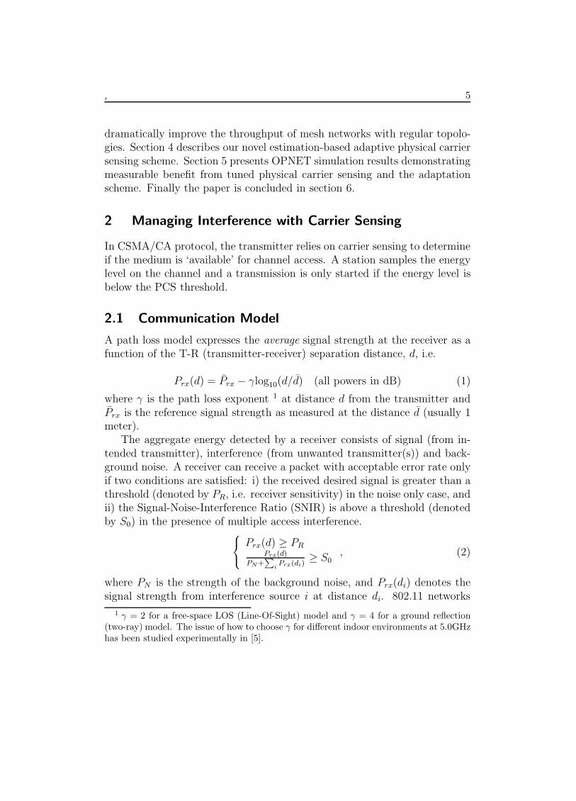
In CSMA/CA protocol, the transmitter relies on carrier sensing to determineif the medium is ‘available’ for channel access. A station samples the energylevel on the channel and a transmission is only started if the energy level isbelow the PCS threshold.

2.1 Communication Model

A path loss model expresses the average signal strength at the receiver as afunction of the T-R (transmitter-receiver) separation distance, d, i.e.

Prx(d) = P̄rx − γlog10(d/d̄) (all powers in dB) (1)

where γ is the path loss exponent 1 at distance d from the transmitter andP̄rx is the reference signal strength as measured at the distance d̄ (usually 1meter).

The aggregate energy detected by a receiver consists of signal (from in-tended transmitter), interference (from unwanted transmitter(s)) and back-ground noise. A receiver can receive a packet with acceptable error rate onlyif two conditions are satisfied: i) the received desired signal is greater than athreshold (denoted by PR, i.e. receiver sensitivity) in the noise only case, andii) the Signal-Noise-Interference Ratio (SNIR) is above a threshold (denotedby S0) in the presence of multiple access interference.

Prx(d) ≥ PR

Prx(d)

PN+∑

iPrx(di)

≥ S0, (2)

where PN is the strength of the background noise, and Prx(di) denotes thesignal strength from interference source i at distance di. 802.11 networks

1 γ = 2 for a free-space LOS (Line-Of-Sight) model and γ = 4 for a ground reflection(two-ray) model. The issue of how to choose γ for different indoor environments at 5.0GHzhas been studied experimentally in [5].

, 6

support multiple data rates, and a higher data rate typically requires a higherthreshold S0.

It is clear from Eq.2 that successful reception at any T-R separation de-pends on the received SINR; hence any definition of transmission range fora given communication depends on the local network (interference) environ-ment. However as a starting point, we define the transmission range basedonly on the receiver sensitivity PR; i.e. the transmission range is the maxi-mum T-R separation for successful reception in additive noise only.

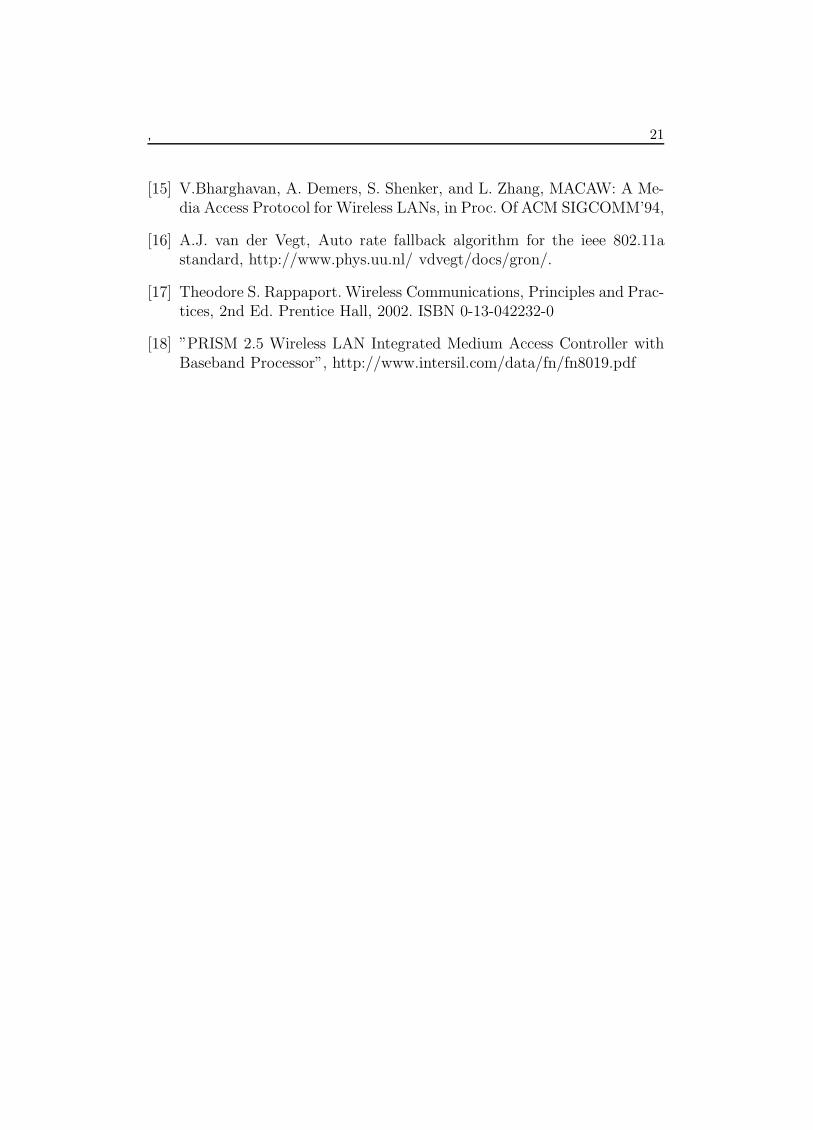
Fig.1 2 shows a segment in a typical mesh network with a reference trans-mission from a TX node to a RX node and four other neighboring nodes (A,B, C, and E), where the same transmission power is used by every node. Wedefine the following:

D: T-R separation distance, such that PD = Prx(D).

R: Transmission range, given by

R = d̄(P̄rx

max(PR, S0PN))

1γ = d̄(

P̄rx

PR

)1γ , (3)

I: Interference range: a single transmitter within that range of the receiverwill disrupt reception of desired transmisssion, given by

I = D(1

1S0

− (Dd̄)γ PN

P̄rx

)1/γ . (4)

With negligible background noise, Eq.4 turns to

I ≈ S1/γ0 D. (5)

X: Physical carrier sensing range – a node will be able to detect an existingtransmitter within that range via physical carrier sensing, given by

X = d̄(P̄rx

PC)

1γ , (6)

where PC denotes the physical carrier sensing (PCS) threshold.

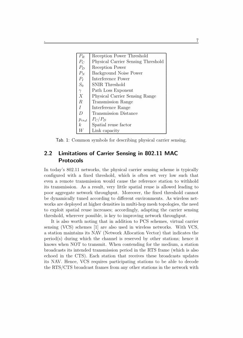
Table 1 briefly summarizes the common symbols used throughout thispaper to describe carrier sensing.

2 The exact relation between the physical carrier sensing range X and the interferencerange I is determined by Eq.4 and 6. Here, we just show an example with X > I.

, 7

PR Reception Power ThresholdPC Physical Carrier Sensing ThresholdPD Reception PowerPN Background Noise PowerPI Interference PowerS0 SNIR Thresholdγ Path Loss ExponentX Physical Carrier Sensing RangeR Transmission RangeI Interference RangeD Transmission Distancepcs t PC/PD

k Spatial reuse factorW Link capacity

Tab. 1: Common symbols for describing physical carrier sensing.

2.2 Limitations of Carrier Sensing in 802.11 MACProtocols

In today’s 802.11 networks, the physical carrier sensing scheme is typicallyconfigured with a fixed threshold, which is often set very low such thateven a remote transmission would cause the reference station to withholdits transmission. As a result, very little spatial reuse is allowed leading topoor aggregate network throughput. Moreover, the fixed threshold cannotbe dynamically tuned according to different environments. As wireless net-works are deployed at higher densities in multi-hop mesh topologies, the needto exploit spatial reuse increases; accordingly, adapting the carrier sensingthreshold, wherever possible, is key to improving network throughput.

It is also worth noting that in addition to PCS schemes, virtual carriersensing (VCS) schemes [1] are also used in wireless networks. With VCS,a station maintains its NAV (Network Allocation Vector) that indicates theperiod(s) during which the channel is reserved by other stations; hence itknows when NOT to transmit. When contending for the medium, a stationbroadcasts its intended transmission period in the RTS frame (which is alsoechoed in the CTS). Each station that receives these broadcasts updatesits NAV. Hence, VCS requires participating stations to be able to decodethe RTS/CTS broadcast frames from any other stations in the network with

, 8

which they may potentially interfere. Unfortunately, this requirement cannotbe guaranteed in most dense wireless networks [10]. Fig. 1 demonstrates thelimitations of the VCS scheme for preventing interference as was shown in[10]. The VCS scheme can effectively prevent nodes A and B from initiatingan interfering transmission, as they are in the transmission range of TX andRX, respectively; however node C is too far away from both TX and RXto reliably decode the RTS or CTS packets, yet it is still a potential hiddennode that could interfere with the packet reception at RX.

3 Enhancing Physical Carrier Sensing

3.1 Tuning Physical Carrier Sensing (PCS) to AvoidInterference

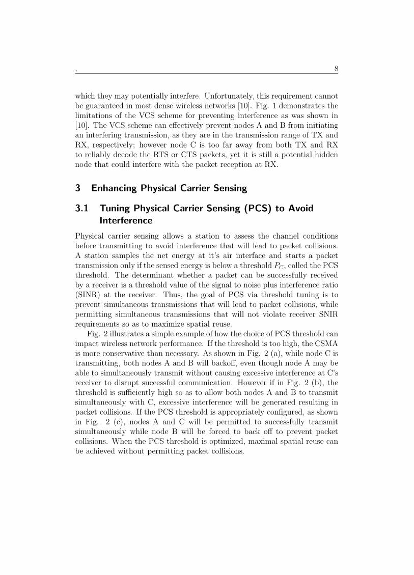
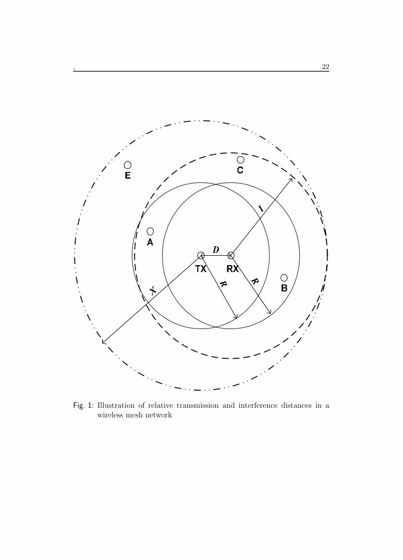
Physical carrier sensing allows a station to assess the channel conditionsbefore transmitting to avoid interference that will lead to packet collisions.A station samples the net energy at it’s air interface and starts a packettransmission only if the sensed energy is below a threshold PC , called the PCSthreshold. The determinant whether a packet can be successfully receivedby a receiver is a threshold value of the signal to noise plus interference ratio(SINR) at the receiver. Thus, the goal of PCS via threshold tuning is toprevent simultaneous transmissions that will lead to packet collisions, whilepermitting simultaneous transmissions that will not violate receiver SNIRrequirements so as to maximize spatial reuse.

Fig. 2 illustrates a simple example of how the choice of PCS threshold canimpact wireless network performance. If the threshold is too high, the CSMAis more conservative than necessary. As shown in Fig. 2 (a), while node C istransmitting, both nodes A and B will backoff, even though node A may beable to simultaneously transmit without causing excessive interference at C’sreceiver to disrupt successful communication. However if in Fig. 2 (b), thethreshold is sufficiently high so as to allow both nodes A and B to transmitsimultaneously with C, excessive interference will be generated resulting inpacket collisions. If the PCS threshold is appropriately configured, as shownin Fig. 2 (c), nodes A and C will be permitted to successfully transmitsimultaneously while node B will be forced to back off to prevent packetcollisions. When the PCS threshold is optimized, maximal spatial reuse canbe achieved without permitting packet collisions.

, 9

When properly tuned, PCS is more robust than the VCS, because it doesnot require control packets to be received and correctly decoded. It is alsomore flexible, since the PCS sensing range can be easily adjusted by tuningthe PCS threshold. In Fig.1, all potentially interfering nodes, including nodeC, can be eliminated by enlarging the PCS sensing range to cover the entirepotential interference area, i.e.

X ≥ D + I. (7)

Combining Eq.7 with Eq.5, we obtain

X ≥ D(1 + S1/γ0 ), (8)

that leads to

Pcs t ≤ 1

(1 + S1/γ0 )γ

. (9)

Another well-known problem occurs due to exposed terminals [8]; for ex-ample, even though a transmission by node E will not disrupt RX, because itis within the sensing range of TX, E will defer its transmission. Having toomany exposed terminals can potentially reduce the overall network through-put. By tuning the physical carrier sensing threshold, we will demonstratea good tradeoff between hidden terminals and exposed terminals so as toobtain high aggregate throughput.

3.2 Estimating Optimal PCS Threshold to MaximizeSpatial Reuse

We now investigate the choice of the optimal PCS threshold that allows formaximum spatial reuse, by assuming homogeneous wireless links and iden-tical interference and noise environments at all nodes 3. To initiate channelaccess by a node, the interference and noise sensed by its receiver cannotexceed the tolerable level according to Eq.2,

PI + PN ≤ PD/S0, (10)

It therefore follows that the PCS threshold should satisfy

PC ≤ PD/S0, (11)

3 This assumption is clearly the primary weakness of the model.

, 10

for successful simultaneous transmissions. Since higher the PCS thresholdimplies more simultaneous transmissions, PD/S0 is the optimal PCS thresh-old for maximal spatial reuse. The corresponding optimal pcs t defined as βis seen to be independent of path loss exponent γ, i.e.,

β =1

S0(12)

Let ρ denote the ratio of the exposed terminal area to the whole PCSsensing area with 1

(1+S1/γ0 )γ

; then using Eq. 9, this is given by

ρ =πX2 − πI2

πX2≈ D2(1 + S

1/γ0 )2 − D2S

2/γ0

D2(1 + S1/γ0 )2

= 1 − (S

1/γ0

1 + S1/γ0

)2. (13)

When S1/γ0 is small, ρ is not negligible; but with S

1/γ0 >> 1 4, we have ρ ≈ 0

so that the exposed terminal problem can be ignored, and Eq.9 turns intopcs t ≤ β.

3.3 Analysis Model for Aggregate Throughput Limits

In [4] the authors investigated spatial reuse from a physical layer perspective.A homogeneous environment was assumed where every transmitter uses thesame transmission power and data rate, and communicates to an immedi-ate neighbor at the constant T-R distance d. Under such conditions, spatialreuse can be characterized by the distance between neighboring simultaneoustransmitters (minimum T-T separation distance) that results in optimal spa-tial reuse. The authors investigated the optimal spatial reuse for two regularnetwork topologies: the 1-D chain network and the 2-D grid network. Let kdenote the T-T distance (also called spatial reuse factor), in number of hops(hop distance being d), then the lower bounds of k for the two topologies are

k ≥[2

(1 + 1

γ−1

)S0

] 1γ , Chain network

k ≥[6

(1 + 1

γ−2

)S0

] 1γ , 2-D grid

(14)

If we assume a perfect MAC protocol that schedules simultaneous com-munications only on transmitters that are k hops away from each other, the

4 More so for higher data rates since higher S0 values will be required.

, 11

network will be able to accommodate the maximum number of simultaneoustransmitters, hence reaching its aggregate throughput limit. Hence the lowerbounds of k can be used to extrapolate to aggregate throughput limits. Forexample, in a chain network of N nodes, where a packet will require relay byeach of the N − 2 intermediate nodes in order to be routed end-to-end, atmost N/k simultaneous transmitters can be supported in the chain. Let Cth

denote the end-to-end throughput, then

Cth ≈ W

k(15)

where W denotes the effective MAC layer data rate achieved at each relay,i.e. link capacity.

4 An Estimation-based Adaptive Physical Carrier Sensing(APCS) Scheme

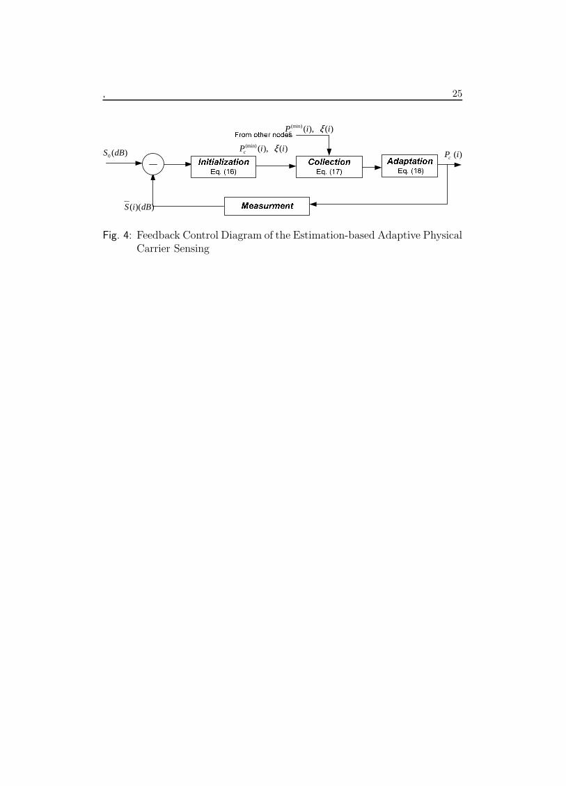
In the previous section, a theoretical estimate for optimal β or normalizedcarrier sensing threshold pcs t was derived for a spatially homogeneous net-work. It is difficult to repeat the above analysis for a network with het-erogeneous links (i.e. different receiver sensitivities and/or transmit power).In this section, we propose an adaptive scheme which allows each individualstation to calculate and self-configure a near-optimal PCS threshold based onits estimate of the current local interference condition. As a result, the entirenetwork is able to achieve the near-optimal aggregate throughput. Further-more, such distributed adaptation is also designed to make stations adoptthe same threshold. Hence, each station will have equal time-share of thechannel, resulting in fair usage of network bandwidth.

The objective of the estimation-based adaptation is to allow simultaneousspatially separated transmissions while ensuring that SINR at each stationremains above the desired threshold S0. This is accomplished by local mea-surement and statistics exchange between radio neighbors.

Each node keeps track of the following state variables for the purpose ofestimation and adaptation:

Te: The periodic duration of estimation and adaptation (seconds)

S(i): The estimation of the average SINR in a duration at the ith update

, 12

ξ(i): Indicator for adaptation at the ith update (2: Increase, 1: No Change,0: Decrease)

P(min)C (i): The estimation of the minimum PC(i) in the network at the

ith update.

and uses a key parameter of the APCS algorithm:

δ(i): The one-step adjustment unit at the ith update.

Both S(i) and PC(i) are updated only once every Te seconds while, ξ(i)

and P(min)C (i) are updated whenever ACK is received with ”More Frag” off.

The value of S(i) in this interval is the estimate of average SNIR in theprevious interval. At the beginning of each interval, we set ξ(i) with respectto S(i) as follows

ξ(i) =

2 , S(i)/S0 ≥ δ1 , 1/δ < S(i)/S0 < δ0 , S(i)/S0 ≤ δ

(16)

and P(min)C (i) = PC(i).

This scheme requires disseminating the locally measured statistics ξ(i)

and P(min)C (i) throughout the network neighborhood. For easy implementa-

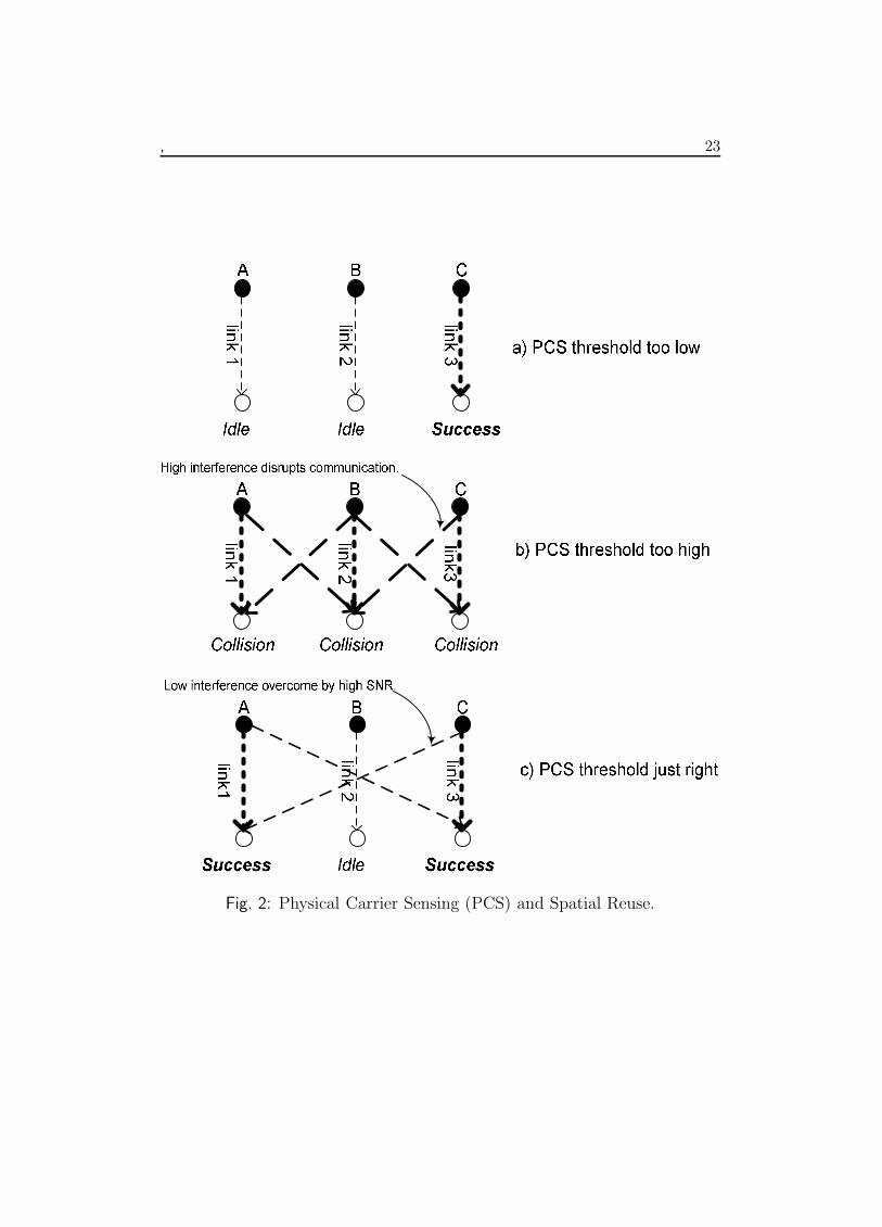
tion, we piggyback the information into the 16 bits ”Duration ID” field of802.11 ACK frame when it is not used. Fig.3 shows the header format of802.11 MAC ACK packet. When overhearing an ACK, a node will check its”More Frag” flag and ”Duration ID” field regardless of whether the ACK isdestined for the node. In the standard 802.11 MAC protocol, the ”DurationID” field in an ACK frame is used for the purpose of virtual carrier sensingwhen the ”More Frag” flag is set to 1 ( meaning there are more fragments ofa packet following). If the ACK is for the last fragment of the packet or frag-mentation is not used, the ”More Frag” is turned off (set to 0) and ”durationID” field is not used. Hence we can piggyback information in the ”DurationID” field for the estimation-based adaptive PCS scheme when ”More Frag”is 1 5.

5 While this implementation was convenient for simulation purposes to avoid potentialinteroperability problems from non-standard use of ACK frames, it may be preferable todefine a new frame format for this purpose.

, 13

Let x and y be the value of ξ(i) and P(min)C (i) carried by that ACK packet,

the node updates its own ξ(i) and P(min)C (i) with

{ξ(i) = min(x, ξ(i))

P(min)C (i) = min(y, P

(min)C (i))

. (17)

At the end of the interval, each node update its own PC(i) as follows:

PC(i) =

P(min)C (i) × δ , (ξ = 2)

P(min)C (i) , (ξ = 1)

P(min)C (i)/δ , (ξ = 0)

. (18)

The initial value of PC(i = 0) for all nodes is set to PR/S0, where PR is thereceiver sensitivity and results in the minimum value of PD. Fig. 4 illustratesthe feedback control diagram for the scheme.

5 Simulation Results and Discussions

All the simulation experiments reported were conducted in the OPNET sim-ulation environment [13]. Accordingly, we have extended OPNET kernelmodules to support tunable physical carrier sensing, a configurable propa-gation environment and multiple 802.11b data rates. In all simulations, weconfigured each node to be always backlogged with packets to send, and eachMAC data frame to be 1024 bytes long. Each node transmits at a fixed powerof 0 dbm. By default, the OPNET simulator configures the physical carriersensing threshold to be the same as the reception threshold. Furthermore,the ambient noise level was set at −200 dBm.

The primary performance metric studied in this paper is throughput, de-fined as the total number of bits successfully received in a second. Due toMAC semantics, if the sender does not receive an intended ACK packet, itassumes that the data packet is lost and performs a retransmission. How-ever, it is also possible that a data packet is received correctly, but the ACKpacket is lost. This situation also causes a retransmission and can result inmultiple copies of the data packet at the receiver; in this case, only the firstwill be forwarded up to higher layers, and the duplicates discarded. Whencomputing throughput in this paper, we only count non-duplicate data pack-ets that are successfully received, i.e., goodput, which is less than the actualnetwork throughput. However, since ACK packets are much smaller than

, 14

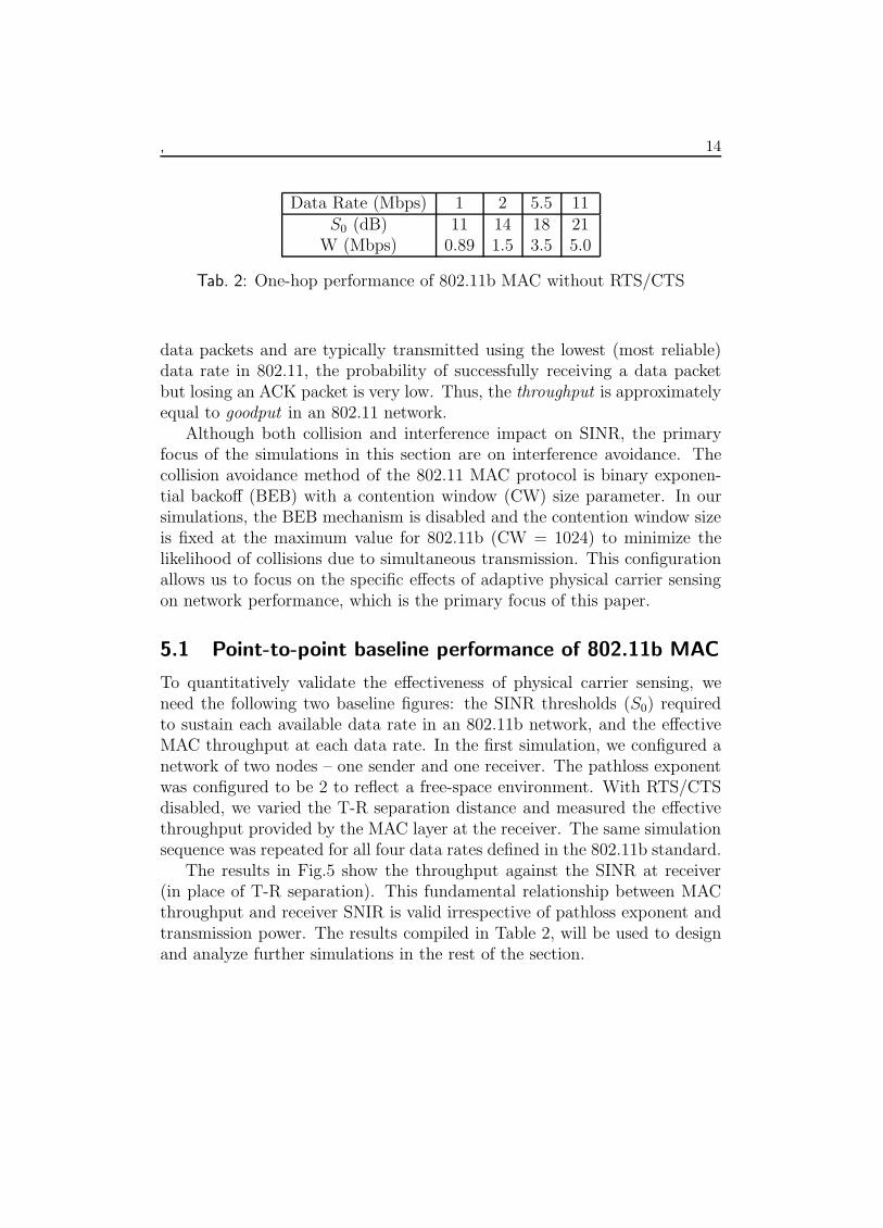
Data Rate (Mbps) 1 2 5.5 11S0 (dB) 11 14 18 21

W (Mbps) 0.89 1.5 3.5 5.0

Tab. 2: One-hop performance of 802.11b MAC without RTS/CTS

data packets and are typically transmitted using the lowest (most reliable)data rate in 802.11, the probability of successfully receiving a data packetbut losing an ACK packet is very low. Thus, the throughput is approximatelyequal to goodput in an 802.11 network.

Although both collision and interference impact on SINR, the primaryfocus of the simulations in this section are on interference avoidance. Thecollision avoidance method of the 802.11 MAC protocol is binary exponen-tial backoff (BEB) with a contention window (CW) size parameter. In oursimulations, the BEB mechanism is disabled and the contention window sizeis fixed at the maximum value for 802.11b (CW = 1024) to minimize thelikelihood of collisions due to simultaneous transmission. This configurationallows us to focus on the specific effects of adaptive physical carrier sensingon network performance, which is the primary focus of this paper.

5.1 Point-to-point baseline performance of 802.11b MAC

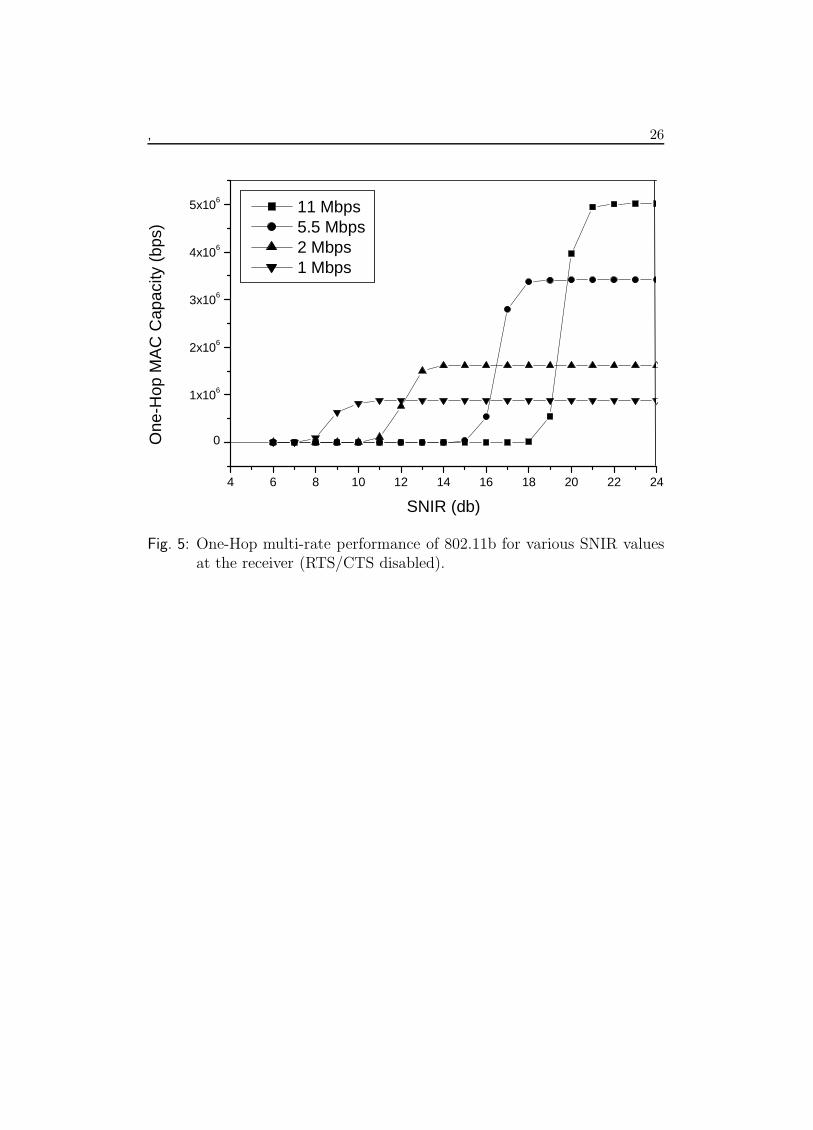
To quantitatively validate the effectiveness of physical carrier sensing, weneed the following two baseline figures: the SINR thresholds (S0) requiredto sustain each available data rate in an 802.11b network, and the effectiveMAC throughput at each data rate. In the first simulation, we configured anetwork of two nodes – one sender and one receiver. The pathloss exponentwas configured to be 2 to reflect a free-space environment. With RTS/CTSdisabled, we varied the T-R separation distance and measured the effectivethroughput provided by the MAC layer at the receiver. The same simulationsequence was repeated for all four data rates defined in the 802.11b standard.

The results in Fig.5 show the throughput against the SINR at receiver(in place of T-R separation). This fundamental relationship between MACthroughput and receiver SNIR is valid irrespective of pathloss exponent andtransmission power. The results compiled in Table 2, will be used to designand analyze further simulations in the rest of the section.

, 15

5.2 Maximizing Spatial Reuse with the Optimal PCS

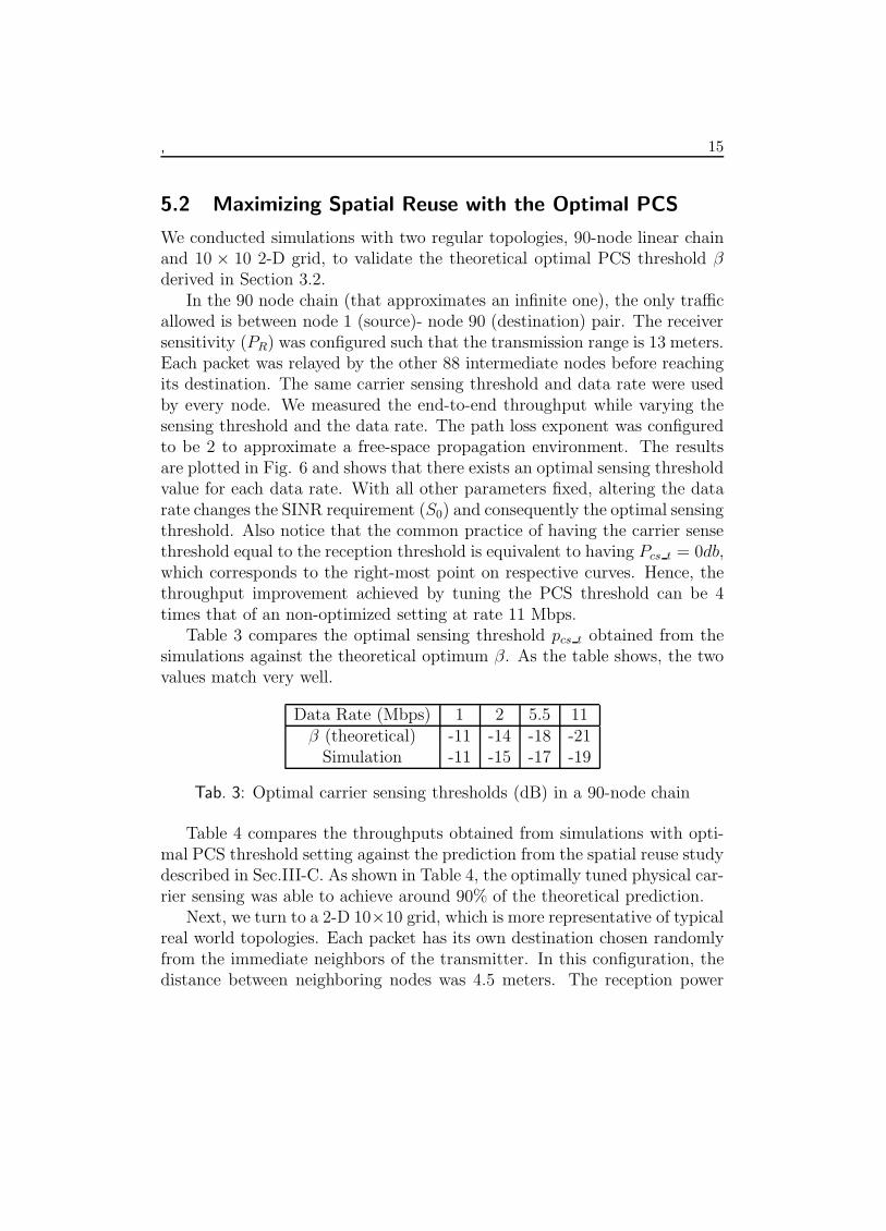
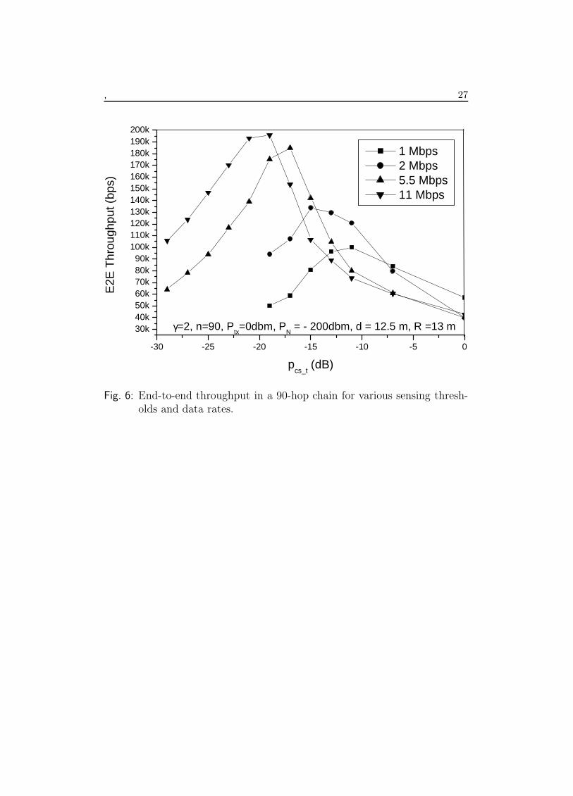
We conducted simulations with two regular topologies, 90-node linear chainand 10 × 10 2-D grid, to validate the theoretical optimal PCS threshold βderived in Section 3.2.

In the 90 node chain (that approximates an infinite one), the only trafficallowed is between node 1 (source)- node 90 (destination) pair. The receiversensitivity (PR) was configured such that the transmission range is 13 meters.Each packet was relayed by the other 88 intermediate nodes before reachingits destination. The same carrier sensing threshold and data rate were usedby every node. We measured the end-to-end throughput while varying thesensing threshold and the data rate. The path loss exponent was configuredto be 2 to approximate a free-space propagation environment. The resultsare plotted in Fig. 6 and shows that there exists an optimal sensing thresholdvalue for each data rate. With all other parameters fixed, altering the datarate changes the SINR requirement (S0) and consequently the optimal sensingthreshold. Also notice that the common practice of having the carrier sensethreshold equal to the reception threshold is equivalent to having Pcs t = 0db,which corresponds to the right-most point on respective curves. Hence, thethroughput improvement achieved by tuning the PCS threshold can be 4times that of an non-optimized setting at rate 11 Mbps.

Table 3 compares the optimal sensing threshold pcs t obtained from thesimulations against the theoretical optimum β. As the table shows, the twovalues match very well.

Data Rate (Mbps) 1 2 5.5 11β (theoretical) -11 -14 -18 -21

Simulation -11 -15 -17 -19

Tab. 3: Optimal carrier sensing thresholds (dB) in a 90-node chain

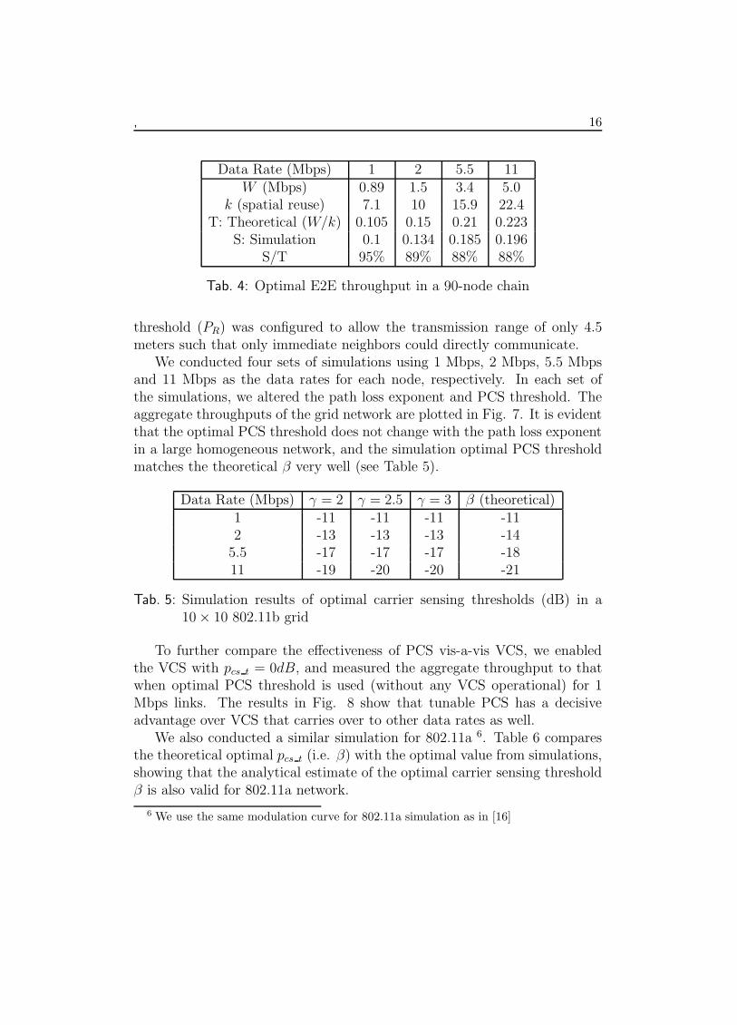
Table 4 compares the throughputs obtained from simulations with opti-mal PCS threshold setting against the prediction from the spatial reuse studydescribed in Sec.III-C. As shown in Table 4, the optimally tuned physical car-rier sensing was able to achieve around 90% of the theoretical prediction.

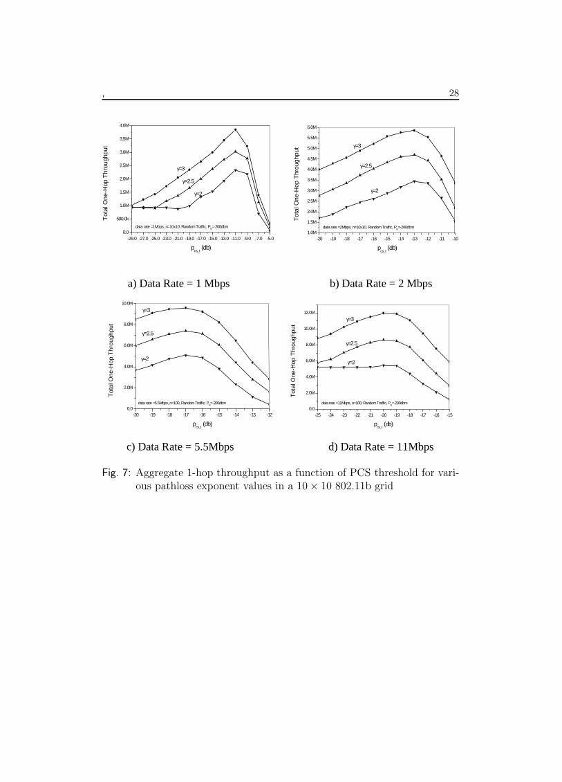
Next, we turn to a 2-D 10×10 grid, which is more representative of typicalreal world topologies. Each packet has its own destination chosen randomlyfrom the immediate neighbors of the transmitter. In this configuration, thedistance between neighboring nodes was 4.5 meters. The reception power

, 16

Data Rate (Mbps) 1 2 5.5 11W (Mbps) 0.89 1.5 3.4 5.0

k (spatial reuse) 7.1 10 15.9 22.4T: Theoretical (W/k) 0.105 0.15 0.21 0.223

S: Simulation 0.1 0.134 0.185 0.196S/T 95% 89% 88% 88%

Tab. 4: Optimal E2E throughput in a 90-node chain

threshold (PR) was configured to allow the transmission range of only 4.5meters such that only immediate neighbors could directly communicate.

We conducted four sets of simulations using 1 Mbps, 2 Mbps, 5.5 Mbpsand 11 Mbps as the data rates for each node, respectively. In each set ofthe simulations, we altered the path loss exponent and PCS threshold. Theaggregate throughputs of the grid network are plotted in Fig. 7. It is evidentthat the optimal PCS threshold does not change with the path loss exponentin a large homogeneous network, and the simulation optimal PCS thresholdmatches the theoretical β very well (see Table 5).

Data Rate (Mbps) γ = 2 γ = 2.5 γ = 3 β (theoretical)1 -11 -11 -11 -112 -13 -13 -13 -14

5.5 -17 -17 -17 -1811 -19 -20 -20 -21

Tab. 5: Simulation results of optimal carrier sensing thresholds (dB) in a10 × 10 802.11b grid

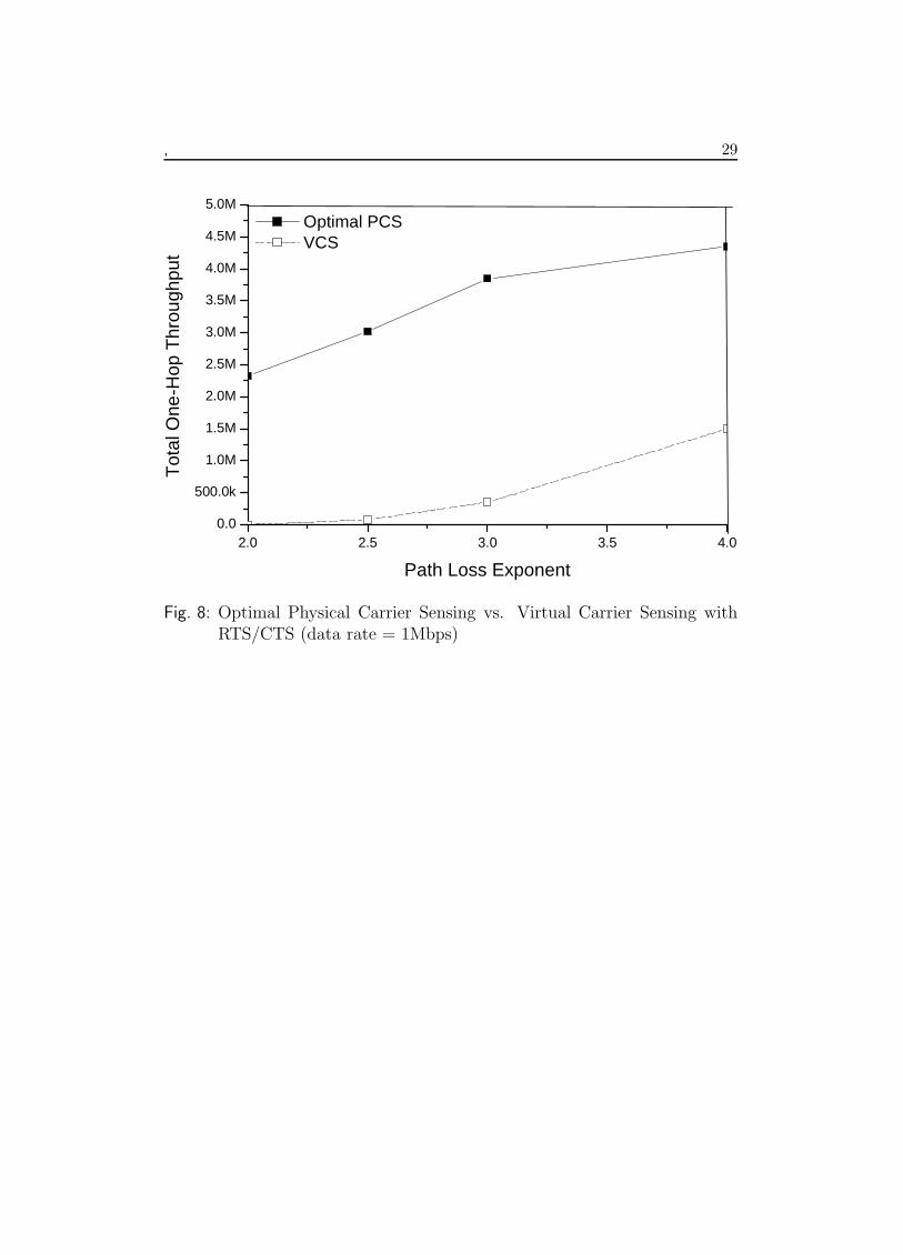
To further compare the effectiveness of PCS vis-a-vis VCS, we enabledthe VCS with pcs t = 0dB, and measured the aggregate throughput to thatwhen optimal PCS threshold is used (without any VCS operational) for 1Mbps links. The results in Fig. 8 show that tunable PCS has a decisiveadvantage over VCS that carries over to other data rates as well.

We also conducted a similar simulation for 802.11a 6. Table 6 comparesthe theoretical optimal pcs t (i.e. β) with the optimal value from simulations,showing that the analytical estimate of the optimal carrier sensing thresholdβ is also valid for 802.11a network.

6 We use the same modulation curve for 802.11a simulation as in [16]

, 17

Data Rate (Mbps) 6 9 12 18 24 36 48 54β (theoretical) -7 -9 -11 -13 -17 -22 -27 -29

Simulation -7 -9 -11 -13 -17 -21 -27 -29

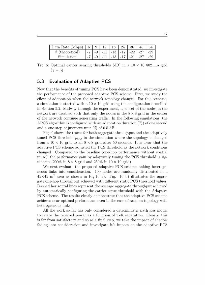
Tab. 6: Optimal carrier sensing thresholds (dB) in a 10 × 10 802.11a grid(γ = 3)

5.3 Evaluation of Adaptive PCS

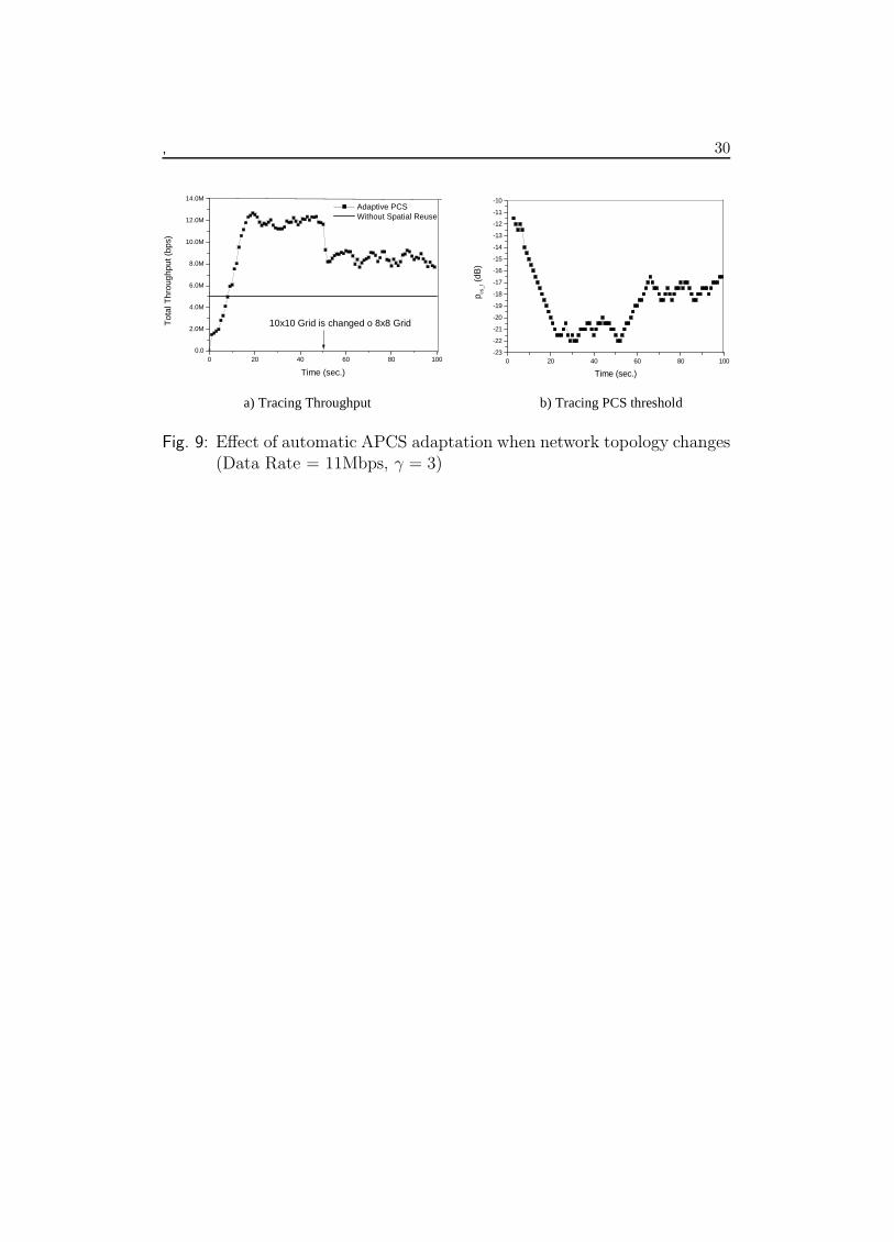
Now that the benefits of tuning PCS have been demonstrated, we investigatethe performance of the proposed adaptive PCS scheme. First, we study theeffect of adaptation when the network topology changes. For this scenario,a simulation is started with a 10× 10 grid using the configuration describedin Section 5.2. Midway through the experiment, a subset of the nodes in thenetwork are disabled such that only the nodes in the 8× 8 grid in the centerof the network continue generating traffic. In the following simulations, theAPCS algorithm is configured with an adaptation duration (Te) of one secondand a one-step adjustment unit (δ) of 0.5 dB.

Fig. 9 shows the traces for both aggregate throughput and the adaptivelytuned PCS threshold pcs t in the simulation where the topology is changedfrom a 10 × 10 grid to an 8 × 8 grid after 50 seconds. It is clear that theadaptive PCS scheme adjusted the PCS threshold as the network conditionschanged. Compared to the baseline (one-hop performance without spatialreuse), the performance gain by adaptively tuning the PCS threshold is sig-nificant (200% in 8 × 8 grid and 250% in 10 × 10 grid).

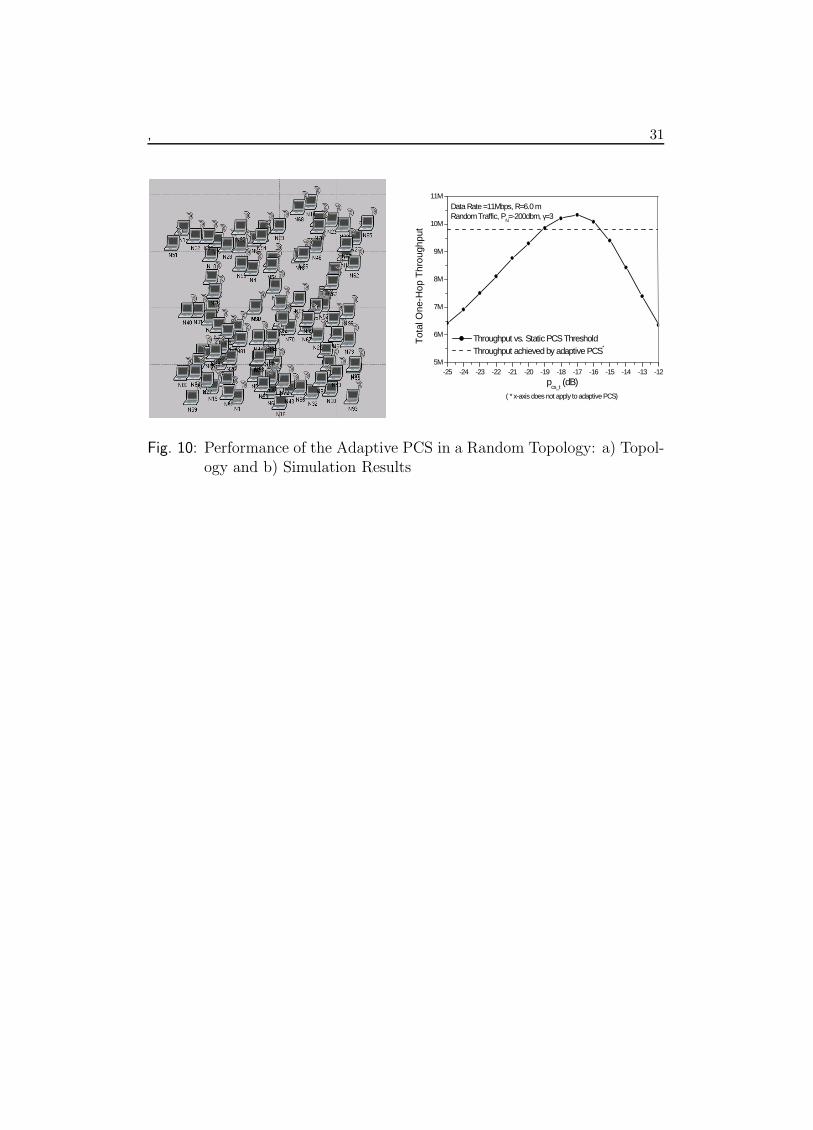
We next evaluate the proposed adaptive PCS scheme, taking heteroge-neous links into consideration. 100 nodes are randomly distributed in a45×45 m2 area as shown in Fig.10 a). Fig. 10 b) illustrates the aggre-gate one-hop throughput achieved with different static PCS threshold values.Dashed horizontal lines represent the average aggregate throughput achievedby automatically configuring the carrier sense threshold with the AdaptivePCS scheme. The results clearly demonstrate that the adaptive PCS schemeachieves near-optimal performance even in the case of random topology withheterogeneous links.

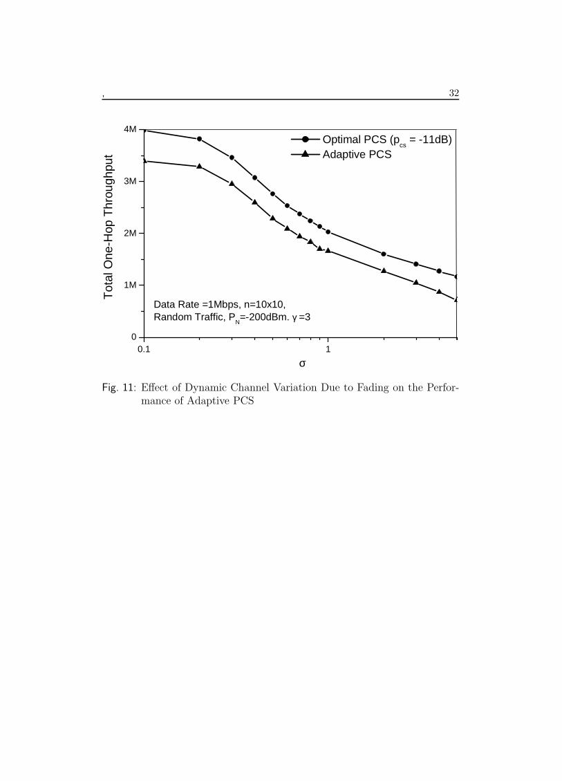
All the work so far has only considered a deterministic path loss modelto relate the received power as a function of T-R separation. Clearly, thisis far from satisfactory and so as a final step, we take the impact of shadowfading into consideration and investigate it’s impact on the adaptive PCS

, 18

scheme performance. Here we revert back to a 10x10 regular grid as in Fig.7to remove the effects of random topology.

Lognormal shadow fading on a link is modelled by modifying Eq.1 asfollows:

Prx(d) = P̄rx − 10γlog10(d/d̄) + X (all powers in dB), (19)

where X is a Gaussian random variable (also called fading factor) with zeromean and variance σ2. Usually, the fading should be on a small scale (saymillisecond), i.e. X is randomly chosen for every millisecond (ms). However,this will dramatically increase the complexity of simulation and slow downthe speed. Here, we use the packet level energy calculation that allows simplerand faster simulation of a lognormal fading channel with σ on the range (0,5).

Fig.11 shows that the performance of the adaptive PCS degrades as thedeviation σ increases, which is reasonable since the prediction of interferencelevel by energy sensing becomes less and less dependable with σ increasing.For comparison, we also demonstrated the performance of the static PCSwith the PCS threshold manually set as the optimal value (-11dB), showingthat near-optimal performance can be still achieved by the adaptive schemeeven in a fading environment. One solution to the performance degradationis to lengthen the sensing duration DIFS, but the side effect of using longerDIFS is the increased overhead. Nevertheless, unless the DIFS exceeds thetransmission time of RTS/CTS handshaking, the overhead of PCS will notbe higher than VCS, hence PCS threshold adaptation is a viable option.

5.4 Remark on Implementation Aspects

As stated in IEEE 802.11 standards [1], the task of physical carrier sensingis carried by the Clear Channel Assessment (CCA). There are three CCAmodes available for 802.11 DSSS (Direct Sequence Spread Spectrum) PHY:

“CCA Mode 1: Energy above threshold. CCA shall report a busy mediumupon detection of any energy above the Energy Detection (ED) threshold.

CCA Mode 2: Carrier sense only. CCA shall report a busy medium onlyupon detection of a DSSS signal. This signal may be above or below the EDthreshold.

CCA Mode 3: Carrier sense with energy above threshold. CCA shallreport a busy upon detection of a DSSS signal with energy above the EDthreshold. ” (page 223 in [1])

, 19

Clearly the ED threshold in the CCA Mode 1 has the same physicalmeaning as the PCS threshold in this paper, and can be used for enhancedphysical carrier sensing. Unfortunately, the idea of enhancing PCS to miti-gate interference via tuning the threshold does not appear to have attractedsignificant industry or academic attention, at least in relation to the litera-ture on VCS based approaches. As a consequence, the ED threshold is nottunable or even accessible in most current 802.11 chips. However, a few ven-dors do allow ED threshold tuning, namely the Prism 2.5 ISL3873B 7 chipset,for example. ISL3873B has a 8-bit register to configure the ED threshold,where Bit 7 is ED threshold control: 0 = threshold is relative to noise floorand 1 = threshold is absolute, and Bits 6∼ 0 is the ED threshold that couldbe set to any value on the range [0, 127](dBm).

6 Conclusion

In this paper, we proposed to enhance physical carrier sensing with a dy-namically tunable sensing threshold to improve spatial reuse in 802.11 meshnetworks, to increase the aggregate network throughput. Simulations wereperformed for both 1-D chain and 2-D grid topologies to validate the analysisand the proposed scheme. The main contributions of this paper are:

(1) We first provided a simple estimate of the optimal PCS threshold formaximizing the aggregate network throughput in a homogeneous meshnetwork and was validated by simulations.

(2) Next, we demonstrated an adaptive PCS scheme intended for hetero-geneous networks where the PCS threshold is tuned by individualnodes based on local carrier sensing to achieve a substantial aggregatethroughput improvement.

References

[1] IEEE Standard for Wireless LAN Medium Access Control (MAC) andPhysical Layer (PHY) specifications, ISO/IEC 8802-11: 1999(E), Aug.1999.

7 http://www.intersil.com

, 20

[2] B. P. Crow, J. G. Kim, IEEE 802.11 Wireless Local Area Networks,IEEE Comm. Mag., Sept. 1999.

[3] G. Bianchi, Performance Analysis of the IEEE 802.11 Distributed Co-ordination Function, IEEE JSAC, vol. 18, no. 3, March 2000.

[4] X. Guo, S. Roy, W. Steven Conner, Spatial Reuse in Wireless Ad-HocNetworks, VTC2003.

[5] J. Medbo and J.-E. Berg, Simple and accurate path loss modeling at 5GHz in indoor environments with corridors, IEEE VTS-Fall VTC 2000.52nd , Volume: 1 , 24-28 Sept. 2000.

[6] X. Guo, ”Personal Communication”, 2003.

[7] Z. Li, S. Nandi, and A. K. Gupta, Improving Fairness inIEEE 802.11 based MANETs using Enhanced Carrier Sensing,http://www.ntu.edu.sg/home5/pg03802331/papers/ecs.pdf.

[8] D. Shukla, L. Chandran-Wadia, S. Iyer, Mitigating the exposed nodeproblem in IEEE 802.11 adhoc networks, IEEE ICCCN 2003, Dallas,Oct 2003.

[9] F. A. Tobagi, L. Kleinrock, Packet Switching in Radio Channels: PARTII- The Hidden Terminal Problem in Carrier Sensing Multiple Accessand Busy Tone Solution”, IEEE Trans. on Commun, Vol. COM-23, No.12, pp. 1417-1433, 1975.

[10] K. Xu, M. Gerla, S. Bae, How effective is the IEEE 802.11 RTS/CTShandshake in ad hoc networks?, GLOBECOM02, Nov 17-21, 2002.

[11] S. Xu, T. Saadawi, Does the IEEE 802.11 MAC Protocol Work Well inMultihop Wireless Ad Hoc Networks? IEEE Communications Magazine,P130-137, June 2001.

[12] F. Ye, B. Sikdar, Improving Spatial Reuse of IEEE 802.11 Based AdHoc Networks, IEEE GLOBECOM, San Francisco, December 2003.

[13] http://www.opnet.com

[14] Intersil, Direct Sequence Spread Spectrum Baseband Processor, Doc#FN 4816.2, Feb. 2002, http://www.intersil.com/

, 21

[15] V.Bharghavan, A. Demers, S. Shenker, and L. Zhang, MACAW: A Me-dia Access Protocol for Wireless LANs, in Proc. Of ACM SIGCOMM’94,

[16] A.J. van der Vegt, Auto rate fallback algorithm for the ieee 802.11astandard, http://www.phys.uu.nl/ vdvegt/docs/gron/.

[17] Theodore S. Rappaport. Wireless Communications, Principles and Prac-tices, 2nd Ed. Prentice Hall, 2002. ISBN 0-13-042232-0

[18] ”PRISM 2.5 Wireless LAN Integrated Medium Access Controller withBaseband Processor”, http://www.intersil.com/data/fn/fn8019.pdf

, 22

Fig. 1: Illustration of relative transmission and interference distances in awireless mesh network

, 23

Fig. 2: Physical Carrier Sensing (PCS) and Spatial Reuse.

, 24

ACK Frame Header of 802.11

MAC

Type To DS

Protocol Sub Type = ACK

2 2 4 1

From DS

1

More Frag

1

Retry

1

Pwr Mgmt

1

More Data

1 1 1

WEP

Order

B0 B1B2 B3B4 B7 B8 B9 B10 B11 B12 B13 B14 B15

2 2 6 4

Duration ID

Frame Control

RA FCS

Bytes

Bits

Fig. 3: 802.11 MAC ACK Head

, 25

)(0 dBS

))(( dBiS

)(),((min) iiPc ξ

)(iPc

)(),((min) iiPc ξ

Fig. 4: Feedback Control Diagram of the Estimation-based Adaptive PhysicalCarrier Sensing

, 26

4 6 8 10 12 14 16 18 20 22 24

0

1x106

2x106

3x106

4x106

5x106 11 Mbps 5.5 Mbps 2 Mbps 1 Mbps

One

-Hop

MA

C C

apac

ity (

bps)

SNIR (db)

Fig. 5: One-Hop multi-rate performance of 802.11b for various SNIR valuesat the receiver (RTS/CTS disabled).

, 27

-30 -25 -20 -15 -10 -5 0

30k40k50k60k70k80k90k

100k110k120k130k140k150k160k170k180k190k200k

γ=2, n=90, Ptx=0dbm, P

N = - 200dbm, d = 12.5 m, R =13 m

1 Mbps 2 Mbps 5.5 Mbps 11 Mbps

E2E

Thr

ough

put (

bps)

pcs_t

(dB)

Fig. 6: End-to-end throughput in a 90-hop chain for various sensing thresh-olds and data rates.

, 28

-29.0 -27.0 -25.0 -23.0 -21.0 -19.0 -17.0 -15.0 -13.0 -11.0 -9.0 -7.0 -5.00.0

500.0k

1.0M

1.5M

2.0M

2.5M

3.0M

3.5M

4.0M

γ=2.5

γ=3

γ=2

data rate =1Mbps, n=10x10, Random Traffic, PN=-200dbm

Tot

al O

ne-H

op T

hrou

ghpu

t

pcs_t

(db)

-20 -19 -18 -17 -16 -15 -14 -13 -12 -11 -101.0M

1.5M

2.0M

2.5M

3.0M

3.5M

4.0M

4.5M

5.0M

5.5M

6.0M

γ=2.5

γ=3

γ=2

data rate =2Mbps, n=10x10, Random Traffic, PN=-200dbm

Tot

al O

ne-H

op T

hrou

ghpu

t

pcs_t

(db)

a) Data Rate = 1 Mbps b) Data Rate = 2 Mbps

-20 -19 -18 -17 -16 -15 -14 -13 -120.0

2.0M

4.0M

6.0M

8.0M

10.0M

γ=2.5

γ=3

γ=2

data rate =5.5Mbps, n=100, Random Traffic, PN=-200dbm

Tot

al O

ne-H

op T

hrou

ghpu

t

pcs_t

(db)

-25 -24 -23 -22 -21 -20 -19 -18 -17 -16 -150.0

2.0M

4.0M

6.0M

8.0M

10.0M

12.0M

γ=2.5

γ=3

γ=2

data rate =11Mbps, n=100, Random Traffic, PN=-200dbm

Tot

al O

ne-H

op T

hrou

ghpu

t

pcs_t

(db)

c) Data Rate = 5.5Mbps d) Data Rate = 11Mbps

Fig. 7: Aggregate 1-hop throughput as a function of PCS threshold for vari-ous pathloss exponent values in a 10 × 10 802.11b grid

, 29

2.0 2.5 3.0 3.5 4.00.0

500.0k

1.0M

1.5M

2.0M

2.5M

3.0M

3.5M

4.0M

4.5M

5.0M Optimal PCS VCS

Tot

al O

ne-H

op T

hrou

ghpu

t

Path Loss Exponent

Fig. 8: Optimal Physical Carrier Sensing vs. Virtual Carrier Sensing withRTS/CTS (data rate = 1Mbps)

, 30

0 20 40 60 80 1000.0

2.0M

4.0M

6.0M

8.0M

10.0M

12.0M

14.0M Adaptive PCS Without Spatial Reuse

10x10 Grid is changed o 8x8 GridTot

al T

hrou

ghpu

t (bp

s)

Time (sec.)0 20 40 60 80 100

-23

-22

-21

-20

-19

-18

-17

-16

-15

-14

-13

-12

-11

-10

p cs_t (

dB)

Time (sec.)

a) Tracing Throughput b) Tracing PCS threshold

Fig. 9: Effect of automatic APCS adaptation when network topology changes(Data Rate = 11Mbps, γ = 3)

, 31

-25 -24 -23 -22 -21 -20 -19 -18 -17 -16 -15 -14 -13 -125M

6M

7M

8M

9M

10M

11M

( * x-axis does not apply to adaptive PCS)

Throughput vs. Static PCS Threshold Throughput achieved by adaptive PCS*

Data Rate =11Mbps, R=6.0 mRandom Traffic, P

N=-200dbm, γ=3

Tot

al O

ne-H

op T

hrou

ghpu

t

pcs_t

(dB)

Fig. 10: Performance of the Adaptive PCS in a Random Topology: a) Topol-ogy and b) Simulation Results

, 32

0.1 10

1M

2M

3M

4M Optimal PCS (p

cs = -11dB)

Adaptive PCS

Data Rate =1Mbps, n=10x10, Random Traffic, P

N=-200dBm. γ =3

Tot

al O

ne-H

op T

hrou

ghpu

t

σ

Fig. 11: Effect of Dynamic Channel Variation Due to Fading on the Perfor-mance of Adaptive PCS