The Economics of Weather and Climate Risks Working Paper Series Working Paper No. 12/2011 ADAPTATION TO CLIMATE CHANGE IN AUSTRIA (ADAPT.AT) CLIMATE CHANGE IMPACTS ON TOURISM Judith Köberl, 1 Franz Prettenthaler, 1,2 Christoph Töglhofer 1,212 Study commissioned by the Austrian Climate Research Programme (ACRP) 1 Wegener Center for Climate and Global Change, University Graz 2 POLICIES - Centre for Economic and Innovation Research, JOANNEUM RESEARCH ISSN 2074-9317

Welcome message from author
This document is posted to help you gain knowledge. Please leave a comment to let me know what you think about it! Share it to your friends and learn new things together.
Transcript
The Economics of Weather and Climate Risks Working Paper Series Working Paper No. 12/2011
ADAPTATION TO CLIMATE CHANGE IN
AUSTRIA (ADAPT.AT) CLIMATE CHANGE IMPACTS ON TOURISM Judith Köberl,1 Franz Prettenthaler,1,2 Christoph Töglhofer1,212
Study commissioned by the Austrian Climate Research Programme (ACRP)
1 Wegener Center for Climate and Global Change, University Graz 2 POLICIES - Centre for Economic and Innovation Research, JOANNEUM RESEARCH
ISSN 2074-9317

PROJECT PARTNERS:
Wegener Center for Climate and Global Change Karl-Franzens-University of Graz
POLICIES – Centre for Economic and Innovation Research, JOANNEUM RESEARCH
Department of Economics and Social Sciences, University of Natural Resources and Applied Life Sciences Vienna (BOKU)

Climate Change Impacts on Tourism
1
TABLE OF CONTENTS
1 Aim of the Working Paper .......................................................................................................... 2
2 Impact functions ........................................................................................................................... 2 2.1 Methods ........................................................................................................................................ 2
2.2 Data ................................................................................................................................................ 5
2.2.1 Overview of base data ................................................................................................................ 6
2.2.2 Data preparation – overnight stays .......................................................................................... 6
2.2.3 Data preparation – weather indices .......................................................................................... 9
2.3 Results ......................................................................................................................................... 11
2.3.1 Winter season analysis ............................................................................................................. 11
2.3.2 Summer season analysis .......................................................................................................... 13
2.3.3 Concluding remarks ................................................................................................................. 18
3 Impact scenarios ......................................................................................................................... 18 3.1 Methods ...................................................................................................................................... 18
3.2 Data .............................................................................................................................................. 19
3.2.1 Meteorological data for the baseline scenario ....................................................................... 20
3.2.2 Meteorological data for the climate change scenarios ......................................................... 20
3.3 Results ......................................................................................................................................... 21
3.3.1 Winter season ............................................................................................................................ 22
3.3.2 Summer season.......................................................................................................................... 29
3.3.3 Tourism year .............................................................................................................................. 32
3.4 Sensitivity analysis .................................................................................................................... 35
4 References .................................................................................................................................... 40
5 Appendix ...................................................................................................................................... 42

Climate Change Impacts on Tourism
2
1 Aim of the Working Paper The working paper at hand constitutes research material that was generated within the project “Adaptation to Climate Change in Austria (ADAPT.AT)", founded by the Austrian Climate Research Programme (ACRP), but deserves separate exposition. It aims at modeling a tourism impact function of changes in meteorological parameters for each tourism region/type identified by the cluster analysis outlined in Köberl et al. (2010)1 and using this function to quantify the potential impacts of climate change on tourism demand under the assumption of no additional adaptation measures. The paper consists of two parts. Part one (chapter 2) deals with quantifying the weather sensitivity of tourism demand by means of multiple regression analysis and results in the mentioned tourism impact functions. Part two (chapter 3), on the other hand, describes the application of these tourism impact functions on meteorological scenario data that are generated by four different regional climate models and cover a time horizon until 2050. Comparing the resulting climate change scenarios to a baseline scenario indicates the potential impacts of climate change on tourism demand.
2 Impact functions Direction and extent of climate change impacts on tourism demand in a particular region depend on two factors: (i) the weather sensitivity of tourism demand in the considered region described by the impact function and (ii) the region’s exposure to changes in the climate. The present chapter deals with the first of these two factors by using historical observational data to analyze the weather sensitivity of tourism demand for the four tourism regions identified by cluster analysis. The following subsections describe methods and data employed to determine these weather sensitivities and outline the results of the analyses.
2.1 Methods
Weather sensitive tourism forms related to the winter season (e.g. skiing tourism) generally require and benefit from completely different weather and climatic conditions than weather sensitive tourism forms related to the summer season (e.g. lake tourism). Thus, it makes sense to analyze the weather sensitivity of tourism demand for winter and summer season separately. As we do not expect the weather sensitivity of tourism demand to vary
1 Regarding the labeling of the four tourism regions identified by cluster analysis in Köberl et al. (2010), throughout the paper at hand “urban” is used as short form for urban and thermal spa tourism, “mixed” as abbreviation for mixed portfolio of lower intensity tourism, “focus summer” as short form for focus on summer tourism and “focus winter” as abbreviation for focus on winter tourism.

Climate Change Impacts on Tourism
3
considerably between the single months of the winter season - i.e. November to April - analyses concerning the winter half year are carried out on a seasonal basis. On the contrary, investigations related to the summer season – i.e. May to October – are done for each month separately since in this case it seems likely that there are considerable differences between the single months. Despite the different temporal resolution, the models applied to quantify the weather sensitivity of tourism demand are the same for the winter season as well as the single summer months.
In order to determine the weather sensitivity of tourism demand in a particular tourism region we make use of partial adjustment models, a special form of the general Autoregressive Distributed Lag (ADL) model, where the dependent variable is explained by lagged endogenous variables, i.e. autoregressive terms, as well as simultaneous exogenous variables. Within tourism demand modeling, models including dynamic effects are generally preferred to static models since the latter tend to show highly autocorrelated error terms, which indicate the possibility of spurious demand relationships that are characterized by invalid inference statistics and inconsistent parameter estimates (Song and Witt, 2000). The introduction of dynamic effects, such as lagged values of the endogenous variable, has the potential to reduce the amount of spurious regression. In addition, the inclusion of lagged dependent variables also makes sense from a theoretical point of view as it allows considering tourist expectations and habit persistence (Witt, 1980).
Within the analyses at hand the dependent variable is represented by the natural logarithm of overnight stays in one of the four tourism regions during the winter season or a particular summer month, whereas one of the weather indices listed in Table 2-5 enters the model as independent variable.2 We choose overnight stays instead of arrivals as tourism demand indicator since they also encompass the length of the trips. In fact, weather conditions frequently cause tourists to depart earlier or spontaneously extend their holidays, whereas the terms of cancellation most often encourage tourists to set out on a trip, even if bad weather is anticipated. As mentioned above, overnight stays are additionally transformed to logarithms. This procedure is quite common within tourism demand modeling since it generates time series with more or less constant variance over time.
For each of the four tourism regions, each of the separately considered times of the year (i.e. the winter season and the single summer months) and each of the weather indices taken into account various model specifications are tested, which differ in the number of considered lags of the dependent variable (between one and three periods) as well as the inclusion of a trend variable. Table 2-1 summarizes all model specifications tested within the analyses at hand, where ln(nightsit) describes the natural logarithm of the overnight stays in tourism
2 Snow indices serve for analyzing the weather sensitivity of tourism demand during the winter season whereas temperature and precipitation indices are applied for quantifying the weather sensitivity of tourism demand during the single summer months.

Climate Change Impacts on Tourism
4
region i at time t, WIit/sd(WIi) denotes the considered weather index in tourism region i at time t divided by its standard deviation (i.e. the standardized weather index), βi0, βi1, øi1, øi2, øi3, and γi1 represent the parameters for tourism region i, which are estimated by means of ordinary least squares3 (OLS), and εit indicates the error term. As shown in Table 2-1, all tested model specifications are of semi-logarithmic form, thus the coefficient of the standardized weather index can be interpreted as semi-elasticity each time.
Table 2-1: Overview of the tested model specifications
Model No. Model specification
1.1 itiitiitiiit WIsdWInightsnights εβφβ +++= − )(/)ln()ln( 1110
1.2 itiitij jitijiit WIsdWInightsnights εβφβ +++= ∑ = − )(/)ln()ln( 12
10
1.3 itiitij jitijiit WIsdWInightsnights εβφβ +++= ∑ = − )(/)ln()ln( 13
10
2.1 itiitiiitiiit WIsdWItrendnightsnights εβγφβ ++++= − )(/)ln()ln( 11110
2.2 itiitiij jitijiit WIsdWItrendnightsnights εβγφβ ++++= ∑ = − )(/)ln()ln( 112
10
2.3 itiitiij jitijiit WIsdWItrendnightsnights εβγφβ ++++= ∑ = − )(/)ln()ln( 113
10
In order to prevent multicollinearity, only one weather index enters the regression model at a time. This holds for both, the analyses of the winter season and the analyses of the single summer months. With six different model specifications and three different snow indices, 18 model estimations are carried out for each tourism region within the winter season analyses, whereas the application of four different temperature and precipitation indices within the summer season analyses leads to 24 model estimations per tourism region and summer month. Thus, some kind of selection procedure is needed to end up with the most adequate model specification and the most appropriate weather index for quantifying the weather sensitivity of tourism demand in a particular tourism region and for a particular time of the year4. For reasons of clarity, the selection procedure is divided into two steps:
3 Note, that from a theoretical point of view the parameter estimates resulting from using OLS are biased and inconsistent, since the lagged dependent variables, which are by nature correlated to the error term, lead to an endogeneity problem (see e.g. Verbeek 2008). However, we accept this bias in order to avoid the problems related to static models.
4 Besides allowing the finally selected model specification and weather index to vary from tourism region to tourism region, also more restrictive selection approaches are imaginable in principle, such as choosing the most adequate model specification and weather index on condition that all tourism regions end up with one and the same model specification and/or with one and the same weather

Climate Change Impacts on Tourism
5
STEP 1: Selection of the most appropriate model specification per considered weather index
Regarding the selection of the most adequate model specification out of those at choice (see Table 2-1) the following two selection criteria are applied:
• 1. Criterion - The considered model passes diagnostic checking and thus can be considered as statistically acceptable Each model is tested for the absence of residual autocorrelation by means of the Breusch-Godfrey test (Breusch 1978; Godfrey 1978), for the absence of heteroscedasticity by use of the Breusch-Pagan test (Breusch and Pagan 1979), for the normal distribution of the residuals by means of both the Lilliefors test (Lilliefors 1969) and the Jarque-Bera test (Jarque and Bera 1980), and for the absence of functional form misspecification employing Ramsey’s (1969) RESET test. Each of these tests is carried out at the 5 percent level of significance. Those models that pass all tests mentioned above form the subsample to which the second selection criterion is applied.
• 2. Criterion - The considered model shows the smallest BIC-value of all tested models that fulfill the first criterion The Bayesian information criterion (BIC)5 is then used to choose between those model specifications that pass the first selection criterion.
STEP 2: Selection of the most appropriate weather index
The first step of the selection procedure results in a particular model specification for each of the considered weather indices. In order to select the most adequate weather index we again make use of the BIC-criterion by choosing the model with the smallest BIC-value. With this second step, the selection procedure results in a unique season-specific impact function for each of the four tourism regions identified by cluster analysis.
2.2 Data
Having outlined the methods employed to model region- and season -specific impact functions we now present the data used for the calibration of these impact functions. Starting
index for each analyzed season. However, we aim at selecting the most appropriate model specification and most adequate weather index for each tourism region and thus do not apply such kind of restrictions.
5 ∑ =+=
N
i i nnke
nBIC
12 log1log , where n denotes the number of observations, ei indicates the residual
and k describes the number of parameters.

Climate Change Impacts on Tourism
6
with an overview of the base data, the main steps of data preparation are described hereafter.
2.2.1 Overview of base data Table 2-2 gives an overview of the base data that is used to calibrate the impact functions and thus to determine the weather sensitivity of tourism demand in the identified tourism regions. Data on overnight stays are available at district level on a monthly base as well as at the municipal level on a seasonal base, where the former does not encompass all accommodation facilities but only overnight stays in hotels and similar establishments. Meteorological data are given on a monthly scale either at grid cell level (snow indices) or at the municipal level (temperature and precipitation indices).
Table 2-2: Overview of the base data used for examining the weather sensitivity of tourism demand
Data set Time horizon
Temporal resolution
Regional resolution
Source
Overnight stays (hotels and similar establishments)
1977-2009 monthly district Statistics Austria (2010a)
Overnight stays (all accommodation facilities)
1973-2007 seasonal (winter)
municipality Statistics Austria (2008)
Meteorological data (snow) 1948-2006 monthly 1 × 1 km grid ZAMG (2009a)
Meteorological data (temperature, precipitation)
1948-2006 monthly municipality ZAMG (2009b)
As appears from Table 2-2, the available data sets encompass different time horizons and partly do not show the temporal and/or regional resolution required for the methods outlined in chapter 2.1. Thus, before using the data within our econometric analyses some preparations are needed. Data used within the winter season analyses is needed at tourism region level and on a seasonal base, whereas data employed within the summer season analyses is required at tourism region level and on a monthly base. The auxiliary data employed for the purpose of data preparation is outlined in Table 2-3.
Table 2-3: Overview of auxiliary data
Data set Time horizon
Temporal resolution
Regional resolution
Source
Overnight stays (all accommodation facilities)
2000-2005 seasonal municipality Statistics Austria (2007)
Overnight stays (all accommodation facilities)
1990-2009 seasonal NUTS 3 Statistics Austria (2010b)
2.2.2 Data preparation – overnight stays As already mentioned in chapter 2.1, winter and summer season are analyzed separately, with the weather impacts on regional winter overnight stays being studied on a seasonal basis. Thus, for the analyses of the winter half year seasonal data on overnight stays is

Climate Change Impacts on Tourism
7
required for each tourism region. Starting from seasonal data on winter overnight stays at the municipal level (Statistics Austria 2008), simple aggregation from the municipal to the tourism region level translates the data into the desired form6. A graphical illustration of the resulting time series is given in Figure 2-1, where the upper image shows the evolution of winter overnight stays per tourism region between 1973 and 2006, which represents the time horizon for regression analyses.
Contrary to the winter season analyses, weather impacts on regional summer overnight stays are studied for each month of the summer season separately. Thus, the analyses of the summer half year require monthly data on overnight stays for each tourism region. The longest time series concerning overnight stays on a monthly basis is only available at district level (Statistics Austria 2010a). However, translating data from district level to tourism region level is not as trivial as translating data from the municipal to the tourism region level, since some districts refer to more than one NUTS 3 region and also to more than one tourism region7. Overnight stays of those districts have to be allocated to the respective tourism regions according to some allotment formula. In order to derive such an allotment formula for each district that refers to more than one tourism region we make use of the fact that districts consist of communities that are in turn clearly assigned to one tourism region. Thus, the overnight stays of a district that refers to more than one tourism region are allocated to the respective tourism regions according to the distribution at communal level as reported for the tourism year 2000 (Statistics Austria 2007). A graphical illustration of the resulting time series is given in Figure 2-2, where the evolution of overnight stays per tourism region is presented for each month of the summer season from 1977 to 2006, which represents the time horizon for regression analyses. Since the original data set only comprises overnight stays in hotels and similar establishments, the time series illustrated in Figure 2-2 are grossed up to all accommodation facilities using the region-specific shares of 2006 (see Table 2-4) in order to make their dimension comparable to the data on winter overnight stays. In addition to these monthly illustrations, the lower graphic in Figure 2-1 shows the evolution of overnight stays for the summer season as a whole.
6 Each tourism region consists of 6 to 14 NUTS 3 regions (see Working Paper “Identification of Tourism Types”). Since each municipality is clearly assigned to one NUTS 3 region and each NUTS 3 region is in turn clearly assigned to one tourism region, no problems occur in transforming overnight stays from the municipal to the tourism region level.
7 There are six districts that refer to more than one NUTS 3 region (Baden, Bregenz, Gänserndorf, Mistelbach, Urfahr‐Umgebung, and Wien Umgebung) and four districts that refer to more than one tourism region (Baden, Bregenz, Urfahr‐Umgebung and Wien Umgebung).

Climate Change Impacts on Tourism
8
Table 2-4: Summer overnights stays – Region-specific shares of hotels and similar establishments in all accommodation facilities (2006)
Tourism region Region-specific share [%]
Urban 78.86
Mixed 56.75
Focus Summer 51.14
Focus Winter 64.26
Source: Statistics Austria (2010a; 2010b)
As illustrated in the upper graphic of Figure 2-1, each of the four tourism regions identified by cluster analysis recorded increases in their winter overnight stays between 1973 and 2006, ranging from a gain of 50 % in the “mixed” tourism region to a rise of almost 160 % in the “focus winter” tourism region. Summer overnight stays, on the contrary, only increased in the “urban” tourism region, where a gain of about 40 % was registered between 1977 and 2006 (see the lower graphic of Figure 2-1). The remaining tourism regions, by contrast, faced losses ranging from -4 % (“focus winter”) to -35 % (“focus summer”).
Figure 2-1: Evolution of winter overnight stays (top) and summer overnights stays (bottom) per tourism region/type

Climate Change Impacts on Tourism
9
Looking at the summer season in a higher temporal resolution identifies July and August as those months with the highest number of overnight stays per tourism region (see Figure 2-2). However, except for the “urban” tourism region, overnight stays in both months showed a decreasing tendency throughout the observation period.
Figure 2-2: Evolution of overnight stays per tourism region/type for each month of the summer season (May-October)
2.2.3 Data preparation – weather indices Within winter season analyses the weather sensitivity of winter overnight stays in a particular tourism region is quantified by employing data on the natural snow conditions in ski areas

Climate Change Impacts on Tourism
10
located within the region under consideration. Thus, snow data on Austria’s ski areas8 is required. Since longer time series of consistent snow measurements are only available for a limited number of measurement stations, data from a snow cover model developed by the Austrian Central Institute for Meteorology and Geodynamics is used (ZAMG 2009a). This model reconstructs historic snow conditions on a daily base by using temperature and precipitation data. Several snow indices calculated for 550 selected ski area coordinates9 (1×1 km grid cells) and aggregated on a monthly base by ZAMG are available within the project at hand. These include the mean depth of natural snow (Smean), the number of days with at least 1 cm depth of natural snow (Sday1), and the number of days with at least 30 cm depth of natural snow (Sday30).
To translate the original snow data from grid cell level to tourism region level and from a monthly to a seasonal base we proceed in three steps. The first step comprises the translation from grid cell level to ski area level by averaging snow data from coordinates belonging to the same ski area10. Within the second step, the snow data is aggregated from ski area level to tourism region level11 by forming the weighted average, where overnight stays in communities with a ski resort averaged over the winter seasons 2000 to 2005 (Statistics Austria 2007) serve as weighting factor. In a third step, the monthly snow data at tourism region level is summed (in case of the snow indices Sday1 and Sday30) or averaged (in case of snow index Smean) over the months of the winter season.
Within summer season analyses temperature and precipitation indices are employed to quantify the weather sensitivity of overnight stays in a particular tourism region during a particular summer month. The weather indices for the summer season analyses include mean temperature (Tmean), the number of days with at least 1 mm precipitation (Rday1), the number of days with at least 10 mm precipitation (Rday10), and the sum of precipitation (Rsum). The original data are given on a monthly scale and at the municipal level (see Table 2-2), which means that the meteorological conditions are reported for the centers of the communities, or in other words for those points, where the bulk of economic activities takes place. The aggregation of the original data from the municipal to the tourism region level is
8 The classification of ski areas applied within the paper at hand follows that of Töglhofer (2011, p. 54‐56), who takes all areas with more than five transport facilities or at least one cable car into account and results in a total of 202 ski areas.
9 For further details on the selection procedure of the 550 ski area coordinates see Töglhofer (2011, p. 55f).
10 Snow data from up to five coordinates are potentially available per ski area. However, if the mean grid altitude of a particular coordinate deviates significantly from the altitude of the respective ski area, snow data from this coordinate is excluded from averaging. For further details see again Töglhofer (2011, p. 57f).
11 In this case, tourism region level means “all considered ski resorts within a tourism region”.

Climate Change Impacts on Tourism
11
done by forming the weighted average, where the communal overnight stays averaged over the summer seasons 2000 to 2005 serve as weighting factor.
Table 2-5 once more summarizes the weather indices that are used to quantify the weather sensitivity of tourism demand by means of the methods outlined in chapter 2.1.
Table 2-5: Overview of the weather indices
Abbreviation Explanation Time horizon
Temporal Resolution
Regional Resolution
Smean Mean depth of natural snow (in ski areas) [cm] 1973-2006 seasonal tourism region
Sday1 Number of days with at least 1 cm depth of natural snow (in ski areas) [days/winter season]
1973-2006 seasonal tourism region
Sday30 Number of days with at least 30 cm depth of natural snow (in ski areas) [days/winter season]
1973-2006 seasonal tourism region
Tmean Average of the near-grounded temperature (2 m above the ground) [°C]
1977-2006 monthly tourism region
Rdays1 Number of days with at least 1 mm precipitation [days/month]
1977-2006 monthly tourism region
Rdays10 Number of days with at least 10 mm precipitation [days/month]
1977-2006 monthly tourism region
Rsum Sum of precipitation [mm/month] 1977-2006 monthly tourism region
2.3 Results
Having outlined methods and data employed to model and calibrate region- and season-specific impact functions we now turn to the presentation of the resulting outcomes. Thereby, the focus is on the weather sensitivity of tourism demand, i.e. the relationship between overnight stays and the considered weather index. Thus, parameter estimates of control variables (lagged dependent variables and trend variable) are not pointed out explicitly.
2.3.1 Winter season analysis Table 2-6 presents the snow sensitivities of the tourism regions’ winter overnight stays depending on the snow index chosen for representing the natural snow conditions in the regions’ ski areas. It results from the first step of the selection procedure, where for each tourism region and each snow index the most adequate model specification was selected out of those outlined in Table 2-1. The values presented in Table 2-6 indicate the percentage change in the winter overnight stays of the considered tourism region due to an increase in the employed snow index by its standard deviation. Regarding the “focus summer” tourism region none of the six tested model specifications passes diagnostic checking when using Sday1 as snow index. Apart from that, more or less the same picture evolves regardless of the snow index chosen, namely that neither the winter overnight stays in the “urban” tourism region nor the winter overnight stays in the “mixed” tourism region show a statistically significant snow dependency and that winter overnight stays in the “focus summer” tourism region are more sensitive to the natural snow conditions in the region’s ski areas than winter

Climate Change Impacts on Tourism
12
overnight stays in the “focus winter” tourism region. This result is quite intuitive. Measured in terms of transport capacity per winter overnight stay, the “focus summer” tourism region shows the highest relative importance of skiing tourism for winter overnight stays closely followed by the “focus winter” tourism region. In addition, the ski areas of the “focus summer” tourism region are on average located at a lower altitude than the ski areas of the “focus winter” tourism region.
Table 2-6: Snow sensitivity of winter overnights stays depending on the chosen snow index
Smean Sday1 Sday30
Urban 0.70 0.38 0.67
Mixed 0.61 0.50 0.56
Focus Summer 2.82*** - 1.91*
Focus Winter 1.60*** 1.58** 1.43**
Significance codes: *** … 0.01, ** … 0.05, * … 0.1
Table 2-7 summarizes the most important characteristics of the model finally selected for representing the impact function of a particular tourism region. The first column contains the snow sensitivity of winter overnight stays (i.e. the coefficient of the considered standardized snow index multiplied by 100), indicating the percentage change in winter overnight stays resulting from an increase in the considered snow index by its standard deviation. In addition, the statistical significance of the snow index coefficient is pointed out. The second column indicates whether the estimated snow index coefficient shows the expected sign. Column three presents the 95 % confidence interval corresponding to the point estimate outlined in column one. The fourth column contains the name of the finally selected snow index, column five outlines the number of the finally selected model specification and column six shows the adjusted R².
Table 2-7: Attributes and results of the finally selected models (winter season)
Snow coefficient (× 100)
Expected sign
95% confidence interval Snow index Model Adj. R²
Urban 0.70 √ -0.30 – 1.70 Smean 2.1 0.982
Mixed 0.61 √ -0.25 – 1.47 Smean 1.1 0.900
Focus Summer 2.82*** √ 1.08 – 4.56 Smean 1.1 0.972
Focus Winter 1.60** √ 0.42 – 2.78 Smean 1.1 0.980
Significance codes: *** … 0.01, ** … 0.05, * … 0.1
As outlined in the fifth column of Table 2-7 each of the finally selected model specifications includes a one period lag of the dependent variable, whereas the model chosen for the “urban” tourism region additionally contains a trend variable. Furthermore, each of the finally selected models employs snow index Smean for indicating the snow conditions in the region’s ski resorts. As reported by the second column of Table 2-7 each snow coefficient shows the expected (positive) sign – the better the natural snow conditions in a region’s ski resorts

Climate Change Impacts on Tourism
13
during a winter season the higher the number of winter overnight stays. As already mentioned above, results suggest that winter overnight stays in the “focus summer” tourism region show the highest dependency on the natural snow conditions in the region’s ski resorts followed by winter overnights stays in the “focus winter” tourism region. No statistically significant dependency of the region’s winter overnight stays on the natural snow conditions in the region’s ski resorts is found for the “urban” and the “mixed” tourism region at the 10 % level of significance.
2.3.2 Summer season analysis Since within summer season analyses each month was studied separately, for reasons of clarity only the results of the finally chosen models are outlined in the following. Tables with the weather sensitivities resulting from the first step of the selection procedure, where for each tourism region and each weather index the most adequate model specification was chosen, are however given in the appendix (see Table 5-1 to Table 5-6).
Table 2-8 presents the most important attributes and results of the models finally selected for representing the regional impact functions of month May. The first column contains the weather sensitivity of overnight stays (i.e. the coefficient of the considered standardized weather index multiplied by 100), indicating the percentage change in overnight stays during May due to a one standard deviation increase in the considered weather index. Additionally, the statistical significance of the weather index coefficient is pointed out. The second column again indicates whether the estimated weather index coefficient shows the expected sign, whereas column three shows the 95 % significance interval corresponding to the point estimate outlined in column one. Column four presents the name of the finally selected weather index and column five the number of the finally selected model specification. The last column outlines the value of the adjusted R².
Table 2-8: Attributes and results of the finally selected models (May)
Weather coefficient (× 100)
Expected sign
95% confidence interval Weather index Model Adj. R²
Urban -2.00** × -3.52 – -0.48 Tmean 2.1 0.917
Mixed -1.07 × -3.29 – 1.15 Tmean 2.1 0.351
Focus Summer -2.65 √ -6.68 – 1.38 Rday10 1.1 0.024
Focus Winter -2.33 × -7.26 – 2.60 Tmean 1.1 0.020
Significance codes: *** … 0.01, ** … 0.05, * … 0.1
As reported in the fifth column of Table 2-8 each of the finally selected model specifications includes a one period lag of the dependent variable. The models chosen for the “urban” and the “mixed” tourism region additionally contain a trend variable. Tmean is selected by the BIC-criterion as the most appropriate weather index, except for the “summer” tourism region where Rday10 represents the chosen weather index. However, apart from the “urban” tourism region, none of the finally selected weather indices is found to show a statistically significant

Climate Change Impacts on Tourism
14
influence on regional overnight stays in May. Moreover, the sign of the only statistically significant weather index coefficient seems somewhat unexpected at first sight as it states that higher temperatures during May cause overnight stays in the “urban” tourism region to decrease. However, a possible explanation for the negative sign arises by Table 2-9 that indicates the “urban” tourism region’s temperature index to be highly positively correlated to the other regions’ temperature indices. This means that if the mean May temperatures in the “urban” tourism region decrease from one year to the next, the other tourism regions are also very likely to report a decline in their mean May temperatures. As we expect vacations in the “urban” tourism region to become more attractive relative to the other tourism regions when mean temperatures are decreasing in all regions, the negative sign seems somewhat intuitive.
Table 2-9: Correlation between the tourism regions’ weather indices Tmean (May)
Pearson\Spearman Urban Mixed Focus Summer Focus Winter
Urban 1.000 0.984 0.965 0.979
Mixed 0.994 1.000 0.953 0.962
Focus Summer 0.983 0.973 1.000 0.960
Focus Winter 0.977 0.966 0.970 1.000
Note that measured by means of the adjusted R² (see the last column in Table 2-8) the performances of the finally selected models for the “focus summer” and the “focus winter” tourism region are rather poor. This is also reflected in the comparatively large 95 % confidence intervals of the respective weather index coefficients.
Table 2-10 shows the main characteristics of the models finally selected for representing the regional impact functions of month June. As outlined in column five, all finally selected model specifications contain a one period lag of the dependent variable and, except for the “mixed” tourism region, a trend variable. Apart from the “summer” tourism region, one of the precipitation indices is selected by the BIC-criterion as the most adequate weather index.
Table 2-10: Attributes and results of the finally selected models (June)
Weather coefficient (× 100)
Expected sign
95% confidence interval Weather index Model Adj. R²
Urban 2.20** × 0.12 – 4.28 Rday1 2.1 0.599
Mixed 1.37 × -0.56 – 3.30 Rday10 1.1 0.237
Focus Summer 1.01 √ -2.51 – 4.53 Tmean 2.1 0.803
Focus Winter 2.14 × -0.76 – 5.04 Rday10 2.1 0.417
Significance codes: *** … 0.01, ** … 0.05, * … 0.1
In accordance with the analysis of month May a statistically significant weather index coefficient is only reported for the “urban” tourism region. Again the sign of the only significant weather index coefficient seems somewhat unexpected at first sight as it indicates
Climate Change Impacts on Tourism
15
that a higher number of days with more than 1 mm precipitation during June causes overnight stays in the “urban” tourism region to increase. However, as indicated in Table 2-11 the number of days with at least 1 mm precipitation in the “urban” tourism region is positively correlated to the number of days with at least 1 mm precipitation in the other tourism regions. As we expect vacations in the “urban” tourism region to become more attractive relative to the other tourism regions when the number of days with at least 1 mm precipitation is increasing in all regions, the positive sign seems fairly intuitive.
Table 2-11: Correlation between the tourism regions’ weather indices Rday1 (June)
Pearson\Spearman Urban Mixed Focus Summer Focus Winter
Urban 1.000 0.900 0.663 0.816
Mixed 0.941 1.000 0.713 0.834
Focus Summer 0.667 0.705 1.000 0.794
Focus Winter 0.819 0.831 0.816 1.000
The main attributes and outcomes of the final models for July are summarized in Table 2-12. Contrary to the other tourism regions, the model specification finally chosen for the “mixed” tourism region not only includes a one but also a two period lag of the dependent variable. Furthermore, a trend variable is considered within the finally selected model specifications of the “mixed” and the “focus summer” tourism region. Again, with the “focus summer” tourism region being the only exception, one of the precipitation indices is selected by the BIC-criterion as most appropriate weather index. However, this time none of the chosen weather indices shows a statistically significant influence on regional overnight stays in July.
Table 2-12: Attributes and results of the finally selected models (July)
Weather coefficient (× 100)
Expected sign
95% confidence interval Weather index Model Adj. R²
Urban -1.09 √ -2.86 – 0.68 Rday10 1.1 0.288
Mixed 0.33 × -0.77 – 1.43 Rday10 2.2 0.952
Focus Summer 0.58 √ -1.83 – 2.99 Tmean 2.1 0.966
Focus Winter 1.30 × -0.57 – 3.17 Rday1 1.1 0.882
Significance codes: *** … 0.01, ** … 0.05, * … 0.1
Table 2-13 outlines the main characteristics of the models finally selected for representing the regional impact functions of month August. As reported in the fifth column of the table, the finally chosen model specifications for the “mixed” and the “focus summer” tourism region include a one period lag of the dependent variable, whereas the models for the “urban” and the “focus winter” tourism region additionally consider a two period lag. Furthermore, three out of four selected model specifications take a trend variable into account. Apart from the “urban” tourism region, the finally chosen weather index - each time represented by one of the precipitation indices - shows a statistically significant influence on regional overnight

Climate Change Impacts on Tourism
16
stays in August. Moreover, the statistically significant weather index coefficients all exhibit the expected sign.
Table 2-13: Attributes and results of the finally selected models (August)
Weather coefficient (× 100)
Expected sign
95% confidence interval Weather index Model Adj. R²
Urban -0.58 √ -1.94 – 0.78 Rday1 1.2 0.714
Mixed -2.01*** √ -3.33 – -0.69 Rday10 2.1 0.906
Focus Summer -1.88* √ -3.80 – 0.03 Rday1 2.1 0.955
Focus Winter -2.99*** √ -5.06 – -0.92 Rday10 2.2 0.811
Significance codes: *** … 0.01, ** … 0.05, * … 0.1
The main attributes and results of the final models for month September are summarized in Table 2-14. As outlined in column five, the finally chosen model specifications for the “mixed” and the “focus winter” tourism region not only include a one but also a two period lag of the dependent variable, whereas a trend variable is additionally considered within the models of the “mixed” and the “focus summer” tourism region. Moreover, the BIC-criterion each time suggests one of the precipitation indices to be the most appropriate weather index. However, apart from the “mixed” tourism region, no statistically significant influence of the weather index on regional overnight stays in September is found.
Table 2-14: Attributes and results of the finally selected models (September)
Weather coefficient (× 100)
Expected sign
95% confidence interval Weather index Model Adj. R²
Urban -1.06 √ -2.54 – 0.42 Rday10 1.1 0.767
Mixed -1.35** √ -2.65 – -0.05 Rday1 2.2 0.857
Focus Summer -1.20 √ -3.18 – 0.78 Rsum 2.1 0.933
Focus Winter -1.44 √ -3.19 – 0.31 Rday10 1.2 0.793
Significance codes: *** … 0.01, ** … 0.05, * … 0.1
Table 2-15 represents the main characteristics of the models finally selected for representing the regional impact functions of month October. As reported in column five each of the finally chosen model specifications includes a one period lag of the dependent variable, whereas the model selected for the “urban” tourism region additionally involves a trend variable. Apart from the “focus winter” tourism region, one of the precipitation indices is finally chosen for quantifying the weather sensitivity of a tourism region’s overnight stays during October. As outlined in column one results suggest that both, overnight stays in the “mixed” and in the “focus summer” tourism region show a statistically significant sensitivity towards precipitation. Moreover, both statistically significant weather index coefficients exhibit the expected sign.

Climate Change Impacts on Tourism
17
Table 2-15: Attributes and results of the finally selected models (October)
Weather coefficient (× 100)
Expected sign
95% confidence interval Weather index Model Adj. R²
Urban -0.96 √ -2.55 – 0.63 Rday1 2.1 0.956
Mixed -2.25*** √ -3.54 – -0.96 Rday10 1.1 0.935
Focus Summer -2.41* √ -4.90 – 0.08 Rsum 1.1 0.863
Focus Winter 1.60 √ -0.85 – 4.05 Tmean 1.1 0.937
Significance codes: *** … 0.01, ** … 0.05, * … 0.1
To give a better overview, Table 2-16 once more summarizes the weather indices finally employed for quantifying the weather sensitivities of the regional overnight stays on a monthly basis. As reported in the table in 25 % of cases the BIC-criterion selects the temperature index for quantifying the weather impacts on regional overnight stays, whereas in 75 % of cases one of the precipitation indices is chosen. An overview of the quantified weather sensitivities corresponding to the indices outlined in Table 2-16 is presented in Table 2-17.
Table 2-16: Overview of the finally selected weather indices
May June July August September October
Urban Tmean Rday1 Rday10 Rday1 Rday10 Rday1
Mixed Tmean Rday10 Rday10 Rday10 Rday1 Rday10
Focus Summer Rday10 Tmean Tmean Rday1 Rsum Rsum
Focus Winter Tmean Rday10 Rday1 Rday10 Rday10 Tmean
Measured in terms of the number of regional impact functions that exhibit statistically significant weather index coefficients, results suggest overnight stays to be most weather sensitive during August, followed by October. No statistically significant weather dependency at all is found for overnight stays during July.
Table 2-17: Overview of the weather sensitivities of regional overnight stays
May June July August September October
Urban -2.00** × 2.20** × -1.09 √ -0.58 √ -1.06 √ -0.96 √
Mixed -1.07 × 1.37 × 0.33 × -2.01*** √ -1.35** √ -2.25*** √
Focus Summer -2.65 √ 1.01 √ 0.58 √ -1.88* √ -1.20 √ -2.41* √
Focus Winter -2.33 × 2.14 × 1.30 × -2.99*** √ -1.44 √ 1.60 √
Finally, it is important to note that, based on the initial data being available for summer season analyses, the weather impacts quantified for each summer month strictly speaking only refer to overnight stays in hotels and similar establishments. Nevertheless, for the analyses presented in chapter 3 we assume the estimated impact functions to be also
Climate Change Impacts on Tourism
18
representative for overnight stays in other accommodation facilities than hotels and similar establishments.
2.3.3 Concluding remarks Using observational data12 of the periods 1973 to 2006 (winter season analysis) and 1977 to 2006 (summer season analysis) respectively, we calibrated region- and season-specific impact functions of changes in a particular weather index on overnight stays. Except for the occasional one, the finally selected models all show an acceptable to high adjusted R². Note that the historical weather sensitivities derived from the calibrated impact functions already consider some degree of adaptation, namely the average level observed within the calibration period.
3 Impact scenarios Chapter 2 focused on the region- and season-specific weather sensitivity of tourism demand, which represents one of the two factors that determine the direction and extent of climate change impacts on tourism demand. The present chapter on the one hand deals with the second factor – the region- and season-specific exposure to changes in the climate – and on the other hand merges both factors in order to quantify the potential impacts of climate change on tourism demand. The following subsections describe methods and data employed as well as the results.
3.1 Methods
In order to quantify the potential impacts of climate change on tourism demand under the assumption of no additional adaptation measures - i.e. under the assumption of the same adaptation level as in the calibration period - we proceed in three steps:
STEP 1: Generation of region- and season-specific baseline scenarios
In a first step, the calibrated region- and season-specific impact functions outlined in chapter 2 are used to simulate how overnight stays could potentially evolve until 2050 if the climatic conditions remained the same as in the recent past. For this purpose, some sort of climate baseline scenario, which exhibits the same climatic mean and variability as observed in the climate normal period 1971-2000, is simulated for the scenario period 2007 to 2050 for each weather index finally selected to enter one of the impact functions. This is done by randomly drawing (without replacement) 44 times from the set of weather-index-specific observational
12 Actually, the data on snow employed for calibrating the impact functions represents data generated by a snow model. However, since observed temperature and precipitation data enter this model, the snow indices are referred to as observational data.

Climate Change Impacts on Tourism
19
data points used for calibrating the respective impact function. Mean and standard deviation of the resulting time series are adjusted to the ones observed for the period 1971-2000. Note that this method of generating climate baseline scenarios would not work properly
• if more than one weather index was considered in a region- and season-specific impact function at once, as the method ignores correlations between different weather indices,
• or if the analysis was carried out at a higher temporal resolution (e.g. on a daily instead of a seasonal or monthly base).
It is further important to state that, contrary to actually observed time series of the considered weather indices, a climate baseline scenario generated by the above mentioned approach does not exhibit any autocorrelation. Moreover, since our approach involves some randomness in generating a climate baseline scenario, the sensitivity of the final results with respect to different simulations of the climate baseline scenario will be investigated in chapter 3.4.
Note that, besides the meteorological data representing the climatic conditions of the recent past, the simulations of region- and season-specific overnight stays are solely based on the functional relationships and evolutions observed within the calibration period and describe one of a countless number of possible developments. It is also important to mention that our prior interest does not refer to the evolution of the overnight stays itself, but to the difference between the development described by the baseline scenario and the development described by several climate change scenarios, i.e. the result of STEP 3.
STEP 2: Generation of region- and season-specific climate change scenarios
In a second step, again the calibrated region- and season-specific impact functions outlined in chapter 2 are applied to simulate how overnight stays could potentially evolve until 2050. But this time instead of using meteorological data representing the climatic conditions of the recent past, meteorological scenario data, generated by four different regional climate models, are employed. By the way, the difference between the climate as simulated for the baseline scenario and the climate as simulated for the climate change scenarios represents the exposure to potential changes in the climate.
STEP 3: Generation of region- and season-specific impact scenarios
In a final step, the deviation of each climate change scenario from the baseline scenario is calculated, which results in the region- and season-specific impact scenarios.
3.2 Data
Having outlined the methods employed to quantify the potential impacts of climate change on tourism demand, the present chapter presents the meteorological data used to generate the baseline as well as the climate change scenarios.
Climate Change Impacts on Tourism
20
3.2.1 Meteorological data for the baseline scenario For each of the weather indices finally selected to enter one of the region- and season-specific impact functions a time series consisting of 44 data points and exhibiting the climatic mean and variability as observed during the climate normal period 1971-2000 needs to be simulated in order to generate region- and season-specific baseline scenarios for the period 2007 to 2050. As already mentioned, we construct each of these time series by randomly drawing (without replacement) from the set of weather-index-specific observational data points used for calibrating the respective impact function. In order to ensure that the statistical key figures (mean and standard deviation) of the meteorological time series simulated for the baseline scenarios coincide with that observed during the climate normal period 1971-2000, some adjustments need to be taken. First of all, each data point of a simulated time series is multiplied by a constant factor that causes the standard deviation of the respective simulated time series to adjust to the standard deviation observed during the climate normal period. In a second step, a positive or negative constant is added to each data point of the already partly adjusted time series in order to adapt its mean to that observed during the climate normal period. The whole procedure, ranging from the simulation of the time series to its mean and variability adjustment, is carried out for each weather index finally selected to enter one of the region- and season-specific impact functions.
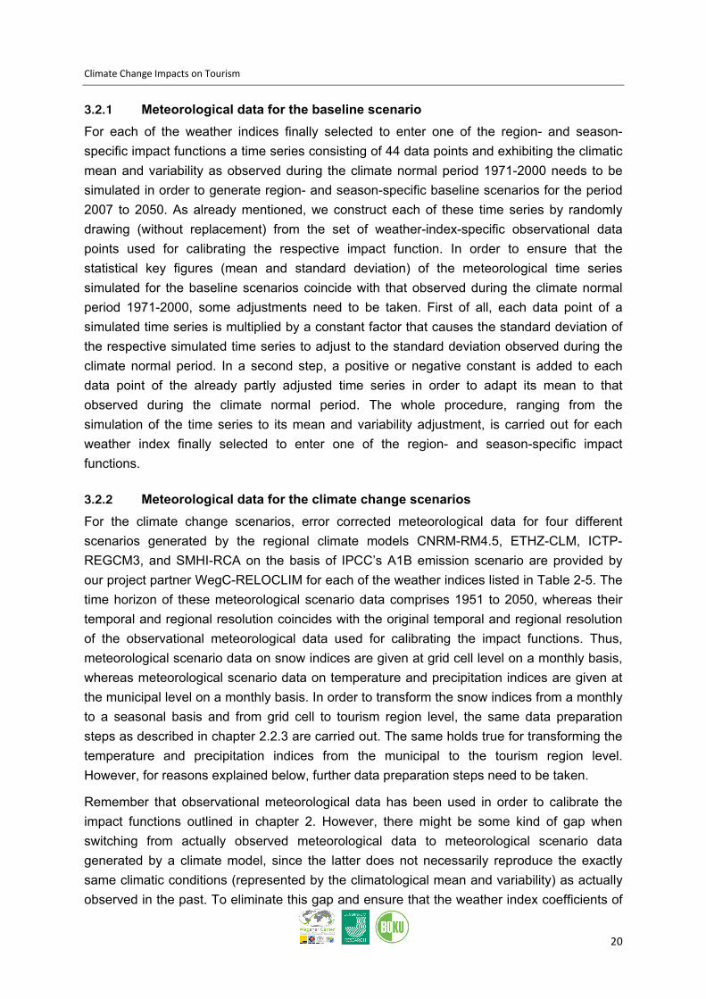
3.2.2 Meteorological data for the climate change scenarios For the climate change scenarios, error corrected meteorological data for four different scenarios generated by the regional climate models CNRM-RM4.5, ETHZ-CLM, ICTP-REGCM3, and SMHI-RCA on the basis of IPCC’s A1B emission scenario are provided by our project partner WegC-RELOCLIM for each of the weather indices listed in Table 2-5. The time horizon of these meteorological scenario data comprises 1951 to 2050, whereas their temporal and regional resolution coincides with the original temporal and regional resolution of the observational meteorological data used for calibrating the impact functions. Thus, meteorological scenario data on snow indices are given at grid cell level on a monthly basis, whereas meteorological scenario data on temperature and precipitation indices are given at the municipal level on a monthly basis. In order to transform the snow indices from a monthly to a seasonal basis and from grid cell to tourism region level, the same data preparation steps as described in chapter 2.2.3 are carried out. The same holds true for transforming the temperature and precipitation indices from the municipal to the tourism region level. However, for reasons explained below, further data preparation steps need to be taken.
Remember that observational meteorological data has been used in order to calibrate the impact functions outlined in chapter 2. However, there might be some kind of gap when switching from actually observed meteorological data to meteorological scenario data generated by a climate model, since the latter does not necessarily reproduce the exactly same climatic conditions (represented by the climatological mean and variability) as actually observed in the past. To eliminate this gap and ensure that the weather index coefficients of
Climate Change Impacts on Tourism
21
the impact functions, which were estimated by using observational data, can be applied to the meteorological scenario data, the latter need some adjustment. Thus, in a first step, each data point of a particular scenario time series encompassing the period 1951 to 2050 is multiplied by a constant factor that causes the time series’ standard deviation during the climate normal period 1971-2000 to coincide with the actually observed one. In a second step, a positive or negative constant is added to each data point of the already partly adjusted time series such that its mean during the climate normal period is adjusted to that of the actually observed data. This adjustment procedure is applied on each of the four scenarios given for those weather indices that are finally selected to enter one of the region- and season-specific impact functions. As an example, Figure 3-1 illustrates this adjustment for scenario data (generated by the climate model CNRM-RM4.5) on weather index Rday10 in the “focus summer” tourism region during May.
Figure 3-1: Adjustment of the scenario data using the example of weather index Rday10 in the “focus summer” tourism region during May
3.3 Results
Having described methods and data applied to quantify the potential impacts of climate change on tourism demand the following subsections outline the resulting outcomes. Besides the separate presentation of the results for the winter season and the summer season, outcomes are also aggregated and outlined for the whole tourism year.
Climate Change Impacts on Tourism
22
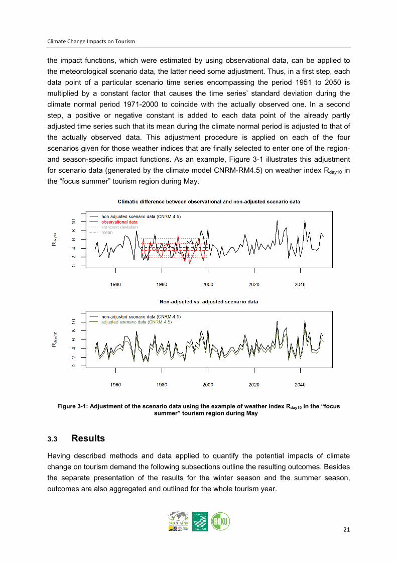
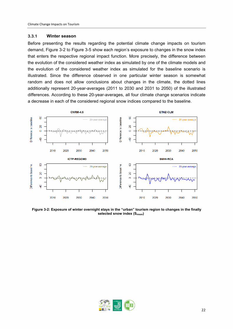
3.3.1 Winter season Before presenting the results regarding the potential climate change impacts on tourism demand, Figure 3-2 to Figure 3-5 show each region’s exposure to changes in the snow index that enters the respective regional impact function. More precisely, the difference between the evolution of the considered weather index as simulated by one of the climate models and the evolution of the considered weather index as simulated for the baseline scenario is illustrated. Since the difference observed in one particular winter season is somewhat random and does not allow conclusions about changes in the climate, the dotted lines additionally represent 20-year-averages (2011 to 2030 and 2031 to 2050) of the illustrated differences. According to these 20-year-averages, all four climate change scenarios indicate a decrease in each of the considered regional snow indices compared to the baseline.
Figure 3-2: Exposure of winter overnight stays in the “urban” tourism region to changes in the finally selected snow index (Smean)
Climate Change Impacts on Tourism
23
Figure 3-3: Exposure of winter overnight stays in the “mixed” tourism region to changes in the finally selected snow index (Smean)
Figure 3-4: Exposure of winter overnight stays in the “focus summer” tourism region to changes in the finally selected snow index (Smean)

Climate Change Impacts on Tourism
24
Figure 3-5: Exposure of winter overnight stays in the “focus winter” tourism region to changes in the finally selected snow index (Smean)
Having illustrated the regions’ exposure to changes in the considered snow index, we now turn to the presentation of the potential climate change impacts on tourism demand as indicated by the results of our analyses. Figure 3-6 shows the outcomes of the first two steps of the procedure that is employed to quantify the potential climate change impacts on tourism demand (see chapter 3.1), namely the regional evolution of winter overnight stays as simulated by the baseline and the four climate change scenarios.
Climate Change Impacts on Tourism
25
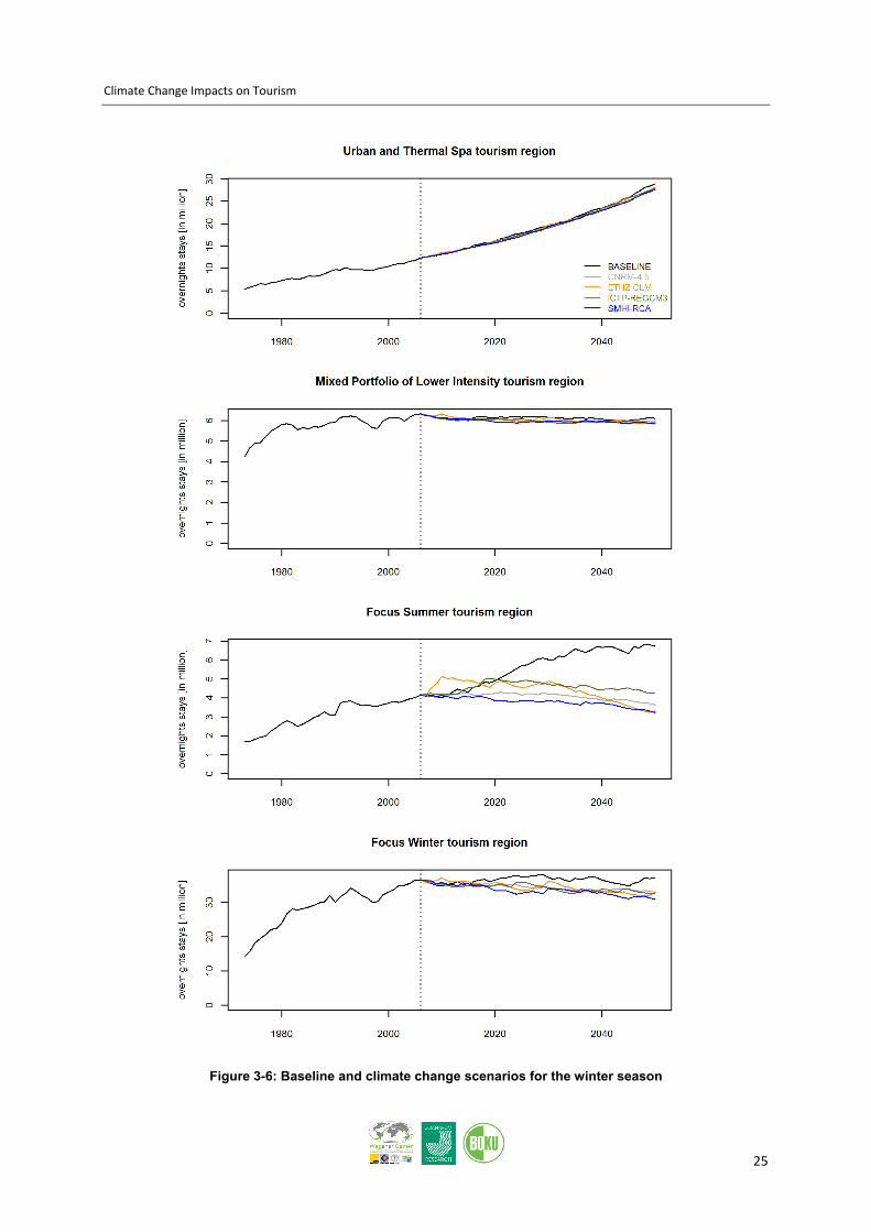
Figure 3-6: Baseline and climate change scenarios for the winter season

Climate Change Impacts on Tourism
26
On the left-hand side of the dotted vertical line, each of the plots in Figure 3-6 outlines the historical evolution of the regional overnight stays as observed for the respective tourism region in the period 1973 to 2006. On the right-hand side of the dotted line, potential evolutions of the overnight stays until 2050 are illustrated. As outlined in chapter 3.1, these were simulated by inserting five different meteorological scenario data sets – representing a baseline scenario and four climate change scenarios – into the calibrated regional impact functions.
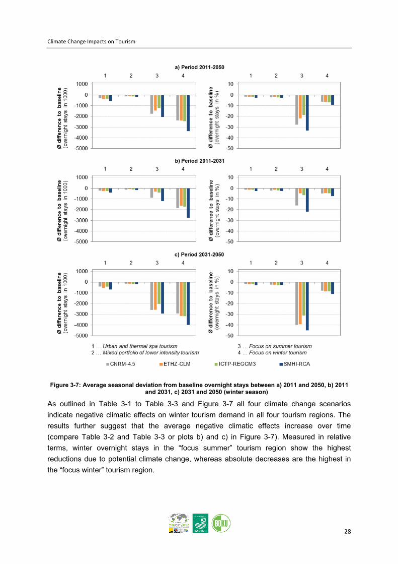
Remember that our primary interest is not the evolution of the overnight stays itself, but the deviation of the climate change scenarios to the baseline scenario, which represents the potential impacts of climate change on overnight stays. As mentioned above, the exposure observed in one particular winter season is somewhat random. The same holds true for the potential impacts, since the exposure forms one of the factors they depend on. Thus, long-term averages are calculated again. Besides the 20-year-averages for the periods 2011 to 2030 and 2031 to 2050, also 40-year-averages that encompass the period 2011 to 2050 are pointed out (see Table 3-1 to Table 3-3 and Figure 3-7).
Table 3-1: Average seasonal deviation from baseline overnight stays between 2011 and 2050 (winter season)
Absolute [in 1.000] Relative [in %]
CNRM ETHZ ICTP SMHI CNRM ETHZ ICTP SMHI
Urban -314 -374 -329 -544 -1.45 -1.69 -1.55 -2.54
Mixed -127 -106 -140 -159 -2.07 -1.72 -2.28 -2.58
Focus Summer -1,741 -1,443 -1,207 -2,057 -27.82 -21.78 -18.71 -33.21
Focus Winter -2,373 -2,375 -2,441 -3,370 -6.40 -6.41 -6.60 -9.11
Table 3-2: Average seasonal deviation from baseline overnight stays between 2011 and 2030 (winter season)
Absolute [in 1.000] Relative [in %]
CNRM ETHZ ICTP SMHI CNRM ETHZ ICTP SMHI
Urban -223 -240 -245 -404 -1.30 -1.38 -1.43 -2.37
Mixed -127 -77 -112 -160 -2.06 -1.24 -1.82 -2.59
Focus Summer -886 -319 -386 -1,178 -16.06 -4.53 -6.54 -21.61
Focus Winter -1,827 -1,627 -1,716 -2,753 -4.88 -4.30 -4.60 -7.34

Climate Change Impacts on Tourism
27
Table 3-3: Average seasonal deviation from baseline overnight stays between 2031 and 2050 (winter season)
Absolute [in 1.000] Relative [in %]
CNRM ETHZ ICTP SMHI CNRM ETHZ ICTP SMHI
Urban -404 -508 -413 -684 -1.61 -1.99 -1.68 -2.72
Mixed -127 -135 -167 -157 -2.08 -2.21 -2.74 -2.58
Focus Summer -2,595 -2,568 -2,027 -2,936 -39.57 -39.03 -30.89 -44.81
Focus Winter -2,919 -3,124 -3,165 -3,987 -7.93 -8.52 -8.60 -10.88
Climate Change Impacts on Tourism
28
Figure 3-7: Average seasonal deviation from baseline overnight stays between a) 2011 and 2050, b) 2011 and 2031, c) 2031 and 2050 (winter season)
As outlined in Table 3-1 to Table 3-3 and Figure 3-7 all four climate change scenarios indicate negative climatic effects on winter tourism demand in all four tourism regions. The results further suggest that the average negative climatic effects increase over time (compare Table 3-2 and Table 3-3 or plots b) and c) in Figure 3-7). Measured in relative terms, winter overnight stays in the “focus summer” tourism region show the highest reductions due to potential climate change, whereas absolute decreases are the highest in the “focus winter” tourism region.

Climate Change Impacts on Tourism
29
3.3.2 Summer season In fact, results regarding the summer season are available on a monthly basis. However, for reasons of clarity, figures and tables relating to these monthly results are outlined in the Appendix. The following presentations, by contrast, refer to the summer season as a whole and represent the aggregated monthly results.
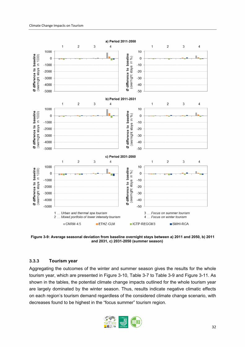
Figure 3-8 outlines the regional evolution of summer overnight stays as simulated by the baseline and the climate change scenarios, whereas Table 3-4 to Table 3-6 as well as Figure 3-9 present the potential impacts of climate change on summer overnight stays. Compared to the winter season, results suggest the extent of the climate change impacts to be smaller (both, in absolute and relative terms). Regarding the impact direction, outcomes are by far less clear than in case of the winter season, as in many cases the direction depends on the regional climate model employed to generate the scenario data used for the simulation.

Climate Change Impacts on Tourism
30
Figure 3-8: Baseline and climate change scenarios for the summer season
Climate Change Impacts on Tourism
31
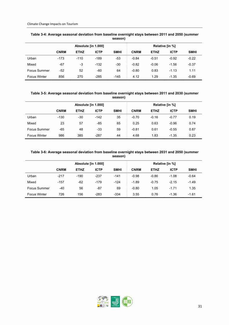
Table 3-4: Average seasonal deviation from baseline overnight stays between 2011 and 2050 (summer season)
Absolute [in 1.000] Relative [in %]
CNRM ETHZ ICTP SMHI CNRM ETHZ ICTP SMHI
Urban -173 -110 -189 -53 -0.84 -0.51 -0.92 -0.22
Mixed -67 -3 -132 -30 -0.82 -0.06 -1.56 -0.37
Focus Summer -52 52 -60 64 -0.80 0.83 -1.13 1.11
Focus Winter 856 270 -285 -145 4.12 1.29 -1.35 -0.69
Table 3-5: Average seasonal deviation from baseline overnight stays between 2011 and 2030 (summer season)
Absolute [in 1.000] Relative [in %]
CNRM ETHZ ICTP SMHI CNRM ETHZ ICTP SMHI
Urban -130 -30 -142 35 -0.70 -0.16 -0.77 0.19
Mixed 23 57 -85 65 0.25 0.63 -0.96 0.74
Focus Summer -65 48 -33 59 -0.81 0.61 -0.55 0.87
Focus Winter 986 385 -287 44 4.68 1.83 -1.35 0.23
Table 3-6: Average seasonal deviation from baseline overnight stays between 2031 and 2050 (summer season)
Absolute [in 1.000] Relative [in %]
CNRM ETHZ ICTP SMHI CNRM ETHZ ICTP SMHI
Urban -217 -190 -237 -141 -0.98 -0.86 -1.08 -0.64
Mixed -157 -62 -179 -124 -1.89 -0.75 -2.15 -1.49
Focus Summer -40 56 -87 69 -0.80 1.05 -1.71 1.35
Focus Winter 726 156 -283 -334 3.55 0.76 -1.36 -1.61
Climate Change Impacts on Tourism
32
Figure 3-9: Average seasonal deviation from baseline overnight stays between a) 2011 and 2050, b) 2011 and 2031, c) 2031-2050 (summer season)
3.3.3 Tourism year Aggregating the outcomes of the winter and summer season gives the results for the whole tourism year, which are presented in Figure 3-10, Table 3-7 to Table 3-9 and Figure 3-11. As shown in the tables, the potential climate change impacts outlined for the whole tourism year are largely dominated by the winter season. Thus, results indicate negative climatic effects on each region’s tourism demand regardless of the considered climate change scenario, with decreases found to be highest in the “focus summer” tourism region.

Climate Change Impacts on Tourism
33
Figure 3-10: Baseline and climate change scenarios for the tourism year

Climate Change Impacts on Tourism
34
Table 3-7: Average annual deviation from baseline overnight stays between 2011 and 2050 (tourism year)
Absolute [in 1.000] Relative [in %]
CNRM ETHZ ICTP SMHI CNRM ETHZ ICTP SMHI
Urban -487 -484 -519 -597 -1.15 -1.11 -1.24 -1.39
Mixed -194 -108 -272 -188 -1.34 -0.75 -1.86 -1.29
Focus Summer -1,793 -1,391 -1,267 -1,993 -14.92 -11.84 -10.64 -16.55
Focus Winter -1,517 -2,105 -2,726 -3,515 -2.63 -3.65 -4.73 -6.10
Table 3-8: Average annual deviation from baseline overnight stays between 2011 and 2030 (tourism year)
Absolute [in 1.000] Relative [in %]
CNRM ETHZ ICTP SMHI CNRM ETHZ ICTP SMHI
Urban -353 -270 -386 -369 -0.99 -0.75 -1.08 -1.03
Mixed -105 -20 -197 -95 -0.70 -0.14 -1.32 -0.63
Focus Summer -951 -271 -419 -1,119 -7.42 -2.23 -3.30 -8.72
Focus Winter -840 -1,242 -2,003 -2,709 -1.43 -2.11 -3.43 -4.63
Table 3-9: Average annual deviation from baseline overnight stays between 2031 and 2050 (tourism year)
Absolute [in 1.000] Relative [in %]
CNRM ETHZ ICTP SMHI CNRM ETHZ ICTP SMHI
Urban -621 -698 -651 -825 -1.32 -1.47 -1.40 -1.75
Mixed -284 -197 -346 -282 -1.97 -1.37 -2.41 -1.96
Focus Summer -2,635 -2,511 -2,115 -2,867 -22.41 -21.45 -17.99 -24.38
Focus Winter -2,193 -2,969 -3,448 -4,321 -3.83 -5.20 -6.02 -7.57

Climate Change Impacts on Tourism
35
Figure 3-11: Average annual deviation from baseline overnight stays between a) 2011 and 2050, b) 2011 and 2031, c) 2031-2050 (tourism year)
3.4 Sensitivity analysis
As mentioned in chapter 3.1, our approach of generating climate baseline scenarios involves some randomness. Thus, within this section the sensitivity of the final results with respect to different simulations of the climate baseline scenario is investigated. For this purpose, simulating a climate baseline scenario for each of the weather indices finally selected to enter one of the region- and season-specific impact functions is repeated 1,000 times, resulting in 1,000 different simulations of the climate baseline scenario per considered weather index. Then, for each considered tourism region and season the three-step-

Climate Change Impacts on Tourism
36
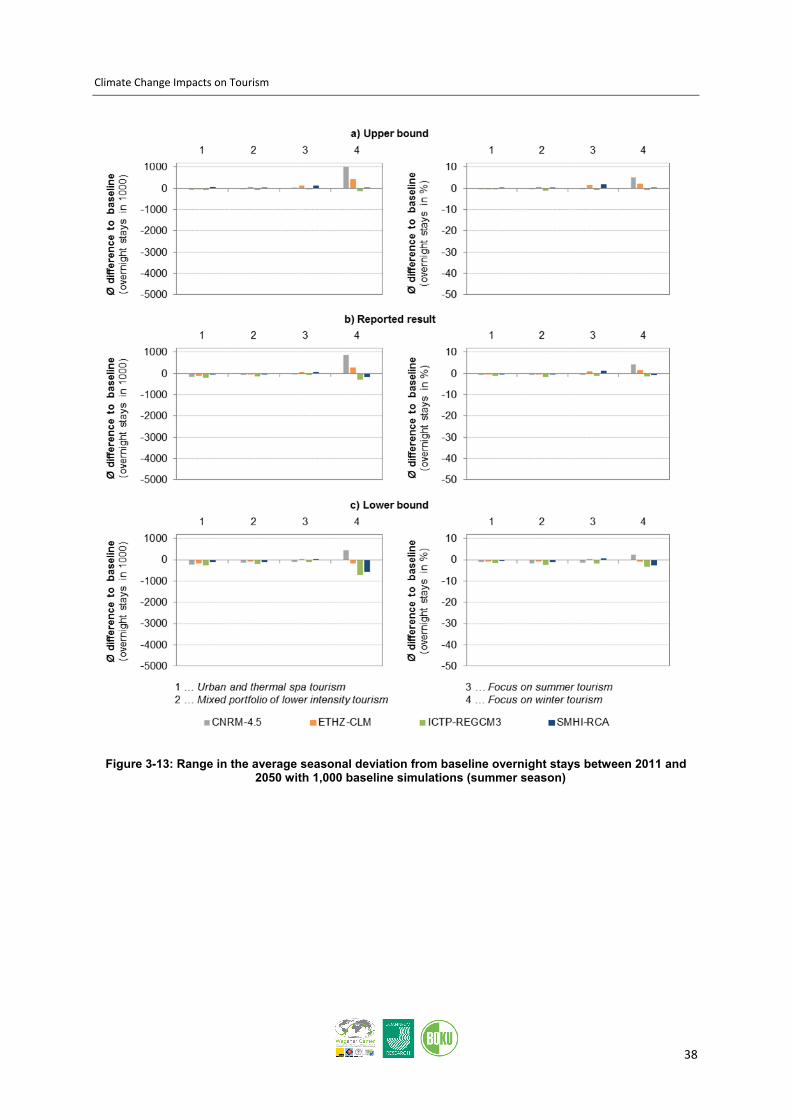
procedure for quantifying the potential impacts of climate change on tourism demand as described in chapter 3.1 is carried out 1,000 times, using each time another simulation of the climate baseline scenario. This results in 1,000 different estimations of the potential impacts of climate change on tourism demand per considered tourism region and season. Figure 3-12 (winter season), Figure 3-13 (summer season) and Figure 3-14 (tourism year) illustrate the range in the resulting quantified potential climate change impacts on tourism demand by reporting for each considered tourism region and each applied climate change scenario the upper (a) and lower (c) bound of the 1,000 estimations on the average deviation from baseline overnight stays between 2011 and 2050. For reasons of comparison, the result reported in chapter 3.3, which lies somewhere between the upper and lower bound, is illustrated as well (b).

Climate Change Impacts on Tourism
37
Figure 3-12: Range in the average seasonal deviation from baseline overnight stays between 2011 and 2050 with 1,000 baseline simulations (winter season)
Climate Change Impacts on Tourism
38
Figure 3-13: Range in the average seasonal deviation from baseline overnight stays between 2011 and 2050 with 1,000 baseline simulations (summer season)

Climate Change Impacts on Tourism
39
Figure 3-14: Range in the average annual deviation from baseline overnight stays between 2011 and 2050 with 1,000 baseline simulations (tourism year)

Climate Change Impacts on Tourism
40
4 References Breusch, T. S. (1978), Testing for autocorrelation in dynamic linear models, Australian
Economic Papers, 17(31), 334–355.
Breusch, T. and A. Pagan (1979), A simple test for heteroscedasticity and random coefficient variation, Econometrica, 47(5), 1287–1294.
Godfrey, L. G. (1978), Testing against general autoregressive and moving average error models when the regressors include lagged dependent variables, Econometrica, 46(6), 1293–1302.
Jarque, C. M. and A. K. Bera (1980), Efficient tests for normality, homoscedasticity and serial independence of regression residuals, Economics Letters, 6(3), 255–259.
JOANNEUM RESEARCH (2008), Austrian ski resort database, Graz: Institute of Technology and Regional Policy.
Köberl, J., Prettenthaler, F., Töglhofer, C. (2010), Adaptation to Climate Change in Austria (ADAPT.AT) – Identification of Tourism Types, Working Paper No. 11/2010 in The Economics of Weather and Climate Risks (EWCR) Working Paper Series.
Lilliefors, H. (1969), On the Kolmogorov-Smirnov test for the exponential distribution with mean unknown, Journal of the American Statistical Association, 64, 387–389.
Ramsey, J. B. (1969), Tests for specification errors in classical linear least squares regression analysis, Journal of the Royal Statistical Society, 31(2), 350–371.
Statistics Austria (2007), Overnights stays in Austrian municipalities on a seasonal basis from 2000 to 2005, Vienna.
Statistics Austria (2008), Overnight stays in Austrian municipalities in the winter season 1973 to 2007, Vienna.
Statistics Austria (2010a), Overnight stays in hotels and similar establishments in Austrian districts on a monthly basis from 1977 to 2009, Vienna.
Statistics Austria (2010b), Overnight stays in Austrian NUTS 3 regions on a seasonal basis from 1990 to 2009, Vienna.
Song, H., Witt, S.F. (2000), Tourism demand modelling and forecasting: Modern econometric approaches, Oxford: Pergamon.
Töglhofer, C., Prettenthaler, F. (2009), Estimating Climatic and Economic Impacts on Tourism Demand in Austrian Ski Areas, Working Paper No. 6/2009 in The Economics of Weather and Climate Risks (EWCR) Working Paper Series.

Climate Change Impacts on Tourism
41
Töglhofer, C. (2011), From climate variability to weather risk: The impact of snow conditions on tourism demand in Austrian ski areas, Doctoral Thesis to be awarded the degree of Doctor of Social and Economic Sciences at the University of Graz, Graz.
Verbeek, M. (2008), A guide to modern econometrics, 3rd edition, Wiley, Chichester/UK.
Witt, S.F. (1980), An abstract mode-abstract (destination) node model of foreign holiday demand (UK residents), Applied Economics, 12(2), 163-180.
ZAMG (Central Institute for Meteorology and Geodynamics) (2009), Regionalized data (1x1 km grid cells) for temperature, precipitation and snow 1948-2006, Vienna.

Climate Change Impacts on Tourism
42
5 Appendix Table 5-1: Weather sensitivity of overnights stays in May depending on the chosen weather index
Tmean Rday1 Rday10 Rsum
Urban -2.00** -0.37 -0.28 0.00
Mixed -1.07 0.13 -0.62 -0.10
Focus Summer -0.33 -2.32 -2.65 -3.63*
Focus Winter -2.33 -1.09 -1.89 -1.50
Table 5-2: Weather sensitivity of overnights stays in June depending on the chosen weather index
Tmean Rday1 Rday10 Rsum
Urban -1.10 2.20** 0.68 1.13
Mixed 0.17 1.01 1.37 1.05
Focus Summer 1.01 -0.29 -0.11 -0.42
Focus Winter 1.43 1.18 2.14 1.75
Table 5-3: Weather sensitivity of overnights stays in July depending on the chosen weather index
Tmean Rday1 Rday10 Rsum
Urban -0.11 0.33 -1.09 -1.02
Mixed 0.10 0.23 0.33 0.06
Focus Summer 0.58 -0.19 -0.44 -0.49
Focus Winter -0.83 1.30 0.56 0.51
Table 5-4: Weather sensitivity of overnights stays in August depending on the chosen weather index
Tmean Rday1 Rday10 Rsum
Urban 0.15 -0.58 -0.58 -0.40
Mixed 1.07 -1.7** -2.01*** -1.78**
Focus Summer 1.96* -1.88* -1.61 -1.76
Focus Winter 0.95 -1.80* -2.99*** -2.37**
Table 5-5: Weather sensitivity of overnights stays in September depending on the chosen weather index
Tmean Rday1 Rday10 Rsum
Urban 0.71 -0.78 -1.06 -0.72
Mixed 1.10 -1.35** -1.06 -1.30*
Focus Summer - -2.04** -1.09 -1.20
Focus Winter 0.72 -1.39 -1.44 -1.30

Climate Change Impacts on Tourism
43
Table 5-6: Weather sensitivity of overnights stays in October depending on the chosen weather index
Tmean Rday1 Rday10 Rsum
Urban -0.73 -0.96 -0.74 -0.82
Mixed 1.19 -2.13*** -2.25*** -2.22***
Focus Summer 0.19 -2.25* -2.30* -2.41*
Focus Winter 1.60 -1.17 -0.75 -0.91
Figure 5-1: Exposure of May overnight stays in the “urban” tourism region to changes in the finally selected weather index (Tmean)
Figure 5-2: Exposure of May overnight stays in the “mixed” tourism region to changes in the finally selected weather index (Tmean)
Climate Change Impacts on Tourism
44
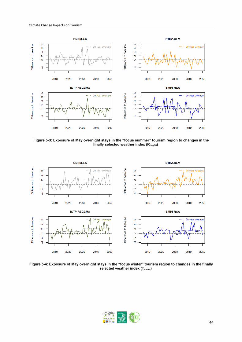
Figure 5-3: Exposure of May overnight stays in the “focus summer” tourism region to changes in the finally selected weather index (Rday10)
Figure 5-4: Exposure of May overnight stays in the “focus winter” tourism region to changes in the finally selected weather index (Tmean)

Climate Change Impacts on Tourism
45
Figure 5-5: Exposure of June overnight stays in the “urban” tourism region to changes in the finally selected weather index (Rday1)
Figure 5-6: Exposure of June overnight stays in the “mixed” tourism region to changes in the finally selected weather index (Rday10)
Climate Change Impacts on Tourism
46
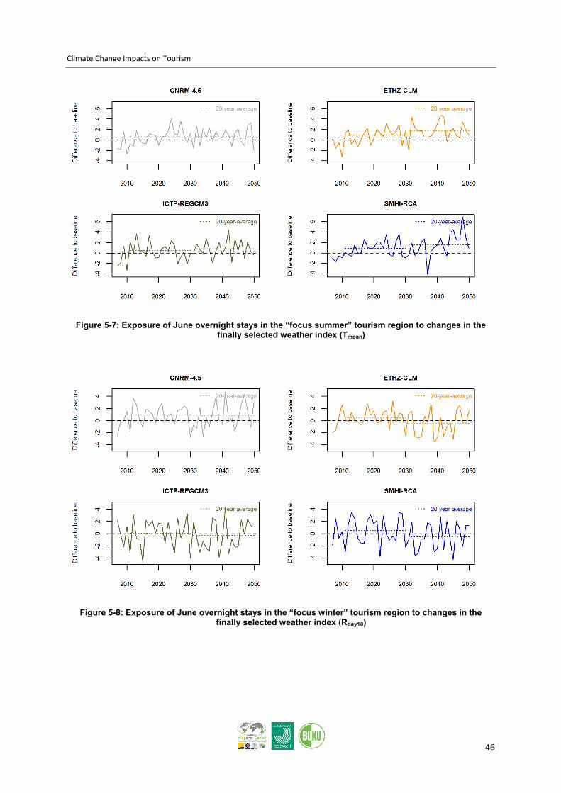
Figure 5-7: Exposure of June overnight stays in the “focus summer” tourism region to changes in the finally selected weather index (Tmean)
Figure 5-8: Exposure of June overnight stays in the “focus winter” tourism region to changes in the finally selected weather index (Rday10)
Climate Change Impacts on Tourism
47
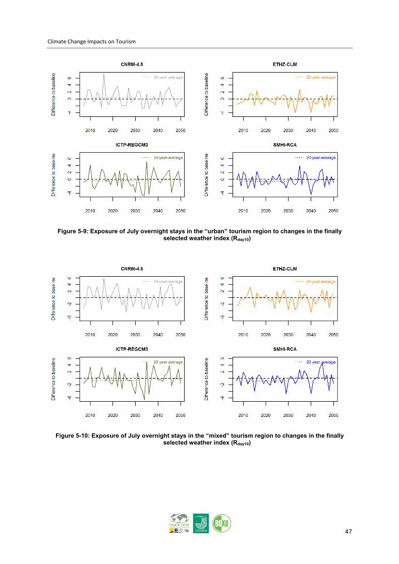
Figure 5-9: Exposure of July overnight stays in the “urban” tourism region to changes in the finally selected weather index (Rday10)
Figure 5-10: Exposure of July overnight stays in the “mixed” tourism region to changes in the finally selected weather index (Rday10)

Climate Change Impacts on Tourism
48
Figure 5-11: Exposure of July overnight stays in the “focus summer” tourism region to changes in the finally selected weather index (Tmean)
Figure 5-12: Exposure of July overnight stays in the “focus winter” tourism region to changes in the finally selected weather index (Rday1)

Climate Change Impacts on Tourism
49
Figure 5-13: Exposure of August overnight stays in the “urban” tourism region to changes in the finally selected weather index (Rday1)
Figure 5-14: Exposure of August overnight stays in the “mixed” tourism region to changes in the finally selected weather index (Rday10)
Climate Change Impacts on Tourism
50
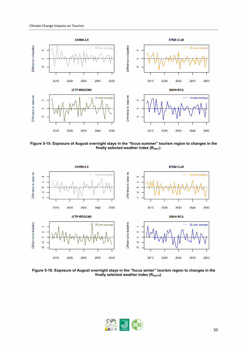
Figure 5-15: Exposure of August overnight stays in the “focus summer” tourism region to changes in the finally selected weather index (Rday1)
Figure 5-16: Exposure of August overnight stays in the “focus winter” tourism region to changes in the finally selected weather index (Rday10)
Climate Change Impacts on Tourism
51
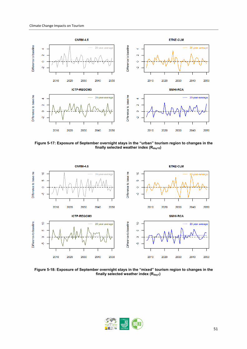
Figure 5-17: Exposure of September overnight stays in the “urban” tourism region to changes in the finally selected weather index (Rday10)
Figure 5-18: Exposure of September overnight stays in the “mixed” tourism region to changes in the finally selected weather index (Rday1)

Climate Change Impacts on Tourism
52
Figure 5-19: Exposure of September overnight stays in the “focus summer” tourism region to changes in the finally selected weather index (Rsum)
Figure 5-20: Exposure of September overnight stays in the “focus winter” tourism region to changes in the finally selected weather index (Rday10)
Climate Change Impacts on Tourism
53
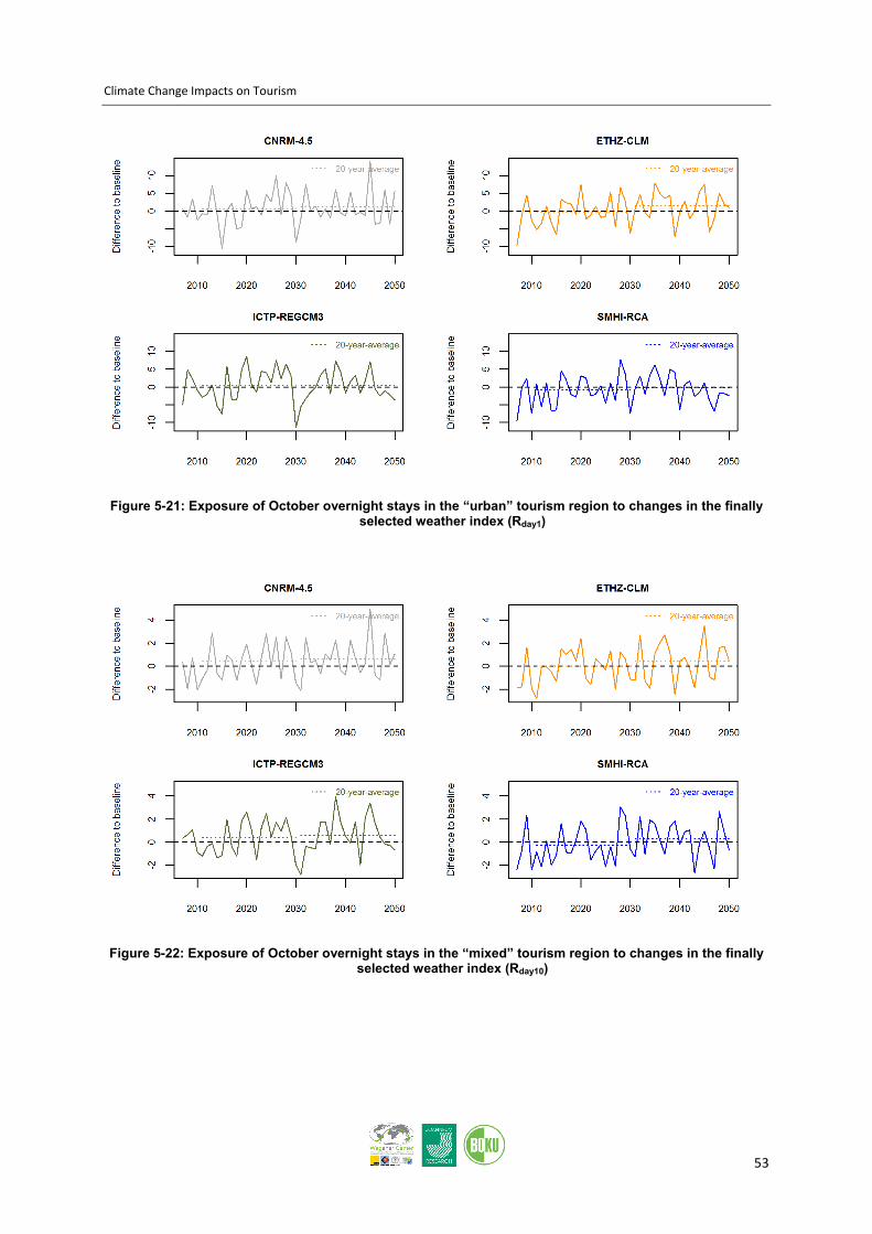
Figure 5-21: Exposure of October overnight stays in the “urban” tourism region to changes in the finally selected weather index (Rday1)
Figure 5-22: Exposure of October overnight stays in the “mixed” tourism region to changes in the finally selected weather index (Rday10)

Climate Change Impacts on Tourism
54
Figure 5-23: Exposure of October overnight stays in the “focus summer” tourism region to changes in the finally selected weather index (Rsum)
Figure 5-24: Exposure of October overnight stays in the “focus winter” tourism region to changes in the finally selected weather index (Tmean)

Climate Change Impacts on Tourism
55
Figure 5-25: Baseline and climate change scenarios for month May

Climate Change Impacts on Tourism
56
Table 5-7: Difference to the baseline scenario regarding the average monthly overnight stays (May) between 2011 and 2050
Absolute [in 1.000] Relative [in %]
CNRM ETHZ ICTP SMHI CNRM ETHZ ICTP SMHI
Urban b) -94 -79 -117 -67 -2.25 -1.91 -2.94 -1.65
Mixed a,b) -12 -10 -13 -9 -0.78 -0.66 -0.92 -0.61
Focus Summer -14 10 10 -8 -1.11 0.98 0.95 -0.55
Focus Winter a,b) -42 -43 -52 -31 -2.20 -2.24 -2.70 -1.62 a) The weather coefficient of the underlying model is not significant (at a 10% level) b) The weather coefficient of the underlying model shows a not expected sign
Table 5-8: Difference to the baseline scenario regarding the average monthly overnight stays (May) between 2011 and 2030
Absolute [in 1.000] Relative [in %]
CNRM ETHZ ICTP SMHI CNRM ETHZ ICTP SMHI
Urban b) -49 -25 -59 -41 -1.46 -0.78 -1.87 -1.26
Mixed a,b) -7 -4 -8 -7 -0.49 -0.29 -0.63 -0.50
Focus Summer -25 -6 -6 -24 -1.98 -0.41 -0.47 -1.96
Focus Winter a,b) -14 -15 -27 -17 -0.71 -0.77 -1.42 -0.89 a) The weather coefficient of the underlying model is not significant (at a 10% level) b) The weather coefficient of the underlying model shows a not expected sign
Table 5-9: Difference to the baseline scenario regarding the average monthly overnight stays (May) between 2031 and 2050
Absolute [in 1.000] Relative [in %]
CNRM ETHZ ICTP SMHI CNRM ETHZ ICTP SMHI
Urban b) -139 -132 -175 -93 -3.04 -3.05 -4.01 -2.05
Mixed a,b) -16 -15 -18 -11 -1.06 -1.02 -1.21 -0.71
Focus Summer -3 27 27 9 -0.25 2.36 2.36 0.86
Focus Winter a,b) -71 -71 -77 -45 -3.70 -3.71 -3.98 -2.34 a) The weather coefficient of the underlying model is not significant (at a 10% level) b) The weather coefficient of the underlying model shows a not expected sign

Climate Change Impacts on Tourism
57
Figure 5-26: Baseline and climate change scenarios for month June
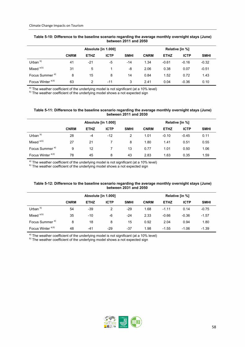
Climate Change Impacts on Tourism
58
Table 5-10: Difference to the baseline scenario regarding the average monthly overnight stays (June) between 2011 and 2050
Absolute [in 1.000] Relative [in %]
CNRM ETHZ ICTP SMHI CNRM ETHZ ICTP SMHI
Urban b) 41 -21 -5 -14 1.34 -0.61 -0.16 -0.32
Mixed a,b) 31 5 1 -8 2.06 0.38 0.07 -0.51
Focus Summer a) 8 15 8 14 0.84 1.52 0.72 1.43
Focus Winter a,b) 63 2 -11 3 2.41 0.04 -0.36 0.10 a) The weather coefficient of the underlying model is not significant (at a 10% level) b) The weather coefficient of the underlying model shows a not expected sign
Table 5-11: Difference to the baseline scenario regarding the average monthly overnight stays (June) between 2011 and 2030
Absolute [in 1.000] Relative [in %]
CNRM ETHZ ICTP SMHI CNRM ETHZ ICTP SMHI
Urban b) 28 -4 -12 2 1.01 -0.10 -0.45 0.11
Mixed a,b) 27 21 7 8 1.80 1.41 0.51 0.55
Focus Summer a) 9 12 7 13 0.77 1.01 0.50 1.06
Focus Winter a,b) 78 45 8 43 2.83 1.63 0.35 1.59 a) The weather coefficient of the underlying model is not significant (at a 10% level) b) The weather coefficient of the underlying model shows a not expected sign
Table 5-12: Difference to the baseline scenario regarding the average monthly overnight stays (June) between 2031 and 2050
Absolute [in 1.000] Relative [in %]
CNRM ETHZ ICTP SMHI CNRM ETHZ ICTP SMHI
Urban b) 54 -39 2 -29 1.68 -1.11 0.14 -0.75
Mixed a,b) 35 -10 -6 -24 2.33 -0.66 -0.36 -1.57
Focus Summer a) 8 18 8 15 0.92 2.04 0.94 1.80
Focus Winter a,b) 48 -41 -29 -37 1.98 -1.55 -1.06 -1.39 a) The weather coefficient of the underlying model is not significant (at a 10% level) b) The weather coefficient of the underlying model shows a not expected sign

Climate Change Impacts on Tourism
59
Figure 5-27: Baseline and climate change scenarios for month July
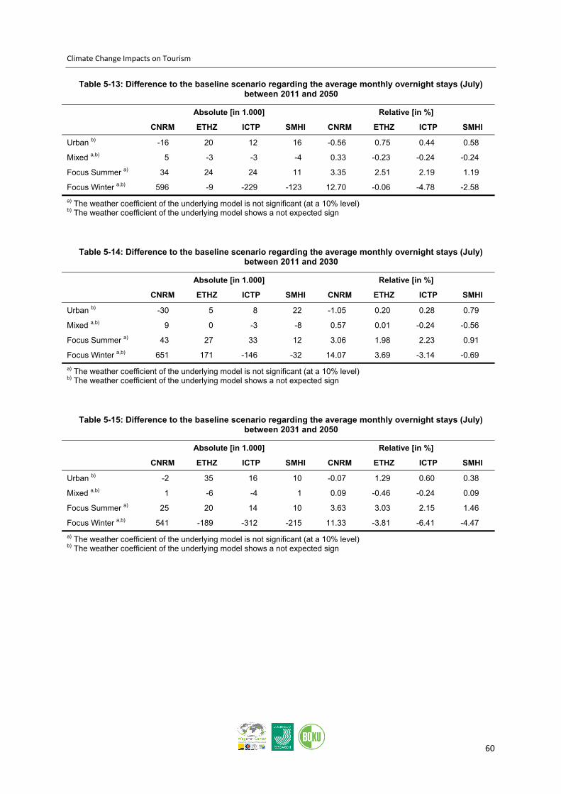
Climate Change Impacts on Tourism
60
Table 5-13: Difference to the baseline scenario regarding the average monthly overnight stays (July) between 2011 and 2050
Absolute [in 1.000] Relative [in %]
CNRM ETHZ ICTP SMHI CNRM ETHZ ICTP SMHI
Urban b) -16 20 12 16 -0.56 0.75 0.44 0.58
Mixed a,b) 5 -3 -3 -4 0.33 -0.23 -0.24 -0.24
Focus Summer a) 34 24 24 11 3.35 2.51 2.19 1.19
Focus Winter a,b) 596 -9 -229 -123 12.70 -0.06 -4.78 -2.58 a) The weather coefficient of the underlying model is not significant (at a 10% level) b) The weather coefficient of the underlying model shows a not expected sign
Table 5-14: Difference to the baseline scenario regarding the average monthly overnight stays (July) between 2011 and 2030
Absolute [in 1.000] Relative [in %]
CNRM ETHZ ICTP SMHI CNRM ETHZ ICTP SMHI
Urban b) -30 5 8 22 -1.05 0.20 0.28 0.79
Mixed a,b) 9 0 -3 -8 0.57 0.01 -0.24 -0.56
Focus Summer a) 43 27 33 12 3.06 1.98 2.23 0.91
Focus Winter a,b) 651 171 -146 -32 14.07 3.69 -3.14 -0.69 a) The weather coefficient of the underlying model is not significant (at a 10% level) b) The weather coefficient of the underlying model shows a not expected sign
Table 5-15: Difference to the baseline scenario regarding the average monthly overnight stays (July) between 2031 and 2050
Absolute [in 1.000] Relative [in %]
CNRM ETHZ ICTP SMHI CNRM ETHZ ICTP SMHI
Urban b) -2 35 16 10 -0.07 1.29 0.60 0.38
Mixed a,b) 1 -6 -4 1 0.09 -0.46 -0.24 0.09
Focus Summer a) 25 20 14 10 3.63 3.03 2.15 1.46
Focus Winter a,b) 541 -189 -312 -215 11.33 -3.81 -6.41 -4.47 a) The weather coefficient of the underlying model is not significant (at a 10% level) b) The weather coefficient of the underlying model shows a not expected sign
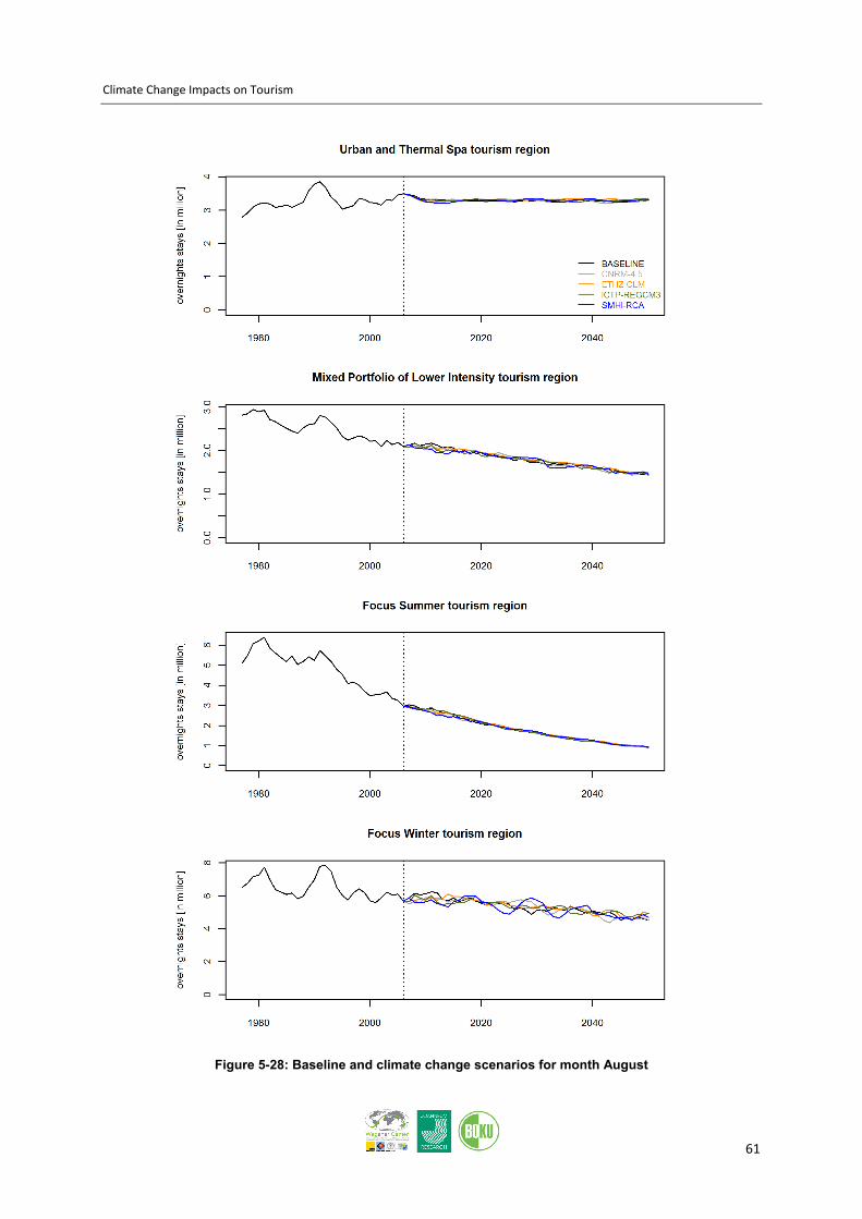
Climate Change Impacts on Tourism
61
Figure 5-28: Baseline and climate change scenarios for month August

Climate Change Impacts on Tourism
62
Table 5-16: Difference to the baseline scenario regarding the average monthly overnight stays (August) between 2011 and 2050
Absolute [in 1.000] Relative [in %]
CNRM ETHZ ICTP SMHI CNRM ETHZ ICTP SMHI
Urban b) -3 24 12 -3 -0.10 0.75 0.36 -0.09
Mixed -6 19 -15 -16 -0.38 1.16 -0.73 -0.77
Focus Summer -30 29 1 -7 -1.56 2.04 -0.24 0.18
Focus Winter 14 77 23 -18 0.31 1.61 0.67 -0.12 a) The weather coefficient of the underlying model is not significant (at a 10% level) b) The weather coefficient of the underlying model shows a not expected sign
Table 5-17: Difference to the baseline scenario regarding the average monthly overnight stays (August) between 2011 and 2030
Absolute [in 1.000] Relative [in %]
CNRM ETHZ ICTP SMHI CNRM ETHZ ICTP SMHI
Urban b) 17 16 12 -3 0.52 0.50 0.36 -0.09
Mixed 14 10 -23 -18 0.90 0.61 -1.08 -0.66
Focus Summer -41 22 18 -30 -1.55 1.18 0.62 -0.83
Focus Winter 121 57 -33 -22 2.46 1.17 -0.39 -0.05 a) The weather coefficient of the underlying model is not significant (at a 10% level) b) The weather coefficient of the underlying model shows a not expected sign
Table 5-18: Difference to the baseline scenario regarding the average monthly overnight stays (August) between 2031 and 2050
Absolute [in 1.000] Relative [in %]
CNRM ETHZ ICTP SMHI CNRM ETHZ ICTP SMHI
Urban b) -23 33 12 -3 -0.71 0.99 0.37 -0.09
Mixed -27 27 -7 -15 -1.65 1.71 -0.38 -0.87
Focus Summer -19 35 -16 15 -1.57 2.90 -1.09 1.18
Focus Winter -94 97 78 -15 -1.83 2.05 1.73 -0.20 a) The weather coefficient of the underlying model is not significant (at a 10% level) b) The weather coefficient of the underlying model shows a not expected sign

Climate Change Impacts on Tourism
63
Figure 5-29: Baseline and climate change scenarios for month September
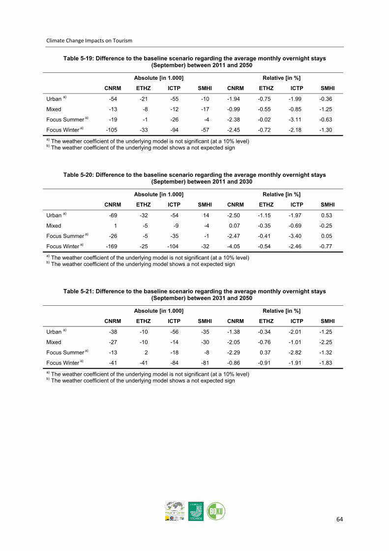
Climate Change Impacts on Tourism
64
Table 5-19: Difference to the baseline scenario regarding the average monthly overnight stays (September) between 2011 and 2050
Absolute [in 1.000] Relative [in %]
CNRM ETHZ ICTP SMHI CNRM ETHZ ICTP SMHI
Urban a) -54 -21 -55 -10 -1.94 -0.75 -1.99 -0.36
Mixed -13 -8 -12 -17 -0.99 -0.55 -0.85 -1.25
Focus Summer a) -19 -1 -26 -4 -2.38 -0.02 -3.11 -0.63
Focus Winter a) -105 -33 -94 -57 -2.45 -0.72 -2.18 -1.30 a) The weather coefficient of the underlying model is not significant (at a 10% level) b) The weather coefficient of the underlying model shows a not expected sign
Table 5-20: Difference to the baseline scenario regarding the average monthly overnight stays (September) between 2011 and 2030
Absolute [in 1.000] Relative [in %]
CNRM ETHZ ICTP SMHI CNRM ETHZ ICTP SMHI
Urban a) -69 -32 -54 14 -2.50 -1.15 -1.97 0.53
Mixed 1 -5 -9 -4 0.07 -0.35 -0.69 -0.25
Focus Summer a) -26 -5 -35 -1 -2.47 -0.41 -3.40 0.05
Focus Winter a) -169 -25 -104 -32 -4.05 -0.54 -2.46 -0.77 a) The weather coefficient of the underlying model is not significant (at a 10% level) b) The weather coefficient of the underlying model shows a not expected sign
Table 5-21: Difference to the baseline scenario regarding the average monthly overnight stays (September) between 2031 and 2050
Absolute [in 1.000] Relative [in %]
CNRM ETHZ ICTP SMHI CNRM ETHZ ICTP SMHI
Urban a) -38 -10 -56 -35 -1.38 -0.34 -2.01 -1.25
Mixed -27 -10 -14 -30 -2.05 -0.76 -1.01 -2.25
Focus Summer a) -13 2 -18 -8 -2.29 0.37 -2.82 -1.32
Focus Winter a) -41 -41 -84 -81 -0.86 -0.91 -1.91 -1.83 a) The weather coefficient of the underlying model is not significant (at a 10% level) b) The weather coefficient of the underlying model shows a not expected sign

Climate Change Impacts on Tourism
65
Figure 5-30: Baseline and climate change scenarios for month October

Climate Change Impacts on Tourism
66
Table 5-22: Difference to the baseline scenario regarding the average monthly overnight stays (October) between 2011 and 2050
Absolute [in 1.000] Relative [in %]
CNRM ETHZ ICTP SMHI CNRM ETHZ ICTP SMHI
Urban a,b) -48 -34 -36 26 -0.96 -0.53 -0.71 0.70
Mixed -72 -7 -89 24 -5.86 -0.36 -7.26 2.20
Focus Summer -32 -25 -76 58 -4.22 -3.25 -10.28 8.03
Focus Winter a) 331 276 78 82 15.45 12.84 3.66 3.87 a) The weather coefficient of the underlying model is not significant (at a 10% level) b) The weather coefficient of the underlying model shows a not expected sign
Table 5-23: Difference to the baseline scenario regarding the average monthly overnight stays (October) between 2011 and 2030
Absolute [in 1.000] Relative [in %]
CNRM ETHZ ICTP SMHI CNRM ETHZ ICTP SMHI
Urban a,b) -28 9 -36 41 -0.62 0.43 -0.79 1.37
Mixed -22 34 -48 93 -1.66 3.17 -3.84 8.06
Focus Summer -26 -3 -50 88 -3.30 -0.23 -6.74 12.28
Focus Winter a) 319 152 15 104 15.00 7.10 0.81 5.01 a) The weather coefficient of the underlying model is not significant (at a 10% level) b) The weather coefficient of the underlying model shows a not expected sign
Table 5-24: Difference to the baseline scenario regarding the average monthly overnight stays (October) between 2031 and 2050
Absolute [in 1.000] Relative [in %]
CNRM ETHZ ICTP SMHI CNRM ETHZ ICTP SMHI
Urban a,b) -68 -77 -36 10 -1.30 -1.50 -0.62 0.04
Mixed -123 -48 -131 -45 -10.06 -3.89 -10.68 -3.67
Focus Summer -38 -46 -102 27 -5.14 -6.27 -13.82 3.78
Focus Winter a) 343 401 140 59 15.89 18.58 6.51 2.74 a) The weather coefficient of the underlying model is not significant (at a 10% level) b) The weather coefficient of the underlying model shows a not expected sign
Related Documents