The Use of Central Tendency Measures from an Operational Short Lead-time Hydrologic Ensemble Forecast System for Real-time Forecasts Thomas E Adams, III Dissertation submitted to the Faculty of the Virginia Polytechnic Institute and State University in partial fulfillment of the requirements for the degree of Doctor of Philosophy in Civil Engineering Randel L. Dymond, Chair Kevin J. McGuire Andrew W. Ellis Mark A. Widdowson May 8, 2018 Blacksburg, Virginia Keywords: Hydrology, Forecasting, Precipitation, Uncertainty, Prediction, Modeling Copyright 2018, Thomas E Adams, III

Welcome message from author
This document is posted to help you gain knowledge. Please leave a comment to let me know what you think about it! Share it to your friends and learn new things together.
Transcript
The Use of Central Tendency Measures from an Operational Short
Lead-time Hydrologic Ensemble Forecast System for Real-time
Forecasts
Thomas E Adams, III
Dissertation submitted to the Faculty of the
Virginia Polytechnic Institute and State University
in partial fulfillment of the requirements for the degree of
Doctor of Philosophy
in
Civil Engineering
Randel L. Dymond, Chair
Kevin J. McGuire
Andrew W. Ellis
Mark A. Widdowson
May 8, 2018
Blacksburg, Virginia
Keywords: Hydrology, Forecasting, Precipitation, Uncertainty, Prediction, Modeling
Copyright 2018, Thomas E Adams, III

The Use of Central Tendency Measures from an Operational Short
Lead-time Hydrologic Ensemble Forecast System for Real-time
Forecasts
Thomas E Adams, III
(ABSTRACT)
A principal factor contributing to hydrologic prediction uncertainty is modeling error intro-
duced by the measurement and prediction of precipitation. The research presented demon-
strates the necessity for using probabilistic methods to quantify hydrologic forecast uncer-
tainty due to the magnitude of precipitation errors. Significant improvements have been
made in precipitation estimation that have lead to greatly improved hydrologic simulations.
However, advancements in the prediction of future precipitation have been marginal. This
research shows that gains in forecasted precipitation accuracy have not significantly improved
hydrologic forecasting accuracy. The use of forecasted precipitation, referred to as quantita-
tive precipitation forecast (QPF), in hydrologic forecasting remains commonplace. Non-zero
QPF is shown to improve hydrologic forecasts, but QPF duration should be limited to 6
to 12 hours for flood forecasting, particularly for fast responding watersheds. Probabilistic
hydrologic forecasting captures hydrologic forecast error introduced by QPF for all forecast
durations. However, public acceptance of probabilistic hydrologic forecasts is problematic.
Central tendency measures from a probabilistic hydrologic forecast, such as the ensemble
median or mean, have the appearance of a single-valued deterministic forecast. The research
presented shows that hydrologic ensemble median and mean forecasts of river stage have
smaller forecast errors than current operational methods with forecast lead-time beginning
at 36-hours for fast response basins. Overall, hydrologic ensemble median and mean forecasts
display smaller forecast error than current operational forecasts.
The Use of Central Tendency Measures from an Operational Short
Lead-time Hydrologic Ensemble Forecast System for Real-time
Forecasts
Thomas E Adams, III
(GENERAL AUDIENCE ABSTRACT)
Flood forecasting is uncertain, in part, because of errors in measuring precipitation and
predicting the location and amount of precipitation accumulation in the future. Because of
this, the public and other end-users of flood forecasts should understand the uncertainties
inherent in forecasts. But, there is reluctance by many to accept forecasts that explicitly
convey flood forecast uncertainty, such as, ”there is a 67% chance your house will be flooded”.
Instead, most prefer ”your house will not be flooded” or something like ”flood levels will
reach 0.5 feet in your house”. We hope the latter does not happen, but due to forecast
uncertainties, explicit statements such as ”flood levels will reach 0.5 feet in your house”
will be wrong. If by chance, flood levels do exactly reach 0.5 feet, that will have been a
lucky forecast, very likely involving some skill, but the flood level could have reached 0.43
or 0.72 feet as well. This research presents a flood forecasting method that improves on
traditional methods by directly incorporating uncertainty information into flood forecasts
that still appear like forecasts people are familiar and comfortable with and understandable
by them.

Acknowledgements
I must recognize the most influential men in my life: my father, Lt. Col. Thomas E. Adams,
Jr. (U.S. Army, Retired), my father-in-law, CMDR, Dr. James F. Phelan, PhD (U.S. Navy,
Retired), Dr. Joseph C. Pitt, PhD who all helped me to become a better person; any and
all failings are my own. I am very indebted to my PhD Advisor, Dr. Randel L. Dymond,
PhD for helping me through the past several years to finally bring my PhD to a conclusion.
I am grateful to my other PhD committee members for their time and feedback.
I am, of course, very grateful to my wife, Dr. Anne L. Phelan-Adams, MD for sticking with
me through life.
It is with honor that I dedicate this work to Dr. G.V. Loganathan, PhD – friend, colleague,
and teacher, whose life was cut short horrifically. . .
From Homer Il. XIV, 200 [101]:
For I am going to see the limits of fertile earth, Okeanos begetter of gods and
mother Tethys. . .
Data do not give up their secrets easily. They must be tortured to confess.
Jeff Hopper, Bell Labs. . .
iv
Contents
List of Figures ix
List of Tables xix
1 Introduction 1
1.1 Nature of the Problem . . . . . . . . . . . . . . . . . . . . . . . . . . . . . . 1
1.2 Dissertation Objectives . . . . . . . . . . . . . . . . . . . . . . . . . . . . . . 2
1.3 Research Approach . . . . . . . . . . . . . . . . . . . . . . . . . . . . . . . . 3
2 Literature Review 5
2.1 Precipitation variability . . . . . . . . . . . . . . . . . . . . . . . . . . . . . 10
2.1.1 Observed precipitation variability . . . . . . . . . . . . . . . . . . . . 11
2.1.2 Forecast precipitation variability . . . . . . . . . . . . . . . . . . . . . 18
2.2 Ensemble Hydrologic Forecasting . . . . . . . . . . . . . . . . . . . . . . . . 21
3 Hydrometeorological Forcing Errors for a Real-time Flood Forecast System
v
in the Ohio River Valley, USA 28
3.1 Abstract . . . . . . . . . . . . . . . . . . . . . . . . . . . . . . . . . . . . . . 28
3.2 Introduction . . . . . . . . . . . . . . . . . . . . . . . . . . . . . . . . . . . . 29
3.3 QPE biases . . . . . . . . . . . . . . . . . . . . . . . . . . . . . . . . . . . . 34
3.3.1 History . . . . . . . . . . . . . . . . . . . . . . . . . . . . . . . . . . . 34
3.3.2 Data Analysis . . . . . . . . . . . . . . . . . . . . . . . . . . . . . . . 36
3.3.3 Statistical methods . . . . . . . . . . . . . . . . . . . . . . . . . . . . 38
3.4 QPF errors . . . . . . . . . . . . . . . . . . . . . . . . . . . . . . . . . . . . 56
3.4.1 WPC . . . . . . . . . . . . . . . . . . . . . . . . . . . . . . . . . . . . 57
3.4.2 NPVU . . . . . . . . . . . . . . . . . . . . . . . . . . . . . . . . . . . 59
3.4.3 Hyrdrologic simulation experiments . . . . . . . . . . . . . . . . . . . 60
3.5 Summary and conclusions . . . . . . . . . . . . . . . . . . . . . . . . . . . . 67
4 The Effect of QPF on Real-time Deterministic Hydrologic Forecast Un-
certainty 73
4.1 Abstract . . . . . . . . . . . . . . . . . . . . . . . . . . . . . . . . . . . . . . 73
4.2 Introduction . . . . . . . . . . . . . . . . . . . . . . . . . . . . . . . . . . . . 74
4.2.1 Background . . . . . . . . . . . . . . . . . . . . . . . . . . . . . . . . 75
4.2.2 Research goals . . . . . . . . . . . . . . . . . . . . . . . . . . . . . . . 77
4.3 Research Approach . . . . . . . . . . . . . . . . . . . . . . . . . . . . . . . . 77
4.3.1 Statistical verification . . . . . . . . . . . . . . . . . . . . . . . . . . 78
vi
4.3.2 Experiment 1 . . . . . . . . . . . . . . . . . . . . . . . . . . . . . . . 79
4.3.3 Experiment 2 . . . . . . . . . . . . . . . . . . . . . . . . . . . . . . . 80
4.4 Experimental results . . . . . . . . . . . . . . . . . . . . . . . . . . . . . . . 83
4.4.1 Experiment 1 . . . . . . . . . . . . . . . . . . . . . . . . . . . . . . . 83
4.4.2 Experiment 2 . . . . . . . . . . . . . . . . . . . . . . . . . . . . . . . 86
4.5 Discussion . . . . . . . . . . . . . . . . . . . . . . . . . . . . . . . . . . . . . 91
4.6 Summary and conclusions . . . . . . . . . . . . . . . . . . . . . . . . . . . . 96
5 Use of Central Tendency Measures from an Operational Short Lead-time
Hydrologic Ensemble Forecast System 97
5.1 Abstract . . . . . . . . . . . . . . . . . . . . . . . . . . . . . . . . . . . . . . 97
5.2 Introduction . . . . . . . . . . . . . . . . . . . . . . . . . . . . . . . . . . . . 98
5.2.1 Background . . . . . . . . . . . . . . . . . . . . . . . . . . . . . . . . 100
5.2.2 Research goals . . . . . . . . . . . . . . . . . . . . . . . . . . . . . . . 102
5.3 Research Approach . . . . . . . . . . . . . . . . . . . . . . . . . . . . . . . . 103
5.3.1 Operational legacy forecasts . . . . . . . . . . . . . . . . . . . . . . . 104
5.3.2 MMEFS ensemble forecasts . . . . . . . . . . . . . . . . . . . . . . . 108
5.3.3 Forecast verification . . . . . . . . . . . . . . . . . . . . . . . . . . . 108
5.4 Study results . . . . . . . . . . . . . . . . . . . . . . . . . . . . . . . . . . . 109
5.5 Discussion . . . . . . . . . . . . . . . . . . . . . . . . . . . . . . . . . . . . . 111
5.5.1 MMEFS ensemble median and mean forecasts . . . . . . . . . . . . . 111
vii

5.5.2 Ensemble verification . . . . . . . . . . . . . . . . . . . . . . . . . . . 116
5.5.3 MMEFS improvements . . . . . . . . . . . . . . . . . . . . . . . . . . 124
5.6 Summary and conclusions . . . . . . . . . . . . . . . . . . . . . . . . . . . . 126
6 Conclusions 128
6.1 Summary . . . . . . . . . . . . . . . . . . . . . . . . . . . . . . . . . . . . . 128
6.2 Engineering Significance . . . . . . . . . . . . . . . . . . . . . . . . . . . . . 130
6.3 Future Work . . . . . . . . . . . . . . . . . . . . . . . . . . . . . . . . . . . . 131
Bibliography 133
Appendices 167
Appendix A Data Sources 168
Appendix B Data Analyses 170
B.1 Methodology . . . . . . . . . . . . . . . . . . . . . . . . . . . . . . . . . . . 170
B.1.1 Chapter 3 analyses . . . . . . . . . . . . . . . . . . . . . . . . . . . . 170
B.1.2 Chapter 4 analyses . . . . . . . . . . . . . . . . . . . . . . . . . . . . 171
B.1.3 Chapter 5 analyses . . . . . . . . . . . . . . . . . . . . . . . . . . . . 171
B.2 Codes . . . . . . . . . . . . . . . . . . . . . . . . . . . . . . . . . . . . . . . 172
viii

List of Figures
2.1 Example Ohio River Forecast Center (OHRFC) hydrologic forecast hydro-
graph for Findlay, OH (with the location identifier, FDYO1) showing Quanti-
tative Precipitation Forecast (QPF) as downward directed cyan colored bars
to the right of the current time (vertical white dashed line). The graphic was
generated by the NWS River Forecast System (NWSRFS) Interactive Fore-
cast Program (IFP) for the period 28 February 2008 to 9 March 2008. The
forecast exceeds the Major Flood level (dashed purple line) and top of the
forecast point rating curve by over 5 Feet. . . . . . . . . . . . . . . . . . . . 6
2.2 NWS forecast verification for 13 River Forecast Centers (RFCs), showing Root
Mean Square Error (RMSE) by lead time, 2002 – 2015, and comparing above
flood forecasts to below flood forecasts. . . . . . . . . . . . . . . . . . . . . . 7
ix
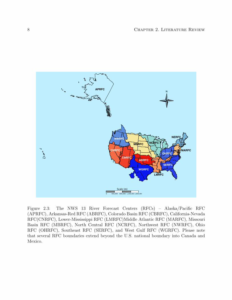
2.3 The NWS 13 River Forecast Centers (RFCs) – Alaska/Pacific RFC (APRFC),
Arkansas-Red RFC (ABRFC), Colorado Basin RFC (CBRFC), California-
Nevada RFC(CNRFC), Lower-Mississippi RFC (LMRFC)Middle Atlantic RFC
(MARFC), Missouri Basin RFC (MBRFC), North Central RFC (NCRFC),
Northwest RFC (NWRFC), Ohio RFC (OHRFC), Southeast RFC (SERFC),
and West Gulf RFC (WGRFC). Please note that several RFC boundaries
extend beyond the U.S. national boundary into Canada and Mexico. . . . . . 8
2.4 Location of NWS NEXRAD radar sites and radar coverage below 10,000 Feet
above ground level (AGL). Note the areas in the western U.S. where there is
no NEXRAD radar coverage (white). . . . . . . . . . . . . . . . . . . . . . . 12
2.5 Mean correlation decay with distance between measurements for 1-minute
rainfall rate & storm total rainfall for warm-season events (from Huff [93]). . 15
2.6 Correlation coefficients of concurrent rainfall intensity with distance from ref-
erence site (from Jones and Wendland [98]). . . . . . . . . . . . . . . . . . . 16
2.7 PRISM precipitation climatology for the period 1971-2000. . . . . . . . . . . 18
2.8 MPE bias with respect to PRISM for 2010 for the OHRFC forecast region;
MPE over-estimation is indicated by blue colors and under-estimation are
shades of red. Bias values equal to 1.0 are unbiased (white areas). . . . . . . 19
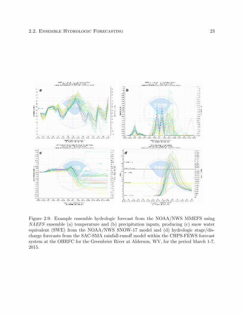
2.9 Example ensemble hydrologic forecast from the NOAA/NWS MMEFS using
NAEFS ensemble (a) temperature and (b) precipitation inputs, producing (c)
snow water equivalent (SWE) from the NOAA/NWS SNOW-17 model and (d)
hydrologic stage/discharge forecasts from the SAC-SMA rainfall-runoff model
within the CHPS-FEWS forecast system at the OHRFC for the Greenbrier
River at Alderson, WV, for the period March 1-7, 2015. . . . . . . . . . . . . 23
x
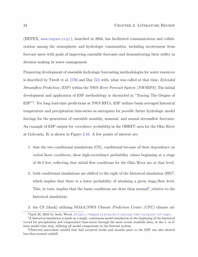
2.10 Probability of exceedance for OHRFC AHPS/ESP ensemble hydrologic fore-
cast for the Ohio River at Golconda, IL, March 11 – June 6, 2007, showing
historical simulation (HS, blue), conditional simulation without CPC climate
adjustments (CS, green), and conditional simulation with CPC climate ad-
justments (CS, black). The orange region designates above Minor Flood level
and red above Moderate Flood level. . . . . . . . . . . . . . . . . . . . . . . . 26
3.1 The NWS 13 River Forecast Centers (RFCs) – Alaska/Pacific RFC (APRFC),
Arkansas-Red RFC (ABRFC), Colorado Basin RFC (CBRFC), California-
Nevada RFC(CNRFC), Lower-Mississippi RFC (LMRFC)Middle Atlantic RFC
(MARFC), Missouri Basin RFC (MBRFC), North Central RFC (NCRFC),
Northwest RFC (NWRFC), Ohio RFC (OHRFC), Southeast RFC (SERFC),
and West Gulf RFC (WGRFC). Please note that several RFC boundaries
extend beyond the U.S. national boundary into Canada and Mexico. . . . . . 32
3.2 NEXRAD WSR-88D radar locations (black circles) in the NOAA/NWS OHRFC
area of forecast responsibility. Refer to Table 3.1 for details. Also shown are
796 OHRFC modeling subbasins (light gray outlined areas) modeled opera-
tionally within the CHPS-FEWS hydrologic forecasting system and, for ref-
erence, the Ohio River and major tributaries (black lines). The Greenbrier
River basin, WV, discussed below, is shaded gray. . . . . . . . . . . . . . . . 35
3.3 Timeline for OHRFC implementation of Stage III and MPE with changes
to the NEXRAD network, with the addition of VWX and HPX radars (see
Figure 3.2), and PPS changes. . . . . . . . . . . . . . . . . . . . . . . . . . . 36
3.4 Spatial pattern of Stage III/MPE precipitation estimate biases with respect
to PRISM over the OHRFC forecast area of responsibility, 1997-2016 . . . . 43
xi
3.5 Annual time-series of Stage III/MPE precipitation estimate biases with re-
spect to PRISM over the (a) OHRFC forecast area of responsibility and (b)
the Greenbrier River basin at Alderson, West Virginia (see Figure 3.2), 1997-
2016. The horizontal gray line is used for reference with bias = 1. . . . . . . 45
3.6 OHRFC Stage III/MPE precipitation estimation bias density by year with
respect to PRISM for 1997-2016. . . . . . . . . . . . . . . . . . . . . . . . . 47
3.7 OHRFC spatial pattern of MPE precipitation estimation bias by season, sum-
mer (JJA) and winter (DJF), with respect to PRISM for 2015-2016. . . . . . 48
3.8 OHRFC MPE precipitation estimation bias density by season, summer (JJA)
and winter (DJF), with respect to PRISM for 2015-2016. . . . . . . . . . . . 49
3.9 Monthly time-series of MPE biases with respect to PRISM over the OHRFC
forecast area of responsibility, 2015-2016. The horizontal gray line is used for
reference with bias = 1. . . . . . . . . . . . . . . . . . . . . . . . . . . . . . 50
3.10 RDHM uncalibrated historical simulation for the Greenbrier River at Alder-
son, WV, 1997-2016, compared against USGS observed flows for the period
October 18, 2015 to June 19, 2016. . . . . . . . . . . . . . . . . . . . . . . . 54
3.11 Mean annual goodness-of-fit statistics for the uncalibrated RDHM histori-
cal simulation and USGS observed flows, (a) MAE (m3s−1), ME (m3s−1),
NRMSE (%), PBIAS (%), and RMSE (m3s−1) and (b) NSE and Coefficient
of Determination (R2), for the Greenbrier River basin, for years 1998-2016. . 55
3.12 WPC monthly and annual average QPF Bias and Threat Score, by year, for
Day-1 (1970-2015) and Day-2 (1991-2015), for accumulations≥2.00 in (50.8
mm). . . . . . . . . . . . . . . . . . . . . . . . . . . . . . . . . . . . . . . . . 58
xii
3.13 NPVU (a) Mean Absolute Error (MAE) and (b) Root Mean Square Error
(RMSE), by month, for QPF thresholds, ranging from ≤0.01 (0.254 mm)
to ≥1.00 in (25.4 mm), for the period June 2001 to December 2009 for all
NOAA/NWS CONUS River Forecast Centers (rfc), NOAA/NWS Nested
Gridded Model (ngm), North American Model (nam), Hydrometeorological
Prediction Center (hpc) – now Weather Prediction Center (WPC) – Global
Forecast System (gfs), ETA Model (eta), and Aviation Model (avn). . . . . 61
3.14 NPVU Correlation Coefficient (R) for QPF thresholds, ranging from ≤0.01
(0.254 mm) to ≥1.00 in (25.4 mm), for the period June 2001 to December
2009 for all NOAA/NWS CONUS River Forecast Centers (rfc), NOAA/NWS
Nested Gridded Model (ngm), North American Model (nam), Hydrometeo-
rological Prediction Center (hpc) – now Weather Prediction Center (WPC)
– Global Forecast System (gfs), ETA Model (eta), and Aviation Model (avn). 62
3.15 OHRFC forecast area of responsibility (a) (blue shading) showing 1000 ran-
domly generated locations for QPF transposition of the 24-h precipitation
accumulation for amounts ≥50.8 mm (2.0 in) from June 23, 2016 07 UTC to
June 24, 2017 06 UTC. Points identifying transposition locations with Threat
Scores ≥0.06 are colored yellow to purple; values <0.06 are filled white. A
closer view (b) shows the reference location, used for storm transposition
(identified with a red cross), which is the location of the maximum 24-h pre-
cipitation. . . . . . . . . . . . . . . . . . . . . . . . . . . . . . . . . . . . . . 64
xiii
3.16 Example of a transposed storm (shaded blue) relative to the observed MPE
storm (yellow); the green region shows overlap between the observed MPE
and transposed storm. Also shown are the OHRFC forecast area of respon-
sibility (light blue shading) and 1000 randomly generated locations for QPF
transposition of the 24-h precipitation accumulation for amounts ≥50.8 mm
(2.0 in) from June 23, 2016 07 UTC to June 24, 2017 06 UTC. Points identi-
fying transposition locations with Threat Scores ≥0.06 are colored yellow to
purple; values <0.06 are filled white. The reference location, identified with a
red cross, is the location of the maximum 24-h precipitation, from which storm
transpositions are made. The heavy black line indicates the transposition vector. 65
3.17 Flow hydrographs for the June 23, 2016 07 UTC to June 25, 2017 12 UTC
model experiment period for the Greenbrier River at Alderson, WV, showing
USGS observed flows (black circles), RDHM simulated hydrographs derived
from observed MPE precipitation (blue circles), and the experimental QPF for
Threat Score ranges 0.06-0.15 (cyan lines) and 0.15-0.25 (magenta lines). For
reference, the Minor and Major Flood levels are shown as horizontal orange
and purple lines, respectively. . . . . . . . . . . . . . . . . . . . . . . . . . . 68
3.18 Threat Scores (TS≥0.06) of 88 randomly transposed QPF instances with re-
spect to distance from a reference location (see Figure 3.15 (b)). Maximum
flows derived from RDHM simulations are shown by point size and threat
score range, by color, for the Greenbrier River at Alderson, WV, within the
June 23, 2016 07 UTC to June 25, 2017 12 UTC model experiment period. . 69
xiv
3.19 Comparison of RDHM simulated peak flows for QPF for Threat Score ranges
0.06-0.15, 0.15-0.25, 0.25-0.30, and 0.30-0.49. For reference, the Minor and
Major Flood levels are shown as horizontal orange and purple lines, respec-
tively for the Greenbrier River at Alderson, WV, within the June 23, 2016 07
UTC to June 25, 2017 12 UTC model experiment period. The USGS observed
peak flow is indicated as a red line. . . . . . . . . . . . . . . . . . . . . . . . 70
4.1 The NWS 13 River Forecast Centers (RFCs) – Alaska/Pacific RFC (APRFC),
Arkansas-Red RFC (ABRFC), Colorado Basin RFC (CBRFC), California-
Nevada RFC(CNRFC), Lower-Mississippi RFC (LMRFC)Middle Atlantic RFC
(MARFC), Missouri Basin RFC (MBRFC), North Central RFC (NCRFC),
Northwest RFC (NWRFC), Ohio RFC (OHRFC), Southeast RFC (SERFC),
and West Gulf RFC (WGRFC). Please note that several RFC boundaries
extend beyond the U.S. national boundary into Canada and Mexico. . . . . . 76
4.2 Map showing the location of 38 Experiment 1 and Experiment 2 forecast
point locations used in the OHRFC forecast area, listed in Tables 4.1 and 4.2,
identifying fast, medium, and slow responding basins. . . . . . . . . . . . . . 82
4.3 Comparison of OHRFC hydrologic forecasts both with and without WPC
QPF, showing ME (a), MAE (b), and RMSE (c) for all basins, for all response
times, for the OHRFC operational forecast area. Shown for the period August
10, 2007 - August 31, 2009. . . . . . . . . . . . . . . . . . . . . . . . . . . . 84
4.4 RMSE of OHRFC hydrologic forecasts for both with and without WPC QPF,
for All basins (a) and Fast (b), Medium (c) and Slow (d) response basins for
the OHRFC operational forecast area. Shown for the period August 10, 2007
- August 31, 2009. . . . . . . . . . . . . . . . . . . . . . . . . . . . . . . . . 85
xv
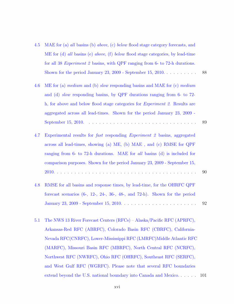
4.5 MAE for (a) all basins (b) above, (c) below flood stage category forecasts, and
ME for (d) all basins (e) above, (f) below flood stage categories, by lead-time
for all 38 Experiment 2 basins, with QPF ranging from 6- to 72-h durations.
Shown for the period January 23, 2009 - September 15, 2010. . . . . . . . . . 88
4.6 ME for (a) medium and (b) slow responding basins and MAE for (c) medium
and (d) slow responding basins, by QPF durations ranging from 6- to 72-
h, for above and below flood stage categories for Experiment 2. Results are
aggregated across all lead-times. Shown for the period January 23, 2009 -
September 15, 2010. . . . . . . . . . . . . . . . . . . . . . . . . . . . . . . . 89
4.7 Experimental results for fast responding Experiment 2 basins, aggregated
across all lead-times, showing (a) ME, (b) MAE , and (c) RMSE for QPF
ranging from 6- to 72-h durations. MAE for all basins (d) is included for
comparison purposes. Shown for the period January 23, 2009 - September 15,
2010. . . . . . . . . . . . . . . . . . . . . . . . . . . . . . . . . . . . . . . . . 90
4.8 RMSE for all basins and response times, by lead-time, for the OHRFC QPF
forecast scenarios (6-, 12-, 24-, 36-, 48-, and 72-h). Shown for the period
January 23, 2009 - September 15, 2010. . . . . . . . . . . . . . . . . . . . . . 92
5.1 The NWS 13 River Forecast Centers (RFCs) – Alaska/Pacific RFC (APRFC),
Arkansas-Red RFC (ABRFC), Colorado Basin RFC (CBRFC), California-
Nevada RFC(CNRFC), Lower-Mississippi RFC (LMRFC)Middle Atlantic RFC
(MARFC), Missouri Basin RFC (MBRFC), North Central RFC (NCRFC),
Northwest RFC (NWRFC), Ohio RFC (OHRFC), Southeast RFC (SERFC),
and West Gulf RFC (WGRFC). Please note that several RFC boundaries
extend beyond the U.S. national boundary into Canada and Mexico. . . . . . 101
xvi

5.2 Map showing the location of 54 Experiment forecast point locations used in
the OHRFC forecast area, listed in Tables 5.1, 5.2, and 5.3, identifying fast,
medium, and slow responding basins. Locations of dams are shown with
maximum storage capacities ≥250,000 ac-ft (308,370,000 m3). Gray outlined
polygons are 696 modeled subbasins. . . . . . . . . . . . . . . . . . . . . . . 105
5.3 Example MMEFS NAEFS ensemble forecast, showing 42 individual ensemble
model members (various colors), ensemble median (black line identified with
triangles), and the 75% to 25% probability of exceedance confidence band
is shown as the orange region. The Minor and Moderate flood levels are
indicated for reference. . . . . . . . . . . . . . . . . . . . . . . . . . . . . . . 108
5.4 ME, MAE, and RMSE by leadtime for All and Fast Response basins identified
in Figure 5.2 and in Tables 5.1, 5.2, and 5.3. Results are shown for opera-
tional forecast (OHRFC 24-h QPF) and MMEFS NAEFS ensemble mean and
median forecasts, November 30, 2010 through May 24, 2012. Units are meters. 112
5.5 MAE by leadtime for Medium and Slow response basins identified in Fig-
ure 5.2 and in Tables 5.2 and 5.3. Results are shown for operational forecast
(OHRFC 24-h QPF) and MMEFS NAEFS ensemble mean and median fore-
casts, November 30, 2010 through May 24, 2012. Units are meters. . . . . . . 113
5.6 CRPSS by leadtime for all forecast point locations identified in Figure 5.2, for
all forecast stage ranges and stage ranges ≥0.90 probability of non-exceedance.
Point shading identifies basin response category. Units are dimensionless. . . 119
5.7 Reliability Diagram for all 54 basins, for lead-times 24-, 48-, 96-, 120-, and
168-h. Shown for stage ranges ≥0.90 probability of non-exceedance. . . . . . 121
xvii

5.8 ROC for all 54 basins, for lead-times 24-, 96-, 120-, and 168-h. Shown for
stage ranges ≥0.90 probability of non-exceedance. . . . . . . . . . . . . . . . 123
5.9 Rank histograms for all forecast point locations identified in Figure 5.2 and
for fast response basins, for 24- and 168-h leadtimes. . . . . . . . . . . . . . 125
xviii

List of Tables
2.1 Table showing the coefficients of determination for runoff prediction equations
Fogel [74]. . . . . . . . . . . . . . . . . . . . . . . . . . . . . . . . . . . . . . 15
2.2 Correlation coefficients of rainfall rates with respect to distance from a central
raingage (from Huff [93]). . . . . . . . . . . . . . . . . . . . . . . . . . . . . 15
3.1 NEXRAD WSR-88D locations used by the OHRFC in the Stage III and MPE
PPS, with the radar commissioning date, ground elevation, and tower height,
listed in order of the commissioning date. . . . . . . . . . . . . . . . . . . . . 37
3.2 Annual OHRFC Stage III/MPE PPS bias statistics by year. . . . . . . . . . 38
3.3 Goodness-of-fit statistics for the uncalibrated RDHM historical simulation
and USGS observed flows for the Greenbrier River at Alderson, WV (USGS
05050003), by year, for the period 1998-2016. Unless indicated otherwise,
units are m3s−1, except for NSE and R2, which are dimensionless. . . . . . . 52
3.4 Contingency table for QPF Threat Score calculation. . . . . . . . . . . . . . 56
4.1 Experiment 1 fast response basins, listing NWS station identifier (ID), USGS
identifier, Station name, Response time category, and basin area. . . . . . . . 80
xix
4.2 Experiment 1 medium and slow response basins, listing NWS station identifier
(ID), USGS identifier, Station name, Response time category, and basin area. 81
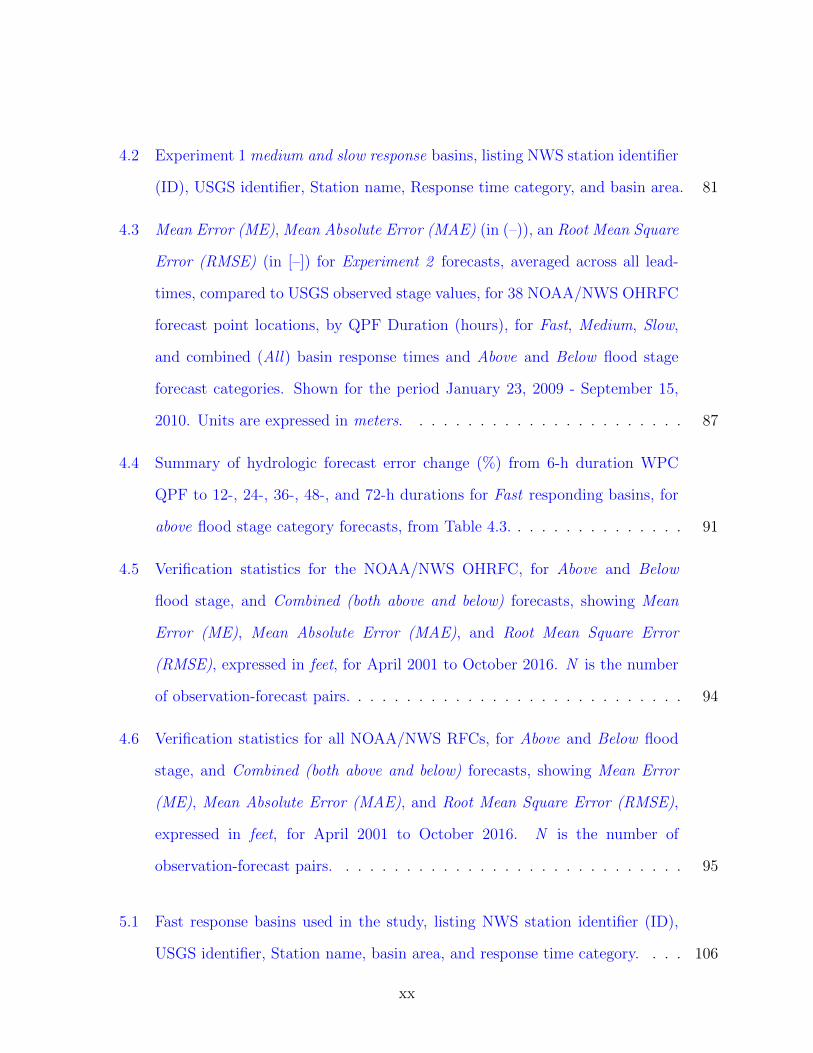
4.3 Mean Error (ME), Mean Absolute Error (MAE) (in (–)), an Root Mean Square
Error (RMSE) (in [–]) for Experiment 2 forecasts, averaged across all lead-
times, compared to USGS observed stage values, for 38 NOAA/NWS OHRFC
forecast point locations, by QPF Duration (hours), for Fast, Medium, Slow,
and combined (All) basin response times and Above and Below flood stage
forecast categories. Shown for the period January 23, 2009 - September 15,
2010. Units are expressed in meters. . . . . . . . . . . . . . . . . . . . . . . 87
4.4 Summary of hydrologic forecast error change (%) from 6-h duration WPC
QPF to 12-, 24-, 36-, 48-, and 72-h durations for Fast responding basins, for
above flood stage category forecasts, from Table 4.3. . . . . . . . . . . . . . . 91
4.5 Verification statistics for the NOAA/NWS OHRFC, for Above and Below
flood stage, and Combined (both above and below) forecasts, showing Mean
Error (ME), Mean Absolute Error (MAE), and Root Mean Square Error
(RMSE), expressed in feet, for April 2001 to October 2016. N is the number
of observation-forecast pairs. . . . . . . . . . . . . . . . . . . . . . . . . . . . 94
4.6 Verification statistics for all NOAA/NWS RFCs, for Above and Below flood
stage, and Combined (both above and below) forecasts, showing Mean Error
(ME), Mean Absolute Error (MAE), and Root Mean Square Error (RMSE),
expressed in feet, for April 2001 to October 2016. N is the number of
observation-forecast pairs. . . . . . . . . . . . . . . . . . . . . . . . . . . . . 95
5.1 Fast response basins used in the study, listing NWS station identifier (ID),
USGS identifier, Station name, basin area, and response time category. . . . 106
xx

5.2 Same as Table 5.1 but for medium response basins. . . . . . . . . . . . . . . 107
5.3 Same as Table 5.1 but for slow response basins. . . . . . . . . . . . . . . . . 107
5.4 CRPSS for Pittsburgh, PA (PTTP1) for all stage ranges and for stages with
probability of exceedance, p=0.90, by Leadtime. . . . . . . . . . . . . . . . . 120
5.5 Contingency table. . . . . . . . . . . . . . . . . . . . . . . . . . . . . . . . . 122
A.1 Data sources. . . . . . . . . . . . . . . . . . . . . . . . . . . . . . . . . . . . 169
xxi

xxii

Chapter 1
Introduction
1.1 Nature of the Problem
All forecasts are uncertain. Hydrologic forecasts are uncertain largely because of errors in the
measurement and prediction of hydrologic model forcings, such as temperature and precipi-
tation. Advances have been made over recent decades in the measurement and prediction of
precipitation that have been adopted operationally for flood prediction and water resources
forecasting by U.S. National Oceanic and Atmospheric Administration (NOAA), National
Weather Service (NWS) River Forecast Centers (RFCs). But hydrologic forecast accuracy
gains have not been fully quantified with the adoption of these scientific advances. This
dissertation quantifies error reduction in hydrologic forecasting derived from advancements
in radar based precipitation measurement and precipitation forecasting at the NOAA/NWS
Ohio River Forecast Center (OHRFC). However, despite improvements in the measurement
and prediction of hydrometeorological variables, considerable forecast uncertainty remains,
yet official NWS river stage forecasts do not currently convey forecast uncertainty. Conse-
quently, this study further explores the use of hydrologic ensemble median and mean river
1

2 Chapter 1. Introduction
stage forecasts as a possible alternative to current single-valued deterministic river stage
forecasts to both reduce forecast uncertainty and to further motivate adoption of the use of
probabilistic hydrologic forecasts by the public and decision makers.
1.2 Dissertation Objectives
The central research objective of this dissertation is to demonstrate the necessity for using
probabilistic hydrologic forecasting, using hydrologic ensembles, in place of current methods
that rely on the use of single-valued deterministic forecast of precipitation, known as Quan-
titative Precipitation Forecast (QPF). Due to resistance by the general public and many
decision-makers to accept probabilistic hydrologic forecasts, the use of hydrologic ensemble
median and mean forecasts is explored as a mechanism to reduce hydrologic forecast uncer-
tainty and to explicitly include the notion of uncertainty in hydrologic forecasts in terms of
expectation or ”best estimate”. The manuscript is structured to:
• quantify, in relative terms, gains achieved in the reduction of hydrologic prediction error
due to advancements in the measurement of precipitation, referred to as Quantitative
Precipitation Estimate (QPE) and prediction of precipitation, QPF, over the past ∼50
years;
• quantify hydrologic prediction error using deterministic single-valued QPF, to deter-
mine (1) if the use of non-zero QPF is warranted in hydrologic forecasting, because
of reduced forecast error relative to zero-QPF forecasts, and (2) if the answer is that
non-zero QPF does produce hydrologic forecasts with smaller error, what hydrologic
prediction error structures are incurred with the use of longer QPF periods (6-, 12-,
24-,. . . , 72-hours,. . . ) and;

1.3. Research Approach 3
• quantify hydrologic ensemble median and mean forecasts error relative to current op-
erational methods that use single-valued deterministic QPF.
These issues will be addressed in 3 chapters:
1. Hydrometeorological Forcing Errors for a Real-time Flood Forecast System in the Ohio
River Valley, USA;
2. The Effect of QPF on Real-time Deterministic Hydrologic Forecast Uncertainty;
3. The Use of Central Tendency Measures from an Operational Short Lead-time Hydro-
logic Ensemble Forecast System for Real-time Forecasts.
1.3 Research Approach
The first research objective is achieved by quantifying radar derived precipitation estimation
errors relative to a widely accepted historical precipitation database over an approximate
20-year period. A hydrologic simulation experiment is run to quantify the hydrologic impact
of precipitation estimation improvements. QPF verification results from two sources are
reported to show forecast improvements since the 1970s. A hydrologic monte carlo simulation
experiment is conducted to assess the impact of the improvements on hydrologic forecast
error.
The second research objective is attained by using two real-time hydrologic forecast exper-
iments, the first to assess the magnitude of hydrologic prediction error with zero-QPF and
non-zero QPF. The second experiment investigates hydrologic prediction error incurred due
to varying ranges of QPF duration.

4 Chapter 1. Introduction
The third research objective is met by utilizing hydrologic ensemble forecasts from the Me-
teorological Model-based Ensemble Forecast System (MMEFS) [1] methodology to estimate
hydrologic prediction uncertainty at numerous forecast point locations in the NOAA/NWS
OHRFC area of responsibility. The research methodology makes use of the U.S. NOAA/NWS,
National Centers for Environmental Prediction (NCEP) North American Ensemble Forecast
System (NAEFS) numerical weather prediction (NWP) model output of precipitation and
temperature as gridded hydrometeorological field forcings to a physically-based conceptual
hydrologic model which generates, as output, ensemble hydrological time series. The result-
ing hydrologic time series ensembles are analyzed to provide probabilistic forecasts of peak
flow and stage for short lead-time events out to 168 hours. Probabilistic verification measures
are used to evaluate the reasonableness of the MMEFS hydrologic ensemble forecasts.

Chapter 2
Literature Review
Real-time, operational hydrologic forecasting is needed throughout the world for flood predic-
tion and is necessary in many water resources applications. A key requirement, especially for
flood forecasting, is the delivery of accurate and timely flood warnings/alerts to the general
public and decision makers, thus providing the opportunity to initiate preventative flood de-
fense measures or for possible emergency response. Currently, hydrologic forecasts typically
take the form of single-valued deterministic river stage predictions that are derived from
observed and forecasted temperature and precipitation as input to a hydrologic modeling
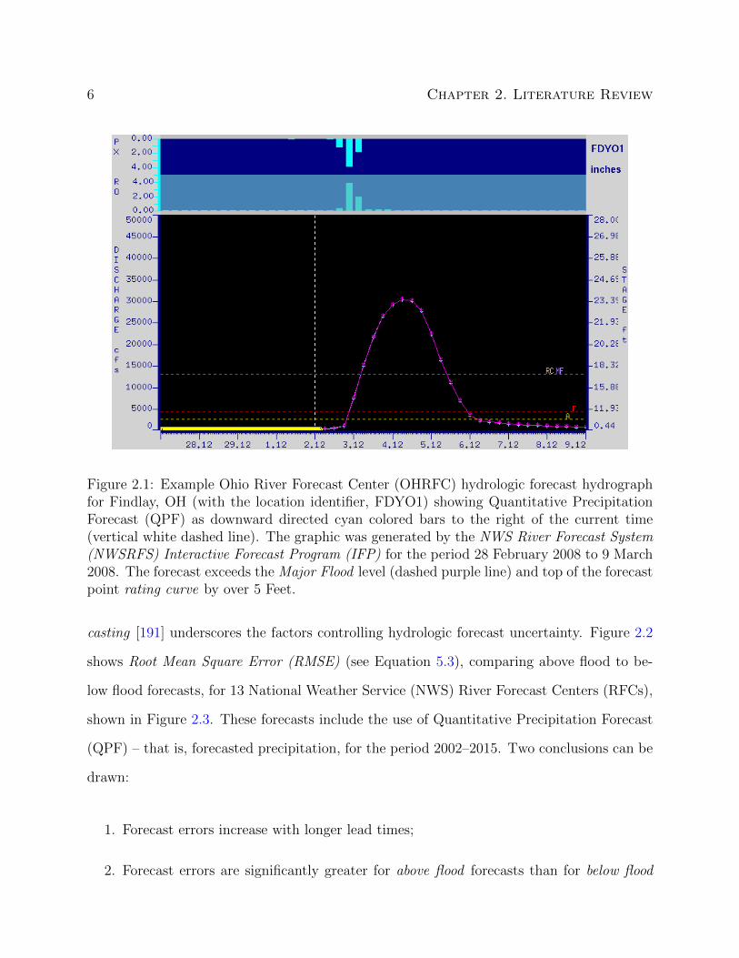
system, as depicted in Figure 2.1. However, operational experience and significant research
(Welles et al. [181]; Demargne et al. [56]; and Demargne et al. [57]) have demonstrated
that errors resulting from observational measurement and prediction of air temperature and
the magnitude and location of precipitation (or other hydrometeorological variables, such as
relative humidity, wind speed and direction, etc.) can produce significant hydrologic pre-
diction/forecasting errors, which can lead to erroneous alerts and warnings (False Alarms)
or the failure to issue alerts and warnings. The World Meteorological Organization (WMO)
statement on the Scientific Basis for and Limitations of River Discharge and Stage Fore-
5
6 Chapter 2. Literature Review
Figure 2.1: Example Ohio River Forecast Center (OHRFC) hydrologic forecast hydrographfor Findlay, OH (with the location identifier, FDYO1) showing Quantitative PrecipitationForecast (QPF) as downward directed cyan colored bars to the right of the current time(vertical white dashed line). The graphic was generated by the NWS River Forecast System(NWSRFS) Interactive Forecast Program (IFP) for the period 28 February 2008 to 9 March2008. The forecast exceeds the Major Flood level (dashed purple line) and top of the forecastpoint rating curve by over 5 Feet.
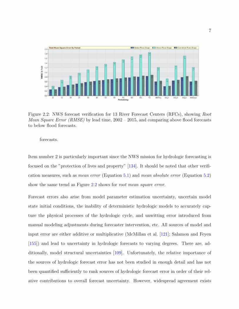
casting [191] underscores the factors controlling hydrologic forecast uncertainty. Figure 2.2
shows Root Mean Square Error (RMSE) (see Equation 5.3), comparing above flood to be-
low flood forecasts, for 13 National Weather Service (NWS) River Forecast Centers (RFCs),
shown in Figure 2.3. These forecasts include the use of Quantitative Precipitation Forecast
(QPF) – that is, forecasted precipitation, for the period 2002–2015. Two conclusions can be
drawn:
1. Forecast errors increase with longer lead times;
2. Forecast errors are significantly greater for above flood forecasts than for below flood
7
Figure 2.2: NWS forecast verification for 13 River Forecast Centers (RFCs), showing RootMean Square Error (RMSE) by lead time, 2002 – 2015, and comparing above flood forecaststo below flood forecasts.
forecasts.
Item number 2 is particularly important since the NWS mission for hydrologic forecasting is
focused on the ”protection of lives and property” [134]. It should be noted that other verifi-
cation measures, such as mean error (Equation 5.1) and mean absolute error (Equation 5.2)
show the same trend as Figure 2.2 shows for root mean square error.
Forecast errors also arise from model parameter estimation uncertainty, uncertain model
state initial conditions, the inability of deterministic hydrologic models to accurately cap-
ture the physical processes of the hydrologic cycle, and unwitting error introduced from
manual modeling adjustments during forecaster intervention, etc. All sources of model and
input error are either additive or multiplicative (McMillan et al. [121]; Salamon and Feyen
[155]) and lead to uncertainty in hydrologic forecasts to varying degrees. There are, ad-
ditionally, model structural uncertainties [109]. Unfortunately, the relative importance of
the sources of hydrologic forecast error has not been studied in enough detail and has not
been quantified sufficiently to rank sources of hydrologic forecast error in order of their rel-
ative contributions to overall forecast uncertainty. However, widespread agreement exists
8 Chapter 2. Literature Review
APRFC
CNRFC MARFC
NERFC
MBRFC
CBRFC
NWRFC
ABRFC
WGRFCSERFC
OHRFC
NCRFC
LMRFC
Figure 2.3: The NWS 13 River Forecast Centers (RFCs) – Alaska/Pacific RFC(APRFC), Arkansas-Red RFC (ABRFC), Colorado Basin RFC (CBRFC), California-NevadaRFC(CNRFC), Lower-Mississippi RFC (LMRFC)Middle Atlantic RFC (MARFC), MissouriBasin RFC (MBRFC), North Central RFC (NCRFC), Northwest RFC (NWRFC), OhioRFC (OHRFC), Southeast RFC (SERFC), and West Gulf RFC (WGRFC). Please notethat several RFC boundaries extend beyond the U.S. national boundary into Canada andMexico.

9
that hydrologic forecast uncertainty must be quantified and that the magnitude of hydro-
logic forecast uncertainty should be passed on to decision makers and end-users in clear,
understandable ways (Pappenberger et al. [144]; Wetterhall et al. [184]).
To illustrate the basis of hydrologic forecast uncertainty, this research will draw on data
from U.S. National Oceanic and Atmospheric Administration (NOAA) NWS RFCs, specif-
ically, the OHRFC, which is shown in Figure 2.3. The focus of the research is to establish
the effect of model forcing (focusing on observed and forecast precipitation1) error on hy-
drologic forecast uncertainty. The main points to be made are that the most significant
inputs to hydrologic models for rainfall-driven events used in forecasting are QPE, that is,
observed precipitation and QPF, namely predicted/forecasted precipitation and that there
are significant errors associated with their measurement and prediction, respectively.
Explicit quantification of hydrologic forecast uncertainty is one of the central themes of
the NWS Hydrologic Services Program Advanced Hydrologic Prediction Services (AHPS)
initiative [120]. The estimation of hydrologic forecast uncertainty for short lead-time (days 1
to 5) events is a area of active research within the NWS and elsewhere. Krzysztofowicz [112]
outlines the need for probabilistic hydrologic forecasting, stating that probabilistic forecasts:
1. are scientifically more honest by providing prediction uncertainty
2. enable risk-based warnings for floods
3. allow rational decision making under the knowledge of prediction uncertainty
4. offer additional economic benefits due to improved decision making
1While significant in many regions of the world due to the influence of snow accumulation and meltprocesses, temperature estimation and prediction uncertainty will not be considered in order to limit thescope of the research task.
10 Chapter 2. Literature Review
Probabilistic forecasts must include estimates of all the components of forecast uncertainty,
including:
1. model input errors
2. inherent modeling errors (independent of the inputs)
Explicit quantification of hydrologic forecast uncertainty is one of the central themes of
the NWS Hydrologic Services Program Advanced Hydrologic Prediction Services (AHPS)
initiative, National Research Council (NRC) [141]. The estimation of hydrologic forecast
uncertainty for short lead-time (days 1 to 5) events is a area of active research within the
NWS. On the need to characterize the effects of input uncertainties for forecast precipi-
tation and temperature, the NRC [133] states in Completing the Forecast: Characterizing
and Communicating Uncertainty for Better Decisions Using Weather and Climate Forecasts
(http://www.nap.edu/catalog/11699.html):
The NWS operational hydrology short-term forecast products carry uncertainty
that is to a large degree due to forecasts of precipitation and temperature that
serve as hydrologic model input and which are generated by objective or in some
cases subjective procedures applied to the operational NCEP model forecasts.
2.1 Precipitation variability
Principle data inputs for NOAA/NWS RFC hydrologic models are observed and forecasted
precipitation and temperature. Observed precipitation is estimated through a multisensor
estimation process using the Multisensor Precipitation Estimator (MPE) software [103] which
utilizes rain gauges, NWS Next Generation Radar (NEXRAD) doppler radar, shown in
2.1. Precipitation variability 11
Figure 2.4, and, in some instances, satellite precipitation estimates to produce an un-biased
optimal estimate of hourly precipitation fields. Forecasted precipitation is derived from
numerical weather prediction (NWP) models, but meteorological forecaster adjustments are
made at both the NWS Weather Prediction Center (WPC) and at local RFCs. However,
the greatest sources of hydrologic prediction error derives from uncertainties in precipitation
forecasts (Ebert and McBride, 2000 and Ebert et al, 2003), also known as quantitative
precipitation forecast (QPF) and errors with the estimation of observed precipitation, or
quantitative precipitation estimates (QPE) (see Anagnostou et al. [11], Seo et al. [160], and
Krajewski and Ciach [108]).
2.1.1 Observed precipitation variability
One way to decrease hydrologic modeling uncertainty is to apply hydrologic models (and
other models - snow model, for instance) at smaller subbasins scales with the hope of cap-
turing the finer structure of precipitation and other hydrometeorological variability and spa-
tial heterogeneities of basin characteristics. Finnerty et al. [73] and Smith et al. [165] with
the Hydrologic Research Laboratory (HRL) of the NWS Office of Hydrology (OH) experi-
mented with various approaches of applying the SAC-SMA model in a distributed modeling
approach. Namely, they calibrated the SAC-SMA at a gaged location and applied the pa-
rameters to nested subbasins of varying sizes. These experiments demonstrated increased
hydrograph peaks and runoff volumes with smaller basins and decreased hydrograph peaks
and runoff volumes with larger basins. Attempts to identify consistent scaling relationships
for parameter values between basins of differing sizes have been unsuccessful. It does not
seem possible, as yet, to rationally adjust calibrated SAC-SMA parameters to be suitable
for the differing characteristics of ungaged subbasins and maintain consistent hydrograph
response.

12 Chapter 2. Literature Review
KYUX
KLTX
KICT
KSRX
KVBXKVNX
KINX
KEMX
KTWX
KTBW
KTLH
KLWX
KCCX
KLSX
KSGF
KOTX
KLIX
KFSD
KSHV
KATX
KSOX
KHNX
KMUX
KNKX
KSJT
KMTX
KDAX
KJGX
KFCX
KRIW
KRGX
KUDX
KRAX
KDVN
KPUX
KRTX
KGYX
KSFX
KEAX
KPBZ
KIWA
KDIX
KPDT
KPAH
KOAXKIWX
KHTX
KLNX
KTLX
KAKQ
KAPX
KOHX KMHX
KVAXKMOB
KMSX KMBX
KMPX
KMKX
KMAF
KAMX
KNQA
KMLB
KMAX
KMXX
KMQT
KLBB
KLVX
KVTX
KLZK
KILX
KDFX
KESX
KLCH
KARX
KMRX
KBYX
KJAX
KDGX
KJKL
KIND
KHGX
KHDX
KGSP
KGRB
KTFX
KGRR
KGJXKUEX
KGLD
KGGW
KEOXKPOE
KGRK
KTYX
KHPX
KFSX
KMVX
KVWX
KBHX
KLRX
KEPZ
KEVX
KEYX
KDYX
KDLH
KDOX
KDDC
KDTX
KDMX
KFTG
KFWS
KCRP
KGWXKCAE
KCLE
KILN
KLOTKCYS
KRLX
KCLX
KICX
KCBW
KFDX
KCXX
KBUF
KBRO
KOKX
KBOXKCBX
KBIS
KBMX
KBGM
KBLX
KBBX
KEWX
KFFC
KAMA
KFDR
KABX
KENX
KABR
KLGX
VCP12 Coverage4,000 ft above ground level*6,000 ft above ground level*10,000 ft above ground level*
0 250 500 750125 Miles* Bottom of beam height (assuming Standard Atmospheric Refraction).Terrain blockage indicated where 50% or more of beam blocked.
NEXRAD Coverage Below 10,000 Feet AGL
Figure 2.4: Location of NWS NEXRAD radar sites and radar coverage below 10,000 Feetabove ground level (AGL). Note the areas in the western U.S. where there is no NEXRADradar coverage (white).
2.1. Precipitation variability 13
Rainfall variability over watersheds is the dominant factor influencing runoff variability ob-
served in hydrographs and provides the chief motivation for the adoption of distributed
hydrologic modeling by the NWS in RFCs. Dawdy and Bergmann [50] showed that spa-
tial rainfall variations significantly altered parameter calibration of the Stanford Watershed
Model. Also using a hydrologic model, Wilson et al. [186] found large differences in the
time-to-peak, peak discharge, and runoff volume depending on whether numerically gener-
ated rainfall input came from a single raingage, implying a spatially uniform distribution of
rainfall, or from 20 covering the simulated drainage basin, where the rainfall was spatially
variable. Based on raingage and flood data, Reich [152] found that there was no consistent
relationship between point rainfall maxima and peak runoff maxima for 24 basins in Penn-
sylvania. However, subsequently, Larson and Reich [113] found that while there was high
variability for individual years with Reich’s 1970 data, the rank and recurrence interval of
storm rainfall and peak runoff do have a central tendency of equality. This confirms, in other
words, the accepted notion that the largest rain-induced floods tend to be produced by the
greatest rainfalls.
In a somewhat different approach, Fogel [74] produced multiple regression equations for
predicting runoff volumes from three small catchments ranging in area from 0.47 to 7.77 mi2
(Table 2.1). He found that the spatially averaged storm rainfall and other factors accounted
for appreciably less explained variance with increased drainage area, where Q : storm runoff
(inches); R: mean storm rainfall over the basin (inches); i15: maximum 15-minute rainfall
intensity (inches); tm: time to the center of mass of rainfall (hours); and b0, b1, b2: regression
coefficients. Fogel’s results indicate that the relationship between basin mean rainfall and
peak storm runoff is consistent, that is, greater rainfalls produce larger flood peaks, but that
considerable deviations occur about this tendency. Clearly, these deviations result from (1)
the areal variability of rainfall over the individual basins, (2) the temporal distribution of

14 Chapter 2. Literature Review
storm rainfall, and (3) antecedent watershed conditions. But for these Arizona watersheds,
antecedent conditions are probably not significant since the time between rainfalls is large
and considerable drying occurs during the intervening rain periods. By inspection, it appears
the rainfall intensity factors explain less variance within basins than the differences in basin
areas explain the variance between the different basins. This seems to confirm the idea that
rainfall variability is the dominant factor in explaining runoff variability, which is especially
evident with the simplest of the runoff prediction equations, Q = b0 + b1R.
Studies of rainfall patterns of storms using dense raingage networks have shown that large
spatial rainfall gradients exist within storms over short durations (<15 minutes). Huff [93],
for example, obtained spatial correlations of 1, 5, and 10 minute rainfall rates, shown in Table
2.2, and total storm accumulations for a raingage network of 50 recording gages over a 100
sq. mi. area in east central Illinois from a 29 storm sample (see Figure 2.5). Additionally, an
analysis by Jones and Wendland [98] of continuous recording raingage networks throughout
the world reveals that 1-minute rainfall intensities for showery rains, that is, storms exhibit-
ing thunderstorm or near-thunderstorm intensity rainfalls, were essentially uncorrelated at
distances of 12 km from the reference raingage (Figure 2.6) for July and October storms.
Osborn et al (1979) found that total rainfall accumulations of, primarily, air-mass thunder-
storms, had correlation coefficients between 0.4 to 0.6 at 5 km, 0.1 to 0.3 at 15 km, and 0.0
to 0.1 at 25 km for raingage networks in Arizona and New Mexico. Since the deployment
of NEXRAD systems by the NWS, routine observation of the spatial variability of rainfall
is commonplace. NEXRAD Stage-3 Precipitation Processing rainfall estimates, which are
made on a 4 km spatial grid, reveal detailed rainfall variations within storms that are evident
nationwide.
Adams [3] studied the intra-storm spatial variability of flooding indicated by comparisons
of interval estimates of the return periods of peak flows for basins in close proximity to
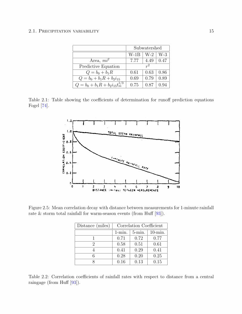
2.1. Precipitation variability 15
Subwatershed
W-1B W-2 W-3Area, mi2 7.77 4.49 0.47
Predictive Equation r2
Q = b0 + b1R 0.61 0.63 0.86Q = b0 + b1R + b2i15 0.69 0.79 0.89
Q = b0 + b1R + b2i15t1/3m 0.75 0.87 0.94
Table 2.1: Table showing the coefficients of determination for runoff prediction equationsFogel [74].
Figure 2.5: Mean correlation decay with distance between measurements for 1-minute rainfallrate & storm total rainfall for warm-season events (from Huff [93]).
Distance (miles) Correlation Coefficient
1-min. 5-min. 10-min.1 0.71 0.72 0.772 0.58 0.51 0.614 0.41 0.29 0.416 0.28 0.20 0.258 0.16 0.13 0.15
Table 2.2: Correlation coefficients of rainfall rates with respect to distance from a centralraingage (from Huff [93]).
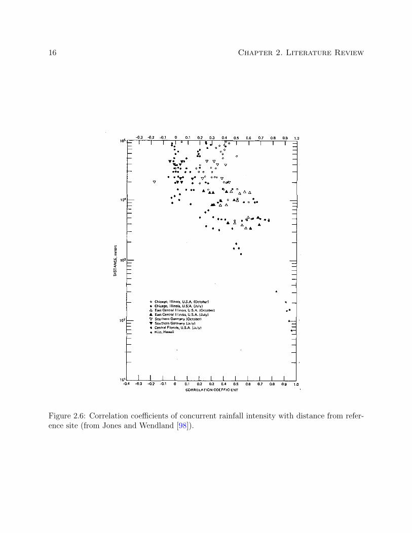
16 Chapter 2. Literature Review
Figure 2.6: Correlation coefficients of concurrent rainfall intensity with distance from refer-ence site (from Jones and Wendland [98]).

2.1. Precipitation variability 17
each other within the Piedmont region of Maryland. Results showed substantial differences
between interval estimates on return periods between nearby basins within individual storms,
which suggests substantial rainfall differences between basins.
Hamlin [89] emphasizes the importance of rainfall variability and the need for accurate
rainfall estimates for variable source area models. He suggests that lumped-parameter models
do not require as stringent rainfall estimates, since significant averaging is made within the
lumped process modeling. Faures et al. [72] and Goodrich et al. [84] found very significant
rainfall measurement and runoff modeling errors for a small, 4.4 ha semiarid catchment,
where the coefficient of variation for peak rate and runoff volume ranged from 9 to 76%, and
from 2 to 65%, respectively, over eight storm events. They concluded that the assumption
of spatial uniformity of rainfall at the 5 ha scale in convective environments appeared to be
invalid.
Analyses of precipitation estimates from radar can be problematic. Reed and Maidment
[150] have identified coordinate transformation errors in the NEXRAD HRAP coordinate
system which is the basis of the digital precipitation data used by the NWS for input to
NWSRFS hydrologic models. The magnitude of these shape distortion errors depend on
latitude and range between 0.3% to 0.6% in the conterminous U.S. These errors translate
into HRAP grid size variations, causing the true area of HRAP grid cells to range from 13
km2 in Miami to 19 km2 in Minneapolis.
The use of gridded historical datasets, such as the Parameter-elevation Regressions on Inde-
pendent Slopes Model (PRISM) at the Spatial Climate Analysis Service Oregon State Uni-
versity (http://www.prism.oregonstate.edu), desribed by Taylor et al. [171], Daly
et al. [46], Taylor et al. [172], Daly et al. [47], and Daly et al. [48] are useful analyzing the
spatial bias patterns of radar-derived precipitation estimates. PRISM is an expert system
that uses point data and a digital elevation model (DEM) to generate gridded estimates
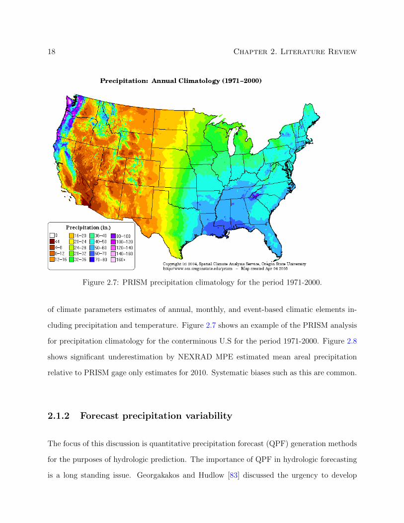
18 Chapter 2. Literature Review
Figure 2.7: PRISM precipitation climatology for the period 1971-2000.
of climate parameters estimates of annual, monthly, and event-based climatic elements in-
cluding precipitation and temperature. Figure 2.7 shows an example of the PRISM analysis
for precipitation climatology for the conterminous U.S for the period 1971-2000. Figure 2.8
shows significant underestimation by NEXRAD MPE estimated mean areal precipitation
relative to PRISM gage only estimates for 2010. Systematic biases such as this are common.
2.1.2 Forecast precipitation variability
The focus of this discussion is quantitative precipitation forecast (QPF) generation methods
for the purposes of hydrologic prediction. The importance of QPF in hydrologic forecasting
is a long standing issue. Georgakakos and Hudlow [83] discussed the urgency to develop
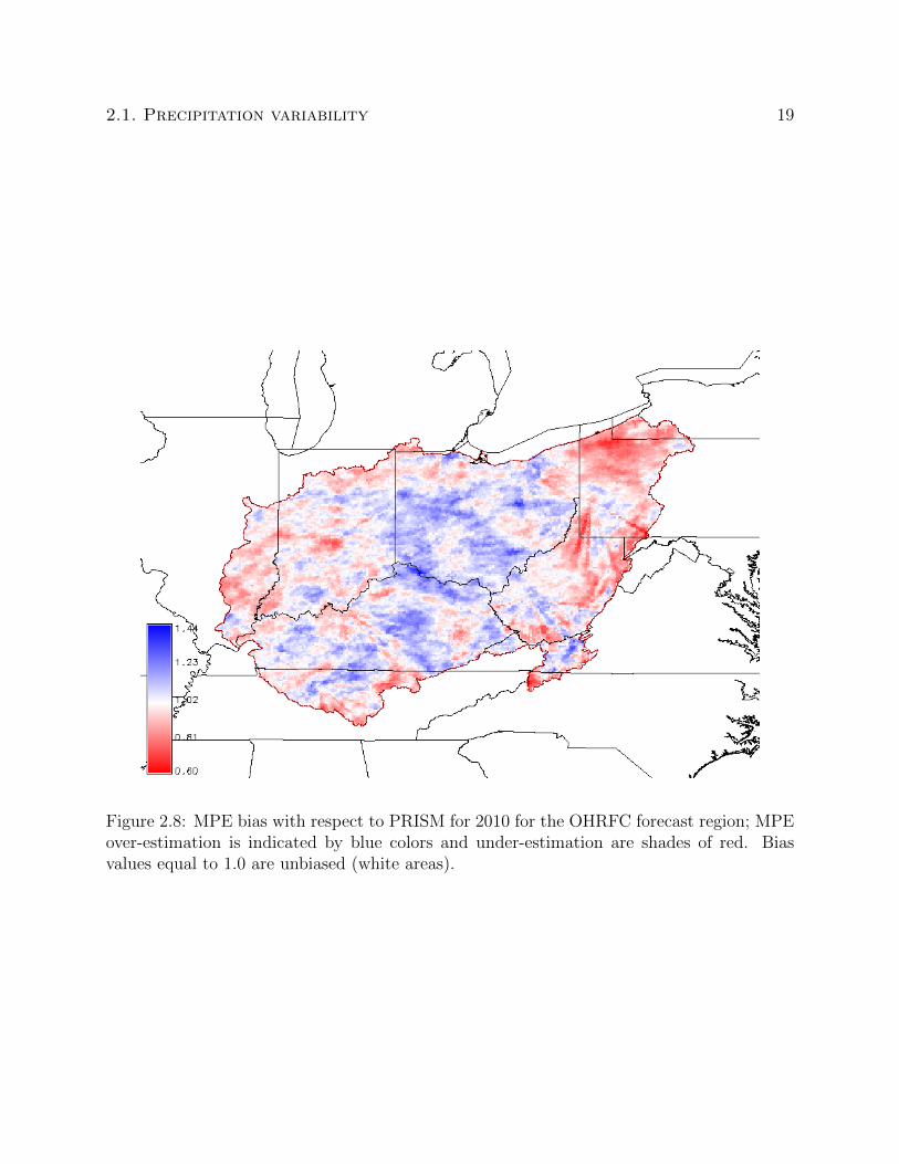
2.1. Precipitation variability 19
Figure 2.8: MPE bias with respect to PRISM for 2010 for the OHRFC forecast region; MPEover-estimation is indicated by blue colors and under-estimation are shades of red. Biasvalues equal to 1.0 are unbiased (white areas).
20 Chapter 2. Literature Review
QPF methods to meet the needs of hydrologic prediction. Unfortunately, as recently as 1998
Gaudet and Cotton [81] report that ”precipitation is notorious for being difficult to predict
accurately”.
Recently Ebert et al. [65] studied QPF performance of General Circulation Models (GCMs)
from the National Centers for Environmental Prediction (NCEP) in the United States, the
Deutscher Wetterdienst (DWD) in Germany, and the Bureau of Meteorology Research Cen-
tre (BMRC) in Australia for the period 1997 through 2000. This work was done within
auspices of the Working Group on Numerical Experimentation (WGNE), established under
the World Meteorological Organisation’s World Climate Research Programme (WCRP) and
Commission for Atmospheric Sciences (CAS). They report that QPFs produced by NWPs
easily outperformed persistence and provided useful routine guidance, but the forecasts, also,
were far from perfect. Ebert et al. [65] also found that the predicted rainfall of models is
highly sensitive to the predicted atmospheric and surface conditions, imply that a good rain-
fall forecast points to a good forecast of other atmospheric variables. On the other hand, a
bad rainfall forecast may have little to do with the model parameterization for precipitation,
but yet me be much more a function of how a NWP is tuned to optimize model performance
of other variables. They state:
“The process of improving model numerics and physics is a complicated jug-
gling act. Unless the accurate prediction of rainfall is made a top priority then
improvements in NWP model QPF will continue to be realized slowly.”
Buizza [31] performed an experiment to test the magnitude of QPF errors resulting from
initial conditions alone with forecasts of rainfall over Australia during January and July
1998 from the European Centre for Medium-Range Forecasts (ECMWF) Ensemble Prediction
System (EPS) for 24- and 48-hr forecasts. Results showed that most of the difference in
2.2. Ensemble Hydrologic Forecasting 21
performance between what is currently achieved in skill and perfect QPF skill could be
eliminated with a perfect model. This suggests that, by far, errors in the model initial
conditions were far less important than the errors induced by current model numerics and
physics in QPF skill. Ebert et al. [65] draw some important conclusions, stating:
“. . . one of the most promising and practical ways to improve quantitative precip-
itation forecasting using existing NWP models is the use of ensembles to generate
multiple rain scenarios and probabilistic forecasts.”
and continues by saying:
“While improvements in our understanding of rainfall process, numerical models,
and data assimilation are important steps toward improving quantitative precip-
itation forecasting, ensemble prediction may offer the most effective means of
making best use of the imperfect QPFs available to us at present.”
Work by Stensrud et al. [168], Wandishin et al. [178], and Ebert [64] have shown the utility
of NWP model ensembles of QPF.
2.2 Ensemble Hydrologic Forecasting
There has been considerable research into probabilistic methods to quantify hydrologic fore-
cast uncertainty (see for example, Buizza [31], Wandishin et al. [178], Franz et al. [77],
National Research Council [133], Schaake et al. [157], and Adams and Ostrowski [1]).
Probabilistic hydrologic forecasting addresses the inherent uncertainties found in determinis-
tic forecasting discussed in previous sections, ranging from short lead-time (1-7 days) to long
22 Chapter 2. Literature Review
lead-time (monthly, seasonal, and annual) temporal scales. For short lead-time probabilistic
forecasting, Krzysztofowicz [111] proposed a Bayesian approach while others have employed
monte carlo methods utilizing variations of ensemble methodologies, such as Adams and
Ostrowski [1] with the MMEFS, Demargne et al. [58] with the Hydrologic Ensemble Forecast
Service (HEFS), as part of the Advanced Hydrologic Prediction Service, and Werner et al.
[183] with medium-range meteorological ensemble inputs of temperature and precipitation
derived from the NCEP Medium-Range Forecast (MRF) model. Example output from such
an ensemble hydrologic forecast system is shown in Figure 2.9 for the OHRFC MMEFS
NAEFS, for the Greenbrier River at Alderson, WV, for the period March 1-7, 2015. Hydro-
logic model inputs for the MMEFS are forecasted mean areal precipitation and temperature
time-series derived from output grids from numerical weather prediction (NWP) models
comprising the NOAA/NWS National Centers for Environmental Prediction (NCEP) North
American Ensemble Forecast System (NAEFS) [35] and Short Range Ensemble Forecast Sys-
tem (SREF) [62]. A recent review by Cloke and Pappenberger [40] describes features of many
recently implemented medium-range lead-time ensemble hydrologic forecast systems. Sid-
dique and Mejia [162] and Alfieri et al. [10], further illustrate regional and global systems,
respectively, for ensemble hydrologic forecasting. These forecasting systems have been im-
plemented for the issuance of routine flood alerts and warnings and broader water resources
applications, important in reservoir and drought management (Hamlet et al. [88]; Raff et al.
[146]; Anghileri et al. [14]; Turner et al. [175]).
International efforts in ensemble hyrometeorological modeling include The Observing Sys-
tem Research and Predictability Experiment (THORPEX) Interactive Grand Global Ensem-
ble (TIGGE) project, which includes as one of its primary goals ”facilitate exploring the
concept and benefits of multimodel probabilistic weather forecasts, with a particular fo-
cus on high-impact weather prediction” [22]. Hydrological Ensemble Prediction Experiment
2.2. Ensemble Hydrologic Forecasting 23
a b
c d
Figure 2.9: Example ensemble hydrologic forecast from the NOAA/NWS MMEFS usingNAEFS ensemble (a) temperature and (b) precipitation inputs, producing (c) snow waterequivalent (SWE) from the NOAA/NWS SNOW-17 model and (d) hydrologic stage/dis-charge forecasts from the SAC-SMA rainfall-runoff model within the CHPS-FEWS forecastsystem at the OHRFC for the Greenbrier River at Alderson, WV, for the period March 1-7,2015.
24 Chapter 2. Literature Review
(HEPEX; www.hepex.org/), launched in 2004, has facilitated communication and collab-
oration among the atmospheric and hydrologic communities, including involvement from
forecast users with goals of improving ensemble forecasts and demonstrating their utility in
decision making in water management.
Pioneering development of ensemble hydrologic forecasting methodologies for water resources
is described by Twedt et al. [176] and Day [51] with, what was called at that time, Extended
Streamflow Prediction (ESP) within the NWS River Forecast System (NWSRFS). The initial
development and application of ESP methodology is chronicled in ”Tracing The Origins of
ESP”2. For long lead-time predictions at NWS RFCs, ESP utilizes basin averaged historical
temperature and precipitation time-series as surrogates for possible future hydrologic model
forcings for the generation of ensemble monthly, seasonal, and annual streamflow forecasts.
An example of ESP output for exceedance probability in the OHRFC area for the Ohio River
at Golconda, IL is shown in Figure 2.10. A few points of interest are:
1. that the two conditional simulations (CS), conditional because of their dependence on
initial basin conditions, show high-exceedance probability values beginning at a stage
of 38.2 feet, reflecting that initial flow conditions for the Ohio River are at that level;
2. both conditional simulations are shifted to the right of the historical simulation (HS)3,
which implies that there is a lower probability of attaining a given stage/flow level.
This, in turn, implies that the basin conditions are drier than normal4, relative to the
historical simulation;
3. the CS (black) utilizing NOAA/NWS Climate Prediction Center (CPC) climate ad-
2April 26, 2016 by Andy Wood, https://hepex.irstea.fr/tracing-the-origins-of-esp/.3A historical simulation is made as a single, continuous model simulation at the beginning of the historical
record for precipitation and temperature time-series through the most recent available data, at the 1- or 6-hour model time step, utilizing all model components in the forecast system.
4Observed antecedent rainfall that had occurred weeks and months prior to the ESP run also showedless-than-normal rainfall.

2.2. Ensemble Hydrologic Forecasting 25
justments is shifted to the right of the CS (green), which does not utilize CPC climate
adjustments, thus implying drier future conditions.
Item (3) points to the need that, for longer lead-time forecasts, the influence of predictable,
climate-scale meteorological features should be included in hydrological forecasts5, such as
El Nino–Southern Oscillation (ENSO) and, the cooling phase, La Nina effects (Werner et al.
[183]; Wood and Lettenmaier [188], Moradkhani and Meier [127]; Bastola et al. [16]; Forzieri
et al. [75]; Bradley et al. [25]; Beckers et al. [17]; Mendoza et al. [122]; Crochemore et al.
[42]). For OHRFC AHPS monthly and seasonal streamflow forecasts, CPC near term climate
adjustments of historical precipitation and temperature time-series are made prior to use in
ESP simulations to reflect wetter/dryer or warmer/cooler future conditions that are associ-
ated with climate influences. For short lead-time hydrologic forecasts climate influences are
minimal, but other factors are important, such as initial basin conditions or model structure
that lead to systematic biases. Considerable research can be found on these topics (Ebtehaj
et al. [66]; DeChant and Moradkhani [52], Zalachori et al. [198], DeChant and Moradkhani
[53]).
Franz et al. [77], Demargne et al. [56], Demargne et al. [57], DeChant and Moradkhani [54],
and others have identified the need for bias correction and correction of ensemble spread
of hydrologic ensemble forecasts. Wood and Schaake [190] and Bogner and Pappenberger
[20] discuss methods for correcting hydrologic ensemble forecast bias and reliability errors.
Consequently there has been considerable effort to develop methodologies to address hy-
drologic ensemble biases and spread using pre- and post-processing techniques. Zhao et al.
[203] evaluated the performance of a statistical post-processor for imperfect hydrologic model
forecasts and show that a proposed General Linear Model (GLM) Post-Processor (GLMPP),
5Chapman Conference (2013) on Seasonal to Interannual Hydroclimate Forecasts, http://chapman.agu.org/watermanagement/files/2013/07/Final-Program1.pdf.
26 Chapter 2. Literature Review
Figure 2.10: Probability of exceedance for OHRFC AHPS/ESP ensemble hydrologic forecastfor the Ohio River at Golconda, IL, March 11 – June 6, 2007, showing historical simulation(HS, blue), conditional simulation without CPC climate adjustments (CS, green), and condi-tional simulation with CPC climate adjustments (CS, black). The orange region designatesabove Minor Flood level and red above Moderate Flood level.

2.2. Ensemble Hydrologic Forecasting 27
built using data from the calibration period, removes the mean bias when applied to hydro-
logic model simulations from both the calibration and verification periods. Li et al. [116]
present a comprehensive review of commonly used statistical post-processing methods for
meteorological and hydrological forecasts. Sharma et al. [161] propose a method for prepro-
cessing ensemble precipitation forecasts for hydrologic forecasting, finding greater skill than
the raw forecasts.
Ensemble pre-processing methods and hydrologic hindcast experiments proposed by De-
margne et al. [58] are specifically aimed at bias correction of forecast meteorological inputs
and quantification of hydrologic model error, respectively. For the purposes of the proposed
research, no pre- or post-processing or bias-correction techniques will be utilized. The reason
for this is that applying such techniques could obfuscate the underlying goal of the research,
which is to assess the whether or not ensemble hydrologic mean or mean forecasts are supe-
rior to current deterministic forecasts. The literature shows that the application of various
methodologies will improve ensemble forecasts; this is known. Making use of such techniques
in the proposed research could cause confusion as to whether the outcomes resulted from
the underlying hypothesis or the use of bias correction or some other pre- or post-processing
methodology.
Chapter 3
Hydrometeorological Forcing Errors
for a Real-time Flood Forecast
System in the Ohio River Valley, USA
3.1 Abstract
Errors in hydrometeorological forcings for hydrologic modeling lead to considerable predic-
tion uncertainty of hydrologic variables. Analyses of Quantitative Precipitation Estimate
(QPE) and Quantitative Precipitation Forecast (QPF) errors over the Ohio River Valley
were made to quantify QPE and QPF errors and identify hydrologic impacts of forcing
errors and possible improvements resulting from advancements in precipitation estimation
and forecasting. Monthly, seasonal, and annual bias analyses of Ohio River Forecast Center
(OHRFC) NEXt-generation RADar (NEXRAD) based Stage III and Multisensor Precipi-
tation Estimator (MPE) precipitation estimates, for the period 1997-2016, were made with
respect to Parameter-elevation Regressions on Independent Slopes Model (PRISM) precipita-
28
3.2. Introduction 29
tion estimates. Verification of QPF from NWS River Forecast Centers from the NOAA/NWS
National Precipitation Verification Unit (NPVU) was compared to QPF verification mea-
sures from several numerical weather prediction models and the NOAA/NWS Weather Pre-
diction Center (WPC). Improvements in NEXRAD based QPE over the OHRFC area have
been dramatic from 1997 to present. However, from the perspective of meeting hydrologic
forecasting needs, QPF shows marginal improvement. A hydrologic simulation experiment
illustrates the sensitivity of hydrologic forecasts to QPF errors based on Threat Score (TS).
Experiments show there is considerable hydrologic forecast error associated with QPF at ex-
pected WPC TS levels and, importantly, that higher TS values do not necessarily translate
into improved hydrologic simulation results.
3.2 Introduction
Hydrologic forecast accuracy is largely dependent on the magnitude of measurement and pre-
diction errors of hydrometeorological forcings used as model inputs (Maurer and Lettenmaier
[119]; Tetzlaff and Uhlenbrook [173]; Benke et al. [18]; Wood and Lettenmaier [189]; New-
man et al. [137]). As early as 1969, research by Fogel [74] quantified differences in watershed
runoff due to rainfall variability, using a dense raingauge network for the Atterbury experi-
mental watershed in Arizona. More recently, using distributed precipitation inputs, Wilson
et al. [186] and Faures et al. [72] demonstrated that large variations in modeled watershed
runoff can result from spatially variable rainfall, on the order of 9 to 76% for peak runoff
rates and 2 to 65% for runoff volume, for a 4.4 ha semiarid catchment [72]. Also utilizing
dense raingauge networks, Jones and Wendland [98], Goodrich et al. [84], and Zhang et al.
[201] report the occurrence of significant rainfall variability over short distances (100-1000
m) which, with gridded precipitation fields, would be considered the subgrid scale.
30Chapter 3. Hydrometeorological Forcing Errors for a Real-time Flood
Forecast System in the Ohio River Valley, USA
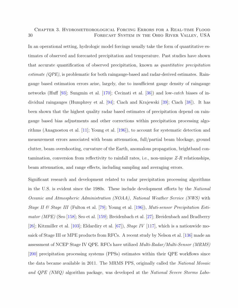
In an operational setting, hydrologic model forcings usually take the form of quantitative es-
timates of observed and forecasted precipitation and temperature. Past studies have shown
that accurate quantification of observed precipitation, known as quantitative precipitation
estimate (QPE), is problematic for both raingauge-based and radar-derived estimates. Rain-
gauge based estimation errors arise, largely, due to insufficient gauge density of raingauge
networks (Huff [93]; Sungmin et al. [170]; Cecinati et al. [36]) and low-catch biases of in-
dividual raingauges (Humphrey et al. [94]; Ciach and Krajewski [39]; Ciach [38]). It has
been shown that the highest quality radar based estimates of precipitation depend on rain-
gauge based bias adjustments and other corrections within precipitation processing algo-
rithms (Anagnostou et al. [11]; Young et al. [196]), to account for systematic detection and
measurement errors associated with beam attenuation, full/partial beam blockage, ground
clutter, beam overshooting, curvature of the Earth, anomalous propagation, brightband con-
tamination, conversion from reflectivity to rainfall rates, i.e., non-unique Z-R relationships,
beam attenuation, and range effects, including sampling and averaging errors.
Significant research and development related to radar precipitation processing algorithms
in the U.S. is evident since the 1980s. These include development efforts by the National
Oceanic and Atmospheric Administration (NOAA), National Weather Service (NWS) with
Stage II & Stage III (Fulton et al. [79]; Young et al. [196]), Muti-sensor Precipitation Esti-
mator (MPE) (Seo [158]; Seo et al. [159]; Breidenbach et al. [27]; Breidenbach and Bradberry
[26]; Kitzmiller et al. [103]; Eldardiry et al. [67]), Stage IV [117], which is a nationwide mo-
saick of Stage III or MPE products from RFCs. A recent study by Nelson et al. [136] made an
assessment of NCEP Stage IV QPE. RFCs have utilized Multi-Radar/Multi-Sensor (MRMS)
[200] precipitation processing systems (PPSs) estimates within their QPE workflows since
the data became available in 2011. The MRMS PPS, originally called the National Mosaic
and QPE (NMQ) algorithm package, was developed at the National Severe Storms Labo-

3.2. Introduction 31
ratory (NSSL) and subsequently moved to the NOAA National Centers for Environmental
Prediction (NCEP) for operational support of NWS River Forecast Centers (RFCs), shown
in Figure 3.1, and Weather Forecast Offices (WFOs).
In western regions of the U.S., where radar beam blockage is problematic in mountainous
areas, NWS estimation methods rely on data from raingauge and Natural Resources Conser-
vation Service (NRCS), Snow Telemetry (SNOTEL) networks for precipitation estimation.
Gauge data are processed at RFCs, using spatial interpolation algorithms and historical data,
such as Parameter-elevation Relationships on Independent Slopes Model (PRISM) (Taylor
et al. [171]; Taylor et al. [172]; Daly et al. [47]), within the Advanced Weather Interactive Pro-
cessing System (AWIPS), to generate gridded estimates of precipitation utilizing Mountain
Mapper and Data QC [156].
Difficulties with the prediction of future precipitation, referred to as quantitative precipi-
tation forecast (QPF), are compounded by the need to accurately predict occurrences of
heavy precipitation accumulations spatially. That is, the location of flood producing rainfall
matters significantly, which is demonstrably evident with flash flood scale events, where the
occurrence of excessive rainfall, accompanied by flooding, can be hit-or-miss over very short
distances with devastating outcomes (Smith et al. [163]; Baeck and Smith [15]; Smith et al.
[164]; Borga et al. [21]; Alfieri et al. [9]; Broxton et al. [30]).
With winter time storms, errors in temperature estimation and prediction can incorrectly
identify the physical state of hydrometeors, suggesting the occurrence of rainfall rather than
snowfall, or the reverse [180]. Mizukami et al. [125] and Hunter and Holroyd [95] discuss the
implications of mis-typing the physical state of precipitation (rain, snow, ice, hail, etc.) and
how such errors lead directly to hydrologic forecast error. Moine et al. [126], Rossler et al.
[154], and Wayand [179] show that errors in the estimation of snow accumulation and snow
water equivalent (SWE) become especially problematic during rain-on-snow and significant

32Chapter 3. Hydrometeorological Forcing Errors for a Real-time Flood
Forecast System in the Ohio River Valley, USA
APRFC
CNRFC MARFC
NERFC
MBRFC
CBRFC
NWRFC
ABRFC
WGRFCSERFC
OHRFC
NCRFC
LMRFC
Figure 3.1: The NWS 13 River Forecast Centers (RFCs) – Alaska/Pacific RFC(APRFC), Arkansas-Red RFC (ABRFC), Colorado Basin RFC (CBRFC), California-NevadaRFC(CNRFC), Lower-Mississippi RFC (LMRFC)Middle Atlantic RFC (MARFC), MissouriBasin RFC (MBRFC), North Central RFC (NCRFC), Northwest RFC (NWRFC), OhioRFC (OHRFC), Southeast RFC (SERFC), and West Gulf RFC (WGRFC). Please notethat several RFC boundaries extend beyond the U.S. national boundary into Canada andMexico.

3.2. Introduction 33
temperature-driven snowmelt events. With temperature-index based snow models, such as
the NWS Snow Accumulation and Ablation model, SNOW-17 [12], used by NWS RFCs,
erroneous temperature estimates can lead to inaccurate snowmelt rates. The effects of wind,
terrain, and vegetation on snow estimation (Winstral et al. [187]; Essery and Pomeroy [69])
and modeling (Essery et al. [70]; Xiao et al. [195]; Bowling et al. [23]; Liston and Elder [118])
are significant as well.
Thiboult et al. [174] identify three broad sources of of total hydrologic forecast uncertainty,
namely (1) model structure, (2) model state initial conditions (such as initial soil moisture,
snow water equivalent, streamflow, etc.), and (3) forcing uncertainties. The focus of this
study are the latter two sources of hydrologic forecast uncertainty. Specifically, first, we
analyze QPE and QPF errors over the NOAA/NWS Ohio River Forecast Center (OHRFC)
area of responsibility, shown in Figure 3.1, and, second, the hydrologic modeling and forecast
error produced in response to QPE and QPF forcing errors. The OHRFC region was selected
for this study because of the availability of data. Section 3.3 examines the spatial bias pat-
terns of Stage III/MPE precipitation estimates and changes over time for the OHRFC area.
A historical simulation using Stage III/MPE precipitation estimates as the principal model
forcing, demonstrates improvements in hydrologic model simulation resulting from changes
in precipitation estimation. Section 3.4 presents results of WPC and NOAA/NWS National
Precipitation Verification Unit (NPVU) QPF verification. Additionally, the implications to
hydrologic forecast uncertainty are examined with respect to past and current expected levels
of QPF accuracy, using a hydrologic monte carlo simulation experiment. A summary and
discussion of the limitations of the work, as well as implications to hydrologic forecasting,
and final conclusions are presented in section 3.5.

34Chapter 3. Hydrometeorological Forcing Errors for a Real-time Flood
Forecast System in the Ohio River Valley, USA
3.3 QPE biases
The OHRFC, shown in Figure 3.1, has produced radar-based precipitation estimates derived
from the NEXRAD network of Weather Surveillance Radar-1988 Doppler (WSR-88D) radars
[43] since 1996. NEXRAD radars utilized by the OHRFC are shown in Figure 3.2 and
are listed in Table 3.1. However, use of NEXRAD data as model forcings for operational
hydrologic forecasting did not begin immediately due to significant changes in the OHRFC
operational hydrological environment, which included operational implementation of the
Advanced Weather Interactive Processing System (AWIPS) [140] and the NWS River Forecast
System (NWSRFS) (U.S. Department of Commerce [177]; Adams [5]).
3.3.1 History
Although Stage II/III products were generated beginning in 1996 at the OHRFC, these data
were not used in hydrologic forecast operations until 1998. A timeline of the period of use
of Stage II & III and MPE by the OHRFC is shown in Figure 3.3. Stage II & III and MPE
estimates are generated from the individual radars to produce mosaicked, gridded precipita-
tion fields within the NWS Hydrologic Rainfall Analysis Project (HRAP) polar stereographic
projection grid, which is described by Fulton [78] and Reed and Maidment [151]. Significant
changes to the NEXRAD PPS at RFCs followed Stage II & III implementation. With the
development of MRMS [200] at NSSL, the OHRFC and other RFCs began use of MRMS
precipitation estimates in late 2012 as the initial step in MPE precipitation processing, which
includes manual, interactive quality control by hydrometeorological forecasters using AWIPS
MPE software.
An early significant MPE improvement, identified in Figure 3.3, was the correction of an
algorithmic error that produced truncated rain-rate values, leading to precipitation under-
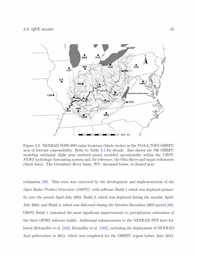
3.3. QPE biases 35
Figure 3.2: NEXRAD WSR-88D radar locations (black circles) in the NOAA/NWS OHRFCarea of forecast responsibility. Refer to Table 3.1 for details. Also shown are 796 OHRFCmodeling subbasins (light gray outlined areas) modeled operationally within the CHPS-FEWS hydrologic forecasting system and, for reference, the Ohio River and major tributaries(black lines). The Greenbrier River basin, WV, discussed below, is shaded gray.
estimation [80]. This error was corrected by the development and implementation of the
Open Radar Product Generator (ORPG), with software Build 1 which was deployed primar-
ily over the period April-July 2002, Build 3, which was deployed during the months April-
July 2003, and Build 4, which was delivered during the October-December 2003 period [80].
ORPG Build 1 contained the most significant improvements to precipitation estimation of
the three OPRG software builds. Additional enhancements to the NEXRAD PPS have fol-
lowed (Kitzmiller et al. [102]; Kitzmiller et al. [103]), including the deployment of NEXRAD
dual polarization in 2011, which was completed for the OHRFC region before June 2013.
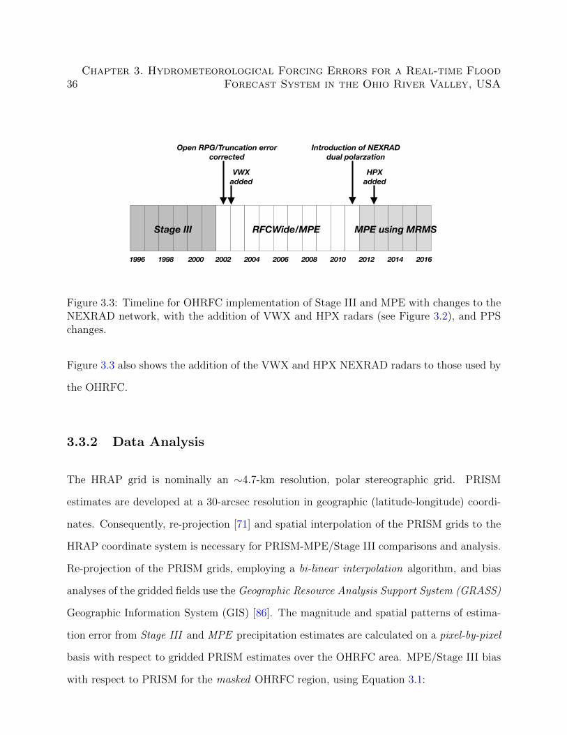
36Chapter 3. Hydrometeorological Forcing Errors for a Real-time Flood
Forecast System in the Ohio River Valley, USA
1996 1998 2000 2002 2004 2006 2008 2010 2012 2014 2016
Stage III RFCWide/MPE MPE using MRMS
Open RPG/Truncation errorcorrected
VWXadded
HPXadded
Introduction of NEXRADdual polarzation
Figure 3.3: Timeline for OHRFC implementation of Stage III and MPE with changes to theNEXRAD network, with the addition of VWX and HPX radars (see Figure 3.2), and PPSchanges.
Figure 3.3 also shows the addition of the VWX and HPX NEXRAD radars to those used by
the OHRFC.
3.3.2 Data Analysis
The HRAP grid is nominally an ∼4.7-km resolution, polar stereographic grid. PRISM
estimates are developed at a 30-arcsec resolution in geographic (latitude-longitude) coordi-
nates. Consequently, re-projection [71] and spatial interpolation of the PRISM grids to the
HRAP coordinate system is necessary for PRISM-MPE/Stage III comparisons and analysis.
Re-projection of the PRISM grids, employing a bi-linear interpolation algorithm, and bias
analyses of the gridded fields use the Geographic Resource Analysis Support System (GRASS)
Geographic Information System (GIS) [86]. The magnitude and spatial patterns of estima-
tion error from Stage III and MPE precipitation estimates are calculated on a pixel-by-pixel
basis with respect to gridded PRISM estimates over the OHRFC area. MPE/Stage III bias
with respect to PRISM for the masked OHRFC region, using Equation 3.1:
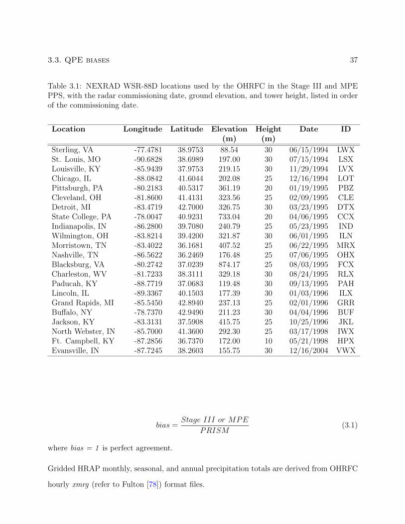
3.3. QPE biases 37
Table 3.1: NEXRAD WSR-88D locations used by the OHRFC in the Stage III and MPEPPS, with the radar commissioning date, ground elevation, and tower height, listed in orderof the commissioning date.
Location Longitude Latitude Elevation Height Date ID(m) (m)
Sterling, VA -77.4781 38.9753 88.54 30 06/15/1994 LWXSt. Louis, MO -90.6828 38.6989 197.00 30 07/15/1994 LSXLouisville, KY -85.9439 37.9753 219.15 30 11/29/1994 LVXChicago, IL -88.0842 41.6044 202.08 25 12/16/1994 LOTPittsburgh, PA -80.2183 40.5317 361.19 20 01/19/1995 PBZCleveland, OH -81.8600 41.4131 323.56 25 02/09/1995 CLEDetroit, MI -83.4719 42.7000 326.75 30 03/23/1995 DTXState College, PA -78.0047 40.9231 733.04 20 04/06/1995 CCXIndianapolis, IN -86.2800 39.7080 240.79 25 05/23/1995 INDWilmington, OH -83.8214 39.4200 321.87 30 06/01/1995 ILNMorristown, TN -83.4022 36.1681 407.52 25 06/22/1995 MRXNashville, TN -86.5622 36.2469 176.48 25 07/06/1995 OHXBlacksburg, VA -80.2742 37.0239 874.17 25 08/03/1995 FCXCharleston, WV -81.7233 38.3111 329.18 30 08/24/1995 RLXPaducah, KY -88.7719 37.0683 119.48 30 09/13/1995 PAHLincoln, IL -89.3367 40.1503 177.39 30 01/03/1996 ILXGrand Rapids, MI -85.5450 42.8940 237.13 25 02/01/1996 GRRBuffalo, NY -78.7370 42.9490 211.23 30 04/04/1996 BUFJackson, KY -83.3131 37.5908 415.75 25 10/25/1996 JKLNorth Webster, IN -85.7000 41.3600 292.30 25 03/17/1998 IWXFt. Campbell, KY -87.2856 36.7370 172.00 10 05/21/1998 HPXEvansville, IN -87.7245 38.2603 155.75 30 12/16/2004 VWX
bias =Stage III or MPE
PRISM(3.1)
where bias = 1 is perfect agreement.
Gridded HRAP monthly, seasonal, and annual precipitation totals are derived from OHRFC
hourly xmrg (refer to Fulton [78]) format files.
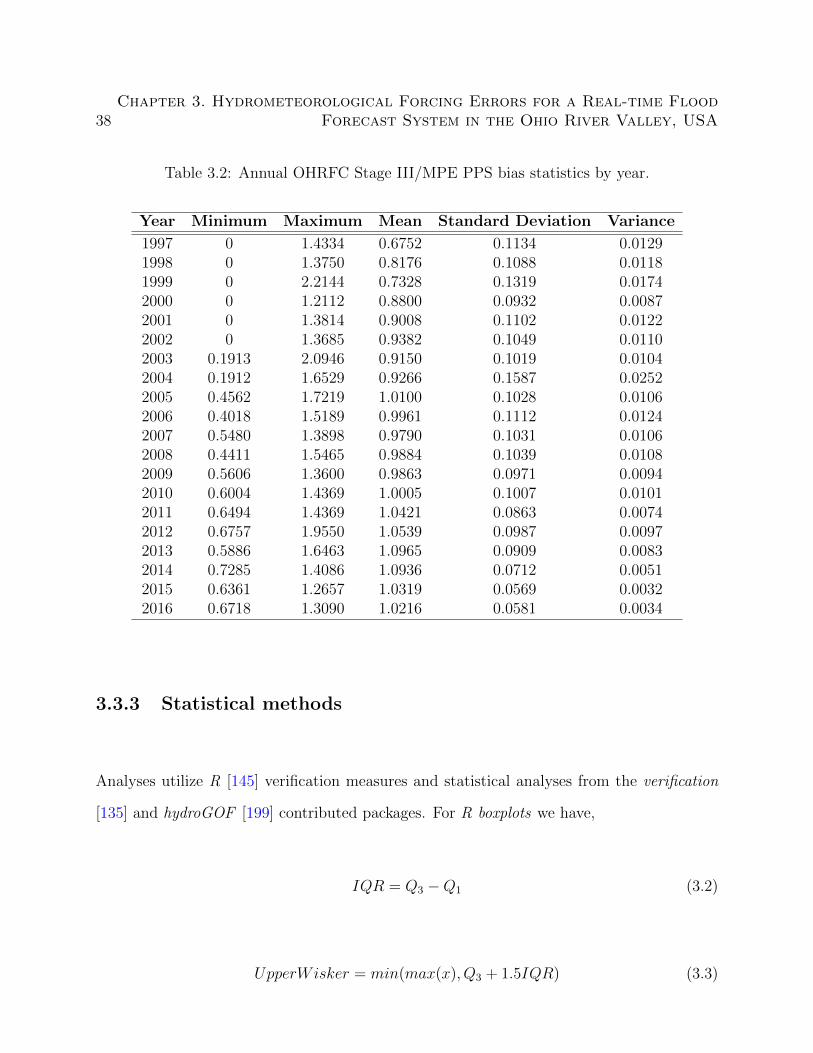
38Chapter 3. Hydrometeorological Forcing Errors for a Real-time Flood
Forecast System in the Ohio River Valley, USA
Table 3.2: Annual OHRFC Stage III/MPE PPS bias statistics by year.
Year Minimum Maximum Mean Standard Deviation Variance
1997 0 1.4334 0.6752 0.1134 0.01291998 0 1.3750 0.8176 0.1088 0.01181999 0 2.2144 0.7328 0.1319 0.01742000 0 1.2112 0.8800 0.0932 0.00872001 0 1.3814 0.9008 0.1102 0.01222002 0 1.3685 0.9382 0.1049 0.01102003 0.1913 2.0946 0.9150 0.1019 0.01042004 0.1912 1.6529 0.9266 0.1587 0.02522005 0.4562 1.7219 1.0100 0.1028 0.01062006 0.4018 1.5189 0.9961 0.1112 0.01242007 0.5480 1.3898 0.9790 0.1031 0.01062008 0.4411 1.5465 0.9884 0.1039 0.01082009 0.5606 1.3600 0.9863 0.0971 0.00942010 0.6004 1.4369 1.0005 0.1007 0.01012011 0.6494 1.4369 1.0421 0.0863 0.00742012 0.6757 1.9550 1.0539 0.0987 0.00972013 0.5886 1.6463 1.0965 0.0909 0.00832014 0.7285 1.4086 1.0936 0.0712 0.00512015 0.6361 1.2657 1.0319 0.0569 0.00322016 0.6718 1.3090 1.0216 0.0581 0.0034
3.3.3 Statistical methods
Analyses utilize R [145] verification measures and statistical analyses from the verification
[135] and hydroGOF [199] contributed packages. For R boxplots we have,
IQR = Q3 −Q1 (3.2)
UpperWisker = min(max(x), Q3 + 1.5IQR) (3.3)
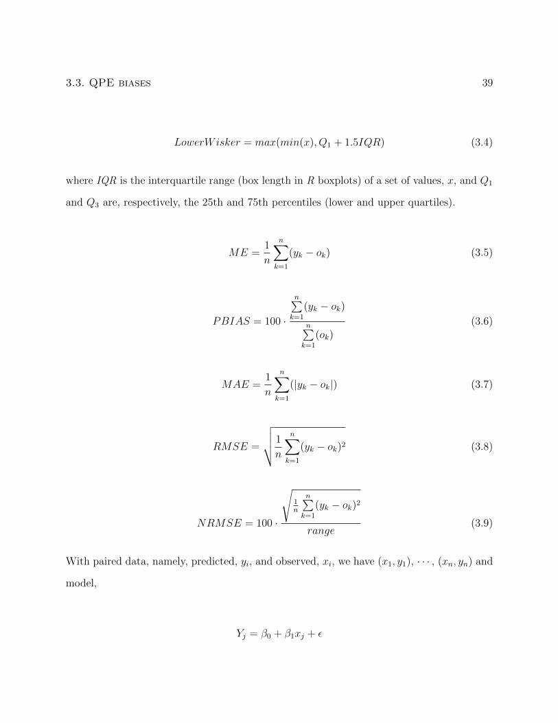
3.3. QPE biases 39
LowerWisker = max(min(x), Q1 + 1.5IQR) (3.4)
where IQR is the interquartile range (box length in R boxplots) of a set of values, x, and Q1
and Q3 are, respectively, the 25th and 75th percentiles (lower and upper quartiles).
ME =1
n
n∑k=1
(yk − ok) (3.5)
PBIAS = 100 ·
n∑k=1
(yk − ok)
n∑k=1
(ok)(3.6)
MAE =1
n
n∑k=1
(|yk − ok|) (3.7)
RMSE =
√√√√ 1
n
n∑k=1
(yk − ok)2 (3.8)
NRMSE = 100 ·
√1n
n∑k=1
(yk − ok)2
range(3.9)
With paired data, namely, predicted, yi, and observed, xi, we have (x1, y1), · · · , (xn, yn) and
model,
Yj = β0 + β1xj + ε
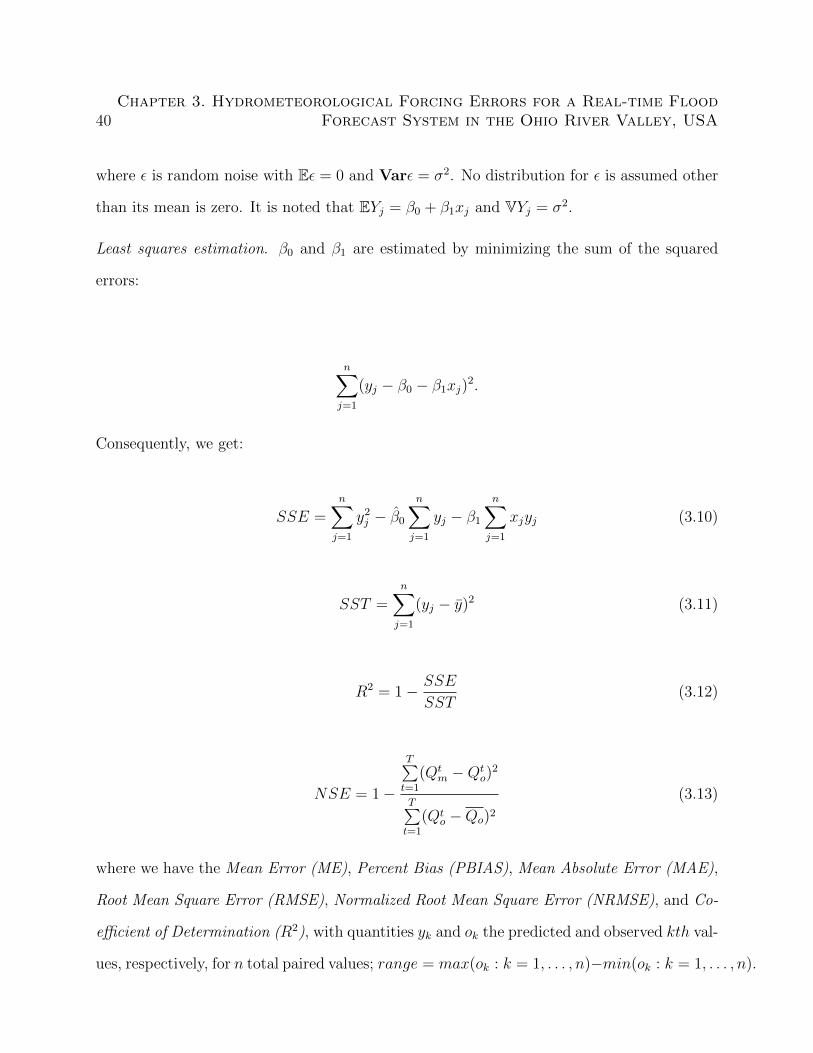
40Chapter 3. Hydrometeorological Forcing Errors for a Real-time Flood
Forecast System in the Ohio River Valley, USA
where ε is random noise with Eε = 0 and Varε = σ2. No distribution for ε is assumed other
than its mean is zero. It is noted that EYj = β0 + β1xj and VYj = σ2.
Least squares estimation. β0 and β1 are estimated by minimizing the sum of the squared
errors:
n∑j=1
(yj − β0 − β1xj)2.
Consequently, we get:
SSE =n∑
j=1
y2j − β0
n∑j=1
yj − β1
n∑j=1
xjyj (3.10)
SST =n∑
j=1
(yj − y)2 (3.11)
R2 = 1− SSE
SST(3.12)
NSE = 1−
T∑t=1
(Qtm −Qt
o)2
T∑t=1
(Qto −Qo)2
(3.13)
where we have the Mean Error (ME), Percent Bias (PBIAS), Mean Absolute Error (MAE),
Root Mean Square Error (RMSE), Normalized Root Mean Square Error (NRMSE), and Co-
efficient of Determination (R2), with quantities yk and ok the predicted and observed kth val-
ues, respectively, for n total paired values; range = max(ok : k = 1, . . . , n)−min(ok : k = 1, . . . , n).
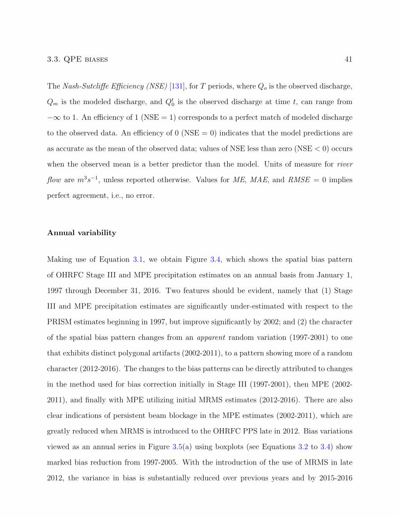
3.3. QPE biases 41
The Nash-Sutcliffe Efficiency (NSE) [131], for T periods, where Qo is the observed discharge,
Qm is the modeled discharge, and Qt0 is the observed discharge at time t, can range from
−∞ to 1. An efficiency of 1 (NSE = 1) corresponds to a perfect match of modeled discharge
to the observed data. An efficiency of 0 (NSE = 0) indicates that the model predictions are
as accurate as the mean of the observed data; values of NSE less than zero (NSE < 0) occurs
when the observed mean is a better predictor than the model. Units of measure for river
flow are m3s−1, unless reported otherwise. Values for ME, MAE, and RMSE = 0 implies
perfect agreement, i.e., no error.
Annual variability
Making use of Equation 3.1, we obtain Figure 3.4, which shows the spatial bias pattern
of OHRFC Stage III and MPE precipitation estimates on an annual basis from January 1,
1997 through December 31, 2016. Two features should be evident, namely that (1) Stage
III and MPE precipitation estimates are significantly under-estimated with respect to the
PRISM estimates beginning in 1997, but improve significantly by 2002; and (2) the character
of the spatial bias pattern changes from an apparent random variation (1997-2001) to one
that exhibits distinct polygonal artifacts (2002-2011), to a pattern showing more of a random
character (2012-2016). The changes to the bias patterns can be directly attributed to changes
in the method used for bias correction initially in Stage III (1997-2001), then MPE (2002-
2011), and finally with MPE utilizing initial MRMS estimates (2012-2016). There are also
clear indications of persistent beam blockage in the MPE estimates (2002-2011), which are
greatly reduced when MRMS is introduced to the OHRFC PPS late in 2012. Bias variations
viewed as an annual series in Figure 3.5(a) using boxplots (see Equations 3.2 to 3.4) show
marked bias reduction from 1997-2005. With the introduction of the use of MRMS in late
2012, the variance in bias is substantially reduced over previous years and by 2015-2016

42Chapter 3. Hydrometeorological Forcing Errors for a Real-time Flood
Forecast System in the Ohio River Valley, USA
median biases are close to 1. Results presented in Figure 3.5(b) for the Greenbrier River
basin, WV, identified in Figure 3.2, are discussed below.
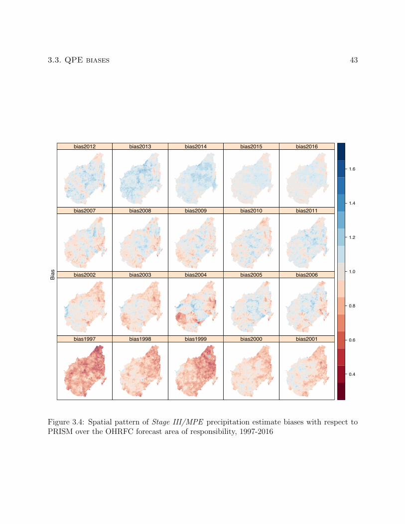
3.3. QPE biases 43Bias
bias1997 bias1998 bias1999 bias2000 bias2001
bias2002 bias2003 bias2004 bias2005 bias2006
bias2007 bias2008 bias2009 bias2010 bias2011
bias2012 bias2013 bias2014 bias2015 bias2016
0.4
0.6
0.8
1.0
1.2
1.4
1.6
Figure 3.4: Spatial pattern of Stage III/MPE precipitation estimate biases with respect toPRISM over the OHRFC forecast area of responsibility, 1997-2016

44Chapter 3. Hydrometeorological Forcing Errors for a Real-time Flood
Forecast System in the Ohio River Valley, USA
The change in annual Stage III/MPE bias is further illustrated in Figure 3.6 with bias density
plots, which shows a shift in mean bias, with significant underestimation in 1997, to nearly
unbiased estimates by 2015-2016, and a consistent reduction in bias spread from 1997 to
2016.
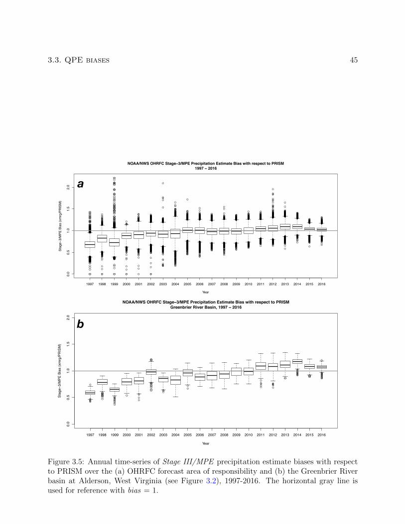
3.3. QPE biases 45
1997 1998 1999 2000 2001 2002 2003 2004 2005 2006 2007 2008 2009 2010 2011 2012 2013 2014 2015 2016
0.0
0.5
1.0
1.5
2.0
NOAA/NWS OHRFC Stage−3/MPE Precipitation Estimate Bias with respect to PRISM1997 − 2016
Year
Stag
e−3/
MPE
Bia
s (x
mrg
/PR
ISM
)
1997 1998 1999 2000 2001 2002 2003 2004 2005 2006 2007 2008 2009 2010 2011 2012 2013 2014 2015 2016
0.0
0.5
1.0
1.5
2.0
NOAA/NWS OHRFC Stage−3/MPE Precipitation Estimate Bias with respect to PRISMGreenbrier River Basin, 1997 − 2016
Year
Stag
e−3/
MPE
Bia
s (x
mrg
/PR
ISM
)
a
b
Figure 3.5: Annual time-series of Stage III/MPE precipitation estimate biases with respectto PRISM over the (a) OHRFC forecast area of responsibility and (b) the Greenbrier Riverbasin at Alderson, West Virginia (see Figure 3.2), 1997-2016. The horizontal gray line isused for reference with bias = 1.
46Chapter 3. Hydrometeorological Forcing Errors for a Real-time Flood
Forecast System in the Ohio River Valley, USA
Seasonal variability
Seasonal variability of MPE biases is presented for the years 2015 and 2016 only because these
years reflect current best estimates and PPS performance. Summer months are defined as
June-July-August (JJA) and winter months as December-January-February (DJF). Seasonal
bias values are calculated as monthly JJA and DJF averages using Equation 3.1. Figure 3.7
shows the summer and winter spatial bias patterns for 2015 and 2016. Bias patterns during
the summer months exhibit more of a random pattern compared to the winter months for
2015-2016. These differences are expected due to the prevalence of more isolated, convective
rainfall during the summer months and wide-spread, stratiform and synoptic-scale precipi-
tation during the winter months. Also evident during the 2015 and 2016 winter seasons is
widespread MPE over-estimation in central and east-central regions of the OHRFC forecast
area, quite possibly due to brightband influences (Gourley and Calvert [85]; Cunha et al.
[44]).
Clear differences are seen between winter and summer season biases for the 2015-2016 period
in Figure 3.8 with bias density plots. Summer biases are very close to 1 and, while winter
season biases are not much different from 1, with slight over-estimation, the spread in bias
values is much greater during the winter season compared to summer.
Monthly variability
The analysis of monthly MPE biases, using Equation 3.1, is based on monthly accumulations
of hourly xmrg HRAP gridded fields. The bias analysis is restricted to the years 2015 and
2016. Figure 3.9 shows significant month-to-month bias variability. Monthly median biases
are very close to unity, interquartile (25 to 75 percentile) differences are generally small,
but large outliers are evident. This points to the complex nature of both precipitation pro-
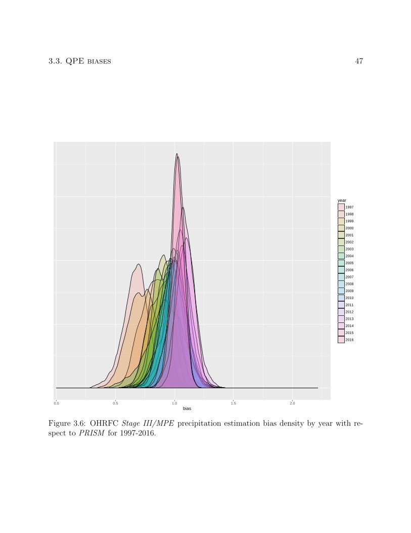
3.3. QPE biases 47
0
2
4
6
0.0 0.5 1.0 1.5 2.0
bias
dens
ity
year
1997
1998
1999
2000
2001
2002
2003
2004
2005
2006
2007
2008
2009
2010
2011
2012
2013
2014
2015
2016
Figure 3.6: OHRFC Stage III/MPE precipitation estimation bias density by year with re-spect to PRISM for 1997-2016.
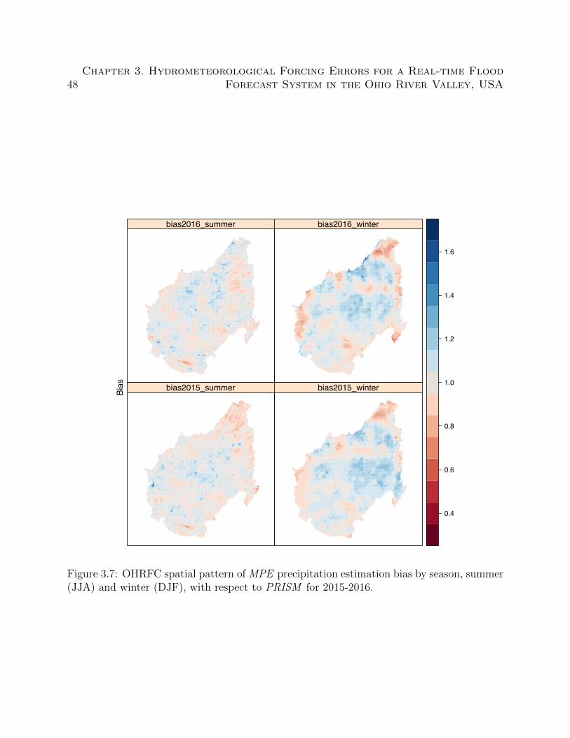
48Chapter 3. Hydrometeorological Forcing Errors for a Real-time Flood
Forecast System in the Ohio River Valley, USA
Bias bias2015_summer bias2015_winter
bias2016_summer bias2016_winter
0.4
0.6
0.8
1.0
1.2
1.4
1.6
Figure 3.7: OHRFC spatial pattern of MPE precipitation estimation bias by season, summer(JJA) and winter (DJF), with respect to PRISM for 2015-2016.
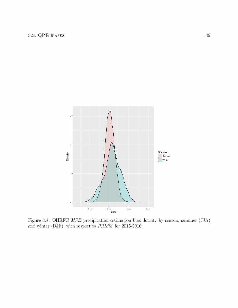
3.3. QPE biases 49
0
2
4
6
0.75 1.00 1.25 1.50
Bias
Den
sity Season
Summer
Winter
Figure 3.8: OHRFC MPE precipitation estimation bias density by season, summer (JJA)and winter (DJF), with respect to PRISM for 2015-2016.
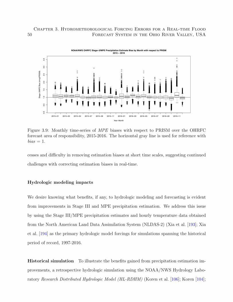
50Chapter 3. Hydrometeorological Forcing Errors for a Real-time Flood
Forecast System in the Ohio River Valley, USA
2015−01 2015−03 2015−05 2015−07 2015−09 2015−11 2016−01 2016−03 2016−05 2016−07 2016−09 2016−11
0.0
0.5
1.0
1.5
2.0
2.5
3.0
3.5
NOAA/NWS OHRFC Stage−3/MPE Precipitation Estimate Bias by Month with respect to PRISM2015 − 2016
Year−Month
Sta
ge−
3/M
PE
Bia
s (x
mrg
/PR
ISM
)
Figure 3.9: Monthly time-series of MPE biases with respect to PRISM over the OHRFCforecast area of responsibility, 2015-2016. The horizontal gray line is used for reference withbias = 1.
cesses and difficulty in removing estimation biases at short time scales, suggesting continued
challenges with correcting estimation biases in real-time.
Hydrologic modeling impacts
We desire knowing what benefits, if any, to hydrologic modeling and forecasting is evident
from improvements in Stage III and MPE precipitation estimation. We address this issue
by using the Stage III/MPE precipitation estimates and hourly temperature data obtained
from the North American Land Data Assimilation System (NLDAS-2) (Xia et al. [193]; Xia
et al. [194] as the primary hydrologic model forcings for simulations spanning the historical
period of record, 1997-2016.
Historical simulation To illustrate the benefits gained from precipitation estimation im-
provements, a retrospective hydrologic simulation using the NOAA/NWS Hydrology Labo-
ratory Research Distributed Hydrologic Model (HL-RDHM) (Koren et al. [106]; Koren [104];
3.3. QPE biases 51
Koren et al. [107]) is made. The historical simulation spans the full period (1997-2016) of
available Stage III/MPE, NEXRAD radar derived precipitation estimates. RDHM simula-
tions are made for the Greenbrier River basin in West Virginia, shown in Figure 3.2, with
the model defined at the HRAP grid resolution, using an hourly time-step. The Greenbrier
River basin defined at Alderson, WV (USGS 05050003), located in the valley and ridge
physiographic province of the Appalachian Mountains, has an area of 3533 km2, and ranges
in elevation from 466 to 1433 m. The basin was selected for study largely because of recent
major flooding in June 2016 and data availability. Retrospective RDHM simulations are
made without prior calibration to avoid biasing model performance to any model period.
In this way, model results will best reflect PPS improvements implemented at the OHRFC
without confounding influences from other factors. Initial, a priori, estimation of RDHM
Sacramento Soil Moisture Accounting (SAC-SMA) (Burnash et al. [34]; Burnash [33]) model
parameters is described by Koren et al. [105]. Parameter estimation includes 12 SAC-SMA
parameters and several channel routing parameters. RDHM simulations also include use of
the SNOW-17 snow accumulation and ablation model to account for wintertime precipita-
tion and snowmelt. SNOW-17 model parameters are also estimated and the model is used
uncalibrated.
RDHM model simulations begin June 1, 1996 from a cold state, that is, without prior model
state initialization that reflect existing basin conditions, using hourly NLDAS-2 precipitation
and temperature model inputs. OHRFC Stage III and MPE are used for the full period
January 1, 1997 to December 31, 2016. Verification of RDHM simulations is restricted to
the January 1998 to December 2016 period, to allow sufficient RDHM SAC-SMA model
warm-up, nearly 18 months.
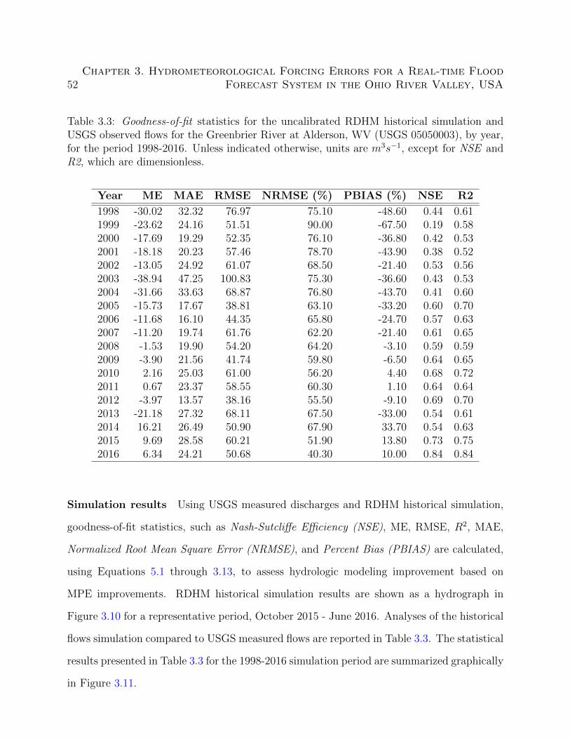
52Chapter 3. Hydrometeorological Forcing Errors for a Real-time Flood
Forecast System in the Ohio River Valley, USA
Table 3.3: Goodness-of-fit statistics for the uncalibrated RDHM historical simulation andUSGS observed flows for the Greenbrier River at Alderson, WV (USGS 05050003), by year,for the period 1998-2016. Unless indicated otherwise, units are m3s−1, except for NSE andR2, which are dimensionless.
Year ME MAE RMSE NRMSE (%) PBIAS (%) NSE R2
1998 -30.02 32.32 76.97 75.10 -48.60 0.44 0.611999 -23.62 24.16 51.51 90.00 -67.50 0.19 0.582000 -17.69 19.29 52.35 76.10 -36.80 0.42 0.532001 -18.18 20.23 57.46 78.70 -43.90 0.38 0.522002 -13.05 24.92 61.07 68.50 -21.40 0.53 0.562003 -38.94 47.25 100.83 75.30 -36.60 0.43 0.532004 -31.66 33.63 68.87 76.80 -43.70 0.41 0.602005 -15.73 17.67 38.81 63.10 -33.20 0.60 0.702006 -11.68 16.10 44.35 65.80 -24.70 0.57 0.632007 -11.20 19.74 61.76 62.20 -21.40 0.61 0.652008 -1.53 19.90 54.20 64.20 -3.10 0.59 0.592009 -3.90 21.56 41.74 59.80 -6.50 0.64 0.652010 2.16 25.03 61.00 56.20 4.40 0.68 0.722011 0.67 23.37 58.55 60.30 1.10 0.64 0.642012 -3.97 13.57 38.16 55.50 -9.10 0.69 0.702013 -21.18 27.32 68.11 67.50 -33.00 0.54 0.612014 16.21 26.49 50.90 67.90 33.70 0.54 0.632015 9.69 28.58 60.21 51.90 13.80 0.73 0.752016 6.34 24.21 50.68 40.30 10.00 0.84 0.84
Simulation results Using USGS measured discharges and RDHM historical simulation,
goodness-of-fit statistics, such as Nash-Sutcliffe Efficiency (NSE), ME, RMSE, R2, MAE,
Normalized Root Mean Square Error (NRMSE), and Percent Bias (PBIAS) are calculated,
using Equations 5.1 through 3.13, to assess hydrologic modeling improvement based on
MPE improvements. RDHM historical simulation results are shown as a hydrograph in
Figure 3.10 for a representative period, October 2015 - June 2016. Analyses of the historical
flows simulation compared to USGS measured flows are reported in Table 3.3. The statistical
results presented in Table 3.3 for the 1998-2016 simulation period are summarized graphically
in Figure 3.11.

3.3. QPE biases 53
With the exception of Mean Absolute Error (MAE), which is relatively unchanged at about
25 m3s−1 and Root Mean Square Error (RMSE) at about 55 m3s−1, all other measures
indicate improvement between observed and simulated flow values over the 1998-2016 ret-
rospective simulation period. Improvements in values for Mean Error (ME) (from -30.02 to
6.34), Nash-Sutcliffe Efficiency (NSE) (from 0.44 to 0.84), Coefficient of Determination (R2)
(from 0.61 to 0.84), and Percent Bias (PBIAS) (from -48.60 to 10.00) are notable.
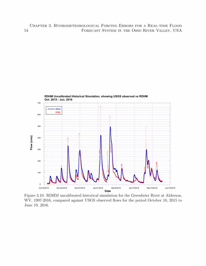
54Chapter 3. Hydrometeorological Forcing Errors for a Real-time Flood
Forecast System in the Ohio River Valley, USA
0
100
200
300
400
500
600
700
Oct/18/2015 Nov/22/2015 Dec/27/2015 Jan/31/2016 Mar/6/2016 Apr/10/2016 May/15/2016 Jun/19/2016
RDHM Uncalibrated Historical Simulation, showing USGS observed vs RDHMOct. 2015 - Jun. 2016
rdhmusgs
Flow
(cm
s)
DateFigure 3.10: RDHM uncalibrated historical simulation for the Greenbrier River at Alderson,WV, 1997-2016, compared against USGS observed flows for the period October 18, 2015 toJune 19, 2016.
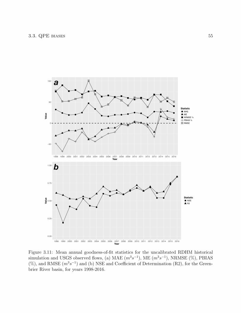
3.3. QPE biases 55
●
●● ●
●
●
●
● ●● ● ●
● ●
●
● ● ●●
−50
0
50
100
1998 1999 2000 2001 2002 2003 2004 2005 2006 2007 2008 2009 2010 2011 2012 2013 2014 2015 2016Year
Value
Statistic● MAE
ME NRMSE %PBIAS %RMSE
●
●
●
●
●
●●
●●
●●
●
●
●
●
● ●
●
●
0.00
0.25
0.50
0.75
1.00
1998 1999 2000 2001 2002 2003 2004 2005 2006 2007 2008 2009 2010 2011 2012 2013 2014 2015 2016Year
Value Statistic
● NSE R2
a
b
Figure 3.11: Mean annual goodness-of-fit statistics for the uncalibrated RDHM historicalsimulation and USGS observed flows, (a) MAE (m3s−1), ME (m3s−1), NRMSE (%), PBIAS(%), and RMSE (m3s−1) and (b) NSE and Coefficient of Determination (R2), for the Green-brier River basin, for years 1998-2016.
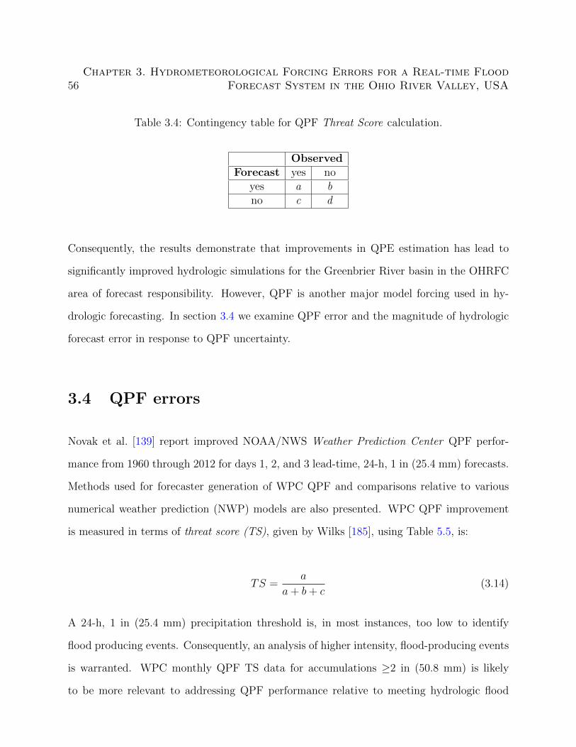
56Chapter 3. Hydrometeorological Forcing Errors for a Real-time Flood
Forecast System in the Ohio River Valley, USA
Table 3.4: Contingency table for QPF Threat Score calculation.
ObservedForecast yes no
yes a bno c d
Consequently, the results demonstrate that improvements in QPE estimation has lead to
significantly improved hydrologic simulations for the Greenbrier River basin in the OHRFC
area of forecast responsibility. However, QPF is another major model forcing used in hy-
drologic forecasting. In section 3.4 we examine QPF error and the magnitude of hydrologic
forecast error in response to QPF uncertainty.
3.4 QPF errors
Novak et al. [139] report improved NOAA/NWS Weather Prediction Center QPF perfor-
mance from 1960 through 2012 for days 1, 2, and 3 lead-time, 24-h, 1 in (25.4 mm) forecasts.
Methods used for forecaster generation of WPC QPF and comparisons relative to various
numerical weather prediction (NWP) models are also presented. WPC QPF improvement
is measured in terms of threat score (TS), given by Wilks [185], using Table 5.5, is:
TS =a
a+ b+ c(3.14)
A 24-h, 1 in (25.4 mm) precipitation threshold is, in most instances, too low to identify
flood producing events. Consequently, an analysis of higher intensity, flood-producing events
is warranted. WPC monthly QPF TS data for accumulations ≥2 in (50.8 mm) is likely
to be more relevant to addressing QPF performance relative to meeting hydrologic flood

3.4. QPF errors 57
forecasting needs. Two important issues are, (1) the degree to which errors in operational
QPF influence hydrologic prediction and (2) how these influences can be quantified. In an
attempt to address these concerns, results from a hydrologic modeling study are presented,
noting that:
1. We present QPF verification statistics taken from the NOAA/NWS National Precipi-
tation Verification Unit (NPVU) covering the 12 Conterminous U.S. (CONUS) RFCs;
2. Results from Monte Carlo simulations using the RDHM for the Greenbrier River basin,
WV are presented spanning the June 22-24, 2016 flooding episode to assess the range
of hydrologic errors in response to expected WPC QPF accuracy;
3. Threat Score (TS), a commonly used statistical measure of forecast accuracy in mete-
orology, will serve as the basis for evaluating QPF accuracy in the RDHM hydrologic
experiments.
3.4.1 WPC
Monthly mean bias and TS data for precipitation accumulations ≥2 in (50.8 mm), obtained
from NOAA/NWS WPC [148], are summarized in Figure 3.12 for the period 1970-2015
for Day-1 and 1991-2015 for Day-2 lead-times. Day-2 data were not collected before 1991
by WPC. Annual averages are also shown, based on monthly averaged values. The large
variability of monthly bias and TS values is evident. We note that expected Day-1, ≥2 in
(50.8 mm) TS values are about 0.06 in 1970 and 0.22 by 2015.
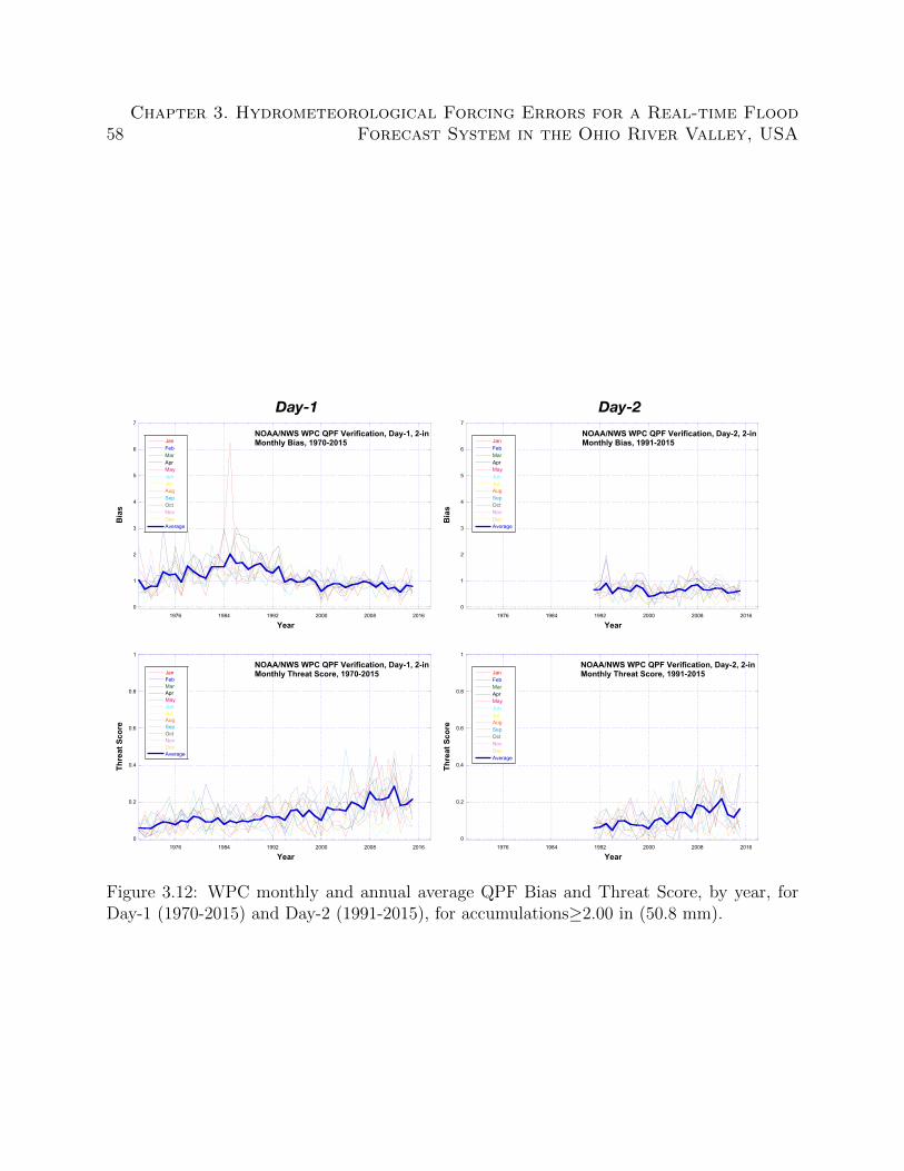
58Chapter 3. Hydrometeorological Forcing Errors for a Real-time Flood
Forecast System in the Ohio River Valley, USA
0
0.2
0.4
0.6
0.8
1
1976 1984 1992 2000 2008 2016
NOAA/NWS WPC QPF Verification, Day-1, 2-inMonthly Threat Score, 1970-2015Jan
FebMarAprMayJunJulAugSepOctNovDecAverage
Thre
at S
core
Year
0
1
2
3
4
5
6
7
1976 1984 1992 2000 2008 2016
NOAA/NWS WPC QPF Verification, Day-2, 2-inMonthly Bias, 1991-2015Jan
FebMarAprMayJunJulAugSepOctNovDecAverage
Bia
s
Year
0
1
2
3
4
5
6
7
1976 1984 1992 2000 2008 2016
NOAA/NWS WPC QPF Verification, Day-1, 2-inMonthly Bias, 1970-2015Jan
FebMarAprMayJunJulAugSepOctNovDecAverage
Bia
s
Year
0
0.2
0.4
0.6
0.8
1
1976 1984 1992 2000 2008 2016
NOAA/NWS WPC QPF Verification, Day-2, 2-inMonthly Threat Score, 1991-2015Jan
FebMarAprMayJunJulAugSepOctNovDecAverage
Thre
at S
core
Year
Day-1 Day-2
Figure 3.12: WPC monthly and annual average QPF Bias and Threat Score, by year, forDay-1 (1970-2015) and Day-2 (1991-2015), for accumulations≥2.00 in (50.8 mm).
3.4. QPF errors 59
3.4.2 NPVU
Charba et al. [37] describe a methodology for evaluating QPF forecast accuracy relative
to RFC produced Stage III and MPE QPE at WPC, RFCs, and Weather Forecast Offices
(WFOs) compared against national guidance produced by operational numerical weather
prediction (NWP) models run at the National Centers for Environmental Prediction (NCEP).
Also described is the implementation of the National Precipitation Verification Unit (NPVU)
to carry-out national QPF verification from the various sources (WPC, WFOs, RFCs, NWP
models). NPVU QPF verification data was produced for the period 2001-2012.
Figure 3.13 shows a time series of NPVU monthly (a) Mean Absolute Error (MAE) and
(b) Root Mean Square Error (RMSE) for all NOAA/NWS CONUS River Forecast Centers
(rfc), NOAA/NWS Nested Gridded Model (ngm), North American Model (nam), Hydrom-
eteorological Prediction Center (hpc) – now Weather Prediction Center (WPC) – Global
Forecast System (gfs), ETA Model (eta), and Aviation Model (avn) for the period June
2001 to December 2009. The gap in data from late 2003 to mid-2004 was due to an NPVU
data processing failure. Several points are notable (1) seasonal variability for all the QPF
sources is clear; (2) while there are differences between QPF sources, there is relatively lit-
tle discernible MAE or RMSE improvement over the June 2001 to December 2009 analysis
period displayed by any of the QPF sources; and (3) for all QPF sources there is less QPF
error for the smaller precipitation intervals, ≥0.01 in (0.254 mm), than the larger intervals,
≥1.0 in (25.4 mm). The highest precipitation interval used by NPVU is ≥1.0 in (25.4 mm).
Figure 3.14 shows the correlation coefficient, R, of QPF versus QPE, aggregated across the
June 2001 to December 2009 NPVU analysis period, grouped by QPF source and precipi-
tation interval. It is evident, as reported by Charba et al. [37], that forecasters add value
over NWP modeled QPF, based on HPC (WPC) and RFC results compared to NWP model

60Chapter 3. Hydrometeorological Forcing Errors for a Real-time Flood
Forecast System in the Ohio River Valley, USA
results. Also apparent is that for 24-h accumulations, especially for the larger precipita-
tion intervals, ≥1.0 in (25.4 mm), QPF is poorly correlated with observed QPE and that
there is considerable correlation spread within the precipitation intervals. Little difference
is apparent between HPC and RFC QPF on the basis of R values and spread.
Implications
We can see that deterministic QPF can be quite erroneous, based on a range of statistical
verification measures, demonstrated by both NWP model generated QPF and QPF produced
with the aid of forecaster input. It has been reported [139], correctly, that by some statis-
tical measures, specifically, threat score, QPF accuracy has improved since the beginning of
systematic record keeping to the present. Nevertheless, the question must be asked, what
benefits have accrued to hydrologic forecasting from QPF improvements? To answer this
question a hydrologic simulation experiment is presented using the near-record Greenbrier
River basin (defined at Alderson, WV, USGS 05050003) flooding event in West Virginia,
June 22-24, 2016.
3.4.3 Hyrdrologic simulation experiments
A hydrologic simulation experiment is used to assess how QPF improvements have impacted
hydrologic prediction. Simulations take the form of a monte carlo experiment, using a storm
transposition methodology (Foufoula-Georgiou [76]; England et al. [68]; Wright et al. [192]).
The aim of the experiment is to illustrate the inadequacy of current deterministic QPF for
hydrologic forecasting purposes. The experiment first produces 1000 randomly located storm
centers based on the maximum 24-h MPE grid cell precipitation accumulation for the period
beginning June 23, 2016 0600 UTC within the region, shown in Figure 3.15 (a). An example
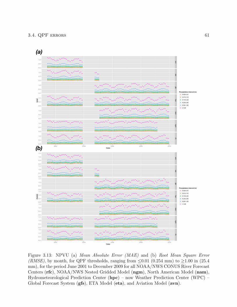
3.4. QPF errors 61
0.0
0.5
1.0
0.0
0.5
1.0
0.0
0.5
1.0
0.0
0.5
1.0
0.0
0.5
1.0
0.0
0.5
1.0
0.0
0.5
1.0
avneta
gfshpc
namngm
rfc
2002 2004 2006 2008 2010Date
MAE
Precipitation Interval (in)
0.00-0.01
0.01-0.10
0.10-0.25
0.25-0.50
0.50-1.00
≥1.00
0.0
0.5
1.0
1.5
0.0
0.5
1.0
1.5
0.0
0.5
1.0
1.5
0.0
0.5
1.0
1.5
0.0
0.5
1.0
1.5
0.0
0.5
1.0
1.5
0.0
0.5
1.0
1.5
avneta
gfshpc
namngm
rfc
2002 2004 2006 2008 2010Date
RMSE
Precipitation Interval (in)
0.00-0.01
0.01-0.10
0.10-0.25
0.25-0.50
0.50-1.00
>1.00
(a)
(b)
Figure 3.13: NPVU (a) Mean Absolute Error (MAE) and (b) Root Mean Square Error(RMSE), by month, for QPF thresholds, ranging from ≤0.01 (0.254 mm) to ≥1.00 in (25.4mm), for the period June 2001 to December 2009 for all NOAA/NWS CONUS River ForecastCenters (rfc), NOAA/NWS Nested Gridded Model (ngm), North American Model (nam),Hydrometeorological Prediction Center (hpc) – now Weather Prediction Center (WPC) –Global Forecast System (gfs), ETA Model (eta), and Aviation Model (avn).
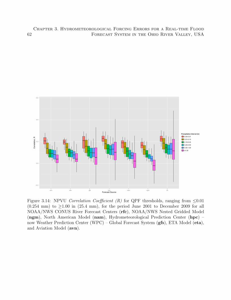
62Chapter 3. Hydrometeorological Forcing Errors for a Real-time Flood
Forecast System in the Ohio River Valley, USA
-0.2
0.0
0.2
0.4
0.6
avn eta gfs hpc nam ngm rfcForecast Source
Cor
rela
tion,
R
Precipitation Interval (in)0.00-0.01
0.01-0.10
0.10-0.25
0.25-0.50
0.50-1.00
≥1.00
Figure 3.14: NPVU Correlation Coefficient (R) for QPF thresholds, ranging from ≤0.01(0.254 mm) to ≥1.00 in (25.4 mm), for the period June 2001 to December 2009 for allNOAA/NWS CONUS River Forecast Centers (rfc), NOAA/NWS Nested Gridded Model(ngm), North American Model (nam), Hydrometeorological Prediction Center (hpc) –now Weather Prediction Center (WPC) – Global Forecast System (gfs), ETA Model (eta),and Aviation Model (avn).
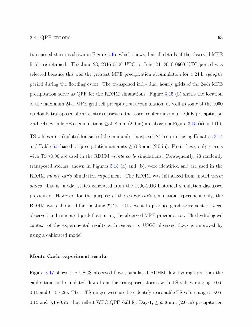
3.4. QPF errors 63
transposed storm is shown in Figure 3.16, which shows that all details of the observed MPE
field are retained. The June 23, 2016 0600 UTC to June 24, 2016 0600 UTC period was
selected because this was the greatest MPE precipitation accumulation for a 24-h synoptic
period during the flooding event. The transposed individual hourly grids of the 24-h MPE
precipitation serve as QPF for the RDHM simulations. Figure 3.15 (b) shows the location
of the maximum 24-h MPE grid cell precipitation accumulation, as well as some of the 1000
randomly transposed storm centers closest to the storm center maximum. Only precipitation
grid cells with MPE accumulations ≥50.8 mm (2.0 in) are shown in Figure 3.15 (a) and (b).
TS values are calculated for each of the randomly transposed 24-h storms using Equation 3.14
and Table 5.5 based on precipitation amounts ≥50.8 mm (2.0 in). From these, only storms
with TS≥0.06 are used in the RDHM monte carlo simulations. Consequently, 88 randomly
transposed storms, shown in Figures 3.15 (a) and (b), were identified and are used in the
RDHM monte carlo simulation experiment. The RDHM was initialized from model warm
states, that is, model states generated from the 1996-2016 historical simulation discussed
previously. However, for the purpose of the monte carlo simulation experiment only, the
RDHM was calibrated for the June 22-24, 2016 event to produce good agreement between
observed and simulated peak flows using the observed MPE precipitation. The hydrological
context of the experimental results with respect to USGS observed flows is improved by
using a calibrated model.
Monte Carlo experiment results
Figure 3.17 shows the USGS observed flows, simulated RDHM flow hydrograph from the
calibration, and simulated flows from the transposed storms with TS values ranging 0.06-
0.15 and 0.15-0.25. These TS ranges were used to identify reasonable TS value ranges, 0.06-
0.15 and 0.15-0.25, that reflect WPC QPF skill for Day-1, ≥50.8 mm (2.0 in) precipitation
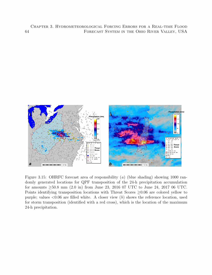
64Chapter 3. Hydrometeorological Forcing Errors for a Real-time Flood
Forecast System in the Ohio River Valley, USA
ThreatScore
Precipitation (mm)
a b
Figure 3.15: OHRFC forecast area of responsibility (a) (blue shading) showing 1000 ran-domly generated locations for QPF transposition of the 24-h precipitation accumulationfor amounts ≥50.8 mm (2.0 in) from June 23, 2016 07 UTC to June 24, 2017 06 UTC.Points identifying transposition locations with Threat Scores ≥0.06 are colored yellow topurple; values <0.06 are filled white. A closer view (b) shows the reference location, usedfor storm transposition (identified with a red cross), which is the location of the maximum24-h precipitation.
3.4. QPF errors 65
Figure 3.16: Example of a transposed storm (shaded blue) relative to the observed MPEstorm (yellow); the green region shows overlap between the observed MPE and transposedstorm. Also shown are the OHRFC forecast area of responsibility (light blue shading) and1000 randomly generated locations for QPF transposition of the 24-h precipitation accumu-lation for amounts ≥50.8 mm (2.0 in) from June 23, 2016 07 UTC to June 24, 2017 06 UTC.Points identifying transposition locations with Threat Scores ≥0.06 are colored yellow topurple; values <0.06 are filled white. The reference location, identified with a red cross, isthe location of the maximum 24-h precipitation, from which storm transpositions are made.The heavy black line indicates the transposition vector.

66Chapter 3. Hydrometeorological Forcing Errors for a Real-time Flood
Forecast System in the Ohio River Valley, USA
accumulations in 1970 and 2016, respectively. By doing this we believe we can assess, in
relative terms, the gain in hydrologic forecast accuracy reflected by improvements in WPC
QPF. It is evident from the Figure 3.17 simulations that hydrograph peaks are, in general,
greater for storms with TS values ranging 0.15-0.25 than for storms with TS values 0.06-0.15.
However, none of the simulated hydrographs exceed the Major Flood level and none approach
the observed near-record flood peak level. Moreover, there is considerable variability between
the simulated hydrographs within the separate 0.06-0.15 and 0.15-0.25 TS categories.
A better perspective on the problem inherent with using deterministic QPF in hydrologic
forecasting is found by looking at simulation results from all 88 storms used in the RDHM
monte carlo experiment with TS≥0.06. Figure 3.18 shows peak flow and storm TS relative to
distance from the reference storm center maximum of the observed 24-h MPE, with points
identified by color, reflecting storm TS value ranges. Point size indicates the peak flow
magnitude. The high degree of peak flow variability within TS categories is illustrated in
Figure 3.19, which is greatest for the 0.30-0.49 TS interval. Also quite evident is that smaller
distances of the transposed storm from the reference storm center does not guarantee either
higher TS values or peak flows. In fact, the storm with the highest TS and closest to the
reference storm center produced a peak flow approximately the same as other transposed
storms with significantly lower TS values and at distances much further from the reference
storm center. The large degree in the variability of hydrograph response and peak flow
relative to the magnitude of the transposed storm TS values, underscores the complex nature
of hydrologic prediction using deterministic QPF. Rezacova et al. [153] and Mittermaier and
Roberts [124] address the difficulty of QPF verification due to the complex structure of
observed precipitation fields due to embedded convection.
3.5. Summary and conclusions 67
WPC QPF for the June 23, 2016 event
For the benefit of completeness, we report results from the RDHM simulation using June 23,
2016 0600 UTC, 24-h WPC QPF. The simulated peak flow was 143 m3s−1 with TS = 0.30.
Importantly, no 24-h WPC QPF ≥50.8 mm (2.0 in), for the June 23, 2016 0700 UTC to June
24, 2016 0600 UTC period, fell with within the Greenbrier River basin. The USGS observed
peak flow value, 2285.2 m3s−1, at Alderson, WV occurred June 24, 2016 0930 UTC. The
OHRFC forecast from June 23, 2016 1423 UTC was 180.7 m3s−1, corresponding to a peak
river stage 5.70 feet (1.74 m), which was forecasted to occur June 24, 2016 0600 UTC [41].
3.5 Summary and conclusions
Results presented demonstrate that (1) NOAA/NWS NEXt generation RADar (NEXRAD)
derived QPE has improved dramatically from 1997-present for the OHRFC area, which is
reflected in significantly improved hydrologic simulations over the 1997-2016 hindcast pe-
riod and that (2) from the perspective of meeting the needs of hydrologic forecasting, QPF
improvements have been marginal. The monte carlo hydrologic simulation experiment il-
lustrates the sensitivity of hydrologic forecasts to QPF errors, resulting in large peak flow
differences within narrow ranges of TS differences. Results from these experiments show
that greater QPF Threat Score (TS) values do not necessarily produce improved hydro-
logic forecasts and that considerable variability in hydrologic response should be expected,
independent of antecedent basin conditions.
Improved hydrologic simulations resulting from QPE improvements are important in sev-
eral ways. First, since hydrologic forecasts in large part depend on accurately translating
observed precipitation into watershed response through modeling, without consideration of
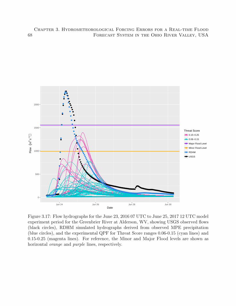
68Chapter 3. Hydrometeorological Forcing Errors for a Real-time Flood
Forecast System in the Ohio River Valley, USA
●●●●●●●●●●●●●●●●●
●
●
●
●
●
●
●
●
●●
●
●
●
●
●●
●
●
●
●
●
●
●
●
●
●
●
●
●
●●●
●●●
●●●
●●●
●●●●●●●●●●●●●●●●●●●●●●●●●●●●●●●●●●●●●●●●●●●●●●●●●●●●●●●●●●●●
●●●●●●●●●●●●●●●●●●●●●●●●●●●●●●●●●●●●●●●●●●●●●●●●●●●
●●●●●●●●●●●●●
●
●
●
●
●
●
●
●
●
●
●
●●●
●
●
●
●
●
●
●
●
●
●
●
●
●
●
●●●
●●
●●●
●●●
●●●
●●●
●●
●●●
●●●
●●●
●●●
●●●●●●●●●●●●●●●●●●●●●●●●●●●●●●●●●●●●●●●●●●●●●●●●●●●●●●●●●●●●●●●●●●●●●●●●●●●●●●●●●●●●●●●●●●●●●●●●●
0
500
1000
1500
2000
Jun 24 Jun 26 Jun 28 Jun 30
Date
Flo
w
(m3 s
−1)
Threat Score●●
●●
●●
●●
●●
●●
0.15−0.25
0.06−0.15
Major Flood Level
Minor Flood Level
RDHM
USGS
Figure 3.17: Flow hydrographs for the June 23, 2016 07 UTC to June 25, 2017 12 UTC modelexperiment period for the Greenbrier River at Alderson, WV, showing USGS observed flows(black circles), RDHM simulated hydrographs derived from observed MPE precipitation(blue circles), and the experimental QPF for Threat Score ranges 0.06-0.15 (cyan lines) and0.15-0.25 (magenta lines). For reference, the Minor and Major Flood levels are shown ashorizontal orange and purple lines, respectively.
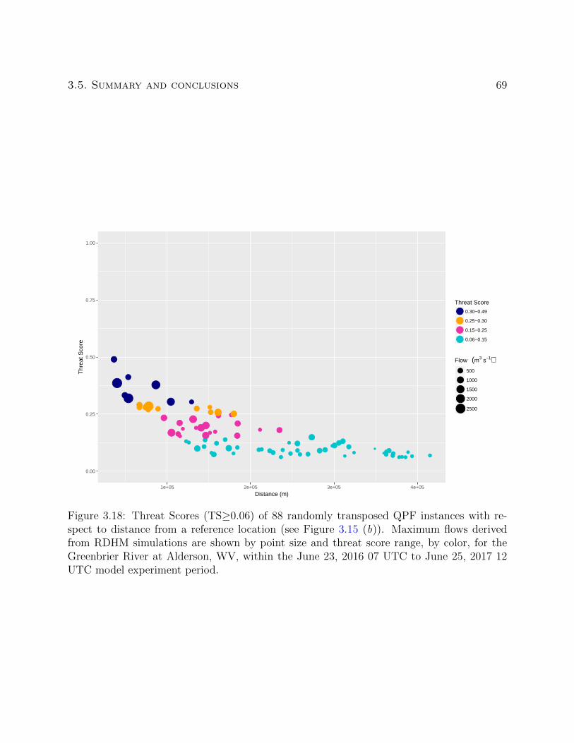
3.5. Summary and conclusions 69
●
●●
●
●
●
●
●
●
●
●●
●
●
●
●
●
●
●
●
● ●
●
●
●
●
●●
●
●
●
●
●●
●
●
●
●
●
●
●
●
●
●
●
●
●
●●
●
●
●
●
●
●
●
●
●
●
●
●
●
●●
●●
●●
●
●
● ●
●
●
●
● ●
●
●●
●
●●
●●
●
●
●
0.00
0.25
0.50
0.75
1.00
1e+05 2e+05 3e+05 4e+05
Distance (m)
Thr
eat S
core
Threat Score
●●●●
0.30−0.49
0.25−0.30
0.15−0.25
0.06−0.15
Flow (m3 s−1)●
●
●●●
500
1000
1500
2000
2500
Figure 3.18: Threat Scores (TS≥0.06) of 88 randomly transposed QPF instances with re-spect to distance from a reference location (see Figure 3.15 (b)). Maximum flows derivedfrom RDHM simulations are shown by point size and threat score range, by color, for theGreenbrier River at Alderson, WV, within the June 23, 2016 07 UTC to June 25, 2017 12UTC model experiment period.
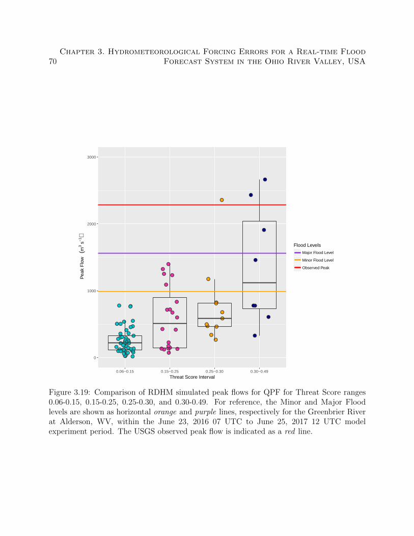
70Chapter 3. Hydrometeorological Forcing Errors for a Real-time Flood
Forecast System in the Ohio River Valley, USA
●
●
●●
●
● ●
●
●
●●
●
●
●
●
●
●
●
●
●
●
●
●
●
●
●
●●
●
●●
●
●
● ●
●
●
●
●
●
●
●
●
●
●●
●
●●
●
●
● ●
●
●●
●
●
●
●
●
●
●
●
●
●
●●
●
●
●
●
●
●
●
●
●
●
●●
●
●
●
●
●
●
●●
0
1000
2000
3000
0.06−0.15 0.15−0.25 0.25−0.30 0.30−0.49
Threat Score Interval
Pea
k F
low
(m
3 s−1
)
Flood Levels
Major Flood Level
Minor Flood Level
Observed Peak
Figure 3.19: Comparison of RDHM simulated peak flows for QPF for Threat Score ranges0.06-0.15, 0.15-0.25, 0.25-0.30, and 0.30-0.49. For reference, the Minor and Major Floodlevels are shown as horizontal orange and purple lines, respectively for the Greenbrier Riverat Alderson, WV, within the June 23, 2016 07 UTC to June 25, 2017 12 UTC modelexperiment period. The USGS observed peak flow is indicated as a red line.
3.5. Summary and conclusions 71
QPF, forecasts are improved with improved QPE. Second, improved QPE improves mainte-
nance of model states which are intended to reflect current basin conditions. Consequently,
hydrologic forecasts are improved because initial basin conditions are improved and the need
for ad hoc forecaster adjustments is reduced, which could be made for inappropriate reasons.
Namely, an observed difference between simulated and observed flows/stage could simply re-
flect random model error and not indicate divergence between model states and actual basin
conditions. Finally, for well-calibrated models, improved QPE provides greater confidence
in the initial model states needed for probabilistic hydrologic forecast systems [40] that run
automatically, without direct forecaster intervention.
There are some indications of improved QPF accuracy, shown by WPC with increased threat
score values from 1970-present. These QPF accuracy gains are reflected by improvements
in hydrologic response, which were demonstrated with the RDHM monte carlo experiment.
However WPC QPF bias statistics do not show improvement. In addition, for a variety
of QPF sources, NPVU verification statistics do not reveal discernible improvement for
the 2001-2009 analysis period. The RDHM monte carlo experiments demonstrated signifi-
cant uncertainty in hydrologic response at current expected WPC QPF threat score levels.
Importantly, significant uncertainty with deterministic QPF has been widely shown to be
problematic (Damrath et al. [49]; Ebert [64]; Im et al. [96]; Diomede et al. [60]; Cuo et al.
[45]). Significant research and development activity (Cloke and Pappenberger [40]; Adams
and Ostrowski [1]; Demargne et al. [58]) in the hydrologic community has been directed at
the implementation of probabilistic hydrologic forecast systems with a principal aim to quan-
tify the uncertainties inherent in hydrological forecasting, including uncertainties associated
with model forcings, in particular, QPF uncertainties.
The central problem with deterministic QPF is that, in principle, the placement, timing,
and magnitude of QPF should all be reasonable estimates for each of the basins shown, for

72Chapter 3. Hydrometeorological Forcing Errors for a Real-time Flood
Forecast System in the Ohio River Valley, USA
example, in Figure 3.2. The RDHM monte carlo hydrologic experiment demonstrated how
far current deterministic QPF is from consistently providing the needed skill in hydrologic
forecasting. It is only for much larger basins where QPF errors are sufficiently masked by
spatial and temporal averaging that deterministic QPF has sufficient skill to have value
in hydrologic forecasting. The problem is significantly more difficult for flash floods, with
affected areas that are considerably smaller than the OHRFC subbasins shown in Figure 3.2.
The methods applied should be applicable to other locations due to the general nature of the
techniques used. Data availability is, of course, an issue in many areas where, for instance,
radar estimates of precipitation do not exist. In areas where snowmelt flooding dominates
results could be different from what is shown where rainfall forced flooding is the principal
hydrometeorological flooding process.

Chapter 4
The Effect of QPF on Real-time
Deterministic Hydrologic Forecast
Uncertainty
4.1 Abstract
The use of Quantitative Precipitation Forecast (QPF) in hydrologic forecasting is common-
place, but QPF is subject to considerable error. When QPF is included as a model forcing
in the hydrological forecast process, significant error is passed to subsequent hydrologic
predictions. Two questions arise: (1) are the resulting observed hydrologic forecast errors
sufficiently large to suggest the use of zero QPF in the forecast process; if the use of QPF
is indicated, (2) how many periods (hours) of QPF (1-, 6-, 12-,. . . , 72-h. . . ) should be
used? Also, do forecast conditions exist under which the use of QPF should be different?
This study presents results from two real-time hydrologic forecast experiments, focused on
the NOAA/NWS Ohio River Forecast Center (OHRFC). The experiments rely on forecasts
73

74Chapter 4. The Effect of QPF on Real-time Deterministic Hydrologic
Forecast Uncertainty
from subbasins at 38 forecast point locations, ranging in drainage area, geographic location
within the Ohio River Valley, and watershed response time. Results from an experiment,
spanning all flow ranges, for the August 10, 2007 - August 31, 2009 period, show that non-
zero QPF produces smaller hydrologic forecast error than zero QPF. A second experiment,
January 23, 2009 through September 15, 2010, suggests that QPF should be limited to 6-
to 12-h duration for flood forecasts. Beyond 12-h, hydrologic forecast error increases sub-
stantially across all forecast ranges, but errors are much larger for flood forecasts. Increased
durations of QPF produce smaller forecast error than shorter QPF durations only for non-
flood forecasts. Experimental results are shown to be consistent with NWS, April 2001 to
October 2016, forecast verification statistics for the OHRFC.
4.2 Introduction
Single-valued, deterministic Quantitative Precipitation Forecast (QPF) is a commonly used
model forcing in hydrologic forecasting (Georgakakos and Hudlow [82]; Sokol [167]; Adams
[5]; Li et al. [114]). All 13 U.S. National Oceanic and Atmospheric Administration (NOAA),
National Weather Service (NWS) River Forecast Centers (RFCs), shown in Figure 4.1, uti-
lize QPF operationally for hydrologic forecasting, ranging in duration from 1- to 10-days.
Research has demonstrated that the use of deterministic QPF introduces considerable er-
ror into hydrologic forecasting (Cuo et al. [45]; Diomede et al. [61]). Sources of hydrologic
forecast uncertainty, including QPF, are recognized by the National Research Council [133].
Adams and Dymond [6] report on the magnitude of QPF uncertainty over the Conterminous
United States (CONUS) and illustrate, from analyses of a hydrologic modeling experiment
for a 3533 km2 watershed in the Ohio River Valley, that large prediction uncertainties are
obtained from the use of deterministic QPF. Despite the advances in our understanding of

4.2. Introduction 75
QPF errors, unanswered questions remain with the use of QPF.
4.2.1 Background
NWS RFCs are responsible for providing routine river and flood forecasts of stage/flow values
to the general public and others on a daily basis, often including evening updates. Addi-
tional forecasts are issued during operational periods, as needed, during flooding episodes,
subject to changing meteorological conditions, including 24-h per day operational coverage.
RFCs currently use the NWS Community Hydrologic Prediction System (CHPS) based on
the Flood Early Warning System (FEWS) [55] as the basis of their modeling system [4].
All RFC CHPS modeling is done within the Linux based NOAA/NWS Advanced Weather
Interactive Processing System (AWIPS) [140, 141]. The OHRFC uses the Sacramento Soil
Moisture Accounting (SAC-SMA) model (Burnash et al. [34]; Burnash [32]), SNOW-17 snow
accumulation and ablation model [12], several lumped-parameter hydrologic routing mod-
els, and three reservoir simulation models within the CHPS operational environment. All
OHRFC CHPS models were migrated from the legacy NWS River Forecast System (NWS-
RFS) (U.S. Department of Commerce [177]) in 2011.
In addition to QPF, principal hydrologic model forcings are observed precipitation and ob-
served and forecasted temperature. Precipitation observations are obtained from a multisen-
sor estimation process, involving rain gauges, NWS NEXt-generation RADar (NEXRAD)
doppler radar, and, in some instances, remotely-sensed satellite estimates of precipitation
[103]. Forecasted precipitation is derived from numerical weather prediction (NWP) models,
usually with meteorological forecaster adjustments made at both the NWS Weather Predic-
tion Center (WPC), formerly the Hydrometeorological Prediction Center (HPC), referred to
henceforth as WPC, and/or at local RFCs [139]. The hydrologic forecast process in other
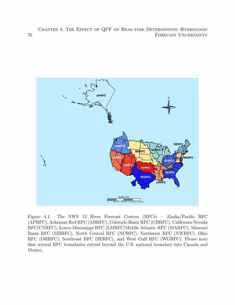
76Chapter 4. The Effect of QPF on Real-time Deterministic Hydrologic
Forecast Uncertainty
APRFC
CNRFC MARFC
NERFC
MBRFC
CBRFC
NWRFC
ABRFC
WGRFCSERFC
OHRFC
NCRFC
LMRFC
Figure 4.1: The NWS 13 River Forecast Centers (RFCs) – Alaska/Pacific RFC(APRFC), Arkansas-Red RFC (ABRFC), Colorado Basin RFC (CBRFC), California-NevadaRFC(CNRFC), Lower-Mississippi RFC (LMRFC)Middle Atlantic RFC (MARFC), MissouriBasin RFC (MBRFC), North Central RFC (NCRFC), Northwest RFC (NWRFC), OhioRFC (OHRFC), Southeast RFC (SERFC), and West Gulf RFC (WGRFC). Please notethat several RFC boundaries extend beyond the U.S. national boundary into Canada andMexico.

4.3. Research Approach 77
countries is similar to that used in the U.S. [5].
4.2.2 Research goals
The aim of this research is to frame the potential limits to the use of deterministic QPF
for hydrologic forecasting. Section 4.3 of this paper describes two real-time hydrologic fore-
casting experiments used in this study. We focus model simulations on watersheds in the
NOAA/NWS Ohio River Forecast Center (OHRFC) area of responsibility, shown in Fig-
ure 4.1. The first experiment addresses the issue of whether or not non-zero deterministic
QPF should be used in hydrological forecasting. The second experiment identifies the ex-
pected range of hydrologic forecast error using QPF for OHRFC forecast point locations
and a possible limit to the duration of QPF that should be used for flood forecasting before
forecast error grows too large for acceptable use. Results of the experiments are presented
in section 4.4. The overall context of the experimental results in relation to other RFCs
and the conditions under which the use of QPF should possibly be limited are identified in
section 4.5. Section 4.6 summarizes the experimental results and presents conclusions.
4.3 Research Approach
Two sets of real-time hydrologic forecast experiments are presented. The experiments, which
were made using the legacy NWSRFS, rely on a geographically broad distribution of forecast
point locations, with varying basin sizes and hydrologic response times for the OHRFC.
Calibrations of SAC-SMA, SNOW-17, channel routing, and reservoir simulation models for
operational use for all OHRFC subbasins were completed prior to the time the experiments
started, following guidelines presented by Anderson [13] and Smith et al. [166]. All model

78Chapter 4. The Effect of QPF on Real-time Deterministic Hydrologic
Forecast Uncertainty
experiments were conducted using 1200 UTC model initializations following routine OHRFC
operations. Operational and experimental simulations utilize a 6-h time step for model
forcings, internally, and output. The two experiments are focused on answering the questions,
respectively:
1. should non-zero QPF be used in hydrologic forecasting;
2. if the use of non-zero QPF is suggested, what duration of QPF seems warranted?
Forecasts are evaluated on the basis of comparisons between U.S. Geological Survey (USGS)
observations and simulated river stage values. Results from the experiment are reported in
terms of verification statistics using methods proposed by Welles et al. [181] and Demargne
et al. [56].
4.3.1 Statistical verification
Verification of hydrologic forecasts are made using:
ME =1
n
n∑k=1
(yk − ok) (4.1)
MAE =1
n
n∑k=1
(|yk − ok|) (4.2)
RMSE =
√√√√ 1
n
n∑k=1
(yk − ok)2 (4.3)
where we have the Mean Error (ME), Mean Absolute Error (MAE), Root Mean Square Error
(RMSE), with quantities yk and ok the predicted and observed kth stage values, respectively,

4.3. Research Approach 79
for n total paired values. Units of measure for stage are feet, unless reported otherwise.
Values for ME, MAE, and RMSE = 0 implies perfect agreement, i.e., no error.
4.3.2 Experiment 1
Watersheds are identified to obtain a range of drainage basin areas and locations to in-
vestigate all possible combinations of the use of OHRFC and WPC QPF and interactive
forecaster adjustments, termed runtime modifications, known as MODs. Consequently, 8
independent forecast simulations were made daily, at 12 UTC, for each of the 38 basins,
shown in Figure 4.2. The operational and experimental forecasts were made for the period
August 10, 2007 - August 31, 2009, using 24-h duration (4, 6-h periods (24 h)−1) QPF. The
experimental period spanned 753 days at 38 locations, with 28 forecast periods each (4 6-h
periods per day for 7-days), resulting in 801,192 forecast verification pairs for analysis. The
experiment was structured to assess:
• if non-zero QPF produces smaller error in hydrologic forecasts than zero QPF;
• whether or not the use of MODs produces smaller error in hydrologic forecasts than
without MODs;
• if the use of local OHRFC QPF or QPF from the WPC produces smaller error in
hydrologic forecasts in the OHRFC region?
Two experimental forecast scenarios for this experiment are: with MODs, No QPF and with
MODs, with WPC. All experimental forecast results were analyzed using the R Language
and Environment for Statistical Computing [145] and contributed verification package [135]
from experimental data stored in the OHRFC PostgreSQL verification database.
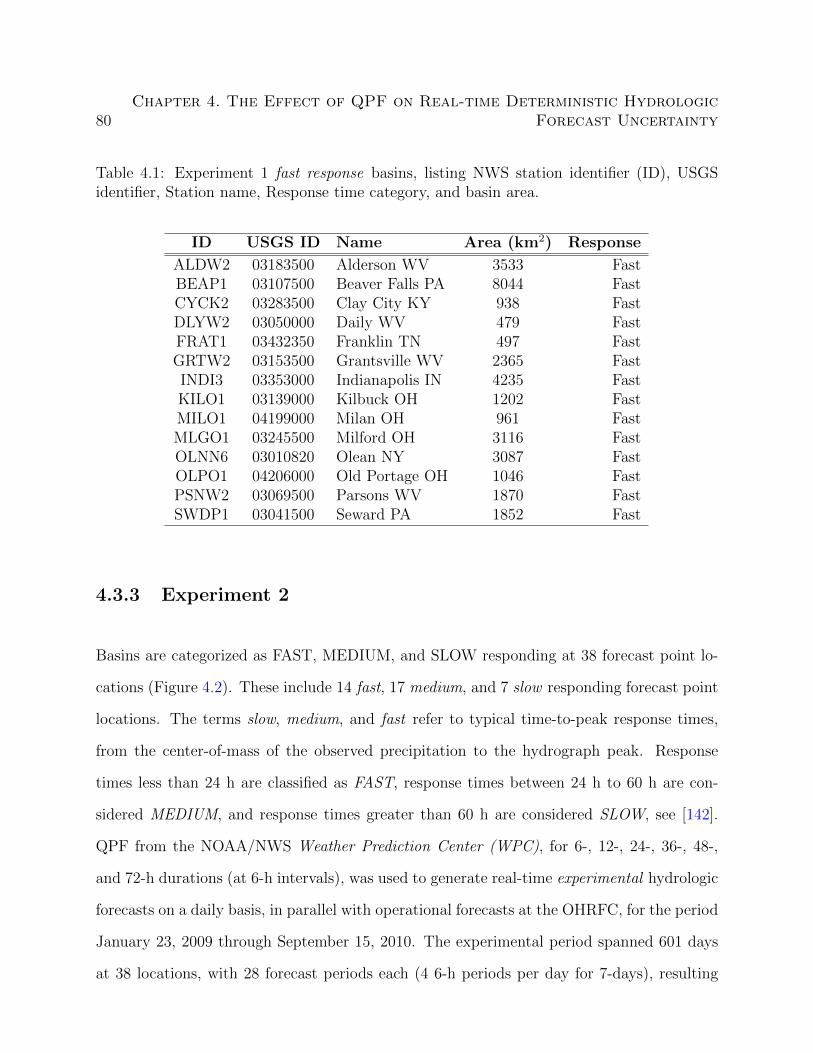
80Chapter 4. The Effect of QPF on Real-time Deterministic Hydrologic
Forecast Uncertainty
Table 4.1: Experiment 1 fast response basins, listing NWS station identifier (ID), USGSidentifier, Station name, Response time category, and basin area.
ID USGS ID Name Area (km2) Response
ALDW2 03183500 Alderson WV 3533 FastBEAP1 03107500 Beaver Falls PA 8044 FastCYCK2 03283500 Clay City KY 938 FastDLYW2 03050000 Daily WV 479 FastFRAT1 03432350 Franklin TN 497 FastGRTW2 03153500 Grantsville WV 2365 FastINDI3 03353000 Indianapolis IN 4235 FastKILO1 03139000 Kilbuck OH 1202 FastMILO1 04199000 Milan OH 961 FastMLGO1 03245500 Milford OH 3116 FastOLNN6 03010820 Olean NY 3087 FastOLPO1 04206000 Old Portage OH 1046 FastPSNW2 03069500 Parsons WV 1870 FastSWDP1 03041500 Seward PA 1852 Fast
4.3.3 Experiment 2
Basins are categorized as FAST, MEDIUM, and SLOW responding at 38 forecast point lo-
cations (Figure 4.2). These include 14 fast, 17 medium, and 7 slow responding forecast point
locations. The terms slow, medium, and fast refer to typical time-to-peak response times,
from the center-of-mass of the observed precipitation to the hydrograph peak. Response
times less than 24 h are classified as FAST, response times between 24 h to 60 h are con-
sidered MEDIUM, and response times greater than 60 h are considered SLOW, see [142].
QPF from the NOAA/NWS Weather Prediction Center (WPC), for 6-, 12-, 24-, 36-, 48-,
and 72-h durations (at 6-h intervals), was used to generate real-time experimental hydrologic
forecasts on a daily basis, in parallel with operational forecasts at the OHRFC, for the period
January 23, 2009 through September 15, 2010. The experimental period spanned 601 days
at 38 locations, with 28 forecast periods each (4 6-h periods per day for 7-days), resulting
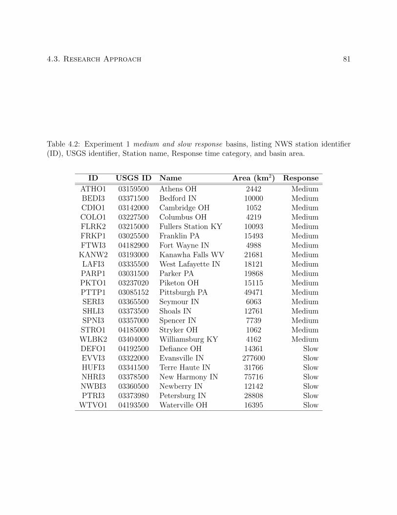
4.3. Research Approach 81
Table 4.2: Experiment 1 medium and slow response basins, listing NWS station identifier(ID), USGS identifier, Station name, Response time category, and basin area.
ID USGS ID Name Area (km2) Response
ATHO1 03159500 Athens OH 2442 MediumBEDI3 03371500 Bedford IN 10000 MediumCDIO1 03142000 Cambridge OH 1052 MediumCOLO1 03227500 Columbus OH 4219 MediumFLRK2 03215000 Fullers Station KY 10093 MediumFRKP1 03025500 Franklin PA 15493 MediumFTWI3 04182900 Fort Wayne IN 4988 MediumKANW2 03193000 Kanawha Falls WV 21681 MediumLAFI3 03335500 West Lafayette IN 18121 MediumPARP1 03031500 Parker PA 19868 MediumPKTO1 03237020 Piketon OH 15115 MediumPTTP1 03085152 Pittsburgh PA 49471 MediumSERI3 03365500 Seymour IN 6063 MediumSHLI3 03373500 Shoals IN 12761 MediumSPNI3 03357000 Spencer IN 7739 MediumSTRO1 04185000 Stryker OH 1062 MediumWLBK2 03404000 Williamsburg KY 4162 MediumDEFO1 04192500 Defiance OH 14361 SlowEVVI3 03322000 Evansville IN 277600 SlowHUFI3 03341500 Terre Haute IN 31766 SlowNHRI3 03378500 New Harmony IN 75716 SlowNWBI3 03360500 Newberry IN 12142 SlowPTRI3 03373980 Petersburg IN 28808 Slow
WTVO1 04193500 Waterville OH 16395 Slow
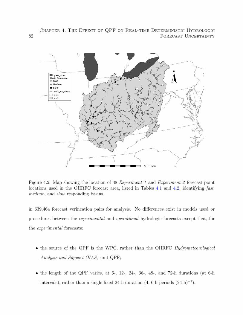
82Chapter 4. The Effect of QPF on Real-time Deterministic Hydrologic
Forecast Uncertainty
Figure 4.2: Map showing the location of 38 Experiment 1 and Experiment 2 forecast pointlocations used in the OHRFC forecast area, listed in Tables 4.1 and 4.2, identifying fast,medium, and slow responding basins.
in 639,464 forecast verification pairs for analysis. No differences exist in models used or
procedures between the experimental and operational hydrologic forecasts except that, for
the experimental forecasts:
• the source of the QPF is the WPC, rather than the OHRFC Hydrometeorological
Analysis and Support (HAS) unit QPF;
• the length of the QPF varies, at 6-, 12-, 24-, 36-, 48-, and 72-h durations (at 6-h
intervals), rather than a single fixed 24-h duration (4, 6-h periods (24 h)−1).
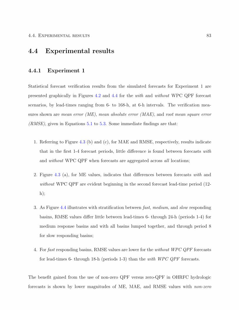
4.4. Experimental results 83
4.4 Experimental results
4.4.1 Experiment 1
Statistical forecast verification results from the simulated forecasts for Experiment 1 are
presented graphically in Figures 4.2 and 4.4 for the with and without WPC QPF forecast
scenarios, by lead-times ranging from 6- to 168-h, at 6-h intervals. The verification mea-
sures shown are mean error (ME), mean absolute error (MAE), and root mean square error
(RMSE), given in Equations 5.1 to 5.3. Some immediate findings are that:
1. Referring to Figure 4.3 (b) and (c), for MAE and RMSE, respectively, results indicate
that in the first 1-4 forecast periods, little difference is found between forecasts with
and without WPC QPF when forecasts are aggregated across all locations;
2. Figure 4.3 (a), for ME values, indicates that differences between forecasts with and
without WPC QPF are evident beginning in the second forecast lead-time period (12-
h);
3. As Figure 4.4 illustrates with stratification between fast, medium, and slow responding
basins, RMSE values differ little between lead-times 6- through 24-h (periods 1-4) for
medium response basins and with all basins lumped together, and through period 8
for slow responding basins;
4. For fast responding basins, RMSE values are lower for the without WPC QPF forecasts
for lead-times 6- through 18-h (periods 1-3) than the with WPC QPF forecasts.
The benefit gained from the use of non-zero QPF versus zero-QPF in OHRFC hydrologic
forecasts is shown by lower magnitudes of ME, MAE, and RMSE values with non-zero
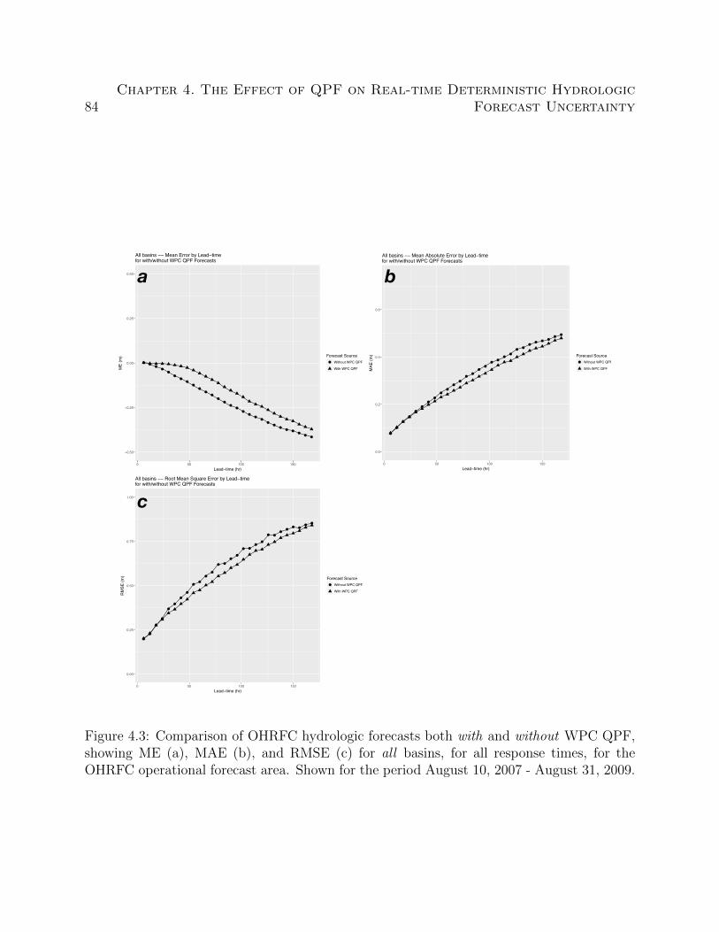
84Chapter 4. The Effect of QPF on Real-time Deterministic Hydrologic
Forecast Uncertainty
●
●
●
●
●
●
●
●
●●
●●
● ●
●●
● ●●
●
● ●●
●● ●
● ●
0.00
0.25
0.50
0.75
1.00
0 50 100 150Lead−time (hr)
RM
SE (m
) Forecast Source● Without WPC QPF
With WPC QPF
All basins −− Root Mean Square Error by Lead−timefor with/without WPC QPF Forecasts
●
●
●
●
●
●
●●
●●
●●
●●
●●
●●
●●
● ●●
● ● ●●
●
0.0
0.2
0.4
0.6
0 50 100 150Lead−time (hr)
MAE
(m) Forecast Source● Without WPC QPF
With WPC QPF
All basins −− Mean Absolute Error by Lead−timefor with/without WPC QPF Forecasts
● ●●
●●
●●
●●
●●
●●
●●
●●
●●
●●
●●
● ●●
● ●
−0.50
−0.25
0.00
0.25
0.50
0 50 100 150Lead−time (hr)
ME
(m) Forecast Source
● Without WPC QPF
With WPC QPF
All basins −− Mean Error by Lead−timefor with/without WPC QPF Forecasts
a
c
b
Figure 4.3: Comparison of OHRFC hydrologic forecasts both with and without WPC QPF,showing ME (a), MAE (b), and RMSE (c) for all basins, for all response times, for theOHRFC operational forecast area. Shown for the period August 10, 2007 - August 31, 2009.
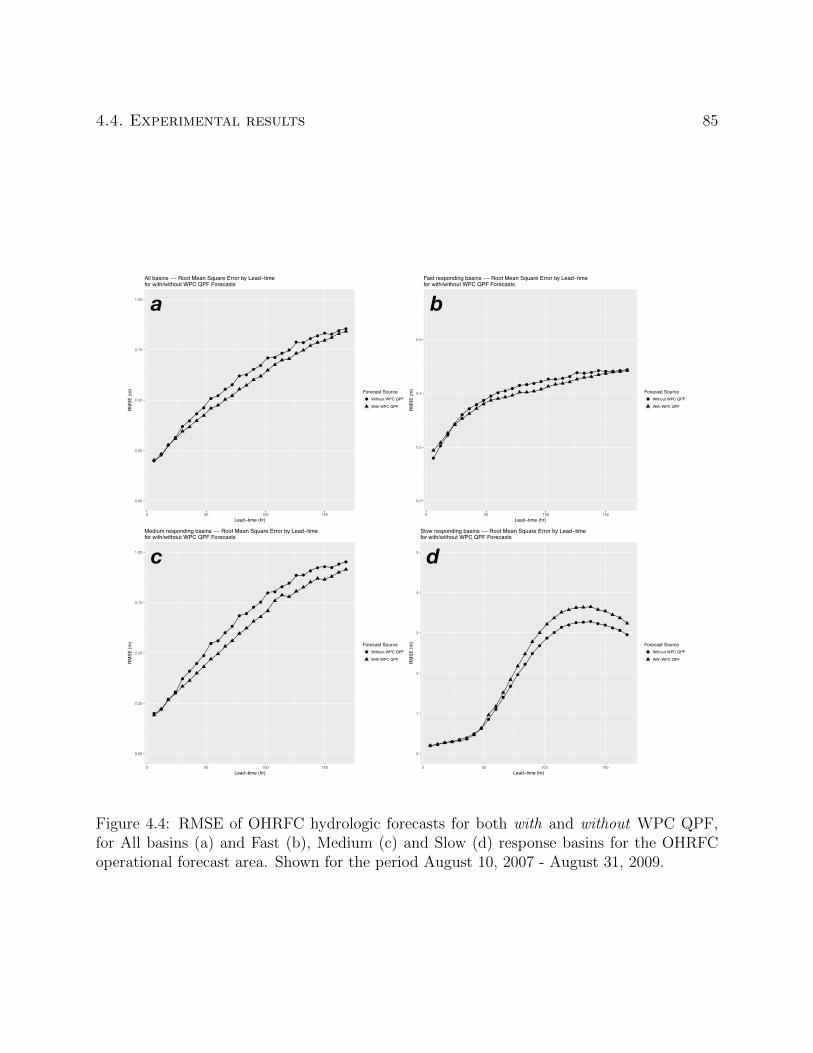
4.4. Experimental results 85
●
●
●
●
●
●●
●●
● ●●
● ● ● ●● ● ● ●
● ● ● ● ● ● ● ●
0.0
0.2
0.4
0.6
0 50 100 150Lead−time (hr)
RM
SE (m
) Forecast Source● Without WPC QPF
With WPC QPF
Fast responding basins −− Root Mean Square Error by Lead−timefor with/without WPC QPF Forecasts
● ● ● ● ● ●●
●
●
●
●
●
●
●
●
●
●
●
●●
● ● ●● ●
●●
●
0
1
2
3
4
5
0 50 100 150Lead−time (hr)
RM
SE (m
) Forecast Source● Without WPC QPF
With WPC QPF
Slow responding basins −− Root Mean Square Error by Lead−timefor with/without WPC QPF Forecasts
●●
●
●
●
●
●
●
●●
●
●
●●
●●
● ●●
●
● ●●
● ● ●●
●
0.00
0.25
0.50
0.75
1.00
0 50 100 150Lead−time (hr)
RM
SE (m
) Forecast Source● Without WPC QPF
With WPC QPF
Medium responding basins −− Root Mean Square Error by Lead−timefor with/without WPC QPF Forecasts
●
●
●
●
●
●
●
●
●●
●●
● ●
●●
● ●●
●
● ●●
●● ●
● ●
0.00
0.25
0.50
0.75
1.00
0 50 100 150Lead−time (hr)
RM
SE (m
) Forecast Source● Without WPC QPF
With WPC QPF
All basins −− Root Mean Square Error by Lead−timefor with/without WPC QPF Forecasts
a
c
b
d
Figure 4.4: RMSE of OHRFC hydrologic forecasts for both with and without WPC QPF,for All basins (a) and Fast (b), Medium (c) and Slow (d) response basins for the OHRFCoperational forecast area. Shown for the period August 10, 2007 - August 31, 2009.

86Chapter 4. The Effect of QPF on Real-time Deterministic Hydrologic
Forecast Uncertainty
QPF compared to zero QPF. That is, Experiment 1 shows that non-zero QPF in hydrologic
forecasting produces lower error with longer lead-times than for zero-QPF forecasts. It should
be noted that a full 24-h duration (4, 6-h periods (24 h)−1) of WPC QPF was used for the
experimental QPF scenarios, which was, at the time, the duration of QPF used operationally
at the OHRFC. Experiment 2 investigates the influence of the duration of QPF on hydrologic
forecast error.
4.4.2 Experiment 2
Experiment 2 results are summarized in Figures 4.5 - 4.8. Table 4.3 provides detailed results
of ME, MAE, and RMSE verification measures for fast response basins. The following
observations can be made:
1. With all basin locations grouped together, verification results show that the magnitude
of ME, MAE, and RMSE values increase with longer durations of QPF, which is
expected and generally understood;
2. When basins are stratified according to above and below flood level forecasts categories,
non-flood (below flood) level forecasts exhibit reduced forecast error with longer dura-
tions of QPF compared to above flood forecasts. In other words, flood forecasts show
larger errors than non-flood forecasts, which confirms expectations;
3. Little or no change in hydrologic forecast error is observed with increasing the duration
of QPF from 6- to 12-h, irrespective of forecast category or verification measure;
4. For fast responding basins, increases in forecast error jump significantly from 6- and 12-
h QPF durations to longer QPF durations. Specifically, we see (using Table 4.3) that
lengthening the duration of QPF from 6-h to 24-h, increases ME by 114.9% (greater
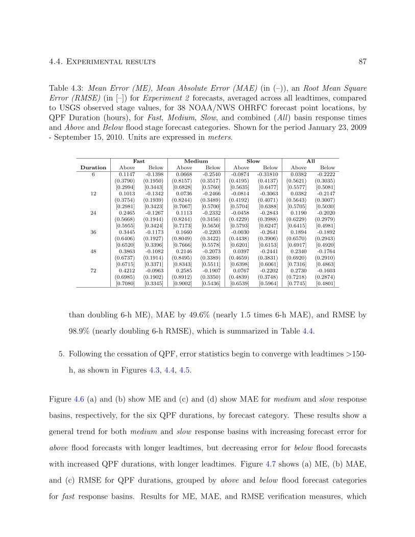
4.4. Experimental results 87
Table 4.3: Mean Error (ME), Mean Absolute Error (MAE) (in (–)), an Root Mean SquareError (RMSE) (in [–]) for Experiment 2 forecasts, averaged across all leadtimes, comparedto USGS observed stage values, for 38 NOAA/NWS OHRFC forecast point locations, byQPF Duration (hours), for Fast, Medium, Slow, and combined (All) basin response timesand Above and Below flood stage forecast categories. Shown for the period January 23, 2009- September 15, 2010. Units are expressed in meters.
Fast Medium Slow AllDuration Above Below Above Below Above Below Above Below
6 0.1147 -0.1398 0.0668 -0.2540 -0.0874 -0.31810 0.0382 -0.2222(0.3790) (0.1950) (0.8157) (0.3517) (0.4195) (0.4137) (0.5621) (0.3035)[0.2994] [0.3443] [0.6828] [0.5760] [0.5635] [0.6477] [0.5577] [0.5081]
12 0.1013 -0.1342 0.0736 -0.2466 -0.0814 -0.3063 0.0382 -0.2147(0.3754) (0.1939) (0.8244) (0.3489) (0.4192) (0.4071) (0.5643) (0.3007)[0.2981] [0.3423] [0.7067] [0.5700] [0.5704] [0.6388] [0.5705] [0.5030]
24 0.2465 -0.1267 0.1113 -0.2332 -0.0458 -0.2843 0.1190 -0.2020(0.5668) (0.1944) (0.8244) (0.3456) (0.4229) (0.3988) (0.6229) (0.2979)[0.5955] [0.3424] [0.7173] [0.5650] [0.5793] [0.6247] [0.6415] [0.4981]
36 0.3445 -0.1173 0.1660 -0.2203 -0.0030 -0.2641 0.1894 -0.1892(0.6406) (0.1927) (0.8049) (0.3422) (0.4438) (0.3906) (0.6570) (0.2943)[0.6520] [0.3396] [0.7666] [0.5578] [0.6201] [0.6153] [0.6917] [0.4920]
48 0.3863 -0.1082 0.2146 -0.2073 0.0397 -0.2441 0.2340 -0.1764(0.6737) (0.1914) (0.8495) (0.3389) (0.4659) (0.3831) (0.6920) (0.2910)[0.6715] [0.3371] [0.8343] [0.5511] [0.6398] [0.6061] [0.7316] [0.4863]
72 0.4212 -0.0963 0.2585 -0.1907 0.0767 -0.2202 0.2730 -0.1603(0.6985) (0.1902) (0.8912) (0.3350) (0.4839) (0.3748) (0.7218) (0.2874)[0.7080] [0.3345] [0.9002] [0.5436] [0.6539] [0.5964] [0.7745] [0.4801]
than doubling 6-h ME), MAE by 49.6% (nearly 1.5 times 6-h MAE), and RMSE by
98.9% (nearly doubling 6-h RMSE), which is summarized in Table 4.4.
5. Following the cessation of QPF, error statistics begin to converge with leadtimes >150-
h, as shown in Figures 4.3, 4.4, 4.5.
Figure 4.6 (a) and (b) show ME and (c) and (d) show MAE for medium and slow response
basins, respectively, for the six QPF durations, by forecast category. These results show a
general trend for both medium and slow response basins with increasing forecast error for
above flood forecasts with longer leadtimes, but decreasing error for below flood forecasts
with increased QPF durations, with longer leadtimes. Figure 4.7 shows (a) ME, (b) MAE,
and (c) RMSE for QPF durations, grouped by above and below flood forecast categories
for fast response basins. Results for ME, MAE, and RMSE verification measures, which
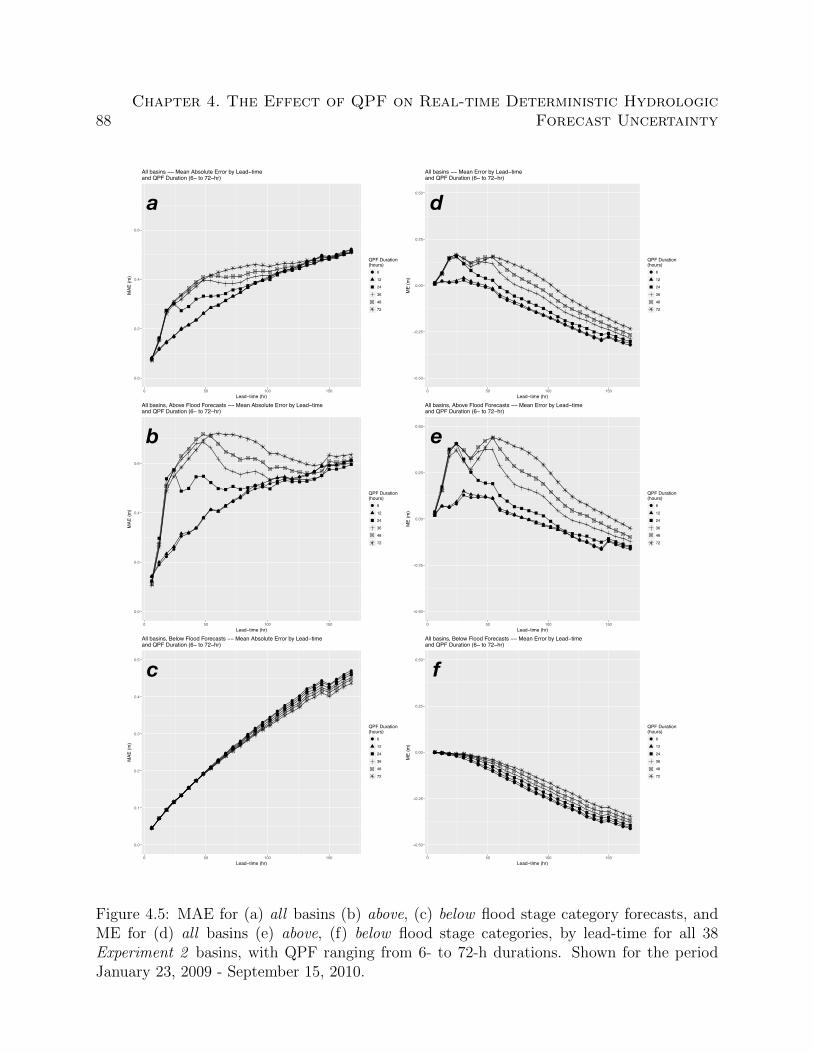
88Chapter 4. The Effect of QPF on Real-time Deterministic Hydrologic
Forecast Uncertainty
●
● ●●
●● ● ● ●
●● ●
● ●●
●●
●●
●●
●●
●
●●
●●
−0.50
−0.25
0.00
0.25
0.50
0 50 100 150Lead−time (hr)
ME
(m)
QPF Duration(hours)● 6
12
24
36
48
72
All basins, Above Flood Forecasts −− Mean Error by Lead−timeand QPF Duration (6− to 72−hr)
● ● ● ● ●●
●●
●●
●●
●●
●●
●●
●●
●●
●● ●
●● ●
−0.50
−0.25
0.00
0.25
0.50
0 50 100 150Lead−time (hr)
ME
(m)
QPF Duration(hours)● 6
12
24
36
48
72
All basins, Below Flood Forecasts −− Mean Error by Lead−timeand QPF Duration (6− to 72−hr)
●
●
●
●
●
●
●
●
●
●
●
●
●
●
●
●
●
●
●●
●
●●
●●
●●
●
0.0
0.1
0.2
0.3
0.4
0.5
0 50 100 150Lead−time (hr)
MAE
(m)
QPF Duration(hours)● 6
12
24
36
48
72
All basins, Below Flood Forecasts −− Mean Absolute Error by Lead−timeand QPF Duration (6− to 72−hr)
●
●
●
●
●●
●
●
● ●
●●
●
●● ●
●●
● ●●
●●
● ● ●●
●
0.0
0.2
0.4
0.6
0 50 100 150Lead−time (hr)
MAE
(m)
QPF Duration(hours)● 6
12
24
36
48
72
All basins, Above Flood Forecasts −− Mean Absolute Error by Lead−timeand QPF Duration (6− to 72−hr)
●● ● ●
●●
● ●●
●●
●●
●●
●●
●●
●●
●●
●●
●● ●
−0.50
−0.25
0.00
0.25
0.50
0 50 100 150Lead−time (hr)
ME
(m)
QPF Duration(hours)● 6
12
24
36
48
72
All basins −− Mean Error by Lead−timeand QPF Duration (6− to 72−hr)
●
●
●
●
●●
●
●
●●
●●
●●
●●
●●
● ●●
●●
● ●●
●●
0.0
0.2
0.4
0.6
0 50 100 150Lead−time (hr)
MAE
(m)
QPF Duration(hours)● 6
12
24
36
48
72
All basins −− Mean Absolute Error by Lead−timeand QPF Duration (6− to 72−hr)
a
c
b
d
e
f
Figure 4.5: MAE for (a) all basins (b) above, (c) below flood stage category forecasts, andME for (d) all basins (e) above, (f) below flood stage categories, by lead-time for all 38Experiment 2 basins, with QPF ranging from 6- to 72-h durations. Shown for the periodJanuary 23, 2009 - September 15, 2010.
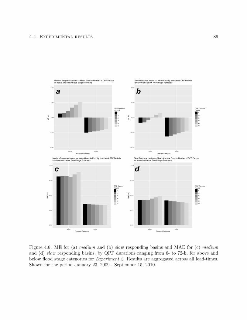
4.4. Experimental results 89
−0.50
−0.25
0.00
0.25
0.50
above belowForecast Category
ME
(m)
QPF Duration(hours)
6
12
24
36
48
72
Medium Response basins −− Mean Error by Number of QPF Periodsfor above and below Flood Stage Forecasts
0.00
0.25
0.50
0.75
1.00
above belowForecast Category
MAE
(m)
QPF Duration(hours)
6
12
24
36
48
72
Medium Response basins −− Mean Absolute Error by Number of QPF Periodsfor above and below Flood Stage Forecasts
−0.50
−0.25
0.00
0.25
0.50
above belowForecast Category
ME
(m)
QPF Duration(hours)
6
12
24
36
48
72
Slow Response basins −− Mean Error by Number of QPF Periodsfor above and below Flood Stage Forecasts
0.00
0.25
0.50
0.75
1.00
above belowForecast Category
MAE
(m)
QPF Duration(hours)
6
12
24
36
48
72
Slow Response basins −− Mean Absolute Error by Number of QPF Periodsfor above and below Flood Stage Forecasts
a
dc
b
Figure 4.6: ME for (a) medium and (b) slow responding basins and MAE for (c) mediumand (d) slow responding basins, by QPF durations ranging from 6- to 72-h, for above andbelow flood stage categories for Experiment 2. Results are aggregated across all lead-times.Shown for the period January 23, 2009 - September 15, 2010.
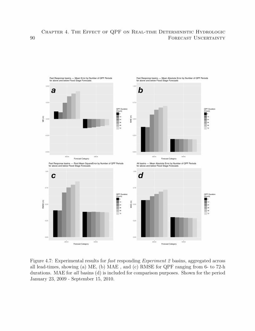
90Chapter 4. The Effect of QPF on Real-time Deterministic Hydrologic
Forecast Uncertainty
0.00
0.25
0.50
0.75
1.00
above belowForecast Category
RM
SE (m
)
QPF Duration(hours)
6
12
24
36
48
72
Fast Response basins −− Root Mean SquareError by Number of QPF Periodsfor above and below Flood Stage Forecasts
−0.50
−0.25
0.00
0.25
0.50
above belowForecast Category
ME
(m)
QPF Duration(hours)
6
12
24
36
48
72
Fast Response basins −− Mean Error by Number of QPF Periodsfor above and below Flood Stage Forecasts
0.00
0.25
0.50
0.75
1.00
above belowForecast Category
MAE
(m)
QPF Duration(hours)
6
12
24
36
48
72
Fast Response basins −− Mean Absolute Error by Number of QPF Periodsfor above and below Flood Stage Forecasts
0.00
0.25
0.50
0.75
1.00
above belowForecast Category
MAE
(m)
QPF Duration(hours)
6
12
24
36
48
72
All basins −− Mean Absolute Error by Number of QPF Periodsfor above and below Flood Stage Forecasts
a
dc
b
Figure 4.7: Experimental results for fast responding Experiment 2 basins, aggregated acrossall lead-times, showing (a) ME, (b) MAE , and (c) RMSE for QPF ranging from 6- to 72-hdurations. MAE for all basins (d) is included for comparison purposes. Shown for the periodJanuary 23, 2009 - September 15, 2010.

4.5. Discussion 91
Table 4.4: Summary of hydrologic forecast error change (%) from 6-h duration WPC QPFto 12-, 24-, 36-, 48-, and 72-h durations for Fast responding basins, for above flood stagecategory forecasts, from Table 4.3.
QPF Duration ME MAE RMSE
6 – – –12 -11.7 -0.9 -0.424 114.9 49.6 98.936 200.3 69.0 117.848 236.8 77.8 124.372 267.2 84.3 136.5
are summarized in Table 4.3, show significant increases in hydrologic forecast error with
longer QPF durations for above flood level forecasts. Below flood level forecasts reflect
slight decreases in hydrologic forecast error with longer QPF durations.
4.5 Discussion
Forecast verification results from Experiments 1 and 2 have demonstrated several key points
related to the use of deterministic QPF, namely,
1. The use of non-zero QPF reduces hydrologic forecast error compared to zero QPF;
2. Hydrologic forecast error generally increases with longer durations of QPF. The ex-
ception occurs with below flood level forecasts, where forecast error diminishes with
longer durations of QPF;
3. For flood forecasting purposes, the use of QPF beyond either 6- or 12-h is not recom-
mended due to greatly increased hydrologic forecast error.
The latter point is underscored in Figure 4.8, which shows RMSE for all basins and response
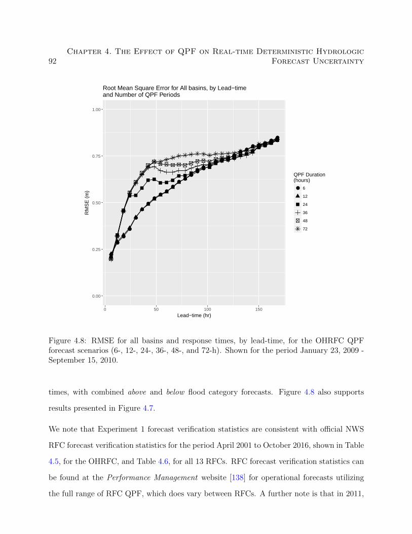
92Chapter 4. The Effect of QPF on Real-time Deterministic Hydrologic
Forecast Uncertainty
●
●
●
●
●
●
●●
●●
●●
●●
●●
●●
● ●●
● ●● ● ●
●●
0.00
0.25
0.50
0.75
1.00
0 50 100 150
Lead−time (hr)
RM
SE
(m
)
QPF Duration(hours)
● 6
12
24
36
48
72
Root Mean Square Error for All basins, by Lead−timeand Number of QPF Periods
Figure 4.8: RMSE for all basins and response times, by lead-time, for the OHRFC QPFforecast scenarios (6-, 12-, 24-, 36-, 48-, and 72-h). Shown for the period January 23, 2009 -September 15, 2010.
times, with combined above and below flood category forecasts. Figure 4.8 also supports
results presented in Figure 4.7.
We note that Experiment 1 forecast verification statistics are consistent with official NWS
RFC forecast verification statistics for the period April 2001 to October 2016, shown in Table
4.5, for the OHRFC, and Table 4.6, for all 13 RFCs. RFC forecast verification statistics can
be found at the Performance Management website [138] for operational forecasts utilizing
the full range of RFC QPF, which does vary between RFCs. A further note is that in 2011,

4.5. Discussion 93
the OHRFC changed the use of QPF from 24-h duration (4, 6-h periods (24 h)−1) to 48-h
duration (8, 6-h periods (48 h)−1) for routine operations.
The findings from Experiment 2 show that the use of longer durations of QPF as a model
forcing leads to increased hydrologic forecast error, except for below flood forecasts, where
errors are reduced with increased durations of QPF. Figure 4.6 shows smaller MAE values
at a given lead-time and QPF duration, reflecting smaller error, for slow responding basins
relative to medium and fast responding basins, shown in Figure 4.7. In turn, smaller MAE
values for a given lead-time and QPF duration are found with medium response basins than
for fast responding basins. This reflects the relative insensitivity of larger watersheds to QPF
location errors compared to smaller watersheds. Dramatic increases in flood forecast error
for fast responding watersheds was demonstrated for QPF durations >12-h. Because larger
watersheds are comprised of many smaller, fast responding basins where flood forecasts are
issued, we believe QPF with durations ≤12-h should be recommended for flood forecasting
purposes.
However, these results beg the issue of how QPF uncertainty is translated into the expres-
sion of uncertainty in hydrologic forecasting. Advancements in probabilistic and ensemble
hydrologic forecasting capture the need to quantify hydrologic forecast uncertainty, particu-
larly as it relates to QPF uncertainty (Cloke and Pappenberger [40]; Adams and Ostrowski
[1]; Demargne et al. [58]). We believe that the findings from this study, taken together
with conclusions drawn from Adams and Dymond [6], which quantifies the magnitude of
hydrologic forecast error that can ensue from the use of deterministic QPF, underscores the
necessity for the use of ensemble, or, more generally, probabilistic hydrologic forecasting over
deterministic forecasting using single-valued deterministic QPF.
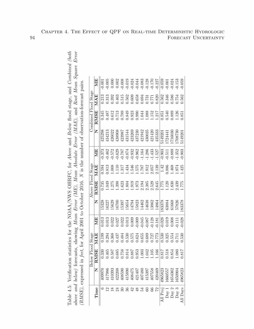
94Chapter 4. The Effect of QPF on Real-time Deterministic Hydrologic
Forecast Uncertainty
Tab
le4.
5:V
erifi
cati
onst
atis
tics
for
the
NO
AA
/NW
SO
HR
FC
,fo
rA
bove
and
Bel
owflood
stag
e,an
dC
ombi
ned
(bot
hab
ove
and
belo
w)
fore
cast
s,sh
owin
gM
ean
Err
or(M
E),
Mea
nA
bsol
ute
Err
or(M
AE
),an
dR
oot
Mea
nS
quar
eE
rror
(RM
SE
),ex
pre
ssed
infe
et,
for
Apri
l20
01to
Oct
ober
2016
.N
isth
enum
ber
ofob
serv
atio
n-f
orec
ast
pai
rs.
Bel
owF
lood
Sta
geA
bov
eF
lood
Sta
ge
Com
bin
edF
lood
Sta
ge
Tim
eN
RM
SE
MAE
ME
NRM
SE
MAE
ME
NRM
SE
MAE
ME
640
9970
0.33
00.
199
0.01
315328
0.7
35
0.5
94
-0.3
73
425298
0.3
45
0.2
13
-0.0
01
1241
7986
0.46
50.
294
0.01
316227
1.0
49
0.8
13
-0.4
62
434213
0.4
87
0.3
13
-0.0
05
1841
0393
0.58
70.
368
0.02
215629
1.2
75
1.0
08
-0.5
72
426022
0.6
12
0.3
92
0.0
00
2442
2208
0.68
50.
437
0.02
716700
1.3
98
1.1
10
-0.6
29
438908
0.7
13
0.4
63
0.0
02
3040
8590
0.75
80.
484
0.02
215397
1.6
23
1.3
17
-0.7
87
423987
0.7
89
0.5
15
-0.0
08
3641
5890
0.81
40.
530
0.01
315654
1.8
04
1.4
34
-0.8
74
431544
0.8
49
0.5
62
-0.0
19
4240
8475
0.88
70.
575
0.00
914794
1.9
19
1.5
46
-0.9
32
423269
0.9
23
0.6
09
-0.0
24
4842
1407
0.95
30.
624
-0.0
0915823
1.9
73
1.5
75
-0.9
62
437230
0.9
90
0.6
58
-0.0
44
5440
7480
1.00
30.
655
-0.0
4514462
2.1
94
1.7
87
-1.1
64
421942
1.0
44
0.6
94
-0.0
83
6041
5397
1.04
20.
689
-0.0
8714638
2.3
85
1.9
12
-1.2
86
430035
1.0
88
0.7
31
-0.1
28
6640
7558
1.10
50.
727
-0.1
2813862
2.5
29
2.0
57
-1.4
33
421420
1.1
52
0.7
71
-0.1
70
7242
0469
1.16
60.
773
-0.1
8114864
2.6
45
2.1
39
-1.5
27
435333
1.2
17
0.8
20
-0.2
27
All
Pro
j49
6582
30.
817
0.53
0-0
.028
183378
1.7
75
1.4
2-0
.903
5149201
0.8
51
0.5
62
-0.0
59
Day
116
6055
70.
518
0.32
50.
019
63884
1.1
20
0.8
86
-0.5
11
1724441
0.5
40
0.3
46
-0.0
01
Day
216
5436
20.
854
0.55
40.
008
61668
1.8
30
1.4
68
-0.8
89
1716030
0.8
89
0.5
86
-0.0
24
Day
316
5090
41.
080
0.71
1-0
.111
57826
2.4
39
1.9
74
-1.3
52
1708730
1.1
26
0.7
54
-0.1
53
All
Day
s49
6582
30.
817
0.53
0-0
.028
183378
1.7
75
1.4
25
-0.9
03
5149201
0.8
51
0.5
62
-0.0
59
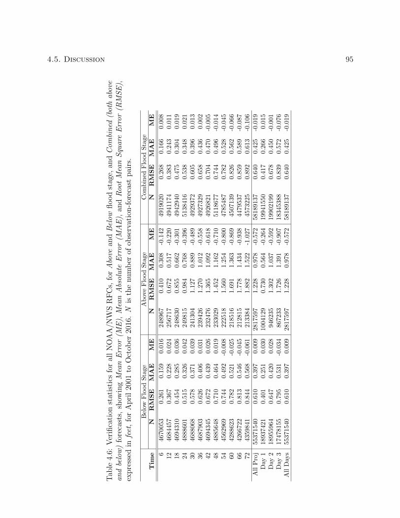
4.5. Discussion 95
Tab
le4.
6:V
erifi
cati
onst
atis
tics
for
all
NO
AA
/NW
SR
FC
s,fo
rA
bove
and
Bel
owflood
stag
e,an
dC
ombi
ned
(bot
hab
ove
and
belo
w)
fore
cast
s,sh
owin
gM
ean
Err
or(M
E),
Mea
nA
bsol
ute
Err
or(M
AE
),an
dR
oot
Mea
nS
quar
eE
rror
(RM
SE
),ex
pre
ssed
infe
et,
for
Apri
l20
01to
Oct
ober
2016
.N
isth
enum
ber
ofob
serv
atio
n-f
orec
ast
pai
rs.
Bel
owF
lood
Sta
geA
bov
eF
lood
Sta
ge
Com
bin
edF
lood
Sta
ge
Tim
eN
RM
SE
MAE
ME
NRM
SE
MAE
ME
NRM
SE
MAE
ME
646
7005
30.
261
0.15
90.
016
248967
0.4
10
0.3
08
-0.1
42
4919020
0.2
68
0.1
66
0.0
08
1246
8445
70.
367
0.22
80.
024
256717
0.6
72
0.5
17
-0.2
20
4941174
0.3
83
0.2
43
0.0
11
1846
9431
00.
454
0.28
50.
036
248630
0.8
55
0.6
62
-0.3
01
4942940
0.4
75
0.3
04
0.0
19
2448
8860
10.
515
0.32
60.
042
249815
0.9
84
0.7
68
-0.3
96
5138416
0.5
38
0.3
48
0.0
21
3046
8806
80.
578
0.37
10.
039
241304
1.1
27
0.8
89
-0.4
89
4929372
0.6
05
0.3
96
0.0
13
3646
8790
30.
626
0.40
60.
031
239426
1.2
70
1.0
12
-0.5
58
4927329
0.6
58
0.4
36
0.0
02
4246
9434
50.
672
0.43
90.
026
232476
1.3
65
1.0
92
-0.6
18
4926821
0.7
04
0.4
70
-0.0
05
4848
8564
80.
710
0.46
40.
019
233029
1.4
52
1.1
62
-0.7
10
5118677
0.7
44
0.4
96
-0.0
14
5445
6296
90.
744
0.49
2-0
.008
222518
1.5
60
1.2
54
-0.8
00
4785487
0.7
82
0.5
28
-0.0
45
6042
8862
30.
782
0.52
1-0
.025
218516
1.6
91
1.3
63
-0.8
69
4507139
0.8
26
0.5
62
-0.0
66
6642
6672
20.
813
0.54
6-0
.045
212815
1.7
78
1.4
34
-0.9
38
4479537
0.8
59
0.5
89
-0.0
87
7243
5984
10.
844
0.56
8-0
.061
213384
1.8
82
1.5
22
-1.0
27
4573225
0.8
92
0.6
13
-0.1
06
All
Pro
j55
3715
400.
610
0.39
70.
009
2817597
1.2
28
0.9
78
-0.5
72
58189137
0.6
40
0.4
25
-0.0
19
Day
118
9374
210.
401
0.25
10.
030
1004129
0.7
30
0.5
64
-0.2
64
19941550
0.4
17
0.2
66
0.0
15
Day
218
9559
640.
647
0.42
00.
028
946235
1.3
02
1.0
37
-0.5
92
19902199
0.6
78
0.4
50
-0.0
01
Day
317
4781
550.
795
0.53
1-0
.034
867233
1.7
26
1.3
91
-0.9
07
18345388
0.8
39
0.5
72
-0.0
76
All
Day
s55
3715
400.
610
0.39
70.
009
2817597
1.2
28
0.9
78
-0.5
72
58189137
0.6
40
0.4
25
-0.0
19

96Chapter 4. The Effect of QPF on Real-time Deterministic Hydrologic
Forecast Uncertainty
4.6 Summary and conclusions
Two independent sets of experimental forecasts, initialized with 1200 UTC saved model
states from OHRFC daily operational forecasts, were conducted to assess the value of de-
terministic QPF as a model forcing in hydrologic forecasting. Specifically, in Experiment 1,
we investigated if the use of non-zero QPF as a model forcing produced hydrologic forecasts
exhibiting smaller forecast error than hydrologic forecasts using zero QPF. Experiment 2
examined the influence of QPF duration on hydrologic forecast error, if the use of non-zero
QPF produces hydrologic forecasts with smaller error than zero QPF forecasts. Both Exper-
iment 1 and Experiment 2 demonstrate that hydrologic forecast error increases with longer
forecast lead-times. Experiment 1 forecast verification statistics suggest that the use of non-
zero QPF as a hydrologic model forcing produces forecasts with less error than forecasts
using zero QPF. Experiment 2 forecast verification statistics indicate that, for above flood
forecasts, longer durations of QPF increases hydrologic forecast error irrespective of basin
size and hydrologic response time. For non-flood forecasts, longer durations of QPF reduces
hydrologic forecast uncertainty. We emphasize the finding from Experiment 2 that shows for
fast responding basins, for above flood forecasts, the use of QPF beyond 6- or 12-h durations
increases hydrologic forecast error dramatically. Consequently, from the perspective of flood
forecasting, the use of deterministic QPF should be restricted to 6- to 12-h duration, be-
yond 6- to 12-h QPF durations hydrologic forecast errors are increased significantly without
benefit.
Chapter 5
Use of Central Tendency Measures
from an Operational Short Lead-time
Hydrologic Ensemble Forecast System
5.1 Abstract
This study presents findings from a real-time forecast experiment that compares legacy de-
terministic hydrologic stage forecasts to ensemble mean and median stage forecasts from
the NOAA/NWS Meteorological Model-based Ensemble Forecast System (MMEFS). The
NOAA/NWS Ohio River Forecast Center (OHRFC) area of responsibility defines the exper-
imental region. Real-time forecasts from subbasins at 54 forecast point locations, ranging
in drainage area, geographic location within the Ohio River Valley, and watershed response
time serve as the basis for analyses. In the experiment, operational hydrologic forecasts, with
24-h QPF and forecast temperatures, are compared to MMEFS hydrologic ensemble mean
and median forecasts, with model forcings from the NOAA/NWS National Centers for En-
97

98Chapter 5. Use of Central Tendency Measures from an Operational Short
Lead-time Hydrologic Ensemble Forecast System
vironmental Prediction (NCEP) North American Ensemble Forecast System (NAEFS), over
the period, November 30, 2010 through May 24, 2012. Experiments indicate that MMEFS
ensemble mean and median forecasts exhibit lower errors beginning at about lead-time 90-h
when forecasts at all locations are aggregated. With fast response basins, that peak ≤24-h,
ensemble mean and median forecasts exhibit lower errors much earlier, beginning at about
lead-time 36-h, which suggests the viability of using MMEFS ensemble forecasts as an alter-
native to OHRFC legacy forecasts. Analyses show that ensemble median forecasts generally
exhibit smaller errors than ensemble mean forecasts for all stage ranges. Verification re-
sults suggest that OHRFC MMEFS NAEFS ensemble forecasts are reasonable, but needed
improvements are identified.
5.2 Introduction
The use of hydrologic ensembles to produce probabilistic flood and water resources forecasts,
using Ensemble Prediction Systems (EPSs), is rapidly gaining acceptance [40, 58, 133, 141].
However, full adoption of probabilistic forecasts by the public and decision-makers as a
replacement to traditional single-valued deterministic hydrologic forecasts is problematic,
particularly with how risk-based forecasts are communicated to end-users [59, 123, 143, 147]
and because of ”institutional conservatism” [149]. National Academies [132] report that with
weather related decision making, end-users of weather related forecasts benefit from (1) their
understanding of forecasts developed over time, (2) prior experience with severe weather,
and (3) other factors, such as family relationships. Related to end-user familiarity with
hydrometeorlogical forecasts, National Research Council [133] and Joslyn and Savelli [99]
found that end-users understand hydrometeorological forecasts are uncertain, but they make
internal adjustments to account for these uncertainties. Morss et al. [128] also found that

5.2. Introduction 99
end-users of weather forecasts understood forecasts are uncertain and that most preferred the
inclusion of uncertainty information with the forecasts. But as Demeritt et al. [59] points out,
resistance to the acceptance of EPS forecasts is ”not simply cognitive or communicative”,
there is also the need by decision makers to ”shift institutional liability for decisions taken
in the face of uncertainty”. Murphy [129] and Krzysztofowicz [110] argue for the adoption of
probabilistic hydrometeorological forecasting, pointing out that rational decision-making in
such a system necessarily shifts decision making from the forecaster to end-users of forecasts.
An intuitive understanding of this undoubtedly helps to shape the reluctance by end users to
adopt probabilistic hydrometeorological forecasts. In other words, resistance to the adoption
of forecasts derived from EPSs, in the form of a probabilistic forecast, by both individuals
and many decision makers, is complex, even with prior understanding that single-valued
deterministic forecasts are uncertain. There is the added issue pointed to by Stern and
Easterling [169] that addresses the need for climate forecasts to be relevant to make them
useful. This need applies to weather and hydrologic forecasts as well, which points to the
broad issue, not addressed in this paper, of how to best convey forecast uncertainty to end-
users in ways that are relevant to them. We might ask, however, if there is an interim step
with the use of EPSs, that can be taken that addresses two issues related to flood forecasting
and the eventual adoption of probabilistic hydrologic forecasts, namely:
1. Improving flood forecast accuracy over current deterministic hydrologic forecasting
methods that rely on single-valued Quantitative Precipitation Forecast (QPF);
2. Softening the landscape for end-users for eventual adoption of forecasts derived from
EPSs in the form of probabilistic forecasts.
In this paper we explore the use of ensemble mean and median hydrologic forecasts from
an EPS as alternatives to deterministic predictions that depend on single-valued QPF. The
100Chapter 5. Use of Central Tendency Measures from an Operational Short
Lead-time Hydrologic Ensemble Forecast System
study region in this paper is the forecast area of responsibility of the National Oceanic
and Atmospheric Administration (NOAA), National Weather Service (NWS), Ohio River
Forecast Center (OHRFC), shown in Figure 5.1, which is one of thirteen NOAA/NWS River
Fortecast Centers (RFCs). Single-valued, deterministic QPF is a commonly used model
forcing in hydrologic forecasting (Georgakakos and Hudlow [82]; Sokol [167]; Adams [5];
Li et al. [114]), and used by all NWS RFCs. Research has demonstrated that the use of
deterministic QPF introduces considerable error into hydrologic forecasting (Cuo et al. [45];
Diomede et al. [61]; Adams and Dymond [6]; [7]). We hypothesize that ensemble mean
or median forecasts have smaller error than deterministic hydrologic forecasts that rely on
single-valued QPF, suggested by Du et al. [63], Mylne et al. [130] with numerical weather
prediction (NWP) ensemble modeling systems.
5.2.1 Background
NWS RFCs are responsible for providing routine river stage/flow forecast guidance to NWS
Weather Forecast Offices (WFOs) following procedures described in Adams [4] and Adams
and Dymond [7]. The central responsibility of most RFCs is flood prediction, although for
RFCs in western States, water supply forecasting, largely for reservoir inflows is, perhaps,
of greater importance. RFCs utilize the NWS Community Hydrologic Prediction System
(CHPS) [4], based on the Flood Early Warning System (FEWS) [55]. CHPS modeling is
predominantly interactive, as described by Adams and Smith [2], within the Linux based
NOAA/NWS Advanced Weather Interactive Processing System (AWIPS) [140, 141]. The
OHRFC employs several models within the CHPS operational environment, including the
Sacramento Soil Moisture Accounting (SAC-SMA) model Burnash [32], Burnash et al. [34],
SNOW-17 snow accumulation and ablation model [12], several lumped-parameter hydrologic
routing models, and three reservoir simulation models. All OHRFC CHPS models were mi-

5.2. Introduction 101
APRFC
CNRFC MARFC
NERFC
MBRFC
CBRFC
NWRFC
ABRFC
WGRFCSERFC
OHRFC
NCRFC
LMRFC
Figure 5.1: The NWS 13 River Forecast Centers (RFCs) – Alaska/Pacific RFC(APRFC), Arkansas-Red RFC (ABRFC), Colorado Basin RFC (CBRFC), California-NevadaRFC(CNRFC), Lower-Mississippi RFC (LMRFC)Middle Atlantic RFC (MARFC), MissouriBasin RFC (MBRFC), North Central RFC (NCRFC), Northwest RFC (NWRFC), OhioRFC (OHRFC), Southeast RFC (SERFC), and West Gulf RFC (WGRFC). Please notethat several RFC boundaries extend beyond the U.S. national boundary into Canada andMexico.

102Chapter 5. Use of Central Tendency Measures from an Operational Short
Lead-time Hydrologic Ensemble Forecast System
grated from the legacy NWS River Forecast System (NWSRFS) (U.S. Department of Com-
merce [177]) in 2011, with parallel NWSRFS and CHPS modeling through 2012. In addition
to QPF, principal hydrologic model forcings are observed precipitation and observed and
forecasted temperature. Observed precipitation forcings are obtained from a multisensor es-
timation process, involving rain gauges, NWS NEXt-generation RADar (NEXRAD) doppler
radar, and, at some RFCs, remotely-sensed satellite estimates of precipitation [92, 103, 202].
Forecasted precipitation is derived from numerical weather prediction (NWP) models, usu-
ally with meteorological forecaster adjustments made at both the NWS Weather Prediction
Center (WPC) and/or at local RFCs [139].
5.2.2 Research goals
The aim of this research is to determine the utility of using hydrologic ensemble mean or
median forecasts of river stage from the NOAA/NWS Meteorological Model-based Ensem-
ble Forecast System (MMEFS), described in Adams and Ostrowski [1], as an alternative to
current, operational, single-valued deterministic hydrologic stage forecasts at the OHRFC
and, possibly, elsewhere. Section 5.3 of this paper describes the real-time hydrologic fore-
casting experiment used in this study. Model simulations are restricted to watersheds in the
OHRFC area of responsibility, shown in Figure 5.1. The experiment consists of concurrent
generation of OHRFC operational river stage forecasts and MMEFS ensemble forecasts for
the November 30, 2010 through May 24, 2012 period. Verification results of the ensemble
median and mean forecasts relative to the OHRFC operational forecasts are presented in
section 5.4. Experimental results are discussed in relation to verification of the MMEFS en-
semble forecasts in section 5.5. Section 5.6 summarizes the experimental results and presents
conclusions.

5.3. Research Approach 103
5.3 Research Approach
The approach of this study is to compare OHRFC operational forecasts to MMEFS ensemble
mean and median forecasts that use numerical weather prediction (NWP) model precipita-
tion and temperature output from the NOAA/NWS National Centers for Environmental
Prediction (NCEP), North American Ensemble Forecast System (NAEFS) [35] as hydrologic
model forcings. The study period was November 30, 2010 through May 24, 2012. The
NAEFS consists of 42 ensemble members. The research methodology includes:
1. capturing OHRFC operational forecasts initialized at 1200 UTC (daily), with a 5-day
forecast horizon;
2. capturing automated MMEFS NAEFS hydrologic ensemble forecasts based on OHRFC
1200 UTC saved model states (daily), with a 7-day forecast horizon;
3. deterministic verification of operational forecasts and MMEFS NAEFS ensemble mean
and median forecasts (after May 24, 2012);
4. verification of MMEFS NAEFS ensemble forecasts (after May 24, 2012).
The real-time hydrologic forecasts were made using the legacy NWSRFS, relying on a ge-
ographically broad distribution of forecast point locations, with varying basin sizes and
hydrologic response times for the OHRFC. All model forcing inputs and internal and out-
put time-steps are 6-hourly. A total of 54 basins, shown in Figure 5.2, were selected for the
study. Calibrations of SAC-SMA, SNOW-17, channel routing, and reservoir simulation mod-
els for operational use for all OHRFC subbasins were completed long before the experiments
started, following guidelines presented by Anderson [13] and Smith et al. [166]. Operational
and MMEFS simulations utilize a 6-h time step for model forcings, internally, and output.
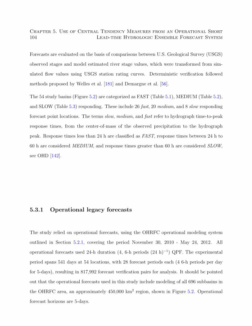
104Chapter 5. Use of Central Tendency Measures from an Operational Short
Lead-time Hydrologic Ensemble Forecast System
Forecasts are evaluated on the basis of comparisons between U.S. Geological Survey (USGS)
observed stages and model estimated river stage values, which were transformed from sim-
ulated flow values using USGS station rating curves. Deterministic verification followed
methods proposed by Welles et al. [181] and Demargne et al. [56].
The 54 study basins (Figure 5.2) are categorized as FAST (Table 5.1), MEDIUM (Table 5.2),
and SLOW (Table 5.3) responding. These include 26 fast, 20 medium, and 8 slow responding
forecast point locations. The terms slow, medium, and fast refer to hydrograph time-to-peak
response times, from the center-of-mass of the observed precipitation to the hydrograph
peak. Response times less than 24 h are classified as FAST, response times between 24 h to
60 h are considered MEDIUM, and response times greater than 60 h are considered SLOW,
see OHD [142].
5.3.1 Operational legacy forecasts
The study relied on operational forecasts, using the OHRFC operational modeling system
outlined in Section 5.2.1, covering the period November 30, 2010 - May 24, 2012. All
operational forecasts used 24-h duration (4, 6-h periods (24 h)−1) QPF. The experimental
period spans 541 days at 54 locations, with 28 forecast periods each (4 6-h periods per day
for 5-days), resulting in 817,992 forecast verification pairs for analysis. It should be pointed
out that the operational forecasts used in this study include modeling of all 696 subbasins in
the OHRFC area, an approximately 450,000 km2 region, shown in Figure 5.2. Operational
forecast horizons are 5-days.
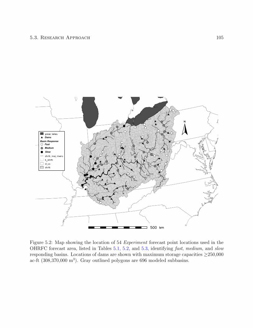
5.3. Research Approach 105
Figure 5.2: Map showing the location of 54 Experiment forecast point locations used in theOHRFC forecast area, listed in Tables 5.1, 5.2, and 5.3, identifying fast, medium, and slowresponding basins. Locations of dams are shown with maximum storage capacities ≥250,000ac-ft (308,370,000 m3). Gray outlined polygons are 696 modeled subbasins.
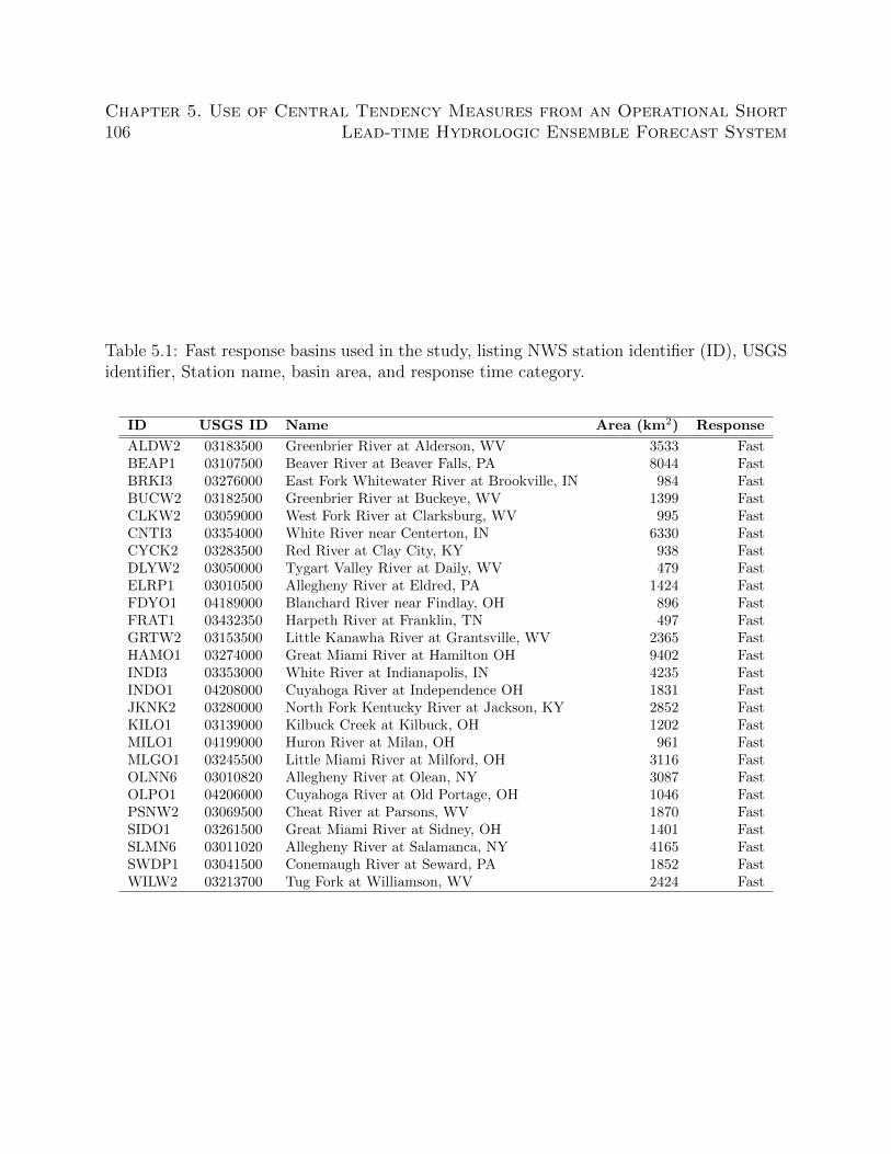
106Chapter 5. Use of Central Tendency Measures from an Operational Short
Lead-time Hydrologic Ensemble Forecast System
Table 5.1: Fast response basins used in the study, listing NWS station identifier (ID), USGSidentifier, Station name, basin area, and response time category.
ID USGS ID Name Area (km2) Response
ALDW2 03183500 Greenbrier River at Alderson, WV 3533 FastBEAP1 03107500 Beaver River at Beaver Falls, PA 8044 FastBRKI3 03276000 East Fork Whitewater River at Brookville, IN 984 FastBUCW2 03182500 Greenbrier River at Buckeye, WV 1399 FastCLKW2 03059000 West Fork River at Clarksburg, WV 995 FastCNTI3 03354000 White River near Centerton, IN 6330 FastCYCK2 03283500 Red River at Clay City, KY 938 FastDLYW2 03050000 Tygart Valley River at Daily, WV 479 FastELRP1 03010500 Allegheny River at Eldred, PA 1424 FastFDYO1 04189000 Blanchard River near Findlay, OH 896 FastFRAT1 03432350 Harpeth River at Franklin, TN 497 FastGRTW2 03153500 Little Kanawha River at Grantsville, WV 2365 FastHAMO1 03274000 Great Miami River at Hamilton OH 9402 FastINDI3 03353000 White River at Indianapolis, IN 4235 FastINDO1 04208000 Cuyahoga River at Independence OH 1831 FastJKNK2 03280000 North Fork Kentucky River at Jackson, KY 2852 FastKILO1 03139000 Kilbuck Creek at Kilbuck, OH 1202 FastMILO1 04199000 Huron River at Milan, OH 961 FastMLGO1 03245500 Little Miami River at Milford, OH 3116 FastOLNN6 03010820 Allegheny River at Olean, NY 3087 FastOLPO1 04206000 Cuyahoga River at Old Portage, OH 1046 FastPSNW2 03069500 Cheat River at Parsons, WV 1870 FastSIDO1 03261500 Great Miami River at Sidney, OH 1401 FastSLMN6 03011020 Allegheny River at Salamanca, NY 4165 FastSWDP1 03041500 Conemaugh River at Seward, PA 1852 FastWILW2 03213700 Tug Fork at Williamson, WV 2424 Fast
5.3. Research Approach 107
Table 5.2: Same as Table 5.1 but for medium response basins.
ID USGS ID Name Area (km2) Response
ATHO1 03159500 Hocking River at Athens, OH 2442 MediumBEDI3 03371500 East Fork White River near Bedford, IN 10000 MediumCDIO1 03142000 Wills Creek at Cambridge, OH 1052 MediumCOLO1 03227500 Scioto River at Columbus, OH 4219 MediumELZW2 03155000 Little Kanawha River at Palestine, WV 3926 MediumFFTK2 03287500 Kentucky River at Lock 4 at Frankfort, KY 13706 MediumFLRK2 03215000 Big Sandy River at Fullers Station, KY 10093 MediumFRKP1 03025500 Allegheny River at Franklin, PA 15493 MediumFTWI3 04182900 Maumee River at Fort Wayne, IN 4988 MediumKANW2 03193000 Kanawha River at Kanawha Falls, WV 21681 MediumLAFI3 03335500 Wabash River at West Lafayette, IN 18121 MediumNATP1 03049500 Allegheny River at Natrona, PA 29552 MediumPARP1 03031500 Allegheny River at Parker, PA 19868 MediumPKTO1 03237020 Scioto River at Piketon, OH 15115 MediumPTTP1 03085152 Monongahela R. at Point State Park, Pittsburgh, PA 49471 MediumSERI3 03365500 East Fork White River at Seymour, IN 6063 MediumSHLI3 03373500 East Fork White River at Shoals, IN 12761 MediumSPNI3 03357000 White River at Spencer, IN 7739 MediumSTRO1 04185000 Tiffin River at Stryker, OH 1062 MediumWLBK2 03404000 Cumberland River at Williamsburg, KY 4162 Medium
Table 5.3: Same as Table 5.1 but for slow response basins.
ID USGS ID Name Area (km2) Response
CARI2 03381500 Little Wabash River at Carmi, IL 8034 SlowEVVI3 03322000 Ohio River at Evansville, IN 277600 SlowGOLI2 03384500 Ohio River at Dam 51 at Golconda, IL 372699 SlowHUFI3 03341500 Wabash River at Terre Haute, IN 31766 SlowNHRI3 03378500 Wabash River at New Harmony, IN 75716 SlowNWBI3 03360500 White River at Newberry, IN 12142 SlowPTRI3 03373980 White River above Petersburg, IN 28808 SlowWTVO1 04193500 Maumee River at Waterville, OH 16395 Slow
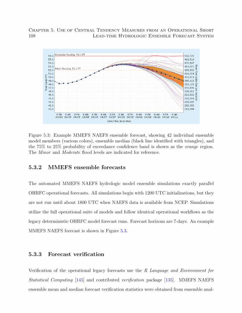
108Chapter 5. Use of Central Tendency Measures from an Operational Short
Lead-time Hydrologic Ensemble Forecast System
Figure 5.3: Example MMEFS NAEFS ensemble forecast, showing 42 individual ensemblemodel members (various colors), ensemble median (black line identified with triangles), andthe 75% to 25% probability of exceedance confidence band is shown as the orange region.The Minor and Moderate flood levels are indicated for reference.
5.3.2 MMEFS ensemble forecasts
The automated MMEFS NAEFS hydrologic model ensemble simulations exactly parallel
OHRFC operational forecasts. All simulations begin with 1200 UTC initializations, but they
are not run until about 1800 UTC when NAEFS data is available from NCEP. Simulations
utilize the full operational suite of models and follow identical operational workflows as the
legacy deterministic OHRFC model forecast runs. Forecast horizons are 7-days. An example
MMEFS NAEFS forecast is shown in Figure 5.3.
5.3.3 Forecast verification
Verification of the operational legacy forecasts use the R Language and Environment for
Statistical Computing [145] and contributed verification package [135]. MMEFS NAEFS
ensemble mean and median forecast verification statistics were obtained from ensemble anal-
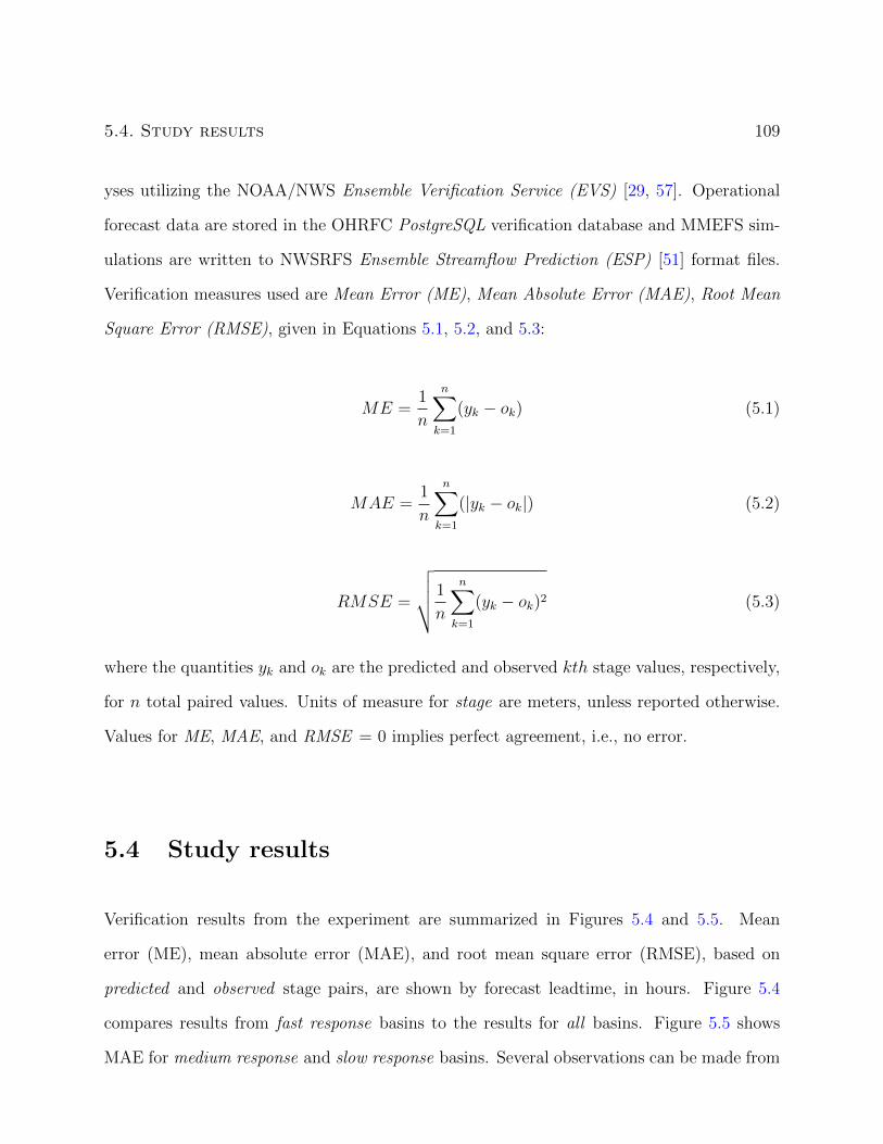
5.4. Study results 109
yses utilizing the NOAA/NWS Ensemble Verification Service (EVS) [29, 57]. Operational
forecast data are stored in the OHRFC PostgreSQL verification database and MMEFS sim-
ulations are written to NWSRFS Ensemble Streamflow Prediction (ESP) [51] format files.
Verification measures used are Mean Error (ME), Mean Absolute Error (MAE), Root Mean
Square Error (RMSE), given in Equations 5.1, 5.2, and 5.3:
ME =1
n
n∑k=1
(yk − ok) (5.1)
MAE =1
n
n∑k=1
(|yk − ok|) (5.2)
RMSE =
√√√√ 1
n
n∑k=1
(yk − ok)2 (5.3)
where the quantities yk and ok are the predicted and observed kth stage values, respectively,
for n total paired values. Units of measure for stage are meters, unless reported otherwise.
Values for ME, MAE, and RMSE = 0 implies perfect agreement, i.e., no error.
5.4 Study results
Verification results from the experiment are summarized in Figures 5.4 and 5.5. Mean
error (ME), mean absolute error (MAE), and root mean square error (RMSE), based on
predicted and observed stage pairs, are shown by forecast leadtime, in hours. Figure 5.4
compares results from fast response basins to the results for all basins. Figure 5.5 shows
MAE for medium response and slow response basins. Several observations can be made from

110Chapter 5. Use of Central Tendency Measures from an Operational Short
Lead-time Hydrologic Ensemble Forecast System
Figure 5.4, namely,
1. In most instances, there is little difference between ensemble mean and median values,
by leadtime. With the exception of RMSE, where ensemble mean values are smaller
than ensemble median values, ensemble median values are always smaller in magnitude
than ensemble mean values, which suggests that ensemble median forecasts should be
preferred over ensemble mean forecasts, since less error is incurred;
2. With the the aggregation of all 54 basins, with respect to ME, little difference ex-
ists between the ensemble median forecast (and mean) and the OHRFC operational
forecast (OHRFC 24-h QPF) through leadtime 54-h. Beginning with leadtime 60-
h, OHRFC operational forecast become increasingly more negatively biased with in-
creased leadtimes, whereas the MMEFS ensemble median forecasts remain unbiased
through leadtime 168-h;
3. With fast response basins, the ensemble median forecast always shows ME values equal
to or smaller in magnitude than the OHRFC operational forecasts, which get increas-
ingly more negative with longer leadtimes after leadtime 72-h compared to ensemble
median forecasts that very slowly become more negative with longer leadtimes;
4. OHRFC operational forecasts have smaller MAE values compared to MMEFS ensemble
median and mean forecasts until leadtime 96-h, with all basins aggregated; however, for
fast response basins, MMEFS ensemble median and mean forecasts have MAE values
equal to or smaller than OHRFC operational forecasts beginning at about leadtime
36-h;
5. With respect to RMSE, with all basins aggregated, OHRFC operational forecasts ex-
hibit smaller error compared to MMEFS ensemble median and mean forecasts until

5.5. Discussion 111
leadtime 90-h, after which MMEFS ensemble median and mean forecast RMSE values
are smaller than OHRFC operational forecast RMSE values; however, for fast response
basins, MMEFS ensemble median and mean forecast RMSE values are approximately
equal to or less than OHRFC operational forecast RMSE values beginning with lead-
time 72-h.
Figure 5.5 shows that for medium and slow response basins, OHRFC operational forecasts
tend to exhibit smaller forecast error compared to MMEFS ensemble median and mean
forecasts until longer leadtimes are reached, ≥102-h. An explanation for this finding is
discussed in Section 5.5.
5.5 Discussion
Three topics of discussion follow, (1) MMEFS ensemble median and mean forecasts com-
pared to OHRFC operational forecasts, (2) MMEFS ensemble verification, and (3) needed
improvements to the MMEFS. A discussion of MMEFS ensemble verification is needed to
demonstrate that MMEFS NAEFS ensemble median and mean forecasts are derived from
a system that has the properties of acceptable forecast skill, reliability, sharpness, and dis-
crimination [185]. A demonstration of acceptable ensemble forecast verification results will
provide a degree of confidence that the ensemble median and mean forecast are derived from
a reasonably robust ensemble forecast system.
5.5.1 MMEFS ensemble median and mean forecasts
Results presented in Figure 5.4 clearly show, in Section 5.4, with all 54 basins aggregated,
that MMEFS ensemble median and mean forecast add considerable value at longer leadtimes
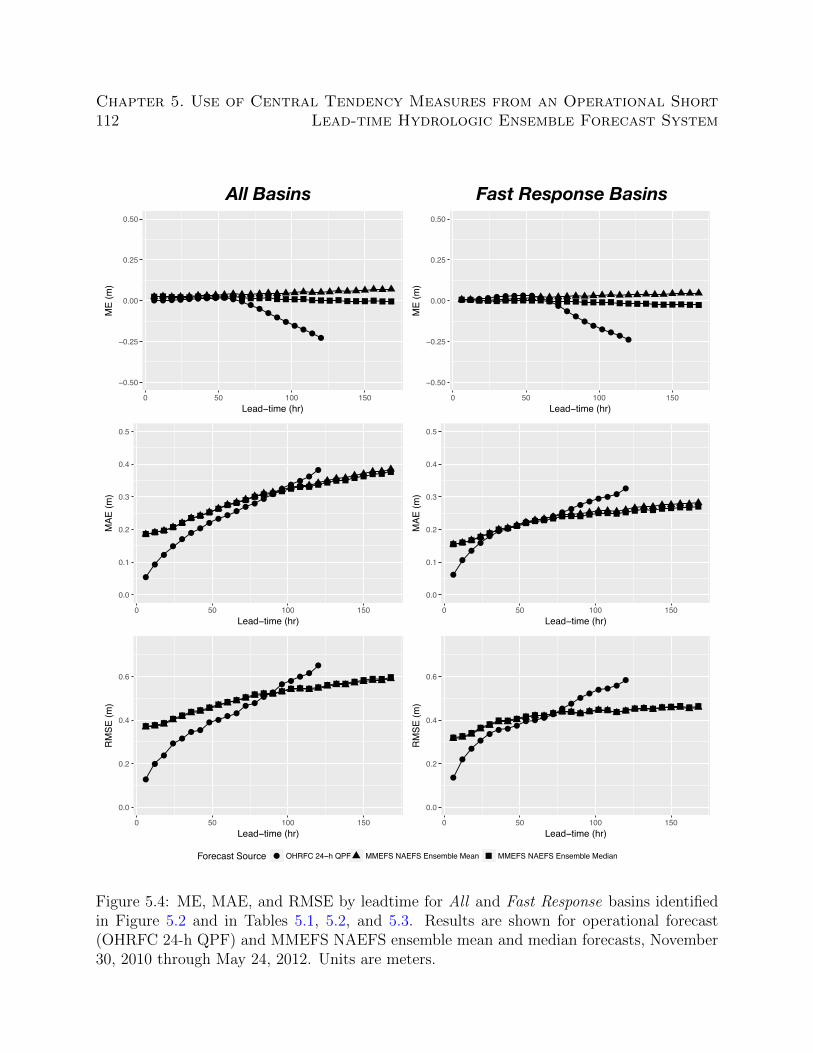
112Chapter 5. Use of Central Tendency Measures from an Operational Short
Lead-time Hydrologic Ensemble Forecast System
All Basins Fast Response Basins
● ● ● ● ● ● ● ● ● ● ● ● ●●
●● ● ● ●
●
−0.50
−0.25
0.00
0.25
0.50
0 50 100 150Lead−time (hr)
ME
(m)
● ● ● ● ● ● ● ● ● ● ●●
●●
●● ● ● ● ●
−0.50
−0.25
0.00
0.25
0.50
0 50 100 150Lead−time (hr)
ME
(m)
●
●●
●●
●●
●● ●
●● ●
●●
●● ●
●●
0.0
0.1
0.2
0.3
0.4
0.5
0 50 100 150Lead−time (hr)
MAE
(m)
●
●●
●●
● ● ● ● ● ● ● ● ● ● ● ● ● ●●
0.0
0.1
0.2
0.3
0.4
0.5
0 50 100 150Lead−time (hr)
MAE
(m)
●
●●
●●
● ●● ● ● ●
● ●●
●● ●
● ●●
0.0
0.2
0.4
0.6
0 50 100 150Lead−time (hr)
RMSE
(m)
●
●
●●
●● ● ●
● ● ● ●●
●●
● ● ● ●●
0.0
0.2
0.4
0.6
0 50 100 150Lead−time (hr)
RMSE
(m)
Forecast Source ● OHRFC 24−h QPF MMEFS NAEFS Ensemble Mean MMEFS NAEFS Ensemble Median
Figure 5.4: ME, MAE, and RMSE by leadtime for All and Fast Response basins identifiedin Figure 5.2 and in Tables 5.1, 5.2, and 5.3. Results are shown for operational forecast(OHRFC 24-h QPF) and MMEFS NAEFS ensemble mean and median forecasts, November30, 2010 through May 24, 2012. Units are meters.
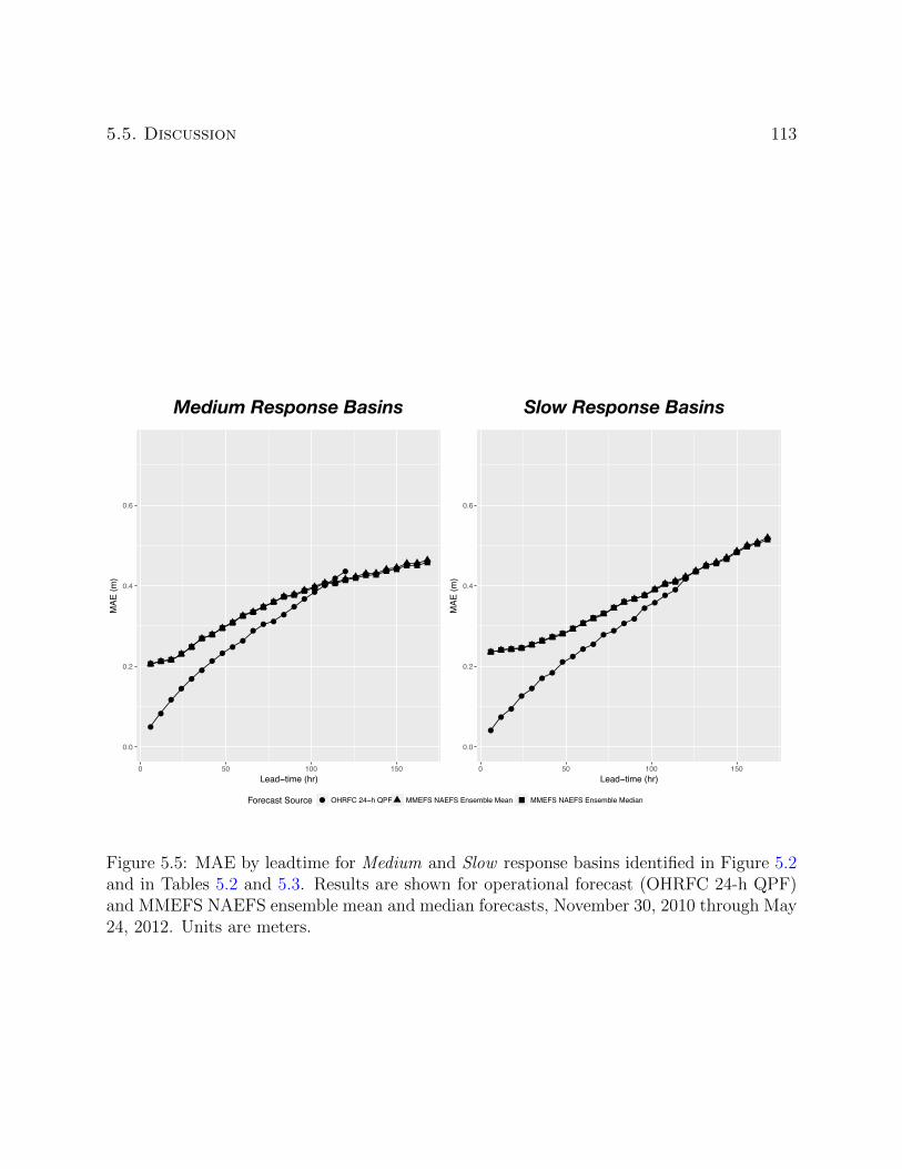
5.5. Discussion 113
Medium Response Basins Slow Response Basins
●
●
●
●
●●
●●
●●
●● ●
●●
●●
●●
●
0.0
0.2
0.4
0.6
0 50 100 150Lead−time (hr)
MAE
(m)
●
●●
●●
●●
●●
●●
●●
●●
●●
●●
●
0.0
0.2
0.4
0.6
0 50 100 150Lead−time (hr)
MAE
(m)
Forecast Source ● OHRFC 24−h QPF MMEFS NAEFS Ensemble Mean MMEFS NAEFS Ensemble Median
Figure 5.5: MAE by leadtime for Medium and Slow response basins identified in Figure 5.2and in Tables 5.2 and 5.3. Results are shown for operational forecast (OHRFC 24-h QPF)and MMEFS NAEFS ensemble mean and median forecasts, November 30, 2010 through May24, 2012. Units are meters.

114Chapter 5. Use of Central Tendency Measures from an Operational Short
Lead-time Hydrologic Ensemble Forecast System
above OHRFC operational forecasts, at leadtimes ≥90-h. An important result is that the
MMEFS ensemble median and mean forecasts for fast response basins have smaller forecast
errors than basins with longer basin response times beginning with leadtimes ≥36-h for MAE
and for ME, MMEFS ensemble median and mean forecasts, for fast response basins, display
smaller error immediately, at leadtime 6-h. This finding is important because it demonstrates
the viability of using MMEFS ensemble median and mean forecast as an alternative to the
continued use of OHRFC operational forecasts relying on 24-h or, currently, 48-h QPF.
Several factors influence the disparity in MMEFS ensemble median and mean forecast verifi-
cation results for medium and slow response basins compared to fast response basins. These
include:
1. Model calibrations are good for fast response, headwater basins, but calibrations for
medium and slow response basins are more problematic. Calibration for non-headwater
basins is more difficult due to, in part, overwhelming upstream flow influences that can
not be accurately separated from total observed streamflow at local non-headwater
gauges. The separation of flows routed from upstream basins from the observed to-
tal streamflow is necessary to estimate the local observed streamflow. With the local
observed streamflow, model parameter adjustments to the local basin can be made ap-
propriately to reflect the hydrologic response of the local watershed being calibrated.
The consequence is that hydrologic model parameters used for downstream basins usu-
ally can only be estimated, not calibrated. The outcome is that local downstream
basin simulations can be considerably more in error than fast response headwater
basins that have been calibrated. Also, overall modeling for downstream medium and
slow response basin is more complex, involving the use of flow routing and reservoir
simulation models, which adds to modeling uncertainty and error;

5.5. Discussion 115
2. For some medium and all slow response basins, complex channel flow dynamics, in-
cluding hydrodynamic backwater effects, adversely affects stage-discharge relationships
and, on the mainstem of the Ohio River, lock & dam controls influence stage-discharge
relationships. The implication here is that, while flow simulations may be good, stage-
discharge relationships are non-unique because of hysteresis. This non-unique stage-
discharge relationship precludes unique conversion from flow to stage. Consequently,
considerable error is incurred, which adversely influences verification scores due to the
introduction of erroneous stage values. Manual forecaster adjustments in the OHRFC
operational workflow are made, in part, to minimize stage-discharge ratings hysteresis
effects. Such adjustments are not possible in MMEFS NAEFS simulations. The need
for dynamic flow routing modeling served as the basis for the development and opera-
tional implementation of the Ohio River Community HEC-RAS Model into CHPS [8].
Unfortunately, this model was not used in the MMEFS NAEFS simulations;
3. Reservoir releases significantly alter downstream flows. OHRFC operational forecasts
benefit from the inclusion of U.S. Army Corps of Engineers (USACE) deterministic
reservoir release schedules, including flow releases from locks & dams, which are in-
corporated into the operational forecasts. MMEFS modeling relies on NWSRFS (now
CHPS) based reservoir model simulations, which, under many scenarios, can be quite
erroneous compared to actual USACE reservoir releases, which involves human deci-
sion making that is difficult to capture in a reservoir simulation model. Figure 5.2
shows that all slow and all but two medium response basin locations are downstream
of significant reservoirs with maximum storage capacities ≥250,000 ac-ft (308,370,000
m3). All of the fast response basins are upstream of these reservoirs. Consequently,
OHRFC operational forecast errors are reduced in the near-term relative to MMEFS
NAEFS ensemble median and mean forecasts that rely solely on model simulations of
116Chapter 5. Use of Central Tendency Measures from an Operational Short
Lead-time Hydrologic Ensemble Forecast System
reservoir outflows.
5.5.2 Ensemble verification
Demargne et al. [57] discuss the need for verification of hydrologic ensemble forecasts, iden-
tifying the need to improve research and operations, specifically aimed at (1) monitoring
changes in forecast quality over time, (2) analyzing sources of forecast error, and (3) evaluat-
ing forecast skill improvements resulting from the introduction of new science and technology.
Consequently, we present some ensemble verification results to serve as a baseline evaluation
of MMEFS forecast quality to identify areas of needed system improvement, which should
further reduce MMEFS ensemble median and mean prediction errors.
Many statistical measures have been used to evaluate probabilistic forecasts. Johnson and
Bowler [97] suggests that, for example, resolution, the property that there should be large
variability of observed frequencies associated with different forecast probabilities around the
climatological value, is desirable. Also, ensemble forecasts should be reliable, that is, fore-
cast probabilities should give an estimate of the expected frequencies of the event occurring.
Welles et al. [181] and Demargne et al. [56] explain the necessity of hydrologic forecast verifi-
cation. Hydrologic ensemble forecast verification methods, as recommended and discussed by
Brown et al. [29] and Demargne et al. [57] are used to assess the MMEFS NAEFS ensemble
forecasts.
The statistical measures to evaluate MMEFS ensemble forecasts are discussed below.
Continuous ranked probability skill score (CRPSS)
The ranked probability score (RPS), shown in Equation 5.4, is a measure of how well fore-
casts, that are expressed as probability distributions, are in matching observed outcomes
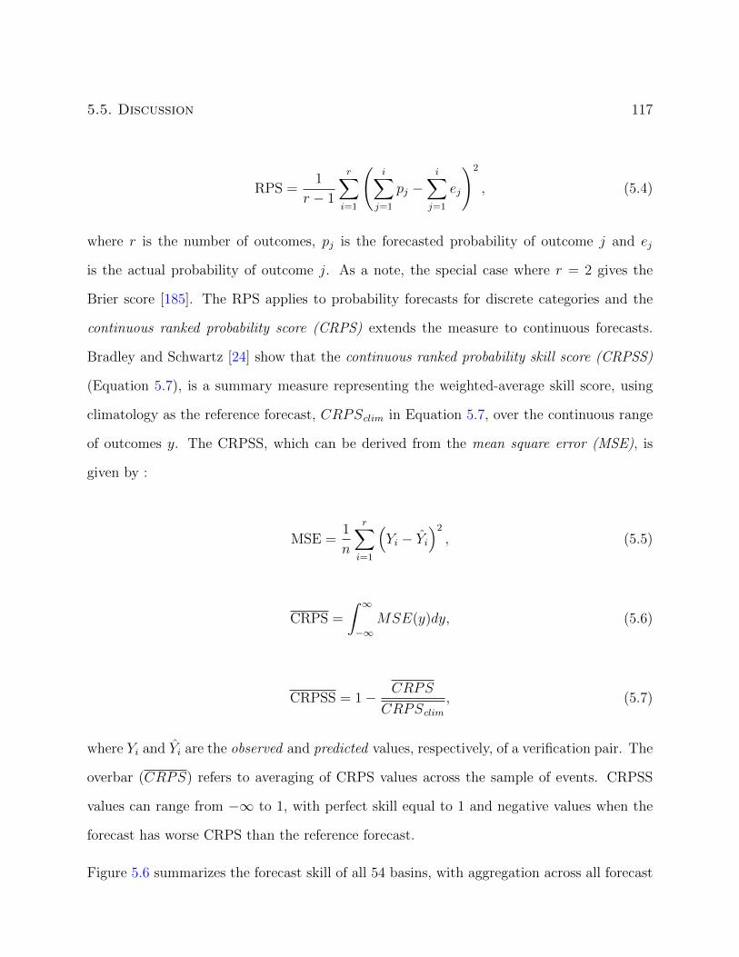
5.5. Discussion 117
RPS =1
r − 1
r∑i=1
(i∑
j=1
pj −i∑
j=1
ej
)2
, (5.4)
where r is the number of outcomes, pj is the forecasted probability of outcome j and ej
is the actual probability of outcome j. As a note, the special case where r = 2 gives the
Brier score [185]. The RPS applies to probability forecasts for discrete categories and the
continuous ranked probability score (CRPS) extends the measure to continuous forecasts.
Bradley and Schwartz [24] show that the continuous ranked probability skill score (CRPSS)
(Equation 5.7), is a summary measure representing the weighted-average skill score, using
climatology as the reference forecast, CRPSclim in Equation 5.7, over the continuous range
of outcomes y. The CRPSS, which can be derived from the mean square error (MSE), is
given by :
MSE =1
n
r∑i=1
(Yi − Yi
)2
, (5.5)
CRPS =
∫ ∞−∞
MSE(y)dy, (5.6)
CRPSS = 1− CRPS
CRPSclim
, (5.7)
where Yi and Yi are the observed and predicted values, respectively, of a verification pair. The
overbar (CRPS) refers to averaging of CRPS values across the sample of events. CRPSS
values can range from −∞ to 1, with perfect skill equal to 1 and negative values when the
forecast has worse CRPS than the reference forecast.
Figure 5.6 summarizes the forecast skill of all 54 basins, with aggregation across all forecast

118Chapter 5. Use of Central Tendency Measures from an Operational Short
Lead-time Hydrologic Ensemble Forecast System
stage ranges (a) and for stage ranges ≥0.90 probability of non-exceedance (b). The results
show that MMEFS NAEFS forecasts are skillful relative to sample climatology and that
forecasts for stage ranges ≥0.90 probability of non-exceedance are more skillful than forecasts
which are aggregated across all stage ranges, which is encouraging since RFCs emphasize
flood forecasting. Also depicted in Figure 5.6 is differentiation between fast, medium, and
slow response basins, which shows MMEFS ensemble forecasts to be most skillful for slow
response basins and that forecast skill is most variable for medium response basins. Forecast
skill, as expected, declines with increased leadtimes.
An interesting point relates to some of the lowest CRPSS values in Figure 5.6(a) which
correspond to the forecast point location at Pittsburgh, PA (PTTP1). Referring to Table 5.4,
CRPSS values aggregated across all forecast stage ranges demonstrate little to no skill.
However, for stage ranges ≥0.90 probability of non-exceedance, MMEFS ensemble forecasts
show reasonable skill. The reason for this difference relates to the complex physical setting
described by Adams et al. [8] involving downstream control at Dashields, PA Lock & Dam
that regulates the pool level at the PTTP1 streamgauge at low flows in a manner that is not
well-captured by the OHRFC modeling system. With higher flows, particularly flood flows,
this control does not exist.
Reliability diagram
Reliability diagrams [90] represent, graphically, the observed frequency of an event plotted
against the forecast probability of an event. This expresses how often (as a relative frequency)
a forecast probability actually occurred. The hit rate is calculated from the sets of forecasts
for each probability separately. Consequently, the hit rate for each probability bin, n, is
given by:
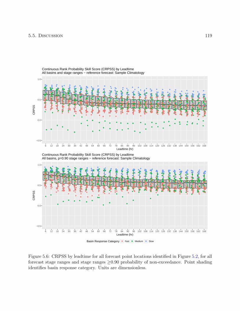
5.5. Discussion 119
−0.5
0.0
0.5
1.0
6 12 18 24 30 36 42 48 54 60 66 72 78 84 90 96 102 108 114 120 126 132 138 144 150 156 162 168
Leadtime (hr)
CR
PS
S
Continuous Rank Probability Skill Score (CRPSS) by LeadtimeAll basins and stage ranges − reference forecast: Sample Climatology
−0.5
0.0
0.5
1.0
6 12 18 24 30 36 42 48 54 60 66 72 78 84 90 96 102 108 114 120 126 132 138 144 150 156 162 168
Leadtime (hr)
CR
PS
S
Continuous Rank Probability Skill Score (CRPSS) by LeadtimeAll basins, p=0.90 stage ranges − reference forecast: Sample Climatology
Basin Response Category Fast Medium Slow
Figure 5.6: CRPSS by leadtime for all forecast point locations identified in Figure 5.2, for allforecast stage ranges and stage ranges ≥0.90 probability of non-exceedance. Point shadingidentifies basin response category. Units are dimensionless.
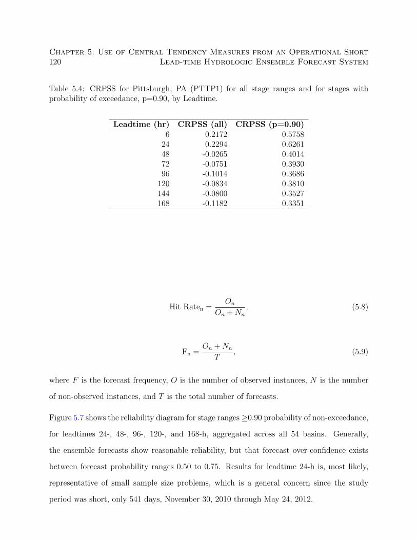
120Chapter 5. Use of Central Tendency Measures from an Operational Short
Lead-time Hydrologic Ensemble Forecast System
Table 5.4: CRPSS for Pittsburgh, PA (PTTP1) for all stage ranges and for stages withprobability of exceedance, p=0.90, by Leadtime.
Leadtime (hr) CRPSS (all) CRPSS (p=0.90)6 0.2172 0.5758
24 0.2294 0.626148 -0.0265 0.401472 -0.0751 0.393096 -0.1014 0.3686
120 -0.0834 0.3810144 -0.0800 0.3527168 -0.1182 0.3351
Hit Raten =On
On +Nn
, (5.8)
Fn =On +Nn
T, (5.9)
where F is the forecast frequency, O is the number of observed instances, N is the number
of non-observed instances, and T is the total number of forecasts.
Figure 5.7 shows the reliability diagram for stage ranges≥0.90 probability of non-exceedance,
for leadtimes 24-, 48-, 96-, 120-, and 168-h, aggregated across all 54 basins. Generally,
the ensemble forecasts show reasonable reliability, but that forecast over-confidence exists
between forecast probability ranges 0.50 to 0.75. Results for leadtime 24-h is, most likely,
representative of small sample size problems, which is a general concern since the study
period was short, only 541 days, November 30, 2010 through May 24, 2012.

5.5. Discussion 121
●
●
●
●
●
0.00
0.25
0.50
0.75
1.00
0.00 0.25 0.50 0.75 1.00Forecast Probability
Obs
erve
d P
roba
bilit
y
Leadtime (hr)● 24
4896120168
Reliability Diagram −− All Basins, p=0.90for 24−, 48−, 96, 120−, and 168−h Leadtimes
Figure 5.7: Reliability Diagram for all 54 basins, for lead-times 24-, 48-, 96-, 120-, and 168-h.Shown for stage ranges ≥0.90 probability of non-exceedance.

122Chapter 5. Use of Central Tendency Measures from an Operational Short
Lead-time Hydrologic Ensemble Forecast System
ObservedForecast yes no
yes a bno c d
Table 5.5: Contingency table.
Relative Operating Characteristic (ROC)
The Relative Operating Characteristic (ROC) [100] provides information on the hit rates
and false alarm rates that can be expected from use of different probability thresholds. The
ROC is a summary score used to describe the ability of forecasts to discriminate between
events and non-events. From Table 5.5:
Hit Rate =a
a+ c(5.10)
False Alarm Rate =b
b+ d(5.11)
Figure 5.8 shows the ROC diagram, aggregated across all 54 basins, for stage ranges ≥0.90
probability of non-exceedance, for forecast leadtimes 24-, 96-, 120-, and 168-h, indicating
that MMEFS NAEFS ensemble forecasts discriminate between events and non-events very
well. This result is representative of similar analyses, done for individual basins and for all
forecast stage ranges.
Rank Histogram
Rank histograms are useful for evaluating ensemble forecasts because they can efficaciously
assess the reliability and errors in the mean and spread of ensemble forecasts [87]. Rank his-
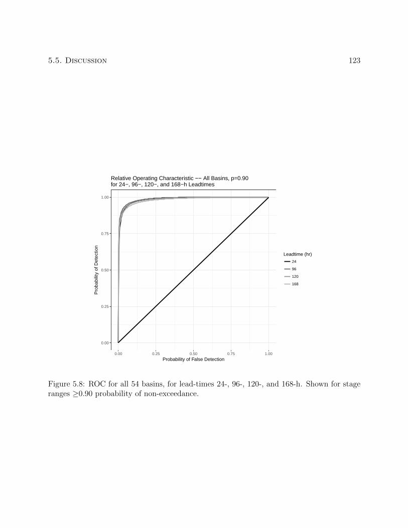
5.5. Discussion 123
0.00
0.25
0.50
0.75
1.00
0.00 0.25 0.50 0.75 1.00
Probability of False Detection
Pro
babi
lity
of D
etec
tion
Leadtime (hr)
24
96
120
168
Relative Operating Characteristic −− All Basins, p=0.90for 24−, 96−, 120−, and 168−h Leadtimes
Figure 5.8: ROC for all 54 basins, for lead-times 24-, 96-, 120-, and 168-h. Shown for stageranges ≥0.90 probability of non-exceedance.
124Chapter 5. Use of Central Tendency Measures from an Operational Short
Lead-time Hydrologic Ensemble Forecast System
tograms are created by tallying the rank of observations relative to values from an ensemble
sorted from lowest to highest rank, which produces, ideally, a uniform distribution across
the ranks.
Rank histogram analyses are summarized by Figure 5.9, which shows severe under-spread
of MMEFS ensemble forecasts, particularly at shorter leadtimes, illustrated for leadtime
24-h. An explanation for this result is shown in Figure 5.3, which was specifically selected
to illustrate the under-spread problem. In this example, the 42 MMEFS NAEFS ensembles
appear as a single-valued forecast from the beginning of the forecast at 2 PM 04/04 through 8
AM 04/07. This occurred because there were (1) no model forcings to substantially perturbe
the hydrologic models over the 2 PM 04/04 through 8 AM 04/07 period and (2) because
inherent model error is not included in the MMEFS.
5.5.3 MMEFS improvements
MMEFS ensemble forecasts do not currently make use of ensemble model-error correction
methods suggested by, for example, Bogner and Kalas [19], Li et al. [115] or post-processing
bias correction of raw ensemble forecasts proposed by Brown and Seo [28], Hashino et al.
[91], Yuan and Wood [197] and others to reduce uncertainties arising from model inputs and
outputs, initial and boundary conditions, and the structure and parameter estimates of mod-
els. Wentao et al. [182] recently reviewed statistical postprocessing methods for hydromete-
orological ensemble forecasting, citing the need for further work on many fronts. These con-
cerns include the need to address stationarity assumptions, handle extreme events, including
the timing of flood peaks, in the case streamflow modeling, further investigate methods pro-
posed to make adjustments at un-gauged locations, and continue research into methods that
attempt to address total uncertainty, including model structure, parameter estimation, and
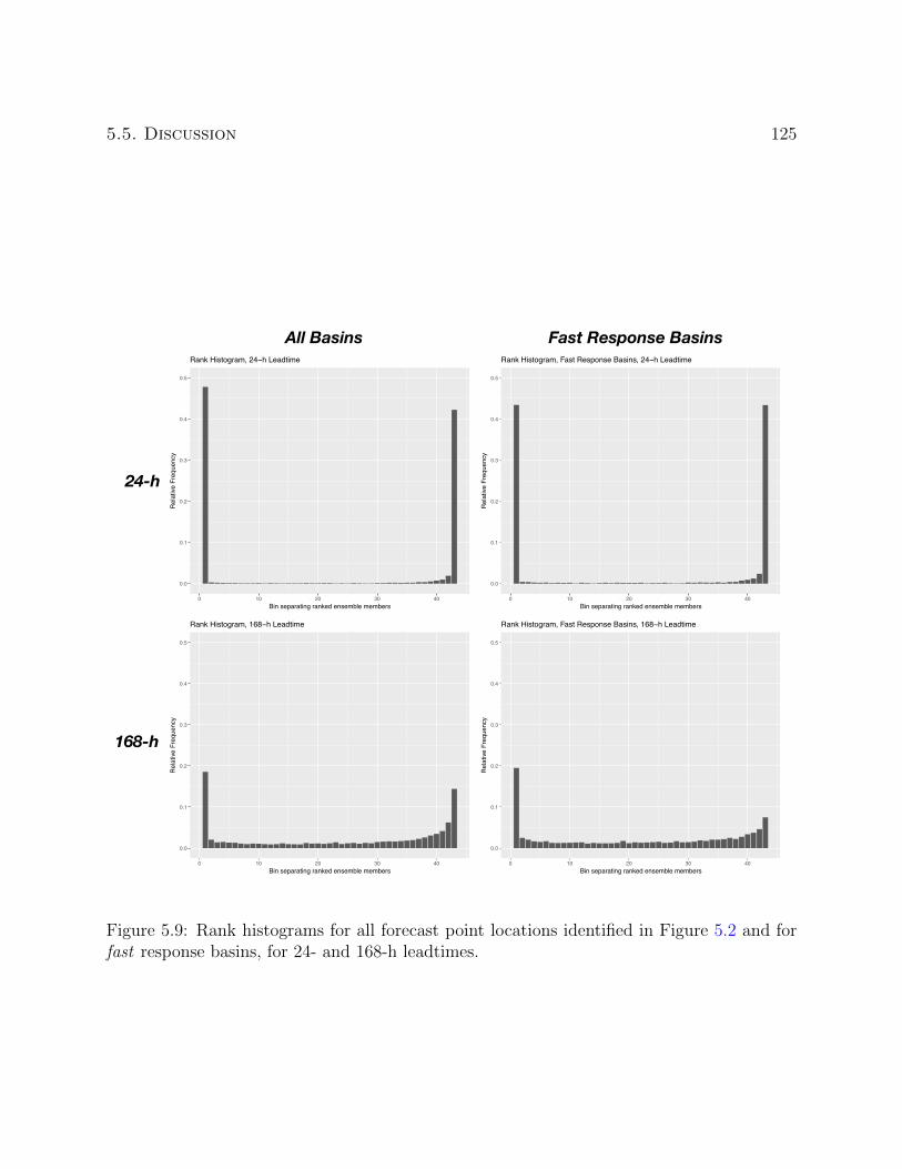
5.5. Discussion 125
0.0
0.1
0.2
0.3
0.4
0.5
0 10 20 30 40Bin separating ranked ensemble members
Rel
ative
Fre
quen
cy
Rank Histogram, 24−h Leadtime
0.0
0.1
0.2
0.3
0.4
0.5
0 10 20 30 40Bin separating ranked ensemble members
Rel
ative
Fre
quen
cy
Rank Histogram, 168−h Leadtime
0.0
0.1
0.2
0.3
0.4
0.5
0 10 20 30 40Bin separating ranked ensemble members
Rel
ative
Fre
quen
cy
Rank Histogram, Fast Response Basins, 24−h Leadtime
0.0
0.1
0.2
0.3
0.4
0.5
0 10 20 30 40Bin separating ranked ensemble members
Rel
ative
Fre
quen
cy
Rank Histogram, Fast Response Basins, 168−h Leadtime
All Basins Fast Response Basins
24-h
168-h
Figure 5.9: Rank histograms for all forecast point locations identified in Figure 5.2 and forfast response basins, for 24- and 168-h leadtimes.

126Chapter 5. Use of Central Tendency Measures from an Operational Short
Lead-time Hydrologic Ensemble Forecast System
model initial and boundary conditions. The need for the use of such techniques is illustrated
in Section 5.5.2 where MMEFS ensemble verification results are discussed related to ensemble
under-spread and apparent biases. Although not strictly an ensemble modeling related issue,
MMEFS ensemble forecasts would benefit from improved hydrologic model calibrations for
many basins. Model simulation error would be reduced further and MMEFS verification
would also improve by incorporating the Ohio River Community HEC-RAS Model directly
into MMEFS ensemble simulations for slow-response rivers where complex hydrodynamics
are inadequately handled by simple streamflow routing models. MMEFS ensemble verifica-
tion metrics are clearly better for basins known to have good calibrations than for basins
with sub-optimal model calibrations.
5.6 Summary and conclusions
Experimental results from this study demonstrate that NAEFS based MMEFS ensemble
median forecasts have smaller forecast error than ensemble mean forecasts based on ME
and MAE verification measures. Even though RMSE values suggest slightly lower forecast
error with ensemble mean compared to ensemble median forecasts, analyses, overall, suggest
that ensemble median forecasts should be preferred over ensemble mean forecasts. More
importantly, when forecasts spanning all ranges in stage and basin response times are aggre-
gated, MMEFS ensemble mean and median forecasts show lower forecast error than legacy
OHRFC operational forecasts, based on 24-h deterministic QPF, at long forecast leadtimes,
that is, beginning at approximately ≥90-h. This result shows the viability of using ensem-
ble mean/median forecasts for extended forecasts beyond the 4-day forecast horizon. When
analyses are restricted to fast response basins only, MMEFS ensemble mean and median
forecasts have smaller forecast error than legacy OHRFC operational forecasts beginning at

5.6. Summary and conclusions 127
about leadtime 36-h. This finding has potentially significant implications on forecast op-
erations at the OHRFC and other hydrologic forecast centers. Specifically, lower MMEFS
ensemble mean/median forecast errors compared to the current operational OHRFC deter-
ministic forecasts suggests the feasibility of changing operational workflows from manually
intensive, interactive forecasting procedures to a more automated operational environment
using ensemble forecasting methodologies. Of course, the generation of full probabilistic
forecasts from ensemble methods is greatly preferred over the use of the ensemble mean or
median because the former conveys forecast uncertainty to end-users, where the latter does
not [133]. In addition, a wide range of water resources applications requires the use of flow
hydrographs; the proposed ensemble median/mean stage forecasts should not be translated
to flow hydrographs because mass balance is not preserved. Consequently, for most other
water resources applications, full hydrologic ensemble forecasts are needed.
MMEFS ensemble verification results covering the November 30, 2010 through May 24, 2012
study period demonstrate forecast skill and reasonable forecast discrimination, reliability,
and sharpness. However, verification results also identify needed areas of improvement, such
as the need to account for model error, utilizing a priori hindcast experiments to quantify
model error, and the adoption of a post-forecast, ensemble bias correction methodology.

Chapter 6
Conclusions
The results of each Chapter of this dissertation are presented within the individual Chapters,
with their associated conclusions. The conclusions presented here summarize the results and
conclusions drawn from the entire dissertation (Section 6.1). Section 6.2 discusses the signif-
icance of the research within the broader hydrologic community, especially how the findings
could impact decision-making by those establishing policy. Finally, the Future Work section,
Section 6.3, summarizes future research that is needed to fill knowledge gaps identified or
implied in the individual Chapters within the dissertation.
6.1 Summary
The main objective of the research was to demonstrate the necessity for using probabilistic
hydrologic forecasting in place of current forecast methods that rely on the use single-valued
deterministic QPF. This goal was reached, first, by identifying that QPE improvements
have been significant, which has lead directly to significantly improved hydrologic modeling
simulations, indicated by accepted measures of model error estimation. Second, Chapter 3
128

6.1. Summary 129
illustrated that QPF improvements have been marginal over the period 1970-2015. Moreover,
a hydrologic monte carlo simulation experiment demonstrated that the small gains in QPF
accuracy did not produce significant reductions in hydrologic forecast error. On the basis of
QPF threat score (TS), an important finding was that very large hydrologic forecast errors
could still result from significantly reduced QPF error. Moreover, results from the monte
carlo experiment showed that there should be no expectation that a high QPF TS value
should be associated with a smaller hydrologic forecast error than a lower TS value. The
implication is that there are spatial scale effects that relate to watershed size and the intra-
storm variability of areas of strong convection that complicate the interaction between cores
of heavy rainfall and watershed response.
Experiment-1 of Chapter 4 demonstrated that hydrologic forecasts using non-Zero QPF
had smaller errors than forecasts that used zero-QPF. Experiment-2 showed that for non-
flood forecasts, forecast error diminished with longer durations of QPF. However, for flood
forecasts, this finding was reversed; that is, increased durations of QPF increased hydrologic
forecast error. Moreover, for fast response basins, Experiment-2 showed that forecast error
increased dramatically when QPF durations changed from 12-h to 24-h or greater. This
is problematic because one does not know beforehand whether or not flooding will occur.
Consequently, the findings suggest that QPF should be restricted to 6- or 12-h durations.
This implies that hydrologic forecasts for non-flood events, which is by far, most common,
will experience reduced forecast accuracy. This presents a paradox with the use of QPF for
flood and non-flood forecasting.
The answer to the QPF paradox, of course, is that ensemble hydrologic forecasting should
be preferred over current deterministic forecasting approaches, which is demonstrated in
Chapter 5. In Chapter 5, the use of hydrologic ensemble median and mean forecasts was
explored as a mechanism to reduce hydrologic forecast uncertainty. The operational experi-

130 Chapter 6. Conclusions
ment illustrated that when results from all 54 experimental basins are aggregated, forecast
verification showed that the MMEFS NAEFS ensemble median and mean forecasts had less
error than OHRFC operational forecasts beginning at lead-time 90-h. However, with fast re-
sponse basins, ensemble median and mean forecasts had less error than OHRFC operational
forecasts beginning at lead-time 36-h, based on mean absolute error and at lead-time 6-h for
mean error. This demonstrates the viability of using ensemble median and mean forecasts as
a replacement for OHRFC operational forecasts. Moreover, the use of hydrologic ensemble
median or mean forecasts includes the notion of uncertainty in hydrologic forecasts in terms
of expectation or ”best estimate”. Since an ensemble median or mean stage forecast looks
like a single-valued, deterministic hydrologic forecast, acceptance by the general public and
decision makers should be achievable. A minor finding was that ensemble median forecasts
had smaller error than ensemble mean forecasts, based on mean absolute error and mean
error. Differences in root mean square error were nearly negligible.
6.2 Engineering Significance
The most significant outcome of the research presented in this dissertation is a demonstration
of the necessity for using ensemble hydrologic forecasting methods over current operational
methods that rely on single-valued QPF. The research demonstrated that very large hy-
drologic forecast errors are introduced by single-valued QPF, particularly for rainfall driven
events. The conclusion is that traditional QPF should not be used in hydrologic forecasting.
While the hydrologic forecast community has been moving in the direction of ensemble fore-
casting methods, national hydrologic services (NHSs), such as the NWS in the U.S., have
been very slow to adopt ensemble methods operationally to replace legacy forecasting meth-
ods and forecast products that convey forecast uncertainty. The general public and decision

6.3. Future Work 131
makers need to receive flood alerts and warnings in the form of probabilistic statements and
graphics. Research presented in this dissertation shows that ensemble median forecasts are
a viable replacement for current operational forecasts that rely on deterministic QPF. En-
semble median and mean forecast have the added benefit of conveying a measure of forecast
uncertainty in much the same manner that, with hurricane or tropical storm prediction of
storm tracks, meteorological forecasters display both the expected storm track (the ensemble
mean) and the individual storm tracks from numerous numerical weather prediction models.
Finally, research presented in this dissertation showed that significant improvements in the
accuracy of hydrologic modeling have resulted from scientific advances in remote sensing of
precipitation by radar and development of improved radar-precipitation estimation systems.
6.3 Future Work
Research presented in this dissertation underscores the need for improved hydrologic model
calibrations to minimize forecast errors. The research also demonstrates the value of im-
proved precipitation estimation methods that reduce hydrologic simulation hindcast and
forecast errors. Further reduction of modeling and forecast error will result from the incor-
poration of hydrodynamic and improved reservoir simulation models into hydrologic forecast
systems, which will also improve the reliability of ensemble forecast systems.
The MMEFS ensemble forecast experimental period was too short, resulting in small sample
sizes that affected verification statistics. Future verification efforts of the MMEFS are needed
to better evaluate MMEFS strengths and areas of needed improvement. Consequently, future
analyses should include longer experimental periods, on the order of years. This requirement
is especially needed for smaller, fast responding basins that experience flooding infrequently.
MMEFS verification results show clear under-spread of ensemble members, largely because

132 Chapter 6. Conclusions
model error is not represented in MMEFS forecasts. Consequently, future MMEFS de-
velopment should include methods to account for model error, utilizing a priori hindcast
experiments to quantify model error, and the adoption of a post-forecast, ensemble bias
correction methodology.
The greatest need for future work falls into three categories:
1. Education of forecasters, NHS managers and policymakers, the public, decision-makers,
emergency managers, and politicians to promote an understanding of probabilistic
forecasts and the necessity of adopting probabilistic hydrologic forecasting over current
single-valued, deterministic forecasts;
2. Creation of forecast products in the form of graphics and digital and written statements
that convey probabilistic forecasts that are meaningful to and usable by end-users.
On this point, it would be a mistake to believe that there is, say, a single graphical
representation of a probabilistic forecast that will be meaningful to all. A range of
representations are needed that convey probabilistic forecasts that meet the needs of
end-users, ranging from sophisticated to naıve;
3. Raw and bias-corrected ensemble forecast time-series data should be made publicly
available to researchers and emergency and water resources managers for use in decision
support systems. This implies the need for the creation of a standardized format for
ensemble time-series data transmission and storage.

Bibliography
[1] T. Adams and J. Ostrowski. Short lead-time hydrologic ensemble forecasts from nu-
merical weather prediction model ensembles. In Proceedings World Environmental and
Water Resources Congress 2010, Providence, R.I., 2010. EWRI.
[2] T. Adams and G. Smith. National Weather Service Interactive River Forecasting
Using State, Parameter, and Data Modifications. In Proceedings of the International
Symposium on Engineering Hydrology, San Francisco, CA, 1993. EWRI.
[3] Thomas E. Adams. An assessment of the intra-storm spatial variability of floods in the
Piedmont region of Maryland. Master’s thesis, Virginia Tech, Blacksburg, VA, 1986.
[4] Thomas E. Adams. Flood Forecasting in the United States NOAA/National Weather
Service. In Thomas E. Adams and Thomas C. Pagano, editors, Flood Forecasting:
a global perspective, chapter 12, pages 275–325. Elsevier/Academic Press., New York,
NY, first edition, 2016.
[5] Thomas E. Adams. Flood Forecasting in the United States NOAA/National Weather
Service. In Thomas E. Adams and Thomas C. Pagano, editors, Flood Forecasting:
a global perspective, chapter 12, pages 275–325. Elsevier/Academic Press., New York,
NY, first edition, 2016.
133

134 BIBLIOGRAPHY
[6] Thomas E. Adams and Randle Dymond. Hydrometeorological Forcing Errors for a
Real-time Flood Forecast System in the Ohio River Valley, USA. Journal of Hydrom-
eteorology, 2018, submitted to the AMS J Hydrometeorology.
[7] Thomas E. Adams and Randle Dymond. The Effect of QPF on Real-time Deterministic
Hydrologic Forecast Uncertainty. Journal of Hydrometeorology, 2018b, submitted to
the AMS J Hydrometeorology.
[8] Thomas E. Adams, Sherry Chen, and Randle Dymond. Results from Operational
Hydrologic Forecasts using the NOAA/NWS OHRFC Ohio River Community HEC-
RAS Model. Journal of Hydrologic Engineering, in press 2018.
[9] L. Alfieri, D. Velasco, and J. Thielen. Flash flood detection through a multi-
stage probabilistic warning system for heavy precipitation events. Advances in Geo-
sciences, 29:69–75, 2011. doi: 10.5194/adgeo-29-69-2011. URL https://www.adv-
geosci.net/29/69/2011/.
[10] L. Alfieri, P. Burek, E. Dutra, B. Krzeminski, D. Muraro, J. Thielen, and F. Pappen-
berger. Glofas – global ensemble streamflow forecasting and flood early warning. Hy-
drology and Earth System Sciences, 17(3):1161–1175, 2013. doi: 10.5194/hess-17-1161-
2013. URL https://www.hydrol-earth-syst-sci.net/17/1161/2013/.
[11] E.N. Anagnostou, W.F. Krajewski, D.-J. Seo, and E.R. Johnson. Mean-field radar
rainfall bias studies for WSR-88D. ASCE Journal of Engineering Hydrology, 3(3):
149–159, 1998.
[12] E. A. Anderson. National Weather Service River Forecast System-Snow Accumula-
tion and Ablation Model. Technical Report NWS-HYDRO-17, U.S. National Weather
Service, Office of Hydrology, Hydrology Laboratory. Technical Memo., 1325 East West
Highway, Room 8372 Silver Spring, Maryland 20910, 1973.

BIBLIOGRAPHY 135
[13] Eric A. Anderson. Calibration of conceptual hydrologic models for use in river forecast-
ing. Technical report, U.S. National Weather Service, Office of Hydrology, Hydrology
Laboratory, 2002.
[14] D. Anghileri, N. Voisin, A. Castelletti, F. Pianosi, B. Nijssen, and D. P. Lettenmaier.
Value of long-term streamflow forecasts to reservoir operations for water supply in
snow-dominated river catchments. Water Resour. Res., 52, 2016. doi: doi:10.1002/
2015WR017864.
[15] Mary Lynn Baeck and James A. Smith. Rainfall estimation by the wsr-88d for heavy
rainfall events. Weather and Forecasting, 13(2):416–436, 1998. doi: 10.1175/1520-
0434(1998)013〈0416:REBTWF〉2.0.CO;2.
[16] Satish Bastola, Vasubandhu Misra, and Haiqin Li. Seasonal hydrological forecasts
for watersheds over the southeastern united states for the boreal summer and fall
seasons. Earth Interactions, 17(25):1–22, 2013. doi: 10.1175/2013EI000519.1. URL
https://doi.org/10.1175/2013EI000519.1.
[17] J. V. L. Beckers, A. H. Weerts, E. Tijdeman, and E. Welles. Enso-conditioned
weather resampling method for seasonal ensemble streamflow prediction. Hydrology
and Earth System Sciences, 20(8):3277–3287, 2016. doi: 10.5194/hess-20-3277-2016.
URL https://www.hydrol-earth-syst-sci.net/20/3277/2016/.
[18] Kurt K. Benke, Kim E. Lowell, and Andrew J. Hamilton. Parameter uncertainty, sensi-
tivity analysis and prediction error in a water-balance hydrological model. Mathemat-
ical and Computer Modelling, 47(11):1134 – 1149, 2008. ISSN 0895-7177. doi: https:
//doi.org/10.1016/j.mcm.2007.05.017. URL http://www.sciencedirect.com/
science/article/pii/S0895717707002373.

136 BIBLIOGRAPHY
[19] K. Bogner and M. Kalas. Error?correction methods and evaluation of an ensem-
ble based hydrological forecasting system for the upper danube catchment. Atmo-
spheric Science Letters, 9(2):95–102, 2008. doi: 10.1002/asl.180. URL https:
//rmets.onlinelibrary.wiley.com/doi/abs/10.1002/asl.180.
[20] K. Bogner and F. Pappenberger. Multiscale error analysis, correction, and predictive
uncertainty estimation in a flood forecasting system. Water Resources Research, 47
(7):n/a–n/a, 2011. ISSN 1944-7973. doi: 10.1029/2010WR009137. URL http://
dx.doi.org/10.1029/2010WR009137. W07524.
[21] M. Borga, E.N. Anagnostou, G. Blschl, and J.-D. Creutin. Flash floods: Ob-
servations and analysis of hydro-meteorological controls. Journal of Hydrol-
ogy, 394(12):1 – 3, 2010. ISSN 0022-1694. doi: https://doi.org/10.1016/
j.jhydrol.2010.07.048. URL https://www.sciencedirect.com/science/
article/pii/S0022169410004877. Flash Floods: Observations and Analysis
of Hydrometeorological Controls.
[22] Philippe Bougeault, Zoltan Toth, Craig Bishop, Barbara Brown, David Burridge,
De Hui Chen, Beth Ebert, Manuel Fuentes, Thomas M. Hamill, Ken Mylne, Jean
Nicolau, Tiziana Paccagnella, Young-Youn Park, David Parsons, Baudouin Raoult,
Doug Schuster, Pedro Silva Dias, Richard Swinbank, Yoshiaki Takeuchi, Warren Ten-
nant, Laurence Wilson, and Steve Worley. The thorpex interactive grand global en-
semble. Bulletin of the American Meteorological Society, 91(8):1059–1072, 2010. doi:
10.1175/2010BAMS2853.1. URL https://doi.org/10.1175/2010BAMS2853.1.
[23] L. C. Bowling, J. W. Pomeroy, and D. P. Lettenmaier. Parameterization of blowing-
snow sublimation in a macroscale hydrology model. Journal of Hydrometeorology, 5
(5):745–762, 2004. doi: 10.1175/1525-7541(2004)005〈0745:POBSIA〉2.0.CO;2.
BIBLIOGRAPHY 137
[24] A. Allen Bradley and Stuart S. Schwartz. Summary verification measures and
their interpretation for ensemble forecasts. Monthly Weather Review, 139(9):3075–
3089, 2011. doi: 10.1175/2010MWR3305.1. URL https://doi.org/10.1175/
2010MWR3305.1.
[25] A. Allen Bradley, Mohamed Habib, and Stuart S. Schwartz. Climate index weighting
of ensemble streamflow forecasts using a simple bayesian approach. Water Resources
Research, 51(9):7382–7400, 2015. ISSN 1944-7973. doi: 10.1002/2014WR016811. URL
http://dx.doi.org/10.1002/2014WR016811.
[26] J. Breidenbach and J. Bradberry. Multisensor precipitation estimates produced by
National Weather Service forecast centers for hydrologic applications. In Proc., 2001
Georgia Water Resources Conf., pages 179–182, Athens, GA, 2001.
[27] J. Breidenbach, D.-J. Seo, P. Tilles, and K. Roy. Accounting for radar beam blockage
patterns in radar-derived precipitation mosaics for River Forecast Centers. In Proc.,
15th Conf. on Interactive Information Processing Systems, pages 179–182, Boston,
MA, 1999.
[28] James D. Brown and Dong-Jun Seo. A nonparametric postprocessor for bias cor-
rection of hydrometeorological and hydrologic ensemble forecasts. Journal of Hy-
drometeorology, 11(3):642–665, 2010. doi: 10.1175/2009JHM1188.1. URL https:
//doi.org/10.1175/2009JHM1188.1.
[29] J.D. Brown, J. Demargne, D-J. Seo, and Y. Liu. The Ensemble Verification System
(EVS): a software tool for verifying ensemble forecasts of hydrometeorological and
hydrologic variables at discrete locations. Environmental Modelling and Software, 25
(7):854–872, 2010.

138 BIBLIOGRAPHY
[30] Patrick Broxton, Peter A. Troch, Mike Schaffner, Carl Unkrich, and David Goodrich.
An all-season flash flood forecasting system for real-time operations. Bulletin of the
American Meteorological Society, 95(3):399–407, 2014. doi: 10.1175/BAMS-D-12-
00212.1.
[31] Roberto Buizza. Potential forecast skill of ensemble prediction and spread and skill
distributions of the ECMWF ensemble prediction system. Mon. Wea. Rev., 125:99–
119, 1997.
[32] R.J. Burnash. The NWS River Forecast System - Catchment Model. Water Resources
Publications, first edition, 1995.
[33] R.J. Burnash. The NWS River Forecast System - Catchment Model. Water Resources
Publications, first edition, 1995.
[34] R.J. Burnash, R.L. Ferral, and R.A. McGuire. A generalized streamflow simulation
system: Conceptual modeling for digital computers. Technical report, U.S. Department
of Commerce National Weather Service and State of California Department of Water
Resources, 1973.
[35] Guillem Candille. The multiensemble approach: The naefs example. Monthly Weather
Review, 137(5):1655–1665, 2009. doi: 10.1175/2008MWR2682.1. URL https://
doi.org/10.1175/2008MWR2682.1.
[36] Francesca Cecinati, Miguel Angel Rico-Ramirez, Gerard B.M. Heuvelink, and
Dawei Han. Representing radar rainfall uncertainty with ensembles based
on a time-variant geostatistical error modelling approach. Journal of Hydrol-
ogy, 548(Supplement C):391 – 405, 2017. ISSN 0022-1694. doi: https://
doi.org/10.1016/j.jhydrol.2017.02.053. URL http://www.sciencedirect.com/
science/article/pii/S0022169417301324.

BIBLIOGRAPHY 139
[37] Jerome P. Charba, David W. Reynolds, Brett E. McDonald, and Gary M. Carter.
Comparative Verification of Recent Quantitative Precipitation Forecasts in the Na-
tional Weather Service: A Simple Approach for Scoring Forecast Accuracy. Weather
and Forecasting, 18(2):161–183, 2003.
[38] Grzegorz J. Ciach. Local random errors in tipping-bucket rain gauge measurements.
Journal of Atmospheric and Oceanic Technology, 20(5):752–759, 2003. doi: 10.1175/
1520-0426(2003)20〈752:LREITB〉2.0.CO;2.
[39] Grzegorz J. Ciach and Witold F. Krajewski. Radar-Rain Gauge Comparisons under
Observational Uncertainties. Journal of Applied Meteorology, 38(10):1519–1525, 1999.
doi: 10.1175/1520-0450(1999)038〈1519:RRGCUO〉2.0.CO;2.
[40] H.L. Cloke and F. Pappenberger. Ensemble flood forecasting: A review. Jour-
nal of Hydrology, 375(3):613 – 626, 2009. ISSN 0022-1694. doi: https://
doi.org/10.1016/j.jhydrol.2009.06.005. URL http://www.sciencedirect.com/
science/article/pii/S0022169409003291.
[41] P. Corrigan. Email June 29. personal communication, 2016. Weather Forecast Office
- Blacksburg, VA, NOAA, National Weather Service.
[42] L. Crochemore, M.H. Ramos, F. Pappenberger, and C. Perrin. Seasonal stream-
flow forecasting by conditioning climatology with precipitation indices. Hydrology and
Earth System Sciences, 21(3):1573–1591, 2017. doi: 10.5194/hess-21-1573-2017. URL
https://www.hydrol-earth-syst-sci.net/21/1573/2017/.
[43] Timothy D. Crum and Ron L. Alberty. The wsr-88d and the wsr-88d operational
support facility. Bulletin of the American Meteorological Society, 74(9):1669–1687,
1993. doi: 10.1175/1520-0477(1993)074〈1669:TWATWO〉2.0.CO;2.
140 BIBLIOGRAPHY
[44] Luciana K. Cunha, James A. Smith, Mary Lynn Baeck, and Witold F. Krajewski. An
early performance evaluation of the nexrad dual-polarization radar rainfall estimates
for urban flood applications. Weather and Forecasting, 28(6):1478–1497, 2013. doi:
10.1175/WAF-D-13-00046.1.
[45] Lan Cuo, Thomas C. Pagano, and Q. J. Wang. A review of quantitative precipitation
forecasts and their use in short- to medium-range streamflow forecasting. Journal of
Hydrometeorology, 12(5):713–728, 2011. doi: 10.1175/2011JHM1347.1.
[46] C. Daly, R.P. Neilson, and D.L. Phillips. A Statistical-Topographic model for mapping
climatological precipitation over mountainous terrain. J. Appl. Meteor., 33:140–158,
1994.
[47] Christopher Daly, Michael Halbleib, Joseph I. Smith, Wayne P. Gibson, Matthew K.
Doggett, George H. Taylor, Jan Curtis, and Phillip P. Pasteris. Physiographically sensi-
tive mapping of climatological temperature and precipitation across the conterminous
united states. International Journal of Climatology, 28(15):2031–2064, 2008. ISSN
1097-0088. doi: 10.1002/joc.1688. URL http://dx.doi.org/10.1002/joc.1688.
[48] Christopher Daly, Joseph I. Smith, and Keith V. Olson. Mapping atmospheric mois-
ture climatologies across the conterminous united states. PLOS ONE, 10(10):1–33,
10 2015. doi: 10.1371/journal.pone.0141140. URL https://doi.org/10.1371/
journal.pone.0141140.
[49] U. Damrath, G. Doms, D. Fruehwald, E. Heise, B. Richter, and J. Steppeler. Opera-
tional quantitative precipitation forecasting at the german weather service. J. Hydrol-
ogy, 239:260–285, 2000.
[50] D.R. Dawdy and J.M. Bergmann. Effect of rainfall variability on streamflow simulation.
Water Resour. Res., 5(5):140–158, 1969.
BIBLIOGRAPHY 141
[51] G. N. Day. Extended streamflow forecasting using NWSRFS. ASCE, J. Water Resour.
Plann. Manage., 3:157–170, 1985.
[52] C. M. DeChant and H. Moradkhani. Improving the characterization of initial con-
dition for ensemble streamflow prediction using data assimilation. Hydrology and
Earth System Sciences, 15(11):3399–3410, 2011. doi: 10.5194/hess-15-3399-2011. URL
https://www.hydrol-earth-syst-sci.net/15/3399/2011/.
[53] Caleb M. DeChant and Hamid Moradkhani. Toward a reliable prediction of sea-
sonal forecast uncertainty: Addressing model and initial condition uncertainty
with ensemble data assimilation and sequential bayesian combination. Journal
of Hydrology, 519(Part D):2967 – 2977, 2014. ISSN 0022-1694. doi: https://
doi.org/10.1016/j.jhydrol.2014.05.045. URL http://www.sciencedirect.com/
science/article/pii/S0022169414004090.
[54] Caleb M. DeChant and Hamid Moradkhani. On the assessment of reliability in
probabilistic hydrometeorological event forecasting. Water Resources Research, 51
(6):3867–3883, 2015. ISSN 1944-7973. doi: 10.1002/2014WR016617. URL http:
//dx.doi.org/10.1002/2014WR016617.
[55] Deltares. Flood Early Warning System (FEWS). Online: http://
www.deltares.nl/en/software/479962/delft-fews, 3 2018.
[56] J. Demargne, M. Mulluski, K. Werner, T. Adams, S. Lindsey, N. Schwein, W. Marosi,
and E. Welles. Application of forecast verification science to operational river fore-
casting in the u.s. national weather service. Bulletin of the American Meteorological
Society, 90(6):779–784, 2009.
[57] J. Demargne, J.D. Brown, D-J. Seo, L. Wu, Z. Toth, and Y. Zhu. Diagnostic verification

142 BIBLIOGRAPHY
of hydrometeorological and hydrologic ensembles. Atmospheric Science Letters, 11(2):
114–122, 2010.
[58] Julie Demargne, Limin Wu, Satish K. Regonda, James D. Brown, Haksu Lee, Minxue
He, Dong-Jun Seo, Robert Hartman, Henry D. Herr, Mark Fresch, John Schaake, and
Yuejian Zhu. The science of noaa’s operational hydrologic ensemble forecast service.
Bulletin of the American Meteorological Society, 95(1):79–98, 2014. doi: 10.1175/
BAMS-D-12-00081.1. URL https://doi.org/10.1175/BAMS-D-12-00081.1.
[59] David Demeritt, Sbastien Nobert, Hannah Cloke, and Florian Pappenberger. Chal-
lenges in communicating and using ensembles in operational flood forecasting. Me-
teorological Applications, 17(2):209–222, 2010. doi: 10.1002/met.194. URL https:
//rmets.onlinelibrary.wiley.com/doi/abs/10.1002/met.194.
[60] T. Diomede, F. Nerozzi, T. Paccagnella, and E. Todini. The use of meteorological
analogues to account for lam qpf uncertainty. Hydrology and Earth System Sciences,
12(1):141–157, 2008. doi: 10.5194/hess-12-141-2008. URL https://www.hydrol-
earth-syst-sci.net/12/141/2008/.
[61] Tommaso Diomede, Chiara Marsigli, Andrea Montani, Fabrizio Nerozzi, and Tiziana
Paccagnella. Calibration of limited-area ensemble precipitation forecasts for hy-
drological predictions. Monthly Weather Review, 142(6):2176–2197, 2014. doi:
10.1175/MWR-D-13-00071.1.
[62] J. Du and M. S. Tracton. Implementation of a real-time short-range ensemble fore-
casting system at ncep: an update. In Preprints, 9th Conference on Mesoscale
Processes, Ft. Lauderdale,Florida, pages 355–356. Amer. Meteor. Soc., 2001. URL
http://www.emc.ncep.noaa.gov/mmb/SREF/reference.html.
BIBLIOGRAPHY 143
[63] J. Du, G. DiMego, M. S. Tracton, and B. Zhou. NCEP short-range ensemble forecasting
(SREF) system: multi-IC, multi-model and multi-physics approach. Technical Report
TD No. 1161, Research Activities in Atmospheric and Oceanic Modeling, J. Cote (ed.),
2003.
[64] E. E. Ebert. Ability of a poor man’s ensemble to predict the probability and distribu-
tion of precipitation. Mon. Wea. Rev., 129:2461–2480, 2001.
[65] E. E. Ebert, U. Damrath, W. Wergen, and J.L. McBride. The WGNE assessment
of short-term quantitative precipitation forecasts. Bull. Am. Meteorol. Soc., 84(4):
481–492, 2003.
[66] Mohammad Ebtehaj, Hamid Moradkhani, and Hoshin V. Gupta. Improving robust-
ness of hydrologic parameter estimation by the use of moving block bootstrap re-
sampling. Water Resources Research, 46(7):n/a–n/a, 2010. ISSN 1944-7973. doi:
10.1029/2009WR007981. URL http://dx.doi.org/10.1029/2009WR007981.
W07515.
[67] Hisham Eldardiry, Emad Habib, Yu Zhang, and Jeffrey Graschel. Artifacts in Stage
IV NWS Real-Time Multisensor Precipitation Estimates and Impacts on Identification
of Maximum Series. Journal of Hydrologic Engineering, 22(5):E4015003, 2017. doi:
10.1061/(ASCE)HE.1943-5584.0001291.
[68] John F. England, Pierre Y. Julien, and Mark L. Velleux. Physically-based ex-
treme flood frequency with stochastic storm transposition and paleoflood data
on large watersheds. Journal of Hydrology, 510(Supplement C):228 – 245, 2014.
ISSN 0022-1694. doi: https://doi.org/10.1016/j.jhydrol.2013.12.021. URL http:
//www.sciencedirect.com/science/article/pii/S0022169413009189.
144 BIBLIOGRAPHY
[69] Richard Essery and John Pomeroy. Vegetation and topographic control of wind-
blown snow distributions in distributed and aggregated simulations for an arctic tun-
dra basin. Journal of Hydrometeorology, 5(5):735–744, 2004. doi: 10.1175/1525-
7541(2004)005〈0735:VATCOW〉2.0.CO;2.
[70] Richard Essery, Long Li, and John Pomeroy. A distributed model of blowing snow
over complex terrain. Hydrological Processes, 13(14-15):2423–2438, 1999. ISSN 1099-
1085. doi: 10.1002/(SICI)1099-1085(199910)13:14/15〈2423::AID-HYP853〉3.0.CO;2-
U. URL http://dx.doi.org/10.1002/(SICI)1099-1085(199910)13:14/
15<2423::AID-HYP853>3.0.CO;2-U.
[71] Gerald I. Evenden. Cartographic Projection Procedures for the UNIX Environment
– A User’s Manual. Technical Report Open-File Report 90-284, U.S. Dept. of the
Interior, Geological Survey, 1990.
[72] J.-M. Faures, D. C. Goodrich, D. A. Woolhiser, and S. Sorooshian. Impact of small-
scale spatial rainfall variability on runoff modeling. Journal of Hydrology, 173:309–326,
December 1995. doi: 10.1016/0022-1694(95)02704-S.
[73] B.D. Finnerty, M.B. Smith, D-J Seo, V. Koren, and G. Moglen. Space-time scale
sensitivity of the sacramento model to radar-gage precipitation inputs. Journal of
Hydrology, 203:21–38, 1997.
[74] M.M. Fogel. Effect of storm rainfall variability on runoff from small semiarid water-
sheds. Transactions of the ASAE, 12(6):808–812, 1969.
[75] G. Forzieri, L. Feyen, R. Rojas, M. Florke, F. Wimmer, and A. Bianchi. Ensem-
ble projections of future streamflow droughts in europe. Hydrology and Earth Sys-
tem Sciences, 18(1):85–108, 2014. doi: 10.5194/hess-18-85-2014. URL https:
//www.hydrol-earth-syst-sci.net/18/85/2014/.
BIBLIOGRAPHY 145
[76] E. Foufoula-Georgiou. A probabilistic storm transposition approach for estimating
exceedance probabilities of extreme precipitation depths. Water Resources Research,
25(5):799–815, 1989. ISSN 1944-7973. doi: 10.1029/WR025i005p00799. URL http:
//dx.doi.org/10.1029/WR025i005p00799.
[77] Kristie J. Franz, Holly C. Hartmann, Soroosh Sorooshian, and Roger Bales. Verifi-
cation of National Weather Service ensemble streamflow predictions for water supply
forecasting in the Colorado River Basin. Journal of Hydrometeorology, 4(12):1105–
1118, 2003.
[78] R. A. Fulton. WSR-88D Polar-to-HRAP Mapping. Technical Report Tech. Memo.,
Hydrologic Research Laboratory, Office of Hydrology, National Weather Service, 1998.
[79] Richard A. Fulton, Jay P. Breidenbach, Dong-Jun Seo, Dennis A. Miller, and Timothy
O’Bannon. The WSR-88D Rainfall Algorithm. Weather and Forecasting, 13(2):377–
395, 1998. doi: 10.1175/1520-0434(1998)013〈0377:TWRA〉2.0.CO;2.
[80] Richard A. Fulton, Feng Ding, and Dennis A. Miller. Truncation errors in historical
WSR-88D rainfall products. In 31st Conference on Radar Meteorology. Amer. Meteor.
Soc., 2003.
[81] Brian Gaudet and William R. Cotton. Statistical characteristics of a real-time precip-
itation forecasting model. Wea. Forecasting, 13:966–982, 1998.
[82] Konstantine P. Georgakakos and Michael D. Hudlow. Quantitative precipitation fore-
cast techniques for use in hydrologic forecasting. Bulletin of the American Mete-
orological Society, 65(11):1186–1200, 1984. doi: 10.1175/1520-0477(1984)065〈1186:
QPFTFU〉2.0.CO;2.

146 BIBLIOGRAPHY
[83] Konstantine P. Georgakakos and Michael D. Hudlow. Quantitative precipitation fore-
cast techniques for use in hydrologic forecasting. Bull. Amer. Meteor. Soc., 65:1186–
1200, 1984.
[84] David C. Goodrich, Jean-Marc Faurs, David A. Woolhiser, Leonard J. Lane, and
Soroosh Sorooshian. Measurement and analysis of small-scale convective storm
rainfall variability. Journal of Hydrology, 173(1?4):283 – 308, 1995. ISSN 0022-
1694. doi: http://dx.doi.org/10.1016/0022-1694(95)02703-R. URL http://
www.sciencedirect.com/science/article/pii/002216949502703R.
[85] Jonathan J. Gourley and Chris M. Calvert. Automated detection of the bright band
using wsr-88d data. Weather and Forecasting, 18(4):585–599, 2003. doi: 10.1175/1520-
0434(2003)018〈0585:ADOTBB〉2.0.CO;2.
[86] GRASS Development Team. Geographic Resources Analysis Support System (GRASS
GIS) Software. Open Source Geospatial Foundation, USA, 2016. URL http://
grass.osgeo.org.
[87] Thomas M. Hamill. Interpretation of rank histograms for verifying ensemble
forecasts. Monthly Weather Review, 129(3):550–560, 2001. doi: 10.1175/1520-
0493(2001)129〈0550:IORHFV〉2.0.CO;2. URL https://doi.org/10.1175/1520-
0493(2001)129<0550:IORHFV>2.0.CO;2.
[88] Alan F. Hamlet, Daniel Huppert, and Dennis P. Lettenmaier. Economic value
of long-lead streamflow forecasts for columbia river hydropower. Journal of Wa-
ter Resources Planning and Management, 128(2):91–101, 2002. doi: 10.1061/
(ASCE)0733-9496(2002)128:2(91). URL http://ascelibrary.org/doi/abs/
10.1061/%28ASCE%290733-9496%282002%29128%3A2%2891%29.

BIBLIOGRAPHY 147
[89] M.J. Hamlin. The significance of rainfall in the study of hydrological pro-
cesses at basin scale. Journal of Hydrology, 65(1?3):73 – 94, 1983. ISSN
0022-1694. doi: http://dx.doi.org/10.1016/0022-1694(83)90211-1. URL http:
//www.sciencedirect.com/science/article/pii/0022169483902111.
Scale Problems in Hydrology.
[90] Holly C. Hartmann, Thomas C. Pagano, S. Sorooshian, and R. Bales. Confi-
dence builders. Bulletin of the American Meteorological Society, 83(5):683–698,
2002. doi: 10.1175/1520-0477(2002)083〈0683:CBESCF〉2.3.CO;2. URL https:
//doi.org/10.1175/1520-0477(2002)083<0683:CBESCF>2.3.CO;2.
[91] T. Hashino, A. A. Bradley, and S. S. Schwartz. Evaluation of bias-correction methods
for ensemble streamflow volume forecasts. Hydrology and Earth System Sciences, 11
(2):939–950, 2007. doi: 10.5194/hess-11-939-2007. URL https://www.hydrol-
earth-syst-sci.net/11/939/2007/.
[92] Yuxiang He, Yu Zhang, Robert Kuligowski, Robert Cifelli, and David Kitzmiller. In-
corporating satellite precipitation estimates into a radar-gauge multi-sensor precip-
itation estimation algorithm. Remote Sensing, 10(1), 2018. ISSN 2072-4292. doi:
10.3390/rs10010106. URL http://www.mdpi.com/2072-4292/10/1/106.
[93] F.A. Huff. Sampling errors in measurement of mean precipitation. J. Appl. Met., 9
(1):35–44, 1970.
[94] M. D. Humphrey, J. D. Istok, J. Y. Lee, J. A. Hevesi, and A. L. Flint. A new
method for automated dynamic calibration of tipping-bucket rain gauges. Journal
of Atmospheric and Oceanic Technology, 14(6):1513–1519, 1997. doi: 10.1175/1520-
0426(1997)014〈1513:ANMFAD〉2.0.CO;2.
148 BIBLIOGRAPHY
[95] Steven M. Hunter and Edmond W. Holroyd. Demonstration of improved operational
water resources management through the use of better snow water equivalent infor-
mation. Technical Report R-02-02, U.S. Dept. of the Interior, Bureau of Reclamation,
Technical Service Center, River Systems and Meteorology Group, Water Resources
Services Div., September 2002.
[96] Jung-Sun Im, Keith Brill, and Edwin Danaher. Confidence interval estimation for
quantitative precipitation forecasts (qpf) using short-range ensemble forecasts (sref).
Weather and Forecasting, 21(1):24–41, 2006. doi: 10.1175/WAF902.1.
[97] Christine Johnson and Neill Bowler. On the reliability and calibration of ensem-
ble forecasts. Monthly Weather Review, 137(5):1717–1720, 2009. doi: 10.1175/
2009MWR2715.1. URL https://doi.org/10.1175/2009MWR2715.1.
[98] D.M.A. Jones and W.M. Wendland. Some statistics of instantaneous precipitation.
Journal of Climate and Applied Meteorology, 23(9):1273–1285, 1984.
[99] Susan Joslyn and Sonia Savelli. Communicating forecast uncertainty: public perception
of weather forecast uncertainty. Meteorological Applications, 17(2):180–195, 2010. doi:
10.1002/met.190. URL https://rmets.onlinelibrary.wiley.com/doi/abs/
10.1002/met.190.
[100] Viatcheslav V. Kharin and Francis W. Zwiers. On the roc score of proba-
bility forecasts. Journal of Climate, 16(24):4145–4150, 2003. doi: 10.1175/
1520-0442(2003)016〈4145:OTRSOP〉2.0.CO;2. URL https://doi.org/10.1175/
1520-0442(2003)016<4145:OTRSOP>2.0.CO;2.
[101] G.S. Kirk and J.E. Raven. The Presocratic Philosophers: A Critical History with a
Selection of Texts. University Press, 1957. URL https://books.google.com/
books?id=2pzWAAAAMAAJ.
BIBLIOGRAPHY 149
[102] David Kitzmiller, Suzanne Van Cooten, Feng Ding, Kenneth Howard, Carrie Langston,
Jian Zhang, Heather Moser, Yu Zhang, Jonathan J. Gourley, Dongsoo Kim, and David
Riley. Evolving multisensor precipitation estimation methods: Their impacts on flow
prediction using a distributed hydrologic model. Journal of Hydrometeorology, 12(6):
1414–1431, 2011. doi: 10.1175/JHM-D-10-05038.1.
[103] David Kitzmiller, Dennis Miller, Richard Fulton, and Feng Ding. Radar and mul-
tisensor precipitation estimation techniques in national weather service hydrologic
operations. Journal of Hydrologic Engineering, 18(2):133–142, 2013. doi: 10.1061/
(ASCE)HE.1943-5584.0000523.
[104] V. I. Koren. Parameterization of frozen ground effects: sensitivity to soil properties.
predictions in ungauged basins: Promises and progress. In Symposium S7, Seventh
IAHS Scientific Assembly, pages 125–133, Foz do Iquacu, Brazil, 2006. IAHS Publica-
tion 303.
[105] V. I. Koren, M. Smith, D. Wang, and Z. Zhang. Use of soil property data in the
derivation of conceptual rainfall-runoff model parameters. In Conference on Hydrology,
Long Beach, CA, 2000. AMS.
[106] Victor Koren, Seann Reed, Michael Smith, Ziya Zhang, and Dong-Jun Seo. Hydrol-
ogy laboratory research modeling system (hl-rms) of the us national weather ser-
vice. Journal of Hydrology, 291(3):297 – 318, 2004. ISSN 0022-1694. doi: https:
//doi.org/10.1016/j.jhydrol.2003.12.039. URL http://www.sciencedirect.com/
science/article/pii/S002216940400037X. Catchment modelling: Towards
an improved representation of the hydrological processes in real-world model applica-
tions.
[107] Victor Koren, Michael Smith, Zhengtao Cui, Brian Cosgrove, Kevin Werner, and
150 BIBLIOGRAPHY
Robert Zamora. Modification of Sacramento Soil Moisture Accounting Heat Trans-
fer Component (SAC-HT) for Enhanced Evapotranspiration. Technical Report NOAA
NWS Technical Report NWS 53, Department of Commerce, NOAA/NWS, October
2010.
[108] W.F. Krajewski and G.J. Ciach. Towards probabilistic quantitative precipitation wsr-
88d algorithms: Preliminary studies and problem formulation. Technical report, Final
Report for the Office of Hydrologic Development, NOAA/NWS, Washington, D.C.,
May 2003.
[109] Tobias Krueger, Jim Freer, John N. Quinton, Christopher J. A. Macleod, Gary S.
Bilotta, Richard E. Brazier, Patricia Butler, and Philip M. Haygarth. Ensemble eval-
uation of hydrological model hypotheses. Water Resources Research, 46(7):n/a–n/a,
2010. ISSN 1944-7973. doi: 10.1029/2009WR007845. URL http://dx.doi.org/
10.1029/2009WR007845. W07516.
[110] Roman Krzysztofowicz. Probabilistic hydrometeorological forecasts: Toward a new era
in operational forecasting. Bulletin of the American Meteorological Society, 79(2):243–
252, 1998. doi: 10.1175/1520-0477(1998)079〈0243:PHFTAN〉2.0.CO;2. URL https:
//doi.org/10.1175/1520-0477(1998)079<0243:PHFTAN>2.0.CO;2.
[111] Roman Krzysztofowicz. Bayesian theory of probabilistic forecasting via determin-
istic hydrologic model. Water Resources Research, 35(9):2739–2750, 1999. ISSN
1944-7973. doi: 10.1029/1999WR900099. URL http://dx.doi.org/10.1029/
1999WR900099.
[112] Roman Krzysztofowicz. The case for probabilistic forecasting in hydrology. Journal of
Hydrology, 249(1?4):2 – 9, 2001. ISSN 0022-1694. doi: http://dx.doi.org/10.1016/

BIBLIOGRAPHY 151
S0022-1694(01)00420-6. URL http://www.sciencedirect.com/science/
article/pii/S0022169401004206.
[113] C.L. Larson and B.M. Reich. Relationship of observed rainfall and runoff recurrence
intervals. In Proc. 2nd Int. Hydrol. Symp., volume 1, pages 34–43, Fort Collins, Col-
orado, 1972.
[114] J. Li, Y. Chen, H. Wang, J. Qin, J. Li, and S. Chiao. Extending flood forecast-
ing lead time in a large watershed by coupling wrf qpf with a distributed hydro-
logical model. Hydrology and Earth System Sciences, 21(2):1279–1294, 2017. doi:
10.5194/hess-21-1279-2017. URL https://www.hydrol-earth-syst-sci.net/
21/1279/2017/.
[115] M. Li, Q. J. Wang, J. C. Bennett, and D. E. Robertson. Error reduction and representa-
tion in stages (erris) in hydrological modelling for ensemble streamflow forecasting. Hy-
drology and Earth System Sciences, 20(9):3561–3579, 2016. doi: 10.5194/hess-20-3561-
2016. URL https://www.hydrol-earth-syst-sci.net/20/3561/2016/.
[116] Wentao Li, Qingyun Duan, Chiyuan Miao, Aizhong Ye, Wei Gong, and Zhenhua Di.
A review on statistical postprocessing methods for hydrometeorological ensemble fore-
casting. Wiley Interdisciplinary Reviews: Water, pages e1246–n/a, 2017. ISSN 2049-
1948. doi: 10.1002/wat2.1246. URL http://dx.doi.org/10.1002/wat2.1246.
e1246.
[117] Y. Lin and K. E. Mitchell. The NCEP Stage II/IV hourly precipitation analyses:
Development and applications. In Pre-prints, 19th Conf. on Hydrology, 1.2. [Available
online at https://ams.confex.com/ ams/pdfpapers/83847.pdf.], San Diego, CA, 2005.
Amer. Meteor. Soc.

152 BIBLIOGRAPHY
[118] Glen E. Liston and Kelly Elder. A distributed snow-evolution modeling system (snow-
model). Journal of Hydrometeorology, 7(6):1259–1276, 2006. doi: 10.1175/JHM548.1.
[119] Edwin P. Maurer and Dennis P. Lettenmaier. Predictability of seasonal runoff in the
Mississippi River basin. Journal of Geophysical Research: Atmospheres, 108(D16):n/a–
n/a, 2003. ISSN 2156-2202. doi: 10.1029/2002JD002555. URL http://dx.doi.org/
10.1029/2002JD002555. 8607.
[120] J. McEnery, J. Ingram, Q. Duan, T. Adams, and L. Anderson. NOAAs Advanced Hy-
drologic Prediction Service: Building pathways for better science in water forecasting.
Bull. of the American Meteorological Society, 24(3):375–385, 2005.
[121] Hilary McMillan, Bethanna Jackson, Martyn Clark, Dmitri Kavetski, and Ross Woods.
Rainfall uncertainty in hydrological modelling: An evaluation of multiplicative error
models. Journal of Hydrology, 400(1):83–94, 2011.
[122] P. A. Mendoza, A. W. Wood, E. Clark, E. Rothwell, M. P. Clark, B. Nijssen, L. D.
Brekke, and J. R. Arnold. An intercomparison of approaches for improving operational
seasonal streamflow forecasts. Hydrology and Earth System Sciences, 21(7):3915–3935,
2017. doi: 10.5194/hess-21-3915-2017. URL https://www.hydrol-earth-syst-
sci.net/21/3915/2017/.
[123] Sarah Michaels. Probabilistic forecasting and the reshaping of food risk man-
agement. Journal of Natural Resources Policy Research, 7(1):41?51, 2015. doi:
10.1080/19390459.2014.970800.
[124] Marion Mittermaier and Nigel Roberts. Intercomparison of spatial forecast verification
methods: Identifying skillful spatial scales using the fractions skill score. Weather and
Forecasting, 25(1):343–354, 2010. doi: 10.1175/2009WAF2222260.1.
BIBLIOGRAPHY 153
[125] Naoki Mizukami, Victor Koren, Michael Smith, David Kingsmill, Ziya Zhang, Brian
Cosgrove, and Zhengtao Cui. The impact of precipitation type discrimination on
hydrologic simulation: Rain?snow partitioning derived from hmt-west radar-detected
brightband height versus surface temperature data. Journal of Hydrometeorology, 14
(4):1139–1158, 2013. doi: 10.1175/JHM-D-12-035.1.
[126] Nicolas Le Moine, Frederic Hendrickx, and Joel Gailhard. Rainfall-runoff modelling
as a tool for constraining the reanalysis of daily precipitation and temperature fields
in mountainous regions. In Cold and Mountain Region Hydrological Systems Under
Climate Change Towards Improved Projections 1 Proceedings of H02, 2013.
[127] Hamid Moradkhani and Matthew Meier. Long-lead water supply forecast us-
ing large-scale climate predictors and independent component analysis. Journal
of Hydrologic Engineering, 15(10):744–762, 2010. doi: 10.1061/(ASCE)HE.1943-
5584.0000246. URL http://ascelibrary.org/doi/abs/10.1061/%28ASCE%
29HE.1943-5584.0000246.
[128] Rebecca E. Morss, Julie L. Demuth, and Jeffrey K. Lazo. Communicating uncertainty
in weather forecasts: A survey of the u.s. public. Weather and Forecasting, 23(5):974–
991, 2008. doi: 10.1175/2008WAF2007088.1. URL https://doi.org/10.1175/
2008WAF2007088.1.
[129] Allan H. Murphy. Probabilities, odds, and forecasts of rare events. Weather and
Forecasting, 6(2):302–307, 1991. doi: 10.1175/1520-0434(1991)006〈0302:POAFOR〉
2.0.CO;2. URL https://doi.org/10.1175/1520-0434(1991)006<0302:
POAFOR>2.0.CO;2.
[130] Kenneth R. Mylne, Ruth E. Evans, and Robin T. Clark. Multi-model multi-
analysis ensembles in quasi-operational medium-range forecasting. Quarterly Jour-
154 BIBLIOGRAPHY
nal of the Royal Meteorological Society, 128(579):361–384, 2006. doi: 10.1256/
00359000260498923. URL https://rmets.onlinelibrary.wiley.com/doi/
abs/10.1256/00359000260498923.
[131] J.E. Nash and J.V. Sutcliffe. River flow forecasting through conceptual models
part i - a discussion of principles. Journal of Hydrology, 10(3):282–290, 1970.
ISSN 0022-1694. doi: https://doi.org/10.1016/0022-1694(70)90255-6. URL http:
//www.sciencedirect.com/science/article/pii/0022169470902556.
[132] National Academies. Integrating Social and Behavioral Sciences Within the Weather
Enterprise. The National Academies Press, Washington, DC, 2018. ISBN 978-
0-309-46422-2. doi: 10.17226/24865. URL https://www.nap.edu/catalog/
24865/integrating-social-and-behavioral-sciences-within-the-
weather-enterprise.
[133] National Research Council. Completing the Forecast: Characterizing and Communi-
cating Uncertainty for Better Decisions Using Weather and Climate Forecasts. Tech-
nical report, Committee on Estimating and Communicating Uncertainty in Weather
and Climate Forecasts, Washington, D.C., 2006.
[134] National Weather Service. National Weather Service Strategic Plan 2011 – Build-
ing A Weather-Ready Nation. Online: https://www.weather.gov/media/wrn/
strategic plan.pdf, 3 2011.
[135] NCAR. verification – Weather Forecast Verification Utilities. NCAR, Research
Applications Laboratory, 2015. URL https://CRAN.R-project.org/package=
verification. R package version 1.42.
[136] Brian R. Nelson, Olivier P. Prat, D.-J. Seo, and Emad Habib. Assessment and implica-
tions of ncep stage iv quantitative precipitation estimates for product intercomparisons.
BIBLIOGRAPHY 155
Weather and Forecasting, 31(2):371–394, 2016. doi: 10.1175/WAF-D-14-00112.1. URL
https://doi.org/10.1175/WAF-D-14-00112.1.
[137] Andrew J. Newman, Martyn P. Clark, Jason Craig, Bart Nijssen, Andrew Wood,
Ethan Gutmann, Naoki Mizukami, Levi Brekke, and Jeff R. Arnold. Gridded ensemble
precipitation and temperature estimates for the contiguous united states. Journal of
Hydrometeorology, 16(6):2481–2500, 2015. doi: 10.1175/JHM-D-15-0026.1.
[138] NOAA/NWS Performance Management. NOAA/NWS Verification. Online:
https://verification.nws.noaa.gov/services/public/index.aspx, 3
2018. Password access reqired.
[139] David R. Novak, Christopher Bailey, Keith F. Brill, Patrick Burke, Wallace A. Hogsett,
Robert Rausch, and Michael Schichtel. Precipitation and temperature forecast per-
formance at the weather prediction center. Weather and Forecasting, 29(3):489–504,
2014. doi: 10.1175/WAF-D-13-00066.1.
[140] NRC. An Assessment of the Advanced Weather Interactive Processing system: Op-
erational Test and Evaluation of the First System Build. Technical report, National
Research Council, Washington, D.C., 1997.
[141] NRC. Toward a New Advanced Hydrologic Prediction Service (AHPS). Technical
report, Committee to Assess the National Weather Service Advanced Hydrologic Pre-
diction Service Initiative, Water Science and Technology Board, Washington, D.C.,
2006.
[142] OHD. National Weather Service Verification Software Users’ Manual. Technical report,
NOAA/NWS, Office of Hydrologic Development, 1325 East West Highway, Room 8372
Silver Spring, Maryland 20910, 2000.

156 BIBLIOGRAPHY
[143] Florian Pappenberger, Elisabeth Stephens, Jutta Thielen, Peter Salamon, David
Demeritt, Schalk Jan Andel, Fredrik Wetterhall, and Lorenzo Alfieri. Visualizing
probabilistic flood forecast information: expert preferences and perceptions of best
practice in uncertainty communication. Hydrological Processes, 27(1):132–146, 2012.
doi: 10.1002/hyp.9253. URL https://onlinelibrary.wiley.com/doi/abs/
10.1002/hyp.9253.
[144] Florian Pappenberger, Elisabeth Stephens, Jutta Thielen, Peter Salamon, David De-
meritt, Schalk Jan van Andel, Fredrik Wetterhall, and Lorenzo Alfieri. Visualizing
probabilistic flood forecast information: expert preferences and perceptions of best
practice in uncertainty communication. Hydrological Processes, 27(1):132–146, 2013.
ISSN 1099-1085. doi: 10.1002/hyp.9253. URL http://dx.doi.org/10.1002/
hyp.9253.
[145] R Core Team. R: A Language and Environment for Statistical Computing. R Foun-
dation for Statistical Computing, Vienna, Austria, 2017. URL https://www.R-
project.org/.
[146] David Raff, Levi Brekke, Kevin Werner, Andy Wood, and Kathleen White. Short-
term water management decisions: User needs for improved climate, weather, and
hydrologic information. Technical report, U.S. Army Corps of Engineers, Bureau of
Reclamation, National Oceanic and Atmospheric Administration, Washington, D.C.,
January 2013.
[147] M. H. Ramos, S. J. van Andel, and F. Pappenberger. Do probabilistic forecasts lead to
better decisions? Hydrology and Earth System Sciences, 17(6):2219–2232, 2013. doi:
10.5194/hess-17-2219-2013. URL https://www.hydrol-earth-syst-sci.net/
17/2219/2013/.
BIBLIOGRAPHY 157
[148] R. Rausch. Email July 28. personal communication, 2016. Weather Prediction Center,
NOAA, National Weather Service.
[149] Steve Rayner, Denise Lach, and Helen Ingram. Weather forecasts are for wimps:
Why water resource managers do not use climate forecasts. Climatic Change, 69(2):
197–227, Apr 2005. ISSN 1573-1480. doi: 10.1007/s10584-005-3148-z. URL https:
//doi.org/10.1007/s10584-005-3148-z.
[150] Seann M. Reed and David R. Maidment. A GIS procedure for merg-
ing NEXRAD precipitation data and digital elevation models to deter-
mine rainfall-runoff modeling parameters. Technical report, University of
Texas, 1995. URL http://www.ce.utexas.edu/prof/maidment/gishyd97/
library/nexrad/rep95 3.htm.
[151] Seann M. Reed and David R. Maidment. Coordinate transformations for using nexrad
data in gis-based hydrologic modeling. Journal of Hydrologic Engineering, 4(2):174–
182, 1999. doi: 10.1061/(ASCE)1084-0699(1999)4:2(174).
[152] Brian M. Reich. Flood series compared to rainfall extremes. Water Resources Research,
6(6):1655–1667, 1970. ISSN 1944-7973. doi: 10.1029/WR006i006p01655. URL http:
//dx.doi.org/10.1029/WR006i006p01655.
[153] Daniela Rezacova, Petr Zacharov, and Zbynek Sokol. Uncertainty in the
area-related qpf for heavy convective precipitation. Atmospheric Research,
93(1):238 – 246, 2009. ISSN 0169-8095. doi: https://doi.org/10.1016/
j.atmosres.2008.12.005. URL http://www.sciencedirect.com/science/
article/pii/S0169809508003475. 4th European Conference on Severe Storms.
[154] O. Rossler, P. Froidevaux, U. Borst, R. Rickli, O. Martius, and R. Weingartner.
Retrospective analysis of a nonforecasted rain-on-snow flood in the alps: a mat-

158 BIBLIOGRAPHY
ter of model limitations or unpredictable nature? Hydrology and Earth System
Sciences, 18(6):2265–2285, 2014. doi: 10.5194/hess-18-2265-2014. URL https:
//www.hydrol-earth-syst-sci.net/18/2265/2014/.
[155] Peter Salamon and Luc Feyen. Disentangling uncertainties in distributed hydro-
logical modeling using multiplicative error models and sequential data assimilation.
Water Resources Research, 46(12):n/a–n/a, 2010. ISSN 1944-7973. doi: 10.1029/
2009WR009022. URL http://dx.doi.org/10.1029/2009WR009022. W12501.
[156] J. Schaake, A. Henkel, and S. Cong. Application of PRISM climatologies for hydrologic
modeling and forecasting in the western U.S. In Proc., 18th Conf. on Hydrology, 2004.
[157] J. Schaake, T. M. Hamill, and R. Buizza. Hepex: The hydrological ensemble prediction
experiment. Bull. Amer. Meteor. Soc., 88:1541–1547, 2007.
[158] D.-J. Seo. Real-time estimation of rainfall fields using radar rainfall and rain gage
data. Journal of Hydrology, 208(1):37 – 52, 1998. ISSN 0022-1694. doi: https://
doi.org/10.1016/S0022-1694(98)00141-3. URL http://www.sciencedirect.com/
science/article/pii/S0022169498001413.
[159] D.-J Seo, J.P Breidenbach, and E.R Johnson. Real-time estimation of mean field
bias in radar rainfall data. Journal of Hydrology, 223(3):131 – 147, 1999. ISSN
0022-1694. doi: https://doi.org/10.1016/S0022-1694(99)00106-7. URL http://
www.sciencedirect.com/science/article/pii/S0022169499001067.
[160] D.-J. Seo, J. Breidenbach, R. Fulton, and D. Miller. Real-time adjustment of range-
dependent biases in WSR-88D rainfall estimates due to nonuniform vertical profile of
reflectivity. J. Hydrometeorology, 1:222–240, 2000.
[161] S. Sharma, R. Siddique, S. Reed, P. Ahnert, P. Mendoza, and A. Mejia. Relative

BIBLIOGRAPHY 159
effects of statistical preprocessing and postprocessing on a regional hydrological en-
semble prediction system. Hydrology and Earth System Sciences Discussions, 2017:1–
30, 2017. doi: 10.5194/hess-2017-514. URL https://www.hydrol-earth-syst-
sci-discuss.net/hess-2017-514/.
[162] R. Siddique and A. Mejia. Ensemble streamflow forecasting across the U.S. Middle
Atlantic region with a distributed hydrological model forced by GEFS reforecasts. J.
Hydrometeor, 2017. doi: doi:10.1175/JHM-D-16-0243.1.
[163] James A. Smith, Mary Lynn Baeck, Matthias Steiner, and Andrew J. Miller. Catas-
trophic rainfall from an upslope thunderstorm in the central appalachians: The rapidan
storm of june 27, 1995. Water Resources Research, 32(10):3099–3113, 1996. ISSN 1944-
7973. doi: 10.1029/96WR02107. URL http://dx.doi.org/10.1029/96WR02107.
[164] James A. Smith, Mary Lynn Baeck, Julia E. Morrison, and Paula Sturdevant-Rees.
Catastrophic rainfall and flooding in texas. Journal of Hydrometeorology, 1(1):5–25,
2000. doi: 10.1175/1525-7541(2000)001〈0005:CRAFIT〉2.0.CO;2.
[165] M. Smith, V. Koren, B. Finnerty, and D. Johnson. Distributed Modeling: Phase 1
Results. Technical report, Department of Commerce, NOAA Technical Report NWS
44, Washington, D.C., 1999.
[166] Michael B. Smith, Donald P. Laurine, Victor I. Koren, Seann M. Reed, and Ziya
Zhang. Hydrologic Model Calibration in the National Weather Service, pages 133–152.
American Geophysical Union, 2013. ISBN 9781118665671. doi: 10.1029/WS006p0133.
URL http://dx.doi.org/10.1029/WS006p0133.
[167] Zbynek Sokol. Mos-based precipitation forecasts for river basins. Weather and Forecast-
ing, 18(5):769–781, 2003. doi: 10.1175/1520-0434(2003)018〈0769:MPFFRB〉2.0.CO;2.
160 BIBLIOGRAPHY
[168] D. J. Stensrud, H. E. Brooks, J. Du, M. S. Tracton, and E. Rogers. Using ensembles
for short-range forecasting. Mon. Wea. Rev., 127:433–446, 1999.
[169] Paul C. Stern and William E. Easterling, editors. Making Climate Forecasts Mat-
ter. The National Academies Press, Washington, DC, 1999. ISBN 978-0-309-06475-
0. doi: 10.17226/6370. URL https://www.nap.edu/catalog/6370/making-
climate-forecasts-matter.
[170] O. Sungmin, U. Foelsche, G. Kirchengast, and J. Fuchsberger. Validation and
correction of rainfall data from the WegenerNet high density network in south-
east Austria. Journal of Hydrology, 2016. ISSN 0022-1694. doi: https://
doi.org/10.1016/j.jhydrol.2016.11.049. URL http://www.sciencedirect.com/
science/article/pii/S0022169416307648.
[171] G.H. Taylor, C. Daly, and W.P. Gibson. Development of an isohyetal analysis for
Oregon using the PRISM model. In 8th Conf. on Applied Climatology, pages 126–127,
Anaheim, CA, 1993.
[172] G.H. Taylor, C. Daly, and W.P. Gibson. Development of a model for use in estimating
the spatial distribution of precipitation. In 9th Conf. on Applied Climatology, pages
92–93, Dallas, TX, 1995.
[173] D. Tetzlaff and S. Uhlenbrook. Significance of spatial variability in precipitation
for process-oriented modelling: results from two nested catchments using radar and
ground station data. Hydrology and Earth System Sciences, 9(1/2):29–41, 2005. doi:
10.5194/hess-9-29-2005. URL https://www.hydrol-earth-syst-sci.net/9/
29/2005/.
[174] A. Thiboult, F. Anctil, and M.-A. Boucher. Accounting for three sources of uncertainty
in ensemble hydrological forecasting. Hydrology and Earth System Sciences, 20(5):
BIBLIOGRAPHY 161
1809–1825, 2016. doi: 10.5194/hess-20-1809-2016. URL https://www.hydrol-
earth-syst-sci.net/20/1809/2016/.
[175] S. W. D. Turner, J. C. Bennett, D. E. Robertson, and S. Galelli. Complex relationship
between seasonal streamflow forecast skill and value in reservoir operations. Hydrology
and Earth System Sciences, 21(9):4841–4859, 2017. doi: 10.5194/hess-21-4841-2017.
URL https://www.hydrol-earth-syst-sci.net/21/4841/2017/.
[176] T. M. Twedt, J. C. Schaake Jr., and E. L. Peck. National Weather Service extended
streamflow prediction. In Proceedings Western Snow Conference, pages 52–57, 1977.
[177] U.S. Department of Commerce. National Weather Service River Forecast System
(NWSRFS-Model). Technical report, NOAA Technical Memorandum NWS-Hydro-14,
Washington, D.C., 1972.
[178] M. S. Wandishin, S. L. Mullen, D. J. Stensrud, and H.E. Brooks. Evaluation of short-
range multimodel ensemble system. Mon. Wea. Rev., 129:729–747, 2001.
[179] Nicholas E. Wayand. Observation, Simulation, and Evaluation of Snow Dynamics in
the Transitional Snow Zone. PhD dissertation, University of Washington, 2016.
[180] Nicholas E. Wayand, Martyn P. Clark, and Jessica D. Lundquist. Diagnosing snow
accumulation errors in a rain-snow transitional environment with snow board ob-
servations. Hydrological Processes, 31(2):349–363, 2017. ISSN 1099-1085. doi:
10.1002/hyp.11002. URL http://dx.doi.org/10.1002/hyp.11002. HYP-16-
0027.R2.
[181] Edwin Welles, Soroosh Sorooshian, Gary Carter, and Billy Olsen. Hydrologic verifica-
tion: A call for action and collaboration. Bull. of the American Meteorological Society,
88:503–511, 2007.

162 BIBLIOGRAPHY
[182] Li Wentao, Duan Qingyun, Miao Chiyuan, Ye Aizhong, Gong Wei, and Di Zhen-
hua. A review on statistical postprocessing methods for hydrometeorological en-
semble forecasting. Wiley Interdisciplinary Reviews: Water, 4(6):e1246, 2017.
doi: 10.1002/wat2.1246. URL https://onlinelibrary.wiley.com/doi/abs/
10.1002/wat2.1246.
[183] Kevin Werner, David Brandon, Martyn Clark, and Subhrendu Gangopadhyay. Incor-
porating medium-range numerical weather model output into the ensemble streamflow
prediction system of the national weather service. Journal of Hydrometeorology, 6
(2):101–114, 2005. doi: 10.1175/JHM411.1. URL https://doi.org/10.1175/
JHM411.1.
[184] F. Wetterhall, F. Pappenberger, L. Alfieri, H. L. Cloke, J. Thielen-del Pozo, S. Bala-
banova, J. Danhelka, A. Vogelbacher, P. Salamon, I. Carrasco, A. J. Cabrera-Tordera,
M. Corzo-Toscano, M. Garcia-Padilla, R. J. Garcia-Sanchez, C. Ardilouze, S. Jurela,
B. Terek, A. Csik, J. Casey, G. Stanknavicius, V. Ceres, E. Sprokkereef, J. Stam,
E. Anghel, D. Vladikovic, C. Alionte Eklund, N. Hjerdt, H. Djerv, F. Holmberg,
J. Nilsson, K. Nystrom, M. Susnik, M. Hazlinger, and M. Holubecka. Hess opin-
ions ”forecaster priorities for improving probabilistic flood forecasts”. Hydrology and
Earth System Sciences, 17(11):4389–4399, 2013. doi: 10.5194/hess-17-4389-2013. URL
https://www.hydrol-earth-syst-sci.net/17/4389/2013/.
[185] D.S. Wilks. Statistical Methods in the Atmospheric Sciences. Academic Press, second
edition, 2006.
[186] Charles B. Wilson, Juan B. Valdes, and Ignacio Rodriguez-Iturbe. On the influence
of the spatial distribution of rainfall on storm runoff. Water Resources Research, 15
BIBLIOGRAPHY 163
(2):321–328, 1979. ISSN 1944-7973. doi: 10.1029/WR015i002p00321. URL http:
//dx.doi.org/10.1029/WR015i002p00321.
[187] Adam Winstral, Kelly Elder, and Robert E. Davis. Spatial snow modeling of wind-
redistributed snow using terrain-based parameters. Journal of Hydrometeorology, 3(5):
524–538, 2002. doi: 10.1175/1525-7541(2002)003〈0524:SSMOWR〉2.0.CO;2.
[188] Andrew W. Wood and Dennis P. Lettenmaier. A test bed for new seasonal hydrologic
forecasting approaches in the western united states. Bulletin of the American Me-
teorological Society, 87(12):1699–1712, 2006. doi: 10.1175/BAMS-87-12-1699. URL
https://doi.org/10.1175/BAMS-87-12-1699.
[189] Andrew W. Wood and Dennis P. Lettenmaier. An ensemble approach for attribution
of hydrologic prediction uncertainty. Geophysical Research Letters, 35(14):n/a–n/a,
2008. ISSN 1944-8007. doi: 10.1029/2008GL034648. URL http://dx.doi.org/
10.1029/2008GL034648. L14401.
[190] Andrew W. Wood and John C. Schaake. Correcting errors in streamflow forecast
ensemble mean and spread. Journal of Hydrometeorology, 9(1):132–148, 2008. doi:
10.1175/2007JHM862.1. URL https://doi.org/10.1175/2007JHM862.1.
[191] World Meteorological Organization. WMO Statement on the Scientific Ba-
sis for, and Limitations of, River Discharge and Stage Forecasting. Online:
http://www.wmo.int/pages/prog/hwrp/publications/statements/
stmnt limitations08042010.pdf, 3 2018.
[192] Daniel B. Wright, James A. Smith, and Mary Lynn Baeck. Flood frequency analysis
using radar rainfall fields and stochastic storm transposition. Water Resources Re-
search, 50(2):1592–1615, 2014. ISSN 1944-7973. doi: 10.1002/2013WR014224. URL
http://dx.doi.org/10.1002/2013WR014224.
164 BIBLIOGRAPHY
[193] Youlong Xia, Kenneth Mitchell, Michael Ek, Brian Cosgrove, Justin Sheffield, Lifeng
Luo, Charles Alonge, Helin Wei, Jesse Meng, Ben Livneh, Qingyun Duan, and
Dag Lohmann. Continental-scale water and energy flux analysis and validation for
north american land data assimilation system project phase 2 (nldas-2): 2. val-
idation of model-simulated streamflow. Journal of Geophysical Research: Atmo-
spheres, 117(D3):n/a–n/a, 2012. ISSN 2156-2202. doi: 10.1029/2011JD016051. URL
http://dx.doi.org/10.1029/2011JD016051. D03110.
[194] Youlong Xia, Kenneth Mitchell, Michael Ek, Justin Sheffield, Brian Cosgrove, Eric
Wood, Lifeng Luo, Charles Alonge, Helin Wei, Jesse Meng, Ben Livneh, Den-
nis Lettenmaier, Victor Koren, Qingyun Duan, Kingtse Mo, Yun Fan, and David
Mocko. Continental-scale water and energy flux analysis and validation for the north
american land data assimilation system project phase 2 (nldas-2): 1. intercompar-
ison and application of model products. Journal of Geophysical Research: Atmo-
spheres, 117(D3):n/a–n/a, 2012. ISSN 2156-2202. doi: 10.1029/2011JD016048. URL
http://dx.doi.org/10.1029/2011JD016048. D03109.
[195] Jingbing Xiao, Richard Bintanja, Stephen J. Dery, Graham W. Mann, and Peter A.
Taylor. An Intercomparison Among Four Models Of Blowing Snow. Boundary-
Layer Meteorology, 97(1):109–135, 2000. URL https://doi.org/10.1023/A:
1002795531073.
[196] C. Bryan Young, A. Allen Bradley, Witold F. Krajewski, Anton Kruger, and Mark L.
Morrissey. Evaluating nexrad multisensor precipitation estimates for operational hy-
drologic forecasting. Journal of Hydrometeorology, 1(3):241–254, 2000. doi: 10.1175/
1525-7541(2000)001〈0241:ENMPEF〉2.0.CO;2.
[197] Xing Yuan and Eric F. Wood. Downscaling precipitation or bias?correcting stream-

BIBLIOGRAPHY 165
flow? some implications for coupled general circulation model (cgcm)?based en-
semble seasonal hydrologic forecast. Water Resources Research, 48(12), 2012. doi:
10.1029/2012WR012256. URL https://agupubs.onlinelibrary.wiley.com/
doi/abs/10.1029/2012WR012256.
[198] I. Zalachori, M.-H. Ramos, R. Garcon, T. Mathevet, and J. Gailhard. Statistical
processing of forecasts for hydrological ensemble prediction: a comparative study of
different bias correction strategies. Advances in Science and Research, 8(1):135–141,
2012. doi: 10.5194/asr-8-135-2012. URL https://www.adv-sci-res.net/8/
135/2012/.
[199] Mauricio Zambrano-Bigiarini. hydroGOF: Goodness-of-fit functions for comparison
of simulated and observed hydrological time series, 2014. URL https://CRAN.R-
project.org/package=hydroGOF. R package version 0.3-8.
[200] Jian Zhang, Kenneth Howard, Carrie Langston, Brian Kaney, Youcun Qi, Lin Tang,
Heather Grams, Yadong Wang, Stephen Cocks, Steven Martinaitis, Ami Arthur, Karen
Cooper, Jeff Brogden, and David Kitzmiller. Multi-Radar Multi-Sensor (MRMS)
Quantitative Precipitation Estimation: Initial Operating Capabilities. Bulletin of
the American Meteorological Society, 97(4):621–638, 2016. doi: 10.1175/BAMS-D-
14-00174.1.
[201] Yu Zhang, Thomas Adams, and James V. Bonta. Subpixel-Scale Rainfall Variabil-
ity and the Effects on Separation of Radar and Gauge Rainfall Errors. Journal of
Hydrometeorology, 8(6):1348–1363, 2007. doi: 10.1175/2007JHM835.1.
[202] Yu Zhang, Seann Reed, and David Kitzmiller. Effects of retrospective gauge-based
readjustment of multisensor precipitation estimates on hydrologic simulations. Jour-

166 BIBLIOGRAPHY
nal of Hydrometeorology, 12(3):429–443, 2011. doi: 10.1175/2010JHM1200.1. URL
https://doi.org/10.1175/2010JHM1200.1.
[203] L. Zhao, Q. Duan, J. Schaake, A. Ye, and J. Xia. A hydrologic post-processor for
ensemble streamflow predictions. Advances in Geosciences, 29:51–59, 2011. doi:
10.5194/adgeo-29-51-2011. URL https://www.adv-geosci.net/29/51/2011/.

Appendices
167
Appendix A
Data Sources
Data sources used in Chapters 3 and 4 are listed in Table A.1. Most data sources required re-
formatting (covered in Appendix B) and spatial data needed to be re-projected to a common
map projection and vertical and horizontal datums for:
1. precipitation bias analyses (Chapter 3); and
2. use in the NOAA/NWS RDHM for the hydrologic monte carlo experiments discussed
in Chapter 3.
Chapter 5 utilized USGS river stage observation data and operational forecast data archived
in the OHRFC PostgreSQL archive database, vfypairs and pecrcep tables, used by verifica-
tion software to compare OHRFC operational forecast errors to MMEFS NAEFS ensemble
median and mean forecast errors. MMEFS simulation output ensemble time-series data
were written to custom binary files by the NWSRFS Ensemble Streamflow Prediction (ESP)
system software, described by Day [51]. These data are available by request from the author.
Explanations of the individual datasets are given in the Chapters listed in Table A.1. The
168
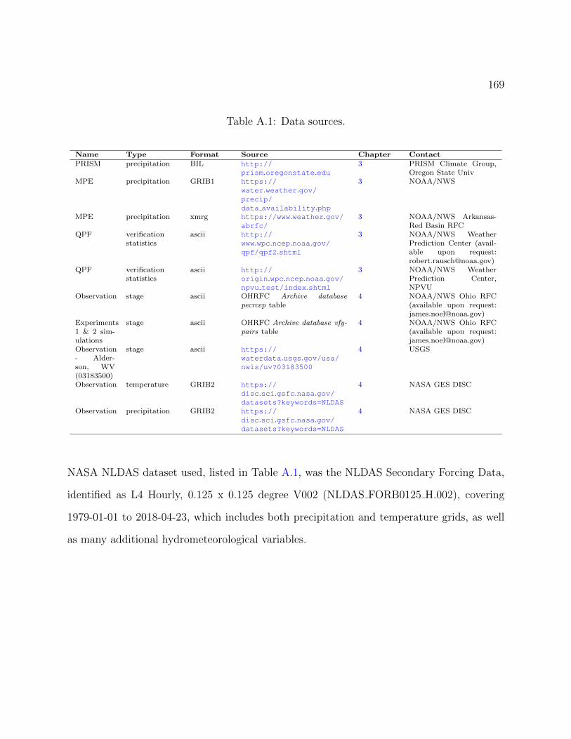
169
Table A.1: Data sources.
Name Type Format Source Chapter ContactPRISM precipitation BIL http://
prism.oregonstate.edu3 PRISM Climate Group,
Oregon State UnivMPE precipitation GRIB1 https://
water.weather.gov/precip/data availability.php
3 NOAA/NWS
MPE precipitation xmrg https://www.weather.gov/abrfc/
3 NOAA/NWS Arkansas-Red Basin RFC
QPF verificationstatistics
ascii http://www.wpc.ncep.noaa.gov/qpf/qpf2.shtml
3 NOAA/NWS WeatherPrediction Center (avail-able upon request:[email protected])
QPF verificationstatistics
ascii http://origin.wpc.ncep.noaa.gov/npvu test/index.shtml
3 NOAA/NWS WeatherPrediction Center,NPVU
Observation stage ascii OHRFC Archive databasepecrcep table
4 NOAA/NWS Ohio RFC(available upon request:[email protected])
Experiments1 & 2 sim-ulations
stage ascii OHRFC Archive database vfy-pairs table
4 NOAA/NWS Ohio RFC(available upon request:[email protected])
Observation- Alder-son, WV(03183500)
stage ascii https://waterdata.usgs.gov/usa/nwis/uv?03183500
4 USGS
Observation temperature GRIB2 https://disc.sci.gsfc.nasa.gov/datasets?keywords=NLDAS
4 NASA GES DISC
Observation precipitation GRIB2 https://disc.sci.gsfc.nasa.gov/datasets?keywords=NLDAS
4 NASA GES DISC
NASA NLDAS dataset used, listed in Table A.1, was the NLDAS Secondary Forcing Data,
identified as L4 Hourly, 0.125 x 0.125 degree V002 (NLDAS FORB0125 H.002), covering
1979-01-01 to 2018-04-23, which includes both precipitation and temperature grids, as well
as many additional hydrometeorological variables.

Appendix B
Data Analyses
B.1 Methodology
B.1.1 Chapter 3 analyses
Chapter 3 utilizes GRASS GIS [86] for analyses consisting of:
1. bias calculation (Equation 3.1), comparison of OHRFC MPE estimates to PRISM
estimates on a monthly, seasonal, and annual basis;
2. spatial transposition of 1000 randomly selected geographical locations used as storm
centers, using observed precipitation for the 24-h period, spanning the June 22-24,
2016 period;
3. threat score (TS) calculation (Equation 3.14) for the 24-h rainfall accumulation using
the 1000 transposed storms;
4. run RDHM hydrologic monte carlo simulations for 88 transposed storms with TS≥0.06,
170

B.1. Methodology 171
including transposing each of the hourly precipitation grids for the 88 storms, and
reformatting each file to xmrg format for use in the RDHM;
5. pair RDHM peak flow value, TS, and storm transposed distance from the reference
location for the 88 simulated events;
6. the paired data is imported into the R Language and Environment for Statistical Com-
puting [145] for graphical analysis.
B.1.2 Chapter 4 analyses
Chapter 4 includes two independent operational experiments. Experiment-1 compares, by
lead-time, ME, MAE, and RMSE values for forecasts using WPC 24-h QPF with forecasts
using zero-QPF. Experiment-2 uses WPC QPF for six QPF durations (6-, 12-, 24-, 36-
, 48-,72-h) and the OHRFC NWSRFS modeling system for experimental simulations. Air
temperature forcings are the same for all simulations.. Analyses consist simply of calculating
ME, MAE, and RMSE for the six WPC QPF scenarios, by lead-time, from the simulated
data stored in the OHRFC archive database using the R Language and Environment for
Statistical Computing [145] and the contributed verification package [135].
B.1.3 Chapter 5 analyses
Analyses utilize OHRFC operational and MMEFS NAEFS ensemble river stage forecasts
from 54 forecast point locations, representing different geographical location, watershed ar-
eas, and basin response times. Chapter 5 analyses include:
1. deterministic forecast verification using the R Language and Environment for Statistical
Computing [145] and the contributed verification package [135] from forecast data

172 Appendix B. Data Analyses
stored in the OHRFC PostgreSQL archive database, vfypairs table;
2. forecast verification of the MMEFS NAEFS ensemble river stage forecasts using the
NOAA/NWS EVS software [29] and USGS observed river stage data stored in the
OHRFC PostgreSQL archive database, pecrcep table. Ensemble mean and median river
stage forecast ME, MAE, RMSE, and CRPSS values, by lead-time, are also generated
for each forecast point location;
3. data re-formatting of the MMEFS NAEFS ensemble mean and median river stage
forecast verification statistics from the EVS XML data format for import into R (for
CRPSS: Listing B.22; for ME, MAE, RMSE: Listing B.23);
4. forecast comparisons and graphics generation using R, following data import.
B.2 Codes
The complete set of Perl, Bash shell, and R scripts used in the dissertation for the various
experiments and analyses, discussed in Chapter B, Section B.1, are listed in the code Listings.
Listings
B.1 Listing of forecast point locations in the paper3 exp pts.txt file from Chapter 5.175
B.2 Example PostgreSQL query from pecrcep table for river stage observations for
use in MMEFS EVS verification software used in Chapter 5. . . . . . . . . . 176
B.3 Example code to read EVS XML code from MMEFS ensemble forecast ex-
periments used in Chapter 5. . . . . . . . . . . . . . . . . . . . . . . . . . . . 176
B.4 Definition of R summarySE function. . . . . . . . . . . . . . . . . . . . . . . 176
B.5 R code for Experiment-2 Chapter 3. . . . . . . . . . . . . . . . . . . . . . . . 177
B.6 R code for the Experiment in Chapter 5 to query PostgreSQL vfypairs table
and calculate ME MAE and RMSE for each of the 54 forecast point locations
for OHRFC operational forecasts. . . . . . . . . . . . . . . . . . . . . . . . . 179
B.7 run extractMany Bash shell script code used to extract NWSRFS ESP binary
CS file time-series data for MMEFS verification in the EVS. . . . . . . . . . 181
B.8 extractMany Bash shell script called by the run extractMany Bash shell script 181
B.9 The run bil2grass bash shell script is used to import PRISM precipitation
data into GRASS GIS for MPE bias analyses. . . . . . . . . . . . . . . . . . 182
B.10 bil2grass bash shell script is called by run bil2grass. . . . . . . . . . . . . . . 182
B.11 run nldas2xmrg bash shell script is used to import NASA NLDAS precipita-
tion and temperature grids into GRASS GIS. . . . . . . . . . . . . . . . . . 183
173
174 LISTINGS
B.12 nldas2xmrg bash shell script is called by the run nldas2xmrg bash shell script. 185
B.13 run QPF TS experiment bash shell script calculates threat score values from
the RDHM monte carlo hydrologic simulations for the Chapter 5 experiment. 187
B.14 renameCONUS2xmrg shell script is used to rename CONUS scale MPE xmrg
format file used in RDHM simulations. . . . . . . . . . . . . . . . . . . . . . 190
B.15 setupRDHMwarm states is a shell script used to create a directory structure
and move RDHM model initialization files for the RDHM monte carlo simu-
lation experiments. . . . . . . . . . . . . . . . . . . . . . . . . . . . . . . . . 190
B.16 grassTranslateXMRG shell script is called by run QPF TS RDHM used to
translate xmrg storm maps in GRASS GIS. . . . . . . . . . . . . . . . . . . 191
B.17 importxmrg2grass shell script is used to import MPE xmrg files into GRASS
GIS. . . . . . . . . . . . . . . . . . . . . . . . . . . . . . . . . . . . . . . . . 194
B.18 xmrg2newster is a shell script called by importxmrg2grass. . . . . . . . . . . 195
B.19 run QPF TS RDHM is the main shell script used to run the RDHM monte
carlo hydrologic simulation experiment in Chapter 3. . . . . . . . . . . . . . 196
B.20 run RDHMthreatScoreOutput2TS.sh shell script used to calculate threat score
from the RDHM monte carlo hydrologic simulation experiment in Chapter 3 198
B.21 run obsText2Datacard shell script is used to run the pecrsepObs2TS.pl and
ts2datacard.pl Perl scripts. . . . . . . . . . . . . . . . . . . . . . . . . . . . . 198
B.22 evsCRPSSXML2R.pl Perl script reads EVS generated XML files for CRPSS
values from MMEFS ensemble simulations for each forecast point location for
import into R. . . . . . . . . . . . . . . . . . . . . . . . . . . . . . . . . . . . 199
B.23 mmefsXML2R.pl Perl script Perl script reads EVS generated XML files of
ME MAE and RMSE from MMEFS forecast ensemble simulations for each
forecast point location for import into R . . . . . . . . . . . . . . . . . . . . 201
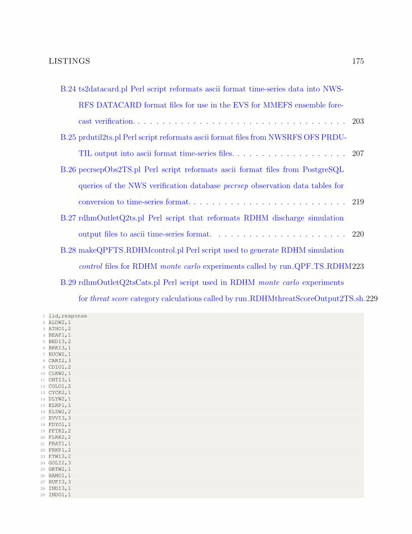
LISTINGS 175
B.24 ts2datacard.pl Perl script reformats ascii format time-series data into NWS-
RFS DATACARD format files for use in the EVS for MMEFS ensemble fore-
cast verification. . . . . . . . . . . . . . . . . . . . . . . . . . . . . . . . . . . 203
B.25 prdutil2ts.pl Perl script reformats ascii format files from NWSRFS OFS PRDU-
TIL output into ascii format time-series files. . . . . . . . . . . . . . . . . . . 207
B.26 pecrsepObs2TS.pl Perl script reformats ascii format files from PostgreSQL
queries of the NWS verification database pecrsep observation data tables for
conversion to time-series format. . . . . . . . . . . . . . . . . . . . . . . . . . 219
B.27 rdhmOutletQ2ts.pl Perl script that reformats RDHM discharge simulation
output files to ascii time-series format. . . . . . . . . . . . . . . . . . . . . . 220
B.28 makeQPFTS RDHMcontrol.pl Perl script used to generate RDHM simulation
control files for RDHM monte carlo experiments called by run QPF TS RDHM223
B.29 rdhmOutletQ2tsCats.pl Perl script used in RDHM monte carlo experiments
for threat score category calculations called by run RDHMthreatScoreOutput2TS.sh.229
1 lid,response2 ALDW2,13 ATHO1,24 BEAP1,15 BEDI3,26 BRKI3,17 BUCW2,18 CARI2,39 CDIO1,2
10 CLKW2,111 CNTI3,112 COLO1,213 CYCK2,114 DLYW2,115 ELRP1,116 ELZW2,217 EVVI3,318 FDYO1,119 FFTK2,220 FLRK2,221 FRAT1,122 FRKP1,223 FTWI3,224 GOLI2,325 GRTW2,126 HAMO1,127 HUFI3,328 INDI3,129 INDO1,1
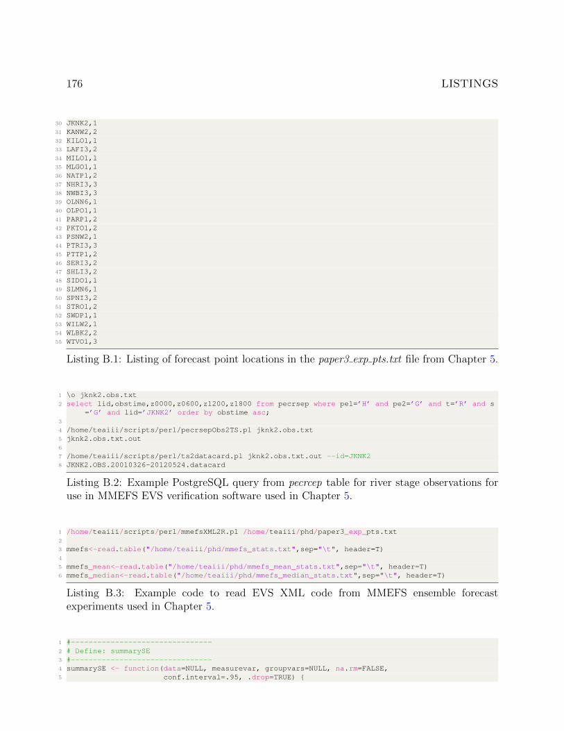
176 LISTINGS
30 JKNK2,131 KANW2,232 KILO1,133 LAFI3,234 MILO1,135 MLGO1,136 NATP1,237 NHRI3,338 NWBI3,339 OLNN6,140 OLPO1,141 PARP1,242 PKTO1,243 PSNW2,144 PTRI3,345 PTTP1,246 SERI3,247 SHLI3,248 SIDO1,149 SLMN6,150 SPNI3,251 STRO1,252 SWDP1,153 WILW2,154 WLBK2,255 WTVO1,3
Listing B.1: Listing of forecast point locations in the paper3 exp pts.txt file from Chapter 5.
1 \o jknk2.obs.txt2 select lid,obstime,z0000,z0600,z1200,z1800 from pecrsep where pe1=’H’ and pe2=’G’ and t=’R’ and s
=’G’ and lid=’JKNK2’ order by obstime asc;3
4 /home/teaiii/scripts/perl/pecrsepObs2TS.pl jknk2.obs.txt5 jknk2.obs.txt.out6
7 /home/teaiii/scripts/perl/ts2datacard.pl jknk2.obs.txt.out --id=JKNK28 JKNK2.OBS.20010326-20120524.datacard
Listing B.2: Example PostgreSQL query from pecrcep table for river stage observations foruse in MMEFS EVS verification software used in Chapter 5.
1 /home/teaiii/scripts/perl/mmefsXML2R.pl /home/teaiii/phd/paper3_exp_pts.txt2
3 mmefs<-read.table("/home/teaiii/phd/mmefs_stats.txt",sep="\t", header=T)4
5 mmefs_mean<-read.table("/home/teaiii/phd/mmefs_mean_stats.txt",sep="\t", header=T)6 mmefs_median<-read.table("/home/teaiii/phd/mmefs_median_stats.txt",sep="\t", header=T)
Listing B.3: Example code to read EVS XML code from MMEFS ensemble forecastexperiments used in Chapter 5.
1 #--------------------------------2 # Define: summarySE3 #--------------------------------4 summarySE <- function(data=NULL, measurevar, groupvars=NULL, na.rm=FALSE,5 conf.interval=.95, .drop=TRUE) {
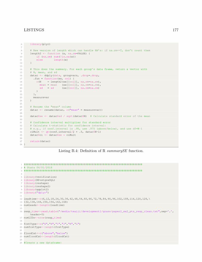
LISTINGS 177
6 library(plyr)7
8 # New version of length which can handle NA’s: if na.rm==T, don’t count them9 length2 <- function (x, na.rm=FALSE) {
10 if (na.rm) sum(!is.na(x))11 else length(x)12 }13
14 # This does the summary. For each group’s data frame, return a vector with15 # N, mean, and sd16 datac <- ddply(data, groupvars, .drop=.drop,17 .fun = function(xx, col) {18 c(N = length2(xx[[col]], na.rm=na.rm),19 mean = mean (xx[[col]], na.rm=na.rm),20 sd = sd (xx[[col]], na.rm=na.rm)21 )22 },23 measurevar24 )25
26 # Rename the "mean" column27 datac <- rename(datac, c("mean" = measurevar))28
29 datac$se <- datac$sd / sqrt(datac$N) # Calculate standard error of the mean30
31 # Confidence interval multiplier for standard error32 # Calculate t-statistic for confidence interval:33 # e.g., if conf.interval is .95, use .975 (above/below), and use df=N-134 ciMult <- qt(conf.interval/2 + .5, datac$N-1)35 datac$ci <- datac$se * ciMult36
37 return(datac)38 }
Listing B.4: Definition of R summarySE function.
1 ###########################################################################2 # Stats 04/01/20183 ###########################################################################4
5 library(verification)6 library(RPostgreSQL)7 library(reshape)8 library(reshape2)9 library(ggplot2)
10 library("dplyr")11
12 leadtime<-c(6,12,18,24,30,36,42,48,54,60,66,72,78,84,90,96,102,108,114,120,126,\13 132,138,144,150,156,162,168)14 numLeads<-length(leadtime)15
16 resp_time<-read.table("/media/teaiii/development1/grass/paper2_ex2_pts_resp_clean.txt",sep=’,’,header=T)
17 numLIDs<-nrow(resp_time)18
19 fcstType<-c("G","H","I","J","K","L")20 numfcstType<-length(fcstType)21
22 floodCat<-c("above","below")23 numfloodCat<-length(floodCat)24
25 #Create a new dataframe:
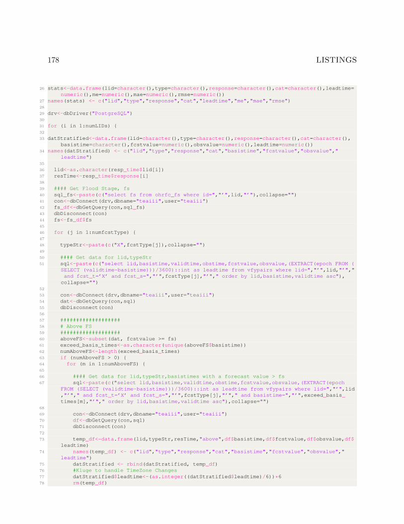
178 LISTINGS
26 stats<-data.frame(lid=character(),type=character(),response=character(),cat=character(),leadtime=numeric(),me=numeric(),mae=numeric(),rmse=numeric())
27 names(stats) <- c("lid","type","response","cat","leadtime","me","mae","rmse")28
29 drv<-dbDriver("PostgreSQL")30
31 for (i in 1:numLIDs) {32
33 datStratified<-data.frame(lid=character(),type=character(),response=character(),cat=character(),basistime=character(),fcstvalue=numeric(),obsvalue=numeric(),leadtime=numeric())
34 names(datStratified) <- c("lid","type","response","cat","basistime","fcstvalue","obsvalue","leadtime")
35
36 lid<-as.character(resp_time$lid[i])37 resTime<-resp_time$response[i]38
39 #### Get Flood Stage, fs40 sql_fs<-paste(c("select fs from ohrfc_fs where id=","’",lid,"’"),collapse="")41 con<-dbConnect(drv,dbname="teaiii",user="teaiii")42 fs_df<-dbGetQuery(con,sql_fs)43 dbDisconnect(con)44 fs<-fs_df$fs45
46 for (j in 1:numfcstType) {47
48 typeStr<-paste(c("X",fcstType[j]),collapse="")49
50 #### Get data for lid,typeStr51 sql<-paste(c("select lid,basistime,validtime,obstime,fcstvalue,obsvalue,(EXTRACT(epoch FROM (
SELECT (validtime-basistime)))/3600)::int as leadtime from vfypairs where lid=","’",lid,"’","and fcst_t=’X’ and fcst_s=","’",fcstType[j],"’"," order by lid,basistime,validtime asc"),collapse="")
52
53 con<-dbConnect(drv,dbname="teaiii",user="teaiii")54 dat<-dbGetQuery(con,sql)55 dbDisconnect(con)56
57 ###################58 # Above FS59 ###################60 aboveFS<-subset(dat, fcstvalue >= fs)61 exceed_basis_times<-as.character(unique(aboveFS$basistime))62 numAboveFS<-length(exceed_basis_times)63 if (numAboveFS > 0) {64 for (m in 1:numAboveFS) {65
66 #### Get data for lid,typeStr,basistimes with a forecast value > fs67 sql<-paste(c("select lid,basistime,validtime,obstime,fcstvalue,obsvalue,(EXTRACT(epoch
FROM (SELECT (validtime-basistime)))/3600)::int as leadtime from vfypairs where lid=","’",lid,"’"," and fcst_t=’X’ and fcst_s=","’",fcstType[j],"’"," and basistime=","’",exceed_basis_times[m],"’"," order by lid,basistime,validtime asc"),collapse="")
68
69 con<-dbConnect(drv,dbname="teaiii",user="teaiii")70 df<-dbGetQuery(con,sql)71 dbDisconnect(con)72
73 temp_df<-data.frame(lid,typeStr,resTime,"above",df$basistime,df$fcstvalue,df$obsvalue,df$leadtime)
74 names(temp_df) <- c("lid","type","response","cat","basistime","fcstvalue","obsvalue","leadtime")
75 datStratified <- rbind(datStratified, temp_df)76 #Kluge to handle TimeZone Changes77 datStratified$leadtime<-(as.integer((datStratified$leadtime)/6))*678 rm(temp_df)
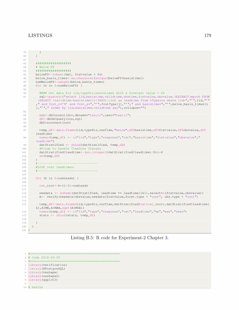
LISTINGS 179
79 }80 }81
82 ###################83 # Below FS84 ###################85 belowFS<-subset(dat, fcstvalue < fs)86 below_basis_times<-as.character(unique(belowFS$basistime))87 numBelowFS<-length(below_basis_times)88 for (n in 1:numBelowFS) {89
90 #### Get data for lid,typeStr,basistimes with a forecast value < fs91 sql<-paste(c("select lid,basistime,validtime,obstime,fcstvalue,obsvalue,(EXTRACT(epoch FROM
(SELECT (validtime-basistime)))/3600)::int as leadtime from vfypairs where lid=","’",lid,"’"," and fcst_t=’X’ and fcst_s=","’",fcstType[j],"’"," and basistime=","’",below_basis_times[n],"’"," order by lid,basistime,validtime asc"),collapse="")
92
93 con<-dbConnect(drv,dbname="teaiii",user="teaiii")94 df<-dbGetQuery(con,sql)95 dbDisconnect(con)96
97 temp_df<-data.frame(lid,typeStr,resTime,"below",df$basistime,df$fcstvalue,df$obsvalue,df$leadtime)
98 names(temp_df) <- c("lid","type","response","cat","basistime","fcstvalue","obsvalue","leadtime")
99 datStratified <- rbind(datStratified, temp_df)100 #Kluge to handle TimeZone Changes101 datStratified$leadtime<-(as.integer((datStratified$leadtime)/6))*6102 rm(temp_df)103 }104 #--------------------------------105 #LOOP over leadtimes:106 #--------------------------------107
108 for (k in 1:numLeads) {109
110 cat_incr<-k+(i-1)*numLeads111
112 newdata <- subset(datStratified, leadtime == leadtime[[k]],select=c(fcstvalue,obsvalue))113 A<- verify(newdata$obsvalue,newdata$fcstvalue,frcst.type = "cont", obs.type = "cont")114
115 temp_df<-data.frame(lid,typeStr,resTime,datStratified$cat[cat_incr],datStratified$leadtime[k],A$ME,A$MAE,sqrt(A$MSE))
116 names(temp_df) <- c("lid","type","response","cat","leadtime","me","mae","rmse")117 stats <- rbind(stats, temp_df)118
119 }120 }121 }
Listing B.5: R code for Experiment-2 Chapter 3.
1 #================================================2 # Code 2018-03-293 #================================================4 library(verification)5 library(RPostgreSQL)6 library(reshape)7 library(reshape2)8 library(ggplot2)9
10 # basins
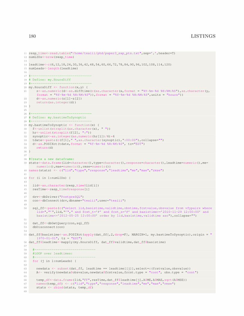
180 LISTINGS
11 resp_time<-read.table("/home/teaiii/phd/paper3_exp_pts.txt",sep=’,’,header=T)12 numLIDs<-nrow(resp_time)13
14 leadtime<-c(6,12,18,24,30,36,42,48,54,60,66,72,78,84,90,96,102,108,114,120)15 numLeads<-length(leadtime)16
17 #--------------------------------18 # Define: my.HoursDiff19 #--------------------------------20 my.HoursDiff <- function(x,y) {21 z<-as.numeric(d<-as.difftime(c(as.character(x,format = "%Y-%m-%d %H:%M:%S"),as.character(y,
format = "%Y-%m-%d %H:%M:%S")),format = "%Y-%m-%d %H:%M:%S",units = "hours"))22 d<-as.numeric(z[1]-z[2])23 return(as.integer(d))24 }25
26 #--------------------------------27 # Define: my.bastimeToSynoptic28 #--------------------------------29 my.bastimeToSynoptic <- function(x) {30 f<-unlist(strsplit(as.character(x), " "))31 hr<-unlist(strsplit(f[2], ":"))32 synoptic<-as.integer(as.numeric(hr[1])/6)*633 tdate<-paste(c(f[1]," ",as.character(synoptic),":00:00"),collapse="")34 d<-as.POSIXct(tdate,format = "%Y-%m-%d %H:%M:%S", tz="EST")35 return(d)36 }37
38 #Create a new dataframe:39 stats<-data.frame(lid=character(),type=character(),response=character(),leadtime=numeric(),me=
numeric(),mae=numeric(),rmse=numeric())40 names(stats) <- c("lid","type","response","leadtime","me","mae","rmse")41
42 for (i in 1:numLIDs) {43
44 lid<-as.character(resp_time$lid[i])45 resTime<-resp_time$response[i]46
47 drv<-dbDriver("PostgreSQL")48 con<-dbConnect(drv,dbname="teaiii",user="teaiii")49
50 sql_ff<-paste(c("select lid,basistime,validtime,obstime,fcstvalue,obsvalue from vfypairs wherelid=","’",lid,"’"," and fcst_t=’F’ and fcst_s=’F’ and basistime>=’2010-11-29 12:00:00’ andbasistime<=’2012-05-25 12:00:00’ order by lid,basistime,validtime asc"),collapse="")
51
52 dat_ff<-dbGetQuery(con,sql_ff)53 dbDisconnect(con)54
55 dat_ff$basistime<-as.POSIXct(apply(dat_ff[,2,drop=F], MARGIN=1, my.bastimeToSynoptic),origin = "1970-01-01", tz = "EST")
56 dat_ff$leadtime<-mapply(my.HoursDiff, dat_ff$validtime,dat_ff$basistime)57
58 #--------------------------------59 #LOOP over leadtimes:60 #--------------------------------61 for (j in 1:numLeads) {62
63 newdata <- subset(dat_ff, leadtime == leadtime[[j]],select=c(fcstvalue,obsvalue))64 A<- verify(newdata$obsvalue,newdata$fcstvalue,frcst.type = "cont", obs.type = "cont")65
66 temp_df<-data.frame(lid,"FF",resTime,dat_ff$leadtime[j],A$ME,A$MAE,sqrt(A$MSE))67 names(temp_df) <- c("lid","type","response","leadtime","me","mae","rmse")68 stats <- rbind(stats, temp_df)69
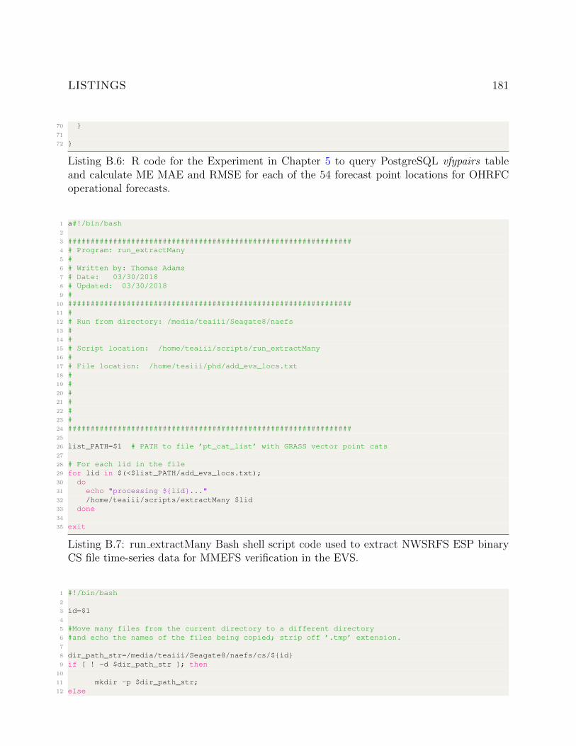
LISTINGS 181
70 }71
72 }
Listing B.6: R code for the Experiment in Chapter 5 to query PostgreSQL vfypairs tableand calculate ME MAE and RMSE for each of the 54 forecast point locations for OHRFCoperational forecasts.
1 a#!/bin/bash2
3 ###############################################################4 # Program: run_extractMany5 #6 # Written by: Thomas Adams7 # Date: 03/30/20188 # Updated: 03/30/20189 #
10 ###############################################################11 #12 # Run from directory: /media/teaiii/Seagate8/naefs13 #14 #15 # Script location: /home/teaiii/scripts/run_extractMany16 #17 # File location: /home/teaiii/phd/add_evs_locs.txt18 #19 #20 #21 #22 #23 #24 ###############################################################25
26 list_PATH=$1 # PATH to file ’pt_cat_list’ with GRASS vector point cats27
28 # For each lid in the file29 for lid in $(<$list_PATH/add_evs_locs.txt);30 do31 echo "processing ${lid}..."32 /home/teaiii/scripts/extractMany $lid33 done34
35 exit
Listing B.7: run extractMany Bash shell script code used to extract NWSRFS ESP binaryCS file time-series data for MMEFS verification in the EVS.
1 #!/bin/bash2
3 id=$14
5 #Move many files from the current directory to a different directory6 #and echo the names of the files being copied; strip off ’.tmp’ extension.7
8 dir_path_str=/media/teaiii/Seagate8/naefs/cs/${id}9 if [ ! -d $dir_path_str ]; then
10
11 mkdir -p $dir_path_str;12 else
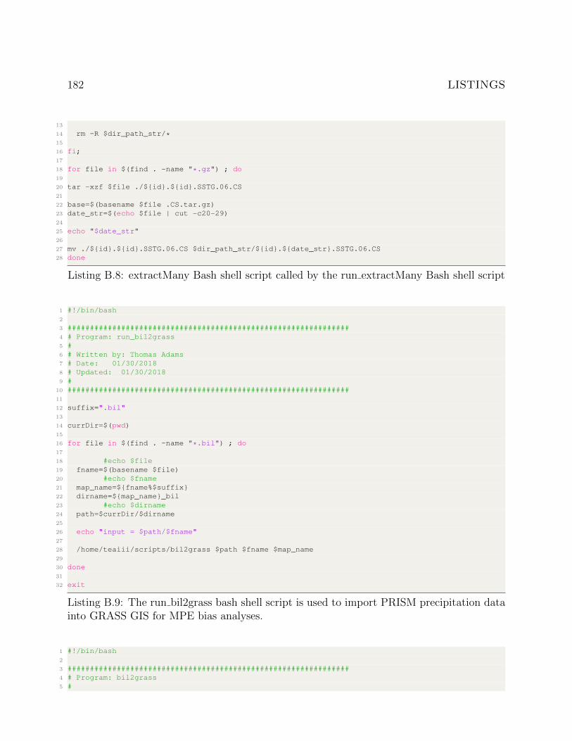
182 LISTINGS
13
14 rm -R $dir_path_str/*15
16 fi;17
18 for file in $(find . -name "*.gz") ; do19
20 tar -xzf $file ./${id}.${id}.SSTG.06.CS21
22 base=$(basename $file .CS.tar.gz)23 date_str=$(echo $file | cut -c20-29)24
25 echo "$date_str"26
27 mv ./${id}.${id}.SSTG.06.CS $dir_path_str/${id}.${date_str}.SSTG.06.CS28 done
Listing B.8: extractMany Bash shell script called by the run extractMany Bash shell script
1 #!/bin/bash2
3 ###############################################################4 # Program: run_bil2grass5 #6 # Written by: Thomas Adams7 # Date: 01/30/20188 # Updated: 01/30/20189 #
10 ###############################################################11
12 suffix=".bil"13
14 currDir=$(pwd)15
16 for file in $(find . -name "*.bil") ; do17
18 #echo $file19 fname=$(basename $file)20 #echo $fname21 map_name=${fname%$suffix}22 dirname=${map_name}_bil23 #echo $dirname24 path=$currDir/$dirname25
26 echo "input = $path/$fname"27
28 /home/teaiii/scripts/bil2grass $path $fname $map_name29
30 done31
32 exit
Listing B.9: The run bil2grass bash shell script is used to import PRISM precipitation datainto GRASS GIS for MPE bias analyses.
1 #!/bin/bash2
3 ###############################################################4 # Program: bil2grass5 #
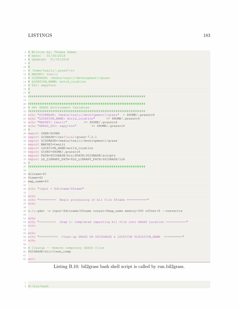
LISTINGS 183
6 # Written by: Thomas Adams7 # Date: 01/30/20188 # Updated: 01/30/20189 #
10 #11 # /home/teaiii/.grass7/rc12 # MAPSET: teaiii13 # GISDBASE: /media/teaiii/development1/grass14 # LOCATION_NAME: world_location15 # GUI: wxpython16 #17 #18 ###############################################################19
20 ###############################################################21 # Set GRASS Environment Variables22 ###############################################################23 echo "GISDBASE: /media/teaiii/development1/grass" > $HOME/.grassrc624 echo "LOCATION_NAME: world_location" >> $HOME/.grassrc625 echo "MAPSET: teaiii" >> $HOME/.grassrc626 echo "GRASS_GUI: wxpython" >> $HOME/.grassrc627 #28 export USER=$USER29 export GISBASE=/usr/local/grass-7.2.130 export GISDBASE=/media/teaiii/development1/grass31 export MAPSET=teaiii32 export LOCATION_NAME=world_location33 export GISRC=$HOME/.grassrc634 export PATH=$GISBASE/bin:$PATH:$GISBASE/scripts35 export LD_LIBRARY_PATH=$LD_LIBRARY_PATH:$GISBASE/lib36 #37 ###############################################################38
39 dirname=$140 fname=$241 map_name=$342
43 echo "input = $dirname/$fname"44
45 echo46 echo "========= Begin processing of bil file $fname ==========="47 echo48
49 r.in.gdal -o input=$dirname/$fname output=$map_name memory=300 offset=0 --overwrite50
51 echo52 echo "========= Step 1: Completed importing bil file into GRASS Location ==========="53 echo54
55 echo56 echo "========== Clean-up GRASS DB $GISDBASE & LOCATION $LOCATION_NAME =========="57 echo58
59 # Cleanup -- Remove temporary GRASS files60 $GISBASE/etc/clean_temp61
62 exit
Listing B.10: bil2grass bash shell script is called by run bil2grass.
1
2 #!/bin/bash
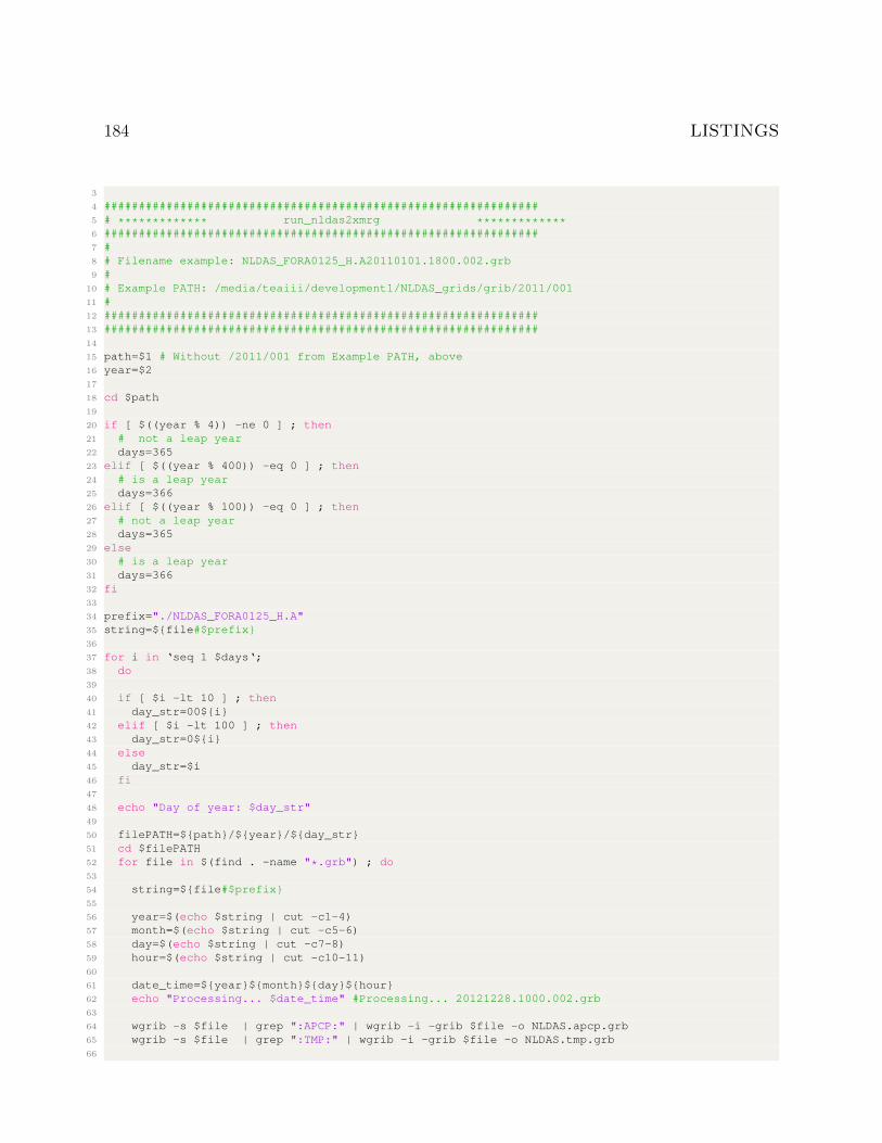
184 LISTINGS
3
4 ###############################################################5 # ************* run_nldas2xmrg *************6 ###############################################################7 #8 # Filename example: NLDAS_FORA0125_H.A20110101.1800.002.grb9 #
10 # Example PATH: /media/teaiii/development1/NLDAS_grids/grib/2011/00111 #12 ###############################################################13 ###############################################################14
15 path=$1 # Without /2011/001 from Example PATH, above16 year=$217
18 cd $path19
20 if [ $((year % 4)) -ne 0 ] ; then21 # not a leap year22 days=36523 elif [ $((year % 400)) -eq 0 ] ; then24 # is a leap year25 days=36626 elif [ $((year % 100)) -eq 0 ] ; then27 # not a leap year28 days=36529 else30 # is a leap year31 days=36632 fi33
34 prefix="./NLDAS_FORA0125_H.A"35 string=${file#$prefix}36
37 for i in ‘seq 1 $days‘;38 do39
40 if [ $i -lt 10 ] ; then41 day_str=00${i}42 elif [ $i -lt 100 ] ; then43 day_str=0${i}44 else45 day_str=$i46 fi47
48 echo "Day of year: $day_str"49
50 filePATH=${path}/${year}/${day_str}51 cd $filePATH52 for file in $(find . -name "*.grb") ; do53
54 string=${file#$prefix}55
56 year=$(echo $string | cut -c1-4)57 month=$(echo $string | cut -c5-6)58 day=$(echo $string | cut -c7-8)59 hour=$(echo $string | cut -c10-11)60
61 date_time=${year}${month}${day}${hour}62 echo "Processing... $date_time" #Processing... 20121228.1000.002.grb63
64 wgrib -s $file | grep ":APCP:" | wgrib -i -grib $file -o NLDAS.apcp.grb65 wgrib -s $file | grep ":TMP:" | wgrib -i -grib $file -o NLDAS.tmp.grb66
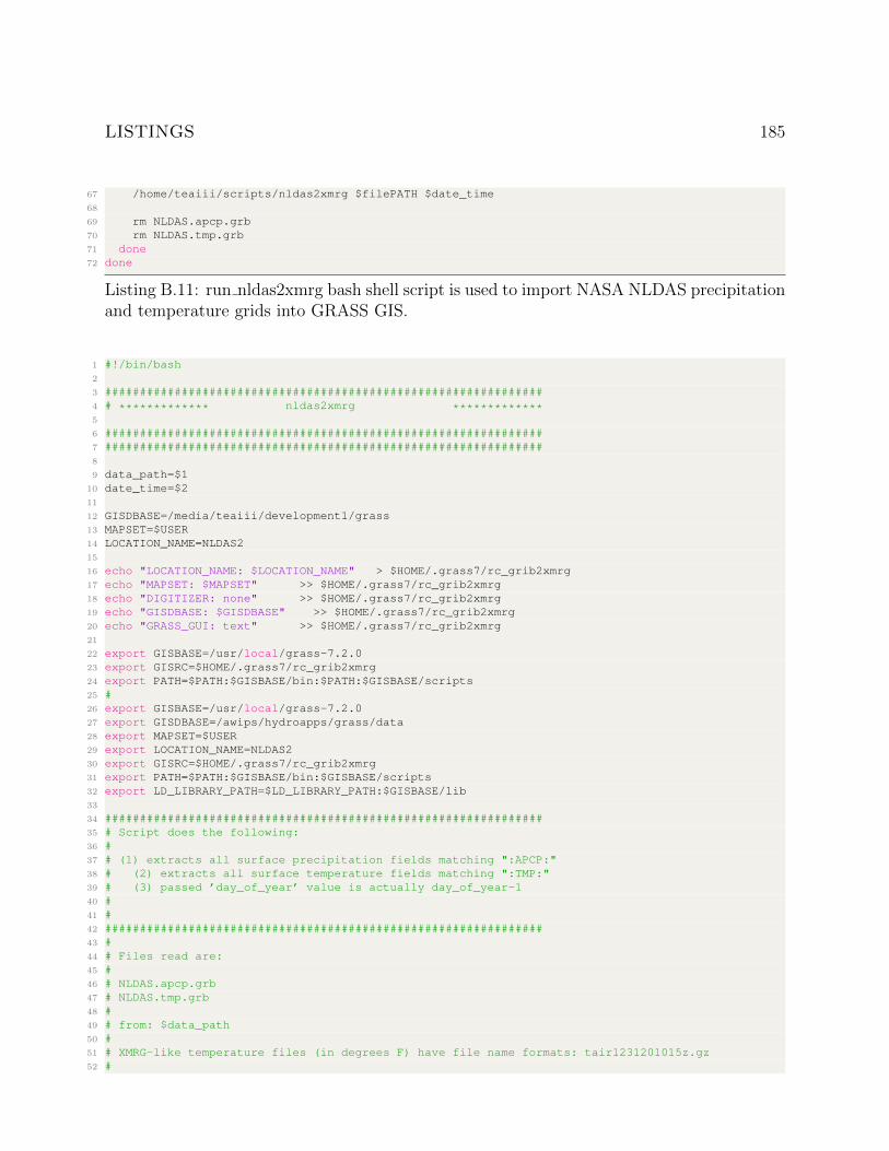
LISTINGS 185
67 /home/teaiii/scripts/nldas2xmrg $filePATH $date_time68
69 rm NLDAS.apcp.grb70 rm NLDAS.tmp.grb71 done72 done
Listing B.11: run nldas2xmrg bash shell script is used to import NASA NLDAS precipitationand temperature grids into GRASS GIS.
1 #!/bin/bash2
3 ###############################################################4 # ************* nldas2xmrg *************5
6 ###############################################################7 ###############################################################8
9 data_path=$110 date_time=$211
12 GISDBASE=/media/teaiii/development1/grass13 MAPSET=$USER14 LOCATION_NAME=NLDAS215
16 echo "LOCATION_NAME: $LOCATION_NAME" > $HOME/.grass7/rc_grib2xmrg17 echo "MAPSET: $MAPSET" >> $HOME/.grass7/rc_grib2xmrg18 echo "DIGITIZER: none" >> $HOME/.grass7/rc_grib2xmrg19 echo "GISDBASE: $GISDBASE" >> $HOME/.grass7/rc_grib2xmrg20 echo "GRASS_GUI: text" >> $HOME/.grass7/rc_grib2xmrg21
22 export GISBASE=/usr/local/grass-7.2.023 export GISRC=$HOME/.grass7/rc_grib2xmrg24 export PATH=$PATH:$GISBASE/bin:$PATH:$GISBASE/scripts25 #26 export GISBASE=/usr/local/grass-7.2.027 export GISDBASE=/awips/hydroapps/grass/data28 export MAPSET=$USER29 export LOCATION_NAME=NLDAS230 export GISRC=$HOME/.grass7/rc_grib2xmrg31 export PATH=$PATH:$GISBASE/bin:$GISBASE/scripts32 export LD_LIBRARY_PATH=$LD_LIBRARY_PATH:$GISBASE/lib33
34 ###############################################################35 # Script does the following:36 #37 # (1) extracts all surface precipitation fields matching ":APCP:"38 # (2) extracts all surface temperature fields matching ":TMP:"39 # (3) passed ’day_of_year’ value is actually day_of_year-140 #41 #42 ###############################################################43 #44 # Files read are:45 #46 # NLDAS.apcp.grb47 # NLDAS.tmp.grb48 #49 # from: $data_path50 #51 # XMRG-like temperature files (in degrees F) have file name formats: tair1231201015z.gz52 #
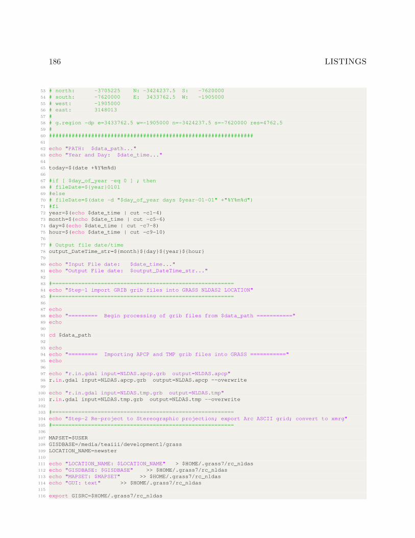
186 LISTINGS
53 # north: -3705225 N: -3424237.5 S: -762000054 # south: -7620000 E: 3433762.5 W: -190500055 # west: -190500056 # east: 314801357 #58 # g.region -dp e=3433762.5 w=-1905000 n=-3424237.5 s=-7620000 res=4762.559 #60 ###############################################################61
62 echo "PATH: $data_path..."63 echo "Year and Day: $date_time..."64
65 today=$(date +%Y%m%d)66
67 #if [ $day_of_year -eq 0 ] ; then68 # fileDate=${year}010169 #else70 # fileDate=$(date -d "$day_of_year days $year-01-01" +"%Y%m%d")71 #fi72 year=$(echo $date_time | cut -c1-4)73 month=$(echo $date_time | cut -c5-6)74 day=$(echo $date_time | cut -c7-8)75 hour=$(echo $date_time | cut -c9-10)76
77 # Output file date/time78 output_DateTime_str=${month}${day}${year}${hour}79
80 echo "Input File date: $date_time..."81 echo "Output File date: $output_DateTime_str..."82
83 #========================================================84 echo "Step-1 import GRIB grib files into GRASS NLDAS2 LOCATION"85 #========================================================86
87 echo88 echo "========= Begin processing of grib files from $data_path ==========="89 echo90
91 cd $data_path92
93 echo94 echo "========= Importing APCP and TMP grib files into GRASS ==========="95 echo96
97 echo "r.in.gdal input=NLDAS.apcp.grb output=NLDAS.apcp"98 r.in.gdal input=NLDAS.apcp.grb output=NLDAS.apcp --overwrite99
100 echo "r.in.gdal input=NLDAS.tmp.grb output=NLDAS.tmp"101 r.in.gdal input=NLDAS.tmp.grb output=NLDAS.tmp --overwrite102
103 #========================================================104 echo "Step-2 Re-project to Stereographic projection; export Arc ASCII grid; convert to xmrg"105 #========================================================106
107 MAPSET=$USER108 GISDBASE=/media/teaiii/development1/grass109 LOCATION_NAME=newster110
111 echo "LOCATION_NAME: $LOCATION_NAME" > $HOME/.grass7/rc_nldas112 echo "GISDBASE: $GISDBASE" >> $HOME/.grass7/rc_nldas113 echo "MAPSET: $MAPSET" >> $HOME/.grass7/rc_nldas114 echo "GUI: text" >> $HOME/.grass7/rc_nldas115
116 export GISRC=$HOME/.grass7/rc_nldas
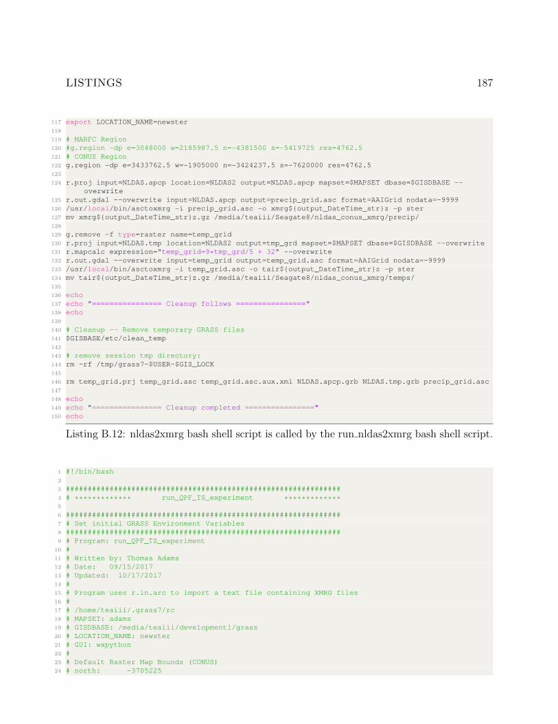
LISTINGS 187
117 export LOCATION_NAME=newster118
119 # MARFC Region120 #g.region -dp e=3048000 w=2185987.5 n=-4381500 s=-5419725 res=4762.5121 # CONUS Region122 g.region -dp e=3433762.5 w=-1905000 n=-3424237.5 s=-7620000 res=4762.5123
124 r.proj input=NLDAS.apcp location=NLDAS2 output=NLDAS.apcp mapset=$MAPSET dbase=$GISDBASE --overwrite
125 r.out.gdal --overwrite input=NLDAS.apcp output=precip_grid.asc format=AAIGrid nodata=-9999126 /usr/local/bin/asctoxmrg -i precip_grid.asc -o xmrg${output_DateTime_str}z -p ster127 mv xmrg${output_DateTime_str}z.gz /media/teaiii/Seagate8/nldas_conus_xmrg/precip/128
129 g.remove -f type=raster name=temp_grid130 r.proj input=NLDAS.tmp location=NLDAS2 output=tmp_grd mapset=$MAPSET dbase=$GISDBASE --overwrite131 r.mapcalc expression="temp_grid=9*tmp_grd/5 + 32" --overwrite132 r.out.gdal --overwrite input=temp_grid output=temp_grid.asc format=AAIGrid nodata=-9999133 /usr/local/bin/asctoxmrg -i temp_grid.asc -o tair${output_DateTime_str}z -p ster134 mv tair${output_DateTime_str}z.gz /media/teaiii/Seagate8/nldas_conus_xmrg/temps/135
136 echo137 echo "================ Cleanup follows ================"138 echo139
140 # Cleanup -- Remove temporary GRASS files141 $GISBASE/etc/clean_temp142
143 # remove session tmp directory:144 rm -rf /tmp/grass7-$USER-$GIS_LOCK145
146 rm temp_grid.prj temp_grid.asc temp_grid.asc.aux.xml NLDAS.apcp.grb NLDAS.tmp.grb precip_grid.asc147
148 echo149 echo "================ Cleanup completed ================"150 echo
Listing B.12: nldas2xmrg bash shell script is called by the run nldas2xmrg bash shell script.
1 #!/bin/bash2
3 ###############################################################4 # ************* run_QPF_TS_experiment *************5
6 ###############################################################7 # Set initial GRASS Environment Variables8 ###############################################################9 # Program: run_QPF_TS_experiment
10 #11 # Written by: Thomas Adams12 # Date: 09/15/201713 # Updated: 10/17/201714 #15 # Program uses r.in.arc to import a text file containing XMRG files16 #17 # /home/teaiii/.grass7/rc18 # MAPSET: adams19 # GISDBASE: /media/teaiii/development1/grass20 # LOCATION_NAME: newster21 # GUI: wxpython22 #23 # Default Raster Map Bounds (CONUS)24 # north: -3705225
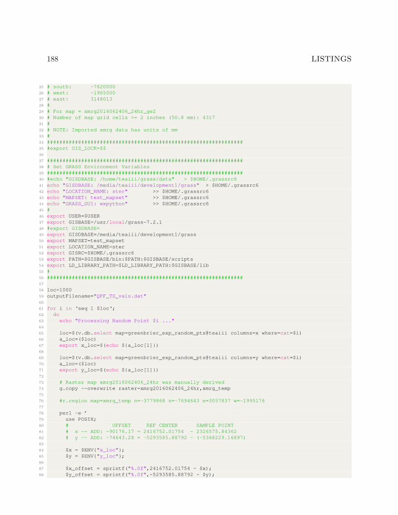
188 LISTINGS
25 # south: -762000026 # west: -190500027 # east: 314801328 #29 # For map = xmrg2016062406_24hr_ge230 # Number of map grid cells >= 2 inches (50.8 mm): 431731 #32 # NOTE: Imported xmrg data has units of mm33 #34 ###############################################################35 #export GIS_LOCK=$$36
37 ###############################################################38 # Set GRASS Environment Variables39 ###############################################################40 #echo "GISDBASE: /home/teaiii/grass/data" > $HOME/.grassrc641 echo "GISDBASE: /media/teaiii/development1/grass" > $HOME/.grassrc642 echo "LOCATION_NAME: ster" >> $HOME/.grassrc643 echo "MAPSET: test_mapset" >> $HOME/.grassrc644 echo "GRASS_GUI: wxpython" >> $HOME/.grassrc645 #46 export USER=$USER47 export GISBASE=/usr/local/grass-7.2.148 #export GISDBASE=49 export GISDBASE=/media/teaiii/development1/grass50 export MAPSET=test_mapset51 export LOCATION_NAME=ster52 export GISRC=$HOME/.grassrc653 export PATH=$GISBASE/bin:$PATH:$GISBASE/scripts54 export LD_LIBRARY_PATH=$LD_LIBRARY_PATH:$GISBASE/lib55 #56 ###############################################################57
58 loc=100059 outputFilename="QPF_TS_vals.dat"60
61 for i in ‘seq 1 $loc‘;62 do63 echo "Processing Random Point $i ..."64
65 loc=$(v.db.select map=greenbrier_exp_random_pts@teaiii columns=x where=cat=$i)66 a_loc=($loc)67 export x_loc=$(echo ${a_loc[1]})68
69 loc=$(v.db.select map=greenbrier_exp_random_pts@teaiii columns=y where=cat=$i)70 a_loc=($loc)71 export y_loc=$(echo ${a_loc[1]})72
73 # Raster map xmrg2016062406_24hr was manually derived74 g.copy --overwrite raster=xmrg2016062406_24hr,xmrg_temp75
76 #r.region map=xmrg_temp n=-3779868 s=-7694643 e=3057837 w=-199517677
78 perl -e ’79 use POSIX;80 # OFFSET REF CENTER SAMPLE POINT81 # x -- ADD: -90176.17 = 2416752.01754 - 2326575.8436282 # y -- ADD: -74643.28 = -5293585.88792 - (-5368229.16897)83
84 $x = $ENV{"x_loc"};85 $y = $ENV{"y_loc"};86
87 $x_offset = sprintf("%.0f",2416752.01754 - $x);88 $y_offset = sprintf("%.0f",-5293585.88792 - $y);
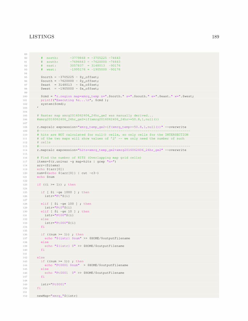
LISTINGS 189
89
90 # north: -3779868 = -3705225 -7464391 # south: -7694643 = -7620000 -7464392 # east: 3057837 = 3148013 -9017693 # west: -1995176 = -1905000 -9017694
95 $north = -3705225 - $y_offset;96 $south = -7620000 - $y_offset;97 $east = 3148013 - $x_offset;98 $west = -1905000 - $x_offset;99
100 $cmd = "r.region map=xmrg_temp n=".$north." s=".$south." e=".$east." w=".$west;101 printf("Executing %s...\n", $cmd );102 system($cmd);103 ’104
105 # Raster map xmrg2016062406_24hr_ge2 was manually derived...106 #xmrg2016062406_24hr_ge2=if(xmrg2016062406_24hr>=50.8,1,null())107
108 r.mapcalc expression="xmrg_temp_ge2=if(xmrg_temp>=50.8,1,null())" --overwrite109 #------------------------------------------------------------------------------110 # hits are NOT calculated for null() cells, so only cells for the INTERSECTION111 # of the two maps will show values of ’2’ -- we only need the number of such112 # cells113 #------------------------------------------------------------------------------114 r.mapcalc expression="hits=xmrg_temp_ge2+xmrg2016062406_24hr_ge2" --overwrite115
116 # Find the number of HITS (Overlapping map grid cells)117 items=$(r.univar -g map=hits | grep "n=")118 arr=($items)119 echo ${arr[0]}120 num=$(echo ${arr[0]} | cut -c3-)121 echo $num122
123 if ((i >= 1)) ; then124
125 if [ $i -ge 1000 ] ; then126 istr="Pt"${i}127
128 elif [ $i -ge 100 ] ; then129 istr="Pt0"${i}130 elif [ $i -ge 10 ] ; then131 istr="Pt00"${i}132 else133 istr="Pt000"${i}134 fi135
136 if ((num >= 1)) ; then137 echo "${istr} $num" >> $HOME/$outputFilename138 else139 echo "${istr} 0" >> $HOME/$outputFilename140 fi141
142 else143 if ((num >= 1)) ; then144 echo "Pt0001 $num" > $HOME/$outputFilename145 else146 echo "Pt0001 0" >> $HOME/$outputFilename147 fi148
149 istr="Pt0001"150 fi151
152 newMap="xmrg_"${istr}
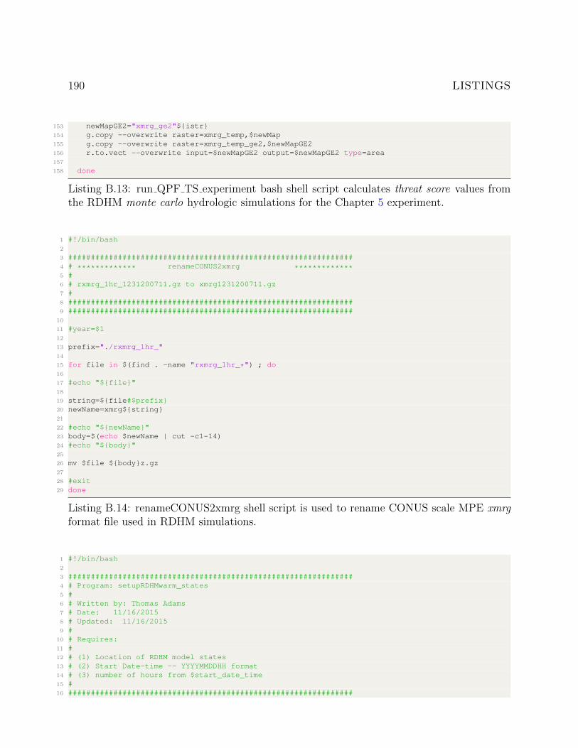
190 LISTINGS
153 newMapGE2="xmrg_ge2"${istr}154 g.copy --overwrite raster=xmrg_temp,$newMap155 g.copy --overwrite raster=xmrg_temp_ge2,$newMapGE2156 r.to.vect --overwrite input=$newMapGE2 output=$newMapGE2 type=area157
158 done
Listing B.13: run QPF TS experiment bash shell script calculates threat score values fromthe RDHM monte carlo hydrologic simulations for the Chapter 5 experiment.
1 #!/bin/bash2
3 ###############################################################4 # ************* renameCONUS2xmrg *************5 #6 # rxmrg_1hr_1231200711.gz to xmrg1231200711.gz7 #8 ###############################################################9 ###############################################################
10
11 #year=$112
13 prefix="./rxmrg_1hr_"14
15 for file in $(find . -name "rxmrg_1hr_*") ; do16
17 #echo "${file}"18
19 string=${file#$prefix}20 newName=xmrg${string}21
22 #echo "${newName}"23 body=$(echo $newName | cut -c1-14)24 #echo "${body}"25
26 mv $file ${body}z.gz27
28 #exit29 done
Listing B.14: renameCONUS2xmrg shell script is used to rename CONUS scale MPE xmrgformat file used in RDHM simulations.
1 #!/bin/bash2
3 ###############################################################4 # Program: setupRDHMwarm_states5 #6 # Written by: Thomas Adams7 # Date: 11/16/20158 # Updated: 11/16/20159 #
10 # Requires:11 #12 # (1) Location of RDHM model states13 # (2) Start Date-time -- YYYYMMDDHH format14 # (3) number of hours from $start_date_time15 #16 ###############################################################
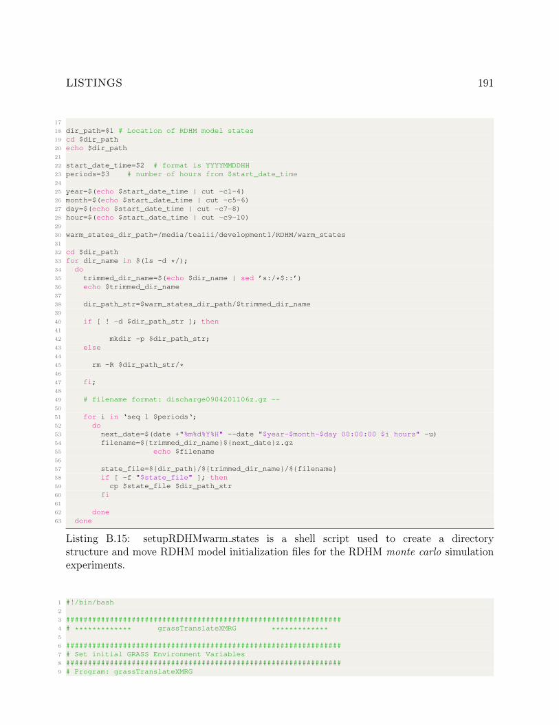
LISTINGS 191
17
18 dir_path=$1 # Location of RDHM model states19 cd $dir_path20 echo $dir_path21
22 start_date_time=$2 # format is YYYYMMDDHH23 periods=$3 # number of hours from $start_date_time24
25 year=$(echo $start_date_time | cut -c1-4)26 month=$(echo $start_date_time | cut -c5-6)27 day=$(echo $start_date_time | cut -c7-8)28 hour=$(echo $start_date_time | cut -c9-10)29
30 warm_states_dir_path=/media/teaiii/development1/RDHM/warm_states31
32 cd $dir_path33 for dir_name in $(ls -d */);34 do35 trimmed_dir_name=$(echo $dir_name | sed ’s:/*$::’)36 echo $trimmed_dir_name37
38 dir_path_str=$warm_states_dir_path/$trimmed_dir_name39
40 if [ ! -d $dir_path_str ]; then41
42 mkdir -p $dir_path_str;43 else44
45 rm -R $dir_path_str/*46
47 fi;48
49 # filename format: discharge0904201106z.gz --50
51 for i in ‘seq 1 $periods‘;52 do53 next_date=$(date +"%m%d%Y%H" --date "$year-$month-$day 00:00:00 $i hours" -u)54 filename=${trimmed_dir_name}${next_date}z.gz55 echo $filename56
57 state_file=${dir_path}/${trimmed_dir_name}/${filename}58 if [ -f "$state_file" ]; then59 cp $state_file $dir_path_str60 fi61
62 done63 done
Listing B.15: setupRDHMwarm states is a shell script used to create a directorystructure and move RDHM model initialization files for the RDHM monte carlo simulationexperiments.
1 #!/bin/bash2
3 ###############################################################4 # ************* grassTranslateXMRG *************5
6 ###############################################################7 # Set initial GRASS Environment Variables8 ###############################################################9 # Program: grassTranslateXMRG
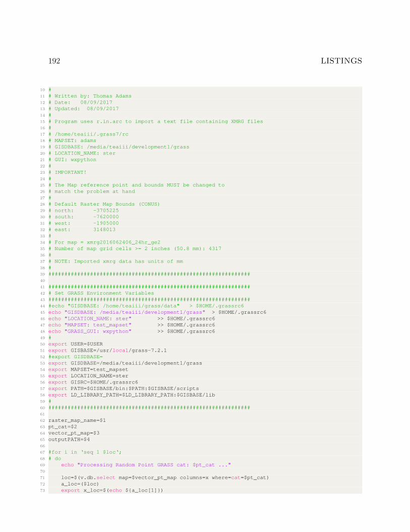
192 LISTINGS
10 #11 # Written by: Thomas Adams12 # Date: 08/09/201713 # Updated: 08/09/201714 #15 # Program uses r.in.arc to import a text file containing XMRG files16 #17 # /home/teaiii/.grass7/rc18 # MAPSET: adams19 # GISDBASE: /media/teaiii/development1/grass20 # LOCATION_NAME: ster21 # GUI: wxpython22 #23 # IMPORTANT!24 #25 # The Map reference point and bounds MUST be changed to26 # match the problem at hand27 #28 # Default Raster Map Bounds (CONUS)29 # north: -370522530 # south: -762000031 # west: -190500032 # east: 314801333 #34 # For map = xmrg2016062406_24hr_ge235 # Number of map grid cells >= 2 inches (50.8 mm): 431736 #37 # NOTE: Imported xmrg data has units of mm38 #39 ###############################################################40
41 ###############################################################42 # Set GRASS Environment Variables43 ###############################################################44 #echo "GISDBASE: /home/teaiii/grass/data" > $HOME/.grassrc645 echo "GISDBASE: /media/teaiii/development1/grass" > $HOME/.grassrc646 echo "LOCATION_NAME: ster" >> $HOME/.grassrc647 echo "MAPSET: test_mapset" >> $HOME/.grassrc648 echo "GRASS_GUI: wxpython" >> $HOME/.grassrc649 #50 export USER=$USER51 export GISBASE=/usr/local/grass-7.2.152 #export GISDBASE=53 export GISDBASE=/media/teaiii/development1/grass54 export MAPSET=test_mapset55 export LOCATION_NAME=ster56 export GISRC=$HOME/.grassrc657 export PATH=$GISBASE/bin:$PATH:$GISBASE/scripts58 export LD_LIBRARY_PATH=$LD_LIBRARY_PATH:$GISBASE/lib59 #60 ###############################################################61
62 raster_map_name=$163 pt_cat=$264 vector_pt_map=$365 outputPATH=$466
67 #for i in ‘seq 1 $loc‘;68 # do69 echo "Processing Random Point GRASS cat: $pt_cat ..."70
71 loc=$(v.db.select map=$vector_pt_map columns=x where=cat=$pt_cat)72 a_loc=($loc)73 export x_loc=$(echo ${a_loc[1]})
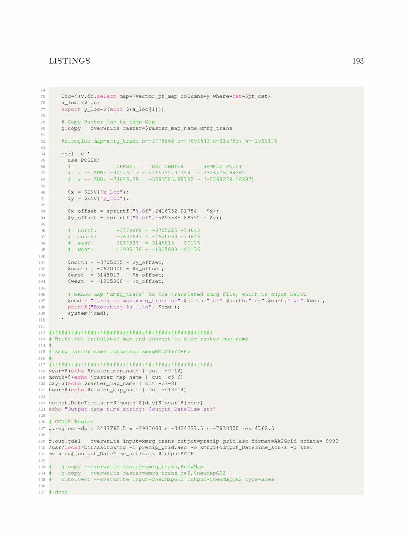
LISTINGS 193
74
75 loc=$(v.db.select map=$vector_pt_map columns=y where=cat=$pt_cat)76 a_loc=($loc)77 export y_loc=$(echo ${a_loc[1]})78
79 # Copy Raster map to temp Map80 g.copy --overwrite raster=$raster_map_name,xmrg_trans81
82 #r.region map=xmrg_trans n=-3779868 s=-7694643 e=3057837 w=-199517683
84 perl -e ’85 use POSIX;86 # OFFSET REF CENTER SAMPLE POINT87 # x -- ADD: -90176.17 = 2416752.01754 - 2326575.8436288 # y -- ADD: -74643.28 = -5293585.88792 - (-5368229.16897)89
90 $x = $ENV{"x_loc"};91 $y = $ENV{"y_loc"};92
93 $x_offset = sprintf("%.0f",2416752.01754 - $x);94 $y_offset = sprintf("%.0f",-5293585.88792 - $y);95
96 # north: -3779868 = -3705225 -7464397 # south: -7694643 = -7620000 -7464398 # east: 3057837 = 3148013 -9017699 # west: -1995176 = -1905000 -90176
100
101 $north = -3705225 - $y_offset;102 $south = -7620000 - $y_offset;103 $east = 3148013 - $x_offset;104 $west = -1905000 - $x_offset;105
106 # GRASS map ’xmrg_trans’ is the translated xmrg file, which is ouput below107 $cmd = "r.region map=xmrg_trans n=".$north." s=".$south." e=".$east." w=".$west;108 printf("Executing %s...\n", $cmd );109 system($cmd);110 ’111
112 ###################################################113 # Write out translated map and convert to xmrg raster_map_name114 #115 # xmrg raster name formated: xmrgMMDDYYYYHHz116 #117 ###################################################118 year=$(echo $raster_map_name | cut -c9-12)119 month=$(echo $raster_map_name | cut -c5-6)120 day=$(echo $raster_map_name | cut -c7-8)121 hour=$(echo $raster_map_name | cut -c13-14)122
123 output_DateTime_str=${month}${day}${year}${hour}124 echo "Output date-time string: $output_DateTime_str"125
126 # CONUS Region127 g.region -dp e=3433762.5 w=-1905000 n=-3424237.5 s=-7620000 res=4762.5128
129 r.out.gdal --overwrite input=xmrg_trans output=precip_grid.asc format=AAIGrid nodata=-9999130 /usr/local/bin/asctoxmrg -i precip_grid.asc -o xmrg${output_DateTime_str}z -p ster131 mv xmrg${output_DateTime_str}z.gz $outputPATH132
133 # g.copy --overwrite raster=xmrg_trans,$newMap134 # g.copy --overwrite raster=xmrg_trans_ge2,$newMapGE2135 # r.to.vect --overwrite input=$newMapGE2 output=$newMapGE2 type=area136
137 # done
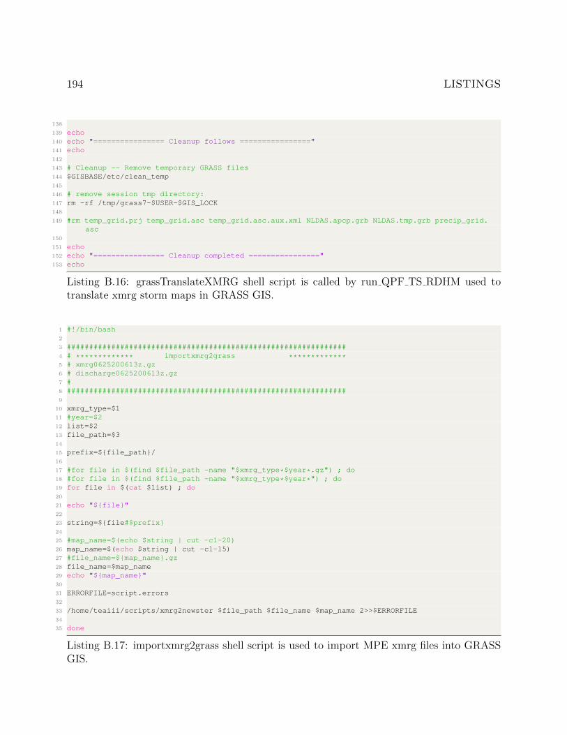
194 LISTINGS
138
139 echo140 echo "================ Cleanup follows ================"141 echo142
143 # Cleanup -- Remove temporary GRASS files144 $GISBASE/etc/clean_temp145
146 # remove session tmp directory:147 rm -rf /tmp/grass7-$USER-$GIS_LOCK148
149 #rm temp_grid.prj temp_grid.asc temp_grid.asc.aux.xml NLDAS.apcp.grb NLDAS.tmp.grb precip_grid.asc
150
151 echo152 echo "================ Cleanup completed ================"153 echo
Listing B.16: grassTranslateXMRG shell script is called by run QPF TS RDHM used totranslate xmrg storm maps in GRASS GIS.
1 #!/bin/bash2
3 ###############################################################4 # ************* importxmrg2grass *************5 # xmrg0625200613z.gz6 # discharge0625200613z.gz7 #8 ###############################################################9
10 xmrg_type=$111 #year=$212 list=$213 file_path=$314
15 prefix=${file_path}/16
17 #for file in $(find $file_path -name "$xmrg_type*$year*.gz") ; do18 #for file in $(find $file_path -name "$xmrg_type*$year*") ; do19 for file in $(cat $list) ; do20
21 echo "${file}"22
23 string=${file#$prefix}24
25 #map_name=$(echo $string | cut -c1-20)26 map_name=$(echo $string | cut -c1-15)27 #file_name=${map_name}.gz28 file_name=$map_name29 echo "${map_name}"30
31 ERRORFILE=script.errors32
33 /home/teaiii/scripts/xmrg2newster $file_path $file_name $map_name 2>>$ERRORFILE34
35 done
Listing B.17: importxmrg2grass shell script is used to import MPE xmrg files into GRASSGIS.
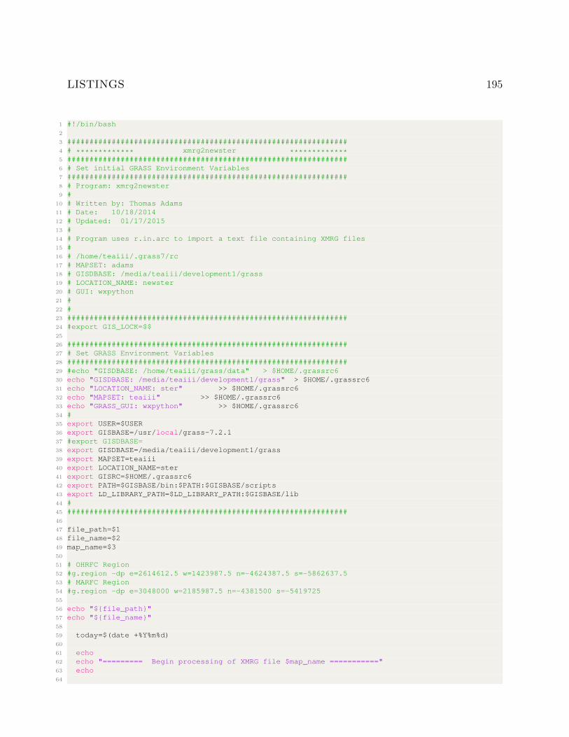
LISTINGS 195
1 #!/bin/bash2
3 ###############################################################4 # ************* xmrg2newster *************5 ###############################################################6 # Set initial GRASS Environment Variables7 ###############################################################8 # Program: xmrg2newster9 #
10 # Written by: Thomas Adams11 # Date: 10/18/201412 # Updated: 01/17/201513 #14 # Program uses r.in.arc to import a text file containing XMRG files15 #16 # /home/teaiii/.grass7/rc17 # MAPSET: adams18 # GISDBASE: /media/teaiii/development1/grass19 # LOCATION_NAME: newster20 # GUI: wxpython21 #22 #23 ###############################################################24 #export GIS_LOCK=$$25
26 ###############################################################27 # Set GRASS Environment Variables28 ###############################################################29 #echo "GISDBASE: /home/teaiii/grass/data" > $HOME/.grassrc630 echo "GISDBASE: /media/teaiii/development1/grass" > $HOME/.grassrc631 echo "LOCATION_NAME: ster" >> $HOME/.grassrc632 echo "MAPSET: teaiii" >> $HOME/.grassrc633 echo "GRASS_GUI: wxpython" >> $HOME/.grassrc634 #35 export USER=$USER36 export GISBASE=/usr/local/grass-7.2.137 #export GISDBASE=38 export GISDBASE=/media/teaiii/development1/grass39 export MAPSET=teaiii40 export LOCATION_NAME=ster41 export GISRC=$HOME/.grassrc642 export PATH=$GISBASE/bin:$PATH:$GISBASE/scripts43 export LD_LIBRARY_PATH=$LD_LIBRARY_PATH:$GISBASE/lib44 #45 ###############################################################46
47 file_path=$148 file_name=$249 map_name=$350
51 # OHRFC Region52 #g.region -dp e=2614612.5 w=1423987.5 n=-4624387.5 s=-5862637.553 # MARFC Region54 #g.region -dp e=3048000 w=2185987.5 n=-4381500 s=-541972555
56 echo "${file_path}"57 echo "${file_name}"58
59 today=$(date +%Y%m%d)60
61 echo62 echo "========= Begin processing of XMRG file $map_name ==========="63 echo64
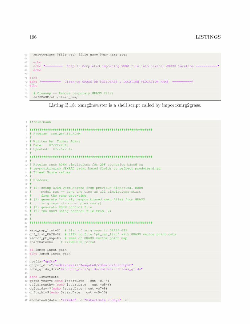
196 LISTINGS
65 xmrgtograss $file_path $file_name $map_name ster66
67 echo68 echo "========= Step 1: Completed importing XMRG file into newster GRASS Location ==========="69 echo70
71 echo72 echo "========== Clean-up GRASS DB $GISDBASE & LOCATION $LOCATION_NAME =========="73 echo74
75 # Cleanup -- Remove temporary GRASS files76 $GISBASE/etc/clean_temp
Listing B.18: xmrg2newster is a shell script called by importxmrg2grass.
1 #!/bin/bash2
3 ###############################################################4 # Program: run_QPF_TS_RDHM5 #6 # Written by: Thomas Adams7 # Date: 07/22/20178 # Updated: 07/25/20179 #
10 ###############################################################11 #12 # Program runs RDHM simulations for QPF scenarios based on13 # re-positioning NEXRAD radar based fields to reflect predetermined14 # Threat Score values15 #16 # Process:17 #18 # (0) setup RDHM warm states from previous historical RDHM19 # model run -- done one time as all simulations start20 # from the same date-time21 # (1) generate 1-hourly re-positioned xmrg files from GRASS22 # xmrg maps (imported previously)23 # (2) generate RDHM control file24 # (3) run RDHM using control file from (2)25 #26 #27 ###############################################################28
29 xmrg_map_list=$1 # List of xmrg maps in GRASS GIS30 qpf_list_PATH=$2 # PATH to file ’pt_cat_list’ with GRASS vector point cats31 vector_pt_map=$3 # Name of GRASS vector point map32 startDate=$4 # YYYMMDDHH format33
34 cd $xmrg_input_path35 echo $xmrg_input_path36
37 prefix="qpfts"38 output_dir="/media/teaiii/Seagate8/rdhm/ohrfc/output"39 rdhm_grids_dir="${output_dir}/grids/coldstart/nldas_grids"40
41 echo $startDate42 qpfts_year=$(echo $startDate | cut -c1-4)43 qpfts_month=$(echo $startDate | cut -c5-6)44 qpfts_day=$(echo $startDate | cut -c7-8)45 qpfts_hr=$(echo $startDate | cut -c9-10)46
47 endDate=$(date +"%Y%m%d" -d "$startDate 7 days" -u)
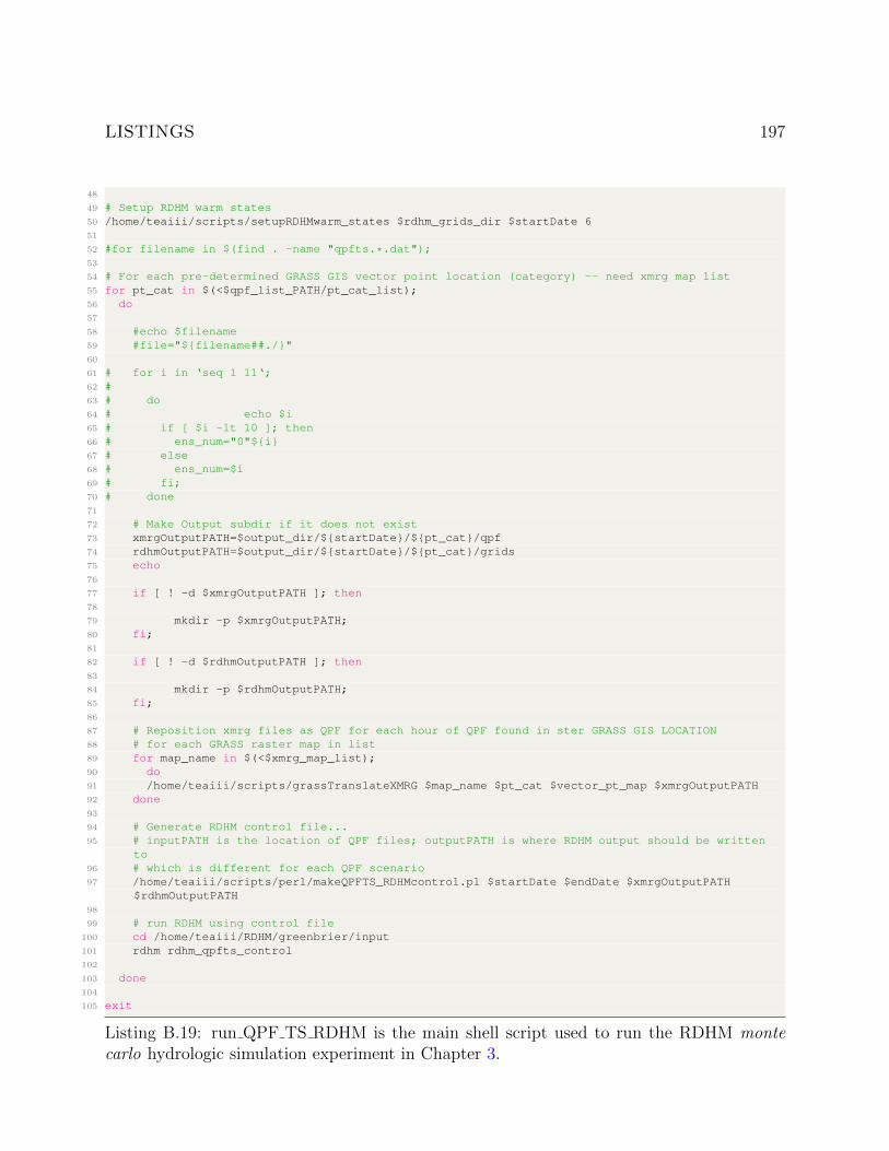
LISTINGS 197
48
49 # Setup RDHM warm states50 /home/teaiii/scripts/setupRDHMwarm_states $rdhm_grids_dir $startDate 651
52 #for filename in $(find . -name "qpfts.*.dat");53
54 # For each pre-determined GRASS GIS vector point location (category) -- need xmrg map list55 for pt_cat in $(<$qpf_list_PATH/pt_cat_list);56 do57
58 #echo $filename59 #file="${filename##./}"60
61 # for i in ‘seq 1 11‘;62 #63 # do64 # echo $i65 # if [ $i -lt 10 ]; then66 # ens_num="0"${i}67 # else68 # ens_num=$i69 # fi;70 # done71
72 # Make Output subdir if it does not exist73 xmrgOutputPATH=$output_dir/${startDate}/${pt_cat}/qpf74 rdhmOutputPATH=$output_dir/${startDate}/${pt_cat}/grids75 echo76
77 if [ ! -d $xmrgOutputPATH ]; then78
79 mkdir -p $xmrgOutputPATH;80 fi;81
82 if [ ! -d $rdhmOutputPATH ]; then83
84 mkdir -p $rdhmOutputPATH;85 fi;86
87 # Reposition xmrg files as QPF for each hour of QPF found in ster GRASS GIS LOCATION88 # for each GRASS raster map in list89 for map_name in $(<$xmrg_map_list);90 do91 /home/teaiii/scripts/grassTranslateXMRG $map_name $pt_cat $vector_pt_map $xmrgOutputPATH92 done93
94 # Generate RDHM control file...95 # inputPATH is the location of QPF files; outputPATH is where RDHM output should be written
to96 # which is different for each QPF scenario97 /home/teaiii/scripts/perl/makeQPFTS_RDHMcontrol.pl $startDate $endDate $xmrgOutputPATH
$rdhmOutputPATH98
99 # run RDHM using control file100 cd /home/teaiii/RDHM/greenbrier/input101 rdhm rdhm_qpfts_control102
103 done104
105 exit
Listing B.19: run QPF TS RDHM is the main shell script used to run the RDHM montecarlo hydrologic simulation experiment in Chapter 3.
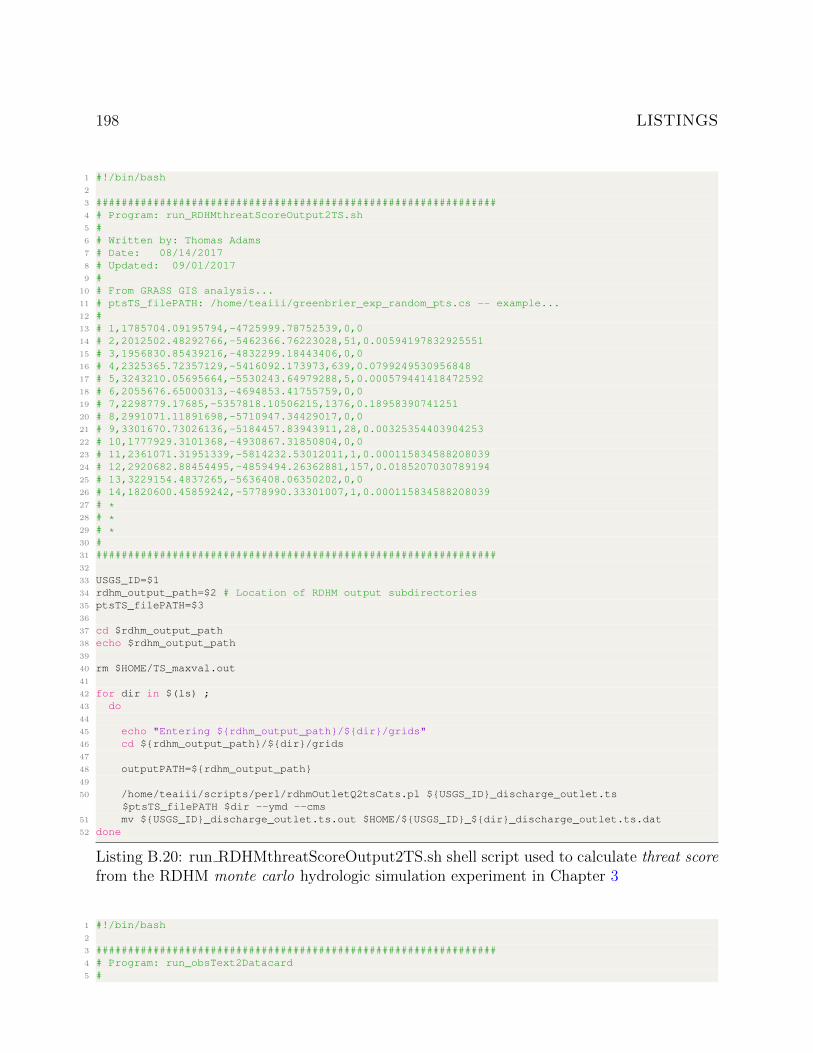
198 LISTINGS
1 #!/bin/bash2
3 ###############################################################4 # Program: run_RDHMthreatScoreOutput2TS.sh5 #6 # Written by: Thomas Adams7 # Date: 08/14/20178 # Updated: 09/01/20179 #
10 # From GRASS GIS analysis...11 # ptsTS_filePATH: /home/teaiii/greenbrier_exp_random_pts.cs -- example...12 #13 # 1,1785704.09195794,-4725999.78752539,0,014 # 2,2012502.48292766,-5462366.76223028,51,0.0059419783292555115 # 3,1956830.85439216,-4832299.18443406,0,016 # 4,2325365.72357129,-5416092.173973,639,0.079924953095684817 # 5,3243210.05695664,-5530243.64979288,5,0.00057944141847259218 # 6,2055676.65000313,-4694853.41755759,0,019 # 7,2298779.17685,-5357818.10506215,1376,0.1895839074125120 # 8,2991071.11891698,-5710947.34429017,0,021 # 9,3301670.73026136,-5184457.83943911,28,0.0032535440390425322 # 10,1777929.3101368,-4930867.31850804,0,023 # 11,2361071.31951339,-5814232.53012011,1,0.00011583458820803924 # 12,2920682.88454495,-4859494.26362881,157,0.018520703078919425 # 13,3229154.4837265,-5636408.06350202,0,026 # 14,1820600.45859242,-5778990.33301007,1,0.00011583458820803927 # *28 # *29 # *30 #31 ###############################################################32
33 USGS_ID=$134 rdhm_output_path=$2 # Location of RDHM output subdirectories35 ptsTS_filePATH=$336
37 cd $rdhm_output_path38 echo $rdhm_output_path39
40 rm $HOME/TS_maxval.out41
42 for dir in $(ls) ;43 do44
45 echo "Entering ${rdhm_output_path}/${dir}/grids"46 cd ${rdhm_output_path}/${dir}/grids47
48 outputPATH=${rdhm_output_path}49
50 /home/teaiii/scripts/perl/rdhmOutletQ2tsCats.pl ${USGS_ID}_discharge_outlet.ts$ptsTS_filePATH $dir --ymd --cms
51 mv ${USGS_ID}_discharge_outlet.ts.out $HOME/${USGS_ID}_${dir}_discharge_outlet.ts.dat52 done
Listing B.20: run RDHMthreatScoreOutput2TS.sh shell script used to calculate threat scorefrom the RDHM monte carlo hydrologic simulation experiment in Chapter 3
1 #!/bin/bash2
3 ###############################################################4 # Program: run_obsText2Datacard5 #
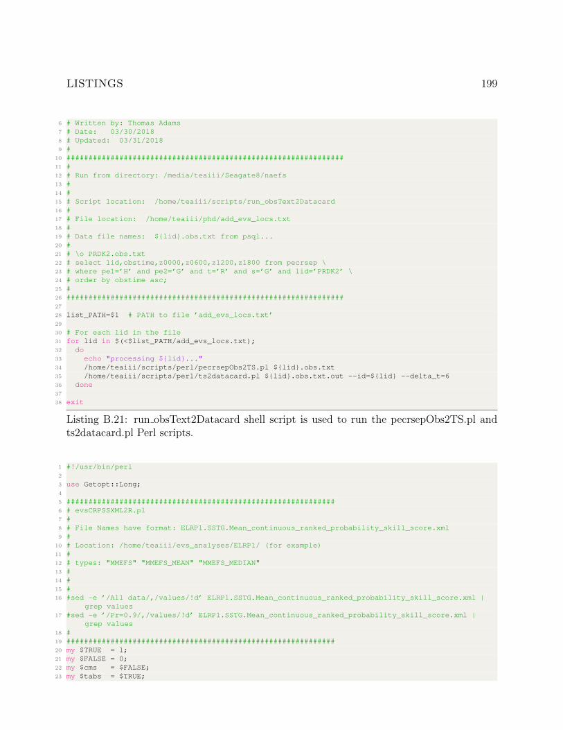
LISTINGS 199
6 # Written by: Thomas Adams7 # Date: 03/30/20188 # Updated: 03/31/20189 #
10 ###############################################################11 #12 # Run from directory: /media/teaiii/Seagate8/naefs13 #14 #15 # Script location: /home/teaiii/scripts/run_obsText2Datacard16 #17 # File location: /home/teaiii/phd/add_evs_locs.txt18 #19 # Data file names: ${lid}.obs.txt from psql...20 #21 # \o PRDK2.obs.txt22 # select lid,obstime,z0000,z0600,z1200,z1800 from pecrsep \23 # where pe1=’H’ and pe2=’G’ and t=’R’ and s=’G’ and lid=’PRDK2’ \24 # order by obstime asc;25 #26 ###############################################################27
28 list_PATH=$1 # PATH to file ’add_evs_locs.txt’29
30 # For each lid in the file31 for lid in $(<$list_PATH/add_evs_locs.txt);32 do33 echo "processing ${lid}..."34 /home/teaiii/scripts/perl/pecrsepObs2TS.pl ${lid}.obs.txt35 /home/teaiii/scripts/perl/ts2datacard.pl ${lid}.obs.txt.out --id=${lid} --delta_t=636 done37
38 exit
Listing B.21: run obsText2Datacard shell script is used to run the pecrsepObs2TS.pl andts2datacard.pl Perl scripts.
1 #!/usr/bin/perl2
3 use Getopt::Long;4
5 #############################################################6 # evsCRPSSXML2R.pl7 #8 # File Names have format: ELRP1.SSTG.Mean_continuous_ranked_probability_skill_score.xml9 #
10 # Location: /home/teaiii/evs_analyses/ELRP1/ (for example)11 #12 # types: "MMEFS" "MMEFS_MEAN" "MMEFS_MEDIAN"13 #14 #15 #16 #sed -e ’/All data/,/values/!d’ ELRP1.SSTG.Mean_continuous_ranked_probability_skill_score.xml |
grep values17 #sed -e ’/Pr=0.9/,/values/!d’ ELRP1.SSTG.Mean_continuous_ranked_probability_skill_score.xml |
grep values18 #19 #############################################################20 my $TRUE = 1;21 my $FALSE = 0;22 my $cms = $FALSE;23 my $tabs = $TRUE;
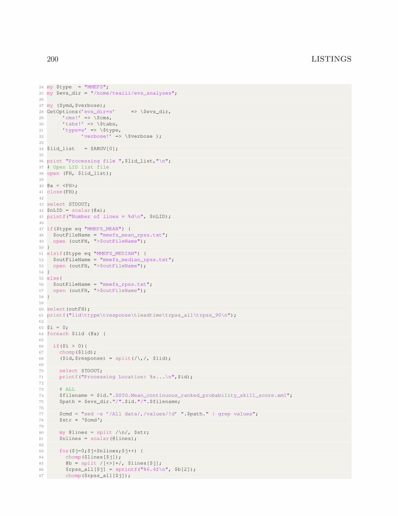
200 LISTINGS
24 my $type = "MMEFS";25 my $evs_dir = "/home/teaiii/evs_analyses";26
27 my ($ymd,$verbose);28 GetOptions(’evs_dir=s’ => \$evs_dir,29 ’cms!’ => \$cms,30 ’tabs!’ => \$tabs,31 ’type=s’ => \$type,32 ’verbose!’ => \$verbose );33
34 $lid_list = $ARGV[0];35
36 print "Processing file ",$lid_list,"\n";37 # Open LID list file38 open (FH, $lid_list);39
40 @a = <FH>;41 close(FH);42
43 select STDOUT;44 $nLID = scalar(@a);45 printf("Number of lines = %d\n", $nLID);46
47 if($type eq "MMEFS_MEAN") {48 $outFileName = "mmefs_mean_rpss.txt";49 open (outFH, ">$outFileName");50 }51 elsif($type eq "MMEFS_MEDIAN") {52 $outFileName = "mmefs_median_rpss.txt";53 open (outFH, ">$outFileName");54 }55 else{56 $outFileName = "mmefs_rpss.txt";57 open (outFH, ">$outFileName");58 }59
60 select(outFH);61 printf("lid\ttype\tresponse\tleadtime\trpss_all\trpss_90\n");62
63 $i = 0;64 foreach $lid (@a) {65
66 if($i > 0){67 chomp($lid);68 ($id,$response) = split(/\,/, $lid);69
70 select STDOUT;71 printf("Processing Location: %s...\n",$id);72
73 # ALL74 $filename = $id.".SSTG.Mean_continuous_ranked_probability_skill_score.xml";75 $path = $evs_dir."/".$id."/".$filename;76
77 $cmd = "sed -e ’/All data/,/values/!d’ ".$path." | grep values";78 $str = ‘$cmd‘;79
80 my @lines = split /\n/, $str;81 $nlines = scalar(@lines);82
83 for($j=0;$j<$nlines;$j++) {84 chomp($lines[$j]);85 @b = split /[<>]+/, $lines[$j];86 $rpss_all[$j] = sprintf("%6.4f\n", $b[2]);87 chomp($rpss_all[$j]);
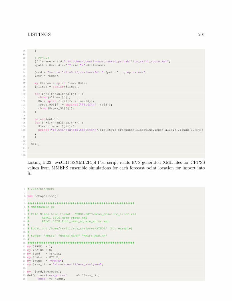
LISTINGS 201
88 }89
90 # Pr=0.991 $filename = $id.".SSTG.Mean_continuous_ranked_probability_skill_score.xml";92 $path = $evs_dir."/".$id."/".$filename;93
94 $cmd = "sed -e ’/Pr=0.9/,/values/!d’ ".$path." | grep values";95 $str = ‘$cmd‘;96
97 my @lines = split /\n/, $str;98 $nlines = scalar(@lines);99
100 for($j=0;$j<$nlines;$j++) {101 chomp($lines[$j]);102 @b = split /[<>]+/, $lines[$j];103 $rpss_90[$j] = sprintf("%6.4f\n", $b[2]);104 chomp($rpss_90[$j]);105 }106
107 select(outFH);108 for($j=0;$j<$nlines;$j++) {109 $leadtime = ($j+1)*6;110 printf("%s\t%s\t%d\t%d\t%s\t%s\n",$id,$type,$response,$leadtime,$rpss_all[$j],$rpss_90[$j])
;111 }112 }113 $i++;114 }115
116
Listing B.22: evsCRPSSXML2R.pl Perl script reads EVS generated XML files for CRPSSvalues from MMEFS ensemble simulations for each forecast point location for import intoR.
1 #!/usr/bin/perl2
3 use Getopt::Long;4
5 ###########################################################6 # mmefsXML2R.pl7 #8 # File Names have format: ATHO1.SSTG.Mean_absolute_error.xml9 # ATHO1.SSTG.Mean_error.xml
10 # ATHO1.SSTG.Root_mean_square_error.xml11 #12 # Location: /home/teaiii/evs_analyses/ATHO1/ (for example)13 #14 # types: "MMEFS" "MMEFS_MEAN" "MMEFS_MEDIAN"15 #16 ###########################################################17 my $TRUE = 1;18 my $FALSE = 0;19 my $cms = $FALSE;20 my $tabs = $TRUE;21 my $type = "MMEFS";22 my $evs_dir = "/home/teaiii/evs_analyses";23
24 my ($ymd,$verbose);25 GetOptions(’evs_dir=s’ => \$evs_dir,26 ’cms!’ => \$cms,
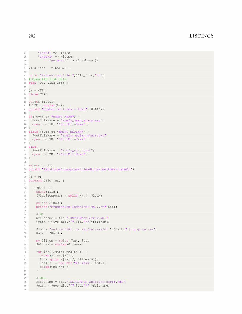
202 LISTINGS
27 ’tabs!’ => \$tabs,28 ’type=s’ => \$type,29 ’verbose!’ => \$verbose );30
31 $lid_list = $ARGV[0];32
33 print "Processing file ",$lid_list,"\n";34 # Open LID list file35 open (FH, $lid_list);36
37 @a = <FH>;38 close(FH);39
40 select STDOUT;41 $nLID = scalar(@a);42 printf("Number of lines = %d\n", $nLID);43
44 if($type eq "MMEFS_MEAN") {45 $outFileName = "mmefs_mean_stats.txt";46 open (outFH, ">$outFileName");47 }48 elsif($type eq "MMEFS_MEDIAN") {49 $outFileName = "mmefs_median_stats.txt";50 open (outFH, ">$outFileName");51 }52 else{53 $outFileName = "mmefs_stats.txt";54 open (outFH, ">$outFileName");55 }56
57 select(outFH);58 printf("lid\ttype\tresponse\tleadtime\tme\tmae\trmse\n");59
60 $i = 0;61 foreach $lid (@a) {62
63 if($i > 0){64 chomp($lid);65 ($id,$respone) = split(/\,/, $lid);66
67 select STDOUT;68 printf("Processing Location: %s...\n",$id);69
70 # ME71 $filename = $id.".SSTG.Mean_error.xml";72 $path = $evs_dir."/".$id."/".$filename;73
74 $cmd = "sed -e ’/All data/,/values/!d’ ".$path." | grep values";75 $str = ‘$cmd‘;76
77 my @lines = split /\n/, $str;78 $nlines = scalar(@lines);79
80 for($j=0;$j<$nlines;$j++) {81 chomp($lines[$j]);82 @b = split /[<>]+/, $lines[$j];83 $me[$j] = sprintf("%6.4f\n", $b[2]);84 chomp($me[$j]);85 }86
87 # MAE88 $filename = $id.".SSTG.Mean_absolute_error.xml";89 $path = $evs_dir."/".$id."/".$filename;90
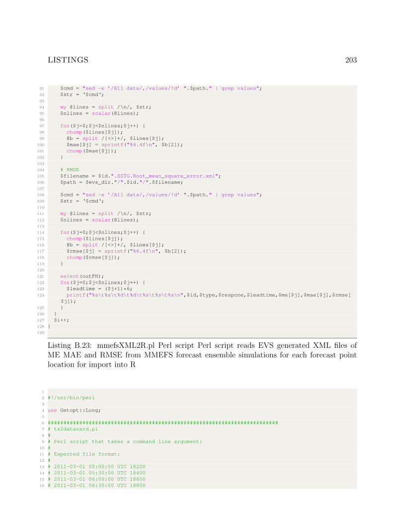
LISTINGS 203
91 $cmd = "sed -e ’/All data/,/values/!d’ ".$path." | grep values";92 $str = ‘$cmd‘;93
94 my @lines = split /\n/, $str;95 $nlines = scalar(@lines);96
97 for($j=0;$j<$nlines;$j++) {98 chomp($lines[$j]);99 @b = split /[<>]+/, $lines[$j];
100 $mae[$j] = sprintf("%6.4f\n", $b[2]);101 chomp($mae[$j]);102 }103
104 # RMSE105 $filename = $id.".SSTG.Root_mean_square_error.xml";106 $path = $evs_dir."/".$id."/".$filename;107
108 $cmd = "sed -e ’/All data/,/values/!d’ ".$path." | grep values";109 $str = ‘$cmd‘;110
111 my @lines = split /\n/, $str;112 $nlines = scalar(@lines);113
114 for($j=0;$j<$nlines;$j++) {115 chomp($lines[$j]);116 @b = split /[<>]+/, $lines[$j];117 $rmse[$j] = sprintf("%6.4f\n", $b[2]);118 chomp($rmse[$j]);119 }120
121 select(outFH);122 for($j=0;$j<$nlines;$j++) {123 $leadtime = ($j+1)*6;124 printf("%s\t%s\t%d\t%d\t%s\t%s\t%s\n",$id,$type,$respone,$leadtime,$me[$j],$mae[$j],$rmse[
$j]);125 }126 }127 $i++;128 }129
Listing B.23: mmefsXML2R.pl Perl script Perl script reads EVS generated XML files ofME MAE and RMSE from MMEFS forecast ensemble simulations for each forecast pointlocation for import into R
1
2 #!/usr/bin/perl3
4 use Getopt::Long;5
6 #########################################################################7 # ts2datacard.pl8 #9 # Perl script that takes a command line argument:
10 #11 # Expected file format:12 #13 # 2011-03-01 05:00:00 UTC 1820014 # 2011-03-01 05:30:00 UTC 1840015 # 2011-03-01 06:00:00 UTC 1860016 # 2011-03-01 06:30:00 UTC 18800
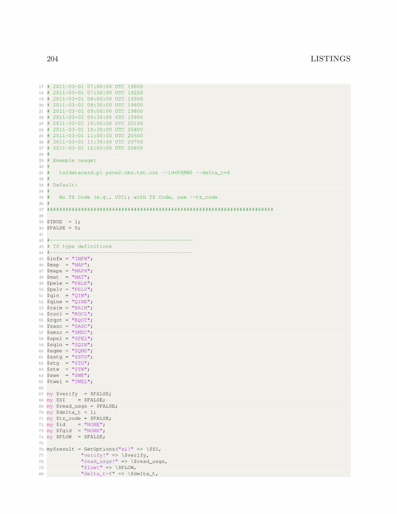
204 LISTINGS
17 # 2011-03-01 07:00:00 UTC 1900018 # 2011-03-01 07:30:00 UTC 1920019 # 2011-03-01 08:00:00 UTC 1930020 # 2011-03-01 08:30:00 UTC 1960021 # 2011-03-01 09:00:00 UTC 1980022 # 2011-03-01 09:30:00 UTC 1990023 # 2011-03-01 10:00:00 UTC 2010024 # 2011-03-01 10:30:00 UTC 2040025 # 2011-03-01 11:00:00 UTC 2050026 # 2011-03-01 11:30:00 UTC 2070027 # 2011-03-01 12:00:00 UTC 2080028 #29 # Example usage:30 #31 # ts2datacard.pl psnw2.obs.txt.out --id=PSNW2 --delta_t=632 #33 # Default:34 #35 # No TZ Code (e.g., UTC); with TZ Code, use --tz_code36 #37 #########################################################################38
39 $TRUE = 1;40 $FALSE = 0;41
42 #----------------------------------------------43 # TS type definitions44 #----------------------------------------------45 $infw = "INFW";46 $map = "MAP";47 $mapx = "MAPX";48 $mat = "MAT";49 $pele = "PELE";50 $pelv = "PELV";51 $qin = "QIN";52 $qine = "QINE";53 $raim = "RAIM";54 $rocl = "ROCL";55 $rqot = "RQOT";56 $sasc = "SASC";57 $smzc = "SMZC";58 $spel = "SPEL";59 $sqin = "SQIN";60 $sqme = "SQME";61 $sstg = "SSTG";62 $stg = "STG";63 $stw = "STW";64 $swe = "SWE";65 $twel = "TWEL";66
67 my $verify = $FALSE;68 my $SI = $FALSE;69 my $read_usgs = $FALSE;70 my $delta_t = 1;71 my $tz_code = $FALSE;72 my $id = "NONE";73 my $fgid = "NONE";74 my $FLOW = $FALSE;75
76 my$result = GetOptions("si!" => \$SI,77 "verify!" => \$verify,78 "read_usgs!" => \$read_usgs,79 "flow!" => \$FLOW,80 "delta_t=f" => \$delta_t,
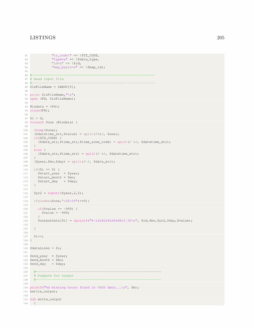
LISTINGS 205
81 "tz_code!" => \$TZ_CODE,82 "type=s" => \$data_type,83 "id=s" => \$id,84 "map_basin=s" => \$map_id);85
86 #--------------------------------------------------------------87 # Read input file88 #--------------------------------------------------------------89 $inFileName = $ARGV[0];90
91 print $inFileName,"\n";92 open (FH, $inFileName);93
94 @tsdata = <FH>;95 close(FH);96
97 $i = 0;98 foreach $one (@tsdata) {99
100 chomp($one);101 ($datetime_str,$value) = split(/\t/, $one);102 if($TZ_CODE) {103 ($date_str,$time_str,$time_zone_code) = split(/ +/, $datetime_str);104 }105 else {106 ($date_str,$time_str) = split(/ +/, $datetime_str);107 }108 ($year,$mo,$day) = split(/-/, $date_str);109
110 if($i == 0) {111 $start_year = $year;112 $start_month = $mo;113 $start_day = $day;114 }115
116 $yr2 = substr($year,2,2);117
118 if(index($one,":00:00")>=0){119
120 if($value <= -999) {121 $value = -999;122 }123 $outputData[$i] = sprintf("%-12s%2s%2s%4d%10.3f\n", $id,$mo,$yr2,$day,$value);124
125 }126
127 $i++;128 }129
130 $dataLines = $i;131
132 $end_year = $year;133 $end_month = $mo;134 $end_day = $day;135
136 #---------------------------------------------------------------137 # Prepare for output138 #---------------------------------------------------------------139
140 printf("%d missing hours found in USGS data...\n", $m);141 &write_output;142
143 sub write_output144 {
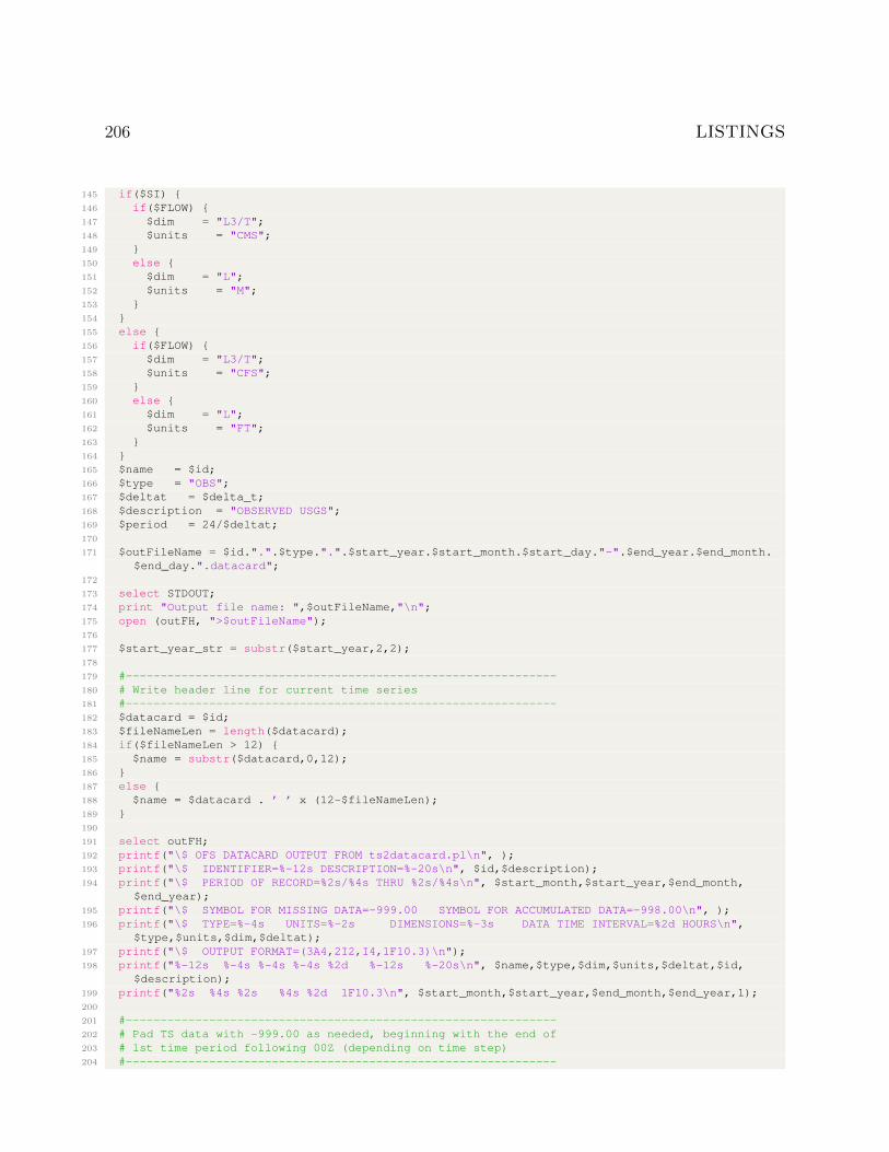
206 LISTINGS
145 if($SI) {146 if($FLOW) {147 $dim = "L3/T";148 $units = "CMS";149 }150 else {151 $dim = "L";152 $units = "M";153 }154 }155 else {156 if($FLOW) {157 $dim = "L3/T";158 $units = "CFS";159 }160 else {161 $dim = "L";162 $units = "FT";163 }164 }165 $name = $id;166 $type = "OBS";167 $deltat = $delta_t;168 $description = "OBSERVED USGS";169 $period = 24/$deltat;170
171 $outFileName = $id.".".$type.".".$start_year.$start_month.$start_day."-".$end_year.$end_month.$end_day.".datacard";
172
173 select STDOUT;174 print "Output file name: ",$outFileName,"\n";175 open (outFH, ">$outFileName");176
177 $start_year_str = substr($start_year,2,2);178
179 #--------------------------------------------------------------180 # Write header line for current time series181 #--------------------------------------------------------------182 $datacard = $id;183 $fileNameLen = length($datacard);184 if($fileNameLen > 12) {185 $name = substr($datacard,0,12);186 }187 else {188 $name = $datacard . ’ ’ x (12-$fileNameLen);189 }190
191 select outFH;192 printf("\$ OFS DATACARD OUTPUT FROM ts2datacard.pl\n", );193 printf("\$ IDENTIFIER=%-12s DESCRIPTION=%-20s\n", $id,$description);194 printf("\$ PERIOD OF RECORD=%2s/%4s THRU %2s/%4s\n", $start_month,$start_year,$end_month,
$end_year);195 printf("\$ SYMBOL FOR MISSING DATA=-999.00 SYMBOL FOR ACCUMULATED DATA=-998.00\n", );196 printf("\$ TYPE=%-4s UNITS=%-2s DIMENSIONS=%-3s DATA TIME INTERVAL=%2d HOURS\n",
$type,$units,$dim,$deltat);197 printf("\$ OUTPUT FORMAT=(3A4,2I2,I4,1F10.3)\n");198 printf("%-12s %-4s %-4s %-4s %2d %-12s %-20s\n", $name,$type,$dim,$units,$deltat,$id,
$description);199 printf("%2s %4s %2s %4s %2d 1F10.3\n", $start_month,$start_year,$end_month,$end_year,1);200
201 #--------------------------------------------------------------202 # Pad TS data with -999.00 as needed, beginning with the end of203 # 1st time period following 00Z (depending on time step)204 #--------------------------------------------------------------
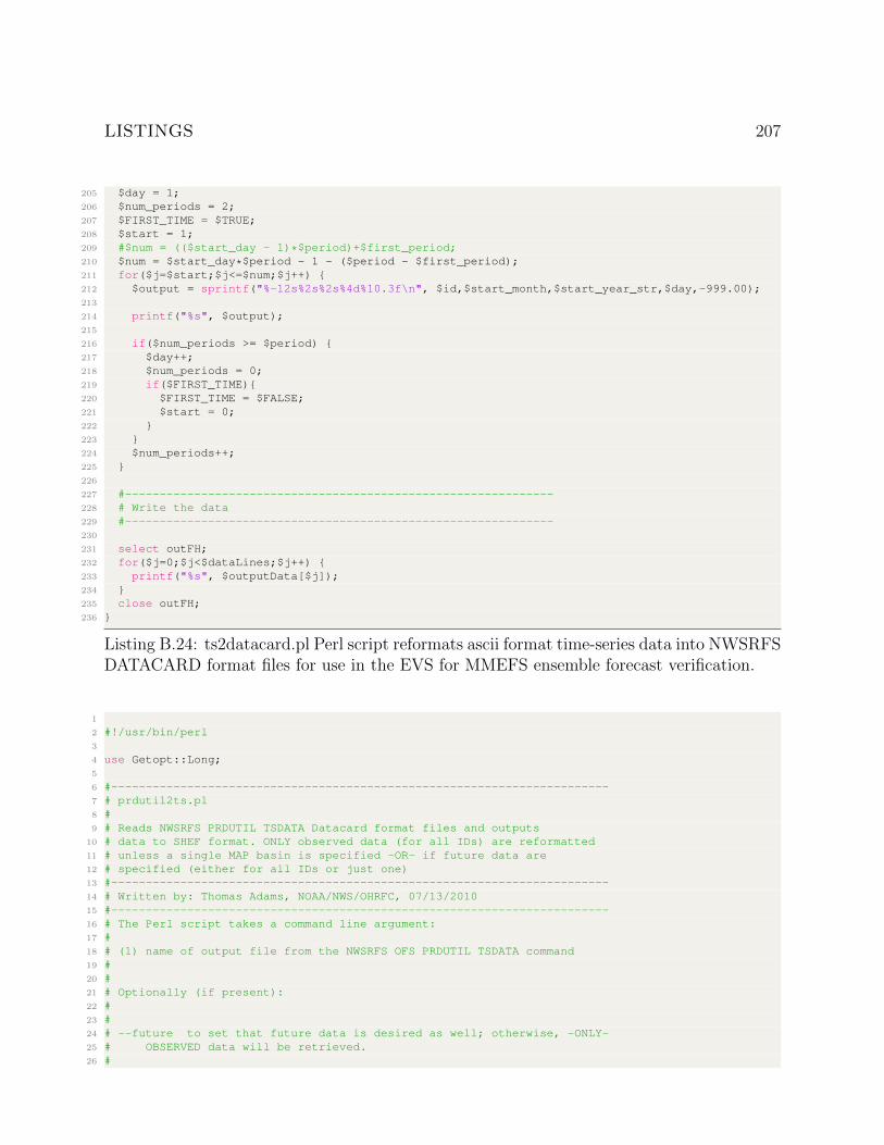
LISTINGS 207
205 $day = 1;206 $num_periods = 2;207 $FIRST_TIME = $TRUE;208 $start = 1;209 #$num = (($start_day - 1)*$period)+$first_period;210 $num = $start_day*$period - 1 - ($period - $first_period);211 for($j=$start;$j<=$num;$j++) {212 $output = sprintf("%-12s%2s%2s%4d%10.3f\n", $id,$start_month,$start_year_str,$day,-999.00);213
214 printf("%s", $output);215
216 if($num_periods >= $period) {217 $day++;218 $num_periods = 0;219 if($FIRST_TIME){220 $FIRST_TIME = $FALSE;221 $start = 0;222 }223 }224 $num_periods++;225 }226
227 #--------------------------------------------------------------228 # Write the data229 #--------------------------------------------------------------230
231 select outFH;232 for($j=0;$j<$dataLines;$j++) {233 printf("%s", $outputData[$j]);234 }235 close outFH;236 }
Listing B.24: ts2datacard.pl Perl script reformats ascii format time-series data into NWSRFSDATACARD format files for use in the EVS for MMEFS ensemble forecast verification.
1
2 #!/usr/bin/perl3
4 use Getopt::Long;5
6 #------------------------------------------------------------------------7 # prdutil2ts.pl8 #9 # Reads NWSRFS PRDUTIL TSDATA Datacard format files and outputs
10 # data to SHEF format. ONLY observed data (for all IDs) are reformatted11 # unless a single MAP basin is specified -OR- if future data are12 # specified (either for all IDs or just one)13 #------------------------------------------------------------------------14 # Written by: Thomas Adams, NOAA/NWS/OHRFC, 07/13/201015 #------------------------------------------------------------------------16 # The Perl script takes a command line argument:17 #18 # (1) name of output file from the NWSRFS OFS PRDUTIL TSDATA command19 #20 #21 # Optionally (if present):22 #23 #24 # --future to set that future data is desired as well; otherwise, -ONLY-25 # OBSERVED data will be retrieved.26 #
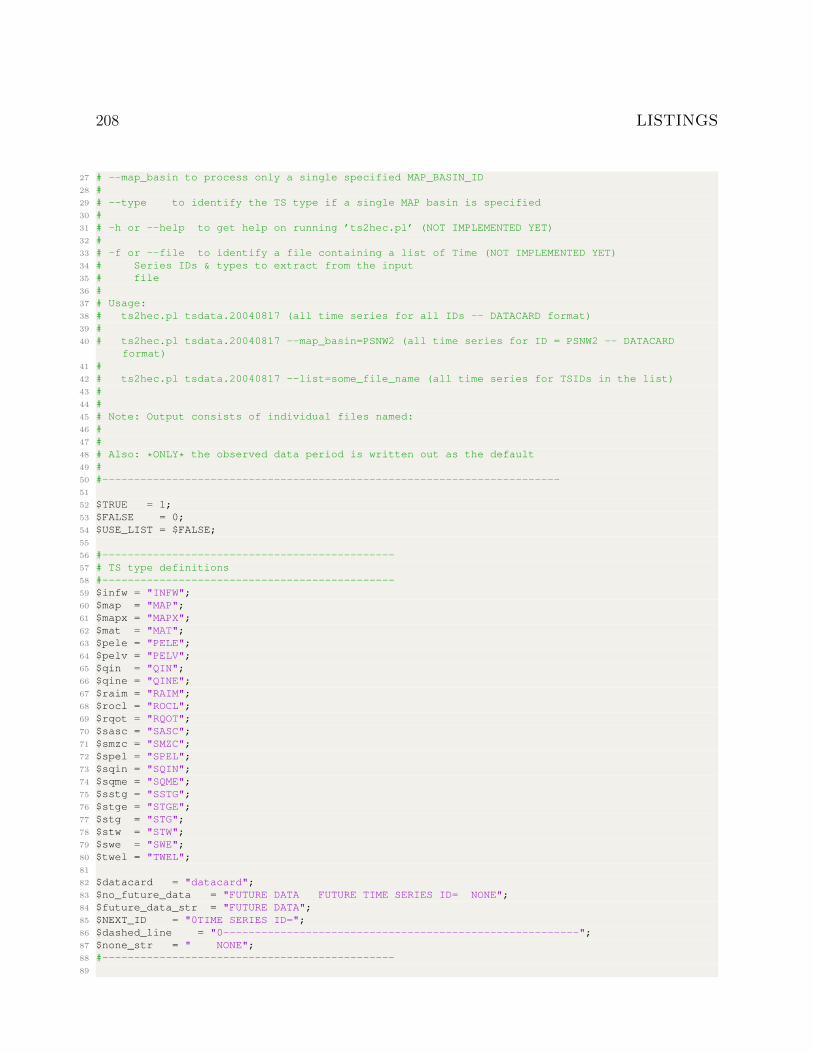
208 LISTINGS
27 # --map_basin to process only a single specified MAP_BASIN_ID28 #29 # --type to identify the TS type if a single MAP basin is specified30 #31 # -h or --help to get help on running ’ts2hec.pl’ (NOT IMPLEMENTED YET)32 #33 # -f or --file to identify a file containing a list of Time (NOT IMPLEMENTED YET)34 # Series IDs & types to extract from the input35 # file36 #37 # Usage:38 # ts2hec.pl tsdata.20040817 (all time series for all IDs -- DATACARD format)39 #40 # ts2hec.pl tsdata.20040817 --map_basin=PSNW2 (all time series for ID = PSNW2 -- DATACARD
format)41 #42 # ts2hec.pl tsdata.20040817 --list=some_file_name (all time series for TSIDs in the list)43 #44 #45 # Note: Output consists of individual files named:46 #47 #48 # Also: *ONLY* the observed data period is written out as the default49 #50 #------------------------------------------------------------------------51
52 $TRUE = 1;53 $FALSE = 0;54 $USE_LIST = $FALSE;55
56 #----------------------------------------------57 # TS type definitions58 #----------------------------------------------59 $infw = "INFW";60 $map = "MAP";61 $mapx = "MAPX";62 $mat = "MAT";63 $pele = "PELE";64 $pelv = "PELV";65 $qin = "QIN";66 $qine = "QINE";67 $raim = "RAIM";68 $rocl = "ROCL";69 $rqot = "RQOT";70 $sasc = "SASC";71 $smzc = "SMZC";72 $spel = "SPEL";73 $sqin = "SQIN";74 $sqme = "SQME";75 $sstg = "SSTG";76 $stge = "STGE";77 $stg = "STG";78 $stw = "STW";79 $swe = "SWE";80 $twel = "TWEL";81
82 $datacard = "datacard";83 $no_future_data = "FUTURE DATA FUTURE TIME SERIES ID= NONE";84 $future_data_str = "FUTURE DATA";85 $NEXT_ID = "0TIME SERIES ID=";86 $dashed_line = "0--------------------------------------------------------";87 $none_str = " NONE";88 #----------------------------------------------89
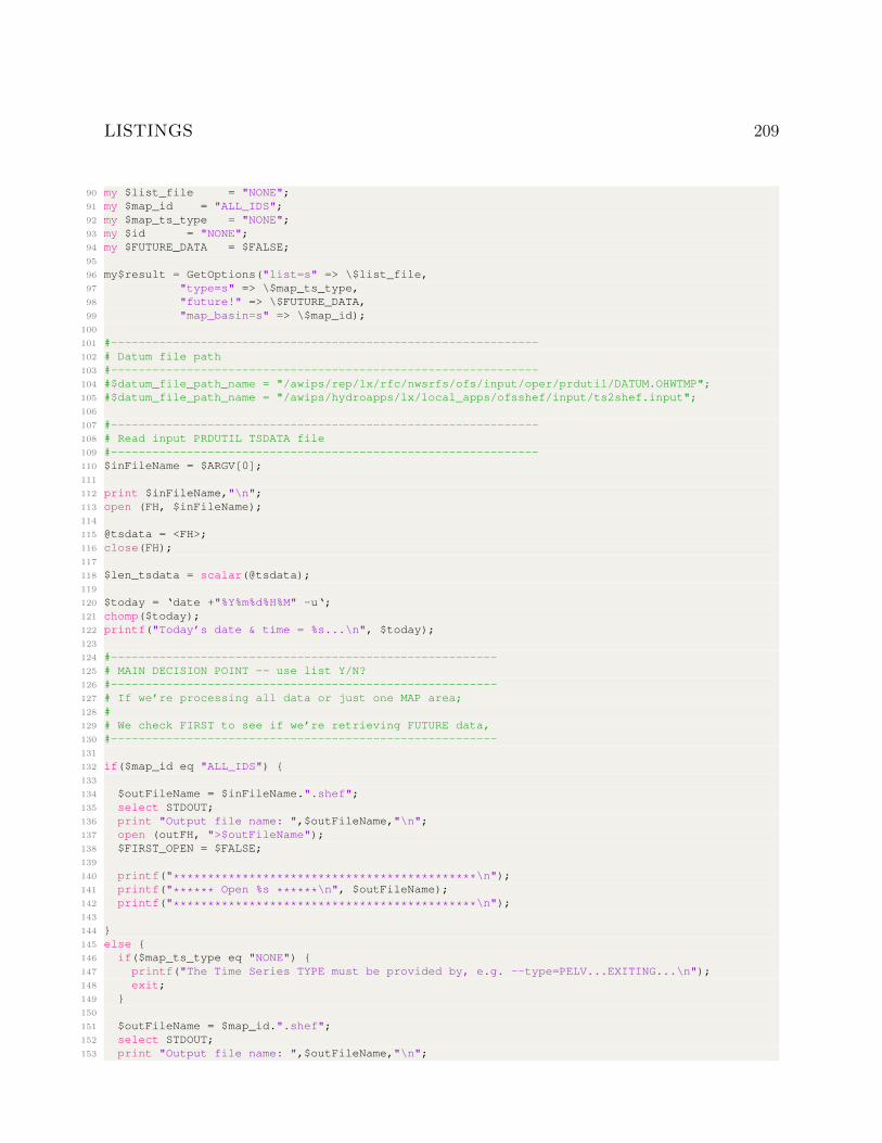
LISTINGS 209
90 my $list_file = "NONE";91 my $map_id = "ALL_IDS";92 my $map_ts_type = "NONE";93 my $id = "NONE";94 my $FUTURE_DATA = $FALSE;95
96 my$result = GetOptions("list=s" => \$list_file,97 "type=s" => \$map_ts_type,98 "future!" => \$FUTURE_DATA,99 "map_basin=s" => \$map_id);
100
101 #--------------------------------------------------------------102 # Datum file path103 #--------------------------------------------------------------104 #$datum_file_path_name = "/awips/rep/lx/rfc/nwsrfs/ofs/input/oper/prdutil/DATUM.OHWTMP";105 #$datum_file_path_name = "/awips/hydroapps/lx/local_apps/ofsshef/input/ts2shef.input";106
107 #--------------------------------------------------------------108 # Read input PRDUTIL TSDATA file109 #--------------------------------------------------------------110 $inFileName = $ARGV[0];111
112 print $inFileName,"\n";113 open (FH, $inFileName);114
115 @tsdata = <FH>;116 close(FH);117
118 $len_tsdata = scalar(@tsdata);119
120 $today = ‘date +"%Y%m%d%H%M" -u‘;121 chomp($today);122 printf("Today’s date & time = %s...\n", $today);123
124 #--------------------------------------------------------125 # MAIN DECISION POINT -- use list Y/N?126 #--------------------------------------------------------127 # If we’re processing all data or just one MAP area;128 #129 # We check FIRST to see if we’re retrieving FUTURE data,130 #--------------------------------------------------------131
132 if($map_id eq "ALL_IDS") {133
134 $outFileName = $inFileName.".shef";135 select STDOUT;136 print "Output file name: ",$outFileName,"\n";137 open (outFH, ">$outFileName");138 $FIRST_OPEN = $FALSE;139
140 printf("********************************************\n");141 printf("****** Open %s ******\n", $outFileName);142 printf("********************************************\n");143
144 }145 else {146 if($map_ts_type eq "NONE") {147 printf("The Time Series TYPE must be provided by, e.g. --type=PELV...EXITING...\n");148 exit;149 }150
151 $outFileName = $map_id.".shef";152 select STDOUT;153 print "Output file name: ",$outFileName,"\n";
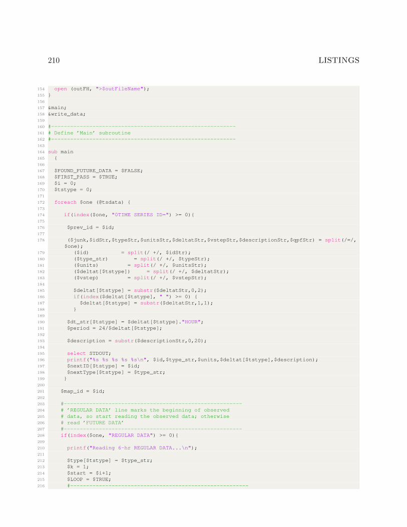
210 LISTINGS
154 open (outFH, ">$outFileName");155 }156
157 &main;158 &write_data;159
160 #----------------------------------------------------------161 # Define ’Main’ subroutine162 #----------------------------------------------------------163
164 sub main165 {166
167 $FOUND_FUTURE_DATA = $FALSE;168 $FIRST_PASS = $TRUE;169 $i = 0;170 $tstype = 0;171
172 foreach $one (@tsdata) {173
174 if(index($one, "0TIME SERIES ID=") >= 0){175
176 $prev_id = $id;177
178 ($junk,$idStr,$typeStr,$unitsStr,$deltatStr,$vstepStr,$descriptionStr,$qpfStr) = split(/=/,$one);
179 ($id) = split(/ +/, $idStr);180 ($type_str) = split(/ +/, $typeStr);181 ($units) = split(/ +/, $unitsStr);182 ($deltat[$tstype]) = split(/ +/, $deltatStr);183 ($vstep) = split(/ +/, $vstepStr);184
185 $deltat[$tstype] = substr($deltatStr,0,2);186 if(index($deltat[$tstype], " ") >= 0) {187 $deltat[$tstype] = substr($deltatStr,1,1);188 }189
190 $dt_str[$tstype] = $deltat[$tstype]."HOUR";191 $period = 24/$deltat[$tstype];192
193 $description = substr($descriptionStr,0,20);194
195 select STDOUT;196 printf("%s %s %s %s %s\n", $id,$type_str,$units,$deltat[$tstype],$description);197 $nextID[$tstype] = $id;198 $nextType[$tstype] = $type_str;199 }200
201 $map_id = $id;202
203 #--------------------------------------------------------204 # ’REGULAR DATA’ line marks the beginning of observed205 # data, so start reading the observed data; otherwise206 # read ’FUTURE DATA’207 #--------------------------------------------------------208 if(index($one, "REGULAR DATA") >= 0){209
210 printf("Reading 6-hr REGULAR DATA...\n");211
212 $type[$tstype] = $type_str;213 $k = 1;214 $start = $i+1;215 $LOOP = $TRUE;216 #--------------------------------------------------------
LISTINGS 211
217 # 1-hour data218 #--------------------------------------------------------219 if($deltat[$tstype] == 1) {220 while($LOOP) {221 #-----------------------------------------------------------------------222 # Test if the current & previous lines have ’/’223 #-----------------------------------------------------------------------224 if(index($tsdata[$i+$k], "\/") < 0 && index($tsdata[$i+$k-1], "\/") < 0) {225 if(index($tsdata[$i+$k], $future_data_str) >= 0) {226
227 $FOUND_FUTURE_DATA = $TRUE;228 select STDOUT;229 printf("Found future data... %d %d\n", $k,$end_obs_line);230
231 $future_lines = $i;232 printf("Future lines = %d...\n", $future_lines);233
234 if (index($tsdata[$i+$k+1], $none_str) >= 0) {235 $k++;236 printf("No future data found... %d\n", $k);237 $LOOP = $FALSE;238 }239 #elsif(index($tsdata[$i+$k-1], "NWSRFS FORECAST SYSTEM") < 0) {240 # if (index($tsdata[$i+$k], $future_data_str) < 0) {241 # $k++;242 # printf("End of future data... %d\n", $k);243 # $LOOP = $FALSE;244 # }245 #}246 $k++;247 $end_obs_line = $i+$k;248 }249 elsif(index($tsdata[$i+$k], $no_future_data) >= 0) {250 printf("No future data found... %d\n", $k);251 $LOOP = $FALSE;252 }253 elsif(index($tsdata[$i+$k], $dashed_line) >= 0) {254 printf("Dashed line found... %d\n", $i+$k);255 $LOOP = $FALSE;256 }257 elsif(index($tsdata[$i+$k], ">>>>>>>> END") >= 0) {258 printf("File line end found... %d\n", $i+$k);259 $LOOP = $FALSE;260 }261 #elsif(index($tsdata[$i+$k-1], "NWSRFS FORECAST SYSTEM") < 0) {262 # if(length($tsdata[$i+$k-1]) > 1) {263 # $LOOP = $FALSE;264 # }265 #}266 else {267 $k++;268 }269 }270 select STDOUT;271 printf("k = %d\n", $k);272 #printf("%s",$tsdata[$i+$k]);273 $k++;274 } # end 1-hr loop275 }276 #--------------------------------------------------------277 # 6-hour data (assumed)278 #--------------------------------------------------------279 else {280 printf("Reading 6-hr FUTURE data...\n");
212 LISTINGS
281 $FUTURE_DATA_LINE = $i+$k;282 while($LOOP) {283
284 if(index($tsdata[$i+$k], "\/") < 0) {285
286 if(index($tsdata[$i+$k], $future_data_str) >= 0) {287
288 $FOUND_FUTURE_DATA = $TRUE;289 select STDOUT;290 printf("Found future data... %d %d\n", $k,$end_obs_line);291
292 $future_lines = $i - 3;293 printf("Future lines = %d...\n", $future_lines);294
295 if (index($tsdata[$i+$k+1], $none_str) >= 0) {296 printf("No future data found... %d\n", $k);297 $LOOP = $FALSE;298 }299 elsif(index($tsdata[$i+$k-1], "NWSRFS FORECAST SYSTEM") < 0) {300 if (index($tsdata[$i+$k], $future_data_str) < 0) {301 printf("End of future data... %d\n", $k);302 $LOOP = $FALSE;303 }304 }305 $k++;306 $end_obs_line = $i+$k;307 }308 elsif(index($tsdata[$i+$k], $no_future_data) >= 0) {309 $k++;310 printf("No future data found... %d\n", $k);311 $LOOP = $FALSE;312 }313 elsif(index($tsdata[$i+$k-1], "NWSRFS FORECAST SYSTEM") < 0) {314 if(length($tsdata[$i+$k-1]) > 1) {315 $LOOP = $FALSE;316 }317 }318 else {319 $k++;320 }321 }322 select STDOUT;323 printf("k = %d\n", $k);324 #printf("%s",$tsdata[$i+$k]);325 $k++;326 } # end 6-hr loop327 }328
329 $end = $i+$k-1;330 #if($deltat[$tstype] == 1) {331 # $end = $i+$k;332 #}333
334 if($FUTURE_DATA == $FALSE) {335 $end = $end_obs_line;336 }337 printf("start = %d, end = %d, DT = %d\n", $start,$end, $deltat[$tstype]);338 &extract_data;339 $tstype++;340 }341 #--------------------------------------------------------342 # End ’REGULAR DATA’343 #--------------------------------------------------------344 $i++;
LISTINGS 213
345
346 } # End foreach347 } # End sub348
349 #----------------------------------------------------------350 # Define ’Extract Data’ subroutine351 #----------------------------------------------------------352
353 sub extract_data {354
355 $dataLines = 0;356 $less[$tstype] = 0;357
358 select STDOUT;359 printf("extract_data(): number of lines, i = %d %d\n", $nlines,$i);360
361 $REDUCE_LINES = $FALSE;362 $lines = 0;363 $lessLines = 0;364 for($j=$start;$j<=$end;$j++) {365
366 #printf("%s", $tsdata[$j]);367
368 if(index($tsdata[$j], "NWSRFS FORECAST SYSTEM") >= 0) {369 shift @tsdata;370 $REDUCE_LINES = $TRUE;371 $lessLines++;372 }373 elsif(index($tsdata[$j], $future_data_str) >= 0) {374 $REDUCE_LINES = $TRUE;375 $lessLines++;376 }377 else {378 $data_line[$lines] = $tsdata[$j];379 #printf("%d %s", $lines,$data_line[$lines]);380 $lines++;381 }382 }383
384 #if($deltat[$tstype] == 1) {385 # $lessLines = 0;386 #}387
388 if($REDUCE_LINES == $TRUE) {389 $lines = $lines-$lessLines;390 }391
392 printf("%d lines will be processed; lessLines = %d...\n", $lines,$lessLines);393 $k = 0;394 $first_time = $TRUE;395 $first_line = $TRUE;396 $num_counter = 0;397
398 #--------------------------------------------------------399 # Read the data lines400 #--------------------------------------------------------401 for($j=0;$j<$lines;$j++) {402
403 printf("Inside extract_data() %s",$data_line[$j]);404
405 $data[0] = substr($data_line[$j],1,13);406 for($m=1;$m<=12;$m++) {407 $data[$m] = substr($data_line[$j],15+($m-1)*9,8);408 printf("%d %s\n", $m,$data[$m]);
214 LISTINGS
409
410 #--------------------------------------------------------411 # If we have trailing white space on the last line, it’ll412 # get converted to ZERO values & get written out. So, count413 # the occurences and NOT write it out in ’sub write_data’414 #--------------------------------------------------------415 $_ = $data[$m];416 s/\s+$//;417 $data[$m] =$_;418 if(length($data[$m]) == 0) {419 $less[$tstype]++;420 #printf("%d *%s*\n", $m,$data[$m]);421 }422 }423
424 $len = scalar(@data);425 #printf("%s\n", $len);426 $num = $len;427
428 #-------------------------------------------------------------429 # Get the date for the current line; for 1-hour data the 2nd430 # line does not have the date, which is the NEXT day431 #-------------------------------------------------------------432 if($deltat[$tstype] == 1 && $first_line == $FALSE) {433 $dateStr = sprintf("%s/%s/%s", $month,$day,$year);434 printf("DateStr: %s\n", $dateStr);435 $mo_day_yr = ‘date +"%m %d %Y" -d "$dateStr"‘;436
437 ($month,$day,$yr) = split(/ +/, $mo_day_yr);438 chomp $yr;439 $first_line == $TRUE;440 #printf("1-hr, 2nd line...\n");441 }442 else {443 $date[$k] = $data[0];444 ($month,$day,$year,$time_str) = split(/\//, $date[$k]);445 $time = substr($time_str,0,2);446 $time_len = length($time);447
448 if($time_len == 2) {449 $start_time = $time;450 $timeStr = $time."00";451 }452 else {453 $start_time = substr($time_str,1,1);454 $timeStr = "0".$time."00";455 }456
457 if($deltat[$tstype] == 1) {458 $first_line = $FALSE;459 }460 }461
462 if($first_time == $TRUE) {463 $first_time = $FALSE;464 $counter = $start_time/$deltat[$tstype];465
466 $first_period = $counter;467 $start_month = $month;468 $start_day = $day;469 $start_year_str = $year;470
471 if($year < 40) {472 $start_year = 2000+$year;
LISTINGS 215
473 }474 else {475 $start_year = 1900+$year;476 }477 $yr = $start_year;478 $dateStr = sprintf("%s/%s/%s", $month,$day,$year);479 printf("Date String: %s\n", $dateStr);480 }481
482 for($m=1;$m<$num;$m++) {483
484 #-------------------------------------------------------------485 # Skip zero-length data values486 #-------------------------------------------------------------487 if(length($data[$m])!=0) {488
489 if(index($data[$m], "/") >= 0) {490 ($new,$trash) = split(/\//, $data[$m]);491 $data[$m] = $new;492 }493
494 if($month == 1) {495 $mo_str = "01";496 }497 elsif($month == 2) {498 $mo_str = "02";499 }500 elsif($month == 3) {501 $mo_str = "03";502 }503 elsif($month == 4) {504 $mo_str = "04";505 }506 elsif($month == 5) {507 $mo_str = "05";508 }509 elsif($month == 6) {510 $mo_str = "06";511 }512 elsif($month == 7) {513 $mo_str = "07";514 }515 elsif($month == 8) {516 $mo_str = "08";517 }518 elsif($month == 9) {519 $mo_str = "09";520 }521 elsif($month == 10) {522 $mo_str = "10";523 }524 elsif($month == 11) {525 $mo_str = "11";526 }527 elsif($month == 12) {528 $mo_str = "12";529 }530
531 $dateStr = $mo_str."/".$day."/".$yr;532 printf("%s...\n", $dateStr);533
534 #-------------------------------------------------------------535 # Handle ’**NONE**’ in future data (different from NULL or missing data)536 #-------------------------------------------------------------
216 LISTINGS
537 if(index("**NONE**",$data[$m]) == 0) {538 $data[$m] = -999.;539 }540
541 $outputData[$tstype][$dataLines] = sprintf("%s,%s,%s,%s,", $fgid,$map_id,$dateStr,$timeStr);
542 chomp($data[$m]);543 $data_t[$num_counter] = $data[$m];544
545 printf("%s %s %f %s...\n", $dateStr,$timeStr,$data_t[$num_counter],$type[$tstype]);546
547 #-------------------------------------------------------------548 # For Time Series types:549 #550 # STG,SSTG,STGE,TWEL,PELV,SPEL,PELE,STW551 #552 # add the gauge datum553 #-------------------------------------------------------------554 if(index("STG",$type[$tstype]) == 0 ||555 index("SSTG",$type[$tstype]) == 0 ||556 index("STGE",$type[$tstype]) == 0 ||557 index("TWEL",$type[$tstype]) == 0 ||558 index("PELV",$type[$tstype]) == 0 ||559 index("PELE",$type[$tstype]) == 0 ||560 index("STW",$type[$tstype]) == 0 ||561 index("SPEL",$type[$tstype]) == 0) {562
563 #printf("Processing Time Series types: STG,SSTG,STGE,TWEL,PELV,SPEL,PELE,STW\n");564
565 if($data_t[$num_counter] != -999) {566 if($id_datum[$tstype] != -999) {567 if(length($data_t[$num_counter])!=0) {568
569 $dataVal[$tstype][$dataLines] = $data_t[$num_counter];570 $idType[$tstype][$dataLines] = $datum_type[$tstype];571 printf("Adding datum for: %s %s %s %s %s %s...\n",572 $map_id,573 $datum_type[$tstype],574 $data_t[$num_counter],575 $id_datum[$tstype],576 $dataVal[$tstype][$dataLines],577 $tstype);578 }579 }580 else {581 $dataVal[$tstype][$dataLines] = $data_t[$num_counter];582 }583 }584 else {585 $dataVal[$tstype][$dataLines] = $data_t[$num_counter];586 }587 }588 else {589 $dataVal[$tstype][$dataLines] = $data_t[$num_counter];590 }591
592 $num_counter++;593 $dataLines++;594
595 }596
597 if($counter == $period) {598 $dateStr = sprintf("%s/%s/%s", $month,$day,$year);599 $mo_day_yr = ‘date +"%m %d %Y" -d "$dateStr +1 day"‘;
LISTINGS 217
600 printf("Month-Day-Year: %s\n", $mo_day_yr);601 ($month,$day,$yr) = split(/ +/, $mo_day_yr);602 chomp $yr;603
604 $end_month = $month;605 $end_day = $day;606 $end_year = $yr;607
608 $year = substr($yr,2,2);609 $counter = 0;610 }611
612 $counter++;613
614 $curr_time = $counter*$deltat[$tstype];615 $curr_time_len = length($curr_time);616 if($curr_time_len == 2) {617 if($curr_time == 24) {618 #$timeStr = "0000";619 $timeStr = "2400";620 }621 else {622 $timeStr = $curr_time."00";623 }624 }625 else {626 $timeStr = "0".$curr_time."00";627 }628 $k++;629 }630 }631 $last_data_value[$tstype] = $dataLines;632 $numDataLines[$tstype] = $dataLines;633 printf("%d lines for Type = %d...\n", $dataLines,$tstype);634 }635
636 #----------------------------------------------------------637 # Define ’Write Data’ subroutine638 #----------------------------------------------------------639
640 sub write_data641 {642
643 $dt = $deltat[0];644 $numLines = $numDataLines[0];645 $tsIndex = 0;646
647 #--------------------------------------------------------------648 # Write header line for current time series649 #--------------------------------------------------------------650 select STDOUT;651 $ts = "";652 for($j=0;$j<$tstype;$j++) {653 $ts = $ts.",".$type[$j];654
655 if($deltat[$j] > $dt) {656 $dt = $deltat[$j];657 if($numDataLines[$j] >= $numLines) {658 $numLines = $numDataLines[$j];659 }660 $tsIndex = $j;661 }662
663 #--------------------------------------------------------------
218 LISTINGS
664 # Find the time series start date & time665 #--------------------------------------------------------------666 ($fg_str,$id_str,$date_str[$j],$time_str[$j]) = split(/\,/, $outputData[$j][0]);667 $hour_str[$j] = substr($time_str[$j],0,2);668 $min_str[$j] = substr($time_str[$j],2,2);669 $date_time_str[$j] = $date_str[$j]." ".$hour_str[$j];670 printf("Time series start date & time -- date_time_str: %s\n", $date_time_str[$j]);671 $start_date_time_str[$j] = $date_time_str[$j];672 }673
674 #--------------------------------------------------------------675 # Write the data676 #--------------------------------------------------------------677
678 $j = 0;679 for($k=0;$k<$tstype;$k++) {680 for($i=0;$i<$numDataLines[$k];$i++) {681 $hrStr = $deltat[$k]*$i;682 $next_date_string = $start_date_time_str[$k]." +".$hrStr." hours";683 $next_date[$i] = ‘date +"%Y%m%d" -u -d "$next_date_string"‘;684 chomp($next_date[$i]);685 $next_hour[$i] = ‘date +"%H" -u -d "$next_date_string"‘;686 chomp($next_hour[$i]);687
688 if($next_hour[$i] == 00) {689 $next_hour[$i] = 24;690 $next_date_string = $prevDate;691 $next_date[$i] = ‘date +"%Y%m%d" -u -d "$next_date_string"‘;692 chomp($next_date[$i]);693 }694
695 #printf("%s\n",$next_date[$i]);696 if($deltat[$k] == 1) {697 $output_Data[$j] = sprintf(".A %s %s Z DH%s/DC%s/DUE/XXHRZ ", $nextID[$k],$next_date[$i],
$next_hour[$i],$today);698 }699 else {700 $output_Data[$j] = sprintf(".A %s %s Z DH%s/DC%s/DUE/XXQRZ ", $nextID[$k],$next_date[$i],
$next_hour[$i],$today);701 }702
703 $datVal[$j] = $dataVal[$k][$i];704 #printf("Data Line output: %s %d %d\n", $datVal[$j],$i,$k);705 $dstr[$j] = sprintf("%7.2f",$datVal[$j]);706 if ("TWEL" eq $nextType[$k]) {707 $shef_type[$j] = HT;708 }709 elsif("PELV" eq $nextType[$k]) {710 $shef_type[$j] = HP;711 }712 else {713 $shef_type[$j] = HG;714 }715
716 $prevDate = $next_date[$i];717 $j++;718 }719 }720 $nperiods = $j;721
722 select outFH;723 for($j=0;$j<$nperiods;$j++) {724 $_ = $output_Data[$j];725 s/XX/$shef_type[$j]/g;
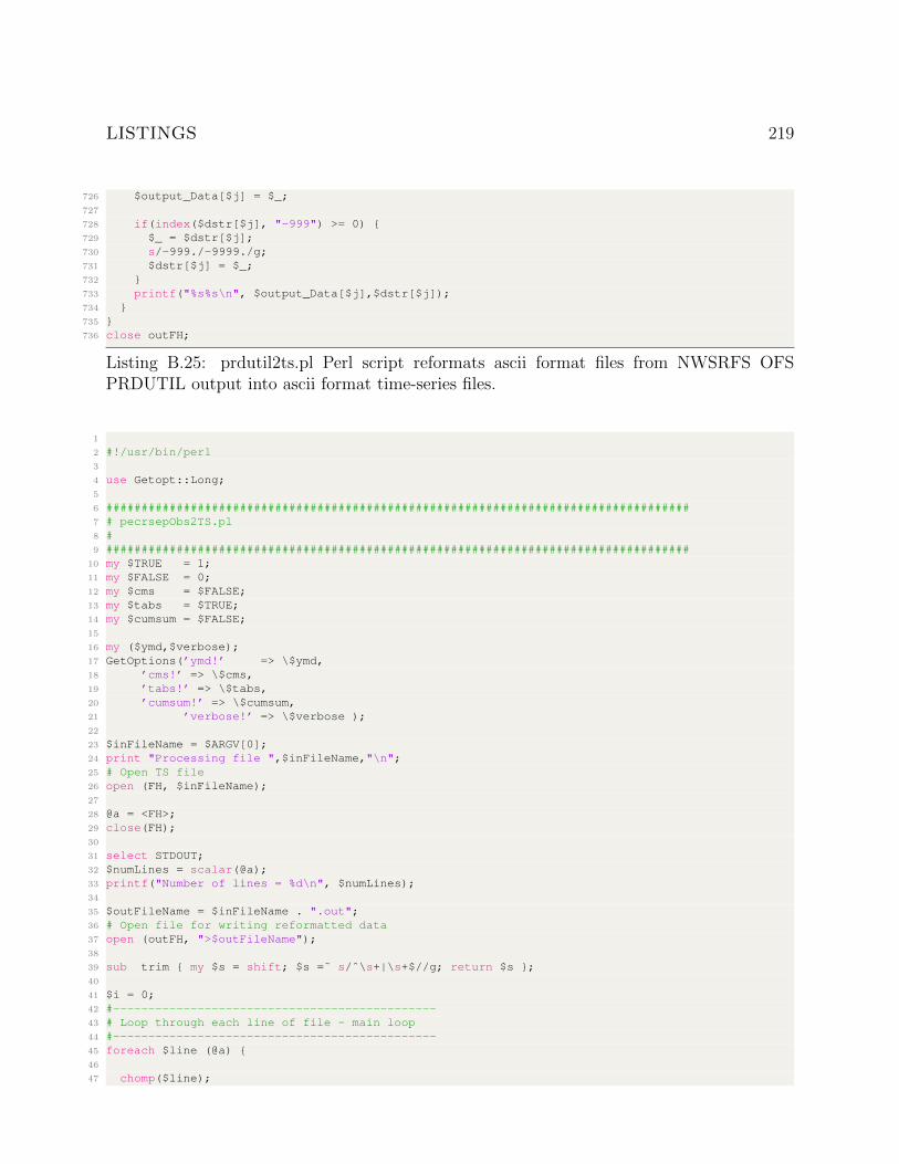
LISTINGS 219
726 $output_Data[$j] = $_;727
728 if(index($dstr[$j], "-999") >= 0) {729 $_ = $dstr[$j];730 s/-999./-9999./g;731 $dstr[$j] = $_;732 }733 printf("%s%s\n", $output_Data[$j],$dstr[$j]);734 }735 }736 close outFH;
Listing B.25: prdutil2ts.pl Perl script reformats ascii format files from NWSRFS OFSPRDUTIL output into ascii format time-series files.
1
2 #!/usr/bin/perl3
4 use Getopt::Long;5
6 ###################################################################################7 # pecrsepObs2TS.pl8 #9 ###################################################################################
10 my $TRUE = 1;11 my $FALSE = 0;12 my $cms = $FALSE;13 my $tabs = $TRUE;14 my $cumsum = $FALSE;15
16 my ($ymd,$verbose);17 GetOptions(’ymd!’ => \$ymd,18 ’cms!’ => \$cms,19 ’tabs!’ => \$tabs,20 ’cumsum!’ => \$cumsum,21 ’verbose!’ => \$verbose );22
23 $inFileName = $ARGV[0];24 print "Processing file ",$inFileName,"\n";25 # Open TS file26 open (FH, $inFileName);27
28 @a = <FH>;29 close(FH);30
31 select STDOUT;32 $numLines = scalar(@a);33 printf("Number of lines = %d\n", $numLines);34
35 $outFileName = $inFileName . ".out";36 # Open file for writing reformatted data37 open (outFH, ">$outFileName");38
39 sub trim { my $s = shift; $s =˜ s/ˆ\s+|\s+$//g; return $s };40
41 $i = 0;42 #----------------------------------------------43 # Loop through each line of file - main loop44 #----------------------------------------------45 foreach $line (@a) {46
47 chomp($line);
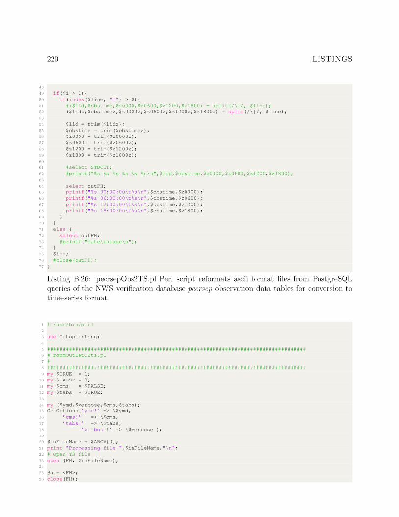
220 LISTINGS
48
49 if($i > 1){50 if(index($line, "|") > 0){51 #($lid,$obstime,$z0000,$z0600,$z1200,$z1800) = split(/\|/, $line);52 ($lidz,$obstimez,$z0000z,$z0600z,$z1200z,$z1800z) = split(/\|/, $line);53
54 $lid = trim($lidz);55 $obstime = trim($obstimez);56 $z0000 = trim($z0000z);57 $z0600 = trim($z0600z);58 $z1200 = trim($z1200z);59 $z1800 = trim($z1800z);60
61 #select STDOUT;62 #printf("%s %s %s %s %s %s\n",$lid,$obstime,$z0000,$z0600,$z1200,$z1800);63
64 select outFH;65 printf("%s 00:00:00\t%s\n",$obstime,$z0000);66 printf("%s 06:00:00\t%s\n",$obstime,$z0600);67 printf("%s 12:00:00\t%s\n",$obstime,$z1200);68 printf("%s 18:00:00\t%s\n",$obstime,$z1800);69 }70 }71 else {72 select outFH;73 #printf("date\tstage\n");74 }75 $i++;76 #close(outFH);77 }
Listing B.26: pecrsepObs2TS.pl Perl script reformats ascii format files from PostgreSQLqueries of the NWS verification database pecrsep observation data tables for conversion totime-series format.
1 #!/usr/bin/perl2
3 use Getopt::Long;4
5 ###################################################################################6 # rdhmOutletQ2ts.pl7 #8 ###################################################################################9 my $TRUE = 1;
10 my $FALSE = 0;11 my $cms = $FALSE;12 my $tabs = $TRUE;13
14 my ($ymd,$verbose,$cms,$tabs);15 GetOptions(’ymd!’ => \$ymd,16 ’cms!’ => \$cms,17 ’tabs!’ => \$tabs,18 ’verbose!’ => \$verbose );19
20 $inFileName = $ARGV[0];21 print "Processing file ",$inFileName,"\n";22 # Open TS file23 open (FH, $inFileName);24
25 @a = <FH>;26 close(FH);
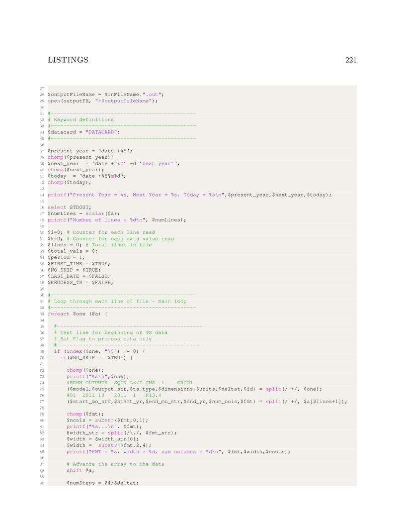
LISTINGS 221
27
28 $outputFileName = $inFileName.".out";29 open(outputFH, ">$outputFileName");30
31 #----------------------------------------------32 # Keyword definitions33 #----------------------------------------------34 $datacard = "DATACARD";35 #----------------------------------------------36
37 $present_year = ‘date +%Y‘;38 chomp($present_year);39 $next_year = ‘date +’%Y’ -d ’next year’‘;40 chomp($next_year);41 $today = ‘date +%Y%m%d‘;42 chomp($today);43
44 printf("Present Year = %s, Next Year = %s, Today = %s\n",$present_year,$next_year,$today);45
46 select STDOUT;47 $numLines = scalar(@a);48 printf("Number of lines = %d\n", $numLines);49
50 $i=0; # Counter for each line read51 $k=0; # Counter for each data value read52 $lines = 0; # Total lines in file53 $total_vals = 0;54 $period = 1;55 $FIRST_TIME = $TRUE;56 $NO_SKIP = $TRUE;57 $LAST_DATE = $FALSE;58 $PROCESS_TS = $FALSE;59
60 #----------------------------------------------61 # Loop through each line of file - main loop62 #----------------------------------------------63 foreach $one (@a) {64
65 #----------------------------------------------66 # Test line for beginning of TS data67 # Set Flag to process data only68 #----------------------------------------------69 if (index($one, "\$") != 0) {70 if($NO_SKIP == $TRUE) {71
72 chomp($one);73 printf("%s\n",$one);74 #RDHM OUTPUTS SQIN L3/T CMS 1 CRCO175 ($model,$output_str,$ts_type,$dimensions,$units,$deltat,$id) = split(/ +/, $one);76 #01 2011 10 2011 1 F13.477 ($start_mo_str,$start_yr,$end_mo_str,$end_yr,$num_cols,$fmt) = split(/ +/, $a[$lines+1]);78
79 chomp($fmt);80 $ncols = substr($fmt,0,1);81 printf("%s...\n", $fmt);82 @width_str = split(/\./, $fmt_str);83 $width = $width_str[0];84 $width = substr($fmt,2,4);85 printf("FMT = %s, width = %d, num columns = %d\n", $fmt,$width,$ncols);86
87 # Advance the array to the data88 shift @a;89
90 $numSteps = 24/$deltat;
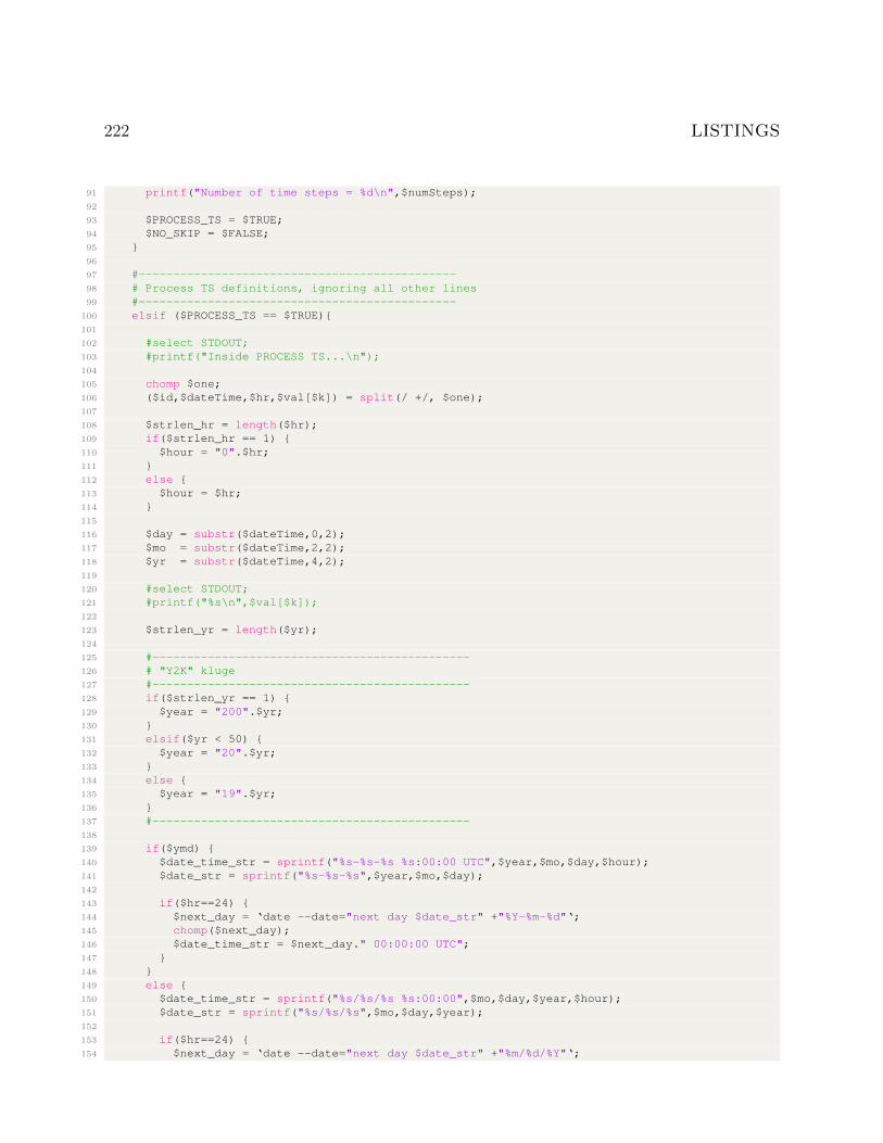
222 LISTINGS
91 printf("Number of time steps = %d\n",$numSteps);92
93 $PROCESS_TS = $TRUE;94 $NO_SKIP = $FALSE;95 }96
97 #----------------------------------------------98 # Process TS definitions, ignoring all other lines99 #----------------------------------------------
100 elsif ($PROCESS_TS == $TRUE){101
102 #select STDOUT;103 #printf("Inside PROCESS TS...\n");104
105 chomp $one;106 ($id,$dateTime,$hr,$val[$k]) = split(/ +/, $one);107
108 $strlen_hr = length($hr);109 if($strlen_hr == 1) {110 $hour = "0".$hr;111 }112 else {113 $hour = $hr;114 }115
116 $day = substr($dateTime,0,2);117 $mo = substr($dateTime,2,2);118 $yr = substr($dateTime,4,2);119
120 #select STDOUT;121 #printf("%s\n",$val[$k]);122
123 $strlen_yr = length($yr);124
125 #----------------------------------------------126 # "Y2K" kluge127 #----------------------------------------------128 if($strlen_yr == 1) {129 $year = "200".$yr;130 }131 elsif($yr < 50) {132 $year = "20".$yr;133 }134 else {135 $year = "19".$yr;136 }137 #----------------------------------------------138
139 if($ymd) {140 $date_time_str = sprintf("%s-%s-%s %s:00:00 UTC",$year,$mo,$day,$hour);141 $date_str = sprintf("%s-%s-%s",$year,$mo,$day);142
143 if($hr==24) {144 $next_day = ‘date --date="next day $date_str" +"%Y-%m-%d"‘;145 chomp($next_day);146 $date_time_str = $next_day." 00:00:00 UTC";147 }148 }149 else {150 $date_time_str = sprintf("%s/%s/%s %s:00:00",$mo,$day,$year,$hour);151 $date_str = sprintf("%s/%s/%s",$mo,$day,$year);152
153 if($hr==24) {154 $next_day = ‘date --date="next day $date_str" +"%m/%d/%Y"‘;
LISTINGS 223
155 chomp($next_day);156 $date_time_str = $next_day." 00:00:00";157 }158 }159 # 1.0 mˆ3 = 35.3147 ftˆ3160 $convert = 35.3147;161
162 # Set the field separator...163 if($tabs){164 $sep = "\t";165 $sep_str = "TAB";166 }167 else {168 $sep = "|";169 $sep_str = "|";170 }171
172 #select STDOUT;173 #printf("SEPARATOR %s\n", $sep_str);174
175 select outputFH;176 if($val[$k]>0) {177 if($cms){178 printf("%s%s%.2f\n",$date_time_str,$sep,$val[$k]);179 }180 else {181 $value = $val[$k]*$convert;182 printf("%s%s%.2f\n",$date_time_str,$sep,$value);183
184 }185 }186 $k++;187 }188 }189 #----------------------------------------------190 # End processing of TS data191 #----------------------------------------------192 else {193 select STDOUT;194 print $one;195 }196 $lines++;197 close(outFH);198 }
Listing B.27: rdhmOutletQ2ts.pl Perl script that reformats RDHM discharge simulationoutput files to ascii time-series format.
1 #!/usr/bin/perl2
3 use Getopt::Long;4
5 #------------------------------------------------------------------------6 # makeQPFTS_RDHMcontrol.pl7 #------------------------------------------------------------------------8 # USAGE: (on one line)9 #
10 #------------------------------------------------------------------------11
12 $TRUE = 1;13 $FALSE = 0;14
224 LISTINGS
15 #--------------------------------------------------------------16 # Read command line arguments.test17 #--------------------------------------------------------------18 $start_date = $ARGV[0]; # 2016031519 $end_date = $ARGV[1]; # 2016032220 $input_path = $ARGV[2]; # /home/teaiii/Desktop/GMEFP_schaake_shuffle/2010/0313/0921 $output_path = $ARGV[3]; # /home/teaiii/Desktop/GMEFP_schaake_shuffle/output/20100313/0922
23 #--------------------------------------------------------------24 # Open file for output25 #--------------------------------------------------------------26 $outputDir = "/home/teaiii/RDHM/greenbrier/input/";27 printf("Output directory: %s\n", $outputDir);28 $outFileName = $outputDir."rdhm_qpfts_control";29 open (outFH, ">$outFileName");30
31 #--------------------------------------------------------------32 # Write out the RDHM control File33 #--------------------------------------------------------------34 select(outFH);35
36 printf("#simulation time period\n");37 printf("time-period = %sT06 %sT06\n", $start_date, $end_date);38 printf("\n");39 printf("ignore-1d-xmrg = true\n");40 printf("\n");41 printf("#\n");42 printf("#simulation time step in the format of HH:MM:SS.XXXX\n");43 printf("time-step = 1\n");44 printf("#\n");45 printf("#OHRFC connectivity file\n");46 printf("connectivity = ./ohrfc_adj_bsn.con\n");47 printf("\n");48 printf("#\n");49 printf("pixel-size-hrap = 1.00\n");50 printf("#\n");51 printf("output-path = %s\n",$output_path);52 printf("#\n");53 printf("#input paths\n");54 printf("#\n");55 printf("input-path = ../parameters\n");56 printf("input-path = %s\n", $input_path);57 printf("\n");58 printf("input-path = /media/teaiii/Seagate8/nldas_conus_xmrg/temps\n");59 printf("\n");60 printf("input-path = /media/teaiii/development1/RDHM/warm_states\n");61 printf("\n");62 printf("#------------------------#--------------------------------------------------------------\
n");63 printf("# 6-hourly uniform xmrg disaggregation\n");64 printf("#--------------------------------------------------------------\n");65 printf("#disaggregation = xmrg interpolation=uniform freq=6:00:00 start=0:00:00\n");66 printf("\n");67 printf("#select operations\n");68 printf("#available snow17, snow17_mcp3, sac, frz, api, rutpix7, rutpix9, musk\n");69 printf("operations = snow17 sac frz rutpix9\n");70 printf("\n");71 printf("\n");72 printf("#--------------------------------------------------------------\n");73 printf("#------------------Information for SAC-HT-----------------------\n");74 printf("DSINT = 0.10 0.30 0.60 1.00 1.50\n");75 printf("DSINTW = 0.10 0.30 0.60 1.00 1.50\n");76 printf("\n");77 printf("normalize-soil-moisture = true\n");

LISTINGS 225
78 printf("\n");79 printf("#--------------------------------------------------------------\n");80 printf("#output-grid-after-timeloop =\n");81 printf("#--------------------------------------------------------------\n");82 printf("output-grid-inside-timeloop = tsint1 tsint2 tsint3 tsint4 tsint5\n");83 printf("output-grid-inside-timeloop = discharge\n");84 printf("output-grid-inside-timeloop = areac areac1 areac2 areac3 areac4 depth\n");85 printf("output-grid-inside-timeloop = swint1 swint2 swint3 swint4 swint5\n");86 printf("output-grid-inside-timeloop = smc0 smc1 smc2 smc3 smc4 smc5\n");87 printf("output-grid-inside-timeloop = sh2o0 sh2o1 sh2o2 sh2o3 sh2o4 sh2o5\n");88 printf("output-grid-inside-timeloop = uztwc uzfwc lztwc lzfsc lzfpc adimpc\n");89 printf("output-grid-inside-timeloop = upperSwint real_uztwc real_lztwc\n");90 printf("output-grid-inside-timeloop = surfaceFlow subsurfaceFlow\n");91 printf("output-grid-inside-timeloop = we neghs liqw tindex accmax sndpt sntmp cover\n");92 printf("\n");93 printf("#\n");94 printf("#In number of timestep, example, 2 means output every 2 timestep\n");95 printf("#\n");96 printf("output-grid-step = 1\n");97 printf("\n");98 printf("#\n");99 printf("#data to be output at the last 23hr, such as states\n");
100 printf("output-grid-last-step = uztwc uzfwc lztwc lzfsc lzfpc adimpc \n");101 printf("output-grid-after-timeloop = discharge surfaceFlow subsurfaceFlow\n");102 printf("\n");103 printf("output-grid-last-step = swint1 swint2 swint3 swint4 swint5\n");104 printf("output-grid-last-step = we neghs liqw tindex accmax sndpt sntmp cover\n");105 printf("output-grid-last-step = uztwc uzfwc lztwc lzfsc lzfpc adimpc\n");106 printf("\n");107 printf("# VK ---- you need to output these states too --------------------------\n");108 printf("output-grid-last-step = uztwh uzfwh lztwh lzfsh lzfph \n");109 printf("output-grid-last-step = smc0 smc1 smc2 smc3 smc4 smc5\n");110 printf("output-grid-last-step = sh2o0 sh2o1 sh2o2 sh2o3 sh2o4 sh2o5\n");111 printf("output-grid-last-step = ts0 ts1 ts2 ts3 ts4\n");112 printf("output-grid-last-step = uztwc_prv uzfwc_prv lztwc_prv lzfsc_prv \n");113 printf("output-grid-last-step = lzfpc_prv adimpc_prv\n");114 printf("# VK ------------------------------------------------------------------\n");115 printf("\n");116 printf("#\n");117 printf("#Time series to be averaged over every basin\n");118 printf("#\n");119 printf("output-timeseries-basin-average = xmrg\n");120 printf("#output-timeseries-basin-average = surfaceFlow\n");121 printf("\n");122 printf("#Time series at the outlet\n");123 printf("output-timeseries-basin-outlet = discharge\n");124 printf("\n");125 printf("#basin id and factors for input data\n");126 printf("#------------------\n");127 printf("#----- 03182700 ------\n");128 printf("#------------------\n");129 printf("input-data = 03182700\n");130 printf("#========================================================\n");131 printf("# calibration adjustments\n");132 printf("#========================================================\n");133 printf("#SAC Parameters, includes EFC/PCTIM\n");134 printf("input-data = sac_UZTWM=-0.40\n");135 printf("input-data = sac_UZFWM=-0.60\n");136 printf("input-data = sac_UZK=-1.60\n");137 printf("#input-data = sac_RIVA=0.04\n");138 printf("#input-data = sac_ZPERC=-1.00\n");139 printf("#input-data = sac_REXP=-1.0\n");140 printf("#input-data = sac_LZTWM=-0.776\n");141 printf("#input-data = sac_LZPK=-0.273\n");
226 LISTINGS
142 printf("input-data = sac_LZFPM=-1.00\n");143 printf("#input-data = sac_PFREE=-1.00\n");144 printf("input-data = sac_LZSK=-01.00\n");145 printf("#input-data = sac_LZFSM=-2.04\n");146 printf("#input-data = sac_RSERV=0.3\n");147 printf("#input-data = sac_PCTIM=-0.513\n");148 printf("#input-data = sac_ADIMP=0\n");149 printf("#input-data = sac_SIDE=0\n");150 printf("#rutpix states\n");151 printf("#input-data = rutpix_Q0CHN=-1.2\n");152 printf("input-data = rutpix_QMCHN=-0.94\n");153 printf("#========================================================\n");154 printf("#SAC parameters\n");155 printf("input-data = sac_ADIMP=0.0 sac_RIVA=0.001 sac_EFC=0.5\n");156 printf("input-data = sac_SIDE=0.0 sac_RSERV=0.3\n");157 printf("input-data = surf_water=-9999\n");158 printf("\n");159 printf("#rutpix states\n");160 printf("#input-data = rutpix_QMCHN=1.35\n");161 printf("#snow states\n");162 printf("input-data = snow_PXTMP=1.0 snow_PLWHC=0.05 snow_TIPM=0.1 snow_SCF=1.0\n");163 printf("input-data = snow_NMF=0.15 snow_MBASE=0.0 snow_PGM=0.0 snow_LAEC=0.0\n");164 printf("\n");165 printf("input-data = snow_SI=0.0 snow_ADC1=0.05 snow_ADC2=0.15 snow_ADC3=0.29\n");166 printf("input-data = snow_ADC4=0.41 snow_ADC5=0.51 snow_ADC6=0.60 snow_ADC7=0.65\n");167 printf("input-data = snow_ADC8=0.68 snow_ADC9=0.72 snow_ADC10=0.76 snow_ADC11=1.0\n");168 printf("\n");169 printf("input-data = frz_RSMAX=0.58 frz_CKSL=8 frz_ZBOT=2.5\n");170 printf("\n");171 printf("input-data = psfrac=9\n");172 printf("input-data = snow_RDCO=1\n");173 printf("#----------------------------------\n");174 printf("input-data = 03184000\n");175 printf("#----------------------------------\n");176 printf("#========================================================\n");177 printf("# calibration adjustments\n");178 printf("#========================================================\n");179 printf("#SAC Parameters, includes EFC/PCTIM\n");180 printf("input-data = sac_UZTWM=-0.40\n");181 printf("input-data = sac_UZFWM=-0.60\n");182 printf("input-data = sac_UZK=-1.60\n");183 printf("#input-data = sac_RIVA=0.04\n");184 printf("#input-data = sac_ZPERC=-1.00\n");185 printf("#input-data = sac_REXP=-1.0\n");186 printf("#input-data = sac_LZTWM=-0.776\n");187 printf("#input-data = sac_LZPK=-0.273\n");188 printf("input-data = sac_LZFPM=-1.00\n");189 printf("#input-data = sac_PFREE=-1.00\n");190 printf("input-data = sac_LZSK=-01.00\n");191 printf("#input-data = sac_LZFSM=-2.04\n");192 printf("#input-data = sac_RSERV=0.3\n");193 printf("#input-data = sac_PCTIM=-0.513\n");194 printf("#input-data = sac_ADIMP=0\n");195 printf("#input-data = sac_SIDE=0\n");196 printf("#rutpix states\n");197 printf("#input-data = rutpix_Q0CHN=-1.2\n");198 printf("input-data = rutpix_QMCHN=-0.94\n");199 printf("#========================================================\n");200 printf("#SAC parameters\n");201 printf("input-data = sac_ADIMP=0.0 sac_RIVA=0.001 sac_EFC=0.5\n");202 printf("input-data = sac_SIDE=0.0 sac_RSERV=0.3\n");203 printf("input-data = surf_water=-9999\n");204 printf("\n");205 printf("#rutpix states\n");
LISTINGS 227
206 printf("#input-data = rutpix_QMCHN=1.35\n");207 printf("#snow states\n");208 printf("input-data = snow_PXTMP=1.0 snow_PLWHC=0.05 snow_TIPM=0.1 snow_SCF=1.0\n");209 printf("input-data = snow_NMF=0.15 snow_MBASE=0.0 snow_PGM=0.0 snow_LAEC=0.0\n");210 printf("\n");211 printf("input-data = snow_SI=0.0 snow_ADC1=0.05 snow_ADC2=0.15 snow_ADC3=0.29\n");212 printf("input-data = snow_ADC4=0.41 snow_ADC5=0.51 snow_ADC6=0.60 snow_ADC7=0.65\n");213 printf("input-data = snow_ADC8=0.68 snow_ADC9=0.72 snow_ADC10=0.76 snow_ADC11=1.0\n");214 printf("\n");215 printf("input-data = frz_RSMAX=0.58 frz_CKSL=8 frz_ZBOT=2.5\n");216 printf("\n");217 printf("input-data = psfrac=9\n");218 printf("input-data = snow_RDCO=1\n");219 printf("#----------------------------------\n");220 printf("input-data = 03180500\n");221 printf("#----------------------------------\n");222 printf("#========================================================\n");223 printf("# calibration adjustments\n");224 printf("#========================================================\n");225 printf("#SAC Parameters, includes EFC/PCTIM\n");226 printf("input-data = sac_UZTWM=-0.40\n");227 printf("input-data = sac_UZFWM=-0.60\n");228 printf("input-data = sac_UZK=-1.60\n");229 printf("#input-data = sac_RIVA=0.04\n");230 printf("#input-data = sac_ZPERC=-1.00\n");231 printf("#input-data = sac_REXP=-1.0\n");232 printf("#input-data = sac_LZTWM=-0.776\n");233 printf("#input-data = sac_LZPK=-0.273\n");234 printf("input-data = sac_LZFPM=-1.00\n");235 printf("#input-data = sac_PFREE=-1.00\n");236 printf("input-data = sac_LZSK=-01.00\n");237 printf("#input-data = sac_LZFSM=-2.04\n");238 printf("#input-data = sac_RSERV=0.3\n");239 printf("#input-data = sac_PCTIM=-0.513\n");240 printf("#input-data = sac_ADIMP=0\n");241 printf("#input-data = sac_SIDE=0\n");242 printf("#rutpix states\n");243 printf("#input-data = rutpix_Q0CHN=-1.2\n");244 printf("input-data = rutpix_QMCHN=-0.94\n");245 printf("#========================================================\n");246 printf("#SAC parameters\n");247 printf("input-data = sac_ADIMP=0.0 sac_RIVA=0.001 sac_EFC=0.5\n");248 printf("input-data = sac_SIDE=0.0 sac_RSERV=0.3\n");249 printf("input-data = surf_water=-9999\n");250 printf("\n");251 printf("#rutpix states\n");252 printf("#input-data = rutpix_QMCHN=1.35\n");253 printf("#snow states\n");254 printf("input-data = snow_PXTMP=1.0 snow_PLWHC=0.05 snow_TIPM=0.1 snow_SCF=1.0\n");255 printf("input-data = snow_NMF=0.15 snow_MBASE=0.0 snow_PGM=0.0 snow_LAEC=0.0\n");256 printf("\n");257 printf("input-data = snow_SI=0.0 snow_ADC1=0.05 snow_ADC2=0.15 snow_ADC3=0.29\n");258 printf("input-data = snow_ADC4=0.41 snow_ADC5=0.51 snow_ADC6=0.60 snow_ADC7=0.65\n");259 printf("input-data = snow_ADC8=0.68 snow_ADC9=0.72 snow_ADC10=0.76 snow_ADC11=1.0\n");260 printf("\n");261 printf("input-data = frz_RSMAX=0.58 frz_CKSL=8 frz_ZBOT=2.5\n");262 printf("\n");263 printf("input-data = psfrac=9\n");264 printf("input-data = snow_RDCO=1\n");265 printf("#----------------------------------\n");266 printf("input-data = 03182500\n");267 printf("#----------------------------------\n");268 printf("#========================================================\n");269 printf("# calibration adjustments\n");
228 LISTINGS
270 printf("#========================================================\n");271 printf("#SAC Parameters, includes EFC/PCTIM\n");272 printf("input-data = sac_UZTWM=-0.40\n");273 printf("input-data = sac_UZFWM=-0.60\n");274 printf("input-data = sac_UZK=-1.60\n");275 printf("#input-data = sac_RIVA=0.04\n");276 printf("#input-data = sac_ZPERC=-1.00\n");277 printf("#input-data = sac_REXP=-1.0\n");278 printf("#input-data = sac_LZTWM=-0.776\n");279 printf("#input-data = sac_LZPK=-0.273\n");280 printf("input-data = sac_LZFPM=-1.00\n");281 printf("#input-data = sac_PFREE=-1.00\n");282 printf("input-data = sac_LZSK=-01.00\n");283 printf("#input-data = sac_LZFSM=-2.04\n");284 printf("#input-data = sac_RSERV=0.3\n");285 printf("#input-data = sac_PCTIM=-0.513\n");286 printf("#input-data = sac_ADIMP=0\n");287 printf("#input-data = sac_SIDE=0\n");288 printf("#rutpix states\n");289 printf("#input-data = rutpix_Q0CHN=-1.2\n");290 printf("input-data = rutpix_QMCHN=-0.94\n");291 printf("#========================================================\n");292 printf("#SAC parameters\n");293 printf("input-data = sac_ADIMP=0.0 sac_RIVA=0.001 sac_EFC=0.5\n");294 printf("input-data = sac_SIDE=0.0 sac_RSERV=0.3\n");295 printf("input-data = surf_water=-9999\n");296 printf("\n");297 printf("#rutpix states\n");298 printf("#input-data = rutpix_QMCHN=1.35\n");299 printf("#snow states\n");300 printf("input-data = snow_PXTMP=1.0 snow_PLWHC=0.05 snow_TIPM=0.1 snow_SCF=1.0\n");301 printf("input-data = snow_NMF=0.15 snow_MBASE=0.0 snow_PGM=0.0 snow_LAEC=0.0\n");302 printf("\n");303 printf("input-data = snow_SI=0.0 snow_ADC1=0.05 snow_ADC2=0.15 snow_ADC3=0.29\n");304 printf("input-data = snow_ADC4=0.41 snow_ADC5=0.51 snow_ADC6=0.60 snow_ADC7=0.65\n");305 printf("input-data = snow_ADC8=0.68 snow_ADC9=0.72 snow_ADC10=0.76 snow_ADC11=1.0\n");306 printf("\n");307 printf("input-data = frz_RSMAX=0.58 frz_CKSL=8 frz_ZBOT=2.5\n");308 printf("\n");309 printf("input-data = psfrac=9\n");310 printf("input-data = snow_RDCO=1\n");311 printf("#----------------------------------\n");312 printf("input-data = 03183500\n");313 printf("#----------------------------------\n");314 printf("#========================================================\n");315 printf("# calibration adjustments\n");316 printf("#========================================================\n");317 printf("#SAC Parameters, includes EFC/PCTIM\n");318 printf("input-data = sac_UZTWM=-0.40\n");319 printf("input-data = sac_UZFWM=-0.60\n");320 printf("input-data = sac_UZK=-1.60\n");321 printf("#input-data = sac_RIVA=0.04\n");322 printf("#input-data = sac_ZPERC=-1.00\n");323 printf("#input-data = sac_REXP=-1.0\n");324 printf("#input-data = sac_LZTWM=-0.776\n");325 printf("#input-data = sac_LZPK=-0.273\n");326 printf("input-data = sac_LZFPM=-1.00\n");327 printf("#input-data = sac_PFREE=-1.00\n");328 printf("input-data = sac_LZSK=-01.00\n");329 printf("#input-data = sac_LZFSM=-2.04\n");330 printf("#input-data = sac_RSERV=0.3\n");331 printf("#input-data = sac_PCTIM=-0.513\n");332 printf("#input-data = sac_ADIMP=0\n");333 printf("#input-data = sac_SIDE=0\n");
LISTINGS 229
334 printf("#rutpix states\n");335 printf("#input-data = rutpix_Q0CHN=-1.2\n");336 printf("input-data = rutpix_QMCHN=-0.94\n");337 printf("#========================================================\n");338 printf("#SAC parameters\n");339 printf("input-data = sac_ADIMP=0.0 sac_RIVA=0.001 sac_EFC=0.5\n");340 printf("input-data = sac_SIDE=0.0 sac_RSERV=0.3\n");341 printf("input-data = surf_water=-9999\n");342 printf("\n");343 printf("#rutpix states\n");344 printf("#input-data = rutpix_QMCHN=1.35\n");345 printf("#snow states\n");346 printf("input-data = snow_PXTMP=1.0 snow_PLWHC=0.05 snow_TIPM=0.1 snow_SCF=1.0\n");347 printf("input-data = snow_NMF=0.15 snow_MBASE=0.0 snow_PGM=0.0 snow_LAEC=0.0\n");348 printf("\n");349 printf("input-data = snow_SI=0.0 snow_ADC1=0.05 snow_ADC2=0.15 snow_ADC3=0.29\n");350 printf("input-data = snow_ADC4=0.41 snow_ADC5=0.51 snow_ADC6=0.60 snow_ADC7=0.65\n");351 printf("input-data = snow_ADC8=0.68 snow_ADC9=0.72 snow_ADC10=0.76 snow_ADC11=1.0\n");352 printf("\n");353 printf("input-data = frz_RSMAX=0.58 frz_CKSL=8 frz_ZBOT=2.5\n");354 printf("\n");355 printf("input-data = psfrac=9\n");356 printf("input-data = snow_RDCO=1\n");357 printf("#----------------------------------\n");358
359 close(outFH);
Listing B.28: makeQPFTS RDHMcontrol.pl Perl script used to generate RDHM simulationcontrol files for RDHM monte carlo experiments called by run QPF TS RDHM
1 #!/usr/bin/perl2
3 use Getopt::Long;4
5 ###################################################################################6 # rdhmOutletQ2tsCats.pl7 #8 ###################################################################################9 my $TRUE = 1;
10 my $FALSE = 0;11 my $cms = $FALSE;12 my $tabs = $TRUE;13
14 my ($ymd,$verbose,$cms,$tabs);15 GetOptions(’ymd!’ => \$ymd,16 ’cms!’ => \$cms,17 ’tabs!’ => \$tabs,18 ’verbose!’ => \$verbose );19
20 $inFileName1 = $ARGV[0];21 $inFileName2 = $ARGV[1];22 $cat = $ARGV[2]; # Category from GRASS GIS analysis, used to set factor23 print "Processing file ",$inFileName1,"\n"; # Data file24 print "Processing file ",$inFileName2,"\n"; # File used to set factor from Category25 # Open TS file26 open (FH, $inFileName1);27
28 @a = <FH>;29 close(FH);30
31 open (FH2, $inFileName2);32 @b = <FH2>;
230 LISTINGS
33 close(FH2);34
35 $num_lines = scalar(@b);36 printf("Number of lines in Random Points file: %s\n", $num_lines);37 for($i=0;$i<$num_lines;$i++) {38 chomp($b[$i]);39 ($which_cat,$x,$y,$num,$ts) = split(/\,/, $b[$i]);40 chomp($b[$i]);41 select STDOUT;42 #printf("%s %s %s %s %s\n",$which_cat,$x,$y,$num,$ts);43
44 if($cat == $which_cat){45 if($ts > 0.30){46 $factor = "A";47 }48 elsif ($ts <= 0.30 && $ts >0.25){49 $factor = "B";50 }51 elsif ($ts <= 0.25 && $ts >0.15){52 $factor = "C";53 }54 elsif ($ts <= 0.15 && $ts >0.06){55 $factor = "D";56 }57 else{58 $factor = "E";59 }60 last;61 }62 }63
64 printf("Factor is %s %s\n", $factor, $cat);65
66 $outputFileName = $inFileName1.".out";67 open(outputFH, ">$outputFileName");68
69 $outputFileName2 = "/home/teaiii/TS_maxval.out";70 open(outFH, ">>$outputFileName2");71
72 #----------------------------------------------73 # Keyword definitions74 #----------------------------------------------75 $datacard = "DATACARD";76 #----------------------------------------------77
78 $present_year = ‘date +%Y‘;79 chomp($present_year);80 $next_year = ‘date +’%Y’ -d ’next year’‘;81 chomp($next_year);82 $today = ‘date +%Y%m%d‘;83 chomp($today);84
85 printf("Present Year = %s, Next Year = %s, Today = %s\n",$present_year,$next_year,$today);86
87 select STDOUT;88 $numLines = scalar(@a);89 printf("Number of lines = %d\n", $numLines);90
91 $i=0; # Counter for each line read92 $k=0; # Counter for each data value read93 $lines = 0; # Total lines in file94 $total_vals = 0;95 $period = 1;96 $FIRST_TIME = $TRUE;
LISTINGS 231
97 $NO_SKIP = $TRUE;98 $LAST_DATE = $FALSE;99 $PROCESS_TS = $FALSE;
100
101 #----------------------------------------------102 # Loop through each line of file - main loop103 #----------------------------------------------104 foreach $one (@a) {105
106 #----------------------------------------------107 # Test line for beginning of TS data108 # Set Flag to process data only109 #----------------------------------------------110 if (index($one, "\$") != 0) {111 if($NO_SKIP == $TRUE) {112
113 chomp($one);114 printf("%s\n",$one);115 #RDHM OUTPUTS SQIN L3/T CMS 1 CRCO1116 ($model,$output_str,$ts_type,$dimensions,$units,$deltat,$id) = split(/ +/, $one);117 #01 2011 10 2011 1 F13.4118 ($start_mo_str,$start_yr,$end_mo_str,$end_yr,$num_cols,$fmt) = split(/ +/, $a[$lines+1]);119
120 chomp($fmt);121 $ncols = substr($fmt,0,1);122 printf("%s...\n", $fmt);123 @width_str = split(/\./, $fmt_str);124 $width = $width_str[0];125 $width = substr($fmt,2,4);126 printf("FMT = %s, width = %d, num columns = %d\n", $fmt,$width,$ncols);127
128 # Advance the array to the data129 shift @a;130
131 $numSteps = 24/$deltat;132 printf("Number of time steps = %d\n",$numSteps);133
134 $PROCESS_TS = $TRUE;135 $NO_SKIP = $FALSE;136 }137
138 #----------------------------------------------139 # Process TS definitions, ignoring all other lines140 #----------------------------------------------141 elsif ($PROCESS_TS == $TRUE){142
143 #select STDOUT;144 #printf("Inside PROCESS TS...\n");145
146 chomp $one;147 ($id,$dateTime,$hr,$val[$k]) = split(/ +/, $one);148
149 $strlen_hr = length($hr);150 if($strlen_hr == 1) {151 $hour = "0".$hr;152 }153 else {154 $hour = $hr;155 }156
157 $day = substr($dateTime,0,2);158 $mo = substr($dateTime,2,2);159 $yr = substr($dateTime,4,2);160
232 LISTINGS
161 #select STDOUT;162 #printf("%s\n",$val[$k]);163
164 $strlen_yr = length($yr);165
166 #----------------------------------------------167 # "Y2K" kluge168 #----------------------------------------------169 if($strlen_yr == 1) {170 $year = "200".$yr;171 }172 elsif($yr < 50) {173 $year = "20".$yr;174 }175 else {176 $year = "19".$yr;177 }178 #----------------------------------------------179
180 if($ymd) {181 $date_time_str = sprintf("%s-%s-%s %s:00:00 UTC",$year,$mo,$day,$hour);182 $date_str = sprintf("%s-%s-%s",$year,$mo,$day);183
184 if($hr==24) {185 $next_day = ‘date --date="next day $date_str" +"%Y-%m-%d"‘;186 chomp($next_day);187 $date_time_str = $next_day." 00:00:00 UTC";188 }189 }190 else {191 $date_time_str = sprintf("%s/%s/%s %s:00:00",$mo,$day,$year,$hour);192 $date_str = sprintf("%s/%s/%s",$mo,$day,$year);193
194 if($hr==24) {195 $next_day = ‘date --date="next day $date_str" +"%m/%d/%Y"‘;196 chomp($next_day);197 $date_time_str = $next_day." 00:00:00";198 }199 }200 # 1.0 mˆ3 = 35.3147 ftˆ3201 $convert = 35.3147;202
203 # Set the field separator...204 if($tabs){205 $sep = "\t";206 $sep_str = "TAB";207 }208 else {209 $sep = "|";210 $sep_str = "|";211 }212
213 #select STDOUT;214 #printf("SEPARATOR %s\n", $sep_str);215
216 if($val[$k]>0) {217
218 if($k == 1){219 $maxal = $val[$k];220 }221 else {222 if($val[$k] > $maxal){223 $maxal = $val[$k];224 }
LISTINGS 233
225 }226
227 select outputFH;228 if($cms){229 printf("%s%s%.2f%s%s\n",$date_time_str,$sep,$val[$k],$sep,$factor);230 }231 else {232 $value = $val[$k]*$convert;233 printf("%s%s%.2f%s%s\n",$date_time_str,$sep,$value,$sep,$factor);234
235 }236 }237 $k++;238 }239 }240 #----------------------------------------------241 # End processing of TS data242 #----------------------------------------------243 else {244 select STDOUT;245 print $one;246 }247 $lines++;248 #close(outputFH);249 }250
251 open (FH3, "/media/teaiii/development1/grass/Linear_dist_TS.txt");252 @dist_array = <FH3>;253 close(FH3);254
255 $numDlines = scalar(@dist_array);256 printf("Number of lines in cat-distance file: %s\n", $numDlines);257 for($j=0;$j<$numDlines;$j++) {258 chomp($dist_array[$j]);259 ($from_cat,$to_cat,$distance[$j]) = split(/\|/, $dist_array[$j]);260 chomp($distance[$j]);261 }262
263 select outFH;264 if($cms){265 printf("%s\t%s\t%s\t%s\t%s\n", $cat,$ts,$maxal,$factor,$distance[$cat-1]);266 }267 else{268 $value = $maxval*$convert;269 printf("%s\t%s\t%s\t%s\t%s\n", $cat,$ts,$value,$factor,$distance[$cat-1]);270 }271 #close(outFH);
Listing B.29: rdhmOutletQ2tsCats.pl Perl script used in RDHM monte carlo experimentsfor threat score category calculations called by run RDHMthreatScoreOutput2TS.sh.
Related Documents