CDISC ADaM Implementation Guide Version 1.0 © 2009 Clinical Data Interchange Standards Consortium, Inc. All rights reserved Page 1 FINAL December 17, 2009 Analysis Data Model (ADaM) Implementation Guide Prepared by the CDISC Analysis Data Model Team Notes to Readers This Implementation Guide is Version 1.0 (V1.0) and corresponds to Version 2.1 of the CDISC Analysis Data Model. Revision History Date Version Summary of Changes Dec. 17, 2009 1.0 Final Released version reflecting all changes and corrections identified during comment period. May 30, 2008 1.0 Draft Draft for Public Comment Note: Please see Appendix B for Representations and Warranties; Limitations of Liability, and Disclaimers.

ADAM Implementation Guide
Oct 21, 2015
ADAM Implementation Guide
Welcome message from author
This document is posted to help you gain knowledge. Please leave a comment to let me know what you think about it! Share it to your friends and learn new things together.
Transcript
CDISC ADaM Implementation Guide Version 1.0
© 2009 Clinical Data Interchange Standards Consortium, Inc. All rights reserved Page 1 FINAL December 17, 2009
Analysis Data Model (ADaM)
Implementation Guide
Prepared by the
CDISC Analysis Data Model Team
Notes to Readers
This Implementation Guide is Version 1.0 (V1.0) and corresponds to Version 2.1 of the CDISC Analysis Data
Model.
Revision History Date Version Summary of Changes
Dec. 17, 2009 1.0 Final Released version reflecting all changes and corrections identified during comment
period.
May 30, 2008 1.0 Draft Draft for Public Comment
Note: Please see Appendix B for Representations and Warranties; Limitations of Liability, and Disclaimers.
CDISC ADaM Implementation Guide Version 1.0
© 2009 Clinical Data Interchange Standards Consortium, Inc. All rights reserved Page 2 FINAL December 17, 2009
Contents
Analysis Data Model (ADaM) ....................................................................................................................................... 1
Implementation Guide ................................................................................................................................................... 1
Prepared by the .............................................................................................................................................................. 1
CDISC Analysis Data Model Team ............................................................................................................................... 1
Revision History ............................................................................................................................................................ 1
1 Introduction .......................................................................................................................................................... 4
1.1 Purpose ....................................................................................................................................................... 4
1.2 Background................................................................................................................................................. 4
1.3 What is Covered in the ADaMIG ............................................................................................................... 4
1.4 Organization of this Document ................................................................................................................... 5
1.5 Definitions .................................................................................................................................................. 5
1.5.1 General ADaM Definitions .................................................................................................................... 5
1.5.2 Basic Data Structure Definitions............................................................................................................ 6
2 Fundamentals of the ADaM Standard .................................................................................................................. 7
2.1 Fundamental Principles .............................................................................................................................. 7
2.2 Traceability ................................................................................................................................................. 7
2.3 The ADaM Data Structures ........................................................................................................................ 8
2.3.1 The ADaM Subject-Level Analysis Dataset ADSL ............................................................................... 8
2.3.2 The ADaM Basic Data Structure (BDS) ................................................................................................ 9
3 Standard ADaM Variables .................................................................................................................................. 10
3.1 ADSL Variables ........................................................................................................................................ 14
3.2 ADaM Basic Data Structure (BDS) Variables .......................................................................................... 20
3.2.1 Subject Identifier Variables for BDS Datasets ..................................................................................... 20
3.2.2 Treatment Variables for BDS Datasets................................................................................................. 21
3.2.3 Timing Variables for BDS Datasets ..................................................................................................... 22
3.2.4 Analysis Parameter Variables for BDS Datasets .................................................................................. 27
3.2.5 Analysis Descriptor Variables for BDS Datasets ................................................................................. 30
3.2.6 Indicator Variables for BDS Datasets .................................................................................................. 33
3.2.7 Differences Between SDTM and ADaM Population and Baseline Flags ............................................ 37
3.2.8 Other Variables .................................................................................................................................... 38
4 Implementation Issues, Standard Solutions, and Examples ............................................................................... 39
4.1 Examples of Treatment Variables for Common Trial Designs.................................................................. 40
4.2 Creation of Derived Columns Versus Creation of Derived Rows ............................................................. 42
4.2.1 Rules for the Creation of Rows and Columns ...................................................................................... 42

CDISC ADaM Implementation Guide Version 1.0
© 2009 Clinical Data Interchange Standards Consortium, Inc. All rights reserved Page 3 FINAL December 17, 2009
4.3 Inclusion of All Observed and Derived Records for a Parameter Versus the Subset of Records Used for
Analysis 56
4.3.1 ADaM Methodology and Examples .................................................................................................... 56
4.4 Inclusion of Input Data that are not Analyzed but that Support a Derivation in the Analysis Dataset ..... 60
4.4.1 ADaM Methodology and Examples .................................................................................................... 60
4.5 Identification of Rows Used for Analysis ................................................................................................. 65
4.5.1 Identification of Rows Used in a Timepoint Imputation Analysis ....................................................... 65
4.5.2 Identification of Baseline Rows ........................................................................................................... 67
4.5.3 Identification of Post-Baseline Conceptual Timepoint Rows .............................................................. 69
4.5.4 Identification of Rows Used for Analysis – General Case ................................................................... 71
4.6 Identification of Population-Specific Analyzed Rows .............................................................................. 74
4.6.1 ADaM Methodology and Examples .................................................................................................... 74
4.7 Identification of Rows Which Satisfy a Predefined Criterion for Analysis Purposes ............................... 76
4.7.1 ADaM Methodology and Examples .................................................................................................... 76
4.8 Other Issues to Consider ........................................................................................................................... 79
4.8.1 Adding Records to Create a Full Complement of Analysis Timepoints for Every Subject ................. 79
4.8.2 Creating Multiple Datasets to Support Analysis of the Same Type of Data......................................... 79
Appendices .................................................................................................................................................................. 80
Appendix A References and Abbreviations ......................................................................................................... 80
Appendix B Representations And Warranties; Limitations of Liability, And Disclaimers .................................. 81
CDISC ADaM Implementation Guide Version 1.0
© 2009 Clinical Data Interchange Standards Consortium, Inc. All rights reserved Page 4 FINAL December 17, 2009
1 Introduction 1.1 Purpose
This document comprises the Clinical Data Interchange Standards Consortium (CDISC) Version 1.0 Analysis Data
Model Implementation Guide (ADaMIG), which has been prepared by the Analysis Data Model (ADaM) team of
CDISC. The ADaMIG specifies ADaM standard dataset structures and variables, including naming conventions. It
also specifies standard solutions to implementation issues.
The ADaMIG must be used in close concert with the current version of the Analysis Data Model document (ADaM
document) which is available for download at http://www.cdisc.org/adam. The ADaM document explains the
purpose of the Analysis Data Model. It describes fundamental principles that apply to all analysis datasets, with the
driving principle being that the design of analysis datasets and associated metadata facilitate explicit communication
of the content of, input to, and purpose of submitted analysis datasets. The Analysis Data Model supports efficient
generation, replication, and review of analysis results.
1.2 Background
The user of the ADaMIG must be familiar with the CDISC Study Data Tabulation Model (SDTM) and the Study
Data Tabulation Model Implementation Guide (SDTMIG), both of which are available at http://www.cdisc.org/sdtm,
since SDTM is the source for ADaM data.
Both the SDTM and ADaM standards were designed to support submission by a sponsor to a regulatory agency such
as the United States Food and Drug Administration (FDA). Since inception, the CDISC ADaM team has been
encouraged and informed by FDA statistical and medical reviewers who participate in ADaM meetings as observers,
and who have participated in CDISC-FDA pilots. The origin of the fundamental principles of ADaM is the need for
transparency of communication with and scientifically valid review by regulatory agencies. The ADaM standard has
been developed to meet the needs of the FDA and industry. ADaM is applicable to a wide range of drug
development activities in addition to FDA regulatory submissions. It provides a standard for transferring datasets
between sponsors and contract research organizations (CROs), development partners, and independent data
monitoring committees. As adoption of the model becomes more widespread, in–licensing, out–licensing and
mergers are facilitated through the use of a common model for analysis data and metadata across sponsors.
1.3 What is Covered in the ADaMIG
This document describes two ADaM standard data structures: the subject-level analysis dataset (ADSL) and the
Basic Data Structure (BDS).
The ADSL dataset contains one record per subject. It contains variables such as subject-level population flags,
planned and actual treatment variables for each period, demographic information, stratification and subgrouping
variables, important dates, etc. ADSL contains required variables (as specified in this document) plus other subject-
level variables that are important in describing a subject’s experience in the trial. ADSL and its related metadata are
required in a CDISC-based submission of data from a clinical trial even if no other analysis datasets are submitted.
A BDS dataset contains one or more records per subject, per analysis parameter, per analysis timepoint. Analysis
timepoint is not required; it is dependent on the analysis. In situations where there is no analysis timepoint, the
structure is one or more records per subject per analysis parameter. This structure contains a central set of variables
that represent the actual data being analyzed. The BDS supports parametric and nonparametric analyses such as
analysis of variance (ANOVA), analysis of covariance (ANCOVA), categorical analysis, logistic regression,
Cochran-Mantel-Haenszel, Wilcoxon rank-sum, time-to-event analysis, etc.
Though the BDS supports most statistical analyses, it does not support all statistical analyses. For example, it does
not support simultaneous analysis of multiple dependent (response/outcome) variables or a correlation analysis
CDISC ADaM Implementation Guide Version 1.0
© 2009 Clinical Data Interchange Standards Consortium, Inc. All rights reserved Page 5 FINAL December 17, 2009
across a range of response variables. The BDS was not designed to support analysis of incidence of adverse events
or other occurrence data.
This version of the implementation guide does not fully cover dose escalation trials or integration of multiple
studies.
Future Developments
The ADaM team is working on several additional documents:
A specification document for an ADAE dataset supporting analysis of incidence of adverse events. ADAE may
be the first example of a more general structure supporting analysis of incidence data, such as concomitant
medications, medical history, etc.
A document that provides detailed specifications for and examples of applying the BDS to time-to-event
analysis.
A document that contains examples with data and metadata using the BDS for analyses such as analysis of
covariance.
A document that provides a detailed description of the ADaM metadata model and its implementation.
A document defining ADaM compliance.
It is expected that most or all of these documents will ultimately be incorporated into future releases of the ADaM
document and the ADaM Implementation Guide.
Integration of multiple studies will also be addressed in a future release of the documents.
1.4 Organization of this Document
This document is organized into the following sections:
Section 1 provides an overall introduction to the importance of the ADaM standards and how they relate to
other CDISC data standards.
Section 2 provides a review of the fundamental principles that apply to all ADaM datasets and introduces two
standard structures that are flexible enough to represent the great majority of analysis situations. Categories of
analysis variables are defined and criteria that are deemed important to users of analysis datasets are presented.
Section 3 defines standard variables for analysis variables that commonly will be used in the ADaM standard
data structures.
Section 4 presents standard solutions for BDS implementation issues, illustrated with examples.
1.5 Definitions
1.5.1 General ADaM Definitions
Analysis-enabling – Required for analysis. A column or row is analysis-enabling if it is required to perform the
analysis. Examples: the hypertension category column was added to the analysis dataset in order to enable
subgroup analysis, a covariate age was added in order to enable for the analysis to be age-adjusted, a
stratification factor for center was added in multicenter studies.
Traceability – The property that enables the understanding of the data’s lineage and/or the relationship between
an element and its predecessor(s). Traceability facilitates transparency, which is an essential component in
building confidence in a result or conclusion. Ultimately traceability in ADaM permits the understanding
of the relationship between the analysis results, the analysis datasets, and the SDTM domains. Traceability
is built by clearly establishing the path between an element and its immediate predecessor. The full path is
traced by going from one element to its predecessors, then on to their predecessors, and so on, back to the

CDISC ADaM Implementation Guide Version 1.0
© 2009 Clinical Data Interchange Standards Consortium, Inc. All rights reserved Page 6 FINAL December 17, 2009
SDTM domains, and ultimately to the data collection instrument. Note that the CDISC Clinical Data
Acquisition Standards Harmonization (CDASH) standard is harmonized with SDTM and therefore assists
in assuring end-to-end traceability.
Supportive – Enabling traceability. A column or row is supportive if it is not required in order to perform an
analysis but is included in order to facilitate traceability. Example: the LBSEQ and VISIT columns were
carried over from SDTM in order to promote understanding of how the analysis dataset rows related to the
study tabulation dataset.
Record – A row in a dataset.
Variable – A column in a dataset.
1.5.2 Basic Data Structure Definitions
Analysis parameter – A row identifier used to uniquely characterize a group of values that share a common
definition. Note that the ADaM analysis parameter contains all of the information needed to uniquely
identify a group of related analysis values. In contrast, the SDTM --TEST column may need to be
combined with qualifier columns such as --POS, --LOC, --SPEC, etc., in order to identify a group of related
values. Example: The primary efficacy analysis parameter is “3-Minute Sitting Systolic Blood Pressure
(mm Hg).” In this document the word “parameter” is used as a synonym for “analysis parameter.”
Analysis timepoint – A row identifier used to classify values within an analysis parameter into temporal or
conceptual groups used for analyses. These groupings may be observed, planned or derived. Example:
The primary efficacy analysis was performed at the Week 2, Week 6, and Endpoint analysis timepoints.
Analysis value – (1) The character (AVALC) or numeric (AVAL) value described by the analysis parameter.
The analysis value may be present in the input data, a categorization of an input data value, or derived.
Example: The analysis value of the parameter “Average Heart Rate (bpm)” was derived as the average of
the three heart rate values measured at each visit. (2) In addition, values of certain functions are considered
to be analysis values. Examples: baseline value (BASE), change from baseline (CHG).
Parameter-invariant – A derived column is parameter-invariant if, whenever it is populated within an analysis
dataset, it is always calculated the same way within the analysis dataset. For example, whenever CHG is
populated, it is always calculated as AVAL - BASE, regardless of the parameter. However CHG may be
left null where it does not apply, for example for a time-to-event parameter, or if CHG isn’t calculated for
pre-baseline rows. The property of parameter invariance applies only to analysis variables (columns) that
are functions of AVAL. The purpose of defining parameter invariance is to apply the concept in the rules in
Section 4.2 that help to define the BDS.

CDISC ADaM Implementation Guide Version 1.0
© 2009 Clinical Data Interchange Standards Consortium, Inc. All rights reserved Page 7 FINAL December 17, 2009
2 Fundamentals of the ADaM
Standard 2.1 Fundamental Principles
Analysis datasets must adhere to certain fundamental principles as described in the Analysis Data Model document:
Analysis datasets and associated metadata must clearly and unambiguously communicate the content and source
of the datasets supporting the statistical analyses performed in a clinical study.
Analysis datasets and associated metadata must provide traceability to allow an understanding of where an
analysis value (whether an analysis result or an analysis variable) came from, i.e., the data’s lineage or
relationship between an analysis value and its predecessor(s). The metadata must also identify when analysis
data have been derived or imputed.
Analysis datasets must be readily usable with commonly available software tools.
Analysis datasets must be associated with metadata to facilitate clear and unambiguous communication. Ideally
the metadata are machine-readable.
Analysis datasets should have a structure and content that allow statistical analyses to be performed with
minimal programming. Such datasets are described as “analysis-ready.” Note that within the context of ADaM,
analysis datasets contain the data needed for the review and re-creation of specific statistical analyses. It is not
necessary to collate data into “analysis-ready” datasets solely to support data listings or other non-analytical
displays.
Refer to the ADaM document at www.cdisc.org for more details.
2.2 Traceability
To assist review, analysis datasets and metadata must clearly communicate how the analysis datasets were created.
This requirement implies that the user of the analysis dataset must have at hand the input data used to create the
analysis dataset in order to be able to verify derivations. A CDISC-compliant submission includes both SDTM and
ADaM datasets; therefore, it follows that the relationship between SDTM and ADaM must be clear. This highlights
the -importance of traceability between the input data (SDTM) and the analyzed data (ADaM).
Traceability is built by clearly establishing the path between an element and its immediate predecessor. The full
path is traced by going from one element to its predecessors, then on to their predecessors, and so on, back to the
SDTM domains, and ultimately to the data collection instrument. Note that the CDISC Clinical Data Acquisition
Standards Harmonization (CDASH) standard is harmonized with SDTM and therefore assists in assuring end-to-end
traceability. Traceability establishes across-dataset relationships as well as within-dataset relationships. For
example, the metadata for flags and other supportive variables within the analysis dataset enables the user to
understand how (and perhaps why) derived records were created.
There are two levels of traceability:
Metadata traceability enables the user to understand the relationship of the analysis variable to its source
dataset(s) and variable(s) and is required for ADaM compliance. This traceability is established by describing
(via metadata) the algorithm used or steps taken to derive or populate an analysis value from its immediate
predecessor. Metadata traceability is also used to establish the relationship between an analysis result and
analysis dataset(s).
CDISC ADaM Implementation Guide Version 1.0
© 2009 Clinical Data Interchange Standards Consortium, Inc. All rights reserved Page 8 FINAL December 17, 2009
Data point traceability enables the user to go directly to the specific predecessor record(s) and should be
implemented if practically feasible. This level of traceability can be very helpful when a reviewer is trying to
trace a complex data manipulation path. This traceability is established by providing clear links in the data
(e.g., use of SEQ variable) to the specific data values used as input for an analysis value.
It may not always be practical or feasible to provide data-point traceability via record-identifier variables from the
source dataset(s). However metadata traceability must always clearly explain how an analysis value was populated
regardless of whether data-point traceability is also provided.
Very complex derivations may require the creation of intermediate analysis datasets. In these situations, traceability
may be accomplished by submitting those intermediate analysis datasets along with their associated metadata.
Traceability would then involve several steps. The analysis results would be linked by appropriate metadata to the
data which supports the analytical procedure; those data would be linked to the intermediate analysis data; the
intermediate data would in turn be linked to the source SDTM data.
When traceability is successfully implemented, reviewers are able to identify:
information that exists in the submitted SDTM study tabulation data
information that is derived or imputed within the ADaM analysis dataset
the method used to create derived or imputed data
information used for analyses, in contrast to information that is not used for analyses yet is included to support
traceability or future analysis
2.3 The ADaM Data Structures
A fundamental principle of analysis datasets is clear communication. Given that analysis datasets contain both
source and derived data, a central issue becomes communicating how the variables and observations were derived
and how observations are used to produce analysis results. The user of an analysis dataset must be able to identify
clearly the data inputs and the algorithms used to create the derived information. If this information is
communicated in a predictable manner through the use of a standard data structure and metadata, the user of an
analysis dataset should be able to understand how to appropriately use the analysis dataset to replicate results or to
explore alternative analyses.
Many types of statistical analyses do not require a specialized structure. In other words, the structure of an analysis
dataset does not necessarily limit the type of analysis that can be done, nor should it limit the communication about
the dataset itself. Instead, if a predictable structure can be used for the majority of analysis datasets, communication
should be enhanced.
A predictable structure has other advantages in addition to supporting clear communication to the user of the
analysis dataset. First, a predictable structure eases the burden of the management of dataset metadata because there
is less variability in the types of observations and variables that are included. Second, software tools can be
developed to support metadata management and data review, including tools to restructure the data (e.g.,
transposing) based on known key variables. Finally, a predictable structure allows an analysis dataset to be checked
for conformance with ADaM standards, using a set of known conventions which can be verified.
As described in Section 1, the ADaMIG describes two ADaM standard data structures: the subject-level analysis
dataset (ADSL) and the Basic Data Structure (BDS). Standard ADaM variables are described in Section 3.
Implementation issues, solutions, and examples are presented in Section 4. Together, Sections 3 and 4 fully specify
the standard data structures.
2.3.1 The ADaM Subject-Level Analysis Dataset ADSL
ADSL contains one record per subject, regardless of the type of clinical trial design. ADSL is used to provide the
variables that describe attributes of a subject. This allows simple combining with any other dataset, including
SDTM domains and analysis datasets. ADSL is a source for subject-level variables used in other analysis datasets,
such as population flags and treatment variables. There is only one ADSL per study. ADSL and its related metadata

CDISC ADaM Implementation Guide Version 1.0
© 2009 Clinical Data Interchange Standards Consortium, Inc. All rights reserved Page 9 FINAL December 17, 2009
are required in a CDISC-based submission of data from a clinical trial even if no other analysis datasets are
submitted.
Although it would be technically feasible to take every single data value in a study and include them all as variables
in a subject-level dataset, such as ADSL, that is not the intent or the purpose of ADSL. The correct location for key
endpoints and data that vary over time during the course of a study is in a BDS dataset.
2.3.2 The ADaM Basic Data Structure (BDS)
A BDS dataset contains one or more records per subject, per analysis parameter, per analysis timepoint. Analysis
timepoint is conditionally required, depending on the analysis. In situations where there is no analysis timepoint, the
structure is one or more records per subject per analysis parameter. This structure contains a central set of variables
that represent the data being analyzed. These variables include the value being analyzed (e.g., AVAL) and the
description of the value being analyzed (e.g., PARAM). Other variables in the dataset provide more information
about the value being analyzed (e.g., the subject identification) or describe and trace the derivation of it (e.g.,
DTYPE) or support the analysis of it (e.g., treatment variables, covariates).
Readers are cautioned that ADaM dataset structures do not have counterparts in SDTM. Because the BDS tends
toward a vertical design, some might perceive it as similar to the SDTM findings class. However, BDS datasets may
be derived from findings, events, interventions and special-purpose SDTM domains, other ADaM datasets, or any
combination thereof. Furthermore, in contrast to SDTM findings class datasets, BDS datasets provide robust and
flexible support for the performance and review of most statistical analyses.
A record in an analysis dataset can represent an observed, derived, or imputed value required for analysis. For
example, it may be a time to an event, such as the time to when a score became greater than a threshold value or the
time to discontinuation, or it may be a highly derived quantity such as a surrogate for tumor growth rate derived by
fitting a regression model to laboratory data. A data value may be derived from any combination of SDTM and/or
ADaM datasets.
The BDS is flexible in that additional rows and columns can be added to support the analyses and provide
traceability, according to the rules described in Section 4.2. However, it should be stressed that in a study there is
often more than one analysis dataset that follows the BDS. The capability of adding rows and columns does not
mean that everything should be forced into a single analysis dataset. The optimum number of analysis datasets
should be designed for a study, as discussed in the ADaM document.

CDISC ADaM Implementation Guide Version 1.0
© 2009 Clinical Data Interchange Standards Consortium, Inc. All rights reserved Page 10 FINAL December 17, 2009
3 Standard ADaM Variables This section defines the required characteristics of standard variables (columns) that are frequently needed in analysis datasets. The ADaM standard requires that
these variable names be used when a variable that contains the content defined in Section 3 is included in an analysis dataset.
Section 3.1 describes variables in ADSL. Section 3.2 describes variables in the BDS.
In this section, ADaM variables are described in tabular format. The two rightmost columns, “Core” and “CDISC Notes” provide information about the variables
to assist users in preparing their datasets. These columns are not meant to be metadata submitted in define.xml. The “Core” column describes whether a variable
is required, conditionally required, or permissible. The “CDISC Notes” column provides more information about the variable. In addition, the “Type” column is
being used to define whether the variable being described is character or numeric. More specific information will be provided in metadata (e.g., text, integer,
float).
Values of ADaM “Core” Attribute
Req = Required. The variable must be included in the dataset.
Cond = Conditionally required. The variable must be included in the dataset in certain circumstances.
Perm = Permissible. The variable may be included in the dataset, but is not required.
Unless otherwise specified, all ADaM variables are populated as appropriate, meaning nulls are allowed.
General Variable Naming Conventions
1. In a pair of corresponding variables (e.g., TRTP and TRTPN, AVAL and AVALC), the primary or most commonly used variable does not have the suffix or
extension (e.g., N for Numeric or C for Character).
2. The names of date imputation flag variables end in DTF, and the names of time imputation flag variables end in TMF.
3. The names of all other character flag (or indicator) variables end in FL, and the names of the corresponding numeric flag (or indicator) variables end in FN
If the flag is used, the character version (*FL) is required but the numeric version (*FN) can also be included.
4. Any ADaM variable whose name is the same as an SDTM variable must be a copy of the SDTM variable, and its label, meaning, and values must not be
modified. ADaM adheres to a principle of harmonization known as “same name, same meaning, same values.”
5. To ensure compliance with SAS Transport file and Oracle constraints, all ADaM variable names must be no more than 8 characters in length, start with a
letter (not underscore), and be comprised only of letters (A-Z), underscore (_), and numerals (0-9). All ADaM variable labels must be no more than 40
characters in length. All ADaM character variables must be no more than 200 characters in length.

CDISC ADaM Implementation Guide Version 1.0
© 2009 Clinical Data Interchange Standards Consortium, Inc. All rights reserved Page 11 FINAL December 17, 2009
6. In Section 3, an asterisk (*) is sometimes used as a variable name prefix or suffix. The asterisk that appears in a variable name must be replaced by a
suitable character string, so that the actual variable name is meaningful and complies with the above restrictions.
7. The lower case letters “xx”, “y”, and “zz” that appear in a variable name or label must be replaced in the actual variable name or label using the
following conventions. The letters “xx” in a variable name (e.g., TRTxxP, APxxSDT) refer to a specific period where “xx” is replaced with a zero-padded
two-digit integer [01-99]. The lower case letter “y” in a variable name (e.g., SITEGRy) refers to a grouping or other categorization, an analysis criterion, or
an analysis range, and is replaced with a single digit [1-9]. The lower case letter “zz” in a variable name (i.e., ANLzzFL) is an index for the zzth record
selection algorithm where “zz” is replaced with a zero-padded two-digit integer [01-99].
8. Variables whose names end in GRy are grouping variables, where y refers to the grouping scheme or algorithm (not the category within the grouping). For
example, SITEGR3 is the name of a variable containing site group (pooled site) names, where the grouping has been done according to the third site
grouping algorithm; SITEGR3 does not mean the third group of sites.
9. In general, if SDTM character variables are converted to numeric variables in ADaM datasets, then they should be named as they are in the SDTM with an
“N” suffix added. For example, the numeric version of the DM SEX variable is SEXN in an ADaM dataset, and a numeric version of RACE is RACEN. If
necessary to keep within the 8-character variable name length limit, the last character may be removed prior to appending the N. Note that this naming
scheme applies only to numeric variables whose values map one-to-one to the values of the equivalent character variables. Note also that this convention
does not apply to date/time variables.
10. If any combining of the SDTM character categories is done, the name of the derived ADaM character grouping variable should end in GRy and the name of
its numeric equivalent should end in GRyN where y is an integer from 1-9 representing a grouping scheme. For example, if a character analysis variable is
created to contain values of Caucasian and Non-Caucasian from the SDTM RACE variable that has 5 categories, then it should be named RACEGRy and its
numeric equivalent should be named RACEGRyN (e.g., RACEGR1, RACEGR1N). Truncation of the original variable name may be necessary when
appending suffix fragments GRy, or GRyN.
General Timing Variable Conventions
1. Numeric dates, times and datetimes should be formatted, so as to be human readable with no loss of precision. The anchor or reference day that all other
dates are numbered from should be clearly identified in the metadata.
2. Variables whose names end in DT are numeric dates.
3. Variables whose names end in DTM are numeric datetimes.
4. Variables whose names end in TM are numeric times.
5. If a *DTM and associated *TM variable exist, then the *TM variable must match the time part of the *DTM variable. If a *DTM and associated *DT
variable exist, then the *DT variable must match the date part of the *DTM variable.
6. Variables whose names end in DTF are date imputation flags. *DTF variables represent the level of imputation of the *DT variable based on the source
SDTM DTC variable. *DTF = Y if the entire date is imputed. *DTF = M if month and day are imputed. *DTF = D if only day is imputed. *DTF = null if
*DT equals the SDTM DTC variable date part equivalent. If a date was imputed, *DTF must be populated and is required. Both *DTF and *TMF may be
needed to describe the level of imputation in *DTM if imputation was done.

CDISC ADaM Implementation Guide Version 1.0
© 2009 Clinical Data Interchange Standards Consortium, Inc. All rights reserved Page 12 FINAL December 17, 2009
7. Variables whose names end in TMF are time imputation flags. *TMF variables represent the level of imputation of the *TM (and *DTM) variable based on
the source SDTM DTC variable. *TMF = H if the entire time is imputed. *TMF = M if minutes and seconds are imputed. *TMF = S if only seconds are
imputed. *TMF = null if *TM equals the SDTM DTC variable time part equivalent. For a given SDTM DTC variable, if only hours and minutes are ever
collected, and seconds are imputed in *DTM as 00, then it is not necessary to set *TMF to “S”. However if seconds are generally collected but are missing
in a given value of the DTC variable and imputed as 00, or if a collected value of seconds is changed in the creation of *DTM, then the difference is
significant and should be qualified in *TMF. If a time was imputed *TMF must be populated and is required. Both *DTF and *TMF may be needed to
describe the level of imputation in *DTM if imputation was done.
8. Variables whose names end in DY are relative day variables. In ADaM as in the SDTM, there is no day 0. If there is a need to create a relative day variable
that includes day 0, then its name must not end in DY. ADaM relative day variables need not be anchored by SDTM RFSTDTC. When SDTM.RFSTDTC
is not the anchor date then the anchor date used must be stored in an ADaM dataset.
9. Names of timing start variables end with an S followed by the two characters indicating the type of timing (e.g., SDT, STM), unless otherwise specified
elsewhere in Section 3.
10. Names of timing end variables end with an E followed by the two characters indicating the type of timing (e.g., EDT, ETM), unless otherwise specified
elsewhere in Section 3.
11. The last section of Table 3.2.3.1 presents standard suffix naming conventions for user-defined supportive variables containing numeric dates, times,
datetimes, and relative days, as well as date and time imputation flags. These conventions are applicable to both ADSL and BDS datasets.
The reader is cautioned that the root or prefix (represented by *) of such user-specified supportive ADaM date/time variable names must be chosen with care,
to prevent unintended conflicts among other such names and standard numeric versions of possible SDTM variable names. In particular, potentially
problematic values for user-defined roots/prefixes (*) include:
One-letter prefixes.
For an example of the problem, if * is Q, then a date *DT would be QDT; however, a starting date *SDT would be QSDT, which would potentially be
confusing if the user intended QSDT to be something other than the numeric date version of the SDTM variable QSDTC.
Two-letter prefixes, except when intentionally chosen to refer explicitly to a specific SDTM domain and its --DTC, --STDTC, and/or --ENDTC
variables.
For an example of an appropriate intentional use of a two letter-prefix, if * is LB, then *DT is LBDT, the numeric date version of SDTM LBDTC.
For an example of the problem, if * is QQ, then a date *DT would be QQDT, which would potentially be confusing if the user intended QQDT to be
something other than the numeric date version of a potential SDTM variable QQDTC.
Three-letter prefixes ending in S or E.
For an example of the problem, if * is QQS, then a date *DT would be QQSDT, which would potentially be confusing if the user intended QQSDT to be
something other than the numeric date version of a potential SDTM variable QQSTDTC.
General Flag Variable Conventions
1. The terms “flag” and “indicator” are synonymous, and “flag variables” are sometimes referred to simply as “flags.”

CDISC ADaM Implementation Guide Version 1.0
© 2009 Clinical Data Interchange Standards Consortium, Inc. All rights reserved Page 13 FINAL December 17, 2009
2. Population flags must be included in a dataset if the dataset is analyzed by the given population. At least one population flag is required for datasets used for
analysis. All applicable subject-level population flags must be present in ADSL.
3. Character and numeric subject-level population flag names end in FL and FN, respectively. Similarly, parameter-level population flag names end in PFL
and PFN, and record-level population flag names end in RFL and RFN.
4. For subject-level character population flag variables: N = no (not included in the population), Y = yes (included). Null values are not allowed.
5. For subject-level numeric population flag variables: 0 = no (not included), 1 = yes (included). Null values are not allowed.
6. For parameter-level and record-level character population flag variables: Y = yes (included). Null values are allowed.
7. For parameter-level and record-level numeric population flag variables: 1 = yes (included). Null values are allowed.
8. In addition to the population flag variables defined in Section 3, other population flag variables may be added to ADaM datasets as needed, and must comply
with these conventions.
9. For character flags that are not population flags, a scheme of Y/N/null, or Y/null may be specified. As indicated in Table 3.2.6.1, some common character
flags use the scheme Y/null. Corresponding 1/0/null and 1/null schemes apply to numeric flags that are not population indicators.
10. Additional flags may be added if their names and values comply with these conventions.
Additional Information about Section 3
In general, the variable labels specified in the tables in Section 3 are required. There are only two exceptions to this rule:
(1) descriptive text is allowed at the end of the labels of variables whose names contain indexes “y” or “zz”; and
(2) asterisks (*) and ellipses (...) in specified variable labels should be replaced by the sponsor with appropriate text.
It is important to note that the standard variable labels by no means imply the use of standard derivation algorithms across studies and/or sponsors.
Controlled terminology has been developed for the values of certain ADaM variables. The most current CDISC terminology sets can be accessed via the CDISC
website (www.cdisc.org). In the tables in Section 3, the parenthesized external codelist name appears in the column labeled “Codelist / Controlled Terms” where
relevant. Where examples of controlled terms appear in this document, they should be considered examples only; the official source is the latest CDISC set
available through the website.
Note that CDISC external controlled terminology sets do not permit inclusion of null (absence of a value) in the list of valid terms. However, unless specified in
the definition for a specific variable below, null is allowed.
Additional variables not defined in Section 3 may be necessary to enable the analysis or to support traceability and may therefore be added to ADaM datasets,
providing that they adhere to the ADaM naming conventions and rules as defined in this document.
CDISC ADaM Implementation Guide Version 1.0
© 2009 Clinical Data Interchange Standards Consortium, Inc. All rights reserved Page 14 FINAL December 17, 2009
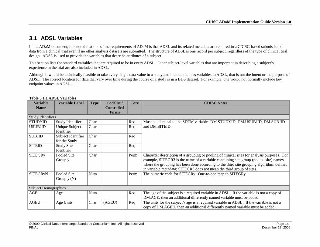
3.1 ADSL Variables
In the ADaM document, it is noted that one of the requirements of ADaM is that ADSL and its related metadata are required in a CDISC-based submission of
data from a clinical trial even if no other analysis datasets are submitted. The structure of ADSL is one record per subject, regardless of the type of clinical trial
design. ADSL is used to provide the variables that describe attributes of a subject.
This section lists the standard variables that are required to be in every ADSL. Other subject-level variables that are important in describing a subject’s
experience in the trial are also included in ADSL.
Although it would be technically feasible to take every single data value in a study and include them as variables in ADSL, that is not the intent or the purpose of
ADSL. The correct location for data that vary over time during the course of a study is in a BDS dataset. For example, one would not normally include key
endpoint values in ADSL.
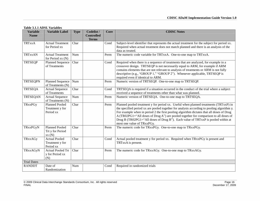
Table 3.1.1 ADSL Variables
Variable
Name
Variable Label Type Codelist /
Controlled
Terms
Core CDISC Notes
Study Identifiers
STUDYID Study Identifier Char Req Must be identical to the SDTM variables DM.STUDYID, DM.USUBJID, DM.SUBJID
and DM.SITEID. USUBJID Unique Subject
Identifier
Char Req
SUBJID Subject Identifier
for the Study
Char Req
SITEID Study Site
Identifier
Char Req
SITEGRy Pooled Site
Group y
Char Perm Character description of a grouping or pooling of clinical sites for analysis purposes. For
example, SITEGR3 is the name of a variable containing site group (pooled site) names,
where the grouping has been done according to the third site grouping algorithm, defined
in variable metadata; SITEGR3 does not mean the third group of sites.
SITEGRyN Pooled Site
Group y (N)
Num Perm The numeric code for SITEGRy. One-to-one map to SITEGRy.
Subject Demographics
AGE Age Num Req The age of the subject is a required variable in ADSL. If the variable is not a copy of
DM.AGE, then an additional differently named variable must be added.
AGEU Age Units Char (AGEU) Req The units for the subject’s age is a required variable in ADSL. If the variable is not a
copy of DM.AGEU, then an additional differently named variable must be added.

CDISC ADaM Implementation Guide Version 1.0
© 2009 Clinical Data Interchange Standards Consortium, Inc. All rights reserved Page 15 FINAL December 17, 2009
Table 3.1.1 ADSL Variables
Variable
Name
Variable Label Type Codelist /
Controlled
Terms
Core CDISC Notes
SEX Sex Char (SEX) Req The sex of the subject is a required variable in ADSL. If the variable is not a copy of
DM.SEX, then an additional differently named variable must be added.
RACE Race Char (RACE) Req The race of the subject is a required variable in ADSL. If the variable is not a copy of
DM.RACE, then an additional differently named variable must be added.
RACEGRy Pooled Race
Group y
Char Perm Character description of a grouping or pooling of subject race for analysis purposes.
RACEGRyN Pooled Race
Group y (N)
Num Perm The numeric code for RACEGRy. Orders the grouping or pooling of subject race for
analysis and reporting. One-to-one map to RACEGRy.
Population Indicator(s)
FASFL Full Analysis Set
Population Flag
Char Y, N Cond A character indicator variable is required for every population that is defined in the
statistical analysis plan. A minimum of one subject-level population flag variable is
required for every clinical trial. Additional population flags may be added. The values
of subject-level population flags cannot be blank. If a flag is used, the corresponding
numeric version (*FN) can also be included.
SAFFL Safety Population
Flag
Char Y, N Cond
ITTFL Intent-To-Treat
Population Flag
Char Y, N Cond
PPROTFL Per-Protocol
Population Flag
Char Y, N Cond
COMPLFL Completers
Population Flag
Char Y, N Cond
RANDFL Randomized
Population Flag
Char Y, N Cond
ENRLFL Enrolled
Population Flag
Char Y, N Cond
Treatment Variables
ARM Description of
Planned Arm
Char Req DM.ARM
TRTxxP Planned
Treatment for
Period xx
Char Req Subject-level identifier that represents the planned treatment for period xx. In a one-
period randomized trial, TRT01P would be the treatment to which the subject was
randomized. TRTxxP might be derived from the SDTM DM variable ARM. At least
TRT01P is required.
TRTxxPN Planned
Treatment for
Period xx (N)
Num Perm The numeric code variable for TRTxxP. One-to-one map to TRTxxP.
CDISC ADaM Implementation Guide Version 1.0
© 2009 Clinical Data Interchange Standards Consortium, Inc. All rights reserved Page 16 FINAL December 17, 2009
Table 3.1.1 ADSL Variables
Variable
Name
Variable Label Type Codelist /
Controlled
Terms
Core CDISC Notes
TRTxxA Actual Treatment
for Period xx
Char Cond Subject-level identifier that represents the actual treatment for the subject for period xx.
Required when actual treatment does not match planned and there is an analysis of the
data as treated.
TRTxxAN Actual Treatment
for Period xx (N)
Num Perm The numeric code variable for TRTxxA. One-to-one map to TRTxxA.
TRTSEQP Planned Sequence
of Treatments
Char Cond Required when there is a sequence of treatments that are analyzed, for example in a
crossover design. TRTSEQP is not necessarily equal to ARM, for example if ARM
contains elements that are not relevant to analysis of treatments or ARM is not fully
descriptive (e.g., “GROUP 1,” “GROUP 2”). Whenever applicable, TRTSEQP is
required even if identical to ARM.
TRTSEQPN Planned Sequence
of Treatments (N)
Num Perm Numeric version of TRTSEQP. One-to-one map to TRTSEQP.
TRTSEQA Actual Sequence
of Treatments
Char Cond TRTSEQA is required if a situation occurred in the conduct of the trial where a subject
received a sequence of treatments other than what was planned.
TRTSEQAN Actual Sequence
of Treatments (N)
Num Perm Numeric version of TRTSEQA. One-to-one map to TRTSEQA.
TRxxPGy Planned Pooled
Treatment y for
Period xx
Char Perm Planned pooled treatment y for period xx. Useful when planned treatments (TRTxxP) in
the specified period xx are pooled together for analysis according to pooling algorithm y.
For example when in period 2 the first pooling algorithm dictates that all doses of Drug
A (TR02PG1=“All doses of Drug A”) are pooled together for comparison to all doses of
Drug B (TR02PG1=“All doses of Drug B”). Each value of TRTxxP is pooled within at
most one value of TRxxPGy.
TRxxPGyN Planned Pooled
Trt y for Period
xx (N)
Char Perm The numeric code for TRxxPGy. One-to-one map to TRxxPGy.
TRxxAGy Actual Pooled
Treatment y for
Period xx
Char Cond Actual pooled treatment y for period xx. Required when TRxxPGy is present and
TRTxxA is present.
TRxxAGyN Actual Pooled Trt
y for Period xx
(N)
Char Perm The numeric code for TRxxAGy. One-to-one map to TRxxAGy.
Trial Dates
RANDDT Date of
Randomization
Num Cond Required in randomized trials

CDISC ADaM Implementation Guide Version 1.0
© 2009 Clinical Data Interchange Standards Consortium, Inc. All rights reserved Page 17 FINAL December 17, 2009
Table 3.1.1 ADSL Variables
Variable
Name
Variable Label Type Codelist /
Controlled
Terms
Core CDISC Notes
TRTSDT Date of First
Exposure to
Treatment
Num Cond Date of first exposure to treatment for a subject in a study. TRTSDT and/or TRTSDTM
are required if there is an investigational product.
TRTSTM Time of First
Exposure to
Treatment
Num Perm Time of first exposure to treatment for a subject in a study.
TRTSDTM Datetime of First
Exposure to
Treatment
Num Cond Datetime of first exposure to treatment for a subject in a study. TRTSDT and/or
TRTSDTM are required if there is an investigational product.
TRTSDTF Date of First
Exposure Imput.
Flag
Char (DATEFL) Cond The level of imputation of date of first exposure to treatment. See General Timing
Variable Convention #6.
TRTSTMF Time of First
Exposure Imput.
Flag
Char (TIMEFL) Cond The level of imputation of time of first exposure to treatment. See General Timing
Variable Convention #7.
TRTEDT Date of Last
Exposure to
Treatment
Num Cond Date of last exposure to treatment for a subject in a study. TRTEDT and/or TRTEDTM
are required if there is an investigational product.
TRTETM Time of Last
Exposure to
Treatment
Num Perm Time of last exposure to treatment for a subject in a study.
TRTEDTM Datetime of Last
Exposure to
Treatment
Num Cond Datetime of last exposure to treatment for a subject in a study. TRTEDT and/or
TRTEDTM are required if there is an investigational product.
TRTEDTF Date of Last
Exposure Imput.
Flag
Char (DATEFL) Cond The level of imputation of date of last exposure to treatment. See General Timing
Variable Convention #6.
TRTETMF Time of Last
Exposure Imput.
Flag
Char (TIMEFL) Cond The level of imputation of time of last exposure to treatment. See General Timing
Variable Convention #7.
TRxxSDT Date of First
Exposure in
Period xx
Num Cond Date of first exposure to treatment in period xx. TRxxSDT and/or TRxxSDTM is
required in trial designs where multiple treatments are given to the same subject, such as
a crossover design. Also useful in designs where multiple periods exist for the same
treatment (i.e., multiple cycles of the same study treatment).

CDISC ADaM Implementation Guide Version 1.0
© 2009 Clinical Data Interchange Standards Consortium, Inc. All rights reserved Page 18 FINAL December 17, 2009
Table 3.1.1 ADSL Variables
Variable
Name
Variable Label Type Codelist /
Controlled
Terms
Core CDISC Notes
TRxxSTM Time of First
Exposure in
Period xx
Num Cond The starting time of exposure in period xx. TRxxSTM and/or TRxxSDTM are required
in trial designs where multiple treatments are given to the same subject, such as a
crossover design, and time is important to the analysis.
TRxxSDTM Datetime of First
Exposure in
Period xx
Num Cond Datetime of first exposure to treatment in period xx. TRxxSDT and/or TRxxSDTM are
required in trial designs where multiple treatments are given to the same subject, such as
a crossover design.
TRxxSDTF Date 1st Exposure
Period xx Imput.
Flag
Char (DATEFL) Cond The level of imputation of date of first exposure to treatment in period xx. See General
Timing Variable Convention #6.
TRxxSTMF Time 1st
Exposure Period
xx Imput. Flag
Char (TIMEFL) Cond The level of imputation of time of first exposure in period xx. See General Timing
Variable Convention #7.
TRxxEDT Date of Last
Exposure in
Period xx
Num Cond Date of last exposure in period xx. TRxxEDT and/or TRxxEDTM are required in trial
designs where multiple treatments are given to the same subject, such as a crossover
design.
TRxxETM Time of Last
Exposure in
Period xx
Num Cond The ending time of exposure in period xx. TRxxETM and/or TRxxEDTM are required
in trial designs where multiple treatments are given to the same subject, such as a
crossover design, and ending time is important to the analysis.
TRxxEDTM Datetime of Last
Exposure in
Period xx
Num Cond The datetime of last exposure to treatment in period xx. TRxxEDT and/or TRxxEDTM
are required in trial designs where multiple treatments are given to the same subject, such
as a crossover design.
TRxxEDTF Date Last
Exposure Period
xx Imput. Flag
Char (DATEFL) Cond The level of imputation of date of last exposure in period xx. See General Timing
Variable Convention #6.
TRxxETMF Time Last
Exposure Period
xx Imput. Flag
Char (TIMEFL) Cond The level of imputation of time of last exposure in period xx. See General Timing
Variable Convention #7.
APxxSDT Period xx Start
Date
Num Perm The starting date of period xx.
APxxSTM Period xx Start
Time
Num Perm The starting time of period xx.
APxxSDTM Period xx Start
Datetime
Num Perm The starting datetime of period xx.
APxxSDTF Period xx Start
Date Imput. Flag
Char (DATEFL) Cond The level of imputation of period xx start date. See General Timing Variable Convention
#6.

CDISC ADaM Implementation Guide Version 1.0
© 2009 Clinical Data Interchange Standards Consortium, Inc. All rights reserved Page 19 FINAL December 17, 2009
Table 3.1.1 ADSL Variables
Variable
Name
Variable Label Type Codelist /
Controlled
Terms
Core CDISC Notes
APxxSTMF Period xx Start
Time Imput. Flag
Char (TIMEFL) Cond The level of imputation of period xx start time. See General Timing Variable Convention
#7.
APxxEDT Period xx End
Date
Num Perm The ending date of period xx.
APxxETM Period xx End
Time
Num Perm The ending time of period xx.
APxxEDTM Period xx End
Date/Time
Num Perm The ending datetime of period xx.
APxxEDTF Period xx End
Date Imput. Flag
Char (DATEFL) Cond The level of imputation of period xx end date. See General Timing Variable Convention
#6.
APxxETMF Period End Time
Imput. Flag
Char (TIMEFL) Cond The level of imputation of period xx end time. See General Timing Variable Convention
#7.
CDISC ADaM Implementation Guide Version 1.0
© 2009 Clinical Data Interchange Standards Consortium, Inc. All rights reserved Page 20 FINAL December 17, 2009
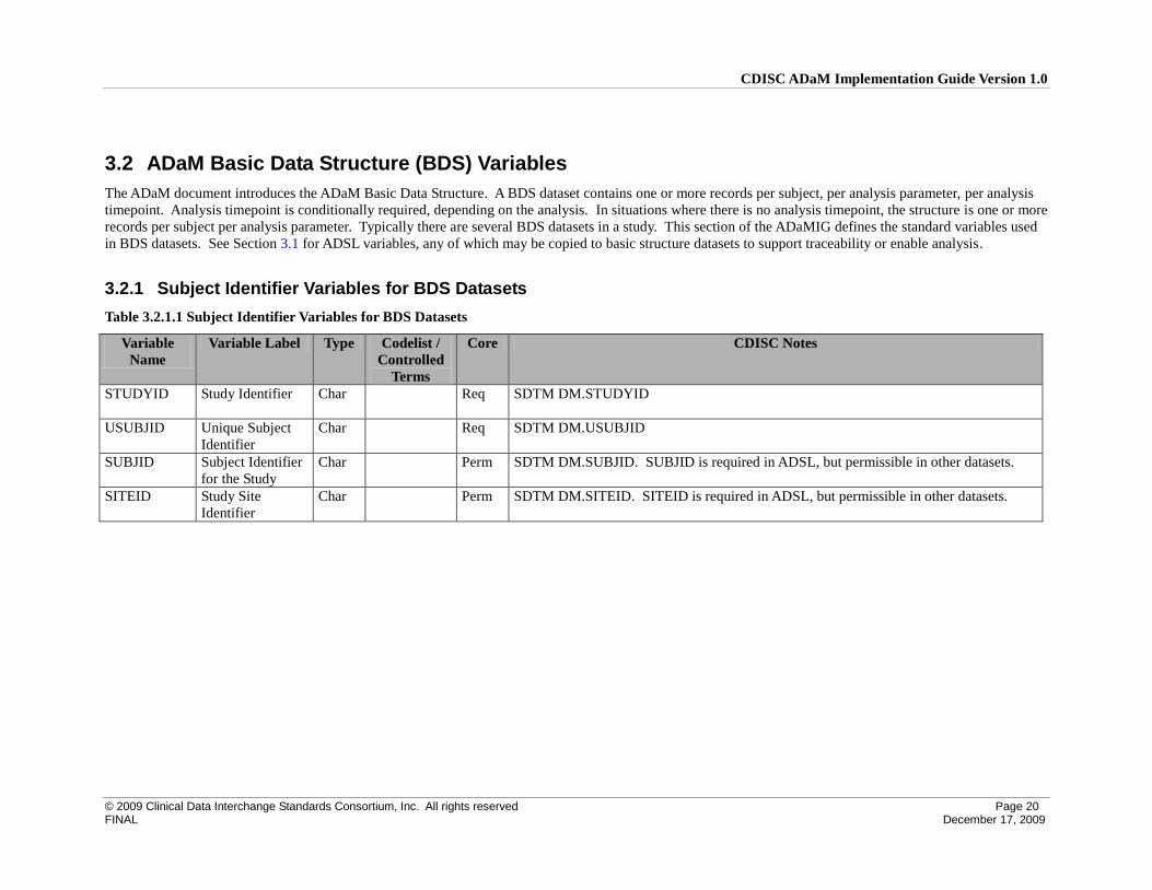
3.2 ADaM Basic Data Structure (BDS) Variables
The ADaM document introduces the ADaM Basic Data Structure. A BDS dataset contains one or more records per subject, per analysis parameter, per analysis
timepoint. Analysis timepoint is conditionally required, depending on the analysis. In situations where there is no analysis timepoint, the structure is one or more
records per subject per analysis parameter. Typically there are several BDS datasets in a study. This section of the ADaMIG defines the standard variables used
in BDS datasets. See Section 3.1 for ADSL variables, any of which may be copied to basic structure datasets to support traceability or enable analysis.
3.2.1 Subject Identifier Variables for BDS Datasets
Table 3.2.1.1 Subject Identifier Variables for BDS Datasets
Variable
Name
Variable Label Type Codelist /
Controlled
Terms
Core CDISC Notes
STUDYID Study Identifier Char Req SDTM DM.STUDYID
USUBJID Unique Subject
Identifier
Char Req SDTM DM.USUBJID
SUBJID Subject Identifier
for the Study
Char Perm SDTM DM.SUBJID. SUBJID is required in ADSL, but permissible in other datasets.
SITEID Study Site
Identifier
Char Perm SDTM DM.SITEID. SITEID is required in ADSL, but permissible in other datasets.

CDISC ADaM Implementation Guide Version 1.0
© 2009 Clinical Data Interchange Standards Consortium, Inc. All rights reserved Page 21 FINAL December 17, 2009
3.2.2 Treatment Variables for BDS Datasets
Table 3.2.2.1 Treatment Variables for BDS Datasets
Variable
Name
Variable Label Type Codelist /
Controlled
Terms
Core CDISC Notes
TRTP Planned
Treatment
Char Req TRTP is a record-level identifier that represents the planned treatment attributed to a
record for analysis purposes. TRTP indicates how treatment varies by record within a
subject and enables analysis of crossover and other designs. TRTxxP (copied from
ADSL) may also be needed for some analysis purposes, and may be useful for
traceability and to provide context.
TRTPN Planned
Treatment (N)
Num Perm The numeric code for TRTP. One-to-one map to TRTP.
TRTA Actual Treatment Char Cond TRTA is a record-level identifier that represents the actual treatment attributed to a
record for analysis purposes. TRTA indicates how treatment varies by record within a
subject and enables analysis of crossover and other multi-period designs. TRTxxA
(copied from ADSL) may also be needed for some analysis purposes, and may be useful
for traceability and to provide context. TRTA is required when there is an analysis of
data as treated and at least one subject has any data associated with a treatment other
than the planned treatment.
TRTAN Actual Treatment
(N)
Num Perm The numeric code for TRTA. One-to-one map to TRTA.
TRTPGy Planned Pooled
Treatment y
Char Perm Planned pooled treatment y. “y” represents an integer [1-9] corresponding to a
particular pooling scheme. Useful when planned treatments (TRTP) are pooled together
for analysis, for example when all doses of Drug A (TRTPG1=All doses of Drug A) are
compared to all doses of Drug B (TRTPG1=All doses of Drug B). Each value of TRTP
is pooled within at most one value of TRTPGy. May vary by record within a subject.
TRTPGyN Planned Pooled
Treatment y (N)
Num Perm The numeric code for TRTPGy. One-to-one map to TRTPGy.
TRTAGy Actual Pooled
Treatment y
Char Cond Actual pooled treatment y. “y” represents an integer [1-9] corresponding to a particular
pooling scheme. Required when TRTPGy is present and TRTA is present. May vary by
record within a subject.
TRTAGyN Actual Pooled
Treatment y (N)
Num Perm The numeric code for TRTAGy. One-to-one map to TRTAGy.
CDISC ADaM Implementation Guide Version 1.0
© 2009 Clinical Data Interchange Standards Consortium, Inc. All rights reserved Page 22 FINAL December 17, 2009
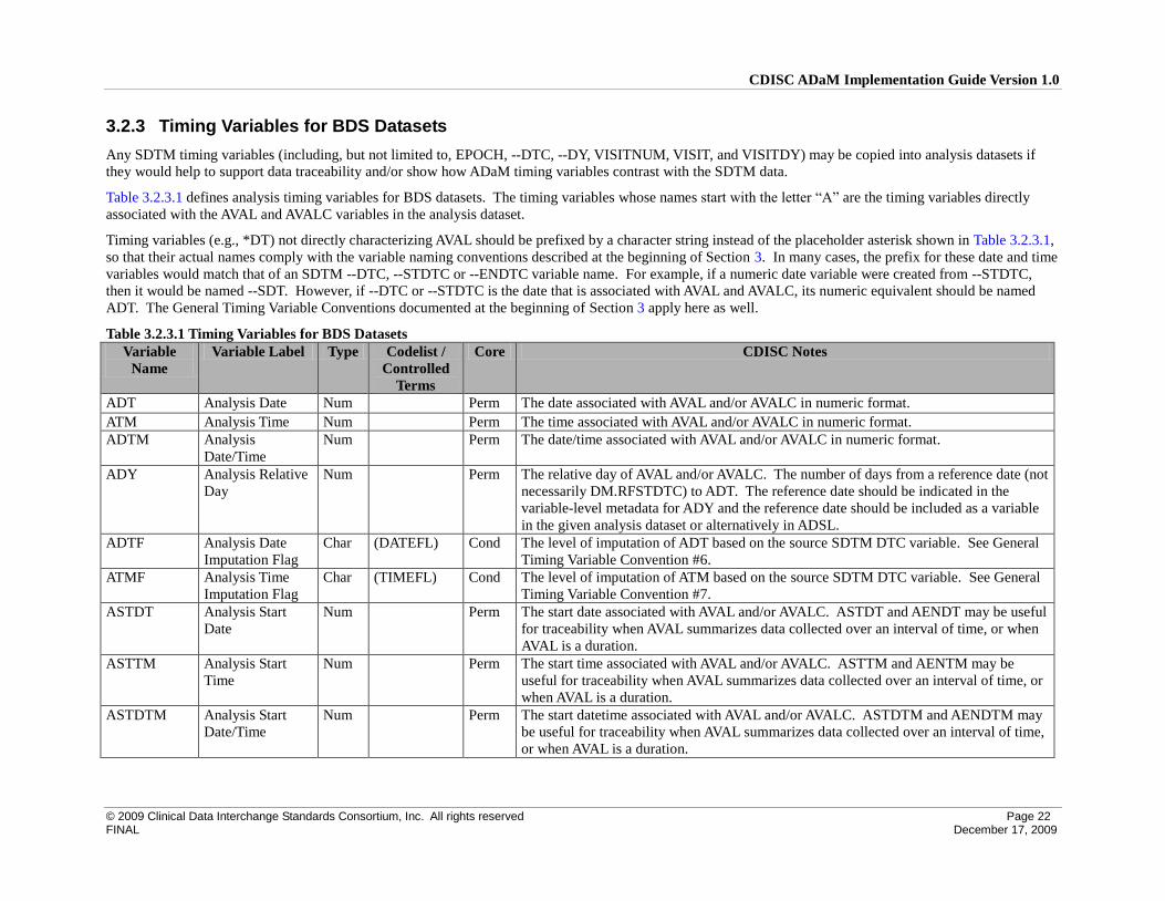
3.2.3 Timing Variables for BDS Datasets
Any SDTM timing variables (including, but not limited to, EPOCH, --DTC, --DY, VISITNUM, VISIT, and VISITDY) may be copied into analysis datasets if
they would help to support data traceability and/or show how ADaM timing variables contrast with the SDTM data.
Table 3.2.3.1 defines analysis timing variables for BDS datasets. The timing variables whose names start with the letter “A” are the timing variables directly
associated with the AVAL and AVALC variables in the analysis dataset.
Timing variables (e.g., *DT) not directly characterizing AVAL should be prefixed by a character string instead of the placeholder asterisk shown in Table 3.2.3.1,
so that their actual names comply with the variable naming conventions described at the beginning of Section 3. In many cases, the prefix for these date and time
variables would match that of an SDTM --DTC, --STDTC or --ENDTC variable name. For example, if a numeric date variable were created from --STDTC,
then it would be named --SDT. However, if --DTC or --STDTC is the date that is associated with AVAL and AVALC, its numeric equivalent should be named
ADT. The General Timing Variable Conventions documented at the beginning of Section 3 apply here as well.
Table 3.2.3.1 Timing Variables for BDS Datasets
Variable
Name
Variable Label Type Codelist /
Controlled
Terms
Core CDISC Notes
ADT Analysis Date Num Perm The date associated with AVAL and/or AVALC in numeric format.
ATM Analysis Time Num Perm The time associated with AVAL and/or AVALC in numeric format.
ADTM Analysis
Date/Time
Num Perm The date/time associated with AVAL and/or AVALC in numeric format.
ADY Analysis Relative
Day
Num Perm The relative day of AVAL and/or AVALC. The number of days from a reference date (not
necessarily DM.RFSTDTC) to ADT. The reference date should be indicated in the
variable-level metadata for ADY and the reference date should be included as a variable
in the given analysis dataset or alternatively in ADSL.
ADTF Analysis Date
Imputation Flag
Char (DATEFL) Cond The level of imputation of ADT based on the source SDTM DTC variable. See General
Timing Variable Convention #6.
ATMF Analysis Time
Imputation Flag
Char (TIMEFL) Cond The level of imputation of ATM based on the source SDTM DTC variable. See General
Timing Variable Convention #7.
ASTDT Analysis Start
Date
Num Perm The start date associated with AVAL and/or AVALC. ASTDT and AENDT may be useful
for traceability when AVAL summarizes data collected over an interval of time, or when
AVAL is a duration.
ASTTM Analysis Start
Time
Num Perm The start time associated with AVAL and/or AVALC. ASTTM and AENTM may be
useful for traceability when AVAL summarizes data collected over an interval of time, or
when AVAL is a duration.
ASTDTM Analysis Start
Date/Time
Num Perm The start datetime associated with AVAL and/or AVALC. ASTDTM and AENDTM may
be useful for traceability when AVAL summarizes data collected over an interval of time,
or when AVAL is a duration.

CDISC ADaM Implementation Guide Version 1.0
© 2009 Clinical Data Interchange Standards Consortium, Inc. All rights reserved Page 23 FINAL December 17, 2009
Table 3.2.3.1 Timing Variables for BDS Datasets
Variable
Name
Variable Label Type Codelist /
Controlled
Terms
Core CDISC Notes
ASTDY Analysis Start
Relative Day
Num Perm The number of days from a reference date (not necessarily DM.RFSTDTC) to ASTDT.
The reference date variable should be indicated in the variable-level metadata for
ASTDY and the reference date variable should be included as a variable in an analysis
dataset (typically, but not necessarily, ADSL).
ASTDTF Analysis Start
Date Imputation
Flag
Char (DATEFL) Cond The level of imputation of ASTDT based on the source SDTM DTC variable. See
General Timing Variable Convention #6.
ASTTMF Analysis Start
Time Imputation
Flag
Char (TIMEFL) Cond The level of imputation of ASTTM based on the source SDTM DTC variable. See
General Timing Variable Convention #7.
AENDT Analysis End
Date
Num Perm The end date associated with AVAL and/or AVALC. See also ASTDT.
AENTM Analysis End
Time
Num Perm The end time associated with AVAL and/or AVALC. See also ASTTM.
AENDTM Analysis End
Date/Time
Num Perm The end datetime associated with AVAL and/or AVALC. See also ASTDTM.
AENDY Analysis End
Relative Day
Num Perm The number of days from a reference date (not necessarily DM.RFSTDTC) to AENDT.
See also ASTDY.
AENDTF Analysis End
Date Imputation
Flag
Char (DATEFL) Cond The level of imputation of AENDT based on the source SDTM DTC variable. See
General Timing Variable Convention #6.
AENTMF Analysis End
Time Imputation
Flag
Char (TIMEFL) Cond The level of imputation of AENTM based on the source SDTM DTC variable. See
General Timing Variable Convention #7.
CDISC ADaM Implementation Guide Version 1.0
© 2009 Clinical Data Interchange Standards Consortium, Inc. All rights reserved Page 24 FINAL December 17, 2009
Table 3.2.3.1 Timing Variables for BDS Datasets
Variable
Name
Variable Label Type Codelist /
Controlled
Terms
Core CDISC Notes
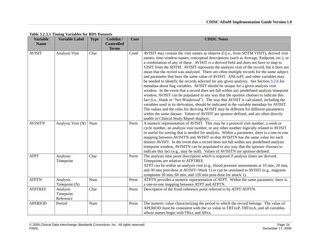
AVISIT Analysis Visit Char Cond AVISIT may contain the visit names as observe d (i.e., from SDTM VISIT), derived visit
names, time window names, conceptual descriptions (such as Average, Endpoint, etc.), or
a combination of any of these. AVISIT is a derived field and does not have to map to
VISIT from the SDTM. AVISIT represents the analysis visit of the record, but it does not
mean that the record was analyzed. There are often multiple records for the same subject
and parameter that have the same value of AVISIT. ANLzzFL and other variables may
be needed to identify the records selected for any given analysis. See Section 3.2.6 for
metadata about flag variables. AVISIT should be unique for a given analysis visit
window. In the event that a record does not fall within any predefined analysis timepoint
window, AVISIT can be populated in any way that the sponsor chooses to indicate this
fact (i.e., blank or “Not Windowed”). The way that AVISIT is calculated, including the
variables used in its derivation, should be indicated in the variable metadata for AVISIT.
The values and the rules for deriving AVISIT may be different for different parameters
within the same dataset. Values of AVISIT are sponsor-defined, and are often directly
usable in Clinical Study Report displays.
AVISITN Analysis Visit (N) Num Perm A numeric representation of AVISIT. This may be a protocol visit number, a week or
cycle number, an analysis visit number, or any other number logically related to AVISIT
or useful for sorting that is needed for analysis. Within a parameter, there is a one-to-one
mapping between AVISITN and AVISIT so that AVISITN has the same value for each
distinct AVISIT. In the event that a record does not fall within any predefined analysis
timepoint window, AVISITN can be populated in any way that the sponsor chooses to
indicate this fact (e.g., may be null). Values of AVISITN are sponsor-defined.
ATPT Analysis
Timepoint
Char Perm The analysis time point description which is required if analysis times are derived.
Timepoints are relative to ATPTREF.
ATPT can be within an analysis visit (e.g., blood pressure assessments at 10 min, 20 min,
and 30 min post-dose at AVISIT=Week 1) or can be unrelated to AVISIT (e.g., migraine
symptoms 30 min, 60 min, and 120 min post-dose for attack 1).
ATPTN Analysis
Timepoint (N)
Num Perm ATPTN provides a numeric representation of ATPT. Within the same parameter, there is
a one-to-one mapping between ATPT and ATPTN.
ATPTREF Analysis
Timepoint
Reference
Char Perm Description of the fixed reference point referred to by ATPT/ATPTN.
APERIOD Period Num Perm The numeric value characterizing the period to which the record belongs. The value of
APERIOD must be consistent with the xx value in TRTxxP, TRTxxA, and all variables
whose names begin with TRxx and APxx.

CDISC ADaM Implementation Guide Version 1.0
© 2009 Clinical Data Interchange Standards Consortium, Inc. All rights reserved Page 25 FINAL December 17, 2009
Table 3.2.3.1 Timing Variables for BDS Datasets
Variable
Name
Variable Label Type Codelist /
Controlled
Terms
Core CDISC Notes
APERIODC Period (C) Char Perm Text characterizing to which period the record belongs. One-to-one map to APERIOD.
APHASE Phase Char Perm Generally, a higher-level categorization of APERIOD. Does not replace APERIOD,
because APERIOD provides the indexing for the TRxx and APxx variables.
ARELTM Analysis Relative
Time
Num Perm The time relative to an anchor time. When ARELTM is present, the anchor time variable
and ARELTMU must also be included in the dataset, and the anchor time variable must
be identified in the metadata for ARELTM.
ARELTMU Analysis Relative
Time Unit
Char Cond The units of ARELTM. For example, “HOURS” or “MINUTES.” ARELTMU is
required if ARELTM is present.
APERSDT Period Start Date Num Perm The starting date for the period defined by APERIOD.
APERSTM Period Start Time Num Perm The starting time for the period defined by APERIOD.
APERSDTM Period Start
Date/Time
Num Perm The starting datetime for the period defined by APERIOD.
APERSDTF Period Start Date
Imput. Flag
Char (DATEFL) Cond The level of imputation of APERSDT based on the source SDTM DTC variable. See
General Timing Variable Convention #6.
APERSTMF Period Start Time
Imput. Flag
Char (TIMEFL) Cond The level of imputation of APERSTM based on the source SDTM DTC variable. See
General Timing Variable Convention #7.
APEREDT Period End Date Num Perm The ending date for the period defined by APERIOD.
APERETM Period End Time Num Perm The ending time for the period defined by APERIOD.
APEREDTM Period End
Date/Time
Num Perm The ending datetime for the period defined by APERIOD.
APEREDTF Period End Date
Imput. Flag
Char (DATEFL) Cond The level of imputation of APEREDT based on the source SDTM DTC variable. See
General Timing Variable Convention #6.
APERETMF Period End Time
Imput. Flag
Char (TIMEFL) Cond The level of imputation of APERETM based on the source SDTM DTC variable. See
General Timing Variable Convention #7.
The following timing variables are not directly descriptive of the analysis value (AVAL and/or AVALC) but may be included for support of review. There may
be a number of “sets” of these variables as indicated by the “*” prefix. See General Timing Variable Convention #11 for important cautions regarding the
“*” prefix.
*DT Date of … Num Perm Analysis date not directly characterizing AVAL and/or AVALC in numeric format.
*TM Time of … Num Perm Analysis time not directly characterizing AVAL and/or AVALC in numeric format.
*DTM Date/Time of … Num Perm Analysis date/time not directly characterizing AVAL and/or AVALC in numeric format.
*ADY Relative Day of
…
Num Perm Analysis relative day not directly characterizing AVAL and/or AVALC.
*DTF Date Imputation
Qual of …
Char (DATEFL) Cond The level of imputation of *DT based on the source SDTM DTC variable. See General
Timing Variable Convention #6.

CDISC ADaM Implementation Guide Version 1.0
© 2009 Clinical Data Interchange Standards Consortium, Inc. All rights reserved Page 26 FINAL December 17, 2009
Table 3.2.3.1 Timing Variables for BDS Datasets
Variable
Name
Variable Label Type Codelist /
Controlled
Terms
Core CDISC Notes
*TMF Time Imputation
Flag of …
Char (TIMEFL) Cond The level of imputation of *TM based on the source SDTM DTC variable. See General
Timing Variable Convention #7.
*SDT Start Date of … Num Perm Starting analysis date not directly characterizing AVAL and/or AVALC in numeric
format.
*STM Start Time of … Num Perm Starting analysis time not directly characterizing AVAL and/or AVALC in numeric
format.
*SDTM Start Date/Time
of …
Num Perm Starting analysis date/time not directly characterizing AVAL and/or AVALC in numeric
format.
*SDY Relative Start Day
of …
Num Perm Starting analysis relative day not directly characterizing AVAL and/or AVALC.
*SDTF Start Date
Imputation Flag
of …
Char (DATEFL) Cond The level of imputation of *SDT based on the source SDTM DTC variable. See General
Timing Variable Convention #6.
*STMF Start Time
Imputation Qual
of …
Char (TIMEFL) Cond The level of imputation of *STM based on the source SDTM DTC variable. See General
Timing Variable Convention #7.
*EDT End Date of … Num Perm Ending analysis date not directly characterizing AVAL and/or AVALC in numeric format.
*ETM End Time of … Num Perm Ending analysis time not directly characterizing AVAL and/or AVALC in numeric format.
*EDTM End Date/Time of
…
Num Perm Ending analysis date/time not directly characterizing AVAL and/or AVALC in numeric
format.
*EDY Relative End Day
of …
Num Perm Ending analysis relative day not directly characterizing AVAL and/or AVALC.
*EDTF End Date
Imputation Flag
of …
Char (DATEFL) Cond The level of imputation of *EDT based on the source SDTM DTC variable. See General
Timing Variable Convention #6.
*ETMF End Time
Imputation Flag
of …
Char (TIMEFL) Cond The level of imputation of *ETM based on the source SDTM DTC variable. See General
Timing Variable Convention #7.
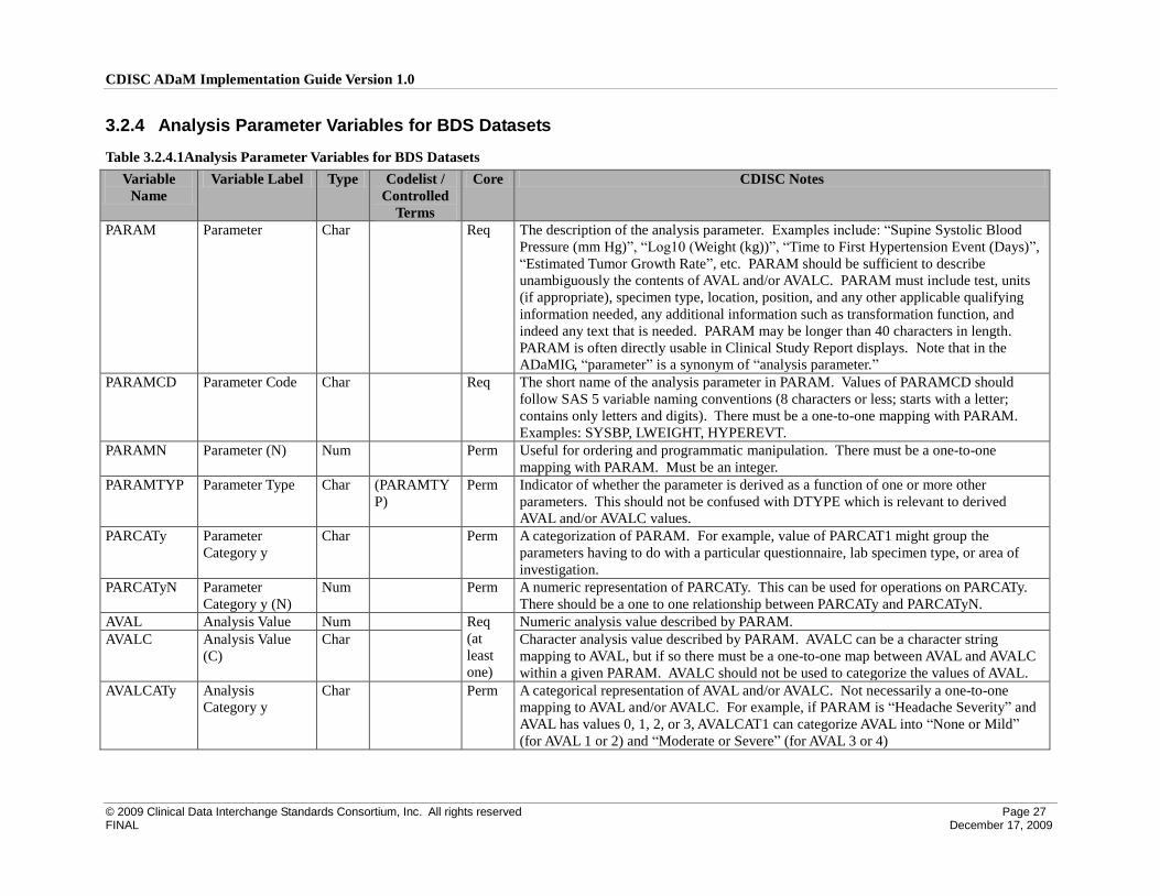
CDISC ADaM Implementation Guide Version 1.0
© 2009 Clinical Data Interchange Standards Consortium, Inc. All rights reserved Page 27 FINAL December 17, 2009
3.2.4 Analysis Parameter Variables for BDS Datasets
Table 3.2.4.1Analysis Parameter Variables for BDS Datasets
Variable
Name
Variable Label Type Codelist /
Controlled
Terms
Core CDISC Notes
PARAM Parameter Char Req The description of the analysis parameter. Examples include: “Supine Systolic Blood
Pressure (mm Hg)”, “Log10 (Weight (kg))”, “Time to First Hypertension Event (Days)”,
“Estimated Tumor Growth Rate”, etc. PARAM should be sufficient to describe
unambiguously the contents of AVAL and/or AVALC. PARAM must include test, units
(if appropriate), specimen type, location, position, and any other applicable qualifying
information needed, any additional information such as transformation function, and
indeed any text that is needed. PARAM may be longer than 40 characters in length.
PARAM is often directly usable in Clinical Study Report displays. Note that in the
ADaMIG, “parameter” is a synonym of “analysis parameter.”
PARAMCD Parameter Code Char Req The short name of the analysis parameter in PARAM. Values of PARAMCD should
follow SAS 5 variable naming conventions (8 characters or less; starts with a letter;
contains only letters and digits). There must be a one-to-one mapping with PARAM.
Examples: SYSBP, LWEIGHT, HYPEREVT.
PARAMN Parameter (N) Num Perm Useful for ordering and programmatic manipulation. There must be a one-to-one
mapping with PARAM. Must be an integer.
PARAMTYP Parameter Type Char (PARAMTY
P)
Perm Indicator of whether the parameter is derived as a function of one or more other
parameters. This should not be confused with DTYPE which is relevant to derived
AVAL and/or AVALC values.
PARCATy Parameter
Category y
Char Perm A categorization of PARAM. For example, value of PARCAT1 might group the
parameters having to do with a particular questionnaire, lab specimen type, or area of
investigation.
PARCATyN Parameter
Category y (N)
Num Perm A numeric representation of PARCATy. This can be used for operations on PARCATy.
There should be a one to one relationship between PARCATy and PARCATyN.
AVAL Analysis Value Num Req
(at
least
one)
Numeric analysis value described by PARAM.
AVALC Analysis Value
(C)
Char Character analysis value described by PARAM. AVALC can be a character string
mapping to AVAL, but if so there must be a one-to-one map between AVAL and AVALC
within a given PARAM. AVALC should not be used to categorize the values of AVAL.
AVALCATy Analysis
Category y
Char Perm A categorical representation of AVAL and/or AVALC. Not necessarily a one-to-one
mapping to AVAL and/or AVALC. For example, if PARAM is “Headache Severity” and
AVAL has values 0, 1, 2, or 3, AVALCAT1 can categorize AVAL into “None or Mild”
(for AVAL 1 or 2) and “Moderate or Severe” (for AVAL 3 or 4)
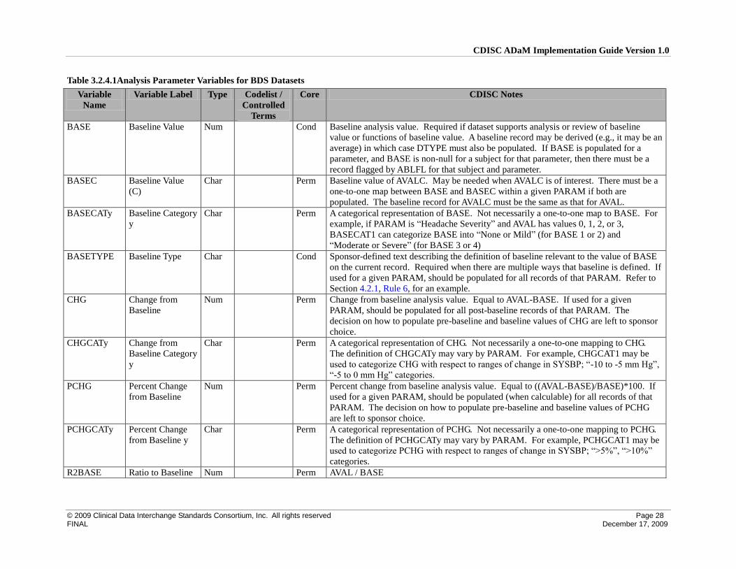
CDISC ADaM Implementation Guide Version 1.0
© 2009 Clinical Data Interchange Standards Consortium, Inc. All rights reserved Page 28 FINAL December 17, 2009
Table 3.2.4.1Analysis Parameter Variables for BDS Datasets
Variable
Name
Variable Label Type Codelist /
Controlled
Terms
Core CDISC Notes
BASE Baseline Value Num Cond Baseline analysis value. Required if dataset supports analysis or review of baseline
value or functions of baseline value. A baseline record may be derived (e.g., it may be an
average) in which case DTYPE must also be populated. If BASE is populated for a
parameter, and BASE is non-null for a subject for that parameter, then there must be a
record flagged by ABLFL for that subject and parameter.
BASEC Baseline Value
(C)
Char Perm Baseline value of AVALC. May be needed when AVALC is of interest. There must be a
one-to-one map between BASE and BASEC within a given PARAM if both are
populated. The baseline record for AVALC must be the same as that for AVAL.
BASECATy Baseline Category
y
Char Perm A categorical representation of BASE. Not necessarily a one-to-one map to BASE. For
example, if PARAM is “Headache Severity” and AVAL has values 0, 1, 2, or 3,
BASECAT1 can categorize BASE into “None or Mild” (for BASE 1 or 2) and
“Moderate or Severe” (for BASE 3 or 4)
BASETYPE Baseline Type Char Cond Sponsor-defined text describing the definition of baseline relevant to the value of BASE
on the current record. Required when there are multiple ways that baseline is defined. If
used for a given PARAM, should be populated for all records of that PARAM. Refer to
Section 4.2.1, Rule 6, for an example.
CHG Change from
Baseline
Num Perm Change from baseline analysis value. Equal to AVAL-BASE. If used for a given
PARAM, should be populated for all post-baseline records of that PARAM. The
decision on how to populate pre-baseline and baseline values of CHG are left to sponsor
choice.
CHGCATy Change from
Baseline Category
y
Char Perm A categorical representation of CHG. Not necessarily a one-to-one mapping to CHG.
The definition of CHGCATy may vary by PARAM. For example, CHGCAT1 may be
used to categorize CHG with respect to ranges of change in SYSBP; “-10 to -5 mm Hg”,
“-5 to 0 mm Hg” categories.
PCHG Percent Change
from Baseline
Num Perm Percent change from baseline analysis value. Equal to ((AVAL-BASE)/BASE)*100. If
used for a given PARAM, should be populated (when calculable) for all records of that
PARAM. The decision on how to populate pre-baseline and baseline values of PCHG
are left to sponsor choice.
PCHGCATy Percent Change
from Baseline y
Char Perm A categorical representation of PCHG. Not necessarily a one-to-one mapping to PCHG.
The definition of PCHGCATy may vary by PARAM. For example, PCHGCAT1 may be
used to categorize PCHG with respect to ranges of change in SYSBP; “>5%”, “>10%”
categories.
R2BASE Ratio to Baseline Num Perm AVAL / BASE
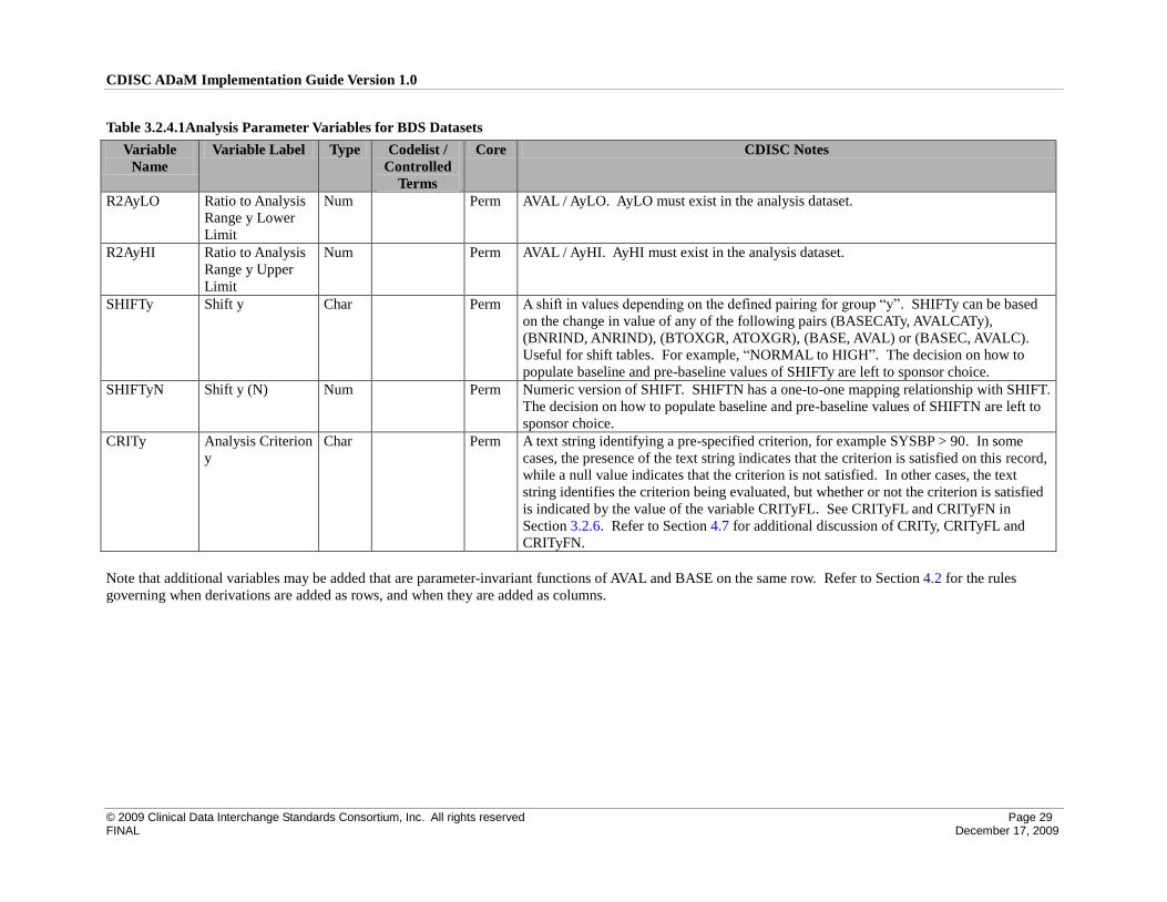
CDISC ADaM Implementation Guide Version 1.0
© 2009 Clinical Data Interchange Standards Consortium, Inc. All rights reserved Page 29 FINAL December 17, 2009
Table 3.2.4.1Analysis Parameter Variables for BDS Datasets
Variable
Name
Variable Label Type Codelist /
Controlled
Terms
Core CDISC Notes
R2AyLO Ratio to Analysis
Range y Lower
Limit
Num Perm AVAL / AyLO. AyLO must exist in the analysis dataset.
R2AyHI Ratio to Analysis
Range y Upper
Limit
Num Perm AVAL / AyHI. AyHI must exist in the analysis dataset.
SHIFTy Shift y Char Perm A shift in values depending on the defined pairing for group “y”. SHIFTy can be based
on the change in value of any of the following pairs (BASECATy, AVALCATy),
(BNRIND, ANRIND), (BTOXGR, ATOXGR), (BASE, AVAL) or (BASEC, AVALC).
Useful for shift tables. For example, “NORMAL to HIGH”. The decision on how to
populate baseline and pre-baseline values of SHIFTy are left to sponsor choice.
SHIFTyN Shift y (N) Num Perm Numeric version of SHIFT. SHIFTN has a one-to-one mapping relationship with SHIFT.
The decision on how to populate baseline and pre-baseline values of SHIFTN are left to
sponsor choice.
CRITy Analysis Criterion
y
Char Perm A text string identifying a pre-specified criterion, for example SYSBP > 90. In some
cases, the presence of the text string indicates that the criterion is satisfied on this record,
while a null value indicates that the criterion is not satisfied. In other cases, the text
string identifies the criterion being evaluated, but whether or not the criterion is satisfied
is indicated by the value of the variable CRITyFL. See CRITyFL and CRITyFN in
Section 3.2.6. Refer to Section 4.7 for additional discussion of CRITy, CRITyFL and
CRITyFN.
Note that additional variables may be added that are parameter-invariant functions of AVAL and BASE on the same row. Refer to Section 4.2 for the rules
governing when derivations are added as rows, and when they are added as columns.
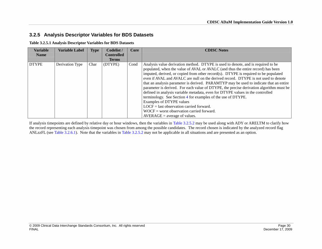
CDISC ADaM Implementation Guide Version 1.0
© 2009 Clinical Data Interchange Standards Consortium, Inc. All rights reserved Page 30 FINAL December 17, 2009
3.2.5 Analysis Descriptor Variables for BDS Datasets
Table 3.2.5.1 Analysis Descriptor Variables for BDS Datasets
Variable
Name
Variable Label Type Codelist /
Controlled
Terms
Core CDISC Notes
DTYPE Derivation Type Char (DTYPE) Cond Analysis value derivation method. DTYPE is used to denote, and is required to be
populated, when the value of AVAL or AVALC (and thus the entire record) has been
imputed, derived, or copied from other record(s). DTYPE is required to be populated
even if AVAL and AVALC are null on the derived record. DTYPE is not used to denote
that an analysis parameter is derived. PARAMTYP may be used to indicate that an entire
parameter is derived. For each value of DTYPE, the precise derivation algorithm must be
defined in analysis variable metadata, even for DTYPE values in the controlled
terminology. See Section 4 for examples of the use of DTYPE.
Examples of DTYPE values
LOCF = last observation carried forward.
WOCF = worst observation carried forward.
AVERAGE = average of values.
If analysis timepoints are defined by relative day or hour windows, then the variables in Table 3.2.5.2 may be used along with ADY or ARELTM to clarify how
the record representing each analysis timepoint was chosen from among the possible candidates. The record chosen is indicated by the analyzed record flag
ANLzzFL (see Table 3.2.6.1). Note that the variables in Table 3.2.5.2 may not be applicable in all situations and are presented as an option.

CDISC ADaM Implementation Guide Version 1.0
© 2009 Clinical Data Interchange Standards Consortium, Inc. All rights reserved Page 31 FINAL December 17, 2009
Table 3.2.5.2 Analysis Visit Windowing Variables for BDS Datasets
Variable
Name
Variable
Label
Type Codelist /
Controlled
Terms
Core CDISC Notes
AWRANGE Analysis Window
Valid Relative
Range
Char Perm The range of values that are valid for a given analysis timepoint (a given value of
AVISIT). For example, “5-9 DAYS”.
AWTARGET Analysis Window
Target
Num Perm The target or most desired analysis relative day (ADY) value or analysis relative time
(ARELTM) value for a given value of AVISIT.
AWTDIFF Analysis Window
Diff from Target
Num Perm Absolute difference between ADY or ARELTM and AWTARGET. It will be necessary to
adjust for the fact that there is no day 0 in the event that ADY and AWTARGET are not of
the same sign.
If the sign of the difference is important, then AWTDIFF might have to be used in
conjunction with ADY or ARELTM and possibly AWTARGET when choosing among
records.
AWLO Analysis Window
Beginning
Timepoint
Num Perm The value of the beginning timepoint (inclusive) needs to be used in conjunction to
AWRANGE. For example, if AWRANGE is“5-9 DAYS”, then AWLO is “5”.
AWHI Analysis Window
Ending Timepoint
Num Perm The value of the ending timepoint (inclusive) needs to be used in conjunction to
AWRANGE. For example, if AWRANGE is“5-9 DAYS”, then AWHI is “9”.
AWU Analysis Window
Unit
Char Perm Unit used for AWLO and AWHI. Examples: DAYS, HOURS.
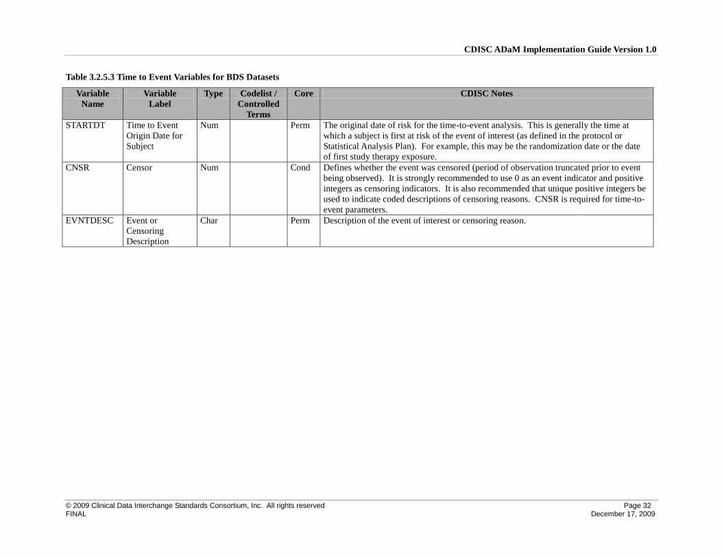
CDISC ADaM Implementation Guide Version 1.0
© 2009 Clinical Data Interchange Standards Consortium, Inc. All rights reserved Page 32 FINAL December 17, 2009
Table 3.2.5.3 Time to Event Variables for BDS Datasets
Variable
Name
Variable
Label
Type Codelist /
Controlled
Terms
Core CDISC Notes
STARTDT Time to Event
Origin Date for
Subject
Num Perm The original date of risk for the time-to-event analysis. This is generally the time at
which a subject is first at risk of the event of interest (as defined in the protocol or
Statistical Analysis Plan). For example, this may be the randomization date or the date
of first study therapy exposure.
CNSR Censor Num Cond Defines whether the event was censored (period of observation truncated prior to event
being observed). It is strongly recommended to use 0 as an event indicator and positive
integers as censoring indicators. It is also recommended that unique positive integers be
used to indicate coded descriptions of censoring reasons. CNSR is required for time-to-
event parameters.
EVNTDESC Event or
Censoring
Description
Char Perm Description of the event of interest or censoring reason.

CDISC ADaM Implementation Guide Version 1.0
© 2009 Clinical Data Interchange Standards Consortium, Inc. All rights reserved Page 33 FINAL December 17, 2009
Table 3.2.5.4 Lab Related Analysis Variables for BDS Datasets
Variable
Name
Variable
Label
Type Codelist /
Controlled
Terms
Core CDISC Notes
ATOXGR Analysis Toxicity
Grade
Char Perm Toxicity grade for analysis; may be based on SDTM --TOXGR or an imputed or
assigned value.
BTOXGR Baseline Toxicity
Grade
Char Perm ATOXGR of the baseline record identified by ABLFL.
ANRIND Analysis
Reference Range
Indicator
Char Perm Normal range indicator for analysis; may be based on SDTM --NRIND or an imputed or
assigned value.
BNRIND Baseline
Reference Range
Indicator
Char Perm ANRIND of the baseline record identified by ABLFL.
ANRLO Analysis Normal
Range Lower
Limit
Char Perm Normal range lower limit for analysis; may be based on SDTM --NRLO or an imputed
or assigned value.
ANRHI Analysis Normal
Range Upper
Limit
Char Perm Normal range upper limit for analysis; may be based on SDTM --NRHI or an imputed or
assigned value.
AyLO Analysis Range y
Lower Limit
Char Cond AyLO and/or AyHI are used where there are multiple ranges used for analysis. AyLO
and/or AyHI are created to capture the different levels of cutoff values used to determine
whether an analysis is within a clinically acceptable value range or outside that value
range. AyLO and/or AyHI are usually but not necessarily constants, parameter-specific
constants, or subject-specific constants. AyLO must be included if R2AyLO is included
in the dataset.
AyHI Analysis Range y
Upper Limit
Char Cond See AyLO.
For example, if ECG QTc values are summarized based on values 450, values >480, and
values >500, there is a need for 3 “hi value” range variables to calculate values against:
A1HI=450, A2HI=480, A3HI=500.
AyHI must be included if R2AyHI is included in the dataset.
3.2.6 Indicator Variables for BDS Datasets
See Section 3.2.7 for a discussion of the differences between ADaM population and baseline flags and the flags in SDTMIG 3.1.1 and 3.1.2.
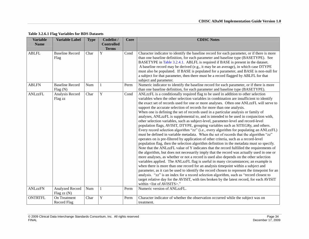
CDISC ADaM Implementation Guide Version 1.0
© 2009 Clinical Data Interchange Standards Consortium, Inc. All rights reserved Page 34 FINAL December 17, 2009
Table 3.2.6.1 Flag Variables for BDS Datasets
Variable
Name
Variable Label Type Codelist /
Controlled
Terms
Core CDISC Notes
ABLFL Baseline Record
Flag
Char Y
Cond Character indicator to identify the baseline record for each parameter, or if there is more
than one baseline definition, for each parameter and baseline type (BASETYPE). See
BASETYPE in Table 3.2.4.1. ABLFL is required if BASE is present in the dataset.
A baseline record may be derived (e.g., it may be an average), in which case DTYPE
must also be populated. If BASE is populated for a parameter, and BASE is non-null for
a subject for that parameter, then there must be a record flagged by ABLFL for that
subject and parameter.
ABLFN Baseline Record
Flag (N)
Num 1 Perm Numeric indicator to identify the baseline record for each parameter, or if there is more
than one baseline definition, for each parameter and baseline type (BASETYPE).
ANLzzFL Analysis Record
Flag zz
Char Y Cond ANLzzFL is a conditionally required flag to be used in addition to other selection
variables when the other selection variables in combination are insufficient to identify
the exact set of records used for one or more analyses. Often one ANLzzFL will serve to
support the accurate selection of records for more than one analysis.
When one is defining the set of records used in a particular analysis or family of
analyses, ANLzzFL is supplemental to, and is intended to be used in conjunction with,
other selection variables, such as subject-level, parameter-level and record-level
population flags, AVISIT, DTYPE, grouping variables such as SITEGRy, and others.
Every record selection algorithm “zz” (i.e., every algorithm for populating an ANLzzFL)
must be defined in variable metadata. When the set of records that the algorithm “zz”
operates on is pre-filtered by application of other criteria, such as a record-level
population flag, then the selection algorithm definition in the metadata must so specify.
Note that the ANLzzFL value of Y indicates that the record fulfilled the requirements of
the algorithm, but does not necessarily imply that the record was actually used in one or
more analyses, as whether or not a record is used also depends on the other selection
variables applied. The ANLzzFL flag is useful in many circumstances; an example is
when there is more than one record for an analysis timepoint within a subject and
parameter, as it can be used to identify the record chosen to represent the timepoint for an
analysis. “zz” is an index for a record selection algorithm, such as “record closest to
target relative day for the AVISIT, with ties broken by the latest record, for each AVISIT
within <list of AVISITS>.”
ANLzzFN Analyzed Record
Flag zz (N)
Num 1 Perm Numeric version of ANLzzFL.
ONTRTFL On Treatment
Record Flag
Char Y Perm Character indicator of whether the observation occurred while the subject was on
treatment.
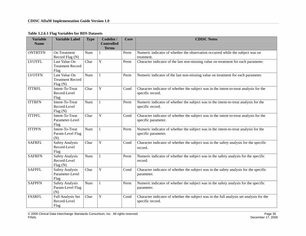
CDISC ADaM Implementation Guide Version 1.0
© 2009 Clinical Data Interchange Standards Consortium, Inc. All rights reserved Page 35 FINAL December 17, 2009
Table 3.2.6.1 Flag Variables for BDS Datasets
Variable
Name
Variable Label Type Codelist /
Controlled
Terms
Core CDISC Notes
ONTRTFN On Treatment
Record Flag (N)
Num 1 Perm Numeric indicator of whether the observation occurred while the subject was on
treatment.
LVOTFL Last Value On
Treatment Record
Flag
Char Y Perm Character indicator of the last non-missing value on treatment for each parameter.
LVOTFN Last Value On
Treatment Record
Flag (N)
Num 1 Perm Numeric indicator of the last non-missing value on treatment for each parameter.
ITTRFL Intent-To-Treat
Record-Level
Flag
Char Y Cond Character indicator of whether the subject was in the intent-to-treat analysis for the
specific record.
ITTRFN Intent-To-Treat
Record-Level
Flag (N)
Num 1 Perm Numeric indicator of whether the subject was in the intent-to-treat analysis for the
specific record.
ITTPFL Intent-To-Treat
Parameter-Level
Flag
Char Y Cond Character indicator of whether the subject was in the intent-to-treat analysis for the
specific parameter.
ITTPFN Intent-To-Treat
Param-Level Flag
(N)
Num 1 Perm Numeric indicator of whether the subject was in the intent-to-treat analysis for the
specific parameter.
SAFRFL Safety Analysis
Record-Level
Flag
Char Y Cond Character indicator of whether the subject was in the safety analysis for the specific
record.
SAFRFN Safety Analysis
Record-Level
Flag (N)
Num 1 Perm Numeric indicator of whether the subject was in the safety analysis for the specific
record.
SAFPFL Safety Analysis
Parameter-Level
Flag
Char Y Cond Character indicator of whether the subject was in the safety analysis for the specific
parameter.
SAFPFN Safety Analysis
Param-Level Flag
(N)
Num 1 Perm Numeric indicator of whether the subject was in the safety analysis for the specific
parameter.
FASRFL Full Analysis Set
Record-Level
Flag
Char Y Cond Character indicator of whether the subject was in the full analysis set analysis for the
specific record.

CDISC ADaM Implementation Guide Version 1.0
© 2009 Clinical Data Interchange Standards Consortium, Inc. All rights reserved Page 36 FINAL December 17, 2009
Table 3.2.6.1 Flag Variables for BDS Datasets
Variable
Name
Variable Label Type Codelist /
Controlled
Terms
Core CDISC Notes
FASRFN Full Analysis Set
Record-Level
Flag (N)
Num 1 Perm Numeric indicator of whether the subject was in the full analysis set analysis for the
specific record.
FASPFL Full Analysis Set
Parameter-Level
Flag
Char Y Cond Character indicator of whether the subject was in the full analysis set analysis for the
specific parameter.
FASPFN Full Analysis Set
Param-Level Flag
(N)
Num 1 Perm Numeric indicator of whether the subject was in the full analysis set analysis for the
specific parameter.
PPROTRFL Per-Protocol
Record-Level
Flag
Char Y Cond Character indicator of whether the subject was in the per-protocol analysis for the
specific record.
PPROTRFN Per-Protocol
Record-Level
Flag (N)
Num 1 Perm Numeric indicator of whether the subject was in the per-protocol analysis for the specific
record.
PPROTPFL Per-Protocol
Parameter-Level
Flag
Char Y Cond Character indicator of whether the subject was in the per-protocol analysis for the
specific parameter.
PPROTPFN Per-Protocol
Parameter-Level
Flag (N)
Num 1 Perm Numeric indicator of whether the subject was in the per-protocol analysis for the specific
parameter.
COMPRFL Completers
Record-Level
Flag
Char Y Cond Character indicator of whether the subject was in the completed subjects analysis for the
specific record.
COMPRFN Completers
Record-Level
Flag (N)
Num 1 Perm Numeric indicator of whether the subject was in the completed subjects analysis for the
specific record.
COMPPFL Completers
Parameter-Level
Flag
Char Y Cond Character indicator of whether the subject was in the completed subjects analysis for the
specific parameter.
COMPPFN Completers
Parameter-Level
Flag (N)
Num 1 Perm Numeric indicator of whether the subject was in the completed subjects analysis for the
specific parameter.

CDISC ADaM Implementation Guide Version 1.0
© 2009 Clinical Data Interchange Standards Consortium, Inc. All rights reserved Page 37 FINAL December 17, 2009
Table 3.2.6.1 Flag Variables for BDS Datasets
Variable
Name
Variable Label Type Codelist /
Controlled
Terms
Core CDISC Notes
CRITyFL Criterion y
Evaluation Result
Flag
Char Y
or
Y, N
Cond Character indicator of whether the criterion defined in CRITy was met. See also CRITy
in Section 3.2.4. Required if CRITy exists. Refer to Section 4.7 for additional
discussion.
CRITyFN Criterion y
Evaluation Result
Flag (N)
Num 1
or
1, 0
Perm Numeric indicator of whether the criterion defined in CRITy was met.
3.2.7 Differences Between SDTM and ADaM Population and Baseline Flags
The SDTM Implementation Guide includes controlled terminology for some Supplemental Qualifier values for subject-level population flags. The conceptual
mapping from those terms to ADaM indicator variables is presented in Table 3.2.7.1.
Table 3.2.7.1 ADaM Subject-Level Population Flags Corresponding to SDTM Supplemental Qualifiers
SDTM QNAM SDTM QLABEL ADaM Subject-Level Population Flags
COMPLT Completers Population Flag COMPFL
FULLSET Full Analysis Set Flag FASFL
ITT Intent-to-Treat Population Flag ITTFL
PPROT Per Protocol Set Flag PPROTFL
SAFETY Safety Population Flag SAFFL
It is possible that the ADaM subject-level population flags might not match their conceptual counterparts in the SDTM. For example, the SDTM ITT
supplemental qualifier may not match the ADaM ITTFL indicator variable for a given subject. These population indicators may not match because of operational
issues. It is entirely possible that a company could inherit a SDTM database that for various reasons cannot be changed. It is not incumbent on those creating
analysis datasets to go back and “fix” the SDTM population supplemental qualifiers and there may be good reason not to do so. The ADaM team agrees that it
would be best if the SDTM subject-level population supplemental qualifiers are in harmony with the ADaM population indicator variables, but it is important to
recognize that there may be situations where they differ. There are additional ADaM subject-level population flags that do not have counterparts in SDTM.
ADaM also supports parameter-level and record-level population flags, which do not exist in SDTM.
Similarly, a baseline record identified in SDTM may not be the record identified in an ADaM dataset and there are many reasons why this may occur. For
example it may be necessary to have a baseline for blood glucose and a different one for urine glucose. These would comprise two distinct parameters in an
ADaM dataset, each with its own baseline, whereas in SDTM there might be only one baseline for glucose. Additionally, there are ADaM parameters that are
highly derived and do not have simple counterparts in a findings domain. An ADaM parameter may be derived from SDTM data spanning multiple domains and
classes. Such a parameter would not exist in the SDTM and so its baseline could only exist in the ADaM dataset. Also, it may be necessary to have separate
baselines for different periods within the study, for example to support analyses of change from screening baseline, double-blind treatment baseline, and open
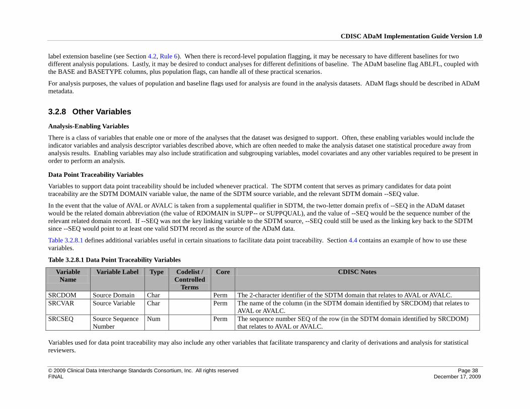
CDISC ADaM Implementation Guide Version 1.0
© 2009 Clinical Data Interchange Standards Consortium, Inc. All rights reserved Page 38 FINAL December 17, 2009
label extension baseline (see Section 4.2, Rule 6). When there is record-level population flagging, it may be necessary to have different baselines for two
different analysis populations. Lastly, it may be desired to conduct analyses for different definitions of baseline. The ADaM baseline flag ABLFL, coupled with
the BASE and BASETYPE columns, plus population flags, can handle all of these practical scenarios.
For analysis purposes, the values of population and baseline flags used for analysis are found in the analysis datasets. ADaM flags should be described in ADaM
metadata.
3.2.8 Other Variables
Analysis-Enabling Variables
There is a class of variables that enable one or more of the analyses that the dataset was designed to support. Often, these enabling variables would include the
indicator variables and analysis descriptor variables described above, which are often needed to make the analysis dataset one statistical procedure away from
analysis results. Enabling variables may also include stratification and subgrouping variables, model covariates and any other variables required to be present in
order to perform an analysis.
Data Point Traceability Variables
Variables to support data point traceability should be included whenever practical. The SDTM content that serves as primary candidates for data point
traceability are the SDTM DOMAIN variable value, the name of the SDTM source variable, and the relevant SDTM domain --SEQ value.
In the event that the value of AVAL or AVALC is taken from a supplemental qualifier in SDTM, the two-letter domain prefix of --SEQ in the ADaM dataset
would be the related domain abbreviation (the value of RDOMAIN in SUPP-- or SUPPQUAL), and the value of --SEQ would be the sequence number of the
relevant related domain record. If --SEQ was not the key linking variable to the SDTM source, --SEQ could still be used as the linking key back to the SDTM
since --SEQ would point to at least one valid SDTM record as the source of the ADaM data.
Table 3.2.8.1 defines additional variables useful in certain situations to facilitate data point traceability. Section 4.4 contains an example of how to use these
variables.
Table 3.2.8.1 Data Point Traceability Variables
Variable
Name
Variable Label Type Codelist /
Controlled
Terms
Core CDISC Notes
SRCDOM Source Domain Char Perm The 2-character identifier of the SDTM domain that relates to AVAL or AVALC.
SRCVAR Source Variable Char Perm The name of the column (in the SDTM domain identified by SRCDOM) that relates to
AVAL or AVALC.
SRCSEQ Source Sequence
Number
Num Perm The sequence number SEQ of the row (in the SDTM domain identified by SRCDOM)
that relates to AVAL or AVALC.
Variables used for data point traceability may also include any other variables that facilitate transparency and clarity of derivations and analysis for statistical
reviewers.

CDISC ADaM Implementation Guide Version 1.0
© 2009 Clinical Data Interchange Standards Consortium, Inc. All rights reserved Page 39 FINAL December 17, 2009
4 Implementation Issues, Standard
Solutions, and Examples The ADaM standard variables (columns) are described in Section 3. However, there is more to ADaM compliance than adherence to Section 3. The purpose of
Section 4 is to provide additional guidance on how to implement ADaM standard datasets correctly, illustrated with examples.
Section 4.1 provides examples of treatment variables for common trial designs.
Sections 4.2-4.8 are concerned with the BDS. These sections provide standard solutions to BDS implementation issues, illustrated with examples. In contrast
with ADSL, there is usually more than one dataset that follows the BDS in a study. As discussed in the ADaM document, the number of analysis datasets should
be “optimal” to support analysis and review. The Class attribute of analysis dataset metadata indicates the structure that a dataset follows: ADSL, BDS, or Other.
For space reasons, the examples in Section 4 necessarily omit many required and permissible ADaM variables, and show only the variables needed to facilitate
understanding of the points being addressed.

CDISC ADaM Implementation Guide Version 1.0
© 2009 Clinical Data Interchange Standards Consortium, Inc. All rights reserved Page 40 FINAL December 17, 2009
4.1 Examples of Treatment Variables for Common Trial Designs
The following examples illustrate the concepts around treatment variables in ADSL for several different trial designs, including a parallel design, a cross-over
design, and an open-label extension of a parallel design study. Note that only selected variables are illustrated; these examples are not intended to imply that
these are the only variables in ADSL.
In the first example (Table 4.1.1), the treatment variables for three subjects in a parallel design study are illustrated. Note that the third subject was randomized
to active treatment yet received placebo instead.
Table 4.1.1 Randomized Parallel Design
Row USUBJID ARM TRT01P TRT01A TR01SDT TR01EDT
1 1001 Drug X 5 mg Drug X 5 mg Drug X 5 mg 23OCT2007 17DEC2007
2 1002 Placebo Placebo Placebo 19JUL2006 20SEP2007
3 1003 Drug X 5 mg Drug X 5 mg Placebo 01NOV2007 20NOV2007
The second example (Table 4.1.2) illustrates the treatment variables for three subjects in a two-period cross-over design. It should be noted that TRTSDT and
TRTEDT are not displayed, but TRTSDT=TR01SDT and TRTEDT is the maximum of TR01EDT and TR02EDT as some subjects may have discontinued before
receiving TRT02P. Note that subjects 1002 and 1003 (in rows 2 and 3) were each exposed to placebo for both trial periods.
Table 4.1.2 Two Period Cross-Over Design
Row USUBJID TRTSEQP TRT01P TRT02P TRTSEQA TRT01A TRT02A TR01SDT TR01EDT TR02SDT TR02EDT
1 1001 Placebo – Drug X Placebo Drug X Placebo – Drug X Placebo Drug X 15FEB2006 03MAY2006 10MAY2006 15AUG2006
2 1002 Placebo – Drug X Placebo Drug X Placebo – Placebo Placebo Placebo 01MAR2006 12JUN2006 20JUN2006 23SEP2006
3 1003 Drug X – Placebo Drug X Placebo Placebo – Placebo Placebo Placebo 03FEB2006 25APR2006 01MAY2006 04AUG2006
The third example (Table 4.1.3) illustrates the treatment variables for three subjects in a three-period cross-over design. It should be noted that TRTSDT and
TRTEDT are not displayed, but TRTSDT=TR01SDT and TRTEDT is the maximum of TR01EDT, TR02EDT, and TR03EDT as some subjects may have
discontinued before receiving TRT03P. In this trial, all subjects received the planned treatment at each period so the TRTxxA variables are not needed.
Table 4.1.3 Three Period Cross-Over Design
Row USUBJID TRTSEQP TRT01P TRT02P TRT03P TR01SDT TR01EDT TR02SDT TR02EDT TR03SDT TR03EDT
1 1001 Placebo – Drug X –
Drug Y
Placebo Drug X Drug Y 15FEB2006 03MAY2006 10MAY2006 15AUG2006 23AUG2006 14NOV2006
2 1002 Drug Y – Placebo –
Drug X
Drug Y Placebo Drug X 01MAR2006 12JUN2006 20JUN2006 23SEP2006 01OCT2006 05DEC2006
3 1003 Drug X – Drug Y –
Placebo
Drug X Drug Y Placebo 03FEB2006 25APR2006 01MAY2006 04AUG2006 12AUG2006 15OCT2006
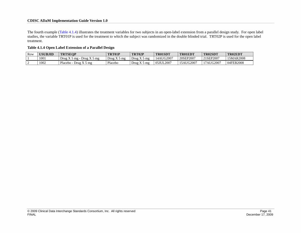
CDISC ADaM Implementation Guide Version 1.0
© 2009 Clinical Data Interchange Standards Consortium, Inc. All rights reserved Page 41 FINAL December 17, 2009
The fourth example (Table 4.1.4) illustrates the treatment variables for two subjects in an open-label extension from a parallel design study. For open label
studies, the variable TRT01P is used for the treatment to which the subject was randomized in the double blinded trial. TRT02P is used for the open label
treatment.
Table 4.1.4 Open Label Extension of a Parallel Design
Row USUBJID TRTSEQP TRT01P TRT02P TR01SDT TR01EDT TR02SDT TR02EDT
1 1001 Drug X 5 mg - Drug X 5 mg Drug X 5 mg Drug X 5 mg 14AUG2007 20SEP2007 21SEP2007 15MAR2008
2 1002 Placebo - Drug X 5 mg Placebo Drug X 5 mg 05JUL2007 15AUG2007 17AUG2007 04FEB2008

CDISC ADaM Implementation Guide Version 1.0
© 2009 Clinical Data Interchange Standards Consortium, Inc. All rights reserved Page 42 FINAL December 17, 2009
4.2 Creation of Derived Columns Versus Creation of Derived Rows
In the ADaM BDS, subjects, analysis parameters, and analysis timepoints define rows and are identified in standard columns. Subject, parameter and timepoint
in combination may not be enough to serve as natural keys (unique record identifiers). There may be multiple rows within a given combination, depending on
the number of observations collected or derived, baseline definition, etc.
Standard columns exist for a variety of purposes, such as SDTM record identifiers for traceability, population and other record selection flags, analysis values,
and some standard functions of analysis values. Permissible columns are not limited to those whose variable names are specified in Section 3, and may include
study-specific analysis model covariates, subgrouping variables, variables supportive of traceability, and other variables needed for analysis or useful for review.
However, there are some constraints on when derived data may be added as columns. Specifically, the subject of Section 4.2 is to address when functions of
analysis values should be added as additional columns, and when they should be added as additional rows instead.
The precise sequence of steps involved in creating a BDS analysis dataset varies according to operational and study-specific needs. For the purposes of this
discussion, it is useful to think of two initial steps.
The first step is to create a set of rows and columns more or less directly derived from or loaded from input SDTM domains into their appropriate places. This
step may include creation of analysis parameters (PARAM etc.), analysis timepoint (AVISIT etc.) and analysis variables (AVAL and AVALC). It would also
include addition of identifiers (STUDYID, SITEID, USUBJID, SUBJID) and other SDTM variables for traceability (VISIT, --SEQ, etc.).
The second step consists of further derivation of additional rows and columns based on this precursor set of analysis dataset records and columns. It is this
second step that is addressed in Section 4.2.
To be specific, derived rows and columns are defined in Section 4.2 to be rows and columns that are created based on data already present in the analysis dataset,
as opposed to data that are (1) copied or derived directly from SDTM; or (2) copied or derived directly from other analysis datasets or metadata. This section
only addresses the creation of columns and rows to accommodate such internally-derived data.
This section discusses the ADaM rules that govern when such internal derivation of data should result in creation of columns, and when it should result in
creation of rows. These rules are an essential part of the definition of the BDS.
4.2.1 Rules for the Creation of Rows and Columns
To preserve the BDS, it is necessary to place constraints on when one is allowed to create derived columns. Rule 1 describes a situation in which one should
derive data in columns. Rules 2-6 describe situations in which one should derive data in new rows, whether in entire new parameters, or as additional rows in
existing parameters.
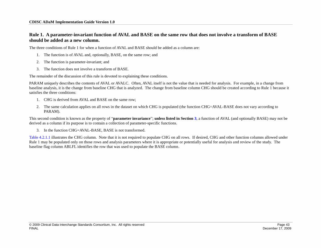
CDISC ADaM Implementation Guide Version 1.0
© 2009 Clinical Data Interchange Standards Consortium, Inc. All rights reserved Page 43 FINAL December 17, 2009
Rule 1. A parameter-invariant function of AVAL and BASE on the same row that does not involve a transform of BASE
should be added as a new column.
The three conditions of Rule 1 for when a function of AVAL and BASE should be added as a column are:
1. The function is of AVAL and, optionally, BASE, on the same row; and
2. The function is parameter-invariant; and
3. The function does not involve a transform of BASE.
The remainder of the discussion of this rule is devoted to explaining these conditions.
PARAM uniquely describes the contents of AVAL or AVALC. Often, AVAL itself is not the value that is needed for analysis. For example, in a change from
baseline analysis, it is the change from baseline CHG that is analyzed. The change from baseline column CHG should be created according to Rule 1 because it
satisfies the three conditions:
1. CHG is derived from AVAL and BASE on the same row;
2. The same calculation applies on all rows in the dataset on which CHG is populated (the function CHG=AVAL-BASE does not vary according to
PARAM).
This second condition is known as the property of “parameter invariance”; unless listed in Section 3, a function of AVAL (and optionally BASE) may not be
derived as a column if its purpose is to contain a collection of parameter-specific functions.
3. In the function CHG=AVAL-BASE, BASE is not transformed.
Table 4.2.1.1 illustrates the CHG column. Note that it is not required to populate CHG on all rows. If desired, CHG and other function columns allowed under
Rule 1 may be populated only on those rows and analysis parameters where it is appropriate or potentially useful for analysis and review of the study. The
baseline flag column ABLFL identifies the row that was used to populate the BASE column.
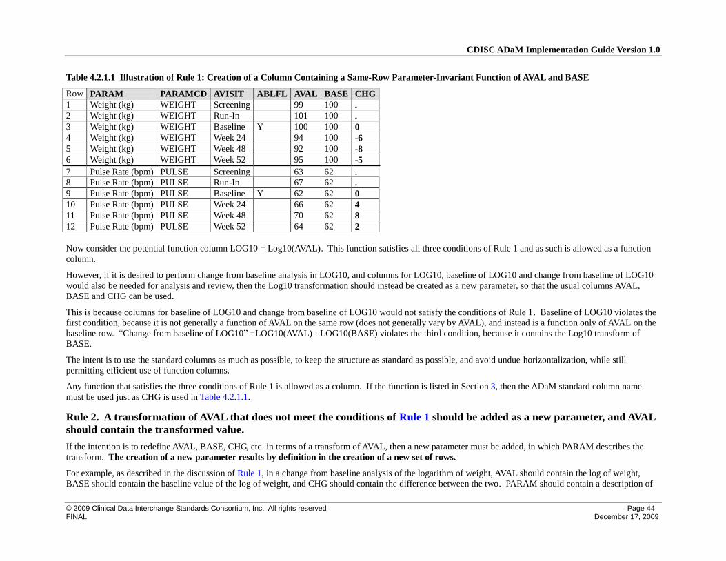
CDISC ADaM Implementation Guide Version 1.0
© 2009 Clinical Data Interchange Standards Consortium, Inc. All rights reserved Page 44 FINAL December 17, 2009
Table 4.2.1.1 Illustration of Rule 1: Creation of a Column Containing a Same-Row Parameter-Invariant Function of AVAL and BASE
Row PARAM PARAMCD AVISIT ABLFL AVAL BASE CHG
1 Weight (kg) WEIGHT Screening 99 100 .
2 Weight (kg) WEIGHT Run-In 101 100 .
3 Weight (kg) WEIGHT Baseline Y 100 100 0
4 Weight (kg) WEIGHT Week 24 94 100 -6
5 Weight (kg) WEIGHT Week 48 92 100 -8
6 Weight (kg) WEIGHT Week 52 95 100 -5
7 Pulse Rate (bpm) PULSE Screening 63 62 .
8 Pulse Rate (bpm) PULSE Run-In 67 62 .
9 Pulse Rate (bpm) PULSE Baseline Y 62 62 0
10 Pulse Rate (bpm) PULSE Week 24 66 62 4
11 Pulse Rate (bpm) PULSE Week 48 70 62 8
12 Pulse Rate (bpm) PULSE Week 52 64 62 2
Now consider the potential function column LOG10 = Log10(AVAL). This function satisfies all three conditions of Rule 1 and as such is allowed as a function
column.
However, if it is desired to perform change from baseline analysis in LOG10, and columns for LOG10, baseline of LOG10 and change from baseline of LOG10
would also be needed for analysis and review, then the Log10 transformation should instead be created as a new parameter, so that the usual columns AVAL,
BASE and CHG can be used.
This is because columns for baseline of LOG10 and change from baseline of LOG10 would not satisfy the conditions of Rule 1. Baseline of LOG10 violates the
first condition, because it is not generally a function of AVAL on the same row (does not generally vary by AVAL), and instead is a function only of AVAL on the
baseline row. “Change from baseline of LOG10” =LOG10(AVAL) - LOG10(BASE) violates the third condition, because it contains the Log10 transform of
BASE.
The intent is to use the standard columns as much as possible, to keep the structure as standard as possible, and avoid undue horizontalization, while still
permitting efficient use of function columns.
Any function that satisfies the three conditions of Rule 1 is allowed as a column. If the function is listed in Section 3, then the ADaM standard column name
must be used just as CHG is used in Table 4.2.1.1.
Rule 2. A transformation of AVAL that does not meet the conditions of Rule 1 should be added as a new parameter, and AVAL
should contain the transformed value.
If the intention is to redefine AVAL, BASE, CHG, etc. in terms of a transform of AVAL, then a new parameter must be added, in which PARAM describes the
transform. The creation of a new parameter results by definition in the creation of a new set of rows.
For example, as described in the discussion of Rule 1, in a change from baseline analysis of the logarithm of weight, AVAL should contain the log of weight,
BASE should contain the baseline value of the log of weight, and CHG should contain the difference between the two. PARAM should contain a description of

CDISC ADaM Implementation Guide Version 1.0
© 2009 Clinical Data Interchange Standards Consortium, Inc. All rights reserved Page 45 FINAL December 17, 2009
the transformed data contained in AVAL, e.g., “Log10 (Weight (kg))”. In this way the ADaM standard accommodates an analysis of transformed data in the
standard columns without creating a multiplicity of new special-purpose columns.
In Table 4.2.1.2 we see that the sponsor has chosen values of AVISITN that correspond to week number and which serve well for sorting and for plotting.
VISITNUM is the SDTM visit number.
Note that when SDTM variables, such as USUBJID, SUBJID, SITEID, VISIT, VISITNUM and --SEQ, are included in an ADaM dataset with their original
SDTM variable names, their values must not be altered in any way.
For clarity, to indicate that PARAM Log10(Weight (kg)) is derived, permissible variable PARAMTYP has been populated. PARAMTYP is not required.
Table 4.2.1.2 Illustration of Rule 2: Creation of a New Parameter to Handle a Transformation
Row PARAM PARAMCD AVISIT AVISITN VISITNUM ABLFL AVAL BASE CHG PARAMTYP
1 Weight (kg) WEIGHT Screening -4 1 99 100 .
2 Weight (kg) WEIGHT Run-In -2 2 101 100 .
3 Weight (kg) WEIGHT Baseline 0 3 Y 100 100 0
4 Weight (kg) WEIGHT Week 24 24 4 94 100 -6
5 Weight (kg) WEIGHT Week 48 48 5 92 100 -8
6 Weight (kg) WEIGHT Week 52 52 6 95 100 -5
7 Log10(Weight (kg)) L10WT Screening -4 1 1.9956 2 . DERIVED
8 Log10(Weight (kg)) L10WT Run-In -2 2 2.0043 2 . DERIVED
9 Log10(Weight (kg)) L10WT Baseline 0 3 Y 2 2 0 DERIVED
10 Log10(Weight (kg)) L10WT Week 24 24 4 1.9731 2 -0.0269 DERIVED
11 Log10(Weight (kg)) L10WT Week 48 48 5 1.9638 2 -0.0362 DERIVED
12 Log10(Weight (kg)) L10WT Week 52 52 6 1.9777 2 -0.0223 DERIVED
A related application of Rule 2 is in the case where it is necessary to support analysis and reporting in two different systems of units. In SDTM findings domains
such as LB, QS, EG, etc., the --STRESN column is the only numeric result column, and is also the only standardized numeric result column. The --ORRES
column contains a character representation of the collected result, in the collected units specified in the --ORRESU column. The --ORRES column is not
standardized. So for example, if data are typically collected in conventional units, SDTM cannot accommodate standardized data in both conventional units and
the International System of Units (SI). In SDTM, for any given --TEST, a sponsor can standardize in one system of units but not two. If one wishes to be able to
analyze standardized results in both conventional units and in SI units, a transform in an analysis dataset is needed. In each such case, a new parameter must be
created in order to accommodate standardized data in the other system of units.
The description in the PARAM column must contain the units, as well as any other information such as location and specimen type that is needed to ensure that
PARAM uniquely describes what is in AVAL, and differentiates between parameters as needed. PARAM cannot be the same for different units.
Table 4.2.1.3 shows an example of data supporting analyses of low-density lipoprotein (LDL) cholesterol in both conventional units (mg/dL) and SI units
(mmol/L). In this study, SDTM cholesterol data were standardized in mg/dL. In the analysis dataset, two records, one for each system of units, were generated
from each original SDTM record.
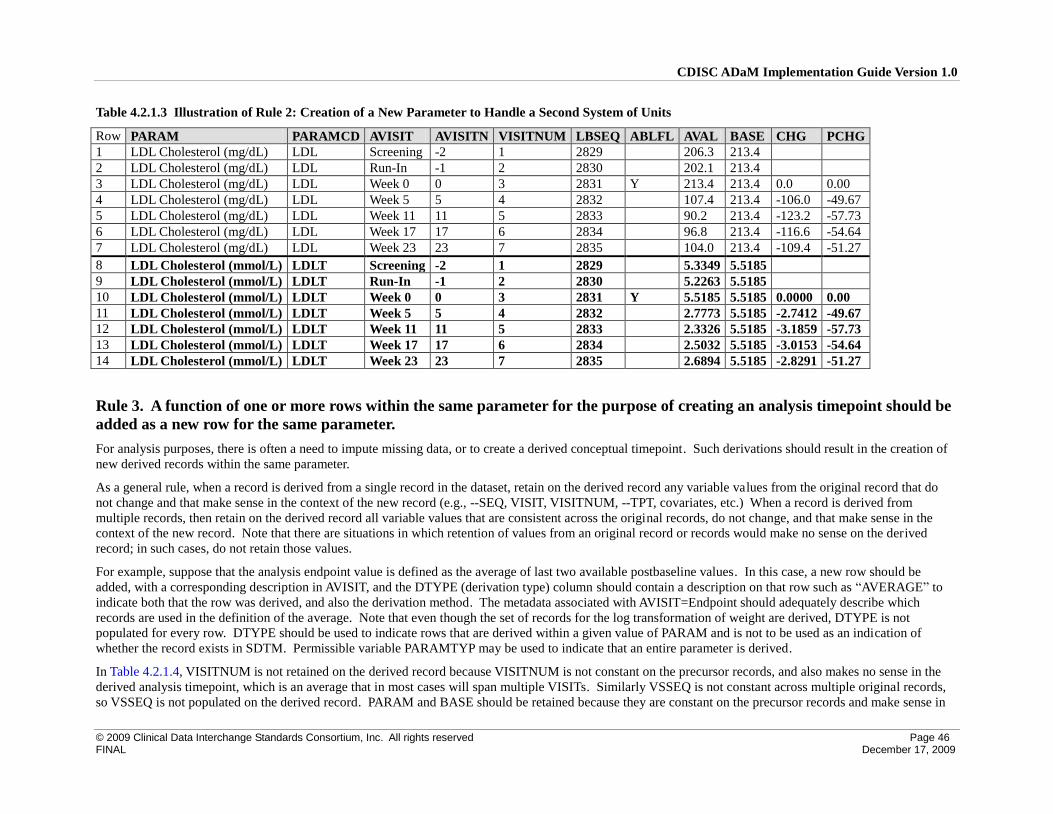
CDISC ADaM Implementation Guide Version 1.0
© 2009 Clinical Data Interchange Standards Consortium, Inc. All rights reserved Page 46 FINAL December 17, 2009
Table 4.2.1.3 Illustration of Rule 2: Creation of a New Parameter to Handle a Second System of Units
Row PARAM PARAMCD AVISIT AVISITN VISITNUM LBSEQ ABLFL AVAL BASE CHG PCHG
1 LDL Cholesterol (mg/dL) LDL Screening -2 1 2829 206.3 213.4
2 LDL Cholesterol (mg/dL) LDL Run-In -1 2 2830 202.1 213.4
3 LDL Cholesterol (mg/dL) LDL Week 0 0 3 2831 Y 213.4 213.4 0.0 0.00
4 LDL Cholesterol (mg/dL) LDL Week 5 5 4 2832 107.4 213.4 -106.0 -49.67
5 LDL Cholesterol (mg/dL) LDL Week 11 11 5 2833 90.2 213.4 -123.2 -57.73
6 LDL Cholesterol (mg/dL) LDL Week 17 17 6 2834 96.8 213.4 -116.6 -54.64
7 LDL Cholesterol (mg/dL) LDL Week 23 23 7 2835 104.0 213.4 -109.4 -51.27
8 LDL Cholesterol (mmol/L) LDLT Screening -2 1 2829 5.3349 5.5185
9 LDL Cholesterol (mmol/L) LDLT Run-In -1 2 2830 5.2263 5.5185
10 LDL Cholesterol (mmol/L) LDLT Week 0 0 3 2831 Y 5.5185 5.5185 0.0000 0.00
11 LDL Cholesterol (mmol/L) LDLT Week 5 5 4 2832 2.7773 5.5185 -2.7412 -49.67
12 LDL Cholesterol (mmol/L) LDLT Week 11 11 5 2833 2.3326 5.5185 -3.1859 -57.73
13 LDL Cholesterol (mmol/L) LDLT Week 17 17 6 2834 2.5032 5.5185 -3.0153 -54.64
14 LDL Cholesterol (mmol/L) LDLT Week 23 23 7 2835 2.6894 5.5185 -2.8291 -51.27
Rule 3. A function of one or more rows within the same parameter for the purpose of creating an analysis timepoint should be
added as a new row for the same parameter.
For analysis purposes, there is often a need to impute missing data, or to create a derived conceptual timepoint. Such derivations should result in the creation of
new derived records within the same parameter.
As a general rule, when a record is derived from a single record in the dataset, retain on the derived record any variable values from the original record that do
not change and that make sense in the context of the new record (e.g., --SEQ, VISIT, VISITNUM, --TPT, covariates, etc.) When a record is derived from
multiple records, then retain on the derived record all variable values that are consistent across the original records, do not change, and that make sense in the
context of the new record. Note that there are situations in which retention of values from an original record or records would make no sense on the derived
record; in such cases, do not retain those values.
For example, suppose that the analysis endpoint value is defined as the average of last two available postbaseline values. In this case, a new row should be
added, with a corresponding description in AVISIT, and the DTYPE (derivation type) column should contain a description on that row such as “AVERAGE” to
indicate both that the row was derived, and also the derivation method. The metadata associated with AVISIT=Endpoint should adequately describe which
records are used in the definition of the average. Note that even though the set of records for the log transformation of weight are derived, DTYPE is not
populated for every row. DTYPE should be used to indicate rows that are derived within a given value of PARAM and is not to be used as an indication of
whether the record exists in SDTM. Permissible variable PARAMTYP may be used to indicate that an entire parameter is derived.
In Table 4.2.1.4, VISITNUM is not retained on the derived record because VISITNUM is not constant on the precursor records, and also makes no sense in the
derived analysis timepoint, which is an average that in most cases will span multiple VISITs. Similarly VSSEQ is not constant across multiple original records,
so VSSEQ is not populated on the derived record. PARAM and BASE should be retained because they are constant on the precursor records and make sense in
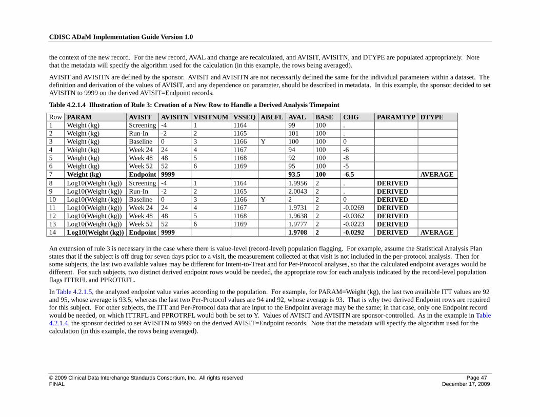
CDISC ADaM Implementation Guide Version 1.0
© 2009 Clinical Data Interchange Standards Consortium, Inc. All rights reserved Page 47 FINAL December 17, 2009
the context of the new record. For the new record, AVAL and change are recalculated, and AVISIT, AVISITN, and DTYPE are populated appropriately. Note
that the metadata will specify the algorithm used for the calculation (in this example, the rows being averaged).
AVISIT and AVISITN are defined by the sponsor. AVISIT and AVISITN are not necessarily defined the same for the individual parameters within a dataset. The
definition and derivation of the values of AVISIT, and any dependence on parameter, should be described in metadata. In this example, the sponsor decided to set
AVISITN to 9999 on the derived AVISIT=Endpoint records.
Table 4.2.1.4 Illustration of Rule 3: Creation of a New Row to Handle a Derived Analysis Timepoint
Row PARAM AVISIT AVISITN VISITNUM VSSEQ ABLFL AVAL BASE CHG PARAMTYP DTYPE
1 Weight (kg) Screening -4 1 1164 99 100 .
2 Weight (kg) Run-In -2 2 1165 101 100 .
3 Weight (kg) Baseline 0 3 1166 Y 100 100 0
4 Weight (kg) Week 24 24 4 1167 94 100 -6
5 Weight (kg) Week 48 48 5 1168 92 100 -8
6 Weight (kg) Week 52 52 6 1169 95 100 -5
7 Weight (kg) Endpoint 9999 93.5 100 -6.5 AVERAGE
8 Log10(Weight (kg)) Screening -4 1 1164 1.9956 2 . DERIVED
9 Log10(Weight (kg)) Run-In -2 2 1165 2.0043 2 . DERIVED
10 Log10(Weight (kg)) Baseline 0 3 1166 Y 2 2 0 DERIVED
11 Log10(Weight (kg)) Week 24 24 4 1167 1.9731 2 -0.0269 DERIVED
12 Log10(Weight (kg)) Week 48 48 5 1168 1.9638 2 -0.0362 DERIVED
13 Log10(Weight (kg)) Week 52 52 6 1169 1.9777 2 -0.0223 DERIVED
14 Log10(Weight (kg)) Endpoint 9999 1.9708 2 -0.0292 DERIVED AVERAGE
An extension of rule 3 is necessary in the case where there is value-level (record-level) population flagging. For example, assume the Statistical Analysis Plan
states that if the subject is off drug for seven days prior to a visit, the measurement collected at that visit is not included in the per-protocol analysis. Then for
some subjects, the last two available values may be different for Intent-to-Treat and for Per-Protocol analyses, so that the calculated endpoint averages would be
different. For such subjects, two distinct derived endpoint rows would be needed, the appropriate row for each analysis indicated by the record-level population
flags ITTRFL and PPROTRFL.
In Table 4.2.1.5, the analyzed endpoint value varies according to the population. For example, for PARAM=Weight (kg), the last two available ITT values are 92
and 95, whose average is 93.5; whereas the last two Per-Protocol values are 94 and 92, whose average is 93. That is why two derived Endpoint rows are required
for this subject. For other subjects, the ITT and Per-Protocol data that are input to the Endpoint average may be the same; in that case, only one Endpoint record
would be needed, on which ITTRFL and PPROTRFL would both be set to Y. Values of AVISIT and AVISITN are sponsor-controlled. As in the example in Table
4.2.1.4, the sponsor decided to set AVISITN to 9999 on the derived AVISIT=Endpoint records. Note that the metadata will specify the algorithm used for the
calculation (in this example, the rows being averaged).
CDISC ADaM Implementation Guide Version 1.0
© 2009 Clinical Data Interchange Standards Consortium, Inc. All rights reserved Page 48 FINAL December 17, 2009
Table 4.2.1.5 Illustration of Rule 3: Creation of New Rows to Handle a Derived Analysis Timepoint When There is Value-Level Population Flagging
Row PARAM AVISIT AVISITN VISITNUM VSSEQ ABLFL AVAL BASE CHG DTYPE ITTRFL PPROTRFL
1 Weight (kg) Screening -4 1 1164 99 100 . Y Y
2 Weight (kg) Run-In -2 2 1165 101 100 . Y Y
3 Weight (kg) Baseline 0 3 1166 Y 100 100 0 Y Y
4 Weight (kg) Week 24 24 4 1167 94 100 -6 Y Y
5 Weight (kg) Week 48 48 5 1168 92 100 -8 Y Y
6 Weight (kg) Week 52 52 6 1169 95 100 -5 Y
7 Weight (kg) Endpoint 9999 93.5 100 -6.5 AVERAGE Y
8 Weight (kg) Endpoint 9999 93 100 -7 AVERAGE Y
9 Log10 (Weight (kg)) Screening -4 1 1164 1.9956 2 . Y Y
10 Log10 (Weight (kg)) Run-In -2 2 1165 2.0043 2 . Y Y
11 Log10 (Weight (kg)) Baseline 0 3 1166 Y 2 2 0 Y Y
12 Log10 (Weight (kg)) Week 24 24 4 1167 1.9731 2 -0.0269 Y Y
13 Log10 (Weight (kg)) Week 48 48 5 1168 1.9638 2 -0.0362 Y Y
14 Log10 (Weight (kg)) Week 52 52 6 1169 1.9777 2 -0.0223 Y
15 Log10 (Weight (kg)) Endpoint 9999 1.9708 2 -0.0292 AVERAGE Y
16 Log10 (Weight (kg)) Endpoint 9999 1.9685 2 -0.0315 AVERAGE Y
In the example in Table 4.2.1.6, missing post-baseline values are imputed by last observation carried forward, and also by worst observation carried forward.
In this study, at Week 8, there is a scheduled visit (visit number 6). At that visit, blood pressure should be collected. However, for this subject, either there was
no visit 6, or there was a visit 6, but no data on blood pressure were collected. The SAP says that missing postbaseline data should be imputed (derived) by two
methods: LOCF (last observation carried forward), and WOCF (worst observation carried forward).
For LOCF analysis, the missing Week 8 (VISITNUM 6) result is imputed by carrying forward the most recent prior available postbaseline value, which is the
VISITNUM 5 value. That the Week 8 value is imputed is indicated by LOCF in the derivation type (DTYPE) column.
For WOCF analysis, even though the unscheduled VISITNUM 4.1 value was not chosen to represent the Week 2 analysis timepoint, it is used to impute the
missing Week 8 timepoint because it was the worst postbaseline result up to that point.
The exact algorithms employed in the record derivation methods (LOCF and WOCF in this case) must be indicated in the metadata for DTYPE.
Traceability is enhanced by the addition of the SDTM VISITNUM and --SEQ columns. The combination of USUBJID and VSSEQ provides a link to the exact
input record in the SDTM VS domain. On the derived LOCF and WOCF rows, VISITNUM and VSSEQ provide clarity about where the value came from.
There are several other concepts presented in this example. Analysis relative day (ADY) in this protocol is defined relative to date of first dose. In many but not
all protocols, ADY would equal the value of the SDTM --DY variable (or --STDY for some kinds of data). The data presented here illustrate that this particular
subject did not take drug until two days after randomization, so the value of ADY is -2 at the randomization visit, Visit 3 (VISITNUM 3). As is the case for
SDTM study day, there is no day 0 for ADY.
CDISC ADaM Implementation Guide Version 1.0
© 2009 Clinical Data Interchange Standards Consortium, Inc. All rights reserved Page 49 FINAL December 17, 2009
In this protocol, if there are multiple data points within an analysis time window, the value that is observed closest to a pre-specified target planned relative day is
the value that is chosen to represent the analysis timepoint. For this study and parameter, AWTARGET = VISITDY (Planned Study Day) from SDTM, and
ADY=VSDY. AWTDIFF is the absolute value of ADY - AWTARGET, adjusted for the fact that there is no day 0 (so that if ADY and AWTARGET have
different signs, then AWTDIFF = |ADY - AWTARGET - 1| ).
For AVISIT=Week 2, there were two values observed, at study days 13 and 17 (rows 4 and 5). Day 13 is closer to the target, day 14. So the day 13 record (row
4) is chosen for analysis, as denoted by the analyzed record flag ANL01FL = Y. ANL01FL is used in conjunction with other selection variables in order to obtain
the exact set of records used for analysis.
AVISIT by itself functions as a description of an analysis time window. AVISIT, DTYPE, and ANL01FL are all needed to identify the records to be used in a
given analysis.
On the derived AVIST=Week 8 records, AWTARGET was set to the target for Week 8, and AWTDIFF was calculated accordingly. It did not make sense to retain
the values of AWTARGET and AWTDIFF from the original records.
Table 4.2.1.6 Illustration of Rule 3: Creation of New Rows to Handle Imputation of Missing Values by Last Observation Carried Forward and Worst
Observation Carried Forward
Row PARAM AVISIT AVISITN VISITNUM VSSEQ ABLFL AVAL BASE CHG DTYPE ADY AWTARGET AWTDIFF ANL01FL
1 Systolic BP (mm Hg) Screening -4 1 3821 120 114 . -30 -28 2 Y
2 Systolic BP (mm Hg) Run-In -2 2 3822 116 114 . -16 -14 2 Y
3 Systolic BP (mm Hg) Week 0 0 3 3823 Y 114 114 0 -2 1 2 Y
4 Systolic BP (mm Hg) Week 2 2 4 3824 118 114 4 13 14 1 Y
5 Systolic BP (mm Hg) Week 2 2 4.1 3825 126 114 12 17 14 3
6 Systolic BP (mm Hg) Week 4 4 5 3826 122 114 8 23 28 5 Y
7 Systolic BP (mm Hg) Week 8 8 5 3826 122 114 8 LOCF 23 56 33 Y
8 Systolic BP (mm Hg) Week 8 8 4.1 3825 126 114 12 WOCF 17 56 39 Y
9 Systolic BP (mm Hg) Week 12 12 7 3827 134 114 20 83 84 1 Y
Table 4.2.1.7 contains an example of data supporting change from baseline analyses of migraine pain. In this study, missing postbaseline data are imputed by the
methods of Baseline Observation Carried Forward (BOCF) and Last Observation Carried Forward (LOCF).
When a migraine headache occurs, subjects self-administer a single dose of blinded study treatment. Subjects assess migraine pain at planned timepoints Pre-
Dose, 30 Minutes Post Dose, 1 Hour Post-Dose, and 2 Hours Post-Dose. Collected data on migraine pain are tabulated in the SDTM Clinical Findings domain.
ATPT is the analysis timepoint description. ATPTN is the analysis timepoint number. CFTPTNUM is the collected timepoint number from SDTM. AVALC
contains the pain assessment, and AVAL contains the numeric coded value of the assessment. AVAL is a one-to-one map to AVALC.
Subject 000276 did not continue to provide data after 1 Hour Post-Dose. For this subject, the 2-Hours Post-Dose planned observation must be imputed.
Subject 001863 had complete data, so no imputation was necessary.
Subject 000276 is excluded from an observed case analysis of Migraine Pain at 2 Hours Post Dose.
The data for both subjects are included in the BOCF and LOCF analyses of Migraine Pain at 2 Hours Post-Dose.
CDISC ADaM Implementation Guide Version 1.0
© 2009 Clinical Data Interchange Standards Consortium, Inc. All rights reserved Page 50 FINAL December 17, 2009
Table 4.2.1.7 Illustration of Rule 3: Creation of New Rows to Handle Imputation of Missing Values by Baseline Observation Carried Forward and Last
Observation Carried Forward
Row USUBJID TRTP PARAM ATPT ATPTN FATPTNUM FASEQ ABLFL AVAL AVALC BASE CHG DTYPE
1 000276 Placebo Migraine Pain Pre-Dose 0 1 14 Y 3 Severe Pain 3 0
2 000276 Placebo Migraine Pain 30 Minutes Post-Dose 0.5 2 22 2 Moderate Pain 3 -1
3 000276 Placebo Migraine Pain 1 Hour Post-Dose 1 3 27 1 Mild Pain 3 -2
4 000276 Placebo Migraine Pain 2 Hours Post-Dose 2 1 14 3 Severe Pain 3 0 BOCF
5 000276 Placebo Migraine Pain 2 Hours Post-Dose 2 3 27 1 Mild Pain 3 -2 LOCF
6 001863 Soma 30 mg Migraine Pain Pre-Dose 0 1 638 Y 3 Severe Pain 3 0
7 001863 Soma 30 mg Migraine Pain 30 Minutes Post-Dose 0.5 2 639 1 Mild Pain 1 -2
8 001863 Soma 30 mg Migraine Pain 1 Hour Post-Dose 1 3 640 1 Mild Pain 1 -2
9 001863 Soma 30 mg Migraine Pain 2 Hours Post-Dose 2 4 641 1 Mild Pain 1 -2
Table 4.2.1.8 contains an example of some of the columns in a dataset supporting analysis of a 2-period crossover study.
In a crossover trial design, all subjects are planned to receive all of the study treatments. The sequence of treatments is randomized. If in a study there are two
treatments in a crossover design, two treatment periods are necessary.
In this example, the planned visits are 1 (Screening and beginning of placebo run-in period), 2 (Week -2, halfway through placebo run-in period), 3 (Week 0, end
of placebo run-in and randomization), 4 (Week 4, the end of the first treatment period), and 5 (Week 8, the end of the second treatment period). Baseline is
defined in the Statistical Analysis Plan as the average of the Week -2 (VISIT 2) and Week 0 (VISIT 3) measurements. This baseline is used for the analysis of
both the first and the second crossover periods. USUBJID 0987_4252 has no VISIT 2 measurement, so the average is just the Week 0 (VISIT 3) measurement.
Within any postbaseline week window, the last observation is used to characterize that week. For example, for USUBJID 0987_3984, the VISIT 5 (row 7) value is
used to characterize AVISIT=Week 8, as opposed to the earlier VISIT 4.1 value (row 6), which was also observed during the Week 8 time window. The variable
ANL01FL is used in this study to identify the record selected for analysis when there are multiple records for a given AVISIT, and must be used in conjunction
with other selection variables in order to identify the exact set of records used in a given analysis or summary.
APERIODC is the crossover period character description.
Note that in general, APERIODC is not the same as EPOCH. APERIOD/APERIODC would not be defined for periods of time such as prebaseline during which
there is no study treatment to be analyzed. Also, it is possible in some cases that boundaries of APERIODs would not align exactly with boundaries of EPOCHs.
A simple example is a post-discontinuation record that is associated with the most recent treatment period for analysis.
TRTSEQP, from ADSL, is the planned ordering of crossover treatments. TRTP is the analyzed planned treatment for the given period. The two endpoint records
are derived only for the subjects who have data for both periods.
The conventions used in AVISITN are sponsor-defined. In this example, the sponsor has decided that AVISITN contains -8888 for the derived baseline records,
9999 for the derived endpoint records, and week number otherwise.
CDISC ADaM Implementation Guide Version 1.0
© 2009 Clinical Data Interchange Standards Consortium, Inc. All rights reserved Page 51 FINAL December 17, 2009
Table 4.2.1.8 Illustration of Rule 3: Creation of Endpoint Rows to Facilitate Analysis of a Crossover Design
Row USUBJID PARAMCD AVISIT AVISITN VISITNUM DTYPE ANL01FL
1 0987_3984 ALT Screening -4 1 Y
2 0987_3984 ALT Week -2 -2 2 Y
3 0987_3984 ALT Week 0 0 3 Y
4 0987_3984 ALT Baseline -8888 AVERAGE Y
5 0987_3984 ALT Week 4 4 4 Y
6 0987_3984 ALT Week 8 8 4.1
7 0987_3984 ALT Week 8 8 5 Y
8 0987_3984 ALT Endpoint 9999 4 ENDPOINT Y
9 0987_3984 ALT Endpoint 9999 5 ENDPOINT Y
10 0987_4252 ALT Screening -4 1 Y
11 0987_4252 ALT Week 0 0 3 Y
12 0987_4252 ALT Baseline -8888 AVERAGE Y
13 0987_4252 ALT Week 4 4 4 Y
14 0987_4252 ALT Week 8 8 5 Y
15 0987_4252 ALT Endpoint 9999 4 ENDPOINT Y
16 0987_4252 ALT Endpoint 9999 5 ENDPOINT Y
Row TRTP APERIOD APERIODC TRTSEQP AVAL ABLFL BASE CHG
1 (cont) Drug B, Drug A 16 17 .
2 (cont) Drug B, Drug A 16 17 .
3 (cont) Drug B, Drug A 18 17 .
4 (cont) Drug B, Drug A 17 Y 17 0
5 (cont) Drug B 1 Period 1 Drug B, Drug A 14 17 -3
6 (cont) Drug A 2 Period 2 Drug B, Drug A 10 17 -7
7 (cont) Drug A 2 Period 2 Drug B, Drug A 12 17 -5
8 (cont) Drug B 1 Period 1 Drug B, Drug A 14 17 -3
9 (cont) Drug A 2 Period 2 Drug B, Drug A 12 17 -5
10 (cont) Drug A, Drug B 12 11 .
11 (cont) Drug A, Drug B 11 11 .
12 (cont) Drug A, Drug B 11 Y 11 0
13 (cont) Drug A 1 Period 1 Drug A, Drug B 14 11 3
14 (cont) Drug B 2 Period 2 Drug A, Drug B 15 11 4
15 (cont) Drug A 1 Period 1 Drug A, Drug B 14 11 3
16 (cont) Drug B 2 Period 2 Drug A, Drug B 15 11 4

CDISC ADaM Implementation Guide Version 1.0
© 2009 Clinical Data Interchange Standards Consortium, Inc. All rights reserved Page 52 FINAL December 17, 2009
Rule 4. A function of multiple rows within a parameter should be added as a new parameter.
Rule 4 is a special case of Rule 2. The functions covered by this rule violate the second condition of Rule 1 (they are not same-row functions of AVAL), and may
also violate the first and third conditions.
For example, in a clinical trial of a Human Immunodeficiency Virus (HIV) vaccine, blood samples are drawn at each visit, and CD4 cell count is measured. To
assess efficacy, it is important to look at the cumulative effect over time on CD4 cell count during follow-up after administration.
Let AVAL(t) equal the value of CD4 cell count at postbaseline visit t, and let VISITDY(t) be the planned study day of visit t.
CD4AUC (cumulative daily CD4 count over follow-up) is calculated at any given postbaseline visit as follows:
CD4AUC at baseline visit is set to 0.
CD4AUC(t) = CD4AUC(t-1) + [ 0.5 * AVAL(t-1) + 0.5 * AVAL(t) ] * [ VISITDY(t) - VISITDY(t-1) ].
CD4AUC is not a simple same-row function of BASE and AVAL. It is calculated based on data from multiple observations (rows) of CD4 data, so it should be
added as a new parameter rather than as a new column. CD4AUC is not defined pre-baseline, which is why there is no Week -1 for this parameter.
CD4AUCMB (cumulative average change from baseline in daily CD4 count over follow-up) is calculated as
CD4AUCMB(t) = CD4AUC(t) / [ VISITDY(t) - 1 ] - baseline value of CD4 cell count.
CD4AUCMB is a function of both CD4AUC and the baseline value of CD4, so it also must be its own parameter (see Rule 5 below). CD4AUCMB is not
defined for pre-baseline and baseline records and therefore these records are not represented within this value of PARAM.

CDISC ADaM Implementation Guide Version 1.0
© 2009 Clinical Data Interchange Standards Consortium, Inc. All rights reserved Page 53 FINAL December 17, 2009
Table 4.2.1.9 Illustration of Rule 4: Creation of a New Parameter to Handle a Function of More Than One Row of a Parameter
Row PARAM PARAMCD AVISIT VISITDY ABLFL AVAL BASE
1 CD4 (cells/mm3) CD4 Week -1 -7 75 76
2 CD4 (cells/mm3) CD4 Week 0 1 Y 76 76
3 CD4 (cells/mm3) CD4 Week 2 15 128 76
4 CD4 (cells/mm3) CD4 Week 4 29 125 76
5 CD4 (cells/mm3) CD4 Week 8 57 191 76
6 CD4 (cells/mm3) CD4 Week 12 85 167 76
7 CD4 (cells/mm3) CD4 Week 16 113 136 76
8 CD4 Cumulative AUC CD4AUC Week 0 1 Y 0 0
9 CD4 Cumulative AUC CD4AUC Week 2 15 1428 0
10 CD4 Cumulative AUC CD4AUC Week 4 29 3199 0
11 CD4 Cumulative AUC CD4AUC Week 8 57 7623 0
12 CD4 Cumulative AUC CD4AUC Week 12 85 12635 0 13 CD4 Cumulative AUC CD4AUC Week 16 113 16877 0 14 CD4 Cumulative AUCMB CD4AUCMB Week 2 15 26 . 15 CD4 Cumulative AUCMB CD4AUCMB Week 4 29 38.25 . 16 CD4 Cumulative AUCMB CD4AUCMB Week 8 57 60.125 .
17 CD4 Cumulative AUCMB CD4AUCMB Week 12 85 74.4167 .
18 CD4 Cumulative AUCMB CD4AUCMB Week 16 113 74.6875 .
Rule 5. A function of more than one parameter should be added as a new parameter.
There is often a need to derive for analysis a parameter that was not collected. Such parameters may be quite complex functions of data from multiple SDTM
domains and domain classes. Rule 5 addresses the case where a parameter is derived from other parameters already present in the dataset.
For example, a questionnaire total domain score is calculated as a function of more than one observed question. The total domain score should be added as a new
parameter, with its corresponding set of derived rows. For this derived parameter, the value of PARAM would be e.g., “Total Domain Score”, and the value of
the total domain score would be stored in the standard AVAL column, the baseline value would be stored in the standard BASE column, change from baseline
would be stored in CHG, as usual.
In the example in Table 4.2.1.10, blood samples are drawn at every visit, and laboratory test measurements of total cholesterol and high-density lipoprotein
cholesterol are found in the SDTM LB domain. The protocol calls for analysis of each individual lab analyte, and also for an analysis of the ratio of total
cholesterol (C) to high-density lipoprotein (HDL) cholesterol. The analysis dataset contains parameters for each of the two measured lab tests, as well as a new
set of derived rows where the description in PARAM is “Total Cholesterol:HDL-C ratio”, and AVAL contains the calculated ratio at each timepoint.
The analysis of percent change from baseline (PCHG) is of interest for all three parameters and is therefore populated on all records. In general, however, if
percent change is not analyzed for a particular value of PARAM, then it is not necessary to populate PCHG for those rows.

CDISC ADaM Implementation Guide Version 1.0
© 2009 Clinical Data Interchange Standards Consortium, Inc. All rights reserved Page 54 FINAL December 17, 2009
Table 4.2.1.10 Illustration of Rule 5: Creation of New Parameter to Handle a Function of More Than One Parameter
Row PARAM PARAMCD AVISIT AVISITN VISITNUM LBSEQ ABLFL AVAL BASE CHG PCHG
1 Total Cholesterol (mg/dL) CHOL Screening -2 1 39394 265 266 . .
2 Total Cholesterol (mg/dL) CHOL Run-In -1 2 25593 278 266 . .
3 Total Cholesterol (mg/dL) CHOL Week 0 0 3 23213 Y 266 266 0 0.000
4 Total Cholesterol (mg/dL) CHOL Week 2 2 4 32952 259 266 -7 -2.632
5 Total Cholesterol (mg/dL) CHOL Week 4 4 5 12768 235 266 -31 -11.654
6 Total Cholesterol (mg/dL) CHOL Week 8 8 6 18773 242 266 -24 -9.023
7 Total Cholesterol (mg/dL) CHOL Week 12 12 7 28829 217 266 -49 -18.421
8 High-Density Lipoprotein Chol (mg/dL) HDL Screening -2 1 32437 44 42 . .
9 High-Density Lipoprotein Chol (mg/dL) HDL Run-In -1 2 26884 40 42 . .
10 High-Density Lipoprotein Chol (mg/dL) HDL Week 0 0 3 52657 Y 42 42 0 0.000
11 High-Density Lipoprotein Chol (mg/dL) HDL Week 2 2 4 38469 43 42 1 2.381
12 High-Density Lipoprotein Chol (mg/dL) HDL Week 4 4 5 12650 47 42 5 11.905 13 High-Density Lipoprotein Chol (mg/dL) HDL Week 8 8 6 24345 46 42 4 9.524 14 High-Density Lipoprotein Chol (mg/dL) HDL Week 12 12 7 23484 47 42 5 11.905
15 Total Cholesterol:HDL-C ratio CHOLH Screening -2 1 6.023 6.333 . . 16 Total Cholesterol:HDL-C ratio CHOLH Run-In -1 2 6.950 6.333 . .
17 Total Cholesterol:HDL-C ratio CHOLH Week 0 0 3 Y 6.333 6.333 0.000 0.000
18 Total Cholesterol:HDL-C ratio CHOLH Week 2 2 4 6.023 6.333 -0.310 -4.896
19 Total Cholesterol:HDL-C ratio CHOLH Week 4 4 5 5.000 6.333 -1.333 -21.053
20 Total Cholesterol:HDL-C ratio CHOLH Week 8 8 6 5.261 6.333 -1.072 -16.934
21 Total Cholesterol:HDL-C ratio CHOLH Week 12 12 7 4.617 6.333 -1.716 -27.100
Rule 6. When there is more than one definition of baseline, each additional definition of baseline requires the creation of its
own set of rows.
In case there is more than one definition of baseline, new rows must be created for each additional alternative definition of baseline. There will therefore be
multiple sets of rows, where each set of rows corresponds to a particular definition of baseline. Whenever there is more than one definition of baseline, the
BASETYPE column is required. BASETYPE identifies the definition of baseline that corresponds to the value of BASE in each row. There is only one BASE
column, and only one column for each qualifying function of AVAL and BASE.
The example in Table 4.2.1.11 presents a dataset supporting shift analysis from three different baselines. Accordingly, it makes use of the BASETYPE variable
described above. The ANRIND, BNRIND, and SHIFTy variables are also illustrated.
For space reasons, the ANLzzFL variable is not shown, although it would be needed to identify which record is selected in cases of multiple observed records
within an analysis timepoint, as is the case for AVISIT=WEEK 12 (DB) for this subject and parameter.

CDISC ADaM Implementation Guide Version 1.0
© 2009 Clinical Data Interchange Standards Consortium, Inc. All rights reserved Page 55 FINAL December 17, 2009
Table 4.2.1.11 Illustration of Rule 6: Creation of New Rows to Handle Multiple Baseline Definitions
Row BASETYPE EPOCH AVISIT VISIT AVAL ANRLO ANRHI ANRIND ABLFL BASE BNRIND SHIFT1
1 RUN-IN RUN-IN BASELINE (RUN-IN) BASELINE 34.5 15.4 48.5 NORMAL Y 34.5 NORMAL
2 RUN-IN RUN-IN WEEK 8 (RUN-IN) DAY 57 11.6 15.4 48.5 LOW 34.5 NORMAL NORMAL to LOW
3 RUN-IN RUN-IN END POINT (RUN-IN) DAY 57 11.6 15.4 48.5 LOW 34.5 NORMAL NORMAL to LOW
4 RUN-IN STABILIZATION WEEK 14 (STAB.) DAY 99 13.1 15.4 48.5 LOW 34.5 NORMAL NORMAL to LOW
5 RUN-IN STABILIZATION END POINT (STAB.) DAY 99 13.1 15.4 48.5 LOW 34.5 NORMAL NORMAL to LOW
6 RUN-IN DOUBLE BLIND BASELINE (DB) DAY 99 13.1 15.4 48.5 LOW 34.5 NORMAL NORMAL to LOW
7 RUN-IN DOUBLE BLIND WEEK 12 (DB) DAY 184 13.7 15.4 48.5 LOW 34.5 NORMAL NORMAL to LOW
8 RUN-IN DOUBLE BLIND WEEK 12 (DB) VISIT 98 19.7 15.4 48.5 NORMAL 34.5 NORMAL NORMAL to NORMAL
9 RUN-IN DOUBLE BLIND END POINT (DB) VISIT 98 19.7 15.4 48.5 NORMAL 34.5 NORMAL NORMAL to NORMAL
10 RUN-IN OPEN LABEL BASE (OPEN) VISIT 98 19.7 15.4 48.5 NORMAL 34.5 NORMAL NORMAL to NORMAL
11 RUN-IN OPEN LABEL WEEK 24 (OPEN) DAY 169 28.1 15.4 48.5 NORMAL 34.5 NORMAL NORMAL to NORMAL
12 RUN-IN OPEN LABEL ENDPOINT (OPEN) DAY 169 28.1 15.4 48.5 NORMAL 34.5 NORMAL NORMAL to NORMAL
13 DOUBLE-BLIND DOUBLE BLIND BASELINE (DB) DAY 99 13.1 15.4 48.5 LOW Y 13.1 LOW
14 DOUBLE-BLIND DOUBLE BLIND WEEK 12 (DB) DAY 184 13.7 15.4 48.5 LOW 13.1 LOW LOW to LOW
15 DOUBLE-BLIND DOUBLE BLIND WEEK 12 (DB) VISIT 98 19.7 15.4 48.5 NORMAL 13.1 LOW LOW to NORMAL
16 DOUBLE-BLIND DOUBLE BLIND END POINT (DB) VISIT 98 19.7 15.4 48.5 NORMAL 13.1 LOW LOW to NORMAL
17 DOUBLE-BLIND OPEN LABEL BASE (OPEN) VISIT 98 19.7 15.4 48.5 NORMAL 13.1 LOW LOW to NORMAL
18 DOUBLE-BLIND OPEN LABEL WEEK 24 (OPEN) DAY 169 28.1 15.4 48.5 NORMAL 13.1 LOW LOW to NORMAL
19 DOUBLE-BLIND OPEN LABEL END POINT (OPEN) DAY 169 28.1 15.4 48.5 NORMAL 13.1 LOW LOW to NORMAL
20 OPEN LABEL OPEN LABEL BASE (OPEN) VISIT 98 19.7 15.4 48.5 NORMAL Y 19.7 NORMAL
21 OPEN LABEL OPEN LABEL WEEK 24 (OPEN) DAY 169 28.1 15.4 48.5 NORMAL 19.7 NORMAL NORMAL to NORMAL
22 OPEN LABEL OPEN LABEL END POINT (OPEN) DAY 169 28.1 15.4 48.5 NORMAL 19.7 NORMAL NORMAL to NORMAL

CDISC ADaM Implementation Guide Version 1.0
© 2009 Clinical Data Interchange Standards Consortium, Inc. All rights reserved Page 56 FINAL December 17, 2009
4.3 Inclusion of All Observed and Derived Records for a Parameter Versus the Subset of Records Used for Analysis
This section discusses whether the analysis dataset should include all rows of an analysis parameter, or only the subset of rows that are used for analysis. A value
of AVAL or AVALC for an analysis parameter at a specific time point may be observed (i.e., collected on the case report form or in an electronic diary at that time
point), it may be imputed because it was missing, or it may be derived from a combination of other values.
To illustrate the issue being presented, assume that the total scores for Questionnaire A (administered at Visits 1, 2, and 3) are in the SDTM QS domain as
illustrated below. Any missing total scores are imputed by carrying the last post-baseline (post-Visit 1) total score forward. The total score for visit 3 will be
analyzed.
In the SDTM QS domain data shown below, subject 0001 has data for visits 1, 2, and 3; subject 0002 will not be included in the analysis, as there are no post-
baseline data for the subject; subject 0003 has data for visits 1 and 2, but is missing data for visit 3.
Table 4.3.1 Illustration of Issue, Data as Found in SDTM QS Dataset
Row DOMAIN USUBJID VISITNUM QSSEQ QSCAT QSTESTCD QSSTRESN
1 QS 0001 1 101 QUES-A TOTSCORE 7
2 QS 0001 2 201 QUES-A TOTSCORE 12
3 QS 0001 3 555 QUES-A TOTSCORE 14
4 QS 0002 1 91 QUES-A TOTSCORE 4
5 QS 0003 1 156 QUES-A TOTSCORE 2
6 QS 0003 2 300 QUES-A TOTSCORE 6
The questions that arise are whether or not the analysis dataset should contain data for subject 0002 even though the subject is not included in the analysis and if
the analysis dataset should contain totals for visits 1 and 2 even though the data being analyzed are from visit 3.
4.3.1 ADaM Methodology and Examples
The ADaM methodology is to include all observed and derived rows for a given analysis parameter. The inclusion of all the rows in the analysis dataset,
including those not used in the analysis, requires a way to identify the rows used in the specified analysis. This approach increases the size of the dataset, and
introduces a risk that users will not incorporate the appropriate selection criteria and thereby generate incorrect analysis results. The advantage is that the
inclusion of all rows makes it easier to verify that the selection and derived time-point processing was done correctly, thus providing useful traceability. In
addition, the data are also then available to enable other analyses, including sensitivity analyses.
Regulatory reviewers prefer that the path followed in creating and/or selecting analysis rows be clearly delineated and traceable all the way back to the
originating rows in the SDTM domain, if possible and within reason. Simply including the algorithm in the metadata is often not sufficient, as any complicated
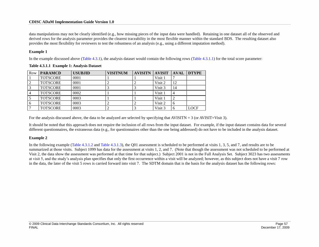
CDISC ADaM Implementation Guide Version 1.0
© 2009 Clinical Data Interchange Standards Consortium, Inc. All rights reserved Page 57 FINAL December 17, 2009
data manipulations may not be clearly identified (e.g., how missing pieces of the input data were handled). Retaining in one dataset all of the observed and
derived rows for the analysis parameter provides the clearest traceability in the most flexible manner within the standard BDS. The resulting dataset also
provides the most flexibility for reviewers to test the robustness of an analysis (e.g., using a different imputation method).
Example 1
In the example discussed above (Table 4.3.1), the analysis dataset would contain the following rows (Table 4.3.1.1) for the total score parameter:
Table 4.3.1.1 Example 1: Analysis Dataset
Row PARAMCD USUBJID VISITNUM AVISITN AVISIT AVAL DTYPE
1 TOTSCORE 0001 1 1 Visit 1 7
2 TOTSCORE 0001 2 2 Visit 2 12
3 TOTSCORE 0001 3 3 Visit 3 14
4 TOTSCORE 0002 1 1 Visit 1 4
5 TOTSCORE 0003 1 1 Visit 1 2
6 TOTSCORE 0003 2 2 Visit 2 6
7 TOTSCORE 0003 2 3 Visit 3 6 LOCF
For the analysis discussed above, the data to be analyzed are selected by specifying that AVISITN = 3 (or AVISIT=Visit 3).
It should be noted that this approach does not require the inclusion of all rows from the input dataset. For example, if the input dataset contains data for several
different questionnaires, the extraneous data (e.g., for questionnaires other than the one being addressed) do not have to be included in the analysis dataset.
Example 2
In the following example (Table 4.3.1.2 and Table 4.3.1.3), the Q01 assessment is scheduled to be performed at visits 1, 3, 5, and 7, and results are to be
summarized at those visits. Subject 1099 has data for the assessment at visits 1, 2, and 7. (Note that though the assessment was not scheduled to be performed at
Visit 2, the data show the assessment was performed at that time for that subject.) Subject 2001 is not in the Full Analysis Set. Subject 3023 has two assessments
at visit 5, and the study’s analysis plan specifies that only the first occurrence within a visit will be analyzed; however, as this subject does not have a visit 7 row
in the data, the later of the visit 5 rows is carried forward into visit 7. The SDTM domain that is the basis for the analysis dataset has the following rows:
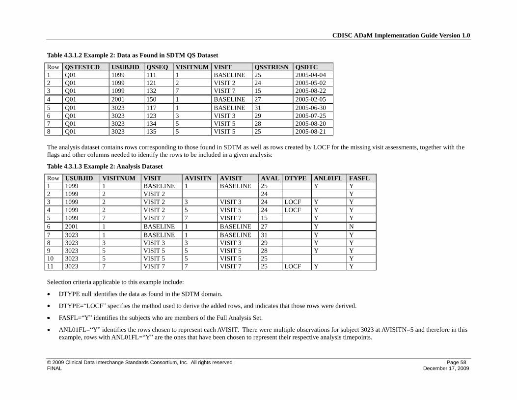
CDISC ADaM Implementation Guide Version 1.0
© 2009 Clinical Data Interchange Standards Consortium, Inc. All rights reserved Page 58 FINAL December 17, 2009
Table 4.3.1.2 Example 2: Data as Found in SDTM QS Dataset
Row QSTESTCD USUBJID QSSEQ VISITNUM VISIT QSSTRESN QSDTC
1 Q01 1099 111 1 BASELINE 25 2005-04-04
2 Q01 1099 121 2 VISIT 2 24 2005-05-02
3 Q01 1099 132 7 VISIT 7 15 2005-08-22
4 Q01 2001 150 1 BASELINE 27 2005-02-05
5 Q01 3023 117 1 BASELINE 31 2005-06-30
6 Q01 3023 123 3 VISIT 3 29 2005-07-25
7 Q01 3023 134 5 VISIT 5 28 2005-08-20
8 Q01 3023 135 5 VISIT 5 25 2005-08-21
The analysis dataset contains rows corresponding to those found in SDTM as well as rows created by LOCF for the missing visit assessments, together with the
flags and other columns needed to identify the rows to be included in a given analysis:
Table 4.3.1.3 Example 2: Analysis Dataset
Row USUBJID VISITNUM VISIT AVISITN AVISIT AVAL DTYPE ANL01FL FASFL
1 1099 1 BASELINE 1 BASELINE 25 Y Y
2 1099 2 VISIT 2 24 Y
3 1099 2 VISIT 2 3 VISIT 3 24 LOCF Y Y
4 1099 2 VISIT 2 5 VISIT 5 24 LOCF Y Y
5 1099 7 VISIT 7 7 VISIT 7 15 Y Y
6 2001 1 BASELINE 1 BASELINE 27 Y N
7 3023 1 BASELINE 1 BASELINE 31 Y Y
8 3023 3 VISIT 3 3 VISIT 3 29 Y Y
9 3023 5 VISIT 5 5 VISIT 5 28 Y Y
10 3023 5 VISIT 5 5 VISIT 5 25 Y
11 3023 7 VISIT 7 7 VISIT 7 25 LOCF Y Y
Selection criteria applicable to this example include:
DTYPE null identifies the data as found in the SDTM domain.
DTYPE=“LOCF” specifies the method used to derive the added rows, and indicates that those rows were derived.
FASFL=“Y” identifies the subjects who are members of the Full Analysis Set.
ANL01FL=“Y” identifies the rows chosen to represent each AVISIT. There were multiple observations for subject 3023 at AVISITN=5 and therefore in this
example, rows with ANL01FL=“Y” are the ones that have been chosen to represent their respective analysis timepoints.
CDISC ADaM Implementation Guide Version 1.0
© 2009 Clinical Data Interchange Standards Consortium, Inc. All rights reserved Page 59 FINAL December 17, 2009
ANL01FL=null for subject 1099 for VISIT=“VISIT 2” (row 2) because visit 2 is an unscheduled visit for this questionnaire and Visit 2 will not be presented
in the analyses; AVISITN and AVISIT are also null because visit 2 will not be analyzed per the study’s analysis plan.
“(ANL01FL=“Y” and FASFL=“Y” and AVISITN=5)” identifies the rows used in a FAS analysis of Visit 5 data.
Approaches Considered and Not Adopted
The other approach considered was to include in the analysis dataset only the rows that are actually used in the analysis of the analysis parameter. In Example 1
above, only Visit 3 rows that were either observed or derived by LOCF would be included in the analysis dataset. The main advantage of this approach would be
to simplify the analysis, as no selection clause would need to be used to identify the appropriate rows for inclusion in the analysis. However, the primary
disadvantages would be the loss of traceability and the loss of flexibility for reviewers to test the robustness of the analysis. Because of these disadvantages, this
approach was not chosen.

CDISC ADaM Implementation Guide Version 1.0
© 2009 Clinical Data Interchange Standards Consortium, Inc. All rights reserved Page 60 FINAL December 17, 2009
4.4 Inclusion of Input Data that are not Analyzed but that Support a Derivation in the Analysis Dataset
Section 4.3 states that for a given analysis parameter, all observed and derived rows of that parameter should be included in the dataset, not just the rows that are
used in the analysis.
Section 4.3 is a simple case of a more general question addressed here in Section 4.4.
This section addresses the broader issue if whether an analysis dataset should contain the input data used in the derivation of the analysis data as well as the
actual data being analyzed. This includes:
Input data rows and columns to support traceability of the derivation of analyzed rows and columns, and
Raw or derived predecessor parameters that are not analyzed themselves but are used to derive an analyzed parameter.
The above input data rows and columns could come from one SDTM domain or multiple domains as necessary to derive the analysis data captured in the
analysis variable, as described by the analysis parameter.
4.4.1 ADaM Methodology and Examples
Analysis datasets are developed to facilitate intended analyses. SDTM is provided as source data; therefore, it is logical for reviewers to expect some level of
traceability between SDTM domain(s) and analysis dataset(s).
The ADaM methodology to achieve the expected traceability is to describe the derivation algorithms in the metadata and, if practical and feasible, to include
supportive rows as appropriate for traceability. To include the input data as rows in the analysis dataset, columns should be added where feasible to indicate the
source of the input data – domain, variable name, and sequence number. While this methodology increases both the size of the dataset and the complexity of
selecting the appropriate rows for analysis, it also provides input data in an immediately accessible manner. In addition, intermediate values can be retained if
appropriate flags are used to distinguish them.
In general, it is strongly recommended to include as much supporting data as is needed for traceability. However, there are situations in which it may not be
practical. For example, if an analyzed parameter is a summary derived from a very large number of raw e-diary input records, it may be neither useful nor
practical to include all of the raw e-diary records as rows in the analysis dataset.
The remainder of this section addresses cases where the analysis datasets contain not only the analysis data but also input data that are necessary to provide
clearer traceability of the algorithms used to derive the analysis data. In addition to the actual values used in the analysis, the dataset may include rows not used
in the analysis, rows containing input data, and rows containing intermediate values computed during the derivation of the analysis data. Flags or other columns
are used to distinguish the various data types as well as to provide a traceable path from the input data to the value used in the analysis. The analysis results
metadata specify how the appropriate rows are identified (by a specific selection clause). The identification of rows used in an analysis is addressed in Sections
4.5 and 4.6.
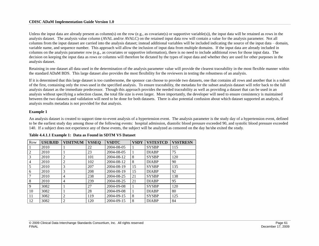
CDISC ADaM Implementation Guide Version 1.0
© 2009 Clinical Data Interchange Standards Consortium, Inc. All rights reserved Page 61 FINAL December 17, 2009
Unless the input data are already present as column(s) on the row (e.g., as covariate(s) or supportive variable(s)), the input data will be retained as rows in the
analysis dataset. The analysis value column (AVAL and/or AVALC) on the retained input data row will contain a value for the analysis parameter. Not all
columns from the input dataset are carried into the analysis dataset; instead additional variables will be included indicating the source of the input data – domain,
variable name, and sequence number. This approach will allow the inclusion of input data from multiple domains. If the input data are already included in
columns on the analysis parameter row (e.g., as covariates or supportive information), there is no need to include additional rows for those input data. The
decision on keeping the input data as rows or columns will therefore be dictated by the types of input data and whether they are used for other purposes in the
analysis dataset.
Retaining in one dataset all data used in the determination of the analysis parameter value will provide the clearest traceability in the most flexible manner within
the standard ADaM BDS. This large dataset also provides the most flexibility for the reviewers in testing the robustness of an analysis.
If it is determined that this large dataset is too cumbersome, the sponsor can choose to provide two datasets, one that contains all rows and another that is a subset
of the first, containing only the rows used in the specified analysis. To ensure traceability, the metadata for the subset analysis dataset will refer back to the full
analysis dataset as the immediate predecessor. Though this approach provides the needed traceability as well as providing a dataset that can be used in an
analysis without specifying a selection clause, the total file size is even larger. More importantly, the developer will need to ensure consistency is maintained
between the two datasets and validation will need to be done for both datasets. There is also potential confusion about which dataset supported an analysis, if
analysis results metadata is not provided for that analysis.
Example 1
An analysis dataset is created to support time-to-event analysis of a hypertension event. The analysis parameter is the study day of a hypertension event, defined
to be the earliest study day among those of the following events: hospital admission, diastolic blood pressure exceeded 90, and systolic blood pressure exceeded
140. If a subject does not experience any of these events, the subject will be analyzed as censored on the day he/she exited the study.
Table 4.4.1.1 Example 1: Data as Found in SDTM VS Dataset
Row USUBJID VISITNUM VSSEQ VSDTC VSDY VSTESTCD VSSTRESN
1 2010 1 22 2004-08-05 1 SYSBP 115
2 2010 1 23 2004-08-05 1 DIABP 75
3 2010 2 101 2004-08-12 8 SYSBP 120
4 2010 2 102 2004-08-12 8 DIABP 90
5 2010 3 207 2004-08-19 15 SYSBP 135
6 2010 3 208 2004-08-19 15 DIABP 92
7 2010 4 238 2004-08-25 21 SYSBP 138
8 2010 4 239 2004-08-25 21 DIABP 95
9 3082 1 27 2004-09-08 1 SYSBP 120
10 3082 1 28 2004-09-08 1 DIABP 80
11 3082 2 119 2004-09-15 8 SYSBP 125
12 3082 2 120 2004-09-15 8 DIABP 84
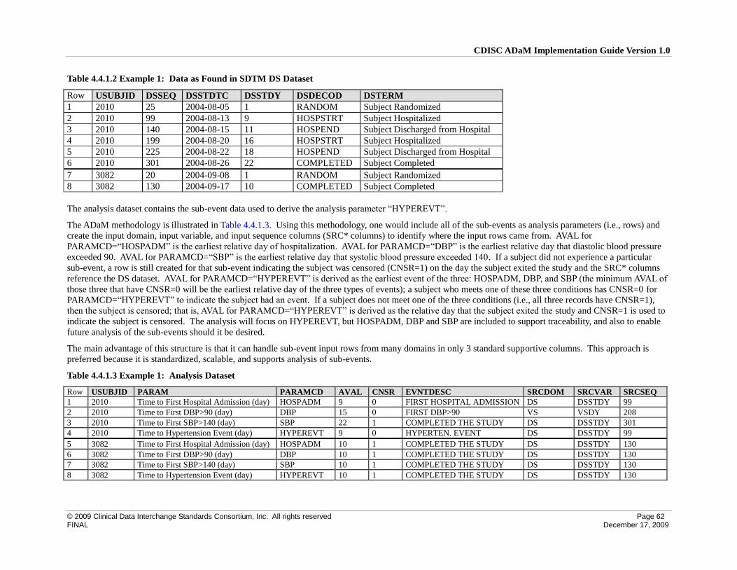
CDISC ADaM Implementation Guide Version 1.0
© 2009 Clinical Data Interchange Standards Consortium, Inc. All rights reserved Page 62 FINAL December 17, 2009
Table 4.4.1.2 Example 1: Data as Found in SDTM DS Dataset
Row USUBJID DSSEQ DSSTDTC DSSTDY DSDECOD DSTERM
1 2010 25 2004-08-05 1 RANDOM Subject Randomized
2 2010 99 2004-08-13 9 HOSPSTRT Subject Hospitalized
3 2010 140 2004-08-15 11 HOSPEND Subject Discharged from Hospital
4 2010 199 2004-08-20 16 HOSPSTRT Subject Hospitalized
5 2010 225 2004-08-22 18 HOSPEND Subject Discharged from Hospital
6 2010 301 2004-08-26 22 COMPLETED Subject Completed
7 3082 20 2004-09-08 1 RANDOM Subject Randomized
8 3082 130 2004-09-17 10 COMPLETED Subject Completed
The analysis dataset contains the sub-event data used to derive the analysis parameter “HYPEREVT”.
The ADaM methodology is illustrated in Table 4.4.1.3. Using this methodology, one would include all of the sub-events as analysis parameters (i.e., rows) and
create the input domain, input variable, and input sequence columns (SRC* columns) to identify where the input rows came from. AVAL for
PARAMCD=“HOSPADM” is the earliest relative day of hospitalization. AVAL for PARAMCD=“DBP” is the earliest relative day that diastolic blood pressure
exceeded 90. AVAL for PARAMCD=“SBP” is the earliest relative day that systolic blood pressure exceeded 140. If a subject did not experience a particular
sub-event, a row is still created for that sub-event indicating the subject was censored (CNSR=1) on the day the subject exited the study and the SRC* columns
reference the DS dataset. AVAL for PARAMCD=“HYPEREVT” is derived as the earliest event of the three: HOSPADM, DBP, and SBP (the minimum AVAL of
those three that have CNSR=0 will be the earliest relative day of the three types of events); a subject who meets one of these three conditions has CNSR=0 for
PARAMCD=“HYPEREVT” to indicate the subject had an event. If a subject does not meet one of the three conditions (i.e., all three records have CNSR=1),
then the subject is censored; that is, AVAL for PARAMCD=“HYPEREVT” is derived as the relative day that the subject exited the study and CNSR=1 is used to
indicate the subject is censored. The analysis will focus on HYPEREVT, but HOSPADM, DBP and SBP are included to support traceability, and also to enable
future analysis of the sub-events should it be desired.
The main advantage of this structure is that it can handle sub-event input rows from many domains in only 3 standard supportive columns. This approach is
preferred because it is standardized, scalable, and supports analysis of sub-events.
Table 4.4.1.3 Example 1: Analysis Dataset
Row USUBJID PARAM PARAMCD AVAL CNSR EVNTDESC SRCDOM SRCVAR SRCSEQ
1 2010 Time to First Hospital Admission (day) HOSPADM 9 0 FIRST HOSPITAL ADMISSION DS DSSTDY 99
2 2010 Time to First DBP>90 (day) DBP 15 0 FIRST DBP>90 VS VSDY 208
3 2010 Time to First SBP>140 (day) SBP 22 1 COMPLETED THE STUDY DS DSSTDY 301
4 2010 Time to Hypertension Event (day) HYPEREVT 9 0 HYPERTEN. EVENT DS DSSTDY 99
5 3082 Time to First Hospital Admission (day) HOSPADM 10 1 COMPLETED THE STUDY DS DSSTDY 130
6 3082 Time to First DBP>90 (day) DBP 10 1 COMPLETED THE STUDY DS DSSTDY 130
7 3082 Time to First SBP>140 (day) SBP 10 1 COMPLETED THE STUDY DS DSSTDY 130
8 3082 Time to Hypertension Event (day) HYPEREVT 10 1 COMPLETED THE STUDY DS DSSTDY 130
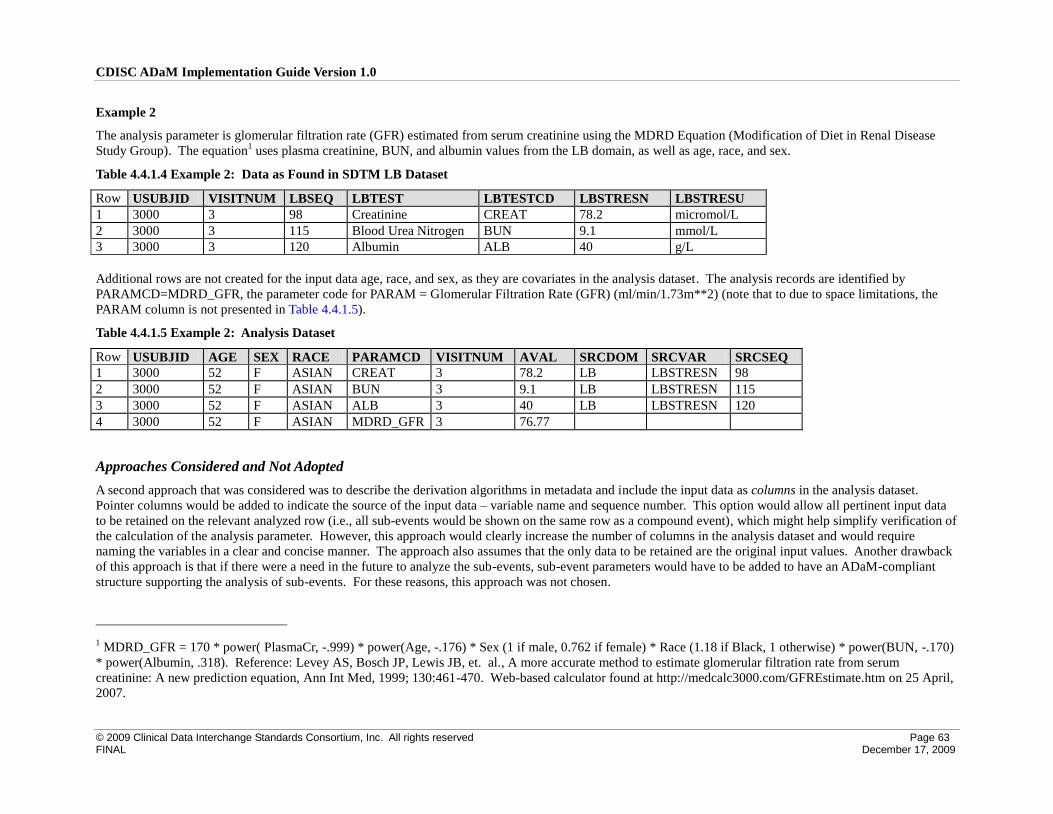
CDISC ADaM Implementation Guide Version 1.0
© 2009 Clinical Data Interchange Standards Consortium, Inc. All rights reserved Page 63 FINAL December 17, 2009
Example 2
The analysis parameter is glomerular filtration rate (GFR) estimated from serum creatinine using the MDRD Equation (Modification of Diet in Renal Disease
Study Group). The equation1 uses plasma creatinine, BUN, and albumin values from the LB domain, as well as age, race, and sex.
Table 4.4.1.4 Example 2: Data as Found in SDTM LB Dataset
Row USUBJID VISITNUM LBSEQ LBTEST LBTESTCD LBSTRESN LBSTRESU
1 3000 3 98 Creatinine CREAT 78.2 micromol/L
2 3000 3 115 Blood Urea Nitrogen BUN 9.1 mmol/L
3 3000 3 120 Albumin ALB 40 g/L
Additional rows are not created for the input data age, race, and sex, as they are covariates in the analysis dataset. The analysis records are identified by
PARAMCD=MDRD_GFR, the parameter code for PARAM = Glomerular Filtration Rate (GFR) (ml/min/1.73m**2) (note that to due to space limitations, the
PARAM column is not presented in Table 4.4.1.5).
Table 4.4.1.5 Example 2: Analysis Dataset
Row USUBJID AGE SEX RACE PARAMCD VISITNUM AVAL SRCDOM SRCVAR SRCSEQ
1 3000 52 F ASIAN CREAT 3 78.2 LB LBSTRESN 98
2 3000 52 F ASIAN BUN 3 9.1 LB LBSTRESN 115
3 3000 52 F ASIAN ALB 3 40 LB LBSTRESN 120
4 3000 52 F ASIAN MDRD_GFR 3 76.77
Approaches Considered and Not Adopted
A second approach that was considered was to describe the derivation algorithms in metadata and include the input data as columns in the analysis dataset.
Pointer columns would be added to indicate the source of the input data – variable name and sequence number. This option would allow all pertinent input data
to be retained on the relevant analyzed row (i.e., all sub-events would be shown on the same row as a compound event), which might help simplify verification of
the calculation of the analysis parameter. However, this approach would clearly increase the number of columns in the analysis dataset and would require
naming the variables in a clear and concise manner. The approach also assumes that the only data to be retained are the original input values. Another drawback
of this approach is that if there were a need in the future to analyze the sub-events, sub-event parameters would have to be added to have an ADaM-compliant
structure supporting the analysis of sub-events. For these reasons, this approach was not chosen.
1 MDRD_GFR = 170 * power( PlasmaCr, -.999) * power(Age, -.176) * Sex (1 if male, 0.762 if female) * Race (1.18 if Black, 1 otherwise) * power(BUN, -.170)
* power(Albumin, .318). Reference: Levey AS, Bosch JP, Lewis JB, et. al., A more accurate method to estimate glomerular filtration rate from serum
creatinine: A new prediction equation, Ann Int Med, 1999; 130:461-470. Web-based calculator found at http://medcalc3000.com/GFREstimate.htm on 25 April,
2007.

CDISC ADaM Implementation Guide Version 1.0
© 2009 Clinical Data Interchange Standards Consortium, Inc. All rights reserved Page 64 FINAL December 17, 2009
A third approach that was considered was to describe the derivation algorithms in metadata and include no input data or identification of the input data in the
analysis dataset. The advantage to this approach would be simplification of the analysis dataset. However, due to the simplified structure, there would be a loss
of traceability between the data collected in the study (i.e., SDTM domain) and the data analyzed (i.e., analysis dataset). Unless the derivation algorithms
described in the metadata are straightforward, verification of the analysis data computation could be very challenging or even impossible. This approach should
not be used.

CDISC ADaM Implementation Guide Version 1.0
© 2009 Clinical Data Interchange Standards Consortium, Inc. All rights reserved Page 65 FINAL December 17, 2009
4.5 Identification of Rows Used for Analysis
This section addresses how to identify the rows of an analysis dataset that are used for analysis. The four specific issues addressed include: 1) identification of
the rows used in a last observation carried forward (LOCF) analysis ; 2) identification of the row containing the baseline value; 3) identification of post-baseline
conceptual timepoint rows, such as endpoint, minimum, maximum, or average ; and 4) identification of specific rows used in an analysis.
4.5.1 Identification of Rows Used in a Timepoint Imputation Analysis
This section considers the issue of how to identify rows used in a timepoint-related imputation analysis as well as how to represent data imputed for missing
timepoints in an analysis dataset. Last observation carried forward (LOCF) is one of the most commonly used timepoint-related imputation analyses, and is
therefore specifically mentioned. However, the methodology is general and is not restricted to LOCF analysis. Worst observation carried forward (WOCF)
analysis is also mentioned to emphasis the generalizability.
4.5.1.1 ADaM Methodology and Examples
When an analysis timepoint is missing, the ADaM methodology is to create a new row in the analysis dataset to represent the missing timepoint and identify
these imputed rows by populating the derivation type variable DTYPE.
For example, when an LOCF/WOCF analysis is being performed, create LOCF/WOCF rows when the LOCF/WOCF analysis timepoints are missing, and
identify these imputed rows by populating the derivation type variable DTYPE with values LOCF or WOCF. All of the original rows would have null values in
DTYPE. It would be very simple to select the appropriate rows for analysis by selecting DTYPE = null for Data as Observed (DAO) analysis, DTYPE = null or
LOCF for LOCF analysis, and DTYPE = null or WOCF for WOCF analysis. This approach would require understanding and communication that if the DTYPE
flag were not referenced correctly, the analysis would default to using all rows, including the DAO rows, plus the rows derived by LOCF and WOCF. To
perform a correct DAO analysis, one would need to explicitly select DTYPE = null.
Example 1: Identification of rows used in a LOCF analysis
In the example below (Table 4.5.1.1.1), some subjects have complete data and others have rows imputed by one method (LOCF). Subjects with no missing data
have the observed number of rows with all DTYPE values blank. Subject 1001 has complete data. DTYPE is blank for all rows indicating they are not imputed.
AVISIT matches VISIT (from SDTM) in this example. AVISIT does not always match VISIT from SDTM even in scenarios where there is no missing data.
Subject 1002 is missing the Week 2 assessment. Week 2 is imputed using the LOCF method. AVISIT=Week 2 but VISIT=Week 1 so one can see where the
imputed value came from in the original data. Subject 1003 is missing Week 2 and 3 data. A Data as Observed (DAO) analysis can be performed by selecting
only those rows where DTYPE is null. For a LOCF analysis, all rows (DTYPE=null or DTYPE=“LOCF”) should be used.

CDISC ADaM Implementation Guide Version 1.0
© 2009 Clinical Data Interchange Standards Consortium, Inc. All rights reserved Page 66 FINAL December 17, 2009
Table 4.5.1.1.1 Example 1: Analysis Dataset with Identification of Rows Used in a LOCF Analysis
Row USUBJID VISIT AVISIT ADY PARAM AVAL DTYPE
1 1001 Baseline Baseline -4 SUPINE SYSBP (mm Hg) 145
2 1001 Week 1 Week 1 3 SUPINE SYSBP (mm Hg) 130
3 1001 Week 2 Week 2 9 SUPINE SYSBP (mm Hg) 133
4 1001 Week 3 Week 3 20 SUPINE SYSBP (mm Hg) 125
5 1002 Baseline Baseline -1 SUPINE SYSBP (mm Hg) 145
6 1002 Week 1 Week 1 7 SUPINE SYSBP (mm Hg) 130
7 1002 Week 1 Week 2 7 SUPINE SYSBP (mm Hg) 130 LOCF
8 1002 Week 3 Week 3 22 SUPINE SYSBP (mm Hg) 135
9 1003 Baseline Baseline 1 SUPINE SYSBP (mm Hg) 150
10 1003 Week 1 Week 1 8 SUPINE SYSBP (mm Hg) 140
11 1003 Week 1 Week 2 8 SUPINE SYSBP (mm Hg) 140 LOCF
12 1003 Week 1 Week 3 8 SUPINE SYSBP (mm Hg) 140 LOCF
Example 2: Identification of rows used in both LOCF and WOCF analyses
This set of rows (Table 4.5.1.1.2) shows a situation where there is more than one imputation method used. In this case, additional rows are generated for each
type of imputation. A DAO analysis can be performed by selecting only those rows where DTYPE is null. For LOCF analysis, all rows with DTYPE=null or
DTYPE=“LOCF” should be used. For WOCF analysis, all rows with DTYPE=null or DTYPE=“WOCF” should be used.
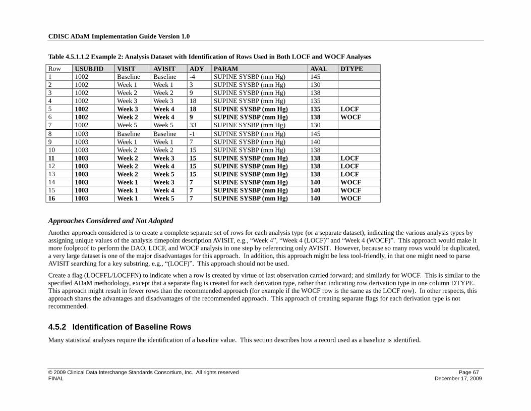
CDISC ADaM Implementation Guide Version 1.0
© 2009 Clinical Data Interchange Standards Consortium, Inc. All rights reserved Page 67 FINAL December 17, 2009
Table 4.5.1.1.2 Example 2: Analysis Dataset with Identification of Rows Used in Both LOCF and WOCF Analyses
Row USUBJID VISIT AVISIT ADY PARAM AVAL DTYPE
1 1002 Baseline Baseline -4 SUPINE SYSBP (mm Hg) 145
2 1002 Week 1 Week 1 3 SUPINE SYSBP (mm Hg) 130
3 1002 Week 2 Week 2 9 SUPINE SYSBP (mm Hg) 138
4 1002 Week 3 Week 3 18 SUPINE SYSBP (mm Hg) 135
5 1002 Week 3 Week 4 18 SUPINE SYSBP (mm Hg) 135 LOCF
6 1002 Week 2 Week 4 9 SUPINE SYSBP (mm Hg) 138 WOCF
7 1002 Week 5 Week 5 33 SUPINE SYSBP (mm Hg) 130
8 1003 Baseline Baseline -1 SUPINE SYSBP (mm Hg) 145
9 1003 Week 1 Week 1 7 SUPINE SYSBP (mm Hg) 140
10 1003 Week 2 Week 2 15 SUPINE SYSBP (mm Hg) 138
11 1003 Week 2 Week 3 15 SUPINE SYSBP (mm Hg) 138 LOCF
12 1003 Week 2 Week 4 15 SUPINE SYSBP (mm Hg) 138 LOCF
13 1003 Week 2 Week 5 15 SUPINE SYSBP (mm Hg) 138 LOCF
14 1003 Week 1 Week 3 7 SUPINE SYSBP (mm Hg) 140 WOCF
15 1003 Week 1 Week 4 7 SUPINE SYSBP (mm Hg) 140 WOCF
16 1003 Week 1 Week 5 7 SUPINE SYSBP (mm Hg) 140 WOCF
Approaches Considered and Not Adopted
Another approach considered is to create a complete separate set of rows for each analysis type (or a separate dataset), indicating the various analysis types by
assigning unique values of the analysis timepoint description AVISIT, e.g., “Week 4”, “Week 4 (LOCF)” and “Week 4 (WOCF)”. This approach would make it
more foolproof to perform the DAO, LOCF, and WOCF analysis in one step by referencing only AVISIT. However, because so many rows would be duplicated,
a very large dataset is one of the major disadvantages for this approach. In addition, this approach might be less tool-friendly, in that one might need to parse
AVISIT searching for a key substring, e.g., “(LOCF)”. This approach should not be used.
Create a flag (LOCFFL/LOCFFN) to indicate when a row is created by virtue of last observation carried forward; and similarly for WOCF. This is similar to the
specified ADaM methodology, except that a separate flag is created for each derivation type, rather than indicating row derivation type in one column DTYPE.
This approach might result in fewer rows than the recommended approach (for example if the WOCF row is the same as the LOCF row). In other respects, this
approach shares the advantages and disadvantages of the recommended approach. This approach of creating separate flags for each derivation type is not
recommended.
4.5.2 Identification of Baseline Rows
Many statistical analyses require the identification of a baseline value. This section describes how a record used as a baseline is identified.
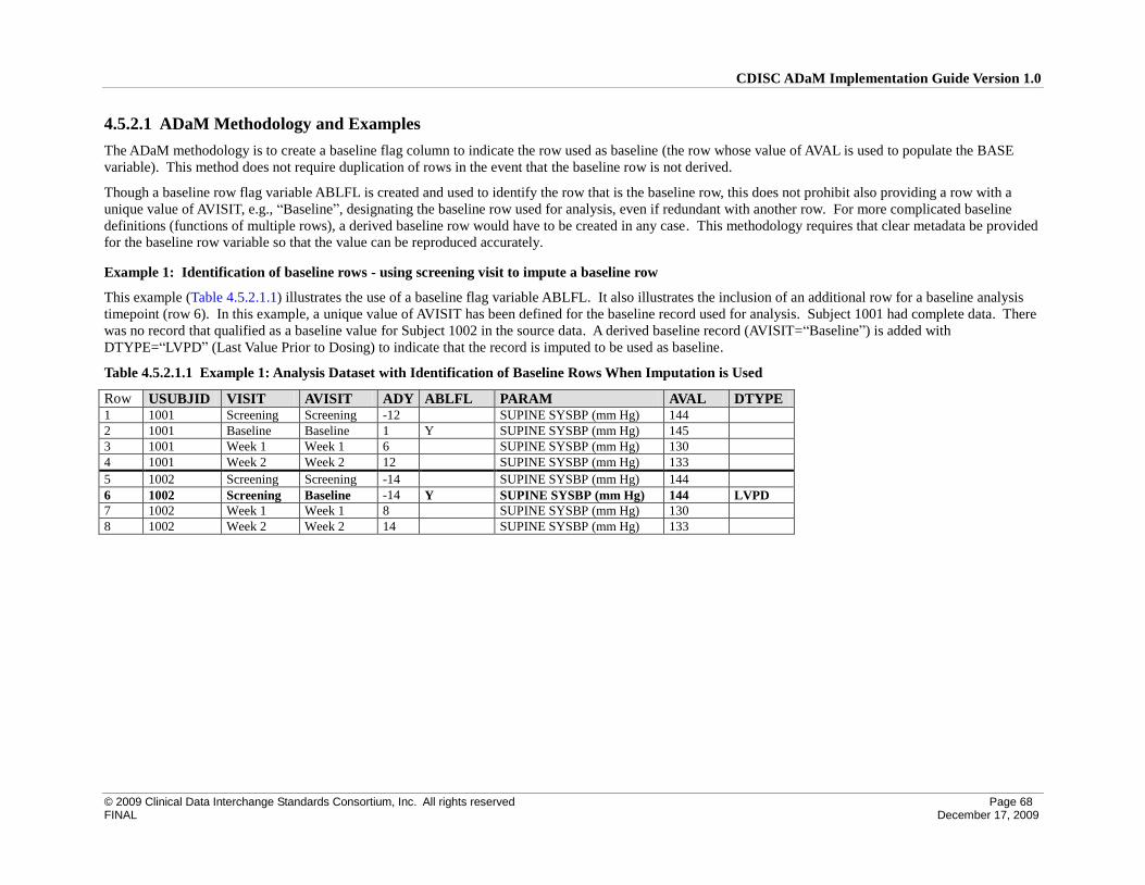
CDISC ADaM Implementation Guide Version 1.0
© 2009 Clinical Data Interchange Standards Consortium, Inc. All rights reserved Page 68 FINAL December 17, 2009
4.5.2.1 ADaM Methodology and Examples
The ADaM methodology is to create a baseline flag column to indicate the row used as baseline (the row whose value of AVAL is used to populate the BASE
variable). This method does not require duplication of rows in the event that the baseline row is not derived.
Though a baseline row flag variable ABLFL is created and used to identify the row that is the baseline row, this does not prohibit also providing a row with a
unique value of AVISIT, e.g., “Baseline”, designating the baseline row used for analysis, even if redundant with another row. For more complicated baseline
definitions (functions of multiple rows), a derived baseline row would have to be created in any case. This methodology requires that clear metadata be provided
for the baseline row variable so that the value can be reproduced accurately.
Example 1: Identification of baseline rows - using screening visit to impute a baseline row
This example (Table 4.5.2.1.1) illustrates the use of a baseline flag variable ABLFL. It also illustrates the inclusion of an additional row for a baseline analysis
timepoint (row 6). In this example, a unique value of AVISIT has been defined for the baseline record used for analysis. Subject 1001 had complete data. There
was no record that qualified as a baseline value for Subject 1002 in the source data. A derived baseline record (AVISIT=“Baseline”) is added with
DTYPE=“LVPD” (Last Value Prior to Dosing) to indicate that the record is imputed to be used as baseline.
Table 4.5.2.1.1 Example 1: Analysis Dataset with Identification of Baseline Rows When Imputation is Used
Row USUBJID VISIT AVISIT ADY ABLFL PARAM AVAL DTYPE 1 1001 Screening Screening -12 SUPINE SYSBP (mm Hg) 144
2 1001 Baseline Baseline 1 Y SUPINE SYSBP (mm Hg) 145
3 1001 Week 1 Week 1 6 SUPINE SYSBP (mm Hg) 130
4 1001 Week 2 Week 2 12 SUPINE SYSBP (mm Hg) 133
5 1002 Screening Screening -14 SUPINE SYSBP (mm Hg) 144
6 1002 Screening Baseline -14 Y SUPINE SYSBP (mm Hg) 144 LVPD
7 1002 Week 1 Week 1 8 SUPINE SYSBP (mm Hg) 130
8 1002 Week 2 Week 2 14 SUPINE SYSBP (mm Hg) 133
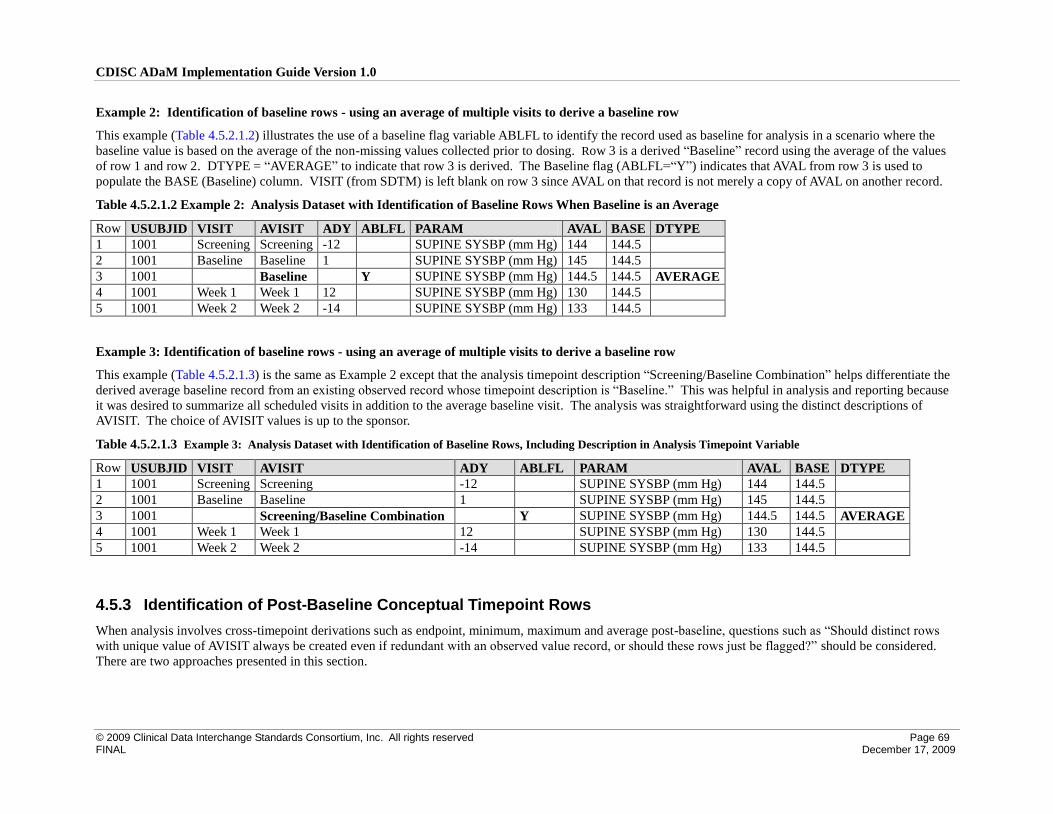
CDISC ADaM Implementation Guide Version 1.0
© 2009 Clinical Data Interchange Standards Consortium, Inc. All rights reserved Page 69 FINAL December 17, 2009
Example 2: Identification of baseline rows - using an average of multiple visits to derive a baseline row
This example (Table 4.5.2.1.2) illustrates the use of a baseline flag variable ABLFL to identify the record used as baseline for analysis in a scenario where the
baseline value is based on the average of the non-missing values collected prior to dosing. Row 3 is a derived “Baseline” record using the average of the values
of row 1 and row 2. DTYPE = “AVERAGE” to indicate that row 3 is derived. The Baseline flag (ABLFL=“Y”) indicates that AVAL from row 3 is used to
populate the BASE (Baseline) column. VISIT (from SDTM) is left blank on row 3 since AVAL on that record is not merely a copy of AVAL on another record.
Table 4.5.2.1.2 Example 2: Analysis Dataset with Identification of Baseline Rows When Baseline is an Average
Row USUBJID VISIT AVISIT ADY ABLFL PARAM AVAL BASE DTYPE
1 1001 Screening Screening -12 SUPINE SYSBP (mm Hg) 144 144.5
2 1001 Baseline Baseline 1 SUPINE SYSBP (mm Hg) 145 144.5
3 1001 Baseline Y SUPINE SYSBP (mm Hg) 144.5 144.5 AVERAGE
4 1001 Week 1 Week 1 12 SUPINE SYSBP (mm Hg) 130 144.5
5 1001 Week 2 Week 2 -14 SUPINE SYSBP (mm Hg) 133 144.5
Example 3: Identification of baseline rows - using an average of multiple visits to derive a baseline row
This example (Table 4.5.2.1.3) is the same as Example 2 except that the analysis timepoint description “Screening/Baseline Combination” helps differentiate the
derived average baseline record from an existing observed record whose timepoint description is “Baseline.” This was helpful in analysis and reporting because
it was desired to summarize all scheduled visits in addition to the average baseline visit. The analysis was straightforward using the distinct descriptions of
AVISIT. The choice of AVISIT values is up to the sponsor.
Table 4.5.2.1.3 Example 3: Analysis Dataset with Identification of Baseline Rows, Including Description in Analysis Timepoint Variable
Row USUBJID VISIT AVISIT ADY ABLFL PARAM AVAL BASE DTYPE
1 1001 Screening Screening -12 SUPINE SYSBP (mm Hg) 144 144.5
2 1001 Baseline Baseline 1 SUPINE SYSBP (mm Hg) 145 144.5
3 1001 Screening/Baseline Combination Y SUPINE SYSBP (mm Hg) 144.5 144.5 AVERAGE
4 1001 Week 1 Week 1 12 SUPINE SYSBP (mm Hg) 130 144.5
5 1001 Week 2 Week 2 -14 SUPINE SYSBP (mm Hg) 133 144.5
4.5.3 Identification of Post-Baseline Conceptual Timepoint Rows
When analysis involves cross-timepoint derivations such as endpoint, minimum, maximum and average post-baseline, questions such as “Should distinct rows
with unique value of AVISIT always be created even if redundant with an observed value record, or should these rows just be flagged?” should be considered.
There are two approaches presented in this section.
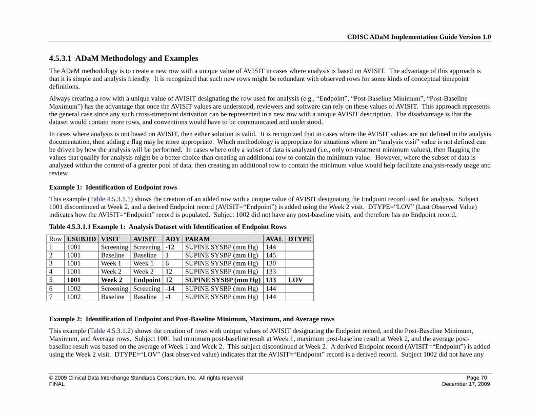
CDISC ADaM Implementation Guide Version 1.0
© 2009 Clinical Data Interchange Standards Consortium, Inc. All rights reserved Page 70 FINAL December 17, 2009
4.5.3.1 ADaM Methodology and Examples
The ADaM methodology is to create a new row with a unique value of AVISIT in cases where analysis is based on AVISIT. The advantage of this approach is
that it is simple and analysis friendly. It is recognized that such new rows might be redundant with observed rows for some kinds of conceptual timepoint
definitions.
Always creating a row with a unique value of AVISIT designating the row used for analysis (e.g., “Endpoint”, “Post-Baseline Minimum”, “Post-Baseline
Maximum”) has the advantage that once the AVISIT values are understood, reviewers and software can rely on these values of AVISIT. This approach represents
the general case since any such cross-timepoint derivation can be represented in a new row with a unique AVISIT description. The disadvantage is that the
dataset would contain more rows, and conventions would have to be communicated and understood.
In cases where analysis is not based on AVISIT, then either solution is valid. It is recognized that in cases where the AVISIT values are not defined in the analysis
documentation, then adding a flag may be more appropriate. Which methodology is appropriate for situations where an “analysis visit” value is not defined can
be driven by how the analysis will be performed. In cases where only a subset of data is analyzed (i.e., only on-treatment minimum values), then flagging the
values that qualify for analysis might be a better choice than creating an additional row to contain the minimum value. However, where the subset of data is
analyzed within the context of a greater pool of data, then creating an additional row to contain the minimum value would help facilitate analysis-ready usage and
review.
Example 1: Identification of Endpoint rows
This example (Table 4.5.3.1.1) shows the creation of an added row with a unique value of AVISIT designating the Endpoint record used for analysis. Subject
1001 discontinued at Week 2, and a derived Endpoint record (AVISIT=“Endpoint”) is added using the Week 2 visit. DTYPE=“LOV” (Last Observed Value)
indicates how the AVISIT=“Endpoint” record is populated. Subject 1002 did not have any post-baseline visits, and therefore has no Endpoint record.
Table 4.5.3.1.1 Example 1: Analysis Dataset with Identification of Endpoint Rows
Row USUBJID VISIT AVISIT ADY PARAM AVAL DTYPE
1 1001 Screening Screening -12 SUPINE SYSBP (mm Hg) 144
2 1001 Baseline Baseline 1 SUPINE SYSBP (mm Hg) 145
3 1001 Week 1 Week 1 6 SUPINE SYSBP (mm Hg) 130
4 1001 Week 2 Week 2 12 SUPINE SYSBP (mm Hg) 133
5 1001 Week 2 Endpoint 12 SUPINE SYSBP (mm Hg) 133 LOV
6 1002 Screening Screening -14 SUPINE SYSBP (mm Hg) 144
7 1002 Baseline Baseline -1 SUPINE SYSBP (mm Hg) 144
Example 2: Identification of Endpoint and Post-Baseline Minimum, Maximum, and Average rows
This example (Table 4.5.3.1.2) shows the creation of rows with unique values of AVISIT designating the Endpoint record, and the Post-Baseline Minimum,
Maximum, and Average rows. Subject 1001 had minimum post-baseline result at Week 1, maximum post-baseline result at Week 2, and the average post-
baseline result was based on the average of Week 1 and Week 2. This subject discontinued at Week 2. A derived Endpoint record (AVISIT=“Endpoint”) is added
using the Week 2 visit. DTYPE=“LOV” (last observed value) indicates that the AVISIT=“Endpoint” record is a derived record. Subject 1002 did not have any
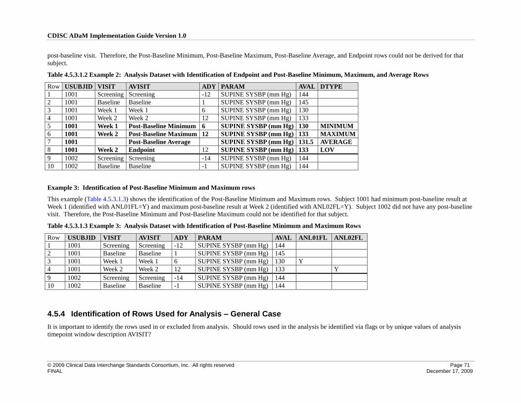
CDISC ADaM Implementation Guide Version 1.0
© 2009 Clinical Data Interchange Standards Consortium, Inc. All rights reserved Page 71 FINAL December 17, 2009
post-baseline visit. Therefore, the Post-Baseline Minimum, Post-Baseline Maximum, Post-Baseline Average, and Endpoint rows could not be derived for that
subject.
Table 4.5.3.1.2 Example 2: Analysis Dataset with Identification of Endpoint and Post-Baseline Minimum, Maximum, and Average Rows
Row USUBJID VISIT AVISIT ADY PARAM AVAL DTYPE
1 1001 Screening Screening -12 SUPINE SYSBP (mm Hg) 144
2 1001 Baseline Baseline 1 SUPINE SYSBP (mm Hg) 145
3 1001 Week 1 Week 1 6 SUPINE SYSBP (mm Hg) 130
4 1001 Week 2 Week 2 12 SUPINE SYSBP (mm Hg) 133
5 1001 Week 1 Post-Baseline Minimum 6 SUPINE SYSBP (mm Hg) 130 MINIMUM
6 1001 Week 2 Post-Baseline Maximum 12 SUPINE SYSBP (mm Hg) 133 MAXIMUM
7 1001 Post-Baseline Average SUPINE SYSBP (mm Hg) 131.5 AVERAGE
8 1001 Week 2 Endpoint 12 SUPINE SYSBP (mm Hg) 133 LOV
9 1002 Screening Screening -14 SUPINE SYSBP (mm Hg) 144
10 1002 Baseline Baseline -1 SUPINE SYSBP (mm Hg) 144
Example 3: Identification of Post-Baseline Minimum and Maximum rows
This example (Table 4.5.3.1.3) shows the identification of the Post-Baseline Minimum and Maximum rows. Subject 1001 had minimum post-baseline result at
Week 1 (identified with ANL01FL=Y) and maximum post-baseline result at Week 2 (identified with ANL02FL=Y). Subject 1002 did not have any post-baseline
visit. Therefore, the Post-Baseline Minimum and Post-Baseline Maximum could not be identified for that subject.
Table 4.5.3.1.3 Example 3: Analysis Dataset with Identification of Post-Baseline Minimum and Maximum Rows
Row USUBJID VISIT AVISIT ADY PARAM AVAL ANL01FL ANL02FL
1 1001 Screening Screening -12 SUPINE SYSBP (mm Hg) 144
2 1001 Baseline Baseline 1 SUPINE SYSBP (mm Hg) 145
3 1001 Week 1 Week 1 6 SUPINE SYSBP (mm Hg) 130 Y
4 1001 Week 2 Week 2 12 SUPINE SYSBP (mm Hg) 133 Y
9 1002 Screening Screening -14 SUPINE SYSBP (mm Hg) 144
10 1002 Baseline Baseline -1 SUPINE SYSBP (mm Hg) 144
4.5.4 Identification of Rows Used for Analysis – General Case
It is important to identify the rows used in or excluded from analysis. Should rows used in the analysis be identified via flags or by unique values of analysis
timepoint window description AVISIT?
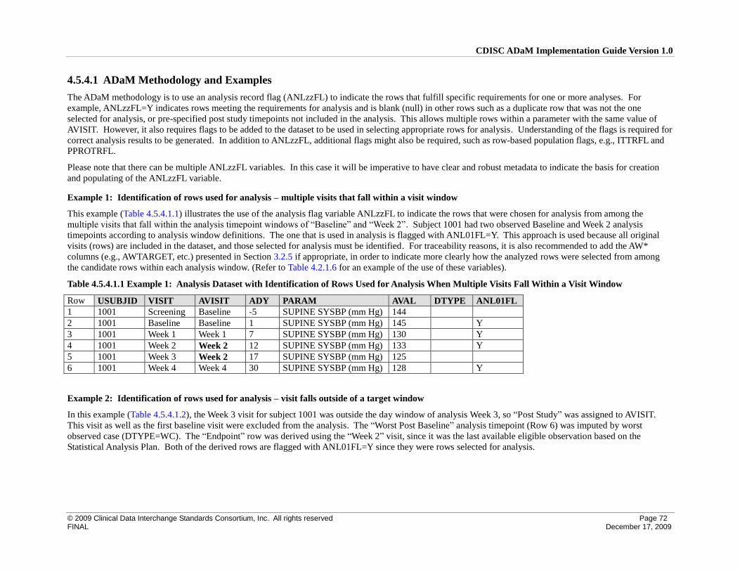
CDISC ADaM Implementation Guide Version 1.0
© 2009 Clinical Data Interchange Standards Consortium, Inc. All rights reserved Page 72 FINAL December 17, 2009
4.5.4.1 ADaM Methodology and Examples
The ADaM methodology is to use an analysis record flag (ANLzzFL) to indicate the rows that fulfill specific requirements for one or more analyses. For
example, ANLzzFL=Y indicates rows meeting the requirements for analysis and is blank (null) in other rows such as a duplicate row that was not the one
selected for analysis, or pre-specified post study timepoints not included in the analysis. This allows multiple rows within a parameter with the same value of
AVISIT. However, it also requires flags to be added to the dataset to be used in selecting appropriate rows for analysis. Understanding of the flags is required for
correct analysis results to be generated. In addition to ANLzzFL, additional flags might also be required, such as row-based population flags, e.g., ITTRFL and
PPROTRFL.
Please note that there can be multiple ANLzzFL variables. In this case it will be imperative to have clear and robust metadata to indicate the basis for creation
and populating of the ANLzzFL variable.
Example 1: Identification of rows used for analysis – multiple visits that fall within a visit window
This example (Table 4.5.4.1.1) illustrates the use of the analysis flag variable ANLzzFL to indicate the rows that were chosen for analysis from among the
multiple visits that fall within the analysis timepoint windows of “Baseline” and “Week 2”. Subject 1001 had two observed Baseline and Week 2 analysis
timepoints according to analysis window definitions. The one that is used in analysis is flagged with ANL01FL=Y. This approach is used because all original
visits (rows) are included in the dataset, and those selected for analysis must be identified. For traceability reasons, it is also recommended to add the AW*
columns (e.g., AWTARGET, etc.) presented in Section 3.2.5 if appropriate, in order to indicate more clearly how the analyzed rows were selected from among
the candidate rows within each analysis window. (Refer to Table 4.2.1.6 for an example of the use of these variables).
Table 4.5.4.1.1 Example 1: Analysis Dataset with Identification of Rows Used for Analysis When Multiple Visits Fall Within a Visit Window
Row USUBJID VISIT AVISIT ADY PARAM AVAL DTYPE ANL01FL
1 1001 Screening Baseline -5 SUPINE SYSBP (mm Hg) 144
2 1001 Baseline Baseline 1 SUPINE SYSBP (mm Hg) 145 Y
3 1001 Week 1 Week 1 7 SUPINE SYSBP (mm Hg) 130 Y
4 1001 Week 2 Week 2 12 SUPINE SYSBP (mm Hg) 133 Y
5 1001 Week 3 Week 2 17 SUPINE SYSBP (mm Hg) 125
6 1001 Week 4 Week 4 30 SUPINE SYSBP (mm Hg) 128 Y
Example 2: Identification of rows used for analysis – visit falls outside of a target window
In this example (Table 4.5.4.1.2), the Week 3 visit for subject 1001 was outside the day window of analysis Week 3, so “Post Study” was assigned to AVISIT.
This visit as well as the first baseline visit were excluded from the analysis. The “Worst Post Baseline” analysis timepoint (Row 6) was imputed by worst
observed case (DTYPE=WC). The “Endpoint” row was derived using the “Week 2” visit, since it was the last available eligible observation based on the
Statistical Analysis Plan. Both of the derived rows are flagged with ANL01FL=Y since they were rows selected for analysis.
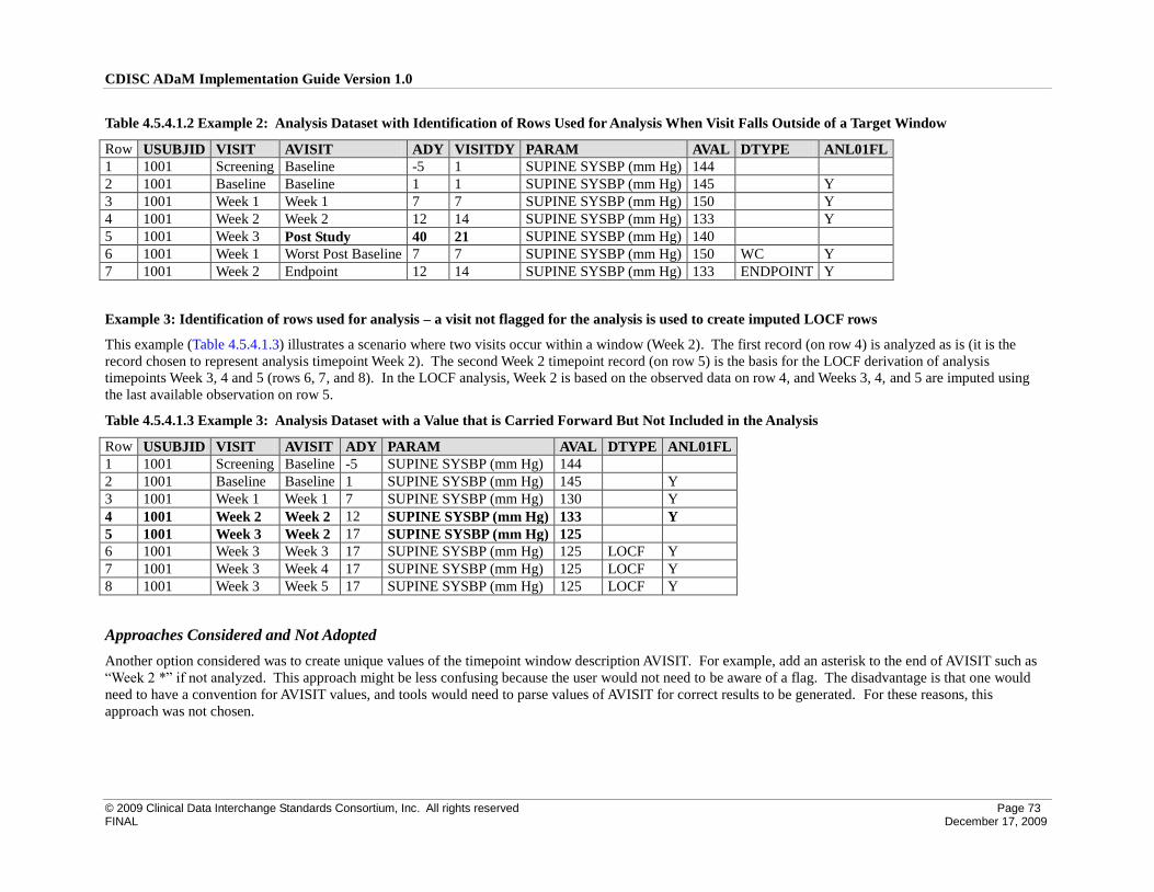
CDISC ADaM Implementation Guide Version 1.0
© 2009 Clinical Data Interchange Standards Consortium, Inc. All rights reserved Page 73 FINAL December 17, 2009
Table 4.5.4.1.2 Example 2: Analysis Dataset with Identification of Rows Used for Analysis When Visit Falls Outside of a Target Window
Row USUBJID VISIT AVISIT ADY VISITDY PARAM AVAL DTYPE ANL01FL
1 1001 Screening Baseline -5 1 SUPINE SYSBP (mm Hg) 144
2 1001 Baseline Baseline 1 1 SUPINE SYSBP (mm Hg) 145 Y
3 1001 Week 1 Week 1 7 7 SUPINE SYSBP (mm Hg) 150 Y
4 1001 Week 2 Week 2 12 14 SUPINE SYSBP (mm Hg) 133 Y
5 1001 Week 3 Post Study 40 21 SUPINE SYSBP (mm Hg) 140
6 1001 Week 1 Worst Post Baseline 7 7 SUPINE SYSBP (mm Hg) 150 WC Y
7 1001 Week 2 Endpoint 12 14 SUPINE SYSBP (mm Hg) 133 ENDPOINT Y
Example 3: Identification of rows used for analysis – a visit not flagged for the analysis is used to create imputed LOCF rows
This example (Table 4.5.4.1.3) illustrates a scenario where two visits occur within a window (Week 2). The first record (on row 4) is analyzed as is (it is the
record chosen to represent analysis timepoint Week 2). The second Week 2 timepoint record (on row 5) is the basis for the LOCF derivation of analysis
timepoints Week 3, 4 and 5 (rows 6, 7, and 8). In the LOCF analysis, Week 2 is based on the observed data on row 4, and Weeks 3, 4, and 5 are imputed using
the last available observation on row 5.
Table 4.5.4.1.3 Example 3: Analysis Dataset with a Value that is Carried Forward But Not Included in the Analysis
Row USUBJID VISIT AVISIT ADY PARAM AVAL DTYPE ANL01FL
1 1001 Screening Baseline -5 SUPINE SYSBP (mm Hg) 144
2 1001 Baseline Baseline 1 SUPINE SYSBP (mm Hg) 145 Y
3 1001 Week 1 Week 1 7 SUPINE SYSBP (mm Hg) 130 Y
4 1001 Week 2 Week 2 12 SUPINE SYSBP (mm Hg) 133 Y
5 1001 Week 3 Week 2 17 SUPINE SYSBP (mm Hg) 125
6 1001 Week 3 Week 3 17 SUPINE SYSBP (mm Hg) 125 LOCF Y
7 1001 Week 3 Week 4 17 SUPINE SYSBP (mm Hg) 125 LOCF Y
8 1001 Week 3 Week 5 17 SUPINE SYSBP (mm Hg) 125 LOCF Y
Approaches Considered and Not Adopted
Another option considered was to create unique values of the timepoint window description AVISIT. For example, add an asterisk to the end of AVISIT such as
“Week 2 *” if not analyzed. This approach might be less confusing because the user would not need to be aware of a flag. The disadvantage is that one would
need to have a convention for AVISIT values, and tools would need to parse values of AVISIT for correct results to be generated. For these reasons, this
approach was not chosen.

CDISC ADaM Implementation Guide Version 1.0
© 2009 Clinical Data Interchange Standards Consortium, Inc. All rights reserved Page 74 FINAL December 17, 2009
4.6 Identification of Population-Specific Analyzed Rows
It is not uncommon in the statistical analysis of clinical trials to repeat analyses based on multiple populations of interest. The population of interest can be
defined either at the subject level, the row (measurement) level or both. For example, when defining an analysis population, a subject may be included in one
analysis population such as Intent-to-Treat but may be excluded from another analysis population such as Per-Protocol. Analysis populations may also be
defined using characteristics of individual measurements. For example, a measurement that was assessed outside of a pre-specified time window for a particular
visit may not be included in a per-protocol visit-level population. In this section, it is assumed that the definition of a row-level analysis population is dependent
on the definition of the subject-level population. In other words, if a subject is excluded from the subject-level Per-Protocol population, then none of that
subject’s rows would be candidates for inclusion within the row-level Per-Protocol population. Given the variety of possible population definitions, the same row
in an analysis data set could be included in one analysis and excluded from another, depending on characteristics of the subject as a whole and the characteristics
of the individual measurement. Therefore, the issue becomes how best to select rows for each analysis.
4.6.1 ADaM Methodology and Examples
The ADaM methodology to this analysis issue is to have one analysis dataset that can be used to perform multiple analyses using population specific indicator
variables to identify rows that are used for each type of analysis. The advantage of this approach is that the one analysis dataset can be used for multiple analyses
and the use of flag variables obviates the need to replicate rows for each type of analysis. This promotes efficiency in the operational aspects of electronic
submissions, clarity of analyses, and ease for FDA reviewers to compare selected values for each population. This approach does, however, require that clear
metadata be provided for the indicator variable so that each specific analysis can be reproduced accurately. Below are several examples of the use of population
specific indicator variables to identify rows used for different analyses.
Example 1: Use of subject-level indicator variables (ITTFL and PPROTFL) and row (measurement) level indicator variables (ANL01FL, ITTRFL, and
PPROTRFL)
This analysis dataset (Table 4.6.1.1) can be used to repeat analyses based on multiple populations of interest either at subject level or at the row (measurement)
level.
ITTFL and PPROTFL are subject-level analysis population flags. If a subject is in the Intent-to-Treat population, then the column ITTFL will have the value of
“Y” (“N” if not). In Table 4.6.1.1, subjects 1001, 1002, and 1003 are in the Intent-to-Treat population. Similarly, if a subject is in the Per-Protocol population,
the column PPROTFL will have the value of “Y” (“N” if not). Subjects 1001 and 1003 in Table 4.6.1.1 are in the Per-Protocol population while subject 1002
with PPROTFL=N is excluded from any Per-Protocol analysis. These indicator variables are used to identify individual subjects that belong to each subject-level
population.
In contrast to the subject-level population flags, the columns ITTRFL and PPROTRFL are the analysis flags at the row level. If a row is eligible for the Intent-to-
Treat analysis, the variable ITTRFL is set to “Y”; it is null if the row is not a candidate for this analysis. In Table 4.6.1.1, all rows under the column ITTRFL are
all set to “Y”. Similarly, if a row is a candidate for the Per-Protocol analysis, the variable PPROTRFL is set to “Y”, it is null if the row does not fulfill the criteria
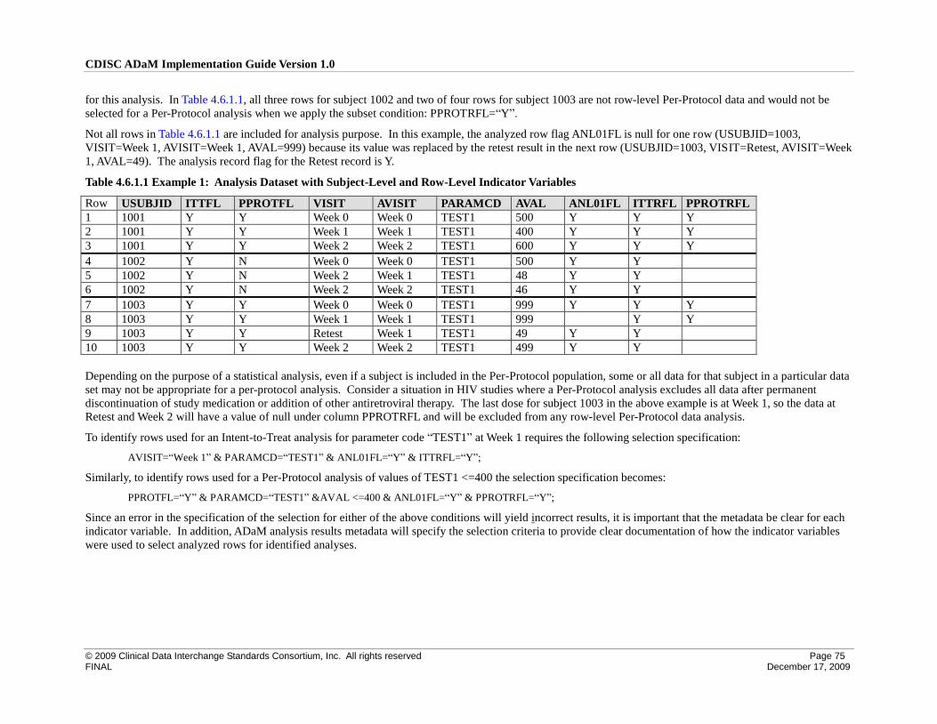
CDISC ADaM Implementation Guide Version 1.0
© 2009 Clinical Data Interchange Standards Consortium, Inc. All rights reserved Page 75 FINAL December 17, 2009
for this analysis. In Table 4.6.1.1, all three rows for subject 1002 and two of four rows for subject 1003 are not row-level Per-Protocol data and would not be
selected for a Per-Protocol analysis when we apply the subset condition: PPROTRFL=“Y”.
Not all rows in Table 4.6.1.1 are included for analysis purpose. In this example, the analyzed row flag ANL01FL is null for one row (USUBJID=1003,
VISIT=Week 1, AVISIT=Week 1, AVAL=999) because its value was replaced by the retest result in the next row (USUBJID=1003, VISIT=Retest, AVISIT=Week
1, AVAL=49). The analysis record flag for the Retest record is Y.
Table 4.6.1.1 Example 1: Analysis Dataset with Subject-Level and Row-Level Indicator Variables
Row USUBJID ITTFL PPROTFL VISIT AVISIT PARAMCD AVAL ANL01FL ITTRFL PPROTRFL
1 1001 Y Y Week 0 Week 0 TEST1 500 Y Y Y
2 1001 Y Y Week 1 Week 1 TEST1 400 Y Y Y
3 1001 Y Y Week 2 Week 2 TEST1 600 Y Y Y
4 1002 Y N Week 0 Week 0 TEST1 500 Y Y
5 1002 Y N Week 2 Week 1 TEST1 48 Y Y
6 1002 Y N Week 2 Week 2 TEST1 46 Y Y
7 1003 Y Y Week 0 Week 0 TEST1 999 Y Y Y
8 1003 Y Y Week 1 Week 1 TEST1 999 Y Y
9 1003 Y Y Retest Week 1 TEST1 49 Y Y
10 1003 Y Y Week 2 Week 2 TEST1 499 Y Y
Depending on the purpose of a statistical analysis, even if a subject is included in the Per-Protocol population, some or all data for that subject in a particular data
set may not be appropriate for a per-protocol analysis. Consider a situation in HIV studies where a Per-Protocol analysis excludes all data after permanent
discontinuation of study medication or addition of other antiretroviral therapy. The last dose for subject 1003 in the above example is at Week 1, so the data at
Retest and Week 2 will have a value of null under column PPROTRFL and will be excluded from any row-level Per-Protocol data analysis.
To identify rows used for an Intent-to-Treat analysis for parameter code “TEST1” at Week 1 requires the following selection specification:
AVISIT=“Week 1” & PARAMCD=“TEST1” & ANL01FL=“Y” & ITTRFL=“Y”;
Similarly, to identify rows used for a Per-Protocol analysis of values of TEST1 <=400 the selection specification becomes:
PPROTFL=“Y” & PARAMCD=“TEST1” &AVAL <=400 & ANL01FL=“Y” & PPROTRFL=“Y”;
Since an error in the specification of the selection for either of the above conditions will yield incorrect results, it is important that the metadata be clear for each
indicator variable. In addition, ADaM analysis results metadata will specify the selection criteria to provide clear documentation of how the indicator variables
were used to select analyzed rows for identified analyses.

CDISC ADaM Implementation Guide Version 1.0
© 2009 Clinical Data Interchange Standards Consortium, Inc. All rights reserved Page 76 FINAL December 17, 2009
4.7 Identification of Rows Which Satisfy a Predefined Criterion for Analysis Purposes
For analysis purposes, criteria are often defined to group results based on the collected value’s relationship to one or more algorithmic conditions. For example,
subjects who had a result greater than five times the upper limit of the normal range or subjects who had a systolic blood pressure value > 160 mmHg with at
least a 25 point increase from the BASE value. In addition to creating subgroups of subjects, the categorization of the presence or absence of a criterion is often
used in listings, tabular displays or statistical modeling (as a covariate or a response variable).
4.7.1 ADaM Methodology and Examples
ADaM methodology requires the use of an analysis criterion variable, CRITy, along with a criterion evaluation result flag, CRITyFL, to identify whether a
criterion is met. These variables are defined in Sections 3.2.4 and 3.2.6, respectively.
CRITy is populated with a text description defining the conditions necessary to satisfy the presence of the criterion. The definition of CRITy can use any
variable(s) located on the row and the definition must stay constant across all rows within the same value of PARAM. A criterion can be complex, drawing from
multiple rows (see Example 3: Compound criteria) and involving AVAL, AVALC, CHG, PCHG., etc.
CRITyFL, “Criterion Evaluation Result Flag”, is the character indicator of whether the criterion described in CRITy was met. Variable CRITyFL must be present
on the dataset if variable CRITy is present. CRITyFN is permitted if a numeric result flag is needed.
ADaM methodology allows the option of only populating CRITy on a row if the CRITy criterion is met for that row (see Example 1). In that case, CRITyFL is
set to “Y” only if CRITy is populated and is null otherwise. If this option is not used and CRITy is populated on all rows within the parameter, then CRITyFL is
set to “Y” or “N” or null (see Example 2).
CRITy and CRITyFL facilitate subgroup analyses. ADaM methodology does not preclude the addition of rows (in contrast to the addition of multiple CRITy and
CRITyFL columns) to the BDS for the criterion CRITy. However, CRITy must be kept constant (if populated) across all rows within the same value of PARAM.
CRITy, CRITyFL and CRITyFN are not parameter-invariant.
Example 1: CRITy populated only when criterion met
Using this approach, when a criterion is defined for a PARAM but conditions are not met on a specific row, CRITy and CRITyFL are set to null. CRITy and
CRITyFL are also set to null if one or more missing data inputs to a criterion result in an unevaluable criterion (unevaluability is sponsor-defined, and is not
necessarily triggered by missing data inputs).
One purpose of this option is to facilitate subsetting within a parameter when the interest is in the subgroup of subjects who fulfilled the criterion. It is also
relevant when simple counts of criteria are desired. The following conditions must be true when this option is used:
1 Variables CRITy and CRITyFL are present on the dataset;
2 Analysis Variable Metadata defines CRITy relative to the specific parameter;

CDISC ADaM Implementation Guide Version 1.0
© 2009 Clinical Data Interchange Standards Consortium, Inc. All rights reserved Page 77 FINAL December 17, 2009
3 CRITy and CRITyFL are set to null for rows within the parameter where the criterion is not met or is unevaluable.
Table 4.7.1.1 illustrates ADaM methodology option “CRITy populated only when criterion met”. The presence of a value in CRIT1 indicates Subject 1001
satisfied the criterion. With this option, CRIT1 facilitates subsetting when the interest is in the subgroup of subjects who fulfilled the criterion. The null value in
CRIT1 is because Subject 1002 did not satisfy the criterion. The null value in CRIT1 is because the criterion is unevaluable due to missing inputs for Subject
1003.
Table 4.7.1.1 Example 1: Analysis Dataset with CRITy Populated Only When Criterion Met
Row USUBJID PARAM AVAL BASE CHG CRIT1 CRIT1FL
1 1001 Systolic Blood Pressure (mm Hg) 163 148 15 Systolic Pressure >160 Y
2 1002 Systolic Blood Pressure (mm Hg) 140 148 -8
3 1003 Systolic Blood Pressure (mm Hg) 120
Example 2: CRITy populated on all rows within a parameter
Using this approach, CRITy is populated on all rows within the parameter and CRITyFL is set to “Y” or “N” or null. The purpose of this option is to facilitate
analyses where the criterion is used in tabular displays and/or statistical modeling for the parameter.
Table 4.7.1.2 illustrates ADaM methodology option “CRITy populated on all rows within a parameter”. Since this criterion is used for modeling or analysis in
this example, it is necessary to populate the rows which fail to satisfy the criterion. CRIT1FL indicates whether or not the subject meets the criterion. CRIT1FL
is set to null for Subject 1005 because the criterion is unevaluable due to missing input(s).
Table 4.7.1.2 Example 2: Analysis Dataset with CRITy Populated on All Rows Within a Parameter
Row USUBJID PARAM AVAL BASE CHG CRIT1 CRIT1FL
1 1001 Systolic Blood Pressure (mm Hg) 163 148 15 Systolic Pressure >160 and Change from Baseline in Systolic Pressure>10 Y
2 1002 Systolic Blood Pressure (mm Hg) 140 148 -8 Systolic Pressure >160 and Change from Baseline in Systolic Pressure>10 N
3 1005 Systolic Blood Pressure (mm Hg) 120 Systolic Pressure >160 and Change from Baseline in Systolic Pressure>10
Example 3: Compound criteria
If the definition of a criterion uses values located on multiple rows (different parameters or multiple rows for a single parameter), then a new row must be added
with the value of PARAM being the textual description of the criterion and PARAMTYP set to “DERIVED” (see Section 4.2.1, Rule 5). The text of PARAM
(and CRITy) are sponsor-defined and can be as long or as short as needed to be meaningful, within the 200 character limitation for the columns.
For compound criterion rows, AVALC must always be populated with Y/N/null. If an analysis also requires a numeric indicator variable, either of the following
two options may be chosen:
1 CRITy may be set to the same criterion text as PARAM, CRITyFL set to the same Y/N/null value as AVALC, and CRITyFN set to 1/0/null.
2 AVAL may be set to a numeric 1/0/null indicator value.
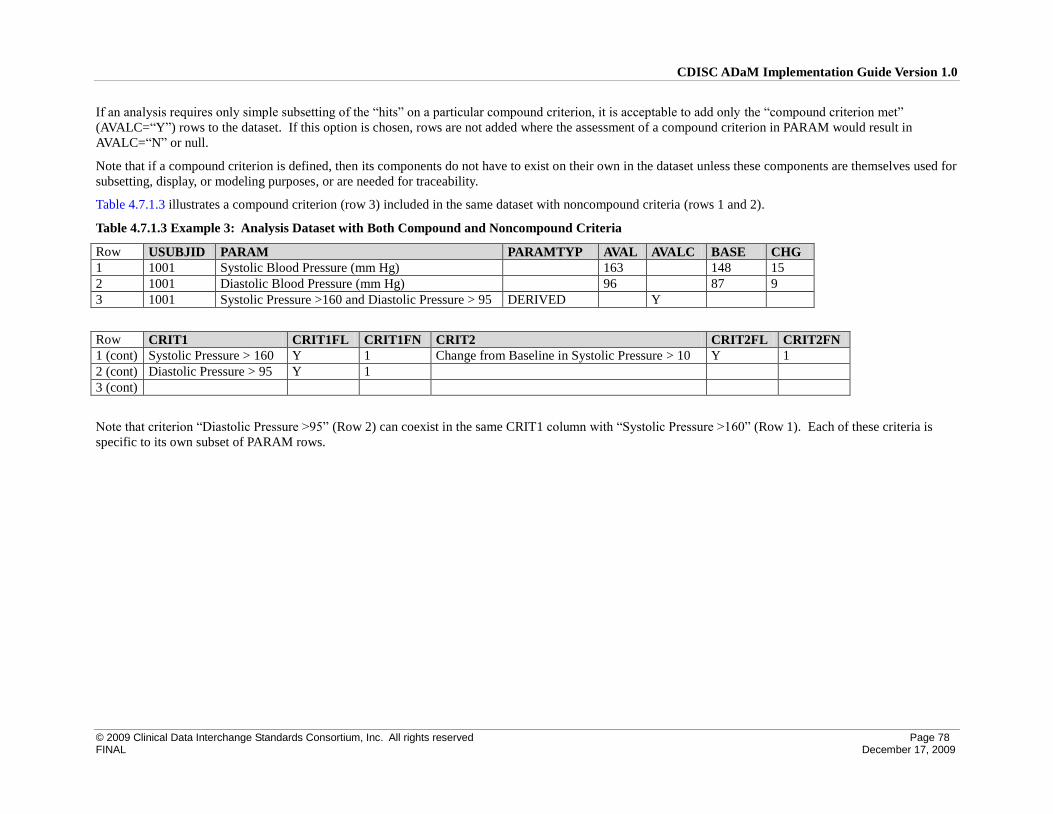
CDISC ADaM Implementation Guide Version 1.0
© 2009 Clinical Data Interchange Standards Consortium, Inc. All rights reserved Page 78 FINAL December 17, 2009
If an analysis requires only simple subsetting of the “hits” on a particular compound criterion, it is acceptable to add only the “compound criterion met”
(AVALC=“Y”) rows to the dataset. If this option is chosen, rows are not added where the assessment of a compound criterion in PARAM would result in
AVALC=“N” or null.
Note that if a compound criterion is defined, then its components do not have to exist on their own in the dataset unless these components are themselves used for
subsetting, display, or modeling purposes, or are needed for traceability.
Table 4.7.1.3 illustrates a compound criterion (row 3) included in the same dataset with noncompound criteria (rows 1 and 2).
Table 4.7.1.3 Example 3: Analysis Dataset with Both Compound and Noncompound Criteria
Row USUBJID PARAM PARAMTYP AVAL AVALC BASE CHG
1 1001 Systolic Blood Pressure (mm Hg) 163 148 15
2 1001 Diastolic Blood Pressure (mm Hg) 96 87 9
3 1001 Systolic Pressure >160 and Diastolic Pressure > 95 DERIVED Y
Row CRIT1 CRIT1FL CRIT1FN CRIT2 CRIT2FL CRIT2FN
1 (cont) Systolic Pressure > 160 Y 1 Change from Baseline in Systolic Pressure > 10 Y 1
2 (cont) Diastolic Pressure > 95 Y 1
3 (cont)
Note that criterion “Diastolic Pressure >95” (Row 2) can coexist in the same CRIT1 column with “Systolic Pressure >160” (Row 1). Each of these criteria is
specific to its own subset of PARAM rows.

CDISC ADaM Implementation Guide Version 1.0
© 2009 Clinical Data Interchange Standards Consortium, Inc. All rights reserved Page 79 FINAL December 17, 2009
4.8 Other Issues to Consider
The issues presented in the previous sections represent analysis decisions that commonly occur when creating analysis datasets. However, the ADaM team
recognizes that those are not an exhaustive list. This section provides comment on some additional issues that may arise.
4.8.1 Adding Records to Create a Full Complement of Analysis Timepoints for Every Subject
It is not unusual for a given subject to have missing data for a specified analysis timepoint. For example, suppose an analysis is to be performed for the data
obtained at each of 4 visits and that no imputation is to be performed. For subjects who did not attend all 4 visits, it would be possible to create records in the
analysis dataset for these missed assessments, with AVAL and AVALC missing (null) and appropriate variable(s) set to indicate these added records. For
example, DTYPE could contain a sponsor-defined value such as “PHANTOM.” There are some advantages of having an analysis dataset contain the same
number of observations for each subject. For example, programming is facilitated by having the same data dimensions for all subjects, and by explicitly
representing missing data rather than implicitly representing it by the absence of a record. This also allows ADaM datasets to support listing creation, especially
for data that is not present in SDTM (e.g., added analysis parameters). For some categorical analyses, the denominators can be obtained directly from the
analysis dataset rather than from another input such as ADSL. The disadvantage of this approach is that it may require additional metadata to explain the use of
these derived blank records and would require in some cases that subsetting statements be used to exclude the rows on which AVAL is missing. The ADaM team
neither advocates nor discourages this practice.
4.8.2 Creating Multiple Datasets to Support Analysis of the Same Type of Data
The statistical analysis plan often specifies that an analysis will be performed using slightly different methodologies. For example, the primary efficacy analysis
may be performed using two different imputation algorithms for missing values. The sponsor must decide whether to include both sets of the imputed
observations in one analysis dataset or create two analysis datasets, each representing just one of the imputation algorithms. ADaM provides variables that can
be used to identify records that are used for different purposes. However, this does not imply that the sponsor should not or cannot submit multiple analysis
datasets of similar content, each designed for a specific analysis.

CDISC ADaM Implementation Guide Version 1.0
© 2009 Clinical Data Interchange Standards Consortium, Inc. All rights reserved Page 80 FINAL December 17, 2009
Appendices Appendix A Abbreviations and Acronyms
The following is a list of abbreviations and acronyms used multiple times in this document. Not included here are
explanations of the various SDTM domains (e.g., QS, DM). Also not included is a description of the variables
referenced.:
ADAE ADaM Adverse Event Analysis Dataset
ADaM CDISC Analysis Data Model
ADaM document Analysis Data Model document
ADaMIG Analysis Data Model Implementation Guide
ADSL ADaM Subject-Level Analysis Dataset
BDS ADaM Basic Data Structure
BOCF Baseline Observation Carried Forward
CDASH Clinical Data Acquisition Standards Harmonization
CDISC Clinical Data Interchange Standards Consortium
DAO Data as Observed
eCTD electronic Common Technical Document
FDA United States Food and Drug Administration
ITT Intent-to-Treat
LOCF Last Observation Carried Forward
LOV Last Observed Value
LVPD Last Value Prior to Dosing
SAP Statistical Analysis Plan
SDS Submission Data Standards
SDTM Study Data Tabulation Model
SDTMIG Study Data Tabulation Model Implementation Guide
WC Worst Observed Case
WOCF Worst Observation Carried Forward
XML Extensible Markup Language

CDISC ADaM Implementation Guide Version 1.0
© 2009 Clinical Data Interchange Standards Consortium, Inc. All rights reserved Page 81 FINAL December 17, 2009
Appendix B Representations And Warranties; Limitations of Liability, And Disclaimers
CDISC Patent Disclaimers
It is possible that implementation of and compliance with this standard may require use of subject matter covered by
patent rights. By publication of this standard, no position is taken with respect to the existence or validity of any
claim or of any patent rights in connection therewith. CDISC, including the CDISC Board of Directors, shall not be
responsible for identifying patent claims for which a license may be required in order to implement this standard or
for conducting inquiries into the legal validity or scope of those patents or patent claims that are brought to its
attention.
Representations and Warranties
Each Participant in the development of this standard shall be deemed to represent, warrant, and covenant, at the time
of a Contribution by such Participant (or by its Representative), that to the best of its knowledge and ability: (a) it
holds or has the right to grant all relevant licenses to any of its Contributions in all jurisdictions or territories in
which it holds relevant intellectual property rights; (b) there are no limits to the Participant’s ability to make the
grants, acknowledgments, and agreements herein; and (c) the Contribution does not subject any Contribution, Draft
Standard, Final Standard, or implementations thereof, in whole or in part, to licensing obligations with additional
restrictions or requirements inconsistent with those set forth in this Policy, or that would require any such
Contribution, Final Standard, or implementation, in whole or in part, to be either: (i) disclosed or distributed in
source code form; (ii) licensed for the purpose of making derivative works (other than as set forth in Section 4.2 of
the CDISC Intellectual Property Policy (“the Policy”)); or (iii) distributed at no charge, except as set forth in
Sections 3, 5.1, and 4.2 of the Policy. If a Participant has knowledge that a Contribution made by any Participant or
any other party may subject any Contribution, Draft Standard, Final Standard, or implementation, in whole or in
part, to one or more of the licensing obligations listed in Section 9.3, such Participant shall give prompt notice of the
same to the CDISC President who shall promptly notify all Participants.
No Other Warranties/Disclaimers. ALL PARTICIPANTS ACKNOWLEDGE THAT, EXCEPT AS PROVIDED
UNDER SECTION 9.3 OF THE CDISC INTELLECTUAL PROPERTY POLICY, ALL DRAFT STANDARDS
AND FINAL STANDARDS, AND ALL CONTRIBUTIONS TO FINAL STANDARDS AND DRAFT
STANDARDS, ARE PROVIDED “AS IS” WITH NO WARRANTIES WHATSOEVER, WHETHER EXPRESS,
IMPLIED, STATUTORY, OR OTHERWISE, AND THE PARTICIPANTS, REPRESENTATIVES, THE CDISC
PRESIDENT, THE CDISC BOARD OF DIRECTORS, AND CDISC EXPRESSLY DISCLAIM ANY WARRANTY
OF MERCHANTABILITY, NONINFRINGEMENT, FITNESS FOR ANY PARTICULAR OR INTENDED
PURPOSE, OR ANY OTHER WARRANTY OTHERWISE ARISING OUT OF ANY PROPOSAL, FINAL
STANDARDS OR DRAFT STANDARDS, OR CONTRIBUTION.
Limitation of Liability
IN NO EVENT WILL CDISC OR ANY OF ITS CONSTITUENT PARTS (INCLUDING, BUT NOT LIMITED TO,
THE CDISC BOARD OF DIRECTORS, THE CDISC PRESIDENT, CDISC STAFF, AND CDISC MEMBERS) BE
LIABLE TO ANY OTHER PERSON OR ENTITY FOR ANY LOSS OF PROFITS, LOSS OF USE, DIRECT,
INDIRECT, INCIDENTAL, CONSEQUENTIAL, OR SPECIAL DAMAGES, WHETHER UNDER CONTRACT,
TORT, WARRANTY, OR OTHERWISE, ARISING IN ANY WAY OUT OF THIS POLICY OR ANY RELATED
AGREEMENT, WHETHER OR NOT SUCH PARTY HAD ADVANCE NOTICE OF THE POSSIBILITY OF
SUCH DAMAGES.
Note: The CDISC Intellectual Property Policy can be found at
http://www.cdisc.org/about/bylaws_pdfs/CDISCIPPolicy-FINAL.pdf.
Related Documents