Ad hoc networking with Bluetooth: key metrics and ...kom.aau.dk/group/05gr1116/reference/Ad hoc networking with... · Ad hoc networking with Bluetooth: key metrics and distributed

ARTICLE IN PRESS

Ad Hoc Networks xxx (2003) xxx–xxx

www.elsevier.com/locate/adhoc

Ad hoc networking with Bluetooth: key metrics anddistributed protocols for scatternet formation

Tommaso Melodia *, Francesca Cuomo

INFOCOM Department, University of Rome ‘‘La Sapienza’’, Via Eudossiana 18, 00184 Rome, Italy

Received 15 June 2003; received in revised form 20 August 2003; accepted 15 September 2003

Abstract

Bluetooth is a promising technology for personal/local area wireless communications. A Bluetooth scatternet is

composed of simple overlapping piconets, each with a low number of devices sharing the same radio channel. A

scatternet may have different topological configurations, depending on the number of composing piconets, the role of

the devices involved and the configuration of the links. This paper discusses the scatternet formation issue by analyzing

topological characteristics of the scatternet formed. A matrix-based representation of the network topology is used to

define metrics that are applied to evaluate the key cost parameters and the scatternet performance. Numerical examples

are presented and discussed, highlighting the impact of metric selection on scatternet performance. Then, a distributed

algorithm for scatternet topology optimization is introduced, that supports the formation of a ‘‘locally optimal’’ scat-

ternet based on a selected metric. Numerical results obtained by adopting this distributed approach to ‘‘optimize’’ the

network topology are shown to be close to the global optimum.

� 2003 Published by Elsevier B.V.

Keywords: Ad hoc networks; Bluetooth; Scatternet formation; Topology optimization; Distributed protocols

1. Introduction

Bluetooth (BT) is a promising technology for adhoc networking that could impact several wireless

communication fields providing WPAN (Wireless

Personal Area Networks) extensions of public ra-

dio networks (e.g., GPRS, UMTS, Internet) or of

local area ones (e.g. 802.11 WLANs, Home RF)

[1,2]. The BT system is described in the Bluetooth

Specifications 1.1 [3] and supports a 1 Mbit/s gross

* Corresponding author.

E-mail addresses: [email protected] (T.

Melodia), [email protected] (F. Cuomo).

1570-8705/$ - see front matter � 2003 Published by Elsevier B.V.

doi:10.1016/S1570-8705(03)00054-4

rate in a so-called piconet, where up to 8 devices

can simultaneously be interconnected. The radius

of a piconet (transmission range––TR) is about 10m for Class 3 devices. A BT based standard has

been released by the IEEE 802.15, which also ad-

dresses coexistence with the 802.11 wireless LAN

technology, in the un-licensed 2.4 GHz ISM (In-

dustrial, Scientific and Medical) band [4].

One of the key issues associated with the BT

technology is the possibility of dynamically setting-

up and tearing down piconets. Devices (named alsonodes in the following) can join and leave piconets.

Different piconets can coexist by sharing the spec-

trum with different frequency hopping sequences,

and interconnect in a scatternet. When all nodes

mail to: [email protected]

2 T. Melodia, F. Cuomo / Ad Hoc Networks xxx (2003) xxx–xxx

ARTICLE IN PRESS

are in radio visibility, scenario which we will refer

to as single hop, the formation of overlapping pic-

onets allows more than 8 nodes to contemporary

communicate and may enhance system capacity. In

a multi-hop scenario, where nodes are not all in

radio vicinity, a scatternet is mandatory to developa connected platform for ad-hoc networking.

This paper addresses the scatternet formation

issue by considering topological properties that

affect the performance of the system. Most works

in literature aim at forming a connected scatternet

while performance related topological issues typi-

cally remain un-addressed. To this aim we intro-

duce a matrix based scatternet representation thatis used to define metrics and to evaluate the rele-

vant performance. We then propose a distributed

algorithm that performs topology optimization by

relying on the previously introduced metrics. We

conclude by describing a two-phases scatternet

formation algorithm based on the optimization

algorithm. To the best of our knowledge, this is the

first scatternet formation algorithm explicitlyaimed at optimizing network topology.

The paper is organized as follows. Section 3

briefly summarizes the state of the art in scatternet

formation, while in Section 4 we present a frame-

work for scatternet analysis, based on a matrix

representation of the scatternet. Section 5 presents

some metrics that can be used to evaluate a scat-

ternet; related numerical results are shown inSection 6. Section 7 presents the Distributed

Scatternet Optimization Algorithm (DSOA) while

Section 8 describes a two-phase scatternet forma-

tion algorithm based on DSOA. Section 9 con-

cludes the paper.

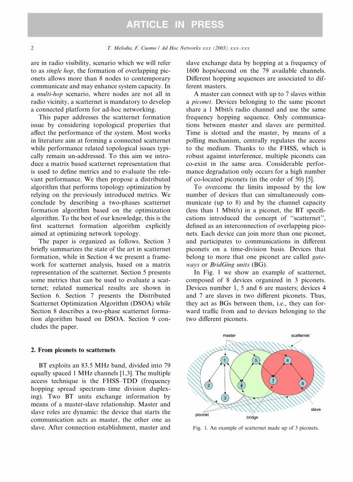
Fig. 1. An example of scatternet made up of 3 piconets.

2. From piconets to scatternets

BT exploits an 83.5 MHz band, divided into 79

equally spaced 1 MHz channels [1,3]. The multiple

access technique is the FHSS–TDD (frequency

hopping spread spectrum–time division duplex-

ing). Two BT units exchange information by

means of a master-slave relationship. Master and

slave roles are dynamic: the device that starts thecommunication acts as master, the other one as

slave. After connection establishment, master and

slave exchange data by hopping at a frequency of

1600 hops/second on the 79 available channels.

Different hopping sequences are associated to dif-

ferent masters.

A master can connect with up to 7 slaves within

a piconet. Devices belonging to the same piconetshare a 1 Mbit/s radio channel and use the same

frequency hopping sequence. Only communica-

tions between master and slaves are permitted.

Time is slotted and the master, by means of a

polling mechanism, centrally regulates the access

to the medium. Thanks to the FHSS, which is

robust against interference, multiple piconets can

co-exist in the same area. Considerable perfor-mance degradation only occurs for a high number

of co-located piconets (in the order of 50) [5].

To overcome the limits imposed by the low

number of devices that can simultaneously com-

municate (up to 8) and by the channel capacity

(less than 1 Mbit/s) in a piconet, the BT specifi-

cations introduced the concept of ‘‘scatternet’’,

defined as an interconnection of overlapping pico-nets. Each device can join more than one piconet,

and participates to communications in different

piconets on a time-division basis. Devices that

belong to more that one piconet are called gate-

ways or BridGing units (BG).

In Fig. 1 we show an example of scatternet,

composed of 8 devices organized in 3 piconets.

Devices number 1, 5 and 6 are masters; devices 4and 7 are slaves in two different piconets. Thus,

they act as BGs between them, i.e., they can for-

ward traffic from and to devices belonging to the

two different piconets.

T. Melodia, F. Cuomo / Ad Hoc Networks xxx (2003) xxx–xxx 3

ARTICLE IN PRESS

It is easy to see that there are many topological

alternatives to form a scatternet out of the same

group of devices. The way a scatternet is formed

considerably affects its performance.

3. Related works

Scatternet formation in BT has recently re-

ceived a significant attention in the scientific

literature. Existing works can be classified as sin-

gle-hop [6–9] and multi-hop solutions [10–15].

Paper [6] addresses the BT scatternet formation

with a distributed logic that selects a leader nodewhich subsequently assigns roles to the other

nodes in the system. The scheme works for a

number of nodes 6 36. In [7] a distributed for-

mation protocol is defined, with the goal of re-

ducing formation time and message complexity. In

both [7,8], the resulting scatternet has a number of

piconets close to the theoretical minimum. The

works in [9–11] form tree shaped scatternets. Thetree structure is shown to be simple to realize and

efficient for packet scheduling and routing. The

work [9], by Tan et al., presents the TSF (Tree

Scatternet Formation) protocol. The topology of

the scatternet is a collection of one or more rooted

spanning trees, each autonomously attempting to

merge and converge to a topology with a smaller

number of trees. TSF assures connectivity only insingle-hop scenarios since trees can merge only if

their root nodes are in transmission range of each

other. Zaruba et al. propose a protocol which

operates also in a multi-hop environment [10].

This latter protocol is based on a process that is

initiated by a unique node (named blueroot) and

repeated recursively till the ‘‘leaves’’ of the tree are

reached. In order to operate in a distributed wayand to avoid deadlocks the algorithm is based on

time-outs that could affect the formation time.

SHAPER [11] also forms tree-shaped scatternets,

but is fully distributed, works in a multi-hop set-

ting, has very limited formation time and assures

self-healing properties of the network, i.e. nodes

can enter and leave the network at any time

without causing loss of connectivity. The Bluenet

protocol in [12] forms a scatternet which has rea-

sonably good connectivity.

A second class of multi-hop proposals is con-

cerned with algorithms based on clustering

schemes. These algorithms principally aim at

forming connected scatternets. In [13,14] the

BlueStars and BlueMesh protocols are described

respectively. The BlueStars protocol has threephases: device discovery, partitioning of the net-

work into Bluetooth piconets and interconnection

of the piconets into a connected scatternet. It is

executed at each node with no prior knowledge of

the network topology, thus being fully distributed.

The selection of the Bluetooth masters is driven by

the suitability of a node to be the ‘‘best fit’’ for

serving as a master. Finally, the generated scat-ternet is a connected mesh with multiple paths

between any pair of nodes, which guarantees ro-

bustness. Simulation results are provided which

evaluate the impact of the Bluetooth device dis-

covery phase on the performance of the protocol.

Also the protocol in BlueMesh forms scatternets

without requiring the BT devices to be all in each

other�s transmission range. BlueMesh scatternettopologies are meshes with multiple paths between

any pair of nodes. BlueMesh piconets are made up

of no more than 7 slaves. Simulation results in

networks with over 200 nodes show that BlueMesh

is effective in quickly generating a connected

scatternet in which each node, on average, does

not assume more than 2.4 roles. Moreover, the

route length between any two nodes in the networkis comparable to that of the shortest paths be-

tween the nodes. Also [15] defines a protocol that

limits the number of slaves per master to 7 by

applying the Yao degree reduction technique, as-

suming that each node knows its geographical

position and that of each neighbor.

Recently, the work in [16] proposed a new on-

demand route discovery and construction ap-proach which, however, requires substantial

modifications to the Bluetooth standard to guar-

antee acceptable route-setup delay.

Some other works discuss the optimization of

the scatternet topology. This issue is faced in

[17,20] by means of centralized approaches. In [17]

the aim is minimizing the load of the most con-

gested node in the network while [20] discusses theimpact of different metrics on the scatternet to-

pology. A distributed approach based on simple


ARTICLE IN PRESS

heuristics is presented in [21]. In [18], an analytical

model of a scatternet based on queuing theory is

introduced, aimed at determining the number of

non-gateway and gateway slaves to guarantee ac-

ceptable delay characteristics.

In this framework the objectives of our contri-bution are

• provide a framework for scatternet topology

analysis based on matrices which turns out to

be a very simple and effective design tool;

• identify metrics that can be used to form and to

evaluate scatternets; we emphasize differences

between traffic dependent metrics and traffic in-dependent ones and we show selected numerical

results;

• to present the building blocks for the implemen-

tation of a distributed algorithm that optimizes

the scatternet topology.

4. The scatternet formation issue

Before addressing the issue of scatternet for-

mation, we introduce a suitable scatternet repre-

sentation.

4.1. Scatternet representation

Let us consider a scenario with N devices. Thescenario can be modeled as an undirected graph

GðV ;EÞ, where V is the set of nodes and an edge

eij, between any two nodes vi and vj, belongs to the

set E iff distðvi; vjÞ < TR, i.e., if vi and vj are withineach other�s transmission range. GðV ;EÞ can be

represented by a N � N adjacency matrix A ¼ ½aij�,whose element aij equals 1 iff device j is in the TR

of device i (i.e., j can directly receive the trans-mission of i).

Besides the adjacency graph GðV ;EÞ, in accor-

dance to, we use a bipartite graph GBðVM ; VS ; LÞ, tomodel the scatternet, where jVM j ¼ M is the num-

ber of masters, jVS j ¼ S is the number of slaves,

and L is the set of links (with N ¼ M þ S,VM \ VS ¼ f0g, VM \ VS ¼ V ). A link may exist

between two nodes only if they belong to the twodifferent sets VM and VS. Obviously, for any feasible

scatternet, we have L � E. This model is valid

under the hypothesis that a master in a piconet

does not assume the role of slave in another pic-

onet; in other words, by adopting this model, the

BGs are slaves in all the piconets they belong to.

We rely on this hypothesis to slightly simplify the

scatternet representation, the complexity in thedescription of the metrics and to reduce the space

of possible topologies. Moreover, intuitively, the

use of master/slave BGs can lead to losses in sys-

tem efficiency. If the BG is also a master, no

communications can occur in the piconet where it

plays the role of master when it communicates as

slave. However, to the best of our knowledge, this

claim has never been proved to be true. Futurework will thus extend the results presented in this

paper to non-bipartite graphs.

The bipartite graph GB can be represented by a

rectangular M � S binary matrix B [19]. In B, each

row is associated with one master and each column

with one slave. Element bij in the matrix equals 1

iff slave j belongs to master i�s piconet. The scat-

ternet of Fig. 1 may be represented by the fol-lowing matrix B (Eq. 1a).

In addition, a path between a pair of nodes (h,k) can be represented by another M � S matrix

Ph;kðBÞ, whose element ph;kij equals 1 iff the link

between master i and slave j is part of the path

between node h and node k ð16 i; j; h; k6NÞ. As

an example, and referring again to Fig. 1, the path

between nodes 2 and 8 can be represented by thematrix P2;8ðBÞ of Eq. (1b)

B= 0 0 1 15

0 0 0 16

1 1 1 01

2 3 4 7

0

1

0

8

B= 0 0 1 15

0 0 0 16

1 1 1 01

2 3 4 7

0

1

0

8

(a)

P2,8(B)= 0 0 1 15

0 0 0 16

1 0 1 01

2 3 4 7

0

1

0

8

P2,8(B)= 0 0 1 15

0 0 0 16

1 0 1 01

2 3 4 7

0

1

0

8

(b)

:

ð1Þ

Given a set V of N nodes, and an adjacency matrix

A, we can build the M � S matrix B ¼ ½bij� by as-

sociating its rows to a VM non-empty subset of Mnodes in V , and the columns to a VS non-emptysubset of S nodes in V (with N ¼ M þ S,VM \ VS ¼ f0g and VM [ VS ¼ V ), and by selecting

a subset of links in E. The resulting matrix B

represents a ‘‘BT-compliant’’ scatternet with Mmasters and S slaves if the following properties

apply:


ARTICLE IN PRESS

1. Each master is connected at least to a slave,PSj¼1 bij P 1; i ¼ 1; . . . ;M .

2. No more than seven slaves belong to a piconet,PSj¼1 bij 6 7; i ¼ 1; . . . ;M .

3. Each slave is connected at least to a master,PMi¼1 bij P 1; j ¼ 1; . . . ; S.

4. The resulting network is connected, the matrix

B does not have a block structure, row permu-

tations notwithstanding.

4.2. A framework for scatternet topology analysis

By exploiting the above matrix representations,we are interested in

(a) characterize the space of solutions; i.e., all the

B matrices compliant with rules 1–4;

(b) define metrics to evaluate the scatternet per-

formance;

(c) single out the optimal scatternet (B�) with re-

spect to a selected metric;(d) analyze the topological properties of the ex-

tracted solutions.

We stress that our objective is to enucleate

scatternet characteristics related to specific metrics

that could be adopted in the formation process.

We do not aim at proposing sophisticated algo-

rithms that elaborate the matrix A to derive theoptimal scatternet, also because, due to the com-

plexity of the problem, they probably shall operate

in a centralized manner while scatternet formation

should be solved by adopting distributed opera-

tions performed by all network nodes. To work

out points (a) and (c) we rely on space state enu-

meration that pays the complexity of examining

and listing all potential scatternets but on the otherhand allows us to completely characterize the

space of possible solutions. In the following we

briefly describe our approach to go along steps a–

d, while further details can be found in [20].

We randomly generate communication scenar-

ios taking as inputs the number of devices, N , and

the dimensions of the area where the nodes are

located; the scenario is represented by the A ma-trix.

We then identify and enumerate all the ‘‘BT-

compliant’’ scatternets that may be obtained from

the scenario; if we let M be the number of masters

in the scatternet, with Mmin 6M 6Mmax the num-

ber of possible choices of roles for the network

nodes is equal toPMmax

M¼Mmin

NM

� �, since there are N

M

� �possible ways of selecting M masters among Nnodes. Each choice implies a set L0 of possible links(with L0 � E) and we consider every subset L � L0

which gives rise to a scatternet that respects

properties 1–4. All these scatternets constitute our

B matrices. We consider Mmin ¼ dN=ð7þ 1Þe and

Mmax ¼ bN=2c. A number of masters greater than

half the nodes introduces inefficiencies (e.g., in-

terference) without bringing benefits to the scat-

ternet.The B matrices are evaluated by applying suit-

able metrics described in Section 5. For a given

metric, the output of the overall process is the

identification of the optimal B (indicated with B�),

which represents the scatternet with the optimal

topology, and a distribution of the metric values.

5. Metrics for scatternet evaluation

Metrics for scatternet evaluation can either be

dependent on or independent of the traffic loading

the scatternet. In the traffic independent (TI) case,

the scatternet is formed without a priori knowl-

edge of traffic patterns among involved devices.

The scenario is described only by means of theadjacency matrix A, without associating to possi-

ble pairs of devices a description of the related

exchanged traffic. On the other hand, it may be

useful to form a scatternet by taking into account

traffic patterns, if such information is available. In

that case, the traffic patterns can conveniently be

described by a traffic matrix, T. In the following

we refer to this case as traffic dependent (TD).In the following, we introduce several metrics;

each of them has pros and cons.

5.1. TI metrics: scatternet with maximum capacity

A first traffic independent metric is the overall

capacity of the scatternet. Evaluating such a ca-

pacity is not an easy task, since it is related to thecapacity of the composing piconets which in turn


ARTICLE IN PRESS

depends on the intra-piconet and interpiconet

scheduling policies. To the best of our knowledge,

no such evaluation is available in literature. In the

following, we introduce a simple model to estimate

the capacity of a scatternet and we exploit this

evaluation for scatternet formation.In the model we assume that

• a master may offer the same amount of capacity

to each of its slaves by equally partitioning the

piconet capacity;

• a BG slave spends the same time in any piconet

it belongs to.

These assumptions are tied to intra and inter

piconet scheduling; here, for the sake of simplicity,

we assume policies that equally divide resources;

however the model can be straightforwardly ex-

tended to whatever scheduling policy.

The scatternet capacity will be evaluated by

normalizing its value to the overall capacity of a

piconet (i.e., 1 Mbit/s). Let us define two M � Smatrices, OTIðBÞ ¼ ½oij�, and RTIðBÞ ¼ ½rij� with

oij ¼ bij=si and rij ¼ bij=mj, where si denotes the

number of slaves connected to master i and mj

denotes the number of masters connected to slave j(for j ¼ 1; . . . ; S and i ¼ 1; . . . ;M):

mj ¼XMi¼1

bij for j ¼ 1; . . . ; S;

si ¼XS

j¼1

bij for i ¼ 1; . . . ;M : ð2Þ

The matrix OTIðBÞ represents the portions of ca-

pacity a master may offer to each of its slaves. The

RTIðBÞ matrix represents the portions of capacity a

slave may ‘‘spend’’ in the piconet it is connected

to. The overall capacity of the scatternet is given

by the sum of the capacities of all links. The ca-pacity cij of link (i; j) is the minimum between the

capacity oij and the capacity rij. Let us define the

matrix CTIðBÞ, whose elements represent the nor-

malized link capacity, as

CTIðBÞ ¼ ½cij� ¼ ½minðoij; rijÞ�: ð3Þ

The associated metric is the normalized capacity

cTIðBÞ of a scatternet defined as

cTIðBÞ ¼XMi¼1

XS

j¼1

minðoij; rijÞ: ð4Þ

As an example, let us consider the scatternet ofFig. 1. The matrices OTIðBÞ and RTIðBÞ are

ð5Þ

and the related matrix CTIðBÞ is

ð6Þ

The resulting normalized capacity is cTIðBÞ ¼ 3

(¼ 3 Mbit/s).

Eq. (4) is valid in the ideal case where both in-terference from co-located piconets and switching

overhead, caused by BGs that change piconet, are

neglected. In order to include these two effects, Eq.

(4) can be rewritten as

�ccTIðBÞ ¼ ðcTIðBÞ � DðBÞÞ � IðBÞ; ð7Þ

where DðBÞ represents a loss of capacity due to theswitching overhead and IðBÞ is a decreasing factor

that accounts for interference from co-located

piconets.

5.2. TD metrics: scatternet with maximum residual

capacity or minimum average load

We consider two traffic dependent metrics: (i)the so-called residual capacity (i.e., the capacity

that remains available in a scatternet, after that all

pre-defined traffic patterns are accommodated); (ii)

the nodes’ average load.

The evaluation of the above metrics is TD, and

as such, is dependent on the adopted routing

strategy too. As an example, given a traffic pattern,

for instance a data flow between device h and de-vice k (with 16 h, k6N ), the capacity that such

flow requires from the overall scatternet depends

on the number of hops that make up the path

between device h and device k. In our analysis, we

assume without loss of generality, that a shortest

path routing algorithm is adopted.


ARTICLE IN PRESS

To evaluate the metrics, we start by describing

the traffic relationships with an N � N traffic ma-

trix T ¼ ½thk�, whose element thk represents the ca-

pacity, normalized with respect to the piconet�scapacity, required by the (h; k) relationship,

(16 h; k6N ). We assume that the thk (normalizedtraffic rates) are fixed for each source–destination

couple. We also denote by R the number of traffic

relationships expressed by this matrix.

It is easy to see that the capacity required on

each link by the traffic relationship between node hand node k is given by thkP

h;kðBÞ.The matrix of the overall normalized capacity

required for each link to transport the traffic pat-terns expressed by T is given by

CTDðBÞ ¼XNh¼1

XNk¼1;k 6¼h

thk � Ph;kðBÞ

¼ dij

"¼

XNh¼1

XNk¼1;k 6¼h

thk � ph;kij

#: ð8Þ

It is to be noted that the traffic relationships defined

by the matrix T can effectively be supported by thescatternet represented by B if the following condi-

tions, that assure the steady state, are verified:

masters are not over-loaded

)XS

j¼1

dij 6 1 8i 2 M ; ð9Þ

slaves are not over-loaded

)XMi¼1

dij 6 1 8j 2 S: ð10Þ

The total capacity required by the traffic rela-

tionships of matrix T is

cTDðBÞ ¼XMi¼1

XS

j¼1

dij: ð11Þ

Based on the above definitions, we can finally in-

troduce two TD metrics. The first measures the

capacity that remains available in a scatternet,

after all traffic patterns are accommodated. Re-

calling that the capacity of each link is assignedaccording to Eq. (3), the residual capacity matrix,

is given by

Cres;TDðBÞ ¼ CTIðBÞ � CTDðBÞ ¼ bfijc: ð12ÞThe information contained in this matrix can be

summarized in a single parameter, the residual

capacity, cres;TDðBÞ, given by

cres;TDðBÞ ¼XMi¼1

XS

j¼1

fij: ð13Þ

Also in this case considerations about decreasing

factors due to interference and switching overhead

can be applied.

According to this metric, a scatternet is optimal,

when the value of cres;TDðBÞ is maximized.Alternatively, we can adopt as metric the nodes’

average normalized load.

In accordance to Eq. (8) the normalized load on

a slave j is lSj ¼PM

i¼1 dij, while the normalized load

on a master is lMi ¼PS

j¼1 dij.The normalized load averaged over the N

nodes, which we denote as lðBÞ, is

lðBÞ ¼PS

j¼1 lSj þ

PMi¼1 l

Mi

N

¼2 �

PMi¼1

PSj¼1 dij

N¼ 2 � cTDðBÞ

N: ð14Þ

With this metric, the target is the minimization of

lðBÞ; we point out that the minimization of the

average load goes in the direction of a minimiza-tion of the average energy consumption of the

scatternet.

5.3. Metrics associated to the path length

As will be shown in Section 6 path lengths have

a considerable impact on scatternet performance.

As a consequence, in this section, we define threemetrics that do take into account path lengths. The

first two are not dependent on the traffic loading

the scatternet and are defined as follows.

Let us denote, for a scatternet represented by a

matrix B, the length of the path between device hand device k (expressed in number of hops) as

qh;kðBÞ ¼XMi¼1

XS

j¼1

ph;kij : ð15Þ


ARTICLE IN PRESS

The first metric that we introduce is the average

path length, which is the path length averaged over

all possible source–destination couples, and is gi-

ven by

qTIðBÞ ¼XNh¼1

XNk¼1;k 6¼h

qh;kðBÞN � ðN � 1Þ ; ð16Þ

the optimization target of this metric is the mini-

mization of qTIðBÞ.Given the capacity of a scatternet cTIðBÞ and

the relevant average path length qTIðBÞ, on averagethe capacity available for the generic source–des-

tination couple among the nodes in B is

aTIðBÞ ¼cTIðBÞ

qTIðBÞ � N � ðN � 1Þ : ð17Þ

We will call this last metric average path capacity.

The last metric we introduce depends on traffic

and thus it depends on the matrix T, which definesR traffic relationships. The metric is the path length

averaged over the R traffic relationships, instead

that over all possible N � ðN � 1Þ relationships, as

done in Eq. (15); it is given by

qTDðBÞ ¼X

ðh;kÞ2T ;h6¼k

qh;kðBÞR

: ð18Þ

The associated target consists in minimizing this

path length; this metric goes in the direction of

minimizing the transfer delay related to the num-

ber of hops.

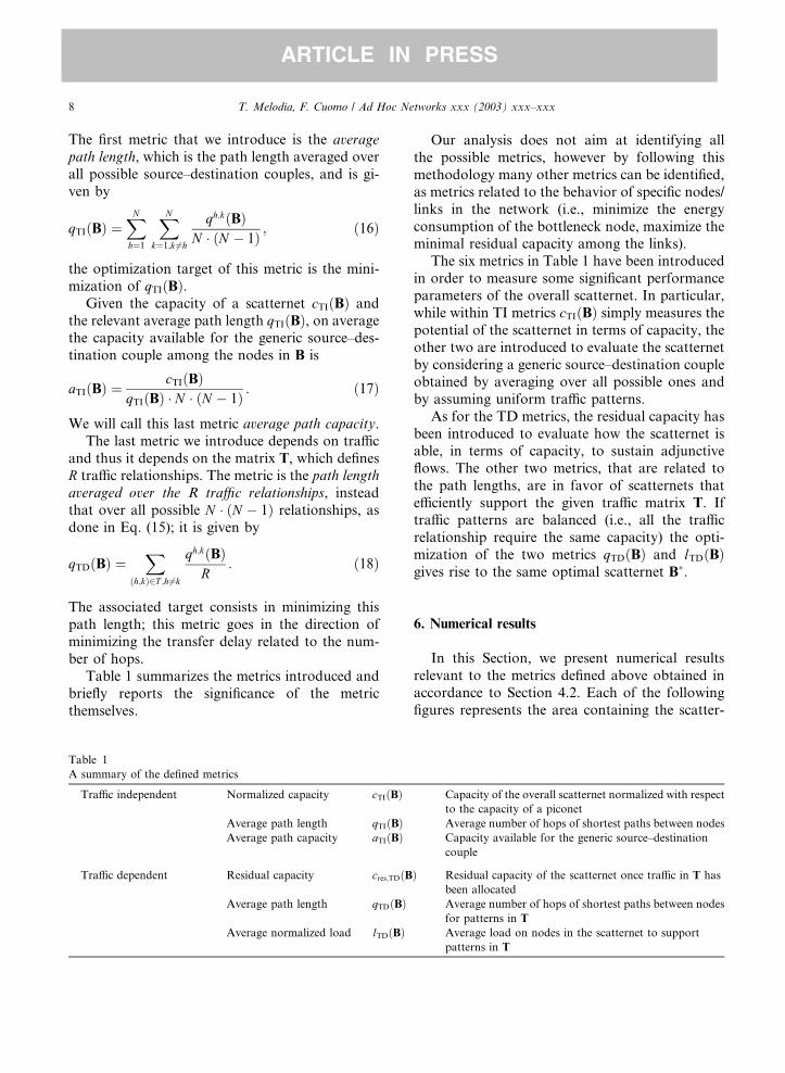
Table 1 summarizes the metrics introduced and

briefly reports the significance of the metric

themselves.

Table 1

A summary of the defined metrics

Traffic independent Normalized capacity cTIðBÞ

Average path length qTIðBÞAverage path capacity aTIðBÞ

Traffic dependent Residual capacity cres;TDðB

Average path length qTDðBÞ

Average normalized load lTDðBÞ

Our analysis does not aim at identifying all

the possible metrics, however by following this

methodology many other metrics can be identified,

as metrics related to the behavior of specific nodes/

links in the network (i.e., minimize the energy

consumption of the bottleneck node, maximize theminimal residual capacity among the links).

The six metrics in Table 1 have been introduced

in order to measure some significant performance

parameters of the overall scatternet. In particular,

while within TI metrics cTIðBÞ simply measures the

potential of the scatternet in terms of capacity, the

other two are introduced to evaluate the scatternet

by considering a generic source–destination coupleobtained by averaging over all possible ones and

by assuming uniform traffic patterns.

As for the TD metrics, the residual capacity has

been introduced to evaluate how the scatternet is

able, in terms of capacity, to sustain adjunctive

flows. The other two metrics, that are related to

the path lengths, are in favor of scatternets that

efficiently support the given traffic matrix T. Iftraffic patterns are balanced (i.e., all the traffic

relationship require the same capacity) the opti-

mization of the two metrics qTDðBÞ and lTDðBÞgives rise to the same optimal scatternet B�.

6. Numerical results

In this Section, we present numerical results

relevant to the metrics defined above obtained in

accordance to Section 4.2. Each of the following

figures represents the area containing the scatter-

Capacity of the overall scatternet normalized with respect

to the capacity of a piconet

Average number of hops of shortest paths between nodes

Capacity available for the generic source–destination

couple

Þ Residual capacity of the scatternet once traffic in T has

been allocated

Average number of hops of shortest paths between nodes

for patterns in T

Average load on nodes in the scatternet to support

patterns in T


ARTICLE IN PRESS

net; x and y axes are measured in meters. The TR is

assumed to be equal to 10 m. Nodes are numbered

according to the order they are generated in the

communication scenario. Figures report nodes,

their roles (master, slave or bridge) and radio

links connecting them. Since number of possiblescatternets quickly becomes overwhelming with

respects to the number of nodes, in this section

we analyze networks with a limited number of

devices.

6.1. Traffic independent metrics

This subsection shows examples of scatternetsresulting from TI optimization. The scenario

consists of 12 devices not all the nodes are in radio

visibility. The scatternet in Fig. 2 is obtained by

selecting the one with maximum normalized ca-

pacity. The interference effect in Eq. (7) is evalu-

ated by relying on the model presented in [22]. The

switching overhead, which depends on the adopted

interpiconet scheduling policy [2], has been con-sidered here with simple assumptions on the

switching frequency.

It can be immediately noticed that the scatternet

presents a linear structure, i.e., every node is con-

nected with two other nodes only. The value as-

sumed by cTIðBÞ, evaluated as in Eq. (4) is 5.5.

When switching overhead is considered cTIðBÞdecreases to 5.2727 and by considering also the

65 70 75 80 85 90 95 10015

20

25

30

35

40

45

50

Node: 1

Node: 2

Node: 3

Node: 4

Node: 5

Node: 6

Node: 7

Node: 8

Node: 9

Node: 10

Node: 11

Node: 12

meters

met

ers

masterslavebridge

Fig. 2. Scatternet with maximum normalized capacity.

interference effect it becomes 4.7151. Although this

scatternet is the one with maximum normalized

capacity, it has characteristics that make its to-

pology undesirable: it presents large values of the

average path length that could lead to high

transfer delays, and, since for Class 3 devices nopower control mechanisms have been defined, in-

creasing the number of hops per traffic relation-

ship does not bring any benefit in terms of power

consumption and consumes capacity as function

of the involved links. As an example, a single 500

kbit/s bi-directional flow between node 10 and

node 12 in Fig. 2 would use all scatternet capacity:

nodes along the path would spend half their timereceiving traffic from one of the two directions and

the remaining time relaying traffic in the opposite

direction.

The peculiar structure produced by this metric

is due to the following reasons:

• The metric tends to favor scatternets formed by

a large number of piconets, since each new pic-onet increases the overall capacity with its con-

tribution.

• The interference effect is not significant since

the number of co-located piconets is low (<50).

• When the switching overhead effect is taken

into account, a BG loses capacity as a function

of the number of piconets it is connected to.

Thus, high performance, in terms of capacity,is attained when a bridge node is connected to

only two piconets.

These considerations explain why path lengths

have to be taken into account. However, mini-

mizing the path lengths without considering ca-

pacity at the same time, could lead to undesirable

scatternet topologies too since, if the nodes aredistributed in a small area, the resulting scatternet

presents a fully meshed topology where every slave

is connected to every master. In this case, the re-

sulting capacity is low because of the high number

of BGs connected to a high number of piconets.

Fig. 3 refers to the metric that minimizes the av-

erage path length in the same scenario of Fig. 2. In

this case the nodes in the lower part of the figure(which are in radio visibility of each other) are all

connected.

65 70 75 80 85 90 95 10015

20

25

30

35

40

45

50

Node: 9

Node: 10

Node: 11

Node: 1

Node: 4

Node: 3

Node: 5

Node: 6

Node: 2

Node: 7

Node: 12

Node: 8

meters

met

ers

masterslavebridge

Fig. 3. Scatternet with minimum average path length.

Cmin=0.0087 Cmax=0.01880

100

200

300

400

500

600

700

800

900

Average Path Capacity

Num

bero

f Sca

ttern

ets

(centralized

0.0132 0.0166

Mean value

approach)

Fig. 5. Distribution of the values of average path capacity.


ARTICLE IN PRESS

Let us now look at Fig. 4, which shows a

scatternet obtained with a metric that maximizes

the average path capacity. This metric seems to be

the most suited to maximize network performance,

since both capacity and path length are taken into

account. The scatternet of Fig. 4 presents a ca-

pacity, cTIðBÞ equal to 4.667 (4.5271 taking intoaccount the switching overhead and 4.0483 taking

into account also the interference effect). The

overall capacity is smaller than the value obtained

by maximizing the normalized capacity, but, while

in that case the average path length was 4.33, and

65 70 75 80 85 90 95 10015

20

25

30

35

40

45

50

Node: 1

Node: 2

Node: 3

Node: 4

Node: 5

Node: 6

Node: 7

Node: 8

Node: 9

Node: 10

Node: 11

Node: 12

meters

met

ers

masterslavebridge

Fig. 4. Scatternet with maximum average path capacity.

the resulting capacity available for a generic

source–destination pair was 0.0082, in the case of

Fig. 4 the average path length is 2.81 and the re-

sulting capacity per source–destination pair is0.0109.

As a result, we select as suitable TI metric the

average path capacity. In order to better analyze

the space of feasible scatternets Fig. 5 shows the

histogram of the average path capacity of all pos-

sible ‘‘BT-compliant’’ scatternets obtained in a

scenario constituted by 10 nodes distributed in an

area of 25 · 25 m but, as will be shown later, asimilar distribution holds in general. As indicated

in Section 4.2 the number of different feasible to-

pology is huge. The values of aTIðBÞ are distrib-

uted in a range starting form aTI;minðBÞ ¼ 0:0087(�8 kbit/s for every possible node pair) to

aTI;maxðBÞ ¼ 0:0188 (�19 kbit/s per pair); the mean

value of aTIðBÞ is also shown (equal to 0.0132).

Note that the mean value is quite distant from themaximum value, which corresponds to the one

associated with the optimal scatternet. Moreover,

a few scatternets have a high value of aTIðBÞ and

are thus contained in the right tail of the histo-

gram. This is an interesting result because it indi-

cates that topology optimization is going to be a

fundamental issue for Bluetooth scatternets: in

fact, this distribution of the metric values meansthat it is highly unlikely to obtain a high perfor-

mance scatternet by randomly selecting a topol-

ogy. We need to deploy protocols that not only

Table 2

Traffic relationships

Traffic relationship Required normalized capacity Traffic relationship Required normalized capacity

1 $ 2 0.08 5 $ 6 0.125

1 $ 5 0.1 6 $ 2 0.125

3 $ 4 0.1 7 $ 8 0.05

3 $ 9 0.1 10 $ 7 0.1

4 $ 9 0.1 10 $ 8 0.05

0 5 10 15 20 250

2

4

6

8

10

12

14

16

18

20

Node: 1

Node: 2

Node: 3

Node: 4

Node: 5

Node: 6

Node: 7

Node: 8

Node: 9

Node: 10

meters

met

ers

masterslave bridge

Fig. 7. Scatternet with minimum average path length per traffic

relationship.

18

20Node: 7 master

slave bridge

0.1518masterslave bridge


ARTICLE IN PRESS

search for a connected scatternet but also explicitly

aim at maximizing its performance.

6.2. Traffic dependent metrics

In this Section, we show results derived by ap-

plying the TD metrics. The scenario is composed

of 10 nodes; the relevant traffic relationships are

shown in Table 2. In Fig. 6 we depict the scatternet

with maximum residual capacity. It can be noticed

that this metric suffers from the same drawbacks of

the metric it is derived from (i.e., normalized ca-

pacity, see Fig. 2): the resulting scatternet is likelyto present a linear structure.

In Fig. 7 we show the scatternet presenting the

minimum average path length per traffic relation-

ship, see Eq. (18). In this case the scatternet pre-

sents a more connected structure, with respect to

that of Fig. 6.

Finally, in Fig. 8 we minimize the average nor-

malized load. The resulting normalized loads are

0 5 10 15 20 250

2

4

6

8

10

12

14

16

18

20

Node: 1

Node: 2

Node: 3

Node: 4

Node: 5

Node: 6

Node: 7

Node: 8

Node: 9

Node: 10

meters

met

ers

slave bridge

0.15

0.55

0.73

0.66

0.480.5

0.7 0.7

0.5

0.15

0

4

masterslave bridge

Fig. 6. Scatternet with maximum residual capacity.

0 5 10 15 20 250

2

4

6

8

10

12

14

16

Node: 1

Node: 2

Node: 3

Node: 4

Node: 5

Node: 6

Node: 8

Node: 9

Node: 10

meters

met

ers

0.25

0.935

0.205

0.2

0.18 0.7

0.7

0.2

0.15

20

Fig. 8. Scatternet with minimum average load.

reported in the figure, next to each node. Thescatternet average load is 0.3058. It can be noticed

that nodes that are located in specific positions


ARTICLE IN PRESS

have to take care of all the forwarding load (i.e.,

traffic handled on behalf of other nodes). Never-

theless, since reducing load means reducing energy

consumption, this scatternet consumes 70% of the

energy required by the scatternet of Fig. 6 (the

average load for the latter scatternet is 0.4267).

7. A distributed algorithm for topology optimization

In this section we describe a Distributed Scat-

ternet Optimization Algorithm (DSOA) that aims

at optimizing the topology to obtain a perfor-

mance (in terms of the chosen metric) as close aspossible to the optimum. Note that the selection of

the optimized topology is decoupled from the es-

tablishment of the links that compose it, as will

become clearer in Section 8, where we will describe

a two-phases distributed scatternet formation al-

gorithm based on DSOA.

7.1. Distributed scatternet optimization algorithm

(DSOA)

We consider the adjacency graph GðV ;EÞ. First,We aim at obtaining an ordered set of the nodes in

V . The first procedure orders the nodes in the

graph according to a simple property: a node kmust be in transmission range of at least one node

in the set 1 . . . k � 1.

ORDER_NODES

Input: GðV ;EÞOutput: ordered set of the nodes in V ,W ¼ fwkg, k ¼ 1; 2; ::;N , N ¼ jV jbegin

w1 ¼ random selection of

a node v from VW ¼ fw1gfor k ¼ 1 : N

wk ¼ random selection of a node vfrom V such that:

(1) m 62 W(2) 9 u 2 W such that distance

ðu; vÞ6 TRW ¼ W [ fwkg

endforend

Since with DSOA the nodes sequentially select

how to connect, each node must be in TR of at

least another already entered node. The following

proofs that it is always possible to obtain such an

ordering of the nodes, i.e. that this procedure al-

ways ends.

Theorem 1. Given a connected graph GðV ;EÞ, theprocedure ORDER_NODES always terminates, andjW j ¼ N .

Proof. Suppose that at some step k of the proce-

dure, k < N , we have W ¼ fw1;w2; . . . ;wk�1g and

no couple (v;w) with v 2 V n W , w 2 W exists suchthat distðv;wÞ < TR. Therefore, since W � V , thereexist two disconnected components, namely W and

V n W , of GðV ;EÞ. h

At the end of this procedure, then, node k is in

transmission range of at least one of the nodes

1; 2; . . . ; k � 1. The second procedure is the core of

the algorithm. Here we let eij be the link betweenthe nodes wi and wj of a scatternet ði; j 2 1; . . . ;NÞ.This part of the algorithm is dependent on the

selected metricM . At each step k, node wk ‘‘enters’’

in the scatternet in the best possible way, accord-

ing to M .

SCATTERNET_OPTIMIZATION_ALGORITHM

(SOA)

Input: W , GðV ;EÞ, MOutput:locally optimal scatternet

B�

beginVM ¼ Ø

VS ¼ Ø

VM ¼ VM [ w1

VS ¼ VS [ w2

B2 ¼ ½1�for k ¼ 3 : N

case 1) consider wk in VM* derive all BT-compliant ma-

trices Bk with jVM j þ 1 rows and

jVS j columnscalculate values of MðBkÞ

case 2) consider wi in VS* derive all BT-compliant ma-

trices Bkwith jVM j rows and


ARTICLE IN PRESS

jVSj þ 1 columns

calculate values of MðBkÞselect the Bk

with optimal MðBk)

if optimum in case 1)

thenVM ¼ VM [ wk

elseif optimum in case 2)

VS ¼ VS [ wk

elseRECONFIGURE(Bk�1; VM ; VSÞ

endifendif

endforend

The RECONFIGURE procedure is executed in

the (unlikely) case when wk is only in transmissionrange of master nodes that have already 7 slaves in

their piconet. For the sake of simplicity, details of

this procedure are only given in the following

proof of correctness. In this case, one of the 7

slaves is forced to become master of one of the

other slaves. This is shown to be always possible.

The following proves the correctness of SOA,

i.e. it is always possible for a node to enter thenetwork respecting the Bluetooth properties.

Proof of correctness. Node w2 is in transmission

range of w1, thus the two nodes can connect. Each

node wk, with k > 2 can always establish a new

piconet, thus connecting as a master, whenever a

node v 2 fw1;w2; . . . ;wk�1g exists s.t. v 2 VS and

distance ðwk; vÞ6TR, i.e. one of the slave

nodes already in the network is in transmissionrange of wk. If no slaves are in transmission range

of wk, whenever a node v 2 VM exists, with

distance ðwk; vÞ6TR, and slaves ðvÞ <¼ 7, wk

can be a slave of v. Otherwise, at least one node

wi 2 VM must exist, with distance ðwk; vÞ6TR,

and slaves ðvÞ ¼ 7, with i6 k. The RECONFIGUREprocedure can always be executed in this way. If at

step i node wi selected more than 1 slave, it candisconnect from the slave that causes the minimum

decrease/increase in the metric value. The topology

is still connected, and wk can select wi as its slave.

If, otherwise, wi selected only one slave at step i,this cannot be disconnected, since this could cause

loss of connectivity for the network. Thus, one of

the other 6 slaves has to be disconnected. How-

ever, it was proven in [10] that in a piconet with at

least 5 slaves, at least 2 of them are in TR of each

other. Thus, at least one of the slaves can become

master and select another slave. The network can

therefore be reconfigured by forcing the seventhslave that connected to wi to become master of

another slave of wi, to minimize reconfigurations.

If it is not in TR of any other slave of wi, we can

try with the sixth, and so on. At least one of the six

slaves must be able to become master and select

one of the other 5 as its slave.

The local optimization in SOA (steps with mark

*) can be performed by means of state spaceenumeration, as in the simulations results we

show, or, e.g., by means of randomized local

search algorithms.

The distributed version of the SOA (distributed

SOA, DSOA) straightforwardly follows. At each

step k, a new node wk receives information on the

topology selected up to that step ðBk�1 matrix) and

selects the role (master or slave) it will assume andthe links it will establish, with the aim of maxi-

mizing the global scatternet metric. If the node

becomes a master it will select a subset of the

slaves in its TR already in the scatternet; if it be-

comes a slave it will select a subset of the masters

in its TR, already in the scatternet. ORDER_NODES

is needed to guarantee that, when node k enters, it

can connect to at least one of the previously en-tered nodes. DSOA can be classified as a greedyalgorithm, since it tries to achieve the optimal so-

lution by selecting at each step the locally optimalsolution, i.e. the solution that maximizes the met-

ric of the overall scatternet, given local knowledge

and sequential decisions. Greedy algorithms do

not always yield the global optimal solution. As

will be shown in the next subsection, the resultsobtained with DSOA are close to the optimum.

7.2. Examples and numerical results

In this section we show some results obtained

with DSOA, by using average path capacity as a

metric. As previously discussed, we believe that

average path capacity is a good metric since ittakes into account both capacity and average path

length of the scatternet.

40 45 50 55 60 6568

70

72

74

76

78

80

82

84

86

88

Node: 1

Node: 2Node: 3

Node: 4

Node: 5

Node: 6

Node: 7

Node: 8

Node: 9

Node: 10

meters

met

ers

masterslave bridge

Fig. 9. Scatternet formed with DSOA.

40 45 50 55 60 6568

70

72

74

76

78

80

82

84

86

88

Node: 1

Node: 2

Node: 3

Node: 4

Node: 5

Node: 6

Node: 7

Node: 8

Node: 9

Node: 10

meters

met

ers

masterbridge

Fig. 10. Optimal scatternet.

aTI,min(B)=0.0087 a

TI,maxB)=0.0188

100

200

300

400

500

600

700

800

900

Average Path Capacity

Num

ber

of S

catte

rnet

s

Mean value (centralized approach)

Mean value (distributed approach)

0.0132 0.0166(

0

Fig. 11. Comparison between results obtained with DSOA and

results derived from scatternet space enumeration.


ARTICLE IN PRESS

An example is shown in Figs. 9 and 10, where

10 nodes are distributed in an area of 25 · 25 m

(the same scenario of Fig. 5). The first figure re-

ports the scatternet formed with the DSOA (with

an aTIðBÞ ¼ 0:0145). Fig. 10 depicts the optimal

scatternet (that presents an aTIðBÞ ¼ 0:0188Þ. Fig.11 shows a comparison between the optimal aTIðBÞand the one obtained with the DSOA. The dottedcurve shows the histogram of the average pathcapacity of all possible ‘‘BT-compliant’’ scatternets

feasible in this scenario. The values of aTIðBÞ are

distributed in a range starting form aTI;minðBÞ ¼0:0087 (�8 kbit/s for every possible node pair) to

aTI;maxðBÞ ¼ 0:0188 (�19 kbit/s per pair); the mean

value of aTIðBÞ is also shown (equal to 0.0132).

Note that the mean value is quite distant from the

maximum value, which corresponds to the one

associated with the optimal scatternet. Moreover,

a few scatternets have a high value of aTIðBÞ andthus are contained in the right tail of the histo-

gram. This is an interesting results because it

suggests that topology optimization is a funda-

mental issue for Bluetooth scatternets: in fact, this

distribution for the metric values means that it is

highly unlikely to obtain a high performance

scatternet by randomly selecting a topology. We

need to deploy protocols that explicitly aim atmaximizing performance.

As regards the DSOA, the vertical lines in Fig.

11 correspond to the values of aTIðBÞ for 100 dif-

ferent scatternets formed by using 100 different

randomly chosen sequential orders. The lines are

concentrated in the right part of the figure (i.e., the

scatternets formed have a value of aTIðBÞ greater

than the overall mean value of all possible scat-ternets). The mean value of aTIðBÞ of these 100

DSOA scatternets is equal to 0.0166. The un-

normalized values of the average capacity per path

obtained with DSOA is about 17 kbit/s, while the

maximum possible value is 19 kbit/s; this confirms

the good behavior of the DSOA.

Fig. 12 shows a similar distribution in a scenario

with 15 nodes in a multi-hop context. In Fig. 13 adistribution mediated on 100 different scenarios,

with varying number of nodes is shown, while Fig.

14 reports the distribution of the values obtained

Fig. 12. Distribution of average path capacity for 15 nodes.

Fig. 13. Distribution of average path capacity on different

scenarios.

Fig. 14. Distribution of average path capacity for DSOA

scatternets.


ARTICLE IN PRESS

with DSOA in the same scenarios. The probability

of obtaining a value of the metric between the op-

timal and 70% of the optimal by randomly selecting

a topology is very low; by using DSOA this prob-

ability is close to 1. For a higher number of nodes,

the state-space enumeration approach, which hasbeen useful in obtaining the distribution of the

metric values, becomes unfeasible.

The conclusion we can draw from the above

figures is that scatternets formed with DSOA have

a structure quite similar to the optimal ones,

obtained with the centralized approach. Corre-

spondingly, the value of the metric obtained with

DSOA is close (sometimes equal) to the one ob-

tained with the centralized approach. The same

behavior has been observed in numerous experi-

ments, carried out with different metrics and num-

ber of nodes.

8. A two-phases scatternet formation algorithm

The actual Distributed Scatternet Formation

Protocol is divided in two phases:

1. Tree scatternet formation (SHAPER).

2. DSOA and new connections establishment.

To implement DSOA we need a mechanism to

distribute the ‘‘right’’ to enter in the network to

every node k at step k, and to convey the topology

selected by the previous k � 1 nodes (Bk�1 matrix).

The distributed implementation in Bluetooth

however is not simple since the system lacks a

shared broadcast medium that would allow sig-

naling among nodes.A good solution which guarantees: (i) the re-

quired ordering of the nodes; (ii) synchronization of

the decisions; (iii) a shared communicationmedium,

is to form a tree-shaped ‘‘provisional’’ scatternet.

A tree-shaped scatternet can asynchronously

be formed in a distributed fashion. In [11], we

1,11,25

2,10

3,5,7,9

4

6

8

12,24

13,23

14,16,18,20,22

15 17 19 21

1

2

3

4 5 6

7

8

9

10 11 12 13

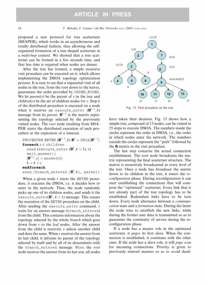
Fig. 15. Visit procedure on the tree.


ARTICLE IN PRESS

proposed a new protocol for tree scatternets

(SHAPER), which works in an asynchronous and

totally distributed fashion, thus allowing the self-

organized formation of a tree shaped scatternet in

a multi-hop context. We showed that a tree scat-

ternet can be formed in a few seconds time, andthat less time is required when nodes are denser.

After the tree has formed, a simple recursive

visit procedure can be executed on it, which allows

implementing the DSOA topology optimization

process. It is easy to see that a sequential visit of all

nodes in the tree, from the root down to the leaves,

guarantees the order provided by ORDER_NODES.

We let parent(v) be the parent of v in the tree andchildren(v) be the set of children nodes for v. Step kof the distributed procedure is executed on a node

when it receives an execute_enter (Bk�1; k)message from its parent. Bk�1 is the matrix repre-

senting the topology selected by the previously

visited nodes. The root node resulting from SHA-

PER starts the distributed execution of such pro-

cedure at the expiration of a timeout.

PROCEDURE ENTER (Bk�1; k) Bk ¼ DSOAðBk�1Þforeach v 2 children

send (execute_enter (Bk; k þ 1), v)wait_answer()

½Bkþc; c� ¼ answerðvÞk ¼ k þ c

endforeachsend (branch_entered (Bk; k), parent)

When a given node v starts the ENTER proce-

dure, it executes the DSOA, i.e. it decides how to

enter in the network. Then, the node randomly

picks up one of its children nodes, and sends it the

execute_enter(Bk, k þ 1) message. This causes

the execution of the ENTER procedure on the child.

After sending the execute_enter command, vwaits for an answer message (branch_entered)

from the child. This contains information about the

topology selected by the whole branch which goes

down from v to the leaf nodes. After the answer

from the child is received, v selects another child

and does the same.When v receives the answer fromits last child, it informs its parent of the topology

selected by itself and by all of its descendents withthe branch_entered message. When the rootnode receives the answer from its last son, all nodes

have taken their decision. Fig. 15 shows how a

simple tree, composed of 13 nodes, can be visited in

25 steps to execute DSOA. The numbers inside the

circles represent the order in DSOA, i.e., the order

in which nodes enter the network. The numbers

outside the circles represent the ‘‘path’’ followed bythe B matrix in the visit procedure.

The last step concerns the actual connection

establishment. The root node broadcasts the ma-

trix representing the final scatternet structure. The

matrix is recursively broadcasted at every level of

the tree. Once a node has broadcast the matrix

down to its children in the tree, it enters the re-configuration phase. During reconfiguration it canstart establishing the connections that will com-

pose the ‘‘optimized’’ scatternet. Every link that is

not already part of the tree topology has to be

established. Redundant links have to be torn

down. Every node alternates between a communi-cation state and a formation state. During the latter

the node tries to establish the new links, while

during the former user data is transmitted so as toguarantee the continuity of service during the re-

configuration phase.

If a node has a master role in the optimized

scatternet, it pages its first slave. When the con-

nection is established, it continues with the other

ones. If the node has a slave role, it will page scanfor incoming connections. Priority is given to

previously entered masters so as to avoid dead-


ARTICLE IN PRESS

locks. Every node starts tearing down the old links

only when the new ones have been established, so

as to preserve connectivity.

Since all nodes know the overall topology, the

routing task is also simplified. Route discovery

algorithms have to be implemented only whenmobility has to be dealt with or in other particular

situations.

The most time consuming phase of the algo-

rithm is the formation of the tree, which, as said

before, becomes necessary because Bluetooth lacks

a shared broadcast medium. However, we showed

in [11] that the tree can be formed in a few seconds.

During the tree formation phase data exchangeamong nodes can start, so users don�t have to wait

for the overall structure to be set up. Data ex-

change can continue on the provisional tree scat-

ternet during the optimization process. Work is in

progress to add self-healing functionalities to the

algorithm (nodes can enter and exit the network

which is re-optimized periodically) and to simulate

the integration of SHAPER and DSOA with theBlueware [23] simulator.

9. Conclusions

In this paper, we discussed the scatternet for-

mation issue in Bluetooth, by setting a framework

for scatternet analysis based on a representation ina matrix form, which allows developing and ap-

plying different metrics. We identified several

metrics both in a traffic independent and in a

traffic dependent context, and we showed the rel-

evant numerical results. The analysis of these re-

sults allows selecting the most suitable metric for a

given scenario.

A distributed algorithm for scatternet topologyoptimization, DSOA, was then described. The

performance of DSOA has been evaluated and is

encouraging: the distributed approach gives results

very similar to a centralized one. The integration

with the SHAPER Scatternet Formation Algo-

rithm and other implementation concerns have

been discussed. Ongoing activities include the full

design of a distributed scatternet formation algo-rithm which implements DSOA and deals with

mobility and failures of nodes, as well as a simu-

lative evaluation of the time needed to set-up a

scatternet and its performance in presence of dif-

ferent traffic patterns.

References

[1] J.C. Haartsen, The Bluetooth radio system, IEEE Personal

Communications 7 (1) (2000) 28–36.

[2] P. Johansson, M. Kazantzidis, R. Kapoor, M. Gerla,

Bluetooth––an enabler for personal area networking, IEEE

Network 15 (5) (2001) 28–37.

[3] Bluetooth SIG Specification of the Bluetooth System,

Version 1.1––Core, February 2001.

[4] IEEE Std 802.15.1TM-2002, Available from <http://

www.ieee802.org/15/pub/TG1.html>.

[5] S. Zurbes, Considerations on Link and System Throughput

of Bluetooth Networks, 11th IEEE International Sympo-

sium on Personal Indoor and Mobile Radio Communica-

tions, vol. 2, 2000, pp. 1315–1319.

[6] T. Salonidis, P. Bhagwat, L. Tassiulas, R. LaMaire. Dis-

tributedTopologyConstruction of BluetoothPersonalArea

Networks, IEEE INFOCOM �01, 2001, pp. 1577–1586.[7] C. Law, A. Mehta, K. Siu, Performance of a new Bluetooth

formation protocol, ACM Symposium on Mobile Ad Hoc

Networking and Computing (MobiHoc), October 2001.

[8] H. Zhang, J.C. Hou, L. Sha, A Bluetooth loop scatternet

formation algorithm, Proceedings of the IEEE ICC 2003,

Anchorage, 2003, pp. 1174–1180.

[9] G. Tan, A. Miu, J. Guttag, H. Balakrishnan, An efficient

scatternet formation algorithm for dynamic environments,

IASTED Communications and Computer Networks

(CCN), Cambridge, MA, November 2002.

[10] G.V. Zaruba, S. Basagni, I. Chlamtac, Bluetrees-scatternet

formation to enable Bluetooth-based ad hoc networks,

IEEE International Conference on Communications

(ICC�01), vol. 1, 2001, pp. 273–277.[11] F. Cuomo, G. Di Bacco, T. Melodia, SHAPER: A self-

healing algorithm producing multi-hop Bluetooth scattER-

nets, Proceedings of the IEEE Globecom 2003, San

Francisco, USA, in press.

[12] Z. Wang, R. Thomas, Z. Haas, bluenet––a new scatternet

formation scheme, Proceedings of the Hawaii International

Conference on System Science (HICSS-35), 2002.

[13] C. Petrioli, S. Basagni, I. Chlamtac, Configuring bluestars:

multihop scatternet formation for Bluetooth networks,

IEEE Transactions on Computers (Special Issue on Wire-

less Internet) 52 (6) (2003) 779–790.

[14] C. Petrioli, S. Basagni, I. Chlamtac, BlueMesh: degree-

constrained multihop scatternet formation for Bluetooth

networks, Mobile Networks and Applications (Special

Issue on Advances in Research of Wireless Personal Area

Networking and Bluetooth Enabled Networks), in press.

[15] I. Stojmenovic, Dominating set based scatternet formation

with localized maintenance, Proceedings of the Workshop

on Advances in Parallel and Distributed Computational

Models, April 2002.

http://www.ieee802.org/15/pub/TG1.html

http://www.ieee802.org/15/pub/TG1.html


ARTICLE IN PRESS

[16] Y. Liu, M.J. Lee, T.N. Saadawi, A Bluetooth scatternet-

route structure for multihop ad hoc networks, IEEE

Journal on Selected Areas in Communications 21 (2)

(2003) 229–239.

[17] M. Ajmone Marsan, C.F. Chiasserini, A. Nucci, G.

Carrello, L. De Giovanni, Optimizing the topology of

Bluetooth Wireless Personal Area Networks, IEEE INFO-

COM �02.[18] R. Kapoor, M.Y.M. Sanadidi, M. Gerla, An analysis of

Bluetooth scatternet topologies, Proceedings of the ICC

2003, 2003.

[19] P. Bhagwat, S.P. Rao, On the characterization of Blue-

tooth scatternet topologies, Available from <http://win-

www.rutgers.edu/~pravin/bluetooth/>.

[20] F. Cuomo, T. Melodia, A general methodology and key

metrics for scatternet formation in Bluetooth, IEEE

Globecom 2002, November 2002.

[21] C.F. Chiasserini, M. Ajmone Marsan, E. Baralis, P. Garza,

Towards feasible distributed topology formation algo-

rithms for Bluetooth-based WPANs, Hawaii International

Conference on System Science (HICSS-36), Big Island,

Hawaii, 6 January 2003.

[22] E.-H. Amre, Interference between Bluetooth networks-

upper bound on the packet error rate, IEEE Communica-

tions Letters 5 (2001) 245–247.

[23] G. Tan, Blueware: Bluetooth simulator for ns, MIT Labo-

ratory for Computer Science, Cambridge, October 2002.

Tommaso Melodia received his ‘‘lau-rea’’ degree in TelecommunicationsEngineering from the University ofRome ‘‘La Sapienza’’ in 2001. He iscurrently a Ph.D. student in Informa-tion and Communication Engineeringat the same University. From Febru-ary to August 2003 he was a VisitingResearcher at the Broadband andWireless Networking Laboratory atthe Georgia Institute of Technology.His main research interests are relatedto Computer Networks, Wireless adhoc Networks, Wireless Sensor Net-

works, Personal and Mobile Communications.

Francesca Cuomo received her ‘‘Lau-rea’’ degree in Electrical Engineeringin 1993, magna cum laude, from theUniversity of Rome ‘‘La Sapienza’’,Italy. She earned the Ph.D. degree inInformation and Communication En-gineering in 1998, also from the Uni-versity of Rome ‘‘La Sapienza’’. Since1996 she is a ‘‘Researcher’’ (AssistantProfessor) at the INFOCOM Depart-ment of this University. She teachescourses in Telecommunication Net-works.

Her main research interests focus
on: Modeling and Control of broadband integrated networks,Signaling and Intelligent Networks, Architectures and protocolfor fixed an mobile wireless networks, Mobile and PersonalCommunications, Quality of Service guarantees and real timeservice support in the Internet and in the radio access, Recon-figurable radio systems and Wireless ad hoc networks. Sheparticipated in: (I) the European ACTS INSIGNIA projectdedicated to the definition of an Integrated IN and B-ISDNnetwork (1995–1998); (II) RAMON project, funded by theItalian Public Education Ministry, focused on the definition ofa reconfigurable access module for mobile computing applica-tions (2000–2002); (III) National project ‘‘5% Multimedialit�aa’’CNR-MURST. She is now participating to the European ISTWHYLESS.COM project focusing on adoption of the UltraWide Band radio technology for the definition of an OpenMobile Access Network (2000–2003). In this project she isleader of the WP4 (Network Resource Manager). As for currentnational projects: (I) she is involved in FIRB project VIRTUALIMMERSIVE COMMUNICATIONS (VICOM) where she isresponsible of the research activities on the BAN and VANnetworks; (II) she is responsible of the research unit at theUniversity of Rome ‘‘La Sapienza’’ in the EURO project fun-ded by the Italian Public Education Ministry.In 1995 she joined Coritel, a research institute on telecom-
munications, and she has been responsible for two years of theSWAP project in the Radio Access area.

http://winwww.rutgers.edu/~pravin/bluetooth/

http://winwww.rutgers.edu/~pravin/bluetooth/

Ad hoc networking with Bluetooth: key metrics and ...kom.aau.dk/group/05gr1116/reference/Ad hoc networking with... · Ad hoc networking with Bluetooth: key metrics and distributed

Documents