_ _ _ _OIC FILE COPY SECURITY CLASSIFICATION OF THIS PAGE Form Approved REPORT DOCUMENTATION PAGE OMBNo. 0704-0mp e lb. RESTRICTIVE MARKINGS NONE 3. DISTRIBUTION /AVAILABILITY OF REPORT AD-A218 059 APPROVED FOR PUBLIC RELEASE; • 05 ADISTRIBUTION UNLIMITED. 5. MONITORING ORGANIZATION REPORT NUMBER(S) AFIT/CI/CIA- 89 -011 6a. NAME OF PERFORMING ORGANIZATION 6b. OFFICE SYMBOL 7a. NAME OF MONITORING ORGANIZATION AFIT STUDENT AT UNIVERSITY (if applicable) OF DAYTON 6c. ADDRESS (City, State, and ZIP Code) 7b. ADDRESS (City, State, and ZIP Code) Wright-Patterson AFB OH 45433-6583 8a. NAME OF FUNDING /SPONSORING 8b. OFFICE SYMBOL 9. PROCUREMENT INSTRUMENT IDENTIFICATION NUMBER ORGANIZATION (If applicable) 8"c. ADDRESS (City, State, and ZIP Code) 10. SOURCE OF FUNDING NUMBERS PROGRAM PROJECT TASK WORK UNIT ELEMENT NO. NO. NO. ACCESSION NO. 1I. TITLE (Include Security Classification) (UNCLASSIFIED) R LEOR ANTENNA DESIGNS FOR AIRBORNE RADAR APPLICATIONS 12. PERSONAL AUTHOR(S) GEORGE MARIO BESENYEI 13a. TYPE OF REPORT 13b. TIME COVERED 14. DATE OF REPORT (Year, Month, Day) 15. PAGE COUNT THSIS/tIiinIem FROM TO 1988 I 131 16. SUPPLEMENTARY NOTATION APFRUVkU rQR PUB1LIC RELEASE IAW AFR 190-1 ERNEST A. HAYGOOD, 1st Lt, USAF Executive Officer, Civilian Institution Programs 17. COSATI CODES 18. SUBJECT TERMS (Continue on reverse If necessary and identify by block number) FIELD GROUP SUB-GROUP 19. ABSTRACT (Continue on reverse if necessary and identify by block number) DTIC FEB 15 1990 ) D qO 0 ILI 0 5-I 20. DISTRIBUTION/ AVAILABILITY OF ABSTRACT 21. ABSTRACT SECURITY CLASSIFICATION [UNCLASSIFIEDAJNLIMITED 0 SAME AS RPT. DTIC USERS UNCLASSIFIED 22a. NAME OF RESPONSIBLE INDIVIDUAL 22b. TELEPHONE (Include Area Code) 22c. OFFICE SYMBOL ERNEST A. HAYGOOD, 1st Lt, USAF (513) 255-2259 AFIT/CI DD Form 1473, JUN 86 Previous editions are obsolete. SECURITY CLASSIFICATION OF THIS PAGE AFIT/CI "OVERPRINT"

Welcome message from author
This document is posted to help you gain knowledge. Please leave a comment to let me know what you think about it! Share it to your friends and learn new things together.
Transcript

_ _ _ _OIC FILE COPYSECURITY CLASSIFICATION OF THIS PAGE
Form Approved
REPORT DOCUMENTATION PAGE OMBNo. 0704-0mp e
lb. RESTRICTIVE MARKINGSNONE
3. DISTRIBUTION /AVAILABILITY OF REPORTAD-A218 059 APPROVED FOR PUBLIC RELEASE;• 05 ADISTRIBUTION UNLIMITED.
5. MONITORING ORGANIZATION REPORT NUMBER(S)
AFIT/CI/CIA- 8 9 -011
6a. NAME OF PERFORMING ORGANIZATION 6b. OFFICE SYMBOL 7a. NAME OF MONITORING ORGANIZATIONAFIT STUDENT AT UNIVERSITY (if applicable)OF DAYTON
6c. ADDRESS (City, State, and ZIP Code) 7b. ADDRESS (City, State, and ZIP Code)
Wright-Patterson AFB OH 45433-6583
8a. NAME OF FUNDING /SPONSORING 8b. OFFICE SYMBOL 9. PROCUREMENT INSTRUMENT IDENTIFICATION NUMBERORGANIZATION (If applicable)
8"c. ADDRESS (City, State, and ZIP Code) 10. SOURCE OF FUNDING NUMBERSPROGRAM PROJECT TASK WORK UNITELEMENT NO. NO. NO. ACCESSION NO.
1I. TITLE (Include Security Classification) (UNCLASSIFIED)R LEOR ANTENNA DESIGNS FOR AIRBORNE RADAR APPLICATIONS
12. PERSONAL AUTHOR(S)GEORGE MARIO BESENYEI
13a. TYPE OF REPORT 13b. TIME COVERED 14. DATE OF REPORT (Year, Month, Day) 15. PAGE COUNTTHSIS/tIiinIem FROM TO 1988 I 13116. SUPPLEMENTARY NOTATION APFRUVkU rQR PUB1LIC RELEASE IAW AFR 190-1
ERNEST A. HAYGOOD, 1st Lt, USAFExecutive Officer, Civilian Institution Programs
17. COSATI CODES 18. SUBJECT TERMS (Continue on reverse If necessary and identify by block number)FIELD GROUP SUB-GROUP
19. ABSTRACT (Continue on reverse if necessary and identify by block number)
DTICFEB 15 1990
) D
qO 0 ILI 0 5-I20. DISTRIBUTION/ AVAILABILITY OF ABSTRACT 21. ABSTRACT SECURITY CLASSIFICATION
[UNCLASSIFIEDAJNLIMITED 0 SAME AS RPT. DTIC USERS UNCLASSIFIED22a. NAME OF RESPONSIBLE INDIVIDUAL 22b. TELEPHONE (Include Area Code) 22c. OFFICE SYMBOLERNEST A. HAYGOOD, 1st Lt, USAF (513) 255-2259 AFIT/CI
DD Form 1473, JUN 86 Previous editions are obsolete. SECURITY CLASSIFICATION OF THIS PAGE
AFIT/CI "OVERPRINT"

ABSTRACT
REFLECTOR ANTENNA DESIGNS FOR AIRBORNE RADAR APPLICATIONS
Name: Besenyei, George M.University of Dayton, 1988
Advisors: Dr. G. A. Thiele, Dr. R. P. Penno, and
Dr. K. M. Pasala
This paper examines simple Cassegrain, Twist-
Cassegrain, and Inverse Cassegrain reflector antenna
designs for airborne radar applications. The author
chooses an optimized Twist-Cassegrain design and examines
its performance using the Hughes Vector Diffraction
simulation run on an IBM 3038 mainframe at building R-2,
Radar Systems Group, Hughes Aircraft Company, Los Angeles,
CA. Numerous historical examples of Twist-Cassegrain
designs are also presented. " , , I
iii

REFLECTOR ANTENNA DESIGNS FOR
AIRBORNE RADAR APPLICATIONS
Thesis
Submitted to
The School of Engineering of the
UNIVERSITY OF DAYTON
In Partial Fulfillment of the Requirements for
The Degree
Master of Science in Electrical Engineering
by Accesiori For
George Mario Besenyei NTIS CRA&IDTI'C TrH
UNIVERSITY OF DAYTON
Dayton, Ohio Dtby :.
November, 1988 . -
I Av-,. i oDiAt
I

REFLECTOR ANTENNA DESIGNS FOR AIRBORNE RADAR APPLICATIONS
APPROVED BY:
Gary A. Thiele, Ph.D. Krishna M. Pasala, Ph.D.Associate Dean/Director Associate ProfessorGraduate Engineering & Research Electrical EngineeringSchool of Engineering Committee MemberCommittee Chairperson
Robert P. Penno, Ph.D.Assistant ProfessorElectrical EngineeringCommittee Member
Gary A. Thiele, Ph.D. Gordon A. Sargent, Ph.D.Associate Dean/Director DeanGraduate Engineering & Research School of EngineeringSchool Of Engineering
ii

Table of Contents
page
ABSTRACT ......... ....................... iii
TABLE OF CONTENTS .......... .................. iv
LIST OF ILLUSTRATIONS ...... ............... . vi
LIST OF TABLES ........ .................. . ix
LIST OF SYMBOLS .......... ................... x
ACKNOWLEDGEMENTS ........ ................... xi
CHAPTER
1. INTRODUCTION ...... ................. 1
BackgroundPurpose StatementMethod of InvestigationLiterature SearchOverview
2. FUNDAMENTAL PRINCIPLES AND THEORY ... ....... 8
Simple Cassegrain DesignTwist-Cassegrain DesignInverse-Cassegrain DesignSoviet Cassegrain DesignPropagation ModesHorn Feed DesignEffective Radiated PowerMethod of ScanningAntenna Gain and Loss BudgetsThree DB Beamwidth
3. OPTIMIZED TWIST-CASSEGRAIN DESIGNS .. ..... .. 52
English Twist-Cassegrain DesignsSwedish Twist-Cassegrain DesignsOptimized Swedish Design
Basic Parameters of Optimized Design
iv

4. PERFORMANCE ANALYSIS OF OPTIMIZED DESIGN . . . . 70
Modified Vector Diffraction ProgramRusch Scattering EquationsFar Field Pattern Results
5. CONCLUSIONS AND RECOMMENDATIONS ... ........ 105
APPENDICES
Appendix A: Proofs of Fundamental Principlesand Approximations ... ........ 108
Appendix B: Suitable Traveling Wave Tubes . . .115
Appendix C: Swedish Antenna Design-Simulated
Patterns ...... .............. 116
Appendix D: Vector Diffraction Program Inputs .125
REFERENCES ......... ...................... 128
V

LIST OF ILLUSTRATIONS
page
1. Cassegrain Telescope . . . . . . . .......... 9
2. Simple Cassegrain Reflector Antenna .... ......... 9
3. A Double Refector Antenna With PolarizationShiftability ........ ................... 16
4. Early Polarization Changing Antenna Design ...... .19
5. Early Twist-Reflector Antenna .... ........... 21
6. Twist-Reflector Design With a HyperboloidSubreflector ....... .................. 22
7. Transmission Line Equivalents For a Twist-Reflector 24
8. Geometry of Inverse Cassegrain Antenna ....... 27
9. Measured Gain of Inverse Cassegrain Antenna . . 29
10. Monopulse Feed Excitation .... ............ 33
11. Four Quadrant Monopulse Feed Design ... ....... 34
12. Universal Radiation Pattern of a Horn Flared in theE-Plane ........ ................... 38
13. Universal Radiation Pattern of a Horn Flared in theH-Plane ....................... 40
14. The Pyramidal Horn ...... ................ 41
15. Airborne Radar Block Diagram ... ........... .. 43
16. Five Bar Raster Search Pattern .. ......... 45
17. Edge Illumination Versus Efficiency Factor. . .. 48
vi

page
18. The Marconi Twist-Cassegrain Antenna (Aerial). . . 53
19. GEC Twist-Cassegrain Antenna Installed in a TornadoF MK 2 Aircraft (Front View) ... .......... 55
20. Swedish Twist-Cassegrain Antenna ... ......... .57
21. Multimode Monopulse Feed For Swedish Antenna . . . 58
22. Dual-band Twist Cassegrain Design ... ......... .59
23. Twist-Reflector Cross Section ... .......... 59
24. Optimized Swedish Twist-Cassegrain Antenna WithPyramidal Feed ....... ................. 61
25. Geometry of Hughes Simulation .... ........... .. 71
26. Geometry of Rusch Integrals .... ............ .74
27. Secondary Pattern for E-Plane for Design A . . .. 80
28. Secondary Pattern for H-Plane for Design A . . . 81
29. Primary Pattern for E-Plane for Design A . . ... 82
30. Primary Pattern for H-Plane for Design A ..... 83
31. Secondary Pattern for E-Plane for Design B . . . 86
32. Secondary Pattern for H-Plane for Design B . . . 87
33. Primary Pattern for E-Plane for Design B ..... 88
34. Primary Pattern for H-Plane for Design B ..... 89
35. Secondary Pattern for E-Plane for Design C . . . 91
36. Secondary Pattern for H-Plane for Design C . . .. 92
37. Primary Pattern for E-Plane for Design C ...... .. 93
38. Primary Pattern for H-Plane for Design C ...... .. 94
39. Primary Pattern for E-Plane for Design D ...... .. 96vii

page
40. Primary Pattern for H-Plane for Design D ..... 97
41. Secondary Pattern for E-Plane for Design D .... 98
42. Secondary Pattern for H-Plane for Design D . . . 99
43. Secondary Pattern for E-Plane for Design E . . . 101
44. Secondary Pattern for H-Plane for Design E . . . 102
45. Primary Pattern for E-Plane for Design E ..... .103
46. Primary Pattern for H-Plane for Design E ..... .104
47. Geometry of Apperture Blockage ... ......... .. 109
48. Geometry for Rectangular Apperture .. ....... .. 112
49. Pattern of Uniformly Illuminated RectangularApperture .......... .................. 114
50. Secondary Pattern for E-Plane for Swedish Designat 9.2 GHz ......... ................ 117
51. Secondary Pattern for H-Plane for Swedish Designat 9.2 GHz .......... ............... 118
52. Primary Pattern for E-Plane for Swedish Designat 9.2 GHz ......... ................ 119
53. Primary Pattern for H-Plane for Swedish Designat 9.2 GHz . . . . .. . . . . . . . . . . . . . . 120
54. Secondary Pattern for E-Plane for Swedish Designat 9.3 GHz ......... ................ 121
55. Secondary Pattern for H-Plane for Swedish Designat 9.3 GHz ......... ................ 122
56. Primary Pattern for E-Plane for Swedish Designat 9.3 GHz ......... ................. 123
57. Primary Pattern for H-Plane for Swedish Designat 9.3 Ghz ......... ................. 124
viii

LIST OF TABLES
page
1. Calculation of Area Gain .............. .12
2. Antenna Loss Budget ....... ................ 13
3. Four Quandrant Monopulse Feed Design ... ........ 35
4. Loss Budget for a Twist-Cassegrain ReflectorAntenna ......... .................... . 47
5. Parameters of Optimized Design A ... ......... .. 64
6. Basic Parameters of Design B ............. 65
7. Basic Parameters of Design C ..... .......... .66
8. Basic Parameters of Design D .... ........... .67
9. Basic Parameters of Design E .... ........... .68
ix

LIST OF SYMBOLS
Symbol Definition
a distance between grid and ground plane
bg equivalent susceptance of wire grid
B blockage ratio = d/D
angle from focal pt. to subreflector
edge
D paraboloid diameter
d hyperboloid diameter
F focal length of paraboloid
f focal length of hyperboloid
hyperboloid half angle
x

ACKNOWLEDGMENTS
This paper is dedicated to my wife Paula, without
whose constant encouragement this paper could never have
been completed. In addition, this paper is also dedicated
to the late Frederick Williams, Chief Scientist, Hughes
Aircraft Company, for his technical expertise in air-to-air
radar systems design imparted to me during 1984 and 1985,
while serving as a consultant to the Air Force.
The author would especially like to thank Arthur F.
Seaton, Senior Scientist, Hughes Aircraft Company, for his
overwhelming support in the simulation activity, as well
as, for his ability to answer difficult antenna design
questions. Furthermore, the author is greatful for the
Independent Research and Development funding of the
simulation activity provided by the Hughes Aircraft
Company, through William Kessler, Radar Systems Group.
In addition, the author would like to thank Robert
Dahlin, Arkady Associates, for his source material on
Soviet reflector antenna design. This material was
quite unique and otherwise totally nonexistent in U.S. and
European literature.
xi

Finally, this author would like to thank Dr. Gary A.
Thiele, Dr. K. M. Pasala, and Dr. Robert Penno, all of the
University of Dayton, for their technical assistance and
review of this paper. Also, this author would like to
thank all the personnel of AFIT/CI who have assisted this
project through the funding of two trips to Los Angeles,
CA.
xii

Chapter 1
INTRODUCTION
BACKGROUND
Reflector antennas derived from geometric optics have
been used extensively for radio telpscope and ground
search radars over the years. However, only within the
last 20 years have airborne radar applications even been
proposed, prototyped, and developed. Much of the critical
development of these reflector antenna designs have been
accomplished by the United Kingdom (Marconi), Israel (IAI
Elta Electronics), Sweden, and the Soviet Union. American
efforts were accomplished by the Wheeler Labs (now part of
Hazeltine Corp.), and Westinghouse Defense Electronics.
Westinghouse abandoned their design due to tracking
problems. Hughes purchased a Swedish design for testing,
but never incorporated it into any production airborne
radar. Currently no US military aircraft use reflector
antenna designs such as the simple Cassegrain, Twist
Cassegrain, or Inverse Cassegrain. This is due to the US
insistence upon using only state-of-the art technology.

PURPOSE STATEMENT
It is the purpose of this paper to show the
feasibility of using reflector antennas derived from
geometric optics for airborne radar applications in low
cost jet fighter aircraft of the future. Feasibility will
be shown by: adequate antenna gain for a 85 dBW Effective
Radiated Power specification, low first sidelobes (less
than -20 Db down from main beam), adequate scan pattern,
and low system losses. In addition, this antenna should be
able to radiate anywhere in the I-band regime (8-10 GHZ).
This antenna will be used strictly with low Pulse-
Repetition Frequency (PRF) signals only (1000 pulses per
second or less). While these specifications on sidelobe
level are higher than what could be achieved with array
antennas, they are lower than the standard 13 dB criteria
to detect targets.

METHOD OF INVESTIGATION
The writer will examine the following reflector
antenna designs for suitability in meeting the feasibility
requirements established in the purpose statement: simple
Cassegrain, Twist-Cassegrain, and Inverse Cassegrain (also
refered to as mirror antennas in most foreign literature).
Real data will be furnished whenever possible. Finally the
writer will choose an optimum antenna design and show the
optimum theoretical performance acheivable in the form of
primary and secondary reflector patterns. This will be
accomplished using the Hughes Aircraft Vector Diffraction
simulation, which integrates the Rusch integrals. A brief
description of this simulation is given in Chapter 4 of
this paper.
3

LITERATURE SEARCH
The subject of reflector antenna designs using
geometric optics approaches has been widely researched
primarily in the 1960's and 1970's in this country. Very
little attention is being given to these designs in the US
today. No airborne radar in this country presently uses or
is being designed which is built around any geometric
optics type antenna (simple Cassegrain, Twist-Cassegrain,
or Inverse Cassegrain). Foreign sources have
overwhelmingly dominated the research and development in
this area since the mid-1970's. Nevertheless, the concept
of these antenna structures for airborne radar applications
has been well proven in many foreign radar systems. The
documentation on these systems is however quite limited.
Detailed design information is often left out in many
juurnals in which these foreign radars appear.
The US documentation on reflector antennas designed
using geometric optics seem to begin with the work done by
Peter Hannon, Harold Wheeler, and others from the Wheeler
Laboratories (Hannon 1955 and 1961). Other work, in the
area of simulation for Cassegrain antennas has been
accomplished by W.V.T Rusch and P.D. Potter for NASA.
4

The analysis techniques used by Rusch and Potter are
published in the textbook: Analysis of Reflector Antennas
(Rusch and Potter, 1970). Much of this work is based on
two studies done by Rusch (July, 1963 and May, 1963).
Furthermore, the Hughes Vector Diffraction Simulation, on
which most of the analysis of this paper is based upon, was
derived originally from a NASA Jet Propulsion Laboratory
simulation developed by Rusch, Potter, and Jungmeyer.
About the same time period Paul Jensen, Hughes
Aircraft Company conducted research into simple Cassegrain
type antennas for ground based tracking purposes (Jensen,
1961). He later made a significant contribution to The
Handbook of Antenna Design (1984) with detailed design
procedures for a simple Cassegrain reflector.
Twist-Cassegrain designs using double wire grid twist-
reflectors were first reported in Sweden (Josefsson, 1973)
which essentially provided 100% bandwidth capabality, a
great improvement over the single wire grid twist-
reflectors which provided a 30% bandwidth capability.
Later, L.G. Josefsson would write his doctoral dissertation
on "Wire Polarizers for Microwave Antennas" (1978), which
essentially developed wire grid polarizers suitable for
Twist-Cassegrain antennas. In Los Angeles, at RADAR 86,
Josefsson presented a dual band Twist-Cassegrain antenna.
5

Furthermore, a low sidelobe Twist-cassegrain antenna was
presented at the 1973 Internal Radar conference
(Dahlsjo, 1973). This is the design referred to in this
paper as the "Swedish Twist-Cassegrain Design".
In England, GEC Avionics developed their own Twist-
Cassegrain antenna (aerial) for use in the Tornado F Mk2
interceptor for the Royal Air Force (Spooner and Sage,
1985). This antenna is part of the Foxhunter AI radar
which is designed to operate fully coherently. In
addition, Marconi Avionics Ltd. developed a Twist-
Cassagrain antenna which is described in this paper
(Mahony, 1981).
In the USSR, several books and papers refer to off-
axis capability in Cassegrain type (two mirror) antennas
(Galimov, 1969 and Bakhrakh and Galimov, 1981). The
translation into English is not fully adequate at times to
preserve the original meaning of ideas and concepts being
presented. In addition, these documents tend to be terse.
Finally, in Israel, Elta Electronics developed an
Inverse Cassegrain design based on US Naval Research
Laboratory principles and designs (Orleansky, Samson, and
Havkin, 1987; Lewis anr Shelton, 1980).
OVERVIEW
This paper will develop the fundamental principles and
theory of cassegrain type (those derived from geometric
optics) reflector antennas in Chapter 2. In Chapter 3, the
author will develop an optimized Swedish design that t;ould
be desirable to the US Air Force. Other designs will be
examined. Chapter 4 will contain the performance analysis
of the optimized design by way of far-field patterns
obtained by simulation using the Hughes Vector Diffraction
Program on an IBM 3038 computer. Finally, conclusions and
recommendations will be presented in Chapter 5.

CHAPTER 2
FUNDAMENTAL PRINCIPLES AND THEORY
SIMPLE CASSEGRAIN DESIGN
Simple Cassegrain reflectors are those derived from a
Cassegrain telescope. A Cassegrain telescope consists of
two mirrors and an observing optical instrument, as shown
in Figure 1, reference Ingalls, 1953. Simple Cassegrain
reflector antennas are described in detail in Hannon, 1961.
They are composed primarily of a paraboloidal main
reflector and a hyperboloidal subreflector. The feed
(generally four horn monopulse or single pyramidal horn) is
located at the vertex of the paraboloid. This is quite a
desirable position since its rear location and forward
direction of the feed eliminate long transmission lines and
provide more flexibility in feed design than front-fed
paraboloids. A diagram of a simple Cassegrain antenna is
depicted in Figure 2.
8

Secondary Mirror
Optical I trument
Primary Mirror
Figure 1. Cassegrain telescope
F ed
I SubreflectorMain Reflector
Figure 2. Simple Cassegrain reflector antenna
9

Basic Design Parameters and Calculations
The diameter of the paraboloid main reflector is fixed
in order to fit within the radome of the aircraft. The
author assumes the limitation is 30 inches for the maximum
possible diameter. Simulation cases will be run at both 27
and 30 inches diameters. The results are presented in
Chapter 4 of this paper. The paraboloid diameter
principally governs the total system gain and the antenna
efficiency achievable.
The focal length (of the paraboloid) / diameter (of
the paraboloid) ratio of 0.6 will be used. This will be
referred to as the F/D ratio. For the 27 inch case of the
paraboloid main reflector, simulations with F/D = 0.5 and
F/D = 0.7 will also be run, with the results presented in
Chapter 4 as well. The F/D ratio is chiefly governed by
mechanical considerations. To minimize spillover, past the
paraboloid edges, according to Hansen (1959), a deep dish
with a small F/D is desirable. This is however, not
practical in an airborne radar design, with limited
available space. Furthermore, Carter (1955) found that in
low noise design, the far out side lobes caused by the
longitudinal and cross-polarized currents on a highly
curved reflector dictate the choice of a shallower dish (a
larger F/D).10

According to Jensen (1962), the typical values of F/D
chosen range between 0.25 and 0.42 for simple Cassegrain
ground based reflectors. The author will work strictly in
the range of F/D between 0.5 and 0.7 for his airborne radar
application.
Next, the diameter, d, of the subreflector will be
minimized to avoid blockage using the minimum blockage
condition presented in Hannon (1961). Specifically, we
have d = (2 X F/k)1/2, where k is ordinarily slightly less
than one. The proof of this equation appears in Appendix A
of this paper. Furthermore, two of the assumptions upon
which this proof is based upon (the beamwidth between nulls
and Eo relationship) are also proven in Appendix A.
The blockage ratio can be defined as B = d/D. It is
usually chosen to meet the minimum blockage condition above
for a simple Cassegrain design. However, the author will
show in a case presented in Chapter 4 that for an airborne
radar application, this configuration is extremely degraded
by edge diffraction effects, resulting in an undesirable
antenna pattern (see pattern in Chapter 4).
Jensen (1962) developed an expression for the loss in
antenna gain due to blockage by the subreflector, GL, as:
GL = 20 log (I - 2B2). For our considerations, at minimum
blockage and 9.3 GHz operation, GL is about 0.3 dB.
11

Calculation of antenna gain, G, without losses (also
referred to as the area gain in the literature) can be
approximated by (Dl /X )2 (Culter, 1947). Table I below
shows the calculation of area gain for various frequencies
of interest between 8 to 10 GHz for D = 27 inches.
Table 1
Calculation of Area Gain
Frequency Wavelength Area Gain
(GHz) (meters) (dB)
8.5 0.0353 35.7
9.0 0.0344 35.9
9.3 0.0333 36.2
9.4 0.0319 36.6
9.6 0.3125 36.8
12

We can now develop an antenna loss budget such as the
one depicted below in Table 2 for the case of frequency
equal to 9.3 GHz, ignoring the losses due to the radome.
Table 2
Antenna Loss Budget
Antenna gain without losses 36.20 dB
Loss due to subreflector blockage - 0.26 dB
Taper and spillover loss - 1.20 dB
Monopulse sum & differ. network - 0.40 dB
Random Error - 0.25 dB
Mismatch - 0.30 dB
Effective antenna gain 33.79 dB
The result is an effective antenna gain quite suitable for
airborne radar applications. However, there are a number
of penalties associated with this design. The most severe
penalty is a limit in the usable 3-dB beamwidth for a
simple Cassegrain antenna.
13

Problems With Simple Cassegrain Designs
According to Hannon (1961), a one-degree beamwidth
might be considered as a rough boundary above which the
simple Cassegrain design, even though optimized, would be
unattractive. Hannon developed a formula relating ld/D)2
to beamwidth, primarily based on experimental evidence.
Essentially he states (d/D)2 = (W/2k) x (203d3) x (F/D).
It is apparent from this relationship that an antenna with
a narrow beamwidth can have less relative aperture blocking
than one with a wide beamwidth _n airborne radars 2 to 3
degree beamwidths art- quite commonly used. Therefore the
simple cassegraii design is simply not suitable for the
narrow beamwidths it imposes upon the radar system.
In addition, subreflectors less than 10 \ exhibit huge
amounts of edge diffraction and simply do not make sense to
build according to A. F. Seaton, Senior Scientist, Radar
Systems Group, Hughes Aircraft Company, Los Angeles, CA.
In Chapter 4 of this paper, a simulation is run with a 5 A
subreflector resulting in an unacceptable antenna pattern.
Similarily, Dijk, Jeuken, and Manders state that blocking
and diffraction by the subreflector decrease the overall
efficiency by about 8% (Dijk, Jeuken, and Manders, 1968).
The simple Cassegrain design will be abandoned in lieu of a
Twist-Cassegrain design described next.
14

TWIST-CASSEGRAIN REFLECTOR ANTENNAS
The Principle of Polarization Twisting
A polarization twisting double-reflector antenna is
shown in Figure 3. Essentially it is composed of three
major elements. They are the reflector, the polarization
changer, and the transreflector. In addition, a feed and
some means for focusing are required to complete the
antenna.
An incoming plane wave having a certain polarization,
say PA, is portrayed by ray 1 (at the right). This wave
passes through the first surface, called the
transreflector, because the surface is designed to be
transparent to polarization, PA. The wave next encounters
a surface, called the polarization changer, which changes
the polarization of the wave in a particular manner as it
passes through. Next, the wave is incident on a surface
called the reflector, which is designed to completely
reflect any wave. Finally, the wave again passes through
the polarization changer, with a new polarization, Pa.
This new polarization is such that the transreflector may
be designed to completely reflect it, while still remaining
transparent to polarization, PA.
15

PolarizationReflector Changer Transreflector
Polarization 'A
2< -
Polari tion PB
Figure 3. A double reflector antenna with polarizationshiftability
16

Thus the wave is now reflected at the transreflector.
In Figure 3, the polarization changer is shown as a
distinct component between the two reflecting surfaces. In
some designs however, the polarization changer may be
incorporated as part of either the reflector or the
transreflector.
In an antenna, the wave is focused into a feed. The
focusing may be accomplished by the two reflecting
surfaces, an additional focusing element, or both. The
feed may be located on either side of the polarization
changer. The polarization of the feed should be that of
the focused wave it is receiving.
17

Early Twist Cassegrain Designs
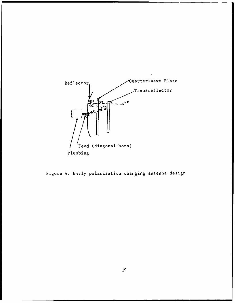
The design in Figure 4 employs a quarter-wave plate as
the polarization changer. An incoming vertically polarized
wave (VP) passes through the transreflector unchanged. The
wave then goes through the plate, which changes the
polarization to right-hand circular polarization (RCP).
Upon reflection from the reflector, the wave is changed to
left-hand circular polarization (LCP). Then, after
traveling across the plate again, the wave becomes
polarized horizontally (HP). The wave is now completely
reflected by the transreflector. Upon passing through the
quarter-wave plate again, this wave is finally changed to
left-hand circular polarization. The feed is designed for
left-hand circular polarization, and transmits the wave to
the plumbing through a hole in the apex of the reflector.
The design in Figure 4 is shown with a paraboloidal
reflector and a flat transreflector. For this antenna, all
the focusing action is provided by the paraboloid. The
transreflector provides an image of the feed at the focus
of the paraboloid. The distance from the paraboloidal apex
to the flat transreflector is one-half that to the image of
the feed. Thus this antenna is half as long as one using a
single reflector of the same focal length.
18
Reflector uarter-wave Plate
Transreflector
P Vt ,P
Feed (diagonal horn)
Plumbing
Figure 4. Early polarization changing antenna design
19
Another advantage is that the feed is not required to
be located out in front of the main reflector. Therefore,
there is a minimum of blockage and diffraction caused by
the feed, and the feed and plumbing are close together.
Feed blockage for an ordinary parabolic reflector is
typically characterized by a loss of -0.5 dB according to
Georgia Institute of Technology's D.G. Bodnar (1984).
In the design shown in Figure 5 is the same as that of
Figure 4, except that the polarization changer is now
incorporated with the reflector to make a "twistreflector"
(ref. Hannon, 1961). Since the polarization changer now
has a hole for the feed, the wave incident on the feed is
horizontally polarized. Therefore the feed is horizontally
polarized.
With this design in mind, the transreflector can now
be replaced by a hyperboloid such as that shown in Figure
6. In this design the paraboloid reflector surface
"twists" the reflected polarization to vertical, which
passes through the subreflector (which is horizontally
polarized) essentially unaffected. The subreflector
blockage associated with the simple Cassegrain design
can now be reduced since the subreflector is transparent to
the wave from the paraboloid (Jensen and Rusch, 1984).
20

Twist-reflector
Transreflector
Waveguie\
Feed
Figure 5. Early twist-reflector antenna
21

Twist-reflector (paraboloid)
YTransreflector(hyperboloid)
Feed
Waveguide
Figure 6. Twist-reflector design with a hyperboloidsubreflector
22

Detailed Design of a Twist-Reflector
In 1955 Wheeler Labs developed a design for a twist-
reflector having wideband and wide angle performance
(Hannon, 1955). This twist-reflector was comprised of
parallel metal wires in one wire grid in front of a metal
sheet. It was designed according to the following
equations:
bg = -2.05 (fo/f) and,
a = 0.358 )o
where bg is the equivalent susceptance of the wire grid
normalized to the admittance of free space, a is the
distance between the grid and the ground plane, and Xo is
the wavelength at the center frequency fo (G.G. MacFarlane,
1946).
To analyze the twist-reflector we must look at the two
transmission line equivalents, one for the component of the
incident (linearly polarized) electric field which is
parallel to the wire grid as shown in Figure 7(a), and the
other for the orthogonal component which is perpendicular
to the wire grid as shown in Figure 7(b). In order to
physically twist the polarization 90 degrees, the preceding
components should have the same magnitude or a mismatch
loss results (the grid is inclined 45 degrees with respect
to the incident polarization).
23

Figure 7. Transmission line equivalents for a twist-reflector(a) parallel, (b) perpendicular polarization
24

It is shown in Hannon, 1955 that in order to obtain a
linearly polarized reflected wave, the input admittances
should be reciprocals of each other, that is Y1y = /Y,.
A departure from this condition implies some degree of
elliptical polarization, which may be characterized by a
cross polarization attenuation constant, Pcroso, such that
Pcrous 1 + [(boo - b.)/(1 + b,, b.,)]2 ,
where y,, j b,, and y.= j bl. In addition, wire grid
spacing was 3 X / 8 from a ground plane (H. Jasik, 1961).
Two wire grids require a general synthesis that is
rather complex. The general approach is start from a
common single-wire grid twist-reflector, with a center
frequency fl, and add an additional wire grid such that
the wires are parallel to the first grid and in such a
position that the adittance of the equivalent line
equivalent (for parallel polarization) is infinite in the
position of the additional grid. This holds true only for
one frequency chosen as fl. Further, the insertion of the
additional grid has not changed the polarization twisting
properties of the reflector at frequency fl. Twist-
reflectors, with two wire grids can be constructed to give
very broad bandwidths in the order of 100 percent, while
single grid twist-reflectors have a bandwidth of 30 percent
at the most (Josefsson, 1971).
25

THE INVERSE CASSEGRAIN ANTENNA
Background
The Inverse Cassegrain antenna (also referred to as a
mirror antenna in the literature) was developed primarily
by the Naval Research Laboratories (NRL) and Elta
Electronics (Israel). It is a relatively new design and
not known to be installed in any jet fighter to date. Its
design, however, is unique and is developed below.
Design Characteristics
The Inverse Cassegrain antenna design is shown in
Figure 8 on the next page. Note that the only moving part
is a broadband meanderline twistreflector which is scanned.
A double-ridged feed and a wire grid paraboloid are
stationary in this design. The twistreflector reflects the
beam of the parababoloid and at the same time rotates its
plane of polarization by 90 degrees. The twisted beam now
passes through the wire grid paraboloid reflector. If the
beam were not twisted, it would imply have been reflected
back to the twistreflector.
26

Twistreflector
Double-RidgedFeed -
Figure 8. Geometry of Inverse Cassegrain Antenna
27

Collimation of the beam is accomplished by fixing the
wire grid (of the paraboloid) parallel to the plane of
polarization of the beam (Orleansky, Samson, and Havkin,
1987). According to Elta Electronics the twistreflector
need only be moved through half of the scan angle required.
Also rotary joints can be completely eliminated in this
configuration.
The advantage of this configuation is that an ultra-
wideband twistreflector can be constructed from a
meanderline structure. This structure is in turn made up
of a meanderline polarizer and a flat reflecting surface
(Orlansky, et al., 1987). Meanderline polarizers are
described by Young, Robinson, and Hacking in their
paper,"Meanderline Polarizer" (Young, et al., 1973).
Basically, the polarizer consists of a stack of insulating
sheets, each printed with conductive meanderlines and
separated by foam spacers. Since the meanderline polarizer
can be designed for wideband performance, this
twistreflector can operate over more than an oct&ve.
Finally, Figure 9 shows the total measured gain versus
normalized frequency for an Inverse Cassegrain antenna.
Note the overall gain measured at the compact antenna range
at Elta Electronics is erratic, and unpredictable.
28

The total average gain, which is 29.77 dB, is sufficient
for airborne radar applications. The Hughes simulation can
not accurately represent this geometry, as it was designed
for a twist-Cassegrain geometry. While this antenna is
interesting, more data on performance (and losses) is
needed to optimize this configuration.
i6.0
o. 1.0 I. 1. 4 4 M.- 11 is 0.1 J.1 2&..o J. 1 3 .
Figure 9. Measured gain of Inverse Cassegrain Antenna
29

SOVIET CASSEGRAIN DESIGN
A number of open source Soviet publications on "Mirror"
antennas have appeared over the years. They include many
works such as Reflector Scanning Antennas (Bakhrakh and
Galimov, 1981), as well as, the Design of Optimum Two-Mirror
Antennas with the Oscillation of the Radiation Patterns
(Galimov, 1969).
According to an evaluation of the above two sources by
Arkady (Dahlin, 1982), it appears new designs for reflector
antennas have been implemented in the USSR. No equivalent
has been found in US antenna design approaches. The Galimov
text contains a design of very wide scan angle cassegrain
antennas. The objective of the design seems to indicate a
desire for achieving a nearly uniform gain over the entire
angular coverage. The approach adopted is a technique for
generating special reflector shapes for achieving nearly
uniform performance over the scanned volume, but at the
expense of "On-axis" (boresight) performance (Dahlin, 1982).
The performance and use of such an antenna if applied
to a tracking system have an enormous impact. With this
design philosophy, the tracking need not be maintained on
boresight ("on-axis"). 30

PROPAGATION MODES
Using the familiar relation developed in microwaves
for a hollow rectangular waveguide (Chatterjee, 1986, and
Liao, 1985), one can determine the cutoff frequency of
standard WR-90 waveguides (a = 2.286 cm, b = 1.016 cm).
The cutoff frequency for the TEio mode occurs at the 6.562
GHz. The TEao mode occurs at 13.12 GHz. The TE0, mode
occurs at 14.76 GHz. The TMii mode occurs at 16.16 GHz.
Thus if we operate below 13 GHz, only the TEo mode will be
present. Thus since we are operating strictly between 8 to
10 GHz, we do not have to design a mode filter to remove
all unwanted higher modes of propagation.
31

HORN FEED DESIGN
Monopulse Feed Design
A four horn monopulse feed system (Leonov and
Fomichev, 1986) will be utilized in this design in order to
provide three different signals. The signals are (a) the
sum signal, (b) the azimuth error signal, and (c) an
elevation error signal. In order to generate the sum
pattern, the feed circuitry drives all four horns in phase.
In addition, to produce maximum radiation the horns will
give the largest antenna gain when generating the sum
pattern. Thus the sum signal is used for range tracking.
Difference signals for azimuth and elevation tracking
may be processed on a time shared basis. In order to form
the difference patterns, horn pairs are driven in antiphase
as shown in Figure 10. This will produce two regions of
opposite polarity, which creates the two lobes necessary
for tracking both azimuth and elevation.
In Figure 11, we show a four quadrant monopulse feed
design. For simplicity, the figure shows a circular feed
separated by both horizontal and vertical septums. In
reality the overall feed can be rectangular in shape, with
the same basic results shown in Table 3 on the next page.
32

F + Sum signal
SAzimuth Difference signal
Elevation Difference signal
Figure 10. Monopulse Feed Excitations
33

A
Figure 1L Four Quadrant Monopulse Feed Design
34

Table 3
Four Quadrant Monopulse Feed Design
Signal Composition
1 =A+B+C+D
AEL = A + B - C - D
AAZ = A - B + C - D
35

The basic idea of the four quadrant monopulse feed can
now be generalized as follows. The sum signal is the sum
of all beams. That is:
= A + B + C + D,
where A, B, C, and D are the signals from each beam. This
is the signal used to measure and track range, and as a
reference for the error signals. The error signals are the
difference signals for both azimuth, & AZ, and elevation,
A EL :
4AZ = A - B + C - D
which is the error in the azimuthal plane, and
EL = A + B - C - D
which is the error in the elevation plane.
The monopulse horn does demand increased complexity
and cost (compared to a rectangular horn) as it requires
three receiver channels matched in amplitude and phase.
However, a monopulse radar can in theory track a target
with a single pulse (Tzannes, 1985). This is not possible
with a rectangular horn fed radar system, but it is not
essential for our purposes so we will now examine the
rectangular feed designs available and show how they can be
combined using the superposition principle into a pyramidal
horn.
36

Rectangular E-Plane Horn Design
We will choose a horn flared in the E-plane to
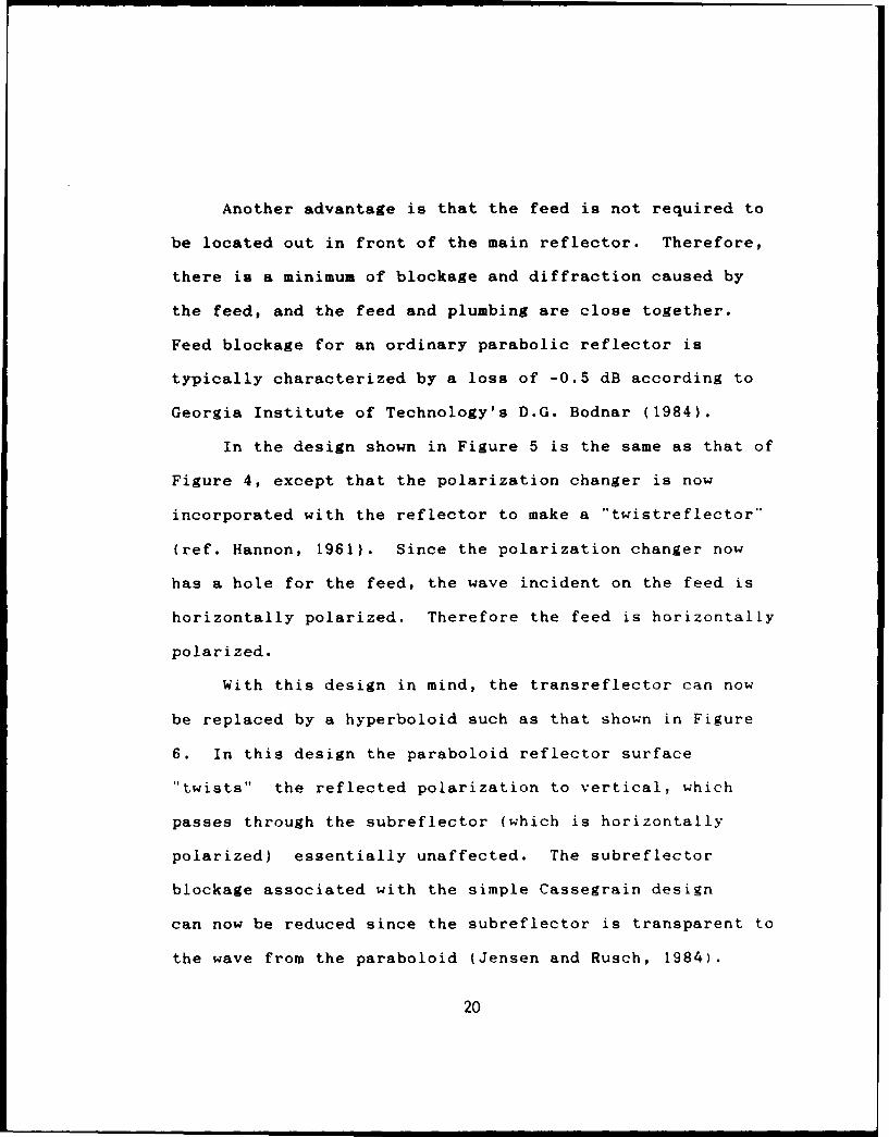
establish the TEa, mode. Using Figure 12 on the next page,
we will determine the size of the apperture, b, required in
wavelengths (Johnson and Jasik, 1984). For a 10 dB edge
taper, the corresponding relative voltage required is
0.3162 volts without losses. We choose \/4 of phase error
as acceptable.
Then, b/X sin Ot is approximately equal to 1.6 without
losses (obtained from Figure 12). Now we must take the
path loss taper into account. This has been found
experimentally as (ITE Antenna Handbook, 2nd Edition):
L (db) = 10 logio (cos 4 (EE/2})
and,
eE/2 = tan-'(.25/ (F/D})
Therefore L(dB), at an F/D value of 0.6, is equal to
approximately -1.39 dB. Thus the actual taper on the E-
plane horn is 10 dB -1.39 dB = 8.61 dB.
Now we must find the actual b/X required, using a
taper of 8.61 dB (.3711 volts) and \/4 of phase error. Then
b/X sin e = 0.8 and b = 1.127 A at GE =45.235 degrees.
Therefore at a frequency of 9.2 GHz, A 1.283 inches, and
b = 1.446 inches.
37
0.
P.
2
(, So.1
0
t64
ao5
Figure 1I. Universal radiation pattern of a hornflared in the E-plane (sectoral orpyramidal)
38

Rectangular H-plane Horn Feed Design
The H-plane horn design will be accomplished similarly
to that of the E-plane design. Now, we will determine the
apperture, a, required in wavelengths using Figure 13.
For a 10 dB edge taper, the corresponding voltage is 0.3162
volts without losses. We again choose X/4 of phase error
as acceptable. Then a/A sin On = 1.2 (without losses),
obtained from Figure 13. Again, we must take the path loss
taper into account. Now let @E = On, then L(dB) = -1.39 dB
which are the path losses. Again, using 8.61 dB as the
actul taper (subtracting out losses), a relative voltage of
approximately 0.3711 volts can be obtained. We choose X/4
of phase error as acceptable. Then,
a/X sin e = 1.1
and On = 45.235 degrees, then a = 1.159 A.
The Pyramidal Horn Feed
A pyramidal horn is obtained by flaring both the E-
plane and H-plane horns simultaneously as shown in Figure
14. By the superposition principle, the results obtained
independently for appertures "a" and "b" are still valid.
39

L.0-
0.4
o.1
I
o.r
I7
04

E
Figure 14. The Pyramidal Horn
41

EFFECTIVE RADIATED POWER
The Effective Radiated Power (ERP) for any radar
system, whether ground based or airborne can be calculated
using the equation given below:
ERP(dB) = G(dB) + 10 log (PT) - Ls(dB)
where G is the antenna gain (area gain - antenna losses),
PT is the power available out of a microwave tube, and Ls
is the total system losses.
Antenna gain calculations can be found for both the
simple cassegrain and twist cassegrain reflector antennas
in Chapter 2 and 3 respectively. Output power for various
commercially available Traveling Wave Tubes (TWT's) is
listed in Appendix B of this paper. A TWT was chosen as
the microwave power tube due to its high frequency
stability and its ability to produce waveforms with pulse
to pulse coherency.
System losses are generally taken to be in the order
of 3-6 dB by various airborne radar designers. These
losses include both waveguide and rotary joint losses for a
typical airborne radar depicted in Figure 15.
42

RF 1w__
IModulator Transmitt r Antenna
DupLexFr. c _
Protection q~evice
Vido Receiver
•Dis pla-
[ControlI ~ ServSCnrl- eoIPanel n
Figure 15. Airborne Radar Block Diagram
43

METHOD OF SCANNING
The entire antenna structure for the optimized Swedish
design is to be mechanically scanned through a maximum an
angle of + 60 degrees off boresight. The antenna scan
pattern is essentially a five bar raster scan pattern as
shown in Figure 16. Four bars are actually used for
scanning (search pattern) and one bar will be used as the
"flyback bar" to reset the search pattern. In track mode
the antenna scan pattern will narrow to + 25 degrees off
boresight, for a more rapid update rate on hostile
threats. The five bar scan pattern is to be used in track
mode as well as in search mode to give a track while scan
capability of up to ten targets. Beyond ten threats the
system will simply track (with a coordinate position
memory) of the nearest ten threats. To attempt to track
multiple threats in any extremely saturated environment has
historically proven quite difficult for most radar
designers, with reliance on secondary sensors such as
Identify Friend or Foe (IFF) sensors or electro-optic
means. A boresight mode will be used for weapons delivery.
44

i I
ai
Figure 16. Five Bar Raster Search Pattern
45

ANTENNA GAIN AND LOSS BUDGETS
The antenna gain for a paraboloid reflector can be
calculated using the relationship G = Eap(i'D/))2 (Cutler,
1947). The efficiency for a front fed paraboloid is in the
order of 55 percent while that of the cassegrain designs is
substantially higher, within the range of 70 to 80 percent.
The antenna efficiency can be approximated by use of the
equation (Stutzman and Thiele, 1981):
Eap = e Et E I E2 E 3 9- 4 E s E6 7 E
where e represents ohmic losses, E is the spillover
efficiency, 62 represents random surface error, E 3 is the
aperture blockage efficiency, E 4 is the spar blockage
efficiency, E.s is the squint factor, E g is the
astigmatism efficiency, E7 is the surface leakage
efficiency, E8 is the depolarization efficiency, etc.
By working with a loss budget in decibels, we can
compute (usually within 3dB) the total antenna gain for a
particular reflector antenna, which is achievable
experimentally. Table 4, on the next page gives typical
losses associated with a Twist-Cassegrain reflector
antenna that are most significant. Several of the losses
(given as efficiencies) can be assumed to be negligible.
46

Table 4
Loss Budget for a Twist-Cassegrain Reflector Antenna
Gain or loss source Gain or loss (dB)
Area Gain (27 inch reflector,
9.2 GHz) 36.83
Taper and Spillover efficiency -1.1
Mismatch (VSWR = 1.7) -0.3
Leakage thru the subreflector -0.2
Loss in the polarization rotation
device -0.1
Imperfect rotation of polarization -0.1
Scattering by wires in the subreflector
to the desired polarization -0.25
Sum and difference network -0.4
Random errors in the surfaces of the
two reflectors -.0.25
Total Antenna Gain 34.13
Note: This loss data is nearly the best physically
achievable, in actual practice we can expect greater loss.
47

I0-4
Figure 17. Edge Illumination Versus Efficiency Factor
48

Spillover efficiency, E,, is defined as that
percentage of the total energy radiated from the feed that
is intercepted by the subreflector (Jensen, 1986). It can
be calculated as follows:
where f( ,y ) is the feed pattern.
In our case, the efficiency factor,ft E, is
approximately equal to 0.774 or -1.11 dB (including the
edge taper) for an angle,le, from the focal point to the
edge of the subreflector equal to 45.24 degrees (see
listing EG621310). The Hughes Vector diffraction program
computes these losses as a function of V. , and prints
results at one degree intervals. Interpolation is required
to get the correct loss figure accuracy to 0.1 dB. A value
of -10 dB edge taper is frequently quoted as providing an
optimum efficiency factor, EE I (Stutzman and Thiele,
1981). Figure 17 shows the general relationship for this
efficiency factor (Stutzman and Thiele, 1981, Figure 8-26).
The maximum value of this efficiency factor is
approximately 0.8, near -11 dB edge tapers.
The efficiency factor for random surface error, E2, is
associated with far-field cancellations arising from random
phase errors in the apperture field. It is defined as:
Ee 2(4 , A)
49

Here I' is the rms surface deviation (Stutzman & Thiele).
In most cases E2 is almost unity. RMS surface tolerances
generally depend on the type of surface and range from .04
mm for machined aluminum to 0.64 for spun aluminum. A
simple formula for representing surface accuracy as a
function of reflector diameter is by Stutzman and Thiele as
%' = 3 x 10⁻² D mm
where D (reflector diameter) is in meters.
Aperture blockage efficiency, E3, is due to the
presence of a subreflector in front of the main reflector.
This efficiency ranges from 0.990 (for d/D = 0.05) to 0.835
(for d/D = 0.20) according to Stutzman and Thiele.
Other efficiency factors E4 through E 9 are also
values very near unity and will not be discussed here. For
example E 7 , the surface leakage efficiency = 0.99 for a
mesh with several grid wires per wavelength (Stutzman and
Thiele).
50

THREE DB BEAMWIDTH
The Three DB Beamwidth can be approximated using the
formula (Williams, 1984):
9393 = Kaw ( X / D) degrees
where Kiw is the beamwidth constant which is generally
equal to 50 to 80, but is dependent on the apperture
distribution used. For example, for a paraboloidal
distribution, the beamwidth constant is equal to 72.8
(Jasik, 1961). For an airborne radar a narrow 2 to 3
degree pencil beam is sufficient to track targets, in
angle (Williams, 1984).
51

CHAPTER 3
OPTIMIZED TWIST-CASSEGRAIN DESIGNS
ENGLISH TWIST-CASSEGRAIN DESIGNS
Marconi has developed a Twist-Cassegrain aerial
(antenna) design for use in airborne radars. In this case
the feed was a pyramidal horn, the subreflector was
composed of a wire grid, and the main reflector was
utilized to twist the polarization from horizontal to
vertical (Scorer, Graham, and Barnard, 1978).
The twist-reflector was comprised of a solid metal
back reflector and a wire grid which are spaced
approximately one quarter wavelength apart. The F/D ratio
chosen was 0.46, with a value of D = 20 ). Figure 18 shows
the layout of this antenna design.
Another Twist-Cassegrain aerial, shown in Figure 19,
is used in the GEC Foxhunter Airborne Radar (Spooner and
Sage, 1985). It has a wide RF bandwidth to accommodate
both the radar and CW illuminator operating bands. This
type of aerial enables the high gain required for long
detection ranges necessary for search modes.52

Fee '
I
•Wire Grid,Wire Grid Subreflector
I
Metal \
Figure 18. Marconi Twist-Cassegrain Antenna (Aerial)
53
• i I I I ii "

A two-plane monopulse feed is provided for track modes
and separate dipoles are provided at a lower frequency for
the transmission and reception of Identify Friend or Foe
interrogation signals (Spooner and Sage, 1985). Nomex
honeycomb and glass fiber materials are used in the
construction of the aerial to produce a rigid, low inertia
assembly.
54

//
Figure 19. GEC Twist-Cassegrain Antenna Installed in Tornado F
MK 2 Aircraft (Front View)
55
Figure 19. E TIstCserin Anen Insaldi ond F

SWEDISH TWIST-CASSEGRAIN DESIGNS
The Swedish design principally consists of a 27.0
inch diameter main reflector and a subreflector
approximately 23.91 inches in diameter as shown in Figure
20. In addition, it contains an elaborate three channel,
two port, multimode monopulse feed as shown in Figure 21.
It is designed to radiate in X-band. Another Swedish
It is fully described in a paper entitled "A Low Side Lobe
Cassegrain Antenna" (Dahlsjo, 1973). In addition, another
Swedish design allows for both X-band and Ka-band
capabilites. This design is shown in Figures 22 and 23
(Dahlsjo, Ljungstrom, and Magnusson, 1986).
The general principle of both designs is to have a
linearly polarized monopulse feed illuminating a
subreflector, which is placed directly in front of the
vertex of main reflector. The polarization of the ray
reflected off the subreflector is twisted ninety degrees in
the main reflector. Now, no aperture blockage is caused by
the polarization sensitive subreflector. Finally, a
transparent cone supports the subreflector. This cone is
lined with polarization sensitive absorbers which are used
to reduce the spillover effects of the monopulse feed.56

Figure 20. Swedish Twist-Cassegrain Antenna
57

-. 4-9
Figure 21. Multimode Swedish Monopulse Feed
58

Feed (>
/ ! Subreflector
Ka Main Reflectorband
X-band
Figure 2Z Dual-band Twist Cassegrain Design
\1. Kev lar Skin2. X-band Metallic Grid3. Nomex Honeycomb4. Ka-band Metallic Grid5. Kevlar Skin6. Metallic Mesh
Figure 23.Twist-Reflector Cross Section
59

OPTIMIZED SWEDISH DESIGN
The writer will utilize the Swedish design, because of
its more compact structure and its ability to be given a
broad-band capability by the simple addition of another
wire grid structure to the twist-reflector (Josefsson,
1981). Furthermore, this design has been experimentally
shown to produce antenna gains in excess of 25 dB and
moderate to low sidelobes.
The writer will encorporate a pyramidal horn feed
instead of the monopulse feed. The Hughes Vector
Diffraction Program described in Chapter 4 will treat this
feed as a point source in its simulation. The pyramidal
horn feed is chosen for high reliability, low cost, and a
desire to maintain a single mode structure radiating the
TEio mode only. Corrugated horns were ruled out due to
their multimode structures and the writer's desire not to
introduce a mode filter into the design.
Figure 24 on the next page shows the layout of this
design with a paraboloid twist-reflector and a hyperboloid
subreflector. The design retains the support cones which
are equipped with absorber material to attenuate the
spillover radiation.60

Transreflector
Pyramidal Feed
Twist-Reflector
Support Cone
Figure 24. Optimized Swedish Twist-Cassegrain AntennaWith Pyramidal Feed
61

System Design Description
The twist-Cassegrain antenna has a weight of
approximately 10 pounds and has a parabaloid diameter of
nearly 28.4 inches (approximately 5 per cent larger than
the basic Swedish design for greater antenna gain). Note
that a 30.0 inch design was also considered, but disgarded
in Chapter 4 of this paper, as well as, a 27.0 inch
paraboloid with a 6.4 inch subreflector.
The curved subreflector is constructed with a quarter-
wave sandwich of two gratings of closely spaced thin wires
inbedded between the fiberglass skins and the foam core.
This gives us a perfect reflector for horizontal
polarization and in addition, good transmission for
vertical polarization. The twist reflector grating of
-ires is oriented at 45 degrees to the incident
polarization and placed about 3/8 \ from the reflecting
surface. This gives a 90 degree twisting of the incident
)olarization over a broad frequency band (I-band) and over
'I wide range of incident angles. The reflector surface is
A fine structure wire mesh inbedded in the outer fiberglass
skin.
62

BASIC PARAMETERS OF THE OPTIMIZED DESIGN
The parameters of the candidate designs A through E
are listed in the following pages in Tables 5 through 9.
The basic 27 inch diameter (of the paraboloid) was not
considered due to its inferior antenna gain than that of
the 28.4 or 30.0 inch designs, even though it produced
respectable first sidelobe levels greater than -25 dB down
from the main lobe.
63

Table 5
Parameters of Optimized Design A
Diameter of the paraboloid 28.4 inches
Diameter of the subreflector 25.0 inches
Focal length of the paraboloid 17.0 inches
F/D ratio 0.6
Eccentricity -9.0
Wavelength 1.28 inches
Frequency 9.21 GHz
Angle Alpha 0 61.50 degrees
64

Table 6
Basic Parameters of Design B
Diameter of the paraboloid 28.4 inches
Diameter of the subreflector 25.0 inches
Focal length of the paraboloid 14.2 inches
F/D ratio 0.5
Eccentricity -49.6
Wavelength 1.28 inches
Frequency 9.21 GHz
Angle Alpha 0 61.50 degrees
65

Table 7
Basic Parameters of Design C
Diameter of the paraboloid 28.4 inches
Diameter of the subreflector 25.0 inches
Focal length of the paraboloid 19.8 inches
F/D ratio 0.7
Eccentricity -5.4
Wavelength 1.28 inches
Frequency 9.21 GHz
Angle Alpha 0 61.50 degrees
66

Table 8
Basic Parameters of Design D
Diameter of the paraboloid 30.0 inches
Diameter of the subreflector 26.6 inches
Focal length of the paraboloid 18.0 inches
F/D ratio 0.6
Eccentricity -9.02
Wavelength 1.28 inches
Frequency 9.21 GHz
Angle Alpha 0 61.50
67

Table 9
Basic Parameters of Design E
Diameter of the paraboloid 27.0 inches
Diameter of the hyperboloid 6.4 inches
Focal length of the paraboloid 16.2 inches
F/D ratio 0.6
Eccentricity 1.82
Wavelength 1.28 inches
Frequency 9.21 GHz
Angle Alpha 0 13.87 degrees
Note: This represents a case with approximately a 5 A
subreflector. The purpose is to show edge diffraction
effects of small subreflectors.
68

First Sidelobe Level Estimates
Using the approximations for a circular apperture
distribution developed in the Antenna Theory and Design
(Stutzman and Thiele, 1984), we choose a cosine on a
pedestal distribution (equivalent to a cos 2 6) since that is
the distribtion utitized in the Hughes Vector Diffraction
Program and is not easily changable. We assume -10 dB edge
illumination and therefore expect -22.3 dB first sidelobe
levels which is very near those obtained by simulation in
Chapter 4.
69

CHAPTER 4
PERFORMANCE ANALYSIS OF OPTIMIZED DESIGN
MODIFIED VECTOR DIFFRACTION PROGRAM
The Hughes Aircraft Company's Modified Vector
Diffraction Program currently is executable in Building R-2
of the Radar Systems Group facility in El Segundo,
California. In 1975, Hughes modified an existing vector
diffraction computer program originally written by W.V.T.
Rusch for the Jet Propulsion Laboratory. At that time it
was modified to be used on an IBM 370 computer. Over the
years, it has been upgraded and currently runs on an IBM
3038 computer.
The computer program basically calculates the
integrals for scattering from an arbibtrary reflector. In
its present form, the program is used to compute far field
patterns of the hyperbolic subreflectors and parabolic
reflectors in a Cassegrain arrangement. Figure 25 shows
the geometry of this arrangement (Bargeliotes, 1975). The
descriptive variable names of the parameters used in the
program are shown in Appendix D.70

L_ _ - ---
PRl
FocalLengh Paabol
(F?
FoalLentcPaalant yebl
Figure25. Gemetry(FHgeimlto
Foal -e

The illumination of the hyperbolic subreflector is
assumed to be symmetric with respect z-axis. A symmetrical
feed pattern of cos29 is utilized in the program. The
scattering field from the hyperbolic subreflector is then
found by a mode expansion and integration process and is
added to the incident field to yield the total field of the
feed-hyperboloid system. This field is then taken as the
incident field to the paraboloid and the process is
repeated by computation of the scattering field from the
paraboloid by mode expansion and integration and addition
to the incident field. Next, far field patterns of the E-
plane and the H-plane are computed and plotted by a CALCOMP
1055 plotter for both the primary (hyperboloid) and
secondary (paraboloid) reflectors. The program takes into
account the aperture blocking by the hyperboloid and also
computes the efficiency of the antenna by use of the EFFY
subroutine.
72

RUSCH SCATTERING EQUATIONS
Background
Rusch uses the Kirchhoff theory of physical optics
(current-distribution method) to calculate the diffraction
pattern resulting from a spherical wave incident upon an
arbitrary truncated surface of revolution such as a
hyperboloid or a paraboloid (Rusch, 1963).
The Field Integrals
In terms of the geometry shown in Figure 26, the
incident electric field, Einc, of the spherical wave
emerging from point 0 may be described as:
Ei c(@,O) = A(@) eikR/R E(0,0) (4.1)
Here the unit vector E(0,0) describes the polarization of
the incident field, and A(9) is the pattern factor of the
incident field assumed to be axially symmetric.
Rusch assumes that the axially symmetric reflecting
surface can be described by a polar equation:
(k E )g(0') = -1, e. e- < IT (4.2)
where, for a paraboloid of focal length, F, we have:
9(0'):(l-cos0')/(41T F/ X). (4.373

Figure 26. Geometry of Rusch Integrals
74

Also, for a hyperboloid of eccentricity, e, we have:
g(91) = (I + ecos8')/kep. (4.4)
Note that equation 4.2 is sufficiently general to include
all axially symmetric surfaces which are single-valued
functions of e.
75

From Equation 4.2 and the geometry of Figure 26 it can
be shown that the outward surface normal, n, from the front
of the reflector is:
n (g(e') + g'(e') ,/{(g(G') J[g'(Q')l2t1i2
(4.5)
The differential surface element, dS, on the reflector is:
dS - e2 {[g(e) ]P+ [g'(@')]2 )/g(@') sinQ.'d@'dV'
(4.6)
If the wavelength of the incident field is small
compared with the transverse dimensions and the radius of
curvature of the reflector, and if the reflector is many
wavelengths distant from the source, the current
distribution induced on the illuminated front of the
surface can be closely approximated by assuming that at
every point the incident field is reflected as an infinite
plane wave from an infinite plane tangent at the point of
incidence. The current in the "shadow" region on the back
of the reflector is assumed to make a neglible contribution
to the field. By integrating the induced surface current
distribution over the front of the reflector, it is
possible to compute the scattered field as shown in Silver,
1949 as:
Es(8,0) = (i/ )0eikR/R) A( ) ( eik E( I'-a t .7
[ X h(O',4')]trn, dS(9',O') (4.7)76

In Equation 4.7, (e',1') is defined as AP X e(e',0') and
the only components involved in the integration are the
transverse components of n X h(O',#). If the primary
source is polarized in the x-direction, in which case
: [-cosoa-sin@a*], the 4-component of the
scattered field is::oE (i/kX)(eiiR/R) I [A(G')eiasin8'll[g(9']2
t[(1+cos8')g(e') - sine'g'(0')]
cos#'sin(O'-O)eif cog(f'V-)d ' + g(6')-
sino fei 0 8 (4'- )d@l ) d@' (4.8)
where:
a(e,e') : [cose'cose - 1I/g(e') (4.9)
and:
{e e' : [-sin~sinG']/g(E)1). (4.10)
In addition, we have:
fcos@'sin(* -0) ekOcos(,'-O)df' : -,Tsin4[Jo()
+J 2 ( @ ) (4.11)
and:
fo e' cO ( '-)d ' 2I Jo(@ ). (4.12)
Next, the O-component of the total field is:
(Ei.c + Es) a* (4.13)
or:
E# (R,e, ) = (i/2)(ek'/R)sinO(R* + iI#). (4.14)
77

R# and I# in Equation 4.14 are defined as:
-J2(P )] + [g'(0')sine'-g(e')cose'] [Jo(O
+J2 ( e )]) dQ' (4.15)
(JO(p ) -J2 (( ) + [g'(e'sine' - g(8')cose']
(JO(# ) -j2(# ) dO' (4.16)
The H-plane pattern is then [(R#)2 + (Io)2 ]1/2
Similarly the e-component of the total field is:
Eo(R,9,0) =(i/2)(e'I/R)cosO [Re + iT,] (4.17)
where Re and I. are defined as:
Re [AO)oaie'1[('j (cosetll + cos8'j
g(e ) - sin49'g(G')I X (Jo (# ) - J2 ( F H -
2sine [sinO'g(e' ) + cosE)'g' (0'] X Ji ( )-
2coseg(G')Jo(Pt )I de' (4.18)
I* = 2A(9) +f[a(@P)sinsinOt)]/Ig(G')12 (cosO
H(1 + cosG')g(G') - sing'g(O')J X fJO(@ -
J2 (* eHj 2sine [sineg'g@') + cos9'g(E)')]
X Ji(I )-2coseg(9') Jo(V ) dO'. (4.19)
The E-plane pattern is then [(R9)2 + (t,)2 Jia
78

FAR FIELD PATTERN RESULTS
Design A
The F/D ratio is fixed at 0.6 (approximately the same
as the Swedish design). The diameter of the main reflector
is 28.346 inches (about 5 percent larger than the basic
Swedish design). The purpose of this size increase is to
increase directivity and gain, but not increase the volume
or weight significantly. The simulation is run over a
frequency of 9.2 GHz with the output incremented every
degree over 180 degrees.
The far field patterns (secondary pattern off of the
main reflector) are shown in Figures 27 and 28 for the E-
and H-planes respectively. The data and results for this
case can be found in listing EG62131J. The results are too
voluminous to be included in this paper in other than
graphical form.
In addition, the primary pattern off of the
hyperboloid are shown in Figures 29 and 30 respectively.
Notice the first sidelobe in 'he E-plane appears at -21 dB
below the main lobe and -22.5 dB below the main lobe for
the H-plane.
79

N
E---
mc
Ut
aa
w - - - -0

aczU
44 U1-
z
00
U
Soo
0
C-)
NIN/

0N0
NL 0
-C
- a
00
4.4
'82

U
CCI
00
-C4,
z w
za
z J --
C1 lI-I.,... t
CID
-J '
4..4
it
:¢3
on
In I I In I
83

Since we desired at symmetrical -25 dB first sidelobes
for both planes, this design is not chosen as the
optimized design. While airborne radars with -13 dB first
sidelobe level have been found experimentally to operate
over the years primarily in "pulsed systems", they
represent poor designs in todays jamming environment.
State-of-the art systems today, using array technology can
achieve below -35 dB first sidelobe levels (Williams,
1984).
84

Design B
In this design we again have a 28.346 inch main
reflector, however, now we have changed the F/D ratio to
0.5 for a more compact antenna structure. The frequency
was kept at 9.2 GHz for consistancy. The results for this
case can be found in listing EG62131L. These results are
plotted for the far field pattern for the E and H planes in
Figures 31 and 32 respectively. The primary patterns for
bothe the E and H planes are plotted in Figures 33 and 34
respectively. The far field pattern for the E-plane shows
a first sidelobe level at -22.3 dB, while the H-plane
pattern shows a -22.5 dB first sidelobe level. While, both
are above the required -25 dB first sidelobe level goal
stated in the purpose statement, the patterns show good
uniformity overall.
85

N
amTuiU
1 do
arz
'a-S4
C10
U
E -
00
V) C In W1z
- - - a

0 00
N L
400
04
* ow
E-- wz.z -C 7
z ui (
C/ -J i
z
0-40
inL
090
C,87

'I-m
zL
40
NC 0
-j-
0
0:ow: 0C.D co
CL 40E-~ 4-
C/)co
NY
cm
88

UU-C
.w.wmi
CLC
CL
In
7 T
89w
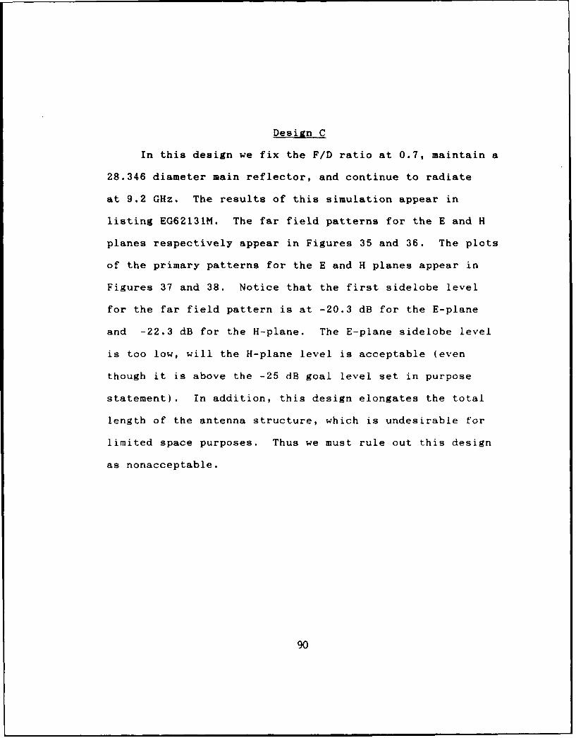
Design C
In this design we fix the F/D ratio at 0.7, maintain a
28.346 diameter main reflector, and continue to radiate
at 9.2 GHz. The results of this simulation appear in
listing EG62131M. The far field patterns for the E and H
planes respectively appear in Figures 35 and 36. The plots
of the primary patterns for the E and H planes appear in
Figures 37 and 38. Notice that the first sidelobe level
for the far field pattern is at -20.3 dB for the E-plane
and -22.3 dB for the H-plane. The E-plane sidelobe level
is too low, will the H-plane level is acceptable (even
though it is above the -25 dB goal level set in purpose
statement). In addition, this design elongates the total
length of the antenna structure, which is undesirable for
limited space purposes. Thus we must rule out this design
as nonacceptable.
90

00
ccO
go-cv ~
zz
LU,
wu,
IL t4-4
00
U)o
0
CL)
I I I I I I I I I I
91

CKU.40- -
zzz c
E- ww -
.C4 _
- c
- 0
a - - - -- 1
zt
fm Co roc0
E~w z92

CN
CLN
CK 0cz
CYC
zI
4o0
93-

z C
co
94.

Design D
This design uses a 30 inch main reflector and an F/D
ratio of 0.6, radiating at 9.2 GHz. The subreflector size
has been increased to maintain the same proportion as in
the basic Swedish design. The results for this simulation
are in listing EG62131k. The Far-Field Patterns are shown
in Figures 41 and 42 for the E-Plane and H-Plane
respectively. The primary patterns are shown in Figures 39
and 40 for the E-Plane and H-Plane respectively. The E-
Plane far field paatern for Design D has a first sidelobe
level at approximately -21 dB. The H-Plane pattern has a
first sidelobe level of -23 dB. While the H-Plane pattern
is superior to that of Design B, the E-Plane pattern is
not. We thus rule out this design.
95

0
CT7
N P.
I 0 0W CL
- cc
ot
II 0
C- cm V
7 7 1 1imz
096

CLC
N
ca
E-
0 W).c N
a 97

00
C3 0
U) OD
z z4
w - --4 U),
zz0 L
o I
E-4-
1 It 0
w ow
98 u

- IM
40
0
a a a 0 0 Wl a W n 0 V
aa
99U

Design E
In this design we use a 27 inch main reflector,
maintain an F/D ratio of 0.6, but reduce the size of the
subreflector to approximately 5 A. Since the subreflector
size is now less than 10 A we would expect edge diffraction
problems. This is indeed the case with the results
obtained by simulation. The data for this simulation is in
listing EG62131N. The E-Plane and H-Plane far field
patterns are shown in Figures 43 and 44. The primary
patterns are shown in Figures 45 and 46. Note the far-
field patterns are totally unacceptable with the first
sidelobe levels around -18 dB (only partial sidelobe forms
here). Thus, this design is also ruled out.
100

6;
CK aW ~I0
CL)
IiL 4
6- !2- 0- 0
101

N U
U. CIA
E- 0j
3i 0
0 U.1
z w (a,
00
ago
102I

Ln
N ~0 In
w (A
ww
I 0
IV N. MIn O 0 0
1031

z
z
E-C
!Z; 0
Z z
cn'
40
ama
1040

CHAPTER 5
CONCLUSIONS AND RECOMMENDATIONS
Of all the reflector antennas derived from geometric
optics, the optimized Swedish Twist-Cassegrain design seems
to be most appropriate for airborne radar applications,
especially for airborne intereptor radars. The basic
Swedish approach is desirable, however, it is not optimized
for this application. The two channel monopulse feed
creates multiple modes, which simply complicates the
design. By use of a rectangular horn feed, we can create
the TEo mode without higher order modes appearing. A
pyramidal horn structure can be used for a dual mode
operation. Corrugated (pyramidal) horns simply add higher
order modes which may need to be removed by a mode filter.
The Hughes Modified Vector Diffraction simulation
provides an accurate approximation of the scattering of
spherical waves by an arbitary truncated surface of
revolution, such as a paraboloid or a hyperboloid. This
program currently is resident on an IBM 3038 computer.
The simulation, is written in Fortran IV and is in excess
of 10.000 lines of code.105
The optimized Swedish design is derived by simulation
of the far field (and near field) patterns. Seven cases
were run (including two cases of the Swedish design) in
order to get the most desirable patterns for both the E-
plane and H-plane in the far field. Simulations were quite
extensive taking an average of two hours per run to get
results. These results were then plotted on a CAL COMP
plotter model 1055 to actually obtain antenna patterns.
Design B, which uses the 28.346 inch main reflector
and an F/D ratio of 0.5 provides the best far-field
patterns of those designs simulated, except for the
Swedish design. It has the lowest and most uniform
sidelobes of those cases simulated. Though the original
goal of -25 dB first sidelobes could not be met with any of
these designs, the -22.3 to -22.5 dB first sidelobe levels
are still respectable. Going to a wider paraboloid and
hyperboloid combination improves gain significantly,
however the far field patterns seem to degrade. The best
compromise, then, is to choose the 28.346 design to get
reasonable first sidelobes, yet still benefit from the
increased antenna gain. This will yield a higher Effective
Radiated Power than the basic Swedish Design and result in
good overall target detection performance.
106

Finally, the writer recommends more work be
accomplished in designing a coherent medium or high pulse
repetition frequency airborne radar using a Twist-
Cassegrain antenna design with low sidelobes in the
neighborhood of -30 dB. This will be the subject for my
doctoral dissertation at the University of Dayton in the
near future.
107

APPENDIX A
PROOFS OF FUNDAMENTAL PRINCIPLES AND APPROXIMATIONS
Blockage From A Subreflector
In Cassegrain antenna configurations the size and
shape of the hyperboloidal subreflector is critical to the
overall performance of the entire antenna system. It has
been found that the size of the subreflector for minimum
blockage in a simple Cassegrain arrangement (non-twist
reflector), is:
daia z ([2 A F) / k)1/2. (A.1)
Here k is the ratio of the feed-aperture diameter to its
effective blocking aperture diameter. Ordinarily k is
slightly less than 1.0 (Hannon, 1961).
Now given Figure 47, shown on the following page,
which portrays the geometry for aperture blockage, we can
prove Hannon's relationship given above. The values d,'
and dt are the diameter of the shadow cast on the
paraboloid by the feed (equal to the diameter of the
subreflector) and the aperture of the feed respectively.
If the feed is adjusted so that the nulls of the main beam
occur at the edges of the subreflector, then
2 ro = 2 A / df. (A.2)108

63
Figure 47. Geometry of Apperture Blockage
109

This is true since the beamwidth between nulls is given by
(Wolff, 1988):
On = 2 A /a, at z = 0, (A.3)
where a = length of aperture. This relationship is proved
in the next section by integrating the electric field
component E0 , and examining where the nulls of this
pattern occur.
If the structure supporting the feed has significant
dimensions, the blocking aperture diameter may be different
from the radiating feed aperture diameter. Then equation
A.2 becomes:
2 .o = 2 X / k dt. (A.4)
Also, from the geometry of Figure 47, it can be seen that:
2 *o = d, / 2F' (A.51
The portion of the paraboloid that is shadowed by the feed
is then:
ds' = 2 YF = df F / 2 F'. (A.6)
Then, for minimum blocking, the ratio of the subreflector
diameter to the feed diameter is:
do / df = F / 2 F'. (A.7)
The subreflector diameter is also given in Figure 47 as:
do = 4 4oF'. (A.8)
Then equation A.4 can be rewritten as:
-t o /k dr . (A.4')110

Equation A.7 can also be rewritten in terms of F' as:
F' = F df / 2 ds. (A.7')
Now substituting A.4' and A.7' into A.8 we get the
equation:
(d,)z = 2 \ F / k or d, = (2 \ F/ k)' 2 . (A.9)
Proof of Beamwidth Between Nulls Formula
The writer will now examine a rectangular aperture of
lengths a and b in the x- and y-directions respectively as
shown in Figure 48. Let the electric field, E, be aligned
with the y-axis and the magnetic field, H, be aligned with
the z-axis to give a plane wave traveling in the x-
direction. With uniform illumination, the E-field is
constant over the entire rectangular aperture. Using the
relation below and integrating over the entire aperture
(Silver, 1949):
Es = jEoe- J kr(sin 9 + cos 2) / 2 X r ff ejkr'cos dy'dz'.(A. 10)
Let r'cosY = ar x r' = (a, sine cosO + aysinesino + acose)x (ayy' + azz') (A.11)
orr'cos* = y'sine sino + z'cose. (A.12)
ill

lb6
Figure 48. Geometry for Rectangular Apperture
112

Therefore Equation A.10 becomes:
Eo=jEo e-Jkr (sine + coso)/2 X rf fexp[ik(y'sine9sino +
z 'cosel dy' dz' (A. 13)
Performing the integration gives:
E= jEo e-jkr(sine + cosO)/2 X r [(ejky'sin~sino/jk sine
sini)I.-% (ejkz'cose/jkcose) jbL(A. 14)
and simplifying we get:
Er=abEoeijkr(sin e +cosO)/2 Xr (sin(kasin~sino/2) /(ka/2)
(sinesino)] [sin(kbcosOl2) / (kb/2)cose] (A.15)
The field in the z = 0 plane is:
E#(r,1T/2,O) =abEoe-!Kri1+coso)/2 Xr [sinu/u], (A.16)
where u =(ka/2)sino. This function is plotted in Figure
49. The nulls in this pattern occur approximately at the
points where:
or
(lla/X) sine. = n .(A. 18)
For relatively large apertures, the first nulls occur at
9,where:
0 = X /a. (A. 19)
and the beamwidth between nulls is:
BW. 2 X~ /a, z = 0. (A. 20)
113

-5
-10
--15
-20"-4
-25
o -30
-40
2 4 6 8 10
Apperture Width, u, in radians
Figure 49. Pattern of Uniformly IlluminatedRectangular Apperture
114

APPENDIX B
SUITABLE TRAVELING WAVE TUBES
Manufacturer/ Frequency MaximumNumber Type Range Output Power
Hughes/752H Pulsed 8.4-9.4 GHz 150 KWThompson/TH3574 Pulsed 8.0-12.0 GHz 100 KWHughes/8"453H Pulsed 8.5-9.6 GHz 150 KWHughes/8716H Pulsed 9.0-9.2 GHz 120 KW
Note: Data from manufacturer's specifications.
115

APPENDIX C
SWEDISH ANTENNA DESIGN-SIMULATED PATTERNS
The far-field patterns for the basic Swedish antenna
design (27 inch diameter paraboloid, F/D = 0.6) are shown
in Figures 50 and 51 respectively for the E-plane and H-
plane at a simulation case run at 9.2 GHz. Figures 52 and
53 show the primary patterns for the E-plane and H-plane
respectively.
For a simulation case of the Swedish design run at 9.3
GHz, Figures 54 and 55 depict the far-field patterns of the
E-plane and H-plane respectively. Finally, Figures 56 and
57 depict the primary patterns of the E-plane and H-plane
repectively.
116

o IL
*(A
, &,
(* -4
o3;E-- (A
0"--- 0
u V,
Q ,,)
z 0
Z -'-4
I17
Z11

CL
ua* .. 0
01U.
C, 0 0
z
oA 0
c7
a
U ci
- 0
In Ot V)
v f
118

0 0 m
C 0
0 0
ILL
z
-4
C -wj
ac
0) 0-N r
119i

_ _
a LJ
3--~
oo
E- m
z --
7z 0
Z
0
C12-12-

L L.
aa C
,0 0
r
Iu
4 01
L1
1P __ _ -
121i

o cco
U C
C- a
u MQ)c
_ _ _ _ _ _ _ _ _2

.c.0 9L
z 4L
- !3E-4 m -z
0
I- •
.c
-- -- --_ _ _ _
C., _ _ _ _ 1-
CO 2-
I I i ii C• )

No 82
CCd
aUA 0
a cn
N.N
* I-
2 w
a
124

APPENDIX D
VECTOR DIFFRACTION PROGRAMMODIFIED JENSEN PROGRAMTHE RUSCH SCATTER EQUATIONS
THIS IS THE MAIN PROGRAM TO CALCULATE THE INTERGRALSFOR SCATTERING FROM AN ARBITRARY REFLECTOR
INPUT DATACARD 1TITLE
CARD 2FK=FREQ(GHZ)Yl=START OF OUTPUT(DEG)DY=OUTPUT INCREMENT(DEG)Xl=START OF INTEGRATION(DEG) SUBREFLECTOR EDGEX2=INTERMEDIATE DIVISION OF INTEGRATION(DEG)X3=END OF INTEGRATICN(NORMALLY 180 DEG)P1=START OF AZIMUTH CUTS (DEG) H-PLANE = 0 DEG
CARD 3DP=AZIMUTHAL ANGLE INCREMENT(DEG)E=HYPERBOLOID ECCENTRICITYE>I. USES CONVEX HYPERBOLOID SURFACE+-1. USES CONCAVE HYPERBOLOID SURFACE
A=HYPERBOLOID EQUATION CONSTANTXL=LENGTH OF PLOTS (NOT USED AT THIS TIME)7- - PARABOLOID FOCAL LENGTHFF - PARABOLOID RADIUSZChE=0 THIS IS THE FINAL CASE
=1 ANOTHER CASE FOLLOWS THIS ONE
I2RD 4f.1=1 NORMALLY COS(M*PHI) DEPENDENCE LOWER LIMITr2=1 NORMALLY COS(M*PHI) DEPENDENCE UPPER LIMITrFl=NUMBER OF INTEGRATION POINTS X2>X>XIh2=NUMBER OF INTEGRATION POINTS X3>X>X2
Ni AND N2 SHOULD BOTH BE EVEN NUMBERSNY-NUMBER OF INCREMENTS DY IN POLAR ANGLE OUTPUT
NY MUST NOT EXCEED 180NP-NUMBER OF INCREMENTS FOR AZIMUTH CUTS OUTPUTIFN-NUMBER OF INPUT POINTS TO DEFINE SUBREFLECTOR
-0 PROGRAM CALCULATES SUBREFLECTOR--1 USE VALUES OF PREVIOUS CASE
125

IAR=NUMBER OF POINTS TO DEFINE INCIDENT FIELDS=0 USE PREVIOUS CASE
ISPOT=PRINTOUT OPTION FOR INTERMEDIATE ANSWERS=0 NORMALLY
NPAR = 0 SUBREFLECTOR SCATTERING ONLY= 1 SUBREFLECTOR AND PARABOLOID SCATTERED FIELDS
CARD 5Y1P=START OF PARABOLOID OUTPUT (DEG)DYP=PARABOLOID OUTPUT INCREMENT (DEG)PNY=NO. OF DYP INCREMENTS IN PARABOLOID POLAR ANGLE
OUTPUT (MUST NOT EXCEED 180)P1P=START OF PARABOLOID AZIMUTH CUTS (DEG) H-PLANE=O DEGDPP=PARABOLOID AZIMUTHAL ANGLE INCREMENT (DEG)PNP=NO. OF OPP INCREMENTS IN PARABOLOID AZIMUTH CUTS OUTPUTPN1=NO. OF PARABOLOID INTEGRATION POINTS X2>X>X1 (EVEN)
CARD 6PN2=NO. OF PARABOLOID INTEGRATION POINTS X3>X>X2 (EVEN)X3P=180. MINUS ANGLE OF EQUIVALENT BLOCKAGE (DEG)
=0 USES CALCULATED SUBREFLECTOR BLOCKAGE ANGLEFPT=FEED PATTERN TAPER AT EDGE OF SUBREFLECTOR
(INPUT FPT AS MINUS DB)
126

CARD GROUP 1DEFINES SUBREFLECTOR SURFACE, F(X), IFN VALUESIF IFN=O OMITCARD GROUP 2SUBREFLECTOR SLOPE, G(X), IFN VALUESOMIT FOR IFN=OCARD GROUP 3POLAR ANGLE FOR WHICH F(X) AND G(X) ARE DEFINED, IFN VALUESOMIT FOR IFt =0CARD GROUP 4 E-PLANE PATTERNREAL PART OF E-THETA AT PHI=90 DEGIMAG PART OF E-THETA AT PHI=90 DEG
CARD GROUP 5 CROSS POLARIZATION IN H-PLANEREAL PART OF E-THETA AT PHI=0IMAG PART OF E-THETA AT PHI=O
CARD GROUP 6 E-PLANE CROSS POLARIZATICNREAL PART OF E-PHI AT PHI=90 DEGIMAG PART CF E-PHI AT PHI=gO DEG
CARD GROUP 7 [-PLANE PATTERNREAL PART OF E-PHI AT PHI=O DEGIMAG PART OF E-PHI AT PHI=O DEG
IAR VALUES FOR EACH COMPONENT OF FIELD
CARC GROUP 8POLAR ANGLE IN RADIANS AT WHICH INCIDENT FIELDS ARE INPUT,IAR VALUES
127

REFERENCES
Bakhrakh L.D. and Galimov, G.K. 1981. Reflector ScanningAntennas: Theory and Design Methods, (Moscow:"Nauka"Publisher).
Bargeliotes, P. C. 1975. Hughes InterdepartmentalCorrespondence, August 20, 1975, No. 2265.30/563.
Bodnar, D. G. 1984. "Radar Antennas", Principles of ModernRadar Short Course, Georgia Institute of Technology,November, 1984.
Carter, D. 1955. "Wide-Angle Radiation in Pencil BeamAntennas" J. Applied Physics, No. 6, June 1955, pp.645-652.
Cutler, C. C. 1947. "Parabolic-Antenna Design forMicrowaves," Proc. IRE, Vol 35, November, 1947,p. 1286.
Dahlin, R. K. 1982. Technical Review of Design of OptimumTwo-Mirror Antennas with the Oscillation of theRadiation Patterns, Arkady Assoc., Garden Grove, CA
Dahlsjo, 0. 1973. "A Low Side Lobe Cassegrain Antenna", IEEInternational Conference on Radar-Present and Future,23-25 October 1973.
Dahlsjo, 0., Lungstrom, B., Magnusson, H. 1986. "Plasticand Composite Materials for Antennas-An EvolutionTowards More Demanding Applications", Proceedings ofthe Military Microwaves '86 Conference, Brighton,England, June 24-26, 1986, pp. 237-242.
Dijk, J., Jeuken, M., and Maanders, E. J. 1968. "Blockingand Diffraction in Cassegrain Antenna Systems", DeIngenieur, July 5, 1968, pp. 79-91.
Galimov, G. K. 1969. Design of Optimum Two-Mirror Antennaswith the Oscillation of the Radiation Patterns,Moscow.
Hannon, Peter, W. 1955. "Design for a Twistreflector HavingWideangle Performance," Wheeler Laboratory Report No.666. 128

Hannon,'Peter, W. 1961. "Microwave Antennas Derived fromthe Cassegrain Telescope," IRE Trans. on Antennas andPropagation, March 1961, pp. 140-153.
Hannon, Peter, W. 1961. "Optimum Feeds for All Three Modesof a Monopulse Antenna," IEEE Trans. on Antennas andPropagation, September 1961, pp. 444-461.
Hansen, R. C. 1959. "Low-Noise Antennas", MicrowaveJournal, June, 1959, pp. 19-24.
Ingalls, A. G., 1953. "Amateur Telescope Making",Scientific American, Vol. 1, pp. 62-65, 215-218, 444-453.
Jasik, Henry, 1961. Antenna Engineering Handbook, FirstEdition, (New York: McGraw Hill).
Jensen, P. A. 1962. "Designing Cassegrain Antennas",Microwaves, December, 1962, pp. 12-19.
Jensen, P. A. 1984. "Cassegrain Systems", Section 3.2 inThe Handbook of Antenna Design, Vol. 1, (London:Peter Peregrinus Ltd.), pp. 162-184.
Johnson, R. C. and Jasik, H. 1984. Antenna EngineeringHandbook, (New York: McGraw-Hill Book Company).
Johnson, R. C. and Jasik, H. 1987. Antenna ApplicationsReference Guide, (New York: McGraw-Hill BookCompany).
Josefsson, L. G. 1973. "A Broad-Band Twist Reflector", IEEETrans. Ant. and Prop., July 1973, pp. 552-554.
Josefsson, L. G. 1978. "Wire Polarizers for MicrowaveAntennas", Technical Report No. 81, Thesis of ChalmersUniv. of Technology, Goteborg, Sweden, March, 1978.
Josefsson, L. G. 1978. "Wire Polarizers for MicrowaveAntennas", Ericsson Technics, No. 4, 1978.
Josefsson, L. G. 1986. "Cassegrain Antennas with Broadbandand Multiband Performance", Proc. IEEE Radar-86Conference, Los Angeles, CA, pp. 115-119.
Kraus, John, D. 1988. Antennas, Second Edition, (New York:
McGraw Hill).
129

Leonov, A. I. and Fomichev, K. I. 1986. Monopulse Radar,(Norwood, MA: Artech House).
Lewis, B. L. and Shelton, J. P. 1980. "Mirror Scan AntennaTechnology", Rec. IEEE International Radar Conference,April, 1980, pp. 279-283.
Liao, Samuel, Y. 1985. Microwave Devices and Circuits(Englewood Cliffs, NJ: Prentice-Hall).
MacFarlane, G. G. 1946. "Surface Impedance of an InfiniteParallel Wire Grid at Oblique Angles of Incidence", J.Inst. Elect. Engrs., pt. 3A, Vol 93, pp. 1523-1527.
Mohony, J. D. 1981. "The Determination of the FieldsReflected From a Twist Reflector FollowingIllumination by a Plane Wave", Proceedings of the 2ndInternational Conference on Antennas and Propagation,York, England, April 13-16 1981, pp. 42-45.
Orleansky, E., Samson, C., and Havkin, M. 1987. "ABroadband Meanderline Twistreflector for the InverseCassegrain Antenna", Microwave Journal, Vol. 30, No.10, pp. 185-190.
Rusch, W.V.T. and Potter, P.D 1970. Analysis of ReflectorAntennas, (New York: Academic Press).
Rusch, W.V.T., 1963. "Scattering From a HyperbololoidalReflector in a Cassegrainian Feed System", IEEE Trans.on Antennas and Propagation, July, 1963, pp. 414-421.
Rusch, W.V.T., 1963. "Scattering of a Spherical Wave by anArbitrary Truncated Surface of Revolution", JPLTechnical Report No. 32-434, May 27, 1963.
Rusch, W.V.T, Jensen, P.A., et al. Hughes VectorDiffraction Program.
Scorer, M., Graham, R., and Barnard, I. 1978. "The Analysisof an Elliptic Twist Reflecting Cassegrain AntennaUsing GTD", Proceedings of the InternationalConference on Antennas and Propagation, London,November 28-30, 1978, pp. 208-212.
Seaton, Arthur, F. 1988. Unpublished technical report atHughes Aircraft Company, "Cassegrain Design".
130

Seaton, Arthur, F. 1988. Unpublished technical data atHughes Aircraft Company, "Cassegrain Reflector LossBudgets".
Silver, Samuel. 1949. Microwave Antenna Theory and Design,MIT Radiation Lab Series, Vol 12, (New York: McGrawHill Book Co., 1949), pp. 447-448.
Skolnik, Merrill. 1980. Introduction to Radar Systems, (NewYork: McGraw Hill Book Co.).
Skolnik, Merrill. 1970. Radar Handbook, (New York: McGrawHill Book Co.)
Spooner, P. W. and Sage, D. S. 1985. "The FoxhunterAirborne Interceptor Radar", The GEC Journal ofResearch, Vol. 3, No. 2, pp. 114-123.
Stimson, George, W. 1983. Introduction to Airborne Radar,(El Segundo, CA: Hughes Aircraft Co.).
Stutzman, Warren L. and Thiele, Gary, A. 1981. AntennaTheory and Design, (New York: John Wiley & Sons).
Tzannes, Nicolaos S. 1985. Communication and Radar Systems,(Englewood Cliffs, NJ: Prentice Hall).
Williams, F. C. and Radant, M. E. 1983. "Airborne Radar andthe Three PRFs", Microwave Journal, July, 1983, pp.129-135.
Williams, Frederick, 1984. Modern Air to Air Radar Systems,George Washington University Short Class 1034.
Wolff Edward A. 1988. Antenna Analysis (Norwood, MA:Artech House).
Young, Leo, Robinson, Lloyd, A. and Hacking, Colin, A.1973. "Meander-Line Polarizer", IEEE Trans. onAntennas and Propagation, May, 1973, pp.376-378.
131
Related Documents