General rights Copyright and moral rights for the publications made accessible in the public portal are retained by the authors and/or other copyright owners and it is a condition of accessing publications that users recognise and abide by the legal requirements associated with these rights. Users may download and print one copy of any publication from the public portal for the purpose of private study or research. You may not further distribute the material or use it for any profit-making activity or commercial gain You may freely distribute the URL identifying the publication in the public portal If you believe that this document breaches copyright please contact us providing details, and we will remove access to the work immediately and investigate your claim. Downloaded from orbit.dtu.dk on: Feb 21, 2022 Actuator Disc Methods Applied to Wind Turbines Mikkelsen, Robert Flemming Publication date: 2004 Document Version Publisher's PDF, also known as Version of record Link back to DTU Orbit Citation (APA): Mikkelsen, R. F. (2004). Actuator Disc Methods Applied to Wind Turbines. Technical University of Denmark. MEK-FM-PHD No. 2003-02

Welcome message from author
This document is posted to help you gain knowledge. Please leave a comment to let me know what you think about it! Share it to your friends and learn new things together.
Transcript

General rights Copyright and moral rights for the publications made accessible in the public portal are retained by the authors and/or other copyright owners and it is a condition of accessing publications that users recognise and abide by the legal requirements associated with these rights.
Users may download and print one copy of any publication from the public portal for the purpose of private study or research.
You may not further distribute the material or use it for any profit-making activity or commercial gain
You may freely distribute the URL identifying the publication in the public portal If you believe that this document breaches copyright please contact us providing details, and we will remove access to the work immediately and investigate your claim.
Downloaded from orbit.dtu.dk on: Feb 21, 2022
Actuator Disc Methods Applied to Wind Turbines
Mikkelsen, Robert Flemming
Publication date:2004
Document VersionPublisher's PDF, also known as Version of record
Link back to DTU Orbit
Citation (APA):Mikkelsen, R. F. (2004). Actuator Disc Methods Applied to Wind Turbines. Technical University of Denmark.MEK-FM-PHD No. 2003-02

MEK-FM-PHD 2003-02
Actuator Disc Methods Appliedto
Wind Turbines
by
Robert Mikkelsen
Dissertation submitted to the Technical University of Denmark in partial fulfillment ofthe requirements for the degree of Doctor of Philosophy in Mechanical Engineering
Fluid MechanicsDepartment of Mechanical Engineering
Technical University of DenmarkJune, 2003

Fluid MechanicsDepartment of Mechanical EngineeringNils Koppels Allé, Building 403Technical University of DenmarkDK-2800 Lyngby, Denmark
Copyright c© Robert Mikkelsen, 2003
Printed in Denmark by DTU-Tryk, Lyngby
MEK-FM-PHD 2003-02 / ISBN 87-7475-296-0
This thesis has been typeset using LATEX2e. Illustrations was drawn with XFIG, graphs werecreated with XMGR and MATLAB and field plots were produced using TecPlot and PostView.

Preface
This thesis is submitted in partial fulfillment of the requirements for the Ph.D. degree fromthe Technical University of Denmark (DTU). The research work was conducted during theperiod from August 1998 to April 2003 at the Department of Mechanical Engineering (MEK),Fluid Mechanics Section. I wish to express my sincere thanks to my supervisor Professor JensNørkær Sørensen for his ever encouraging support and for his advise and patience during ourmany discussions. I would also like to thank him for letting me pursue research on strange newideas on alternative energy conversions concepts and for the fun hours during our weekly gameof football.
I’d like to extend my warm thanks to Associated Professors Wen Zong Shen and Jess A.Michelsen (the Long Man) for many useful conversations and also to Associated Professor StigØye for valuable suggestions.
I also wish to thank my colleagues and fellow student at the section for providing a friendlyenvironment with room for good humor and interesting discussion. Special thanks to MacGaunaa for the collaboration we had on wavelets, MPI, structural dynamics and fun toys.
Finally, I would thank my family and friends for their support and interest and to Laura for herlove and support.
Lyngby, June 3, 2003
Robert Mikkelsen
i

Abstract
This thesis concerns the axisymmetric actuator disc model and its extension to a three di-mensional actuator line technique which, combined with the incompressible Navier-Stokesequations, are applied to describe the aerodynamics of wind turbine rotors. The developedmethods are used to investigate the aerodynamic behaviour of coned rotors, rotors exposedto yawed inflow and tunnel blockage. Miscellaneous investigations are conducted in orderto analyze the consistence of some basic assumptions of the Blade Element Momentum(BEM) method, such as the influence of pressure on expanding streamtubes and the accuracyof tip correction theories. In the latter case an inverse formulation of the equations were applied.
Results for the coned rotor demonstrates that the Navier-Stokes methods, both the actuator discand actuator line, captures the changed aerodynamic flow behaviour whereas a modified BEMmethod is incapable of handling flow through coned rotors. For rotors exposed to yawed inflow,the actuator disc method combined with appropriate sub models predicts structural loads withgood accuracy. At high yaw angles the actuator line method capture observed effects from theroot vortex, which axisymmetric methods is incapable of. Computations on rotors inserted intoa tunnel show that the Navier-Stokes methods fully resolve the effects of tunnel blockage. Anew solution to the inviscid axial momentum analysis on tunnel blockage by Glauert, is alsopresented. The new solution compares excellent with results presented for the equivalent freeair speed obtained with the Navier-Stokes methods.
An analysis of pressure forces acting on expanding the streamtubes revealed that the influenceof pressure forces is negligible for the velocities at the rotor disc. A new approach to solve theheavily loaded actuator disc is presented, using a new numerical technique based on solving theequations original formulated by Wu. The formulations is fast to run on computer, however,less accurate than Navier-Stokes computations. A new method for inverse determination of thetip-correction factor is believed to be correct, however, the obtained results reveal uncertaintieswhich needs further investigations.
ii

Dansk resumé
Den foreliggende afhandling omhandler den akse symmetriske aktuator disk og den fuldttre-diminsionelle aktuator linie teknik kombineret med de inkompressible Navier-Stokesligninger. De udviklede modeller er anvendt til at undersøge den aerodynamiske opførselaf rotorer udsat for koning, skæv anstrømning (yaw) og rotorer indsat i en vindtunnel. Derer foretaget særlige undersøgelser for kunne analysere validiteten af visse fundamentaleantagelser for Blade Element Momentum (BEM) metoden, så som indflydelsen af trykkræfterpå de ekspanderende strømrør og nøjactiheden af tip korrections teorier. I det sidste tilfælde erder anvendt en invers metode.
Resultater for den konede rotor viser, at Navier-Stokes metoderne, både aktuator disk og aktua-tor linie, kan håndtere det ændrede aerodynamiske flow, mens en modificeret BEM model ikkeer istand til at håndtere flow gennem konede rotorer. For rotorer udsat for skæv anstrøning eraktuator disk modellen, kombineret med passende delmodeller, istand til at beregne structurellelaster med god nøjagtighed. For skæv anstrømning ved store vinkler (high yaw) fanger aktuatorlinie modellen målte effekter der hidrører fra rodhvirvlen, som akse-symmetriske modellerikke kan vise. Beregninger på rotorer indsat i vindtunnel viser, at Navier-Stokes metodernekan modellere blokerings effekter. En ny løsning til den inviskose aksiale momentum teorifor tunnel blokering af Glauert, præsenteres også. Den nye løsning passer ekstremt godt medNavier-Stokes simuleringer for den equivalente hastighed i en fri strømning.
En analyse af trykkrafterne på de ekspanderede strømflader viser, at indflydelsen af tryk kræfterkan negligeres med hensyn til hastighederne gennem rotoren. En ny metode til undersøgelsetil løsning af den hårdt belastede rotor er præsenteres, hvor den numeriske teknik er baseret påløsning af ligninger oprindeligt formuleret af Wu. Metoden er hurtig, men mindre nøjagtig sam-melignet med Navier-Stokes modellen. En ny metode til invers bestemmelse af tip-korrektionsfaktoren menes at være korrekt, men de beregnede resultater afslører usikkerheder, der krævervidere undersøgelser.
iii

List of Publications
Published in refereed journalsMikkelsen R, Sørensen JN, Shen WZ. Modelling and analysis of the flow field around conedrotors. Wind Energy, 2001; 4: 121–135.
Published in proceedingsMikkelsen R, Sørensen JN. Yaw Analysis Using a Numerical Actuator Disc Model. Proc. 14thIEA Symp. on the Aerodynamics of Wind Turbines, Boulder, Col, USA, 2000; 53–59
Mikkelsen R, Sørensen JN, Shen WZ. Yaw Analysis Using a 3D Actuator Line Model.European Wind Energy Conf., Copenhagen, Danmark, 2001; 478–480
Mikkelsen R, Sørensen JN. Modelling of Wind Tunnel Blockage. Global Windpower Conf.,Paris, France, 2002; –
Shen WZ, Mikkelsen R, Sørensen JN, Bak C. Evaluation of the Prandtl Tip Correction forWind Turbine Computations. Global Windpower Conf., Paris, France, 2002; –
Sørensen JN, Mikkelsen R. On the Validity of the Blade Element Momentum Method. Euro-pean Wind Energy Conf., Copenhagen, Danmark, 2001; 362–366
iv

Contents
Preface i
Abstract ii
Dansk resumé iii
List of Publications iv
Contents v
List of Symbols viii
1 Introduction 1
A Actuator Disc Modelling 5
2 Basic Rotor Aerodynamics 62.1 The Actuator Disc Principle . . . . . . . . . . . . . . . . . . . . . . . . . . . 6
2.1.1 Annular Streamtubes - The Blade Element Momentum method . . . . . 72.1.2 Aerodynamic Blade Forces . . . . . . . . . . . . . . . . . . . . . . . . 8
3 The Generalized Actuator Disc Model 103.1 The Ψ− ω Formulation of the Navier-Stokes Equations . . . . . . . . . . . . . 10
3.1.1 Numerical Implementation . . . . . . . . . . . . . . . . . . . . . . . . 123.2 The Constant Loaded Rotor Disc . . . . . . . . . . . . . . . . . . . . . . . . . 13
3.2.1 Numerical Results . . . . . . . . . . . . . . . . . . . . . . . . . . . . 133.2.2 Grid Sensitivity . . . . . . . . . . . . . . . . . . . . . . . . . . . . . . 15
3.3 Simulation on Real Rotors - Tip Correction . . . . . . . . . . . . . . . . . . . 163.3.1 Computation using LM 19.1m Blade Data . . . . . . . . . . . . . . . . 16
B Application of the Generalized Actuator Disc Model 19
4 The Coned Rotor 204.1 Coned Rotors . . . . . . . . . . . . . . . . . . . . . . . . . . . . . . . . . . . 20
4.1.1 Geometry and Kinematics - Velocity Triangle . . . . . . . . . . . . . . 204.1.2 Blade Forces . . . . . . . . . . . . . . . . . . . . . . . . . . . . . . . 21
v

vi Contents
4.2 Aerodynamic Modelling - Momentum Balance . . . . . . . . . . . . . . . . . 224.2.1 A Modified BEM Method . . . . . . . . . . . . . . . . . . . . . . . . 224.2.2 The Actuator Disc Model - Applying Forces . . . . . . . . . . . . . . 24
4.3 Numerical Results for the Coned Rotor . . . . . . . . . . . . . . . . . . . . . . 254.3.1 The Constant Loaded Rotor . . . . . . . . . . . . . . . . . . . . . . . 264.3.2 Simulation of the Tjæreborg Wind Turbine . . . . . . . . . . . . . . . 284.3.3 Comparison with the BEM Method for the Tjæreborg Wind Turbine . . 30
4.4 Summary . . . . . . . . . . . . . . . . . . . . . . . . . . . . . . . . . . . . . 31
5 The Yawed Rotor 335.1 Yaw Modelling . . . . . . . . . . . . . . . . . . . . . . . . . . . . . . . . . . 33
5.1.1 3D Geometry and Kinematics . . . . . . . . . . . . . . . . . . . . . . 335.1.2 Projection of Velocities . . . . . . . . . . . . . . . . . . . . . . . . . . 345.1.3 Blade Forces . . . . . . . . . . . . . . . . . . . . . . . . . . . . . . . 355.1.4 Sub Models . . . . . . . . . . . . . . . . . . . . . . . . . . . . . . . . 35
5.2 Numerical Results for the Yawed Rotor . . . . . . . . . . . . . . . . . . . . . 365.3 Summary . . . . . . . . . . . . . . . . . . . . . . . . . . . . . . . . . . . . . 38
6 Modelling of Tunnel Blockage 396.1 Axial Momentum Theory . . . . . . . . . . . . . . . . . . . . . . . . . . . . 39
6.1.1 Actuator Disc Method . . . . . . . . . . . . . . . . . . . . . . . . . . 416.2 Navier-Stokes Computations . . . . . . . . . . . . . . . . . . . . . . . . . . . 41
6.2.1 The Constant Loaded Rotor . . . . . . . . . . . . . . . . . . . . . . . 426.2.2 Simulation of the LM 19.1m Blade . . . . . . . . . . . . . . . . . . . 43
6.3 Summary . . . . . . . . . . . . . . . . . . . . . . . . . . . . . . . . . . . . . 44
C Actuator Line Modelling 45
7 The Actuator Line Model 467.1 The Flow Solver - EllipSys3D . . . . . . . . . . . . . . . . . . . . . . . . . . 467.2 Numerical Formulation . . . . . . . . . . . . . . . . . . . . . . . . . . . . . . 47
7.2.1 Blade Forces and Tip Correction . . . . . . . . . . . . . . . . . . . . . 477.3 Determinations of Velocities . . . . . . . . . . . . . . . . . . . . . . . . . . . 477.4 Distribution of Forces . . . . . . . . . . . . . . . . . . . . . . . . . . . . . . . 49
8 3D Simulations - Numerical Results 528.1 Steady Computations . . . . . . . . . . . . . . . . . . . . . . . . . . . . . . . 52
8.1.1 2D-3D Regularization and Tip Correction . . . . . . . . . . . . . . . . 538.1.2 Simulation of the Tjæreborg . . . . . . . . . . . . . . . . . . . . . . . 54
8.2 The Coned Rotor . . . . . . . . . . . . . . . . . . . . . . . . . . . . . . . . . 558.3 The Yawed Rotor . . . . . . . . . . . . . . . . . . . . . . . . . . . . . . . . . 56
8.3.1 Discussion . . . . . . . . . . . . . . . . . . . . . . . . . . . . . . . . 598.4 Tunnel Blockage . . . . . . . . . . . . . . . . . . . . . . . . . . . . . . . . . 59

Contents vii
D Miscellaneous Investigations 61
9 The Heavily Loaded Actuator Disc 629.1 A Distributed Wake Method . . . . . . . . . . . . . . . . . . . . . . . . . . . 62
9.1.1 Numerical Method . . . . . . . . . . . . . . . . . . . . . . . . . . . . 629.1.2 The Axially Loaded Rotor - Constant Loading . . . . . . . . . . . . . 64
9.2 Numerical Results - The Axially Loaded Rotor . . . . . . . . . . . . . . . . . 659.3 Distributed Wake Method - Numerical Results . . . . . . . . . . . . . . . . . . 66
10 The Influence of Pressure Forces 7010.1 Expanding Stream Tubes . . . . . . . . . . . . . . . . . . . . . . . . . . . . . 70
11 Evaluation of Tip Correction 7511.1 Modified Use of the Prandtl Tip Correction . . . . . . . . . . . . . . . . . . . 7511.2 Inverse Computation of the Tip Correction Using the Actuator Line Model . . . 7611.3 Numerical sensitivity - The 2 Bladed Rotor . . . . . . . . . . . . . . . . . . . 7911.4 Tip correction - The 2 Bladed Rotor . . . . . . . . . . . . . . . . . . . . . . . 83
11.4.1 Uncertainty About Accuracy . . . . . . . . . . . . . . . . . . . . . . . 8411.5 A Lifting Line Model for a Finite Wing with an Elliptic loading . . . . . . . . 86
Conclusions and Future Work 87
A Derivation of the Governing Equations for the Actuator Disc 89A.1 The Vorticity Transport Equation in Rotational Form . . . . . . . . . . . . . . 89A.2 The Conservative Vorticity Transport Equation . . . . . . . . . . . . . . . . . 90A.3 The Conservative Azimuthal Velocity Transport Equation . . . . . . . . . . . . 91A.4 The Poisson Equation . . . . . . . . . . . . . . . . . . . . . . . . . . . . . . . 92A.5 The Pressure Equation . . . . . . . . . . . . . . . . . . . . . . . . . . . . . . 93A.6 The Heavily Loaded Actuator Disc . . . . . . . . . . . . . . . . . . . . . . . . 94
B Sub Models 96B.1 Elastic Model - A Modal Method . . . . . . . . . . . . . . . . . . . . . . . . . 96
B.1.1 Structural Blade Damping . . . . . . . . . . . . . . . . . . . . . . . . 97B.1.2 Integration of Structural Loads . . . . . . . . . . . . . . . . . . . . . . 97
B.2 Tower . . . . . . . . . . . . . . . . . . . . . . . . . . . . . . . . . . . . . . . 100B.3 Dynamic Stall . . . . . . . . . . . . . . . . . . . . . . . . . . . . . . . . . . . 101B.4 Wind Shear . . . . . . . . . . . . . . . . . . . . . . . . . . . . . . . . . . . . 102B.5 Runge-Kutta-Nystrøm Method . . . . . . . . . . . . . . . . . . . . . . . . . . 103
C Thrust and Power Coefficients for the Coned Rotor 104
Bibliography 105

List of Symbols
Roman lettersa, a′ Interference factors [−]A,A Area / Coordinate matrix [m2,−]B Number of blades [−]c Chord length [m]C Tunnel area [m2]CT Thrust coefficient [−]CP Power coefficient [−]D,D Drag force / damping matrix
[
Nm,−]
e Unit vector [−]EI Cross sectional blade stiff-
ness[Nm2]
f Areal loading[
Nm2
]
F Loading / Prandtl tip lossfactor
[
Nm,−]
H Pressure head/height(tower)[
Nm2 , m
]
I, J Indices [−]Kθ,z Relaxation parameter [−]K Stiffness matrix [−]L Lift force, differential oper-
ator
[
Nm,−]
m Cross sectional blade mass[
kgm
]
m Mass Flow[
kgs
]
M,M Bending moment / mass ma-trix
[Nm,−]
Nb Block size: p2n [−]p, d Distance [m]p Pressure / structural loading
[
Nm2 , N
]
P Power [W ]
q Source[
m2
s
]
Q Torque [Nm]r, θ, z Polar coordinates [m, rad,m]R Rotor radius [m]s, t, n Spanwise, tangential, nor-
mal coordinates relative toblade
[m, rad,m]
S Disc area [m2]T Thrust, shear force [N ]Tu.I Turbulent intensity [%]u, V Velocity
[
ms
]
v, v, v Blade deflection, velocityand acceleration
[
m, ms, m
s2
]
W Induced velocity[
ms
]
x, y, z Cartesian coordinates [m]X Stream surface pressure for-
ce[N ]
Greek lettersα, αs Area aspect ratio/wind shear
exponent[−]
β,B Cone angle/matrix [o]γ Pitch angle [o]
Γ Circulation[
m2
s
]
δ Log decrement, structuraldamping
[−]
ε Machine accuracy ' 10−15 [−]
ε Regularization parameter /error quantity
[−]
η Regularization function [−]θ,Θ Azimuthal angle/matrix [o]λ, λo Local and global tip-speed
ratio: ΩrVo, ΩR
Vo
[−]
ν Kinematic viscosity[
m2
s
]
viii

List of Symbols ix
ξ Structural pitch [o]ζ Interpolation ratio [o]
ρ Mass density[
kgm3
]
σ Solidity/Area aspect ratio [−]τ Dynamic time delay [−]φ Flowangle [o]φy,Φy Yaw angle / matrix [o]
φt,Φt Tilt angle / matrix [o]ψ Normal modes [−]
Ψ Stream function[
m3
s
]
ω Vorticity / structural bladeeigenfrequencies
[s−1]
Ω Angular rotor velocity[
rads
]
Indiceso,1 Free stream / far wake′ per volumea Aerodynamicc Cell center / centrifugal /
convectived,
d Disc / damping / diffusivef Deflexiong GravityH Headl LinearB i’th blade / actuator linep Point on actuator lines Stream surfacet,
t Towerw,
w Wake
Ψ Stream line / stream functionlevel
acc Accelerationhub Hubijkn Indiceskin Kineticrθz Polar componentsrel Relativerot Rotational / rotorstn Spanwise, tangential, nor-
mal componentstun Tunnelxyz Cartesian components
Special numbersCFL Courant - Friedrichs - Lewy
number, at center axis :Vθ∆tr∆θ
[−] Re Reynolds number, Rotor:VoR
ν, Aerofoil: Voc
ν
[−]
Acronyms2D,3D Two or Three-DimensionalAD Actuator DiscAL Actuator LineBEM Blade Element Momentum
methodCFD Computational Fluid Dy-
namicsFVM Finite Volume Method
MPI Message Passing Interfacefor parallel computations
N-S Navier-Stokes equationsΨ− ω Stream function - swirl ve-
locity - vorticity formula-tions of N-S equations

Chapter 1
Introduction
This thesis deals with numerical methods that combine the actuator disc and actuator line con-cept with the Navier-Stokes equations applied to wind turbine rotors.
The Development of Rotor Predictive Methods
Rotor predictive methods based on the actuator disc concept use the principle of representingrotors by equivalent forces distributed on a permeable disc of zero thickness in a flow domain.The concept was introduced by Froude [18] as a continuation of the work of Rankine [44] onmomentum theory of propellers. Fundamental results were presented for the velocity at thedisc position which equals one half of the sum of the upstream and far wake air speed. Theanalysis by Lanchester [31](1915) and Betz [3](1920) showed that the maximum extractionof energy possible from a turbine rotor is 16/27 or 59.3%, of the incoming kinetic energy. Amajor step forward in the modelling of flow through rotors came with the development of thegeneralized momentum theory and the introduction of the Blade Element Momentum BEMmethod by Glauert [19](1930). As the method is based on momentum balance equations forindividual annular streamtubes passing through the rotor, it effectively enhance the informationabout spanwise distributions.
Although the BEM method is the only method used routinely by industry, a large variety ofadvanced rotor predictive methods have been developed. Generally, the methods can be cate-gorized into inviscid models that demand the use of tabulated airfoil data, and viscous modelsbased on either viscous-inviscid procedures or Navier-Stokes algorithms. The most widespreadinviscid technique is the vortex wake method. In this method the shed vorticity in the wakeis employed to compute the induced velocity field. The vorticity may either be distributed asvortex line elements (Miller [41], Simoes and Graham [50], Bareiss et al. [1]) or as discretevortices (Voutsinas et al. [68]) with vortex distributions determined either as a prescribed wakeor a free wake. A free wake analysis may in principle provide one with all relevant informationneeded to understand the physics of the wake. However, this method can be very computingcostly and tends to diverge owing to intrinsic singularities of the vortex panels in the developingwake. Another inviscid method is the asymptotic acceleration potential method that was de-veloped primarily for analyzing helicopter rotors by van Holten [66] and later adapted to copewith flows about wind turbines by van Bussel [65]. The method is based on solving a Poisson
1

2 Introduction
equation for the pressure, assuming small perturbations of the mean flow. Compared to vortexwake models, the method is fast to run on a computer, but difficult to apply to general flow cases.
The generalized actuator disc method represent a straight-forward inviscid extension of theBEM technique. The main difference is that the annular independence of the BEM modelis replaced by the solution of a full set of Euler or Navier-Stokes equations. Axisymmetricversions of the method have been developed and solved either by analytical / semi-analyticalmethods (Wu [71], Hough and Ordway [28], Greenberg, [22] and Conway [8], [9]) or by finitedifference / finite volume methods (Sørensen and colleagues [55], [56], [58] and Madsen [32]).In helicopter aerodynamics a similar approach has been applied by e.g. Fejtek and Roberts[17] who solved the flow about a helicopter employing a chimera grid technique in whichthe rotor was modelled as an actuator disc, and Rajagopalan and Mathur [45] who modelleda helicopter rotor using time-averaged momentum source terms in the momentum equations.Whereas the finite difference / finite volume and Finite Element Method (FEM) methods, asformulated by Masson et al. [34] who solve the unsteady 3D flowfield around HAWT usingFEM, facilitates natural unsteady wake development, the analytical / semi-analytical methodsare generally solved for steady conditions. The actuator line concept introduced recently bySørensen and Shen [61](2002) extends beyond the assumption of axial symmetry, where theloading is distributed along lines representing blade forces in a fully 3D flow domain. Such anapproach facilitates analysis of the validity of the assumptions used in simpler methods and ingeneral the 3D behaviour of the wake, which is part of the present investigation.
To avoid the problem of using corrected or calibrated airfoil data various viscous models havebeen developed to compute the full flow field about wind turbine rotors. Sørensen [54] used aquasi-simultaneous interaction technique to study the influence of rotation on the stall character-istics of a wind turbine rotor. Sankar and co-workers [2] developed a hybrid Navier-Stokes / full-potential / free wake method for predicting three-dimensional unsteady viscous flows over iso-lated helicopter rotors in hover and forward flight. The method has recently been extended tocope with horizontal axis wind turbines [72]. Another hybrid method is due to Hansen et al.[24] who combined a three-dimensional Navier-Stokes solver with an axisymmetric actuatordisc model. Full three-dimensional computations employing the Reynolds-Averaged Navier-Stokes (RANS) equations have been carried out by e.g. Ekaterinaris [16], Duque et al. [15] andSørensen and Michelsen [63]. Although the RANS methods are capable of capturing the pre-stall behaviour, because of inaccurate turbulence modelling and grid resolution, RANS methodsstill fail to capture correctly the stall behaviour.
Accuracy of Present Days Rotor Predictive MethodsActuator disc methods have through the years proven their capability to match different types ofrotor predictive methods. Rotor predictive methods are, however, no better than the foundationsof the assumptions inherent or the input data supplied to them. This became clear with theNREL1 blind code comparison, that was carried out December 2000. About 15 participants
1During the December 1999 through May 2000 the National Renewable Energy Laboratory, NREL, conductedthorough unsteady aerodynamic experiments on a 2 bladed (D=10m) Horizontal Axis Wind Turbine, HAWT, inthe NASA Ames 24.4x36.6m wind tunnel.
Introduction 3
from all over the world joined the comparison using various models ranging form simple BladeElement Momentum methods to full 3D Navier-Stokes formulations. Model predictions werecompared at zero yaw and yawed operating conditions. Figure 1.1 depicts the participantsprediction of the low speed shaft torque at zero yaw, where the line marked with diamondsrepresent measurements. The general results showed unexpected large margins of disagreement
NREL←
Risø-NNSDTU-RM
Figure 1.1: NREL experiments - blind code comparison. Predictions of low speed shaft torque,NREL: Black line with diamonds, DTU-RM: Pink, Risø-NNS: Violet
between predicted and measured data (Schreck [48]) and in addition no consistent trends wereapparent regarding the magnitude or the directions of the deviations. The large discrepanciespresented can only be referred to limitations in input data and insufficient modelling and modelassumptions. Assumptions which apply to many used methods include axial symmetry, annularindependence, empirical adjustments (tip-correction, Glauert correction), etc. Models whichrely heavily on being able to tune input data, in order to accurately predict rotor performance,can only perform to the accuracy of the given data.
The prediction by Sørensen et al.[64] using the EllipSys3D RANS method combined with thek − ω SST turbulence model, which only use the blade geometry and inflow data as input,compared rather well for the low speed shaft torque. However, local predictions in the fullystall-separated regions clearly distinguished the EllipSys3D from all other codes. Turbulencemodelling represent a key issue using these methods, since full DNS or LES simulations are farbeyond present days computing capacity. Forced by computational limitations hybrid methodsare emerging which mix conventional turbulence models with LES (see Johansen et al.[29])referred to as Detached-Eddy Simulation or DES. Such methods include considerable more dy-namics and three-dimensional flow behaviour like spanwise development of vortex structures.Although 3D Navier-Stokes methods has a promising future, computing cost will limit there in-fluence for some time and give room for improvements of the simpler methods. Such necessaryimprovements of simpler methods, addressed recently by Sørensen et al.[57], range from bet-ter handling of coned rotors, rotors at high yaw angles, dynamic inflow, large tip-speed ratios,

4 Introduction
etc., to fundamental issues like tip correction, influence of pressure forces on expanding stream-tubes, etc. The aim of this thesis is to analyze some of these aspects with respect to inherentassumptions connected to BEM methods and in general extend the capabilities of actuator discand actuator line methods.
The Present StudyThe present study deals with actuator disc methods of increasing complexity. Part A givesgeneral description of the actuator disc principle and aerodynamic blade forces are introducedin chapter 2 together with the basic idea behind the Blade Element Momentum (BEM) method.In chapter 3 the generalized actuator disc is described followed by basic steady computationson a constant loaded rotor, and using aerofoil data from the LM19.1m blade.
Part B deal with certain applications of the generalized actuator disc method. The aerodynamicbehaviour of wind turbines rotors subject to operational conditions, apart from the fundamentalsteady conditions previously presented, are investigated. First, the coned rotor with constantnormal loading is analyzed. Next, the Tjæreborg wind turbine exposed to up and downstreamconing is investigated. Rotors exposed to yawed inflow are analyzed using the axisymmetricactuator disc method combined with sub-models for tower, wind shear, dynamic stall andelastic deflection of each blade. In connection with experimental tests of turbine rotors, theeffects of tunnel blockage is also investigated.
Part C present the actuator line technique combined with the full three-dimensional Navier-Stokes equation using the EllipSys3D general purpose flow solver. The method extendsbeyond axial symmetry and results are presented for corresponding configurations as for thegeneralized actuator disc.
Part D discuss miscellaneous topics connected to actuator disc methods. The heavily loadedactuator disc is approached by a new numerical technique using the equation derived by Wuand the validity of certain basic assumptions employed in most engineering models is testedby analyzing the influence of pressure forces acting on the expanding stream surfaces. Thelast chapter is devoted to an evaluation of tip correction theories, approached with an inversetechnique combined with the actuator line method.

Part A
Actuator Disc Modelling
5
Chapter 2
Basic Rotor Aerodynamics
A basic description of the actuator disc concept, is presented in this section along with theaxisymmetric flowfield and forces related to rotor aerodynamics of wind turbines.
2.1 The Actuator Disc PrincipleThe function of a wind turbine rotor is to extract the kinetic energy of the incoming flowfieldby reducing the velocity abaft the rotor. Inevitably, a thrust in the direction of the incomingflowfield is produced with a magnitude directly related to the change in kinetic energy. With therotational movement and the frictional drag of the blades, the flowfield is furthermore impartedby a torque which contributes to the change in kinetic energy. Thus, the flowfield and forces re-lated to operating wind turbine rotors are governed by the balance between the thrust and torqueon the rotor and the kinetic energy of the incoming flowfield. The behaviour of a wind turbinerotor in a flowfield may conveniently be analyzed by introducing the actuator disc principle.The basic idea of the actuator disc principle in connection with rotor aerodynamic calculations,is to replace the real rotor with a permeable disc of equivalent area where the forces from theblades are distributed on the circular disc. The distributed forces on the actuator disc altersthe local velocities through the disc and in general the entire flowfield around the rotor disc.Hence, the balance between the applied forces and the changed flowfield is governed by themass conservation law and the balance of momenta, which for a real rotor is given by the axialand tangential momentum equations. Figure 2.1 displays an actuator disc where the expandingstreamlines are due to the reaction from the thrust. The classical Rankine-Froude theory con-siders the balance of axial-momentum far up- and downstream the rotor for a uniformly loadedactuator disc without rotation, where the thrust T and kinetic power Pkin in terms of the freestream Vo and far wake velocity u1 reduces to
T = m(Vo − u1) , Pkin =1
2m(V 2
o − u21). (2.1)
Here the mass flow through the disc is given as m = ρu1A1, where A1 is the far wake areagiven by the limiting streamline through the edge of the disc and ρ is the density. Using massconservation through the disc gives that uA = u1A1, and combining the above relations yieldsthat the power extracted from the flowfield by the thrust equals
Pkin =1
2(Vo + u1)T = uT ⇒ u =
1
2(Vo + u1), (2.2)
6

2.1 The Actuator Disc Principle 7
Vo
R
y
x u u1
AA1
z
Figure 2.1: Flowfield around an actuator disc.
showing that the velocity at the disc u is the arithmetic mean of the freestream Vo and the slip-stream velocity u1. The importance of this result is seen with the evaluation of the aerodynamicblade forces. For convenience Eq.(2.1) is usually presented in non-dimensional form by intro-ducing the axial interference factor a = 1− u
Voand using the free stream dynamic pressure and
rotor area. Thus, the non-dimensional thrust and power coefficients CT , CPkinare established
as
CT =ρuA(Vo − u1)
12 ρV 2
o A= 4a(1− a), (2.3)
CPkin=
12 ρuA(V 2
o − u21)
12 ρV 3
o A= 4a(1− a)2, (2.4)
where u1 = Vo(1 − 2a). The optimal conversion of energy possible is easily found from thegradient d
da(CPkin
) of Eq.(2.4), hence, the highest output is obtained for a = 13 for a thrust
coefficient of CT = 89 . The power coefficient CPkin
attains the maximum value of 16/27 or59.3% usually referred to as the Betz limit.
2.1.1 Annular Streamtubes - The Blade Element Momentum methodA real rotor, however, is never uniformly loaded as assumed by the Rankine-Froude actuatordisc model, and in order to analyze the radial load variation along the blades, the flowfield issubsequently divided into radially independent annular streamtubes in the classical Blade Ele-ment Momentum, (BEM) method by Glauert [19]. Figure 2.2 displays such an annular divisioninto streamtubes passing through the rotor disc. That the annual streamtubes are independentis one the basic assumption for the classical BEM method. Other assumption, discussed indetail later, which apply to BEM methods are the lack of pressure forces on the control vol-ume, discussed in chapter 10 and that the flow may be considered axisymmetric. Assumingthat Eqs.(2.1)-(2.2) is valid for each individual streamtube, the induced velocity Wz = Vo − uis introduced in the rotor plane, by which the balance of axial momentum for each annularstreamtube equals
∆T = 2Wz∆m , (2.5)

8 Basic Rotor Aerodynamics
Vo
R
∆r
θ
r
y
x z
Figure 2.2: Streamtube through a three bladed rotor.
where ∆m = ρ(Vo−Wz)∆A. Correspondingly the angular momentum balance in terms of theinduced angular velocity Wθ is given by
∆Q = 2Wθr∆m, (2.6)
where ∆Q is the resulting torque on each element. Although Wθ is zero infront of the disc, theangular velocity on the disc equals −Wθ and just after the disc −2Wθ. In the wake the angularvelocity along each streamsurface is preserved as rWθ = rsWθs where rs is the streamsurfaceradii.
2.1.2 Aerodynamic Blade ForcesThe momentum changes given by the two previous equations are balanced with aerodynamicforces on the blades which may be analyzed by considering an unfolded streamsurface at a givenradial position. A cascade of aerofoil elements emerges on the surface where each aerofoilelement appears as in figure 2.3. The figure shows a cross-sectional aerofoil element at radiusr in the (θ, z) plane. The aerodynamic forces acting on the rotor are governed by the localvelocities and determined with the use of 2-D aerofoil characteristics. The relative velocity tothe aerofoil element is determined from the velocity triangle as V 2
rel = (Vo−Wz)2+(Ωr+Wθ)
2,where Ω is the angular velocity and the flowangle, φ, between Vrel and the rotor plane, is givenby
φ = tan−1
(
Vo −Wz
Ωr +Wθ
)
. (2.7)
Locally the angle of attack is given by α = φ − γ, where γ is the local pitch angle. Lift anddrag forces per spanwise length are found from tabulated airfoil data as
(L,D) =1
2ρV 2
relcB (CLeL, CDeD) , (2.8)

2.1 The Actuator Disc Principle 9
Vrel
−Ωr
L
D
Fz
Fθ
Vo −Wz
WVo
−Wθ
γ
αφ
−θ
z
Figure 2.3: Cross-sectional airfoil element showing velocity and force vectors
where CL(α,Re) and CD(α,Re) are the lift and drag coefficients, respectively, and Re is theReynolds number based on relative velocity and chord length. The directions of lift and drag aregoverned by the unit vectors eL and eD, respectively, B denotes the number of blades and c isthe chord length. The force per span wise unit length is written as the vector sum F = L+D.Projection in the axial and the tangential direction to the rotor gives the force components
Fz = L cosφ+D sin φ , Fθ = L sin φ−D cos φ . (2.9)
These are the blade forces which balance the momentum changes in the axial and tangentialdirections, respectively. Thus,
∆T = Fz∆r , ∆Q = Fθr∆r, (2.10)
and by equating with Eqs.(2.5)-(2.6) relations for the "standard" BEM method are establishedfrom which the induced velocities and blade forces may be found using an iterative solutionprocedure. The division of the flow domain into annular streamtubes effectively enhances theknowledge about the spanwise load variation on the blades. The BEM method, however, relyon inherent assumptions which include axial symmetry, inviscid flow, annular division intoradially independent streamtubes, the influence of pressure forces on expanding streamtubesis negligible, the induced velocity on the disc equals one half the induced velocity in the farwake and conservation of circulation can be ignored. Some of these assumptions are overcomewith the more advanced methods and will be addressed in the proceeding chapters with theintroduction of the generalized actuator disc and actuator line methods.

Chapter 3
The Generalized Actuator Disc Model
The generalized actuator disc model is based on solving the Euler or Navier-Stokes equa-tion. Axisymmetric versions have been developed and solved with analytical/semi-analyticalmethods (Wu [71], Hough and Ordway [28], Greenberg, [22] and Conway [8], [9]) or usingfinite difference/finite volume methods (Sørensen and colleagues [55], [56], [58] and Madsen[32]). Here the finite difference method by Sørensen and Myken [55] of the generalized actuatordisc is presented.
3.1 The Ψ− ω Formulation of the Navier-Stokes EquationsThe present formulation of the generalized actuator disc was originally developed by Sørensenand Myken [55] and further refined by Sørensen and co-workers. The method (referred to asthe (Ψ − ω) method) is based on the actuator disc concept combined with a finite differencediscretization of the incompressible, axisymmetric Navier-Stokes equations. The equations areformulated in vorticity-swirl velocity-stream function (ω − Vθ − Ψ) variables. The loading ofthe rotor is represented by body forces, f ′ = (f ′
r, f′
θ, f′
z). Due to axial symmetry, the calculationdomain is restricted to a (r, z)-plane with (r, z) ∈ [0 : Lr, 0 : Lz]. Here (Lr, Lz) are the outerdomain limits and the disc is placed at z = zd. The stream function is introduced as
Vr = −1
r
∂Ψ
∂z, Vz =
1
r
∂Ψ
∂r, (3.1)
which satisfies the continuity equation ∇ · V = 0 identically. Transport of vorticity and swirlvelocity are formulated through the two equations
∂ω
∂t+
∂
∂r(Vrω) +
∂
∂z(Vzω)− ∂
∂z
(
V 2θ
r
)
=∂f ′
r
∂z− ∂f ′
z
∂r+
1
Re
[
∂
∂r
(
1
r
∂rω
∂r
)
+∂2ω
∂z2
]
,(3.2)
∂Vθ
∂t+
∂
∂r(VrVθ) +
∂
∂z(VzVθ) +
2VrVθ
r= f ′
θ +1
Re
[
∂
∂r
(
1
r
∂rVθ
∂r
)
+∂2Vθ
∂z2
]
, (3.3)
where the equations are put into non-dimensional form by R and Vo, hence an effectiveReynolds number [58] is defined as Re=VoR/ν. It is important to note that the Reynolds numberis introduced only to stabilize the solution without significantly changing it. Previous investi-gations by Sørensen et al. [56, 58] showed that the Reynolds number only displays a limitedinfluence on the solution, provided that it assumes a certain minimum value. The influence of
10

3.1 The Ψ− ω Formulation of the Navier-Stokes Equations 11
the Reynolds number will be analyzed later. The velocity field in the (r, z)-plane is determinedthrough a Poisson equation for the stream function
∂2Ψ
∂r2− 1
r
∂Ψ
∂r+∂2Ψ
∂z2= −rω, (3.4)
where ω = eθ ·∇ × V = ∂Vr
∂z− ∂Vz
∂ris the azimuthal component of the vorticity vector. A
detailed deduction of the governing equations for the actuator disc is given in Appendix A.The boundary conditions for the calculation domain are defined on the four boundaries (SeeSørensen and Kock [56]). Here the case with a turbine in an infinite domain is considered andsummarized as
• At the axis of symmetry, r=0, the radial derivative of the axial velocity is zero and allother variables vanish i.e.
Vr = Vθ = Ψ = ω = 0 ,∂Vz
∂r= 0 ⇒ ∂2Ψ
∂r2− 1
r
∂Ψ
∂r= 0. (3.5)
• The axial inflow is assumed uniform on the inlet boundary and all other variables equalzero,
Vr = Vθ = ω = 0 , Vz = Vo ⇒ Ψ =Vor
2
2. (3.6)
• At the outlet boundary the wake behind the rotor and the generated swirl and vorticity isconvected out, thus
∂Vθ
∂z= 0 ,
∂ω
∂t+ Vz
∂ω
∂z= 0 ,
∂Vr
∂z= 0 ⇒ ∂2Ψ
∂z2= 0. (3.7)
• The lateral boundary governs the condition for the infinite domain, hence, allowing ex-pansion across the boundary. Thus
Vθ = ω =∂Vz
∂r= 0 ,
∂rVr
∂r= 0 ⇒ ∂Ψ
∂r= 0. (3.8)
In order to apply forces from the rotor an annular area of differential size is considered, dA =2πrdr. Then the loading is given by
f =F (r)dr
2πrdr, f ′ =
f
dz, (3.9)
where the force components of F are determined from Eqs.(2.7)- (2.9). The generalized actu-ator disc solves the entire axisymmetric flowfield and as such the induced velocity is naturallyincluded into the formulation i.e. the relative velocity and flowangle are determined from
φ = tan−1
(
Vz
Ωr − Vθ
)
, V 2rel = V 2
z + (Ωr − Vθ)2, (3.10)
where Vz = Vo −Wz and Vθ = −Wθ are measured on the disc. The interference factors a anda′ may conveniently be introduced as
a = 1− Vz
Vo=Wz
Vo, a′ =
−Vθ
Ωr=Wθ
Ωr. (3.11)
The main resemblance between the blade element momentum method and the generalized ac-tuator disc is the determination of the aerodynamic forces but for the generalized actuator discthey are based on measured local velocities.

12 The Generalized Actuator Disc Model
3.1.1 Numerical ImplementationThe equations are solved on a staggered grid, in which the vorticity and swirl velocity aredefined at the cell center and the stream function at vertices. The Poisson equation is discretizedon a non-uniform grid using a second order central difference scheme and solved with theAlternating-Direction-Implicit (ADI) technique of Wachspress [69]. The Poisson equation issolved for the perturbation stream function ψ by introducing
Ψ(r, z) = Ψo(r) + ψ(r, z), (3.12)
where Ψo(r) = 12 r
2. As the flow is dominated by the axial flow component, a fast solutionis obtained by parabolizing the two transport equations. This is done by marching in axialdirection, hence solving for each radial plane, using an implicit line solver with a second orderupwinding scheme for convective terms and central difference schemes for the remaining terms.Figure 3.1 depicts the calculation domain with a schematic figure of the three point secondorder upwinding scheme used for the convective terms. The time integration is carried out
Vo
r, jz, i
→
→↑Figure 3.1: Calculation domain, three point second order upwinding scheme.
with a Crank-Nicolson type scheme for the convective and diffusive terms and with an explicitAdams-Bashfort extrapolation of the velocities Vr, Vz. Letting Lc and Ld be the convective anddiffusive differential operator, respectively, the two transport equations (3.2) and (3.3) may bewritten in discretized form as (with f ′
r = 0)
ωn+1ij +
1
2∆t[Lc − Ld](ω
n+1ij ) = ωn
ij −∆t∆f ′
z
∆r
∣
∣
∣
∣
n+1/2
ij
+1
2∆t[Ld − Lc](ω
nij), (3.13)
Vθn+1ij +
1
2∆t[Lc − Ld](Vθ
n+1ij ) = Vθ
nij + ∆tf ′
θn+1/2ij +
1
2∆t[Ld − Lc](Vθ
nij), (3.14)
where tn+1 = tn + ∆t and the aerodynamic forces are based on the velocity field V n+1/2. Theforces are modelled as cell-centered sources evaluated using a second order central differenceapproximation, and applied at a single column in the computational domain defining the actu-ator disc. As with the evaluation of the aerodynamic forces, the convective operator Lc usesV n+1/2 to convect the vorticity and swirl velocity. Thus, the two transport equations are solvedin a time true manner. As the method possess excellent stability properties, steady solution maybe obtained relatively fast since large time steps can be performed. The limitations of the im-plementation is given by the thrust level since the wake region is bound to separate for valuesabove CT ∼ 1, hence, violating the assumption that the flow may be parabolized. The limit ispartly dependent on the Reynolds number Re which is investigated later.

3.2 The Constant Loaded Rotor Disc 13
3.2 The Constant Loaded Rotor DiscThe constant loaded rotor disc represents an ideal test case since an exact one-dimensionalsolution exist. It is moreover a challenge for many advanced numerical methods, since the edgeof the disc is singular. From the initially presented axial momentum theory in the previouschapter, the relation between the thrust coefficient and axial interference factor a = Wz
Voequals
CT = 4a(1− a), where the kinetic power coefficient is given by CP kin = 4a(1− a)2. Hence,the highest output is obtained for a = 1
3 at a thrust coefficient of CT = 89 . The geometry of
actual rotors don’t enter the generalized actuator disc formulation, only equivalent forces andtherefore the method is validated against the constant loaded rotor disc at various thrust levelsand at the optimal condition of Betz.
3.2.1 Numerical ResultsFigure 3.2 displays a part of the numerical solution using a domain extending 10 rotor radiiupstream, 20 radii downstream and 10 radii in the radial direction. The rotor is resolved with81 equidistantly distributed grid points where the total amount of grid points is 241 and 161 inthe radial and axial directions, respectively. On the left figure, tip vorticity is shed downstreamfrom the edge of the disc, and to the right the expanding streamlines through the rotor aredisplayed. The thrust coefficient is set to CT = 1.0 and the effect of diffusion is seen enterms of a slight radial smearing of the vorticity. The Reynolds number is set to Re=5000
Figure 3.2: Tip-vorticity (left) and streamlines (right) for a constantly loaded rotor disc, CT =1.0. The disc is inferred as a straight line
in the above simulations. The general behaviour of the flowfield with increasing thrust levelis a corresponding increased expansion of the wake region. Increasing the thrust level aboveCT ' 1 results in a change in the flow regime towards an unsteady wake region. The transitionto unsteady flow is mainly governed by the thrust level and the Reynolds number. Steady andunsteady solutions may be obtained for CT values between 0.89-1.15 by lowering the Reynoldsnumber from about 50.000 to 100. For much higher CT values, separated regions emerges inthe wake. Looking at the axial development of the different quantities, figure 3.3(left) displaysthe total head H , static pressure normalized with the pressure jump (see App.A.5) and Vz alongthe center axis for the constant loaded rotor. Furthermore the radius of the limiting streamlinethrough the tip rΨ/R together with the radial velocity along the streamline is shown. Figure3.3(right) displays the corresponding axial development along a streamline (Ψr=0.7R on disc)

14 The Generalized Actuator Disc Model
-5 0 5z/R
-0.5
0.0
0.5
1.0
1.5
Hp/∆pVz/Vo
rψ/RVr/Vo
H,p
,Vz,r
ψ,V
r
-5 0 5z/R
-0.5
0.0
0.5
1.0
1.5Hp/∆pVz/Vo
rψ/RVr/Vo
rVθ/Vo
H,p
,Vz,r
ψ,V
r,rV
θ
Figure 3.3: Axial development of the head, static pressure, axial velocity, limiting streamlineradii and radial velocity for CT =0.89(left). Correspondingly, axial developmentalong a streamline (Ψr=0.7R on disc) for a real rotor (right) including tangentialvelocity.
for a real rotor including the tangential velocity, which is presented in section 3.3. In terms ofthe axial induction along the rotor disc for the constant loaded rotor, figure 3.4 (left) depicts theinterference factor a for the thrust levels CT =0.4, 0.8, 0.89 and 1.0. The trends compare well
0.0 0.5 1.0r/R
0.0
0.1
0.2
0.3
0.4
0.5
a
1.0CT
0.4
0.80.89
0.0 0.5 1.0a
0.0
0.5
1.0
1.5
2.0
CT
& C
P
CT=4a(1-a)CP=4a(1-a)2
CT - ADCP - AD
Figure 3.4: Axial flow interference factor a(r) along the disc (left) and thrust and power coef-ficients CT (a), CP (a) (right) for thrust levels CT =0.4, 0.8, 0.89 and 1.0.
with the findings by Madsen [32] and Sørensen et al.[58] although the integrated a-level forCT = 1.0 was found to about a=0.39 in [58] and here is determined to about a=0.43. Figure3.4 (right) shows the integrated quantities CT (a), CP (a) (see Appendix C) compared with one-dimensional momentum theory. Inferred with a thin line is the Glauert empirical correlation forhigherCT -values. The results compare extremely well with one-dimensional momentum theoryup CT =0.89, but for CT = 1.0 the trend deviates towards experimental observations quantifiedwith the Glauert empirical correlation.

3.2 The Constant Loaded Rotor Disc 15
3.2.2 Grid SensitivityTo further validate the numerical algorithm the influence of grid density and Reynolds number,Re, has been analyzed for an actuator disc with a constant loading, CT =0.89. The outcome isshown in figure 3.5 that depicts the power coefficient CP (see Appendix C) as a function of Refor 4 different grids. First, it is important to note that the final solution always will exhibit an
103 104 105
Reynolds number
59
60
61
CP[%
]
161814121 16/27
Figure 3.5: The influence of Reynolds number and grid size on CP for CT =0.89. The rotor isresolved by 21, 41, 81 and 161 grid points, respectively, for grids (A), (B), (C)and (D)
influence of grid size and Re, but what is important from a grid sensitivity study is to quantifythe error committed. Next, it shall be emphasized that the flow in principle is inviscid, but,in order to stabilize the solution, diffusive terms are retained. Thus, since vorticity is onlyproduced in the plane of the rotor disc, with the forces acting on the rotor computed from airfoildata, the actual value of the Reynolds number is not important. It is known from flows past bluffbodies that the drag coefficient and the essential flow behaviour do not depend on the Reynoldsnumber, provided that it has reached a certain minimum value. This is illustrated in figure 3.5where it is shown that a change in Reynolds number from 1,000 to 50,000 results in a changein CP of about 1% point. To capture the gradients of the flowfield, grid points are concentratedat the rotor and stretched in the radial and axial direction. In the grid sensitivity study, thefollowing four grids are considered, (A) 61x41, (B) 121x81, (C) 241x161 and (D) 481x321points in r − z direction, respectively. The rotor itself is represented by 1/3 of the radial pointsand the number of grid points is doubled in each direction when going from one grid levelto the next. From figure 3.5 the dependency of the grid is found to decay exponentially. Byextrapolation in Re and grid size, an estimated Re- and grid-independent solution results in aCP -value of 59.5% which is about 0.2% point higher than the Betz limit.
16 The Generalized Actuator Disc Model
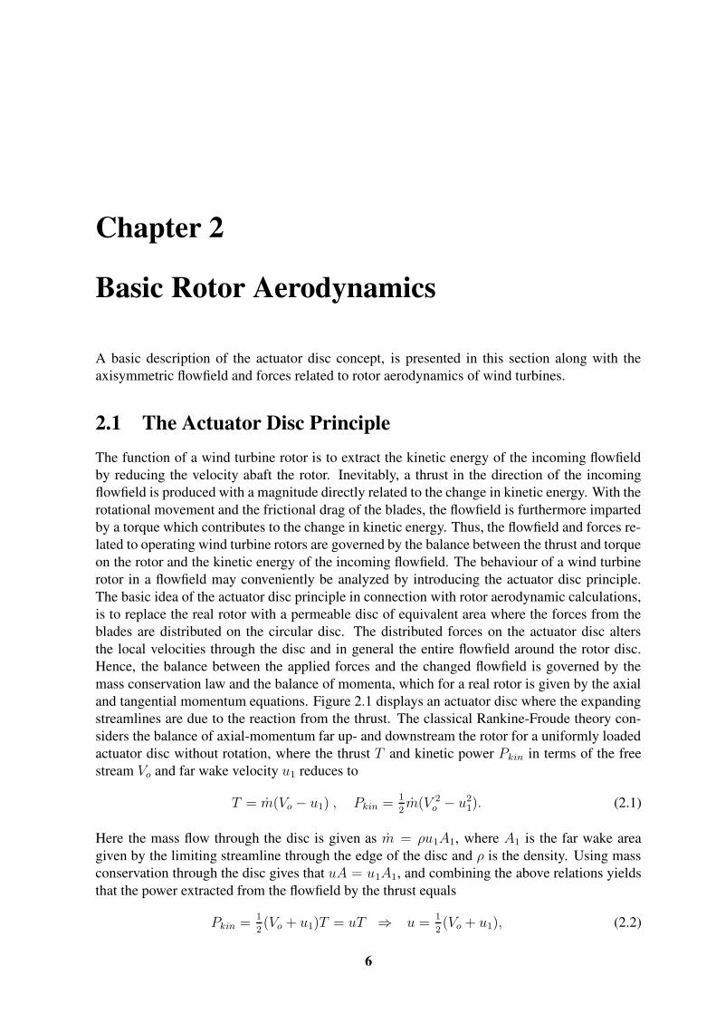
3.3 Simulation on Real Rotors - Tip CorrectionReal rotors, in contrast to the axially loaded rotor, includes angular velocities. Furthermore, realrotors have finite number of blades which produce a system of distinct tip vorticity structures inthe wake. Thus, a different vortex wake is produced by a rotor with infinite number of bladesas compared with one with a finite number of blades. Prandtl [43] derived a formula for the tip-correction, quantified by the factor F , in order to compensate for the finite number of blades. Inorder to include tip-correction effects with the generalized actuator disc model, the aerodynamicforce components given by Eqs.(2.8)-(2.9) are corrected using the Prandtl tip-correction factorF given by the formula
F =2
πcos−1
[
exp
(
−B2
R− rr sin φ
)]
. (3.15)
For the Navier-Stokes methods a different approach is needed as compared to BEM methodswhen applying the Prandtl tip correction formula. In the BEM method [19], the tip correctionis employed to the axial and angular momentum equations, leading to two equations for a anda′
a
1− a =σCn
4 sin2 φ=
F a
1− a ,a′
1 + a′=
σCθ
4 sinφ cosφ=
F a′
1 + a′, (3.16)
where a and a′ are corrected interference factors and F is the tip loss factor. With a BEMmethod a and a′ (or a and a′) are found directly from Eq.(3.16), but with a Navier-Stokes modelthe flowfield is given and the loading has to be modified, hence Eq.(3.16) is rearranged to
a =a
F (1− a) + a, a′ =
a′
F (1 + a′)− a′ , (3.17)
where F serves as a relaxation parameter in the iterative solution process. With these valuesa corrected set of Vz and Vθ are determined from Eq.(3.11). The modified loading is thendetermined through the corrected values for φ, Vrel, L and D found from Eqs.(2.7) and (2.8).
3.3.1 Computation using LM 19.1m Blade DataIn order to display the capabilities of the generalized actuator disc model on real rotors, theNordtank NTK 500/41 stall regulated wind turbine with LM 19.1m blades is analyzed. Theblade sections consist of NACA 63-4xx aerofoils in the outer half of the blade and FFA-W3-xxxaerofoils at the inner part of the blade. The aerofoil characteristics (Hansen [26]) are correctedfor 3-D effects by preserving values within the measuring range and in post stall and deep stallapplying a smooth and somewhat experienced guess, combined with data tuning in order to getthe measured power curve using a "standard" BEM method. The turbine has three blades, adiameter of 41m and it rotates at 27.1 rpm. Applying the (C)-grid and a Reynolds number ofRe=5000, figure 3.6 (left) shows the axial interference at two different wind speeds, 7 m/s and10 m/s. The computations predicts an increasing axial induction towards the tip at both windspeeds, with a level at 7 m/s that indicates a reasonable high thrust coefficient. Correspondingcalculation without the Prandtl tip-correction i.e. F = 1, shows that the influence of thetip-correction may be neglected for the LM 19.1m blade. This behaviour is explained with the

3.3 Simulation on Real Rotors - Tip Correction 17
0.0 0.5 1.0r/R
0.0
0.1
0.2
0.3
0.4
0.5
a
With PrandtlF=1
Vo=10ms-1
Vo=7ms-1
0.0 0.5 1.0r/R
0.0
0.2
0.4
0.6
0.8
Load
ing
F z/ρV
o2 R With PrandtlF=1
Vo=10ms-1
Vo=7ms-1
Figure 3.6: Distribution of axial interference (left) and non-dimensional loading (right) for theLM 19.1m blade at 7m/s and 10m/s.
5 10 15 20 25Freestream Velocity [m/s]
0.0
0.2
0.4
0.6
0.8
CT
& C
P
Exp.CP - ADCT - AD
5 10 15 20 25Freestream Velocity [m/s]
0
200
400
600
Pow
er [k
W]
Exp.AD
Figure 3.7: CT , CP (left) and power distribution (right) for the Nordtank NTK 500/41 windturbine with LM 19.1m blades.
chord distribution for the blade which decreases continuously all the way to the tip, therebyincluding a "natural" decay in loading towards the tip. Looking at the non-dimensional loading,figure 3.6 (right) shows corresponding tendencies in the tip region, to that obtained for theinduced velocities. Letting the freestream velocity vary from 5 to 25 m/s results in the CT , CP
and power distribution presented in figure 3.7. The power curve, measured by Poulsen at Risø[42], is seen to compare within an accuracy of 1-3% through the velocity range, although athigher velocities > 18m/s an increased deviation is observed. Thus, the steady computationscompares well with the experimental measurements. At very low wind speeds the thrust coeffi-cient increases rapidly thereby approaching the unsteady regime. Looking at the convergencerate depicted in figure 3.8 the trend is towards less iterations with increasing wind speed i.e.decreasing thrust-coefficient. At 6m/s the converged solution gives a CT = 0.86 using anon-dimensional time step of 0.1, which may be increased to 0.25 at 9m/s and 0.6 at 12m/s.The magnitude of the non-dimensional time step govern the stability of the convergence andthe maximum value for obtaining steady converged solutions, mainly depends on the thrust co-efficient i.e ∆tmax = ∆t(CT ). The maximum values of ∆tmax are found more or less arbitrarily.

18 The Generalized Actuator Disc Model
0 200 400 600 800Iteration count
-10
-8
-6
-4
-2
0
2
Max
(log 10
|x-x
old|)
6m/s9m/s12m/sΨ
ω
Vθ
Figure 3.8: Numerical convergence of the vorticity, swirl-velocity and stream function at threedifferent wind speeds.
To summarize, the calculations on the axially loaded rotor and a real rotor using data for theNordtank 500/41 wind turbine have demonstrated that a good accuracy may be obtained bysolving the Navier-Stokes equations. The steady solutions are found efficiently with good con-vergence rate using large time steps.

Part B
Application of the Generalized ActuatorDisc Model
19

Chapter 4
The Coned Rotor
This part presents topics beyond the standard steady computations for wind turbine rotors per-formed with the generalized actuator disc. First, the coned rotor is analyzed and next the un-steady behaviour of the yawed rotor is approached with new contribution. Finally, in connectionwith experimental investigations effects of tunnel blockage is analyzed.
4.1 Coned RotorsThe trend in the development of modern wind turbines tends towards larger and more structuralflexible rotor blades. As a consequence, large blade deflections are anticipated and as a firststep in the understanding of the aerodynamics of rotors subject to large blade deflections, theinfluence of coning is investigated. When considering rotors with substantial coning or bladedeflections, the radial flow component has an influence on the loading and induced velocities.For upstream coning the expansion of streamlines tends to make the flow orthogonal to the rotor,whereas the opposite happens for downstream coning. This results in different performancecharacteristics for the two cases. As the standard BEM method (Glauert [19]) does not predictthe radial flow component this difference is difficult to incorporate into a BEM method. Madsenand Rasmussen [33] investigated the induction from a constantly loaded actuator disc withdownstream coning and large blade deflection using a numerical actuator disc model. Here the(Ψ−ω) formulation, as well as a modified BEM method, is used to analyze a rotor with constantnormal loading and a real rotor exposed to up- and downstream coning.
4.1.1 Geometry and Kinematics - Velocity TriangleConsidering a coned rotor in a polar coordinate system (r, θ, z), the axisymmetric flowfieldaround the turbine is described by the velocity components V = (Vr, Vθ, Vz). In figure 4.1 arotor is sketched in the (r, z)-plane at a coning angle β. A local coordinate system, (s, n), isapplied, where s is the spanwise coordinate and n is the direction normal to the blade. Withthe full flowfield given, the velocity components normal to the rotor are (Vn, Vθ), where Vn isdetermined as
Vn = Vz cos β + Vr sin β, (4.1)
and both Vz and Vr are known from the numerical actuator disc computation. The BEM model,however, is not capable of handling the radial flow component. As it is based on momentum
20

4.1 Coned Rotors 21
Vo
R
sn
r
zzd
β
Figure 4.1: Rotor with coning angle β
considerations far upstream and downstream of the rotor, it does not contain any informationabout the radial flow component on the rotor. Figure 4.2 shows the local velocity triangle of aconed rotor in the (s, z)-plane. Letting Wn denote the induced velocity in the direction normal
Vo cos β −Wn
Wz
Wn
s
βVo −Wz
Figure 4.2: Velocity triangle in the (s, z)-plane
to the rotor from the BEM method, the normal velocity is given by
Vn = Vo cos β −Wn, (4.2)
which only contains the first term in Eq.(4.1). The corresponding axial velocity componentacting on the rotor is equal to Vo −Wn cos β. An important limitation of neglecting the radialinfluence is that a distinction between up- and down-stream coning is not possible.
4.1.2 Blade ForcesThe aerodynamic lift and drag forces acting on the coned rotor are determined from Eq.(2.8),however, the local velocity triangle is somewhat altered by the cone angle. Figure 4.3 shows theequivalent cross-sectional airfoil element presented in figure 2.3 for the coned rotor at radiuss in the (θ, n) plane. The relative velocity is determined from V 2
rel = V 2n + (Ωs cos β − Vθ)
2,where Ω is the angular velocity and the angle, φ, between Vrel and the rotor plane, is given as
φ = tan−1
(
Vn
Ωs cos β − Vθ
)
. (4.3)

22 The Coned Rotor
Vrel
−Ωs cos β
L
D
Fn
Fθ
Vn
Vθ
γ
αφ
−θ
n
Figure 4.3: Cross-sectional airfoil element showing velocity and force vectors
As seen from Eqs. (4.1) and (4.3), when the rotor is coned, Vr contributes to the relative velocityand alters the angle of attack. Projection of the lift and drag forces given by Eq.(2.8) in thenormal and the tangential direction to the rotor gives the force components
Fn = L cosφ+D sinφ , Fθ = L sinφ−D cosφ . (4.4)
The normal force is decomposed into axial and radial direction as
Fz = Fn cos β , Fr = Fn sin β. (4.5)
4.2 Aerodynamic Modelling - Momentum BalanceThe aerodynamic behavior of coned rotors is investigated using two different models. To checkthe utility of employing the BEM technique for rotors subject to coning, the consequences ofmodelling coned rotors is analyzed using simple momentum consideration, hence, neglectingthe radial flow component. Next, the generalized actuator disc is employed where considera-tions for the applied forces are presented.
4.2.1 A Modified BEM MethodThe classical BEM method by Glauert [19] presented in section (2.1.1) considers the axialand tangential balance of momenta for a number of individual annular stream tubes passingthrough the rotor from −∞ to +∞. Here the analysis is extended to include effects of coning.Considering the coned rotor on figure 4.2, the local normal thrust, ∆Tn, and torque, ∆Q, actingon a blade element, are equal to the change in normal and angular momentum, respectively. Itis, however, still a purely axial momentum balance which govern the momentum for the conedrotor. Denoting the induced velocities in the rotor plane byWn,Wθ the normal thrust and torquereads
∆Tn cos β = 2Wn cos β∆m , ∆Q = 2Wθ∆ms cosβ, (4.6)

4.2 Aerodynamic Modelling - Momentum Balance 23
where cos β is included on both sides of the first equation in order to emphasize the axial pro-jection. The equation is immediately reduced to ∆Tn = 2Wn∆m, but as the induced velocityin the far wake has a purely axial direction and not normal to the rotor plane, presenting thereduced equation could be misleading with respect to the far wake boundary. Furthermore, theinduced velocity in the tangential direction, Wθ, is equal to −Vθ. Considering the axial inducedvelocity, Wz = Wn cos β, the mass flow through each element is given by,
∆m = ρ(Vo −Wn cos β)2πs∆s cos2 β, (4.7)
where the tip radius is constant and the projected area is reduced with cos2 β. In terms ofinduced velocities, interference factors are introduced for the normal, axial and tangential di-rection, respectively, as
an =Wn
Vo cos β, az =
Wz
Vo, a′ =
Wθ
Ωs cos β. (4.8)
Combining Eqs. (4.6) and (4.7), and normalizing the thrust with the projected area (see Ap-pendix C), gives the axial thrust coefficient CT = 4az(1 − az), which is the same as for thestraight rotor. This shows that the axial induction along the blade only depends on the thrustand is independent of the radial position or coning angle. The relation between an and az isfound to
an =az
cos2 β. (4.9)
The normal and tangential forces generated by the blades give a normal thrust and torque fromeach element that is equal to
∆Tn = Fn∆s , ∆Q = Fθs∆s cos β, (4.10)
where Fn and Fθ are given by Eq.(4.4). Tip correction F is included by using the Prandtl tiploss factor as described in [19] and given by
F =2
πcos−1
[
exp
(
−B2
R− rr sin φ
)]
. (4.11)
In order to handle high values of a the empirical Glauert correction given by Spera [53] isapplied
CT =
4az(1− az)F az ≤ ac,4[a2
c + (1− 2ac)az]F az > ac,(4.12)
where ac = 0.2 (which seems low). By equating Eqs.(4.6) and (4.10), with Vrel and φ given byEq.(4.3) and introducing σ = cB/2πs cos β, the induced velocities are found from the expres-sions
4Wz(Vo −Wz)F = V 2relσCn , (4.13)
4Wθ(Vo −Wz)F cos β = V 2relσCt , (4.14)
where Cn, Ct are the normal and tangential projection of the lift and drag coefficient, respec-tively
Cn = CL cos φ+ CD sinφ , Ct = CL sin φ− CD cosφ . (4.15)
24 The Coned Rotor
In terms of interference factors a, a′, Eqs.(4.13)-(4.14) are normalized and rewritten as follows
4az(1− az)F =V 2
relσCn
V 2o
⇒ az =1
2
(
1−√
V 2relσCn
V 2o F
)
, az ≤ ac, (4.16)
4[a2c + (1− 2ac)az]F =
V 2relσCn
V 2o
⇒ az =
(
V 2relσCn
4V 2o F
− a2c
)
1
1− 2ac, az > ac,(4.17)
a′ =V 2
relσCt
V 2o cos2 β
1
4(1− az)F
Vo
Ωs. (4.18)
In the BEM method the equations are solved iteratively and the procedure is summarized in thefollowing steps: Initial values : a = a′ = 0 or Wz = Wθ = 0,
• Find φ from Eq.(4.3)
• Angle of attack, α = φ− γ
• Relative velocity, V 2rel = (Vo −Wn)2 + (Ωs cos β +Wθ)
2
• Normal and tangential coefficients Cn, Ct from table and projection, Eq.(4.15)
• The induced velocities Wz,Wθ or interference factors a, a′ from Eqs.(4.13-4.14) orEqs.(4.16-4.18)
The sequence is repeated until a, a′ or Wz,Wθ fulfill some convergency criteria.
4.2.2 The Actuator Disc Model - Applying ForcesThe (Ψ− ω) formulation presented previously is a sufficient formulation for capturing the trueaxisymmetric behaviour of the flow through coned rotors. However, the applied forces in theformulation needs some special considerations in order to cope coned rotors. The rest of theformulation as well as the computational domain used to evaluate the flowfield around conedrotors, is preserved from the previous sections. In order to apply forces from a coned rotor, aconed annular area of differential size is considered, dAn = 2πs cosβds. Then the loading isgiven by
f =F (s)ds
2πs cosβds, f ′ =
f
dz. (4.19)
The resulting body force, f ′
ε, is then formed by taking the convolution of the computed load,f ′, and a regularization kernel, ηε, as shown below
f ′
ε = f ′ ⊗ ηε , ηε(p) =1
ε3π3/2exp
[
−(p/ε)2]
. (4.20)
Here ε is a constant that serves to adjust the concentration of the regularized load and p is thedistance between the measured point and the initial force points on the actuator disc. In the caseof a coned rotor, the regularized force becomes
f ′
ε(r, z) =
∫ R
0
∫ 2π
0
F (s)
2πε3π3/2exp
[
−(p/ε)2]
dθds. (4.21)

4.3 Numerical Results for the Coned Rotor 25
The parameter ε is here set equal to ε = εi∆z where εi is of the order 1 . εi . 4 and ∆z is thecell size in axial direction. Eq.(4.21) may be integrated in the θ-direction and reduced1 to
f ′
ε(r, z) =
∫ R
0
F (s)
ε3π3/2exp
(
−d2 + 2rs sin β
ε2
)
Io
(
2rs sin β
ε2
)
ds. (4.22)
The distance d2 = (r−s cos β)2+[(z−zd)+s sinβ]2 is the distance between the measured pointand the initial force points in the axisymmetric plane and Io is the modified Bessel function ofthe first kind of order 0. The approach ensures that the integrated loading is conserved and thatsingular behavior is avoided as the loading is distributed smoothly on several mesh points in a3D Gaussian manner away from each point on the disc. As the actuator disc appears as a one-dimensional line in the axisymmetric plane, suggest that a 1D Gaussian approach also may beapplied to smear the forces away from the line. Hence, the forces are proposed to be distributedor smeared in the normal direction away from the rotor disc using the convolution
f ′
ε = f ′ ⊗ η1Dε , η1D
ε (p) =1
ε√π
exp[
−(p/ε)2]
. (4.23)
Inserting gives the distributed force
f ′
ε(r, z) =
∫ +∞
−∞
f ′(s)
ε√π
exp[
−(p/ε)2]
dn. (4.24)
The normal distance p between any point in the (r, z) plane and the rotor disc is given by
p =(zd − z)− r tanβ√
1 + tan2 β, (4.25)
and the point on the rotor disc sp which is normal to the field point (r, z) is determined as
sp =r + p sin β
cos β. (4.26)
The function of the smearing proposed by the two methods, is basically to distribute loadingalong any line on a regular mesh. Furthermore, the smearing prevents spatial oscillations in thevicinity of the applied forces, although it should be noted that solutions without oscillations havebeen obtained by not using smearing for the straight rotor. As pointed out by Masson et al.[34]who applied forces as pressure discontinuities, explicit treatment of the applied forces is neededto prevent spatial oscillations in the vicinity of the applied forces. Whereas the curl operatoris applied to the (Ψ − ω) formulation, methods formulated in primitive variables depend onaccurate handling of the divergence operator applied to the body force vector when solving thepressure equation. The oscillations or wiggles observed by Sørensen and Kock [56] on the axialinterference factor are completely removed with the regularization and with suitable choice ofgrid resolution. The two distribution methods both apply as smearing function, however, the3D Gaussian tends to smear beyond the edge of the disc whereby the intended spanwise loaddistribution near the tip, is slightly chanced.
4.3 Numerical Results for the Coned RotorTo give an impression of the computational domain and the structure of the grid, a part ofthe grid is shown in figure 4.4. In the figure, a rotor coned −20o is inferred as a straight
1In [37] Eq.(20) should be corrected with sin β instead of cosβ.
26 The Coned Rotor
Vo
r
z
→
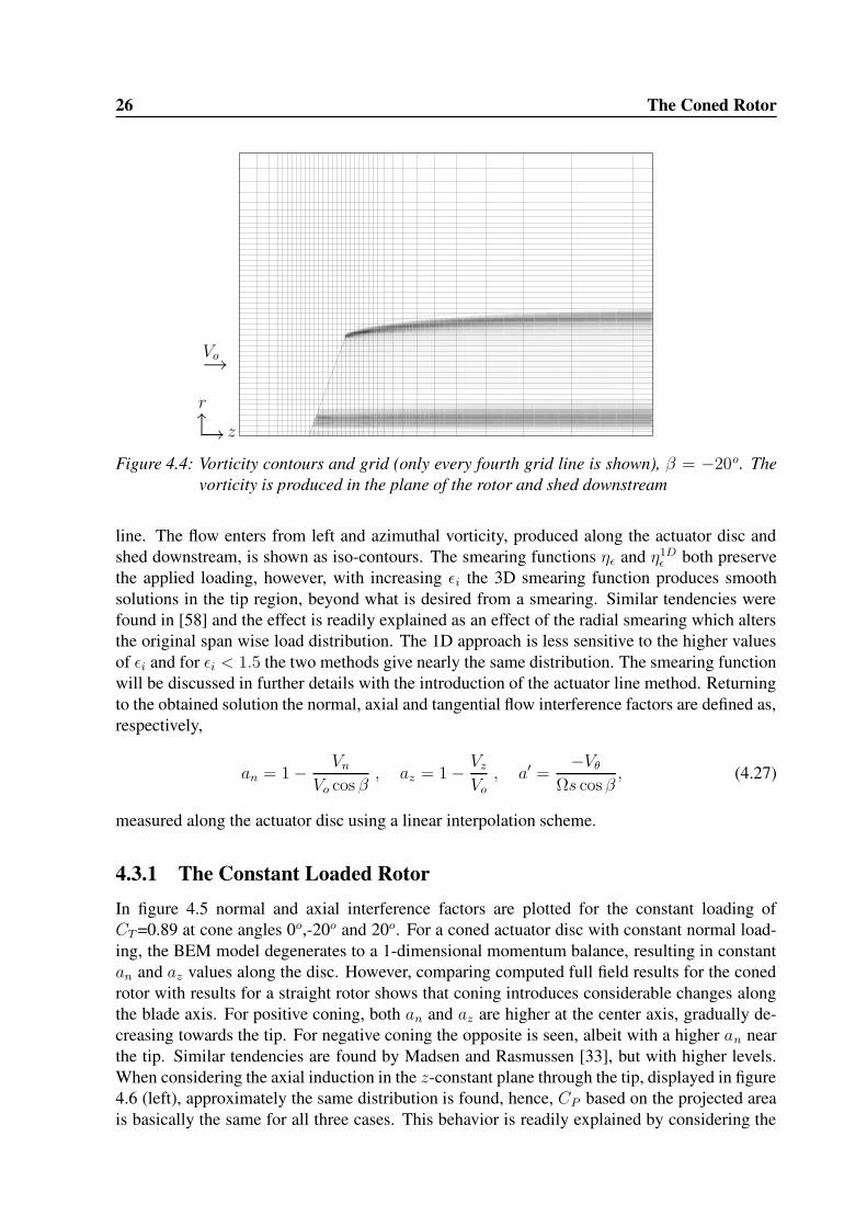
→↑Figure 4.4: Vorticity contours and grid (only every fourth grid line is shown), β = −20o. The
vorticity is produced in the plane of the rotor and shed downstream
line. The flow enters from left and azimuthal vorticity, produced along the actuator disc andshed downstream, is shown as iso-contours. The smearing functions ηε and η1D
ε both preservethe applied loading, however, with increasing εi the 3D smearing function produces smoothsolutions in the tip region, beyond what is desired from a smearing. Similar tendencies werefound in [58] and the effect is readily explained as an effect of the radial smearing which altersthe original span wise load distribution. The 1D approach is less sensitive to the higher valuesof εi and for εi < 1.5 the two methods give nearly the same distribution. The smearing functionwill be discussed in further details with the introduction of the actuator line method. Returningto the obtained solution the normal, axial and tangential flow interference factors are defined as,respectively,
an = 1− Vn
Vo cos β, az = 1− Vz
Vo, a′ =
−Vθ
Ωs cos β, (4.27)
measured along the actuator disc using a linear interpolation scheme.
4.3.1 The Constant Loaded RotorIn figure 4.5 normal and axial interference factors are plotted for the constant loading ofCT =0.89 at cone angles 0o,-20o and 20o. For a coned actuator disc with constant normal load-ing, the BEM model degenerates to a 1-dimensional momentum balance, resulting in constantan and az values along the disc. However, comparing computed full field results for the conedrotor with results for a straight rotor shows that coning introduces considerable changes alongthe blade axis. For positive coning, both an and az are higher at the center axis, gradually de-creasing towards the tip. For negative coning the opposite is seen, albeit with a higher an nearthe tip. Similar tendencies are found by Madsen and Rasmussen [33], but with higher levels.When considering the axial induction in the z-constant plane through the tip, displayed in figure4.6 (left), approximately the same distribution is found, hence, CP based on the projected areais basically the same for all three cases. This behavior is readily explained by considering the

4.3 Numerical Results for the Coned Rotor 27
0.0 1.0 2.0s/R
-0.1
0.0
0.1
0.2
0.3
0.4
0o
+20o
-20oa n
0.0 1.0 2.0s/R
-0.1
0.0
0.1
0.2
0.3
0.40o
+20o
-20oa z
Figure 4.5: Normal and axial interference factors along the radius of the disc for CT =0.89
body forces in Eq.(3.2). These appear as vorticity sources given by the general expression
∇× f ′ · eθ =∂f ′
s
∂n− ∂f ′
n
∂s= −∂f
′
n
∂s, (4.28)
since f ′
s = 0 for any rotor. From this expression it is seen that finite source terms only appearat positions where the normal loading is varied. For a rotor with constant normal loading, thesource term is zero everywhere except at the edge (or tip) of the actuator disc. Furthermore,the value of the source term depends only on the magnitude of the normal loading and not onthe shape of the rotor. Whether the rotor is coned or not, the same source term at the edgeof the disc and therefore the same system of trailing vortices, measured from the location ofthe source term. Schmidt and Sparenberg [52] derived the same result, by considering thepressure field divided into active regions. The induced velocities on the disc are, however,no longer the same as the position of the rotor with respect to the trailing vortex system haschanged. With the BEM model in mind this suggests that the axial induction found by theBEM model is not located along the blade but in the plane through the tip. For comparisonthe level found in Ref. [33], also shown figure 4.6, is seen to be about 5% higher. The radialvelocity along the disc, shown in figure 4.6 (right), is virtually unaffected by changes in coneangle, although a small effect is seen near the tip. The power coefficients are presented inTable 4.1 for the three cases and should ideally be exactly the same. There are, however, smallvariations within 0.3% point, which is attributed to the accuracy of the numerical method. The
CP 0o -20o +20o
Present 0.601 0.601 0.604Ref. [33] 0.573 0.571 -
Table 4.1: Power coefficient for a constant loaded actuator disc at CT =0.89 and cone angles β= 0o, -20o and +20o.
values found by Madsen and Rasmussen are somewhat lower. The power coefficients presentedhere are seen to exceed slightly the Betz limit. Van Kuik [67] argues that a higher value isrelated to the behavior of the tip vortex, but as figure 3.5 shows, the added diffusion tends to

28 The Coned Rotor
0.0 1.0 2.0r/R
0.0
0.1
0.2
0.3
0.4
0.5
a z
0o
+20o
-20o
Ref.[33]
0.0 1.0 2.0s/R
0.0
0.1
0.2
0.3
0.4
0.5
Vr /
Vo
0o
+20o
-20o
Ref.[33]
Figure 4.6: Axial interference factor in the radial plane through the tip and radial velocity alongthe radius of the disc for CT =0.89
over predict CP as compared to the Betz limit. A steady solution could not be obtained forhigher Reynolds numbers (Re≥100,000), suggesting that CT = 0.89 is close to a stability limitat which the solution becomes unsteady. The diffusion can not be completely removed sinceartificial diffusion always is added to the flow, due to the numerics.
4.3.2 Simulation of the Tjæreborg Wind Turbine
In order to investigate the influence of coning for a real rotor, calculations have been performedwith aerofoil data from the 2MW Tjæreborg wind turbine, although it has zero coning. Theblade radius of the turbine is 30.5 m and it rotates at 22.1 RPM, corresponding to a tip speedof 70.7 m/s. The blade sections consist of NACA 44xx airfoils with a chord length of 0.9 m atthe tip, increasing linearly to 3.3 m at hub radius 6 m. The blades are linearly twisted 1o per3 m. Further technical details can be found in [77]. In figure 4.7 the normal and axial inter-ference factors for cone angles 0o,± 10o and ± 20o, computed by the Navier-Stokes algorithm,
0.0 1.0 2.0s/R
-0.1
0.0
0.1
0.2
0.3
0.4
0o
+10o
+20o
-10o
-20o
a n
0.0 0.5 1.0 1.5 2.0s/R
-0.1
0.0
0.1
0.2
0.3
0.4
0o
+10o
+20o
-10o
-20o
a z
Figure 4.7: Normal and axial interference factors along the blade of the Tjæreborg wind turbineat Vo=10 m/s

4.3 Numerical Results for the Coned Rotor 29
are shown. The tip speed ratio is λ = 7.07, corresponding to Vo=10 m/s. Tip-correction iscompensated for with Eq.(3.17) and setting a = an. The loading of the Tjæreborg wind turbineis nearly constant over most of the rotor and the computed an shows the same pattern as for theconstant loaded actuator disc in figure 4.5. For β = +20o, an attains its highest value near thehub after which it decreases continuously towards the tip. For β = −20o, an is lower at the hub,increasing towards the tip to a level above the obtained level for β = 0o. For az, however, thelevel is reduced about 20% for β = −20o, as compared to that of β = 0o. For upstream coningof 10o and 20o, the axial induction is found to be almost the same and about 5% higher than atβ = 0o. The rotational power coefficient, defined by Eq.(C.5) in App. A, is in figure 4.8 (left)compared with experimental data. The power coefficient is consistently defined with respectto the projected area for all considered rotors, since CP is invariant to coning for the constantloaded rotor. For β = 0o the calculated CP -value is found to be within 1-3% point of the ex-perimental results. The velocity at which maximum CP occurs is seen to agree well with themeasured data. Coning of the rotor displays only a minor effect on CP through the considered
6 8 10 12 14 16Vo [m/s]
20
30
40
50
60
CP[%
]
Exp.0o +10o
+20o
-10o
-20o
6 8 10 12 14 16Vo [m/s]
0.0
0.5
1.0
1.5
2.0
2.5P
ower
[MW
]
Exp.0o
+10o
+20o
-10o
-20o
Figure 4.8: CP and power distribution for the Tjæreborg wind turbine
velocity range, with the highest value appearing at upstream coning, where CP max for β = 20o
is increased with about 1% point as compared with β = 0o. For downstream coning CP is re-duced about 1-2% point through the velocity range, which is partly explained by the decreasein relative velocity, as the streamlines are less orthogonal to the rotor plane. When looking atthe power production, figure 4.8 (right), the highest output is obtained at 0o which primarilyis due to the reduced projected area when coning. At velocities above 13 m/s the pitch angleis regulated in order to keep a constant electrical power output of 2 MW and the calculatedpower is based on an averaged measured pitch angle. The structural load on each blade, basedon aerodynamic forces only, is shown in figure 4.9, which depicts the normal load distributionand the shear force. For upstream coning, the changes in loading are a nearly constant reduc-tion over the entire span, whereas for downstream coning the changes take place mostly in theouter part of the blade. Correspondingly, both the shear force (figure 4.9 right) and flap wisebending moment (not shown) are reduced with an increasing cone angle. Although upstreamconing gives a slightly higher shear force at the root section, as compared to the correspondingdownstream coning, the differences are found to be negligible. Thus, even though the differ-ence in induced velocities between up- and downstream coning is considerable, the impact onintegrated parameters is more moderate.

30 The Coned Rotor
0 10 20 30R[m]
0.0
1.0
2.0
3.0
Load
ing
F n [kN
/m]
0o
+10o
+20o
-10o
-20o
0 10 20 30R [m]
0
10
20
30
40
50
F N [k
N]
0o
-10o
+10o
-20o
+20o
Figure 4.9: Distribution of aerodynamic load and shear force along the blade at Vo=10m/s
4.3.3 Comparison with the BEM Method for the Tjæreborg Wind Tur-bine
In figure 4.10 a an-distribution computed by the numerical actuator disc model is comparedwith results from the BEM method. It is observed that the agreement between the two methodsgenerally is very good at β = 0o, although deviations are seen near the tip. This is not the
0.0 0.5 1.0 1.5s/R
-0.1
0.0
0.1
0.2
0.3
0.4
0o
BEM 0o
a n
0.0 0.5 1.0 1.5s/R
-0.1
0.0
0.1
0.2
0.3
0.4
+20o
-20o
BEM 20o
a n
Figure 4.10: Normal interference factor calculated with the BEM and the Navier-Stokes methodfor the Tjæreborg wind turbine at Vo=10 m/s
case at β = ±20o, however, where the an-distribution predicted by BEM has a higher levelthan at β = 0o. The comparison with the Navier-Stokes method shows some agreement forβ = +20o, but at β = −20o the BEM method fails to capture the an-distribution. A simpleestimate of the influence of coning would be to assume that the root shear force, FN , is reducedaccording to the reduction of the projected area, i.e. it follows a cos2 β distribution. In figure4.11 the computed FN = FN(β) distributions are compared to a FN = FN(β = 0o) cos2 βdistribution at Vo = 10m/s. The comparison shows that the BEM method predicts a FN -distribution which is just below the cos2 β dependency. In contrast to this, the distribution bythe Navier-Stokes algorithm is everywhere higher and the error committed by the BEM method

4.4 Summary 31
-20 -10 0 10 20Cone angle β[deg]
30
35
40
45
50
Roo
t she
ar fo
rce
F N[k
N]
BEMActuator disccos2β
Figure 4.11: Shear force at the root section for Vo=10m/s, as a function of cone angle β
at β = ±20o amounts to about 3-4%. The same tendencies are found at higher freestreamvelocities. In figure 4.12, the difference in power coefficient, ∆CP = CP (β) − CP (β = 0o),between a straight and a ±20o coned rotor is shown as function of freestream velocity for thetwo methods. The results show a different behavior between the two models. The Navier-
6 8 10 12 14 16Vo[m/s]
-6
-4
-2
0
2
4
6
∆CP[%
]
+20o
-20o
BEM 20o
Figure 4.12: Difference in CP as function of freestream velocity for β = ±20o
Stokes computations demonstrate a decreasing tendency for an increasing freestream velocity,with a difference between up- and downstream coning that decreases from about 3 to 1% pointover the considered velocity range. The opposite behavior is observed for the BEM methodwhich underpredicts ∆CP by up to 7% point at β = +20o and up to 4% point at β = −20o, ascompared with the numerical actuator disc model. Through the velocity range the two methodsapproach each other with a difference of about ±0.5% point at Vo = 17m/s.
4.4 SummaryThe generalized actuator disc model and a modified BEM method for flows through coned ro-tors have been developed and tested for an actuator disc with constant load and a real rotor at

32 The Coned Rotor
various coning angles. For the coned actuator disc with constant normal loading, the calculatedinterference factors an and az are found to change considerable along the radius of the disc. TheBEM method can not reproduce this and there seems no easy way to model it, without violatingthe radial independence of the annular streamtubes. The calculated CP for a constant loadingof CT =0.89 shows to be independent of coning, in accordance with theoretical considerations.The general trend of the results compares well with the findings of Madsen and Rasmussen[33]. Calculations of the Tjæreborg wind turbine display similar tendencies for the interferencefactors as for those of the constant normal loading. Thus, considerable changes in an and az
were obtained in both cases with varying coning angle. The main explanation for this is thechanged position of the rotor with respect to the trailing vortex system. A marginal increase inCP max of about 1% point was obtained for an upstream coning of 20o. Hence, coning leads toan overall power production that is reduced due to the reduction of the projected area. Compar-ing the structural loads calculated by the two models shows that the BEM method underpredictsthe loads when increasing the cone angle. The predicted root shear force by the Navier-Stokescomputations results only in minor differences between up- and downstream coning. Com-parisons with BEM results at β = ±20o show that the BEM method underestimates the rootshear force by about 3-4% and both methods follows a reduction that is proportional to the re-duced projected area. The difference between the power coefficients computed at β = 0o and atβ = ±20o, ∆CP , shows opposite tendencies between the two models. Where the Navier-Stokesmethod predicts a decreasing ∆CP with increasing freestream velocity, the BEM method pre-dicts an increasing ∆CP with increasing freestream velocity. Furthermore, the BEM methodunderestimates CP with up to 7% point at lower velocities. As a consequence, the BEM methodmay introduce significant errors when applied to rotors with substantial coning or large bladedeflections.

Chapter 5
The Yawed Rotor
Although the flow through a rotor operating at yaw-misaligned conditions exhibit full 3D be-haviour, yawed rotors are generally analyzed using axisymmetric methods. Here the generalizedactuator disc model is used in combination with various sub models.
5.1 Yaw Modelling
Yaw modelling of wind turbine rotors is an important and difficult task to undertake owing tothe unsteady nature of the inflow and the skewed wake geometry. In the past years a lot ofeffort has been put into providing accurate experimental data to improve engineering modelspredicting loads of wind turbine rotors at yawed conditions. In the European JOULE project"Dynamic Inflow: Yawed Conditions and Partial Span Pitch Control" [47] various yaw modelswere developed and incorporated into blade element momentum codes. In some validationcases, the refined models led to considerable improvements as compared to the original model,whereas they in some other cases showed to be in rather poor agreement with experimentaldata. Using the (Ψ− ω) finite difference formulation of the Navier-Stokes equations facilitatestime true simulation of the dynamic wake. Here the method are used in combination with submodels for tower, wind shear, dynamic stall and elastic deflection.
5.1.1 3D Geometry and Kinematics
When considering rotors subjected to tilted or yawed inflow of substantial magnitude, axisym-metric assumptions are no longer sufficient, which calls for a full 3D projection of forces andvelocities. The impact of a yawed rotor on the flow is a skewed wake which axisymmetricmethods are incapable of capturing. However, with the axisymmetric (Ψ − ω) method it isproposed to use the 3D axisymmetric velocity vector extracted on the disc as inflow velocity toeach blade. The disc velocities are then projected onto the normal and tangential directions ofeach individual blade, where, in case of yawed inflow, the radial velocity results in contribu-tions which change sign depending upon whether the blade is moving upstream or downstream.Loading and related quantities are then determined for each individual blade at its circumferen-tial position but the applied aerodynamic forces on the actuator disc are given as the span wiseaverage of each blade.
33

34 The Yawed Rotor
5.1.2 Projection of VelocitiesThe velocities provided by the (Ψ − ω) model are given in a cylindrical polar frame, V rθz =(Vr, Vθ, Vz) where θ = Ωt. Locally, however, the span wise, normal and tangential velocitycomponents are given by V stn = (Vs, Vt, Vn). The local velocities are obtained through a seriesof coordinate transformations with respect to yaw, tilt, coning and flap wise deflection. Figure
φy
s
s r
r
r
x
y
n
zθ
z
Figure 5.1: Yaw transformation seen from above and behind the rotor.
5.1 shows yaw and azimuthal angles, φy and θ, respectively. The yaw, tilt and azimuthal anglesare defined positive using the right hand rule i.e. tilt as rotation about the x-axis, yaw aboutthe y-axis and azimuth about the z-axis. The cone angle is defined positive as upstream coningas in the previous chapter. The polar velocities are first transformed to Cartesian componentsthrough the transformation matrix, Θ,
V xyz = ΘV rθz , Θ =
c −s 0s c 00 0 1
, (5.1)
where s = sin θ and c = cos θ. Yaw, Φy, tilt, Φt, and coning/deflection, B, transformationsfrom Cartesian to spanwise, tangential and normal components are found using
Φy =
c 0 −s0 1 0s 0 c
, Φt =
1 0 00 c s0 −s c
, B =
c 0 −s0 1 0s 0 c
. (5.2)
Whereas Φy and Φt transform a Cartesian vector to Cartesian, B transform from polar to span-wise, tangential and normal components i.e. before compensating for the influence of con-ing and deflection, as shown in Figure 5.2, the velocity vector is transformed back to polarcomponents with Θ
T , hence, the full transformation is obtained by multiplying the matrices asfollows
V stn = BΘTΦtΦyV xyz = AV rθz. (5.3)
For most rotors, however, tilt and coning angles are small and in this case a reduced transfor-mation which only include effects for rotors operating in yawed inflow, reduces to
Vt
Vn
=
[
cos θ sin θ(1− cosφy) cos2 θ + sin2 θ cosφy sin θ sin φy
cos θ sinφy sin θ sinφy cosφy
]
·
Vr
Vθ
Vz
. (5.4)

5.1 Yaw Modelling 35
β
θf
r
w
s
s r
r
n
z
n
n
z
Figure 5.2: Coning and deflection of the blade seen from above, βf = β − θf .
The reduced transformation shows that radial velocity contributes to the unsteady loading, withincreasing yaw angle φy, an effect which many methods neglect. The local flow angle and rela-tive velocity along each blade are, apart from the flowfield velocities, affected by the influencefrom tower, elastic vibration of the blade, wind shear and turbulence. These effect are includedin many different ways and will be introduced later. Using Eq.(5.3) the local flow angle andrelative velocity are defined as φ = tan−1
(
V ′
n
−V ′
t
)
and V 2rel = V ′2
n + V ′2t with
V ′
stn = V stn − etΩs cos β + V Towerstn + vstn + V Turb
stn (5.5)
where vstn denote the velocity of the vibrating blade. It should be noted that wind shear isincluded by correcting the axial velocity component before the stn-projection of the field andtower influence is made.
5.1.3 Blade ForcesGiven the local relative velocity vector V ′
stn the flowangle φ = tan−1(
V ′
n
−V ′
t
)
and relative veloc-
ity Vrel =√
V ′2n + V ′2
t are used to determined the aerodynamic blade forces F stn found fromEqs.(2.8) and (4.4).
5.1.4 Sub ModelsThe measured response on an operating wind turbine blade consist of many individual contri-bution, which should be added to the incoming mean wind speed. For the wind field alonesuch effects include the atmospheric boundary layer, turbulence and terrain topology. Here fourdifferent sub models are considered in order to make a more realistic comparisons with experi-mental data. First of all, a wind turbine is a structure that consists of many different parts withcertain dynamic characteristics. As the main focus of this work concerns the rotor alone, theelastic analysis is restricted to the dynamic response of the blades. In this respect, the towerhas an aerodynamic effect on the loading of each blade which is experienced as a rapid changein aerodynamic load and corresponding blade deflections as it passes the tower. The tower isincluded as a dipole and a source, as described by Bjorck [4]. Unsteady loading in connectionwith yaw-misalignment, wind shear or turbulence which changes the angle of attack may be

36 The Yawed Rotor
included with a dynamic stall model. Wind shear is included by a curve fitted power law. In thepresent work turbulence is not included. To summarize the used models are as follows:
• Elastic modal method, Appendices B.1-B.1.2
• Tower model - dipole and source, Appendix B.2
• Dynamic stall - Øye model, Appendix B.3
• Boundary layer or wind shear - power law, Appendix B.4
The elastic model of the blades is a standard modal method, where the two lowest modes in theflap and chord wise directions are included, hence torsion is neglected.
5.2 Numerical Results for the Yawed RotorThe present investigation concerns the Tjæreborg wind turbine in yawed inflow at conditionspresented in Table 5.1.
φy Vo [m/s] αs Tu. I [%]32o 8.5 0.31 854o 7.8 0.30 2-51o 8.3 0.27 11-3o 8.6 0.17 very low
Table 5.1: Conditions for the measurements on the Tjæreborg wind turbine in yawed inflow,Ω = 22.0 rpm, pitch: 0.5o. From [47]. Wind shear coefficient : αs (See AppendixB.4), Turbulent intensity : Tu. I[% ].
The structural data for the Tjæreborg blade, which may be found in Øye [76] or Hansen [25],are used to establish a basis of eigenmodes representing the relevant deflection shapes of theblades. The modes are obtained with an iterative method described by Hansen [25] and the firstfew eigenfrequencies found using 40 elements are given in table 5.2. The results compare wellwith experimental observations [76].
Eigenfreq.[Hz] Flap Chord Torsion Exp.Flap[76] Exp.Chord1’st 1.198 2.357 - 1.17 2.302’nd 3.434 7.944 - - -
Table 5.2: Obtained eigen-frequencies for the Tjæreborg blade using 40 points.
Using the actuator disc the influence of including projections of the radial flow componentwas investigated in [38]. Although the method is axisymmetric and thereby assumes an evenmagnitude of radial velocity for all the blades, the projection of the radial velocity is justifiedwith figure 5.3. The figure displays a computed radial velocity profile for the Tjæreborgturbine at Vo = 8.6m/s and φy = −3o, which shows that the outward radial flow componentincreases continuously towards tip to a maximum of about 35% of the free stream velocity.

5.2 Numerical Results for the Yawed Rotor 37
0.0 0.5 1.0 1.5 2.0r/R
-0.2
0.0
0.2
0.4
Vr/V
o
Figure 5.3: Computed radial velocity for the Tjæreborg turbine, Vo = 8.6m/s, φy = −3o.
In the hub region the lack of axial thrust results in an inward flow towards the center axis.This is, however, of limited importance as the area of this region is about 5% of the total discarea. The result presented in [38] revealed significant changes by including effects of the radialflow component, towards improved predictions of the flapwise bending moment. Importanteffects from wind shear and dynamic stall were, however, not included which is presented inthe following.
In Figure 5.4 predictions for the root bending moments, Eq.(B.28), at yaw angles−3o and +32o
are compared with bin averaged experimental data from [47] and a case with uniform inflow,presented in [39]. The tower is placed at an angular position of 270o and the drag coefficient is
0 90 180 270 360Angular position[deg]
300
400
500
600
700
Flap
wis
e M
omen
t[kN
m]
Exp.Uniform inflowWind shear and dyn. stall
0 90 180 270 360Angular position [deg]
300
400
500
600
700
Flap
wis
e M
omen
t [kN
m]
Exp.Uniform inflowWind shear and dyn. stall
Figure 5.4: Flap wise moment at the root section (r=2.75m) of the Tjæreborg turbine at yawangles -3o(left) and +32o(right)
set to CD = 0.7. For the yawed case of φy = −3o both predictions are in excellent agreementwith measurements although the tendency from wind shear shows a slightly better trend. In thetower region the huge peak match well for both computations. At a yaw angle of φy = +32o
the prediction for the uniform inflow is in good agreement for the main part but some deviationsstill exist in the tower region. Including wind shear improves the prediction to a nearly perfect

38 The Yawed Rotor
match in the tower region. Computations presented in figure 5.5 shows the two other cases withhigh yaw angles, φy = −51o and φy = +54o. At φy = −51o the full projection gives clearly
0 90 180 270 360Angular position [deg]
300
400
500
600
700
Flap
wis
e M
omen
t [kN
m]
Exp.Uniform inflowWind shear and dyn. stall
0 90 180 270 360Angular position [deg]
200
300
400
500
600
Flap
wis
e M
omen
t [kN
m]
Exp.Uniform inflowWind shear and dyn. stall
Figure 5.5: Flap wise moment at the root section of the Tjæreborg turbine for yaw angles φy =−51o (left) and φy = +54o (right).
the best result. However, at φy = +54o both computations over predict the flap wise momentwith up to 40%, although the general trend is reasonable predicted. The likely explanation forthis deviation is the assumptions of axisymmetry which the actuator disc model is founded on.Finally, it should be noted that the accuracy of the bin averaged measurements is believed to begood, although Øye has stated that the offset error could be of the order ±100kNm. To somedegree, this could explain the rather bad prediction at φy = +54o
5.3 SummaryThe computations carried out on the Tjæreborg wind turbine subjected to yawed inflow condi-tions, have demonstrated that the combined models capture the behaviour of the structural loadswith a good accuracy. Including wind shear and dynamic stall models, result in clear improve-ments as compared with uniform inflow, but at φy = +54o the computed predictions does notshow convincing accuracy. Although the model is axisymmetric, the dynamic wake behind therotor is developed in a fully unsteady manner and the modelling is throughout based on projec-tion of the full axisymmetric velocity vector. The lack of a skewed wake is, however, one of themajor limitations of the method.

Chapter 6
Modelling of Tunnel Blockage
Experimental investigations on rotors has in the past mainly been focused on propellers, how-ever, recently large scale tests on wind turbine rotors were conducted by NREL and similar testare in preparations within the European community. A spin-off in connections with the recentand proposed test is a renewed interest in the effects of tunnel blockage. Wind tunnel blockagein connection with experimental tests of propellers was treated by Glauert (1934) for a constantloaded rotor disc in a tunnel with a constant cross sectional area. Recently Hackett et al. (1998)discussed the accuracy of representing the expansion or contraction of the wake of a turbineor propeller by sources or sinks, respectively, which increases the generality of tunnel correc-tion. Mikkelsen and Sørensen [40](2002) used the generalized actuator disc method modifiedto cope with the influence of tunnel walls, to analyze the effect of tunnel blockage. The methodis presented in the following as well as a new solution to the inviscid momentum analysis byGlauert. Computed results are presented for a constant loaded rotor disc and for the LM 19.1mblade using the generalized actuator disc model.
6.1 Axial Momentum Theory
The direct effect of the tunnel walls is to constrain the flow, thereby changing the resultingloading and induced velocities. This interference may be represented by an equivalent free airspeed V ′. Considering a uniform inflow Vo through a wind tunnel with a rotor disc inserted, asshown in figure 6.1, and assume the flow to be incompressible, continuity through and outsidethe rotor disc yields that
u1S1 = uS , (6.1)u2(C − S1) = VoC − uS , (6.2)
where u is the velocity at the rotor disc, u1, u2 are velocities in the far wake inside and outside,respectively, of the stream tube passing through the rotor disc. The disc area is given by S, C isthe total tunnel area and S1 is the slipstream area in the far wake found as the limiting streamlinethrough the edge of the disc. Outside the slipstream the total pressure head remains constant,i.e. po + 1
2ρV2o = p2 + 1
2 ρu22. Inside, the decrease in total head equals the decrease in pressure
through the disc, po + 12ρV
2o + p′+ = p′
−+ p1 + 1
2ρu21, where p1 = p2. Immediately in front and
after the rotor disc, we have (p′+, p′
−) representing the pressure jump across the disc which is
39

40 Modelling of Tunnel Blockage
Vo
Vo
po
u−Tp+ p−
S
u1
u2, p2
S1C
p1
Figure 6.1: A rotor disc inserted into a wind tunnel where Vo, u are velocities,C, S, S1 are areasfor tunnel, disc and far wake expansion and p is the pressure.
directly proportional to the thrust, T/S = p′+ − p′−. Hence, the thrust and pressure jump yields
T =1
2ρS(u2
1 − u22) , (6.3)
∆p = p1 − po =1
2ρ(V 2
o − u22) . (6.4)
Finally, applying the momentum equation on the whole tunnel, we get
T − (p1 − po)C = ρu1S1(u1 − Vo)
−ρu2(C − S1)(Vo − u2) . (6.5)
Thus, five equations with five unknowns, u, u1, u2, S1, p1 is obtained. Introducing the followingnon-dimensional quantities
σ =S1
S, α =
S
C, u =
u
Vo, u1 =
u1
Vo, u2 =
u2
Vo, (6.6)
the set of equations is rewritten as
u1σ = u, (6.7)u2(1− ασ) = 1− αu, (6.8)
CT = u21 − u2
2, (6.9)
Cp =∆p
12 ρV 2
o
= 1− u22, (6.10)
αCT − Cp = 2u1σα(u1 − 1)
−2u2(1− ασ)(1− u2) , (6.11)
where CT = T/ 12 ρV
2o S is the thrust coefficient. Inserting Eqs.(6.7)-(6.10) into Eq.(6.11) leads
to a 2nd order polynomium for u in terms of σ and α, where the sign on the solution is controlledby the direction of the thrust. It is, however, possible to reduce the polynomium to an explicitexpression for the solution that gives an unique relation of u in terms of σ and α
u =σ(ασ2 − 1)
σα(3σ − 2)− 2σ + 1, (6.12)

6.2 Navier-Stokes Computations 41
This solution is by no means obvious, but may be deduced with the use of formula manipulationsoftware. The range in which α and σ may vary can at first be set to α ≡ S
C≤ 1, σ ≡ S1
S∈
[1, 1α]. With u determined, u1, u2 and CT are obtained from Eqs.(6.7)-(6.9) and the power
coefficient CP as
CP = CTu = u(u21 − u2
2) . (6.13)
The range at which the solution can be considered valid in terms of α and σ is not entirely givenby the range stated above. At least for a turbine some upper CT limit will exist as the flow isbound to separate with increasing CT . Defining the equivalent free air speed V ′ as the speedthat gives the same thrust T for a corresponding disc velocity u from Eq.(6.12), we have in freeair that CT = 4u(u− V ′/Vo), hence
V ′/Vo = u− 1
4
CT
u. (6.14)
Glauert derived the approximate relation
V ′/Vo = 1− 1
4
R2rot
R2tun
CT√1 + CT
, (6.15)
where the thrust coefficient is restricted to −1 < CT ≤ 0 for the wind turbine. As pointed outby Hackett et al. [23], Glauert did not discuss the potential of applying the correction to windturbine flow, but Eq.(6.15) is also valid for negative values of CT , although it becomes singularfor CT = −1. This is not the case with Eq.(6.14). Equation (6.15) has, however, the advantageof only depending on CT and the aspect ratio and not on the expansion ratio σ.
6.1.1 Actuator Disc MethodWith the generalized actuator disc method formulated in vorticity - swirl velocity - stream func-tion variables, axisymmetric tunnel walls are conveniently introduced with a slip condition ap-plied to the outer lateral boundary. The slip condition is introduced by keeping a constant streamfunction level i.e.
Vr = 0 ⇒ Ψ =Vor
2
2, (6.16)
thus restricting the expansion of the streamlines. Although the tunnel walls are consideredinviscid, hence neglecting viscous boundary layer growth from the walls, the main effects fromthe changed static pressure field is naturally included.
6.2 Navier-Stokes ComputationsIn order to compare axial momentum theory with Navier-Stokes computations the constantloaded rotor for CT = 0.8 is considered. The effect of tunnel walls on a real rotor is simu-lated using data for the LM 19.1m blade. Simulations using the numerical actuator disc modelgives the solution of the axisymmetric velocity and vorticity field. During post processing anadditional pressure equation is solved for the total pressure head to give the static pressure (seeAppendix A.5.

42 Modelling of Tunnel Blockage
6.2.1 The Constant Loaded Rotor
The static pressure field for a constantly loaded rotor CT = 0.8 in an infinite domain andRtun/Rrot = 2.5 is shown in figure 6.2. Restricting the tunnel size to Rtun/Rrot = 2.5 gives
Figure 6.2: Static pressure field around a constant loaded rotor, CT = 0.8, Rtun/Rrot → ∞(left) and Rtun/Rrot = 2.5 (right). The high pressure region infront of the disc isred and the low pressure region behind is blue.
a pronounced effect which is clearly seen in terms of a global decrease in static pressure be-tween the inlet and exit of the tunnel. Across the vorticity shed the static pressure is virtuallyunaffected. The axial velocity profile Vz(r) in the plane of the rotor is shown in figure 6.3(left)which shows the speed up in the flow outside the rotor with decreasing aspect ratio; hence an ex-pected velocity increase through the rotor. The equivalent free air speed V ′/Vo, determined by
0.0 1.0 2.0 3.0r/R
0.6
0.7
0.8
0.9
1.0
1.1
Vz/V
o ∞2.02.53.33
Rtun/Rrot
0 0.5 11
1.05
1.1
1.15
CT
V’/V
o
2.02.53.3310∞A. Disc
Figure 6.3: Velocity distribution for the constant loaded rotor, CT = 0.8 (left) and correctionvelocity (right) V ′/Vo for the present model and the actuator disc model, comparedwith the approximate expression by Glauert(thin lines).
the approximate formula given by Eq.(6.15) and by the exact solution, Eq.(6.14), is presentedin figure 6.3(right). The result obtained with the actuator disc model for CT = 0.8, marked intothe plot, shows a nearly perfect match compared to the exact solution. As mentioned earlier,Eq.(6.15) is singular at CT = 1 which results in an error of about 2-4% point for CT = 0.8 as

6.2 Navier-Stokes Computations 43
compared to the actuator disc. Table 6.1 shows the numerical values obtained for CT = 0.8.The values are based on Eq.(6.14) and the mean axial velocity profile
Rtun/Rrot Eq.(6.15) Eq.(6.14) Actuator Disc∞ 1 1 1
10.0 1.004 1.004 -3.33 1.045 1.032 1.0342.5 1.072 1.052 1.0532.0 1.112 1.073 1.075
Table 6.1: The correction on equivalent free air speed V ′/Vo for a constant loaded rotor, CT =0.8.
u =1
S
∫ R
0
Vz(r)
Vo2πrdr . (6.17)
For the propeller, Glauert states that the error using the approximate expression is less than 1%for CT = 6 at an aspect ratio of 2. This shows that Eq.(6.15) is valid for the propeller within thisrange, but for the turbine the error increases faster as the thrust increases, due to the singularbehaviour.
6.2.2 Simulation of the LM 19.1m BladeFigure 6.4 displays equivalent static pressure fields for the LM 19.1m blade for Vo = 7m/s.Inevitably, the flow through real rotors results in added tangential velocities in the wake. From
Figure 6.4: Pressure field using LM 19.5 aerofoil data, Vo = 7m/s, Rtun/Rrot → ∞, andRtun/Rrot = 2.5.
the figure it is seen that the added circulation to the flowfield results in a preserved static lowpressure region along the center axis in the far wake due to the centrifugal forces. Figure6.5 shows the axial velocity profile obtained with a inflow tunnel speed of 7m/s and 10m/s,respectively. Computations on the LM 19.1m blade displays the same trends as observed forthe constant loaded rotor, although the profile is far from constant. Increasing the velocity toVo = 10m/s and Vo = 14m/s, thus reducing the thrust coefficient, results in a reduction of the

44 Modelling of Tunnel Blockage
0.0 1.0 2.0 3.0r/R
0.6
0.7
0.8
0.9
1.0
1.1V
z/Vo ∞
2.02.53.33
Rtun/Rrot
0.0 1.0 2.0 3.0r/R
0.60
0.70
0.80
0.90
1.00
1.10
Vz/V
o ∞2.02.53.33
Rtun/Rrot
Figure 6.5: Velocity distribution for the LM 19.1m blade at Vo = 7m/s and Vo = 10m/s.
effect of tunnel walls, but not completely. Even at Vo = 14m/s there is a noticeable effect. Intable 6.2, corresponding to table 6.1, the equivalent free air speed for the LM19.1m blade at 7,10 and 14 m/s is presented. At 7m/s the thrust coefficient is close to 1 which result in corrections
Rtun/Rrot 7.0 m/s 10.0 m/s 14.0 m/s∞ 1 1 1
10.0 1.004 1.004 1.0043.33 1.041 1.027 1.0152.5 1.069 1.043 1.0232.0 1.101 1.062 1.033
Table 6.2: The correction on equivalent free air speed V ′/Vo for the LM19.1m blade
of the order 4-10 % point on the equivalent free air speed.
6.3 SummaryThe generalized actuator disc effectively models the effects of tunnel blockage by changingthe outer lateral boundary condition. The solutions compares excellent with the exact solu-tion derived from axial momentum balance for the constant loaded rotor. Calculations on theLM19.1m blade predicts comparable trends to that of the constant loaded rotor. The equivalentfree air speed at high loadings may in some cases need correction of up to 10 % point.

Part C
Actuator Line Modelling
45

Chapter 7
The Actuator Line Model
Whereas axisymmetric methods are limited to averaged values of azimuthal variations the ax-isymmetric assumptions are put a side with the actuator line method. The method, introducedrecently by Sørensen and Shen [61], combines the three-dimensional Navier-Stokes equationswith a technique where body forces are distributed along lines representing each blade. Theiranalysis demonstrated a good agreement with a measured power curve for the three-bladed 500kW Nordtank wind turbine. Useful information about the wake structures and the azimuthaldistribution of the induced velocities in the rotor plane were also obtained. The present workis focused on extending the concept to include yaw misalignment, tower effect and elastic be-haviour of each blade. Furthermore, an investigations of the tip correction for the optimal rotor(Betz) is conducted.
7.1 The Flow Solver - EllipSys3D
The first formulation of the actuator line concept [61] was formulated in vorticity-velocity(ω − V ) variables. In the present work the method is combined with EllipSys3D, a generalpurpose 3D flow solver developed by Sørensen [62] and Michelsen [35, 36]. The flow solveris a multi block, finite volume discretization of the Navier-Stokes equations in general curvilin-ear coordinates. The code is formulated in primitive variables (i.e. pressure-velocity variables,polar or Cartesian) in a collocated storage arrangement and Rhie / Chow interpolation is usedto avoid odd / even pressure decoupling. The main differences between the two formulations1
are the absence of pressure in the first formulation and vorticity in the last. Furthermore, bodyforces appear in the (ω − V ) formulation by applying the curl operator to the force vectorwhereas the divergence is applied when solving the pressure equation in the last formulation.In both formulations the forces appear as distributed source terms, however, the numerical for-mulations are very different and therefore sensitivity to grid resolution, and distribution of forcedeviates between the two methods, although they are formulated to the same numerical order.
1Whereas the EllipSys3D code runs on parallel machines with distributed memory using MPI, the (ω − V )formulation was implemented as a one-block vectorized code. Presently, however, access to vector machines arenot available.
46

7.2 Numerical Formulation 47
7.2 Numerical FormulationThe calculation domain is a regular axisymmetric polar grid, divided into a number of blockswith an equal amount of points in each direction. In the vicinity of the actuator lines, referred toas the near domain, grid points are concentrated in order to capture gradients. Within the neardomain points are distributed equidistantly in each direction, 1R up- and downstream and 1R inradial direction. Outside the near domain, the grid points are stretched away towards the outerboundaries, about 10R upstream, 20R downstream and 10R in radial direction. In essencethe grid is first distributed in axial and radial direction and then rotated equidistantly in thecircumferential direction. One block per actuator line is used in the circumferential direction.When considering the flowfield around yawed rotors in a fixed computational domain given by(r, θ, z) and equivalent velocities, the calculation may be approached in two ways:(I) The rotoris yawed relative to the inflow which is chosen parallel with the z-axis or:(II) The direction ofthe inflow, governed by inflow boundary conditions, is yawed relative to the orientation of thedomain or grid. The advantaged of the first approach is that the wake behind the rotor is betterpreserved, however, the evaluation of velocities and distribution of forces is somewhat morecomplicated than with the second approach. In the following both methods are considered.
7.2.1 Blade Forces and Tip CorrectionGiven the local flow angle and relative velocity the aerodynamic forces F stn are found fromEqs.(2.8)-(4.4). In terms of applying the forces onto a flow domain given in a polar frame(r, θ, z), the local forces are reprojected
F rθz = ΘTΦ
Ty Φ
Tt ΘBTF stn = A−1F stn, (7.1)
where the span wise component Fs = 0. With respect to tip correction the theories developedby Prandtl [43] and Goldstein [21] are introduced into BEM and actuator disc methods to com-pensate for the finite number of blades. As the actuator line method in principle is fully threedimensional and naturally includes the number of blades, no correction method, such as the oneby Prandtl is needed. This issue will be addressed in detail later.
7.3 Determinations of VelocitiesFirst, the actuator lines are considered to be straight and rotate in a fixed plane that might beconed, yawed or tilted in any direction relative to the inflow direction (chosen parallel with thez-axis). The blade coordinates are given by the span wise direction along the blade, tangentialdirection within the rotational plane and the normal direction with respect to the rotationalplane, denoted (s, t, n). Preserving the definitions of the yaw, tilt and cone angle previousintroduced, the coordinate transformations presented in section (5.1.1) are used to define therelation between blade xstn and Cartesian grid coordinates xxyz, i.e.
xxyz = ΦTyΦT
tΘBTxstn, (7.2)
and with polar coordinates
xrθz = Θ−11 xxyz = A−1
1 xstn. (7.3)

48 The Actuator Line Model
Here the polar positions coordinates xrθz = (r, θ, z) are found by resolving2 Θ−11 as
r =√
x2 + y2 , z = z
θ1 = tan−12
(y
x
)
, θ = θ1 − π(
θ1 + ε
|θ1 + ε| − 1
)
, θ ∈ [0, 2π[, ε ≈ 10−15. (7.4)
With the blade coordinates xiBstn = (1, t + 2π iB−1
B, 0) a unit vector erθz is determined for each
blade as
eiBxyz = ΦT
yΦT
tΘBTx
iBstn , e
iBrθz = Θ
−11 e
iBxyz = A−1
1 xiBstn , iB = 1, B. (7.5)
In the computational domain the resolution of each line is chosen equal to the grid resolutionin the near domain i.e. ∆s = ∆r, and as the lines move in the regular grid, cells which containline points are identified by means of a truncation procedure. The velocities at predefined linepoints is then found using linear interpolation between the surrounding cell-centered values inall three directions. Figure 7.1 depicts a part of the grid structure with an actuator line inserted.
AC Line
Ghost cellsζr
ζzζθ
i, rk, z
zd
1jk
2jk
Figure 7.1: Grid structure and numbering. Velocities and pressures at points marked with redis found using linear interpolation between surrounding cell-centered values(blackpoints).
The indices to the surrounding cell-centered points are found by first calculating
J iBj =
[
(j − 1
2),
Nb ·B2π
, (j − 1
2) · ∆r
∆z
]
· eiBrθz +
1
2, (7.6)
whereby the indices are found from
IiBj = [Ir, Iθ, Iz] = Truncate
[
JiBj − ε
]
+ 1. (7.7)
Here j = 1, Jrot and Jrot = 1∆r
is the grid point resolution of the blade in the span wise directionand Nb is the number of cells in each direction of a block , i.e. the total number of cells in eachblock equals N3
b . As the EllipSys3D use a multi block technique and MPI, the lines move across
2The function tan−1
2is within FORTRAN,atan2(y,x) defined between ]− π, π].
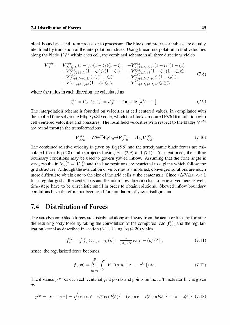
7.4 Distribution of Forces 49
block boundaries and from processor to processor. The block and processor indices are equallyidentified by truncation of the interpolation indices. Using linear interpolation to find velocitiesalong the blade V rθz
j within each cell, the combined scheme in all three directions yields
V rθzj = V rθz
Ir,Iθ ,Iz(1− ζr)(1− ζθ)(1− ζz) +V rθz
Ir+1,Iθ ,Izζr(1− ζθ)(1− ζz)
+V rθzIr,Iθ+1,Iz
(1− ζr)ζθ(1− ζz) +V rθzIr,Iθ,Iz+1(1− ζr)(1− ζθ)ζz
+V rθzIr+1,Iθ+1,Iz
ζrζθ(1− ζz) +V rθzIr+1,Iθ ,Iz+1ζr(1− ζθ)ζz
+V rθzIr,Iθ+1,Iz+1(1− ζr)ζθζz +V rθz
Ir+1,Iθ+1,Iz+1ζrζθζz,
(7.8)
where the ratios in each direction are calculated as
ζiBj = (ζr, ζθ, ζz) = J
iBj − Truncate
[
JiBj − ε
]
. (7.9)
The interpolation scheme is founded on velocities at cell centered values, in compliance withthe applied flow solver the EllipSys3D code, which is a block structured FVM formulation withcell-centered velocities and pressures. The local field velocities with respect to the blades V stn
j
are found through the transformations
V stnj,iB
= BΘT ΦtΦyΘVrθzj,iB
= AiBVrθzj,iB
. (7.10)
The combined relative velocity is given by Eq.(5.5) and the aerodynamic blade forces are cal-culated from Eq.(2.8) and reprojected using Eqs.(2.9) and (7.1). As mentioned, the inflowboundary conditions may be used to govern yawed inflow. Assuming that the cone angle iszero, results in V stn
iB= V rθz
iBand the line positions are restricted to a plane which follow the
grid structure. Although the evaluation of velocities is simplified, converged solutions are muchmore difficult to obtain due to the size of the grid cells at the center axis. Since r∆θ/∆z << 1for a regular grid at the center axis and the main flow direction has to be resolved here as well,time-steps have to be unrealistic small in order to obtain solutions. Skewed inflow boundaryconditions have therefore not been used for simulation of yaw misalignment.
7.4 Distribution of ForcesThe aerodynamic blade forces are distributed along and away from the actuator lines by formingthe resulting body force by taking the convolution of the computed load f iB
rθz and the regular-ization kernel as described in section (3.1). Using Eq.(4.20) yields,
f iBε = f iB
rθz ⊗ ηε , ηε (p) =1
ε3π3/2exp
[
− (p/ε)2] , (7.11)
hence, the regularized force becomes
f ε(x) =B∑
iB=1
∫ R
0
F iB(s)ηε
(
|x− seiB |)
ds. (7.12)
The distance piB between cell centered grid points and points on the iB’th actuator line is givenby
piB = |x− seiB | =√
(r cos θ − riBo cos θiB
o )2 + (r sin θ − riBo sin θiB
o )2 + (z − ziBo )2, (7.13)

50 The Actuator Line Model
where (riBo , θ
iBo , z
iBo ) represent line coordinates. The advantages of using the convolution was
explained in section (3.1). However, using the 3D Gaussian smoothing results in inconsistenciesnear the tip region. This may be illustrated by considering an actuator line with constant normalloading. Since the forces are distributed evenly in all three directions, forces are distributedbeyond the limits of the actual tip i.e. in the tip region a constant axially loaded actuator lineis represented by a span wise decreasing regularized force. In relation to investigation of thetip flow behaviour, a 2D Gaussian distribution is proposed where force is distributed in thedirections normal to each line as depicted in figure 7.2. The regularized force then reads
n
y
z
sp
x
t1
θ
Figure 7.2: 2D Gaussian distribution of forces in a plane normal to each actuator line
f iBε = f
iBrθz ⊗ η2D
ε , η2Dε (p) =
1
ε2πexp
[
− (p/ε)2] , (7.14)
where
f ε(x) =
B∑
iB=1
∫ +∞
−∞
∫ +∞
−∞
F iB(s)η2Dε
(
piB)
dndt1ds. (7.15)
The strategy is to apply loading to all grid points having normal points sp on the lines whichmay be identified from the dot product sp = (xxyz − xo) · eiB
xyz. Only at points x where thevalue of sp is within the range 0 ≤ sp ≤ R is applied a regularized loading. The distance piB
between x and sp is found as the normal distance between a point and a straight line as
piB(x) = |(xxyz − xo)× eiBxyz|, (7.16)
where xo = (0, 0, zo) is the position of the root center. With each line having an equidistantresolution with a distance of ∆s between points and Jrot points, the index j is identified bytruncation of sp/∆s and the applied forces at point x is found by linear interpolation from
ζ = sp/∆s− j , F iB(sp) =[
(1− ζ)F iBj + ζF iB
j+1
]
. (7.17)
The same linear interpolation method is also applied to the 1D Gaussian distribution presentedin section (3.1) for the axisymmetric Navier-Stokes method. The proposed 2D distribution is

7.4 Distribution of Forces 51
only slightly more complicated to use than the 3D distribution. There is, however, a priceto pay in terms of the discontinuity in the span wise direction which will produce numericalwiggles in the vicinity of the tip. The wiggles are partly avoided with suitable choice of ε. Adetailed studied of the influence of the parameter ε is presented in Sørensen et al. [58] for theaxisymmetric case, i.e. an actuator disc. Here ε is chosen to be of the order
ε = εi√
(R∆θ)2 + ∆r2 + ∆z2, (7.18)
and 1 . εi . 4.
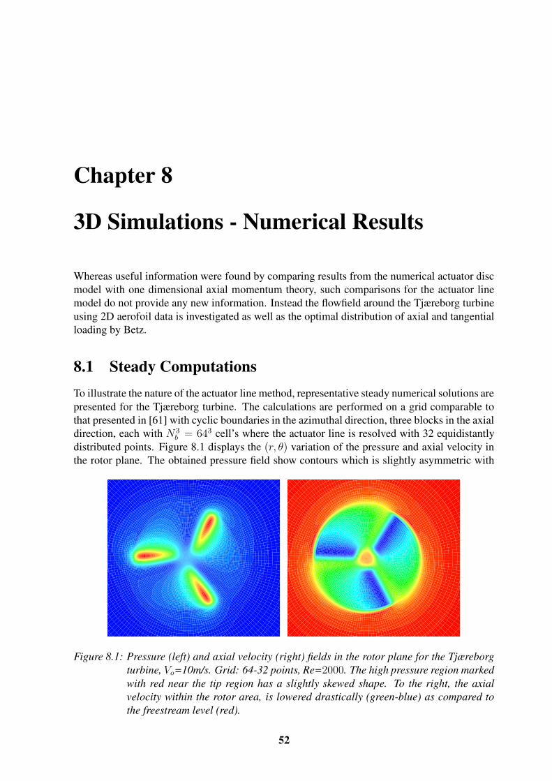
Chapter 8
3D Simulations - Numerical Results
Whereas useful information were found by comparing results from the numerical actuator discmodel with one dimensional axial momentum theory, such comparisons for the actuator linemodel do not provide any new information. Instead the flowfield around the Tjæreborg turbineusing 2D aerofoil data is investigated as well as the optimal distribution of axial and tangentialloading by Betz.
8.1 Steady ComputationsTo illustrate the nature of the actuator line method, representative steady numerical solutions arepresented for the Tjæreborg turbine. The calculations are performed on a grid comparable tothat presented in [61] with cyclic boundaries in the azimuthal direction, three blocks in the axialdirection, each with N 3
b = 643 cell’s where the actuator line is resolved with 32 equidistantlydistributed points. Figure 8.1 displays the (r, θ) variation of the pressure and axial velocity inthe rotor plane. The obtained pressure field show contours which is slightly asymmetric with
Figure 8.1: Pressure (left) and axial velocity (right) fields in the rotor plane for the Tjæreborgturbine, Vo=10m/s. Grid: 64-32 points, Re=2000. The high pressure region markedwith red near the tip region has a slightly skewed shape. To the right, the axialvelocity within the rotor area, is lowered drastically (green-blue) as compared tothe freestream level (red).
52

8.1 Steady Computations 53
respect to the actuator lines and for the axial velocity the contours show a sharp change near thelines. The observed fields were anticipated, however, the full three dimensional behaviour ofthe flowfield through the rotor is illustrated even better by displaying the shed vorticity from theblades, as shown in figure 8.2. The distinct vortex structures are preserved about 1R downstream
Figure 8.2: Vorticity in the rotor plane (left) and the wake vorticity structure shed from blade tipfor the Tjæreborg turbine, Vo=10m/s. High and low pressure regions are markedwith a red and blue contour surface infront and behind each line. Grid: 64-32points, Re=2000
where after they smear out into a continuous vorticity sheet. The structures may be preservedeven further but are smeared mainly due to grid stretching but also due to viscous diffusion. Theexpected expansion is also visual from figure 8.2 (right) as well as the high and low pressureregions marked with a red and blue contour surface infront and behind each line. The pressureregions represent in detail the usual pressure jump known from actuator disc methods.
8.1.1 2D-3D Regularization and Tip CorrectionCalculated loadings along the lines, using the different smearing strategies discussed previ-ously, are presented in figure 8.3. As mentioned earlier, tip correction should not be applied inconnection with the actuator line concept, however, here the influence of the 2D and 3D regu-larization method is tested with and without the Prandtl tip correction. The 3D regularizationwithout Prandtl correction, is seen to give a loading that increases all the way to the tip whichis in contradiction to an expected continuous decreasing trend near the tip. The behaviour wasexplained in the previous chapter as the effect of smeared loading which extends beyond thetip and thereby alters the original spanwise loading. The 2D approach better agrees with theauthors intuition that the forces should be distributed away from the lines only in the plane nor-mal to the line. Applying the 2D approach results in a better trend near the tip, however, whencomparing with results obtained with the generalized actuator disc method nearly the same re-sults are found when the Prandtl tip correction factor is included. From the comparison it mayseem obvious to include the Prandtl tip correction but since the purpose of the correction is tocompensate for finite number of blades, it is inconsistent to include it as the number of bladesare naturally represented by the method. Accordingly, it is chosen that the Prandtl tip correctionnot be included in the forthcoming results presented with the actuator line.

54 3D Simulations - Numerical Results
0.0 0.5 1.0r/R
0.0
0.2
0.4
0.6
0.8
Load
ing
F z/ρV
o2 RAL-2DAL-2D w.PrandtlAL-3DAD with Prandtl
Figure 8.3: Axial loading Fz for the Tjæreborg turbine, Vo=10m/s. Grid: 64-32 points,Re=2000, εi = 2
8.1.2 Simulation of the TjæreborgThe local axial interference factor and loading displayed in figure 8.4 are compared with resultsobtained with the axisymmetric actuator disc model. It should be noted that the induction fromthe actuator disc is the circumferential averaged induction. Although the resolution is betterfor the actuator disc computations, the results generally compares well. The discrepancy in
0.0 0.5 1.0s/R
-0.1
0.0
0.1
0.2
0.3
0.4
ADALa n
0 10 20 30R[m]
0.0
1.0
2.0
3.0
Load
ing[
kN/m
]
ADAL
Figure 8.4: Normal interference an (left) and loading Fn (right) for the Tjæreborg turbine,Vo=10m/s, β = 0o. Grid: 64-32 points, Re=2000
the tip region for the normal loading was addressed previously and is reflected in the obtainedinterference factor, figure 8.4 (left), which explains the differences between the to computations.The influence of the Reynolds number show similar tendencies for the two methods although theactuator line method needs a lowering in Reynolds number in order to get good convergence.A Reynolds number of Re=2000 is chosen for the presented results. The power and CP , CT
curve (not shown) compares well with the actuator disc results but with some differences whichis mainly attributed to the tip correction. An overall evaluation of the presented figures doesleave the impression that a far more complicated method is not more accurate as compared with

8.2 The Coned Rotor 55
simpler methods. The accuracy of the actuator line model is addressed in more detail later.
8.2 The Coned RotorAlthough the generalized actuator disc is able to handle coning, it is interesting to compare witha fully three dimensional analysis. Figure 8.5 depicts the vorticity contours shed from bladesfor a downstream coned rotor β = −20o (left) and an upstream coned rotor β = +20o (right).The high and low pressure regions marked with a red and blue contour surfaces, respectively,
Figure 8.5: Vorticity contours shed from blades for the Tjæreborg turbine, Vo=10m/s, β = −20o
(left) and β = +20o (right). High and low pressure regions are marked with a redand blue contour surface, Grid: 64-32 points, Re=2000
together with the vorticity contours give a clear impression of the flowfield through the conedrotor. Looking at the induction in figure 8.6 the trends compare, but the actuator line inductionis local. Correspondingly, the normal loading, figure 8.6 (right) show resemblance between the
0.0 0.5 1.0s/R
-0.1
0.0
0.1
0.2
0.3
0.4
+20o AD-20o AD+20o AL-20o AL
a n
0 10 20 30R[m]
0.0
1.0
2.0
3.0
Load
ing[
kN/m
]
-20o AD+20o AD-20o AL+20o AL
Figure 8.6: Normal interference an (left) and loading Fn (right) for the Tjæreborg turbine,Vo=10m/s, β = ±20o, Grid: 64-32 points, Re=2000
two methods. The constant normal loaded rotor was analyzed in detail using the actuator disc

56 3D Simulations - Numerical Results
method, but as stated earlier the same analysis with a fully three dimensional method does notprovide any new information. And as expected, the actuator disc method provides adequateinsight to the behaviour of real turbines exposed to coning.
8.3 The Yawed Rotor
Three dimensional methods have now for some time been used to investigate skewed inflowfor some time on helicopter rotors. Vortex or panel methods are are generally the first choiceamong researchers and designers (see Miller [41], Simoes and Graham [50], Bareiss et al. [1] orVoutsinas et al. [68]), but techniques like the asymptotic acceleration potential method by vanHolten [66], adapted by van Bussel [65] to cope with flows about wind turbines, have also beenused to analyze skewed inflow. The actuator line concept naturally facilitates yaw analysis (seeMikkelsen et al.[39], although no results were included) and in general 3D unsteady behaviour.Here the Tjæreborg turbine is exposed to yawed inflow for the same conditions as presented forthe actuator disc using the sub models presented in appendix B. As a tradeoff between necessarycomputing time and resolution results in a grid composed by 9x483 ≈ 106 cells with 3 blocks inaxial and 3 blocks in circumferential direction. Each rotor blade is represented by 20 spanwisepoints. As discussed in section 7.2 yawed inflow in connection with 3D Navier-Stokes methodsmay be approached in two ways, either by setting inflow boundary conditions or by yawingthe rotor relative to the inflow direction which is chosen parallel to the z-axis. Initial tests toobtain numerical results by changing inflow boundary conditions did not give reliable solutionsnear the center axis. Furthermore convergence was bad with respect to velocity and pressureresiduals. The main problem with controlling yawed inflow through boundary conditions is thedegenerated grid cells at the center axis in the circumferential direction. Due to the polar gridstructure the cells are extremely small in the circumferential direction and therefore sensitiveto large cross flow components. It may be compensated for by using corresponding small timesteps in order to obtain a reasonable CFL number (see Hirsch[27]), but as 3D methods in generalare costly in computing time this is not an option. Therefore the lines are chosen to move ina fixed frame. Using the above grid and time steps of the order where the tip needs about 2-4time steps to pass through each cell, a converged solution with a fully developed wake maybe obtained with about 15000 time steps. Using one processor for each block on a SUN Fire6800 machine, one computations takes in the order of 10-14 days. Referring to the yawedinflow conditions presented in table 5.1, figure 8.7 displays the wake vorticity structures forφy = −3 (left) and φy = +32 (right). The vorticity level is chosen arbitrarily to give a goodvisual impact of the flow through the rotor and the flow around the tower. At φy = −3o thetip vorticity contours are fairly symmetrical although the tower wake disturbs the lower region.At φy = +32o, however, the wake region is clearly skewed and from the top and bottom of therotor two large vortex structures are formed in the far wake. The two structures are equivalentto the well known wake behind a regular aeroplane wing, but will be even more visual at higheryaw angles. Figure 8.8 shows the calculated flap wise bending moment, Eq.(B.28), at the rootsection, compared with measurements and actuator disc computations. The general behaviourof the flap wise bending moment reveals an overall good prediction for the two yaw angles usingboth method. A slight phase shift is observed at the low point after the tower for φy = −3o ascompared with experimental measurements. At φy = +32o the actuator line predicts slightlylower values than the corresponding actuator disc computation. Figure 8.9 displays the flowfield

8.3 The Yawed Rotor 57
Figure 8.7: Tip vorticity contours from the Tjæreborg turbine, φy = −3o (left) and φy = +32o
(right). Grid: 48-20 points, Re=2000
0 90 180 270 360Angular position[deg]
300
400
500
600
700
Flap
wis
e M
omen
t[kN
m]
Exp.Actuator DiscActuator Line
0 90 180 270 360Angular position [deg]
300
400
500
600
700
Flap
wis
e M
omen
t [kN
m]
Exp.Actuator DiscActuator Line
Figure 8.8: Flap wise bending moment at the root section (r=2.75) for the Tjæreborg turbine,φy = −3o (left) and φy = +32o (right). Grid: 48-20 points, Re=2000
at high yaw angles, φy = −51o (left) and φy = +54o (right). The wake region is clearly skewedin both cases with a complex structure on a local scale, however, with the two main vortexstructures shed from the rotor top and bottom in the far wake. The computed structural loadsare presented in figure 8.10 for the high yaw angles. For φy = −51o the obtained variationscapture the main behaviour as compared to experiments but no real improvement is found usingthe actuator line technique, which is seen to predict a somewhat lower level than the actuatordisc computations. In fact, the actuator disc simulations appears to give a better prediction thanthe actuator line. However, at φy = +54o the actuator disc over predicts by up to 30% forthe main part, whereas the actuator line model generally is lower and displays better trends ascompared with experiments. In [47] some discussion were addressed to the influence of theroot vortex which is visible as a ’bump’ in the experimental curve beginning at θ ' 160o. Thetrend is not present in the actuator disc computations but visible and somewhat exaggeratedusing the actuator line method. Similar observations were found using 3D free vortex wakemethods [47]. Figure 8.11 shows vorticity contours for φy = +54o seen from below (right)

58 3D Simulations - Numerical Results
Figure 8.9: Tip vorticity contours from the Tjæreborg turbine, φy = −51o (left) and φy = +54o
(right). Grid: 48-20 points, Re=2000
0 90 180 270 360Angular position [deg]
300
400
500
600
700
Flap
wis
e M
omen
t [kN
m]
Exp.Actuator DiscActuator Line
0 90 180 270 360Angular position [deg]
200
300
400
500
600
Flap
wis
e M
omen
t [kN
m]
Exp.Actuator DiscActuator Line
Figure 8.10: Flap wise moment at the root section for the Tjæreborg turbine, φy = −51o (left)and φy = +54o (right). Grid: 48-20 points, Re=2000
and infront (left). As mentioned, the wake region captured by the numerical solution tends toform two vortical structures shed from the top and bottom of highly yawed rotors, which is inaccordance with the flowfield known from a wing section. Øye [75] uses skewed vortex ringsdistributed in the wake which in the extreme case of φy = 90o yaw produces the well knowndownwash from an elliptic wing. The skew angle χ of the wake, which serves as an importantparameter in many yaw models combined with BEM methods, is seen from below in figure 8.11(right) but it is difficult to give a unique interpretation of χ from the calculated flowfield. Seenon the figures are also the shed vorticity from the tower. Although the tower wake resemblesthe flowfield abaft a cylinder, the near field is not sufficient modelled with a static actuator lineapplied with drag forces. As the blade lines passes the tower line, the potential flow solutionaround a cylinder is included into the local velocity projection.

8.4 Tunnel Blockage 59
Figure 8.11: Vorticity contours for the Tjæreborg turbine, φy = +54o, front view (left) and frombelow (right).
8.3.1 DiscussionThe actuator line method combined with sub models includes the full 3D behaviour of the flowthrough a yawed wind turbine rotor. The performance at low yaw angles are equivalent to ax-isymmetric aerodynamic methods, however, at the high yaw angles local trends in calculatedstructural loading, revealed a better resemblance at φy = +54o with experiments than corres-ponding actuator disc simulations. The 3D behaviour of the complex wake structure is fullycaptured by the 3D Navier-Stokes solver, as well as local variations with respect to tower ef-fects and aerodynamic loading. Some limitations in the accuracy can be referred to insufficientstructural modelling and modelling of wind shear. Wind shear should in a future implemen-tation be included naturally by using a Cartesian frame of reference rather than a polar. Thestructural modelling were limited to the blades (with some assumptions) but other componentsshould also be included, like the movement of the tower. For the present computations thegrid resolution were limited to 9 blocks with 48-20 points by the available computing capacity,but the sensitivity to grid resolution, Reynolds number and smearing of the force all have aninfluence which is addressed in detail later in connection with a tip correction study.
8.4 Tunnel BlockageTunnel blockage was treated earlier using the actuator disc method. The actuator line methodfacilitates investigations of rotors inserted into a tunnel to give new insight in the 3D behaviourof the flow. The effects of tunnel walls may be included using the no-slip condition but herea simple symmetry condition is used on the wall boundary equivalent to a slip condition. Thepresent investigation is included in order to display the capabilities of the method and com-pare with actuator disc computations. Thus, the investigation is limited to a single case whereRtun/Rrot = 2.5 for the Tjæreborg turbine at Vo = 10m/s. The steady computation are per-formed on a grid equivalent to the one used for coned rotors adjusted in the radial direction tofit the tunnel aspect ratio. Figure 8.12 displays vorticity and high and low pressure contours.Whereas the vorticity field has a preserved nature the pressure contours are "reflected" on thewall thereby revealing a permanent static pressure drop across the rotor, in good accordance

60 3D Simulations - Numerical Results
Figure 8.12: Vorticity and pressure contours from the Tjæreborg turbine inserted into a tunnelRtun/Rrot = 2.5, Vo = 10m/s.
with actuator disc computations. The obtained force and velocity distribution are depicted infigure 8.13 compared with the actuator disc. In spite of the coarse resolution of the actuator line
0.0 0.5 1.0r/R
0.6
0.7
0.8
0.9
1.0
1.1
Vz/V
o
ALAL, TunnelADAD, Tunnel
2.5
∞
Rtun/Rrot
0.0 0.5 1.0r/R
0.0
0.2
0.4
0.6
0.8
F z/ρV
o2 R
ALAL, TunnelADAD, Tunnel
2.5
∞
Rtun/Rrot
Figure 8.13: Axial Velocity (left) and force (right) distribution for the Rtun/Rrot = 2.5, Vo =10m/s.
computations the trends resemble the axisymmetric predictions excellent. The main differenceis attributed to the tip loading as seen on figure 8.13 (right).

Part D
Miscellaneous Investigations
61

Chapter 9
The Heavily Loaded Actuator Disc
The non-linear heavily loaded actuator disc by Wu is investigated. The formulation resemblesthe generalized actuator disc presented previously in many ways. The motivation for investi-gating the actuator disc by Wu is to develop a fast method where the entire wake is distributedwithout solving transport equations, however, preserving a finite difference approach.
9.1 A Distributed Wake Method
In the wake abaft an actuator disc, the angular momentum varies along a stream tube at a rateproportional to the moment of the tangential force. This result is used in the following todevelop an actuator disc model where the tangential velocity is distributed in the wake com-bined with solution of the Possion equation (3.4) but with the right hand side derived by Wu[71], Eq.(A.51). The deduction given by Wu is presented in Appendix A.6. Restating the twogoverning equations, the axisymmetric, incompressible and inviscid flowfield around a heavilyloaded actuator disc are governed by
∂
∂s(rVθ) =
rf ′
θ
Vs
⇒ rVθ = f(Ψ) in the wake, rVθ = 0 elsewhere (9.1)
∂2Ψ
∂r2− 1
r
∂Ψ
∂r+∂2Ψ
∂z2= (Ωr2 − rVθ)
∂
∂Ψ(rVθ)−
rf ′
Ψ
Vs
, (9.2)
where f ′
Ψ = (Vzf′
r − Vrf′
z)/Vs and s refers to the stream wise coordinate in the axisymmetricplane i.e. s ⊥ Ψ. Since rVθ is preserved along each stream tube passing through the disc it maybe distributed in the wake, hence, for each stream function level in the wake the circulation iscopied from the equivalent stream function level on the disc.
9.1.1 Numerical Method
Assuming that the flow is governed by the incompressible, inviscid Euler equations, the tangen-tial momentum equation is restated from Eq.(A.24) as
∂
∂r(VrVθ) +
∂
∂z(VzVθ) +
2VrVθ
r= f ′
θ, (9.3)
62
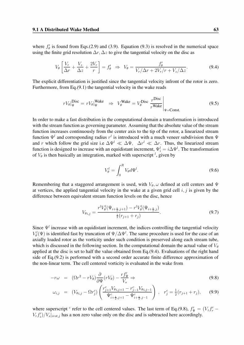
9.1 A Distributed Wake Method 63
where f ′
θ is found from Eqs.(2.9) and (3.9). Equation (9.3) is resolved in the numerical spaceusing the finite grid resolution ∆r,∆z to give the tangential velocity on the disc as
Vθ
[
Vr
∆r+Vz
∆z+
2Vr
r
]
= f ′
θ ⇒ Vθ =f ′
θ
Vr/∆r + 2Vr/r + Vz/∆z. (9.4)
The explicit differentiation is justified since the tangential velocity infront of the rotor is zero.Furthermore, from Eq.(9.1) the tangential velocity in the wake reads
rVθ|DiscΨ = rVθ|Wake
Ψ ⇒ V Wakeθ = V Disc
θ
rDisc
rWake
∣
∣
∣
∣
∣
Ψ=Const.
(9.5)
In order to make a fast distribution in the computational domain a transformation is introducedwith the stream function as governing parameter. Assuming that the absolute value of the streamfunction increases continuously from the center axis to the tip of the rotor, a linearized streamfunction Ψl and corresponding radius rl is introduced with a much veneer subdivision then Ψand r which follow the grid size i.e ∆Ψl ∆Ψ, ∆rl ∆r. Thus, the linearized streamfunction is designed to increase with an equidistant increment, Ψl
i = i∆Ψl. The transformationof Vθ is then basically an integration, marked with superscript l, given by
V lθ =
∫ R
0
VθdΨl. (9.6)
Remembering that a staggered arrangement is used, with Vθ, ω defined at cell centers and Ψat vertices, the applied tangential velocity in the wake at a given grid cell i, j is given by thedifference between equivalent stream function levels on the disc, hence
Vθi,j =rlV l
θ (Ψi+ 12 ,j+1)− rlV l
θ (Ψi+ 12 ,j)
12 (rj+1 + rj)
. (9.7)
Since Ψl increase with an equidistant increment, the indices controlling the tangential velocityV l
θ (Ψ) is identified fast by truncation of Ψ/∆Ψl. The same procedure is used for the case of anaxially loaded rotor as the vorticity under such condition is preserved along each stream tube,which is discussed in the following section. In the computational domain the actual value of Vθ
applied at the disc is set to half the value obtained from Eq.(9.4). Evaluations of the right handside of Eq.(9.2) is performed with a second order accurate finite difference approximation ofthe non-linear term. The cell centered vorticity is evaluated in the wake from
−rω = (Ωr2 − rVθ)∂
∂Ψ(rVθ)−
rf ′
Ψ
Vs⇒ (9.8)
ωi,j = (Vθi,j − Ωrcj)
(
rcj+1Vθi,j+1 − rc
j−1Vθi,j−1
Ψci+ 1
2 ,j+1−Ψc
i+ 12 ,j−1
)
, rcj =
1
2(rj+1 + rj), (9.9)
where superscript c refer to the cell centered values. The last term of Eq.(9.8), f ′
Ψ = (Vzf′
r −Vrf
′
z)/Vs|irot,j has a non zero value only on the disc and is subtracted here accordingly.

64 The Heavily Loaded Actuator Disc
9.1.2 The Axially Loaded Rotor - Constant Loading
For an axially loaded rotor Vθ → 0, Ω→∞ and ΩVθ → constant. From Eq.(A.41) with f ′
r = 0the r and z component reduces to
∂H
∂r= −Vzω,
∂H
∂z= f ′
z + Vrω, (9.10)
where H = p/ρ + 12V
2 is the pressure head. By cross differentiation of Eq.(9.10) the inviscidvorticity transport equation is obtained
∂f ′
z
∂r+
∂
∂r(Vrω) +
∂
∂z(Vzω) =
∂f ′
z
∂r+ Vr
∂ω
∂r+ Vz
∂ω
∂z+ ω
(
∂Vr
∂r+∂Vz
∂z
)
= 0, (9.11)
where the expanded non-linear terms in the last bracket is reduced by using the continuityequation
∂rVr
∂r+∂rVz
∂z= 0, ⇒ ∂Vr
∂r+∂Vz
∂z= −Vr
r. (9.12)
Thereby Eq.(9.11) is reduced to
∂f ′
z
∂r+ Vr
∂ω
∂r+ Vz
∂ω
∂z− ωVr
r= ⇒ ∂f ′
z
∂r+ rVr
∂
∂r
(ω
r
)
+ Vz∂ω
∂z= 0. (9.13)
Utilizing the s-transform, Eq.(A.43) gives the results
∂f ′
z
∂r+ rVs
∂
∂s
(ω
r
)
= 0 ⇒ ∂
∂s
(ω
r
)
= − 1
rVs
∂f ′
z
∂r, (9.14)
however, in the wake where there are no forces the vorticity is preserved as
∂
∂s
(ω
r
)
= 0. (9.15)
This shows that the vorticity produced on the rotor disc divided with the local radius remainsconstant along a stream surface. Recalling figure 3.2 the vorticity produced on the edge of thedisc was clearly preserved along the streamline passing through the edge. The same methodapplied to Eq.(9.1) is used for Eq.(9.15) to distribute vorticity in the wake where the superscriptl refers to transformed values using Ψl. Figure 9.1 displays a schematic view of a point sourceat the tip of the rotor disc. The integration ensures a unique relation between the producedvorticity on the disc and the trailing vortices in the wake. The vorticity applied at cell i, j issimply found as the difference between two integrated vorticity levels as
ωi,j = rcj
[
ωl
rl(Ψi+ 1
2 ,j+1)−ωl
rl(Ψi+ 1
2 ,j)
]
, rcj =
1
2(rj+1 + rj). (9.16)
and since Ψl increases with an equidistant increment ωl(Ψ) may be identified by truncation ofΨ/∆Ψl.

9.2 Numerical Results - The Axially Loaded Rotor 65
ω
i
j
Disc
r=1
ωl=∫ R
0ωdΨl
Ψi+ 12 ,j−1
Ψi+ 12,j
Ψi+ 12,j+1
ωi,j
Wake
Figure 9.1: Scheme for distribution of vorticity in the wake
9.2 Numerical Results - The Axially Loaded RotorConsidering the method of distributing vorticity as just presented, the vorticity on the disc forthe constant loaded rotor disc with no rotation is evaluated from
∂
∂r(Vrω) +
∂
∂z(Vzω) = −∂f
′
z
∂r, (9.17)
since Vθ = 0. Applying explicit numerical differentiation of Eq.(9.17), since ω = 0 infront ofthe disc, gives that the vorticity on the disc equals
ω = − 1
Vr/∆r + Vz/∆z
∂f ′
z
∂r(9.18)
where the only non-zero value is at the tip. Here ∆r,∆z are the finite grid resolution of the discand Vr, Vz are the cell-centered velocities through the tip. Applying the (B)-grid from section3.2.2, figure 9.2 shows the distributed vorticity source (CT = 0.8) from the tip which in thewake is divided on no more than two grid cells in the radial direction. The solution resembles
Figure 9.2: Tip-vorticity and Streamlines for a constantly loaded rotor disc, CT = 0.8. The discis inferred as a straight line
the solution displayed in figure 3.2 perfectly with the expanding wake region. Again, the disc is

66 The Heavily Loaded Actuator Disc
inferred as a straight line. The axial interference factor shown in figure 9.3 depicts a continuoustrend with increasing thrust coefficient. In the tip region the profiles change towards a peak withincreasing CT , in accordance with results obtained previously and by Sørensen et al.[58]. The
0.0 0.5 1.0 1.5r/R
0.0
0.1
0.2
0.3
0.4
a0.20.40.60.8
CT
Figure 9.3: Axial interference factor a for CT = 0.2− 0.8.
integrated kinetic power coefficient for CT = 0.2 − 0.8 is presented in table 9.1 and the ob-served results are in excellent agreement with axial momentum theory. The method, however,
CT 0.2 0.4 0.6 0.8Momentum theory 0.189 0.355 0.490 0.579CP , distributed ω 0.190 0.357 0.496 0.586
Table 9.1: Power coefficient for a constant loaded actuator disc at CT = 0.2 − 0.8. The rotordisc resolved with 41 grid points.
has a limitation with respect to an upper limit on CT h 0.8, after which converged solutionsare difficult to obtain. The limit compares well with solutions obtained solving the differen-tial transport equations presented in section (3.1). However, instead of diverging, solving thetransport equations results in unsteady solutions within the range 0.89 . CT . 1.15, depend-ing upon the Reynolds number. At higher CT values separated regions begin to form behindthe disc, thus the parabolized formulation begins to lose validity. Comparing the computationaleffort used to obtain solution with the two formulations both methods involve solution of thePossion equation. Solving the differential transport equation requires about half the effort ofsolving the Possion equation, whereas the method of distributing the wake is of no importancefor the total computing time.
9.3 Distributed Wake Method - Numerical ResultsWhen Wu presented his (landmark) paper numerical results were not included and to theauthors knowledge numerical result for the heavily loaded actuator disc using nonlinear theorywas first presented by Greenberg [22]. Streamlines for some representative loadings andthe case of CT → ∞ were presented by Greenberg [22], along with profiles for the axial

9.3 Distributed Wake Method - Numerical Results 67
velocity distribution. Here the technique of distributing the wake as presented in section (9.1)is considered for the 2MW Tjæreborg turbine. The distributed circulation field is displayedin figure 9.4 at a freestream velocity of Vo = 12m/s corresponding to a tip speed ratio ofλo = ΩR/Vo = 5.89. It is observed that on the disc the applied tangential momentum is half
Figure 9.4: Wake distribution of circulation rVθ, for the Tjæreborg turbine, Vo = 12m/s
the value applied in the wake. Evaluating Eq.(9.9) results in the vorticity field shown to the leftof figure 9.5, which extends no further than the tangential velocity field in the radial direction.Figure 9.5 right, depicts the equivalent vorticity field including effects of diffusion. Comparing
Figure 9.5: Vorticity distribution for the Tjæreborg turbine, Vo = 12m/s, distributed method(left) and solving the vorticity transport equation(right) where effect of diffusion isevident
the obtained a and λ2a′ distributions using the two methods, figure 9.6 displays an increasingdifference towards the tip for a, but a far better agreement for λ2a′. Here the local tip speed ratiois defined as λ = Ωr
Vo. Included into the plots are also a prediction computed with a "standard"
BEM method which for a compares better with solving the transport equations (Ψ − ω). Forλ2a′, however, a nearly perfect match between BEM and the distributed wake method is found.Obtained force distribution presented in figure 9.7 reveals increasing deviation near the tipbetween distributed wake method and the two other methods. Both the axial and tangentialforce distribution as well as the integrated thrust and torque, compares extremely well between

68 The Heavily Loaded Actuator Disc
0 0.5 1
0
0.1
0.2
0.3
0.4
r/R
a
PresentΨ−ωBEM
0 0.5 1
0
0.1
0.2
0.3
0.4
r/R
λ2 a′
PresentΨ−ωBEM
Figure 9.6: Axial interference a (left) and λ2a′ (right), Tjæreborg Vo = 12m/s, using BEM, thepresent distribution method and solving transport equations
0 0.5 10
0.25
0.5
0.75
r/R
F z, Fθ/ρ
V2 R
PresentΨ−ωBEM
Figure 9.7: Normalized axial and tangential force distribution, Tjæreborg Vo = 12m/s, usingBEM, the present distribution method and solving transport equations
the BEM method and (Ψ− ω).
Reviewing the result presented for the constant loaded rotor disc the method of distributing thewake is seen to have comparable accuracy to the method of solving transport equations for CT
values up to 0.8. It would have been preferable to compare the accuracy of first distributingthe tangential velocity and then evaluating the right hand side of Eq.(9.2) with an analyticalsolution. However, the compared results for the Tjæreborg turbine at Vo = 12m/s togetherwith simulation at other wind speeds (not shown) gives the clear impression that the method isless accurate than the implicit numerical formulation of the transport equations. Whether themethod can be improved using numerical evaluations of higher order, has not been tested.
The two methods, which resembles each other in many ways, has comparable numerical conver-gence rate, although the method of distributing the wake is slightly faster. At the beginning ofthe study the idea of parabolizing the transport equations discussed in the previous section, had

9.3 Distributed Wake Method - Numerical Results 69
not emerged, and as they were solved with a time consuming numerical scheme where hugetime steps not were possible, the potential of distributing the wake was evident. If a choicewere to be made between which method to use, the stability qualities and higher accuracy ofthe (Ψ− ω) formulation would be determining. Furthermore, whereas the method of distribut-ing the wake has the limitations of finding steady solutions, the unsteady (Ψ− ω) formulationfacilitates investigations of the dynamic behaviour of the developing wake.

Chapter 10
The Influence of Pressure Forces
Given the accuracy, presented in the previous chapters, of the axisymmetric Navier-Stokes for-mulation, the method facilitates investigations of certain basic assumptions, which form thefoundation of BEM methods. Local variations are available as well as the global flow be-haviour. The influence of the pressure field near the actuator disc is not taken into account inaxial momentum balance, which is investigated in the following. As BEM methods are basedon what happens far up- and downstream the rotor, effects of the local pressure field is ne-glected in contrast to the Navier-Stokes formulation, where the entire axisymmetric flowfield isdetermined.
10.1 Expanding Stream TubesSome of the basic assumptions behind BEM methods are to a certain degree incorrect, whichGlauert [19] in his original work addressed explicitly. These unverified basic assumptions maybe summarized as
• The flow can be divided into independent annular stream tubes
• The pressure in the ultimate wake equals the pressure far upstream
• The induced velocity in the rotor plane is equal to one half the induced velocity in the farwake
• Axial momentum theory can be applied in differential form, neglecting the resulting axialforce of the pressure acting on the lateral boundaries of the stream tube
• Conservation of circulation can be ignored
The influence of pressure forces acting on the expanding stream tubes lead to the investigationpresented by Sørensen and Mikkelsen [60] where the validity of the axial momentum theorywas discussed, which is presented in the following. Returning to the unverified assumptionsGoorjian [20] proved, in a technical note, that applying the equation of axial momentum ina simple differential form, is incorrect when the pressure acting on the lateral boundaries ofthe stream tubes is neglected. In most cases the inaccuracies display only negligible influenceon the results when using a BEM technique, however, it is important to quantify the impactof the inconsistencies. Figure 10.1 depicts a stream surface through an actuator disc, with
70

10.1 Expanding Stream Tubes 71
u
∆T
p
p−p+
Vo u1
Figure 10.1: Stream tube through rotor with surface pressure acting on the control volume
the contributions from stream surface pressures acting on the control volume. As the loadingincreases the stream surfaces expands, causing a projected area normal to the rotor. Consideringthe axial momentum balance of a control volume with an axial loading ∆T on the rotor, the freestream conditions far upstream read p = po, Vo = V∞ and u1, p1 far downstream. The inviscidaxial momentum balance for the control volume then reads
∆T = ∆m(Vo − u1) + ∆X, (10.1)
where ∆m = ρu∆AD is the mass flow and the contribution from the pressure forces, ∆X ,is determined by integrating the pressure along each stream surface projected onto the axialdirection as,
∆X =
∫
cs
pdS · ex. (10.2)
Here dS is a differential stream surface area, ex is the axial unit vector. The local thrust alsoequals ∆T = (p+ − p−)∆A and the kinetic energy converted by the rotor is given by
∆E =1
2∆m(V 2
o − u21) = u∆T, (10.3)
which combined with Eq.(10.1), leads to an equation for the velocity u at the disc
u =1
2(Vo + u1)
(
1− ∆X
∆T
)
. (10.4)
The expression shows that there exist a direct relation between the error committed withRankine-Froude theory and including pressure forces. In order to quantify the error by neglect-ing lateral forces, ∆X , the axisymmetric Navier-Stokes method is applied. As the pressure isabsent at first in the stream function-swirl velocity-vorticity formulation, the pressure field isfound by solving an additional pressure equation (see appendix A.5) based on the computedflowfield, in order to evaluate ∆X . Figure 10.2 displays the computed static pressure field for aconstant loaded actuator disc, CT = 0.8, in an infinite domain. In front of the disc the expectedpressure build up is displayed as red contours and the negative pressure just behind the disc asblue. Towards the tip the pressure tends to zero and in the wake region the change in pressureacross the vortex sheet is barely visible. Numerically, the integration of the pressure forces isevaluated, for distinct stream function levels at the disc Ψirot,j , and along each streamsurface as
PΨ =
∫ +∞
−∞
pdS · ex
∣
∣
∣
∣
Ψ
'n−1∑
i=1
1
2π(pi+1,Ψ + pi,Ψ)(r2
i+1,Ψ − r2i,Ψ) , Ψ = Ψirot,j (10.5)

72 The Influence of Pressure Forces
Vo
r
z
→
→↑Figure 10.2: Static pressure field for a constant loaded actuator disc, CT = 0.8
Figure 10.3 right depicts radial distribution of integrated axial pressure force along each streamsurface for the constant loaded rotor disc, CT = 0.2 − 0.8. As the stream tube surface normalhas opposite direction for the upper and lower side, ∆X s is determined as a simple differencebetween the two sides
∆Xsj = −∆PΨ|Ψj
' −(PΨj+1− PΨj
). (10.6)
Finally, the total axial pressure forces including end contributions amounts to
0.0 0.2 0.4 0.6 0.8 1.0r/R
-10
-8
-6
-4
-2
0
PΨ=∫
pdS
⋅ex⋅1
03
0.20.40.60.8
CT
Figure 10.3: Radial distribution of integrated axial pressure force along each stream surface,CT = 0.2− 0.8
∆Xj = ∆Xsj +
1
2π[(pn,j+1 + pn,j)(r
2n,j+1 − r2
n,j)
−(p1,j+1 + p1,j)(r21,j+1 − r2
1,j)] , r, p|i,j = r, p|i,Ψj(10.7)
Returning to the axial velocity at the disc given by Eq.(10.4), the equations are rearranged andthe following two error quantities introduced
ε1 =u
12 (Vo + u1)
− 1 , ε2 =∆X
∆T. (10.8)

10.1 Expanding Stream Tubes 73
The error quantity ε1 may be evaluated directly from the Navier-Stokes solution for each streamfunction level at the disc and in the far wake, whereas ε2 is found from Eq.(10.7) divided bythe local thrust ∆T . Figure 10.4 shows the distribution of ε1, ε2 for the constant loaded actuatordisc, CT = 0.2, 0.4 (left), CT = 0.6, 0.8 (right). Away form the viscous layer at the tip, the
0.0 0.2 0.4 0.6 0.8 1.0r/R
-6
-4
-2
0
[%]
ε1
ε2
CT=0.4
CT=0.2
0.0 0.2 0.4 0.6 0.8 1.0r/R
-20
-15
-10
-5
0
5
[%]
ε1
ε2
CT=0.8
CT=0.6
Figure 10.4: Distribution of error function along the plane for constant loaded actuator disc,CT = 0.2− 0.8
ε-values are close to zero. For CT = 0.6 the error is less than 1% and for CT = 0.8 the erroramounts to about 2%. The ε-values are seen to match up for the main part of the actuator discarea. Viscous effects at the tip results, however, in some deviations and much higher values.With u1 being evaluated in the far wake the Reynolds number is expected to display someinfluence. Here the Reynolds number is put equal to 50.000 which is relatively low. Thus, inthe vorticity dominated region near the tip u1 depends largely on the axial position. Near thecenter ε2 is difficult to evaluate since PΨ is close to zero. In figure 10.5 the difference betweenthe axial velocity and the corresponding velocity obtained from momentum theory is presented.It is observed that for CT = 0.8 the difference over the most part of the rotor plane is less than
0.0 0.2 0.4 0.6 0.8 1.0r/R
-3
-2
-1
0
1
2
3
[%]
0.80.60.40.2
CT
Figure 10.5: Difference between computed axial velocity and momentum theory along the planefor constant loaded actuator disc, CT = 0.2− 0.8
1.5%, although near the tip differences up to 3% exist. The presented results for the axially

74 The Influence of Pressure Forces
loaded rotor may be extended to the general momentum theory as presented in [60]. With theintroduction of the angular momentum, Eq.(10.4) may be rewritten to
u =1
2(Vo + u1)
(
1− ε21− ε3
)
, ε3 =(p1 − po) + 1
2 ρ(V2θ1 − V 2
θ )
p+ − p− , (10.9)
although, simulations on the Tjæreborg wind turbine revealed that ε3 is negligible. Thecirculation, however, introduces vorticity everywhere in the wake due to the variable loading.Hence, depending on the Reynolds number, the far wake changes considerably resulting inrelative high values of ε1 and ε2. Figure 10.6 shows velocity distributions in the rotor planeand in the far wake, for the Tjæreborg wind turbine at Vo = 10m/s. Included into the figure is
0.0 0.2 0.4 0.6 0.8 1.0r/R
0.0
0.2
0.4
0.6
0.8
1.0
Vz/V
o
Re=5⋅104
BEM
Figure 10.6: Velocity distribution for the Tjæreborg wind turbine at Vo = 10m/s, in the rotorplane and in the far wake
a corresponding BEM calculation which is seen to compare well at the rotor plane but ratherbad in the far wake. The effect due to diffusion, is observed to change the velocity distributioncontinuously in the far wake.
In conclusion it has been shown that the influence of pressure forces may be analyzed in detailwith good accuracy using the numerical actuator disc method. Although there are inherentinconsistencies in the BEM formulation, the errors are found to be negligible.

Chapter 11
Evaluation of Tip Correction
The tip loss effect for air-screws described by Prandtl [43] concerns the ideal rotor of Betz withoptimal circulation on the blades. With the introduction of the BEM method by Glauert [19]for prediction of rotor performance, the analysis of Prandtl was adopted by Glauert. As theBEM method is based on axisymmetric momentum theory, it is inherent that the rotor disc hasinfinite number of blades, but since real rotors have finite number of blades real rotors havetip loss. The Glauert adoption of the Prandtl tip loss factor is generally accepted within theaerodynamic community as providing good accuracy, but as the upcoming analysis will show,some inconsistencies are inherent in the deduced expressions.
11.1 Modified Use of the Prandtl Tip CorrectionTo get realistic values for the performance of propellers Glauert included the tip loss effect intothe BEM method as a correction to the induced velocities or interference factor, see section(4.2.1). The derived expressions for the axial and tangential interference factors by Glauert1 arehere restated as
a
1− a =σCn
4F sin2 φ,
a′
1 + a′=
σCt
4F sinφ cosφ(11.1)
where F is given by Eq.(4.11). In order to satisfy the orthogonality of the induced velocityto the relative velocity, the mass flux is retained without any correction. Furthermore, a con-sequence of the F -function is that when approaching the tip, i.e. when r → R, the axialinterference factor tends to a → 1, hence, the axial velocity is zero. This is inconsistent sincethe applied force is zero at the tip. The refined model by Wilson and Lissaman [70] applies thecorrection to the axial flow using the concept of circulation, but at the expense of the orthogo-nality between the relative and the induced velocity. The further refinement by De Vries [14]included the correction on the mass flux in the tangential momentum equation, however, thevarious models all lack rigorous consistency when the tip is approached. The new method byShen, Mikkelsen, Sørensen and Bak [49] was proposed in order to overcome the inconsistencyat the tip by considering the balance of momenta for a real rotor with finite number of blades,to the real aerodynamic forces. Here the real aerodynamic forces are corrected with a modified
1In [19] the factor F appears above the division line and not below, however, in the axial and tangential mo-mentum equations F is multiplied which, following a rigorous deduction (see Hansen [25]), leads to Eq.(11.1).
75

76 Evaluation of Tip Correction
tip correction factor F1
Crn = F1Cn , Cr
t = F1Ct. (11.2)
which insures that the forces approach zero at the tip. In general, when applying 2D airfoildata, the angle of attack at the tip does not result in zero lift and drag, but physical intuition saysthat the forces should be zero at the tip. The proposed method is mathematically consistent andsolves the problem of zero force at the tip, however, with the introduction of a new functionF1 which needs to be calibrated with experimental results. The outcome of the work presentedin [49] showed some improvements in comparison with experimental results for the NREL[48] rotor. It should be noted that available experimental data generally don’t have sufficientresolution2 in the tip region to make a detailed comparison. The various methods discussed relycompletely on the assumptions behind the Prandtl tip correction and in the different refinementshis F function is more or less considered as a tool used to satisfy certain conditions. Whether ornot the entire shape of the F function by Prandtl represents the actual physics is not an issue. Inthat sense it should not be forgotten that 2D airfoil data are corrected or tuned to match whateverfew experimental results are available and in this process the tip correction function by Prandtlenters the tuning.
11.2 Inverse Computation of the Tip Correction Using theActuator Line Model
The thorough treatments of the tip loss effect conducted by Prandtl, Glauert and Goldsteinare based on assumptions which the proceeding analysis seeks to avoid. Using the actuatorline method and solving the full 3D Navier-Stokes equations, loading is applied in an inversemanner with the results that the tip correction presents it self from the solution.
The keyword here is the free wake which is naturally inherent in the proposed method. Prandtlconsidered a wake structure of helical vortex sheets to be unfolded half infinite planes movingwith the axial induced velocity aVo relative to the freestream velocity. Due to the complexity,the problem was further simplified by considering the system of vortex sheets to be equidistantparallel flat plates with mutual distance d = 2πR/B sinφR where φR is the flow angle at the tip.Based on these assumptions he deduced that the average induced velocity between two vortexsheets is reduced exponentially with the so-called Prandtl’s tip loss factor F , later adopted byGlauert. The exact solution presented by Goldstein [21] to the problem where the wake hasan inviscid screw surface geometry, has the inherent limitation of the fixed wake. The screwsurface wake geometry, which Goldstein states is unstable, of the form
(r, θ, z) = (r,Ωt, V t) or θ − ωz
V= 0 or π , 0 ≤ r ≤ R, (11.3)
where V is the velocity of wake relative to the rotor, furthermore refers to lightly loadedpropellers, hence, as with the Prandtl analysis, expansion is neglected. Although the optimaldistribution results in angular velocities proportional to 1
rand thereby creates a spiraling vortex
2Experimental data obtained by the FFA [5, 46] are among the few which contain good resolution in the tipregion.

11.2 Inverse Computation of the Tip Correction Using the Actuator Line Model 77
with increasing strength towards the center axis, which contradicts the screw surface wakegeometry, the swirl velocity is generally small for the main part of the rotor area. The solutionderived by Goldstein is complicated to use in connection with BEM-formulations and for thisreason rarely adopted.
With respect to the physical interpretation of the tip correction, the F factor derived by Prandtlrepresent a reduction factor which can be interpreted as expressing the fraction between the ve-locity of the trailing vortex sheets to the mean velocity of the fluid between the sheets. Therebythe F factor also represents the ratio between the circumferential averaged induced velocity tothe local on the blade. The sheets applied in Prandtls analysis are half infinite vorticity sheets ata right angle which result in the well known exponential reduction function. Glauert states thatin a corresponding analogy to the trailing vortex sheets from a propeller the F factor must beapplied to the momentum equation. Thus, the corrected axial and angular momentum equationby Glauert are
dT
dr= 4πrρV 2
o (1− a)aF z ,dQ
dr= 4πr3ρVoΩ(1− a)a′F θ, (11.4)
where both equations formulated under the assumption of axial symmetry, include the tiploss factor F = (F z = F θ). As F only appears once in Eq.(11.4) the interpretation of thetip correction factor F appears to be the ratio between the circumferential averaged loadingto the local blade loading i.e. assuming a uniformed induction is desired, which require auniform loading, the loading on the blades must increase towards the tip proportional to 1/Fi.e. 1
FdTdr
= BFz. This interpretation differs from initially stated. The distinction made inEq.(11.4) between the two tip loss factors F z, F θ is made since the two momentum equationsin principle are independent.
Here a method is proposed that seeks to find loadings which corresponds to the optimal rotorof Betz with infinite number of blades, but in principle any distribution could be applied. Thusa selected distribution of the axial induction a, number of blades B and the tip speed ratioλo = ΩR
Vois chosen as reference loading. Rearranging Eq.(11.4) yields that
F z =BFz
4πrρV 2o (1− a)a , F θ =
BFθ
4πr3ρVoΩa′(1− a), (11.5)
where a, a′ are chosen to fulfill conditions for the optimal the rotor with infinite number ofblades and the loading, BFz, BFθ is then found from converged solutions. The conditions aregoverned by the orthogonality criteria of the induced velocity to the relative velocity, here givenby the axial interference factors. Figure 11.1 displays the velocity triangle for a fast runningrotor at the root section and near the tip region. The two figures combines to
tanφ =a′
a
Ωr
Vo=
(1− a)(1 + a′)
Vo
Ωr, ⇒ a′(1 + a′)λ2 = a(1− a) , λ =
Ωr
Vo. (11.6)
Furthermore, the blade loading designed to give a minimum loss of energy E for given thrust T ,is governed by the relation dE = ΩdQ − VodT where Q is the torque, represents the excess ofthe power absorbed by the rotor to the useful work done by the thrust. Thus, the best distribution(see Glauert [19]) of a, a′, B →∞ giving minimum loss of energy is found from
∆(ΩdQ)
∆(VodT )⇒ 1− a
1 + 2a′− a′λ2
1− 2a= C. (11.7)

78 Evaluation of Tip Correction
Ωr ΩrVθVθ
−θz
a′Ωra′Ωr
aVoaVo
VrelVrel
Vo
Vo
φφ
φW
Figure 11.1: Velocity triangle for a fast running rotor near the tip region (right) and root section(left)
Equation (11.7) is solved for a by inserting Eq.(11.6) for a′ and applying a Newton-Raphsonmethod, where the constant C is fixed for a given value of ao and λo at the tip. Figure 11.2displays the radial distribution of a and λ2a′ obtained by solving Eq.(11.7) for ao = 1
10 , 13
and λo = 3, 9. The shape of λ2a′ corresponds to and approaches the level of a(1 − a) with
0 0.25 0.5 0.75 10
0.1
0.2
0.3
0.4
0.5
r/R
a, λ
2 a′
Optimal, a, B→ ∞Optimal, λ2 a′, B→ ∞Ligthly loaded, a=λ2 a′
ao = 110
ao = 13
0 0.25 0.5 0.75 10
0.1
0.2
0.3
0.4
0.5
r/R
a, λ
2 a′
Optimal, a, B→ ∞Optimal, λ2 a′, B→ ∞Ligthly loaded, a=λ2 a′
ao = 110
ao = 13
Figure 11.2: Axial interference a and λ2a′ for ao = 110 , 1
3 and λo = 3 (left) and λo = 9(right),B →∞.
increasing values of λo. As Goldstein [21] neglects effect of expansion the boundary conditionswhich govern lightly loaded rotor reduces to a = αoλ
2/(1 + λ2) = λ2a′ where αo are fixedfor a given value of ao and λo at the tip. The agreement with the optimal distribution of Betz isreasonable good for ao = 1
10 and rather bad for ao = 13 . Here the distribution of Betz is used in
the inverse study of the tip-correction. In order to obtain solutions with the actuator line methodfulfilling the above conditions, the loading is applied iteratively using a relaxation method
F k+1z = F k
z + (a− a)rKz , F k+1θ = F k
θ + (a′ − a′)ΩrKθ (11.8)
where Kz, Kθ represent relaxation parameters and a, a′ are the measured distributions alongthe line for each iteration. The method insures a smooth convergence.

11.3 Numerical sensitivity - The 2 Bladed Rotor 79
The proposed method could be combined with other free wake methods based on first principlessuch as vortex methods. Fixed and free wake methods have been developed where the vorticityis distributed either as vortex line elements (Miller [41], Simoes and Graham [50], Bareiss et al.[1]) or as discrete vortices (Voutsinas et al. [68]). A fixed wake analysis would provide com-parable results to that of Goldstein [21] whereas a free wake analysis would include expansionand the true dynamic behaviour of the wake. Free wake methods tends, however, to divergeowing to intrinsic singularities of the vortex panels in the developing wake.
11.3 Numerical sensitivity - The 2 Bladed Rotor
The numerical validation of the actuator line method presented in Sørensen and Shen [61], wasperformed using LM 19.5 blade data. The blade is shaped with a chord wise distribution thatdecreases continuously towards the tip to a peak, which result in a smooth decreasing loadingat the tip and thereby less influence of the tip vortex. Some rotors, like the Tjæreborg turbine,has a more abrupt ending at the tip, hence producing a much stronger tip vortex. Thus, usingthe actuator line concept on a turbine with a high loading near the tip, results in a much strongeredge singularity at the tip, which is investigated in the following.
In [61] the forces were applied using the 3D-regularization function which smears the forcesequally in all direction, and thereby also in the span wise direction. The 3D-function is notapplicable in relation with a tip-correction study since when applying Eq.(11.8) a span wisesmearing of the loading will results in solutions with peaks near the tip. This may be realizedby considering a constantly loaded actuator line. Using the 3D-function the last point at thetip has less loading than the second point from the tip since each point shears loading withneighbouring points. On a local scale this is inconsistent in the tip region although on a globalscale the total amount of applied force is preserved. The main drawback of using the 2Dapproach is the partly unknown influence of the spanwise singularity at the tip, however, as2D-regularization only smears is in the direction normal to each actuator line, it is chosen forthis analysis.
The two main parameters governing the numerical accuracy of the actuator line methodare regularization parameter ε and grid resolution, as with any numerical method. Applieddiffusion represented by the Reynolds number Re has a minor influence on the solution if theReynolds number is big. The Reynolds number is set to Re=10.000, which in some casesgives an irregular convergence. Ideally forces should be distributed over an area comparable tothe chord distribution and if possible resemble the chord wise pressure distribution. Presentlyrealistic grid resolutions are by far to coarse to resolve the chord wise pressure distributionfor a modern wind turbine blade, however, for rotors with higher solidity, like hydrodynamicpropellers, it should be applied.
Considering a lightly loaded rotor with an optimal distribution for tip-speed-ratios λo = 3, 9and ao = 0.1 at the tip, loading is applied according to Eq.(11.8). The domain extends about10R upstream, 15R downstream and 8R in the radial direction. Figure 11.3 depicts the influ-ence of ε on the average axial interference factor for a grid with 44 equidistantly distributespoints resolving the rotor and 80 points in total in the span wise direction, stretched away from
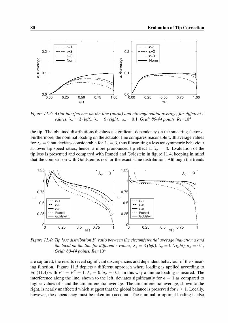
80 Evaluation of Tip Correction
0.00 0.25 0.50 0.75 1.00r/R
0.0
0.1
0.2
a, θ
-ave
rage
ε=1ε=2ε=3Norm
0.00 0.25 0.50 0.75 1.00r/R
0.0
0.1
0.2
a, θ
-ave
rage
ε=1ε=2ε=3Norm
Figure 11.3: Axial interference on the line (norm) and circumferential average, for different εvalues, λo = 3 (left), λo = 9 (right), ao = 0.1, Grid: 80-44 points, Re=104
the tip. The obtained distributions displays a significant dependency on the smearing factor ε.Furthermore, the nominal loading on the actuator line compares reasonable with average valuesfor λo = 9 but deviates considerable for λo = 3, thus illustrating a less axisymmetric behaviourat lower tip speed ratios, hence, a more pronounced tip effect at λo = 3. Evaluation of thetip loss is presented and compared with Prandtl and Goldstein in figure 11.4, keeping in mindthat the comparison with Goldstein is not for the exact same distribution. Although the trends
0 0.25 0.5 0.75 10
0.25
0.5
0.75
1
1.25
r/R
F
ε=1ε=2ε=3PrandtlGoldstein
λo = 3
0 0.25 0.5 0.75 10
0.25
0.5
0.75
1
1.25
r/R
F
ε=1ε=2ε=3PrandtlGoldstein
λo = 9
Figure 11.4: Tip loss distribution F , ratio between the circumferential average induction a andthe local on the line for different ε values, λo = 3 (left), λo = 9 (right), ao = 0.1,Grid: 80-44 points, Re=104
are captured, the results reveal significant discrepancies and dependent behaviour of the smear-ing function. Figure 11.5 depicts a different approach where loading is applied according toEq.(11.4) with F z = F θ = 1, λo = 9, ao = 0.1. In this way a unique loading is insured. Theinterference along the line, shown to the left, deviates significantly for ε = 1 as compared tohigher values of ε and the circumferential average. The circumferential average, shown to theright, is nearly unaffected which suggest that the global balance is preserved for ε ≥ 1. Locally,however, the dependency must be taken into account. The nominal or optimal loading is also

11.3 Numerical sensitivity - The 2 Bladed Rotor 81
0 0.25 0.5 0.75 10
0.1
0.2
r/R
a
ε=1ε=2ε=3θ−average, ε=3
λo = 3
0 0.25 0.5 0.75 10
0.05
0.1
0.15
r/R
a, θ
−ave
rage
ε=1ε=2ε=3Norm
λo = 9
Figure 11.5: Axial interference a on the line (left) and circumferential average (right) for dif-ferent ε values, λo = 9, ao = 0.1, Grid: 80-44 points, Re=104
included into the plot which is slightly higher than the circumferential average. The tangentialcomponent displayed in figure 11.6 left, shows the same tendencies as for the axial component.The distributions tends towards the circumferential average with increasing ε and the same cir-
0 0.25 0.5 0.75 10
0.02
0.04
0.06
r/R
−Vθ
ε=1ε=2ε=3θ−average, ε=3
0 0.25 0.5 0.75 10
0.1
0.2
r/R
λ2 a′
ε=1ε=2ε=3θ−average, ε=3
Figure 11.6: Tangential velocity (left) and λ2a′ (right) on the line for different ε values, Grid:80-44 points, Re=104
cumferential average values for Vθ were obtained (not shown) for the considered ε-values, justas for the axial interference. The quantity λ2a′, shown to the right, displays the convergenceeven better although in the tip region there remains an effect for ε = 3. Looking at the azimuthalvariation of a and −Vθ at 80% radius figure 11.7, reveals a strong dependency near the actuatorlines at θ = 90o and 270o for the axial interference, shown left. The variation of tangential ve-locity is more harmonic for ε = 2, 3, however ε = 1 produces spatial oscillations in the vicinityof the lines. Based on the presented figures ε ≥ 2 gives solutions without the oscillations andfor ε = 3 circumferential averaged profiles nearly match profiles extracted along the line. Next,the grid dependency is investigates for the same loading and using ε = 2. Figure 11.8 showsthe axial interference a on the line (left) and circumferential average (right) for grid resolutions80-44, 64-32, 48-20 and 32-12 points in total and resolving the rotor, respectively. The tendency

82 Evaluation of Tip Correction
0 90 180 270 360−0.05
0
0.05
0.1
0.15
0.2
0.25
θ
a
ε=1ε=2ε=3
0 90 180 270 3600.01
0.012
0.014
0.016
0.018
θ
−Vθ
ε=1ε=2ε=3
Figure 11.7: Axial interference a (left) and tangential velocity (right) at 80% radius for differentε values, Grid: 80-44 points, Re=104
0 0.25 0.5 0.75 10
0.05
0.1
0.15
r/R
a
80−4464−3248−2032−12
0 0.25 0.5 0.75 10
0.05
0.1
0.15
r/R
a, θ
−ave
rage
80−4464−3248−2032−12
Figure 11.8: Axial interference a on the line (left) and circumferential average (right) for dif-ferent grid resolutions, ε = 2, Re=104
near the tip displays increasing spatial oscillations with decreasing grid resolution which is ex-pected since the loading at the edge is singular with respect to the span wise direction. The peakin the solution near the tip will keep on increasing with better grid resolution which makes itdifficult to interpret when or if adequate grid independence is obtained. The behaviour at the tipis critical to the study of tip correction since it governs the entire shape of the loading, and thesolution procedure given by Eq.(11.8) will include the dependency of grid resolution and reg-ularization parameter ε. The tangential component given in figure 11.9 reveals similar patternsto that of the axial interference in the tip region. The effect of refining the grid is comparableto decreasing the ε parameter which can be deduced from the presented figures. Figure 11.10shows the effect even better. The azimuthal variation of a at 80% radius shows growing peakswith increasing resolution whereas Vθ converges towards a higher level. In terms of evaluating3D grid independence, regularization parameter, the presented figures displays trends towardsindependent solutions with increasing resolution and ε. Using the current grid configuration,higher resolutions are possible but very time consuming and therefore not conducted. Choosing

11.4 Tip correction - The 2 Bladed Rotor 83
0 0.25 0.5 0.75 10
0.02
0.04
0.06
r/R
−Vθ
80−4464−3248−2032−12
0 0.25 0.5 0.75 10
0.05
0.1
0.15
r/R
λ2 a′
80−4464−3248−2032−12
Figure 11.9: Tangential velocity (left) and λ2a′ (right) on the line for different grid resolutions,ε = 2, Re=104
0 90 180 270 3600
0.05
0.1
0.15
0.2
θ
a
80−4464−3248−2032−12
0 90 180 270 3600.01
0.012
0.014
0.016
0.018
θ
−Vθ
80−4464−3248−2032−12
Figure 11.10: Axial interference a (left) and tangential velocity (right) at 80% radius for differ-ent grid resolutions, ε = 2, Re=104
higher ε-values is non-desirable in terms of preserving the concept of actuator lines, but on theother hand smooth solutions are obtained with increasing ε. Presently, it is questionable whethersufficient accuracy may be obtained using the applied solver and distributions technique. Thecomputations are, however, carried out in order to display what kind of trends can be expectedby evaluating Eq.(11.5) using the finest grid and using ε = 3.
11.4 Tip correction - The 2 Bladed Rotor
The 2 bladed rotor is considered for four different loadings. First, the lightly loaded rotor withoptimal distribution for λo = 3, 9 and ao = 0.1 at the tip and second, the optimal rotor withoptimal distribution λo = 3, 9 and ao = 1
3 at the tip. Loading is applied iteratively accordingto Eq.(11.8). The derived solution by Goldstein is based on different types of Bessel functions.

84 Evaluation of Tip Correction
Numerical results were included in [21] for the two and four3 blade rotor for the quantity,
BΓΩ
2πVov′=
λ2F
1 + λ2(11.9)
for λo = 2 − 10, B = 2, where Γ is the circulation and v ′ the velocity of the trailing vortexsystem. Figure 11.11 depicts a comparison with Prandtl4 and Goldstein for the lightly loadedrotor ao = 0.1(left) and the optimal rotor ao = 1
3 (right). Also B → ∞ is included. For
0 3 6 90
0.5
1
λ
λ2 F/(1
+λ2 )
ε=3ε=2PrandtlGoldsteinB→ ∞
0 3 6 90
0.5
1
λ
λ2 F/(1
+λ2 )
λ=3λ=9PrandtlGoldsteinB→ ∞
Figure 11.11: Relative blade loading λ2F/(1 + λ2) for rotor with optimal distribution, B = 2,ao = 0.1 at the tip to the left, ao = 1
3 to the right
a = 0.1, ε = 3 the prediction is everywhere above both Prandtl and Goldstein. Although thewake geometry resembles the screw surface geometry, the disagreement is severe and whethera closer comparison to Goldstein can be expected is difficult to say since the foundation ofthe two methods are different. Using ε = 2 lowers the prediction about 10% over the entirespan, however, for λo = 9 the difference is confined to the tip region. Moreover, for λo =9 the solution is above B → ∞ for the main part. Figure 11.11 right, ao = 1
3 , shows anincreasing tendency which referred to an effect of the increasing expansion. Figure 11.12 and11.13 displays the F -function directly for the same cases. The differences in level for λo = 3 areseen to be significant although the overall shape of the F -function for the actuator line methodcompares better with the Goldstein result. For λo = 9 the F -distribution approaches unity forboth ao = 0.1 and ao = 1
3 , however, for a large part F is above unity. Near the tip F decreasesas expected, but the comparison with Prandtl shows significant differences. The dependency orsensitivity to the ε parameters seen in figures 11.11 and 11.12 left, raises the question whetherthe method is suitable to accurately determined tip correction factors and what improvementsare feasible to increase accuracy.
11.4.1 Uncertainty About AccuracyThe method of determining the tip-correction factor in an inverse manner is believed to be cor-rect and will produce accurate results using an appropriate 3D Navier-Stokes solver. As the flow
3Table II and III in [21]4In order to compare the Prandtl tip loss factor F without expansion to Goldsteins result the following notation
was used F = 2
πcos−1 e−f , f = B
2(1− λ
λo
)√
1 + λ2o in [21].

11.4 Tip correction - The 2 Bladed Rotor 85
0 0.25 0.5 0.75 10
0.25
0.5
0.75
1
1.25
r/R
F
Fz, ε=3Fθ, ε=3Fz, ε=2PrandtlGoldstein
0 0.25 0.5 0.75 10
0.25
0.5
0.75
1
1.25
r/R
F
Fz, ε=3Fθ, ε=3PrandtlGoldstein
Figure 11.12: Tip correction factor F for a rotor with optimal distribution, B = 2, λo = 3,ao = 0.1 (left), ao = 1
3 (right)
0 0.25 0.5 0.75 10
0.25
0.5
0.75
1
1.25
r/R
F
Fz, ε=3Fθ, ε=3Fz, ε=2PrandtlGoldstein
0 0.25 0.5 0.75 10
0.25
0.5
0.75
1
1.25
r/R
F
Fz, ε=3Fθ, ε=3PrandtlGoldstein
Figure 11.13: Tip correction factor F , B = 2, λo = 9, ao = 0.1 (left), ao = 13 (right)
is a fully 3D flow and has a strong vortex structure it is anticipated that numerical independentsolution may be difficult to obtain. The obtained results for the different cases clearly showedcomparable trends but the levels compared rather bad with the theories of Prandtl and Goldstein.Although the shape of the presented distributions are comparable, the computed levels differs byup to 50% for the low tip speed ratios. At λo = 9, which corresponds to the values used for theyaw calculations presented in section 8.3, the F function is close to unity for the main part andtherefore less influential on the solution. As the foundation of the method is a velocity-pressureformulation of the Navier-Stokes equations, questions arises whether the method is feasible forresolving the vortical tip structure which in principle is singular. From inviscid theory is wellknown the strength of the tip vortex should be preserved to the ultimate wake. It is, however,difficult to accurately measure how well they are preserved although a rough estimate of theintegrated tip vorticity across an area which covers the concentrated tip vortex (not shown),reveals that the level is preserved about one turn whereafter the grid expands hence making itimpossible to evaluate. Based on the presented results, the applied forces as distributed cell cen-tered sources combined with a finite volume formulation of the Navier-Stokes equations does

86 Evaluation of Tip Correction
not seem to insure sufficient accuracy in the vicinity of singularities. With respect to the appliedpressure solver in the EllipSys3D, the implementation only allows assignment of cell centeredsources, however, techniques based on distributed pressure discontinuities as discussed by Mas-son [34], could improve the results but remains to be implemented. Finally, when comparingwith vortex methods it is inherent that the Kutta condition at the trailing edge is insured whichthe actuator line method, with the present technique, do not insure.
11.5 A Lifting Line Model for a Finite Wing with an Ellipticloading
Inspired by the uncertainty about the accuracy of applying forces along actuator lines, lead totest how the concept performed for finite wing with an elliptic loading. The test case satisfythe criteria of having true 3D analytical flow solution, see Katz [30] or Schlichting [51] whichprescribe a constant downwash across the entire wing span. Figure 11.14 displays obtained dis-tributions where the applied nominal loading should result in a constant downwash of −0.1Vo.The constant downwash prescribed by the solution should be evaluated at the 3/4 chord line
0.0 0.5 1.0x/R
-0.1
0.0
0.1
0.2
Dow
nwas
h
64 ε=232 ε=1.532 ε=232 ε=3
Figure 11.14: Downwash measured on a lifting (actuator) line, using 18 blocks with 323 and643 cells, respectively. The line is resolved equidistantly within one block
whereas the loading is applied at the 1/4 chord line. Using panel methods the two positions areobvious, however, using the concept of a regularization parameter ε is a different mater. As canbe seen from the figure the inner part agrees reasonable well but towards the tip the solutionfails as compared with panel methods. Presently, a unique relation between the ε parameter anda wing with an elliptic loading cannot be derived. As accurate predictions in the tip region is ofkey interest for the analysis of tip-correction, it would be desirable if the actuator line methodcould reproduce the analytical solution better near the tip.
Conclusions and Future Work
The axisymmetric actuator disc and 3D actuator line technique combined with the incompress-ible Navier-Stokes equations have been applied to aerodynamic flows through wind turbinerotors at various conditions. Numerical result have been presented for the the coned rotor,rotors subjected to yawed inflow and rotors inserted into a tunnel.
Simulations of the coned rotor with constant normal loading reveal that the calculated inter-ference factors an and az change considerable along the radius of the disc. A modified BEMmethod can not reproduce this and there seems no easy way to model it, without violatingthe radial independence of the annular streamtubes. Numerical simulations for a constantnormal loaded rotor agrees with theoretical predictions for the calculated CP and the invariantbehaviour of such a rotor, as the flowfield is independent of cone angle and in general the shapeof any rotor. The behaviour of flows through coned rotors is fully captured with the actuatordisc method.
Yawed simulations using the actuator disc method, in combination with sub models, predictsstructural loads with good accuracy, although computations on the Tjæreborg turbine atφy = +54o over predicts as compared with experiments. At high yaw angles the actuatorline method capture observed 3D effects from the root vortex structure, which axisymmetricmethods is incapable of.
Computations on rotors inserted in into a tunnel, is modelled effectively using both methods.Furthermore, a new solution based one dimensional axial momentum theory compared excel-lent with numerical actuator disc computations.
The miscellaneous investigations reveal that the methods can be used to investigate fundamen-tal issues like inherent assumptions connected to BEM methods. The heavily loaded actuatordisc by Wu approached with a new method, is fast to run on computer and were found to agreereasonable with Navier-Stokes computations. The tip-corrections theories by Prandtl and Gold-stein were investigated with the AL technique and an inverse method. The method is believed tobe correct but the results remains inconclusive do to dependencies on grid and force-smearingresolution which affects the accuracy.
Future WorkSome of the ideas that emerged during the writing of this thesis, were impossible to pursuewithin this project. Some of the ideas are presented here as suggestions to further develop the
87

88 Conclusions and Future Work
actuator disc and actuator line methods.
Although the actuator disc is solved efficiently, the method is not applicable as a design tool.It does, however, include the true axisymmetric physics of the flow which could be used toform the basis of a low-dimensional modelling by applying appropriate transformations. Anaccurate representations of the flow using normal modes would increase the calculation speedto a level where it could be used as a design tool.
Presently, the actuator line is formulated in polar frame of reference, but new development ofthe concept should be towards a Cartesian frame of reference. A Cartesian frame of referencenaturally facilitates computations on real turbines fixed on the ground whereby effects fromatmospheric boundary layer, several turbines (parks) and terrain could be included in a truemanner with less model assumptions and projections. It furthermore facilitates computations onrotors inserted into rectangular wind tunnels in connections with experimental investigations.The structural model is somewhat simplified and further improvements could be to combinethe AL technique with a well documented aero-elastic model which includes the structuralbehaviour of all the relevant parts like gearbox, generator, tower, foundation, etc. Fundamentalissues related to the tip-correction is not fully understood with the present investigation whichcalls for new ideas to improve accuracy.

Appendix A
Derivation of the Governing Equations forthe Actuator Disc
The basic equations of fluid mechanics are the Navier-Stokes equations and the continuity equa-tion. For an incompressible fluid with constant viscosity they may by reduced to
∂V
∂t+ V ·∇V = f ′ −∇
(
p
ρ
)
+ ν∇2V , (A.1)
∇ · V = 0, (A.2)
where f ′ represent body forces. Here the Navier-Stokes equations are rewritten as vorticitytransport equations on rotational form whereby the pressure is eliminated. Furthermore, thevelocity field is represented by a stream function which insures that continuity is satisfied iden-tically. For axisymmetric flow, using polar coordinates the calculation domain is restricted toan axial and radial r, z-plane and it is sufficient with the transport equations for the azimuthalvorticity and velocity components, together with a Poisson equation for the azimuthal streamfunction.
A.1 The Vorticity Transport Equation in Rotational FormThe Navier-Stokes equations and continuity equation are put into non-dimensional form withthe free stream velocity Vo and the radius of the rotor R
∂V
∂t+ V ·∇V = f ′ −∇ (p) +
1
Re∇2V , (A.3)
∇ · V = 0, (A.4)
where the Reynolds number is given by Re= VoRν
and p non-dimensional pressure. With thevector identities
V ·∇V = ∇
(
V 2
2
)
− V × (∇× V ), (A.5)
∇2V = ∇(∇ · V )−∇×∇× V , (A.6)
the Navier-Stokes equations is, with the use of the continuity equation Eq.(A.4) rewritten to
∂V
∂t− V × (∇× V ) = f ′ −∇H − 1
Re∇× (∇× V ), (A.7)
89

90 Derivation of the Governing Equations for the Actuator Disc
where H = p+ 12V
2. With the usual definition of the vorticity, ω = ∇ × V , the curl operatoris applied to the Navier-Stokes equations to give the vorticity transport equations
∂ω
∂t−∇× (V × ω) = ∇× f ′ − 1
Re∇× (∇× ω). (A.8)
In the operation the gradient of the pressure head ∇H vanish since the curl of a gradient of ascalar is identically zero, thus, pressure do not appear in the governing equations of motion inthis formulation. It is, however, nessesary to introduce constraints due to the information thathas been lost in the curl operation. That is, for multiple connected domains one has to satisfy theoriginal set of Navier-Stokes equations along closed circuits enclosing each body in the domain(See Sørensen and Nygreen [59]). According to Daube et al. [13], the following theorem holds
ξ =∂V
∂t− V × (∇× V )− f ′ +
1
Re∇× (∇× V ), (A.9)
(
∇× ξ = 0 ,
∫
Γi
ξ · dl = 0, i = 1, ..., p
)
⇔ (∃φ : ξ = ∇φ) , (A.10)
where Γi is the i’te boundary of p closed circuits and l is the tangential vector. Thus, theconstraint reads
∫
Γi
(
∂V
∂t− V × (∇× V )− f ′ +
1
Re∇× (∇× V )
)
· dl = 0, i = 1, ..., p, (A.11)
which ensures that the influence from pressure in the original set of Navier-Stokes equations(A.7) is satisfied.
A.2 The Conservative Vorticity Transport EquationThe vorticity vector was introduced as
ω = ∇× V =1
r
∣
∣
∣
∣
∣
∣
er reθ ez∂∂r
∂∂θ
∂∂z
Vr rVθ Vz
∣
∣
∣
∣
∣
∣
, (A.12)
and setting ω = ωθ the inner part of the convective term from Eq.(A.8) yields
V × ω =
∣
∣
∣
∣
∣
∣
er eθ ez
Vr Vθ Vz
−∂Vθ
∂zω 1
r∂∂r
(rVθ)
∣
∣
∣
∣
∣
∣
. (A.13)
Hence, the azimuthal component of the convective term is given by
−eθ ·∇× (V × ω) =∂
∂r
(
Vrω + Vθ∂Vθ
∂z
)
− ∂
∂z
(
−Vzω +Vθ
r
∂
∂r(rVθ)
)
, (A.14)
and put on conservative form
∂
∂r
(
Vrω +1
2
∂V 2θ
∂z
)
+∂
∂z
(
Vzω −V 2
θ
r− 1
2
∂V 2θ
∂r
)
=∂
∂r(Vrω) +
∂
∂z(Vzω)− ∂
∂z
(
V 2θ
r
)
.(A.15)

A.3 The Conservative Azimuthal Velocity Transport Equation 91
The curl operator applied to the vorticity vector yields
∇× ω =1
r
∣
∣
∣
∣
∣
∣
er reθ ez∂∂r
∂∂θ
∂∂z
−∂Vθ
∂zrω 1
r∂∂r
(rVθ)
∣
∣
∣
∣
∣
∣
, (A.16)
thus, the azimuthal component of the diffusive terms gives, with the use of Eq.(A.6)
eθ ·∇× (∇× ω) = −∇2ω = − ∂
∂r
(
1
r
∂rω
∂r
)
− ∂2ω
∂z2. (A.17)
As the curl operator is applied to the body forces the azimuthal components may be representedby any orthogonal set of vectors in the r, z-plane. Hence, a set of orthogonal vectors in the spanwise and normal directions to the rotor (s, n) is chosen, yielding
eθ ·∇× f ′ =∂f ′
r
∂z− ∂f ′
z
∂r=∂f ′
s
∂n− ∂f ′
n
∂s= −∂f
′
n
∂s, (A.18)
since f ′
s = 0 for any rotor. Inserting the convective terms (A.15), the diffusive terms (A.17) andthe body forces Eq.(A.18) into azimuthal component of vorticity transport equations Eq.(A.8)gives the azimuthal vorticity transport equation on conservative form
∂ω
∂t+
∂
∂r(Vrω) +
∂
∂z(Vzω)− ∂
∂z
(
V 2θ
r
)
= −∂f′
n
∂s+
1
Re
[
∂
∂r
(
1
r
∂rω
∂r
)
+∂2ω
∂z2
]
. (A.19)
A.3 The Conservative Azimuthal Velocity Transport Equa-tion
The azimuthal component of the non-dimensional axisymmetric Navier-Stokes equations reads
∂Vθ
∂t+ Vr
∂Vθ
∂r+ Vz
∂Vθ
∂z+VrVθ
r= f ′
θ +1
Re
[
∂
∂r
(
1
r
∂rVθ
∂r
)
+∂2Vθ
∂z2
]
, (A.20)
and the axisymmetric continuity equation is restated as
∇ · V =1
r
∂
∂r(rVr) +
∂Vz
∂z= 0. (A.21)
The continuity equation (A.21) is expanded, multiplied with Vθ and added to the azimuthalcomponent of the convective terms of Eq.(A.7), which is put on conservative form
−eθ · V × (∇× V ) = Vr∂Vθ
∂r+ Vz
∂Vθ
∂z+VrVθ
r+ Vθ
(
Vr
r+∂Vr
∂r+∂Vz
∂z
)
, (A.22)
=∂
∂r(VrVθ) +
∂
∂z(VzVθ) +
2VrVθ
r. (A.23)
The rewritten convective terms from Eq.(A.23) are inserted into Eq.(A.20) to give the azimuthalvelocity transport equation on conservative form
∂Vθ
∂t+
∂
∂r(VrVθ) +
∂
∂z(VzVθ) +
2VrVθ
r= f ′
θ +1
Re
[
∂
∂r
(
1
r
∂rVθ
∂r
)
+∂2Vθ
∂z2
]
. (A.24)
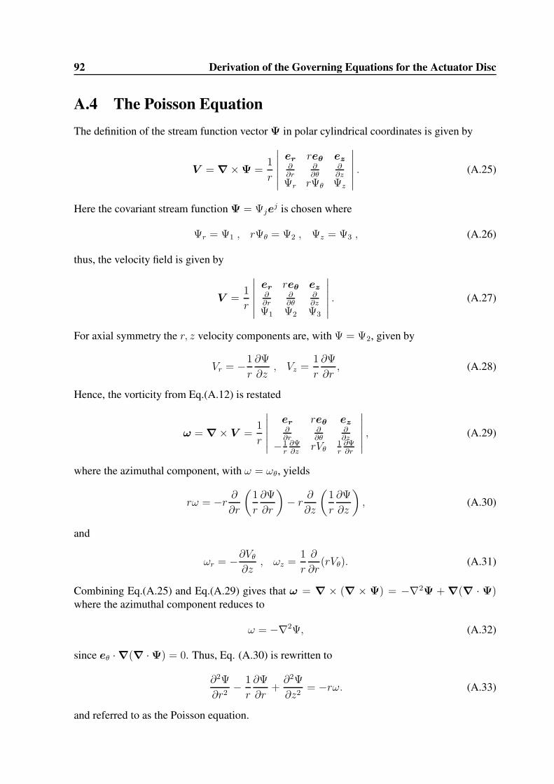
92 Derivation of the Governing Equations for the Actuator Disc
A.4 The Poisson EquationThe definition of the stream function vector Ψ in polar cylindrical coordinates is given by
V = ∇×Ψ =1
r
∣
∣
∣
∣
∣
∣
er reθ ez∂∂r
∂∂θ
∂∂z
Ψr rΨθ Ψz
∣
∣
∣
∣
∣
∣
. (A.25)
Here the covariant stream function Ψ = Ψjej is chosen where
Ψr = Ψ1 , rΨθ = Ψ2 , Ψz = Ψ3 , (A.26)
thus, the velocity field is given by
V =1
r
∣
∣
∣
∣
∣
∣
er reθ ez∂∂r
∂∂θ
∂∂z
Ψ1 Ψ2 Ψ3
∣
∣
∣
∣
∣
∣
. (A.27)
For axial symmetry the r, z velocity components are, with Ψ = Ψ2, given by
Vr = −1
r
∂Ψ
∂z, Vz =
1
r
∂Ψ
∂r, (A.28)
Hence, the vorticity from Eq.(A.12) is restated
ω = ∇× V =1
r
∣
∣
∣
∣
∣
∣
er reθ ez∂∂r
∂∂θ
∂∂z
−1r
∂Ψ∂z
rVθ1r
∂Ψ∂r
∣
∣
∣
∣
∣
∣
, (A.29)
where the azimuthal component, with ω = ωθ, yields
rω = −r ∂∂r
(
1
r
∂Ψ
∂r
)
− r ∂∂z
(
1
r
∂Ψ
∂z
)
, (A.30)
and
ωr = −∂Vθ
∂z, ωz =
1
r
∂
∂r(rVθ). (A.31)
Combining Eq.(A.25) and Eq.(A.29) gives that ω = ∇ × (∇ × Ψ) = −∇2Ψ + ∇(∇ ·Ψ)where the azimuthal component reduces to
ω = −∇2Ψ, (A.32)
since eθ ·∇(∇ ·Ψ) = 0. Thus, Eq. (A.30) is rewritten to
∂2Ψ
∂r2− 1
r
∂Ψ
∂r+∂2Ψ
∂z2= −rω. (A.33)
and referred to as the Poisson equation.

A.5 The Pressure Equation 93
A.5 The Pressure EquationBy applying the divergence operator to the Navier-Stokes equations, a pressure equations maybe obtained. Equation (A.7) is first reduces to
−∇ · (V × ω) = ∇ · f ′ −∇2H (A.34)
since ∂∂t
(∇ · V ) = 0 and with the use of the vector identity Eq.(A.6) the relation ∇·∇×ω ≡ 0removes the diffusion. Assuming axisymmetric conditions, the Laplace operator expands to
∇2H =∂2H
∂r2+
1
r
∂H
∂r+∂2H
∂z2= ωH, (A.35)
which differs form the Ψ-equation with a positive sign on the first order term. The divergence ofthe force vector is conveniently resolved in the local stn coordinate system, thus, the convectivepart and forces expands to
ωH =1
r
∂
∂r
[
Vθ∂rVθ
∂r− rVzω
]
+∂
∂z
[
Vrω + Vθ∂Vθ
∂z
]
+1
r
∂rf ′
r
∂r+∂f ′
z
∂z,
=3
2r
∂V 2θ
∂r+
1
2
(
∂2V 2θ
∂r2+∂2V 2
θ
∂z2
)
− 1
r
∂
∂r(rVzω) +
∂
∂z(Vrω) +
∂f ′
n
∂n, (A.36)
where the boundary conditions at the far field, ie. r →∞ and z → −∞ are that H = 0, and atthe center axis
∂H
∂r
∣
∣
∣
∣
r=0
= µ∂
∂r
(
1
r
∂rVr
∂r
)
, (A.37)
however, a Neumann conditions gives sufficient accuracy. Finally, in the far wake, z → +∞,we have that
∂H
∂z
∣
∣
∣
∣
z→+∞
= 0. (A.38)
The pressure field is determined from the velocity field during post processing by solvingEq.(A.35) for the pressure head H , thus, the static pressure field is found from
p = ρ(H − 1
2V 2). (A.39)
In the numerical space the individual terms are evaluated using second order central differenceschemes with the pressure head H defined at vertices. With respect to the applied force thesmoothing function from Eq.(4.23) is used to form the convolution whereby
∇ · f ′
ε =∂f ′
n ⊗ η1D
∂n=
∫ +∞
−∞
Fn(s)
ε√π
∂η1D(p)
∂ndn,
=
∫ +∞
−∞
Fn(s)
ε√π
−2p
ε2exp
[
−(p/ε)2]
dn ,∂p
∂n= 1, (A.40)
where p in Eq.(A.40) is the normal distance given by Eq.(4.25) and not the static pressure. Thefunction η ensures a smooth, yet confined pressure jump across the actuator disc without spatialoscillations.

94 Derivation of the Governing Equations for the Actuator Disc
A.6 The Heavily Loaded Actuator DiscThe derivation made by Wu of the heavily loaded actuator disc is presented in the following. Thededuction made by Wu contains many details not included in his paper, however, a descriptionof mathematical details may be found in the book by Breslin and Andersen [6]. With the use ofthe vector identity (A.6) the Euler equations are written as
V ·∇V = f ′ −∇
(
p
ρ
)
⇔ V × ω = ∇H − f ′, (A.41)
where H = p/ρ + 12V
2. Introducing orthogonal curvilinear coordinates (s,Ψ) in the meridi-onal plane it is assumed that the ratio between distances correspond to velocity ratios in the
z
s
rΨ
Figure A.1: Orthogonal curvilinear coordinates (s,Ψ) in the meridional plane.
corresponding directions i.e.
dr
ds=Vr
Vs,
dz
ds=Vz
Vs, (A.42)
where V 2s = V 2
r + V 2z . The relation between the system of orthogonal curvilinear coordinates
to the reference coordinates (r, z) can be written with the two transformations
∂
∂s=
1
Vs
(
Vr∂
∂r+ Vz
∂
∂z
)
=1
VsV ·∇, (A.43)
∂
∂Ψ=
1
rV 2s
(
Vz∂
∂r− Vr
∂
∂z
)
=1
rV 2s
eθ · V ×∇. (A.44)
Thus, the θ-component of Eq.(A.41) reduces to
−Vr
r
∂
∂r(rVθ)−
Vz
r
∂
∂z(rVθ) = −f ′
θ ⇔∂
∂s(rVθ) =
rf ′
θ
Vs, (A.45)
which shows that the angular momentum varies along a stream tube at a rate proportional to themoment of tangential blade force. Hence, outside the blade row where f ′
θ = 0, rVθ is a functionof Ψ only. Knowing that Vθ = 0 in the free stream, it follows that
rVθ = f(Ψ) in the wake= 0 elsewhere, (A.46)

A.6 The Heavily Loaded Actuator Disc 95
and if known on the disc, it may be distributed along each stream tube in the wake. Taking thedot product of Eq.(A.41) and V , (using that V ⊥ V × ω) yields
0 = V ·∇H − V · f ′ ⇔ ∂H
∂s=V · f ′
Vs
. (A.47)
The force f ′ acting on a perfect fluid are bound to be perpendicular to the local velocity relativeto the solid surface. This conditions is obtained through the dot product
(V − eθΩr) · f ′ = 0 ⇔ V · f ′ = Ωrf ′
θ, (A.48)
hence, using Eq.(A.45) yields
∂H
∂s=
Ωrf ′
θ
Vs= Ω
∂
∂s(rVθ), (A.49)
and integrating gives thatH = ΩrVθ+Ho, Ho = po/ρ+ 12V
2o , Ho being the free stream pressure
head. Furthermore by taking the cross product between V and Eq.(A.41) the θ-component andusing of the Ψ-transformation (A.44) yields
−ωr = r2∂H
∂Ψ− (rVθ)
∂
∂Ψ(rVθ)− r
Vzf′
r − Vrf′
z
V 2s
. (A.50)
Finally inserting H and ω from Eq.(3.4) the Ψ-equation derived by Wu is obtained
∂2Ψ
∂r2− 1
r
∂Ψ
∂r+∂2Ψ
∂z2= (Ωr2 − rVθ)
∂
∂Ψ(rVθ)−
rf ′
Ψ
Vs
, (A.51)
where f ′
Ψ = (Vzf′
r−Vrf′
z)/Vs is the Ψ-component of the blade force, a term which Wu neglectsas he in general considered it to be small. The boundary conditions are the same as presentedin section (3.1).

Appendix B
Sub Models
The effects from tower, dynamic blade deflection, dynamic stall and wind shear is described inthe following. The purpose of including these models is to make a more realistic comparisonswith experimental data. Here the analysis is limit to these four aspect of wind turbine rotoraerodynamics but other sub models could equally as well have been included.
B.1 Elastic Model - A Modal MethodThe elastic behaviour of the blades are modelled with a "standard" modal method (see Craig,Clough and Hansen [10, 11, 25]) where deflection in the flap- and chord wise directions areconsidered. The continuous vibrating blades (or system) is approximated by a number of normalmodes that describes a deflected shape of the entire blade or structure and a time dependentamplitude as
v(x, t) =N∑
i=1
ψi(x)νi(t), (B.1)
where v(x, t) is the deflection, ψi(x) are the normal modes and νi(t) are the time dependentamplitudes for each mode. The obtained modes ψi are used to create a generalized-parametermodel of the continuous beam. Using the principle of virtual work and assuming that the de-flection may be approximated by the normal modes, a system of equations are obtained as
Mν +Dν +Kν = p, (B.2)
where the massM , dampingD and stiffnessK matrices are determined as
M = mij =
∫ R
0
m(s)ψiψjds, (B.3)
D = dij =
∫ R
0
d(s)ψiψjds, (B.4)
K = kij(t) =
∫ R
0
EI(s)ψ′′
i ψ′′
j ds+
∫ R
0
Ts(s, t)ψ′
iψ′
jds, (B.5)
p = pj(t) =
∫ R
0
F stn(s, t)ψids. (B.6)
96

B.1 Elastic Model - A Modal Method 97
The loading is also transformed with the normal modes and it is seen to vary in time. Also thestiffness matrix is time dependent as the force in the span wise direction contributes by gravityand centrifugal loading. The mass and damping matrices are seen to be diagonal, since themodes are orthogonal. The time integration of the system of equations is done by means of anexplicit Runge-Kutta-Nystrøm method (see Appendix (B.5)).
B.1.1 Structural Blade DampingThe structural damping characteristics of the blade are best determined from measurements ofthe logarithmic decrement, δj , which then can be used to get a correct damped vibration ofthe blade. A simple way to apply viscous damping is by multiplying the generalized mass andstiffness matrices by a fraction proportional to the logarithmic decrement. Here the generalizedmass matrix is used as suggested by Øye [74], resulting in a matrix equal to
dii = miiωi
πδi, (B.7)
where δi corresponds to the i’te eigenfrequency ωi and mode ψi. For the Tjæreborg wind turbinethe damping amounts approximately to 5 % in the flap wise direction and 3% in the chord wisedirection (Øye [76]).
B.1.2 Integration of Structural LoadsThe structural loads i.e. shear forces, normal force and bending moments, T ,M are first esti-mated as the (s, t, n)-projections of gravitational, centrifugal and aerodynamic contributions.
T = T g + T c + T a , M =M g +M c +M a, (B.8)
Referring to the coordinate system previously introduced a beam element of the blade is de-picted in figure B.1. Assuming the mass to vary linearly across a small element of the bladebetween points j and j + 1 (see Hansen [25]), the gravitational force component is found to
T gj = T g
j+1 −1
2(mj +mj+1)∆sg, (B.9)
hence, T g is determined from the tip to the hub with T gN = 0 at the tip. The gravita-
tional force component is affected by tilt, coning/deflection and azimuthal angle variations i.e.T stn = B(βf )Θ
T ΦtT xyz, T xyz = 0, T g, 0. Correspondingly the flap- and edgewise mo-ments Mt,Mn, respectively, are found as
Mgj = M
gj+1 + es ×
[
Tgj+1∆s+
1
6(2mj+1 +mi)g∆s
2 ·B(βf)ΘT Φtey
]
. (B.10)
The centrifugal loading contributes to the flapwise bending moment through coning and theflapwise deflection. Thus we have that the centrifugal loading pc from a differential element dris
dpc = rΩ2mdr , r ' s cos β + vn sin β. (B.11)
Again the deflection and mass is assumed to vary linearly across each element as
s = sj+1 − s , vn = (vnj − vnj+1)s
∆s+ vnj+1, (B.12)
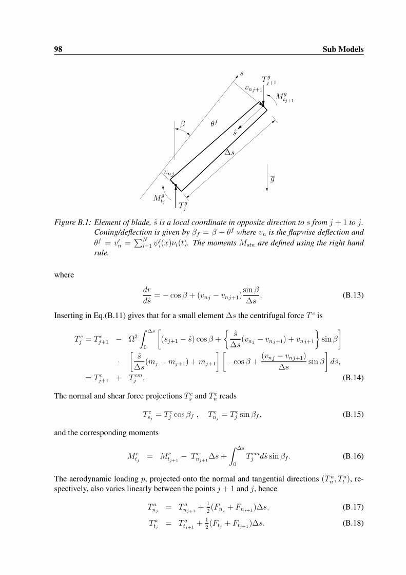
98 Sub Models
s
T gj+1
Mgtj+1
g
vnj+1
∆s
s
β θf
T gj
Mgtj
vnj
Figure B.1: Element of blade, s is a local coordinate in opposite direction to s from j + 1 to j.Coning/deflection is given by βf = β − θf where vn is the flapwise deflection andθf = v′n =
∑Ni=1 ψ
′
i(x)νi(t). The moments Mstn are defined using the right handrule.
where
dr
ds= − cos β + (vnj − vnj+1)
sin β
∆s. (B.13)
Inserting in Eq.(B.11) gives that for a small element ∆s the centrifugal force T c is
T cj = T c
j+1 − Ω2
∫ ∆s
0
[
(sj+1 − s) cos β +
s
∆s(vnj − vnj+1) + vnj+1
sin β
]
·[
s
∆s(mj −mj+1) +mj+1
] [
− cos β +(vnj − vnj+1)
∆ssin β
]
ds,
= T cj+1 + T cm
j . (B.14)
The normal and shear force projections T cs and T c
n reads
T csj
= T cj cos βf , T c
nj= T c
j sin βf , (B.15)
and the corresponding moments
M ctj
= M ctj+1− T c
nj+1∆s +
∫ ∆s
0
T cmj ds sin βf . (B.16)
The aerodynamic loading p, projected onto the normal and tangential directions (T an , T
at ), re-
spectively, also varies linearly between the points j + 1 and j, hence
T anj
= T anj+1
+1
2(Fnj
+ Fnj+1)∆s, (B.17)
T atj
= T atj+1
+1
2(Ftj + Ftj+1
)∆s. (B.18)

B.1 Elastic Model - A Modal Method 99
Likewise, integration of the aerodynamic forces gives corresponding contributions to the mo-ments as
Matj
= Matj+1− T a
nj+1∆s− 1
6(Fnj
+ 2Fnj+1)∆s2, (B.19)
Manj
= Manj+1
+ T atj+1
∆s+1
6(Ftj + 2Ftj+1
)∆s2. (B.20)
The total flapwise bending moment is found as the sum of gravitational, centrifugal and aerody-namic contributions. The loading that is applied in Eq.B.6 is found as the gradient of the forcesgiven by
F tj =Ttj+1
− Ttj−1
2∆s, F nj
=Tnj+1
− Tnj−1
2∆s. (B.21)
Next, the dynamic loads from the damped vibrating blade is determined from the accelerationand velocity of the blade found as
v(s, t) =
n∑
i=1
ψi(s)νi(t) , v(s, t) =
n∑
i=1
ψi(s)νi(t). (B.22)
The contribution from acceleration reads
T accj = T acc
j+1 +1
2(vjmj + vj+1mj+1)∆sj, (B.23)
M accj = M acc
j+1 + es ×[
T accj+1∆sj +
1
6(vjmj + 2vj+1mj+1)∆s
2j
]
, (B.24)
and correspondingly from damping
T dj = T d
j+1 +1
2(dj + dj+1)∆sj, (B.25)
M dj = M d
j+1 + es ×[
T dj+1∆sj +
1
6(dj + 2dj+1)∆s
2j
]
, (B.26)
where d(s, t) =∑N
i=1ωi
πδim(s)ψi(s)vi(t). The shear forces and bending moments are with the
dynamic contributions subtracted given as
T = T g + T c + T a − T acc − T d, (B.27)M = M g +M c +M a −M acc −M d. (B.28)
Using simple beam theory the sectional structural data for wind turbine blade may be definedwith respect to a reference co-ordinate system (s, t, n) and the principal bending axis (1, 2), asdisplayed in figure B.2. The moments (Mt,Mn) are projected onto the cross sectional principalaxis of blade, including the spanwise force, Ts
M ′
t = Mt − Ts · xE sin γ , M ′
n = Mn − Ts · xE cos γ, (B.29)
where γ = γl + γt is the pitch (sum of twist and total pitch). With the principal axis alignedwith an angle γ + ξ the principal moments (M1,M2) are
M1 = −M ′
t cos(γ + ξ) + M ′
n sin(γ + ξ), (B.30)M2 = M ′
t sin(γ + ξ) + M ′
n cos(γ + ξ). (B.31)

100 Sub Models
xE
2
1
s
n
tγ
ξ
Figure B.2: Principal axis (1, 2) in relation to reference system (s, t, n).
Simplifications - The Tjæreborg Structural Data
The structural stiffness data, EI , for the Tjæreborg wind turbine presented in [25], are definedwith respect to the principal axis also referred to as structural pitch, however, the calculatedeigenmodes as well as the loading were assumed to be aligned with the local reference system(s, t, n) for all the presented results. The inconsistency is proportional to the angle (γ + ξ),which in general is small, hence, some inaccuracy may be referred to this simplification.
B.2 Tower
The tower of the wind turbine has an influence on the flow that consist of two contributions, thetower it self and the wake behind the tower as depicted in figure (B.3). A model that consist of adipole and a source as described by Bjorck [4] is used together with the axisymmetric actuatordisc model. Considering the cross section of the tower to be equivalent with a cylinder the flow
t
θ
r WakeRotor
x
ψ
zt
zt
Figure B.3: Tower and wake
may be modelled by potential flow. By superposition of a dipole and a source combined witha free stream a reasonable modelling is achieved. The stream function for the dipole and freestream is
ψ = Uort
(
1− R2t
r2t
)
sin θt, (B.32)

B.3 Dynamic Stall 101
where rt is the radius away from the tower and Rt is the radius of the tower. The radial andtangential velocities are found as
(U tr, U
tθ) =
(
1
r
∂ψ
∂θ, − ∂ψ
∂r
)
= Uo
[(
1− R2t
r2t
)
cos θt, −(
1 +R2
t
r2t
)
sin θt
]
. (B.33)
Projecting gives that
(U tx, U
tz) = (U t
θ cos θt + U tr sin θt, − U t
θ sin θt + U tr cos θt), (B.34)
and inserting yields
(U tx, U
tz) = Uo
[
2R2txz
(x2 + z2)2, 1 +
R2t (x
2 − z2)
(x2 + z2)2
]
, (B.35)
where r2t = x2 + z2. From figure B.3 and the transformations given for the 3D kinematics, the
blade positions relative to the tower xiBxyz are given by Eq.(7.2), the blade deflection v iB
stn and(Rt, zt) as
xiBxyz = ΦT
yΦT
tΘBT (x+ v)iB
stn − ez(Rt + zt)Φy. (B.36)
The dipole gives the correct disturbance due to a 2D cylinder in an inviscid flow. The wakehowever, also influence the flowfield upstream the cylinder. A source is introduced proportionalto the wake size and thereby the drag D = 1
2 ρU2o · 2Rt · CD = qρUo, thus q = UoCDRt and
(Uwx , U
wz ) =
q
2πrt(sin θt, cos θt) =
UoCDRt
2πrt
(
x
rt,z
rt
)
. (B.37)
The combined influence reads
(Ux, Uz) = Uo
[
2R2txz
(x2 + z2)2+
CDRtx
2π(x2 + z2), 1 +
R2t (x
2 − z2)
(x2 + z2)2+
CDRtz
2π(x2 + z2)
]
, (B.38)
and the influence referred to the local coordinate system (s, t, n) reads
V Towerstn = BΘΦtΦy ·
Ux
0Uz − Uo
. (B.39)
The velocity Uo is set equal to Vz at the disc position where Vz is corrected for wind shear aspresented in appendix B.4. Bjorck [4] states that the source is not an ideal way to representwake influence, which may be realized by considering the front surface point of the towerwhere the Uz should be zero. However, far enough away from the cylinder it is a reasonableapproximation. It should be noted that the influence of the dipole decays as 1/r2 whereas thesource influence only decays as 1/r.
B.3 Dynamic StallThe dynamic stall model by Øye [78] is presented in the following. The basic idea of the modelis to interpolate the lift coefficient CL between a CL2π = 2π(α − αo) dependency and a fullyseparated CLsep dependency, with a dynamic time delay τ . The method may be summarized inthe following steps :

102 Sub Models
• Define CL2π(α) = 2π(α− αo)
• Define fully separated CLsep(α)
• Define fst from static lift curve : CLst(α) = fst(α)CL2π(α) + [1− fst(α)]CLsep(α)
• Find dfdt
= 1τ(fst − f), Euler method is sufficient i.e. fi = fi−1 + [fst(α)− fi−1]
∆tτ
• Finally, dynamic lift coefficient is found as : CL(α) = fiCL2π(α) + [1− fi]CLsep(α)
The fully separated CLsep dependency is defined somewhat arbitrarily, although with a startingslope of the order one half of the unseparated curve and with a maximum value fitting theassumed static CLst(α) at approximately 30o degrees angle of attack. The transition betweenCLsep(α) and CLst(α) is usually fitted with a smooth curve. Here a smoothing function isapplied which combine a definition of CLsep and the transition to CLst(α) summarized in thefollowing steps :
• Define CL2π(α) = 2π(α− αo)
• CLsep(α) = G · CLst(α), where G = (1 − Ao) + Ao12 1 + tanh[Bo(|α − αo| − α1)],
Ao ' 0.3− 0.5, Bo ' 5− 15, α1 ' α(CLst,max)
• fst(α) =CLst(α)−CLsep(α)
CL2π(α)−CLsep(α)
The dynamic time delay τ should be chosen to give the best fit to experimental data, but of theorder proportional to the reduced time c/V . Øye suggest a value of the order τ = 4c
Vreland he
states that the resulting response is relative insensitive to variations in the time constant.
B.4 Wind Shear
In order to include wind shear effects, the exponent law used in [47] is applied
Vz(H) = Vz(Hhub)
(
H
Hhub
)αs
, (B.40)
where H is the height from the ground,Hhub the hub height, Vz(Hhub) the velocity at hub heightin the free stream direction and αs the wind shear coefficient. When using the actuator disc andthe actuator line method, the flowfield is given and therefore the local component in the freestream direction is corrected using the local velocity, i.e.
Vz(H) = Vz(H)
(
H
Hhub
)αs
. (B.41)
Consequently, the aerodynamic forces and influence of the tower is based on the projection ofthe corrected component in the free stream direction Vz(H).

B.5 Runge-Kutta-Nystrøm Method 103
B.5 Runge-Kutta-Nystrøm MethodThe Runge-Kutta-Nystrøm method is used to integrate the dynamic system (see Øye,[74] orCollatz [7])
Mx+Dx+Kx = p(t,x, x), (B.42)
in time. The system is solved with respect to x given as
x = f(t,x, x), f =M−1 [p(t,x, x)−Kx−Dx] . (B.43)
Since M is diagonal the inverseM−1 is easily found. With the initial conditions that
t = tn, x = xn, x = xn, x = xn, (B.44)
and time step ∆t we first calculate
A =1
2∆txn, a =
1
2∆t(
xn +1
2A)
,
B =1
2∆tf
(
tn +1
2∆t, xn + a, xn +A
)
,
C =1
2∆tf
(
tn +1
2∆t, xn + a, xn +B
)
, c = ∆t (xn +C) ,
D =1
2∆tf (tn + ∆t,xn + c, xn + 2C) .
Hereafter the real time step is performed yielding
tn+1 = tn + ∆t, (B.45)
xn+1 = xn + ∆t[
xn +1
3(A+B +C)
]
, (B.46)
xn+1 = xn +1
3(A+ 2B + 2C +D) , (B.47)
xn+1 = f(
tn+1,xn+1, xn+1)
. (B.48)
The right hand side p(t,x, x) and the stiffness matrixK should be evaluated at the "half step" inthe evaluation ofB,C,D in order to obtain a true high order time integration. In combinationwith the numerical actuator disc/line models, this would require new solutions of the flowfieldat equivalent time steps. For simplicity, however, p,K are based on the latest flowfield solution.

Appendix C
Thrust and Power Coefficients for theConed Rotor
The thrust is determined by integration of the resulting axial force across the disc,
T =
∫
An
fzdAn =
∫
An
fn cos βdAn = 2π cos2 β
∫ R
0
fnsds. (C.1)
For the constant loaded rotor Ω → ∞ and ΩVθ → constant. Hence, the kinetic power isintegrated as
Pkin =
∫
An
fnVndAn = 2π cos β
∫ R
0
fnVnsds. (C.2)
For the real rotor the rotational power is determined directly from the tangential moment androtational speed given by
Prot = Ω
∫
An
fθ(s cos β)dAn = 2πΩ cos2 β
∫ R
0
fθs2ds. (C.3)
The corresponding dimensionless coefficients are obtained by normalization with the projectedarea in the axial direction. Thus, the thrust coefficient is defined as
CT =T
12ρV 2
o πR2 cos2 β
, (C.4)
and the power coefficients as
CPkin=
Pkin
12 ρV 3
o πR2 cos2 β
, CProt=
Prot
12 ρV 3
o πR2 cos2 β
. (C.5)
104

Bibliography
[1] Bareiss R, Guidati G, Wagner S. Wake simulations for wind turbines with a free, pre-scribed and hybrid wake method. Proc. 10th IEA Symp. on the Aerodynamics of WindTurbines, Edinburgh, 1996; 23–28.
[2] Berkman ME, Sankar LN, Berezin CR, Torok MS. A Navier-Stokes/full potential/freewake method for rotor flows. AIAA Paper 97-0401, 1997.
[3] Betz A. Das maximum der theoretisch möglichen ausnützung des windes durch windmo-toren. Zeitschrift für das gesamte Turbinewessen, 1920; 307–309.
[4] Bjorck A. Aerodynamic engineering calculations of blade tower interaction. Proc. of Int.Energy Agency, IEA 13th Symposium on Aerodynamics of Wind Turbines, Stockholm,Sweden, 1999; 173–186.
[5] Bjorck A, Ronsted G, Mongtgomerie B. Aerodynamic section characteristics of a rotatingand non-rotating 2.375m wind turbine blade. FFA report, TN-1995-03, The AeronauticalResearch Institute of Sweden, Sweden, 1995.
[6] Breslin JP and Andersen P. Hydrodynamics of ship propellers. Cambridge Uni. Press,U.K., 1994.
[7] Collatz L. The numerical treatment of differential equations. 3rd. ed., Springer Verlag,Berlin, 1966;537.
[8] Conway JT. Analytical solutions for the actuator disc with variable radial distribution ofload. J. Fluid Mech., 1995; 297: 327–355.
[9] Conway JT. Exact actuator disc solutions for non-uniform heavy loading and slipstreamcontraction. J. Fluid Mech., 1998; 365: 235–267.
[10] Craig Jr., Roy R. Dynamics of Structures, an introduction to computer methods. JohnWiley & Sons, 1981.
[11] Clough, RW. & Penzien J. Structural Dynamics. McGraw Hill, 1975.
[12] Corten, GP. Flow separation on wind turbine blades. PhD Dissertation. UniversiteitUtrecht, Nederland, 2001.
[13] Daube O, Guermond JL, Sellier A. Sur la formulation vitesse-tourbillon des équation deNavier Stokes en écoulement incompressible. C.R.Acad.Sci.Paris t.313 . Série II, Includ-ing abridged english version titled: On the velocity vorticity formulation of the NavierStokes equations in incompressible flow, 1991; 377-382
105

106 Bibliography
[14] De Vries O. Fluid dynamic aspects of wind energy conversion. AGARD-AG-243. 1979.
[15] Duque EPN, Van Dam CP, Hughes S. Navier-Stokes simulations of the NREL combinedexperiment phase II rotor. AIAA Paper 99-0037, 1999.
[16] Ekaterinaris JA. Numerical simulation of incompressible two-bladed rotor flow field. AIAAPaper 97-0398, 1997.
[17] Fejtek I, Roberts L. Navier-Stokes computation of wing/rotor interaction for a tilted rotorin hover. AIAA Paper 91-0707, 1991.
[18] Froude RE. On the part played in propulsion by difference in pressure. Transaction of theInstitute of Naval Architects, 1889; 30: 390–423.
[19] Glauert H. Airplane propellers. In Durand WF(ed.). Aerodynamic Theory. Dover, NewYork, 1963; 4(Division L): 169-269
[20] Goorjian PM. An invalid equation in the general momentum theory of the actuator disc.AIAA J., 1975; 10(4): 543–544.
[21] Goldstein S. On the vortex theory of screw propellers. Proc. Royal Soc., 1929; 123 A:440–465.
[22] Greenberg MD. Nonlinear actuator disc theory. Zeitschrift fur Flugwissenschaften, 1972;20(3): 90–98.
[23] Hackett JE, Ashill PR, Mokry M. Wall correction methods for powered models of conven-tional take off and landing Aircraft. Wind Tunnel Wall Correction, AGRAD-AG-336, 1998;7.1-7.27.
[24] Hansen MOL, Sørensen JN, Michelsen JA, Sørensen NN. A global Navier-Stokes rotorprediction model. AIAA Paper 97-0970, 1997.
[25] Hansen, MOL. Aerodynamics of Wind Turbines. James & James, London, 2000.
[26] Hansen, MOL. LM19.1m aerofoil characteristics corrected for 3-D effects. Private com-munication, 2000.
[27] Hirsch C. Numerical Computation of Internal and External Flows, Vol 2: ComputationalMethods for Inviscid and Viscous Flows. Wiley Series in Numerical Methods in Engineer-ing, John Wiley & Sons, 1990.
[28] Hough GR, Ordway DE. The generalized actuator disc. Developments in Theoretical andApplied Mechanics, ed. Shaw WA, Pergamon Press, Oxford, 1965; 2: 317–336.
[29] Johansen J, Sørensen NN, Michelsen JA, Schreck S. Detached-eddy simulation of flowaround the NREL phase VI blade. Wind Energy, 2002; 5: 185–197.
[30] Katz J, Plotkin A. Low-Speed Aerodynamics: From Wing Theory to Panel Methods Mc-Graw Hill Series in Aeronautical and Aerospace Engineering, McGraw Hill Inc. 1991.

Bibliography 107
[31] Lanchester FW. A contribution to the theory of propulsion and the screw propeller. Trans-action of the Institution of Naval Architects, 1915; 56: 98–116,135–153.
[32] Madsen HA. A CFD analysis of the actuator disc flow compared with momentum theoryresults. Proc. 10th IEA Symp. on the Aerodynamics of Wind Turbines, Edinburgh, 1996;109–124.
[33] Madsen HA, Rasmussen F. The influence on energy conversion and induction from largeblade deflections. European Wind Energy Conf., Nice, France, 1999; 138–141.
[34] Masson C, Smaïli A, Leclerc C. Aerodynamic analysis of HAWTs operating in unsteadyconditions. Wind Energy, 2001; 4: 1–22.
[35] Michelsen JA. Basis3D – a platform for development of multiblock PDE solvers. ReportAFM 92-05, Dept. of Fluid Mechanics, Technical University of Denmark, DTU, 1992.
[36] Michelsen JA. Block structured multigrid solution of 2D and 3D elliptic PDE’s. ReportAFM 94-06, Dept. of Fluid Mechanics, Technical University of Denmark, DTU, 1994.
[37] Mikkelsen R, Sørensen JN, Shen WZ. Modelling and analysis of the flow field aroundconed rotors. Wind Energy, 2001; 4: 121–135.
[38] Mikkelsen R, Sørensen JN. Yaw Analysis Using a Numerical Actuator Disc Model. Proc.14th IEA Symp. on the Aerodynamics of Wind Turbines, Boulder, Col, USA, 2000; 53–59
[39] Mikkelsen R, Sørensen JN, Shen WZ. Yaw Analysis Using a 3D Actuator Line Model.European Wind Energy Conf., Copenhagen, Danmark, 2001; 478–480
[40] Mikkelsen R, Sørensen JN. Modelling of Wind Tunnel Blockage. Global WindpowerConf., Paris, France, 2002; on CD-ROM
[41] Miller RH. The aerodynamic and dynamic analysis of horizontal axis wind turbines. J.Wind Eng. Ind. Aerodyn., 1983; 15: 329–340.
[42] Paulsen US. Konceptundersøgelse Nordtank 500/41 Strukturelle laster (in Danish). Risø-I-936(DA), Risø Nat. Lab., Roskilde, Denmark, 1995.
[43] Prandtl L, Betz A. Vier abhandlungen zur hydrodynamik und aerodybamik. Göttingen,1927: 88–92.
[44] Rankine, WJM. On the mechnical principles of the action of propellers. Transaction of theInstitute of Naval Architects, 1865; 6: 13–39.
[45] Rajagopalan RG, Mathur SR. Three dimensional analysis of a rotor in forward flight. J.American Helicopter Society, 1993; 38(3): 14–25.
[46] Ronsted G, Dahlberg J, Meijer S, He DX, Chen M. Pressure measurements on a 5.35mHAWT in CARDC 12m x 16m wind tunnel compared to theoretical pressure distributions.Proceedings of the European Wind Energy Conference (EWEC 89), Glasgow, Scotland,1989; 729–735.

108 Bibliography
[47] Schepers JG and Snel H. Dynamic inflow: Yawed conditions and partial span pitch control.Report ECN-C–95-056, Netherlands Energy Research Foundation, ECN, 1995.
[48] Schreck S, Hand M, Fingersh L, Robinson M, Simms D. NREL unsteady aerodynamicsexperiment wind tunnel test: Flow field characterization and model predictions. EuropeanWind Energy Conf., Copenhagen, Danmark, 2001; 35–47
[49] Shen WZ, Mikkelsen R, Sørensen JN, Bak C. Evaluation of the Prandtl Tip Correction forWind Turbine Computations. Global Windpower Conf., Paris, France, 2002; –
[50] Simoes FJ, Graham JMR. Prediction of loading on a horizontal axis wind turbine using afree vortex wake model. Proc. of the 13th BWEA Conf., Swansea, 1991; 247–253.
[51] Schlichting H, Truckenbrodt E. Aerodynamik des Flugzeuges, Teil II. Springer-Verlag,Berlin, 1960.
[52] Schmidt GH, Sparenberg JA. On the edge singularity of an actuator disk with large con-stant normal load. J. Ship Research, 1977; 21(2): 125–131.
[53] Spera DA. Wind Turbine Technology. ASME Press, New York, 1994.
[54] Sørensen JN. Three-level, viscous-inviscid interaction technique for the prediction of sep-arated flow past rotating wing. PhD Dissertation, AFM 86-03, Dept. of Fluid Mechanics,Technical University of Denmark, DTU, 1986.
[55] Sørensen JN, Myken A. Unsteady actuator disc model for horizontal axis wind turbine. J.Wind Eng. Ind. Aerodyn., 1992; 39: 139–149.
[56] Sørensen JN, Kock CW. A model for unsteady rotor aerodynamics. J. Wind Eng. Ind.Aerodyn., 1995; 58: 259–275.
[57] Sørensen JN, Gervang B, Madsen HA. Vindmølle aerodynamik: Status og perspektiver(in danish). Report ET-AFM97-01, Fluid Mechanics, DTU, 1997.
[58] Sørensen JN, Shen WZ, Munduate X. Analysis of wake states by a full-field actuator discmodel. Wind Energy, 1998; 1: 73–88.
[59] Sørensen JN, Nygreen PJ. Unsteady vorticity-stream function algorithm for external flows.Computer & Fluids, 2001; 30: 69–87.
[60] Sørensen JN, Mikkelsen R. On the Validity of the Blade Element Momentum Method.European Wind Energy Conf., Copenhagen, Danmark, 2001; 362–366
[61] Sørensen JN, Shen WZ. Numerical modeling of wind turbine wakes. J. Fluids Engineer-ing, ASME Trans., June 2002; 124: 393–399.
[62] Sørensen NN. General purpose flow solver applied to flow over hills. PhD Dissertation,Risø-R-827(EN), Risø National Laboratory, Roskilde, Denmark, 1995.
[63] Sørensen NN, Michelsen JA. Aerodynamic predictions for the unsteady aerodynamics ex-periment phase-II rotor at the National Renewable Energy Laboratory. AIAA Paper 2000-0037, 2000.

Bibliography 109
[64] Sørensen NN, Michelsen JA, Schreck S. Navier-Stokes predictions of the NREL phase-VIrotor in the NASA Ames 80ft x 120 ft wind tunnel. Wind Energy, 2002; 5: 151–169.
[65] Van Bussel GJW. The aerodynamics of horizontal axis wind turbine rotors explored withasymptotic expansion methods. PhD Dissertation, Technische Universiteit Delft, TheNetherlands, 1995.
[66] Van Holten T. The computation of aerodynamic loads on helicopter blades in forwardflight using the method of the acceleration potential. Report VTH-189, Technische Uni-versiteit Delft, The Netherlands, 1975.
[67] Van Kuik GAM. On the limitations of the Froude’s actuator disc concept. PhD Disserta-tion, Technische Universiteit Eindhoven, 1991.
[68] Voutsinas SG, Belessis MA, Rados KG. Investigation of the yawed operation of windturbines by means of a vortex particle method. In Aerodynamics and Aeroacoustics ofRotorcraft, AGARD-CP-552, 1994; 11.1–11.11.
[69] Wachspress EL. Iterative solutions of elliptic systems. Prentice Hall, Englewood Cliffs,New Jersey, 1966
[70] Wilson RE, Lissaman PBS. Applied aerodynamics of wind powered machines. ReportNSF/RA/N-74113. Oregon State University, 1974.
[71] Wu TY. Flow through a heavily loaded actuator disc. Schifftechnik, 1962; 9: 134–138.
[72] Xu G, Sankar LN. Computational study of horizontal axis wind turbines. AIAA Paper99-0042, 1999.
[73] Øye S. CBEAM4 Beregning af egensvingninger m.v. for centrifugalbelastede bjælker. Re-port AFM83-04, Fluid Mechanics, DTU, 1983.
[74] Øye S. FIX Dynamisk, aeroelastisk beregning af vindmøllevinge. Report AFM83-08,Fluid Mechanics, DTU, 1983.
[75] Øye S. Induced velocities for rotors in yaw Proc. 6th IEA Symp. on the Aerodynamics ofWind Turbines at ECN, Petten, NL, 1992.
[76] Øye S. Tjæreborg Wind Turbine, structural dynamics data. AFM-Notat, Fluid Mechanics,DTU, 1991.
[77] Øye S. Tjæreborg Wind Turbine: Dynamic flow measurement. AFM Notat VK-233, Dept.of Fluid Mechanics, Technical University of Denmark, DTU, 1992.
[78] Øye S. Dynamic stall, simulated as time lag of separation. Proc. 4th IEA Symp. on theAerodynamics of Wind Turbines at ENEA Casaccia Research Laboratory, Rome, Italy,Nov. 1990.

Recent Ph.D.-dissertations in Fluid MechanicsSørensen, J.N. Three-Level, Viscous-Inviscid Interaction Technique for the Prediction of Separated Flow Past Rotating Wing, AFM 86-03,1986
Michelsen, J.A. Modelling of Laminar Incompressible Rotating Fluid Flow, AFM 86-05, and Modelling of Turbulent Incompressible RotatingFluid Flow, AFM 86-07, 1986
Sørensen, L.S. Three-Dimensional Electro-Fluid-Dynamics in Tuft Corona Wire-Plate Precipitators, AFM 89-03, 1989
Gervang, B. Numerical Simulations of 3-Dimensional Flow in Straight and Curved Ducts of Rectangular Cross Section, AFM 89-09, 1989
Andresen, E. Statistical Approach to Continuum Models for Turbulent Gas Particles Flows, AFM 90-04, 1990
Nielsen, N.F. Low Reynolds Number Fluid Dynamics with Applications to Suspending Feeding Animals, AFM 91-10, 1991
Zamany, J. Modelling of Particle Transport in Commercial Electrostatic Precipitators, Ph.D under ATV, EF316, 1992
Christensen, E.A. Laminar-Turbulent Transition in the Rotating Driven Cavity Problem, AFM 93-12, 1993
Trinh, C.M. Turbulence Modelling of Confined Swirling Flows, Risø-R-647,1993
Mayer, K.E. Experimental and Numerical Modelling of Turbulent Flows and Heat Transfer in Staggered Tube Bundles, AFM 94-03, 1994
Mayer, S. Particle Motion in Unsteady Three-Dimensional Flow at Low Reynolds Numbers , AFM 94-04, 1994
Hansen, M.O.L. Vorticity-Velocity Formulation of Navier-Stokes Equations for Aerodynamic Flows, AFM 94-07, 1994
Hvid, S.L. Curvature Based Smoothing of Plane Cubic B-spline Curves, AFM 93-08, Surface Description using Bicubic B-splines, AFM93-10, QM3D, 3D Netgenerering, Brugermanual, AFM 94-02 and Three-Dimensional Algebraic Grid Generation, AFM 94-08 1993-94
Walther, J.H. Discrete Vortex Method for Two-Dimensional Flow past Bodies of Arbitrary Shape Undergoing Prescribed Rotary andTranslational Motion, AFM 94-11, 1994
Nim, E. Energidissipation og Masseoverførsel af Gas i og Omkring Statiske Miksere med Boblestrømning, Ph.D. under ATV, EF410, 1994
Sørensen, N.N. General Purpose Flow Solver Applied to Flow over Hills, Risø-R-827(EN), 1995
Filippone, A. Interaction of Potential Flow Model with the Navier-Stokes Equations for Rotor Aerodynamics, AFM 95-07, 1995
Jensen, E. Optimization of the Electromagnetic Flowmeter, AFM 95-09, 1995
Schmidt, J.J. Experimental and Numerical Investigation of Separated Flows, ET-PHD 97-01 1997
Nygreen, P. A Vorticity-Streamfunction Formulation of the Navier-Stokes Equations for Predicting Unsteady Flow past Bodies in ArbitraryMovement, ET-PHD 97-02, 1997
Sørensen, D.N. Aerodynamic Modelling and Optimization of Axial Fans, ET-PHD 98-01, 1998
Lennart, A.S. Experimental and Theoretical/Numerical Study of Evaporation from Shallow Pools of Organic Liquids, at Simulated WorkConditions, ET-PHD 98-02, 1998
Johansen, J. Unsteady Airfoil Flows with Application to Aeroelastic Stability, Risø-R-1116(EN), 1999
Ullum, U. Imaging Techniques for Planar Velocity and Concentration Measurements, ET-PHD 99-03,1999
Jørgensen, B.H. Low-Dimensional Modelling and Dynamics of the Flow in a Lid Driven Cavity with a Rotating Rod, ET-PHD 2000-02, 2000
Myllerup, L. Turbulence Models for Complex Flows, ET-PHD 2000-03, 2000
Pedersen, N. Experimental Investigation of Flow Structures in a Centrifugal Pump Impeller using Particle Image Velocimetry, ET-PHD2000-05, 2000
Voigt, L.P.K. Navier-Stokes Simulations of Airflows in Rooms and Around a Human Body, ET-PHD 2001-00, 2001
Gaunaa, M. Unsteady Aerodynamic Forces on NACA 0015 Airfoil in Harmonic Translatory Motion, MEK-FM-PHD 2002-02, 2002
Pedersen, J.M. Analysis of Planar Measurements of Turbulent Flows, MEK-FM-PHD 2003-01, 2003
Mikkelsen, R. Actuator Disc Methods Applied to Wind Turbines, MEK-FM-PHD 2003-02, 2003
Ullum, T.U. Investigation of Turbulence and Flow Structures in Electrostatic Precipitator, MEK-FM-PHD 2003-03, 2003
Hjort, S. Incompressible Boundary Layer Instability and Transition, MEK-FM-PHD 2004-01, 2004
Related Documents