Active Transport in Chaotic Rayleigh-B´enard Convection ·  · 2015-08-24Active Transport in Chaotic Rayleigh-B´enard Convection Christopher Omid Mehrvarzi (ABSTRACT) The transport

Active Transport in Chaotic Rayleigh-Benard Convection

Christopher Omid Mehrvarzi

Thesis submitted to the Faculty of theVirginia Polytechnic Institute and State University

in partial fulfillment of the requirements for the degree of

Master of Sciencein

Mechanical Engineering

Mark Paul, ChairBahareh BehkamDanesh Tafti

December 5, 2013Blacksburg, Virginia

Keywords: Transport, Rayleigh-Benard convection, Spatiotemporal chaosCopyright 2013, Christopher O. Mehrvarzi

Active Transport in Chaotic Rayleigh-Benard Convection

Christopher Omid Mehrvarzi

(ABSTRACT)

The transport of a species in complex flow fields is an important phenomenon related tomany areas in science and engineering. There has been significant progress theoretically andexperimentally in understanding active transport in steady, periodic flows such as a chain ofvortices but many open questions remain for transport in complex and chaotic flows. Thisthesis investigates the active transport in a three-dimensional, time-dependent flow field char-acterized by a spatiotemporally chaotic state of Rayleigh-Benard convection. A nonlinearFischer-Kolmogorov-Petrovskii-Piskunov reaction is selected to study the transport withinthese flows. A highly efficient, parallel spectral element approach is employed to solve theBoussinesq and the reaction-advection-diffusion equations in a spatially-extended cylindri-cal domain with experimentally relevant boundary conditions. The transport is quantifiedusing statistics of spreading and in terms of active transport characteristics like front speedand geometry and are compared with those results for transport in steady flows found inthe literature. The results of the simulations indicate an anomalous diffusion process with apower law 2 ≤ γ ≤ 5/2 – a result that deviates from other superdiffusive processes in simplerflows, and reveals that the presence of spiral defect chaos induces strongly anomalous trans-port. Additionally, transport was found to most likely occur in a direction perpendicular toa convection roll in the flow field. The presence of the spiral defect chaos state of the fluidconvection is found to enhance the front perimeter by t3/2 and by a perimeter enhancementratio rp = 2.3.

This work was supported by NSF grant award number: 0747727

Acknowledgments

I would like to thank my advisor, Professor Mark Paul, for granting me the opportunity towork in his group and for all of his insights, assistance, and encouragement throughout mygraduate work. To quantify the value of his contributions would be vain and perhaps betterleft for an investigation into the nature of quality itself. I would also like to thank ProfessorBahareh Behkam and Professor Danesh Tafti for serving as my committee members andtaking the time to review and critique my work. More generally, I am grateful for all ofthe teachers and mentors I’ve worked with in the past five and a half years at Virginia Techat both the graduate and undergraduate level. Their inspirational teaching have challengedme to rise above mediocrity and address difficult problems with confidence. I would liketo extend a special acknowledgement to my brilliant labmates, both past and present: Dr.Alireza Karimi, Brian Robbins, Mu Xu, and Stephen Epstein - thanks for all of your helpand fellowship. Finally, I would like to thank my beloved parents, Jeanne and Shahram, fortheir unconditional love and support throughout my studies. Without them, I would nothave been able to do anything.

iii

Contents

1 Introduction 1

1.1 Motivation . . . . . . . . . . . . . . . . . . . . . . . . . . . . . . . . . . . . . 1

1.2 Thesis outline . . . . . . . . . . . . . . . . . . . . . . . . . . . . . . . . . . . 4

2 Problem description and numerical procedure 5

2.1 Introduction . . . . . . . . . . . . . . . . . . . . . . . . . . . . . . . . . . . . 5

2.2 Ring of vortices . . . . . . . . . . . . . . . . . . . . . . . . . . . . . . . . . . 5

2.3 Rayleigh-Benard convection . . . . . . . . . . . . . . . . . . . . . . . . . . . 8

2.3.1 Governing equations . . . . . . . . . . . . . . . . . . . . . . . . . . . 10

2.3.2 Chaos in both space and time . . . . . . . . . . . . . . . . . . . . . . 11

2.4 Transport equations . . . . . . . . . . . . . . . . . . . . . . . . . . . . . . . 11

2.5 Experimentally accessible parameter values . . . . . . . . . . . . . . . . . . . 14

2.6 Direct numerical simulations . . . . . . . . . . . . . . . . . . . . . . . . . . . 18

3 Results 22

3.1 Simulation results . . . . . . . . . . . . . . . . . . . . . . . . . . . . . . . . . 22

3.1.1 Flow fields . . . . . . . . . . . . . . . . . . . . . . . . . . . . . . . . . 22

3.1.2 Passive transport . . . . . . . . . . . . . . . . . . . . . . . . . . . . . 23

3.1.3 Active transport . . . . . . . . . . . . . . . . . . . . . . . . . . . . . 23

3.2 Diagnostics . . . . . . . . . . . . . . . . . . . . . . . . . . . . . . . . . . . . 31

3.2.1 Statistical moments . . . . . . . . . . . . . . . . . . . . . . . . . . . . 31

3.2.2 Transport enhancement due to spatiotemporal chaos . . . . . . . . . 33

iv

3.2.3 Anomalous diffusion for nonlinear reactions . . . . . . . . . . . . . . 34

3.2.4 Front speed enhancement . . . . . . . . . . . . . . . . . . . . . . . . 36

3.2.5 Transport in terms of local flow field properties . . . . . . . . . . . . 39

3.2.6 Quantifying front geometry . . . . . . . . . . . . . . . . . . . . . . . 45

4 Conclusions 56

4.1 Future Work . . . . . . . . . . . . . . . . . . . . . . . . . . . . . . . . . . . . 56

v

List of Figures

2.1 Two-dimensional stream function . . . . . . . . . . . . . . . . . . . . . . . . 6

2.2 Evolution of reaction in two-dimensional ring-of-vortices for Γ = 10 . . . . . 7

2.3 Transport enhancement in a two-dimensional flow field . . . . . . . . . . . . 7

2.4 Spatially-extended cylindrical Rayleigh-Benard convection cell . . . . . . . . 9

2.5 Typical flow fields for Γ = 10 and Γ = 40 . . . . . . . . . . . . . . . . . . . . 9

2.6 Fischer-Kolmogorov-Petrovskii-Piskunov reaction function . . . . . . . . . . 13

2.7 Typical advection time scales for Rayleigh-Benard convection . . . . . . . . . 15

2.8 Characteristic fluid speeds for Rayleigh-Benard convection . . . . . . . . . . 16

2.9 Parallel speedup plot . . . . . . . . . . . . . . . . . . . . . . . . . . . . . . . 20

2.10 Mesh of 192 spectral elements used for Γ = 10. . . . . . . . . . . . . . . . . . 20

2.11 Mesh of 3072 spectral elements used for Γ = 40. . . . . . . . . . . . . . . . . 21

3.1 Temperature fields for Γ = 10 . . . . . . . . . . . . . . . . . . . . . . . . . . 25

3.2 Temperature fields for Γ = 40 . . . . . . . . . . . . . . . . . . . . . . . . . . 26

3.3 Passive transport for R = 6000 and L = 10−2 . . . . . . . . . . . . . . . . . 27

3.4 Active transport for R = 4000 and Da = 1/2 . . . . . . . . . . . . . . . . . . 28

3.5 Active transport for R = 2000 and Da = 1 . . . . . . . . . . . . . . . . . . . 29

3.6 Vertical cross-section of active transport for R = 2000 and Da = 1 . . . . . . 30

3.7 Mean-square displacement for passive transport for R = 3000 and Γ = 10 . . 32

3.8 Higher-order moments over time for passive transport . . . . . . . . . . . . . 33

3.9 Passive transport enhancement for Γ = 10 . . . . . . . . . . . . . . . . . . . 34

3.10 Mean-square displacement over time for active transport for Γ = 10 . . . . . 35

vi

3.11 Mean-square displacement over time for a RD system . . . . . . . . . . . . . 36

3.12 Mean-square displacement over time for R = 6000 . . . . . . . . . . . . . . . 37

3.13 Azimuthally-averaged front speed as a function of time for Da = 1 . . . . . . 40

3.14 Front speed enhancement as a function of characteristic fluid speed . . . . . 41

3.15 Local properties defined for a flow field . . . . . . . . . . . . . . . . . . . . . 42

3.16 Local properties of a flow field for Γ = 40 and R = 6000 . . . . . . . . . . . 44

3.17 Probability distribution function of the horizontal spreading orientation . . . 45

3.18 Front dynamics for Γ = 40 and R = 6000 . . . . . . . . . . . . . . . . . . . . 47

3.19 Front perimeter over time for Γ = 40 and R = 0 . . . . . . . . . . . . . . . . 48

3.20 Front perimeter over time for Γ = 40 and R = 2000 . . . . . . . . . . . . . . 49

3.21 Front perimeter over time for Γ = 40 and R = 4000 . . . . . . . . . . . . . . 49

3.22 Front perimeter over time for Γ = 40 and R = 6000 . . . . . . . . . . . . . . 50

3.23 Box-dimension convergence plot . . . . . . . . . . . . . . . . . . . . . . . . . 51

3.24 Graphic representation of definitions for front dynamics . . . . . . . . . . . . 52

3.25 Front enhancement ratio over time for Γ = 40 for R = 0 . . . . . . . . . . . 53

3.26 Front enhancement ratio over time for Γ = 40 and R = 2000 . . . . . . . . . 54

3.27 Front enhancement ratio over time for Γ = 40 and R = 6000 . . . . . . . . . 55

vii

List of Tables

2.1 Values of τR, vf , and Da for combustion of pre-mixed gases . . . . . . . . . . 17

2.2 List of simulations for Γ = 10 . . . . . . . . . . . . . . . . . . . . . . . . . . 18

2.3 List of simulations for Γ = 40 . . . . . . . . . . . . . . . . . . . . . . . . . . 18

3.1 Power law scalings for time history of mean-square displacement . . . . . . . 38

3.2 Front speed for Γ = 10. . . . . . . . . . . . . . . . . . . . . . . . . . . . . . . 39

viii

Chapter 1

Introduction

1.1 Motivation

The transport of a scalar species is an important phenomenon related to many areas of scien-tific and engineering interest. Species transport in a bulk fluid motion which does not affectthe motion of the fluid is defined as passive transport. Examples of passive transport includedye diffusing within a liquid, advecting particles in the Earth’s atmosphere and oceans, andthe mixing of non-reacting chemicals. Active transport is defined by an additional consider-ation of a source, or reaction term to the transport equation – this additional term may alsobe coupled to the fluid velocity field to add complexity to the transport model. Examples ofactive transport include the combustion of premixed gases, transport of biological organismsin the oceans, and chemical oscillators, like the extensively studied Belousov-Zhabotinskireaction which has been quantified to yield chaotic dynamics even in the presence of simplestirred flows [36]. Within the scope of this thesis, the investigation of active transport is lim-ited to the presence of a reaction and a traveling front that does not affect the surroundingfluid flow.

The transport of a passive species in a flow field is described by the advection-diffusion(AD) equation. These systems have been studied both numerically and experimentally for arange of flow regimes – from time-independent to turbulent flow. There has been significantprogress understanding transport in steady periodic flows such as a ring of vortices. Thetransport of a passive species in these simplified time-independent flows can be describedas an overall normal diffusive process which can be modeled by an effective diffusion co-efficient due to the presence of a flow field. The presence of time-independent flows havebeen shown theoretically [31] and experimentally [38] to enhance the transport of a passivescalar where the effective diffusion coefficient scales proportionally with the square-root ofthe fluid velocity, v1/2. Transport is also enhanced in time-dependent flows. Experimentsdone with time-dependent cellular flow show transport enhanced 1− 3 orders of magnitude

1

2

higher than that that of time-independent flows [37]. Furthermore, it has been shown thattransport in this flow regime is independent of the molecular diffusion of the tracer used –a conclusion that further reinforces the importance of the flow field characteristics on thespecies transport. The results of these past experiments have shed light on a well-definedtransition from slow, diffusion-limited transport in time-independent flows to fast advective-dominated transport in turbulent flows.

Likewise, active transport has an extensive literature. Much work has been done withtransport described by reaction-diffusion (RD) systems due to their complex dynamics andpattern-forming qualities [8]. These systems have been used to model such biological phe-nomenon as action potential dynamics in neurons [15], heart dynamics [5], and chemicalmorphogenesis [41]. However, life is not static; many biological systems experience trans-port due to a bulk fluid motion. An example of this can be seen in the motion of planktonblooms in the Earth’s oceans. The motion of these species in the oceans is important for theregulation of carbon and other chemicals in the atmosphere and are significant in regulatingglobal temperatures [12]. The transport of an active scalar species within a flow field isdescribed by the reaction-advection-diffusion (RAD) equation. Typically in RAD systemsthe fluid advection is significant to the motion and shape of the reaction front. A well-knowntheory described by Fisher and Kolmogorov [19] predicts front propagation speed as a func-tion of molecular diffusion coefficient and reaction kinetics; however, this front speed changeswith advection and a more detailed theory has yet to be developed.

There have been many studies to develop this theory, especially for active transport insimple laminar flow regimes. Active transport with reaction laws described by the Fischer-Kolmogorov-Petrovskii-Piskunov (FKPP) and Arrhenius type were explored in numericalsimulations to show enhancement for front prorogation due to the presence of simple flows[1]. In systems with open-streamline flows, the front velocity, vf was found to be propor-tional to the typical fluid velocity, U . In cellular flows, the front velocity is enhanced by afactor U1/4 and U3/4 depending on whether the advection is relatively fast or slow [2]. It hasbeen shown that the presence of these flow fields enhance the reaction due to fluid motiondistorting the reaction fronts and thereby increasing the surface area for the reaction kineticsto occur. However, critical values of fluid advection in cellular flows do exist which can alsolead to reaction front extinction [42]. Similar front motion inhibition in addition to otherinteresting dynamics have been seen in experiments with propagating reaction fronts of anexcitable Belousov-Zhabotinski (BZ) reaction. Experiments with the BZ reaction in a drivenoscillatory chain of vortices identified a mode-locking phenomenon of the reaction front as afunction of the amplitude and frequency of the flow field oscillation [29]. This mode-lockingphenomenon is common in many systems in nature, an example of which include circadianrhythms [14]. Furthermore, experiments showed the chemical oscillations of the BZ reactionsynchronized with the flow field oscillations when the transport in the flow became superdif-fusive [28]. Transport inhibition of the reaction front was seen in this oscillating chain flow

3

when an overall wind was imposed. In these flows, the freezing of the propagation fronts wasa function of the range of imposed winds and the strength of the vorticity of the flow field.This front freezing, or pinning, has also been found in cellular flows [33].

Another novel method that is being pursued to describe active transport in advecting flows isthrough the use of burning invariant manifolds (BIMs). These manifolds are the active trans-port analogy to Lagrangian coherent structures (LCS) for passive transport. LCS, knownby some as the “hidden skeleton of fluid flows”, are more rigorously described as the mostlocal repelling or attracting strainlines in a flow field [30]. These stainlines have been usedto effectively identify barriers in a flow field that prohibit transport of advected material.BIMs can be derived theoretically by modeling a propagating front by a system of ordinarydifferential equations [22]. Experiments have shown that these propagating fronts of the BZreaction converge to these theoretical calculated BIMs for time-independent and periodicallydriven flows [25]. Furthermore, experimental evidence suggest that these BIMs collapse ontoLCS in the limit of advection-dominated transport [4].

Indeed we can see from the wealth of research that has been done on RAD and AD systemsthat advection has a significant impact on the transport of a species. One open questionthat remains is whether the results that have been discussed so far are recoverable in sys-tems where the convecting fluid is complex, i.e., flow fields that exhibit spatiotemporalchaos. It is known already that chaotic transport can occur in simple time-dependent flowfields. Aref’s [3] numerical investigations of simple mixing procedures of a passive tracer ina two-point vortex flow suggests the existence of chaotic mixing. Numerical simulations ofspatially-extended fluid convection domains [7] showed passive transport enhancement dueto the presence of more complex, spiral defect chaos flow field that scaled with laws similarto those found in experiments of cellular rolls in Rayeligh-Benard convection [37]. The ex-istence of the two transport scaling regimes is described by the effect of local wavenumberorientation. For large advection-dominated transport, the diffusivity of the passive speciesis enhanced locally in the direction orthogonal to the local wavevector but suppressed in thedirection of the local wavevector [7].

The idea of transport enhancement in these complex flows is an attractive idea for engineeringapplications at the micro- and nano-scale where transport enhancement which cannot be doneby inducing turbulence due to the small characteristic length scales. One such example is“lab-on-a-chip” micro-fluidic devices [17]. One question that remains unaddressed is how areaction front behaves in the presence of a spatially-extended, complex flow field. This thesiswill address this question by studying direct numerical simulations of the transport of anactive scalar species in a three-dimensional, time-dependent flow field given by the chaoticstate of Rayleigh-Benard convection. The active transport that is studied is a unidirectional,“burn-type” reaction where a species transforms from states A → B. This thesis will shedlight on this fundamental example of transport in spatially-extended systems.

4

1.2 Thesis outline

In the preceding section, some current research related to active transport in various flowconditions was presented to motivate the reader to the topic. Chapter 2 of this thesis will dis-cuss theoretical details about two different flow fields: a ring of vortices and Rayleigh-Benardconvection. The equations governing each of the flow phenomenon and their non-dimensionalparameters will be discussed to highlight important physical insights. Additionally, the equa-tions governing the transport of a species will be introduced followed by a presentation ofthe important time scales relevant to the transport of an active species in Rayleigh-Benardconvection. Chapter 2 will conclude with a discussion of the computational fluid dynam-ics solver, Nek5000, and the numerical technique used to solve the full partial differentialequations. Chapter 3 will present the results of the simulations proposed in the precedingchapter. The techniques used to quantify the transport will be defined followed by a discus-sion of the analysis. Chapter 4 will conclude this thesis with suggestions on future researchpaths forward.

Chapter 2

Problem description and numerical

procedure

2.1 Introduction

In this chapter, two flow fields central to this thesis investigation of transport will be dis-cussed: a time-independent ring of vortices, and a time-dependent, chaotic state of Rayleigh-Benard convection. By doing so, we will reinforce the evidence that time-independent con-vection rolls have on the transport of a species, and then investigate how the spatiotem-poral chaos of these convection roll patterns further affects these transport characteristics.The equations describing these phenomena and important parameters that arise from non-dimensionalization will be explored. The computational domains for each of the flow fieldswill be presented with their respective, experimentally relevant boundary conditions. A dis-cussion of the numerical procedure to solve the partial differential equations will concludethis chapter.

2.2 Ring of vortices

A time-independent chain of vortices is a simple laminar flow that has many real-worldapplications such as mixing in industrial processes. As reviewed in the previous chapter,transport of both active and passive species within this type of flow field have been welldocumented. A common function used to model these type of flow fields in a rectangulardomain is

ψ(x, y) =Uλ

2πsin

(

2πx

λ

)

sin

(

2πy

λ

)

(2.1)

5

6

where ψ(x, y) is the stream function of the x-direction and y-direction velocity fields u(x, y)and v(x, y), λ represents a wavelength, and U is the characteristic velocity of the flow field.The aspect ratio for this rectangular domain is defined as

Γ =y

x. (2.2)

The corresponding contour plot of the stream function in Eq. (2.1) with a wavelength λ = 2and a characteristic fluid velocity U = 1 for Γ = 10 is presented in Fig. 2.1 as an example.

Figure 2.1: The stream function ψ(x, y) for a two-dimensional, time-independent ring ofvortices for a domain with an aspect ratio Γ = 10. The colors indicate the magnitude of thestream function and the directionality of the rotation.

The progression of a nonlinear reaction within this type of flow field is shown in Fig. 2.2 fortimes (a) t = 0 (b) t = 0.2 and (c) t = 0.4. The reaction highlights the behavior of these“burn-off” type reactions where a mixture of reactants which in the figure is representedin blue undergoes a reaction and transforms into products which are represented in red.Previous studies of active transport in these time-independent flow fields show front speedenhanced by a factor of U1/4 in a “fast” advecting regime and enhanced by a factor of U3/4 ina “slow” advecting regime [1] [2]. Simple explicit numerical simulations of transport withinthe flow field depicted in Fig. 2.1 show a similar transport enhancement regime as can beseen in the results in Fig. 2.3. Both the results shown in Fig. 2.3 and within the literaturesuggests that the presence and strength of the convection rolls have and affect on the reactionfront speed. This thesis will investigate this mode of enhancement further by the addition ofvaried roll orientation within a large spatially-extended domain due to chaotic flow patterns.

7

(a)

(b)

(c)

Figure 2.2: The evolution of a reaction in a two-dimensional, time-independent ring ofvortices for Γ = 10 at times (a) t = 0, (b) t = 0.2, and (c) t = 0.4. Red represents theproducts and blue represents the reactants.

100

101

100.1

100.2

100.3

U

〈vf〉

Da=10−1

Da=1

〈vf〉 ∝ U1

4

Figure 2.3: Transport enhancement in a two-dimensional ring of vortices. Here the averagespeed of the reaction front 〈vf 〉 is plotted as a function of the characteristic fluid velocity Ufor Damkohler numbers Da = 10−1 and Da = 1 on a log-log plot. The black line indicates acurve fit with a slope equal to 1/4. This power law behavior is similar to those found in [2]for advection-dominated reactions.

8

2.3 Rayleigh-Benard convection

Rayleigh-Benard convection is the natural convection that occurs when a horizontal layer offluid is heated from below and cooled from the top normal to the direction of the gravitationalforce. This results in a temperature gradient across the domain that causes a change indensity in a quiescent fluid and results in a buoyancy force exerted in the direction of gravity.This buoyancy force is matched by the viscous forces in the fluid in the opposing directionwhich prevents fluid motion. The ratio between the buoyancy and viscous forces can bequantified by the Rayleigh number,

R =αgd3

νκ∆T (2.3)

where β is the coefficient of thermal expansion, g is the gravitational constant, ν is thekinematic viscosity, α is the thermal diffusivity, and ∆T is the temperature difference, Th −Tc. In this form, the Rayleigh number can be seen as a non-dimensional measure of thetemperature difference across the domain – the Rayleigh number increases as the temperaturedifference ∆T increases. When ∆T reaches a critical value, the buoyancy force overcomesthe viscous force which causes fluid motion to begin. The critical Rayleigh number, Rc, isdefined as the Rayleigh number at which this convective instability occurs. The quantityused to describe the Rayleigh number relative to the critical Rayleigh number is the reducedRayleigh number which is defined as

ǫ =R−Rc

Rc

. (2.4)

Rayleigh-Benard convection is the canonical form for studying nonlinear and complex phe-nomenon such as the weather due to its experimental accessibility. Large spatially-extendedcylindrical domains, like the one shown in Fig. 2.4 are important to these types of studiesand will be the domain investigated in this thesis. The critical Rayleigh number for thisdomain was determined experimentally to be Rc ≈ 1708 [8]. At a Rayleigh number ofRc , time-independent convection rolls develop across the domain. When the temperaturedifference is increased further the convection rolls undergo another instability and becometime-dependent. In this phase, the convection rolls begin forming intricate patterns, mergingand annihilating with each other to form complex patterns of spirals and defects. When thetemperature difference is increased further, the convection rolls break down into a cascadeof smaller eddies until the flow becomes fully turbulent.

The aspect ratio for the convection domain shown in Fig. 2.4 is defined as the ratio of thecylinder’s radius to the depth,

Γ =r0d

(2.5)

9

Figure 2.4: Schematic of a spatially-extended cylindrical Rayleigh-Benard convection cell.The top wall is held at a cold temperature Tc and the bottom wall a hot temperature Th.The width of the domain is d and r0 is the radius. The direction of the gravitational field isindicated by g.

where r0 is the radius and d is the depth of the domain. For the spatially-extended systemsthat are of interest in this thesis, aspect ratios of Γ ≥ 10 are investigated. Typical temper-ature fields to the pattern-forming range of Rayleigh-Benard convection are shown in Fig.3.1(e) for the Γ = 10 domain and in Fig. 3.2(c) for the Γ = 40 domain.

(a) (b)

Figure 2.5: Typical flow fields visualized by midplane temperature values for the (a) Γ = 10and (b) Γ = 40 domains. The red color represents hot rising fluid while the blue colorrepresents cold sinking fluid. Both of these flow fields exhibit spatiotemporally chaoticdynamics at a Rayleigh number of R = 6000 (ǫ = 2.51).

10

2.3.1 Governing equations

The partial differential equations that govern the fluid flow are the Navier-Stokes equationswhere the body force is represented with a buoyancy term that is a function of the densitygradient in the fluid. In Rayleigh-Benard convection, this density gradient is assumed to bea function of only temperature – a common assumption which is known as the Boussinesqapproximation. The Boussinesq approximation is mathematically described as

(ρ∞ − ρ) ≈ ρβ (T − T∞). (2.6)

where ρ∞ and T∞ are the reference density and temperature, respectively, and β is thevolumetric thermal expansion coefficient which measures the change in density due to tem-perature while the pressure is held constant. The resulting momentum, mass and energyequations once the Boussinesq approximation is applied are

σ−1(∂t + ~u •∇)~u(x, y, z, t) = −∇p +∇2~u+RT z (2.7)

∇ • ~u = 0 (2.8)

(∂t + ~u •∇)T (x, y, z, t) = ∇2T (2.9)

where ∂t is the time derivative, and ~u, T , and p are the velocity, temperature, and pressurefields, respectively, as a function of cartesian coordinates (x, y, z) and of time t. Equations(2.7)-(2.9) are known as the Boussinesq equations. The Prandtl number σ is defined as

σ =ν

κ. (2.10)

Equations (2.7)-(2.9) are non-dimensionalized by the vertical thermal diffusion time, d2/κ,i.e. the amount of time it takes for heat to travel across the depth of the domain, d.

The boundary conditions for this problem are as such: A no-slip boundary condition isimposed for the velocity field ~u along all walls of the non-moving domain,

~u = 0. (2.11)

For the temperature field, conducting surfaces are selected for the boundary condition alongthe sidewalls of the domain,

T (z) = 1− z (2.12)

11

with fixed temperatures Th and Tc at the top and bottom surfaces. The initial temperaturefields adhere to Eq. (2.12) with superimposed random thermal perturbations to break sym-metry in the problem. Since there is no dynamical equation for pressure it does not requireboundary conditions.

2.3.2 Chaos in both space and time

The spirals and defect patterns that emerge in the complex flow regime of spatially-extendedsystems are characteristic of spatiotemporal chaos, i.e. chaos not only temporally but spa-tially as well. Many techniques have been developed to quantify temporally chaotic dynamicssince the phenomenon was first identified in Edward Lorenz’s now seminal paper on aperi-odic dynamics in a deterministic system [21]. Since then, temporal chaos has been identifiedand studied in simple mathematical models [24] and experimental systems alike. In fact, aperiod doubling cascade to chaos was identified in Rayleigh-Benard experiments with mer-cury [20]. The methods that have been developed to quantify these dynamics are basedon Lyapunov exponents which quantify separation of trajectories in phase space [43]. UsingLyapunov and phase space diagnostics have been particularly useful for analyzing experimen-tal evidence since one is able to reconstruct attractors by using time series signals. However,although these methods are useful for quantifying low-dimensional systems, more work needsto be done to use these tools to explore high-dimensional, spatially complex systems. Onlyrecently have developments been made to explore and quantify these far-from-equilibriumsystems. Egolf employed these Lyapunov diagnostics to calculate the fractal dimension ofRayleigh-Benard convection, i.e., the number of degrees of freedom in a spatially-extendedsystem that contribute to the chaotic dynamics. Their conclusions showed that the chaoswas extensive and that the fractal dimension of the system increases linearly with the systemvolume [10]. The chaotic degrees of freedom were found to correlate with the creation andannihilation of defects in the flow pattern [10]. Karimi and Paul [16] went further and foundthat the leading order Lyapunov exponent could be used to track topology features in theflow field that contributed to the chaotic dynamics. Their analysis showed that changes fromboundary-dominated to bulk-dominated dynamics occur as the system size increased.

2.4 Transport equations

The equations governing the active transport of a species in a flow field is given by the RADequation,

(∂t + ~u •∇)c = L∇2c+Daf(c) (2.13)

where c is the concentration field as a function of cartesian coordinates (x, y, z) and time t,

12

L is the Lewis number, Da is the Damkohler number, and f(c) is the reaction term thatis a function of the concentration field. The Lewis number is defined as the ratio of themolecular to thermal diffusivity,

L =D

κ, (2.14)

where D is the molecular diffusivity of the tracer used. The Damkohler number is importantin measuring the “strength” of the reaction term. Specifically, it is the ratio of the advectionto reaction time scales

Da =τVτR

(2.15)

where τV is the advection time scale and τR is the reaction time scale. An AD equation canbe recovered to model passive transport as the Damkohler number approaches zero due tothe reaction time scale approaching infinity.

For the numerical simulations carried out, a simple nonlinear reaction law is selected for thefunction f(c) that appears in Eq. (2.13). The nonlinearity is named the FKPP reaction termand is similar to the one studied in [1] where the function depends on the concentration ofreactants, (1− c) and products, c. Applying this reaction law, the function f(c) becomes

f(c) = c(1− c). (2.16)

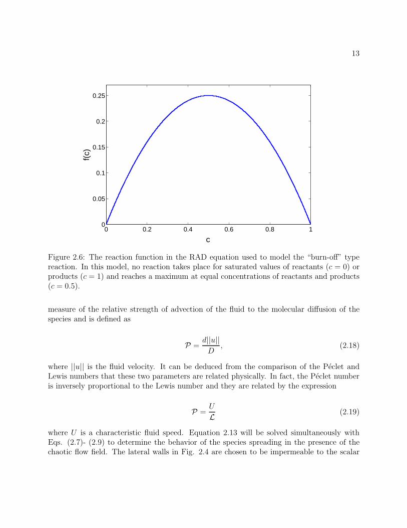
The reason for selecting this reaction can be seen by observing its behavior across a rangeof reactants and products shown in Fig. 2.6. Fig. 2.6 shows that the reaction function f(c)is at a maximum when the concentration of the species is at c = 0.5, and is zero at valuesof c = 0 and c = 1. This means that no reaction occurs when the concentration field isfully saturated with reactants (c = 0) or products (c = 1), and that the maximum reactionrate occurs at an equal concentration of reactants and products (c = 0.5). This behavior isconsistent with the “burn-off” type model that is desired and is similar to physical systemswith combustion-like reactions [32].

Another form of the transport equation described in Eq. (2.13) can be formulated to rep-resent an AD system. In this form, the AD equation is non-dimensionalized by the verticaldiffusion time of a scalar species, d2/D, and is represented by

(∂t + ~u •∇)c =1

P∇2c. (2.17)

By non-dimensionalizing the AD equation by the molecular diffusion time constant, theparameter P emerges in the equation which is the Peclet number. The Peclet number is a

13

0 0.2 0.4 0.6 0.8 10

0.05

0.1

0.15

0.2

0.25

c

f(c)

Figure 2.6: The reaction function in the RAD equation used to model the “burn-off” typereaction. In this model, no reaction takes place for saturated values of reactants (c = 0) orproducts (c = 1) and reaches a maximum at equal concentrations of reactants and products(c = 0.5).

measure of the relative strength of advection of the fluid to the molecular diffusion of thespecies and is defined as

P =d||u||

D, (2.18)

where ||u|| is the fluid velocity. It can be deduced from the comparison of the Peclet andLewis numbers that these two parameters are related physically. In fact, the Peclet numberis inversely proportional to the Lewis number and they are related by the expression

P =U

L(2.19)

where U is a characteristic fluid speed. Equation 2.13 will be solved simultaneously withEqs. (2.7)- (2.9) to determine the behavior of the species spreading in the presence of thechaotic flow field. The lateral walls in Fig. 2.4 are chosen to be impermeable to the scalar

14

species to satisfy the boundary condition,

n •∇c = 0. (2.20)

2.5 Experimentally accessible parameter values

The four non-dimensional quantities that govern the physics of the problem at hand are theRayleigh, Prandtl, Lewis (or Peclet), and Damkohler numbers. The combination of thesevalues create a very large parameter space by which transport may be studied. The goalof this section is to determine the appropriate parameter space that will orientate the nu-merical results towards those that are experimentally relevant. The factors that dictate theparameter space will be through the combination of values that are experimentally accessibleand yield comparable time scales to see the interaction between the three phenomenon: thereacting, diffusing, and advecting time scales.

Experimentally, the values of Lewis numbers that can be investigated are dictated by materialproperties, namely, the diffusion coefficient of the material used as tracers in experiments.In the experiments carried out in [37] and [38], a particulate impurity (vinyl toluene t-butylstyrene latex spheres) and methylene blue were used as the tracers which have diffusioncoefficients of D = 1.74× 10−8 cm2/s and D = 5.7× 10−6 cm2/s, respectively. The diffusioncoefficient in these cases are relatively small values. The corresponding Lewis numbers forthis range of diffusion coefficients are 10−3 ≤ L ≤ 10−1. These values of Lewis numbers werealso investigated in the numerical studies done in [7]. It is in this range of Lewis numbersthat one is able to study a range of transport regimes from diffusion-dominated to advective-dominated transport. The corresponding Peclet numbers for this range of Lewis numbersare 10 ≤ P ≤ 103.

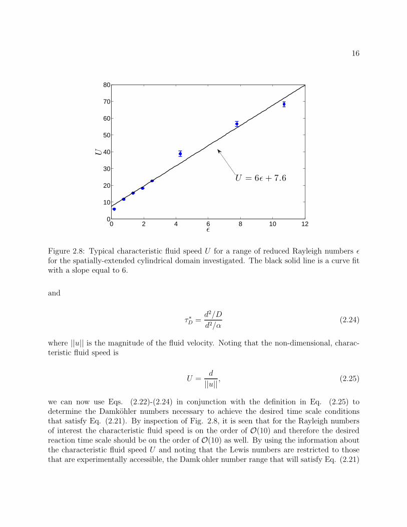
Typical advection time scales for Rayleigh-Benard convection are given in Fig. 2.7 for a rangeof reduced Rayleigh numbers. This thesis is interested in exploring transport in Rayleigh-Benard convection exhibiting spatiotemporal and spiral defect chaos, a phenomenon whichoccurs at Rayleigh numbers ranging from 2000 ≤ R ≤ 104. In this range of Rayleighnumbers, the advection time scales are in the range of τV ≈ 6 to τV → 0. Another usefulway to quantify the advection time scale is to look at the characteristic non-dimensionalspeeds across different Rayleigh number flows. Figure 2.8 displays values of characteristicflow speeds as a function of the reduced Rayleigh numbers. For the range of Rayleighnumbers that are of interest, the magnitude of the non-dimensional speed is on the order ofO(10).

Since the Lewis numbers are restricted to values based on what is accessible to experiments,and the Rayleigh numbers are decided to be values that yield spatiotemporal chaos, theDamkohler numbers will be used as the parameter to achieve a balance between the reaction

15

100

101

100

101

ǫ

τ V

τV ∝ ǫ−1

Figure 2.7: Typical advection time scales τV for a range of reduced Rayleigh numbers ǫ. Theblack solid line is a curve fit with a slope equal to −1 on a log-log plot.

time scale and the diffusion and advection time scales. In particular, we would like to achievea time scale relationship that satisfies the inequality expression

τR ≤ τV < τD. (2.21)

Equation (2.21) signifies that the reaction should be the fastest phenomenon in the problem,or that it should be comparable to the advection time scale. In either case, the diffusionshould be the longest phenomenon in the problem in order to model the most physicallyrelevant description. This desired time scale balance is described further in [42].

A description of the time scales in terms of the non-dimensional parameters are needed tobe able to satisfy Eq. (2.21). To do so, we first non-dimensionalize the reaction, advection,and diffusion time scales by the vertical diffusion time for heat τ = d2

αwhich yields

τ ∗R =τRd2/α

, (2.22)

τ ∗V =d2/α

d/||u||, (2.23)

16

0 2 4 6 8 10 120

10

20

30

40

50

60

70

80

ǫ

U

U = 6ǫ + 7.6

Figure 2.8: Typical characteristic fluid speed U for a range of reduced Rayleigh numbers ǫfor the spatially-extended cylindrical domain investigated. The black solid line is a curve fitwith a slope equal to 6.

and

τ ∗D =d2/D

d2/α(2.24)

where ||u|| is the magnitude of the fluid velocity. Noting that the non-dimensional, charac-teristic fluid speed is

U =d

||u||, (2.25)

we can now use Eqs. (2.22)-(2.24) in conjunction with the definition in Eq. (2.25) todetermine the Damkohler numbers necessary to achieve the desired time scale conditionsthat satisfy Eq. (2.21). By inspection of Fig. 2.8, it is seen that for the Rayleigh numbersof interest the characteristic fluid speed is on the order of O(10) and therefore the desiredreaction time scale should be on the order of O(10) as well. By using the information aboutthe characteristic fluid speed U and noting that the Lewis numbers are restricted to thosethat are experimentally accessible, the Damk ohler number range that will satisfy Eq. (2.21)

17

is

0 ≤ Da ≤ 1. (2.26)

One area of active transport that is of importance to the scientific community is the com-bustion of premixed gases. These type of reactions are generally “fast” compared to thecharacteristic fluid velocity, and therefore have very large Damkohler numbers. Approxi-mate values of front speed and reaction time scales are given in Table 2.1 for methane andhydrogen. Upon inspection of Table 2.1, it can be seen that the very small reaction timescales yield Damkohler numbers in the range of 1.5 × 104 ≤ Da ≤ 2.6 × 106. In this largeDamkohler number regime, the transport is reaction-dominated and advection rolls havelittle effect on the transport of the species.

pre-mixed gas τR(s) vf (m/s) Da

CH4 1.5× 10−4 0.4 O(104)H2 2.6× 10−6 3 O(106)

Table 2.1: Values of τR, vf , and Da for combustion of methane (CH4) and hydrogen (H2).

To summarize, the relevant non-dimensional time scales to the transport problem are listedbelow as functions of the relevant non-dimensional parameters:

τ ∗V =1

U, (2.27)

τ ∗R =1

UDa, (2.28)

and

τ ∗D =1

L. (2.29)

Summarized below are the simulations that will be carried out and analyzed in this thesisand the corresponding time scales and non-dimensional parameters. Table 2.2 show thesimulations for the Γ = 10 domain and Table 2.3 show those for the Γ = 40 domain.

18

R τ ∗V τ ∗R τ ∗D L P Da

0 N/A N/A 1.0 10−1,10−2,10−3 N/A N/A2000 5.46 0 1.0 10−1,10−2,10−3 101, 102, 103 03000 1.87 0 1.0 10−1,10−2,10−3 101, 102, 103 04000 1.02 0 1.0 10−1,10−2,10−3 101, 102, 103 05000 0.82 0 1.0 10−1,10−2,10−3 101, 102, 103 06000 0.5 0, 5, 0.5 1.0 10−1,10−2,10−3 101, 102, 103 0, 10−1, 1

Table 2.2: List of simulations for Γ = 10

R τ ∗V τ ∗R τ ∗D L P Da

0 N/A N/A 1.0 10−1 N/A N/A2000 5.46 0.29 1.0 10−1 101 0, 1/2, 14000 1.02 7.18× 10−3 1.0 10−1 101 0, 1/2, 16000 0.5 4.23× 10−3 1.0 10−1 101 0, 1/2, 120000 0.26 2.13× 10−4 1.0 10−1 101 0, 1/2, 1

Table 2.3: List of simulations for Γ = 40

2.6 Direct numerical simulations

The simulations were carried out using the open source solver Nek5000. The Boussinesqequations in Eqs. (2.7)-(2.9) and the reaction-advection-diffusion equation in Eq. (2.13) aresimultaneously integrated using a parallel spectral element approach. The localized gaussiandistribution is selected for the initial condition of the scalar species such that

c (x, y, z, t = 0) = exp

(

−x2 + y2 + z2

2∆2

)

, (2.30)

where ∆ = 1/2. The initial conditions used for the Boussinesq equations are temperature,pressure and velocity fields that have been “warmed-up” from initial random thermal per-turbations for a total of t = 100 and t = 1600 time units for the Γ = 10 and Γ = 40 domains,respectively, in order to decay any transient effects in the flow field. These warm-up timeswere derived from the fact that it takes one time unit for heat to travel a distance, d, fromthe bottom to the top of the domain. Therefore, it is assumed that any transient effects inthe flow field can be neglected after a time of O(Γ2) needed for heat to travel across the areaof the domain.

19

Spectral element methods are similar to finite element methods in that they utilize a similardiscretization scheme to yield high-order accurate solutions. The spectral element methoddiffers from the finite element method in the orthogonality of the basis functions used. Inthe latter method, orthogonality is due to the use of nonoverlapping local functions as thebasis functions. In spectral methods, Legendre polynomials are used as the basis functionsacross the domain, which is why it lends itself as a global method [9]. Nek5000 is specificallydesigned to solve the incompressible Navier-Stokes equations for a variety of boundary con-ditions. One advantage of employing this spectral element method is that large scale parallelcomputations can be done efficiently and with exponential convergence in space. The solveris capable of using a second or third order accurate Adams-Bashforth time step. Unlessotherwise noted, the simulations are carried out with each element using n = 11 polynomialinterpolating nodes. The solution procedure and more information about the Nek5000 solvercan be found in [13]. The original source code for the solver integrates the mass, momen-tum, energy and the advection-diffusion equation in three-dimensions. Modifications to thecode allow for the explicit solution of a reaction term in the transport equation. Becauseof employing this explicit approach, very high Damkohler numbers, like those found in thecombustion of pre-mixed gasses, are not accessible through the current numerical scheme.Additionally, as can be seen in Table 2.3 that adding an explicit reaction term limits theability to explore the low Lewis number transport regime (i.e. L = 10−2 and L = 10−3), sofor the active transport simulations, only Lewis numbers at L = 10−1 are explored.

Nek5000 was created for a parallelized computer architecture and it has been shown to scaleto over a million processors for some computational problems [40]. However, scaling to alarge number of processors does not necessarily scale the performance. At some point thecommunication cost within the parallel architecture overcomes the savings in computationtime. Figure 2.9 summarizes the speedup study using Nek5000 for a domain size Γ = 40 ata Rayleigh number R = 9000. There is a dramatic increase in performance by scaling from64 to 128 processors; however, this gain in performance diminishes and plateaus past 128processors which suggests it is at this number the simulations should be run.

The spectral element meshes constructed for the Γ = 10 and Γ = 40 domains that are usedfor the simulations are shown in Fig. 2.10 and Fig. 2.11, respectively.

20

102

100

101

102

p

t solv

e(s

)

tsolve = p−2 + 10

Figure 2.9: Average computation time required to advance one time step tsolve as a functionof the number of cores p employed in the job batch. The test case was run for a Γ = 40domain with 3072 elements with n = 11 order polynomial. The black solid line is a curve fitwith a slope of −2.

Figure 2.10: Mesh of 192 spectral elements used for Γ = 10.

21

Figure 2.11: Mesh of 3072 spectral elements used for Γ = 40.

Chapter 3

Results

In this chapter, the results of the simulations will be presented. A discussion of the diagnostictools used to quantify transport will follow and the application of these diagnostics to theresults will be presented.

3.1 Simulation results

3.1.1 Flow fields

The flow fields for Γ = 10 and Γ = 40 are presented in Figs. 3.1-3.2. The flow field isrepresented by the midplane temperature where the red indicates hot rising fluid and theblue represents cold sinking fluid. For the Γ = 10 domain, the flow field is time-independentfor R = 2000 (ǫ = 0.17) consisting of parallel convection rolls with a few defects located ateither corner of the domain. Figure 3.1(a) depicts this case. For Rayleigh numbers greaterthan R = 2000 (ǫ = 0.17), the flow becomes complex and transitions from time-independentto time-dependent patterns described by many defects traveling across the flow field solution.These conditions are present in the flow fields pictured in Fig. 3.1(b)-3.1(e).

The midplane temperature patterns for Γ = 40 are shown in Fig. 3.2. The first differencebetween these patterns to those of Γ = 10 is with the stable solution at R = 2000 (ǫ =0.17). Figure 3.2(a) shows that at this Rayleigh number, the stable solution produced isa series of steady concentric convection rings that form a target pattern. As the Rayleighnumber is increased, the pattern breaks down into an unstable time-dependent pattern that ischaracterized as spiral defect chaos. These types of patterns are depicted in Figs. 3.2(b)-(d).As the Rayleigh number is increased further, the convection rolls exhibit a lateral oscillatoryinstability, as seen in the solutions in Fig. 3.2(e) and Fig. 3.2(f), that is characteristicof plume formation in turbulent flows. These lateral oscillations in the flow fields existwhen solved with higher-order polynomials, which suggest that they are not attributed to

22

23

numerical noise, but instead due to the convection pattern undergoing an instability.

These flow fields were used as the initial pressure, temperature and velocity fields for theevolution of the transport simulations described in the next section.

3.1.2 Passive transport

The set of images shown in Fig. 3.3 display the time evolution of a passive scalar specieswith a Lewis number L = 10−2 within a flow field with Prandtl number σ = 1 and Rayleighnumber R = 6000 (ǫ = 2.51). The domain size used for the passive transport simulationswas Γ = 10. The black contour lines represent midplane (z = 0.5) temperature valuesthat roughly correspond to the boundaries between convection rolls. The colors in the plotsindicate the level of concentration of the species with red indicating the highest concentrationand blue indicating a concentration of zero. The scalar spreading progresses from an initialcondition t = 0 as shown in Fig. 3.3(a) to a final time at t = 50 shown in Fig. 3.3(f). Ateach time the scale for the species concentration changes in order to visualize the spreadingand therefore should not be mistaken as the presence of a species source within the system.Figure 3.3(b) shows transport of the species occurring parallel to the convection roll whilemaintaining a local distribution. At later times, as shown in Fig. 3.3(c)-(e), the speciesbegins to diffuse across the convection rolls and spreads across the domain until it saturatesat about time t = 50 as shown in Fig. 3.3(f).

3.1.3 Active transport

A sample result of active transport governed by a nonlinear FKPP reaction term is presentedin Fig. 3.4 for a Prandtl number σ = 1 and Rayleigh number R = 6000 (ǫ = 2.51) andΓ = 40. The Lewis number of the species is L = 10−1. The midplane temperature contoursare represented by the black lines with with color representing the concentration of the activespecies. In these plots, the red represents the presence of products (c = 1) and the bluerepresents the absence of products (c = 0). The spreading begins from an initial Gaussiandistribution in Fig. 3.4(a) at t = 0 to a complete saturation of products across the domain asshown in Fig. 3.4(f) at around time t = 20. Many interesting features can be seen the timeevolution of the reaction. One feature is the enhanced spreading of the reacting species thatoccurs significantly at times of t < 10 as seen in Fig. 3.4(b) and Fig. 3.4(c). This enhancedspreading orientation is not seen at later times of the species evolution where the reactionfront begins to advance in all directions uniformly. The other important feature to note isthe fractal-like front structure that emerges in the presence of the flow field. This may bean indication of a reaction enhancement taking place due to an increase in the surface areaboundary between reactants and products. Methods to quantify this enhancement will bediscussed in the following sections. Figure 3.5 shows the evolution of a reaction within aR = 2000 flow field at Γ = 40, σ = 1, and L = 10−1. Within this region, the flow field

24

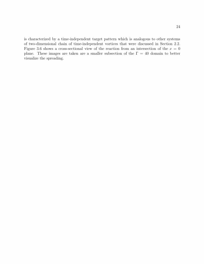
is characterized by a time-independent target pattern which is analogous to other systemsof two-dimensional chain of time-independent vortices that were discussed in Section 2.2.Figure 3.6 shows a cross-sectional view of the reaction from an intersection of the x = 0plane. These images are taken are a smaller subsection of the Γ = 40 domain to bettervisualize the spreading.

25

(a) (b)

(c) (d)

(e)

Figure 3.1: Γ = 10 temperature fields at the midplane location z = 0.5 for Rayleigh numbers(a) R = 2000 (ǫ = 0.17), (b) R = 3000 (ǫ = 0.76), (c) R = 4000 (ǫ = 1.34), (d) R =5000 (ǫ = 1.93), and (e) R = 6000 (ǫ = 2.51). Red represents hot rising fluid while bluerepresents cold sinking fluid. Qualitatively, the complexity of the convection roll patternincreases as the Rayleigh number increases.

26

(a) (b)

(c) (d)

(e) (f)

Figure 3.2: Γ = 40 temperature fields at the midplane location z = 0.5 for Rayleigh numbers(a) R = 2000 (ǫ = 0.17), (b) R = 4000 (ǫ = 1.34), (c) R = 6000 (ǫ = 2.51), (d) R =9000 (ǫ = 4.27), (e) R = 15000 (ǫ = 7.78) and (f) R = 20000 (ǫ = 10.71). Red representshot rising fluid while blue represents cold sinking fluid. Similar to the Γ = 10 flow fields, thecomplexity of the convection roll pattern increases as the Rayleigh number increases.

27

(a) (b)

(c) (d)

(e) (f)

Figure 3.3: Transport of a passive scalar species for Γ = 10, R = 6000 and L = 10−2. Eachfigure represents the passive species concentration at times (a) t = 0, (b) t = 10, (c) t = 20,(d) t = 30, (e) t = 40, and (f) t = 50. In these figures the high concentrations are indicatedby red and zero concentration indicated by blue. The midplane temperature solution forT = 0.5 are indicated by the black contour lines to visualize the convection rolls.

28

(a) (b)

(c) (d)

(e) (f)

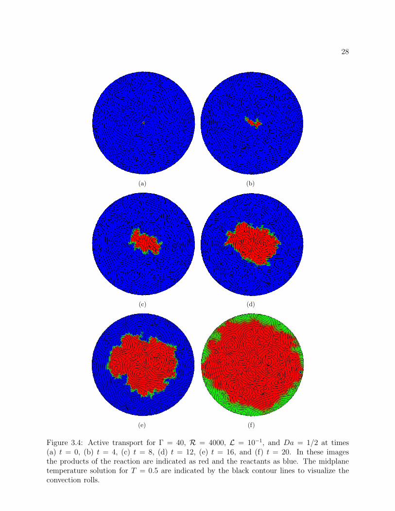
Figure 3.4: Active transport for Γ = 40, R = 4000, L = 10−1, and Da = 1/2 at times(a) t = 0, (b) t = 4, (c) t = 8, (d) t = 12, (e) t = 16, and (f) t = 20. In these imagesthe products of the reaction are indicated as red and the reactants as blue. The midplanetemperature solution for T = 0.5 are indicated by the black contour lines to visualize theconvection rolls.

29

(a) (b)

(c) (d)

(e) (f)

Figure 3.5: Active transport for Γ = 40, R = 2000, L = 10−1, and Da = 1 at times (a) t = 0,(b) t = 4, (c) t = 9, (d) t = 12, (e) t = 16, and (f) t = 20. In these images the productsof the reaction are indicated as red and the reactants as blue. The midplane temperaturesolution for T = 0.5 are indicated by the black contour lines to visualize the convection rolls.

30

(a)

(b)

(c)

(d)

(e)

Figure 3.6: Vertical cross-section of the reaction for the same parameters as those in Fig.3.5 for times (a) just after t = 0, (b) t = 4 (c) t = 9 (d) t = 12 and (e) t = 16. Only half ofthe domain is shown in the figures above to better visualize the details of the spreading.

31

3.2 Diagnostics

There are many ways to quantify the transport of species within a spatially-extended domain.In this section, these methods will be described and applied to the results from the numericalsimulations. The transport of the species is analyzed as a two-dimensional spreading processdue to the large aspect ratio domain studied.

3.2.1 Statistical moments

One way to study the transport of a species is to quantify the spreading globally by calcu-lating the mean-square displacement over time. Since the domains investigated have large-aspect ratios, the statistics of the spreading of the species can be quantified in two dimensions.The mean-square displacement in cylindrical coordinates is represented as

V (t) =

∫ Γ

0

∫ 2π

0[r − r (t)]2 c (r, θ, t) rdrdθ

∫ Γ

0

∫ 2π

0c (r, θ, t) rdrdθ

(3.1)

where the quantity r (t) is the area-averaged species concentration field and is defined as

r (t) =

∫ Γ

0

∫ 2π

0rc (r, θ, t) rdrdθ

∫ Γ

0

∫ 2π

0c (r, θ, t) rdrdθ

. (3.2)

The mean-square displacement was numerically integrated for each of the simulations. Figure3.7 shows the mean-square displacement over time for passive transport in a flow field withR = 3000 (ǫ = 0.17), L = 10−1, L = 10−2, and L = 10−3. The mean-square displacementgrows proportional to time with a power law γ ≈ 1. These results have also been documentedin [7] for numerical simulations in chaotic flow fields. Since the growth of the mean-squaredisplacement over time time follows a unity power law, that is,

V (t) ∝ tγ (3.3)

where γ = 1, the spreading can be described as an overall normal diffusion process andthe averaged spreading of the species, c (t), can be described by a reduced one-dimensionaldiffusion process governed by

∂tc (r, t) = L∗∂rrc (3.4)

where L∗ is the effective Lewis number – in other words, the effective Lewis number capturesthe contributions of convection into the transport equation. This value can be extracted

32

100

101

102

100

101

102

t

V

L = 10−1

L = 10−2

L = 10−3

γ = 1

Figure 3.7: The mean-square displacement V as a function of time t for passive transportfor Γ = 10 and R = 3000. The mean-square displacement grows proportionally with timefollowing a power law γ = 1 for all Lewis numbers L = 10−1, L = 10−2, and L = 10−3. Thedeviation of the trend at large times is due to finite wall effects for Γ = 10.

from the mean-square displacement by the equation,

V (t) = 4L∗t. (3.5)

Another test that can be done to confirm that the averaged spreading is a normal diffusiveprocess is to look at the ratio of higher-order moments to the mean-square displacement.For normal diffusive processes, the higher-order moments should scale

Mq(t) ∝ tq

2 (3.6)

where q is an integer of higher order moments and Mq is the higher-order moment definedas

Mq(t) =

∫ Γ

0

∫ 2π

0[r − r (t)]q c (r, θ, t) rdrdθ

∫ Γ

0

∫ 2π

0c (r, θ, t) rdrdθ

. (3.7)

Notice that when q = 2, the definition of the mean-square displacement V (t) in Eq. (3.1) isrecovered. The ratio of this higher-order moment with the mean-square displacement should

33

then be constant in time for normal diffusive processes. Plotted in Fig. 3.8 are ratios ofhigher-order moments for q = 4, 6, and 8. Each of the higher-order moment ratios approacha constant value over time which confirm that normal diffusion is occurring.

0 20 40 60 80 1000.5

1

1.5

2

2.5

3

3.5

4

4.5

5

t

M2/q

q/M

2

q = 4

q = 6

q = 8

Figure 3.8: Ratio of higher-order moments Mq(t)2/q to the mean-square displacement M2 as

a function of time t for values of q = 4, q = 6, and q = 8. The leveling off of Mq(t)2/q/M2

over a certain time interval suggests a normal diffusion process.

3.2.2 Transport enhancement due to spatiotemporal chaos

One way to quantify transport enhancement is to quantify the difference between the effectiveLewis number L∗ and the Lewis number L in order to isolate effects of the convection on theoverall diffusive process. The non-dimensional transport enhancement factor is defined as

∆ =L∗ −L

L. (3.8)

Distinct enhancement regimes emerge when the transport enhancement factor is plotted as afunction of the Peclet number of the flow. Figure 3.9 highlights the appearance of these twotransport regimes: a diffusion-dominated and an advection-dominated regime that occur as aresult of the presence of the complex flow field. These regimes depend on the relative strengthof the advecting fluid therefore by describing the transport enhancement factor as a functionof the Peclet number, the two regimes may be described based on the relative importance of

34

advection and diffusion in the problem. For diffusion-dominated transport that occurs in thelow Peclet number regime, the transport enhancement factor is proportional to Peclet numberby ∆ ∝ P1/2. At a certain Peclet number, the transport becomes advection-dominated andthe scaling law that the transport enhancement factor follows becomes ∆ ∝ P. It is unclearyet whether this transition between the two scaling regimes is gradual or an abrupt transition.However, these two transport enhancement regimes are in agreement with those found inexperiments of passive tracers in time-independent [37] and time-dependent flow fields [37]as well as in numerical simulations of spiral defect chaos [7].

102

103

104

105

100

101

102

103

104

P

∆

ǫ = 0.17

ǫ = 0.76

ǫ = 1.34

ǫ = 1.92

ǫ = 2.51

∆ ∝ P

∆ ∝ P1/2

Figure 3.9: Transport enhancement ∆ of a passive species as a function of the Peclet number,P for Γ = 10. Two distinct transport enhancement regimes occur for diffusion-dominatedand advective-dominated transport which scale by P1/2 and P, respectively.

3.2.3 Anomalous diffusion for nonlinear reactions

It can be seen from the preceding section that when the spreading of the species follows anormal diffusion process, quantifying transport enhancement can be done relatively easilyby extracting an overall diffusion coefficient from the mean-square displacement. This pro-cedure cannot be used when the diffusive behavior is anomalous – that is, the mean-squaredisplacement follows the trend described by Eq. (3.3) with an exponent γ 6= 1. As willbe seen, transport involving nonlinear reactions like FKPP reaction studied in this thesissubscribe to this type of anomalous behavior.

Figure 3.10 displays the mean-square displacement over time for R = 6000 and Da =

35

0 (passive), Da = 1 and Da = 10. The results show that for Da = 0, the transportrecovers the normal diffusive process with γ = 1 as seen in the previous section. However,for active transport with Da > 0, the mean-square displacement exhibits γ > 1 indicatinga superdiffusive process. Additionally, the finite wall effects of the Γ = 10 domain are morepronounced in the spreading of the active species. It is for this reason that the transition totransport simulations were conducted in Γ = 40 to better quantify the spreading dynamics.

100

101

102

100

101

102

t

V

Da = 0Da = 1Da = 10

γ = 1

Figure 3.10: Mean-square displacement over time for Da = 0 (passive transport), Da = 1,and Da = 10 for Γ = 10. The mean-square displacement for Da = 1 and Da = 10 deviatefrom normal diffusion.

In Fig. 3.11, the time history of the mean-square displacement for a RD system is givenfor Damkohler numbers Da = 0, Da = 1/2, and Da = 1 in the Γ = 40 domain. In theabsence of the fluid advection, the mean-square displacement scales with time by γ = 2.Also plotted in Fig. 3.11 is the mean-square displacement over time for Da = 0 whichrepresents a pure diffusive system with γ = 1. It is interesting to note that these powerlaw relationships for a RD system are similar to those of a RAD system where the fluidadvection is due to a time-independent target pattern flow. For the simulations exhibitingspatiotemporal chaos, classifying the scaling laws will help compare the diffusive nature ofthe spreading compared to those found in RD systems and RAD systems exhibiting simplerflow fields. Figure 3.12 displays the mean-square displacement over time for the Rayleighnumber R = 6000. Superdiffusive behavior is also seen in the reacting flows (Da > 0) butat a larger scaling exponent than is seen in the previous cases.

Table 3.1 shows power laws extracted from mean-square displacement for all the simulations

36

100

101

102

100

101

102

t

V

Da = 0Da = 1/2Da = 1

γ = 2

γ = 1

Figure 3.11: The mean-square displacement as a function of time for a RD system forDamkohler numbers Da = 0, Da = 1/2 and Da = 1 in the Γ = 40 domain. The reactionsfor Da = 1/2 and Da = 1 are superdiffusive that scale by an exponent γ = 2.

in the Γ = 40 domain. The results show that for active transport for spiral defect chaos de-scribe a superdiffusive process that not only describes anomalous diffusion, but is describedby a scaling law γ greater than those found for RD systems in the absence of flow andtime-independent target pattern flow. This deviates from the behavior seen in passive trans-port and suggests that the presence of the spatiotemporally chaotic flows induces stronglyanamolous transport for the spreading of an active species.

3.2.4 Front speed enhancement

The speed of a reacting front is an important property related to quantifying active transportin RAD systems. An existing classical theory developed by Kolmogorov [19] describes thefront velocity for RD systems to prorogate at a speed of

vf =

√

2D

τR. (3.9)

This theory can be extended to RAD systems that exhibit normal diffusive behavior by usingan enhanced molecular diffusivity D∗ in place of the D for Eq. (3.9). Unfortunately thismay not be applied to the complex flow fields under consideration as the results from the

37

100

101

102

100

101

102

103

t

V

Da = 0Da = 1/2Da = 1

γ = 5/2

γ = 1

Figure 3.12: Mean-square displacement over time for Damkohler numbers Da = 0 (passivetransport), Da = 1/2, and Da = 1 in the Γ = 40 domain for R = 6000. The reactions forDa = 1/2 and Da = 1 are superdiffusive that scale by an exponent γ = 5/2.

previous section indicate superdiffusive behavior. The theory describing anomalous diffusionin RAD systems is still in its infancy. Mancinelli et al. [23] advance the theory by derivinglinear operators to describe the diffusion and advection effects in reduced RAD systemswith relatively slow reactions. These linear operators are functions of the scaling law forthe system but also the shape of the probability density function of the diffusive process.Furthermore, this theory is derived for classical flow cases that are unable to be applied in thisparticular RAD system. However, it is noted that this modified FKPP theory is employedin front prorogation of RAD systems studied in [1] and [2] with simpler, time-independentflow fields. These studies show reaction front speeds dependent on the characteristic fluidvelocities for two different reaction regimes. Therefore, the results obtained for front speedsin spiral defect chaos will be compared to those scaling relations.

The front speed in large cylindrical domains is quantified by the time rate of change of theradius of the averaged product spread. This is first done by defining the average growth ofthe area of products as

dA(t)

dt= 2π 〈R(t)〉θ

dR(t)

dt(3.10)

where A(t) is area of the reacted products, R(t) is the radius of the products spread, and

38

Da R γ

0.5 0 (RD system) 22000 24000 26000 5/220000 2

1 0 (RD system) 22000 24000 5/26000 5/220000 5/2

Table 3.1: Mean-square displacement power laws γ for a variety of flow conditions describedby the Rayleigh numberR and the Damkohler numberDa. The presence of chaotic Rayleigh-Benard convection changes the power law scaling from γ = 2 to γ = 5/2.

〈R(t)〉θ is the azimuthally-averaged radius of the products spread across the domain whichis also a function of time and is defined by

〈R(t)〉θ =1

2π

∫ 2π

0

R(t) dθ. (3.11)

The front speed is defined as the quantity, dR(t)dt

and so rearranging Eq. (3.10) the frontspeed can be defined as

〈vf(t)〉θ =1

2π 〈R(t)〉θ

dA(t)

dt. (3.12)

Figure 3.13 shows this azimuthally-averaged velocity as a function of time for active trans-port for Γ = 40, R = 6000, L = 10−1 and Da = 1. The results show that this front speedexperiences an initial transient period in which the speed increases and then oscillates be-tween some maximum value before decreasing again due to the reaction reaching the endof the domain. Equation (3.13) can be used to calculate the front speed averaged over theentire simulation time t0 which will be used as a comparison with the trends published inthe literature. This expression can be obtained by simply taking the time-average of Eq.3.12 to yield

〈vf〉θ =1

t0

∫ t0

0

〈vf(t)〉θ dt. (3.13)

Table 3.2 displays the azimuthal- and time-averaged front speed for active transport simula-

39

tions in the Γ = 10 domain. The reaction speed increases due to an increase in Damkohlernumber as what would be expected for the increase in the reaction time scale. The transitionto the Γ = 40 domain allows us to consider a wider number of flow conditions and examinethe front speed enhancement.

Da 〈vf 〉θ1 1.2910 5.71

Table 3.2: Front speed for Γ = 10.

Figure 3.14 display the azimuthal- and time-averaged front speed as a function of the char-acteristic fluid speed U for Damkohler numbers Da = 1/2 and Da = 1. The plots showa general enhancement in the reaction front speed based on the strength of the flow field.For Da = 1/2 the reaction front speed is enhanced by the presence of the flow by a factor〈vf〉θ ∝ U0.43. For Da = 1 this enhancement factor becomes 〈vf〉θ ∝ U0.38. An interestingfeature to point out in these results is the change in front speed during the transition fromtime-independent to time-dependent spiral defect chaos. The second point in for each set ofdata in Fig. 3.14 represent the front speed at Rayleigh number R = 2000 which correspondsto a stable state of Rayleigh-Benard convection that is analogous to a time-independent ringof vortices. The next point in the plot represents the characteristic velocity in Rayleigh num-ber R = 4000 which represents Rayleigh-Benard convection in the spiral defect chaos state.It is seen that in the Da = 1/2 reaction the front speed actually decreases in the complexflow field, and then increases as the flow field velocity increases. A similar situation happensin the Da = 1 reaction as represented in Fig. 3.14 but while the front speed increases, therate of increase is much smaller than the other points. This suggests that front inhibitionmay occur in the transition from stable to chaotic states of Rayleigh-Benard convection forreactions in advection-dominated transport. More simulations would need to be carried outto investigate further and confirm this behavior.

3.2.5 Transport in terms of local flow field properties

As can be seen in the simulation results that are presented in Fig. 3.1-3.4, one the mostinteresting features of the chaotic flow fields is their pattern forming qualities. Methodshave been developed to quantify the local properties of the flow field by calculating the localwavevectors. Figure 3.15 illustrates how these quantities relate to a flow field pattern.

This section will discuss the attempts to quantify these pattern forming systems in termsof local wavenumbers and derive other important characteristics related to the patterns.Doing so will give qualitative insight into how local convection roll patterns can affect thetransport of reactive species. Egolf [11] describes a fast method to determine local properties

40

0 2 4 6 8 10 12 14 160

0.5

1

1.5

2

2.5

3

3.5

4〈v

f〉 θ

t

〈vf〉θ

Figure 3.13: Azimuthally-averaged front speed 〈vf〉θ as a function of time t for active trans-port with Γ = 10, R = 6000, L = 10−1 and Da = 1. After an initial transient period, thefront speed oscillates between some long-time limit value, denoted by the black dashed line,before decreasing again due to finite-wall effects. The long-time limit value is denoted as theazimuthal- and time-averaged front speed 〈vf〉θ.

in pattern-forming systems which will be employed here. For systems that form a locallystriped pattern, each point in a field can be approximated by the function

u(~x) = A(~x) cos(φ(~x)) (3.14)

where u(~x) is a field quantity that is a function of cartesian coordinates, ~x. The localwavevector is defined as

~k(x) ≡ ∇φ(~x). (3.15)

The assumption made here is that variations in the value of A(~x) in Eq. (3.14) are smallcompared to the variations in φ(~x) and that the local property is sufficiently far from defectsand grain boundaries. The components of the local wavenumber in a two-dimensional plane

41

0 10 20 30 40 50 60 70 80 900

0.5

1

1.5

2

2.5

3

3.5

4

〈vf〉 θ

U

Da=1/2

Da=1

〈vf〉θ=U 0.43− 0.88

〈vf〉θ=U 0.37− 0.38

〈vf〉θ ∝ U 1/4

Figure 3.14: The azimuthal- and time-averaged front speed 〈vf〉θ as a function of the char-acteristic fluid speed U for reactions at Damkohler numbers Da = 1/2 and Da = 1. Thesolid lines represent the fits for both reactions and indicate that for this reaction range, thefront speed is enhanced 〈vf 〉θ ∝ U2/5. The black dashed line represents the upper-bound fora front speed derived for two-dimensional cellular flows found in [1] and [42].

can than be calculated as

k2x = −∂2xu(~x)

u(~x)(3.16)

where kx ≡ ~k • x and ∂2x ≡ ∂2/∂2x. The counterpart equation to Eq. (3.21) that can be usedto calculate the y-direction wavenumber ky is

k2y = −∂2yu(~x)

u(~x). (3.17)

This method introduces two problems when analyzing convection rolls in Rayleigh-Benardconvection. First, Eq. (3.21) can be sensitive to small errors introduced through numericalnoise. To overcome this problem, Eq. (3.21) and Eq. (3.20) can be replaced with

k2x = −∂3xu(~x)

∂xu(~x)(3.18)

42

x

y

) θ

→k

λ

Figure 3.15: Local properties of a flow field where the convection rolls are represented by theblue diagonal lines with a wavelength λ. Perpendicular to the convection rolls is a wavevectordefined ~k whose magnitude is the wavenumber k. A roll orientation angle θ is defined as theangle the wavevector forms with the x-axis in cartesian coordinates.

and

k2y = −∂3yu(~x)

∂yu(~x)(3.19)

respectively. The higher order derivatives in these new expressions can smooth out numericalnoise introduced in the system. Second, this method calculates k2x which is a magnitude ofa vector and does not conserve any information about the wavevector’s orientation. Thisproblem is overcome by keeping the relative sign between the wavevector components inorder to preserve directional information. Procedurally, this can be done by first computingthe wavevector components using Eq. (3.21) and Eq. (3.20) and then computing the other

43

components with the equations,

ky = kx∂2xyu(~x)

∂2xu(~x)(3.20)

and

kx = ky∂2yxu(~x)

∂2yu(~x). (3.21)

In this procedure kx will always be a positive value and ky will contain information about theorientation of the wavedirection. The full procedure is outlined rigorously in [11]. Once theinformation of the wavevectors are obtained, the local roll orientation angle can be computedby

θ = arctan

(

kykx

)

. (3.22)

The curvature of a roll is defined as the divergence of the wavevector and is calculated using

κ =~∇ • k

k. (3.23)

Figure 3.16 displays these local properties calculated for a Γ = 40 and R = 6000 flow field.Figure 3.16(a) displays the deviation from the midplane temperature field. Figure 3.16(b)shows the local wavenumber calculated for this field. The mean wavenumber for this flowfield is k = 2.2 which falls within the unstable region of the “Busse balloon” [6], as shouldbe expected for this particular Rayleigh-Benard convection field. Significant deviation fromthe mean wavenumber are seen in parts of the flow and are shown by the darkened regions.Figure 3.16(c) shows the local roll orientation which using the procedure yields values thatrange between −π/2 ≤ θ ≤ π/2. Lastly, the roll curvature is represented in Fig. 3.16(d),which also shows regions of anomalous values.

From the information of the local properties of the flow field, a horizontal spreading orien-tation angle can be quantified by

cos(Φ) =∇c •

~k

‖∇c‖‖~k‖(3.24)

where Φ is the horizontal spreading orientation, ∇c is the gradient of the concentrationfield, and ~k is the local wavevector. The horizontal spreading orientation can quantifythe spreading of the species relative to the direction of the local wavevector. This gives

44

(a) (b)

(c) (d)

Figure 3.16: Local properties of a flow field for Γ = 40 and R = 6000. Figure 3.16(a) showsthe deviation of the temperature field from the midplane values. Figure 3.16(b) is the filteredlocal wavenumber field. Figure 3.16(c) is the local convection roll orientation. Figure 3.16(d)is the local curvature.

information and insight on how the species spreads across a convection roll. The angleΦ can be calculated at every point in the flow field and quantified statistically. Figure3.17 shows the probability distribution function of the horizontal spreading orientation at aparticular time t = 5.8 for active transport for parameters Γ = 40, R = 6000, and Da = 1/2.This snapshot of the transport shows that the spreading is most likely to occur at Φ = π/2,or in a direction perpendicular to a convection roll. The next likely orientation that thespreading will occur is at an angle close to Φ = 0. The spreading is least likely to occur atangles between these two angles. The results shown here are in agreement with those foundfor passive transport at the same Lewis number L = 10−1 [7]. The mechanisms that explainthese trends are attributed to the higher probability that random walks of particles will cross

45

the separatrix between the convection rolls, as described analytically in [35]. The reason forthe larger peak closer to the angle of Φ = 0 must be attributed to the effect of the additionalreaction. One speculation for the mechanism at work is the spreading perpendicular to theconvection roll might enhance the reaction in parallel. More data would need to be collectedto test this hypothesis.

0 0.1 0.2 0.3 0.4 0.50.02

0.025

0.03

0.035

0.04

0.045

0.05

0.055

0.06

0.065

0.07

Φ/π

P(Φ

)

Figure 3.17: Probability distribution function of the horizontal spreading orientation at atime t = 5.8 for active transport for parameters Γ = 40, R = 6000, and Da = 1/2. Thehighest probability of the spreading occurs at an angle Φ = π/2

3.2.6 Quantifying front geometry

The emergence of the complex front structure for the active transport simulation results asseen in Fig. 3.4 suggest an enhancement in the front area occurs for reactions in the presenceof advection. It has been observed that mixing of active species in RAD systems enhancethe the rate of reaction. The physical explanation for this has been attributed to the theincrease in the surface area of the front which increases the area available for reactants tochange to products [18]. The results obtained in this study suggest that spiral defect chaosalso enhances this reaction.

One method that will be used to quantify the front enhancement is to calculate the reaction

46

area over time for each of the simulations conducted. The reaction area will be defined as

Af = Pfd (3.25)

where Af is the surface area of the front, Pf is the front perimeter and d is the frontdepth. Since the analysis is reduced to a two-dimensional spread, the depth for the spatially-extended system is d = 1. A method is implemented than to track the reaction front for eachtime and to estimate the front perimeter which in turn gives an estimate for the reactionsurface area. Upon observation of the front images in Fig. 3.4, one natural way to estimatethe front area is by identifying the the interface between the reactants and products whichis roughly quantified by the green boundaries. The criteria used to identify the front is

0.45 ≤ c (x, y, t) ≤ 0.55 (3.26)

which turns out to be a good estimate of the reaction front. Figure 3.18 is an example of theprocedure discussed above applied to a reaction front with a Damkohler number Da = 1/2in a Rayleigh number R = 6000 flow field. From this procedure the reaction front wascalculated for each of the active transport simulations. Figures 3.19-3.22 show the frontperimeter Pf for reactions at Damkohler numbers Da = 1/2 and Da = 1 as a function oftime for a variety of flow fields. Figure 3.19 shows this trend for a RD system in the absenceof any fluid advection. In this case, the front perimeter grows with time according to a unitypower law. This power law growth is also observed for a system with advection in the formof a target pattern flow field as indicated in Fig. 3.20. This means that there is no significantenhancement in the surface area of the front with the addition of a time-independent chainof vortices. However, in the transition to a flow field defined by spiral defect chaos, thepower law growth increases to slope of 3/2. It is during this transition that the fractal-likestructure of the front can be seen.

There have been many methods proposed to quantify fractal-like structures in the field ofdynamical systems, including structures that are not self-similar [27] [39]. One simple yeteffective method is to calculate the fractal dimension of the geometry using the box-countingmethod. In this method, a d-dimensional set that represents the reaction front will have anarea N(s) that is approximated by the total number of boxes needed with side length s tocover the planer area. Applying this rule yields the relationship

N(ǫ) ∝1

sd. (3.27)

Rearranging Eq. (3.27) and taking the limit as the box side-length approaches zero yields

47

(a) (b)

(c) (d)

Figure 3.18: Example result of front tracking method for active transport for Γ = 40,Da = 1/2, and R = 6000 for times (a) t = 5, (b) t = 10, (c) t = 15, and (d) t = 20.

the definition of the fractal dimension,

Dbox = lims→0

lnN(s)

ln 1s

. (3.28)

Fig. 3.23 shows the fractal dimension calculated for increasingly smaller box side-lengths.The fractal dimension is constant at Dbox = 2 which means that this tool does not captureany fractional dimension. This is likely attributed to finite pixel size of the images processedand therefore other methods must be explored to quantify the front’s fractional characteristic.

Another way that was used to quantify the perimeter enhancement of the reaction front is tocompare the instantaneous perimeter with a perimeter formed by an azimuthally-averagedradius. Figure 3.24 can aid in visualizing these definitions more clearly. The solid black linein Fig. 3.24 represents the perimeter of the front P (t) at any given time t. This perimetercan be quantified by a perimeter formed by the azimuthally-averaged radius 〈R(t)〉θ at thesame time t. From these definitions an enhancement of the perimeter can be quantified.

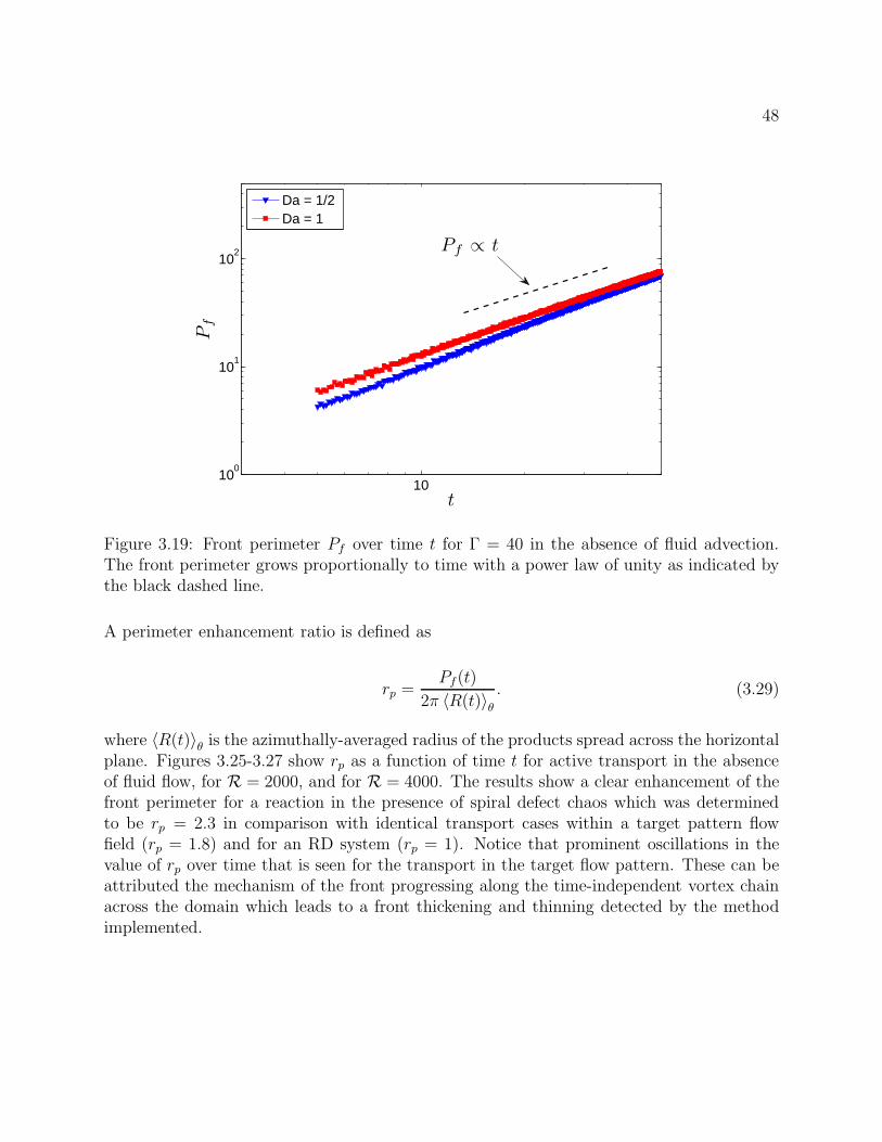
48

1010

0

101

102

t

Pf

Da = 1/2Da = 1

Pf ∝ t

Figure 3.19: Front perimeter Pf over time t for Γ = 40 in the absence of fluid advection.The front perimeter grows proportionally to time with a power law of unity as indicated bythe black dashed line.

A perimeter enhancement ratio is defined as

rp =Pf(t)

2π 〈R(t)〉θ. (3.29)

where 〈R(t)〉θ is the azimuthally-averaged radius of the products spread across the horizontalplane. Figures 3.25-3.27 show rp as a function of time t for active transport in the absenceof fluid flow, for R = 2000, and for R = 4000. The results show a clear enhancement of thefront perimeter for a reaction in the presence of spiral defect chaos which was determinedto be rp = 2.3 in comparison with identical transport cases within a target pattern flowfield (rp = 1.8) and for an RD system (rp = 1). Notice that prominent oscillations in thevalue of rp over time that is seen for the transport in the target flow pattern. These can beattributed the mechanism of the front progressing along the time-independent vortex chainacross the domain which leads to a front thickening and thinning detected by the methodimplemented.

49

100

101

100

101

102

t

Pf

Da = 1/2Da = 1 Pf ∝ t

Figure 3.20: Front perimeter Pf over time t for Γ = 40 and R = 2000. The front perimtergrows proportionally to time with a power law of unity as indicated by the black dashed line.

101

10−1

100

101

102

103

t

Pf

Da = 1/2Da = 1

Pf ∝ t3/2

Figure 3.21: Front perimeter Pf over time t for Γ = 40 and R = 4000. The front perimetergrows proportionally to time with a power law of 3/2 as indicated by the black dashed line.

50

101

102

t

Pf

Da = 1/2Da = 1

Pf ∝ t3/2

Figure 3.22: Front perimeter Pf over time t for Γ = 40 and R = 6000. The front perimetergrows proportionally to time with a power law of 3/2 as indicated by the black dashed line.

51

100

101

102

103

0

0.5

1

1.5

2

2.5

3

1/s

Dbox

Figure 3.23: Semilog plot of the fractal dimension Dbox using the box-counting method as afunction of the inverse of the box-size 1/s. As the box size decreases, the dimension remainsat a constant value of Dbox = 2.

52

Figure 3.24: Graphic representation of definitions for front dynamics. The solid black lineis the perimeter of the front Pf(t) at any given time t. The blue dashed line representsthe perimeter formed by the azimuthally-averaged radius 〈R(t)〉θ at the same time t. Theperimeter enhancement ratio rp is the ratio of these two quantities.

53

0 10 20 30 40 50

0.4

0.5

0.6

0.7

0.8

0.9

1

1.1

rp

t

rp=1

Figure 3.25: The front enhancement ratio rp as a function of time t for a RD system forΓ = 40. Ignoring the transient period, the value of rp becomes one which means that nofront enhancement due to the flow field is occurring.

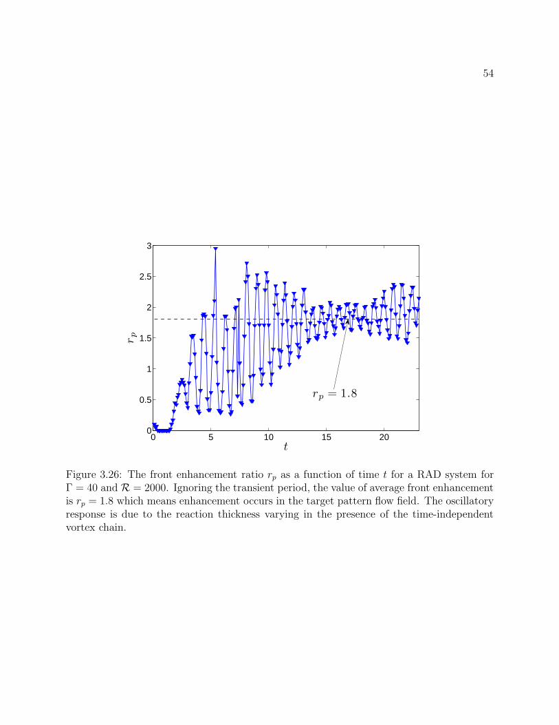
54

0 5 10 15 200

0.5

1

1.5

2

2.5

3

rp

t

rp = 1.8

Figure 3.26: The front enhancement ratio rp as a function of time t for a RAD system forΓ = 40 and R = 2000. Ignoring the transient period, the value of average front enhancementis rp = 1.8 which means enhancement occurs in the target pattern flow field. The oscillatoryresponse is due to the reaction thickness varying in the presence of the time-independentvortex chain.

55

0 2 4 6 8 10 12 14 160

0.5

1

1.5

2

2.5

3

rp

t

rp = 2.3

Figure 3.27: The front enhancement ratio rp as a function of time t for a RAD system forΓ = 40 and R = 6000. Ignoring the transient period, the value of average front enhancementis rp = 2.3 which means enhancement is greatest in the spiral defect chaos flow field.

Chapter 4

Conclusions

This thesis investigates active transport in a three-dimensional, time-dependent flow fieldgiven by chaotic Rayleigh-Benard convection using high performance numerical simulations.The results show transport enhancement deviates from the enhancement studies in the liter-ature for RAD systems with time-independent and time-periodic flow fields suggesting thatthe presence of a chaotic flow field further enhances reactions compared to flow fields studiedin these previous studies. Three different methods to quantify the transport were studied inthis thesis. First, the two-dimensional spreading was quantified statistically by measuringthe time history of the mean-square displacement. The spreading of the active species wascharacterized by anomalous diffusion with scaling exponents between 2.0 ≤ γ ≤ 5/2. Thepresence of spiral defect chaos induced strongly anomalous transport. Second, the trans-port was quantified based on local properties of the convection roll field. These methodsshowed qualitatively that the roll curvature in the spiral defect chaos flow field affected thereaction spreading. In particular, the horizontal spreading of the species was found to mostlikely to occur in the direction perpendicular to the convection roll. Third, the geometryof the front was quantified based on a front tracking method and calculation of the fractaldimension. The surface area was found to be enhanced over time due to the presence of thecomplex field by a factor t3/2 when compared to proportionality for the absence of flow anda time-independent target pattern. Finally, the front perimeter for active transport in spiraldefect chaos was found to be enhanced over transport in RD and time-independent flows bya perimeter enhancement ratio rp = 2.3.

4.1 Future Work

There are many avenues that can be pursued to expand on the work done in this thesis.The methods to quantify the spreading in this thesis were global methods. Another methodthat can be pursued is to study the local spreading and stretching of fluid tracers from a

56

57

Lagrangian perspective. By doing so, one is able to quantify the local stretching using thespectrum of Lyapunov exponents. Shadden et al. [34] provides a comprehensive overview ofthis procedure that has been well-established for research in dynamical systems and showsits natural extension to fluid systems, where transport of passive tracers are studied usingquantities like Finite Time Lyapunov Exponents (FTLE). Taking a Lagrangian approach tothe research presented in this thesis would take steps towards connecting the insights gainedhere to other modern approaches to RAD systems – in particular, those pertaining to BIMs.

Bibliography

[1] M. Abel, A. Celani, D. Vergni, and A. Vulpiani. Front propagation in laminar flows.Physical Review E, 64(4):046307, 2001.

[2] M. Abel, D. Cencini, D. Vergni, and A. Vulpiani. Front speed enhancement in cellularflows. Chaos: An Interdisciplinary Journal of Nonlinear Science, 12:481–488, 2002.

[3] H. Aref. Stirring by chaotic advection. Journal of Fluid Mechanics, 143(1):121, 1984.

[4] D. Bargteil and T. H. Solomon. Barriers to front propagation in ordered and dis-ordered vortex flows. Chaos: An Interdisciplinary Journal of Nonlinear Science,22(3):037103037103, 2012.

[5] D. Barkley. A model for fast computer simulation of waves in excitable media. PhysicaD: Nonlinear Phenomena, 49(1):6170, 1991.

[6] E. Bodenschatz, W. Pesch, and G. Ahlers. Recent developments in Rayleigh-Benardconvection. Annual Review of Fluid Mechanics, 32(1):709–778, 2000.

[7] K.-H. Chiam, M. C. Cross, H. S. Greenside, and P. F. Fischer. Enhanced tracer transportby the spiral defect chaos state of a convecting fluid. Physical Review E, 71(3):036205,2005.

[8] M. C. Cross and H. S. Greenside. Pattern formation and dynamics in nonequilibriumsystems. Cambridge University Press Cambridge, 2009.

[9] M. O. Deville, P. F. Fischer, and E. H. Mund. High-order methods for incompressiblefluid flow, volume 9. Cambridge University Press, 2002.

[10] D. A. Egolf and H. S. Greenside. Relation between fractal dimension and spatial corre-lation length for extensive chaos. Nature, 369(6476):129131, 1994.

[11] D. A. Egolf, I. V. Melnikov, and E. Bodenschatz. Importance of local pattern propertiesin spiral defect chaos. Physical Review Letters, 80:3228–3231, Apr 1998.

[12] P. Falkowski. Ocean science: The power of plankton. Nature, 483(7387):S17S20, 2012.

58

59

[13] P. F. Fischer. An overlapping schwarz method for spectral element solution of the in-compressible Navier-Stokes equations. Journal of Computational Physics, 133(1):84101,1997.

[14] L. Glass. Synchronization and rhythmic processes in physiology. Nature,410(6825):277284, 2001.

[15] A. L. Hodgkin and A. F. Huxley. A quantitative description of membrane currentand its application to conduction and excitation in nerve. The Journal of Physiology,117(4):500, 1952.

[16] A. Karimi and M. R. Paul. Quantifying spatiotemporal chaos in Rayleigh-Benard con-vection. Physical Review E, 85(4):046201, 2012.

[17] B. Kirby. Micro-and nanoscale fluid mechanics. Cambridge University Press, 2010.

[18] A. Kiselev and L. Ryzhik. Enhancement of the traveling front speeds in reaction-diffusion equations with advection. In Annales de l’Institut Henri Poincare (C) NonLinear Analysis, volume 18, pages 309–358. Elsevier, 2001.

[19] A. N. Kolmogorov, I. G. Petrovskii, and N. S. Piskunov. A study of the equation ofdiffusion with increase in the quantity of matter, and its application to a biologicalproblem. Bjul. Moskovskogo Gos. Univ, 1(7):126, 1937.

[20] A. Libchaber, C. Laroche, and S. Fauve. Period doubling cascade in mercury, a quan-titative measurement. Journal de Physique Lettres, 43(7):211–216, 1982.

[21] E. N. Lorenz. Deterministic nonperiodic flow. Journal of the Atmospheric Sciences,20(2):130141, 1963.

[22] J. R. Mahoney, D. Bargteil, M. Kingsbury, K. A. Mitchell, and T. H. Solomon. In-variant barriers to reactive front propagation in fluid flows. EPL (Europhysics Letters),98(4):44005, 2012.

[23] R. Mancinelli, D. Vergni, and A. Vulpiani. Front propagation in reactive systems withanomalous diffusion. Physica D: Nonlinear Phenomena, 185(3):175–195, 2003.

[24] R. M. May. Simple mathematical models with very complicated dynamics. Nature,261(5560):459–467, 1976.

[25] K. A. Mitchell and J. R. Mahoney. Invariant manifolds and the geometry of frontpropagation in fluid flows. Chaos: An Interdisciplinary Journal of Nonlinear Science,22(3):037104037104, 2012.

[26] C. R. Nugent, W. M. Quarles, and T. H. Solomon. Experimental studies of pattern for-mation in a reaction-advection-diffusion system. Physical Review Letters, 93(21):218301,2004.

60

[27] E. Ott. Chaos in dynamical systems. Cambridge University Press, 2002.

[28] M. S. Paoletti, C. R. Nugent, and T. H. Solomon. Synchronization of oscillating reactionsin an extended fluid system. Physical Review Letters, 96(12):124101, 2006.

[29] M. S. Paoletti and T. H. Solomon. Experimental studies of front propagation and mode-locking in an advection-reaction-diffusion system. EPL (Europhysics Letters), 69(5):819,2005.

[30] T. Peacock and G. Haller. Lagrangian coherent structures: The hidden skeleton of fluidflows. Physics Today, 66(2):4147, 2013.

[31] M. N. Rosenbluth, H. L. Berk, I. Doxas, and W. Horton. Effective diffusion in laminarconvective flows. Physics of Fluids, 30:2636, 1987.

[32] H. G. Schuster and R. Grigoriev. Transport and Mixing in Laminar Flows: FromMicrofluidics to Oceanic Currents. Wiley. com, 2012.

[33] M. E. Schwartz and T. H. Solomon. Chemical reaction fronts in ordered and disorderedcellular flows with opposing winds. Physical Review Letters, 100(2):028302, 2008.

[34] S. C. Shadden, F. Lekien, and J. E Marsden. Definition and properties of Lagrangiancoherent structures from finite-time Lyapunov exponents in two-dimensional aperiodicflows. Physica D: Nonlinear Phenomena, 212(3):271–304, 2005.

[35] B. I. Shraiman. Diffusive transport in a Rayleigh-Benard convection cell. PhysicalReview A, 36(1):261, 1987.

[36] R. H. Simoyi, A. Wolf, and H. L Swinney. One-dimensional dynamics in a multicompo-nent chemical reaction. Physical Review Letters, 49(4):245, 1982.

[37] T. H. Solomon and J. P. Gollub. Chaotic particle transport in time-dependent Rayleigh-Benard convection. Physical Review A, 38(12):6280, 1988.

[38] T. H. Solomon and J. P. Gollub. Passive transport in steady Rayleigh-Benard convec-tion. Physics of Fluids, 31:1372, 1988.

[39] S. Strogatz. Nonlinear dynamics and chaos: with applications to physics, biology,chemistry and engineering. 2001.

[40] H. M. Tufo and P. F. Fischer. Terascale spectral element algorithms and implementa-tions. In Proceedings of the 1999 ACM/IEEE conference on Supercomputing (CDROM),page 68. ACM, 1999.

[41] A. M. Turing. The chemical basis of morphogenesis. Bulletin of Mathematical Biology,52(1):153197, 1990.

61

[42] N. Vladimirova, P. Constantin, A. Kiselev, O. Ruchayskiy, and L. Ryzhik. Flameenhancement and quenching in fluid flows. Combustion Theory Modelling, 7(3):487508,2003.

[43] A.Wolf, J. B. Swift, H. L. Swinney, and J. A. Vastano. Determining Lyapunov exponentsfrom a time series. Physica D: Nonlinear Phenomena, 16(3):285317, 1985.