AFFDL-TR.75.136 "•,1 ACTIVE SHIMMY CONTROL SYSTEM LOCKHkED.CALIFORNIA COMPANY BURBANK, CALIFORNIA MAR I1 DECEMBER 1975 ' TECHNICAL REPORT AFFDL-TR-75-186 FINAL REPORT FOR PERIOD I OCTOBER 1974 - 31 DECEMBER 1975 Approved for public •'elesse diutribution unlimited AIR FORCE FLIGHT DYNAMICS LABORATORY AIR FORCE WRIGHT AERONAUTICAL LABORATORIES Air Force Systems Command Wright.Patteron Air Force Base, Ohio 45433 °::= '. .- _• :.. . :.: : .-. . . . .. g-.m .- ,* . . .. • • .. . .. ." i -n ! " •~ . _ _ i iii

Welcome message from author
This document is posted to help you gain knowledge. Please leave a comment to let me know what you think about it! Share it to your friends and learn new things together.
Transcript

AFFDL-TR.75.136
"•,1
ACTIVE SHIMMY CONTROL SYSTEM
LOCKHkED.CALIFORNIA COMPANYBURBANK, CALIFORNIA
MAR I1
DECEMBER 1975 '
TECHNICAL REPORT AFFDL-TR-75-186FINAL REPORT FOR PERIOD I OCTOBER 1974 - 31 DECEMBER 1975
Approved for public •'elesse diutribution unlimited
AIR FORCE FLIGHT DYNAMICS LABORATORYAIR FORCE WRIGHT AERONAUTICAL LABORATORIESAir Force Systems CommandWright.Patteron Air Force Base, Ohio 45433
°::= '. . - _• :.. . :.: : .-. . . . .. g-.m .- ,* . . .. • • . . . .. ." i -n ! " •~ . _ _ i iii

DISULAIIIEINOTICE
THIS DOCUMENT IS BESTQUALITY AVAILABLE. THE COPY
FURNISHED TO DTIC CONTAINED
A SIGNIFICANT NUMBER OFPAGES WHICH DO NOTREPRODUCE LEGIBLY.

"when Goovement arawylis, specifications, or other data are used for any purpose
other than in connection with a definitely related Governmart procurement operation
the TUited States Goverment thereby Incurs no responsibility nor any obligation
whotmoeveri and'the fact that the government mqy have foz'uulatid, funilshe, or in
SanY VOasupplied the @aid drawings, speeitiationlsl,.or other data, is not tO be
rerarded by Inplicution or otherwise as in any manner licensing the holder or any
other person or corporation, or conveying any eights or permission to unufaqture
usej or sell any patented lnventim that may in any vIY be related thereto.
Tais report has been reviewed by thoe nformation Offite (01) end Is reslesuabe to
the National Technical Wnrdstleftiv Oervico (WI2B). At N13..S it iuil be, avail-able
th the general publi,• • ncluding foreign nations.
Nc7EEI K, RBZIRActg Crhief, Mechanical BranchVehicle Equipment DivisionAir Force Flight Dy Oeml~s Laboratory
Vehiale IqutImant Division
Air Fore FPlight Dynamics Laboratory
Copies of this report should not be returned unless -turn Is required by security
eoasidetami5. smtrn•otal obligations, or notice a specific documant.
AIR FM - 1• OAWH 1976 -100
- .. ' .,'J.

IFCASFI_SECUJRITY CLA.ISIVICATION 0OF THIS PAGE ("Ohn Dole. F,,Iorea)
ORT DOCUMENTATION PAGE READnup ISRVCIM'I-S
_4CTVE HIMY ýNTROL SYSTEMA
9. PEftPORMINQ OROANIZATION NAME AND ADtINESS PFOKT TASK
~chpica a a Uul ntDiviio'"Dc 751
APPRCOVED FOR PUBFICN ARELAN E; ADIRSTS BTO NIIE
I). ~ ~ ~ ~ ~ ~ ~ .KE OD C~tn, ,,rv,*deI ...... Oasnds IdeSfl SECRIT CLASS.a u(ofe
I- Simmy Shimy Cntro, Ani--simySystm, AtiUeConrLASyStFEm
17 fS to NUTION ITAl-deg R N T-oW-f e sottc antrd one Bl aok 0,11difego roRepof-rt) o. ~se~
equt.iRORS(onsiouemotio fovrs vIoI ncmar y i du i _dnput b Tlcniin flmbre 4 sigmaue
ShAcimme Shimmy Control, nisim Systemi iorrActdinvte onarl 'ysteimodl
DD AC (i "'1,47 .,DIto.&AiO d# It NOV S4- "i t OSSO etil UNCLASior)A -3 os ea s odld sa utUFiTe ClumpedIT., mass sytHIm with~ (4Ifouira
tosina-dgrasoffredm ndon Qaerl-ege-offeeo. uelf l e x b i l i y i i n c r p o r t ed a n d V o i S c l e t r m o l I s i ed T h

UNCLASSIFIEDSECURITY CLkSSIFICATION OF THIS PAOIE(M("- DOt. Rnf..d) -
L*A feedback signal proportional to angular velocity is used to control thehydraulic actuator pressure. The equations of motion for the Sear withactive control are solved for the same inputs a. for the passive gear and theirresponses are compared.
System parameter values were varied about the nominal measured values todetermine their effects for both active and passive systems.
A breadboard Active Shimmy Control System was built based on the modalresults. A test program was performed establishing regions of shimmy forthe passive gear. The sams conditions were repeated with the active system.Substantial improvement was seen.
A comparision with the theoretical predictions showed good correlation.
IF.CUMITY CLASIFICATION OF TlIS PAOFt'Wh.r, bo1. riterodj)
PREFACE
This report was prepared by the Lockheed-California Company, Burbank, Calif.
under U.S. Air Force Contract F33615-7S-C-3005, Project 1369, "Mechanical
Subsystems for Advanced Military Flight Vehicles", Task No. 01. The work
was administered by the Air Force Flight Dynamics laboratory, Wright-
Patterson AFB. The technical monitors were Lt. Joe Mercer and Peters
I Skele of AFFDL/FEM.
The Loczheed-California Company Project Leader was Paul Durup. The Prin-
cipal Investigator ws Max Gamon. Development of the active control system
design was done by Tom Mahone, with the support of Bob Styerwalt and J.R.
Potts. This report covers work performed from October 1974 to December
i 1975.
I..
...
1..A.gI¶ . .

I NTRlO DUCTION
j ~ANALYTICAL M0DE1L DB,,SC TPxPION3
Gleneral3
Toralouna Degrees of Freedom 3La~teral. 1)etree of Freedom6
I.Tire Model 8
t ~Active System ModelL)
(enerild,
Vte(-ri 1nit ActiAtor- Jraipt Ne sponse
* A&LY'rrCJL ~i;~i!~q::38
BýLuellne Aotive-PlzssI ye :,yntem Compnri sons h I,
P~Ltv~uneter VitriiitI ons
ACTW1 v: ;)1111-44Y CONPR~OT, :8Y,,T1-;M ijIfý1CRIIVr20N
'Vest Object:LIves
* ¶ esc~rlpL.1on of' Test A)otup (,,q
I1n st 1.1 unenl t"! kt. 1,) 7(0
* Tes t Proc~edur 70
I 'Test :"ecquerwe 7(3
'Pest Pefsfl ts 8)1
' M TCEDING PAGE BL.AOlC.NO'V ?ILb7Et

~~t. TABLE OF CON1TENIW1 (con t; ()
PLIe
CORRELATION STUDIES 95
Analytic~l. Model Parameters 95Corre:1.n-tion Results 96
CONCLUSIONS AlnD REC OMvRvWDATTONB5 1O14
Recaimnendutit:.on B 105
I ~APPENDIX A OPEMITION AND MAINTEMNANS TNSTRUCTIONs,,2.0ACTiIVE, S],IIMMY DAN]?EE ."TIMIE
AP1I11NM)IX 13 CI1iC1IT.T DIAGRAM, ACITVIV UI1IMMY CONTVROL.5 1
,xrPPHNDIX C 8rITvINM Vl-::lt 'I'in' III ý1TOEil 1114.
APPENDIX 1) ANALYTICAL MODEL EQUATIONS V14.5
I ~~APPENDIX E ACTIVE S1:MM CoNTROL qYTTUM i EAT;4 1150
'1.

LIST OF ILLUSTNITIO&N3
Figure ?g
1 T-37 Nose Landing Gear 4
2 Torsional Response Model 5
3 Lateral Mode Model 7
4 Tire Model. 9
5 Steering Cylinder Schematic 11
6 Servovalve-Actuator Model 13
"7 Gain Control and Signal Shaping Network 15
8 Test Fixture for Measuring Nose Gear Parameters 21
9 Detalil of Gear Installation in Test Fixture
10 Steering Actuator Impedance Test FixtUre 25
11 Instrumentation Electronics and Data Recorder 25
12 Output Impeduwce Tests, 1.1 11z 27
.13 Output Impedance Tests, 10 11z 28
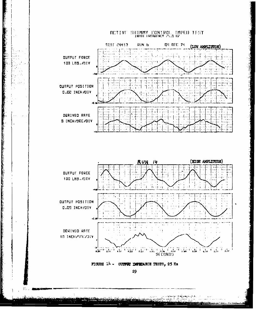
1) Output Impedance Tests, 25 Hz 29
15 Bode Plot, Output Impedance Tests, High Amplitude 30
16 Bode Plot, Output Impedance Tests, Low Amplitude 31
17 Steering Valve Trtmnient Response, Spool Valve in 33
Neutral Position
18 Steering Valve Transient Response, Biased Spool Valve 33
19 Input Response Tests, Small and Large Inputs 34
20 Input Response Tests, IntermediatLe Inputs 35
Bode Plot, Tiput Response Tests37
Active System Phase D)iagrau 1O0
vii 'c 1V1 ,3
- - -. ..---. ---

,IST 0F 1I,IJUSTAIPPTONS (Corit'd)
Figure puge
23 Active/Passive System Comparison, Impulsive Input, 42
Mid Position
24 Active/Passive System Comparison, Impulsive Input, 44
Extended Position
9-5 Active/Passive System Comparison, Wheel Imbalance, 45Mid Position
o6 ActJve/Pussive System Comparison, Wheel Imbalance, 45
Extended Position
27 Variation of' Hydraulic Fluid !.3tiffness, Passive 18
System
,8 Variation of Hydraaulic Fluid Stiffness, Active )18
""ystem
,9 V:rLit1.0lt of Torque Arm ,tiff.tOness, K.M1 50
30 Variation of Lateral Gear 11-tiffnhess, KPHq 50(I
31 Variat.on of' Torque Arm Backlash, f)liI 51
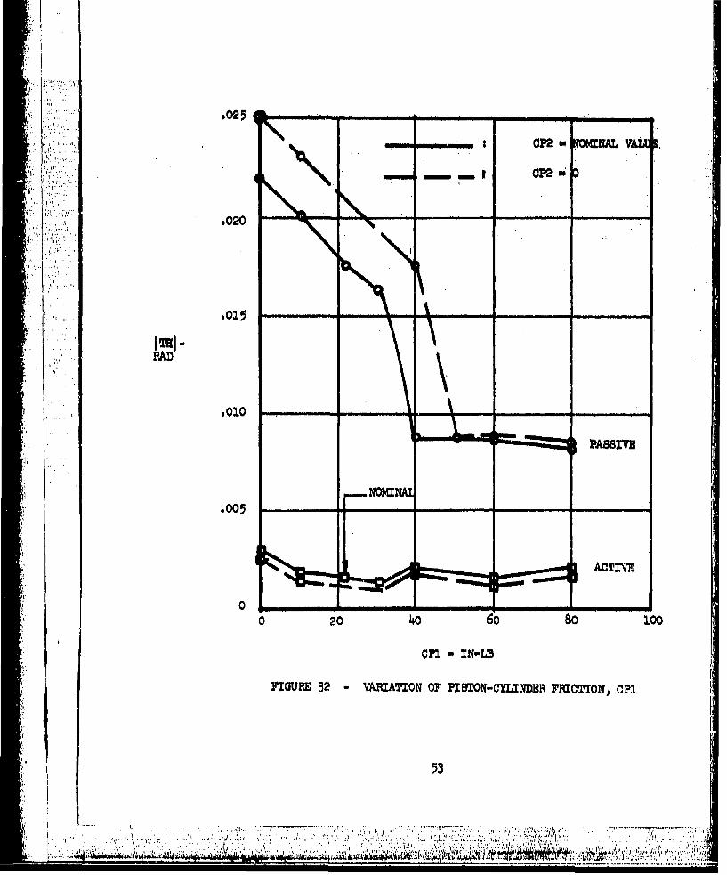
3V VL'-atoion ot:' Piston-Cylinder Friction, CPI. 53
33 Variation oa' Fuselnge amd Lateral. Gear Dlamp:lng, 54
13F Lid 3P311
3h Variattion of liuselage Natural I.Prequency 54
35 T-3'( Nose Steering Actuator in Act(.ive Configuration 57
36 T-37 Nose Steer.'ing Actuator in Passive Cornfifuratio1i 5
37 Schematic of Active Cotrol System 61
38 Block D)i:aram , Active 11h:1lnmmy Contro. System (01
3) •servo valve Installati on, R iht 'ide
;e 'vovu.d.ve T:nms•]u.laion , -.ef't Si.de 1.4
v -1 :t :1t

LI: 3T OFTI TRlJS1TIOx]NS ((CoiL d)Figures Pg
~41 Landing Gear, Rear View 66
42 Landing Gear, Left Side View 66
43 Electronics Module, Front View 68
44 Electronics Module, Rear View 68
45 Passive System Time Histories, Tire Imbaulnce 86
46 Active System Time llistories, Tire Iinbalwaice 8,7
47 Active System Trime Histories, Zero Tire Imbalance 88
48 Passive System Time H~istories, Zero Tire Imrbali-.nce 89
4 ~~Comparison of' Active ond Pasrsive System Responses 9
4J with Wheel ImibaliAnce, Glear Hxctended 9
50 Comparison of Active and Passive System Responses 93with Wheel Dibalance, (lear Mid Po:Int
51 Passive S-y'stem Response to Wheel Imfbid-nce, Mid 9)1i'I.osit-Jon, Nomn:ivil ]Jack2.aah
52 Comparlson of' Test taid Anialyticlo2 P~assi~ve 13ystem 97
Responses with Wheel DIbauance, Extended Sear Positilon
53 Compurison of' Test, and ]Uial.yti,,i3. Active. 14ystem 9(
R4esponsets wit Lb Whoa.ý :1mbo'hi.Lnu , NxteiiCiet Geni' Por;ii t~Ior
5,Conpiiri. sonl of' aurll i aN110,a YOL M Pus f.16 VU ie;SLO I en
Rer3polnse1s with W'he& Tr,11l mce, Kid So' r Prn!ti oi
.1 G~ompari son o t' Test 11,1d Atilk:I.,y L cidt Ad:-:! ve S1yntoi :0
kresponste'u wi Lb iWheel ltiu:1I iice , 14:1 (;eta, Position
A-] ~Ac I,.jv- ye Sh Imtniy Con tro' :;y nteirn Haurdwt ire. Arran prelmont ]'on
P.. 1 II .Irc ni L(Di ai';ram Act:! e h1 -I 111y Con tuol Srystell 11

LSTc OF [LLUSTRATTODIS (Concluded)
Figures Page
E-1 Active Shimmy System Expanded Block Diagram 153
E-2 Root Locus of Linearized Active Shimmy System Model 154
as a Punction of KG
B-3 Bridged-T Notch Filter Transfer Function 156
E-4 Root Locus of Refined Active Shimmy System Model as 157
a Function of' NG
LIST OF TABLES
Table Page
1 Input Parameter Definition, Active Shimmy Model. 17
P Input Parameter Values 19
3 Instrumentation Types, Location, Purpose and 71.
Specific Utions
4 Tape Recording Set-Up 72
5 Passive Shimmy Tests 74
6 Active Shimmy Tests 78
7 Summary of Shimmy Test Run Numbers 84
8 Revised Analytical Model Parameters 95
C-1 Plot Summary 115
C-2 Plot Time Hititory Description 116
D-1 CSMP Special Functions 1.49
x
L'"!
INT[RODUCTION
The methods used to determine the shimmy cbaracteristics for a landing gear
in the design stage of an airplane can vary from a simple rigid tire repre-
sentation to a detailed nonlinear representation including variations in tire
charactertstics as a function of fluid pressure, and variation in strut
friction Us a function of gear load and strut stroking velocity. Testing
varies from running over a two by four placed on the runway for the purpose
of excitin, the nose gear in a shimmy mode to dynamomenter testing using a
feedback control oscillatory drive system to excite the gear at various
controlled torsional frequencies and amplitudes. The latter test technique
provides data for determining shimmy margins under test conditions used to
simulate gear degradation with age. There are various analytical and test
techniques whose capabilities lie between the aforementioned extremes.
Even though gears have performed satisfactorily early in their service life,
some have become chronic shimmiers as they ae. This change ib usually
attributed to wear in the geur which causes tin increase in backlash. Tuas-
much as most shimmy evaluation techniques do not provide a means of assess-
ing margins, and .adequate estimates of the degradation of gear paramueters
affecting shimmy may not be made, a clear understanding of the susceptibil-
ity of' gears to shimmery is not esta~blished.
Therefore, the performance ofr an ideal. sh-immy suppression system should not
be uffected by the gear aging process. Some of the parameters that can
change dur¶..ng operation from the values originally expected include:
o Backlash increase from wear of torque aria tcbtachments,
tri.munons, steering collar, an(d steering actuator linkages.
o Increase In damper fluid air entrapment.
t1
. L i•,

o Reduction in strut bearing friction caused by reduced nose gear
load attributed to an aft shift in operational center-of-gravity,, ~~position.-•]
o Change in tire stiffness characteristocs to accommodate airplane para-
Sgrowth and/or changes in tii operationa l center-of-gravity posi t -•: ~t ion. :,
"nless adequate allowance imade for these parameter changesta hich may nota
be practical in the development of a passive damperi eventually shimmy may'•'ioccur*
lnThe nature of achive pontrol systems is suchthat they may be independent
of come of the aforementioned parameter changes and itn maybe praitical to
provide means of adjusting the system to accommodate the more permanent parl -
meter changes. Accordingly, while an active antsshhmmy system may yield a
more complex gearp the potential for providing shimmy fre• operations through-n
out the control syathe airsl. ne manes development and evealurtion of such aisystem quite attractive.
In order to assess the practicality and performance potential of active .
shilmmy cont'ro!, the present research program was initiated. The objective'•
tof 'hetd progrram is to develop a breadboasd version of an active shimmy control
system for the Tn the 12gear. This particlar gear was chosen because of Ts
its long history of shimmy problemy in service. The program is conducted infour phases. Phase I consists of obtuining a T-37 nose gear from the Air i
Force Flight Dyn~amics Laboratory (A.FFDL,) and measuring certain gear charact-
eristics pertinent to shimmy behavior. During Phase II., an analytical model":
of an active shimmy control. system is developed, and analyses are performed i
to determIne a specific control scheme. In Phase III, a breadboard version
of the control systerl is designed and built. The landing, gear is ailso in-
stclimented for shJ~mmy testIng. ]Ert~ring Phase *-V, the active shimmy control •
system is tested on the 192 Inch dynwnomenter at AFFDL'13 Landing Gear Test
Paoie'ldt~y. :
W,,

ANALYTICAL MODEL DF.SCIIPTION
General
Both the passive and active nose gear shimmy models aro incorporated into
one Continuous System Modeling Program (CSMP) digital computer program".....utilizing computer graphics display and interactive operation. The T-37
nose landing gear is modeled as a multiple lumped mass system with four.
torsional degrees of freedom (aboutthe strut axis) and one lateral degree
of freedom with a Von Schlippe tire model (Reference 1). The active
shimmy control system utilizes axle torsional acceleration feedback signals
to control the steering actuator displacement. Figure 1 shows a
drawing of the T-37 nose gear with the essential mechanical elements identi-
fied. When the axle rotates about the strut axis, the wheel fork transmits
this motion via the torque arms to the bottom' of the outer cylinder. The
outer cylinder rotates inside the trunnion yoke, which attaches to the air-
plane at the trunnions, The top of the outer cylinder in attached to the
steering actuator housing (cylinder) while the steering actuator piston is
attached to the trunnion yoke.
Torsional Degrees of Freedom
The analytical model for the torsional. degrees of freedom is shown in
Figure 2. The unsprung mass ITH is connected to the ground via the tire
(described later) and is connected to the outer cylinder IT112. through the
torque arms of stiffness KTTT with backlush UIIT. Plston-outer cylinder
friction CP damps motion across the toroque arm backlash T[M[ and stiffness KTM.
The outer cylinder I1111l is connected to the actuator housing IAL vith spring KOC,
representing the stiffness of the outer cylinder, in series with backlash
DAL, epresenting the deadband at the actuator housing to outer cylinder con-
nection. Friction CF is the friction between the outer cyl.inder rnd the
trunnion yoke in which it rotates. The trunnion yoke is connected to the
fuselage. ITH2 repre.ients .ocal fuselage stroctuire which is connected to
the "rigid" airplane through the fuselage stiffness TF. BF is a linear
dwnper representing fuselage structural damping.
3
...........................

Steering Aotuator
Trunnion-
Outer Cylinder.
Trtunifon Yoke
Torque Am 0
Wheel Fork
Axle
FIGumH I T-37 NOSE LANDING GEAR~
4

. ... . ..
ELECTRO-HD1AAJLICAU ACTUATOR
;L(ACTU3ATOR MENG
or BAL
cp 3AXN
Km CONTROL
Oro~d Tire (see Fig. 4~)
¶ FIGURE 2- T0R3ITONAL RESPONSE MODEL

CA is the steering actuator friction. BTI, BI -id KALPshown in Figure 2,
- are used only for the passive system. BH and BL are hydraulic (velocity
squared) and linear shimmy damper constants, and KALP in the stiffness of
the hydraulic fluid column in the actuator. For the active system, the
force generated in the steering actuator is computed from a detailed servo-
valve/actuator model shown only as a box in Figure 2. In the active model,
the feedback signal, after passing through a gain control circuit,, is sent
to the actuator which generates the steering actuator force FKAL. The active
a's~tem controls the actuator displacement ALT2 shown in Figure 2.
Lateral Degree of Freedom
The analytical model for the lateral degree of freedom is shown in s igure 3.
Laterally, the gear is assumed to be a rigid "pendulum" rotating about a.
fore-aft axis located H inches above the axle centerline. This'lateral
rotation is resisted by a linear torsional spring X1R,represonting combined
gear lateral flexibility andlocal fuselage flexibility. Acting in parallel
with KPH is a linear damper BPIH representing the structural damping in the
gear and local. fuselage structure. The torsional backlash DPH is in series
with the spring and damper wid depicts rotational deadband from the lateral
piston-cylinder, cylinder-trunnion yoke, and trunnion-fuselage joints. The
landing gear's lateral rotational inertia is IPH.
The axle centerline is located aft of the strut centerline by the mechani-
cal trail L. If the strut is inclined (forward at the bottom), then the
tire forces at the ground contact points are located aft of the axle center-
line by the geometric trail LG. Mhe geometric trail is related to the roll-
ing radius R and the strut inclination angle • by the relation
LG a H sing (I)
Also shown in Figure 3 are the positive mign conventions (right hand rule
for rotations) ror. axle torsional rotation TIn, gear lateral rotation PT,
'1
• i . ...
'.'• •, .. .. . . . .. . . , .' .. . ., . • •,1 • -•4;! ,•-•.•6',:• ' ,• :-,,e'• ' .. - - •.

TORSIONAL SPRING PR
T1ORSIONA~L BAO1KJA.S
F'OR PH ROATIONS TORSIONAL~ DAMP~ER
FF
TIG

t Ire force and moment IF und N, geAr moments FK an I FCP and airplane for-
ward velocity V. Gyroscopic arid inertia coupling terms between the lateral
and torsional modes through L are included in the mcdel. The coupled
dynamic equations of motion for the lateral and torsional degrees-of-freedom
mve shown below. In each equationý the second term represents inertia
coupling and the third term represents gyroscopio coupling.
n'H (PiEDD) - M (L) (1) (TIIDD) - I '1'HD +L iFZ-M(G)1 T + BPX (PED) + PPH
+ IW(H) - (mE.R) F'Z1 PH (M+R) i'T (2)!*ITH(TranD) M(L) (11) (IDD) + I PD +L(FT)wT +FCPr O +(3)40
Tire Model
The tire lateral force and moment are calculated according to a dynamic
model developed by Von Sihlippe (Reference 1). This employs the "stretched
string" representation for the tire equatorp which takes on the deflected
shape shown in Figure 4. ri gure t ,hows a view looking down on the tire con-
tact patch, with forward airplane motion to the right. Z and E are the tire
equator lateral deflections at the forward and aft ends of the contact patch.
Referring to Figure 4, the tire force and moment are given simply by
FT KT(Z +(4)
where KT w K lateral (6)2
ond W U toi sional
K lateral and K torsional are the lateral and torsional tire .tiffnesses,
•'while KT and KM are the corresponding input parameters to the computer pro-
gram. For this study) K lateral end K torsional are determined by using
empirical equations from R~eference (2).
The tire deflections Z and 2 are determined from the tire equator coordi-
nates Y and '7 and the location of the wheel center plane in terms of gear
motions PH and Ti. The following equations for Z and I can be derived by
inspection of Figure 4.Z Y Y - (HS-L-LG) TH - (H + R)1 (8)
+. (H S L + LO) T11 - (H + R) PH (I"PHD , - (PHI), 7IDD - - (PHD), THD -- (TH), THDD , (THD)
dt dt td
' - I..-- -. ... . . .• .. ':, •,- 1, .A..

!' • !
i liiiiiN=•:,a
I•L
S i •. • I-I•-
..-...-... ". - / i.. I . .

1The Von !hM1ippe tire theory (Reference (1)) develops the kinematic con-
straint equations f'or Y and Y. Tihe detuils are not presented here; however,
the resulting differential. equations governing Y and YE are
(SG) YD + Y (69G + IIS-L-t0G) T1! + (H + R) PH (10)
•';: ';:and (t) -Y (t 2 -S) (
YD is the time derivative of Y. Equations (10) and (11) provide the tire model
with its dynamic properties, i.e., the effective tire stiffnesa and damping
vary with velocity and shimmy frequency. The yawed rolling relaxation length
SO and half-footprint length 11S tre determined empiYrically from Reference (2).
Active System Model,
The active shimmy q(rol system for the T-37 nose gear consists of the
following major e.•. •,•:,s.
(1) An electro-hydraulic servovalve attached to the existing
steering cylinder
(2) A torsional :aicelerometer mounted on the wheel. fork to
measule axle torsional acceleration
S' (3) An electronic signal shaping and gain control network to
convert the accelerometer output into the desired feed-
back signal f'or the servovalve.
Figure 5 shows L schematic diagram of the T-37 steering actuator. The
servovalve for the active system is connected to the existing steering
actuator through a coupling mandfold which connects directly to existing
ports in the steering cylinder. Figure 5 shows where the coupling mani-
fold connects to the steering cylinder. Vor the purposes of breadboard
system testing, the passive damping orifices are plugged amd the existing
spool valve is fixed relntiv,• to the actuator housing. Nose gear steering
10
-'4.- . .....,.-. -. *,.-, ...

INLET
POWER-ONDA?1I~NG OR1IFICE
TO COMPENSATOR DA .2IN&RETUR~N
STEERING INPUT
VVMD TO
* ~POWEI&-OFFDAMPING ORIFICES
-DA .8 N SPOOL V'ALVEF- - .CENTERING
* Pbcisting Damping
A oil Orifices Blocole
Connection to Servovalve
1FIGcURE, 8W SfEIING c1MIDEIR ",C1TONATIC
-. ...................

for the shimmy tests is accoimplished through electrical commands to the
active system.
Y'- The analytical model for the servovalve and steering actuator combination
is shown in Figure 6. In this model, the input ALT2C is the electrical
feedback control signal obtained from the signal shaping and gain control
network. The spool valve electrical input signal Xl is the difference be-
tween the control signal ALT2C and the actual measured actuator position
response ALT2 (see Figure 2). The spool valve opening X2 is the result of
X1 passing tbrough a second order filter representing the spool valve dyna-
mic response. The output of the servovalve is the fluid flow rate which
is X9 in Figure 6. This flow rate is proportional to the valve opening X2,as modified by a valve opening amplitude limiter (xn).
Valve flow rate degradation with load pressure is modeled by the following
equation which is characteristic for the type of flow control wervovalve be-
ing used.
(12)Q is the output flow rate X9) X2 is the spool valve opening, pe is the eye-
tem supply pressure and ), is the load pressure. In Figure 6 ,ps is X5 and
pL is X6, which is related directly to the actuator force FKAL. The flow
rate, due to piston motion, XIO (directly related to the actuator velocity
ALT2D) is subtracted from the servo flow rate X9, yielding the load flow
rate Xll. This is the flow rate due to fluid compressibility. The inte-
gral of this term times a constant K3 yields the actuator force FKAL, which
physically feeds back into the system through K5 to yield X6 which is the
load pressure PL, The K6 inner feedback constant represents valve leakage.
The net effect of this system is to control the displacement ALT2 in accor-
dance with the input signal ALT2Cp below the cutoff frequency of the actu-
ator model as controlled by K7. The "output" ALT2 is related to the input
command ALT2C by a lot order filter whose time constant is determined by K7,
in addition to the 2nd order response of the servovalve (X2/xI).
12.v. LilI
- '-lI
.' I .. .. .. .. , . . ,'i • •A ••''•, ''•,, . . ..,.". . . . .. &

113
WOW

Constants Ki. through K are- chosen so as to nondimenslonalize the u.ctuiitor
n.odel "internal" response vur:lubles X;.. through XII. 'Thlus, U value oI.' 1 for
X2 represents full scale spool valve traVel, 1 for X"5 represents system
supply pressure Ps and 1 for X9 represents the rated flow capacity of the
servovalve.
The analytical model for the active system feedback gain control and signal
shaping network is shown in Figure 7. TI{DD is the ca? culated axle torsional
acceleration (the second derivative of M- shown in Figure 2). T'his passes
-through a second order filter representing the dynamic response of the tor-
sional accelerometer, yielding TIIMDD (measured acceleration). A direct low
gain path through the constant GISMAL provides the primary feedback signal.
SM•N. An additional nonlinear high gain path yielding BITWN is provided.This signal path has a gain of GIBIG, which is typically chosen 3-4 times
greater than G1IMAL, but its output is of limited magnitude. BIGOR endSMGN are summed to provide the feedback signal. XC. The purpose of this
network is to provide high effective feedback gain on XC for low magnitude' TYMDD (when BIGGN dominates SMWN because GIBIG 1is much greater than G23MAL),
and to yield a low effective gain of GISMAL, for large amplitude TT.MDD (when
bhe limiter on BIQGN diminishes its magnitude relative to SMGN). The modelalso provides for a first order filter on TIIMDD to reduce the signal noise
content, and a switch to completely remove the rnonlinear high gain path If
desired (leaving only the linear feedback galla OlSMkt).
tle output XC from the g:iin control network is then e:thheri used directly
for the input to the servovnLve :is AL'PC (liee Figure 6), or nFy be routed
through at first order lea.ed-lag. signal shapning network whose output Is then
AT,T2CP.
A complete .listing of' the anal~ytical model equations of motion I.s conta:1ined
in Appendix D.
•:: ,• '•'• '•- •:'"• '•• :•k / • '•< G• a•& '• •,' N• •v -•, , .•''i1:a':" '•' "-: : " ,: .. .. ... .. ... .. '4

MehSystemIDynmuicI
Equat ionig
TIHDDNetor
T~tD])AIM
-MNx
11 WVI1DIM
11171IDD BI-O

PARAM~ER D~ETERNATIO11
General
Parameter measuri, .ant tests were performed Qn the T-37 nose gear to
determine stiffnesees, inertias, frictions, backlashes and passive shimmy
damper performwace. Table 1 contains a definition of all the input para-
meters of the analytical model. Table 2 lists the parameter values used in
the analyses, and indicates the sources for the data. A dash in the "EXTEND-
ED" column means the parameter value is the same as for the mid position,. An (x) in
the column "DESIGN VAR" in Table 2 means that the parameter is a design
variable for the active control system. The values shown for these para- - .
meters represent a baseline active system design chosen from a number of
candidate designs. In particulaur, it should be noted that the lead-lag
signal shaping network is not used in the baseline system. The dynamic
characteristics of the servovalve and torsional accelerometer are tdken
from catalogue data for off-the-shelf hardware. The calculations of actuator
constants K3, K4, K5 end K6 utilize geometric data physically measured on
the actuator and gear. In addition, KI through K6 all involve data peculiar
to the particular servovalve chosen, specifically its rated flow and system
operating pressure.
The followIng subsections present detailed discussions of the methods of
measuring the physical gear parameters and the passive steering actuator
performance.
1. Lateral anJ Torsional Stiffness - KPH, I(TH and KOC
The nose gear assembly, including the drag strut, was hung in the
AFFDL-supplied test fixture and suspended in a structural steel frame-
work as shown in Figures 8 and 9. The gear was londed both laterally
and in torsion by means of weights on a cable passing over a pulley at
the side of the test framework (not shown in Figures 8 and 9). Dial
gages mounted to a vertical extension of the gear holding fixture were
used to measure deflections and rotations. The stiffness measurements
were made with a solid link replacing the steering actuator.
1.6
-- iww 1,011i

TABLE 1 - INPUT PAR•AETR DEFINITION) ACTIVE SHIMMY MODEL
PAAAMETE, UNIT8 DESCRIPTION
4I. IN-/RAD Lateral rotational stiffness (m H2 K lateral)H IN-/RAD Torsional stiffness - uxle to bottom of. outer cyl.
Ky. I•- •rRAD Torsional stiffness - fuselageKO1 In/RAD Torsional stiffness - bottom to top of outer cyl.'.KALF I-/RAD Torsional stiffness -.. steering actuator
SIP ILateral rotational inertia,ITT' IN, * EC Toriional inertia - Wheeltirelforkppiston, ½
torque arm""InI1 IN-#-SEC2 Torsional inertia - Outer cylinder, j torque armITH2 IN-#3:BC0 Torsior*al inertia - FuselageIAL IN#- SECR Torsional inertia - Steering actuator cylinder
V I IN-#ý•2 Polar moment of inertia of wheel & tire
M -#-SCIN "Mass of vheel,. tre & axle (used w/mecb.. trail for
inertia coupling)W Total unsprung weight
CPI IN-# Piston - cylinder friction - CoulombCP2 IN-#/# Piston - cylinder friction per unit side loadFi IN-% Friction between outer cylinder & trunnion yoke -
Coi.IlombCF2 IN-#/# Friction between outer cylinder & trunný.on yoke per
IFunit side loadCA IN- Coulomb friction in steering actuator
MTH RAD Backlash in torque arms (total freeplay n 2 TH)DAL RAD Backlash in steering actuator (total freeplay
P.DAL)DPI! RAAD Lateral rotational backlash (total freeplay - 2DPH)
BH IN- RAD/SEC) Passive hydrau.ic damping in steering actuatorBL IN-#/(RAD/SC0 Passive viscous damping in steering actuatorBF IN-j//(RAD/S= ) Viscous equivalent of fuselage structural damping
in torsionBPH IX-#/(RAD/SE0 Viscous dam.ping of gear lateral rotational mode
GIBIG High gain for THDDGI Sol P Low gain for gTHai' HDDLM RAD/SEC9 Limit amp'litude of THDD for high gain
L IN Mechanical trail of axle aft of strut centerline' G IN Geom,!tric trftil of tire contact patch center aft of
,• ,strut centerline intersectioi, with ground plans11 } IN Hvight of lateral, oato point ofgear aoeal
__rotation__ :::hotiona node
VK KNOTS Airplane forward velocityF FZ •Verticol load on nose gear
-"!
17

].AI.LE, 1. INPU PAILAMETEE DEFINITION, ACTIVE SHIMMY MODV/ (coNT'D)
A .A.IT IR I TN -IS DESCRIPTION
RIN Ti re rolling radiusSG IN Tire relaxation length'HS IN Tire half footprint .lengthKU #/IN (Tire lateral stiffness)/2KM #/RAT (Tire torsional stiffness)/211S
Til SEC Time constant for lead term in signal shaping networkPP SEC Time constant for lag term in signal shaping network
TAUP1I SEC Time ccnatant for filter on axle acceleration signal
KI Ii/AD Servovwlve constant converting input signal in radiansto normalized valve spool position
' ,Servovulve pressure gainK3 IN-LBS Fluid compressibility constant converting nondimensional,
cotnpresssed fluid volume to steering actuator momentK1 RADISIVC)." u3teering actuator constant relating actuator velocity to
nondimensional flow rate5 IN-L3S) Steering actuator cons-twit re.nting actuator moment to
nondimens;.onal. loud Pres sureK6 IN- U3,3 Steering actuator normalized leakage flow constantK7 " Control loop negative feedback gain aonetw'At
ZETAA - Di:mping r-tio Pov second order model of uccelerometerOI.fAA RA'l)/SIC Nat-vria 1'frequency for second order model of accelerometer
TA Dampin ritito for second order model of servovul.ve0141i:GAs RAD/S , C Matlral frequencey Ca'r second order model of servovalve
II
S! ~~~........-.-................ ............o.. ..... , ..• •' """ : ;•.•,•.•. • .',•i5• ..... •.... .. . . .,.. . . . . . ........- •.... ,,,....% ,,,:,.., .... .. ... ... (

,,.' PA3XE, I;] ? - T ]TU'r.' PA VW:P ~7lI',k VA!1AJ1'.L'
SGEAR POSITION DATA SOURCE
PAi iR MIifD EXTENDED MV REP CAiAC(3)I TESTS DE•SIGN VAR. NOTES
KPH i.63E6 1.403E6 xKrI 11.20 5000 .. X
&T, ~ ipl, , xKOC 77270 - XKALP 18000 -X
IPH 69.7 83.9 XITH .68 x"ITI, I .03 - xITII2 3.h9 - xIA .o,285 -x 2
I .771 - X
W 2- X
cP-2 - -- x
CFI .6 - xCF2 0 - XCA 10.15 - x
it.I *Oc4i .0081 XDlAL .oo4 - x'P1 .001.08 .0014•8 x
BI 0 - XBL 186 -x
3P .6 - 3B•I- 853 935
GIBIG .024 - xGISMAI, .oo6 XTT{DDLM 40 - x
PI 0 - XP1 0 - x
TAMrIL 0 - x
.19
h- - . . . . . . . .I" • • " ' ......... .. ... .....'. . , . t _-_
•" I -,,,. " - . .• . . . l"' •• ;" • ;' ':"' • { ' '

TABLE 2 - INPUT PARAMETER VALITES (CONT'd)
GEAR POSITION DATA SOURCEPARAMER MID EXTENDED RPE RP? CALAC
(2) (3) TESTS DESIGN VAR. NOTES1, . .n14 - .x !Ii l14 I
K2 33.3 - xK3 2.62E6 - XK4 a1i4 -x
K5 ooc,412 -X
K(6 4.2E-6 -x
1(7 31.4 -
UZPAA ,7 - X0MHGAA 879.6 XZETAS .6 XOMEGAS 1000 - X
L .48 - XSL• .164 .473, X
H 36.875 40.5 X XVK 0 - 100 - X,. 650 200 X
R 6.96 7.58 xSO 6,649 2.5 3 xHS 3.131 1.961 xKT 203 225 xKM 845 251 x
TABLE 2 Footnotes
I Calculated from fuselage stiffneso in Ref. (3) and assumed naturalfrequency of 30 Hz.
2 Value shown for passive system; IAL - 0.058 for active system dueto added weight of servovalve and manifold
3 Calculated using structural damping ratio of 4%
20
ia

TETYIMFRMIXGMS WPPX2R
nIm,
DOM F GER ISTAUTIONIN EST IIrfl21
TEB~ PfC~3UPOEbUiflUOtRGAEPRG1UBI

V•. 8~teering Actunt-:" c tiffness - KAL
'Eie stocrin4g actuutor pasuive stiffness KALI, given ii Table P wus
obtuined from the Steering Actuator Output Impedance tests described inthe oubsection of the same title* The value shown represents the actuator
stiff'ness under dynamic conditions with cavitation in the actuator.* This is considered the most representative condition for shimmy.
3. La~terial F(otwiofala Inertie, - IPII
The laterrAl rotational Inertia was calculated by sluspending the gear
assembly from a kmown torsion rod spring and meamuring the undknped-':' Inaturql frequency, The geatr assembly (minus th* drag strut) was aus-
peaded with its lateral. plane horizontal and its oenter-of-gravitydirectly uider the torsional spring centerline. The a.g. location was
'imeasured relative to the yoke =d trunnion uxis.
4. Torsionul Inertia - ITIl and I.X
The inertia of the rotating assembly (less steering .iectuator) was cal-culated f 'om it mneAsured undtimped natural frequency and spring rate with
the tulit suspended from a torsion rod spring with the steering axsdirectly under the torsion rod axis.
5, 3te~ering Aotutator Inertia - XA1,
The inerti. was calculated using a. measured weight of the actuator
.ssezibly less u calculated piston rod weight (net weig.ht - ,-.86 lb.)•..nd useng ,in eff'ective lever arm from the steering axis of :2.0 in.
6, Totul lhspi'ug Weight - 14
Tlhe fae•u,' assembly was disassembled and the components that move verti-cally were weighed. (The lower brass bearing was not easily removuble
so Its weight was calculated and subtracted from the total mennured.)
7. Pston/Cylinder Priction CPThe botsion:al r'ict1i.t of the piston inside the outer cylinder was
meaLsured with the term" hanging, ti the test fr.me as shown In Figure 9.
,lij., ilia

The scissor linknge was disconnected by removing the quick release plia.
A spring scale was used to measure the force required at the end of the
scissor arm (6.5 inch lever) to rotate the fork assembly. The outer
cylinder was restrained from turning by replacing the steering ctuiator
with a solid link.
The measurement was repeated at various side loads up to 11.5 lb. by
hanging weights on a cable over a pulley at the side of the test frame-work. The strut was in midposition. The friction increased nonlinear-
ly with increasing side load, A plot was made and an average slopeutilized giving results within + 15%, with a side load between 0 and
120 ýb.
8. Outer Cylinder Friction. - CF'
* The outer cylinder friction was measured by removing the steeringactuutor and centering springs and measuring the torque as above,
Side load produced no detectable change in friction, Since the outer
cylinder rotates on ball bearings within the trunnion yokeo this
friction is very small relative to the piston/cylinder friction.
9. Steering Actuator Friction - CA
The actuator friction about the steering axis was calculated from the
linear actuator friction uind the effective radius.
10. Backlash in Steering System - VIE and DAL
The rotary backlush in the various components of the system was
measured by mounting dial gi.nges from the test fixture to measure
deflection at the end of a lever nrm (5.5 inch radius)p attached to
each of the components. The relative motion at each joint was
calculated from the difference in dial gage readings.
Included in the total steering actuator backlash (DAL) were two
sour em of freeplay: (1) the backlash in the two pins attaching the
)33

actuator, and (2) the backlash in the keyed connection between the
outer cylinder and the collar around it to which the steering actuator
is mounted.
Ile Lateral Backlash at Wheel -IDAT
In addition to the torsional angular backlash as measured above, a* linear lateral backlash was measured at the wheel axle location. A
dial gage war used to measure position directly. The value shown in
-, Table 2 corresponds to the Intersection of the linear load-deflection
curve with the deflection (X) axis.
12. Steering Actuator Damping Constants - El and BL
The damping constants were obtained from the SteerLng Actuator Output
Impedance tents described in the subsection having the same title. Theresults indicate that a linear damping constant represents the observed
results better than a hydraulic (velocity squared)constant.
13. Axle Trail - L
The strut fork positive trail was measured by aligning the steering
pivot axis vertically, measuring the horizontal position of the axle
relative to the test fixture, and then rotating the axle 1800 about
the steering axis and repeating the measurement.
Steering Actuator OutPut Impedance
The T-37 nose landing gear steering actuator was mounted in a test fixture
with an electro-hydraulic driving servo, as shown in Figure 10. The instru-
mentation recorder and supporting electronics for instrumentation and driv-
ing servo loop closure are shown in Figure 11. Force and displacement sig-
nals for impedance measurements were routed to a central data system for
processing and presentation.
The tests consisted of using the drive eer,.,o to generate sine waves of
steering actuator output piston position at amplitude of + 0.05 inches and
24e

H ii
-YOU� tO - ETCRINO ACTUATOR ThW1DAJfl TEST fl��URE
F II
a
Ii Ii I
1 1I FIaU1� 11 - XNBTRW4ENTATION FtUOTROICOS MID DL!& 1�OORDhIi
25
* * 'A. itk.ttinMtLLtnirL�< jŽt..,uJtwzxJdAIi�tAA±.AMt2i. IIkL',�.,L', gLt.... .. 'X .IT.�JI.gO2'��.. ..b r Xz±,.ms.i.&' __ .

+0.15 in. over, a frequency range of 1 to 50 Hz. The steering actuator
spool valve was fixed with respect to the actuator body, and the body was
mounted in the test fixture with a bracket having a spring rate of approxi-
mately 150,000 lb/in. The steering actuator war in the normal "power on"
configuration.
For each displacement and drive frequency; position, derived rate, and
force data were obtained following signal stabilization. Typical results .4
at 1, 10 and 25 Hz. are shown in Figures 12 to 14. The force and displace-
Sment signals were further processed to obtain fundamental sine wave compon-
ents and effective amplitude ratio and phase shift to produce the Bode plots
shown in Figures 15 and 16. The dotted lines on these figures represent a
linear approximation to the amplitude ratio data. For these approxibAte
* curves, the break frequency is taken at the 45 degree phase lag point, and
* .the slope of the curve below the break frequency is 6 DB per octave.
The test data indicates that very little damping is available from the
steering actuator at frequencies above approximately 5 to 10 Hz., depending
upon amplitude, because at these frequencies the force approaches an in-
phase relationship with displacement, with magnitudes of 2000-5000 lb./in.
This low effective spring rate makes it impossible for the actuator to sup-
port the internal or.1fice damping, and the actuator impedance, therefore,levels off, as u function of frequency, at the effective spring rate.
Cavitation wta suspected as the cause of the low spring rate characteristic,
sInce the steering actuator does not have anti-cavitation valves. Because
of the time delay in the formation of a stable flow through the orifice,there is insufficient hydraulic fluid to fill the cavity created when the
piston is pushed away from the fluid on one side of the piston. The pres-
sure on that side instantaneously drops to a sufficiently low pressure to
cause the air dissolved in the fluid to come out of solution. Successive
cycles of piston motion result in more air coming out of solution until a
stabilized hydraulic fluid-air mixture is achieved producing the low effec-
tive spring rate.
26
,ý ,A".,

INI'II r' fW-MILII.NI:Y 1 .1 I/ :'
TrirI 2411'1 WINw 1I' t1~ I (o
OUlPUT FORCE I.~:.10 LBS.AUIV Ii
OUTPUT POSITON j : .
MEfl INCDIMfIV -
.1 INCR/SE[;/DIV. .III
OUTPUT FORCE I I
f.... .... ... ......
0.0e- 4~~/I -. I, I ,. I
227
... . ....
414-A"....A~

n r, ,i v Vr' !i-i I m mY :(JN rr,1ni. IMii'ii TV~I'v
TI-111 011141l W 1.1N 4I O'I ur L: 74 (LOW .A1aTIUDED)
OUTPUT roat~C
100 LEO5./01V ,I
Me INH/
F-ý 147 -7--77-
I NCH/SE~C/UlVa I :T .}. .
RVN 1Z((HIGH L ~ aWDE)
=77T7.7/a~ .t ... . 7 T. 7.
OUTPUI POSITION . I , I
1 In It 11 1 .1 1. 4 1, I .". t l ", 1, IT
VIOURE 1.3 -OX)ThI IMPEDA!CE TEV; 10 H..
L I:
f1r V:T I V :1-1M M Y 1:0N W 'R I 1 M 1.1 1) 1 r:'r TF i Nr'i I i ruirtU NIY r~i n H
Tr-*.!r 011411 WIIN hi OI 111'[ 711 M M NDC
* ~~~~OUTPUT FORCE.....................ion t~./r
.i71....................... .1..... 4...
-0. oi
9.~ E NC II/SE IY . It .1.-
IL -
0.9 NCH/D.t/OV i..,
n, >. DA f 1011.T 117f l. i 'illS . m lN1)ý
OUTPUT FORIE !4i.N~:.....¶00 LiB./[V29

-,in
Ll M~
U I U
I l
L~t.L
rr 'n
r~ l
LiLi
I-I
L~ri
-_ - -- ----- "4r
L.LL
L 1 ItfI ( 0.
t.N r.. ri n0 .3 .0 Xl Il UIn
30J

le1
.r LO2OhLL U,
I . 0-u C= U
2cr N.L]c
~I
~. n
LL,
LI,4
4....4 L
cr t
y in
ru u
CC...........................................................................\
-I3

I.To investigate the cavitation theory, a transient recording was made starting
',.V at the initiation of cycling Inputs at 10 Hz. to the steering actfator. The
result is shown in Figure 17 ,hich indicates a higher initial impedance decay-
ins to the lower stabilized impedance. The teot was then repeate, with the
.i .... .steering actuator spool valve biased out of neutral-position to create aI, , .,•quiescent load pressure and Aissociated damping orifice flow through the,
spool valve, The time history for this test, starting with -the initiation
of cycling inputs, is shown in Figure 18. In this case, the mtab.Llized im-
pedanoe is higher (approximately 15,000 lb./in.), and the oavitt;Mo theory
would indicate that the spool valve can now support a portion of the flowrequirement to prevent as complete a collapse of spring rate as that ob-
,erved when the spool valve was in neutral.
Steering Actuator jnDut Retoyse
The same test fixture and supporting electronics for the impedance tests
"A Y' were used for the response tests, Spool valve input and actuator outpub
signals were routed to the Bye Canyon Central Data System for processing
and presentation.
The tests consisted of using the drive servo to generate a sine wave of
steering actuator spool valve position with respect to the actuator bodty
and measuring the actuator piston, position with respect to the body, The
steering actuator was in the normal "power on" configuration and the output
load was negligible. For each test condition, spool valve Input position,
and piston derived rate were obtained. Sample time traces are shown In
Figures 19 and 20 for various test conditions.
Run I shows the small signal spool overlap region and indicates a deadband
of approximately +0.008 in. spool travel# Run 4 shows the large signal
response characteristic in which a spool valve over-travel condition is
reached in one direction with the output rate decreasing to mero for in-
creasing spool valve travel. Run 3 shows an intermediate drive amplitudewith 0.19 in. peak-to-peak valve travel producing 20 in./sec, peak-to-peak
32
- ,,,".,.;h....- .. . 4Ht;,,, , •; iu.••,/• m,.'t4 •. * .•. • .

ftiI'VI lu !11 MMY LU0N I WIN0. 111:11111TOR'w~ Ni!'u
OUPU FORM
OUTPUT POSITION :-:i:U.Oe INCH/DIV
OEFRIVED RATEI ENCH/SFE/OEV
3,0 0
7X~J~17 :~ ~ SECON DSnmm .7 -enmm vAm TmsxET reponsp MOL VALVE XN SMIPAL PS~~
OUTPUT F'ORflE T 7fF V l. tI I
KID LBjT/13IVII
OUTPUT POSITION I'
O.eINC14/01!V i-.
ucwivrFo Pnrr -
I rNI:H/9D~:/r]IV
F.4.4 -4.- 4 1-1 I 1 1 -1 1 1 1 1 1 1 1 1. I-F 41 I I 11. -1 1 I , 1 1 1 1 4 1 1 1 1 4 1 4. 1.
FIEGUE 18- b'VM2MNO VALVE TRANSIM" RESPONSEt BMAM SPOOL VALVE
33
......................................... .

FUCT IV[r !ll I fity EON 1 [."01. tir.tini oW I ', ON
TarK 1ln RIJ I71 l ..11.
ourrir POMrlo I ION 1 ... j J
1 < ~ T, T_____
.r .L .~ ........-11119 I I I -
.1N.4
.:1.
RUN 't
F..~ -. , 7
0.1JP INCH/UIV IK.L
U H : N 11! .
34.

Tr'Jr 015':Ih RJUN J
INPUT POEJIT ON :2..: 1 px,.7~
O.L1e INF.H/DIV ......
OUTPUT POSITION
H: INHSCII
AUN P
INPUT POSITION l~l~ul~J,.. .ii
0.01 INCH/DIV N...
411
a.I INCH/V . 1
T,.. Al
7TF7RE 20.- IIIMJ RESPONZE TESI~l, INMuMgMZT1' IMMUIS

piston rate. Note the gross non-linear gain characteristics of the
piston rate response. Run P shows the response at a slightly reduced spool
•!: valve travel of 0.17 in. peak-to-peak whioh produces only 4.6 in./sec. peak-to-peak piston rate. This was the maximum spool valve amplitude at which a
reasonably linear response could be obtained.YIFigure 21 shows a Bode plot of output piston rate with respect to input
valve position in the linear region of operation (0.16 in. peak-to-peak
spool valve travel). The response is well behaved with approximately 5 M
attenuation and 45 degrees phase lag at 46 Hz.
* I The above test data indicates an extremely non-linear gain characteristic at
output rates above + 2.3 in/sea and a significant threshold characteristic.
Both effects are undoubtedly caused by the ahaping of the spool valve flow
characteristics The linear region of response corresponds to approximately
+ 87 deg./8ec, of gear rotational rate or + 0.56 dog. (.01 radians)S . at 25 Hz. Since the active shimmy controller must operate at larger rates
to be effective, and since closing the shimmy controller loop around an
extremely non-linear rate characteristics is not practical, it is concluded
that the active shimmy controller cannot be implemented using a modulating
piston stage for driving the present actuator spool valve.
The best alternative approach, without modifying the actuator spool valve,
appears to be a configuration in which an electro-hydraulic volve is used
to directly port flow to the steering actuator piston in parallel wIth the
spool valves Such an approach presents certain problems in synchronization.
hydraulic interaction with the spool valve, valve n%ill offsets, und failure
modes, but in felt to be satisfactory for investigating the potential for
active shimmy control in this experimental program.
36

TiL I)
C !I. t I
cI >
r 'i 9YI'rw oA
-,..............- C,(j*)UAM
(I. m tr I
INiI
. ~ ~ ~ ~ A - tx .. .. . i
mI Li '

ANALYTIC&L RESULTS
General
The types of feedback investigated for the control signal ALT2C all involve
using some form of THD (axle torsional velocity). The objective is to
.. ........ control the actuator displacement ALT2 in phase with the axle velocity
IaD, resulting in actuator forces acting on the axle (via the outer cylinder
and torque arms) which oppose THD motion. Of the systems investigated, the
simplest Whs selected. It uses the overall actuator loop as a pseudo-integrator of a control signal ALT2C that is just the direct output THDD
(times a gain GO) from the accelerometer. This results in the actuator
displacement ALT2 being in phase with axle velocity THD at frequencies well
above the outoff frequency for the actuator loop. To achieve the desiredphase for ALT2 (in phase with THD, or lagging THDD by 90 deg.4 at a shimmy
"frequency of around 16 Hz, the actuator loop cutoff frequency is adjusted
(via K7 in Figure 6) to about 5 INh. With the loop set to 5 H% and the sys-
tem operating at 16 lz, the loop contributes 73 dog., of phase lag, and
the Kccelerometer and servovalve together add about 17 dog,) giving the
desired 90 dog. lug of AI.T relative to MTDD. Therefore, at the shimmy fre-
quency of 16 11z the native system forces the actuator displacement ATMP
to be in phase with the axle velocity T'ID.
At lower operating frequencies the actuator displacement lags THDD by less than
90 deg., und at higher frequencies by more than 90 deg. The system will only
be operatDig a•t frequencies other than the a' ..,imy frequency when it is
driven by u cyclic disturbance such as wheel imbalance. For the T-37 nose
wheel and tire in the static position, the relationship between airplane
velocity and the resulting driving frequency from wheel imbalance is
f - o.46 v (13)
where f is the driving frequency in Hz and V is the airplane ground speed
in knots. From the above equation it can be seen that an airplane ground
speed range of 10 to 100 knots results in wheel imbalance driving frequen-
cies rrom 4.6 to 46 11z, or roughly 5 to 50 Hz. Since the atplitude of the
38
S... ..... . .. ~~~~~~~~~~~~..................................... -• • ........ • .•..... A..; •.. ,:•''u,•,• ,.::•................I....,"

moment, due to wheel Imbalance, is proportional to the velocity squared,
velocity inputs below 5 knots ure no problem with any reasonable wheel im-
balance (lOSe than .0 times the normal imbalance).
r=igure 2 shows a phase diagram for an active system tuned to 5 He. The
vectors shown in the diagram are rotating clockwise at the system operating
frequency. The phase relationship between actuator displacements (ALT2)
and axle velooity THD are shown -at system response frequencies of 5, 16
and 50 Ha.
At 5 Hz the actuator displacement leads THD by 40 deg., and at 50 He it lagsSby 46 deg., while ALT2 is in phase with TED at 16 Re. Therefore, tuning the system
for optimum performwace at the shimmy frequency of 16 Hz (the system will
oscillate at this frequency if given an impulsive disturbance),results in
acceptable performance over a broad spectrum of cyclical disturbance fro-
quenciess The phase lags from the servovalve and accelerometer prevent
reducing the phase angle differences resulting from an operating frequency
range of 5 to 50 He.
This active system without any lead-lag signal shaping and with nonlinear
gain control constitutes the baseline active shimmy control system. The
results obtained with the lead-lag network are very similar to those with
the baseline system. The purpose of the lead-lag system is to Vrovide
feedback signal amplitude attenuation at bigh frequencies ( > 50 He), while
retaining the desired gain at lower frequencies (10-40 Hz) corremponding
to the shimmy response frequency. Although there appear to be only slight
benefits in system stability to be obtW ned from the lead-lag network, it
is included in the breadboard model to provide greater signal shaping flex-
ibility during shimmy testing of the system.
39
I ., , . .IAN . .. .' .. . ., .. ." '•" ' . . . . . . .... ."'.. ".... ... . . . .' "''•"•'':• : ,4 :F.;5;:- .,]. '• ':. . ". -". . .
I I I i i I I-- -rn''-'-i•+ ...&I MI I I

T'HDALT216 Ez
LLT2 ALT2*1.. 50 W OHz 4 5 Hz
460 40
____________ T~RDD
rIGUR 22 -ACTVIVE SYSTEM PHASE DIA.GRAI4
40
................................................. -6k

Baseline Active-Passive System Comparisons
Utilizing the passive/active system model and parameters delineated in the
previous section, the performance of the baseline active system is compared
with that of the basic passive gear. Two types of input disturbing func-
tions are used to excite the gear. One is an initial torsional angular
velocity (TKD)at the axle at time zero. No driving force is involved;
the system dynamic equations are solved with an imposed initial condi-
tion on axle angular velocity. This type of excitation simulates the im-
pulsive type of driving force that is used in most shimmy Wests, where the
force usually comes from an oir blast applied to the wheel rim. An initial
condition of THD - 5 rad/sec is used.
"The other type of excitation used is wheel imbalance. With a single wheel
gear this would not tend to excite shimmy motions if the imbalance were
symmetric about the wheel center plane. However, if the imbalance corres-
ponds to a weight located at the wheel rim on one side only, the result is
a sinusoidal driving moment both in torsion (TH) and lateral bending (PH),
the two being 90 deg, out of phase. The magnitude of the driving force 1s
proportional to the imbalance and varies with the square of airplane forward
velocity (or wheel angular velocity). A wheel imbalance about the axis of
wheel rotation of 10 in-oz is used, assuming all this imbalance is due to
one weight located at the wheel rim on one side only. This magnitude of
imbalance is slightly greater thwa that normally allowed in service
for this size of wheel and tire.
Figure 23 shows the comparison of the active and passive systems for an im-
pulsive type of input, with the landing gear at mid extension. The limit
cycle amplitude of oscillation of TH (axle torsional motion) obtained is
shown plotted against airplwie forward velocity. The passive gear is well
behitved below 40 knots; between 40 4nd 80 knots the limit cycle amplitude
rises rapidly, and above 80 knots the passive gear is unstable.
41
-- • ____•_____'_ -- ' . .. . . ,
-.. .. . .. . . __. i _'.'] . '_. . ........

.05 i
* 03
P AD pAsi lVE
.02 ---
.. 0
0 20 40 6o 80 100 120
VE~LOCITY - KNOTS~
* . FIGURE 23 -ACTIVE/PASSIVE SYSTEM! C0?.PARIB0N, ThWUSIVE XNPUTTVZD POS1ITON
42 ~;ni~Ln, . i'

In comparison, the active gear shows a dramatic reduction in response ampli-
tude ut velocities aibove 40 knots to well. beyond the ground operating velo-
cities of the T-37 airplane. The slightly higher active system response at
veloottes.between 5 and 30 knots is considered of no consequence because
the amplitudes are still well below the total torsional backlash (DT1 +DAI),
* shoyn as a horizontal line in Figure 23., This mild hump in the low velouity
region response of the active system can be eliminated by either reverting
to a passive system at low velocities or by reducing the feedback gain to
zero*
Figure 24 shows the same comparison for the gear In the extended posi-
tion. Below 80 knots, the passive gear is slightly more stable in the
extended position than in the mid position. This is due to the tire input
moments being much less with the gear fully extended, As shown in rTible I1
the tire torsional stiffness parameter KM in the extended position (bire
vertical load a 2001b.) is only 251 compared to 845 with the gear in the mid
position (vertical load n 6501b.).Although the susceptibility of the gea:r to
shimmy is greater in the fully extended position because of its lower tor-
sional stiffness and greater backlash, the greatly reduced tire torsional
Sstiffness more than compensates for th&se effects. Again the active systsm
shows clearly superior performance at all velocities above 40 knots, Aitabil-
izing what would be an unstable passive gear.
The comparison between the active and passive gears subjected to wheel im-
balance is shown in Figures 25 and 26 for the gear in the mid and extended
positions, respe..tively. As with the impulsive disturbanceo the puami¾N gear
is unstable abov'i 80 knots, whereas the actively controlled gear has very
low response amplitudes at all velocities. The hump in the low velocity
region for the active gear, extended gear position, shown in Figure 26, can
be eliminated by reducing the feedback gain or reverting to a passive sys-
tem below 30 knots.
The peak instantaneous power reqýuiremeut for the active system is only .49
horsepower at Vl.00 knots with 1.0 in-oz of' wheel imnoal.ance. At. (0 knots
43
I"~~~N 1:.I,,, .464 .- ,x'." i, i • , ,,:i.. ,• ,,,•,•. . i• - •.-:. • "',•, ¢, " ; , ," ,. ." " . . . '- . -'•: L • • . • , .t.• • , , ' • • : " ' •,•< ',t ,' ' • ,'• ,," -, • •. .. ..
. . . . . . . . . . . . . . . . . . . .. . . . . . . . .

!00
[ ITHI-RAD
.02______ _____ PASSIVE _____
•. -. ,,-
0o ..... .. m..... ji
601,,, ,
0 20 40 60 80 100 120
VELO0CIT - KNOTS
FIGURE 24 - ACTIVE/PASSIVE SYSTEM COMPARISON, IMPULSIVE INPuT,EXTENDED POSITION
'i
44,
...-,.. A

.04 a-
.04I -_ _ _ _ _ _ _
RAD
~ ______________ ____________________________ _____________ ______02_____
0 ACTIVE01- -
0 20 40' 60 80 100 120
VELOCIT - KNO0TS
FIGUR.m 2 5 -ACTIVE/lASSIVE SYSTEM COMPARIS0NP Vw7m I!.BAIANCI'XD POSITION
ITRI - PS1RAD
.02 _____ _____
0 04o 60 80 100 120VELOCITY - KNO0TS
nomJ~ 26 -ACTPIVE/I'ASSIVE SYSTEM COMPARISON, WnE IMB~ALANCE,EXTENDED POSITION?
45
-~ -- V

this drops to .05 HP, and is only 0O1: TIP at 20 knots. For an impulsive type of,
excitation -the peak power requirement in .27 H? at' all velocities from 60 to
100 knots.d Me maximum actuator force requirement is 685 lbs. at 100 knots
with wheel imbalances With an actuse-or area'of 1.08 in 2 , this requires a
pressure differential of- only 6314 Psi., compared to a'system'pressure of
.,.1500 psi. The highest Iintantansous valve flow rqte requir'qment ii 3.,2$
g4ljonh per minute' '(G.)' with wheel imbalance at' 100 knos. The rated- no-
load flow capability of the valve used for the myitem is 4.9 GPM, Euven
assuming the. peak actuator pressure (634 psi) coccurs simultaneously with
K.the peak flow rate requirement, which is conservative, applica~tiona of equa-
tion (12?) shows that the flow capability of the valve under load decreases
to
150 (4i.9) m3.72 G;FM
which is still 15% above the maximum flow rate requirement (3.25 GPM).In order to provide a 6 dR gain margin the feedback gain for the baseline
active system is one-half the value that results in marginally un~stable be..havior of. the active system. No indications of unstable' behavior are evi-
dent for any of the operating conditionsi analyzed. The 6 dB gain margin isbased on O:LSAAL, since GIBIG is only effective when the system is in the
backlash region and can tolerate much larger gains without going unstable.
Parameter Var~atioris
The sensitivity of the foregoing ianalytical results to variations In cer-
tain system p~arameters is described in this section. The parameters in-
vestigated include the following,
1.. KALP and K(3 Hydraulic fluid stiffness in the actuator
~:'.KTHTorque armi stiffness
3. 1091 Glear lateral stiffness
l I 1VH Torque arm backlash
5. CP Piston-cylinder friction
0 , BF and B111 Fuselage and laterul. getir damping
Y(. 1T1Puselcige inertia
... - -- -- . . .. ...

Both active and passive systems were analyzed using the impulsive distwr-
Ji:bance (THD 5 rad/sea) at V u60 kn~ots with the gear in the mid positionas a reference condition.
9,.;1. KAI? and K3 - iurs27 and 28 show the effect of var'iations in the
h-draulic stif neuti parameters KALP and K3,on limit cycle aml tue
for the passive and acti~ve~uyvtams, respectively. Ths:AominaJ. valuesfor hem paameersar4 18000 and 2.62E6. The passive system value
corkiespondo~ to a very low effective bulI% moduium of'4500 lbs/in. Th~svalue was 1Obtained from ,the dynamic Impedance tests performed on the
steerting actuator. Flow cavitation across the passive damping orificesis believed to be the cause of the very low observed actuator hydraiulia
otiftness. The active system has these oririces blocked, and the pass-
ages are sized to preclude any cavitation problems. An effective
bulk modulus of .75200 lbs/in2 is assumed for, the nominal active system.
This corresponds to approximately 3% entrapped air volume (Bulk Modulus(B)a
26500 bs/n2for no air entrapment), which can be maintained with normal
d~esigni and servicing.
Figure 27 indicates that the passive system cannot tolerate much lower
hydraul~ic stiffness than the nominal case (below KAIJP w 15000p the mye-
tern is unstable). This is to be expected in light of the very low hydrau-
lic stiffness f~or the nominal condition. However, even much l.arger hydrau-lie stiffness values ( > 3 times nominal) only reduce the torsional re-
sponhe to 0,011 rad.,,which is still ani order or magniitude greater, than the
active system response. Furthermore, the passive systern is still tui-
stable at 100 knots, even with KAL? - 50000. Allowing for cavi~ta-
tion relief' from the ariditional flow that is available if the spool
valve opens during shimmy, the higrhest value of KALP observed during
the program tests (with open spool valve) Is about 45000. It is not
known whether spool valve opening ils a common occurrence during
Bhimmy; however, even allowing for this, the pussive system limit
cycle resjxunse to an impulsive disturbance at 60 knots is greater than
47
A.":
- - . ,' ? a

.03 zm~A
MD .~~02 _____
.01. -
0 20 140 60
ICALZ 10 l l-LB/R&D
nGRE7 27 -VAZA0N OF' HMrPU=C MDU~ STX7FNRS,PASSIr4 SYSTEM
.0034
.002.
0 6 8 1K3- 106
FIGURE 28 -vARIATION O or PUII Fn~LUcwID sTXMWPNsspACTIVE SYSTEfM
148
"U I .1 ....

By way of contrast, the active system is relatively unaffected by wide
variations in the hydraulic stiffness parameter K3, as shown in Figure
.28, Only when K3 drops below 60000 (equivalent to B = 1700 lbs/in2 )does the active system performance start to degenerate. For any hydrau-
lie stiffness greater than this, the active ýsytem exhibits response
reductions, of an order of magnitude relative to the passive system.
.. , Based on these results it would appear that the active system can be
expected to perform very well at any value of effective hydraulic fluidbulk modulus that can be reasonably expected,
2o. KH - The sensitivity of the analytical results to variations in torque
arm stiffness ITH is shown in Figure 29. Whereas the passive system
performance starts to deteriorate at about 1/2 the nominal value
(112000), the active system behaveb properly down to less than 10000
for KTH which im less than 1/10 the nominal value. 'At values greater
than nominal, both the active and passive results are the same an with
the nominal KTs.
3. KPH - Figure 30 shows the active and passive system performance with
variations in KPH, the lateral gear stiffness. Again the active system
behaves well in the range from below 1/4 of the nominal stiffness to
above 2 times the nominal, The passive system is quite sensitive to
KPHII with an optimum value at about 60% of the nominal value. At this
KPH, the passive response is about 6 times greater than the active
system (0.009 rad. vs. 0.0015 rad.).
4. JYXH - The results of varying torque arm backlash are shown in Figure
31. The solid curves represent nominal values for CPI and CP2, the
piston-cylinder friction. The dashed curves represent zero friction.
The nominal value of DTH, as measured in program tests, corresponds
approximately to the value for the T-37 gear that was tested at AFDL,
as reported in Reference 3. It can be seen that the passive gear is quite
sensitive to increased backlash, whereas the active system with nominal
¶ 149
- - - -,,.- -, ,...-, ._....__.._.,_._._.._, .. ... ,-.•.
-' ~~~~~ ~_ h ..,, , ii ai I II II I r~ ~ mr•m * '*'='•'';;"'

.06_ _ _ _ _ _ _ _ _ _ __
.0~4__ _ _ _ __ _ _ _ _
.02 -
_________ACMVE
0 40 so 120 160 200
-~K as 103 INwL13/PAD
F3BM 29 -V~AMATIN OF TORQU ARK sm~wNRo, Km
.04I -81 E _ _ _ _
BAD
.02
0 12 3 14
KMR - 106 ZN-LB/iPAD
FIGURE 30 -VARIATION Or LATEM~L GEBAR STIPFI'EGSS KPH
* I 50

.06 -
OF-# OP2 w RAL VALLY
3.0
.02
.01 -. 0 /x
0 ,002 oo4 oo06 .008 .010 .012
DM! - RAI)
PIOJBE 31 -VARIXATION OF~ TORQUE AM~ BALCKIAM~, DI!
51
MI ii .d 71 A

friction is completel~y unaffected by the back~lash up to 3 times thenominal value. Crlly with zero pintonwaylinder friction Isl the activesystem somewhat sensitive to large back~lash, This is because the activesystem utilizes the friction for;* to transmit forces from the atituator
to the axle within the backlash region. When this friction is zero)actuator forces are transmitted to the axle only when the dioad'bandregion is traversed. Thus, the outer cylinder "bounces"Iback andforth across the deadbmnd region to stabilize ITHI to a value lsessthanVTH, However# even at- three tinMe. the nominal backlash end zero fric-tion, the active system stabilizes ITHI to within the magfiitude of thebaCaklamh DTIH (straight line curve through origin in Figure 17). FromFigure 31 it is clear that the kctive system, even with zero friction,has a hi&h degree of tolerance for increase torque arm backclash*
5, CP - The sensitivity of the results to piston-cylinder friction CP isindicated in Figure 32. The backlash ML1is fixed at the nominal valuefor -theme results. OPIp the constant on Coulomb type friction Is variedwhile CP20 the friction proportional to gear side loadp is held constantat either zero or the nominal value. The active system appears to have a slightlyImproved performanc, at zero CP2, while the opposite is true for thepassive geur. The passive gear becomes significantly more stable at
V ~values of CP3i greater than 40-50 in-lbs. Even at these friction levels,however, the active system reduces ~1~1I response to less than 1/~4 thepassive value. Furthermore, the performance of the active system isquite Insensitive to the mrsnitude of the piaton-cylinder Coulomb fric-tion CPI. However# it should be recalled from Figure 31 that the perfor-nuince of the active syatem starts to leterioratet slightly at zero fric-
tion with 3 times the nominal backlash.6. BF and BPH - Figure 33 shows the results of varying the structural
damping coeffinients IV (fuselage torsional damping) and BP9 (gear/fuselage lateral dwnaping). Both values are nominally set ut 4% ofcritical. Iri Figure 33, both constants are varied together, keeping uconstant percent of' oritical dlamping for eache The response of both the
52
.025-
O P2m RL
-~ OP2 m
.020
RAD
g.010______
PASSMV
*.005 NMM
ACTIVS
0__
CPI. - ZN-LB
FIOUR!E 32 -VARIATION OF PIEJTON-CXLXRDBR FrMCTION, cpl
53
77, d.,
IJ~.- k ~ t''4

0L 4
________ -V N'P
4:~P PA9tM
C, 0 8lw 10
31'AG sri4UENC -% 0RRTE
1'%CPflE 334 VA~aAT~oN0F)VSEIpA0uo NAuA ~~Ec
1~W

*active and passive systems to virtually unchanged in the range -from 0
to 8~of criticals. This indicates that the structural damping energy
absorbed Is insignificant in compaxison to the energies from torsional
fridtion and actuator damping. (either passi~ve or active).
"7. H Figure ý34 indicates& the der5to vh~ich thepassivw end activesystem results depend on the natural frequency of the local fuselage
structures* This frequency was varied by changing the. local fuselage
inertia TH2, Pmince a reasonable estimate of the oorrect fuselage
stiffness IX' is available from Reference (3). The nominal value ofITP{2 used corresponds to a fuselage natural frequency of 30 Ea. The
right hand data point in Figure 34 corresponds to a completely rigid
fuselages Prop the figure it, can be seen that the resul~ts are ls'sen'si-
tive to this parameter except in the range from 10-30 Hz,. In this
region the passive system performance deteriorates appreciably and the
aotive system improves somewhat.* Since the shimmy frequency is in the
neighborhood of 12 to 20 Hz, it is to be expected that fuselage natural
frequencies in this same region would significantly couple with the
Soar maodes and alter the shimmy response amplitudes. However# it is
niot clear why the passive system becomes loes stable mid the active
system more wtable. (Note that in Figure 34 the curve plotted for the
- . active system is 10 times the response, so -that its variation can be
more clearly seen.)
55
I t

ACTIVEl MMMY CONTROL SYSTEM DESCRIPTION
A breadboard version of the Active Shimmy Control System~ dssck'ibed in the
previouti sections was assembled using for the most part off-the-shelf hard-ware. The system consists of the following major elementsut
o An electro-hydrauliabeirvovslve attached to the ~existing steer!.i rig
Vyi n .r
o System feedback sensors:()Angular accelerometer mounted on the top of the wheel, forki.
()Position transducer on the aatuator body/piston rod (LVT).
(a) Differential pressure transducer on the steering tiotixator
to, sense actuator load.
o, An electronic signal shaping anid gai1n control network to con-vert the angular accelerometer anid actuator pressure and powiti.onLVDT outputs into the desired teedback signal for the servovalveo
Figure 35 shows a schematic diagram or tiie T-37 steer!ing actuator v~ith the
active control system installed, The system utiliaern the existing damping
orifice ports to attach an adaptor manifold. Thi, manifold mounts theelectra-hydraulic servovalve, differential pressure transducer, and actua-
tor position transducer. The airor*t.ft damping orifices are removed,plugs are installed in their place awid the pressure and return lines are
moved from their connection on the steering actuator body to new ports onthe manifold to form the active damper configuration. Thus, the aircraft
steering actuator control valve and related passive damiping orifices are
not used, For comparative system -test purposes) the standdrd aircraftconfiguration can easily be tested with the added actuator position and
load differential pressure instrumentation retained as shown in F~igure 36.Detailed instructions for converting between the active and passive mystems
are contained in Appendix A.
56
....................
.w.,

fl (~~.
MAUA
SMCAOINS/NA4I
VA I '
, c ", .H *~H~O rH .H ?~r~I

VA 4.VE
DAMAIJ'NO
AWR'AFT ACTW7~'1/A va.
A a0XI
FiOUJ, 36 -T-37 MS1J STEERING ACTUA~TOR IN PASSIVA~ COINF'IM7RAON
58
J.j 7, q y 7I

The complete active control system is zhown in Figure 37. The angular
accelez'ometer mounts to the top of the wheel fork to feed back rotational
acceleration of the fork abo~t the strut steering a~xis. The output signals-from the differential pressure transducer and LVMY mounted on the actuator
also feed back to the controller. Nose gear steering for the shimmy tests
I.@ accomtuilled through 'eleqtrioal commands to the 'active system.,
The specific system hardwa~re consists of the following:,
o Angular -accelerometer: .Systr9n-flonner model 4~575-CG servo.accel'erometerj range, :t,,00 rad. per sec2 .
o Actuator displacement sensor: S.~haevitz model 2002XB-Dlinear variable differential transducerj range, :t 2 in,
o Differential pressure sensor: Standard Controls Model 210-
60-010-06 strain gage differential pressure transduceral-*range, +t 3000 psig.
o Linear accelerometers:
(a) Yoke angular acceleration (2 units): Statham Model Ai400TC-15
linear strain gage acn3eleroineter3 range) :t l5g
(b) Lateral accelerationt cDBC molel 14-202-0001 linear strain
gage accelerometer) rangeo :tP5
A block diagram of the complete breadboard electronica system in shown in
rigure 38, Control and inqtrumentation. electronics are housed in a pair
of' 7" x 19" racok-mount card cages. All necessary doc# power supplies are
included so that only 115 vac. 60 Hz external power in required* System
electronics are packaged in modular functional1-unit cards. A fully de-
tailed circuit diagram is shown in Appendix B.
59
~-----..W.- S

I,,(,
¶1 A

N au.
U4,
ItIA' Ii
I'm
It~IFI vi-I
*IhJS
4 NAM
-0 I -.--

NONJLINEAR GAIN COMPENý'A' ION
joX ~ LIM cT~~IVI
74.
'Nt I IT I
SHn. 10 V LIM
10 c-A
1. 9A M0161
,I 'CARD 4
FIUR 8 LCKD.ARM)ATIESHMY OTRLSYTiN(ond
62 I?
.. .. .....

Card 8 is the central focus of the active control function. Summing ampli-
tier A3 and driver. A4 com~prise t~h6 forward taft. of t he controller.i A3 re-ceives a command Input from,th. steering circuit on the seine ard and twofeedback signals (Aieel fork ingulax~ aoceleration end at~ator ~Odetion).
L ~;tActuator position ius bufferod on,.Card 5befoe' erpterini 'the 2.op On Card 8.WJheal fork angia ac raiireciivos"AJA6e, eshpfng. on Caird- I4-:d non-
'linear gain adjuotitent'.on Carda 7), before entering. the,, loop.' Aqt*u*atr pros-sure,, after shapirg on card. 6p enters, -the, non-linear gjain crao4t')- actingprimarily as a b Iias signal & to remnove the non-lineair gain pa'%th d~ i,,ngu).aracceleration during steering and ~uy~ti~o`16d~.ig A ~ tin Signalsused both for instrumuentation and control funLctionh are line 42Viverisolated to prevent deimae to-test -hurdwara -from inadv4ert~nt: r'ecording
systemi shorts.
Tvaelve signals are shomm wired to a 'connector for interface to the 'testfacility 3.netruinentation tape-recorder, The lateral load strain gage bridgein amplified on Card 1) the lateral accelerometer on Card 3, The actuatorpressure signal is amplified on Card 3 and isolated on Card 6. Angularacceleration is buffered, shaped for control, use, and isolated for instru-mentation on Card 4, It is olso integrated twice In the frequency band ofinterest to provide fork rate and displacement for recording,. The actuut-tor position signal) as mentioned above) is buffered and isolated on Card 5.Conditioned by an absolixte value circuit and a compsrator, it is also avail-able as an overrange warning or automatic shutdown signal* The two sensorsarranged to measure yoke 3ngular acceleration are summed and buffered for
recording on Card 5.
Figures 39 and 40 show two views of the hardware connected to the steering
actuator. In Figure 39 Lthe servovalve can be seen mounted tothe mnflblock. Below the manifold block are visible -the LVDT and the bracketsattaching the LVJJJ rod to the steering actuator piston at both ends. Thebody of the LVDTP is attached to the bottom of the manifold block, whichin turn mounts on the steering actuator cylinder. Figure 4o shows the
63
'112 W

640
"aIa O1'"h
...... ...IWN

i mounting of the manifold block to the steering actuator; the pressure
and return line ports on the manifold block cnA also be seeno
Figures 41 and 42 show two views of the landing gear with all the active
system hardware and test eiis'bruentation installed. 3:6 14u" .1 the tor-
uional accelerometer dak b'eOT. eeai molusted on- a btlackcet attaobee4 to the top
rear of the wheel fork. -The lateral acoe~ee one nt.left endof the axle is also visible. On the right web of the trunnion yoke aisem-
bly an acceleromeer can. -be seenj this in usqed in 'oarjction' with one on
the other side paeaotayoeanguilar acceleration can emasrd
Figure 42 is a left side vi-eW in hich the hydraulic system accumulators can
be seen at the top of the photograph. The rectangular box mounted to the
gear test fixture just above the gear is the LVMD qignal conditioning module.
The hydraulic lines are shown attached to the manifold block, which in turn,
is mounted to the steering actuator,
Figures 43 and 4I ae photographs showing front and rear views of the
electronics modules This module contains all the feedback gain control and
signal shaping circuitry, as well as all the instrumentation signal process-ing electronics and necessary D.C. power supplies. The front panel of the
electronics module contains 5 potentiometers for adjusting the following
active system control parameters:
o Feedback linear gain, GISMAL
o Feedback nonlinear gain, GIBZO
o Nonlinear gain limit, THDDU4
o Control loop position negative feedback
gain constant, K7
o Pressure feedback nonlinear gain biasing constant, K9
65
,"... . , ' ,

FIGURE 42 L iNDiNco~ GLAM SIER VIEW$1 66
. . .. . .. .. .. .
-m4m

The other two potentiometers shown in Figure 43 control, the foll~owing test.
parameters: I
o Steering angle. to trigger aut matio gearý lifit splI
o Amplitude of-sleciirio~l steering a IA .s.le . oo m .Ms4 'for act.vsystem steering
Lead-lag foodb~ok signal -shapin4 can be accomplished by meansoaf plugaincapacitors' on--the froavt psnels In addit Ion,) the front pnl otispro-visions for pitching any of the basic instk-uenhtation bignal't. into therear panel oi~tputs for the 8-track Brush recorder. One such connection Is
shown from card 3 to card -13 In. Figure, 43o Both., a stop Input and- sinousoideaelectrical steering command inputs can be selected at the electionics module.The step command is used In the active system tests to steer the Sear oeos-
tricallys
Figure 44~ shows the 8 pairs of connect ions to the 8-track Brash recorder.The two rectangular connectors on the top rear panel in F'igure 44 are for
* ~the wire bundles leading to the gear and to the FM tape-reoz'rders The threesmaller circular connectors on the top rear panel. are for the following:
o Fvnction generator input (for sinusoidal steering command)
o output for automa~tic carriaige lift triggered by preset gearresponsible amplitude
o Hand-held push-button for initiating step input steeringc otnman d s
67

Ala
43 EIMWN7S MOM o MN VIE
no= 44=Ioc o= Rv~
.1 68
*1 jr,
LI- 1 j ®j41J l
.~ .I . .

K,. MaWY~ TEST PROGRAW~
Test Objectives
Th betvso h test program ares tot
0 Determine the shinny charaoteristics of the ,passive gear.0
0 Demonstrate the anti-shimmy capabilities of the activ, 'system'
including its ýperfor'mance ftring nose sear 'steerin~g.
o Provide data for evaluating the capability of the anal.ytical model*
0 Provide data by which limitations associated with the system and/or
significant phenomena, not included in'the'analyses, can be defined,
Description or Test Sit-U
All tests were performed in the USAF Flight Dynamics IaLbor'ator,r in Dayton,
Ohio, The T-37 gear assembly, modified to allow both passive and activesystem operation, wus installed in a forwar'd fuselage section of aL T-37
airplane. The fuselage section, in turn, van installed in the carriage
of the 192 Inch dynamometer such that the gear and tire had the proper
geometric trail for the strut extention values to be tested.
A 1500 psi hydraulic source, to simulate a T-37 ships system, was used to
power the steering actuator using M~t Standard 56o6. hydraulic fluid. A 115volt, 60 Ez alternating current electricnal source was used to power -the
breadboard active shimmy control, system and associated instrumentation*
Torsional gear sxoitation was provided by a cable pull system for the
passive gear and by electrical steering step inputs for the active gear.
In addition, wheel imbalance displaced laterally from the wheel centerline
was used to provide steady state cyclic inputs.
The breadboard electronics module was rack mounted and powered by a 110OV
60 Hz, electrical source. The electronics module was connected via cables
69
. . .. .....

to the lanudinlg gear atnd to the F.M.. tale-recorder. interface. The taipe-
recorder Is remotely located in the data room and is a stondar'd 14 channel
unit with standar'd speaeds single-ended input with a i60K~ ohm input ImpedandeeThe contractor supplied the Time Code QineratoeG'.Wright ftold furnished an8.
Channel Brush Recorder and an oscilloscoope local to the-electronics *Ior
monitoring and dtrect-write recording. Banana Jaolg. are proviid nterear of the breadboard electronics module for th. irh Rocorder interface.The electronics module provides a no~i-latohingý low powrer relay closure &as.
a fnction of a selectable absolute steerin~g an~gle for intetface withi Wright
'±Pieldls gear-Iift cirmuitry for use as an' autom~tio safety feature 'vhen
Instrumentation
Table 3 shown a list of instrumentation utiUlized Inclu~dinag types, loihoa"
tioni, purpose und specifications, Table 4 delineates the actual, signalsrecorded on magnetic tape, including scale~ factors and tape attenuationfaccores Also shown are the 8 responses recorded on the Brumh Recordotr for
quick-look analysis.
Test Procedure
The following sequence of operations was followed for each shimmy test
1, Adjust the carriage for the desired strut axtension,
2s Spin the drum~n up to a groind speed of 40 mph.
3, Activate the recording system.
4. Verbally record the run number and identifying information.
on the tape-recorder,
5. Start the Brush Recorder (Highi Speed) 200 mm/seco).
6. Lower the gear support carriage onto adjustrible stops,, bringingthe tire into contact with the driver with the desired vertical. load*.
70
' I A I W I l A , ~ i'* * † † † -

i.
43 0P4 4.
... ... . .... ..... 7 7
I i]i l - i l , E =1t MALI,•"" •
S" '... .I .
,••~ I , ii iIei.- •I ' .
, ,'"p' CD•'• •"
SI I g
71
-•'-• ! ,.. . . :: i " "....... . . .: :' " , " • • " .,' :-.. "-" . -.-.-. . . . .•.. , ,. , . .. ,. , . .. • ,, ,., ., . . ,. . . , . .. . .: , ,. ,• •. ., .•, .• • , . ,.,,.. ..- ., .. ,. * ,.*j , ;, ,.. ! .I. . . . , ..,

.TABLE - TAPP .. i.coINo.'s-up
Tape Brush Tape ScaleChannel Channel Signal Source Attenuation Factor
1 2 CMD CSA2 .C .0735 Tn,/V
2 1 05A3 .3 .a41 in/V
3 3 04A3 .1 60 rad/sec2/V
4 4 c A4 .6 6 rad/sec/v
5 e 04K5 .25 .o6 rad/V
6 6 0P c6A2 .25 330 phid/V
7 Ay .1 1.13 :/V
8 8oke Ang. Accel. C5A4 1 10 3/rad/secý/V
9 Yoke Lat. Load .25 260 lb/V
10 7 Ai 08A5 .2 2 ma/V
11 Strut Pressure 1 250 psi/V
12 NonlinoAccel.Fdback4 07A6 .1
13 Drum Speed (1) 100 mph/V
1.4 Time Code
Edge Voice
•Filtered aqceleration feedback signal beginning with Run 119
i
72
'(77

7. After 2-3 seconds of free rolling on the drum, input a step
electrical steering command using the hand held push button
control. (For passive system testing, a cable-pull system is
used to directly disturb the wheel fork in torsion). With the
active system, i step command of 30 is used for cases with wheel
imbalance, and 60 for cases without imbalance. Two types of in-
put are .isad. (a) vt,,1,rief an input as possible (f.2 sece,
(b) Sustained input ( f 2 see).
8. Raise the gear support carriage.
9. Stop the Brush-Recorder.
10. Stop the Tape-Recorder.
11. Accelerate the drum to 60 mph.
I.12. Repeat steps 3 through 10.
13. Continue above steps up to 120 mph in 20 mph inci'ements.
For each run, the tire is on the drtun for around 10 seconds. About 5 minutes
are required 'to accelerate the drum each 20 mph increment. Tire heating and
wear presented no problem3.
Test Sequence
The passive shimmy tests were performed from 16 Tune 1975 to 20 June 1975.
The active system testing occurred from 23 June 1975 to 27 June 1975. Table
5 shows the run log for the passive system tests. Runs 1-12 were performed
with the gear in the mid position and nominal torsional backlash. No
indications of free shimmy were present. The next series of runs (13.18)
were made with the strut in the 3/4 extended position. A slight amount of
shimmy is evident at lift-off at 120 mph. Runs 19-23 were made with the
strut fully extended. Free shimmy is evident at 100 Emd 120 mph.
73
L . * < *• •. ". . " . . . ' , ., , . .. *1• • ••: . . . •. •

TABLE 5 -PASSIVE SH~IM~1 TESTS
STRUT*STIVD EXT TIRE TIRE BACK-.
RUN SPEED PIMS8S. SHOWING PRESS. IMBAL. LASH NOTESMH PSI INCH PSI IN-OZ. RAD.
1 40 2.05 3.9 35 '0 Nom
2 6o
14 80 NO
5 100 DATA
6 100
7 11C0
8 140 105 3.9 35 10 NOM
9 60* .. 10 s0
11 100
12 120
13 40 72 5.67 35 2.0 NOM14 40
15 6o16 80
17 10014118 120
"*"Strut Ext. Showing" full.y extended m 7. 5 Inch
" %onpregsed a 0.25 inch
74
I~~~ ~ . ..... .. ......-.-.- - -- -- -

- TABIJ 5 PASSVE~ SHIEMM. TESTS (Coa~ 'd)
STR~UT*STRUT7 KX. TIRE TIRE BACK-
RUN OPIMD PRESS FS10WIh(O PRESS, IMBAL. LAWI NOTE
MH PSI IN1CH PSI IN-OZ4. RADTE
19 410 53 7ý25 35 10 N~OM'6o.
21 80
22 1.00 Shim my
'23 1.20 Shimmy
24 140 53 7.0 50 10 NOM
26 so2'r 100 Siin
28 120 Sh immy
29 4o 50-53 7- 5 0 o
30 6o 7531. 80 11{jShimmy32 100 Sim
33 80 50-53 7.3 50 0 NOM
3410 looII35 120 1111Shimmy*36 110-J - 5~-
37 40 51 7.3 50 0 +00028
38 60
39 80 IShimmy4o 100Simy
3. 120 1Shimmy42 I-AND AT 70O PIT DEC. SPD- TAE1' OFF AT 509~
75
¾' ,, o

TABlLE 5 - PASSIVE SHIMh. TESTS (Cont'd)
STRUT*STRUT EXT, TIRE TIRE BACK-
RUN SPEED PRESS. SHOWING PRESS. IMBAI. LASH NOTES
MPH PSI INCH PSI IN-OZ, BAD
43 40 108 3.9 50 0 +.02444 60
45 80"46 loo Shimmy
47 120 Shimmy
48 40 108 3.9 50 10 +.024
49 6050 80 Shimmy
51 100 Shimmy
52 120 Sbimmy
53 40 108 3,9 50 10 +.o16
54 60"55 8056 i0 , Shimmy
57 o 120 Shimmy
i•: 7 6
... .'.. ...... . .*:I I . : , . , - , ' " ' ' , , '. .. , ',, , : " iS' ' , " • : , ' . .,.• •l. .. . . • , , ,1 ,, , , , ; *, , .,% ,, .,,, .. ..-'•. 1 , ' ,

Runs 24-32 repeat the previous series with the tire pressure increased to
50 psi (from 35 psi). Again shimmy is evident at 100 and 120 mph. The
above runs were made with 10 inroz.wheel imbalance. Runs 33-36 were done
with zero wheel imbalance; some shimmy was evident at 120 mph. At this
point, the torsional backlash was increased from +0.012 rad, to +0.028;rad
for Runs 37-42. Free shimmy at 100 and 120 mph is evident with some ten-
dency to shimmy at 80 mph.
The remaining passive runs were done with the gear in the mid position.
Runs 43-47 had zero tire imbalance, Runs 48-52 had 10 in-oz tire imbalance#
and Runs 53-57 had an intermediate level of backlash, In all these cases
the gear shimmies at 100 and 120 mph, and in some oases at 80 mph.
Table 6 shows the run log for the active system tests. Runs 101 through
118 wer" performed with the basic active syetem without nonlinear gain oon-
trol. ',ihe Ka parameter shown in Table 6 is related to the linear feed-
back constant GlV1AL as follows:
GI5AL - 0.0063 x Ka
Since the fully extended gear position was the most critical for the passive
system, this position was used for the active system tests until the feed-
back signal shaping was finalized. While the perfora4ance of the basic system
was acceptable in that no shimmy oscillations were evident, the system had a
180 Hz structural mode that was being driven to unacceptable levels at feed-
back gains that were lower than desired for good damping of the shimmy mode.
In an effort to eliminate the deleterious effects of the 180 Hz mode, a
Twin-T notch filter was designed, fabricated and installed. Runs 119-124
were performed with this filter in the feedback loop. This approach was
successful in attenuating the 180 Hz responses, but the additional phase
lags, introduced by the notch filter at lower frequencies, resulted in a
40 Hz mode of unacceptable amplitude.
77
. .. . . .... .... . .. - , ,-.- * ;.' .... ...•': .... .;' .•, : , •• . • ,-'. .' ,,.. . ' ,., .. ..,•,... • ... •. ,., ...-, .,,-,...,...,•.,-.•.,;;•...,•,....,•. -/.• " :,::'•i,. ,.''i••1.

TAMBE 6 -ACTIVE MINQY TESTS
STRUTSTRUT E(T. TIRE TIRE BACK-
RUN SPEED PRESS. MHOWING PR4BS* IKBAL. LAMH Ka NOTES
- m~ PSI' 11CR PSI IN-OZ4 RAD.-
2102. 4o 53. 7.3 50 10 Norn. 0.3 N0T~?N102 6o Ig I ONI I ITAPE103 80 -- -
104 4o 53 7.3 50 10 Nomn. 0. 5
105 6oio6 80
107 100
108 120
109 40 53 7.3 50 10 Nomn. 0.3
110 6o
1il2 80111..2 100
11.3 120--- -
11.4 40 53 7.3 50 0 Nt.0.3 oil. hot,17811 Gend
115 60of run
116
117 100118 no~
119 40 53 7-3 50 0 Woin. 0.7 Added noteh~ 40 0.5 filter, doubled
11-1 60
12P 122
123 100
78
". ... ....

TABLE 6 - ACTIVE SHIMMY TESTS (Cont'd)
STMYT EXT. TIRE TIRE BAOK-"MT"N SPEED PRESS. dHOWINO PfI•SSS nau. LAM. K " NOTES
MPH PSI INCH PSI IN-OZ. PAD.
125 4o 53 7.3 50 0 Nom. 0.3 Removed notab1.. 6o filter. Added 12, 60(48),'lead (96)
127 80 filter
128 100
129 120
130 40 53 7.3 50 10 Nom. 0.313. 60132 80
133 100134 120
135 80 53 7.3 50 10 Nom. 0.3 Replaced earvo136 0.o O.3 valve
137 100 0.5 No ma. tape
138 120 0.3C 139 120 0..5
1140 80 0, '5
141 40 53 7'*.3 50 10 Nonl * . ", 1,ul.1', i'u; i
42 I I rJ.6 i.. .)
719
A"' . ' " •.
... . . . . . . . . . . . . . . . . . . . . . . . . . . . . . . .. . . . . . . . . . . . . . . . . . . . . . ........ . . .. . .. ..... ,......' . :. .. ... :'" , • . .• . ............ .... ... . i , I '

..-
TABU 6 -ACTIVE S~MMY TPESTS (Cont'd)
STM)T 'IE TR ACK-
RUN SPEED PRESS. SHOWING PMEBS, INBAL. IASH Ka NOTESPM IMN Paz 1qZ" d0Z, FAD .
146 40 53 7.3 50 0 Nom, 0.3 Removed lag-lead147 4o0.3 filters installed7 0 0 bridged-T, tuned148 40 0.5 to- 180 z149 6o 0.3150 60 0.5151 8o 9.3152 80 0.5153 80 0.7154 1o0 0.3155 100 0.51 56 I.OU 0.7157 120 0.3158 120 0.5159 1.20 0.7
160 40 53 7.3 50 10 Nom. 0.7161 6o ,
162 80163 100164 120
165 40 53 7.3 50 0 0.028 0.7166 60167 80168 100169 120
80
ti
'I . ." ' .' . .... : -" " ' " "1

TABLE 6 - ACTIVE SKIM TESTS (Cont'd)
STEIM -- -
SRT EaT. TIRE TIRE BACK-RUN SPEED PRESS. SHOWING P~RESS. IMA.L- 1ASR l~ NOTES
MPH PSI INCH PSI IN-OZ. "RD,
170 40 53 -7.3 50 10 0.028 0.7
171 60
172 .80
173 1o00
1.74 1.20
175 40 53 3.9 50 10 o.108 0.7
176 6o177 80
178 100
179 120
.180 40 1.09.5 3.9 50 0 0.,028 0.7
181 60
.182 80
183 100
184 120
185 ,40 53 7.3 50 0 Nom. 0.7
3.86 6o 0, .7187 80 0.7188 80 t.o
189 80 1.2
19o 80 1.4
191 801.
192 80 0.5
193 80 0.3
19 80 0.2
81
,!....__ _ _ _ __; .'I
_.___ .• 7 : , ,.. ' ' ' ," . .___-.•_ _--"_"__.__ . ."" .. . . .. : ".. . " ' '. . .',•. .." " , , . . .. . .. . -•. -

- -TABLE 6 -ACTIVE SJHflMf TESTS (conit'd)
STRUT ECT TRE TIRE BACK-RUM SPEED 'PROS. 'MOWING P?3SS* 114L. NOTESC
Pal INCH 'PSI ZIN-OZ. FADs
.195 80 53 73 50 .0 Noni. 0-196 80o 0105
.197 80 0
198 80 5.3 7.3 50 0 Noma. 0.7 5Hz Sint
199 80 10 Hz sine
200 8o 15 Itz Sinj
-201 80~ 20 Hz Sint
202 80 25 H& Sine,
203 80 30 Hz Sine
2o4 .80 40Q Ttz sina
205 80 50 H~z Liine
w06 Servo Fribq. R~esponsae
20"( Filter Freq. Rlesponse,
* J
82

At this point in the testing the notch filter was removed from the system
and a lag-lead network, tuned to 48 Hz and 96 Hz respectively, was installed.
Runs 125-145 were made with this feedback configuration.. At.Run 135 th
servo-valve was replaced with a spare unit- since the system was exhibiti,..
sporadic drifting away from neutral with the wheel otf the drum andS0b feed-
back or steering commands applied to the valve. Apparently the valve had
been contaminated at some point in the previous test series.. The new valve
eliminated the drifting 'proble'm, which never reappeared during the remainder
of the active system tests.
in an effort to achieve tighter damping control at the higher driving fre-
quencies, the antuator position loop feedback gain constant (K7 in the
analytical model) was doubled, beginning at Run 141. This increased the
cutoff frequency for the position loop to 16 Hz. The lag-lead network
suppressed the 180 Nz mode adequately, but the damping performance with wheel
imbalance was reduced from that of the basic system.
Finally; a more refined Bridged-T notch filter was employed in conjunction
with -the 16 Hm position loop. This system sharply attenuated the 180 Hu
mode, allowing an increase in the nominal feedback gain from KI w 0.3 to 0*7,
and alco damped the 40 Hz mode. This final configuration is used from Run
146 on. Runs 146-159 are variations in the K. gain, resulting in the solf+c-
tion of Ka = 0.7 as the nominal value.
Runs 160-174 test the system with the gear fully extended, with nominal anet
increased torsional backlash, and with and without wheel imbalagce. Runs
175-184 verify the performance of the system with the gear in the mid position.
Runs 185-197 represent extreme variations in feedback gain constant KG from
0 to 1.,7, more than twice nominal. These runs were nmide with the gear fully
extended.
Runs 195-205 consisted of steering the gear electrically with a sinusoidal
steering command while the tire was running on the drum at bO taph. Input
83
r ' ' '' p " . . . . . . . ... I " . . . . . .. ."i....I 1 7
~- - - - - - - - - . - - .k~ --- .-. ____ _____~"> .;

staering frequencies from 5 to 50 Hz were rwi. Finally, Runs 206 and 207
consist of frequency responses for the servovalve and the notch filter,respectively.
Table 7 shows a summary of the pertinent test run nambari, for the passive
and finaal active systems, for different combinationis of torsional backlash
and wheel imbalance. The passive system was never Mun in the extended post-
tion- with, both wheel imbalance and increasned torsional. backlash in order
to prevent possible damage to ihe gear. The active system was never.run in
the mid position with nominal backlash, since this configuration was clearly
not criticali
TABLE 7 -SUM~4PRY OF WX~M~VT TEST 1X MNUBERS
SRTWHEEL ACTIVEPO8. ,AkCKAS[ :BAL.. PASSE (BDLG1D-T.NOT CH. .OLY, Ka 0o7)
Ext. Nom. 0 33-36 153, 1560 159, 1,85, 186, 187" 10 24-3p 160 -. 164
+0.028 0 37-42, 165 - 169' ____ 10 170 - .74
Mid Nom, 0 1-710 8-12
+ ,.op.4 0 43-47 180 - 184
"10 48-52 175- 5 7. I
Test Result!
The most important result of the shimmy testing is that the passive system"exhibits free shimmy for a number of parametric combinations, whereas none
of the active systems tested ever allowed the gear to shimmy. The passive
system appears more susceptible to shimmy with tir'e imbalance. It is felt
that the cyclic stroking of the steering actuator caused by wheel imbalance
tends to promote cavitation of the actuator, resulting in the very low effec-
tive stiffness observed in the output impedance tests performed initially.
However, the passive system also shimmies without wheel imbalance.
, ,, ,• -.. . . . . •
I ,. . ,' - * •- *.~ ** *, • '"*,Ii.; .. ; : . . • " ' "* " " ' • " •I• ••S. .. ... ";•'• " ..~~~~.. . . . .......•• .................... ,,..•.... -.- ,,,• .•,•••! • ,..:.•.. .r,•,

A set of time history traces for the more pertinent passive and active syttemshiymm tests is included in Appendix C. Figure 45' illustrates a typical
time history of a passive system test wherein free shimmy occurs. The re-
Smsults shown are from Run 32o, 100 mph with fully extended gear, wheel im-
balance and nominal backlash, The large oscillationsevident in xisetor-sional acceleration axe self-i~nduced and occur' at a frequency of 2. Hz)even though the frequency of the driving moment due to wheel imbalance is
36 Hz at this speed. This clearly represents a degeneration of the response
into free shimmy, and it is alleviated only by steering Jnputs oreby libing "
the gear off the drum.
In contrast, Figure 46 shows t he corresponding condition with the final
active system (Run 163),. In this cae,p.not only .are the oscillation ampli-
tuden lower, they are also at theiwheel Imbalance'driving frequency of 36 Ns.'
Note that the transient response following the sharp step input in steering
angle is very well damped, lasting only one cycle or less. i'hisis'also
illustrated in Figure 47, which is the imne condition without vheel imbalance
I- (R=~ 156).
11e sharp step stesr~.ng command used for the active system tests could not
be duplicated with the cable pull system used to excite raze passive gear.
Had it been possible to sharply pulse the passive jear, it in felt that the
resulting shimmy oscillations would have provided a graphic contrast to the
active system damping evident in Figure 47. With the results available,
Figure 48 showm the zero wheel imbalance, passive system response at 100
mph, from Run 34. A slight tendency to go into the shimmy mode in evident.
Another phenomenon of interest is observable in. Figure 47. For the active
system, the damping of the transient response immediRtely following theinitiation of the step steering command is superior to the damping following
the return of steering command to zero. This is probably the result
of providing a steady lateral tire load and taking up system backlash when
steering away from neutral, while the tire load comes off and the system
85
i ,,)

ACTIVE RND PASSIVE 91IIMMY( TEST-*;FIELD RUN 3e PASSMV
TEST 2bbl-7 RUN q 10 SEP 75
GA INI.S/DI
DITHETP/OT' IIi
200 RAD/SECO /O ___
0 THETA/DT
P FnIU(ELIDIV
.THETA
M~e RAOIRS/lt
100 PStO/0!v i.. AA
5F6CON03
7YauMn 45 - PASSIVE~ sYmmm Tnm HiaTQIVEs, TI Rm XnALNE
86

FIIFLE) RUN 163 .t
TkiU t eIl'bIfi PLN I IIi It SE
1AX
0 THL'M LI
s r%,n I j/,LiF t. In
0.005 RflUfANWION
INO P!iio/UIV
7ZGuRE 146 - AOTVE sxsPU4 Tnh!, HisTO!~Dnf, TIRE! D ~IANCE
87

At'" '.ViL RND P(1i5ii VF- Billm MM f-.sBIBrsF IELD WIN 15hI
1F.11 i01ii1IP RIJN It I /F'?5
r~no ~t**7 .1
0.OS CNCI-EU/0[V
Eli WAiiiC. /14 t
40
a' rHi'tieino
a~~~ .....r...... .
0 Ae FIn IPNN/DI I V ,...
L,-a.

ACTIVE AIND PA9159VE S.HIMIMY TESTSFICLO RUN 3'4 PRA1U(VE
TEST ebbt7 RUN 15 1(8 SEP 75
t . ........ .I
0 .0 LNH S / I .......
OIET / T I k -i
.5flo/,qEC/DLV *. i2~
0.01 PRO[RNS/CIV H i:vKtA
7 -
..L.. .. ..
SF CON DS
Frxufl 48 - PAssivE SYSTEK TI HTSTORIH]S, ZERO TREXH IMBALANCE
itg

reenters the backlash region as the steering returns to neutral, rather than
any asyimetric characteristics of the servovalve and actuator.
A comparison of active and passive system performance with wheel imbalance
is shown in Figure 49 for the fully extended gear with nominal backlash.
The peak-to-peak axle angular acceleration is plotted versus airplane velo-city. Since the angular acceleration traces are somewhat spiky and irregu-
lar, the data in Figure 49 is obtained from the cleaner angular velocity,e , traces, using the relationship
where w is the response frequency in rad/sec. Also shown in Figure 49 is
the "input" angular acceleration due to the wheel imbalance, given by
Mimbal is the sinusoidal forcing moment about the steering axis due to wheelimbalancej 10 is the mass moment of inertia of the wheel, tire and pistonabout the steering axis.
The passive results at 100 and 120 MPH are not at the wheel imbalance driv-ing frequencies of 36 and 43 Hz, respectivelyp but at the shimmy frequency
of 22 Hz. These results are sustained limit cycle shimmy oscillations. Atall velocities, the measured response amplitudes of the passive system are
greater than the input forcing function from wheel imbalance. For theactive system, the responses are attenuated below the input at all veloci-ties except for the resonance at 80 MvfH, corresponding to a driving fre-quency of 29.5 Hz. The results of the steering sine sweep tests of the
active system indicate a fundamental system resonance of 30 Hz. It isshown in Appendix E how the active system has raised the basic torsional
mode natural frequency to 30 Hz or above.
90
.................. .. , .. ,',".',.,.,'•

2000
Extended axr Pomiti
Nominal oklash
S, • ~1.600 . . .
120.. pa give
Input fromW~heal Imba &uoe,- '1
8400
4oo ,,_,.Activ
0 _ _
0 4o 80 120 16o
AIRPIAME VELOCITY, M.P.H.
PIGURE 49 - COMPARISON OP ACTIVE AND PASSIVE SYSTMi RESPONSESWITH WHBEL I MAIANCEp GEAR EXTENDED
*91
--- -- -- -- -- ---.... . . .......~~~~~~~~~~~~~k ... .. : .. ... I • ' - I w _','A41 - .• -,• • -••o, . :i••--..",.- . .

The active system response peaks were driven at the system resonant fre-
quency whereas the passive system response continues to increase at, high
velocities when the response breaks down into the shimmy frequency even
though driven at higher frequencies. (The 22 Rz resonant frequency of the
passive system corresponds to 60 m.p.h.), Thus, the passive system clearly
exhibits sUBtained shimmy oscillations, while the active system only responds
naturally at the driving frequency....
Figure 50 illustrates the satne result,; as Ft.we 49, only with the gear in
the mid position and with increase' 'icklash (±0#024 rad.). The active
system results are similar In that a resonance at 80-100 mph occurs, while
the responses are always lower than those of the passive system, which
shimmies at 100 and 120 mph.
When the passive system is sufficiently stable (no shimmy) it also exhibits
a resonance at around 80 mph in its response to wheel imbalance. Figure 51
shows the response of the passivo system with the gear in the mid position and
nominal backlash. This configuration does not shimmy at the high velocities
(100 and 120 mph), and as a re&ult the response peaks at 80 mph. It should
be noted, however, that the dynamic amplification of the wheel imbalance
input is greatest at 60 mph, which corresponds to a driving frequency of
22 Hz, the gear's observed shimmy frequency. Thus, the dynamic amplifica-
tion of the gear peaks at the expected excitation frequency, while the
absolute magnitude of the response peaks at a higher frequency (correspond-
ing to 80 mph) because the magnitude of the input exictation increases with
velocity.
92
V!%Iý% J .I .
Lsý,. ,1,..

1200 AG iir
Inozareae Saokash
80c
00
AXRPL&NE VEr=OCUY, M.P.H.
7ZGUR 50 - COMPARISON OF' A('IVEI AMD FAS3YM SYSTIM REMBNSES
WXTHf WMM IMALA?!E, GEAR K[D POINT
93

1200
800, __
S Passive nj at f r=oS emi lWho *I lmbalanof
, ~400
0 L. ... ;
0 40 80 120 160
AXPIANE VEOOC•pT, M.P.H.
ýTGURH 51 - PASSIVE SYSTEM RESPONSE VO WnHIEL IEaLaNCE,MID POSITION, NOMINAL PACKIASH
., iiI
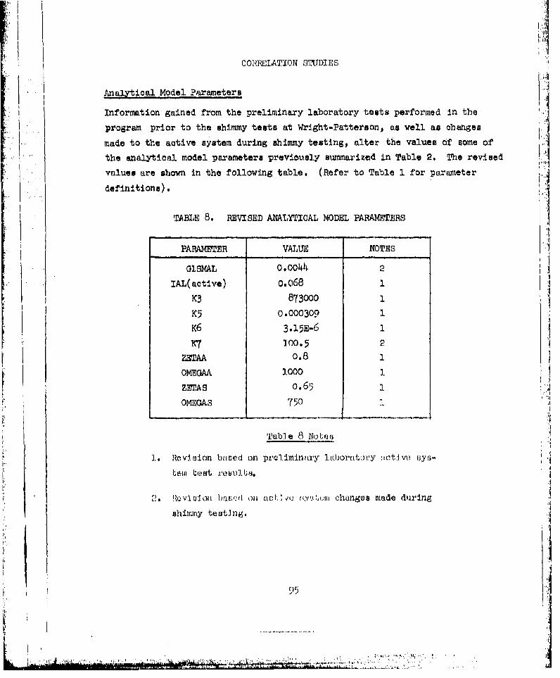
CORREIATION STUDIES
* .1Analytical Model Parameters
'. Information gained from the preliminary laboratory tests performed in the
program prior to the shimmy tests at Wrlght-Patterson, as well as changes
made to the active system during shimmy testing, alter the values of some of
the analytical model parameters previously summarized in Table 2. The revised H* values are shown in the following table. (Refer to Table 1 for parameter
definitions).
TABLE 8. REVISED ANALYTICAL MODEL PARAMETERS
PARAMETER VALUE NOTES
GISMAL 0.oo44 2
IAL(active) o.068 1
K3 873000 1K5 0.000309 1
K6 3.15E-6 1K7 100.5 2
ZETAA 0.8 1
OkEGAA 1000 3.
ZETA S o.65 ..
OM4EGAS 750 1.
.Lab] e 8 Noter .a
1. 1Revi.ion httred on pre'mlriuin1rY labora tuirLy t L('.tAV Uyr,- , 'Itol) e ,ist 1,080.L%.
2. Roviu:1oi b1r,':,d on actJ v "(,,:i changes made during
shimmy Ite it: ng,.
95
[- • •~~~~............................• •=• • ,•'........':.'-.•-.--..... !. '.-'-..1. .. :.......

GISMAL and K7 are the outer and inner loop feedback gains which were both
revised during shimmy testing. The Bridged-T notch filter tuned to 180 Hz,
which was employed in the shimmy tests, is not incorporated In the analyti-
cal model. In the analytical model, the 180 Hz structural mode is at 230
Hz and never gets driven. Since the purpose of the notch filter is solely to
suppress this mode, the filter is not included in the analytical model be-S.. .. cause the mode is never excited*
' 1 Correlation-Results
The passive free shimmy tests were initiated by a cable pull system which
resulted in a rather irregular, prolonged transient input to the gear that
is difficult to duplicate analytically. For the purposes of correlation
studies between analysis and test results, it is desirable to have a well
defined input forcing function. A deliberately induced wheel imbalance
provides an input excitation that is accurately known both in marcitude and
frequency. It is for this reason that the correlation studies are based on
the tests wherein wheel imbalance was used to drive the gear.
Analytical results for the passive system with 10 in-oz wheel imbalance are
compared with the test results in Figure 52, The extended gear position
with nominal backlash is used. Axle angular acceleration derived from
angular velocity is plotted against airplane velocitj. The agreement be-
tween analysis and test data is fairly good at all velocities. Howaver, at
100 and 120 mph, the analytical responses are at the wheel imbalance
driving frequencies (35 and 42 Hz, rather than at the shinmy frequency of
22 llz) as observed in the test results. A steering actuator stiffness of
50,000 in-#/rad is used for these analyses, rather than the 18000 in-f/rad
shown in Table 2, The lower stiffness value will result in a 22 Hz diver-
gent instability at 120 mph, with good correlation at the lower velocities.
Therefore, depending on what value of actuator stiffness is employed, the
120 mph analytical results will agree with the test results either in termsof response amplitude or r'esponse frequency, but not both. (if free shinny
is analyzed, the correct shimmy response frequency of 22 Hz results for abrond range of actuator stiffnesses).
96
L .. ',*,- -

2000Extlended fear Pon.itioi
Nominal Backlash
S 16oo/ ,I!.°. .. .... :~. Tost
1200
400
'If
0 4o 80 120 io
AI1RLAFI VEL0CfTY,, M.Pd.E
FCfURr. 52 COMPARISON OF TEST AND AXALYTCAL PASSIVE SYSM RESPONSE$WITH WKSEL IDfAlANWE0 I'TENDED GE1AR POSITION
97
S.......... • ......... i•'•• •=1] " l•" i'' • •" :l •:P ,'l, •", -•, "-"•,,• •-,-•j... . .

Figure 53 shows the same information for the active system, with the gear
in the extended position and nominal backlash. In this case, the correla-
tion is fair from 40 to 100 mph, but at 120 mph the analysis indicates a
much larger response than that observed during testing.
Figures 54 and 55 show the correlation results forthe passive and active
systems for the mid gear position with increased torsional backlash (+_0.024,
rad.). The results are very similar to the extended gear findings; the
passive system correlates rather well at all velocities while the active
system analytical results are too high at the high velocities.
For these mid gear position analyses, the estimated tire parameters shown
in Table 2 produce high negative tire energy inputs to the system. In parti-
cular, the passive system is divergently unstable at 80 mph and above.
Since no tire parameter test data of the type needed for shimmy analysis was
available for the tire used, estimates of the tire data were made using
empirical equations from Reference 2. The analytical results,mhlan •toIp••i0-.
with the test results, indicate that the maignitude of the tire stAffness as
obtained frnn, Reference P may be high. Because most of the test data which
foriarwd the ba sis of' the empirical equvit:lons contalned in Reference 2 exhibit-
ed cori.eiifble scottel". reduc•(,ed values of the tire parameters obtained from
Lha eq~~�ti~•,na t•e justlf.led and are used for the correlation studies.
Th• t� .I.c parameters may also contribute to the poor correlation encounter-
ed with the active system at 120 mph. In the analysis, the tire acts as a
source of energy to the system at 120 mph. Since driven shimmy tests were
riot performed, it is unknown whether the real tire served as an energy
source or sink. However, if the tire actually absorbed energy at 120 mph,
that could explain the low magnitude of the test response (relative to the
uinalysis) at 120 mph for the active system.
This would imply that a "correct" set of tire parFmneters would lower the
rm.-ly-tcal responses at 120 m,)h. However, this would also hold true for
98
4L. .. .... . ...
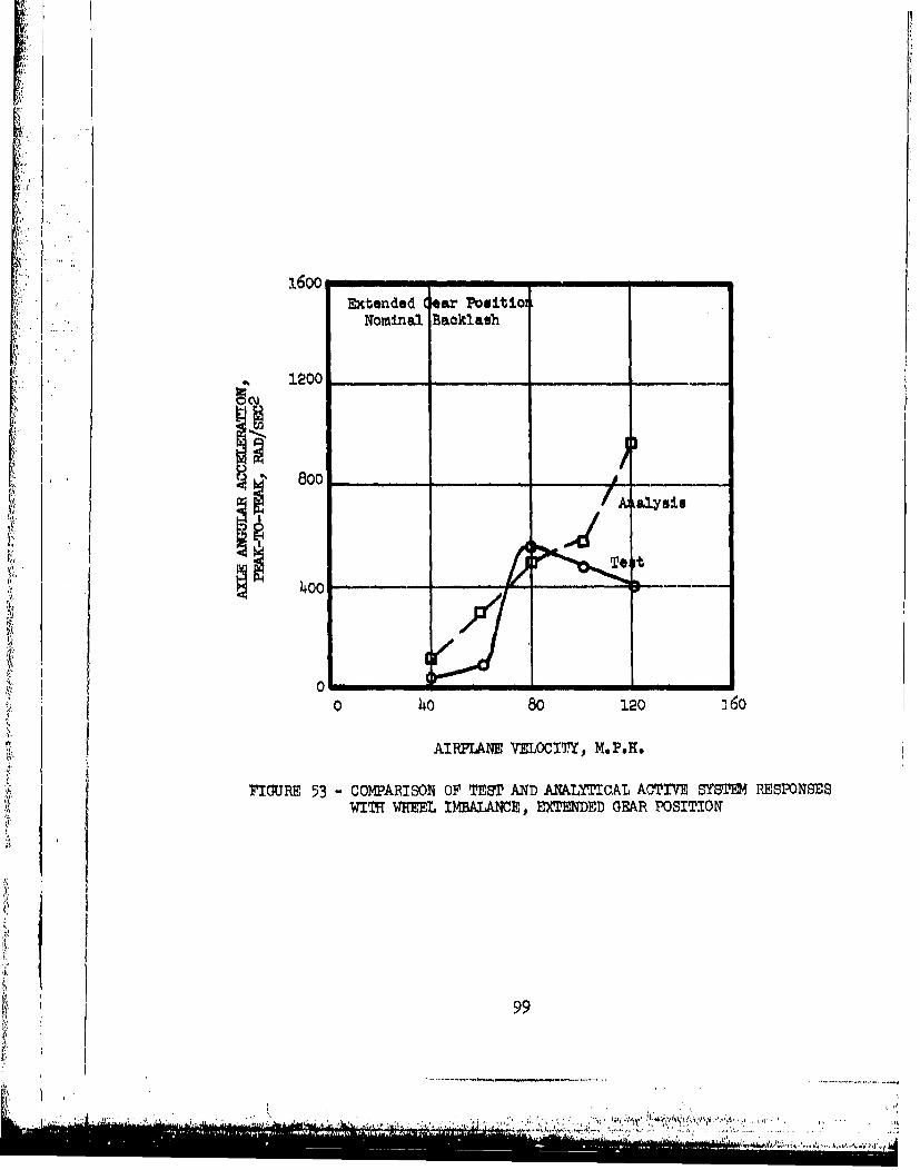
l6ooExtended Gear Positiol
Nominal Baoklash
. ,• 1200
800
1400- _____
0 40 80 120 1 6o
AIRPLANE VELOCITY, M.P.R.
FIGURE 53 - COMPARISON OF TEST AND ANALYTICAL ACTIV'E SYSTE24 RESPONSESWITH WHEEL I.MALANCE, EXTENDED GEAR POSITION
99
..................................-.

i i
i,+ 'i+i
•,+ii, • ,,j
]• .
+, • ..iii ii i :
' " :' + 160C .... ... .I * Yncreased BKoklash/' • 120(
", ' • AnalMs•,• ' '
; "•l b
•. • 4oc .. ,f-!
S. . . .. ., , _ _ +it
o 40 80 imo •_6o
AIRPLANE VELOCI'TY• M.PoB.
FIGURE 54 - C0MPAR•80N OF TEST AND ANALYI•CAL PASSIVE SYST•4 •SPONSESSWEEEL •MBAIANCE• MID GEAR POSITION
ioo
+ ,,.,,:,. .. t" ; l" i
-' .• '+t- •+ , . . , . ++ , + . . 1* .+ + , . . • "• * . +, +, • , , , ,, .. j , t. ;;, . +++ , ,:+ + .•,•. . .. ,. •. t , .+,., .+tL . •.++,•m. +, +,,p+.l.+•..,•,.++.• . t,• .+,+ ,•,++ . ..... ..... l . .... .+ , . .. . .. . . . .. . t

316
Mid Gea~r loitionIIncreased Baklash
12
80
0-101
0 4o 80120 1lAIRLAMwwc,i m.P.H

the passive system which currently correlates fairly well at 120 mph.
In the passive system, the added energy absorption of the tire could beoffset by lowering the actuator stiffness back to around 18000 in-#./rad,
as estimated in Table 2. Thus, both the passive and active systems would
* I'correlate well at high velocity if the tire actually absorbs energy.
Another consideration relative to deterioration in correlation of the active
system at the higher velocities is the use of wheel imbalance to induce
torsional motione in the gear. Classically in shinny analysis the fore
. . . and aft mode is neglected because the lateral and torsional modes dominate.
Accordingly, the analysis used in the prograw!does not include the fore
and aft mode. Wheel imbalance imposes fore and aft loads on the gear,
which result in torsional motions due to the lateral offset of the
imbalance. Thus, the fore-aft and torsional gear mucions are coupled via
the wheel imbalance forcing function as well as any mechanical coupling that
SI may exist in the gear. In the case of a passive system, this coupled
response has a secondary effect on the onset of shimmysince fore-aft gear
motions are not as significant as lateral motions in producing tire forces.
However, with the active system the torsional accelerometer will be exposed
to the coupling which may result in altering the feedback signal by a shift
in phasing over what would be expected from only the lateral and torsional.
modes. The change in signal can be either favorable or unfavorable in
suppressing the response of the gear, and the effect should be more signi-
ficant at high 'velocities. (This fore-aft gear loading could have been
eliminated from the shimmy tests by using equal weights on opposite sides of
the rim, located 1800 apart).
The use of wheel imbalance as a means of providing data for correlation of
analytical and test results of gear response in evaluating its shimmy
characteristics does not provide stability margins as does the driven shimmy
testing method, and also the analysis may require the inclusion of the fore-
Iaft degree of' freedom of the gear. .
102
...

To aid in explaining some of the observed results of the active system tests,
a simplified analysis of a linearized system was developed and is presented
in Appendix E. In particular, the variation of the free shimmy response
frequency with feedback gain and the creation of modes associated with the
active system are discussed.
10.
I.
i.
103
'• I' ' • ~ ~ ~~~~~ I....-'.,• •• i .• . ,-.- ,. -• ••

CONCLUSIONS AND RECOMME'NDATIONS
Conclusions
1, The basic passive system shimmies at velocities above 80 mph in the ex-
tended gear position, as vell as in the mid position with increased tor-sional backlash. This susceptibility to shimmy is the result of a shimmy
damper which behaves as a soft spring with minimal damping at the shimmyfrequency (22 }Iz.).
2, The analytical model used in this program correctly predicts the shimmy
tendencies of the passive system. Quantitative response comparisons
between test and analytical results with wheel imbalance show good agree-
menit in amplitude, but at 100 mph and above, the analytical response is atthe driving frequency while the test response is at the shimmy frequency.
3. All versions of the active shimmy control system tested prevented shimmy
even with wheel imbalance and more than twice the nominal torsionalbacklash.
4. Careful shaping of the feedback control. signal is necessary to prevent
undesired high frequency oscillations. This signal shaping, accomplishedwith a Bridged-T notch filter tuned to 180 I{z, must be done during theshimmy test program. The wanlytical model is not sufficiently preciseto predict potential problems from higher frequency structural modes.
5. In addition to proventing shimmy, the active control system reduces theresponse of the gear to wheel imbalance relative to the passive system.
6. The active shimmy control system is stable at mmme than twice the nomi-nal feedback gain employedj hence, the system as tested has 6 da gain margin.
7. With zero feedback gain, the active control system still has positive
shimmy damping, although Its damping performance is quite poor.
8. The analytical model predicts the observed shimmy suppression capabilitiesof the active control systemp but quantitative response comparisons
lC0
5,•..•' ...-.. ,.•...,;,-,.W...SW.".,,•,•\,•,.r ., ..

are only in fair agreement at velocities above 80 mph.
Re uommetidationsIt Is recommended that:
1. The active system analytical model be further refined to predict
system -esponses more accurately. The refinements to be investigated
Include fore-aft gear response and separate funelage fore-aft and
lateral degrees-of-freedom.
2. Further testing and analysis be performed to assess the limitations of
the present active control system. In particular) its performance with
various signal failures should be determined over a wide range of oper-
ating conditions.
3. A fail safe concept be developed and incorporated into the breadboard
system design to remove the operational limitations of the present
4. After the above has been completed, an active control system suitable
as a flight test prototype for the T-37 be designed and built.
5. This system be flight tested with various degrees of degraded gear
maintenance.
6. Trhe feasibility of providing active shimuy control, in conjunction
with electrical steering commands, for larger airplanes be investigated.
7. Wheel imbalance, if used as a means of inducing torsional response in
single wheel shiiimy tests, be installed such that fore end aft motions
are not introduced.
105
S.• L, . . •t_• .. - •, '.... . ..- " :..J . . . '''' , '. .'.
~~..... .......-..•..•-- -bA,v.-.• j, • ,•. ",•' . .. • ..--.. '•.••........................................................................................................................... ., - '
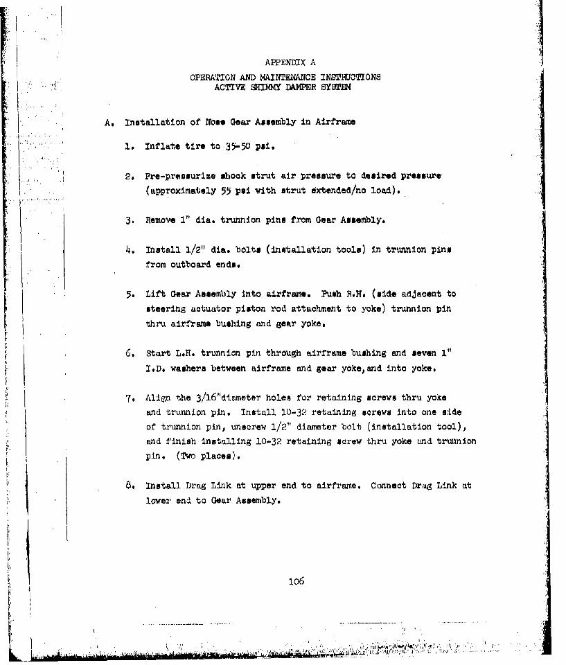
APPEiNDIX A
OPERATION AND MAINTEIACE INSTRUCTIONS.1 ACTIVE S4Y DAMPER SYSTE
A, Installation of Nose Gear Assembly in Airframe
1. Inflate tire to 35-50 psi.
2. Pre-pressurize shock strut air pressure to desired pressure
(approximately 55 psi with strut extended/no load).
3. Remove I" dia. trunnion pins from Gear Assembly,
4. Install 1/2" dia. bolts (installation tools) in trunnion pins
from outboard ends.
5. Lift Gear Assembly into airframe. Push R.H, (side adjacent to
steering actuator piston rod attachment to yoke) trunnion pin
thru airframe bushing and Sear yoke,
6. Start L.H. trunnion pin through airframe bushing and seven 1"
Z.D. washers between airframe and gear yoke, and into yoke.
7. Align the 3/16"diameter holes for retaining screws thru yoke
and trunnion pin. Install 10-32 retaining screws into one side
of trunnion pin, unscrew 1/2" diameter bolt (installation tool),
and finish installing 10-32 retaining screw thru yoke and trunnion
pint (Two places).
8. Install Drag Link at upper end to airframe. Connect Drag Link at
lower end to Gear Assembly.
,o6
. .. . . . .. . . . .. . . . .. .. . .

9. Connect pressure anid return hydraulic lines. (N~ote: Lo0cate accuaa-
lators in pressure and return lines as close as practical to Gear
Assembly. Pre-charge air pressure in accumulators am follows:
Pressure Accum. 800 psi Return Acoum. 12~5 psi
10. Connect electrical cable connectors*
NOTE: Hydraulic System Fl~xid ?vIL-H-5606
Hydraulic System Operating Pressure 1500 psiLocate pressure line filter as close to test as possible
B. Changeover Procedure) Passive to Active Damper Configuration
(Note: If accessible, it should not be necessary to remove Gear Assem-bly from airframe to accomplish configuration ohangeover).
F.igure A-1 is a layout drawing of the system showing the part numbersrýeferred to herein,
1, Disconnect pressure and return flex lines from aircraft steer-
ing actuator. Cap pressure port, plug flex lines.
2. Disconnect connector to L~P transducers
3. Remove three alien head screws holding 9L 1962 LVrft' Bracket to
SL 1960 Manifold and lot Bracket hang on LVD1' probe.
L4* Remove jam nut holding SL 1963 Brace to bulkhead fitting in
return port on aircraft actuator,
Remove four screws holding SL 1963 Brace to SL 1960 Manifold(3 Allen head, 1 slot head) (Note-, 83lot Head screw location
required for clearance, left f'ront.)
R~emove SL 1963 Brace,
107
...............

jios

I5. Remove lower bolt and drop Drag Link from gear.
6. Loosen two SL 1961 Bolts holding SL 1960 ManifoUd to aircraft
actuator.
Loosen two bolts evenly together 1/2 turn at a time. Do not
remove bolts from St 1960 Manifold, remove Manifold and Bolts as
San assembly from aircraft actuator. Watch for loose springs and
orifice poppet valves as Manifold and Bolts are removed.
7. Remove springs and aircraft orifice poppet valves.
8, Using #6-32 screw provided an tool, install SL 1966 plugs in
place of orifice poppeta.
9. Remove and replace two MS 28775-012 "0" Rings and Back-Up Rings
forming face meal on SL 1961 Bolt between Manifold and aircraft
actuator.
10. Re-install two aircraft springs and Manifold/Bolt Assembly. Tighten
bolts evenly together 1/2 turn at a time to bolt SL 1960 Manifold to
aircraft actuator.
1ii Re-connect drag link to Gear Assembly.
"12. Re-install SL 1963 Brace on SL 1960 manifold using bulkhead fittingjam nut and four screws. (Note. Location of one slot head screw
required for clearance.) Cap return port on aircraft actuator.
13. Re-install SL 1962 LVDT Bracket and adjust LVDT Body position tocenter radially on probe.
14. Remove SL 1972 Cover Plate and install Model 31 Moog Servo valve.
0109
. j* * *

15. Connect pressure and return lines to P & R ports on SL 1960
Manifold.
16. Remove aircraft feedback linkage as follows:
(a) Remove cotter key and pivot pin from linkage connection tovalve spool.
(b) Remove phillips-head center pivot screw (watch for loose
Iwasher & bushing).
(c) Slip feedback linkage fork off of pin on pilot input ring.
1.7. Connect electrical cable to Moog valve. Connect electrical cable
to &P transducer.
C. Parts Kit (Gear Assembly in Possive Configuration)I each Filter
2 each Accumulators - I Press
I. Return2 .
2 each 1/4" Hoses
2 each 1/2" Bolts for Trunnion Pine
2 each 1/4" Hydraulic Fitting Caps
2 each 1/4" Hydraulic Fitting Plugs
2 each SL 1966 Plugs to replace orifice poppets
2 each Set 3L Drawings
1 each Model 31 Moog Servo Valve with Dust Cover
4 Sets "0" rings and back-up rings for SL 1960 Manifold
2 each Drag Link Bolts (Attach to Steel Jig)
2 each Drug Link Bolts (for attaching upper end to real aircraft
airfrae )
110
....... ............. . . . ...• ' . , . . , -': , •, •, m .,, ,u.•,' .'•. '.::: , "A

2 each #6-32 Screws, approximately 2" long for installing SL 1966 Piug8
10 each 1" I.D. Washers (Use 7)
"� 4• each Zip Plastic Bags
1 each l/16"Sa•ety Wire Hook
2I each Roll Tape
l each Epoxy Kit
'Ai
•-...|
.. . . . . . . . . . . . . . . . ....... m;.I'.....A'.
4-,,

APPENDIX B
CIRCUIT DIAGRAM, ACTIVE MMW CONTROL SYSTEM
Figure B-I is an electrical circuit diagram for the final configuration
of the active shimmy control system. All test instrumentation electronicsare included. The Bridged-T notch filter added during the shimmy tests is
also shown. An explanation of the functions of the various circuits is con-
tained in the section entitled, "ACTIVE fHIMWT@ CONTROL SYSTEM DESCRIPTION".
I
112
' . i

&IMIlip
All,
1-M4~~~I- Slb ofs-v -coa p
I,i
ISSO

IV.
boo..
I M.1
nmzomm Il .. -. f
It, I3 Igul
# =. IV
.1k.
4.~~a IEP44g4 Too-".___6& -k-* - - - I4)
Mwerma m .Ma. .

.6"3Isaa::v VAN-
-110U
"VMYS%ea ~~~A *Noo e"' tW'-1
1", 1-4-It
19 0J2 .-
ft~ 'a-*... A..
"I AtPP wee,'.
AOTMY MumTCONLRML Y3 11
V. 5ý

APPENDIX C
WlMY TE ST TIME Il STORIES
Contained in this section are time history traces of selected portions of
the more pertinent shimmy tests, These plots were obtained by processing
the FM tape recording from the shimmy tests. Table 0-i summarizes the runs
presented. For the active system tests, only data for the final Bridged-T
notch filter configuration is shown, with the nominal feedback gain
(Kot a 0.7). Only velocities of 80 mph and above are presented. Table 0-2
contains a description of the quantities that are plotted for each run.
On the time history plots, the expression "FIELD RUN X)" refers to the
shimmy test run number shown in Table C-1, The expression "ru. XX" is for
Lockheed reference only.
114
Li. .I -.
i..... 1

TABLE C-12
_______ ~PLOT StDW4RY _ _ __ _ _ _
•0 Oear Gear Wheel Velocity,No. Configuration Position Baciash Imobalance m.p.h.27 Passive ,'t. Nominal 10 if-oz 100
28 120
31 4 8032 100
33 0 80
34 100
35 120
39 Increased 80
40 10041 4 120
153 Acti•ve Ext . Nomin"l 0 80
356 100159 4 120162 10 in-oz 60
163 I100164 o120
167 Inureased 0 80
168 I 100169 4 12.0
172 1.0 In-oz 80173 1006 174 120177 Middle 8017l8 100to
179 120
182 0 80
183 4 100
184 1120
115
i ,-•••' •":'••d -• ' ':'"'~vI"" '= :'* "• = ' ":" . .. . ... .".. . . . . .".'... . . . . . .".'•,,'•./ '.-'•• , ,..

,TABLE C-2
PLOT TIME HISTORY DESORIPIION
F Quantity Units Description
CMI* Inches Electrical steering command signal expressedin terms of actuator displacement
SX Inches Actuator displacement
D2 =/'/•/ rad/sec 2 Axle-angular acceleration about steeringaxis
D TRETA/DT rad/sec Axle angular velocity about steering axis
THETA rad Axle angular position about steering axis
AP p.s.i. Actuator pressure differential
SThis quantity plotted for active system runs only
116
I , .,.
S....- •.. . .. . ,'" ' • . .. ,' • " "",•" . :' " '- ,' ':

ACTIVE AND PASS3IVE SHIMMY TESTSFIELD RUN el PA399VE
TO~T 2bbl7 RIJN b 18 SP is
....... ....AIIfrlE1 . I. -
0.01 ~RUIFINS/Div
. ....... .. .. .
4 -
6-...................

1~FICTIVE AND PASSIVE SHIMMY TESTSFIELD RIJN eb PRVSLV
TESBT EbW1 RIJN 7 l13 SEP. 75 '0.a3S INCHES/T i:
L 100 IRAO/ECO /O[Va
t7 1-- 7.7
0 THE-TR/OT 1
G.eRAOIANS/10IV (
""W"4 t41 -I; W44 1. 44 1~ 4 4444..4*4 444-4
S[ UONI),'3

RE~T1VE AND) FRP VE S3HIMMY TESTSFIrLO UN31 PASSIEVE
TEST 2bila1 NUN8 1 A SO~ ~isP7
OAS NCI4El/a1 II
7 .. ...
e 00 RAO1RN /Dive ..
tlF' I I
I~ R Y ,I-O-4./I ".4-.4.'.4.I..-I-.+.I-...I'44-
1, J.lk I. B 1, , I .
- -- THOR

ACZTIVE AND PASSEIVE SHIIMMY TESTSriELO RUN 3e PRAU51VE
TFR5T ebbt7 RUN q1 18 'SEP' 75
6*~.1 ..i.77i0.05 INCI4E5/0IV It I
04THE TA/0Tff~ii.~: T1j:: 2i~rT :eaa PROa/EC' /GieV
-Jul T. I
0THETA/0T r~Jj.e AID/sEcu A0 .Y~ h
o..t~~e &ARSOI
*t - . . . ..... ... ...
J
.1 .. ... ..... j. v.... :
100 P3[0/01V .. 1. .
120

RET IVE FiNO IRS9I YE 9~HI MMY TESTSTPI~RI RIJN 33 PASS!IVE
TEST1 VbWiI7 WUN I bi 119 SEP 75
AX If1 -[t I1 f1
DITHE TA /07' i
IOU~I 14ME [Ov i-A1,A
.5 RA0/MEC/U CV .
* K K. I ~ .... .. J... . K.:IL..
0901 RRIIRN/0IV
121
-'I

RCTIVE RNP PRI95VE 9IHIMMY TESTS1.0 WIIGN 3- PRIA,11 VE
TEST Ebbh? NUN 15 10 SEP 75
2 :.ili. : ii:1iE:F 971i..,1... ,... . .. .. i :. ._ . : _ ..0.05 INCHES/DIV IJ... 4.~ .:~j
""!U. .
10inn RAo/EC' /0[V
............ ......
THETA.....x , K . 7,, ..,a.01 RADIANS/DIV
.. . .. .. :.. '. i.. , ..... }..; . .z. I .I... I | -" ., .. I. .I
50 P510/DIV
I--i . . . . .. • ., ., 4 . . .4' A ] . ... ..~ ,.I ...* .. ..,• r /1E t I / ... .. '. 4 ... - ., 3, q .... I. I~je t•l i l,) - .!. 1.6. 1,
3222
. .I ..... . . ..... .... . ..

rIFLO RUN 35~ PAPHIVE
0 .0 INC E ID
£A
.77
7 ).. . . . . . . . .......

. P11 I VE AND Pf19,iTV HUI1MMY I :-rT!I3
rT1".AT 01 i'111 R[JN 1 I 7 'S r. ?'i7
7.. :T1 .?!i.. 1' isF!.AX.
0.05 INCHMflDIV A..: L It
Of r[IETP/nI'tIenau Pno /9140 / Ilvao"k~
v
D H1F.TF1/1)
o i rnrQinV-oY11ý iy towo wewhiW f
0.01 k'nn4lN4/rIv%'o
12
... ... ... ..

RI2TIVE RNO PflSIVE SHIMMY( TE9T9
KYICST 2hbbl RIJN .17 11 SrP Is
fl.f5 INCHES/0Iv ... .*
D'II~THE /OT':1.'
E n n n l..ID i >ý,i~~nrii' AfOSC /DL
P17 T- TI
T~ 77-7 .'17 .. . ...
It Df.T.TF r-rE-F--
.E~ ~~~ ~~~~ .1.. ~ O l i t P A 0 C
A ~ ~ i -I-N"--
125r
.71 77

ACTIVE FlNL) PRt3¶iAVE S1HIMMY TEZT5IKI1) RIJN 41j PREi!3fVE
TEST 2d1317 k'UN IR qt 18 FP 111
LIf ... TT
a.02 INCHES/DIV 1 *,i ~ V11 .~ i
...... . .... . . ..................................... i-
0.01 001I~h 4111
*1~ ~ 9 TW9rR/DT01T } '
.5~~ rflLONEUDIV
*1 .,.9 I6

ITI
*no rl WF. HUN ¶
... IWO " '0 " "
L
i nr .c /I)I v*
n nokIUIFNi/I
11111I, IlIiv i
112

f4i I VF rIND Pf19'i1 V(. ý,w m 51 1MM Ti;.'
7 7-7. . . I '
0 Vi I. .,U]/)
t) Tiltin o
11.
I il t Ii tll 111.II
!i I UNl~i
128

nc~r yFIND P(1l5ivi;Fll N11MY rrEu rt 1I EI) OLIN I Y1
0.1.1 Ph 1.3STi4 L I ' O RJ h lr"7"
IAI INM N/
AX0.r01 INf.IIEU',/DIV.
tllf m'l)rirlY ""
1111. T
C) ill I fl i/ D I j
IlilDlili
I A .1 0
1111I11 1111111 I 1114 II II
129
.. ... .. .. .. ... .. ... . . . . .

nlf i.i v i. r-I~N P11LT.ibtV1P- '5I-tt1MY Wi
*ULI II Hi:rlI
chi .. .....
WIN .
AXm~
THI.In
a. ,At' IN) II IPI Ii Af I.t V%'~ ' h I l i
130
Mimi=

mi: i .iv VI fNU P:~MEAE vF: -iiMMY r F. sr'r
tf,"EllPhL~ 01j31IIN ¶III I
n.1w ILAW.1
j~~m ~lii..... .... .... 1
a.Ifi W101nNNI~I:~/mlvr
m~irr la .4 Il I 11 .1
*flI131
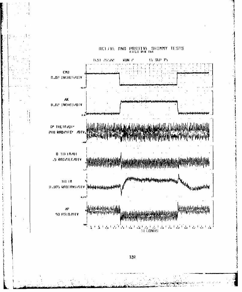
* 1-.. ri:' 1 I fN] '~.PiIVI. fllI M i:m1!
11.111P.... I.....................V.
.,j~a k.n /! oa :/i
11..w01 WnornN!.I/hi[V
I~~ I"hh /f I I I, Ii I 11P h 1a _11 _ -l ll .11 1- l
132I

;I :*i i vi. nfN 1. Pflsi , I V: 91,11 MMY I k ":iT ri
I.........1,18.... RUN It.,I,.i..I.** m
0 .. 119 INI.'HEHI/D!I V
.7 ~AX .
2anf Rflf/,IIIv /1] I v, 'p
r III I (
I'll 1,1' I, 1.7 "IA. IM I I I I I I I ,I I14 A 4 I q'I 41 1 1,1. . ,1 '1A.1
1.33
I -q

r m WIN Ib
I.. T
r.1I"i WfD~I N 111i /D) I Vh.I, W *M u w
U11 wiinmi
*134
L*11i

nE i v t, flNO r'9'. 1:uI MMY Lfr
FM1 t 11WI It il
h' I W? WI lf 1 lWi'
ni x ."I
r liN1111:1/I)TVr C
Till I fI
I fi .1 114111. II i/131 v
I) j i.. Ih II e.lý I¾ ,,e I el.. f. JU ~ ,q *.. Aag , I 4b 4
'35

I I &1, L WI.IN 170(
I.M.1
AX ~-.. Y
U' til; 1 l/UV Moil ~
HE I
nnai wnhimr-1NVD~IV
1.36
A-W-~~ ILAI

ni:,i i vL r NI.) r'U1~i i LVI:: 1 j1.11 M MY *T I "ii
0 .I'. . - . . ./U
I
AX .
u.o ' in i I A R /UIV
rill PH3 11) /0l 1 v W N
., A 1 I .1 1 1 1. , 1 A .. I 1 1- 1 1 I1 1 1 1
1-37

f11:i T.1 1 vi: RNU P r~~l".] V 1 "i ~II M lM Y TFI !iT1 1.1.1, 11 W IN IM
11111.31 IA
..11"
.1)41
0II 1I, Il in/ Ii I~
L liii in/l
11.111 YfIlil I fINNi /A) V .,*
1.1 3 A -I .0 4 4 11.10
!H. I;N Wi
1381
1 iTA
.. Mull
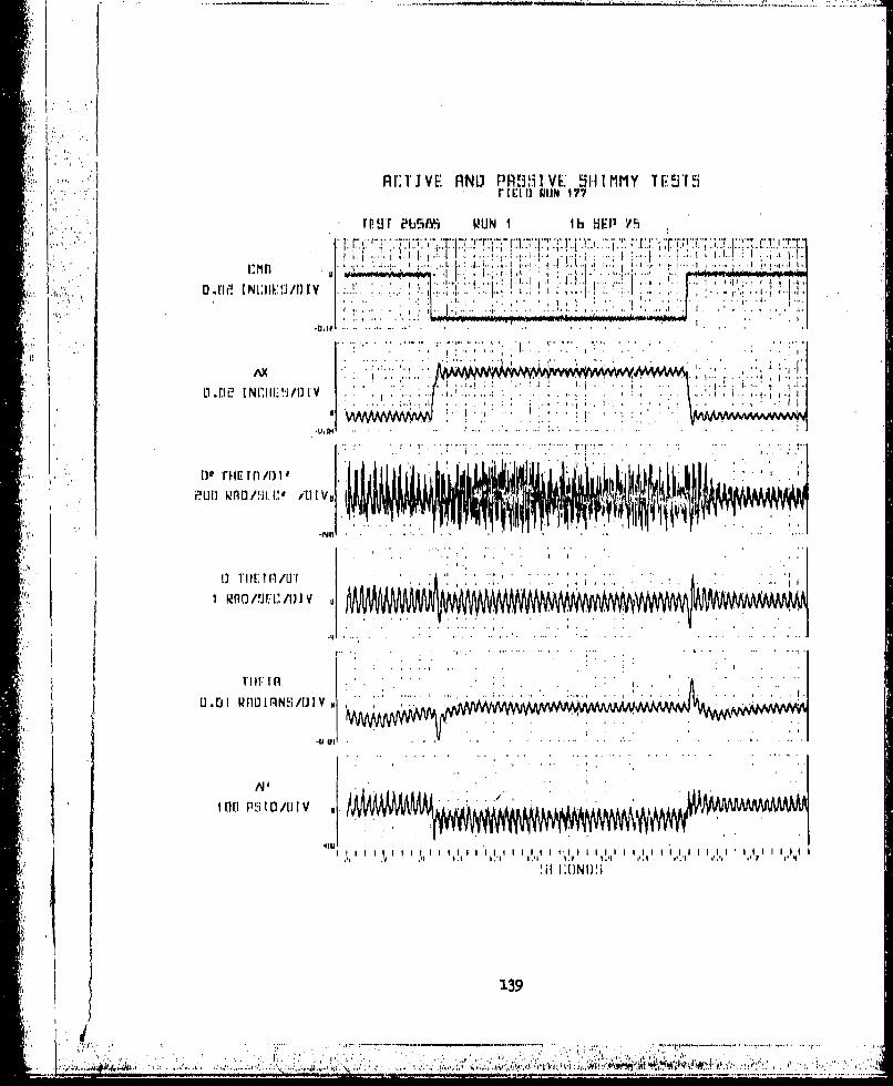
---
aI n 1N1.11; 9/)
% W . . .h
fl~ rE r r#1139
r'~~~~UfI~Y k'0ilid2 i)IV.. .. .. .. ..

nir fi v( vNI PF5~I ~H MMY 'FF1FEIC.171 OLIN 17 6'
O.UI~~ INHf/UIV :II0.11P~~ ~ IlM ..
l j
III
'til Ito
I~~ ~ ~ Ii n PIN CA)I
....... ..
THE~ *r n~

A vI: TIV Fl N1N.1 P F1 S 1 V: L' i 5HI M MY TI~ HiI- rrF.A U fIN 1711
TI-Ht PIaiifij RUN '4¶~ II 14 P/i
- ~~~~" . "T 1.JL rNH~./1 .. ............
n.n INfCHEU/01kt V
e..lI wno !IC /D V,
TIR I RNI
UX R.,3FI;.4,*....... .

rIrari1 WIM IN'O
UJF I .. Il~.'/ I
U .05 INLIWRd/Uiv *
AAX
I'MI I
20 UfWAO/HHC'/0 IV
1... 11 4 4 e' I .- I, -I,,. I.ý
[~~~ ~ ~ ' 9ý .1 0, Nk D!;alI.iq

- . r.I :tVC: RNO FPR~ISIIvL Fill1mmy IPi1U9
G.L15 INI:IIEI..;/DIY
nI'nn ~I NINW"/DI V
THlL I n
alI cegoinU U/D I V
I~ IM1 fil II u AI II v I K~
.1 11 .Ill I I ."'.I .
1~43

Mi.: Ii vI Vl11W:) ilrIpJJ i Vt:. !lit i iMMY i i i iFI Fl.t 0 li N 11N W &
r FS T jIatiIYi IdIN ? Ilb 9.. v!l
(JUiINrHIi~/OIV.Y
*~n I11FS/
ein micno/i ~/
r liio:, i I
01111117INUAM
Ilia 11,1D0/1U(V
1IIJMNJ!
I * I .1A...tL.IL..L.S ~ *,.A*~d. W . . ..144
APPENDIX D. ANALYTICAL XMIL XQUATIOM
Thin appendix contains the eq.atio of motioa rmultiang from the analyti-
cal model ot the Active ShiW Control Oyaten described in the =in bcdy of
the report. These equatiofs are divided into-two seotio.15 initial aoagdi-
tiorn are the calculations perfomed only two per run Involving qamntitioe
independent of time, and the time varying equatiow involve quantities
that change with tim.
With the Continuous System Mcdeling Program (CsM) language umed the
mequence of computations for the time varying equations in determined by the
tranulator which translates the CSMP program into a FORTRAN propsa for cam-
pilation and execution. Therefore, the sequence of equations shomm herein
has no significance. It is appropriate to think of all these equations an
being solved simultsaneouuly as they are on an analog computer.
Table D-1 shown a description of the CSMP special functions used in the pro-
gram,. The nomenclature for the equations ia the ma. am described in the
section ANALYTICAL MODEL DESCRIPTION,
':.
- . I *. * .,. . . . .. .: . .-

2 ~Initial Conditioriav - 88*12/6o*VMM~
PI - 3-1L41 59265
Wl W ~t386 .
11b6M ITH*IPH.t4IMEbH
T**u vanrinu Euat tons
IATACC u H*PHDD/3861.iUB m UNBIO*RIMe1*((V/R)**2)/32/386M'UNBL - MuTSIN*f(V*TDM/'R)
* 1sXflL * ?4UB*SIN(V*TTM/R-PI/2)
PHDB - DIADSP('iDPDP~FHP)
MPH n XPH*PHDB
MPHD a BPH*ZIW
ps a m+(O*WLXG*T+H+)#H*VLYB - Y delayed by Z*HB/V
FT w (Y+YB.e*(L+Lo)*Tii.2*(H+R)*pH)*IcT
ALT2 a AIL-T2
ALM2 - AWD-T2DIn m TH-Tl
TIAL a Ti-AL
*TIALDS - D1IPADOP( -DALDALIT1AL)
TTDS - DEADSP(-DTHlDTHOTT)
TTD aTIM-TiD
.146

TT2. T1-T2
TT1D m TiD-T2D
AT m AL-ALl
THOD - (OMMGA**2)*CMAP~L(OO9ZET-AA, O!GMo T1MD)
THD a .,.*PXAL(O,.1 01TI)~D
T *M.m IRULPL(0te1, THM)
XC w GISMA4L*THMOW
ALT2PP w LMDIAG (PlP2fx0)
ALT20 ALT2PPP
BETAD - (-LýU(B(LB-4B*xL)/-* FXAL 5ý 0
BETAD - (-BL4QRUT(A8(BL*.BL4.4*BH*JCAhL)) )/( .e*H) FKAL > 0
BETA m ALI-T2
ALIl) w BETAD+T2
ALI - INTRL(ALiQAL1,D)
7K m KTH*TTDS
-~FKAL 0 KALP*AT aiv
FKAL w K3*INMTRL (Oo., X11) Active
X1.1 0 x9~xl0-K6*FYAL
X7 -x5-x6
X6 *K5*YKAL
A1 - ABB(X3)
X3 m LIMIT (-l~ltXp)
X2 - K1*0OMAB**2*CM~rPL(0,0,ZETAa ,OMEGAj3,X1)
xi ALT2C + K7*ALT2
1147

OF w ORJ + Cp2*ABS(783)
OF' - CF1 + 072*AB8(FS)
pop * zSW(TT~,-CPiCP)
FOP iNsw(TP3lD,-CV,CF)
PCA INSW(ALT2D i -CA, CA)IPKOC a KQC*TIAWDSPIUS a XQ'*2 + BF*T2D
SPH -* .zV/R*THDWl*L*Ti4nw*H*ffi 4M~ + MPW
-(HR)FT- (H+R)*nN*H4L+wG)*nZ*TH-MMzL
5TH * *V/R*PHT) +7K VO'P 4(L+W4)*FT-MT-MZUNL
PHDD (--I~PH*13Ii-Kksm)/IIMM
M3DD (FCP+FK-PCF-PK0C)/I1M{1T2DD *(FCF*PCA+PKAL-FFUS)/ITH2.
AWD * (IrK O-PKL-FCA)/XAL
PH, * IqTQRL(PHoO'H)PHD INTORL (PliDoIPkum)
TH *INTGRL (THO, MM~)'LI IMTRL (THDOO n=D)
TI INTGRL (Tic, Tin)TiD w INTGRL (T1DoOT1DD)
T2 u INTGRL (Tao9 Tan)T2n a InTOL (Ta~o, T2DD)AL - INTORL (ALo, AD))ALD - INTORL (AwDoIALDaD)
*y a INiML (YOlYD)
**'~*. I * .. i ~ *3.48J* ... ,,

TAMI. D-1 CSMP SPECILT ?MOTIO• S
GI1UUL FOR FUNCTION
F ONTRL (IC, 'X) YF f'X~dt+IC
EQUIVALENT LAPLACE TRANSFORM
.INEGRATOR _.
Y a REALPL (IC, Po X) P' + y XY (0) • I C
1STORERLA (RALPOE)EQUIVALENT LAPLACE TRANSFORM: p +.1ASlT ORDER LAG (REAL POLE) ý+
Y - LEDLAG (iP1,P2I X) P 2 + Y - Pi 9 + x
EQUIVALENT LAPLACE TRANSFORM:P S+I
LEAD-LAG Pq S + 1
Y a CMPXPL (ICo IC , Pit P2,1 X + 2PiP 'Y + P2Y m X
Y (0) -IC1
"(0 *o IC2EQUIVALENT LAPLACE TRANSFORM-.
2ND ORDER LAG (COMPLEX POLE) S2 + PP 2 S + P_
Y- INSW,(X 1, X2, X3 ) YX 2 X1 <O
INPUT SWITCH (RELAY) Y. X3 X1 z 0
Y• LIMIT MI ,, ?V X) Y-"P- X<P'Y ' P2 XP2 X
LIMITER Y 0 X P IX SP?
Y. DkA•SP IPI, 11, XPI X) Yro yx y•X P XPi P'
DEAo SPACE y X-Pi X P1 456V
1j49
-.. _ l I . . . 1 I

APPENDIX E ,.I
AC- ,MAOTIV Y OOROL SYSTEM LINEARIZED ANALYSIS
lo1 Control Law Definition
valve and actuator driving an undamped spring/inertia resonant system
with aooeleration feedbaok.
E lectrohydraulio KO
Valve
xI xActuator i
IISThe block diagram for this system is the following
The parameters and. variables are defined am follower s1
KG is the normalized Accelerometer-Eleotroniou-Valve-Actuator
gain in rad/rad/6eo12
KT is the torsional spring stiffness in in-lb/rad IJ is the torsional inertia in in-lb/rad/uec 2
x is the actuator rotation in radians
0 in the spring - inertia mode rotation in radians
150I
_ I"
i]•. , .. . ,, .:..... "7,'"'":'. . .. ~ .. . . . . _ I ,

The characteristic equation for the system is
K + Te- 0
J52 + ,2Ts + K = o
'on
where
2
!' From the characteristlo equation, it is observed that the value ofSKij directly otol h damping oftespring-insertta re~atmode.
Svhtoe te f h
For the case of a resonant mode at 22 Hz or 138 radians, a KG gain of
0.00725 provides a damping ratio of 0.50.
The above simplified model and analysis served an a basis for selec-
tion of the accelerometer feedback configuration employed in the
active shimmy control system. Note that the tire dynamics are omitted
from the model which alters the resonant frequency only slightly,
and adds negativ, damping under certain conditions, The positive damp-
ing from gear friction is also ignored.
2. Exanded Model
The simpl~iied model is expanded to include accelerometer and valve-
actuator dynamics,position feedback on the actuator for electrical
151
f. ... .. . ....
- .. I.... , . .; ', , . . . "'. ; i

bteering and provisions for electronic compensation. This expanded
, block diagram is shown in Figure E-l. Again, tire and gear damping arenot included in order to focus on the characteristics of the active system.
The lumped inertia of the torsional mode (J) is selected as 0.7
in-lb/rad/sec2 , based on laboratory measurements. The lumped spring
rate of the torsional mode (K) in 1.,1 X 104 in.lb../rad., produeing an
-7 undamped torsional frequency'of 23. Hz or 147 radians/sec in agreement
with laboratory and dynamometer test results. The accelerometer transfer
function is approximated by a second order system with an undamped re-
sonant frequency ("'nA) of 1000 rad/sec and damping ratio ( A of 0.8
to match laboratory frequency response test results.
It is initially assumed that the actuator dynamically produces an actuator
rate In proportion to valve flow so that the combined valve and actuator
transfer function can be approximated by the valve response characteris-
tics alone, This assumption ignores the valve flow rate degradation with
load pressure, the fluid compressibility and leakage effects) all of
which are of minor importance for the conditions tested. Using the
supplier's datathe valve transfer function is approximated by a second
order system with an undamped resonant frequency (WnV) of 1000 rad./sec.
and a damping ratio ( tv) of 0.65.
The root locus for this system with no compensation and a nominal posi-
tion loop gain (Kfb) of 82 is shown in Figure E-2. It is observed that a
KG of 0.0063 (corresponding to K - 1, where K. is the feedback gain
parameter used during the shimmy tests) yields a modified torsional
mode frequency of 16 HIz with a daipin6 ratio of 0.&2) while the next
higher frequency mode created by the active syster ' 7 Hz) has a damp-
ing ratio of 0.62. The system gain margin is 4 (at KG .0.0252, the
67 •Tz mode has increased to 88 Hz with 0 damping). Excellent response
and damping characteiistics are obtained with this configuration.
152
,..... ........................ ,..,...:...•..,..•r .,.._,__,___ ,,____ ,.____._.,_
IE •• i ,,j• "..• , +•-•A • :, ' •L ,• , S~x•'Zz[f,- • '•.:';'• ':'• •:' +•-:•'• • • - :'' "•*- .......*.. '.... ,. * - " ..-*

3.I3

point Gai~n
1 02 0,003153 0.00W3.
5 Bervovulve 4 0:0126and 5 0.0252
ActuatorQuadratic
_ _ _ _r -__ _ 16.zz_ _ _ _ 800
J ~3f w 6T xHz bo.62
1 D~f 88 Ex Cm 0
Mods Created b 5
____ ____ ____ ____ - 400
* 3
2 1 tructural
> 3 ModePosition4
osna
______________Loop 1 . 5
.1200 -800 -0
Real Axis
1UXGURBE 1-2 -ROOT 1=8OPU 1 LTINFARZED ACTXIV EMfMG( SYSTM NUDHL ASA nMflTI0N 0F KO
1 9i4
.at
t a I

3. Model Refinement and Correlation with Exerimental Test Results
Laboratory tests on the breadboard system indicated tk at the steering
actuator characteristics produced, some degradation in dynamic response
of the combined valve and actuator as compared to the original estimates.
The predominant sources of thic degradation were not speoifically identi-
fied but include such factors an dynamic seal leakage and otiffness,
mounting stiffness, and hydraulic line and port characteristics. To
approximate the high frequency dynamics measured in the laboratory, the
valve and actuator quadratic in the active system model was modified to
a resonant frequency ( nV)of 750 rad./sec, with a demping ratio (
of 0.65.
During dynamometer testing at Wright Field) a structural mode at approxi-
mately 160 Hz was observed in the response data which was amplified by the
active system with KO gains as low 0.00189. A 5.o1 to 1 bridged-T else-
tronic compensation network was added to the active system to attenuate
this mode by essentially replacing the mode by two real poles with the
same undamped resonant frequency. This compensation network has the
following transfer function) .bhch in shown plotted in Figure E-3.
2 + 2,.--s + i where Wn0 a 1127 rad./sec.
fl We N 0.257
a + 2D a + 3 - 1.32
The addition of these modifications to the block d:agram shown in
Figuare E-1 produces a simplified linear approximation to the final
configuration actually tested on the Wright Field dynamometer.
The root locus for this refined system model is shown in Figure E-4.
The locus is based on the assumption that the compensation network
numerator quadratic effectively cancels the structural mode quadratic
leaving the compensation network denominator quadratic in the resulting
155
:1 X, ' , " . ., . ,,'" .l"."- .,. •'

60 --
-40___
PRUEf
-20 '
120200000
FRSQUECYA HERTZ
FIGURE E-3 - DIDGID-T NOTCH FILTER TRAMPER 'tmcrNToN
....................................

- - 800
laantd.A uaor
Quadr ic600
6 3
paini Gtfl KG
1 0 62 0,00189 Strdtural'13 0:00315 Torsional* 4 0.00441 Mods
0 0.0636 00126
1> f w38Ilz 9 wo.36
- 53 Eur C0.-01Nos0atyAjivSse
~ ~2 Loo33
- - .1 &
Poito-800 -00 40~ .2 t
k2a Zap IFIGUR0 E-i - RO OU FRýNDA'IES0YSYrl~ 'DLA
* 1 80 _r -40 -20
-' ~ ~ ~ ~ ~ ~ ~ Ra Axis- . j~ I **y

system model*
The locus indicates that the KG selected for the final dynamometer
runs (0.00441i~) is near optimum (maximum damping) and modifies the... torsional mode to a damped natural freq)enoy of approximate 38 Hz
(oompared to about 32 Hi observed in tests) with a damping ratio of
0.36. The lower frequency mode created by the active system for this
value of. KGt has a damped natural Ifrequenay of 18 Hic (16 Hz observed)with a damping ratio of 04.*5 The locus further indicates that thesystem has a gain margin of slightly greater than 3 and will go un-stable at a frequency of approximately 53 Hz. All of these results
-, correlate well with the actual dynamometer test results) particularly
considering the degree of simplification associated with the linearized
analytical model.
158
40. . ,. -. " ' S---...
S....... ....................~~~~~~~~~~~~~............................ ..... lJ..... .'• -, + .-+,.+ ,•, .'••'-,,...-... ... ... -

16-YERENCES
1 M. NCA TM-1365 "himmly of a Pneumatic Wheel"t B. Von S01lippe,
August 195~4
2. NASA TR-R-64 "Mechanical Properties of Pneumatio Tires with
Special Reference to Modern Aircraft Tires", R.F.
Smiley and W. B. Horne, 1960
3. 318B-7305-008 "T-37 Shimmy Investigation Final Report"# CommaAircraft Co., 1973
U S IJ. ! , O V: I N T I N 9TIN n o r r c - t • i n - 6 5 - o s o/ 4 6 4
)n,7
-,I -: •-.. . . .-,: -.
. . .. . . . . . . . ."- . .Ii- "': •;: . . ..
Related Documents