Active Metastructures for Light-Weight Vibration Suppression by Katherine K. Reichl A dissertation submitted in partial fulfillment of the requirements for the degree of Doctor of Philosophy (Aerospace Engineering) in The University of Michigan 2018 Doctoral Committee: Professor Daniel J. Inman, Chair Professor Jerome P. Lynch Professor Henry A. Sodano Associate Professor Veera Sundararaghavan

Welcome message from author
This document is posted to help you gain knowledge. Please leave a comment to let me know what you think about it! Share it to your friends and learn new things together.
Transcript
Active Metastructures for Light-Weight VibrationSuppression
by
Katherine K. Reichl
A dissertation submitted in partial fulfillmentof the requirements for the degree of
Doctor of Philosophy(Aerospace Engineering)
in The University of Michigan2018
Doctoral Committee:
Professor Daniel J. Inman, ChairProfessor Jerome P. LynchProfessor Henry A. SodanoAssociate Professor Veera Sundararaghavan

DEDICATION
To my husband, Dan.
ii
ACKNOWLEDGEMENTS
I would like to thank everyone who has contributed to my research and my graduate
education. I am sincerely grateful for all the support I have received throughout my five
years at the University of Michigan.
First, I would like to thank my advisor Dr. Daniel Inman. He has been a truly supportive
advisor through my whole graduate education. He has helped me develop the various skills
necessary to become a good researcher. The lessons I have learned from him will help me
throughout my career and life. He has always been supportive of my chosen career path and
helped me find a faculty position which was a good fit for me.
I would also like to thank my committee for their input into my research and their support
throughout my graduate career. I met both Dr. Daniel Inman and Dr. Jerome Lynch at the
Los Alamos Dynamics Summer School. My experience meeting with them and others had a
significant influence on my decision to pursue graduate school. Dr. Veera Sundararaghavan
taught some of my structures courses during my first year in graduate school, and I also
got the opportunity to work with him as a graduate student instructor. Dr. Henry Sodano
has always been willing to give me a different perspective on how to become a successful
researcher.
There have been many friends who have encouraged me throughout this process. Most
importantly, the members of the Adaptive Intelligent Multifunctional Structures (AIMS).
Not only have I learned a great deal about becoming a good researcher alongside them,
but they have also supported me through all the ups and downs of research. Specifically, I
would like to thank Alex Pankonien, Cassio Thome de Faria, Jared Hobeck, Brittany Essink,
Lawren Gamble, Andrew Lee, Krystal Acosta, and Lori Groo. Also, I would like to thank
iii

previous students of Dr. Daniel Inman who I never had the chance to work with but have
always been willing to provide me with advice, specifically Kaitlin Spak, Steven Anton and
Ya Wang.
Beyond research, there have been numerous people who have shaped who I have become
throughout my graduate program. The Graduate Society of Women Engineers (GradSWE)
was a large part of my experience at Michigan, and I would like to thank every woman who
has been a part of that organization. Additionally, Kim Elliot, Tiffany Porties, and Andria
Rose from the Office of Graduate Education who encouraged and supported the development
of my leadership skills.
I also want to thank everyone at Michigan who has provided me with resources to develop
my teaching skills and learn about various teaching-focused career paths. A special thanks
to Dr. Susan Montgomery for developing the Teaching Engineering class. Also, thanks to all
the staff at CRLT and CRLT-Engin for all their hard work developing programs to support
graduate student and faculty in their teaching endeavors and also for providing me with
numerous opportunities to learn about teaching and practice teaching, in particular, Tershia
Pinder-Grover. Lastly, thanks to the student chapter of the American Society for Engi-
neering Education and the Engineering Education Research group for providing additional
opportunities to learn about education research.
Thanks to all my friends and family for their tremendous support. My parents have
always been my number one supporters as I pursued my passion to become a professor. My
sisters, Laura and Sarah, are always a phone call away and are willing to provide a listening
ear. A special thanks to my church family through LifePoint Church, iZosh, and GradCru
who have encouraged me throughout the years and helped me see how God is using me and
my career to make an impact on the world.
Lastly, a very special thanks to my husband, Dan for being by my side for every step of
this process. He has supported me in every possible way. He always makes sure I realize the
end goal throughout this process and helps me ensure that I am working towards that goal.
iv

This work is supported in part by the US Air Force Office of Scientific Research under the
grant number FA9550-14-1-0246 “Electronic Damping in Multifunctional Material Systems”
monitored by Dr. BL Lee and in part by the University of Michigan.
v
TABLE OF CONTENTS
DEDICATION . . . . . . . . . . . . . . . . . . . . . . . . . . . . . . . . . . . . . . ii
ACKNOWLEDGEMENTS . . . . . . . . . . . . . . . . . . . . . . . . . . . . . . iii
LIST OF TABLES . . . . . . . . . . . . . . . . . . . . . . . . . . . . . . . . . . . . ix
LIST OF FIGURES . . . . . . . . . . . . . . . . . . . . . . . . . . . . . . . . . . . xii
LIST OF APPENDICES . . . . . . . . . . . . . . . . . . . . . . . . . . . . . . . . xxi
LIST OF ABBREVIATIONS . . . . . . . . . . . . . . . . . . . . . . . . . . . . . xxii
ABSTRACT . . . . . . . . . . . . . . . . . . . . . . . . . . . . . . . . . . . . . . . xxiii
CHAPTER
I. Introduction . . . . . . . . . . . . . . . . . . . . . . . . . . . . . . . . . . 1
1.1 Motivation and scope of dissertation . . . . . . . . . . . . . . . . . . 11.2 Proposed design . . . . . . . . . . . . . . . . . . . . . . . . . . . . . 31.3 Background . . . . . . . . . . . . . . . . . . . . . . . . . . . . . . . . 4
1.3.1 Metastructures and metamaterials . . . . . . . . . . . . . . 51.3.2 3D printing . . . . . . . . . . . . . . . . . . . . . . . . . . 81.3.3 Viscoelastic materials . . . . . . . . . . . . . . . . . . . . . 91.3.4 Active vibration control . . . . . . . . . . . . . . . . . . . . 12
1.4 Outline of dissertation . . . . . . . . . . . . . . . . . . . . . . . . . . 13
II. Mass-Conserved Lumped Mass Metastructure . . . . . . . . . . . . . 15
2.1 Description of lumped mass models . . . . . . . . . . . . . . . . . . . 162.1.1 Model parameters . . . . . . . . . . . . . . . . . . . . . . . 182.1.2 Development of mass, stiffness and damping matrices . . . 22
2.2 Performance measure . . . . . . . . . . . . . . . . . . . . . . . . . . 242.3 Initial simulation results . . . . . . . . . . . . . . . . . . . . . . . . . 262.4 Optimization procedure . . . . . . . . . . . . . . . . . . . . . . . . . 28
vi
2.5 Parameters trends . . . . . . . . . . . . . . . . . . . . . . . . . . . . 302.5.1 Number of absorbers . . . . . . . . . . . . . . . . . . . . . 312.5.2 Mass ratio . . . . . . . . . . . . . . . . . . . . . . . . . . . 322.5.3 Distribution of stiffness . . . . . . . . . . . . . . . . . . . . 332.5.4 Distribution of absorber mass . . . . . . . . . . . . . . . . 34
2.6 Tuned mass damper comparison . . . . . . . . . . . . . . . . . . . . 362.6.1 Tuned mass damper model . . . . . . . . . . . . . . . . . . 382.6.2 Tuned mass damper comparison results . . . . . . . . . . . 39
2.7 Chapter summary . . . . . . . . . . . . . . . . . . . . . . . . . . . . 40
III. Dynamic Characterization of 3D Printed Viscoelastic Materials . . 43
3.1 Viscoelastic modeling . . . . . . . . . . . . . . . . . . . . . . . . . . 443.1.1 Complex modulus method . . . . . . . . . . . . . . . . . . 443.1.2 Temperature-frequency equivalence . . . . . . . . . . . . . 46
3.2 Viscoelastic material characterization of Objet Connex 500 3D printer 473.2.1 Description of the 3D printer . . . . . . . . . . . . . . . . . 473.2.2 Experimental characterization methods . . . . . . . . . . . 493.2.3 Characterization results . . . . . . . . . . . . . . . . . . . . 523.2.4 Summary of characterization . . . . . . . . . . . . . . . . . 59
3.3 Frequency-dependent modeling of viscoelastic materials . . . . . . . 593.3.1 GHM method . . . . . . . . . . . . . . . . . . . . . . . . . 603.3.2 Determination of damped natural frequency and damping
values . . . . . . . . . . . . . . . . . . . . . . . . . . . . . . 643.3.3 Determining the GHM parameters . . . . . . . . . . . . . . 66
3.4 Dynamic response of structure made from viscoelastic materials . . . 663.4.1 Dynamic response of a viscoelastic solid bar . . . . . . . . 673.4.2 Dynamic response of a viscoelastic solid beam . . . . . . . 693.4.3 Effects of testing configuration on dynamic response . . . . 723.4.4 Experimental verification of material characterization . . . 75
3.5 Chapter summary . . . . . . . . . . . . . . . . . . . . . . . . . . . . 76
IV. Mass-Conserved Distributed Mass Metastructure . . . . . . . . . . . 79
4.1 Metastructure design . . . . . . . . . . . . . . . . . . . . . . . . . . 804.1.1 Design parameters . . . . . . . . . . . . . . . . . . . . . . . 814.1.2 Verification of design . . . . . . . . . . . . . . . . . . . . . 82
4.2 Elastic metastructure modeling . . . . . . . . . . . . . . . . . . . . . 914.2.1 Elastic model of a single vibration absorber . . . . . . . . . 914.2.2 Elastic model of metastructure . . . . . . . . . . . . . . . . 94
4.3 Viscoelastic modeling . . . . . . . . . . . . . . . . . . . . . . . . . . 954.3.1 Viscoelastic model of a single vibration absorber . . . . . . 954.3.2 Viscoelastic model of metastructure . . . . . . . . . . . . . 964.3.3 Metastructure design approach . . . . . . . . . . . . . . . . 97
4.4 Metastructure trends . . . . . . . . . . . . . . . . . . . . . . . . . . 105
vii
4.4.1 Effects of absorber natural frequency variation . . . . . . . 1054.4.2 Effect of mass ratio and number of absorbers . . . . . . . . 1094.4.3 Final design . . . . . . . . . . . . . . . . . . . . . . . . . . 112
4.5 Temperature effects . . . . . . . . . . . . . . . . . . . . . . . . . . . 1164.5.1 Temperature effects on a single vibration absorber . . . . . 1164.5.2 Temperature effects on the metastructure . . . . . . . . . . 116
4.6 Experimental verification . . . . . . . . . . . . . . . . . . . . . . . . 1214.6.1 Experimental set-up . . . . . . . . . . . . . . . . . . . . . . 1224.6.2 MFC patch modeling . . . . . . . . . . . . . . . . . . . . . 1264.6.3 Comparison . . . . . . . . . . . . . . . . . . . . . . . . . . 127
4.7 Chapter summary . . . . . . . . . . . . . . . . . . . . . . . . . . . . 129
V. Active Vibration Control of a Metastructure . . . . . . . . . . . . . . 131
5.1 PPF control law and settling time . . . . . . . . . . . . . . . . . . . 1325.2 Lumped mass metastructure model . . . . . . . . . . . . . . . . . . . 134
5.2.1 Observability and controllability . . . . . . . . . . . . . . . 1345.2.2 PPF lumped mass model implementation . . . . . . . . . . 142
5.3 Distributed mass metastructure model . . . . . . . . . . . . . . . . . 1555.3.1 Metastructure with stack actuator . . . . . . . . . . . . . . 1565.3.2 Metastructure with a piezoelectric bimorph actuator . . . . 166
5.4 Chapter summary . . . . . . . . . . . . . . . . . . . . . . . . . . . . 177
VI. Summary and Contributions . . . . . . . . . . . . . . . . . . . . . . . . 181
6.1 Summary . . . . . . . . . . . . . . . . . . . . . . . . . . . . . . . . . 1816.1.1 Chapter II . . . . . . . . . . . . . . . . . . . . . . . . . . . 1816.1.2 Chapter III . . . . . . . . . . . . . . . . . . . . . . . . . . . 1836.1.3 Chapter IV . . . . . . . . . . . . . . . . . . . . . . . . . . . 1846.1.4 Chapter V . . . . . . . . . . . . . . . . . . . . . . . . . . . 185
6.2 Main contributions . . . . . . . . . . . . . . . . . . . . . . . . . . . . 1866.3 Recommendations for future work . . . . . . . . . . . . . . . . . . . 187
6.3.1 Metastructures . . . . . . . . . . . . . . . . . . . . . . . . . 1876.3.2 Viscoelastic modeling . . . . . . . . . . . . . . . . . . . . . 1886.3.3 Controls . . . . . . . . . . . . . . . . . . . . . . . . . . . . 189
6.4 List of publications . . . . . . . . . . . . . . . . . . . . . . . . . . . . 189
APPENDICES . . . . . . . . . . . . . . . . . . . . . . . . . . . . . . . . . . . . . . 191
BIBLIOGRAPHY . . . . . . . . . . . . . . . . . . . . . . . . . . . . . . . . . . . . 233
viii
LIST OF TABLES
TABLE
2.1 Continuous bar parameters . . . . . . . . . . . . . . . . . . . . . . . . . . . 18
2.2 Summary of optimized results for various configurations . . . . . . . . . . . 35
2.3 Optimal tuned mass damper parameters for various mass ratios and struc-tural damping values . . . . . . . . . . . . . . . . . . . . . . . . . . . . . . 41
3.1 Manufacturer provided material properties of Objet Connex digital materials 48
3.2 Material characterizations performed . . . . . . . . . . . . . . . . . . . . . 50
3.3 Arrhenius fit data for materials tested . . . . . . . . . . . . . . . . . . . . . 55
3.4 Material dissipation function approximations for selected viscoelastic models 60
3.5 Geometry properties of the bar model . . . . . . . . . . . . . . . . . . . . . 67
3.6 Geometry and material properties of beam model . . . . . . . . . . . . . . 70
4.1 Parameters for baseline structure and metastructure used in the design ver-ification . . . . . . . . . . . . . . . . . . . . . . . . . . . . . . . . . . . . . 83
4.2 Geometric properties of the vibration absorbers and the resulting naturalfrequencies . . . . . . . . . . . . . . . . . . . . . . . . . . . . . . . . . . . . 86
4.3 Effective properties of the vibration absorber . . . . . . . . . . . . . . . . . 92
4.4 Values of the constrained geometric parameters . . . . . . . . . . . . . . . 100
4.5 Absorber geometry parameter ranges . . . . . . . . . . . . . . . . . . . . . 100
4.6 Optimal results for metastructure designs for varying number of absorbersand absorber weights . . . . . . . . . . . . . . . . . . . . . . . . . . . . . . 103
ix
4.7 Parameters of the final metastructure design . . . . . . . . . . . . . . . . . 114
4.8 Absorber parameters for the final metastructure design . . . . . . . . . . . 115
4.9 Properties of M8528-P1 MFC patches from Smart Materials Corporationused in the experimental testing . . . . . . . . . . . . . . . . . . . . . . . . 122
5.1 Observability norm values for the first 11 modes of the system, for positionsensors located on various absorbers. For each location of the sensor, anaverage value is calculated. . . . . . . . . . . . . . . . . . . . . . . . . . . . 138
5.2 Observability norm values for the first 11 modes of the system, for velocitysensors located on various absorbers. For each location of the sensor, anaverage value is calculated. . . . . . . . . . . . . . . . . . . . . . . . . . . . 139
5.3 Controllability norm values for the first 11 modes of the system, for controlforces acting on various absorbers. For each location of the control force, anaverage value is calculated. . . . . . . . . . . . . . . . . . . . . . . . . . . . 143
5.4 Properties for NAC 2014-H16 stack actuator . . . . . . . . . . . . . . . . . 156
5.5 Properties of the active vibration absorber . . . . . . . . . . . . . . . . . . 166
5.6 Materials properties of PZT-5A piezoceramic . . . . . . . . . . . . . . . . . 168
A.1 Arrhenius fit data for DM 8430 for various configurations . . . . . . . . . . 193
A.2 Complex modulus data for DM 8420 printed in the horizontal direction andtesting using the tensile configuration . . . . . . . . . . . . . . . . . . . . . 194
A.3 Complex modulus data for DM 8420 printed in the vertical direction andtesting using the tensile configuration . . . . . . . . . . . . . . . . . . . . . 197
A.4 Complex modulus data for DM 8420 printed in the horizontal direction andtesting using the cantilevered configuration . . . . . . . . . . . . . . . . . . 200
A.5 Complex modulus data for DM 8420 printed in the vertical direction andtesting using the cantilevered configuration . . . . . . . . . . . . . . . . . . 207
A.6 Complex modulus data for VeroWhitePlus . . . . . . . . . . . . . . . . . . 210
A.7 Complex modulus data for DM 8420 . . . . . . . . . . . . . . . . . . . . . 213
A.8 Complex modulus data for DM 8430 . . . . . . . . . . . . . . . . . . . . . 215
x
A.9 Complex modulus data for TangoPlus . . . . . . . . . . . . . . . . . . . . . 218
B.1 GHM parameters for DM 8420 printed in the horizontal direction and testingusing the tensile configuration . . . . . . . . . . . . . . . . . . . . . . . . . 221
B.2 GHM parameters for DM 8420 printed in the vertical direction and testingusing the tensile configuration . . . . . . . . . . . . . . . . . . . . . . . . . 223
B.3 GHM parameters for DM 8420 printed in the horizontal direction and testingusing the cantilevered configuration . . . . . . . . . . . . . . . . . . . . . . 224
B.4 GHM parameters for DM 8420 printed in the vertical direction and testingusing the cantilevered configuration . . . . . . . . . . . . . . . . . . . . . . 226
B.5 GHM parameters for VeroWhitePlus . . . . . . . . . . . . . . . . . . . . . 227
B.6 GHM parameters for DM 8430 . . . . . . . . . . . . . . . . . . . . . . . . . 229
B.7 GHM parameters for DM 8420 . . . . . . . . . . . . . . . . . . . . . . . . . 230
B.8 GHM parameters for TangoPlus . . . . . . . . . . . . . . . . . . . . . . . . 232
xi
LIST OF FIGURES
FIGURE
2.1 Lumped mass models . . . . . . . . . . . . . . . . . . . . . . . . . . . . . . 17
2.2 Definition of mass displacements . . . . . . . . . . . . . . . . . . . . . . . . 21
2.3 Response of a structure with 2 absorbers tuned to the same frequency . . . 26
2.4 Response of structure with 10 absorbers with constant frequency . . . . . . 27
2.5 Response of a structure with 10 absorbers with linearly varying frequencies 28
2.6 Close-up view of response of a structure with 10 absorbers with linearlyvarying frequency . . . . . . . . . . . . . . . . . . . . . . . . . . . . . . . . 29
2.7 Response of a structure with 10 absorbers of linearly varying optimizedfrequencies . . . . . . . . . . . . . . . . . . . . . . . . . . . . . . . . . . . . 30
2.8 Optimal percent decrease in H2 norm for varying number of absorbers . . . 31
2.9 Optimal FRFs for various number of absorbers . . . . . . . . . . . . . . . . 32
2.10 Optimal percent decrease in H2 norm for varying mass ratios . . . . . . . . 33
2.11 Optimal FRFs for various mass ratios . . . . . . . . . . . . . . . . . . . . . 34
2.12 Natural frequencies of individual vibration absorbers . . . . . . . . . . . . 35
2.13 Effects of varying the absorber mass distribution on performance measureversus the mass ratio for uniform distribution, linear distribution and un-constrained distribution . . . . . . . . . . . . . . . . . . . . . . . . . . . . . 36
xii
2.14 Optimal distribution of absorber mass for uniform distribution, linear dis-tribution and unconstrained distribution for a metastructure with a massratio of µ = 0.40 . . . . . . . . . . . . . . . . . . . . . . . . . . . . . . . . . 37
2.15 The (a) frequency response function and the (b) impulse response functionof the metastructure for uniform, linear and unconstrained absorber massdistributions for a mass ratio of µ = 0.40 . . . . . . . . . . . . . . . . . . . 38
2.16 Lumped mass model of a bar with a single tuned mass damper . . . . . . . 39
2.17 Percent decrease in the H2 norm plotted versus varying mass ratio values fora metastructure and a structure with a tuned mass damper for a dampingratio of ζ1 = 0.0411 . . . . . . . . . . . . . . . . . . . . . . . . . . . . . . . 40
2.18 Percent decrease in the H2 norm plotted versus varying mass ratio values fora metastructure and a structure with a tuned mass damper for a dampingof ζ1 = 0.0203 . . . . . . . . . . . . . . . . . . . . . . . . . . . . . . . . . . 41
2.19 The (a) frequency response function and (b) impulse response function fora metastructure versus a structure with a tuned mass damper for µ = 0.229and ζ1 = 0.0203 . . . . . . . . . . . . . . . . . . . . . . . . . . . . . . . . . 42
3.1 Schematic of print directions . . . . . . . . . . . . . . . . . . . . . . . . . . 49
3.2 Schematic of testing configurations . . . . . . . . . . . . . . . . . . . . . . 49
3.3 Experimental set-up of the tensile configuration in the DMA machine . . . 52
3.4 Wicket plots of experimental data . . . . . . . . . . . . . . . . . . . . . . . 53
3.5 Arrhenius fit of experimental data . . . . . . . . . . . . . . . . . . . . . . . 54
3.6 Master curve of storage modulus versus frequency . . . . . . . . . . . . . . 56
3.7 Master curve of loss factor versus frequency . . . . . . . . . . . . . . . . . . 57
3.8 Effect of print direction . . . . . . . . . . . . . . . . . . . . . . . . . . . . . 58
3.9 Effect of testing configuration . . . . . . . . . . . . . . . . . . . . . . . . . 58
3.10 (a) Storage modulus and (b) loss factor data for DM 8430 at various tem-peratures . . . . . . . . . . . . . . . . . . . . . . . . . . . . . . . . . . . . . 67
3.11 FRFs for a solid bar at varying temperatures . . . . . . . . . . . . . . . . . 69
xiii
3.12 Settling time of a solid bar subjected to a unit impulse at varying temperatures 70
3.13 Settling time of a solid beam subjected to a unit impulse at varying tem-peratures . . . . . . . . . . . . . . . . . . . . . . . . . . . . . . . . . . . . . 73
3.14 Variations in the (a) natural frequency and (b) damping factor of a can-tilevered beam modeling using GHM parameters obtained from a cantileveredand tensile testing configuration . . . . . . . . . . . . . . . . . . . . . . . . 74
3.15 Variations in the FRF factor of a cantilevered beam at 50 C modeling usingGHM parameters obtained from a cantilevered and tensile testing configuration 74
3.16 Comparison of the (a) natural frequencies and (b) damping factors of a GHMmodel and experimental results for a 3D printed VeroWhitePlus cantileveredbeam . . . . . . . . . . . . . . . . . . . . . . . . . . . . . . . . . . . . . . . 77
4.1 Cross-section of the host and baseline structure . . . . . . . . . . . . . . . 80
4.2 Schematic of metastructure. Vibrations occur along the horizontal direction. 81
4.3 1D finite element model with lumped mass vibration absorbers . . . . . . . 83
4.4 Three dimensional models of (a) baseline structure and (b) metastructurewith vibration absorbers with linearly varying natural frequencies . . . . . 86
4.5 Mesh used for the metastructure with vibration absorbers having constantnatural frequencies . . . . . . . . . . . . . . . . . . . . . . . . . . . . . . . 87
4.6 Experimental set-up used for testing of metastructure . . . . . . . . . . . . 88
4.7 Experimental set-up for testing . . . . . . . . . . . . . . . . . . . . . . . . 89
4.8 FRFs for the finite element models of the metastructures and baseline structure 90
4.9 FRFs from experimental testing of the metastructure and baseline structure 91
4.10 Schematics of the vibration absorber consisting of a cantilevered beam witha tip mass where (a) shows the dimensions of the vibration absorber and (b)shows the effective properties used for modeling . . . . . . . . . . . . . . . 92
4.11 Elastic and viscoelastic comparison of the FRF for a single vibration absorber 96
4.12 (a) FRF and (b) impulse response of the a metastructure bar with verticallines representing the setting time of the corresponding structures . . . . . 97
xiv
4.13 Actual mass of various absorber designs versus natural frequency for ab-sorbers with a desired weight of 8 g. Black dashed line indicates desiredweight. . . . . . . . . . . . . . . . . . . . . . . . . . . . . . . . . . . . . . . 99
4.14 Values of the geometric parameters versus frequency of the absorber weigh-ing 8 g for the six geometric parameters . . . . . . . . . . . . . . . . . . . . 101
4.15 Trend of slenderness ratio versus natural frequency for absorber designsweight 8 g. Black dashed line shows slenderness ratio constraint. . . . . . . 102
4.16 Contour plots for a metastructure with 10 absorbers weighting 8 g showingthe variation in the percent decrease in the (a) H norm and (b) settling timefor varying frequency ranges . . . . . . . . . . . . . . . . . . . . . . . . . . 107
4.17 Contour plots for a metastructure with 13 absorbers weighting 24 g showingthe variation in the percent decrease in the (a) H norm and (b) settling timefor varying frequency ranges . . . . . . . . . . . . . . . . . . . . . . . . . . 108
4.18 Plots of the (a) FRF and (b) impulse response function for a metastructurewith 10 absorbers weighing 8 g each and natural frequencies varying from915 to 412 Hz. The vertical lines represent the settling time of the structures.110
4.19 Plots of the (a) FRF and (b) impulse response function for a metastructurewith 10 absorbers weighing 8 g each and natural frequencies varying from1,114 to 475 Hz. The vertical lines represent the settling time of the structures.110
4.20 Plots of the (a) FRF and (b) impulse response function for a metastructurewith 10 absorbers weighing 8 g each and natural frequencies varying from412 to 915 Hz. The vertical lines represent the settling time of the structures.111
4.21 Plots of the (a) FRF and (b) impulse response function for a metastructurewith 10 absorbers weighing 8 g each and a constant natural frequency of 550Hz. The vertical lines represent the settling time of the structures. . . . . . 111
4.22 Percent decrease in the settling time versus mass ratio for varying numberof absorbers . . . . . . . . . . . . . . . . . . . . . . . . . . . . . . . . . . . 112
4.23 Percent decrease in the H norm versus mass ratio for varying number ofabsorbers . . . . . . . . . . . . . . . . . . . . . . . . . . . . . . . . . . . . . 113
4.24 Contour plot of the percent decrease in settling time for all configurations . 114
4.25 Three dimensional CAD model of the final design used with transparentouter walls to show the absorbers . . . . . . . . . . . . . . . . . . . . . . . 115
xv
4.26 FRFs for a single vibration absorber made from VeroWhitePlus at varioustemperatures . . . . . . . . . . . . . . . . . . . . . . . . . . . . . . . . . . 117
4.27 Effects of temperature change on the (a) natural frequency and (b) dampingvalues of vibration absorbers with various geometry . . . . . . . . . . . . . 117
4.28 FRFs for the metastructure and the baseline structure at temperatures of(a) 20 C, (b) 30 C, (c) 40 C, (d) 50 C, (e) 60 C, (f) 70 C, where thered dotted line represents the metastructure and the black solid line is thebaseline structure . . . . . . . . . . . . . . . . . . . . . . . . . . . . . . . . 119
4.29 Impulse the metastructure and the baseline structure at temperatures of(a) 20 C, (b) 30 C, (c) 40 C, (d) 50 C, (e) 60 C, (f) 70 C, where thered dotted line represents the metastructure and the black solid line is thebaseline structure . . . . . . . . . . . . . . . . . . . . . . . . . . . . . . . . 120
4.30 Settling time of the baseline structure and the metastructure versus temper-ature . . . . . . . . . . . . . . . . . . . . . . . . . . . . . . . . . . . . . . . 121
4.31 Percent change in setting time versus temperature . . . . . . . . . . . . . . 122
4.32 Experimental set-up used to test final metastructure design . . . . . . . . . 123
4.33 Close-up image of MFC bonded to base of metastructure . . . . . . . . . . 124
4.34 Close-up image of accelerometer mounted to tip of metastructure to measureaxial accelerations . . . . . . . . . . . . . . . . . . . . . . . . . . . . . . . . 125
4.35 Comparison of the experimental absorber natural frequencies to the GHMmodel and an undamped elastic model . . . . . . . . . . . . . . . . . . . . 128
5.1 Lumped mass model with control force acting on (a) absorber mass and (b)main mass . . . . . . . . . . . . . . . . . . . . . . . . . . . . . . . . . . . . 135
5.2 Normalized frequency response function of the uncontrolled lumped massmetastructure . . . . . . . . . . . . . . . . . . . . . . . . . . . . . . . . . . 136
5.3 Bar graph of observability norm values for position sensors located on variousabsorbers . . . . . . . . . . . . . . . . . . . . . . . . . . . . . . . . . . . . . 139
5.4 Bar graph of observability norm values for velocity sensors located on variousabsorbers . . . . . . . . . . . . . . . . . . . . . . . . . . . . . . . . . . . . . 140
5.5 Average observability norm values for position sensors placed at each absorber141
xvi
5.6 Average observability norm values for velocity sensors placed at each absorber141
5.7 Bar graph of controllability norm values for a control force acting on variousabsorbers . . . . . . . . . . . . . . . . . . . . . . . . . . . . . . . . . . . . . 143
5.8 Average controllability norm values for control forces acting on each absorber144
5.9 The (a) frequency response function and (b) impulse response function ofDesign 1, where the vertical line in the impulse response function shows thesettling time of structures . . . . . . . . . . . . . . . . . . . . . . . . . . . 147
5.10 The (a) frequency response function and (b) impulse response function ofDesign 2, where the vertical line in the impulse response function shows thesettling time of structures . . . . . . . . . . . . . . . . . . . . . . . . . . . 147
5.11 The (a) settling time and (b) H2 norm values for Design 1 when controllervalues are optimized with respect to the settling time for various actuatorlocations . . . . . . . . . . . . . . . . . . . . . . . . . . . . . . . . . . . . . 148
5.12 Optimized values of controller (a) natural frequency and (b) damping valuefor various actuator locations for Design 1 . . . . . . . . . . . . . . . . . . 149
5.13 The (a) FRF of the tip subjected to a force at the tip and (b) displacement ofthe tip subjected to a unit impulse at the tip for design 1 when the actuatoris placed at the tip host mass . . . . . . . . . . . . . . . . . . . . . . . . . 150
5.14 The (a) FRF of the tip subjected to a force at the tip and (b) displacement ofthe tip subjected to a unit impulse at the tip for design 1 when the actuatoris placed at the absorber mass second from the tip . . . . . . . . . . . . . . 150
5.15 The (a) FRF of the tip subjected to a force at the tip and (b) displacement ofthe tip subjected to a unit impulse at the tip for design 1 when the actuatoris placed at the absorber mass fourth from the tip . . . . . . . . . . . . . . 151
5.16 The (a) settling time and (b) H2 norm values for Design 2 when controllervalues are optimized with respect to the settling time for various actuatorlocations . . . . . . . . . . . . . . . . . . . . . . . . . . . . . . . . . . . . . 152
5.17 Optimized values of controller (a) natural frequency and (b) damping valuefor various actuator locations for Design 2 . . . . . . . . . . . . . . . . . . 152
5.18 The (a) FRF and (b) zoomed in FRF of the tip subjected to a force at thetip and (c) displacement of the tip subjected to a unit impulse at the tip forDesign 2 when the actuator is placed at the tip host mass . . . . . . . . . . 153
xvii
5.19 The (a) FRF and (b) zoomed in FRF of the tip subjected to a force at thetip and (c) displacement of the tip subjected to a unit impulse at the tip forDesign 2 when the actuator is placed at the absorber mass second from thetip . . . . . . . . . . . . . . . . . . . . . . . . . . . . . . . . . . . . . . . . 154
5.20 The (a) FRF and (b) zoomed in FRF of the tip subjected to a force at thetip and (c) displacement of the tip subjected to a unit impulse at the tip forDesign 2 when the actuator is placed at the absorber mass fourth from the tip154
5.21 The effects of increasing the gain on settling time for Design 1 with theactuator placed on the absorber mass closest to the tip . . . . . . . . . . . 155
5.22 The effects of increasing the gain on settling time for Design 2 with theactuator placed on the absorber mass fourth from the tip . . . . . . . . . . 156
5.23 Schematics of active vibration absorbers using a (a) stack actuator and (b)piezoelectric bimorph configuration . . . . . . . . . . . . . . . . . . . . . . 157
5.24 One-dimensional finite element model with lumped mass vibration absorbers 159
5.25 FRF of normalized tip displacement due to a force at the tip for a metas-tructure both with and without a a stack actuator . . . . . . . . . . . . . . 164
5.26 Time response of the tip displacement due to an impulsive force at the tip fora metastructure both with and without a stack actuator shown (a) zoomedout and (b) zoomed in . . . . . . . . . . . . . . . . . . . . . . . . . . . . . 165
5.27 Schematic of the active vibration absorber using a piezoelectric cantileveredbimorph concept . . . . . . . . . . . . . . . . . . . . . . . . . . . . . . . . 167
5.28 Natural frequencies of the vibration absorbers for the wide frequency rangedesign where absorber 1 is closest to the base and absorber 10 is closest tothe tip . . . . . . . . . . . . . . . . . . . . . . . . . . . . . . . . . . . . . . 173
5.29 Natural frequencies of the vibration absorbers for the narrow frequency rangedesign where absorber 1 is closest to the base and absorber 10 is closest tothe tip . . . . . . . . . . . . . . . . . . . . . . . . . . . . . . . . . . . . . . 174
5.30 Geometry of absorbers for the higher frequency range design, dimensions inmm . . . . . . . . . . . . . . . . . . . . . . . . . . . . . . . . . . . . . . . . 175
5.31 The (a) FRF and (b) impulse response of the tip of the higher frequencyrange metastructure design for a gain value of 10,000. Vertical lines representthe settling time of the corresponding structure. . . . . . . . . . . . . . . . 175
xviii
5.32 The (a) FRF and (b) impulse response of the tip of the higher frequencyrange metastructure design for a gain value of 20,000. Vertical lines representthe settling time of the corresponding structure. . . . . . . . . . . . . . . . 176
5.33 The (a) percent decrease in the H2 norm and (b) settling time versus gainvalue for the higher frequency range metastructure design. . . . . . . . . . 176
5.34 The (a) FRF and (b) impulse response of the tip of the lower frequency rangemetastructure design for a gain value of 20,000. Vertical lines represent thesettling time of the corresponding structure. . . . . . . . . . . . . . . . . . 177
5.35 The (a) percent decrease in the H2 norm and (b) settling time versus gainvalue for the lower frequency range metastructure design. . . . . . . . . . . 178
5.36 The (a) FRF and (b) impulse response of the tip of the constant frequencymetastructure design for a gain value of 20,000. Vertical lines represent thesettling time of the corresponding structure. . . . . . . . . . . . . . . . . . 178
5.37 The (a) percent decrease in the H2 norm and (b) settling time versus gainvalue for the constant frequency metastructure design. . . . . . . . . . . . . 179
A.1 Wicket plot of experimental data for DM 8420 printed in the horizontaldirection and testing using the tensile configuration . . . . . . . . . . . . . 193
A.2 Arrhenius fit for experimental data for DM 8420 printed in the horizontaldirection and testing using the tensile configuration . . . . . . . . . . . . . 194
A.3 Wicket plot of experimental data for DM 8420 printed in the vertical direc-tion and testing using the tensile configuration . . . . . . . . . . . . . . . . 204
A.4 Arrhenius fit for experimental data for DM 8420 printed in the verticaldirection and testing using the tensile configuration . . . . . . . . . . . . . 204
A.5 Wicket plot of experimental data for DM 8420 printed in the horizontaldirection and testing using the cantilevered configuration . . . . . . . . . . 205
A.6 Arrhenius fit for experimental data for DM 8420 printed in the horizontaldirection and testing using the cantilevered configuration . . . . . . . . . . 205
A.7 Wicket plot of experimental data for DM 8420 printed in the vertical direc-tion and testing using the cantilevered configuration . . . . . . . . . . . . . 206
A.8 Arrhenius fit for experimental data for DM 8420 printed in the verticaldirection and testing using the cantilevered configuration . . . . . . . . . . 206
xix
B.1 GHM fit for DM 8420 printed in the horizontal direction and testing usingthe tensile configuration . . . . . . . . . . . . . . . . . . . . . . . . . . . . 222
B.2 GHM fit for DM 8420 printed in the vertical direction and testing using thetensile configuration . . . . . . . . . . . . . . . . . . . . . . . . . . . . . . . 222
B.3 GHM fit for DM 8420 printed in the horizontal direction and testing usingthe cantilevered configuration . . . . . . . . . . . . . . . . . . . . . . . . . 225
B.4 GHM fit for DM 8420 printed in the vertical direction and testing using thecantilevered configuration . . . . . . . . . . . . . . . . . . . . . . . . . . . . 225
B.5 GHM fit for VeroWhitePlus . . . . . . . . . . . . . . . . . . . . . . . . . . 228
B.6 GHM fit for DM 8430 . . . . . . . . . . . . . . . . . . . . . . . . . . . . . . 228
B.7 GHM fit for DM 8420 . . . . . . . . . . . . . . . . . . . . . . . . . . . . . . 231
B.8 GHM fit for TangoPlus . . . . . . . . . . . . . . . . . . . . . . . . . . . . . 231
xx
LIST OF APPENDICES
APPENDIX
A. Complex Modulus Data Tables . . . . . . . . . . . . . . . . . . . . . . . . . . 192
B. Golla-Hughes-McTavish (GHM) Model Parameters . . . . . . . . . . . . . . . 220
xxi
LIST OF ABBREVIATIONS
ADF Anelastic Displacement Fields
DM Digital Materials
DMA Dynamic Mechanical Analyzer
FD Fractional Derivative
FRF Frequency Response Function
GHM Golla-Hughes-McTavish
MFC Macro Fiber Composite
MSE Modal Strain Energy
PPF Positive Position Feedback
TMD Tuned Mass Damper
xxii
ABSTRACT
The primary objective of this work is to examine the effectiveness of metastructures for
vibration suppression from a weight standpoint. Metastructures, a metamaterial inspired
concept, are structures with distributed vibration absorbers. In automotive and aerospace
industries, it is critical to have low levels of vibrations while also using lightweight materials.
Previous work has shown that metastructures are effective at mitigating vibrations but does
not consider the effects of mass.
This work considers mass by comparing a metastructure to a baseline structure of equal
mass with no absorbers. The metastructures are characterized by the number of vibration
absorbers, the mass ratio, and the natural frequencies of the vibration absorbers. The metas-
tructure and baseline structure are modeled using a lumped mass model and a distributed
mass model. The lumped mass model allows for mass and stiffness parameters to be varied
independently without the need to consider geometry constraints. The distributed mass
model is a more realistic representation of a physical structure and uses relevant material
properties. The steady-state and transient time responses of the structure are obtained. The
results of these models examine how the performance of the structure varies with respect to
the number of vibration absorbers and the mass ratio. Additionally, the stiffness and mass
distributions of the vibration absorbers are considered. When the ratio of stiffness over mass
varies linearly, the absorbers create broad-band suppression. Overall, these results show it
is possible to obtain a favorable vibration response without adding additional mass to the
structure.
The distributed vibration absorbers are realized through geometry modifications on the
centimeter scale. To obtain the complex geometry needed for these structures, the metas-
xxiii
tructures are typically manufactured using 3D printers, specifically the Objet Connex 3D
printer. To better understand the damping properties of the materials used by the Objet
Connex, the viscoelastic properties are characterized. These properties are characterized
by measuring the frequency and temperature dependent complex modulus values using a
dynamic mechanical analysis (DMA) machine. The material properties are incorporated
into the Golla-Hughes-McTavish (GHM) model to capture the damping effect. Using the
time-temperature equivalence, the material properties are transformed to various tempera-
tures, allowing the response of the structures to be modeled at various temperatures. A 3D
printed metastructure is experimentally tested and compared to the GHM model. These
results show the GHM model can accurately predict the natural frequencies of the vibration
absorbers.
Lastly, the concept of adding active vibration control to a metastructure to get additional
vibration suppression is explored. This is done by attaching piezoelectric materials to the
metastructure and utilizing the positive position feedback (PPF) control law to further reduce
vibrations. Two active vibration absorber designs are explored; the first uses a stack actuator
to control the position of a single absorber and the second design bonds PZT patches in a
bimorph cantilevered configuration to the beam of one absorber. This work shows that the
active vibration absorber design utilizing a stack actuator is not practical, but the PZT
bimorph configuration is capable of further reducing vibrations. Due to the metastructure
design, each mode corresponds to the oscillation of a single absorber. When a single vibration
absorber is active, the controller can control the corresponding mode. Overall, this shows
that integrating active vibration control into a metastructure design can provide additional
performance improvements.
xxiv
CHAPTER I
Introduction
1.1 Motivation and scope of dissertation
In recent years, advances in manufacturing techniques have led to stronger and lighter
materials, specifically composite materials. Often, these advances result in structures with
less internal damping making vibrations a more critical issue [1]. Additionally, manufacturing
techniques allow more complex assemblies to be made as a single part. For example, in jet
engines, traditional fans and compressor stages are assembled from a single rotor and multiple
blades. The blades are attached to the rotor via a series of dovetail joints. Dovetail joints
are formed by two parts interlocking with corresponding notches. With recent advances, the
rotor and the blades can be created as a single part eliminating the dovetail joints, known as
a blisk or an integrally bladed rotor. Eliminating the dovetail joints is beneficial since they
commonly develop cracks. However, this is disadvantageous because the friction within the
joints results in higher internal damping of the assembly [2]. These examples show the need
for new lightweight vibration suppression solutions.
A traditional method for suppressing vibrations is through the use of a vibration absorber
or a tuned mass damper. These devices are tuned to the frequency at which a structure is
experiencing high vibrations and can significantly reduce the vibrations at that frequency.
These devices are advantageous but can add up to 30% additional mass to the structure.
Instead of adding a single large vibration absorber to the structure, this work looks at adding
1
many small vibration absorbers distributed throughout the structure. The distributed nature
of the absorbers allows them to be integrated into the design of the structure. Since there are
many absorbers, there are a higher number of parameters to tune producing more desirable
results. Structures with distributed vibration absorbers are defined as metastructures. The
vibration absorbers are realized through geometry modifications on the centimeter scale.
Metastructures typically have complex geometry which is most easily manufactured using
3D printers.
3D printing of polymers has made significant developments in recent years leading to a
cost-effective and efficient method to create prototypes of structures with complex geometry
[3, 4]. In engineering applications, these prototypes are used to verify models which exhibit
a certain behavior. The printed material behavior is usually modeled using an elastic model
with viscous damping. When polymer materials are used, it is important to consider the
viscoelastic effects of these materials, particularly when used in vibration applications and
in scenarios where the temperature varies.
This dissertation focuses on using metastructures to determine light-weight vibration
suppression solutions, including methods to accurately model the materials commonly used
to create prototypes of the structures. Across the literature, a variety of terminology has
been used to describe the same concepts presented here. For consistency, the following
terminology will be used throughout this dissertation. References to the terms utilized in
the original work will also be included. The term metastructure is used to refer to structures
with distributed vibration absorbers designed to suppress vibrations. A metastructure is
composed of two parts, the vibration absorber system and the host structure. Vibration
absorbers consist of a mass and spring whose parameters may be tuned to absorb vibrations
at a specific frequency. The absorbers are connected to the host structure which is the main
load-bearing component of the structure. The vibration absorber system aims to reduce
vibrations in the host structure. Here, higher performance correlates to greater vibration
suppression with a focus on the lower frequencies.
2
While metastructure concepts are widespread in the literature, there has been little in
focus on determining what characteristics lead to higher performance and the effects of ad-
ditional mass on the structure. The primary objective of this dissertation is to investigate
light-weight structures with high vibration suppression properties. This is accomplished by
examining a simple one-dimensional metastructure which is modeled using various methods.
Additionally, the polymer materials used in 3D printers commonly used to create prototypes
of metastructure are characterized, and an appropriate model developed to capture the vi-
bration properties. Lastly, the adding active vibration control to a metastructure is explored
to determine methods to increase the performance of the metastructures further.
1.2 Proposed design
This dissertation examines one-dimensional metastructures. The aim is to suppress vi-
brations in the longitudinal direction of the bar. The one-dimensional model was chosen
for simplicity. One-directional vibrations are straightforward to model allowing the dynam-
ics to be understood easily. In the future, the same ideas presented here could be applied
to bending motion. To provide a basis for performance improvement, the results for each
metastructure are compared to a baseline structure. The baseline structure is a comparable
structure with no vibration absorbers. The baseline structure is chosen such that it has
a similar design to the host structure without the absorbers, and so that the fundamental
natural frequencies of the baseline structure and the metastructure are relatively close. All
designs have the same mass to isolate the results from the effects of mass. The performance
metric used when evaluating the response of these structures is the area under the Frequency
Response Function (FRF) and the settling time. A lower area under the FRF corresponds to
increased suppression and subsequently higher performance. The settling time is a measure
of how quickly the time response of the structure dies out. A lower settling time indicates
that the vibrations die out more quickly, which is desired. The performance metrics for the
metastructure are compared to that of the baseline structure to calculate a percent change.
3
All prototypes used in the experimental testing are fabricated using the Objet Connex
3D printer. This printer was chosen for its ability to print multiple materials in a single
print job and its ability to print viscoelastic materials. Viscoelastic materials inherently
have high damping but are also temperature dependent. To model the viscoelasticity of
the materials, the Golla-Hughes-McTavish (GHM) method is used. A Dynamic Mechanical
Analyzer (DMA) machine is used to characterize the complex modulus of the materials.
Using the characterization results, the viscoelastic metastructure is modeled using the GHM
model.
Active vibration control is added to the metastructure design using piezoelectric ma-
terials. The piezoelectric materials are added to a vibration absorber to create an active
absorber. Two different active absorber designs are considered. The first uses a stack ac-
tuator to control the position of a single absorber, and the second design attaches PZT
material to the beam of one of the absorbers to create a bimorph configuration. The effects
of change the location of the active absorber are explored along with how the design of the
metastructure affects the performance.
1.3 Background
This section provides the background on the various technologies used throughout this
dissertation. The main focus of this dissertation is on metastructures. Therefore, the begin-
ning of the background section talks about the history of metamaterials and how this work
is connected to previous work. The next section goes into detail about the previous work
completed on 3D printed materials and how that works fits into the context of metastruc-
tures. More detail about the specific 3D printer used in this dissertation is presented. The
last background section covers the active vibration control, specifically, control techniques
used for structures with piezoelectric actuators and sensors.
4
1.3.1 Metastructures and metamaterials
Metastructures are a metamaterial inspired concept. Metamaterial research began by
investigating electromagnetic metamaterials which exhibited a negative permittivity and
or permeability [5, 6]. Inspired by the electromagnetic metamaterials, the concepts were
extended to acoustic metamaterials [7]. Traditional metamaterials utilize the theory of Bragg
scattering. The lattices are created such that when the waves reflect off the structure,
they destructively interfere with each other. For the Bragg scattering mechanism to work,
the periodic length of the material must be of a similar length as the wavelength. Thus,
for low frequencies very large structures are required [8]. Metamaterials that rely on the
Bragg scattering mechanism are commonly called phononic crystals. Phononic crystals are
materials which exhibit some periodicity and are reviewed in a paper by Hussein et al.
[9]. Milton and Willis were the first to conceive the idea of using local absorbers to create
structures with a negative effective mass that varies with frequency [10]. Liu et al. created
the first physical metastructure that was able to create a bandgap at a frequency lower than
that of the Bragg scattering mechanism. This structure is designed to suppress acoustic waves
above 300 Hz. Their acoustic metamaterial contains lead spheres coated in a silicone rubber
within an epoxy matrix. The lead balls in the rubber are referred to as local resonators. The
local resonator mechanism is the same mechanism used for vibration suppression [11]. Since
then locally resonant metamaterials have been studied extensively for both acoustic and
vibration isolation applications. The work presented here deals exclusively with vibration
mitigation applications. Structures or materials capable of suppressing vibrations using
these local resonators are often referred to as elastic or mechanical metamaterials [12]. In
a review paper by Zhu et al., the authors provide a review of various type of plate-type
elastic metamaterials and discuss possible applications. They also explain the negative mass
density and negative bulk modulus [13]. Here the term metastructure is used to refer to
structures with distributed vibration absorbers. These structures use conventional materials
with absorbers integrated into the structure through geometry and material changes on the
5
centimeter scale. The periodic-type nature of these structures was inspired by metamaterials,
but the larger scale modifications make the term structure a more fitting term for this work.
In the literature, these are also referred to as locally resonant phononic crystals, elastic
metamaterials or mechanical metamaterials. The field of auxetics also has considerable
overlap with metastructures. Auxetics are materials that exhibit a negative Poisson’s ratio.
These materials are realized by creating periodic lattice structures. Because of the periodic
nature of auxetics, they affect how waves propagate through them and thus can be used for
vibration suppression among other applications [14].
As Hussein et al. describes in his review paper, metastructures are at the crossroads of
vibration and acoustics engineering, and condensed matter physics [9]. Thus, it is crucial
that strengths from both fields are considered and reviewed for relevancy. Sun et al. and
Pai looked into the working mechanism of metastructures for both bending and longitudinal
motion. They were able to conclude that the working mechanism that leads to vibration
suppression is based on the concept of mechanical vibration absorbers that do not need
to be small or closely spaced [15, 16]. Therefore, it is also relevant to explore the litera-
ture regarding vibration absorbers. A vibration absorber can also be called a Tuned Mass
Damper (TMD) or a dynamic vibration absorber. TMDs typically consist of mass-spring-
damper systems, while a vibration absorber does not use a damper to add significant localized
damping. Although there is no localized damper added to the vibration absorber, there is
still a small amount of material damping which is inherent in all structures. TMDs are stud-
ied widely in the field of earthquake engineering. Igusa and Xu were the first researchers to
look at the effects of using multiple TMDs to suppress a single mode of a structure [17, 18].
Later, this was also studied by Yamaguchi and Harnprnchai [19]. Their work focuses on at-
taching multiple TMDs to a single degree of freedom system and shows that multiple TMDs
can be more effective than a single TMD. These results can be leveraged in metastructure
research.
Another important aspect of the TMD literature is how the optimal parameters for the
6
TMDs were determined. Many methods have been used and applied to various systems.
DenHartog developed the optimal parameters for a single TMD as an analytical expression
[20] and this result has since been studied by many others as summarized in Sun et al.s review
paper [21]. The work presented here focuses on some of the numerical methods utilized by
many TMD researchers specifically the H2 norm. Parameters are chosen such that the H2
norm is minimized. This performance metric describes the response of a structure excited
across all frequencies [22, 23]. The H2 norm provides different results than those obtained
by suppressing a specific frequency range and tend to suppress the fundamental mode which
typically has the largest magnitude response.
The model used in this paper is a one-dimensional lumped mass model, which was chosen
for its simplicity, and allows the dynamics to be understood more thoroughly. Some of the
most relevant work related to 1D metastructures is from Pai who models a longitudinal
metastructure consisting of a hollow tube with many small mass-spring systems distributed
throughout the bar. He suggests that the ideal design for a metastructure involves absorbers
with varying tuned frequencies [16]. Xiao et al. looks at a similar structure as Pai but
considers multiple degree of freedom resonators. Their work focuses on modeling procedures
and understanding the bandgap formation mechanisms [24]. Banerjee et al. examines a
frequency graded 1D metamaterial, using a similar model to this work using a mass-in-mass
mechanical model. The mass-in-mass model is similar to the lumped mass model used in
this work but assumes an infinite structure during the analysis [25]. The favorable dynamics
response of these structures can also be described as having a negative effective mass which
has been shown analytically and experimentally [10, 26, 27]. In addition, other researchers
have conducted experiments on longitudinal metastructures. Zhu et al. looked at a thin
plate with cantilever absorbers cut out of the plate. They were able to show the ability to
accurately predict the band-gap and also compared various absorber designs [28]. Wang et
al. tested a glass bar with cantilever absorbers made out of steel slices and a mass [29].
With the rise in additive manufacturing, 3D printing has become a good method to realize
7
the complex geometry needed for these structures [30]. Hobeck et al. and Nobrega et al.
both created longitudinal 3D metastructures and obtained experimental results [31, 32].
The work of Igusa and Xu is similar to the work presented here, but there are some
important differences. They are comparing the effectiveness of a single TMD and multiple
TMDs whereas this work compares multiple vibration absorbers to no absorbers. Thus their
structure with vibration suppression is heavier than their structure without suppression. In
this work, the suppression system does not add weight to the structure. Additionally, Igusa
and Xu use TMDs so they can tune the mass, stiffness and damping of each absorber [18].
The work presented here does not add dampers with high levels of localized damping to the
vibration absorbers, thus only mass and stiffness can be tuned.
1.3.2 3D printing
3D printing of polymers has made significant developments in recent years leading to a
cost-effective and efficient method to create prototypes of structures with complex geometry
[3, 4]. Over the recent years, research has looked at modeling and improving the printing
process [33, 34] and the effects of varying printing parameters on the material properties
of the printed materials [35]. In engineering applications, these prototypes are used to
verify models which exhibit a certain behavior. Structures with complex geometry and are
most easily manufactured via 3D printing. In metastructure and metamaterial applications,
the printed material is typically modeled using an elastic model with viscous damping.
When polymer materials are used, it is important to consider the viscoelastic effects of
these materials, particularly when used in scenarios where there are vibrations and when
the temperature varies. Of these papers studying the material properties, the dynamic
modulus of the printed materials has only been explored a few times [36, 37] and even fewer
papers have used the dynamic modulus data to model the dynamic response of the resulting
structure [38]. Additionally, vibration suppression systems are required to function across
a range of temperatures, yet the literature ignores the effects of temperature on printed
8
materials.
1.3.2.1 Objet Connex printer
This work will focus on a single 3D printer which has frequently been used in the area of vi-
bration suppression [30, 39, 40, 41, 42] and known to exhibit viscoelastic behavior [37, 43, 38].
The 3D printer being investigated in this work is the Objet Connex printer by Stratasys.
This printer is capable of printing rubber-like and stiff materials. These materials exhibit
viscoelastic properties [44]. The Object Connex printer uses PolyJet printing technology
which works like an inkjet printer. The parts are made by depositing many small dots of
material and then curing the resin resulting in a printed material that appears homogeneous.
Because of the digital nature of this method, these materials are referred to as Digital Ma-
terials (DM). This approach allows the printer to easily mix two different base materials in
various ratios to create a gradient of materials with multiple hardness levels [45]. Addition-
ally, this method also allows for parts made in a single print with both rigid and viscoelastic
components. Using this technique and the many base materials available, the Object Con-
nex printer can create many combinations with varying properties. For this paper, the focus
will be on the digital materials created using the two base materials, VeroWhitePlusTM and
TangoPlusTM. VeroWhitePlusTM is a rigid opaque material and TangoPlusTM is a rubber-
like transparent material [46]. Using these two base materials, the printer can print ten
different digital materials [47]. In the field of active composites and origami, Qi et al. has
done extensive work using the Objet Connex 3D printer, and his papers provide many details
the actual mechanisms the 3D printer utilizes [37, 48, 49, 50].
1.3.3 Viscoelastic materials
Viscoelastic materials are a common method for adding vibration damping to structures.
Many materials exhibit viscoelastic behavior such rubbers, adhesives, and plastics [44]. A
typical application method is constrained layer damping where a layer of viscoelastic ma-
9
terial is added to a structure, and a stiffer material is attached to the top [51, 52]. When
subjected to oscillatory motion, the response of viscoelastic material has a phase lag, leading
to hysteresis which causes energy dissipation. Due to the phase lag of the response, the ratio
of stress, σ(t), over strain, ε(t), leads to a complex number, known as the complex modulus,
G?(ω), which is a frequency dependent value
σ(t)
ε(t)= G?(ω) = G′(ω) + G′′(ω) = G′(ω)[1− µ(ω)] (1.1)
where G′(ω) is the strong modulus, G′′(ω) is the loss modulus, and µ(ω) is the loss
factor. Viscoelastic materials are known to have both frequency and temperature dependent
material properties [53, 54]. The complex modulus can also be written in the Laplace domain
as sG(s) and is referred to as the material dissipation function.
1.3.3.1 Modeling of viscoelastic materials
There is a range of modeling methods that can be used to model the viscoelasticity
of materials. The usefulness of the models depends on the application and the desired
accuracy. The classic viscoelastic models are the Maxwell and Kelvin-Voigt models. For these
models, the materials are represented as series of spring and dashpots. These models are
not applicable over a wide range of frequencies thus are not useful for vibration applications
[55].
For vibration applications, the Modal Strain Energy (MSE) method is widely used [56,
57]. The MSE energy method is easy to implement but is only applicable at a single frequency
[58]. To capture the effects of the frequency variance, a class of modeling methods known
as internal variable methods has been developed. These methods approximate the material
dissipation function over a range of frequencies. There are three commonly used interval
variable methods. The Fractional Derivative (FD) model was developed by Bagley and
Torvik in 1983 and closely fits experimental data over an extensive frequency range. The
FD model approximates the material dissipation function as
10

sG(s) =G0 +G1s
α
1 + bsβ(1.2)
where G0, G1, b, α, and β are all parameters used to curve fit experimental data of
the material dissipation to the approximation [59, 60]. The Anelastic Displacement Fields
(ADF) model was developed by Lesieutre and Mingori in 1990 and approximates the material
dissipation function as
sG(s) = G0
[1 +
n∑j=1
∆js
ω2 + Ω2k
](1.3)
where G, Ek, and bk are parameters used to curve fit the experimental data and n is the
number of terms used in the approximation [61]. The last internal variable method is the
GHM model developed by Golla and Hughes in 1985 and expanded upon by McTavish and
Hughes in 1987 [62, 63]. The GHM model is used to model viscoelastic materials in this
dissertation. The material dissipation function is approximated as
sG(s) = G∞
[1 +
n∑j=1
αjs2 + 2ζjωjs
s2 + 2ζjωjs+ ω2j
](1.4)
where G∞, αj, ζj and ωj are the parameters of the model [62].
Since the original GHM model was published, many researchers have made developments
using the GHM model. Inman extended the model to be used with distributed parameters
[64]. Friswell et al. created a reduced parameter model [65]. Friswell and Inman developed
a method for creating a reduced order GHM model [66]. Lam et al. used the GHM method
to model active constrained layer damping [67]. de Lima provides a nice overview of all of
the internal variable methods and describes how they can be incorporated into finite element
models [68].
11
1.3.3.2 Characterizing viscoelastic materials
To use the internal variable methods described in the previous section, the approxima-
tion of the material dissipation function must be curve-fit to experimental data. The book
by Jones describes different methods to obtain this experimental data [44]. Additionally,
Vasques et al. also provides a nice review [69]. The dynamic modulus of a material must
be obtained experimentally at various frequencies. There are two ways to accomplish this.
The first method is by applying an excitation force at varying frequencies and measuring the
magnitude and phase of the response. This is typically accomplished using DMA machine
according to ASTM standards D5026 and D5418 [70, 71]. The second method involves mea-
suring the natural frequency and damping in some simple structure such as a cantilevered
beam. Using the geometric dimensions of the sample, the dynamic modulus can be calcu-
lated. If multiple natural frequencies are measured, then the dynamic modulus can be found
at multiple frequencies. This method is outlined in ASTM standard E756 [72]. Using both of
these methods, only a limited range of frequencies are feasible for these testing methods. In
order get the modulus values over a larger range, the time-temperature superposition method
is utilized. The same procedure outlined above is performed at multiple temperatures. A
relationship between the frequency and temperature is determined experimentally. Using
this relationship, the values at various temperatures can be expressed at a single tempera-
ture but over a wide frequency range [44]. Once the complex modulus data is determined
for a single temperature over the application frequency range, the GHM material dissipation
function is evaluated along the imaginary axis (s = ω) and curve fit to the experimental
data [62].
1.3.4 Active vibration control
Active vibration control is a common method to suppress vibration is structures and has
been utilized by many researchers [73, 74]. Instead of simply taking an active approach,
this work looks at integrating active and passive vibration control into a single structure.
12
Other researchers have implemented active control in conjunction with viscoelastic mate-
rials [75, 76, 77]. This work looks at specifically implementing active vibration control
into metastructures. Much work has been completed in the field of active metamaterials
[78, 79, 80, 81, 82, 83], similar to Section 1.3.1 the focus of these metamaterials is typically
on higher frequency vibrations. The focus of this work is on the fundamental mode of the
structure and therefore lower frequencies. In addition to using metastructure for vibration
suppression, other research has also investigated using metastructures for simultaneous en-
ergy harvesting and vibration suppression [84, 85, 86]. These works integrate active elements
into a metastructure design but do not have a focus on active vibration control.
The specific control law utilized in this work is the Positive Position Feedback (PPF)
which was originally proposed by Goh and Caughey [87]. This control law is easy to im-
plement in vibration control scenarios and can be based on an experimental FRF [73]. The
PPF control law has effectively reduced vibrations in many scenarios [76, 88, 89].
The active vibration control in this work will be implemented using piezoelectric mate-
rials. When a voltage is applied to a piezoelectric material, the material produces a strain.
Additionally, the converse effect also occurs; if the piezoelectric material strains, a voltage
is produced [90]. Because of these properties, piezoelectric materials can be used as both
actuators and sensors in control scenarios. Leo provides specific information on how to use
piezoelectric materials for active vibration control [91]. A single piezoelectric element can
be used simultaneously as a sensor and an actuator; this is called self-sensing or collocated
control. Dosch et al. and Jones et al. provide details about how this can be implemented
[92, 93].
1.4 Outline of dissertation
This dissertation is divided into six chapters. This first chapter provides motivation,
defines the scope of the dissertation and provides a literature review of the various concepts
covered in this dissertation.
13
Chapter II introduces the lumped mass metastructure model which is used to determine
the feasibility of a mass-conserved metastructure. This simple model allows the various
parameters of the system to quickly be modified and integrated into an optimization scheme.
The lumped mass model is characterized by the mass and stiffness of the various components.
These lumped parameters are influenced by a geometric design, but there is no geometry of
material properties associated with the model.
Chapter III examines the viscoelastic properties of materials printed on the Objet Connex
3D printer. This work steams from the need to have a more accurate model of the 3D printed
materials used to print prototypes of the metastructure. The GHM model is used to model
the viscoelastic properties of the 3D printed material. This model is also able to capture the
effects of temperature on the structures. Experimental verification of the GHM model using
a simple cantilevered beam is performed at various temperatures.
Chapter IV expands the concepts learned from the lumped mass model in the previous
chapter and applies them to a realistic distributed mass model. The distributed mass model
utilizes realistic geometry and viscoelastic material properties to model the response of the
metastructure. A design methodology for design the distributed mass metastructures is
presented. The metastructure GHM model is also experimentally verified.
Chapter V implements active vibration control methods into a metastructure model. The
chapter starts by looking at a lumped mass model to determine the general trends that the
addition of active vibration control can provide to the structure using the PPF control law.
Next, the concepts are extended to a distributed mass model and piezoelectric materials are
used to create an active vibration absorber. The effects of varying the position of the active
absorber are explored along with examining how well different metastructure designs can be
controlled.
Lastly, the conclusion provides a summary of the work complemented in this dissertation.
The contributions of this work on the fields of vibration suppression and 3D printing are
also stated.
14
CHAPTER II
Mass-Conserved Lumped Mass Metastructure
This work begins by examining a one-dimensional lumped mass model, chosen for its
simplicity. The one-dimensional nature of this model allows the dynamics to be understood
more thoroughly. The metastructure models used in this chapter are compared to a baseline
structure of equal mass but with no distributed vibration absorbers. The mass-conserved
constraint implies that any increase in performance can be attributed to the addition of the
absorbers and not due to additional mass. The methodology used for this chapter begins by
introducing the model used and the parameter characterizing this model. The main param-
eters varied throughout this study are the number of absorbers, the mass ratio, the natural
frequencies of the individual absorbers, and the mass distributions of vibration absorbers.
Other variables in the model are calculated such that the mass of the structure is constant
and the fundamental frequency of the entire structure stays relatively constant throughout
the analysis. Both steady state and transient responses are examined. A performance mea-
sure is introduced, namely the H2 norm, which measures the total energy of the system. An
optimization procedure is used to minimize H2 norm. Various forms of the optimization pro-
cedure are used to highlight the trade-offs between the various parameters. The effects of the
mass ration, the number of vibration absorbers and the distribution of the mass and stiffness
values of the vibration absorbers are examines. The last part of this chapter compares the
performance of the metastructure to a structure with a tuned mass damper (TMD) attached
15
to the tip of the structure. The TMD damper is a common vibration suppression method
making it a nice comparison to better quantify the performance of the metastructure.
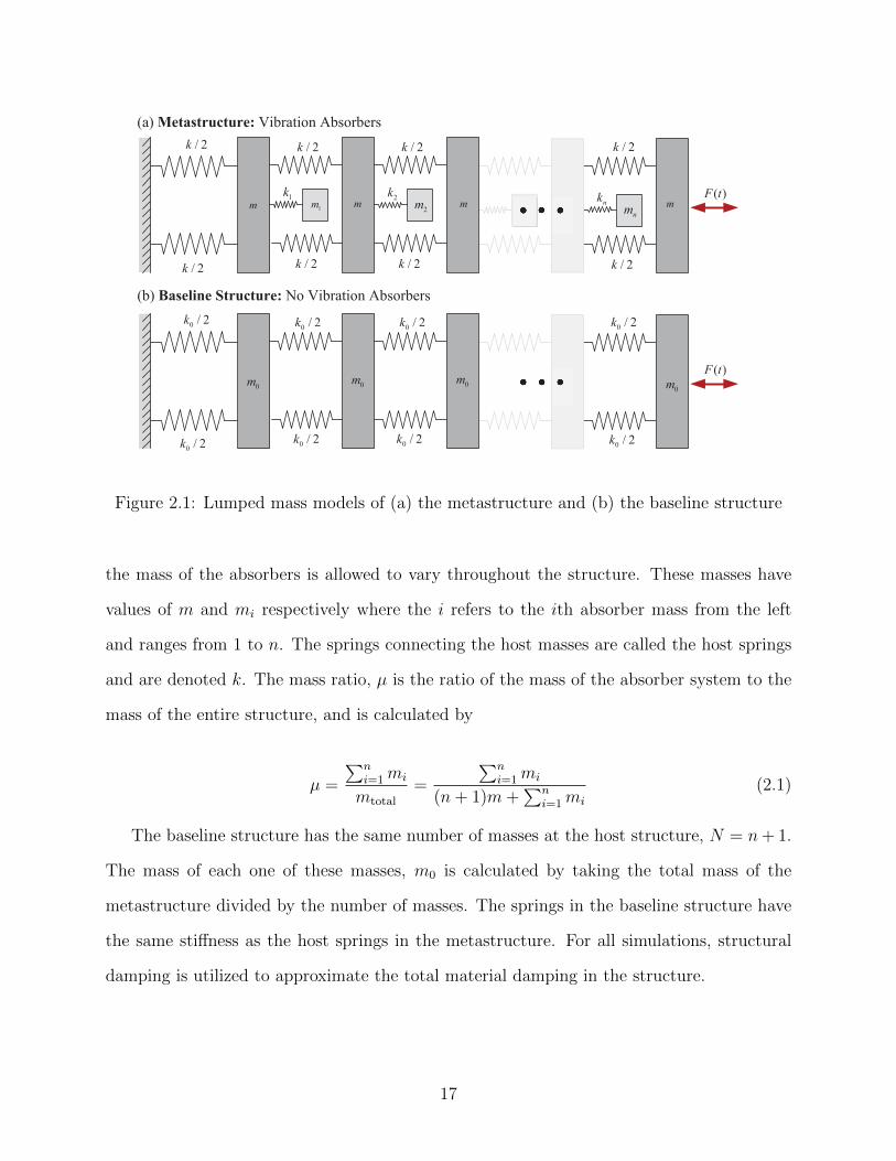
2.1 Description of lumped mass models
The design of the lumped mass model was chosen to behave similarly to an one-dimensional
axial bar but with vibration absorbers distributed throughout the length of the bar. The
metastructure bar lumped mass model is shown in Figure 2.1(a). This model consists of
masses and springs connected in series. Since this is a one dimensional model, all the defor-
mation occurs in the horizontal direction. The model consist of two parts, the host structure
and the vibration absorbers. The larger masses and springs make up the host structure
while the smaller masses and springs represent the vibration absorbers. Small deformation
is desired in the host structure. To provide a basis for performance improvement, the results
for the metastructure are compared to a baseline structure. A simple uniform bar is utilized
as the baseline structure and is modeled as mass and springs connected in series, seen in
Figure 2.1(b). The baseline structure and the metastructure have the same mass, which
shows that better performance from the metastructure is due to the addition of the ab-
sorbers and not from the additional mass. Throughout this chapter, the bars and absorbers
are modeled as lumped mass systems so the dynamics of the system are easily understood
and computational time is small.
The design of these structures was chosen such that the dynamics of structures will be
comparable between the metastructure and the baseline structure. Most importantly, they
will have fundamental natural frequencies near each other. The metastructure is character-
ized by the number of absorbers it has, denoted n. Therefore, n+1 masses make up the host
structure. All masses in the host structure, except the far right mass, have a small absorber
connected to it, modeled as a mass and spring. The larger masses will be referred to as the
host masses since these make up the host structure whereas the smaller masses are called
the absorber masses. The host masses all have the same mass to represent a uniform bar but
16
/ 2k
/ 2k
1m m
/ 2k
/ 2k
mm
( )F t1k
2m2k
/ 2k
/ 2k
/ 2k
/ 2k
m
nm
nk
0 / 2k
0 / 2k
0 / 2k
0 / 2k
0m
( )F t
0 / 2k
0 / 2k
0 / 2k
0 / 2k
0m 0m0m
(a)Metastructure: Vibration Absorbers
(b) Baseline Structure: No Vibration Absorbers
Figure 2.1: Lumped mass models of (a) the metastructure and (b) the baseline structure
the mass of the absorbers is allowed to vary throughout the structure. These masses have
values of m and mi respectively where the i refers to the ith absorber mass from the left
and ranges from 1 to n. The springs connecting the host masses are called the host springs
and are denoted k. The mass ratio, µ is the ratio of the mass of the absorber system to the
mass of the entire structure, and is calculated by
µ =
∑ni=1mi
mtotal
=
∑ni=1mi
(n+ 1)m+∑n
i=1mi
(2.1)
The baseline structure has the same number of masses at the host structure, N = n+ 1.
The mass of each one of these masses, m0 is calculated by taking the total mass of the
metastructure divided by the number of masses. The springs in the baseline structure have
the same stiffness as the host springs in the metastructure. For all simulations, structural
damping is utilized to approximate the total material damping in the structure.
17
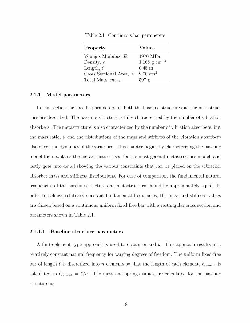
Table 2.1: Continuous bar parameters
Property Values
Young’s Modulus, E 1970 MPaDensity, ρ 1.168 g cm−3
Length, ` 0.45 mCross Sectional Area, A 9.00 cm2
Total Mass, mtotal 597 g
2.1.1 Model parameters
In this section the specific parameters for both the baseline structure and the metastruc-
ture are described. The baseline structure is fully characterized by the number of vibration
absorbers. The metastructure is also characterized by the number of vibration absorbers, but
the mass ratio, µ and the distributions of the mass and stiffness of the vibration absorbers
also effect the dynamics of the structure. This chapter begins by characterizing the baseline
model then explains the metastructure used for the most general metastructure model, and
lastly goes into detail showing the various constraints that can be placed on the vibration
absorber mass and stiffness distributions. For ease of comparison, the fundamental natural
frequencies of the baseline structure and metastructure should be approximately equal. In
order to achieve relatively constant fundamental frequencies, the mass and stiffness values
are chosen based on a continuous uniform fixed-free bar with a rectangular cross section and
parameters shown in Table 2.1.
2.1.1.1 Baseline structure parameters
A finite element type approach is used to obtain m and k. This approach results in a
relatively constant natural frequency for varying degrees of freedom. The uniform fixed-free
bar of length ` is discretized into n elements so that the length of each element, `element is
calculated as `element = `/n. The mass and springs values are calculated for the baseline
structure as
18
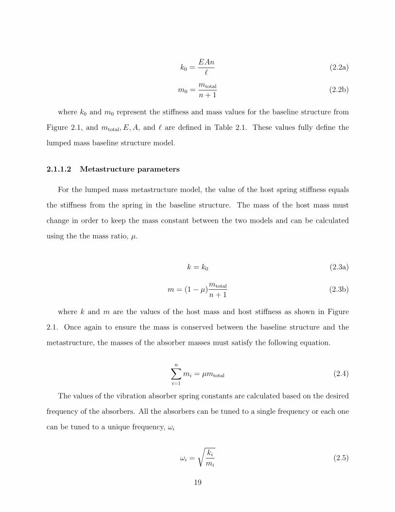
k0 =EAn
`(2.2a)
m0 =mtotal
n+ 1(2.2b)
where k0 and m0 represent the stiffness and mass values for the baseline structure from
Figure 2.1, and mtotal, E,A, and ` are defined in Table 2.1. These values fully define the
lumped mass baseline structure model.
2.1.1.2 Metastructure parameters
For the lumped mass metastructure model, the value of the host spring stiffness equals
the stiffness from the spring in the baseline structure. The mass of the host mass must
change in order to keep the mass constant between the two models and can be calculated
using the the mass ratio, µ.
k = k0 (2.3a)
m = (1− µ)mtotal
n+ 1(2.3b)
where k and m are the values of the host mass and host stiffness as shown in Figure
2.1. Once again to ensure the mass is conserved between the baseline structure and the
metastructure, the masses of the absorber masses must satisfy the following equation.
n∑i=1
mi = µmtotal (2.4)
The values of the vibration absorber spring constants are calculated based on the desired
frequency of the absorbers. All the absorbers can be tuned to a single frequency or each one
can be tuned to a unique frequency, ωi
ωi =
√kimi
(2.5)
19
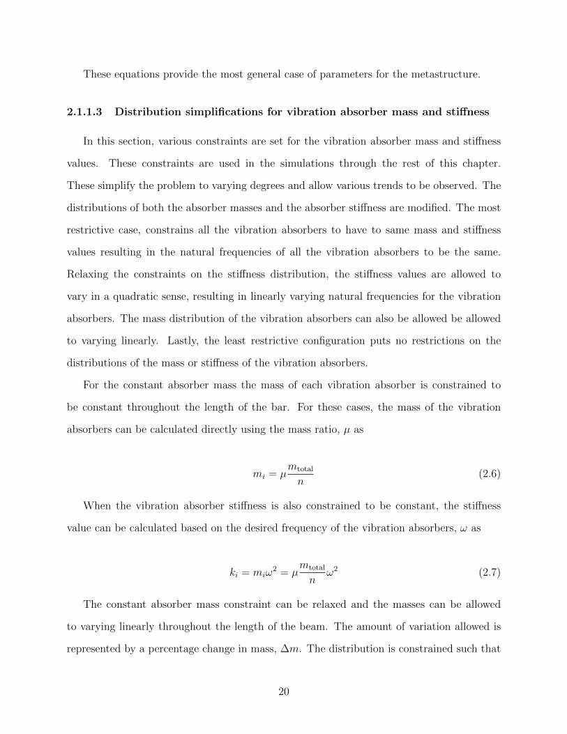
These equations provide the most general case of parameters for the metastructure.
2.1.1.3 Distribution simplifications for vibration absorber mass and stiffness
In this section, various constraints are set for the vibration absorber mass and stiffness
values. These constraints are used in the simulations through the rest of this chapter.
These simplify the problem to varying degrees and allow various trends to be observed. The
distributions of both the absorber masses and the absorber stiffness are modified. The most
restrictive case, constrains all the vibration absorbers to have to same mass and stiffness
values resulting in the natural frequencies of all the vibration absorbers to be the same.
Relaxing the constraints on the stiffness distribution, the stiffness values are allowed to
vary in a quadratic sense, resulting in linearly varying natural frequencies for the vibration
absorbers. The mass distribution of the vibration absorbers can also be allowed be allowed
to varying linearly. Lastly, the least restrictive configuration puts no restrictions on the
distributions of the mass or stiffness of the vibration absorbers.
For the constant absorber mass the mass of each vibration absorber is constrained to
be constant throughout the length of the bar. For these cases, the mass of the vibration
absorbers can be calculated directly using the mass ratio, µ as
mi = µmtotal
n(2.6)
When the vibration absorber stiffness is also constrained to be constant, the stiffness
value can be calculated based on the desired frequency of the vibration absorbers, ω as
ki = miω2 = µ
mtotal
nω2 (2.7)
The constant absorber mass constraint can be relaxed and the masses can be allowed
to varying linearly throughout the length of the beam. The amount of variation allowed is
represented by a percentage change in mass, ∆m. The distribution is constrained such that
20
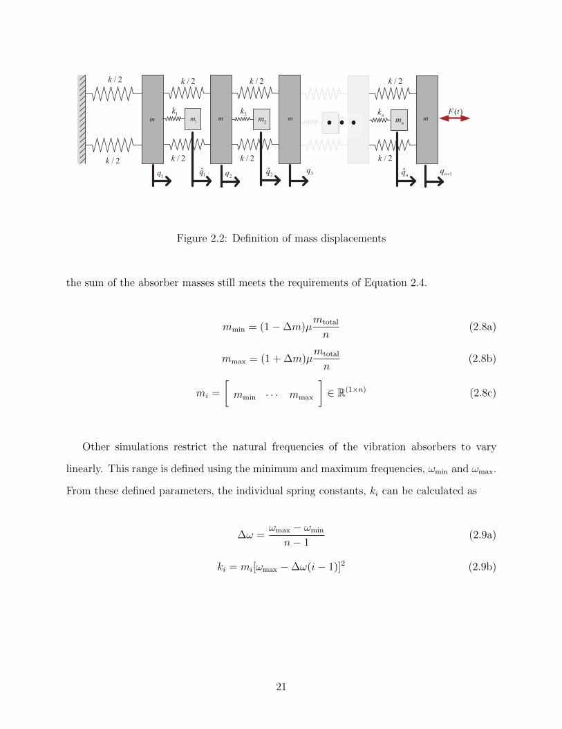
/ 2k
/ 2k
1m m
/ 2k
/ 2k
mm( )F t1k
2m2k
/ 2k
/ 2k
/ 2k
/ 2k
mnm
nk
1q 1q 2q 2q 3q ˆnq 1nq +
Figure 2.2: Definition of mass displacements
the sum of the absorber masses still meets the requirements of Equation 2.4.
mmin = (1−∆m)µmtotal
n(2.8a)
mmax = (1 + ∆m)µmtotal
n(2.8b)
mi =
[mmin · · · mmax
]∈ R(1×n) (2.8c)
Other simulations restrict the natural frequencies of the vibration absorbers to vary
linearly. This range is defined using the minimum and maximum frequencies, ωmin and ωmax.
From these defined parameters, the individual spring constants, ki can be calculated as
∆ω =ωmax − ωmin
n− 1(2.9a)
ki = mi[ωmax −∆ω(i− 1)]2 (2.9b)
21
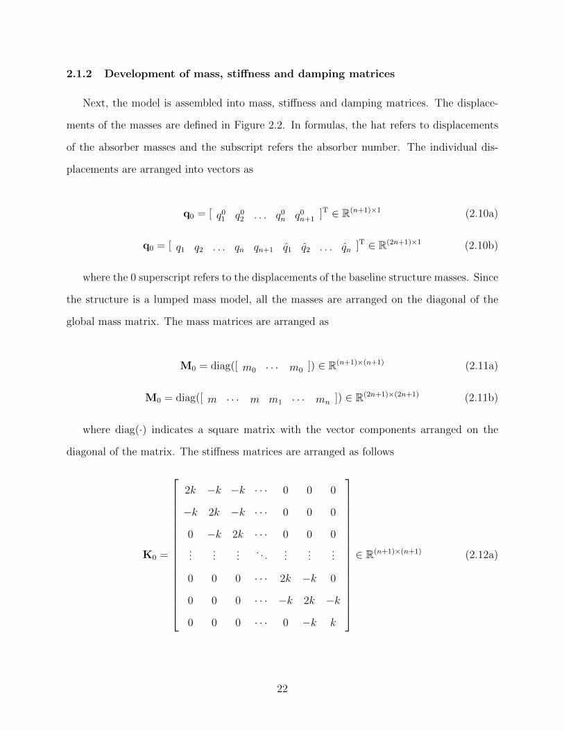
2.1.2 Development of mass, stiffness and damping matrices
Next, the model is assembled into mass, stiffness and damping matrices. The displace-
ments of the masses are defined in Figure 2.2. In formulas, the hat refers to displacements
of the absorber masses and the subscript refers the absorber number. The individual dis-
placements are arranged into vectors as
q0 = [ q01 q02 . . . q0n q0n+1]T ∈ R(n+1)×1 (2.10a)
q0 = [ q1 q2 . . . qn qn+1 q1 q2 . . . qn ]T ∈ R(2n+1)×1 (2.10b)
where the 0 superscript refers to the displacements of the baseline structure masses. Since
the structure is a lumped mass model, all the masses are arranged on the diagonal of the
global mass matrix. The mass matrices are arranged as
M0 = diag([ m0 · · · m0 ]) ∈ R(n+1)×(n+1) (2.11a)
M0 = diag([ m · · · m m1 · · · mn ]) ∈ R(2n+1)×(2n+1) (2.11b)
where diag(·) indicates a square matrix with the vector components arranged on the
diagonal of the matrix. The stiffness matrices are arranged as follows
K0 =
2k −k −k · · · 0 0 0
−k 2k −k · · · 0 0 0
0 −k 2k · · · 0 0 0
......
.... . .
......
...
0 0 0 · · · 2k −k 0
0 0 0 · · · −k 2k −k
0 0 0 · · · 0 −k k
∈ R(n+1)×(n+1) (2.12a)
22
K =
K0 + Vaug
−V
0
−V 0 V
∈ R(2n+1)×(2n+1) (2.12b)
V = diag([ k1 k2 · · · kn ]) ∈ Rn×n (2.12c)
Vaug = diag([ k1 k2 · · · kn 0 ]) ∈ R(n+1)×(n+1) (2.12d)
0 = [ 0 · · · 0 ]T ∈ Rn+1 (2.12e)
For this model, no dampers are added to the system but since all structures have ma-
terial damping inherent in them this must be modeled. This damping does not change the
dynamics of the system; it simply prevents the simulations from tending to infinity. A pro-
portional damping model is utilized choosing an arbitrary damping constant, α and defining
the damping matrices by
D = αK (2.13a)
D0 = αK0 (2.13b)
Note that proportionality to the mass matrix, commonly used, is not used here because
of the recent result of Kabe and Sako [94]. Results are presented as a pair of plots: the FRF
and the impulse response. Each plot shows the baseline structure with no absorbers as a
dotted line and the structure with absorbers as a solid line. The FRF is of the far right main
mass subjected to an input force, i.e. |[Q0n+1(s)]/[Fn+1(s)]|. The impulse response function
is also calculated by applying a unit impulse to the same mass. As a quantitative measure,
the percent decrease of the H2 norm is also reported. This norm is explained in more detail
in the next section.
23
2.2 Performance measure
This section describes the performance measure used to determine how effectively the
structure suppresses vibrations. Here the H2 will be utilized, which is widely used in control
literature to develop optimal control theory. The H2 norm is related to the total energy in
the system. To begin, the system must be transformed into state space. The equations of
motion for the structure are
Mq + Dq + Kq = F (2.14)
where M, D and K are the mass, damping and stiffness matrices defined in the previous
section, F is the force vector, and q are the displacements of the lumped mass. The force
vector, F is taken to have a unit value. The corresponding state space matrices are
A =
0 I
−M−1K −M−1D
(2.15a)
B =
0
M−1F
(2.15b)
C = [ I 0 ] (2.15c)
These can be used to express a transfer function matrix
H(s) = C(sI−A)−1B (2.16)
This results in a transfer function matrix, H(s), which has dimensions m×m and contains
complex numbers, where m is the total number of degrees of freedom in the system. For the
baseline structure, m = n+ 1 and for the metastructure, m = 2n+ 1. The specific entries of
this matrix can be named as
24
H(s) =
H11(s) · · · H1m(s)
.... . .
...
Hm1(s) · · · Hmm(s)
(2.17)
The term of interest to this paper is the HNN(s) entry which describes the relationship
between an input at the tip and the response of the tip, where N = n+ 1. For convenience
the following definition is utilized, HNN(s) = G(s). The H2 norm is a measure of the total
vibration energy of the system over all frequencies and can be calculated by taking the norm
of frequency response function as follows
H2 = ‖G(s)‖22 =1
2π
∫ ∞−∞
tr[G?(ω)G(ω)]dω (2.18)
where the star indicates the complex conjugate of the number. This performance measure
is also related to the impulse response function by Parsevals theorem
‖G(s)‖22 = ‖H(t)‖22 =
∫ ∞0
h(t)hT(t)dt (2.19)
where h(t) is the impulse response function defined as
h(t) = CeAtB (2.20)
The norms of the metastructure and the baseline structure are compared and presented
as a percent decrease in the following section defined as
H2 percent decrease =|(H2)baseline − (H2)metastructure|
(H2)baseline× 100 (2.21)
where (H2)metastructure is the H2 norm calculated for the metastructure and (H2)baseline is
the norm of the baseline structure calculated in the same manner as for the metastructure
but with the M0, D0 and K0 matrices replacing the M, D and K matrices in Equation 2.14.
25
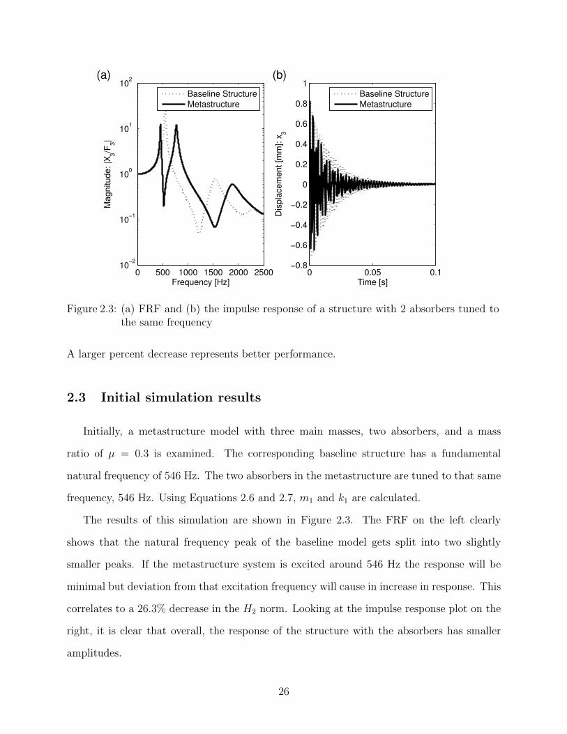
0 500 1000 1500 2000 250010
−2
10−1
100
101
102
Frequency [Hz]
Ma
gn
itu
de
: |X
3/F
3|
Baseline Structure
Metastructure
0 0.05 0.1−0.8
−0.6
−0.4
−0.2
0
0.2
0.4
0.6
0.8
1
Time [s]D
isp
lace
me
nt
[mm
]: x
3
Baseline Structure
Metastructure
(a) (b)
Figure 2.3: (a) FRF and (b) the impulse response of a structure with 2 absorbers tuned tothe same frequency
A larger percent decrease represents better performance.
2.3 Initial simulation results
Initially, a metastructure model with three main masses, two absorbers, and a mass
ratio of µ = 0.3 is examined. The corresponding baseline structure has a fundamental
natural frequency of 546 Hz. The two absorbers in the metastructure are tuned to that same
frequency, 546 Hz. Using Equations 2.6 and 2.7, m1 and k1 are calculated.
The results of this simulation are shown in Figure 2.3. The FRF on the left clearly
shows that the natural frequency peak of the baseline model gets split into two slightly
smaller peaks. If the metastructure system is excited around 546 Hz the response will be
minimal but deviation from that excitation frequency will cause in increase in response. This
correlates to a 26.3% decrease in the H2 norm. Looking at the impulse response plot on the
right, it is clear that overall, the response of the structure with the absorbers has smaller
amplitudes.
26
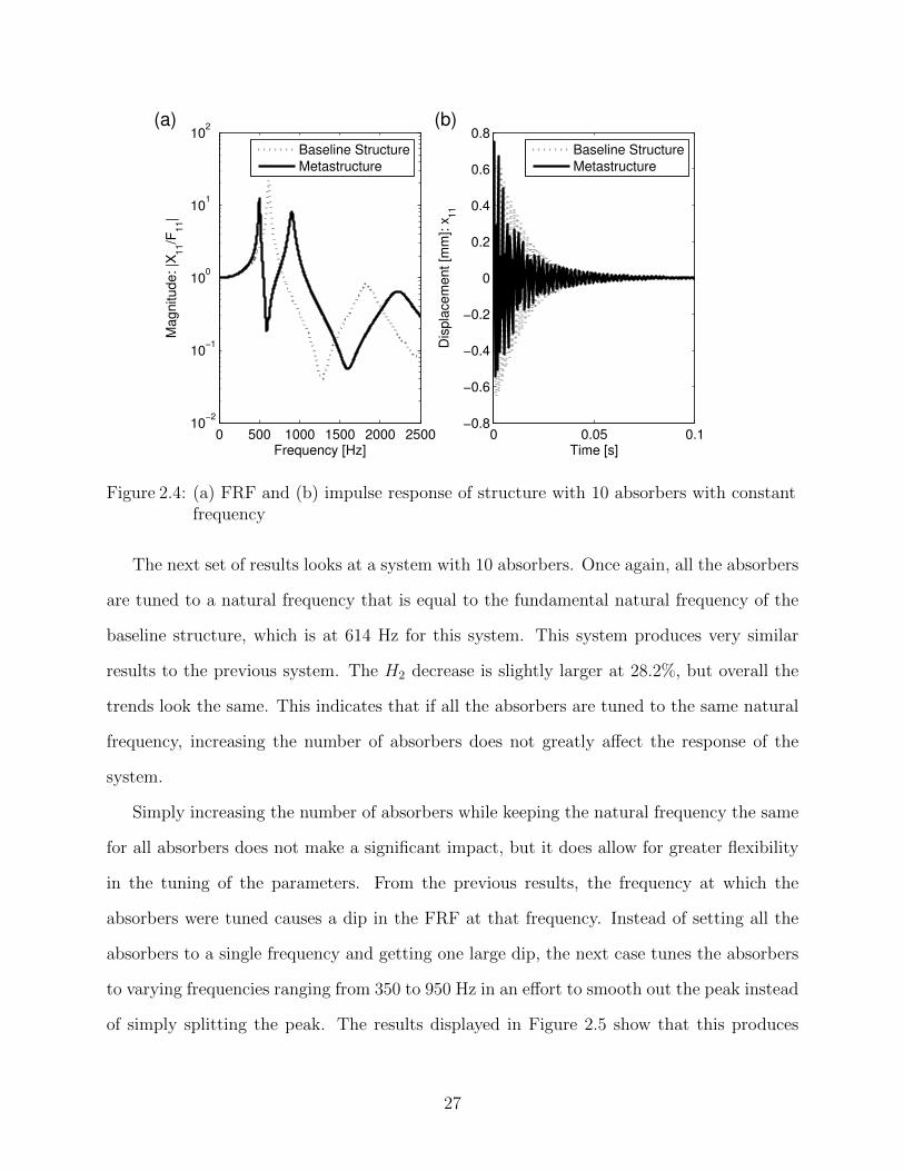
0 500 1000 1500 2000 250010
−2
10−1
100
101
102
Frequency [Hz]
Ma
gn
itu
de
: |X
11/F
11|
Baseline Structure
Metastructure
0 0.05 0.1−0.8
−0.6
−0.4
−0.2
0
0.2
0.4
0.6
0.8
Time [s]D
isp
lace
me
nt
[mm
]: x
11
Baseline Structure
Metastructure
(a) (b)
Figure 2.4: (a) FRF and (b) impulse response of structure with 10 absorbers with constantfrequency
The next set of results looks at a system with 10 absorbers. Once again, all the absorbers
are tuned to a natural frequency that is equal to the fundamental natural frequency of the
baseline structure, which is at 614 Hz for this system. This system produces very similar
results to the previous system. The H2 decrease is slightly larger at 28.2%, but overall the
trends look the same. This indicates that if all the absorbers are tuned to the same natural
frequency, increasing the number of absorbers does not greatly affect the response of the
system.
Simply increasing the number of absorbers while keeping the natural frequency the same
for all absorbers does not make a significant impact, but it does allow for greater flexibility
in the tuning of the parameters. From the previous results, the frequency at which the
absorbers were tuned causes a dip in the FRF at that frequency. Instead of setting all the
absorbers to a single frequency and getting one large dip, the next case tunes the absorbers
to varying frequencies ranging from 350 to 950 Hz in an effort to smooth out the peak instead
of simply splitting the peak. The results displayed in Figure 2.5 show that this produces
27
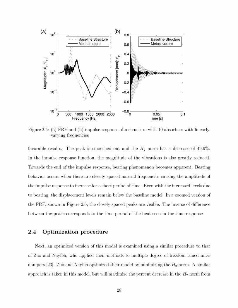
0 500 1000 1500 2000 250010
−2
10−1
100
101
102
Frequency [Hz]
Ma
gn
itu
de
: |X
11/F
11|
Baseline Structure
Metastructure
0 0.05 0.1−0.8
−0.6
−0.4
−0.2
0
0.2
0.4
0.6
0.8
Time [s]D
isp
lace
me
nt
[mm
]: x
11
Baseline Structure
Metastructure
(a) (b)
Figure 2.5: (a) FRF and (b) impulse response of a structure with 10 absorbers with linearlyvarying frequencies
favorable results. The peak is smoothed out and the H2 norm has a decrease of 49.9%.
In the impulse response function, the magnitude of the vibrations is also greatly reduced.
Towards the end of the impulse response, beating phenomenon becomes apparent. Beating
behavior occurs when there are closely spaced natural frequencies causing the amplitude of
the impulse response to increase for a short period of time. Even with the increased levels due
to beating, the displacement levels remain below the baseline model. In a zoomed version of
the FRF, shown in Figure 2.6, the closely spaced peaks are visible. The inverse of difference
between the peaks corresponds to the time period of the beat seen in the time response.
2.4 Optimization procedure
Next, an optimized version of this model is examined using a similar procedure to that
of Zuo and Nayfeh, who applied their methods to multiple degree of freedom tuned mass
dampers [23]. Zuo and Nayfeh optimized their model by minimizing the H2 norm. A similar
approach is taken in this model, but will maximize the percent decrease in the H2 norm from
28
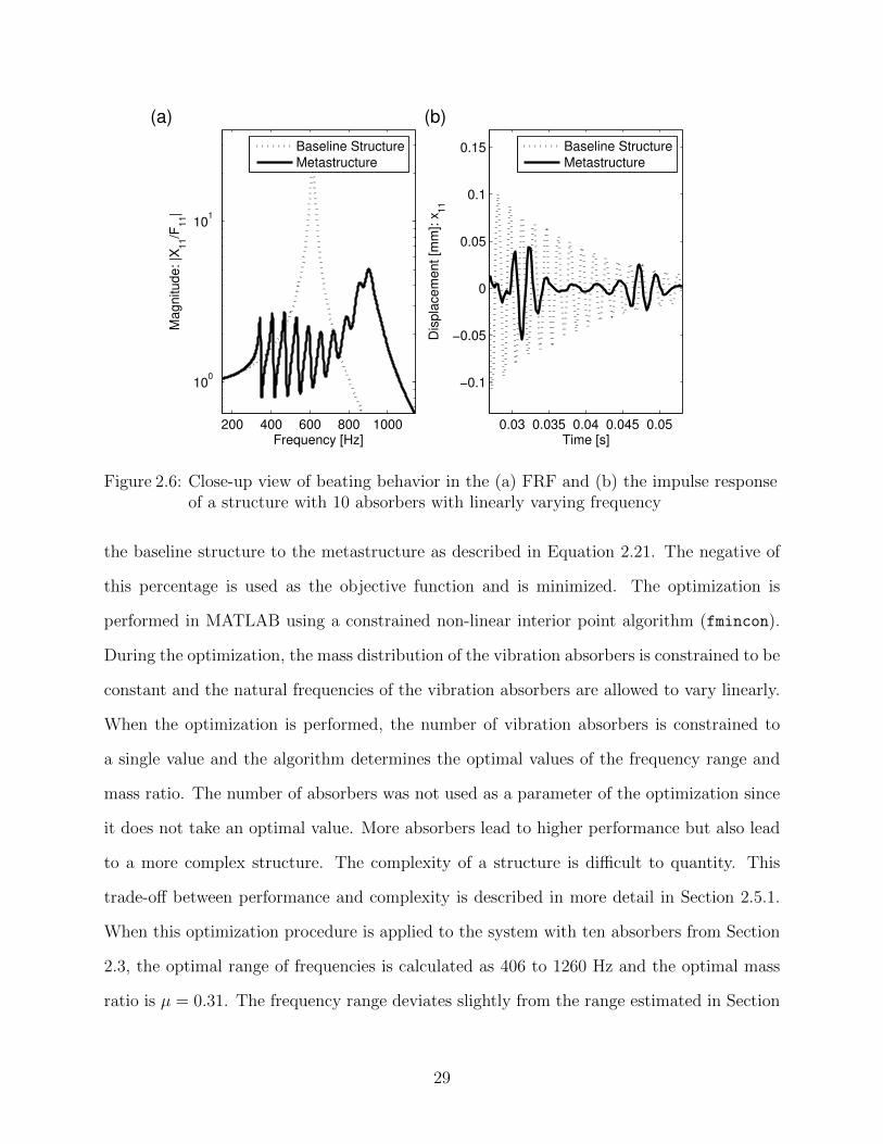
200 400 600 800 1000
100
101
Frequency [Hz]
Ma
gn
itu
de
: |X
11/F
11|
Baseline Structure
Metastructure
0.03 0.035 0.04 0.045 0.05
−0.1
−0.05
0
0.05
0.1
0.15
Time [s]D
isp
lace
me
nt
[mm
]: x
11
Baseline Structure
Metastructure
(a) (b)
Figure 2.6: Close-up view of beating behavior in the (a) FRF and (b) the impulse responseof a structure with 10 absorbers with linearly varying frequency
the baseline structure to the metastructure as described in Equation 2.21. The negative of
this percentage is used as the objective function and is minimized. The optimization is
performed in MATLAB using a constrained non-linear interior point algorithm (fmincon).
During the optimization, the mass distribution of the vibration absorbers is constrained to be
constant and the natural frequencies of the vibration absorbers are allowed to vary linearly.
When the optimization is performed, the number of vibration absorbers is constrained to
a single value and the algorithm determines the optimal values of the frequency range and
mass ratio. The number of absorbers was not used as a parameter of the optimization since
it does not take an optimal value. More absorbers lead to higher performance but also lead
to a more complex structure. The complexity of a structure is difficult to quantity. This
trade-off between performance and complexity is described in more detail in Section 2.5.1.
When this optimization procedure is applied to the system with ten absorbers from Section
2.3, the optimal range of frequencies is calculated as 406 to 1260 Hz and the optimal mass
ratio is µ = 0.31. The frequency range deviates slightly from the range estimated in Section
29
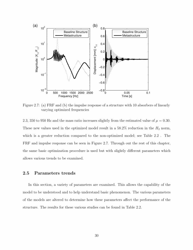
0 500 1000 1500 2000 250010
−2
10−1
100
101
102
Frequency [Hz]
Ma
gn
itu
de
: |X
11/F
11|
Baseline Structure
Metastructure
0 0.05 0.1−0.8
−0.6
−0.4
−0.2
0
0.2
0.4
0.6
0.8
Time [s]D
isp
lace
me
nt
[mm
]: x
11
Baseline Structure
Metastructure
(a) (b)
Figure 2.7: (a) FRF and (b) the impulse response of a structure with 10 absorbers of linearlyvarying optimized frequencies
2.3, 350 to 950 Hz and the mass ratio increases slightly from the estimated value of µ = 0.30.
These new values used in the optimized model result in a 58.2% reduction in the H2 norm,
which is a greater reduction compared to the non-optimized model; see Table 2.2 . The
FRF and impulse response can be seen in Figure 2.7. Through out the rest of this chapter,
the same basic optimization procedure is used but with slightly different parameters which
allows various trends to be examined.
2.5 Parameters trends
In this section, a variety of parameters are examined. This allows the capability of the
model to be understood and to help understand basic phenomenon. The various parameters
of the models are altered to determine how these parameters affect the performance of the
structure. The results for these various studies can be found in Table 2.2.
30
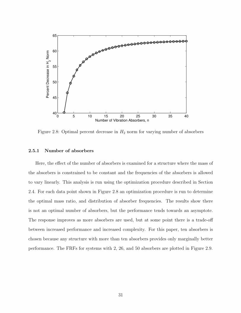
0 5 10 15 20 25 30 35 4040
45
50
55
60
65
Number of Vibration Absorbers, n
Pe
rce
nt
De
cre
ase
in
H2 N
orm
Figure 2.8: Optimal percent decrease in H2 norm for varying number of absorbers
2.5.1 Number of absorbers
Here, the effect of the number of absorbers is examined for a structure where the mass of
the absorbers is constrained to be constant and the frequencies of the absorbers is allowed
to vary linearly. This analysis is run using the optimization procedure described in Section
2.4. For each data point shown in Figure 2.8 an optimization procedure is run to determine
the optimal mass ratio, and distribution of absorber frequencies. The results show there
is not an optimal number of absorbers, but the performance tends towards an asymptote.
The response improves as more absorbers are used, but at some point there is a trade-off
between increased performance and increased complexity. For this paper, ten absorbers is
chosen because any structure with more than ten absorbers provides only marginally better
performance. The FRFs for systems with 2, 26, and 50 absorbers are plotted in Figure 2.9.
31
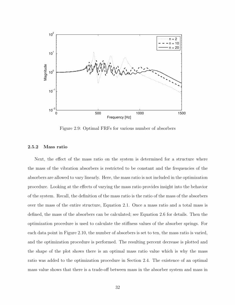
0 500 1000 150010
−2
10−1
100
101
102
Frequency [Hz]
Ma
gn
itu
de
n = 2
n = 10
n = 20
Figure 2.9: Optimal FRFs for various number of absorbers
2.5.2 Mass ratio
Next, the effect of the mass ratio on the system is determined for a structure where
the mass of the vibration absorbers is restricted to be constant and the frequencies of the
absorbers are allowed to vary linearly. Here, the mass ratio is not included in the optimization
procedure. Looking at the effects of varying the mass ratio provides insight into the behavior
of the system. Recall, the definition of the mass ratio is the ratio of the mass of the absorbers
over the mass of the entire structure, Equation 2.1. Once a mass ratio and a total mass is
defined, the mass of the absorbers can be calculated; see Equation 2.6 for details. Then the
optimization procedure is used to calculate the stiffness values of the absorber springs. For
each data point in Figure 2.10, the number of absorbers is set to ten, the mass ratio is varied,
and the optimization procedure is performed. The resulting percent decrease is plotted and
the shape of the plot shows there is an optimal mass ratio value which is why the mass
ratio was added to the optimization procedure in Section 2.4. The existence of an optimal
mass value shows that there is a trade-off between mass in the absorber system and mass in
32
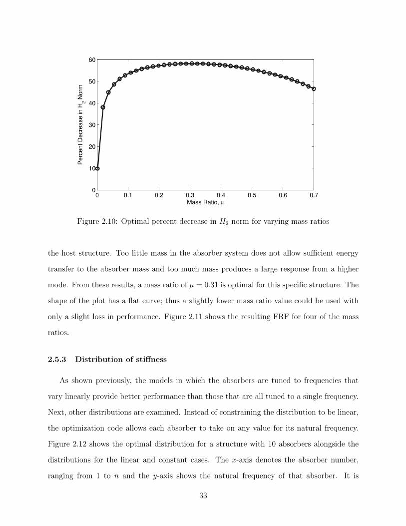
0 0.1 0.2 0.3 0.4 0.5 0.6 0.70
10
20
30
40
50
60
Mass Ratio, µ
Pe
rce
nt
De
cre
ase
in
H2 N
orm
Figure 2.10: Optimal percent decrease in H2 norm for varying mass ratios
the host structure. Too little mass in the absorber system does not allow sufficient energy
transfer to the absorber mass and too much mass produces a large response from a higher
mode. From these results, a mass ratio of µ = 0.31 is optimal for this specific structure. The
shape of the plot has a flat curve; thus a slightly lower mass ratio value could be used with
only a slight loss in performance. Figure 2.11 shows the resulting FRF for four of the mass
ratios.
2.5.3 Distribution of stiffness
As shown previously, the models in which the absorbers are tuned to frequencies that
vary linearly provide better performance than those that are all tuned to a single frequency.
Next, other distributions are examined. Instead of constraining the distribution to be linear,
the optimization code allows each absorber to take on any value for its natural frequency.
Figure 2.12 shows the optimal distribution for a structure with 10 absorbers alongside the
distributions for the linear and constant cases. The x-axis denotes the absorber number,
ranging from 1 to n and the y-axis shows the natural frequency of that absorber. It is
33
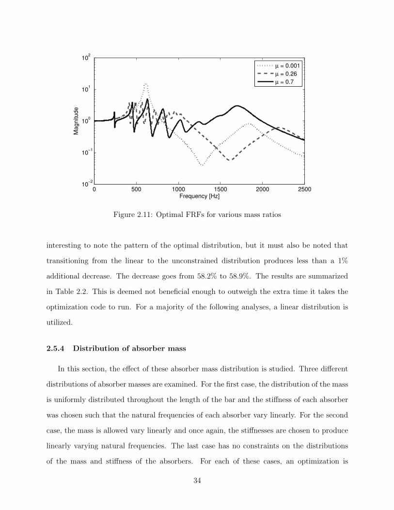
0 500 1000 1500 2000 250010
−2
10−1
100
101
102
Frequency [Hz]
Ma
gn
itu
de
µ = 0.001
µ = 0.26
µ = 0.7
Figure 2.11: Optimal FRFs for various mass ratios
interesting to note the pattern of the optimal distribution, but it must also be noted that
transitioning from the linear to the unconstrained distribution produces less than a 1%
additional decrease. The decrease goes from 58.2% to 58.9%. The results are summarized
in Table 2.2. This is deemed not beneficial enough to outweigh the extra time it takes the
optimization code to run. For a majority of the following analyses, a linear distribution is
utilized.
2.5.4 Distribution of absorber mass
In this section, the effect of these absorber mass distribution is studied. Three different
distributions of absorber masses are examined. For the first case, the distribution of the mass
is uniformly distributed throughout the length of the bar and the stiffness of each absorber
was chosen such that the natural frequencies of each absorber vary linearly. For the second
case, the mass is allowed vary linearly and once again, the stiffnesses are chosen to produce
linearly varying natural frequencies. The last case has no constraints on the distributions
of the mass and stiffness of the absorbers. For each of these cases, an optimization is
34
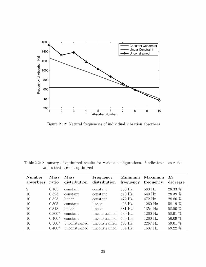
1 2 3 4 5 6 7 8 9 10200
400
600
800
1000
1200
1400
1600
Absorber Number
Fre
qu
en
cy o
f A
bso
rbe
r [H
z]
Constant Constraint
Linear Constraint
Unconstrained
Figure 2.12: Natural frequencies of individual vibration absorbers
Table 2.2: Summary of optimized results for various configurations. *indicates mass ratiovalues that are not optimized
Number Mass Mass Frequency Minimum Maximum H2
absorbers ratio distribution distribution frequency frequency decrease
2 0.165 constant constant 583 Hz 583 Hz 28.33 %10 0.323 constant constant 640 Hz 640 Hz 28.39 %10 0.323 linear constant 472 Hz 472 Hz 28.86 %10 0.305 constant linear 406 Hz 1260 Hz 58.19 %10 0.318 linear linear 381 Hz 1354 Hz 58.50 %10 0.300* constant unconstrained 430 Hz 1260 Hz 58.91 %10 0.400* constant unconstrained 430 Hz 1260 Hz 56.09 %10 0.300* unconstrained unconstrained 405 Hz 2267 Hz 59.01 %10 0.400* unconstrained unconstrained 364 Hz 1537 Hz 59.22 %
35
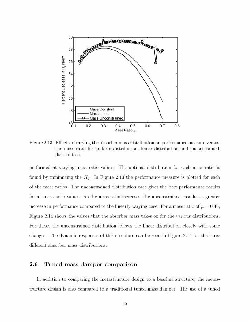
0.1 0.2 0.3 0.4 0.5 0.6 0.7 0.846
48
50
52
54
56
58
60
Mass Ratio, µ
Perc
ent D
ecre
ase in H
2 N
orm
Mass Constant
Mass Linear
Mass Unconstrained
Figure 2.13: Effects of varying the absorber mass distribution on performance measure versusthe mass ratio for uniform distribution, linear distribution and unconstraineddistribution
performed at varying mass ratio values. The optimal distribution for each mass ratio is
found by minimizing the H2. In Figure 2.13 the performance measure is plotted for each
of the mass ratios. The unconstrained distribution case gives the best performance results
for all mass ratio values. As the mass ratio increases, the unconstrained case has a greater
increase in performance compared to the linearly varying case. For a mass ratio of µ = 0.40,
Figure 2.14 shows the values that the absorber mass takes on for the various distributions.
For these, the unconstrained distribution follows the linear distribution closely with some
changes. The dynamic responses of this structure can be seen in Figure 2.15 for the three
different absorber mass distributions.
2.6 Tuned mass damper comparison
In addition to comparing the metastructure design to a baseline structure, the metas-
tructure design is also compared to a traditional tuned mass damper. The use of a tuned
36
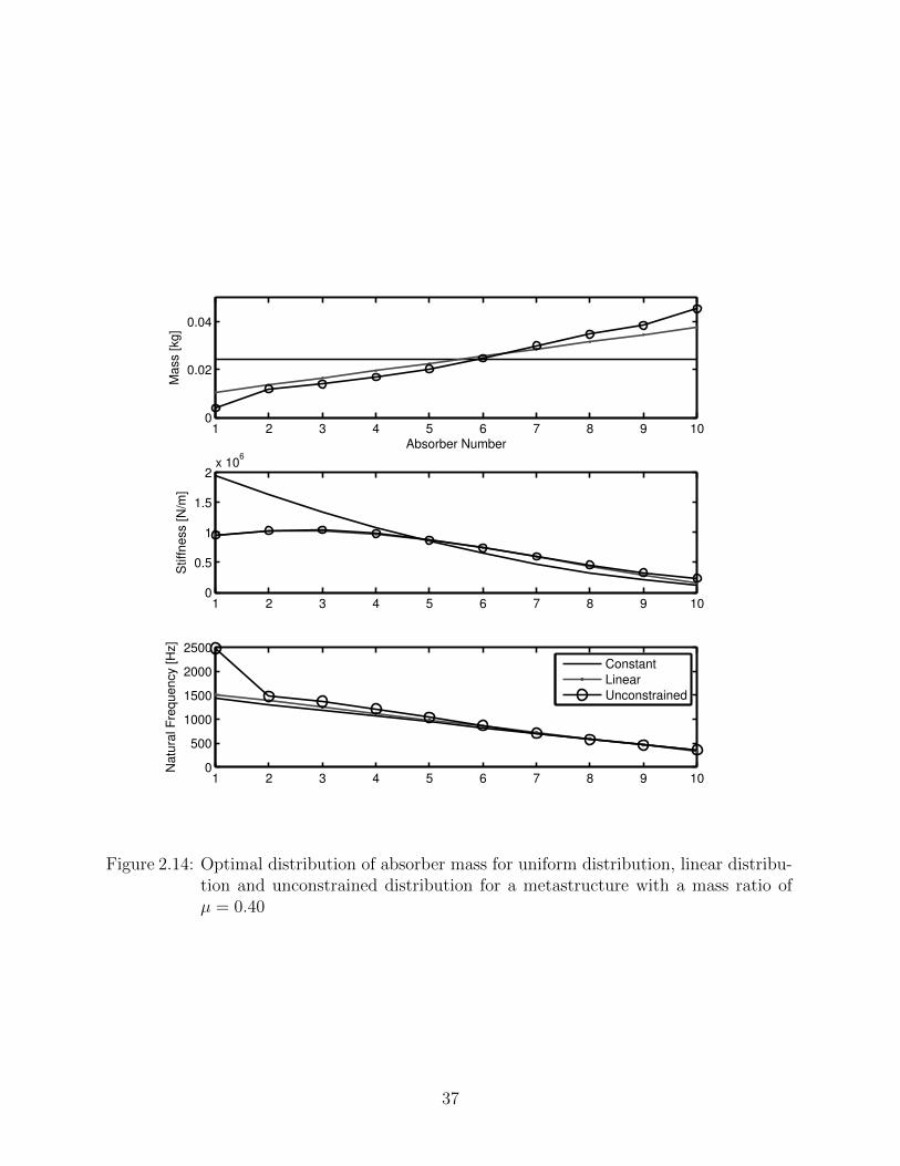
1 2 3 4 5 6 7 8 9 100
0.02
0.04
Ma
ss [
kg]
Absorber Number
1 2 3 4 5 6 7 8 9 100
0.5
1
1.5
2x 10
6
Stiff
ness [N
/m]
1 2 3 4 5 6 7 8 9 100
500
1000
1500
2000
2500
Na
tura
l F
requ
en
cy [
Hz]
Constant
Linear
Unconstrained
Figure 2.14: Optimal distribution of absorber mass for uniform distribution, linear distribu-tion and unconstrained distribution for a metastructure with a mass ratio ofµ = 0.40
37
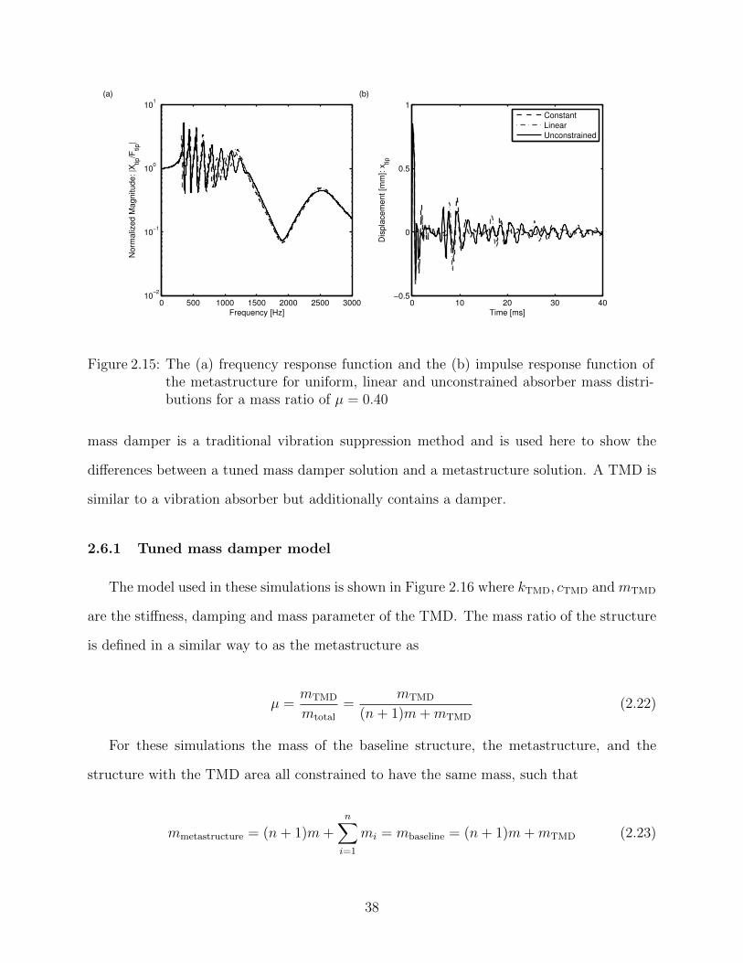
0 500 1000 1500 2000 2500 300010
−2
10−1
100
101
Frequency [Hz]
No
rma
lize
d M
ag
nitu
de
: |X
tip/F
tip|
0 10 20 30 40−0.5
0
0.5
1
Time [ms]
Dis
pla
ce
me
nt
[mm
]: x
tip
Constant
Linear
Unconstrained
(a) (b)
Figure 2.15: The (a) frequency response function and the (b) impulse response function ofthe metastructure for uniform, linear and unconstrained absorber mass distri-butions for a mass ratio of µ = 0.40
mass damper is a traditional vibration suppression method and is used here to show the
differences between a tuned mass damper solution and a metastructure solution. A TMD is
similar to a vibration absorber but additionally contains a damper.
2.6.1 Tuned mass damper model
The model used in these simulations is shown in Figure 2.16 where kTMD, cTMD and mTMD
are the stiffness, damping and mass parameter of the TMD. The mass ratio of the structure
is defined in a similar way to as the metastructure as
µ =mTMD
mtotal
=mTMD
(n+ 1)m+mTMD
(2.22)
For these simulations the mass of the baseline structure, the metastructure, and the
structure with the TMD area all constrained to have the same mass, such that
mmetastructure = (n+ 1)m+n∑i=1
mi = mbaseline = (n+ 1)m+mTMD (2.23)
38
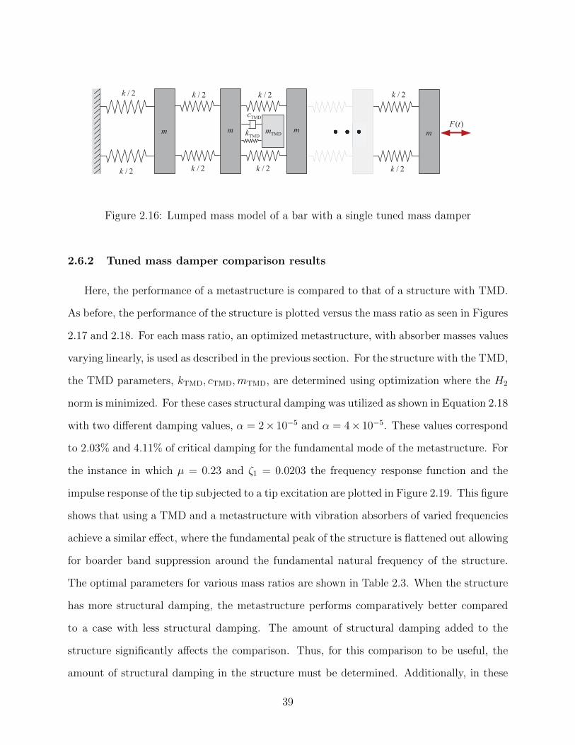
/ 2k
/ 2k
/ 2k
/ 2k
m( )F t
/ 2k
/ 2k
/ 2k
/ 2k
m mmTMDm
TMDk
TMDc
Figure 2.16: Lumped mass model of a bar with a single tuned mass damper
2.6.2 Tuned mass damper comparison results
Here, the performance of a metastructure is compared to that of a structure with TMD.
As before, the performance of the structure is plotted versus the mass ratio as seen in Figures
2.17 and 2.18. For each mass ratio, an optimized metastructure, with absorber masses values
varying linearly, is used as described in the previous section. For the structure with the TMD,
the TMD parameters, kTMD, cTMD,mTMD, are determined using optimization where the H2
norm is minimized. For these cases structural damping was utilized as shown in Equation 2.18
with two different damping values, α = 2× 10⁻⁵ and α = 4× 10⁻⁵. These values correspond
to 2.03% and 4.11% of critical damping for the fundamental mode of the metastructure. For
the instance in which µ = 0.23 and ζ1 = 0.0203 the frequency response function and the
impulse response of the tip subjected to a tip excitation are plotted in Figure 2.19. This figure
shows that using a TMD and a metastructure with vibration absorbers of varied frequencies
achieve a similar effect, where the fundamental peak of the structure is flattened out allowing
for boarder band suppression around the fundamental natural frequency of the structure.
The optimal parameters for various mass ratios are shown in Table 2.3. When the structure
has more structural damping, the metastructure performs comparatively better compared
to a case with less structural damping. The amount of structural damping added to the
structure significantly affects the comparison. Thus, for this comparison to be useful, the
amount of structural damping in the structure must be determined. Additionally, in these
39
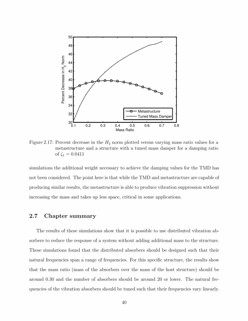
0.1 0.2 0.3 0.4 0.5 0.6 0.7 0.830
32
34
36
38
40
42
44
46
48
50
Mass Ratio
Perc
ent D
ecre
ase in H
2 N
orm
Metastructure
Tuned Mass Damper
Figure 2.17: Percent decrease in the H2 norm plotted versus varying mass ratio values for ametastructure and a structure with a tuned mass damper for a damping ratioof ζ1 = 0.0411
simulations the additional weight necessary to achieve the damping values for the TMD has
not been considered. The point here is that while the TMD and metastructure are capable of
producing similar results, the metastructure is able to produce vibration suppression without
increasing the mass and takes up less space, critical in some applications.
2.7 Chapter summary
The results of these simulations show that it is possible to use distributed vibration ab-
sorbers to reduce the response of a system without adding additional mass to the structure.
These simulations found that the distributed absorbers should be designed such that their
natural frequencies span a range of frequencies. For this specific structure, the results show
that the mass ratio (mass of the absorbers over the mass of the host structure) should be
around 0.30 and the number of absorbers should be around 20 or lower. The natural fre-
quencies of the vibration absorbers should be tuned such that their frequencies vary linearly.
40
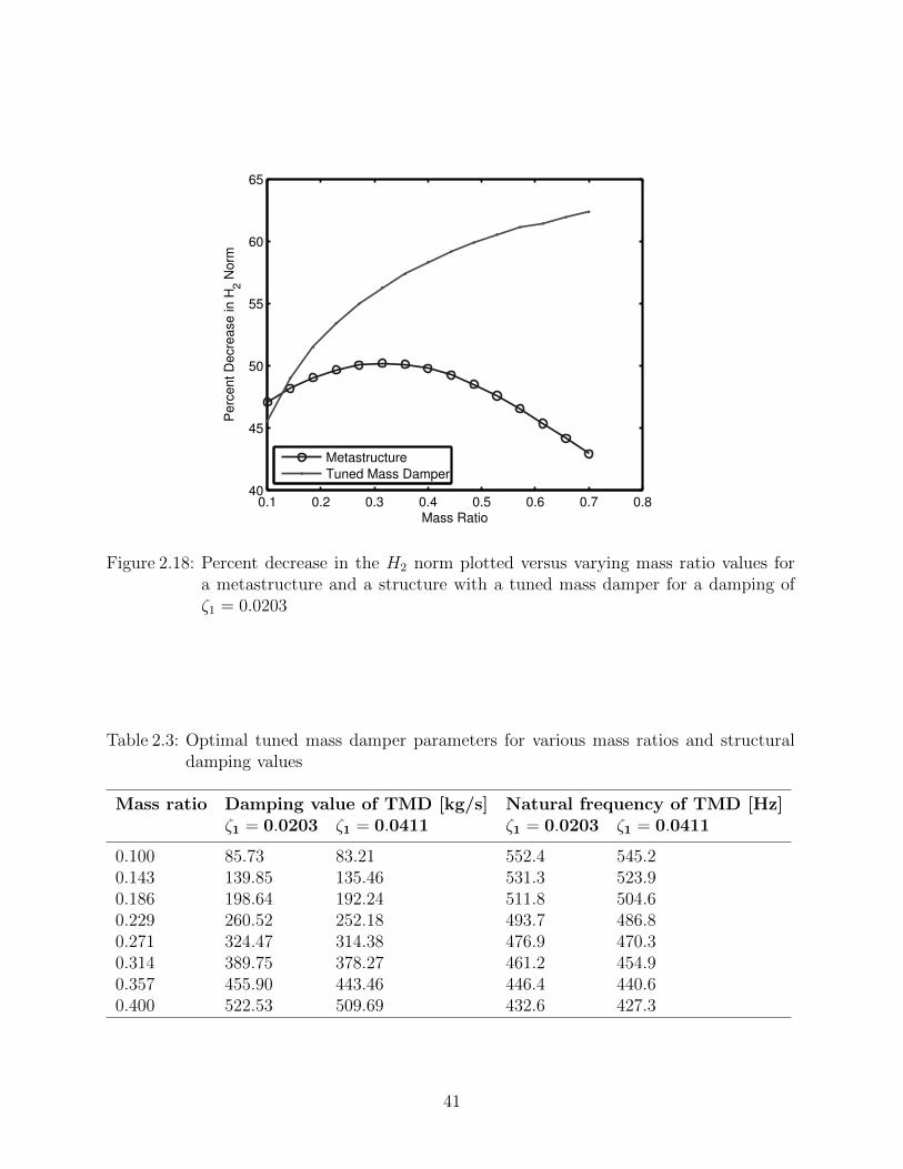
0.1 0.2 0.3 0.4 0.5 0.6 0.7 0.840
45
50
55
60
65
Mass Ratio
Perc
ent D
ecre
ase in H
2 N
orm
Metastructure
Tuned Mass Damper
Figure 2.18: Percent decrease in the H2 norm plotted versus varying mass ratio values fora metastructure and a structure with a tuned mass damper for a damping ofζ1 = 0.0203
Table 2.3: Optimal tuned mass damper parameters for various mass ratios and structuraldamping values
Mass ratio Damping value of TMD [kg/s] Natural frequency of TMD [Hz]ζ1 = 0.0203 ζ1 = 0.0411 ζ1 = 0.0203 ζ1 = 0.0411
0.100 85.73 83.21 552.4 545.20.143 139.85 135.46 531.3 523.90.186 198.64 192.24 511.8 504.60.229 260.52 252.18 493.7 486.80.271 324.47 314.38 476.9 470.30.314 389.75 378.27 461.2 454.90.357 455.90 443.46 446.4 440.60.400 522.53 509.69 432.6 427.3
41
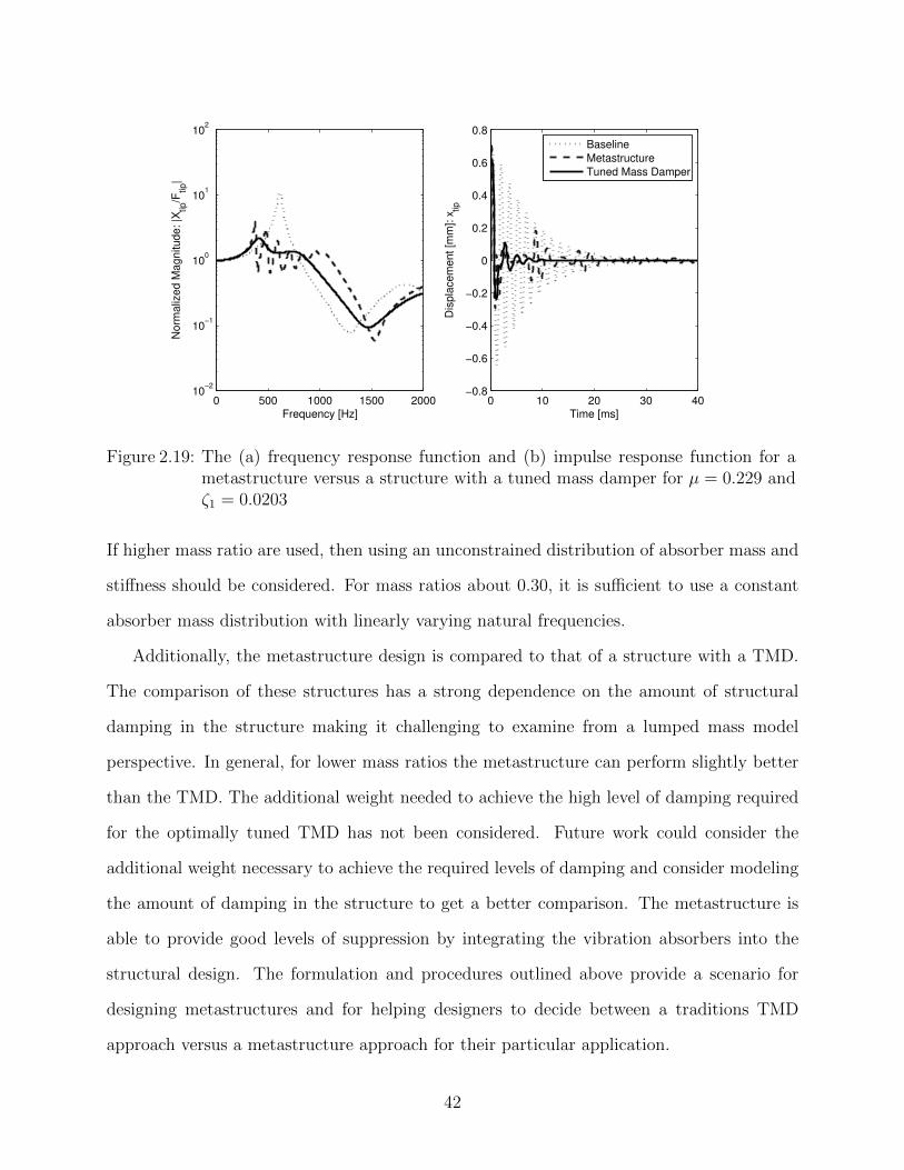
0 500 1000 1500 200010
−2
10−1
100
101
102
Frequency [Hz]
Norm
aliz
ed M
agnitude: |X
tip/F
tip|
0 10 20 30 40−0.8
−0.6
−0.4
−0.2
0
0.2
0.4
0.6
0.8
Time [ms]
Dis
pla
cem
ent [m
m]: x
tip
Baseline
Metastructure
Tuned Mass Damper
Figure 2.19: The (a) frequency response function and (b) impulse response function for ametastructure versus a structure with a tuned mass damper for µ = 0.229 andζ1 = 0.0203
If higher mass ratio are used, then using an unconstrained distribution of absorber mass and
stiffness should be considered. For mass ratios about 0.30, it is sufficient to use a constant
absorber mass distribution with linearly varying natural frequencies.
Additionally, the metastructure design is compared to that of a structure with a TMD.
The comparison of these structures has a strong dependence on the amount of structural
damping in the structure making it challenging to examine from a lumped mass model
perspective. In general, for lower mass ratios the metastructure can perform slightly better
than the TMD. The additional weight needed to achieve the high level of damping required
for the optimally tuned TMD has not been considered. Future work could consider the
additional weight necessary to achieve the required levels of damping and consider modeling
the amount of damping in the structure to get a better comparison. The metastructure is
able to provide good levels of suppression by integrating the vibration absorbers into the
structural design. The formulation and procedures outlined above provide a scenario for
designing metastructures and for helping designers to decide between a traditions TMD
approach versus a metastructure approach for their particular application.
42
CHAPTER III
Dynamic Characterization of 3D Printed Viscoelastic
Materials
This chapter characterizes the viscoelastic properties of materials printed using the Ob-
jet Connex 3D printer and presents a modeling method used to capture the effects of the
viscoelastic behavior. The 3D printer being explored is used in Chapter IV to create a
metastructure prototype. Metastructures tend to have complex geometry, thus are easily
manufactured on 3D printers. The most cost-effective and readily available 3D printers
today, use polymer resins to create the parts. Polymers materials are composed of long
molecular chains, which lead to energy dissipation during cyclic deformation. The energy
dissipation experienced by polymer materials can be modeled using a viscoelastic model [44].
This chapter begins by explaining the modeling procedure used the characterize the viscoelas-
tic material properties which involve the complex modulus and the temperature-frequency
equivalence. After these modeling methods are described, the characterization of the Objet
Connex materials is presented. The characterization is performed using a DMA machine
which can measure the complex modulus of the specimen. The complex modulus values are
found for various frequencies and temperatures. The temperature-frequency equivalence is
used to determine a relationship between those variables. The characterization is performed
on four out of ten of the materials that the 3D printer is capable of printing. For one of these
materials, the testing configuration and the print direction are explored. For the complex
43
modulus data to be used in a transient setting, the frequency dependence of the material
must be modeled. This work uses the GHM model, which utilizes an approximation for
the complex modulus versus frequency data. The GHM approximation is curve-fit to the
experimental data, and the resulting parameters are used to develop finite element mass,
damping and stiffness matrices for the viscoelastic materials. This allows the viscoelastic
material to be modeled in various dynamic applications. This chapter ends by using the
GHM model to examine the dynamic response of a simple bar and beam, specifically looking
at how a temperature change affects the response. For the simple beam case, these results
are experimentally verified.
3.1 Viscoelastic modeling
This section describes the modeling methods used in this work to model the viscoelastic
material behavior. In steady-state dynamic applications, the viscoelastic material behavior
can be described using the complex modulus model. The complex modulus of a viscoelastic
material varies with both frequency and temperature at which the specimen is excited. The
complex modulus data can be experimentally obtained using various methods which will be
described later. The temperature-frequency equivalence develops a relationship between the
frequency and temperature dependence of the complex modulus data, allowing the complex
modulus data to be represented at a wider range of frequencies and temperatures than those
obtained experimentally.
3.1.1 Complex modulus method
For dynamic applications, the most common method used to describe the dynamic re-
sponse of viscoelastic materials is to identify the response of the material subjected to a
sinusoidal load. When a harmonically varying stress is applied to an elastic material, the
strain response will have the same frequency and phase as the load. This is not the case
for a viscoelastic material; the response remains at the same frequency as the input but will
44
have a phase lag. When the following time-varying stress σ(t) is applied to a viscoelastic
material
σ(t) = σ0 sin(ωt)
ε(t) = ε0 sin(ωt− δ)(3.1)
where ω is the frequency of the forcing function, ε(t) is the strain-response of the material
and the phase lag is denoted as δ the dynamic modulus can be expressed as the following
complex number
G?(ω, T ) =σ(t)
ε(t)= G′ + G′′ (3.2)
where G? is the complex modulus, also referred to as the dynamic modulus. Because of
the phase lag, the modulus is a complex number and can be decomposed into its real and
imaginary components, where G′ is the storage modulus and G′′ is the loss modulus. The
complex modulus can also be expressed by factoring out the storage modulus
G?(ω, T ) = G′[1 + η] (3.3)
where η is the loss factor. The modulus values vary with both frequency and temperature
[44]. This relationship can also be expressed in the Laplace domain as
σ(s) = sG(s)ε(s) (3.4)
where the tilde represents the Laplace transform of the variable and the function sG(s) is
called the material dissipation function. When evaluated along the imaginary axis (s = ω)
the material dissipation function is equivalent to the complex modulus representation in
Equation 3.2.
45
3.1.2 Temperature-frequency equivalence
Using the temperature-frequency equivalence, a relationship between the frequency and
temperature can be determined to reduce the number of the variables necessary to describe
the response of the material. We can assume that the complex modulus value at a fre-
quency, f1 and a temperature, T1 is equal to the value at any other frequency f2 and some
temperature, T2 such that the following relationship can be made
G?(f1, T1) = G?(f2 · α(T2)) (3.5)
where α(T2) is the shift factor and describes the relationship between frequency and
temperature. Using the shift factor, the effects of both temperature and frequency can be
combined into a single variable called the reduced frequency, fr(f, T ) = f · α(T ). The shift
factor relationship is determined by testing a material at multiple frequencies and temper-
atures. For each temperature, a shift factor value is determined graphically by examining
the modulus versus reduced frequency plots. Varying the shift factor causes the data at a
specific temperature to shift on the reduced frequency scale. Once the shift factors for each
temperature are determined, the log[α(T )] is plotted versus 1/T . This relationship resem-
bles a slightly curved line, which is approximated by a straight line using the Arrhenius shift
factor equation and takes on the following form
log[α(T )] = TA ·(
1
T− 1
T0
)(3.6)
where T0 is an arbitrarily selected reference temperature, and TA is related to the activa-
tion energy and is represented by the slope of the line. Using this relationship, the storage
modulus and loss factor can be expressed as
G′(f, T ) = G′(f · exp
[−2.303TA
T
]· exp
[−2.303TA
T0
])(3.7a)
46
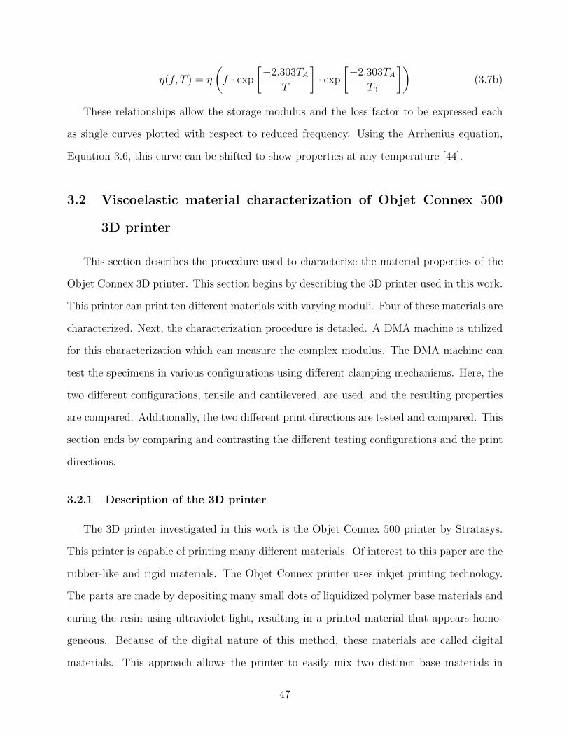
η(f, T ) = η
(f · exp
[−2.303TA
T
]· exp
[−2.303TA
T0
])(3.7b)
These relationships allow the storage modulus and the loss factor to be expressed each
as single curves plotted with respect to reduced frequency. Using the Arrhenius equation,
Equation 3.6, this curve can be shifted to show properties at any temperature [44].
3.2 Viscoelastic material characterization of Objet Connex 500
3D printer
This section describes the procedure used to characterize the material properties of the
Objet Connex 3D printer. This section begins by describing the 3D printer used in this work.
This printer can print ten different materials with varying moduli. Four of these materials are
characterized. Next, the characterization procedure is detailed. A DMA machine is utilized
for this characterization which can measure the complex modulus. The DMA machine can
test the specimens in various configurations using different clamping mechanisms. Here, the
two different configurations, tensile and cantilevered, are used, and the resulting properties
are compared. Additionally, the two different print directions are tested and compared. This
section ends by comparing and contrasting the different testing configurations and the print
directions.
3.2.1 Description of the 3D printer
The 3D printer investigated in this work is the Objet Connex 500 printer by Stratasys.
This printer is capable of printing many different materials. Of interest to this paper are the
rubber-like and rigid materials. The Objet Connex printer uses inkjet printing technology.
The parts are made by depositing many small dots of liquidized polymer base materials and
curing the resin using ultraviolet light, resulting in a printed material that appears homo-
geneous. Because of the digital nature of this method, these materials are called digital
materials. This approach allows the printer to easily mix two distinct base materials in
47
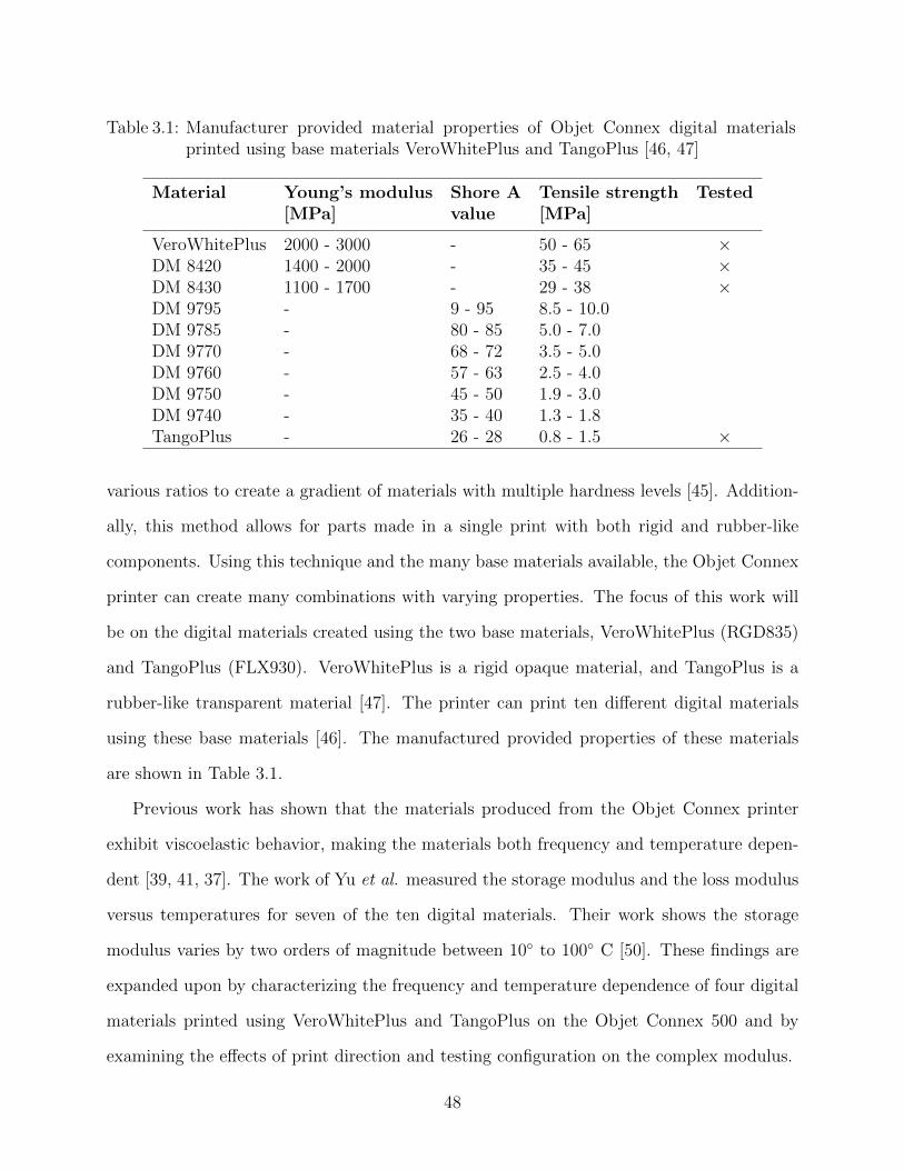
Table 3.1: Manufacturer provided material properties of Objet Connex digital materialsprinted using base materials VeroWhitePlus and TangoPlus [46, 47]
Material Young’s modulus Shore A Tensile strength Tested[MPa] value [MPa]
VeroWhitePlus 2000 - 3000 - 50 - 65 ×DM 8420 1400 - 2000 - 35 - 45 ×DM 8430 1100 - 1700 - 29 - 38 ×DM 9795 - 9 - 95 8.5 - 10.0DM 9785 - 80 - 85 5.0 - 7.0DM 9770 - 68 - 72 3.5 - 5.0DM 9760 - 57 - 63 2.5 - 4.0DM 9750 - 45 - 50 1.9 - 3.0DM 9740 - 35 - 40 1.3 - 1.8TangoPlus - 26 - 28 0.8 - 1.5 ×
various ratios to create a gradient of materials with multiple hardness levels [45]. Addition-
ally, this method allows for parts made in a single print with both rigid and rubber-like
components. Using this technique and the many base materials available, the Objet Connex
printer can create many combinations with varying properties. The focus of this work will
be on the digital materials created using the two base materials, VeroWhitePlus (RGD835)
and TangoPlus (FLX930). VeroWhitePlus is a rigid opaque material, and TangoPlus is a
rubber-like transparent material [47]. The printer can print ten different digital materials
using these base materials [46]. The manufactured provided properties of these materials
are shown in Table 3.1.
Previous work has shown that the materials produced from the Objet Connex printer
exhibit viscoelastic behavior, making the materials both frequency and temperature depen-
dent [39, 41, 37]. The work of Yu et al. measured the storage modulus and the loss modulus
versus temperatures for seven of the ten digital materials. Their work shows the storage
modulus varies by two orders of magnitude between 10 to 100 C [50]. These findings are
expanded upon by characterizing the frequency and temperature dependence of four digital
materials printed using VeroWhitePlus and TangoPlus on the Objet Connex 500 and by
examining the effects of print direction and testing configuration on the complex modulus.
48
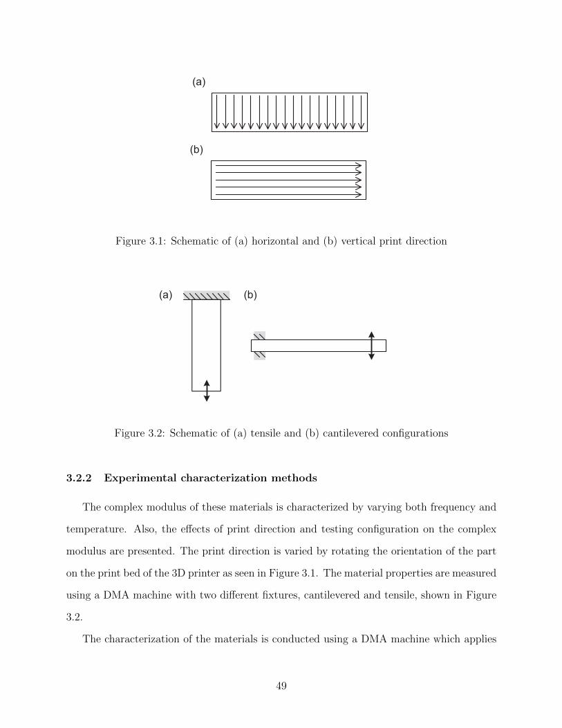
(a)
(b)
Figure 3.1: Schematic of (a) horizontal and (b) vertical print direction
(a) (b)
Figure 3.2: Schematic of (a) tensile and (b) cantilevered configurations
3.2.2 Experimental characterization methods
The complex modulus of these materials is characterized by varying both frequency and
temperature. Also, the effects of print direction and testing configuration on the complex
modulus are presented. The print direction is varied by rotating the orientation of the part
on the print bed of the 3D printer as seen in Figure 3.1. The material properties are measured
using a DMA machine with two different fixtures, cantilevered and tensile, shown in Figure
3.2.
The characterization of the materials is conducted using a DMA machine which applies
49
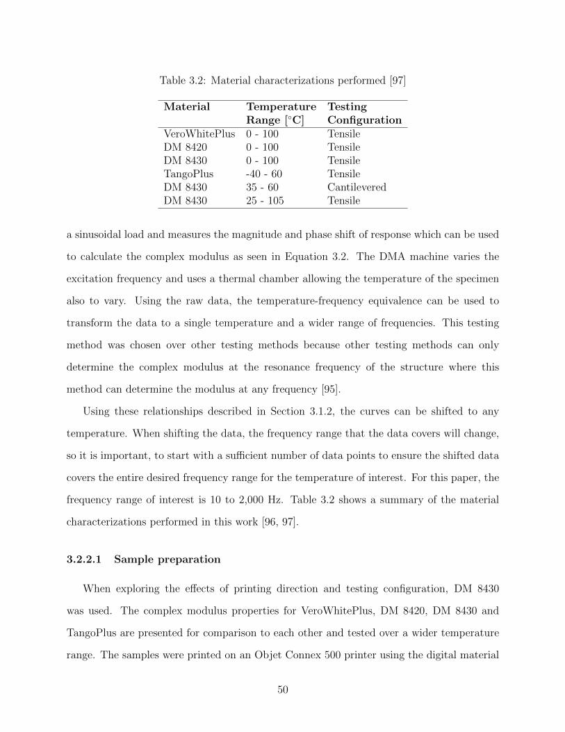
Table 3.2: Material characterizations performed [97]
Material Temperature TestingRange [C] Configuration
VeroWhitePlus 0 - 100 TensileDM 8420 0 - 100 TensileDM 8430 0 - 100 TensileTangoPlus -40 - 60 TensileDM 8430 35 - 60 CantileveredDM 8430 25 - 105 Tensile
a sinusoidal load and measures the magnitude and phase shift of response which can be used
to calculate the complex modulus as seen in Equation 3.2. The DMA machine varies the
excitation frequency and uses a thermal chamber allowing the temperature of the specimen
also to vary. Using the raw data, the temperature-frequency equivalence can be used to
transform the data to a single temperature and a wider range of frequencies. This testing
method was chosen over other testing methods because other testing methods can only
determine the complex modulus at the resonance frequency of the structure where this
method can determine the modulus at any frequency [95].
Using these relationships described in Section 3.1.2, the curves can be shifted to any
temperature. When shifting the data, the frequency range that the data covers will change,
so it is important, to start with a sufficient number of data points to ensure the shifted data
covers the entire desired frequency range for the temperature of interest. For this paper, the
frequency range of interest is 10 to 2,000 Hz. Table 3.2 shows a summary of the material
characterizations performed in this work [96, 97].
3.2.2.1 Sample preparation
When exploring the effects of printing direction and testing configuration, DM 8430
was used. The complex modulus properties for VeroWhitePlus, DM 8420, DM 8430 and
TangoPlus are presented for comparison to each other and tested over a wider temperature
range. The samples were printed on an Objet Connex 500 printer using the digital material
50
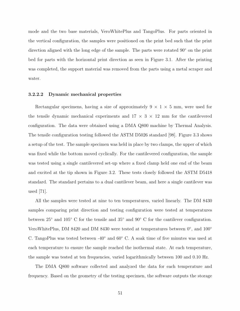
mode and the two base materials, VeroWhitePlus and TangoPlus. For parts oriented in
the vertical configuration, the samples were positioned on the print bed such that the print
direction aligned with the long edge of the sample. The parts were rotated 90 on the print
bed for parts with the horizontal print direction as seen in Figure 3.1. After the printing
was completed, the support material was removed from the parts using a metal scraper and
water.
3.2.2.2 Dynamic mechanical properties
Rectangular specimens, having a size of approximately 9 × 1 × 5 mm, were used for
the tensile dynamic mechanical experiments and 17 × 3 × 12 mm for the cantilevered
configuration. The data were obtained using a DMA Q800 machine by Thermal Analysis.
The tensile configuration testing followed the ASTM D5026 standard [98]. Figure 3.3 shows
a setup of the test. The sample specimen was held in place by two clamps, the upper of which
was fixed while the bottom moved cyclically. For the cantilevered configuration, the sample
was tested using a single cantilevered set-up where a fixed clamp held one end of the beam
and excited at the tip shown in Figure 3.2. These tests closely followed the ASTM D5418
standard. The standard pertains to a dual cantilever beam, and here a single cantilever was
used [71].
All the samples were tested at nine to ten temperatures, varied linearly. The DM 8430
samples comparing print direction and testing configuration were tested at temperatures
between 25 and 105 C for the tensile and 35 and 90 C for the cantilever configuration.
VeroWhitePlus, DM 8420 and DM 8430 were tested at temperatures between 0, and 100
C. TangoPlus was tested between -40 and 60 C. A soak time of five minutes was used at
each temperature to ensure the sample reached the isothermal state. At each temperature,
the sample was tested at ten frequencies, varied logarithmically between 100 and 0.10 Hz.
The DMA Q800 software collected and analyzed the data for each temperature and
frequency. Based on the geometry of the testing specimen, the software outputs the storage
51
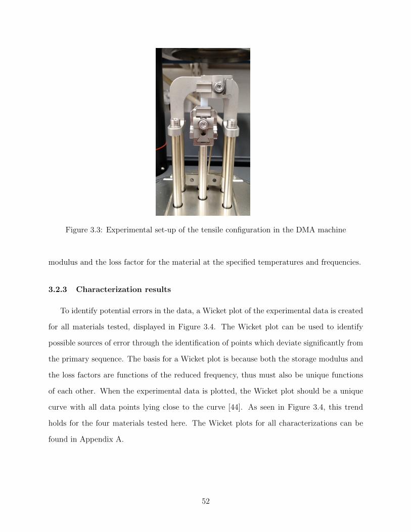
Figure 3.3: Experimental set-up of the tensile configuration in the DMA machine
modulus and the loss factor for the material at the specified temperatures and frequencies.
3.2.3 Characterization results
To identify potential errors in the data, a Wicket plot of the experimental data is created
for all materials tested, displayed in Figure 3.4. The Wicket plot can be used to identify
possible sources of error through the identification of points which deviate significantly from
the primary sequence. The basis for a Wicket plot is because both the storage modulus and
the loss factors are functions of the reduced frequency, thus must also be unique functions
of each other. When the experimental data is plotted, the Wicket plot should be a unique
curve with all data points lying close to the curve [44]. As seen in Figure 3.4, this trend
holds for the four materials tested here. The Wicket plots for all characterizations can be
found in Appendix A.
52
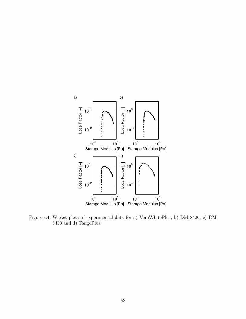
105
1010
10−2
100
Storage Modulus [Pa]
Loss F
acto
r [−
]
105
1010
10−2
100
Storage Modulus [Pa]
Loss F
acto
r [−
]
105
1010
10−2
100
Storage Modulus [Pa]
Loss F
acto
r [−
]
105
1010
10−2
100
Storage Modulus [Pa]
Loss F
acto
r [−
]
a) b)
c) d)
Figure 3.4: Wicket plots of experimental data for a) VeroWhitePlus, b) DM 8420, c) DM8430 and d) TangoPlus
53
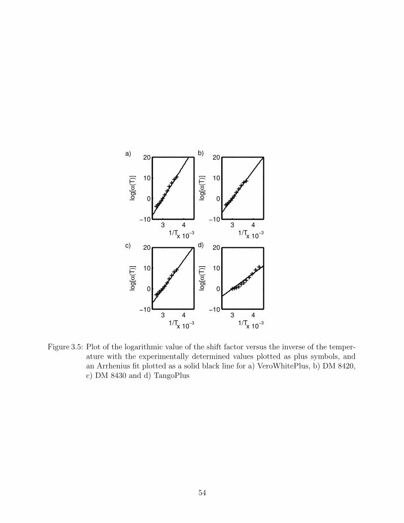
3 4
x 10−3
−10
0
10
20
1/T
log[α
(T)]
3 4
x 10−3
−10
0
10
20
1/T
log[α
(T)]
3 4
x 10−3
−10
0
10
20
1/T
log[α
(T)]
3 4
x 10−3
−10
0
10
20
1/T
log[α
(T)]
a) b)
c) d)
Figure 3.5: Plot of the logarithmic value of the shift factor versus the inverse of the temper-ature with the experimentally determined values plotted as plus symbols, andan Arrhenius fit plotted as a solid black line for a) VeroWhitePlus, b) DM 8420,c) DM 8430 and d) TangoPlus
54
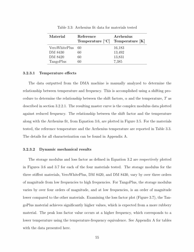
Table 3.3: Arrhenius fit data for materials tested
Material Reference ArrheniusTemperature [C] Temperature [K]
VeroWhitePlus 60 16,183DM 8430 60 13,492DM 8420 60 13,831TangoPlus 60 7,385
3.2.3.1 Temperature effects
The data outputted from the DMA machine is manually analyzed to determine the
relationship between temperature and frequency. This is accomplished using a shifting pro-
cedure to determine the relationship between the shift factors, α and the temperature, T as
described in section 3.2.2.1. The resulting master curve is the complex modulus data plotted
against reduced frequency. The relationship between the shift factor and the temperature
along with the Arrhenius fit, from Equation 3.6, are plotted in Figure 3.5. For the materials
tested, the reference temperature and the Arrhenius temperature are reported in Table 3.3.
The details for all characterization can be found in Appendix A.
3.2.3.2 Dynamic mechanical results
The storage modulus and loss factor as defined in Equation 3.2 are respectively plotted
in Figures 3.6 and 3.7 for each of the four materials tested. The storage modulus for the
three stiffest materials, VeroWhitePlus, DM 8420, and DM 8430, vary by over three orders
of magnitude from low frequencies to high frequencies. For TangoPlus, the storage modulus
varies by over four orders of magnitude, and at low frequencies, is an order of magnitude
lower compared to the other materials. Examining the loss factor plot (Figure 3.7), the Tan-
goPlus material achieves significantly higher values, which is expected from a more rubbery
material. The peak loss factor value occurs at a higher frequency, which corresponds to a
lower temperature using the temperature-frequency equivalence. See Appendix A for tables
with the data presented here.
55
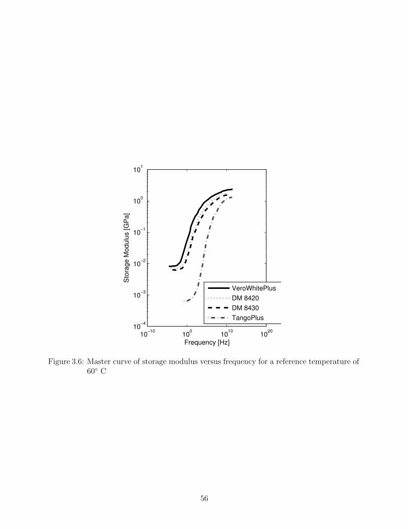
10−10
100
1010
1020
10−4
10−3
10−2
10−1
100
101
Frequency [Hz]
Sto
rage M
odulu
s [G
Pa]
VeroWhitePlus
DM 8420
DM 8430
TangoPlus
Figure 3.6: Master curve of storage modulus versus frequency for a reference temperature of60 C
56
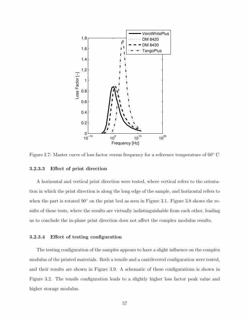
10−10
100
1010
1020
0
0.2
0.4
0.6
0.8
1
1.2
1.4
1.6
1.8
Frequency [Hz]
Loss F
acto
r [−
]
VeroWhitePlus
DM 8420
DM 8430
TangoPlus
Figure 3.7: Master curve of loss factor versus frequency for a reference temperature of 60 C
3.2.3.3 Effect of print direction
A horizontal and vertical print direction were tested, where vertical refers to the orienta-
tion in which the print direction is along the long edge of the sample, and horizontal refers to
when the part is rotated 90 on the print bed as seen in Figure 3.1. Figure 3.8 shows the re-
sults of these tests, where the results are virtually indistinguishable from each other, leading
us to conclude the in-plane print direction does not affect the complex modulus results.
3.2.3.4 Effect of testing configuration
The testing configuration of the samples appears to have a slight influence on the complex
modulus of the printed materials. Both a tensile and a cantilevered configuration were tested,
and their results are shown in Figure 3.9. A schematic of these configurations is shown in
Figure 3.2. The tensile configuration leads to a slightly higher loss factor peak value and
higher storage modulus.
57
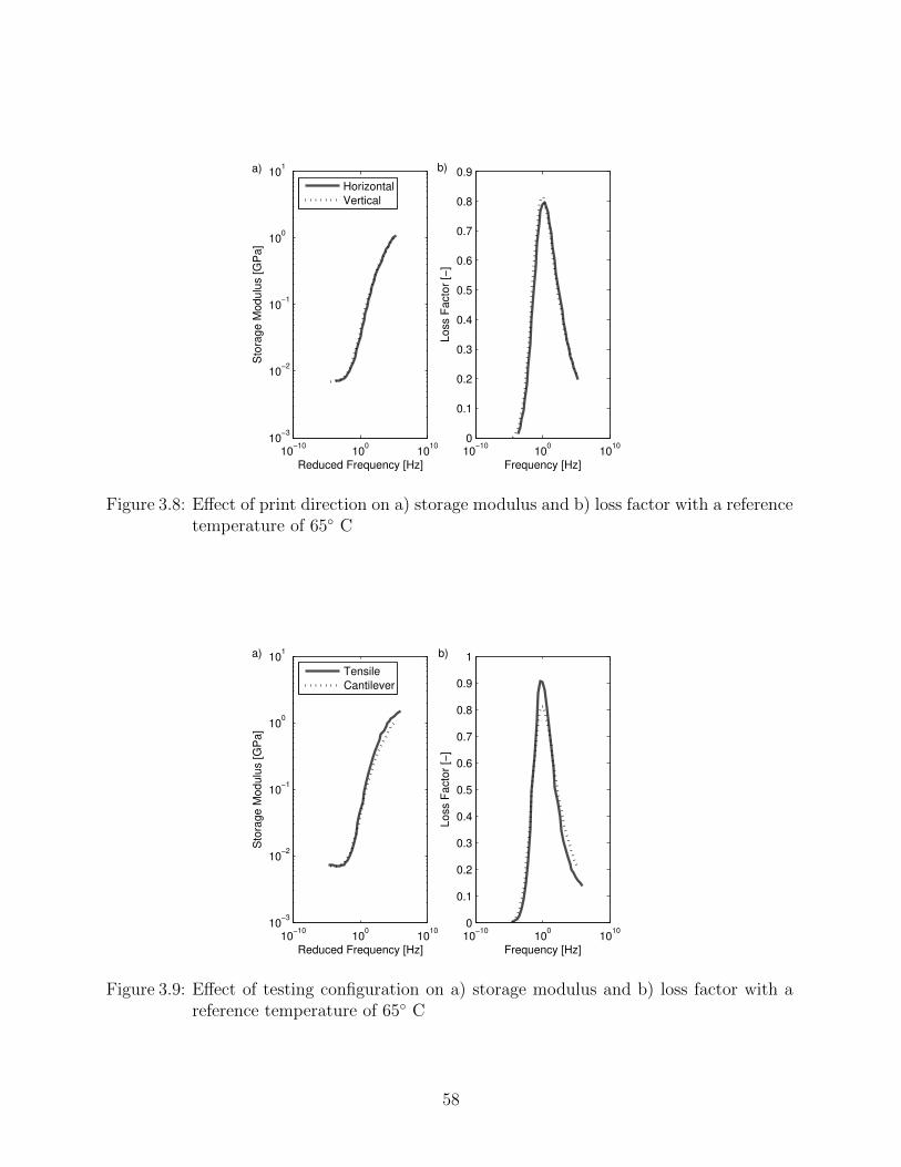
10−10
100
1010
10−3
10−2
10−1
100
101
Reduced Frequency [Hz]
Sto
rage M
odulu
s [G
Pa]
a)
10−10
100
1010
0
0.1
0.2
0.3
0.4
0.5
0.6
0.7
0.8
0.9
Frequency [Hz]
Loss F
acto
r [−
]
b)
Horizontal
Vertical
Figure 3.8: Effect of print direction on a) storage modulus and b) loss factor with a referencetemperature of 65 C
10−10
100
1010
10−3
10−2
10−1
100
101
Reduced Frequency [Hz]
Sto
rage M
odulu
s [G
Pa]
a)
10−10
100
1010
0
0.1
0.2
0.3
0.4
0.5
0.6
0.7
0.8
0.9
1
Frequency [Hz]
Loss F
acto
r [−
]
b)
Tensile
Cantilever
Figure 3.9: Effect of testing configuration on a) storage modulus and b) loss factor with areference temperature of 65 C
58
3.2.4 Summary of characterization
The complex modulus properties of the inkjet printed material from the Objet Connex
printer have been determined. These materials show viscoelastic effects, which should be
considered when modeling these materials for use in vibration applications, particularly
in situations where there are significant temperature changes. Although all materials show
viscoelastic effects, the TangoPlus material exhibits greater variations in the storage modulus
and loss factor than the VeroWhitePlus, DM 8430, and DM 8420. The master curves from
Figures 3.6 and 3.7 can be used to curve fit viscoelastic models to the experimental data
and can also be used for design purposes. Additionally, the effects of testing configuration
and print direction were also investigated. The results show that variations in the in-plane
print direction do not affect the response of the material for both the tensile and cantilevered
configurations. The testing configuration does have a slight effect on the complex modulus
values.
3.3 Frequency-dependent modeling of viscoelastic materials
The complex modulus model can be used to model steady-state applications but for
situations in which the frequency in varying, the frequency dependence of the modulus values
must be accounted for. Three common models are used in the field of vibration suppression
to account the frequency variation and are shown in Table 3.4 [66, 68]. These models are
characterized by the form of the equation used to represent the complex modulus data. The
fractional derivative model developed by Bagley and Torvik uses a derivative of fractional
order and is advantageous because five parameters are sufficient to represent the frequency-
dependent behavior over a broad range of frequencies [59, 60]. The anelastic displacement
fields model was developed by Lesieutre and his coworkers [99, 61, 100]. This model looks at
elastic and the anelastic parts and represents the anelastic part by a first order differential
equation. This model is formulated directly in the time-domain. The model that will be
59
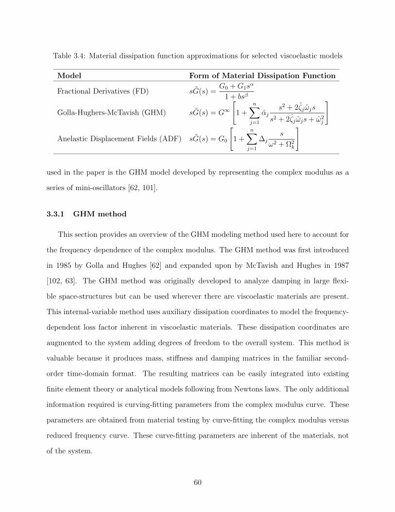
Table 3.4: Material dissipation function approximations for selected viscoelastic models
Model Form of Material Dissipation Function
Fractional Derivatives (FD) sG(s) =G0 +G1s
α
1 + bsβ
Golla-Hughers-McTavish (GHM) sG(s) = G∞
[1 +
n∑j=1
αjs2 + 2ζjωjs
s2 + 2ζjωjs+ ω2j
]
Anelastic Displacement Fields (ADF) sG(s) = G0
[1 +
n∑j=1
∆js
ω2 + Ω2k
]
used in the paper is the GHM model developed by representing the complex modulus as a
series of mini-oscillators [62, 101].
3.3.1 GHM method
This section provides an overview of the GHM modeling method used here to account for
the frequency dependence of the complex modulus. The GHM method was first introduced
in 1985 by Golla and Hughes [62] and expanded upon by McTavish and Hughes in 1987
[102, 63]. The GHM method was originally developed to analyze damping in large flexi-
ble space-structures but can be used wherever there are viscoelastic materials are present.
This internal-variable method uses auxiliary dissipation coordinates to model the frequency-
dependent loss factor inherent in viscoelastic materials. These dissipation coordinates are
augmented to the system adding degrees of freedom to the overall system. This method is
valuable because it produces mass, stiffness and damping matrices in the familiar second-
order time-domain format. The resulting matrices can be easily integrated into existing
finite element theory or analytical models following from Newtons laws. The only additional
information required is curving-fitting parameters from the complex modulus curve. These
parameters are obtained from material testing by curve-fitting the complex modulus versus
reduced frequency curve. These curve-fitting parameters are inherent of the materials, not
of the system.
60
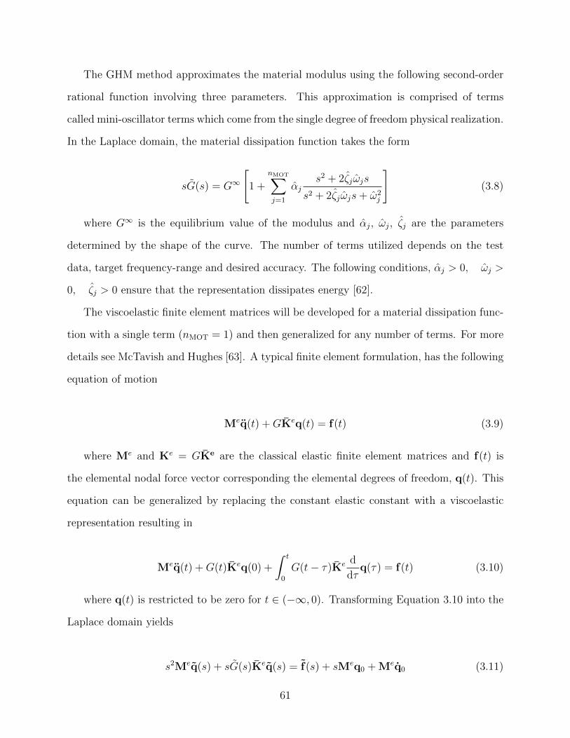
The GHM method approximates the material modulus using the following second-order
rational function involving three parameters. This approximation is comprised of terms
called mini-oscillator terms which come from the single degree of freedom physical realization.
In the Laplace domain, the material dissipation function takes the form
sG(s) = G∞
[1 +
nMOT∑j=1
αjs2 + 2ζjωjs
s2 + 2ζjωjs+ ω2j
](3.8)
where G∞ is the equilibrium value of the modulus and αj, ωj, ζj are the parameters
determined by the shape of the curve. The number of terms utilized depends on the test
data, target frequency-range and desired accuracy. The following conditions, αj > 0, ωj >
0, ζj > 0 ensure that the representation dissipates energy [62].
The viscoelastic finite element matrices will be developed for a material dissipation func-
tion with a single term (nMOT = 1) and then generalized for any number of terms. For more
details see McTavish and Hughes [63]. A typical finite element formulation, has the following
equation of motion
Meq(t) +GKeq(t) = f(t) (3.9)
where Me and Ke = GKe are the classical elastic finite element matrices and f(t) is
the elemental nodal force vector corresponding the elemental degrees of freedom, q(t). This
equation can be generalized by replacing the constant elastic constant with a viscoelastic
representation resulting in
Meq(t) +G(t)Keq(0) +
∫ t
0
G(t− τ)Ke d
dτq(τ) = f(t) (3.10)
where q(t) is restricted to be zero for t ∈ (−∞, 0). Transforming Equation 3.10 into the
Laplace domain yields
s2Meq(s) + sG(s)Keq(s) = f(s) + sMeq0 + Meq0 (3.11)
61
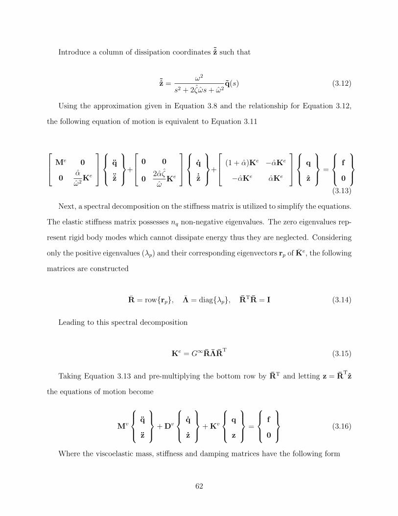
Introduce a column of dissipation coordinates ˜z such that
˜z =ω2
s2 + 2ζωs+ ω2q(s) (3.12)
Using the approximation given in Equation 3.8 and the relationship for Equation 3.12,
the following equation of motion is equivalent to Equation 3.11
Me 0
0α
ω2Ke
q
¨z
+
0 0
02αζ
ωKe
q
˙z
+
(1 + α)Ke −αKe
−αKe αKe
q
z
=
f
0
(3.13)
Next, a spectral decomposition on the stiffness matrix is utilized to simplify the equations.
The elastic stiffness matrix possesses nq non-negative eigenvalues. The zero eigenvalues rep-
resent rigid body modes which cannot dissipate energy thus they are neglected. Considering
only the positive eigenvalues (λp) and their corresponding eigenvectors rp of Ke, the following
matrices are constructed
R = rowrp, Λ = diagλp, RTR = I (3.14)
Leading to this spectral decomposition
Ke = G∞RΛRT
(3.15)
Taking Equation 3.13 and pre-multiplying the bottom row by RT and letting z = RTz
the equations of motion become
Mv
q
z
+ Dv
q
z
+ Kv
q
z
=
f
0
(3.16)
Where the viscoelastic mass, stiffness and damping matrices have the following form
62
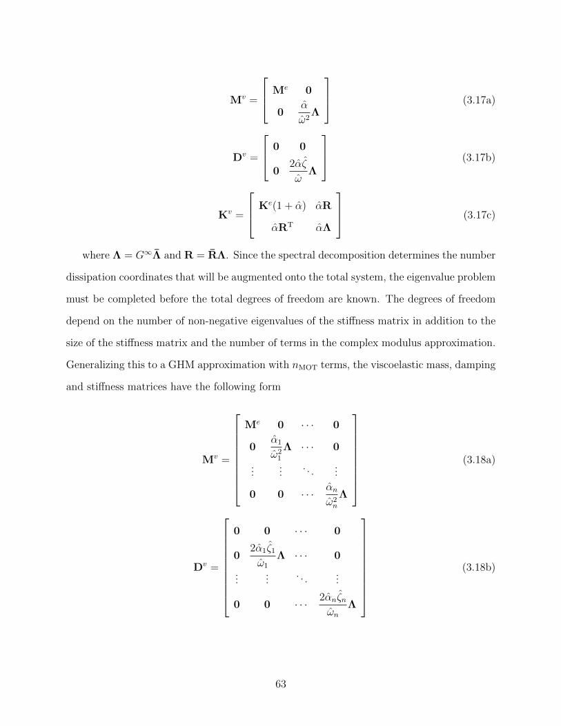
Mv =
Me 0
0α
ω2Λ
(3.17a)
Dv =
0 0
02αζ
ωΛ
(3.17b)
Kv =
Ke(1 + α) αR
αRT αΛ
(3.17c)
where Λ = G∞Λ and R = RΛ. Since the spectral decomposition determines the number
dissipation coordinates that will be augmented onto the total system, the eigenvalue problem
must be completed before the total degrees of freedom are known. The degrees of freedom
depend on the number of non-negative eigenvalues of the stiffness matrix in addition to the
size of the stiffness matrix and the number of terms in the complex modulus approximation.
Generalizing this to a GHM approximation with nMOT terms, the viscoelastic mass, damping
and stiffness matrices have the following form
Mv =
Me 0 · · · 0
0α1
ω21
Λ · · · 0
......
. . ....
0 0 · · · αnω2n
Λ
(3.18a)
Dv =
0 0 · · · 0
02α1ζ1ω1
Λ · · · 0
......
. . ....
0 0 · · · 2αnζnωn
Λ
(3.18b)
63
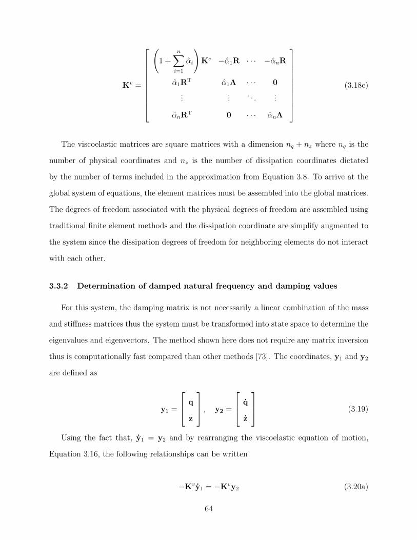
Kv =
(1 +
n∑i=1
αi
)Ke −α1R · · · −αnR
α1RT α1Λ · · · 0
......
. . ....
αnRT 0 · · · αnΛ
(3.18c)
The viscoelastic matrices are square matrices with a dimension nq + nz where nq is the
number of physical coordinates and nz is the number of dissipation coordinates dictated
by the number of terms included in the approximation from Equation 3.8. To arrive at the
global system of equations, the element matrices must be assembled into the global matrices.
The degrees of freedom associated with the physical degrees of freedom are assembled using
traditional finite element methods and the dissipation coordinate are simplify augmented to
the system since the dissipation degrees of freedom for neighboring elements do not interact
with each other.
3.3.2 Determination of damped natural frequency and damping values
For this system, the damping matrix is not necessarily a linear combination of the mass
and stiffness matrices thus the system must be transformed into state space to determine the
eigenvalues and eigenvectors. The method shown here does not require any matrix inversion
thus is computationally fast compared than other methods [73]. The coordinates, y1 and y2
are defined as
y1 =
q
z
, y2 =
q
z
(3.19)
Using the fact that, y1 = y2 and by rearranging the viscoelastic equation of motion,
Equation 3.16, the following relationships can be written
−Kvy1 = −Kvy2 (3.20a)
64
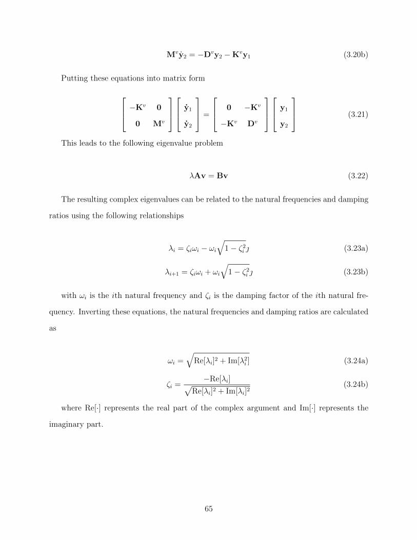
Mvy2 = −Dvy2 −Kvy1 (3.20b)
Putting these equations into matrix form
−Kv 0
0 Mv
y1
y2
=
0 −Kv
−Kv Dv
y1
y2
(3.21)
This leads to the following eigenvalue problem
λAv = Bv (3.22)
The resulting complex eigenvalues can be related to the natural frequencies and damping
ratios using the following relationships
λi = ζiωi − ωi√
1− ζ2i (3.23a)
λi+1 = ζiωi + ωi
√1− ζ2i (3.23b)
with ωi is the ith natural frequency and ζi is the damping factor of the ith natural fre-
quency. Inverting these equations, the natural frequencies and damping ratios are calculated
as
ωi =√
Re[λi]2 + Im[λ2i ] (3.24a)
ζi =−Re[λi]√
Re[λi]2 + Im[λi]2(3.24b)
where Re[·] represents the real part of the complex argument and Im[·] represents the
imaginary part.
65
3.3.3 Determining the GHM parameters
To use the GHM model, the form of Equation 3.8, evaluated along the imaginary axis
(s = ω) must be curve-fit to the complex modulus data from the 3D printed materials.
The curve fit is performed in a logarithmic sense with equal weighting given to the real
and imaginary parts. The number of terms necessary to obtain a good fit of the GHM
approximation depends on the material, the frequency range, and the desired accuracy. In
this paper, the frequency range of interest is 10 to 2,000 Hz. Depending on the shape of the
curve at the temperature and frequency of interest dictates the number of GHM parameters
used. For a complete data table of the GHM parameters for all materials tested, see Appendix
B.
The DM 8430 tensile configuration data tested from 0 to 100 C, is shifted to various
temperatures and a curve fit is performed on the resulting curves. The GHM fits are plotted
over the frequency range of interest for temperatures ranging from 20 to 100 C in Figure
3.10. This figure shows the significant variation resulting from changes in temperature in
both the storage modulus and the loss factor.
3.4 Dynamic response of structure made from viscoelastic mate-
rials
This section utilizes the GHM model described in the previous section and applies the
model to specific structures to study the effect of the viscoelastic properties on the dynamic
response of the structure, including the effects of changing the temperature. Additionally,
the differences in the dynamic response due to the two testing configurations, tensile and
cantilever described above will be explored. Lastly, an experimental prototype of a beam
undergoing temperature change is used to validate the experimental characterization.
66
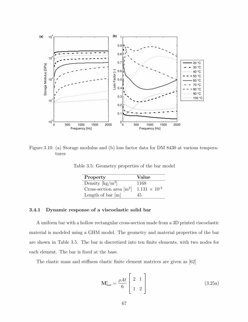
0 500 1000 1500 200010
0
101
102
103
104
Frequency [Hz]
Sto
rage M
odulu
s [G
Pa]
0 500 1000 1500 20000
0.1
0.2
0.3
0.4
0.5
0.6
0.7
0.8
0.9
1
Frequency [Hz]
Loss F
acto
r [−
]
20 °C
30 °C
40 °C
50 °C
60 °C
70 °C
80 °C
90 °C
100 °C
(b)(a)
Figure 3.10: (a) Storage modulus and (b) loss factor data for DM 8430 at various tempera-tures
Table 3.5: Geometry properties of the bar model
Property ValueDensity [kg/m3] 1168Cross-section area [m2] 1.131 × 10⁻³
Length of bar [m] 45
3.4.1 Dynamic response of a viscoelastic solid bar
A uniform bar with a hollow rectangular cross-section made from a 3D printed viscoelastic
material is modeled using a GHM model. The geometry and material properties of the bar
are shown in Table 3.5. The bar is discretized into ten finite elements, with two nodes for
each element. The bar is fixed at the base.
The elastic mass and stiffness elastic finite element matrices are given as [62]
Mebar =
ρA`
6
2 1
1 2
(3.25a)
67
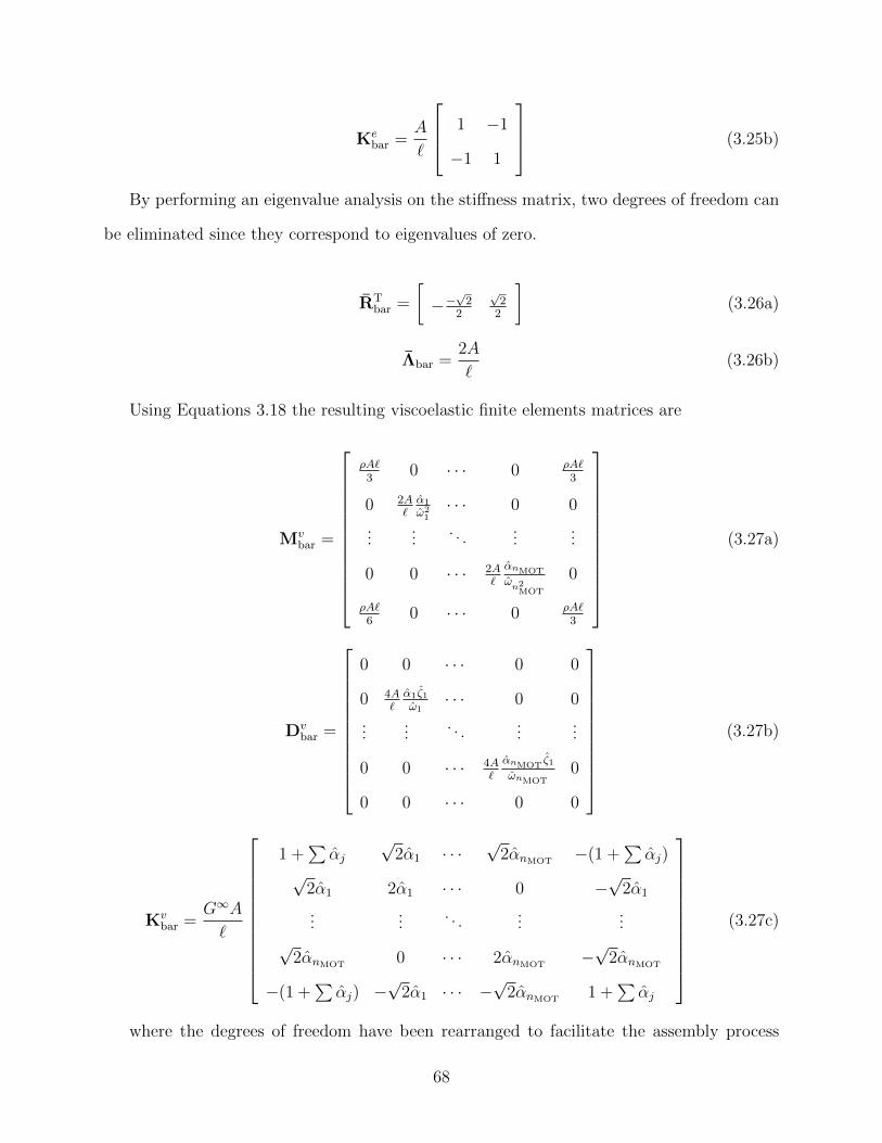
Kebar =
A
`
1 −1
−1 1
(3.25b)
By performing an eigenvalue analysis on the stiffness matrix, two degrees of freedom can
be eliminated since they correspond to eigenvalues of zero.
RTbar =
[−−
√2
2
√22
](3.26a)
Λbar =2A
`(3.26b)
Using Equations 3.18 the resulting viscoelastic finite elements matrices are
Mvbar =
ρA`3
0 · · · 0 ρA`3
0 2A`α1
ω21· · · 0 0
......
. . ....
...
0 0 · · · 2A`
αnMOT
ωn2MOT
0
ρA`6
0 · · · 0 ρA`3
(3.27a)
Dvbar =
0 0 · · · 0 0
0 4A`α1ζ1ω1
· · · 0 0
......
. . ....
...
0 0 · · · 4A`
αnMOTζ1
ωnMOT0
0 0 · · · 0 0
(3.27b)
Kvbar =
G∞A
`
1 +∑αj
√2α1 · · ·
√2αnMOT
−(1 +∑αj)
√2α1 2α1 · · · 0 −
√2α1
......
. . ....
...√
2αnMOT0 · · · 2αnMOT
−√
2αnMOT
−(1 +∑αj) −
√2α1 · · · −
√2αnMOT
1 +∑αj
(3.27c)
where the degrees of freedom have been rearranged to facilitate the assembly process
68
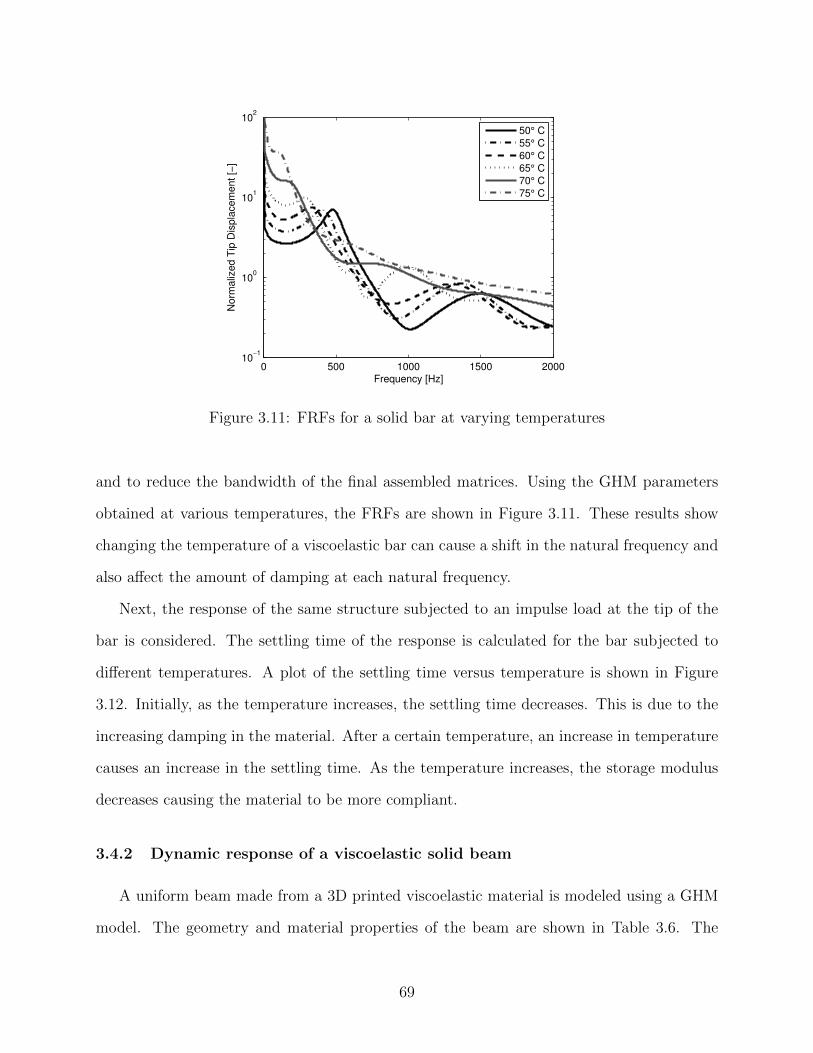
0 500 1000 1500 200010
−1
100
101
102
Frequency [Hz]
Norm
aliz
ed T
ip D
ispla
cem
ent [−
]
50° C
55° C
60° C
65° C
70° C
75° C
Figure 3.11: FRFs for a solid bar at varying temperatures
and to reduce the bandwidth of the final assembled matrices. Using the GHM parameters
obtained at various temperatures, the FRFs are shown in Figure 3.11. These results show
changing the temperature of a viscoelastic bar can cause a shift in the natural frequency and
also affect the amount of damping at each natural frequency.
Next, the response of the same structure subjected to an impulse load at the tip of the
bar is considered. The settling time of the response is calculated for the bar subjected to
different temperatures. A plot of the settling time versus temperature is shown in Figure
3.12. Initially, as the temperature increases, the settling time decreases. This is due to the
increasing damping in the material. After a certain temperature, an increase in temperature
causes an increase in the settling time. As the temperature increases, the storage modulus
decreases causing the material to be more compliant.
3.4.2 Dynamic response of a viscoelastic solid beam
A uniform beam made from a 3D printed viscoelastic material is modeled using a GHM
model. The geometry and material properties of the beam are shown in Table 3.6. The
69
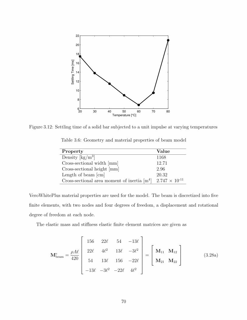
20 30 40 50 60 70 806
8
10
12
14
16
18
20
22
Temperature [°C]
Settlin
g T
ime [m
s]
Figure 3.12: Settling time of a solid bar subjected to a unit impulse at varying temperatures
Table 3.6: Geometry and material properties of beam model
Property ValueDensity [kg/m3] 1168Cross-sectional width [mm] 12.71Cross-sectional height [mm] 2.96Length of beam [cm] 20.32Cross-sectional area moment of inertia [m4] 2.747 × 10⁻¹¹
VeroWhitePlus material properties are used for the model. The beam is discretized into five
finite elements, with two nodes and four degrees of freedom, a displacement and rotational
degree of freedom at each node.
The elastic mass and stiffness elastic finite element matrices are given as
Mebeam =
ρA`
420
156 22` 54 −13`
22` 4`2 13` −3`2
54 13` 156 −22`
−13` −3`2 −22` 4`2
=
M11 M12
M21 M22
(3.28a)
70
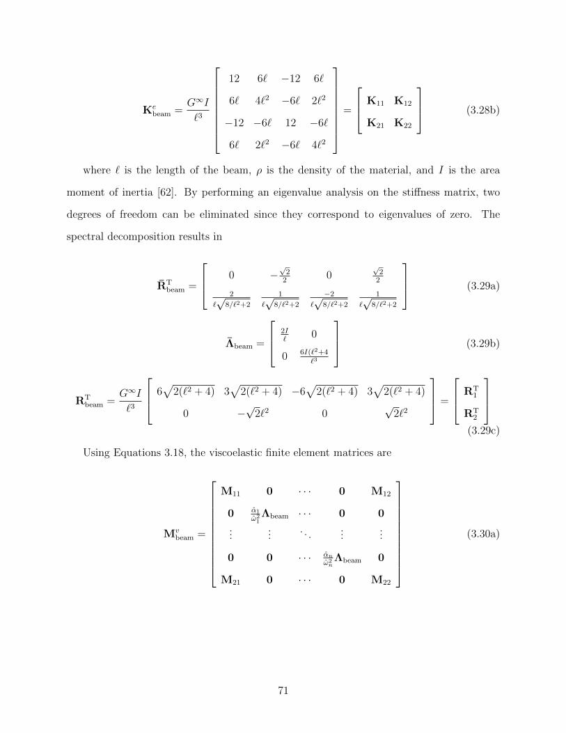
Kebeam =
G∞I
`3
12 6` −12 6`
6` 4`2 −6` 2`2
−12 −6` 12 −6`
6` 2`2 −6` 4`2
=
K11 K12
K21 K22
(3.28b)
where ` is the length of the beam, ρ is the density of the material, and I is the area
moment of inertia [62]. By performing an eigenvalue analysis on the stiffness matrix, two
degrees of freedom can be eliminated since they correspond to eigenvalues of zero. The
spectral decomposition results in
RTbeam =
0 −√22
0√22
2
`√
8/`2+2
1
`√
8/`2+2
−2`√
8/`2+2
1
`√
8/`2+2
(3.29a)
Λbeam =
2I`
0
0 6I(`2+4`3
(3.29b)
RTbeam =
G∞I
`3
6√
2(`2 + 4) 3√
2(`2 + 4) −6√
2(`2 + 4) 3√
2(`2 + 4)
0 −√
2`2 0√
2`2
=
RT1
RT2
(3.29c)
Using Equations 3.18, the viscoelastic finite element matrices are
Mvbeam =
M11 0 · · · 0 M12
0 α1
ω21Λbeam · · · 0 0
......
. . ....
...
0 0 · · · αn
ω2nΛbeam 0
M21 0 · · · 0 M22
(3.30a)
71
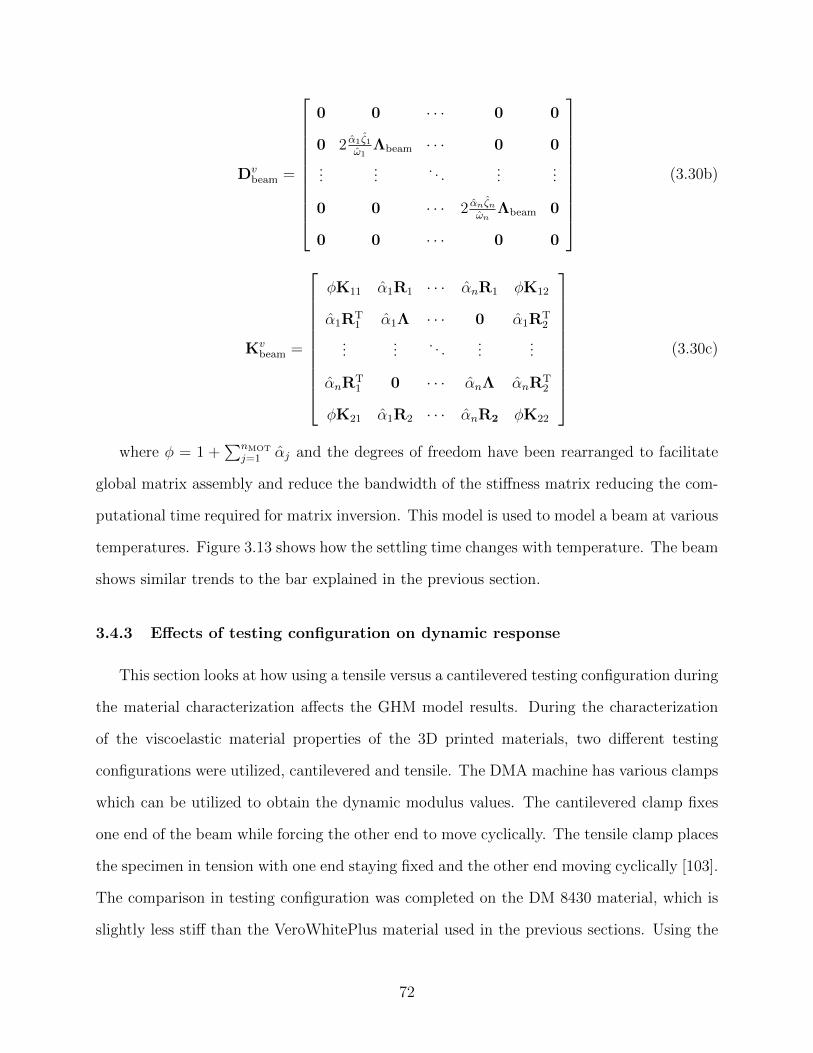
Dvbeam =
0 0 · · · 0 0
0 2 α1ζ1ω1
Λbeam · · · 0 0
......
. . ....
...
0 0 · · · 2 αnζnωn
Λbeam 0
0 0 · · · 0 0
(3.30b)
Kvbeam =
φK11 α1R1 · · · αnR1 φK12
α1RT1 α1Λ · · · 0 α1R
T2
......
. . ....
...
αnRT1 0 · · · αnΛ αnR
T2
φK21 α1R2 · · · αnR2 φK22
(3.30c)
where φ = 1 +∑nMOT
j=1 αj and the degrees of freedom have been rearranged to facilitate
global matrix assembly and reduce the bandwidth of the stiffness matrix reducing the com-
putational time required for matrix inversion. This model is used to model a beam at various
temperatures. Figure 3.13 shows how the settling time changes with temperature. The beam
shows similar trends to the bar explained in the previous section.
3.4.3 Effects of testing configuration on dynamic response
This section looks at how using a tensile versus a cantilevered testing configuration during
the material characterization affects the GHM model results. During the characterization
of the viscoelastic material properties of the 3D printed materials, two different testing
configurations were utilized, cantilevered and tensile. The DMA machine has various clamps
which can be utilized to obtain the dynamic modulus values. The cantilevered clamp fixes
one end of the beam while forcing the other end to move cyclically. The tensile clamp places
the specimen in tension with one end staying fixed and the other end moving cyclically [103].
The comparison in testing configuration was completed on the DM 8430 material, which is
slightly less stiff than the VeroWhitePlus material used in the previous sections. Using the
72
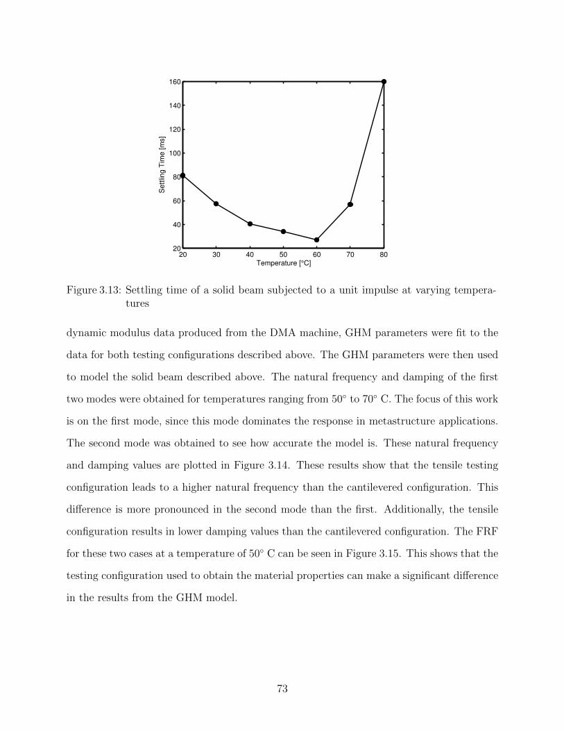
20 30 40 50 60 70 8020
40
60
80
100
120
140
160
Temperature [°C]
Settlin
g T
ime [m
s]
Figure 3.13: Settling time of a solid beam subjected to a unit impulse at varying tempera-tures
dynamic modulus data produced from the DMA machine, GHM parameters were fit to the
data for both testing configurations described above. The GHM parameters were then used
to model the solid beam described above. The natural frequency and damping of the first
two modes were obtained for temperatures ranging from 50 to 70 C. The focus of this work
is on the first mode, since this mode dominates the response in metastructure applications.
The second mode was obtained to see how accurate the model is. These natural frequency
and damping values are plotted in Figure 3.14. These results show that the tensile testing
configuration leads to a higher natural frequency than the cantilevered configuration. This
difference is more pronounced in the second mode than the first. Additionally, the tensile
configuration results in lower damping values than the cantilevered configuration. The FRF
for these two cases at a temperature of 50 C can be seen in Figure 3.15. This shows that the
testing configuration used to obtain the material properties can make a significant difference
in the results from the GHM model.
73
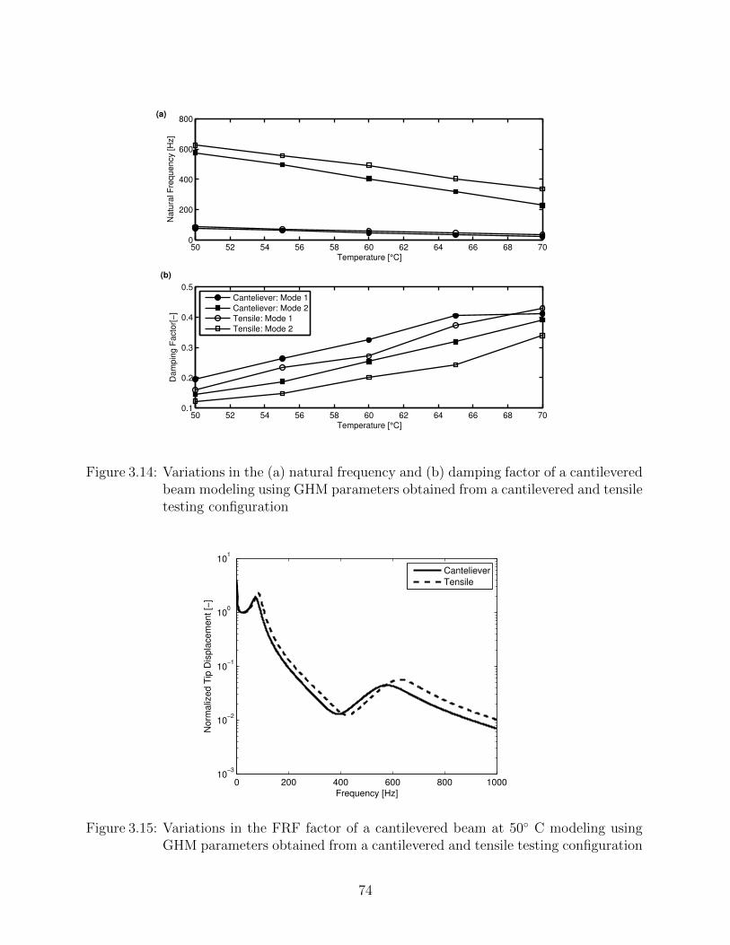
50 52 54 56 58 60 62 64 66 68 700
200
400
600
800
Temperature [°C]
Na
tura
l F
req
ue
ncy [
Hz]
50 52 54 56 58 60 62 64 66 68 700.1
0.2
0.3
0.4
0.5
Temperature [°C]
Da
mp
ing
Fa
cto
r[−
]
Canteliever: Mode 1
Canteliever: Mode 2
Tensile: Mode 1
Tensile: Mode 2
(a)
(b)
Figure 3.14: Variations in the (a) natural frequency and (b) damping factor of a cantileveredbeam modeling using GHM parameters obtained from a cantilevered and tensiletesting configuration
0 200 400 600 800 100010
−3
10−2
10−1
100
101
Frequency [Hz]
Norm
aliz
ed T
ip D
ispla
cem
ent [−
]
Canteliever
Tensile
Figure 3.15: Variations in the FRF factor of a cantilevered beam at 50 C modeling usingGHM parameters obtained from a cantilevered and tensile testing configuration
74
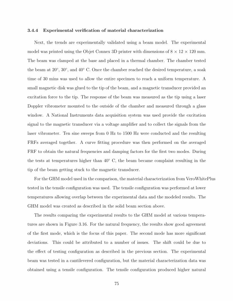
3.4.4 Experimental verification of material characterization
Next, the trends are experimentally validated using a beam model. The experimental
model was printed using the Objet Connex 3D printer with dimensions of 8 × 12 × 120 mm.
The beam was clamped at the base and placed in a thermal chamber. The chamber tested
the beam at 20, 30, and 40 C. Once the chamber reached the desired temperature, a soak
time of 30 mins was used to allow the entire specimen to reach a uniform temperature. A
small magnetic disk was glued to the tip of the beam, and a magnetic transducer provided an
excitation force to the tip. The response of the beam was measured as the tip using a laser
Doppler vibrometer mounted to the outside of the chamber and measured through a glass
window. A National Instruments data acquisition system was used provide the excitation
signal to the magnetic transducer via a voltage amplifier and to collect the signals from the
laser vibrometer. Ten sine sweeps from 0 Hz to 1500 Hz were conducted and the resulting
FRFs averaged together. A curve fitting procedure was then performed on the averaged
FRF to obtain the natural frequencies and damping factors for the first two modes. During
the tests at temperatures higher than 40 C, the beam became complaint resulting in the
tip of the beam getting stuck to the magnetic transducer.
For the GHM model used in the comparison, the material characterization from VeroWhitePlus
tested in the tensile configuration was used. The tensile configuration was performed at lower
temperatures allowing overlap between the experimental data and the modeled results. The
GHM model was created as described in the solid beam section above.
The results comparing the experimental results to the GHM model at various tempera-
tures are shown in Figure 3.16. For the natural frequency, the results show good agreement
of the first mode, which is the focus of this paper. The second mode has more significant
deviations. This could be attributed to a number of issues. The shift could be due to
the effect of testing configuration as described in the previous section. The experimental
beam was tested in a cantilevered configuration, but the material characterization data was
obtained using a tensile configuration. The tensile configuration produced higher natural
75
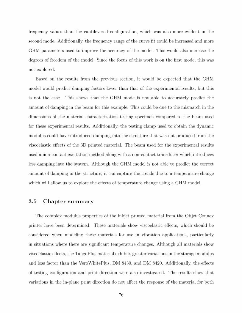
frequency values than the cantilevered configuration, which was also more evident in the
second mode. Additionally, the frequency range of the curve fit could be increased and more
GHM parameters used to improve the accuracy of the model. This would also increase the
degrees of freedom of the model. Since the focus of this work is on the first mode, this was
not explored.
Based on the results from the previous section, it would be expected that the GHM
model would predict damping factors lower than that of the experimental results, but this
is not the case. This shows that the GHM mode is not able to accurately predict the
amount of damping in the beam for this example. This could be due to the mismatch in the
dimensions of the material characterization testing specimen compared to the beam used
for these experimental results. Additionally, the testing clamp used to obtain the dynamic
modulus could have introduced damping into the structure that was not produced from the
viscoelastic effects of the 3D printed material. The beam used for the experimental results
used a non-contact excitation method along with a non-contact transducer which introduces
less damping into the system. Although the GHM model is not able to predict the correct
amount of damping in the structure, it can capture the trends due to a temperature change
which will allow us to explore the effects of temperature change using a GHM model.
3.5 Chapter summary
The complex modulus properties of the inkjet printed material from the Objet Connex
printer have been determined. These materials show viscoelastic effects, which should be
considered when modeling these materials for use in vibration applications, particularly
in situations where there are significant temperature changes. Although all materials show
viscoelastic effects, the TangoPlus material exhibits greater variations in the storage modulus
and loss factor than the VeroWhitePlus, DM 8430, and DM 8420. Additionally, the effects
of testing configuration and print direction were also investigated. The results show that
variations in the in-plane print direction do not affect the response of the material for both
76
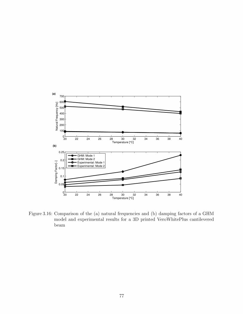
20 22 24 26 28 30 32 34 36 38 400
100
200
300
400
500
600
700
Temperature [°C]
Na
tura
l F
req
ue
ncy [
Hz]
20 22 24 26 28 30 32 34 36 38 400
0.05
0.1
0.15
0.2
0.25
Temperature [°C]
Da
mp
ing
Fa
cto
r[−
]
GHM: Mode 1
GHM: Mode 2
Experimental: Mode 1
Experimental: Mode 2
(a)
(b)
Figure 3.16: Comparison of the (a) natural frequencies and (b) damping factors of a GHMmodel and experimental results for a 3D printed VeroWhitePlus cantileveredbeam
77
the tensile and cantilevered configurations. The testing configuration does have a slight effect
on the complex modulus values.
These results show that the GHM model can accurately predict the fundamental natural
frequency of a structure printed using the Objet Connex 3D printer. It can also predict
the changes in the natural frequency due to temperature changes. This paper shows the
complete process required to accurately use the GHM model; starting from the material
characterization of the viscoelastic material properties to the experimental verification of
the model.
The change in temperature can significantly alter both the storage modulus and the
loss modulus of the material; these changes lead to changes in the natural frequencies and
the damping of the resulting structure. When experimentally characterizing the viscoelastic
material properties of the 3D printed material, the testing configuration of the specimen
should be carefully considered. This work showed that the tensile testing configuration led
to higher natural frequencies and lower damping values than the cantilevered configuration.
The experimental verification results also had lower damping values than the modeled results.
Lastly, the GHM model developed was used to model the dynamics of a metastructure
and studies the effects of a changing temperature. The results showed that the changes in the
natural frequency of the host structure and the vibration absorbers changed at a similar rate,
resulting in similar trends in the dynamic response as the temperature increase. This was
true up to a specific temperature when the performance of the metastructure significantly
decreased resulting in the baseline structure have better performance.
78
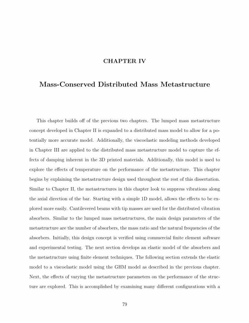
CHAPTER IV
Mass-Conserved Distributed Mass Metastructure
This chapter builds off of the previous two chapters. The lumped mass metastructure
concept developed in Chapter II is expanded to a distributed mass model to allow for a po-
tentially more accurate model. Additionally, the viscoelastic modeling methods developed
in Chapter III are applied to the distributed mass metastructure model to capture the ef-
fects of damping inherent in the 3D printed materials. Additionally, this model is used to
explore the effects of temperature on the performance of the metastructure. This chapter
begins by explaining the metastructure design used throughout the rest of this dissertation.
Similar to Chapter II, the metastructures in this chapter look to suppress vibrations along
the axial direction of the bar. Starting with a simple 1D model, allows the effects to be ex-
plored more easily. Cantilevered beams with tip masses are used for the distributed vibration
absorbers. Similar to the lumped mass metastructures, the main design parameters of the
metastructure are the number of absorbers, the mass ratio and the natural frequencies of the
absorbers. Initially, this design concept is verified using commercial finite element software
and experimental testing. The next section develops an elastic model of the absorbers and
the metastructure using finite element techniques. The following section extends the elastic
model to a viscoelastic model using the GHM model as described in the previous chapter.
Next, the effects of varying the metastructure parameters on the performance of the struc-
ture are explored. This is accomplished by examining many different configurations with a
79
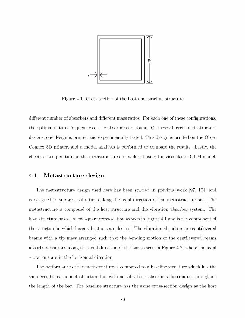
t
w
Figure 4.1: Cross-section of the host and baseline structure
different number of absorbers and different mass ratios. For each one of these configurations,
the optimal natural frequencies of the absorbers are found. Of these different metastructure
designs, one design is printed and experimentally tested. This design is printed on the Objet
Connex 3D printer, and a modal analysis is performed to compare the results. Lastly, the
effects of temperature on the metastructure are explored using the viscoelastic GHM model.
4.1 Metastructure design
The metastructure design used here has been studied in previous work [97, 104] and
is designed to suppress vibrations along the axial direction of the metastructure bar. The
metastructure is composed of the host structure and the vibration absorber system. The
host structure has a hollow square cross-section as seen in Figure 4.1 and is the component of
the structure in which lower vibrations are desired. The vibration absorbers are cantilevered
beams with a tip mass arranged such that the bending motion of the cantilevered beams
absorbs vibrations along the axial direction of the bar as seen in Figure 4.2, where the axial
vibrations are in the horizontal direction.
The performance of the metastructure is compared to a baseline structure which has the
same weight as the metastructure but with no vibrations absorbers distributed throughout
the length of the bar. The baseline structure has the same cross-section design as the host
80
Figure 4.2: Schematic of metastructure. Vibrations occur along the horizontal direction.
section as depicted in Figure 4.1 but with a slightly different thicknesses to account for the
weight constraint. Restricting the metastructure and the baseline structure to have the same
weight allows any performance gains in the metastructure to be attributed to the addition
of the distributed vibration absorbers and not due to any mass added to the structure.
4.1.1 Design parameters
The design of the metastructure is characterized by the number of vibration absorbers,
N , the mass ratio, µ, and the natural frequency of the individual vibration absorbers, ωi.
The mass ratio is the ratio of the mass of the absorbers over the total mass of the structure
and is defined as
µ =
∑Ni=1mi∑N
i=1mi +mhost
(4.1)
where mi is the mass of the ith absorber and mhost is the mass of the host structure.
Similar to the lumped mass metastructure described in Chapter II, this mass ratio provides
a measure of how much mass is being redistributed to the absorber system. A higher mass
ratio represents more mass in the absorber system.
The natural frequencies of the vibrations absorbers are varied by changing the geometry
of the absorbers. For example, making the tip mass larger and therefore heavier will lead to
a lower natural frequency, but increasing the thickness of the beam leads to a higher stiffness
and therefore a higher natural frequency. Throughout this chapter, various methods are used
81
to determine the relationship between the geometric parameters and the resulting natural
frequency.
4.1.2 Verification of design
This section looks at the proposed design and verifies that the design produces the de-
sired effects by looking a commercial finite element model and experimental results. The
finite element model is based on an elastic model. Verifying that an elastic model produces
similar trends as the experimental results is a necessary first step. This verification gives
us confidence in the actual design of the metastructure and provides an intermediate step
before using more complicated models.
The specific design used for this verification is based on the optimal lumped mass metas-
tructure design from Section 2.5.3. The metastructure has ten vibration absorbers and a
mass ratio of 0.206. This section begins by explaining how the natural frequencies of the
vibration absorbers were chosen then goes into the details of the finite element and the ex-
perimental results. The results of the finite element verification are based off two papers by
the authors [97, 104]. These results look at two different metastructure designs, one where
all the vibration absorbers are tuned to the same frequency and another design where the
vibration absorbers are tuned to linearly varying natural frequencies. The finite element
results compare both metastructure designs to the baseline structure. The experimental
results test the baseline structure and the metastructure with vibration absorbers having a
constant natural frequency.
The material properties utilized are those from the Objet Connex 3D printer by Stratasys,
specifically the DM 8430 digital material, which has been studied in detail in Chapter III.
The parameters used for the baseline structure and metastructures are detailed in Table 4.1.
Both the host structure and the baseline structure have cross-sections as shown in Figure
4.1. The parameters are chosen such that the baseline structure and the metastructure have
the same mass, cross-sectional width, and length. The other parameters are varied such that
82
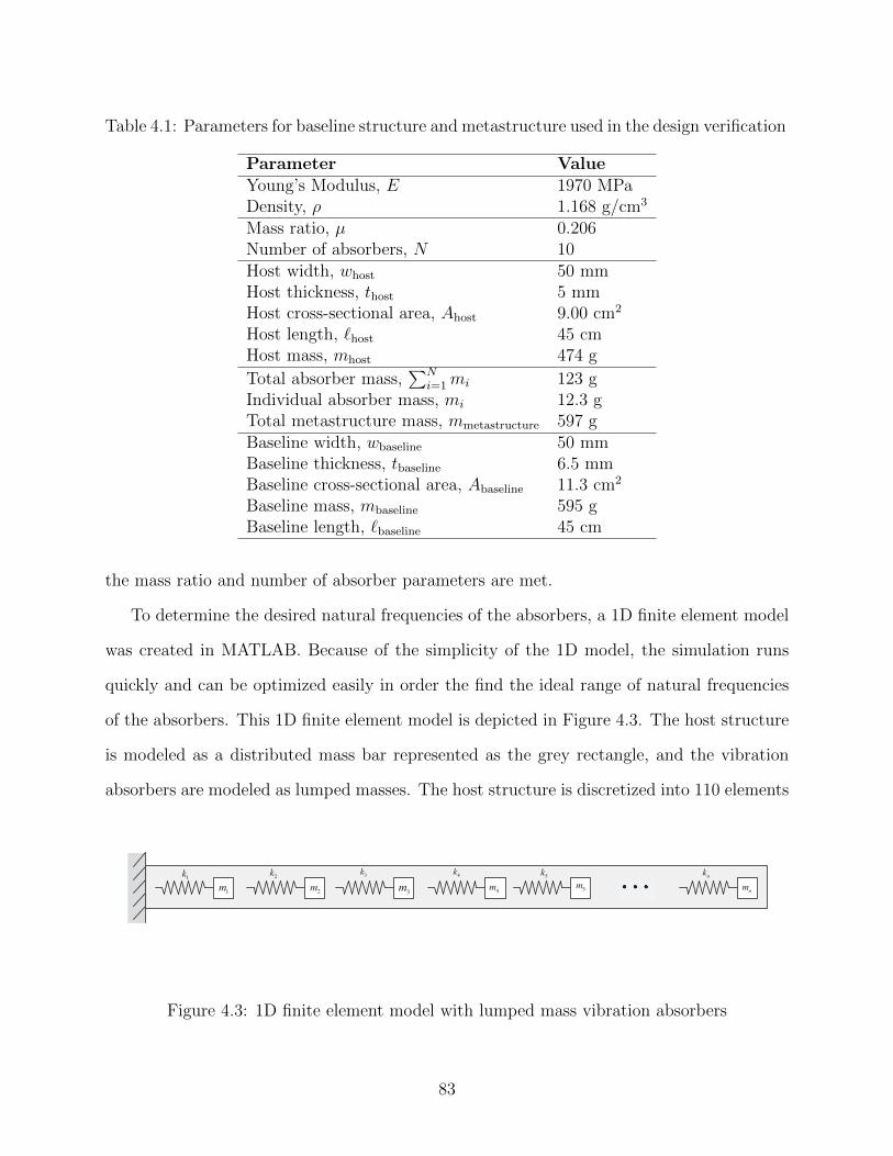
Table 4.1: Parameters for baseline structure and metastructure used in the design verification
Parameter ValueYoung’s Modulus, E 1970 MPaDensity, ρ 1.168 g/cm3
Mass ratio, µ 0.206Number of absorbers, N 10Host width, whost 50 mmHost thickness, thost 5 mmHost cross-sectional area, Ahost 9.00 cm2
Host length, `host 45 cmHost mass, mhost 474 g
Total absorber mass,∑N
i=1mi 123 gIndividual absorber mass, mi 12.3 gTotal metastructure mass, mmetastructure 597 gBaseline width, wbaseline 50 mmBaseline thickness, tbaseline 6.5 mmBaseline cross-sectional area, Abaseline 11.3 cm2
Baseline mass, mbaseline 595 gBaseline length, `baseline 45 cm
the mass ratio and number of absorber parameters are met.
To determine the desired natural frequencies of the absorbers, a 1D finite element model
was created in MATLAB. Because of the simplicity of the 1D model, the simulation runs
quickly and can be optimized easily in order the find the ideal range of natural frequencies
of the absorbers. This 1D finite element model is depicted in Figure 4.3. The host structure
is modeled as a distributed mass bar represented as the grey rectangle, and the vibration
absorbers are modeled as lumped masses. The host structure is discretized into 110 elements
1k
1m
2k
2m
3k
3m
4k
4m
5k
5m
nk
nm
Figure 4.3: 1D finite element model with lumped mass vibration absorbers
83
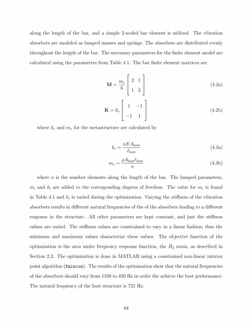
along the length of the bar, and a simple 2-noded bar element is utilized. The vibration
absorbers are modeled as lumped masses and springs. The absorbers are distributed evenly
throughout the length of the bar. The necessary parameters for the finite element model are
calculated using the parameters from Table 4.1. The bar finite element matrices are
M =me
6
2 1
1 2
(4.2a)
K = ke
1 −1
−1 1
(4.2b)
where ke and me for the metastructure are calculated by
ke =nEAhost
`host(4.3a)
me =ρAhost`host
n(4.3b)
where n is the number elements along the length of the bar. The lumped parameters,
mi and ki are added to the corresponding degrees of freedom. The value for mi is found
in Table 4.1 and ki is varied during the optimization. Varying the stiffness of the vibration
absorbers results in different natural frequencies of the of the absorbers leading to a different
response in the structure. All other parameters are kept constant, and just the stiffness
values are varied. The stiffness values are constrained to vary in a linear fashion; thus the
minimum and maximum values characterize these values. The objective function of the
optimization is the area under frequency response function, the H2 norm, as described in
Section 2.2. The optimization is done in MATLAB using a constrained non-linear interior
point algorithm (fmincon). The results of the optimization show that the natural frequencies
of the absorbers should vary from 1100 to 450 Hz in order the achieve the best performance.
The natural frequency of the host structure is 721 Hz.
84
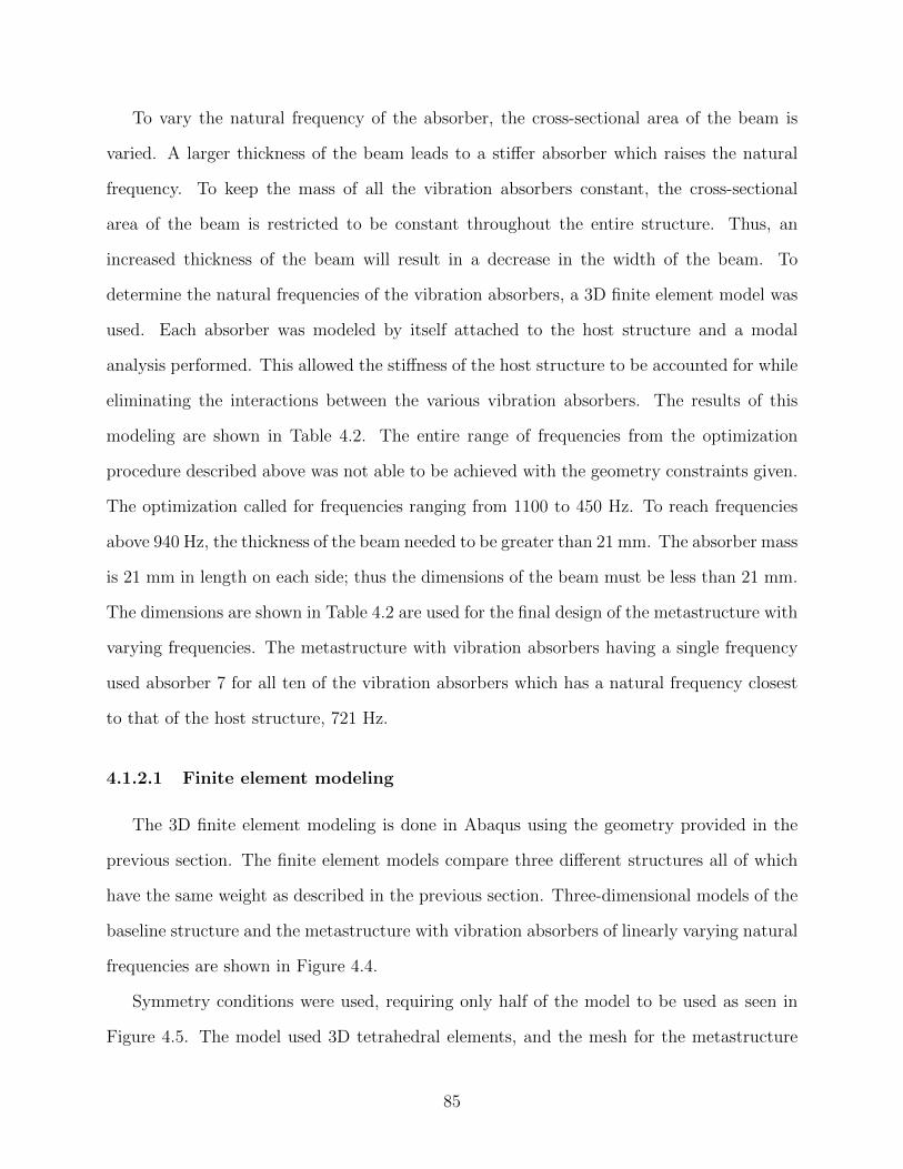
To vary the natural frequency of the absorber, the cross-sectional area of the beam is
varied. A larger thickness of the beam leads to a stiffer absorber which raises the natural
frequency. To keep the mass of all the vibration absorbers constant, the cross-sectional
area of the beam is restricted to be constant throughout the entire structure. Thus, an
increased thickness of the beam will result in a decrease in the width of the beam. To
determine the natural frequencies of the vibration absorbers, a 3D finite element model was
used. Each absorber was modeled by itself attached to the host structure and a modal
analysis performed. This allowed the stiffness of the host structure to be accounted for while
eliminating the interactions between the various vibration absorbers. The results of this
modeling are shown in Table 4.2. The entire range of frequencies from the optimization
procedure described above was not able to be achieved with the geometry constraints given.
The optimization called for frequencies ranging from 1100 to 450 Hz. To reach frequencies
above 940 Hz, the thickness of the beam needed to be greater than 21 mm. The absorber mass
is 21 mm in length on each side; thus the dimensions of the beam must be less than 21 mm.
The dimensions are shown in Table 4.2 are used for the final design of the metastructure with
varying frequencies. The metastructure with vibration absorbers having a single frequency
used absorber 7 for all ten of the vibration absorbers which has a natural frequency closest
to that of the host structure, 721 Hz.
4.1.2.1 Finite element modeling
The 3D finite element modeling is done in Abaqus using the geometry provided in the
previous section. The finite element models compare three different structures all of which
have the same weight as described in the previous section. Three-dimensional models of the
baseline structure and the metastructure with vibration absorbers of linearly varying natural
frequencies are shown in Figure 4.4.
Symmetry conditions were used, requiring only half of the model to be used as seen in
Figure 4.5. The model used 3D tetrahedral elements, and the mesh for the metastructure
85
Table 4.2: Geometric properties of the vibration absorbers and the resulting natural frequen-cies
Absorber Thickness Width Area Distance from Finite element[mm] [mm] [mm2] root [cm] frequency [Hz]
1 20.3 4.93 100.1 40.9 939.82 18.7 5.30 99.1 36.8 913.93 17.2 5.81 99.9 32.7 875.44 15.6 6.38 99.5 28.6 839.25 14.1 7.07 99.7 24.5 794.86 12.6 7.94 100.0 20.5 764.07 11.1 9.05 100.0 16.4 648.38 9.5 10.5 99.9 12.3 610.69 8.0 12.6 100.4 8.2 564.210 4.9 20.5 100.0 4.1 426.5
Figure 4.4: Three dimensional models of (a) baseline structure and (b) metastructure withvibration absorbers with linearly varying natural frequencies
86
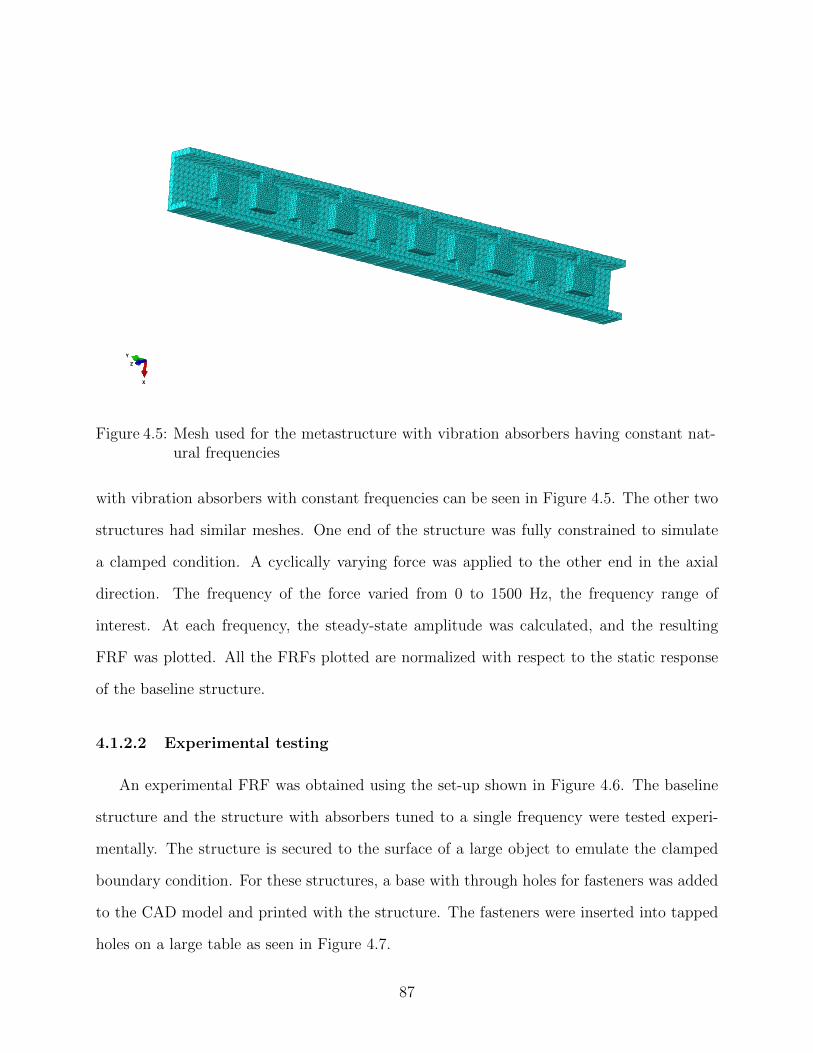
X
Y
Z
Figure 4.5: Mesh used for the metastructure with vibration absorbers having constant nat-ural frequencies
with vibration absorbers with constant frequencies can be seen in Figure 4.5. The other two
structures had similar meshes. One end of the structure was fully constrained to simulate
a clamped condition. A cyclically varying force was applied to the other end in the axial
direction. The frequency of the force varied from 0 to 1500 Hz, the frequency range of
interest. At each frequency, the steady-state amplitude was calculated, and the resulting
FRF was plotted. All the FRFs plotted are normalized with respect to the static response
of the baseline structure.
4.1.2.2 Experimental testing
An experimental FRF was obtained using the set-up shown in Figure 4.6. The baseline
structure and the structure with absorbers tuned to a single frequency were tested experi-
mentally. The structure is secured to the surface of a large object to emulate the clamped
boundary condition. For these structures, a base with through holes for fasteners was added
to the CAD model and printed with the structure. The fasteners were inserted into tapped
holes on a large table as seen in Figure 4.7.
87
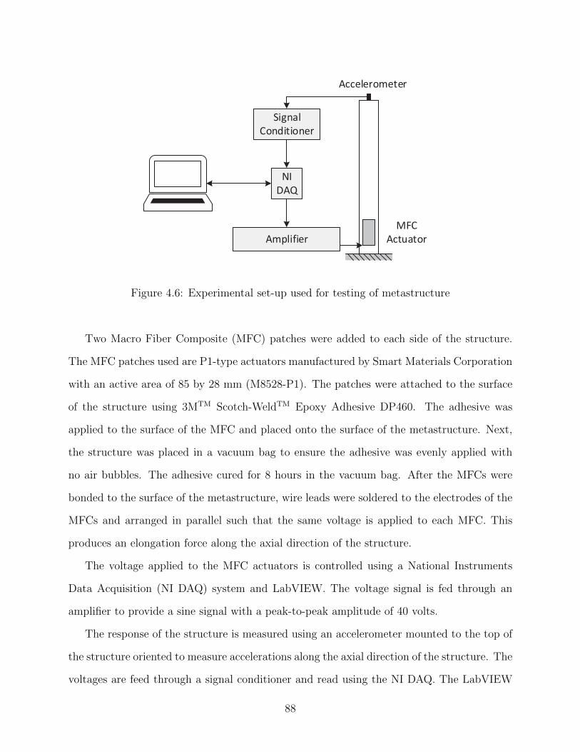
Amplifier
NI
DAQ
Signal
Conditioner
MFC
Actuator
Accelerometer
Figure 4.6: Experimental set-up used for testing of metastructure
Two Macro Fiber Composite (MFC) patches were added to each side of the structure.
The MFC patches used are P1-type actuators manufactured by Smart Materials Corporation
with an active area of 85 by 28 mm (M8528-P1). The patches were attached to the surface
of the structure using 3MTM Scotch-WeldTM Epoxy Adhesive DP460. The adhesive was
applied to the surface of the MFC and placed onto the surface of the metastructure. Next,
the structure was placed in a vacuum bag to ensure the adhesive was evenly applied with
no air bubbles. The adhesive cured for 8 hours in the vacuum bag. After the MFCs were
bonded to the surface of the metastructure, wire leads were soldered to the electrodes of the
MFCs and arranged in parallel such that the same voltage is applied to each MFC. This
produces an elongation force along the axial direction of the structure.
The voltage applied to the MFC actuators is controlled using a National Instruments
Data Acquisition (NI DAQ) system and LabVIEW. The voltage signal is fed through an
amplifier to provide a sine signal with a peak-to-peak amplitude of 40 volts.
The response of the structure is measured using an accelerometer mounted to the top of
the structure oriented to measure accelerations along the axial direction of the structure. The
voltages are feed through a signal conditioner and read using the NI DAQ. The LabVIEW
88
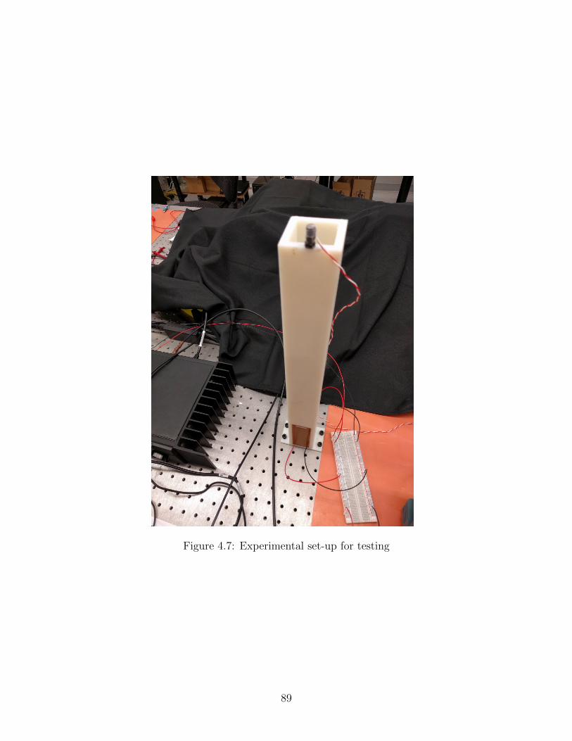
Figure 4.7: Experimental set-up for testing
89
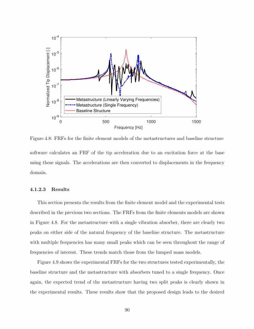
0 500 1000 1500
Frequency [Hz]
10-9
10-8
10-7
10-6
10-5
10-4
Norm
aliz
ed T
ip D
ispla
cem
ent [-
]
Metastructure (Linearly Varying Frequencies)
Metastructure (Single Frequency)
Baseline Structure
Figure 4.8: FRFs for the finite element models of the metastructures and baseline structure
software calculates an FRF of the tip acceleration due to an excitation force at the base
using these signals. The accelerations are then converted to displacements in the frequency
domain.
4.1.2.3 Results
This section presents the results from the finite element model and the experimental tests
described in the previous two sections. The FRFs from the finite elements models are shown
in Figure 4.8. For the metastructure with a single vibration absorber, there are clearly two
peaks on either side of the natural frequency of the baseline structure. The metastructure
with multiple frequencies has many small peaks which can be seen throughout the range of
frequencies of interest. These trends match those from the lumped mass models.
Figure 4.9 shows the experimental FRFs for the two structures tested experimentally, the
baseline structure and the metastructure with absorbers tuned to a single frequency. Once
again, the expected trend of the metastructure having two split peaks is clearly shown in
the experimental results. These results show that the proposed design leads to the desired
90
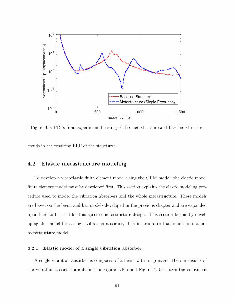
0 500 1000 1500
Frequency [Hz]
10-2
10-1
100
101
102
Norm
aliz
ed T
ip D
ispla
cem
ent [-
]
Baseline Structure
Metastructure (Single Frequency)
Figure 4.9: FRFs from experimental testing of the metastructure and baseline structure
trends in the resulting FRF of the structures.
4.2 Elastic metastructure modeling
To develop a viscoelastic finite element model using the GHM model, the elastic model
finite element model must be developed first. This section explains the elastic modeling pro-
cedure used to model the vibration absorbers and the whole metastructure. These models
are based on the beam and bar models developed in the previous chapter and are expanded
upon here to be used for this specific metastructure design. This section begins by devel-
oping the model for a single vibration absorber, then incorporates that model into a full
metastructure model.
4.2.1 Elastic model of a single vibration absorber
A single vibration absorber is composed of a beam with a tip mass. The dimensions of
the vibration absorber are defined in Figure 4.10a and Figure 4.10b shows the equivalent
91
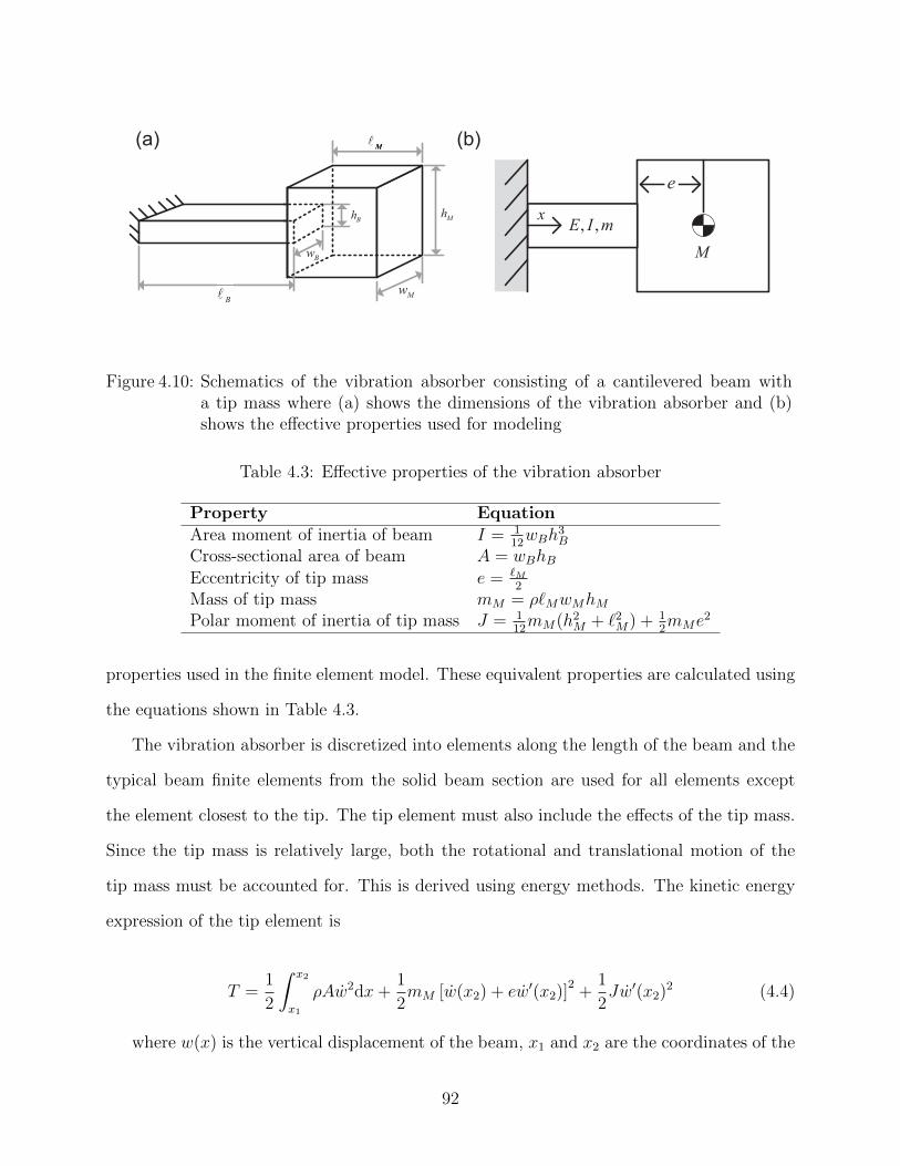
e
, ,E I mx
M
x
mg
eMg
Mg
(a) (b)
BB
Bw
Bh
Mw
Mh
M
Figure 4.10: Schematics of the vibration absorber consisting of a cantilevered beam witha tip mass where (a) shows the dimensions of the vibration absorber and (b)shows the effective properties used for modeling
Table 4.3: Effective properties of the vibration absorber
Property EquationArea moment of inertia of beam I = 1
12wBh
3B
Cross-sectional area of beam A = wBhBEccentricity of tip mass e = `M
2
Mass of tip mass mM = ρ`MwMhMPolar moment of inertia of tip mass J = 1
12mM(h2M + `2M) + 1
2mMe
2
properties used in the finite element model. These equivalent properties are calculated using
the equations shown in Table 4.3.
The vibration absorber is discretized into elements along the length of the beam and the
typical beam finite elements from the solid beam section are used for all elements except
the element closest to the tip. The tip element must also include the effects of the tip mass.
Since the tip mass is relatively large, both the rotational and translational motion of the
tip mass must be accounted for. This is derived using energy methods. The kinetic energy
expression of the tip element is
T =1
2
∫ x2
x1
ρAw2dx+1
2mM [w(x2) + ew′(x2)]
2+
1
2Jw′(x2)
2 (4.4)
where w(x) is the vertical displacement of the beam, x1 and x2 are the coordinates of the
92
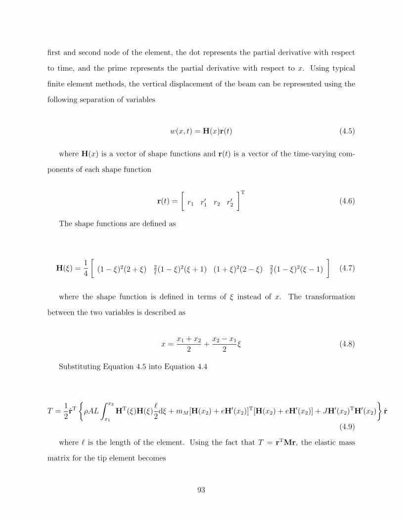
first and second node of the element, the dot represents the partial derivative with respect
to time, and the prime represents the partial derivative with respect to x. Using typical
finite element methods, the vertical displacement of the beam can be represented using the
following separation of variables
w(x, t) = H(x)r(t) (4.5)
where H(x) is a vector of shape functions and r(t) is a vector of the time-varying com-
ponents of each shape function
r(t) =
[r1 r′1 r2 r′2
]T(4.6)
The shape functions are defined as
H(ξ) =1
4
[(1− ξ)2(2 + ξ) 2
`(1− ξ)2(ξ + 1) (1 + ξ)2(2− ξ) 2
`(1− ξ)2(ξ − 1)
](4.7)
where the shape function is defined in terms of ξ instead of x. The transformation
between the two variables is described as
x =x1 + x2
2+x2 − x1
2ξ (4.8)
Substituting Equation 4.5 into Equation 4.4
T =1
2rTρAL
∫ x2
x1
HT(ξ)H(ξ)`
2dξ +mM [H(x2) + eH′(x2)]
T[H(x2) + eH′(x2)] + JH′(x2)TH′(x2)
r
(4.9)
where ` is the length of the element. Using the fact that T = rTMr, the elastic mass
matrix for the tip element becomes
93
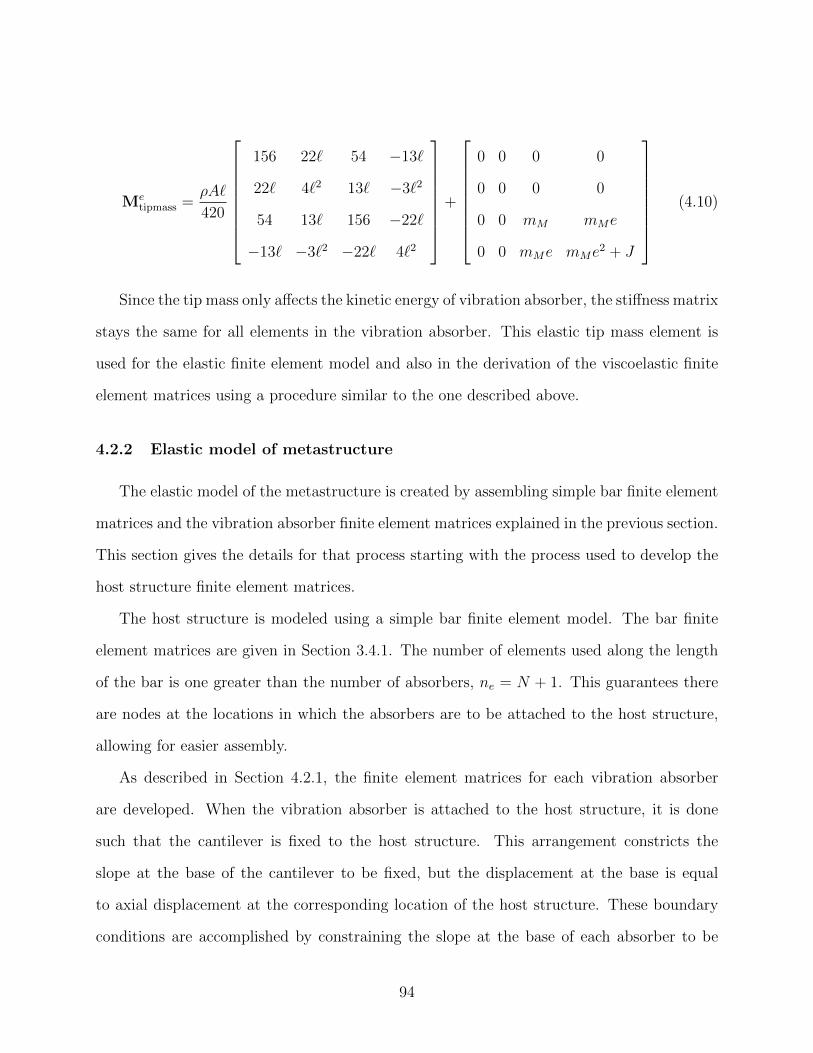
Metipmass =
ρA`
420
156 22` 54 −13`
22` 4`2 13` −3`2
54 13` 156 −22`
−13` −3`2 −22` 4`2
+
0 0 0 0
0 0 0 0
0 0 mM mMe
0 0 mMe mMe2 + J
(4.10)
Since the tip mass only affects the kinetic energy of vibration absorber, the stiffness matrix
stays the same for all elements in the vibration absorber. This elastic tip mass element is
used for the elastic finite element model and also in the derivation of the viscoelastic finite
element matrices using a procedure similar to the one described above.
4.2.2 Elastic model of metastructure
The elastic model of the metastructure is created by assembling simple bar finite element
matrices and the vibration absorber finite element matrices explained in the previous section.
This section gives the details for that process starting with the process used to develop the
host structure finite element matrices.
The host structure is modeled using a simple bar finite element model. The bar finite
element matrices are given in Section 3.4.1. The number of elements used along the length
of the bar is one greater than the number of absorbers, ne = N + 1. This guarantees there
are nodes at the locations in which the absorbers are to be attached to the host structure,
allowing for easier assembly.
As described in Section 4.2.1, the finite element matrices for each vibration absorber
are developed. When the vibration absorber is attached to the host structure, it is done
such that the cantilever is fixed to the host structure. This arrangement constricts the
slope at the base of the cantilever to be fixed, but the displacement at the base is equal
to axial displacement at the corresponding location of the host structure. These boundary
conditions are accomplished by constraining the slope at the base of each absorber to be
94
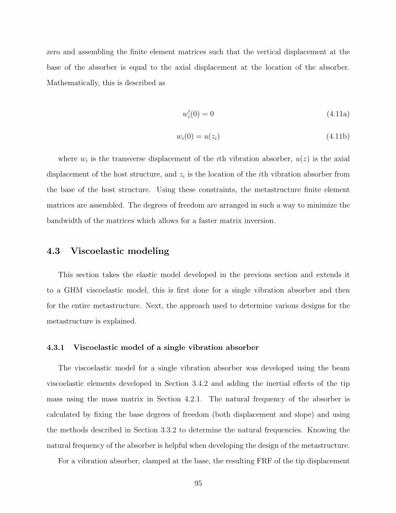
zero and assembling the finite element matrices such that the vertical displacement at the
base of the absorber is equal to the axial displacement at the location of the absorber.
Mathematically, this is described as
w′i(0) = 0 (4.11a)
wi(0) = u(zi) (4.11b)
where wi is the transverse displacement of the ith vibration absorber, u(z) is the axial
displacement of the host structure, and zi is the location of the ith vibration absorber from
the base of the host structure. Using these constraints, the metastructure finite element
matrices are assembled. The degrees of freedom are arranged in such a way to minimize the
bandwidth of the matrices which allows for a faster matrix inversion.
4.3 Viscoelastic modeling
This section takes the elastic model developed in the previous section and extends it
to a GHM viscoelastic model, this is first done for a single vibration absorber and then
for the entire metastructure. Next, the approach used to determine various designs for the
metastructure is explained.
4.3.1 Viscoelastic model of a single vibration absorber
The viscoelastic model for a single vibration absorber was developed using the beam
viscoelastic elements developed in Section 3.4.2 and adding the inertial effects of the tip
mass using the mass matrix in Section 4.2.1. The natural frequency of the absorber is
calculated by fixing the base degrees of freedom (both displacement and slope) and using
the methods described in Section 3.3.2 to determine the natural frequencies. Knowing the
natural frequency of the absorber is helpful when developing the design of the metastructure.
For a vibration absorber, clamped at the base, the resulting FRF of the tip displacement
95
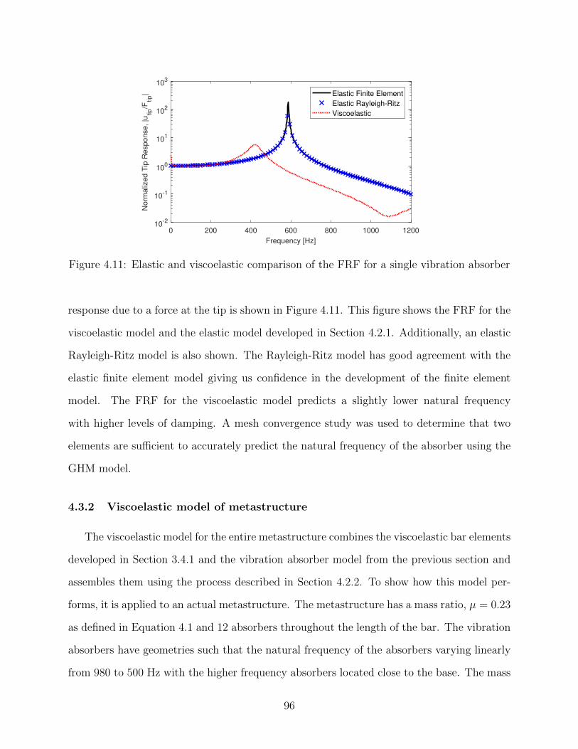
0 200 400 600 800 1000 1200
Frequency [Hz]
10-2
10-1
100
101
102
103
Norm
aliz
ed T
ip R
esponse, |u
tip/F
tip| Elastic Finite Element
Elastic Rayleigh-Ritz
Viscoelastic
Figure 4.11: Elastic and viscoelastic comparison of the FRF for a single vibration absorber
response due to a force at the tip is shown in Figure 4.11. This figure shows the FRF for the
viscoelastic model and the elastic model developed in Section 4.2.1. Additionally, an elastic
Rayleigh-Ritz model is also shown. The Rayleigh-Ritz model has good agreement with the
elastic finite element model giving us confidence in the development of the finite element
model. The FRF for the viscoelastic model predicts a slightly lower natural frequency
with higher levels of damping. A mesh convergence study was used to determine that two
elements are sufficient to accurately predict the natural frequency of the absorber using the
GHM model.
4.3.2 Viscoelastic model of metastructure
The viscoelastic model for the entire metastructure combines the viscoelastic bar elements
developed in Section 3.4.1 and the vibration absorber model from the previous section and
assembles them using the process described in Section 4.2.2. To show how this model per-
forms, it is applied to an actual metastructure. The metastructure has a mass ratio, µ = 0.23
as defined in Equation 4.1 and 12 absorbers throughout the length of the bar. The vibration
absorbers have geometries such that the natural frequency of the absorbers varying linearly
from 980 to 500 Hz with the higher frequency absorbers located close to the base. The mass
96
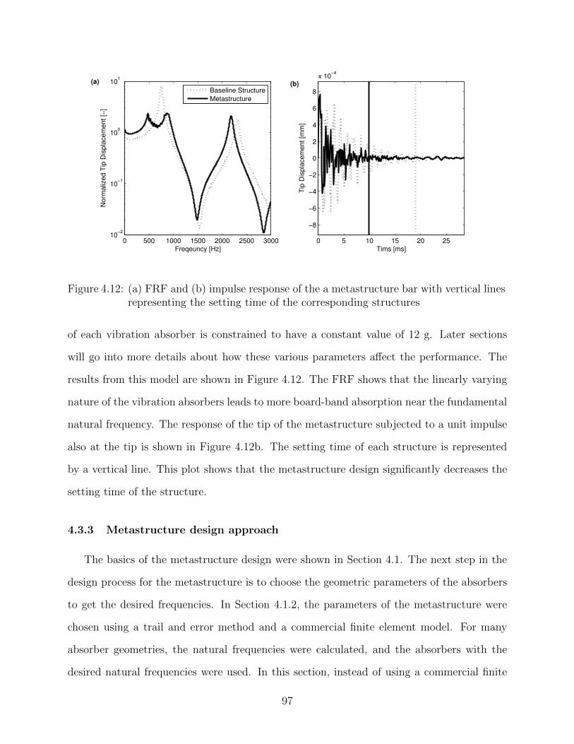
0 500 1000 1500 2000 2500 300010
−2
10−1
100
101
Freqeuncy [Hz]
Norm
aliz
ed T
ip D
ispla
cem
ent [−
]
Baseline Structure
Metastructure
0 5 10 15 20 25
−8
−6
−4
−2
0
2
4
6
8
x 10−4
Tims [ms]
Tip
Dis
pla
cem
ent [m
m]
(a) (b)
Figure 4.12: (a) FRF and (b) impulse response of the a metastructure bar with vertical linesrepresenting the setting time of the corresponding structures
of each vibration absorber is constrained to have a constant value of 12 g. Later sections
will go into more details about how these various parameters affect the performance. The
results from this model are shown in Figure 4.12. The FRF shows that the linearly varying
nature of the vibration absorbers leads to more board-band absorption near the fundamental
natural frequency. The response of the tip of the metastructure subjected to a unit impulse
also at the tip is shown in Figure 4.12b. The setting time of each structure is represented
by a vertical line. This plot shows that the metastructure design significantly decreases the
setting time of the structure.
4.3.3 Metastructure design approach
The basics of the metastructure design were shown in Section 4.1. The next step in the
design process for the metastructure is to choose the geometric parameters of the absorbers
to get the desired frequencies. In Section 4.1.2, the parameters of the metastructure were
chosen using a trail and error method and a commercial finite element model. For many
absorber geometries, the natural frequencies were calculated, and the absorbers with the
desired natural frequencies were used. In this section, instead of using a commercial finite
97
element software to find the natural frequencies, a GHM finite element model of the absorbers
is used. This model is created in MATLAB. This allows the viscoelastic effects to be taken
into account while also speeding up the process by using a 1D model instead of a 3D model.
In Chapter II, choosing the parameters for the metastructure model was fairly straight-
forward because mass and stiffness values could be chosen independently. When designing
real structures, changing the geometric parameters changes both the mass and the stiffness.
Additionally, the geometry of absorbers is defined by six different geometric parameters, as
seen in Figure 4.10. Here, an iterative approach is taken. For many different absorber ge-
ometries, the frequency of the absorber is calculated using the GHM model of the absorber.
If the natural frequency of the absorber falls within the desired frequency range, 100 to
1500 Hz, then that absorber geometry is stored along with its frequency. In addition to the
frequency being within the desired frequency range, a number of other constraints must also
be met. First, there is a constraint on the total overall length of the absorber. The length of
the beam plus the length of the tip mass must be less than 35 mm so that the absorber can
fit inside the host structure which has an inside width of 40 mm. Additionally, the maximum
height of the absorber must be less than 30 mm, allowing for all the absorbers to fit along
the length of the host structure. The last constraint is on the slenderness ratio, SR, of the
absorber beam. The slenderness ratio must be high enough to ensure the Euler-Bernoulli
assumptions are valid. For this work, the slenderness ratio must take on a value higher than
4. The slenderness ratio is calculated as
SR =`Br
(4.12)
where r is the radius of gyration, calculated as
r =
√I
A(4.13)
where I and A are defined in Table 4.3. Different combinations of the six geometric
98
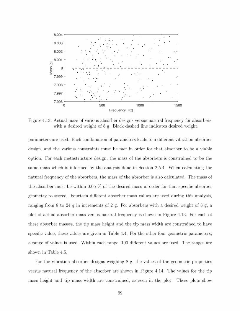
0 500 1000 1500
Frequency [Hz]
7.996
7.997
7.998
7.999
8
8.001
8.002
8.003
8.004
Ma
ss [
g]
Figure 4.13: Actual mass of various absorber designs versus natural frequency for absorberswith a desired weight of 8 g. Black dashed line indicates desired weight.
parameters are used. Each combination of parameters leads to a different vibration absorber
design, and the various constraints must be met in order for that absorber to be a viable
option. For each metastructure design, the mass of the absorbers is constrained to be the
same mass which is informed by the analysis done in Section 2.5.4. When calculating the
natural frequency of the absorbers, the mass of the absorber is also calculated. The mass of
the absorber must be within 0.05 % of the desired mass in order for that specific absorber
geometry to stored. Fourteen different absorber mass values are used during this analysis,
ranging from 8 to 24 g in increments of 2 g. For absorbers with a desired weight of 8 g, a
plot of actual absorber mass versus natural frequency is shown in Figure 4.13. For each of
these absorber masses, the tip mass height and the tip mass width are constrained to have
specific value; these values are given in Table 4.4. For the other four geometric parameters,
a range of values is used. Within each range, 100 different values are used. The ranges are
shown in Table 4.5.
For the vibration absorber designs weighing 8 g, the values of the geometric properties
versus natural frequency of the absorber are shown in Figure 4.14. The values for the tip
mass height and tip mass width are constrained, as seen in the plot. These plots show
99
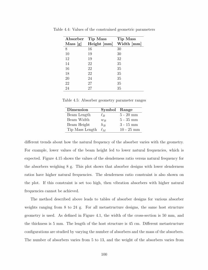
Table 4.4: Values of the constrained geometric parameters
Absorber Tip Mass Tip MassMass [g] Height [mm] Width [mm]8 16 3010 19 3012 19 3214 22 3516 22 3518 22 3520 24 3522 27 3524 27 35
Table 4.5: Absorber geometry parameter ranges
Dimension Symbol RangeBeam Length `B 5 - 20 mmBeam Width wB 5 - 35 mmBeam Height hB 3 - 15 mmTip Mass Length `M 10 - 25 mm
different trends about how the natural frequency of the absorber varies with the geometry.
For example, lower values of the beam height led to lower natural frequencies, which is
expected. Figure 4.15 shows the values of the slenderness ratio versus natural frequency for
the absorbers weighing 8 g. This plot shows that absorber designs with lower slenderness
ratios have higher natural frequencies. The slenderness ratio constraint is also shown on
the plot. If this constraint is set too high, then vibration absorbers with higher natural
frequencies cannot be achieved.
The method described above leads to tables of absorber designs for various absorber
weights ranging from 8 to 24 g. For all metastructure designs, the same host structure
geometry is used. As defined in Figure 4.1, the width of the cross-section is 50 mm, and
the thickness is 5 mm. The length of the host structure is 45 cm. Different metastructure
configurations are studied by varying the number of absorbers and the mass of the absorbers.
The number of absorbers varies from 5 to 13, and the weight of the absorbers varies from
100
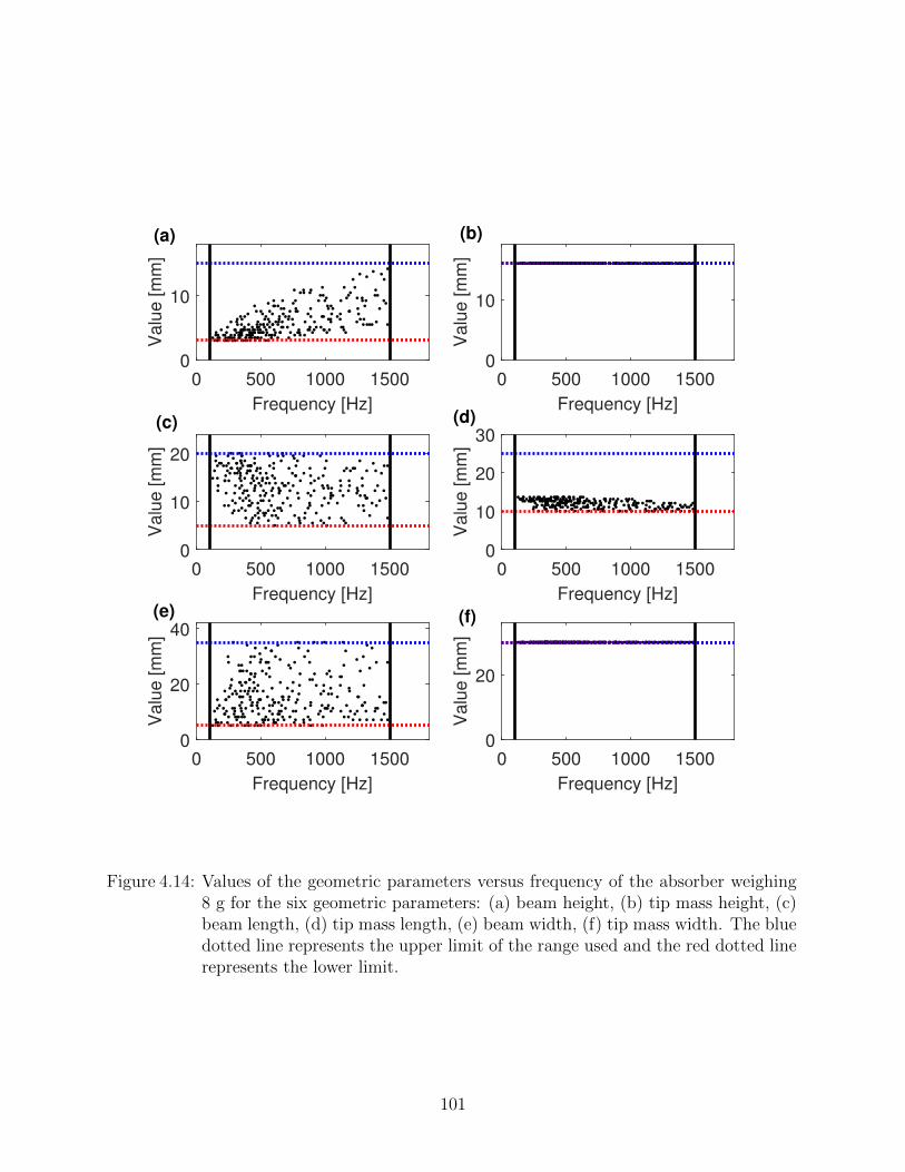
0 500 1000 1500
Frequency [Hz]
0
10
Valu
e [m
m]
0 500 1000 1500
Frequency [Hz]
0
10
Valu
e [m
m]
0 500 1000 1500
Frequency [Hz]
0
10
20
Valu
e [m
m]
0 500 1000 1500
Frequency [Hz]
0
10
20
30
Valu
e [m
m]
0 500 1000 1500
Frequency [Hz]
0
20
40
Valu
e [m
m]
0 500 1000 1500
Frequency [Hz]
0
20
Valu
e [m
m]
(c)
(e)
(a) (b)
(d)
(f)
Figure 4.14: Values of the geometric parameters versus frequency of the absorber weighing8 g for the six geometric parameters: (a) beam height, (b) tip mass height, (c)beam length, (d) tip mass length, (e) beam width, (f) tip mass width. The bluedotted line represents the upper limit of the range used and the red dotted linerepresents the lower limit.
101
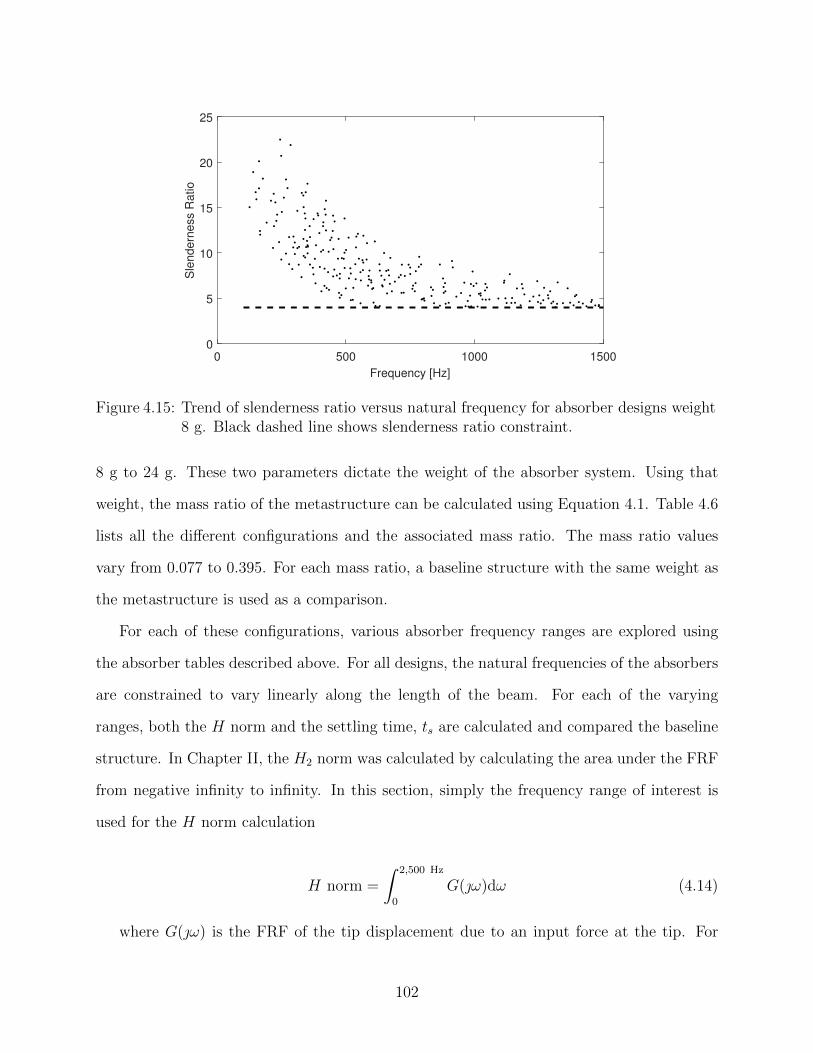
0 500 1000 1500
Frequency [Hz]
0
5
10
15
20
25
Sle
nd
ern
ess R
atio
Figure 4.15: Trend of slenderness ratio versus natural frequency for absorber designs weight8 g. Black dashed line shows slenderness ratio constraint.
8 g to 24 g. These two parameters dictate the weight of the absorber system. Using that
weight, the mass ratio of the metastructure can be calculated using Equation 4.1. Table 4.6
lists all the different configurations and the associated mass ratio. The mass ratio values
vary from 0.077 to 0.395. For each mass ratio, a baseline structure with the same weight as
the metastructure is used as a comparison.
For each of these configurations, various absorber frequency ranges are explored using
the absorber tables described above. For all designs, the natural frequencies of the absorbers
are constrained to vary linearly along the length of the beam. For each of the varying
ranges, both the H norm and the settling time, ts are calculated and compared the baseline
structure. In Chapter II, the H2 norm was calculated by calculating the area under the FRF
from negative infinity to infinity. In this section, simply the frequency range of interest is
used for the H norm calculation
H norm =
∫ 2,500 Hz
0
G(ω)dω (4.14)
where G(ω) is the FRF of the tip displacement due to an input force at the tip. For
102
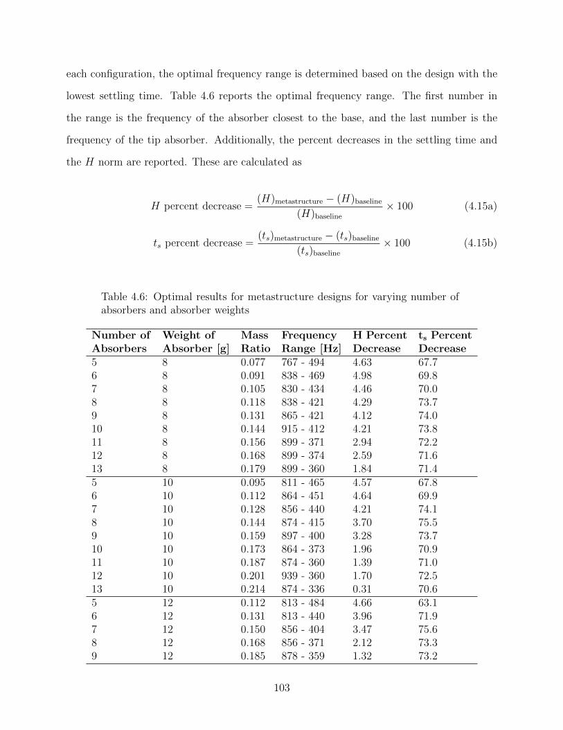
each configuration, the optimal frequency range is determined based on the design with the
lowest settling time. Table 4.6 reports the optimal frequency range. The first number in
the range is the frequency of the absorber closest to the base, and the last number is the
frequency of the tip absorber. Additionally, the percent decreases in the settling time and
the H norm are reported. These are calculated as
H percent decrease =(H)metastructure − (H)baseline
(H)baseline× 100 (4.15a)
ts percent decrease =(ts)metastructure − (ts)baseline
(ts)baseline× 100 (4.15b)
Table 4.6: Optimal results for metastructure designs for varying number ofabsorbers and absorber weights
Number of Weight of Mass Frequency H Percent ts PercentAbsorbers Absorber [g] Ratio Range [Hz] Decrease Decrease5 8 0.077 767 - 494 4.63 67.76 8 0.091 838 - 469 4.98 69.87 8 0.105 830 - 434 4.46 70.08 8 0.118 838 - 421 4.29 73.79 8 0.131 865 - 421 4.12 74.010 8 0.144 915 - 412 4.21 73.811 8 0.156 899 - 371 2.94 72.212 8 0.168 899 - 374 2.59 71.613 8 0.179 899 - 360 1.84 71.45 10 0.095 811 - 465 4.57 67.86 10 0.112 864 - 451 4.64 69.97 10 0.128 856 - 440 4.21 74.18 10 0.144 874 - 415 3.70 75.59 10 0.159 897 - 400 3.28 73.710 10 0.173 864 - 373 1.96 70.911 10 0.187 874 - 360 1.39 71.012 10 0.201 939 - 360 1.70 72.513 10 0.214 874 - 336 0.31 70.65 12 0.112 813 - 484 4.66 63.16 12 0.131 813 - 440 3.96 71.97 12 0.150 856 - 404 3.47 75.68 12 0.168 856 - 371 2.12 73.39 12 0.185 878 - 359 1.32 73.2
103
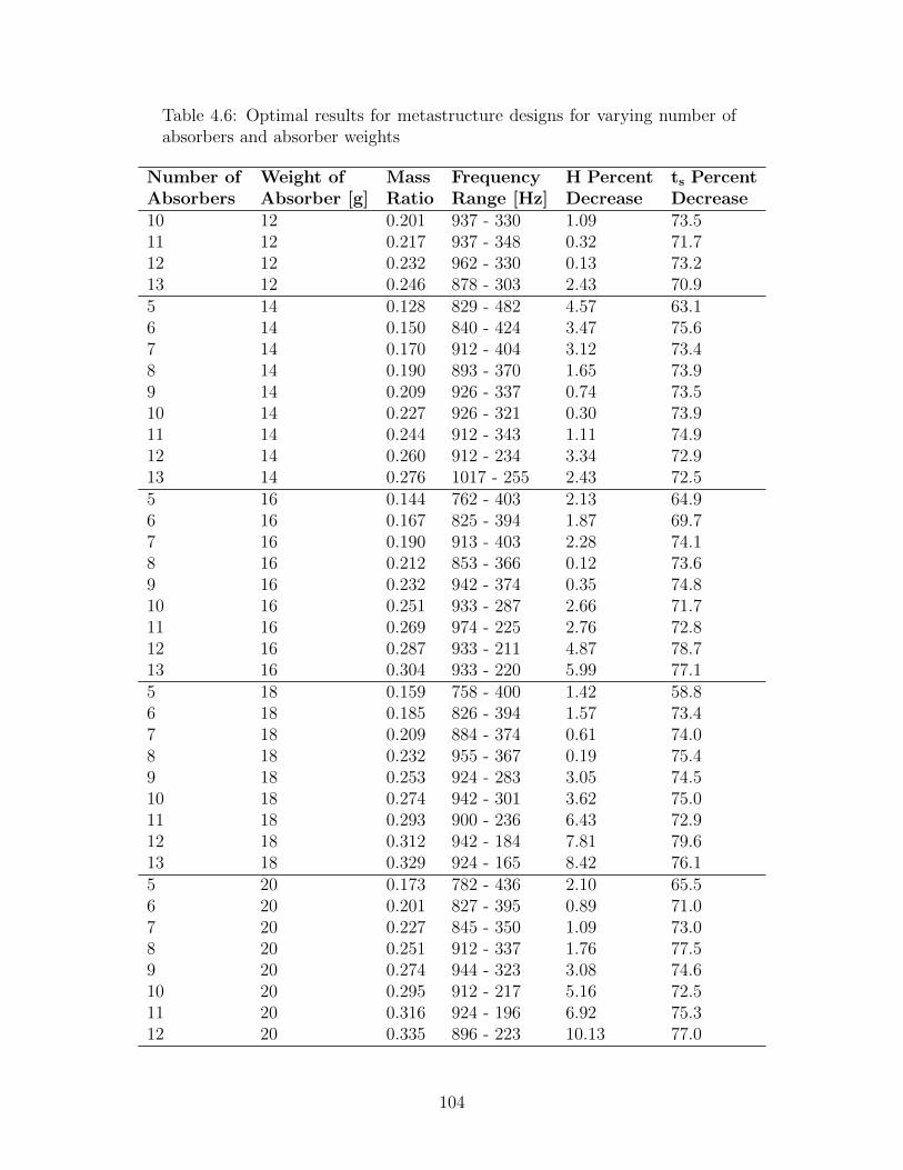
Table 4.6: Optimal results for metastructure designs for varying number ofabsorbers and absorber weights
Number of Weight of Mass Frequency H Percent ts PercentAbsorbers Absorber [g] Ratio Range [Hz] Decrease Decrease10 12 0.201 937 - 330 1.09 73.511 12 0.217 937 - 348 0.32 71.712 12 0.232 962 - 330 0.13 73.213 12 0.246 878 - 303 2.43 70.95 14 0.128 829 - 482 4.57 63.16 14 0.150 840 - 424 3.47 75.67 14 0.170 912 - 404 3.12 73.48 14 0.190 893 - 370 1.65 73.99 14 0.209 926 - 337 0.74 73.510 14 0.227 926 - 321 0.30 73.911 14 0.244 912 - 343 1.11 74.912 14 0.260 912 - 234 3.34 72.913 14 0.276 1017 - 255 2.43 72.55 16 0.144 762 - 403 2.13 64.96 16 0.167 825 - 394 1.87 69.77 16 0.190 913 - 403 2.28 74.18 16 0.212 853 - 366 0.12 73.69 16 0.232 942 - 374 0.35 74.810 16 0.251 933 - 287 2.66 71.711 16 0.269 974 - 225 2.76 72.812 16 0.287 933 - 211 4.87 78.713 16 0.304 933 - 220 5.99 77.15 18 0.159 758 - 400 1.42 58.86 18 0.185 826 - 394 1.57 73.47 18 0.209 884 - 374 0.61 74.08 18 0.232 955 - 367 0.19 75.49 18 0.253 924 - 283 3.05 74.510 18 0.274 942 - 301 3.62 75.011 18 0.293 900 - 236 6.43 72.912 18 0.312 942 - 184 7.81 79.613 18 0.329 924 - 165 8.42 76.15 20 0.173 782 - 436 2.10 65.56 20 0.201 827 - 395 0.89 71.07 20 0.227 845 - 350 1.09 73.08 20 0.251 912 - 337 1.76 77.59 20 0.274 944 - 323 3.08 74.610 20 0.295 912 - 217 5.16 72.511 20 0.316 924 - 196 6.92 75.312 20 0.335 896 - 223 10.13 77.0
104
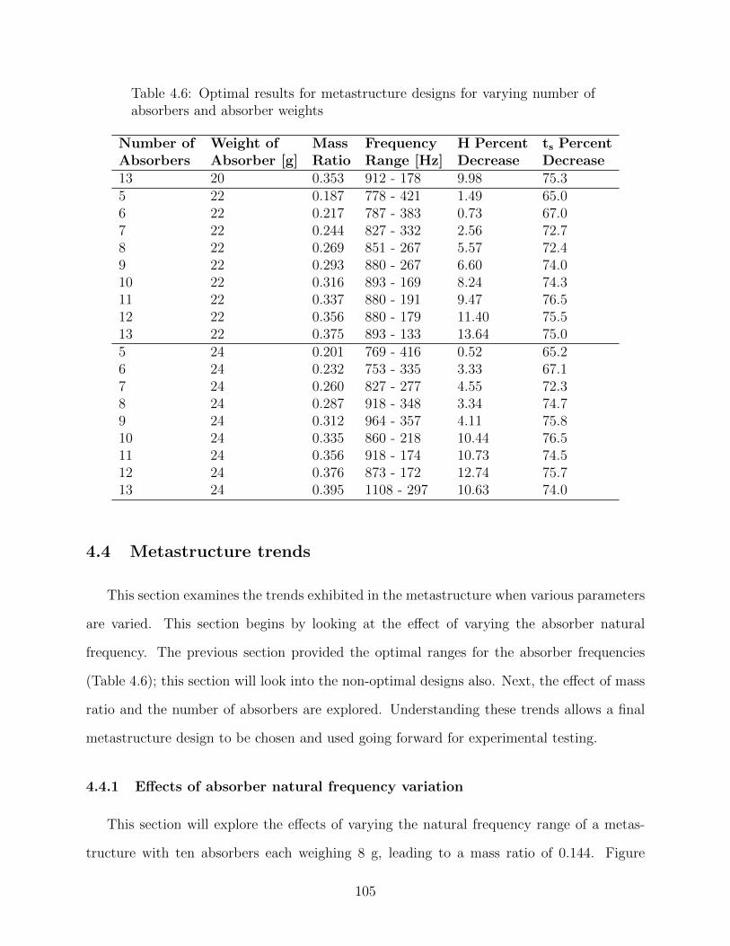
Table 4.6: Optimal results for metastructure designs for varying number ofabsorbers and absorber weights
Number of Weight of Mass Frequency H Percent ts PercentAbsorbers Absorber [g] Ratio Range [Hz] Decrease Decrease13 20 0.353 912 - 178 9.98 75.35 22 0.187 778 - 421 1.49 65.06 22 0.217 787 - 383 0.73 67.07 22 0.244 827 - 332 2.56 72.78 22 0.269 851 - 267 5.57 72.49 22 0.293 880 - 267 6.60 74.010 22 0.316 893 - 169 8.24 74.311 22 0.337 880 - 191 9.47 76.512 22 0.356 880 - 179 11.40 75.513 22 0.375 893 - 133 13.64 75.05 24 0.201 769 - 416 0.52 65.26 24 0.232 753 - 335 3.33 67.17 24 0.260 827 - 277 4.55 72.38 24 0.287 918 - 348 3.34 74.79 24 0.312 964 - 357 4.11 75.810 24 0.335 860 - 218 10.44 76.511 24 0.356 918 - 174 10.73 74.512 24 0.376 873 - 172 12.74 75.713 24 0.395 1108 - 297 10.63 74.0
4.4 Metastructure trends
This section examines the trends exhibited in the metastructure when various parameters
are varied. This section begins by looking at the effect of varying the absorber natural
frequency. The previous section provided the optimal ranges for the absorber frequencies
(Table 4.6); this section will look into the non-optimal designs also. Next, the effect of mass
ratio and the number of absorbers are explored. Understanding these trends allows a final
metastructure design to be chosen and used going forward for experimental testing.
4.4.1 Effects of absorber natural frequency variation
This section will explore the effects of varying the natural frequency range of a metas-
tructure with ten absorbers each weighing 8 g, leading to a mass ratio of 0.144. Figure
105
4.16 shows a contour plot depicting the performance of the structure for various frequency
ranges. The x-axis is the frequency of the tip absorber and the y-axis is the frequency of
the base absorber. The frequencies of the other absorbers varying linearly between those
two values. The color of the contour plot represents the percent decrease in the performance
measures of the structure, where yellow represents better performance and blue represents
worse performance. The top plot, (a) shows the percent decrease in the H norm whereas
the bottom plot, (b) shows the percent decrease in the settling time.
The diagonal line where the frequencies of the tip absorber and the base absorber are
equal represents metastructures in which all the absorbers are tuned to the same natural
frequency. Since the highest values do not lie on this line, we can see that is more beneficial to
have vibration absorbers with varying frequencies, as we saw with the lumped mass model.
Additionally, the contour plot is not symmetric about that line. The upper half, where
the frequency of the base absorber is higher than the frequency of the tip absorber has
higher performance values. This shows that placing the absorbers with higher frequencies
near the base of the metastructure leads to better performance compared to the opposite
arrangement. The agrees with the trends of absorber stiffness observed from the lumped mass
models. When the performance measures are compared, similar trends are observed. The H
norm has more variation where as good settling times are more localized. Additionally, the
H norm percent decrease takes on mostly negative values, meaning the baseline structure is
performing better than the metastructure with respect to the H norm. This will be explored
in more detail when examining the FRFs of specific metastructure designs.
The other configurations take on similar trends. For comparison, the metastructure
design with 13 absorbers weighing 24 g is shown in Figure 4.17. This metastructure has a
much higher mass ratio of 0.395. Although the mass ratio is higher, similar trends hold.
Next, specific metastructure designs for the configuration with ten absorbers weighing 8 g
will be examined in more detail by looking at the FRFs and the impulse response functions.
Figure 4.18 shows the optimal frequency range with respect to settling time where the
106
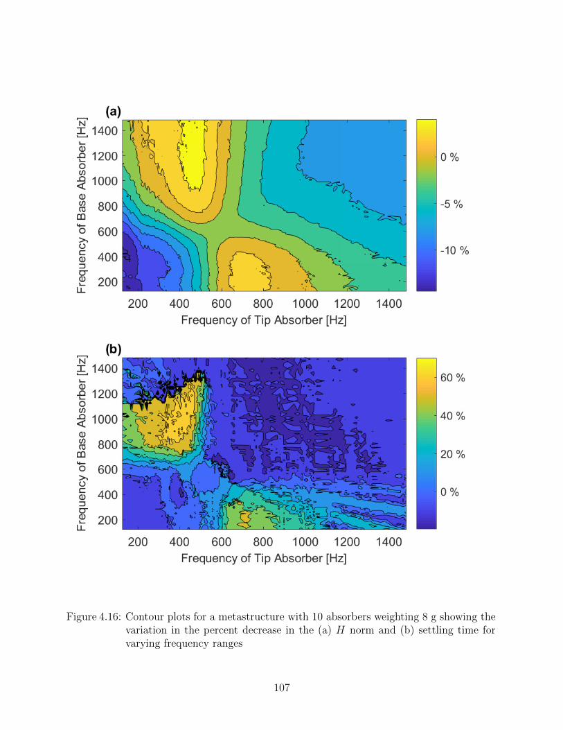
Figure 4.16: Contour plots for a metastructure with 10 absorbers weighting 8 g showing thevariation in the percent decrease in the (a) H norm and (b) settling time forvarying frequency ranges
107
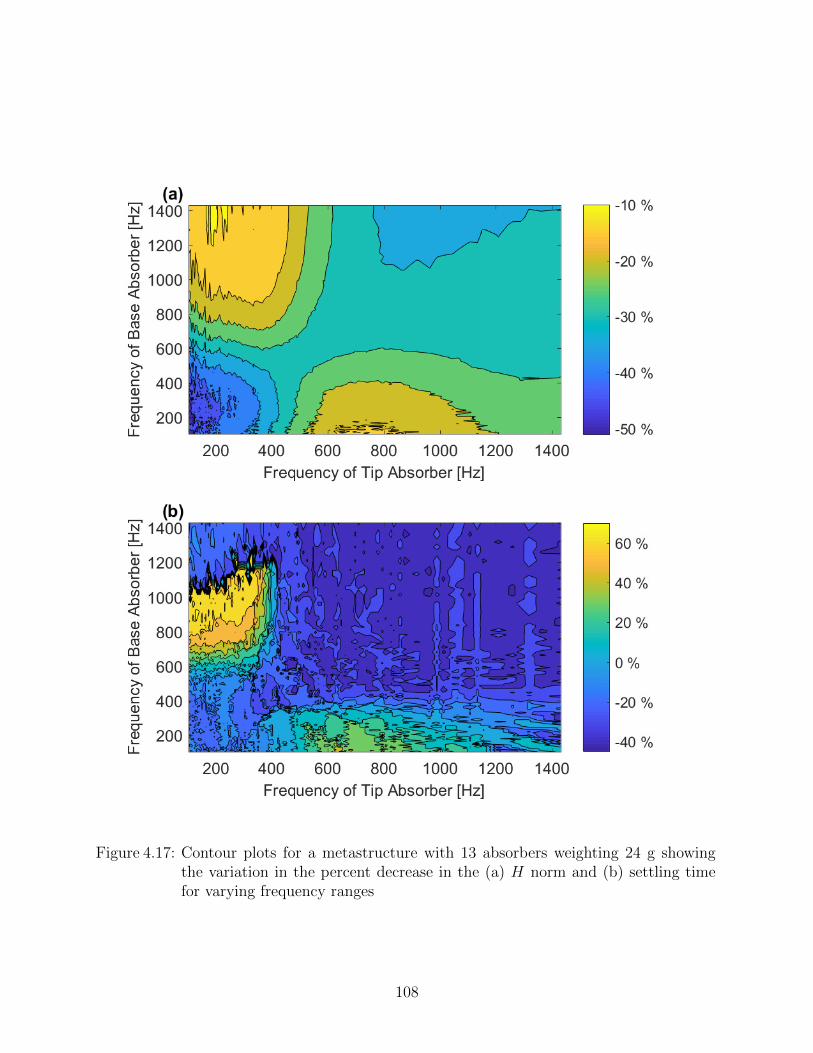
Figure 4.17: Contour plots for a metastructure with 13 absorbers weighting 24 g showingthe variation in the percent decrease in the (a) H norm and (b) settling timefor varying frequency ranges
108
absorbers vary from 915 to 412 Hz. The first number of the range is the frequency of the
base absorber and the second number is the frequency of the tip absorber. The plot on the
left shows the frequency response function of the tip displacement due to an applied force also
at the tip. The plot on the right shows the impulse response function of the tip displacement
due to a unit impulse applied at the tip. The vertical lines represent the settling time for the
corresponding structure. The plots for the optimal structure are compared to the optimal
frequency range with response to the H norm where the absorbers vary from 1,114 to 475
Hz shown in Figure 4.19. The configuration optimized with respect to the H norm provides
slightly better performance for the H norm but significantly worse performance with respect
to the settling time, whereas the design optimized with respect to the settling has good
performance for both the H norm and the setting time. This is why the settling time was
chosen as the performance measure for choosing the optimal frequency ranges.
As another comparison, the metastructure with absorbers having frequencies varying
from 412 to 915 Hz, is shown in Figure 4.20. These absorbers have the same frequencies
as the optimal structure shown in Figure 4.18 but with their locations flipped, meaning the
higher frequency absorbers are near the tip of the metastructure instead of near the base.
The responses of these two structures look very different, showing that the location of the
absorbers makes a significant difference in the response of the structure.
Lastly, a metastructure with all the absorbers tuned to the same frequency is shown
in Figure 4.21. This design shows the characteristic split peak behavior we expect out of
a structure with a single vibration absorber. This aligns with the trends observed in the
lumped mass metastructure results.
4.4.2 Effect of mass ratio and number of absorbers
This section looks at how the mass ratio of the metastructure design impacts the perfor-
mance of the structure. Various configurations with the optimal natural frequency ranges
from Table 4.6 are used to examine these trends. Figure 4.22 shows a plot of the percent de-
109
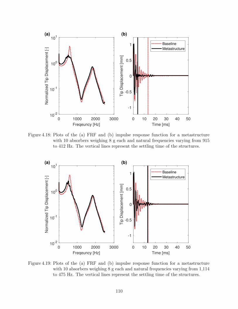
0 1000 2000 3000
Freqeuncy [Hz]
10-2
10-1
100
101
Norm
aliz
ed T
ip D
ispla
cem
ent [-
]
(a)
0 10 20 30 40 50
Time [ms]
-1
-0.5
0
0.5
1
Tip
Dis
pla
cem
ent [m
m]
(b)
Baseline
Metastructure
Figure 4.18: Plots of the (a) FRF and (b) impulse response function for a metastructurewith 10 absorbers weighing 8 g each and natural frequencies varying from 915to 412 Hz. The vertical lines represent the settling time of the structures.
0 1000 2000 3000
Freqeuncy [Hz]
10-2
10-1
100
101
Norm
aliz
ed T
ip D
ispla
cem
ent [-
]
(a)
0 10 20 30 40 50
Time [ms]
-1
-0.5
0
0.5
1
Tip
Dis
pla
cem
ent [m
m]
(b)
Baseline
Metastructure
Figure 4.19: Plots of the (a) FRF and (b) impulse response function for a metastructurewith 10 absorbers weighing 8 g each and natural frequencies varying from 1,114to 475 Hz. The vertical lines represent the settling time of the structures.
110
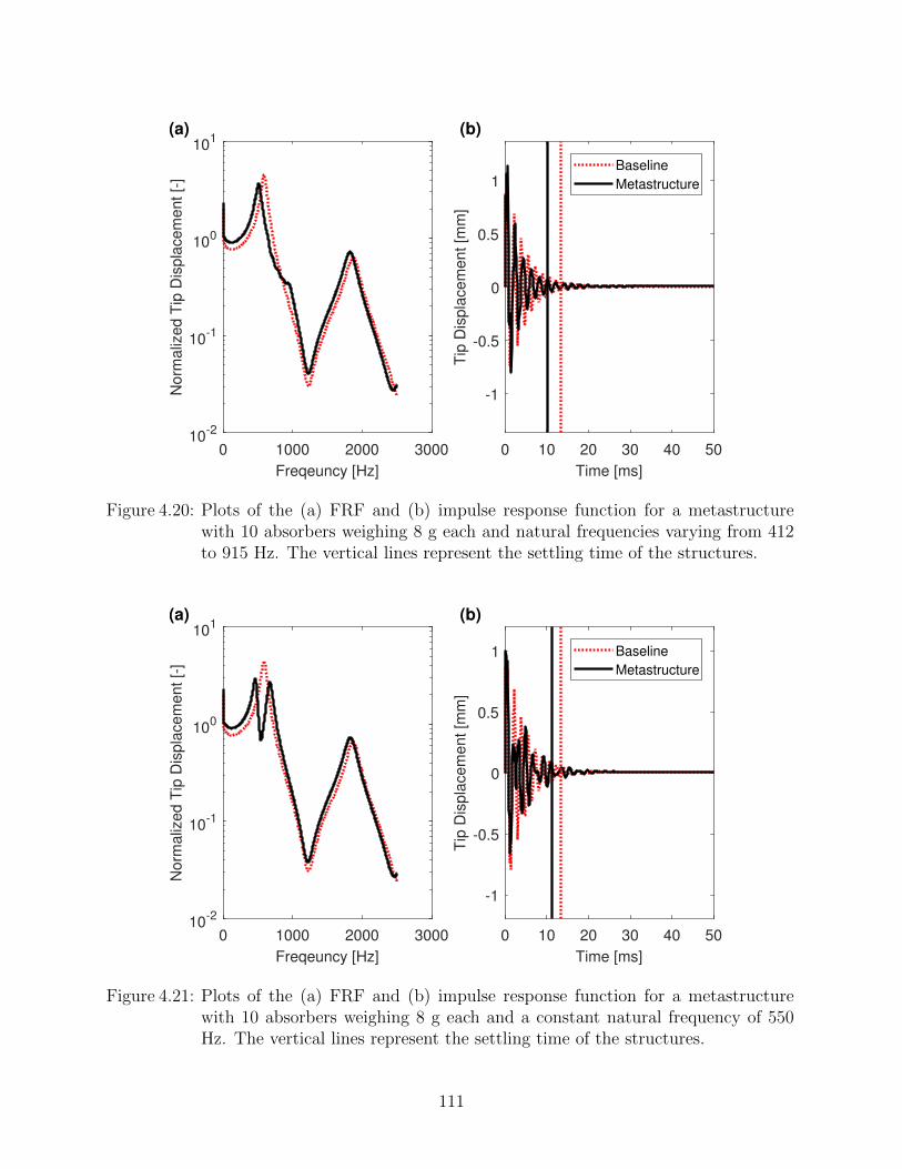
0 1000 2000 3000
Freqeuncy [Hz]
10-2
10-1
100
101
Norm
aliz
ed T
ip D
ispla
cem
ent [-
]
(a)
0 10 20 30 40 50
Time [ms]
-1
-0.5
0
0.5
1
Tip
Dis
pla
cem
ent [m
m]
(b)
Baseline
Metastructure
Figure 4.20: Plots of the (a) FRF and (b) impulse response function for a metastructurewith 10 absorbers weighing 8 g each and natural frequencies varying from 412to 915 Hz. The vertical lines represent the settling time of the structures.
0 1000 2000 3000
Freqeuncy [Hz]
10-2
10-1
100
101
Norm
aliz
ed T
ip D
ispla
cem
ent [-
]
(a)
0 10 20 30 40 50
Time [ms]
-1
-0.5
0
0.5
1
Tip
Dis
pla
cem
ent [m
m]
(b)
Baseline
Metastructure
Figure 4.21: Plots of the (a) FRF and (b) impulse response function for a metastructurewith 10 absorbers weighing 8 g each and a constant natural frequency of 550Hz. The vertical lines represent the settling time of the structures.
111
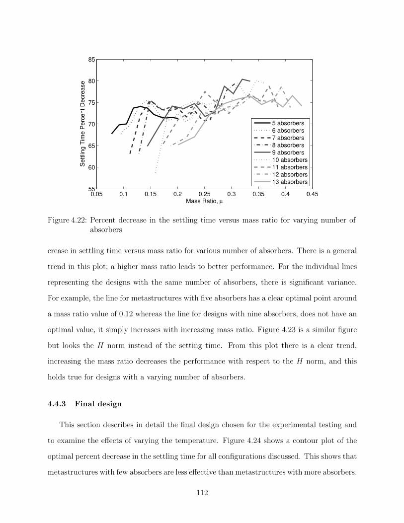
0.05 0.1 0.15 0.2 0.25 0.3 0.35 0.4 0.4555
60
65
70
75
80
85
Mass Ratio, µ
Se
ttlin
g T
ime
Pe
rce
nt
De
cre
ase
5 absorbers
6 absorbers
7 absorbers
8 absorbers
9 absorbers
10 absorbers
11 absorbers
12 absorbers
13 absorbers
Figure 4.22: Percent decrease in the settling time versus mass ratio for varying number ofabsorbers
crease in settling time versus mass ratio for various number of absorbers. There is a general
trend in this plot; a higher mass ratio leads to better performance. For the individual lines
representing the designs with the same number of absorbers, there is significant variance.
For example, the line for metastructures with five absorbers has a clear optimal point around
a mass ratio value of 0.12 whereas the line for designs with nine absorbers, does not have an
optimal value, it simply increases with increasing mass ratio. Figure 4.23 is a similar figure
but looks the H norm instead of the setting time. From this plot there is a clear trend,
increasing the mass ratio decreases the performance with respect to the H norm, and this
holds true for designs with a varying number of absorbers.
4.4.3 Final design
This section describes in detail the final design chosen for the experimental testing and
to examine the effects of varying the temperature. Figure 4.24 shows a contour plot of the
optimal percent decrease in the settling time for all configurations discussed. This shows that
metastructures with few absorbers are less effective than metastructures with more absorbers.
112
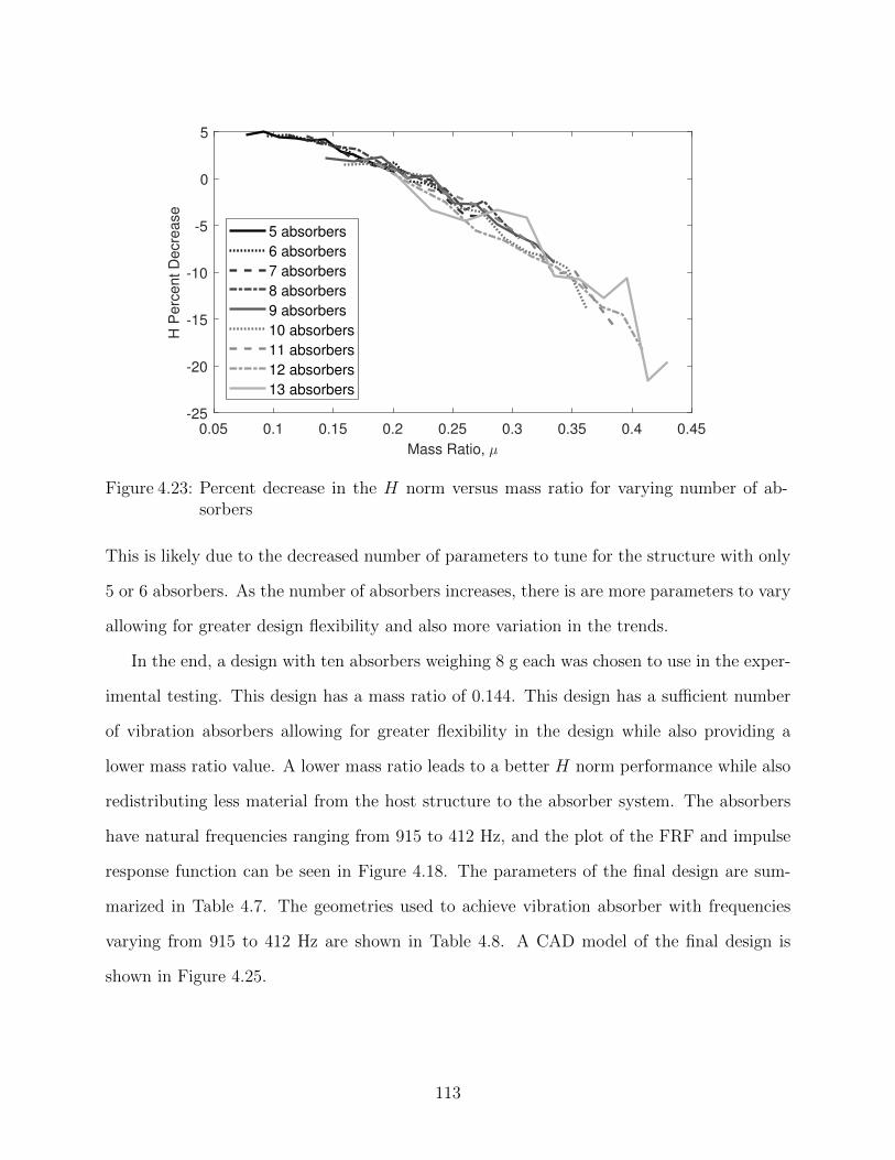
0.05 0.1 0.15 0.2 0.25 0.3 0.35 0.4 0.45
Mass Ratio,
-25
-20
-15
-10
-5
0
5
H P
erc
ent D
ecre
ase
5 absorbers
6 absorbers
7 absorbers
8 absorbers
9 absorbers
10 absorbers
11 absorbers
12 absorbers
13 absorbers
Figure 4.23: Percent decrease in the H norm versus mass ratio for varying number of ab-sorbers
This is likely due to the decreased number of parameters to tune for the structure with only
5 or 6 absorbers. As the number of absorbers increases, there is are more parameters to vary
allowing for greater design flexibility and also more variation in the trends.
In the end, a design with ten absorbers weighing 8 g each was chosen to use in the exper-
imental testing. This design has a mass ratio of 0.144. This design has a sufficient number
of vibration absorbers allowing for greater flexibility in the design while also providing a
lower mass ratio value. A lower mass ratio leads to a better H norm performance while also
redistributing less material from the host structure to the absorber system. The absorbers
have natural frequencies ranging from 915 to 412 Hz, and the plot of the FRF and impulse
response function can be seen in Figure 4.18. The parameters of the final design are sum-
marized in Table 4.7. The geometries used to achieve vibration absorber with frequencies
varying from 915 to 412 Hz are shown in Table 4.8. A CAD model of the final design is
shown in Figure 4.25.
113
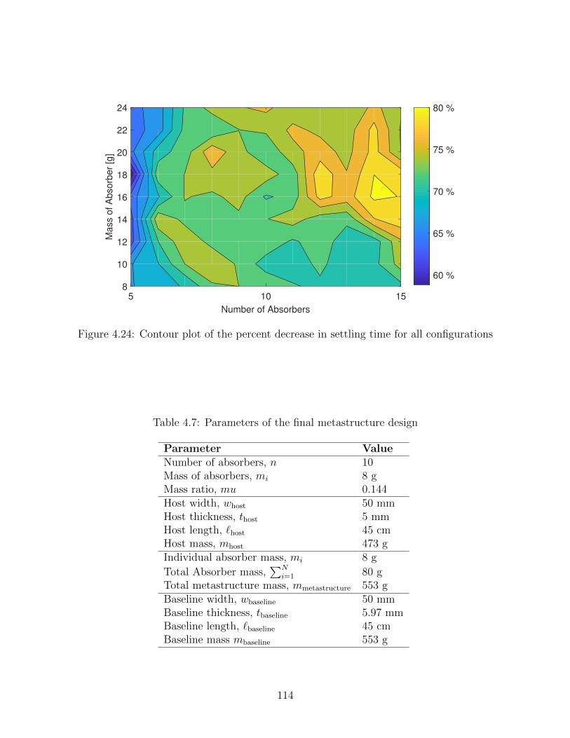
5 10 15
Number of Absorbers
8
10
12
14
16
18
20
22
24M
ass o
f A
bsorb
er
[g]
60 %
65 %
70 %
75 %
80 %
Figure 4.24: Contour plot of the percent decrease in settling time for all configurations
Table 4.7: Parameters of the final metastructure design
Parameter ValueNumber of absorbers, n 10Mass of absorbers, mi 8 gMass ratio, mu 0.144Host width, whost 50 mmHost thickness, thost 5 mmHost length, `host 45 cmHost mass, mhost 473 gIndividual absorber mass, mi 8 g
Total Absorber mass,∑N
i=1 80 gTotal metastructure mass, mmetastructure 553 gBaseline width, wbaseline 50 mmBaseline thickness, tbaseline 5.97 mmBaseline length, `baseline 45 cmBaseline mass mbaseline 553 g
114
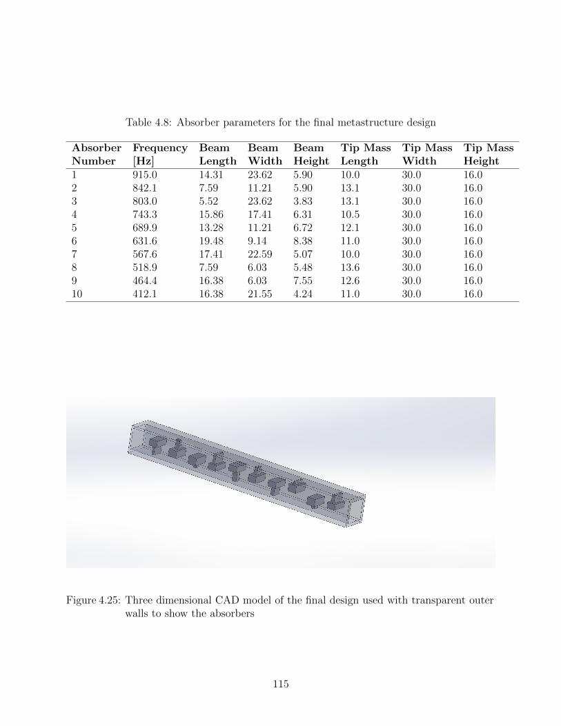
Table 4.8: Absorber parameters for the final metastructure design
Absorber Frequency Beam Beam Beam Tip Mass Tip Mass Tip MassNumber [Hz] Length Width Height Length Width Height1 915.0 14.31 23.62 5.90 10.0 30.0 16.02 842.1 7.59 11.21 5.90 13.1 30.0 16.03 803.0 5.52 23.62 3.83 13.1 30.0 16.04 743.3 15.86 17.41 6.31 10.5 30.0 16.05 689.9 13.28 11.21 6.72 12.1 30.0 16.06 631.6 19.48 9.14 8.38 11.0 30.0 16.07 567.6 17.41 22.59 5.07 10.0 30.0 16.08 518.9 7.59 6.03 5.48 13.6 30.0 16.09 464.4 16.38 6.03 7.55 12.6 30.0 16.010 412.1 16.38 21.55 4.24 11.0 30.0 16.0
Figure 4.25: Three dimensional CAD model of the final design used with transparent outerwalls to show the absorbers
115
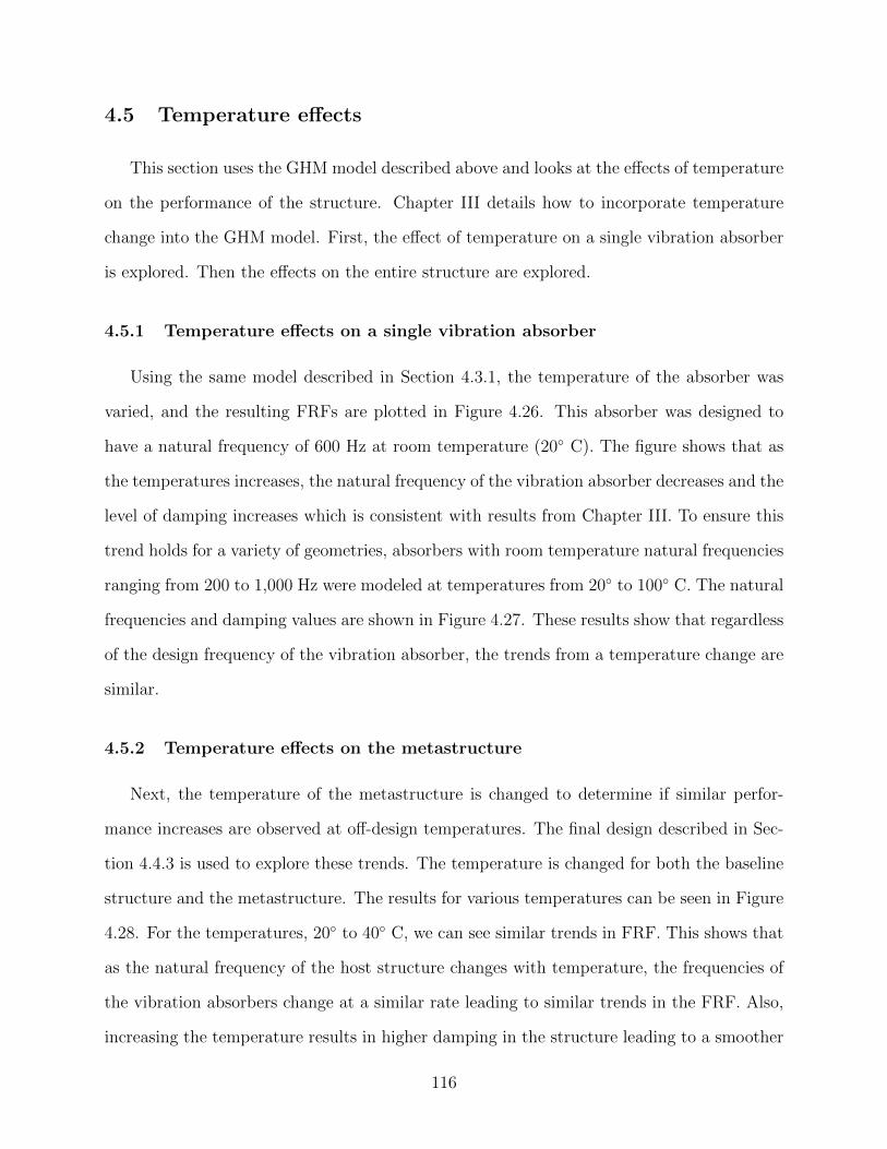
4.5 Temperature effects
This section uses the GHM model described above and looks at the effects of temperature
on the performance of the structure. Chapter III details how to incorporate temperature
change into the GHM model. First, the effect of temperature on a single vibration absorber
is explored. Then the effects on the entire structure are explored.
4.5.1 Temperature effects on a single vibration absorber
Using the same model described in Section 4.3.1, the temperature of the absorber was
varied, and the resulting FRFs are plotted in Figure 4.26. This absorber was designed to
have a natural frequency of 600 Hz at room temperature (20 C). The figure shows that as
the temperatures increases, the natural frequency of the vibration absorber decreases and the
level of damping increases which is consistent with results from Chapter III. To ensure this
trend holds for a variety of geometries, absorbers with room temperature natural frequencies
ranging from 200 to 1,000 Hz were modeled at temperatures from 20 to 100 C. The natural
frequencies and damping values are shown in Figure 4.27. These results show that regardless
of the design frequency of the vibration absorber, the trends from a temperature change are
similar.
4.5.2 Temperature effects on the metastructure
Next, the temperature of the metastructure is changed to determine if similar perfor-
mance increases are observed at off-design temperatures. The final design described in Sec-
tion 4.4.3 is used to explore these trends. The temperature is changed for both the baseline
structure and the metastructure. The results for various temperatures can be seen in Figure
4.28. For the temperatures, 20 to 40 C, we can see similar trends in FRF. This shows that
as the natural frequency of the host structure changes with temperature, the frequencies of
the vibration absorbers change at a similar rate leading to similar trends in the FRF. Also,
increasing the temperature results in higher damping in the structure leading to a smoother
116
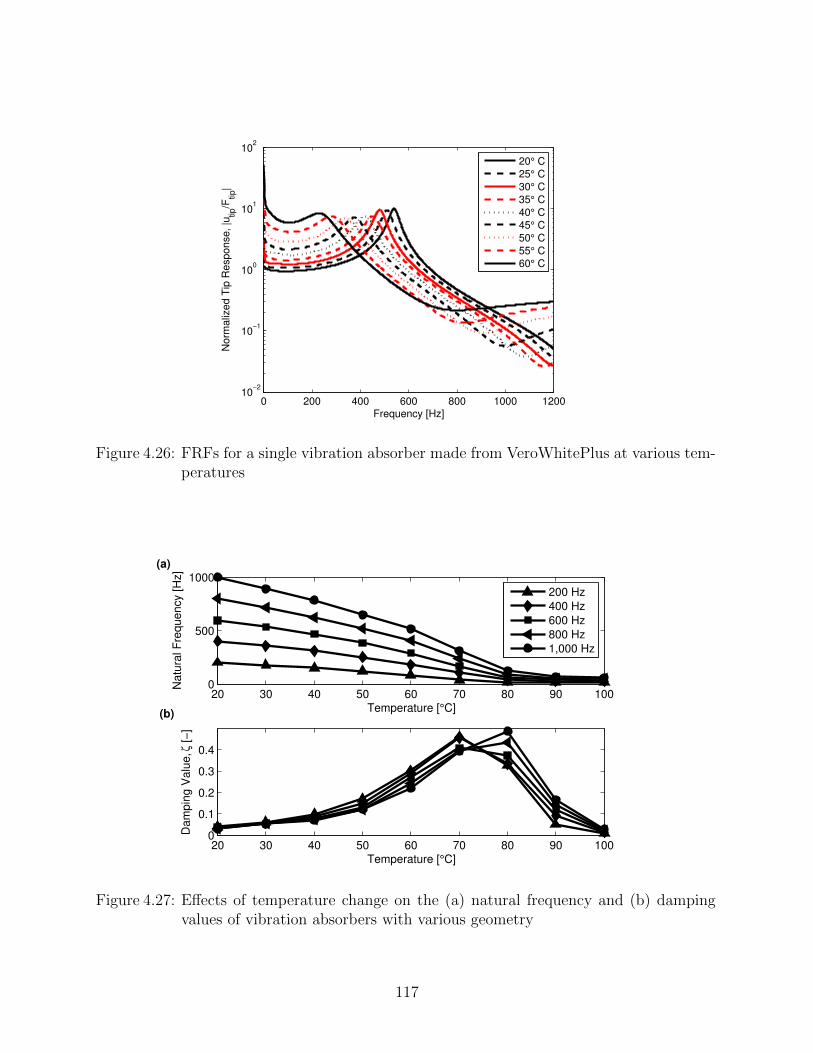
0 200 400 600 800 1000 120010
−2
10−1
100
101
102
Frequency [Hz]
No
rma
lize
d T
ip R
esp
on
se
, |u
tip/F
tip|
20° C
25° C
30° C
35° C
40° C
45° C
50° C
55° C
60° C
Figure 4.26: FRFs for a single vibration absorber made from VeroWhitePlus at various tem-peratures
20 30 40 50 60 70 80 90 1000
500
1000
Temperature [°C]
Natu
ral F
requency [H
z]
200 Hz
400 Hz
600 Hz
800 Hz
1,000 Hz
20 30 40 50 60 70 80 90 1000
0.1
0.2
0.3
0.4
Temperature [°C]
Dam
pin
g V
alu
e, ζ
[−
]
(a)
(b)
Figure 4.27: Effects of temperature change on the (a) natural frequency and (b) dampingvalues of vibration absorbers with various geometry
117
FRF. For temperatures above 30 C, the damping in the structure begins to dominate the
response, almost completely flatting out the curve and leaving only slight differences in the
FRF curves. These trends can also be observed by looking at the impulse response func-
tion for various temperatures, shown in Figure 4.29. In this series of plots, the axes are
constrained to have the same limits to allow for easier comparison. At the temperature
increases, the frequency of the oscillations decreases resulting from the shift in the natural
frequency. Additionally, as the temperature of increases, the initial response of the structure
increases due to the lower modulus of elasticity.
At temperatures ranging from 20 to 70 C, the settling time of the baseline structure
and the metastructure are calculated and plotted in Figure 4.30. Initially, as the tempera-
ture increases, the settling time of both the baseline structure and the metastructure varies
somewhat but stays relatively constant. At 50 C, the settling time of both the metastruc-
ture and the baseline structure rapidly increases. Figure 4.31 shows the same data, but plots
the percent decrease in the setting time as temperature changes. Here, there is a general
trend that as the temperature of the structures increases, the performance of the metas-
tructure compared to the baseline structure decreases. At temperatures of 60 and 70 C,
the baseline structure outperforms the metastructure. This is due to the difference in static
response between the two structures, which can be seen in the slight vertical shift in the
FRF of the metastructure compared to the baseline structure. Since the baseline structure
and the metastructure are constrained to have the same mass, the host structure part of the
metastructure must have a slightly smaller wall thickness than that of the baseline structure.
The smaller thickness causes a decrease in the stiffness of the structure and an increase in
the static response. At higher temperatures, the static response of the structure dominates
the response leading to higher settling times. At lower temperatures, the static response has
a less-significant role in the response.
These results show that the metastructure design can provide performance benefits for a
range of temperatures even if the metastructure is designed for a fixed temperature, but the
118
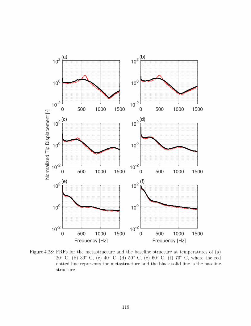
0 500 1000 150010
-2
100
102
(a)
0 500 1000 150010
-2
100
102
(b)
0 500 1000 150010
-2
100
102
Norm
aliz
ed T
ip D
ispla
cem
ent
[-]
(c)
0 500 1000 150010
-2
100
102
(d)
0 500 1000 1500
Frequency [Hz]
10-2
100
102
(e)
0 500 1000 1500
Frequency [Hz]
10-2
100
102
(f)
Figure 4.28: FRFs for the metastructure and the baseline structure at temperatures of (a)20 C, (b) 30 C, (c) 40 C, (d) 50 C, (e) 60 C, (f) 70 C, where the reddotted line represents the metastructure and the black solid line is the baselinestructure
119
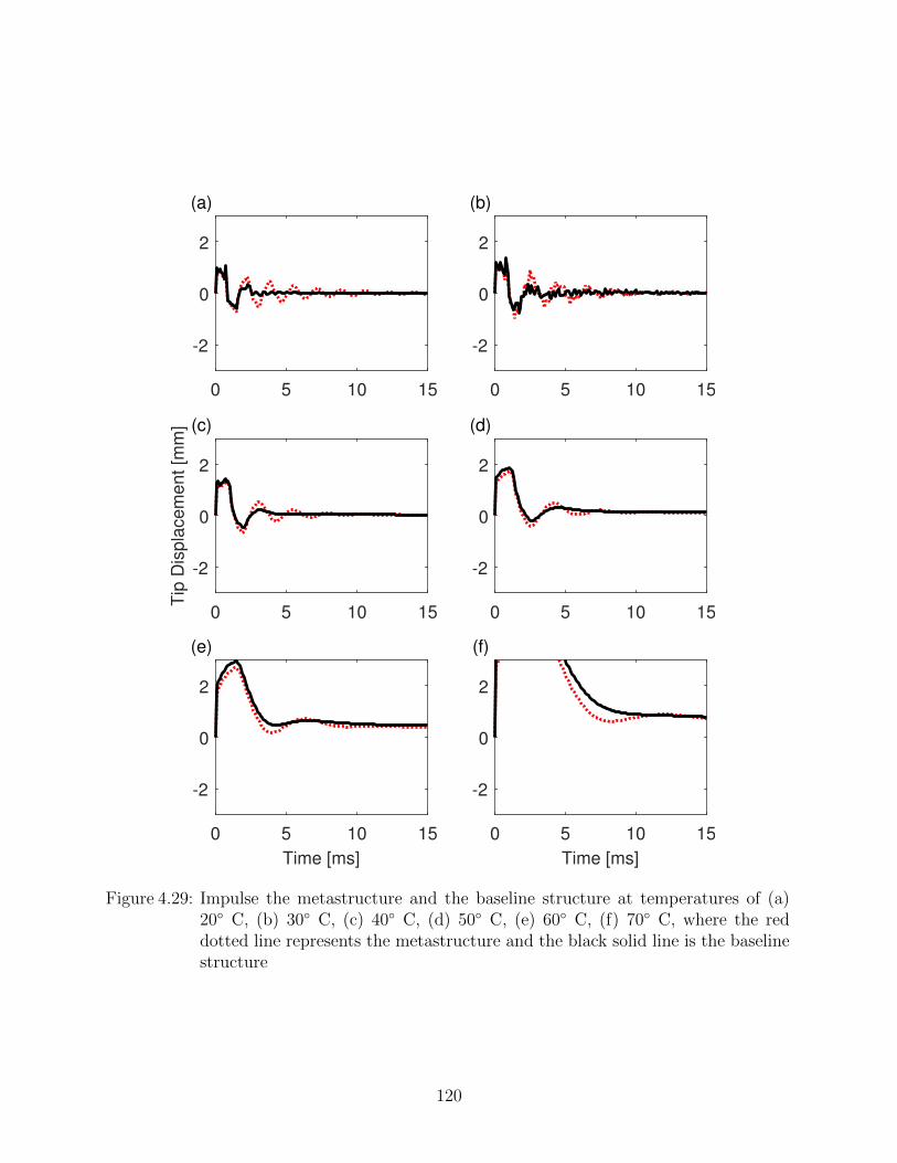
0 5 10 15
-2
0
2
(a)
0 5 10 15
-2
0
2
(b)
0 5 10 15
-2
0
2
Tip
Dis
pla
cem
ent [m
m] (c)
0 5 10 15
-2
0
2
(d)
0 5 10 15
Time [ms]
-2
0
2
(e)
0 5 10 15
Time [ms]
-2
0
2
(f)
Figure 4.29: Impulse the metastructure and the baseline structure at temperatures of (a)20 C, (b) 30 C, (c) 40 C, (d) 50 C, (e) 60 C, (f) 70 C, where the reddotted line represents the metastructure and the black solid line is the baselinestructure
120
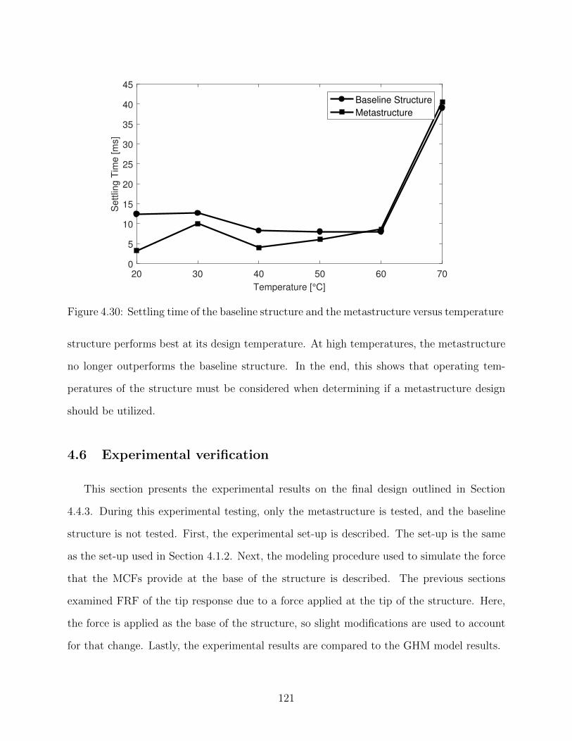
20 30 40 50 60 70
Temperature [°C]
0
5
10
15
20
25
30
35
40
45
Settlin
g T
ime [m
s]
Baseline Structure
Metastructure
Figure 4.30: Settling time of the baseline structure and the metastructure versus temperature
structure performs best at its design temperature. At high temperatures, the metastructure
no longer outperforms the baseline structure. In the end, this shows that operating tem-
peratures of the structure must be considered when determining if a metastructure design
should be utilized.
4.6 Experimental verification
This section presents the experimental results on the final design outlined in Section
4.4.3. During this experimental testing, only the metastructure is tested, and the baseline
structure is not tested. First, the experimental set-up is described. The set-up is the same
as the set-up used in Section 4.1.2. Next, the modeling procedure used to simulate the force
that the MCFs provide at the base of the structure is described. The previous sections
examined FRF of the tip response due to a force applied at the tip of the structure. Here,
the force is applied as the base of the structure, so slight modifications are used to account
for that change. Lastly, the experimental results are compared to the GHM model results.
121
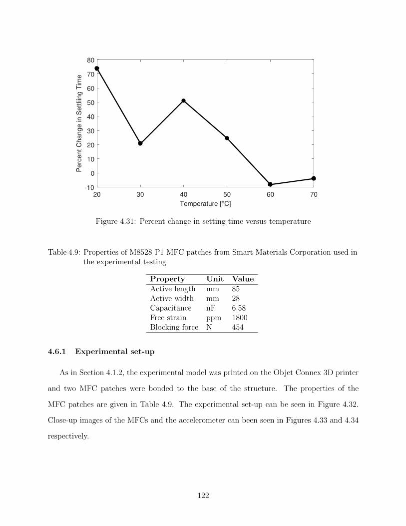
20 30 40 50 60 70
Temperature [°C]
-10
0
10
20
30
40
50
60
70
80
Perc
ent C
hange in S
ettlii
ng T
ime
Figure 4.31: Percent change in setting time versus temperature
Table 4.9: Properties of M8528-P1 MFC patches from Smart Materials Corporation used inthe experimental testing
Property Unit ValueActive length mm 85Active width mm 28Capacitance nF 6.58Free strain ppm 1800Blocking force N 454
4.6.1 Experimental set-up
As in Section 4.1.2, the experimental model was printed on the Objet Connex 3D printer
and two MFC patches were bonded to the base of the structure. The properties of the
MFC patches are given in Table 4.9. The experimental set-up can be seen in Figure 4.32.
Close-up images of the MFCs and the accelerometer can been seen in Figures 4.33 and 4.34
respectively.
122
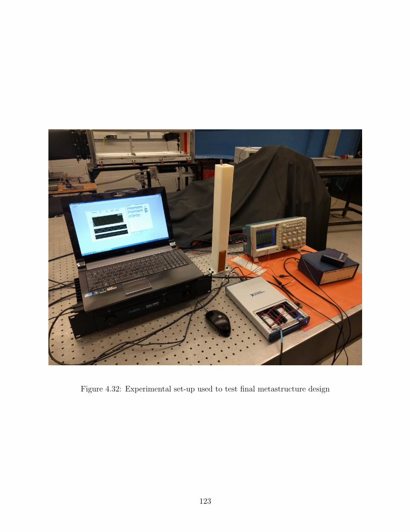
Figure 4.32: Experimental set-up used to test final metastructure design
123
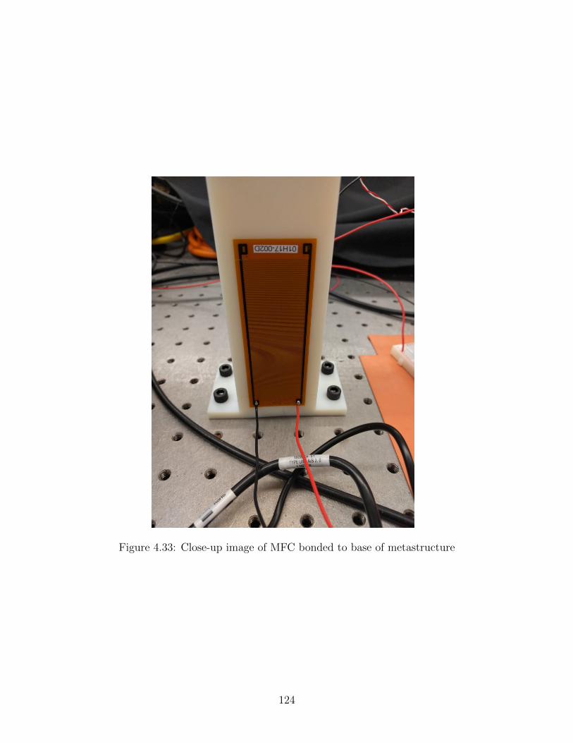
Figure 4.33: Close-up image of MFC bonded to base of metastructure
124
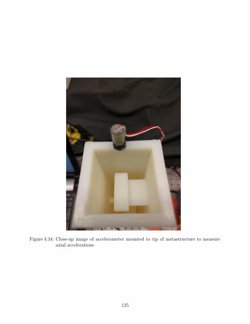
Figure 4.34: Close-up image of accelerometer mounted to tip of metastructure to measureaxial accelerations
125
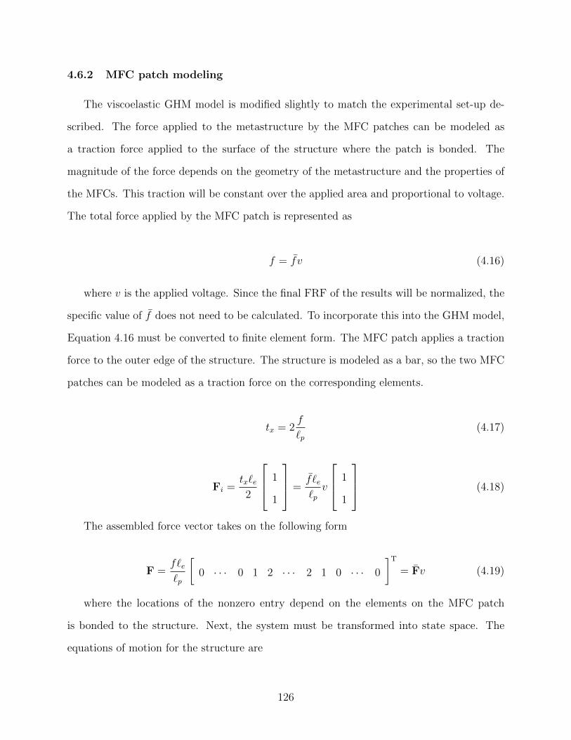
4.6.2 MFC patch modeling
The viscoelastic GHM model is modified slightly to match the experimental set-up de-
scribed. The force applied to the metastructure by the MFC patches can be modeled as
a traction force applied to the surface of the structure where the patch is bonded. The
magnitude of the force depends on the geometry of the metastructure and the properties of
the MFCs. This traction will be constant over the applied area and proportional to voltage.
The total force applied by the MFC patch is represented as
f = fv (4.16)
where v is the applied voltage. Since the final FRF of the results will be normalized, the
specific value of f does not need to be calculated. To incorporate this into the GHM model,
Equation 4.16 must be converted to finite element form. The MFC patch applies a traction
force to the outer edge of the structure. The structure is modeled as a bar, so the two MFC
patches can be modeled as a traction force on the corresponding elements.
tx = 2f
`p(4.17)
Fi =tx`e2
1
1
=f `e`pv
1
1
(4.18)
The assembled force vector takes on the following form
F =f`e`p
[0 · · · 0 1 2 · · · 2 1 0 · · · 0
]T= Fv (4.19)
where the locations of the nonzero entry depend on the elements on the MFC patch
is bonded to the structure. Next, the system must be transformed into state space. The
equations of motion for the structure are
126
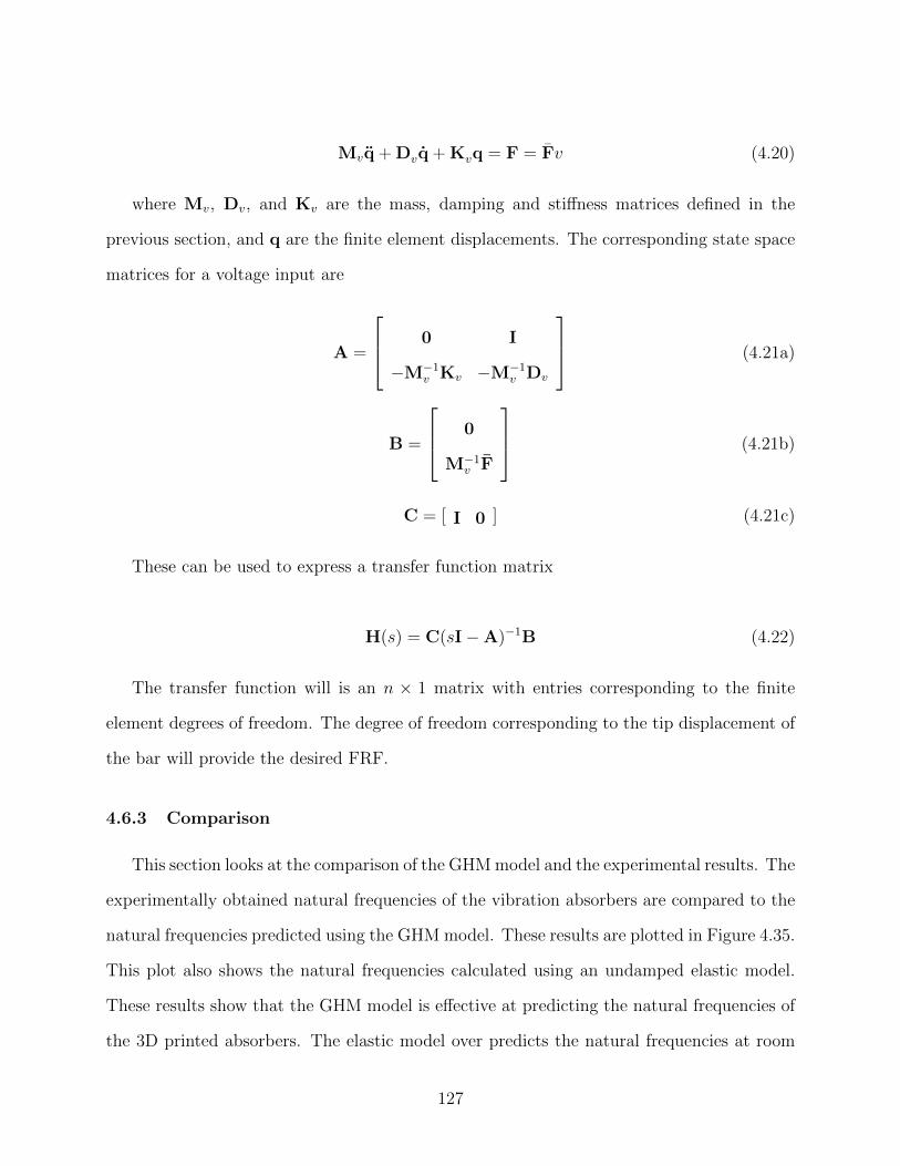
Mvq + Dvq + Kvq = F = Fv (4.20)
where Mv, Dv, and Kv are the mass, damping and stiffness matrices defined in the
previous section, and q are the finite element displacements. The corresponding state space
matrices for a voltage input are
A =
0 I
−M−1v Kv −M−1
v Dv
(4.21a)
B =
0
M−1v F
(4.21b)
C = [ I 0 ] (4.21c)
These can be used to express a transfer function matrix
H(s) = C(sI−A)−1B (4.22)
The transfer function will is an n × 1 matrix with entries corresponding to the finite
element degrees of freedom. The degree of freedom corresponding to the tip displacement of
the bar will provide the desired FRF.
4.6.3 Comparison
This section looks at the comparison of the GHM model and the experimental results. The
experimentally obtained natural frequencies of the vibration absorbers are compared to the
natural frequencies predicted using the GHM model. These results are plotted in Figure 4.35.
This plot also shows the natural frequencies calculated using an undamped elastic model.
These results show that the GHM model is effective at predicting the natural frequencies of
the 3D printed absorbers. The elastic model over predicts the natural frequencies at room
127
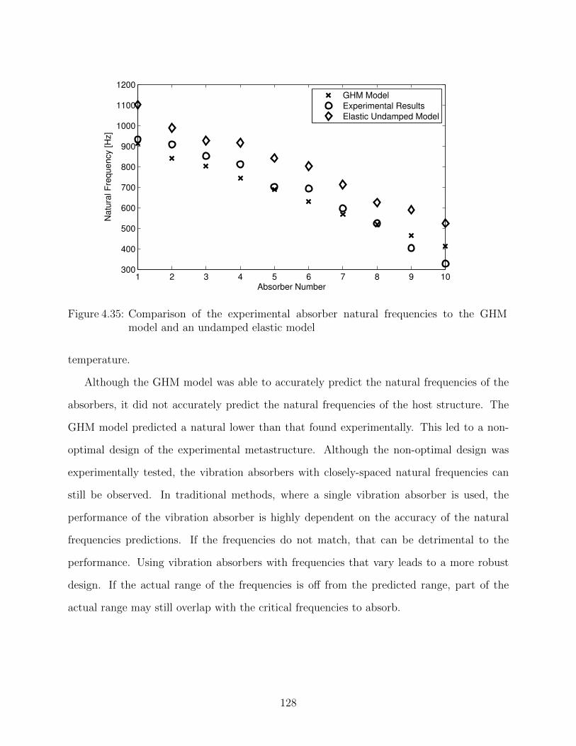
1 2 3 4 5 6 7 8 9 10300
400
500
600
700
800
900
1000
1100
1200
Absorber Number
Na
tura
l F
req
ue
ncy [
Hz]
GHM Model
Experimental Results
Elastic Undamped Model
Figure 4.35: Comparison of the experimental absorber natural frequencies to the GHMmodel and an undamped elastic model
temperature.
Although the GHM model was able to accurately predict the natural frequencies of the
absorbers, it did not accurately predict the natural frequencies of the host structure. The
GHM model predicted a natural lower than that found experimentally. This led to a non-
optimal design of the experimental metastructure. Although the non-optimal design was
experimentally tested, the vibration absorbers with closely-spaced natural frequencies can
still be observed. In traditional methods, where a single vibration absorber is used, the
performance of the vibration absorber is highly dependent on the accuracy of the natural
frequencies predictions. If the frequencies do not match, that can be detrimental to the
performance. Using vibration absorbers with frequencies that vary leads to a more robust
design. If the actual range of the frequencies is off from the predicted range, part of the
actual range may still overlap with the critical frequencies to absorb.
128
4.7 Chapter summary
This chapter presents a metastructure design with vibration absorbers with linearly vary-
ing natural frequencies modeled using a distributed mass viscoelastic model. The design used
consists of a bar with a hollow square cross-section with vibration absorbers distributed along
the length of the bar. The vibration absorbers are cantilevered beams with large tip masses
and arranged such that the bending motion of the beam suppresses vibration in the axial
direction of the bar. The main contribution of this chapter is showing that a distributed
mass metastructure can have better performance than a comparable baseline structure of
the same weight. This was previously shown for the lumped mass model, and here it is also
shown for the distributed mass viscoelastic model.
This chapter begins by explaining the design used throughout the rest of the chapter and
by using a commercial finite element model and experimental results to show this design
produces the expected behavior. Next, this chapter goes into detail about how to model the
metastructure design proposed using a viscoelastic GHM model. The GHM model incorpo-
rates the damping inherent in the 3D printed materials while also providing a model that
takes into account temperature change. After the modeling strategies are presented, a de-
tailed design approach is presented. This dissertation shows the complete process necessary
to implement the GHM model in a metastructure. It starts with the material characteriza-
tion of the 3D printed material in Chapter III and then shows how that data can be used to
create a GHM model of a metastructure in this chapter.
The benefits of using the GHM model are two-fold. First, the model incorporates damp-
ing into the model based on material properties and second, the GHM model can account
for temperature change. A change in temperature can significantly alter both the storage
modulus and the loss modulus of the material; these changes lead to changes in the natural
frequencies and the damping of the resulting structure. The GHM model can capture these
effects.
The GHM model developed was used to model the dynamics of a metastructure and
129
studies the effects of changing temperature. The results showed that the changes in the
natural frequency of the host structure and the vibration absorbers changed at a similar rate,
resulting in similar trends in the dynamic response as the temperature increase. This was
true up until a specific temperature when the performance of the metastructure significantly
decreased resulting in the baseline structure have better performance.
Lastly, the GHM model of the metastructure is compared to experimental results. These
results showed that the experimental metastructure successfully absorbed vibrations at vary-
ing frequencies by using the vibration absorbers with linearly varying natural frequencies.
The GHM model was not able to accurately predict the natural frequency of the host struc-
ture, producing a non-optimal design where the absorbers were absorbing frequencies lower
than necessary based on the predicted design. This shows that although there are many
benefits to using the GHM model, more needs to go into ensuring the model can predict the
natural frequency of structure made from these 3D printed structures.
This work provides a crucial first step in gaining a better understanding of how to model
the viscoelastic natural of 3D printed materials. Future work can explore the variability of
the properties of the 3D printed materials and also how the storage modulus and loss factor
are experimentally tested and how the GHM model parameters are determined.
130
CHAPTER V
Active Vibration Control of a Metastructure
As previous chapters have shown, the concept of adding distributed vibration absorbers,
to create a metastructure, has been shown to improve the performance of the structure,
but these structures still suffer from the effects of temperatures changes. This chapter
will examine the effects of adding an active vibration control system to a metastructure to
counteract the effects of temperature change. The control system is implemented through a
single actuator placed on the structure, and the Positive Position Feedback (PPF) control
law is utilized. This chapter begins by explaining the details of the PPF control law then
describes the performance measures used. Both the settling time and the H2 norm are used,
but the emphasis is placed on the settling time since it can be measured in real-time.
The active vibration control concept is examined for both a lumped mass model and a
distributed mass model, using the models developed in Chapters II and IV. For the lumped
mass model, first, the observability and controllability norms are examined to determine
how the actuator and sensor locations affect the controllability and observability of the
structure. Next, two different lumped mass models designs are examined, a structure that
is optimized with respect to the H2 norm and a structure that is optimized with respect
to the settling time. The location of control force varies by the allowing the force to be
applied to each absorber. For each location, the controller parameters are optimized using
the settling time. This provides insight into how the location of the actuator affects the
131
performance. The relationship between the gain and the settling time is also explored. For
the distributed mass models, the design from Chapter IV is used. The control force is applied
to the absorber masses using piezoelectric actuators. Two different concepts are explored,
one where a stack actuator is attached to the absorber mass and second where a piezoelectric
bimorph configuration is added to the beam of one of the absorbers. The addition of the
piezoelectric materials changes the stiffness of the absorbers, thus must be accounted for in
the design of the metastructure. For each of these cases, the modeling used is described in
addition to how the actuators can be used within the PPF control algorithms.
5.1 PPF control law and settling time
The control law used in this chapter is the PPF control law with a single actuator
on the structure. A single actuator is used because of its ease of implementation into a
metastructure. PPF was first introduced by Goh and Caughey in 1985 and is a popular
control method used in vibration control [87]. This control law adds additional dynamics to
the system. PPF is utilized because of its ease of implementation for vibration control; the
controller can be designed around an experimental transfer function and does not require
an analytic model [73]. Here, the PPF control law will be demonstrated using a single
degree of freedom system. Later in this chapter, the formulation will be developed for the
metastructure and will use piezoelectric materials. For a single degree of freedom system,
the equation of motion is
x+ 2ζωnx+ ω2nx = bu (5.1)
where ζ and ωn are the damping ratio and natural frequency of the structure, x is the
displacement of the structure, u is the control input, and b is the input coefficient. A
compensator is defined as
132
η + 2ζfωf η + ω2fη = gωfx (5.2a)
u =g
bωfη (5.2b)
where η is the value of the compensator, ζf and ωf are the damping ratio and natural
frequency of the controller, and g is the gain, a constant value. Combining Equations 5.1
and 5.2 results in equations of motion in their usual second-order form
x
η
+
2ζωn 0
0 2ζfωf
x
η
+
ω2n −gωf
−gωf ω2f
x
η
=
0
0
(5.3)
To ensure stability of this system, the augmented stiffness matrix must be positive def-
inite. A matrix is positive definite when the determinant of the matrix is positive, leading
to the following stability requirement
g2 < ω2n (5.4)
This chapter references both the H2 norm and the settling time as performance measures.
The H2 is defined in detail in Section 2.2. The settling time calculation will be described
here.
The settling time uses the time response to an impulse response function and determines
when the value of the system falls below a predefined threshold. The impulse response, h(t),
is calculated once the system is put into state space as
h(t) = CeAtB (5.5)
The time at which the error falls below a threshold value is known as the setting time,
ts and occurs with the following relationship is met
133
|h(ts)− hf | = δh0 (5.6)
where hf is the final steady-state value, δ is the threshold percentage and h0 is the initial
value after the impulse. For this dissertation, the threshold percentage used is 5%.
5.2 Lumped mass metastructure model
This section will examine the lumped mass metastructure model developed in Chapter
II. The section begins by examining the controllability and observability of the lumped mass
metastructure model to determine the effects of where the controller force is placed. Next,
the PPF control law is implemented into two different metastructure designs [105]. Note
that the previous work uses q(t) to represent the displacement of the masses, here x(t) will
be used to avoid confusion with charge used later. The lumped mass model used is seen in
Figure 5.1 where Figure 5.1a shows the control force acting on one of the absorber masses
and Figure 5.1b shows. the control force acting on one of the host masses.
5.2.1 Observability and controllability
To determine the best placement of the sensor and actuator, we will examine the control-
lability and observability norms [106, 107]. This analysis is done on a lumped mass model
with ten absorbers, a mass ratio of 0.3, and linearly varying natural frequencies optimized
with respect to the H2 norm. The FRF response of this structure is shown in Figure 5.2.
The equations of motion of this structure including the control force and sensing are
Mx(t) + Dx(t) + Kx(t) = Bfu(t) (5.7a)
y(t) = Cpx(t) + Cvx(t) (5.7b)
134
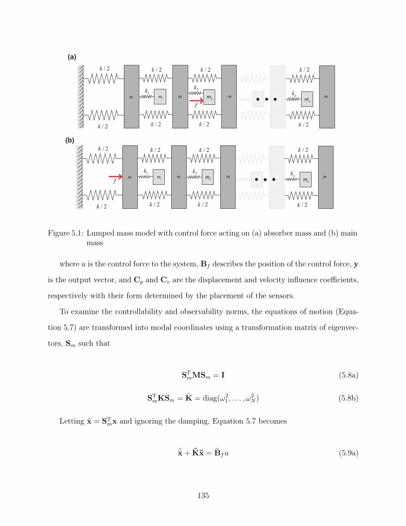
/ 2k
/ 2k
1m m
/ 2k
/ 2k
mm1k
2m
2k
/ 2k
/ 2k
/ 2k
/ 2k
mnm
nk
f
/ 2k
/ 2k
1m m
/ 2k
/ 2k
mm1k
2m
2k
/ 2k
/ 2k
/ 2k
/ 2k
mnm
nk
f
(a)
(b)
Figure 5.1: Lumped mass model with control force acting on (a) absorber mass and (b) mainmass
where u is the control force to the system, Bf describes the position of the control force, y
is the output vector, and Cp and Cv are the displacement and velocity influence coefficients,
respectively with their form determined by the placement of the sensors.
To examine the controllability and observability norms, the equations of motion (Equa-
tion 5.7) are transformed into modal coordinates using a transformation matrix of eigenvec-
tors, Sm such that
STmMSm = I (5.8a)
STmKSm = K = diag(ω2
1, . . . , ω2N) (5.8b)
Letting x = STmx and ignoring the damping, Equation 5.7 becomes
¨x + Kx = Bfu (5.9a)
135
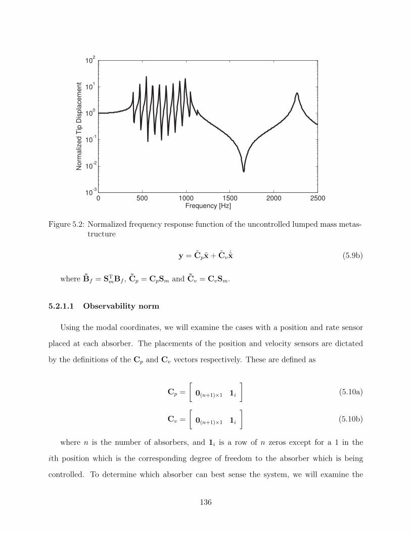
0 500 1000 1500 2000 250010
-3
10-2
10-1
100
101
102
Frequency [Hz]
Norm
aliz
ed T
ip D
ispla
cem
ent
Figure 5.2: Normalized frequency response function of the uncontrolled lumped mass metas-tructure
y = Cpx + Cv˙x (5.9b)
where Bf = STmBf , Cp = CpSm and Cv = CvSm.
5.2.1.1 Observability norm
Using the modal coordinates, we will examine the cases with a position and rate sensor
placed at each absorber. The placements of the position and velocity sensors are dictated
by the definitions of the Cp and Cv vectors respectively. These are defined as
Cp =
[0(n+1)×1 1i
](5.10a)
Cv =
[0(n+1)×1 1i
](5.10b)
where n is the number of absorbers, and 1i is a row of n zeros except for a 1 in the
ith position which is the corresponding degree of freedom to the absorber which is being
controlled. To determine which absorber can best sense the system, we will examine the
136
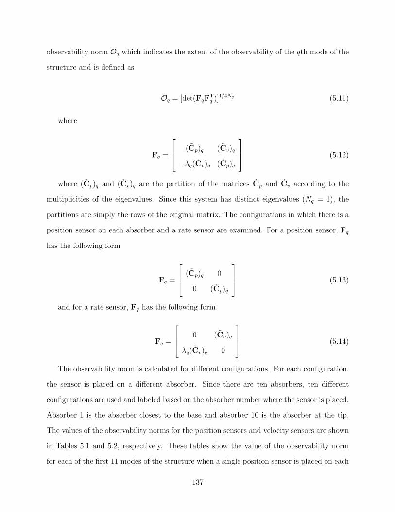
observability norm Oq which indicates the extent of the observability of the qth mode of the
structure and is defined as
Oq = [det(FqFTq )]1/4Nq (5.11)
where
Fq =
(Cp)q (Cv)q
−λq(Cv)q (Cp)q
(5.12)
where (Cp)q and (Cv)q are the partition of the matrices Cp and Cv according to the
multiplicities of the eigenvalues. Since this system has distinct eigenvalues (Nq = 1), the
partitions are simply the rows of the original matrix. The configurations in which there is a
position sensor on each absorber and a rate sensor are examined. For a position sensor, Fq
has the following form
Fq =
(Cp)q 0
0 (Cp)q
(5.13)
and for a rate sensor, Fq has the following form
Fq =
0 (Cv)q
λq(Cv)q 0
(5.14)
The observability norm is calculated for different configurations. For each configuration,
the sensor is placed on a different absorber. Since there are ten absorbers, ten different
configurations are used and labeled based on the absorber number where the sensor is placed.
Absorber 1 is the absorber closest to the base and absorber 10 is the absorber at the tip.
The values of the observability norms for the position sensors and velocity sensors are shown
in Tables 5.1 and 5.2, respectively. These tables show the value of the observability norm
for each of the first 11 modes of the structure when a single position sensor is placed on each
137
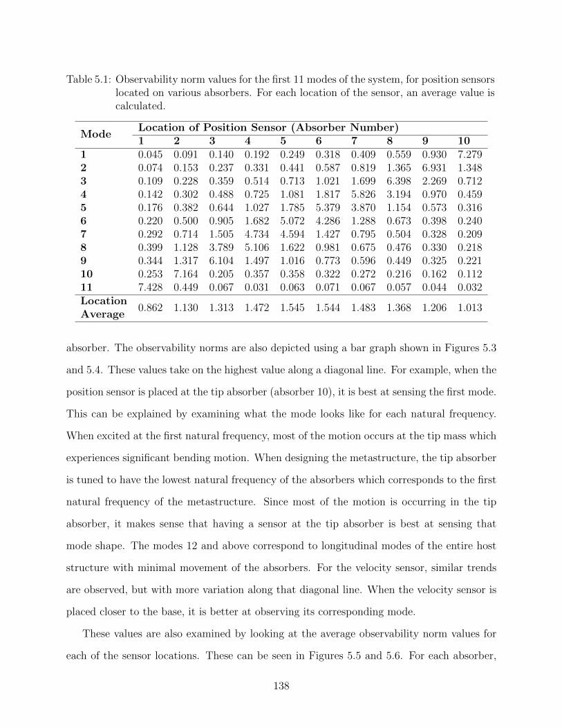
Table 5.1: Observability norm values for the first 11 modes of the system, for position sensorslocated on various absorbers. For each location of the sensor, an average value iscalculated.
ModeLocation of Position Sensor (Absorber Number)1 2 3 4 5 6 7 8 9 10
1 0.045 0.091 0.140 0.192 0.249 0.318 0.409 0.559 0.930 7.2792 0.074 0.153 0.237 0.331 0.441 0.587 0.819 1.365 6.931 1.3483 0.109 0.228 0.359 0.514 0.713 1.021 1.699 6.398 2.269 0.7124 0.142 0.302 0.488 0.725 1.081 1.817 5.826 3.194 0.970 0.4595 0.176 0.382 0.644 1.027 1.785 5.379 3.870 1.154 0.573 0.3166 0.220 0.500 0.905 1.682 5.072 4.286 1.288 0.673 0.398 0.2407 0.292 0.714 1.505 4.734 4.594 1.427 0.795 0.504 0.328 0.2098 0.399 1.128 3.789 5.106 1.622 0.981 0.675 0.476 0.330 0.2189 0.344 1.317 6.104 1.497 1.016 0.773 0.596 0.449 0.325 0.22110 0.253 7.164 0.205 0.357 0.358 0.322 0.272 0.216 0.162 0.11211 7.428 0.449 0.067 0.031 0.063 0.071 0.067 0.057 0.044 0.032LocationAverage
0.862 1.130 1.313 1.472 1.545 1.544 1.483 1.368 1.206 1.013
absorber. The observability norms are also depicted using a bar graph shown in Figures 5.3
and 5.4. These values take on the highest value along a diagonal line. For example, when the
position sensor is placed at the tip absorber (absorber 10), it is best at sensing the first mode.
This can be explained by examining what the mode looks like for each natural frequency.
When excited at the first natural frequency, most of the motion occurs at the tip mass which
experiences significant bending motion. When designing the metastructure, the tip absorber
is tuned to have the lowest natural frequency of the absorbers which corresponds to the first
natural frequency of the metastructure. Since most of the motion is occurring in the tip
absorber, it makes sense that having a sensor at the tip absorber is best at sensing that
mode shape. The modes 12 and above correspond to longitudinal modes of the entire host
structure with minimal movement of the absorbers. For the velocity sensor, similar trends
are observed, but with more variation along that diagonal line. When the velocity sensor is
placed closer to the base, it is better at observing its corresponding mode.
These values are also examined by looking at the average observability norm values for
each of the sensor locations. These can be seen in Figures 5.5 and 5.6. For each absorber,
138
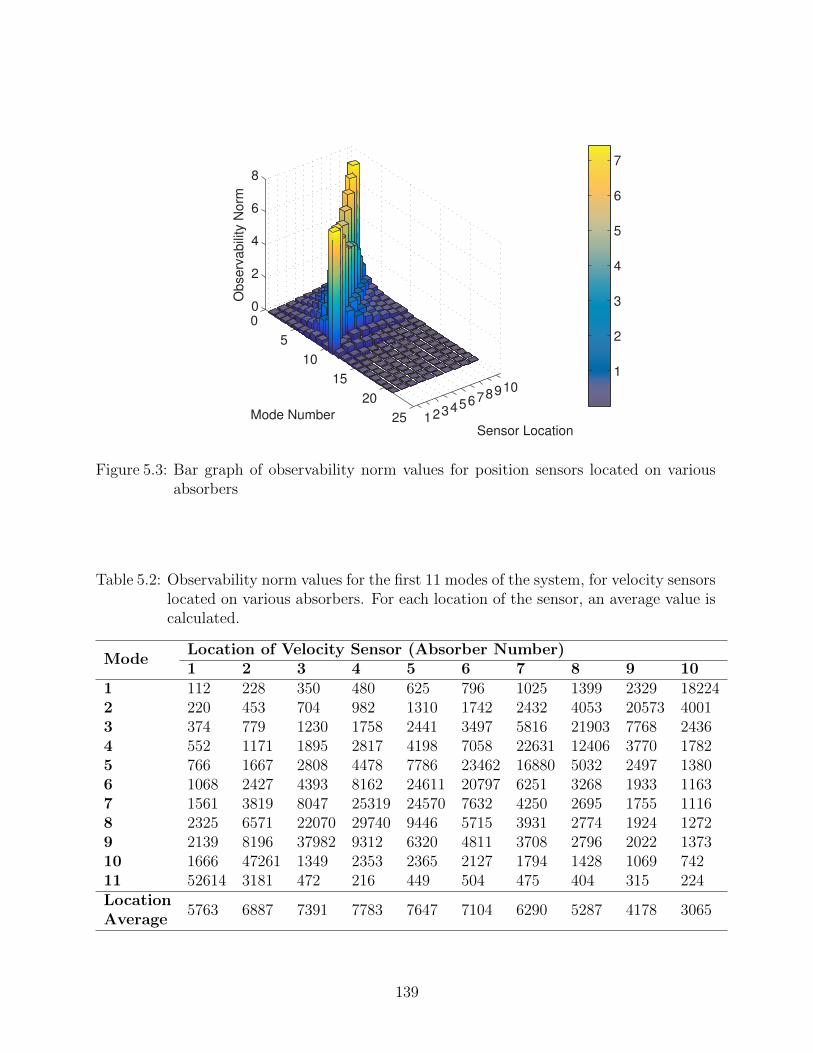
12345678910
0
5
10
15
20
25
0
2
4
6
8
Sensor LocationMode Number
Observ
abili
ty N
orm
1
2
3
4
5
6
7
Figure 5.3: Bar graph of observability norm values for position sensors located on variousabsorbers
Table 5.2: Observability norm values for the first 11 modes of the system, for velocity sensorslocated on various absorbers. For each location of the sensor, an average value iscalculated.
ModeLocation of Velocity Sensor (Absorber Number)1 2 3 4 5 6 7 8 9 10
1 112 228 350 480 625 796 1025 1399 2329 182242 220 453 704 982 1310 1742 2432 4053 20573 40013 374 779 1230 1758 2441 3497 5816 21903 7768 24364 552 1171 1895 2817 4198 7058 22631 12406 3770 17825 766 1667 2808 4478 7786 23462 16880 5032 2497 13806 1068 2427 4393 8162 24611 20797 6251 3268 1933 11637 1561 3819 8047 25319 24570 7632 4250 2695 1755 11168 2325 6571 22070 29740 9446 5715 3931 2774 1924 12729 2139 8196 37982 9312 6320 4811 3708 2796 2022 137310 1666 47261 1349 2353 2365 2127 1794 1428 1069 74211 52614 3181 472 216 449 504 475 404 315 224LocationAverage
5763 6887 7391 7783 7647 7104 6290 5287 4178 3065
139
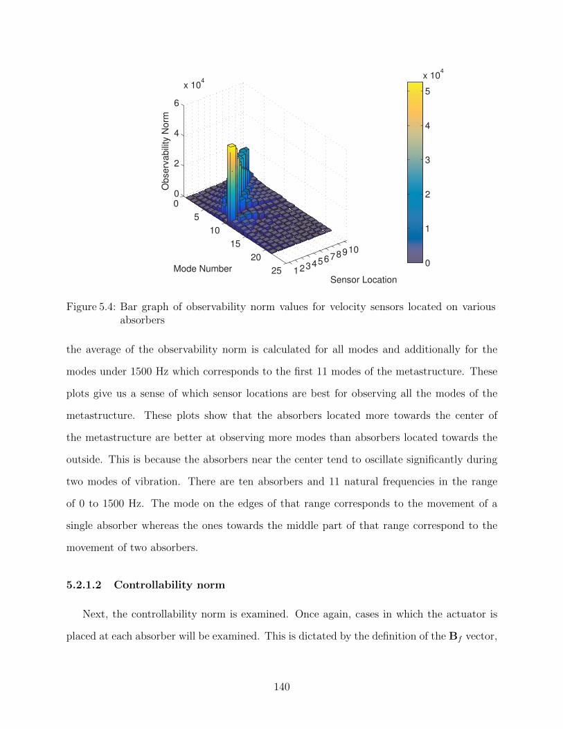
12345678910
0
5
10
15
20
25
0
2
4
6
x 104
Sensor LocationMode Number
Observ
abili
ty N
orm
0
1
2
3
4
5
x 104
Figure 5.4: Bar graph of observability norm values for velocity sensors located on variousabsorbers
the average of the observability norm is calculated for all modes and additionally for the
modes under 1500 Hz which corresponds to the first 11 modes of the metastructure. These
plots give us a sense of which sensor locations are best for observing all the modes of the
metastructure. These plots show that the absorbers located more towards the center of
the metastructure are better at observing more modes than absorbers located towards the
outside. This is because the absorbers near the center tend to oscillate significantly during
two modes of vibration. There are ten absorbers and 11 natural frequencies in the range
of 0 to 1500 Hz. The mode on the edges of that range corresponds to the movement of a
single absorber whereas the ones towards the middle part of that range correspond to the
movement of two absorbers.
5.2.1.2 Controllability norm
Next, the controllability norm is examined. Once again, cases in which the actuator is
placed at each absorber will be examined. This is dictated by the definition of the Bf vector,
140
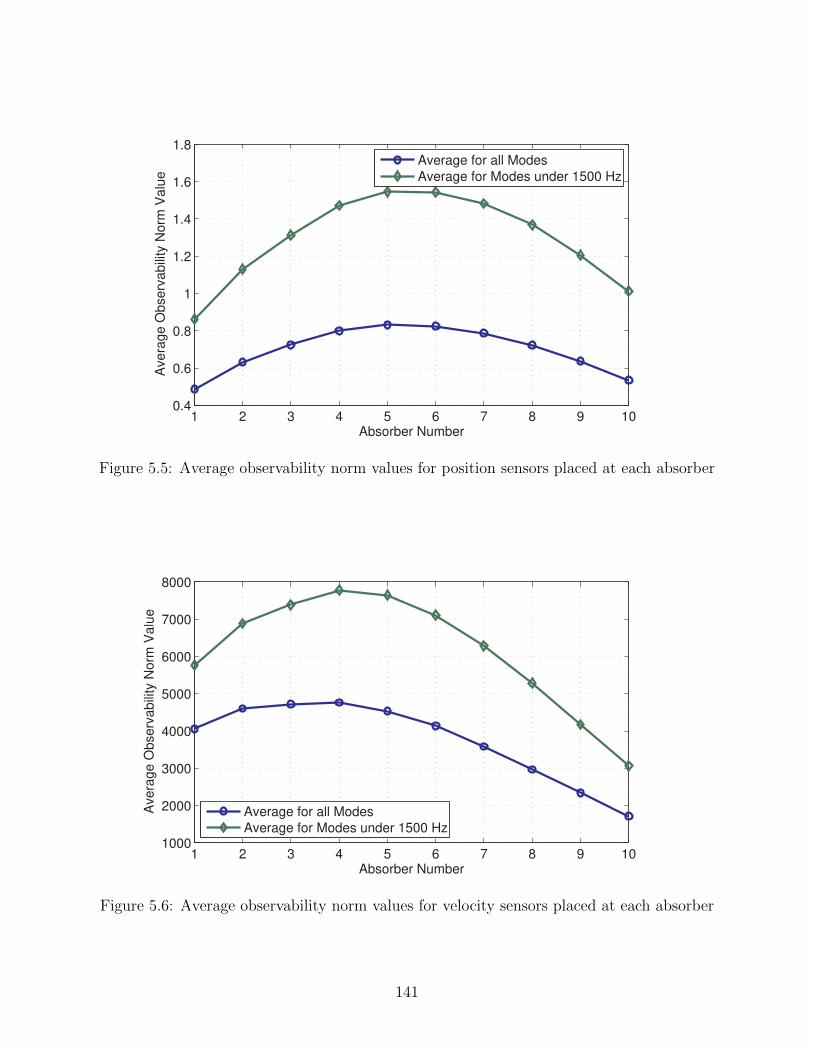
1 2 3 4 5 6 7 8 9 100.4
0.6
0.8
1
1.2
1.4
1.6
1.8
Absorber Number
Avera
ge O
bserv
abili
ty N
orm
Valu
e
Average for all Modes
Average for Modes under 1500 Hz
Figure 5.5: Average observability norm values for position sensors placed at each absorber
1 2 3 4 5 6 7 8 9 101000
2000
3000
4000
5000
6000
7000
8000
Absorber Number
Avera
ge O
bserv
abili
ty N
orm
Valu
e
Average for all Modes
Average for Modes under 1500 Hz
Figure 5.6: Average observability norm values for velocity sensors placed at each absorber
141
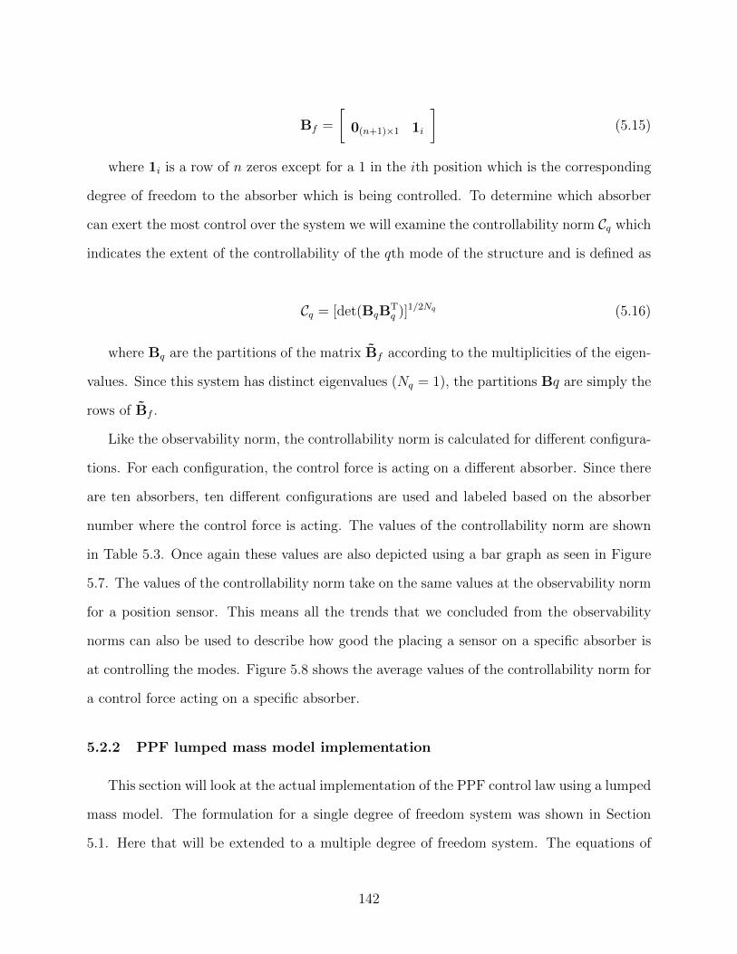
Bf =
[0(n+1)×1 1i
](5.15)
where 1i is a row of n zeros except for a 1 in the ith position which is the corresponding
degree of freedom to the absorber which is being controlled. To determine which absorber
can exert the most control over the system we will examine the controllability norm Cq which
indicates the extent of the controllability of the qth mode of the structure and is defined as
Cq = [det(BqBTq )]1/2Nq (5.16)
where Bq are the partitions of the matrix Bf according to the multiplicities of the eigen-
values. Since this system has distinct eigenvalues (Nq = 1), the partitions Bq are simply the
rows of Bf .
Like the observability norm, the controllability norm is calculated for different configura-
tions. For each configuration, the control force is acting on a different absorber. Since there
are ten absorbers, ten different configurations are used and labeled based on the absorber
number where the control force is acting. The values of the controllability norm are shown
in Table 5.3. Once again these values are also depicted using a bar graph as seen in Figure
5.7. The values of the controllability norm take on the same values at the observability norm
for a position sensor. This means all the trends that we concluded from the observability
norms can also be used to describe how good the placing a sensor on a specific absorber is
at controlling the modes. Figure 5.8 shows the average values of the controllability norm for
a control force acting on a specific absorber.
5.2.2 PPF lumped mass model implementation
This section will look at the actual implementation of the PPF control law using a lumped
mass model. The formulation for a single degree of freedom system was shown in Section
5.1. Here that will be extended to a multiple degree of freedom system. The equations of
142
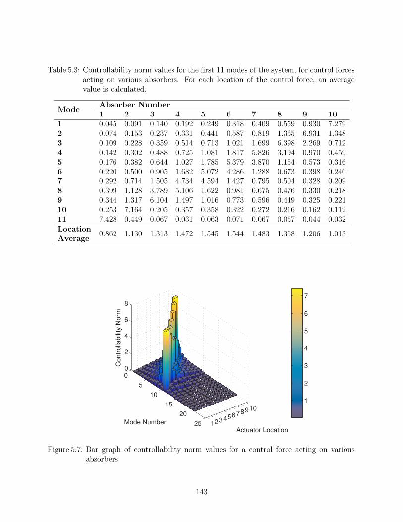
Table 5.3: Controllability norm values for the first 11 modes of the system, for control forcesacting on various absorbers. For each location of the control force, an averagevalue is calculated.
ModeAbsorber Number1 2 3 4 5 6 7 8 9 10
1 0.045 0.091 0.140 0.192 0.249 0.318 0.409 0.559 0.930 7.2792 0.074 0.153 0.237 0.331 0.441 0.587 0.819 1.365 6.931 1.3483 0.109 0.228 0.359 0.514 0.713 1.021 1.699 6.398 2.269 0.7124 0.142 0.302 0.488 0.725 1.081 1.817 5.826 3.194 0.970 0.4595 0.176 0.382 0.644 1.027 1.785 5.379 3.870 1.154 0.573 0.3166 0.220 0.500 0.905 1.682 5.072 4.286 1.288 0.673 0.398 0.2407 0.292 0.714 1.505 4.734 4.594 1.427 0.795 0.504 0.328 0.2098 0.399 1.128 3.789 5.106 1.622 0.981 0.675 0.476 0.330 0.2189 0.344 1.317 6.104 1.497 1.016 0.773 0.596 0.449 0.325 0.22110 0.253 7.164 0.205 0.357 0.358 0.322 0.272 0.216 0.162 0.11211 7.428 0.449 0.067 0.031 0.063 0.071 0.067 0.057 0.044 0.032LocationAverage
0.862 1.130 1.313 1.472 1.545 1.544 1.483 1.368 1.206 1.013
12345678910
0
5
10
15
20
25
0
2
4
6
8
Actuator LocationMode Number
Contr
olla
bili
ty N
orm
1
2
3
4
5
6
7
Figure 5.7: Bar graph of controllability norm values for a control force acting on variousabsorbers
143
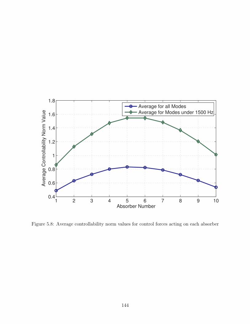
1 2 3 4 5 6 7 8 9 100.4
0.6
0.8
1
1.2
1.4
1.6
1.8
Absorber Number
Avera
ge C
ontr
olla
bili
ty N
orm
Valu
e
Average for all Modes
Average for Modes under 1500 Hz
Figure 5.8: Average controllability norm values for control forces acting on each absorber
144
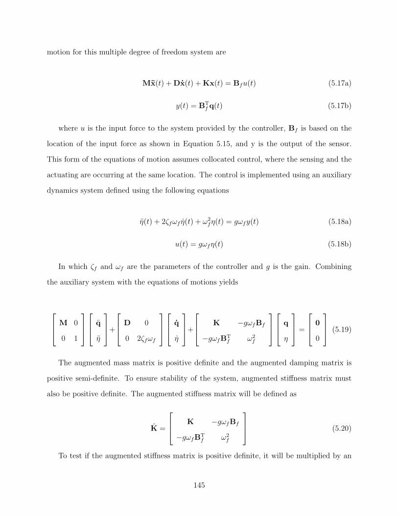
motion for this multiple degree of freedom system are
Mx(t) + Dx(t) + Kx(t) = Bfu(t) (5.17a)
y(t) = BTf q(t) (5.17b)
where u is the input force to the system provided by the controller, Bf is based on the
location of the input force as shown in Equation 5.15, and y is the output of the sensor.
This form of the equations of motion assumes collocated control, where the sensing and the
actuating are occurring at the same location. The control is implemented using an auxiliary
dynamics system defined using the following equations
η(t) + 2ζfωf η(t) + ω2fη(t) = gωfy(t) (5.18a)
u(t) = gωfη(t) (5.18b)
In which ζf and ωf are the parameters of the controller and g is the gain. Combining
the auxiliary system with the equations of motions yields
M 0
0 1
q
η
+
D 0
0 2ζfωf
q
η
+
K −gωfBf
−gωfBTf ω2
f
q
η
=
0
0
(5.19)
The augmented mass matrix is positive definite and the augmented damping matrix is
positive semi-definite. To ensure stability of the system, augmented stiffness matrix must
also be positive definite. The augmented stiffness matrix will be defined as
K =
K −gωfBf
−gωfBTf ω2
f
(5.20)
To test if the augmented stiffness matrix is positive definite, it will be multiplied by an
145
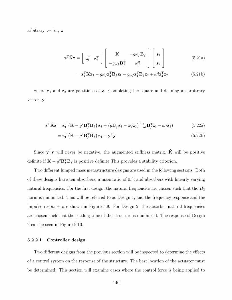
arbitrary vector, z
zTKz =
[zT1 zT
2
] K −gωfBf
−gωfBTf ω2
f
z1
z2
(5.21a)
= zT1 Kz1 − gωfzT
2 Bfz1 − gωfzT1 Bfz2 + ω2
fzT2 z2 (5.21b)
where z1 and z2 are partitions of z. Completing the square and defining an arbitrary
vector, y
zTKz = zT1
(K− g2BT
f Bf
)z1 +
(gBT
f z1 − ωfz2
)T (gBT
f z1 − ωfz2
)(5.22a)
= zT1
(K− g2BT
f Bf
)z1 + yTy (5.22b)
Since yTy will never be negative, the augmented stiffness matrix, K will be positive
definite if K− g2BTf Bf is positive definite This provides a stability criterion.
Two different lumped mass metastructure designs are used in the following sections. Both
of these designs have ten absorbers, a mass ratio of 0.3, and absorbers with linearly varying
natural frequencies. For the first design, the natural frequencies are chosen such that the H2
norm is minimized. This will be referred to as Design 1, and the frequency response and the
impulse response are shown in Figure 5.9. For Design 2, the absorber natural frequencies
are chosen such that the settling time of the structure is minimized. The response of Design
2 can be seen in Figure 5.10.
5.2.2.1 Controller design
Two different designs from the previous section will be inspected to determine the effects
of a control system on the response of the structure. The best location of the actuator must
be determined. This section will examine cases where the control force is being applied to
146
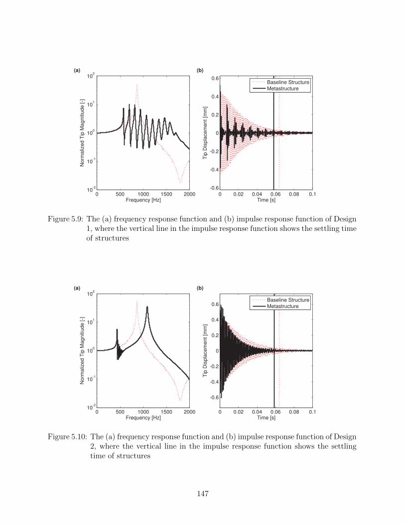
0 500 1000 1500 200010
-2
10-1
100
101
102
Frequency [Hz]
Norm
aliz
ed T
ip M
agnitiu
de [-]
(a)
0 0.02 0.04 0.06 0.08 0.1
-0.6
-0.4
-0.2
0
0.2
0.4
0.6
Time [s]T
ip D
ispla
cem
ent [m
m]
(b)
Baseline Structure
Metastructure
Figure 5.9: The (a) frequency response function and (b) impulse response function of Design1, where the vertical line in the impulse response function shows the settling timeof structures
0 500 1000 1500 200010
-2
10-1
100
101
102
Frequency [Hz]
Norm
aliz
ed T
ip M
agnitiu
de [-]
(a)
0 0.02 0.04 0.06 0.08 0.1
-0.6
-0.4
-0.2
0
0.2
0.4
0.6
Time [s]
Tip
Dis
pla
cem
ent [m
m]
(b)
Baseline Structure
Metastructure
Figure 5.10: The (a) frequency response function and (b) impulse response function of Design2, where the vertical line in the impulse response function shows the settlingtime of structures
147
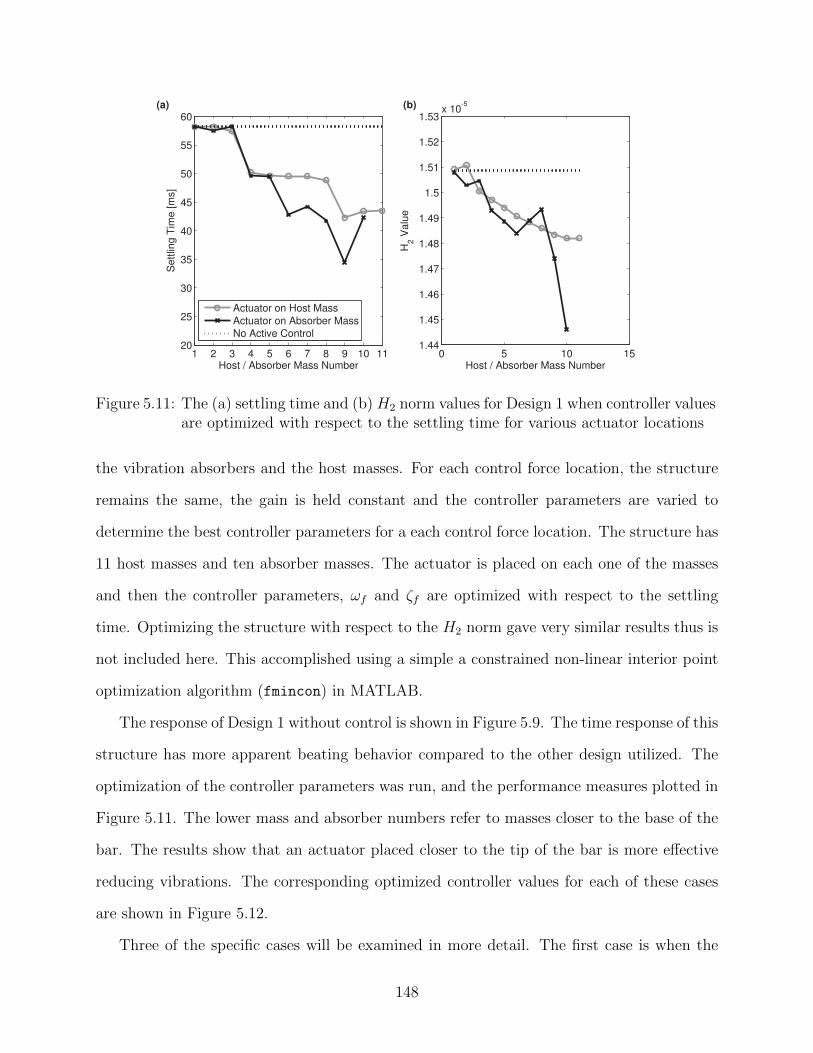
1 2 3 4 5 6 7 8 9 10 1120
25
30
35
40
45
50
55
60
Host / Absorber Mass Number
Settlin
g T
ime [m
s]
(a)
Actuator on Host Mass
Actuator on Absorber Mass
No Active Control
0 5 10 151.44
1.45
1.46
1.47
1.48
1.49
1.5
1.51
1.52
1.53x 10
-5(b)
Host / Absorber Mass Number
H2 V
alu
eFigure 5.11: The (a) settling time and (b) H2 norm values for Design 1 when controller values
are optimized with respect to the settling time for various actuator locations
the vibration absorbers and the host masses. For each control force location, the structure
remains the same, the gain is held constant and the controller parameters are varied to
determine the best controller parameters for a each control force location. The structure has
11 host masses and ten absorber masses. The actuator is placed on each one of the masses
and then the controller parameters, ωf and ζf are optimized with respect to the settling
time. Optimizing the structure with respect to the H2 norm gave very similar results thus is
not included here. This accomplished using a simple a constrained non-linear interior point
optimization algorithm (fmincon) in MATLAB.
The response of Design 1 without control is shown in Figure 5.9. The time response of this
structure has more apparent beating behavior compared to the other design utilized. The
optimization of the controller parameters was run, and the performance measures plotted in
Figure 5.11. The lower mass and absorber numbers refer to masses closer to the base of the
bar. The results show that an actuator placed closer to the tip of the bar is more effective
reducing vibrations. The corresponding optimized controller values for each of these cases
are shown in Figure 5.12.
Three of the specific cases will be examined in more detail. The first case is when the
148
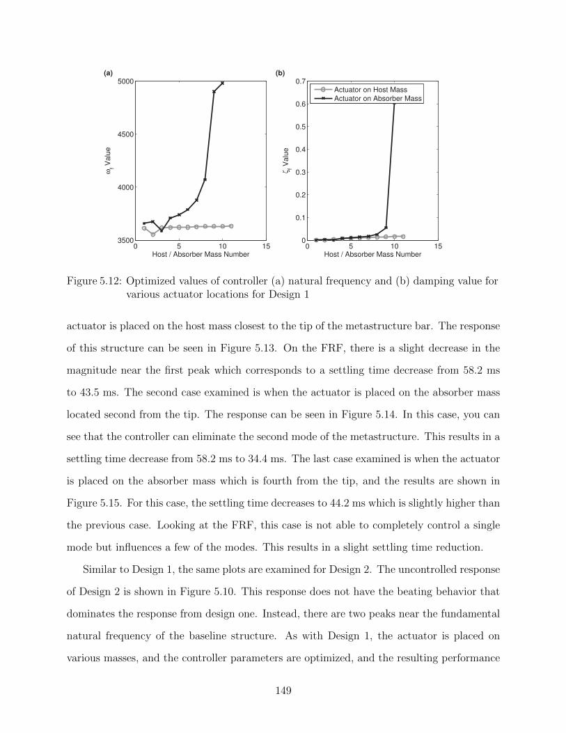
0 5 10 153500
4000
4500
5000
(a)
Host / Absorber Mass Number
ωf V
alu
e
0 5 10 150
0.1
0.2
0.3
0.4
0.5
0.6
0.7
Host / Absorber Mass Number
ζf V
alu
e
(b)
Actuator on Host Mass
Actuator on Absorber Mass
Figure 5.12: Optimized values of controller (a) natural frequency and (b) damping value forvarious actuator locations for Design 1
actuator is placed on the host mass closest to the tip of the metastructure bar. The response
of this structure can be seen in Figure 5.13. On the FRF, there is a slight decrease in the
magnitude near the first peak which corresponds to a settling time decrease from 58.2 ms
to 43.5 ms. The second case examined is when the actuator is placed on the absorber mass
located second from the tip. The response can be seen in Figure 5.14. In this case, you can
see that the controller can eliminate the second mode of the metastructure. This results in a
settling time decrease from 58.2 ms to 34.4 ms. The last case examined is when the actuator
is placed on the absorber mass which is fourth from the tip, and the results are shown in
Figure 5.15. For this case, the settling time decreases to 44.2 ms which is slightly higher than
the previous case. Looking at the FRF, this case is not able to completely control a single
mode but influences a few of the modes. This results in a slight settling time reduction.
Similar to Design 1, the same plots are examined for Design 2. The uncontrolled response
of Design 2 is shown in Figure 5.10. This response does not have the beating behavior that
dominates the response from design one. Instead, there are two peaks near the fundamental
natural frequency of the baseline structure. As with Design 1, the actuator is placed on
various masses, and the controller parameters are optimized, and the resulting performance
149
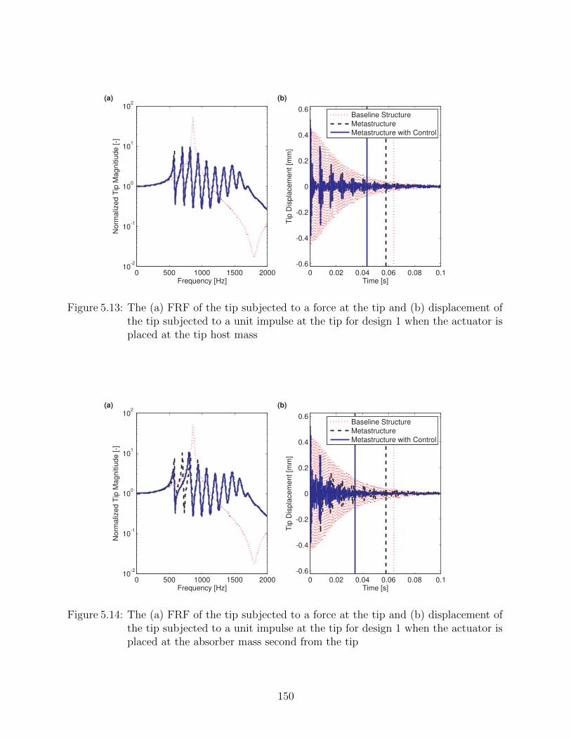
0 500 1000 1500 200010
-2
10-1
100
101
102
Frequency [Hz]
Norm
aliz
ed T
ip M
agnitiu
de [-]
(a)
0 0.02 0.04 0.06 0.08 0.1
-0.6
-0.4
-0.2
0
0.2
0.4
0.6
Time [s]T
ip D
ispla
cem
ent [m
m]
(b)
Baseline Structure
Metastructure
Metastructure with Control
Figure 5.13: The (a) FRF of the tip subjected to a force at the tip and (b) displacement ofthe tip subjected to a unit impulse at the tip for design 1 when the actuator isplaced at the tip host mass
0 500 1000 1500 200010
-2
10-1
100
101
102
Frequency [Hz]
Norm
aliz
ed T
ip M
agnitiu
de [-]
(a)
0 0.02 0.04 0.06 0.08 0.1
-0.6
-0.4
-0.2
0
0.2
0.4
0.6
Time [s]
Tip
Dis
pla
cem
ent [m
m]
(b)
Baseline Structure
Metastructure
Metastructure with Control
Figure 5.14: The (a) FRF of the tip subjected to a force at the tip and (b) displacement ofthe tip subjected to a unit impulse at the tip for design 1 when the actuator isplaced at the absorber mass second from the tip
150
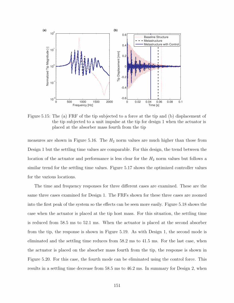
0 500 1000 1500 200010
-2
10-1
100
101
102
Frequency [Hz]
Norm
aliz
ed T
ip M
agnitiu
de [-]
(a)
0 0.02 0.04 0.06 0.08 0.1
-0.6
-0.4
-0.2
0
0.2
0.4
0.6
Time [s]
Tip
Dis
pla
cem
ent [m
m]
(b)
Baseline Structure
Metastructure
Metastructure with Control
Figure 5.15: The (a) FRF of the tip subjected to a force at the tip and (b) displacement ofthe tip subjected to a unit impulse at the tip for design 1 when the actuator isplaced at the absorber mass fourth from the tip
measures are shown in Figure 5.16. The H2 norm values are much higher than those from
Design 1 but the settling time values are comparable. For this design, the trend between the
location of the actuator and performance is less clear for the H2 norm values but follows a
similar trend for the settling time values. Figure 5.17 shows the optimized controller values
for the various locations.
The time and frequency responses for three different cases are examined. These are the
same three cases examined for Design 1. The FRFs shown for these three cases are zoomed
into the first peak of the system so the effects can be seen more easily. Figure 5.18 shows the
case when the actuator is placed at the tip host mass. For this situation, the settling time
is reduced from 58.5 ms to 52.1 ms. When the actuator is placed at the second absorber
from the tip, the response is shown in Figure 5.19. As with Design 1, the second mode is
eliminated and the settling time reduces from 58.2 ms to 41.5 ms. For the last case, when
the actuator is placed on the absorber mass fourth from the tip, the response is shown in
Figure 5.20. For this case, the fourth mode can be eliminated using the control force. This
results in a settling time decrease from 58.5 ms to 46.2 ms. In summary for Design 2, when
151
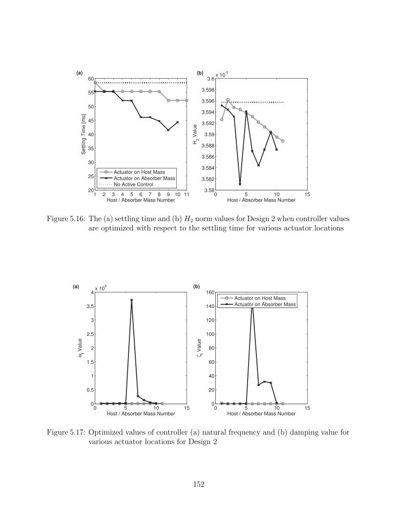
1 2 3 4 5 6 7 8 9 10 1120
25
30
35
40
45
50
55
60
Host / Absorber Mass Number
Settlin
g T
ime [m
s]
(a)
Actuator on Host Mass
Actuator on Absorber Mass
No Active Control
0 5 10 153.58
3.582
3.584
3.586
3.588
3.59
3.592
3.594
3.596
3.598
3.6x 10
-5(b)
Host / Absorber Mass NumberH
2 V
alu
e
Figure 5.16: The (a) settling time and (b) H2 norm values for Design 2 when controller valuesare optimized with respect to the settling time for various actuator locations
0 5 10 150
0.5
1
1.5
2
2.5
3
3.5
4x 10
6(a)
Host / Absorber Mass Number
ωf V
alu
e
0 5 10 150
20
40
60
80
100
120
140
160
Host / Absorber Mass Number
ζf V
alu
e
(b)
Actuator on Host Mass
Actuator on Absorber Mass
Figure 5.17: Optimized values of controller (a) natural frequency and (b) damping value forvarious actuator locations for Design 2
152
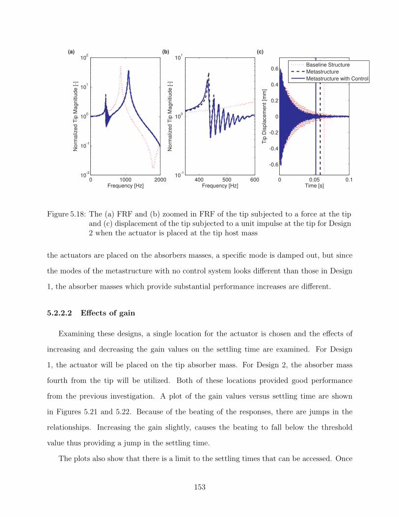
0 1000 200010
-2
10-1
100
101
102
Frequency [Hz]
No
rma
lize
d T
ip M
ag
nitiu
de
[-]
(a)
400 500 60010
-1
100
101
Frequency [Hz]
No
rma
lize
d T
ip M
ag
nitiu
de
[-]
(b)
0 0.05 0.1
-0.6
-0.4
-0.2
0
0.2
0.4
0.6
Time [s]
Tip
Dis
pla
ce
me
nt
[mm
]
(c)
Baseline Structure
Metastructure
Metastructure with Control
Figure 5.18: The (a) FRF and (b) zoomed in FRF of the tip subjected to a force at the tipand (c) displacement of the tip subjected to a unit impulse at the tip for Design2 when the actuator is placed at the tip host mass
the actuators are placed on the absorbers masses, a specific mode is damped out, but since
the modes of the metastructure with no control system looks different than those in Design
1, the absorber masses which provide substantial performance increases are different.
5.2.2.2 Effects of gain
Examining these designs, a single location for the actuator is chosen and the effects of
increasing and decreasing the gain values on the settling time are examined. For Design
1, the actuator will be placed on the tip absorber mass. For Design 2, the absorber mass
fourth from the tip will be utilized. Both of these locations provided good performance
from the previous investigation. A plot of the gain values versus settling time are shown
in Figures 5.21 and 5.22. Because of the beating of the responses, there are jumps in the
relationships. Increasing the gain slightly, causes the beating to fall below the threshold
value thus providing a jump in the settling time.
The plots also show that there is a limit to the settling times that can be accessed. Once
153
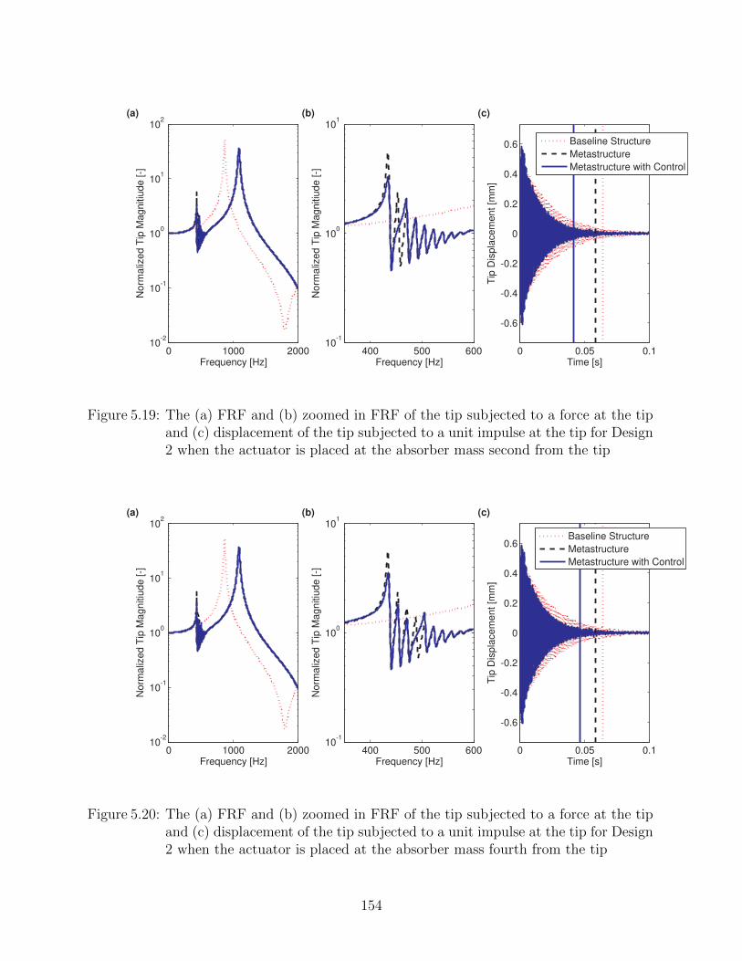
0 1000 200010
-2
10-1
100
101
102
Frequency [Hz]
No
rma
lize
d T
ip M
ag
nitiu
de
[-]
(a)
400 500 60010
-1
100
101
Frequency [Hz]
No
rma
lize
d T
ip M
ag
nitiu
de
[-]
(b)
0 0.05 0.1
-0.6
-0.4
-0.2
0
0.2
0.4
0.6
Time [s]
Tip
Dis
pla
ce
me
nt
[mm
]
(c)
Baseline Structure
Metastructure
Metastructure with Control
Figure 5.19: The (a) FRF and (b) zoomed in FRF of the tip subjected to a force at the tipand (c) displacement of the tip subjected to a unit impulse at the tip for Design2 when the actuator is placed at the absorber mass second from the tip
0 1000 200010
-2
10-1
100
101
102
Frequency [Hz]
No
rma
lize
d T
ip M
ag
nitiu
de
[-]
(a)
400 500 60010
-1
100
101
Frequency [Hz]
No
rma
lize
d T
ip M
ag
nitiu
de
[-]
(b)
0 0.05 0.1
-0.6
-0.4
-0.2
0
0.2
0.4
0.6
Time [s]
Tip
Dis
pla
ce
me
nt
[mm
]
(c)
Baseline Structure
Metastructure
Metastructure with Control
Figure 5.20: The (a) FRF and (b) zoomed in FRF of the tip subjected to a force at the tipand (c) displacement of the tip subjected to a unit impulse at the tip for Design2 when the actuator is placed at the absorber mass fourth from the tip
154
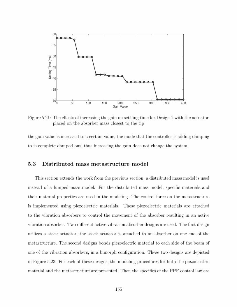
0 50 100 150 200 250 300 350 40030
35
40
45
50
55
60
Gain Value
Settin
g T
ime [m
s]
Figure 5.21: The effects of increasing the gain on settling time for Design 1 with the actuatorplaced on the absorber mass closest to the tip
the gain value is increased to a certain value, the mode that the controller is adding damping
to is complete damped out, thus increasing the gain does not change the system.
5.3 Distributed mass metastructure model
This section extends the work from the previous section; a distributed mass model is used
instead of a lumped mass model. For the distributed mass model, specific materials and
their material properties are used in the modeling. The control force on the metastructure
is implemented using piezoelectric materials. These piezoelectric materials are attached
to the vibration absorbers to control the movement of the absorber resulting in an active
vibration absorber. Two different active vibration absorber designs are used. The first design
utilizes a stack actuator; the stack actuator is attached to an absorber on one end of the
metastructure. The second designs bonds piezoelectric material to each side of the beam of
one of the vibration absorbers, in a bimorph configuration. These two designs are depicted
in Figure 5.23. For each of these designs, the modeling procedures for both the piezoelectric
material and the metastructure are presented. Then the specifics of the PPF control law are
155
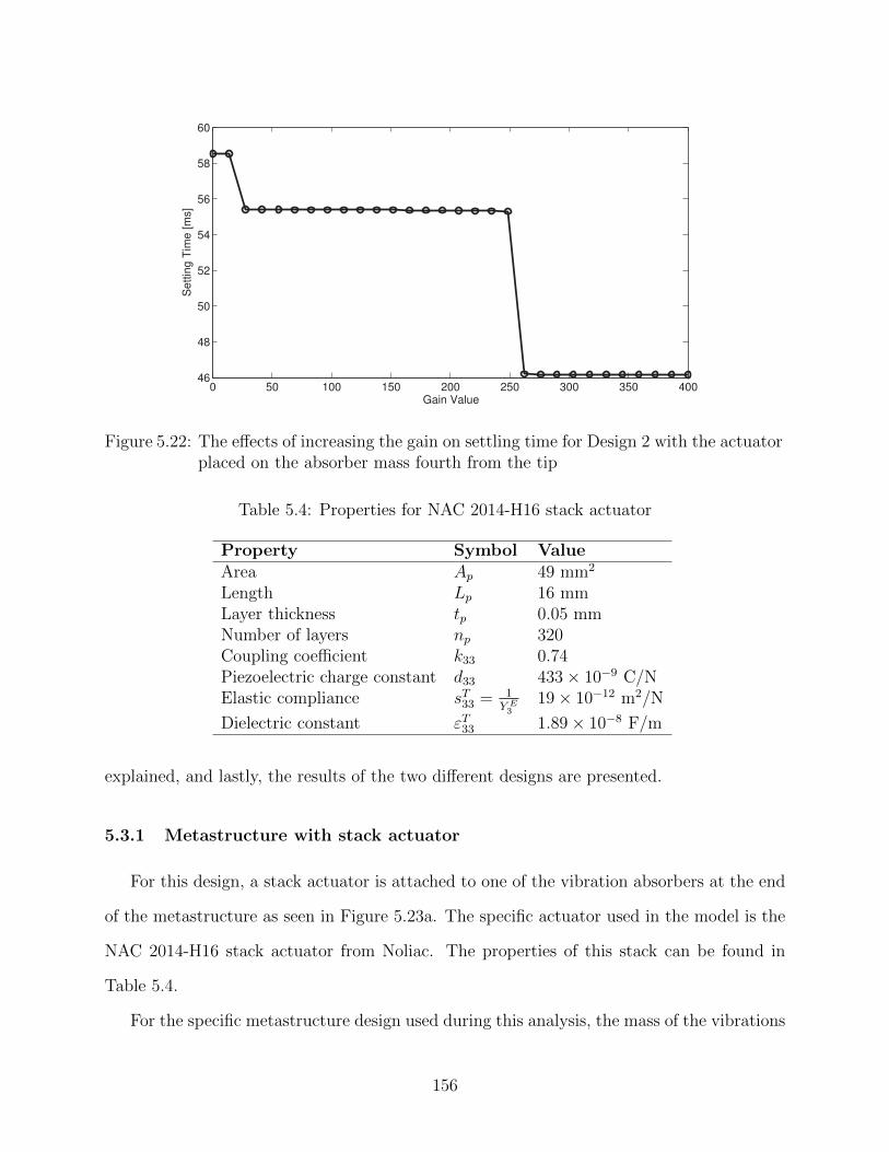
0 50 100 150 200 250 300 350 40046
48
50
52
54
56
58
60
Gain Value
Settin
g T
ime [m
s]
Figure 5.22: The effects of increasing the gain on settling time for Design 2 with the actuatorplaced on the absorber mass fourth from the tip
Table 5.4: Properties for NAC 2014-H16 stack actuator
Property Symbol ValueArea Ap 49 mm2
Length Lp 16 mmLayer thickness tp 0.05 mmNumber of layers np 320Coupling coefficient k33 0.74Piezoelectric charge constant d33 433× 10−9 C/NElastic compliance sT33 = 1
Y E3
19× 10−12 m2/N
Dielectric constant εT33 1.89× 10⁻⁸ F/m
explained, and lastly, the results of the two different designs are presented.
5.3.1 Metastructure with stack actuator
For this design, a stack actuator is attached to one of the vibration absorbers at the end
of the metastructure as seen in Figure 5.23a. The specific actuator used in the model is the
NAC 2014-H16 stack actuator from Noliac. The properties of this stack can be found in
Table 5.4.
For the specific metastructure design used during this analysis, the mass of the vibrations
156
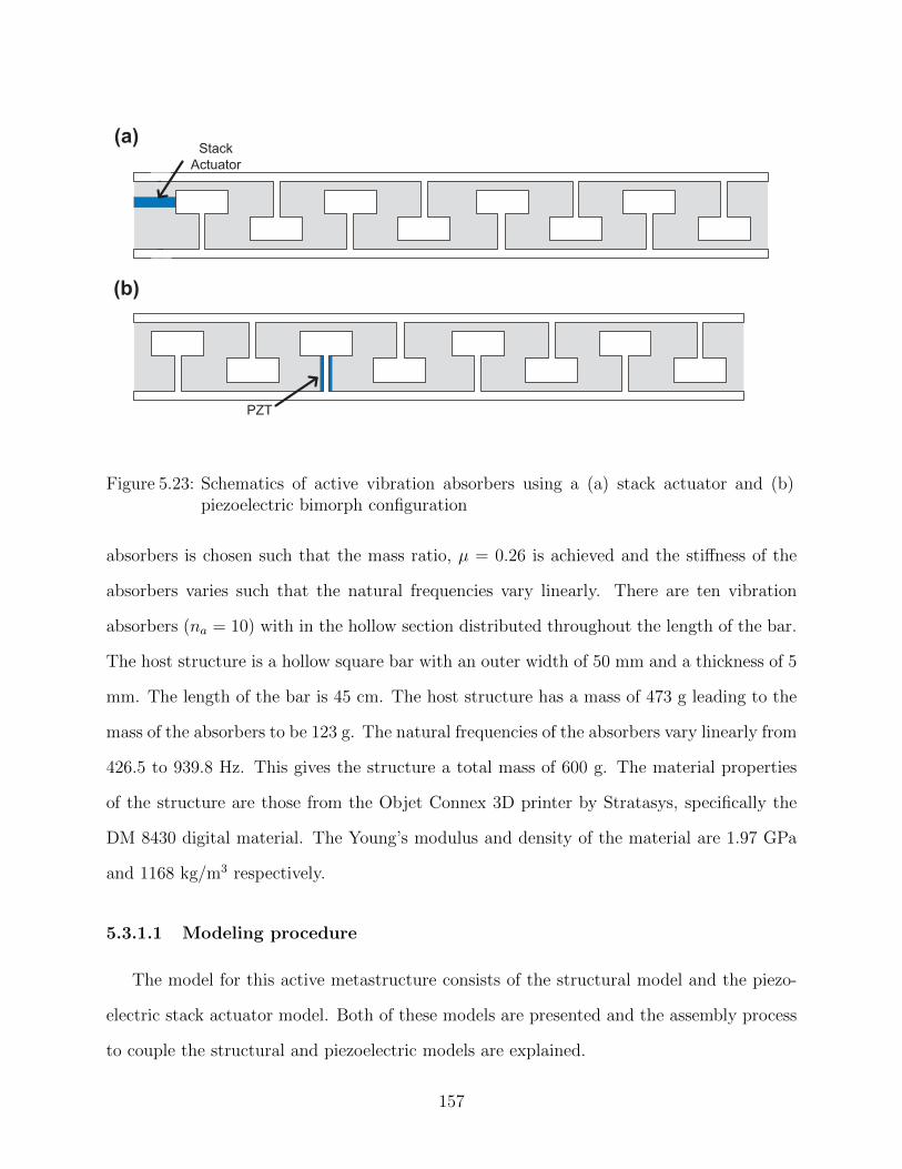
PZT
Stack
Actuator
(a)
(b)
Figure 5.23: Schematics of active vibration absorbers using a (a) stack actuator and (b)piezoelectric bimorph configuration
absorbers is chosen such that the mass ratio, µ = 0.26 is achieved and the stiffness of the
absorbers varies such that the natural frequencies vary linearly. There are ten vibration
absorbers (na = 10) with in the hollow section distributed throughout the length of the bar.
The host structure is a hollow square bar with an outer width of 50 mm and a thickness of 5
mm. The length of the bar is 45 cm. The host structure has a mass of 473 g leading to the
mass of the absorbers to be 123 g. The natural frequencies of the absorbers vary linearly from
426.5 to 939.8 Hz. This gives the structure a total mass of 600 g. The material properties
of the structure are those from the Objet Connex 3D printer by Stratasys, specifically the
DM 8430 digital material. The Young’s modulus and density of the material are 1.97 GPa
and 1168 kg/m3 respectively.
5.3.1.1 Modeling procedure
The model for this active metastructure consists of the structural model and the piezo-
electric stack actuator model. Both of these models are presented and the assembly process
to couple the structural and piezoelectric models are explained.
157
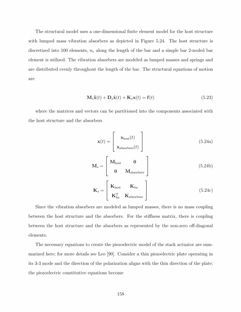
The structural model uses a one-dimensional finite element model for the host structure
with lumped mass vibration absorbers as depicted in Figure 5.24. The host structure is
discretized into 100 elements, ne along the length of the bar and a simple bar 2-noded bar
element is utilized. The vibration absorbers are modeled as lumped masses and springs and
are distributed evenly throughout the length of the bar. The structural equations of motion
are
Msx(t) + Dsx(t) + Ksx(t) = f(t) (5.23)
where the matrices and vectors can be partitioned into the components associated with
the host structure and the absorbers
x(t) =
xhost(t)
xabsorbers(t)
(5.24a)
Ms =
Mhost 0
0 Mabsorbers
(5.24b)
Ks =
Khost Kha
KTha Kabsorbers
(5.24c)
Since the vibration absorbers are modeled as lumped masses, there is no mass coupling
between the host structure and the absorbers. For the stiffness matrix, there is coupling
between the host structure and the absorbers as represented by the non-zero off-diagonal
elements.
The necessary equations to create the piezoelectric model of the stack actuator are sum-
marized here; for more details see Leo [90]. Consider a thin piezoelectric plate operating in
its 3-3 mode and the direction of the polarization aligns with the thin direction of the plate;
the piezoelectric constitutive equations become
158
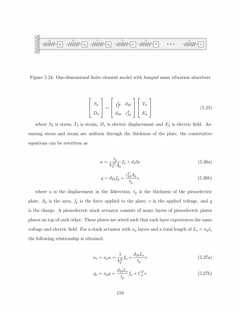
1k
1m
2k
2m
3k
3m
4k
4m
5k
5m
nk
nm
Figure 5.24: One-dimensional finite element model with lumped mass vibration absorbers
S3
D3
=
1Y E3
d33
d33 εT33
T3
E3
(5.25)
where S3 is stress, T3 is strain, Ds is electric displacement and E3 is electric field. As-
suming stress and strain are uniform through the thickness of the plate, the constitutive
equations can be rewritten as
u =tp
Y E3 Ap
fp + d33v (5.26a)
q = d33fp +εT33Aptp
v (5.26b)
where u is the displacement in the 3direction, tp is the thickness of the piezoelectric
plate, Ap is the area, fp is the force applied to the plate, v is the applied voltage, and q
is the charge. A piezoelectric stack actuator consists of many layers of piezoelectric plates
places on top of each other. These plates are wired such that each layer experiences the same
voltage and electric field. For a stack actuator with np layers and a total length of Ls = npts
the following relationship is obtained.
us = npu =1
kEpfp +
d33Lstp
v (5.27a)
qs = npq =d33Lstp
fp + CTp v (5.27b)
159
where CTP is the stress-free capacitance of the device and kEp is the short circuit mechanical
stiffness. These are calculated as
CTp = np
εT33Aptp
(5.28a)
kEp =Y E3 ApLs
(5.28b)
Interchanging the dependent and independent variables from Equation 5.27
fp = kDp us −d33Lptp
kEpCSp
q (5.29a)
v = −d33Lptp
kEpCSp
us +1
CSp
q (5.29b)
where
kDp =kEp
1− k233(5.30a)
CSp = (1− k233)CT
p (5.30b)
The stack actuator equations are coupled to the structural system via the applied force
vector, f(t) from Equation 5.23. The stack actuator will be attached to the tip vibration
absorber and the tip of the structure. The tip of the structure is the ne degree of freedom and
displacement of the absorber is the nt degree of freedom, where nt = ne+na. Assuming there
are no other external forces being applied to the structure, the force vector is composed of
all zeros except for f [ne] = +fp and f [nt] = −fp where v[i] refers to the ith component of the
vector, v. The displacement of the stack is equal to the difference between the displacement
of the tip of the bar and the displacement of the absorber closest to the tip, us = u[ne]−u[nt].
This leads to
160
f [ne] = +fp = +kDp u[ne]− kDp u[nt]−d33Lptp
kEpCSp
q (5.31a)
f [nt] = −fp = −kDp u[ne] + kDp u[nt] +d33Lptp
kEpCSp
q (5.31b)
substituting Equation 5.31 to Equation 5.23, the equations of motion of the smart struc-
ture have the following form
Msx(t) + Dsx(t) + KDs x(t)−Θq(t) = 0 (5.32a)
−ΘTx(t) + (Csp)−1q(t) = v(t) (5.32b)
where
KDs = Ks + KD
KD[ne, ne] = KD[nt, nt] = kDp
KD[ne, nt] = KD[nt, ne] = −kDp
(5.33a)
Θ[ne] = d33Lp
tp
kEpCS
p
Θ[nt] = −d33Lp
tp
kEpCS
p
(5.33b)
Eliminating q(t) from Equation 5.32 the equations of motion can be reduced to
Msx(t) + Dsx(t) + KEx(t) = Bcv(t) (5.34)
where
KE = Ks −ΘCspΘ
T (5.35a)
161
Bc = ΘCSp (5.35b)
Equation 5.34 is the equation of motion for the metastructure with the active vibration
absorber.
5.3.1.2 PPF implementation
Next, the implementation of the PPF control law will be explained for a multiple degree
of freedom system. The general equations of motion for a system with piezoelectric materials
are
Msx(t) + Dsx(t) + KDs x(t)−Θq(t) = 0 (5.36a)
−ΘTx(t) + (Csp)−1q(t) = Bvv(t) (5.36b)
where Bv describes the position where the voltage is being applied. Rearranging Equation
5.36b an expression for charge is
q(t) = CspBvv(t) + Cs
pΘTx(t) (5.37)
Substituting Equation 5.37 in Equation 5.36a results in the following equations of motion
Msx(t) + Dsx(t) + KEx(t) = Bcv(t) (5.38)
where
KE = KDs −ΘCs
pΘT (5.39a)
Bc = ΘCspBv (5.39b)
162
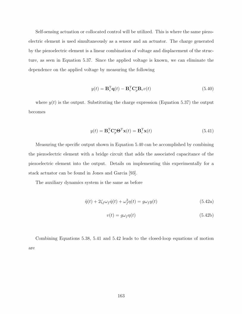
Self-sensing actuation or collocated control will be utilized. This is where the same piezo-
electric element is used simultaneously as a sensor and an actuator. The charge generated
by the piezoelectric element is a linear combination of voltage and displacement of the struc-
ture, as seen in Equation 5.37. Since the applied voltage is known, we can eliminate the
dependence on the applied voltage by measuring the following
y(t) = BTv q(t)−BT
v CspBvv(t) (5.40)
where y(t) is the output. Substituting the charge expression (Equation 5.37) the output
becomes
y(t) = BTv Cs
pΘTx(t) = BT
c x(t) (5.41)
Measuring the specific output shown in Equation 5.40 can be accomplished by combining
the piezoelectric element with a bridge circuit that adds the associated capacitance of the
piezoelectric element into the output. Details on implementing this experimentally for a
stack actuator can be found in Jones and Garcia [93].
The auxiliary dynamics system is the same as before
η(t) + 2ζfωf η(t) + ω2fη(t) = gωfy(t) (5.42a)
v(t) = gωfη(t) (5.42b)
Combining Equations 5.38, 5.41 and 5.42 leads to the closed-loop equations of motion
are
163
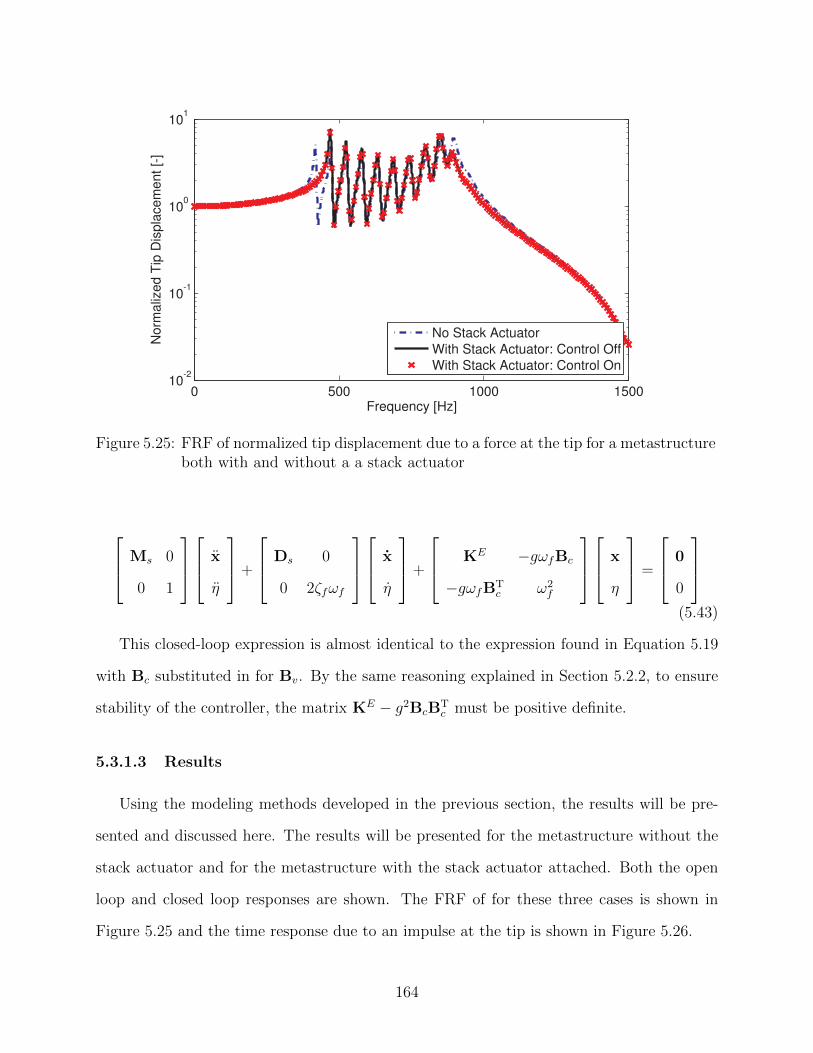
0 500 1000 150010
-2
10-1
100
101
Frequency [Hz]
Norm
aliz
ed T
ip D
ispla
cem
ent [-
]
No Stack Actuator
With Stack Actuator: Control Off
With Stack Actuator: Control On
Figure 5.25: FRF of normalized tip displacement due to a force at the tip for a metastructureboth with and without a a stack actuator
Ms 0
0 1
x
η
+
Ds 0
0 2ζfωf
x
η
+
KE −gωfBc
−gωfBTc ω2
f
x
η
=
0
0
(5.43)
This closed-loop expression is almost identical to the expression found in Equation 5.19
with Bc substituted in for Bv. By the same reasoning explained in Section 5.2.2, to ensure
stability of the controller, the matrix KE − g2BcBTc must be positive definite.
5.3.1.3 Results
Using the modeling methods developed in the previous section, the results will be pre-
sented and discussed here. The results will be presented for the metastructure without the
stack actuator and for the metastructure with the stack actuator attached. Both the open
loop and closed loop responses are shown. The FRF of for these three cases is shown in
Figure 5.25 and the time response due to an impulse at the tip is shown in Figure 5.26.
164
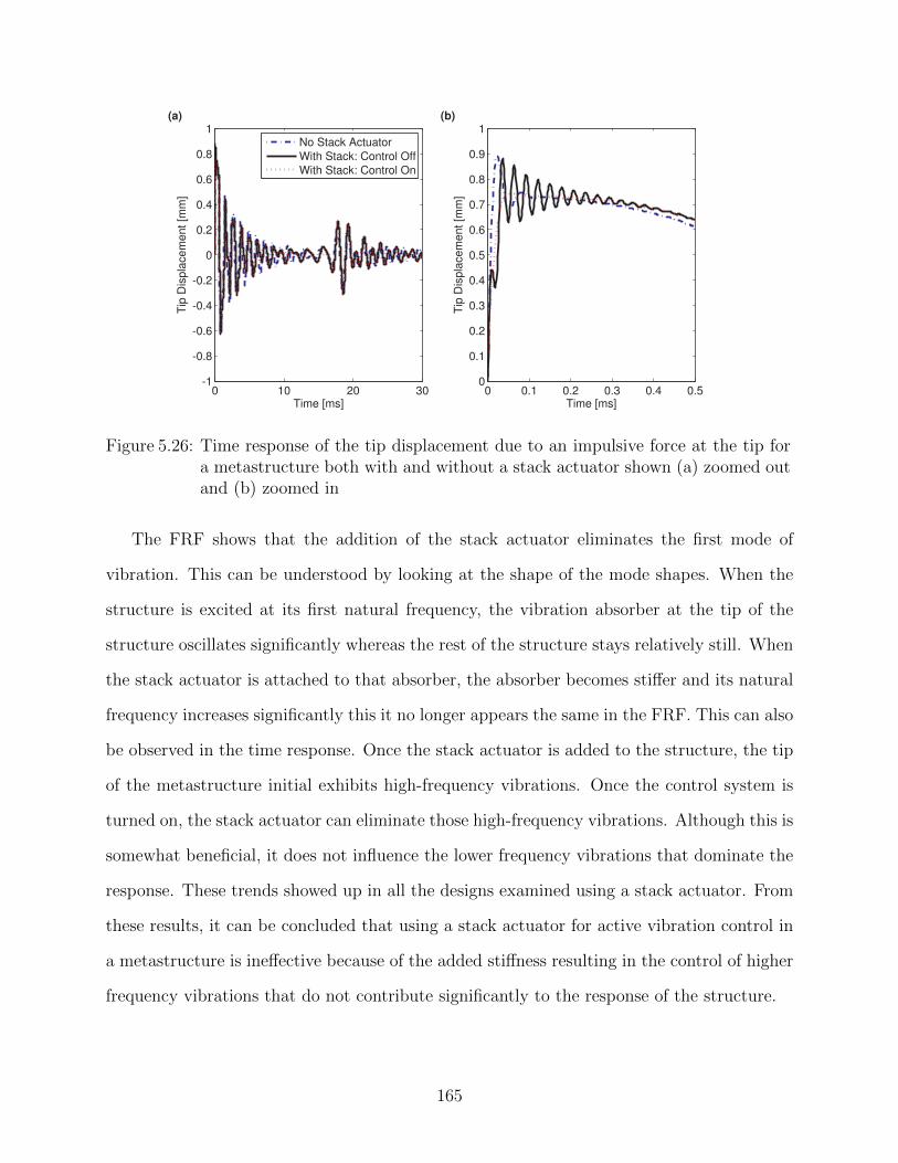
0 10 20 30-1
-0.8
-0.6
-0.4
-0.2
0
0.2
0.4
0.6
0.8
1
Time [ms]
Tip
Dis
pla
cem
ent [m
m]
(a)
No Stack Actuator
With Stack: Control Off
With Stack: Control On
0 0.1 0.2 0.3 0.4 0.50
0.1
0.2
0.3
0.4
0.5
0.6
0.7
0.8
0.9
1
Time [ms]
Tip
Dis
pla
cem
ent [m
m]
(b)
Figure 5.26: Time response of the tip displacement due to an impulsive force at the tip fora metastructure both with and without a stack actuator shown (a) zoomed outand (b) zoomed in
The FRF shows that the addition of the stack actuator eliminates the first mode of
vibration. This can be understood by looking at the shape of the mode shapes. When the
structure is excited at its first natural frequency, the vibration absorber at the tip of the
structure oscillates significantly whereas the rest of the structure stays relatively still. When
the stack actuator is attached to that absorber, the absorber becomes stiffer and its natural
frequency increases significantly this it no longer appears the same in the FRF. This can also
be observed in the time response. Once the stack actuator is added to the structure, the tip
of the metastructure initial exhibits high-frequency vibrations. Once the control system is
turned on, the stack actuator can eliminate those high-frequency vibrations. Although this is
somewhat beneficial, it does not influence the lower frequency vibrations that dominate the
response. These trends showed up in all the designs examined using a stack actuator. From
these results, it can be concluded that using a stack actuator for active vibration control in
a metastructure is ineffective because of the added stiffness resulting in the control of higher
frequency vibrations that do not contribute significantly to the response of the structure.
165
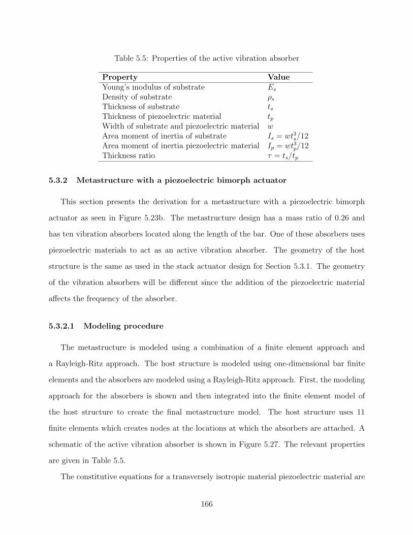
Table 5.5: Properties of the active vibration absorber
Property ValueYoung’s modulus of substrate EsDensity of substrate ρsThickness of substrate tsThickness of piezoelectric material tpWidth of substrate and piezoelectric material wArea moment of inertia of substrate Is = wt3s/12Area moment of inertia piezoelectric material Ip = wt3p/12Thickness ratio τ = ts/tp
5.3.2 Metastructure with a piezoelectric bimorph actuator
This section presents the derivation for a metastructure with a piezoelectric bimorph
actuator as seen in Figure 5.23b. The metastructure design has a mass ratio of 0.26 and
has ten vibration absorbers located along the length of the bar. One of these absorbers uses
piezoelectric materials to act as an active vibration absorber. The geometry of the host
structure is the same as used in the stack actuator design for Section 5.3.1. The geometry
of the vibration absorbers will be different since the addition of the piezoelectric material
affects the frequency of the absorber.
5.3.2.1 Modeling procedure
The metastructure is modeled using a combination of a finite element approach and
a Rayleigh-Ritz approach. The host structure is modeled using one-dimensional bar finite
elements and the absorbers are modeled using a Rayleigh-Ritz approach. First, the modeling
approach for the absorbers is shown and then integrated into the finite element model of
the host structure to create the final metastructure model. The host structure uses 11
finite elements which creates nodes at the locations at which the absorbers are attached. A
schematic of the active vibration absorber is shown in Figure 5.27. The relevant properties
are given in Table 5.5.
The constitutive equations for a transversely isotropic material piezoelectric material are
166
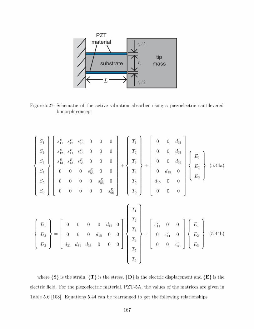
L
st
/ 2pt
/ 2pt
PZT
material
substrate
tip
mass
Figure 5.27: Schematic of the active vibration absorber using a piezoelectric cantileveredbimorph concept
S1
S2
S3
S4
S5
S6
sE11 sE12 sE13 0 0 0
sE12 sE11 sE13 0 0 0
sE13 sE13 sE33 0 0 0
0 0 0 sE55 0 0
0 0 0 0 sE55 0
0 0 0 0 0 sE66
+
T1
T2
T3
T4
T5
T6
+
0 0 d31
0 0 d31
0 0 d33
0 d15 0
d15 0 0
0 0 0
E1
E2
E3
(5.44a)
D1
D2
D3
=
0 0 0 0 d15 0
0 0 0 d15 0 0
d31 d31 d33 0 0 0
T1
T2
T3
T4
T5
T6
+
εT11 0 0
0 εT11 0
0 0 εT33
E1
E2
E3
(5.44b)
where S is the strain, T is the stress, D is the electric displacement and E is the
electric field. For the piezoelectric material, PZT-5A, the values of the matrices are given in
Table 5.6 [108]. Equations 5.44 can be rearranged to get the following relationships
167
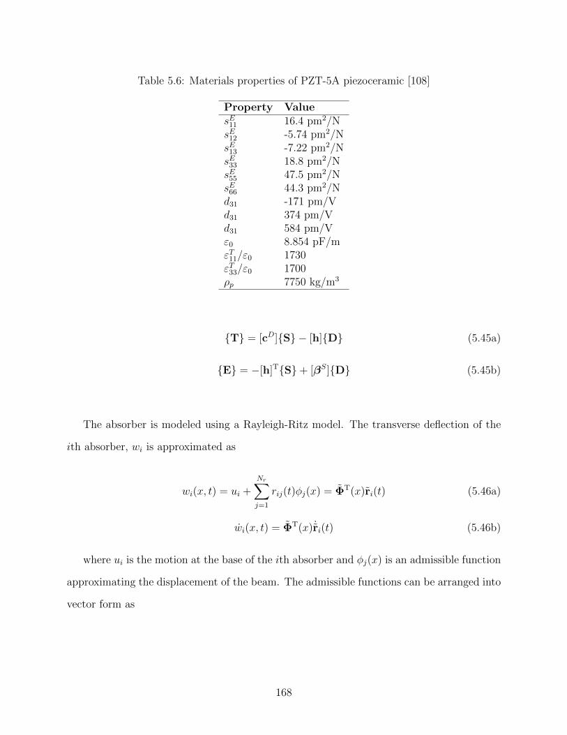
Table 5.6: Materials properties of PZT-5A piezoceramic [108]
Property ValuesE11 16.4 pm2/NsE12 -5.74 pm2/NsE13 -7.22 pm2/NsE33 18.8 pm2/NsE55 47.5 pm2/NsE66 44.3 pm2/Nd31 -171 pm/Vd31 374 pm/Vd31 584 pm/Vε0 8.854 pF/mεT11/ε0 1730εT33/ε0 1700ρp 7750 kg/m3
T = [cD]S − [h]D (5.45a)
E = −[h]TS+ [βS]D (5.45b)
The absorber is modeled using a Rayleigh-Ritz model. The transverse deflection of the
ith absorber, wi is approximated as
wi(x, t) = ui +Nr∑j=1
rij(t)φj(x) = ΦT(x)ri(t) (5.46a)
wi(x, t) = ΦT(x) ˙ri(t) (5.46b)
where ui is the motion at the base of the ith absorber and φj(x) is an admissible function
approximating the displacement of the beam. The admissible functions can be arranged into
vector form as
168
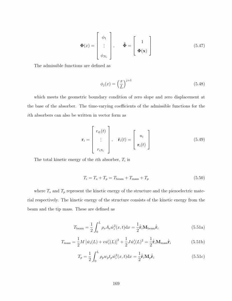
Φ(x) =
φ1
...
φNr
, Φ =
1
Φ(x)
(5.47)
The admissible functions are defined as
φj(x) =(xL
)j+1
(5.48)
which meets the geometric boundary condition of zero slope and zero displacement at
the base of the absorber. The time-varying coefficients of the admissible functions for the
ith absorbers can also be written in vector form as
ri =
ri1(t)
...
riNr
, ri(t) =
ui
ri(t)
(5.49)
The total kinetic energy of the ith absorber, Ti is
Ti = Ts + Tp = Tbeam + Tmass + Tp (5.50)
where Ts and Tp represent the kinetic energy of the structure and the piezoelectric mate-
rial respectively. The kinetic energy of the structure consists of the kinetic energy from the
beam and the tip mass. These are defined as
Tbeam =1
2
∫ L
0
ρsAsw2i (x, t)dx =
1
2˙riMbeam
˙ri (5.51a)
Tmass =1
2M [wi(L) + ew′i(L)]
2+
1
2Jw′i(L)2 =
1
2˙riMmass
˙ri (5.51b)
Tp =1
2
∫ L
0
ρpwptpw2i (x, t)dx =
1
2˙riMp
˙ri (5.51c)
169
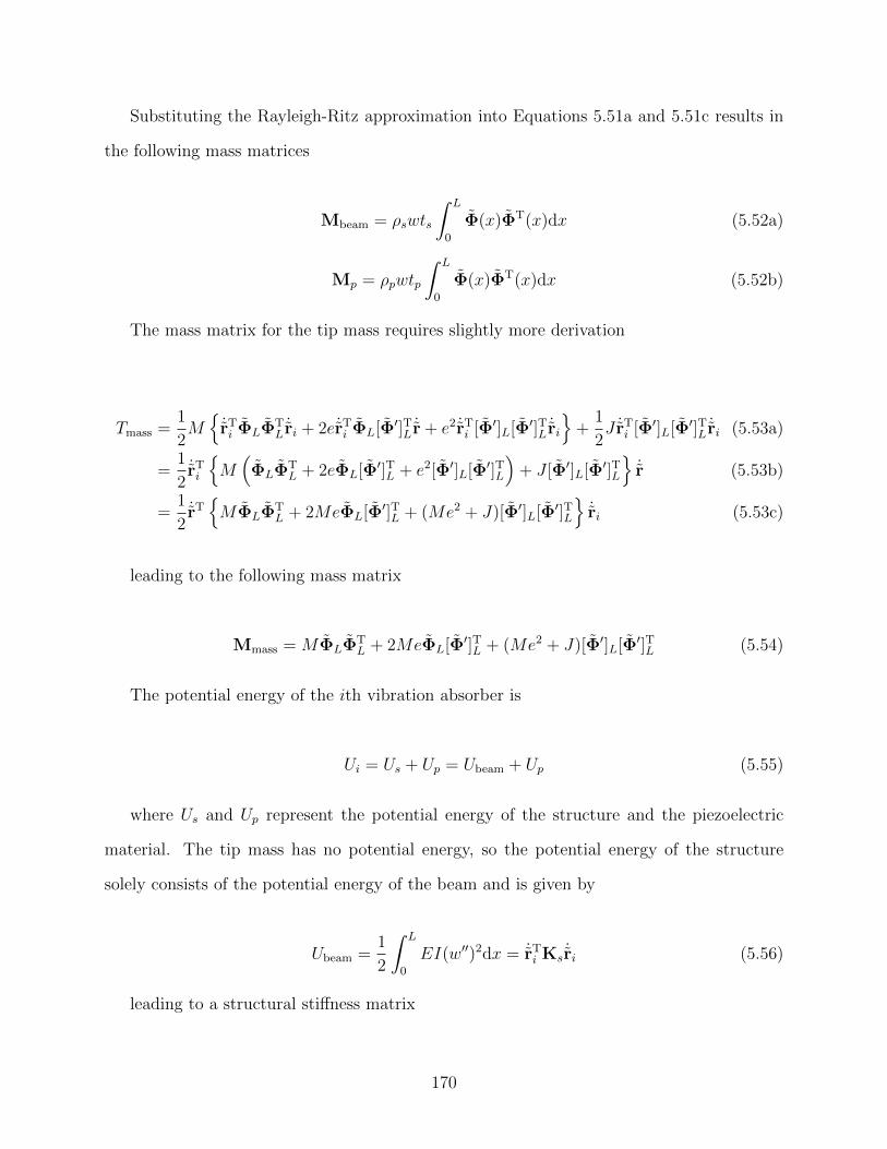
Substituting the Rayleigh-Ritz approximation into Equations 5.51a and 5.51c results in
the following mass matrices
Mbeam = ρswts
∫ L
0
Φ(x)ΦT(x)dx (5.52a)
Mp = ρpwtp
∫ L
0
Φ(x)ΦT(x)dx (5.52b)
The mass matrix for the tip mass requires slightly more derivation
Tmass =1
2M
˙rTi ΦLΦTL
˙ri + 2e ˙rTi ΦL[Φ′]TL ˙r + e2 ˙rTi [Φ′]L[Φ′]TL ˙ri
+
1
2J ˙rTi [Φ′]L[Φ′]TL ˙ri (5.53a)
=1
2˙rTi
M(ΦLΦT
L + 2eΦL[Φ′]TL + e2[Φ′]L[Φ′]TL
)+ J [Φ′]L[Φ′]TL
˙r (5.53b)
=1
2˙rTMΦLΦT
L + 2MeΦL[Φ′]TL + (Me2 + J)[Φ′]L[Φ′]TL
˙ri (5.53c)
leading to the following mass matrix
Mmass = MΦLΦTL + 2MeΦL[Φ′]TL + (Me2 + J)[Φ′]L[Φ′]TL (5.54)
The potential energy of the ith vibration absorber is
Ui = Us + Up = Ubeam + Up (5.55)
where Us and Up represent the potential energy of the structure and the piezoelectric
material. The tip mass has no potential energy, so the potential energy of the structure
solely consists of the potential energy of the beam and is given by
Ubeam =1
2
∫ L
0
EI(w′′)2dx = ˙rTi Ks˙ri (5.56)
leading to a structural stiffness matrix
170
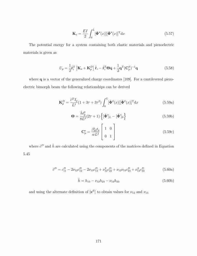
Ks =EI
2
∫ L
0
[Φ′′(x)][Φ′′(x)]Tdx (5.57)
The potential energy for a system containing both elastic materials and piezoelectric
materials is given as
Up =1
2˙rTi[Ks + KD
p
]˙ri − ˙rTi Θq +
1
2qT(CS
p )−1q (5.58)
where q is a vector of the generalized charge coordinates [109]. For a cantilevered piezo-
electric bimorph beam the following relationships can be derived
KDp =
cDIpL4
(1 + 3τ + 3τ 2)
∫ L
0
[Φ′′(x)][Φ′′(x)]Tdx (5.59a)
Θ =ht2p8L3
(2τ + 1)
[Φ′]L − [Φ′]0
(5.59b)
Csp =
βs33tpwL2
1 0
0 1
(5.59c)
where cD and h are calculated using the components of the matrices defined in Equation
5.45
cD = cD11 − 2ν12cD12 − 2ν13c
D13 + ν212c
D22 + ν12ν13c
D23 + ν213c
D33 (5.60a)
h = h13 − ν12h23 − ν13h33 (5.60b)
and using the alternate definition of [sE] to obtain values for ν12 and ν13
171
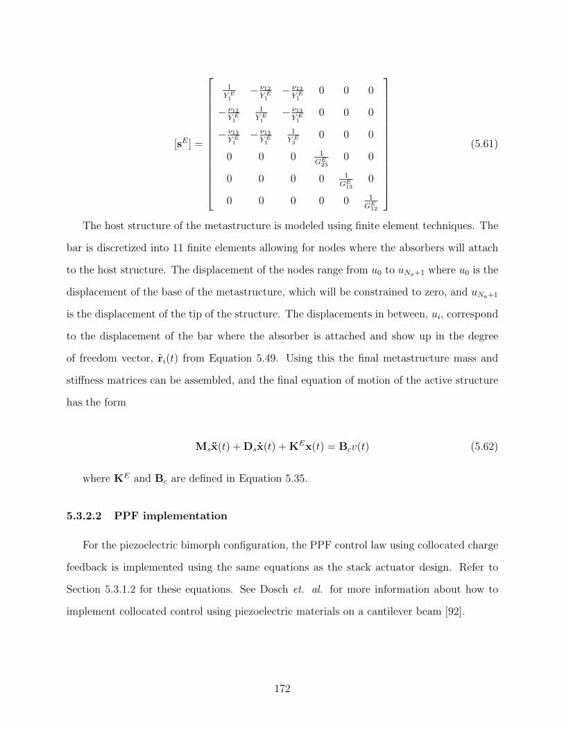
[sE] =
1Y E1− ν12Y E1− ν13Y E1
0 0 0
− ν12Y E1
1Y E1− ν13Y E1
0 0 0
− ν13Y E1− ν13Y E1
1Y E3
0 0 0
0 0 0 1GE
230 0
0 0 0 0 1GE
130
0 0 0 0 0 1GE
12
(5.61)
The host structure of the metastructure is modeled using finite element techniques. The
bar is discretized into 11 finite elements allowing for nodes where the absorbers will attach
to the host structure. The displacement of the nodes range from u0 to uNa+1 where u0 is the
displacement of the base of the metastructure, which will be constrained to zero, and uNa+1
is the displacement of the tip of the structure. The displacements in between, ui, correspond
to the displacement of the bar where the absorber is attached and show up in the degree
of freedom vector, ri(t) from Equation 5.49. Using this the final metastructure mass and
stiffness matrices can be assembled, and the final equation of motion of the active structure
has the form
Msx(t) + Dsx(t) + KEx(t) = Bcv(t) (5.62)
where KE and Bc are defined in Equation 5.35.
5.3.2.2 PPF implementation
For the piezoelectric bimorph configuration, the PPF control law using collocated charge
feedback is implemented using the same equations as the stack actuator design. Refer to
Section 5.3.1.2 for these equations. See Dosch et. al. for more information about how to
implement collocated control using piezoelectric materials on a cantilever beam [92].
172
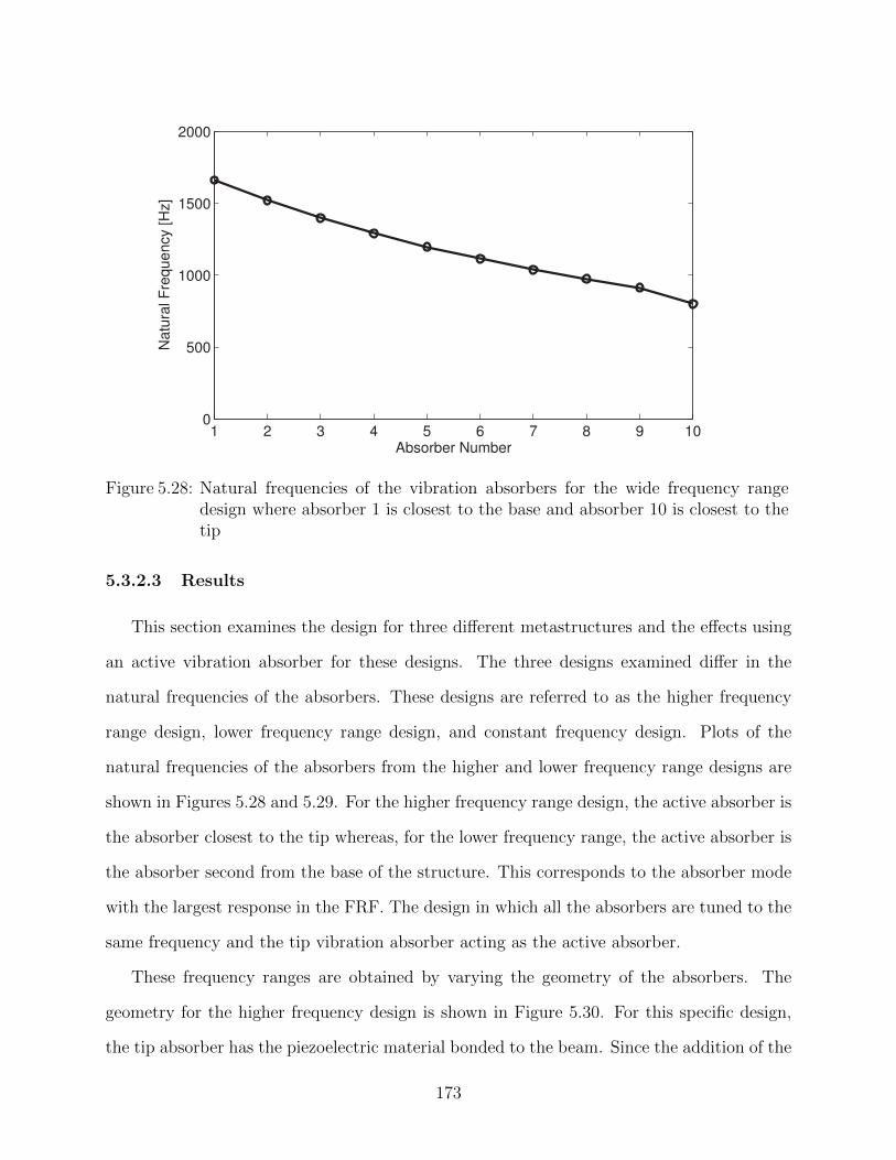
1 2 3 4 5 6 7 8 9 100
500
1000
1500
2000
Absorber Number
Natu
ral F
requency [H
z]
Figure 5.28: Natural frequencies of the vibration absorbers for the wide frequency rangedesign where absorber 1 is closest to the base and absorber 10 is closest to thetip
5.3.2.3 Results
This section examines the design for three different metastructures and the effects using
an active vibration absorber for these designs. The three designs examined differ in the
natural frequencies of the absorbers. These designs are referred to as the higher frequency
range design, lower frequency range design, and constant frequency design. Plots of the
natural frequencies of the absorbers from the higher and lower frequency range designs are
shown in Figures 5.28 and 5.29. For the higher frequency range design, the active absorber is
the absorber closest to the tip whereas, for the lower frequency range, the active absorber is
the absorber second from the base of the structure. This corresponds to the absorber mode
with the largest response in the FRF. The design in which all the absorbers are tuned to the
same frequency and the tip vibration absorber acting as the active absorber.
These frequency ranges are obtained by varying the geometry of the absorbers. The
geometry for the higher frequency design is shown in Figure 5.30. For this specific design,
the tip absorber has the piezoelectric material bonded to the beam. Since the addition of the
173
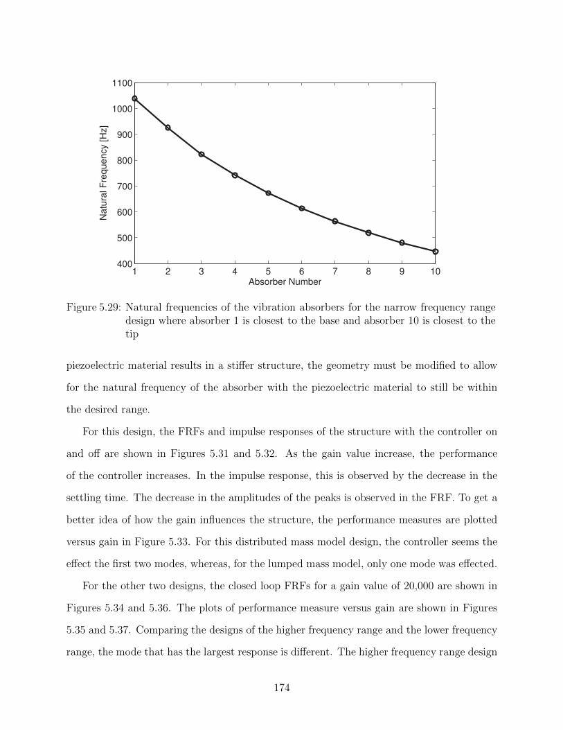
1 2 3 4 5 6 7 8 9 10400
500
600
700
800
900
1000
1100
Absorber Number
Natu
ral F
requency [H
z]
Figure 5.29: Natural frequencies of the vibration absorbers for the narrow frequency rangedesign where absorber 1 is closest to the base and absorber 10 is closest to thetip
piezoelectric material results in a stiffer structure, the geometry must be modified to allow
for the natural frequency of the absorber with the piezoelectric material to still be within
the desired range.
For this design, the FRFs and impulse responses of the structure with the controller on
and off are shown in Figures 5.31 and 5.32. As the gain value increase, the performance
of the controller increases. In the impulse response, this is observed by the decrease in the
settling time. The decrease in the amplitudes of the peaks is observed in the FRF. To get a
better idea of how the gain influences the structure, the performance measures are plotted
versus gain in Figure 5.33. For this distributed mass model design, the controller seems the
effect the first two modes, whereas, for the lumped mass model, only one mode was effected.
For the other two designs, the closed loop FRFs for a gain value of 20,000 are shown in
Figures 5.34 and 5.36. The plots of performance measure versus gain are shown in Figures
5.35 and 5.37. Comparing the designs of the higher frequency range and the lower frequency
range, the mode that has the largest response is different. The higher frequency range design
174
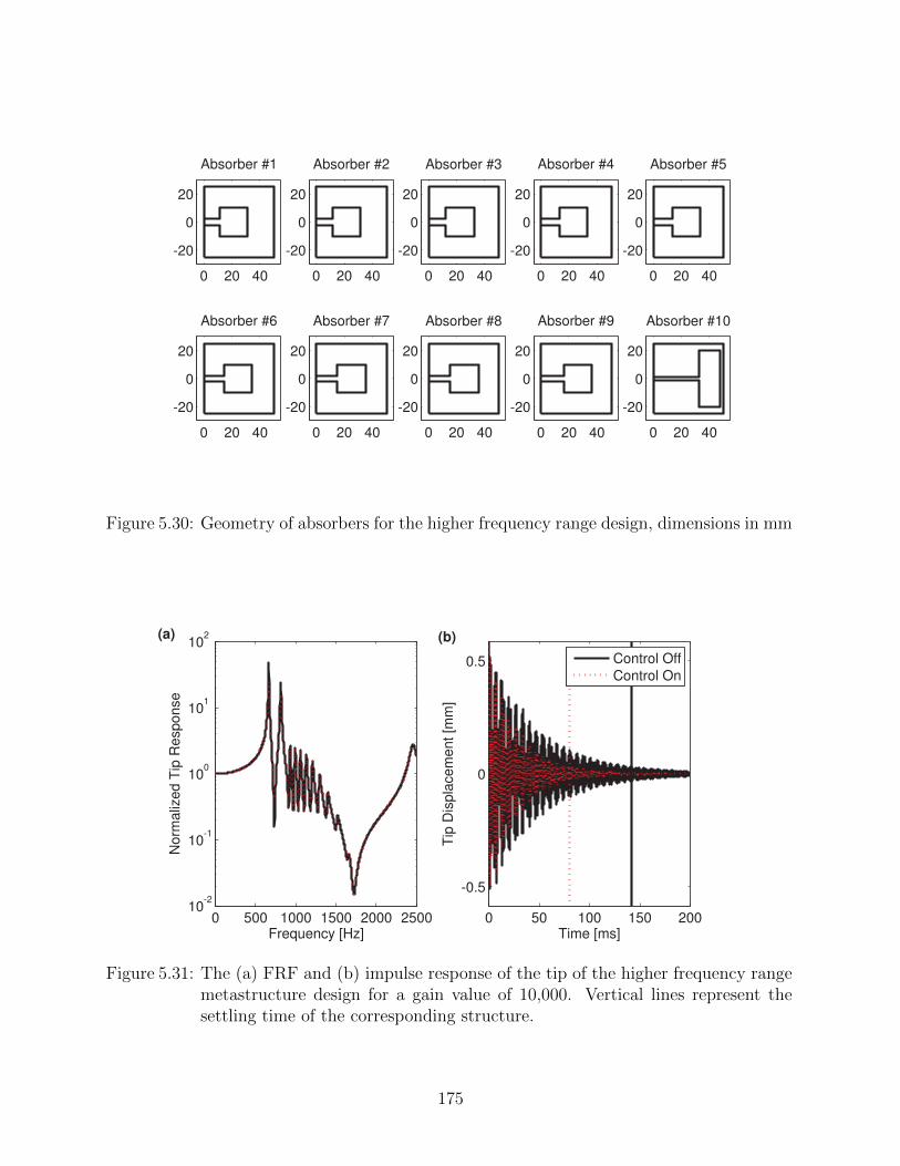
0 20 40
-20
0
20
Absorber #1
0 20 40
-20
0
20
Absorber #2
0 20 40
-20
0
20
Absorber #3
0 20 40
-20
0
20
Absorber #4
0 20 40
-20
0
20
Absorber #5
0 20 40
-20
0
20
Absorber #6
0 20 40
-20
0
20
Absorber #7
0 20 40
-20
0
20
Absorber #8
0 20 40
-20
0
20
Absorber #9
0 20 40
-20
0
20
Absorber #10
Figure 5.30: Geometry of absorbers for the higher frequency range design, dimensions in mm
0 500 1000 1500 2000 250010
-2
10-1
100
101
102
Frequency [Hz]
No
rma
lize
d T
ip R
esp
on
se
0 50 100 150 200
-0.5
0
0.5
Time [ms]
Tip
Dis
pla
ce
me
nt
[mm
]
Control Off
Control On
(b)(a)
Figure 5.31: The (a) FRF and (b) impulse response of the tip of the higher frequency rangemetastructure design for a gain value of 10,000. Vertical lines represent thesettling time of the corresponding structure.
175
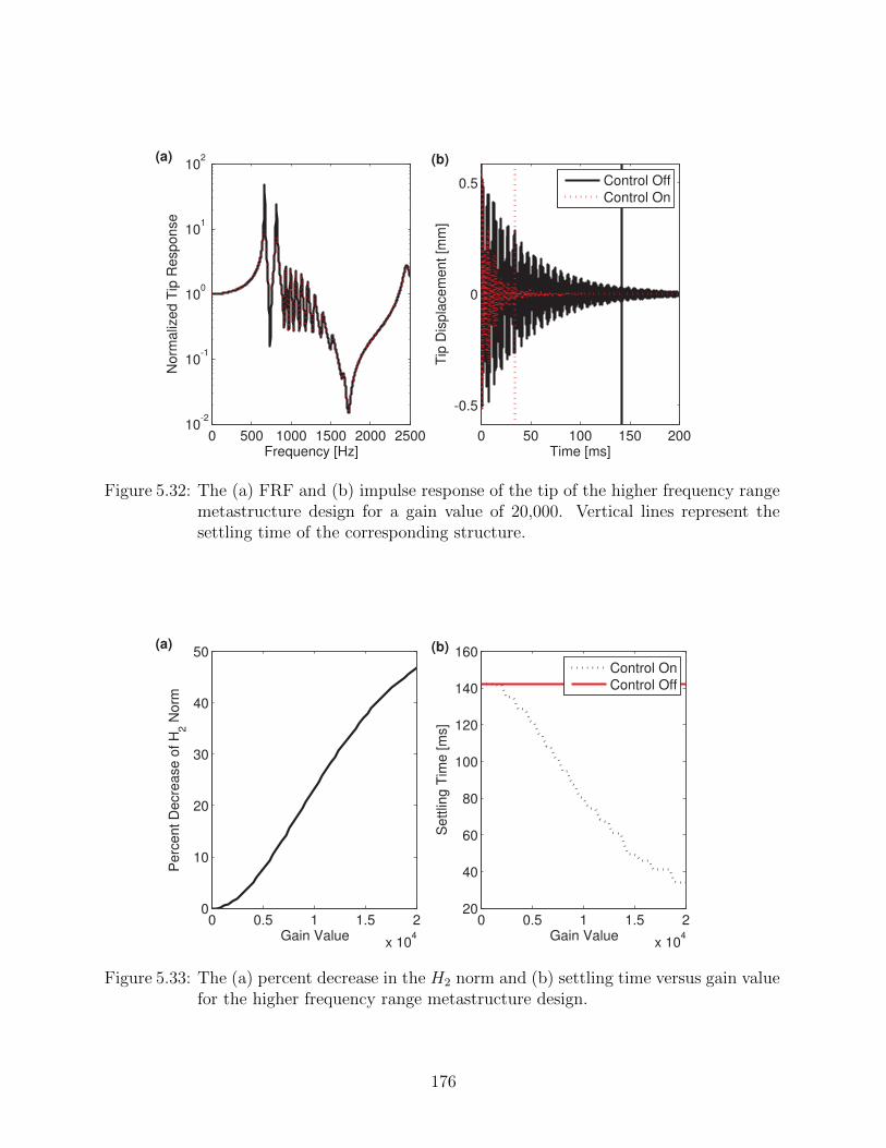
0 500 1000 1500 2000 250010
-2
10-1
100
101
102
Frequency [Hz]
No
rma
lize
d T
ip R
esp
on
se
0 50 100 150 200
-0.5
0
0.5
Time [ms]T
ip D
isp
lace
me
nt
[mm
]
Control Off
Control On
(b)(a)
Figure 5.32: The (a) FRF and (b) impulse response of the tip of the higher frequency rangemetastructure design for a gain value of 20,000. Vertical lines represent thesettling time of the corresponding structure.
0 0.5 1 1.5 2
x 104
0
10
20
30
40
50
Gain Value
Pe
rce
nt
De
cre
ase
of
H2 N
orm
0 0.5 1 1.5 2
x 104
20
40
60
80
100
120
140
160
Gain Value
Se
ttlin
g T
ime
[m
s]
Control On
Control Off
(b)(a)
Figure 5.33: The (a) percent decrease in the H2 norm and (b) settling time versus gain valuefor the higher frequency range metastructure design.
176
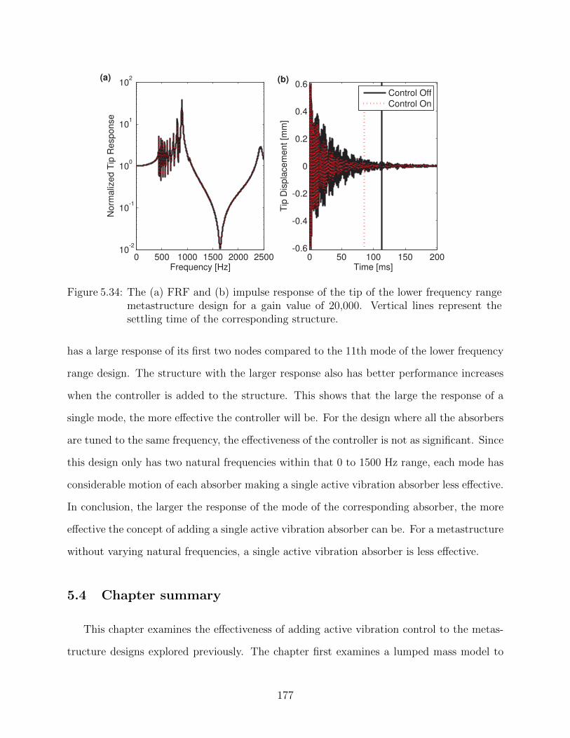
0 500 1000 1500 2000 250010
-2
10-1
100
101
102
Frequency [Hz]
No
rma
lize
d T
ip R
esp
on
se
0 50 100 150 200-0.6
-0.4
-0.2
0
0.2
0.4
0.6
Time [ms]
Tip
Dis
pla
ce
me
nt
[mm
]
Control Off
Control On
(b)(a)
Figure 5.34: The (a) FRF and (b) impulse response of the tip of the lower frequency rangemetastructure design for a gain value of 20,000. Vertical lines represent thesettling time of the corresponding structure.
has a large response of its first two nodes compared to the 11th mode of the lower frequency
range design. The structure with the larger response also has better performance increases
when the controller is added to the structure. This shows that the large the response of a
single mode, the more effective the controller will be. For the design where all the absorbers
are tuned to the same frequency, the effectiveness of the controller is not as significant. Since
this design only has two natural frequencies within that 0 to 1500 Hz range, each mode has
considerable motion of each absorber making a single active vibration absorber less effective.
In conclusion, the larger the response of the mode of the corresponding absorber, the more
effective the concept of adding a single active vibration absorber can be. For a metastructure
without varying natural frequencies, a single active vibration absorber is less effective.
5.4 Chapter summary
This chapter examines the effectiveness of adding active vibration control to the metas-
tructure designs explored previously. The chapter first examines a lumped mass model to
177
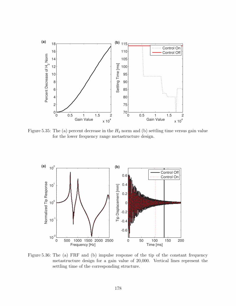
0 0.5 1 1.5 2
x 104
0
2
4
6
8
10
12
14
16
18
Gain Value
Pe
rce
nt
De
cre
ase
of
H2 N
orm
0 0.5 1 1.5 2
x 104
70
75
80
85
90
95
100
105
110
115
Gain ValueS
ett
ling
Tim
e [
ms]
Control On
Control Off
(b)(a)
Figure 5.35: The (a) percent decrease in the H2 norm and (b) settling time versus gain valuefor the lower frequency range metastructure design.
0 500 1000 1500 2000 250010
-2
10-1
100
101
102
Frequency [Hz]
No
rma
lize
d T
ip R
esp
on
se
0 50 100 150 200
-0.6
-0.4
-0.2
0
0.2
0.4
0.6
Time [ms]
Tip
Dis
pla
ce
me
nt
[mm
]
Control Off
Control On
(b)(a)
Figure 5.36: The (a) FRF and (b) impulse response of the tip of the constant frequencymetastructure design for a gain value of 20,000. Vertical lines represent thesettling time of the corresponding structure.
178
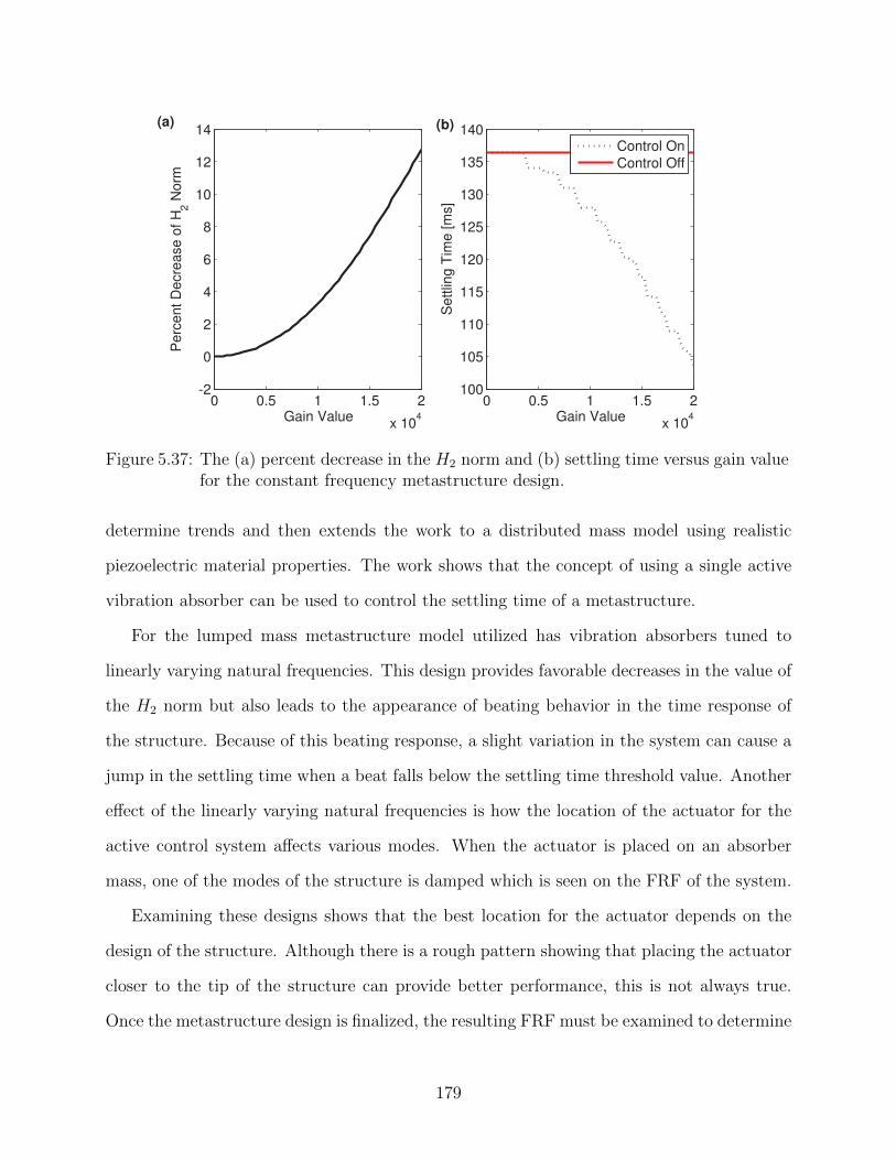
0 0.5 1 1.5 2
x 104
-2
0
2
4
6
8
10
12
14
Gain Value
Pe
rce
nt
De
cre
ase
of
H2 N
orm
0 0.5 1 1.5 2
x 104
100
105
110
115
120
125
130
135
140
Gain Value
Se
ttlin
g T
ime
[m
s]
Control On
Control Off
(b)(a)
Figure 5.37: The (a) percent decrease in the H2 norm and (b) settling time versus gain valuefor the constant frequency metastructure design.
determine trends and then extends the work to a distributed mass model using realistic
piezoelectric material properties. The work shows that the concept of using a single active
vibration absorber can be used to control the settling time of a metastructure.
For the lumped mass metastructure model utilized has vibration absorbers tuned to
linearly varying natural frequencies. This design provides favorable decreases in the value of
the H2 norm but also leads to the appearance of beating behavior in the time response of
the structure. Because of this beating response, a slight variation in the system can cause a
jump in the settling time when a beat falls below the settling time threshold value. Another
effect of the linearly varying natural frequencies is how the location of the actuator for the
active control system affects various modes. When the actuator is placed on an absorber
mass, one of the modes of the structure is damped which is seen on the FRF of the system.
Examining these designs shows that the best location for the actuator depends on the
design of the structure. Although there is a rough pattern showing that placing the actuator
closer to the tip of the structure can provide better performance, this is not always true.
Once the metastructure design is finalized, the resulting FRF must be examined to determine
179
which mode is contributing the most to the response. Once that mode is determined, the
corresponding absorber mass should have the actuator installed.
Once, the active control system is implemented, the nature of the beating behavior will
always cause jumps in the gain versus settling time relationships. This cannot be avoided
without removing the beating behavior. Additionally, there is a limit to the settling time
values the controller can reach. Since the controller damps out a specific mode of the
structure, once that mode is completely damped out, the controller cannot provide any
additional performance increases. These are all important considerations that must be taken
into account when designing an active control system for a metastructure with distributed
vibration absorbers of varying natural frequencies.
For the distributed mass models, two different active vibration absorber designs were
examined. The first design looked at using a stack actuator to control the displacement
of a single absorber. The second design implemented the active vibration absorber using a
piezoelectric bimorph design on a single vibration absorber. The models for both of these
designs were presented along with the necessary equations to implement active control using
the PPF control law. The active vibration absorber design using a stack actuator was shown
to ineffective because the additional stiffness of the stack actuator prevented motion of the
absorber in the lower frequency range only making it effective at higher frequencies.
For the active vibration absorber design using a piezoelectric bimorph configuration,
the PPF control was successfully implemented to reduce the vibrations in the structure.
Examining different designs showed that the larger the response of a mode, the more effective
the active vibration absorber could be. Since the first modes of the structure correspond to
the oscillations of a single absorber, making the absorber active is very effective at controlling
that mode of the metastructure.
In conclusion, depending on the design of the metastructure and the desired performance,
adding an active vibration absorber to the metastructure is a feasible solution to get an
increased performance of the metastructure.
180
CHAPTER VI
Summary and Contributions
6.1 Summary
This dissertation studies the performance of one-dimensional metastructures. These
structures use distributed vibration absorbers to suppress low-frequency vibrations in the
longitudinal direction of the bar. The performance of the metastructures is determined by
examining the frequency response and the time response of the tip of the metastructure bar.
The metastructures are compared to a baseline structure that has the same mass, which
shows that any increase in the performance is due to the addition of the vibration absorbers
and not due to any additional mass being added to the structure. Both lumped mass and
distributed mass models are used to capture the dynamic response of the metastructures.
Additionally, the viscoelastic properties of 3D printed materials are characterized. The ma-
terial properties are implemented into a viscoelastic model of the metastructure and the
effects of temperature are studied. For situations in which high performance is required,
the concept of adding active vibration control to the structure was also investigated. The
following sections provide detailed summaries of the work completed in each chapter.
6.1.1 Chapter II
This chapter uses a lumped mass model to examine the response of a one-dimensional
metastructure. The metastructure is compared to a baseline structure with equal mass.
181
This constraint shows that any increase in performance of the metastructure is due to the
addition of vibration absorbers and not due to the additional mass. The development of
the lumped mass model is shown, and different designs are explored. The metastructure
model is characterized by the number of vibration absorbers, the natural frequencies of the
absorbers, and the mass ratio. The mass ratio is defined as the mass of the absorbers over
the total mass of the metastructure.
The parameters of the structure are optimized with respect to the H2 norm to determine
the best-performing structures. First, the effects of the mass and the stiffness distributions
of the absorbers are studied. The results show that the primary factor influencing the
performance is the ratio of the stiffness over the mass of the absorber, which is related to
the natural frequency of the absorber. The best performance is achieved when the natural
frequencies of the absorbers vary linearly, leading to broadband vibration suppression. For
cases in which the mass ratio is high, the distribution of the mass of the absorbers also
influences the performance.
Looking at metastructures with a varying number of vibration absorbers show that ini-
tially adding more vibration absorbers to the structure results in a better performing struc-
ture, but the performance reaches an asymptote. Once there are around ten absorbers,
adding additional absorbers only increases the performance slightly. The mass ratio trends
show that adding more mass to the absorbers initially increases performance, but after a
certain point, the higher mass ratio leads to a decrease in performance. Lastly, the per-
formance of the metastructure is compared to that of a structure with a single tuned mass
damper. For structures with a lower mass ratio, the metastructure is more effective at re-
ducing vibrations. This comparison has a strong dependence on the level of damping in the
structure.
182
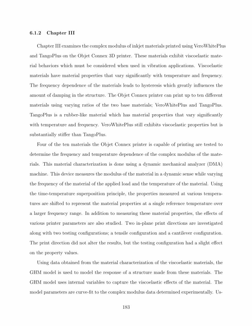
6.1.2 Chapter III
Chapter III examines the complex modulus of inkjet materials printed using VeroWhitePlus
and TangoPlus on the Objet Connex 3D printer. These materials exhibit viscoelastic mate-
rial behaviors which must be considered when used in vibration applications. Viscoelastic
materials have material properties that vary significantly with temperature and frequency.
The frequency dependence of the materials leads to hysteresis which greatly influences the
amount of damping in the structure. The Objet Connex printer can print up to ten different
materials using varying ratios of the two base materials; VeroWhitePlus and TangoPlus.
TangoPlus is a rubber-like material which has material properties that vary significantly
with temperature and frequency. VeroWhitePlus still exhibits viscoelastic properties but is
substantially stiffer than TangoPlus.
Four of the ten materials the Objet Connex printer is capable of printing are tested to
determine the frequency and temperature dependence of the complex modulus of the mate-
rials. This material characterization is done using a dynamic mechanical analyzer (DMA)
machine. This device measures the modulus of the material in a dynamic sense while varying
the frequency of the material of the applied load and the temperature of the material. Using
the time-temperature superposition principle, the properties measured at various tempera-
tures are shifted to represent the material properties at a single reference temperature over
a larger frequency range. In addition to measuring these material properties, the effects of
various printer parameters are also studied. Two in-plane print directions are investigated
along with two testing configurations; a tensile configuration and a cantilever configuration.
The print direction did not alter the results, but the testing configuration had a slight effect
on the property values.
Using data obtained from the material characterization of the viscoelastic materials, the
GHM model is used to model the response of a structure made from these materials. The
GHM model uses internal variables to capture the viscoelastic effects of the material. The
model parameters are curve-fit to the complex modulus data determined experimentally. Us-
183
ing the time-temperature superposition, the curve-fit is conducted at multiple temperatures
allowing the GHM model to also capture the effects of temperature.
The GHM model is verified experimentally by measuring the natural frequency and damp-
ing ratio of a simple cantilevered beam at various temperatures and compared to the pre-
dicted values of the model. The results show the GHM model can accurately predict the
fundamental natural frequency of the cantilevered beam at various temperatures.
6.1.3 Chapter IV
Chapter IV extends the work from Chapters II and III by using the material properties of
the viscoelastic 3D printed materials for a distributed mass metastructure model. A physical
design for a one-dimensional metastructure is proposed, consisting of a bar with a hollow
square cross-section making up the host structure. The vibration absorbers are cantilevered
beams with large tip masses which are distributed along the length of the bar and oriented
such that the bending motion of the cantilevered beams absorbs vibrations along the axial
direction of the bar. The effectiveness of this design is verified experimentally and by using
a commercial finite element model.
The metastructure is then modeled using the GHM model developed in the Chapter III.
The GHM model is beneficial as it allows the response of the metastructure to be calculated
at various temperatures while also incorporating material damping into the model. The
GHM model predicts the damping in a structure using the material properties, not by some
arbitrarily defined damping value.
Next, a design procedure is explained for determining how various parameters affect
the performance of the metastructure. Designs with varying mass ratios and number of
absorbers are examined. For each of these cases, the influences of changing the natural
frequencies of the absorbers are considered. This analysis shows similar results from the
lumped mass model; using vibration absorbers with varying natural frequencies leads to
more board-band suppression. From this analysis, a single metastructure design is chosen
184
to be experimentally tested. The GHM model was able to accurately predict the natural
frequencies of the vibration absorbers within 20%.
The performance of this structure is analytically examined at various temperatures and
compared to a baseline structure of the same weight. The results show the natural frequencies
of the absorbers change at a similar rate to the host structure, allowing the metastructure
to be effective at suppressing vibrations at a range of frequencies. Once the structure gets
to higher temperatures, the damping of the material dominates the response. At these tem-
peratures, the static response of the structure dominates the response, making the baseline
structure more effective at higher temperatures.
6.1.4 Chapter V
Chapter V looks at improving the performance of a metastructure further by adding
active vibration control to the structure. The previously developed lumped mass and dis-
tributed mass models are used for this examination. The models in which controls are
implemented are metastructures with linearly varying natural frequencies. Understanding
the effects of the active vibration absorber requires knowledge about the mode shapes of
the metastructure. The lower-frequency mode shapes of these structures correspond to the
movement a single absorber tuned to the same natural frequency of the natural frequency
of the corresponding mode.
Using the lumped mass model, the controllability and observability norms are examined.
These norms show that placing a sensor on a single absorber is good at sensing the mode
that corresponds to the movement of that absorber. The same goes for an actuator affecting
the controllability of the same mode. Next, the positive position feedback control law is
implemented in the lumped mass model using collocated control, meaning the actuating and
sensing occur at the same location. The control force is placed at various locations. At each
location, the control parameters are optimized to achieve the best performance. This analysis
shows the controller can effectively eliminate a single mode of the structure. Additionally,
185
increasing the gain on the controller causes the settling time of the structure to decrease.
This trend occurs up to a limit, corresponding to when the mode has been eliminated. After
this limit, the controller does not reduce the settling time any further.
For the distributed mass model, two different active vibration absorber designs are con-
sidered using piezoelectric materials. The first uses a stack actuator to control the force
acting on a single absorber. Attaching the stack actuator to the structure results in sig-
nificant additional stiffness, leading to the active vibration absorber only being effective at
higher frequencies. The second design adds PZT materials to the beam of one of the vibra-
tion absorbers in a bimorph configuration. Once again, the PZT materials add additional
stiffness to the structure, but for this design, the geometry of the absorber can be modified
to account for the stiffness change.
The PZT bimorph design is implemented on a few different metastructure designs using
material properties of actual materials. The results show that this design can effectively
be integrated into an actual metastructure design to control the response of the structure.
Additionally, the results show similar trends as the lumped mass model, where a single mode
can be damped out. Furthermore, the larger the uncontrolled response of a mode, the more
effective the controller is.
6.2 Main contributions
The major contributions of this dissertation are focused on the performance of a metas-
tructure bar with linearly varying natural frequencies compared to a baseline structure of
the same weight. The main contributions of this work are summarized as:
• Showing that the concept of using distributed vibration absorbers can effectively reduce
vibrations without adding additional mass to the structure.
• Using vibration absorbers with linearly varying natural frequency leads to more broad-
band suppression.
186
• The creation of a physical one-dimensional metastructure model that experimentally
exhibits the predicted metastructure behavior.
• The characterization of the frequency and temperature dependence of the Objet Con-
nex 3D printed materials.
• Implementing the GHM model to predict the amount of damping in a metastructure
from measured material properties.
• Using the GHM model to accurately predict the fundamental natural frequencies of
cantilevered beams at various temperatures.
• Showing that the concept of adding a single active vibration absorber to a metastruc-
ture can control the response of a single mode of a metastructure with linearly varying
natural frequencies.
• Developing an active vibration absorber design that is effective at reducing the vibra-
tions in a metastructure.
6.3 Recommendations for future work
There are a few different directions the future work for this project could take. These
directions are categorized into the three major parts of this dissertation: metastructures,
viscoelastic modeling, and controls of metastructures. The recommendations for future work
within these three areas are described in future detail below.
6.3.1 Metastructures
This work focused on a one-dimensional metastructure which provided insight into the
general behavior of the metastructures. This work could be extended into two-dimensional
bending metastructures. Beam structures behave differently than bar structures. Thus the
trends for beam structures may look than those found for a metastructure bar here.
187
Additionally, the inverse problem could be considered. This work looked at how changing
the parameters resulted in changes to the dynamic response of the structure. For the inverse
problem, a desired dynamic response could be given and the necessary parameters to achieve
that response could be determined. This would allow for metastructures to be designed for
specific situations.
Another direction of this work could examine the robustness of the metastructure con-
cepts This could be achieved by looking at how sensitive the performance of the metastruc-
ture is to specific parameters. If a vibration absorber is designed to suppress vibrations at a
certain frequency, but the actual frequency of the absorber is off by 5%, how does that affect
the performance of the metastructure?
Before these metastructure concepts can be implemented into real-life applications, the
effects of fatigue on the vibration absorbers must be determined. Since the vibration ab-
sorbers absorb the energy from the rest of the structure, they move significantly. This cyclical
nature can lead to fatigue failure and must be considered.
The work could also take a more application focus, where a specific scenario is chosen, and
a metastructure is designed for that specific case. This would also allow for a more realistic
comparison of the metastructure technique versus other vibration suppression solutions,
such as a tuned mass damper or the addition of viscoelastic materials via constrained layer
damping.
6.3.2 Viscoelastic modeling
This work made an essential first step in modeling the viscoelastic nature of 3D printed
materials. More work could be done in examining the effects of the testing methods used
to experimentally determine the complex modulus. An analysis in the effects of sample size
could be examined. Additionally, the effects of modifying more printing parameters could
be explored. This work examined the effects of two print directions, but a 3D printer has a
total of six different print directions that could be tested.
188
This work solely used the GHM model to model the viscoelastic behavior of the printed
materials. Other viscoelastic models could be used and compared to the GHM model, such
as the augmenting thermodynamic fields model.
6.3.3 Controls
The controls work presented here considered the case in which only a single vibration
absorber was an active vibration absorber. Future work could look at the benefits of using
multiple active vibration absorbers and the trade-offs between adding more active vibration
absorbers and the performance of the active structure.
Additionally, different methods for implementing an active vibration absorber could be
explored. This work looked at using a stack actuator and also a piezoelectric bimorph
configuration. Other designs could be considered and their performance could be compared
to the results here. Additionally, different control laws could be considered.
6.4 List of publications
Journal Publications
1. K. K. Reichl and D. J. Inman, “Lumped mass model of a 1D metastructure for vibration
suppression with no additional mass,” Journal of Sound and Vibration, vol. 403, pp.
75-89, 2017.
2. K. K. Reichl and D. J. Inman, “Dynamic mechanical and thermal analysis of Objet
Connex 3D printed materials,” Experimental Techniques, vol. 42, pp. 19-25, 2018.
3. K. K. Reichl and D. J. Inman, “Temperature-dependent damping in 3D printed poly-
mer structures,” Journal of Vibration and Acoustics, 2018 (in review).
4. K. K. Reichl and D. J. Inman, “Implementation of an active vibration absorber in a
1D metastructure for vibration suppression,” Journal of Intelligent Materials Systems
189
and Structures, 2018 (in preparation).
Conference Proceedings
1. K. K. Reichl and D. J. Inman, “Lumped mass model of a 1D metastructure with vibra-
tion absorbers with varying mass,” in 36th International Modal Analysis Conference,
2018.
2. M. L. Liu, K. K. Reichl and D. J. Inman, “Complex modulus variation by manipula-
tion of mechanical test method and print direction,” in 2017 Society of Engineering
Mechanics Annual Conference, 2017.
3. K. K. Reichl and D. J. Inman, “Constant mass metastructure with vibration absorbers
of linearly varying natural frequencies,” in 35th International Modal Analysis Confer-
ence, 2017.
4. K. K. Reichl and D. J. Inman, “Metastructures and active vibration control,” in 27th
International Conference on Adaptive Structures Technologies, 2016.
5. K. K. Reichl and D. J. Inman, “Dynamic modulus properties of Objet Connex 3D
printer digital materials,” in 34th International Modal Analysis Conference, 2016.
6. K. K. Reichl and D. J. Inman, “Finite element modeling of longitudinal metastruc-
tures for passive vibration suppression,” in 57th AIAA/ASCE/AHS/ASC Structures,
Structural Dynamics, and Materials Conference, 2016.
7. K. K. Reichl and D. J. Inman, “Modeling of low-frequency broadband vibration mit-
igation for a bar experiencing longitudinal vibrations using distributed vibration ab-
sorbers,” in 20th International Conference on Composite Materials, 2015.
190

APPENDICES
191
APPENDIX A
Complex Modulus Data Tables
This appendix provides the complex modulus data for the 3D printed material test for
this work. The specimens tested to compile this data, were all printed from the Objet Connex
3D printer as described in Section 3.2.1. Two different studies were conducted as part of this
work. The first examined the effects of printing direction and testing configuration (Section
3.2.2). Where as, the second study looked at the differences between four materials printed
using the Objet Connex 3D printer. The following sections provide the complex modulus
data for the eight different different testing scenarios using data collected from a dynamic
mechanical analysis (DMA) machine. Using this data, a frequency-temperature analysis
is performed, as described in Section 3.1 including the data for an Arrhenius shift factor
relationship describing the relationship between the temperature and frequency.
A.1 Print direction and testing configuration comparison
This section provides additional details for the DMA testing preformed in Sections 3.2.3.3
and 3.2.3.4 where the effects of print direction and testing configuration were examined for
the 3D printed material DM 8430. Four different specimens were used for this testing.
Schematics showing the print directions and testing configuration are shown in Figures 3.1
and 3.2 respectively. The Arrhenius factor relationship for the four specimens is provided in
Table A.1.
192
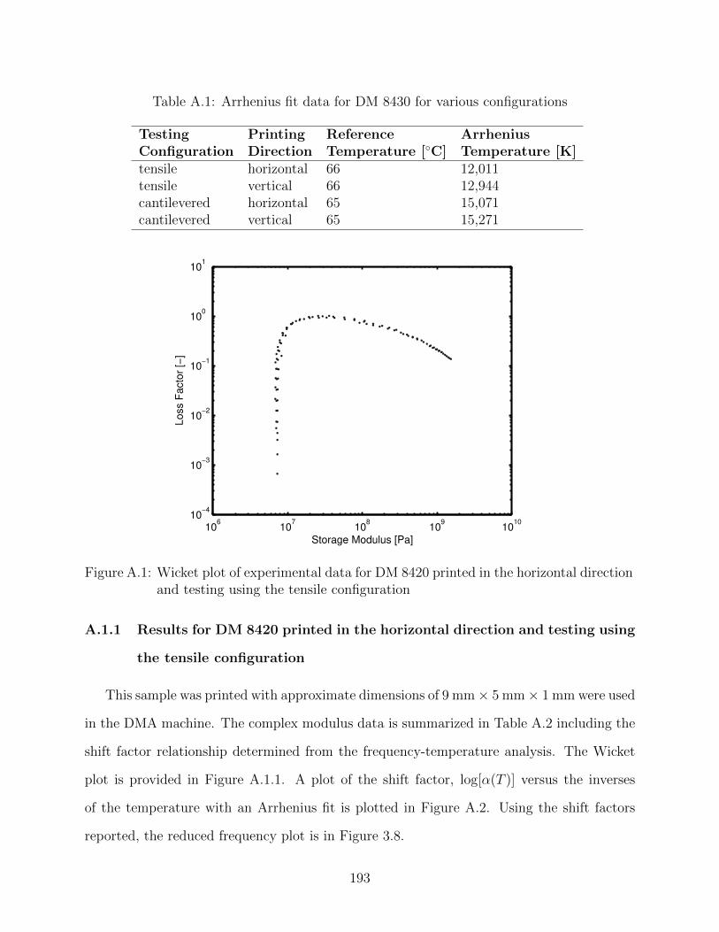
Table A.1: Arrhenius fit data for DM 8430 for various configurations
Testing Printing Reference ArrheniusConfiguration Direction Temperature [C] Temperature [K]tensile horizontal 66 12,011tensile vertical 66 12,944cantilevered horizontal 65 15,071cantilevered vertical 65 15,271
106
107
108
109
1010
10−4
10−3
10−2
10−1
100
101
Storage Modulus [Pa]
Loss F
acto
r [−
]
Figure A.1: Wicket plot of experimental data for DM 8420 printed in the horizontal directionand testing using the tensile configuration
A.1.1 Results for DM 8420 printed in the horizontal direction and testing using
the tensile configuration
This sample was printed with approximate dimensions of 9 mm× 5 mm× 1 mm were used
in the DMA machine. The complex modulus data is summarized in Table A.2 including the
shift factor relationship determined from the frequency-temperature analysis. The Wicket
plot is provided in Figure A.1.1. A plot of the shift factor, log[α(T )] versus the inverses
of the temperature with an Arrhenius fit is plotted in Figure A.2. Using the shift factors
reported, the reduced frequency plot is in Figure 3.8.
193
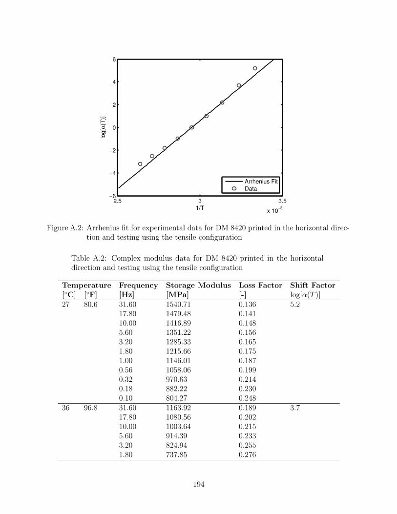
2.5 3 3.5
x 10−3
−6
−4
−2
0
2
4
6
1/T
log[α
(T)]
Arrhenius Fit
Data
Figure A.2: Arrhenius fit for experimental data for DM 8420 printed in the horizontal direc-tion and testing using the tensile configuration
Table A.2: Complex modulus data for DM 8420 printed in the horizontaldirection and testing using the tensile configuration
Temperature Frequency Storage Modulus Loss Factor Shift Factor[C] [F] [Hz] [MPa] [-] log[α(T )]27 80.6 31.60 1540.71 0.136 5.2
17.80 1479.48 0.14110.00 1416.89 0.1485.60 1351.22 0.1563.20 1285.33 0.1651.80 1215.66 0.1751.00 1146.01 0.1870.56 1058.06 0.1990.32 970.63 0.2140.18 882.22 0.2300.10 804.27 0.248
36 96.8 31.60 1163.92 0.189 3.717.80 1080.56 0.20210.00 1003.64 0.2155.60 914.39 0.2333.20 824.94 0.2551.80 737.85 0.276
194
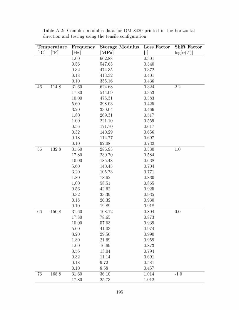
Table A.2: Complex modulus data for DM 8420 printed in the horizontaldirection and testing using the tensile configuration
Temperature Frequency Storage Modulus Loss Factor Shift Factor[C] [F] [Hz] [MPa] [-] log[α(T )]
1.00 662.88 0.3010.56 547.65 0.3400.32 474.35 0.3720.18 413.32 0.4010.10 355.16 0.436
46 114.8 31.60 624.68 0.324 2.217.80 544.09 0.35310.00 475.31 0.3835.60 398.03 0.4253.20 330.04 0.4661.80 269.31 0.5171.00 221.10 0.5590.56 171.70 0.6170.32 140.29 0.6560.18 114.77 0.6970.10 92.08 0.732
56 132.8 31.60 286.93 0.530 1.017.80 230.70 0.58410.00 185.48 0.6385.60 140.43 0.7043.20 105.73 0.7711.80 78.62 0.8301.00 58.51 0.8650.56 42.62 0.9250.32 33.39 0.9350.18 26.32 0.9300.10 19.89 0.918
66 150.8 31.60 108.12 0.804 0.017.80 78.65 0.87310.00 57.63 0.9395.60 41.03 0.9743.20 29.56 0.9901.80 21.69 0.9591.00 16.69 0.8730.56 13.04 0.7940.32 11.14 0.6910.18 9.72 0.5810.10 8.58 0.457
76 168.8 31.60 36.10 1.014 -1.017.80 25.73 1.012
195
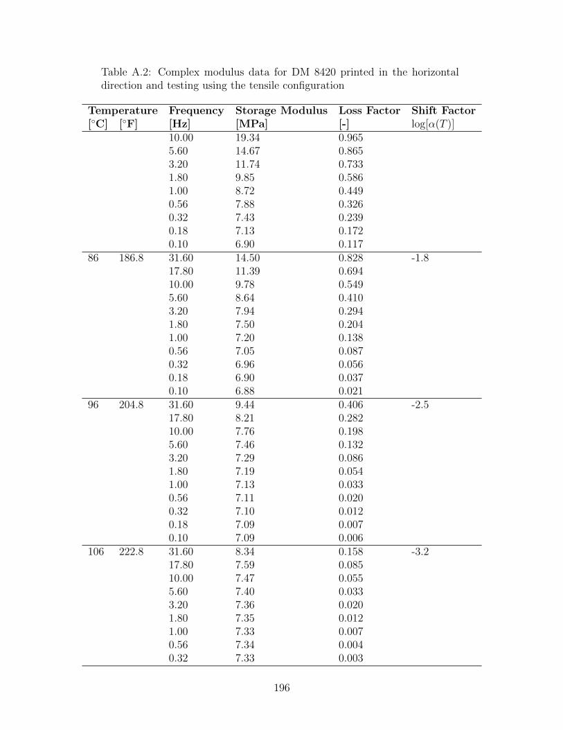
Table A.2: Complex modulus data for DM 8420 printed in the horizontaldirection and testing using the tensile configuration
Temperature Frequency Storage Modulus Loss Factor Shift Factor[C] [F] [Hz] [MPa] [-] log[α(T )]
10.00 19.34 0.9655.60 14.67 0.8653.20 11.74 0.7331.80 9.85 0.5861.00 8.72 0.4490.56 7.88 0.3260.32 7.43 0.2390.18 7.13 0.1720.10 6.90 0.117
86 186.8 31.60 14.50 0.828 -1.817.80 11.39 0.69410.00 9.78 0.5495.60 8.64 0.4103.20 7.94 0.2941.80 7.50 0.2041.00 7.20 0.1380.56 7.05 0.0870.32 6.96 0.0560.18 6.90 0.0370.10 6.88 0.021
96 204.8 31.60 9.44 0.406 -2.517.80 8.21 0.28210.00 7.76 0.1985.60 7.46 0.1323.20 7.29 0.0861.80 7.19 0.0541.00 7.13 0.0330.56 7.11 0.0200.32 7.10 0.0120.18 7.09 0.0070.10 7.09 0.006
106 222.8 31.60 8.34 0.158 -3.217.80 7.59 0.08510.00 7.47 0.0555.60 7.40 0.0333.20 7.36 0.0201.80 7.35 0.0121.00 7.33 0.0070.56 7.34 0.0040.32 7.33 0.003
196
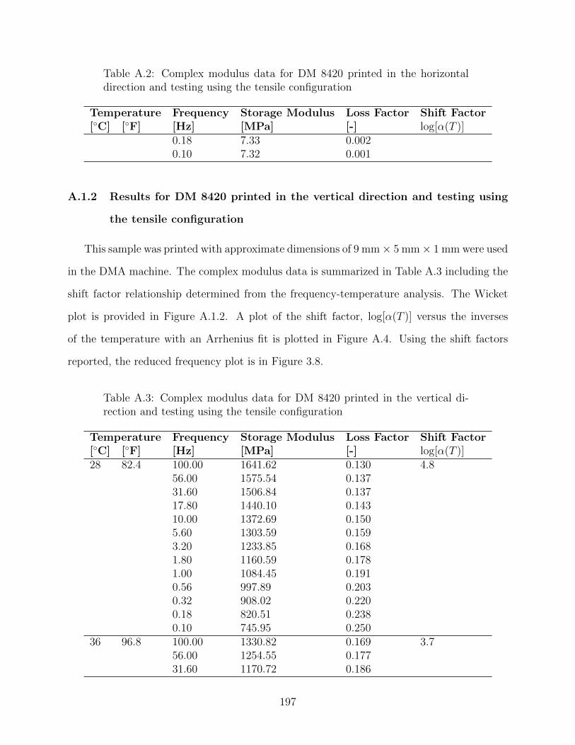
Table A.2: Complex modulus data for DM 8420 printed in the horizontaldirection and testing using the tensile configuration
Temperature Frequency Storage Modulus Loss Factor Shift Factor[C] [F] [Hz] [MPa] [-] log[α(T )]
0.18 7.33 0.0020.10 7.32 0.001
A.1.2 Results for DM 8420 printed in the vertical direction and testing using
the tensile configuration
This sample was printed with approximate dimensions of 9 mm× 5 mm× 1 mm were used
in the DMA machine. The complex modulus data is summarized in Table A.3 including the
shift factor relationship determined from the frequency-temperature analysis. The Wicket
plot is provided in Figure A.1.2. A plot of the shift factor, log[α(T )] versus the inverses
of the temperature with an Arrhenius fit is plotted in Figure A.4. Using the shift factors
reported, the reduced frequency plot is in Figure 3.8.
Table A.3: Complex modulus data for DM 8420 printed in the vertical di-rection and testing using the tensile configuration
Temperature Frequency Storage Modulus Loss Factor Shift Factor[C] [F] [Hz] [MPa] [-] log[α(T )]28 82.4 100.00 1641.62 0.130 4.8
56.00 1575.54 0.13731.60 1506.84 0.13717.80 1440.10 0.14310.00 1372.69 0.1505.60 1303.59 0.1593.20 1233.85 0.1681.80 1160.59 0.1781.00 1084.45 0.1910.56 997.89 0.2030.32 908.02 0.2200.18 820.51 0.2380.10 745.95 0.250
36 96.8 100.00 1330.82 0.169 3.756.00 1254.55 0.17731.60 1170.72 0.186
197
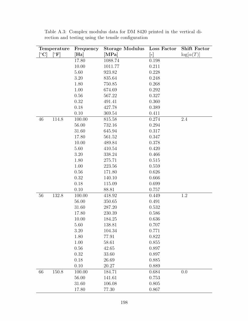
Table A.3: Complex modulus data for DM 8420 printed in the vertical di-rection and testing using the tensile configuration
Temperature Frequency Storage Modulus Loss Factor Shift Factor[C] [F] [Hz] [MPa] [-] log[α(T )]
17.80 1088.74 0.19810.00 1011.77 0.2115.60 923.82 0.2283.20 835.64 0.2481.80 750.85 0.2681.00 674.69 0.2920.56 567.22 0.3270.32 491.41 0.3600.18 427.78 0.3890.10 369.54 0.411
46 114.8 100.00 815.58 0.274 2.456.00 732.16 0.29431.60 645.94 0.31717.80 561.52 0.34710.00 489.84 0.3785.60 410.54 0.4203.20 338.24 0.4661.80 275.71 0.5151.00 223.56 0.5590.56 171.80 0.6260.32 140.10 0.6660.18 115.09 0.6990.10 88.81 0.757
56 132.8 100.00 418.92 0.449 1.256.00 350.65 0.49131.60 287.20 0.53217.80 230.39 0.58610.00 184.25 0.6365.60 138.81 0.7073.20 104.34 0.7711.80 77.91 0.8221.00 58.61 0.8550.56 42.65 0.8970.32 33.60 0.8970.18 26.69 0.8850.10 20.27 0.889
66 150.8 100.00 184.71 0.684 0.056.00 141.61 0.75331.60 106.08 0.80517.80 77.30 0.867
198
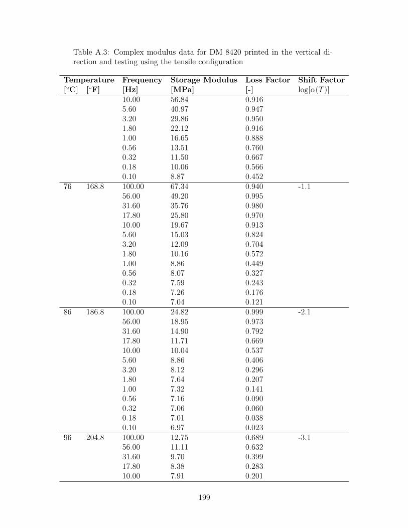
Table A.3: Complex modulus data for DM 8420 printed in the vertical di-rection and testing using the tensile configuration
Temperature Frequency Storage Modulus Loss Factor Shift Factor[C] [F] [Hz] [MPa] [-] log[α(T )]
10.00 56.84 0.9165.60 40.97 0.9473.20 29.86 0.9501.80 22.12 0.9161.00 16.65 0.8880.56 13.51 0.7600.32 11.50 0.6670.18 10.06 0.5660.10 8.87 0.452
76 168.8 100.00 67.34 0.940 -1.156.00 49.20 0.99531.60 35.76 0.98017.80 25.80 0.97010.00 19.67 0.9135.60 15.03 0.8243.20 12.09 0.7041.80 10.16 0.5721.00 8.86 0.4490.56 8.07 0.3270.32 7.59 0.2430.18 7.26 0.1760.10 7.04 0.121
86 186.8 100.00 24.82 0.999 -2.156.00 18.95 0.97331.60 14.90 0.79217.80 11.71 0.66910.00 10.04 0.5375.60 8.86 0.4063.20 8.12 0.2961.80 7.64 0.2071.00 7.32 0.1410.56 7.16 0.0900.32 7.06 0.0600.18 7.01 0.0380.10 6.97 0.023
96 204.8 100.00 12.75 0.689 -3.156.00 11.11 0.63231.60 9.70 0.39917.80 8.38 0.28310.00 7.91 0.201
199
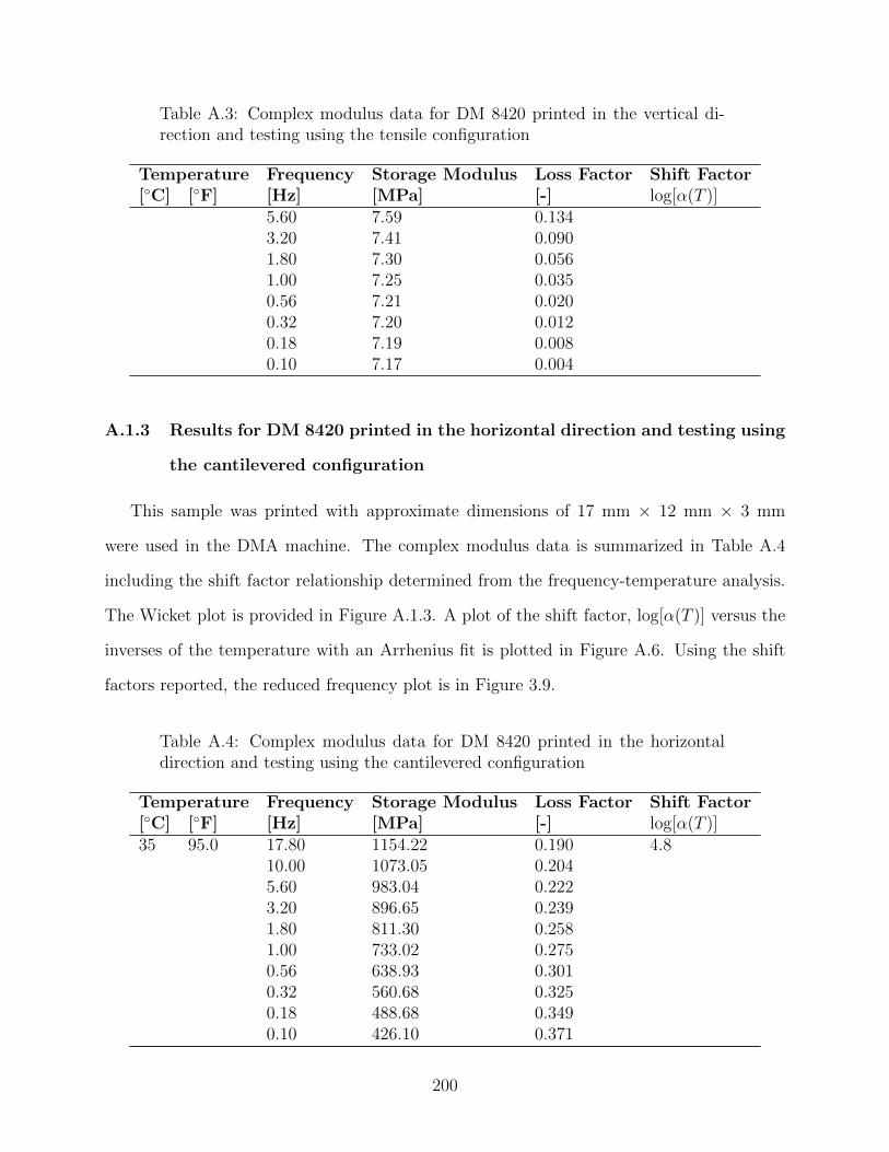
Table A.3: Complex modulus data for DM 8420 printed in the vertical di-rection and testing using the tensile configuration
Temperature Frequency Storage Modulus Loss Factor Shift Factor[C] [F] [Hz] [MPa] [-] log[α(T )]
5.60 7.59 0.1343.20 7.41 0.0901.80 7.30 0.0561.00 7.25 0.0350.56 7.21 0.0200.32 7.20 0.0120.18 7.19 0.0080.10 7.17 0.004
A.1.3 Results for DM 8420 printed in the horizontal direction and testing using
the cantilevered configuration
This sample was printed with approximate dimensions of 17 mm × 12 mm × 3 mm
were used in the DMA machine. The complex modulus data is summarized in Table A.4
including the shift factor relationship determined from the frequency-temperature analysis.
The Wicket plot is provided in Figure A.1.3. A plot of the shift factor, log[α(T )] versus the
inverses of the temperature with an Arrhenius fit is plotted in Figure A.6. Using the shift
factors reported, the reduced frequency plot is in Figure 3.9.
Table A.4: Complex modulus data for DM 8420 printed in the horizontaldirection and testing using the cantilevered configuration
Temperature Frequency Storage Modulus Loss Factor Shift Factor[C] [F] [Hz] [MPa] [-] log[α(T )]35 95.0 17.80 1154.22 0.190 4.8
10.00 1073.05 0.2045.60 983.04 0.2223.20 896.65 0.2391.80 811.30 0.2581.00 733.02 0.2750.56 638.93 0.3010.32 560.68 0.3250.18 488.68 0.3490.10 426.10 0.371
200
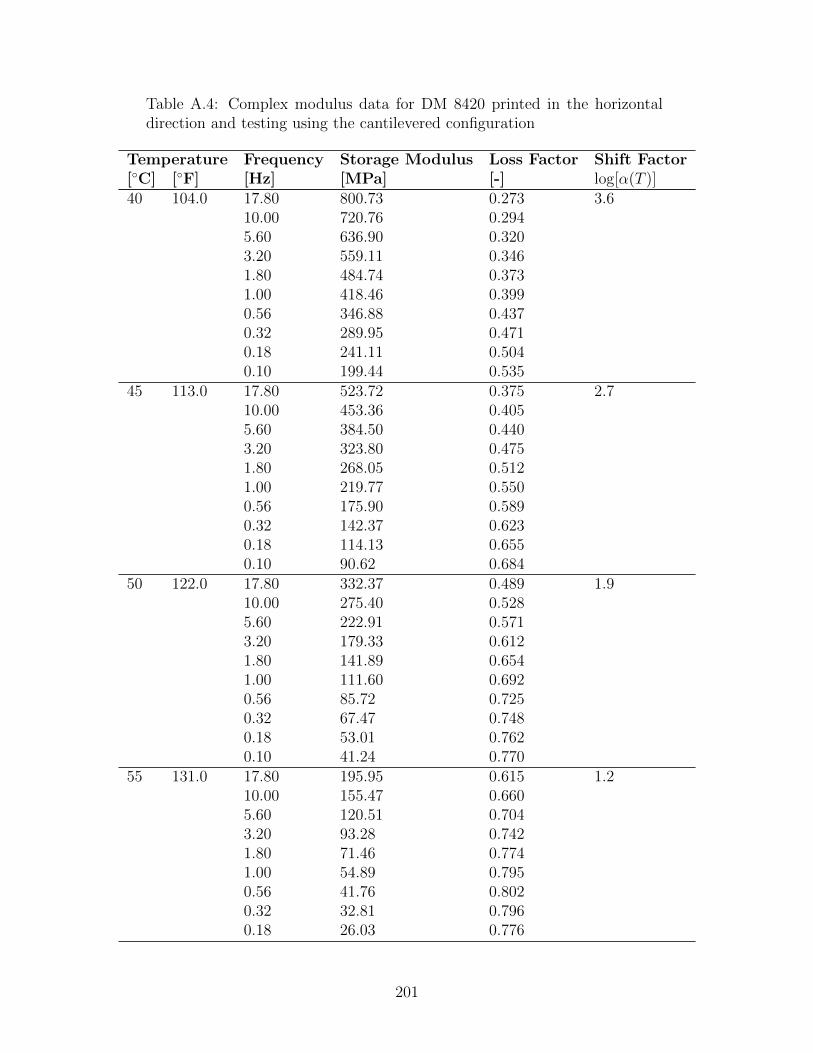
Table A.4: Complex modulus data for DM 8420 printed in the horizontaldirection and testing using the cantilevered configuration
Temperature Frequency Storage Modulus Loss Factor Shift Factor[C] [F] [Hz] [MPa] [-] log[α(T )]40 104.0 17.80 800.73 0.273 3.6
10.00 720.76 0.2945.60 636.90 0.3203.20 559.11 0.3461.80 484.74 0.3731.00 418.46 0.3990.56 346.88 0.4370.32 289.95 0.4710.18 241.11 0.5040.10 199.44 0.535
45 113.0 17.80 523.72 0.375 2.710.00 453.36 0.4055.60 384.50 0.4403.20 323.80 0.4751.80 268.05 0.5121.00 219.77 0.5500.56 175.90 0.5890.32 142.37 0.6230.18 114.13 0.6550.10 90.62 0.684
50 122.0 17.80 332.37 0.489 1.910.00 275.40 0.5285.60 222.91 0.5713.20 179.33 0.6121.80 141.89 0.6541.00 111.60 0.6920.56 85.72 0.7250.32 67.47 0.7480.18 53.01 0.7620.10 41.24 0.770
55 131.0 17.80 195.95 0.615 1.210.00 155.47 0.6605.60 120.51 0.7043.20 93.28 0.7421.80 71.46 0.7741.00 54.89 0.7950.56 41.76 0.8020.32 32.81 0.7960.18 26.03 0.776
201
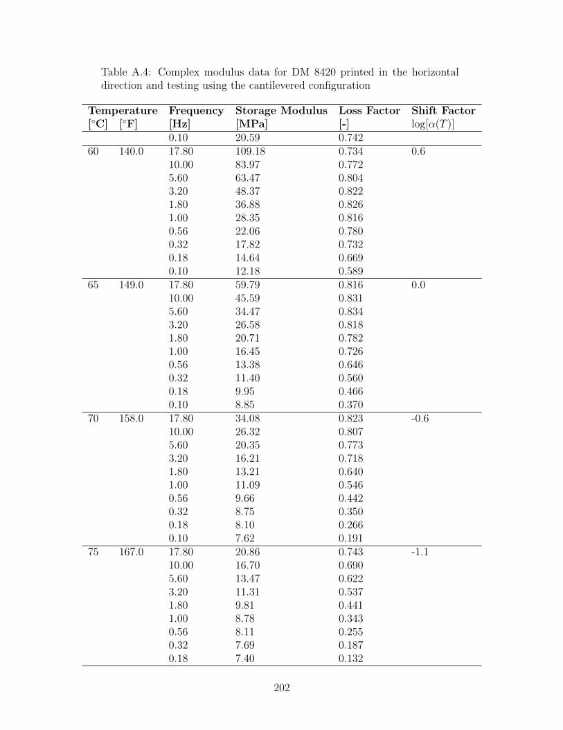
Table A.4: Complex modulus data for DM 8420 printed in the horizontaldirection and testing using the cantilevered configuration
Temperature Frequency Storage Modulus Loss Factor Shift Factor[C] [F] [Hz] [MPa] [-] log[α(T )]
0.10 20.59 0.74260 140.0 17.80 109.18 0.734 0.6
10.00 83.97 0.7725.60 63.47 0.8043.20 48.37 0.8221.80 36.88 0.8261.00 28.35 0.8160.56 22.06 0.7800.32 17.82 0.7320.18 14.64 0.6690.10 12.18 0.589
65 149.0 17.80 59.79 0.816 0.010.00 45.59 0.8315.60 34.47 0.8343.20 26.58 0.8181.80 20.71 0.7821.00 16.45 0.7260.56 13.38 0.6460.32 11.40 0.5600.18 9.95 0.4660.10 8.85 0.370
70 158.0 17.80 34.08 0.823 -0.610.00 26.32 0.8075.60 20.35 0.7733.20 16.21 0.7181.80 13.21 0.6401.00 11.09 0.5460.56 9.66 0.4420.32 8.75 0.3500.18 8.10 0.2660.10 7.62 0.191
75 167.0 17.80 20.86 0.743 -1.110.00 16.70 0.6905.60 13.47 0.6223.20 11.31 0.5371.80 9.81 0.4411.00 8.78 0.3430.56 8.11 0.2550.32 7.69 0.1870.18 7.40 0.132
202
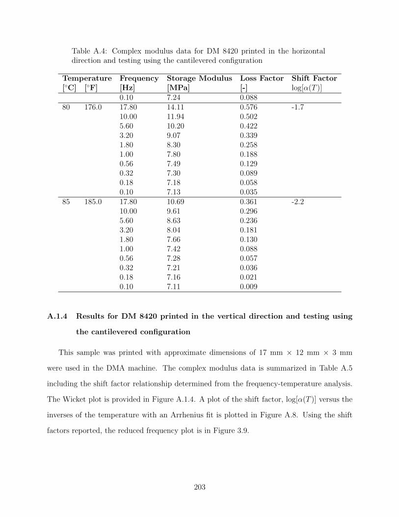
Table A.4: Complex modulus data for DM 8420 printed in the horizontaldirection and testing using the cantilevered configuration
Temperature Frequency Storage Modulus Loss Factor Shift Factor[C] [F] [Hz] [MPa] [-] log[α(T )]
0.10 7.24 0.08880 176.0 17.80 14.11 0.576 -1.7
10.00 11.94 0.5025.60 10.20 0.4223.20 9.07 0.3391.80 8.30 0.2581.00 7.80 0.1880.56 7.49 0.1290.32 7.30 0.0890.18 7.18 0.0580.10 7.13 0.035
85 185.0 17.80 10.69 0.361 -2.210.00 9.61 0.2965.60 8.63 0.2363.20 8.04 0.1811.80 7.66 0.1301.00 7.42 0.0880.56 7.28 0.0570.32 7.21 0.0360.18 7.16 0.0210.10 7.11 0.009
A.1.4 Results for DM 8420 printed in the vertical direction and testing using
the cantilevered configuration
This sample was printed with approximate dimensions of 17 mm × 12 mm × 3 mm
were used in the DMA machine. The complex modulus data is summarized in Table A.5
including the shift factor relationship determined from the frequency-temperature analysis.
The Wicket plot is provided in Figure A.1.4. A plot of the shift factor, log[α(T )] versus the
inverses of the temperature with an Arrhenius fit is plotted in Figure A.8. Using the shift
factors reported, the reduced frequency plot is in Figure 3.9.
203
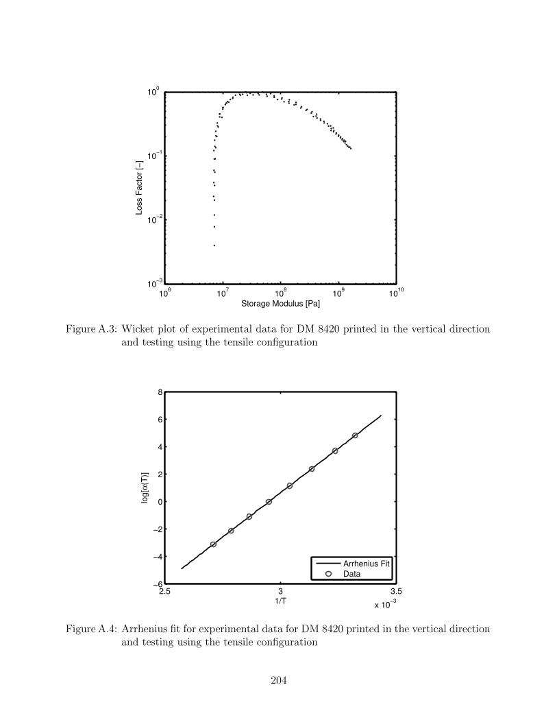
106
107
108
109
1010
10−3
10−2
10−1
100
Storage Modulus [Pa]
Loss F
acto
r [−
]
Figure A.3: Wicket plot of experimental data for DM 8420 printed in the vertical directionand testing using the tensile configuration
2.5 3 3.5
x 10−3
−6
−4
−2
0
2
4
6
8
1/T
log[α
(T)]
Arrhenius Fit
Data
Figure A.4: Arrhenius fit for experimental data for DM 8420 printed in the vertical directionand testing using the tensile configuration
204
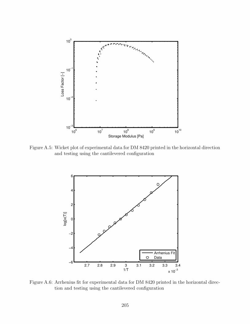
106
107
108
109
1010
10−3
10−2
10−1
100
Storage Modulus [Pa]
Loss F
acto
r [−
]
Figure A.5: Wicket plot of experimental data for DM 8420 printed in the horizontal directionand testing using the cantilevered configuration
2.7 2.8 2.9 3 3.1 3.2 3.3 3.4
x 10−3
−6
−4
−2
0
2
4
6
1/T
log[α
(T)]
Arrhenius Fit
Data
Figure A.6: Arrhenius fit for experimental data for DM 8420 printed in the horizontal direc-tion and testing using the cantilevered configuration
205
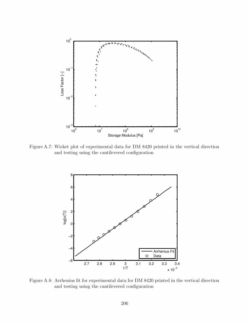
106
107
108
109
1010
10−3
10−2
10−1
100
Storage Modulus [Pa]
Loss F
acto
r [−
]
Figure A.7: Wicket plot of experimental data for DM 8420 printed in the vertical directionand testing using the cantilevered configuration
2.7 2.8 2.9 3 3.1 3.2 3.3 3.4
x 10−3
−6
−4
−2
0
2
4
6
8
1/T
log[α
(T)]
Arrhenius Fit
Data
Figure A.8: Arrhenius fit for experimental data for DM 8420 printed in the vertical directionand testing using the cantilevered configuration
206
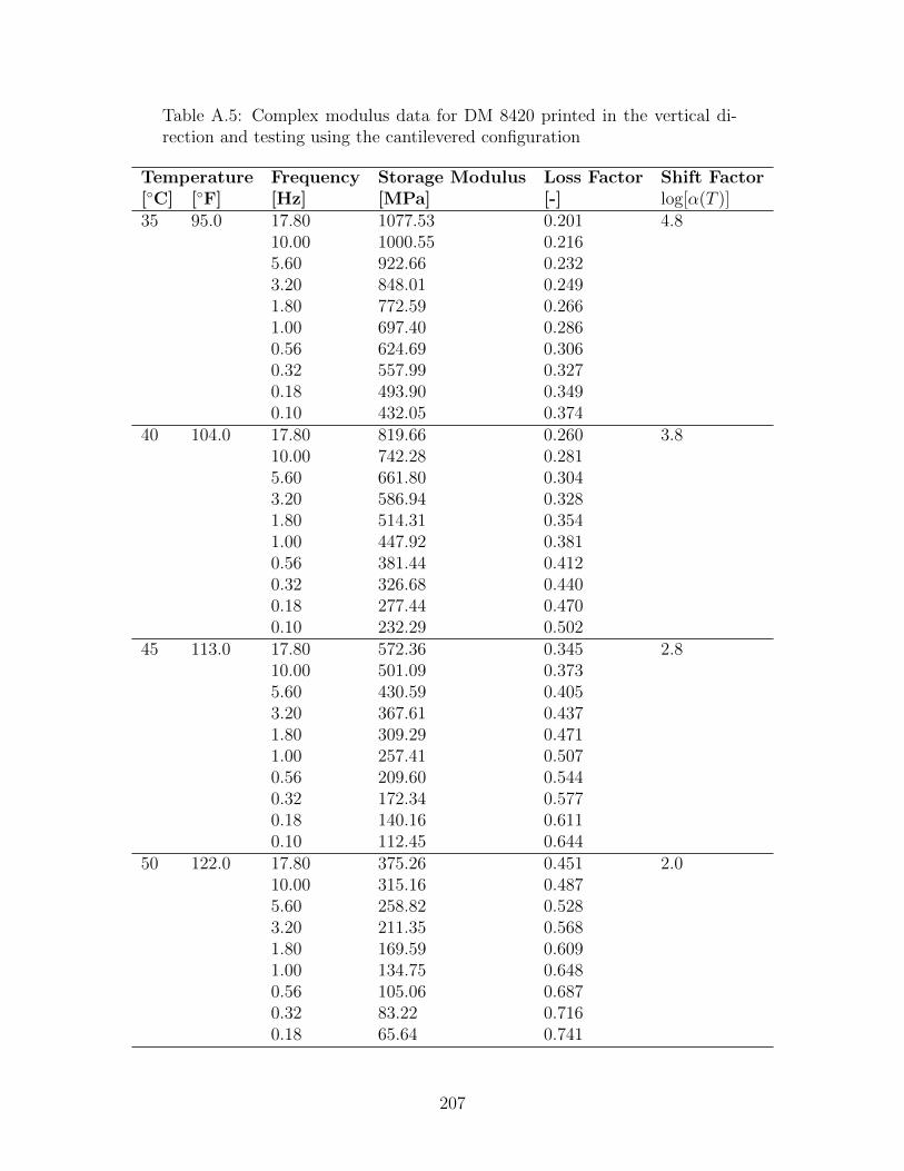
Table A.5: Complex modulus data for DM 8420 printed in the vertical di-rection and testing using the cantilevered configuration
Temperature Frequency Storage Modulus Loss Factor Shift Factor[C] [F] [Hz] [MPa] [-] log[α(T )]35 95.0 17.80 1077.53 0.201 4.8
10.00 1000.55 0.2165.60 922.66 0.2323.20 848.01 0.2491.80 772.59 0.2661.00 697.40 0.2860.56 624.69 0.3060.32 557.99 0.3270.18 493.90 0.3490.10 432.05 0.374
40 104.0 17.80 819.66 0.260 3.810.00 742.28 0.2815.60 661.80 0.3043.20 586.94 0.3281.80 514.31 0.3541.00 447.92 0.3810.56 381.44 0.4120.32 326.68 0.4400.18 277.44 0.4700.10 232.29 0.502
45 113.0 17.80 572.36 0.345 2.810.00 501.09 0.3735.60 430.59 0.4053.20 367.61 0.4371.80 309.29 0.4711.00 257.41 0.5070.56 209.60 0.5440.32 172.34 0.5770.18 140.16 0.6110.10 112.45 0.644
50 122.0 17.80 375.26 0.451 2.010.00 315.16 0.4875.60 258.82 0.5283.20 211.35 0.5681.80 169.59 0.6091.00 134.75 0.6480.56 105.06 0.6870.32 83.22 0.7160.18 65.64 0.741
207
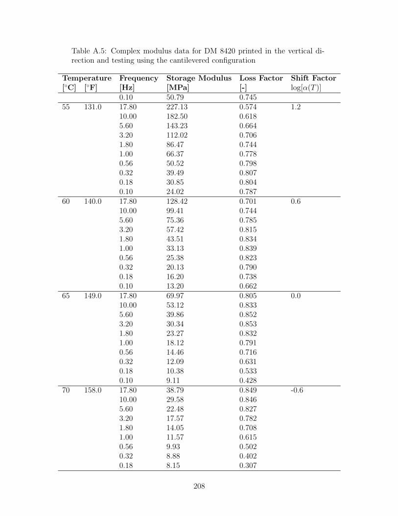
Table A.5: Complex modulus data for DM 8420 printed in the vertical di-rection and testing using the cantilevered configuration
Temperature Frequency Storage Modulus Loss Factor Shift Factor[C] [F] [Hz] [MPa] [-] log[α(T )]
0.10 50.79 0.74555 131.0 17.80 227.13 0.574 1.2
10.00 182.50 0.6185.60 143.23 0.6643.20 112.02 0.7061.80 86.47 0.7441.00 66.37 0.7780.56 50.52 0.7980.32 39.49 0.8070.18 30.85 0.8040.10 24.02 0.787
60 140.0 17.80 128.42 0.701 0.610.00 99.41 0.7445.60 75.36 0.7853.20 57.42 0.8151.80 43.51 0.8341.00 33.13 0.8390.56 25.38 0.8230.32 20.13 0.7900.18 16.20 0.7380.10 13.20 0.662
65 149.0 17.80 69.97 0.805 0.010.00 53.12 0.8335.60 39.86 0.8523.20 30.34 0.8531.80 23.27 0.8321.00 18.12 0.7910.56 14.46 0.7160.32 12.09 0.6310.18 10.38 0.5330.10 9.11 0.428
70 158.0 17.80 38.79 0.849 -0.610.00 29.58 0.8465.60 22.48 0.8273.20 17.57 0.7821.80 14.05 0.7081.00 11.57 0.6150.56 9.93 0.5020.32 8.88 0.4020.18 8.15 0.307
208
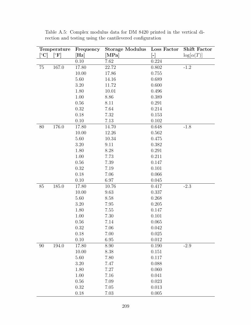
Table A.5: Complex modulus data for DM 8420 printed in the vertical di-rection and testing using the cantilevered configuration
Temperature Frequency Storage Modulus Loss Factor Shift Factor[C] [F] [Hz] [MPa] [-] log[α(T )]
0.10 7.62 0.22475 167.0 17.80 22.72 0.802 -1.2
10.00 17.86 0.7555.60 14.16 0.6893.20 11.72 0.6001.80 10.01 0.4961.00 8.86 0.3890.56 8.11 0.2910.32 7.64 0.2140.18 7.32 0.1530.10 7.13 0.102
80 176.0 17.80 14.70 0.648 -1.810.00 12.26 0.5625.60 10.34 0.4753.20 9.11 0.3821.80 8.28 0.2911.00 7.73 0.2110.56 7.39 0.1470.32 7.19 0.1010.18 7.06 0.0660.10 6.97 0.045
85 185.0 17.80 10.76 0.417 -2.310.00 9.63 0.3375.60 8.58 0.2683.20 7.95 0.2051.80 7.55 0.1471.00 7.30 0.1010.56 7.14 0.0650.32 7.06 0.0420.18 7.00 0.0250.10 6.95 0.012
90 194.0 17.80 8.90 0.190 -2.910.00 8.38 0.1515.60 7.80 0.1173.20 7.47 0.0881.80 7.27 0.0601.00 7.16 0.0410.56 7.09 0.0230.32 7.05 0.0130.18 7.03 0.005
209
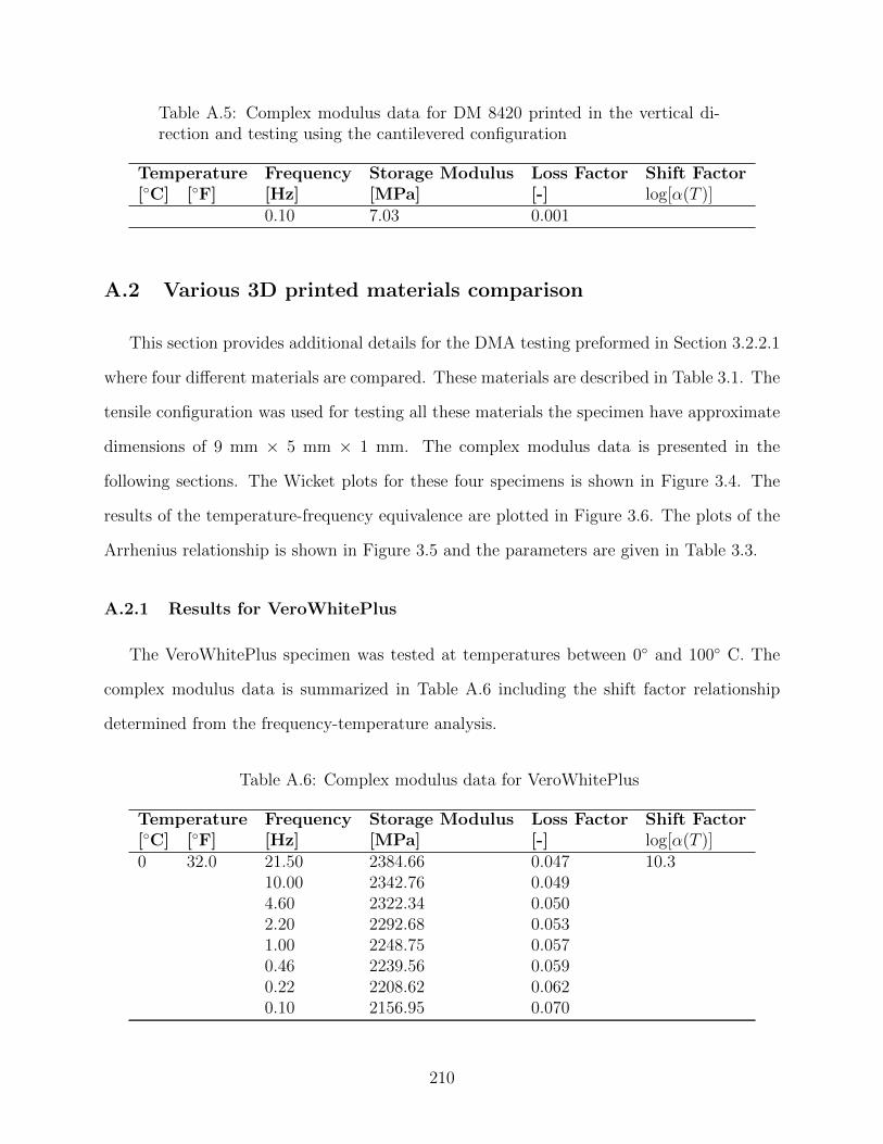
Table A.5: Complex modulus data for DM 8420 printed in the vertical di-rection and testing using the cantilevered configuration
Temperature Frequency Storage Modulus Loss Factor Shift Factor[C] [F] [Hz] [MPa] [-] log[α(T )]
0.10 7.03 0.001
A.2 Various 3D printed materials comparison
This section provides additional details for the DMA testing preformed in Section 3.2.2.1
where four different materials are compared. These materials are described in Table 3.1. The
tensile configuration was used for testing all these materials the specimen have approximate
dimensions of 9 mm × 5 mm × 1 mm. The complex modulus data is presented in the
following sections. The Wicket plots for these four specimens is shown in Figure 3.4. The
results of the temperature-frequency equivalence are plotted in Figure 3.6. The plots of the
Arrhenius relationship is shown in Figure 3.5 and the parameters are given in Table 3.3.
A.2.1 Results for VeroWhitePlus
The VeroWhitePlus specimen was tested at temperatures between 0 and 100 C. The
complex modulus data is summarized in Table A.6 including the shift factor relationship
determined from the frequency-temperature analysis.
Table A.6: Complex modulus data for VeroWhitePlus
Temperature Frequency Storage Modulus Loss Factor Shift Factor[C] [F] [Hz] [MPa] [-] log[α(T )]0 32.0 21.50 2384.66 0.047 10.3
10.00 2342.76 0.0494.60 2322.34 0.0502.20 2292.68 0.0531.00 2248.75 0.0570.46 2239.56 0.0590.22 2208.62 0.0620.10 2156.95 0.070
210
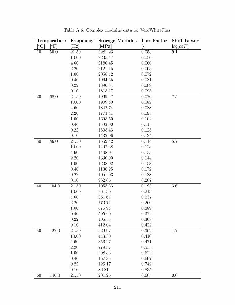
Table A.6: Complex modulus data for VeroWhitePlus
Temperature Frequency Storage Modulus Loss Factor Shift Factor[C] [F] [Hz] [MPa] [-] log[α(T )]10 50.0 21.50 2281.23 0.053 9.1
10.00 2235.47 0.0564.60 2180.45 0.0602.20 2121.15 0.0651.00 2058.12 0.0720.46 1964.55 0.0810.22 1890.84 0.0890.10 1818.17 0.095
20 68.0 21.50 1969.47 0.076 7.510.00 1909.80 0.0824.60 1842.74 0.0882.20 1773.41 0.0951.00 1698.60 0.1020.46 1593.90 0.1150.22 1508.43 0.1250.10 1432.96 0.134
30 86.0 21.50 1569.42 0.114 5.710.00 1492.38 0.1234.60 1408.94 0.1332.20 1330.00 0.1441.00 1238.02 0.1580.46 1136.25 0.1720.22 1051.03 0.1880.10 962.66 0.207
40 104.0 21.50 1055.33 0.193 3.610.00 961.30 0.2134.60 861.61 0.2372.20 773.71 0.2601.00 676.98 0.2890.46 595.90 0.3220.22 496.55 0.3680.10 412.04 0.422
50 122.0 21.50 529.97 0.362 1.710.00 443.30 0.4104.60 356.27 0.4712.20 279.87 0.5351.00 208.33 0.6220.46 167.85 0.6670.22 126.17 0.7420.10 86.81 0.835
60 140.0 21.50 201.26 0.665 0.0
211
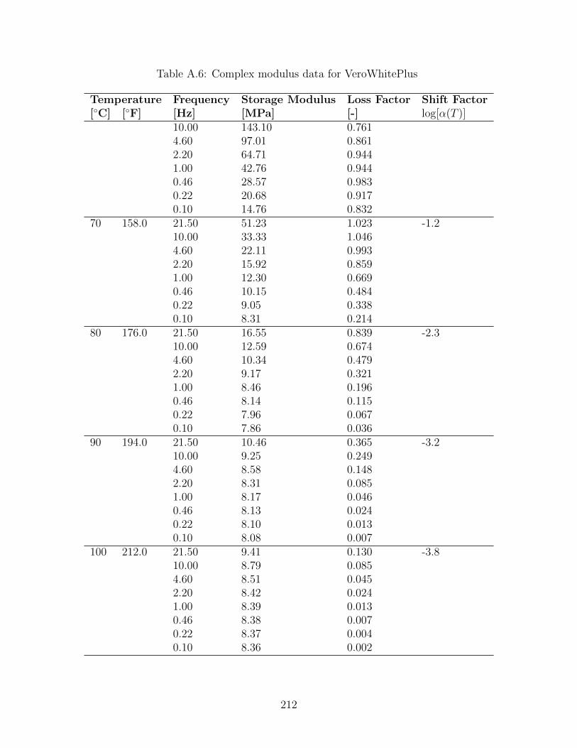
Table A.6: Complex modulus data for VeroWhitePlus
Temperature Frequency Storage Modulus Loss Factor Shift Factor[C] [F] [Hz] [MPa] [-] log[α(T )]
10.00 143.10 0.7614.60 97.01 0.8612.20 64.71 0.9441.00 42.76 0.9440.46 28.57 0.9830.22 20.68 0.9170.10 14.76 0.832
70 158.0 21.50 51.23 1.023 -1.210.00 33.33 1.0464.60 22.11 0.9932.20 15.92 0.8591.00 12.30 0.6690.46 10.15 0.4840.22 9.05 0.3380.10 8.31 0.214
80 176.0 21.50 16.55 0.839 -2.310.00 12.59 0.6744.60 10.34 0.4792.20 9.17 0.3211.00 8.46 0.1960.46 8.14 0.1150.22 7.96 0.0670.10 7.86 0.036
90 194.0 21.50 10.46 0.365 -3.210.00 9.25 0.2494.60 8.58 0.1482.20 8.31 0.0851.00 8.17 0.0460.46 8.13 0.0240.22 8.10 0.0130.10 8.08 0.007
100 212.0 21.50 9.41 0.130 -3.810.00 8.79 0.0854.60 8.51 0.0452.20 8.42 0.0241.00 8.39 0.0130.46 8.38 0.0070.22 8.37 0.0040.10 8.36 0.002
212
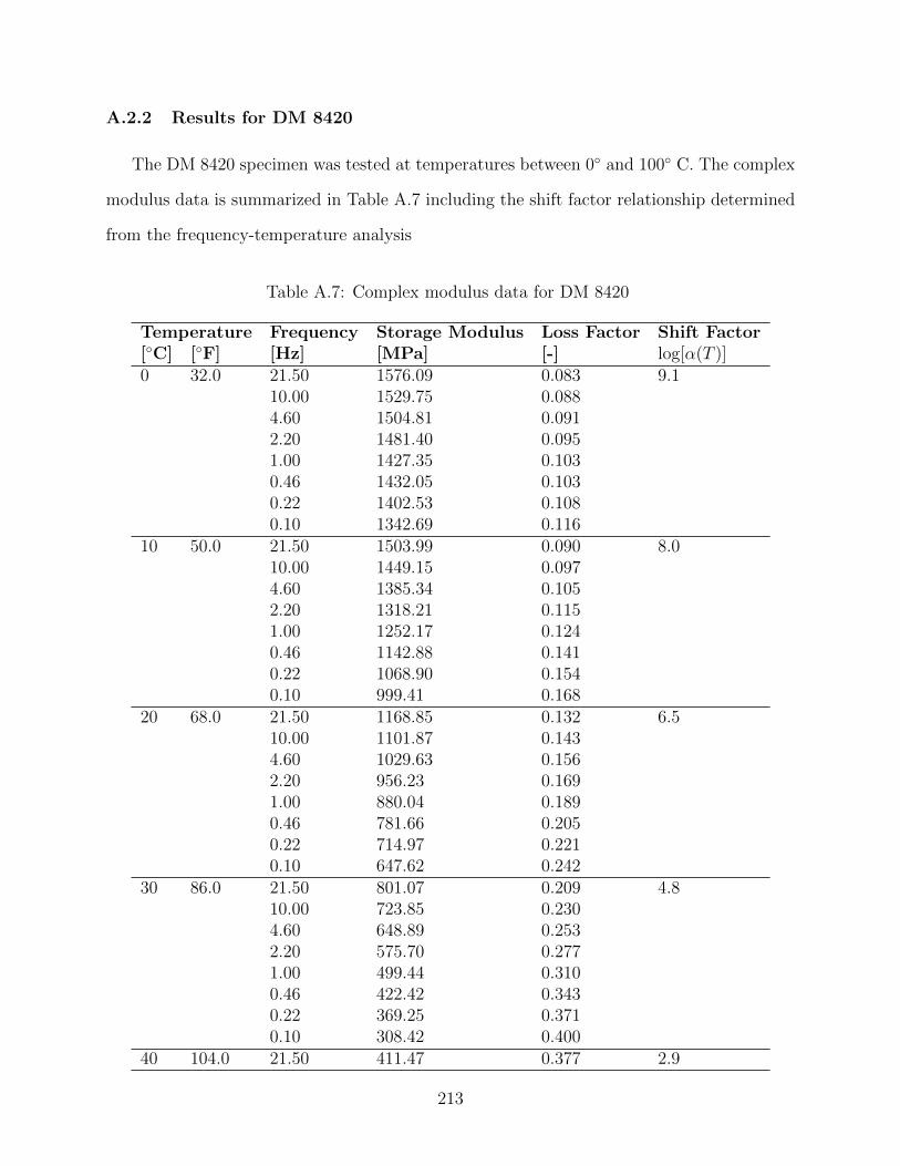
A.2.2 Results for DM 8420
The DM 8420 specimen was tested at temperatures between 0 and 100 C. The complex
modulus data is summarized in Table A.7 including the shift factor relationship determined
from the frequency-temperature analysis
Table A.7: Complex modulus data for DM 8420
Temperature Frequency Storage Modulus Loss Factor Shift Factor[C] [F] [Hz] [MPa] [-] log[α(T )]0 32.0 21.50 1576.09 0.083 9.1
10.00 1529.75 0.0884.60 1504.81 0.0912.20 1481.40 0.0951.00 1427.35 0.1030.46 1432.05 0.1030.22 1402.53 0.1080.10 1342.69 0.116
10 50.0 21.50 1503.99 0.090 8.010.00 1449.15 0.0974.60 1385.34 0.1052.20 1318.21 0.1151.00 1252.17 0.1240.46 1142.88 0.1410.22 1068.90 0.1540.10 999.41 0.168
20 68.0 21.50 1168.85 0.132 6.510.00 1101.87 0.1434.60 1029.63 0.1562.20 956.23 0.1691.00 880.04 0.1890.46 781.66 0.2050.22 714.97 0.2210.10 647.62 0.242
30 86.0 21.50 801.07 0.209 4.810.00 723.85 0.2304.60 648.89 0.2532.20 575.70 0.2771.00 499.44 0.3100.46 422.42 0.3430.22 369.25 0.3710.10 308.42 0.400
40 104.0 21.50 411.47 0.377 2.9
213
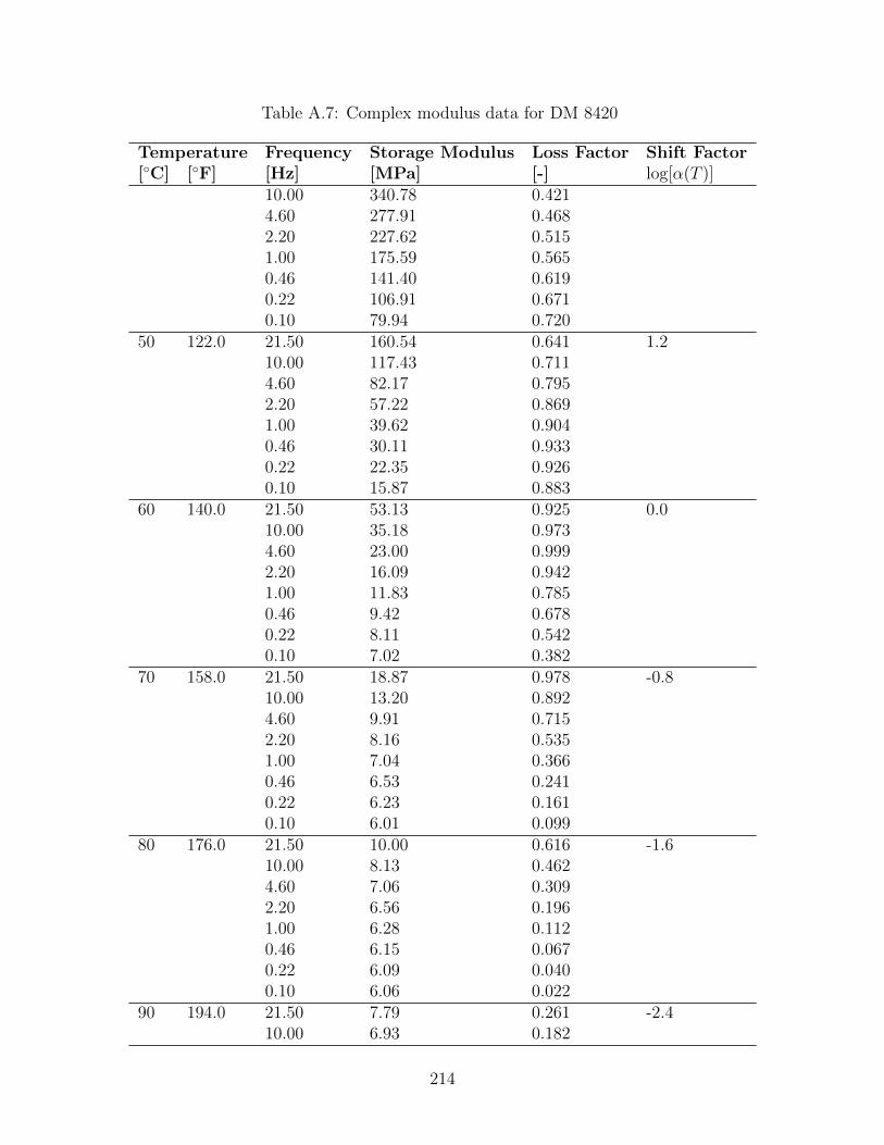
Table A.7: Complex modulus data for DM 8420
Temperature Frequency Storage Modulus Loss Factor Shift Factor[C] [F] [Hz] [MPa] [-] log[α(T )]
10.00 340.78 0.4214.60 277.91 0.4682.20 227.62 0.5151.00 175.59 0.5650.46 141.40 0.6190.22 106.91 0.6710.10 79.94 0.720
50 122.0 21.50 160.54 0.641 1.210.00 117.43 0.7114.60 82.17 0.7952.20 57.22 0.8691.00 39.62 0.9040.46 30.11 0.9330.22 22.35 0.9260.10 15.87 0.883
60 140.0 21.50 53.13 0.925 0.010.00 35.18 0.9734.60 23.00 0.9992.20 16.09 0.9421.00 11.83 0.7850.46 9.42 0.6780.22 8.11 0.5420.10 7.02 0.382
70 158.0 21.50 18.87 0.978 -0.810.00 13.20 0.8924.60 9.91 0.7152.20 8.16 0.5351.00 7.04 0.3660.46 6.53 0.2410.22 6.23 0.1610.10 6.01 0.099
80 176.0 21.50 10.00 0.616 -1.610.00 8.13 0.4624.60 7.06 0.3092.20 6.56 0.1961.00 6.28 0.1120.46 6.15 0.0670.22 6.09 0.0400.10 6.06 0.022
90 194.0 21.50 7.79 0.261 -2.410.00 6.93 0.182
214
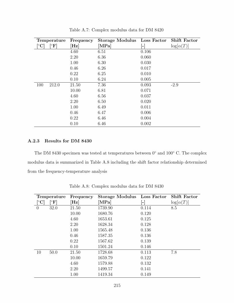
Table A.7: Complex modulus data for DM 8420
Temperature Frequency Storage Modulus Loss Factor Shift Factor[C] [F] [Hz] [MPa] [-] log[α(T )]
4.60 6.51 0.1062.20 6.36 0.0601.00 6.30 0.0300.46 6.26 0.0170.22 6.25 0.0100.10 6.24 0.005
100 212.0 21.50 7.36 0.093 -2.910.00 6.81 0.0714.60 6.56 0.0372.20 6.50 0.0201.00 6.49 0.0110.46 6.47 0.0060.22 6.46 0.0040.10 6.46 0.002
A.2.3 Results for DM 8430
The DM 8430 specimen was tested at temperatures between 0 and 100 C. The complex
modulus data is summarized in Table A.8 including the shift factor relationship determined
from the frequency-temperature analysis
Table A.8: Complex modulus data for DM 8430
Temperature Frequency Storage Modulus Loss Factor Shift Factor[C] [F] [Hz] [MPa] [-] log[α(T )]0 32.0 21.50 1739.90 0.114 8.5
10.00 1680.76 0.1204.60 1653.61 0.1252.20 1628.34 0.1281.00 1565.48 0.1360.46 1587.35 0.1360.22 1567.62 0.1390.10 1501.24 0.146
10 50.0 21.50 1728.68 0.113 7.810.00 1659.79 0.1224.60 1579.88 0.1322.20 1499.57 0.1411.00 1419.34 0.149
215
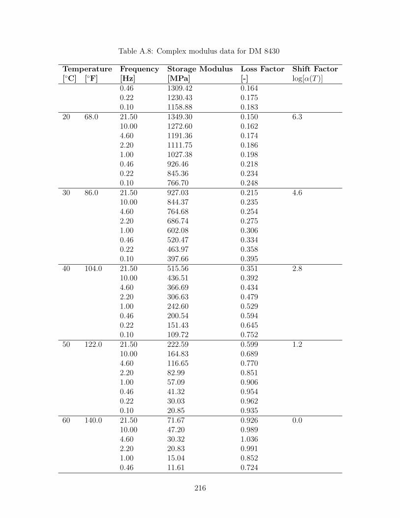
Table A.8: Complex modulus data for DM 8430
Temperature Frequency Storage Modulus Loss Factor Shift Factor[C] [F] [Hz] [MPa] [-] log[α(T )]
0.46 1309.42 0.1640.22 1230.43 0.1750.10 1158.88 0.183
20 68.0 21.50 1349.30 0.150 6.310.00 1272.60 0.1624.60 1191.36 0.1742.20 1111.75 0.1861.00 1027.38 0.1980.46 926.46 0.2180.22 845.36 0.2340.10 766.70 0.248
30 86.0 21.50 927.03 0.215 4.610.00 844.37 0.2354.60 764.68 0.2542.20 686.74 0.2751.00 602.08 0.3060.46 520.47 0.3340.22 463.97 0.3580.10 397.66 0.395
40 104.0 21.50 515.56 0.351 2.810.00 436.51 0.3924.60 366.69 0.4342.20 306.63 0.4791.00 242.60 0.5290.46 200.54 0.5940.22 151.43 0.6450.10 109.72 0.752
50 122.0 21.50 222.59 0.599 1.210.00 164.83 0.6894.60 116.65 0.7702.20 82.99 0.8511.00 57.09 0.9060.46 41.32 0.9540.22 30.03 0.9620.10 20.85 0.935
60 140.0 21.50 71.67 0.926 0.010.00 47.20 0.9894.60 30.32 1.0362.20 20.83 0.9911.00 15.04 0.8520.46 11.61 0.724
216
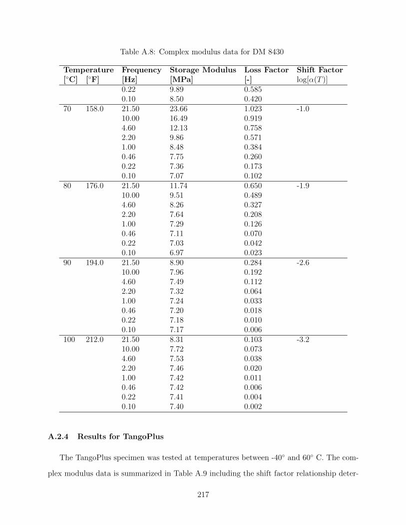
Table A.8: Complex modulus data for DM 8430
Temperature Frequency Storage Modulus Loss Factor Shift Factor[C] [F] [Hz] [MPa] [-] log[α(T )]
0.22 9.89 0.5850.10 8.50 0.420
70 158.0 21.50 23.66 1.023 -1.010.00 16.49 0.9194.60 12.13 0.7582.20 9.86 0.5711.00 8.48 0.3840.46 7.75 0.2600.22 7.36 0.1730.10 7.07 0.102
80 176.0 21.50 11.74 0.650 -1.910.00 9.51 0.4894.60 8.26 0.3272.20 7.64 0.2081.00 7.29 0.1260.46 7.11 0.0700.22 7.03 0.0420.10 6.97 0.023
90 194.0 21.50 8.90 0.284 -2.610.00 7.96 0.1924.60 7.49 0.1122.20 7.32 0.0641.00 7.24 0.0330.46 7.20 0.0180.22 7.18 0.0100.10 7.17 0.006
100 212.0 21.50 8.31 0.103 -3.210.00 7.72 0.0734.60 7.53 0.0382.20 7.46 0.0201.00 7.42 0.0110.46 7.42 0.0060.22 7.41 0.0040.10 7.40 0.002
A.2.4 Results for TangoPlus
The TangoPlus specimen was tested at temperatures between -40 and 60 C. The com-
plex modulus data is summarized in Table A.9 including the shift factor relationship deter-
217
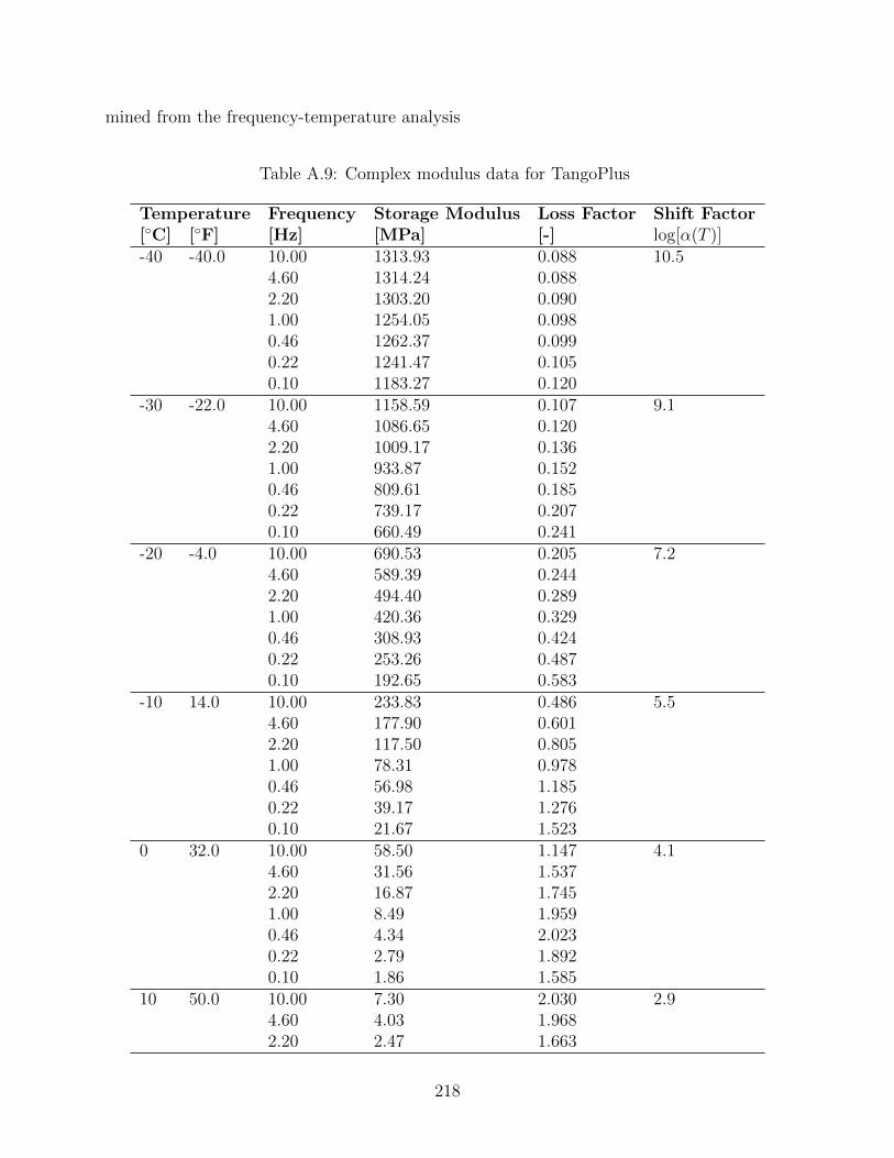
mined from the frequency-temperature analysis
Table A.9: Complex modulus data for TangoPlus
Temperature Frequency Storage Modulus Loss Factor Shift Factor[C] [F] [Hz] [MPa] [-] log[α(T )]-40 -40.0 10.00 1313.93 0.088 10.5
4.60 1314.24 0.0882.20 1303.20 0.0901.00 1254.05 0.0980.46 1262.37 0.0990.22 1241.47 0.1050.10 1183.27 0.120
-30 -22.0 10.00 1158.59 0.107 9.14.60 1086.65 0.1202.20 1009.17 0.1361.00 933.87 0.1520.46 809.61 0.1850.22 739.17 0.2070.10 660.49 0.241
-20 -4.0 10.00 690.53 0.205 7.24.60 589.39 0.2442.20 494.40 0.2891.00 420.36 0.3290.46 308.93 0.4240.22 253.26 0.4870.10 192.65 0.583
-10 14.0 10.00 233.83 0.486 5.54.60 177.90 0.6012.20 117.50 0.8051.00 78.31 0.9780.46 56.98 1.1850.22 39.17 1.2760.10 21.67 1.523
0 32.0 10.00 58.50 1.147 4.14.60 31.56 1.5372.20 16.87 1.7451.00 8.49 1.9590.46 4.34 2.0230.22 2.79 1.8920.10 1.86 1.585
10 50.0 10.00 7.30 2.030 2.94.60 4.03 1.9682.20 2.47 1.663
218
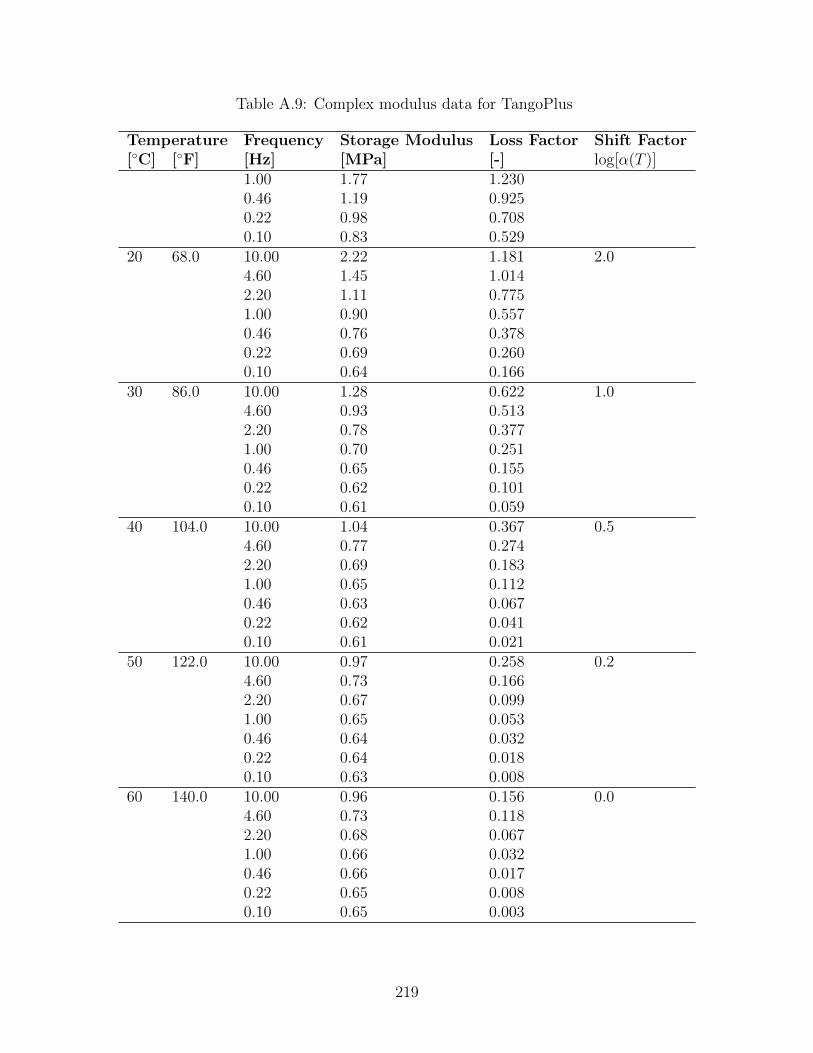
Table A.9: Complex modulus data for TangoPlus
Temperature Frequency Storage Modulus Loss Factor Shift Factor[C] [F] [Hz] [MPa] [-] log[α(T )]
1.00 1.77 1.2300.46 1.19 0.9250.22 0.98 0.7080.10 0.83 0.529
20 68.0 10.00 2.22 1.181 2.04.60 1.45 1.0142.20 1.11 0.7751.00 0.90 0.5570.46 0.76 0.3780.22 0.69 0.2600.10 0.64 0.166
30 86.0 10.00 1.28 0.622 1.04.60 0.93 0.5132.20 0.78 0.3771.00 0.70 0.2510.46 0.65 0.1550.22 0.62 0.1010.10 0.61 0.059
40 104.0 10.00 1.04 0.367 0.54.60 0.77 0.2742.20 0.69 0.1831.00 0.65 0.1120.46 0.63 0.0670.22 0.62 0.0410.10 0.61 0.021
50 122.0 10.00 0.97 0.258 0.24.60 0.73 0.1662.20 0.67 0.0991.00 0.65 0.0530.46 0.64 0.0320.22 0.64 0.0180.10 0.63 0.008
60 140.0 10.00 0.96 0.156 0.04.60 0.73 0.1182.20 0.68 0.0671.00 0.66 0.0320.46 0.66 0.0170.22 0.65 0.0080.10 0.65 0.003
219
APPENDIX B
Golla-Hughes-McTavish (GHM) Model Parameters
This appendix presents the GHM parameters used for simulations in this dissertation.
The GHM model approximates the material dissipation function as
sG(s) = G∞
[1 +
nMOT∑j=1
αis2 + 2ζiωis
s2 + 2ζiωis+ ω2i
](B.1)
where G∞, αi, ζi, and ωi are all parameters of the model and nMOT represents the number
of mini-oscillator terms and is chosen based on the desired accuracy of the model. Equation
B.1 is evaluated along the imaginary axis (s = ω) and curve fit to the experimental data
over a frequency range. The curve fit is performed by optimizing the error fit for both
the complex and the imaginary parts using an equal weighting. For each of the testing
scenarios presented in Appendix A, a GHM fit is performed over the frequency range of 10
to 2,000 Hz at various temperatures. The number of terms, n in the GHM approximation
depends on accuracy of the fit and ranges from n = 3 to n = 5 in this dissertation. For
each temperature, the data is shifted on the reduced frequency scale using the procedure
described in Section 3.3.3. This converts the reduced frequency to the frequency values for
a specific temperatures. The temperatures used for the GHM fits, range the data set.
220
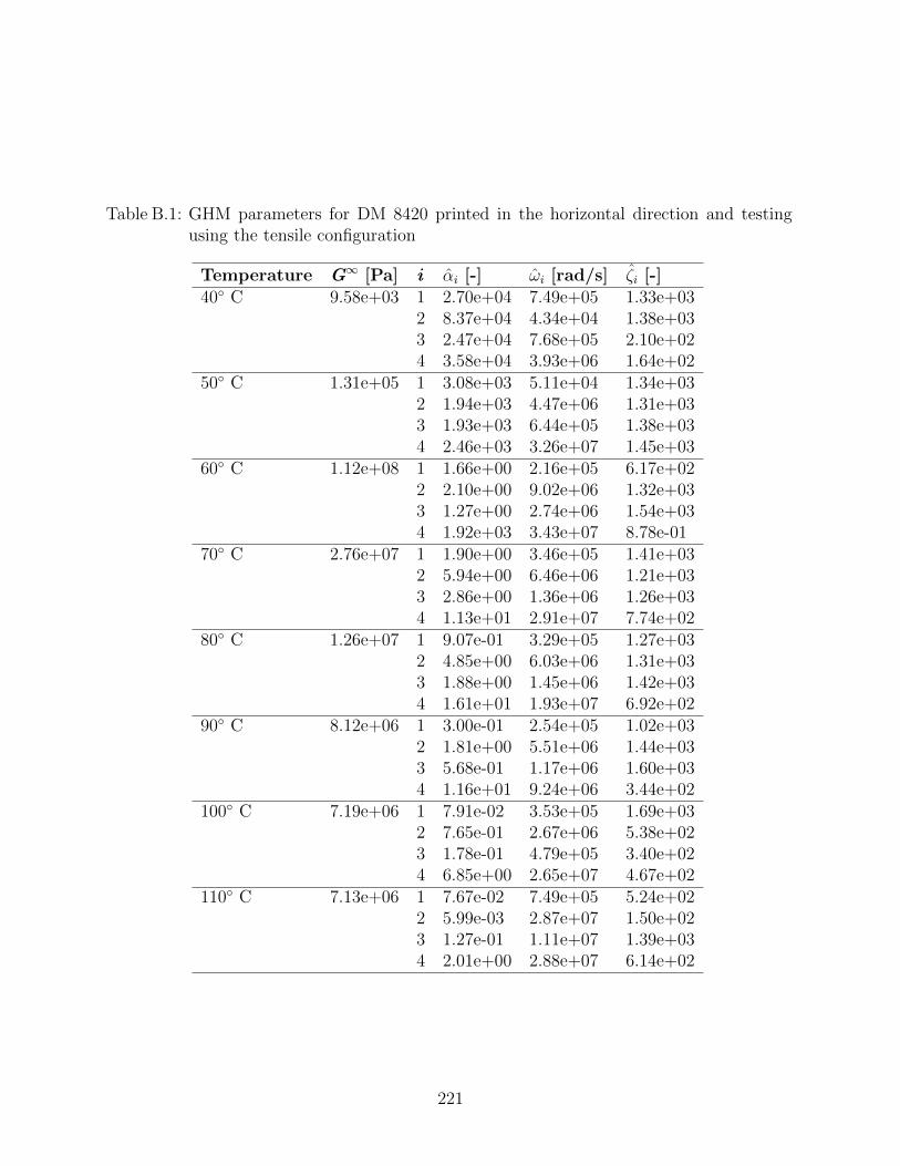
Table B.1: GHM parameters for DM 8420 printed in the horizontal direction and testingusing the tensile configuration
Temperature G∞ [Pa] i αi [-] ωi [rad/s] ζi [-]40 C 9.58e+03 1 2.70e+04 7.49e+05 1.33e+03
2 8.37e+04 4.34e+04 1.38e+033 2.47e+04 7.68e+05 2.10e+024 3.58e+04 3.93e+06 1.64e+02
50 C 1.31e+05 1 3.08e+03 5.11e+04 1.34e+032 1.94e+03 4.47e+06 1.31e+033 1.93e+03 6.44e+05 1.38e+034 2.46e+03 3.26e+07 1.45e+03
60 C 1.12e+08 1 1.66e+00 2.16e+05 6.17e+022 2.10e+00 9.02e+06 1.32e+033 1.27e+00 2.74e+06 1.54e+034 1.92e+03 3.43e+07 8.78e-01
70 C 2.76e+07 1 1.90e+00 3.46e+05 1.41e+032 5.94e+00 6.46e+06 1.21e+033 2.86e+00 1.36e+06 1.26e+034 1.13e+01 2.91e+07 7.74e+02
80 C 1.26e+07 1 9.07e-01 3.29e+05 1.27e+032 4.85e+00 6.03e+06 1.31e+033 1.88e+00 1.45e+06 1.42e+034 1.61e+01 1.93e+07 6.92e+02
90 C 8.12e+06 1 3.00e-01 2.54e+05 1.02e+032 1.81e+00 5.51e+06 1.44e+033 5.68e-01 1.17e+06 1.60e+034 1.16e+01 9.24e+06 3.44e+02
100 C 7.19e+06 1 7.91e-02 3.53e+05 1.69e+032 7.65e-01 2.67e+06 5.38e+023 1.78e-01 4.79e+05 3.40e+024 6.85e+00 2.65e+07 4.67e+02
110 C 7.13e+06 1 7.67e-02 7.49e+05 5.24e+022 5.99e-03 2.87e+07 1.50e+023 1.27e-01 1.11e+07 1.39e+034 2.01e+00 2.88e+07 6.14e+02
221
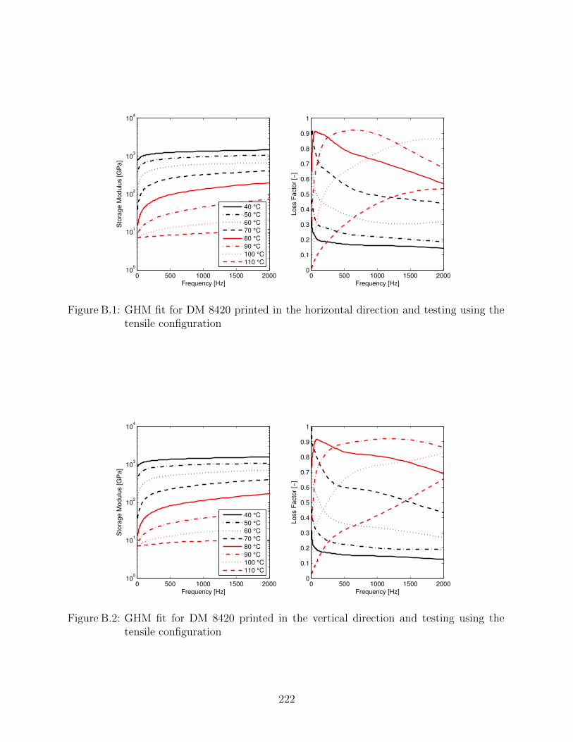
0 500 1000 1500 200010
0
101
102
103
104
Frequency [Hz]
Sto
rage M
odulu
s [G
Pa]
40 °C
50 °C
60 °C
70 °C
80 °C
90 °C
100 °C
110 °C
0 500 1000 1500 20000
0.1
0.2
0.3
0.4
0.5
0.6
0.7
0.8
0.9
1
Frequency [Hz]
Loss F
acto
r [−
]
Figure B.1: GHM fit for DM 8420 printed in the horizontal direction and testing using thetensile configuration
0 500 1000 1500 200010
0
101
102
103
104
Frequency [Hz]
Sto
rage M
odulu
s [G
Pa]
40 °C
50 °C
60 °C
70 °C
80 °C
90 °C
100 °C
110 °C
0 500 1000 1500 20000
0.1
0.2
0.3
0.4
0.5
0.6
0.7
0.8
0.9
1
Frequency [Hz]
Loss F
acto
r [−
]
Figure B.2: GHM fit for DM 8420 printed in the vertical direction and testing using thetensile configuration
222
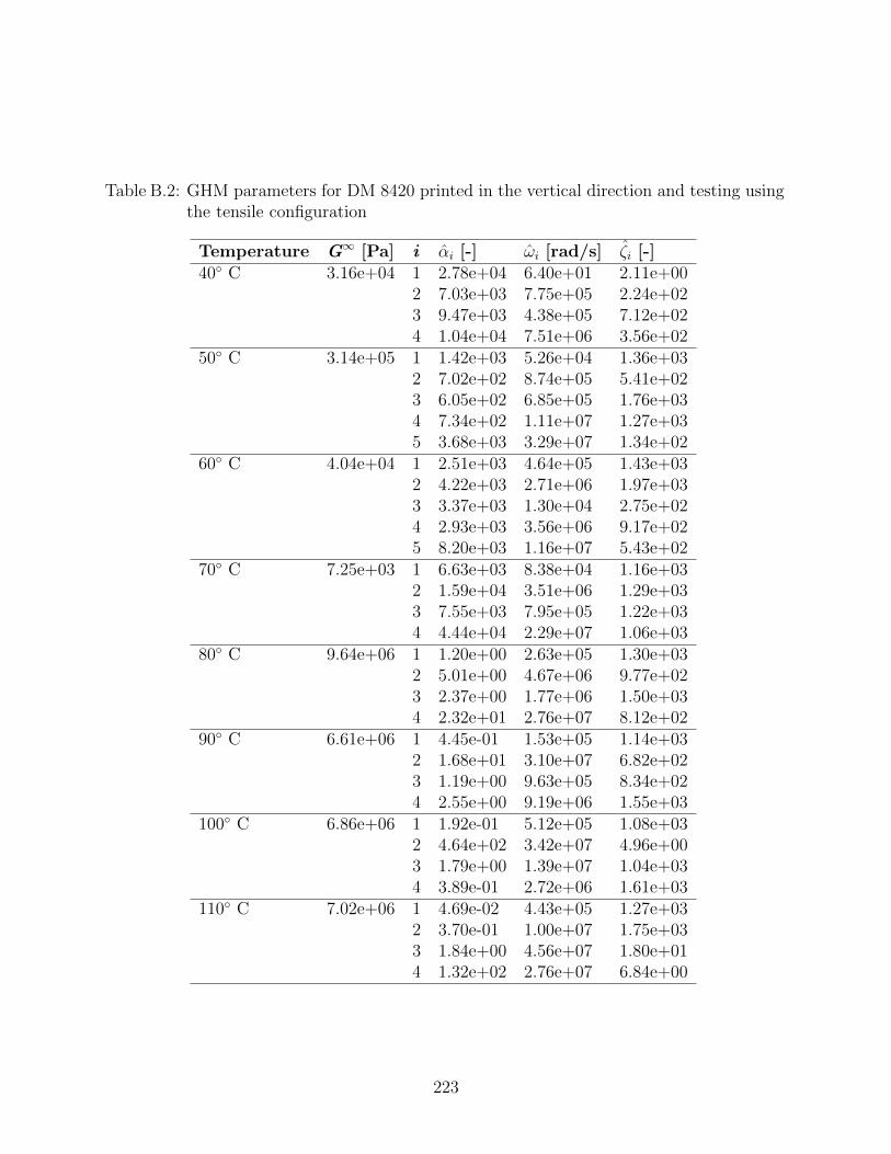
Table B.2: GHM parameters for DM 8420 printed in the vertical direction and testing usingthe tensile configuration
Temperature G∞ [Pa] i αi [-] ωi [rad/s] ζi [-]40 C 3.16e+04 1 2.78e+04 6.40e+01 2.11e+00
2 7.03e+03 7.75e+05 2.24e+023 9.47e+03 4.38e+05 7.12e+024 1.04e+04 7.51e+06 3.56e+02
50 C 3.14e+05 1 1.42e+03 5.26e+04 1.36e+032 7.02e+02 8.74e+05 5.41e+023 6.05e+02 6.85e+05 1.76e+034 7.34e+02 1.11e+07 1.27e+035 3.68e+03 3.29e+07 1.34e+02
60 C 4.04e+04 1 2.51e+03 4.64e+05 1.43e+032 4.22e+03 2.71e+06 1.97e+033 3.37e+03 1.30e+04 2.75e+024 2.93e+03 3.56e+06 9.17e+025 8.20e+03 1.16e+07 5.43e+02
70 C 7.25e+03 1 6.63e+03 8.38e+04 1.16e+032 1.59e+04 3.51e+06 1.29e+033 7.55e+03 7.95e+05 1.22e+034 4.44e+04 2.29e+07 1.06e+03
80 C 9.64e+06 1 1.20e+00 2.63e+05 1.30e+032 5.01e+00 4.67e+06 9.77e+023 2.37e+00 1.77e+06 1.50e+034 2.32e+01 2.76e+07 8.12e+02
90 C 6.61e+06 1 4.45e-01 1.53e+05 1.14e+032 1.68e+01 3.10e+07 6.82e+023 1.19e+00 9.63e+05 8.34e+024 2.55e+00 9.19e+06 1.55e+03
100 C 6.86e+06 1 1.92e-01 5.12e+05 1.08e+032 4.64e+02 3.42e+07 4.96e+003 1.79e+00 1.39e+07 1.04e+034 3.89e-01 2.72e+06 1.61e+03
110 C 7.02e+06 1 4.69e-02 4.43e+05 1.27e+032 3.70e-01 1.00e+07 1.75e+033 1.84e+00 4.56e+07 1.80e+014 1.32e+02 2.76e+07 6.84e+00
223
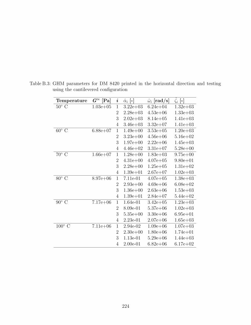
Table B.3: GHM parameters for DM 8420 printed in the horizontal direction and testingusing the cantilevered configuration
Temperature G∞ [Pa] i αi [-] ωi [rad/s] ζi [-]50 C 1.03e+05 1 3.22e+03 6.24e+04 1.32e+03
2 2.28e+03 4.53e+06 1.33e+033 2.02e+03 8.14e+05 1.41e+034 3.46e+03 3.32e+07 1.41e+03
60 C 6.88e+07 1 1.49e+00 3.53e+05 1.20e+032 3.23e+00 4.56e+06 5.16e+023 1.97e+00 2.22e+06 1.45e+034 4.46e+02 3.31e+07 5.28e+00
70 C 1.66e+07 1 1.28e+00 1.83e+03 9.75e+002 4.31e+00 4.07e+05 9.80e+013 2.28e+00 1.25e+05 1.31e+024 1.39e+01 2.67e+07 1.02e+03
80 C 8.97e+06 1 7.11e-01 4.07e+05 1.38e+032 2.93e+00 4.69e+06 6.08e+023 1.36e+00 2.63e+06 1.53e+034 1.39e+01 2.84e+07 5.44e+02
90 C 7.17e+06 1 1.64e-01 3.42e+05 1.23e+032 8.09e-01 5.37e+06 1.02e+033 5.35e+00 3.30e+06 6.95e+014 2.23e-01 2.07e+06 1.65e+03
100 C 7.11e+06 1 2.94e-02 1.09e+06 1.07e+032 2.30e+00 1.80e+06 1.74e+013 1.13e-01 5.29e+06 1.44e+034 2.00e-01 6.82e+06 6.17e+02
224
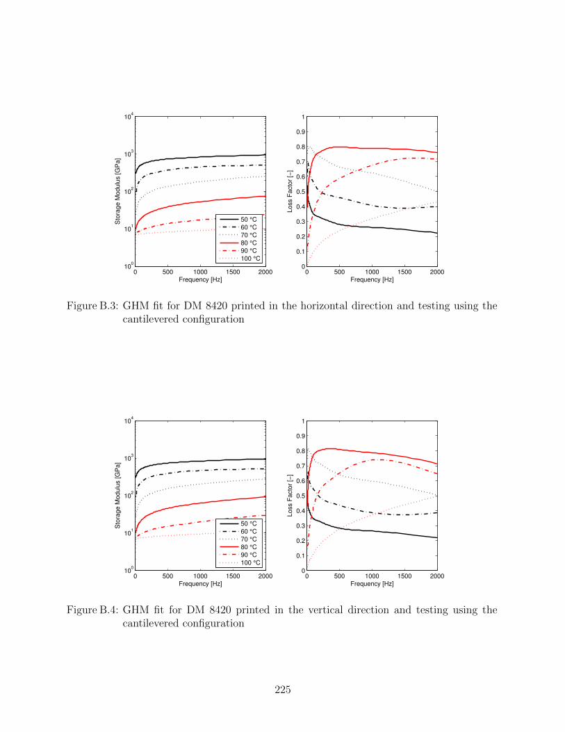
0 500 1000 1500 200010
0
101
102
103
104
Frequency [Hz]
Sto
rage M
odulu
s [G
Pa]
50 °C
60 °C
70 °C
80 °C
90 °C
100 °C
0 500 1000 1500 20000
0.1
0.2
0.3
0.4
0.5
0.6
0.7
0.8
0.9
1
Frequency [Hz]
Loss F
acto
r [−
]
Figure B.3: GHM fit for DM 8420 printed in the horizontal direction and testing using thecantilevered configuration
0 500 1000 1500 200010
0
101
102
103
104
Frequency [Hz]
Sto
rage M
odulu
s [G
Pa]
50 °C
60 °C
70 °C
80 °C
90 °C
100 °C
0 500 1000 1500 20000
0.1
0.2
0.3
0.4
0.5
0.6
0.7
0.8
0.9
1
Frequency [Hz]
Loss F
acto
r [−
]
Figure B.4: GHM fit for DM 8420 printed in the vertical direction and testing using thecantilevered configuration
225

Table B.4: GHM parameters for DM 8420 printed in the vertical direction and testing usingthe cantilevered configuration
Temperature G∞ [Pa] i αi [-] ωi [rad/s] ζi [-]50 C 1.28e+05 1 2.69e+03 6.31e+04 1.32e+03
2 1.82e+03 4.25e+06 1.34e+033 1.44e+03 8.25e+05 1.45e+034 2.81e+03 3.07e+07 1.42e+03
60 C 7.53e+07 1 1.51e+00 3.80e+05 1.30e+032 2.76e+00 3.52e+06 4.06e+023 1.91e+00 2.51e+06 1.47e+034 4.21e+03 2.77e+07 4.36e-01
70 C 1.98e+07 1 1.30e+00 3.58e+03 1.59e+012 4.40e+00 7.37e+04 1.63e+013 2.19e+00 3.74e+04 3.85e+014 1.26e+01 2.81e+06 9.65e+01
80 C 9.48e+06 1 8.12e-01 5.37e+05 1.64e+032 2.95e+00 3.33e+06 4.91e+023 1.46e+00 1.77e+06 1.04e+034 1.37e+01 2.65e+07 6.45e+02
90 C 5.57e+04 1 1.34e+02 5.26e+03 9.89e+022 2.98e+01 7.58e+05 1.52e+033 1.03e+02 4.55e+06 1.44e+034 6.85e+02 2.82e+07 9.15e+02
100 C 7.03e+06 1 4.27e-02 7.03e+05 1.71e+032 1.23e-01 1.40e+06 4.93e+023 4.57e+00 1.35e+07 7.24e+014 3.33e-01 1.15e+06 9.13e+01
226
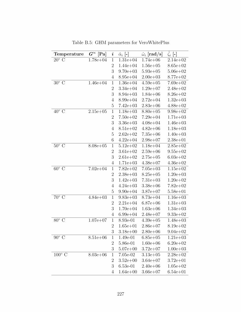
Table B.5: GHM parameters for VeroWhitePlus
Temperature G∞ [Pa] i αi [-] ωi [rad/s] ζi [-]20 C 1.78e+04 1 1.31e+04 1.74e+06 2.14e+02
2 1.44e+04 1.56e+05 8.65e+023 9.70e+03 5.93e+05 5.06e+024 8.95e+04 2.00e+03 8.77e+02
30 C 1.46e+04 1 1.36e+04 4.59e+05 7.69e+022 3.34e+04 1.29e+07 2.48e+023 8.94e+03 1.84e+06 8.26e+024 8.99e+04 2.72e+04 1.32e+035 7.42e+03 2.83e+06 4.88e+02
40 C 2.15e+05 1 1.18e+03 8.80e+05 9.98e+022 7.50e+02 7.29e+04 1.71e+033 3.36e+03 4.08e+04 1.46e+034 8.51e+02 4.82e+06 1.18e+035 2.62e+02 7.35e+06 1.40e+036 4.22e+04 2.98e+07 2.38e+01
50 C 8.08e+05 1 5.12e+02 1.18e+04 2.85e+022 3.61e+02 2.59e+06 9.55e+023 2.61e+02 2.75e+05 6.03e+024 1.71e+03 4.38e+07 4.36e+02
60 C 7.02e+04 1 7.82e+02 7.05e+03 1.15e+022 2.38e+03 8.25e+05 1.20e+033 1.42e+03 7.31e+03 1.20e+024 4.24e+03 3.38e+06 7.82e+025 9.90e+04 3.87e+07 5.58e+01
70 C 4.84e+03 1 9.83e+03 8.73e+04 1.16e+032 2.21e+04 6.87e+06 1.31e+033 1.70e+04 1.63e+06 1.34e+034 6.99e+04 2.48e+07 9.33e+02
80 C 1.07e+07 1 8.93e-01 4.39e+05 1.48e+032 1.65e+01 2.86e+07 8.19e+023 3.18e+00 2.80e+06 9.04e+02
90 C 8.51e+06 1 1.49e-01 6.85e+05 1.21e+032 5.86e-01 1.60e+06 6.20e+023 5.07e+00 3.72e+07 1.00e+03
100 C 8.03e+06 1 7.05e-02 3.13e+05 2.28e+022 3.52e+00 3.64e+07 3.72e+013 6.53e-01 2.40e+06 1.05e+024 1.64e+00 3.66e+07 6.54e+01
227
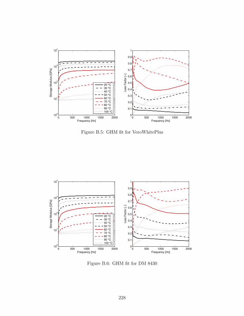
0 500 1000 1500 200010
0
101
102
103
104
Frequency [Hz]
Sto
rage M
odulu
s [G
Pa]
20 °C
30 °C
40 °C
50 °C
60 °C
70 °C
80 °C
90 °C
100 °C
0 500 1000 1500 20000
0.1
0.2
0.3
0.4
0.5
0.6
0.7
0.8
0.9
1
Frequency [Hz]
Loss F
acto
r [−
]
Figure B.5: GHM fit for VeroWhitePlus
0 500 1000 1500 200010
0
101
102
103
104
Frequency [Hz]
Sto
rage M
odulu
s [G
Pa]
20 °C
30 °C
40 °C
50 °C
60 °C
70 °C
80 °C
90 °C
100 °C
0 500 1000 1500 20000
0.1
0.2
0.3
0.4
0.5
0.6
0.7
0.8
0.9
1
Frequency [Hz]
Loss F
acto
r [−
]
Figure B.6: GHM fit for DM 8430
228
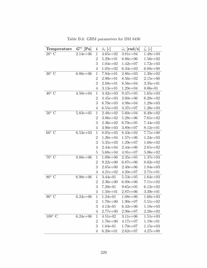
Table B.6: GHM parameters for DM 8430
Temperature G∞ [Pa] i αi [-] ωi [rad/s] ζi [-]20 C 2.14e+06 1 4.65e+02 3.81e+04 1.48e+03
2 5.29e+01 6.86e+06 1.56e+023 1.04e+02 1.42e+07 1.72e+034 1.05e+02 6.34e+03 6.88e+00
30 C 6.86e+06 1 7.94e+01 2.86e+03 1.30e+022 2.90e+01 8.56e+02 2.15e+003 2.88e+01 8.56e+04 3.35e+014 3.13e+01 1.29e+04 8.06e-01
40 C 4.50e+04 1 4.42e+03 9.47e+05 1.65e+032 4.45e+03 2.60e+06 6.20e+023 6.70e+03 4.98e+04 1.29e+034 6.55e+03 3.37e+07 1.26e+03
50 C 5.83e+05 1 2.48e+02 5.60e+04 6.49e+022 3.86e+02 5.28e+06 7.61e+023 2.36e+02 6.70e+05 7.44e+024 3.90e+03 3.89e+07 8.12e+01
60 C 6.53e+03 1 8.05e+03 8.43e+02 7.71e+002 1.26e+04 1.57e+06 1.24e+033 5.35e+03 1.29e+07 1.68e+024 2.44e+04 2.44e+06 2.81e+025 5.68e+04 4.91e+07 5.06e+02
70 C 8.88e+06 1 1.09e+00 2.35e+05 1.37e+032 9.22e+00 6.87e+06 8.02e+023 2.85e+00 2.40e+06 1.84e+034 4.21e+02 4.20e+07 2.71e+01
80 C 6.98e+06 1 3.44e-01 5.53e+05 1.64e+032 2.36e+00 6.09e+06 7.11e+023 7.20e-01 9.65e+05 6.12e+024 1.50e+01 2.87e+06 3.39e+01
90 C 6.24e+06 1 1.24e-01 1.08e+06 1.60e+032 1.70e+00 1.90e+07 5.51e+023 4.13e-01 6.42e+06 1.18e+034 2.77e+00 2.90e+07 2.28e+02
100 C 6.24e+06 1 4.51e-02 3.11e+06 1.51e+032 1.76e+00 4.17e+07 1.19e+013 1.84e-01 1.70e+07 1.15e+034 6.20e+01 2.62e+07 4.27e+00
229
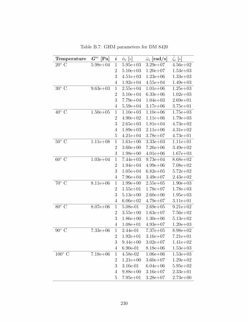
Table B.7: GHM parameters for DM 8420
Temperature G∞ [Pa] i αi [-] ωi [rad/s] ζi [-]20 C 5.98e+04 1 5.95e+03 3.29e+07 4.56e+02
2 5.10e+03 1.20e+07 1.53e+033 4.51e+03 1.23e+06 1.33e+034 1.92e+04 4.55e+04 1.49e+03
30 C 9.63e+03 1 2.55e+04 1.01e+06 1.25e+032 3.10e+04 6.33e+06 1.02e+033 7.79e+04 1.04e+03 2.69e+014 5.59e+04 3.17e+06 3.75e+01
40 C 1.50e+05 1 1.10e+03 1.10e+06 1.75e+032 4.90e+02 1.11e+06 1.79e+033 2.65e+03 1.81e+04 4.73e+024 1.89e+03 2.11e+06 4.31e+025 4.21e+04 3.78e+07 4.73e+01
50 C 1.11e+08 1 1.61e+00 3.33e+03 1.11e+012 3.60e+00 7.26e+06 3.49e+023 1.98e+00 4.01e+06 1.67e+03
60 C 1.03e+04 1 7.44e+03 9.73e+04 8.68e+022 1.94e+04 4.99e+06 7.08e+023 1.05e+04 6.82e+05 5.72e+024 7.96e+04 3.49e+07 2.43e+02
70 C 8.11e+06 1 1.99e+00 2.55e+05 1.90e+032 1.55e+01 1.78e+07 1.78e+033 5.13e+00 2.60e+06 1.95e+034 6.06e+02 4.79e+07 3.11e+01
80 C 8.07e+06 1 5.08e-01 2.69e+05 9.21e+022 3.55e+00 1.63e+07 7.56e+023 1.86e+00 1.30e+06 5.13e+024 1.08e+01 4.93e+07 1.20e+03
90 C 7.33e+06 1 2.44e-01 7.37e+05 8.98e+022 1.92e+01 3.16e+07 7.21e+013 9.44e+00 3.02e+07 1.41e+024 6.90e-01 8.18e+06 1.53e+03
100 C 7.18e+06 1 4.58e-02 1.06e+06 1.53e+032 1.21e+00 3.60e+07 1.29e+023 3.16e-01 6.04e+06 5.95e+024 9.88e+00 3.16e+07 2.33e+015 7.95e+01 3.28e+07 2.73e+00
230
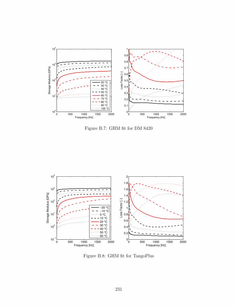
0 500 1000 1500 200010
0
101
102
103
104
Frequency [Hz]
Sto
rage M
odulu
s [G
Pa]
20 °C
30 °C
40 °C
50 °C
60 °C
70 °C
80 °C
90 °C
100 °C
0 500 1000 1500 20000
0.1
0.2
0.3
0.4
0.5
0.6
0.7
0.8
0.9
1
Frequency [Hz]
Loss F
acto
r [−
]
Figure B.7: GHM fit for DM 8420
0 500 1000 1500 200010
−1
100
101
102
103
104
Frequency [Hz]
Sto
rag
e M
od
ulu
s [
GP
a]
−20 °C
−10 °C
0 °C
10 °C
20 °C
30 °C
40 °C
50 °C
60 °C
0 500 1000 1500 20000
0.2
0.4
0.6
0.8
1
1.2
1.4
1.6
1.8
2
Frequency [Hz]
Lo
ss F
acto
r [−
]
Figure B.8: GHM fit for TangoPlus
231
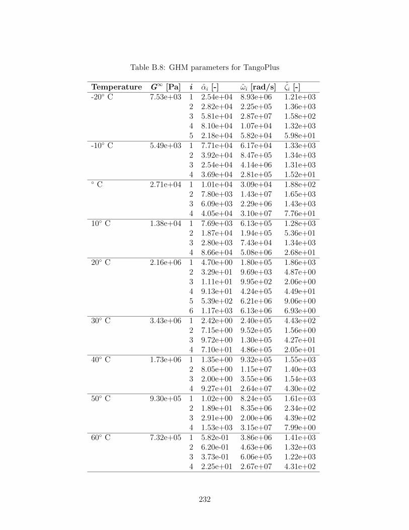
Table B.8: GHM parameters for TangoPlus
Temperature G∞ [Pa] i αi [-] ωi [rad/s] ζi [-]-20 C 7.53e+03 1 2.54e+04 8.93e+06 1.21e+03
2 2.82e+04 2.25e+05 1.36e+033 5.81e+04 2.87e+07 1.58e+024 8.10e+04 1.07e+04 1.32e+035 2.18e+04 5.82e+04 5.98e+01
-10 C 5.49e+03 1 7.71e+04 6.17e+04 1.33e+032 3.92e+04 8.47e+05 1.34e+033 2.54e+04 4.14e+06 1.31e+034 3.69e+04 2.81e+05 1.52e+01
C 2.71e+04 1 1.01e+04 3.09e+04 1.88e+022 7.80e+03 1.43e+07 1.65e+033 6.09e+03 2.29e+06 1.43e+034 4.05e+04 3.10e+07 7.76e+01
10 C 1.38e+04 1 7.69e+03 6.13e+05 1.28e+032 1.87e+04 1.94e+05 5.36e+013 2.80e+03 7.43e+04 1.34e+034 8.66e+04 5.08e+06 2.68e+01
20 C 2.16e+06 1 4.70e+00 1.80e+05 1.86e+032 3.29e+01 9.69e+03 4.87e+003 1.11e+01 9.95e+02 2.06e+004 9.13e+01 4.24e+05 4.49e+015 5.39e+02 6.21e+06 9.06e+006 1.17e+03 6.13e+06 6.93e+00
30 C 3.43e+06 1 2.42e+00 2.40e+05 4.43e+022 7.15e+00 9.52e+05 1.56e+003 9.72e+00 1.30e+05 4.27e+014 7.10e+01 4.86e+05 2.05e+01
40 C 1.73e+06 1 1.35e+00 9.32e+05 1.55e+032 8.05e+00 1.15e+07 1.40e+033 2.00e+00 3.55e+06 1.54e+034 9.27e+01 2.64e+07 4.30e+02
50 C 9.30e+05 1 1.02e+00 8.24e+05 1.61e+032 1.89e+01 8.35e+06 2.34e+023 2.91e+00 2.00e+06 4.39e+024 1.53e+03 3.15e+07 7.99e+00
60 C 7.32e+05 1 5.82e-01 3.86e+06 1.41e+032 6.20e-01 4.63e+06 1.32e+033 3.73e-01 6.06e+05 1.22e+034 2.25e+01 2.67e+07 4.31e+02
232

BIBLIOGRAPHY
233
BIBLIOGRAPHY
[1] R. Chandra, S. P. Singh, and K. Gupta, “Damping studies in fiber-reinforced compos-ites - a review,” Composite Structures, vol. 46, no. 1, pp. 41–51, 1999.
[2] O. Younossi, M. V. Arena, R. M. Moore, M. Lorell, J. Mason, and J. C. Graser,“Trends in Technological Innovation,” in Military Jet Engine Acquisition: TechnologyBasics and Cost-Estimating Methodology, ch. 3, pp. 25–40, Santa Monica, CA: RAND,2002.
[3] R. Singh, “Process capability study of polyjet printing for plastic components,” Evo-lutionary Ecology, vol. 25, no. 4, pp. 1011–1015, 2011.
[4] H. Bikas, P. Stavropoulos, and G. Chryssolouris, “Additive manufacturing methodsand modeling approaches: A critical review,” International Journal of Advanced Man-ufacturing Technology, vol. 83, no. 1-4, pp. 389–405, 2016.
[5] S. Laszlo and E. Shamonina, “Preface,” in Waves in Metamaterials, pp. vii –ix, OxfordUniversity Press, 2009.
[6] R. W. Ziolkowski and N. Engheta, “Introduction, History and Selected Topics in Fun-damental Theories of Metamateraials,” in Metamaterials: Physics and EngineeringExplorations (N. Engheta and R. W. Ziolkowski, eds.), ch. 1, pp. 1–41, Hoboken, NJ:John Wiley & Sons, Inc, 2006.
[7] S. A. Cummer, J. Christensen, and A. Alu, “Controlling sound with acoustic metama-terials,” Nature Reviews Materials, vol. 1, no. 3, p. 16001, 2016.
[8] R. Martınez-Sala, J. Sancho, J. V. Sanchez, V. Gomez, J. Llinares, and F. Meseguer,“Sound attenuation by sculpture,” Nature, vol. 378, no. 6554, pp. 241–241, 1995.
[9] M. I. Hussein, M. J. Leamy, and M. Ruzzene, “Dynamics of Phononic Materials andStructures: Historical Origins, Recent Progress, and Future Outlook,” Applied Me-chanics Reviews, vol. 66, no. 4, p. 040802, 2014.
[10] G. W. Milton and J. R. Willis, “On modifications of Newton’s second law and lin-ear continuum elastodynamics,” Proceedings of the Royal Society A: Mathematical,Physical and Engineering Sciences, vol. 463, no. August 2006, pp. 855–880, 2007.
[11] Z. Liu, X. Zhang, Y. Mao, Y. Y. Zhu, Z. Yang, C. T. Chan, and P. Sheng, “LocallyResonant Sonic Materials,” Science Reports, vol. 289, no. 5485, pp. 1734–1736, 2000.
234
[12] X. Zheng, H. Lee, T. H. Weisgraber, M. Shusteff, J. DeOtte, E. C. Duoss, J. D. Kuntz,M. M. Biener, Q. Ge, J. A. Jackson, S. O. Kucheyev, N. X. Fang, and C. M. Spadaccini,“Ultralight, Ultrastiff Mechanical Metamaterials,” Science Reports, vol. 344, no. 6190,pp. 1373–1378, 2014.
[13] R. Zhu, X. N. Liu, G. K. Hu, F. G. Yuan, and G. L. Huang, “Microstructural de-signs of plate-type elastic metamaterial and their potential applications: a review.,”International Journal of Smart & Nano Materials, vol. 6, no. 1, pp. 14–40, 2015.
[14] K. K. Saxena, R. Das, and E. P. Calius, “Three Decades of Auxetics Research Ma-terials with Negative Poisson’s Ratio: A Review,” Advanced Engineering Materials,pp. 1–24, 2016.
[15] H. Sun, X. Du, and P. F. Pai, “Theory of Metamaterial Beams for Broadband VibrationAbsorption,” Journal of Intelligent Material Systems and Structures, vol. 21, no. 11,pp. 1085–1101, 2010.
[16] P. F. Pai, “Metamaterial-based Broadband Elastic Wave Absorber,” Journal of Intel-ligent Material Systems and Structures, vol. 21, no. 5, pp. 517–528, 2010.
[17] T. Igusa and K. Xu, “Wide-Band Response of Multiple Subsystems with High ModalDensity,” in 2nd International Conference on Stochastic Structural Dynamics, pp. 131–145, 1990.
[18] T. Igusa and K. Xu, “Vibration Control Using Multiple Tuned Mass Dampers,” Journalof Sound and Vibration, vol. 175, no. 4, pp. 491–503, 1994.
[19] H. Yamaguchi and N. Harnpornchai, “Fundamental Characteristics of Multiple TunedMass Dampers for Supressing Harmonically Forced Oscillations,” Earthquake Engi-neering and Structural Dynamics, vol. 22, no. February 1992, pp. 51–62, 1993.
[20] J. P. DenHartog, Mechanical Vibrations. New York: McGraw-Hill, 1947.
[21] J. Q. Sun, M. R. Jolly, and M. A. Norris, “Passive, Adaptive and Active Tuned Vibra-tion AbsorbersA Survey,” Journal of Vibration and Acoustics, vol. 117, pp. 234 – 242,1995.
[22] N. Hoang and P. Warnitchai, “Design of multiple tuned mass dampers by using anumerical optimizer,” Earthquake Engineering & Structural Dynamics, vol. 34, no. 2,pp. 125–144, 2005.
[23] L. Zuo and S. A. Nayfeh, “Minimax optimization of multi-degree-of-freedom tuned-mass dampers,” Journal of Sound and Vibration, vol. 272, pp. 893–908, 2004.
[24] Y. Xiao, J. Wen, and X. Wen, “Longitudinal wave band gaps in metamaterial-basedelastic rods containing multi-degree-of-freedom resonators,” New Journal of Physics,vol. 14, 2012.
235
[25] A. Banerjee, R. Das, and E. P. Calius, “Frequency graded 1D metamaterials: A studyon the attenuation bands,” Journal of Applied Physics, vol. 122, no. 7, p. 075101, 2017.
[26] Y. Shanshan, Z. Xiaoming, and H. Gengkai, “Experimental study on negative effectivemass in a 1D mass-spring system,” New Journal of Physics, vol. 10, pp. 0–11, 2008.
[27] H. H. Huang, C. T. Sun, and G. L. Huang, “On the negative effective mass density inacoustic metamaterials,” International Journal of Engineering Science, vol. 47, no. 4,pp. 610–617, 2009.
[28] R. Zhu, G. L. Huang, H. H. Huang, and C. T. Sun, “Experimental and numerical studyof guided wave propagation in a thin metamaterial plate,” Physics Letters A, vol. 375,no. 30-31, pp. 2863–2867, 2011.
[29] G. Wang, X. S. Wen, J. H. Wen, and Y. Z. Liu, “Quasi-One-Dimensional PeriodicStructure with Locally Resonant Band Gap,” Journal of Applied Mechanics, vol. 73,no. 1, pp. 167–170, 2006.
[30] A. Qureshi, B. Li, and K. T. Tan, “Numerical investigation of band gaps in 3D printedcantilever-in- mass metamaterials,” Scientific Reports, vol. 6, no. 28314, pp. 1–10, 2016.
[31] J. D. Hobeck, C. M. V. Laurant, and D. J. Inman, “3D Printing of Metastructuresfor Passive Broadband Vibration Suppression,” in 20th International Conference onComposite Materials, (Copenhagen), 2015.
[32] E. D. Nobrega, F. Gautier, A. Pelat, and J. M. C. Dos Santos, “Vibration band gapsfor elastic metamaterial rods using wave finite element method,” Mechanical Systemsand Signal Processing, vol. 79, pp. 192–202, 2016.
[33] F. Liravi, R. Darleux, and E. Toyserkani, “Additive manufacturing of 3D structureswith non-Newtonian highly viscous fluids: Finite element modeling and experimentalvalidation,” Additive Manufacturing, vol. 13, pp. 113–123, 2017.
[34] M. M. Francois, A. Sun, W. E. King, N. J. Henson, D. Tourret, C. A. Bronkhorst, N. N.Carlson, C. K. Newman, T. Haut, J. Bakosi, J. W. Gibbs, V. Livescu, S. A. VanderWiel, A. J. Clarke, M. W. Schraad, T. Blacker, H. Lim, T. Rodgers, S. Owen, F. Ab-deljawad, J. Madison, A. T. Anderson, J.-l. Fattebert, R. M. Ferencz, N. E. Hodge,S. A. Khairallah, and O. Walton, “Modeling of additive manufacturing processes formetals : Challenges and opportunities,” Current Opinion in Solid State & MaterialsScience, pp. 1–9, 2017.
[35] J. Mueller, K. Shea, and C. Daraio, “Mechanical properties of parts fabricated withinkjet 3D printing through efficient experimental design,” Materials and Design,vol. 86, pp. 902–912, 2015.
[36] Y. Zhang, L. Hao, M. M. Savalani, R. A. Harris, and K. E. Tanner, “Characterizationand dynamic mechanical analysis of selective laser sintered hydroxyapatite-filled poly-meric composites,” Journal of Biomedical Materials Research - Part A, vol. 86, no. 3,pp. 607–616, 2008.
236
[37] Q. Ge, Y. Mao, K. Yu, M. L. Dunn, and H. J. Qi, “Active Composites and 4D Printing,”in 20th International Conference on Composite Materials, 2015.
[38] Y. Wang and D. J. Inman, “Finite element analysis and experimental study on dynamicproperties of a composite beam with viscoelastic damping,” Journal of Sound andVibration, vol. 332, pp. 6177–6191, nov 2013.
[39] Y. Liu, J. Yi, Z. Li, X. Su, W. Li, and M. Negahban, “Dissipative elastic metamaterialwith a low-frequency passband Dissipative elastic metamaterial with a low-frequencypassband,” AIP Advances, vol. 7, no. 065215, pp. 1–7, 2017.
[40] B. C. Essink and D. J. Inman, “Optimized 3D Printed Chiral Lattice for BroadbandVibration Suppresion,” in Topics in Modal Analysis & Testing, vol. 10, pp. 205–214,2016.
[41] T. Yu and G. A. Lesieutre, “Damping of Sandwich Panels via Acoustic Metamaterials,”AIAA Journal, vol. 55, no. 4, pp. 1–13, 2017.
[42] T. Li, Y. Chen, X. Hu, Y. Li, and L. Wang, “Exploiting negative Poisson’s ratioto design 3D-printed composites with enhanced mechanical properties,” Materials &Design, vol. 142, pp. 247–258, 2018.
[43] M. L. Liu, K. K. Reichl, and D. J. Inman, “Complex Modulus Variation by Manip-ulation of Mechanical Test Method and Print Direction,” in Society of EngineeringMechanics Annual Conference, (Indianapolis, IN), 2017.
[44] D. I. G. Jones, Handbook of Viscoelastic Vibration Damping. John Wiley & Sons, 2001.
[45] “Objet Connex 3D Printers,” 2015.
[46] “Stratasys Digital Materials Data Sheet,” 2015.
[47] “Stratasys PolyJet Materials Data Sheet,” 2014.
[48] Q. Ge, H. J. Qi, and M. L. Dunn, “Active materials by four-dimension printing Activematerials by four-dimension printing,” Applied Physics Letters, vol. 103, no. 131901,pp. 1–5, 2013.
[49] Q. Ge, C. K. Dunn, H. J. Qi, and M. L. Dunn, “Active Origami by 4D Printing,”Smart Materials and Structures, vol. 23, no. 094007, pp. 1–15, 2014.
[50] K. Yu, A. Ritchie, Y. Mao, M. L. Dunn, and H. J. Qi, “Controlled Sequential ShapeChanging Components by 3D Printing of Shape Memory Polymer Multimaterials,”Procedia IUTAM, vol. 12, pp. 193–203, 2015.
[51] R. A. DiTaranto, “Theory of vibratory bending for elastic and viscoelastic layeredfinite-length beams,” Journal of Applied Mechanics, vol. 32, no. 4, pp. 881–886, 1965.
237
[52] M. J. Yan and E. H. Dowell, “Governing Equations for Vibrating Constrained-LayerDamping Sandwich Plates and Beams,” Journal of Applied Mechanics, vol. 39, no. 4,pp. 1041–1046, 1972.
[53] R. A. Christensen, Theory of Viscoelasticity. New York: Academic Press, Inc., 1982.
[54] R. S. Lakes, “Introduction : Phenomena,” in Viscoelastic Materials, ch. 1, pp. 1–13,New York, New York: Cambridge University Press, 2009.
[55] L. B. Eldred, W. P. Baker, and A. N. Palazotto, “Kelvin-Voigt vs Fractional DerivativeModel as Constitutive Relations for Viscoelastic Materials,” AIAA Journal, vol. 33,no. 3, pp. 547–550, 1995.
[56] C. D. Johnson, D. A. Kienholz, and L. C. Rogers, “Finite Element Prediction ofDamping in Beam with Constrained Viscoelastic Layers,” The Shock and VibrationBulletin, vol. 51, 1981.
[57] C. D. Johnson and D. A. Kienholz, “Finite element prediction of damping in structureswith constrained viscoelastic layers,” AIAA Journal, vol. 20, no. 9, pp. 1284–1290,1982.
[58] M. A. Trindade, A. Benjeddou, and R. Ohayon, “Modeling of frequency-dependentviscoelastic materials for active-passive vibration damping,” Journal of Vibration andAcoustics, vol. 122, no. 2, pp. 169–174, 2000.
[59] R. L. Bagley and P. J. Torvik, “Fractional calculus - a different approach to the analysisof viscoelastically damped structures,” AIAA journal, vol. 21, no. 5, pp. 741–748, 1983.
[60] R. L. Bagley and P. J. Torvik, “Fractional calculus in the transient analysis of vis-coelastically damped structures,” AIAA Journal, vol. 23, no. 6, pp. 918–925, 1985.
[61] G. A. Lesieutre and D. L. Mingori, “Finite element modeling of frequency-dependentmaterial damping using augmenting thermodynamic fields,” Journal of Guidance, Con-trol, and Dynamics, vol. 13, pp. 1040–1050, nov 1990.
[62] D. F. Golla and P. C. Hughes, “Dynamics of Viscoelastic Structures - A Time-Domain,Finite Element Formulation,” Journal of Applied Mechanics, vol. 52, pp. 897–906, dec1985.
[63] D. J. McTavish and P. C. Hughes, “Finite Element Modeling of Linear ViscoelasticStructures,” in 1987 ASME Design Technology 11th Biennial Conference on Mechan-ical Vibration and Noise, pp. 9–17, 1987.
[64] D. J. Inman, “Vibration Analysis of Viscoelastic Beams by Seperation of Variables andModal Analysis,” Mechanics Research Communications, vol. 16, no. 4, pp. 213–218,1989.
[65] M. I. Friswell, D. J. Inman, and M. J. Lam, “On the realisation of GHM models inviscoelasticity,” Journal of Intelligent Material Systems and Structures, vol. 8, no. 1,pp. 986–993, 1997.
238
[66] M. I. Friswell and D. J. Inman, “Finite Element Models with Viscoelastic Damping,” in17th International Modal Analysis Conference, (Orlando, Florida), pp. 181–187, 1999.
[67] M. J. Lam, W. R. Saunders, and D. J. Inman, “Modeling Active Constrained LayerDamping Using Golla-Hughes-McTavish Approach,” Smart Structures & Materials’95, vol. 2445, pp. 86–97, may 1995.
[68] A. M. G. de Lima, M. H. Stoppa, and D. A. Rade, “Finite Element Modeling ofStructures Incorporating Viscoelastic Materials,” in 21st International Modal AnalysisConference, (Orlando, Florida), 2003.
[69] C. M. A. Vasques, R. A. S. Moreira, J. Dias Rodrigues, and J. D. Rodrigues, “Vis-coelastic Damping Technologies-Part II: Experimental Identification Procedure andValidation.,” Journal of advanced Research in Mechanical Engineering, vol. 1, no. 2,pp. 96–110, 2010.
[70] ASTM D5026 - 06, “Standard Test Method for Plastics : Dynamic Mechanical Prop-erties : In Tension 1,” 2014.
[71] ASTM D5418 - 15, “Standard Test Method for Plastics: Dynamic Mechanical Prop-erties: In Flexure (Three-Point Bending),” 2007.
[72] ASTM E756 - 05, “Standard Test Method for Measuring Vibration-Damping Proper-ties of Materials,” 2010.
[73] D. J. Inman, Vibration with Control. West Sussex, England: John Wiley, 2nd ed.,2017.
[74] A. Preumont, Vibration Control of Active Structures: An Introduction, vol. 179. NewYork: Springer-Verlag, 2011.
[75] M. A. Trindade, A. Benjeddou, and R. Ohayon, “Piezoelectric Active Vibration Controlof Damped Sandwich Beams,” Journal of Sound and Vibration, vol. 246, no. 4, pp. 653–677, 2001.
[76] T. Hegewald and D. J. Inman, “Vibration Suppression Via Smart Structures Across aTemperature Range,” Journal of Intelligent Material Systems and Structures, vol. 12,pp. 191–203, mar 2001.
[77] A. Baz, “Robust Control of Active Constrained Layer Damping,” Journal of Soundand Vibration, vol. 2720, no. 3, pp. 467–480, 1998.
[78] C. Sugino, M. Ruzzene, and A. Erturk, “Dynamics of hybird mechanical-electromechanical locally resonant piezoelectric metastructures,” in ASME 2017 Con-ference on Smart Materials, Adaptive Structures and Intelligent Systems, (Snowbird,UT), 2017.
[79] S. Xiao, G. Ma, Y. Li, Z. Yang, and P. Sheng, “Active control of membrane-typeacoustic metamaterial by electric field,” Applied Physics Letters, vol. 106, no. 091904,2015.
239
[80] A. M. Baz, “With Tunable Effective Density,” Journal of Vibration and Acoustics,vol. 132, no. 041011, 2010.
[81] Y. Y. Chen, G. L. Huang, and C. T. Sun, “Band Gap Control in an Active ElasticMetamaterial With Negative Capacitance Piezoelectric Shunting,” Journal of Vibra-tion and Acousti, vol. 136, no. 061008, 2014.
[82] H. T. Chen, W. J. Padilla, J. M. O. Zide, A. C. Gossard, A. J. Taylor, and R. D.Averitt, “Active terahertz metamaterial devices,” Nature, vol. 444, pp. 597–600, 2006.
[83] M. Nouh, O. Aldraihem, and A. Baz, “Periodic Metamaterial Plates with Smart Tun-able Local Resonators,” Intelligent Material Systems and Structures, vol. 27, no. 13,2016.
[84] G. Hu, L. Tang, A. Banerjee, and R. Das, “Metastructure With Piezoelectric Elementfor Simultaneous Vibration Suppression and Energy Harvesting,” Journal of Vibrationand Acoustics, vol. 139, no. 1, p. 011012, 2016.
[85] J. D. Hobeck and D. J. Inman, “Simultaneous passive broadband vibration suppressionand energy harvesting with multifunctional metastructures,” in SPIE Smart Structuresand Materials, vol. 10172, p. 101720K, 2017.
[86] J. Li, X. Zhou, G. Huang, and G. Hu, “Acoustic metamaterials capable of both soundinsulation and energy harvesting,” Smart Materials and Structures, vol. 25, no. 5,p. 045013, 2016.
[87] C. J. Goh and T. K. Caughey, “On the stability problem caused by finite actuatordynamics in the collocated control of large space structures,” International Journal ofControl, vol. 41, no. 3, pp. 787–802, 1985.
[88] S. Poh and A. Baz, “Active Control of a Flexible Structure,” Journal of IntelligentMaterial Systems and Structures, vol. 1, no. July, pp. 273–288, 1990.
[89] M. K. Kwak and S. Heo, “Active vibration control of smart grid structure by mul-tiinput and multioutput positive position feedback controller,” Journal of Sound andVibration, vol. 304, no. 1-2, pp. 230–245, 2007.
[90] D. J. Leo, “Piezoelectric Materials,” in Engineering Analysis of Smart Material Sys-tems, ch. 4, pp. 122–204, Hoboken, New Jersey: John Wiley & Sons, 2007.
[91] D. J. Leo, “Active Vibration Control,” in Engineering Analysis of Smart MaterialSystems, ch. 10, pp. 467–510, Hoboken, New Jersey: John Wiley & Sons, 2007.
[92] J. J. Dosch, D. J. Inman, and E. Garcia, “A Self-Sensing Piezoelectric Actuator forCollocated Control,” Journal of Intelligent Material Systems and Structures, vol. 3,no. 1, pp. 166–185, 1992.
[93] L. Jones, E. Garcia, and H. Waitest, “Self-sensing control as applied to a PZT stackactuator used as a micropositioner,” Journal of Smart Materials and Structures, vol. 3,pp. 147–156, 1994.
240
[94] A. M. Kabe and B. H. Sako, “Issues with Proportional Damping,” AIAA Journal,vol. 54, no. 9, pp. 2864–2868, 2016.
[95] H. P. Menard, Dynamic Mechanical Analysis: A Practical Introduction. Boca Raton,FL: Taylor & Francis Group, 2nd ed., 2008.
[96] X. Liu and G. Hu, “Elastic Metamaterials Making Use of Chirality: A Review,” Journalof Mechanical Engineering, vol. 62, no. 7-8, pp. 403–418, 2016.
[97] K. K. Reichl and D. J. Inman, “Lumped Mass Model of a 1D Metastructure for Vibra-tion Suppression with no Additional Mass,” Journal of Sound and Vibration, vol. 403,pp. 75–89, 2017.
[98] ASTM D5026, “Standard Test Method for Measuring the Plastics : Dynamic Mechan-ical Properties of Plastics in Tension Properties : In Tension 1,” Tech. Rep. November,ASTM, 2001.
[99] G. A. Lesieutre and U. Lee, “A finite element for beams having segmented active con-strained layers with frequency-dependent viscoelastics,” Smart Materials and Struc-tures, vol. 5, pp. 615–627, oct 1996.
[100] G. A. Lesieutre, E. Bianchini, and A. Maiani, “Finite element modeling of one-dimensional viscoelastic structures using anelastic displacement fields,” Journal ofGuidance Control and Dynamics, vol. 19, no. 3, pp. 520–527, 1996.
[101] D. J. McTavish and P. C. Hughes, “Modeling of Linear Viscoelastic Space Structures,”Journal of Vibration and Acoustics, vol. 115, pp. 103–110, jan 1993.
[102] D. J. McTavish and P. C. Hughes, “Finite element modeling of linear viscoelasticstructures: the GHM method,” in 33rd AIAA/ASME/ASCE/AHS/ASC Structures,Structural Dynamics and Materials Conference, pp. 1753–1763, 1992.
[103] K. K. Reichl and D. J. Inman, “Dynamic Mechanical and Thermal Analyses of ObjetConnex 3D Printed Materials,” Experimental Techniques, vol. 42, pp. 19–25, 2018.
[104] K. K. Reichl and D. J. Inman, “Constant Mass Metastructure with Vibration Ab-sorbers of Linearly Varying Natural Frequencies,” in 35th International Modal AnalysisConference, vol. 10, (Garden Grove, CA), pp. 153–158, 2017.
[105] K. K. Reichl and D. J. Inman, “Active Vibration Control and Metastructures,” in 27thInternational Conference on Adaptive Structures and Technologies, (Lake George, NY),2016.
[106] R. E. Skelton and P. C. Hughes, “Modal cost analysis for linear matrix-second-ordersystems,” Journal of Dynamic Systems, Measurement, and Control, vol. 102, no. 3,pp. 151–158, 1980.
[107] R. E. Skelton, Dynamic Systems Control: Linear Systems Analysis and Synthesis. JohnWiley & Sons, 1988.
241

[108] A. Erturk and D. J. Inman, “Numerical Data for PZT-5A and PZT-5H Piezoceram-ics,” in Piezoelectric Energy Harvesting, ch. Appendix E, pp. 373–374, West Sussex,England: John Wiley & Sons, 2011.
[109] D. J. Leo, “Piezoelectric material systems,” in Engineering Analysis of Smart MaterialSystems, ch. 5, pp. 205–297, Hoboken, New Jersey: John Wiley & Sons, 2007.
242
Related Documents